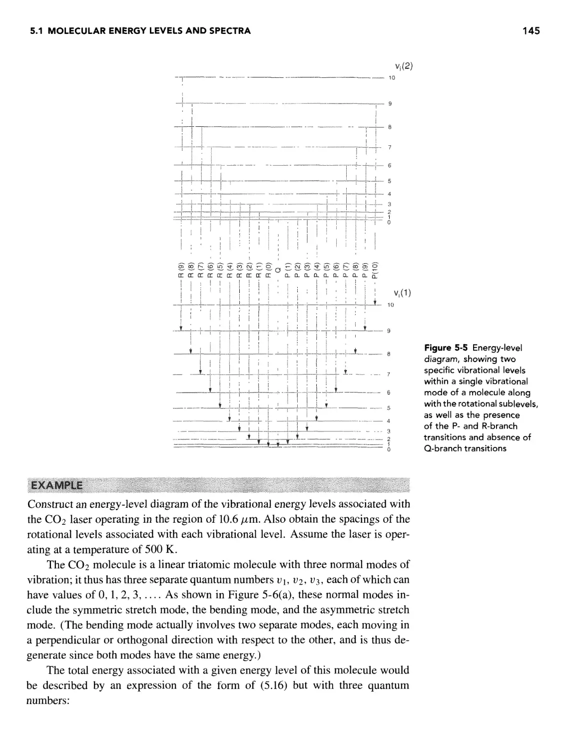
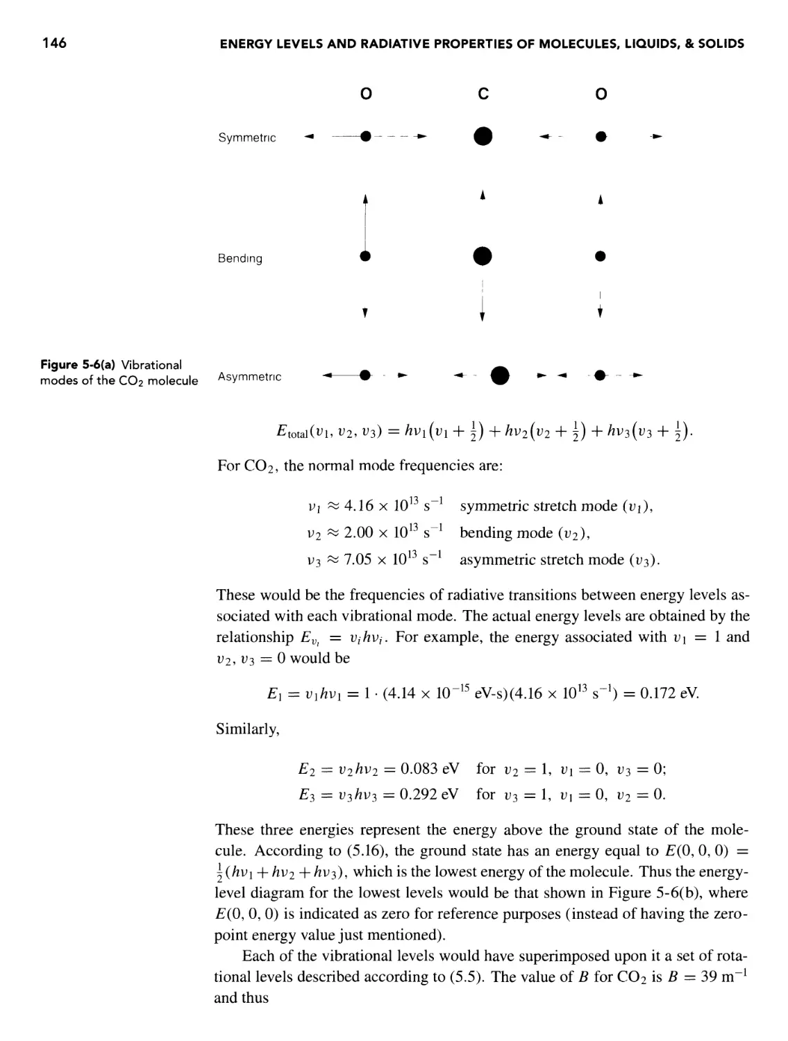
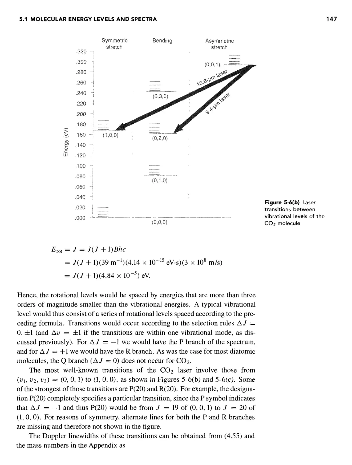
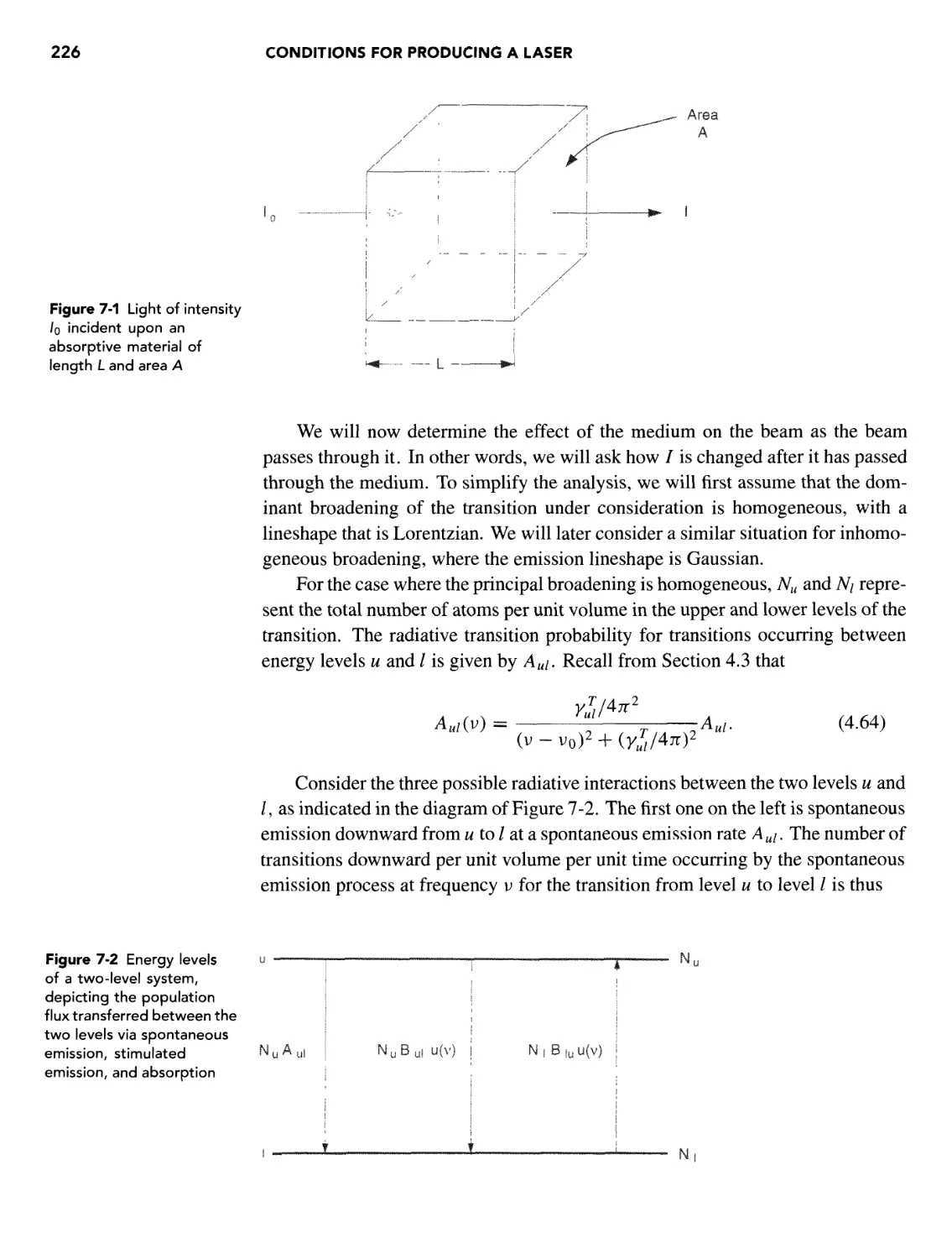
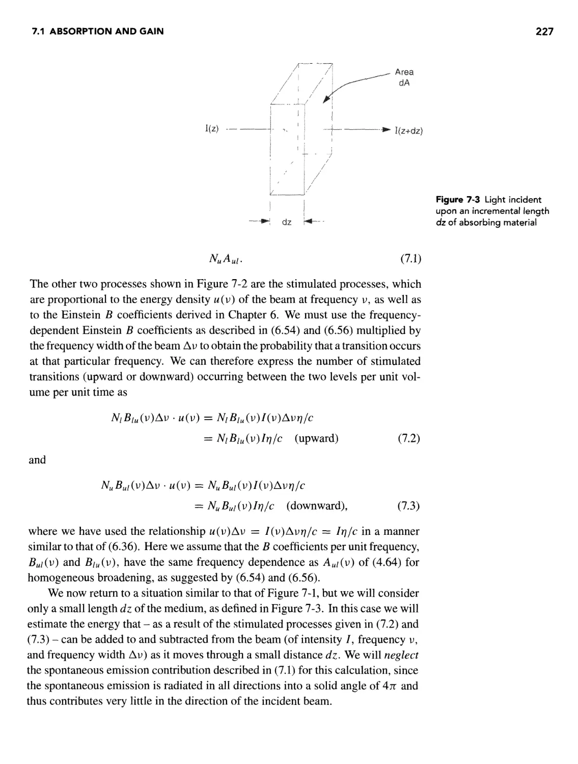
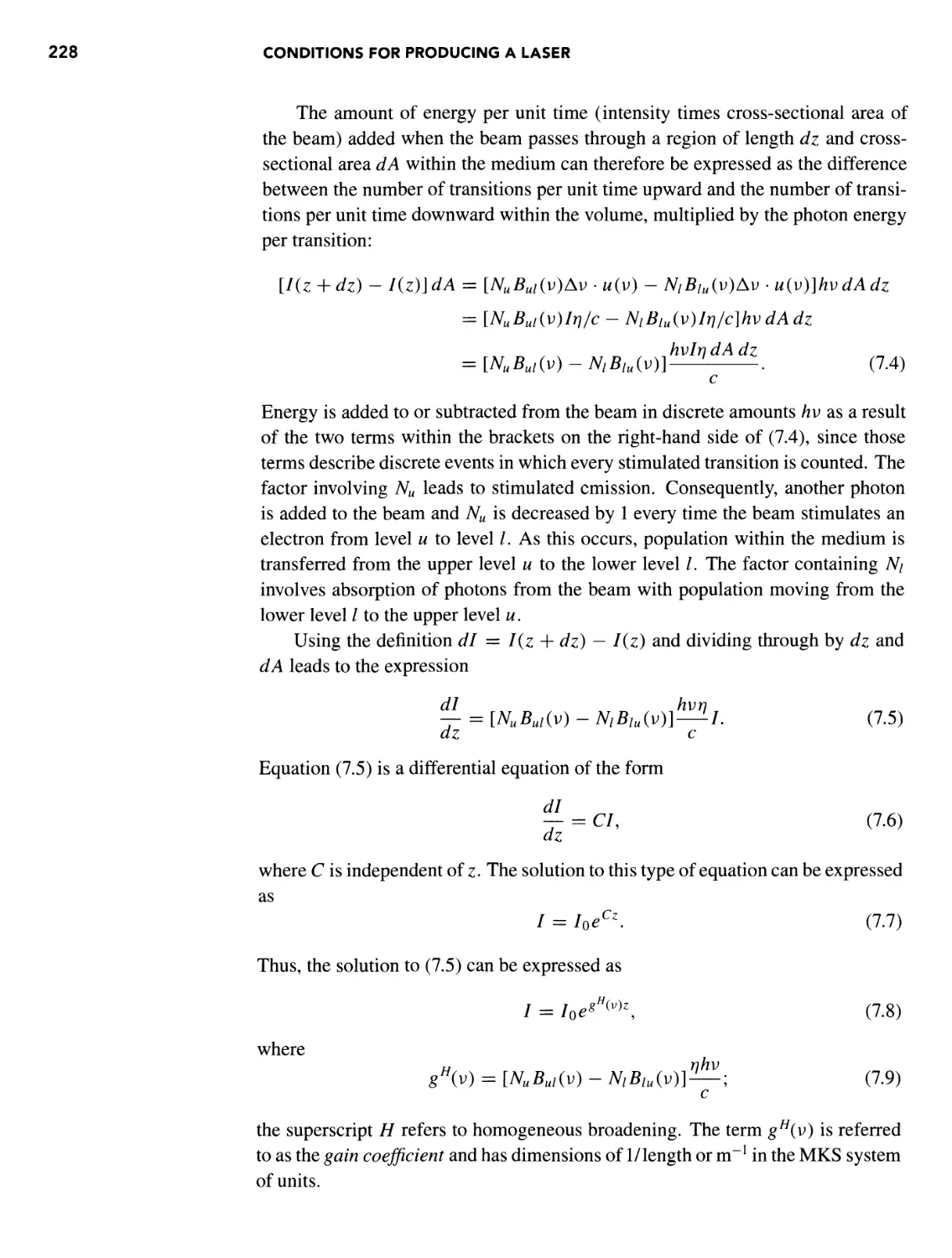
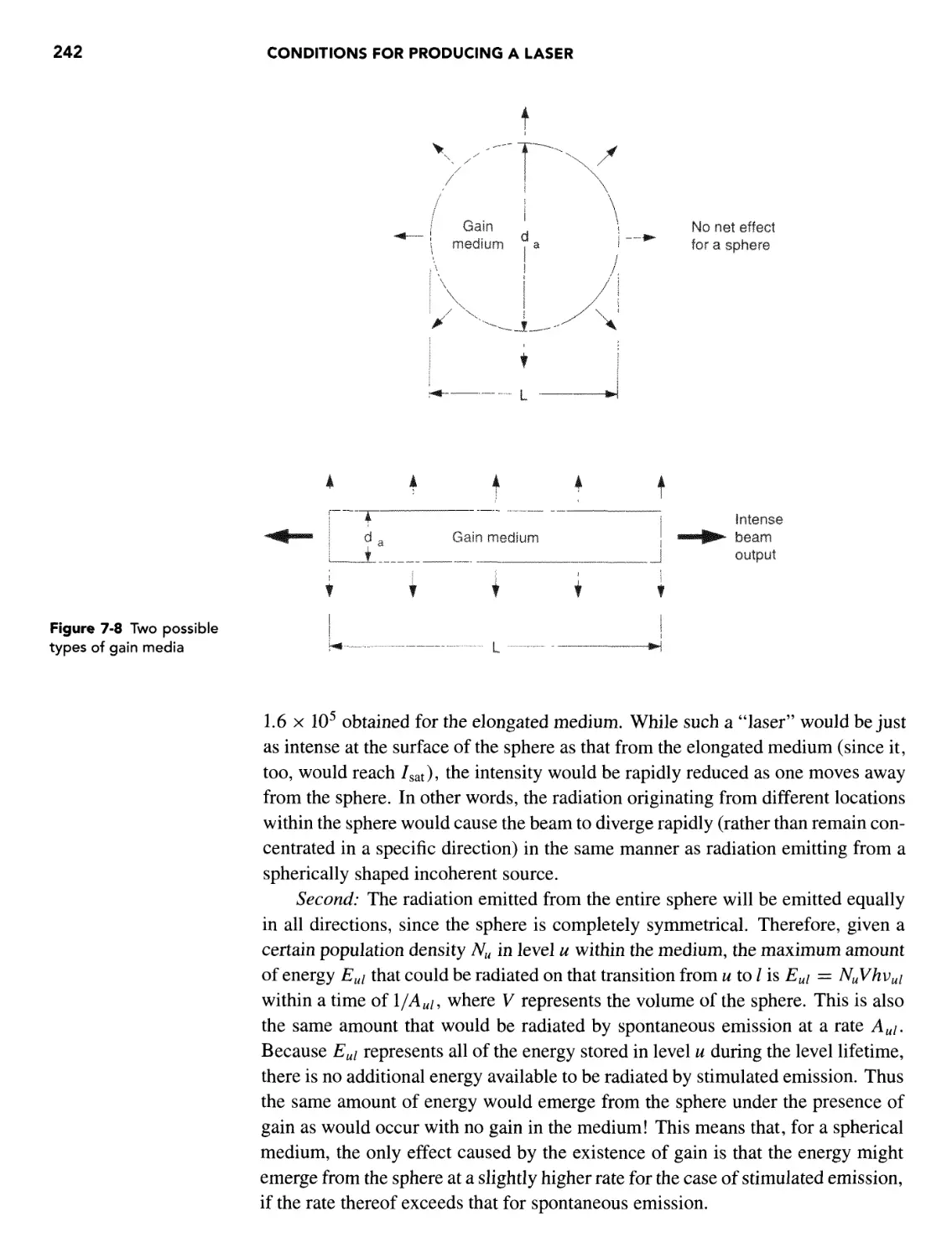
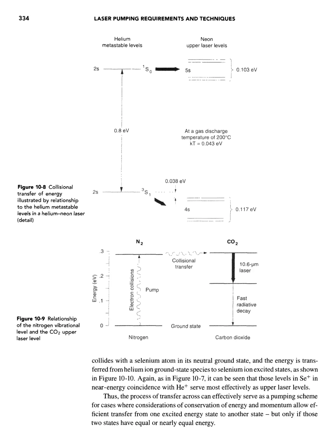
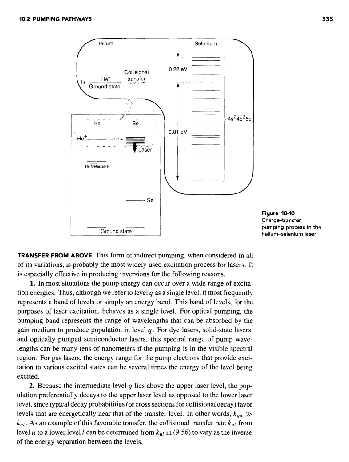
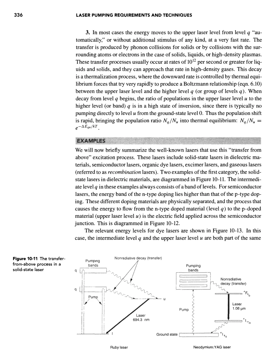
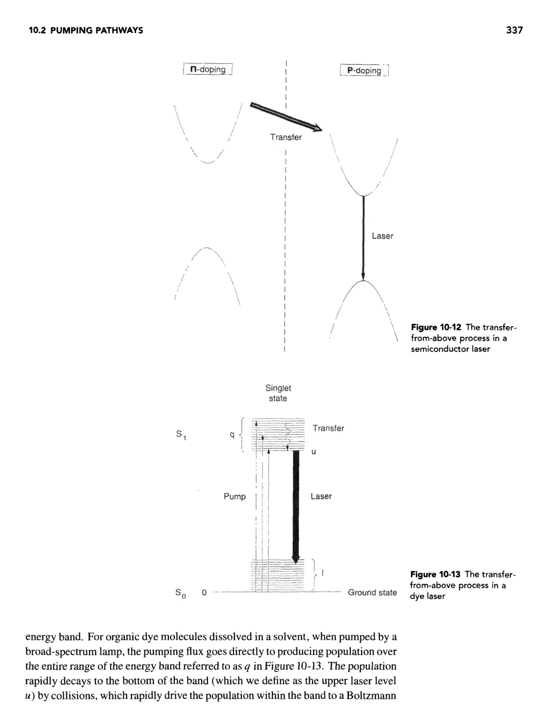
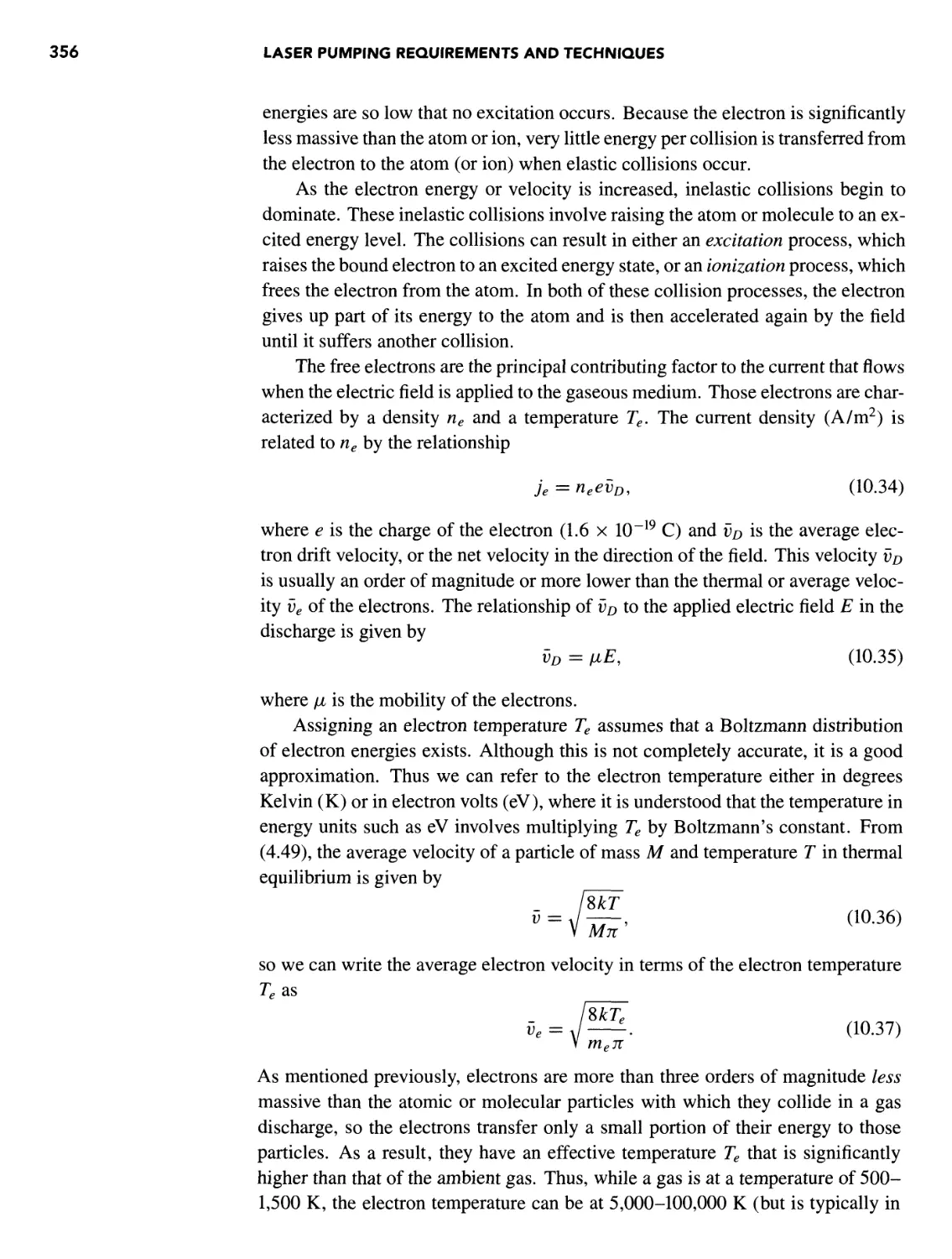
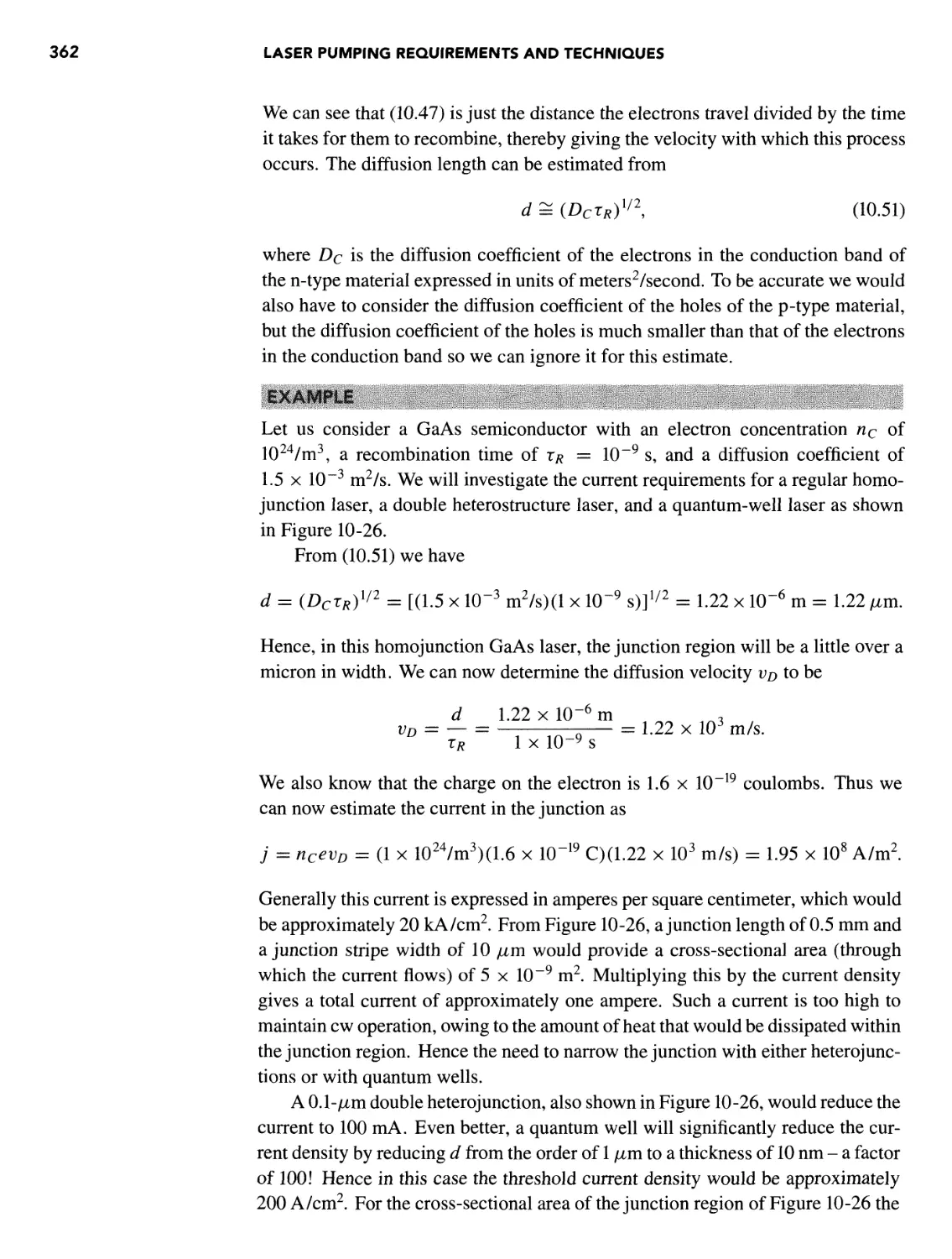
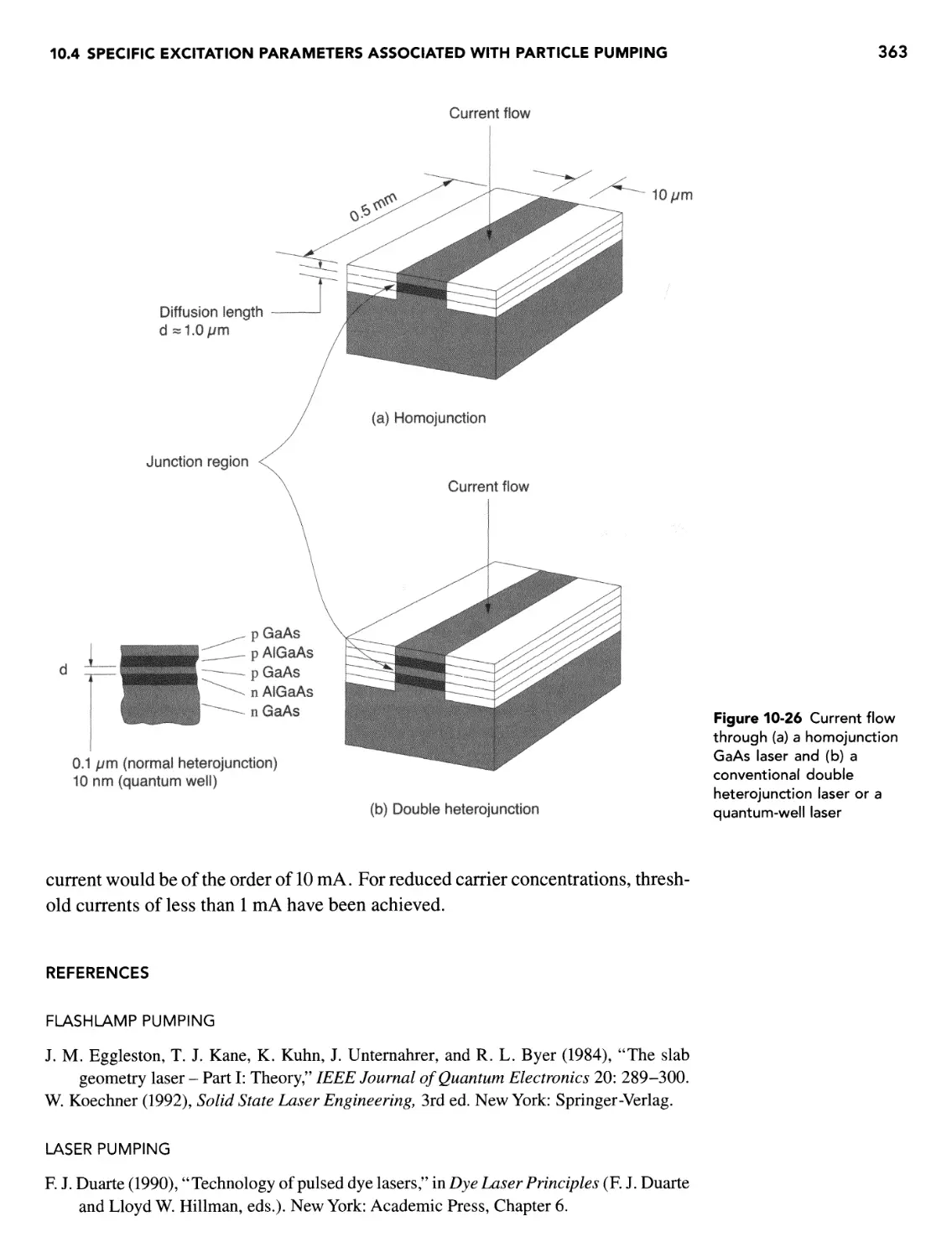
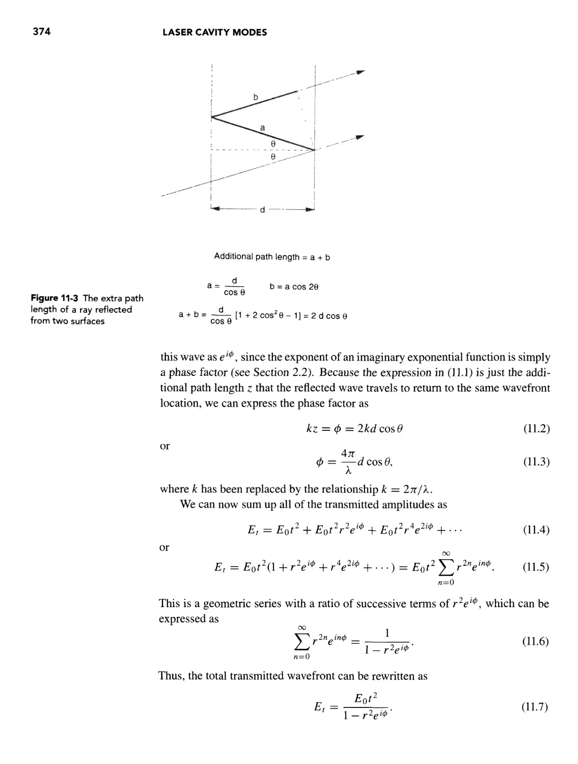
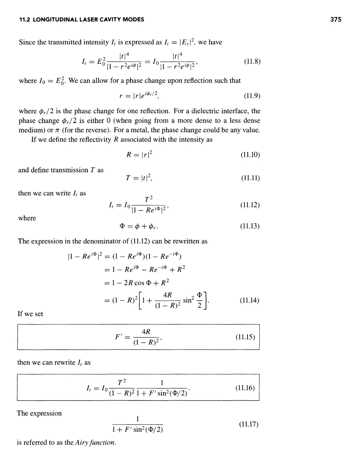
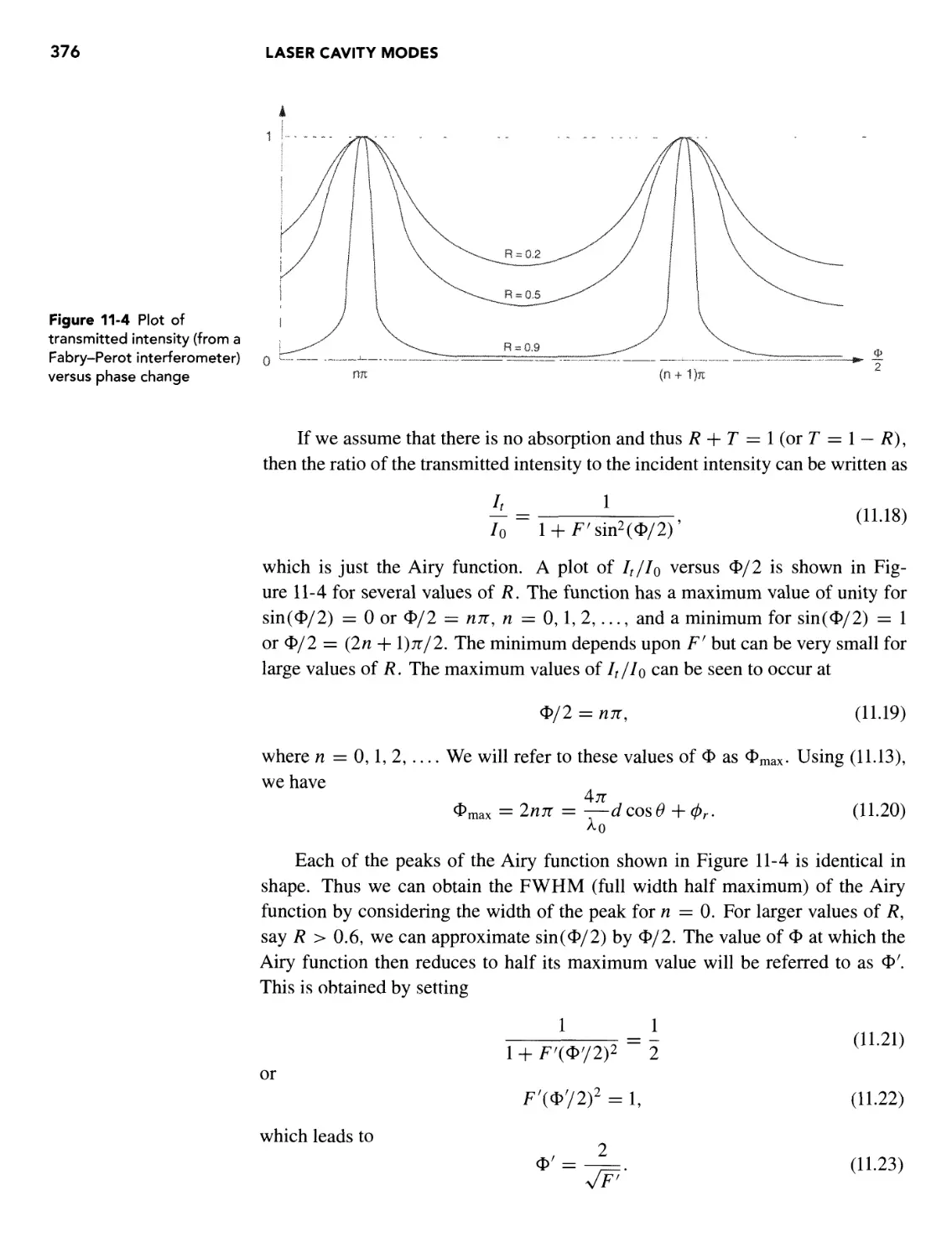
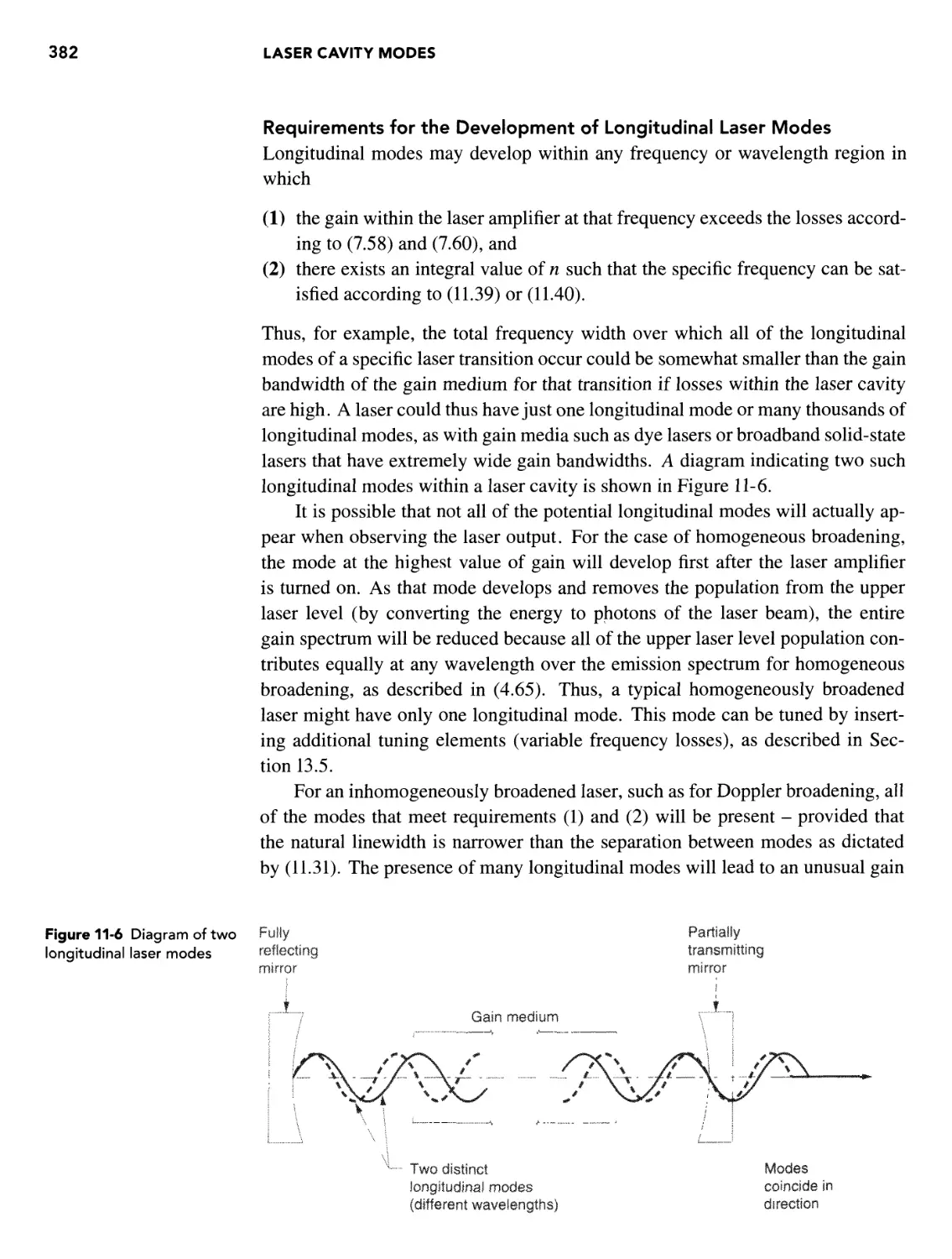
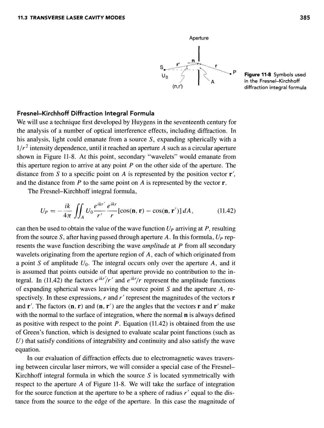
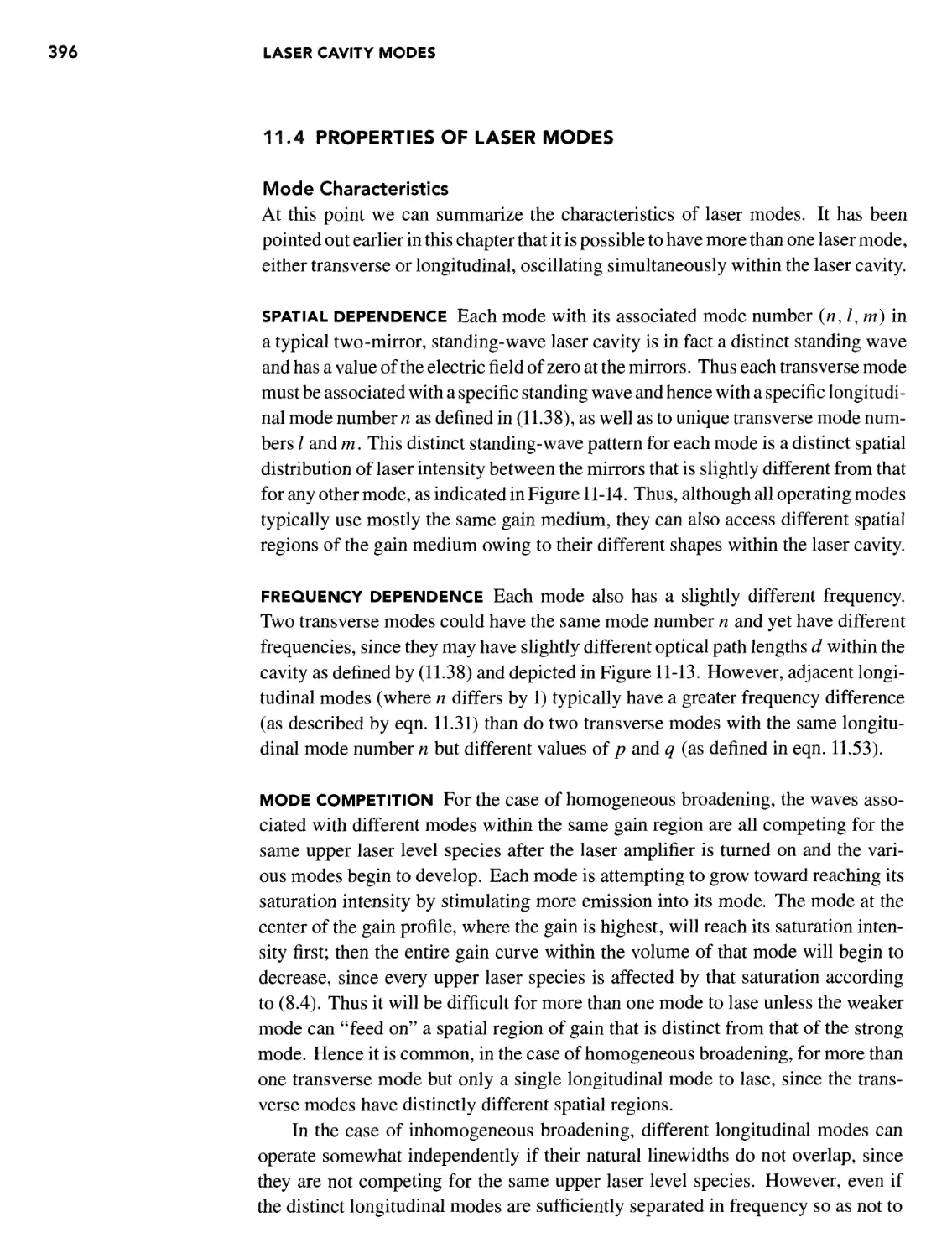
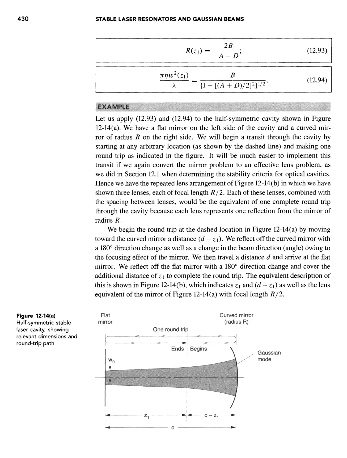
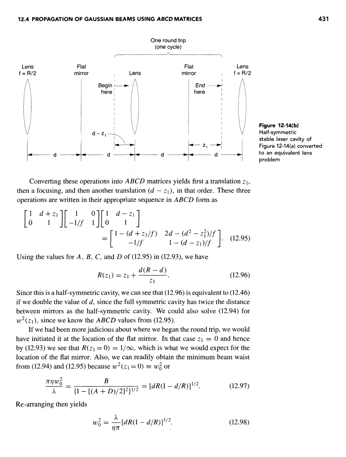
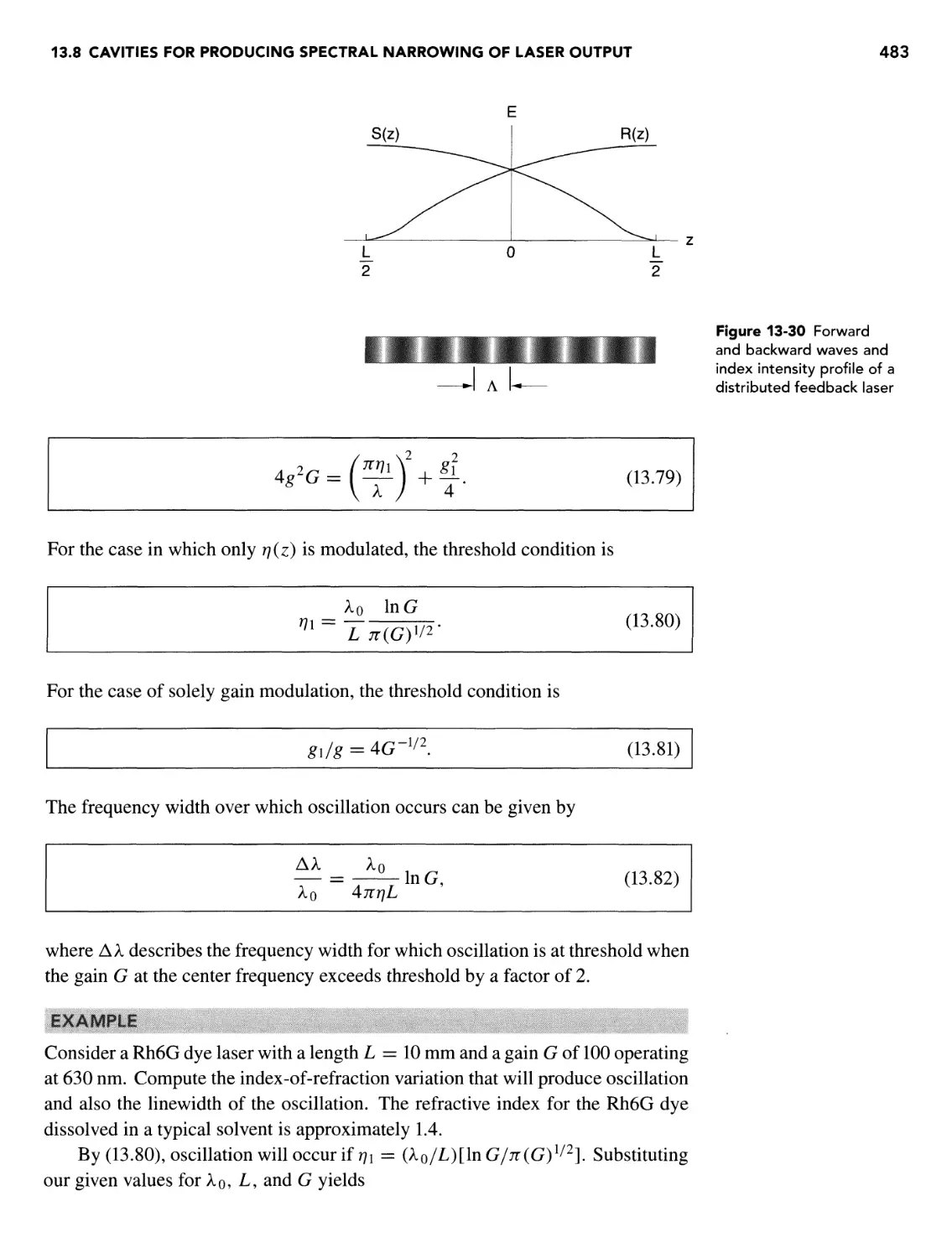
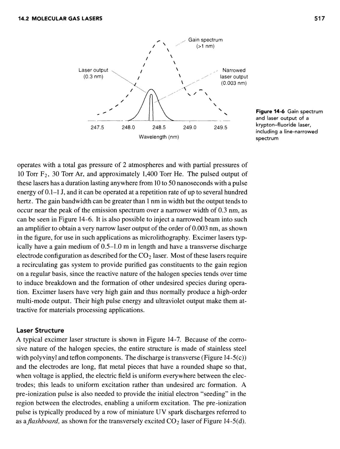
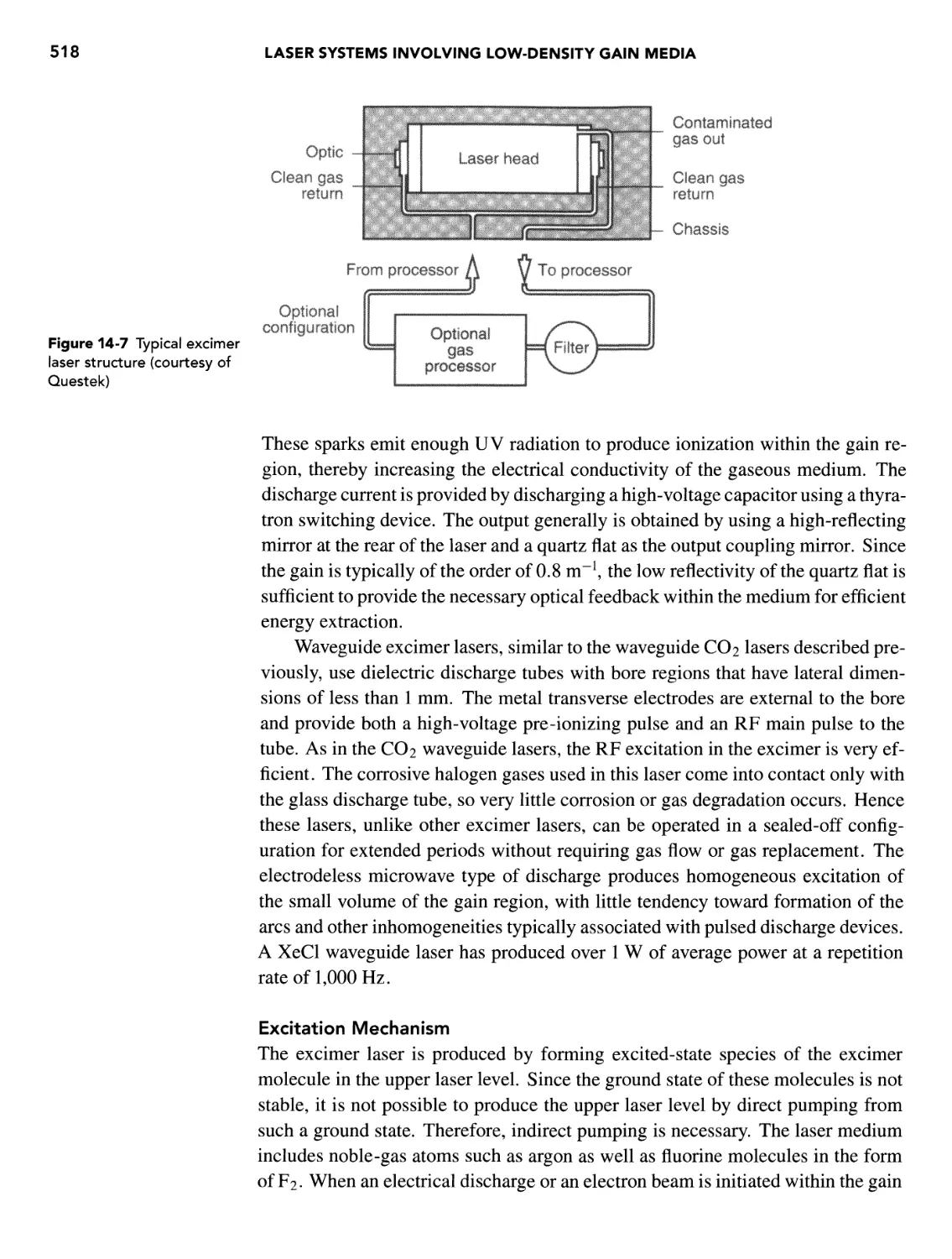
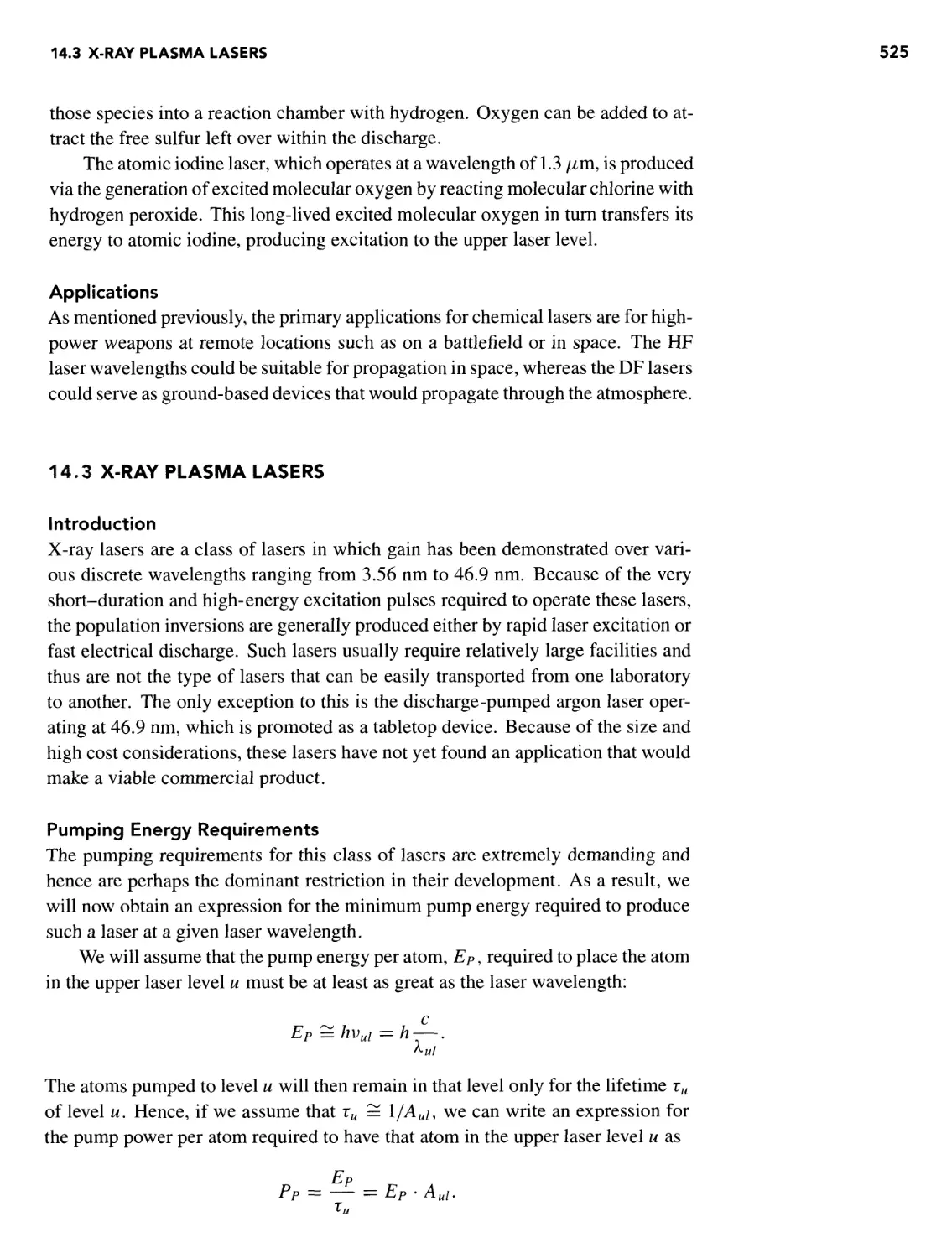
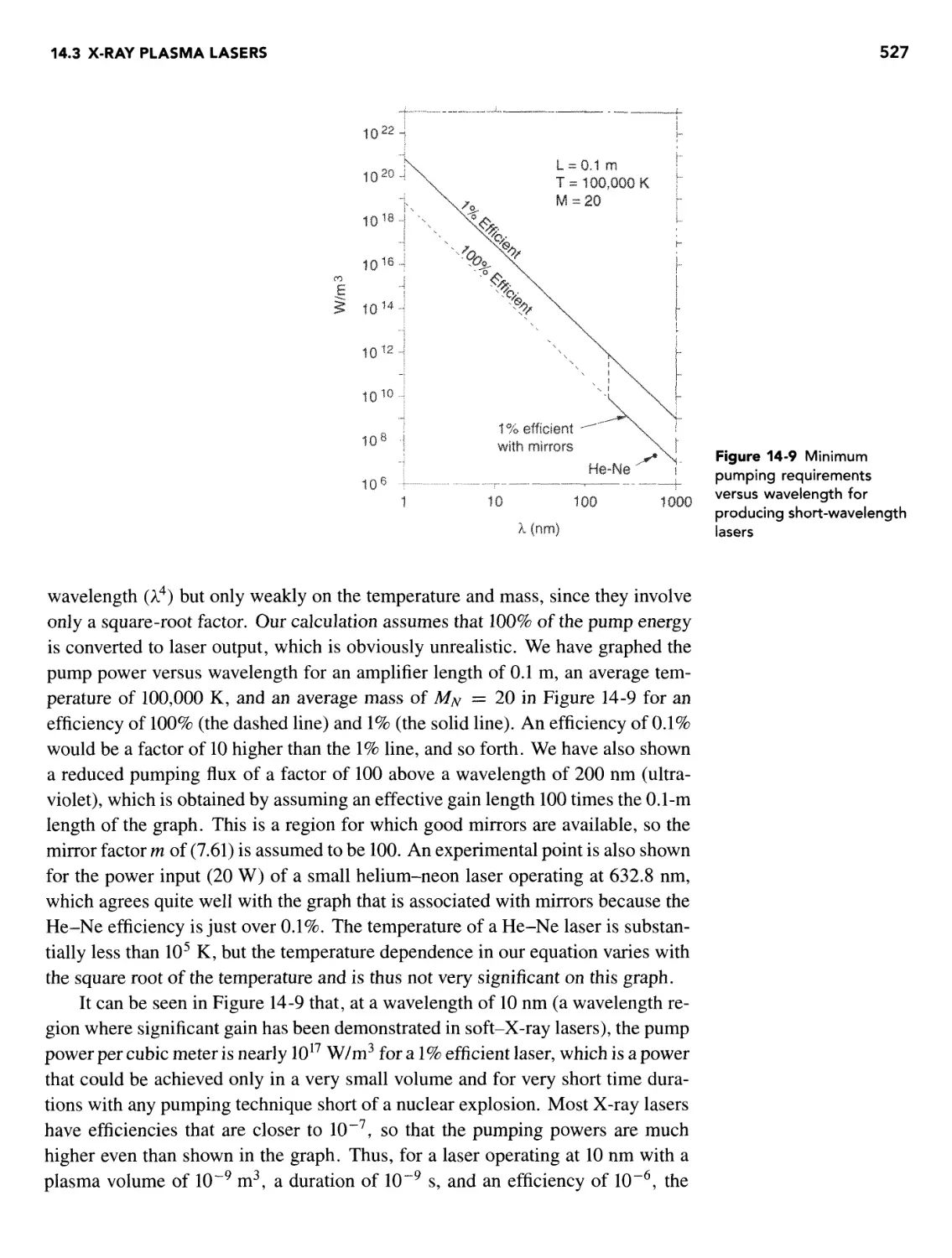
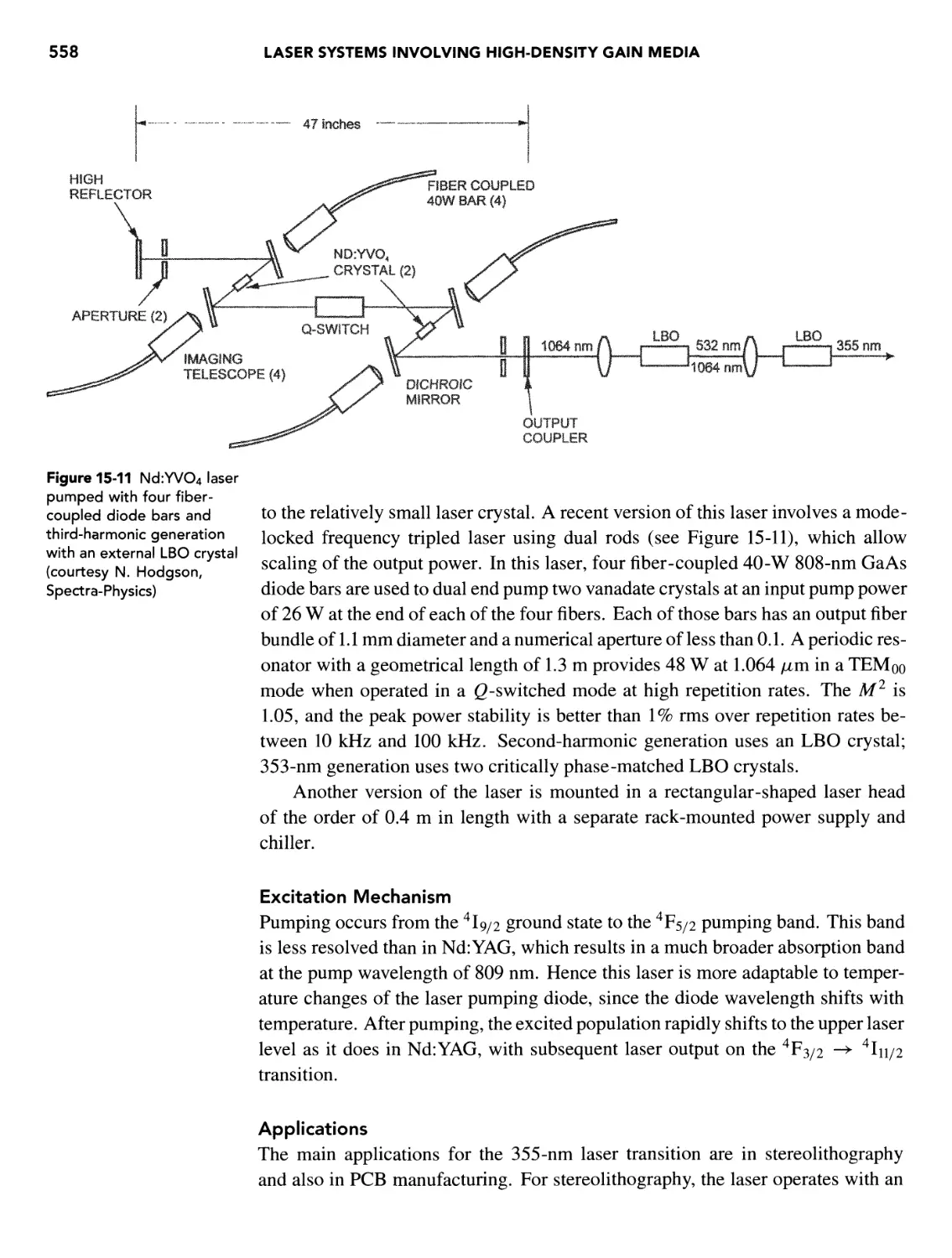
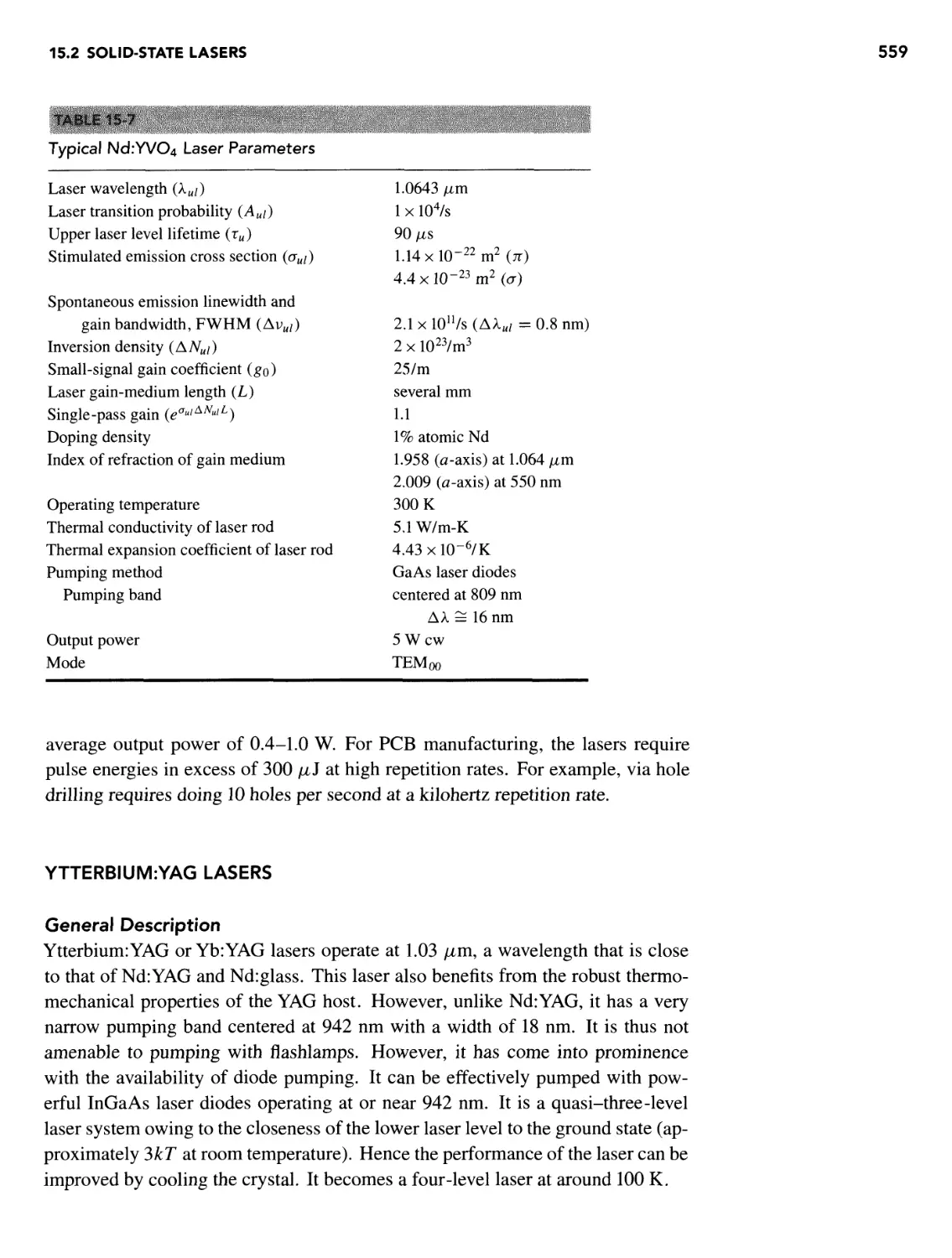
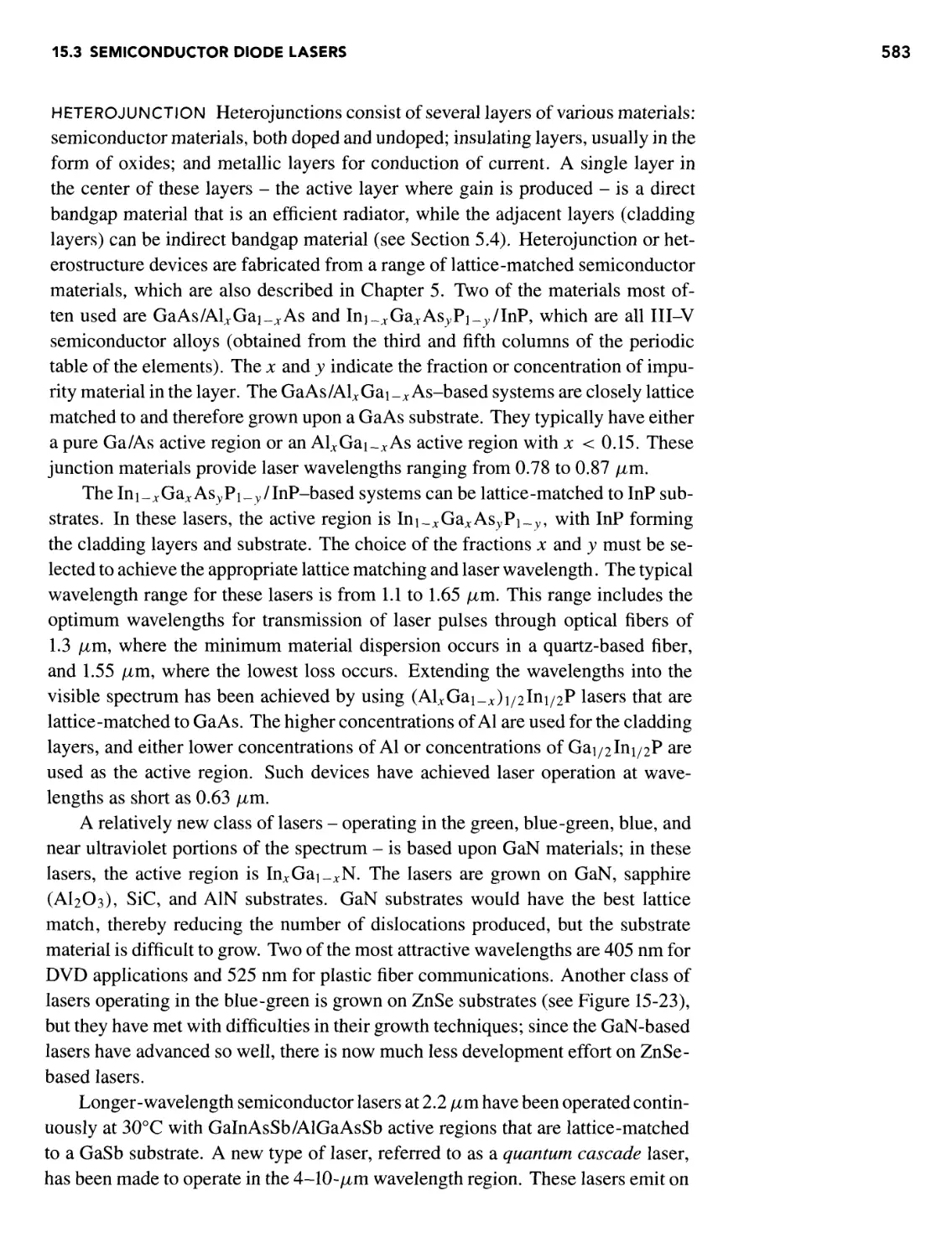
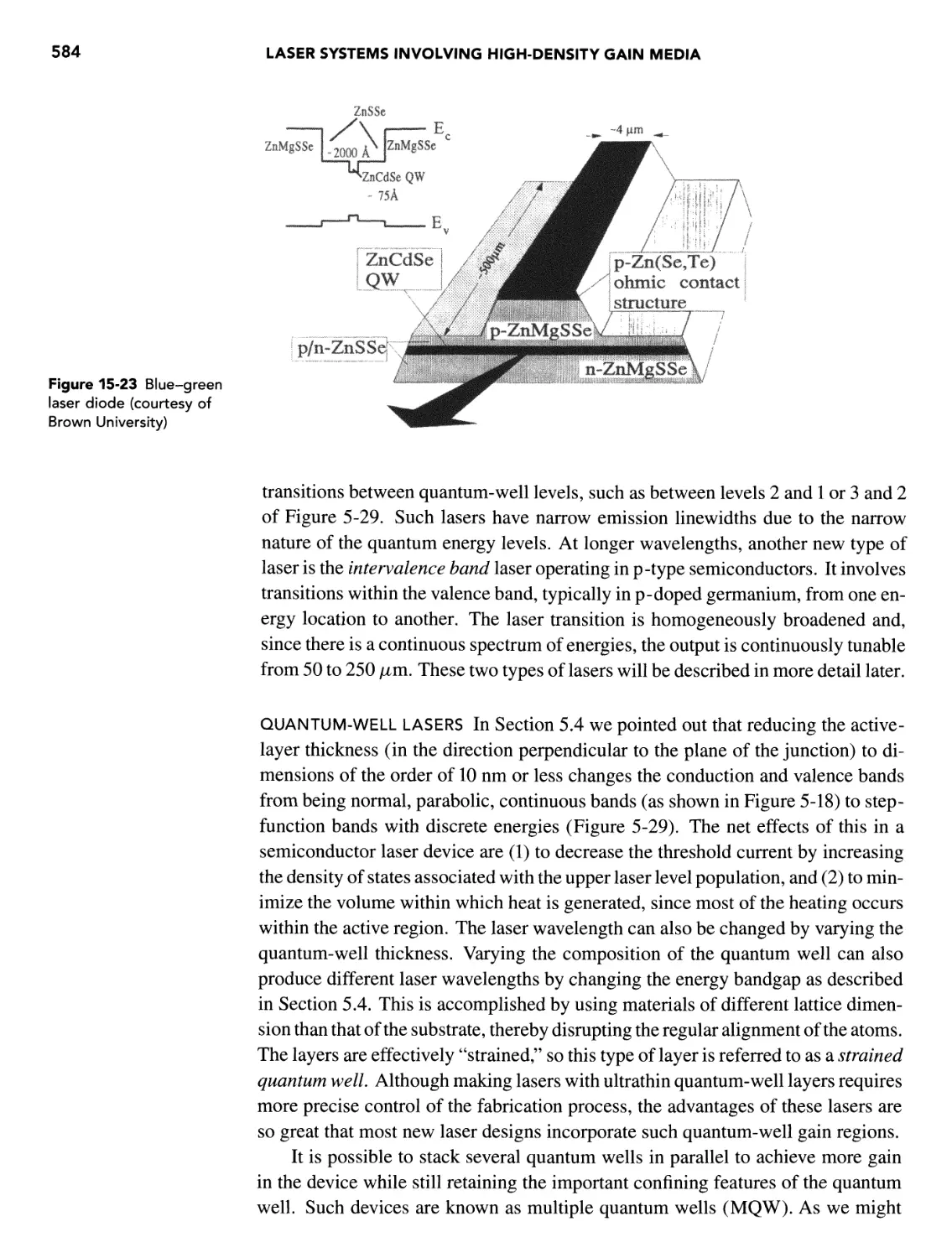
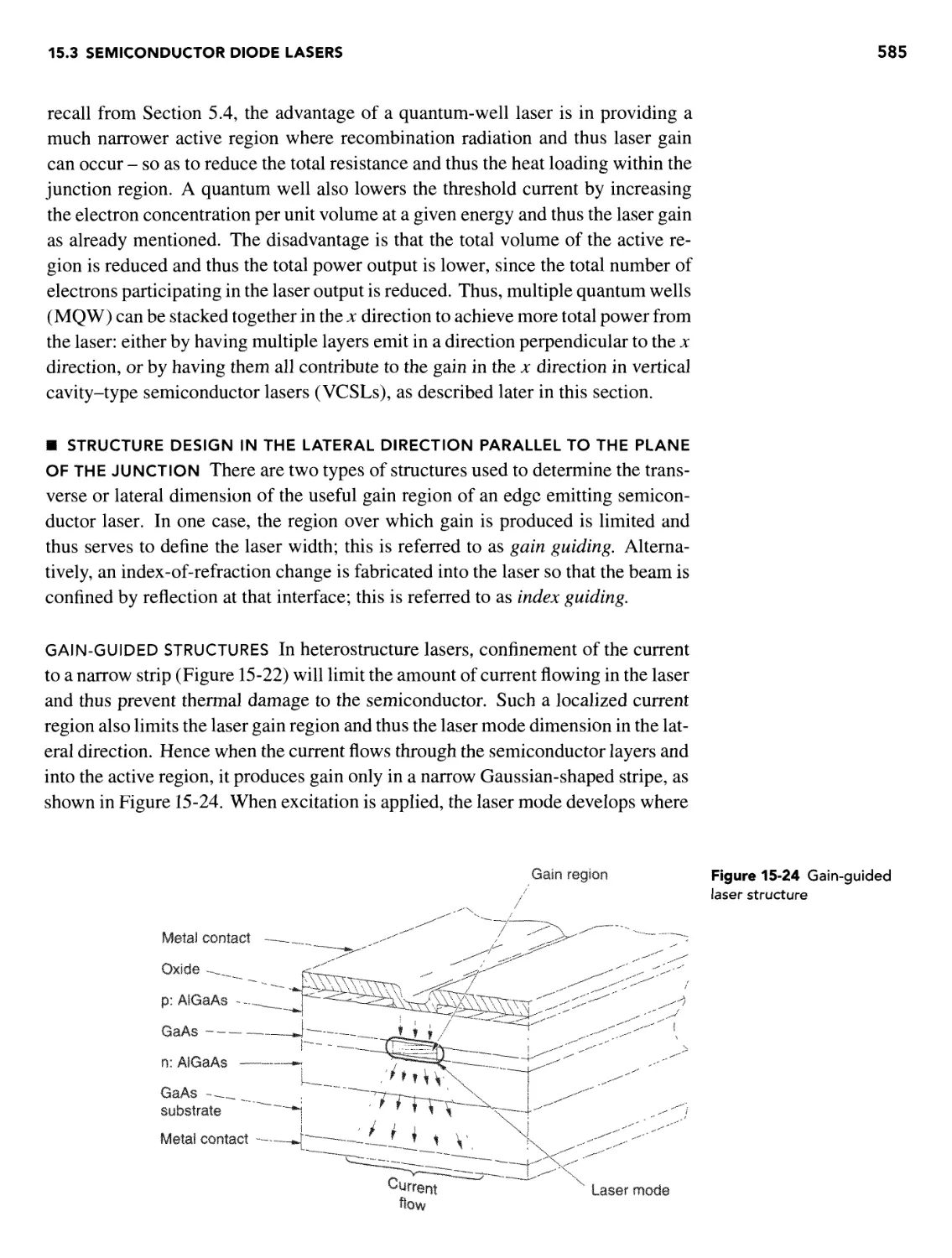
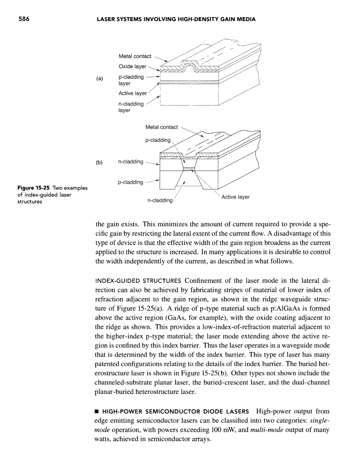
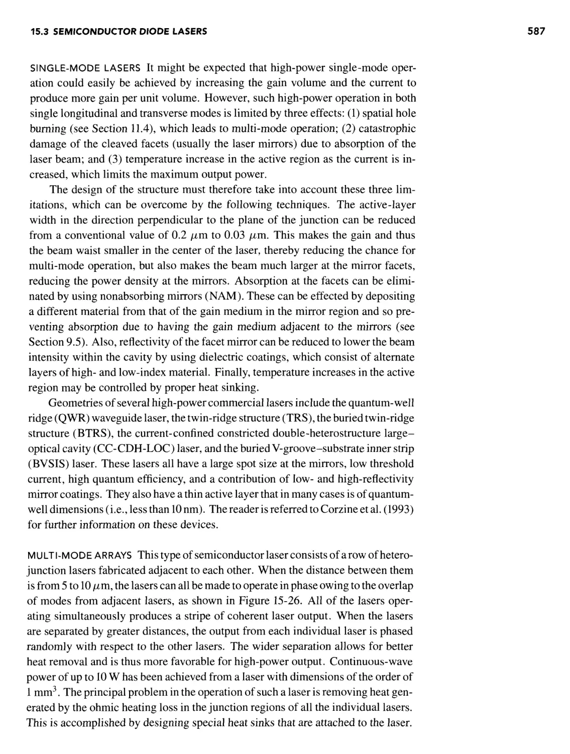
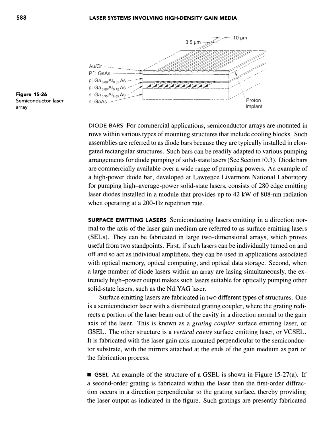
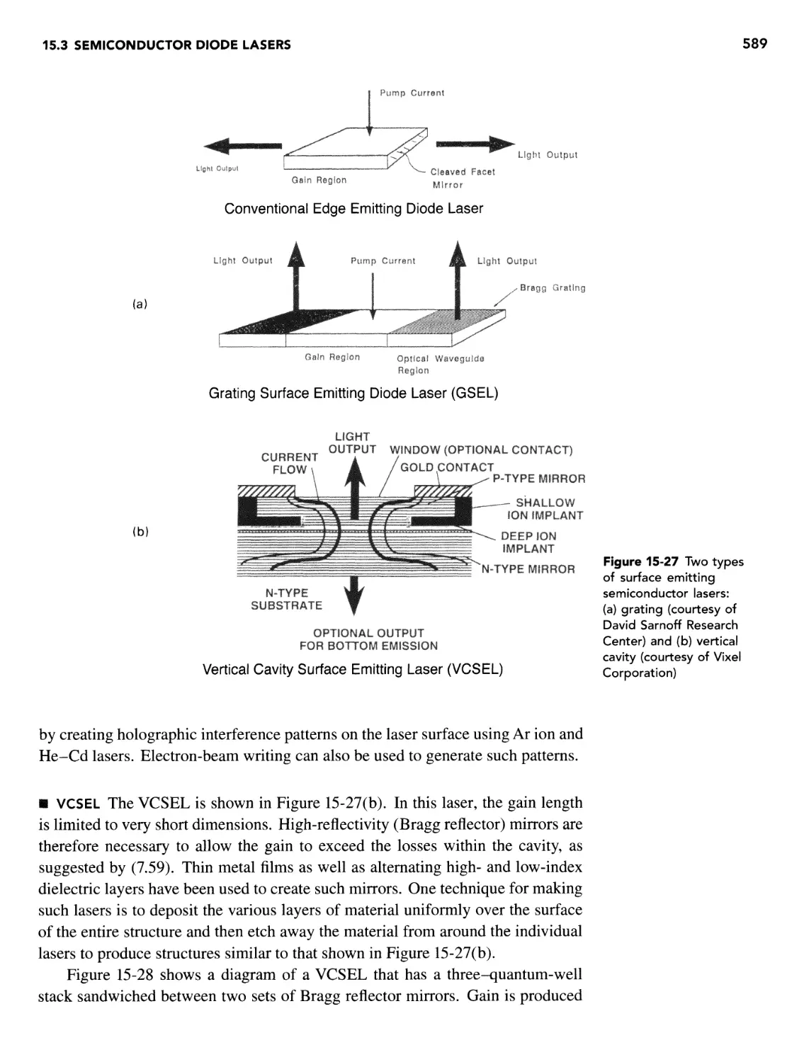
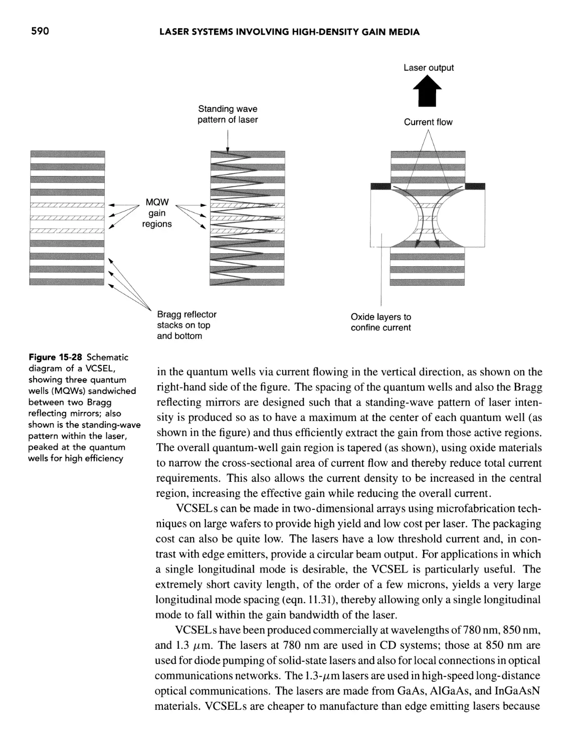
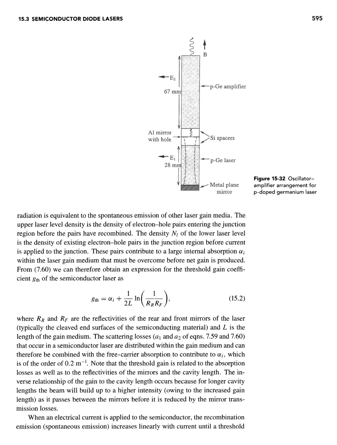
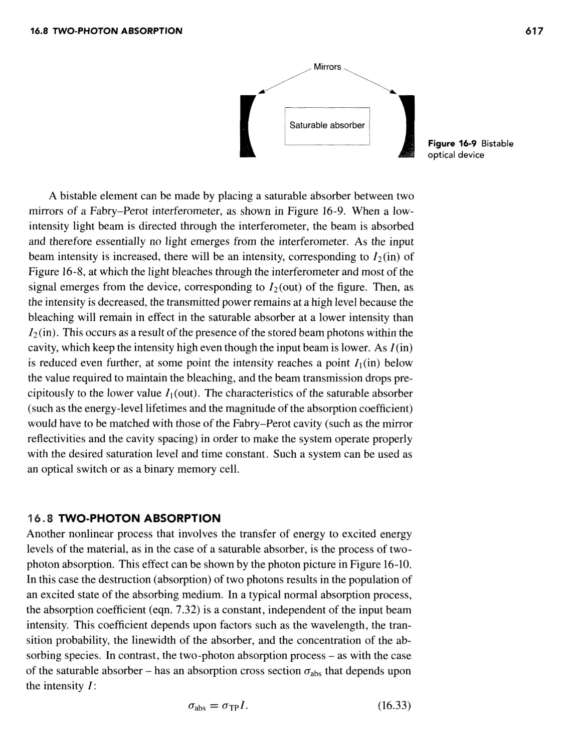
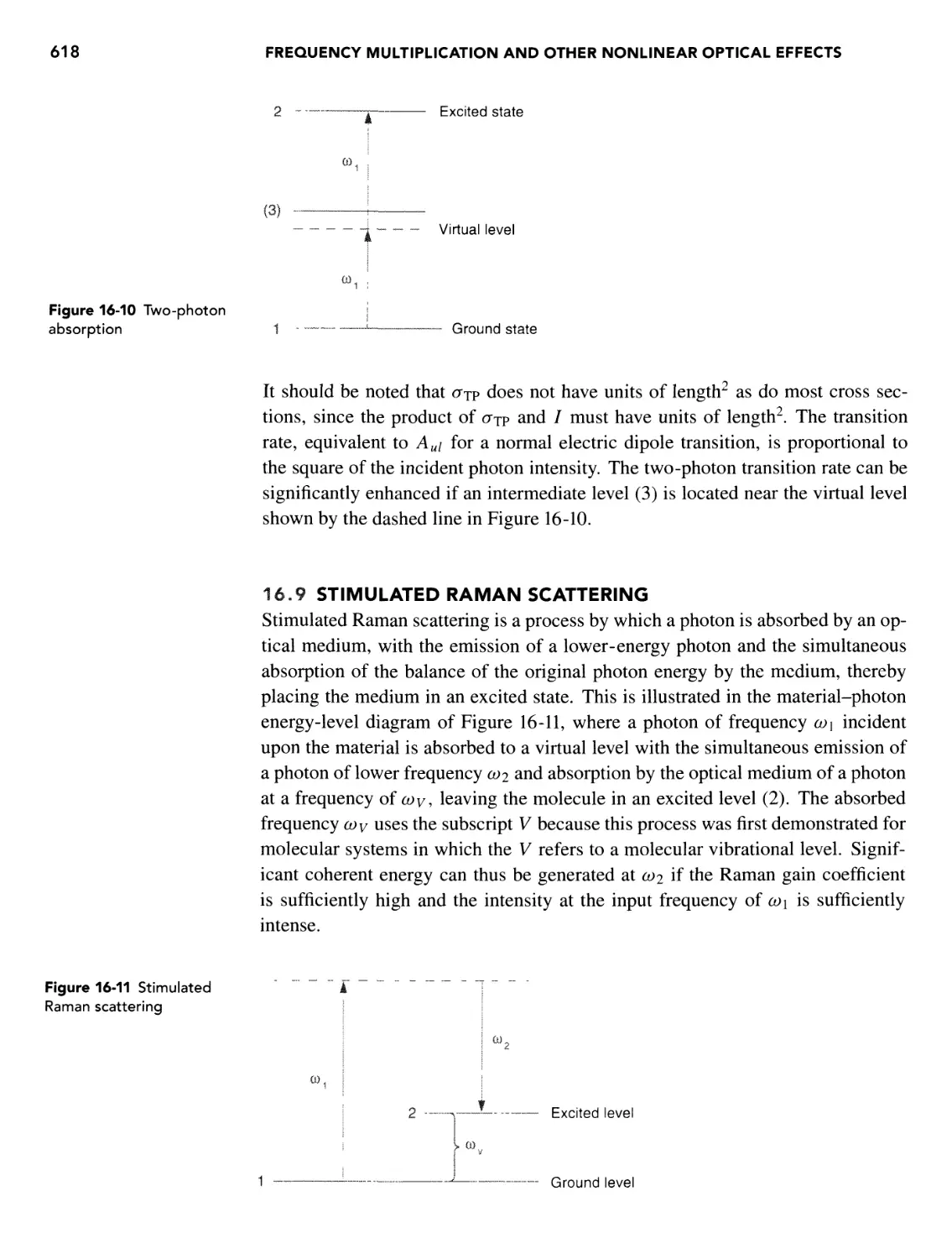
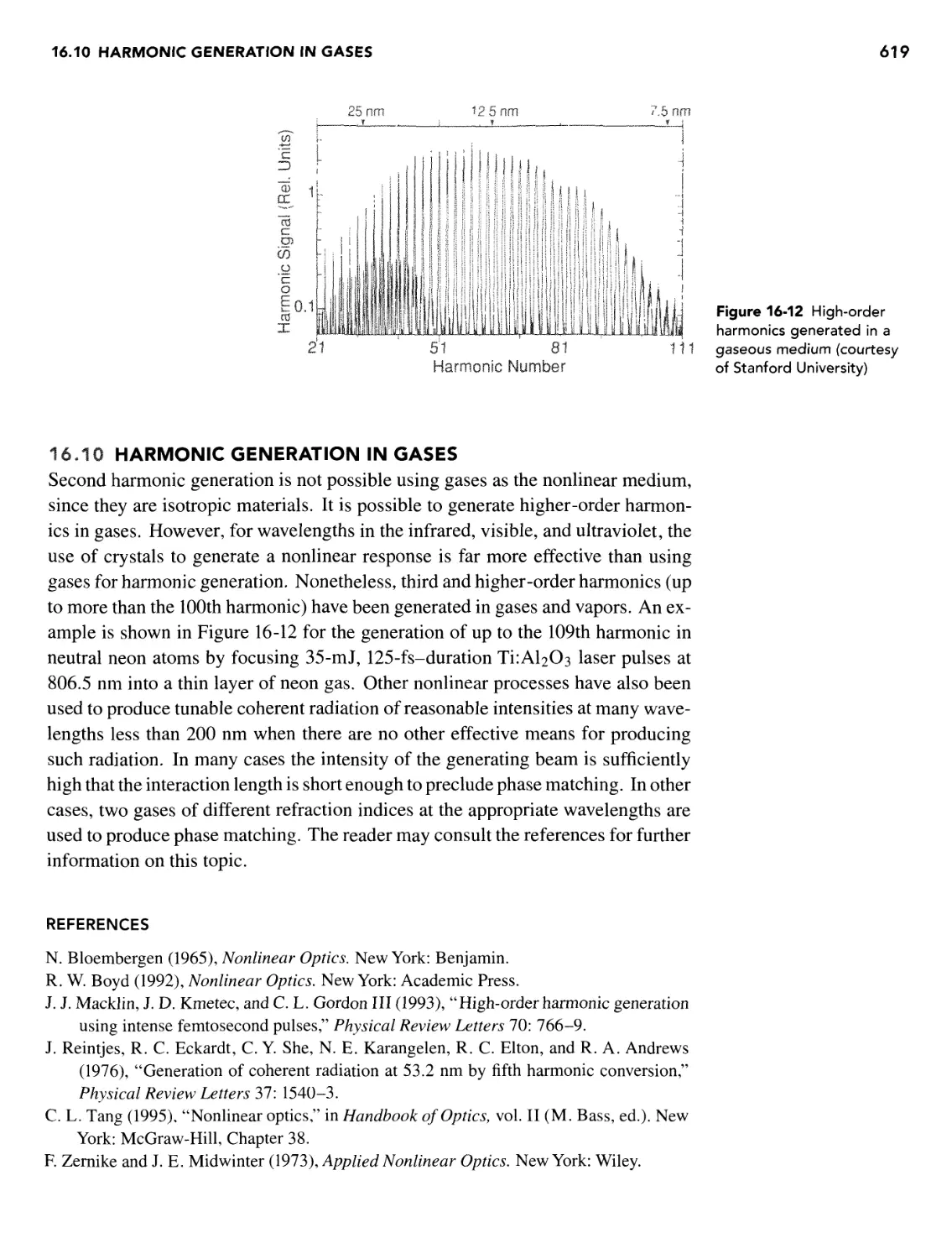
/


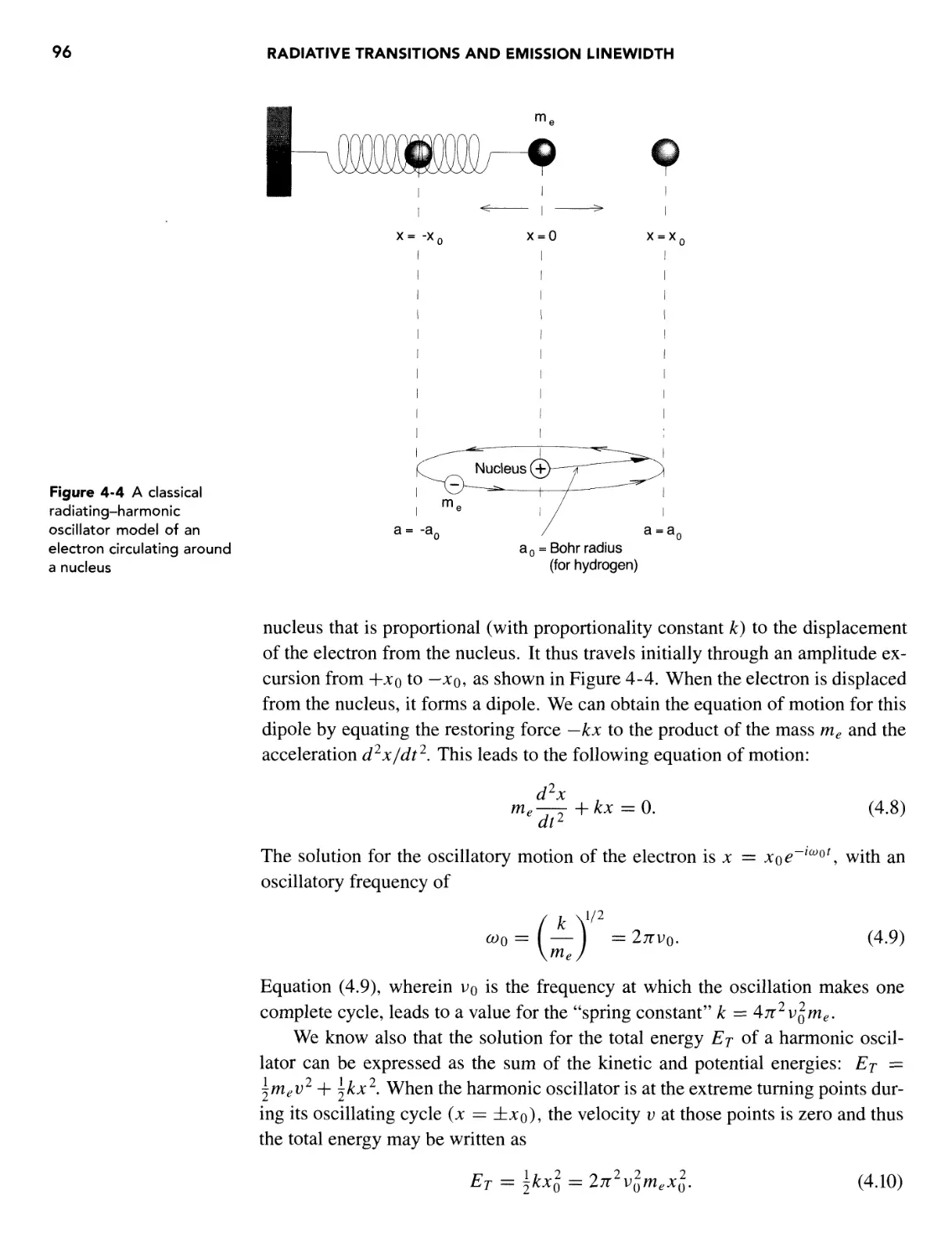
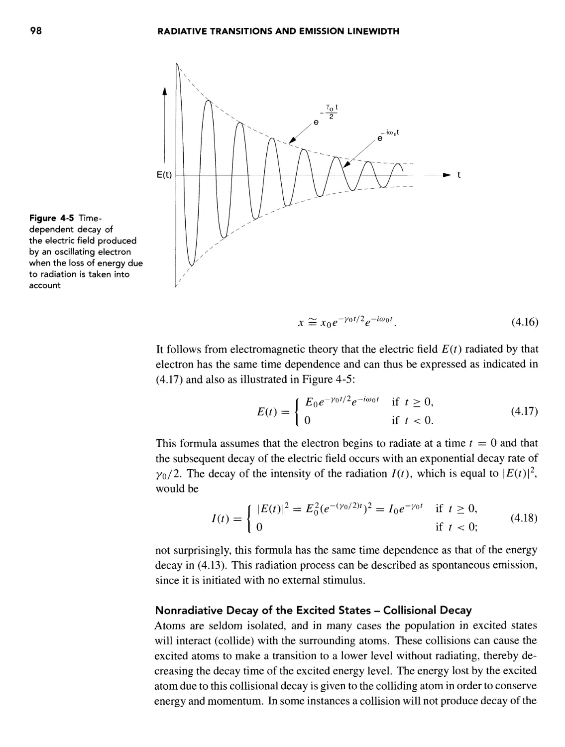
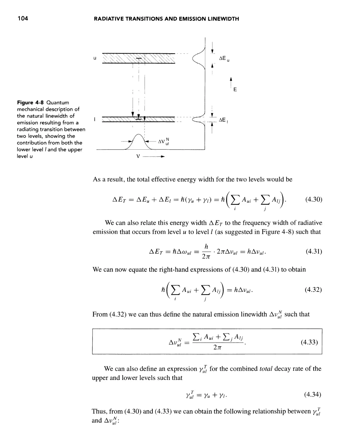
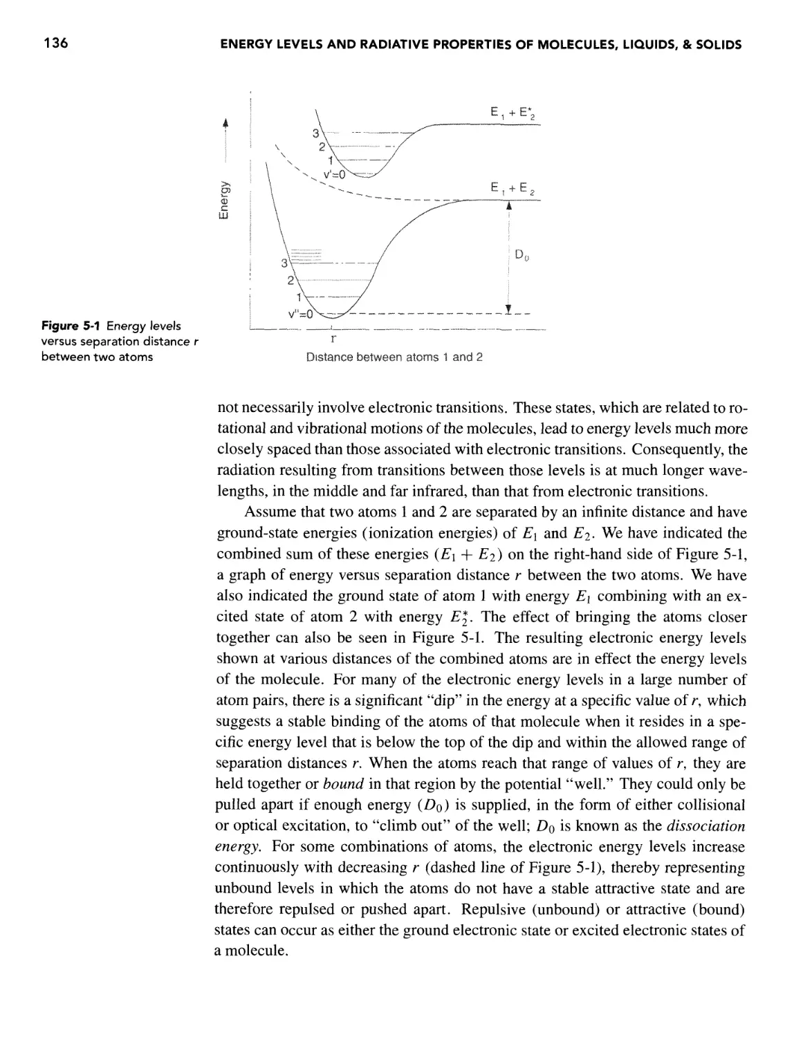
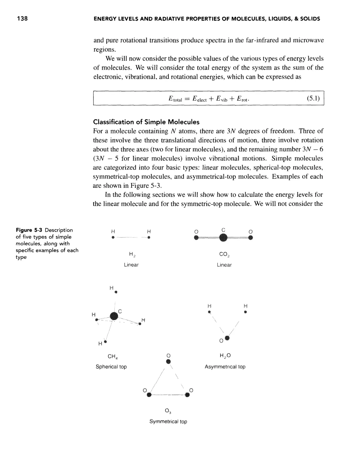
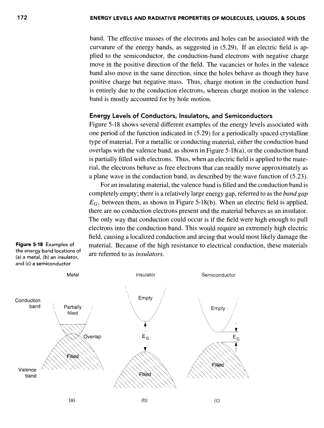
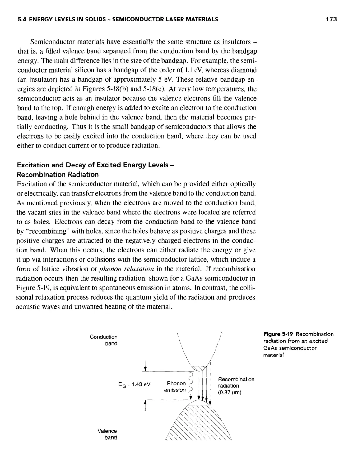
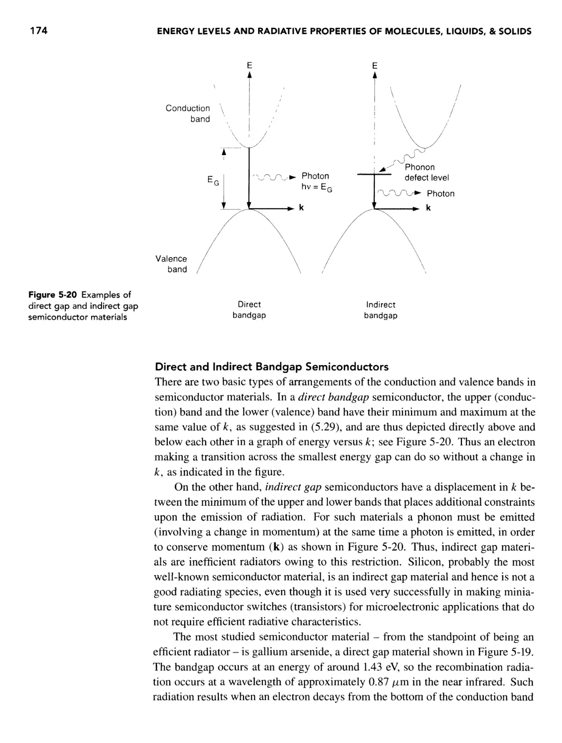
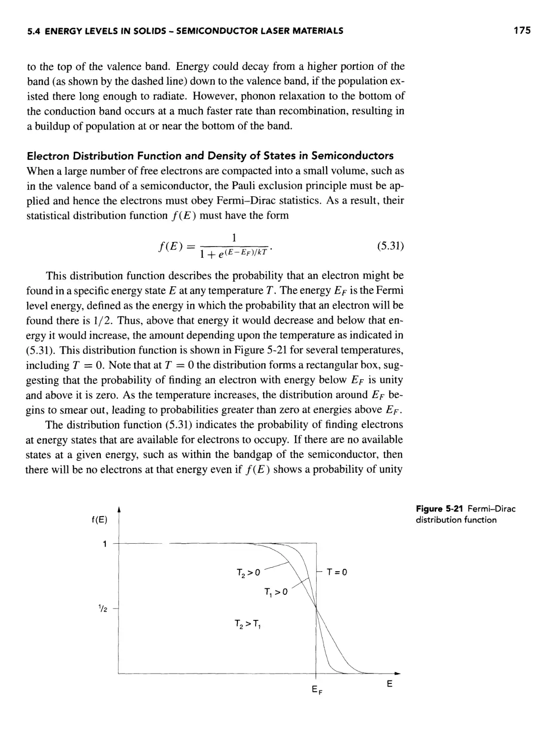
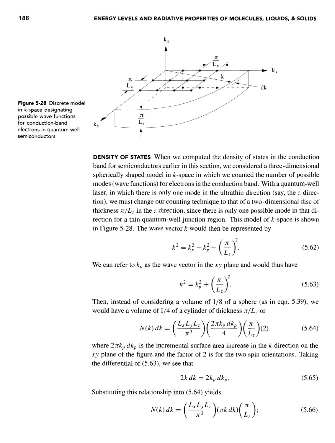
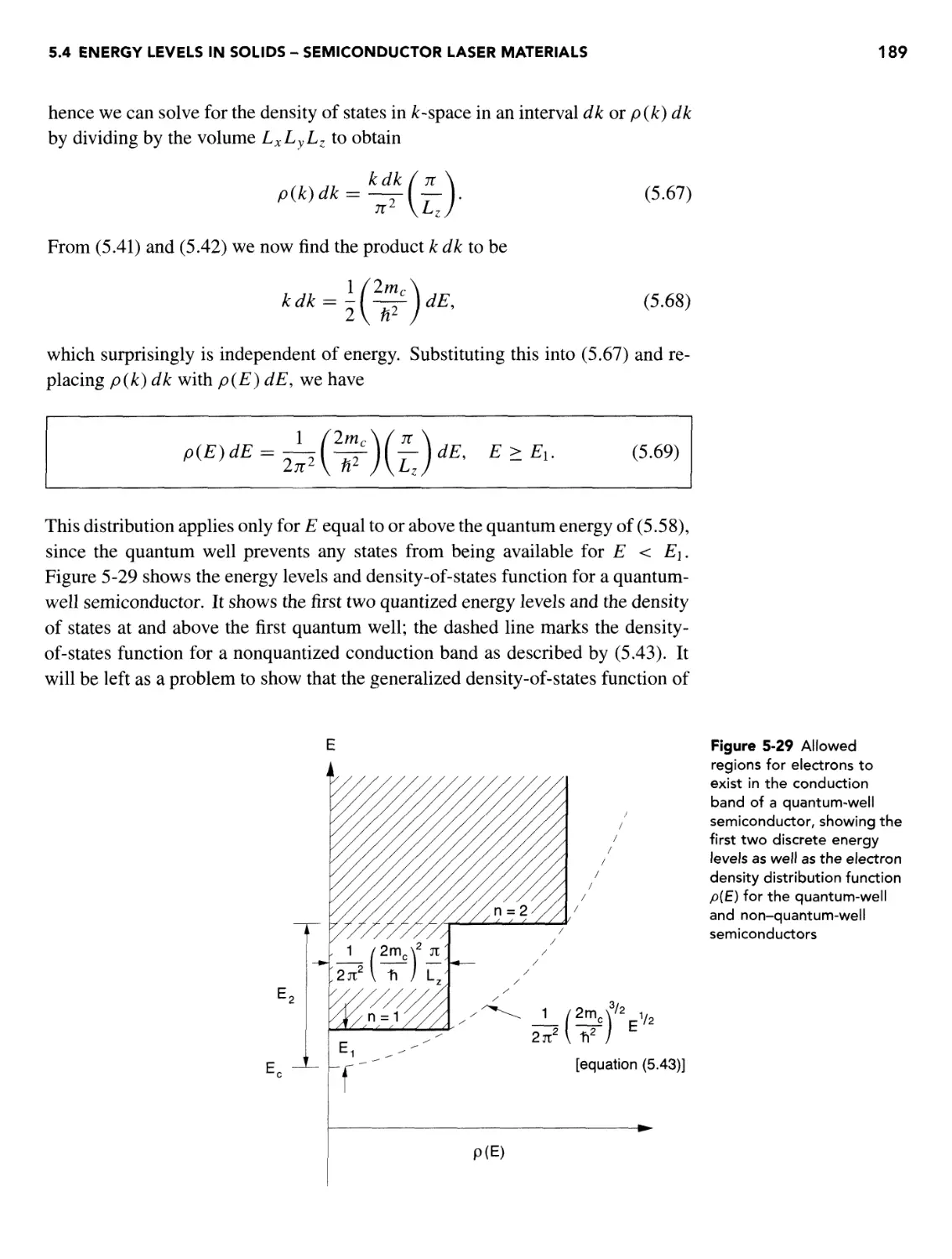
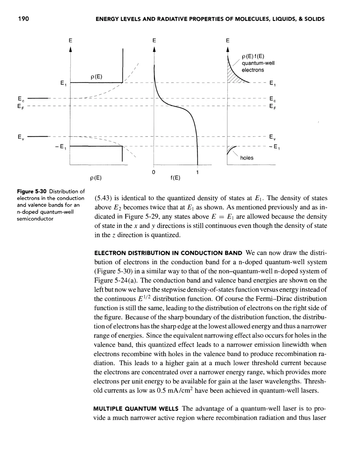
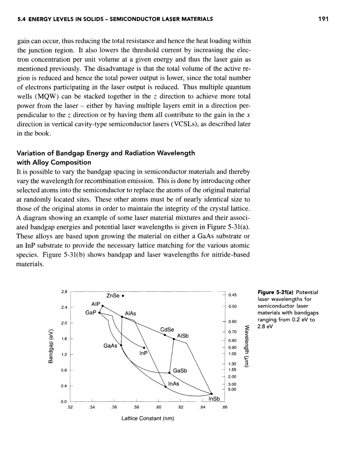
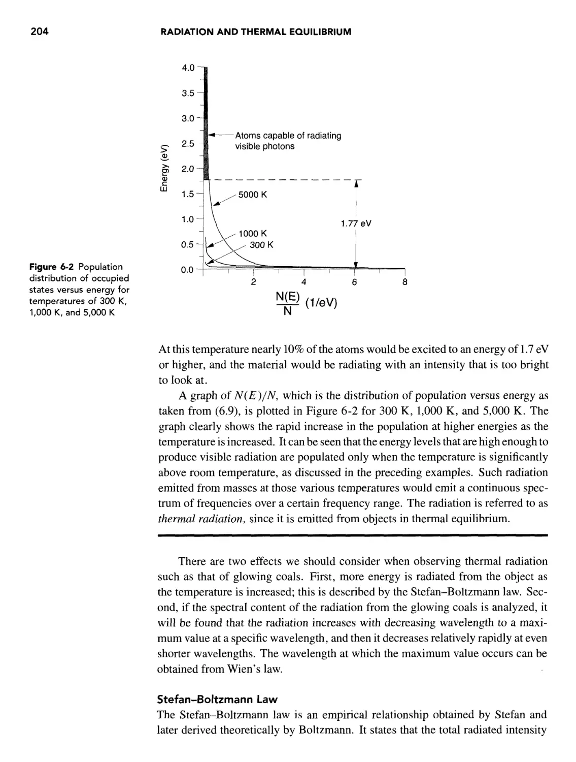
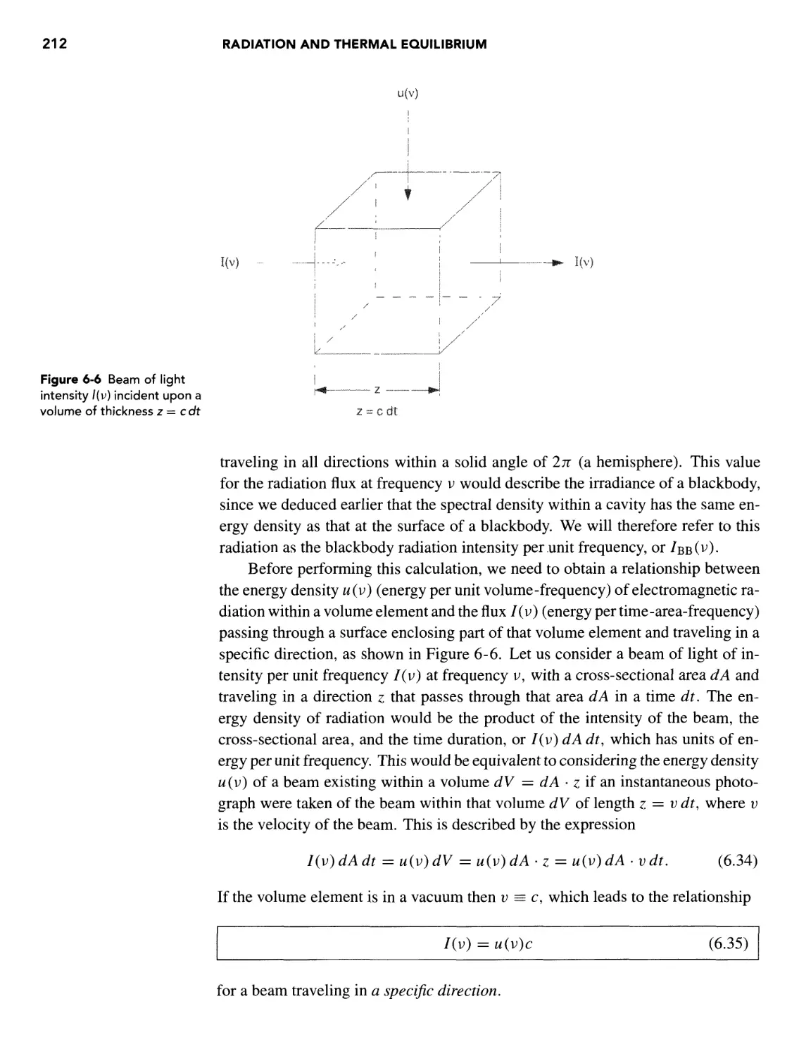
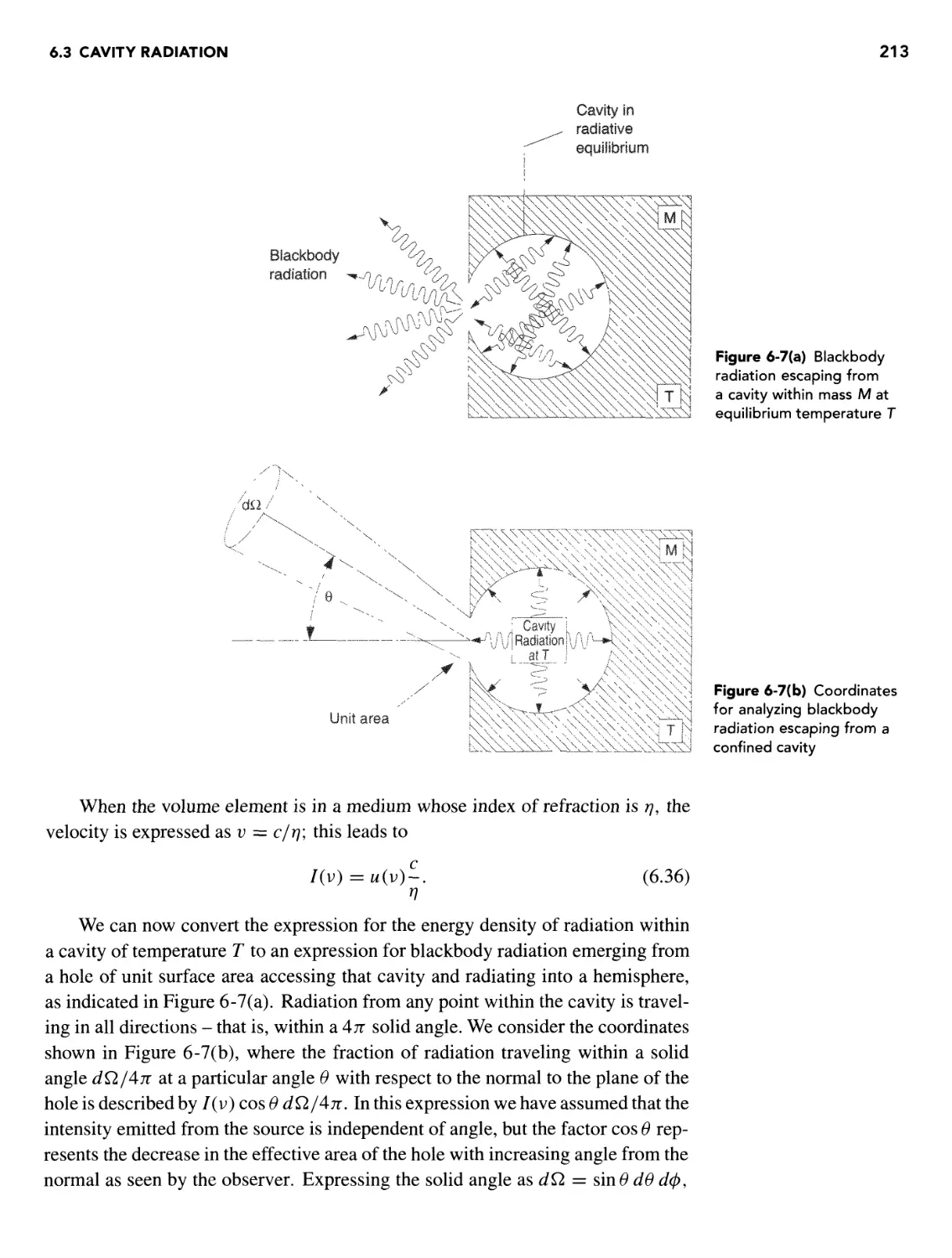
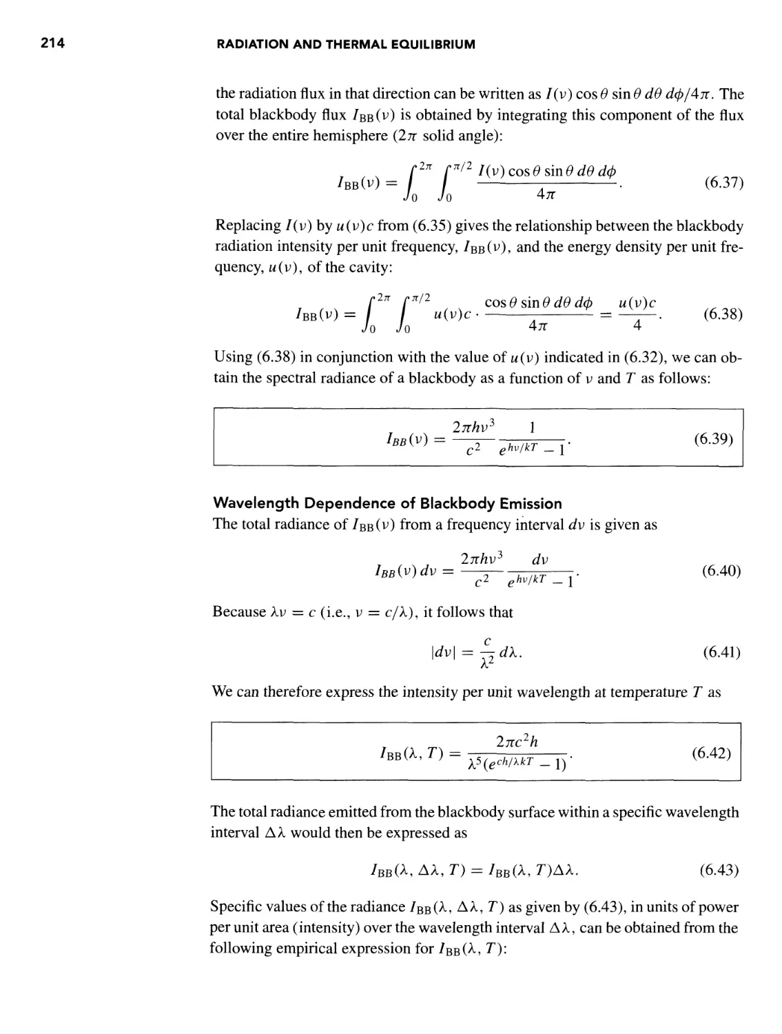


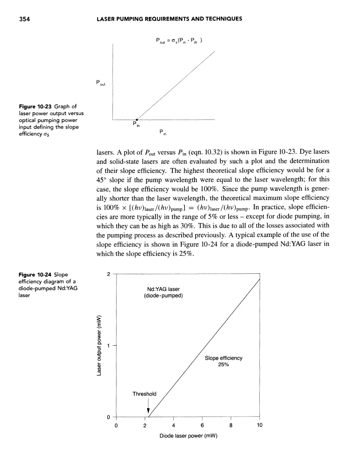
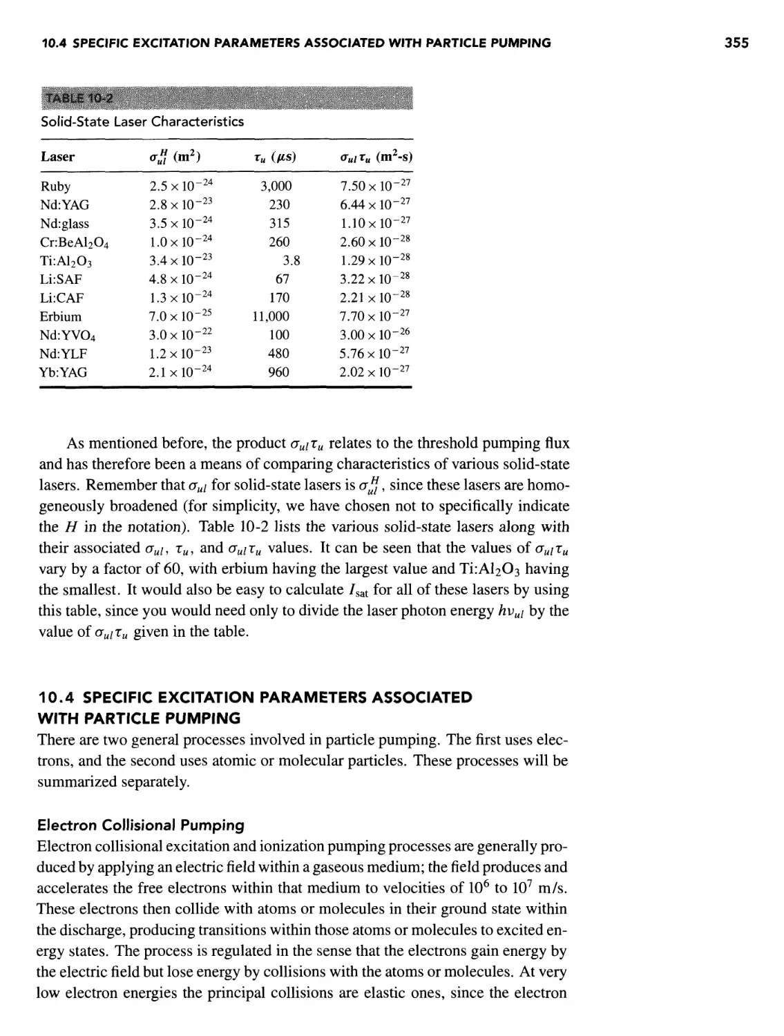


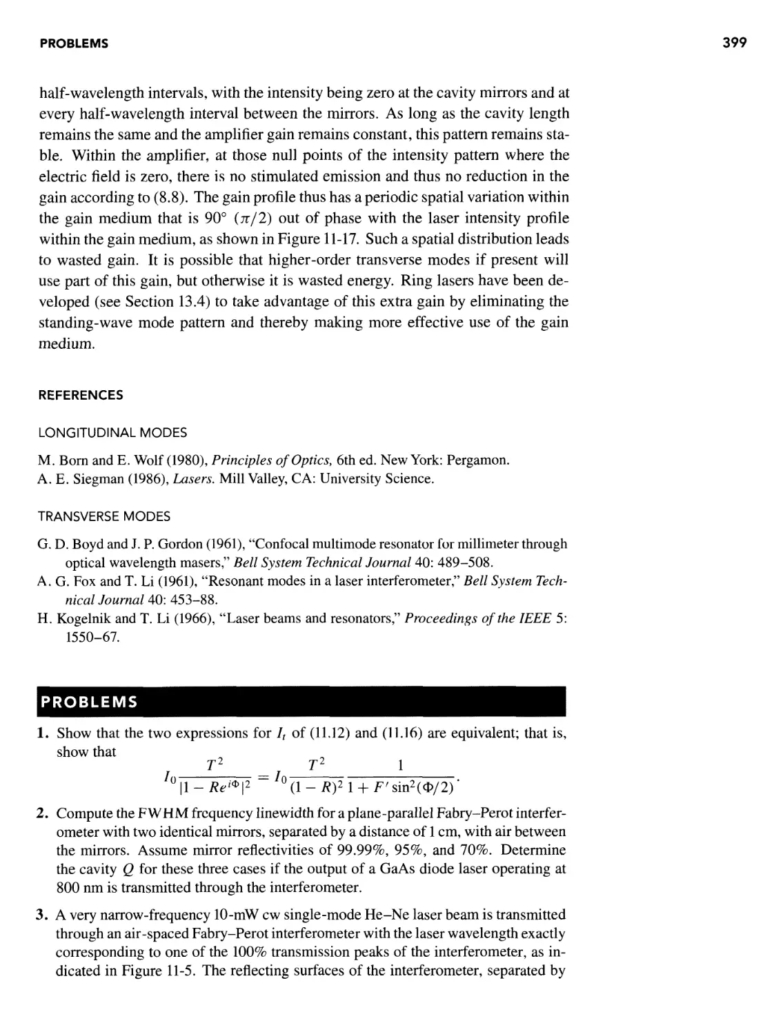


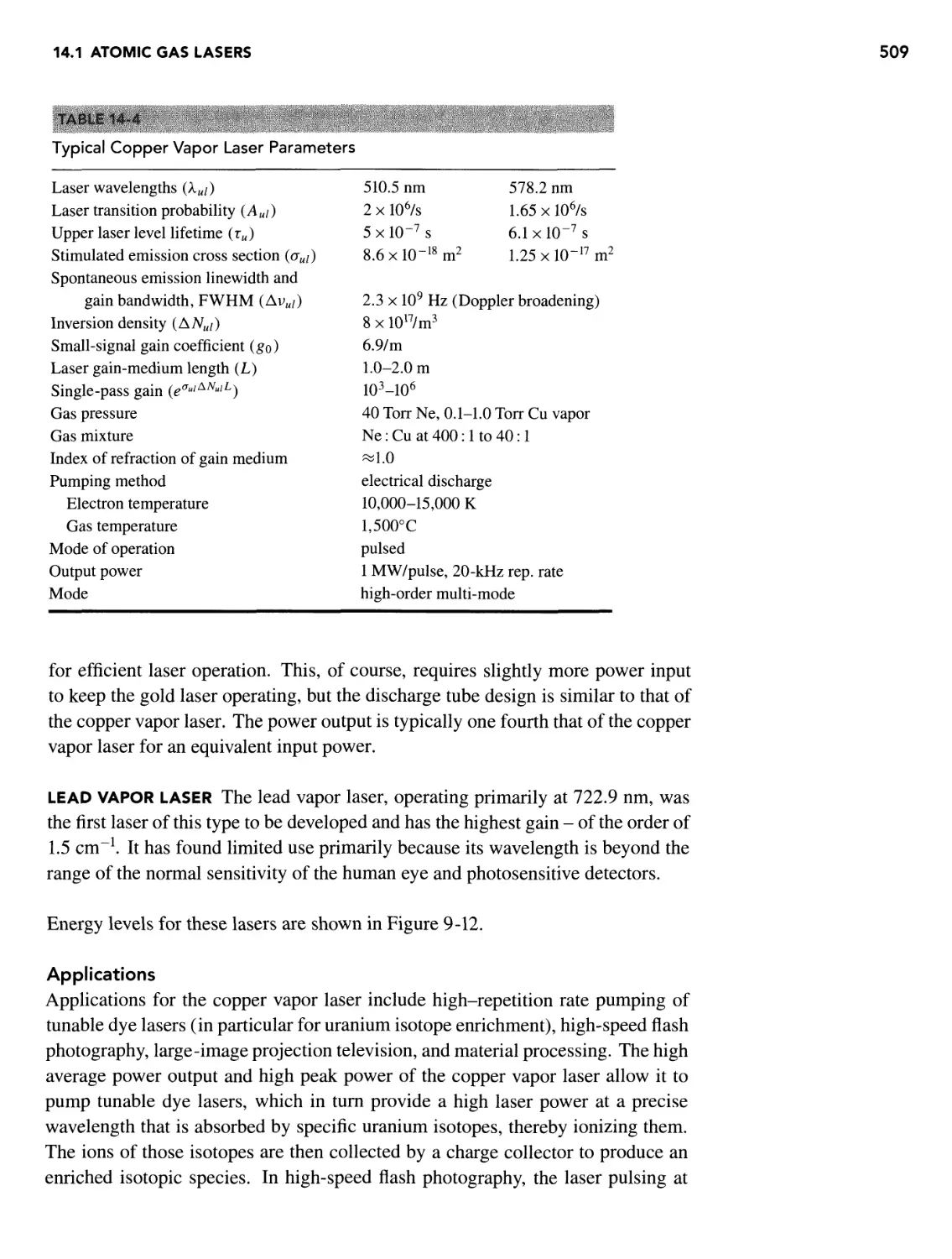
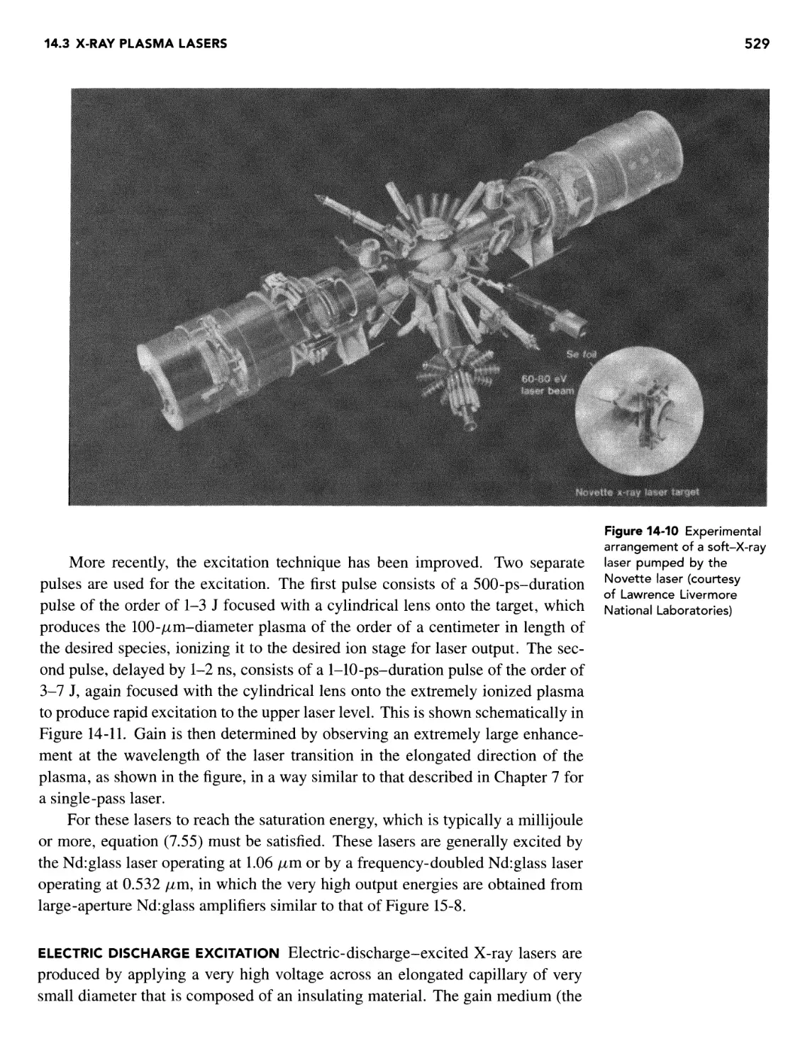
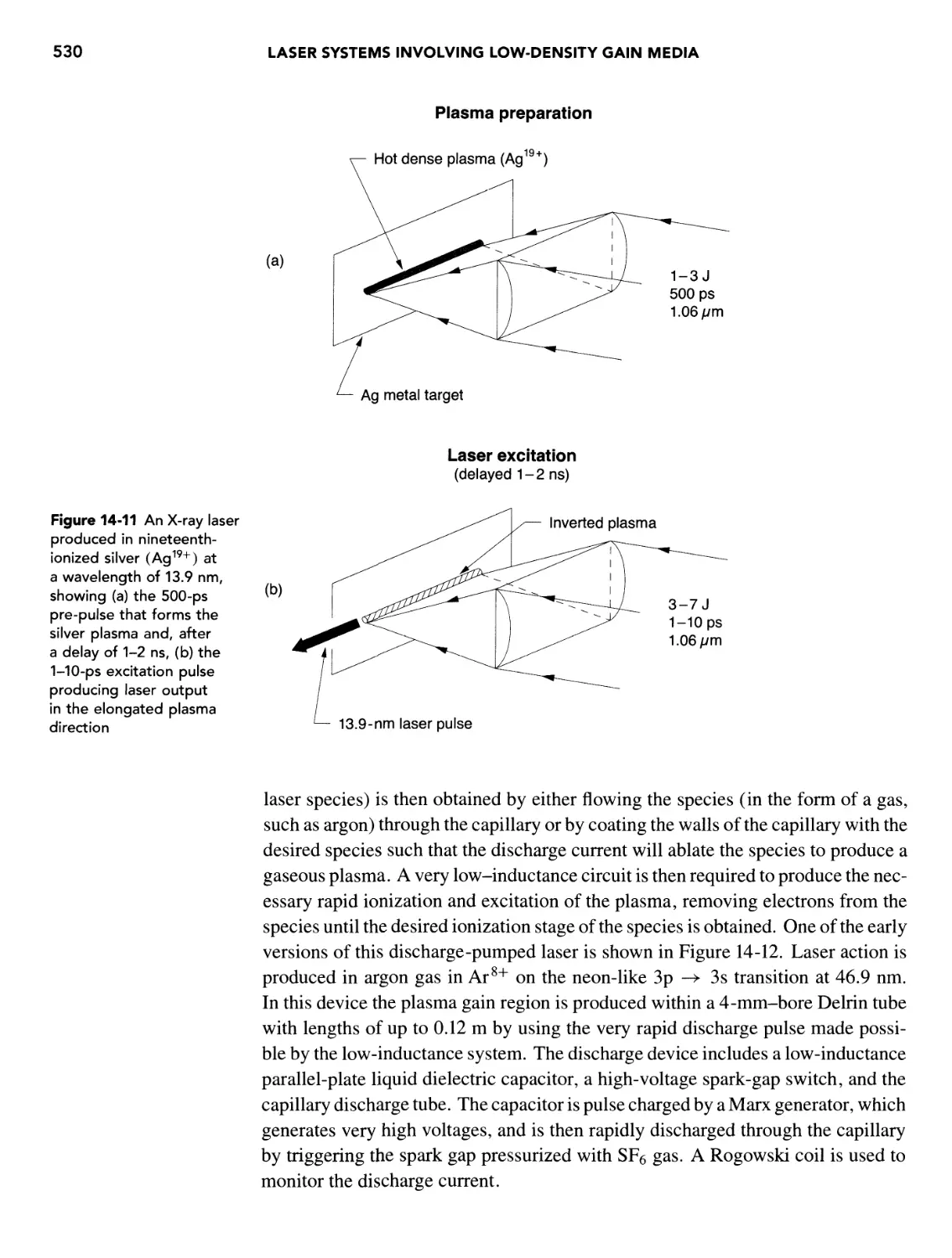

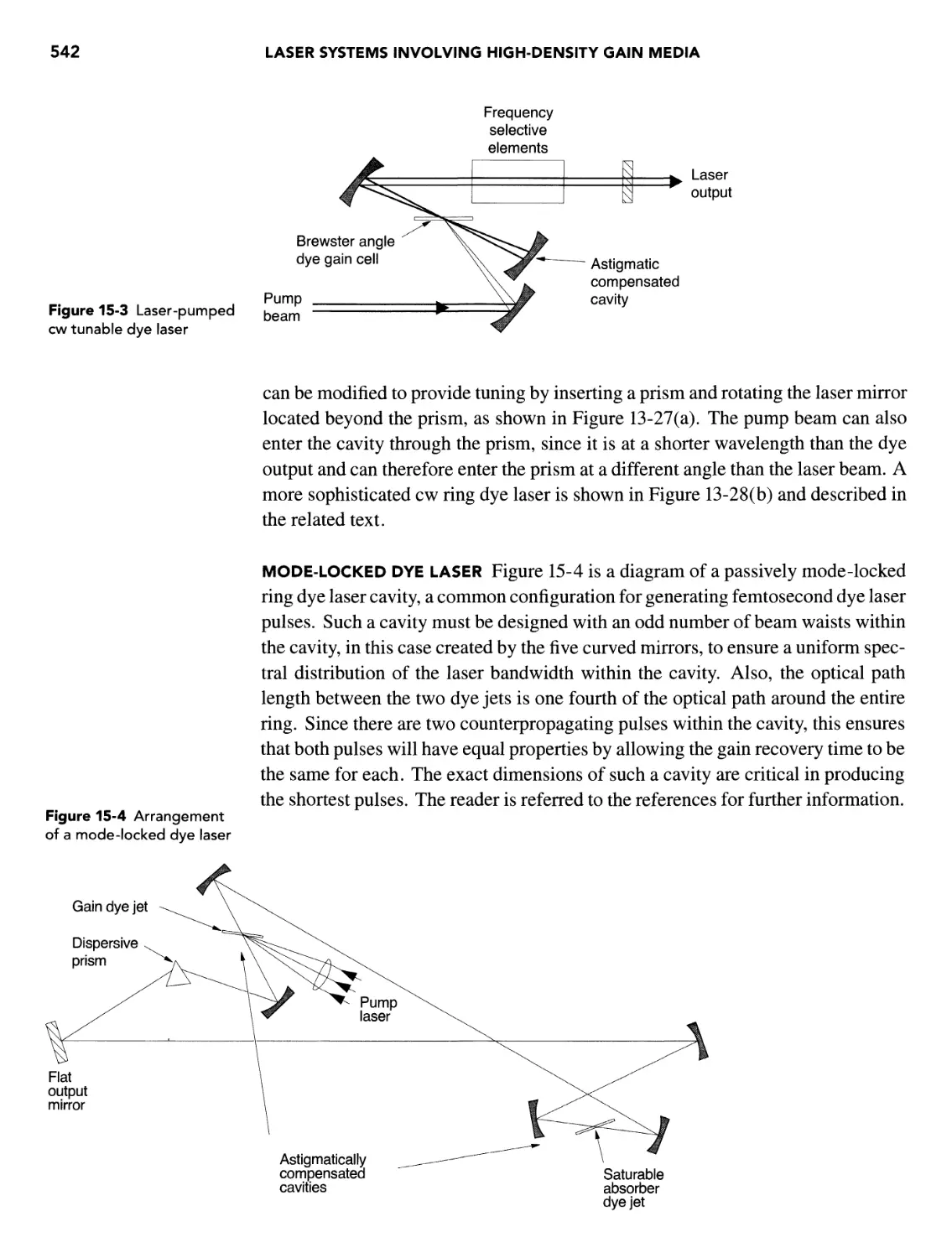
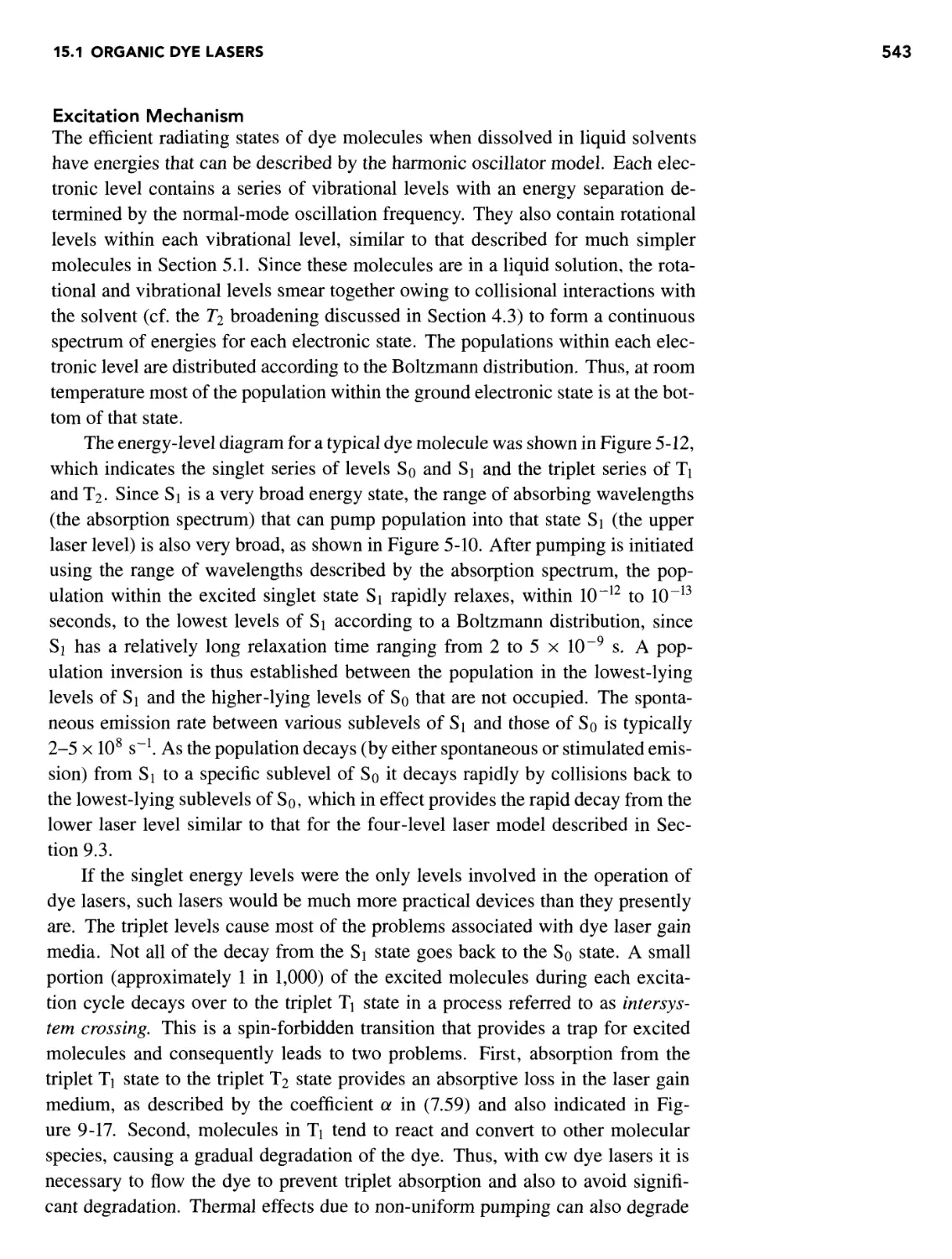
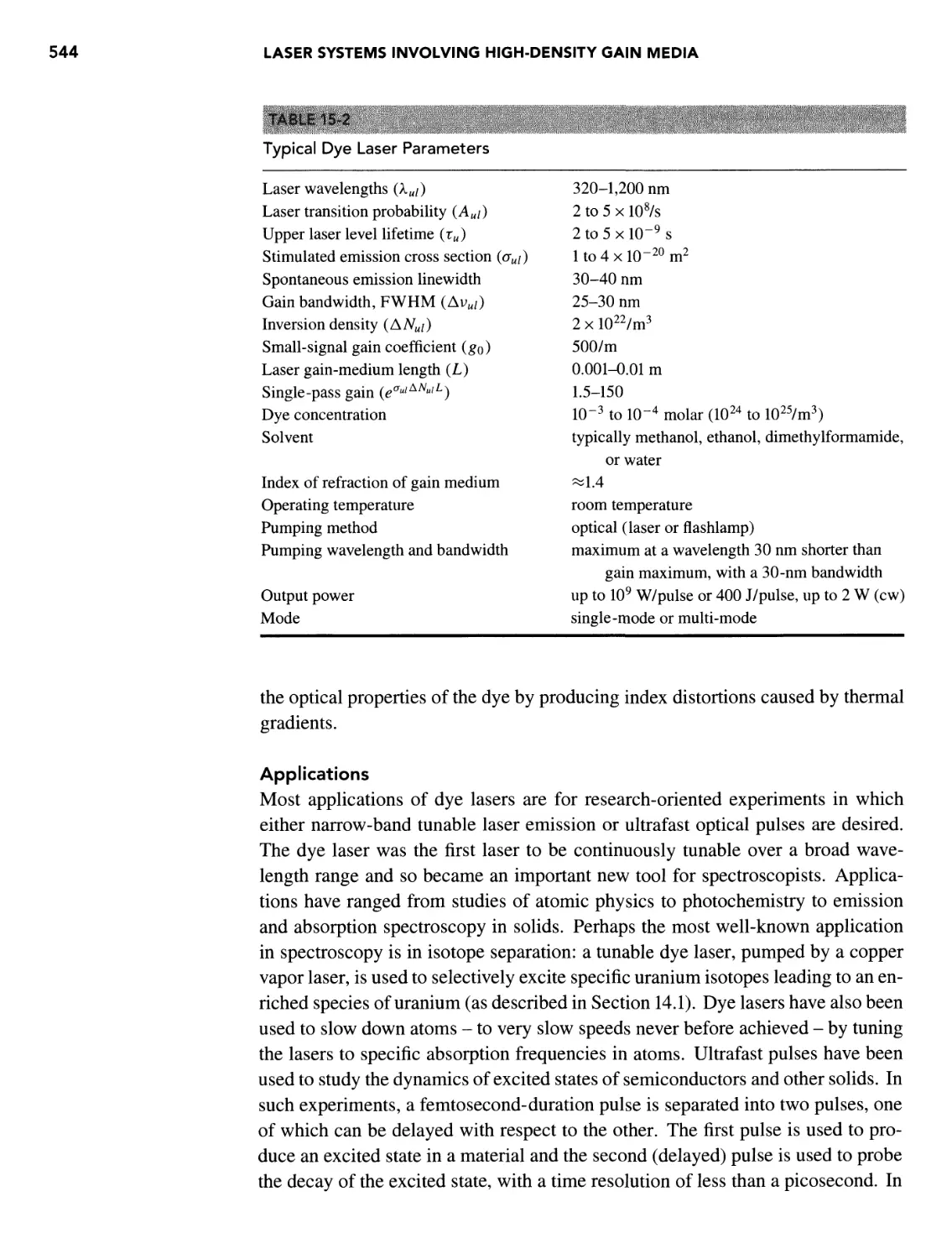
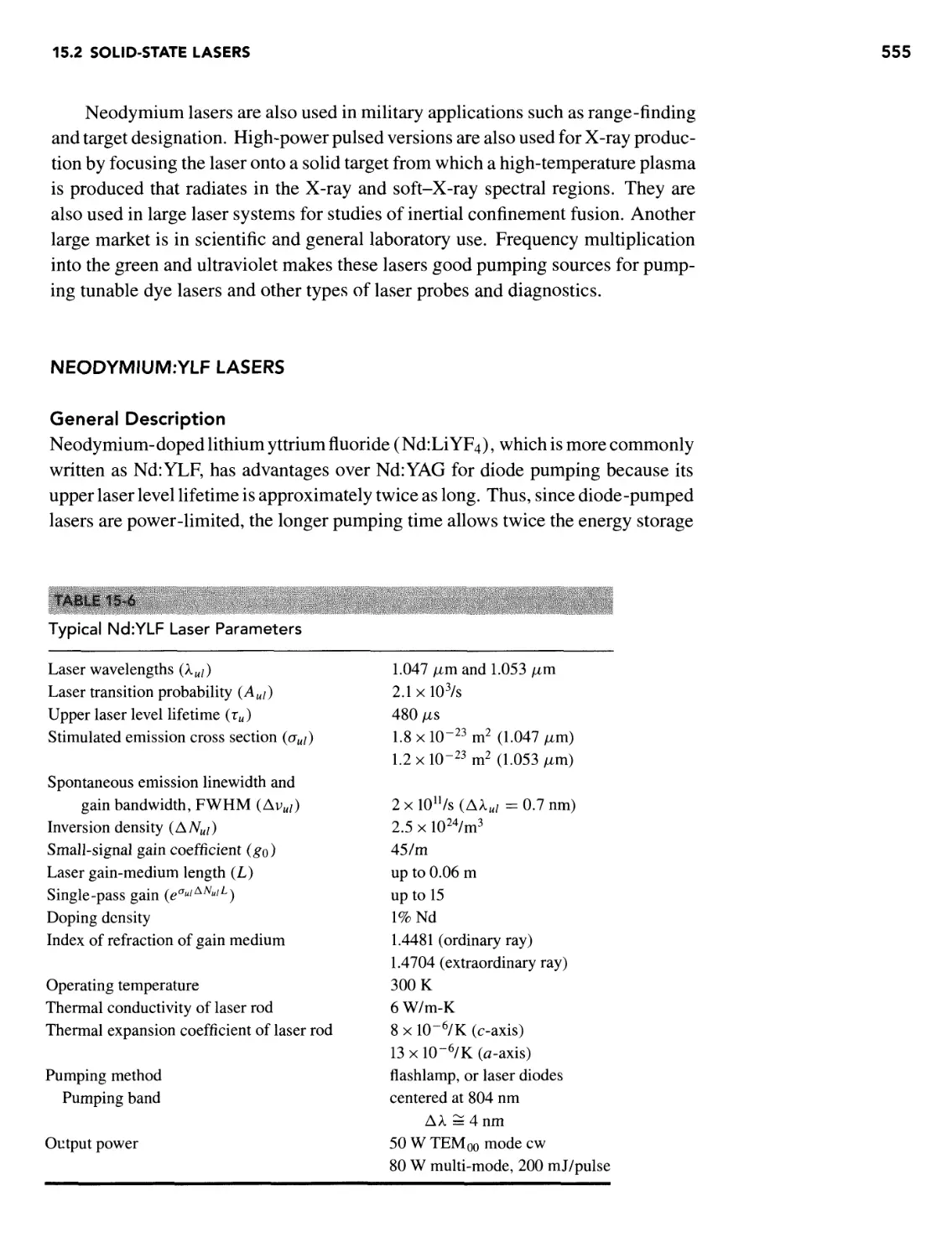

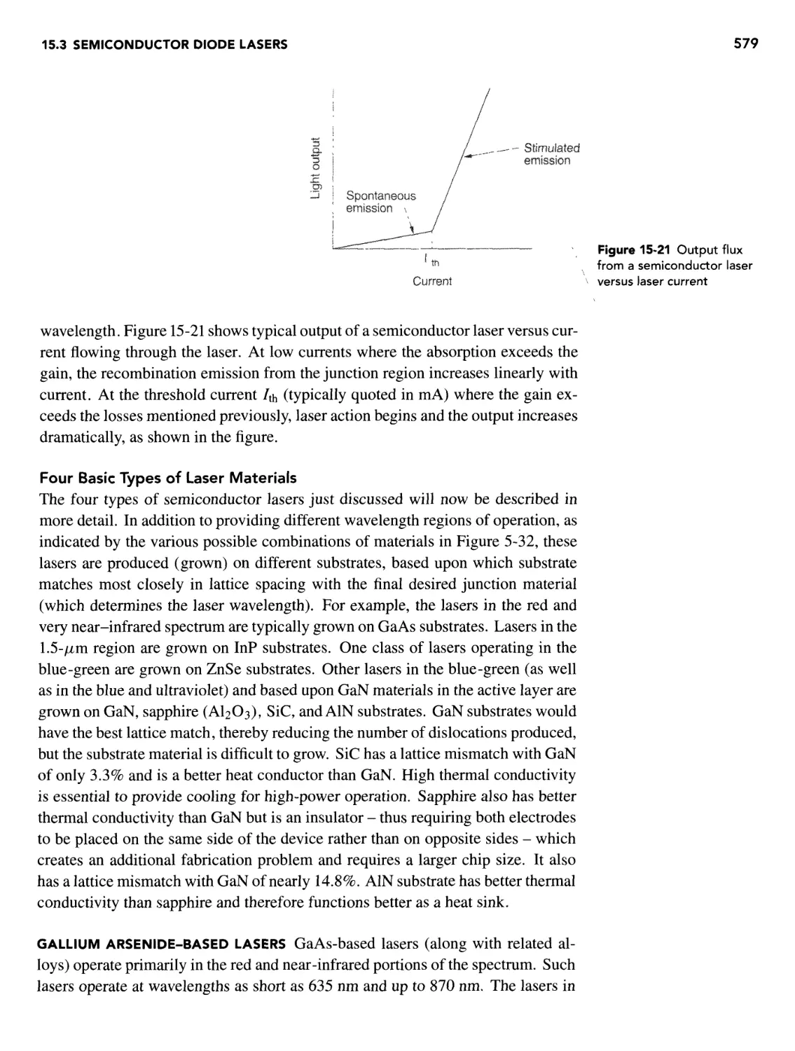


Text
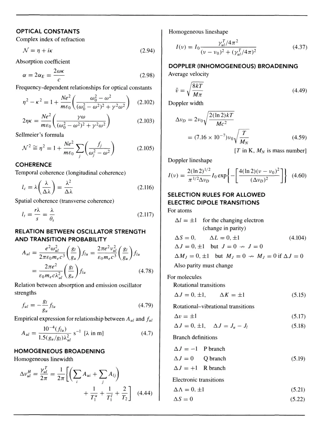
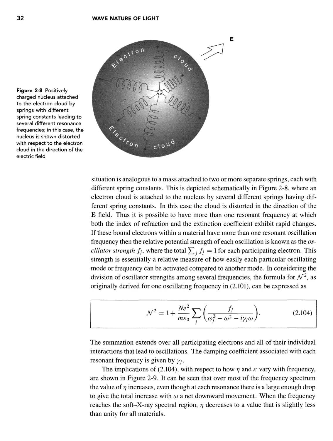
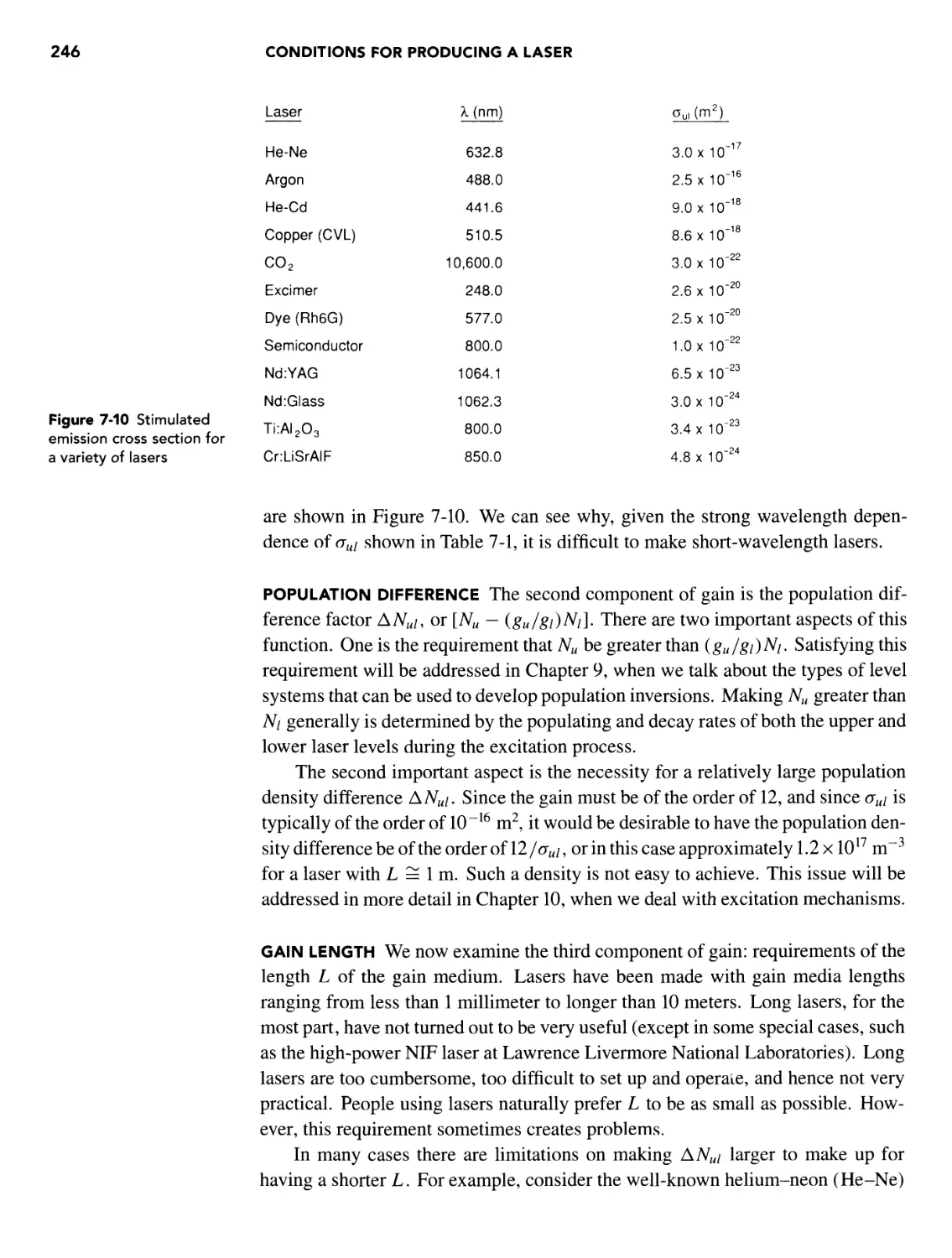
OPTICAL CONSTANTS
Complex index of refraction
M = T] + IK
Absorption coefficient
2cok
a =
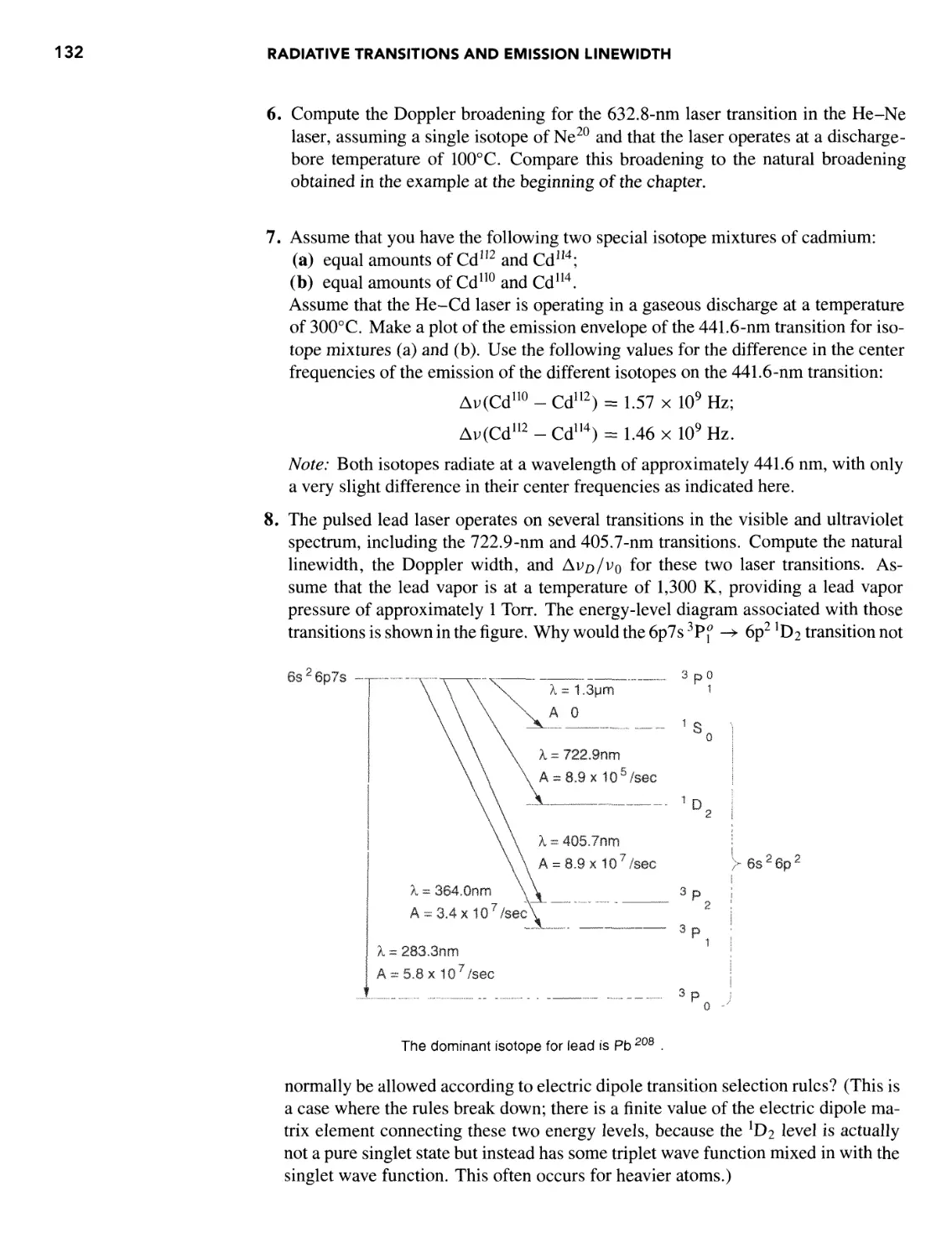
B.94)
B.98)
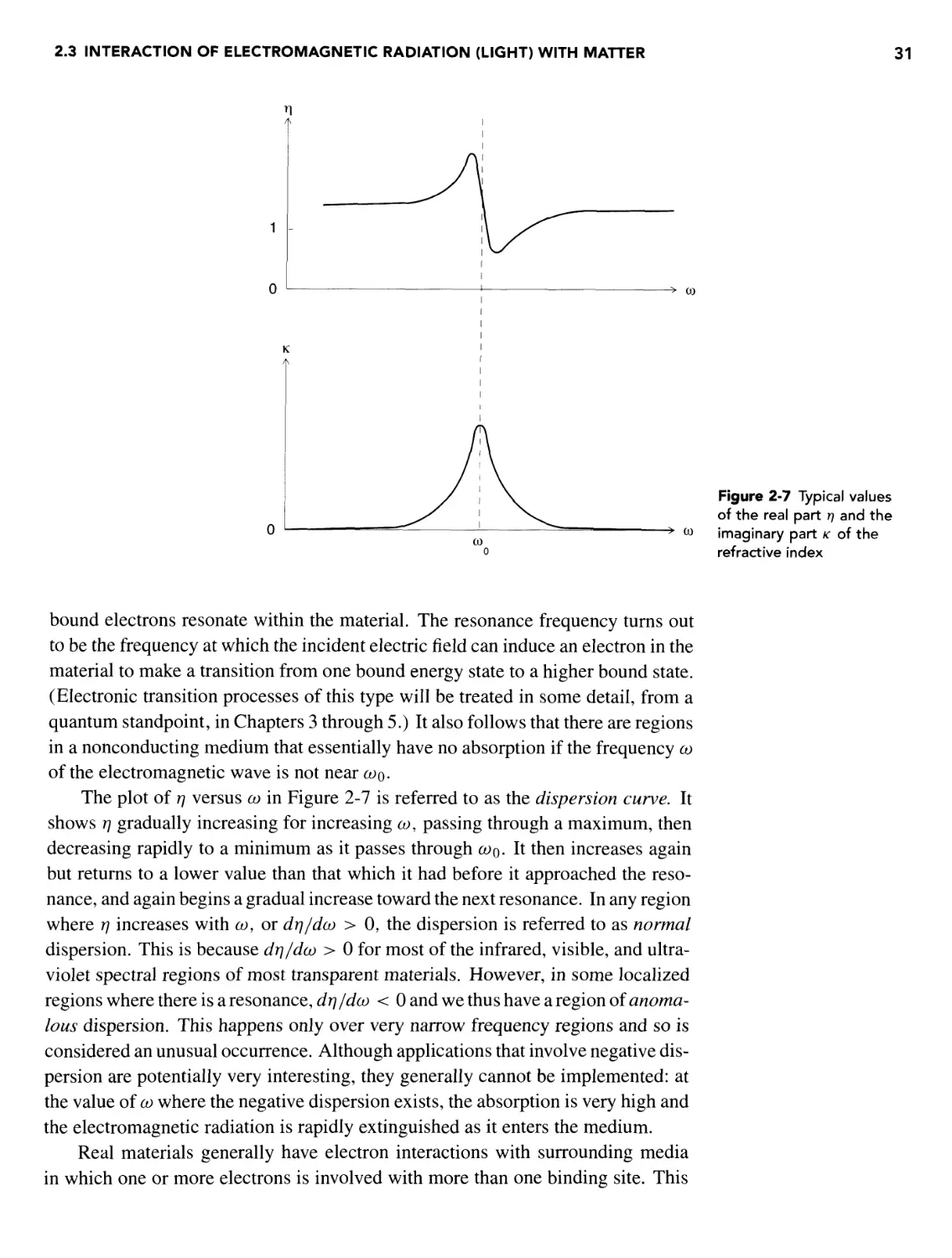
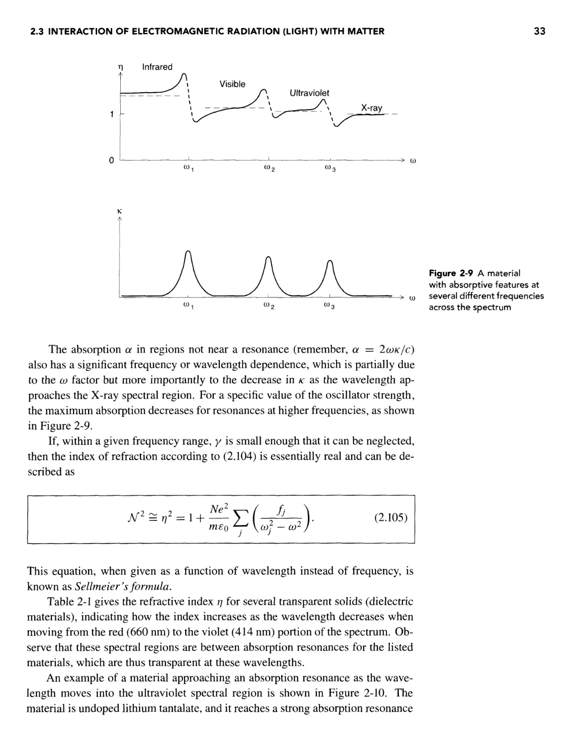
Frequency-dependent relationships for optical constants
o >> . . Ne2
me0
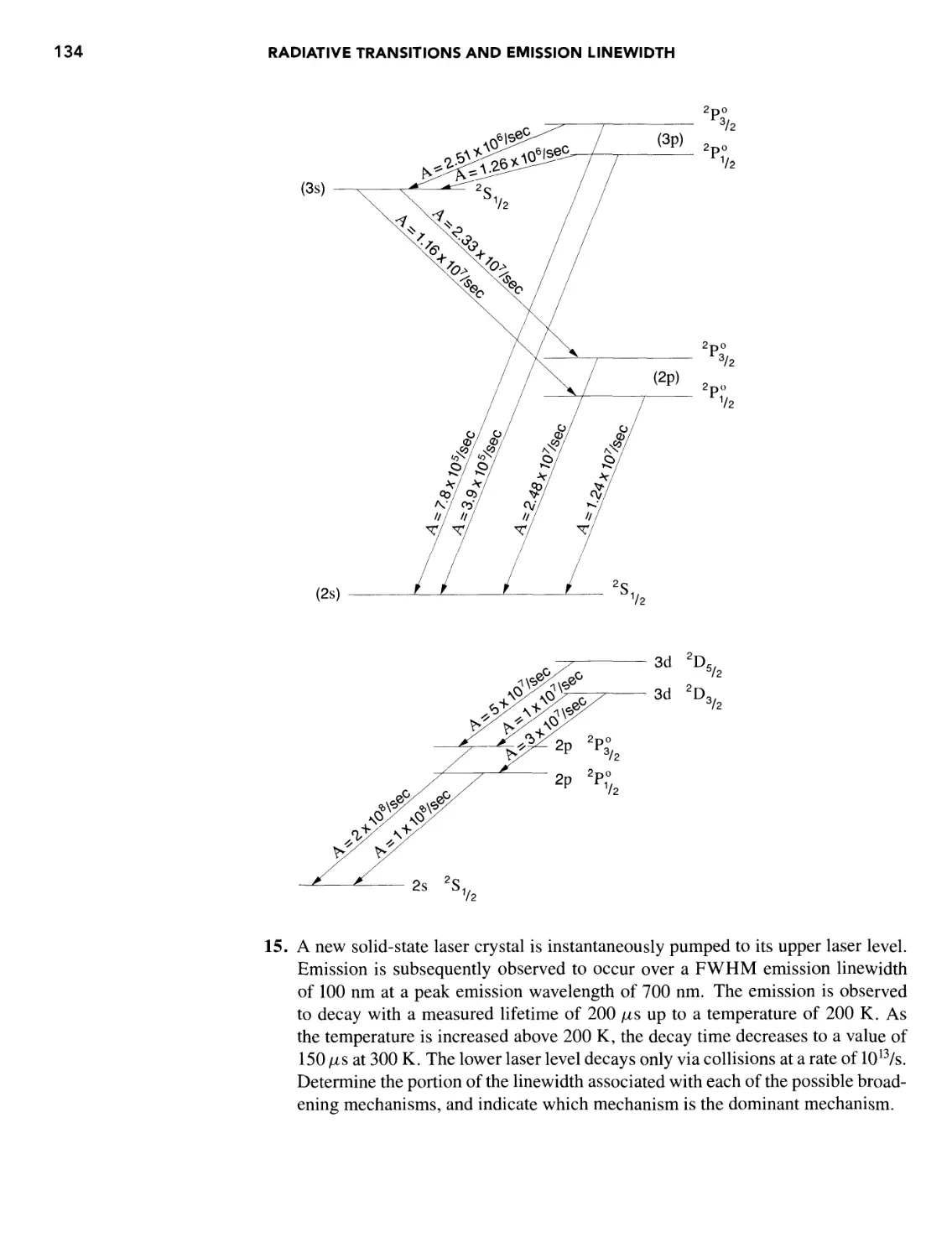
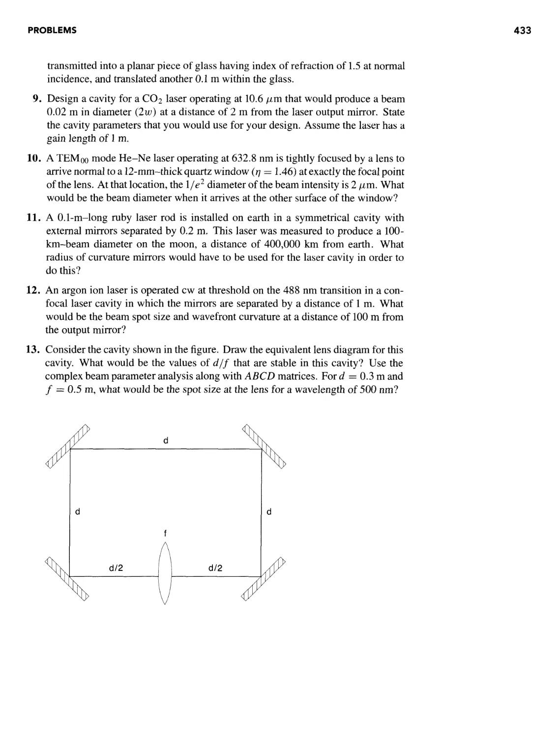
( <-
\(co2-co2)
2-co2
y2co2
Ne2
2tjk =
yco
j2-co2J + y2co2
Sellmeier's formula
mSQ ^-^\co2 — co2
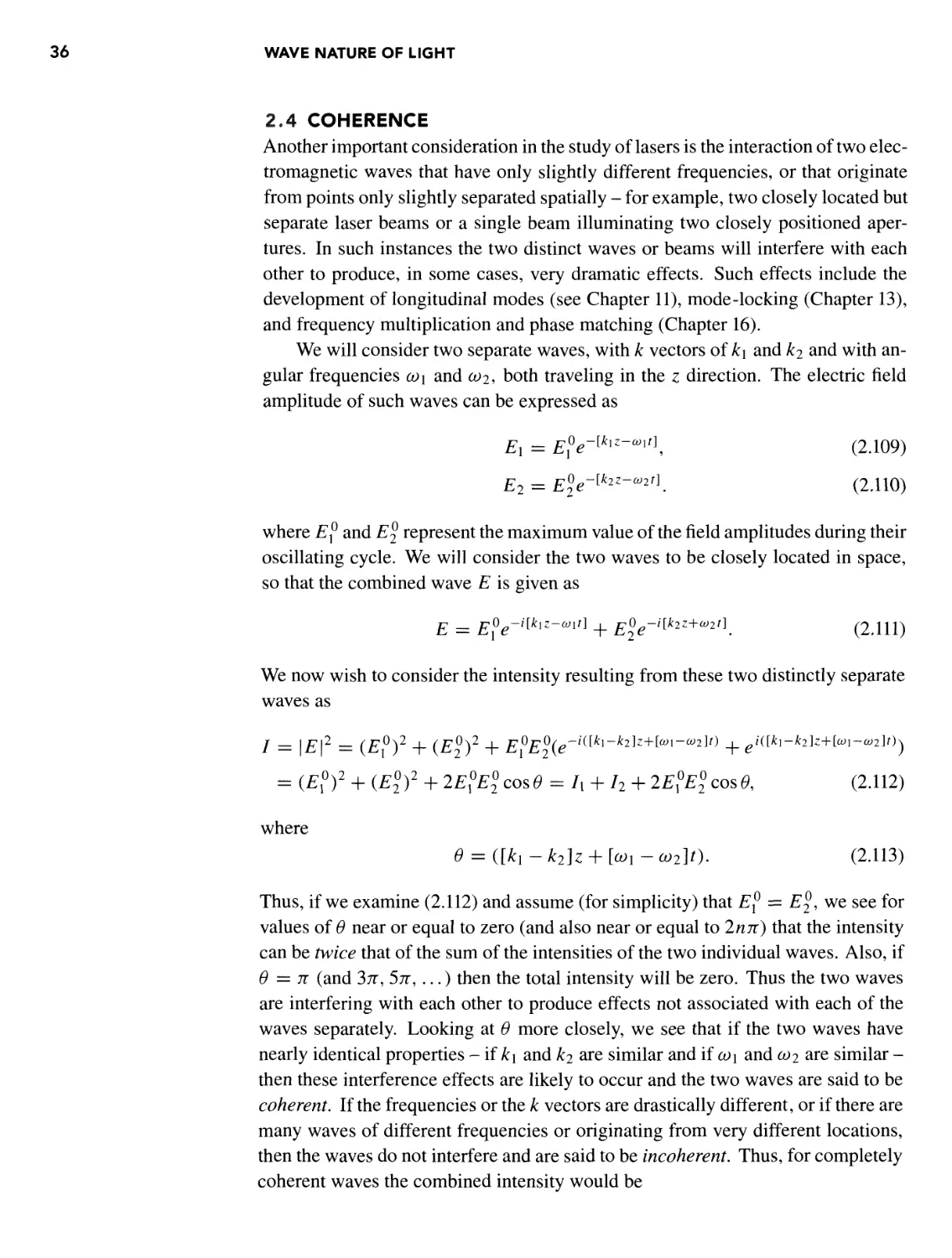
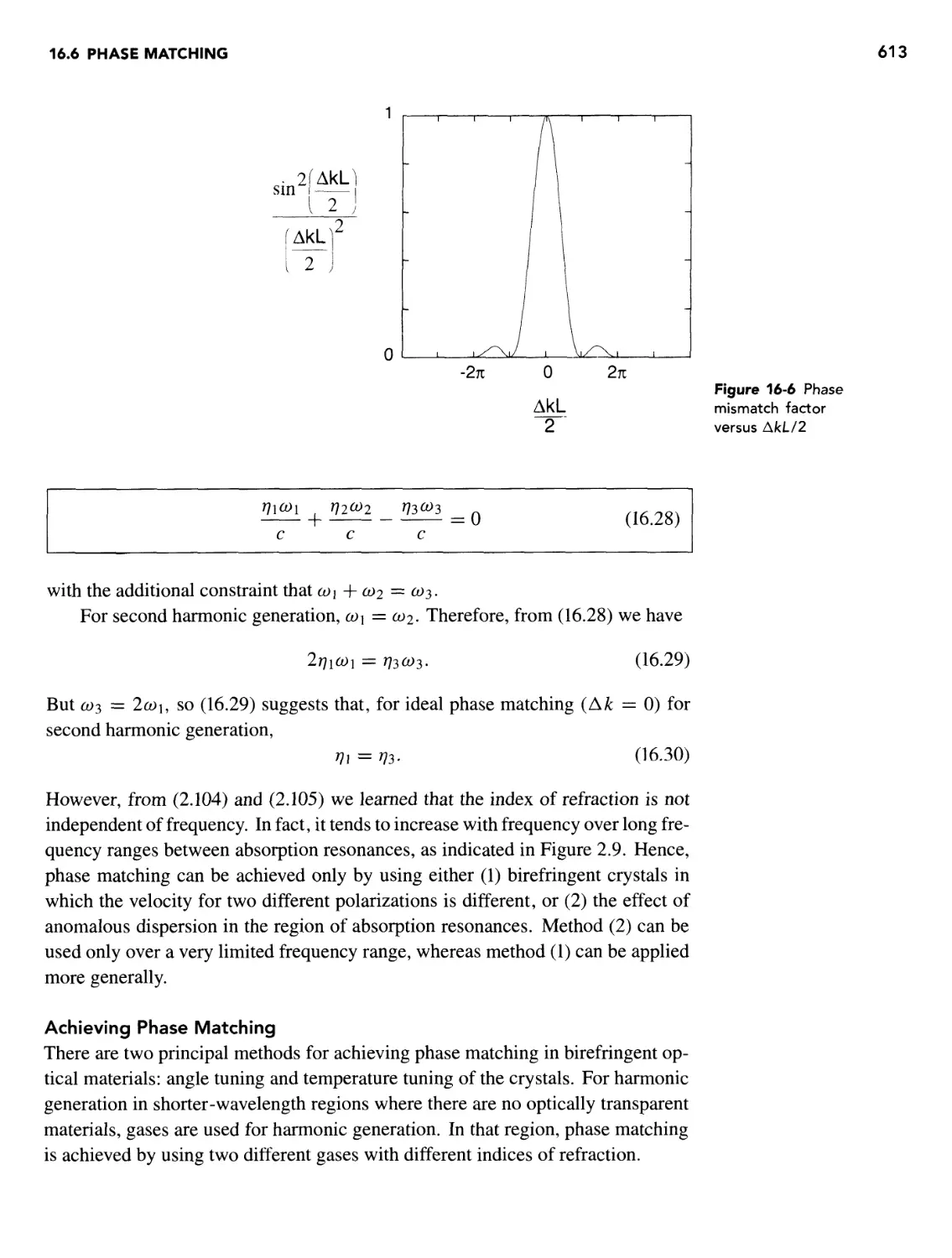
COHERENCE
Temporal coherence (longitudinal coherence)
B.102)
B.103)
B.105)
AX
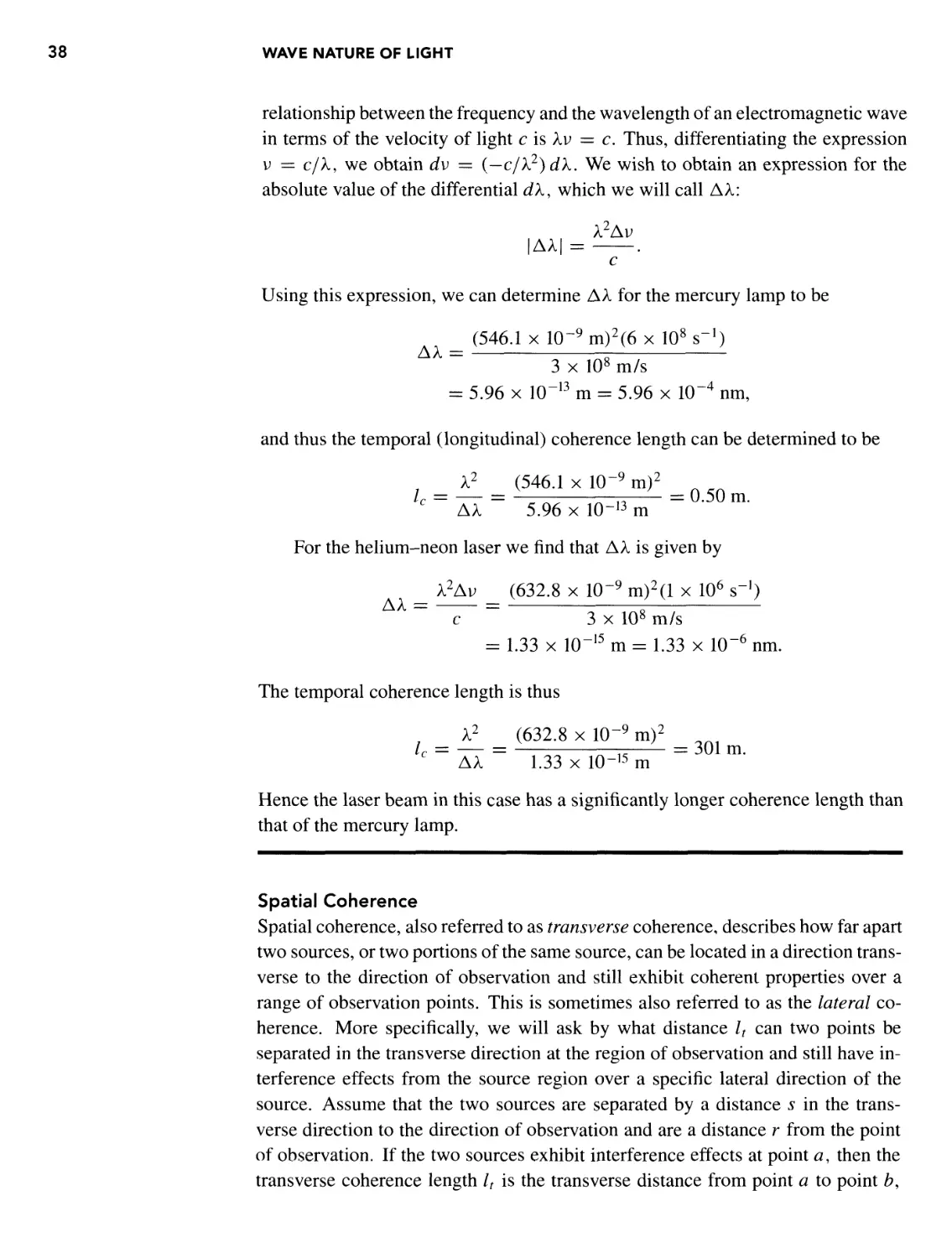
Spatial coherence (transverse coherence)
_ rk _ l
B.116)
B.117)
RELATION BETWEEN OSCILLATOR STRENGTH
AND TRANSITION PROBABILITY
(
2n£0mec3 \gu
— ]Jlu —
)
eomeck2ul \gu
Relation between absorption and emission oscillator
strengths
D.78)
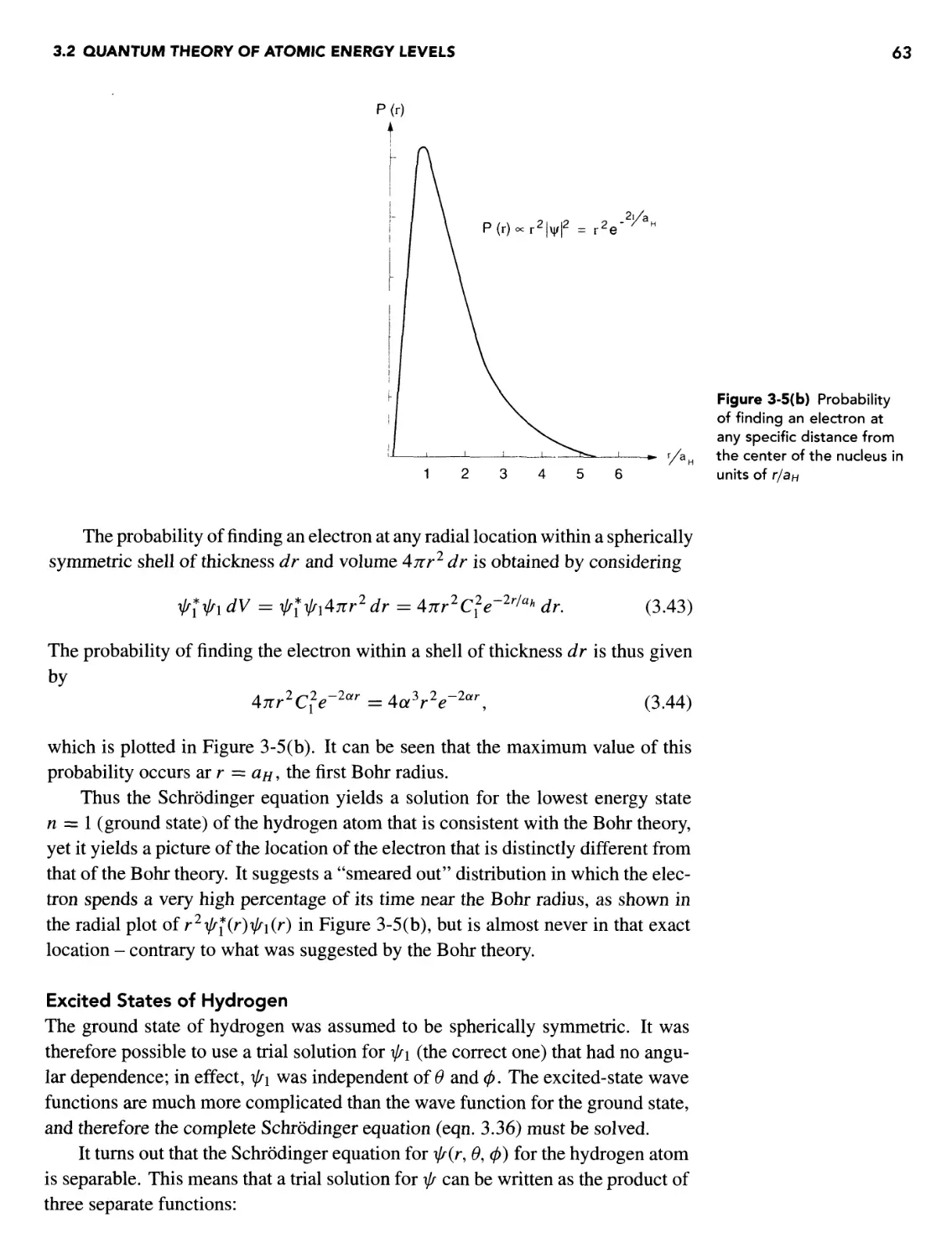
f - 8l f
Jul — Jlu
gu
D.79)
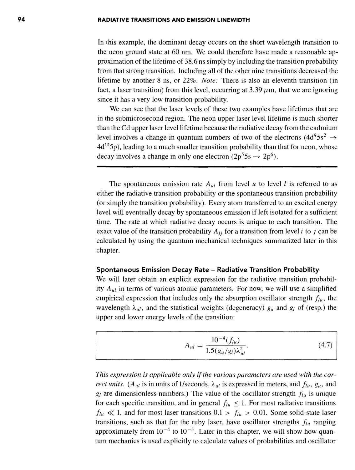
Empirical expression for relationship between Au\ and fu\
Aul = 777—r^V s~] [k in m] D-7)
l-5(gu/gi)Ki
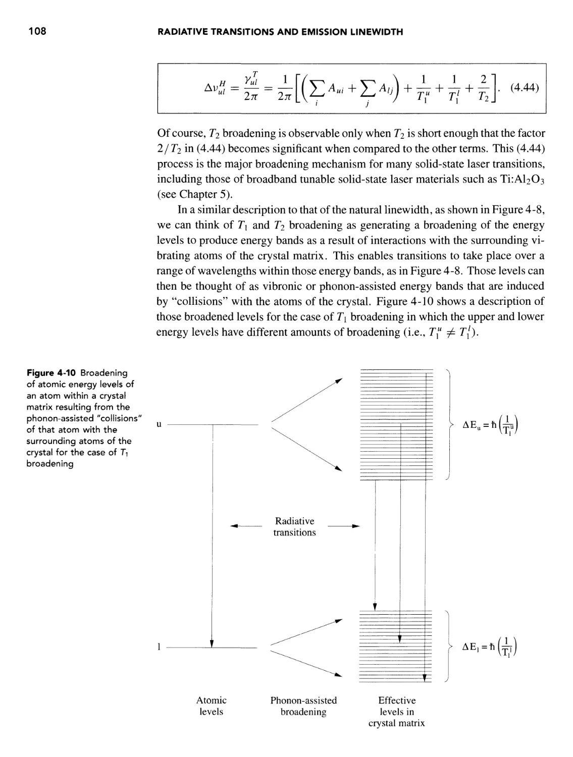
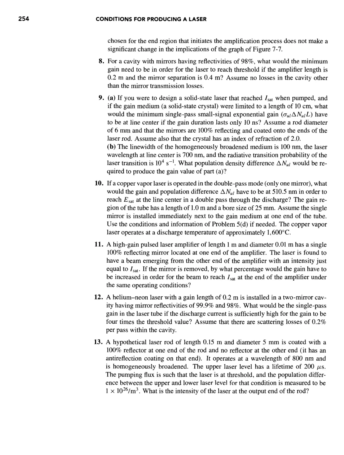
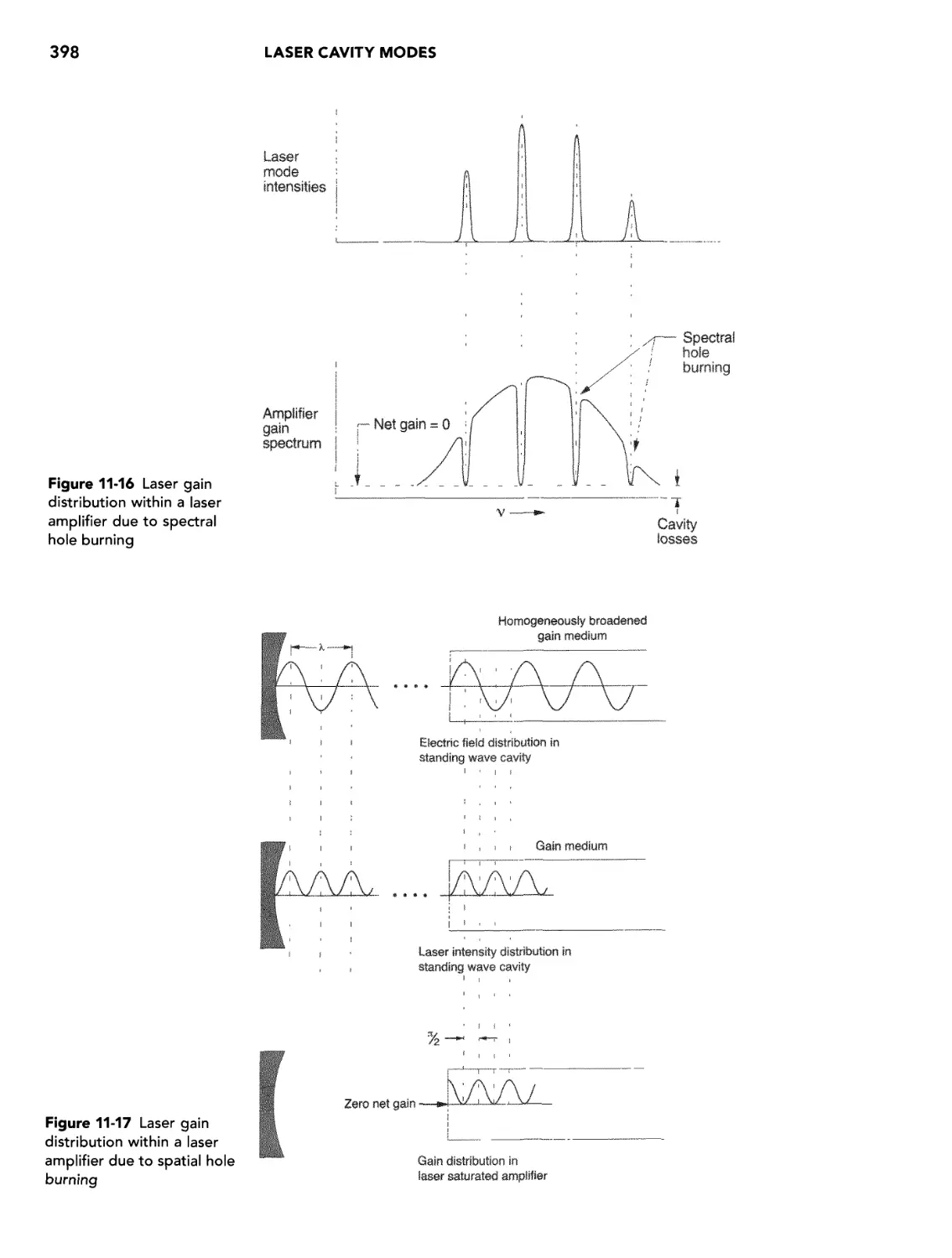
HOMOGENEOUS BROADENING
Homogeneous linewidth
'
JL _1 21
D.44)
Homogeneous lineshape
I(v) = h- }-
D.37)
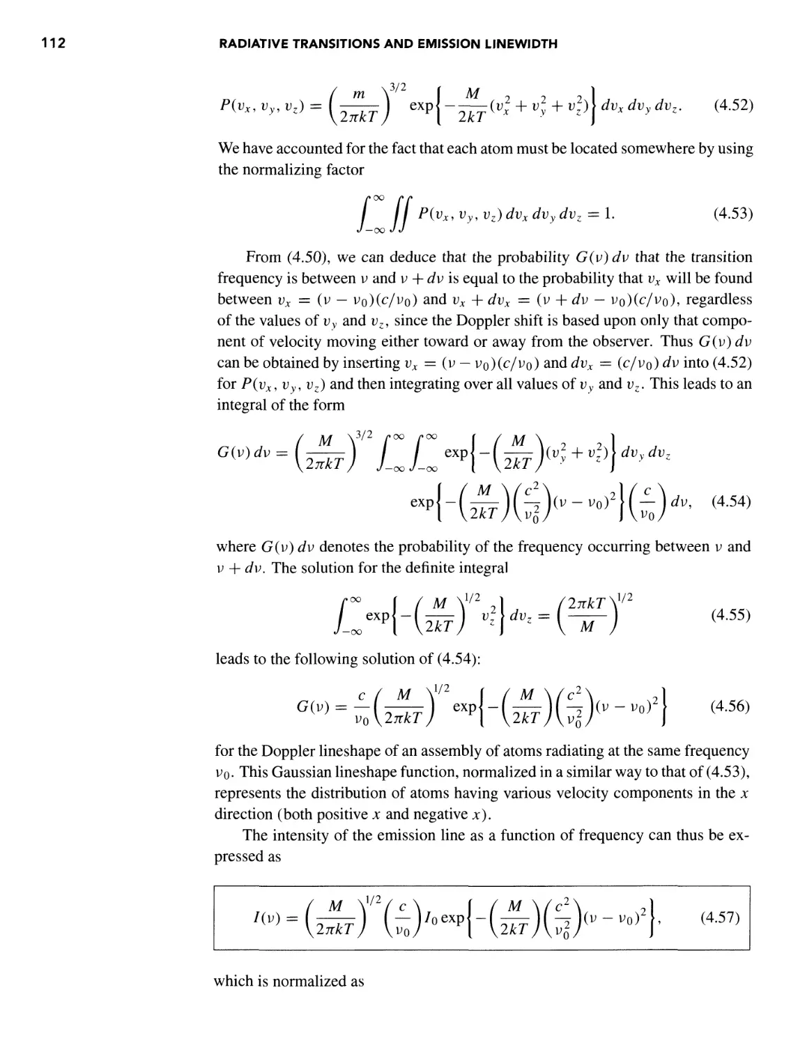
DOPPLER (INHOMOGENEOUS) BROADENING
Average velocity
v =
Mtt
Doppler width
AvD = 2v0
D.49)
2(\n2)kT
lAc1
= G.16xlO-/)voJT^
MN
[T in K,
D.59)
is mass number]
Doppler lineshape
2(ln2I/2
4('f-;°);11 «™>
(AvDJ J J
SELECTION RULES FOR ALLOWED
ELECTRIC DIPOLE TRANSITIONS
For atoms
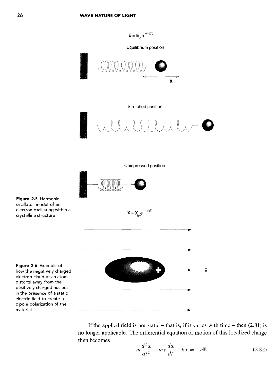
A/ = ±1 for the changing electron
(change in parity)
AS = 0, AL = 0, ±1 D.104)
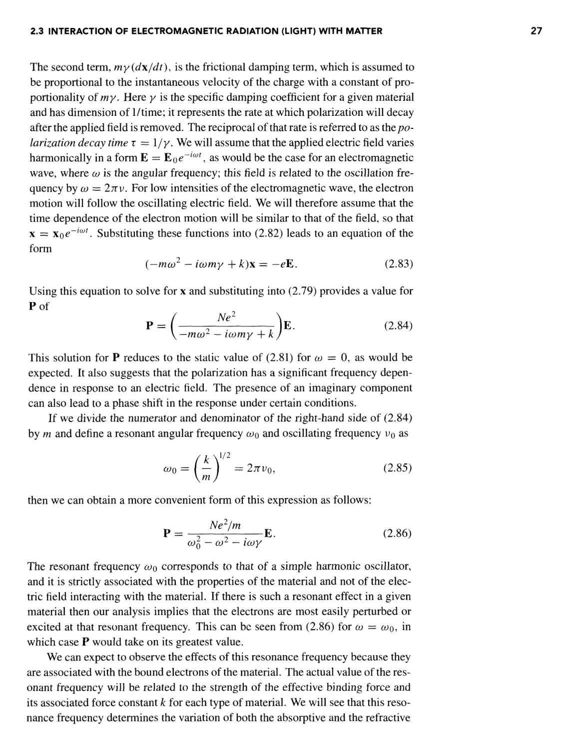
A7 = 0, ±1 but J = 0 +> / = 0
AMy = 0, ±1 but Mj = 0 -» Mj = 0 if AJ = 0
Also parity must change
For molecules
Rotational transitions
A/ = 0,±l, AK = ±l E.15)
Rotational-vibrational transitions
Av - ±1
A7=0, ±1, AJ = Ju
Branch definitions
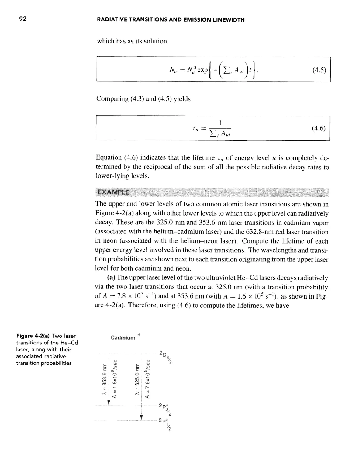
AJ = -I P branch
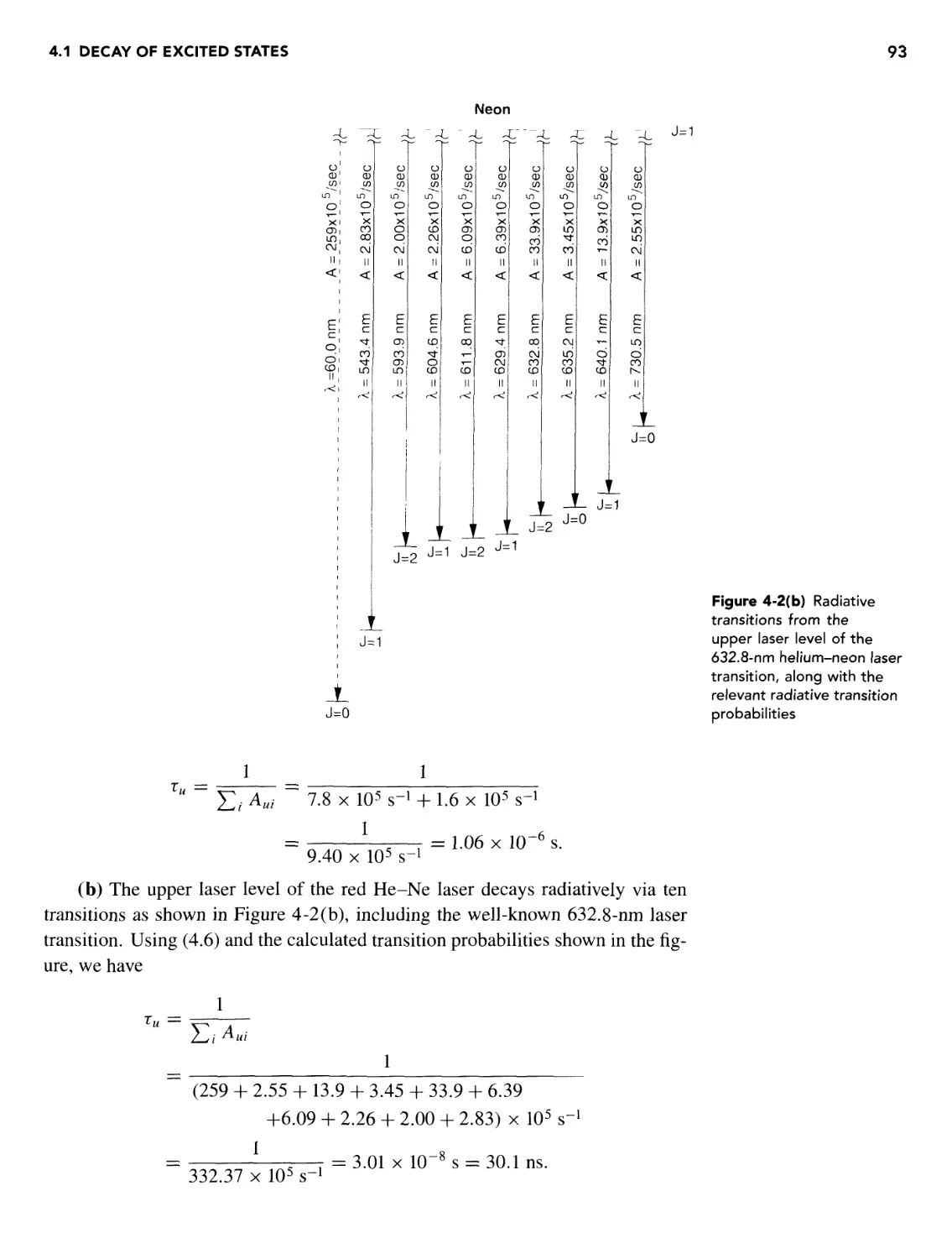
A J = 0 Q branch
AJ = +1 R branch
Electronic transitions
AA = 0, ±1
AS = 0
-Ji
E.17)
E.18)
E.19)
E.21)
E.22)
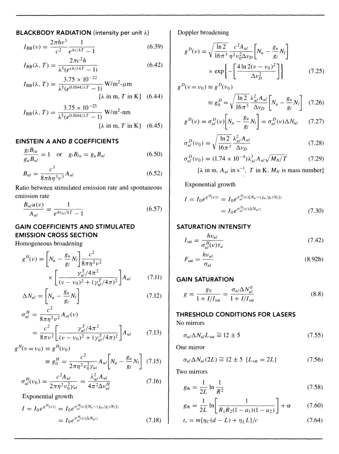
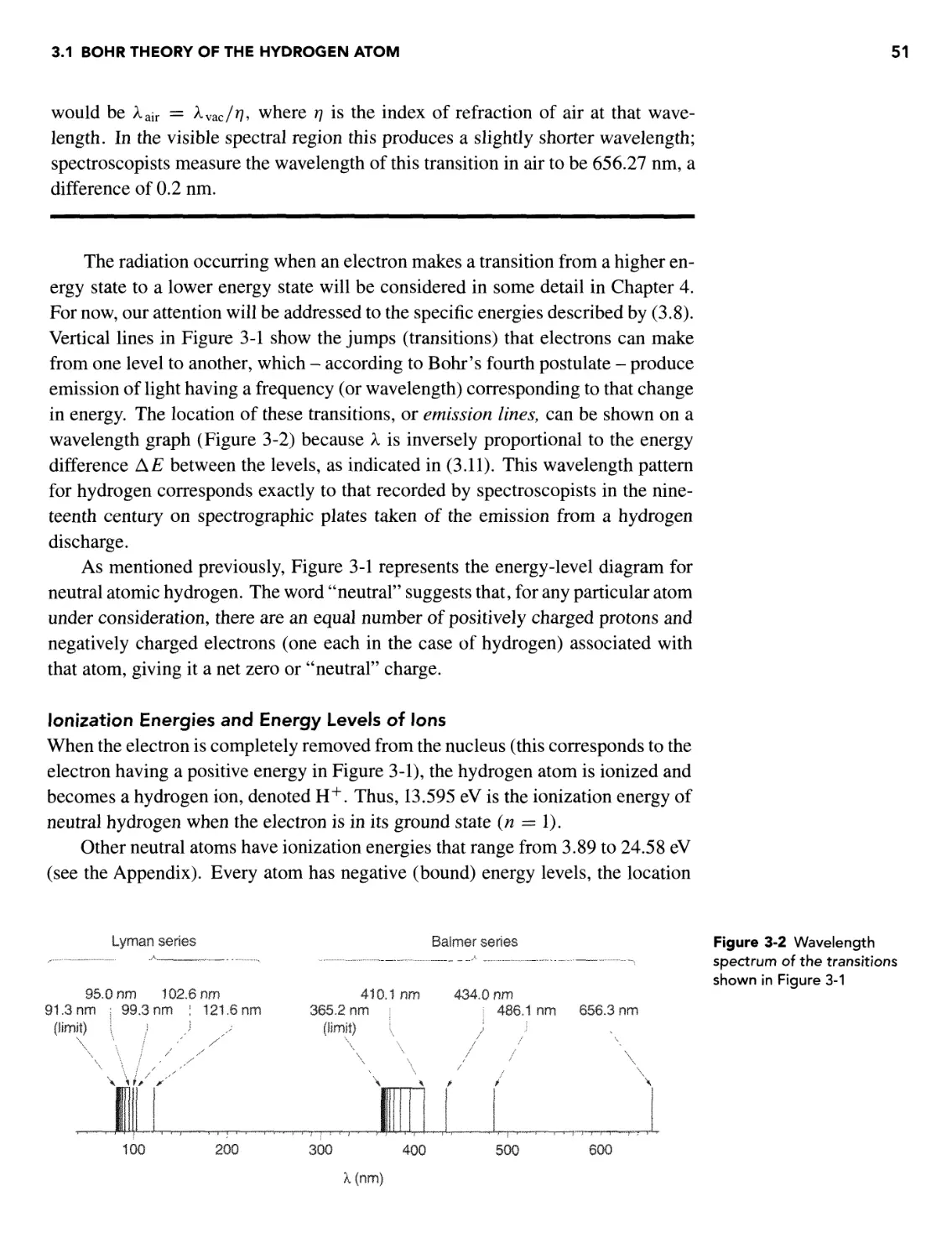
BLACKBODY RADIATION (intensity per unit k)
ehv/kT _ J
/bb(A, T) =
F.39)
F.42)
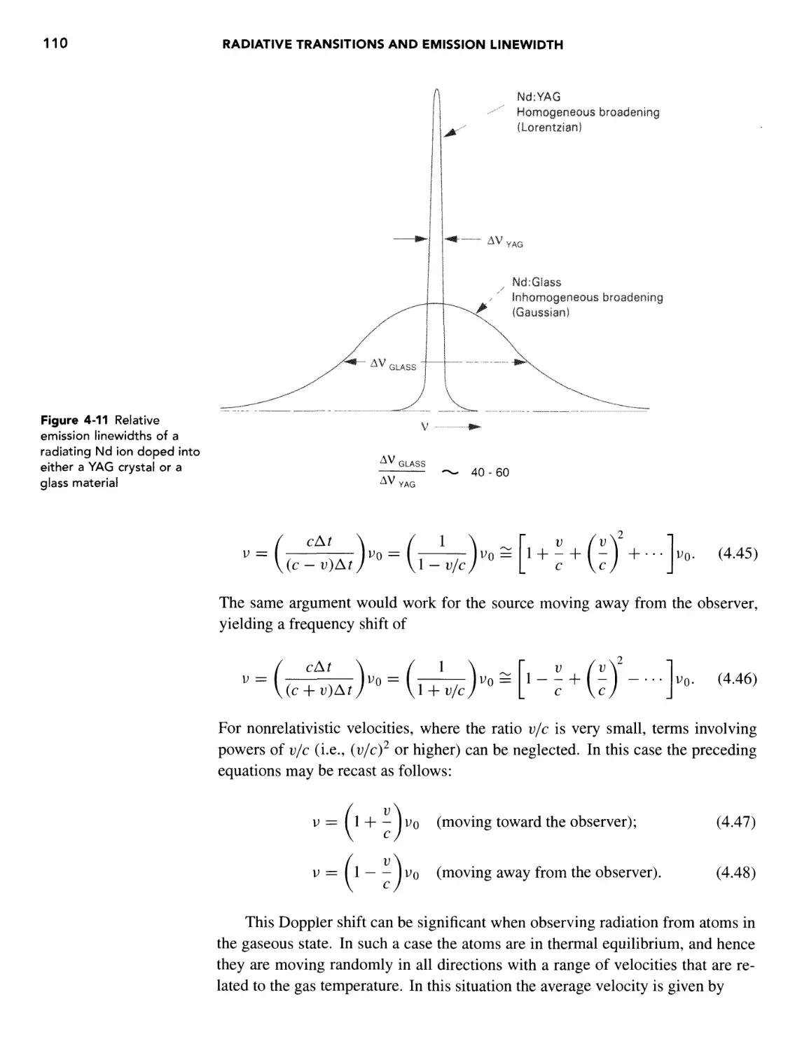
3.75 x 1Q-22
^5(e0.0144Ar _ 1
[A in m, T in K] F.44)
3.75 x IP5
[X in m, T in K] F.45)
EINSTEIN A AND B COEFFICIENTS
~ = l or glBlu=guBul F.50)
tAk/ F.52)
Ratio between stimulated emission rate and spontaneous
emission rate
1
( }
GAIN COEFFICIENTS AND STIMULATED
EMISSION CROSS SECTION
Homogeneous broadening
f **'
ANM/ =
L 8i
CT«' =
—2—Aui\Nu 1
cAui
G.11)
G.12)
G.13)
G.15)
G.16)
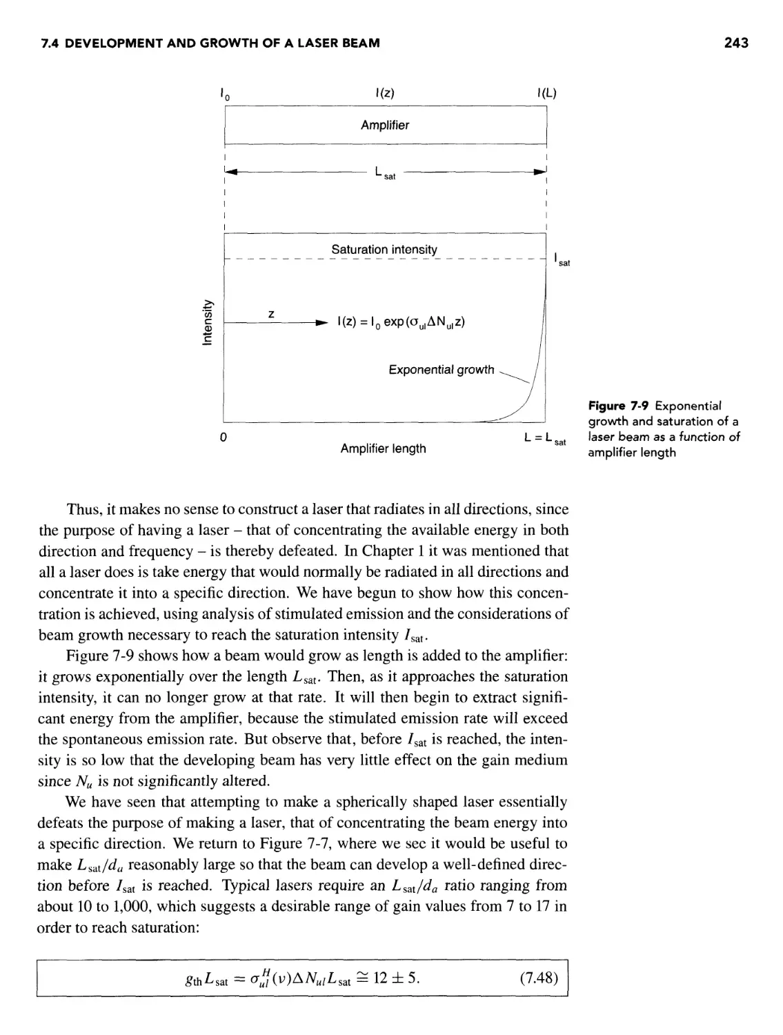
Exponential growth
/ = Ioeg"{v)z — loea"(v)lN"~(x"/gl)Nl]z
= Ioea>)AN«'z
G.18)
Doppler broadening
In2 c2Au!
gu 1
gi J
xexp -
I
r41n2(y-vo)
L
-voJH
b JJ
G.25)
/ In 2 X2ulAul
167T3 AVn
L ft J
— Ni\ G-26)
G.27)
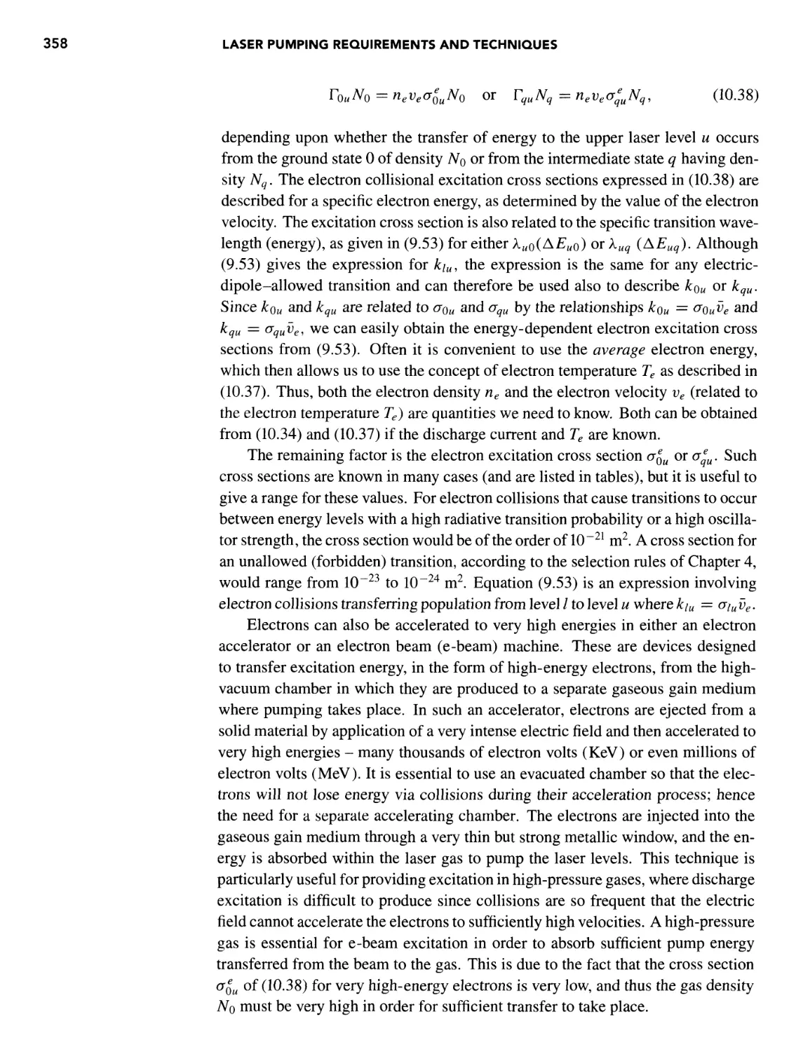
<T$(v0) = A.74 x W~4)Xl}AuiJMN/T G.29)
[X in m, Aul in s, T in K, MN is mass number]
Exponential growth
/ = I§e = iQe ul
SATURATION INTENSITY
/sat = /"'
GAIN SATURATION
1 + ///sat 1 + ///sat
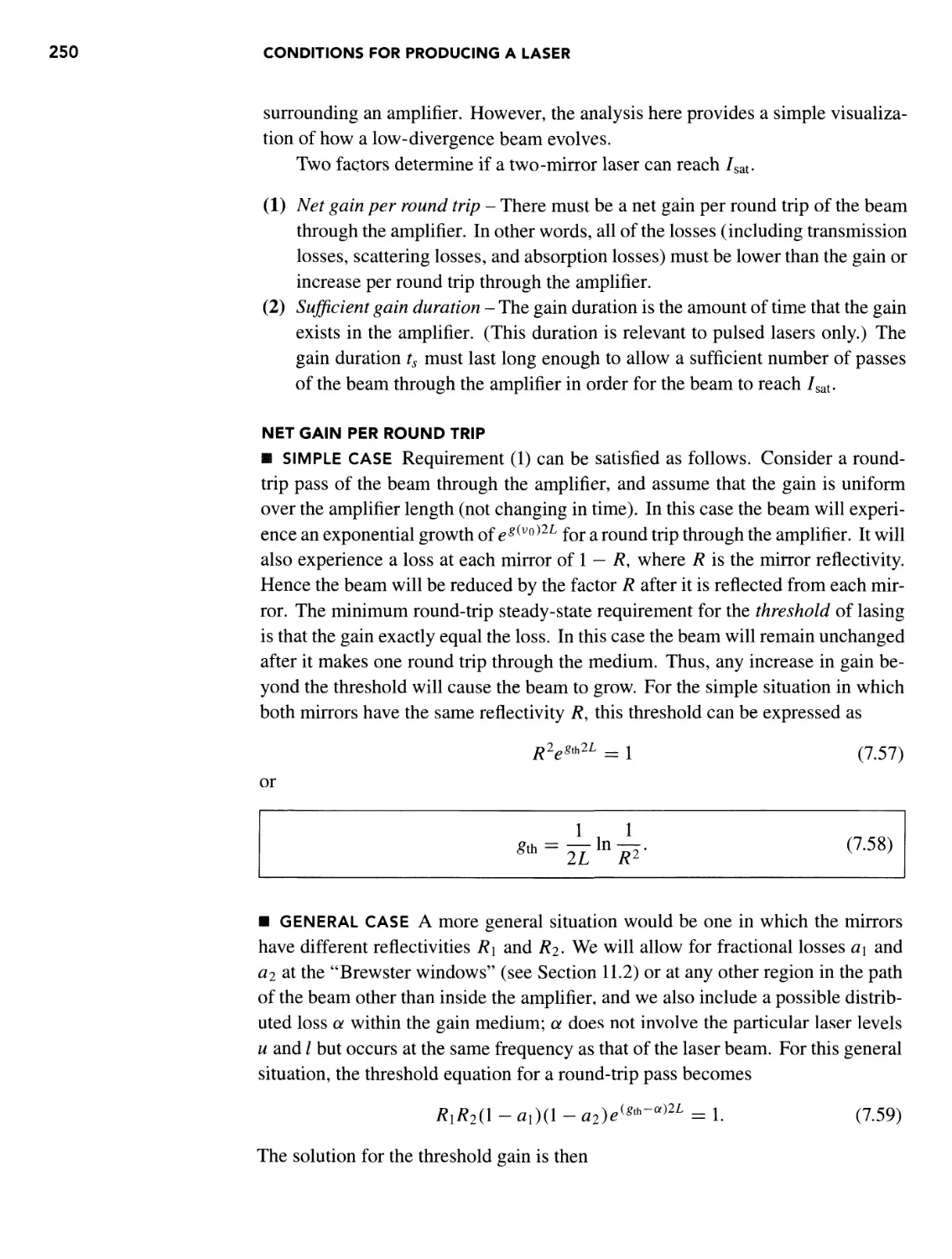
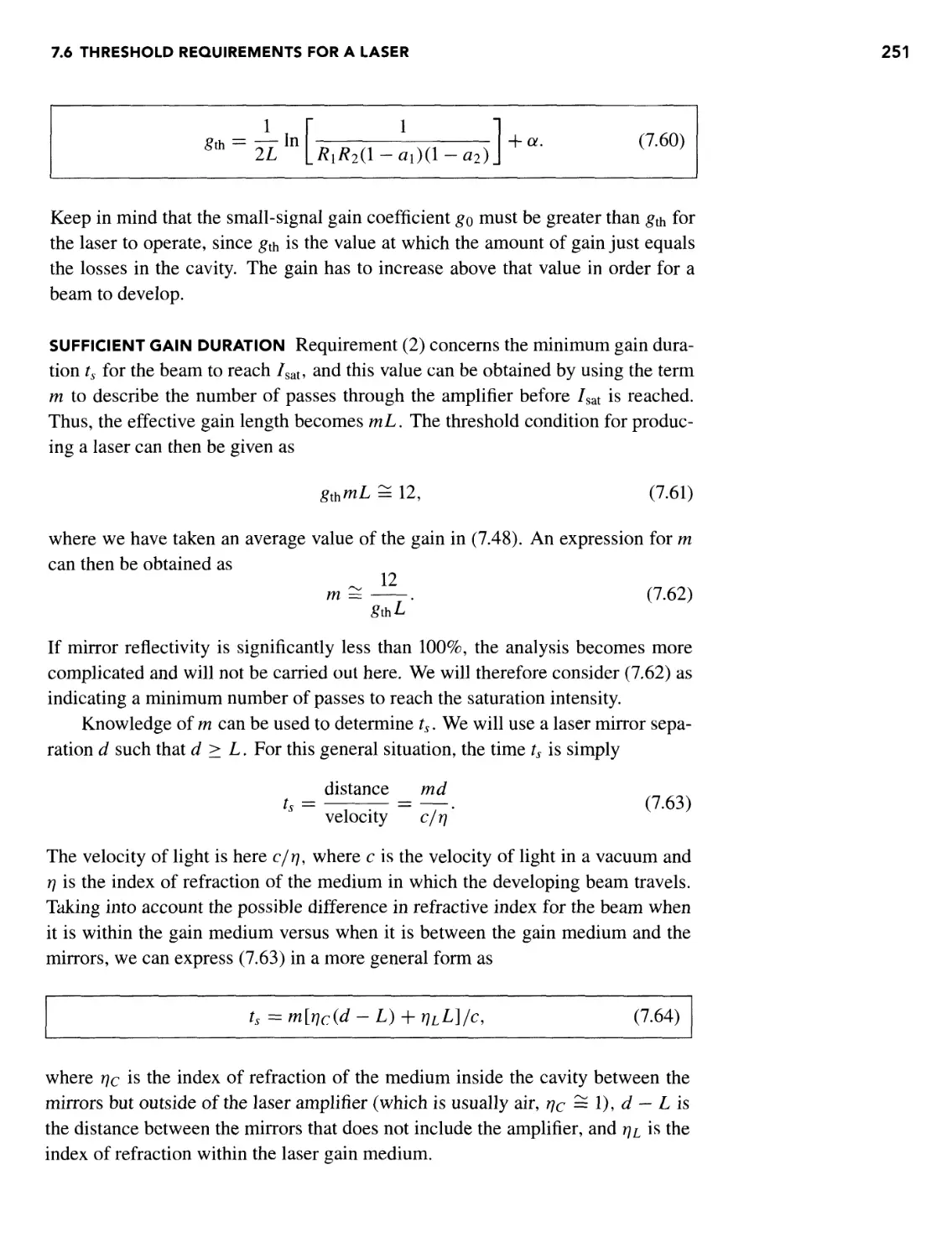
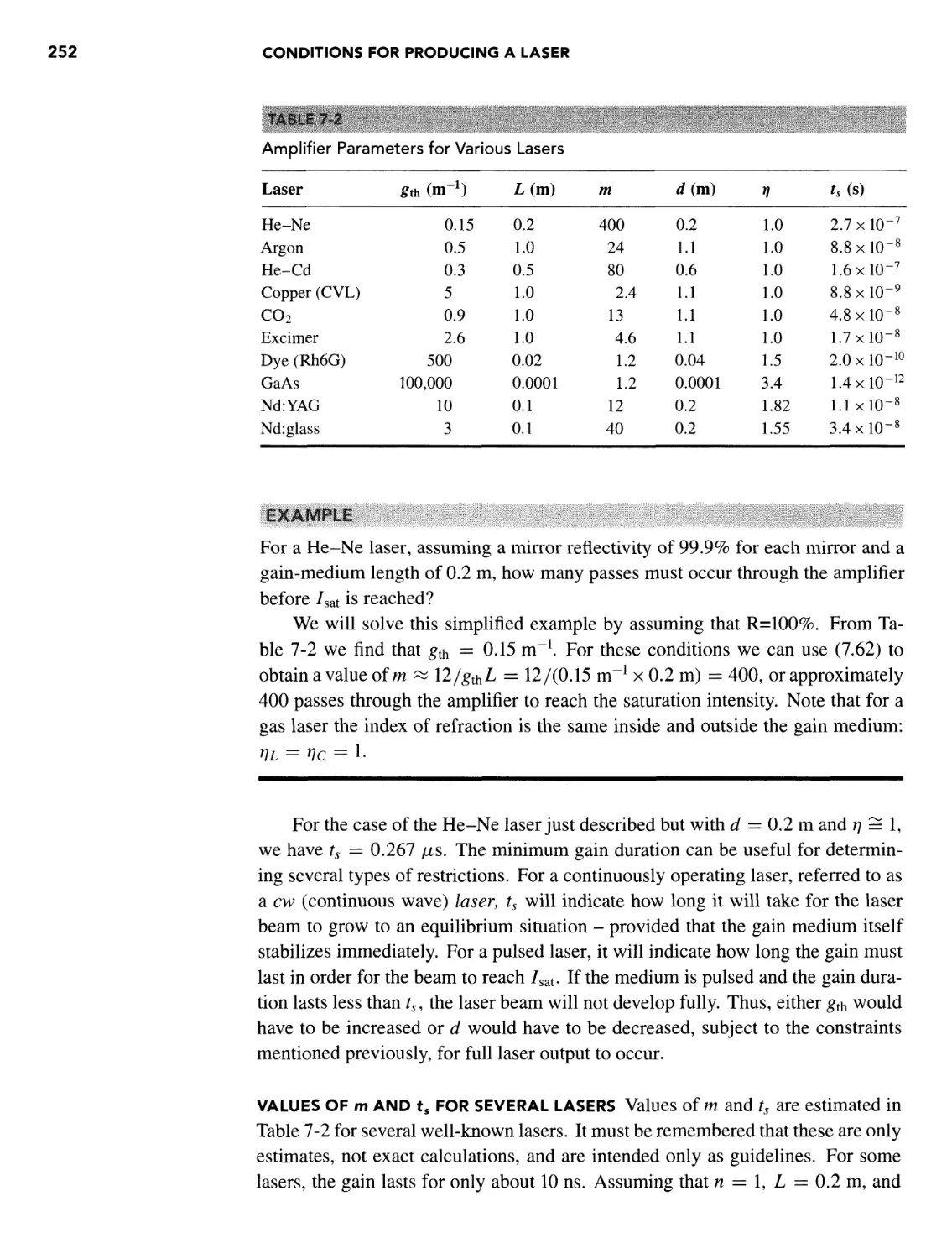
THRESHOLD CONDITIONS FOR LASERS
No mirrors
crM,ANw/Lsat = 12 ± 5
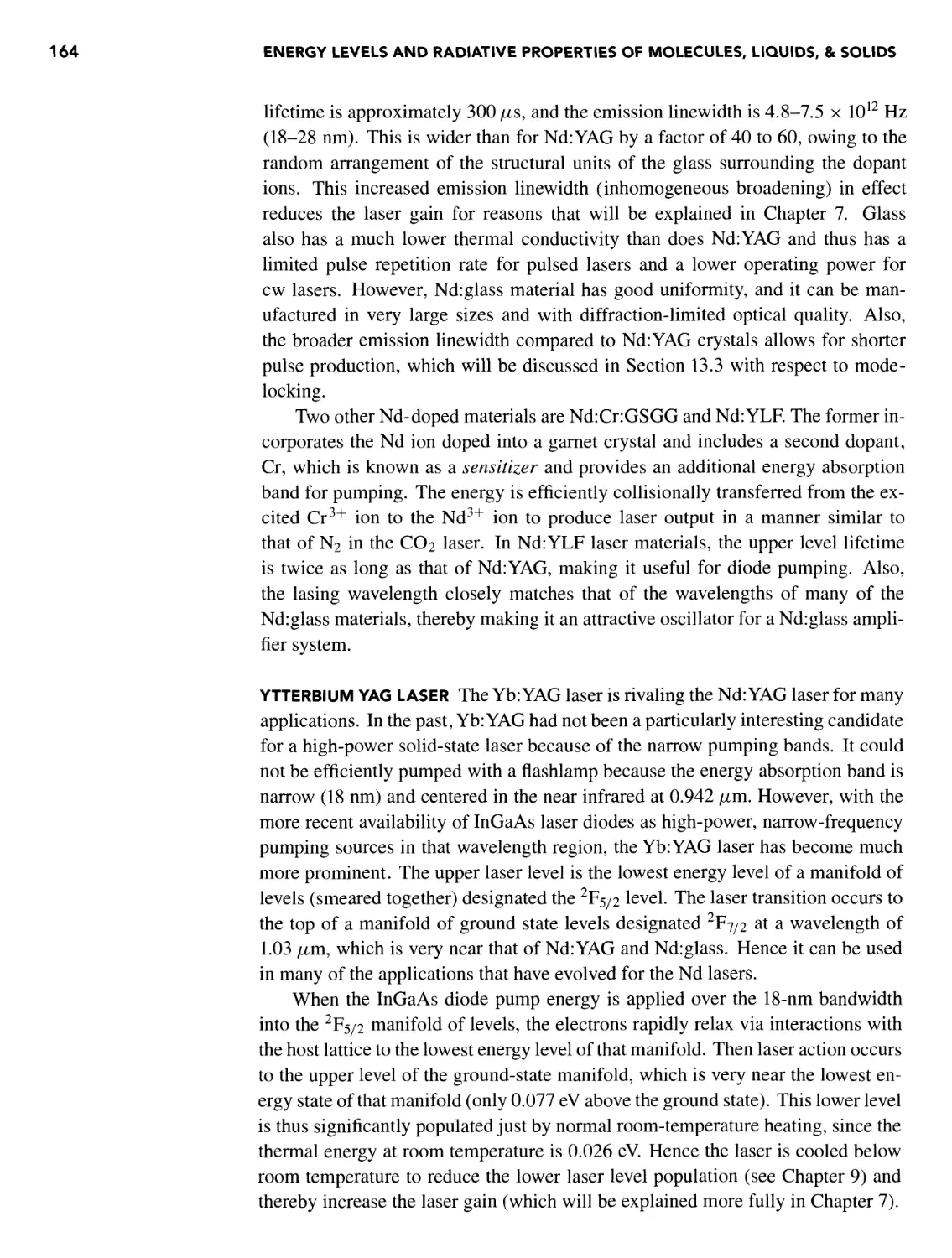
One mirror
cxulANuiBL) = 12 ± 5 [isat = 2L]
Two mirrors
l
G.42)
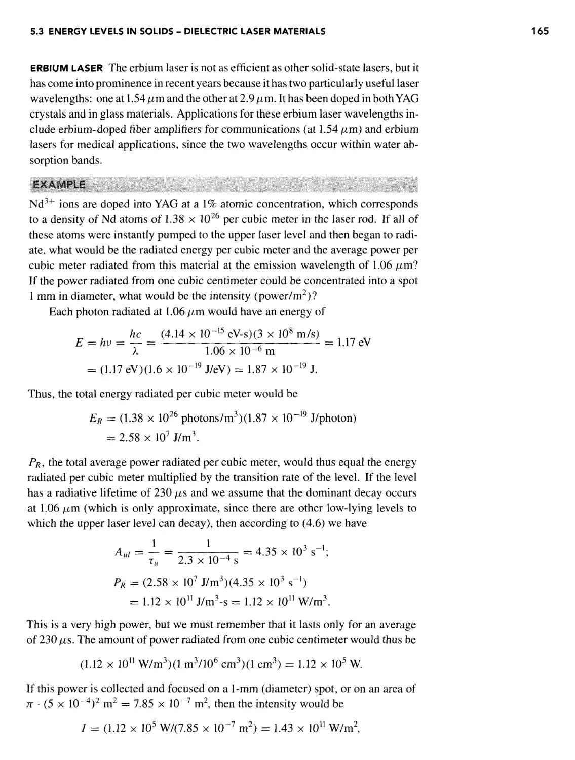
(8.92b)
(8.8)
fth = TT ln
+ a
f, = m[ric(d - L) + r)LL]/c
G.55)
G.56)
G.58)
G.60)
G.64)
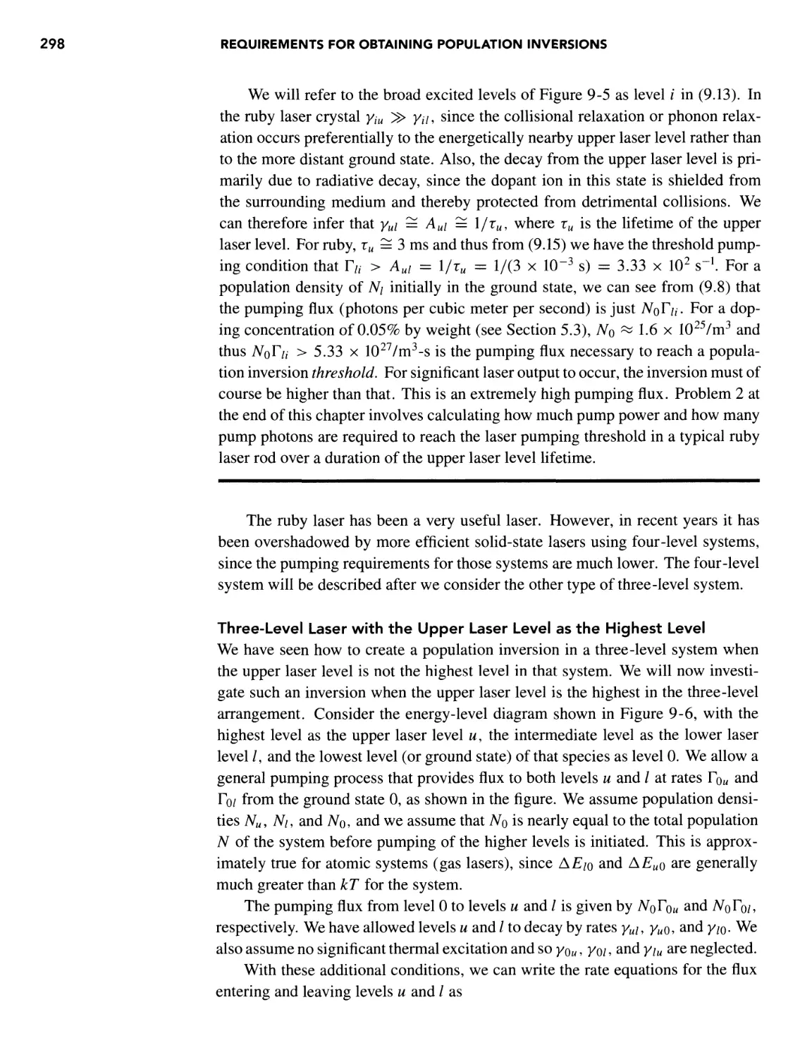
THRESHOLD PUMPING CONDITIONS
FOR INVERSION
Traditional three-level laser
ru>Yui(l-—) (9.14)
For radiative decay and when YnlYiu is small
Three-level gas laser
1 A/o ?
Four-level laser
r0(. > r^L =
Yio
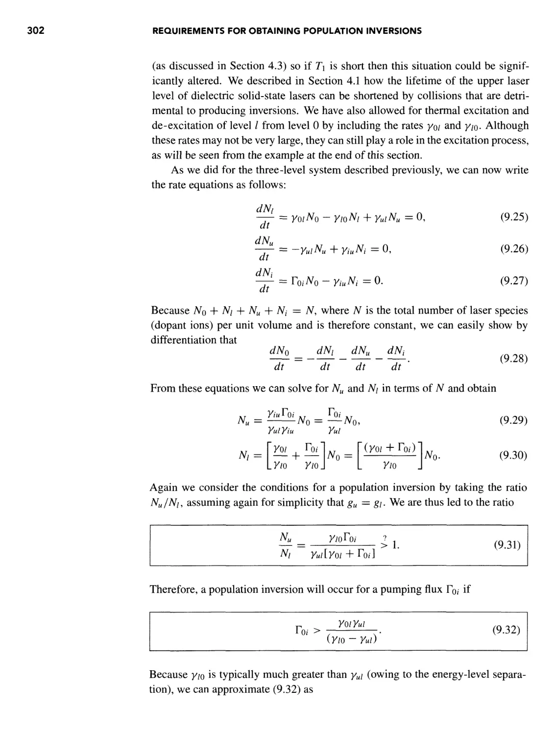
Transient inversion
Nu
(9.23)
(9.33)
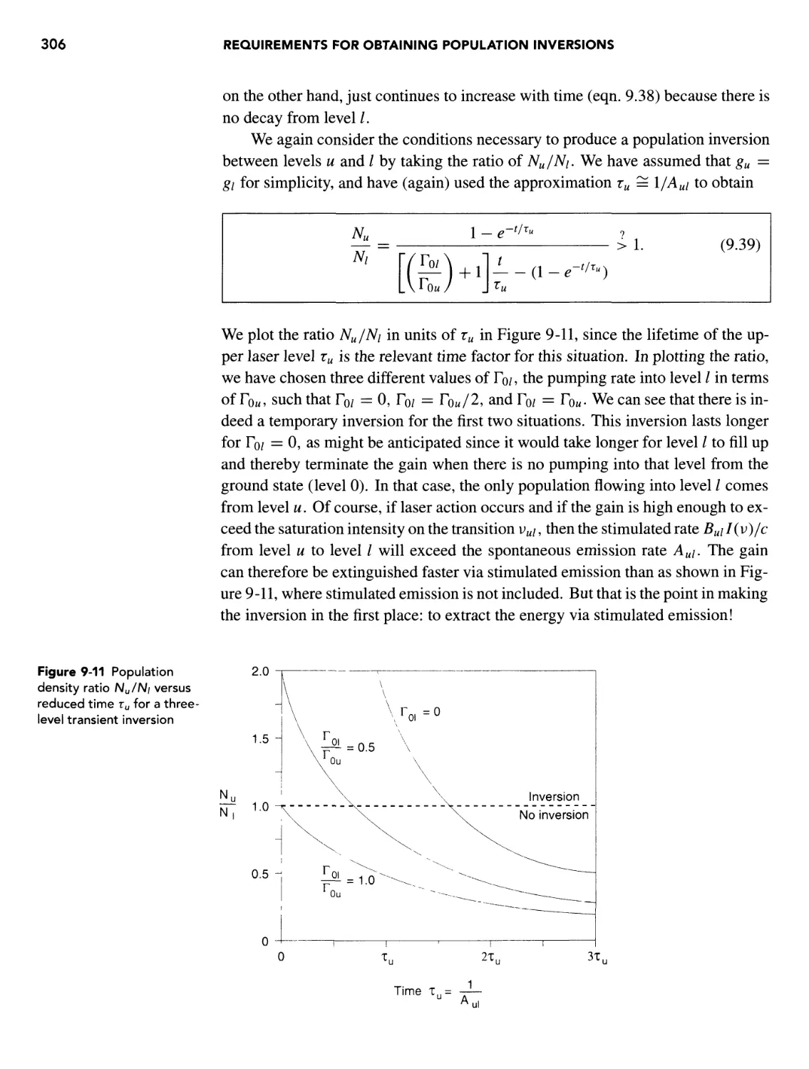
-^j^- > 1. (9.39)
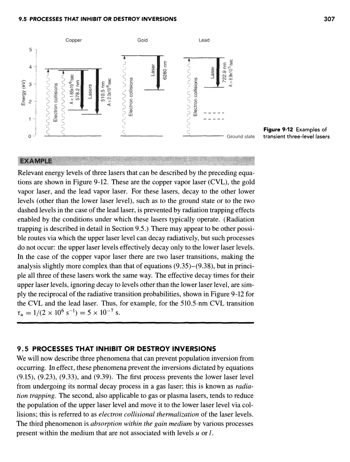
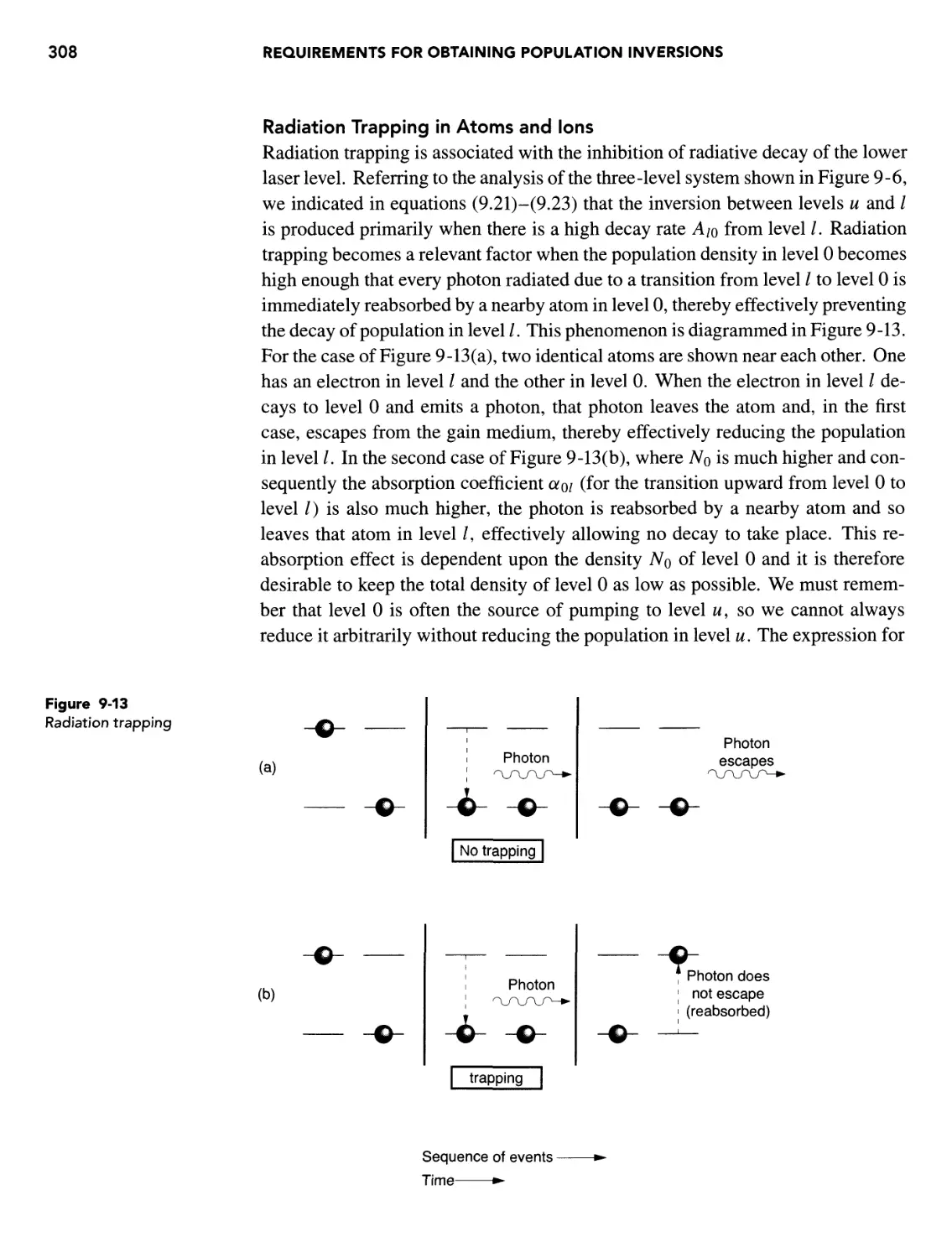
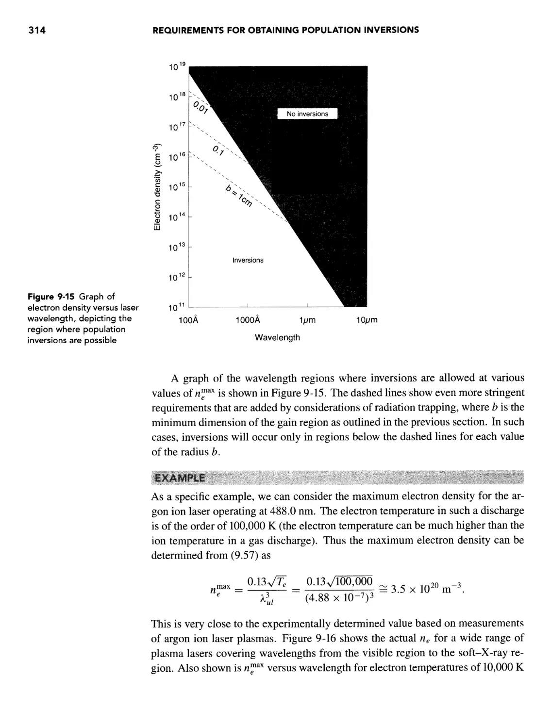
RADIATION TRAPPING
aoiNob = 1.46 [b is bore radius] (9.47)
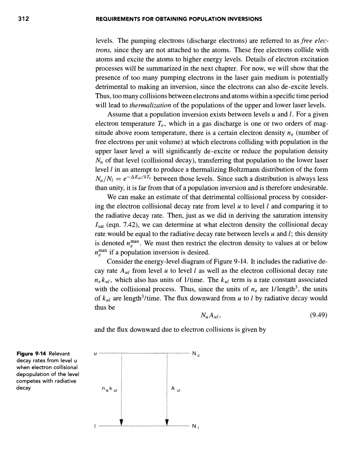
ELECTRON COLLISIONAL THERMALIZATION
4/
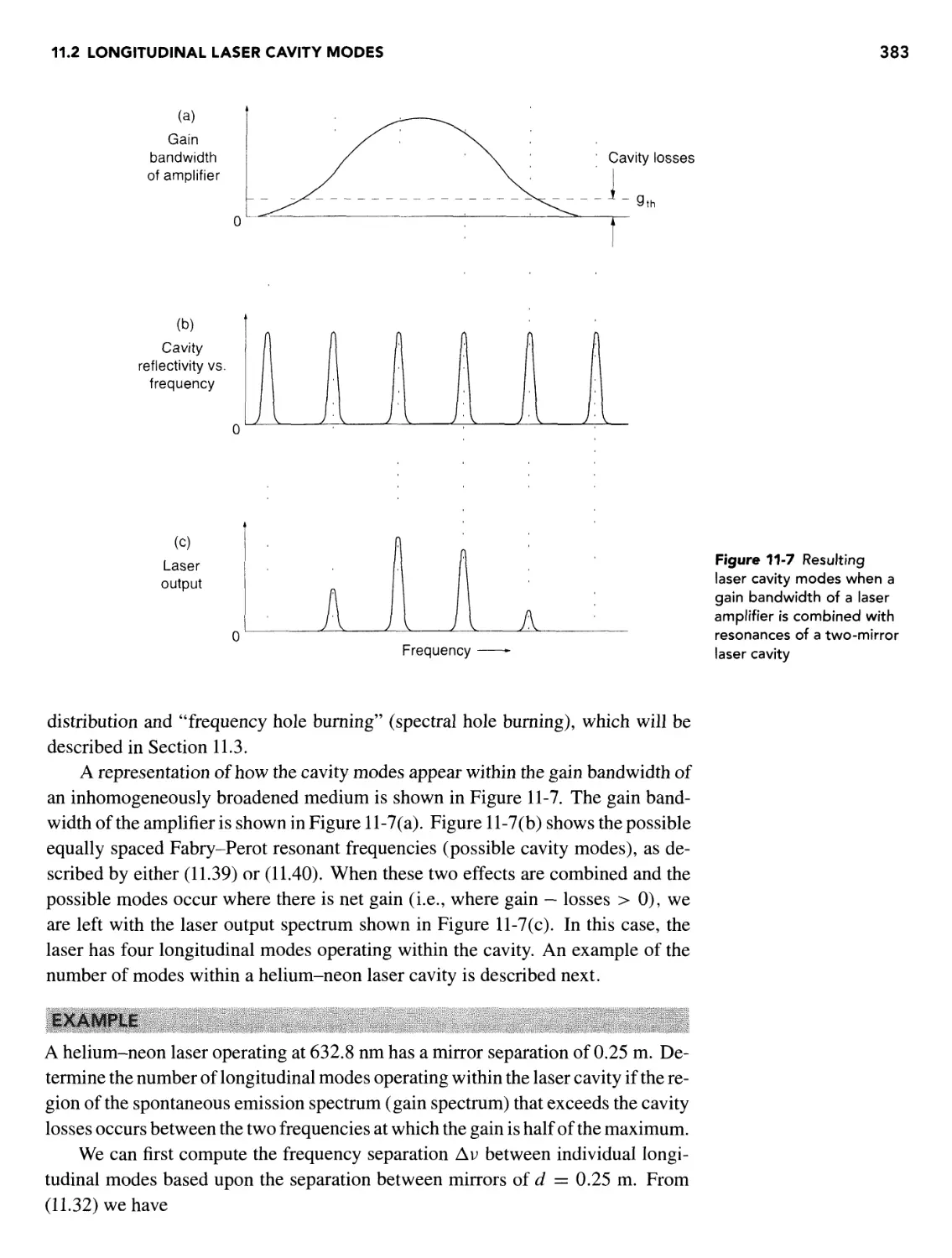
LASER MODES
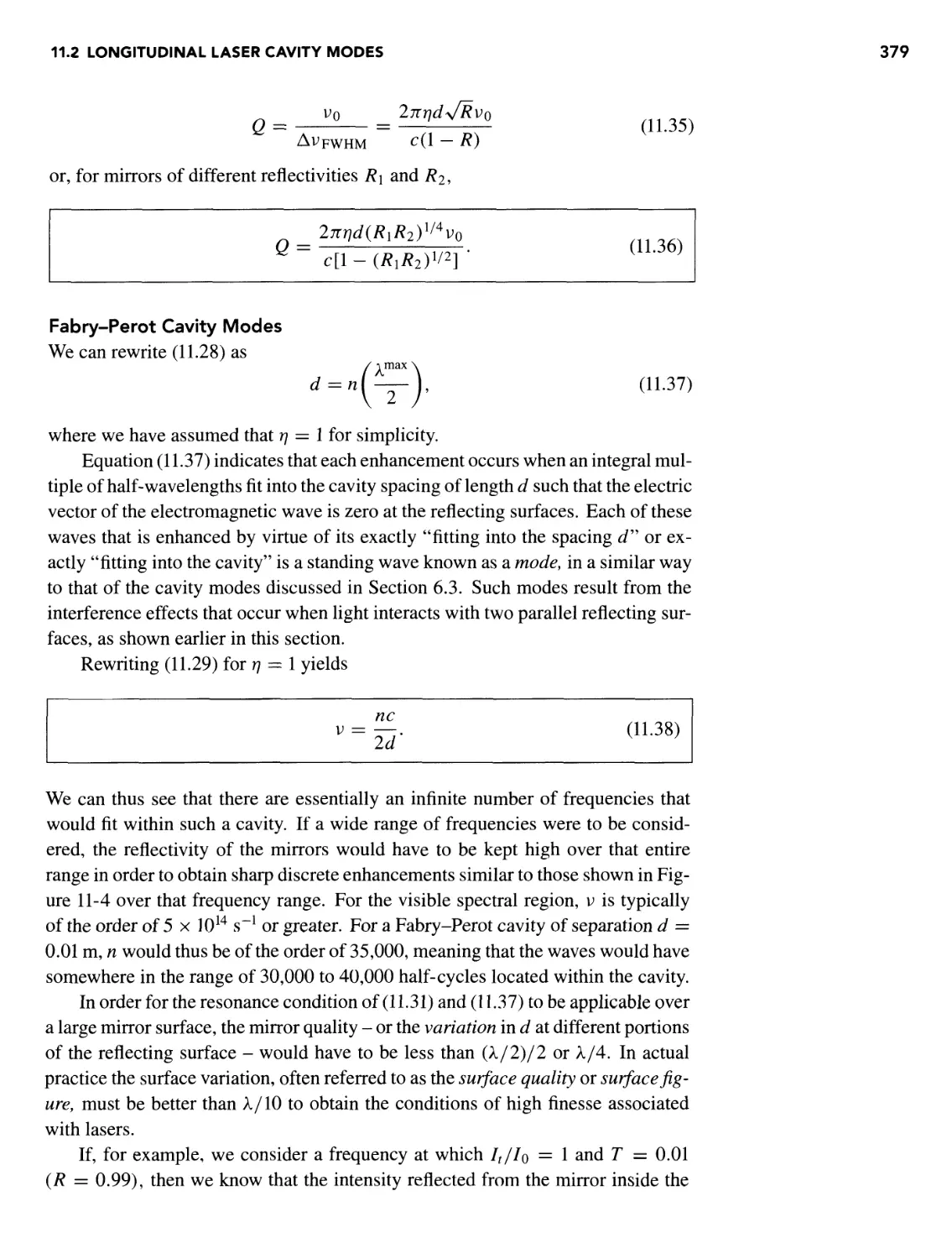
Longitudinal modes
Separation between modes
- m 3 [Te in K, k in m]
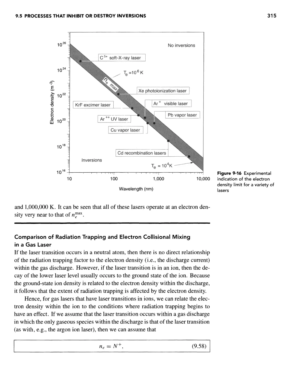
(9.57)
Mode frequency
/ c \
v = n[ [n a positive integer]
\2tidJ
A1.31)
A1.39)
A1.40)
Transverse modes
[p, q are integers] A1.53)
where
HQ(u) = 1 Hi(u) = 2u
H2(u) = 2Bm2 - 1)
Hm(u) = (-1)-^ —J—
A1.54)
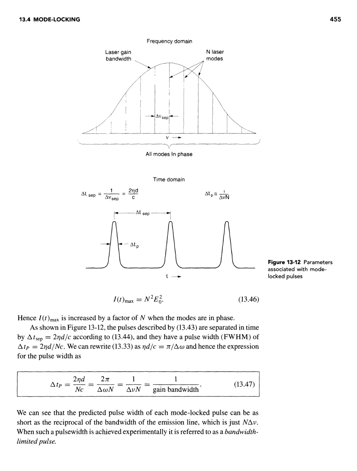
MODE-LOCKING
2t}d
usep
2r]d
Nc AvN
1
gain bandwidth
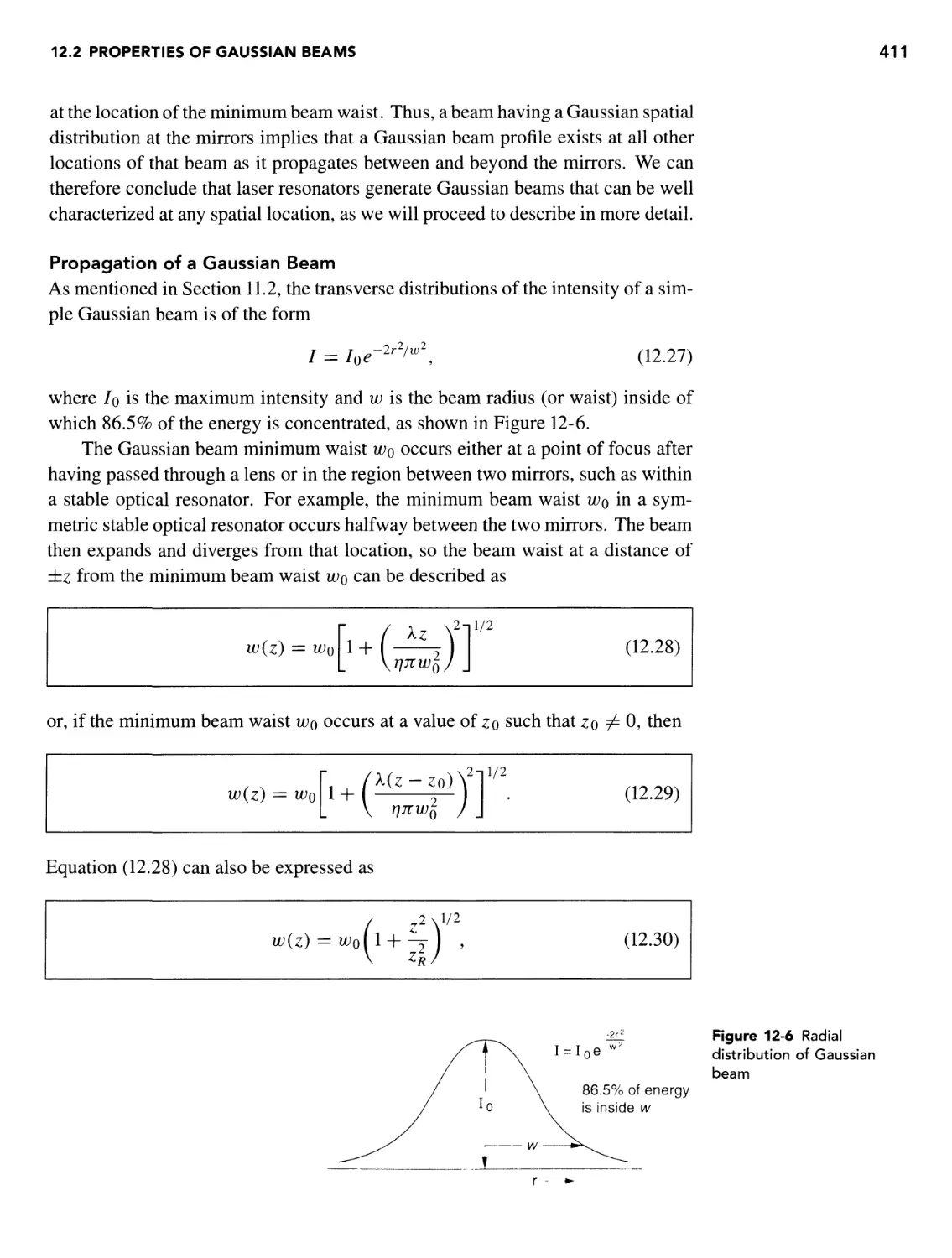
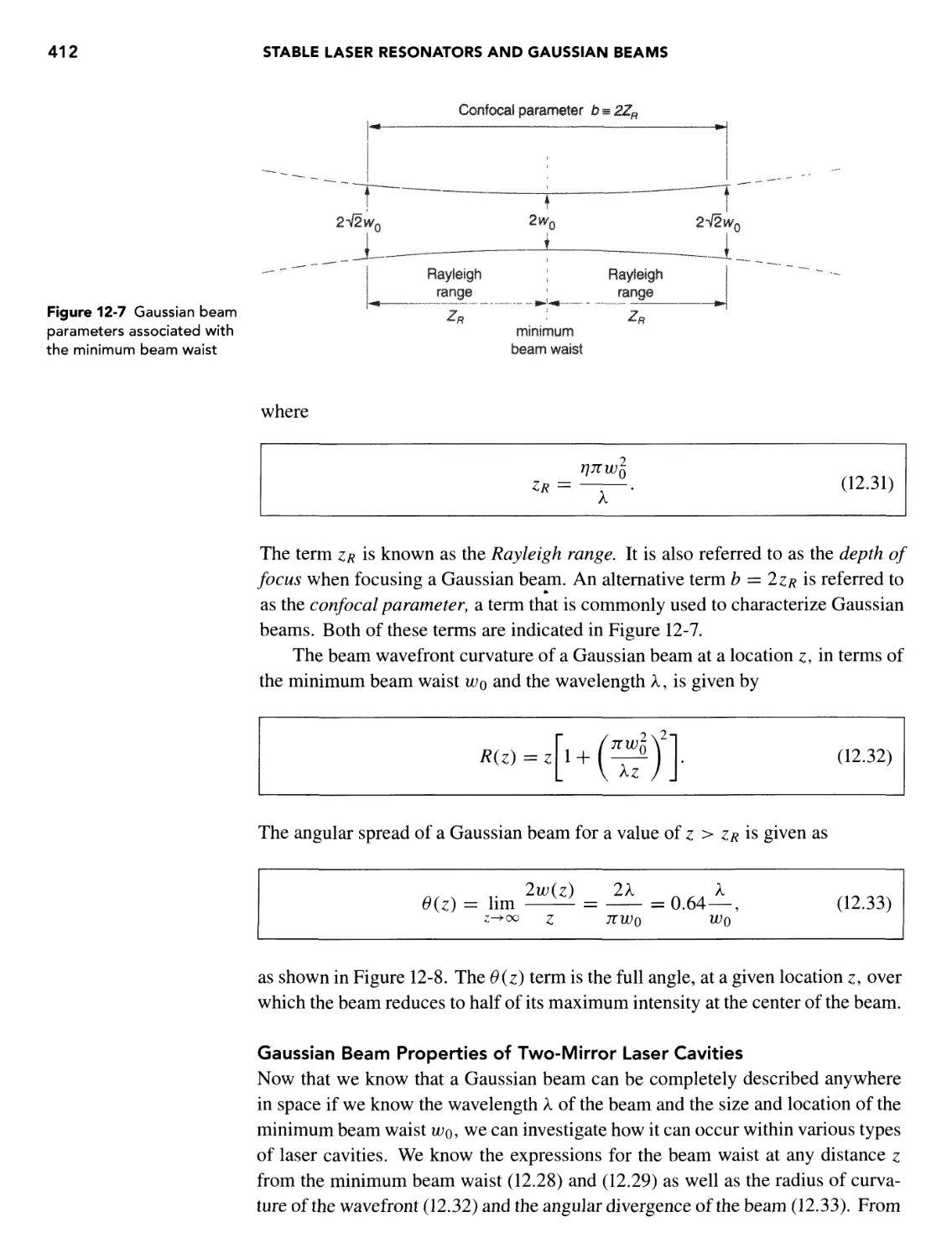
GAUSSIAN BEAMS
Beam waist
w(z) =
W(Z.) = Wq
1/2
01
1/2
2\l/2
Zr =
k
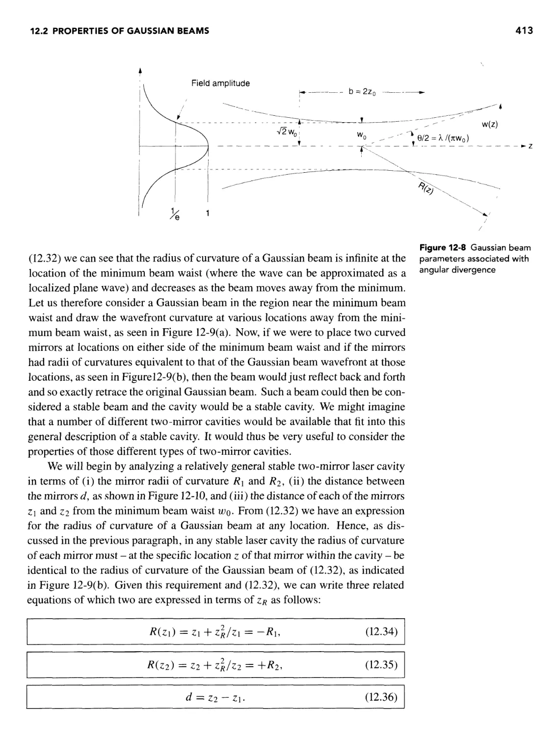
Wavefront curvature
2\2n
Angular spread
2A k
0(z) = = 0.64—
JTWo Wo
Complex beam parameter
1 1
k
J-
q R(z) rjnwHz)
1 C
R2(z)
-;
OPTIMUM MIRROR TRANSMISSION
AND POWER OUTPUT
'opt = (goLa)l/2-a
It*=l£
A3.44)
A3.47)
A2.28)
A2.29)
A2.30)
A2.31)
A2.32)
A2.33)
A2.65)
A2.67)
A2.69)
(8.23)
(8.24)
(8.27)
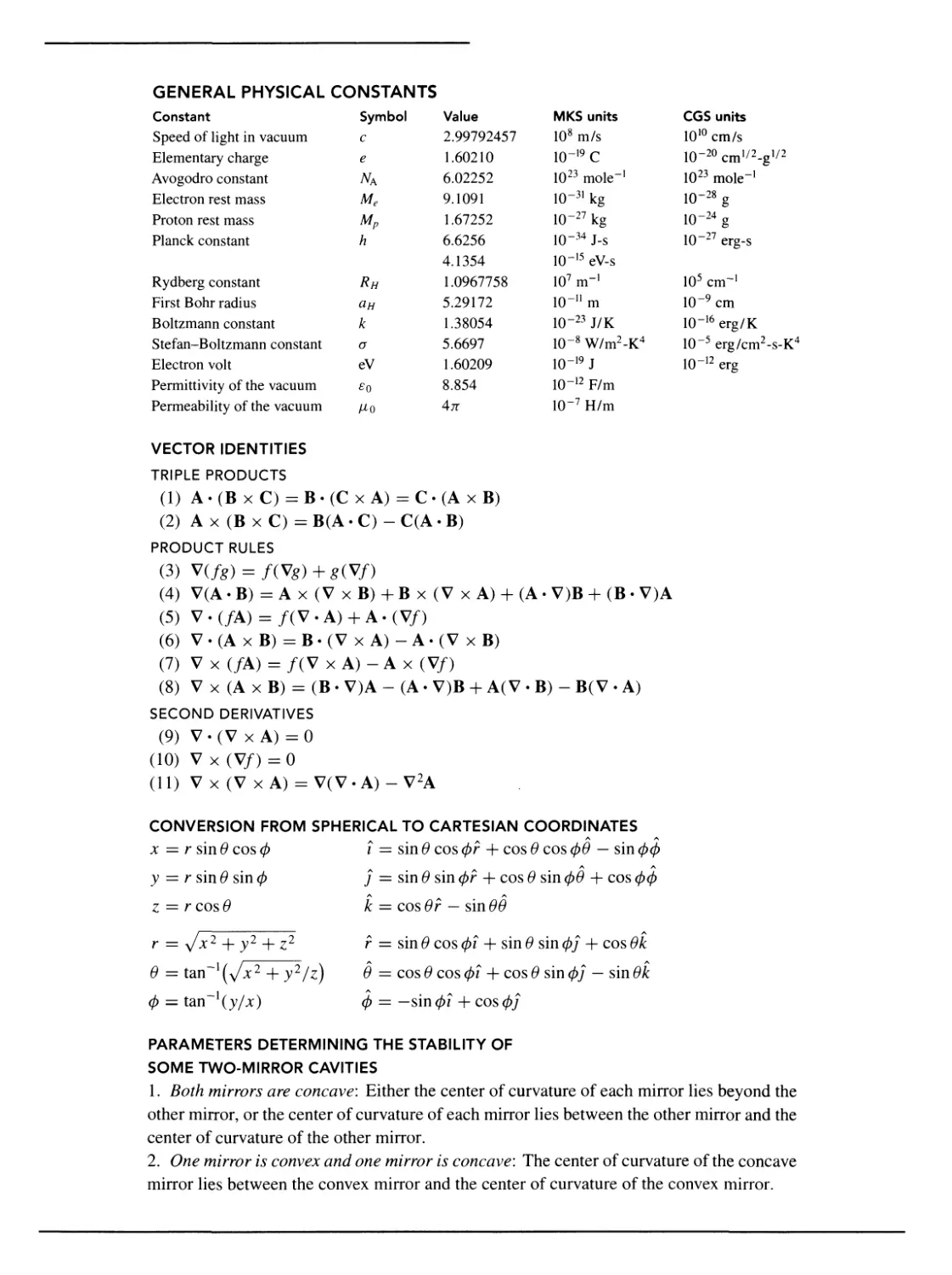
GENERAL PHYSICAL CONSTANTS
Constant
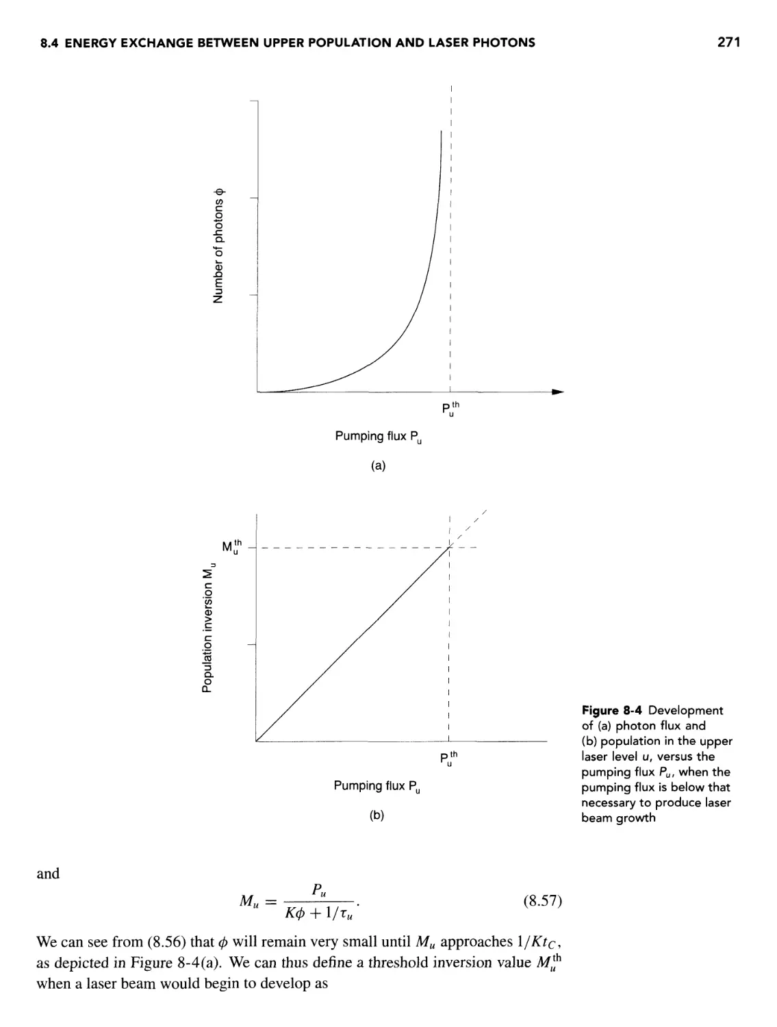
Speed of light in vacuum
Elementary charge
Avogodro constant
Electron rest mass
Proton rest mass
Planck constant
Rydberg constant
First Bohr radius
Boltzmann constant
Stefan-Boltzmann constant
Electron volt
Permittivity of the vacuum
Permeability of the vacuum
Symbol
c
e
NA
Me
Mp
h
Rh
aH
k
a
eV
£o
Mo
Value
2.99792457
1.60210
6.02252
9.1091
1.67252
6.6256
4.1354
1.0967758
5.29172
1.38054
5.6697
1.60209
8.854
An
MKS units
108 m/s
io-19 c
1023 mole
101 kg
io-27 kg
10 4 J-s
105 eV-s
IO7 m
10-11 m
10 3 J/K
10-8 W/m2-K4
io-19 j
10~12 F/m
10 H/m
CGS units
1010 cm/s
10-20 cm^-g172
1023 mole
io-28g
io-24 g
107 erg-s
105 cm-1
IO-9 cm
106 erg/K
10-5 erg/cm2-s-K4
10-12 erg
VECTOR IDENTITIES
TRIPLE PRODUCTS
A) A • (B x C) = B • (C x A) = C • (A x B)
B) A x (B x C) = B(A • C) - C(A • B)
PRODUCT RULES
0) V(/g) = /(Vs) + s(V/)
D) V(A • B) = A x (V x B) + B x (V x A) + (A • V)B + (B • V)A
E) V.(/A) = /(V.A)+A.(V/)
F) V • (A x B) = B • (V x A) - A • (V x B)
G) V x (/A) = /(V x A) - A x (V/)
(8) V x (A x B) = (B • V)A - (A • V)B + A( V . B) - B( V • A)
SECOND DERIVATIVES
(9) V-(V x A) = 0
A0) V x (V/) = 0
A1) V x (V x A) = V( V • A) - V2A
CONVERSION FROM SPHERICAL TO CARTESIAN COORDINATES
x = r sin 0 cos (fi
y = r sin 0 sin (fi
z = r cos 6
i = sin 6 cos (fir + cos 6 cos (fib — sin (ficfi
j = sin 0 sin (fir + cos 6 sin (fi§ + cos 00
k = cos Or — $
r =
0 = torTl(y/x)
r = sin 0 cos (fii + sin 0 sin (fij + cos 0k
0 = cos 0 cos (fii + cos 0 sin (fij — sin 0k
(fi = —sin (fii + cos (fij
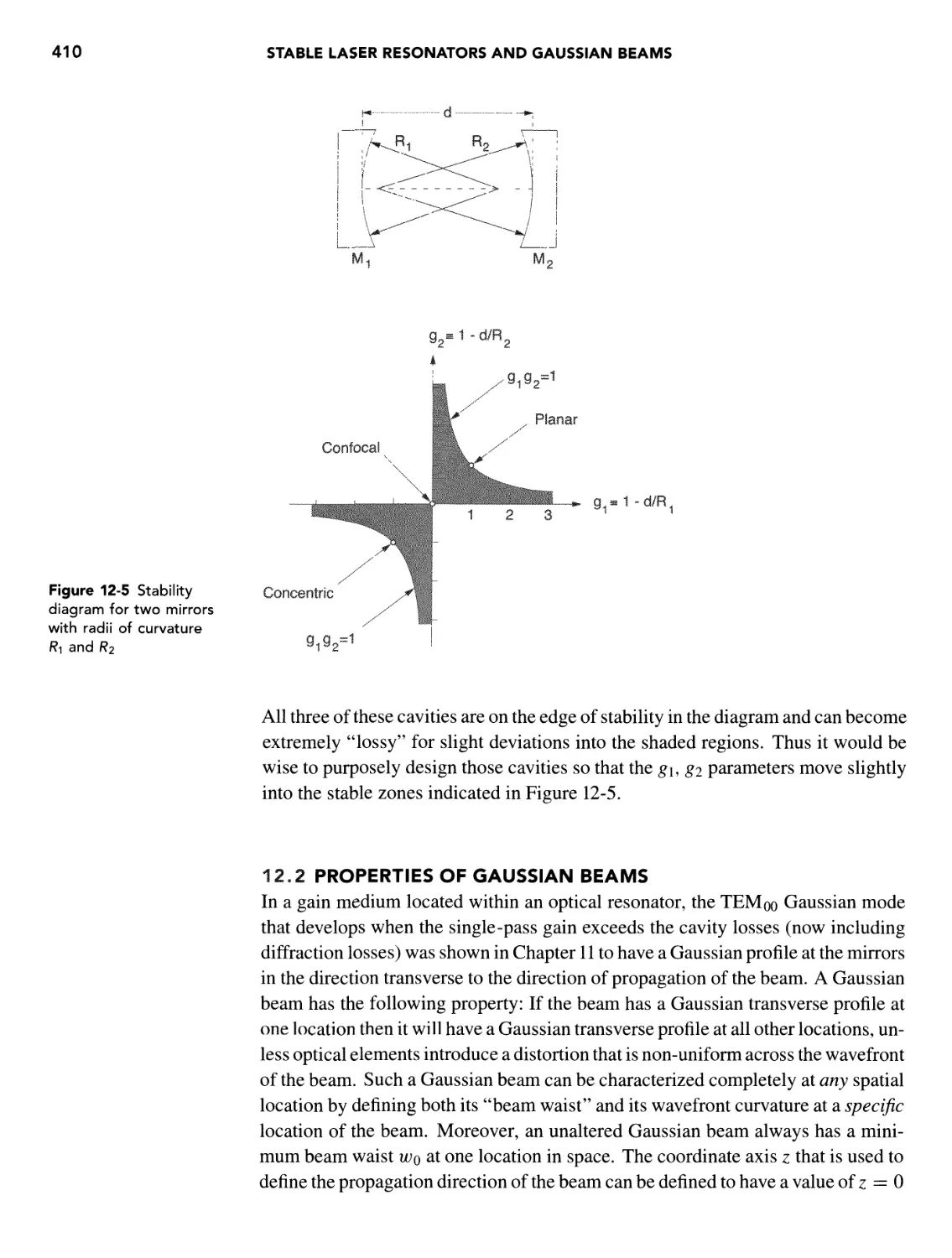
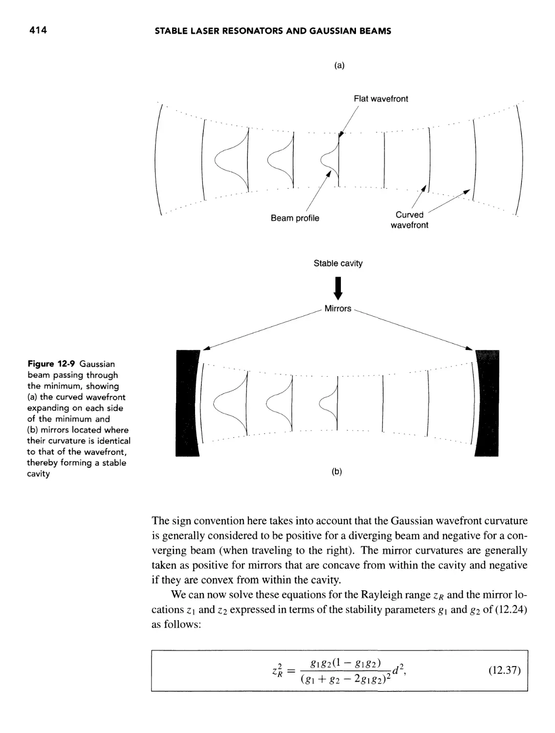
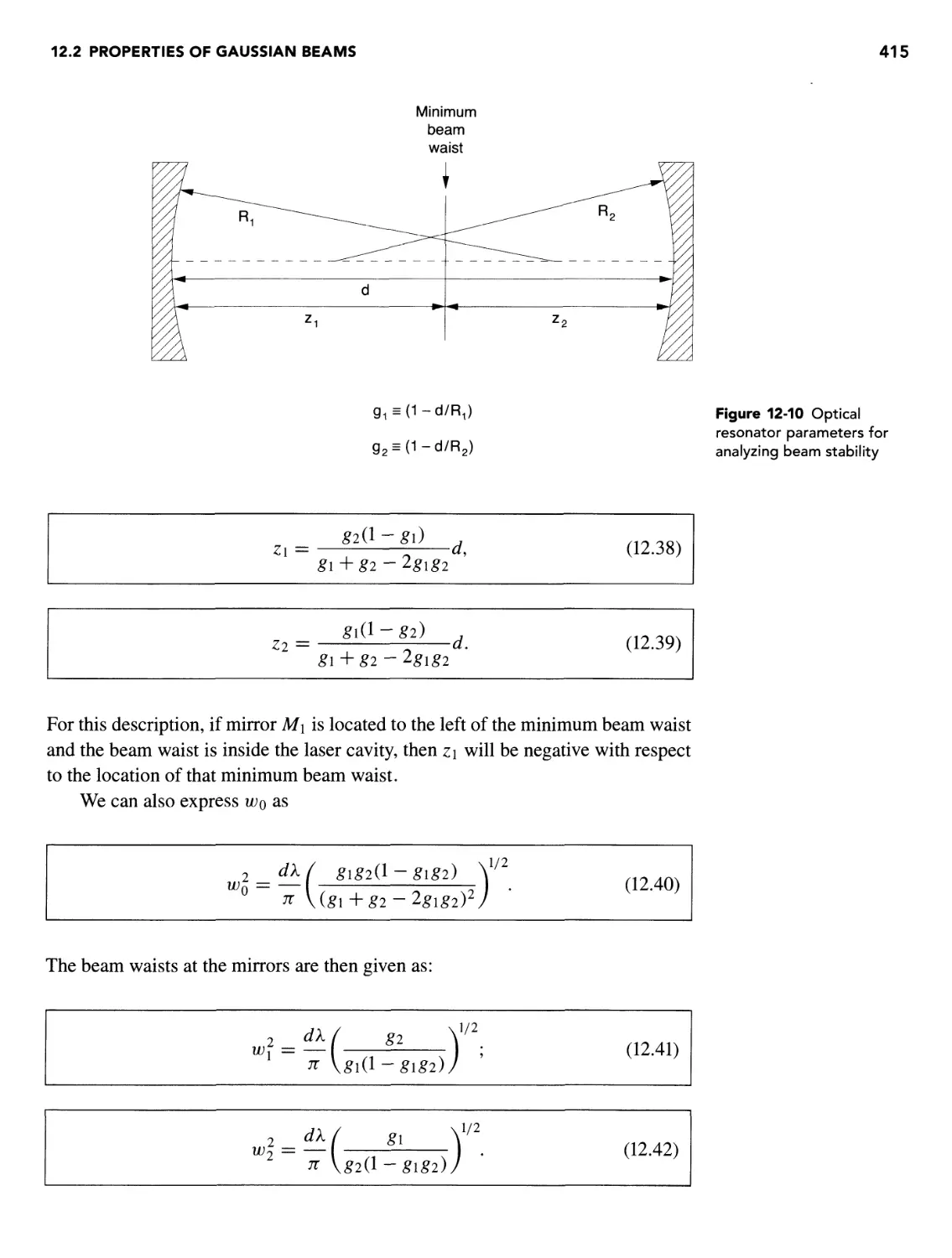
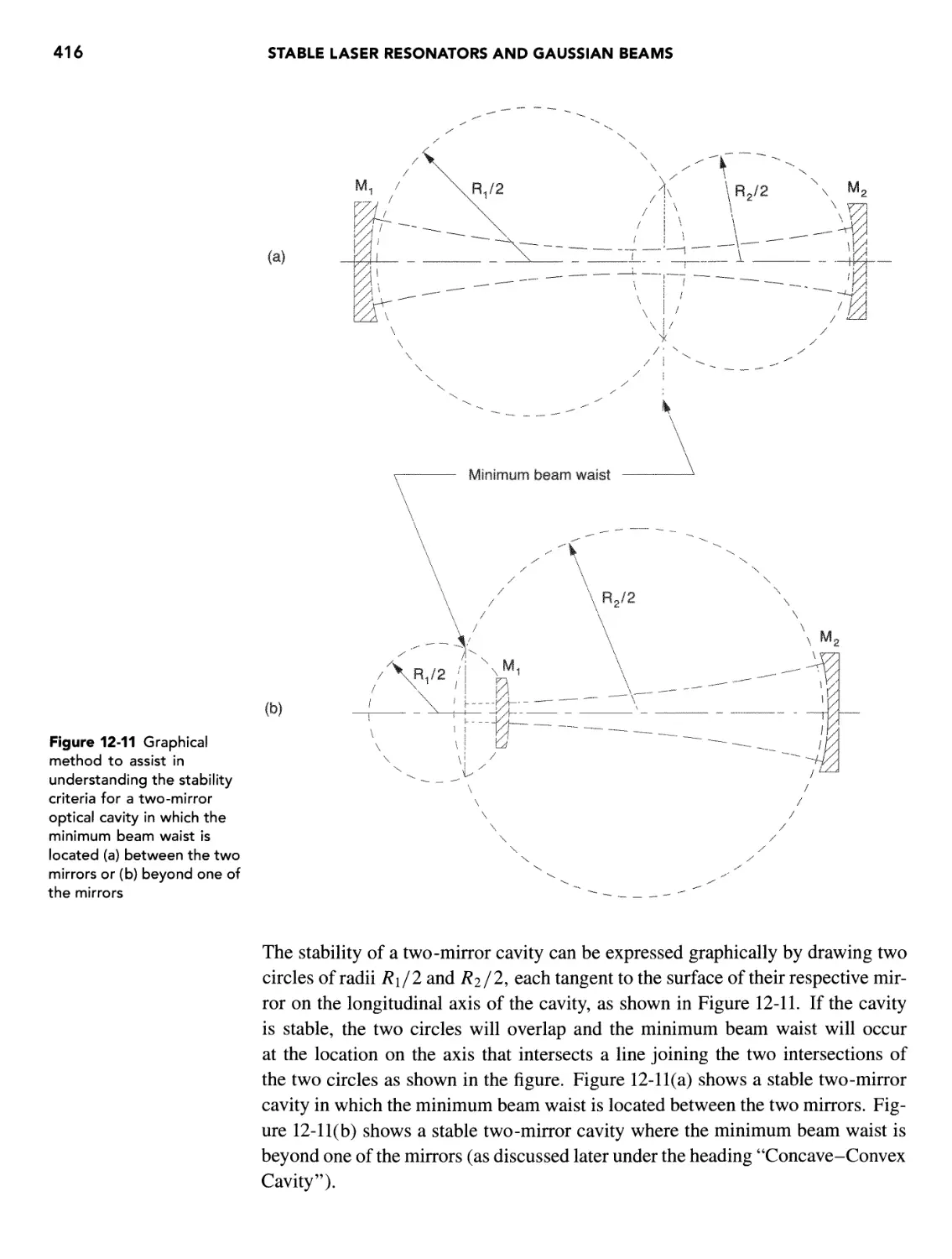
PARAMETERS DETERMINING THE STABILITY OF
SOME TWO-MIRROR CAVITIES
1. Both mirrors are concave: Either the center of curvature of each mirror lies beyond the
other mirror, or the center of curvature of each mirror lies between the other mirror and the
center of curvature of the other mirror.
2. One mirror is convex and one mirror is concave: The center of curvature of the concave
mirror lies between the convex mirror and the center of curvature of the convex mirror.
LASER FUNDAMENTALS
SECOND EDITION
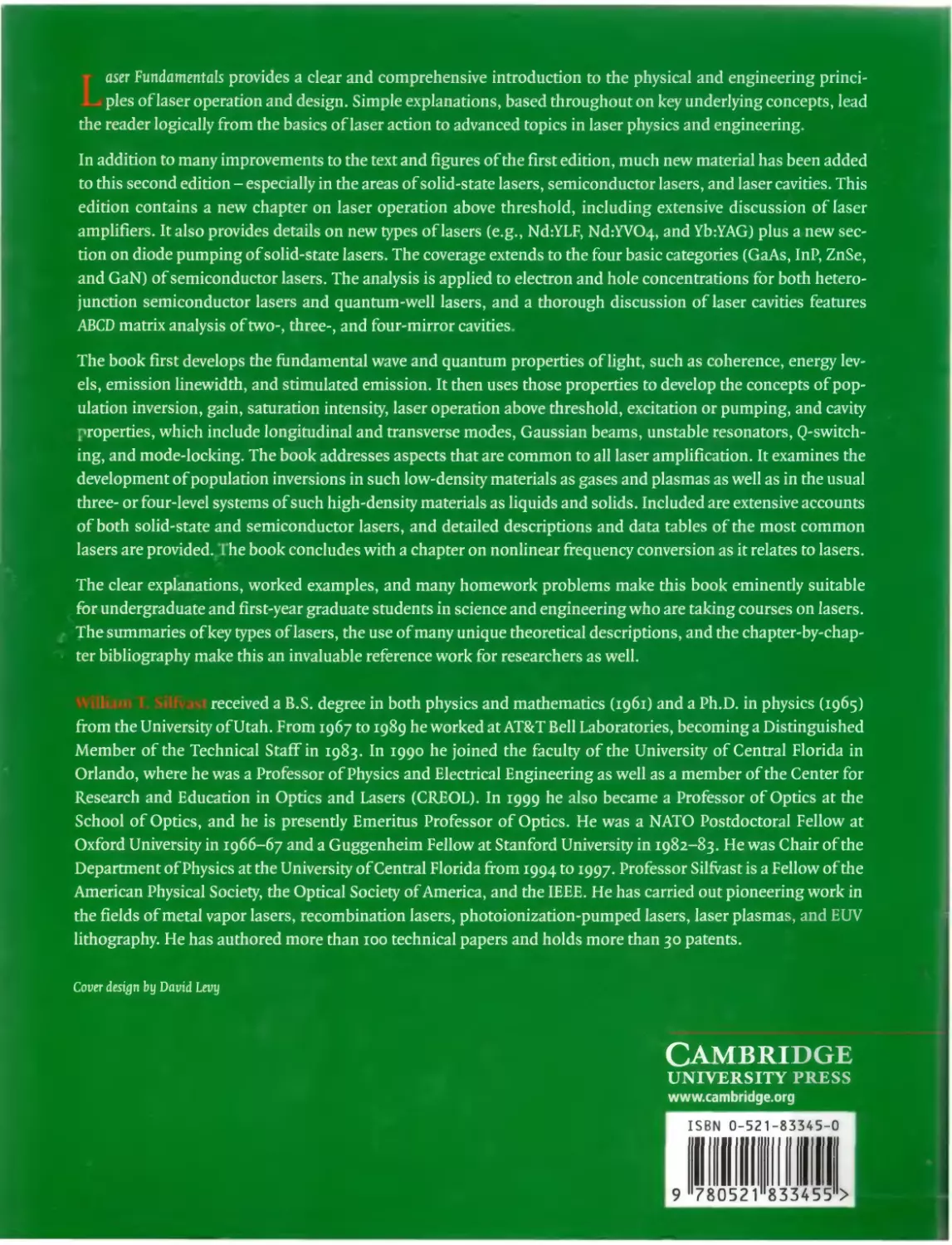
Laser Fundamentals provides a clear and comprehensive introduction to the physical and engi-
engineering principles of laser operation and design. Simple explanations, based throughout on key
underlying concepts, lead the reader logically from the basics of laser action to advanced topics
in laser physics and engineering.
In addition to many improvements to the text and figures of the first edition, much new
material has been added to this second edition - especially in the areas of solid-state lasers,
semiconductor lasers, and laser cavities. This edition contains a new chapter on laser operation
above threshold, including extensive discussion of laser amplifiers. It also provides details on
new types of lasers (e.g., Nd:YLF, Nd:YVO4, andYb:YAG) plus a new section on diode pump-
pumping of solid-state lasers. The coverage extends to the four basic categories (GaAs, InP, ZnSe,
and GaN) of semiconductor lasers. The analysis is applied to electron and hole concentrations
for both heterojunction semiconductor lasers and quantum-well lasers, and a thorough discus-
discussion of laser cavities features ABCD matrix analysis of two-, three-, and four-mirror cavities.
The book first develops the fundamental wave and quantum properties of light, such as
coherence, energy levels, emission linewidth, and stimulated emission. It then uses those prop-
properties to develop the concepts of population inversion, gain, saturation intensity, laser operation
above threshold, excitation or pumping, and cavity properties, which include longitudinal and
transverse modes, Gaussian beams, unstable resonators, Q-switching, and mode-locking. The
book addresses aspects that are common to all laser amplification. It examines the development
of population inversions in such low-density materials as gases and plasmas as well as in the
usual three- or four-level systems of such high-density materials as liquids and solids. Included
are extensive accounts of both solid-state and semiconductor lasers, and detailed descriptions
and data tables of the most common lasers are provided. The book concludes with a chapter on
nonlinear frequency conversion as it relates to lasers.
The clear explanations, worked examples, and many homework problems make this book
eminently suitable for undergraduate and first-year graduate students in science and engineering
who are taking courses on lasers. The summaries of key types of lasers, the use of many unique
theoretical descriptions, and the chapter-by-chapter bibliography make this an invaluable refer-
reference work for researchers as well.
William Silfvast received a B.S. degree in both physics and mathematics A961) and a Ph.D. in
physics A965) from the University of Utah. From 1967 to 1989 he worked at AT&T Bell Labo-
Laboratories, becoming a Distinguished Member of the Technical Staff in 1983. In 1990 he joined the
faculty of the University of Central Florida in Orlando, where he was a Professor of Physics and
Electrical Engineering as well as a member of the Center for Research and Education in Optics
and Lasers (CREOL). In 1999 he also became a Professor of Optics at the School of Optics, and
he is presently Emeritus Professor of Optics. He was a NATO Postdoctoral Fellow at Oxford
University in 1966-67 and a Guggenheim Fellow at Stanford University in 1982-83. He was
Chair of the Department of Physics at the University of Central Florida from 1994 to 1997. Pro-
Professor Silfvast is a Fellow of the American Physical Society, the Optical Society of America, and
the IEEE. He has carried out pioneering work in the fields of metal vapor lasers, recombination
lasers, photoionization-pumped lasers, laser plasmas, and EUV lithography. He has authored
more than 100 technical papers and holds more than 30 patents.
LASER FUNDAMENTALS
SECOND EDITION
WILLIAM T. SILFVAST
School of Optics / CREOL
University of Central Florida
CAMBRIDGE
UNIVERSITY PRESS
PUBLISHED BY THE PRESS SYNDICATE OF THE UNIVERSITY OF CAMBRIDGE
The Pitt Building, Trumpington Street, Cambridge, United Kingdom
CAMBRIDGE UNIVERSITY PRESS
The Edinburgh Building, Cambridge CB2 2RU, UK
40 West 20th Street, New York, NY 10011-4211, USA
477 Williamstown Road, Port Melbourne, VIC 3207, Australia
Ruiz de Alarcon 13, 28014 Madrid, Spain
Dock House, The Waterfront, Cape Town 8001, South Africa
http://www.cambridge.org
First published 1996
Reprinted 1999, 2000, 2003
First edition © Cambridge University Press
Second edition © William T. Silfvast 2004
This book is in copyright. Subject to statutory exception and
to the provisions of relevant collective licensing agreements,
no reproduction of any part may take place without
the written permission of Cambridge University Press.
First published 2004
Printed in the United States of America
Typeface Times 10.5/13.5 and Avenir System AMS-TgX [FH]
A catalog record for this book is available from the British Library.
Library of Congress Cataloging in Publication data
Silfvast, William Thomas, 1937-
Laser fundamentals / William T. Silfvast. - 2nd ed.
p. cm.
Includes bibliographical references and index.
ISBN 0-521-83345-0
1. Lasers. I. Title.
TA1675.S52 2004
621.36'6 - dc21 2003055352
ISBN 0 521 83345 0 hardback
To my wife, Susan, and my three children, Scott, Robert and Stacey,
all of whom are such an important part of my life.
Contents
Preface to the Second Edition page xix
Preface to the First Edition xxi
Acknowledgments xxiii
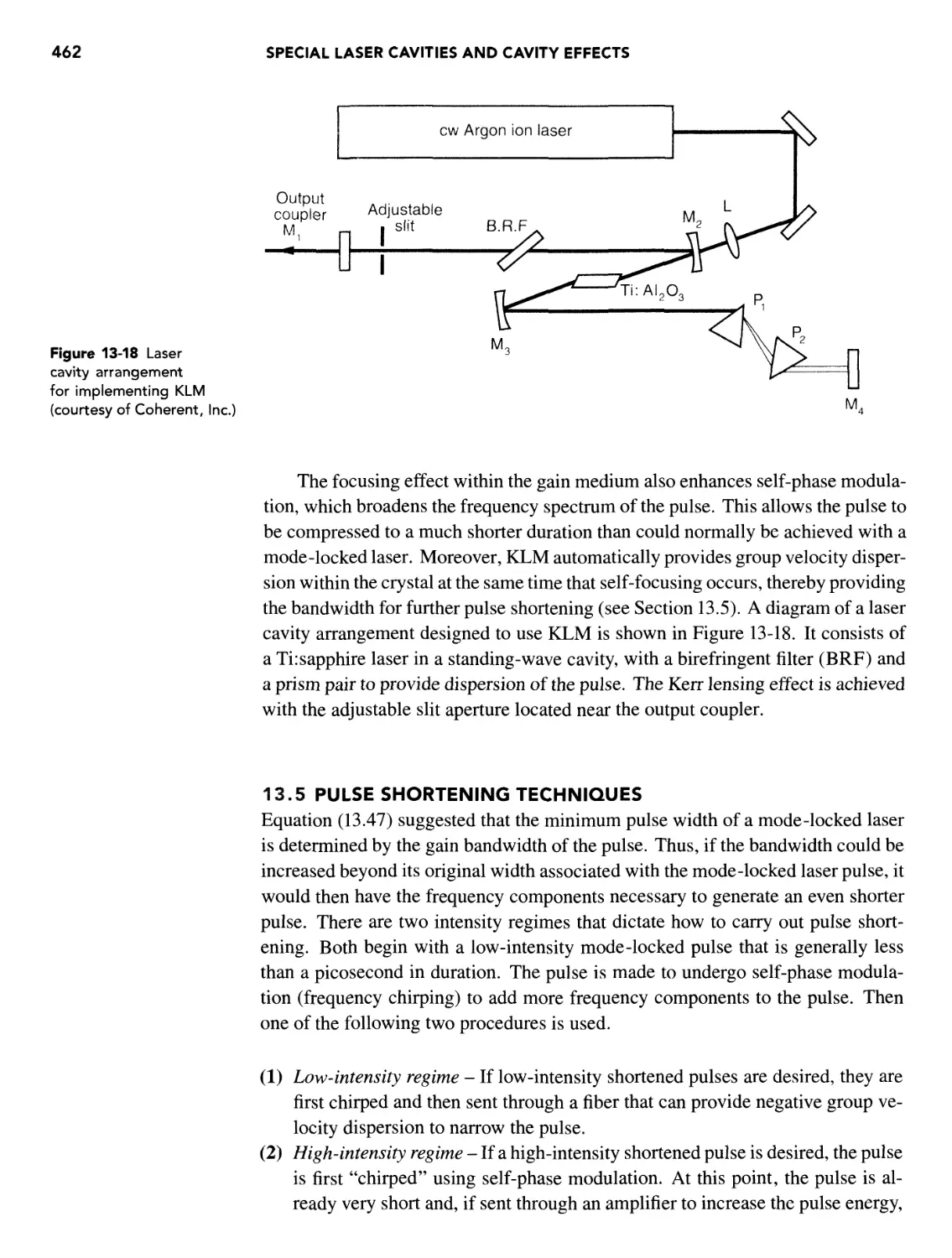
1 INTRODUCTION 1
OVERVIEW 1
Introduction 1
Definition of the Laser 1
Simplicity of a Laser 2
Unique Properties of a Laser 2
The Laser Spectrum and Wavelengths 3
A Brief History of the Laser 4
Overview of the Book 5
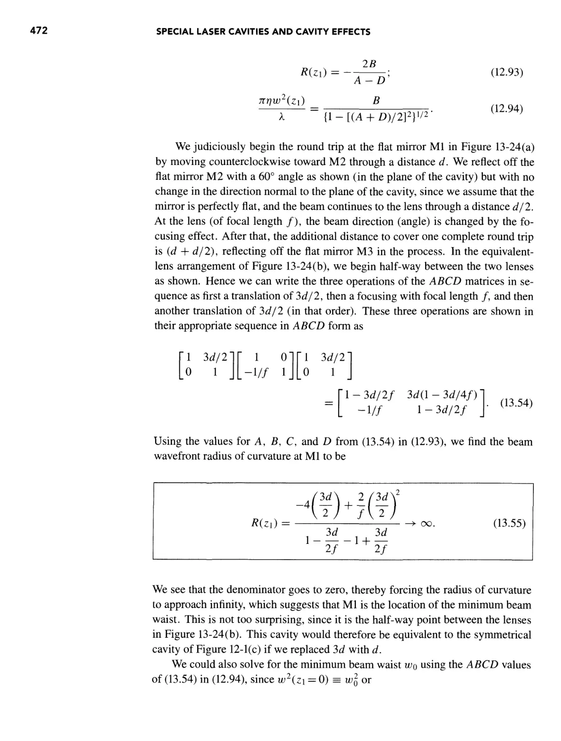
SECTION 1. FUNDAMENTAL WAVE PROPERTIES OF LIGHT
2 WAVE NATURE OF LIGHT - THE INTERACTION OF LIGHT
WITH MATERIALS 9
OVERVIEW 9
2.1 Maxwell's Equations 9
2.2 Maxwell's Wave Equations 12
Maxwell's Wave Equations for a Vacuum 12
Solution of the General Wave Equation - Equivalence of Light and
Electromagnetic Radiation 13
Wave Velocity - Phase and Group Velocities 17
Generalized Solution of the Wave Equation 20
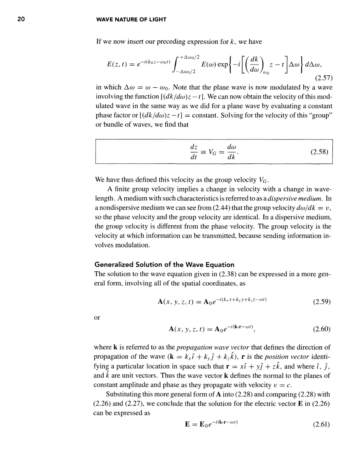
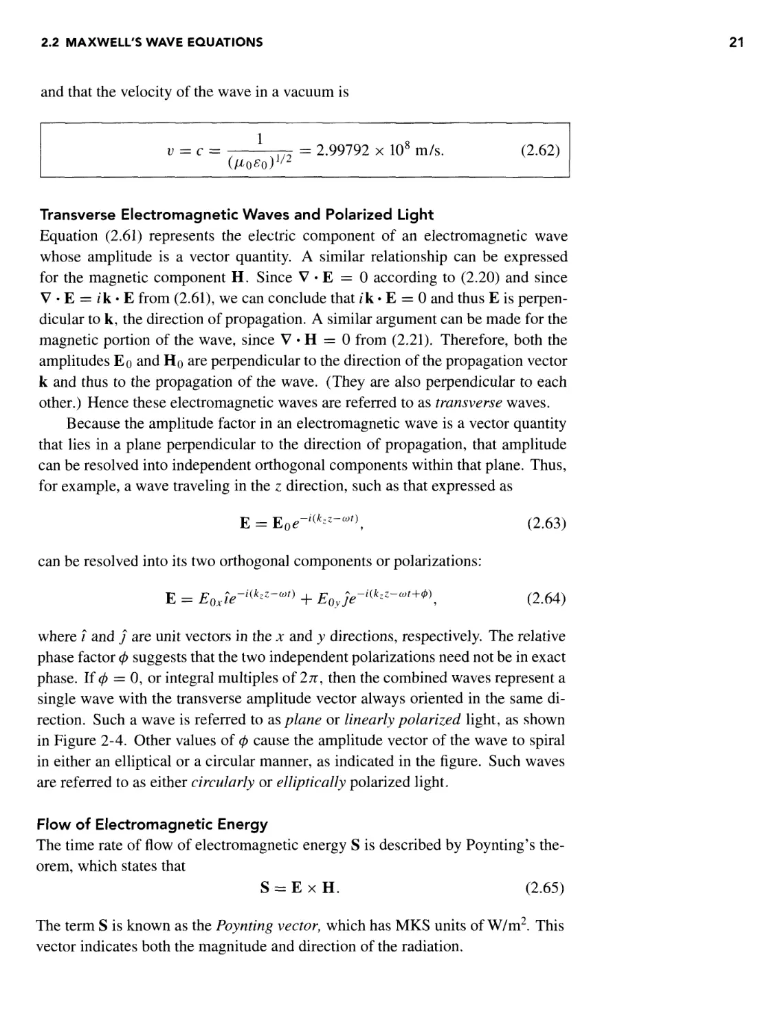
Transverse Electromagnetic Waves and Polarized Light 21
Flow of Electromagnetic Energy 21
Radiation from a Point Source (Electric Dipole Radiation) 22
2.3 Interaction of Electromagnetic Radiation (Light) with Matter 23
Speed of Light in a Medium 23
Maxwell's Equations in a Medium 24
Application of Maxwell's Equations to Dielectric Materials -
Laser Gain Media 25
Complex Index of Refraction - Optical Constants 28
Absorption and Dispersion 29
VII
viii CONTENTS
Estimating Particle Densities of Materials for Use in the
Dispersion Equations 34
2.4 Coherence 36
Temporal Coherence 37
Spatial Coherence 38
REFERENCES 39
PROBLEMS 39
SECTION 2, FUNDAMENTAL QUANTUM PROPERTIES OF LIGHT
3 PARTICLE NATURE OF LIGHT - DISCRETE ENERGY LEVELS 45
OVERVIEW 45
3.1 Bohr Theory of the Hydrogen Atom 45
Historical Development of the Concept of Discrete Energy Levels 45
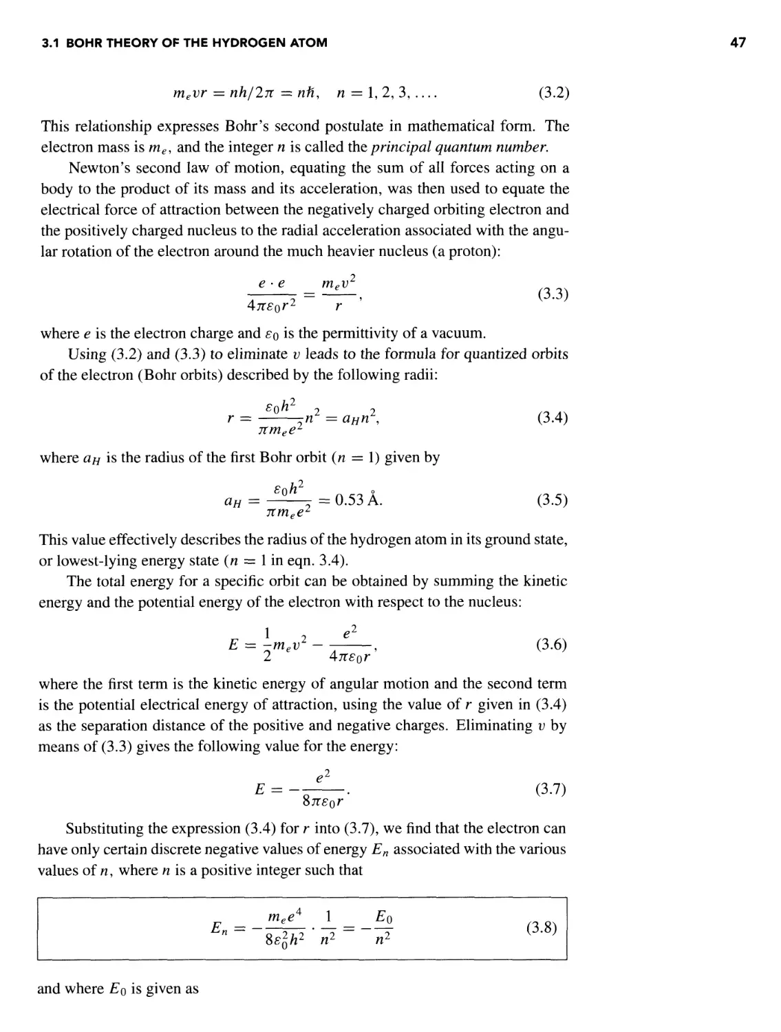
Energy Levels of the Hydrogen Atom 46
Frequency and Wavelength of Emission Lines 49
Ionization Energies and Energy Levels of Ions 51
Photons 54
3.2 Quantum Theory of Atomic Energy Levels 54
Wave Nature of Particles 54
Heisenberg Uncertainty Principle 56
Wave Theory 56
Wave Functions 57
Quantum States 57
The Schrodinger Wave Equation 59
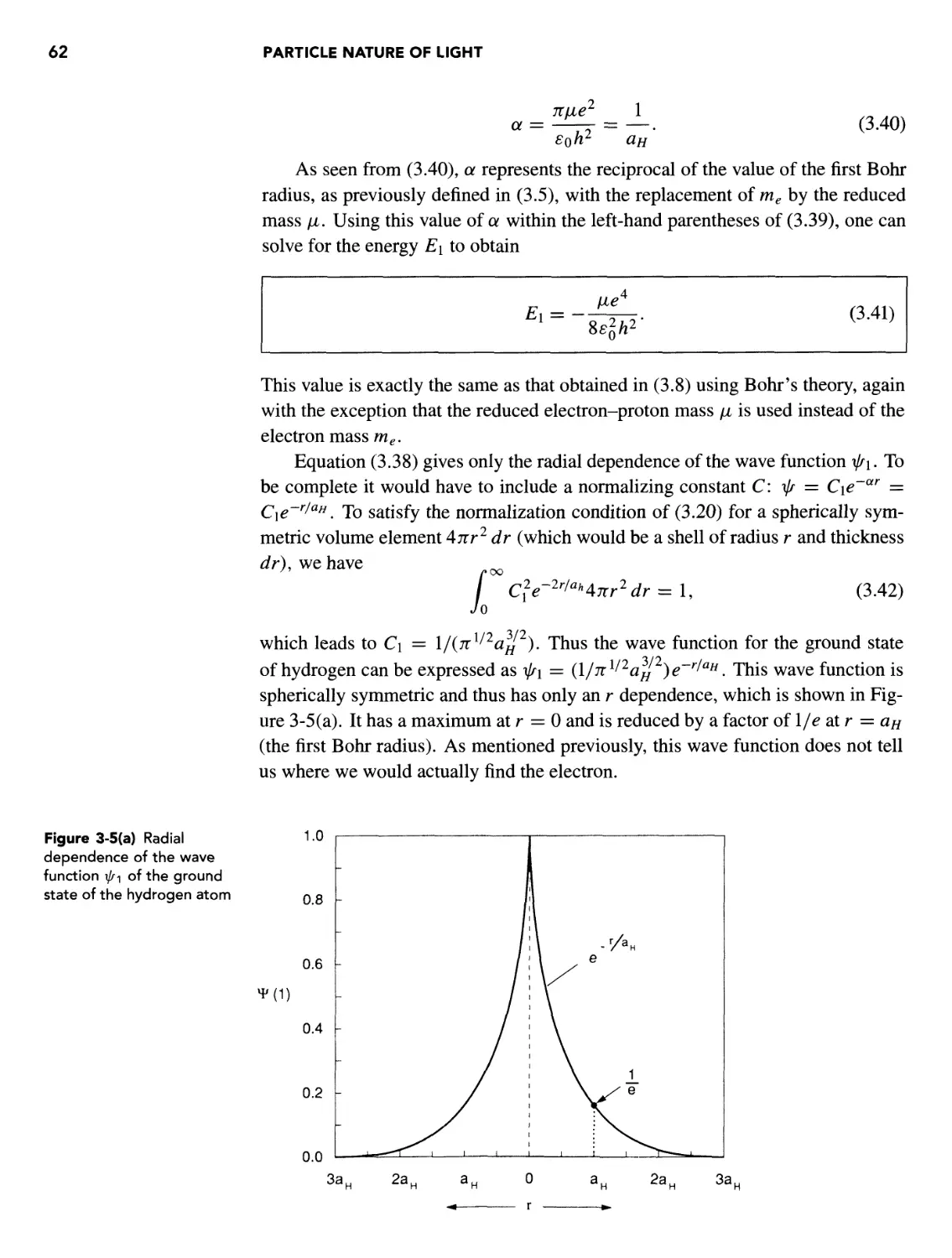
Energy and Wave Function for the Ground State of the
Hydrogen Atom 61
Excited States of Hydrogen 63
Allowed Quantum Numbers for Hydrogen Atom Wave Functions 66
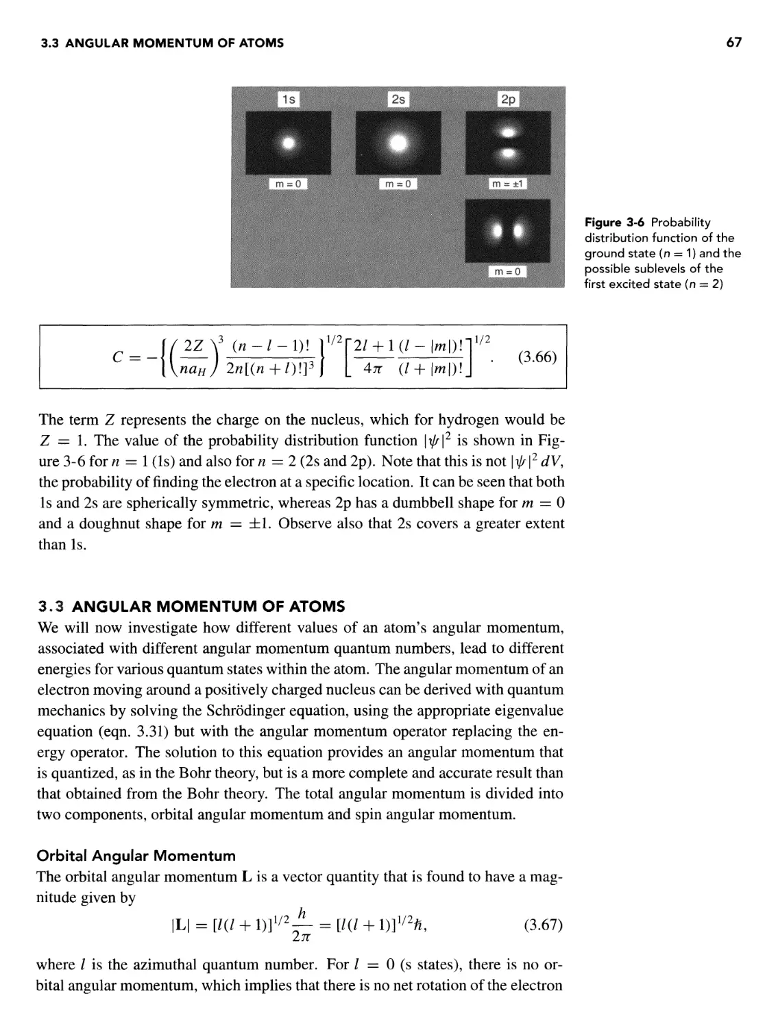
3.3 Angular Momentum of Atoms 67
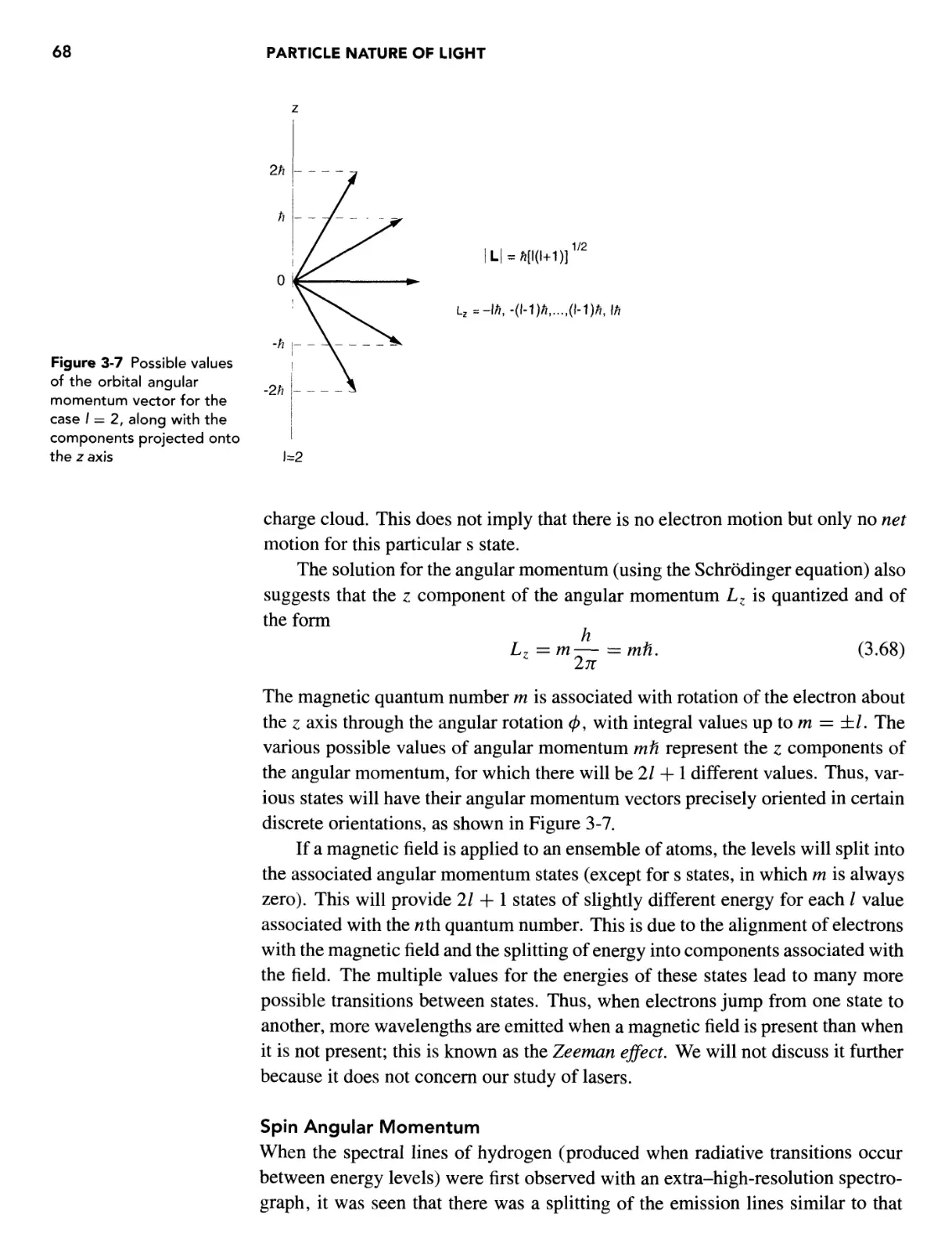
Orbital Angular Momentum 67
Spin Angular Momentum 68
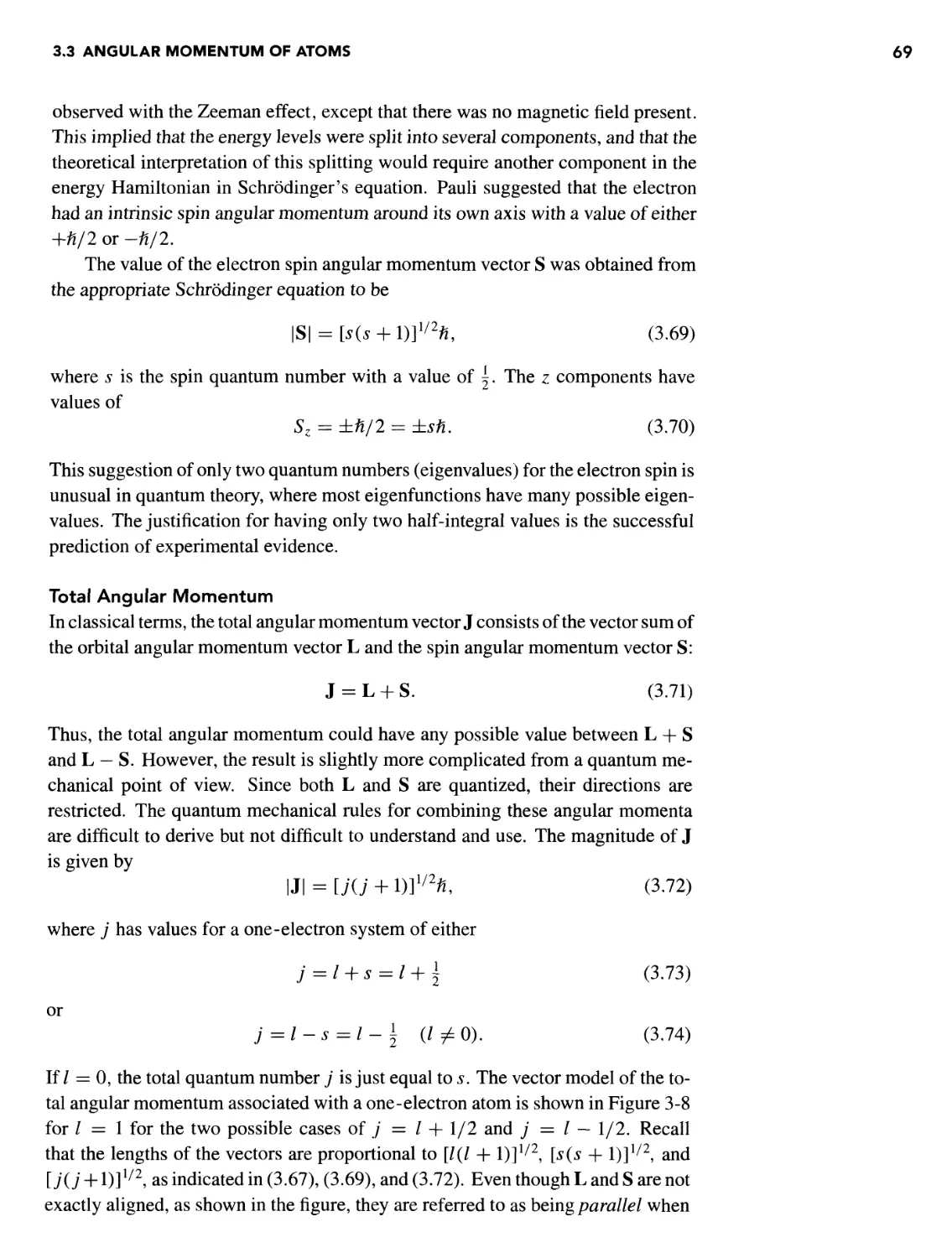
Total Angular Momentum 69
3.4 Energy Levels Associated with One-Electron Atoms 70
Fine Structure of Spectral Lines 70
Pauli Exclusion Principle 72
3.5 Periodic Table of the Elements 72
Quantum Conditions Associated with Multiple Electrons Attached
to Nuclei 72
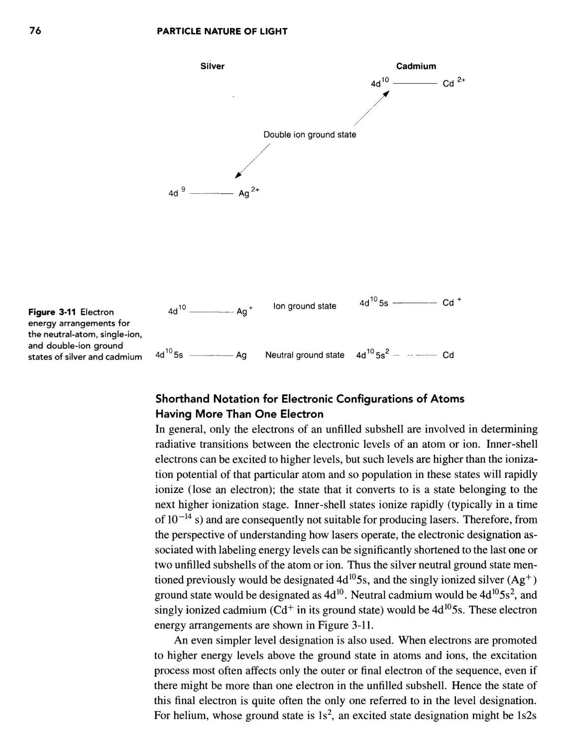
Shorthand Notation for Electronic Configurations of Atoms Having
More Than One Electron 76
3.6 Energy Levels of Multi-Electron Atoms 77
Energy-Level Designation for Multi-Electron States 77
Russell-Saunders or LS Coupling - Notation for Energy Levels 78
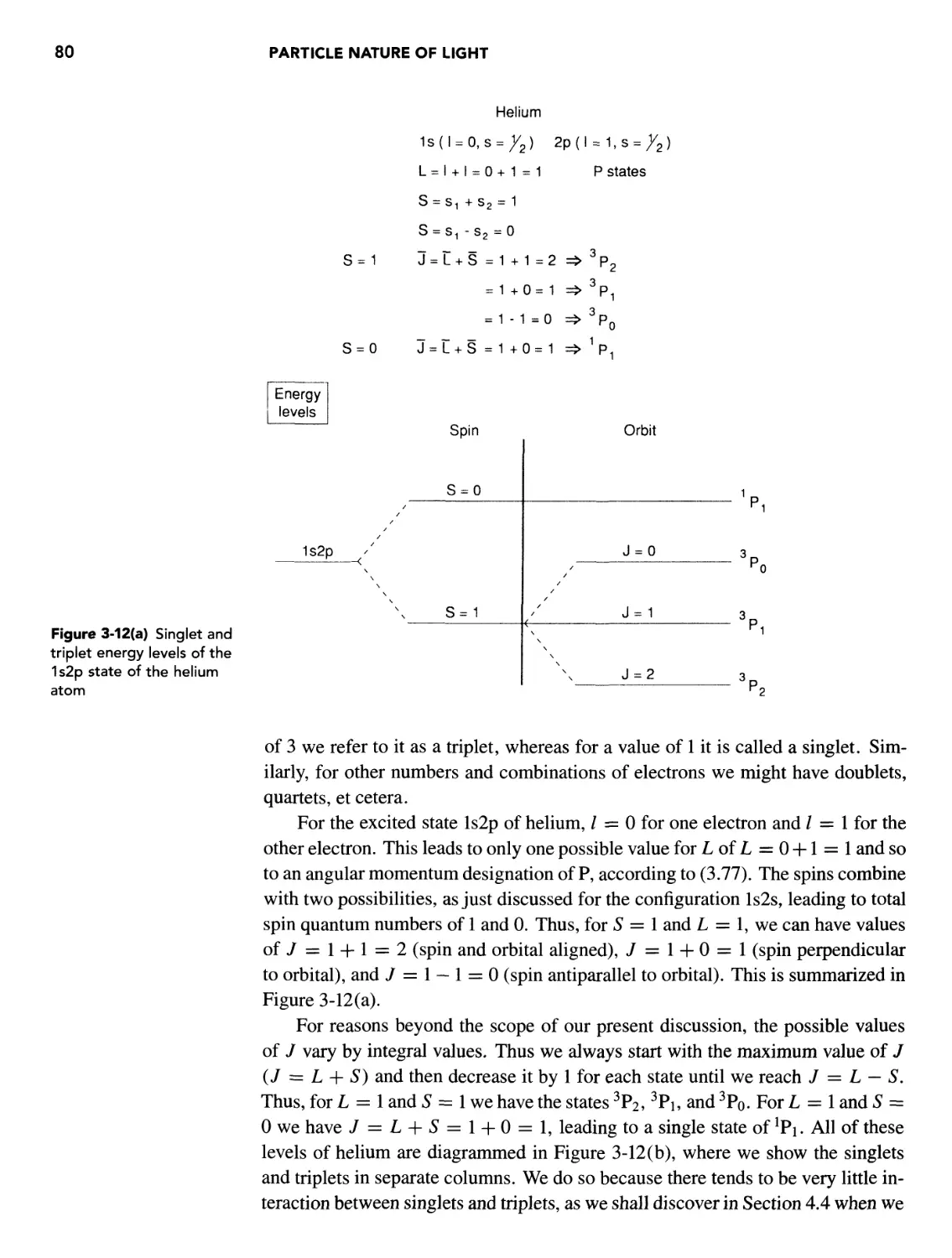
Energy Levels Associated with Two Electrons in Unfilled Shells 79
Rules for Obtaining S, L, and / for LS Coupling 82
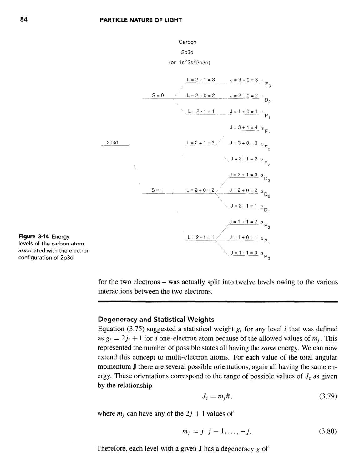
Degeneracy and Statistical Weights 84
j-j Coupling 85
Isoelectronic Scaling 85
CONTENTS ix
REFERENCES 86
PROBLEMS 86
4 RADIATIVE TRANSITIONS AND EMISSION LINEWIDTH 89
OVERVIEW 89
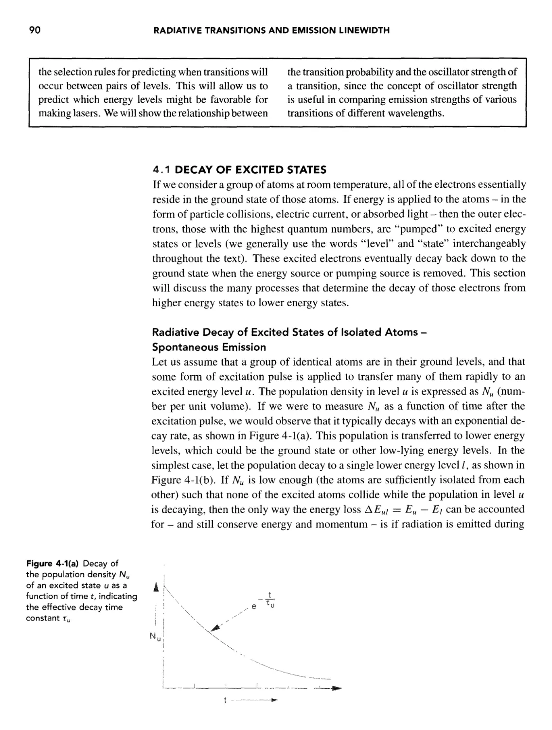
4.1 Decay of Excited States 90
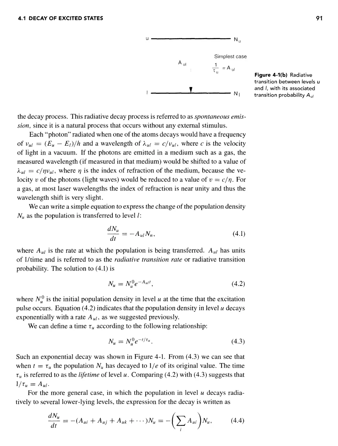
Radiative Decay of Excited States of Isolated Atoms -
Spontaneous Emission 90
Spontaneous Emission Decay Rate - Radiative Transition
Probability 94
Lifetime of a Radiating Electron - The Electron as a Classical
Radiating Harmonic Oscillator 95
Nonradiative Decay of the Excited States - Collisional Decay 98
4.2 Emission Broadening and Line width Due to Radiative Decay 101
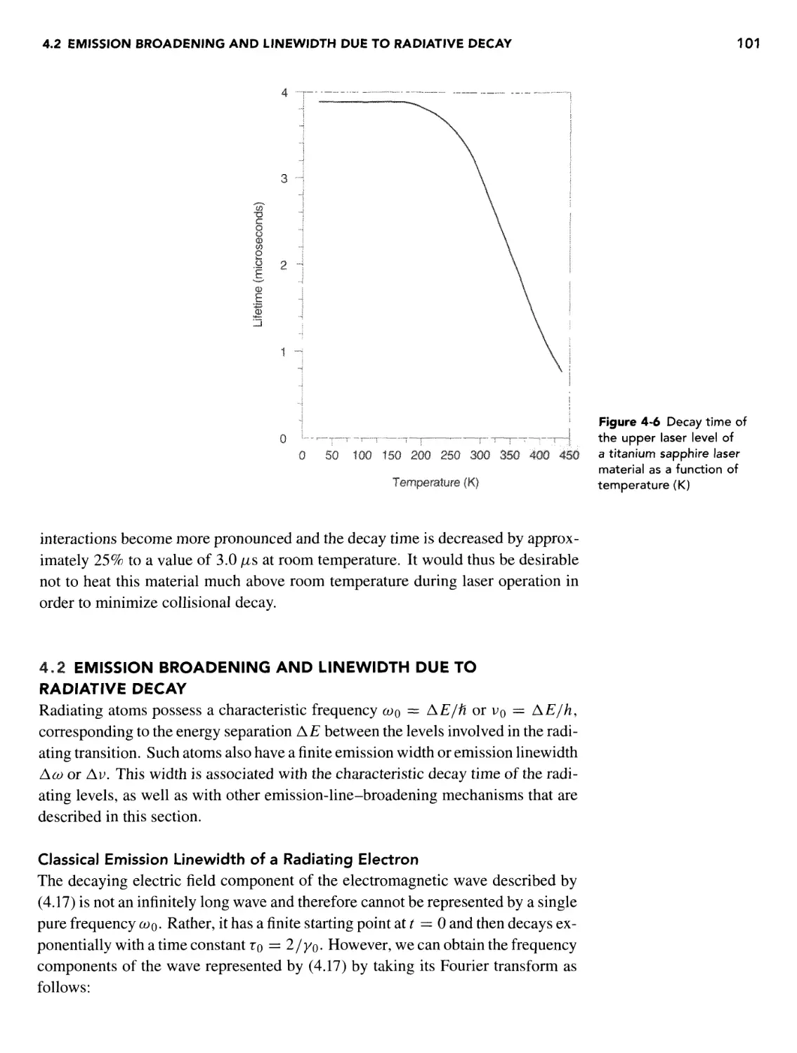
Classical Emission Linewidth of a Radiating Electron 101
Natural Emission Linewidth as Deduced by Quantum Mechanics
(Minimum Linewidth) 103
4.3 Additional Emission-Broadening Processes 105
Broadening Due to Nonradiative (Collisional) Decay 106
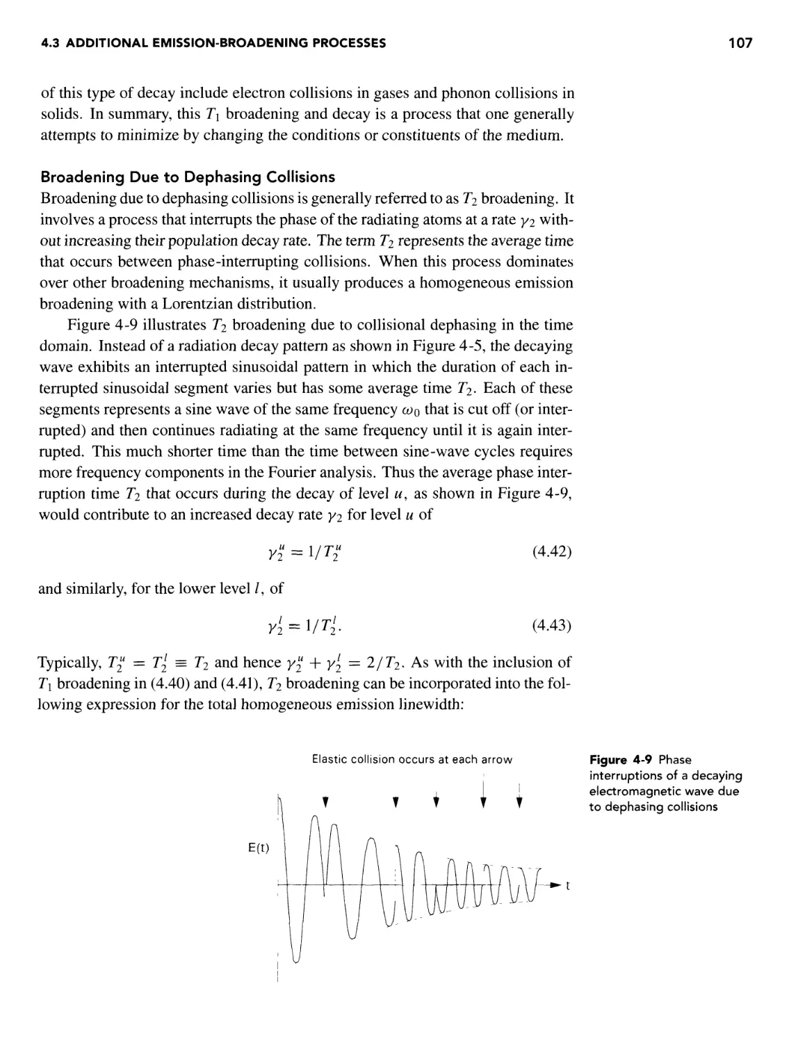
Broadening Due to Dephasing Collisions 107
Amorphous Crystal Broadening 109
Doppler Broadening in Gases 109
Voigt Lineshape Profile 114
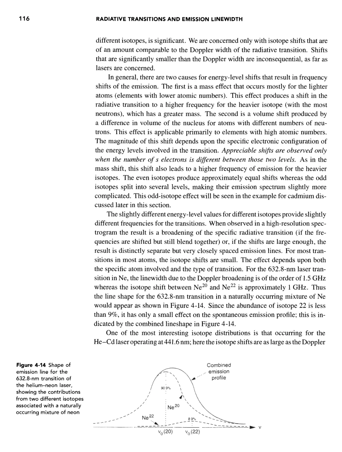
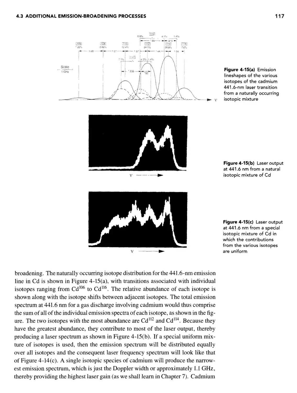
Broadening in Gases Due to Isotope Shifts 115
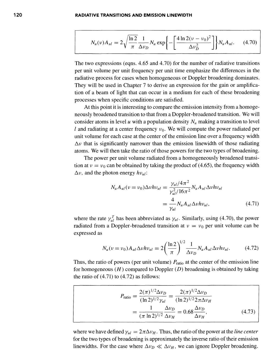
Comparison of Various Types of Emission Broadening 118
4.4 Quantum Mechanical Description of Radiating Atoms 121
Electric Dipole Radiation 122
Electric Dipole Matrix Element 123
Electric Dipole Transition Probability 124
Oscillator Strength 124
Selection Rules for Electric Dipole Transitions Involving Atoms
with a Single Electron in an Unfilled Subshell 125
Selection Rules for Radiative Transitions Involving Atoms with
More Than One Electron in an Unfilled Subshell 129
Parity Selection Rule 130
Inefficient Radiative Transitions - Electric Quadrupole and Other
Higher-Order Transitions 131
REFERENCES 131
PROBLEMS 131
5 ENERGY LEVELS AND RADIATIVE PROPERTIES OF MOLECULES,
LIQUIDS, AND SOLIDS 135
OVERVIEW 135
5.1 Molecular Energy Levels and Spectra 135
Energy Levels of Molecules 135
Classification of Simple Molecules 138
Rotational Energy Levels of Linear Molecules 139
Rotational Energy Levels of Symmetric-Top Molecules 141
Selection Rules for Rotational Transitions 141
CONTENTS
Vibrational Energy Levels 143
Selection Rule for Vibrational Transitions 143
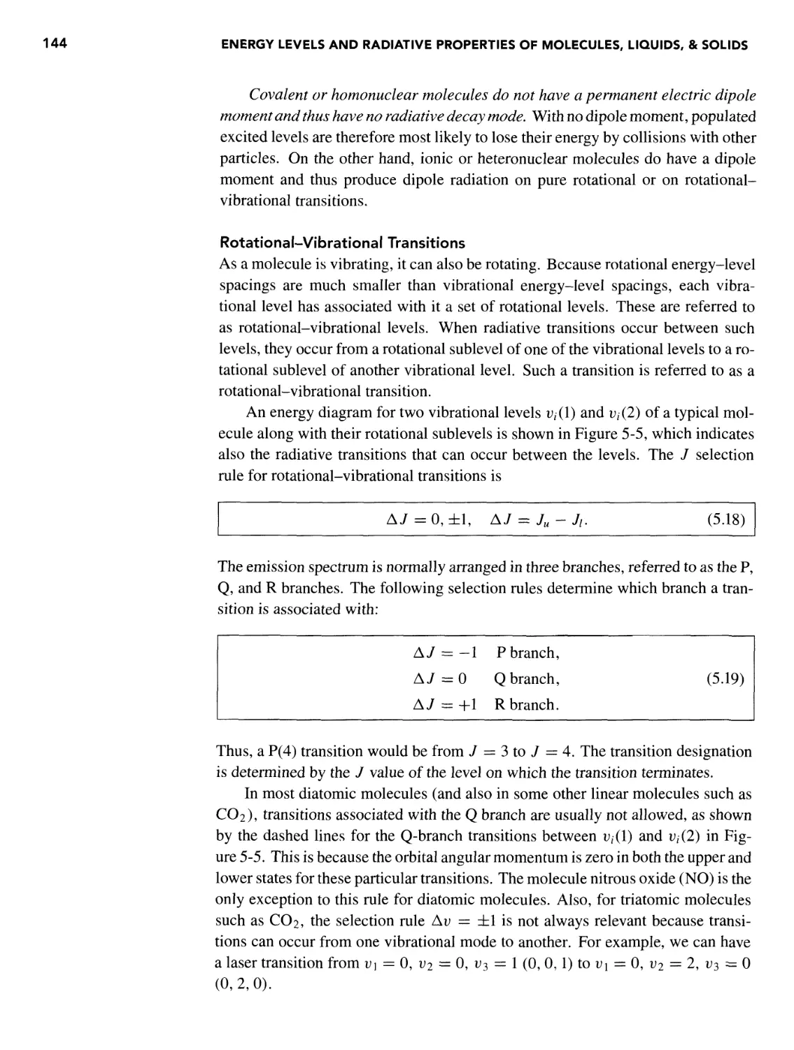
Rotational-Vibrational Transitions 144
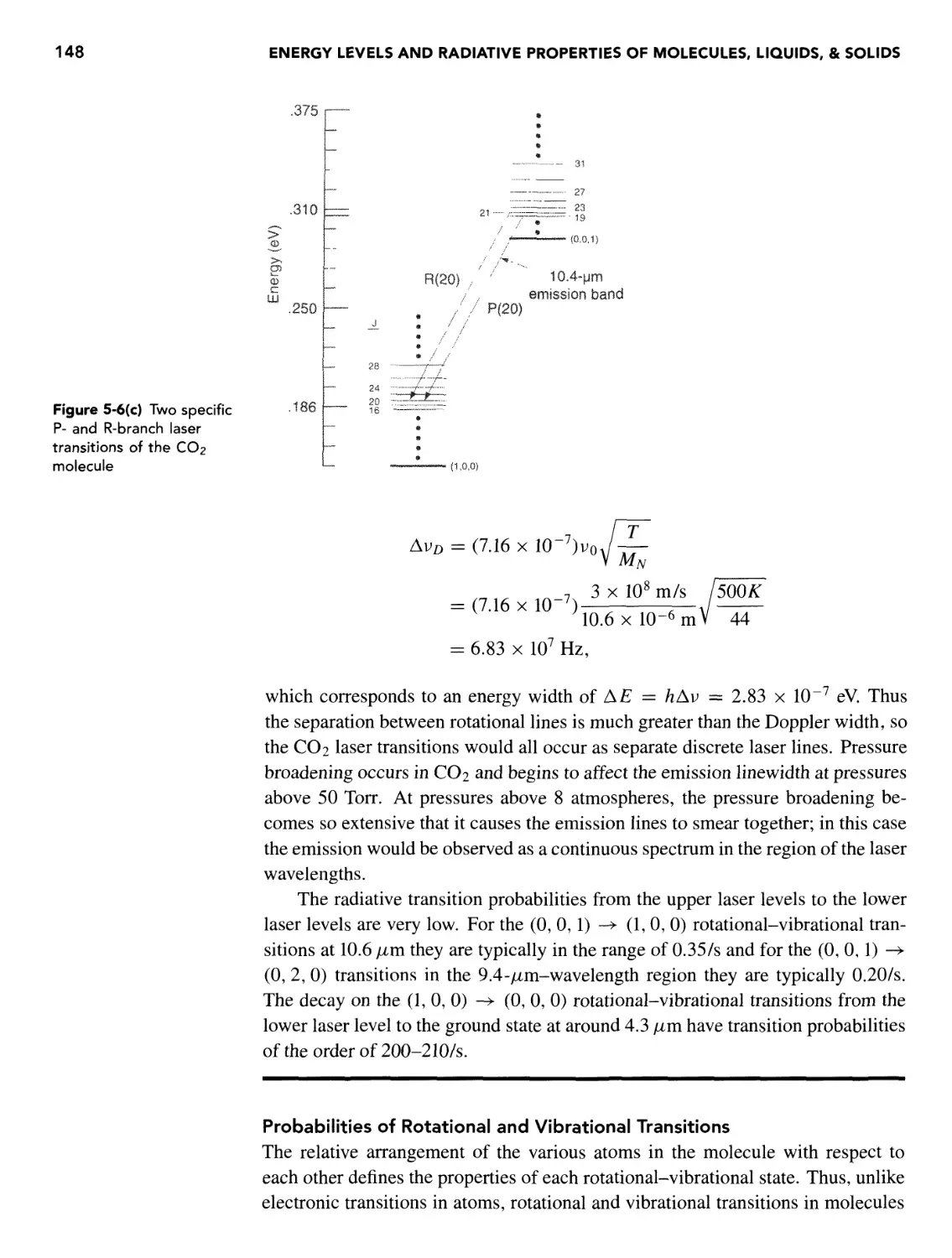
Probabilities of Rotational and Vibrational Transitions 148
Electronic Energy Levels of Molecules 149
Electronic Transitions and Associated Selection Rules of
Molecules 150
Emission Linewidth of Molecular Transitions 150
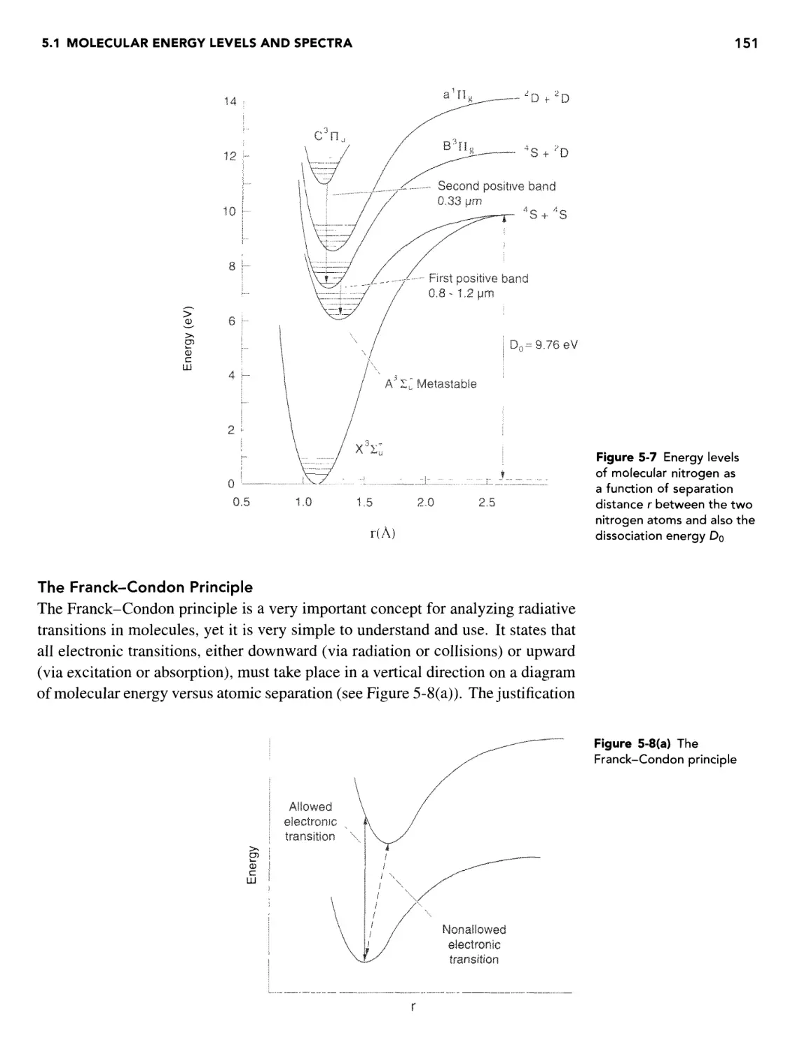
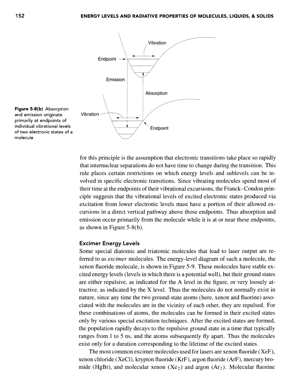
The Franck-Condon Principle 151
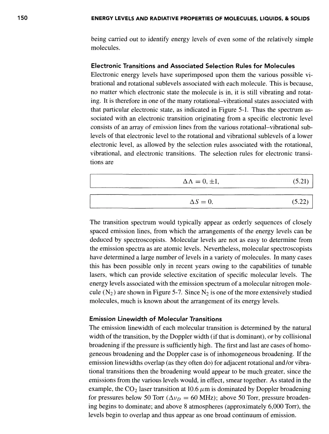
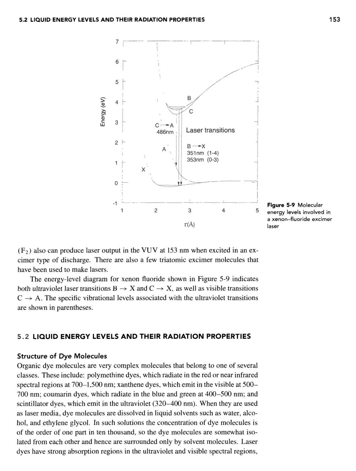
Excimer Energy Levels 152
5.2 Liquid Energy Levels and Their Radiation Properties 153
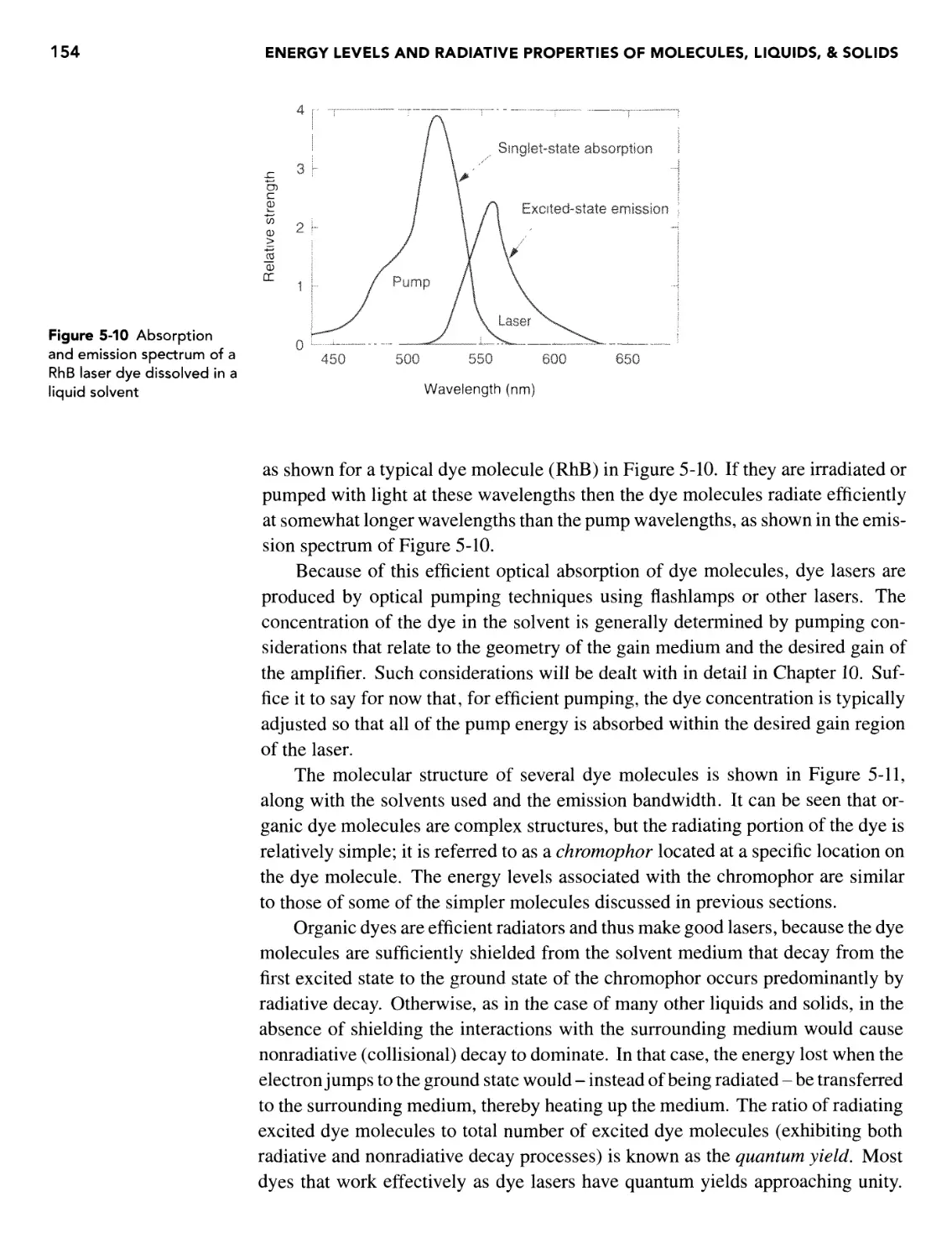
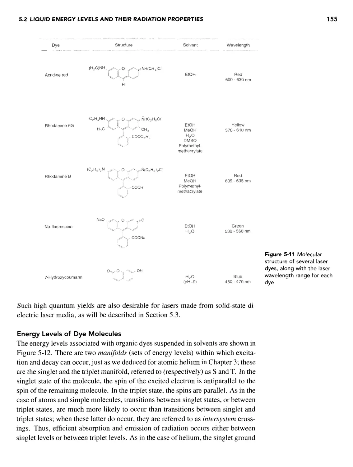
Structure of Dye Molecules 153
Energy Levels of Dye Molecules 155
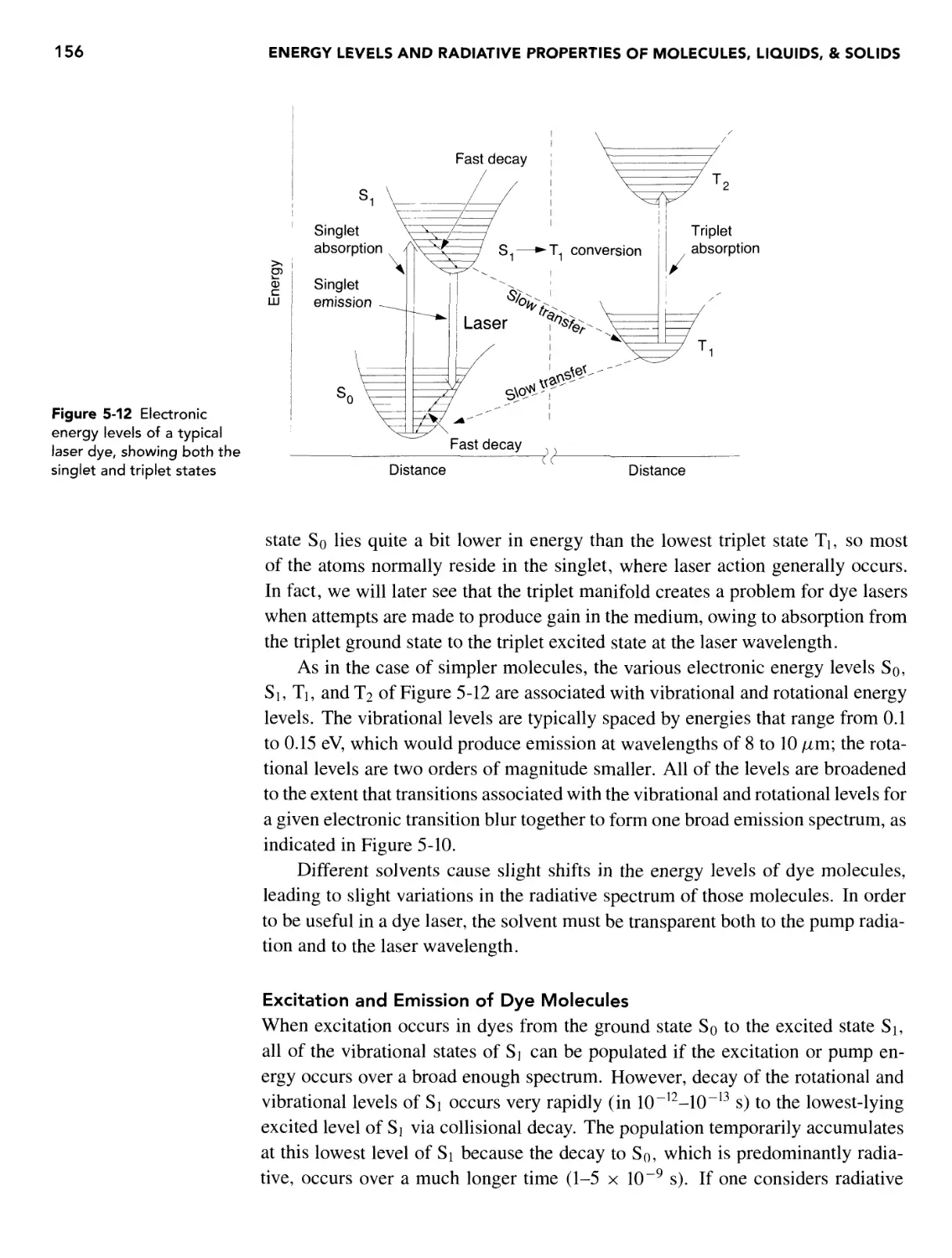
Excitation and Emission of Dye Molecules 156
Detrimental Triplet States of Dye Molecules 157
5.3 Energy Levels in Solids - Dielectric Laser Materials 158
Host Materials 158
Laser Species - Dopant Ions 159
Narrow-Linewidth Laser Materials 161
Broadband Tunable Laser Materials 166
Broadening Mechanism for Solid-State Lasers 168
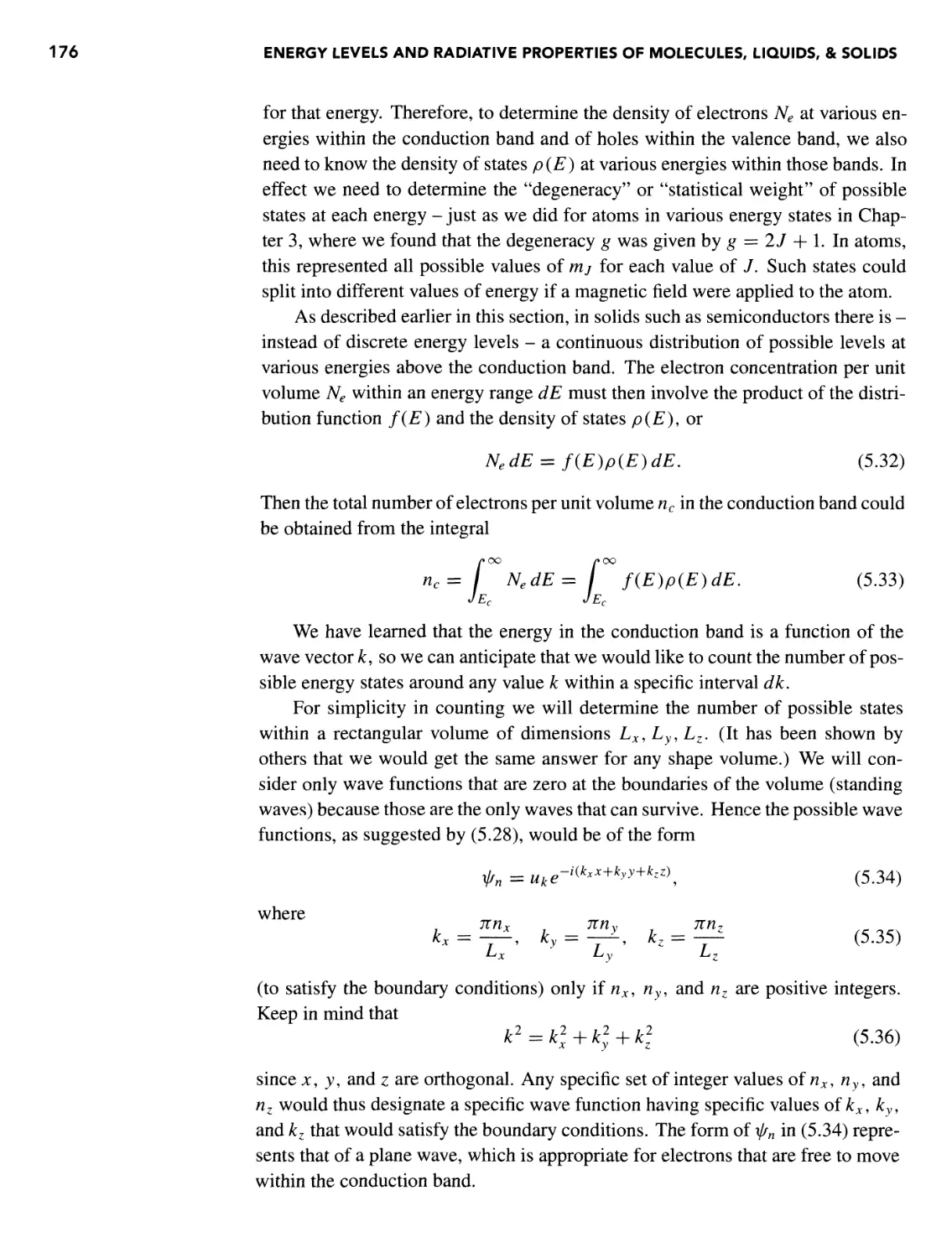
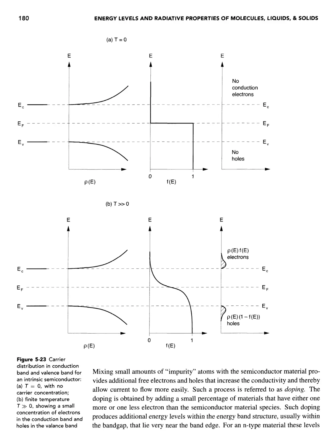
5.4 Energy Levels in Solids - Semiconductor Laser Materials 168
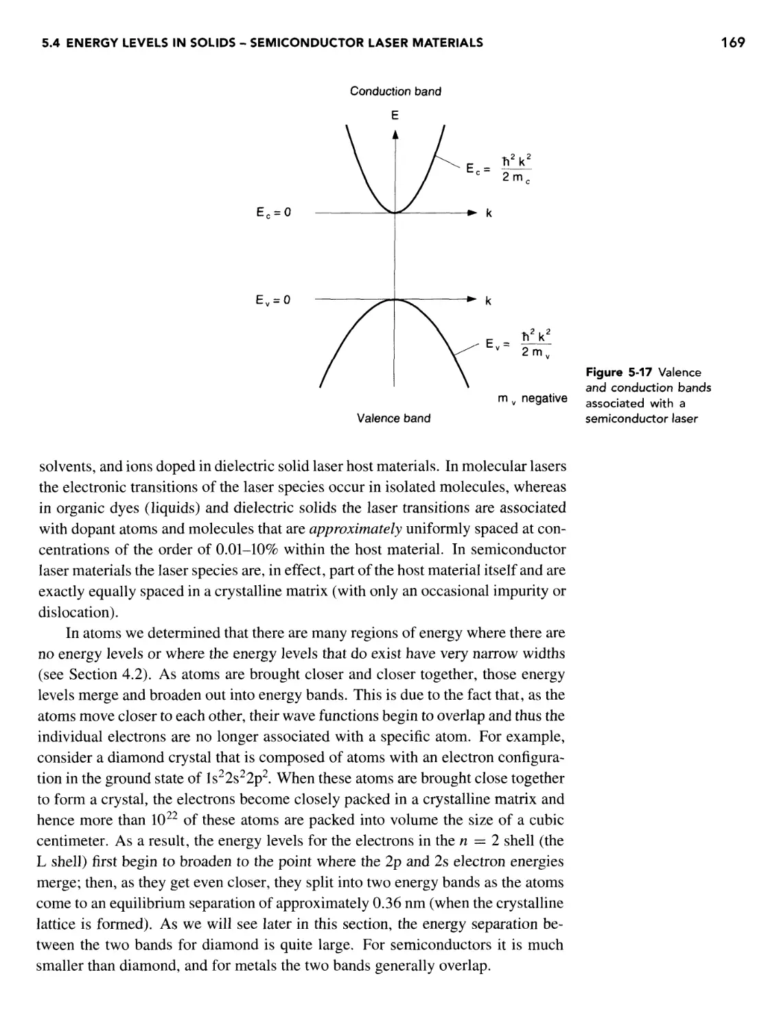
Energy Bands in Crystalline Solids 168
Energy Levels in Periodic Structures 170
Energy Levels of Conductors, Insulators, and Semiconductors 172
Excitation and Decay of Excited Energy Levels - Recombination
Radiation 173
Direct and Indirect Bandgap Semiconductors 174
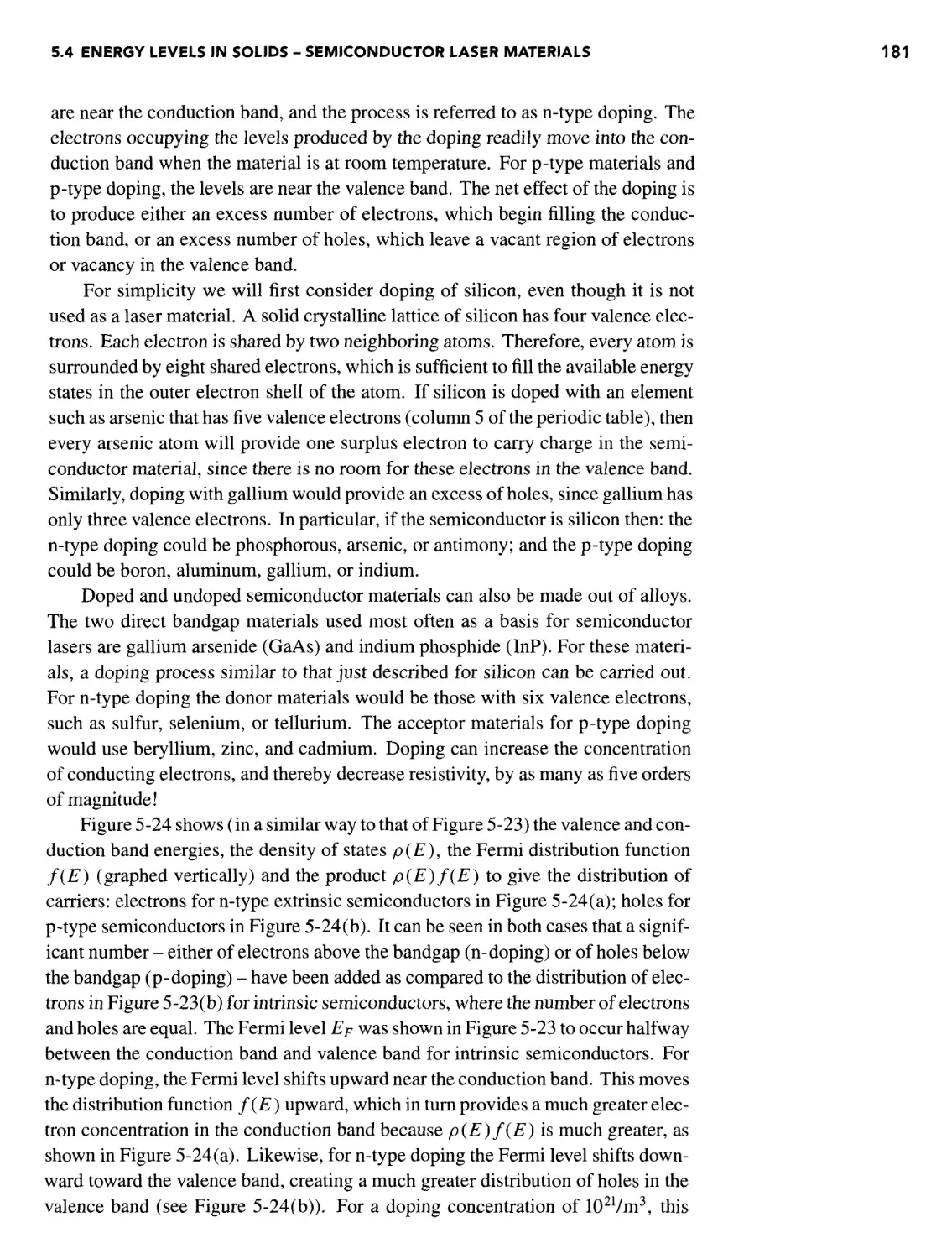
Electron Distribution Function and Density of States in
Semiconductors 175
Intrinsic Semiconductor Materials 179
Extrinsic Semiconductor Materials - Doping 179
p-n Junctions - Recombination Radiation Due to Electrical
Excitation 182
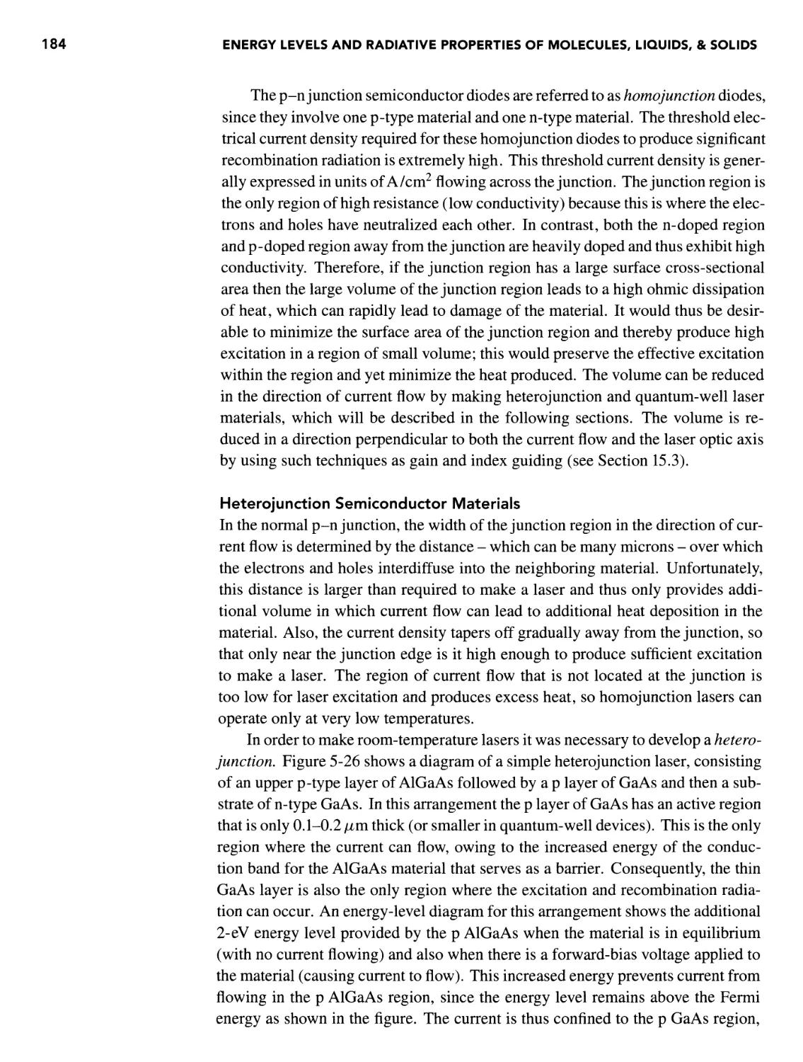
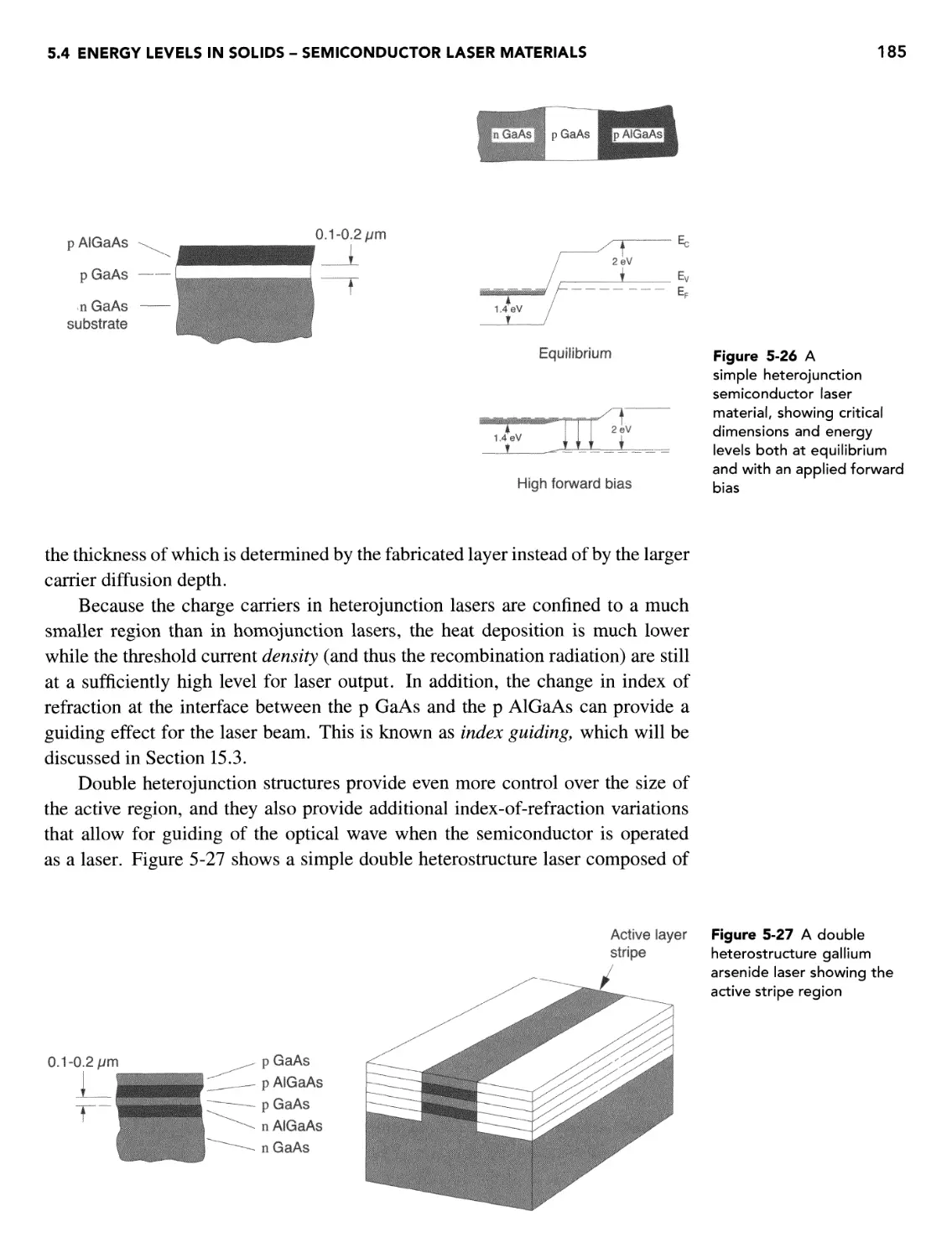
Heterojunction Semiconductor Materials 184
Quantum Wells 186
Variation of Bandgap Energy and Radiation Wavelength with
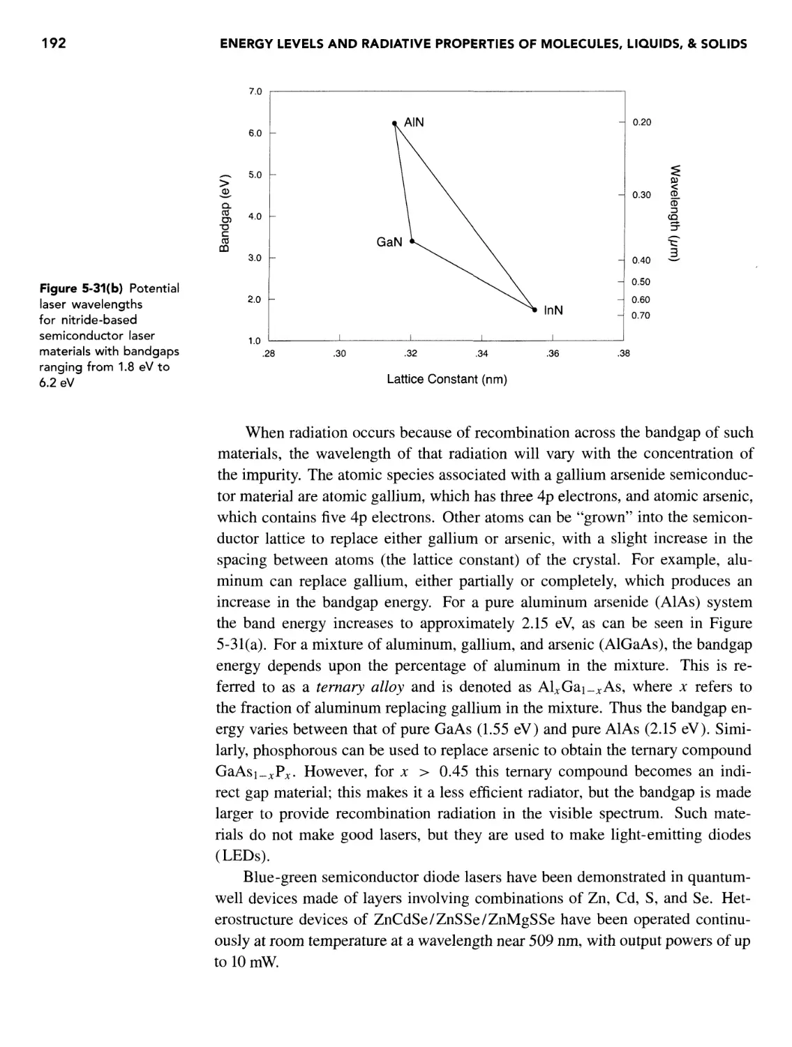
Alloy Composition 191
Recombination Radiation Transition Probability and Linewidth 195
REFERENCES 195
PROBLEMS 195
6 RADIATION AND THERMAL EQUILIBRIUM - ABSORPTION AND
STIMULATED EMISSION 199
OVERVIEW 199
6.1 Equilibrium 199
Thermal Equilibrium 199
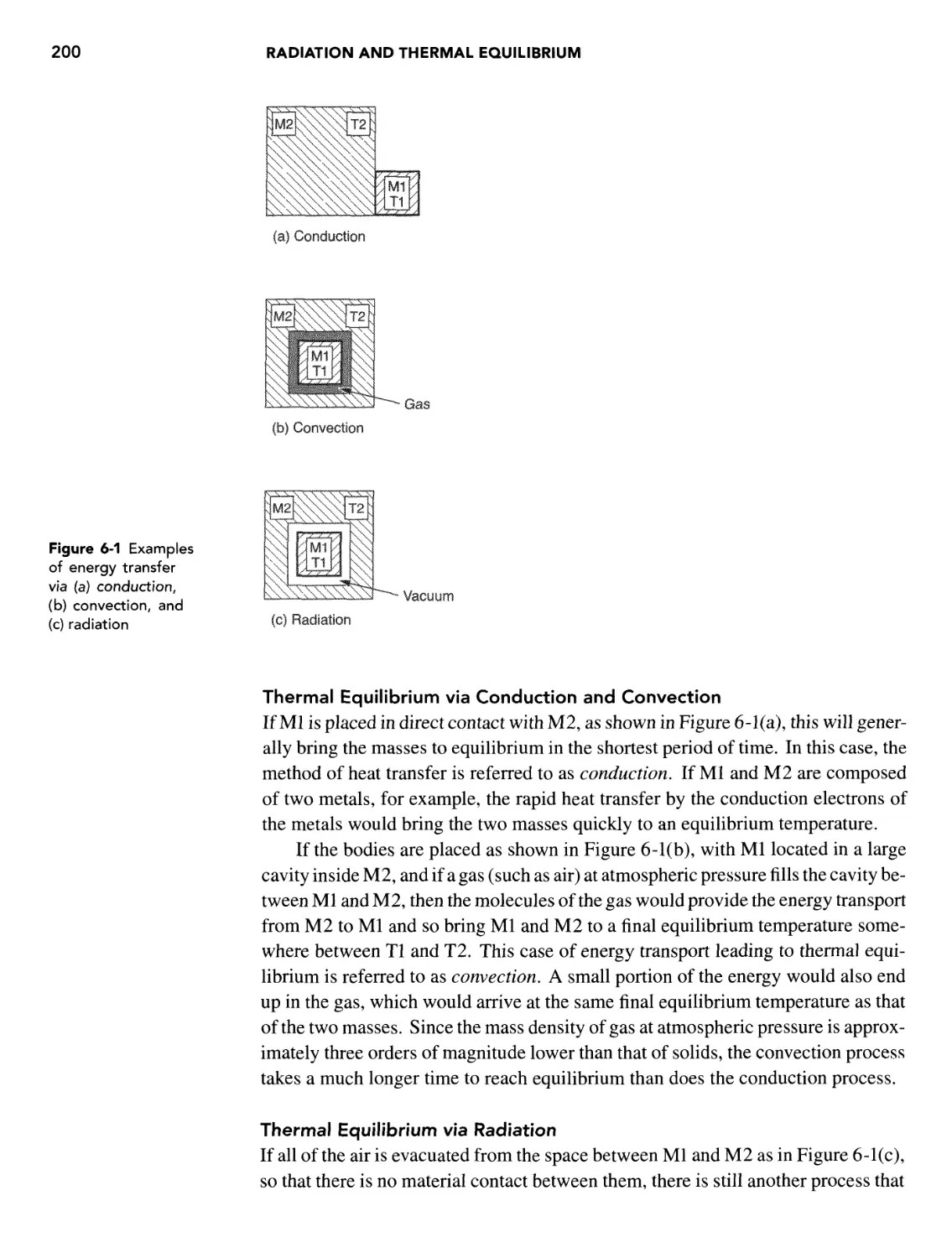
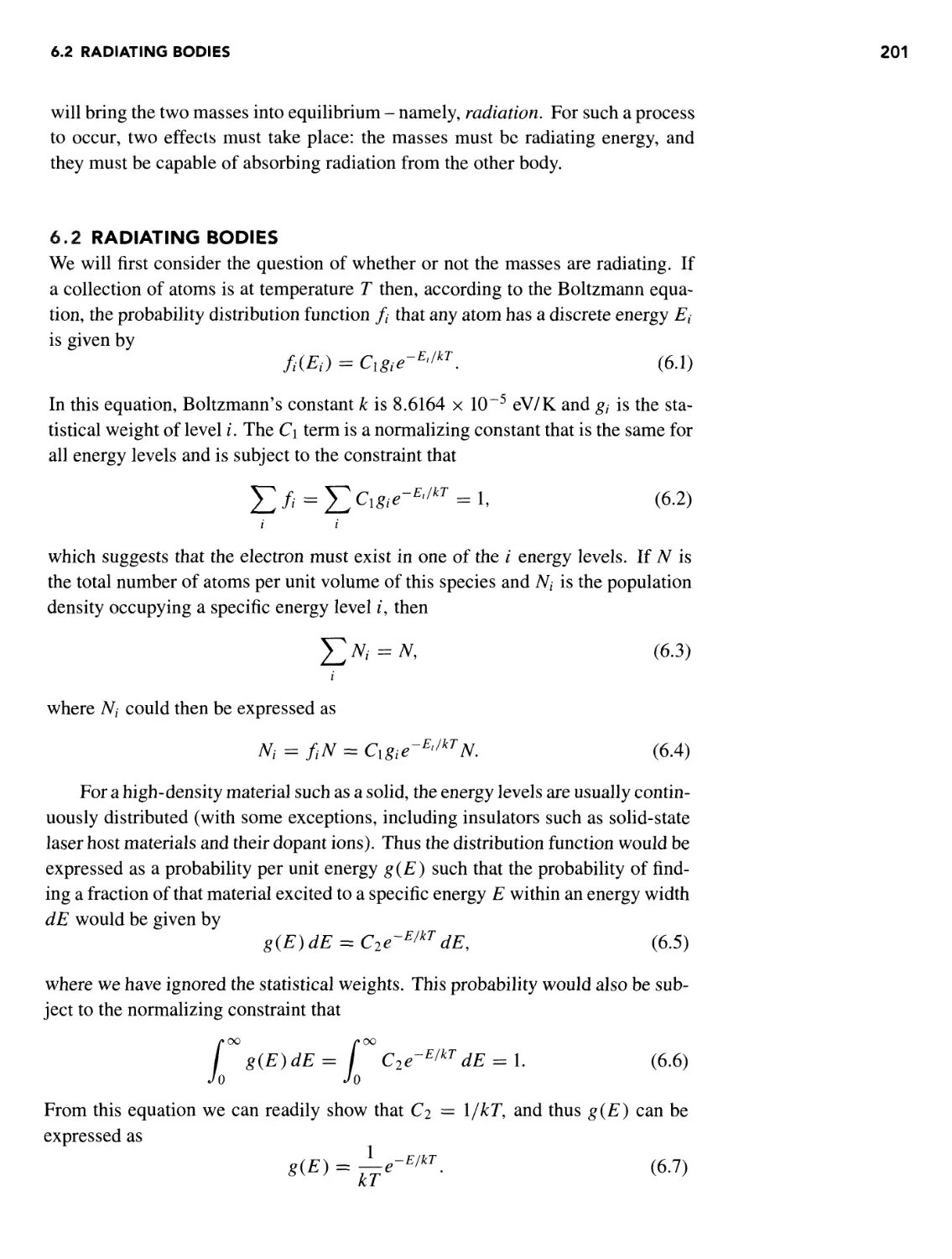
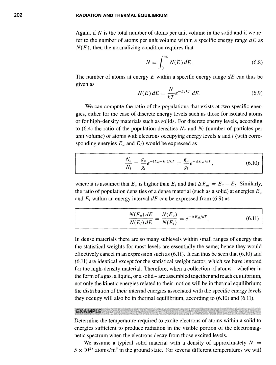
Thermal Equilibrium via Conduction and Convection 200
Thermal Equilibrium via Radiation 200
CONTENTS xi
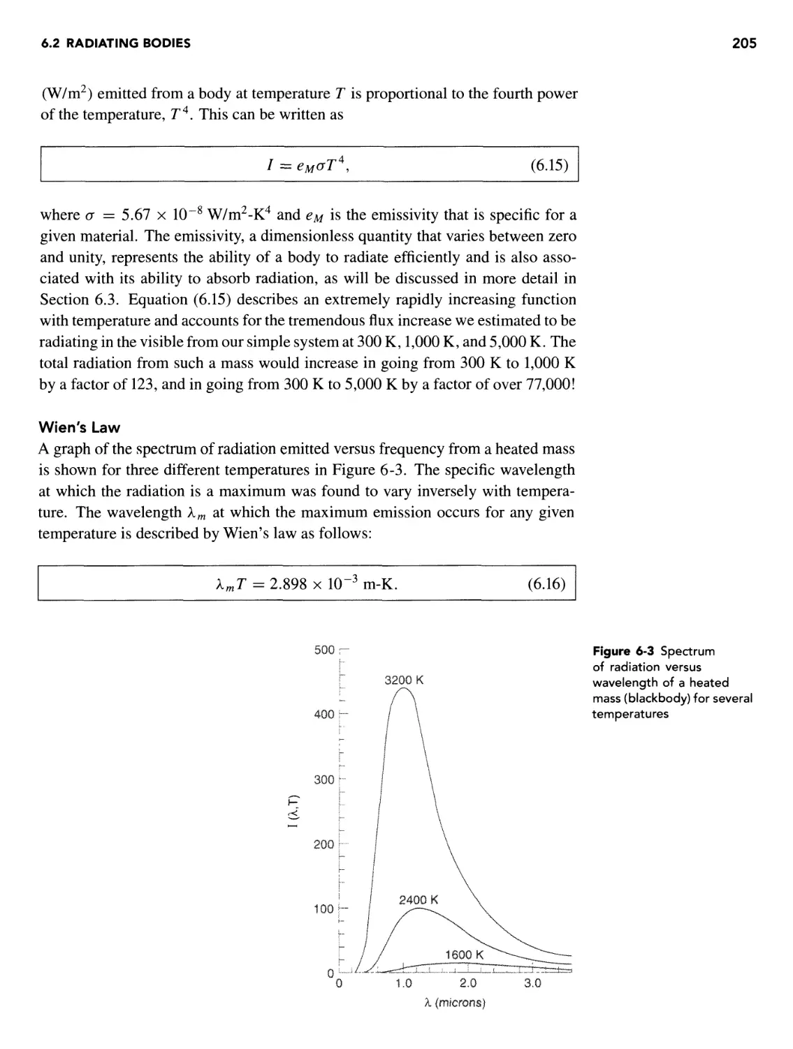
6.2 Radiating Bodies 201
Stefan-Boltzmann Law 204
Wien's Law 205
Irradiance and Radiance 206
6.3 Cavity Radiation 207
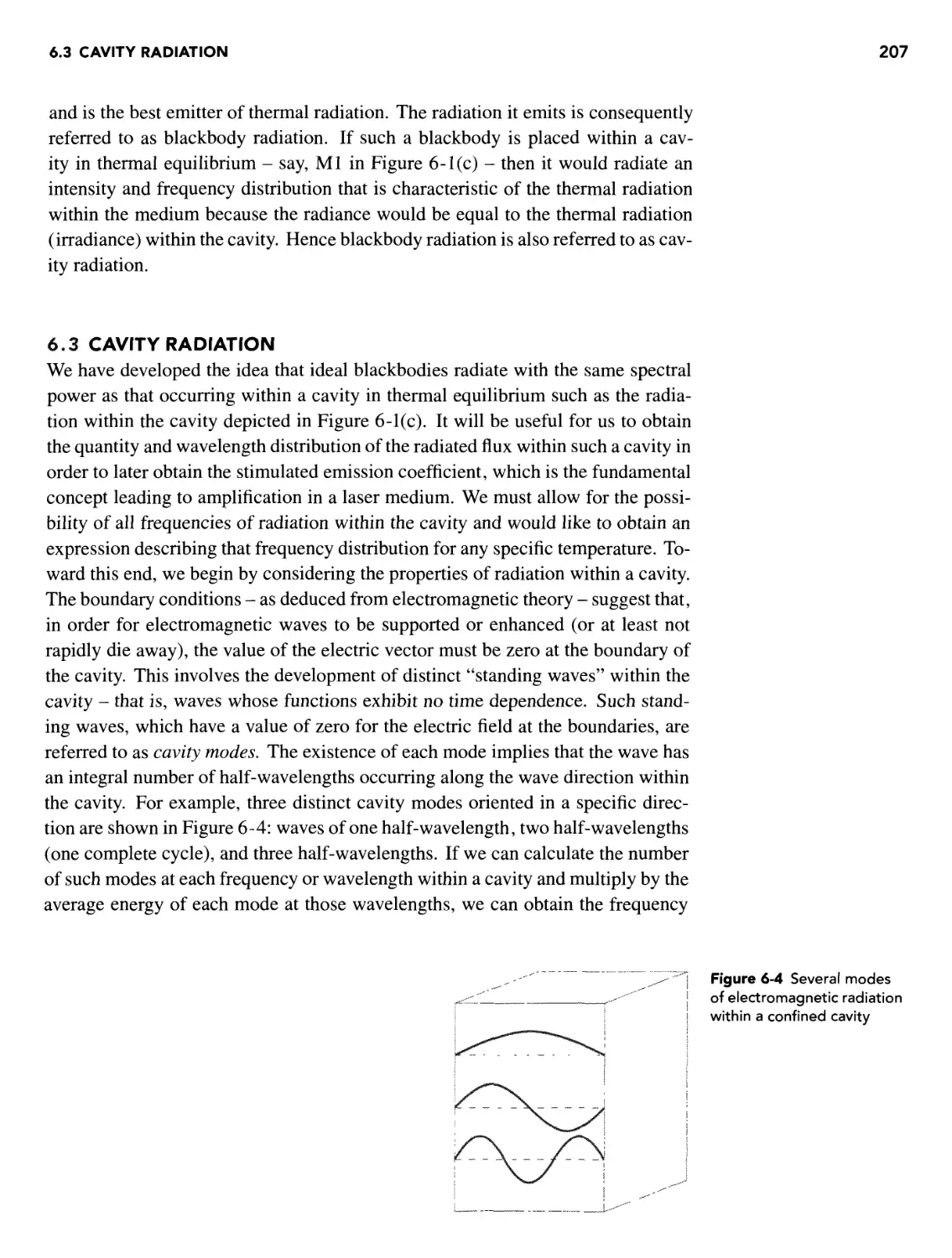
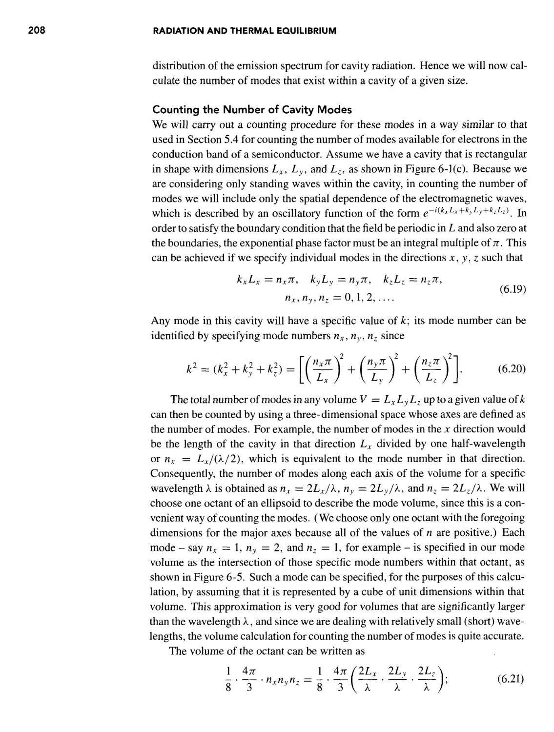
Counting the Number of Cavity Modes 208
Rayleigh-Jeans Formula 209
Planck's Law for Cavity Radiation 210
Relationship between Cavity Radiation and Blackbody
Radiation 211
Wavelength Dependence of Blackbody Emission 214
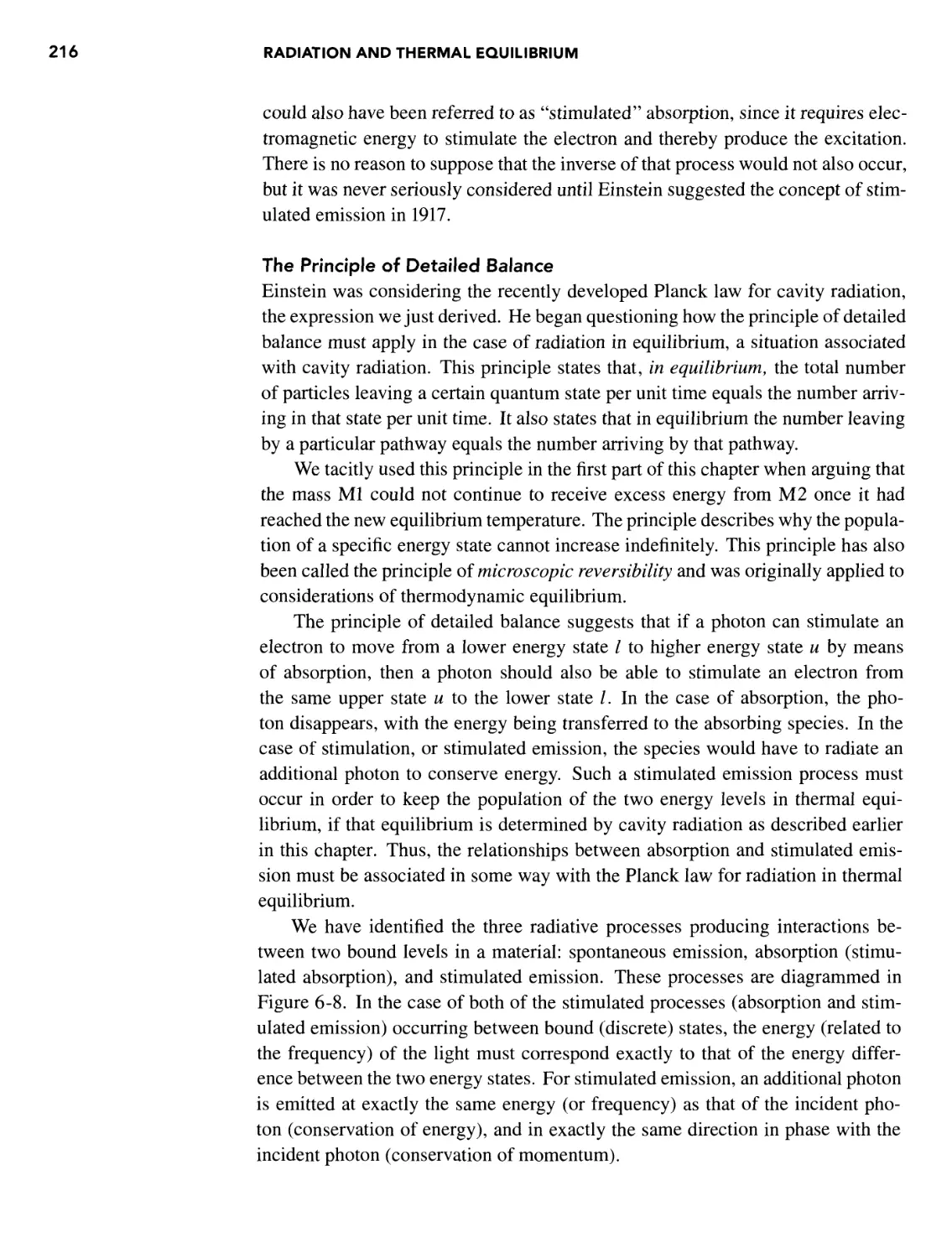
6.4 Absorption and Stimulated Emission 215
The Principle of Detailed Balance 216
Absorption and Stimulated Emission Coefficients 217
REFERENCES 221
PROBLEMS 221
7 CONDITIONS FOR PRODUCING A LASER - POPULATION
INVERSIONS, GAIN, AND GAIN SATURATION 225
OVERVIEW 225
7.1 Absorption and Gain 225
Absorption and Gain on a Homogeneously Broadened Radiative
Transition (Lorentzian Frequency Distribution) 225
Gain Coefficient and Stimulated Emission Cross Section for
Homogeneous Broadening 229
Absorption and Gain on an Inhomogeneously Broadened Radiative
Transition (Doppler Broadening with a Gaussian Distribution) 230
Gain Coefficient and Stimulated Emission Cross Section for
Doppler Broadening 231
Statistical Weights and the Gain Equation 232
Relationship of Gain Coefficient and Stimulated Emission
Cross Section to Absorption Coefficient and Absorption
Cross Section 233
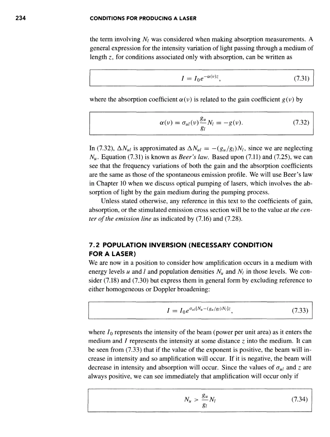
7.2 Population Inversion (Necessary Condition for a Laser) 234
7.3 Saturation Intensity (Sufficient Condition for a Laser) 235
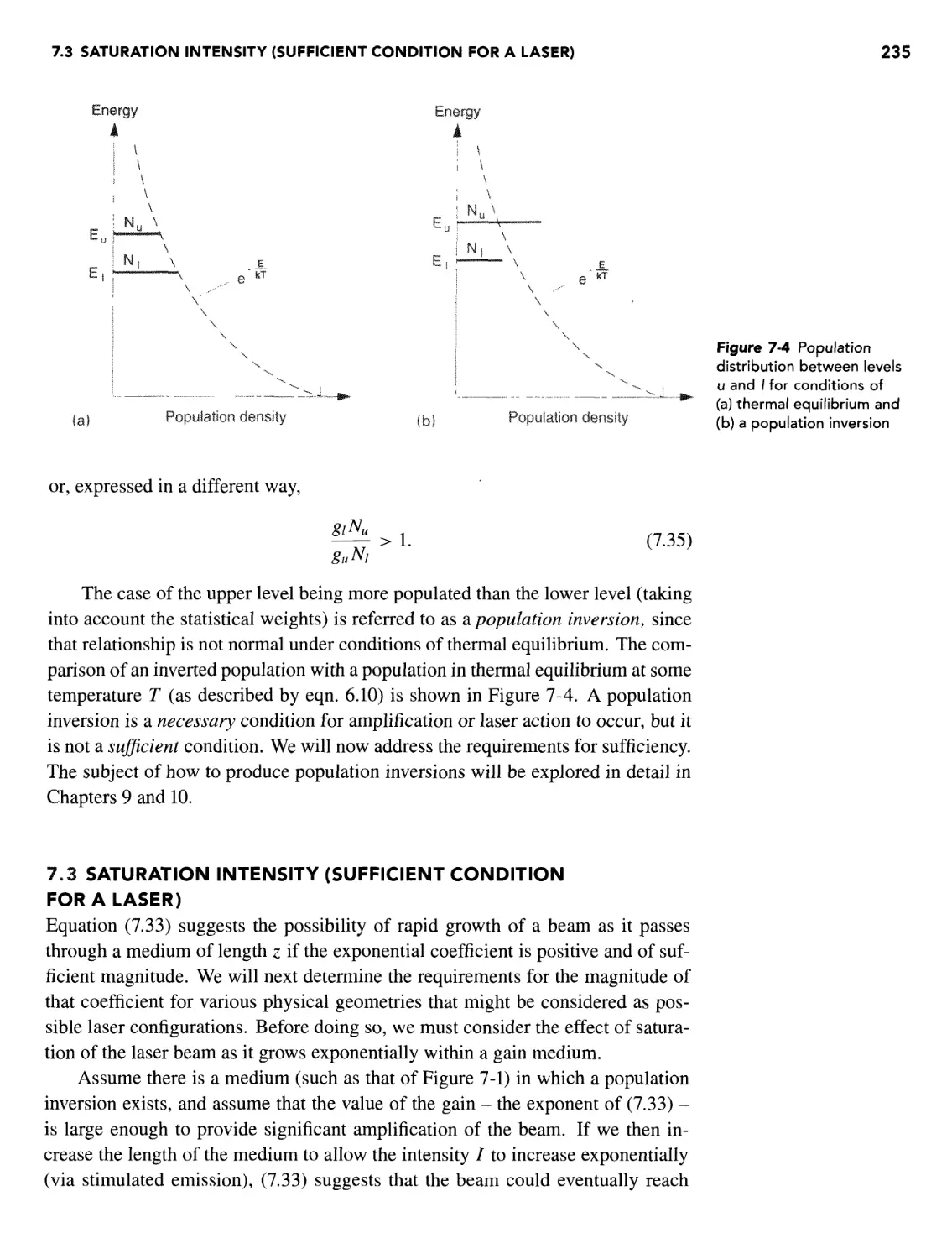
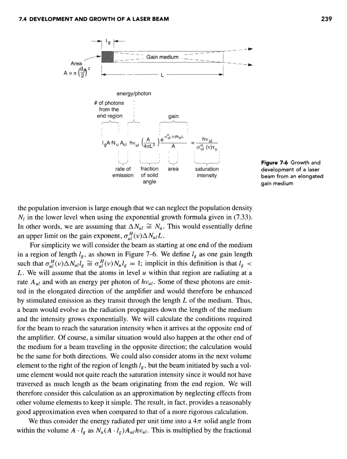
7.4 Development and Growth of a Laser Beam 238
Growth of Beam for a Gain Medium with Homogeneous
Broadening 238
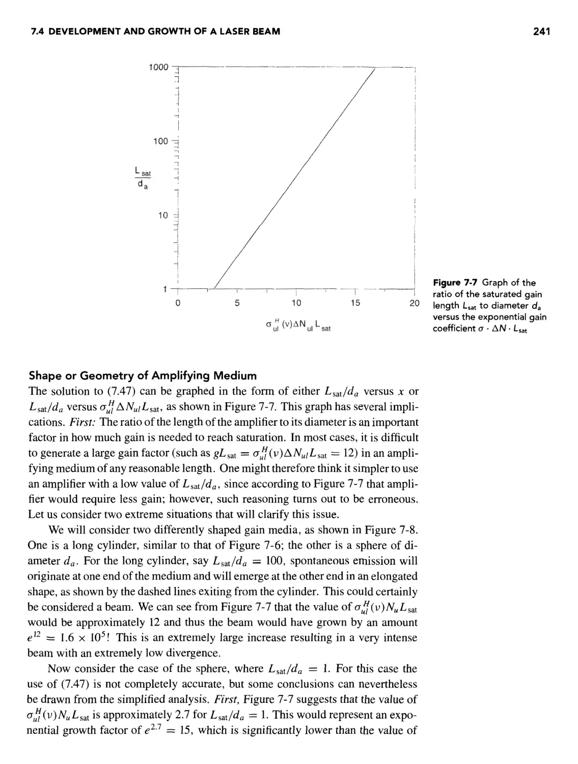
Shape or Geometry of Amplifying Medium 241
Growth of Beam for Doppler Broadening 244
7.5 Exponential Growth Factor (Gain) 245
7.6 Threshold Requirements for a Laser 247
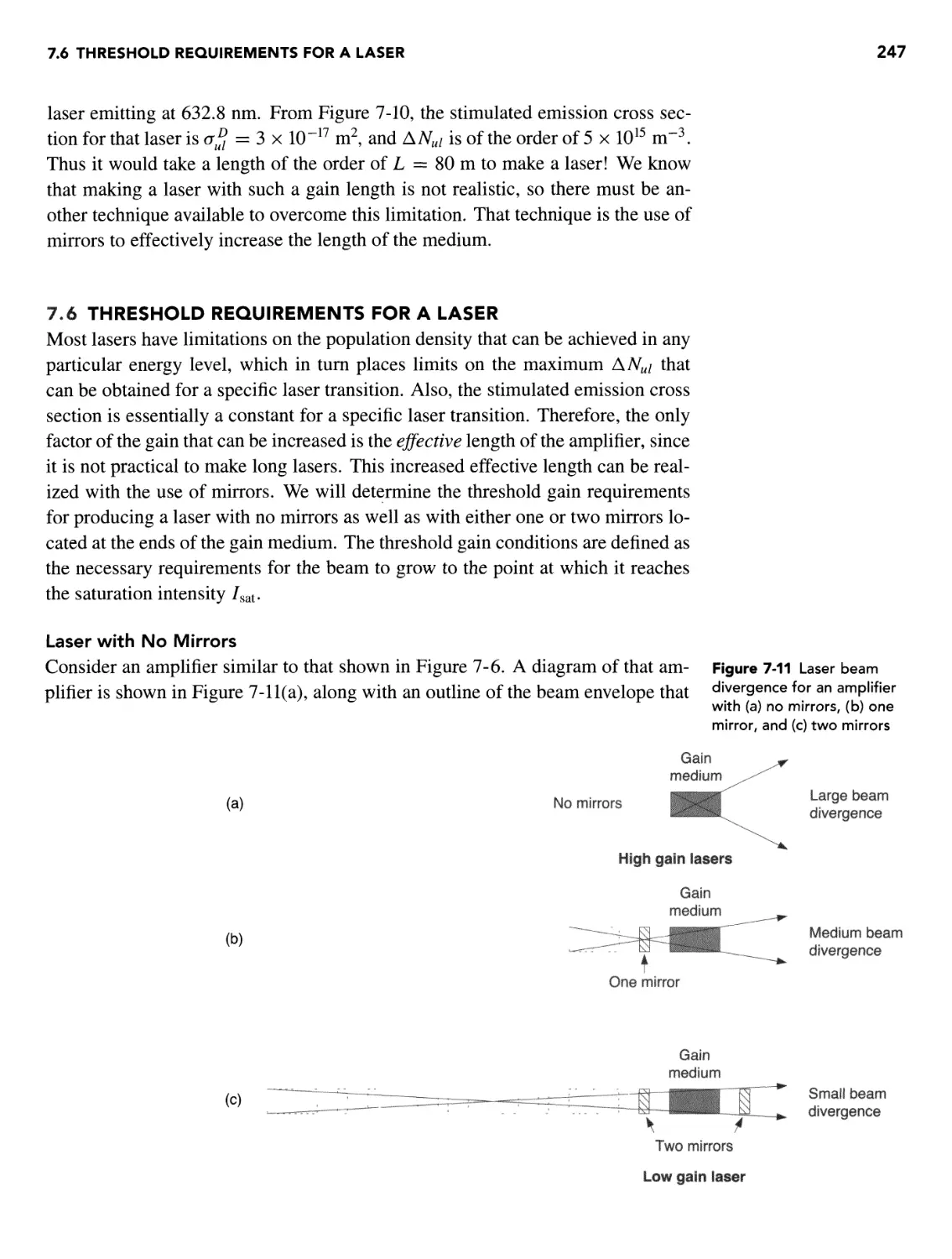
Laser with No Mirrors 247
Laser with One Mirror 248
Laser with Two Mirrors 249
REFERENCES 253
PROBLEMS 253
xii CONTENTS
8 LASER OSCILLATION ABOVE THRESHOLD 255
OVERVIEW 255
8.1 Laser Gain Saturation 255
Rate Equations of the Laser Levels That Include Stimulated
Emission 255
Population Densities of Upper and Lower Laser Levels with
Beam Present 256
Small-Signal Gain Coefficient 257
Saturation of the Laser Gain above Threshold 257
8.2 Laser Beam Growth beyond the Saturation Intensity 258
Change from Exponential Growth to Linear Growth 258
Steady-State Laser Intensity 261
8.3 Optimization of Laser Output Power 261
Optimum Output Mirror Transmission 261
Optimum Laser Output Intensity 264
Estimating Optimum Laser Output Power 264
8.4 Energy Exchange between Upper Laser Level Population and
Laser Photons 266
Decay Time of a Laser Beam within an Optical Cavity 267
Basic Laser Cavity Rate Equations 268
Steady-State Solutions below Laser Threshold 270
Steady-State Operation above Laser Threshold 272
8.5 Laser Output Fluctuations 273
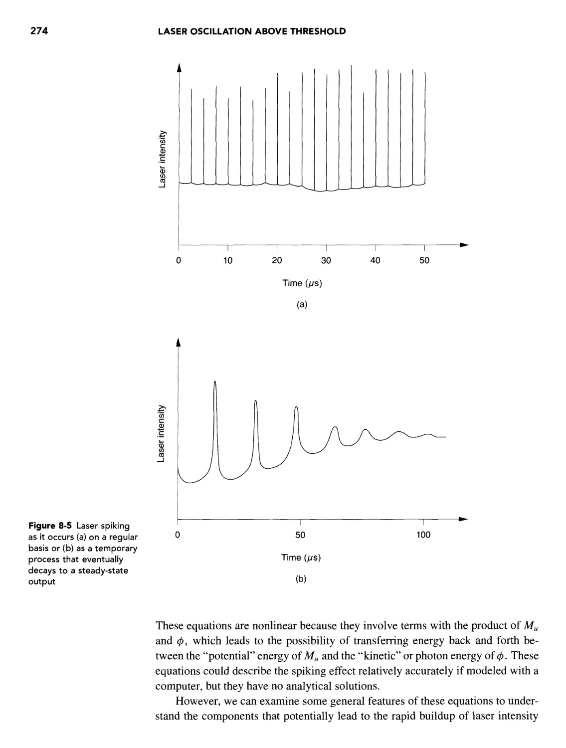
Laser Spiking 273
Relaxation Oscillations 276
8.6 Laser Amplifiers 279
Basic Amplifier Uses 279
Propagation of a High-Power, Short-Duration Optical Pulse through
an Amplifier 280
Saturation Energy Fluence 282
Amplifying Long Laser Pulses 284
Amplifying Short Laser Pulses 284
Comparison of Efficient Laser Amplifiers Based upon Fundamental
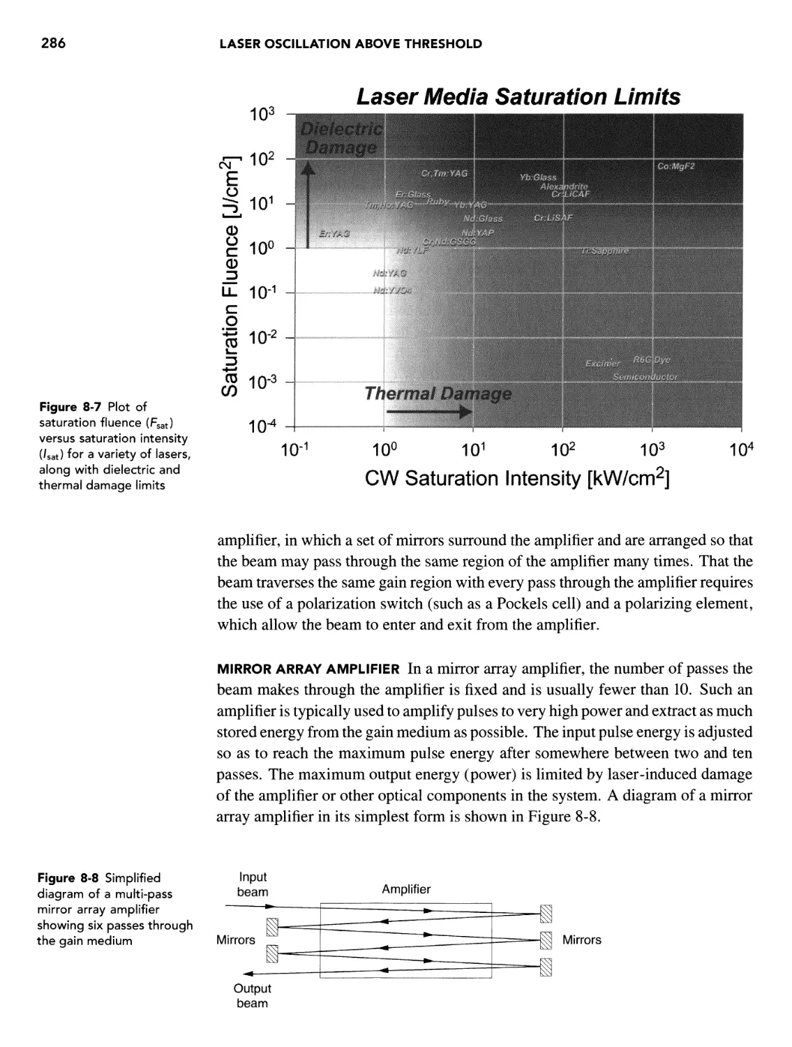
Saturation Limits 285
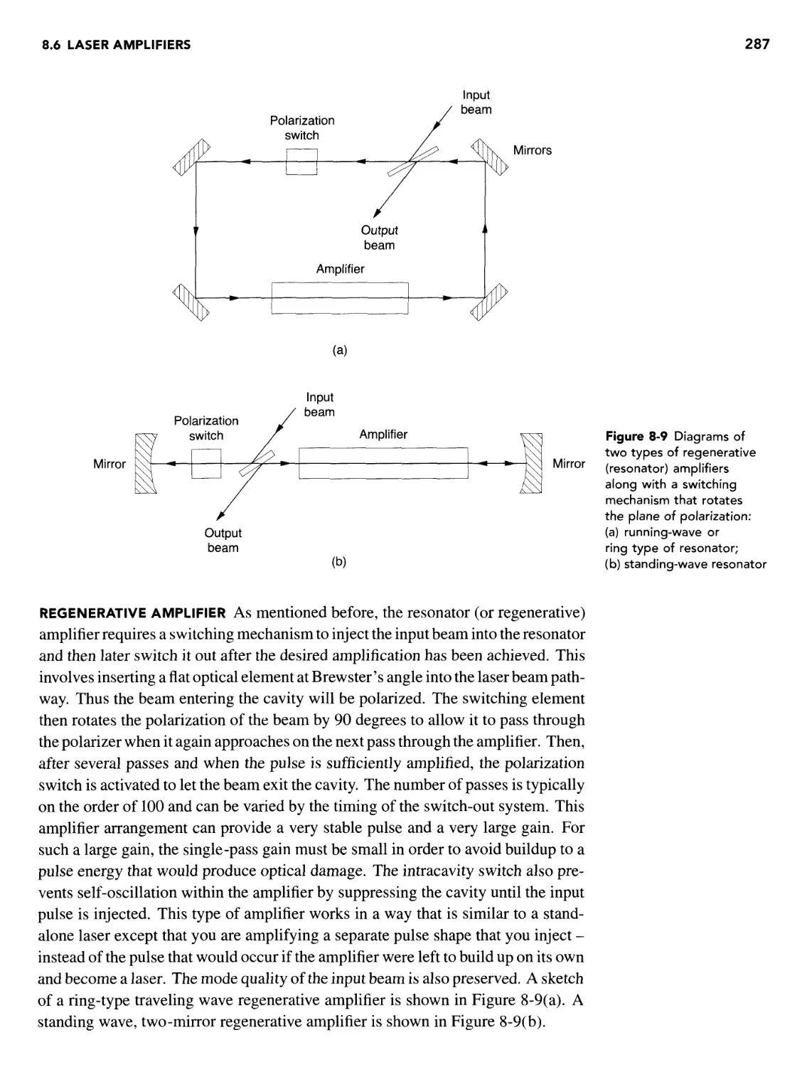
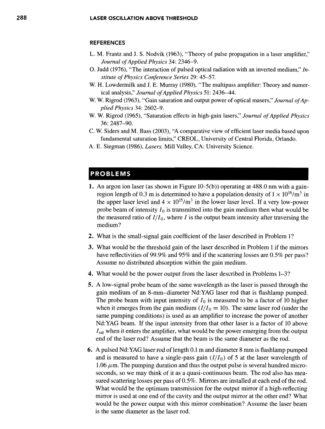
Mirror Array and Resonator (Regenerative) Amplifiers 285
REFERENCES 288
PROBLEMS 288
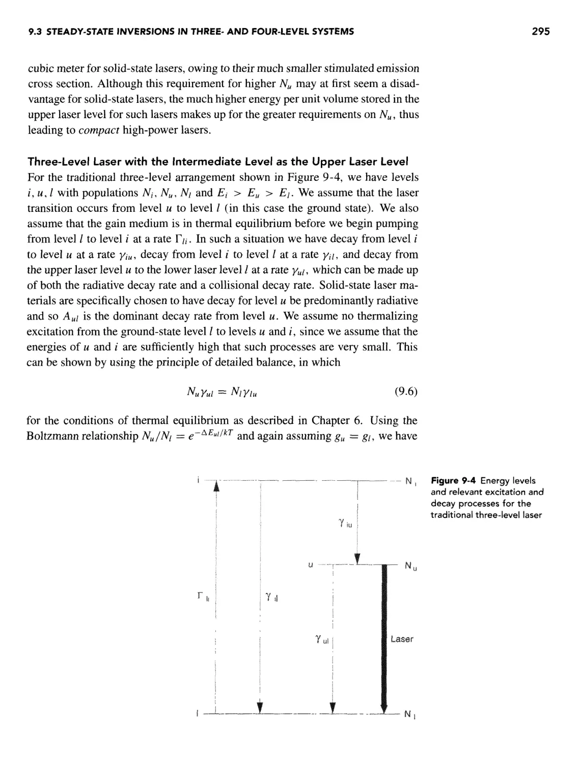
9 REQUIREMENTS FOR OBTAINING POPULATION INVERSIONS 290
OVERVIEW 290
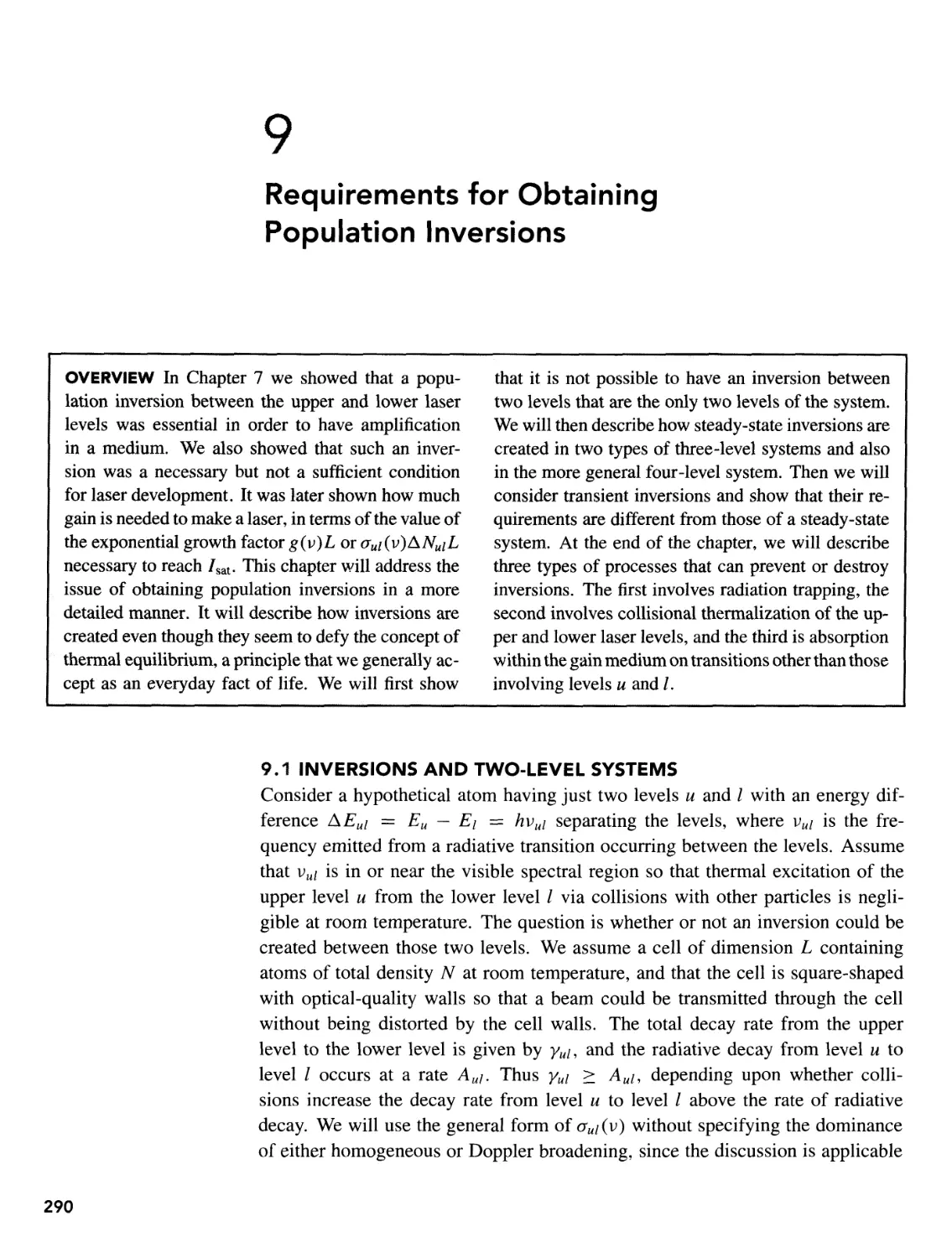
9.1 Inversions and Two-Level Systems 290
9.2 Relative Decay Rates - Radiative versus Collisional 292
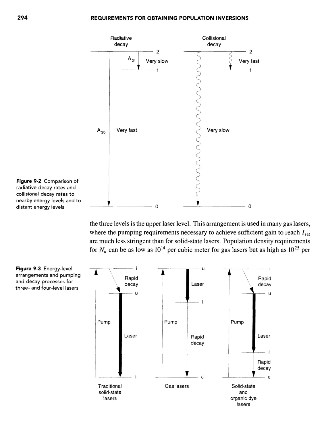
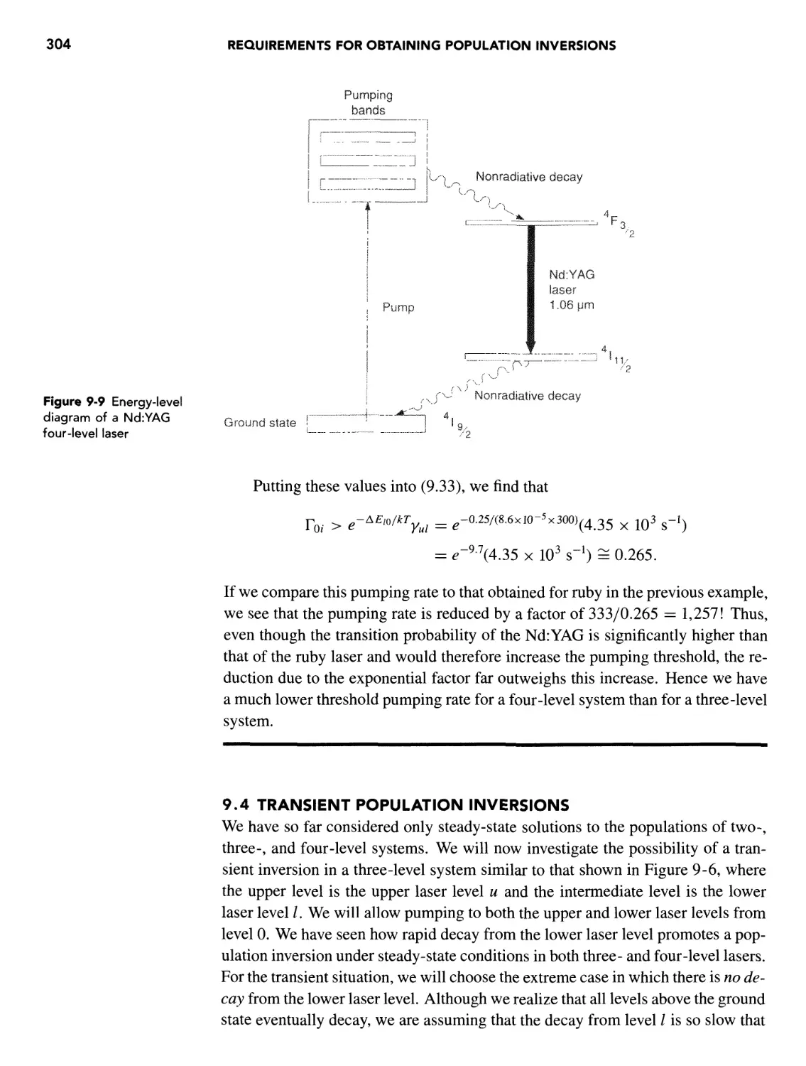
9.3 Steady-State Inversions in Three- and Four-Level Systems 293
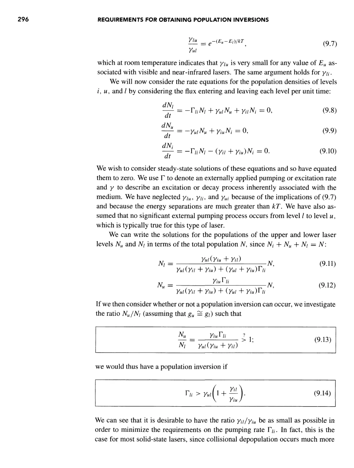
Three-Level Laser with the Intermediate Level as the Upper Laser
Level 295
Three-Level Laser with the Upper Laser Level as the Highest Level 298
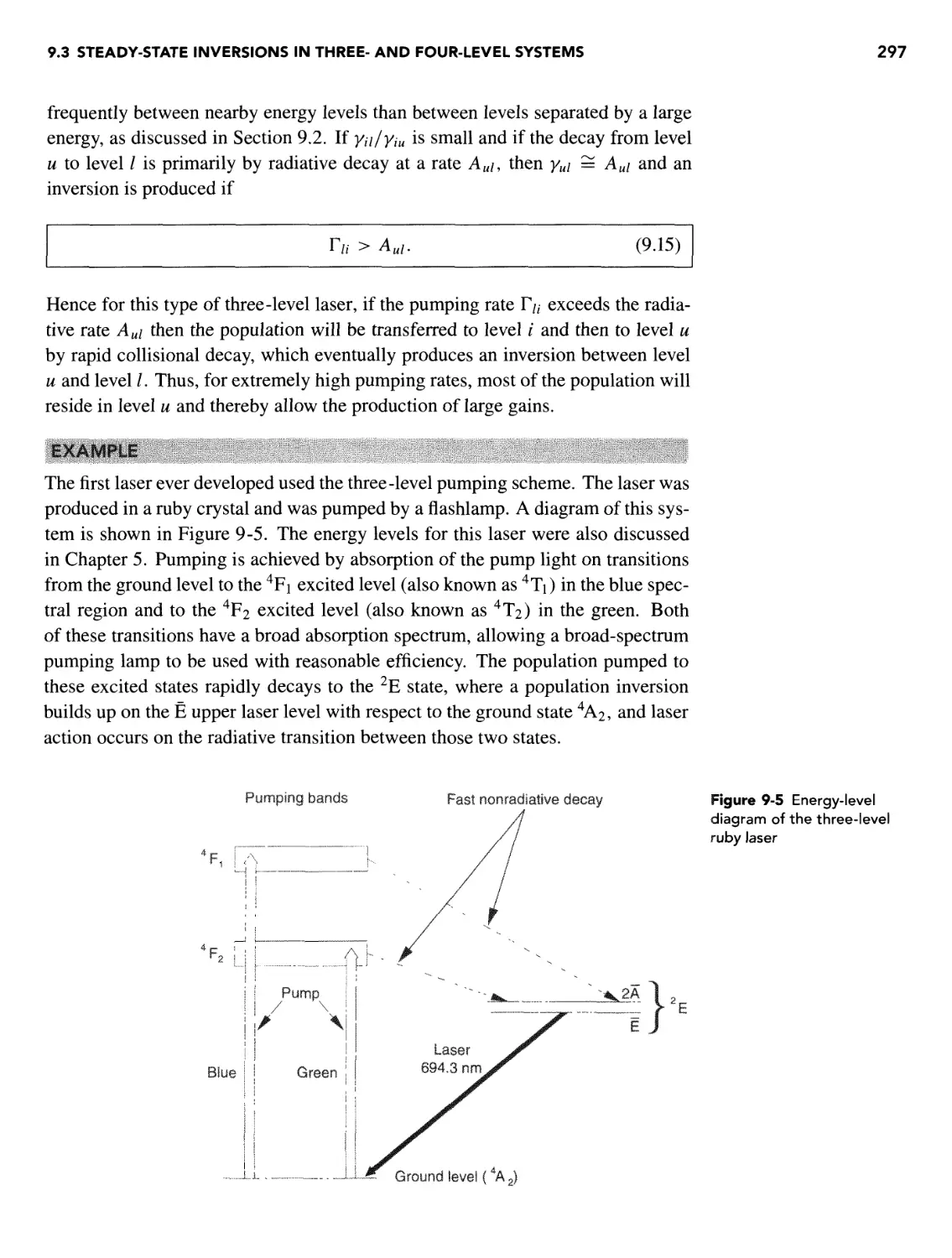
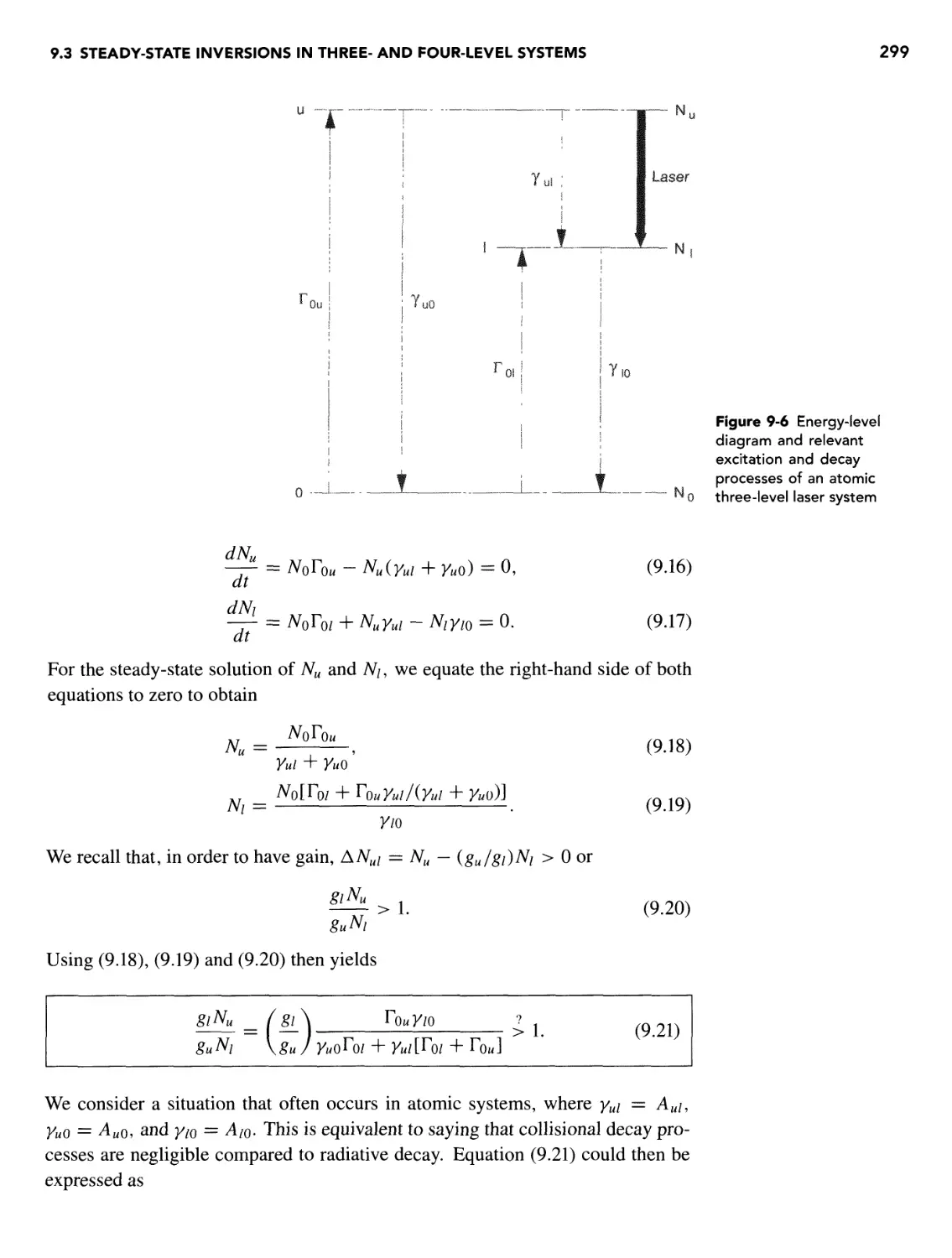
Four-Level Laser 301
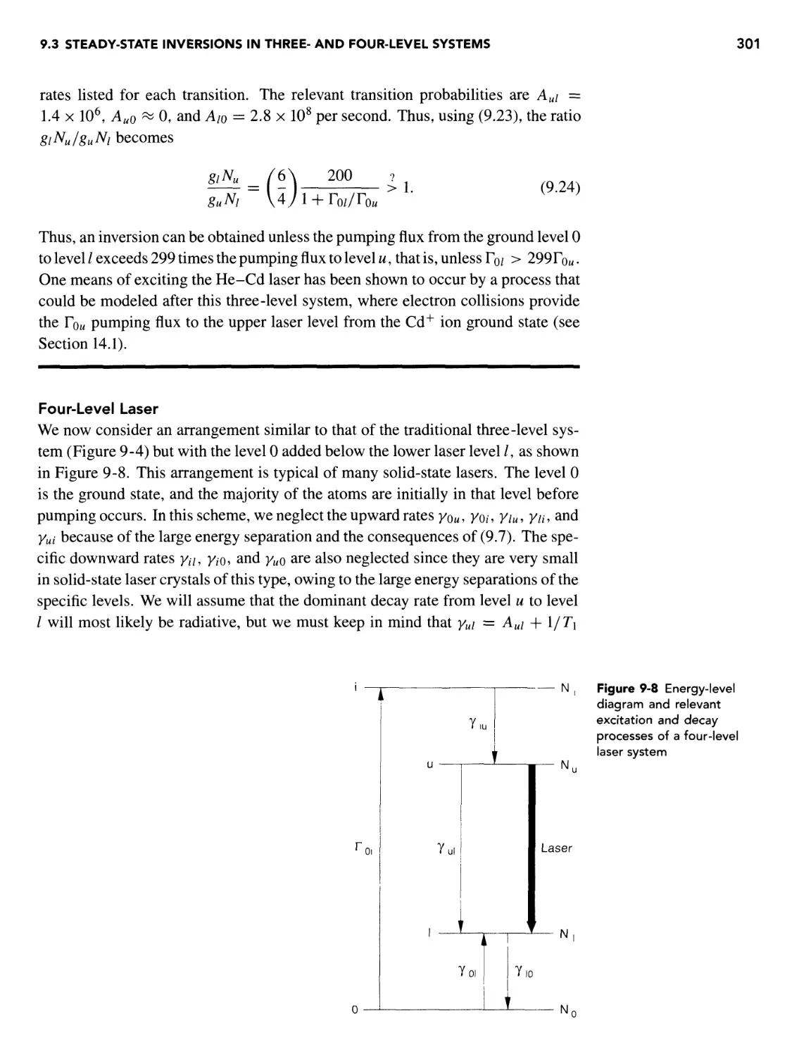
9.4 Transient Population Inversions 304
CONTENTS xiii
9.5 Processes That Inhibit or Destroy Inversions 307
Radiation Trapping in Atoms and Ions 308
Electron Collisional Thermalization of the Laser Levels in Atoms
and Ions 311
Comparison of Radiation Trapping and Electron Collisional Mixing
in a Gas Laser 315
Absorption within the Gain Medium 316
REFERENCES 319
PROBLEMS 319
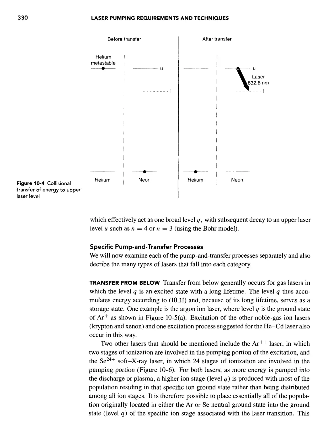
10 LASER PUMPING REQUIREMENTS AND TECHNIQUES 322
overview 322
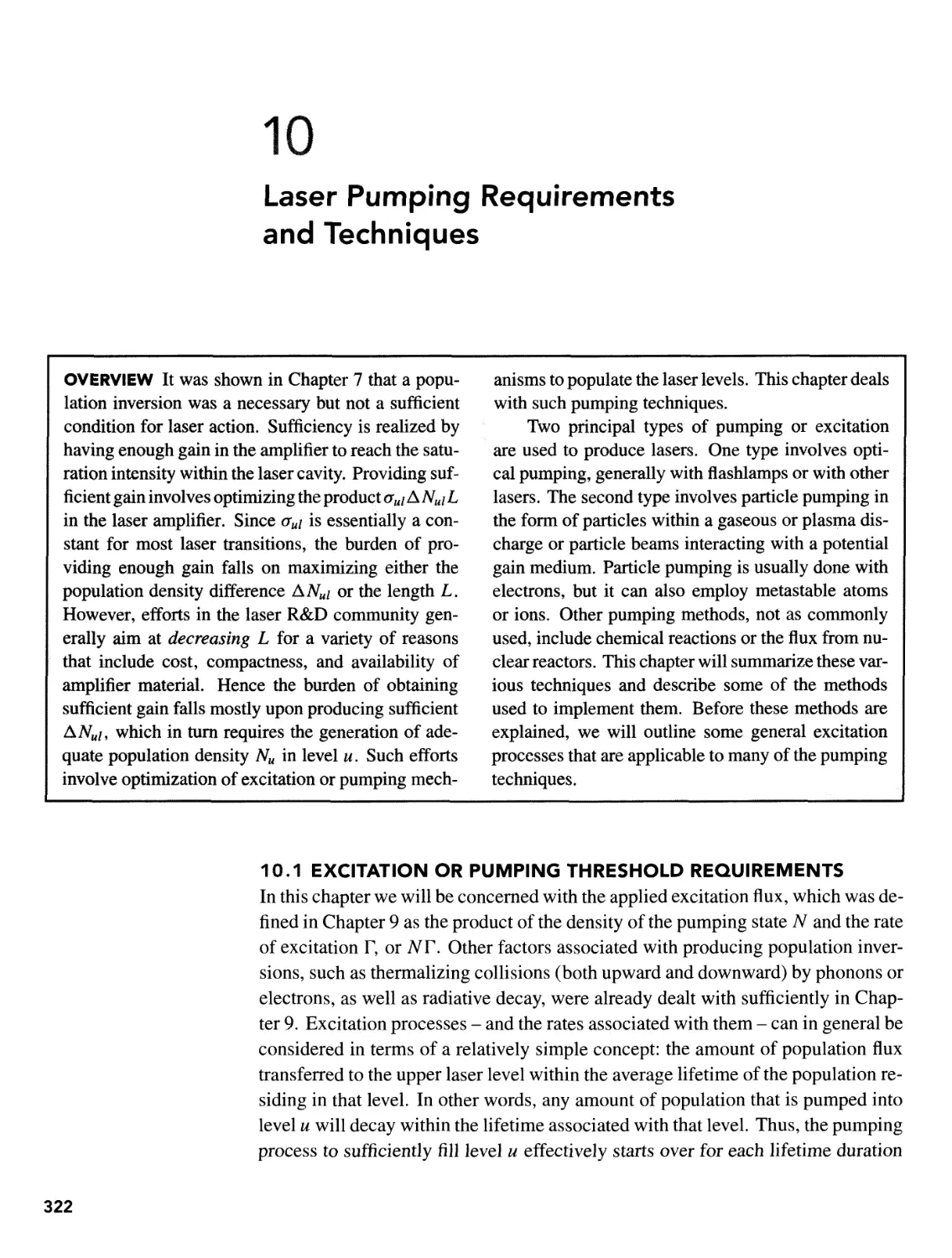
10.1 Excitation or Pumping Threshold Requirements 322
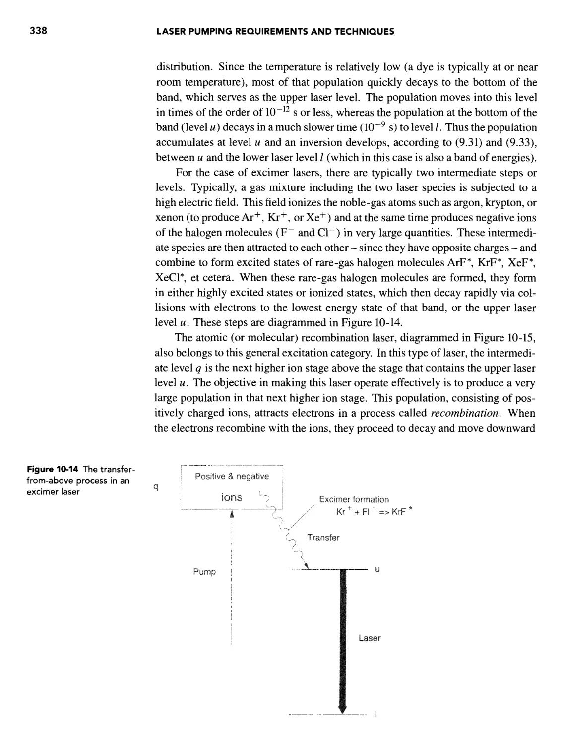
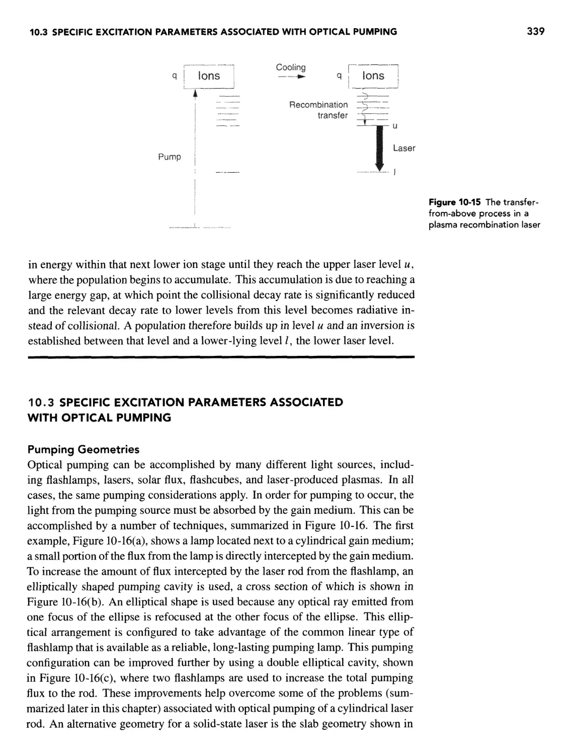
10.2 Pumping Pathways 324
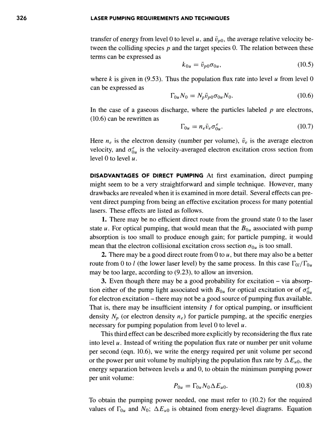
Excitation by Direct Pumping 324
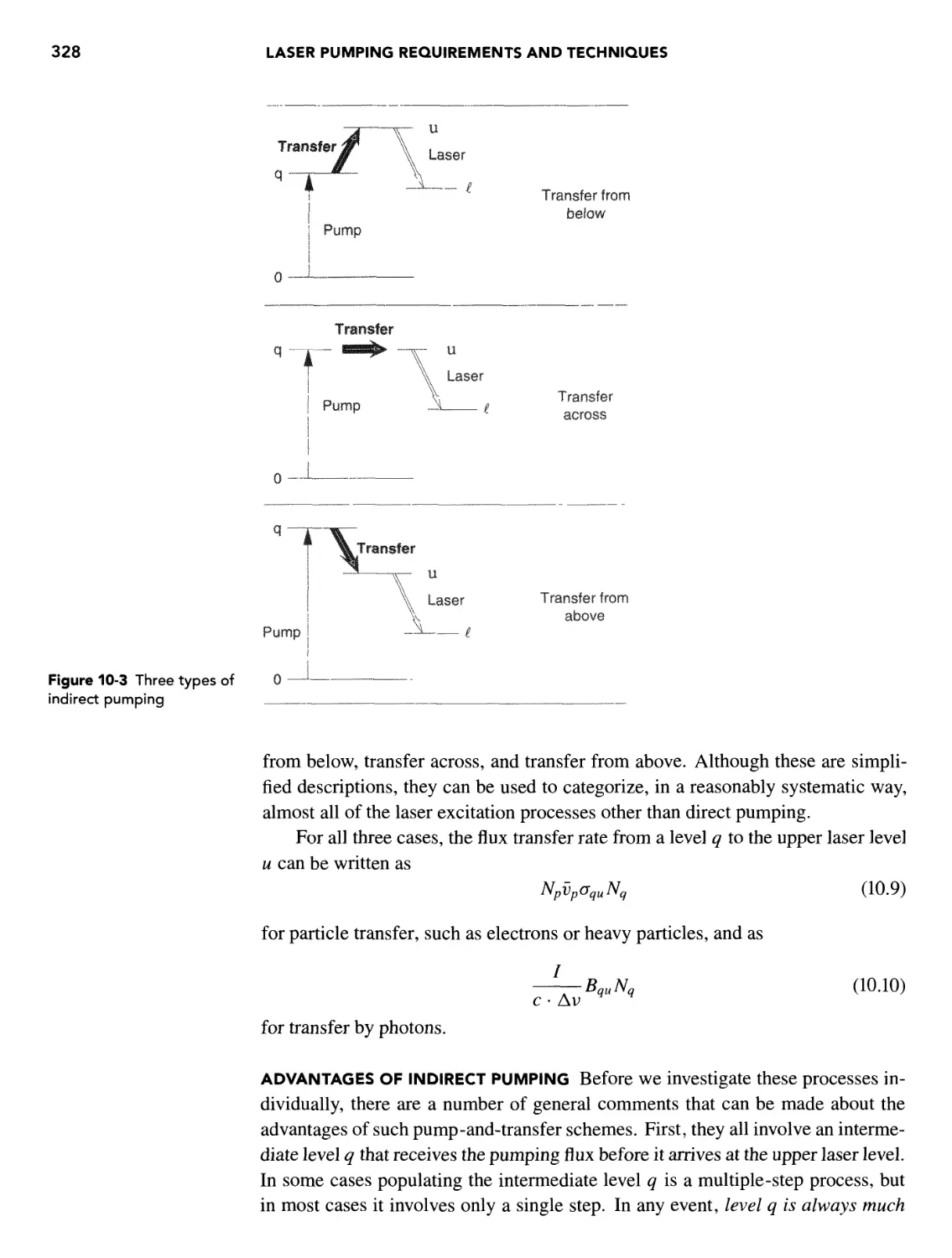
Excitation by Indirect Pumping (Pump and Transfer) 327
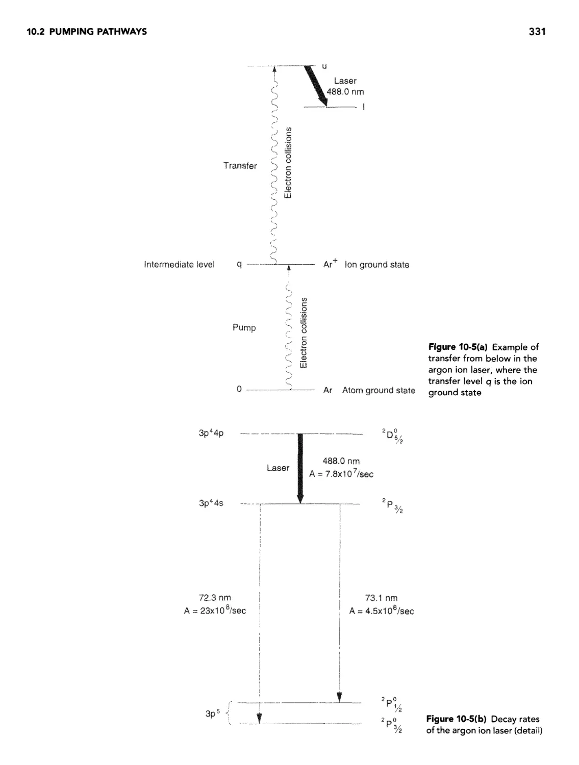
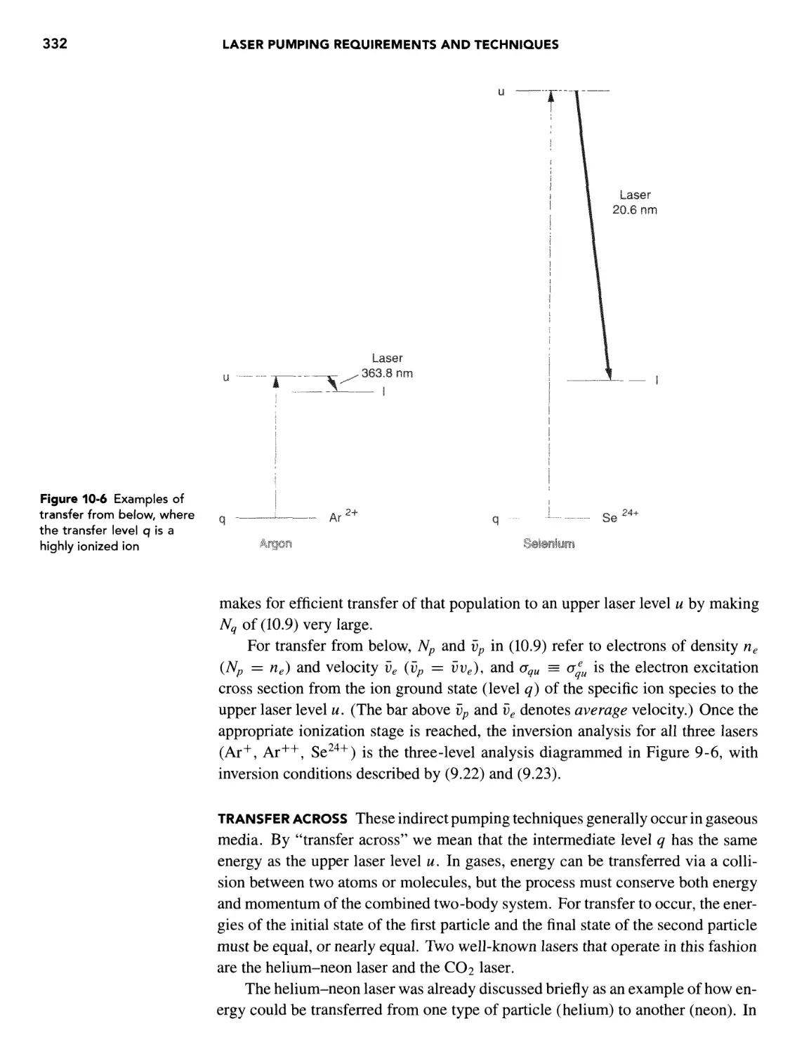
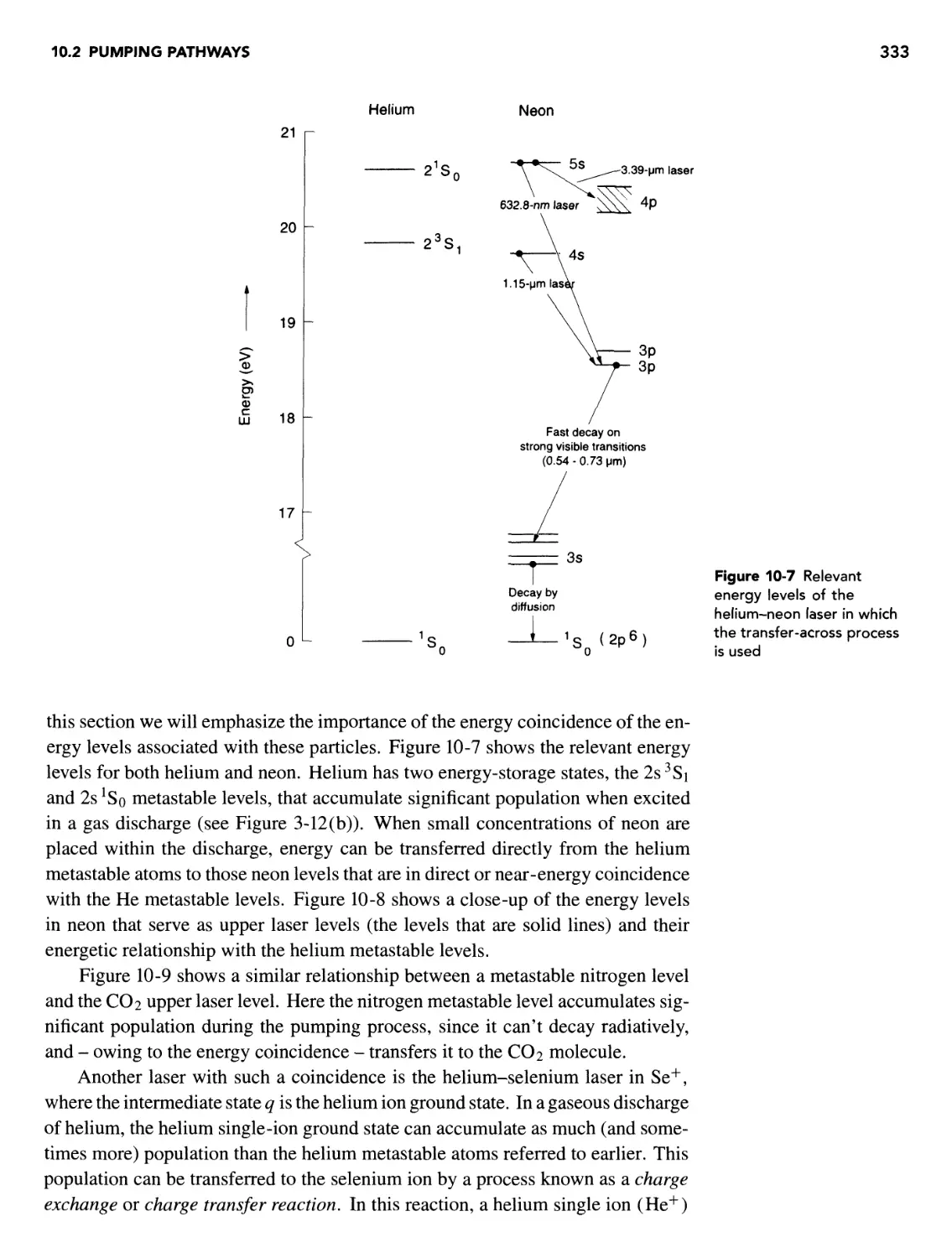
Specific Pump-and-Transfer Processes 330
10.3 Specific Excitation Parameters Associated with
Optical Pumping 339
Pumping Geometries 339
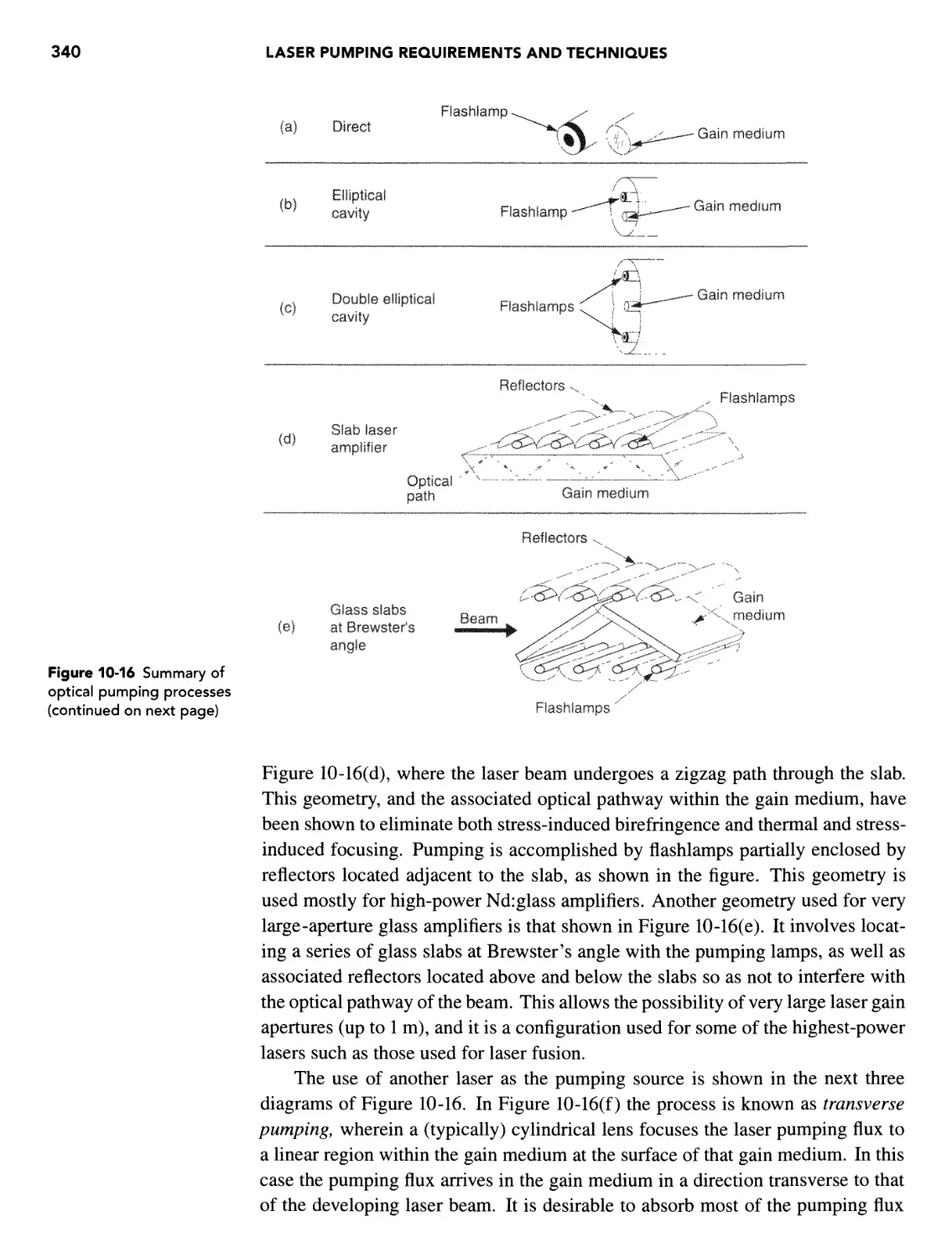
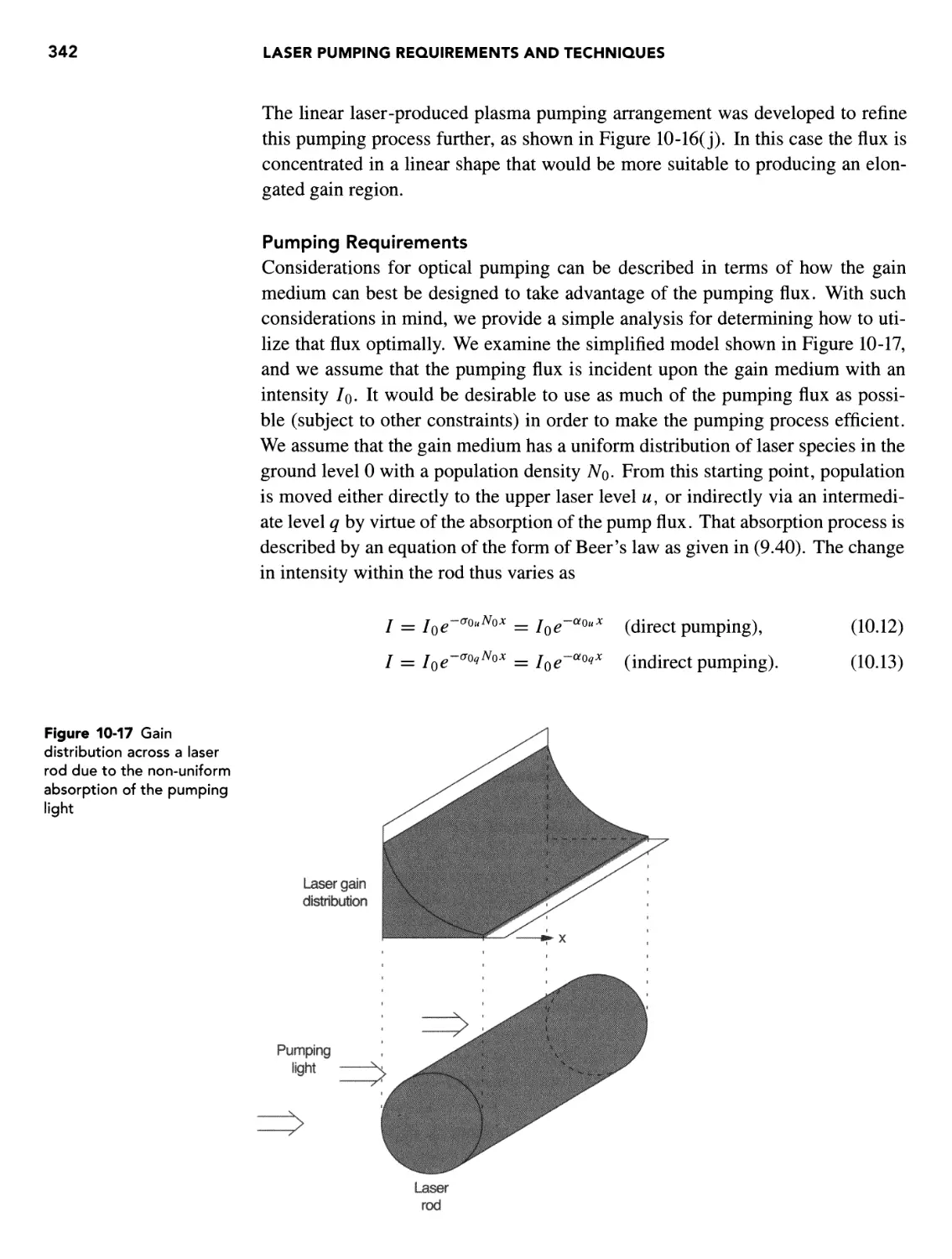
Pumping Requirements 342
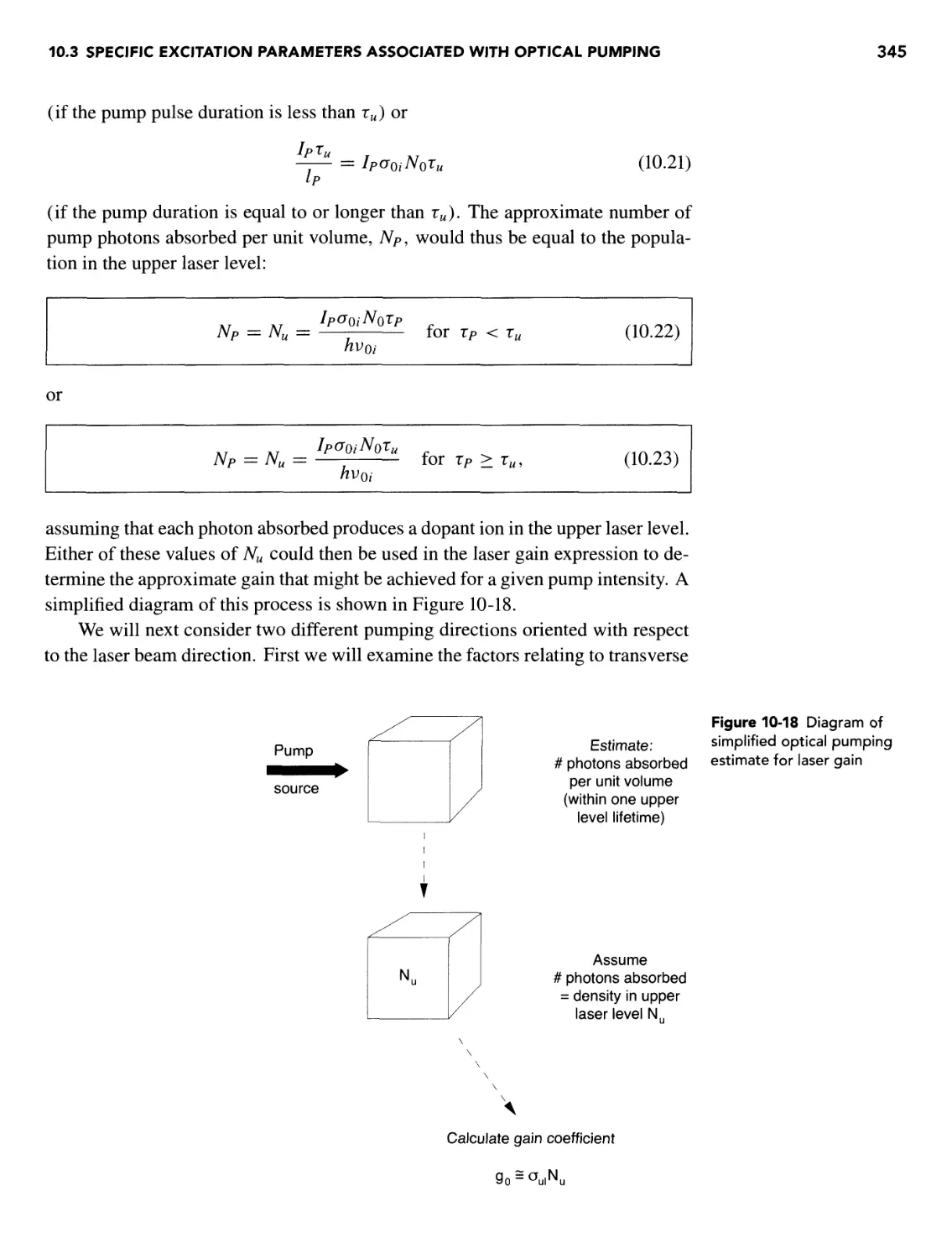
A Simplified Optical Pumping Approximation 344
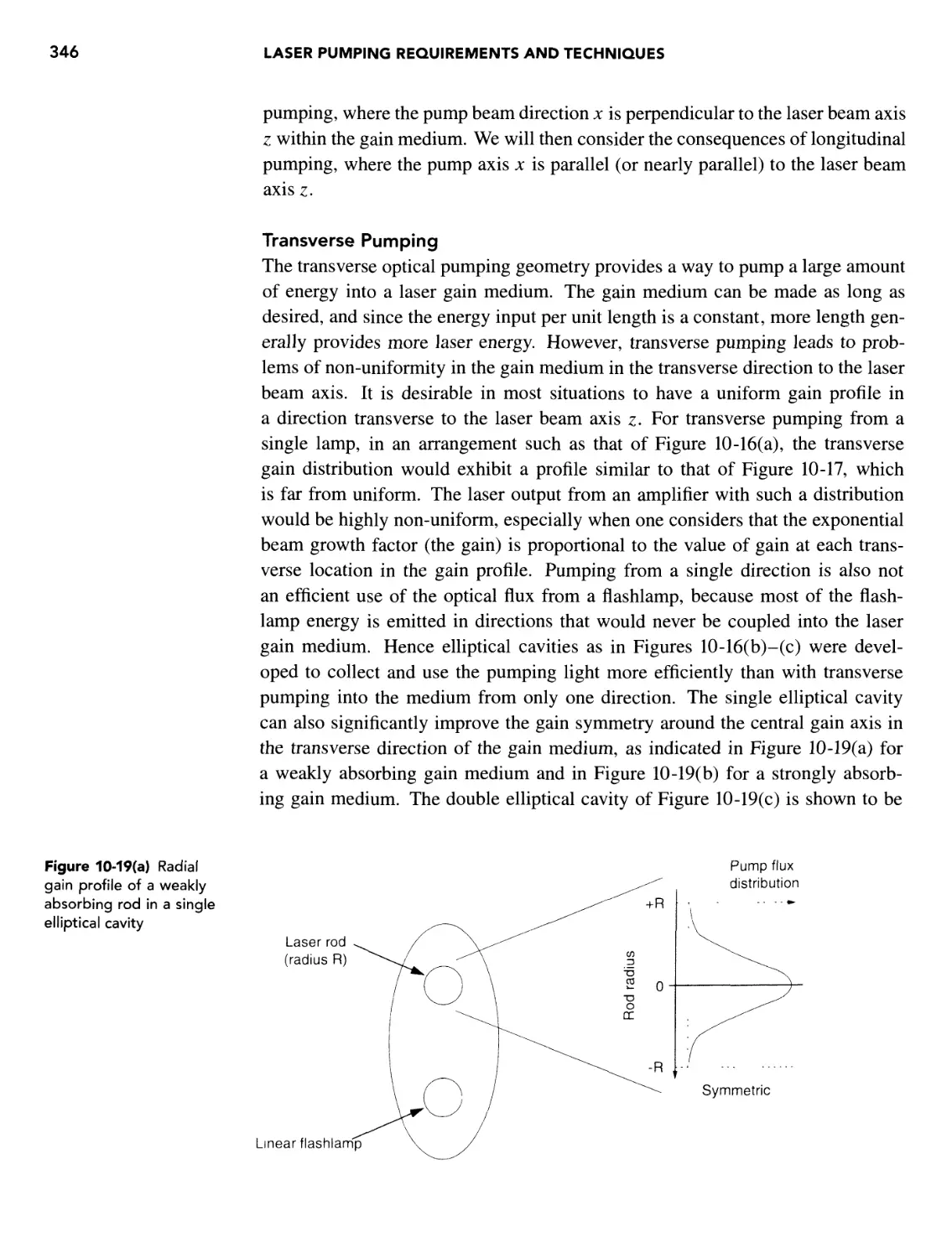
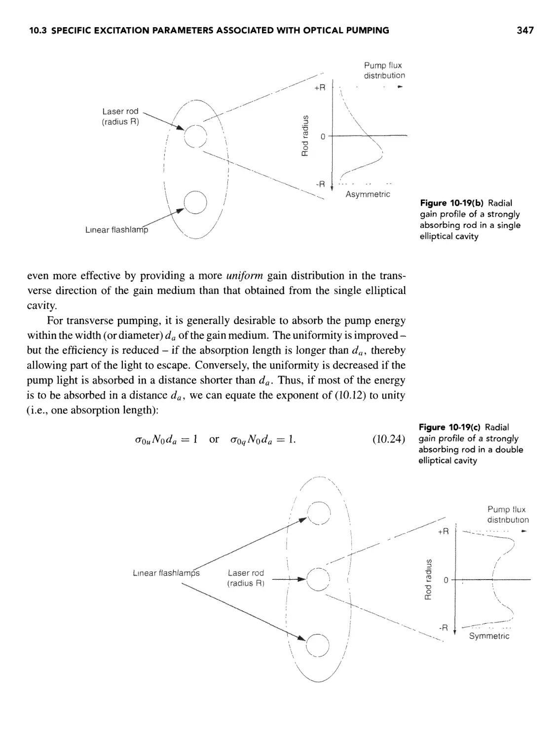
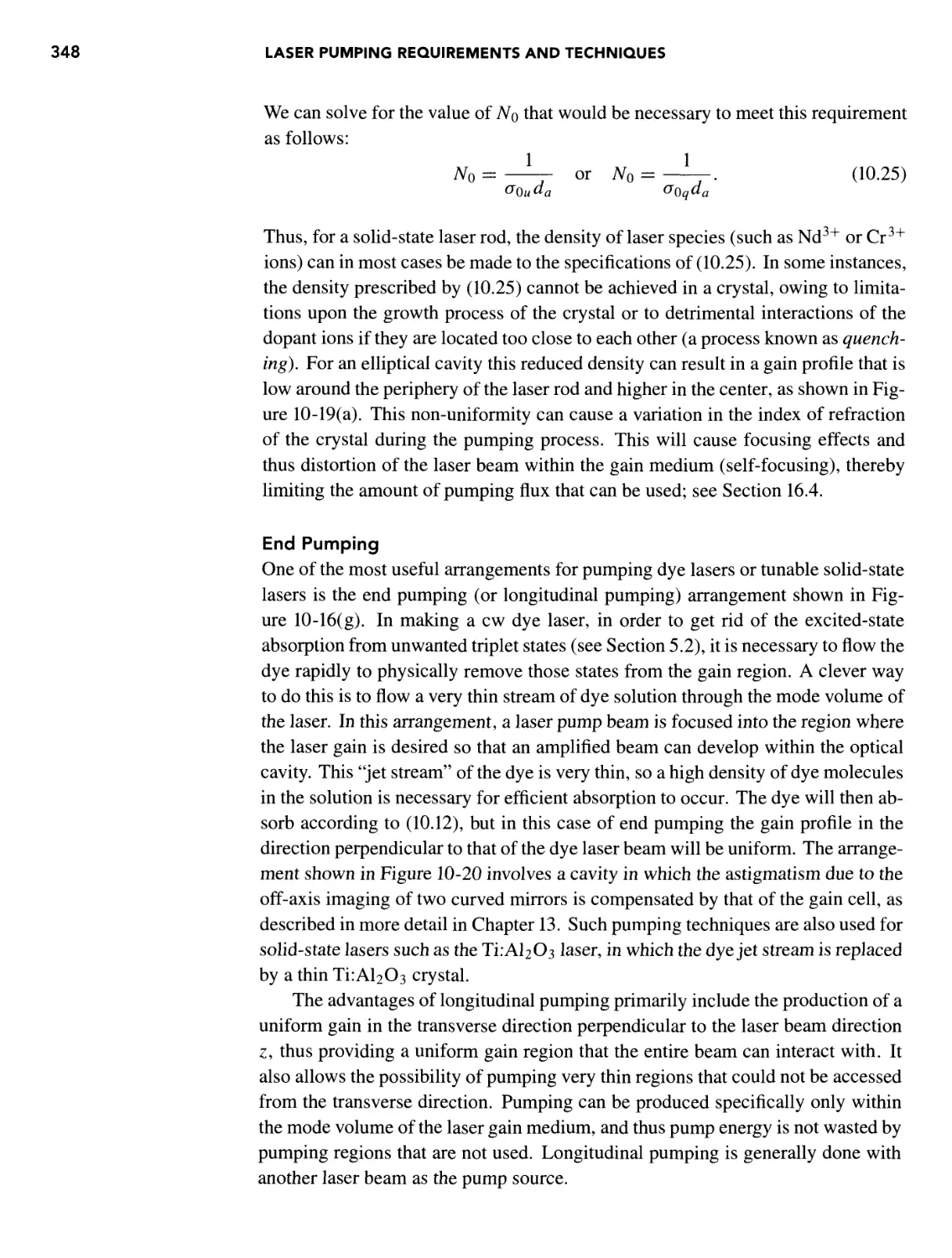
Transverse Pumping 346
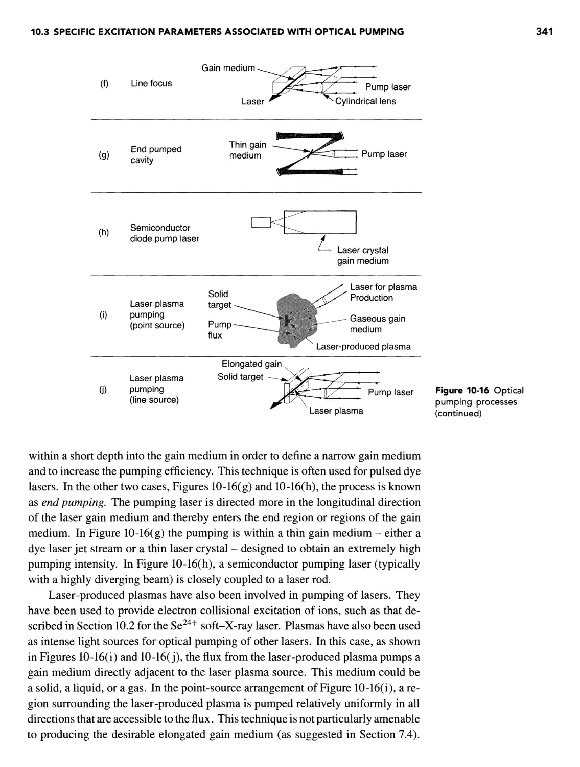
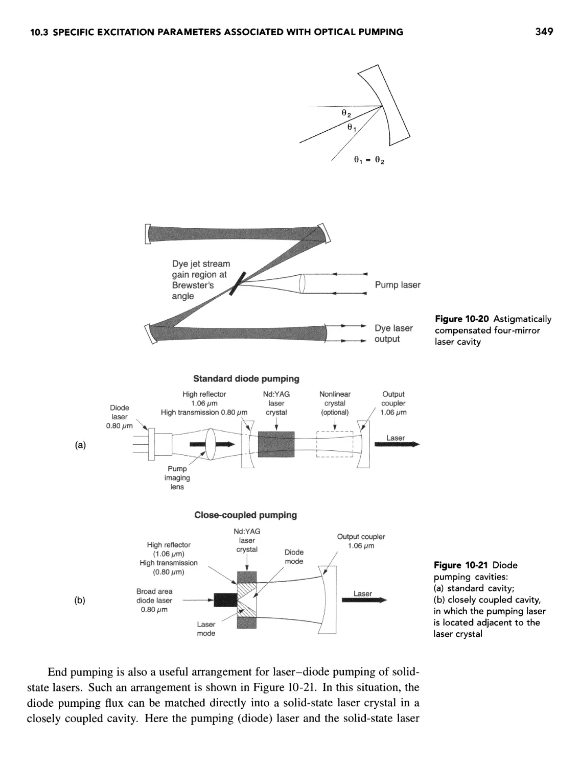
End Pumping 348
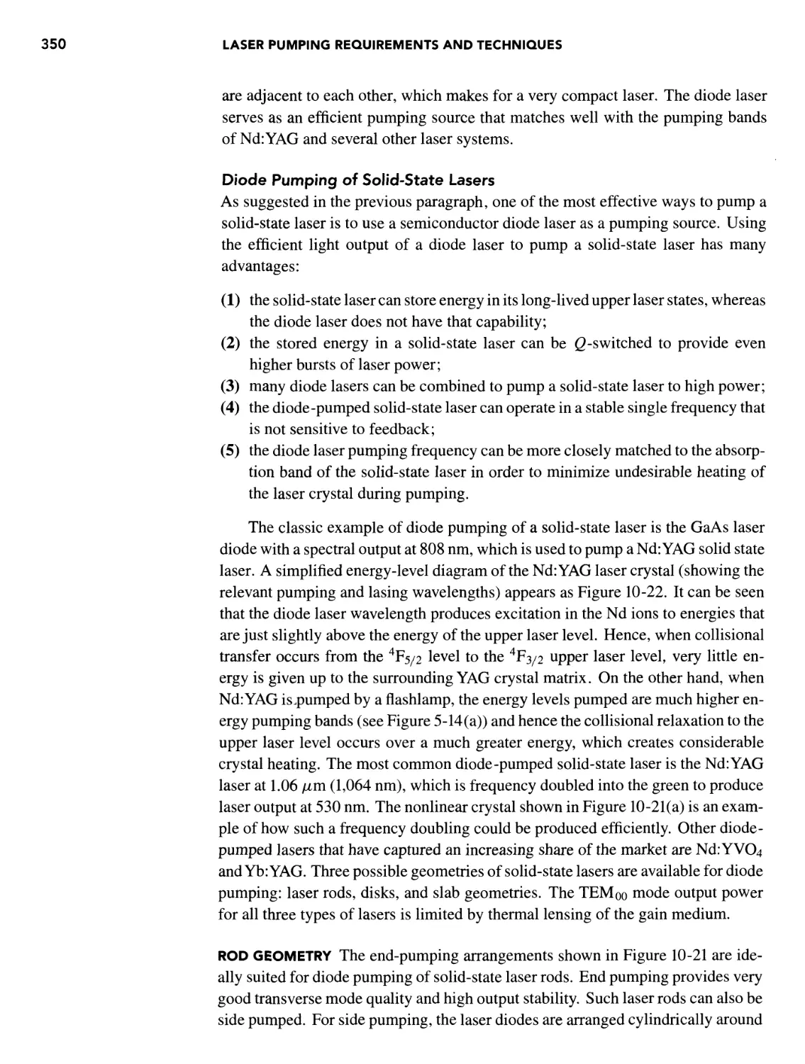
Diode Pumping of Solid-State Lasers 350
Characterization of a Laser Gain Medium with Optical Pumping
(Slope Efficiency) 352
10.4 Specific Excitation Parameters Associated with
Particle Pumping 355
Electron Collisional Pumping 355
Heavy Particle Pumping 359
A More Accurate Description of Electron Excitation Rate to a
Specific Energy Level in a Gas Discharge 359
Electrical Pumping of Semiconductors 361
REFERENCES 363
PROBLEMS 364
11 LASER CAVITY MODES 371
OVERVIEW 371
11.1 Introduction 371
11.2 Longitudinal Laser Cavity Modes 372
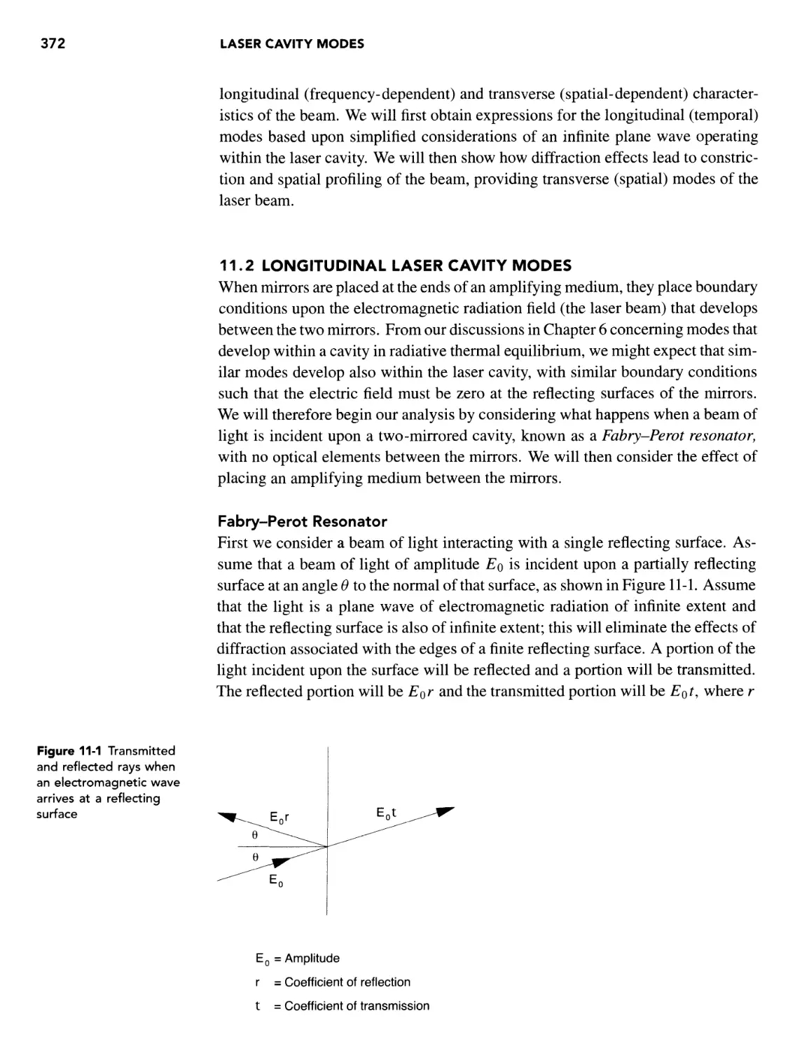
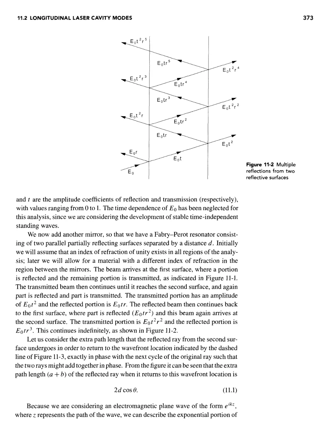
Fabry-Perot Resonator 372
Fabry-Perot Cavity Modes 3 79
Longitudinal Laser Cavity Modes 380
Longitudinal Mode Number 380
Requirements for the Development of Longitudinal
Laser Modes 382
xiv CONTENTS
11.3 Transverse Laser Cavity Modes 384
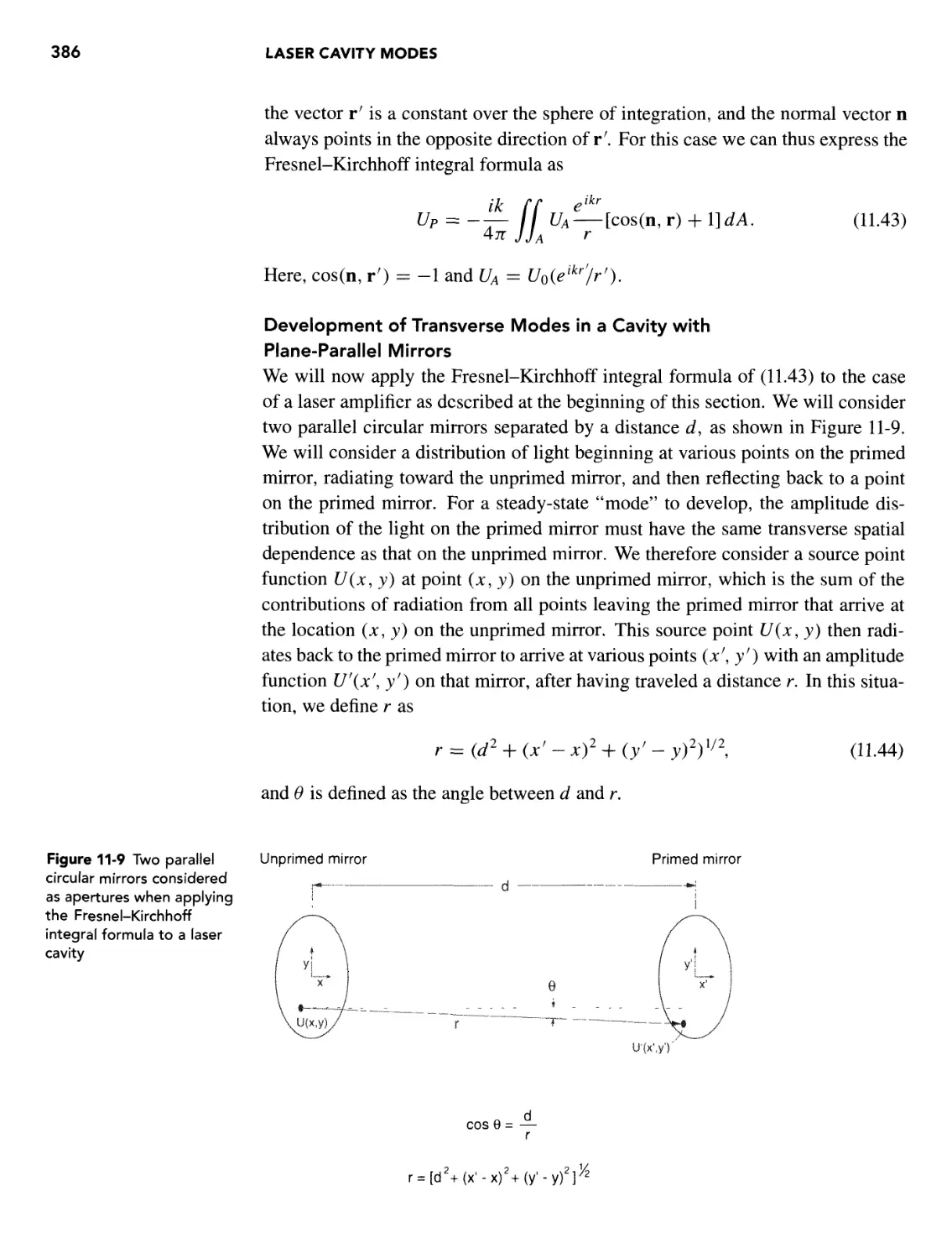
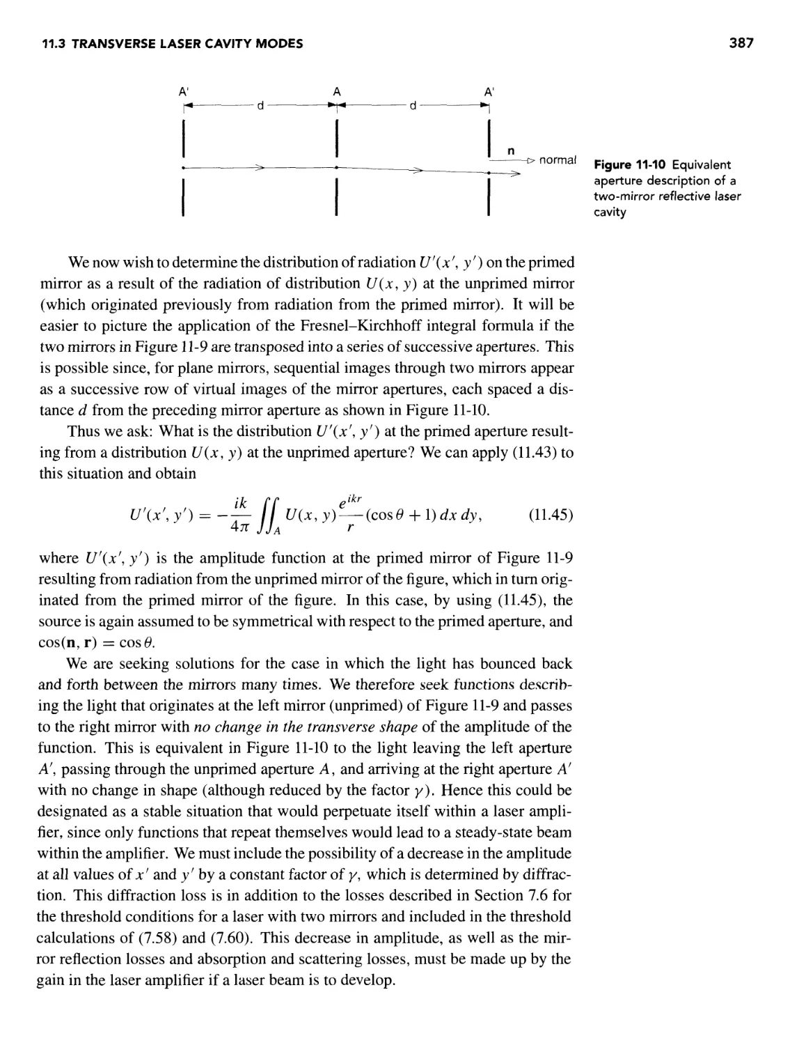
Fresnel-Kirchhoff Diffraction Integral Formula 385
Development of Transverse Modes in a Cavity with Plane-Parallel
Mirrors 386
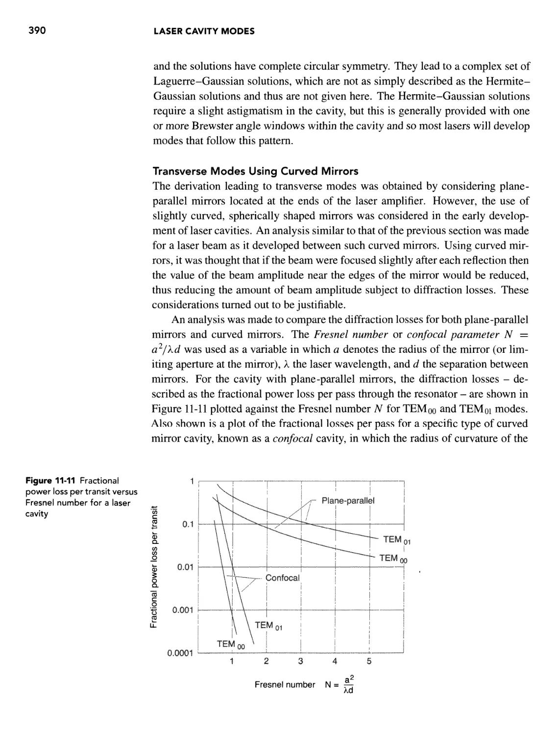
Transverse Modes Using Curved Mirrors 390
Transverse Mode Spatial Distributions 391
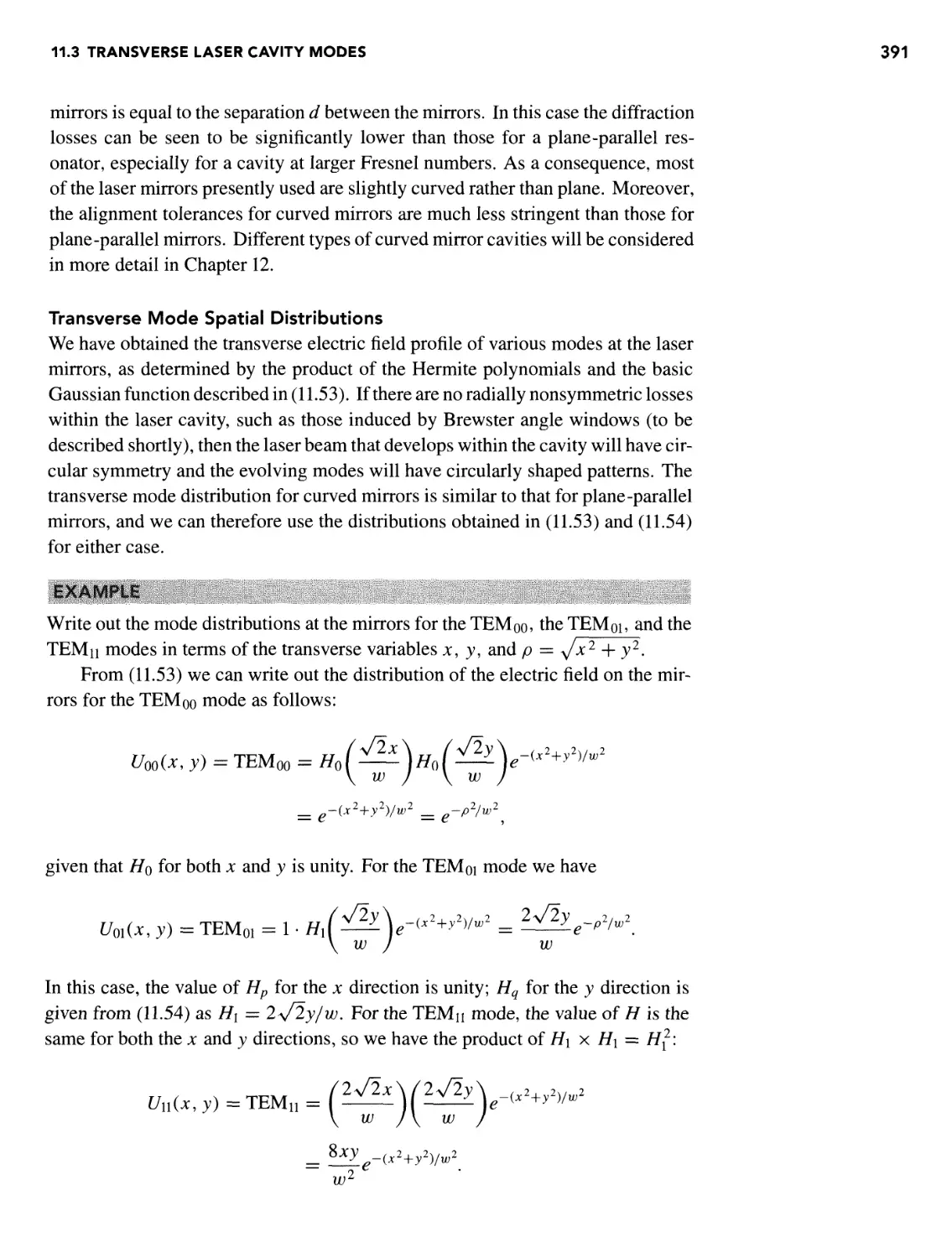
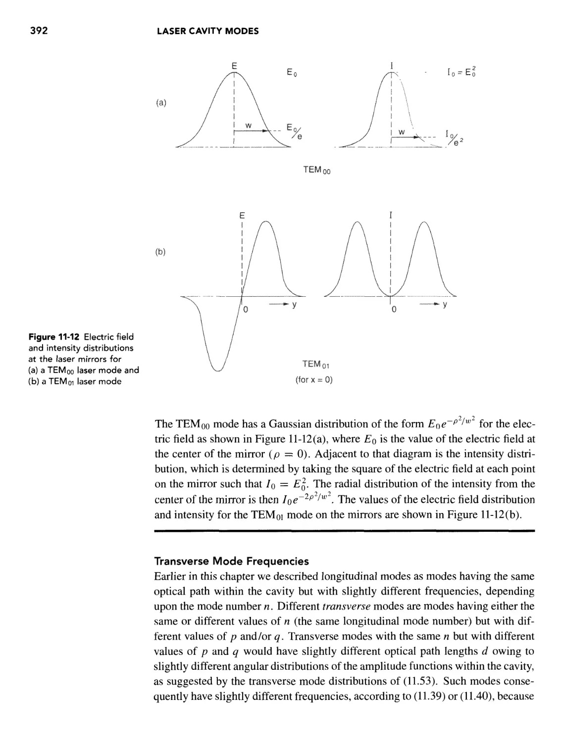
Transverse Mode Frequencies 392
Gaussian-Shaped Transverse Modes within and beyond the
Laser Cavity 393
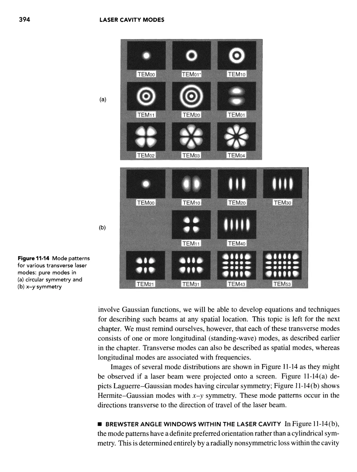
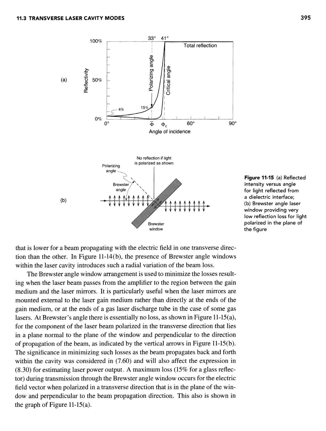
11.4 Properties of Laser Modes 396
Mode Characteristics 396
Effect of Modes on the Gain Medium Profile 397
REFERENCES 399
PROBLEMS 399
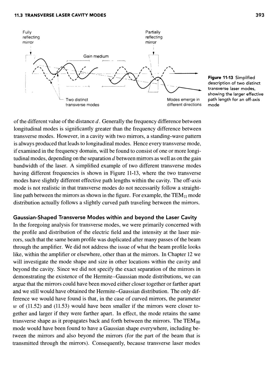
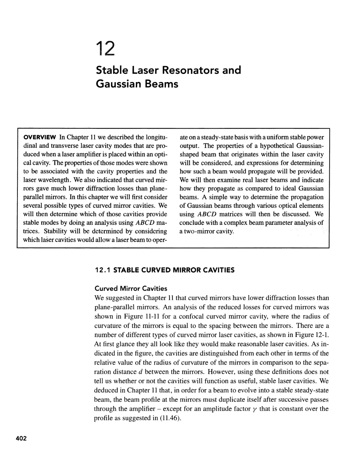
12 STABLE LASER RESONATORS AND GAUSSIAN BEAMS 402
OVERVIEW 402
12.1 Stable Curved Mirror Cavities 402
Curved Mirror Cavities 402
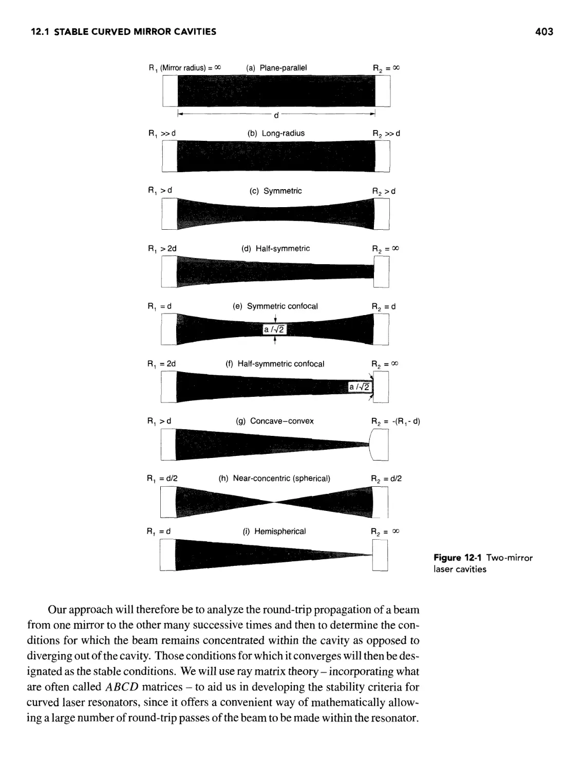
ABCD Matrices 404
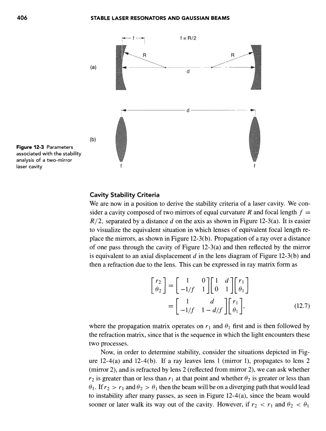
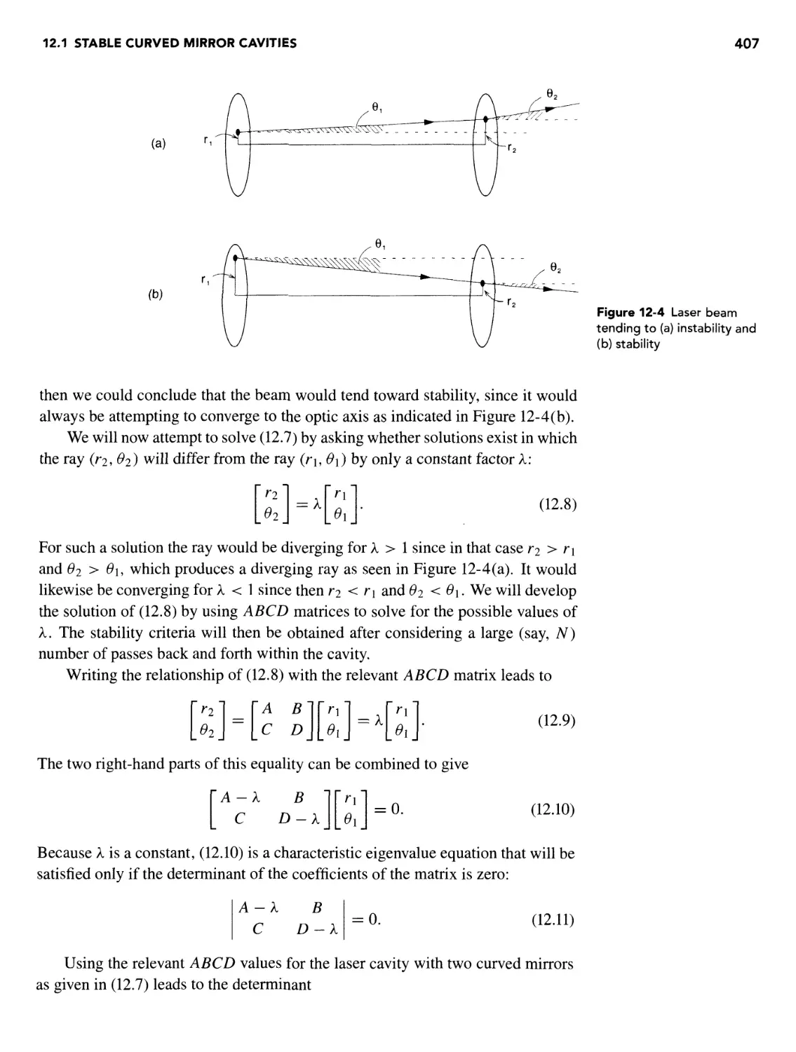
Cavity Stability Criteria 406
12.2 Properties of Gaussian Beams 410
Propagation of a Gaussian Beam 411
Gaussian Beam Properties of Two-Mirror Laser Cavities 412
Properties of Specific Two-Mirror Laser Cavities 417
Mode Volume of a Hermite-Gaussian Mode 421
12.3 Properties of Real Laser Beams 423
12.4 Propagation of Gaussian Beams Using ABCD Matrices -
Complex Beam Parameter 425
Complex Beam Parameter Applied to a Two-Mirror Laser Cavity 428
REFERENCES 432
PROBLEMS 432
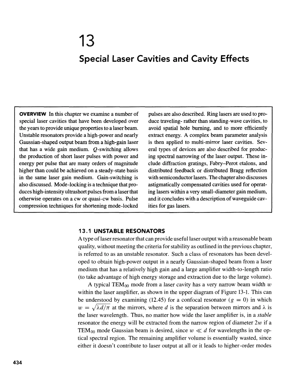
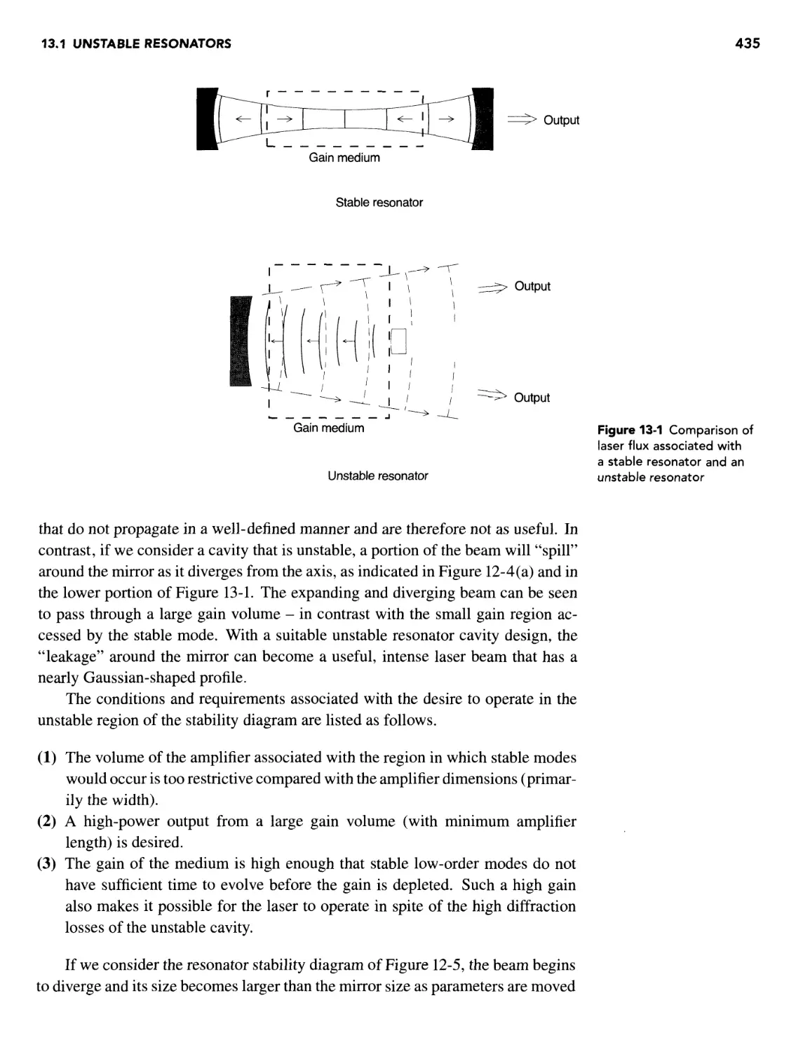
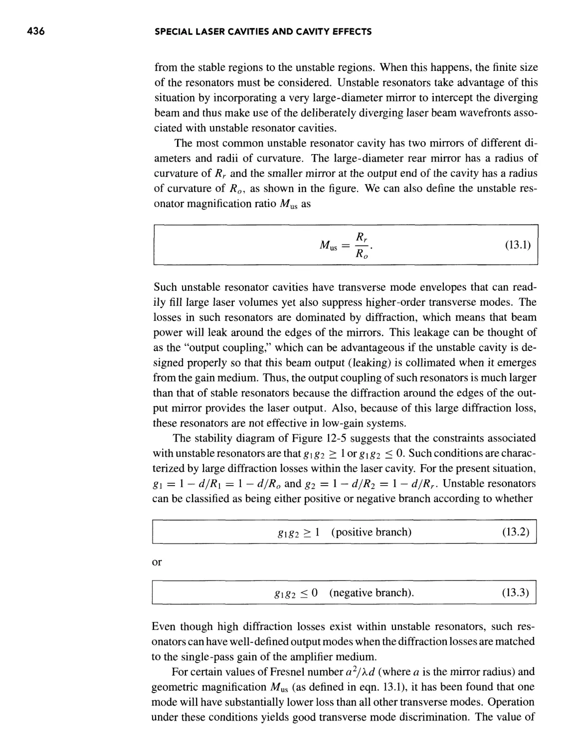
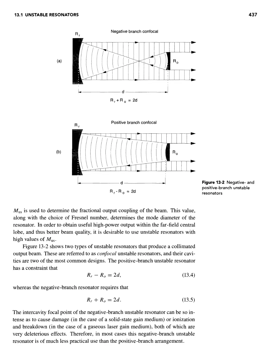
13 SPECIAL LASER CAVITIES AND CAVITY EFFECTS 434
OVERVIEW 434
13.1 Unstable Resonators 434
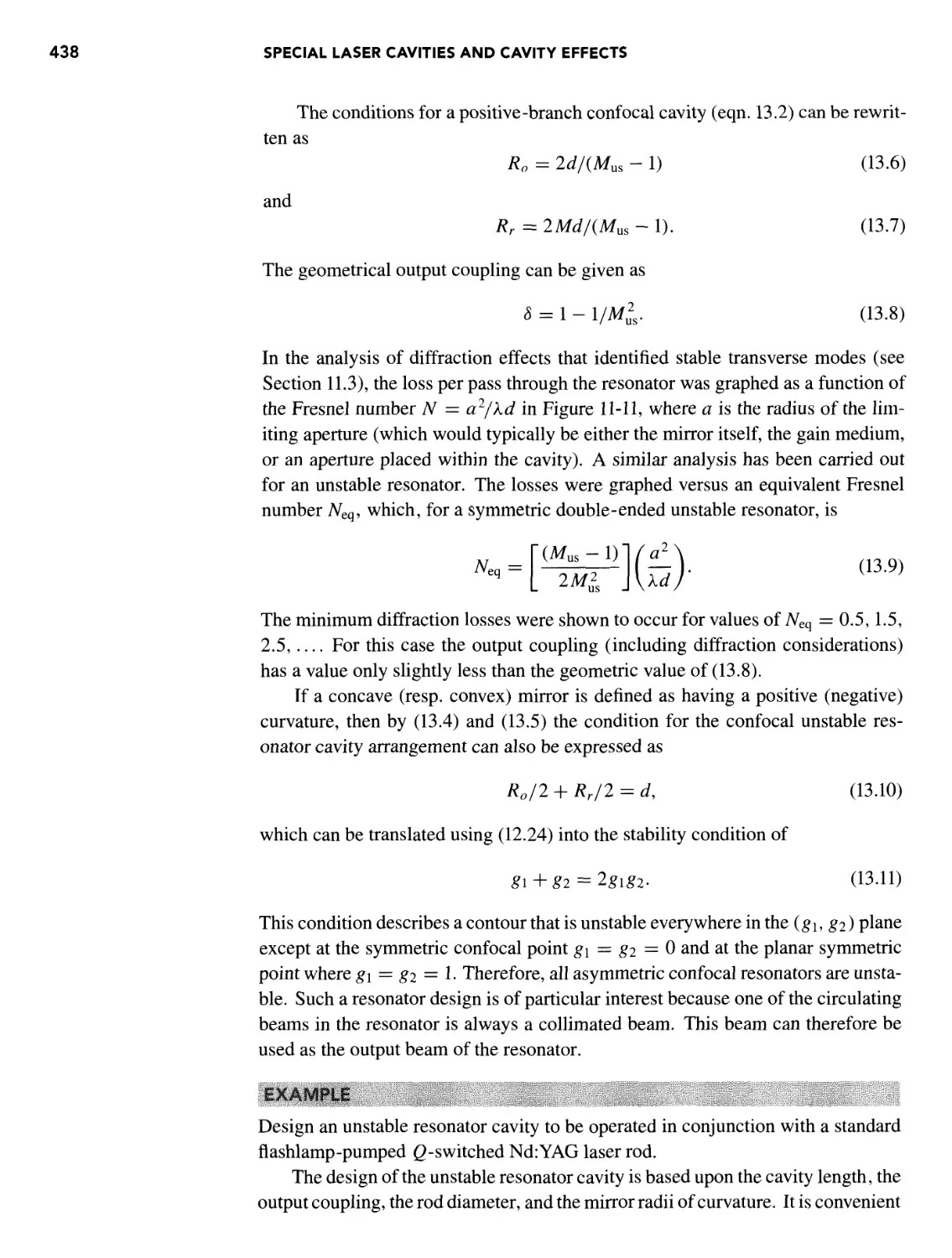
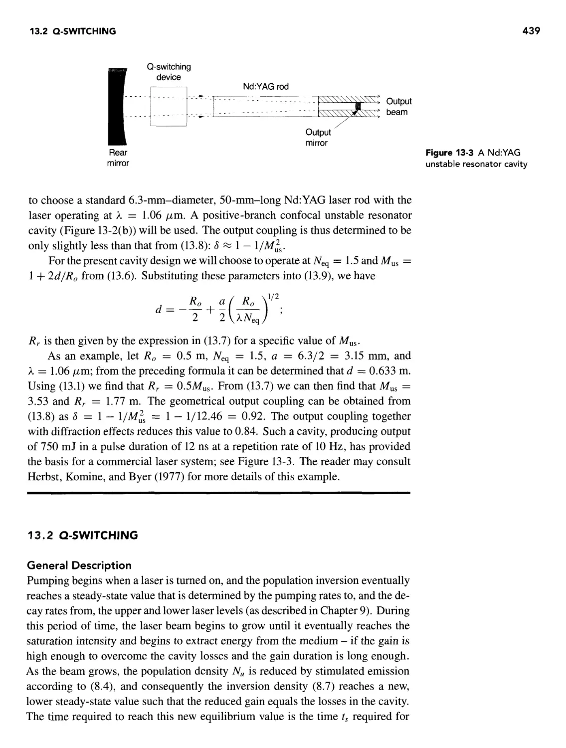
13.2 g-Switching 439
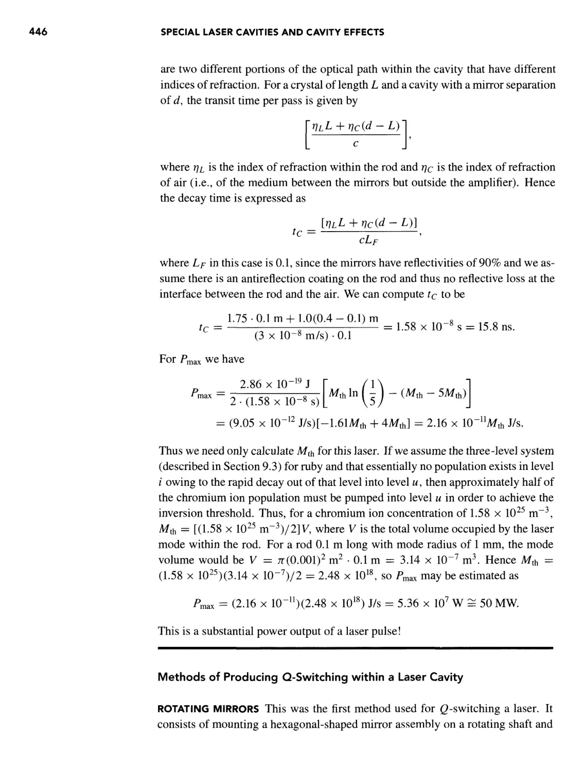
General Description 439
Theory 441
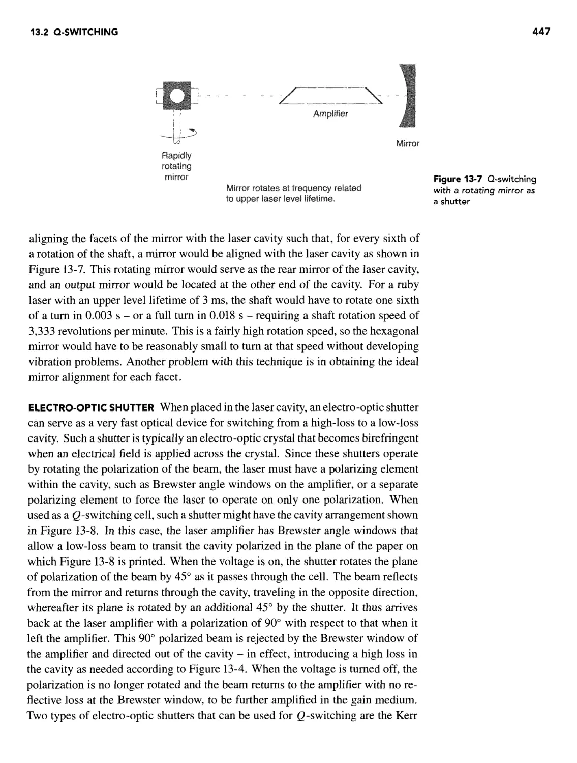
Methods of Producing Q-Switching within a Laser Cavity 446
13.3 Gain-Switching 450
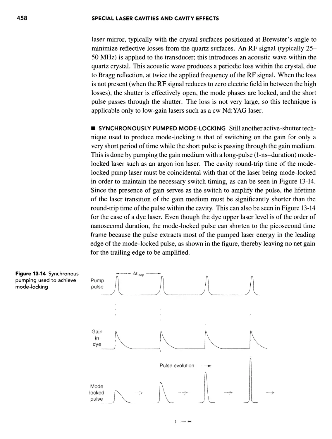
13.4 Mode-Locking 451
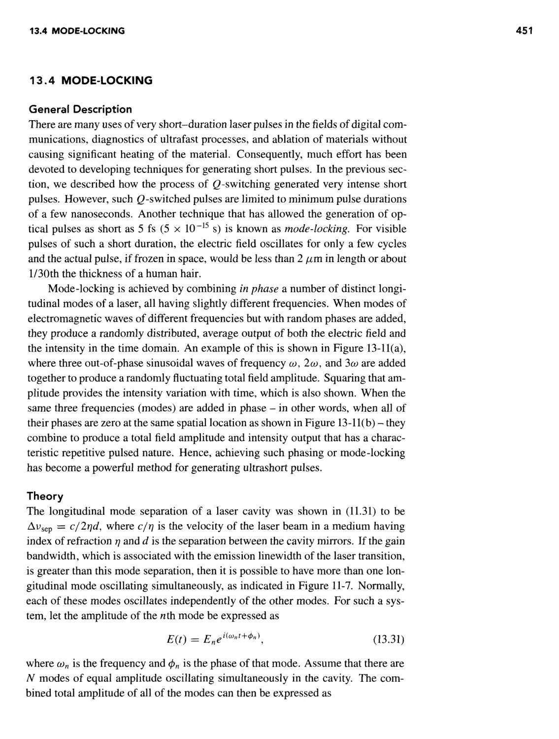
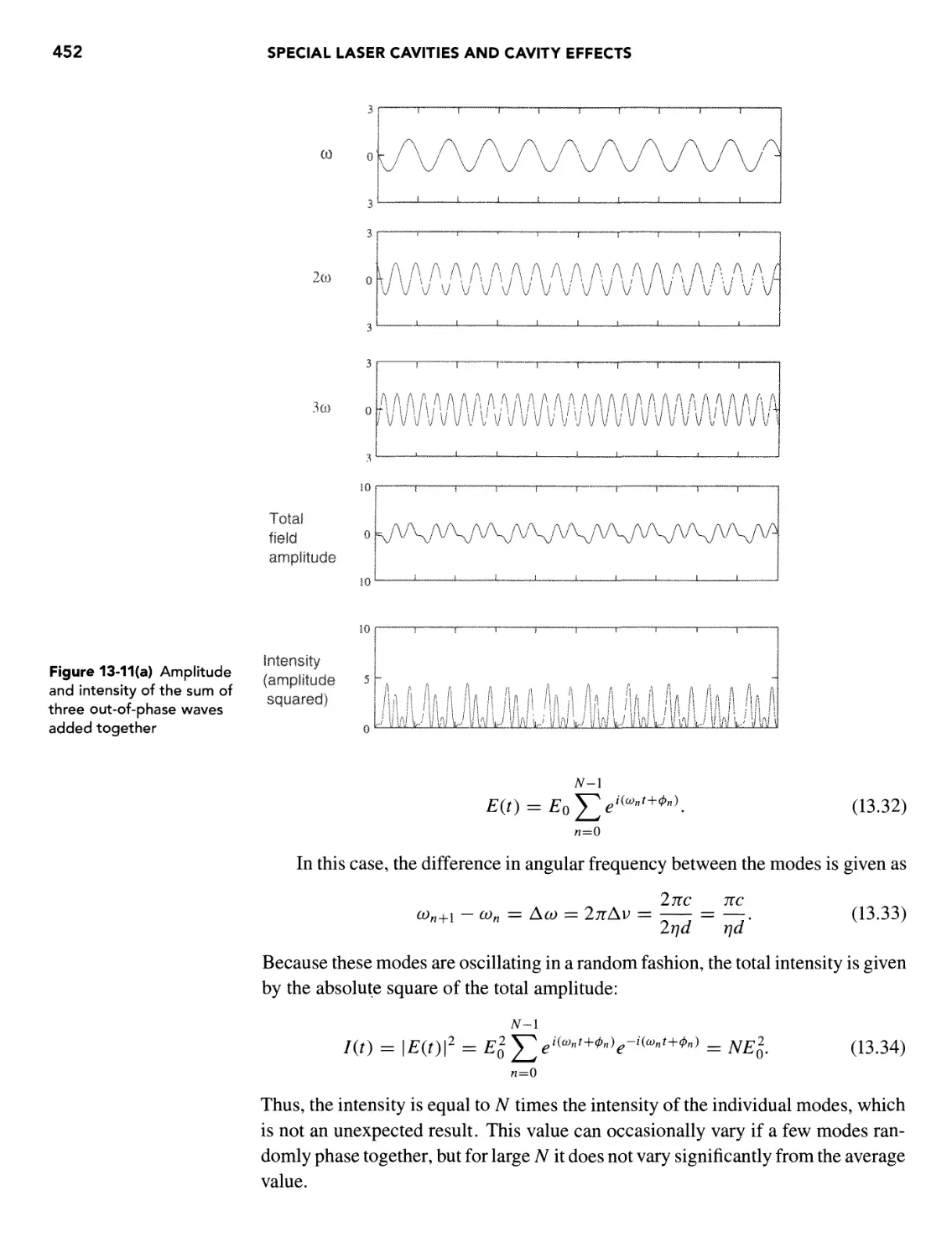
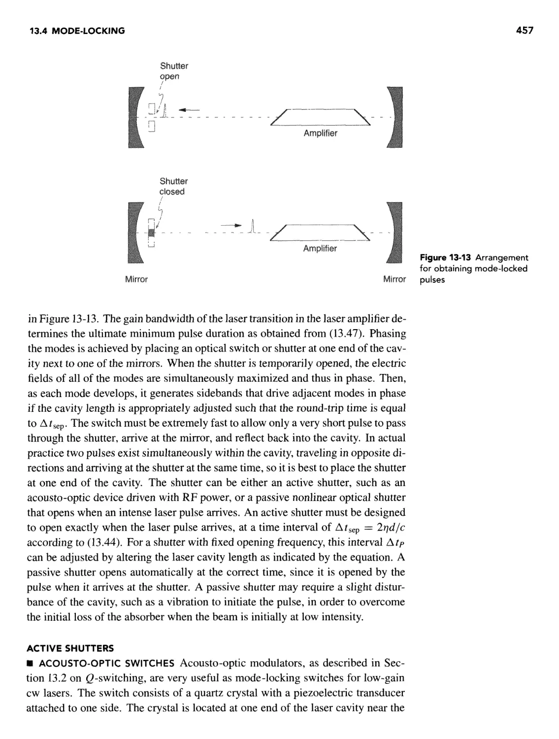
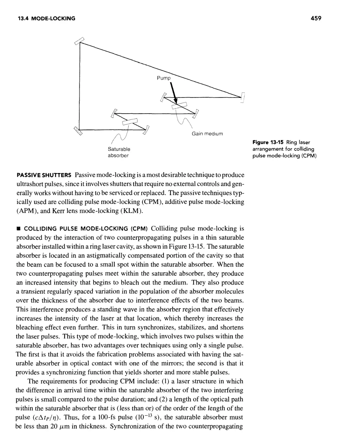
General Description 451
Theory 451
Techniques for Producing Mode-Locking 456
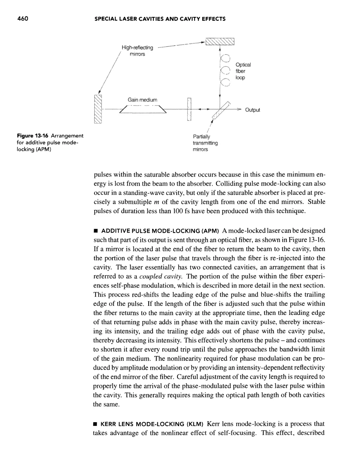
13.5 Pulse Shortening Techniques 462
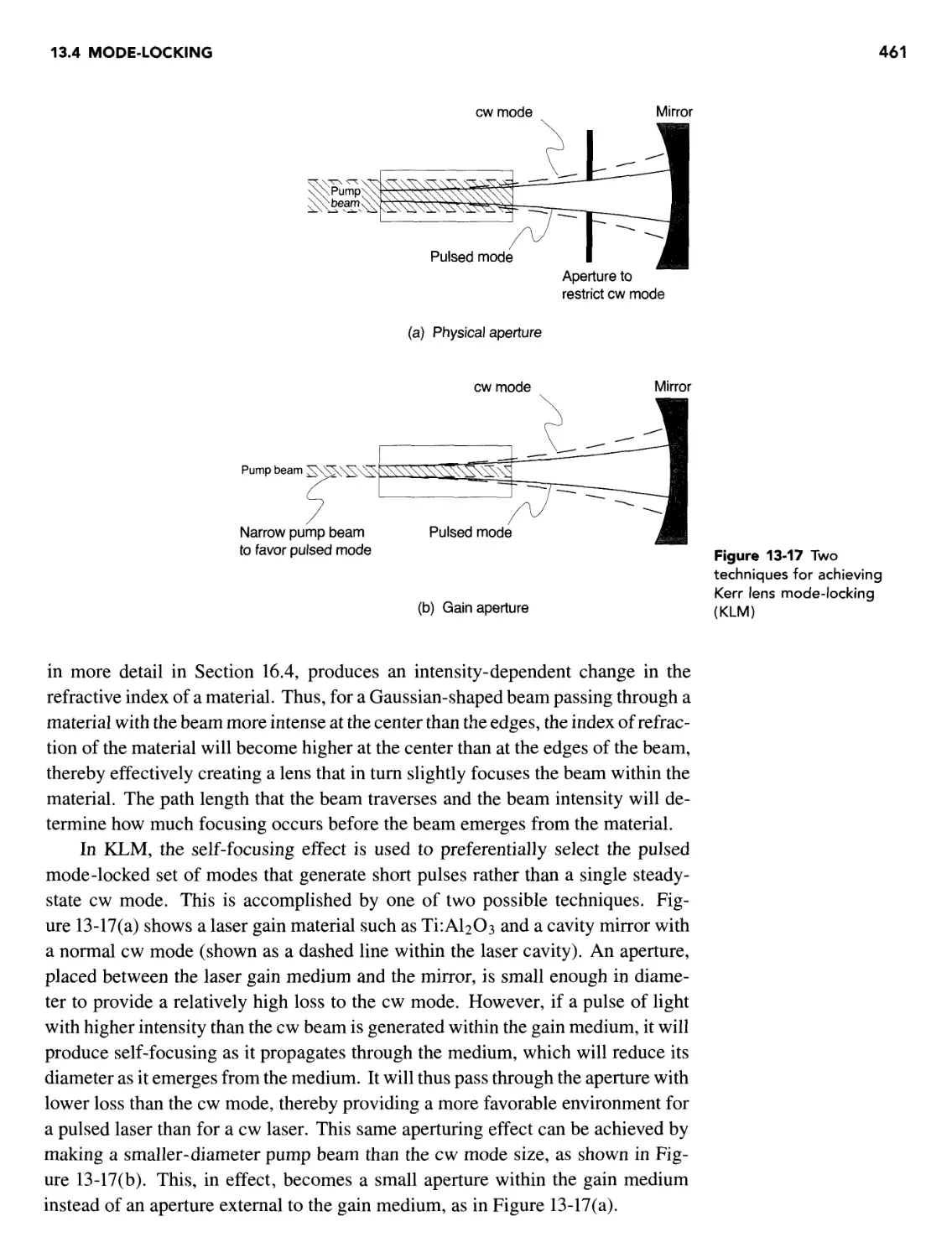
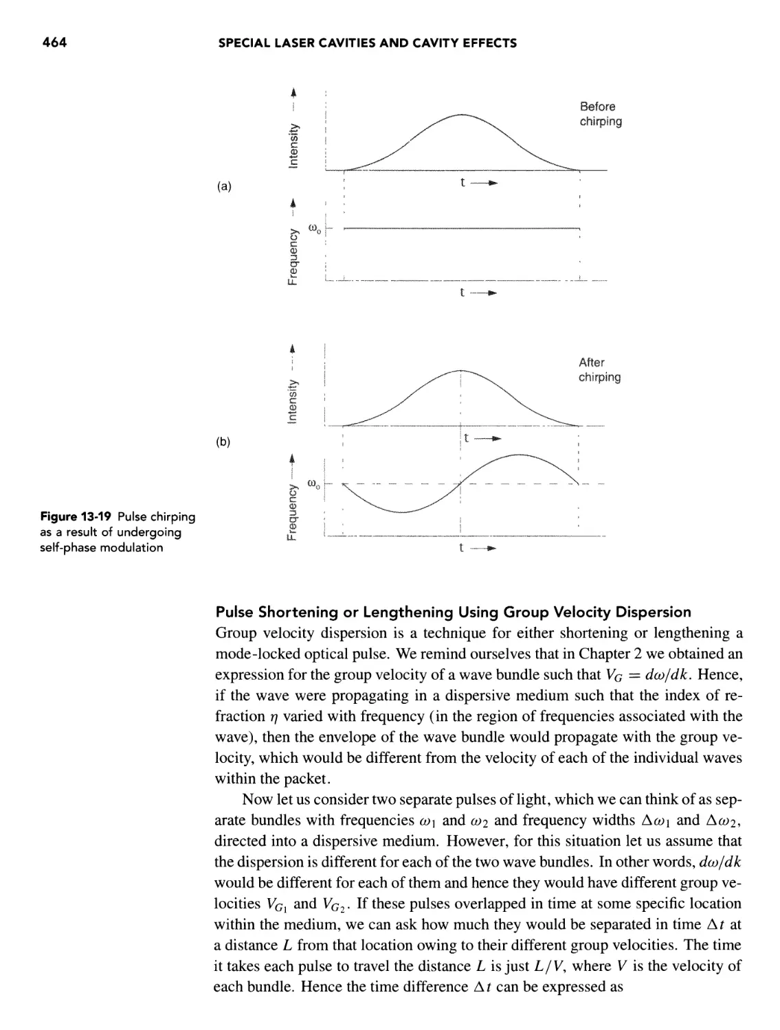
Self-Phase Modulation 463
Pulse Shortening or Lengthening Using Group Velocity Dispersion 464
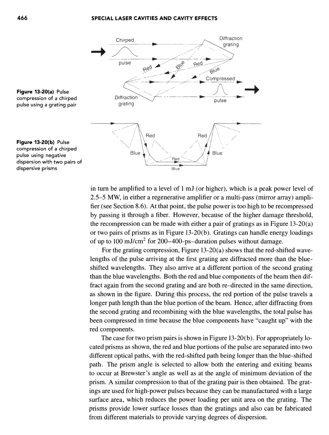
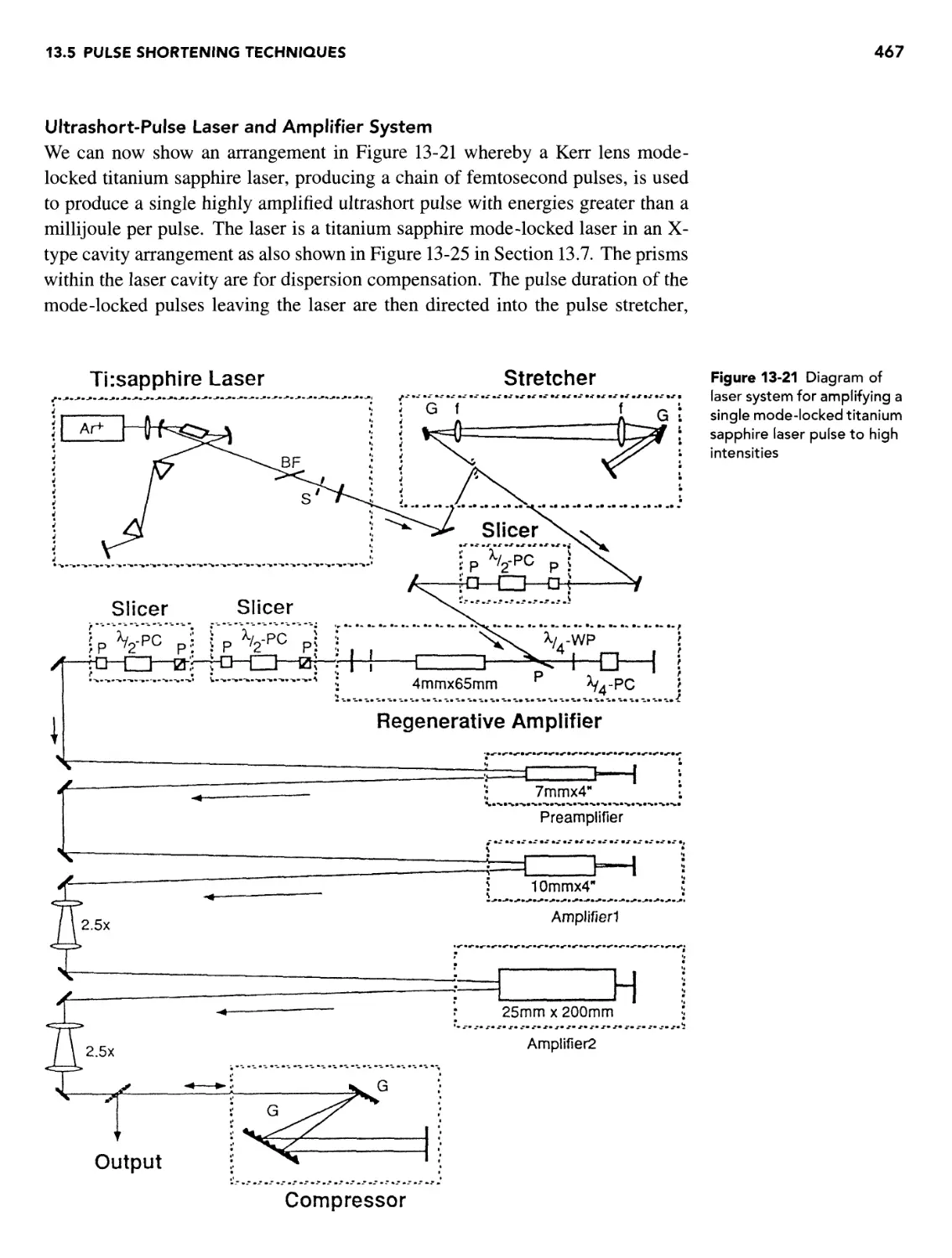
Pulse Compression (Shortening) with Gratings or Prisms 465
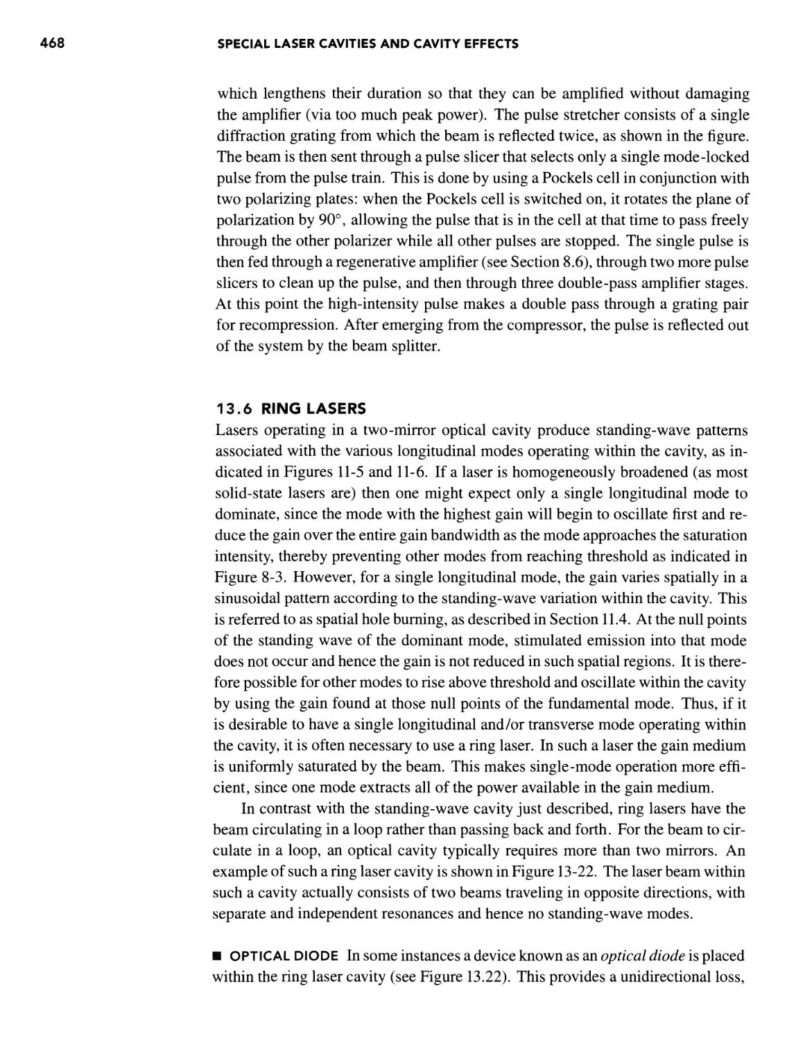
Ultrashort-Pulse Laser and Amplifer System 467
CONTENTS xv
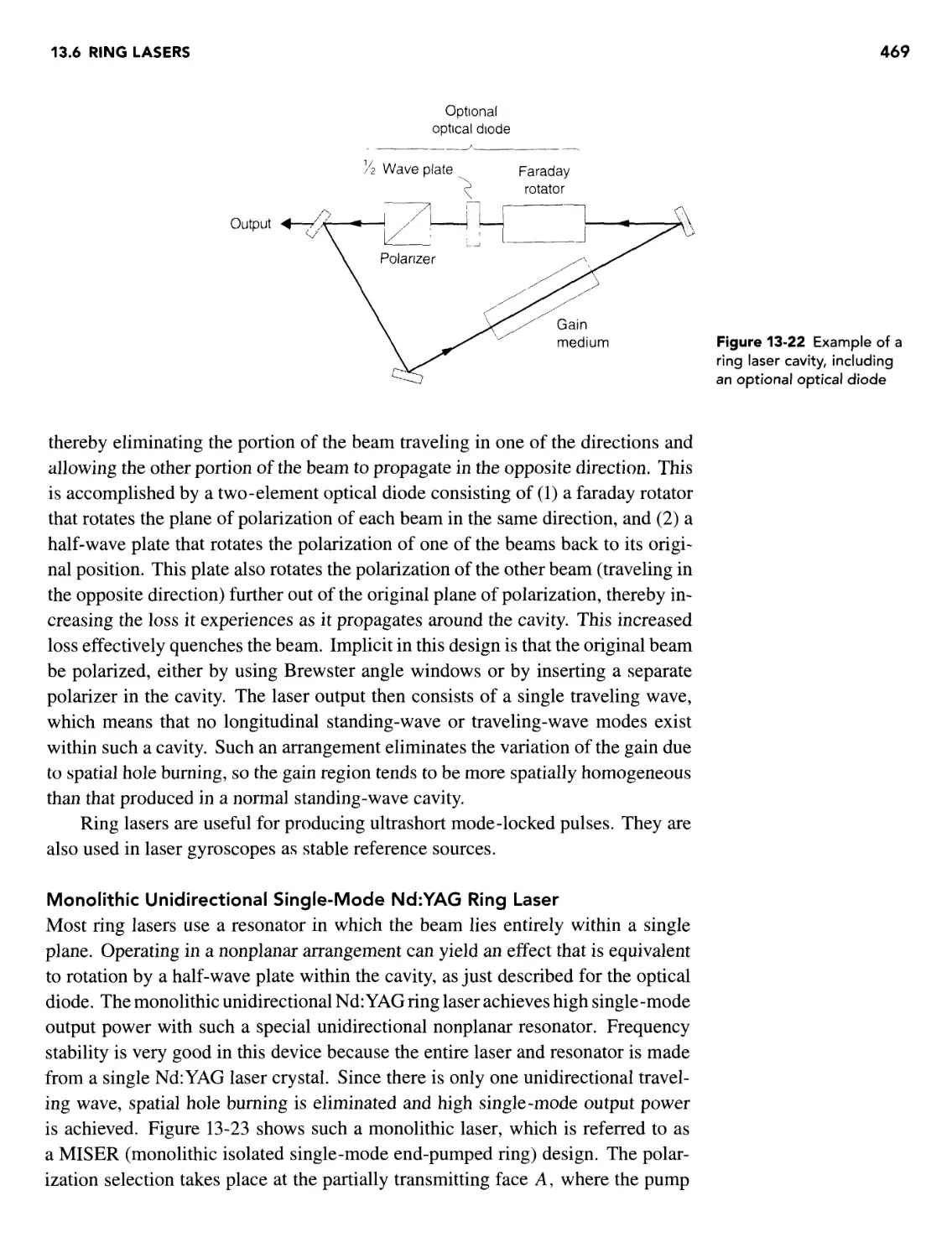
13.6 Ring Lasers 468
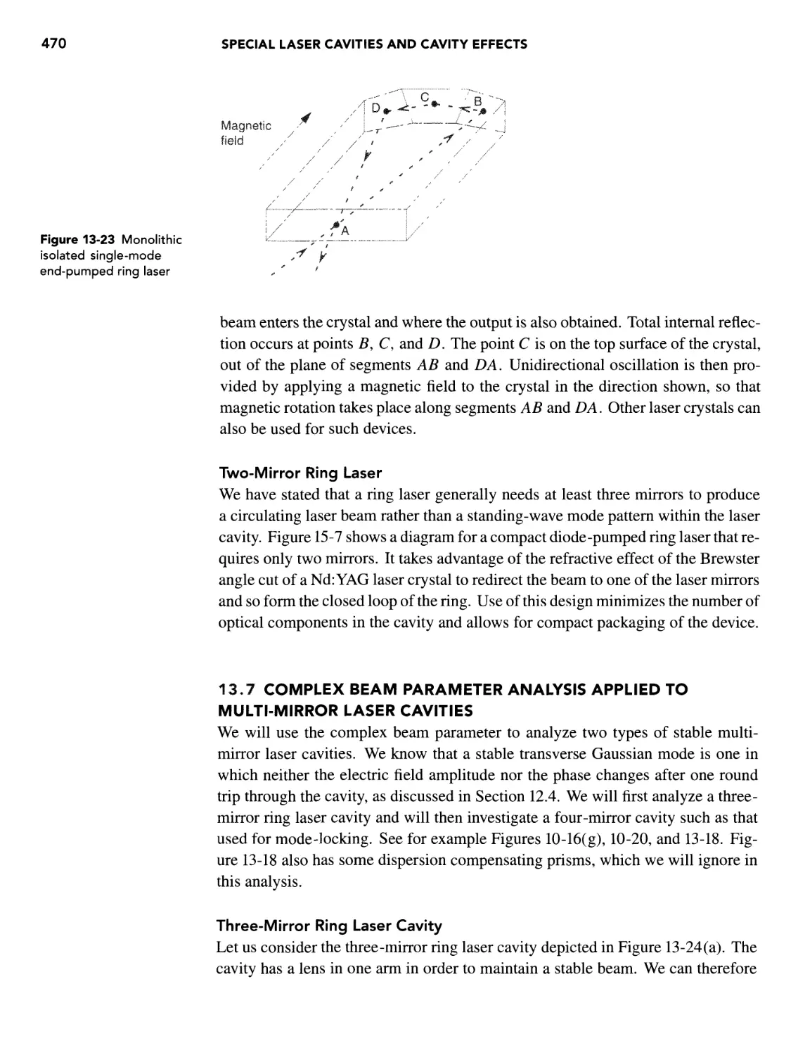
Monolithic Unidirectional Single-Mode Nd:YAG Ring Laser 469
Two-Mirror Ring Laser 470
13.7 Complex Beam Parameter Analysis Applied to Multi-Mirror
Laser Cavities 470
Three-Mirror Ring Laser Cavity 470
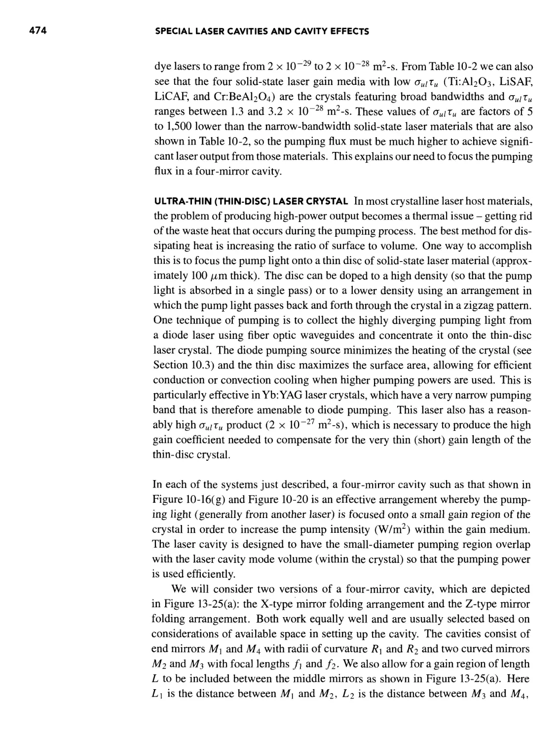
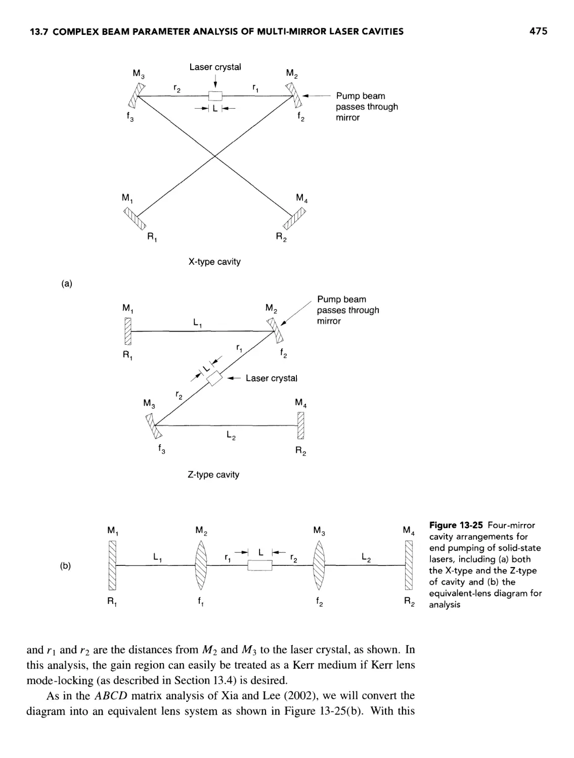
Three- or Four-Mirror Focused Cavity 473
13.8 Cavities for Producing Spectral Narrowing of
Laser Output 478
Cavity with Additional Fabry-Perot Etalon for Narrow-Frequency
Selection 478
Tunable Cavity 478
Broadband Tunable cw Ring Lasers 480
Tunable Cavity for Ultranarrow-Frequency Output 480
Distributed Feedback (DFB) Lasers 481
Distributed Bragg Reflection Lasers 484
13.9 Laser Cavities Requiring Small-Diameter Gain Regions -
Astigmatically Compensated Cavities 484
13.10 Waveguide Cavities for Gas Lasers 485
REFERENCES 486
PROBLEMS 488
mm
14 LASER SYSTEMS INVOLVING LOW-DENSITY GAIN MEDIA 491
OVERVIEW 491
14.1 Atomic Gas Lasers 491
Introduction 491
Helium-Neon Laser 492
General Description 492
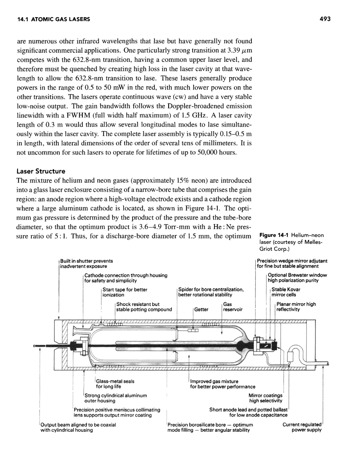
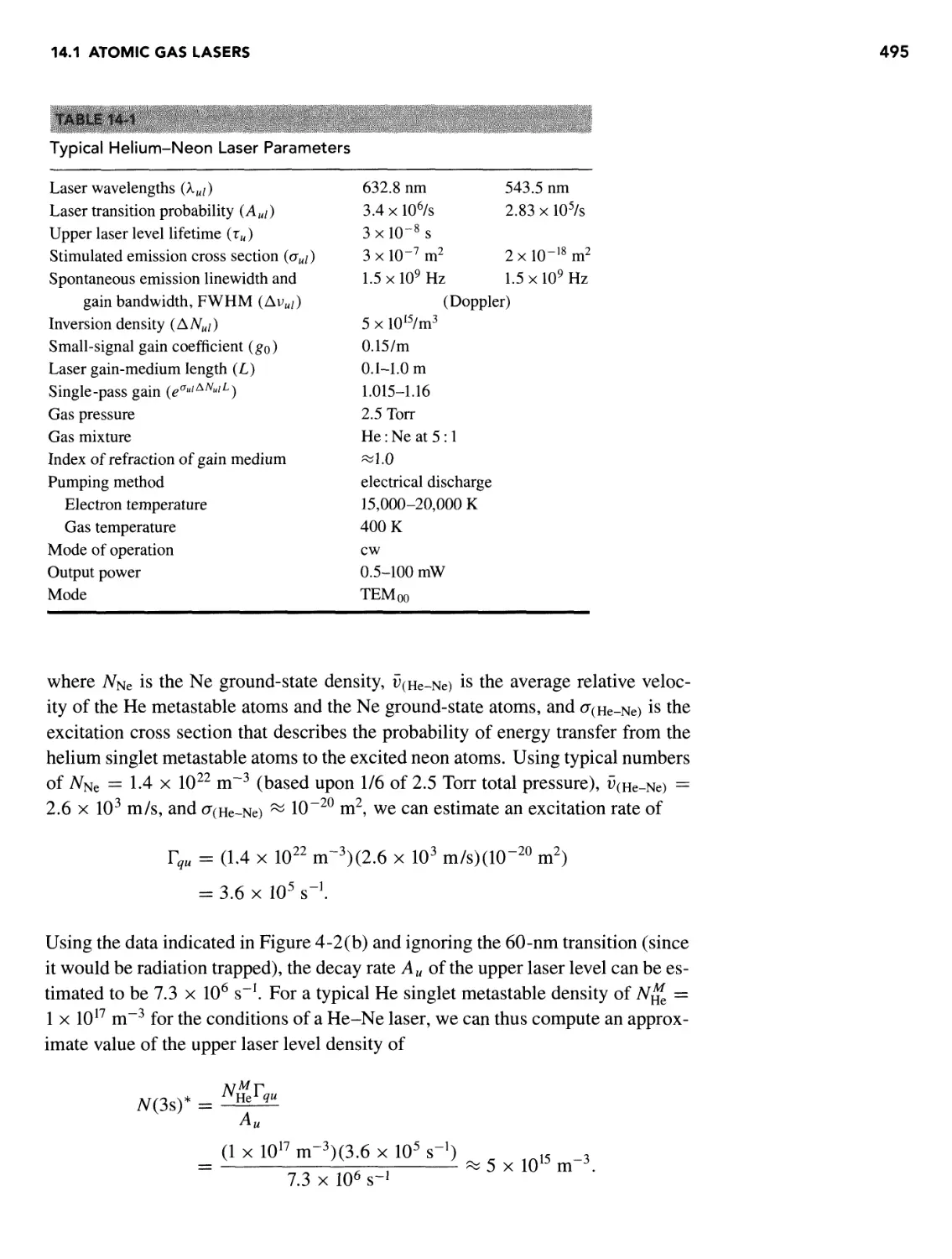
Laser Structure 493
Excitation Mechanism 494
Applications 497
Argon Ion Laser 497
General Description 497
Laser Structure 498
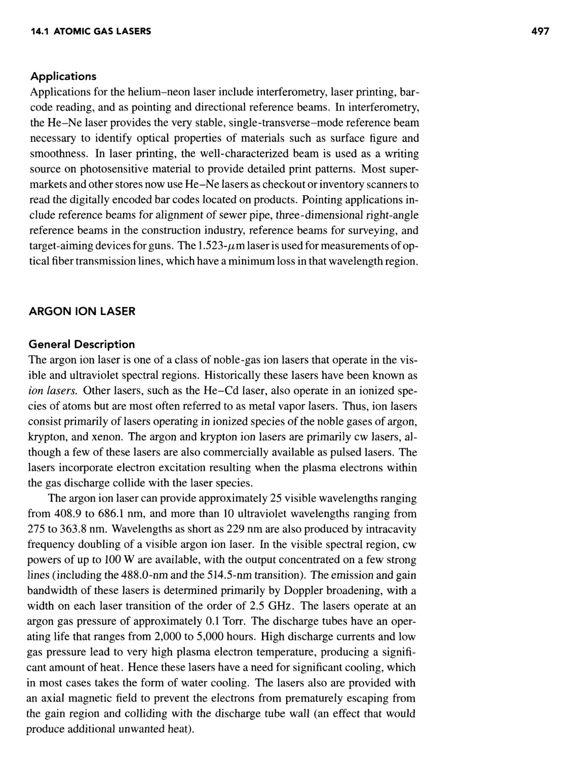
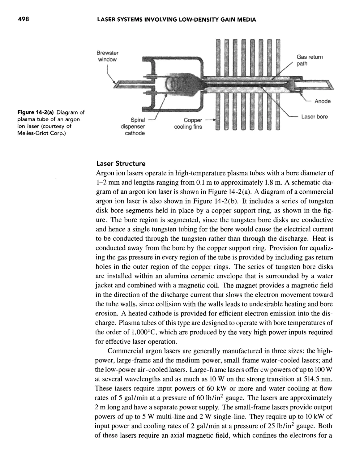
Excitation Mechanism 499
Krypton Ion Laser 500
Applications 501
Helium-Cadmium Laser 501
General Description 501
Laser Structure 502
Excitation Mechanism 504
Applications 505
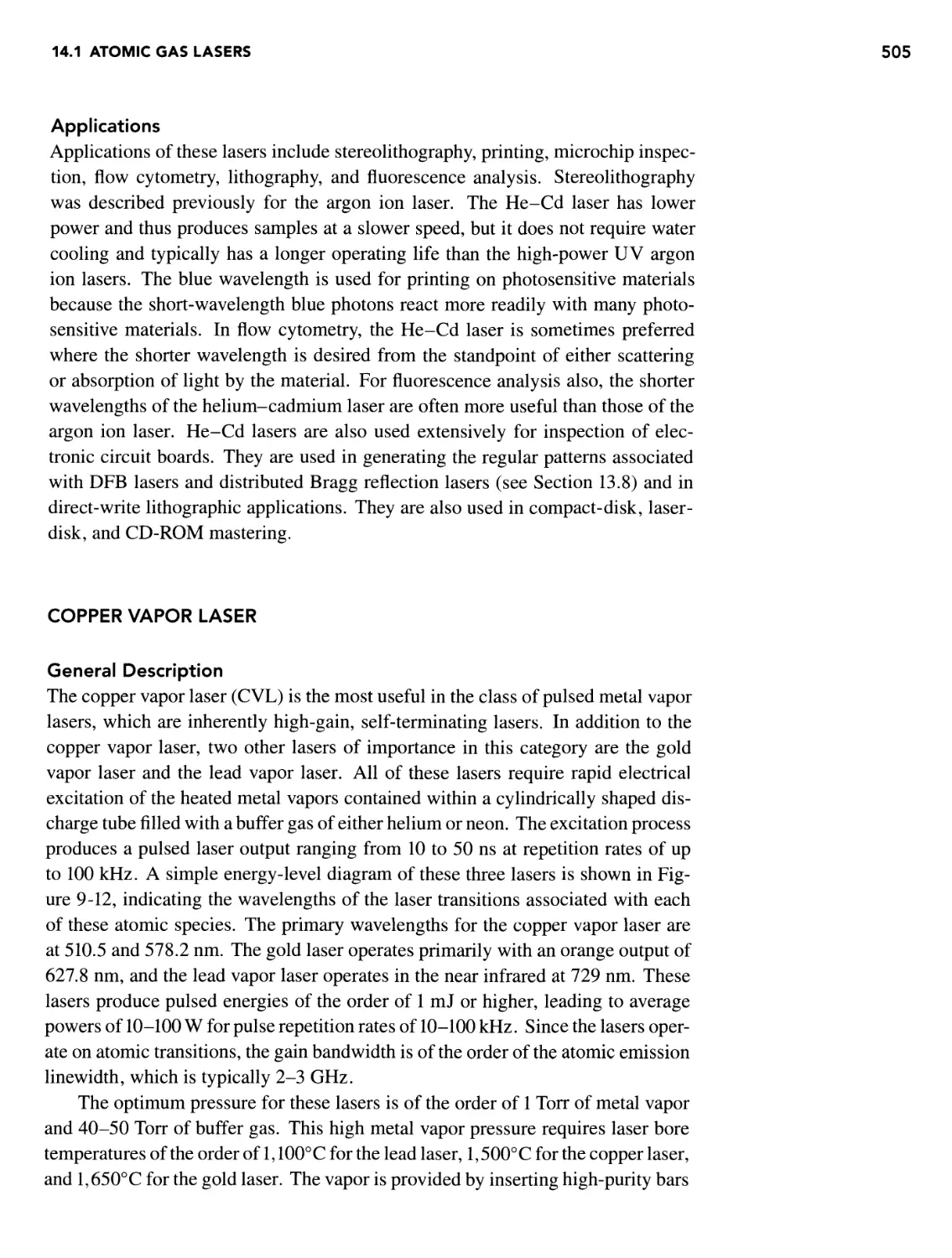
Copper Vapor Laser 505
General Description 505
Laser Structure 507
Excitation Mechanism 507
Applications 509
xvi CONTENTS
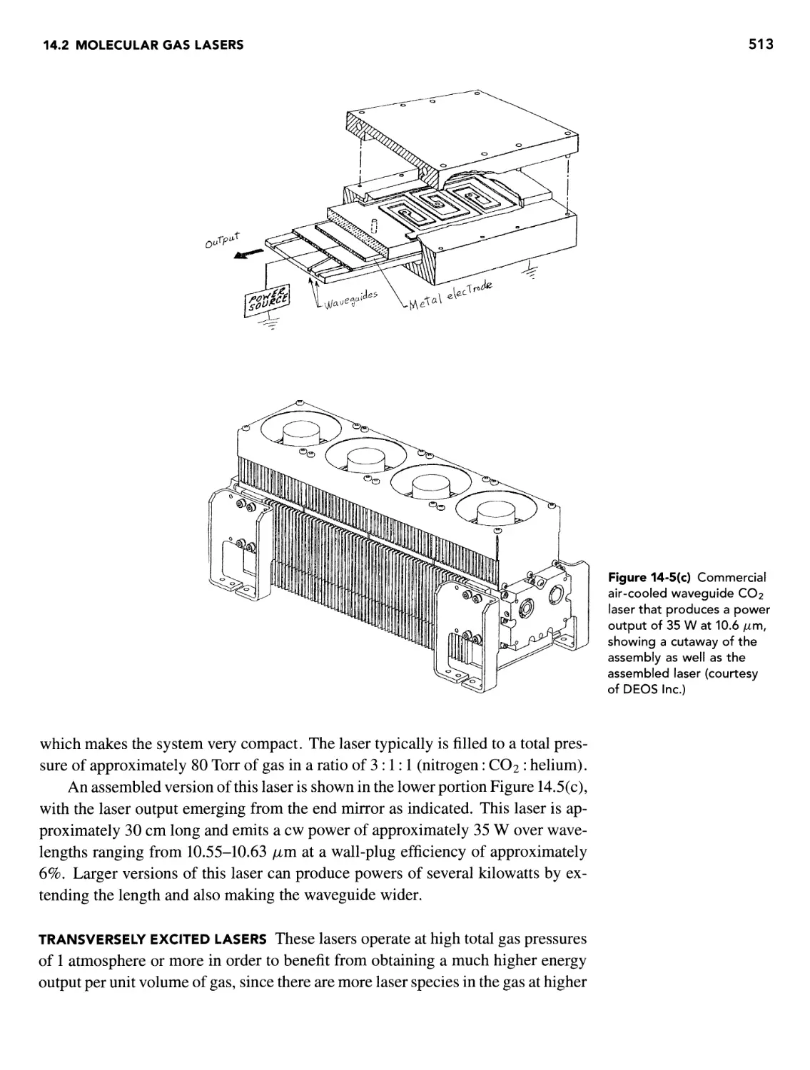
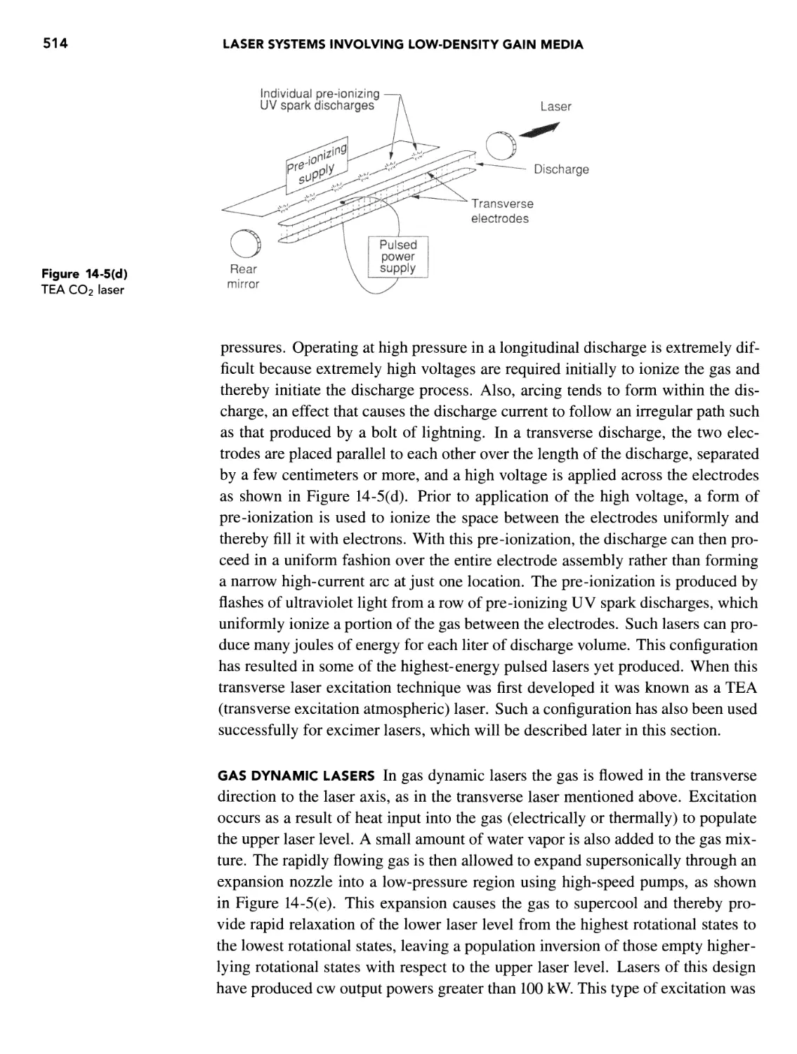
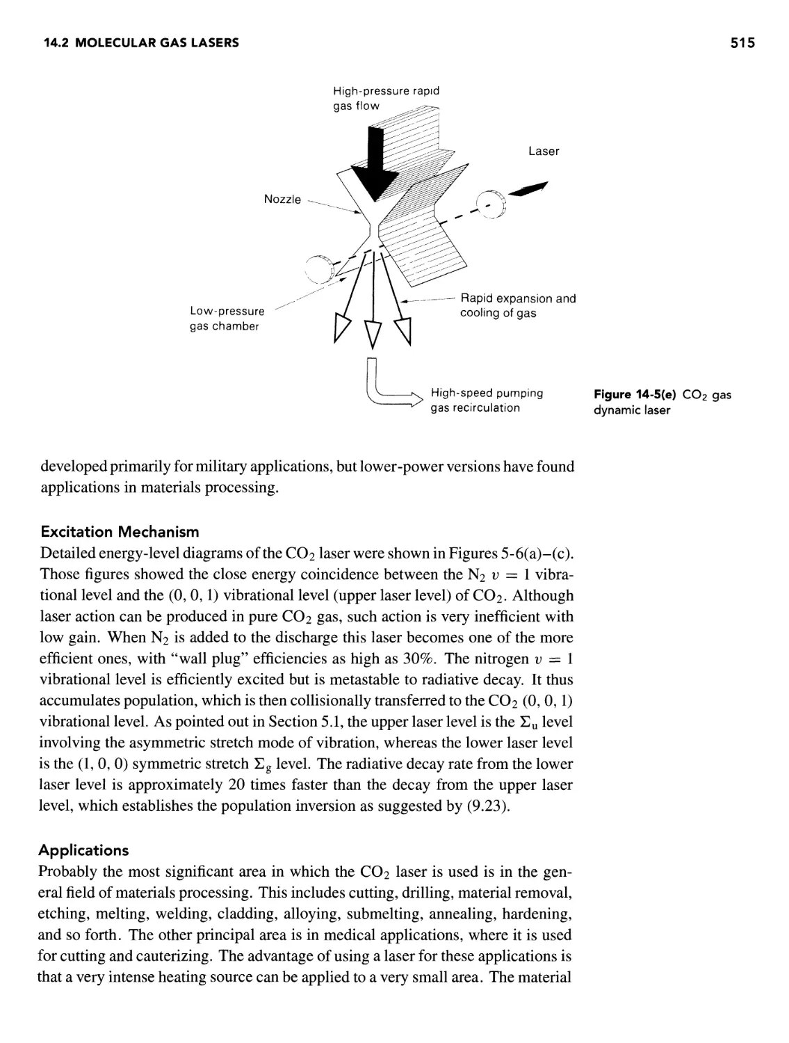
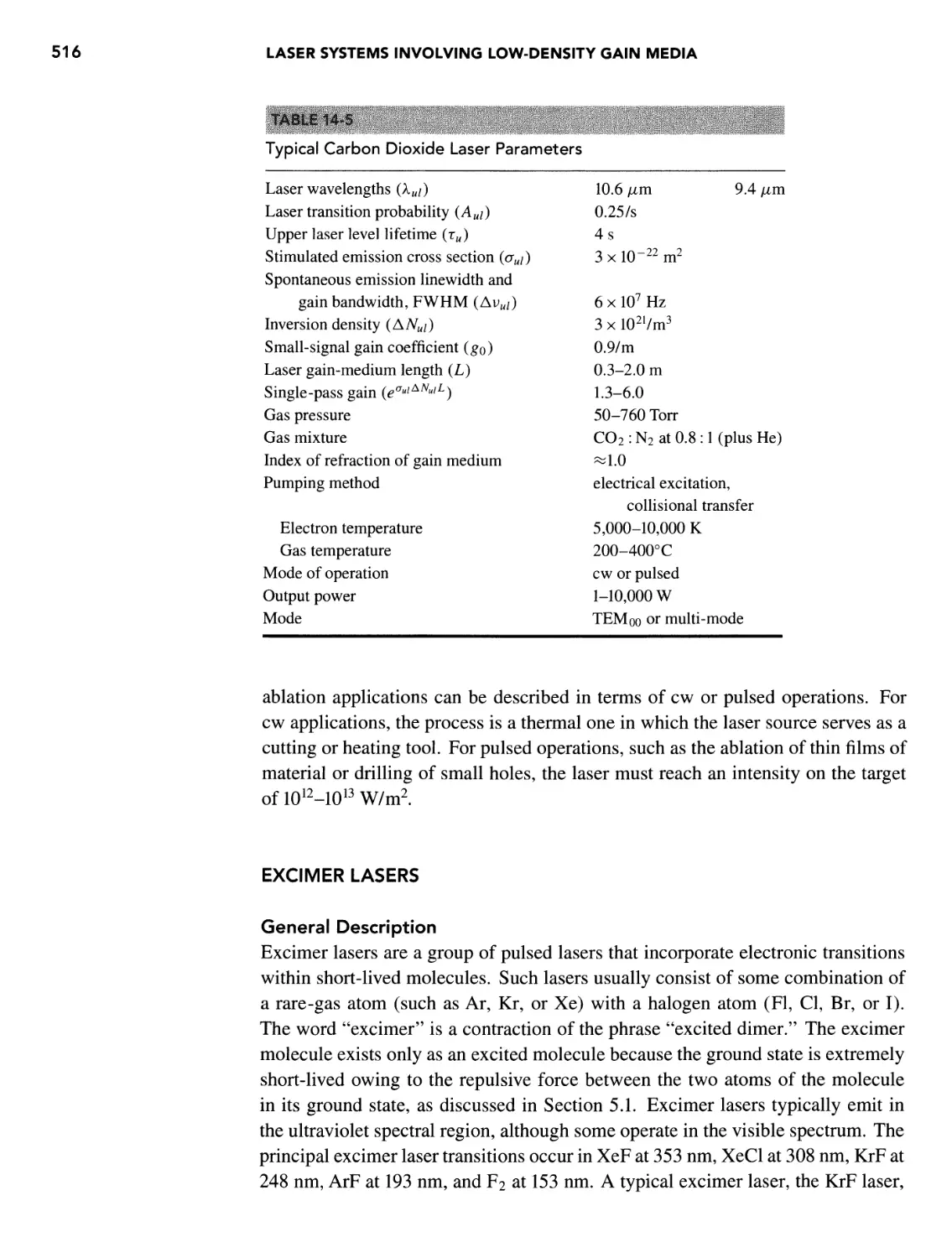
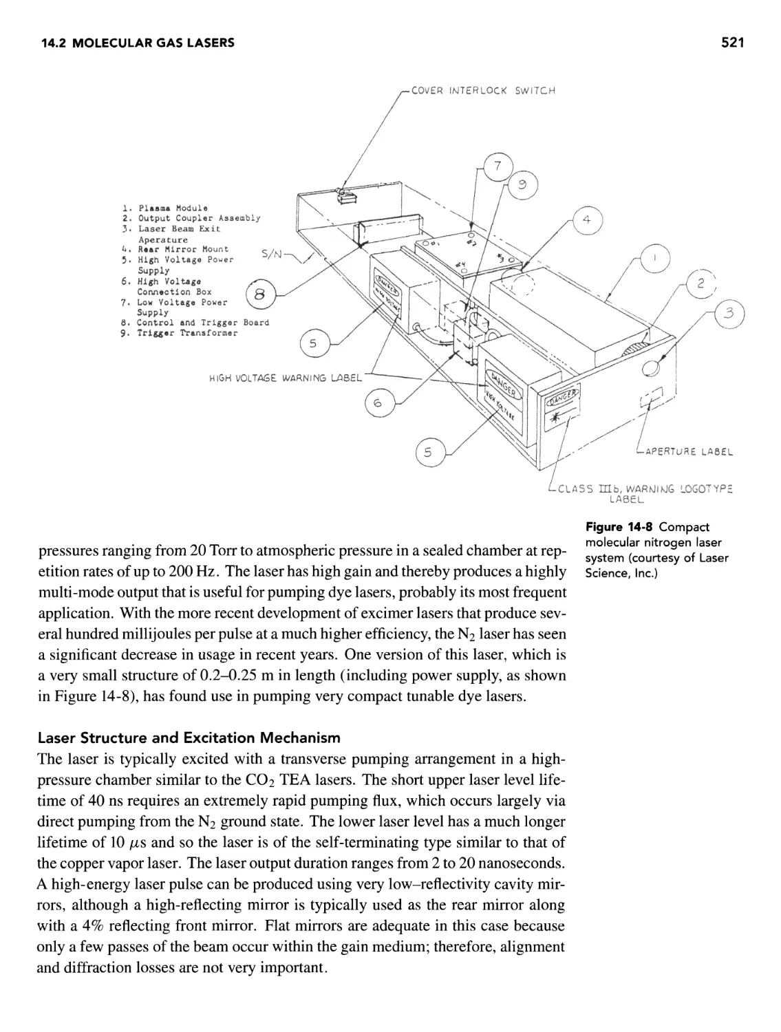
14.2 Molecular Gas Lasers
Introduction
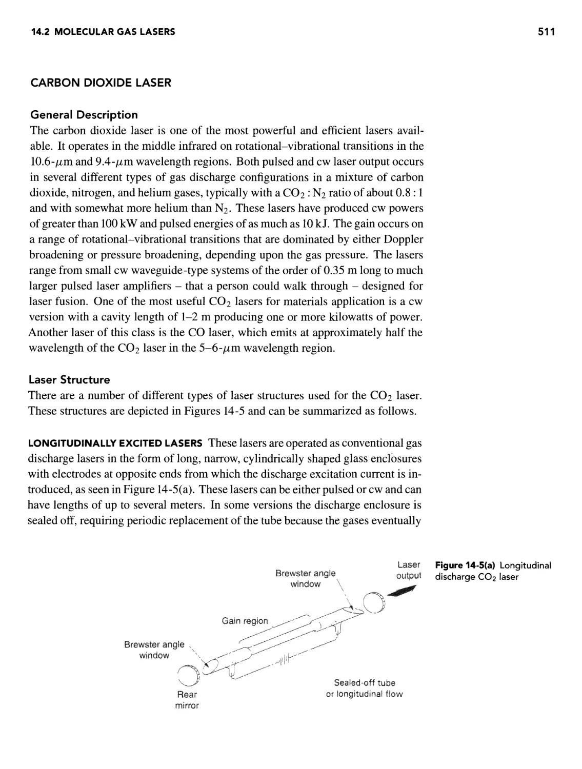
Carbon Dioxide Laser
General Description
Laser Structure
Excitation Mechanism
Applications
Excimer Lasers
General Description
Laser Structure
Excitation Mechanism
Applications
Nitrogen Laser
General Description
Laser Structure and Excitation Mechanism
Applications
Far-Infrared Gas Lasers
General Description
Laser Structure
Excitation Mechanism
Applications
Chemical Lasers
General Description
Laser Structure
Excitation Mechanism
Applications
14.3 X-Ray Plasma Lasers
Introduction
Pumping Energy Requirements
Excitation Mechanism
Optical Cavities
X-Ray Laser Transitions
Applications
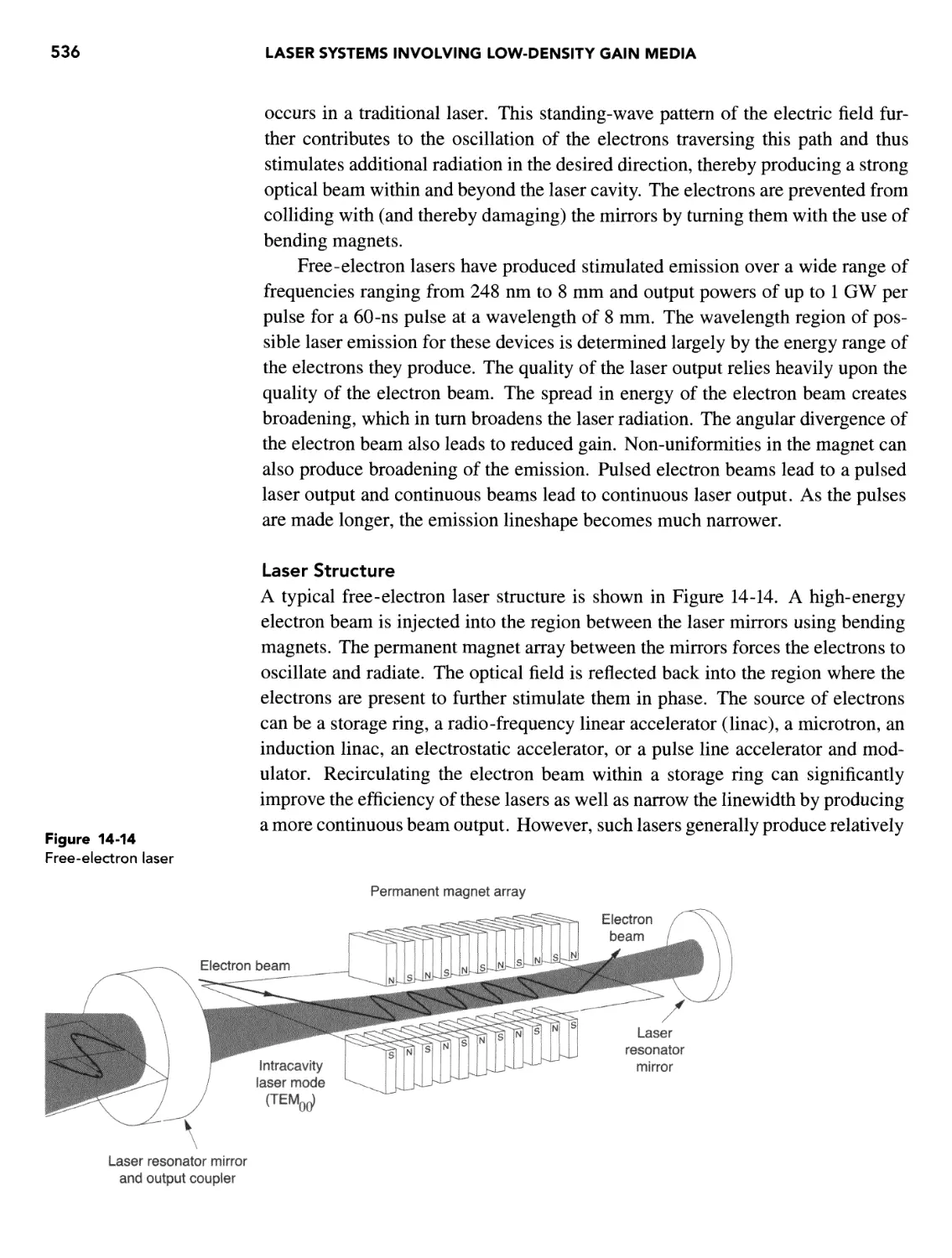
14.4 Free-Electron Lasers
Introduction
Laser Structure
Applications
REFERENCES
15 LASER SYSTEMS INVOLVING HIGH-DENSITY GAIN MEDIA
OVERVIEW
15.1 Organic Dye Lasers
Introduction
Laser Structure
Excitation Mechanism
Applications
15.2 Solid-State Lasers
Introduction
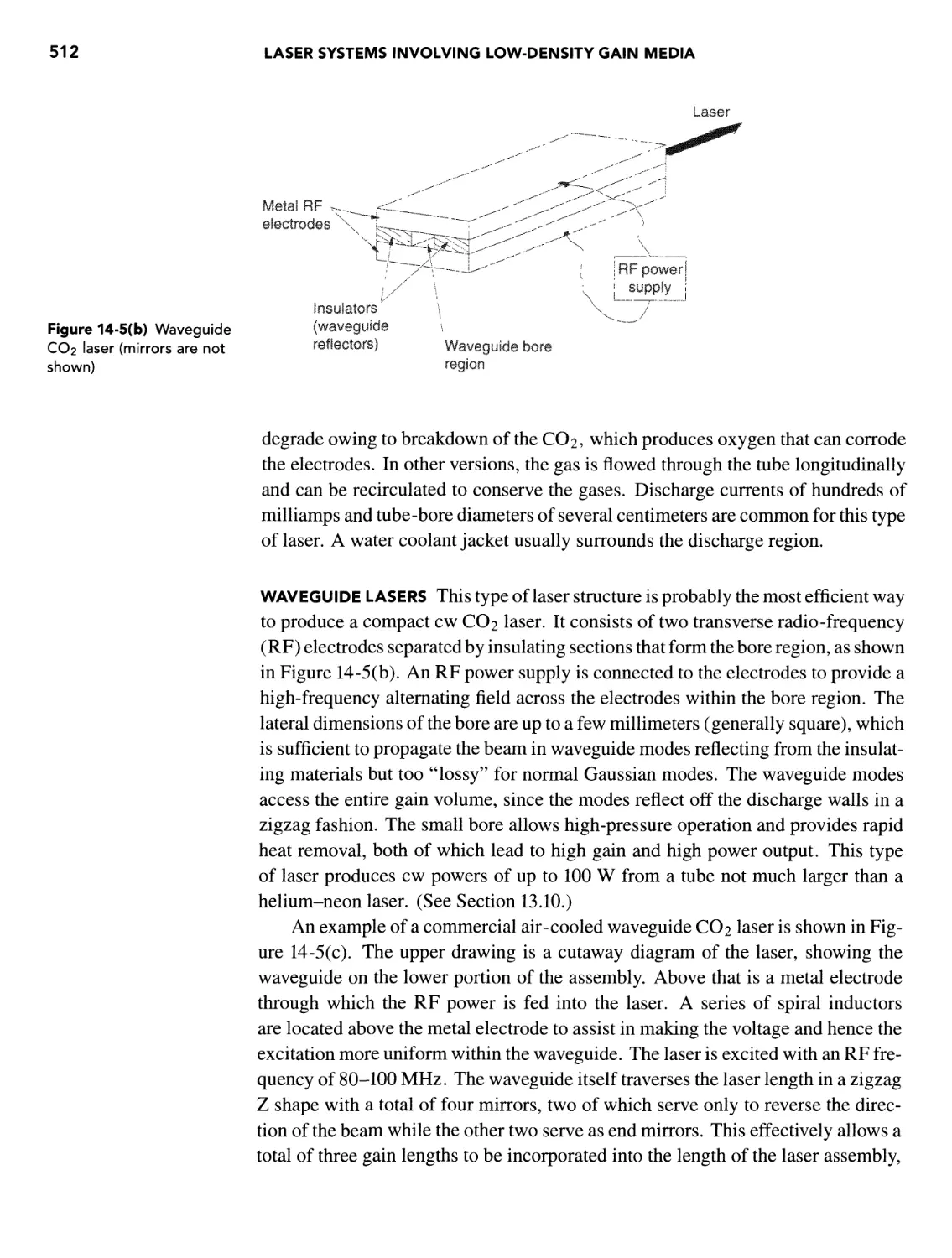
510
510
511
511
511
515
515
516
516
517
518
520
520
520
521
522
522
522
523
523
524
524
524
524
524
525
525
525
525
528
532
532
532
535
535
536
537
537
539
539
539
539
540
543
544
545
545
CONTENTS
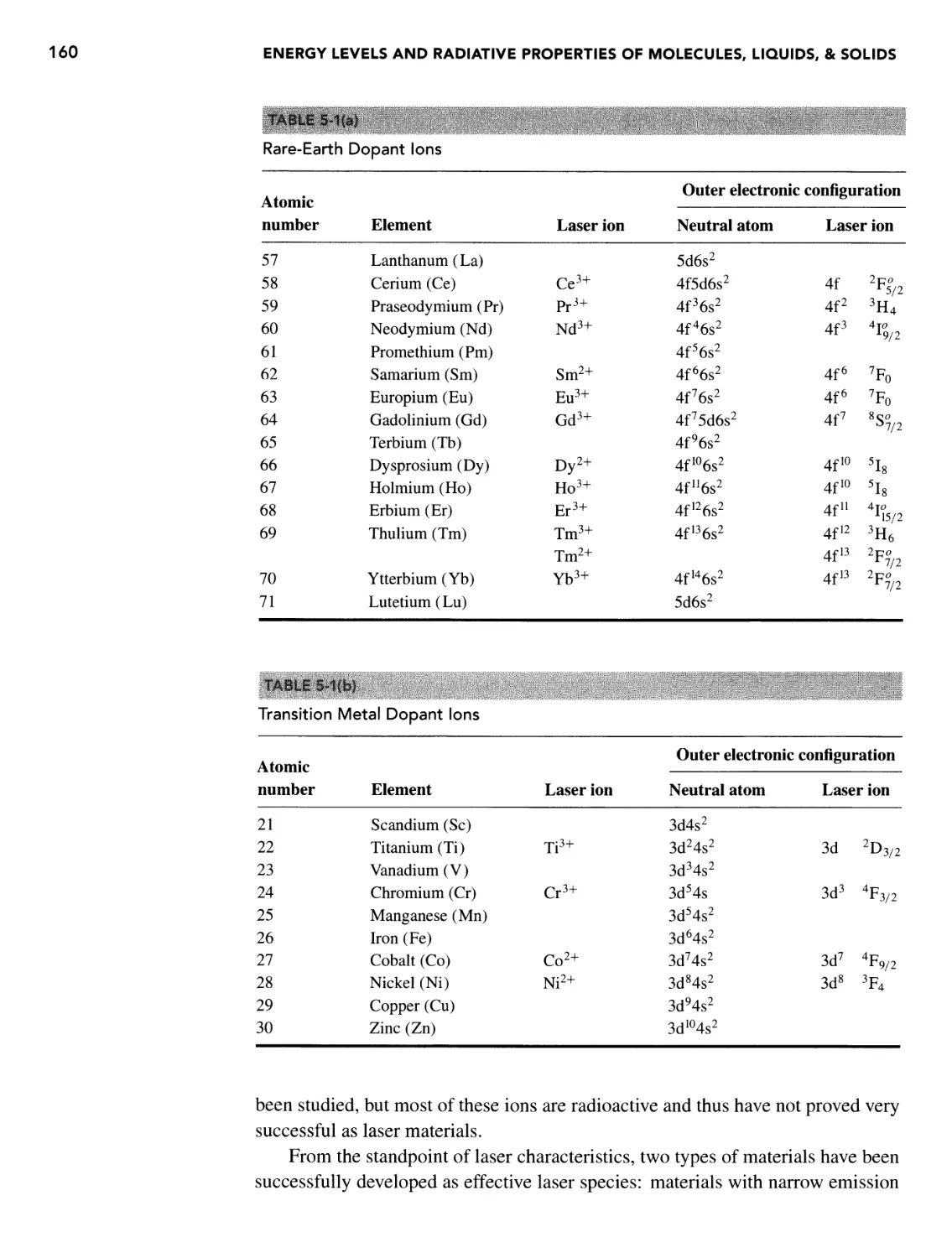
Ruby Laser 547
General Description 547
Laser Structure 548
Excitation Mechanism 548
Applications 549
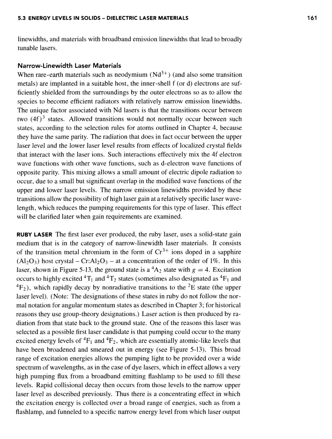
Neodymium YAG and Glass Lasers 550
General Description 550
Laser Structure 551
Excitation Mechanism 553
Applications 554
Neodymium: YLF Lasers 555
General Description 555
Laser Structure 556
Excitation Mechanism 556
Applications 557
Neodymium:Yttrium Vanadate (Nd:YVO4) Lasers 557
General Description 557
Laser Structure 557
Excitation Mechanism 558
Applications 558
Ytterbium:YAG Lasers 559
General Description 559
Laser Structure 560
Excitation Mechanism 560
Applications 561
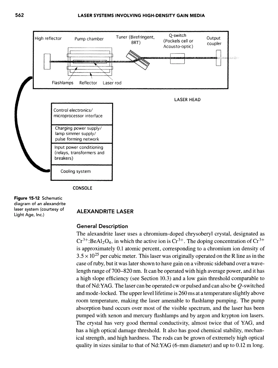
Alexandrite Laser 562
General Description 562
Laser Structure 563
Excitation Mechanism 563
Applications 564
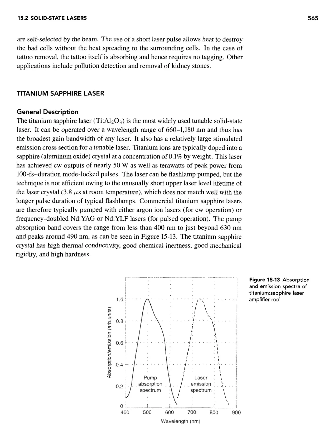
Titanium Sapphire Laser 565
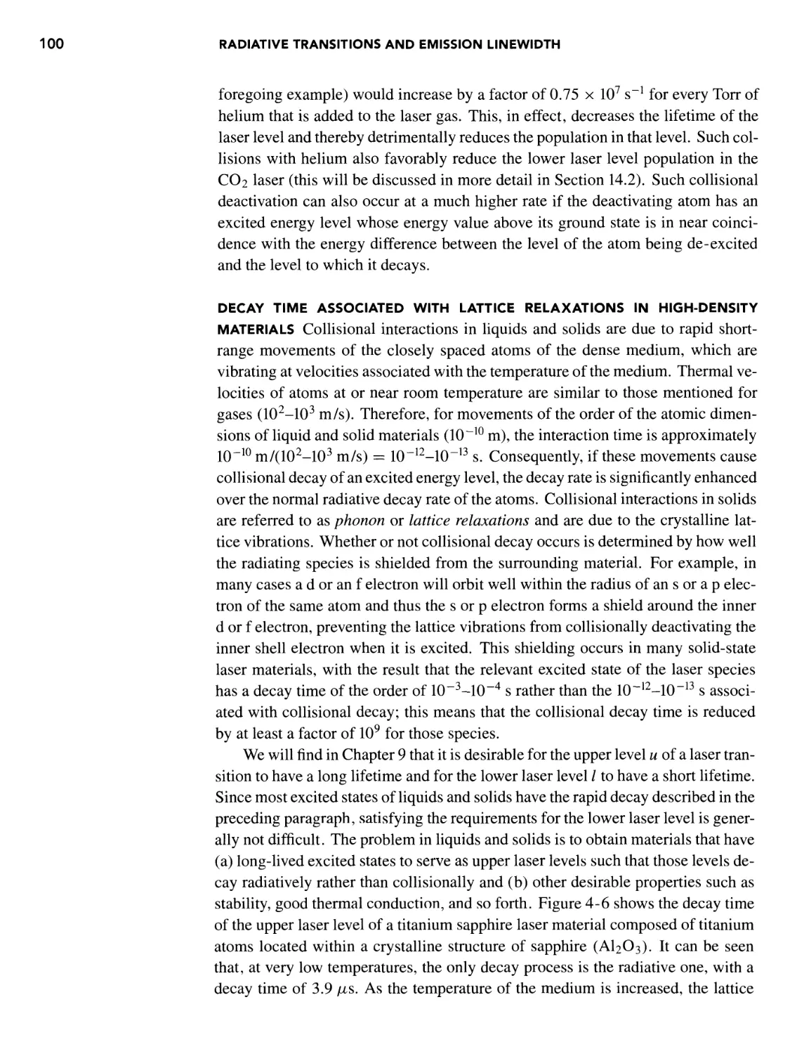
General Description 565
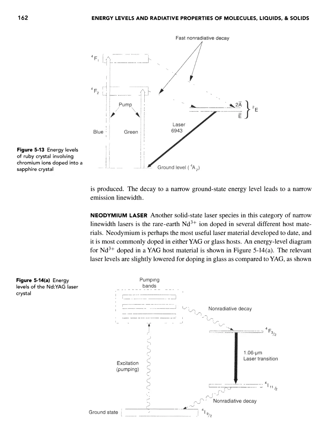
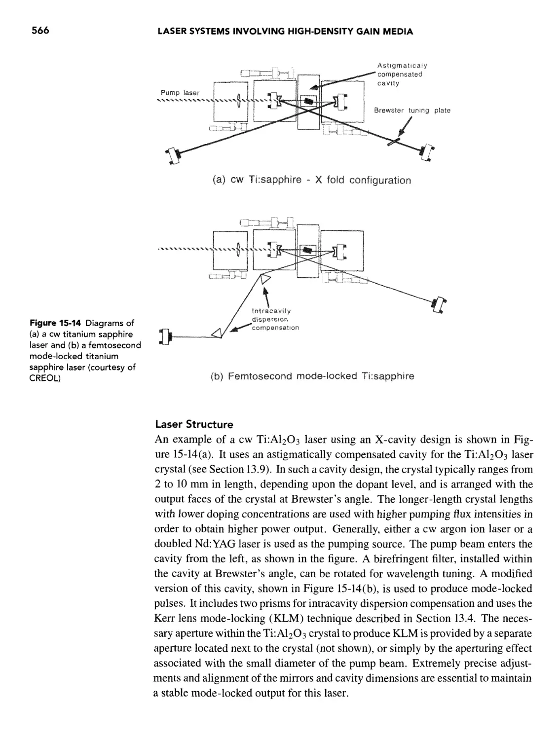
Laser Structure 566
Excitation Mechanism 567
Applications 568
Chromium LiSAF and LiCAF Lasers 568
General Description 568
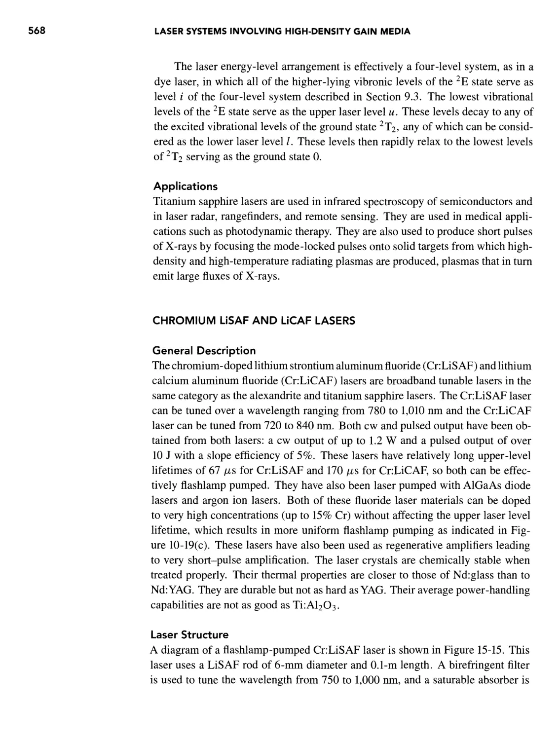
Laser Structure 568
Excitation Mechanism 569
Applications 570
Fiber Lasers 570
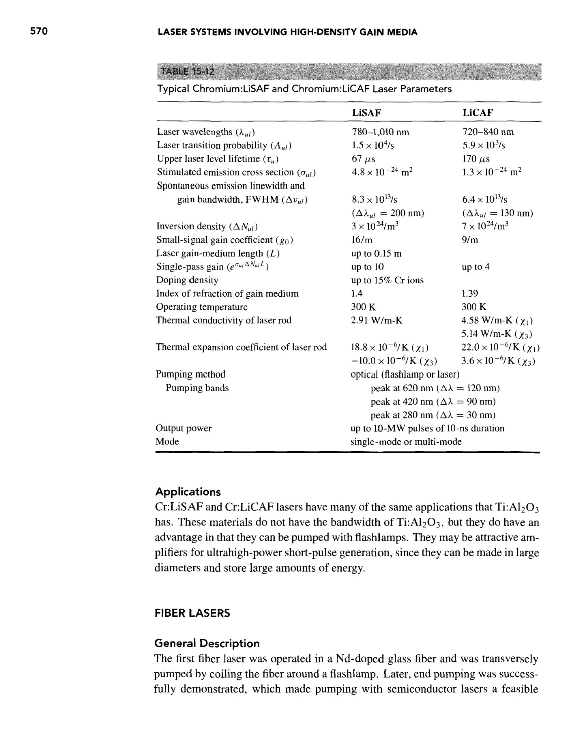
General Description 570
Laser Structure 571
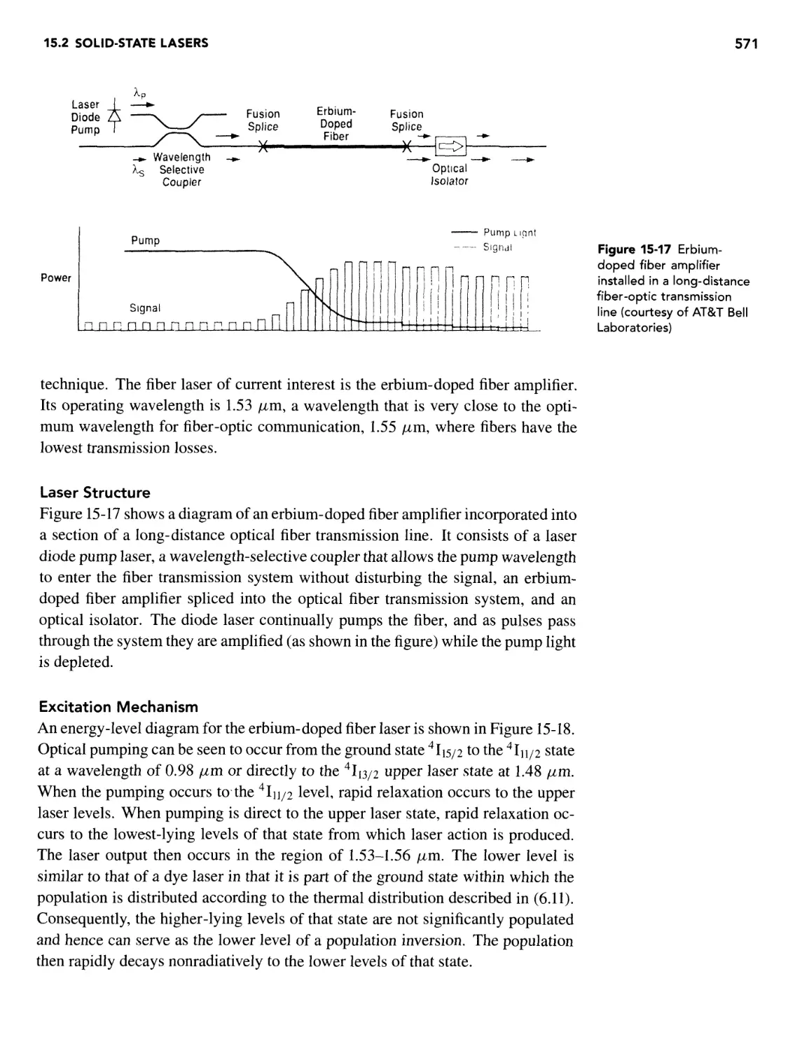
Excitation Mechanism 571
Applications 572
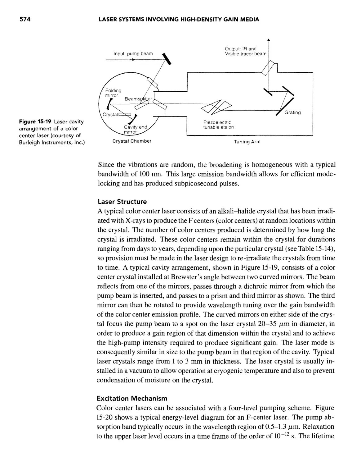
Color Center Lasers 573
General Description 573
Laser Structure 574
xviii CONTENTS
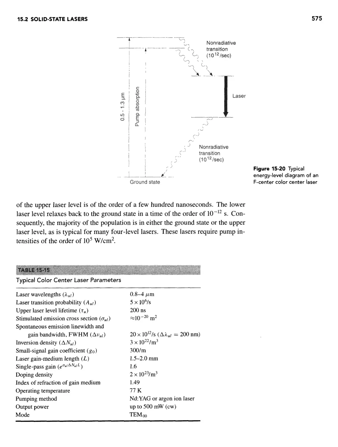
Excitation Mechanism 574
Applications 576
15.3 Semiconductor Diode Lasers 576
Introduction 576
Four Basic Types of Laser Materials 579
Laser Structure 581
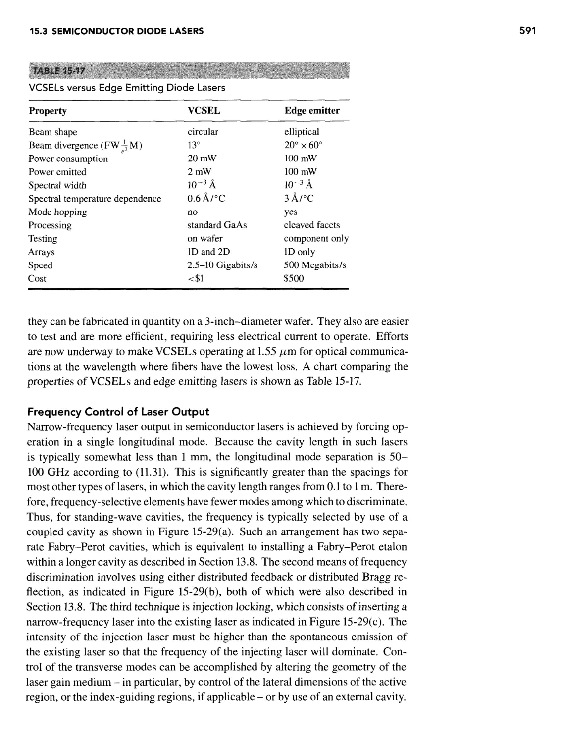
Frequency Control of Laser Output 591
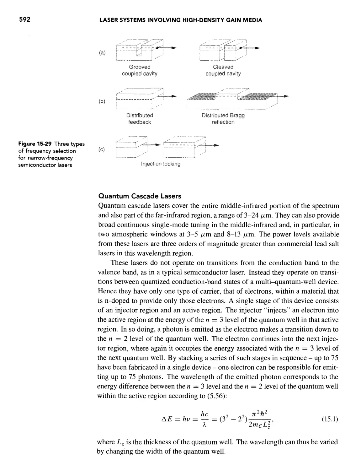
Quantum Cascade Lasers 592
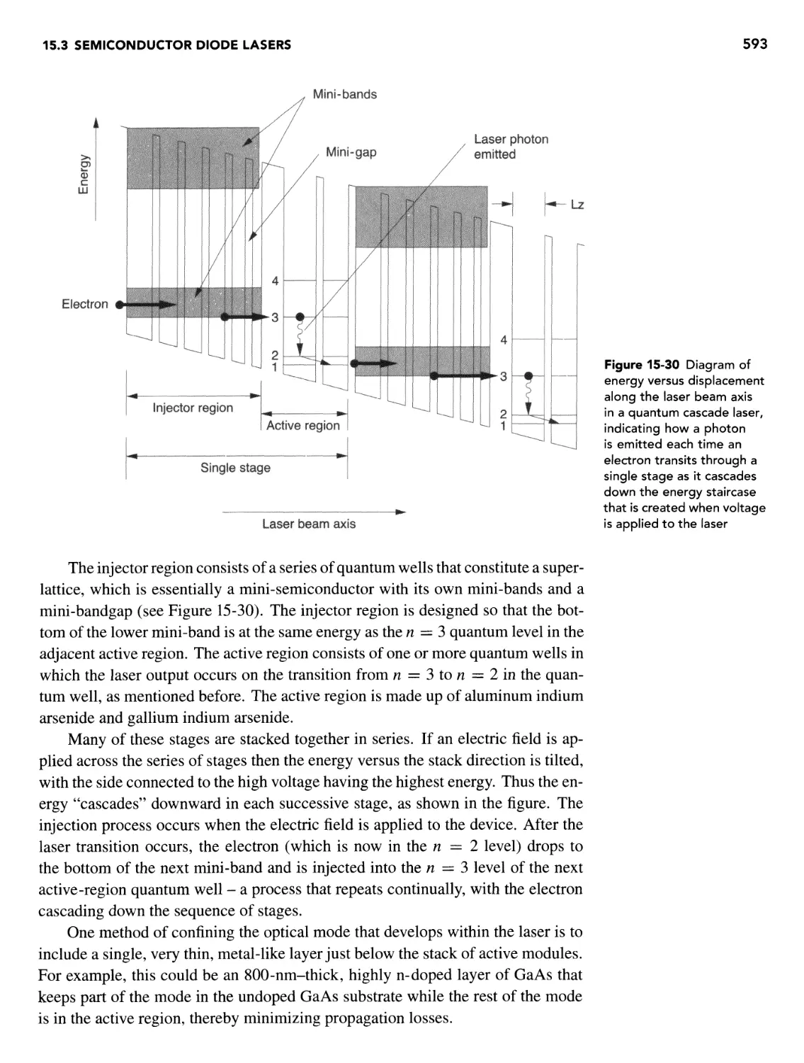
p-Doped Germanium Lasers 594
Excitation Mechanism 594
Applications 596
REFERENCES 597
16 FREQUENCY MULTIPLICATION OF LASERS AND OTHER
NONLINEAR OPTICAL EFFECTS 601
OVERVIEW 601
16.1 Wave Propagation in an Anisotropic Crystal 601
16.2 Polarization Response of Materials to Light 603
16.3 Second-Order Nonlinear Optical Processes 604
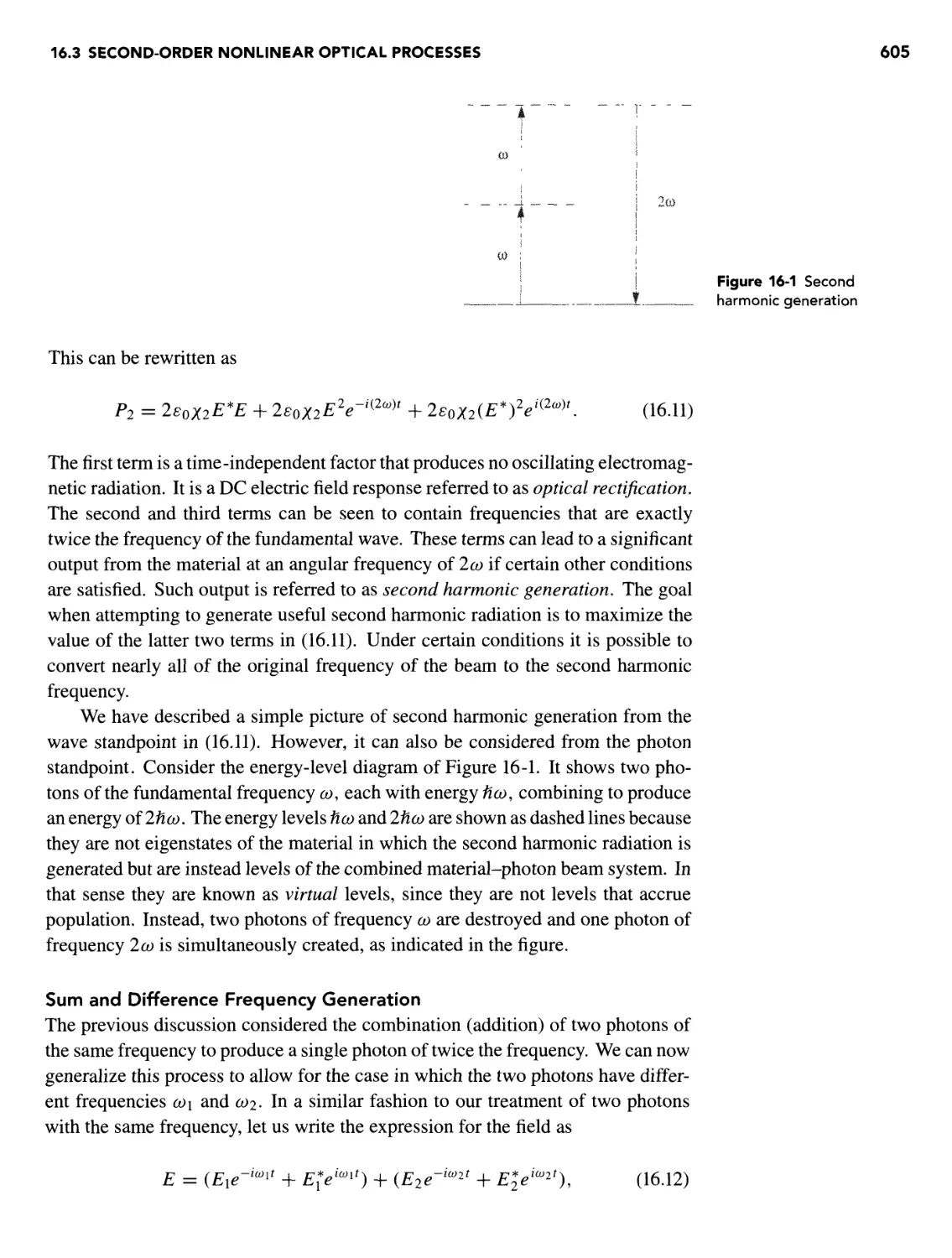
Second Harmonic Generation 604
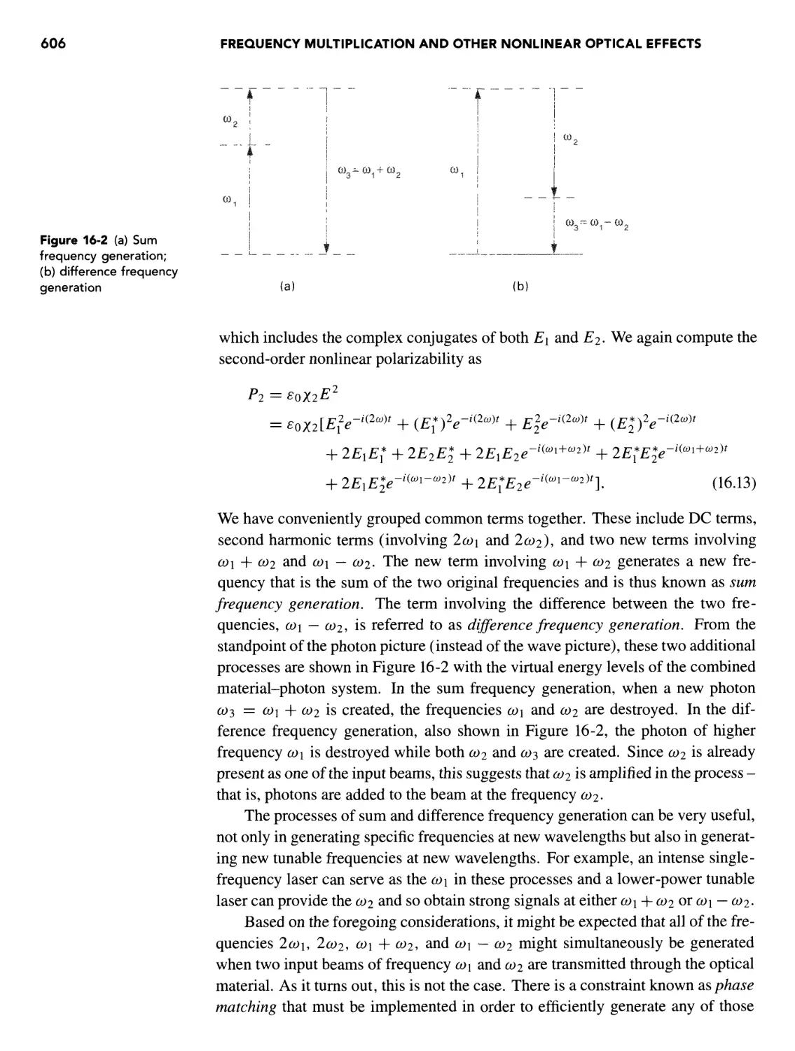
Sum and Difference Frequency Generation 605
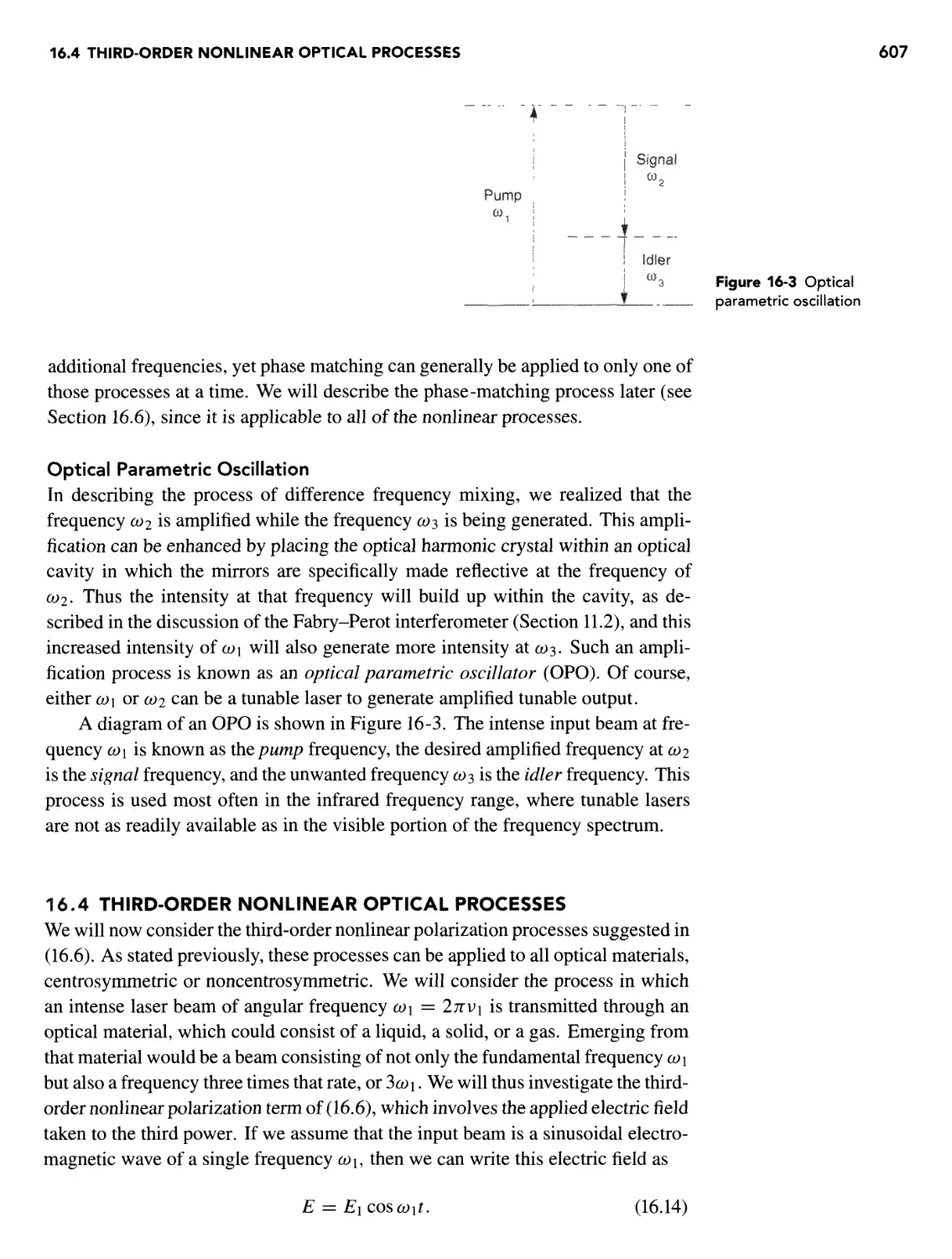
Optical Parametric Oscillation 607
16.4 Third-Order Nonlinear Optical Processes 607
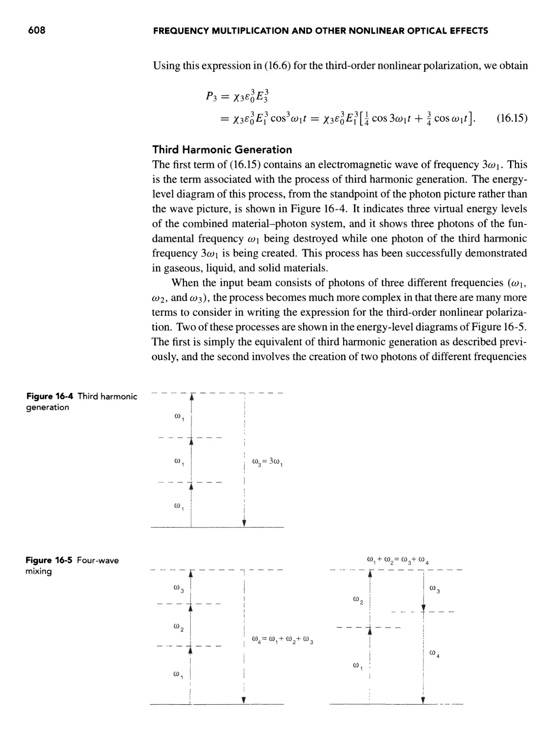
Third Harmonic Generation 608
Intensity-Dependent Refractive Index - Self-Focusing 609
16.5 Nonlinear Optical Materials 610
16.6 Phase Matching 610
Description of Phase Matching 610
Achieving Phase Matching 613
Types of Phase Matching 615
16.7 Saturable Absorption 615
16.8 Two-Photon Absorption 617
16.9 Stimulated Raman Scattering 618
16.10 Harmonic Generation in Gases 619
REFERENCES 619
Appendix 621
Index 625
Preface to the Second Edition
I am very pleased to have completed this Second Edition of Laser Fundamentals.
The encouragement I have received over the past few years from readers as well
as from my editors was sufficient to provide me with the enthusiasm to take on
this new task. Writing the first edition was essentially a ten-year endeavor from
first thoughts to the completed book. I thought I had a better way to explain to
senior-level and first-year graduate students how lasers work. Apparently there
were others who agreed with me, judging from comments I have received. Writing
the second edition was an attempt to fill in some of the gaps, so to speak; not sur-
surprisingly, it took much more time than I had anticipated. Some of the areas of the
First Edition were not as complete as I would have liked. There were also errors
that had to be corrected. In addition, there have been advances - primarily in the
areas of solid-state and semiconductor lasers - that needed to be included. I think
the new edition addresses those issues pretty well. I suppose it's up to the readers
to make that judgment.
Naturally one can't take on a task like this without gleaning information from
experts in the various fields of lasers. I offer special thanks to my colleagues at
the School of Optics/CREOL at the University of Central Florida: Michael Bass,
Glenn Boreman, Peter Delfyett, Dave Hagan, Hans Jenssen, Patrick Li Kam Wa,
Alexandra Rapaport, Kathleen Richardson, Martin Richardson, Craig Siders, Eric
Van Stryland, Nikolai Vorobiev, and Boris Zeldovich. Others who were very help-
helpful include Norm Hodgson, Jason Eichenholz, Jack Jewell, Shuji Nakamura, Jorge
Rocca, Rita Petersen, and Colin Webb (and I'm sure I've inadvertently left out
a few).
I am grateful to have Simon Capelin as my editor at Cambridge University
Press. He has been most encouraging without pressing me with a specific dead-
deadline. It is also a pleasure to work again with Matt Darnell as my production editor.
Most importantly, I thank my wonderful wife, Susan, who was always very sup-
supportive while putting up with the many long hours that I spent in completing this
Second Edition.
XIX
Preface to the First Edition
I wrote Laser Fundamentals with the idea of simplifying the explanation of how
lasers operate. It is designed to be used as a senior-level or first-year graduate stu-
student textbook and/or as a reference book. The first draft was written the first time
I taught the course "Laser Principles" at the University of Central Florida. Before
that, I authored several general laser articles and taught short courses on the sub-
subject, giving careful consideration to the sequence in which various topics should
be presented. During that period I adjusted the sequence, and I am now convinced
that it is the optimal one.
Understanding lasers involves concepts associated with light, viewed either
as waves or as photons, and its interaction with matter. I have used the first part
of the book to introduce these concepts. Chapters 2 through 6 include fundamen-
fundamental wave properties, such as the solution of the wave equation, polarization, and
the interaction of light with dielectric materials, as well as the fundamental quan-
quantum properties, including discrete energy levels, emission of radiation, emission
broadening (in gases, liquids, and solids), and stimulated emission. The concept of
amplification is introduced in Chapter 7, and further properties of laser amplifiers
dealing with inversions and pumping are covered in Chapters 8 and 9 [Chapters
8-10 in the Second Edition - Ed.]. Chapter 10 [11] discusses cavity properties as-
associated with both longitudinal and transverse modes, and Chapters 11 and 12 [12
and 13] follow up with Gaussian beams and special laser cavities. Chapters 13 and
14 [14 and 15] provide descriptions of the most common lasers. The book con-
concludes in Chapter 15 [16] with a brief overview of some of the nonlinear optical
techniques for laser frequency conversion.
Some of the unique aspects of the book are the treatment of emission linewidth
and broadening in Chapter 4, the development of a simple model of a laser ampli-
amplifier in Chapter 7, the discussion of special laser cavities in Chapter 12 [13], and the
laser summaries in Chapters 13 and 14 [14 and 15]. Throughout the book, when-
whenever a particular concept is introduced, I have tried to relate that concept to all
the various types of laser amplifiers including gas lasers, liquid (dye) lasers, and
solid-state lasers. My intention is to give the reader a good understanding, not just
of one specific type of laser but rather of all types of lasers, as each concept is
introduced.
XXI
xxii PREFACE
The book can be used in either a one- or two-semester course. In one semester
the topics of Chapters 2 through 12 [13] would be emphasized. In two semesters,
extended coverage of the specific lasers of Chapters 13 and 14 [14 and 15], as well
as the frequency multiplication in Chapter 15 [16], could be included. In a one-
semester course I have been able to cover a portion of the material in Chapters 13
and 14 [14 and 15] by having each student write a report about one specific laser
and then give a ten- or fifteen-minute classroom presentation about that laser. The
simple quantum mechanical descriptions in Chapters 3 and 4 were introduced to
describe how radiative transitions occur in matter. If the instructor chooses to avoid
quantum mechanics in the course, it would be sufficient to stress the important re-
results that are highlighted at the ends of each of those sections.
Writing this book has been a rewarding experience for me. I have been associ-
associated with lasers since shortly after their discovery in 1960 when, as an undergrad-
undergraduate student at the University of Utah, I helped build a ruby laser for a research
project under Professor Frank Harris. He was the first person to instill in me an en-
enthusiasm for optics and light. I was then very fortunate to be able to do my thesis
work with Professor Grant Fowles, who encouraged me to reduce ideas to simple
concepts. We discovered many new metal vapor lasers during that period. I also
thank Dr. John Sanders for giving me the opportunity to do postdoctoral work at the
Clarendon Laboratory at Oxford University in England, and Dr. Kumar Patel for
bringing me to Bell Laboratories in Holmdel, New Jersey. Being a part of a stim-
stimulating group of researchers at Bell Laboratories during the growth of the field of
lasers was an unparalleled opportunity. During that period I was also able to spend
an extremely rewarding sabbatical year at Stanford University with Professor Steve
Harris. Finally, to round out my career I put on my academic hat at the University
of Central Florida as a member of the Center for Research and Education in Optics
and Lasers (CREOL) and the Department of Physics and of Electrical and Com-
Computer Engineering. Working in the field of lasers at several different institutions
has provided me with a broad perspective that I hope has successfully contributed
to the manner in which many of the concepts are presented in this book.
Acknowledgments
I first acknowledge the support of my wife, Susan. Without her encouragement
and patience, I would never have completed this book.
Second, I am deeply indebted to Mike Langlais, an undergraduate student at
the University of Central Florida and a former graphics illustrator, who did most
of the figures for the book. I provided Mike with rough sketches, and a few days
later he appeared with professional quality figures. These figures add immensely
to the completeness of the book.
Colleagues who have helped me resolve particular issues associated with this
book include Michael Bass, Peter Delfyett, Luis Elias, David Hagan, James Har-
Harvey, Martin Richardson, and Eric Van Stryland of CREOL; Tao Chang, Larry Col-
dren, Dick Fork, Eric Ippen, Jack Jewell, Wayne Knox, Herwig Kogelnik, Tingye
Li, David Miller, Peter Smith, Ben Tell, and Obert Wood of Bell Laboratories; Bob
Byer, Steve Harris, and Tony Siegman of Stanford University; Boris Stoicheff of
the University of Toronto; Gary Eden of the University of Illinois; Ron Waynant of
the FDA; Arto Nurmiko of Brown University; Dennis Matthews of Lawrence Liv-
ermore National Laboratories; Syzmon Suckewer of Princeton University; Colin
Webb of Oxford University; John Macklin of Stanford University and Bell Labs;
Jorge Rocca of Colorado State University; Frank Tittle of Rice University; Frank
Duarte of Kodak; Alan Petersen of Spectra Physics; Norman Goldblatt of Coher-
Coherent, Inc.; and my editor friend, Irwin Cohen. I also thank the many laser companies
who contributed figures, primarily in Chapters 13 and 14 [14 and 15 in 2e]. I'm
sure that I have left a few people out; for that, I apologize to them. In spite of all
the assistance, I accept full responsibility for the final text.
I thank my editor, Philip Meyler, at Cambridge University Press for convincing
me that CUP was the best publishing company and for assisting me in determin-
determining the general layout of my book. I also thank editor Matt Darnell for doing such
a skillful job in taking my manuscript and making it into a "real" book.
I am indebted to several graduate students at CREOL. Howard Bender, Jason
Eichenholz, and Art Hanzo helped with several of the figures. In addition, Jason
Eichenholz assisted me in taking the cover photo, Howard Bender and Art Hanzo
helped with the laser photo on the back cover, and Marc Klosner did a careful
XXIII
xxiv ACKNOWLEDGMENTS
proofreading of one of the later versions of the text. I am also indebted to Al
Ducharme for suggesting the title for the book.
Finally, I thank the students who took the "Laser Principles" course the first
year I taught it (Fall 1991). At that point I was writing and passing out drafts of
my chapters to the students at a frantic pace. Because those students had to suffer
through that first draft, I promised all of them a free copy of the book. I stand by
that promise and hope those students will get in touch with me to collect.
1
Introduction
OVERVIEW A laser is a device that amplifies light
and produces a highly directional, high-intensity
beam that most often has a very pure frequency or
wavelength. It comes in sizes ranging from approx-
approximately one tenth the diameter of a human hair to
the size of a very large building, in powers ranging
from 10~9 to 1020 W, and in wavelengths ranging
from the microwave to the soft-X-ray spectral regions
with corresponding frequencies from 10n to 1017 Hz.
Lasers have pulse energies as high as 104 J and pulse
durations as short as 5 x 10~15 s. They can easily
drill holes in the most durable of materials and can
weld detached retinas within the human eye. They are
a key component of some of our most modern com-
communication systems and are the "phonograph needle"
of our compact disc players. They perform heat treat-
treatment of high-strength materials, such as the pistons of
our automobile engines, and provide a special surgi-
surgical knife for many types of medical procedures. They
act as target designators for military weapons and pro-
provide for the rapid check-out we have come to expect
at the supermarket. What a remarkable range of char-
characteristics for a device that is in only its fifth decade
of existence!
INTRODUCTION
There is nothing magical about a laser. It can be thought of as just another type
of light source. It certainly has many unique properties that make it a special light
source, but these properties can be understood without knowledge of sophisticated
mathematical techniques or complex ideas. It is the objective of this text to explain
the operation of the laser in a simple, logical approach that builds from one con-
concept to the next as the chapters evolve. The concepts, as they are developed, will
be applied to all classes of laser materials, so that the reader will develop a sense
of the broad field of lasers while still acquiring the capability to study, design, or
simply understand a specific type of laser system in detail.
DEFINITION OF THE LASER
The word laser is an acronym for Light Amplification by Stimulated Emission of
Radiation. The laser makes use of processes that increase or amplify light signals
after those signals have been generated by other means. These processes include
A) stimulated emission, a natural effect that was deduced by considerations re-
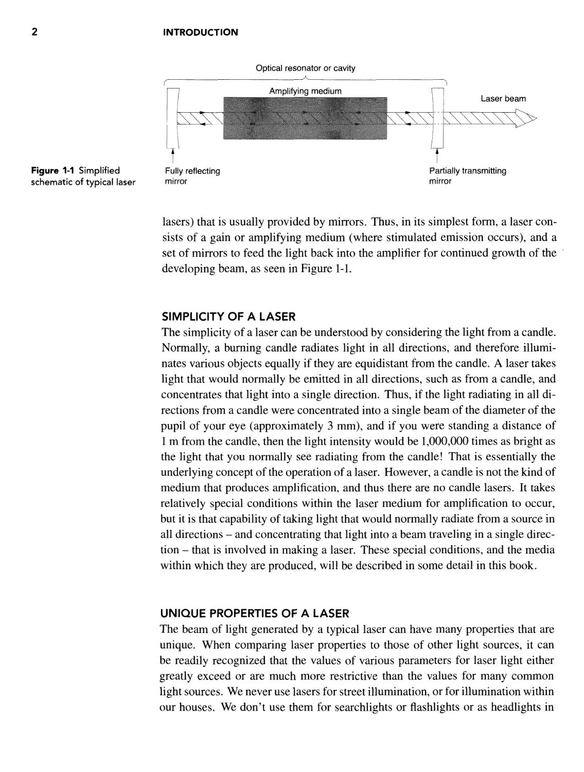
relating to thermodynamic equilibrium, and B) optical feedback (present in most
INTRODUCTION
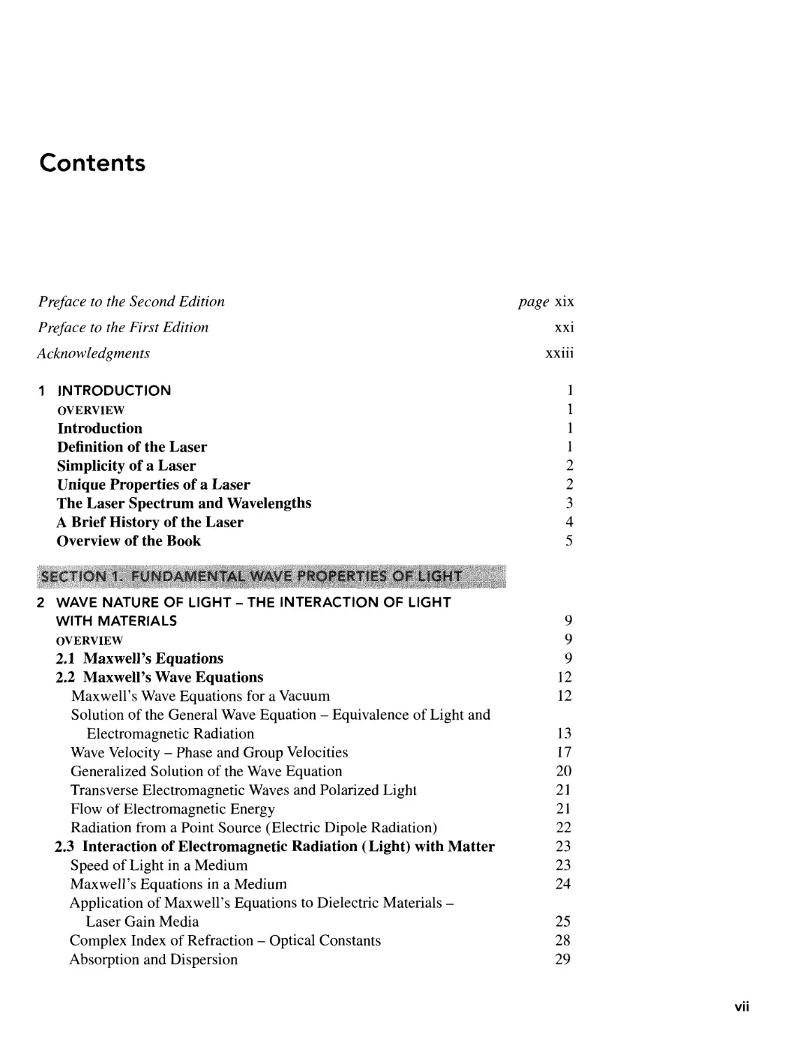
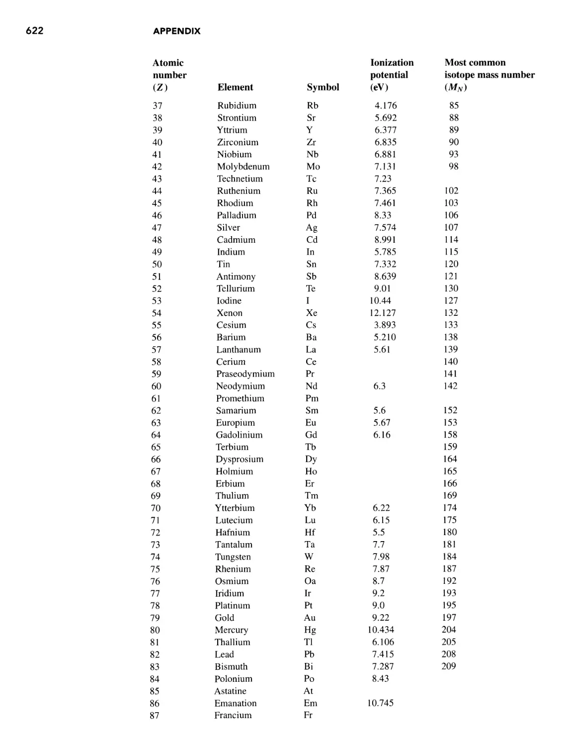
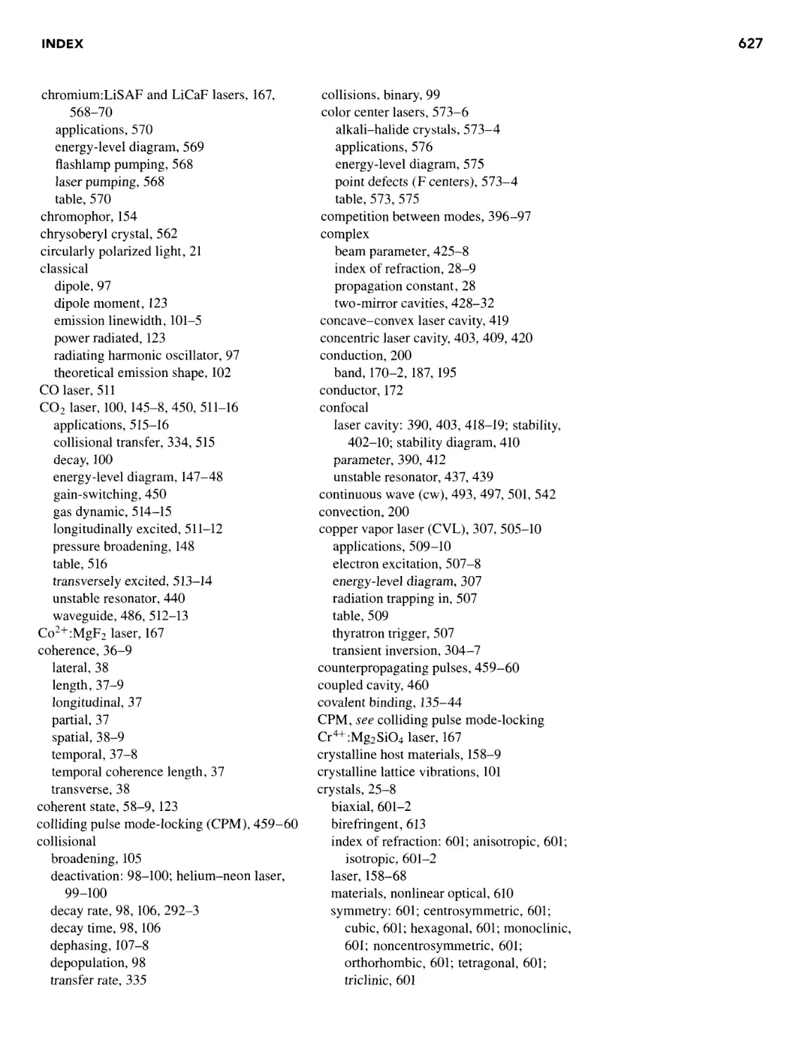
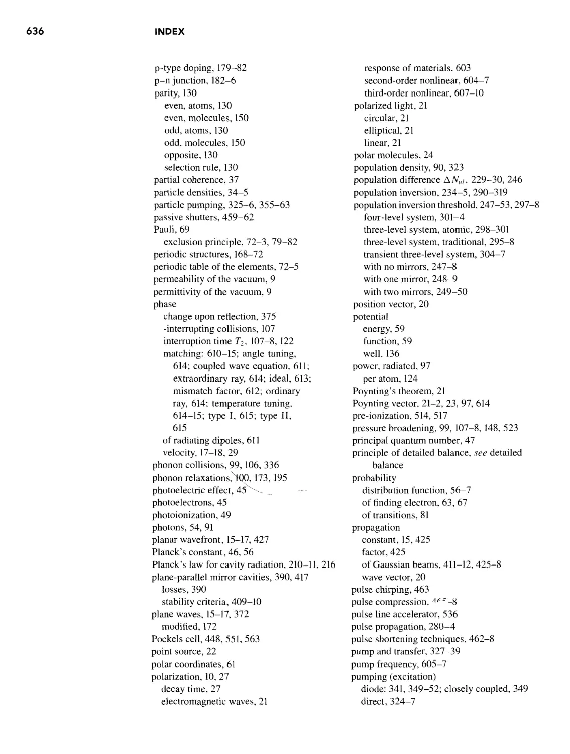
Figure 1-1 Simplified
schematic of typical laser
Optical resonator or cavity
Amplifying medium
Fully reflecting
Laser beam
I
Partially transmitting
mirror
lasers) that is usually provided by mirrors. Thus, in its simplest form, a laser con-
consists of a gain or amplifying medium (where stimulated emission occurs), and a
set of mirrors to feed the light back into the amplifier for continued growth of the
developing beam, as seen in Figure 1-1.
SIMPLICITY OF A LASER
The simplicity of a laser can be understood by considering the light from a candle.
Normally, a burning candle radiates light in all directions, and therefore illumi-
illuminates various objects equally if they are equidistant from the candle. A laser takes
light that would normally be emitted in all directions, such as from a candle, and
concentrates that light into a single direction. Thus, if the light radiating in all di-
directions from a candle were concentrated into a single beam of the diameter of the
pupil of your eye (approximately 3 mm), and if you were standing a distance of
1 m from the candle, then the light intensity would be 1,000,000 times as bright as
the light that you normally see radiating from the candle! That is essentially the
underlying concept of the operation of a laser. However, a candle is not the kind of
medium that produces amplification, and thus there are no candle lasers. It takes
relatively special conditions within the laser medium for amplification to occur,
but it is that capability of taking light that would normally radiate from a source in
all directions - and concentrating that light into a beam traveling in a single direc-
direction - that is involved in making a laser. These special conditions, and the media
within which they are produced, will be described in some detail in this book.
UNIQUE PROPERTIES OF A LASER
The beam of light generated by a typical laser can have many properties that are
unique. When comparing laser properties to those of other light sources, it can
be readily recognized that the values of various parameters for laser light either
greatly exceed or are much more restrictive than the values for many common
light sources. We never use lasers for street illumination, or for illumination within
our houses. We don't use them for searchlights or flashlights or as headlights in
INTRODUCTION
our cars. Lasers generally have a narrower frequency distribution, or much higher
intensity, or a much greater degree of collimation, or much shorter pulse duration,
than that available from more common types of light sources. Therefore, we do use
them in compact disc players, in supermarket check-out scanners, in surveying in-
instruments, and in medical applications as a surgical knife or for welding detached
retinas. We also use them in communications systems and in radar and military
targeting applications, as well as many other areas. A laser is a specialized light
source that should be used only when its unique properties are required.
THE LASER SPECTRUM AND WAVELENGTHS
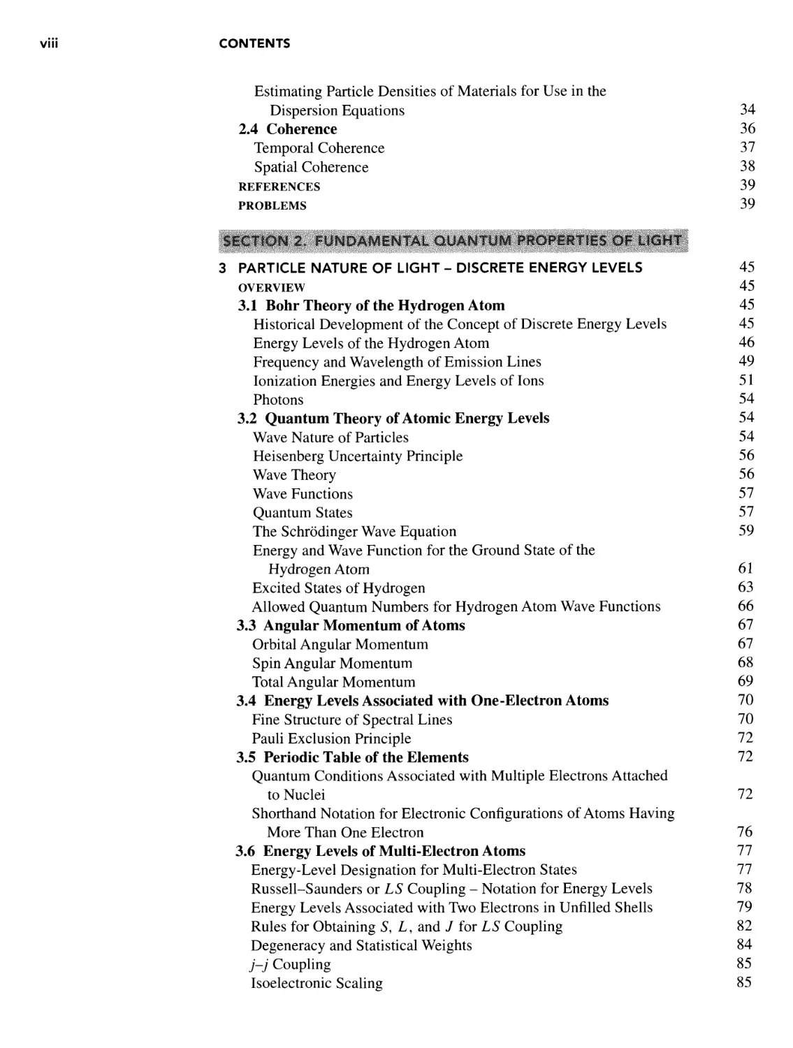
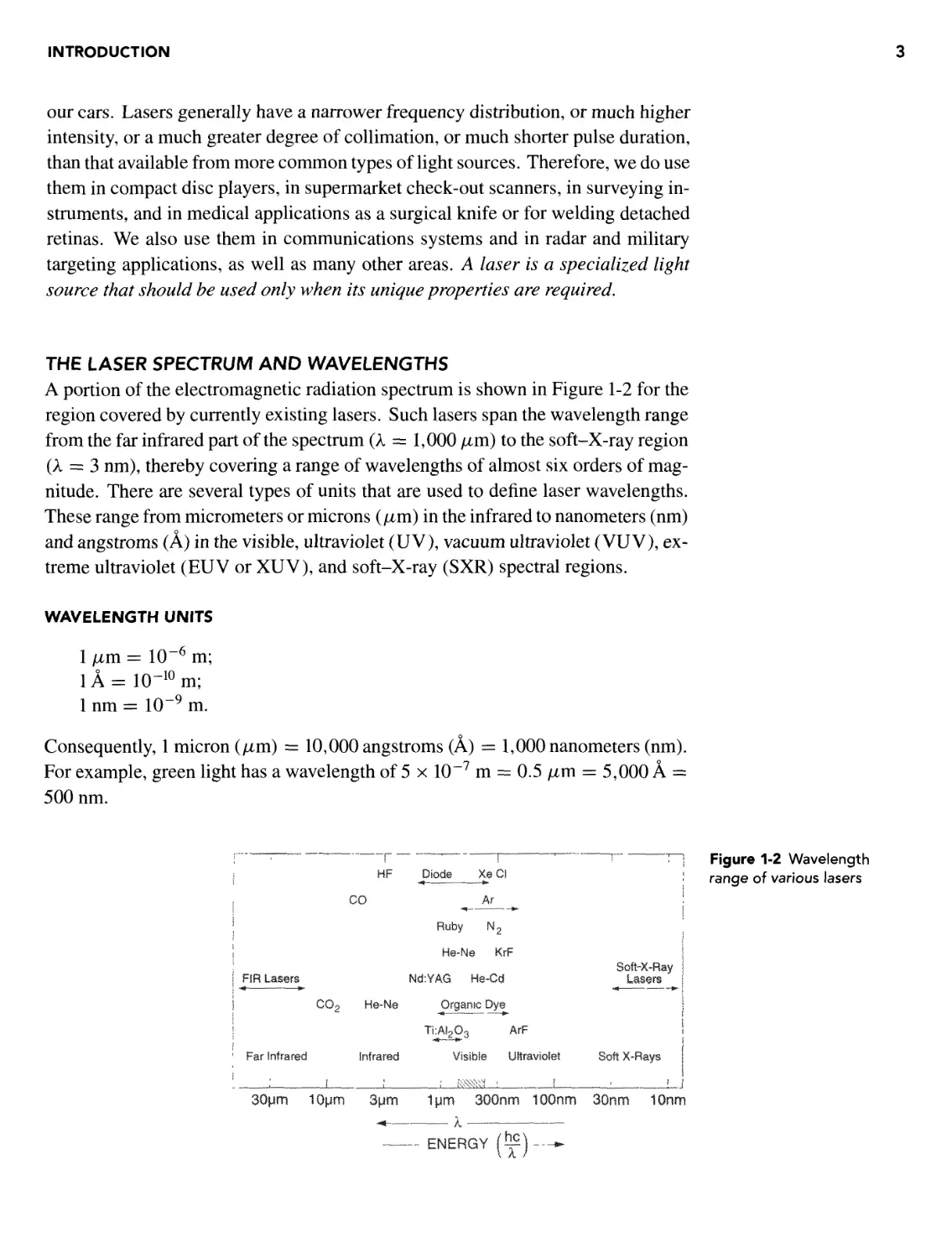
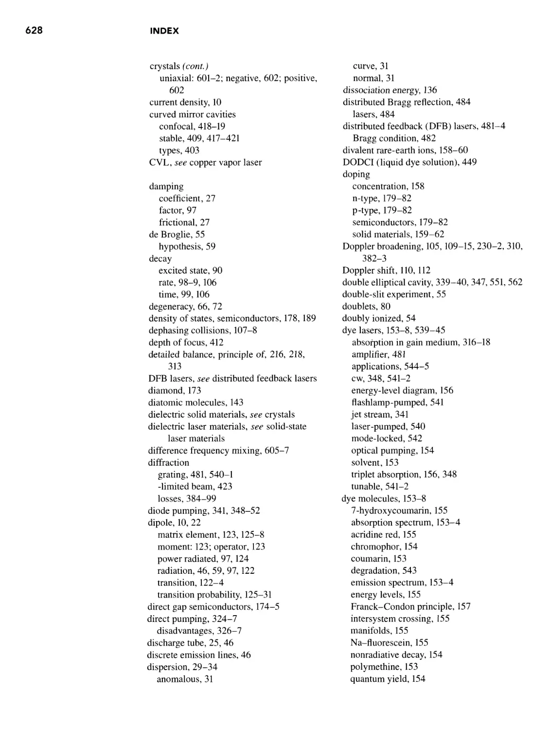
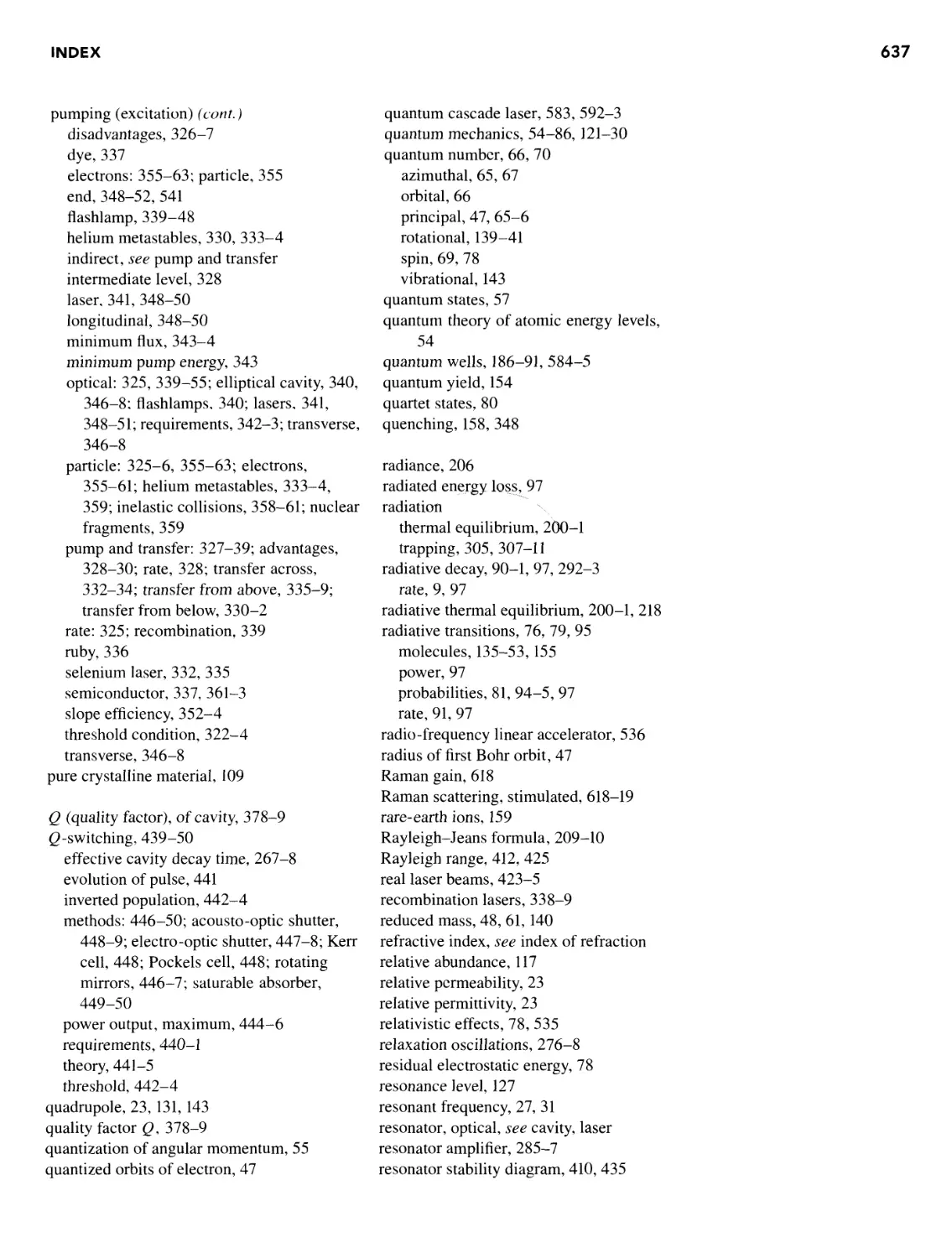
A portion of the electromagnetic radiation spectrum is shown in Figure 1-2 for the
region covered by currently existing lasers. Such lasers span the wavelength range
from the far infrared part of the spectrum (A = 1,000 /zm) to the soft-X-ray region
(k = 3 nm), thereby covering a range of wavelengths of almost six orders of mag-
magnitude. There are several types of units that are used to define laser wavelengths.
These range from micrometers or microns (/xm) in the infrared to nanometers (nm)
and angstroms (A) in the visible, ultraviolet (UV), vacuum ultraviolet (VUV), ex-
extreme ultraviolet (EUV or XUV), and soft-X-ray (SXR) spectral regions.
WAVELENGTH UNITS
= 10 m;
1 nm = 10-9 m.
Consequently, 1 micron (fim) = 10,000 angstroms (A) = 1,000 nanometers (nm).
For example, green light has a wavelength of 5 x 10~7 m = 0.5 fim = 5,000 A =
500 nm.
I FIR lasers
co2
Ruby N2
He-Ne KrF
Nd:¥AG He-Cd
Organic Dye
Ti:A!2O3
ArF
I Far Infrared
Infrared
Visible Ultraviolet
Sofi-X-Ray
Lasers
Soft X-Rays
30pm 10pm 8|jm 1pm 300nrn 100nm 30nm 10nm
_____ ENERGY (^)- ^
Figure 1-2 Wavelength
range of various lasers
INTRODUCTION
WAVELENGTH REGIONS
Far infrared: 10 to 1,000 /xm;
middle infrared: 1 to 10 /xm;
near infrared: 0.7 to 1 /xm;
visible: 0.4 to 0.7 /xm, or 400 to 700 nm;
ultraviolet: 0.2 to 0.4 /xm, or 200 to 400 nm;
vacuum ultraviolet: 0.1 to 0.2 /xm, or 100 to 200 nm;
extreme ultraviolet: 10 to 100 nm;
soft X-rays: 1 nm to approximately 20-30 nm (some overlap with EUV).
A BRIEF HISTORY OF THE LASER
Charles Townes took advantage of the stimulated emission process to construct a
microwave amplifier, referred to as a maser. This device produced a coherent beam
of microwaves to be used for communications. The first maser was produced in
ammonia vapor with the inversion between two energy levels that produced gain at
a wavelength of 1.25 cm. The wavelengths produced in the maser were compara-
comparable to the dimensions of the device, so extrapolation to the optical regime - where
wavelengths were five orders of magnitude smaller - was not an obvious extension
of that work.
In 1958, Townes and Schawlow published a paper concerning their ideas about
extending the maser concept to optical frequencies. They developed the concept
of an optical amplifier surrounded by an optical mirror resonant cavity to allow for
growth of the beam. Townes and Schawlow each received a Nobel Prize for his
work in this field.
In 1960, Theodore Maiman of Hughes Research Laboratories produced the
first laser using a ruby crystal as the amplifier and a flashlamp as the energy source.
The helical flashlamp surrounded a rod-shaped ruby crystal, and the optical cavity
was formed by coating the flattened ends of the ruby rod with a highly reflecting
material. An intense red beam was observed to emerge from the end of the rod
when the flashlamp was fired!
The first gas laser was developed in 1961 by A. Javan, W. Bennett, and D. Har-
Harriott of Bell Laboratories, using a mixture of helium and neon gases. At the same
laboratories, L. F. Johnson and K. Nassau demonstrated the first neodymium laser,
which has since become one of the most reliable lasers available. This was followed
in 1962 by the first semiconductor laser, demonstrated by R. Hall at the General
Electric Research Laboratories. In 1963, C. K. N. Patel of Bell Laboratories dis-
discovered the infrared carbon dioxide laser, which is one of the most efficient and
powerful lasers available today. Later that same year, E. Bell of Spectra Physics
discovered the first ion laser, in mercury vapor. In 1964 W. Bridges of Hughes Re-
Research Laboratories discovered the argon ion laser, and in 1966 W. Silfvast, G. R.
Fowles, and B. D. Hopkins produced the first blue helium-cadmium metal vapor
INTRODUCTION
laser. During that same year, P. P. Sorokin and J. R. Lankard of the IBM Research
Laboratories developed the first liquid laser using an organic dye dissolved in a sol-
solvent, thereby leading to the category of broadly tunable lasers. Also at that time,
W. Walter and co-workers at TRG reported the first copper vapor laser.
The first vacuum ultraviolet laser was reported to occur in molecular hydro-
hydrogen by R. Hodgson of IBM and independently by R. Waynant et al. of the Naval
Research Laboratories in 1970. The first of the well-known rare-gas-halide ex-
cimer lasers was observed in xenon fluoride by J. J. Ewing and C. Brau of the
Avco-Everett Research Laboratory in 1975. In that same year, the first quantum-
well laser was made in a gallium arsenide semiconductor by J. van der Ziel and
co-workers at Bell Laboratories. In 1976, J. M. J. Madey and co-workers at Stan-
Stanford University demonstrated the first free-electron laser amplifier operating in the
infrared at the CO2 laser wavelength. In 1979, Walling and co-workers at Allied
Chemical Corporation obtained broadly tunable laser output from a solid-state laser
material called alexandrite, and in 1985 the first soft-X-ray laser was successfully
demonstrated in a highly ionized selenium plasma by D. Matthews and a large num-
number of co-workers at the Lawrence Livermore Laboratories. In 1986, P. Moulton
discovered the titanium sapphire laser. In 1991, M. Hasse and co-workers devel-
developed the first blue-green diode laser in ZnSe. In 1994, F. Capasso and co-workers
developed the quantum cascade laser. In 1996, S. Nakamura developed the first
blue diode laser in GaN-based materials.
In 1961, Fox and Li described the existence of resonant transverse modes in
a laser cavity. That same year, Boyd and Gordon obtained solutions of the wave
equation for confocal resonator modes. Unstable resonators were demonstrated
in 1969 by Krupke and Sooy and were described theoretically by Siegman. Q-
switching was first obtained by McClung and Hellwarth in 1962 and described
later by Wagner and Lengyel. The first mode-locking was obtained by Hargrove,
Fork, and Pollack in 1964. Since then, many special cavity arrangements, feedback
schemes, and other devices have been developed to improve the control, operation,
and reliability of lasers.
OVERVIEW OF THE BOOK
Isaac Newton described light as small bodies emitted from shining substances.
This view was no doubt influenced by the fact that light appears to propagate in a
straight line. Christian Huygens, on the other hand, described light as a wave mo-
motion in which a small source spreads out in all directions; most observed effects -
including diffraction, reflection, and refraction - can be attributed to the expansion
of primary waves and of secondary wavelets. The dual nature of light is still a use-
useful concept, whereby the choice of particle or wave explanation depends upon the
effect to be considered.
Section One of this book deals with the fundamental wave properties of light,
including Maxwell's equations, the interaction of electromagnetic radiation with
INTRODUCTION
matter, absorption and dispersion, and coherence. Section Two deals with the fun-
fundamental quantum properties of light. Chapter 3 describes the concept of discrete
energy levels in atomic laser species and also how the periodic table of the ele-
elements evolved. Chapter 4 deals with radiative transitions and emission linewidths
and the probability of making transitions between energy levels. Chapter 5 con-
considers energy levels of lasers in molecules, liquids, and solids - both dielectric
solids and semiconductors. Chapter 6 then considers radiation in equilibrium and
the concepts of absorption and stimulated emission of radiation. At this point the
student has the basic tools to begin building a laser.
Section Three considers laser amplifiers. Chapter 7 describes the theoreti-
theoretical basis for producing population inversions and gain. Chapter 8 examines laser
gain and operation above threshold, Chapter 9 describes how population inversions
are produced, and Chapter 10 considers how sufficient amplification is achieved
to make an intense laser beam. Section Four deals with laser resonators. Chap-
Chapter 11 considers both longitudinal and transverse modes within a laser cavity, and
Chapter 12 investigates the properties of stable resonators and Gaussian beams.
Chapter 13 considers a variety of special laser cavities and effects, including un-
unstable resonators, g-switching, mode-locking, pulse narrowing, ring lasers, and
spectral narrowing.
Section Five covers specific laser systems. Chapter 14 describes eleven of
the most well-known gas and plasma laser systems. Chapter 15 considers twelve
well-known dye lasers and solid-state lasers, including both dielectric solid-state
lasers and semiconductor lasers. The book concludes with Section Six (Chap-
(Chapter 16), which provides a brief overview of frequency muliplication with lasers and
other nonlinear effects.
SECTION ONE
FUNDAMENTAL WAVE
PROPERTIES OF LIGHT
Wave Nature of Light
The Interaction of Light with Materials
OVERVIEW This chapter will consider some of the
wave properties of light that are relevant to the un-
understanding of lasers. We will first briefly review the
derivation of Maxwell's wave equations based upon
the experimentally obtained laws of electricity and
magnetism. We will consider Maxwell's equations in
a vacuum, and will demonstrate the equivalence of
light and electromagnetic radiation. We will describe
both the phase velocity and group velocity of light and
will show how polarized light occurs in these trans-
transverse electromagnetic waves.
We will, then use the wave equations to consider
the interaction of electromagnetic waves with trans-
transparent and semitransparent materials such as those
used for the gain media of solid-state lasers. We will
derive expressions for the optical constants r\ and k
(the real and imaginary components of the index of
refraction) that suggest the presence of strong ab-
absorptive and dispersive regions at particular resonant
wavelengths or frequencies of the dielectric materials.
These are regions where rj and k vary quite signifi-
significantly with frequency. These resonances will later
(in Chapters 4, 5, and 6) be related to optical transi-
transitions (both emission and absorption) between energy
levels in those materials. We will conclude the chap-
chapter with a brief description of coherence.
2.1 MAXWELL'S EQUATIONS
Maxwell's wave equations, predicting the propagation - even in a vacuum - of
transversely oscillating electromagnetic waves, were the first indication of the true
nature of light. His wave equations, published in 1864, predicted a velocity c for
such a wave in a vacuum (c = (mo£o)~1/2) that agreed with independent measure-
measurements of the velocity of light. This velocity was based solely upon the value of
two previously known constants: /zo> the permeability of the vacuum; and e$, the
permittivity of the vacuum. These constants had arisen from totally separate inves-
investigations of electricity and magnetism that had nothing to do with studies of light!
By definition, the exact value of /xo is 4n x 10~7 H/m; the measured value of £o
is 8.854 x 10² F/m.
The fundamental electric and magnetic field vectors E and B (respectively) can
produce forces on physical entities. These vectors are measurable quantities that
led to the experimentally derived laws of Gauss, Biot-Savart, Ampere, and Fara-
Faraday, all of which are briefly outlined in what follows. These laws in turn formed
the foundation upon which Maxwell built to develop his equations predicting the
existence and properties of electromagnetic radiation.
10 WAVE NATURE OF LIGHT
In addition to E and B, we must consider properties associated with the elec-
electromagnetic state of matter. Such matter can be described at a given location in
space by four quantities:
A) the charge density p (charge per unit volume);
B) the polarization P (electric dipole moment per unit volume) for magnetic ma-
materials, in particular for a dielectric material;
C) the magnetization M (magnetic dipole moment per unit volume); and
D) the current density J (current per unit area).
For our purposes, all of these quantities are assumed to be average values.
Other relationships that will be useful include:
E) the Lorentz force law,
B), B.1)
where F is the force resulting from a charge q moving with a velocity v; and
F) a form of Ohm's law given by
J = <tE, B.2)
which describes the response of electrons in a conducting medium of conduc-
conductivity a to an electric field vector E.
Maxwell defined the electric displacement vector D as follows:
D = s0E + P (for general use); B.3)
D is used so as to avoid explicit inclusion of the charge associated with the polar-
polarization P in Gauss's flux law.
For the case of free space,
D - £0E, B.4)
and for an isotropic linear dielectric,
D = eE, B.5)
which describes the aggregate response of the bound charges to the electric field.
An alternate way of expressing this is to write
P = (£-£O)E = X£oE, B.6)
which gives the relationship between the polarization P and the electric field E that
produces P. The factor x, known as the electric susceptibility, is given by
X = (e/e0) - 1; B.7)
X is a useful parameter when considering effects in the optical frequency range.
For spherically symmetric materials such as glass, x is a simple scalar quantity,
2.1 MAXWELL'S EQUATIONS 11
but for arrisotropic materials, x is expressed as a tensor to account for the varia-
variation in polarization response for different directions of the applied field. If B.6) is
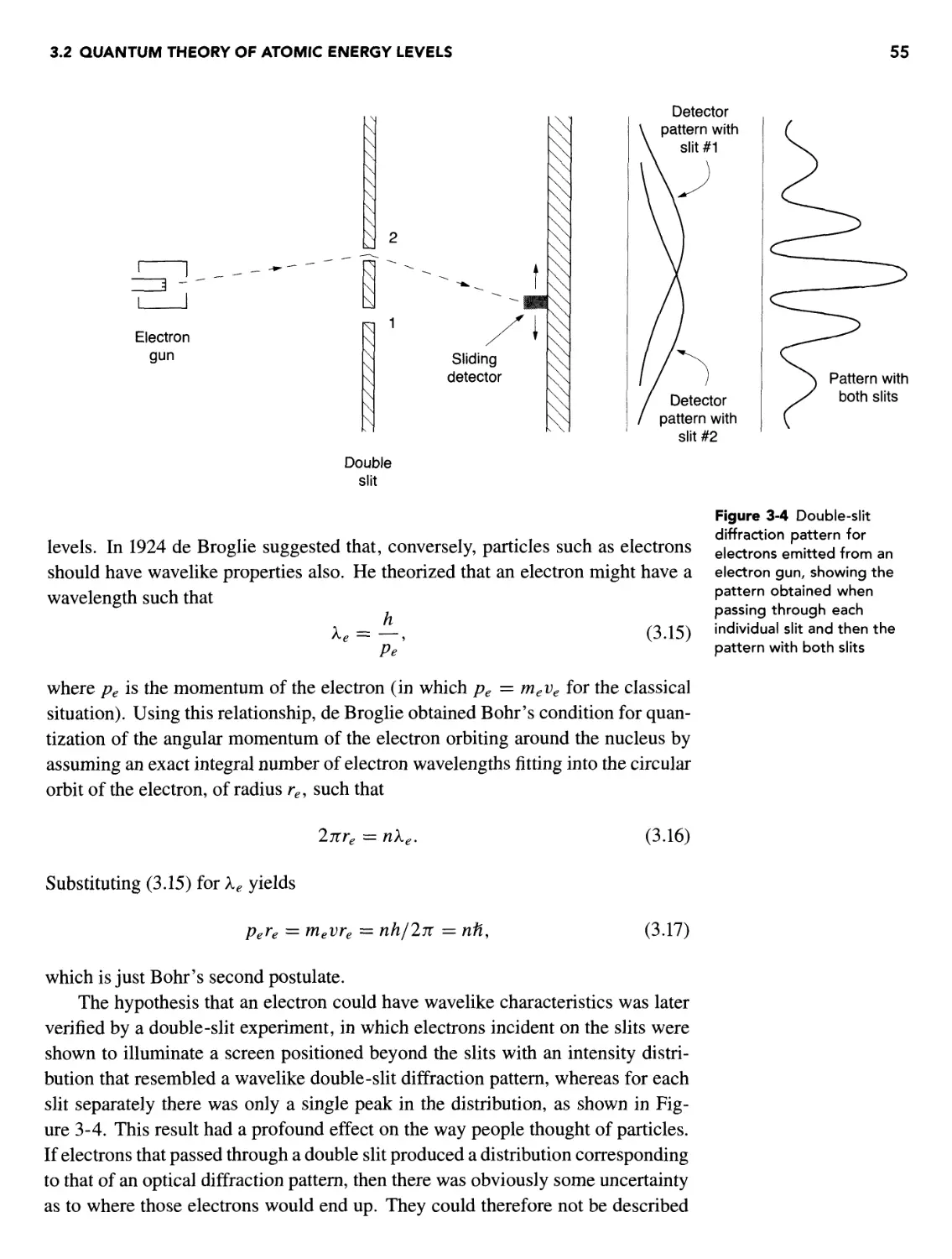
generalized by expressing the polarization P as a power series in the field strength
E, higher-order values of x are obtained that describe the nonlinear optical prop-
properties of materials. Such properties are used for frequency conversion and other
effects associated with lasers, and will be described in more detail in Chapter 16.
The general expression for B can be written as
B = /zo(H + M), B.8)
where H is a convenient vector quantity that provides for a different expression
of the magnetic flux B, that is, in a form that allows the parallel treatment of the
electric and magnetic flux laws. For a vacuum,
B = M0H, B.9)
and for isotropic linear magnetic media,
B = /iH. B.10)
Using these quantities, Maxwell's equations can be derived from the following ex-
experimentally determined relationships.
GAUSS'S LAW This law states that the total electric flux 0 through any closed
surface, or (equivalently) the surface integral over the normal component of the
electric field vector E over that closed surface, equals the net charge ^2nqn inside
the surface:
iE-dS= — y^qn = — f pdV, B.11)
80 ^ 80 Jv
where dS is the surface element vector at any point p on the surface surround-
surrounding the volume V. If the charge is distributed within the volume, p is the localized
charge density within a volume element dV. This law can be expressed in differ-
differential form as
V-D = p. B.12)
This is considered the first of Maxwell's equations.
BIOT-SAVART LAW This law is expressed here in a form similar to that of Cou-
Coulomb's law relating the force of attraction of two charges:
-^JF, B.13)
|r|3
where J(V) is the current density within volume element dV and r is the posi-
position vector from volume element dV to the point of measurement of B. It can be
expressed in differential form as
12 WAVE NATURE OF LIGHT
rV, B.14)
which leads directly to
V • B = 0, B.15)
since B is the curl of another vector. This is considered the second of Maxwell's
equations.
AMPERE'S LAW This law, in its simple form, states that the line integral of the
magnetic induction vector B around any closed path is equal to the product of the
permeability /xo and the net current / flowing across the area bounded by the path:
B.16)
In differential form, this law can be written as
) B.17)
and represents the third of Maxwell's equations.
FARADAY'S LAW This law is analogous to Ampere's law in stating that the line in-
integral of the electric field vector E around any closed path / is equal to the time
rate of change of magnetic flux <J>M passing through the area defined by that path:
dl = -^. B.18)
dt
In differential form, this law is written as
VxE=-^, B.19)
and historically it represents the fourth of Maxwell's equations.
The third equation (eqn. 2.17) was modified by Maxwell to satisfy the law of
continuity of charge. Maxwell's four equations relate charge density, current den-
density, and field quantities at a single point in space through their time and space
derivatives.
2,2 MAXWELL'S WAVE EQUATIONS
Maxwell's Wave Equations for a Vacuum
Maxwell's equations will first be considered for a vacuum in order to obtain the
simplest form of the electromagnetic wave equation and also to demonstrate that
2.2 MAXWELL'S WAVE EQUATIONS 13
the predicted waves require no medium to support their existence. In that case the
equations reduce to
V • E = 0, B.20)
VH = 0, B.21)
VxH^Op B.22)
at
CJTT
V x E = -no—. B.23)
at
These four equations constitute Maxwell's equations for a vacuum (the absence of
matter). In rewriting these equations, B has been replaced by its equivalent /xoH
(eqn. 2.8) since M = 0. Equations B.20) and B.21) indicate the absence of charge
at the point of consideration.
The solutions for E and H can be separated by taking the curl of B.23) and
the time derivative of B.22). Then, using the fact that the order of differentiation
can be reversed, one can obtain the following parallel equations:
Vx(VxE) = -/xO£o^y, B.24)
Vx(VxH) = -/xo«ott. B.25)
Because V x (V x A) = V( V • A) - V2A for any vector A, B.24) and B.25) lead
to the following two Maxwell wave equations:
and
Solution of the General Wave Equation - Equivalence of Light
and Electromagnetic Radiation
Equations B.26) and B.27) are wave equations of the form
2 i a2A
V2A= — —, B.28)
where the vector A is a function of x, y, z, and t that may be expressed as
A(jc, y, z, 0 and where v is a positive constant. In our situation, A could represent
14 WAVE NATURE OF LIGHT
either the electric field vector E(jc, y, z, t) or the magnetic field vector H(x, y, z, t).
We will show that A is an oscillatory wave function with an amplitude that is trans-
transverse to the direction of propagation, and that v is associated with the velocity of
that wave.
The left side of B.28) involves derivatives of A with respect to the spatial vari-
variables x, y, and z. For simplicity we will consider the wave propagating in only a
single spatial direction, the z direction, and consequently we use only the z com-
component A(z, t) of A. We can then rewrite B.28) as
d*A(z,t)_ id'Ajzj)
dz2 v2 dt2
We will assume that the wave function A(z, t) is separable and thus can be written
as a product of functions Az{z) and At(t) as follows:
A(z, t) = Az(z)At(t) or A(z, t) = AzAt. B.30)
Substitution into B.29) then leads to
d2Az Az d2At
1 dz2 v2 dt2 ~~
or
v2 d2A1_ j_D2At
Az dz At dt
The left side of B.32) is dependent only upon z and the right side only upon t, and
so - in order to satisfy the equation - both sides must be equal to the same con-
constant, which we will arbitrarily denote as -co2. This leads us to the following two
equations:
d2A7 co2
dz2 v2
d2At
+ — Az = 0, B.33)
+ co2At = 0. B.34)
dt2
These equations are of a familiar form and have the following solutions:
Az = Cxei{a)/V)z + C2e-i(a)/v)z, B.35)
At = Dxeicot + D2e-ia)t, B.36)
where the constants C\, C2, D\, and D2 are determined by the boundary condi-
conditions. We can now express the general solution A(z, t) as
A(z, t) = Az(z)At(t) oc e±i{a)/v)ze±i0Jt = £?±/[(<w/i;)z=FG"]. B.37)
2.2 MAXWELL'S WAVE EQUATIONS
15
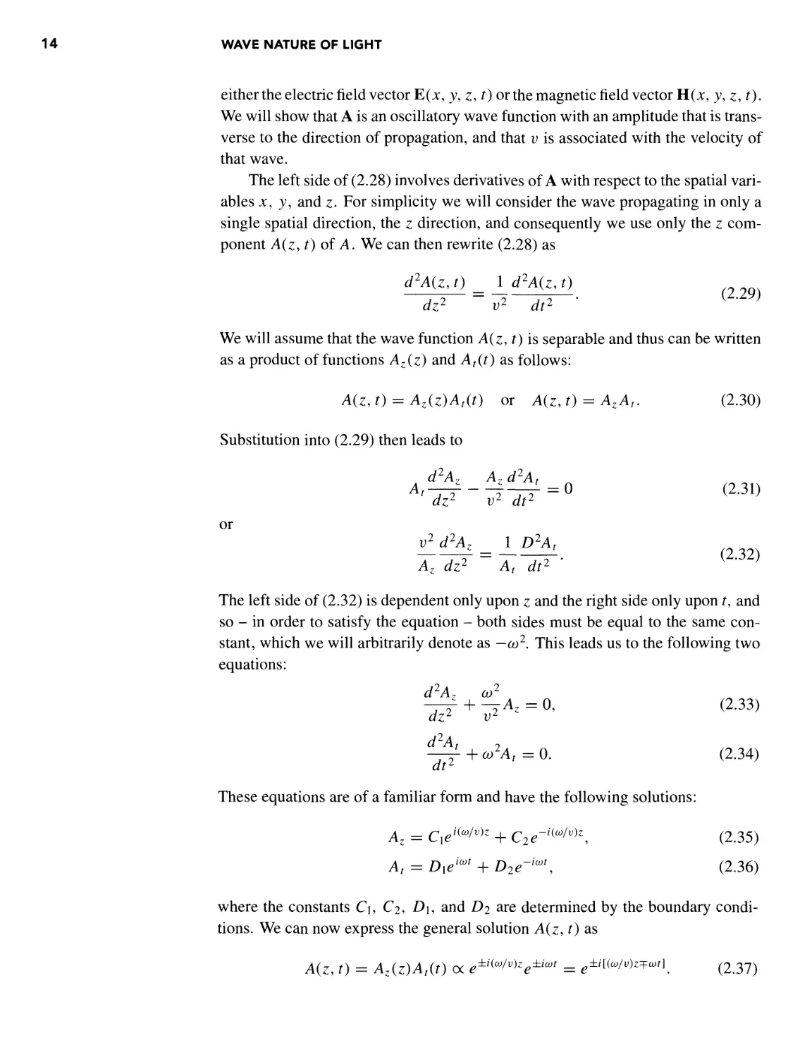
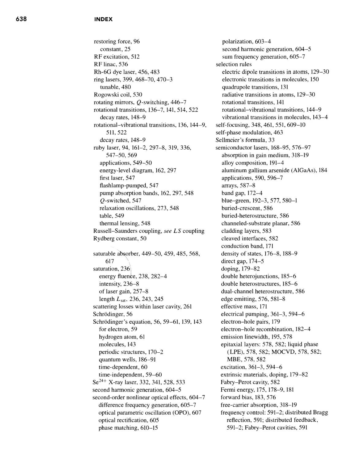
Figure 2-1 Wavelength of a
sinusoidally oscillating wave
This general solution involves a complex wave function. For our purposes, con-
consider a wave traveling from left to right that is a function of the form
kzz-ct>t)
B.38)
where we have defined k7 as
*, = -.
v
B.39)
The quantity kz is called the propagation constant or the wave number (the num-
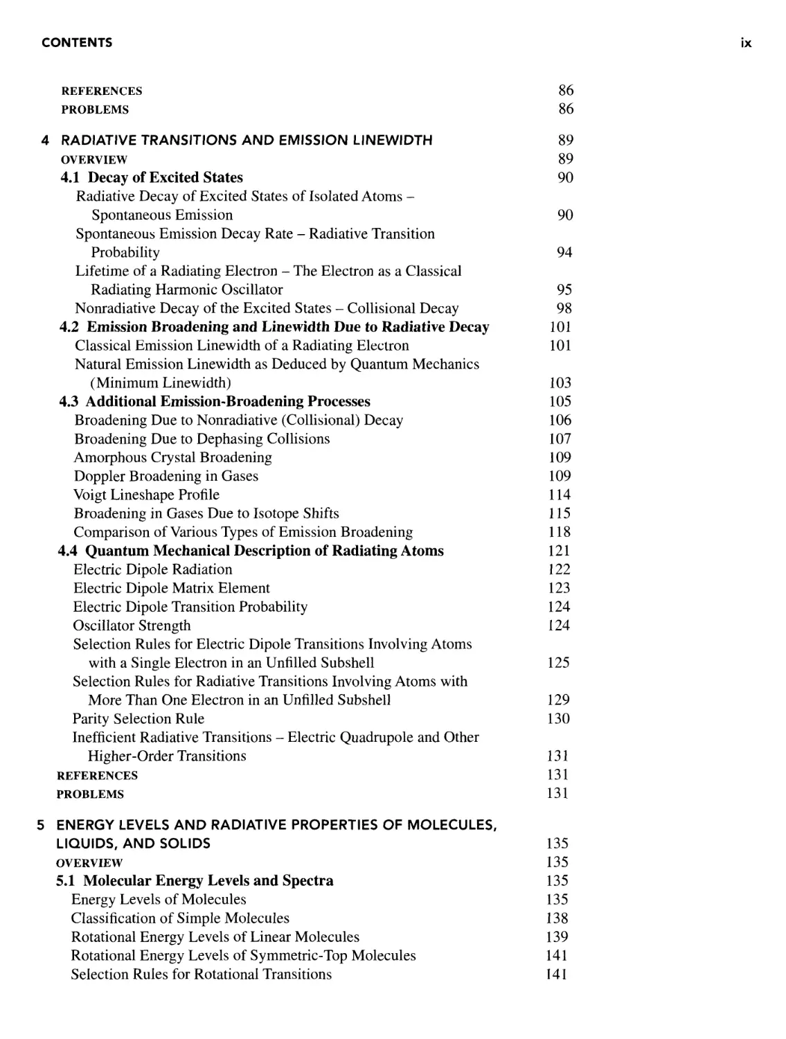
number of waves per unit length) and has dimension of 1/length. The wavelength k
is the distance over which the maximum amplitude of the wave travels during the
time it makes one complete cycle of oscillation, or the distance between succes-
successive peaks of a wave frozen in time as shown in Figure 2-1. The velocity of a wave
of wavelength k and frequency v is equal to the product of k and v: v ~ kv. Also,
the frequency of oscillation v is related to the angular frequency co by v = to/In.
Hence
v v 2nv
v co/2tt co
B.40)
where v is the frequency or the number of complete cycles of oscillation per unit
time and k is related to kz by
k --
kz~~ k'
B.41)
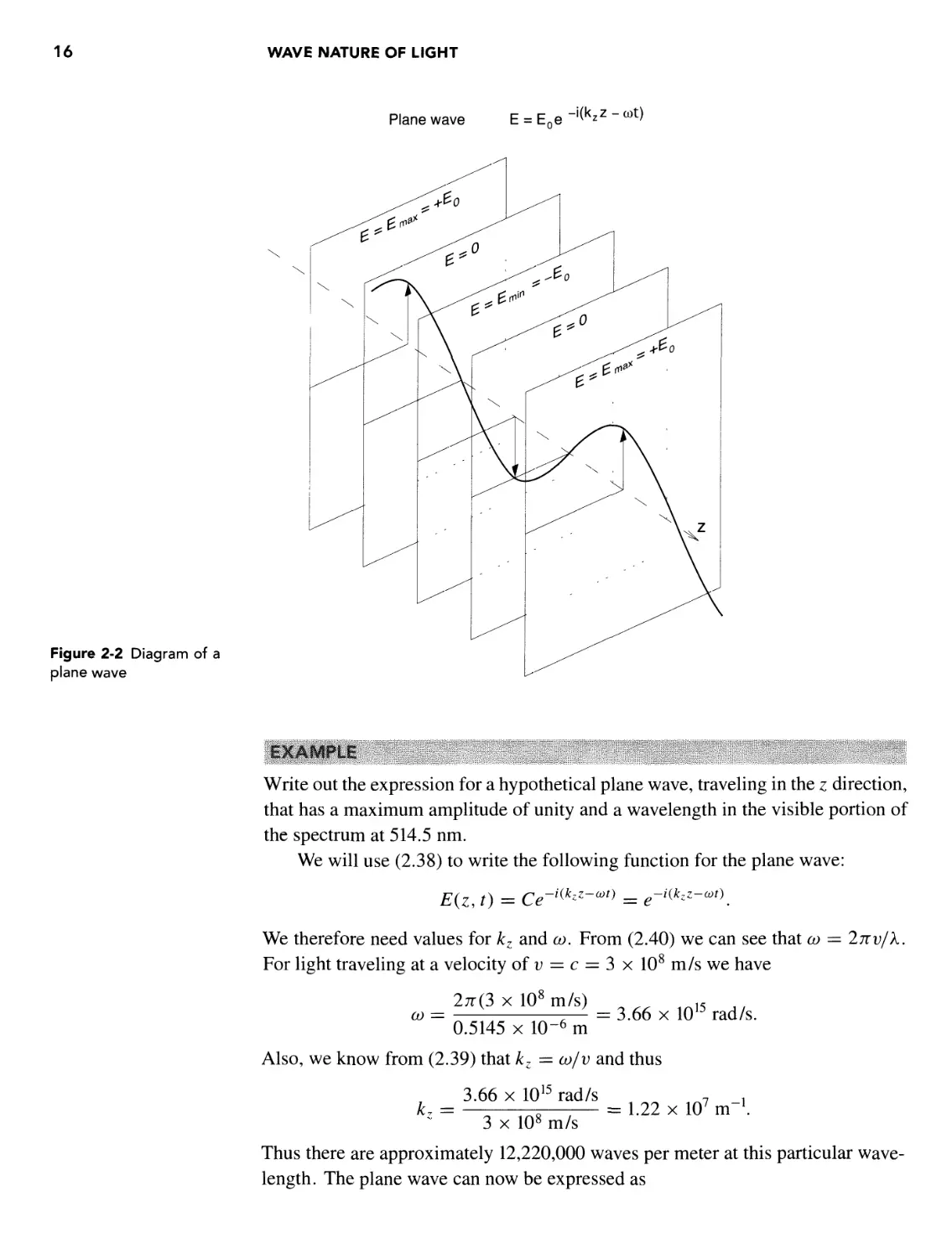
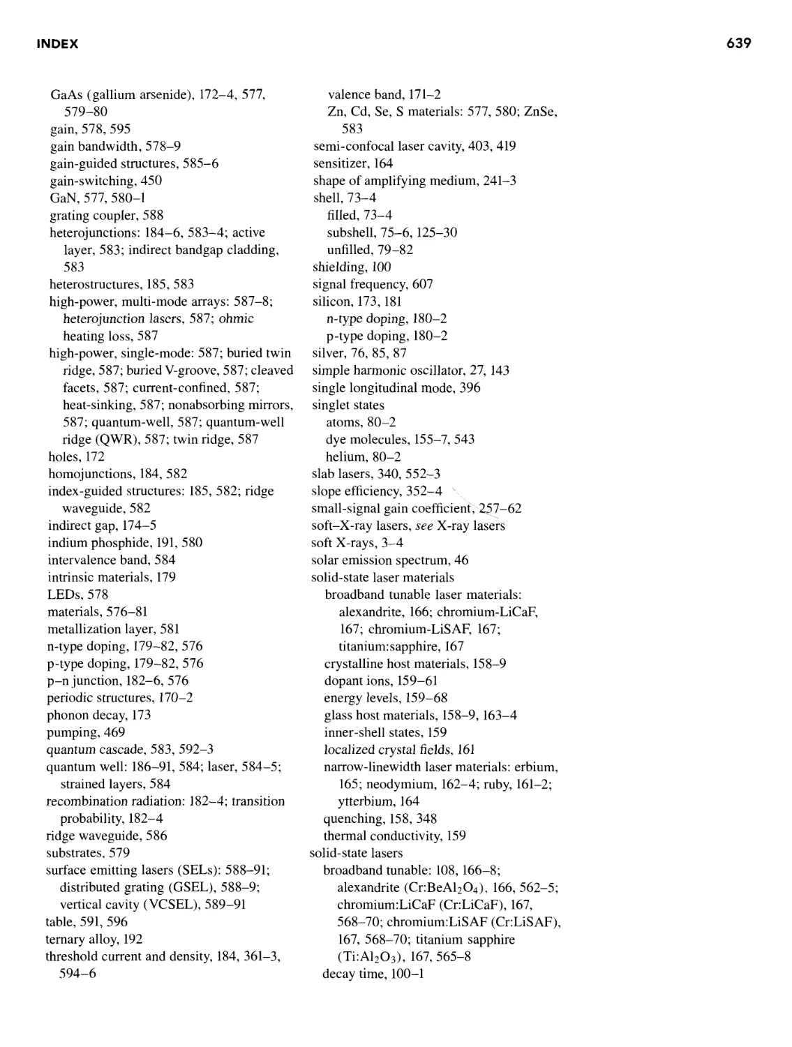
m PLANE WAVES The wave described in B.38) represents a wave that, for any
value of z, has the same amplitude value for all values of x and y. It is thus re-
referred to as a plane wave since it represents planes of constant value that are of
infinite lateral extent, as indicated in Figure 2-2.
16
WAVE NATURE OF LIGHT
Plane wave E = Ene
Figure 2-2 Diagram of a
plane wave
Write out the expression for a hypothetical plane wave, traveling in the z direction,
that has a maximum amplitude of unity and a wavelength in the visible portion of
the spectrum at 514.5 nm.
We will use B.38) to write the following function for the plane wave:
E(Z, t) = Ce-1^-^ = *-'<***-*">.
We therefore need values for kz and to. From B.40) we can see that to = 2nv/X.
For light traveling at a velocity of v = c = 3 x 10⁸ m/s we have
2ttC x 108 m/s)
CO =
0.5145 x 10 m
Also, we know from B.39) that kz = co/v and thus
3.66 x 10¹⁵ rad/s
= 3.66 x 10¹⁵ rad/s.
k7 =
= 1.22 x 10⁷ m.
3 x 10⁸ m/s
Thus there are approximately 12,220,000 waves per meter at this particular wave-
wavelength. The plane wave can now be expressed as
2.2 MAXWELL'S WAVE EQUATIONS
17
_ £-/[A.22xl07)z-C.66xl015)/]
where z is expressed in meters and t is in seconds.
Wave Velocity - Phase and Group Velocities
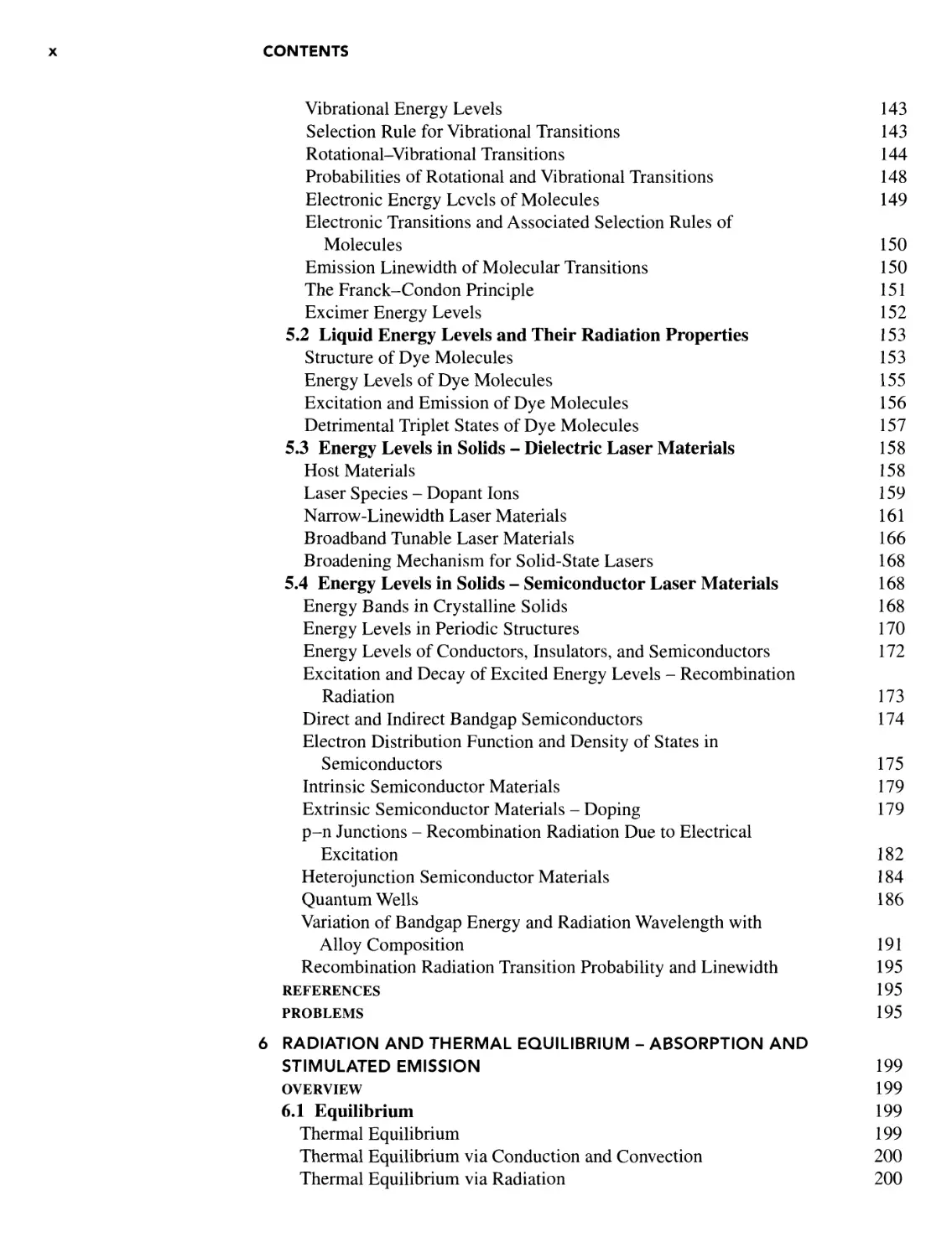
PHASE VELOCITY Equation B.38) describes an oscillatory function that has a si-
sinusoidal variation with either z or t. If we set t equal to a constant (we choose t =
0) then we have a sinusoidally varying function of the form e~kzZ, as shown in Fig-
Figure 2-3(a), that is frozen in time. If we set z equal to a constant (we choose z = 0)
then we have a similar function of the form elcot, which is shown in Figure 2-3(b).
In either case, it is understood that we take the real part of the function to obtain
the value of the amplitude.
The argument of B.38) is a phase factor 0 such that
= kzz — cot.
B.42)
(a)
Figure 2-3(a) Snapshot of a
wave frozen in time
Camera
Snapshot in time
(Wave frozen in space)
Figure 2-3(b) Temporal
display of a wave traveling
past a fixed location in
space
(b)
1
,A@
t) = Ce
A
iwt
1
Fixed spatial location
(Wave oscillating in time)
18 WAVE NATURE OF LIGHT
By considering the value of the wave for </> = constant we can track how the wave
moves with time, since the amplitude of the wave function remains constant when
the argument of the wave function is constant. The velocity at which the wave
form propagates is called the phase velocity. We obtain this velocity by taking the
derivative of (j) and equating it to zero, which denotes the maximum value of the
wave form. For d(p — 0 we are led to
B A3)
from which we obtain the phase velocity of the wave as
VphaSe = ff = J = V. B.44)
This tells us that the constant v in B.28) is the velocity at which the wave moves
in time.
Comparing B.26) and B.27) with B.28) suggests that v = l/(//O£oI/2- A
precise measurement of the capacitance of a condenser of accurately determined
dimensions by two different techniques (at the National Bureau of Standards) pro-
provided a value of l/(/zO£oI/2, suggesting that v = 299,784 ± 10 km/s with a
precision of 1 part in 30,000. This compares favorably with the most accurate di-
direct measurement of the speed of light of c = 299,792,457.4 ± 1.1 m/s. We can
thus conclude that v = c.
In this section, for simplicity we have considered a special case of waves prop-
propagating in the z direction with the associated propagation constant or wave number
kz. Later we will consider a more general wave, propagating in an arbitrary direc-
direction with a propagation vector k of magnitude k.
GROUP VELOCITY An infinite wave train of a single frequency has no starting or
stopping point; it can't be modulated. Any attempt at modulation - to start and
stop a wave train - requires a wave involving more than one frequency (see Chap-
Chapter 4 for an example). We will first consider two plane waves with electric fields
of E\ and E2 described as
Ei — cos(k[Z - co\t), E2 = cos(k2z - co2t). B.45)
We can add these two waves to obtain
E = Ei + E2 = cos(kiz - coit) + cos(k2z - co2t). B.46)
This can be rewritten as
E = 2cos £[(fci + k2)z - (o>i + aJ)t]
x cos \[{kx - k2)z - (coi - co2)t]. B.47)
2.2 MAXWELL'S WAVE EQUATIONS 19
Now, if co \ and C02 are nearly the same then we can define co and k such that sum-
summation can be rewritten as averages of the two waves:
go = ±(<wi + co2) and k = \(kx + k2). B.48)
Also let com and km be modulation frequency and modulation propagation numbers
such that
com = \(<oi - (o2) and km = \{kx - k2). B.49)
Thus we have
E = 2cos(£mz - comt) cos(kz -cot). B.50)
If co\ % C02 then for co\ and &>2 quite large, which is typical of optical frequencies,
we have
co^>com. B.51)
Just as we did for a single plane wave, we can determine the velocity of vm by
considering the phase factor <pm associated with the modulation frequency com,
0m = kmz -comt, B.52)
and then taking the derivative and equating it to zero:
d(j)m =kmdz- com dt = 0. B.53)
From this we can solve for vm = dz/dt to obtain
dz com j(o>\-<o2) Aco dco
dt km ^/Cl-k2) Ak dk
Hence the group velocity of those two combined waves is
^-. B.55)
dk
Let us do a more general derivation of the group velocity by considering a wave
of center frequency coq but now with a finite width Aco. In effect, the finite width
allows for the wave to consist of more than one frequency and hence modulation
could occur. Assume a propagation constant k0 at frequency coq but now allow it to
vary with frequency co in the region of coq> such that/: = kQ^idk/do^^^^ico—co^).
Let us take a Fourier expansion of the electric field of the wave as follows:
E(z, t)= I E(co)e~i(kz-OJt) dco. B.56)
20 WAVE NATURE OF LIGHT
If we now insert our preceding expression for k, we have
/•+AwO/2 r V / dk\ 1
E(z, t) = e~l{koz~mt) / E(co) exp{ -/ — z - t\
J~Acoq/2 [ l\da)/(v0 J
B.57)
in which Aco = co — coq. Note that the plane wave is now modulated by a wave
involving the function [(dk/da))z — t]. We can now obtain the velocity of this mod-
modulated wave in the same way as we did for a plane wave by evaluating a constant
phase factor or [(dk/dco)z — t] = constant. Solving for the velocity of this "group"
or bundle of waves, we find that
dt dk
We have thus defined this velocity as the group velocity Vq.
A finite group velocity implies a change in velocity with a change in wave-
wavelength . A medium with such characteristics is referred to as a dispersive medium. In
a nondispersive medium we can see from B.44) that the group velocity dco/dk = u,
so the phase velocity and the group velocity are identical. In a dispersive medium,
the group velocity is different from the phase velocity. The group velocity is the
velocity at which information can be transmitted, because sending information in-
involves modulation.
Generalized Solution of the Wave Equation
The solution to the wave equation given in B.38) can be expressed in a more gen-
general form, involving all of the spatial coordinates, as
A(x, y, z, t) = A<>e-Kk*x+kyy+k*-(Ot) B.59)
or
A/v ,, _ i\ A _—/(k«r— cot) /r\ /:r\\
x\\X, y, Zi i) — -^o^ ' \LXi\j)
where k is referred to as the propagation wave vector that defines the direction of
propagation of the wave (k = kxi + kyj + kzk), r is the position vector identi-
identifying a particular location in space such that r = xi + yj + zk, and where i, j,
and k are unit vectors. Thus the wave vector k defines the normal to the planes of
constant amplitude and phase as they propagate with velocity v = c.
Substituting this more general form of A into B.28) and comparing B.28) with
B.26) and B.27), we conclude that the solution for the electric vector E in B.26)
can be expressed as
El? ,-»~~*(k«r—cot) c*\ /ci\
= 1^0^ B-Oi)
2.2 MAXWELL'S WAVE EQUATIONS 21
and that the velocity of the wave in a vacuum is
= c= — = 2.99792 x 10⁸ m/s. B.62)
Transverse Electromagnetic Waves and Polarized Light
Equation B.61) represents the electric component of an electromagnetic wave
whose amplitude is a vector quantity. A similar relationship can be expressed
for the magnetic component H. Since V • E = 0 according to B.20) and since
V • E = zk • E from B.61), we can conclude that /k • E = 0 and thus E is perpen-
perpendicular to k, the direction of propagation. A similar argument can be made for the
magnetic portion of the wave, since V • H = 0 from B.21). Therefore, both the
amplitudes Eo and Ho are perpendicular to the direction of the propagation vector
k and thus to the propagation of the wave. (They are also perpendicular to each
other.) Hence these electromagnetic waves are referred to as transverse waves.
Because the amplitude factor in an electromagnetic wave is a vector quantity
that lies in a plane perpendicular to the direction of propagation, that amplitude
can be resolved into independent orthogonal components within that plane. Thus,
for example, a wave traveling in the z direction, such as that expressed as
E = Eoe-i{k*z-°>t\ B.63)
can be resolved into its two orthogonal components or polarizations:
E = EoJe-M*-0*0 + Eoyje-W*-0"*®, B.64)
where i and / are unit vectors in the x and y directions, respectively. The relative
phase factor 0 suggests that the two independent polarizations need not be in exact
phase. If 0 = 0, or integral multiples of 27r, then the combined waves represent a
single wave with the transverse amplitude vector always oriented in the same di-
direction. Such a wave is referred to as plane or linearly polarized light, as shown
in Figure 2-4. Other values of 0 cause the amplitude vector of the wave to spiral
in either an elliptical or a circular manner, as indicated in the figure. Such waves
are referred to as either circularly or elliptically polarized light.
Flow of Electromagnetic Energy
The time rate of flow of electromagnetic energy S is described by Poynting's the-
theorem, which states that
S = ExH. B.65)
The term S is known as the Poynting vector, which has MKS units of W/m2. This
vector indicates both the magnitude and direction of the radiation.
22
WAVE NATURE OF LIGHT
Figure 2-4 Examples of
both plane and circularly
polarized waves
"~" 90° Rotations
For a plane wave whose electric vector is expressed as in B.61) and whose
magnetic vector is expressed similarly, it can be easily shown that the average
value of the Poynting vector, written as (S), can be expressed as
x H
o.
B.66)
Radiation from a Point Source (Electric Dipole Radiation)
Radiation from a point source, such as that from an isolated atom, is a more compli-
complicated situation. It is analyzed in terms of a vector potential A and a scalar potential
0 such that, for example, the electric field vector E is obtained from
E—V,-I£.
d
B.67)
Since we are dealing with oscillating fields from a point charge, it is not sur-
surprising that the vector and scalar potentials are oscillating functions that can be
obtained from Maxwell's equations B.12), B.15), B.17), and B.19). The solution
for the scalar potential is of the form
='""'/¦
ikr
l
B.68)
where p is the charge density of the radiating charge and dV is the volume ele-
element of that charge under consideration. The spatial variation of the oscillatory
2.3 INTERACTION OF ELECTROMAGNETIC RADIATION (LIGHT) WITH MATTER 23
potential is of the form elkr/r, where r is the distance between a volume element of
the radiating charge and the point of observation. The solution for the vector po-
potential is similar. The solution for (j) involves a function that decreases with 1/r as
the distance from the source is increased, and consequently the electric field vec-
vector decreases with a function that involves 1/r2. For distances far from the source,
where r ^> k ^> [source size] or kr ^> 1, it is conventional to expand 4> and A
in powers of kr in the form of elkr/kr and to obtain values for E from B.67) and
H from the equivalent equation for A, These fields E and H are then used to ob-
obtain the energy flow or the Poynting vector (S) from a point source using B.66).
The results of such an expansion lead to an expression for the Poynting vector (at
a significant distance from the source) involving a dominant term that is referred
to as the electric dipole term. The next term in the expansion involves both a mag-
magnetic dipole term and an electric quadrupole term, both of which have values that
are typically many orders of magnitude lower than the electric dipole term. As we
develop a quantum mechanical description of radiation in Chapter 4, we will con-
consider only electric dipole radiation, since generally it is by far the most dominant
component of the radiation.
2.3 INTERACTION OF ELECTROMAGNETIC RADIATION (LIGHT)
WITH MATTER
When considering either the design or use of lasers, one encounters the interac-
interaction of laser beams (electromagnetic waves) with matter. This interaction occurs
within the gain medium and also at windows, mirrors, optical modulators installed
within the laser cavity, and other associated optics. It is therefore appropriate to
review some of the simple relationships entailed by that interaction. We will con-
consider the propagation of light through transparent or partially transparent materials,
since nontransparent materials would not allow propagation of the beam through
the medium.
Speed of Light in a Medium
Maxwell's equations for isotropic nonconducting media are identical to those for
a vacuum, with the exception that /xo and £o are replaced by their media values /x
and e\ these provide a velocity of v = (/x£)~1//2. The terms /x and e can be related
to /xo and £0 by
K = s/£0 (relative permittivity) B.69)
and
Km = /x//xo (relative permeability). B.70)
Thus, from B.62) we have
i, = (/x£)~1/2 - (Kmn0Ke0)-l/2 = c(KmKyl/2, B.71)
24 WAVE NATURE OF LIGHT
and the index of refraction r\ is defined as
B.72)
Most transparent media are nonmagnetic, yielding Km = 1. The index of re-
refraction is therefore given by
rj = Kl/2. B.73)
This value is quite good for most nonpolar materials, including most gases and non-
polar solids such as polystyrene. For polar molecules (such as water) the agreement
is poor, owing to their high static polarizability. The index of refraction for a given
medium varies significantly with wavelength over the near-infrared, visible, and
shorter wavelengths, and it is responsible for velocity dispersion effects for light
that has broad spectral content. This topic will be described further in the follow-
following sections.
Maxwell's Equations in a Medium
In applying Maxwell's equations to dielectric materials, we can write them in the
following form using the fact that M and p are both zero in such materials:
V.E = - — VP, B.74)
V • H = 0, B.75)
VxH^of + f+J, B.76)
dt ot
V xE = -/x0 —. B.77)
Taking the curl of B.77) and the time derivative of B.76) and then eliminating
H, one obtains the general wave equation for the electric field E:
The left-hand side of this equation is the familiar wave equation for a vacuum,
as described in B.24). The two additional terms on the right-hand side are called
source terms. The first source term involves polarization charges, relating to local-
localized charge effects in dielectric (nonconducting) media; the second term involves
conduction charges that are applicable to metallic materials. The first term, for di-
dielectric media, can be used to explain many optical effects, including dispersion,
absorption, double refraction, optical activity, and so forth. The second term, for
metals, can explain the high absorption and large reflectivity of such materials.
The evaluation of semiconductor materials requires the use of both equations and
hence increases the complexity of obtaining solutions to the wave equation. The
2.3 INTERACTION OF ELECTROMAGNETIC RADIATION (LIGHT) WITH MATTER 25
present discussion will consider the effects of only the first source term, involving
the polarization P, which is applicable to dielectric media.
Application of Maxwell's Equations to Dielectric Materials -
Laser Gain Media
Laser gain media are typically made from partially transparent materials, referred
to here as dielectric materials. Such materials could be crystalline or glass solids,
organic dyes dissolved in liquid solvents, or various types of gases or gas mixtures.
All of these materials behave as dielectric materials in that they have essentially
no significant conductivity under normal conditions. All of these materials will
conduct when a sufficiently high electric field is applied to them, but this is not
the case under normal circumstances. In most gas discharges, even when an elec-
electrical current is generated in the gas, the atoms that are not ionized (i.e., most
of the atoms) still behave like dielectric media, so the following analysis is still
applicable.
It is important to understand the response of these materials to electromagnetic
waves in terms of optical constants and wavelength-dependent absorptive and re-
refractive features of the materials. We will therefore carry out a simple wave analysis
that leads to an explanation of some of the optical properties of laser media. We
will consider only the simplest case, that of an isotropic dielectric medium (which
could be a glass material or a gaseous material) in which the electrons are local-
localized to each atom in a symmetric fashion and thus there is no preferred orientation
of the material. We assume that the medium is capable of having a macroscopic
polarization P that is determined by
P = -Afex, B.79)
where x is a vector representing the distance that the electron with charge — e is dis-
displaced from its equilibrium position (as shown in Figure 2-5) and N is the number
of charges displaced per unit volume. The term ex is known as an electric dipole,
which will be discussed further in Chapter 4. If this displacement vector x is due to
a static electric field E, and if k is the restoring-force constant acting on the elec-
electron to return it to its central equilibrium position, then the equation balancing the
force due to the electric field and the restoring force can be written as
~eE = kx. B.80)
This k has no relationship to the wave vector k but is used by convention. Substi-
Substituting B.80) into B.79) leads to the following formula for the static polarization:
Ne2
P = E. B.81)
k
In a more realistic picture, Figure 2-6 shows how an electron cloud is pulled away
from the nucleus in the presence of an electric field.
26
WAVE NATURE OF LIGHT
-icot
Equilibrium position
Stretched position
Compressed position
Figure 2-5 Harmonic
oscillator model of an
electron oscillating within a
crystalline structure
-icot
Figure 2-6 Example of
how the negatively charged
electron cloud of an atom
distorts away from the
positively charged nucleus
in the presence of a static
electric field to create a
dipole polarization of the
material
-? E
If the applied field is not static - that is, if it varies with time - then B.81) is
no longer applicable. The differential equation of motion of this localized charge
then becomes
m
~d^
+
'— + kx = — e
dt
B.82)
2.3 INTERACTION OF ELECTROMAGNETIC RADIATION (LIGHT) WITH MATTER 27
The second term, my(dx/dt), is the frictional damping term, which is assumed to
be proportional to the instantaneous velocity of the charge with a constant of pro-
proportionality of my. Here y is the specific damping coefficient for a given material
and has dimension of I/time; it represents the rate at which polarization will decay
after the applied field is removed. The reciprocal of that rate is referred to as the po-
polarization decay time z = l/y. We will assume that the applied electric field varies
harmonically in a form E = Eoe~la)t, as would be the case for an electromagnetic
wave, where co is the angular frequency; this field is related to the oscillation fre-
frequency by co = 2ttv. For low intensities of the electromagnetic wave, the electron
motion will follow the oscillating electric field. We will therefore assume that the
time dependence of the electron motion will be similar to that of the field, so that
x = xoe~lcot. Substituting these functions into B.82) leads to an equation of the
form
(-mco2 - icomy + Jfc)x = -eE. B.83)
Using this equation to solve for x and substituting into B.79) provides a value for
Pof
P = ( ~ —V B.84)
\—mcoz — icomy + k /
This solution for P reduces to the static value of B.81) for co = 0, as would be
expected. It also suggests that the polarization has a significant frequency depen-
dependence in response to an electric field. The presence of an imaginary component
can also lead to a phase shift in the response under certain conditions.
If we divide the numerator and denominator of the right-hand side of B.84)
by m and define a resonant angular frequency coo and oscillating frequency v0 as
/ k \ 1/2
co0 = - = 27Tv0, B.85)
\mj
then we can obtain a more convenient form of this expression as follows:
P = 2 Ne2'm. E B.86)
cOq — co1 — icoy
The resonant frequency co$ corresponds to that of a simple harmonic oscillator,
and it is strictly associated with the properties of the material and not of the elec-
electric field interacting with the material. If there is such a resonant effect in a given
material then our analysis implies that the electrons are most easily perturbed or
excited at that resonant frequency. This can be seen from B.86) for co = coo, in
which case P would take on its greatest value.
We can expect to observe the effects of this resonance frequency because they
are associated with the bound electrons of the material. The actual value of the res-
resonant frequency will be related to the strength of the effective binding force and
its associated force constant k for each type of material. We will see that this reso-
resonance frequency determines the variation of both the absorptive and the refractive
28 WAVE NATURE OF LIGHT
characteristics of the material as the applied oscillating electric field (the optical
wavelength) incident upon the material is varied.
We can now include this formula for the polarization P in the wave equation,
as given in B.78) for J = 0 (nonconducting medium), to obtain
¦ )g ,2.87)
VX(V»,)+ (, ,
cL at1 m \coq — a)z — iya)
For a medium in which there is no localized charge density, Gauss's law (eqn. 2.12)
shows that V • D = 0. Using B.3) we can thus show that £0V • E + V • P = 0. For
a spatially uniform medium, V • P = 0 and thus V • E = 0. Therefore, using the
vector relationship as given after B.25), we can show that Vx(VxE) = -V2E.
Hence B.87) reduces to the simplified wave equation (using c = ^2
Complex Index of Refraction - Optical Constants
We will use a trial solution for B.88) of the form
B.89)
where we have allowed for a complex propagation constant K,z. Equation B.89)
represents a plane wave traveling in the z direction and is a solution of B.88) if
B.90,
)Q — coz — l
The constant Kz is a complex number that can be separated into real and imaginary
parts as follows:
K,z=kz + iaE. B.91)
In this relationship, the subscript E refers to the electric field. We can now rewrite
the solution for E, given previously in B.63), for waves propagating in a vacuum as
E = Eoe'^V^-. B.92)
The first exponential factor of B.92) involves a^, the extinction index. This
factor represents an exponential decay of the electric field E with distance z into
the medium. The energy absorption is proportional to |E|2, which leads to an ex-
exponential decay of the energy that is proportional to e~lctEZ. We will define
a = 2aE, B.93)
where a is the absorption coefficient. This term has dimension of 1/length and
determines the amount of energy absorption that occurs within each interval of
2.3 INTERACTION OF ELECTROMAGNETIC RADIATION (LIGHT) WITH MATTER
29
distance the electromagnetic beam penetrates into a specific material. The recip-
reciprocal of the absorption coefficient a is the absorption depth /j = I/a, the average
depth over which the absorption of the beam occurs within the material.
The use of the complex coefficient K,z is equivalent to using a complex index
of refraction
Af =r] + iK B.94)
such that
c
Using B.94) and B.95) in B.91) allows us to rewrite B.92) as
B.95)
B.96)
Therefore, ole can be related to the imaginary coefficient k of the complex index
of refraction M as
CO
0iE = —
c
B.97)
and so
a = 2otE —
2cok
B.98)
Using the same argument as that leading to B.43) and B.44), we find from B.96)
that
Vphase = "^ = V = -;
F dt
dt
B.99)
hence the wave velocity is directly affected by the value of r), which we will see is
wavelength-sensitive. Also, the effective energy absorption equation is
-2(a>/c)KZa B.100)
B.101)
Using B.90) and B.95), we can show that
)\ — co2 — iyco
Absorption and Dispersion
If we now equate the real and imaginary parts of B.101), we obtain
2 2
Ne2
— co1
oq - co2J + y2co2 /'
B.102)
2r\K =
yco
(
\ (col ~~
Y2(J°2
B.103)
30 WAVE NATURE OF LIGHT
Determine a relationship for r\ at the resonance frequency.
At the resonance frequency, co = co®. From B.102) and B.103) we therefore
have
2 2 1 ^ „ ^2
77 — a: = 1 and 2tjk =
Thus, solving for k in the second expression, we have
Ne2
K = .
Inserting this into the first expression yields
) = !•
\2r]m£oycoo )
This can be rewritten as
K2msoyco0
which has the solution for rj2 of
2 1 1 / ( Ne2 X
2 2y \msoycooj
For a real situation, only the plus of the plus-or-minus yields a valid solution, since
a minus would render the value of rj2 less than zero (which has no physical mean-
meaning). At very high frequencies, the expression for rj2 and thus also for r\ can be
seen to approach unity.
We will see in Chapter 4 that the y in both B.102) and B.103) can be asso-
associated with the decay rate of the electron population in an excited atomic energy
level, and that the variation of k with angular frequency co has a similar shape to
that of the radiative emission from such a level.
Equations B.102) and B.103) are used to solve for the optical coefficients as-
associated with a specific optical material. These coefficients are more commonly
known as the optical constants r\ and k. Plots of typical values of r\ and k versus
frequency are shown in Figure 2-7. The value of k goes through a maximum at the
resonance frequency coq. Since the angular frequency co is approximately constant
at optical frequencies over the region where k has a significant value, it follows
from B.99) that the absorption coefficient a also goes through a maximum at coq.
This frequency-sensitive absorption factor a suggests that the material absorption
is largely dependent upon the electronic characteristics of the material and how the
2.3 INTERACTION OF ELECTROMAGNETIC RADIATION (LIGHT) WITH MATTER
31
Figure 2-7 Typical values
of the real part r? and the
imaginary part k of the
refractive index
bound electrons resonate within the material. The resonance frequency turns out
to be the frequency at which the incident electric field can induce an electron in the
material to make a transition from one bound energy state to a higher bound state.
(Electronic transition processes of this type will be treated in some detail, from a
quantum standpoint, in Chapters 3 through 5.) It also follows that there are regions
in a nonconducting medium that essentially have no absorption if the frequency co
of the electromagnetic wave is not near co$.
The plot of r) versus co in Figure 2-7 is referred to as the dispersion curve. It
shows r\ gradually increasing for increasing co, passing through a maximum, then
decreasing rapidly to a minimum as it passes through coq. It then increases again
but returns to a lower value than that which it had before it approached the reso-
resonance, and again begins a gradual increase toward the next resonance. In any region
where r\ increases with co, or drj/dco > 0, the dispersion is referred to as normal
dispersion. This is because dri/dco > 0 for most of the infrared, visible, and ultra-
ultraviolet spectral regions of most transparent materials. However, in some localized
regions where there is a resonance, drj/dco < 0 and we thus have a region of anoma-
anomalous dispersion. This happens only over very narrow frequency regions and so is
considered an unusual occurrence. Although applications that involve negative dis-
dispersion are potentially very interesting, they generally cannot be implemented: at
the value of co where the negative dispersion exists, the absorption is very high and
the electromagnetic radiation is rapidly extinguished as it enters the medium.
Real materials generally have electron interactions with surrounding media
in which one or more electrons is involved with more than one binding site. This
32
WAVE NATURE OF LIGHT
Figure 2-8 Positively
charged nucleus attached
to the electron cloud by
springs with different
spring constants leading to
several different resonance
frequencies; in this case, the
nucleus is shown distorted
with respect to the electron
cloud in the direction of the
electric field
situation is analogous to a mass attached to two or more separate springs, each with
different spring constants. This is depicted schematically in Figure 2-8, where an
electron cloud is attached to the nucleus by several different springs having dif-
different spring constants. In this case the cloud is distorted in the direction of the
E field. Thus it is possible to have more than one resonant frequency at which
both the index of refraction and the extinction coefficient exhibit rapid changes.
If these bound electrons within a material have more than one resonant oscillation
frequency then the relative potential strength of each oscillation is known as the os-
oscillator strength fj, where the total ]T\- fj = 1 for each participating electron. This
strength is essentially a relative measure of how easily each particular oscillating
mode or frequency can be activated compared to another mode. In considering the
division of oscillator strengths among several frequencies, the formula for A/*2, as
originally derived for one oscillating frequency in B.101), can be expressed as
The summation extends over all participating electrons and all of their individual
interactions that lead to oscillations. The damping coefficient associated with each
resonant frequency is given by yj.
The implications of B.104), with respect to how rj and k vary with frequency,
are shown in Figure 2-9. It can be seen that over most of the frequency spectrum
the value of r] increases, even though at each resonance there is a large enough drop
to give the total increase with co a net downward movement. When the frequency
reaches the soft-X-ray spectral region, r\ decreases to a value that is slightly less
than unity for all materials.
2.3 INTERACTION OF ELECTROMAGNETIC RADIATION (LIGHT) WITH MATTER
33
r\ Infrared
Visible
Ultraviolet
1 -
X-ray
Figure 2-9 A material
with absorptive features at
several different frequencies
across the spectrum
The absorption a in regions not near a resonance (remember, a = 2a)tc/c)
also has a significant frequency or wavelength dependence, which is partially due
to the co factor but more importantly to the decrease in k as the wavelength ap-
approaches the X-ray spectral region. For a specific value of the oscillator strength,
the maximum absorption decreases for resonances at higher frequencies, as shown
in Figure 2-9.
If, within a given frequency range, y is small enough that it can be neglected,
then the index of refraction according to B.104) is essentially real and can be de-
described as
This equation, when given as a function of wavelength instead of frequency, is
known as Sellmeier'sformula.
Table 2-1 gives the refractive index rj for several transparent solids (dielectric
materials), indicating how the index increases as the wavelength decreases when
moving from the red F60 nm) to the violet D14 nm) portion of the spectrum. Ob-
Observe that these spectral regions are between absorption resonances for the listed
materials, which are thus transparent at these wavelengths.
An example of a material approaching an absorption resonance as the wave-
wavelength moves into the ultraviolet spectral region is shown in Figure 2-10. The
material is undoped lithium tantalate, and it reaches a strong absorption resonance
34
WAVE NATURE OF LIGHT
TABLE 24
Refractive Index for Transparent Solid Materials
Material
Crown glass
Light flint
Dense flint
Quartz
Diamond
Ice
Strontium titanate (SrTiO3)
Rutile (TiO2), Eray
90 J
80"
^ 60-
.2 50"
.8 40-
§ 30
<5 20-
Fiqure 2-10 Transmission
¦1
i . r 260 3(
versus wavelength ot
undoped lithium tantalate
/
1H 350 400 4!
414 470
1.5380 1.5310
1.6040 1.5960
1.6980 1.6836
1.5570 1.5510
2.4580 2.4439
1.3170 1.3136
2.6310 2.5106
3.3408 3.1031
MM II '
mm in.—'
Wavelength (nm)
550
1.5260
1.5910
1.6738
1.5468
2.4260
1.3110
2.4360
2.9529
580
1.5225
1.5875
1.6670
1.5438
2.4172
1.3087
2.4170
2.9180
^ll HI !!¦»'' *
»> m*»+*
50 500 550 600 650 700 750 800 Si
Wavelength [nm]
610 660
1.5216 1.5200
1.5867 1.5850
1.6650 1.6620
1.5432 1.5420
2.4150 2.4100
1.3080 1.3060
2.3977 2.3740
2.8894 2.8535
30 900 950 1C
00
below 280 nm; it can be seen to be transparent above 400 nm. The reduced trans-
transmission (below 100%) in the transparent region is just the Fresnel reflection from
the surfaces of the material that occurred during the measurement.
Estimating Particle Densities of Materials for Use
in the Dispersion Equations
GASES Gas density at atmospheric pressure and room temperature:
N = 2x 1025 atoms/m3. B.106)
Gas density at 1 Torr pressure A Torr = 1/760 of atmospheric pressure):
N = 33x 1022 atoms/m3. B.107)
Concentration of the active gas laser species may vary from 0.001 Torr for some
atomic gas laser species to hundreds of Torr for some molecular laser species. The
2.3 INTERACTION OF ELECTROMAGNETIC RADIATION (LIGHT) WITH MATTER
35
Examples of Number Densities of Some Elements at Solid Density
Species
Molecular weight Mass density Particle density
Lithium
Silicon
Cadmium
Lead
7 g/mole
28 g/mole
112 g/mole
208 g/mole
0.534 g/cm3
1.570 g/cm3
8.642 g/cm3
11.343 g/cm3
4.58 x
3.36 x
4.60 x
3.27 x
1028 atoms/m3
1028 atoms/m3
1028 atoms/m3
1028 atoms/m3
total gas pressure is generally higher than this, since most gas lasers consist of a
mixture of gases.
An example of partial pressure of the active species is the neon species in a
helium neon gas laser. The neon species is typically 1/6 of the total gas pressure
(the rest is helium) and thus, for a total gas pressure of 2.4 Torr, the neon pres-
pressure would be 0.4 Torr or a density of approximately 0.55 x 10²² atoms/m3. The
gas pressures of gas lasers are generally low enough that index-of-refraction varia-
variations at the laser wavelength can be ignored; however, some of the lasers at higher
pressures can produce a slight dispersion at the laser wavelength.
LIQUIDS AND SOLIDS The number density of atoms or molecules within a solid
can be obtained from the formula
N =
F x 1023 atoms/mole)(mass density [g/cm3])A06 cm3/m3)
(molecular weight [g/mole])
B.108)
where the first factor in the numerator is Avogodro's number, the second is the
mass density in g/cm3, and the last factor is a conversion from centimeters to me-
meters. The denominator consists of the molecular weight in g/mole, which is simply
the number of nucleons (protons and neutrons) of the atomic or moleculer spe-
species under consideration. The first example in Table 2-2 is lithium. Lithium has
4 protons and 3 neutrons in the atomic nucleus and hence its molecular weight is
7 g/mole.
Laser species that are doped into solid crystals (as well as organic dyes that are
doped into liquid solvents) are produced at concentrations of 0.1% to 10% of the
particle density values listed in Table 2.2. Take note, however, that the dominant
species causing index-of-refraction variations in crystalline solid laser materials
is the host species and not the dopant ions (laser species), owing to the former's
much larger concentration. Host materials are naturally chosen to be transparent at
the dopant ion laser wavelength in order to preclude any absorption at that wave-
wavelength, but the host material is still subject to variation in index of refraction in the
region of the laser wavelength, which must be taken into account for some broad-
broadband lasers and for mode-locked lasers.
36 WAVE NATURE OF LIGHT
2.4 COHERENCE
Another important consideration in the study of lasers is the interaction of two elec-
electromagnetic waves that have only slightly different frequencies, or that originate
from points only slightly separated spatially - for example, two closely located but
separate laser beams or a single beam illuminating two closely positioned aper-
apertures. In such instances the two distinct waves or beams will interfere with each
other to produce, in some cases, very dramatic effects. Such effects include the
development of longitudinal modes (see Chapter 11), mode-locking (Chapter 13),
and frequency multiplication and phase matching (Chapter 16).
We will consider two separate waves, with k vectors of k\ and k2 and with an-
angular frequencies co\ and co2, both traveling in the z direction. The electric field
amplitude of such waves can be expressed as
E1 = Efe-V1*-**1*, B.109)
E2 = E$e-[k2Z-QJt]. B.110)
where E® and E® represent the maximum value of the field amplitudes during their
oscillating cycle. We will consider the two waves to be closely located in space,
so that the combined wave E is given as
E = E?e~mz-mt] + E^e-i[k2Z+0>2t]. B.111)
We now wish to consider the intensity resulting from these two distinctly separate
waves as
/ _ i£|2 _ (£0J _|_ (E0J + E°E0(e~i^kl~k2]z+[a)]~CO2^ + e^^-^+^i-^2^))
= (£°J + (E°f + 2£1°£2° cos 0 = IX + I2 + 2£1°£2°cos6>, B.112)
where
6 = ([jfci - k2]z + [cox ~ co2]t). B.113)
Thus, if we examine B.112) and assume (for simplicity) that E® = E2, we see for
values of 9 near or equal to zero (and also near or equal to 2nn) that the intensity
can be twice that of the sum of the intensities of the two individual waves. Also, if
9 — Ti (and 3n, 5tt, ...) then the total intensity will be zero. Thus the two waves
are interfering with each other to produce effects not associated with each of the
waves separately. Looking at 9 more closely, we see that if the two waves have
nearly identical properties - if k\ and ki are similar and if co\ and 0J are similar -
then these interference effects are likely to occur and the two waves are said to be
coherent. If the frequencies or the k vectors are drastically different, or if there are
many waves of different frequencies or originating from very different locations,
then the waves do not interfere and are said to be incoherent. Thus, for completely
coherent waves the combined intensity would be
2.4 COHERENCE
37
Figure 2-11 (a) Temporal
coherence length lc
/ = /i + 72 ±
'|) (coherent),
and for completely incoherent waves the total intensity would be
/ = Ix + I2 (incoherent).
B.114)
B.115)
When complete coherence is not achieved but some interference still exists, the
condition is referred to as partial coherence. It is useful to have some guidelines
as to how different the beams can be and still achieve some degree of coherence or
interference. These conditions can be grouped into two categories: temporal co-
coherence, associated with the difference in frequencies of the two waves; and spatial
coherence, associated with the location of the two waves.
Temporal Coherence
The case of temporal coherence refers to the relative phase or the coherence of
the two waves at two separate locations along the propagation direction of the two
beams. It is sometimes referred to as longitudinal coherence. If we assume that
the two waves are exactly in phase at the first location, then they will still be at
least partially in phase at the second location up to a distance /o where lc is defined
as the coherence length as shown in Figure 2-1 l(a). The coherence length can be
determined to be
where AX represents the difference in wavelength between the two waves and X
is their average wavelength. It can be seen from B.116) that lc has a significant
value only when A A <£C A, that is, when the wavelengths of both waves are nearly
identical.
What is the temporal coherence length lc of A) a mercury vapor lamp emitting in
the green portion of the spectrum at a wavelength of 546.1 nm with an emission
bandwidth of Av = 6 x 10⁸ Hz, and B) a helium-neon laser operating at a wave-
wavelength of 632.8 nm with an emission width of Av = 106 Hz?
We will use the expression in B.116) for /c, and will therefore need to de-
determine the value of AA for both of these sources. From B.40) we know that the
38 WAVE NATURE OF LIGHT
relationship between the frequency and the wavelength of an electromagnetic wave
in terms of the velocity of light c is Xv — c. Thus, differentiating the expression
v = c/X, we obtain dv = (—c/X2) dX. We wish to obtain an expression for the
absolute value of the differential dX, which we will call AX:
X2Av
\AX\ = .
c
Using this expression, we can determine AX for the mercury lamp to be
_ E46.1 x 10~9 mJF x 108 s)
~ 3 x 10⁸ m/s
- 5.96 x 1(T13 m = 5.96 x 10~4 nm,
and thus the temporal (longitudinal) coherence length can be determined to be
X2 E46.1 x 10-9 mJ
lc=A~X= 5.96 x 10⁻¹³ m = °-5° m"
For the helium-neon laser we find that AX is given by
X2Av F32.8 x 10~9 mJ(l x 106 s)
AX =
c 3 x 10⁸ m/s
= 1.33 x 10⁵ m = 1.33 x 10 nm.
The temporal coherence length is thus
X2 F32.8 x 1Q-9 mJ
c ~ ~AX~ 1.33 x 10⁵ m
= 301 m.
Hence the laser beam in this case has a significantly longer coherence length than
that of the mercury lamp.
Spatial Coherence
Spatial coherence, also referred to as transverse coherence, describes how far apart
two sources, or two portions of the same source, can be located in a direction trans-
transverse to the direction of observation and still exhibit coherent properties over a
range of observation points. This is sometimes also referred to as the lateral co-
coherence. More specifically, we will ask by what distance lt can two points be
separated in the transverse direction at the region of observation and still have in-
interference effects from the source region over a specific lateral direction of the
source. Assume that the two sources are separated by a distance s in the trans-
transverse direction to the direction of observation and are a distance r from the point
of observation. If the two sources exhibit interference effects at point a, then the
transverse coherence length lt is the transverse distance from point a to point b,
PROBLEMS
39
Source
n,
4a
Figure 2-11(b) Transverse
coherence length /t
where the two sources cease to show interference effects; see Figure 2-1 l(b). This
distance is given by
It =
s
X
os
B.117)
where 9 = s/r.
A laser-produced plasma consisting of a 100-/xm-diameter ball radiates very
strongly at a wavelength of 10 nm. At a distance of 0.5 m from the source, what
is the spatial coherence resulting from light emitted from opposite sides of the
plasma?
We will use the expression for spatial coherence (transverse coherence length)
lt taken from B.117) to be lt = rX/s. For this example, r = 0.5 m, A. = 10 nm,
and s — 100 /xm = 10 ~4 m. We can therefore compute the spatial coherence to be
_ rk _ @.5m)(l x 10"*
1 = 7 ~ 1 x 10 m
m)
= 5x m
~5
m.
Hence, at any location within 50 /xm in any transverse direction from a specific
point P that is 0.5 m from the source, the flux will be incoherent with respect to
the radiation arriving at the point P.
REFERENCES
J. D. Jackson A975), Classical Electrodynamics, 2nd ed. New York: Wiley, Section 6.
P. W. Milonni and J. H. Eberly A988), Lasers. New York: Wiley, Chapter 3.
PROBLEMS
1. Show how to go from the integral form to the differential form of Maxwell's four
equations.
2. Calculate the electrical force of attraction between a positive and negative charge
separated by a distance of 5.3 x 10~n m (the average distance between an electron
in its ground state and the nucleus). How does this force compare to the gravita-
gravitational force an electron would experience at sea level?
40 WAVE NATURE OF LIGHT
3. Show that the function E = Eoe l(kzz-ojt) -s a soiutjon t0 Maxwell's wave equa-
equation (eqn. 2.26), assuming that c = l/(/zO£oI/2-
4. Consider two waves, having slightly different angular frequencies oj\ and a>2 and
wave numbers k\ and k2, of the form
Ex = E®e-i{kxz-mt) and E2 = £2V/(*2Z-W2r),
where E® = E®. Assume their "difference" wave numbers and frequencies can
be written as
Ak = k\ — &2 and Aco = co\ — a>2.
Show that the sum of these two waves leads to a slowly varying amplitude func-
function associated with the difference frequencies and wave numbers multiplied by a
term associated with the actual frequencies and wave numbers. Hint: Reduce the
sum to the product of two cosine functions.
5. Show that the group velocity and the phase velocity are equal when there is no
dispersion and are different when dispersion is present. Hint: Begin with the def-
definitions of group and phase velocity.
6. Obtain B.101) from B.90) and B.95).
7. Express B.102) and B.103) in terms of frequency (instead of angular frequency)
and r (instead of y).
8. For a medium (such as a gas) of low density and with a single resonance frequency,
show that, if the imaginary part k of the complex index of refraction is signifi-
significantly smaller than the real part rj, then for values of a; far from a>o the expressions
for rj and k can be expressed as follows:
Ne2 / 1 \ _ Ne2 / yco
2me0\co2 - co2) m * ~ 2ms0\(co2 - aJJ
9. Assume that a dielectric material has a single resonance frequency at vq =
3 x 10¹⁴ Hz, the polarization decay time is r = 2 x 10~7 s, and the density
of polarizable charges is 5 x 1026 m~3. Determine the full width at half maximum
(FWHM) of the absorption resonance in the material and determine the maximum
numerical value of a.
10. A species of atomic weight 60 is doped into an A12O3 crystal at a concentration of
0.1% by weight (cf. Section 5.3). The combined material is found to have an ab-
absorbing feature that peaks at 750 nm and a damping constant of 1013 s. Assume
that each atom of the species contributes to the macroscopic polarization associ-
associated with that absorbing feature. Make a plot of rj and k versus wavelength in the
wavelength region of the absorbing feature.
_
11. Show that, for a low-density medium such as a gas (as in Problem 8), the maxi-
maximum and minimum values of r\ are located at frequencies that correspond to the
half-maximum values of k. Hint: Assume that in this frequency region y2co2 ^>
(col — co2J near resonance.
12. In regions of the spectrum where the absorption is small, rj can be expressed as
me0 \(coq - co2J + y2co
PROBLEMS 41
Convert this equation to wavelength A instead of angular frequency w. Show that
it is of the form
Use the following index data for crown glass in the expression just displayed to
plot 0;2 — I) versus k~2 and obtain the values of C, N, and Aq.
Wavelength
(nm)
728.135
706.519
667.815
587.562
504.774
501.567
492.193
471.314
447.148
438.793
414.376
412.086
401.619
388.865
Index of
refraction
1.5346
1.5352
1.53629
1.53954
1.54417
1.54473
1.54528
1.54624
1.54943
1.55026
1.55374
1.55402
1.55530
1.55767
13. Two electromagnetic waves in the blue spectral region D50 nm) are separated in
frequency by 1 MHz and in wavelength by 1 pm. What is the group velocity of
this wave combination?
14. Two electromagnetic waves of nearly the same F00-nm) wavelength are mea-
measured on a spectrum analyzer to have a frequency difference of 1.0 x 10⁸ Hz.
While traveling through a dispersive medium, an interferometer is used to mea-
measure their wavelength difference of 0.0010 nm. What is the group velocity of the
wave combination in that medium?
15. Determine what emission frequency width would be required to have a temporal
coherence length of 10 m at a source wavelength of 488 nm.
16. If a photographic film has a minimum resolution of 10 /xm, what minimum feature
size could be observed at a distance of 2 m without observing coherent effects?
(Assume the minimum feature size is equal to the minimum resolution.)
SECTION TWO
FUNDAMENTAL
QUANTUM PROPERTIES
OF LIGHT
Particle Nature of Light
Discrete Energy Levels
OVERVIEW In this chapter we will derive equations
that indicate the existence of discrete energy levels in
atoms. For this derivation we will use a simple model
of an atom, consisting of an electron orbiting around
a much heavier nucleus. The energy levels will be
obtained by using Newton's laws of motion with a
modification to include quantization of the angular
momentum of the electron. This model describes the
energy levels of hydrogen reasonably well but does
not describe those of other atoms; nor does it pro-
provide information concerning the relative intensities
of emission at various wavelengths when the electron
makes transitions from one energy level to another.
We will therefore develop a simplified introduction to
the quantum theory of matter that will provide a more
accurate description of the energy levels of atoms.
We will also devise a labeling method for the energy
levels of all atoms that will allow us, in subsequent
chapters, to determine the likelihood that radiative
transitions might occur between such energy levels
in various laser materials.
3,1 BOHR THEORY OF THE HYDROGEN ATOM
Historical Development of the Concept of Discrete Energy Levels
In Chapter 2 we saw how Maxwell's wave equations predicted the existence of
transversely oscillating electromagnetic waves with a velocity essentially iden-
identical, within experimental error, to that measured for the velocity of light. Re-
Researchers demonstrated that the behavior of such waves was consistent with such
wavelike properties of light as diffraction, reflection, and refraction. However,
this wavelike description of light could not explain the results of several other
experiments. One such result is the photoelectric effect, which involves the emis-
emission of photoelectrons when light is focused onto a solid surface. It was found
that the number of electrons emitted was proportional to the intensity of the light,
but that the kinetic energies of the electrons were independent of the intensity.
Such results, when considered on a microscopic level, implied that the radiant
energy impinging upon a surface area comprising approximately 108 atoms re-
resulted in the transfer of nearly all of that energy to the kinetic energy of a sin-
single photoelectron emitted from one atom within that area. What a remarkable
concentration process! Another difficulty arising from that experiment was in ex-
explaining the existence of a sharp threshold wavelength of the incident light, below
45
46 PARTICLE NATURE OF LIGHT
which the electrons would not be emitted from the surface regardless of the light's
intensity.
A third problem became apparent with the observation, using high-resolution
spectroscopic instruments, of spectral emission from gaseous discharge tubes.
These observations indicated discrete wavelengths or colors of light, as indicated
by patterns of closely spaced dark lines on spectroscopic film (the lines were pro-
produced by imaging the long, narrow slit of the spectrometer onto the film). Also,
when a spectrum of the sun was taken, similar closely spaced spectral sequences
were observed on spectroscopic film plates as dark bands, called Fraunhofer lines,
superimposed upon the bright continuous solar emission spectrum.
Energy Levels of the Hydrogen Atom
One of the most far-reaching ideas of modern science was conceived by Niels Bohr
in 1913 when he set out to explain anomalies in the emission spectrum of a gas
discharge containing hydrogen. At this period in time, electrons had been discov-
discovered A897); their mass, size, and charge had been measured; and, as a result of
the Zeeman effect (see Section 3.3), they were shown to participate in the emis-
emission of spectral radiation (discrete emission lines) from a gaseous discharge. This
spectral radiation was associated with electric dipole radiation resulting from os-
oscillating charged particles within individual atoms of that gas. But the discrete,
closely spaced, and orderly sequences of emission lines occurring at various wave-
wavelengths, as observed with a spectrograph, were unexplained.
In its final form, Bohr's theory used the following concepts, known as Bohr's
hypotheses, to explain the spectrum of hydrogen.
A) The hydrogen atom included a positively charged nucleus (proton) and a neg-
negatively charged electron orbiting in a circular motion around the nucleus.
B) The electron could temporarily remain in a particular state (an orbit having a
specific radius), provided that the angular momentum of the electron associ-
associated with that radius had a value that was an integral multiple of fi (ft = h/2n,
where h is Planck's constant).
C) Radiation is emitted from the atom when the electron "jumps" from a higher
energy E2 (larger orbit) to a lower energy E\ (smaller orbit).
D) When such radiation is emitted, its frequency is determined by the Einstein
frequency condition
E2-E1. C.1)
Planck's constant h (initially termed Planck's quantum) was introduced in two
ways. First, it was related to the angular momentum of the electron in orbit around
the nucleus. Second, it was associated - through Einstein's frequency equation
(eqn. 3.1) - with the frequency of the radiation emitted.
Bohr obtained values of the energies of various states or levels of the hydro-
hydrogen atom by assuming that an electron with velocity v rotates in a circular orbit of
radius r around the nucleus with an angular momentum of
3.1 BOHR THEORY OF THE HYDROGEN ATOM 47
mevr = nh/ln = nh, n = 1, 2, 3, C.2)
This relationship expresses Bohr's second postulate in mathematical form. The
electron mass is me, and the integer n is called the principal quantum number.
Newton's second law of motion, equating the sum of all forces acting on a
body to the product of its mass and its acceleration, was then used to equate the
electrical force of attraction between the negatively charged orbiting electron and
the positively charged nucleus to the radial acceleration associated with the angu-
angular rotation of the electron around the much heavier nucleus (a proton):
e'e m^2 n ^
where e is the electron charge and £o is the permittivity of a vacuum.
Using C.2) and C.3) to eliminate v leads to the formula for quantized orbits
of the electron (Bohr orbits) described by the following radii:
r = -n = aHn\ C.4)
nmeeL
where an is the radius of the first Bohr orbit (n = 1) given by
aH =
ixmPeL
= 0.53 A. C.5)
This value effectively describes the radius of the hydrogen atom in its ground state,
or lowest-lying energy state (n — 1 in eqn. 3.4).
The total energy for a specific orbit can be obtained by summing the kinetic
energy and the potential energy of the electron with respect to the nucleus:
1 e2
E = -mev2 - , C.6)
2 4t£
where the first term is the kinetic energy of angular motion and the second term
is the potential electrical energy of attraction, using the value of r given in C.4)
as the separation distance of the positive and negative charges. Eliminating v by
means of C.3) gives the following value for the energy:
e2
E C.7)
Substituting the expression C.4) for r into C.7), we find that the electron can
have only certain discrete negative values of energy En associated with the various
values of n, where n is a positive integer such that
and where Eq is given as
48
PARTICLE NATURE OF LIGHT
For a slightly more accurate value of the energy we must use the reduced mass \x
of the combined electron and proton system,
meMp
mP
Mp
me
1 + me/Mp irip
instead of the mass of the electron as in C.9). We will use the reduced mass when we
solve this problem later in this chapter using quantum mechanics. The reduced mass
takes into account the finite size of the nucleus and the fact that both the electron
and the proton rotate about the center of mass of the electron-proton system, rather
than rotating about the center of mass of the proton as assumed in the Bohr theory.
Thus, from C.8) we find that the electron can have any one of a series of nega-
negative energies, which are referred to as energy states or levels (these terms are used
interchangeably). The lowest value of energy (the most negative) corresponds to
setting n = 1 in C.8). Since this is the lowest energy, it is called the ground state;
every atom has such a lowest energy state or ground state. The ground state is the
energy state that normally occurs in nature unless additional energy in the form of
heat or light is applied to the atom to raise it to a higher state.
The values of the negative energies for the hydrogen atom are shown in Fig-
Figure 3-1, where the energy levels are indicated as horizontal lines. The vertical lines
Figure 3-1 Energy-level
diagram of atomic hydrogen
showing the first five
energy levels and some of
the radiative transitions
between those levels
0
-0.543
-0.849
-1.511
-3.399 -
I
-13.595 -"
n = 5
n = 4
n = 3
- n = 2
Balmer series
Lyman series
L n =
3.1 BOHR THEORY OF THE HYDROGEN ATOM 49
indicate transitions between such levels that will be discussed later. The actual
value of the discrete negative energy indicates the amount of energy required to
remove that electron completely away from its orbit around the nucleus, and thus
that energy is sometimes referred to as a binding energy. It is also referred to as the
ionization energy, since the result is to create a positively charged ion and a free
electron. Once an electron is removed from the attractive force of the ion, it can
have any value of velocity and thus can have any value of positive energy associ-
associated with its kinetic energy. In summary, all atoms can have only discrete negative
values of energy associated with the binding of the electrons to the nucleus, but
they can have any value of positive energy of the electrons once removed suffi-
sufficiently far from the nucleus (ionized).
Calculate the binding energy of the electron for the first three energy levels of the
hydrogen atom (n = 1, 2, and 3).
Because
___£o 13.595 eV
nl nl
we can obtain the first three values of energy by substituting the appropriate value
of n as follows:
H2°£—13.J95*
£) ,511eV.
Thus the lowest value of the negative binding energy is approximately —13.595 eV
(electron volts) or 2.178 x 10~18 J (joules). Using Einstein's relationship of en-
energy and frequency, E = hv, and the relationship of frequency and wavelength
Xv — c (resulting from Maxwell's wave equation), one could relate this binding
energy to an equivalent wavelength of X = c/v = hc/E\ = 91.4 nm. Stated an-
another way, this suggests that light of a wavelength 91.4 nm or shorter would have
sufficient energy, if absorbed by a hydrogen atom, to remove the electron to an infi-
infinitely large distance, or ionize the atom, thereby leaving only a positively charged
nucleus. This process is known as photoionization.
Frequency and Wavelength of Emission Lines
Using Bohr's fourth hypothesis, one can estimate the frequency vp of radiation
occurring when an electron makes a transition from a higher energy level Ej to a
lower level E{ as
50 PARTICLE NATURE OF LIGHT
= C.28 x 1015)| -i - -4 ) s. C.10)
\nf njj
This formula relates the frequency of radiation to the energy differences between
the various "quantized" negative energy states / and j. It is customary to label
higher energy states with larger numbers or with letters higher in alphabetical se-
sequence. Therefore, in this situation we indicated j as having a higher energy value
than /.
Using C.10) and the relationship v = c/k, we can obtain
-V - "T ) = (L0967758 x 10v)( 4- - -^ ) m, C.11)
nj nj
\nf nj
where RH — 1.0967758 x 10⁷ m x is referred to as the Rydberg constant for
hydrogen.
Compute the frequency and wavelength of the radiative transition from n = 3 to
n = 2 in the hydrogen atom.
Using C.10) for the frequency, we have
vn = C.28 x 1015)(l - 1) s = C.28 x 1015)(l - 1) s
= C.28 x 1015)( - - -\ s = 4.56 x 10¹⁴ s'1 = 4.56 x 10¹⁴ Hz.
\4 9/
We can compute the wavelength, using C.11), as
7- = R"(K -\) = d-0967758 x 107)(\ - \) m;
J- = A.0967758 x 107)(l - 1) m;
= A.0967758 x 107)( - - - | m = 1.523299 x 10⁶ m.
\4 9/
Therefore,
1.523299 x 106
= 656.47 nm.
This wavelength value is the wavelength that would be measured in a vacuum.
To determine the wavelength measured in an environment of air, the relationship
3.1 BOHR THEORY OF THE HYDROGEN ATOM
51
would be Aair = Avac/^, where r\ is the index of refraction of air at that wave-
wavelength. In the visible spectral region this produces a slightly shorter wavelength;
spectroscopists measure the wavelength of this transition in air to be 656.27 nm, a
difference of 0.2 nm.
The radiation occurring when an electron makes a transition from a higher en-
energy state to a lower energy state will be considered in some detail in Chapter 4.
For now, our attention will be addressed to the specific energies described by C.8).
Vertical lines in Figure 3-1 show the jumps (transitions) that electrons can make
from one level to another, which - according to Bohr's fourth postulate - produce
emission of light having a frequency (or wavelength) corresponding to that change
in energy. The location of these transitions, or emission lines, can be shown on a
wavelength graph (Figure 3-2) because k is inversely proportional to the energy
difference AE between the levels, as indicated in C.11). This wavelength pattern
for hydrogen corresponds exactly to that recorded by spectroscopists in the nine-
nineteenth century on spectrographic plates taken of the emission from a hydrogen
discharge.
As mentioned previously, Figure 3-1 represents the energy-level diagram for
neutral atomic hydrogen. The word "neutral" suggests that, for any particular atom
under consideration, there are an equal number of positively charged protons and
negatively charged electrons (one each in the case of hydrogen) associated with
that atom, giving it a net zero or "neutral" charge.
lonization Energies and Energy Levels of Ions
When the electron is completely removed from the nucleus (this corresponds to the
electron having a positive energy in Figure 3-1), the hydrogen atom is ionized and
becomes a hydrogen ion, denoted H+. Thus, 13.595 eV is the ionization energy of
neutral hydrogen when the electron is in its ground state (n = 1).
Other neutral atoms have ionization energies that range from 3.89 to 24.58 eV
(see the Appendix). Every atom has negative (bound) energy levels, the location
lyman series
95.0 nm 102.8 nm
91.3 nm j 99.3 nm j 121.6nm
(limit) I j ) )
Balrner series
410.1 nm 4340 nm
365.2 nm ] j 486,1 nm 856.3 nm
(limit)
\
\
100
200
300 400
X (nm)
500
600
Figure 3-2 Wavelength
spectrum of the transitions
shown in Figure 3-1
52
PARTICLE NATURE OF LIGHT
of which are determined in most cases by only the outermost electron moving in
an orbit located at one of many possible discrete locations with respect to the nu-
nucleus. For atoms with more than one electron, the electrons orbiting closer to the
nucleus are not involved in the determination of the energy levels of interest for
making lasers, since those electrons are more tightly bound and therefore would
generally require more than the ionization energy to be moved to an excited state.
All atoms other than hydrogen have more than one electron and can there-
therefore also have negative energy states of their ions (one or more electrons removed)
as well as those of the neutral atom, because those atoms still have other elec-
electrons remaining in orbit around the nucleus after the first electron is removed.
The energy states of those atoms and ions, and the radiation spectrum associ-
associated with their negative energy states, cannot be as easily described as that of
hydrogen owing to the complexities associated with the multiple electrons orbiting
around the nucleus. The only exceptions are hydrogen-like ions that have energy
levels similar to those of hydrogen; these will be described in the next paragraph.
In spite of the difficulties associated with multiple electrons, complex computer
codes have been developed that consider all of the associated forces on these many
electrons circulating around the nucleus, and so reasonably accurate bound en-
energy levels can now be predicted for most atomic and ionic species of all of the
elements.
For atoms with many electrons, as each successive electron is removed (ion-
(ionized), the ionization energy or ionization potential of the next ion stage is found
to be much larger than that of the lower ionization stage owing to the tighter bind-
binding energy of what has become the new outer electron. Figure 3-3 shows the range
of ionization potentials for all atoms versus the number of electrons that are re-
removed from each atom. Neutral cesium requires the lowest energy to remove the
Figure 3-3 Range of
ionization potentials
(binding energies) for all
atoms versus the number of
electrons removed from the
atoms
100 eV = 12.4 nm
LLJ
i
1000
100.0-^
10.00 -^
1.000
1
\
2 4 6 8
Number of Electrons Removed
10
3.1 BOHR THEORY OF THE HYDROGEN ATOM 53
first electron to produce a Cs+ ion, requiring only 3.89 eV. Neutral helium is the
most difficult, needing 24.58 eV. Removing the second electron from any atom
requires more energy (as can be seen in the figure) because the next electron is al-
always more tightly bound than the first electron. On the low end, barium requires
10.00 eV to go from Ba+ to Ba++. On the high end, lithium requires 75.6 eV to
go from Li+ to Li++. This trend continues as more electrons are removed from
an atom. Note that Ba is next to Cs in the periodic table and that Li is next to He.
This is no coincidence, since Ba+ has the same number of electrons as neutral Cs
and Li+ has the same number as neutral He.
Another example of this is to consider the ionization energy of the He+ ion,
which consists of a helium nucleus (two positively charged protons and two neu-
neutrons) with one electron rotating about the nucleus. This ion is hydrogen-like,
having only one electron in orbit around the nucleus. Hence C.3) can be used to
determine the electron orbits, with the exception that there would be two positive
charges in the nucleus instead of one and thus the electron orbit radius would be
half that of hydrogen as given in C.4). A more general equation for the radius of
any hydrogen-like (one-electron) ion, such as He+, Li++, Be+++, B4+, et cetera,
can therefore be written as
r = ~^-2n\ C.12)
nmeZel
where Z represents the number of protons in the nucleus. In a similar manner, the
H-like energy levels can be described by
If Z = 1 then the value of En reduces to that of hydrogen, as would be expected.
For the helium ion (Z = 2), the levels would be in the same proportion to each
other as for hydrogen, but the magnitude of the spacings, as well as the ioniza-
ionization limit (the energy for n = 1 in eqn. 3.13), would be four times greater since the
nuclear charge is twice as great.
The frequencies of emission also have the same relationship as C.10), once
the Z2 term is included:
Compute the frequency for the transition from n = 2 to n = 1 in hydrogen-like
lithium.
For lithium, there are three protons in the nucleus so Z = 3. When two of the
electrons are stripped from a lithium atom to make a hydrogen-like lithium ion,
54 PARTICLE NATURE OF LIGHT
that ion is referred to a doubly ionized lithium or Li++. Using C.14), we can now
compute the frequency of the transition from n = 2 to n = 1 as
Z2E0 ( 1 1
A-1)
;( h
= 32C.28xl015,, 12
We can compute the wavelength by using the relationship A2i = c/v2i to obtain
_ 3 x 10⁸ m-s-1 _
k21 ~ 2.214 x 10¹⁶ s-1 = ' "m;
this is a wavelength in the extreme ultraviolet (EU V) or soft-X-ray spectral region.
Photons
When an electron jumps from a higher energy state to a lower energy state and radi-
radiates an exact amount of energy A£)j, as calculated for the hydrogen atom in C.10),
that exact amount of energy is thought of as a single bundle of energy because of
its discrete nature. We referred to light as consisting of electromagnetic waves in
Chapter 2; however, when individual atoms radiate discrete values of energy, those
small bundles of energy are considered to be particles rather than waves and are re-
referred to as photons. Thus we refer to the process of a photon being emitted from
an atom (when the atom changes from a higher energy state to a lower energy state)
with the understanding that the photon has an energy A£);, where the frequency
and wavelength of the photon correspond to the values given in C.10) and C.11).
3.2 QUANTUM THEORY OF ATOMIC ENERGY LEVELS
The Bohr theory of the atom provided a major advance in the understanding of the
nature of the atom and in explaining the general characteristics of spectral emis-
emission from the hydrogen atom. It did not, however, describe the structure of more
complex atoms, in which multiple electrons surround the nucleus. It also did not
explain the complicated discrete spectral lines radiating from those other atoms
when excited in a gas discharge. But perhaps more significant was the unsatisfying
nature of the Bohr theory, which used classical mechanics along with an arbitrary
quantization of the angular momentum to obtain the correct answer for the energy
levels of hydrogen. Scientists began to look for a more universal theory to describe
matter, a theory that would also reduce to the well-known classical theory that had
proved so successful in describing everyday situations.
Wave Nature of Particles
Light does not behave in only a wavelike fashion; it also has discrete quantized
values (photons) that result when an electron makes a transition between energy
3.2 QUANTUM THEORY OF ATOMIC ENERGY LEVELS
55
Electron
gun
Sliding
detector
Detector
pattern with
slit #1
Detector
pattern with
slit #2
Pattern with
both slits
Double
slit
levels. In 1924 de Broglie suggested that, conversely, particles such as electrons
should have wavelike properties also. He theorized that an electron might have a
wavelength such that
ke = —> C.15)
Pe
where pe is the momentum of the electron (in which pe = meve for the classical
situation). Using this relationship, de Broglie obtained Bohr's condition for quan-
quantization of the angular momentum of the electron orbiting around the nucleus by
assuming an exact integral number of electron wavelengths fitting into the circular
orbit of the electron, of radius re, such that
2nre = nke.
Substituting C.15) for ke yields
pere = mevre = nh/ln = nfi,
C.16)
C.17)
which is just Bohr's second postulate.
The hypothesis that an electron could have wavelike characteristics was later
verified by a double-slit experiment, in which electrons incident on the slits were
shown to illuminate a screen positioned beyond the slits with an intensity distri-
distribution that resembled a wavelike double-slit diffraction pattern, whereas for each
slit separately there was only a single peak in the distribution, as shown in Fig-
Figure 3-4. This result had a profound effect on the way people thought of particles.
If electrons that passed through a double slit produced a distribution corresponding
to that of an optical diffraction pattern, then there was obviously some uncertainty
as to where those electrons would end up. They could therefore not be described
Figure 3-4 Double-slit
diffraction pattern for
electrons emitted from an
electron gun, showing the
pattern obtained when
passing through each
individual slit and then the
pattern with both slits
56 PARTICLE NATURE OF LIGHT
by normal classical trajectories, as Bohr had postulated, when circulating around
a positively charged nucleus.
Heisenberg Uncertainty Principle
At about the same time that the wavelike properties of electrons were verified,
Heisenberg put forth his uncertainty principle. This principle suggested that canon-
canonical variables, such as distance x and momentum /?, or energy E and time t, have
an uncertainty in their product, below which the value of the product could never
be determined. This minimum uncertainty fi, the value of Planck's constant di-
divided by 2n, is expressed as
AxAp ^fi or AEAt ^ ft, C.18)
where A represents the uncertainty of that variable. This relationship was arrived
at by considering a thought experiment in which an electron was illuminated with
a photon that was subsequently observed on a screen. The very act of illumination
would impart momentum to the electron, causing it to be displaced, so it would no
longer arrive at the same location as it would had the illumination not occurred.
In addition, there would be some uncertainty in where the photon arrived on the
measuring screen because of the photon's wavelike properties.
Wave Theory
The two considerations just summarized - of particles having wavelike properties,
and of uncertainties in determining exact values of various parameters - suggested
the need for a theory leading to probability distributions of such parameters as po-
position, momentum, energy, and time instead of precise values such as exact x, y,
z, and t coordinates. Thus evolved the theory of quantum mechanics. It was de-
developed independently at about the same time A926-1927) by Schrodinger and
by Heisenberg, using what were then thought to be two completely different tech-
techniques: wave mechanics and matrix mechanics. These techniques were later shown
to be equivalent. If you find quantum mechanics a bit challenging at first as a new
way of thinking about matter, just remember the following quotations of two lead-
leading quantum physicists, both of whom received the Nobel Prize in Physics for
their work: "Anyone who is not shocked by quantum theory does not understand
it" (Neils Bohr, 1927); "Nobody understands quantum theory" (Richard Feyn-
man, 1967).
The development of quantum mechanics is beyond the scope of this text.
We will only outline briefly some of the results that are important for under-
understanding the atomic theory of energy levels and the radiation that occurs when
electrons jump from a higher to a lower energy level, using the wave mechanics
method of Schrodinger. This will be useful in understanding the interaction of
light with various types of laser gain media, including gaseous, liquid, and solid
materials.
3.2 QUANTUM THEORY OF ATOMIC ENERGY LEVELS 57
Wave Functions
Wave functions ^ are used in quantum mechanics to describe various atomic pa-
parameters, including the properties of an electron associated with an atom. They are
mathematical functions that depend upon the variables necessary to describe the
particular features of that electron. For example, the location of the electron would
be described with the three spatial variables x, y, z and the time t, or ^(x, y, z, t).
The term ^ is a complex quantity that has no physical meaning in itself, but the
square of its absolute value, |*I>|2 or ^>*ty, associated with any specific set of
variables, is defined as the probability distribution function associated with those
variables (where ^* is the complex conjugate of ^). For example, in describing
the location of the electron in space, |^|2 dV is the probability that the electron
is located within a specific volume element dV. Remember, it is a probability and
not an exact value! It is equivalent to the one-dimensional probability f(x) dx in
statistics, where f(x) is the probability distribution function and dx is the incre-
incremental region over which the probability is being evaluated.
If vj/*vj/ denotes the probability distribution function of an electron bound to
an atom, circulating around the nucleus in a given orbit, then the probability that
the electron could be found at a specific location between x and x + dx, y and
y + dy, and z and z + dz at time t could be given by
**(*, y, z, *)*(*, y, z, t) dx dy dz. C.19)
This probability is completely consistent with Heisenberg's uncertainty principle
and also with the concept that particles can be wavelike.
As in all probability distribution functions, the probability that the electron is
located somewhere must be unity, which leads to the normalizing definition for
Vof
/ / I V*Vdxdydz = l. C.20)
J x J y Jz
Quantum States
Two kinds of quantum mechanical states of the electron will be described here.
The first is the characteristic state or eigenstate, which has a well-defined energy
and is therefore referred to as a stationary state. It corresponds to the electron re-
residing in one of the discrete energy levels described by C.8) in the Bohr theory.
The second is a state of an electron in transition, referred to as a coherent state,
which describes the movement of the electron from one stationary state to another.
STATIONARY STATES An electron circulating around a nucleus can exist in one of
many different stationary energy states, as deduced by Bohr. Each of the n sta-
stationary states is described by a wave function ^n that can be used to determine the
probability of finding the electron at a specific location with respect to the nucleus.
Let En denote the energy of state n. Quantum theory suggests that the time depen-
dependence of the wave function in describing that state n is given by the exponential
58 PARTICLE NATURE OF LIGHT
factor e iE"^n^ where H = h/2n. Although no formal justification will be made
here for including this time-dependence factor, we note that the resulting descrip-
description is not an unreasonable one since E = hv = Hco and thus E/H = co. Therefore
e~iEnt/n _ e-iHa)t/n _ e-ia)t an(j conseqUentiy the time dependence becomes a fac-
factor e~l0)t, an oscillatory behavior that will have relevance later in defining coherent
states.
The description for Wn, the nth state of the electron, now becomes
*„(*, y, z, t) = 1rn(x, y, z)e~ia)t, C.21)
where x//n represents only the spatial distribution of the electron. The probability
of locating the electron at a point x, y, z can now be obtained as
*n*(x, y, z, t)Vn(x, y, z, t) dx dy dz
= xlft(x,y,z)eia)txl,n(x,y,z)e-i0>tdxdydz = f^dxdy dz. C.22)
We can see that the time dependence is effectively eliminated, which is the basis
for referring to this state as a stationary state. Thus the probability distribution
function described by ^I>**I> for any location in space is independent of time. When
the electron is in a stationary state, it does not radiate and it gives up no energy to
its surrounding medium. The electron in this state can therefore be described as a
"charge cloud" having a constant distribution of electron density surrounding the
atom that does not change with time (as long as it resides in that state).
COHERENT STATES When the electron moves into a mode of changing from one
specific state to a lower state, the wave function must incorporate both the state
where it initially resides and the state where it finally ends up. The intermediate
state during this transition is therefore a linear combination of the initial and final
states:
* = Ci1ne-iElt/n + C2if2e-iE2t/H. C.23)
The constant factors are slowly varying functions of time when compared to the
time-dependent exponential factors. In the coherent state, the energy is not well
defined. The probability distribution function of this state can be represented as
~ia>2lt + CZCtfZine™21', C.24)
where
E2 — Ei E2 — Ei
co2\ = r or v2i = 7 • C.25)
n h
From C.24) and C.25) it can be seen that an oscillation between the two states
occurs at a frequency corresponding to the energy separation between the states,
which agrees exactly with the fourth Bohr condition. Thus the quantum mechani-
mechanical description of an atom changing states, with no external interference, consists
3.2 QUANTUM THEORY OF ATOMIC ENERGY LEVELS 59
of an electron oscillating between the initial and final states at a frequency corre-
corresponding to the second Bohr condition Et — Ef — hvif, where / refers to the initial
state and / refers to the final state. The oscillating electron produces the corre-
corresponding electric dipole radiation from its cyclical motion at the frequency vif.
The Schrodinger Wave Equation
It was suggested in previous sections that wave functions would form the basis
for predicting the probability functions for locating electrons as they exist in vari-
various possible orbits around the nucleus. However, no mention was made of how to
derive the electron energies associated with those orbits. The derivation of such en-
energies and their related wave functions is one of the basic applications of quantum
mechanics, involving the solution of a differential equation referred to as the Schro-
Schrodinger equation. Seeking stable or stationary energy states of the electron implies
the use of a time-independent form of the wave function as described earlier.
In considering only the time-independent form of the wave function, it is not
unreasonable to assume that \j/ must also have a wavelike or sinusoidal variation
of the form elkr, just as we assumed a sinusoidal variation of the time dependence
when electrons were observed to have spatial wavelike properties including the
generation of a spatial diffraction pattern when passed through a double slit. For
such a spatial dependence, k is the propagation vector (|k| = 2n/X) in the direc-
direction of the wave and r is the position vector associated with a particular coordinate
location in space, as discussed in Section 2.2. Therefore, \js must satisfy a standard
time-independent wave equation of the form
VV + k2if = 0 or VV + BttA)V = 0, C.26)
where we recall that V2 is just a symbol for the second partial derivative with re-
respect to the spatial coordinates.
Now consider the case of an electron orbiting a nucleus. If we invoke de Brog-
lie's hypothesis that the electron has a wavelength X = h/p (eqn. 3.15), then C.26)
for that electron can be rewritten as
VV + {2np/hJ\lf = 0. C.27)
Consider now the energy of that electron. Its energy E would include the ki-
kinetic energy plus the potential energy V, or E = \mev2 + V, where v is the velocity
of the electron. Since the momentum p = mev, the energy can be rewritten as
E = p2/2me + V, or p2 can be expressed as
p2 = 2me(E - V). C.28)
Using C.28) in C.27) leads to the Schrodinger wave equation for an electron,
+ ^_J^£(£ _ y)yjf = Q C
h2
which can be written in terms of h as
60 PARTICLE NATURE OF LIGHT
H2
C.30)
This is the famous wave equation developed by Schrodinger in 1926 and referred
to by his name. It is a linear second-order partial differential equation, the solu-
solutions for which are obtained by inserting the appropriate potential function V into
the equation. The wave functions must be quadratically integrable and thereby fi-
finite in extent, as suggested by C.20).
The Schrodinger equation is often written in the following form:
1
where
H -
Hf = Ex//,
_ v
2m^
- V.
C.31)
C.32)
The term H is known as the Hamiltonian operator of the system, or the energy op-
operator. When it operates upon i//, by taking the product of H and x/s, it yields the
solutions for E or the energy eigenvalues.
The goal is to obtain the energy E and the wave functions i/s for each of the
various states of the electron as described by solutions to the Schrodinger equa-
equation. This equation is known mathematically as a characteristic value equation,
which has solutions of finite extent only if the characteristic values (in this case,
the values of the energy E) have finite discrete eigenvalues En. Then a solution for
the wave function \jrn associated with each value of the energy En can be obtained.
The solutions for i/rw are known as eigenfunctions. Thus, using the Schrodinger
equation, it is possible to determine first the electron energies (eigenvalues) and
then the wave functions (eigenfunctions). These wave functions can then be used
to determine the probability distribution function if*ifn of the electron for the var-
various discrete energies it can have as it circulates around the nucleus.
TIME-DEPENDENT SCHRODINGER EQUATION The time-dependent Schrodinger
equation, which is the basic expression for describing nonstationary functions, can
be written as 2
ih— = V2vj/ + V*. C.33)
dt 2me
Expressing this in operator form leads to
iH— = HV. C.34)
dt
We will not need to consider solutions to this more complicated time-dependent
equation, since they are not necessary for understanding the fundamentals of ra-
radiative emission from excited states of matter. At this point we will return to the
3.2 QUANTUM THEORY OF ATOMIC ENERGY LEVELS 61
time-independent Schrodinger equation and obtain solutions of the energy values
and wave functions for the various electronic states of the hydrogen atom.
SCHRODINGER'S EQUATION FOR THE HYDROGEN ATOM Solving Schrodinger's
equation for the hydrogen atom is most easily carried out by using polar coordi-
coordinates, which take advantage of the spherical symmetry of the combined system of
an electron circulating around a proton. In such a situation, the Laplacian operator
becomes (in polar coordinates)
C-35)
using this in C.29) yields
i r a / 2 a \ . i 9 /. „ a\ . 1 a2
C.36)
for the Schrodinger equation for the hydrogen atom. Here /x represents the reduced
mass of the combined electron mass me and proton mass M; \i — meM/(me + M).
For this situation, the potential V is that of a positive and negative point charge
separated by a distance r,
V = —, C.37)
as was used for the Bohr theory in C.6).
Energy and Wave Function for the Ground State of the Hydrogen Atom
It is appropriate to solve for the energy E\ and the wave function yj/\ of the ground
state (n = 1) of the hydrogen atom first, since this is the simplest electronic energy
state of any atom and perhaps even of all matter. The solution for V^i turns out to
be completely spherically symmetric and relatively simple. Instead of investigat-
investigating a general solution, we will use a trial solution for \j/\ which, if it works, will
be at least one real solution to the equation. It turns out that it is the only solution,
but we will proceed without that assumption. Thus we substitute a solution for \j/\
that is radially symmetric and decays exponentially:
C.38)
where a is a constant of dimension 1/length and whose value is to be determined.
Using this solution for \j/\, Schrodinger's equation becomes
In order for this equation to be valid for all values of r, both factors in parentheses
must separately be equal to zero. Equating the right-hand terms to zero leads to a
solution for a of
62
PARTICLE NATURE OF LIGHT
a =
Tt/xe
1
C.40)
As seen from C.40), a represents the reciprocal of the value of the first Bohr
radius, as previously defined in C.5), with the replacement of me by the reduced
mass /x. Using this value of a within the left-hand parentheses of C.39), one can
solve for the energy E\ to obtain
This value is exactly the same as that obtained in C.8) using Bohr's theory, again
with the exception that the reduced electron-proton mass \x is used instead of the
electron mass me.
Equation C.38) gives only the radial dependence of the wave function rfr\. To
be complete it would have to include a normalizing constant C: \[r = C\e~ar =
C\e~rlaii. To satisfy the normalization condition of C.20) for a spherically sym-
symmetric volume element 4nr2 dr (which would be a shell of radius r and thickness
dr), we have ^
I C?e-2r/ah47tr2 dr = 1, C.42)
Jo
which leads to C\ = l/Gr1/2a^2). Thus the wave function for the ground state
of hydrogen can be expressed as \j/\ = (l/7tl^2aj )e~r^aH. This wave function is
spherically symmetric and thus has only an r dependence, which is shown in Fig-
Figure 3-5(a). It has a maximum at r = 0 and is reduced by a factor of l/e at r = an
(the first Bohr radius). As mentioned previously, this wave function does not tell
us where we would actually find the electron.
Figure 3-5(a) Radial
dependence of the wave
function \J/<\ of the ground
state of the hydrogen atom
2au 3aL
3.2 QUANTUM THEORY OF ATOMIC ENERGY LEVELS
63
Figure 3-5(b) Probability
of finding an electron at
any specific distance from
the center of the nucleus in
units of r/aH
The probability of finding an electron at any radial location within a spherically
symmetric shell of thickness dr and volume Anr2 dr is obtained by considering
dV =
= Anr2C2e~2r/ah dr.
C.43)
The probability of finding the electron within a shell of thickness dr is thus given
by
ar = 4a3r
3r V2
C.44)
which is plotted in Figure 3-5(b). It can be seen that the maximum value of this
probability occurs ar r = aH, the first Bohr radius.
Thus the Schrodinger equation yields a solution for the lowest energy state
n = 1 (ground state) of the hydrogen atom that is consistent with the Bohr theory,
yet it yields a picture of the location of the electron that is distinctly different from
that of the Bohr theory. It suggests a "smeared out" distribution in which the elec-
electron spends a very high percentage of its time near the Bohr radius, as shown in
the radial plot of r2^*(^)^i(r) in Figure 3-5(b), but is almost never in that exact
location - contrary to what was suggested by the Bohr theory.
Excited States of Hydrogen
The ground state of hydrogen was assumed to be spherically symmetric. It was
therefore possible to use a trial solution for x//\ (the correct one) that had no angu-
angular dependence; in effect, \j/\ was independent of 6 and 0. The excited-state wave
functions are much more complicated than the wave function for the ground state,
and therefore the complete Schrodinger equation (eqn. 3.36) must be solved.
It turns out that the Schrodinger equation for \j/(r, #, 0) for the hydrogen atom
is separable. This means that a trial solution for ^ can be written as the product of
three separate functions:
64 PARTICLE NATURE OF LIGHT
xjf(r, 0, (p) = C7?(rH@)<l>@), C.45)
where C is a constant. Inserting this solution into C.36) yields
1 d2® sin<9 d ( d@
+ —-—- sine—-
d<p2 e de\ do
sin26> d ( -,dR\ , „-. -..
¦- [r2— +Sin^—^-(£-V) = 0, C.46)
R dr\ dr J
which is a simpler equation to deal with than C.36). Since only the left term in
C.46) contains 0, the only way that a solution can exist for all values of r, 0, and 0
is if the left-hand term equals a constant. Using foresight, we will let that constant
be —m2. Substituting that value for the left-hand term in C.46) leaves an equation
that can be separated into two components: a radial component with variable r,
and an angular component with variable 0. Using the same arguments as before, a
solution for this equation for all values of r, 0, and 0 can be obtained by equating
both components to the same constant, which we choose (again with foresight) to
be /(/ + 1). This leads to the following set of differential equations:
—"'•
C-48)
sin2# e sin 0d0\ dO )
,3.49,
(,)+ (BV)_/(/ + 1).
R dr\ dr J hz
As in the solution for the ground state, the potential function V that will be used
here is the coulomb potential of C.37).
In examining these three equations, C.47) appears to be relatively simple
whereas the other two are rather complex. The first equation, rewritten as
d2<& 9
m2o = 0, C.50)
d<pL
has a solution of the form
O = eim*. C.51)
This function must have the same value at0 = 0,27r,47r,67r,..., since that would
be one complete revolution around the atom. This would occur only if the constant
m is either 0 or an integer. We thus have the following restriction on m:
m =0, ±1, ±2, ±3, .... C.52)
Solving C.48) and C.49) is somewhat more complex, so in this treatment we
simply provide the solutions. More detailed discussions can be found in any text
on quantum mechanics. The solutions of both, however, are equations of the type
3.2 QUANTUM THEORY OF ATOMIC ENERGY LEVELS 65
that had been solved prior to the development of the Schrodinger equation and
hence did not pose extensive difficulties for Schrodinger in obtaining his results.
Equation C.48) has the form of Legendre's differential equation, which has
solutions only if / is a positive integer with a value greater than or equal to \m\.
This integer / is called the azimuthal quantum number. The solutions to Legendre's
equation involve terms known as Legendre polynomials. These polynomials are of
the form Pzm(cos 0) and can be generated by the function
/i _ r2\l/2|m| j\m\+l
lmi ( */ (*2 -D'. 0.53)
PlM = /, dxm+l
where in this case x represents cos 0. Several of these functions for values of both
/ and m of 0,1, and 2 are listed as follows:
P?(x) = x, P\{x) = 3*A - x2I/2, C.54)
P2°(jc) - \(?*2 - 1), P2{x) = 3A - x2).
Now we must address the solution of C.49), the radial portion of the equation.
This equation is of a form known as Laguerre's differential equation. Solutions
are given by the formula
R(p) = ple-p/2L2nl+l(p), C.55)
where p is a simple linear function of r,
C.56)
naH
From the standpoint of solutions to the Schrodinger equation, n is a positive
integer and is referred to as the principal quantum number. It can only have the
values n > I + 1. The functions L2^(p) are known as associated Laguerrepoly-
Laguerrepolynomials and can be generated by the following equation:
1 "I
(Pn+le~p) \. C.57)
As with the Legendre functions, we list a few examples of the low-order poly-
polynomials:
1 P " ' L\ P " C.58)
L2(p) = 1p — 4, L\(p) = —6.
The radial equation C.49) contains the energy E, from which the energy eigen-
eigenvalues can be obtained as
66 PARTICLE NATURE OF LIGHT
This can be viewed as identical to C.8), the Bohr equation for the energy of vari-
various electronic levels or states of the hydrogen atom, except for its use of the more
accurate reduced mass /x in place of me.
Allowed Quantum Numbers for the Hydrogen Atom Wave Functions
We can now summarize the constraints placed upon the possible wave functions in
terms of the restrictions on various quantum numbers that are dictated by solutions
to the preceding equations:
n > 1,
n>l + l,
/>o,
l>\m\,
m=0,±l,±2,...,±l.
C.60)
C.61)
C.62)
C.63)
C.64)
We are familiar with the quantum number n from the Bohr theory, but / and m are
new at this point. The / quantum number, which is the angular momentum quan-
quantum number, can have n values ranging from 0 to n - 1. Historically these values
were given names of s, p, d, f,... respectively for increasing values of/; for exam-
example, / = 0 refers to an s eigenstate. This labeling will be dealt with in more detail
in the next section.
The quantum number m is referred to as the magnetic quantum number. In
examining C.64) one can deduce that there are 2/ +1 values of m for every value
of /. Thus, using the rules just summarized, we can write down all the allowed
eigenfunctions describing the various possible quantum states (eigenstates) for the
hydrogen atom by using the notation i/s(n, /, m) for each state. In doing this it can
be seen that there is one possible state for n = 1 (^r(l, 0, 0)), four states for n — 2
ArB, 0, 0), f{2,1,1), VB,1, 0), and \frB,1, -1)), nine for n = 3, and so forth,
suggesting that there are n2 states for every possible value of n (taking into account
all allowed values of/ and m). We thus have - according to C.59) - several states
all with the same energy for any value of n > 1. These energy states are therefore
said to be degenerate.
We can now provide the entire wave function for various states of the hydro-
hydrogen atom as follows:
C.65)
where p = 2r/nan and C is a normalizing constant. Substituting this wave func-
function into C.20) leads to the following value for C:
3.3 ANGULAR MOMENTUM OF ATOMS
67
The term Z represents the charge on the nucleus, which for hydrogen would be
Z = 1. The value of the probability distribution function \\/f\2 is shown in Fig-
Figure 3-6 for n = 1 (Is) and also for n = 2 Bs and 2p). Note that this is not |\jr |2 dV,
the probability of finding the electron at a specific location. It can be seen that both
Is and 2s are spherically symmetric, whereas 2p has a dumbbell shape for m = 0
and a doughnut shape for m — ±1. Observe also that 2s covers a greater extent
than Is.
Figure 3-6 Probability
distribution function of the
ground state (n = 1) and the
possible sublevels of the
first excited state (n = 2)
3,3 ANGULAR MOMENTUM OF ATOMS
We will now investigate how different values of an atom's angular momentum,
associated with different angular momentum quantum numbers, lead to different
energies for various quantum states within the atom. The angular momentum of an
electron moving around a positively charged nucleus can be derived with quantum
mechanics by solving the Schrodinger equation, using the appropriate eigenvalue
equation (eqn. 3.31) but with the angular momentum operator replacing the en-
energy operator. The solution to this equation provides an angular momentum that
is quantized, as in the Bohr theory, but is a more complete and accurate result than
that obtained from the Bohr theory. The total angular momentum is divided into
two components, orbital angular momentum and spin angular momentum.
Orbital Angular Momentum
The orbital angular momentum L is a vector quantity that is found to have a mag-
magnitude given by
I)]
1/2 A =
In
C.67)
where / is the azimuthal quantum number. For / = 0 (s states), there is no or-
orbital angular momentum, which implies that there is no net rotation of the electron
68
PARTICLE NATURE OF LIGHT
Figure 3-7 Possible values
of the orbital angular
momentum vector for the
case / = 2, along with the
components projected onto
the z axis
1/2
1=2
charge cloud. This does not imply that there is no electron motion but only no net
motion for this particular s state.
The solution for the angular momentum (using the Schrodinger equation) also
suggests that the z component of the angular momentum Lz is quantized and of
the form
Lz=m^-=mH. C.68)
In
The magnetic quantum number m is associated with rotation of the electron about
the z axis through the angular rotation 0, with integral values up to m = ±1. The
various possible values of angular momentum mti represent the z components of
the angular momentum, for which there will be 2/ +1 different values. Thus, var-
various states will have their angular momentum vectors precisely oriented in certain
discrete orientations, as shown in Figure 3-7.
If a magnetic field is applied to an ensemble of atoms, the levels will split into
the associated angular momentum states (except for s states, in which m is always
zero). This will provide 2/ + 1 states of slightly different energy for each / value
associated with the nth quantum number. This is due to the alignment of electrons
with the magnetic field and the splitting of energy into components associated with
the field. The multiple values for the energies of these states lead to many more
possible transitions between states. Thus, when electrons jump from one state to
another, more wavelengths are emitted when a magnetic field is present than when
it is not present; this is known as the Zeeman effect. We will not discuss it further
because it does not concern our study of lasers.
Spin Angular Momentum
When the spectral lines of hydrogen (produced when radiative transitions occur
between energy levels) were first observed with an extra-high-resolution spectro-
graph, it was seen that there was a splitting of the emission lines similar to that
3.3 ANGULAR MOMENTUM OF ATOMS 69
observed with the Zeeman effect, except that there was no magnetic field present.
This implied that the energy levels were split into several components, and that the
theoretical interpretation of this splitting would require another component in the
energy Hamiltonian in Schrodinger's equation. Pauli suggested that the electron
had an intrinsic spin angular momentum around its own axis with a value of either
+H/2 or -fi/2.
The value of the electron spin angular momentum vector S was obtained from
the appropriate Schrodinger equation to be
\S\ = [s(s + l)]l/2h, C.69)
where s is the spin quantum number with a value of |. The z components have
values of
Sz = ±H/2 = ±stt. C.70)
This suggestion of only two quantum numbers (eigenvalues) for the electron spin is
unusual in quantum theory, where most eigenfunctions have many possible eigen-
eigenvalues. The justification for having only two half-integral values is the successful
prediction of experimental evidence.
Total Angular Momentum
In classical terms, the total angular momentum vector J consists of the vector sum of
the orbital angular momentum vector L and the spin angular momentum vector S:
J = L + S. C.71)
Thus, the total angular momentum could have any possible value between L 4- S
and L - S. However, the result is slightly more complicated from a quantum me-
mechanical point of view. Since both L and S are quantized, their directions are
restricted. The quantum mechanical rules for combining these angular momenta
are difficult to derive but not difficult to understand and use. The magnitude of J
is given by
l/2 C.72)
where j has values for a one-electron system of either
j=!+s=l+i C.73)
or
j=l-s=l-\ (Z^O). C.74)
If/ = 0, the total quantum number j is just equal to s. The vector model of the to-
total angular momentum associated with a one-electron atom is shown in Figure 3-8
for / = 1 for the two possible cases of j = I + 1/2 and j = / — 1/2. Recall
that the lengths of the vectors are proportional to [/(/ + 1)]1/2, [s(s + 1)]1/2, and
[j(j +1)]1/2, as indicated in C.67), C.69), and C.72). Even though L and S are not
exactly aligned, as shown in the figure, they are referred to as being parallel when
70
PARTICLE NATURE OF LIGHT
Spin and orbit angular momenta - same direction
¦ s = 3/2
Figure 3-8 The two
possible values of the total
angular momentum J for a
one-electron atom
Spin and orbit angular momenta - opposite direction
s = -1/2
I = 1
i = i - s =
j = / + s and antiparallel when j = I — s. A few examples of total angular mo-
momentum quantum numbers are: for / = 1, j = \ or |; for / = 2, j = | or |; and so
on. For / = 0, a special case exists in which there is only one value of j (j = ^).
3.4 ENERGY LEVELS ASSOCIATED WITH ONE-ELECTRON ATOMS
Fine Structure of Spectral Lines
With the Bohr theory, energy levels of the hydrogen atom are arranged according to
the value of the n quantum number (eqn. 3.8). We have also seen that hydrogen-like
ions have a similar relationship associated with the n quantum number, but with a
scale factor related to the total number of protons or positive charge in the nucleus;
this factor is designated Z, as indicated in C.13). From the foregoing derivation
using quantum mechanics, we realize that the electron also has quantum numbers
associated with the orbital angular momentum 1 and the magnetic quantum num-
number m, as indicated in C.65) for the wave functions of the hydrogen atom. This
derivation did not consider the electron spin angular momentum, which we later
added as a relevant quantum number of either -f | or — |. We will see in the follow-
following discussions that the most useful four quantum numbers for designating energy
levels are n, /, 51, and j rather than n, /, m, and s, since j indicates the relative ori-
orientation of the electron orbital and spin angular momenta. Thus j determines the
energy of the state (as will be shown next), whereas m is not relevant except when
an external magnetic field is present.
When we referred to the electron spin angular momentum in the previous
paragraph, we referred to the splitting of emission lines that was observed by spec-
troscopists, suggesting that in many cases there were at least two energy levels
3.4 ENERGY LEVELS ASSOCIATED WITH ONE-ELECTRON ATOMS
71
Without spin
With spin
= 3/2
j = l-s=
c
LLJ
n= 1
l = 0
s= 1
i=
j = 1/2 Figure 3-9 Energy-level
splitting due to the electron
spin for n = 2 and / = 1 and
also for n = 1 and / = 0
corresponding to each value of n. A simple explanation for this splitting of energy
levels due to the electron spin can be envisioned by assuming that, as the electron
orbits around the nucleus, it produces a magnetic field that in turn interacts with
the magnetic moment of the electron produced by its own spin. This field then
shifts the electron's energy in a manner that depends upon whether the electron
spin is aligned with or against the orbital magnetic field. This is the equivalent of
the alignment of the electron spin angular momentum S with the electron orbital
angular momentum L. The energy-level splitting due to this interaction is shown
in Figure 3-9.
Thus we realize that there may be many possible states associated with each
value of n, and that these states can have different energy values (referred to as
sublevels) depending upon the values of the quantum numbers j, /, and s. For ex-
example, the energy is higher for / = 1 when the alignment of the orbital and spin
angular momenta is parallel than when it is antiparallel, as shown in Figure 3-9.
Table 3-1 lists the energy levels associated with a one-electron atom (in the ab-
absence of a magnetic field) for n = 1, 2, and 3. It can be seen that for n = 1 (the
ground state) there is only one energy level. For n = 2 there are three levels, for
n = 3 there are five levels, and so forth. Also note that there is but one value of s
and therefore one level for / = 0 for all values of n. This is because there is no or-
orbital angular momentum with which to reference both a +^ and a -\ spin state.
Therefore, the spin and total angular momentum are equal and have only one value.
We will later establish a notation for the levels that will help distinguish between
the different angular momentum states.
As mentioned previously, each energy level having a specific value of / actu-
actually consists of 2/ + 1 energy sublevels, each associated with a specific value of
72 PARTICLE NATURE OF LIGHT
3-1
Energy Levels Associated
with a One-Electron Atom
n
1
2
2
2
3
3
3
3
3
/
0
0
1
1
0
1
1
2
2
Spin
+1
+1
l
2
l
2
i
2
7
+ 2"
+ 2"
+ 1
+1
+§
+ 2"
+ 1
+ 1
m. Normally these sublevels all have the same energy, but when a magnetic field
is applied to the atom the sublevels split into distinguishably separate levels. We
will not be concerned further with this splitting of energies according to m, since
this effect is not applicable to most lasers, but it is important to know that such an
effect can occur. Note that each sublevel counts as part of the degeneracy gi (the
total number of such sublevels) that is associated with each energy level /. The
degeneracy gi of level / is equal to 27/ + 1:
gi = 2Jt + 1. C.75)
Pauli Exclusion Principle
Pauli also suggested that no two electrons could occupy the same state. This means
that no two electrons could have all of the same quantum numbers, including the
n and / and m quantum numbers as well as the spin quantum number of either +|
or — \. This is referred to as the Pauli exclusion principle; we will use it when we
develop the periodic table of the elements and also when we determine the desig-
designation for states or levels involving more than one electron (multi-electron states).
3.5 PERIODIC TABLE OF THE ELEMENTS
Quantum Conditions Associated with Multiple Electrons
Attached to Nuclei
The periodic table is built up of elements (atoms) that have various numbers of
protons, neutrons, and electrons. In order to consider the excited states of those
3.5 PERIODIC TABLE OF THE ELEMENTS
73
Quantum Numbers for Various Shells and Subshells
Shell
n
K
1
L
2
M
3
N
4
O
5
P
6
Subshell Is 2s 2p 3s 3p 3d 4s 4p 4d 4f 5s 5p 5d 5f 5g 6s 6p 6d
/ 001012012301234012
Number of
electrons 2 2 6 2 6 10 2 6 10 14 2 6 10 14 18 2 6 10
various kinds of atoms from which laser action can take place, we must first know
their ground-state electronic configurations. The periodic table of the elements can
be viewed as sequentially adding protons, neutrons, and electrons such that charge
neutrality is satisfied. Each element is uniquely determined by the number of pro-
protons in the nucleus. Different isotopes of each element result from the different
numbers of neutrons that are also within the nucleus. Only certain specific num-
numbers of neutrons can lead to stable atom configurations for a given element. The
number of electrons must balance the number of protons in order to have a neutral
atom. Those electrons can be excited to higher neutral energy levels or removed
(ionized) from the atom to produce ions, but they will eventually decay back to the
neutral atom ground state. In developing the periodic table of the elements, as more
protons and electrons are added to produce new elements, the electrons are added
sequentially into shells according to their n, /, m, and s quantum numbers, begin-
beginning with the lowest allowed values and working toward higher values, with the
maximum number of electrons determined by the number of protons in the nucleus.
From the rules of equations C.60)-C.64), we know of the restrictions on quan-
quantum numbers n, /, and m. We also have the restrictions on s of ±^, and also the
Pauli exclusion principle indicating that no two electrons can occupy the same state
(i.e., all four quantum numbers cannot be the same). Keeping these restrictions in
mind, Table 3-2(a) shows how the various elements evolve according to the way
electrons fill the possible quantum states. For people working with X-rays, the
value of n for a given energy level is specified alphabetically in a sequence that be-
begins with the letter K. Thus n = 1 is referred to as the K shell, n = 2 is the L shell,
n — 3 is the M shell, et cetera. Each shell is made up of various subshells accord-
according to the possible values of /. We remind ourselves that in this discussion we are
referring to the electronic configuration of the ground state of the specific element
or type of atom; we will refer to excited states later. Since from C.61) we know
that n > I + 1, the possible values of / are given as the subshell designation in Ta-
Table 3-2(a). Table 3-2(a) also lists the number of electrons that can fill each subshell
according to the number of m values for each /, and the two allowed values of s
for each value of m. The notation discussed previously for a single electron is used
to describe each of the electrons of a specific element - namely, s, p, d, f,... for
74 PARTICLE NATURE OF LIGHT
/ = 0,1, 2, 3,..., respectively. These electrons fill various shells in the sequence
shown in Table 3-2(a), going from left to right.
A hydrogen atom contains one Is electron. Helium atoms consist of two Is
electrons (Is2) such that the K shell is completely filled. The spins of the two elec-
electrons must be in opposite directions for the ground state, since the n and / quantum
numbers of both electrons are the same. Lithium has three electrons: two Is elec-
electrons and one 2s electron (Is2 2s). Beryllium has four electrons (Is2 2s2), while
boron has five electrons: two Is electrons, two 2s electrons, and one 2p electron
(Is22s22p). Carbon has six electrons, two in the K shell and four in the L shell; its
ground state would therefore be Is22s22p2 for a total of six electrons. The com-
completely filled p subshell (/ = 1) for n = 2 would contain six electrons, since we
have m = ± 1 and 0 for / = 1 and two values of spin for each value of m. Neon is the
atom with a completely filled p subshell; its electronic configuration is Is22s22p6.
It also has a completely filled L shell since, according to C.61), there are no d elec-
electrons allowed in the n = 2 shell.
As more electrons are added to form different elements, the inner shell electrons
tend to screen the outer electrons from the strong positive charge of the nucleus.
This affects the filling order of electrons in creating the elements. For example,
consider whether an s or a p electron would be first in filling the L shell. It turns out
that the wave functions of electrons in the lower-angular momentum states (s elec-
electrons) are relatively large near the nucleus, where the screening of the inner shell
states is not as strong, thereby making those electrons more tightly bound than p
electrons. Thus, for shells higher than the K shell, states of smaller / lie lower in
energy within a given shell and hence the 2s subshell fills before the 2p subshell.
Another phenomenon also begins to take effect for the M shell and higher shells.
As more electrons begin to fill the shells, the energy difference between outer shells
becomes smaller and smaller for higher values of n, as suggested in the 1/n2 de-
dependence of the energy (eqn. 3.59). However, the lower-angular momentum states
(s states) still have wave functions that penetrate the inner shell wave functions and
thus are more tightly bound than those with higher angular momentum. As a result,
the low-angular momentum states of the next higher shell may have lower energy
than the higher-angular momentum states of a given shell. This first occurs when
the 4s subshell fills before the 3d subshell. For example, the outer shell for potas-
potassium (K) is 3s23p64s; calcium (Ca) is 3s23p64s2 and then the 3d shell begins to fill
with scandium (Sc), which is 3s2 3p64s2 3d. For higher shells this is not a hard-and-
fast rule. The actual shell-filling sequence has not been worked out in any system-
systematic manner but has been determined primarily from spectroscopic evidence. For
example, yttrium (Y) has an outer electron configuration of 4s24p65s24d and zirco-
zirconium (Zr) has 4s24p65s24d2, but the next element, niobium (Nb), has 4s24p65s4d4.
In niobium, two 4d electrons are added and one 5s electron is removed.
The complete periodic table (with indicators for the shells and subshells) is
shown in Figure 3-10 as obtained from the general rules just described. Some of
the interesting features of the table are as follows.
3.5 PERIODIC TABLE OF THE ELEMENTS
75
1s
2s
3s
4s
5s
6s
7s
1
H
3
Li
11
Na
19
K
37
Rb
55
Cs
87
Fr
4
Be
12
Mg
20
Ca
38
Sr
56
Ba
88
Ra
3d
4d
5d
6d
21
Sc
39
Y
57-71
*
89
Ac
22
Ti
40
Zr
72
Hf
90
t
23
V
41
Nb
73
Ta
24
Cr
42
Mo
74
W
25
Mn
43
Tc
75
Re
26
Fe
44
Ru
76
Os
27
Co
45
Rh
77
Ir
28
Ni
46
Pd
78
Pt
29
Cu
47
Ag
79
Au
30
Zn
48
Cd
80
Hg
2p
3p
4p
5p
6p
5
B
13
Al
31
Ga
49
In
81
Tl
6
C
14
Si
32
Ge
50
Sn
82
Pb
7
N
15
P
33
As
51
Sb
83
Bi
8
O
' 16
S
34
Se
52
Te
84
Po
9
F
17
Cl
35
Br
53
I
85
At
2
He
10
Ne
18
Ar
36
Kr
54
Xe
86
Rn
4f *
5f
Rare
Earths
57
La
58
Ce
59
Pr
60
Nd
61
Pm
62
Sm
63
Eu
64
Gd
65
Tb
66
Dy
67
Ho
68
Er
69
Tm
Heavy
Elements
90
Th
91
Pa
92
U
93
Np
94
Pu
95
Am
96
Cm
97
Bk
98
Cf
99
Es
100
Fm
101
Md
102
No
70
Yb
71
Lu
A) The chemical similarity of some groups of substances results from the simi-
similarity of the outermost subshell of those atoms.
B) The "noble" gases result from the filling of any p subshell (helium, Is2, is ex-
cepted) as summarized in Table 3-2 (b). These gases are monotonic (individual
atoms) and chemically inert because the wave functions of the filled p subshells
are completely symmetric and the energy of the next higher level above the p
subshell is very large, which deters bonding with other atoms.
C) The elements with the strongest chemical activity are found just before a noble
gas (halogens such as fluorine) and just after a noble gas (alkali metals such
as sodium). In effect they are atoms that are seeking, respectively, to share an
electron with another atom or to get rid of an electron in order to complete
their subshell.
Figure 3-10 Periodic table
of the elements showing the
s, p, d, and f subshells
Closed Subshells Corresponding to the Noble Gases
Subshells
Number of
electrons in
outer shell
Total
number of
electrons
Element
(IsJ
BsJ
CsJ
DsJ
EsJ
FsJ
+ BpN
+ CpN
+ CdI0H
+ DdI0H
+ DfI4-f
h DpN
h EpN
-EdI0 + FP;
2
8
8
18
18
I6 32
2
10
18
36
54
86
He
Ne
Ar
Kr
Xe
Em
76
PARTICLE NATURE OF LIGHT
Silver
Cadmium
4d10 Cd 2+
Double ion ground state
4d '
Ag
2+
Figure 3-11 Electron
energy arrangements for
the neutral-atom, single-ion,
and double-ion ground
states of silver and cadmium
10
4d
4d105s
Ion ground state
Ag Neutral ground state
4d105s -
4d105s2
— Cd
Cd
Shorthand Notation for Electronic Configurations of Atoms
Having More Than One Electron
In general, only the electrons of an unfilled subshell are involved in determining
radiative transitions between the electronic levels of an atom or ion. Inner-shell
electrons can be excited to higher levels, but such levels are higher than the ioniza-
tion potential of that particular atom and so population in these states will rapidly
ionize (lose an electron); the state that it converts to is a state belonging to the
next higher ionization stage. Inner-shell states ionize rapidly (typically in a time
of 10 ~14 s) and are consequently not suitable for producing lasers. Therefore, from
the perspective of understanding how lasers operate, the electronic designation as-
associated with labeling energy levels can be significantly shortened to the last one or
two unfilled subshells of the atom or ion. Thus the silver neutral ground state men-
mentioned previously would be designated 4d105s, and the singly ionized silver (Ag+)
ground state would be designated as 4d10. Neutral cadmium would be 4d105s2, and
singly ionized cadmium (Cd+ in its ground state) would be 4dlo5s. These electron
energy arrangements are shown in Figure 3-11.
An even simpler level designation is also used. When electrons are promoted
to higher energy levels above the ground state in atoms and ions, the excitation
process most often affects only the outer or final electron of the sequence, even if
there might be more than one electron in the unfilled subshell. Hence the state of
this final electron is quite often the only one referred to in the level designation.
For helium, whose ground state is Is2, an excited state designation might be Is2s
3.6 ENERGY LEVELS OF MULTI-ELECTRON ATOMS 77
or Is3p. However, in most situations reference is made only to the outer electron
Bs or 3p in this case). For neutral carbon, levels such as Is22s22p3s or Is22s22p5d
would simply be designated as 3s or 5d. For doubly ionized carbon (C2+) the
ground state would be Is22s2 or just 2s2 for the shortened notation, since both
of the p electrons were removed in the ionizing process. An excited state of C2+
might be Is22s3p or simply 3p. Fifth-ionized carbon, C5+, would have only a sin-
single electron. Its ground state would be designated Is, the same as hydrogen; this
ion is therefore referred to as hydrogen-like or H-like.
3.6 ENERGY LEVELS OF MULTI-ELECTRON ATOMS
Energy-Level Designation for Multi-Electron States
The energies of the electronic levels or states, as mentioned in the previous para-
paragraph, are determined primarily by the particular electrons that exist in the unfilled
subshells. For hydrogen (and for hydrogen-like ions) this creates no problem, be-
because we already know how to solve the Schrodinger equation for one electron
circulating around a nucleus. For two or more electrons in unfilled subshells the
solutions are much more complicated, so we will not concern ourselves here with
how to obtain such solutions. However, it is important to understand how the
energy levels evolve and how they are designated (labeled), so that potential tran-
transitions between energy levels can be identified and understood within a simple
framework.
For the hydrogen atom, we used both the kinetic and potential energy of the
electron in the Hamiltonian when determining the values of bound energy states
or levels of the atom. This led to a dependence of the energy on the value of the
quantum number n only. We later suggested that the electron spin and orbital an-
angular momenta interact to produce two different possible energy states for a given
value of /. There are a number of possible interactions that must be included in
the Hamiltonian in order to obtain a more exact solution for the possible energy
levels of atoms, especially for multi-electron atoms. These interactions are listed
as follows.
A) Kinetic energy of the electrons - the energy associated with the electron ve-
velocities.
B) Electrostatic interaction energy of the electrons with the nucleus - for hydro-
hydrogen, this was the coulomb potential between the proton and the electron.
C) Mutual electrostatic energy of the electrons, or the electrons being repulsed by
each other.
D) Spin-orbit interaction - the alignment of the electron spin angular momentum
with respect to the orbital angular momentum.
E) Spin-spin interactions of the electrons - the perturbations caused by the spin
of one electron interacting with the spin of another electron.
F) Interaction between the orbital magnetic moments of different electrons.
78 PARTICLE NATURE OF LIGHT
G) Interactions between the electron spins and the nuclear spin.
(8) Nuclear spin interaction with the orbital angular momentum of the electrons.
(9) Relativistic effects.
A0) An "exchange correlation" that tends to align electronic spins parallel to each
other.
Items 1 and 2 were used for the solution of the hydrogen atom earlier in this chapter.
For most atoms, in addition to the kinetic and potential energies (items 1 and 2), the
residual electrostatic energy (item 3) and the spin-spin correlations (item 10) are
the largest. The technique that has been the most successful in determining energy
levels when such interactions are considered is referred to as Russell-Saunders or
LS coupling. For some atoms, mainly heavier atoms, the spin-orbit energy (item 4)
dominates; that condition is referred to as j-j coupling.
We must be aware of these different couplings and their designations in order
to understand the notation for various energy levels and to appreciate why there
are so many different energy levels. In this book we will primarily be concerned
with energy levels associated with the LS coupling scheme. In Chapter 4 we will
learn how to predict when electronic transitions can occur between certain levels
by learning selection rules that relate to the specific energy-level designations.
Russell-Saunders or LS Coupling - Notation for Energy Levels
Because the LS coupling model assumes that (in addition to items 1 and 2) the elec-
electrostatic interaction (item 3) dominates for atoms with two electrons in unfilled
subshells, the orbital angular momenta of the two electrons couple with each other
such that L = Li + L2. Separately, the spins also couple such that S = S\ + S2.
Thus the total angular momentum, represented by J, is the vector sum J = L + S.
The radiating properties associated with a level, and to some extent the relative en-
energy of a level, can be deduced from the spectroscopic level notation associated
with the quantum numbers of L, S, and J. This notation (term designation) is
25+11
C.76)
where S is the total spin quantum number, L is the total orbital angular momen-
momentum quantum number, and / is the total angular momentum quantum number of
that particular level or state. This notation is applicable both to one-electron and
multi-electron atoms. When we use J, L, and S without the (bold) vector notation,
we mean the quantum number instead of the actual magnitude of the angular mo-
momentum. (The magnitude of, e.g., the angular momentum is designated |J|.) In so
doing we use designations as they have historically evolved for the classification
of atomic energy levels. The total orbital angular momentum quantum number L
carries the same historical classification that the individual /s do in the sense that
S is used for L = 0, P for L = 1, D for L = 2, and so on:
L: 0 1 2 3 4 5 6 ...,
term designation: S P D F G H I .... C/77)
3.6 ENERGY LEVELS OF MULTI-ELECTRON ATOMS 79
We must wait until the next chapter to appreciate the usefulness of this designation
for energy levels.
When energy levels involving more than one electron are split into more than
one sublevel (owing to various interactions of the electrons with each other and with
the nucleus), the number of component energy levels associated with the splittings
is called the multiplicity of the levels. The actual multiplicity is given by either
25 +1 or 2L +1, whichever is smaller. In most cases 25 +1 is smaller than 2L +1,
so the superscript 25 + 1 in the term designation of C.76) generally indicates the
multiplicity of that level. Thus, for example, a XY>2 level would indicate that the
total orbital angular momentum has a value of 2, the total spin angular momentum
has a value of 0, and the total angular momentum has a value of 2 (which is ob-
obtained by adding 2 + 0 = 2). In this case the multiplicity is 1, indicating only one
sublevel. Such a level could result, for instance, from a d electron combining with
an s electron in such a way that the spins of the two electrons are opposite (anti-
parallel); in this case, the orbital angular momentum is determined by that of the
d electron only. We will see how to determine the energy-level designations for
various multi-electron configurations in the next section.
Energy Levels Associated with Two Electrons in Unfilled Shells
We have seen that when two electrons in unfilled shells interact with each other it
leads to a number of energy sublevels. Radiative transitions can occur from these
various sublevels, for a given n value, to various sublevels having an equal or lower
value of the n quantum number. Because we examine such transitions in the next
chapter, it is important to understand how the splitting of the energy levels into
these various sublevels occurs. We will first consider the simplest example of a
two-electron system, that of helium. In its ground state we have two Is electrons,
or Is2. For this system / = 0 for both electrons, and the only way the spins can
align is antiparallel (according to the Pauli exclusion principle). Thus 5 = 0 for
the combined electrons and L = 0 + 0 = 0 for the orbital angular momentum.
This also makes 7=0, since / = L + 5. Hence the term designation for the
ground state of helium, according to C.76), is JSo.
Designations for the excited states of helium become a little more complicated,
since there are many possible ways of combining the electrons. Let us assume that
one of the electrons is excited to the 2s level, yielding a configuration of Is2s (n =
1 for the first electron and n = 2 for the second electron). This level also has / =
0 for both electrons so that L = 0 + 0 = 0, and the orbital angular momentum
term designation for L = 0 would be S according to C.77). In this case, however,
the spins can be either parallel or antiparallel; the Pauli exclusion principle does
not apply, because each electron has a different value of n. We therefore have two
possible states for the spin: 5=^+^=1 and 5 = \ — \ = 0. In the first case
E = 1), the multiplicity (number of levels) is 1 even though 25 + 1 = 3, since the
multiplicity is determined by whichever is the smaller of 25 + 1 and 2L + 1. The
second case E = 0) leads to a multiplicity of 1. We thus have two possible states,
3Si and ^o, for the electron configuration Is2s. When the superscript has a value
80
PARTICLE NATURE OF LIGHT
Figure 3-12(a) Singlet and
triplet energy levels of the
1s2p state of the helium
atom
S =
s = o
1s (I
L = l
S = s
J = L
J = L
Helium
= 0,s =
+ 1 = 0 +
;, +S2 =
+ S =1
= 1
= 1
+ S =1
1 = 1
1
+ 1 =2
+ 0= 1
-1=0
+ 0=1
:p(i = i,s =
P states
^3p2
^3Po
Energy
levels
1s2p
Spin
S = 0
S=1
Orbit
J = 0
J = 1
J = 2
of 3 we refer to it as a triplet, whereas for a value of 1 it is called a singlet. Sim-
Similarly, for other numbers and combinations of electrons we might have doublets,
quartets, et cetera.
For the excited state Is2p of helium, / = 0 for one electron and / = 1 for the
other electron. This leads to only one possible value for L of L = 0 +1 = 1 and so
to an angular momentum designation of P, according to C.77). The spins combine
with two possibilities, as just discussed for the configuration Is2s, leading to total
spin quantum numbers of 1 and 0. Thus, for S = 1 and L = 1, we can have values
of 7 = 1 + 1 = 2 (spin and orbital aligned), 7 = 1 + 0 = 1 (spin perpendicular
to orbital), and J = 1 — 1 = 0 (spin antiparallel to orbital). This is summarized in
Figure 3-12(a).
For reasons beyond the scope of our present discussion, the possible values
of J vary by integral values. Thus we always start with the maximum value of J
(J = L + S) and then decrease it by 1 for each state until we reach J = L — S.
Thus, for L = 1 and S = 1 we have the states 3P2,3Pi, and 3P0. For L = 1 and S =
0 we have / = L + 5 = l + 0 = l, leading to a single state of JPi. All of these
levels of helium are diagrammed in Figure 3-12(b), where we show the singlets
and triplets in separate columns. We do so because there tends to be very little in-
interaction between singlets and triplets, as we shall discover in Section 4.4 when we
3.6 ENERGY LEVELS OF MULTI-ELECTRON ATOMS
81
Helium
Singlet manifold
= 0 1 = 1
Triplet manifold
l = 0 1 =
24.58
CD
C
LU
21.22 eV ! o
1s2s
1s'
Allowed
transition:
X = 58.4 nm
A= 1.8 x 10⁹/sec
f 20.96233
is2p <j 20.96221 -3
L 20.96220
3p0
°
3 0
1s2s
19.82eV
Figure 3-12(b) The first
several energy levels of
helium, along with the
ionization limit (not to scale)
consider radiative transition probabilities between various energy levels. We show
the approximate relative values of the energies for these various levels without ac-
actually deriving them, since the derivation is too complicated to be included in this
text. The value of the energy for the triplet levels of equivalent electrons is almost
always lower than that for the singlet, as can be seen in Figure 3-12(a). We will see
later that these combinations of singlet and triplet levels will occur in the energy
levels associated with organic dye solutions and will also play an important role
in the operation of a dye laser. The first several energy levels of helium are shown
in Figure 3-12(b). The only allowed transition from any of the energy levels as-
associated with n = 2 to the single level with n = 1 is the transition ]P] -> !So, as
shown on the diagram. Determining the probability of such transitions occurring
between any pair of levels will be examined in the next chapter.
We now consider the case of neutral carbon, in which two 2p electrons are in
an unfilled shell. Remember that the ground state for carbon is Is22s22p2 or sim-
simply 2p2. Thus, in order to determine the structure of this state, we must consider
how these two 2p electrons combine. We will first consider a more general case,
where one of the electrons is excited to the 3p state so that we have an arrangement
of 2p3p. Figure 3-13 shows the splitting of the resulting energy levels according
to LS coupling. The two different total values of spin, S = 0 and 5 = 1, have the
largest effect on the splitting of energy levels that yields singlet and triplet states.
Next, the splitting of the L values occurs to produce S, P, and D states, and then
82
PARTICLE NATURE OF LIGHT
/ (Singlets) \
"Pi
npn'p
Figure 3-13 Energy levels
associated with two p
electrons, where the dashed
lines indicate the levels that
are absent when the two
p electrons are equivalent
(have the same value of n)
S =
(Triplets) \
.--- 3
¦¦¦?¦-:¦;¦ 2
the spin and orbital numbers are combined to yield all of the allowed J values on
the extreme right. Now for the slightly more complicated case of two equivalent p
electrons, or 2p2p, we must exclude 3Di2,3, lPu a^d 3Si states owing to the Pauli
exclusion principle. This is a general rule that always applies for two identical p
electrons. The states that are excluded are shown as dashed lines in Figure 3-13.
The justification for excluding these particular levels is beyond the scope of this
text; we must simply accept it when dealing with equivalent p electrons.
RULES FOR OBTAINING 5, L, AND J FOR LS COUPLING
(for nonequivalent electrons)
A) Consider only those electrons not in closed subshells; for example,
2s,
Is22s
Is22s22p2
Is22s22p3d
2P2p,
2p3d,
2p2p3d.
Is2 2s2 2p2 3d
B) If a subshell is nearly full, treat it as though the missing electron(s) is (are)
the active electron(s). In other words, take the difference between the filled
subshell and the unfilled subshell. Examples:
F Is22s22p5 or 2p5 -* 2p6 - 2p5 = 2p,
Cd3+ Is22s22p63s23p63dio4s24p64d95s or 4d95s -* 4d5s.
3.6 ENERGY LEVELS OF MULTI-ELECTRON ATOMS 83
C) First consider both possibilities of the electron spin orientation (up or down,
±^) for each electron in an unfilled subshell. For two electrons in unfilled
subshells, take the sum of the two spin angular momenta by adding the indi-
individual spins to obtain 1 and then take the difference by subtracting them to
obtain 0. For three electrons, add all three for the sum (|) and then add two
and subtract one for the difference (|) because the total 5 cannot be negative.
D) Second, consider all possible values of L for each value of 5. For two elec-
electrons in unfilled shells, take the sum of the two orbital angular momenta by
adding the individual / values, and then take the difference by subtracting them,
making sure you subtract the smaller from the larger. For three electrons you
would add all three / values for the sum and then add two and subtract one
for the difference, because the total L cannot be negative. Then take all pos-
possible values of L in between the sum and difference by changing the value of
L in integral units. Example: 2p3d, where l\ — 2 and I2 = 1. Therefore L =
2 + 1 = 3,2 — 1 = 1, and (stepping down in unit intervals) 3 — 1 = 2.
E) Finally, compute all values of J in the range from J = L + S to J = L — 5,
decreasing / by 1 each time.
F) Label the energy levels according to:
j C.78)
G) For equivalent electrons - such as the example in the text for BpJ for carbon -
you will have to find how the splitting occurs from a spectroscopy book.
Assume that one of the 2p electrons of carbon is excited to the 3d state. The un-
unfilled outer shell would then consist of one 2p and one 3d electron, a 2p3d state.
Obtain the splitting and designation for all of the energy levels from this combina-
combination of 2p3d electrons surrounding the closed shell and subshell of Is2 2s2.
Let us first consider the electron spins. For this situation, the two electrons can
have their spins aligned either parallel or antiparallel. If they are parallel then 5 =
1 + 1 = 1; if they are antiparallel then 5 = ^ - | = 0. Thus the state splits into two
spin values of 5 = 1 and 5 = 0. This is shown as the first splitting in Figure 3-14.
The quantum numbers for the orbital angular momenta of the two electrons are 1
and 2 for p and d, respectively. Thus the total orbital angular momentum can take
on values ranging from 2 -f 1 to 2 — 1 (changing in integral values) - that is, 3,
2, and 1 - which are decoded as F, D, and P states from C.77). This splitting of
orbital angular momentum is shown as the next splitting in Figure 3-14.
Finally, the total angular momentum is equal to L + 5 for each of the spin
states. For 5 = 0, there are only three states as shown, each with the same value
for / and L since 5 = 0. For 5 = 1, there are three / values for each L value,
where J ranges from L + 5 to L — 5. Thus, for L = 1, / = 0, 1, and 2; for L =
2, / = 1, 2, and 3; and for L = 3, / = 2, 3, and 4. This total splitting is shown
as the final splitting in Figure 3-14. Thus, what might originally have been consid-
considered one energy level - that associated with the quantum numbers n = 2 and n = 3
84 PARTICLE NATURE OF LIGHT
Carbon
2p3d
(or 1s22s22p3d)
. _ F^
S = 0 / L = 2 + 0 = 2 J = 2 + 0 = 2 j
\ 2
\ L = 2j_1^_1 __ J = 1 + 0 =_1 i
- ._._ ..... p
2p3d / L = 2 + 1 = 3 / J = 3j-_0 =
3
2
Figure 3-14 Energy \ L = 2 -1 = 1 / J = 1 + 0 = 1 3
levels of the carbon atom \ 1
associated with the electron \ j _ 1 .1 _ 0 3
configuration of 2p3d po
for the two electrons - was actually split into twelve levels owing to the various
interactions between the two electrons.
Degeneracy and Statistical Weights
Equation C.75) suggested a statistical weight g; for any level / that was defined
as gj — 2ji + 1 for a one-electron atom because of the allowed values of my. This
represented the number of possible states all having the same energy. We can now
extend this concept to multi-electron atoms. For each value of the total angular
momentum J there are several possible orientations, again all having the same en-
energy. These orientations correspond to the range of possible values of Jz as given
by the relationship
Jz = mjfi, C.79)
where ray can have any of the 2j + 1 values of
rrij =7,y — 1 —7. C.80)
Therefore, each level with a given J has a degeneracy g of
3.6 ENERGY LEVELS OF MULTI-ELECTRON ATOMS 85
gj = 27 + 1, C.81)
indicating the number of states at that energy. Thus, for example, the energy level
3P2 has a value of 7 = 2. Hence it has five states at that energy or a degeneracy of
5, since g = B x 2) + 1 = 5.
Do not confuse the degeneracy C.81) with the multiplicity of levels. The mul-
multiplicity is the number of levels having the same values of L and S but different
energies; it is either 2S + 1 or 2L + 1, whichever is smaller. The degeneracy gj =
27 -f-1 is the number of states that have the same energy.
j-j Coupling
Using the j-j coupling scheme for two electrons involves, first, coupling the spin
and orbit values so that Ji = Li + S\ and J2 = L2 + S2 for each of the two elec-
electrons. Then the total angular momentum is obtained by combining Ji and J2 such
that J = Ji + J2. The quantum numbers would therefore take on values ranging
from | j\ + j21 to | ji — j21 • The reader may consult those references at the end of this
chapter and other books on spectroscopy for further details about j-j coupling.
We will use LS notation for energy levels throughout the rest of this text because
LS coupling is more common for laser transitions.
Isoelectronic Scaling
The occurrence of similar energy-level relationships among atoms having identi-
identical electron configurations but different quantities of nuclear charge is referred to
as isoelectronic scaling of energy levels. A graph of energy-level relationships for
H atoms, He+ ions, and Li++ and other ions, indicating the transition from n = 3
to n = 2 in each case, is shown in Figure 3-15; this is referred to as an isoelectronic
sequence of atoms. The energy (in eV) for each atom is the ionization potential
required to remove the last electron from that H-like ion. The roman numerals af-
after each atom designation indicate the ion stage. For example, HI means neutral
hydrogen, Li III means doubly ionized lithium, and so on. It can be seen that, for
higher values of Z, the wavelengths of the transition from n = 3 to n = 2 become
increasingly shorter, corresponding to the greater separation of energy levels man-
mandated by C.13). Such isoelectronic scaling will be used extensively in discussing
X-ray lasers (see Section 14.10). As mentioned previously, the greatest separation
between energy levels for a neutral atom is 24.6 eV for helium, which would corre-
correspond to a wavelength of 50,4 nm; this is not an X-ray wavelength. Therefore, in
order to make X-ray wavelengths available from transitions between bound states,
one must remove (strip) electrons from an atom until one obtains an ionic species of
that atom that contains energy-level separations - and consequently wavelengths -
that are available for making X-ray lasers. Hydrogen and helium do not have en-
energy levels that could lead to X-ray wavelengths for transitions and thus are not
candidates for X-ray lasers.
Another example of an isoelectronic sequence is shown in Figure 3-16, which
includes some of the energy levels of silver, cadmium, and indium along with an
86
PARTICLE NATURE OF LIGHT
Figure 3-15 Isoelectronic
sequence of the hydrogen
atom (along with
hydrogen-like helium,
lithium, beryllium, boron,
and carbon), showing the
n = 3 to n = 2 transition for
each ion
500-
400 1
300 1
200-
100
Be IV
217.28
Li III
122,22
Hell
54.32
jE729A
HI
13.58
: 1641 A
1 8563 A
CVI
488.88
BV
339.5
182 A
I
263 A
410 A
isoelectronic sequence of lasers produced on the identical 4f —> 5d transition in
each atom (or ion). In this situation the energy levels of neutral silver, singly ion-
ionized cadmium, and doubly ionized indium have exactly the same total electronic
configuration and thus have similar energy-level arrangements and designations.
However, the separation between levels, and consequently the wavelength for tran-
transitions between the identical electronic configurations, is shorter with increasing
ionization stage, as shown in Figure 3-16.
REFERENCES
C. Cohen-Tannoudji, B. Diu, and F. Laloe A977), Quantum Mechanics, vol. 1. New York:
Wiley.
R. B. Leighton A959), Principles of Modern Physics. New York: McGraw-Hill.
L. I. Schiff A955), Quantum Mechanics, 2nd ed. New York: McGraw-Hill.
PROBLEMS
1. Using the Bohr theory, carry out the derivation of the electron orbit radius r (eqn. 3.4)
and the orbital energy En (eqn. 3.8) for the hydrogen atom.
2. Compute the wavelengths for the following transitions in the hydrogen atom using
the Bohr theory:
PROBLEMS
87
Ag
Cd
in
50
Z
300.8nm
298.3nm
>
CD
C
Cd
533.7nm
537.8nm
4d1°5s
Cd1
1.83nm
_ 4d1°5s
4d1°5s
4d105s2
¦ 4d105s2
4d705s25p
Figure 3-16 IsoeJectronic
sequence of laser transitions
in neutral silver atoms,
cadmium single ions, and
indium double ions
(a) n = 2 to n = 1;
(b) n = 3 ton = 1;
(c) n = 4 to n = 2;
(d) n = 5 to n = 3;
(e) n = 6 to n = 4.
3. Compute the ionization potential for five-times ionized carbon (C5+) and also com-
compute the wavelength of the transition from n = 3 to n = 2 for that species.
4. In the isoelectronic scaling of hydrogen-like species, what is the lowest-atomic
number element that would have a possible X-ray laser transition at a wavelength
shorter than 4.4 nm? (Here, consider the transition from n = 3 to n = 2 as the laser
transition.)
5. Solve the Schrodinger equation for the energy eigenvalue of the ground state of the
hydrogen atom, assuming a solution of the form ^i(r) = Ce~ar (eqn. 3.38).
6. Write out the wave function for the hydrogen atom for n = 3, / = 2, and m = +1
using C.65) and C.66).
7. Obtain the possible term designations for a hydrogen atom in which the electron is
in the 3d level.
8. Give the electron configuration for a lithium atom in its ground state, and write out
the term designation for that state.
88 PARTICLE NATURE OF LIGHT
9. List the electron configurations for the following elements in their ground states:
aluminum, fluorine, calcium, germanium, and krypton.
10. Determine the number of states and write out the term designations (eqn. 3.76) for
those states that result from an outer electron configuration of 2s4p.
11. You are told that a short-wavelength laser is measured to have a wavelength of
30.38 nm and occurs on an H-like transition from n = 4 to n — 3. In what element
does the laser action occur? Justify your answer.
12. The element magnesium (Mg) is vaporized to produce a gas of magnesium atoms.
An electrical current is passed through the gas in order to excite the atoms to levels
above the ground state. Give the complete ground-state electron configuration.
Make an energy-level diagram and provide the labels of the ground state and all
of the excited energy levels associated with the same n quantum number as that of
the ground state. Allow only one of the outer electrons to be excited.
13. Obtain the spectroscopic designation and diagram the energy levels for the follow-
following three electronic configurations:
Is22s2, Is22s2p, Is22s3d.
14. Determine the number of energy levels and the term designations for those levels
of an atom in a state in which the two outer electrons are 2s and 2p.
Radiative Transitions and Emission Linewidth
OVERVIEW In Chapter 3 we provided a theoretical
basis for the existence of discrete, bound negative en-
energy levels of atoms in which the lowest energy level
was referred to as the ground state. When hydrogen
atoms were excited in a low-pressure gaseous dis-
discharge, experimental observation of radiative emis-
emission at various discrete wavelengths was found to
agree with the predicted wavelengths determined by
computing differences in energy between the theoret-
theoretically derived negative energy levels. This provided
strong justification for concluding that atoms radi-
radiate electromagnetic energy when an excited electron
jumps from an upper energy state (u) to a lower en-
energy state (/), thereby emitting a photon of frequency
vui and wavelength Xui corresponding to the exact en-
energy difference AEu], between the two levels such that
AEui = hvui = hc/kui.
Some of the characteristics of radiating atoms can
be most easily visualized if classical theory is used
rather than the quantum theory. We will first con-
consider radiation from a specific excited level u from
the standpoint of how it affects the decay in popula-
population residing in that level. We will also consider the
increased decay rate from that level due to interaction
with nearby atoms. We will then calculate classically
the decay in population due to the radiating electron,
assuming that the electron is oscillating sinusoidally
at a specific frequency and emitting electromagnetic
radiation at that frequency. We will show that the
radiation intensity coming from the electron will de-
decrease exponentially, with a decay time of the order
of zu, owing strictly to the loss of energy of the elec-
electron by the emission of that radiation.
Broadening of the emission wavelength will be
shown to be an inevitable consequence of the decay
of population from an excited level. The emission
linewidth of the radiation resulting from a transition
from level u to I will be shown quantum mechani-
mechanically to be associated with the radiative decay from
both levels u and /. This linewidth is referred to as
the natural linewidth Av^. The shape of the emis-
emission linewidth will be shown to be either Lorentzian
(for homogeneous broadening) or Gaussian (for most
forms of inhomogeneous broadening). We will dis-
discuss how collisions while the species is radiating can
reduce the decay time of the emission and cause in-
increased broadening of the emission linewidth. An-
Another form of interaction with the radiating species
merely interrupts its phase, leading to broadening
without increasing the decay rate. These effects can
be associated with interactions (collisions) of other
atoms or electrons with a species and its oscillating
electron, as in a gas (e.g., a gas laser), or phonons in
a crystal matrix (such as a solid-state laser material),
or in a liquid solvent (such as an organic dye laser
medium).
Thermal motion will be shown to produce Dopp-
ler broadening, particularly in gaseous laser media.
Also, if the gain medium is composed of several iso-
isotopic species of a material, there may be frequency
broadening due to the isotopic shifts in the energy
levels for the different isotopic species.
We will conclude this chapter with a quantum
mechanical analysis of how radiative transitions occur
between energy levels and how we can estimate the
probability for such transitions. We will then obtain
89
90
RADIATIVE TRANSITIONS AND EMISSION LINE WIDTH
the selection rules for predicting when transitions will
occur between pairs of levels. This will allow us to
predict which energy levels might be favorable for
making lasers. We will show the relationship between
the transition probability and the oscillator strength of
a transition, since the concept of oscillator strength
is useful in comparing emission strengths of various
transitions of different wavelengths.
Figure 4-1 (a) Decay of
the population density Nu
of an excited state u as a
function of time t, indicating
the effective decay time
constant zu
4.1 DECAY OF EXCITED STATES
If we consider a group of atoms at room temperature, all of the electrons essentially
reside in the ground state of those atoms. If energy is applied to the atoms - in the
form of particle collisions, electric current, or absorbed light - then the outer elec-
electrons, those with the highest quantum numbers, are "pumped" to excited energy
states or levels (we generally use the words "level" and "state" interchangeably
throughout the text). These excited electrons eventually decay back down to the
ground state when the energy source or pumping source is removed. This section
will discuss the many processes that determine the decay of those electrons from
higher energy states to lower energy states.
Radiative Decay of Excited States of Isolated Atoms -
Spontaneous Emission
Let us assume that a group of identical atoms are in their ground levels, and that
some form of excitation pulse is applied to transfer many of them rapidly to an
excited energy level u. The population density in level u is expressed as Nu (num-
(number per unit volume). If we were to measure Nu as a function of time after the
excitation pulse, we would observe that it typically decays with an exponential de-
decay rate, as shown in Figure 4-l(a). This population is transferred to lower energy
levels, which could be the ground state or other low-lying energy levels. In the
simplest case, let the population decay to a single lower energy level /, as shown in
Figure 4-l(b). If Nu is low enough (the atoms are sufficiently isolated from each
other) such that none of the excited atoms collide while the population in level u
is decaying, then the only way the energy loss AEui = Eu — E\ can be accounted
for - and still conserve energy and momentum - is if radiation is emitted during
t -
4.1 DECAY OF EXCITED STATES
91
Simplest case
a
Figure 4-1(b) Radiative
transition between levels u
and /, with its associated
transition probability Au\
the decay process. This radiative decay process is referred to as spontaneous emis-
emission, since it is a natural process that occurs without any external stimulus.
Each "photon" radiated when one of the atoms decays would have a frequency
of vui = (Eu — E[)jh and a wavelength of ku[ = c/vui, where c is the velocity
of light in a vacuum. If the photons are emitted in a medium such as a gas, the
measured wavelength (if measured in that medium) would be shifted to a value of
Xui = c/rjvui, where rj is the index of refraction of the medium, because the ve-
velocity v of the photons (light waves) would be reduced to a value of v = c/r). For
a gas, at most laser wavelengths the index of refraction is near unity and thus the
wavelength shift is very slight.
We can write a simple equation to express the change of the population density
Nu as the population is transferred to level /:
dt
= -AulNn,
D.1)
where Aui is the rate at which the population is being transferred. Au\ has units
of I/time and is referred to as the radiative transition rate or radiative transition
probability. The solution to D.1) is
Nu =
D.2)
where N® is the initial population density in level u at the time that the excitation
pulse occurs. Equation D.2) indicates that the population density in level u decays
exponentially with a rate Aw/, as we suggested previously.
We can define a time ru according to the following relationship:
Nu =
D.3)
Such an exponential decay was shown in Figure 4-1. From D.3) we can see that
when t = tu the population Nu has decayed to l/e of its original value. The time
tu is referred to as the lifetime of level u. Comparing D.2) with D.3) suggests that
1AM = Aui.
For the more general case, in which the population in level u decays radia-
tively to several lower-lying levels, the expression for the decay is written as
dNu
~dT
AuJ + Auk
D.4)
92
RADIATIVE TRANSITIONS AND EMISSION LINEWIDTH
which has as its solution
Comparing D.3) and D.5) yields
Equation D.6) indicates that the lifetime ru of energy level u is completely de-
determined by the reciprocal of the sum of all the possible radiative decay rates to
lower-lying levels.
WKKK
The upper and lower levels of two common atomic laser transitions are shown in
Figure 4-2(a) along with other lower levels to which the upper level can radiatively
decay. These are the 325.0-nm and 353.6-nm laser transitions in cadmium vapor
(associated with the helium-cadmium laser) and the 632.8-nm red laser transition
in neon (associated with the helium-neon laser). Compute the lifetime of each
upper energy level involved in these laser transitions. The wavelengths and transi-
transition probabilities are shown next to each transition originating from the upper laser
level for both cadmium and neon.
(a) The upper laser level of the two ultraviolet He-Cd lasers decays radiatively
via the two laser transitions that occur at 325.0 nm (with a transition probability
of A = 7.8 x 10⁵ s-1) and at 353.6 nm (with A = 1.6 x 10⁵ s), as shown in Fig-
Figure 4-2(a). Therefore, using D.6) to compute the lifetimes, we have
Figure 4-2(a) Two laser
transitions of the He-Cd
laser, along with their
associated radiative
transition probabilities
£
c
<q
€0
id
CO
ii
«¦<
Cadmium
I o
i 1
I o
I
1 <
L_ _
-r
E
c
o
&
04
CO
H
o
<D
©
= 7.8x1
1!
<
1Z
O
O _ o
^P°
34
- 2po
4.1 DECAY OF EXCITED STATES
93
Neon
J=0
J- , 1 , p J=1
J=2 J~1 J=^
J=1
J=1
J- J=1
Figure 4-2(b) Radiative
transitions from the
upper laser level of the
632.8-nm helium-neon laser
transition, along with the
relevant radiative transition
probabilities
1
1
f. Aui 7.8 x 10⁵ s + 1.6 x 10⁵ s
1
9.40 x 10⁵ s
= 1.06 x 10 s.
(b) The upper laser level of the red He-Ne laser decays radiatively via ten
transitions as shown in Figure 4-2(b), including the well-known 632.8-nm laser
transition. Using D.6) and the calculated transition probabilities shown in the fig-
figure, we have
1
l
B59 + 2.55 + 13.9 + 3.45 + 33.9 + 6.39
+6.09 + 2.26 + 2.00 + 2.83) x 105
I
332.37 x 10⁵ s-1
= 3.01 x 10~8s = 30.1ns.
94 RADIATIVE TRANSITIONS AND EMISSION LINEWIDTH
In this example, the dominant decay occurs on the short wavelength transition to
the neon ground state at 60 nm. We could therefore have made a reasonable ap-
approximation of the lifetime of 38.6 ns simply by including the transition probability
from that strong transition. Including all of the other nine transitions decreased the
lifetime by another 8 ns, or 22%. Note: There is also an eleventh transition (in
fact, a laser transition) from this level, occurring at 3.39 /xm, that we are ignoring
since it has a very low transition probability.
We can see that the laser levels of these two examples have lifetimes that are
in the submicrosecond region. The neon upper laser level lifetime is much shorter
than the Cd upper laser level lifetime because the radiative decay from the cadmium
level involves a change in quantum numbers of two of the electrons Dd95s2 —?
4dlo5p), leading to a much smaller transition probability than that for neon, whose
decay involves a change in only one electron Bp55s -> 2p6).
The spontaneous emission rate Aui from level u to level / is referred to as
either the radiative transition probability or the spontaneous transition probability
(or simply the transition probability). Every atom transferred to an excited energy
level will eventually decay by spontaneous emission if left isolated for a sufficient
time. The rate at which radiative decay occurs is unique to each transition. The
exact value of the transition probability Atj for a transition from level / to j can be
calculated by using the quantum mechanical techniques summarized later in this
chapter.
Spontaneous Emission Decay Rate - Radiative Transition Probability
We will later obtain an explicit expression for the radiative transition probabil-
probability Aui in terms of various atomic parameters. For now, we will use a simplified
empirical expression that includes only the absorption oscillator strength fiu, the
wavelength Xui, and the statistical weights (degeneracy) gu and gi of (resp.) the
upper and lower energy levels of the transition:
This expression is applicable only if the various parameters are used with the cor-
correct units, {Aui is in units of I/seconds, \ui is expressed in meters, and fiu, gu, and
gi are dimensionless numbers.) The value of the oscillator strength f\u is unique
for each specific transition, and in general fiu < 1. For most radiative transitions
fiu <$C 1, and for most laser transitions 0.1 > fiu > 0.01. Some solid-state laser
transitions, such as that for the ruby laser, have oscillator strengths fiu ranging
approximately from 10 ~4 to 10 ~5. Later in this chapter, we will show how quan-
quantum mechanics is used explicitly to calculate values of probabilities and oscillator
4.1 DECAY OF EXCITED STATES
95
= 1
10,000
Figure 4-3 Plot of
the radiative transition
probability as a function
of wavelength for several
values of oscillator strength
f (assuming g<\ = g2 = 1)
strengths for various transitions. It is useful at this point to obtain a general idea
of the value of Aui for various wavelengths and oscillator strengths. It can be seen
from D.7) that, for a given oscillator strength, Au\ is strongly dependent upon the
wavelength Aw/. Figure 4-3 shows a plot of the radiative transition probability ver-
versus wavelength for values of oscillator strength of 1.0, 0.1, and 0.01 (eqn. 4.7),
where for simplicity we have assumed that gu/gi ^ 1. The ratio gu/gi will vary
from 0.5 to 2 for most transitions, so the graphs of Figure 4-3 provide good esti-
estimates for fiu.
Lifetime of a Radiating Electron - The Electron as a
Classical Radiating Harmonic Oscillator
We know from electromagnetic theory that a charged particle oscillating back and
forth radiates electromagnetic waves. We will therefore use this model to obtain
an expression for the decay time of an electron residing in an excited energy level
as it makes the transition to a lower level. Use of such a model is justified because
we know that electromagnetic radiation is emitted from atoms, we can measure the
frequency coq of that radiation, and we know from observations of emission spec-
spectra that an electron jumping from one orbit to another can produce radiation at that
frequency. We need not know the exact nature of the radiation process within the
atom to obtain a classical expression for the decay time of the radiating electron.
We will use an electron model that is similar to that used in Chapter 2 for simu-
simulating the interaction of electromagnetic radiation with a dielectric solid material.
In the present situation, we consider the electron to be radiating at its oscillating
resonant frequency.
We assume that such an electron of mass me is oscillating at an angular fre-
frequency coq with the constraints of a classical harmonic oscillator. Suppose the
electron is displaced from an equilibrium position by an amount xo and that it
has a restoring force due to the coulomb attractive force of the positively charged
96
RADIATIVE TRANSITIONS AND EMISSION LINEWIDTH
mo
Figure 4-4 A classical
radiating-harmonic
oscillator model of an
electron circulating around
a nucleus
x= -xr
x = 0
a= -a
0
(for hydrogen)
nucleus that is proportional (with proportionality constant k) to the displacement
of the electron from the nucleus. It thus travels initially through an amplitude ex-
excursion from +xo to — jco, as shown in Figure 4-4. When the electron is displaced
from the nucleus, it forms a dipole. We can obtain the equation of motion for this
dipole by equating the restoring force — kx to the product of the mass me and the
acceleration d2x/dt2. This leads to the following equation of motion:
d2x
me—T +kx = 0.
dl2
D.8)
The solution for the oscillatory motion of the electron is x = x$e lc°ot, with an
oscillatory frequency of
co0 =
me
1/2
D.9)
Equation D.9), wherein v0 is the frequency at which the oscillation makes one
complete cycle, leads to a value for the "spring constant" k = An2v\me.
We know also that the solution for the total energy ET of a harmonic oscil-
oscillator can be expressed as the sum of the kinetic and potential energies: ET =
\mev2 + jkx2. When the harmonic oscillator is at the extreme turning points dur-
during its oscillating cycle (x = ±jco), the velocity v at those points is zero and thus
the total energy may be written as
ET = \kx\ =
D.10)
4.1 DECAY OF EXCITED STATES 97
In this simple model we have neglected the loss in energy due to the power ra-
radiated by the oscillating electron. The power PR radiated from a classical dipole
(representing the oscillating electron) can be found in any book on electricity and
magnetism; it is obtained from the Poynting vector discussed in Section 2.2. This
power can also be thought of as the loss of energy per unit time and is given by
dET _ 16jt3v40(ex0J _ co40(ex0J
Fr — — — — — —. D.11)
dt 3£oc3 3ttsoc3
In this equation, e is the charge of the electron and £o is the permittivity of a vac-
vacuum. Comparing D.10) and D.11), we can express D.11) in the form
^ = -YoET, D.12)
which is a reasonable expression in that it suggests that the radiated energy is
proportional to the instantaneous energy at a given time. Here y0 is the propor-
proportionality factor, representing the rate at which energy is lost. The solution for ET
from D.12) is
ET = E$e-yoi = E$e-t/T0, D.13)
which is an exponentially decreasing function of time that decays with a time con-
constant To such that
r0 = 1/yo. D.14)
It is possible to solve for an explicit expression of y0 from equations D.9), D.11),
and D.12), but we will not do so at this time because it does not give us the correct
answer. Later in this chapter we will solve this expression quantum mechanically
to obtain the correct expression for y0, which we will refer to as the radiative de-
decay rate Au\ as given in D.7).
We will now perform a somewhat more careful classical analysis to show that
the envelope of the electromagnetic wave decays with an overall rate y0 (with a
corresponding decay time of r0) while oscillating at a much higher frequency coq
within that envelope. We begin by rewriting the equation of motion for the oscil-
oscillating electron to include a damping factor yo> representing the radiated energy
loss that is proportional to the velocity. This more closely represents the realistic
situation of an oscillating electron. The revised equation for electron motion then
becomes
d2x dx
me-r^- + meyo— + An2vlmex = 0, D.15)
atL dt
where we have replaced k with the value ofAn2v^me = oo\me as the coefficient
for x, and where yo is the decay rate derived previously. In D.15), the solution for
x (based upon initial conditions in which the oscillator is displaced a distance xq
and then released) and for yo <gi a>o has the form of a damped oscillation similar
to that obtained for the decaying electric field in Chapter 2 (eqn. 2.92):
98
RADIATIVE TRANSITIONS AND EMISSION LINEWIDTH
Figure 4-5 Time-
dependent decay of
the electric field produced
by an oscillating electron
when the loss of energy due
to radiation is taken into
account
-ico()t
x=x0e-yot/2e-icoot.
D.16)
It follows from electromagnetic theory that the electric field E(t) radiated by that
electron has the same time dependence and can thus be expressed as indicated in
D.17) and also as illustrated in Figure 4-5:
E0e-yot/2e~i(oot
0
if t > 0,
if t < 0.
D.17)
This formula assumes that the electron begins to radiate at a time t = 0 and that
the subsequent decay of the electric field occurs with an exponential decay rate of
Yo/2. The decay of the intensity of the radiation I(t), which is equal to \E(t)\2,
would be
\E(t)\2 = E2(e-(y°/2)tJ = Ioe-yot if t > 0,
0 if t < 0;
D.18)
not surprisingly, this formula has the same time dependence as that of the energy
decay in D.13). This radiation process can be described as spontaneous emission,
since it is initiated with no external stimulus.
Nonradiative Decay of the Excited States - Collisional Decay
Atoms are seldom isolated, and in many cases the population in excited states
will interact (collide) with the surrounding atoms. These collisions can cause the
excited atoms to make a transition to a lower level without radiating, thereby de-
decreasing the decay time of the excited energy level. The energy lost by the excited
atom due to this collisional decay is given to the colliding atom in order to conserve
energy and momentum. In some instances a collision will not produce decay of the
4.1 DECAY OF EXCITED STATES 99
excited level but instead will interrupt the phase of the radiating atom. This effect
will produce a broadening of the emission frequency, as described in Section 4.3.
A general term for the decay rate of an excited state (level) u is the symbol yu,
which has units of I/seconds. The general expression for the decay of the excited
state u would thus be
Nu = N?e-*', D.19)
where
Yu = Y?d + Y£oU. D.20)
In this expression, ywrad = £\ Aui represents the radiative decay rate and yMco11 =
1/T" represents the collisional decay rate; 7", the collisional decay time from
level u, will be explained in more detail later in this chapter. It can be seen from
D.20) that if the collisional decay rate is negligible then the decay rate is simply
the radiative decay rate. A more general expression than D.6) for the decay time
may thus be given as
Collisional decay occurs in all types of media. In atoms and molecules it gen-
generally occurs in the form of binary collisions, or collisions between two atoms or
molecules. In liquids and solids, it occurs owing to the interactions of the closely
located surrounding material with the excited atoms. In solids these are generally
referred to as phonon collisions.
DECAY TIME ASSOCIATED WITH COLLISIONAL DEPOPULATION IN ATOMIC OR
MOLECULAR GASES Collisional depopulation of excited atoms in a gaseous state
can occur when electrons, atoms, or molecules colliding with the excited species
move the population of that species to another level (generally a lower level). Elec-
Electron collisional de- excitation is more common at high electron densities and is very
sensitive to the energy difference between the excited level and the level to which
the excited population decays. For example, the electron collisional depopula-
depopulation rate is proportional to the reciprocal of the energy difference between the two
levels. This process will be more appropriately treated in Chapter 8. Collisional
deactivation by atomic or molecular collisions is a process that is sensitive to the
gas pressure because at higher pressures the colliding species will travel shorter
distances before making collisions, which will therefore occur more frequently.
For example, the collisional deactivation of the upper laser level of the 632.8-nm
helium-neon laser (via collisions of ground-state helium atoms with neon atoms
in the upper laser level) increases the decay rate of the neon upper laser level by
a factor of 7.5 x 10⁶/s-Torr (He), where 1 Torr = 1/760 atmosphere. In other
words, the decay rate of ^ Aui = 3.32 x 10⁷ s (calculated for that level in the
100 RADIATIVE TRANSITIONS AND EMISSION LI NEW IDT H
foregoing example) would increase by a factor of 0.75 x 10⁷ s~l for every Torr of
helium that is added to the laser gas. This, in effect, decreases the lifetime of the
laser level and thereby detrimentally reduces the population in that level. Such col-
collisions with helium also favorably reduce the lower laser level population in the
CO2 laser (this will be discussed in more detail in Section 14.2). Such collisional
deactivation can also occur at a much higher rate if the deactivating atom has an
excited energy level whose energy value above its ground state is in near coinci-
coincidence with the energy difference between the level of the atom being de-excited
and the level to which it decays.
DECAY TIME ASSOCIATED WITH LATTICE RELAXATIONS IN HIGH-DENSITY
MATERIALS Collisional interactions in liquids and solids are due to rapid short-
range movements of the closely spaced atoms of the dense medium, which are
vibrating at velocities associated with the temperature of the medium. Thermal ve-
velocities of atoms at or near room temperature are similar to those mentioned for
gases A02-103 m/s). Therefore, for movements of the order of the atomic dimen-
dimensions of liquid and solid materials A0 ~10 m), the interaction time is approximately
10~10 m/A02-103 m/s) = 102-103 s. Consequently, if these movements cause
collisional decay of an excited energy level, the decay rate is significantly enhanced
over the normal radiative decay rate of the atoms. Collisional interactions in solids
are referred to as phonon or lattice relaxations and are due to the crystalline lat-
lattice vibrations. Whether or not collisional decay occurs is determined by how well
the radiating species is shielded from the surrounding material. For example, in
many cases a d or an f electron will orbit well within the radius of an s or a p elec-
electron of the same atom and thus the s or p electron forms a shield around the inner
d or f electron, preventing the lattice vibrations from collisionally deactivating the
inner shell electron when it is excited. This shielding occurs in many solid-state
laser materials, with the result that the relevant excited state of the laser species
has a decay time of the order of 10~3-10~4 s rather than the 10~12-10~13 s associ-
associated with collisional decay; this means that the collisional decay time is reduced
by at least a factor of 109 for those species.
We will find in Chapter 9 that it is desirable for the upper level u of a laser tran-
transition to have a long lifetime and for the lower laser level / to have a short lifetime.
Since most excited states of liquids and solids have the rapid decay described in the
preceding paragraph, satisfying the requirements for the lower laser level is gener-
generally not difficult. The problem in liquids and solids is to obtain materials that have
(a) long-lived excited states to serve as upper laser levels such that those levels de-
decay radiatively rather than collisionally and (b) other desirable properties such as
stability, good thermal conduction, and so forth. Figure 4-6 shows the decay time
of the upper laser level of a titanium sapphire laser material composed of titanium
atoms located within a crystalline structure of sapphire (AI2O3). It can be seen
that, at very low temperatures, the only decay process is the radiative one, with a
decay time of 3.9 /xs. As the temperature of the medium is increased, the lattice
4.2 EMISSION BROADENING AND LINEWIDTH DUE TO RADIATIVE DECAY
101
03
8
0>
1
50 100 150 200 250 300 350 400 450
Temperature (K)
Figure 4-6 Decay time of
the upper laser level of
a titanium sapphire laser
material as a function of
temperature (K)
interactions become more pronounced and the decay time is decreased by approx-
approximately 25% to a value of 3.0 /xs at room temperature. It would thus be desirable
not to heat this material much above room temperature during laser operation in
order to minimize collisional decay.
4,2 EMISSION BROADENING AND LINEWIDTH DUE TO
RADIATIVE DECAY
Radiating atoms possess a characteristic frequency coo = AE/H or v0 = AE/h,
corresponding to the energy separation AE between the levels involved in the radi-
radiating transition. Such atoms also have a finite emission width or emission linewidth
Ao) or Av. This width is associated with the characteristic decay time of the radi-
radiating levels, as well as with other emission-line-broadening mechanisms that are
described in this section.
Classical Emission Linewidth of a Radiating Electron
The decaying electric field component of the electromagnetic wave described by
D.17) is not an infinitely long wave and therefore cannot be represented by a single
pure frequency co$. Rather, it has a finite starting point at t = 0 and then decays ex-
exponentially with a time constant to = 1/yo- However, we can obtain the frequency
components of the wave represented by D.17) by taking its Fourier transform as
follows:
102
RADIATIVE TRANSITIONS AND EMISSION LINEWIDTH
Figure 4-7 Graph of the
intensity \{cd) versus a>
from a classical analysis of
a decaying and radiating
electron as it makes a
transition from one energy
level to a lower-lying level
(co-co0)
E(a)) =
E(t)eicotdt.
Using the value of E(t) from D.17) in D.22), we have
E{a>)
= -^= / e
VIn Jo
i[(a)-a)o)+iyo/2]t
D.22)
dt
1
tt i[(co - coo)
D.23)
The intensity distribution per unit frequency I(co) for this wave is proportional to
\E(co)\2 and is therefore given by
1@)) = I0-
yo/27T
D.24)
Equation D.24) has been normalized such that
h =
D.25)
where /q represents the total intensity of the emission integrated over the entire
frequency width of the emission line. We made the approximation yo/co <£ 1 in
D.24) in order to carry out the normalization integral. This is a reasonable approx-
approximation for the wavelength regions we are dealing with in this text.
A graph of I(co) versus co—coq is shown in Figure 4-7. We will refer to this spec-
spectral distribution as the classical theoretical emission shape (or broadening) of the
radiation emitted by the oscillating electron. The form of the lineshape (eqn. 4.24)
is known as a Lorentzian distribution and is symmetrical with respect to coq. The
full width of this emission at half maximum intensity Ao/WHM is obtained by set-
setting D.24) equal to half the value of I(co) at co = coo,
4.2 EMISSION BROADENING AND LINEWIDTH DUE TO RADIATIVE DECAY 103
and solving for oo — coq. We can then obtain the FWHM emission linewidth as
= 2ttAvc, D.26)
where Avc denotes the classical linewidth.
Although the lineshape function of D.24) was derived for a single electron, it
can be shown that an identical lineshape function will result for an assembly of N
atoms in the same upper level, all radiating on the same transition with random
phases, with the intensity of the emission increased by a factor of N. This type
of emission broadening occurs when every atom of the same species making the
same transition produces an identical emission lineshape and width. Such a sit-
situation leads to the Lorentzian lineshape function of D.24) and is referred to as
homogeneous broadening.
Natural Emission Linewidth as Deduced by Quantum Mechanics
(Minimum Linewidth)
Equation D.26) showed the relationship between the frequency width A&>FWHM,
the decay rate yo, the decay time To, and the linewidth Avc of a classically radiat-
radiating electron. As we have seen previously, classical analysis is not always complete
when considering atomic interactions. In determining the true emission linewidth
when an electron radiates while decaying from an upper energy level u to a lower
energy level /, the classical width Avc is not the only factor that is associated with
an accurate description of the observed emission width. We must turn to the un-
uncertainty principle to obtain what we refer to as the natural emission linewidth, or
AvN, of the transition.
The uncertainty principle (eqn. 3.18) states that the uncertainty in determin-
determining the energy width A E of an energy level that has a minimum uncertainty in its
lifetime of A t is obtained from the relationship
AE • At ^ ft = h/2n. D.27)
Thus an energy level u will have an uncertainty in energy AEU associated with the
uncertainty in the radiative lifetime rM, as described by D.21), such that At ^ xu.
We can then express AEU as
AEU = - = Hyu = H ]T Aui. D.28)
In considering a radiative transition from energy level u to energy level / (as seen
in Figure 4-8), the lower level would also have a finite width, given by
= - =nyi=nJ2^U- D.29)
104
RADIATIVE TRANSITIONS AND EMISSION LINEWIDTH
Figure 4-8 Quantum
mechanical description of
the natural linewidth of
emission resulting from a
radiating transition between
two levels, showing the
contribution from both the
lower level / and the upper
level u
AV
AE,
f4Et
As a result, the total effective energy width for the two levels would be
AET = AEU + AE, = h(yu
A
D.30)
We can also relate this energy width AEj to the frequency width of radiative
emission that occurs from level u to level / (as suggested in Figure 4-8) such that
AEj = fiAojui = — • 2ttAvui — hAvui. D.31)
2tt
We can now equate the right-hand expressions of D.30) and D.31) to obtain
D32)
j) = hAv»>-
From D.32) we can thus define the natural emission linewidth Av% such that
We can also define an expression yjt for the combined total decay rate of the
upper and lower levels such that
Yi-
D.34)
Thus, from D.30) and D.33) we can obtain the following relationship between y£
and Av,^:
4.3 ADDITIONAL EMISSION-BROADENING PROCESSES
105
Taking into account this total decay rate yj} describing the minimum emission
linewidth, the lineshape function of D.24) becomes
If the lower level is a ground state or an excited state that has a very long lifetime
(i.e., a "metastable" state), then the total emission linewidth is just that determined
by the energy width of the upper level since // ~ 0.
We can express D.36) in terms of decay yjt and frequency v (instead of angu-
angular frequency co) as
4.3 ADDITIONAL EMISSION-BROADENING PROCESSES
When atoms are relatively isolated and an energy level u above the ground state is
populated by an excitation process, radiation occurs from level u to level /, in the
manner just described, at a rate associated with the radiative decay rate Aui due to
spontaneous emission and with an emission linewidth Av% associated with natu-
natural broadening. When a large number of atoms are concentrated in a small volume
to produce a high density of atoms, their interactions with each other can produce
significant broadening of the emission linewidth in addition to the effect they have
upon the decay time of the level (collisional decay). This collisional broadening
can be divided into two categories.
The first category is that which decreases the decay time ru of the atoms re-
residing in the excited level u. This decreased decay time occurs when other atoms,
molecules, or free electrons (or phonons in solids) collide with the excited atom
and "knock" its electron down from the excited level u before that electron has
the opportunity to radiate spontaneously. This is usually a homogeneous process,
thereby producing a Lorentzian-shaped emission spectrum.
The second category involves processes that do not affect the lifetime but do
affect the linewidth. These processes include collisional broadening due to de-
phasing collisions, amorphous crystal broadening, Doppler broadening, and iso-
isotope broadening. The first of these is a homogeneous type of broadening, whereas
106 RADIATIVE TRANSITIONS AND EMISSION LINEWIDTH
the last three are inhomogeneous broadening processes. A comparison of the rela-
relative lineshapes for both homogeneous (Lorentzian) and inhomogeneous (Gaussian)
broadening processes having the same effective linewidth and total emission in-
intensity will be made later in this chapter (see Figure 4-16).
Broadening Due to Nonradiative (Collisional) Decay
An increase in the decay rate of population in level u (and a corresponding de-
decrease in the decay time) due to collisional interactions with surrounding atoms, as
described earlier in this chapter, produces increased broadening that is referred to
as T\ broadening. If we define an additional decay rate due to collisions in terms
of the decay time T\ associated with those collisions such that y\ = 1/T\, then by
using D.20) we can express the increased decay rate yu of a specific level u due to
collisions as
y« = 7- = !>«<•+ i- D-38)
u i 1
where 7" refers specifically to the decreased collisional decay time of level u. A
similar equation would apply to the decay of the lower level / with a collisional
decay time 7/:
7,
Thus we can obtain an expression for the total emission linewidth when taking
into account the T\ decay by using the relationships of D.35) to obtain the follow-
following expression relating yj: and Avu;:
HYu + Yi) = *yZi = x-Yui = hAVuh D'40)
lit
The increased emission linewidth AvM/ can then be written as
Thus, as T\ becomes shorter than the radiative decay time for a given level, the
collisional decay rate 1/7*1 begins to dominate over the radiative decay rate of that
level, thereby increasing the emission linewidth as described by D.41).
The more rapid decay of the upper laser level due to T\ has a negative effect
upon the efficiency of the laser amplifier: it reduces the population in the upper
laser level and also increases the emission linewidth, both of which have a dele-
deleterious effect upon laser amplifier gain (as will be seen in Chapter 7). Examples
4.3 ADDITIONAL EMISSION-BROADENING PROCESSES
107
of this type of decay include electron collisions in gases and phonon collisions in
solids. In summary, this T\ broadening and decay is a process that one generally
attempts to minimize by changing the conditions or constituents of the medium.
Broadening Due to Dephasing Collisions
Broadening due to dephasing collisions is generally referred to as T2 broadening. It
involves a process that interrupts the phase of the radiating atoms at a rate y2 with-
without increasing their population decay rate. The term T2 represents the average time
that occurs between phase-interrupting collisions. When this process dominates
over other broadening mechanisms, it usually produces a homogeneous emission
broadening with a Lorentzian distribution.
Figure 4-9 illustrates T2 broadening due to collisional dephasing in the time
domain. Instead of a radiation decay pattern as shown in Figure 4-5, the decaying
wave exhibits an interrupted sinusoidal pattern in which the duration of each in-
interrupted sinusoidal segment varies but has some average time T2. Each of these
segments represents a sine wave of the same frequency o>0 that is cut off (or inter-
interrupted) and then continues radiating at the same frequency until it is again inter-
interrupted. This much shorter time than the time between sine-wave cycles requires
more frequency components in the Fourier analysis. Thus the average phase inter-
interruption time T2 that occurs during the decay of level w, as shown in Figure 4-9,
would contribute to an increased decay rate y2 for level u of
72 =
and similarly, for the lower level /, of
D.42)
D.43)
Typically, T% = T[ = T2 and hence y% + y[ = 2/T2. As with the inclusion of
T\ broadening in D.40) and D.41), T2 broadening can be incorporated into the fol-
following expression for the total homogeneous emission linewidth:
Elastic collision occurs at each arrow
1 t i i I
Figure 4-9 Phase
interruptions of a decaying
electromagnetic wave due
to dephasing collisions
108
RADIATIVE TRANSITIONS AND EMISSION LINEWIDTH
Of course, T2 broadening is observable only when T2 is short enough that the factor
2/T2 in D.44) becomes significant when compared to the other terms. This D.44)
process is the major broadening mechanism for many solid-state laser transitions,
including those of broadband tunable solid-state laser materials such as Ti:Al2O3
(see Chapter 5).
In a similar description to that of the natural linewidth, as shown in Figure 4-8,
we can think of T\ and T2 broadening as generating a broadening of the energy
levels to produce energy bands as a result of interactions with the surrounding vi-
vibrating atoms of the crystal matrix. This enables transitions to take place over a
range of wavelengths within those energy bands, as in Figure 4-8. Those levels can
then be thought of as vibronic or phonon-assisted energy bands that are induced
by "collisions" with the atoms of the crystal. Figure 4-10 shows a description of
those broadened levels for the case of T\ broadening in which the upper and lower
energy levels have different amounts of broadening (i.e., T" 7^ T[),
Figure 4-10 Broadening
of atomic energy levels of
an atom within a crystal
matrix resulting from the
phonon-assisted "collisions"
of that atom with the
surrounding atoms of the
crystal for the case of T<\
broadening
Radiative
transitions
AE,=tl [tft
Atomic
levels
Phonon-assisted
broadening
Effective
levels in
crystal matrix
4.3 ADDITIONAL EMISSION-BROADENING PROCESSES 109
We must remember that y2 is a rate that is strictly associated with phase inter-
interruption, leading to broadening of the emission associated with a radiative transition
between levels u and / as described in D.44). It is not a factor associated with the
decay rate of a level, in contrast with y\.
Amorphous Crystal Broadening
Glass materials are composed of a molasses-type mixture of molecules frozen into
a solid, leaving various small regions of the material oriented in slightly different
directions. Thus, each of the glass molecules can have slightly different energy
levels depending upon the strains that are placed upon them in the frozen matrix.
The different energy values of excited states for various portions of this "molasses"
lead to different radiating frequencies for different regions. Since the emission line
is composed of the sum of all of the individual lines, this leads to a much broader
emission spectrum than would occur if they were composed of one crystalline struc-
structure. Thus the emission from a glass material such as Nd:glass is inhomogeneously
broadened with a Gaussian shape and is usually much broader than the emission
line of a pure crystalline material such as Nd: YAG, which is homogeneously broad-
broadened with a Lorentzian shape. Thus Nd doped in glass (cf. Section 5.3) will have
a broadening of Av = 7.5 x 10¹² Hz compared to the much narrower linewidth
of Ay = 1.2 x 10" Hz for Nd doped in a crystalline matrix. Consequently, for
the same doping concentration, the maximum emission at the center frequency of
the Nd:YAG material is much greater than that of Nd:glass, since there are the
same number of radiating species and the radiative rates from the upper laser level
are similar (but not identical, since they have different upper-level lifetimes). A
comparison of Nd:glass and Nd:YAG emission linewidths and shapes is shown in
Figure 4-11.
Doppler Broadening in Gases
We are all familiar with the Doppler effect associated with sound waves, such as
when a train is approaching and sounding its horn. As the train approaches, the
sound is first heard at a higher frequency and then changes to a lower frequency as
the train passes.
This same frequency shift is characteristic of the emission of light waves from
moving atoms. Consider light of frequency vo and velocity c being emitted over a
time interval At from an atom moving toward you with a velocity v. At the end of
the period At, those waves will cover a distance, in your direction, of (c — v)At,
whereas if the source had not been moving with respect to you (the observer), they
would have been emitted into a distance of cAt. In effect, the separation between
wave peaks, which is the wavelength A, is compressed for waves traveling in your
direction, which thereby raises their frequency in order to satisfy the requirement
that Xv = c.
The value of this frequency shift, for a source moving toward the observer, can
be obtained by letting the observed frequency v shift with respect to the original
frequency vq as just described; that is,
110
RADIATIVE TRANSITIONS AND EMISSION LINEWIDTH
Figure 4-11 Relative
emission linewidths of a
radiating Nd ion doped into
either a YAG crystal or a
glass material
Homogeneous broadening
(Lorentzian)
%r AV ,
Nd:G!ass
Inhomogeneous broadening
(Gaussian)
AV,
40-60
V =
D-45)
The same argument would work for the source moving away from the observer,
yielding a frequency shift of
v =
cAt
v)At
For nonrelativistic velocities, where the ratio v/c is very small, terms involving
powers of v/c (i.e., (v/cJ or higher) can be neglected. In this case the preceding
equations may be recast as follows:
v = I 1 H
V
( v
v = II
(moving toward the observer); D.47)
(moving away from the observer). D.48)
This Doppler shift can be significant when observing radiation from atoms in
the gaseous state. In such a case the atoms are in thermal equilibrium, and hence
they are moving randomly in all directions with a range of velocities that are re-
related to the gas temperature. In this situation the average velocity is given by
4.3 ADDITIONAL EMISSION-BROADENING PROCESSES 111
where T is the average atom temperature, k is Boltzmann's constant, and M is the
mass of the atom. For atoms at or slightly above room temperature, the velocities
typically range from 102 to 103 m/s, with lighter atoms (such as helium) having
the higher velocities.
For such a thermal distribution of velocities, some of the atoms are moving di-
directly toward you or away from you at any given instant, while some are moving
only partially toward you or away from you. These groups of atoms will appear
to have shifted frequencies if you observe the radiation with an instrument having
sufficient spectral resolution. Another group of atoms will be moving directly to
one side or the other with respect to the observer and will therefore have no com-
component of their velocity in a direction toward or away from you. These atoms will
be observed to have frequencies radiating at the center frequency v0 according to
D.47) and D.48), since v represents the component of velocity moving either to-
toward or away from the observer and for this situation v = 0.
We have shown that all radiating transitions have a characteristic natural emis-
emission linewidth, so we would observe the Doppler broadening only if it were sig-
significantly larger than the natural broadening for that transition. We will therefore
calculate the Doppler width of an emission line under the assumption that the nat-
natural emission linewidth is significantly narrower than the Doppler width and thus
can be ignored. We will then compare it to the natural linewidth for several differ-
different atoms in various situations.
If we define the direction of atoms moving in a straight line toward the ob-
observer as the x direction, then from D.47) the frequency shift seen by the observer
would be
D.50)
where vx is the component of the velocity in the x direction.
If the radiating atoms are in thermal equilibrium then they have a velocity dis-
distribution that is spherically symmetric. The probability P(vx) that an atom with a
velocity component (in the x direction) is between vx and vx + dvx is given by the
Maxwellian probability distribution function,
1/2 < M
which has a Gaussian shape of the form e ax where a is a positive constant.
(Recall that exp{^} denotes ex.) In more general terms, the probability for finding
the atom within a velocity range of (vx + dvx, vy + dvy, vz + dvz) is given by
112 RADIATIVE TRANSITIONS AND EMISSION LINEWIDTH
3/2 , M
P(vx, vy, vz) = C^f) exp{ ~ J£f(yx + y2y + vln dv* dx)
We have accounted for the fact that each atom must be located somewhere by using
the normalizing factor
P(vx, vy, vz) dvx dvy dvz = 1. D.53)
From D.50), we can deduce that the probability G(y)dv that the transition
frequency is between v and v + dv is equal to the probability that vx will be found
between vx = (v — vq){c/vq) and vx + dvx = (v + dv — vo)(c/vo), regardless
of the values of vy and vz, since the Doppler shift is based upon only that compo-
component of velocity moving either toward or away from the observer. Thus G(v) dv
can be obtained by inserting vx = (v — vo)(c/vo) and dvx = (c/vo) dv into D.52)
for P(vx, vy, vz) and then integrating over all values of vy and vz. This leads to an
integral of the form
where G(v) dv denotes the probability of the frequency occurring between v and
v + dv. The solution for the definite integral
V/2 ] /27tkT\l/2
leads to the following solution of D.54):
for the Doppler lineshape of an assembly of atoms radiating at the same frequency
y0. This Gaussian lineshape function, normalized in a similar way to that of D.53),
represents the distribution of atoms having various velocity components in the x
direction (both positive x and negative x).
The intensity of the emission line as a function of frequency can thus be ex-
expressed as
""-(^raw-^x^--1}- <457>
which is normalized as
4.3 ADDITIONAL EMISSION-BROADENING PROCESSES
113
Jo
D.58)
so that the total emission intensity from the transition is Iq. It should be noted that
D.57) is the inhomogeneous (Gaussian) shape function, which dominates the ho-
homogeneous (Lorentzian) lineshape function of D.37) if the Doppler broadening is
significantly larger than the homogeneous broadening.
The effective width or broadening of the emission line can be derived by de-
determining the frequency shift (v — vq) with respect to the center frequency vq at
which the distribution falls to half its maximum value. By taking twice this value
(for both positive and negative shifts from the center frequency) and adding them
to obtain the FWHM, one arrives at a value for the Doppler width of
2(ln2)kT
Me2
= G.16 x 10 )voj--—
T
D.59)
where the second equality gives the linewidth in hertz if T is temperature in de-
degrees Kelvin, M^ denotes mass number (see the Appendix), and vo has units of
I/seconds. Equation D.57) can then be rewritten in terms of AvD as
2(ln2I/2
/oexpj-
r4(ln2)(v-v0J
L
]}¦
D.60)
The shape of this emission line is shown in Figure 4-12. It consists of a sum of
Lorentzian function of atoms traveling in different directions that are thus observed
Overall
Doppler profile
of all atoms
combined
Toward
observer
Natural emission linewidth (Lorentzian profile) of many
individual atoms traveling in different directions,
thereby producing an overall Doppler profile
Figure 4-12 Shape of
a Doppler-broadened
emission line, indicating the
natural emission linewidths
of individual atoms radiating
while traveling in various
directions
114
RADIATIVE TRANSITIONS AND EMISSION LINEWIDTH
^m^^^^mm^^^^^mm
Doppler versus Natural Broadening
Laser species
A. (nm)
A (s)
AvN (Hz) AvD (Hz)
Neon (He-Ne)
Argon ion
Cadmium (He-Cd)
Copper
632.8
488.0
441.6
510.5
0.012
0.418
0.006
0.005
3.4
7.8
1.4
2.0
X
x
X
X
106
107
106
106
1.4
4.5
4.5
3.6
X
X
X
X
107
108
107
105
1.5
2.7
1.1
2.3
x
X
X
X
109
109
109
109
to radiate at different frequencies. Those frequencies are all superimposed to pro-
produce the total Gaussian emission spectrum of Figure 4-12.
A few examples of Doppler versus natural broadening are given in Table 4-1
for a number of well-known laser transitions in various gases. It can be seen that
in most instances the Doppler broadening dominates the natural broadening by a
significant amount.
Voigt Lineshape Profile
There are many transitions in gases for which the emission linewidth due to natural
(homogeneous) broadening and that due to Doppler (inhomogeneous) broaden-
broadening are comparable or nearly comparable. In such cases the line profile would
be a convolution of both these effects. When these two effects are comparable
for a given transition, each subgroup of atoms with a specific velocity component
in the viewer's direction radiates with its natural linewidth, and all the different
velocity components are superimposed to produce the total lineshape shown in
Figure 4-13. The resulting line profile, a combination of Doppler and Lorentzian
shapes, is known as a Voigt profile. We can express this spectral profile as the sum
of individual groups of Lorentzian shapes over a Doppler distribution of velocities.
Figure 4-13 Shape of an
emission line in which the
natural emission linewidths
of the atoms are comparable
to the Doppler width
Natural emission linewidth of
individual atoms traveling
in different directions
fLorentzian lineshape)
z Voigt profile
+vX3
+VV
4.3 ADDITIONAL EMISSION-BROADENING PROCESSES 115
If we define the Doppler parameter as A = Djrvo/c)BkT/M)^2 then, using
D.37) and D.57), the intensity distribution can be written in terms of the ratio
Yui/^ as
(v - W,J + {yIiH*)
lf^W}. D.61)
The Voigt profile cannot be expressed in analytical form. It can, however, be eval-
evaluated numerically; see Corney A977) for tabulations and references.
The natural linewidth is generally much smaller than the Doppler linewidth,
so Doppler broadening is the dominant broadening for most gas laser transitions.
The natural linewidth Av^ is proportional to the transition probability (eqn. 4.33),
which in turn is proportional to the reciprocal of the square of the wavelength of the
transition for a given oscillator strength (eqn. 4.7). The Doppler width is propor-
proportional to the frequency or the reciprocal of the wavelength, as well as to the square
root of the ratio of the gas temperature to the atomic mass number (see eqn. 4.59).
The ratio of the natural linewidth to the Doppler linewidth thus increases inversely
with wavelength. It also increases for heavier elements and for lower gas tempera-
temperatures. Therefore, since the Voigt profile must be considered when the ratio of y/A
becomes significant, this would more likely occur for transitions in heavier ele-
elements at lower temperatures and at shorter wavelengths.
Broadening in Gases Due to Isotope Shifts
Another form of inhomogeneous broadening is that determined by the frequency
shifts due to the presence of more than one isotopic form of the species in the laser
gas mixture. Different isotopic forms of the same element exist in various relative
abundances when the element is obtained in its naturally occurring form. These
different isotopes consist of atoms having the same number of protons and elec-
electrons (which identifies them as belonging to the same element) but with different
numbers of neutrons. Naturally occurring quantities of various elements contain
certain specific fractions of various isotopes. For example, helium exists natu-
naturally in a relative abundance of 99.0008% He4 B neutrons) and 0.00013% He3 A
neutron), where the superscripts 3 and 4 denote the mass number. Neon exists nat-
naturally as 90.8% Ne20 A0 neutrons), 0.26% Ne21 A1 neutrons), and 8.9% Ne22 A2
neutrons).
Atoms with slightly different numbers of neutrons within their nuclei exhibit
small differences in energy-level values. Such energy shifts cause a slight differ-
difference in center frequency of the emission lines for the different isotopes. In many
cases these different values of energy are too small to be noticed from the stand-
standpoint of the emission linewidth in a laser medium. However, in some cases the en-
energy differences, which produce an isotope shift in the emission spectrum between
116
RADIATIVE TRANSITIONS AND EMISSION LINEWIDTH
different isotopes, is significant. We are concerned only with isotope shifts that are
of an amount comparable to the Doppler width of the radiative transition. Shifts
that are significantly smaller than the Doppler width are inconsequential, as far as
lasers are concerned.
In general, there are two causes for energy-level shifts that result in frequency
shifts of the emission. The first is a mass effect that occurs mostly for the lighter
atoms (elements with lower atomic numbers). This effect produces a shift in the
radiative transition to a higher frequency for the heavier isotope (with the most
neutrons), which has a greater mass. The second is a volume shift produced by
a difference in volume of the nucleus for atoms with different numbers of neu-
neutrons. This effect is applicable primarily to elements with high atomic numbers.
The magnitude of this shift depends upon the specific electronic configuration of
the energy levels involved in the transition. Appreciable shifts are observed only
when the number of s electrons is different between those two levels. As in the
mass shift, this shift also leads to a higher frequency of emission for the heavier
isotopes. The even isotopes produce approximately equal shifts whereas the odd
isotopes split into several levels, making their emission spectrum slightly more
complicated. This odd-isotope effect will be seen in the example for cadmium dis-
discussed later in this section.
The slightly different energy-level values for different isotopes provide slightly
different frequencies for the transitions. When observed in a high-resolution spec-
spectrogram the result is a broadening of the specific radiative transition (if the fre-
frequencies are shifted but still blend together) or, if the shifts are large enough, the
result is distinctly separate but very closely spaced emission lines. For most tran-
transitions in most atoms, the isotope shifts are small. The effect depends upon both
the specific atom involved and the type of transition. For the 632.8-nm laser tran-
transition in Ne, the linewidth due to the Doppler broadening is of the order of 1.5 GHz
whereas the isotope shift between Ne20 and Ne22 is approximately 1 GHz. Thus
the line shape for the 632.8-nm transition in a naturally occurring mixture of Ne
would appear as shown in Figure 4-14. Since the abundance of isotope 22 is less
than 9%, it has only a small effect on the spontaneous emission profile; this is in-
indicated by the combined lineshape in Figure 4-14.
One of the most interesting isotope distributions is that occurring for the
He-Cd laser operating at 441.6 nm; here the isotope shifts are as large as the Doppler
Figure 4-14 Shape of
emission line for the
632.8-nm transition of
the helium-neon laser,
showing the contributions
from two different isotopes
associated with a naturally
occurring mixture of neon
Combined
emission
profile
voBO) voB2)
4.3 ADDITIONAL EMISSION-BROADENING PROCESSES
117
Figure 4-15(a) Emission
lineshapes of the various
isotopes of the cadmium
441.6-nm laser transition
from a naturally occurring
v isotopic mixture
v
Figure 4-15(b) Laser output
at 441.6 nm from a natural
isotopic mixture of Cd
Figure 4-15(c) Laser output
at 441.6 nm from a special
isotopic mixture of Cd in
which the contributions
from the various isotopes
are uniform
broadening. The naturally occurring isotope distribution for the 441.6-nm emission
line in Cd is shown in Figure 4-15(a), with transitions associated with individual
isotopes ranging from Cd106 to Cd116. The relative abundance of each isotope is
shown along with the isotope shifts between adjacent isotopes. The total emission
spectrum at 441.6 nm for a gas discharge involving cadmium would thus comprise
the sum of all of the individual emission spectra of each isotope, as shown in the fig-
figure. The two isotopes with the most abundance are Cdm and Cd114. Because they
have the greatest abundance, they contribute to most of the laser output, thereby
producing a laser spectrum as shown in Figure 445(b). If a special uniform mix-
mixture of isotopes is used, then the emission spectrum will be distributed equally
over all isotopes and the consequent laser frequency spectrum will look like that
of Figure 4-14(c). A single isotopic species of cadmium will produce the narrow-
narrowest emission spectrum, which is just the Doppler width or approximately 1.1 GHz,
thereby providing the highest laser gain (as we shall learn in Chapter 7). Cadmium
118 RADIATIVE TRANSITIONS AND EMISSION LINEWIDTH
is therefore an obvious case in which inhomogeneous broadening, due to the com-
combined effects of Doppler broadening and isotope broadening, plays the dominant
role in determining both the width and shape of the emission spectrum.
Comparison of Various Types of Emission Broadening
In this section we will investigate the differences between the Lorentzian- and
Gaussian-shaped emission on two equivalent radiative transitions from a hypo-
hypothetical level u to a level /. We will assume that excitation has occurred within
a medium that contains energy levels u and /, such that a population density Nu
(number of species per unit volume) has been produced in level u. The total num-
number of transitions downward to level / per unit volume per unit time is then NuAui,
as described in D.1). This expression does not, however, describe the frequency
distribution of this process. Since we now know that emission broadening occurs,
we can consider the details of both the Lorentzian- and Gaussian-shaped processes.
HOMOGENEOUS BROADENING It was stated previously that, in the homogeneous
emission processes that lead to a Lorentzian distribution of emitting frequencies,
all of the atoms in level u have an equal probability of participating in the emission
at any frequency v of that emission lineshape. The factor that varies for different
frequencies within the Lorentzian emission lineshape is the transition probability.
We can thus express the radiative transition probability per unit frequency as hav-
having a Lorentzian-shaped frequency dependence of
Aui(v) = -^—p -, D.62)
where v0 is the center frequency of the emission and yjd is related to the frequency
width Avui of the emission line at full width half maximum, according to D.44).
The term C\ is a constant that is determined by the relationship
Aui= f Aul{v)dv. D.63)
Jo
Equation D.63) states that the total transition probability Aui from level u to level
/ is the sum of all of the probabilities at all frequencies over the emission linewidth
for that transition. Using this relationship, the expression for the transition proba-
probability per unit frequency Aui(v) can be written as
Au,(v) = Yu''An Aul. D.64)
(v - v0J + (yJi/^nJ
We can thus write the number of transitions per unit volume per unit frequency for
a homogeneously broadened (Lorentzian-shaped) transition as
4.3 ADDITIONAL EMISSION-BROADENING PROCESSES 119
INHOMOGENEOUS BROADENING For inhomogeneous emission processes that
lead to a Gaussian distribution of emitting frequencies, we described how specific
portions of the population density Nu contribute to different portions of the emis-
emission linewidth. These differences were shown to occur, for example, in Doppler
broadening for atoms that are moving in different directions with respect to the lo-
location from which the emission is observed. Each of those separate directions was
described as having different velocities vx with respect to the observer. For an in-
incrementally small velocity segment Avx ranging from vx to vx -f Avx, all of the
atoms within that segment will radiate with their homogeneously broadened emis-
emission linewidth. But since it represents only a small portion of the entire frequency
distribution if Doppler broadening is dominant, this homogeneous broadening is
not apparent when the entire emission line is observed. What is apparent is the con-
consequence of all of the individual velocity segments adding up over the linewidth,
yielding the Gaussian shape that is determined by the population distribution ac-
according to velocity as shown in Figure 4-12.
We can thus express the population distribution per unit frequency as a func-
function of the frequency v as follows:
{[41n2^-y"J]} D.66)
where the Gaussian profile was obtained from D.60). The normalizing constant
can be derived by assuming that the sum of all of the population densities Nu (v) dv
radiating at specific frequency intervals dv over the Doppler-broadened emission
linewidth must equal the total population density Nu in level u:
Nu= / Nu(v)dv. D.67)
Jo
Carrying out this normalization integral using D.66) for Nu(v), we find that
i7V
7Vw;
n AvD
as a result, the population density per unit frequency is
D.68)
Thus we have
120 RADIATIVE TRANSITIONS AND EMISSION LINEWIDTH
The two expressions (eqns. 4.65 and 4.70) for the number of radiative transitions
per unit volume per unit frequency per unit time emphasize the differences in the
radiative process for cases when homogeneous or Doppler broadening dominates.
They will be used in Chapter 7 to derive an expression for the gain or amplifica-
amplification of a beam of light that can occur in a medium for each of these broadening
processes when specific conditions are satisfied.
At this point it is interesting to compare the emission intensity from a homoge-
homogeneously broadened transition to that from a Doppler-broadened transition. We will
consider atoms in level u with a population density Nu making a transition to level
/ and radiating at a center frequency v>o- We will compute the power radiated per
unit volume for each case at the center of the emission line over a frequency width
Av that is significantly narrower than the emission linewidth of those radiating
atoms. We will then take the ratio of those powers for the two types of broadening.
The power per unit volume radiated from a homogeneously broadened transi-
transition at v = vo can be obtained by taking the product of D.65), the frequency width
Av, and the photon energy hvu\\
u
NuAuiAvhvui
= — NuAulAvhvul, D.71)
Yui
where the rate yjt has been abbreviated as yui. Similarly, using D.70), the power
radiated from a Doppler-broadened transition at v = v0 per unit volume can be
expressed as
Nu(v = v0)AulAvhvul =2( —) -—NuAuiAvhvul. D.72)
V n ) AvD
Thus, the ratio of powers (per unit volume) Prati0 at the center of the emission line
for homogeneous (H) compared to Doppler (D) broadening is obtained by taking
the ratio of D.71) to D.72) as follows:
'ratio
2Gt)l/2AvD 2(
(\n2)l>2 yui (In:
Grln2)'/2 Avw
ZI/22^AvH
Ayw'
D.73)
where we have defined yu\ — 2nAvH. Thus, the ratio of the power at the line center
for the two types of broadening is approximately the inverse ratio of their emission
linewidths. For the case where AvD <$C AvH, we can ignore Doppler broadening.
4.4 QUANTUM MECHANICAL DESCRIPTION OF RADIATING ATOMS
121
Gaussian
line shape
(Doppler broadening)
Lorentzian
fine shape
(Homogeneous
broadening)
Figure 4-16 Comparison of
emission lineshapes from
two species radiating at the
same center frequency vo,
in which the total emission
is the same but with one
species homogeneously
broadened (Lorentzian
shape) and one Doppler
broadened (Gaussian shape)
For the case where AvH <£ AvD, the Doppler effect essentially spreads the emis-
emission over a much broader range of frequencies than would normally occur for
homogeneous broadening, especially if that homogeneous broadening were deter-
determined by natural broadening.
We can now compare the shapes of the two types of emission lines, Lorentzian
and Gaussian, for the equivalent emission linewidths AvH = AvD, where they
have the same total power or emission intensity integrated over the entire emis-
emission line as derived in the foregoing. This is shown in Figure 4-16. It can be seen
that the center of the homogeneously broadened line is lower (by the factor 0.68
obtained in eqn. 4.73) and higher in the wings of the emission.
Table 4-2 gives a summary of the various types of broadening and decay
processes.
4.4 QUANTUM MECHANICAL DESCRIPTION OF RADIATING ATOMS
In this chapter we first considered the classical model of an electron oscillating
back and forth over a constrained distance d in a sinusoidal or harmonic motion.
Such a description is exactly the motion one would observe if an electron were
rotating about a positive charge at a radius r = d/2 and viewed in the plane of
rotation. This classical radiation picture was developed to illustrate how radiation
from an oscillating electron can lead to an exponential decay of the population
of the radiating state as well as how some of the emission-broadening processes
occur. It was not, however, a sufficient model to explain the details of the radia-
radiation emitted from atoms, including the relative strengths or intensities of various
emission lines and how to determine the probability of emission when electron tran-
transitions occur between various energy levels associated with the electron-nucleus
system.
We will therefore use the techniques available from quantum mechanics to de-
derive some atomic emission parameters. We will give only a brief outline of the
technique, because the main emphasis of this book is not on the details of atomic
122
RADIATIVE TRANSITIONS AND EMISSION LINEWIDTH
Summary of Broadening and Decay Processes
Type of
broadening
Nature of broadening
Special features
Natural
Doppler
Isotope
AET = AEU
T"' are the decay times of levels u and / due to
outside disturbances;
1 T ! l 1
= toil? + Til'
It will be relevant only if Avj, > Av^.
T2 is the average phase interruption time of level
u or / for outside disturbances. It usually occurs
equally for levels u and /. Therefore,
2
It will be relevant only if Avt2 ^ Av
AvD =
Mc2
It will be relevant only if AvD > AvN.
If there is more than one isotope present, each
isotope behaves independently and has its own
broadening (usually Doppler). The linewidth and
shape are determined by the sum of the emissions
from each isotope. It is relevant only if the isotope
shift is significant compared to linewidths of
individual isotopes.
Determines the minimum emission linewidth of a
radiating transition. It involves decay rates of both
the upper and lower levels. It is homogeneous with
a Lorentzian profile.
Both Ti and T2 determine the increased broaden-
broadening on a transition from level u to level / due to
outside influences, if T\ and/or T2 > \/{2txAvn).
We cannot determine which form is dominant in a
given instance merely by measuring the broadening.
T2 broadening is less detrimental because it does
not destroy population; however, it still reduces
the laser gain because of the increased broadening.
Both are homogeneous with a Lorentzian profile.
This is due entirely to the motion of atoms; it
has nothing to do with decay rates or phase
interruptions. Each atom still radiates with its own
natural width. The total Doppler width is the sum
of the shifted natural emission widths of all the
atoms.
This is essentially a sum of separate emitters
that have slight shifts in frequency. The overall
emission envelope is therefore an unusually shaped
sum of many separate Doppler widths.
emission but rather on how various energy levels and transitions between those
levels are used to produce population inversions and gain in various media.
Electric Dipole Radiation
In C.21) and C.23) we described the electronic wave functions for energy states of
atoms that were identified as either stationary or coherent states, the latter occur-
occurring when the electron jumps from an upper state u to a lower state /. We argued
that when this transition occurs, the electronic wave function must be made up of
4.4 QUANTUM MECHANICAL DESCRIPTION OF RADIATING ATOMS 123
a mixture of both the initial and final states. It is useful to know how to determine
if a transition will occcur between two specific energy states, and also how likely
it is to occur. We can surmise that such a transition must involve a calculation
using both the initial and final state wave functions. Whether or not a transition
will occur can be determined by various selection rules concerning the angular mo-
momentum quantum numbers of the various states, as well as the parity of the states
(all of which will be outlined in this chapter). We will first determine how to esti-
estimate the likelihood or probability of a particular transition occurring - its emission
strength, or oscillator strength.
In the Chapter 3 derivation of energy eigenvalues using the Schrodinger equa-
equation, the Hamiltonian (representing the energy of the system) incorporated only
the energy associated with the atomic particles, including the kinetic energy of the
electron rotating about the nucleus and the potential energy of attraction between
positive and negative charges. One of the most important phenomena associated
with atomic physics is the consideration of the emission (and absorption, to be
treated later) of electromagnetic radiation. In order to consider the emission of ra-
radiation in the form of an electromagnetic wave from such a system, it is necessary
to include in the Hamiltonian an additional term expressing the interaction of the
atom with such a radiation field. The solution involves factors associated with both
the electromagnetic field and the electron involved in the transition. Valid quantum
solutions of the electromagnetic component of that problem are possible only if
the radiation field increases (or decreases, for absorption) by a value of one photon
when the electron makes a transition to a lower level, which of course results from
the emission of one photon from the atom. We will not delve into that analysis in
this treatment, but only bring it to the reader's attention and suggest that details,
for those who are interested, can be found in books on quantum mechanics.
Electric Dipole Matrix Element
We now look more closely at the interaction associated with the bound electron
that changes energy states during a transition from level u to level /. That inter-
interaction involves computation of the electric dipole matrix element MM/, which is
defined as
= f tf
Mul = (er) = f tferr/n dV D.74)
for r = xi + yj + zk, where i, /, k are unit vectors, e is the electron charge, and
the integral is taken over the entire volume V associated with the radiating atom.
The factor er represents the electric dipole moment of the electron-proton system
that is equivalent to the term exo in the classical expression of D.11). Equation
D.74) is essentially a calculation of the amplitude of the oscillating dipole moment
of the coherent state formed by the two stationary state wave functions \j/u and ^/ •
Since the dipole moment operator is "sandwiched" between the two wave func-
functions x//u and i/si, one can think of the integral in D.74) as calculating the spatial
124
RADIATIVE TRANSITIONS AND EMISSION LINEWIDTH
overlap of the electron wave functions of the two states weighted with the dipole
moment. The evaluation of the extent of that overlap provides the probability that
the transition will occur.
Electric Dipole Transition Probability
We can write a quantum mechanical expression for the power radiated per atom as
dE
Pr = — =
at
D.75)
where Aui is the transition probability per second and hvu\ is the energy of the ra-
radiated photon. Using D.11), this expression can be equated to the classical power
radiated as
dE l67T3v*}(exo)
, D.76)
T
at
3soc3
where we have set vo = vui. If we replace the classical dipole moment (exo) by
the quantum mechanical dipole matrix element Mui and solve for the transition
probability Aui, we obtain
where the last term follows by converting from v to co and from htoH.
Oscillator Strength
We introduced the concept of oscillator strength / in Chapter 2 (eqn. 2.104) and
provided an expression relating Au\ and flu in D.7). We can now define the transi-
transition probability in terms of the oscillator strength and either the angular frequency
coui, the frequency vuu or the wavelength Xui as follows:
where f\u is called the absorption oscillator strength of the transition. The expres-
expression on the right-hand side in terms of Xui is that used to obtain D.7). There is also
an emission oscillator strength, which has a value of
f gl f
Jul — flu-
gu
D.79)
4.4 QUANTUM MECHANICAL DESCRIPTION OF RADIATING ATOMS 125
For historical reasons, most tables and expressions involving oscillator strengths
use the absorption oscillator strength instead of the emission oscillator strength.
This is due to the fact that, before the advent of lasers, oscillator strengths were
most often used in calculating absorption effects in various materials.
If we assume that a classical oscillator has a total strength of unity, then we
can make the analogy that the sum of the oscillator strengths to all other energy
levels from a specific level should add up to unity. Therefore, we can define / as
being the fraction of either the radiated or absorbed energy that is associated with
the electron making a transition from one level to any other specific energy level.
The concept of oscillator strengths is a useful tool for estimating how strong a tran-
transition is compared to other transitions originating from the same energy level. It
can be shown, for example, that if level / is the lowest level in a one-electron atom,
then the values of the absorption oscillator strength to all allowed higher energy
levels k obey the sum rule
£//* = !• D.80)
k
This summation indicates that a single electron, when undergoing an absorptive
transition from the ground state to many possible excited states, divides its absorp-
absorption in proportion to the values of the individual oscillator strengths to each of those
excited states, and that the total oscillator strength is unity. A similar rule applies
to an excited state w, except that we must consider both absorption and emission
from state u such that
J2 & + S fuk = 1- D.81)
i<u k>u
This is known as the Thomas-Kuhn-Reiche sum rule. Since the emission oscilla-
oscillator strengths fui are negative according to D.79), the separate summations in D.81)
will partially cancel each other. If more than one electron is involved in making
a transition (which is usually not the case), then the total oscillator strength could
be greater than unity.
Selection Rules for Electric Dipole Transitions Involving Atoms
with a Single Electron in an Unfilled Subshell
Obtaining the transition probability from D.77) involves calculating the square of
the electric dipole matrix element Mui as defined in D.74). We thus have
M2ul = e2(X2 + Y2 + Z2), D.82)
where X, F, and Z each involve three separate integrals as follows:
X = I f*u(n', /', m) - x - Vr/(n, Z, m) dV
= / / / K'Vm'r sin ° cos Hnimr2 sin 0 dO dQ dr\ D.83)
Jo Jo Jo
126 RADIATIVE TRANSITIONS AND EMISSION LINEWIDTH
/• OO nn rln
/ / is*>lwrsin0sin(l)}lfnimr2sin0d0d(l)dr; D.84)
Y = f fl(n', /', m')-y fi(n, I, m) dV
/• OO nn rl
= I / /
Jo Jo Jo
Z= I \ls*(n\ /', m')-Z' ^/(w, /. rn) dV
= / / / *:rm,r cos0xlrnlmr2 smO dO d4>dr. D.85)
Jo Jo Jo
For example, the X-matrix element from D.83), using the values of \/r from
C.65) and C.66), is
Rn>i>rRnir2 dr
x
A P™'(cos 0) sin OPf1 (cos 0) sin 6 dO \
a In \
e-im(t> cos 4)eim(t) d(t)\. D.86)
/
Substituting cos0 = \(eld + e~l°) into the integral for 0 leads to
1 f2n .
m — m'-\~X)(j) I i{m—m' — \
0 otherwise.
Using this result in D.86) while also making use of the recurring relation
D/?+1(cos0)- P™_x(cos0)
D.88)
zr -t-1
yields an integral of a product of P™(cosO) functions having the same upper in-
index. This suggests that
/ P™±] sinOPp sin0 dO = 0 unless /' = / ± 1 D.89)
Jo
and
there exist no restrictions on the R integral if V = I ± 1. D.90)
If we carried out the evaluation of the Z2 integral, we would find also that the
dipole matrix element is allowed only for m' — m or Am = 0. This type of analy-
analysis leads to the selection rules for electric dipole transitions, which we will not
develop any further but only summarize. These selection rules, which were ob-
obtained by ignoring electron spin, indicate that transitions can occur between two
levels only if A/ = ±1 and Am = ±1 or 0. If the spin is taken into account, then
the selection rules for an atom with a single electron in an unfilled subshell become
4.4 QUANTUM MECHANICAL DESCRIPTION OF RADIATING ATOMS
127
Arrij
Ay
= ±1
= ±1
orO
orO
but
A/ =
As -
but
nij =
±1,
j =
0 +
0 -+
? nij
• j =
= 0
= 0,
if Ay
D.91)
= 0.
An arrow with a cancellation slash indicates that such transitions are not allowed
for the cases specified. For instance, it is not possible to have a transition from one
state with j = 0 to another state with j — 0.
llllliii
¦¦in
Calculate the transition probability for the transition in hydrogen from one of the
levels of the first excited state defined by the quantum numbers w = 2,/ = l,m =
+1 Bp2P3*/2) to the ground level n = 1, / = 0, m = 0 (ls2S1/2). (The super-
superscript o denotes odd parity.) Then obtain the oscillator strength and determine the
radiative lifetime of the upper level. The 2p level is sometimes referred to as the
resonance level (or state) because it has the greatest probability of making a transi-
transition to the ground state compared to other possible transitions from higher energy
levels. This is the equivalent of driving a harmonic oscillator at its most likely res-
resonance frequency.
We must remember that we are here considering only the transition from the
m = +1 sublevel of the 2p energy level. The other values of m (i.e., m = 0 and
m = -1) must also be calculated to obtain the total transition probability from n —
2, / = 1 to n = 1, / = 0. As before, we will designate the upper p state with a sub-
subscript u for upper state, and the ground state s with an / for lower state. We will
use D.74) and D.82) to obtain the transition probability. From C.65) and C.66),
the wave functions for the upper and lower levels involved in the transition are
and
2p2P3°/2B,l,+l)
Is 2Si/2 A,0,0)
1
Using D.77), we have
Aw,Bp+
Is)
1,0,0
A
8*1/24/2
3/2c
H
re-r/2aH sin9ei4f
D.92)
D.93)
J tf
dV
Using the wave function values of D.92) and D.93) together with
r = xi -f yj + zk,
D.94)
D.95)
where
128
RADIATIVE TRANSITIONS AND EMISSION LINEWIDTH
and
x = r sin#cos0, y = r sin#sin0, z = rcos#,
dV =r2sin0drd0d(l),
D.96)
D.97)
we can proceed to calculate AM/Bp+i -> Is) using D.82) to obtain
2
/«.
dV
=
+
+
J ^zfidV j.
D.98)
We will compute the integral associated with X, and then merely state the values
of the integrals for Y and Z, to obtain the total value for the dipole matrix element
as follows:
X
= j flxfidV
= f l——re-r/2aH sin<?<r'«Vsin6»cos0 l—rHe-r
= —^p III r4e-3r/2afi dr (cos2 6 - 1) rfCcosgjg-
2 sin 6 dr dO d<j>
= —J-r- I r4e-3r/2aif dr f (cos20 - \)d(cos9) I -
xna^ Jo Jo Jo
-L.
d<t>
d<j)
Similarly,
and
Therefore, from D.98) we obtain
2
levin dV
-Am
|0|2
D-99)
Hence
AB/Bp+i -? Is) =
9 \
-J e2a2H = 6.2 x 10⁸ s.
D.100)
We have calculated the transition probability only from a specific sublevel of n —
2 for hydrogen. Energy level 2 has four levels, all with the same energy since we
4.4 QUANTUM MECHANICAL DESCRIPTION OF RADIATING ATOMS 129
have / = 1 (mi = +1, mi = 0, and m/ = —1) and / = 0; therefore this state is re-
referred to as degenerate. Thus, when a transition occurs from such a state, we do
not know which level the electron actually originated from. It is therefore useful
in such situations to calculate an average transition probability from n = 2 to n =
1. We know from the selection rules that the transition probability is zero from the
sublevel in which / = 0. Therefore, in order to determine the average transition
probability of all possible transitions from n = 2 to n = 1, we use the value ob-
obtained in D.100) for one of the 2p states (m = +1), weighted by the statistical
weights g = 6 for all of the 2p states (since they all have that same transition prob-
probability), divided by the combined statistical weights for all of the 2p and 2s states
(g = 6 + 2 = 8), leading to
AB -> 1) = F/8)F.2 x 108 s) = 4.7 x 10⁸ s. D.101)
Using D.7), we can then obtain a value of the oscillator strength for the B -> 1)
transition as
fn = A.5 x 104)(^)k22lA2l. D.102)
From Chapter 3 we know that A.21 = 1.2157 x 10~7 m, g2 = 8, and g\ = 2. Hence
fl2 = 0.416. D.103)
Selection Rules for Radiative Transitions Involving Atoms with
More Than One Electron in an Unfilled Subshell
At the end of Chapter 3, the splittings of electron energy levels were described for
atoms with more than one electron in an unfilled subshell. In doing so, the notation
for labeling the energy levels was introduced in terms of the angular momentum
quantum numbers of the system. The values of the spin, orbital, and total angular
momentum quantum numbers for the combined electrons of the unfilled shell were
given in the energy-level notation with the capital letters S, L, and J (eqn. 3.76) for
each energy level. For such multiple electron levels, the following selection rules
apply:
A/ = ±1 for the changing electron (change in parity),
AS = 0, AL = 0,±l,
D 104)
A7=0,±l but ; = 0^/ = 0, }
AMj = 0, ±1 but Mj = 0 ^ Mj = 0 if A7 = 0,
where again 7 = 0^7 = 0 indicates that a particular level with quantum num-
number 7 = 0 cannot radiate and decay to a lower level also having a value of 7 = 0.
130 RADIATIVE TRANSITIONS AND EMISSION LINEWIDTH
We generally need to use only the AL, AS, and AJ selection rules, as well as
the parity selection rule, when we are using LS coupling notation. We can ignore
the AM rules in most cases.
Parity Selection Rule
The wave functions for the various electronic states possess either even or odd sym-
symmetry, as viewed when reflected through the origin (the nucleus of the atom or center
of symmetry). The states with odd orbital angular momentum quantum numbers
(L) possess odd symmetry, or parity, while those with even quantum numbers pos-
possess even symmetry or parity. If an overlap integral of the form / \/r*(A)\lr(B) dV
is made between two states A and B, the integral will have a nonzero value only if
A and B have the same parity. Thus, when the dipole matrix element MAb in the
form of / i/r*(A) • er • i/(B) dV (eqn. 4.74) is determined, that integral will have
nonzero values only when the wave functions \//(A) and \//(B) have opposite par-
parity, since the vector r is an odd function and therefore introduces odd symmetry
to the integral. This effect is reflected in the foregoing selection rules by requir-
requiring that A/ = ±1, which entails that the electron involved in the transition must
change parity.
The energy-level parity is determined by the number of electrons having odd
parity, those with / = 1, 3, 5,... designated as p, f, h,.... If there are an even num-
number of odd-parity electrons then the energy level has even parity. If there are an odd
number of odd-parity electrons then the energy level has odd parity. In determin-
determining parity, it is necessary to count the number of odd-parity electrons in unfilled
subshells only, since all filled shells and subshells have an even number of odd elec-
electrons. For example, an energy level having an unfilled subshell with 2p or BpK or
4f would have an odd number of odd-parity electrons and would therefore be des-
designated as an odd state. Energy levels with an even number of odd-parity electrons
(such as BpJ, Df L, 2p4f, etc.) would all have an even number of odd-parity elec-
electrons and would thus be recognized as even-parity states. For example, an electron
might make a transition from a 2p to a Is electronic state; the net change is to go
from an odd number of odd electrons (one 2p electron) to an even number of odd
electrons (zero p electrons) in the unclosed subshell. This transition would be al-
allowed by the parity selection rule.
For convenience, the energy levels with odd parity are often denoted in the
energy-level notation with a superscript o in the upper right-hand corner, such as
3Pf or lD%. Thus, a transition 2p2P3°/2 -> ls2Si/2 would be allowed from the
standpoint of the angular momentum selection rules (AS = 0, AL = —1, and
A7 = —1) as well as from the standpoint of the parity selection rule (A/ = —1).
On the other hand, transitions of the form lp3d3D£ -> lp3d3Pf or 2p3p3D2 ->
2p4f 3F3, which would be allowed according to the angular momentum selection
rules, would not be allowed because parity does not change from one level to the
other in the transition.
PROBLEMS 131
Inefficient Radiative Transitions - Electric Quadrupole and
Other Higher-Order Transitions
Electric dipole transition probabilities are those involving matrix elements hav-
having the dipole moment operator er sandwiched between the wave functions of the
two states involved in the transition. This involves the linear dependence r of the
separation between the positive and negative charges of the atom. Higher-order ra-
radiating functions, such as those leading to magnetic dipole and electric quadrupole
transitions, are described theoretically by inserting higher-order factors (such as
r2, etc.) associated with the separation between the charges, giving rise to much
weaker transition probabilities than those of electric dipole transitions. Electric
quadrupole transitions, for example, can be shown to have selection rules of AL =
±2. Radiative lifetimes of states that can decay only by quadrupole radiation are
as much as four to six orders of magnitude longer than for electric dipole radia-
radiation, leading to decay rates four to six orders of magnitude slower than for electric
dipole transitions. These "forbidden" transitions do play a role in some laser sys-
systems, so it is important to be aware of their existence.
REFERENCES
A. Corney A977), Atomic and Laser Spectroscopy. Oxford: Clarendon Press.
H. G. Kuhn A969), Atomic Spectra, 2nd ed. New York: Academic Press.
R. B. Leighton A959), Principles of Modem Physics. New York: McGraw-Hill.
PROBLEMS
1. Show how to solve the differential equation D.1) for Nu to obtain D.2). Show that
your answer is in fact a solution of the equation.
2. Compute the power radiated from an electron oscillating at an angular frequency of
co = 1015 rad/s. Assume that jcq is equal to the Bohr radius of an orbiting electron.
3. If 10 Torr of He gas is added to an electrical discharge composed of H atoms,
how much would the decay time of the n ~ 2 state of H decrease if the pressure -
broadening factor due to He is 107/s-Torr? What would it be if the He pressure were
increased to 100 Torr? (Recall that 1 Torr = 1/760 of atmospheric pressure.) Hint:
Use the average value of the transition probability for n = 2 to n = 1 of H calcu-
calculated in the example at the end of this chapter.
4. With reference to D.24), obtain values of the frequency at which the intensity drops
to one half its maximum value. What is the FWHM (full width at half maximum)
value for the frequency width?
5. Using the value of I(co) in D.24), show that /0°° I(co) dco = Io (eqn. 4.25). Hint:
You need to assume that yui ^ a>o» a reasonable approximation.
132
RADIATIVE TRANSITIONS AND EMISSION LINEWIDTH
6. Compute the Doppler broadening for the 632.8-nm laser transition in the He-Ne
laser, assuming a single isotope of Ne20 and that the laser operates at a discharge-
bore temperature of 100°C. Compare this broadening to the natural broadening
obtained in the example at the beginning of the chapter.
7. Assume that you have the following two special isotope mixtures of cadmium:
(a) equal amounts of Cd112 and Cdm;
(b) equal amounts of Cd110 and Cd114.
Assume that the He-Cd laser is operating in a gaseous discharge at a temperature
of 300°C. Make a plot of the emission envelope of the 441.6-nm transition for iso-
isotope mixtures (a) and (b). Use the following values for the difference in the center
frequencies of the emission of the different isotopes on the 441.6-nm transition:
Av(Cdllu - Cd112) = 1.57 x 10y Hz;
Av(Cd112 - Cd114) = 1.46 x 10⁹ Hz.
Note: Both isotopes radiate at a wavelength of approximately 441.6 nm, with only
a very slight difference in their center frequencies as indicated here.
8. The pulsed lead laser operates on several transitions in the visible and ultraviolet
spectrum, including the 722.9-nm and 405.7-nm transitions. Compute the natural
linewidth, the Doppler width, and /S.vD/v$ for these two laser transitions. As-
Assume that the lead vapor is at a temperature of 1,300 K, providing a lead vapor
pressure of approximately 1 Torr. The energy-level diagram associated with those
transitions is shown in the figure. Why would the 6p7s 3Pj° —> 6p2 lD2 transition not
6s18p7s
X = 3S4,0nrn
A = 3.4x1G'
X - 283.3nm
A-5.8x 10⁷/sec
The dominant isotope for lead is Pb 208 .
normally be allowed according to electric dipole transition selection rules? (This is
a case where the rules break down; there is a finite value of the electric dipole ma-
matrix element connecting these two energy levels, because the lD2 level is actually
not a pure singlet state but instead has some triplet wave function mixed in with the
singlet wave function. This often occurs for heavier atoms.)
PROBLEMS 133
9. The selenium soft-X-ray laser operates at a wavelength of 20.6 nm in Se24+ ions.
Those ions are produced at a plasma temperature of approximately 107 K. How
large is the Doppler width of that laser transition compared with the width of the
He-Ne 632.8-nm laser determined in Problem 6?
10. If two emission lines in two different species have the same center frequency v0
and the same emission linewidth Avfwhm, but one is homogeneously broadened
and the other is Doppler broadened, how much greater is the value of the emis-
emission from the homogeneously broadened line at a frequency displaced from vq by
a factor of v = 5AvFWHm?
11. Obtain the expression for the oscillator strength of D.7) from D.78).
12. The first nine levels of atomic calcium are tabulated as follows.
4s4p XV° 2.3652 x 10⁶ m
4s3d
JD2 2.1850 xl
3D3 2.0370 x 10⁶ m
-l
3D2 2.0349 x 10⁶ m
3Di 2.0335 x 10⁶ m
3P2° 1.5316 x 10⁶ m
4s4p 3Pj° 1.5210 x 10⁶ m-1
3P£ 1.5158 x 10⁶ m-1
4s2 !S0 0.00
Determine which transitions are most likely to occur based upon the selection rules
given in this chapter. Also determine the wavelengths of those transitions. The en-
energy value for a specific level i above the ground level 1 is given on the right-hand
side in wavenumbers an. The wavenumber atj of the transition from level / to
level j is determined from the equation for the energy difference between the two
levels involved in the transition: AEy = E[ — E-} = hv(j = hccrij = he (an — Oj\).
Therefore, the wavelength of the transition would be ky = 1/oty = l/(<7n — o}i).
13. Shown in the first figure on page 134 are the first six energy levels of neutral lithium
(Li). Determine the natural linewidth for the following transitions:
3P2p3/2 -* 2s2Si/2;
3s2Si/2 -> 2p2Pf/2.
Explain why there is no transition shown for
3s S1/2 —> 2s S1/2.
14. Consider the set of energy levels and related transitions shown in the second figure
on page 134. What is the natural emission linewidth of the 2D3/2 -> 2P3/2 transi-
transition? If the species associated with these transitions is active within an electrically
excited gaseous medium and if the emission shown in the diagram is produced at
a gas pressure of 4 Torr, what would the pressure-broadening coefficient have to
be (in MHz/Torr) in order for it to equal the natural emission linewidth?
134
RADIATIVE TRANSITIONS AND EMISSION LINEWIDTH
1/2
3d 2D
3d 2D
5/2
3/2
15. A new solid-state laser crystal is instantaneously pumped to its upper laser level.
Emission is subsequently observed to occur over a FWHM emission linewidth
of 100 nm at a peak emission wavelength of 700 nm. The emission is observed
to decay with a measured lifetime of 200 fis up to a temperature of 200 K. As
the temperature is increased above 200 K, the decay time decreases to a value of
150 /xs at 300 K. The lower laser level decays only via collisions at a rate of 1013/s.
Determine the portion of the linewidth associated with each of the possible broad-
broadening mechanisms, and indicate which mechanism is the dominant mechanism.
Energy Levels and Radiative Properties
of Molecules, Liquids, and Solids
OVERVIEW In Chapter 3, the concept of discrete en-
energy levels was introduced, and both the classical
and quantum mechanical derivations of the energy
levels and state functions (wave functions) associ-
associated with those energy levels were outlined. Chap-
Chapter 4 then dealt with the radiative properties of transi-
transitions between energy levels. Various emission-line-
broadening mechanisms were also introduced to pro-
provide a basis for understanding the widths of emission
and absorption lines and, later on in the book, for pre-
predicting the spectral width over which gain occurs in
the laser medium. Transition probabilities were then
discussed, and selection rules were summarized for
predicting which transitions were most likely to occur
between energy levels.
The present chapter will now extend these con-
concepts of energy levels and radiative properties to more
complex types of laser materials, including mole-
molecules, liquids (organic dyes), and solids (both di-
dielectric and semiconductor laser materials). Discrete
energy levels of molecules will be shown to include
rotational and vibrational levels in addition to those
determined by various electronic configurations. En-
Energy levels of organic dye molecules will be described
and related to the singlet and triplet levels derived
in Chapter 3 for the helium atom. Energy levels of
solid-state dielectric materials will be outlined, and
the notation for those levels will be associated with
the atomic level designations previously obtained in
Chapter 3. Finally, the energy levels and radiative
properties of semiconductors will be discussed. These
levels will be shown to be significantly different from
those of the other species discussed in this chapter,
owing to the regularity and close spacing of the atoms
in the crystal matrix of the semiconductor material.
5.1 MOLECULAR ENERGY LEVELS AND SPECTRA
Energy Levels of Molecules
When two or more atoms are located in proximity of each other (within distances
of the order of atomic dimensions), certain short-range forces act between them;
in many instances those forces bind the atoms together to make molecules. This
binding can take the form of covalent binding if the two atoms are similar, such
as H2 or O2, or ionic binding if the atoms are highly dissimilar, such as NaCl or
CaF2. In either situation, the energy levels that result from the molecular binding
are found to be quantized as they were for atoms, and, as in the case of atoms,
the molecules also emit photons when the molecules transition from higher energy
states to lower ones. Unlike atoms, however, molecules have energy states that do
135
136 ENERGY LEVELS AND RADIATIVE PROPERTIES OF MOLECULES, LIQUIDS, & SOLIDS
c
Figure 5-1 Energy levels
versus separation distance r r
between two atoms Distance between atoms 1 and 2
not necessarily involve electronic transitions. These states, which are related to ro-
rotational and vibrational motions of the molecules, lead to energy levels much more
closely spaced than those associated with electronic transitions. Consequently, the
radiation resulting from transitions between those levels is at much longer wave-
wavelengths, in the middle and far infrared, than that from electronic transitions.
Assume that two atoms 1 and 2 are separated by an infinite distance and have
ground-state energies (ionization energies) of E\ and E^. We have indicated the
combined sum of these energies (E\ + E2) on the right-hand side of Figure 5-1,
a graph of energy versus separation distance r between the two atoms. We have
also indicated the ground state of atom 1 with energy E\ combining with an ex-
excited state of atom 2 with energy E\. The effect of bringing the atoms closer
together can also be seen in Figure 5-1. The resulting electronic energy levels
shown at various distances of the combined atoms are in effect the energy levels
of the molecule. For many of the electronic energy levels in a large number of
atom pairs, there is a significant "dip" in the energy at a specific value of r, which
suggests a stable binding of the atoms of that molecule when it resides in a spe-
specific energy level that is below the top of the dip and within the allowed range of
separation distances r. When the atoms reach that range of values of r, they are
held together or bound in that region by the potential "well." They could only be
pulled apart if enough energy (Do) is supplied, in the form of either collisional
or optical excitation, to "climb out" of the well; Do is known as the dissociation
energy. For some combinations of atoms, the electronic energy levels increase
continuously with decreasing r (dashed line of Figure 5-1), thereby representing
unbound levels in which the atoms do not have a stable attractive state and are
therefore repulsed or pushed apart. Repulsive (unbound) or attractive (bound)
states can occur as either the ground electronic state or excited electronic states of
a molecule.
5.1 MOLECULAR ENERGY LEVELS AND SPECTRA
137
Electronic
emission
::iir:
Pure rotational
emission
. Rotational and vibrational
emission
Figure 5-2 Energy levels
of a molecule, indicating
electronic emission as well
as pure rotational emission
and rotational-vibrational
Electronic energy levels of molecules typically have the largest energy sepa-
separations. However, superimposed upon each electronic state of the molecule are the
possible vibrational levels, which are equally spaced ladderlike levels contained
within the potential wells as shown in Figure 5-1. Associated with each vibrational
level are a series of more closely spaced rotational energy levels that do not have
equal spacing but instead are separated in proportion to their rotational quantum
numbers.
The dipped curve indicates the extreme values of r that can be attained by
atoms of the molecule for any specific electronic state. Thus, when higher vi-
vibrational levels are populated within an electronic state, the molecules oscillate
through wider excursions of r as shown in Figure 5-1.
Figure 5-2 is a diagram of two electronic energy levels of a hypothetical mole-
molecule, indicating both equally spaced vibrational levels and the more closely spaced
rotational levels associated with each electronic level. Several possible types of
transitions are shown, including pure rotational transitions (in which only the rota-
rotational level changes), rotational-vibrational transitions (in which both the rotational
and vibrational levels change), and electronic transitions that could occur between
any two sublevels of the two electronic levels, subject to certain selection rules that
will be discussed later. Transitions between electronic states typically produce
emission in the visible or ultraviolet spectral regions. Transitions between vibra-
vibrational states are generally observed in the middle-infrared portion of the spectrum,
138
ENERGY LEVELS AND RADIATIVE PROPERTIES OF MOLECULES, LIQUIDS, & SOLIDS
and pure rotational transitions produce spectra in the far-infrared and microwave
regions.
We will now consider the possible values of the various types of energy levels
of molecules. We will consider the total energy of the system as the sum of the
electronic, vibrational, and rotational energies, which can be expressed as
total
— Select H~ ^vib H~
E.1)
Classification of Simple Molecules
For a molecule containing N atoms, there are 3N degrees of freedom. Three of
these involve the three translational directions of motion, three involve rotation
about the three axes (two for linear molecules), and the remaining number 3N — 6
CN — 5 for linear molecules) involve vibrational motions. Simple molecules
are categorized into four basic types: linear molecules, spherical-top molecules,
symmetrical-top molecules, and asymmetrical-top molecules. Examples of each
are shown in Figure 5-3.
In the following sections we will show how to calculate the energy levels for
the linear molecule and for the symmetric-top molecule. We will not consider the
Figure 5-3 Description
of five types of simple
molecules, along with
specific examples of each
type
H2
Linear
O
co2
Linear
V."#
~.-V.:.>.;. H
H
«
CH4
Spherical top
O
H2O
Asymmetrical top
o3
Symmetrical top
5.1 MOLECULAR ENERGY LEVELS AND SPECTRA 139
asymmetric-top molecule or the spherical-top molecule, since they are much more
complicated.
Rotational Energy Levels of Linear Molecules
The allowed rotational energies of simple molecules are dependent upon which
type of molecules are involved. The classical rotational kinetic energy for linear
molecules is given by
where / is the moment of inertia of rotation, co is the angular velocity of rotation,
and L is the angular momentum loo. The solution of the Schrodinger equation (see
Chapter 3) for the rotation of a rigid body leads to the quantization of the angular
momentum:
L2 = J(J + 1)#2, E.3)
where J is the angular momentum quantum number with values of
7 = 0,1,2,3,.... E.4)
Equation E.3) has the same form as that obtained for the angular momentum of
the hydrogen atom in C.67), with the angular momentum quantum number / re-
replaced by the symbol J used by molecular spectroscopists. Using E.2) and E.3),
the rotational energy can be expressed as
where
B
is
defined
as
EJM
7G +
2/
B
W2
h
~ Sn2
-- J(J -
cl'
h \)Bhc,
E
E
.5)
•6)
Here / is the moment of inertia of the molecule about the axis of rotation and c is
the velocity of light. The moment of inertia / is defined as the summation of all
of the mass points ra, times the square of the distances rt from those mass points
to the center of mass of the system, or
~ 'trf. E.7)
The center of mass of the system is essentially the center of gravity of the system.
The total mass is M = J2i mi an^ tne center of gravity r is defined as
140 ENERGY LEVELS AND RADIATIVE PROPERTIES OF MOLECULES, LIQUIDS, & SOLIDS
E.8)
In a one-dimensional object, such as a set of lifting weights, the center of gravity
would be located on the bar connecting the two end weights where the bar bal-
balances. For a diatomic molecule in which the masses are identical it follows that
/ = Mb2, where 2b is the average separation distance between the atoms of the
molecule and the mass of each atom is M/2. For a diatomic molecule in which the
masses are different, say m\ and m2, the moment of inertia from E.7) would be
/ = m]r2 +m2rl E.9)
in which
rx = —^—2r and r2 = ———2r, E.10)
m\ + m2 m\ + m2
where r\ and r2 are the distances of the atoms m\ and m2 from the center of gravity
and 2r is the distance between the two atoms. Substituting E.10) into E.9) yields
/ = J™-Vr)\ E.11)
m\ +m2
This suggests that the moment of inertia of the two atoms is the same as that of a
single mass point of mass /x at a distance 2r from the rotational axis. In this case
/x is called the reduced mass, the same as used in Chapter 3 for the hydrogen atom,
and is given by
m\m2
fi = . E.12)
m\ +ra2
Compute the energy of the first excited rotational energy level (J = 1) of the lin-
linear molecule H2. Also compute the wavelength of a hypothetical radiative transi-
transition from the first excited rotational state to the ground rotational state G=0).
(Such a transition cannot actually occur in H2, since it is a homonuclear mole-
molecule and hence has no dipole moment. However we will use H2 for its simplicity,
assuming for the sake of this exercise that it can radiate.) For a hydrogen mole-
molecule, the average separation between the two hydrogen atoms in the ground state
is 0.107 nm.
We will first compute the energy for J = 1 from E.5), with b = 0.107/2 nm =
0.0535 nm and M = 2MH =2x 1.67 x 10 7 kg = 3.34 x 10⁷ kg:
/ = Mb2 = C.34 x 10~27 kg)@.0535 nmJ = 9.56 x 10⁸ kg-m2,
h 6.62 x 10⁴ J-s
8;r2c/ ~ 8tt2C x 108 m/s)(9.56 x IO-48 kg-m2)
= 2.92xl03J-s2/kg-m3.
The values of the rotational energies can therefore be expressed as
5.1 MOLECULAR ENERGY LEVELS AND SPECTRA 141
, J(J + \)H2
2/
= J(J + 1)B.92 x 103 J-s2/kg-m3)F.62 x 1(T34 J-s)C x 108 m/s)
= J(J + l)E.80 x 102 J2-s2/kg-m2) = J(J + l)E.80 x 102 J).
Thus, for the first excited energy level 7 = 1,
E]rot = 1A + l)E.80 x 10~22 J) = 1.16 x 10~21 J = 7.25 x 1(T3 eV.
The transition wavelength between E\ol and E®ot is
he F.62 x 1(T34 J-s)C x 108 m/s)
Xm ~ Ejot - E?ot ~ 1.16 x 10⁻²¹ J
= 1.71 x 10~4 m = 171 n,m,
which is obviously a transition in the far-infrared portion of the spectrum.
Rotational Energy Levels of Symmetric-Top Molecules
For symmetric-top molecules, two quantum numbers 7 and K are necessary to
specify the rotational energy levels. The values of the rotational energy levels are
then given by
ETOt = 7G + \)Bhc + K2(C - B)hc, E.13)
where 7 = K, K +1, K + 2, etc., K has values of 1, 2, 3, ..., and B and C involve
the two moments of inertia of the molecule:
where Ic is the moment of inertia about the symmetry axis (normal to the plane of
the atoms) and h is the moment of inertia about the perpendicular axis.
Selection Rules for Rotational Transitions
When considering radiation that involves changes in rotational levels, the general
selection rules for rotational states can be summarized as follows:
A7=0,±l, AK = ±l. E.15)
Thus, transitions can occur either between rotational levels with the same 7 value
or between different 7 values separated by a value of ±1, whereas K must change
by±l.
142
ENERGY LEVELS AND RADIATIVE PROPERTIES OF MOLECULES, LIQUIDS, & SOLIDS
Radiative transitions between rotational levels of a diatomic molecule occur
as a result of changes of the rotational or spinning rate of such a molecule in which
the positive and negative charges are slightly separated. Symmetric molecules with
no charge asymmetry have no dipole distribution or dipole moment and hence pro-
produce no emission from pure rotational transitions.
Draw a diagram of the first five rotational energy levels of the ground state of a
diatomic molecule and the possible allowed transitions between those levels.
The first five rotational energy levels are spaced according to E.5) in units of
Bhc. Thus the energy levels increase in separation in ratios of
(J + \)(J + 2)Bhc J + 2
J(J + I) Bhc
J
The energy levels are shown in Figure 5-4 with their appropriate J values. Ac-
According to the selection rules of E.15), transitions are allowed for changes in /
of A/ = 0, ±1. In this case, the only allowed transitions are those for A7 = —1
(adjacent / levels) because transitions can move only downward, and downward
movements correspond to a decrease in values of / as shown in Figure 5-4. Tran-
Transitions for A7 = 0 or +1 will occur only when they are between rotational levels
of different vibrational levels, as will be described in the following sections. For
those cases it will be possible to have transitions to lower energy levels that have
higher J values.
Figure 5-4 The first five
rotational levels of a
diatomic molecule, showing
the relative energies
between the levels
-- J=4
J=3
-— J=2
— - - J=0
5.1 MOLECULAR ENERGY LEVELS AND SPECTRA 143
Vibrational Energy Levels
The simplest way to describe the vibrational levels of a molecule is to compare the
molecule to a simple harmonic oscillator; this was done in Chapter 3 for the Bohr
model of an atom. In the molecular case, the most appropriate model we can use
is that of two atoms attached to opposite ends of a vibrating spring, with the sys-
system oscillating in various possible normal modes. This harmonic oscillator model
for a molecule is more realistic and much more like an actual molecule than the
Bohr atomic model was like an atom, especially for the case of a linear diatomic
molecule.
The Schrodinger equation can be solved for the eigenvalues of the energy by
using the harmonic oscillator term J2. \kixf for the potential energy, where kf is
the effective spring constant for each vibrational mode and xt is the displacement
from the equilibrium position for each "spring." The solution provides values of
the vibrational energies of
£vib = (V] + \)hvx + (v2 + \)hv2 + • • • ; E.16)
vi, v 2, ... are the resonant frequencies of the oscillator and v\, v 2,... are the vibra-
vibrational quantum numbers for each vibrational mode, where vt can have only integral
values 0,1, 2, Equation E.16) thus describes a molecule having two separate
vibrational modes, with vibration quantum numbers v\ and v2.
For the linear diatomic molecule consisting of masses M\ and M2, there would
be only one vibrational quantum number v\ and one resonant frequency v\ =
(l/27t)y/k\/iJL, where /x = M\M2/(M\ + M2) is the reduced mass of the molecule
system. For the case of a molecule such as H2, where both atoms are identical,
/x = M/2. The vibrational energy levels are thus represented by a series of equi-
equidistant levels, with the lowest level having a nonzero energy that is hv\/2 above
zero energy. This level is referred to as the zero-point energy and is occupied even
at absolute zero temperature. The zero-point energy represents the lowest possible
value of energy for the system, and it cannot be explained by classical calculations.
Selection Rule for Vibrational Transitions
The selection rule for vibrational transitions within one vibrational mode is
Av = ±1 E.17)
and is strictly applicable only for pure harmonic motion. In many instances the
motion is anharmonic (nonsinusoidal); in such cases transitions involving Av =
±2, ±3, ... are also possible, although they are generally much weaker than the
fundamental transitions (Av = ±1), much like electric quadrupole radiation is
much weaker than electric dipole radiation for an atom.
144 ENERGY LEVELS AND RADIATIVE PROPERTIES OF MOLECULES, LIQUIDS, & SOLIDS
Covalent or homonuclear molecules do not have a permanent electric dipole
moment and thus have no radiative decay mode. With no dipole moment, populated
excited levels are therefore most likely to lose their energy by collisions with other
particles. On the other hand, ionic or heteronuclear molecules do have a dipole
moment and thus produce dipole radiation on pure rotational or on rotational-
vibrational transitions.
Rotational-Vibrational Transitions
As a molecule is vibrating, it can also be rotating. Because rotational energy-level
spacings are much smaller than vibrational energy-level spacings, each vibra-
tional level has associated with it a set of rotational levels. These are referred to
as rotational-vibrational levels. When radiative transitions occur between such
levels, they occur from a rotational sublevel of one of the vibrational levels to a ro-
rotational sublevel of another vibrational level. Such a transition is referred to as a
rotational-vibrational transition.
An energy diagram for two vibrational levels i>;(l) and i>;B) of a typical mol-
molecule along with their rotational sublevels is shown in Figure 5-5, which indicates
also the radiative transitions that can occur between the levels. The / selection
rule for rotational-vibrational transitions is
=0, ±1, AJ = Ju-Jh E.18)
The emission spectrum is normally arranged in three branches, referred to as the P,
Q, and R branches. The following selection rules determine which branch a tran-
transition is associated with:
A/ =
AJ =
AJ =
-1
0
+1
P branch,
Q branch,
R branch.
E.19)
Thus, a PD) transition would be from / = 3 to / = 4. The transition designation
is determined by the J value of the level on which the transition terminates.
In most diatomic molecules (and also in some other linear molecules such as
CO2), transitions associated with the Q branch are usually not allowed, as shown
by the dashed lines for the Q-branch transitions between i;z(l) and uzB) in Fig-
Figure 5-5. This is because the orbital angular momentum is zero in both the upper and
lower states for these particular transitions. The molecule nitrous oxide (NO) is the
only exception to this rule for diatomic molecules. Also, for triatomic molecules
such as CO2, the selection rule Ai; = ±1 is not always relevant because transi-
transitions can occur from one vibrational mode to another. For example, we can have
a laser transition from v\ = 0, V2 = 0, i>3 = 1 @, 0,1) to v\ = 0, t>2 = 2, V3 = 0
@,2,0).
5.1 MOLECULAR ENERGY LEVELS AND SPECTRA
145
52- S-
cr cc
<£_to ^ 2, w ^ o ^ £S ?1 5, H2- iEt
CL £L CL O. O. Q.
ocirittccccirii
N CO O! O
Figure 5-5 Energy-level
diagram, showing two
specific vibrational levels
within a single vibrational
mode of a molecule along
with the rotational sublevels,
as well as the presence
of the P- and R-branch
transitions and absence of
Q-branch transitions
Construct an energy-level diagram of the vibrational energy levels associated with
the CO2 laser operating in the region of 10.6 /xm. Also obtain the spacings of the
rotational levels associated with each vibrational level. Assume the laser is oper-
operating at a temperature of 500 K.
The CO2 molecule is a linear triatomic molecule with three normal modes of
vibration; it thus has three separate quantum numbers v\, V2, ^3, each of which can
have values of 0,1, 2, 3,.... As shown in Figure 5-6(a), these normal modes in-
include the symmetric stretch mode, the bending mode, and the asymmetric stretch
mode. (The bending mode actually involves two separate modes, each moving in
a perpendicular or orthogonal direction with respect to the other, and is thus de-
degenerate since both modes have the same energy.)
The total energy associated with a given energy level of this molecule would
be described by an expression of the form of E.16) but with three quantum
numbers:
146 ENERGY LEVELS AND RADIATIVE PROPERTIES OF MOLECULES, LIQUIDS, & SOLIDS
Symmetric
Bending
Figure 5-6(a) Vibrational
modes of the CO2 molecule Asymmetric
Vi -
v2 -
v3 *
s2.
«7.
.16
.00
05
X
X
X
1013
1013
1013
s
s
+ \) + hv3(v3 + \).
For CO2, the normal mode frequencies are:
symmetric stretch mode (v\),
bending mode A*2),
asymmetric stretch mode A*3).
These would be the frequencies of radiative transitions between energy levels as-
associated with each vibrational mode. The actual energy levels are obtained by the
relationship EVi — Vihvt. For example, the energy associated with v\ = 1 and
t>2, v3 = 0 would be
Ei = vihvi = 1 • D.14 x 105 eV-s)D.16 x 1013 s) = 0.172 eV.
Similarly,
E2 = v2hv2 = 0.083 eV for v2 = 1, v\ = 0, v3 = 0;
E3 = v3hv3 = 0.292 eV for v3 = 1, v\ = 0, v2 = 0.
These three energies represent the energy above the ground state of the mole-
molecule. According to E.16), the ground state has an energy equal to Zs(O, 0, 0) =
\(hv\ + hv2 + hv3), which is the lowest energy of the molecule. Thus the energy-
level diagram for the lowest levels would be that shown in Figure 5-6(b), where
£@, 0, 0) is indicated as zero for reference purposes (instead of having the zero-
point energy value just mentioned).
Each of the vibrational levels would have superimposed upon it a set of rota-
rotational levels described according to E.5). The value of B for CO2 is B = 39 m
and thus
5.1 MOLECULAR ENERGY LEVELS AND SPECTRA
147
.320
.300
,280
.280
.240
.220
.200
.180
S .160
£? .140
iS .120
.100
,080
.060
,040
.020
,000
^rot — J =
= 7G-
Symmetric
stretch
H
_j
-|
" ¦ ^^
-; A.0,0)
.-.a—
7G + \)Bhc
+ l)C9m-')(
Bending
Asymmetric
stretch
@}2?Q)
@,1,0)
@,0,0)
x 10~15 eV-s)C x 108 m/s)
~5)
l)D.84x 10~5)eV.
Hence, the rotational levels would be spaced by energies that are more than three
orders of magnitude smaller than the vibrational energies. A typical vibrational
level would thus consist of a series of rotational levels spaced according to the pre-
preceding formula. Transitions would occur according to the selection rules AJ =
0, ±1 (and Av = ±1 if the transitions are within one vibrational mode, as dis-
discussed previously). For A/ = —1 we would have the P branch of the spectrum,
and for A7 = +1 we would have the R branch. As was the case for most diatomic
molecules, the Q branch (AJ = 0) does not occur for CO2.
The most well-known transitions of the CO2 laser involve those from
(V[, V2, V3) = @, 0,1) to A, 0, 0), as shown in Figures 5-6(b) and 5-6(c). Some
of the strongest of those transitions are PB0) and RB0). For example, the designa-
designation PB0) completely specifies a particular transition, since the P symbol indicates
that AJ = -1 and thus PB0) would be from J = 19 of @, 0,1) to J = 20 of
A, 0, 0). For reasons of symmetry, alternate lines for both the P and R branches
are missing and therefore not shown in the figure.
The Doppler linewidths of these transitions can be obtained from D.55) and
the mass numbers in the Appendix as
Figure 5-6(b) Laser
transitions between
vibrational levels of the
CO2 molecule
148
ENERGY LEVELS AND RADIATIVE PROPERTIES OF MOLECULES, LIQUIDS, & SOLIDS
Figure 5-6(c) Two specific
P- and R-branch laser
transitions of the CO2
molecule
.375
.310
c
UJ
..250
,186
2i ii= ?2
RB0) / / " 10.4-pm
/ / emission band
. / / PB0)
— 28
- A,0,0)
= G.16 x 10"')
10.6 x 10m^
= 6.83 x 10⁷ Hz,
which corresponds to an energy width of AE = hAv = 2.83 x 10~7 eV. Thus
the separation between rotational lines is much greater than the Doppler width, so
the CO2 laser transitions would all occur as separate discrete laser lines. Pressure
broadening occurs in CO2 and begins to affect the emission linewidth at pressures
above 50 Torr. At pressures above 8 atmospheres, the pressure broadening be-
becomes so extensive that it causes the emission lines to smear together; in this case
the emission would be observed as a continuous spectrum in the region of the laser
wavelengths.
The radiative transition probabilities from the upper laser levels to the lower
laser levels are very low. For the @, 0,1) -> A, 0, 0) rotational-vibrational tran-
transitions at 10.6 /xm they are typically in the range of 0.35/s and for the @, 0,1) —?
@, 2, 0) transitions in the 9.4-/xm-wavelength region they are typically 0.20/s.
The decay on the A, 0, 0) —> @, 0, 0) rotational-vibrational transitions from the
lower laser level to the ground state at around 4.3 /xm have transition probabilities
of the order of 200-210/s.
Probabilities of Rotational and Vibrational Transitions
The relative arrangement of the various atoms in the molecule with respect to
each other defines the properties of each rotational-vibrational state. Thus, unlike
electronic transitions in atoms, rotational and vibrational transitions in molecules
5.1 MOLECULAR ENERGY LEVELS AND SPECTRA 149
involve changes from one specific atomic arrangement (state) to another. Estimat-
Estimating the transition probabilities therefore requires calculating the quantum mechan-
mechanical matrix element associated with a change in the nuclear moment rather than
a change in the electronic dipole moment, as was the case for the atomic transi-
transitions described by D.74). Such calculations indicate that typical decay rates for
rotational-vibrational transitions range from 10 to 103 s; pure rotational tran-
transition rates are even slower.
Electronic Energy Levels of Molecules
The electronic energy levels of molecules, as shown in Figure 5-1, are historically
labeled in a way similar to that of atomic levels (Chapter 3), except that capital
Greek letters replace English letters for the orbital angular momentum designa-
designations. The orbital and spin angular momenta of the electrons interact in much the
same way as they do in atoms. The angular momentum quantum number for a
diatomic molecule involves the sum of the projections of the orbital angular mo-
momentum of each atom onto the axis connecting the two atoms.
The orbital angular momentum quantum number is given the symbol A, and
the various electronic states are identified by the Greek letters as follows:
A: 0 1 2 3,
electronic state: E n A O.
For any specific value of A, the rotational quantum number / can take on values
of A, A+ 1, A+ 2, ....
The spin determines the multiplicity of the electronic state and is given by
25 + 1, as in the case of atoms; it describes the number of sublevels for a given J
value. Hence there are singlet states (S = 0) ]E, 1FI, JA, ..., doublet states (S =
^JE,2n,2A,..., and so forth. As in the case of atoms, the multiplicity or num-
number of degenerate sublevels is always odd if the total number of electrons is even,
and vice versa.
Historically, the lowest electronic "manifold" or ground state is usually labeled
X followed by the notation just outlined for the specific angular momentum des-
designation for that configuration. Excited states that have been identified are labeled
A, B, C,..., usually in the order of their identification. For example, a ground-state
designation might be X2E, and an excited state might be labeled A2n. We have
omitted the subscript associated with the total angular momentum for the labeling
of atomic transitions. For molecular transitions, the subscript notation is either g
(gerade), which refers to an even-parity state, or u (ungerade), which denotes an
odd-parity state. Thus the two levels listed previously might be expressed as X2 Su
and A2ng states. It must be remembered that the complexity of the interactions -
not only of all the electrons of each atom of the molecule with each other, but
also with the other electrons and nuclei - lead to extremely complex energy-level
structures for all but the simplest of molecules. Thus, the identification of energy
levels (and the radiative transitions associated with them) has not been a readily
forthcoming process. There is much work, both experimental and theoretical, still
150 ENERGY LEVELS AND RADIATIVE PROPERTIES OF MOLECULES, LIQUIDS, & SOLIDS
being carried out to identify energy levels of even some of the relatively simple
molecules.
Electronic Transitions and Associated Selection Rules for Molecules
Electronic energy levels have superimposed upon them the various possible vi-
brational and rotational sublevels associated with each molecule. This is because,
no matter which electronic state the molecule is in, it is still vibrating and rotat-
rotating. It is therefore in one of the many rotational-vibrational states associated with
that particular electronic state, as indicated in Figure 5-1. Thus the spectrum as-
associated with an electronic transition originating from a specific electronic level
consists of an array of emission lines from the various rotational-vibrational sub-
levels of that electronic level to the rotational and vibrational sublevels of a lower
electronic level, as allowed by the selection rules associated with the rotational,
vibrational, and electronic transitions. The selection rules for electronic transi-
transitions are
AA = 0, ±1, E.21)
AS = 0. E.22)
The transition spectrum would typically appear as orderly sequences of closely
spaced emission lines, from which the arrangements of the energy levels can be
deduced by spectroscopists. Molecular levels are not as easy to determine from
the emission spectra as are atomic levels. Nevertheless, molecular spectroscopists
have determined a large number of levels in a variety of molecules. In many cases
this has been possible only in recent years owing to the capabilities of tunable
lasers, which can provide selective excitation of specific molecular levels. The
energy levels associated with the emission spectrum of a molecular nitrogen mole-
molecule (N2) are shown in Figure 5-7. Since N2 is one of the more extensively studied
molecules, much is known about the arrangement of its energy levels.
Emission Linewidth of Molecular Transitions
The emission linewidth of each molecular transition is determined by the natural
width of the transition, by the Doppler width (if that is dominant), or by collisional
broadening if the pressure is sufficiently high. The first and last are cases of homo-
homogeneous broadening and the Doppler case is of inhomogeneous broadening. If the
emission linewidths overlap (as they often do) for adjacent rotational and/or vibra-
vibrational transitions then the broadening would appear to be much greater, since the
emissions from the various levels would, in effect, smear together. As stated in the
example, the CO2 laser transition at 10.6 /xm is dominated by Doppler broadening
for pressures below 50 Torr (AvD = 60 MHz); above 50 Torr, pressure broaden-
broadening begins to dominate; and above 8 atmospheres (approximately 6,000 Torr), the
levels begin to overlap and thus appear as one broad continuum of emission.
5.1 MOLECULAR ENERGY LEVELS AND SPECTRA
151
>
CD
c
LU
14
12
10 I
a' II o
8 I
<rn
„ 4s+2d
Second positive band
0.33 p
4S+4S
- - First positive band
0.8 - 1,2 pm
I Dn=9.76eV
Figure 5-7 Energy levels
of molecular nitrogen as
a function of separation
distance r between the two
nitrogen atoms and also the
dissociation energy Do
The Franck-Condon Principle
The Franck-Condon principle is a very important concept for analyzing radiative
transitions in molecules, yet it is very simple to understand and use. It states that
all electronic transitions, either downward (via radiation or collisions) or upward
(via excitation or absorption), must take place in a vertical direction on a diagram
of molecular energy versus atomic separation (see Figure 5-8(a)). The justification
Allowed
electronic
transition
Nonailowed
electronic
transition
Figure 5-8(a) The
Franck-Condon principle
152
ENERGY LEVELS AND RADIATIVE PROPERTIES OF MOLECULES, LIQUIDS, & SOLIDS
Figure 5-8(b) Absorption
and emission originate
primarily at endpoints of
individual vibrational levels
of two electronic states of a
molecule
Endpoint
Vibration
Endpoint
for this principle is the assumption that electronic transitions take place so rapidly
that internuclear separations do not have time to change during the transition. This
rule places certain restrictions on which energy levels and sublevels can be in-
involved in specific electronic transitions. Since vibrating molecules spend most of
their time at the endpoints of their vibrational excursions, the Franck-Condon prin-
principle suggests that the vibrational levels of excited electronic states produced via
excitation from lower electronic levels must have a portion of their allowed ex-
excursions in a direct vertical pathway above those endpoints. Thus absorption and
emission occur primarily from the molecule while it is at or near these endpoints,
as shown in Figure 5-8(b).
Excimer Energy Levels
Some special diatomic and triatomic molecules that lead to laser output are re-
referred to as excimer molecules. The energy-level diagram of such a molecule, the
xenon fluoride molecule, is shown in Figure 5-9. These molecules have stable ex-
excited energy levels (levels in which there is a potential well), but their ground states
are either repulsive, as indicated for the A level in the figure, or very loosely at-
attractive, as indicated by the X level. Thus the molecules do not normally exist in
nature, since any time the two ground-state atoms (here, xenon and fluorine) asso-
associated with the molecules are in the vicinity of each other, they are repulsed. For
these combinations of atoms, the molecules can be formed in their excited states
only by various special excitation techniques. After the excited states are formed,
the population rapidly decays to the repulsive ground state in a time that typically
ranges from 1 to 5 ns, and the atoms subsequently fly apart. Thus the molecules
exist only for a duration corresponding to the lifetime of the excited states.
The most common excimer molecules used for lasers are xenon fluoride (XeF),
xenon chloride (XeCl), krypton fluoride (KrF), argon fluoride (ArF), mercury bro-
bromide (HgBr), and molecular xenon (Xe2) and argon (Ar2). Molecular fluorine
5.2 LIQUID ENERGY LEVELS AND THEIR RADIATION PROPERTIES
153
7 \ —
5 h
486nm ! i i Laser transitions
A''
-1 — -
1 2
\!
l B—^x
; | 351 nm A-4)
|: 353nm @-3)
3
r(A)
Figure 5-9 Molecular
energy levels involved in
a xenon-fluoride excimer
laser
(F2) also can produce laser output in the VUV at 153 nm when excited in an ex-
excimer type of discharge. There are also a few triatomic excimer molecules that
have been used to make lasers.
The energy-level diagram for xenon fluoride shown in Figure 5-9 indicates
both ultraviolet laser transitions B -> X and C -> X, as well as visible transitions
C -> A. The specific vibrational levels associated with the ultraviolet transitions
are shown in parentheses.
5.2 LIQUID ENERGY LEVELS AND THEIR RADIATION PROPERTIES
Structure of Dye Molecules
Organic dye molecules are very complex molecules that belong to one of several
classes. These include: polymethine dyes, which radiate in the red or near infrared
spectral regions at 700-1,500 nm; xanthene dyes, which emit in the visible at 500-
700 nm; coumarin dyes, which radiate in the blue and green at 400-500 nm; and
scintillator dyes, which emit in the ultraviolet C20-400 nm). When they are used
as laser media, dye molecules are dissolved in liquid solvents such as water, alco-
alcohol, and ethylene glycol. In such solutions the concentration of dye molecules is
of the order of one part in ten thousand, so the dye molecules are somewhat iso-
isolated from each other and hence are surrounded only by solvent molecules. Laser
dyes have strong absorption regions in the ultraviolet and visible spectral regions,
154
ENERGY LEVELS AND RADIATIVE PROPERTIES OF MOLECULES, LIQUIDS, & SOLIDS
Figure 5-10 Absorption
and emission spectrum of a
RhB laser dye dissolved in a
liquid solvent
en
c
CD
Relat
Singlet-state absorption
Excited-state emission
450 500 550 800 650
Wavelength (nm)
as shown for a typical dye molecule (RhB) in Figure 5-10. If they are irradiated or
pumped with light at these wavelengths then the dye molecules radiate efficiently
at somewhat longer wavelengths than the pump wavelengths, as shown in the emis-
emission spectrum of Figure 5-10.
Because of this efficient optical absorption of dye molecules, dye lasers are
produced by optical pumping techniques using flashlamps or other lasers. The
concentration of the dye in the solvent is generally determined by pumping con-
considerations that relate to the geometry of the gain medium and the desired gain of
the amplifier. Such considerations will be dealt with in detail in Chapter 10. Suf-
Suffice it to say for now that, for efficient pumping, the dye concentration is typically
adjusted so that all of the pump energy is absorbed within the desired gain region
of the laser.
The molecular structure of several dye molecules is shown in Figure 5-11,
along with the solvents used and the emission bandwidth. It can be seen that or-
organic dye molecules are complex structures, but the radiating portion of the dye is
relatively simple; it is referred to as a chromophor located at a specific location on
the dye molecule. The energy levels associated with the chromophor are similar
to those of some of the simpler molecules discussed in previous sections.
Organic dyes are efficient radiators and thus make good lasers, because the dye
molecules are sufficiently shielded from the solvent medium that decay from the
first excited state to the ground state of the chromophor occurs predominantly by
radiative decay. Otherwise, as in the case of many other liquids and solids, in the
absence of shielding the interactions with the surrounding medium would cause
nonradiative (collisional) decay to dominate. In that case, the energy lost when the
electron jumps to the ground state would - instead of being radiated - be transferred
to the surrounding medium, thereby heating up the medium. The ratio of radiating
excited dye molecules to total number of excited dye molecules (exhibiting both
radiative and nonradiative decay processes) is known as the quantum yield. Most
dyes that work effectively as dye lasers have quantum yields approaching unity.
5.2 LIQUID ENERGY LEVELS AND THEIR RADIATION PROPERTIES
155
Dye
Structure
Solvent
Wavelength
o^
f t
I3)CI"
EtOH
Red
600 - 830 rim
Rhodarnine 8G
H3C
-COOC2H3
Rhodamine B
EtOH
fvteGH
H2O
DMSO
Poiyrnethyt-
methacrylate
EfOH
UeQH
Polymefhyj-
meth aery late
Yellow
570 - 610 nm
Red
80S - 835 nm
Na-ffuorescein
-COONa
EtOH
H2O
Green
530 - 560 nm
O.v-G-.,..-" ¦-, -OH
7-Hydroxycoumarin
H2O
(pH-9)
Blue
450 - 470 nm
Figure 5-11 Molecular
structure of several laser
dyes, along with the laser
wavelength range for each
dye
Such high quantum yields are also desirable for lasers made from solid-state di-
dielectric laser media, as will be described in Section 5.3.
Energy Levels of Dye Molecules
The energy levels associated with organic dyes suspended in solvents are shown in
Figure 5-12. There are two manifolds (sets of energy levels) within which excita-
excitation and decay can occur, just as we deduced for atomic helium in Chapter 3; these
are the singlet and the triplet manifold, referred to (respectively) as S and T. In the
singlet state of the molecule, the spin of the excited electron is antiparallel to the
spin of the remaining molecule. In the triplet state, the spins are parallel. As in the
case of atoms and simple molecules, transitions between singlet states, or between
triplet states, are much more likely to occur than transitions between singlet and
triplet states; when these latter do occur, they are referred to as inter system cross-
crossings. Thus, efficient absorption and emission of radiation occurs either between
singlet levels or between triplet levels. As in the case of helium, the singlet ground
156
ENERGY LEVELS AND RADIATIVE PROPERTIES OF MOLECULES, LIQUIDS, & SOLIDS
Figure 5-12 Electronic
energy levels of a typical
laser dye, showing both the
singlet and triplet states
emission
absorption
Singlet
absorption
Singlet
Distance
Distance
state So lies quite a bit lower in energy than the lowest triplet state Ti, so most
of the atoms normally reside in the singlet, where laser action generally occurs.
In fact, we will later see that the triplet manifold creates a problem for dye lasers
when attempts are made to produce gain in the medium, owing to absorption from
the triplet ground state to the triplet excited state at the laser wavelength.
As in the case of simpler molecules, the various electronic energy levels So,
Si, Ti, and T2 of Figure 5-12 are associated with vibrational and rotational energy
levels. The vibrational levels are typically spaced by energies that range from 0.1
to 0.15 eV, which would produce emission at wavelengths of 8 to 10 /xm; the rota-
rotational levels are two orders of magnitude smaller. All of the levels are broadened
to the extent that transitions associated with the vibrational and rotational levels for
a given electronic transition blur together to form one broad emission spectrum, as
indicated in Figure 5-10.
Different solvents cause slight shifts in the energy levels of dye molecules,
leading to slight variations in the radiative spectrum of those molecules. In order
to be useful in a dye laser, the solvent must be transparent both to the pump radia-
radiation and to the laser wavelength.
Excitation and Emission of Dye Molecules
When excitation occurs in dyes from the ground state So to the excited state Si,
all of the vibrational states of Sj can be populated if the excitation or pump en-
energy occurs over a broad enough spectrum. However, decay of the rotational and
vibrational levels of Si occurs very rapidly (in 10~12-10~13 s) to the lowest-lying
excited level of Sj via collisional decay. The population temporarily accumulates
at this lowest level of Si because the decay to So, which is predominantly radia-
radiative, occurs over a much longer time A-5 x 10~9 s). If one considers radiative
5.2 LIQUID ENERGY LEVELS AND THEIR RADIATION PROPERTIES 157
transitions between all of the many possible combinations of allowed level pairs
between the lowest level of Si and the full manifold of levels of So, the resulting
emission is a continuous spectrum of radiation, which includes transitions origi-
originating from the bottom of Sj to a spectrum of energies ranging from the top of So
to the bottom of So, as shown in Figures 5-10 and 5-12. In considering possible
transitions one must keep in mind the Franck-Condon principle, which restricts
the range of possible states to which the upper level S\ can decay.
Without the radial shift or displacement of the excited level Si, the emission
spectrum would overlap with the absorption spectrum (So to Si) of Figure 5-10 and
so prevent gain from being obtained in these dye media (for reasons we will in-
investigate later). As it is, with the occurrence of the radial shift of the excited state,
the peak of the absorption spectrum is shifted to shorter wavelengths with respect
to the emission spectrum (Figure 5-10), owing to this displaced level Si and the
Franck-Condon effect (see Figure 5-12).
Detrimental Triplet States of Dye Molecules
Dye molecules that exist in triplet states are essentially different molecules than
those of the same dye that exist in singlet states, since the former are only weakly
coupled to the singlet states by weak radiative or collisional interactions. Since
Ti lies below Si - as can be seen from Figure 5-12 - some of the population of
Si can decay, mostly collisionally, to Ti when Si is excited. The population will
then accumulate in Th since the weak decay from Ti to So occurs within a time
frame of 10-100 /xs. The wavelength region over which triplet absorption from Tj
to T2 occurs is similar to that of the emission from Si to So at the laser wave-
wavelengths shown in Figure 5-10. Thus the triplet state absorption of a dye can reduce
or cancel the laser gain produced in the singlets if enough population moves into
the triplet state Ti from S\. Thus, for continuous wave (cw) laser operation, it is
desirable to "flow the dye" in the excitation region in order to physically remove
the triplet state population from that region and thereby enhance laser output from
the singlet system (see Section 10.3).
A rhodamine-B dye mixture in ethyl alcohol (EtOH) emits over a spectral band-
bandwidth ranging from 525 to 625 nm, as seen in Figure 5-10, with a peak spontaneous
emission wavelength of 565 nm. Assume that the emission is homogeneously
broadened and that the emission originates from the lowest energy of the Si level.
Determine the energy width of the lower level S o to which transitions occur from S i.
If all of the emission originates from the bottom of energy level Si, then the
entire tuning range occurs as a result of transitions from Sj down to levels ranging
from the top to the bottom of So. The energy width of So can therefore be obtained
as follows:
he
AE = hAv = — AA
AT
158 ENERGY LEVELS AND RADIATIVE PROPERTIES OF MOLECULES, LIQUIDS, & SOLIDS
since | Av| = c/k2\ AA|, where k is the peak emission wavelength and Ak is the
wavelength spread. For the conditions listed for RhB, k = 565 nm and A A. =
625 nm — 525 nm = 100 nm. Thus AE can be calculated to be
hc F.63xlQ-34J-s)Cxl08m/s)/iAn 9
A00 X 10 m)
a/7 hcA, F.63xlQJs)Cxl0m/s)/iAn
AE = TY AA = 777i in 7 ^2 A00 X 10
k2 E.65 x 10 mJ
= 6.23 x 100 J = 0.389 eV,
or approximately 0.4 eV.
5.3 ENERGY LEVELS IN SOLIDS - DIELECTRIC LASER MATERIALS
Laser gain media produced in solid-state dielectric laser materials are in some
ways analogous to organic dyes in solution. The laser species generally consist
of ionic species, such as chromium ions (Cr3+) grown or doped within a host
material such as aluminum oxide (AI2O3), or neodymium ions (Nd3+) grown
within a yttrium aluminum garnet (YAG) host or even a glass host, at a concentra-
concentration ranging from 0.1 to 10 percent. This is analogous to the organic dye laser in
which the dye molecules are suspended in a solvent. In the case of the solid-state
host material, the host behaves as a matrix that suspends the laser ions, rendering
them isolated and effectively "frozen" at nearly regularly spaced locations, so the
ions are approximately equidistant from each other. This isolation of the ions pre-
prevents undesired interactions between them, which would produce collisional decay
(quenching) of the laser levels instead of the desired radiative decay.
In dielectric solid laser materials, the laser species is selected and manufac-
manufactured or "grown" to have specific properties: long upper laser level lifetime and
specific emission linewidths (either broad or narrow) depending upon the desired
application. Thus, solid-state lasers are engineered for particular laser applications
(as are dye lasers), whereas atomic and molecular gas lasers are generally used
in their naturally occurring form. The specific engineering in the design of these
solid-state materials is to produce energy levels with long lifetimes (from 10 ~6 to
10~3 s) that can therefore accumulate and store energy to be later extracted as laser
output. Almost all laser species other than dielectric solids have energy-level life-
lifetimes (associated with upper laser levels) that are shorter than 10 ~6 s and in many
cases shorter than 10~8 s. Thus, dielectric solid-state lasers have unique properties
as laser gain media because of their long excited-state lifetimes and their compact,
high-density, durable structures.
Host Materials
Host materials for solid-state lasers can be grouped into two categories, crystalline
solids and glasses. Crystalline solids provide a homogeneous regular array or ma-
matrix within which the laser species is imbedded, providing homogeneous broaden-
broadening for the laser material. Glasses have very small, irregular structural units that
5.3 ENERGY LEVELS IN SOLIDS - DIELECTRIC LASER MATERIALS 159
are randomly oriented and generally lead to inhomogeneous broadening of the ra-
radiating dopant species.
The host material must possess good optical properties as well as good me-
mechanical and thermal properties. Poor optical properties include variations in index
of refraction, which lead to irregular beam quality in the laser output, and impuri-
impurities, which lead to scattering and undesired absorption of the pump light or laser
beam output. Poor mechanical and thermal properties lead to material deformation
or fracturing of the host when the laser is operated under such high thermal load-
loading conditions as a high pulse-repetition rate or high steady-state pumping. The
host must also be able to accept the dopant material in a way that will not distort
the desired properties of the dopant - a long lifetime and an appropriate lineshape.
The host must also be capable of being grown with a uniform distribution of the
dopant and in sizes that are required for laser gain media.
Crystalline hosts have higher thermal conductivity and in some cases provide
narrower emission (fluorescence) linewidths for the dopant ion laser transitions
than glass hosts, and in many cases these materials also have greater hardness and
thus greater durability than glasses. The advantages of glasses are their ease of
fabrication and growth in large sizes with very good optical quality. Candidates
for crystalline hosts are oxides, phosphates, silicates, tungstates, molybdates, vana-
dates, beryllates, fluorides, and in some cases optical ceramic materials. The oxides
include sapphire (A12O3), garnets such as YAG, aluminates, and oxysulfides.
Laser Species - Dopant Ions
The laser species are specific ions implanted as dopants within the solid-state host,
chosen to obtain the desired long lifetime as well as other suitable laser proper-
properties. The property of long lifetime is achieved by using ionic species in which
the laser levels consist of inner shell states having electron wave functions that
are confined to a relatively small spatial extent near the nucleus and are thereby
significantly shielded by outer electron shells from interactions with the solid-
state host materials. This shielding prevents rapid quenching of the laser levels
by collisional effects (vibronic or phonon-assisted decay), which would other-
otherwise destroy the long-lived characteristics of those levels if the shielding were not
present.
Dopant ions can be categorized as rare-earth ions, transition metal ions, and
actinide ions. The rare-earth ions generally have a number of sharp emission lines
due to the atomic-like character of the radiating 4f states. They usually exist in
solids in the trivalent form. Rare-earth triple ions include neodymium (Nd3+), er-
bium(Er3+), holmium(Ho3+), and thulium (Tm3+). Other (less often used) rare-
earth ions are praseodymium, gadolinium, europium, ytterbium, and cerium. Diva-
Divalent rare-earth ions include samarium (Sm2+), dysprosium (Dy2+), and thulium
(Tm2+), as listed in Table 5-l(a). The most well-known transition metal ions in-
include chromium (Cr3+) and titanium (Ti3+). Others include nickel as Ni2+ and
cobalt as Co2+, as indicated in Table 5-l(b). Actinide ions with 5f electrons have
160
ENERGY LEVELS AND RADIATIVE PROPERTIES OF MOLECULES, LIQUIDS, & SOLIDS
TABLE 5-1{a)
Rare-Earth Dopant Ions
Atomic
number
57
58
59
60
61
62
63
64
65
66
67
68
69
70
71
TABLE 5-1(b)
Element
Lanthanum (La)
Cerium (Ce)
Praseodymium (Pr)
Neodymium (Nd)
Promethium (Pm)
Samarium (Sm)
Europium (Eu)
Gadolinium (Gd)
Terbium (Tb)
Dysprosium (Dy)
Holmium (Ho)
Erbium (Er)
Thulium (Tm)
Ytterbium (Yb)
Lutetium (Lu)
Transition Metal Dopant Ions
Atomic
number
21
22
23
24
25
26
27
28
29
30
Element
Scandium (Sc)
Titanium (Ti)
Vanadium (V)
Chromium (Cr)
Manganese (Mn)
Iron (Fe)
Cobalt (Co)
Nickel (Ni)
Copper (Cu)
Zinc (Zn)
Laser ion
Ce3+
pr3+
Nd3+
Sm2+
Eu3+
Gd3+
Dy2+
Ho3+
Er3+
Tm3+
Tm2+
Yb3+
Laser ion
Ti3+
Cr3+
Co2+
Ni2+
Outer electronic configuration
Neutral atom
5d6s2
4f5d6s2
4f36s2
4f46s2
4f56s2
4f66s2
4f76s2
4f75d6s2
4f96s2
4flo6s2
4fn6s2
4f126s2
4f136s2
4f146s2
5d6s2
Laser ion
4f 2F5»/2
4f2 3H4
/if 3 4to
41 X9/2
4f6 7F0
4f6 7F0
4f7 8S°7/2
4f10 5I8
4f10 5I8
4fH %/2
4f12 3H6
4f13 2¥°1/2
4fl3 2po
41 r7/2
Outer electronic configuration
Neutral atom
3d4s2
3d24s2
3d34s2
3d54s
3d54s2
3d64s2
3d74s2
3d84s2
3d94s2
3dlo4s2
Laser ion
3d 2D3/2
3d3 4F3/2
3d7 4F9/2
3d8 3F4
been studied, but most of these ions are radioactive and thus have not proved very
successful as laser materials.
From the standpoint of laser characteristics, two types of materials have been
successfully developed as effective laser species: materials with narrow emission
5.3 ENERGY LEVELS IN SOLIDS - DIELECTRIC LASER MATERIALS 161
linewidths, and materials with broadband emission linewidths that lead to broadly
tunable lasers.
Narrow-Linewidth Laser Materials
When rare-earth materials such as neodymium (Nd3+) (and also some transition
metals) are implanted in a suitable host, the inner-shell f (or d) electrons are suf-
sufficiently shielded from the surroundings by the outer electrons so as to allow the
species to become efficient radiators with relatively narrow emission linewidths.
The unique factor associated with Nd lasers is that the transitions occur between
two DfK states. Allowed transitions would not normally occur between such
states, according to the selection rules for atoms outlined in Chapter 4, because
they have the same parity. The radiation that does in fact occur between the upper
laser level and the lower laser level results from effects of localized crystal fields
that interact with the laser ions. Such interactions effectively mix the 4f electron
wave functions with other wave functions, such as d-electron wave functions of
opposite parity. This mixing allows a small amount of electric dipole radiation to
occur, due to a small but significant overlap in the modified wave functions of the
upper and lower laser levels. The narrow emission linewidths provided by these
transitions allow the possibility of high laser gain at a relatively specific laser wave-
wavelength, which reduces the pumping requirements for this type of laser. This effect
will be clarified later when gain requirements are examined.
RUBY LASER The first laser ever produced, the ruby laser, uses a solid-state gain
medium that is in the category of narrow-linewidth laser materials. It consists
of the transition metal chromium in the form of Cr3+ ions doped in a sapphire
(AI2O3) host crystal - CnA^Os - at a concentration of the order of 1%. In this
laser, shown in Figure 5-13, the ground state is a 4A2 state with g = 4. Excitation
occurs to highly excited 4Ti and 4T2 states (sometimes also designated as 4Fi and
4F2), which rapidly decay by nonradiative transitions to the 2E state (the upper
laser level). (Note: The designations of these states in ruby do not follow the nor-
normal notation for angular momentum states as described in Chapter 3; for historical
reasons they use group-theory designations.) Laser action is then produced by ra-
radiation from that state back to the ground state. One of the reasons this laser was
selected as a possible first laser candidate is that pumping could occur to the many
excited energy levels of 4Fi and 4F2, which are essentially atomic-like levels that
have been broadened and smeared out in energy (see Figure 5-13). This broad
range of excitation energies allows the pumping light to be provided over a wide
spectrum of wavelengths, as in the case of dye lasers, which in effect allows a very
high pumping flux from a broadband emitting flashlamp to be used to fill these
levels. Rapid collisional decay then occurs from those levels to the narrow upper
laser level as described previously. Thus there is a concentrating effect in which
the excitation energy is collected over a broad range of energies, such as from a
flashlamp, and funneled to a specific narrow energy level from which laser output
162
ENERGY LEVELS AND RADIATIVE PROPERTIES OF MOLECULES, LIQUIDS, & SOLIDS
Fast nonradiative decay
Blue
Figure 5-13 Energy levels
of ruby crystal involving
chromium ions doped into a
sapphire crystal
Pump
Figure 5-14(a) Energy
levels of the Nd:YAG laser
crystal
is produced. The decay to a narrow ground-state energy level leads to a narrow
emission linewidth.
NEODYMIUM LASER Another solid-state laser species in this category of narrow
linewidth lasers is the rare-earth Nd3+ ion doped in several different host mate-
materials. Neodymium is perhaps the most useful laser material developed to date, and
it is most commonly doped in either YAG or glass hosts. An energy-level diagram
for Nd3+ doped in a YAG host material is shown in Figure 5-14(a). The relevant
laser levels are slightly lowered for doping in glass as compared to YAG, as shown
Pumping
bands
Nonradiative decay
Excitation
(pumping)
^ ,4F3
1.06-pm
Laser transition
nSxJ Nonradiative decay
Ground state I
5.3 ENERGY LEVELS IN SOLIDS - DIELECTRIC LASER MATERIALS
163
Nd:YAG
Nd.Glass
11,502 cm*1
11,390 cm"
1.064-jjm
Laser
Laser
1
2,111 cm"
1950 cm'
Figure 5-14(b) Comparison
of energy levels of the laser
transition for Nd doped in
YAG and glass
in Figure 5-14(b). The upper laser level is shifted downward by 112 cm l and the
lower laser level is shifted downward by 161 cm, producing a net decrease in the
laser wavelength for glass. The transition in YAG is at 1.064 /am whereas for glass
it is typically at 1.054 /xm. The strong excitation bands occur in the blue and the
green. The pump energy then transfers nonradiatively (collisionally) to the upper
laser level 4F3/2. The laser terminates on the 4In/2 lower level, from which colli-
sional decay (phonon relaxations) takes the population back to the ground state.
Two other radiative transitions in the Nd ion are also used as laser transitions. They
originate from the same upper laser level as the 1.06-/xm transition and decay to
the 4Ii3/2 level radiating at 1.35 /xm and to the 4l9/2 level producing 0.88-/xm radi-
radiation. These transitions have lower gain than the 1.06-/xm transition and therefore
are not as easily made to lase.
Nd ions doped in YAG crystals are limited to a maximum concentration of
1.0-1.5%. Higher concentrations lead to increased collisional decay, resulting in
a reduced upper laser level lifetime. At room temperature, the 1.06-/xm radia-
radiative transition is homogeneously broadened with a narrow emission linewidth of
1.2 x 10¹¹ Hz (AA = 0.45 nm) and the upper level lifetime is 230 jlls. Nd:YAG
rods have good heat conduction properties, which make them desirable for high-
repetition rate laser operation. They have a disadvantage, however, in that they are
limited by crystal growth capabilities to small laser rods, of the order of up to 1 cm
in diameter and lengths of the order of 10 cm.
Neodymium can be doped to very high concentrations in glass. Many types
of phosphate and silicate glasses have been used for these lasers. The fluorescent
164 ENERGY LEVELS AND RADIATIVE PROPERTIES OF MOLECULES, LIQUIDS, & SOLIDS
lifetime is approximately 300 {is, and the emission linewidth is 4.8-7.5 x 10¹² Hz
A8-28 nm). This is wider than for Nd: YAG by a factor of 40 to 60, owing to the
random arrangement of the structural units of the glass surrounding the dopant
ions. This increased emission linewidth (inhomogeneous broadening) in effect
reduces the laser gain for reasons that will be explained in Chapter 7. Glass
also has a much lower thermal conductivity than does Nd:YAG and thus has a
limited pulse repetition rate for pulsed lasers and a lower operating power for
cw lasers. However, Nd:glass material has good uniformity, and it can be man-
manufactured in very large sizes and with diffraction-limited optical quality. Also,
the broader emission linewidth compared to Nd:YAG crystals allows for shorter
pulse production, which will be discussed in Section 13.3 with respect to mode-
locking.
Two other Nd-doped materials are Nd:Cr:GSGG and Nd: YLF. The former in-
incorporates the Nd ion doped into a garnet crystal and includes a second dopant,
Cr, which is known as a sensitizer and provides an additional energy absorption
band for pumping. The energy is efficiently collisionally transferred from the ex-
excited Cr3+ ion to the Nd3+ ion to produce laser output in a manner similar to
that of N2 in the CO2 laser. In Nd:YLF laser materials, the upper level lifetime
is twice as long as that of Nd:YAG, making it useful for diode pumping. Also,
the lasing wavelength closely matches that of the wavelengths of many of the
Nd:glass materials, thereby making it an attractive oscillator for a Nd:glass ampli-
amplifier system.
YTTERBIUM YAG LASER The Yb: YAG laser is rivaling the Nd: YAG laser for many
applications. In the past, Yb: YAG had not been a particularly interesting candidate
for a high-power solid-state laser because of the narrow pumping bands. It could
not be efficiently pumped with a flashlamp because the energy absorption band is
narrow A8 nm) and centered in the near infrared at 0.942 /im. However, with the
more recent availability of InGaAs laser diodes as high-power, narrow-frequency
pumping sources in that wavelength region, the Yb: YAG laser has become much
more prominent. The upper laser level is the lowest energy level of a manifold of
levels (smeared together) designated the 2¥$/2 level. The laser transition occurs to
the top of a manifold of ground state levels designated 2F7/2 at a wavelength of
1.03 /xm, which is very near that of Nd:YAG and Nd:glass. Hence it can be used
in many of the applications that have evolved for the Nd lasers.
When the InGaAs diode pump energy is applied over the 18-nm bandwidth
into the 2¥^/2 manifold of levels, the electrons rapidly relax via interactions with
the host lattice to the lowest energy level of that manifold. Then laser action occurs
to the upper level of the ground-state manifold, which is very near the lowest en-
energy state of that manifold (only 0.077 eV above the ground state). This lower level
is thus significantly populated just by normal room-temperature heating, since the
thermal energy at room temperature is 0.026 eV. Hence the laser is cooled below
room temperature to reduce the lower laser level population (see Chapter 9) and
thereby increase the laser gain (which will be explained more fully in Chapter 7).
5.3 ENERGY LEVELS IN SOLIDS - DIELECTRIC LASER MATERIALS 165
ERBIUM LASER The erbium laser is not as efficient as other solid-state lasers, but it
has come into prominence in recent years because it has two particularly useful laser
wavelengths: one at 1.54 /xm and the other at 2.9 /xm. It has been doped in both YAG
crystals and in glass materials. Applications for these erbium laser wavelengths in-
include erbium-doped fiber amplifiers for communications (at 1.54 /xm) and erbium
lasers for medical applications, since the two wavelengths occur within water ab-
absorption bands.
Nd3+ ions are doped into YAG at a 1% atomic concentration, which corresponds
to a density of Nd atoms of 1.38 x 1026 per cubic meter in the laser rod. If all of
these atoms were instantly pumped to the upper laser level and then began to radi-
radiate, what would be the radiated energy per cubic meter and the average power per
cubic meter radiated from this material at the emission wavelength of 1.06 /xm?
If the power radiated from one cubic centimeter could be concentrated into a spot
1 mm in diameter, what would be the intensity (power/m2)?
Each photon radiated at 1.06 /xm would have an energy of
he D.14 x 10~15 eV-s)C x 108 m/s)
E = hv — — = = 1.17 ev
X 1.06 x 10~6 m
= A.17 eV)A.6 x KT19 J/eV) = 1.87 x 10'19 J.
Thus, the total energy radiated per cubic meter would be
ER = A.38 x 1026 photons/m3)A.87 x 10~19 J/photon)
= 2.58 x 10⁷ J/m3.
Pr , the total average power radiated per cubic meter, would thus equal the energy
radiated per cubic meter multiplied by the transition rate of the level. If the level
has a radiative lifetime of 230 /xs and we assume that the dominant decay occurs
at 1.06 /xm (which is only approximate, since there are other low-lying levels to
which the upper laser level can decay), then according to D.6) we have
= 4.35 x 10
3 s-1;
PR = B.58 x 107 J/m3)D.35 x 103 s)
= 1.12 x 10¹¹ J/m3-s = 1.12 x 10¹¹ W/m3.
This is a very high power, but we must remember that it lasts only for an average
of 230 /xs. The amount of power radiated from one cubic centimeter would thus be
A.12 x 1011 W/m3)(l m3/106 cm3)(l cm3) = 1.12 x 10⁵ W.
If this power is collected and focused on a 1-mm (diameter) spot, or on an area of
TV - E x 10~4J m2 = 7.85 x 10~7 m2, then the intensity would be
/ = A.12 x 105 W/G.85 x 10~7 m2) = 1.43 x 10¹¹ W/m2,
166
ENERGY LEVELS AND RADIATIVE PROPERTIES OF MOLECULES, LIQUIDS, & SOLIDS
Figure 5-15 Energy
levels associated with the
alexandrite laser
an extremely high intensity. This indicates the kind of intensity that could be ob-
obtained in a laser beam from a crystal of this size if all of the radiated energy could
be concentrated in a single direction.
Broadband Tunable Laser Materials
All of the materials in this class of solid-state laser materials produce emission over
a very broad linewidth. This provides either significant tunability of the laser output
or broadband mode-locking, which leads to very short pulse production. The most
noted lasers of this type are the alexandrite lasers (CnBeA^OzO, titanium doped
in sapphire (Ti:Al2O3), and, more recently, chromium doped into either lithium
strontium aluminum fluoride (CnLiSAF) or lithium strontium calcium fluoride
(LiSCaF). In all of these species, the emission bandwidth (homogeneously broad-
broadened) is 100-400 nm in width, thereby providing the possibility of laser output
over a wide range of frequencies in the near-infrared spectral region from a single
laser crystal. The only other laser materials having wide bandwidths are organic
dye solutions, but their linewidths are significantly narrower than the broadband
solid-state materials. Broadband emission is due to the interaction of the electron
with the lattice vibrations or phonons of the crystal. In effect, this is a coupling
of the vibrational and the electronic states of the system, which is referred to as a
vibronic transition.
ALEXANDRITE LASER Alexandrite is a transition metal, chromium (Cr3+), doped
in an oxide host (BeAl2O4) with a chromium concentration of up to 0.4%. The
material is optically and mechanically similar to a ruby laser crystal in that it has
strength, chemical stability, very high hardness, and thermal conductivity greater
than Nd:YAG. The pumping wavelength band ranges from 380 to 630 nm, with
peaks at 410 nm and 590 nm. The emission bandwidth of A A, = 120 nm ranges
from 700 to 818 nm, as can be seen in the energy-level diagram of Figure 5-15.
The upper laser level has a radiative lifetime of 260 /xs.
A
(-0.1 eV) 5
f
Terminal level vibrational ; „;
band associated -\ • ~ ~-jz .: =r- J
with tuning range j ——————
-- •• Initial ievel
i F.6-jjsec lifetime)
Storage level
A.54-msec lifetime)
^— Laser transition
G00-818 nm)
r
> (Phonon
< relaxation)
- J- - Ground level
5.3 ENERGY LEVELS IN SOLIDS - DIELECTRIC LASER MATERIALS
167
Pump
absorption
¦ Coflislona!
relaxation
Tunable
laser
output
- Coliisional
relaxation
Figure 5-16 Energy levels
of the titanium:sapphire
laser
TITANIUM SAPPHIRE LASER The titanium-doped sapphire (or Ti:AI2O3 crystal)
is probably the most well-known material for use as a tunable solid-state laser; its
energy-level diagram is given in Figure 5-16. It has a very broad emission linewidth
(AA. = 400 nm), with the emission ranging from 660 to 1,180 nm and the peak
near 800 nm. It also has minimal excited-state absorption. It has high thermal
conductivity, good chemical inertness, and good mechanical stability. The pump
band ranges from under 400 nm to just beyond 600 nm. Flashlamp pumping is not
as effective in this material as in other solid-state lasers because of the relatively
short upper laser level lifetime of 3.2 /xs, which does not allow as much pump-
pumping flux to accumulate in the upper laser level. Most commercial TiiAhOs lasers
are therefore pumped by argon ion lasers and frequency-doubled Nd:YAG lasers.
Blue-green diode lasers are also important for this use.
CHROMIUM LiSAF AND CHROMIUM LiCaF LASERS Chromium-doped fluoride
laser crystals such as Cr.LiSrAlF (or LiSAF for short) and CrrLiCaF (LiCaF)
have some advantages over Ti:AI2O3 crystals. For LiSAF these include longer up-
upper-level lifetime F7 /xs) and the capability of being grown in large sizes. The
long lifetime allows efficient flashlamp pumping. The absorption (pump) band
range for LiSAF is 300-720 nm, which also allows the crystal to be diode pumped
with short-wavelength semiconductor diodes. However, the emission linewidth is
narrower (AA = 250 nm) than Ti:Al2O3, with emission occurring from 800 to
1,050 nm. As in most fluoride crystals, LiSAF is chemically stable (except for
being slightly sensitive to humidity or water), but the mechanical strength and
thermal conductivity are not as good as with sapphire-based crystals. LiCaF has
a longer upper-level lifetime than LiSAF A90 /xs), and operates at shorter wave-
wavelengths over a somewhat narrower wavelength range of 700-900 nm.
Other broadband tunable lasers include Tm3+:YAG emitting from 1.8 to
2.2 /xm, Co2+:MgF2 emitting from 1.8 to 2.5 /xm, and Cr4+:Mg2Si04 covering
the spectral range from 1.2 to 1.35 /xm.
168 ENERGY LEVELS AND RADIATIVE PROPERTIES OF MOLECULES, LIQUIDS, & SOLIDS
Solid-state Dielectric Laser Characteristics
Species
Cr:Al2O3 (ruby)
Nd:YAG
Nd:glass
Nd:YLF
Nd:YVO4
Yb:YAG
Cr:BeAl2O3 (alexandrite)
Ti:Al2O3
Cr:LiSAF
Laser
wavelength (nm)
694.3
1,064.1
1,054-1,062
1,047 & 1,053
1,064
1,030
700-800
660-1,180
800-1,050
Upper-level
lifetime (fis)
3,000
230
^300
480
90
960
260
3
67
Emission
line width (Hz)
3.3 xlO11
1.2 xlO11
7.5 xlO12
2 xlO11
2.1 xlO11
1.7 xlO12
^5 x 10°
^1.5 x 10¹⁴
%9 x 10¹³
Broadening Mechanism for Solid-State Lasers
Table 5-2 shows the energy level lifetimes and emission linewidths for a number
of solid-state dielectric laser materials doped in various types of hosts. The long
lifetimes of these materials A0 ~3 to 10 ~6 s) entail a relatively small radiative decay
rate, which leads to a very narrow natural linewidth of 10 KHz to 1 MHz accord-
according to D.33). From examination of the experimentally measured broad emission
linewidths indicated in Table 5-2, it can be seen that the radiative decay time of the
upper level is many orders of magnitude too long to be responsible for the dominant
line-broadening mechanism. All of these doped materials (except the glasses) have
homogeneously broadened linewidths that are determined by the T2 broadening as-
associated with crystal interactions (see Section 4.3). Inhomogeneously broadened
glass materials are broadened by the randomly arranged and shaped structural units
(such as SiO4) of the glass. The structural units have their own individual emission
wavelengths that are homogeneously broadened, with maxima at slightly different
wavelengths owing to the different shapes and consequent strains of the individual
structural units.
5.4 ENERGY LEVELS IN SOLIDS - SEMICONDUCTOR
LASER MATERIALS
Energy Bands in Crystalline Solids
We saw in Chapter 3 how electrons interact with the nucleus of an atom to form a
range of bound energy levels that are associated with the attraction of the electrons
to the nucleus and also with the effects of the angular momentum of the electrons.
In this chapter, we have shown how such energy levels carry over into the forma-
formation and labeling of electronic energy levels in molecules, organic dyes dissolved in
5.4 ENERGY LEVELS IN SOLIDS - SEMICONDUCTOR LASER MATERIALS
169
Conduction band
E
c 2mc
-? k
Valence band
2m,
m v negative
Figure 5-17 Valence
and conduction bands
associated with a
semiconductor laser
solvents, and ions doped in dielectric solid laser host materials. In molecular lasers
the electronic transitions of the laser species occur in isolated molecules, whereas
in organic dyes (liquids) and dielectric solids the laser transitions are associated
with dopant atoms and molecules that are approximately uniformly spaced at con-
concentrations of the order of 0.01-10% within the host material. In semiconductor
laser materials the laser species are, in effect, part of the host material itself and are
exactly equally spaced in a crystalline matrix (with only an occasional impurity or
dislocation).
In atoms we determined that there are many regions of energy where there are
no energy levels or where the energy levels that do exist have very narrow widths
(see Section 4.2). As atoms are brought closer and closer together, those energy
levels merge and broaden out into energy bands. This is due to the fact that, as the
atoms move closer to each other, their wave functions begin to overlap and thus the
individual electrons are no longer associated with a specific atom. For example,
consider a diamond crystal that is composed of atoms with an electron configura-
configuration in the ground state of Is22s22p2. When these atoms are brought close together
to form a crystal, the electrons become closely packed in a crystalline matrix and
hence more than 1022 of these atoms are packed into volume the size of a cubic
centimeter. As a result, the energy levels for the electrons in the n — 2 shell (the
L shell) first begin to broaden to the point where the 2p and 2s electron energies
merge; then, as they get even closer, they split into two energy bands as the atoms
come to an equilibrium separation of approximately 0.36 nm (when the crystalline
lattice is formed). As we will see later in this section, the energy separation be-
between the two bands for diamond is quite large. For semiconductors it is much
smaller than diamond, and for metals the two bands generally overlap.
170 ENERGY LEVELS AND RADIATIVE PROPERTIES OF MOLECULES, LIQUIDS, & SOLIDS
Energy Levels in Periodic Structures
To obtain an expression for the energy of these energy bands, we will first consider
the Schrodinger equation for electrons as derived in Chapter 3:
p = 0 C 29)
For atomic-like states, the potential energy V we used was negative and led to
the development of discrete negative bound energy states or levels, as indicated in
C.8), and their associated eigenfunctions or wave functions such as obtained for
hydrogen in C.65).
In contrast, if V is a positive constant (with respect to a zero-energy reference
frame), then the electron moves in a field-free space and is described by a wave
function of the type
if = eikr, E.23)
which represents a plane wave. Such a wave propagates in a specific direction
(the direction of k) with a uniform velocity. The probability distribution function
for the electron described by this wave function has an infinite extent and uniform
value in any plane perpendicular to the direction of propagation, as discussed in
Section 2.2. Using E.23) as a solution for the Schrodinger equation leads to the
following energy value:
h2k2
E = -— + V. E.24)
2me
Since E is the total energy we have E = Ek + Ep, where Ek is the kinetic energy
and Ep the potential energy of the electron. The kinetic energy can be written as
Ek = W = J!- = ±L, E.25)
2 2me 2me
where we have equated the classical expression for the kinetic energy to the kinetic
energy term in E.24). This leads to a value of the momentum of the electron of
p = mev = fik, E.26)
where me is the mass of the free electron.
When V is a periodic potential (as is the case for crystalline-type solid mate-
materials), with regular, repeated alignment or stacking of the atoms the potential must
be expressed as
V(x) = V(x +a) = V(x + 2a) = -- = V(x + no), E.27)
where a is the periodic spacing between identical atoms or repeated groups of
different atoms and n is an integer. The solution of the Schrodinger equation de-
describing the probability distribution associated with the location of the electron is
then of the form
5.4 ENERGY LEVELS IN SOLIDS - SEMICONDUCTOR LASER MATERIALS 171
x/r = uk(x+na)eik'r, E.28)
where Uk(x + na) is a periodic function of x with period a, and where the sub-
subscript A: is a constant that is a quantum number used to label the specific state of the
wave function given in E.28). This wave function is similar to that of the free elec-
electron (eqn. 5.23), but the interpretation of k now becomes more complex. It is not
directly proportional to the momentum as in the case of the free electron in E.26).
However, the relationship between the kinetic energy and k can be approxi-
approximated in the region of small k by using the energy of a free electron (eqn. 5.24) if
the electron mass me is replaced with the effective electron mass mc:
This relationship between Ek and k is a parabola curving upward in energy for in-
increasing values of k. The subscript c for the electron mass in E.29) refers to this
parabolic energy band, which is known as the conduction band. The parabolic-
shaped conduction band is shown as the upper curved region of Figure 5-17. It
describes the range of energies in which electrons can move around freely in the
material if induced by an electric field. The downward curve refers to the band of
possible energy levels, known as the valence band, where electrons reside but can-
cannot easily move around (because the band is generally full). The negative curve
for the valence band can be described by using a negative effective mass mv in the
equation for kinetic energy (eqn. 5.29).
It can be seen from Figure 5-17 that the curvature of the valence band, de-
determined by d2E/dk2 in the region of the minima (maxima), is not generally the
same as the curvature in the conduction band. Since the effective mass raeff can be
determined by
it can be seen from the curvatures shown in Figure 5-17 that the effective masses
for the conduction and valence bands, mc and mv, are also not generally the same.
For example, for the semiconductor GaAs, mc = 0.067me and mv = 0.48me.
If an electron that normally resides in the valence band at a specific energy
is excited up to the conduction band, it leaves a vacancy or a missing electron at
the original energy. This vacancy is referred to as a hole. When electrons in the
conduction band are caused to move by an electric field, they move as a modified
plane wave according to E.28). The effective mass mc describes the increased re-
resistance of the electron plane wave due to interactions of the wave with the periodic
lattice. In a similar fashion, holes can also move as a plane wave in the valence
172
ENERGY LEVELS AND RADIATIVE PROPERTIES OF MOLECULES, LIQUIDS, & SOLIDS
Figure 5-18 Examples of
the energy band locations of
(a) a metal, (b) an insulator,
and (c) a semiconductor
Metal
Conduction
band
band. The effective masses of the electrons and holes can be associated with the
curvature of the energy bands, as suggested in E.29). If an electric field is ap-
applied to the semiconductor, the conduction-band electrons with negative charge
move in the positive direction of the field. The vacancies or holes in the valence
band also move in the same direction, since the holes behave as though they have
positive charge but negative mass. Thus, charge motion in the conduction band
is entirely due to the conduction electrons, whereas charge motion in the valence
band is mostly accounted for by hole motion.
Energy Levels of Conductors, Insulators, and Semiconductors
Figure 5-18 shows several different examples of the energy levels associated with
one period of the function indicated in E.29) for a periodically spaced crystalline
type of material. For a metallic or conducting material, either the conduction band
overlaps with the valence band, as shown in Figure 5-18(a), or the conduction band
is partially filled with electrons. Thus, when an electric field is applied to the mate-
material, the electrons behave as free electrons that can readily move approximately as
a plane wave in the conduction band, as described by the wave function of E.23).
For an insulating material, the valence band is filled and the conduction band is
completely empty; there is a relatively large energy gap, referred to as the band gap
Eg, between them, as shown in Figure 5-18(b). When an electric field is applied,
there are no conduction electrons present and the material behaves as an insulator.
The only way that conduction could occur is if the field were high enough to pull
electrons into the conduction band. This would require an extremely high electric
field, causing a localized conduction and arcing that would most likely damage the
material. Because of the high resistance to electrical conduction, these materials
are referred to as insulators.
Insulator
Valence A
band
Semiconductor
Empty
(a)
(b)
(c)
5.4 ENERGY LEVELS IN SOLIDS - SEMICONDUCTOR LASER MATERIALS
173
Semiconductor materials have essentially the same structure as insulators -
that is, a filled valence band separated from the conduction band by the bandgap
energy. The main difference lies in the size of the bandgap. For example, the semi-
semiconductor material silicon has a bandgap of the order of 1.1 eV, whereas diamond
(an insulator) has a bandgap of approximately 5 eV. These relative bandgap en-
energies are depicted in Figures 5-18(b) and 5-18(c). At very low temperatures, the
semiconductor acts as an insulator because the valence electrons fill the valence
band to the top. If enough energy is added to excite an electron to the conduction
band, leaving a hole behind in the valence band, then the material becomes par-
partially conducting. Thus it is the small bandgap of semiconductors that allows the
electrons to be easily excited into the conduction band, where they can be used
either to conduct current or to produce radiation.
Excitation and Decay of Excited Energy Levels -
Recombination Radiation
Excitation of the semiconductor material, which can be provided either optically
or electrically, can transfer electrons from the valence band to the conduction band.
As mentioned previously, when the electrons are moved to the conduction band,
the vacant sites in the valence band where the electrons were located are referred
to as holes. Electrons can decay from the conduction band to the valence band
by "recombining" with holes, since the holes behave as positive charges and these
positive charges are attracted to the negatively charged electrons in the conduc-
conduction band. When this occurs, the electrons can either radiate the energy or give
it up via interactions or collisions with the semiconductor lattice, which induce a
form of lattice vibration or phonon relaxation in the material. If recombination
radiation occurs then the resulting radiation, shown for a GaAs semiconductor in
Figure 5-19, is equivalent to spontaneous emission in atoms. In contrast, the colli-
sional relaxation process reduces the quantum yield of the radiation and produces
acoustic waves and unwanted heating of the material.
Conduction
band
EG = 1.43eV Phonon
emission
Recombination
radiation
@.87/vm)
Figure 5-19 Recombination
radiation from an excited
GaAs semiconductor
material
174
ENERGY LEVELS AND RADIATIVE PROPERTIES OF MOLECULES, LIQUIDS, & SOLIDS
Conduction \
band \
i_
"\_/\/\ ? Photon
hv = EG
^ Phonon
defect level
+* Photon
? k
Figure 5-20 Examples of
direct gap and indirect gap
semiconductor materials
Valence /
band /
Direct
bandgap
Indirect
bandgap
Direct and Indirect Bandgap Semiconductors
There are two basic types of arrangements of the conduction and valence bands in
semiconductor materials. In a direct bandgap semiconductor, the upper (conduc-
(conduction) band and the lower (valence) band have their minimum and maximum at the
same value of k, as suggested in E.29), and are thus depicted directly above and
below each other in a graph of energy versus k\ see Figure 5-20. Thus an electron
making a transition across the smallest energy gap can do so without a change in
k, as indicated in the figure.
On the other hand, indirect gap semiconductors have a displacement in k be-
between the minimum of the upper and lower bands that places additional constraints
upon the emission of radiation. For such materials a phonon must be emitted
(involving a change in momentum) at the same time a photon is emitted, in order
to conserve momentum (k) as shown in Figure 5-20. Thus, indirect gap materi-
materials are inefficient radiators owing to this restriction. Silicon, probably the most
well-known semiconductor material, is an indirect gap material and hence is not a
good radiating species, even though it is used very successfully in making minia-
miniature semiconductor switches (transistors) for microelectronic applications that do
not require efficient radiative characteristics.
The most studied semiconductor material - from the standpoint of being an
efficient radiator - is gallium arsenide, a direct gap material shown in Figure 5-19.
The bandgap occurs at an energy of around 1.43 eV, so the recombination radia-
radiation occurs at a wavelength of approximately 0.87 /xm in the near infrared. Such
radiation results when an electron decays from the bottom of the conduction band
5.4 ENERGY LEVELS IN SOLIDS - SEMICONDUCTOR LASER MATERIALS
175
to the top of the valence band. Energy could decay from a higher portion of the
band (as shown by the dashed line) down to the valence band, if the population ex-
existed there long enough to radiate. However, phonon relaxation to the bottom of
the conduction band occurs at a much faster rate than recombination, resulting in
a buildup of population at or near the bottom of the band.
Electron Distribution Function and Density of States in Semiconductors
When a large number of free electrons are compacted into a small volume, such as
in the valence band of a semiconductor, the Pauli exclusion principle must be ap-
applied and hence the electrons must obey Fermi-Dirac statistics. As a result, their
statistical distribution function f(E) must have the form
f(E) =
1
e(E-EF)/kT'
E.31)
This distribution function describes the probability that an electron might be
found in a specific energy state E at any temperature T. The energy Ef is the Fermi
level energy, defined as the energy in which the probability that an electron will be
found there is 1/2. Thus, above that energy it would decrease and below that en-
energy it would increase, the amount depending upon the temperature as indicated in
E.31). This distribution function is shown in Figure 5-21 for several temperatures,
including T — 0. Note that at T = 0 the distribution forms a rectangular box, sug-
suggesting that the probability of finding an electron with energy below Ef is unity
and above it is zero. As the temperature increases, the distribution around EF be-
begins to smear out, leading to probabilities greater than zero at energies above Ef.
The distribution function E.31) indicates the probability of finding electrons
at energy states that are available for electrons to occupy. If there are no available
states at a given energy, such as within the bandgap of the semiconductor, then
there will be no electrons at that energy even if f{E) shows a probability of unity
T = o
Figure 5-21 Fermi-Dirac
distribution function
176 ENERGY LEVELS AND RADIATIVE PROPERTIES OF MOLECULES, LIQUIDS, & SOLIDS
for that energy. Therefore, to determine the density of electrons Ne at various en-
energies within the conduction band and of holes within the valence band, we also
need to know the density of states p(E) at various energies within those bands. In
effect we need to determine the "degeneracy" or "statistical weight" of possible
states at each energy - just as we did for atoms in various energy states in Chap-
Chapter 3, where we found that the degeneracy g was given by g = 27 + 1. In atoms,
this represented all possible values of rtij for each value of J. Such states could
split into different values of energy if a magnetic field were applied to the atom.
As described earlier in this section, in solids such as semiconductors there is -
instead of discrete energy levels - a continuous distribution of possible levels at
various energies above the conduction band. The electron concentration per unit
volume Ne within an energy range dE must then involve the product of the distri-
distribution function f(E) and the density of states p{E), or
Ne dE = f(E)p(E) dE. E.32)
Then the total number of electrons per unit volume nc in the conduction band could
be obtained from the integral
/»OO /»OO
nc= NedE= f(E)p{E)dE. E.33)
JEC JEC
We have learned that the energy in the conduction band is a function of the
wave vector k, so we can anticipate that we would like to count the number of pos-
possible energy states around any value k within a specific interval dk.
For simplicity in counting we will determine the number of possible states
within a rectangular volume of dimensions Lx, Ly, Lz. (It has been shown by
others that we would get the same answer for any shape volume.) We will con-
consider only wave functions that are zero at the boundaries of the volume (standing
waves) because those are the only waves that can survive. Hence the possible wave
functions, as suggested by E.28), would be of the form
^ = uke-iikxX+kyy+kzZ\ E.34)
.,=^. *,-=*. *..=*
Lx Ly Lz
(to satisfy the boundary conditions) only if nx, ny, and nz are positive integers.
Keep in mind that
k2 = k2x+k^k2z E.36)
since x, y, and z are orthogonal. Any specific set of integer values of nx, ny, and
nz would thus designate a specific wave function having specific values of kx, ky,
and kz that would satisfy the boundary conditions. The form of \{rn in E.34) repre-
represents that of a plane wave, which is appropriate for electrons that are free to move
within the conduction band.
5.4 ENERGY LEVELS IN SOLIDS - SEMICONDUCTOR LASER MATERIALS
177
Figure 5-22 Discrete modes
in /c-space designating
possible wave functions for
conduction-band electrons
in semiconductors
We now wish to estimate the total number of states that have unique combi-
combinations of nx, ny, and nz up to a given value of k, as suggested by E.36). For
example, we might consider two adjacent states in the kx direction having values
of n of B,1,1) and C,1,1). According to E.35), the difference in kx for these two
states would be Cn/Lx — 2jt/Lx) = (n/Lx), which is just the distance between
the two points 3 and 2 in the kx direction of fc-space. A similar situation could ap-
apply in the ky and kz directions. We could thus consider a three-dimensional grid
of points each represented by a set of three unique integers that would specify a
unique wave function of the form E.34) with the appropriate A:-vector terminat-
terminating on that point, as shown in Figure 5-22. We refer to each of these as a separate
mode. Each of those points could then be represented by a cubic volume in Jt-space
(mode) that has dimensions of
LxLyLz
E.37)
Hence the density of these modes in fc-space would be the reciprocal of the volume
of any one of these cubes, or
For the size of a typical semiconductor laser, the density of modes would be
quite large. Hence we can count the number of modes by considering a sphere of
radius k (a very large sphere by the foregoing considerations) that contains all of
the little cubic volumes described by E.37), as seen in Figure 5-22. For counting
purposes we will obtain the number of states N(k) dk in fc-space in a shell between
178 ENERGY LEVELS AND RADIATIVE PROPERTIES OF MOLECULES, LIQUIDS, & SOLIDS
k and k -f dk by considering only 1/8 of that sphere - so as to include only positive
fc-vector directions as shown in Figure 5-22. Thus the number of possible states
between k and k-\-dk would be the density of modes times the volume of the shell
times a factor of 2 (to take into account the two possible spin orientations for each
mode):
(Mi)(^)ffl. E.39)
We can now compute the density of states p(k) in an interval dk in A:-space by
dividing the number of states N(k) dk (eqn. 5.39) by the volume LxLyLz to obtain
k2 dk
p(k)dk = -—. E.40)
In E.25) we showed that Ek = h2k2/2me. Referring now to the conduction band,
we can replace me with mc and can also eliminate the subscript on Ek. Then, solv-
solving for k, we obtain
E.41)
\ n- /
and thus
E.42)
Substituting this expression into E.40) yields
We can now calculate the total number of electrons nc in the conduction band
at a given temperature by rewriting the integral E.33) as
f
»c= /
JO
f(E)p(E)dE9 E.44)
where we have taken the zero lower limit of the energy in the integral as the bottom
of the conduction band or Ec since there are no allowed states below that energy.
If we assume that (E — EF) y>> kT, which is realistic since EF is halfway between
the conduction and valence bands, we have
E.45)
which by E.42)-E.44) leads to
nc = —[Z^L) e*F'*> I E^e-t'k'dE =
Jo
E.46)
5.4 ENERGY LEVELS IN SOLIDS - SEMICONDUCTOR LASER MATERIALS 179
If we now replace the bottom of the conduction band with Ec instead of E =
0 then we obtain for the concentration of electrons nc in the conduction band
A similar calculation can be made for the number of holes in the valence band
in the p-doped material. We can see from E.47) that, as the Fermi energy £> moves
closer to the conduction band, the concentration of electrons in the band increases
quite significantly. We will use this concept later when we dope the semiconductor
material to obtain higher concentrations of conduction electrons and holes.
Intrinsic Semiconductor Materials
An intrinsic semiconductor material is a crystalline material with no impurities and
no lattice defects (no irregularities in the atomic spacing). Figure 5-23 shows the
valence and conduction band energies, the density of states p(E), the Fermi dis-
distribution function /(£) (graphed vertically) and the product p(E)f(E) to give
the distribution of electrons Ne. Figure 5-23(a) shows that, at T = 0 K, there are
states available in the conduction band according to the density-of-states function
E.42). However, since f(E) is zero above £>, it follows by E.31) that the va-
valence band would be filled but there would be no electrons in the conduction band
and hence no conductivity in the semiconductor material. This filling of only the
valence band is also shown in Figure 5-18(c).
When the temperature is raised significantly above T = 0, the Fermi distri-
distribution function takes a shape similar to that of T2 in Figure 5-21, which has part
of the tail of the distribution extending above Ec (and below Ev for holes). This
distribution function is then combined with p(E) above the conduction band, as
shown in Figure 5-23(b), to obtain the distribution of electrons in the band as seen
on the right side of the figure. It also shows the distribution of holes in the valence
band in a similar fashion. The semiconductor can now provide conductivity be-
because of the free electrons in the conduction band (and an equal number of holes
in the valence band). This is a situation of thermal equilibrium, so recombination
of electrons and holes would occur at the same rate as thermal excitation in order
to provide the steady-state distribution shown. The number of electron-hole pairs
is relatively small and hence the conductivity is not very large in an intrinsic semi-
semiconductor. In silicon, for example, at room temperature the intrinsic conduction
band electron concentration nc (eqn. 5.47) is of the order of 1016/m3 when there
are approximately 3 x 1028 atoms/m3.
Extrinsic Semiconductor Materials - Doping
Electrical current flow in semiconductor laser materials is essential in order to
provide excitation energy to the laser levels. It is therefore desirable to control
the electrical conductivity associated with the charge-carrier concentration in the
material. Pure intrinsic semiconductor materials have relatively low conductivity.
180
ENERGY LEVELS AND RADIATIVE PROPERTIES OF MOLECULES, LIQUIDS, & SOLIDS
(a) T = 0
E
c
F
v
E E
^
E
>
?
i
No
conduction
electrons
Ec
EF
Ev
No
holes
. ?
P(E)
f(E)
(b) T » 0
E
i
c
F
V
i E
{ i
—-^^
?
E
\
?
p(E)f(E)
l electrons
c
EF
1
holes
P(E)
f(E)
Figure 5-23 Carrier
distribution in conduction
band and valence band for
an intrinsic semiconductor:
(a) 7=0, with no
carrier concentration;
(b) finite temperature
T » 0, showing a small
concentration of electrons
in the conduction band and
holes in the valance band
Mixing small amounts of "impurity" atoms with the semiconductor material pro-
provides additional free electrons and holes that increase the conductivity and thereby
allow current to flow more easily. Such a process is referred to as doping. The
doping is obtained by adding a small percentage of materials that have either one
more or one less electron than the semiconductor material species. Such doping
produces additional energy levels within the energy band structure, usually within
the bandgap, that lie very near the band edge. For an n-type material these levels
5.4 ENERGY LEVELS IN SOLIDS - SEMICONDUCTOR LASER MATERIALS 181
are near the conduction band, and the process is referred to as n-type doping. The
electrons occupying the levels produced by the doping readily move into the con-
conduction band when the material is at room temperature. For p-type materials and
p-type doping, the levels are near the valence band. The net effect of the doping is
to produce either an excess number of electrons, which begin filling the conduc-
conduction band, or an excess number of holes, which leave a vacant region of electrons
or vacancy in the valence band.
For simplicity we will first consider doping of silicon, even though it is not
used as a laser material. A solid crystalline lattice of silicon has four valence elec-
electrons. Each electron is shared by two neighboring atoms. Therefore, every atom is
surrounded by eight shared electrons, which is sufficient to fill the available energy
states in the outer electron shell of the atom. If silicon is doped with an element
such as arsenic that has five valence electrons (column 5 of the periodic table), then
every arsenic atom will provide one surplus electron to carry charge in the semi-
semiconductor material, since there is no room for these electrons in the valence band.
Similarly, doping with gallium would provide an excess of holes, since gallium has
only three valence electrons. In particular, if the semiconductor is silicon then: the
n-type doping could be phosphorous, arsenic, or antimony; and the p-type doping
could be boron, aluminum, gallium, or indium.
Doped and undoped semiconductor materials can also be made out of alloys.
The two direct bandgap materials used most often as a basis for semiconductor
lasers are gallium arsenide (GaAs) and indium phosphide (InP). For these materi-
materials, a doping process similar to that just described for silicon can be carried out.
For n-type doping the donor materials would be those with six valence electrons,
such as sulfur, selenium, or tellurium. The acceptor materials for p-type doping
would use beryllium, zinc, and cadmium. Doping can increase the concentration
of conducting electrons, and thereby decrease resistivity, by as many as five orders
of magnitude!
Figure 5-24 shows (in a similar way to that of Figure 5-23) the valence and con-
conduction band energies, the density of states p(E), the Fermi distribution function
f(E) (graphed vertically) and the product p(E)f(E) to give the distribution of
carriers: electrons for n-type extrinsic semiconductors in Figure 5-24(a); holes for
p-type semiconductors in Figure 5-24(b). It can be seen in both cases that a signif-
significant number - either of electrons above the bandgap (n-doping) or of holes below
the bandgap (p-doping) - have been added as compared to the distribution of elec-
electrons in Figure 5-23(b) for intrinsic semiconductors, where the number of electrons
and holes are equal. The Fermi level EF was shown in Figure 5-23 to occur halfway
between the conduction band and valence band for intrinsic semiconductors. For
n-type doping, the Fermi level shifts upward near the conduction band. This moves
the distribution function /(£) upward, which in turn provides a much greater elec-
electron concentration in the conduction band because p(E)f(E) is much greater, as
shown in Figure 5-24(a). Likewise, for n-type doping the Fermi level shifts down-
downward toward the valence band, creating a much greater distribution of holes in the
valence band (see Figure 5-24(b)). For a doping concentration of 1021/m3, this
182
ENERGY LEVELS AND RADIATIVE PROPERTIES OF MOLECULES, LIQUIDS, & SOLIDS
(a) n-type
E
Cc
EF
1— ,.
Lv
E E
. ^
[
?
i
{ p(E)f(E)
yy electrons
EF
k" Ev
( holes
?
P(E)
0 1
f(E)
(b) p-type
E
j
c
F
V
E E
i i
__^
—^~~\
f
\
^w-
\
l
yyy/ holes
Ev
-f(E))
P(E)
f(E)
Figure 5-24 Carrier
distribution in the
conduction band and
valence band for an extrinsic
semiconductor for (a) n-type
doping (excess electrons)
and (b) p-type doping
(excess holes)
represents an increase of 105 more carriers/m3 to the electron (hole) concentration
in the conduction (valence) band for doped semiconductors when compared to in-
intrinsic semiconductors - a factor that significantly increases material conductivity.
p-n Junctions - Recombination Radiation Due to Electrical Excitation
In order to produce radiation from a semiconductor, it is desirable to cause the ex-
excess electrons of the n-type material to come into contact with the excess holes
5.4 ENERGY LEVELS IN SOLIDS - SEMICONDUCTOR LASER MATERIALS
183
of the p-type material. This is made possible by using separate samples of p-type
material and of n-type material with distinctly different Fermi energies, as shown
in Figure 5-24 and Figure 5-25(a). A p-n junction is formed by bringing the n-
type material into contact with the p-type material. When this is done, the excess
electrons along the edge of the n-type material flow into the p-type material, fill-
filling the vacancies or holes in the barrier region. This flow ceases when a space
charge builds up owing to the extra doped electrons and holes, as indicated in Fig-
Figure 5-25(b). The consequent voltage Vb that results from this space charge stops
the electron flow. When the initial flow occurs, the electrons and holes produce
the minimal amount of recombination, which ceases as soon as the space charge
stabilizes the junction region. From the energy-level diagram of this junction re-
region shown in Figure 5-25(b) it can be seen that, where the two materials meet,
the Fermi levels of the p- and n-doped materials must be the same in order to pro-
produce an equilibrium. Otherwise, the electrons and holes would continue to flow
until the Fermi levels were the same. The p-n junction effectively shifts the va-
valence and conduction bands of the p-type material to a higher value relative to the
n-type material, as shown in Figure 5-25(b).
We have remarked that the recombination occurring when the materials are
brought into contact is a very small amount, since the charges quickly equilibrate
and the current flow and recombination cease. However, by applying an electric
field (an applied voltage Vf) across the junction, with the positive voltage attached
to the p-type material (this is referred to as forward bias), the energy barrier be-
between the two materials is reduced significantly, as shown in Figure 5-25(c), and
current readily flows between the two materials. Large quantities of electrons then
flow through the junction region, and recombination radiation occurs in proportion
to the current flow. This radiation leads to semiconductor laser output when the
conditions associated with the diode geometry are optimized. Nonradiative decay
also occurs in the junction, producing heat that limits the amount of current flow
in the material before excessive heating produces permanent damage.
"n.r" i
E
4
Figure 5-25 Relevant
energy levels for valence
band, conduction band, and
Fermi level of a p-n junction
for (a) separated materials,
(b) p and n materials in
contact, and (c) p and n
materials in contact with an
applied forward bias
(a)
(b)
(c)
184 ENERGY LEVELS AND RADIATIVE PROPERTIES OF MOLECULES, LIQUIDS, & SOLIDS
The p-n junction semiconductor diodes are referred to as homojunction diodes,
since they involve one p-type material and one n-type material. The threshold elec-
electrical current density required for these homojunction diodes to produce significant
recombination radiation is extremely high. This threshold current density is gener-
generally expressed in units of A/cm2 flowing across the junction. The junction region is
the only region of high resistance (low conductivity) because this is where the elec-
electrons and holes have neutralized each other. In contrast, both the n-doped region
and p-doped region away from the junction are heavily doped and thus exhibit high
conductivity. Therefore, if the junction region has a large surface cross-sectional
area then the large volume of the junction region leads to a high ohmic dissipation
of heat, which can rapidly lead to damage of the material. It would thus be desir-
desirable to minimize the surface area of the junction region and thereby produce high
excitation in a region of small volume; this would preserve the effective excitation
within the region and yet minimize the heat produced. The volume can be reduced
in the direction of current flow by making heteroj unction and quantum-well laser
materials, which will be described in the following sections. The volume is re-
reduced in a direction perpendicular to both the current flow and the laser optic axis
by using such techniques as gain and index guiding (see Section 15.3).
Heterojunction Semiconductor Materials
In the normal p-n junction, the width of the junction region in the direction of cur-
current flow is determined by the distance - which can be many microns - over which
the electrons and holes interdiffuse into the neighboring material. Unfortunately,
this distance is larger than required to make a laser and thus only provides addi-
additional volume in which current flow can lead to additional heat deposition in the
material. Also, the current density tapers off gradually away from the junction, so
that only near the junction edge is it high enough to produce sufficient excitation
to make a laser. The region of current flow that is not located at the junction is
too low for laser excitation and produces excess heat, so homojunction lasers can
operate only at very low temperatures.
In order to make room-temperature lasers it was necessary to develop a hetero-
heterojunction. Figure 5-26 shows a diagram of a simple heterojunction laser, consisting
of an upper p-type layer of AlGaAs followed by a p layer of GaAs and then a sub-
substrate of n-type GaAs. In this arrangement the p layer of GaAs has an active region
that is only 0.1-0.2 /xm thick (or smaller in quantum-well devices). This is the only
region where the current can flow, owing to the increased energy of the conduc-
conduction band for the AlGaAs material that serves as a barrier. Consequently, the thin
GaAs layer is also the only region where the excitation and recombination radia-
radiation can occur. An energy-level diagram for this arrangement shows the additional
2-eV energy level provided by the p AlGaAs when the material is in equilibrium
(with no current flowing) and also when there is a forward-bias voltage applied to
the material (causing current to flow). This increased energy prevents current from
flowing in the p AlGaAs region, since the energy level remains above the Fermi
energy as shown in the figure. The current is thus confined to the p GaAs region,
5.4 ENERGY LEVELS IN SOLIDS - SEMICONDUCTOR LASER MATERIALS
185
p AIGaAs
pGaAs
-n GaAs
substrate
0.1-0.
J
r
i
Equilibrium
High forward bias
Figure 5-26 A
simple heterojunction
semiconductor laser
material, showing critical
dimensions and energy
levels both at equilibrium
and with an applied forward
bias
the thickness of which is determined by the fabricated layer instead of by the larger
carrier diffusion depth.
Because the charge carriers in heterojunction lasers are confined to a much
smaller region than in homojunction lasers, the heat deposition is much lower
while the threshold current density (and thus the recombination radiation) are still
at a sufficiently high level for laser output. In addition, the change in index of
refraction at the interface between the p GaAs and the p AIGaAs can provide a
guiding effect for the laser beam. This is known as index guiding, which will be
discussed in Section 15.3.
Double heterojunction structures provide even more control over the size of
the active region, and they also provide additional index-of-refraction variations
that allow for guiding of the optical wave when the semiconductor is operated
as a laser. Figure 5-27 shows a simple double heterostructure laser composed of
Active layer Figure 5-27 A double
stripe heterostructure gallium
arsenide laser showing the
active stripe region
0.1-0.2//nr
t
T ~~
p GaAs
p AIGaAs
p GaAs
n AIGaAs
n GaAs
186 ENERGY LEVELS AND RADIATIVE PROPERTIES OF MOLECULES, LIQUIDS, & SOLIDS
various doping combinations of GaAs and AlGaAs. In addition to the control of
layer thickness during fabrication, the side walls of the active region are narrowed
via lithographic techniques, confining the laser to a narrow surface region and thus
reducing the threshold current even further.
Quantum Wells
ENERGY LEVELS AND WAVE FUNCTIONS The thickness of the heterostructure
laser active region is from 0.1 to 0.2 /xm, which lowers the threshold current re-
required for laser action because the thickness comprising the region of high resis-
resistance (the active layer) is small. If that thickness is further reduced to dimensions
of 5-20 nm, then the energy levels exhibit quantum-type behavior. For such a nar-
narrow active layer, the structure is referred to as a quantum well.
Schrodinger's equation for such a system can be developed by assuming the
electron is trapped in an infinitely deep potential well such that the potential V(z)
is zero except at the boundaries of the well at z = 0 and z = Lz, where the poten-
potential is infinitely high. We can thus describe the potential V(z) as
f 0 if 0 < z < Lz,
V(z) = \ E.48)
I oo if z = 0 or z = Lz.
Thus we will use C.30) with V = 0 to obtain
= 0. 0<z<Lz, E.49)
which is the wave equation for a free particle (representing an electron in the con-
conduction band but restricted by the dimensions described previously in one direction,
here defined as the z direction). The wave equation is of the form
^+*?*(*) = <>, E.50)
dz2 z
where k7 is given by
The only solution for E.50) is a sine wave of the form
\jr{z) = Asinkzz, E.52)
since the wave function must be zero at the boundaries (at z = 0 or Lz),
^r(z) = O for z = 0orz = LZ, E.53)
and since the wave function cannot penetrate beyond the infinite potential barrier.
We will evaluate the constant A but first we must apply the boundary con-
conditions of E.53). In order for these conditions to apply, kz must be an integral
multiple of it/Lz:
5.4 ENERGY LEVELS IN SOLIDS - SEMICONDUCTOR LASER MATERIALS
187
= -, n = 1,2,3,
Substituting E.54) into E.51) yields
BmcEn)l/2 nit
E.54)
E.55)
or, solving for the total energy E,
We thus see that the energy is quantized in the z direction, with each energy as-
associated with a particular wave function irn(z)- The energy eigenvalues of E.56)
suggest a series of possible discrete energy levels in which En represents the en-
energy value above the bottom of the conduction band; hence the total energy E
above the valence band would be
En.
E.57)
Likewise, for holes the energy would simply be — En below the top of the valence
band, with mc replaced by mv for the valence band effective mass (the effective
mass of holes).
Because it is the lowest possible allowed energy within the conduction band,
the dominant energy that we will be concerned with is for n = 1 such that
It is also possible for electrons to occupy energy states above this value because the
density-of-states function in both the x and y directions is continuous and follows
E.43).
We can now solve for the value of the constant A by integrating x/r*\/r between
z = 0 and z = Lz as follows:
Z l Jo A Vm Lz)dZ A 2 '
indicating that
and thus
5.59)
E.60)
188
ENERGY LEVELS AND RADIATIVE PROPERTIES OF MOLECULES, LIQUIDS, & SOLIDS
Figure 5-28 Discrete model
in /c-space designating
possible wave functions
for conduction-band
electrons in quantum-well
semiconductors
dk
DENSITY OF STATES When we computed the density of states in the conduction
band for semiconductors earlier in this section, we considered a three-dimensional
spherically shaped model in &-space in which we counted the number of possible
modes (wave functions) for electrons in the conduction band. With a quantum-well
laser, in which there is only one mode in the ultrathin direction (say, the z direc-
direction), we must change our counting technique to that of a two-dimensional disc of
thickness n/Lz in the z direction, since there is only one possible mode in that di-
direction for a thin quantum-well junction region. This model of &-space is shown
in Figure 5-28. The wave vector k would then be represented by
E.62)
We can refer to kp as the wave vector in the xy plane and would thus have
E.63)
Then, instead of considering a volume of 1/8 of a sphere (as in eqn. 5.39), we
would have a volume of 1/4 of a cylinder of thickness n/Lz or
,5.64,
where 2rckp dkp is the incremental surface area increase in the k direction on the
xy plane of the figure and the factor of 2 is for the two spin orientations. Taking
the differential of E.63), we see that
2kdk = 2kpdkp.
Substituting this relationship into E.64) yields
E.65)
E.66)
5.4 ENERGY LEVELS IN SOLIDS - SEMICONDUCTOR LASER MATERIALS
189
hence we can solve for the density of states in fc-space in an interval dk or p(k) dk
by dividing by the volume LxLyLz to obtain
,w, kdk n\
p(k)dk = -—I — ).
From E.41) and E.42) we now find the product k dk to be
E.67)
E.68)
which surprisingly is independent of energy. Substituting this into E.67) and re-
replacing p(k) dk with p(E) dE, we have
This distribution applies only for E equal to or above the quantum energy of E.58),
since the quantum well prevents any states from being available for E < E\.
Figure 5-29 shows the energy levels and density-of-states function for a quantum-
well semiconductor. It shows the first two quantized energy levels and the density
of states at and above the first quantum well; the dashed line marks the density-
of-states function for a nonquantized conduction band as described by E.43). It
will be left as a problem to show that the generalized density-of-states function of
[equation E.43)]
Figure 5-29 Allowed
regions for electrons to
exist in the conduction
band of a quantum-well
semiconductor, showing the
first two discrete energy
levels as well as the electron
density distribution function
p(E) for the quantum-well
and non-quantum-well
semiconductors
190
ENERGY LEVELS AND RADIATIVE PROPERTIES OF MOLECULES, LIQUIDS, & SOLIDS
Figure 5-30 Distribution of
electrons in the conduction
and valence bands for an
n-doped quantum-well
semiconductor
P(E)
E.43) is identical to the quantized density of states at E\. The density of states
above E^ becomes twice that at E\ as shown. As mentioned previously and as in-
indicated in Figure 5-29, any states above E = E\ are allowed because the density
of state in the x and y directions is still continuous even though the density of state
in the z direction is quantized.
ELECTRON DISTRIBUTION IN CONDUCTION BAND We can now draw the distri-
distribution of electrons in the conduction band for a n-doped quantum-well system
(Figure 5-30) in a similar way to that of the non-quantum-well n-doped system of
Figure 5-24(a). The conduction band and valence band energies are shown on the
left but now we have the stepwise density-of-states function versus energy instead of
the continuous £1/2 distribution function. Of course the Fermi-Dirac distribution
function is still the same, leading to the distribution of electrons on the right side of
the figure. Because of the sharp boundary of the distribution function, the distribu-
distribution of electrons has the sharp edge at the lowest allowed energy and thus a narrower
range of energies. Since the equivalent narrowing effect also occurs for holes in the
valence band, this quantized effect leads to a narrower emission linewidth when
electrons recombine with holes in the valence band to produce recombination ra-
radiation. This leads to a higher gain at a much lower threshold current because
the electrons are concentrated over a narrower energy range, which provides more
electrons per unit energy to be available for gain at the laser wavelengths. Thresh-
Threshold currents as low as 0.5 mA/cm2 have been achieved in quantum-well lasers.
MULTIPLE QUANTUM WELLS The advantage of a quantum-well laser is to pro-
provide a much narrower active region where recombination radiation and thus laser
5.4 ENERGY LEVELS IN SOLIDS - SEMICONDUCTOR LASER MATERIALS
191
gain can occur, thus reducing the total resistance and hence the heat loading within
the junction region. It also lowers the threshold current by increasing the elec-
electron concentration per unit volume at a given energy and thus the laser gain as
mentioned previously. The disadvantage is that the total volume of the active re-
region is reduced and hence the total power output is lower, since the total number
of electrons participating in the laser output is reduced. Thus multiple quantum
wells (MQW) can be stacked together in the z direction to achieve more total
power from the laser - either by having multiple layers emit in a direction per-
perpendicular to the z direction or by having them all contribute to the gain in the x
direction in vertical cavity-type semiconductor lasers (VCSLs), as described later
in the book.
Variation of Bandgap Energy and Radiation Wavelength
with Alloy Composition
It is possible to vary the bandgap spacing in semiconductor materials and thereby
vary the wavelength for recombination emission. This is done by introducing other
selected atoms into the semiconductor to replace the atoms of the original material
at randomly located sites. These other atoms must be of nearly identical size to
those of the original atoms in order to maintain the integrity of the crystal lattice.
A diagram showing an example of some laser material mixtures and their associ-
associated bandgap energies and potential laser wavelengths is given in Figure 5-31(a).
These alloys are based upon growing the material on either a GaAs substrate or
an InP substrate to provide the necessary lattice matching for the various atomic
species. Figure 5-31(b) shows bandgap and laser wavelengths for nitride-based
materials.
0.45
0.50
0.60
0.70
0.80
0.90
1.00
1.30
1.55
2.00
3.00
5.00
<
CD
CD
ngt
z
1
Figure 5-31(a) Potential
laser wavelengths for
semiconductor laser
materials with bandgaps
ranging from 0.2 eV to
2.8 eV
Lattice Constant (nm)
192
ENERGY LEVELS AND RADIATIVE PROPERTIES OF MOLECULES, LIQUIDS, & SOLIDS
Figure 5-31 (b) Potential
laser wavelengths
for nitride-based
semiconductor laser
materials with bandgaps
ranging from 1.8 eV to
6.2 eV
0
Bandgap
6.0
5.0
4.0
3.0
2.0
1 n
K'N
GaN *v \
-
^* InN
i
5
0.30 CD.
CD
0.40
0.50
0.60
0.70
.30 .32 .34
Lattice Constant (nm)
.36
When radiation occurs because of recombination across the bandgap of such
materials, the wavelength of that radiation will vary with the concentration of
the impurity. The atomic species associated with a gallium arsenide semiconduc-
semiconductor material are atomic gallium, which has three 4p electrons, and atomic arsenic,
which contains five 4p electrons. Other atoms can be "grown" into the semicon-
semiconductor lattice to replace either gallium or arsenic, with a slight increase in the
spacing between atoms (the lattice constant) of the crystal. For example, alu-
aluminum can replace gallium, either partially or completely, which produces an
increase in the bandgap energy. For a pure aluminum arsenide (AlAs) system
the band energy increases to approximately 2.15 eV, as can be seen in Figure
5-31(a). For a mixture of aluminum, gallium, and arsenic (AlGaAs), the bandgap
energy depends upon the percentage of aluminum in the mixture. This is re-
referred to as a ternary alloy and is denoted as AlxGai_xAs, where x refers to
the fraction of aluminum replacing gallium in the mixture. Thus the bandgap en-
energy varies between that of pure GaAs A.55 eV) and pure AlAs B.15 eV). Simi-
Similarly, phosphorous can be used to replace arsenic to obtain the ternary compound
GaAsi-^Pj. However, for x > 0.45 this ternary compound becomes an indi-
indirect gap material; this makes it a less efficient radiator, but the bandgap is made
larger to provide recombination radiation in the visible spectrum. Such mate-
materials do not make good lasers, but they are used to make light-emitting diodes
(LEDs).
Blue-green semiconductor diode lasers have been demonstrated in quantum-
well devices made of layers involving combinations of Zn, Cd, S, and Se. Het-
erostructure devices of ZnCdSe/ZnSSe/ZnMgSSe have been operated continu-
continuously at room temperature at a wavelength near 509 nm, with output powers of up
to 10 mW.
5.4 ENERGY LEVELS IN SOLIDS - SEMICONDUCTOR LASER MATERIALS 193
The most recently developed class of semiconductor lasers are those based
upon the GaN compound and related alloys. This material is probably the most
important semiconductor since silicon. In addition to the blue and ultraviolet
wavelengths available for lasers, GaN has a high breakdown field (allowing it
to withstand high power levels) and also very favorable electron transport proper-
properties (allowing high frequency modulation).
Presently lasers are being developed at wavelengths in the blue-violet at 405 nm
and in the green at 525 nm. In both lasers the active region is In^Gai-^N, where
the value of x (which is less than unity) determines the laser wavelength and where
x is greater for the green lasers than for the blue lasers; see Figure 5-31(b).
Attempts to grow this material were unsuccessful for many years, and the
breakthrough was development of a novel MOC VD method in which the reactant
gases are flowed in two directions instead of the traditional one direction, thereby
greatly improving the material quality. To obtain wavelengths in the blue spectral
region, indium is added to the GaN. The more indium added, the further the laser
wavelength shifts toward the blue-green and then into the green.
Structural and chemical mismatch occurs between sapphire substrates and GaN
active layers. A1N substrates have better thermal conductivity than sapphire and
therefore function better as a heat sink.
A semiconductor heteroj unction laser is grown with a GaAsP active-region layer
with a lattice constant of 0.56 nm. Assume that the laser transition occurs from the
bottom of the conduction band. Determine the laser wavelength of this material.
From Figure 5-31(a) we can estimate the bandgap energy to be 1.85 eV. If we
assume that the laser transition will occur from the bottom of the conduction band
to the top of the valence band, then the laser transition wavelength will correspond
to the bandgap energy. Associating the bandgap energy with the wavelength, we
therefore have
E = hv = h(c/k)
and thus
he _ F.626 x KT34 J-s)C x 108 m/s)
= ~¥ ~ A.85 eV)A.602 x 10~19 J/eV)
= 6.707 x 10~7 m = 670.7 nm.
There will be some broadening of the emission, due to the finite distribution
of electrons above the bottom of the conduction band and of holes below the
top of the valence band, as indicated in Figure 5-24. The value just obtained
F70.7 nm) represents the longest wavelength in the emission band produced by
this laser.
194
ENERGY LEVELS AND RADIATIVE PROPERTIES OF MOLECULES, LIQUIDS, & SOLIDS
— Ultraviolet —| Visible
0.1
cb
Gaxln-|.xAsy P-|.y
Ga ASxSb^x
lnAsxP-|.x f
(A!xGai-x)yln ,.yAs *
Infrared
PbxS
In ASxSb^x
-• CdxPth-xS
0.5
Figure 5-32 Materials
available for making
semiconducter lasers over
a range of wavelengths
1 5 10
Laser emission wavelength (pm)
50
100
A chart showing the possible materials that either have been used or might be
used to make semiconductor lasers is shown as Figure 5-32. It can be seen that
the possibilities extend from the near ultraviolet to the middle infrared spectral
regions.
The bandgap energies of a number of semiconductor laser materials are given
in Table 5-3 along with the effective electron and hole masses of those materials.
TABLE 5-3
Bandgap Energies of Semiconductor Laser Materials
Material
InAs
InP
GaAs
AlAs
GaP
A1P
GaN
Bandgap (eV)
0.36
1.36
1.43
2.16
2.26
2.45
3.39
Effective
Electrons
0.023
0.077
0.067
0.82
0.19
mass
Holes
0.40
0.64
0.48
1.4
PROBLEMS 195
Recombination Radiation Transition Probability and Linewidth
When the electrons and holes arrive at the junction and recombine, the electrons
revert to their location in the valence band, thereby giving up the excited energy
they had while in the conduction band. As explained previously, this energy can
either be given up to the crystalline lattice in the form of collisional relaxations
(phonon interactions) or it can be radiated. The photon energy is at or near that of
the bandgap, so that Eg = hc/X. As in the other laser materials we have discussed,
the electron-hole recombination time in semiconductors is the longest decay time
of the system, equivalent to the radiative lifetime in a free atom. If collisions be-
become significant, then the decay rate increases and the decay time is shortened to the
typical relaxation time in a solid, approximately 10~13-10~14 s. As was the case for
organic dyes dissolved in solvents, radiative decay times for most semiconductor
diode lasers are approximately 10 "9 s, which corresponds to a radiative transition
probability of A = 109 s. And just as with liquids and dielectric solids, the most
desirable laser materials are generally those with a high radiation efficiency as op-
opposed to phonon decay. Phonon relaxation, which leads to an undesirably high
decay rate, is significantly enhanced by the presence of impurities. Thus it is es-
essential to maintain a very clean system during the semiconductor growth process
in order to minimize the presence of such impurities.
The spontaneous emission (or recombination radiation) linewidth is deter-
determined by the widths of the density-of-states distributions for both the conduction-
band doped electrons and the valence-band doped holes, as shown in Figure 5-24;
this linewidth is therefore sensitive to temperature. The width is reduced in a
heterojunction laser and is even narrower for a quantum-well laser, as suggested
by Figure 5-30. A typical linewidth at room temperature for a heterojunction laser
is approximately 20 nm and for a quantum-well laser is approximately 5 nm. Of
course, the actual laser output is significantly narrower than this value, which is
reduced by gain narrowing and cavity effects that will be discussed in Chapter 11.
REFERENCES
F. J. Duarte and L. W. Hillman, eds. A990), Dye Laser Principles. New York: Academic
Press.
G. Herzberg A945), Infrared and Raman Spectra. New York: Van Nostrand Reinhold.
G. Herzberg A950), Spectra of Diatomic Molecules. New York: Van Nostrand Reinhold.
C. Kittel A968), Introduction to Solid State Physics, 3rd ed. New York: Wiley.
W. Koechner A999), Solid State Laser Engineering, 5th ed. New York: Springer-Verlag.
B. G. Streetman A990), Solid State Electronic Devices, 3rd ed. New York: Prentice-Hall.
PROBLEMS
1. Derive all of the allowed frequencies of radiation that might occur among the first
four rotational energy levels of the hydrogen molecule H2. Assume that H2 has a
196 ENERGY LEVELS AND RADIATIVE PROPERTIES OF MOLECULES, LIQUIDS, & SOLIDS
permanent electric dipole moment (which it does not) so that it can radiate. Draw
an energy-level diagram of those first four levels, and indicate the possible transi-
transitions and their frequencies.
2. Consider the first two vibrational energy levels of the CO molecule, which we will
assume have an energy separation of 0.2 eV. Consider also the first four rotational
levels of each of those vibrational levels. Derive all of the frequencies of radiation
that can occur among all of these levels, including pure rotational transitions and
rotational-vibrational transitions. Include an energy-level diagram for those levels,
and indicate the allowed transitions and wavelengths. Assume that the separation
between C and O is 0.111 nm.
3. Label the molecular electronic energy levels listed in the following table.
1
1
0
0
1
1/2
3/2
1/2
1
3/2
3/2
1/2
2
1
1
0
2
1
2
3
0
1
0
2
Identify which levels can have allowed transitions between them, indicating those
transitions in the following form:2 S -* 2 n.
4. Which dyes of Figure 5-11 would make the best lasers at the following wavelengths:
(a) the green helium-neon laser wavelength;
(b) the yellow copper vapor laser wavelength;
(c) the strong atomic sodium emission at 589 nm.
5. For the dyes given in Figure 5-11, assume that the given range of emission wave-
wavelengths corresponds to the available laser wavelengths. Assume that the dyes radiate
with a quantum yield of 100%. Compute the width of the quasi-molecular energy
levels of So that are involved in the laser transition.
6. Compare the emission bandwidths of Nd:YAG and Nd:glass laser materials. De-
Determine the collisional interaction time (either Ti or T2; see Section 4.3) that would
be required to produce such broadening. Indicate whether this broadening is due to
either Ti orT2.
7. Assume that both Nd:YAG and Nd:glass laser materials are doped to the same Nd
concentration of 1026/m3. Assume they are both pumped identically, so that they
have approximately 0.1% of the Nd3+ ions in the upper laser level. Compare the
PROBLEMS 197
radiated power of a cubic volume 10 mm on a side from each of these materials.
Assume that both materials radiate at approximately the same wavelength of
1.06 /im. Compute the radiated power per unit frequency by assuming that all
of the power radiated is averaged over the FWHM emission linewidth of each of
the transitions.
8. Make a sketch of the emission spectrum for Cr:BeAl2O4, Ti:Al2O3, CnLiSAF,
and CnLiCaF broadband laser materials. Compute the collision interruption time
T2 associated with phonon broadening for each of these materials by using the
experimental emission linewidths. Compare these times to the upper laser level
lifetimes.
9. Look up and compare the electrical conductivity of glass (insulator), silicon (semi-
(semiconductor), and copper (conductor).
10. From the chart in Figure 5-31(a), determine the laser wavelength for each of the
six different compounds listed in the chart: A1P, GaP, AlAs, GaAs, InP, and InAs.
11. Using the chart of Figure 5-32, determine which semiconductor laser materials
could replace the He-Ne laser operating at 632.8 nm.
12. Assume that an electron is subjected to a potential energy function V of the form
IVb = 0 for x = 0 to jc = L,
00 for x = —00 to x = 0,
00 for x — L to jc = -j-oo.
Solve the Schrodinger equation to determine the energy levels for this system,
which is called an infinite square-well potential. Assuming this is a quantum-well
laser, how high would the first energy level occur above the bandgap?
13. Suppose that the XeF excimer upper laser level C (as labeled in Figure 5-9) is
being populated in an electric discharge and decays in a time of 5 x 10 ~9 s to the
lower level A in Figure 5-9. Assume the transition takes place at the value of r (the
separation distance between the Xe and F atoms) as shown in the figure, and that
the molecule subsequently exists temporarily in the A state at that distance. How
long would it take for the molecules to be repulsed and thereby separated while
in the A state to the point where they are no longer bound to each other? Assume
that the molecules are at a temperature of 100°C in the discharge and that their ve-
velocity is the thermal velocity (it might be higher than that owing to the repulsive
force). Compare that time of repulsion to the time the molecule exists in the upper
laser level C.
14. Using the data concerning CO2 lasers, compute the wavelength for the PB) tran-
transition in the V\ symmetric stretch rotational-vibrational mode.
15. The R(l) rotational-vibrational transition in a nonhomonuclear molecule is mea-
measured to occur at a wavelength of 12.0 /xm. The vibrational energy spacing for this
molecule is 0.10 eV. What is the wavelength of the longest-wavelength pure rota-
rotational transition in this molecule?
16. Consider a hypothetical nonhomonuclear molecule that consists of only the first
two vibrational levels, each of which has only the first three rotational levels. The
longest wavelength emission on a rotational-vibrational transition is measured to
198 ENERGY LEVELS AND RADIATIVE PROPERTIES OF MOLECULES, LIQUIDS, & SOLIDS
occur at 8.00 /xm, and the next-longest wavelength transition occurs at 7.90 fim. At
what wavelength would the next-shorter-wavelength rotational-vibrational tran-
transition occur, what branch would it be associated with, and what is the vibrational
energy spacing (in eV) of the molecule? Assume that the Q-branch transitions are
not allowed in this molecule.
17. A semiconductor laser material has a bandgap of 1.0 eV and an effective mass of
the conduction band that is twice that of the effective mass of the valence band. If a
recombination transition occurs from an energy that is 0.03 eV above the bandgap,
what would be the transition wavelength?
18. A semiconductor laser material has a bandgap energy of 1.55 eV. This material is
used to form a quantum-well laser having a 5-nm-thick active region. The effec-
effective masses of both the conduction band and the valence band are measured to be
greater by a factor of 2 than the mass of an electron. What would be the long-
longest wavelength of the laser when an electrical current is passed through the active
layer?
19. A gallium arsenide quantum-well semiconductor with an active region of 10 nm
is excited by a pulsed laser to produce electrons in the conduction band. That
excitation subsequently decays within the active region back to the valence band
via recombination radiation. What would be the longest wavelength transition ob-
observed during that decay? GaAs has a bandgap energy of 1.43 eV and an index
of refraction of 3.4. The effective mass for electrons in the conduction band is
0.067m., and the effective mass for holes in the valence band is 0.48m..
Radiation and Thermal Equilibrium
Absorption and Stimulated Emission
OVERVIEW Chapters 3 through 5 dealt with energy
levels of gaseous, liquid, and solid materials and dis-
discussed the spontaneous radiative properties associ-
associated with transitions occurring between those levels.
The rate of radiation occurring from energy levels was
described in terms of transition probabilities and rel-
relative oscillator strengths of the transitions. So far,
no attempt has been made to consider the collective
properties of a large number of radiating atoms or
molecules. Such considerations will be dealt with
in this chapter and will lead to the concept of radi-
radiation in thermodynamic equilibrium. Planck's radi-
radiation law evolved from the analysis of equilibrium
radiation from dense bodies. From this law and other
principles, Einstein was able to deduce the concept of
stimulated emission, which is the underlying princi-
principle leading to the development of the laser.
6.1 EQUILIBRIUM
Thermal Equilibrium
We will consider the processes that bring various masses into equilibrium when
they are located near each other. In the study of thermodynamics, thermal equi-
equilibrium describes the case where all of the individual masses within a closed
system have the same temperature. If a substance of small mass Ml and tem-
temperature Tl is placed near to or in contact with a much larger mass M2 at a
higher temperature T2, then the state of thermal equilibrium is achieved when
the mass Ml reaches the same temperature as that of M2. The duration over
which this occurs could be a period as short as picoseconds or as long as min-
minutes or even hours, depending upon the situation. In fact, the final temperature
will be less than T2, since M2 will also be cooled slightly as it transfers some
of its energy to Ml. The temperature decrease of M2 will depend upon the rel-
relative masses of Ml and M2, but the relevant factor, when a new equilibrium is
reached, is that the total energy will be divided equally among all of the atoms
of the combined system. Thermal equilibrium can be achieved between the two
masses by one or more possible heat transfer processes: conduction, convection,
and radiation.
199
200
RADIATION AND THERMAL EQUILIBRIUM
(a) Conduction
(b) Convection
Gas
Figure 6-1 Examples
of energy transfer
via (a) conduction,
(b) convection, and
(c) radiation
(c) Radiation
Vacuum
Thermal Equilibrium via Conduction and Convection
If Ml is placed in direct contact with M2, as shown in Figure 6-l(a), this will gener-
generally bring the masses to equilibrium in the shortest period of time. In this case, the
method of heat transfer is referred to as conduction. If Ml and M2 are composed
of two metals, for example, the rapid heat transfer by the conduction electrons of
the metals would bring the two masses quickly to an equilibrium temperature.
If the bodies are placed as shown in Figure 6-l(b), with Ml located in a large
cavity inside M2, and if a gas (such as air) at atmospheric pressure fills the cavity be-
between Ml and M2, then the molecules of the gas would provide the energy transport
from M2 to Ml and so bring Ml and M2 to a final equilibrium temperature some-
somewhere between Tl and T2. This case of energy transport leading to thermal equi-
equilibrium is referred to as convection. A small portion of the energy would also end
up in the gas, which would arrive at the same final equilibrium temperature as that
of the two masses. Since the mass density of gas at atmospheric pressure is approx-
approximately three orders of magnitude lower than that of solids, the convection process
takes a much longer time to reach equilibrium than does the conduction process.
Thermal Equilibrium via Radiation
If all of the air is evacuated from the space between Ml and M2 as in Figure 6-l(c),
so that there is no material contact between them, there is still another process that
6.2 RADIATING BODIES 201
will bring the two masses into equilibrium - namely, radiation. For such a process
to occur, two effects must take place: the masses must be radiating energy, and
they must be capable of absorbing radiation from the other body.
6.2 RADIATING BODIES
We will first consider the question of whether or not the masses are radiating. If
a collection of atoms is at temperature T then, according to the Boltzmann equa-
equation, the probability distribution function /, that any atom has a discrete energy Et
is given by
= Clgie-^kT. F.1)
In this equation, Boltzmann's constant k is 8.6164 x 10 5 eV/K and gt is the sta-
statistical weight of level /. The C\ term is a normalizing constant that is the same for
all energy levels and is subject to the constraint that
igte = 1, F.2)
which suggests that the electron must exist in one of the / energy levels. If N is
the total number of atoms per unit volume of this species and N( is the population
density occupying a specific energy level i, then
?=M F.3)
where N( could then be expressed as
Nt = ftN = Clgie'El/kTN. F.4)
For a high-density material such as a solid, the energy levels are usually contin-
continuously distributed (with some exceptions, including insulators such as solid-state
laser host materials and their dopant ions). Thus the distribution function would be
expressed as a probability per unit energy g(E) such that the probability of find-
finding a fraction of that material excited to a specific energy E within an energy width
dE would be given by
g(E) dE = C2e~E/kT dE, F.5)
where we have ignored the statistical weights. This probability would also be sub-
subject to the normalizing constraint that
poo poo
/ g(E) dE = / C2e'E/kT dE = 1. F.6)
Jo Jo
From this equation we can readily show that C2 = 1/kT, and thus g(E) can be
expressed as
g(E) = -U-£/w\ F.7)
202 RADIATION AND THERMAL EQUILIBRIUM
Again, if N is the total number of atoms per unit volume in the solid and if we re-
refer to the number of atoms per unit volume within a specific energy range dE as
N(E), then the normalizing condition requires that
oo
N(E)dE. F.8)
o
The number of atoms at energy E within a specific energy range dE can thus be
given as
N(E) dE = —e-E/kT dE. F.9)
kT
We can compute the ratio of the populations that exists at two specific ener-
energies, either for the case of discrete energy levels such as those for isolated atoms
or for high-density materials such as solids. For discrete energy levels, according
to F.4) the ratio of the population densities Nu and Ni (number of particles per
unit volume) of atoms with electrons occupying energy levels u and / (with corre-
corresponding energies Eu and E{) would be expressed as
where it is assumed that Eu is higher than Ei and that AEui = Eu — E\. Similarly,
the ratio of population densities of a dense material (such as a solid) at energies Eu
and Ei within an energy interval dE can be expressed from F.9) as
N(tu) dt ^ - v—uj _ e-Atui/ia /^ jj\
N(Ei)dE N(Ei) ~
In dense materials there are so many sublevels within small ranges of energy that
the statistical weights for most levels are essentially the same; hence they would
effectively cancel in an expression such as F.11). It can thus be seen that F.10) and
F.11) are identical except for the statistical weight factor, which we have ignored
for the high-density material. Therefore, when a collection of atoms - whether in
the form of a gas, a liquid, or a solid - are assembled together and reach equilibrium,
not only the kinetic energies related to their motion will be in thermal equilibrium;
the distribution of their internal energies associated with the specific energy levels
they occupy will also be in thermal equilibrium, according to F.10) and F.11).
Determine the temperature required to excite electrons of atoms within a solid to
energies sufficient to produce radiation in the visible portion of the electromag-
electromagnetic spectrum when the electrons decay from those excited levels.
We assume a typical solid material with a density of approximately N =
5 x 1028 atoms/m3 in the ground state. For several different temperatures we will
6.2 RADIATING BODIES 203
compute how many of those atoms would occupy energy levels high enough to
radiate that energy as visible light. Visible radiation comprises wavelengths rang-
ranging from 700 nm in the red to 400 nm in the violet, or photons with energies
ranging from approximately 1.7 to 3.1 eV. We would thus be interested in energy
levels above 1.7 eV that are populated within the solid, since any electron having
an energy higher than 1.7 eV will have the potential of radiating a visible photon.
We will calculate the number of species that have an electron in an excited energy
level that lies higher than 1.7 eV above the ground state for several different tem-
temperatures by taking the integral of N(E) dE from F.9) over the energy range from
1.7 eV to infinity. We must recognize that, for a typical solid, most of the atoms
will decay nonradiatively from these excited levels, but a certain portion could emit
visible radiation depending upon the radiation efficiency of the material.
At room temperature, T = 300 K and kT = 0.026 eV. Thus Nw-ls can be ex-
expressed as
A^vis = — I e ¦ ulj — —i\ic Jl.7eV
= (-5 x 1028)[0 - 4 x 10⁹] = -^-. F.12)
m3
Thus there are essentially no atoms in this energy range from which visible pho-
photons could radiate. This is, of course, why we can see nothing when we enter a
room that has no illumination, even though the human eye is very sensitive and can
detect as little as only a few photons. No thermal radiation in the visible spectrum
could be emitted from the walls, floors, ceiling, or furniture when those various
masses are at room temperature.
We next consider a temperature of 1,000 K or 0.086 eV. At this temperature
we determine the population able to emit visible photons as
oo
1.7 eV
1 3 x 1020
= (-5 x 1028)[0 - 2.6 x KT9] = . F.13)
m3
Thus, increasing the temperature by little more than a factor of 3, we have gone
from essentially no atoms in those excited levels to an appreciable number in those
levels. We can and do see such radiation: in the glowing coals of a campfire, in the
glowing briquettes of a barbecue fire, or from the heating elements of an electric
stove; all are at temperatures of approximately 1,000 K.
A temperature of 5,000 K or 0.43 eV (the temperature of the sun) can also be
considered for comparison:
Nvis = — f e ul. = — iy \e Jl 7eV
1.7 eV
9 5 x 1026
= (-5 x 1028)[0 - 1.9 x KT2] = . F.14)
204
RADIATION AND THERMAL EQUILIBRIUM
Figure 6-2 Population
distribution of occupied
states versus energy for
temperatures of 300 K,
1,000 K, and 5,000 K
-Atoms capable of radiating
visible photons
At this temperature nearly 10% of the atoms would be excited to an energy of 1.7 eV
or higher, and the material would be radiating with an intensity that is too bright
to look at.
A graph of N(E)/N, which is the distribution of population versus energy as
taken from F.9), is plotted in Figure 6-2 for 300 K, 1,000 K, and 5,000 K. The
graph clearly shows the rapid increase in the population at higher energies as the
temperature is increased. It can be seen that the energy levels that are high enough to
produce visible radiation are populated only when the temperature is significantly
above room temperature, as discussed in the preceding examples. Such radiation
emitted from masses at those various temperatures would emit a continuous spec-
spectrum of frequencies over a certain frequency range. The radiation is referred to as
thermal radiation, since it is emitted from objects in thermal equilibrium.
There are two effects we should consider when observing thermal radiation
such as that of glowing coals. First, more energy is radiated from the object as
the temperature is increased; this is described by the Stefan-Boltzmann law. Sec-
Second, if the spectral content of the radiation from the glowing coals is analyzed, it
will be found that the radiation increases with decreasing wavelength to a maxi-
maximum value at a specific wavelength, and then it decreases relatively rapidly at even
shorter wavelengths. The wavelength at which the maximum value occurs can be
obtained from Wien's law.
Stefan-Boltzmann Law
The Stefan-Boltzmann law is an empirical relationship obtained by Stefan and
later derived theoretically by Boitzmann. It states that the total radiated intensity
6.2 RADIATING BODIES
205
(W/m2) emitted from a body at temperature T is proportional to the fourth power
of the temperature, T4. This can be written as
F.15)
where o = 5.67 x 10 8 W/m2-K4 and eM is the emissivity that is specific for a
given material. The emissivity, a dimensionless quantity that varies between zero
and unity, represents the ability of a body to radiate efficiently and is also asso-
associated with its ability to absorb radiation, as will be discussed in more detail in
Section 6.3. Equation F.15) describes an extremely rapidly increasing function
with temperature and accounts for the tremendous flux increase we estimated to be
radiating in the visible from our simple system at 300 K, 1,000 K, and 5,000 K. The
total radiation from such a mass would increase in going from 300 K to 1,000 K
by a factor of 123, and in going from 300 K to 5,000 K by a factor of over 77,000!
Wien's Law
A graph of the spectrum of radiation emitted versus frequency from a heated mass
is shown for three different temperatures in Figure 6-3. The specific wavelength
at which the radiation is a maximum was found to vary inversely with tempera-
temperature. The wavelength km at which the maximum emission occurs for any given
temperature is described by Wien's law as follows:
XmT = 2.898 x 10"jm-K.
F.16)
500-
400 h
300
200
100
Figure 6-3 Spectrum
of radiation versus
wavelength of a heated
mass (blackbody) for several
temperatures
1.0 2.0
X (microns)
3.0
206 RADIATION AND THERMAL EQUILIBRIUM
Total Emissivity e/vj at
Temperatures
Highly polished silver
Aluminum
Copper
Cast iron
Polished brass
Black gloss paint
Lampblack
Low
0.02
0.08
0.15
0.25
0.60
0.90
0.95
Irradiance and Radiance
Recall the case depicted in Figure 6-l(c). Because M2 is initially at a higher tem-
temperature than Ml, we surmise that Ml will eventually be raised to equilibrium with
M2, at a temperature T3 such that Tl < T3 < T2, by absorbing the radiation from
M2. However, when Ml reaches the same temperature as M2, it must radiate as
much energy as it absorbs. Otherwise, it would continue to heat up to a higher
temperature than T2, which defies the laws of thermodynamics. Thus the relation-
relationship - in total power per unit area - between the irradiance I\ incident upon Ml
and the radiance H\ leaving Ml must be proportional:
H{=bili or /i = ^, F.17)
where b\ < 1 is the proportionality constant that represents the fraction of the
power absorbed by Ml. If instead of just Ml there were several masses (Ml, M3,
and M4) all inside the cavity of M2, we could express their radiative characteris-
characteristics with respect to the incident flux in the same way as that of F.17) for Ml. We
would obtain the relationships H\ = b\I\, H^ = ^3/3, and H4 = 64/4. Because /
(the power per unit area) arriving at each body would be the same, we can write
7 = ^1 = ^ = ^ = ..., F.18)
b\ 03 6>4
which indicates that the ratio of the power radiated from a body to the fraction of ra-
radiation absorbed is a constant, independent of the material. Thus strong absorbers
are also strong radiators, and since b represents the fraction of radiation absorbed
we can conclude that b — eM- This relationship is known as Kirchhoff's law. Ex-
Examples of emissivity are shown in Table 6-1. It can be seen that emissivities range
from very small numbers for highly reflecting materials to values near unity for
highly absorbing materials. Lampblack, the soot deposited from burning candles,
is perhaps the blackest material we ever observe; it has an emissivity of eM — 0.95.
The ideal case of a perfect absorber (b = sM = 1) is also a perfect emitter in
that it would radiate as much energy as is incident upon it. Such a perfectly ab-
absorbing body is known as a blackbody (since it appears to be very black in color)
6.3 CAVITY RADIATION
207
and is the best emitter of thermal radiation. The radiation it emits is consequently
referred to as blackbody radiation. If such a blackbody is placed within a cav-
cavity in thermal equilibrium - say, Ml in Figure 6-l(c) - then it would radiate an
intensity and frequency distribution that is characteristic of the thermal radiation
within the medium because the radiance would be equal to the thermal radiation
(irradiance) within the cavity. Hence blackbody radiation is also referred to as cav-
cavity radiation.
6.3 CAVITY RADIATION
We have developed the idea that ideal blackbodies radiate with the same spectral
power as that occurring within a cavity in thermal equilibrium such as the radia-
radiation within the cavity depicted in Figure 6-l(c). It will be useful for us to obtain
the quantity and wavelength distribution of the radiated flux within such a cavity in
order to later obtain the stimulated emission coefficient, which is the fundamental
concept leading to amplification in a laser medium. We must allow for the possi-
possibility of all frequencies of radiation within the cavity and would like to obtain an
expression describing that frequency distribution for any specific temperature. To-
Toward this end, we begin by considering the properties of radiation within a cavity.
The boundary conditions - as deduced from electromagnetic theory - suggest that,
in order for electromagnetic waves to be supported or enhanced (or at least not
rapidly die away), the value of the electric vector must be zero at the boundary of
the cavity. This involves the development of distinct "standing waves" within the
cavity - that is, waves whose functions exhibit no time dependence. Such stand-
standing waves, which have a value of zero for the electric field at the boundaries, are
referred to as cavity modes. The existence of each mode implies that the wave has
an integral number of half-wavelengths occurring along the wave direction within
the cavity. For example, three distinct cavity modes oriented in a specific direc-
direction are shown in Figure 6-4: waves of one half-wavelength, two half-wavelengths
(one complete cycle), and three half-wavelengths. If we can calculate the number
of such modes at each frequency or wavelength within a cavity and multiply by the
average energy of each mode at those wavelengths, we can obtain the frequency
Figure 6-4 Several modes
of electromagnetic radiation
within a confined cavity
208 RADIATION AND THERMAL EQUILIBRIUM
distribution of the emission spectrum for cavity radiation. Hence we will now cal-
calculate the number of modes that exist within a cavity of a given size.
Counting the Number of Cavity Modes
We will carry out a counting procedure for these modes in a way similar to that
used in Section 5.4 for counting the number of modes available for electrons in the
conduction band of a semiconductor. Assume we have a cavity that is rectangular
in shape with dimensions Lx, Ly, and Lz, as shown in Figure 6-l(c). Because we
are considering only standing waves within the cavity, in counting the number of
modes we will include only the spatial dependence of the electromagnetic waves,
which is described by an oscillatory function of the form e-^kxLx+kyLy+kzLz)_ jn
order to satisfy the boundary condition that the field be periodic in L and also zero at
the boundaries, the exponential phase factor must be an integral multiple of n. This
can be achieved if we specify individual modes in the directions x,y,z such that
kxLx — nxn, kyLy = nyn, kzLz~nzn,
nx, ny, nz — 0,1, 2,
Any mode in this cavity will have a specific value of k\ its mode number can be
identified by specifying mode numbers nx,ny, nz since
The total number of modes in any volume V = LxLyLz up to a given value of k
can then be counted by using a three-dimensional space whose axes are defined as
the number of modes. For example, the number of modes in the x direction would
be the length of the cavity in that direction Lx divided by one half-wavelength
or nx = Lx/(X/2), which is equivalent to the mode number in that direction.
Consequently, the number of modes along each axis of the volume for a specific
wavelength X is obtained as nx = 2LX/X, ny = 2Ly/X, and nz — 2LZ/X. We will
choose one octant of an ellipsoid to describe the mode volume, since this is a con-
convenient way of counting the modes. (We choose only one octant with the foregoing
dimensions for the major axes because all of the values of n are positive.) Each
mode - say nx = 1, ny = 2, and nz = 1, for example - is specified in our mode
volume as the intersection of those specific mode numbers within that octant, as
shown in Figure 6-5. Such a mode can be specified, for the purposes of this calcu-
calculation, by assuming that it is represented by a cube of unit dimensions within that
volume. This approximation is very good for volumes that are significantly larger
than the wavelength X, and since we are dealing with relatively small (short) wave-
wavelengths, the volume calculation for counting the number of modes is quite accurate.
The volume of the octant can be written as
1 An 1 An BLX 2Ly 2LZ
- • — • nxitvn7 = - • — I • —- • I; F.21)
8 3 y z 8 3 V A. k k '
6.3 CAVITY RADIATION
209
2Ly
A,0,0)
x @,0,1)
Figure 6-5
Three-dimensional
diagram of the cavity
mode volume
likewise, the number of modes M can be expressed as
4ttt]3v\
1 An BLx2Ly2Ll
3c3
F.22)
where V = LxLyLz and we have used the relationship A.v = c/yy. This calculation
defines the number of modes for all frequencies up to and including the frequency
v within a volume V. This number must be doubled to allow for the fact that two or-
orthogonal polarizations of the electromagnetic waves must be represented for each
spatial mode. Higher frequencies would be outside of this volume and thus would
not be counted. For frequencies up to the value v, the mode density p (number of
modes per unit volume) is then given by
2M
F.23)
This equation can be differentiated to obtain the number of modes per unit volume
within a given frequency interval between v and v + dv,
We have used a rectangular cavity to derive the mode density as well as the mode
density per unit frequency for the number of modes up to frequency v, but it can
be shown that F.23) and F.24) are generally applicable formulas for any shape of
cavity.
Rayleigh-Jeans Formula
If we assume that the average energy per mode is of the order of kT, then we can
obtain the Rayleigh-Jeans formula for the energy density u(v) of radiation per unit
210 RADIATION AND THERMAL EQUILIBRIUM
volume within the frequency v to v + dv. We do this by multiplying the mode den-
density per unit frequency by the average energy kT per mode. Therefore, using kT
as the value of the energy per mode, for the energy density per unit frequency we
have
u(v) = -^-—kT = '—- kT. F.25)
dv c5
This result suggests that there is a continuous increase in energy density with fre-
frequency for a given temperature T. This expression is referred to as the Rayleigh-
Jeans formula for the energy density of cavity radiation. It agrees with experiments
for lower frequencies but does not predict the experimentally observed maximum
value for a given temperature at higher frequencies as shown in Figure 6.3. Instead,
the Rayleigh-Jeans expression suggests that energy density approaches infinity as
the frequency is increased.
Planck's Law for Cavity Radiation
Planck was disturbed by the invalidity of the Rayleigh-Jeans formula for the in-
intensity of cavity radiation at higher frequencies and so he questioned the basic
assumption of assigning a value of kT for the average energy per cavity mode. As
an alternative, Planck explored the possibility of quantizing the mode energy, pos-
postulating that an oscillator of frequency v could have only discrete values mhv of
energy, where m = 0,1, 2, 3,.... He referred to this unit of energy hv as a quan-
quantum that could not be further divided. We can apply this condition to obtain the
energy of each cavity mode in thermal equilibrium. We will use the Boltzmann
distribution function (eqn. 6.1) to describe the energy distribution of the modes;
however, we will assign discrete values for the energy Em = mhv in the function
instead of a continuous variable E, and we will ignore the statistical weight factor
since we are talking about very dense materials. Thus, for a given temperature T,
we can express the distribution function as
fm = Ce~E^kT = Ce~mhv/kT. F.26)
The normalizing condition for the distribution function requires that
oo oo oo
J^ fm = J^ Ce-mhv/kT = Cj^ e-mhv/kT = 1, F.27)
which can be solved for C to obtain
C = l-e-hv/kT. F.28)
We can then compute the average mode energy E of those oscillators in the usual
manner:
6.3 CAVITY RADIATION 211
=0I1mJm <- 2^m=0ymnV)e
_
E°° f C Y^°° o-mhvjkT
m=0 J™ <- Z^m=0 c
[1 _ e-
j • F-29)
The value of the summation in the numerator on the right-hand side of F.29) is
aJZL F30)
m=0 V '
This leads to an expression for the average energy E of
E = , ^ . F.31)
ehv/kT I v 7
ehv
Using this expression for the average energy per mode instead of the kT value used
in the Rayleigh-Jeans law to obtain F.25), we arrive at the following relationship
for the energy density per unit frequency:
This relationship has a maximum at a specific frequency for a given temperature,
and both the location of the maximum and the shape of the distribution agree very
well with experimental observations. This expression became known as Planck's
law for cavity radiation.
The expression u(y) describes the energy density per unit frequency v for ra-
radiation anywhere within an enclosed cavity in thermal equilibrium at temperature
T. It consists of waves traveling in all directions within the cavity. If we wanted to
compute the total energy density u emitted at all frequencies, we could of course
simply integrate the energy density u(v)dv over the frequencies:
u = / u(v)dv. F.33)
Jo
Carrying out this integration leads to the Stefan-Boltzmann law.
Relationship between Cavity Radiation and Blackbody Radiation
If we were able to make a small hole of unit area through mass M2 into the cav-
cavity within M2 of Figure 6-l(c), we would observe a small amount of radiation of
intensity /(v) at any specific frequency v emerging from the hole; that intensity
is related to the energy density u(v) within the cavity. We could then calculate
the total radiation flux emerging from that cavity at frequency v, through the hole,
212
RADIATION AND THERMAL EQUILIBRIUM
u(v)
I
Figure 6-6 Beam of light
intensity /(v) incident upon a
volume of thickness z = cdt
Kv)
traveling in all directions within a solid angle of 2tt (a hemisphere). This value
for the radiation flux at frequency v would describe the irradiance of a blackbody,
since we deduced earlier that the spectral density within a cavity has the same en-
energy density as that at the surface of a blackbody. We will therefore refer to this
radiation as the blackbody radiation intensity per unit frequency, or /bb(^)-
Before performing this calculation, we need to obtain a relationship between
the energy density u(v) (energy per unit volume-frequency) of electromagnetic ra-
radiation within a volume element and the flux I(v) (energy per time-area-frequency)
passing through a surface enclosing part of that volume element and traveling in a
specific direction, as shown in Figure 6-6. Let us consider a beam of light of in-
intensity per unit frequency I(v) at frequency v, with a cross-sectional area dA and
traveling in a direction z that passes through that area dA in a time dt. The en-
energy density of radiation would be the product of the intensity of the beam, the
cross-sectional area, and the time duration, or I(v) dA dt, which has units of en-
energy per unit frequency. This would be equivalent to considering the energy density
u(v) of a beam existing within a volume dV = dA • z if an instantaneous photo-
photograph were taken of the beam within that volume dV of length z = vdt, where v
is the velocity of the beam. This is described by the expression
I(v) dA dt = u(y) dV = u(v) dA • z = u(v) dA • v dt.
F.34)
If the volume element is in a vacuum then v = c, which leads to the relationship
(v) = u(v)c
F.35)
for a beam traveling in a specific direction.
6.3 CAVITY RADIATION
213
Blackbody
radiation
Cavity in
radiative
equilibrium
Figure 6-7(a) Blackbody
radiation escaping from
a cavity within mass M at
equilibrium temperature T
Unit area
' Cavity !
"^ - °V /\ ii Radiation p^ A A-
" " ' at T
Figure 6-7(b) Coordinates
for analyzing blackbody
radiation escaping from a
confined cavity
When the volume element is in a medium whose index of refraction is rj, the
velocity is expressed as v = c/rj\ this leads to
I(v) = m(v)-. F.36)
We can now convert the expression for the energy density of radiation within
a cavity of temperature T to an expression for blackbody radiation emerging from
a hole of unit surface area accessing that cavity and radiating into a hemisphere,
as indicated in Figure 6-7(a). Radiation from any point within the cavity is travel-
traveling in all directions - that is, within a An solid angle. We consider the coordinates
shown in Figure 6-7(b), where the fraction of radiation traveling within a solid
angle dQ/An at a particular angle 0 with respect to the normal to the plane of the
hole is described by I(v) cos 0 dQ/An. In this expression we have assumed that the
intensity emitted from the source is independent of angle, but the factor cos 6 rep-
represents the decrease in the effective area of the hole with increasing angle from the
normal as seen by the observer. Expressing the solid angle as d£l — sin 6 d6 d(j),
214 RADIATION AND THERMAL EQUILIBRIUM
the radiation flux in that direction can be written as I(v) cos 0 sin 0 dO dcfr/An. The
total blackbody flux /bb(^) is obtained by integrating this component of the flux
over the entire hemisphere {In solid angle):
[2* f^2 I{v) cosO sinO dO d<p
/bb(v) = / / • F.37)
J J ^n
Replacing I(v) by u(y)c from F.35) gives the relationship between the blackbody
radiation intensity per unit frequency, Ibb(v), and the energy density per unit fre-
frequency, u(v), of the cavity:
f2n f^2 cos 0 sin Od0d</) u(v)c
/bb(v) = / / u(v)c ^ = -y-. F.38)
Jo Jo 4tt 4
Using F.38) in conjunction with the value of u(v) indicated in F.32), we can ob-
obtain the spectral radiance of a blackbody as a function of v and T as follows:
Wavelength Dependence of Blackbody Emission
The total radiance of Ibb(v) from a frequency interval dv is given as
Inhv3 dv
IBB(v)dv= c2 ehv/kT_v F.40)
Because Xv = c (i.e., v = c/k), it follows that
\dv\ = ~dk. F.41)
A
We can therefore express the intensity per unit wavelength at temperature T as
The total radiance emitted from the blackbody surface within a specific wavelength
interval Ak would then be expressed as
/BB(A, AA, T) = 7BB(A, T)AX. F.43)
Specific values of the radiance /bb(^5 AA, T) as given by F.43), in units of power
per unit area (intensity) over the wavelength interval AA, can be obtained from the
following empirical expression for /rb(^5 T):
6.4 ABSORPTION AND STIMULATED EMISSION
215
3.75 x 10~22
W/m -/xm,
F.44)
where A must be given in meters, A A. in micrometers (/xm), and T in degrees
Kelvin. Alternatively,
3 75 x 10"5
W/m2-nm
F.45)
for X in meters, AX in nanometers, and T in degrees Kelvin. Remember that these
expressions are for the radiation into a 2n steradian solid angle.
Compute the radiation flux or power in watts coming from a surface of tempera-
temperature 300 K (near room temperature) and area 0.02 m2 over a wavelength interval
of 0.1 /xm at a wavelength of 1.0 /xm.
Use F.43) and F.44) to obtain the intensity (W/m2) and multiply it by the
area A A (m2) to obtain the power P in watts coming from the surface:
P =
T)AXAA
3.75 x 10²
A x l0~6M(^00144Alxl0-6K00 —
1)
1-15 ¦
We can see that at room temperature the power radiated from a blackbody within
this wavelength region is almost too small to be measurable.
6.4 ABSORPTION AND STIMULATED EMISSION
We have examined the issues relating to the decay of electrons from a higher en-
energy level to a lower level. We have also investigated the natural radiative decay
process, which is inherent in all excited states of all materials and is referred to as
spontaneous emission. However, we saw in Chapter 4 that such emission is not
always the dominant decay process. We described how collisions with other par-
particles (in the case of gases) or phonons (in the case of solids) can depopulate a
level faster than the normal radiative process. Such collisions can also populate or
excite energy levels.
Excitation or de-excitation can also occur by way of photons - "light parti-
particles" that have specific energies. The phenomenon of light producing excitation,
referred to as absorption, has been known for well over 100 years. Such a process
216 RADIATION AND THERMAL EQUILIBRIUM
could also have been referred to as "stimulated" absorption, since it requires elec-
electromagnetic energy to stimulate the electron and thereby produce the excitation.
There is no reason to suppose that the inverse of that process would not also occur,
but it was never seriously considered until Einstein suggested the concept of stim-
stimulated emission in 1917.
The Principle of Detailed Balance
Einstein was considering the recently developed Planck law for cavity radiation,
the expression we just derived. He began questioning how the principle of detailed
balance must apply in the case of radiation in equilibrium, a situation associated
with cavity radiation. This principle states that, in equilibrium, the total number
of particles leaving a certain quantum state per unit time equals the number arriv-
arriving in that state per unit time. It also states that in equilibrium the number leaving
by a particular pathway equals the number arriving by that pathway.
We tacitly used this principle in the first part of this chapter when arguing that
the mass Ml could not continue to receive excess energy from M2 once it had
reached the new equilibrium temperature. The principle describes why the popula-
population of a specific energy state cannot increase indefinitely. This principle has also
been called the principle of microscopic reversibility and was originally applied to
considerations of thermodynamic equilibrium.
The principle of detailed balance suggests that if a photon can stimulate an
electron to move from a lower energy state / to higher energy state u by means
of absorption, then a photon should also be able to stimulate an electron from
the same upper state u to the lower state /. In the case of absorption, the pho-
photon disappears, with the energy being transferred to the absorbing species. In the
case of stimulation, or stimulated emission, the species would have to radiate an
additional photon to conserve energy. Such a stimulated emission process must
occur in order to keep the population of the two energy levels in thermal equi-
equilibrium, if that equilibrium is determined by cavity radiation as described earlier
in this chapter. Thus, the relationships between absorption and stimulated emis-
emission must be associated in some way with the Planck law for radiation in thermal
equilibrium.
We have identified the three radiative processes producing interactions be-
between two bound levels in a material: spontaneous emission, absorption (stimu-
(stimulated absorption), and stimulated emission. These processes are diagrammed in
Figure 6-8. In the case of both of the stimulated processes (absorption and stim-
stimulated emission) occurring between bound (discrete) states, the energy (related to
the frequency) of the light must correspond exactly to that of the energy differ-
difference between the two energy states. For stimulated emission, an additional photon
is emitted at exactly the same energy (or frequency) as that of the incident pho-
photon (conservation of energy), and in exactly the same direction in phase with the
incident photon (conservation of momentum).
6.4 ABSORPTION AND STIMULATED EMISSION
217
Before
After
Spontaneous
emission
or decay
upper
level
lower
level
photon
Stimulated
emission
photon
upper
level
lower
level
2 photons
Stimulated
absorption
hoton
upper
level
lower
level
Figure 6-8 The three
fundamental radiation
processes associated with
the interaction of light
with matter: spontaneous
emission, stimulated
emission, and absorption
Absorption and Stimulated Emission Coefficients
We will now derive the absorption and stimulated emission coefficients associated
with these processes by considering radiation in thermal equilibrium. We will con-
consider a group of atoms having electrons occupying either energy levels u or / with
population densities Nu and Ni (number of atoms per unit volume). We assume
the atoms are in thermal equilibrium with each other and must therefore be related
by the Boltzmann distribution function given in F.10),
= Su_e-AEut/kT ^
F.46)
"I gl gl
where gu and gi are the statistical weights of levels u and / and where Eu — E\ =
We will consider photons interacting with such a collection of atoms. The pho-
photons will be assumed to have energies AEui such that AEui = hvui, corresponding
to the exact difference in energy between the levels u and /. We have defined Auj
as the spontaneous transition probability, the rate at which spontaneous transitions
218 RADIATION AND THERMAL EQUILIBRIUM
occur from level u to level / (number per unit time). Thus, the number of sponta-
spontaneous transitions from u to / per unit time per unit volume is simply NuAui.
We have also suggested that stimulated processes should occur. These pro-
processes would be proportional to the photon energy density u(v) at frequency vui
as well as to the population in the appropriate level. If we assume that the propor-
proportionality constant for such stimulated transitions is B, then the upward flux - the
number of stimulated upward transitions per unit volume per unit time per unit fre-
frequency - would be NiBiuu(v). Similarly, the downward flux would be NuBuiu(v).
The constants Aui, Bui, and B\u are referred to as the Einstein A and B coefficients.
For the populations Nu and Ni to be in radiative thermal equilibrium (as de-
described by eqn. 6.46) and for the principle of detailed balance to apply, the down-
downward radiative flux should equal the upward radiative flux between the two levels:
NuAul + NuBulu(v) = NtBluu{y). F.47)
From this equation we can solve for u(v) as follows:
u(v) = M RNuAulT . F.48)
NBiu - NuBul
Dividing the top and bottom terms in the right-hand side of F.48) by Nu and then
using F.46) for the ratio Nu/Ni, we are led to the expression
F49)
where we have used the relationship AEui = hvu[.
Equation F.49) has a familiar form if we compare it to F.32). Since both equa-
equations concern radiation in thermal equilibrium, if true then they must be equivalent.
The equivalence follows if
and
Aui %nhr]v
— = ; • F.51)
Bui c3
We have thus derived the relationship between the stimulated emission and ab-
absorption coefficients Bu\ and B\u (respectively), along with their relationship to the
spontaneous emission coefficient Aui. We can rewrite F.51) to obtain
6.4 ABSORPTION AND STIMULATED EMISSION 219
We can now substitute the expression for Au\ in terms of AM/(v) from D.64) to
obtain
3 2 ^
q I, 3 3T^Hr<6-53>
Sjthr]3v3 Yui/^71
If we now define _ o
Bui (v) = ~ jr-— Bul, F.54)
which describes the frequency dependence of Bui, then F.53) may be rewritten as
AM/(v) _ STvh^v3 _ Aui
Bui(v) " c3 " BM/'
Hence the frequency-dependent expressions for Bui(v) and Biu(v) will satisfy
F.49) if
^(y) =1 or ftB/M(v)=gMSIl/(v). F.56)
We have thus derived the stimulated emission coefficients Bu\ and Bju, as well
as their frequency-dependent counterparts Bui(v) and Biu(v), that define the way
a photon beam interacts with a two-level system of atoms that was obtained by
considering radiation in thermal equilibrium. These relationships provide the fun-
fundamental concepts necessary for producing a laser.
It is interesting to examine the ratio of stimulated to spontaneous emission
rates from level u. This ratio can be obtained from F.32) and F.51) as
Thus, stimulated emission plays a significant role only for temperatures in which
kT is of, or greater than, the order of the photon energy hvu[. The ratio is unity
when hvui/kT = In 2 = 0.693. For visible transitions in the green portion of the
spectrum (photons of the order of 2.5 eV), such a relationship would be achieved
for a temperature of 33,500 K. Thus, in the visible spectrum, the dominance of
stimulated emission over spontaneous emission normally happens only in stars, in
high-temperature and -density laboratory plasmas such as laser-produced plasmas,
or in lasers. In low-pressure plasmas the radiation can readily escape, so there is
no opportunity for the radiation density to build up to a value where the stimulated
decay rate is comparable to the radiative decay rate. In lasers, however, the ratio
of F.57) can be significantly greater than unity.
A helium-neon laser operating at 632.8 nm has an output power of 1.0 mW with a
1-mm beam diameter. The beam passes through a mirror that has 99% reflectiv-
reflectivity and 1% transmission at the laser wavelength. What is the ratio of Buiu{v)/Aui
220 RADIATION AND THERMAL EQUILIBRIUM
for this laser? What is the effective blackbody temperature of the laser beam as it
emerges from the laser output mirror? Assume the beam diameter is also 1 mm in-
inside the laser cavity and that the power is uniform over the beam cross section (this
is only an approximation, as we will learn in Chapter 11). Assume also that the
laser linewidth is approximately one tenth of the Doppler width for the transition.
The laser frequency is determined by
= c_ = ^1_I:^::_:_ = x 4 ^^
A 6.328 x 10~7 m
From F.51) we can now compute the ratio of Aui/Bui for rj = 1 as
AM/ _ Sithv3 _ (8;r)F.63 x 104 J-s)D.74 x 1014 HzK
Ib^i ~ c3 ~~ C x 108 m/sK
= 6.57xl(T14J-s/m3;
hence
— = 1.52 x 10¹³ m3/J-s.
Aui
We must now compute the energy density w(v), which from F.35) is related
to the intensity per unit frequency I(v) as u(v) = I(v)/c. We can compute I(v)
by dividing the laser beam power in the cavity by the beam cross-sectional area
and the frequency width of the beam. The power of the beam within the cav-
cavity traveling toward the output mirror must be 100 mW and that reflected would
be 99 mW A mW passes through the mirror). Thus, the total power in the cav-
cavity is 199 mW. The Doppler width of the helium-neon 632.8-nm transition (see
Table 4-1) is 1.5 x 10⁹ Hz. Thus
u(v) =
c
_ [A99 x 1.0 mW)/(;r • E x 10~4 mJ)]/@.1)A.5 x 109 Hz)
" 3 x 10⁸ m/s
= 5.63 x KT12J-s/m3,
so the ratio is
Buiu{v)
= A.52 x 1013 m3/J-s)E.63 x 102 J-s/m3) = 85.6.
The stimulated emission rate is therefore almost 86 times the spontaneous emis-
emission rate on transitions from the upper to the lower laser level at 632.8 nm.
Using F.57), the preceding ratio can be rewritten as
1 _
hvi/kT 1 "
Aui
which yields
hvul/kT _ j =
PROBLEMS 221
or
hvui/kT = lnA.0117) = 1.16 x 10.
We can thus solve for T as follows:
hvui F.63 x 10~34 J-s)D.74 x 1014 Hz)
T =
A.16 x 10-2)fc A.16 x 10)A.38 x 103 J/K)
= 1.96 x 10⁶ K = 1,960,000 K.
This calculation indicates that the radiation intensity of the laser beam inside the
laser cavity has a value equivalent to that of a nearly 2,000,000-K blackbody - if
we consider only the radiation emitted from the blackbody in the frequency (or
wavelength interval) over which the laser operates.
REFERENCES
A. Corney A977), Atomic and Laser Spectroscopy. Oxford: Clarendon Press, Chapter 9.
R. B. Leighton A959), Principles of Modern Physics. New York: McGraw-Hill, Chapter 2.
R. Loudon A973), The Quantum Theory of Light. Oxford: Clarendon Press, Chapter 1.
PROBLEMS
1. Calculate the number of radiation modes in a cube 1 mm on a side for a spread of
0.001 nm centered at 514.5 nm and a spread of 0.01 /xm centered at 10.6 /xm.
2. Consider a 1-mm-diameter surface area of carbon (graphite). Calculate how many
atoms would exist in energy levels from which they could emit radiation at wave-
wavelengths shorter than 700 nm (visible light and shorter wavelengths) for surface
temperatures of 300 K, 1,000 K, and 5,000 K when the solid is in thermal equilib-
equilibrium at those temperatures. Assume that only those atoms within a depth of 10 nm
of the material surface can emit observable radiation.
3. In Problem 2, if the excited atoms that emit visible radiation decay in 10~13 s and
if only 0.002% of them decay radiatively (quantum yield of 2%), how much power
would be radiated from that surface at the aforementioned temperatures? Assume
that half of the atoms that radiate emit into the 2n solid angle that would result
in their leaving the surface of the material, and assume an average visible photon
energy of 2.5 eV. Also compute the total amount of power that could be radiated
(over all wavelengths) from the surface at the given temperatures using the Stefan-
Boltzmann law (eqn. 6.15). Speculate as to why the two approaches for computing
the radiated power are inconsistent at a temperature of 5,000 K.
4. How much power is radiated from a 1-mm2 surface of a body at temperature T when
the peak measured wavelength is that of green light at 500 nm?
5. Determine the number of modes in a 1-cm3 box for frequencies in the visible spec-
spectrum between 400 and 700 nm. Compare that value to the number of modes in a
222 RADIATION AND THERMAL EQUILIBRIUM
sodium streetlamp that emits over a wavelength interval of 3 nm at a center wave-
wavelength of 589 nm. Assume that the streetlamp is a cylinder of radius 0.5 cm and
length 10 cm.
6. Estimate the number of photons in both the box and the streetlamp of Problem 5
for temperatures of 300 K, 1,000 K, and 5,000 K.
7. A 100-W incandescent lamp has a tungsten filament composed of a wire, 0.05 cm
in diameter and 10 cm in length, that is coiled up to fit within the light bulb. Assume
the filament is heated to a temperature of 3,000 K when the light bulb is turned
on. How much power (watts) is emitted within the visible spectrum from the fila-
filament, assuming that it is emitting as a blackbody? As an approximation, you could
divide the visible spectral region into several segments and compute the average
contribution from each segment. Then simply add the averages together (instead
of trying to integrate the blackbody function over the entire visible spectral range).
8. Show that Planck's radiation law of F.39) will lead to the Stefan-Boltzmann re-
relationship of F.15) if the power radiated over all wavelengths is considered. De-
Determine the coefficients of the Stefan-Boltzmann constant. Hint:
x3dx n4
f
Jo
Jo e*-l 15
9. An argon ion laser emits 2 W of power at 488.0 nm in a 2-mm-diameter beam.
What would be the effective blackbody temperature of the output beam of that
laser radiating over the frequency width of the laser transition, given that the laser
linewidth is approximately one fifth of the Doppler linewidth? Assume that the
laser is operating at an argon gas temperature of 1,500 K and that the laser output
is uniform over the width of the beam.
10. For the laser in Problem 9, how much power would be required for the stimulated
emission rate to equal the radiative decay rate?
11. A pulsed and g-switched Nd:YAG laser is focused to a 200-/xm-diameter spot
size on a solid flat metal target in an attempt to produce a bright plasma source
for microlithography applications. The plasma is observed to radiate uniformly
into 2jt steradians with a wavelength distribution that is approximately that of a
blackbody. The intensity of the Nd: YAG laser is adjusted so that the peak of the
blackbody emission occurs at a wavelength of 13.5 nm, the optimum wavelength
as a source for EUV microlithography. What is the temperature of the blackbody?
What fraction of the total energy radiated by the blackbody would be radiated
within the useful bandwidth for microlithography of 0.4 nm centered around the
emission maximum? Assume that the plasma doesn't expand significantly during
the 10-ns emission time (the duration of the Nd:YAG laser pulses).
12. The blackbody spectral distribution curve has a maximum wavelength Xm that is
dependent upon the temperature T of the radiating body. Show that the product
XmT is a constant for any temperature (Wien's law, eqn. 6.16). Hint: Use the
frequency version of the blackbody radiation formula instead of the wavelength
version to show this.
13. A blue argon laser beam at 488 nm is propagating around a coliseum as part of a
laser light show. The power is measured to be 10 W cw at a specific location with
a beam diameter of 5 mm. What is the energy density per unit frequency u(v) of
the beam at that location?
SECTION THREE
LASER AMPLIFIERS
Conditions for Producing a Laser
Population Inversions, Gain# and Gain Saturation
OVERVIEW In Chapter 6 we developed the concept
of stimulated emission and the relationships of the
Einstein A and B coefficients. Those coefficients are
associated with the interaction of radiation with two
specific energy levels, where the radiation has the ex-
exact frequency corresponding to the energy separation
between the two levels. We are now prepared to con-
consider how gain (amplification) and absorption of radi-
radiation can occur in a medium containing populations
in those two levels. We will derive the equation that
predicts the amount of exponential growth or absorp-
absorption of an incident light beam passing through such
a medium based upon specific conditions of both the
beam and the medium, including the beam frequency,
the value of the stimulated emission cross section of
the laser transition, the population densities of the up-
upper and lower laser levels, and the length of the gain
medium. The conditions associated with amplifica-
amplification will be shown to be necessary for making a laser
but not sufficient. We will then obtain the sufficient
conditions that suggest how much gain is necessary
for the beam to reach the saturation intensity as it
grows within the medium* We will consider increas-
increasing the gain length by putting either a mirror at one end
of the medium or mirrors at both ends of the medium,
Threshold conditions for laser operation will be ob-
obtained for mirrorless amplifiers as well as for the more
common laser amplifiers having two mirrors.
7.1 ABSORPTION AND GAIN
Absorption and Gain on a Homogeneously Broadened Radiative
Transition (Lorentzian Frequency Distribution)
We will consider a beam of light having an intensity per unit frequency I(v) at
frequency v and frequency width Av, passing through a medium of thickness L
and cross-sectional area A as indicated in Figure 7-1. We define the intensity / as
/ = I(v) Av. We also let /0 denote the value of / just before it enters the medium.
Within the medium we assume there are atoms occupying at least two specific en-
energy levels, designated as u for the upper (energetically higher) level and / for the
lower level. Radiative transitions from u to I can occur over a narrow range of
frequencies within the emission linewidth (with the center frequency at vo)« We
also assume that the frequency of the incident beam falls somewhere within that
linewidth. Implicit in this assumption is that the energy difference AEui between
levels u and / is nominally given by AEui = Eu- Ei = hvui.
225
226
CONDITIONS FOR PRODUCING A LASER
Figure 7-1 Light of intensity
/o incident upon an
absorptive material of
length L and area A
i
We will now determine the effect of the medium on the beam as the beam
passes through it. In other words, we will ask how / is changed after it has passed
through the medium. To simplify the analysis, we will first assume that the dom-
dominant broadening of the transition under consideration is homogeneous, with a
lineshape that is Lorentzian. We will later consider a similar situation for inhomo-
geneous broadening, where the emission lineshape is Gaussian.
For the case where the principal broadening is homogeneous, Nu and Ni repre-
represent the total number of atoms per unit volume in the upper and lower levels of the
transition. The radiative transition probability for transitions occurring between
energy levels u and / is given by Au\. Recall from Section 4.3 that
Aui(v) =
(v - v0J
D.64)
Consider the three possible radiative interactions between the two levels u and
/, as indicated in the diagram of Figure 7-2. The first one on the left is spontaneous
emission downward from u to / at a spontaneous emission rate Aui. The number of
transitions downward per unit volume per unit time occurring by the spontaneous
emission process at frequency v for the transition from level u to level / is thus
Figure 7-2 Energy levels
of a two-level system,
depicting the population
flux transferred between the
two levels via spontaneous
emission, stimulated
emission, and absorption
NuAu!
u(v)
N i B ,u u{v) |
7.1 ABSORPTION AND GAIN
227
I(z+dz)
—*i dz
U-
Figure 7-3 Light incident
upon an incremental length
dz of absorbing material
NuAul.
G.1)
The other two processes shown in Figure 7-2 are the stimulated processes, which
are proportional to the energy density u(v) of the beam at frequency v, as well as
to the Einstein B coefficients derived in Chapter 6. We must use the frequency-
dependent Einstein B coefficients as described in F.54) and F.56) multiplied by
the frequency width of the beam Av to obtain the probability that a transition occurs
at that particular frequency. We can therefore express the number of stimulated
transitions (upward or downward) occurring between the two levels per unit vol-
volume per unit time as
and
NiBtu(v)Av • u(v) = NiBlu(v)I(v)Avri/c
= NiBiu(y)Irj/c (upward)
NuBul(v)Av • u(v) = NuBul(v)I(v)Avr]/c
= NuBui(v)Ir)/c (downward),
G.2)
G.3)
where we have used the relationship u(v)Av = I(v)Avy)/c ~ Irj/c in a manner
similar to that of F.36). Here we assume that the B coefficients per unit frequency,
Bui{y) and #/w(v), have the same frequency dependence as AM/(v) of D.64) for
homogeneous broadening, as suggested by F.54) and F.56).
We now return to a situation similar to that of Figure 7-1, but we will consider
only a small length dz of the medium, as defined in Figure 7-3. In this case we will
estimate the energy that - as a result of the stimulated processes given in G.2) and
G.3) - can be added to and subtracted from the beam (of intensity /, frequency v,
and frequency width Av) as it moves through a small distance dz. We will neglect
the spontaneous emission contribution described in G.1) for this calculation, since
the spontaneous emission is radiated in all directions into a solid angle of 4n and
thus contributes very little in the direction of the incident beam.
228 CONDITIONS FOR PRODUCING A LASER
The amount of energy per unit time (intensity times cross-sectional area of
the beam) added when the beam passes through a region of length dz and cross-
sectional area dA within the medium can therefore be expressed as the difference
between the number of transitions per unit time upward and the number of transi-
transitions per unit time downward within the volume, multiplied by the photon energy
per transition:
[I(z + dz) - I(z)]dA = [NuBul(v)Av • u(y) - NiBlu(v)Av • u(v)]hvdAdz
= [NuBul(v)Iri/c - NtBlu{v)lri/c\hvdAdz
. G.4)
Energy is added to or subtracted from the beam in discrete amounts hv as a result
of the two terms within the brackets on the right-hand side of G.4), since those
terms describe discrete events in which every stimulated transition is counted. The
factor involving Nu leads to stimulated emission. Consequently, another photon
is added to the beam and Nu is decreased by 1 every time the beam stimulates an
electron from level u to level /. As this occurs, population within the medium is
transferred from the upper level u to the lower level /. The factor containing Ni
involves absorption of photons from the beam with population moving from the
lower level / to the upper level u.
Using the definition dl = I(z + dz) — I(z) and dividing through by dz and
dA leads to the expression
^ = [NuBul(v) - NlBlu(v)] — L G.5)
dz c
Equation G.5) is a differential equation of the form
dl
— = CI9 G.6)
dz
where C is independent of z. The solution to this type of equation can be expressed
as
/ - IoeCz. G.7)
Thus, the solution to G.5) can be expressed as
/ = IoegH(v)z, G.8)
where
gH(v) = [NuBul{v) - NtB^iv)] — ; G.9)
c
the superscript H refers to homogeneous broadening. The term gH(y) is referred
to as the gain coefficient and has dimensions of 1/length or m in the MKS system
of units.
7.1 ABSORPTION AND GAIN
229
Gain Coefficient and Stimulated Emission Cross Section
for Homogeneous Broadening
Using the relationships of the Einstein A and B coefficients from F.55) and F.56),
we can rewrite the gain coefficient gH(v) (eqn. 7.9) as
G.10)
g»(v) = \nu - ^
L 8i
Alternatively, by substituting the value for Au!{v) from D.64) we have
gu 1 C2
gi ]%nri2i
Let us define the first factor on the
difference,
ajvb,=r
r
right-hand
K - 8-^N,
gi
jJ + (y«V47
side of G.11)
]¦
r)d "" ( }
as the population
G.12)
which has units of 1/length3 or number per unit volume. We define the second term
on the right of G.11) as
c2
c2
r
2L-vo
\Aul, G.13)
which has dimensions of length2 or area; hence we refer to it as the stimulated
emission cross section. Thus, G.10) could be rewritten as
gH(v) = (T*(v)ANuh G.14)
We will generally be interested in the value of gH(y) at the center of the emis-
emission line (v = vo), since it can be seen by examination of G.11) that the gain
coefficient is highest at that frequency. Therefore, for v = v0 (center of the emis-
emission line), from G.11) we obtain the gain coefficient g^vo) as
c2 Tel
gH(v = v0) = gH(v0) = g0* = o 2 2 Aul\Nu -—Nil G.15)
2nri2v£yu! |_ 8i J
where we have used g$ for the gain coefficient and expressed yjt as just yuj. From
G.14) and G.15) we can also express the stimulated emission cross section c^(vq)
at the center frequency of the emission profile (v = vo) as
230 CONDITIONS FOR PRODUCING A LASER
where we have used the relationship yu\ — inAv^ from Chapter 4 and where Aw/
is the wavelength in free space (AM/Vo = c), as determined external to the laser
gain medium (which is not necessarily the same as the wavelength within the gain
medium, where kvo = c/rj). However, for most gas lasers these two wavelengths
are the same because r\ = 1 for gases. For the special case in which natural broad-
broadening dominates (i.e., where yu\ = 2ttAv^), we obtain the following expression
for the stimulated emission cross section <J%(vo) at the center of the emission line,
G.17)
using the relationship D.33) for Av^.
The relationship for the intensity at a specific distance z into the medium for
homogeneous broadening can now be expressed as
= IoegH(v)z = lQeG>){N--^/&)mz = lQeG>^Nulz. G.18)
Thus, since gH(v), crM^(v), and z are positive quantities, if ANui is positive then
the beam intensity will increase exponentially with distance z and so provide am-
amplification; conversely, if ANui is negative then the beam will decrease in intensity,
leading to absorption of the beam. The consequences of this relation will be ex-
explored in detail after we carry out the same analysis for Doppler broadening in the
following section.
Absorption and Gain on an Inhomogeneously Broadened Radiative
Transition (Doppler Broadening with a Gaussian Distribution)
We will now consider the case for Doppler broadening in which the emission
lineshape is Gaussian. Again we consider Figure 7-3 for a beam (of intensity /,
frequency v, and frequency width Av) passing through a medium of thickness dz
containing energy levels u and / and with the possibility that each of those levels
is populated. For Doppler broadening, we have a population density per unit fre-
frequency of Nu (v) and Ni (v), as described by D.69). Thus the amount of energy per
unit time that is added to the beam when it passes through a volume of the medium
having length dz and cross-sectional area dA is given by
[I(z + dz)-I(z)]dA
= [Nu(v)Av • Bulu(v) - 7V/(v)Av • Biuu(v)]hvdAdz. G.19)
7.1 ABSORPTION AND GAIN 231
Again, as in the case of homogeneous broadening, photons are added to the beam
via stimulated emission from the term involving Nu (v) Av and photons are removed
from the beam via absorption from the term involving Ni(v)Av.
Using F.35) and the definition dl = I(z + dz) — I(z) and dividing through
by dz and dA leads to
d-L = [Nu(v)Bul - Ni{y)Blu\^-I, G.20)
dz c
where we have again used u(v)Av = I(v)r]Av/c = Irj/c. As in the previous case
for homogeneous broadening, the solution to G.20) can be written as
/ = IoegD(v)\ G.21)
where
gD(v) = [Nu{v)Bul - Ni{v)Biuf^. G.22)
c
Again, using the relationships of the Einstein A and B coefficients of F.50) and
F.52), we can rewrite gD{v) (eqn. 7.22) as
g^v) = k(v) - ^Nl(v)]-^f-2. G.23)
L gi ]&22
As shown in D.69) for the case of Doppler broadening, we can express the
population densities of the upper and lower laser levels per unit frequency as
[\n2Nui f T41n2(v-voJll
NuJ(v) - 2 J — -±L exp - \ 2 , G.24)
V it AvD { I Avl JJ
where exp{x} denotes ex'. Substituting values for Nu(v) and Ni(v) from G.24) into
G.23) leads to
c2Aul f gu 1 t [4 In 2 v-yoJll ,n-*,
—^—\NU Ni exp - -—- |, G.25)
2v^AvDL gi J I L Av£ JJ
where we have replaced the variable v in the denominator by the constant vo
because, for optical frequencies, the variation in frequency over the emission
linewidth is negligible compared to the value of vq.
Gain Coefficient and Stimulated Emission Cross Section
for Doppler Broadening
We are again interested in the value of the gain coefficient gD(v) at the center of the
Doppler-broadened emission line (v = vq), since it can be seen by examination of
G.25) that the gain is highest at that location. Thus we can write gD(v = vq) as
232
CONDITIONS FOR PRODUCING A LASER
G.26)
where g® is shorthand for the gain coefficient at the center of the emission line. We
have also used the fact that r\ = 1, which is true for most lasers in which Doppler
broadening dominates (i.e., gas lasers). The factor not associated with the pop-
population densities in G.25) and G.26) can again be separated from the population
density difference and expressed as a stimulated emission cross section cr$(v):
As for the case of homogeneous broadening, for Doppler broadening at the
emission line center (v = vo) we have the following definition of the stimulated
emission cross section:
'i
The stimulated emission cross
ter of the emission profile can
section
also be
1 In 2 ^2uiAui
V 16;r3 Avd
G.28)
or^(v0) for Doppler broadening at the cen-
expressed in empirical form as follows:
A.74 x \0-4)k3ulAulJMN/T,
G.29)
where the Doppler width has been incorporated directly into the equation. In this
formula a^(vo) is in square meters, Xui is in meters, Au\ is in units of I/seconds,
T is degrees Kelvin, and MN is the mass number of the laser species (the total
number of protons and neutrons per atom or molecule; see the Appendix).
Thus, as in the case of homogeneous broadening expressed in G.18), the inten-
intensity / of a beam passing through a medium at a frequency v and width Ay would,
for the case of Doppler broadening, be modified according to the expression
G.30)
at any specific distance z measured from the point the beam enters the medium.
Statistical Weights and the Gain Equation
The statistical weights are important because they enter into the gain equation,
where their ratio (gu/gi) is a factor preceding the population density Ni as indi-
indicated in G.12). The statistical weights arise in Boltzmann statistical theory, where
7.1 ABSORPTION AND GAIN 233
they represent the number of levels at any specific energy as indicated in F.1). The
g value of any energy is the number of possible states that all have that same en-
energy. For example, for the n = 2 level of hydrogen we have two possible s states
(one with the electron spin up and one with the electron spin down). They both
have the same energy - at least according to the simple quantum theory of the hy-
hydrogen atom derived in Chapter 3. At that same energy we also have six p states:
two with m — +1, two with m = 0, and two with m = — 1. There are two for
each of these m values, one with the electron spin up and the other with the elec-
electron spin down. But they all have the same energy. Hence, the statistical weight
for n = 2 in hydrogen is g = 2 + 6 = 8 for this energy level.
A simple explanation of this can be seen by considering a stepladder with
several rungs used for climbing up the ladder. Let the different rungs represent dif-
different energies (they actually do have different potential energies). Then imagine
small boxes are placed upon each rung of the ladder, each box capable of accept-
accepting a ball. The number of boxes represents the statistical weight of that particular
rung (energy) of the ladder. Every ball on a specific ladder rung has the same en-
energy. Maybe not every box contains a ball, but the maximum number of balls that
can exist at that energy is equal to the total number of boxes on that rung of the
ladder.
There is one caveat to this discussion. For solid-state lasers there are so many
levels smeared together that the statistical weights for each level are approximately
equal. You can therefore ignore the statistical weights in the gain equation for
solid-state, dye, and semiconductor lasers (since gu/gi = 1), but they can be very
important for gas lasers. For example, if gu =2 and gi = 4 for a specific laser
transition then gu/gi = 1/2. Hence, the population difference would be ANui =
(Nu - (gu/gi)Ni) = (Nu - 0.57V/). This essentially indicates that only half of the
population in the lower laser level is applicable in the gain equation. Thus you
might have a situation in which Nu/Ni < 1 and yet still have gain! This actually
occurs in many gas lasers and has been shown to be important in those situations.
Relationship of Gain Coefficient and Stimulated Emission Cross Section
to Absorption Coefficient and Absorption Cross Section
In G.18) and G.30) we have obtained two of the most important formulas for the
understanding and development of lasers. These formulas - associated with the
gain coefficient, or the product of the stimulated emission cross section and popu-
population difference - suggest how to achieve gain or amplification in a medium. Long
before the concept of gain was proposed, such formulas were used by chemists and
others who were primarily interested in measuring the absorption of light by vari-
various materials. The significant difference was their assumption that the population
density Nu in level u was insignificant compared to Ni. This was based upon con-
considerations of thermal equilibrium, which led to a very small ratio of Nu/Ni for
excited-state energies that could lead to absorption and emission in or near the visi-
visible spectral region, as predicted by the Boltzmann distribution of F.10). Thus, only
234 CONDITIONS FOR PRODUCING A LASER
the term involving Ni was considered when making absorption measurements. A
general expression for the intensity variation of light passing through a medium of
length z, for conditions associated only with absorption, can be written as
where
the
absorption
coefficient
«(v) =
/ =
a(v)
= *,<
is related to
81
the
gain
coefficient
G.31)
g(v) by
G.32)
In G.32), ANui is approximated as ANui = —(gu/gi)^h since we are neglecting
Nu. Equation G.31) is known as Beer's law. Based upon G.11) and G.25), we can
see that the frequency variations of both the gain and the absorption coefficients
are the same as those of the spontaneous emission profile. We will use Beer's law
in Chapter 10 when we discuss optical pumping of lasers, which involves the ab-
absorption of light by the gain medium during the pumping process.
Unless stated otherwise, any reference in this text to the coefficients of gain,
absorption, or the stimulated emission cross section will be to the value at the cen-
center of the emission line as indicated by G.16) and G.28).
7.2 POPULATION INVERSION (NECESSARY CONDITION
FOR A LASER)
We are now in a position to consider how amplification occurs in a medium with
energy levels u and / and population densities Nu and Ni in those levels. We con-
consider G.18) and G.30) but express them in general form by excluding reference to
either homogeneous or Doppler broadening:
/ = ioeGult-Nu~(gu/gl>}Nriz, G.33)
where Iq represents the intensity of the beam (power per unit area) as it enters the
medium and / represents the intensity at some distance z into the medium. It can
be seen from G.33) that if the value of the exponent is positive, the beam will in-
increase in intensity and so amplification will occur. If it is negative, the beam will
decrease in intensity and absorption will occur. Since the values of ou\ and z are
always positive, we can see immediately that amplification will occur only if
Nu > ^-N, G.34)
8i
7.3 SATURATION INTENSITY (SUFFICIENT CONDITION FOR A LASER)
235
Energy
N, \
J
" kf
(a) Population density
(b)
Population density
Figure 7-4 Population
distribution between levels
u and / for conditions of
(a) thermal equilibrium and
(b) a population inversion
or, expressed in a different way,
giNu
> 1.
G.35)
The case of the upper level being more populated than the lower level (taking
into account the statistical weights) is referred to as a population inversion, since
that relationship is not normal under conditions of thermal equilibrium. The com-
comparison of an inverted population with a population in thermal equilibrium at some
temperature T (as described by eqn. 6.10) is shown in Figure 7-4. A population
inversion is a necessary condition for amplification or laser action to occur, but it
is not a sufficient condition. We will now address the requirements for sufficiency.
The subject of how to produce population inversions will be explored in detail in
Chapters 9 and 10.
7,3 SATURATION INTENSITY (SUFFICIENT CONDITION
FOR A LASER)
Equation G.33) suggests the possibility of rapid growth of a beam as it passes
through a medium of length z if the exponential coefficient is positive and of suf-
sufficient magnitude. We will next determine the requirements for the magnitude of
that coefficient for various physical geometries that might be considered as pos-
possible laser configurations. Before doing so, we must consider the effect of satura-
saturation of the laser beam as it grows exponentially within a gain medium.
Assume there is a medium (such as that of Figure 7-1) in which a population
inversion exists, and assume that the value of the gain - the exponent of G.33) -
is large enough to provide significant amplification of the beam. If we then in-
increase the length of the medium to allow the intensity / to increase exponentially
(via stimulated emission), G.33) suggests that the beam could eventually reach
236
CONDITIONS FOR PRODUCING A LASER
Figure 7-5 Terms
associated with the flux
input and decay from
energy level u
^u^ul
an intensity (at some specific length z) such that the energy stored in the upper
laser level is not sufficient to satisfy the exponential growth demands of the beam.
Hence, there must be a limiting expression to estimate the intensity at which this
saturation process occurs. If we consider what happens on a microscopic scale as
the beam transits the medium, we will be able to derive a simple relationship that
provides the intensity at which the beam stops growing exponentially. The length
z of the medium at which that saturation effect occurs can be expressed as the sat-
saturation length Lsat. From our previous analysis, we can anticipate that the specific
length Lsat would be associated with the specific value of the product auiANui for
a given medium. The intensity achieved by the beam when z = Lsat will be re-
referred to as the saturation intensity, /sat, in units of power per unit area or energy
per unit time per unit area.
We will perform a simple calculation to estimate /sat by considering levels u
and / in a case where a steady-state population density Nu exists in the upper level.
We are assuming that a population inversion exists between levels u and /, so we
can surmise that the steady state is not one of thermal equilibrium. We will assume,
as indicated in Figure 7-5, that there is a pumping flux Ru (number of excitations
per unit volume per unit time) that is populating level u (which has a lifetime xu)
and would therefore normally decay at a rate of l/rM. We also assume that the pop-
population in level u can be reduced by stimulated emission resulting from a beam of
intensity I(v) and frequency vu\ transiting the medium such that AEU\ = hvu\.
We will first consider a homogeneously broadened gain medium. We assume
that the population in level u can be reduced by stimulated emission resulting from
a beam of frequency v and intensity /(v), where v lies somewhere within the range
of frequencies associated with the bandwidth Avui of the transition. We also as-
assume the frequency width Av of the beam is sufficiently less than the bandwidth
Avui of the transition, so that the gain (in frequency space) accessed by the beam
can be considered as approximately constant over the frequency range that the beam
interacts with the medium. In summary, we are considering the effect of a beam of
intensity / = I(v)Av as it interacts with the two-level system of the medium. The
stimulated emission rate from level u to level / at frequency v, Bui(y)Av • u(v) =
Bui(v)I(v)Av/c = Bui(v)I/c, is also shown in Figure 7-5. Here we have again
7.3 SATURATION INTENSITY (SUFFICIENT CONDITION FOR A LASER) 237
used the relationship u(v) = I(v)/c to relate the energy density per unit frequency
to the intensity per unit frequency.
We have assumed that level u is in a steady-state equilibrium, so we can write
a rate equation taking into account all of the population changes affecting level u
and equate it to zero, since "steady state" implies that there are no net changes in
Nu. This equation can be expressed as
dNu „ ,
dt " LVW c J
This analysis is carried out for the case where homogeneous broadening domi-
dominates. For Doppler broadening, the beam would interact with any subset of atoms
traveling in any specific direction and over a frequency width equal to the width of
the beam, which could be the equivalent of one or more natural linewidths of the
system. The same conclusion would be reached in this situation. Equation G.36)
suggests that the steady-state solution for Nu is
Nu = *" G.37)
1 | Bul(v)I
ru c
When 7=0, the value of the population density Nu is given as
Nu = RUTU- G.38)
In previous chapters we considered values of xu for many different lasers and
found that they vary over many orders of magnitude. For upper laser levels of most
visible laser levels, the values of xu range from 10~3 to 10~9 s. We can examine
G.37) and see that as / increases (according to eqn. 7.33) as the beam traverses a
long gain medium, a value of z (z = Lsat) would eventually be reached such that
the intensity /, and consequently the stimulated emission term in the denomina-
denominator of that equation, could eventually become as large as the term associated with
the level lifetime. Since the value of l/xu can be quite large (ranging from 103/s to
109/s), a significant intensity / would be required for that to happen. We will de-
define that intensity as 7sat. When saturation occurs, the population of level u would
decrease by a factor of 2 to a value of Ruxu/2 owing to stimulated emission. Ac-
According to G.37), the exponential growth factor aui(v)ANuiz of G.33) for z — Lsat
(the gain) would also decrease by approximately a factor of 2 because Nu would
decrease by 2. Further increase in 7 would further decrease the gain in regions
where the beam propagates further into the medium, as suggested by G.37). Thus,
for our analysis we will arbitrarily define 7sat as that intensity at which the stimu-
stimulated rate downward equals the normal radiative decay rate:
— =Aul = -, G.39)
238 CONDITIONS FOR PRODUCING A LASER
where we have assumed that the decay rate from level u to level / is the primary
radiative decay process. This leads to a value of /sat of
/sat = -5-7^ • G.40)
Bui(v)rjru
Using the Einstein relationship of F.55) between Bui(v) and AM/(v), we find
that
Sh^3 S^V^ hvul
ui(v)r]Tu c2Aui(v) ru
Using the expression for cr^j(v) of G.13), we can write
^] ^^ hvul
/sat = -TT—r\ = 2, , , • G-41)
3A() 2A()
For situations in which the stimulating beam has a pulse duration Arp that is shorter
than ru {Axp < rM), the saturation energy fluence Fsat (energy per unit area) de-
derived later in Section 8.6 is
Fsat = *£. (8.92)
This expression for Fsat would be particularly applicable to solid-state lasers where
ru is relatively long. Some exceptions are discussed in Section 8.6.
7.4 DEVELOPMENT AND GROWTH OF A LASER BEAM
Growth of Beam for a Gain Medium with Homogeneous Broadening
We now have a formula for the intensity /sat above which the laser beam can no
longer grow exponentially according to G.33). It would be useful to obtain a value
of the gain or the exponent of G.33), aui (v)ANuiz, at which the beam would reach
the saturation intensity. We will consider a beam that starts by spontaneous emis-
emission and is subsequently amplified over a frequency width approximately equal to
the homogeneous linewidth AvH centered at the center of the emission frequency
vui. We will not be able to derive an exact value of the gain required to reach 7sat
that can be applied to every situation. We will, however, obtain an approximate
range of values that are dependent on the length and width of the gain medium.
Consider a cylindrical gain medium, as shown in Figure 7-6, that has a length
L, a cross-sectional area A, and a diameter da. Within that gain medium we as-
assume that a population inversion exists. Assume that the upper laser level u is
instantaneously populated by some form of pumping process to achieve a density
Nu, and suppose that the radiative decay rate from level u to level / at frequency
vui is A ui. Because this calculation is only an approximation, we will assume that
7.4 DEVELOPMENT AND GROWTH OF A LASER BEAM
239
Area
-*-
¦:::=
^
ZI Gain
energy/photon
# of photons I
from the ;
end region s
IgANuAu, hv
rate of
emission
ul Hni-2
s V
fraction
of solid
angle
medium
L-
gain
8 u l
A
area
¦¦ Bs»»
X
L J
saturation
intensity
^
Figure 7-6 Growth and
development of a laser
beam from an elongatec
gain medium
the population inversion is large enough that we can neglect the population density
Ni in the lower level when using the exponential growth formula given in G.33).
In other words, we are assuming that ANui = Nu. This would essentially define
an upper limit on the gain exponent, a^(v)ANuiL.
For simplicity we will consider the beam as starting at one end of the medium
in a region of length lg, as shown in Figure 7-6. We define lg as one gain length
such that a^j(v)ANuilg = a^j(v)Nulg = 1; implicit in this definition is that lg <
L. We will assume that the atoms in level u within that region are radiating at a
rate Aui and with an energy per photon of hvui. Some of these photons are emit-
emitted in the elongated direction of the amplifier and would therefore be enhanced
by stimulated emission as they transit through the length L of the medium. Thus,
a beam would evolve as the radiation propagates down the length of the medium
and the intensity grows exponentially. We will calculate the conditions required
for the beam to reach the saturation intensity when it arrives at the opposite end of
the amplifier. Of course, a similar situation would also happen at the other end of
the medium for a beam traveling in the opposite direction; the calculation would
be the same for both directions. We could also consider atoms in the next volume
element to the right of the region of length lg, but the beam initiated by such a vol-
volume element would not quite reach the saturation intensity since it would not have
traversed as much length as the beam originating from the end region. We will
therefore consider this calculation as an approximation by neglecting effects from
other volume elements to keep it simple. The result, in fact, provides a reasonably
good approximation even when compared to that of a more rigorous calculation.
We thus consider the energy radiated per unit time into a An solid angle from
within the volume A • lg as NU(A • ls)Auihvui. This is multiplied by the fractional
240 CONDITIONS FOR PRODUCING A LASER
portion of the energy radiating within a solid angle d£2 that would reach the op-
opposite end of the medium: dQ/4ir. This fraction of the total solid angle can be
expressed as (A/L2)(l/47r), or simply A/47rL2. We assume that the energy radi-
radiated from that volume element per unit time is amplified by an amount equal to
eaul (v)Nul ^ ^ t-me • t reaches t^e 0^ex en(j of ^ medium. We divide that energy
per unit time by the area A to obtain an intensity. We then equate that intensity to
the saturation intensity 7sat. This entire process is described as follows:
(NU.A- lg)Aulhvul-^e Ul A U = 7sat = J?* . G.43)
For the simplest case - where the only decay process from level u is via radiative
decay to level / - we can express the decay time as xu = 1/AM/, so that G.43) can
be rewritten as
,K, A , W U A e> hV»>A«t (lAA^
(Nu-A- lg)Auihvui——r = — , G.44)
4nL2 A aj(v)
which reduces to
where the area A has been rewritten as A = n(da/2J and lg has been replaced by
\/<jH(y)Nu. Recall that we use Lsat to denote the length at which the beam reaches
the saturation intensity. Further simplification then leads to
G.46)
This equation can be expressed more simply as
ex = 16(LsatA/J2, G.47)
where x = cx^j(v)NuLsat = a^(v)ANuiLsat. Choosing a length lg leads to a sim-
simplified result. If a very much shorter region than lg were chosen then a significant
amount of the energy that might eventually be amplified would be left out of the
calculation. If a significantly longer region than lg were chosen, a much shorter
exponential growth length than Lsat would have to be used and the beam would not
gain as much energy through amplification. However, minor changes do not alter
the results significantly. A problem at the end of this chapter considers a region of
length da (the diameter of the amplifier) rather than lg, and it will be seen that such
a length change for the initial radiating region does not make a significant differ-
difference in the final result, that is, in the amount of gain required to reach /sat. This
gain will be referred to as the threshold gain and will be indicated by writing the
gain coefficient as gth-
7.4 DEVELOPMENT AND GROWTH OF A LASER BEAM
241
1000
100
10 d
Figure 7-7 Graph of the
ratio of the saturated gain
length Lsat to diameter da
versus the exponential gain
coefficient a • AN • Lsat
Shape or Geometry of Amplifying Medium
The solution to G.47) can be graphed in the form of either L%dX/da versus x or
Lsat/da versus a^ANuiLsaU as shown in Figure 7-7. This graph has several impli-
implications. First: The ratio of the length of the amplifier to its diameter is an important
factor in how much gain is needed to reach saturation. In most cases, it is difficult
to generate a large gain factor (such as gLsat = aj^(y)AAjrM/Lsat = 12) in an ampli-
amplifying medium of any reasonable length. One might therefore think it simpler to use
an amplifier with a low value of Lsat/da, since according to Figure 7-7 that ampli-
amplifier would require less gain; however, such reasoning turns out to be erroneous.
Let us consider two extreme situations that will clarify this issue.
We will consider two differently shaped gain media, as shown in Figure 7-8.
One is a long cylinder, similar to that of Figure 7-6; the other is a sphere of di-
diameter da. For the long cylinder, say LS2ii/da = 100, spontaneous emission will
originate at one end of the medium and will emerge at the other end in an elongated
shape, as shown by the dashed lines exiting from the cylinder. This could certainly
be considered a beam. We can see from Figure 7-7 that the value of a^f(v)NuLsat
would be approximately 12 and thus the beam would have grown by an amount
e12 = 1.6 x 10⁵! This is an extremely large increase resulting in a very intense
beam with an extremely low divergence.
Now consider the case of the sphere, where Lsdit/da = 1. For this case the
use of G.47) is not completely accurate, but some conclusions can nevertheless
be drawn from the simplified analysis. First, Figure 7-7 suggests that the value of
0$(v)NuLsat is approximately 2.7 for LS3ii/da = 1. This would represent an expo-
exponential growth factor of e2J = 15, which is significantly lower than the value of
242
CONDITIONS FOR PRODUCING A LASER
f
T
Gain
medium
No net effect
for a sphere
- L ¦
Figure 7-8 Two possible
types of gain media
Gain medium
Intense
beam
output
I - —
1.6 x 10⁵ obtained for the elongated medium. While such a "laser" would be just
as intense at the surface of the sphere as that from the elongated medium (since it,
too, would reach 7sat), the intensity would be rapidly reduced as one moves away
from the sphere. In other words, the radiation originating from different locations
within the sphere would cause the beam to diverge rapidly (rather than remain con-
concentrated in a specific direction) in the same manner as radiation emitting from a
spherically shaped incoherent source.
Second: The radiation emitted from the entire sphere will be emitted equally
in all directions, since the sphere is completely symmetrical. Therefore, given a
certain population density Nu in level u within the medium, the maximum amount
of energy Eui that could be radiated on that transition from u to / is Eu\ — NuVhvui
within a time of 1/AM/, where V represents the volume of the sphere. This is also
the same amount that would be radiated by spontaneous emission at a rate Aui.
Because Eui represents all of the energy stored in level u during the level lifetime,
there is no additional energy available to be radiated by stimulated emission. Thus
the same amount of energy would emerge from the sphere under the presence of
gain as would occur with no gain in the medium! This means that, for a spherical
medium, the only effect caused by the existence of gain is that the energy might
emerge from the sphere at a slightly higher rate for the case of stimulated emission,
if the rate thereof exceeds that for spontaneous emission.
7.4 DEVELOPMENT AND GROWTH OF A LASER BEAM
243
1B)
Amplifier
I
Saturation intensity
= loexp(aulANulz)
Exponential growth
Amplifier length
Figure 7-9 Exponential
growth and saturation of a
laser beam as a iunction of
amplifier length
Thus, it makes no sense to construct a laser that radiates in all directions, since
the purpose of having a laser - that of concentrating the available energy in both
direction and frequency - is thereby defeated. In Chapter 1 it was mentioned that
all a laser does is take energy that would normally be radiated in all directions and
concentrate it into a specific direction. We have begun to show how this concen-
concentration is achieved, using analysis of stimulated emission and the considerations of
beam growth necessary to reach the saturation intensity 7sat.
Figure 7-9 shows how a beam would grow as length is added to the amplifier:
it grows exponentially over the length Lsat. Then, as it approaches the saturation
intensity, it can no longer grow at that rate. It will then begin to extract signifi-
significant energy from the amplifier, because the stimulated emission rate will exceed
the spontaneous emission rate. But observe that, before /sat is reached, the inten-
intensity is so low that the developing beam has very little effect on the gain medium
since Nu is not significantly altered.
We have seen that attempting to make a spherically shaped laser essentially
defeats the purpose of making a laser, that of concentrating the beam energy into
a specific direction. We return to Figure 7-7, where we see it would be useful to
make LSiit/da reasonably large so that the beam can develop a well-defined direc-
direction before /sat is reached. Typical lasers require an Lsat/da ratio ranging from
about 10 to 1,000, which suggests a desirable range of gain values from 7 to 17 in
order to reach saturation:
= aM7(v)AATM/Lsat = 12 ± 5.
G.48)
244 CONDITIONS FOR PRODUCING A LASER
Growth of Beam for Doppler Broadening
The analysis for the growth and development of a laser beam was carried out for
homogeneous broadening in equations G.43)-G.48) by estimating the amount of
gain (ajjf (v) A.NM/Lsat) required for the beam to reach 7sat. We can perform a similar
analysis for Doppler broadening by considering a similar beam-growth equation to
that of G.43). We still need to reach the same value of 7sat on the right-hand side of
the equation, since that value is associated only with the beam intensity needed to
produce a certain rate of stimulated emission and not with the details concerning
the frequency distribution of the spontaneous emission and the gain profile.
We must use only a portion of the population residing in Nu to generate the
spontaneous emission factor that initiates the beam at one end of the medium.
We do this by using the portion of the Nu population that is within the homoge-
homogeneous linewidth of a given group of the radiating atoms, (AvH/AvD)Nu. We must
also replace the stimulated emission cross section cr^(v) with the value cr®(v) for
Doppler broadening in the exponential growth factor of G.43). We will simplify
the process by considering the ratio of cr%(v)/cr$(v) at the center frequency v0,
since that frequency value has the highest gain and is therefore the frequency at
which 7sat will first be reached. The ratio of those cross sections is given by
AvD
and thus we have
Equation G.43) can then be written as
Nu\-r-^)-A-L\Auihvul-—-r = —-—, G.51)
where we have again assumed that the dominant decay mode from level u is ra-
radiative decay to level / such that l/rM = Aui. For this case, lg = l/a$(vo)Nu.
We did not have to adjust the value for Nu in the exponent because this was al-
already taken into account by using the lower stimulated emission cross section for
Doppler broadening, as demonstrated previously in equations G.23)-G.25). We
can now re-arrange G.51) as
Thus, for the case of Doppler broadening, if we substitute the expression for
Avw/AvD from G.50) we obtain
Y. G.53)
daj
7.5 EXPONENTIAL GROWTH FACTOR (GAIN) 245
We have thus derived an expression similar to that of G.47), with similar require-
requirements for the gain. The factor l/^n\n2 doesn't change the result by more than 3%.
Hence we arrive at the same conclusion for the requirements of the exponential
growth factor for Doppler broadening,
= a$(v)ANulLs,t = 12 ± 5. G.54)
7,5 EXPONENTIAL GROWTH FACTOR (GAIN)
It is appropriate at this time to examine the various components of the gain in order
to understand the important factors associated with producing a gain of 12. From
the analysis we will see that mirrors are required to enable most lasers to reach /sat.
STIMULATED EMISSION CROSS SECTION If we look at the stimulated emission
cross section ou\, as summarized by the formulas in Table 7-1, we can see that none
of the coefficients can be easily adjusted. The transition probability is fixed for a
given laser transition. We could make the wavelength longer, since ou\ depends
upon the square of the wavelength, but we may need a laser to be at a specific wave-
wavelength - ruling out any such adjustments. We could try to reduce the linewidth.
For Doppler broadening this would involve reducing the temperature, but since the
linewidth depends upon the square root of the temperature, this is not a very sensi-
sensitive factor. In other words, there is generally not much we can do about increasing
the stimulated emission cross section; we must think of it as a constant for a specific
laser transition in a specific gain medium. Typical values of ou\ for various lasers
Expressions for Stimulated Emission Cross Section
for the Gain Medium
Formula for a Maximum (usually at the center of the
emission band)
Homogeneous Broadening
H 1 f^2uiAui\
An2 \t]zAvM )
Doppler Broadening
'\n2\1/2(\2ulAul
Xui = wavelength
r\ = index of refraction
Aui = radiative transition probability from level u to /
Ay = bandwidth of emission
246
CONDITIONS FOR PRODUCING A LASER
Laser
Figure 7-10 Stimulated
emission cross section for
a variety of lasers
He-Ne
Argon
He-Cd
Copper (CVL)
CO2
Excimer
Dye (Rh6G)
Semiconductor
Nd:YAG
Nd:Glass
Ti:AI2O3
CrrLiSrAIF
632.8
488.0
441.6
510.5
10,600.0
248.0
577.0
800.0
1064.1
1062.3
800.0
850.0
3.0 x 10~17
2.5 x 10~16
9.0 x 10~18
8.6 x 10⁸
3.0 x 10~22
2.6 x 100
2.5 x100
1.0 x 10~22
6.5 x10³
3.0 x10⁴
3.4 x 10~23
are shown in Figure 7-10. We can see why, given the strong wavelength depen-
dependence of gu\ shown in Table 7-1, it is difficult to make short-wavelength lasers.
POPULATION DIFFERENCE The second component of gain is the population dif-
difference factor ANui, or [Nu — (gu/gi)Ni]. There are two important aspects of this
function. One is the requirement that Nu be greater than (gu/gi)Ni. Satisfying this
requirement will be addressed in Chapter 9, when we talk about the types of level
systems that can be used to develop population inversions. Making Nu greater than
Ni generally is determined by the populating and decay rates of both the upper and
lower laser levels during the excitation process.
The second important aspect is the necessity for a relatively large population
density difference ANui. Since the gain must be of the order of 12, and since oui is
typically of the order of 10 ~16 m2, it would be desirable to have the population den-
density difference be of the order of 12/aM/, or in this case approximately 1.2 x 10¹⁷ m~3
for a laser with L = 1 m. Such a density is not easy to achieve. This issue will be
addressed in more detail in Chapter 10, when we deal with excitation mechanisms.
GAIN LENGTH We now examine the third component of gain: requirements of the
length L of the gain medium. Lasers have been made with gain media lengths
ranging from less than 1 millimeter to longer than 10 meters. Long lasers, for the
most part, have not turned out to be very useful (except in some special cases, such
as the high-power NIF laser at Lawrence Livermore National Laboratories). Long
lasers are too cumbersome, too difficult to set up and operate, and hence not very
practical. People using lasers naturally prefer L to be as small as possible. How-
However, this requirement sometimes creates problems.
In many cases there are limitations on making ANui larger to make up for
having a shorter L. For example, consider the well-known helium-neon (He-Ne)
7.6 THRESHOLD REQUIREMENTS FOR A LASER
247
laser emitting at 632.8 nm. From Figure 7-10, the stimulated emission cross sec-
section for that laser is o% = 3 x 10⁷ m2, and ANui is of the order of 5 x 10¹⁵ m.
Thus it would take a length of the order of L = 80 m to make a laser! We know
that making a laser with such a gain length is not realistic, so there must be an-
another technique available to overcome this limitation. That technique is the use of
mirrors to effectively increase the length of the medium.
7.6 THRESHOLD REQUIREMENTS FOR A LASER
Most lasers have limitations on the population density that can be achieved in any
particular energy level, which in turn places limits on the maximum ANui that
can be obtained for a specific laser transition. Also, the stimulated emission cross
section is essentially a constant for a specific laser transition. Therefore, the only
factor of the gain that can be increased is the effective length of the amplifier, since
it is not practical to make long lasers. This increased effective length can be real-
realized with the use of mirrors. We will determine the threshold gain requirements
for producing a laser with no mirrors as well as with either one or two mirrors lo-
located at the ends of the gain medium. The threshold gain conditions are defined as
the necessary requirements for the beam to grow to the point at which it reaches
the saturation intensity /sat.
Laser with No Mirrors
Consider an amplifier similar to that shown in Figure 7-6. A diagram of that am-
amplifier is shown in Figure 7-ll(a), along with an outline of the beam envelope that
Figure 7-11 Laser beam
divergence for an amplifier
with (a) no mirrors, (b) one
mirror, and (c) two mirrors
Gain
(a)
No mirrors
Large beam
divergence
(b)
High gain lasers
Gain
medium
One mirror
Medium beam
divergence
Gain
medium
(c)
Two mirrors
Low gain laser
Small beam
divergence
248 CONDITIONS FOR PRODUCING A LASER
would emerge if the length L were sufficient for the beam to reach /sat at the end
of the amplifier. The beam would then meet the threshold gain requirement that
- crulANulLsat = 12 ± 5. G.55)
A laser medium has a gain coefficient of 60 m at the center of the emission pro-
profile and an amplifier length of 0.2 m. For what diameter da of the gain medium
would the saturation intensity be reached in a single pass through the amplifier?
What would be the divergence half-angle of the beam exiting from the medium?
(See Figure 7-1 l(a).)
Since g = 60 m and L = 0.2 m, we have an exponential growth factor (gain)
of 60 m x 0.2 m = 12. Thus, spontaneous emission originating from the end of
the amplifier would grow according to / = I§en = A.63 x lO7)/o. Using G.47)
we can determine that, for a gain of 12, Lsat/da = 100 and thus da = 2 mm. The
half-angle of the emerging beam would have an angular divergence determined by
the length divided by the diameter, since spontaneous emission originating from
any radial position at the end of the amplifier would emit radiation (toward the other
end of the amplifier) that would reach the saturation intensity when those rays were
amplified as they traveled the entire length L of the amplifier. This half-angle di-
divergence da/LSSit would thus be 1/100 = 0.01 rad A0 mrad).
Laser with One Mirror
If the length L were not sufficient to reach saturation, we could add a mirror be-
behind the amplifier as shown in Figure 7-1 l(b). Adding a mirror can be thought
of as adding a second amplifier behind the first one, as shown in the figure, since
the mirror effectively produces an image of the existing amplifier located behind
that amplifier. For this simplified discussion, we assume that the mirror reflectiv-
reflectivity is 100% at the laser wavelength and that the mirror is placed directly behind the
amplifier. In this case, we can again indicate the beam envelope that would occur,
assuming that the beam just reaches /sat after two passes through the amplifier.
We can see that the beam is narrower, as it emerges from the end of the amplifier,
when compared to the case with no mirrors shown in Figure 7-ll(a). For this ar-
arrangement involving one mirror, the gain medium would meet the threshold gain
requirement if
= 8thBL) = gthLeff = aulANulBL) = 12 ± 5. G.56)
In this case Lsat = 2L, and here we have referred to this length as the effective
saturation length or Leff.
7.6 THRESHOLD REQUIREMENTS FOR A LASER 249
A laser amplifier with a length of 0.12 m and a gain coefficient of 60 m l has a
100% reflecting mirror at the laser wavelength coated on one end of the laser rod.
For a rod diameter of 5 mm, what would be the half-angle of the diverging beam
exiting from the amplifier? (See Figure 7-1 l(b).) Would the beam reach the satu-
saturation intensity as it emerges from the rod after having made a double pass through
the rod?
With one mirror on the end of the rod, this laser has an effective saturation
length Leff = 2L, as shown in Figure 7-1 l(b). Thus the effective L/da ratio for
this laser is L&/da = B x 0.12 m)/@.005 m) = 48. The half-angle would be de-
determined by the factor da/2L = @.005 m)/2@.12 m) = 2.1 x 10 rad B1 mrad).
Equation G.47) can be expressed as
ex = 16(LeffA/aJ = 16[B x 0.12 m)/@.005 m)]2
= 16D8J = 3.7 x 10⁴,
where x — g(vo)Leff = g(yoJL. The beam would thus reach the saturation in-
intensity for an amplifier length of L = x/2g(vo). We can solve for x in the equation
just displayed to find that x = 10.5 and L = x/2g = 10.4/2F0) nr1 = 0.087 m.
Thus the 0.12-m rod will be more than sufficient to reach the saturation intensity.
If the rod had not been coated (i.e., no mirror) then the beam would have grown by
a factor of only e525 — 191 as it made a single pass through the amplifier, and thus
it would not have become a very intense beam (with an intensity well below /sat).
It would also have had twice the divergence angle as that determined previously
for the double-pass laser.
Laser with Two Mirrors
If the length L were still not sufficient for the beam to reach /sat after two passes
through the amplifier, we could add a second mirror in front of the amplifier. We
will allow a slight amount of light to "leak" out of the end by using a mirror with
only 99.9% reflectivity, so that a portion of the beam can escape and provide an
observable signal. Placing a mirror at each end of the amplifier effectively adds
an infinite series of amplifiers behind the original amplifier, as shown in Figure
7-1 l(c); this essentially allows the amplifier to have as much length as necessary
to reach /sat, provided that the mirror reflectivities are sufficiently high (as will be
determined in the following section). For such an arrangement, the beam emerges
with a very narrow angular divergence. This results in a very low-divergence laser
beam, and is therefore the arrangement used for most lasers. The details of such
a two-mirror laser and the associated beam that develops are much more complex
than suggested in this simple analysis. These details will be covered extensively in
Chapter 11, when we discuss the cavity effects associated with having two mirrors
250 CONDITIONS FOR PRODUCING A LASER
surrounding an amplifier. However, the analysis here provides a simple visualiza-
visualization of how a low-divergence beam evolves.
Two factors determine if a two-mirror laser can reach Jsat.
A) Net gain per round trip - There must be a net gain per round trip of the beam
through the amplifier. In other words, all of the losses (including transmission
losses, scattering losses, and absorption losses) must be lower than the gain or
increase per round trip through the amplifier.
B) Sufficient gain duration - The gain duration is the amount of time that the gain
exists in the amplifier. (This duration is relevant to pulsed lasers only.) The
gain duration ts must last long enough to allow a sufficient number of passes
of the beam through the amplifier in order for the beam to reach /sat.
NET GAIN PER ROUND TRIP
m SIMPLE CASE Requirement A) can be satisfied as follows. Consider a round-
trip pass of the beam through the amplifier, and assume that the gain is uniform
over the amplifier length (not changing in time). In this case the beam will experi-
experience an exponential growth of eg(v°JL for around trip through the amplifier. It will
also experience a loss at each mirror of 1 — R, where R is the mirror reflectivity.
Hence the beam will be reduced by the factor R after it is reflected from each mir-
mirror. The minimum round-trip steady-state requirement for the threshold of lasing
is that the gain exactly equal the loss. In this case the beam will remain unchanged
after it makes one round trip through the medium. Thus, any increase in gain be-
beyond the threshold will cause the beam to grow. For the simple situation in which
both mirrors have the same reflectivity R, this threshold can be expressed as
R2egth2L = j G>57)
or
G-58)
¦ GENERAL CASE A more general situation would be one in which the mirrors
have different reflectivities R\ and R2. We will allow for fractional losses a\ and
<22 at the "Brewster windows" (see Section 11.2) or at any other region in the path
of the beam other than inside the amplifier, and we also include a possible distrib-
distributed loss a within the gain medium; a does not involve the particular laser levels
u and / but occurs at the same frequency as that of the laser beam. For this general
situation, the threshold equation for a round-trip pass becomes
RiR2(l - ai)(l - a2)e(8th~aJL = 1. G.59)
The solution for the threshold gain is then
7.6 THRESHOLD REQUIREMENTS FOR A LASER 251
Keep in mind that the small-signal gain coefficient go must be greater than gth for
the laser to operate, since g± is the value at which the amount of gain just equals
the losses in the cavity. The gain has to increase above that value in order for a
beam to develop.
SUFFICIENT GAIN DURATION Requirement B) concerns the minimum gain dura-
duration ts for the beam to reach /sat, and this value can be obtained by using the term
m to describe the number of passes through the amplifier before /sat is reached.
Thus, the effective gain length becomes mL. The threshold condition for produc-
producing a laser can then be given as
gthmL = 12, G.61)
where we have taken an average value of the gain in G.48). An expression for m
can then be obtained as
^ G.62)
If mirror reflectivity is significantly less than 100%, the analysis becomes more
complicated and will not be carried out here. We will therefore consider G.62) as
indicating a minimum number of passes to reach the saturation intensity.
Knowledge of m can be used to determine ts. We will use a laser mirror sepa-
separation d such that d > L. For this general situation, the time ts is simply
distance md
ts = ^—- = —. G.63)
velocity c/rj
The velocity of light is here c/rj, where c is the velocity of light in a vacuum and
y} is the index of refraction of the medium in which the developing beam travels.
Taking into account the possible difference in refractive index for the beam when
it is within the gain medium versus when it is between the gain medium and the
mirrors, we can express G.63) in a more general form as
ts = m[ric(d -L) + r)LL]/c, G.64)
where r\c is the index of refraction of the medium inside the cavity between the
mirrors but outside of the laser amplifier (which is usually air, rjc = 1), d — L is
the distance between the mirrors that does not include the amplifier, and r\L is the
index of refraction within the laser gain medium.
252
CONDITIONS FOR PRODUCING A LASER
TABLE 7-2
Amplifier Parameters for Various Lasers
Laser
He-Ne
Argon
He-Cd
Copper (CVL)
co2
Excimer
Dye (Rh6G)
GaAs
Nd:YAG
Nd:glass
gth (m)
0.15
0.5
0.3
5
0.9
2.6
500
100,000
10
3
L(m)
0.2
1.0
0.5
1.0
1.0
1.0
0.02
0.0001
0.1
0.1
m
400
24
80
2.4
13
4.6
1.2
1.2
12
40
d(m)
0.2
1.1
0.6
1.1
1.1
1.1
0.04
0.0001
0.2
0.2
1.0
1.0
1.0
1.0
1.0
1.0
1.5
3.4
1.82
1.55
*s(s)
2.7 xlO
8.8 xKT8
1.6 xlO-7
8.8 xlO-9
4.8 xKT8
1.7 xlO"8
2.0 xlO0
1.4 xlO2
1.1 xlO"8
3.4 xlO-8
For a He-Ne laser, assuming a mirror reflectivity of 99.9% for each mirror and a
gain-medium length of 0.2 m, how many passes must occur through the amplifier
before /sat is reached?
We will solve this simplified example by assuming that R=100%. From Ta-
Table 7-2 we find that g± = 0.15 m. For these conditions we can use G.62) to
obtain a value of m % 12/g^L = 12/@.15 m x 0.2 m) = 400, or approximately
400 passes through the amplifier to reach the saturation intensity. Note that for a
gas laser the index of refraction is the same inside and outside the gain medium:
For the case of the He-Ne laser just described but with d = 0.2 m and r\ = 1,
we have ts = 0.267 /xs. The minimum gain duration can be useful for determin-
determining several types of restrictions. For a continuously operating laser, referred to as
a cw (continuous wave) laser, ts will indicate how long it will take for the laser
beam to grow to an equilibrium situation - provided that the gain medium itself
stabilizes immediately. For a pulsed laser, it will indicate how long the gain must
last in order for the beam to reach /sat. If the medium is pulsed and the gain dura-
duration lasts less than ts, the laser beam will not develop fully. Thus, either gth would
have to be increased or d would have to be decreased, subject to the constraints
mentioned previously, for full laser output to occur.
VALUES OF m AND ts FOR SEVERAL LASERS Values of m and ts are estimated in
Table 7-2 for several well-known lasers. It must be remembered that these are only
estimates, not exact calculations, and are intended only as guidelines. For some
lasers, the gain lasts for only about 10 ns. Assuming that n — 1, L = 0.2 m, and
PROBLEMS 253
d = L, if ts = 10 ns then we find that the maximum number of passes would be
m — 15 before the gain would cease. For d = 1 m, we find that m — 3. These esti-
estimates are do not allow for at least one extra pass, after /sat is reached, for the beam
to extract energy from the amplifier.
REFERENCES
A. Corney A977), Atomic and Laser Spectroscopy. Oxford: Clarendon Press.
A. C. G. Mitchell and M. W. Zemansky A961), Resonance Radiation and Excited Atoms.
Cambridge University Press.
A. E. Siegman A986), Lasers. Mill Valley, CA: University Science.
PROBLEMS
1. Derive the frequency distribution for Aui(v), Bui(v), and Bju(v) for the case of
natural broadening. Assume that the total decay rate for level u (when taking into
account all frequencies associated with the decay from level u to level /) is Aui,
and assume that the total B coefficients are Bui and B\u when integrated over all
frequencies associated with the emission of the specific transition from level u to
level/.
2. Derive the frequency distributions of the population densities Nu(y) and AT/(v), as
described by G.24), for the case of Doppler broadening. Assume that the total pop-
population densities in levels u and / are Nu and Ni.
3. Calculate the stimulated emission cross section for the He-Ne laser operating at
632.8 nm, and for the He-Cd laser at 441.6 nm, using the necessary coefficients for
those transitions given in earlier chapters. It will be necessary to determine which
broadening mechanism is dominant in order to use the appropriate expression for
the stimulated emission cross section.
4. Calculate the stimulated emission cross section for the Nd:YAG laser using G.16)
together with the necessary values from Table 15-5 for the Nd: YAG laser.
5. Using the expression derived in this chapter, obtain the saturation intensities of the
following lasers.
(a) A helium-neon laser operating at 632.8 nm.
(b) An argon ion laser at 488.0 nm and at 514.5 nm.
(c) A helium-cadmium laser operating at 441.6 nm.
(d) A copper vapor laser at 510.5 nm and 578.2 nm.
Relevant parameters are available from Chapter 4 or Chapter 14.
6. What is the ratio of the stimulated emission cross sections at the peak of the emission
linewidth for two identical transitions (same Aui and AvM/), where one is dominated
by natural broadening and the other by Doppler broadening?
7. In Figure 7-6, assume an incremental length of da (equal to the diameter of the am-
amplifier) at the left end of the amplifier instead of lg. Obtain an expression similar to
G.46) in terms of x and L/da. Make a plot of L/d versus a^(v)ANuiL, compar-
comparing it to the graph shown in Figure 7-7. You will realize that the incremental length
254 CONDITIONS FOR PRODUCING A LASER
chosen for the end region that initiates the amplification process does not make a
significant change in the implications of the graph of Figure 7-7.
8. For a cavity with mirrors having reflectivities of 98%, what would the minimum
gain need to be in order for the laser to reach threshold if the amplifier length is
0.2 m and the mirror separation is 0.4 m? Assume no losses in the cavity other
than the mirror transmission losses.
9. (a) If you were to design a solid-state laser that reached /sat when pumped, and
if the gain medium (a solid-state crystal) were limited to a length of 10 cm, what
would the minimum single-pass small-signal exponential gain (auiANuiL) have
to be at line center if the gain duration lasts only 10 ns? Assume a rod diameter
of 6 mm and that the mirrors are 100% reflecting and coated onto the ends of the
laser rod. Assume also that the crystal has an index of refraction of 2.0.
(b) The linewidth of the homogeneously broadened medium is 100 nm, the laser
wavelength at line center is 700 nm, and the radiative transition probability of the
laser transition is 104 s. What population density difference ANui would be re-
required to produce the gain value of part (a)?
10. If a copper vapor laser is operated in the double-pass mode (only one mirror), what
would the gain and population difference ANui have to be at 510.5 nm in order to
reach £sat at the line center in a double pass through the discharge? The gain re-
region of the tube has a length of 1.0 m and a bore size of 25 mm. Assume the single
mirror is installed immediately next to the gain medium at one end of the tube.
Use the conditions and information of Problem 5(d) if needed. The copper vapor
laser operates at a discharge temperature of approximately l,600°C.
11. A high-gain pulsed laser amplifier of length 1 m and diameter 0.01 m has a single
100% reflecting mirror located at one end of the amplifier. The laser is found to
have a beam emerging from the other end of the amplifier with an intensity just
equal to /sat. If the mirror is removed, by what percentage would the gain have to
be increased in order for the beam to reach /sat at the end of the amplifier under
the same operating conditions?
12. A helium-neon laser with a gain length of 0.2 m is installed in a two-mirror cav-
cavity having mirror reflectivities of 99.9% and 98%. What would be the single-pass
gain in the laser tube if the discharge current is sufficiently high for the gain to be
four times the threshold value? Assume that there are scattering losses of 0.2%
per pass within the cavity.
13. A hypothetical laser rod of length 0.15 m and diameter 5 mm is coated with a
100% reflector at one end of the rod and no reflector at the other end (it has an
antireflection coating on that end). It operates at a wavelength of 800 nm and
is homogeneously broadened. The upper laser level has a lifetime of 200 /xs.
The pumping flux is such that the laser is at threshold, and the population differ-
difference between the upper and lower laser level for that condition is measured to be
1 x 1026/m3. What is the intensity of the laser at the output end of the rod?
8
Laser Oscillation above Threshold
OVERVIEW Chapter 7 considered the conditions nec-
necessary to achieve amplification within a laser gain
medium and defined the necessary and sufficient con-
conditions that would allow the laser beam to reach the
saturation intensity. We will now investigate the prin-
principal regime of laser operation, in which the laser gain
is well above threshold and the laser is producing suf-
sufficient output power for use in a wide variety of appli-
applications. We will consider the effect of the laser beam
growth due to stimulated emission as well as its effect
in reducing the gain within the amplifier to the point
where it reaches the threshold value, or where the
gain equals the losses. Next we consider how to de-
determine the optimization of the output coupling mirror
of the laser in order to obtain the maximum power out-
output for any specific gain and scattering losses within
the laser cavity. We will then investigate the inter-
interplay of energy between the energy stored in the upper
laser level and the energy of the laser photons within
the laser cavity. This will lead to equations that ex-
explain some effects of steady-state operation below and
above threshold. These equations will also help us
understand laser spiking and relaxation oscillations.
We will then consider the gain medium as a laser am-
amplifier through which the laser beam can be inserted
to achieve an increase in power. Various configura-
configurations of amplifiers will be described
8.1 LASER GAIN SATURATION
Rate Equations of the Laser Levels That Include Stimulated Emission
In Section 7.3 we obtained an expression for the saturation intensity /sat by equat-
equating the radiative decay rate from the upper laser level u to the stimulated emission
rate from that level. We were able to do this because we know that the intensity
of the beam / in a medium with net gain will continue to grow exponentially until
the stimulated emission rate dominates. However, we did not consider the effect
of this intense beam on the population densities Nu and Ni.
Following the development of an expression for Lsat initiated with G.36), we
can write steady-state rate equations for the change in the population densities of
levels u and / in the presence of a beam of intensity / as
dt
AU AB;
B
ul(v)I\
= 0.
(8.1)
(8.2)
255
256
LASER OSCILLATION ABOVE THRESHOLD
Figure 8-1 Relevant
excitation and decay
processes for a two-level
system in which stimulated
emission is a significant
process
B|U(v) £
BU|(VI
As before, Ru and Ri represent the excitation flux from any source other than that
from one of the two levels u and / to the other. We have also assumed for simplicity
that the only radiative decay pathway from level u is to level / at a rate of Au\ and
from level / at a rate A/, and that there is no collisional decay. Both (8.1) and (8.2)
are equated to zero in order to obtain steady-state solutions. All of the processes in
these equations are depicted in Figure 8-1. The equations can be solved for popu-
population densities Nu and Ni in terms of the laser intensity / within the gain medium.
Population Densities of Upper and Lower Laser Levels
with Beam Present
Adding (8.1) and (8.2), we can eliminate Nu and obtain an expression for Ni as
Ni = I^-L-^i = N». (8.3)
We can see that Ni is independent of / and is therefore identically equal to A^0, the
population in the lower laser level when 7=0.
From (8.1) we can express Nu as
u H
Blu(v)I
u H
(gu/8i)Bul(v)I
Aui
Bul(v)I
1
c c
Ru/Aul + (gu/glHI/hat)N,
1 + ///s
Ru/Au,
1 + ///sat
and finally
8.1 LASER GAIN SATURATION 257
In this expression we have used the relationship Bui(v)Isat/c = \/xu = Au\ (by
eqn. 7.39), that Blu(v) = (gu/gi)Bul(v) (by eqn. 6.56), and that N® = Ru/Rh
which represents the steady-state population in level u when there is no laser beam
present. Examining (8.4), we can see that the population in level u is significantly
changed (reduced) by the presence of the field of intensity /, especially when /
becomes equal to or greater than the order of /sat.
Small-Signal Gain Coefficient
We define the small-signal gain coefficient go - that is, the gain coefficient at the
center of the emission line when no beam is present - as:
go = °ui(n° - ^<) = <*«*<• (8-5)
Here AN% = N® — (gu/gDN®, which represents the capability of the gain medium
to produce a laser beam. In order to do this, the small-signal gain coefficient go, as
defined in (8.5), must be greater than the threshold gain coefficient gth, as defined
in G.58) and G.60):
go > gth- (8.6)
Thus the gain I/Iq = egoL is the amount of gain that would be measured if
a low-intensity (small-signal) beam of intensity Iq were directed through a gain
medium of length L and the output intensity / (after the beam had passed through
the medium) was then measured. For example, in a two-mirror laser it would be
the amount of gain that is present when the pumping source is applied to the gain
medium if one of the mirrors is blocked to prevent laser oscillation.
Saturation of the Laser Gain above Threshold
We can now investigate the effect that a beam of intensity / has on the population
difference ANui = Nu - (gu/gi)Ni associated with the laser gain. Using (8.3) and
(8.4) for Nu and Ni, we express the population difference as
- (gu/gi)Ni =
A + '/'s
- (gu/gl)Nl>
1 + ///sat
and thus
We saw previously that the beam does not alter the population in level / even when
the intensity / is very high.
258 LASER OSCILLATION ABOVE THRESHOLD
Because the gain coefficient g is expressed as g = auiANui, as obtained from
either G.14) or G.27), we can write a more explicit expression for g to include the
effects of the laser beam intensity / within the gain medium as
1 + ///sat 1 + ///sat
(8.8)
At first it may seem odd that the laser intensity within the gain medium does
not alter the population density Nt in level /, as indicated in (8.3). The only way
this can happen is if the additional population flux into level / from level u due to
stimulated emission is equal to the population flux passing (via absorption) from
level / to level u. This would require that
M!>£ = JV/M^ (8.9)
c c
or
NuBul(v) = NiBlu(v). (8.10)
Using the relationship from F.55) that giBiu(v) = giBiu(v), we can rewrite (8.10)
as
Nu = [ — )Ni or [Nu - — Ni = ANui = 0. (8.11)
\gij \ Si J
This suggests that the gain coefficient is reduced to zero, since (8.11) suggests that
ANui = 0. This would be true for the ideal situation in which there are no losses
within the laser cavity to decrease the intensity of the beam. However, for a real
situation only the net gain (i.e., the gain minus the losses) will go to zero. Thus Nu
of (8.11) will always be slightly greater than (gu/gi)Ni, adjusting to a steady-state
value gss = gth defined by G.58) and G.60) in which there is just enough increase
in the beam per pass through the amplifier to make up for the mirror transmission
losses and the absorption and scattering losses.
8.2 LASER BEAM GROWTH BEYOND THE SATURATION INTENSITY
Change from Exponential Growth to Linear Growth
We have seen how the laser beam initially grows exponentially until it approaches
the saturation intensity, /sal. It is now appropriate to investigate what happens when
/ grows beyond 7sat. We will begin with the equation we developed at the begin-
beginning of Chapter 7 as expressed in equations G.8) and G.21), which we can now
express as
^-=gdz. (8.12)
8.2 LASER BEAM GROWTH BEYOND THE SATURATION INTENSITY
259
Kz)
CO
I
Amplifier
^ i ¦»
^ Lsat *"
1
1
l(z) = loexp(goz)
z
Exponential growth
l(z) = lo + golsatz ^
/ X Linear
,/^ growth
Figure 8-2 Exponential
growth changes to linear
growth as the beam
intensity increases above
the saturation intensity /sat
Using the value of g from (8.8) and rewriting (8.12) yields the relationship
— = /= 8o1
dz g l + Z/Z"
(8.13)
If / grows to become significantly greater than 7sat, then ///sat becomes much
greater than unity; this means that (8.13) can now be approximated as
dl
-r = go I sat-
dz
(8.14)
Re-arranging yields dl = go^sat dz for the incremental increase in intensity for an
incremental length dz. Integrating gives us the increase within the amplifier of 7 =
gohatZ for a length z. Thus, the intensity emerging from the end of the amplifier
would be the input intensity 70 plus the added energy gained from the amplifier:
/ = /o +
(8.15)
which is an equation relating the beam growth with length. It can be seen from
(8.15) that the beam grows linearly above 7sat. This is not difficult to understand,
since there is only so much energy per unit length stored within the amplifier and, if
it is all being extracted via stimulated emission, the energy added to the beam would
increase linearly with length. A plot of (8.13) is shown in Figure 8-2, indicating the
exponential growth switching over to linear growth as the beam intensity increases.
Now let us consider a laser in a two-mirror cavity. As the beam develops, the
intensity within the cavity will eventually grow well beyond 7sat to a steady-state
value Iss • At that point, the gain will have been reduced to its steady-state value gss,
where it just equals the threshold value or gth as defined by the cavity losses of equa-
equations G.58) and G.60). Hence we can equate the steady-state gain to gth as follows:
260
LASER OSCILLATION ABOVE THRESHOLD
This effect on the gain for a homogeneously broadened emission line can be
seen in Figure 8-3, where the maximum gain just equals the losses and the gain at
other frequencies is below the loss line. Hence the laser will operate only at the
location where the gain first exceeds the losses (net gain > 0). One might think that
this would occur at the center of the gain profile, and for some cases this is true.
However, we will see in Chapter 11 that longitudinal modes of the laser cavity can
introduce additional losses across the gain bandwidth such that a mode that is not
at the center of the emission profile might be the first to exceed the losses, and laser
output would then occur at that location of the gain profile. Of course, the laser fre-
frequency can also be tuned to other values within the gain bandwidth by inserting a
frequency variable loss such as that described in Chapter 13 (see e.g. Figure 13-23).
The case of an inhomogeneously broadened gain profile will be described in detail
in Section 11.1 (see Figure 11-6) and in Section 11.3, when we discuss the effect of
"hole burning" associated with laser cavity modes.
Figure 8-3 Laser output
and gain profile for a
homogeneously broadened
gain medium that has
no additional frequency-
selective elements within
the laser cavity
No laser beam present
Amplifier
gain
O
i
Cavity fosses
i
Cavity losses
With laser beam present
8.3 OPTIMIZATION OF LASER OUTPUT POWER 261
Steady-State Laser Intensity
From (8.16) we can now obtain an expression for the steady-state laser beam inten-
intensity inside the laser cavity in terms of the saturation intensity /sat, the small-signal
gain coefficient go, and the threshold gain coefficient g{h as
Recalling that gth is based upon losses within the cavity (including mirror transmis-
transmission losses), we can see how important it is to reduce those losses and/or increase
the small-signal gain in order to achieve maximum power from the laser.
8.3 OPTIMIZATION OF LASER OUTPUT POWER
Optimum Output Mirror Transmission
A laser will operate satisfactorily with many possible combinations of mirror re-
reflectivities, provided that the gain in a single pass through the amplifier is large
enough to equal or exceed the mirror transmission losses (and other losses). If that
single-pass gain were (say) 20%, then any combination of mirror transmissions
and other losses up to 20% - corresponding to mirror reflectivities ranging from
80% to 99+% - would produce laser output. Since lasers are devices that are con-
constructed to provide useful beam output, it is desirable to choose a mirror reflectivity
that will produce the maximum output. We can imagine that a reflectivity of 80%
in our hypothetical example would be too low in the sense that the laser would just
barely be at threshold. On the other hand, a laser with mirror reflectivity of 99+%
would have high intensity within the cavity, but very little would escape through
the mirrors owing to the low transmission factor. Thus there is an optimum mirror
transmission between these two extreme cases that would provide the maximum
power output coupling for the laser beam. The analysis that follows is applicable to
low-gain lasers and/or small-output coupling mirrors. For high-output coupling,
see Rigrod A965).
Remember that g^L is the gain per pass through the amplifier of length L at
threshold when the gain is just equal to the cavity losses per pass. Let us consider
a symmetrical mirror cavity in which the transmission through each mirror is t and
the absorption and scattering losses per pass are given by a. Hence we can write
gihL = a + t or gth = (a + t)/L.
The laser beam traveling in either direction within the cavity would have an
average intensity of /ss/2, since /ss represents the combined laser power traveling
in both directions within the cavity and only that portion of the beam approaching
each mirror will contribute to the beam transmitted through the mirror.
262
LASER OSCILLATION ABOVE THRESHOLD
Thus, for mirrors of equal transmittance t, the output power at each end of the
laser is
It = *-ft. (8.18)
Using (8.17), we can therefore write
This is an expression for the laser output It, through a mirror of transmission t,
in terms of the small-signal gain goL of the amplifier, the saturation intensity /sat,
and the scattering and absorption losses a, averaged over a single pass of the beam
through the amplifier.
We would like to determine the optimum transmission "coupling" through the
mirror of such a laser by optimizing the value of the transmission coefficient of the
mirror. We can do this by taking the derivative of It in (8.19) with respect to the
transmission t and then equating the result to zero:
dt
a
(a + tJ
(8.20)
This will be zero for all values of /sat only if the expression in brackets is equal to
zero:
J
\a + t J (a + tJ
With some re-arranging, this can be expressed as
g0La-(a + tJ = 0.
= 0.
(8.21)
(8.22)
Solving this equation for t will give us a specific value of t that we will refer to
as £Opt:
or
^opt
^opt —
(goLa)l/2
¦>1-(
— a,
'a V/21
(8.23)
(8.24)
We can thus see that topt depends upon both the small-signal gain goL and the
absorption and scattering losses/pass a. Equations (8.23) and (8.24) give iopt for
the case of a symmetrical cavity in which t is the same for both mirrors. This
8.3 OPTIMIZATION OF LASER OUTPUT POWER 263
arrangement was carried out in order to simplify the derivation. However, in most
cases it is desirable to have the laser output occur at only one end of the cavity.
Thus we would use a high reflectivity mirror for one mirror and choose the other
mirror to have an output transmission of 2/opt.
In the He-Ne gas laser, the output transmission is typically less than a few per-
percent. In the He-Cd and argon ion laser, the optimum transmission might be 3-5%
or more, depending upon the gain length. In solid-state lasers, the pulsed lasers
have significantly higher gain and hence might have output transmission mirrors
of 50-70% reflectivity, whereas for cw solid-state lasers it is more in the range of
2-20%. Semiconductor lasers usually use the cleaved ends of the semiconductor
as mirrors; with the high index of refraction, the inherent Fresnel reflection is thus
in the range of 30% at both ends, thereby providing an output transmission of 70%
at each end. An antireflection coating is sometimes used on both ends of the semi-
semiconductor laser so that an external mirror arrangement can be used as the optical
cavity. This coating must have very low reflectivity in order for this arrangement
to be effective.
A helium-neon laser has a small-signal gain coefficient g0 of 0.1/m at 632.8 nm and
absorption and scattering losses of 0.5% per pass. For a discharge amplifier length
of 0.2 m, what would be the optimum transmission for the output mirror, assuming
that the other mirror is a high-reflecting mirror with a reflectivity of 99.9%?
From (8.23) we see that we need only the small-signal gain and the absorption
and scattering loss factor a to determine the optimum transmission. The small-
signal gain is the product of the small-signal gain coefficient go and the amplifier
length L, or
g0L = 0.1/m x 0.2 m = 0.02.
Inserting this value for g$L and the value of 0.005 for a into (8.23), we have
topi = (g0La)l/2 -a = @.02 x 0.005I/2 - 0.005 = 0.005.
Thus, a transmission of 0.005 (or 0.5%) would be the optimum transmission from
each of two mirrors. But we want the power to be transmitted from only one end
of the laser with a high-reflectivity mirror at the other end, so we must double the
output transmission or output coupling of the other mirror to obtain 2 x 0.5% =
1%. Hence, the optimum output transmission for this laser is 1%. The difficult part
of solving for this output transmission is in knowing what the absorption and scat-
scattering losses are in the laser cavity, since it is often difficult to measure such small
losses. They can occur as scattering from irregularities on the mirror surfaces, from
the reflective coatings on the mirrors, or from the Brewster angle windows (if such
windows are used in the optical cavity).
264 LASER OSCILLATION ABOVE THRESHOLD
Optimum Laser Output Intensity
We can now obtain an expression for the optimum transmitted intensity /ropt from
the laser by replacing t by topi in (8.19) such that
) (8.25)
2 "Wopt
Inserting the value of fOpt from (8.23), we obtain the following expression for /°pt:
t 7" I 1 I 1 I Opt /q O/C\
= gQL 1 — I I := , (o.ZO)
or
Thus it is desirable to have the losses a be as low as possible and the transmission
t be as high as possible. For example, if the optimum mirror transmission is deter-
determined to be 5% and the absorption is 1%, then the optimum output intensity Itopt
would be 12.5% of/sat-
This analysis is valid for a homogeneously broadened laser transition, where
generally all of the laser output occurs at or near the frequency within the gain band-
bandwidth where the gain is the highest, since that frequency will dominate. For Doppler
broadening, the calculation applies to any portion of the Doppler-broadened gain
bandwidth over a frequency width of the order of the natural linewidth. That is
why orjjf appears in the saturation intensity even if Doppler broadening dominates
for the emission linewidth. We will see later that, if a two-mirror optical cavity is
placed around the gain medium and Doppler broadening is dominant, then there
can be several individual longitudinal laser modes operating at slightly different
frequencies - each with a different gain, depending upon its location within the
gain-bandwidth curve of that transition. Each of those modes is largely indepen-
independent, interacting with different atoms of the gain profile (i.e., atoms traveling in
different directions). Hence the optimum mirror transmission, from (8.27), would
be different for each of those modes. The gain nearest the center of the emission
line would be largest and thus one could optimize the mirror transmission and out-
output intensity for that gain. With several modes lasing, however, the optimum mirror
transmission for obtaining the most power from all of the modes combined might
be a compromise in which the mirror transmission is lower than that determined
for the maximum gain at the center of the emission line.
Estimating Optimum Laser Output Power
In (8.27) we obtained an estimate for the transmitted laser output intensity It in
terms of the saturation intensity /sat, the gain per pass go L»the mirror transmission
8.3 OPTIMIZATION OF LASER OUTPUT POWER
265
/, and the combined losses per pass a. Since the intensity is just the power per unit
area, to obtain the power output Pt transmitted by the laser we multiply It by the
cross-sectional area A of the beam to obtain
To obtain an estimate of the optimum transmitted power output Ptopt from the
laser, we use an expression for If?1 from (8.26) and multiply it by the area A of
the beam; this yields
pop, =
l/2-|2
(g 2
Now let us substitute the expression for /sat from G.42) into (8.29) to obtain
As explained previously, it is desirable to have all of the laser power emitted
from only one end of the laser. To do this we install a high-reflecting mirror at one
end of the cavity and double the value of the mirror transmission at the other end
to 2fopt. Then tne total power emerging from the one mirror would be 2Pt°vl.
For optimization of output coupling for high-gain lasers, see Rigrod A965).
Consider a He-Cd laser operating at 441.6 nm. Assume that it has scattering losses
of 0.2% per pass and a small-signal gain coefficient of 0.5/m in an amplifier of
length 0.3 m. Also assume that the laser has a beam diameter at the output mirror
of 2 mm. Determine the optimum output power of this laser.
We will use (8.30) to determine the optimum output power. Then we will dou-
double that power to obtain the optimum for a laser emitting only at one end. The other
factors we need to know in (8.30) are the photon energy hvui in joules (to obtain
the power in watts), the homogeneous stimulated emission cross section orjjf, the
upper laser level lifetime ru, and the cross-sectional area of the beam at the output.
For the photon energy in joules we have
he F.63 x 10~34 J-s)C x 108 m/s) ^ 19 , ,
hv"' = r:= 441.6x10-*- = 4-50 x 10 J/photon-
m
The value of crjjf can be obtained from equation G.16) as
(8.31)
266 LASER OSCILLATION ABOVE THRESHOLD
where the right-hand side of (8.31) is used because natural broadening is the ap-
appropriate homogeneous broadening process in a gas laser. (We must remember
that, even though we use (8.31) in obtaining the homogeneous stimulated emission
cross section, the appropriate stimulated emission cross section for determining
the laser gain for the He-Cd laser is that of equation G.28) or G.29) for Doppler
broadening.) From Figure 9-7 we can see that Auj = 1.4 x 10⁶/s, which is also
Y^t Aui = 1.4 x 10⁶/s since there are no other decay routes for the electron leav-
leaving the 2D5/2 level. Thus xu = \/Aui = 7.1 x 10~7 s. Also from Figure 9-7 we can
compute ]T . A// = 2.8 x 10⁸/s, since again there is only one decay pathway from
the lower laser level. We can now obtain a£f from (8.31) as
_ D41.6 x IP-* mJ 1.4 x 10⁶/s 16
*« ~ 2n 1.4 x 10⁶/s + 2.8 x ~ h54 X 10 m '
The only other term we need in (8.30) is one for the laser beam cross-sectional
area. For a beam diameter of 2 mm the area would be n(dj 2J = 7r@.001 mJ/4 =
7.85 x 10 ~7 m2. We will learn in Chapter 12 how to obtain a more accurate value
for the beam diameter for various types of laser cavities and modes, and for various
locations of the beam, but our rough estimate will suffice for now.
We are finally ready to calculate the optimum output power of the laser from
(8.30) as follows:
= @.5/m)@.3 m)
' 2 L" V@.5/m)@.3m)
)"T
4-50Xl0""J .G.85xUr'm')-0.2mW.
A.54 x 10-16 m2)G.1 x 10 s)
We can see from this example that the power output is not very high. However,
this represents the power in only one longitudinal mode. Since there are typically
seven or eight longitudinal modes lasing in this laser (see Chapter 11), the power
would be approximately 1.5 mW. And since we must double the power for the beam
emerging from only one end of the laser, the total power would actually be 3 mW. A
laser operating with many transverse modes would have several times that power.
8.4 ENERGY EXCHANGE BETWEEN UPPER LASER LEVEL
POPULATION AND LASER PHOTONS
Equation (8.17) describes the steady-state laser output intensity in terms of /sat, the
gain coefficient g0 of the amplifying medium, and the threshold gain coefficient
gth, which takes into account such losses within the amplifier system as mirror
losses, scattering losses, and so forth. This equation has no time-dependent fac-
factors and thus one might expect the laser would provide an extremely stable output.
In the real world, however, variations in output power might occur owing to vibra-
vibrations of the laser assembly, causing mirror alignment fluctuations as well as other
8.4 ENERGY EXCHANGE BETWEEN UPPER POPULATION AND LASER PHOTONS 267
perturbing effects of the laser system if not properly designed. But there is also
an additional effect within the amplifying medium itself, one that can lead to laser
fluctuations resulting from the transfer of a portion of the energy within the laser
system between the stored energy in the upper laser level and the photon energy of
the laser beam. This interplay can lead to laser output variations that range from
small fluctuations to large spiking effects. It can also be used to obtain large con-
controlled bursts of energy from a laser, effects that will be considered in Chapter 13
when Q-switching and gain-switching are discussed.
Decay Time of a Laser Beam within an Optical Cavity
We will first obtain an expression for the decay time of a laser beam bounc-
bouncing back and forth within an optical cavity when there is no gain present. If a
beam of energy E were instantaneously placed within such a cavity, the beam
would subsequently reflect back and forth and allow part of the energy to escape
via transmission through the mirrors. The energy would decay according to the
relationship
at tc
where tc is the effective decay time of the optical cavity typically resulting from
losses due to transmission of a portion of the light through the mirrors during each
pass through the cavity.
If the fractional loss of E per pass in the cavity is given by LF, rjd/c is the
transit time per pass, and d is the distance between mirrors, then the decay time tc
can be expressed as
tc = ^y~ (8.33)
cLF
and the fractional loss of E per pass from (8.32) is then
dE c
— = —LFE. (8.34)
dt rjd
Consider the round-trip steady-state equation for a laser G.60), which can be
written as
R]R2e{g-aJL = 1. (8.35)
Here we have ignored the scattering losses per pass of a\ and a2 that were incor-
incorporated into G.60) but have included the distributed absorption loss a within the
amplifier. This expression can be re-arranged to group all of the losses (mirror +
absorption) together as follows:
RxR2e-2aLe2gL = 1. (8.36)
This is just the product of the loss term and the gain term grouped together. The
loss term can thus be expressed as an exponential factor LF as
268 LASER OSCILLATION ABOVE THRESHOLD
-2aL =e~2LF, (8.37)
where the factor of 2 is included because (8.35) involves a round trip within the
cavity whereas LF is the fractional loss for a single pass. From (8.37), the frac-
fractional loss per pass LF can thus be written as
LF =aL- ln(/?i/?2I/2. (8.38)
Using this relationship for LF, we can now write a more explicit expression for
tc as
Basic Laser Cavity Rate Equations
Suppose the volume that the beam (of cross-sectional area A) intercepts within the
laser gain region is Vg = A x L while the volume of the beam within the entire
laser cavity is Vc = A x d, which is greater than or equal to Vg. Also we know
that g = auiANui = crui(Nu — Ni). We thus can write NuVg = Mu and N{Vg =
Mi, where the Ms represent the total number of laser species in each level (not the
density). We will also define a pumping flux Pu as the number of electrons excited
to level u per unit time; this is just RuVgi where Ru is the pumping flux per unit
volume per unit time as first used in G.36).
Our goal is to develop an expression for the instantaneous photon number 0
within a single laser cavity mode at any given time during the laser process. We
assume that 0 is distributed uniformly throughout the laser cavity at any instant
during the laser operation. This is only an approximation, since the beam intensity
can vary both in the transverse direction (as will be described later in Chapter 11
when we consider laser cavity modes) and in the longitudinal direction owing to
amplification of the beam as it travels through the length of the amplifier. We begin
by considering the change in intensity per unit time, dl/dt, within the amplifier:
— = -. (8.40)
dt dz dt
However, if we assume the distributed loss a (in the expression for gain of eqn. 7.59)
is small enough to neglect, we can write
%-=gI (8.41)
dz
and also
8.4 ENERGY EXCHANGE BETWEEN UPPER POPULATION AND LASER PHOTONS 269
hence we can rewrite expression (8.40) as
dl gel
— = —. (8.43)
dt Y)
We thus have an expression for the intensity change due to the amplifier.
We are now in a position to obtain the number of photons in the cavity at any
specific time; this number is proportional to the instantaneous intensity /. We will
first consider the general expression, using the fact that only a fraction L/d of the
photons are within the gain region and are therefore undergoing amplification at
any given time. This suggests that the average intensity change in the cavity can
be modified from (8.43) by the fraction L/d as follows:
dt rj \dj
Since (/> is proportional to the intensity / and hence d(p/dt is proportional to
dl/dt, the rate of change of the number of the photons within the cavity due to the
amplifier can now be expressed as
£ _*£(£). (8.45)
dt r\ \d)
The decrease in the number of photons per unit time within the cavity due to the
loss of photons transmitted through the mirrors is just <f>/tc, the product of the
number of photons <f) and the resonator decay rate 1/f c (defined in eqn. 8.39). We
can thus combine this decrease due to the resonator decay rate with the increase
due to the amplifier of (8.45) to obtain an expression for the total change in number
of photons within the cavity with time:
(£). (8.46)
dt K] \d) t
Now assume that we have populations Mu and Mj in the upper and lower laser
levels of the amplifier. We can rewrite the first term on the right-hand side of (8.46)
as
Jj
_ = K(Mu _
r, \d) n \dJ\Aj nvc
where we have defined K as
K = —. (8.48)
Thus (8.46) reduces to
— = K(MU — Mi) 6 . (8.49)
dt tr
270 LASER OSCILLATION ABOVE THRESHOLD
However, this expression is not quite complete because we must also include a
spontaneous rate into the laser mode in the form of Ks Mu, where Ks determines the
rate of spontaneous emission into the laser mode. Equation (8.49) then becomes
^ = K(MU - MM + KSMU - ^-. (8.50)
at tc
For now we will assume that M/ is significantly less than Mu, so we will ignore
it as we did in Section 7.4. We must remember, however, that even though we as-
assume Mu^> Mi, the population Mi in level / is nonzero because it is fed from the
population in level u by stimulated emission. It also serves as the feedback mech-
mechanism to transfer population back to level u from the photon flux 0 via absorption
of photons in the laser mode. It just makes this analysis simpler if we ignore Mi,
and doing so does not significantly alter the results obtained here.
A fundamental result of quantum theory says that the rate of spontaneous emis-
emission into a specific laser cavity mode from any given set of atoms - such as those
residing in the upper level laser level - must be exactly equal to the rate of stimu-
stimulated emission into that mode (from the same population) produced by one photon
present in the same mode. Therefore, Ks = K. As a consequence, (8.50) reduces to
dd> 6
-y- = KMUD> + 1)-—. (8.51)
at tc
We can also write an expression for the time dependence of Mu by consider-
considering the pumping flux Pu into that level, the transfer of population from Mu to 0
as indicated in (8.51), and the decay of Mu by spontaneous emission at a rate Au.
This leads us to
—JL = pu- KMU4> - MUAU\ (8.52)
at
since Au = l/rw, we have
^-^L. (8.53)
Steady-State Solutions below Laser Threshold
We can obtain steady-state solutions for 0 and Mu by equating the time rate of
change to zero in both (8.51) and (8.53) as follows:
deb <b
JL = KMu(<l> + l)-Z-=0; (8.54)
at tc
0. (8.55)
^ PuKMu4>
Solving for <f> in (8.54) and for Mu in (8.55), we obtain
8.4 ENERGY EXCHANGE BETWEEN UPPER POPULATION AND LASER PHOTONS
271
-e-
I
0
.Q
Pumping flux Pu
(a)
M
I
Pumping flux Pu
(b)
Figure 8-4 Development
of (a) photon flux and
(b) population in the upper
laser level u, versus the
pumping flux PUI when the
pumping flux is below that
necessary to produce laser
beam growth
and
(8.57)
We can see from (8.56) that (p will remain very small until Mu approaches l/Ktc,
as depicted in Figure 8-4(a). We can thus define a threshold inversion value MMth
when a laser beam would begin to develop as
272 LASER OSCILLATION ABOVE THRESHOLD
We can also see from
early with increasing
™u —
(8.57) that, while
pumping flux Pu\
ivlu —
= 1/KTc.
0 is low,
- P T
the
population
K
will
(8.58)
grow lin-
(8.59)
as shown in Figure 8-4(b).
Now we can solve for the pumping flux from (8.57) to obtain
pu = MuK(f) + Mu/xu. (8.60)
Remembering how we defined the small-signal gain coefficient go as the gain when
no beam is present within the amplifier, similarly we can also consider the small-
signal population MM° in the upper laser level, which would be the population for
low values of (/> when the beam is not strong enough to affect the population via
stimulated emission. The steady-state pumping flux PMSS required to provide any
specific value of MM° under these small-signal conditions would then be
(8.61)
Steady-State Operation above Laser Threshold
Re-arranging (8.56), we can solve for Mu to obtain
(8.62)
From (8.58) we can then replace l/Ktc with M^h, or
(8.63)
From this expression we can see that the population Mu in the laser gain remains
locked at the value M* as 0 increases above threshold, since (p at that point is or-
orders of magnitude greater than unity. We can thereby conclude from (8.63) that
the gain coefficient g, which is proportional to Mu, will be locked at gth- This is
consistent with the conclusion of (8.16), where gth is defined by G.58) and G.60).
From (8.57) we can also solve for <j> as follows:
if A 1Y (8.64)
V KMU K\MU
Because we have defined M* as the value that Mu must reach in order for 0 to be-
begin to develop, we can see from (8.46) that Pu would need to have the threshold
value P,!h such that
8.5 LASER OUTPUT FLUCTUATIONS 273
Mth
P* = -a-. (8.65)
Hence, solving for ru and substituting into (8.64) yields
But we also know from (8.63) that Mu can never increase above MMth. We will
therefore replace Mu with MMth in (8.66) to finally obtain
From (8.67) we can see that the photon flux 0 will increase approximately linearly
with pumping flux Pu when the latter rises above threshold.
8.5 LASER OUTPUT FLUCTUATIONS
Many lasers, including the very first ruby laser, exhibit fluctuations in their out-
output intensity that appear as either a sequence of sharp, narrow pulses (spikes) or a
small oscillatory "ripple" superimposed upon the steady-state laser output signal.
The lasers that experience these fluctuations are lasers in which the recovery time
of the excited-state population inversion is significantly longer than the laser cav-
cavity decay time as described in (8.39). Solid-state lasers and semiconductor lasers
are in this category: solid-state lasers owing to their long upper laser level lifetime
(see Section 5.3); and semiconductor lasers owing to their very short optical cavity
length, which makes their cavity decay time very short. Gas lasers typically have
relatively short upper laser level lifetimes and long cavity lengths, so they do not
exhibit this fluctuating behavior.
Laser Spiking
Laser spiking might appear as either a series of irregularly spaced spikes with vary-
varying intensity, as seen in Figure 8-5(a), or as a series of regularly spaced spikes that
are decaying to eventually produce a relatively steady-state output, as shown in
Figure 8-5(b). We can understand this spiking by looking again at the rate equa-
equations for the photon population 0 in the cavity,
-^- = KMU(<P + D--, (8.51)
at tc
and the population Mu in the upper laser level,
*%L = PH-KMH*-^- (8.53)
dt xu
274
LASER OSCILLATION ABOVE THRESHOLD
10
I
20
30
40
50
Time (£;s)
(a)
Figure 8-5 Laser spiking
as it occurs (a) on a regular
basis or (b) as a temporary
process that eventually
decays to a steady-state
output
r
50
Time (j;s)
(b)
100
These equations are nonlinear because they involve terms with the product of Mu
and 0, which leads to the possibility of transferring energy back and forth be-
between the "potential" energy of Mu and the "kinetic" or photon energy of 0. These
equations could describe the spiking effect relatively accurately if modeled with a
computer, but they have no analytical solutions.
However, we can examine some general features of these equations to under-
understand the components that potentially lead to the rapid buildup of laser intensity
8.5 LASER OUTPUT FLUCTUATIONS
275
Figure 8-6 Graphical
description of laser spiking,
showing how both the
upper laser level population
and the photon flux change
during that process
and also to the subsequent rapid shutoff of that intensity. In (8.51), if Mu is in-
increasing approximately linearly owing to a steady pumping flux and then 0 also
begins to grow, there is a relatively sudden increase in the term involving the prod-
product Mu(j) in (8.51). When this term exceeds the loss term on the right-hand side of
the equation (that of losing flux via escape through the mirrors), the photon growth
becomes very rapid.
At the same time the photon flux is rapidly growing because of the product
term Mu(p in (8.51), that identical term in (8.53) is rapidly extracting population
from Mu. That pace soon becomes much faster than the loss rate due to sponta-
spontaneous emission (extreme right term in eqn. 8.53). Hence the population inversion
drops dramatically, thereby reducing the inversion to the point where 0 begins to
drop rapidly.
This process is best described by a graphical illustration as given in Figure 8-6.
The top portion of the figure shows an approximate description of the population
inversion (actually of Mu) versus time during the pumping process. The popula-
population inversion moves above threshold for laser output A) and the photon number (p
in the lower portion of the figure begins to grow. It increases rapidly until, at B),
the photon number in the pulse begins to significantly deplete the population in the
276 LASER OSCILLATION ABOVE THRESHOLD
upper level u and the population thereby begins to decrease. The laser output peaks
at C), when the population inversion then crosses threshold as it rapidly decreases.
The population in level u still continues downward at that point - contributing to (j>
via stimulated emission - since there is still gain in the oscillator (at threshold the
gain is equal to the cavity losses, as shown in Section 7.6; see eqns. 7.57 and 7.59).
When 0 then gets low enough at D), the pumping flux Pu into level u again ex-
exceeds the loss rate due to stimulated emission and the cycle begins again.
Note that we have used Mu to describe the population inversion. We can do
this because the population of the lower level / is unaffected by the presence of
stimulated emission, as shown in (8.3), and hence Mu is proportional to AMM/ as
long as AMui > 0.
Relaxation Oscillations
From Figure 8-5(b), we can see that under certain conditions the spiking can settle
down to a very small oscillation superimposed upon a steady-state laser intensity.
This occurs for lasers in which the upper laser level lifetime rw is much longer than
the cavity decay time tc, and this includes most solid-state lasers. We will develop
the equations that cover this situation and then provide the solution as given by
Siegman A986).
We will write expressions for 0 and Mu that involve a steady-state component
0SS and MMSS, as well as a small time-dependent component (p(t) and M(t), as
follows:
(8.68)
f (8.69)
We can plug these expressions into (8.51) and (8.53) and neglect the spontaneous
emission term (KMU) in (8.51), since the laser is operating well above threshold
and hence the contribution from spontaneous emission is very small. We find that
several of the steady-state terms cancel out, and we are left with
(8.70)
P
at
and
dt
CQ M(t)
KM(t)(/)SS —. (8.71)
Recall from (8.63) that, for any value above the threshold for laser oscillation,
MMSS — MMth. Thus we can substitute this relationship for M^s as well as the ex-
expression for 0SS from (8.52) into (8.56) and (8.57) to obtain
(8.72)
dt
and
8.5 LASER OUTPUT FLUCTUATIONS
277
dM{t)
Pu \
y
(8.73)
For the types of gain media in which zu ^> tc (e.g., for solid-state lasers), solving
for (8.72) and (8.73) leads to the following expression for (p(t):
(j)(t) — 0SS + Acpe Yrot coscoTOt.
(8.74)
It can thus be seen that the relaxation oscillation (ro) involves an oscillatory
cosine function at frequency coro superimposed with an exponential decay of initial
amplitude A</> and decay time constant yxo. The values of coro and yT0 are deter-
determined to be
COro = V(Pu/PMth - \)/Tutc
and
I / pu\
(8.75)
(8.76)
Determine the relaxation oscillation frequency and decay time constant for the fol-
following lasers.
(a) A 10-mm-long Nd: YAG laser rod is installed in a 0.2-m-long optical cav-
cavity in which the residual absorption within the laser rod at the laser wavelength
is essentially zero. Assume laser mirror reflectivities of 99.9% and 90%, that the
index of refraction of the laser rod is 1.82, and that the laser pumping flux is a fac-
factor of 2 above the threshold value.
We must first determine the cavity decay rate tc. From (8.39) and using the
values just specified, we have
tc =
rid
c[aL-\n{RxR2)x'2}
A.82X0.2 m)
C x 108 m/s) • [-ln@.999 x 0.90)V2]
= 2.28 x 10"8 s.
We also know that xu = 230 /xs. Therefore, since Pu/P^ = 2, we can estimate
coro to be
coTO = y/{2 - l)/B.30 x 10-4 s)B.28 x 10~8 s) = 43.7 x 10⁵ rad/s,
or a frequency of
278 LASER OSCILLATION ABOVE THRESHOLD
yro = cdyo/2tt = D3.7 x 105 rad/s)/27r = 6.96 x 10⁴ Hz = 70 kHz.
The relaxation oscillation decay rate would then be
= 8.7 x 10³/s,
2.3xlOs
and thus the decay time constant rro would be
rro = — = 115 ms.
Kro
(b) A GaAs semiconductor laser has a cavity length of 0.4 mm, with the cleaved
ends of the semiconductor serving as the laser mirrors. The index of refraction of
the material is 3.4, and the distributed loss within the GaAs material at the laser
wavelength is 0.3 m. As in the Nd:YAG case, assume that the pumping flux is a
factor of 2 above the threshold value.
We must first compute the mirror reflectivities R, which are due to the Fres-
nel reflections at the interface of the material and the air around it owing to the
difference in index of refraction:
,3.4
Thus we can solve for tc as follows:
tc = c[aL_^RiR2)ll2]
C.4) @.0004 m)
C x 108 m/s) • [@.3 m-1)@.0004 m) - ln@.30 x 0.30I/2]
= 3.76 x KT12 s.
We can now solve for com to obtain
colo = 7B - l)/C.76 x lO2 s)(l x 10"9 s) = 1.63 x 10¹⁰ rad/s,
or a frequency of
pr0 = coIO/2n = A.63 x 1010 rad/s)/2;r = 2.59 x 10⁹ Hz = 2.6 MHz.
The relaxation oscillation decay rate is
2 = 2 x 10⁹/s
) 1.0xl0"9s
and hence the relaxation time is
rro = — = 0.5 ns.
Kro
8.6 LASER AMPLIFIERS 279
8.6 LASER AMPLIFIERS
We have defined lasers as having a gain or amplifying medium that has both a pop-
population inversion and sufficient gain for the developing beam to reach the saturation
intensity 7sat. We have also suggested that, when the laser reaches 7sat, the beam
will continue to grow until the gain has been reduced to the value of the losses
within the medium. In many cases this value of laser intensity, or the intensity
of the beam that develops, may not be sufficient for a specific application. Over-
Overcoming these problems may require the use of additional amplifiers to enhance the
beam further. Such amplifiers could therefore be placed at a location beyond and
in line with the laser output and would add more photons to the beam in replica of
the input beam, since stimulated emission occurs in the same direction as that of
the stimulating photons. An amplifier is usually (though not always) composed of
the same gain medium as that of the input beam.
Basic Amplifier Uses
An amplifier can be used to obtain a very large exponential enhancement of a very
weak beam without modifying the shape of the beam, or it can be used to add en-
energy to an already intense beam. To obtain exponential growth of a weak beam of
intensity 7o entering the amplifier, the upper limit on 7q would be governed by the
equation
he8oL < /sat. (8.77)
This would prevent the beam from reaching the saturation intensity and thereby
suppressing the exponential growth. Solving for 70 and using G.41) for /sat, for
the upper limit we have
7
There is, however, a minimum value that Iq must have in order to be effective.
The intensity of the input beam must be significantly greater by a factor of 10-
100 over the spontaneous emission of the amplifier at that same wavelength that
is directed in the same solid angle as the input beam. Otherwise, the amplified
spontaneous emission (ASE) from the amplifier will appear as part of the emerg-
emerging beam and will not generally have the desired characteristics of the input beam.
Equation G.43) described spontaneous emission that began at one end of an am-
amplifying medium and grew to a much larger beam at the other end. In that analysis
we determined how high the gain would have to be within the medium in order
for spontaneous emission to reach 7sat by the time it reached the other end of the
amplifier. We depended upon the spontaneous emission to initiate the laser beam;
in the present case, we do not want that spontaneous emission to contribute to the
amplified beam. In cases where the input beam to the amplifier is weak, it may be
necessary to estimate the contribution from ASE (in the same manner as was done
in eqn. 7.43) to determine how intense the input beam must be for a given gain in
280 LASER OSCILLATION ABOVE THRESHOLD
the amplifier. If the ASE appears to be too great, then the input beam intensity
must obviously be increased.
In order to add energy to an already intense beam, it is desirable to have the in-
input intensity be above /sat or Esat for the amplifier. Then the beam will transfer all
of the stored energy, in the form of population in the upper laser level, to stimulated
emission. Of course, this will occur only in the regions of the amplifier accessed
by the input beam. It is thus most desirable to ensure that the amplifier is designed
properly - that is, so as to use the maximum possible volume of the gain region.
For amplifier systems in which many stages of amplification are used to in-
increase the input beam energy by many orders of magnitude, the beam cross-
sectional area can be increased from one amplifier to the next in order to take
advantage of more stored energy within the larger amplifier (due to its increased
gain volume) and also to reduce the chance of optical damage from the high-energy
laser beam. In the earlier amplifier stages, expanding the cross-sectional area of
the beam is not desired because it would reduce the intensity below /sat. But as the
beam grows in intensity, 7sat can be maintained over a much larger cross-sectional
area of the beam and thus larger-diameter amplifiers can be accommodated. See
for example the Nd:glass amplifier discussed in Section 15.3.
Propagation of a High-Power, Short-Duration Optical Pulse
through an Amplifier
Our use of the expressions for amplified intensity in (8.77) and (8.78) entails the
consideration of quasi-steady-state or cw beams. However, there are many appli-
applications in which it is desirable to amplify short-duration pulses, and such cases
involve considerations that differ from those for cw beams. The point at which
the analysis changes is when the pulse to be amplified has a shorter duration than
the upper laser level lifetime. The upper-level lifetime is the time beyond which
quasi-steady-state conditions can be considered. This section thus examines the
case of short laser pulses (as just defined), showing that we can describe the ampli-
amplification process in terms of an energy fluence F (in units of energy per unit area)
and a saturation energy fluence (Fsat) - in a manner akin to our earlier considera-
considerations of intensity / and saturation intensity 7sat.
We will use the equations involving the photon population </>, as developed
previously in this chapter, to investigate how a laser beam will propagate through
an amplifier. We also will develop equations enabling us to determine what ef-
effects the amplifier has on the input beam in terms of pulse energy and pulse shape.
Here we use both terms in the population difference (Mu — Mi) in the interaction
term K(MU — Mj)(j), as was done in (8.50) before we made the approximation to
neglect Mt.
The analogue to (8.52) can now be written as
^ ^ (8.79)
the similar expression for M/ is
8.6 LASER AMPLIFIERS 281
= Pj + K(MU - MiL> - —, (8.80)
x
^ Pj + K(MU MiL>
at x\
where x\ is the decay time of level / and K is given by (8.48). Now, when in-
incorporating the time dependence of 0, we will consider both temporal and spatial
coordinates or <f>(z, t), where z is the direction of propagation of the pulse. Taking
the total time derivative of </>(z, t), we have
d<fi(z,t) d<j> d<pdz
+(881)
Yet we know that dz/dt is just the velocity of the beam and so dz/dt — c. We thus
have an equation similar to (8.51) but with propagation in the z direction included:
d4~ + c^- = K(MU - Mi)<f> - -. (8.82)
at az tc
In this expression we have dropped the spontaneous emission term of (8.51) be-
because (a) we are considering a relatively high-power beam propagating in the z
direction and (b) the spontaneous emission would be small in any given direction.
Let us also assume that the pulse we are propagating into the amplifier has a
much shorter duration than ru and r/ ; this means we can ignore the term on the
right in (8.79) and (8.80). With these considerations in mind, we can subtract (8.80)
from (8.79) to obtain
M-Ml) =PU-Pl- 2K(MU - Af/H. (8.83)
at
We would now like to convert (8.83) to intensity from photon number. Using
considerations similar to those that led to F.35), we can deduce that the photon
energy density u (energy per unit volume) is related to / by u = I/c. We can thus
express 0 in terms of / as
u = ^ = I, (8.84)
where 4>hvui is the total photon energy and Vc is the photon volume. Substituting
for K from (8.48) then yields
^("*) <8.85)
d(Mu-Ml)a^
If we divide (8.86) by the volume of the amplifier gain region Vg, then the popula-
populations Mu and M/ and the pumping rates Pu and Pi become the more familiar NM,
TV/, Ru, and /?/, which are just the population densities and the pumping flux per
unit volume. We then have
= Ku - Ki {Nu -
dt r)hvui
282 LASER OSCILLATION ABOVE THRESHOLD
We can also rewrite (8.82) in terms of the intensity, dropping the factor involv-
involving tc because we are considering an amplifier with no cavity (no mirrors). Since
0 appears in every term in (8.82), it becomes simply
%-+ct = —<n'-n'V- (8-88)
at dz r\
The gain coefficient g is then
g = cyui{Nu-Nl), (8.89)
where if / = 0 then g = g0.
Saturation Energy Fluence
Frantz and Nodvik A963) obtained the analytic solutions for (8.87) and (8.88). For
(8.87) we have
{(^ £)} <8.9o>
where (N® — N®) is the inversion before the beam arrives as defined in the ex-
expression for the small-signal gain coefficient in (8.5). The pulse energy fluence F
(energy per unit area) up to time t is then
F(t) = I Idt. (8.91)
•/ — CO
Looking at (8.90), we can define the saturation energy fluence Fsat to be
Fsat = -^- (energy/area). (8.92a)
This definition of Fsat was obtained because no pumping or relaxation terms were
included in the derivation. It is valid if the lower laser level does not empty out
rapidly but instead accumulates population. But for most solid-state lasers, in
which the lower laser level empties rapidly, Fsat is defined as
Fsat = -^ (energy/area), (8.92b)
in which the factor of 2 in the denominator is removed. (Please note that there
are several different symbols for the energy fluence and saturation energy fluence;
these include F and Fsat as used here, J and 7sat, and E and Zssat. This text uses F
(and Fsat) because it is the first letter of the wordfluence, just as / is used to denote
intensity.)
Using (8.92) and the relationship ANui = (Nu — Ni), we can rewrite (8.90) as
) j
ANul = AA^expj-^) j (8.93)
8.6 LASER AMPLIFIERS 283
and
o f / F W
g = cruiAN% expj -I I y. (8.94)
Bear in mind that - as can be seen from (8.91) - the energy fluence F appearing
in all these expressions has dimensions of / dt and thus is energy per unit areay
as indicated in (8.92). Hence, to obtain the actual energy, one must multiply the
saturation energy by the cross-sectional area of the beam.
When pulses propagate through the gain medium, saturation will occur when
F = Fsat and so the gain is reduced by l/e.
The solution to (8.88) is
Hz, t) = ^— , (8.95)
[{££"}]
where I0(t) is the shape of the pulse at t = 0. If a step function is used as the initial
pulse, then pulse sharpening effects can be obtained from (8.95).
The change in the pulse energy fluence F does not depend upon the shape of
I(z, t). However, because the pulse envelope is finite,
—dt = 0. (8.96)
Using this in (8.88) yields
— =aul\ ANulI dt = au,A°ul / exp -1 -f^ ) / dt. (8.97)
™Z J-oo J-oo [ \ ^sat / J
Now, since / dt = dF, it follows that the energy fluence gain for the amplifier is
-T = goFsAl - e~iF/F^l (8.98)
dz
For a gain medium of length L, the solution of (8.98) for the output energy fluence
F of the amplifier is
F = Fsatlnfl + eSQL[e{FQ/F^ - 1]}, (8.99)
where Fo is the input energy fluence.
We can see that if Fo/Fsat <£C 1 then
F = Foe8oL, (8.100)
which is just the small-signal gain equation (8.77) with the intensity / replaced
with the energy fluence F.
284 LASER OSCILLATION ABOVE THRESHOLD
When the input energy fluence is high (Fo ^> Fsat), we have
L; (8.101)
this shows that the energy fluence grows linearly with length L (as was shown in
a similar fashion for the intensity / in eqn. 8.15).
Amplifying Long Laser Pulses
g-switched pulses in solid state lasers are typically of the order of 10-50 ns in
duration. For example, a g-switched Nd:YAG laser operating in an unstable res-
resonator cavity, similar to that in the example of Section 13.1, might produce a pulse
energy of 0.5-1 J at 1.06 /zm. The saturation energy fluence Fsat from (8.74) for
that Nd:YAG laser operating at 1.064 fim would be Fsat = 3.77 kJ/m2. Thus for a
rod 0.01 m in diameter, the energy when saturation occurs would be 296 mJ and
hence the laser in the unstable resonator cavity just described would be near or
above the saturation energy when it emerges from the laser. This energy can then
be fed into an amplifier where it will extract energy, growing linearly with ampli-
amplifier length according to (8.101). If the output energy of the laser pulses is not above
Fsat then multiple passes through the amplifier might be necessary in order to build
it up above Fsat, where it can efficiently extract the energy. One of the multi-pass
amplifier configurations described in the following sections can then be used.
Amplifying Short Laser Pulses
When an ultrashort-duration optical pulse is sent through a laser amplifier, there is
only a very slight perturbation of the population inversion density - and hence of
the optical gain - because the time that the pulse spends in the medium is so short.
It simply isn't around long enough to produce significant stimulated emission and
thus deplete the energy from the upper laser level. The ultrashort pulse wouldn't
be anywhere near the energy of 296 mJ described above for the longer pulse; that
would be a lot of energy, especially for a short-duration pulse! For example, a
100-fs, 296-mJ pulse would have an instantaneous power of nearly 3 x 10¹⁵ W and
when focused to a 10-/zm-diameter spot on a solid target would provide an inten-
intensity of 3 x 10²³ W/m2 - enough intensity to strip all the electrons from atoms of
that target if such a beam were focused onto a solid target material. People spend
years attempting to build amplifier chains that could produce anything like that
amount of energy in a femtosecond pulse!
More typically, a femtosecond pulse produced from a mode-locked Ti:Al2C>3
laser (before amplification) would have an energy of approximately ten nanojoules
A0~8 J). Hence it would take a lot of amplification to reach the saturation energy
of 296 mJ - in fact, it would take more than a gain of 107! That would be diffi-
difficult to accomplish when one considers that typical amplifiers feature gain factors
of only 3-10 per single pass. Hence it would be very useful to be able to pass the
beam back and forth through the amplifier in order to build up the pulse energy
from ten nanojoules to energies in the millijoule range. To do this, one would have
to pass the beam through the amplifier on the order of 5-15 times.
8.6 LASER AMPLIFIERS 285
Comparison of Efficient Laser Amplifiers Based upon
Fundamental Saturation Limits
For a number of reasons (including size, cost, etc.) it is desirable to maximize
the efficiency of laser amplifiers. Large output powers of 1-10 kW from aper-
apertures of the order of 10-100-mm diameter generate average intensities of up to
30 MW/m2 C kW/cm2) emerging from the amplifier. For applications involving
short pulses, not only the average power but also the pulse energy fluence F is im-
important. Such an energy fluence might be as high as several tens of kilojoules per
square meter (several J/cm2). Efficient operation of lasers requires that the output
intensity / and/or the output energy fluence F be at or above their saturation lim-
limits. Thus, for continuous (cw) lasers or quasi-continuous lasers in which the pulse
duration is longer than the upper laser level lifetime, the saturation intensity /sat as
given in G.42) would be a good guideline. How much / might exceed /sat would
be determined by thermal damage limits of 1-10 kW/cm2 A04-105 kW/m2), as-
assuming that the surface area for cooling is the same as the output aperture of the
laser. This thermal effect can be addressed in different ways. For example, fiber
laser amplifiers are now being developed to solve the thermal problem because
they have a high ratio of surface area to volume and so provide more efficient
cooling.
For short-pulsed lasers - those in which the pulse duration is shorter than the
upper laser level lifetime - both the saturation energy fluence Fsat and the saturation
intensity (representing the average power for high-repetition-rate pulsed lasers) are
the relevant parameters. How much F could exceed Fsat would be limited by di-
dielectric (optical) damage fluence levels of the laser materials and laser mirrors. For
example, state-of-the-art high-damage-threshold dielectric laser mirrors damage
at fluences of 1-10 J/cm2 A04—105 J/m2) for nanosecond-duration pulses. This
damage threshold is a firm number that cannot be exceeded.
A material that meets both the dielectric damage limit and the thermal dam-
damage limit would be desirable in many situations. Figure 8-7 charts the loca-
location of various lasers on a graph of Fsat versus 7sat and so provides a useful
comparison of these qualities (see Siders and Bass 2003); also shown are the
dielectric and thermal damage ranges just described. For example, it can be
seen that the Ti:Al2O3 laser well exceeds the limit for operating both at high
pulse energy and high repetition rate (high average power), but the repetition rate
can be reduced to the thermal limit range for safe operation. For selecting gain
media to provide high pulse energy and also high average power, the most de-
desirable gain media are those with saturation fluences that are below the damage
threshold.
Mirror Array and Resonator (Regenerative) Amplifiers
There are two types of multi-pass amplifiers. One is the mirror array (MA) am-
amplifier, where an array of mirrors is used to reflect the pulse repeatedly through
the gain medium and with the pulse taking a slightly different path for each pass
through the medium. The other is a resonator amplifier (RA) or a regenerative
286
LASER OSCILLATION ABOVE THRESHOLD
Figure 8-7 Plot of
saturation fluence (Fsat)
versus saturation intensity
(/sat) for a variety of lasers,
along with dielectric and
thermal damage limits
103 -
102 -
o
I 10° -
CD
H 10 -
c
g
'¦g 10-2-
to in-3
10-4 -
Laser Media Saturation Limits
10° 101 102 103
CW Saturation Intensity [kW/cm2]
104
amplifier, in which a set of mirrors surround the amplifier and are arranged so that
the beam may pass through the same region of the amplifier many times. That the
beam traverses the same gain region with every pass through the amplifier requires
the use of a polarization switch (such as a Pockels cell) and a polarizing element,
which allow the beam to enter and exit from the amplifier.
MIRROR ARRAY AMPLIFIER In a mirror array amplifier, the number of passes the
beam makes through the amplifier is fixed and is usually fewer than 10. Such an
amplifier is typically used to amplify pulses to very high power and extract as much
stored energy from the gain medium as possible. The input pulse energy is adjusted
so as to reach the maximum pulse energy after somewhere between two and ten
passes. The maximum output energy (power) is limited by laser-induced damage
of the amplifier or other optical components in the system. A diagram of a mirror
array amplifier in its simplest form is shown in Figure 8-8.
Figure 8-8 Simplified
diagram of a multi-pass
mirror array amplifier
showing six passes through
the gain medium
Input
beam
Amplifier
Mirrors
Mirrors
Output
beam
8.6 LASER AMPLIFIERS
287
Input
beam
Mirrors
(a)
Polarization
switch
Mirror
Input
beam
Output
beam
Amplifier
Mirror
(b)
Figure 8-9 Diagrams of
two types of regenerative
(resonator) amplifiers
along with a switching
mechanism that rotates
the plane of polarization:
(a) running-wave or
ring type of resonator;
(b) standing-wave resonator
REGENERATIVE AMPLIFIER As mentioned before, the resonator (or regenerative)
amplifier requires a switching mechanism to inject the input beam into the resonator
and then later switch it out after the desired amplification has been achieved. This
involves inserting a flat optical element at Brewster 's angle into the laser beam path-
pathway. Thus the beam entering the cavity will be polarized. The switching element
then rotates the polarization of the beam by 90 degrees to allow it to pass through
the polarizer when it again approaches on the next pass through the amplifier. Then,
after several passes and when the pulse is sufficiently amplified, the polarization
switch is activated to let the beam exit the cavity. The number of passes is typically
on the order of 100 and can be varied by the timing of the switch-out system. This
amplifier arrangement can provide a very stable pulse and a very large gain. For
such a large gain, the single-pass gain must be small in order to avoid buildup to a
pulse energy that would produce optical damage. The intracavity switch also pre-
prevents self-oscillation within the amplifier by suppressing the cavity until the input
pulse is injected. This type of amplifier works in a way that is similar to a stand-
standalone laser except that you are amplifying a separate pulse shape that you inject -
instead of the pulse that would occur if the amplifier were left to build up on its own
and become a laser. The mode quality of the input beam is also preserved. A sketch
of a ring-type traveling wave regenerative amplifier is shown in Figure 8-9(a). A
standing wave, two-mirror regenerative amplifier is shown in Figure 8-9(b).
288 LASER OSCILLATION ABOVE THRESHOLD
REFERENCES
L. M. Frantz and J. S. Nodvik A963), "Theory of pulse propagation in a laser amplifier,"
Journal of Applied Physics 34: 2346-9.
O. Judd A976), "The interaction of pulsed optical radiation with an inverted medium," In-
Institute of Physics Conference Series 29: 45-57.
W. H. Lowdermilk and J. E. Murray A980), "The multipass amplifier: Theory and numer-
numerical analysis," Journal of Applied Physics 51: 2436-44.
W. W. Rigrod A963), "Gain saturation and output power of optical masers," Journal of Ap-
Applied Physics 34: 2602-9.
W. W. Rigrod A965), "Saturation effects in high-gain lasers," Journal of Applied Physics
36: 2487-90.
C. W. Siders and M. Bass B003), "A comparative view of efficient laser media based upon
fundamental saturation limits," CREOL, University of Central Florida, Orlando.
A. E. Siegman A986), Lasers. Mill Valley, CA: University Science.
PROBLEMS
1. An argon ion laser (as shown in Figure 10-5(b)) operating at 488.0 nm with a gain-
region length of 0.3 m is determined to have a population density of 1 x 10¹⁶/m3 in
the upper laser level and 4 x 10¹⁵/m3 in the lower laser level. If a very low-power
probe beam of intensity /o is transmitted into the gain medium then what would be
the measured ratio of ///o, where / is the output beam intensity after traversing the
medium?
2. What is the small-signal gain coefficient of the laser described in Problem 1?
3. What would be the threshold gain of the laser described in Problem 1 if the mirrors
have reflectivities of 99.9% and 95% and if the scattering losses are 0.5% per pass?
Assume no distributed absorption within the gain medium.
4. What would be the power output from the laser described in Problems 1-3?
5. A low-signal probe beam of the same wavelength as the laser is passed through the
gain medium of an 8-mm-diameter Nd:YAG laser rod that is flashlamp pumped.
The probe beam with input intensity of Iq is measured to be a factor of 10 higher
when it emerges from the gain medium (///o = 10). The same laser rod (under the
same pumping conditions) is used as an amplifier to increase the power of another
Nd: YAG beam. If the input intensity from that other laser is a factor of 10 above
/sat when it enters the amplifier, what would be the power emerging from the output
end of the laser rod? Assume that the beam is the same diameter as the rod.
6. A pulsed Nd:YAG laser rod of length 0.1 m and diameter 8 mm is flashlamp pumped
and is measured to have a single-pass gain (///o) of 5 at the laser wavelength of
1.06 /xm. The pumping duration and thus the output pulse is several hundred micro-
microseconds, so we may think of it as a quasi-continuous beam. The rod also has mea-
measured scattering losses per pass of 0.5%. Mirrors are installed at each end of the rod.
What would be the optimum transmission for the output mirror if a high-reflecting
mirror is used at one end of the cavity and the output mirror at the other end? What
would be the power output with this mirror combination? Assume the laser beam
is the same diameter as the laser rod.
PROBLEMS 289
7. What would be the output intensity of a helium-neon laser operating at 632.8 nm
if it has a small-signal gain of 0.15/m? The laser has two mirrors of reflectivity
99.99% and 98%, a gain-medium length of 0.2 m, and essentially no scattering
losses.
8. Obtain (8.100) and (8.101) from the general expression of (8.99) by using approx-
approximations for low initial beam energy (Eo/ESSit <3C 1) and high initial beam energy
(£0/£sat » 1).
9. Determine the saturation energy of the following lasers:
(a) Nd:YAG at 1.06 /xm;
(b) Ti:Al2O3 at 800 nm;
(c) ruby at 694.3 nm;
(d) Nd:YVO4 at 1.06 /xm.
10. A Nd: YVO4 laser operating in a pulsed mode at 1.06 /xm is placed in a cavity with
mirrors of 95% reflectivity at each end of the laser. The scattering losses are deter-
determined to be 0.4% per pass. If the laser produces output pulses of 200-/xs duration
in a beam of diameter 6 mm and if the small-signal gain is measured to be 20%
per pass, what would be the energy of the pulses emerging from the laser?
11. A Nd: YLF amplifier operating at a wavelength of 1.047 /xm was measured to pro-
provide an increase of a factor of 5 when a low-intensity probe beam was passed
through it. A laser beam operating at the same wavelength with a pulse duration
of 10 ns and an energy of 100 mJ is then injected into the amplifier. What would
be the output energy of the beam when it emerges from the amplifier?
Requirements for Obtaining
Population Inversions
OVERVIEW In Chapter 7 we showed that a popu-
population inversion between the upper and lower laser
levels was essential in order to have amplification
in a medium. We also showed that such an inver-
inversion was a necessary but not a sufficient condition
for laser development. It was later shown how much
gain is needed to make a laser, in terms of the value of
the exponential growth factor g(v)L or aui(v)ANuiL
necessary to reach /sat. This chapter will address the
issue of obtaining population inversions in a more
detailed manner. It will describe how inversions are
created even though they seem to defy the concept of
thermal equilibrium, a principle that we generally ac-
accept as an everyday fact of life. We will first show
that it is not possible to have an inversion between
two levels that are the only two levels of the system.
We will then describe how steady-state inversions are
created in two types of three-level systems and also
in the more general four-level system. Then we will
consider transient inversions and show that their re-
requirements are different from those of a steady-state
system. At the end of the chapter, we will describe
three types of processes that can prevent or destroy
inversions. The first involves radiation trapping, the
second involves collisional thermalization of the up-
upper and lower laser levels, and the third is absorption
within the gain medium on transitions other than those
involving levels u and /.
9.1 INVERSIONS AND TWO-LEVEL SYSTEMS
Consider a hypothetical atom having just two levels u and / with an energy dif-
difference AEui = Eu — Ei = hvui separating the levels, where vu\ is the fre-
frequency emitted from a radiative transition occurring between the levels. Assume
that vui is in or near the visible spectral region so that thermal excitation of the
upper level u from the lower level / via collisions with other particles is negli-
negligible at room temperature. The question is whether or not an inversion could be
created between those two levels. We assume a cell of dimension L containing
atoms of total density N at room temperature, and that the cell is square-shaped
with optical-quality walls so that a beam could be transmitted through the cell
without being distorted by the cell walls. The total decay rate from the upper
level to the lower level is given by yuu and the radiative decay from level u to
level / occurs at a rate Auj. Thus yu\ > Aui, depending upon whether colli-
collisions increase the decay rate from level u to level / above the rate of radiative
decay. We will use the general form of oui(v) without specifying the dominance
of either homogeneous or Doppler broadening, since the discussion is applicable
290
9.1 INVERSIONS AND TWO-LEVEL SYSTEMS
291
Yui
I
AEn, = EN -E, =hv.
Figure 9-1 Energy levels
and decay rate of a two-
level system
to both types. We also shorten the expression for the stimulated emission cross
section to aui.
Figure 9-1 shows the two levels, with population moving from level u to level
/ at a rate yu\. Atoms in the cell are at room temperature so that - according to the
Boltzmann distribution - nearly all of the atoms would be in the lower level / (the
ground state) of this hypothetical atom, which is another way of saying that col-
lisional or thermalizing excitation from level / to level u can be neglected. Thus,
initially Ni = N. We will attempt to "pump" those atoms from level / to level u
by shining light of intensity /q and of frequency vu\ into the cell and will then ex-
examine the intensity / emerging from the opposite side after having passed through
the cell. In this case the light would be absorbed by the atoms in level /, and for
every absorbed photon, an atom would be promoted to level u. This process would
occur according to the following equation, which was derived in Chapter 7 (see
eqns. 7.18 and 7.30) for two different types of broadening:
— In£,°ui{Nu-Ni)L
(9.1)
In the right side of (9.1), we have assumed that gu/gi = 1 for simplicity and have
replaced the variable length z by the cell length L.
Because we assumed that the total population density of the combined two
levels is TV and that all of the population is initially in level / such that Ni = N,
(9.1) can be written as
/ = loe-a"lNL. (9.2)
We can see from (9.2) that, as we increase the input light intensity /q, the energy
absorbed in the medium would increase and thus, for very high intensities /q, we
might expect all of the population to be transferred from level / to level u by ab-
absorption of photons from the beam.
This is not the case, however, as is suggested by examining (9.1). As soon as
population is pumped up to level u, Nu becomes greater than zero. Since Nu+N[ =
N (or Nu = N - Ni), we can rewrite (9.1) as
292 REQUIREMENTS FOR OBTAINING POPULATION INVERSIONS
J _ ioeoui[\-2(Ni/N)]NL^ ^gj)
Hence from (9.3) we can see that as the population leaves level /, the ratio Ni/N be-
begins to drop from a value of unity, and when it reaches 0.5, no more energy will be
absorbed because the value of the exponent in (9.3) will be reduced to zero. If no
more energy can be absorbed, then there is no mechanism to increase the population
in level u. Also, if Ni/N = 0.5 then Nu = Ni and, since no further absorption can
occur, Nu can never exceed Ni. Radiative decay (or whatever other decay process is
dominant) will continually reduce the population in level u, which will also increase
the population in level / and therefore lead to more absorption. But Ni/N will never
decrease to a value lower than 0.5, so there will never be a population inversion.
This is a simple-minded argument. To analyze the situation more thoroughly,
we could write out a set of rate equations by considering the flux of population as-
associated with excitation and de-excitation of level u from level /. Not only would
transitions from level / occur via absorption of the radiation at frequency vui, but
also transitions from level u to level / would occur via stimulated emission. How-
However, as long as Nu < Ni, the net effect would be absorption of the beam in the cell.
A similar argument can be made if energetic electrons are present in the cell
that could provide excitation from level / to level u. For the case of electrons, Ni/N
will never be reduced to the value of 0.5 (Nu/Ni = 1), because the electrons will
try to create a thermal distribution of the two populations according to the Boltz-
mann equation Nu/Ni = e-AE"i/kTe 9 where Te is the electron temperature. It can
be seen that this ratio can never have a value of unity except for an infinite electron
temperature Te. Although we are not addressing the issue of excitation techniques
in this chapter, we can point out that it is the principle of detailed balance that
leads to this Boltzmann distribution of Nu/Ni, with electrons colliding with atoms
in either level / or level u. The more atoms that are excited to level w, the more
collisions electrons make with those atoms in level u, returning them to level /.
We have not calculated the additional effect of the radiative decay rate Aui, which
would only further decrease the ratio Nu/N[. This in turn increases the ratio of
Ni/N to a value somewhat greater than 0.5, such that - according to (9.3) - there
would never be any gain.
We can thus conclude from this simple analysis that it is impossible to have
a population inversion between levels u and / for a system with only those two
energy levels. In Section 9.3 we will therefore add another level and consider in-
inversions in two different types of three-level systems.
9.2 RELATIVE DECAY RATES - RADIATIVE VERSUS COLLISIONAL
Before we analyze level systems that allow population inversions to develop, it is
useful to review some properties of both radiative decay (spontaneous emission) and
collisional decay from excited energy levels. We learned in Chapter 4 (eqn. 4.78)
9.3 STEADY-STATE INVERSIONS IN THREE- AND FOUR-LEVEL SYSTEMS 293
that the radiative decay rate from any level u to a lower level / is proportional to v^.
Hence, since the energy difference between level u and level / is given by AEui =
hvui, it follows that
Aui a AE*. (9.4)
This expression states that the radiative transition probability from an excited level
u increases very rapidly as the energy separation between levels u and / increases.
Now let us examine the same effect for collisional (vibronic) decay. It will be
shown later in this chapter that the collisional decay rate constant associated with
electron collisions transferring population from level u to level / is given by
k 1^J <956)
Since )?ul = l/(hvuiK = 1/A£^, the relationship between kui and AEui (taking
into account eqn. 9.4) is given by
kul(x\/AEul. (9.5)
From this we can see that the collisional rate downward from level u is inversely
proportional to the energy separation A Eu\ between level u and level /. Although
this relationship was obtained for electron collisions with gas atoms, a similar in-
inverse relationship holds for solids as well.
We can therefore draw a diagram comparing the decay versus energy sepa-
separation for both radiative decay and collisional decay, as indicated in Figure 9-2.
It shows that, for rapid decay, radiative transitions like to have large energy sep-
separations between levels whereas collisional transitions downward prefer a close
energy separation. These factors will be useful in considering the ways in which
population inversions are produced as described in the next section.
9,3 STEADY-STATE INVERSIONS IN THREE- AND
FOUR-LEVEL SYSTEMS
We now consider two types of three-level systems and also a general four-level sys-
system, as diagrammed in Figure 9-3, that can provide steady-state population inver-
inversions (i.e., Nu > (gu/gi)Ni). Steady-state conditions are those in which the pump-
pumping flux is constant and the populations are not changing with time, even though
there is population moving in and out of the relevant levels. We will derive expres-
expressions for the ratio Nu/Ni to determine where a population inversion is obtained.
The first three-level system we investigate will be one in which the upper laser
level is the intermediate of the three levels; this is the arrangement in the ruby laser,
the first laser. We will then consider the three-level scheme in which the upper of
294
REQUIREMENTS FOR OBTAINING POPULATION INVERSIONS
Radiative
decay
Collisional
decay
Figure 9-2 Comparison of
radiative decay rates and
collisional decay rates to
nearby energy levels and to
distant energy levels
Very slow
1
Very fast
1
Very fast
Very slow
the three levels is the upper laser level. This arrangement is used in many gas lasers,
where the pumping requirements necessary to achieve sufficient gain to reach /sat
are much less stringent than for solid-state lasers. Population density requirements
for Nu can be as low as 1014 per cubic meter for gas lasers but as high as 1025 per
Figure 9-3 Energy-level
arrangements and pumping
and decay processes for
three- and four-level lasers
Pump
Rapid
decay
T
Laser
I
I Laser
f I
Pump
I Pump
Rapid
decay
Rapid
decay
Laser
Rapid
decay
Traditional
solid-state
lasers
Gas lasers
Solid-state
and
organic dye
lasers
9.3 STEADY-STATE INVERSIONS IN THREE- AND FOUR-LEVEL SYSTEMS
295
cubic meter for solid-state lasers, owing to their much smaller stimulated emission
cross section. Although this requirement for higher Nu may at first seem a disad-
disadvantage for solid-state lasers, the much higher energy per unit volume stored in the
upper laser level for such lasers makes up for the greater requirements on Nu, thus
leading to compact high-power lasers.
Three-Level Laser with the Intermediate Level as the Upper Laser Level
For the traditional three-level arrangement shown in Figure 9-4, we have levels
i,u,l with populations Ni, Nu, N[ and Et > Eu > Ej.. We assume that the laser
transition occurs from level u to level / (in this case the ground state). We also
assume that the gain medium is in thermal equilibrium before we begin pumping
from level / to level / at a rate Tu. In such a situation we have decay from level /
to level u at a rate yiu, decay from level / to level / at a rate yu, and decay from
the upper laser level u to the lower laser level / at a rate yui, which can be made up
of both the radiative decay rate and a collisional decay rate. Solid-state laser ma-
materials are specifically chosen to have decay for level u be predominantly radiative
and so Aui is the dominant decay rate from level u. We assume no thermalizing
excitation from the ground-state level / to levels u and i, since we assume that the
energies of u and i are sufficiently high that such processes are very small. This
can be shown by using the principle of detailed balance, in which
(9.6)
for the conditions of thermal equilibrium as described in Chapter 6. Using the
Boltzmann relationship Nu/Ni = e-AE>*i/kT and again assuming gu = gi, we have
- N j Figure 9-4 Energy levels
and relevant excitation and
decay processes for the
traditional three-level laser
__*_
Laser
296 REQUIREMENTS FOR OBTAINING POPULATION INVERSIONS
Yul
which at room temperature indicates that y\u is very small for any value of Eu as-
associated with visible and near-infrared lasers. The same argument holds for yu.
We will now consider the rate equations for the population densities of levels
/, w, and / by considering the flux entering and leaving each level per unit time:
dNi
—± = -TuNt + YulNu + YuNi = 0, (9.8)
at
dN
-T = -YuiNu + yiuNi=Q, (9.9)
dt
dNi
—± = -TuNi - (yn + Yiu)Ni = 0. (9.10)
dt
We wish to consider steady-state solutions of these equations and so have equated
them to zero. We use F to denote an externally applied pumping or excitation rate
and y to describe an excitation or decay process inherently associated with the
medium. We have neglected yiu, yu, and yui because of the implications of (9.7)
and because the energy separations are much greater than kT. We have also as-
assumed that no significant external pumping process occurs from level / to level u,
which is typically true for this type of laser.
We can write the solutions for the populations of the upper and lower laser
levels Nu and Ni in terms of the total population N, since Nt + Nu + Ni = N:
Nl = YuliYiu + Yil) N, (9.11)
YuliYil + Yiu) + (/«/ + YiuWli
YuliYil + Yiu) + iYul + YiuWli
If we then consider whether or not a population inversion can occur, we investigate
the ratio Nu/Ni (assuming that gu = gi) such that
N,
we would thus have a population
Yiul
YuliYiu
inversion
> YuiU
+ Yu) ' l
if
Yiu)
(9.13)
(9.14)
We can see that it is desirable to have the ratio yu/yiu be as small as possible in
order to minimize the requirements on the pumping rate F/z. In fact, this is the
case for most solid-state lasers, since collisional depopulation occurs much more
9.3 STEADY-STATE INVERSIONS IN THREE- AND FOUR-LEVEL SYSTEMS
297
frequently between nearby energy levels than between levels separated by a large
energy, as discussed in Section 9.2. If yu/yiu is small and if the decay from level
u to level / is primarily by radiative decay at a rate Au\, then yu\ = Au\ and an
inversion is produced if
(9.15)
Hence for this type of three-level laser, if the pumping rate F// exceeds the radia-
radiative rate Au\ then the population will be transferred to level / and then to level u
by rapid collisional decay, which eventually produces an inversion between level
u and level /. Thus, for extremely high pumping rates, most of the population will
reside in level u and thereby allow the production of large gains.
The first laser ever developed used the three-level pumping scheme. The laser was
produced in a ruby crystal and was pumped by a flashlamp. A diagram of this sys-
system is shown in Figure 9-5. The energy levels for this laser were also discussed
in Chapter 5. Pumping is achieved by absorption of the pump light on transitions
from the ground level to the 4Fi excited level (also known as 4Ti) in the blue spec-
spectral region and to the 4F2 excited level (also known as 4T2) in the green. Both
of these transitions have a broad absorption spectrum, allowing a broad-spectrum
pumping lamp to be used with reasonable efficiency. The population pumped to
these excited states rapidly decays to the 2E state, where a population inversion
builds up on the E upper laser level with respect to the ground state 4A2, and laser
action occurs on the radiative transition between those two states.
Pumping bands
Fast nonradiative decay
Blue
Figure 9-5 Energy-level
diagram of the three-level
ruby laser
¦i -^ Ground level ( A2)
298 REQUIREMENTS FOR OBTAINING POPULATION INVERSIONS
We will refer to the broad excited levels of Figure 9-5 as level / in (9.13). In
the ruby laser crystal yiu ^> yn, since the collisional relaxation or phonon relax-
relaxation occurs preferentially to the energetically nearby upper laser level rather than
to the more distant ground state. Also, the decay from the upper laser level is pri-
primarily due to radiative decay, since the dopant ion in this state is shielded from
the surrounding medium and thereby protected from detrimental collisions. We
can therefore infer that yu\ = Au\ = \/xu, where xu is the lifetime of the upper
laser level. For ruby, xu = 3 ms and thus from (9.15) we have the threshold pump-
pumping condition that F// > Aui = l/xu = 1/C x 10 s) = 3.33 x 10² s. For a
population density of Ni initially in the ground state, we can see from (9.8) that
the pumping flux (photons per cubic meter per second) is just NoVu. For a dop-
doping concentration of 0.05% by weight (see Section 5.3), No ^ 1.6 x 1025/m3 and
thus NoTn > 5.33 x 1027/m3-s is the pumping flux necessary to reach a popula-
population inversion threshold. For significant laser output to occur, the inversion must of
course be higher than that. This is an extremely high pumping flux. Problem 2 at
the end of this chapter involves calculating how much pump power and how many
pump photons are required to reach the laser pumping threshold in a typical ruby
laser rod over a duration of the upper laser level lifetime.
The ruby laser has been a very useful laser. However, in recent years it has
been overshadowed by more efficient solid-state lasers using four-level systems,
since the pumping requirements for those systems are much lower. The four-level
system will be described after we consider the other type of three-level system.
Three-Level Laser with the Upper Laser Level as the Highest Level
We have seen how to create a population inversion in a three-level system when
the upper laser level is not the highest level in that system. We will now investi-
investigate such an inversion when the upper laser level is the highest in the three-level
arrangement. Consider the energy-level diagram shown in Figure 9-6, with the
highest level as the upper laser level w, the intermediate level as the lower laser
level /, and the lowest level (or ground state) of that species as level 0. We allow a
general pumping process that provides flux to both levels u and / at rates FOm and
To/ from the ground state 0, as shown in the figure. We assume population densi-
densities Nu, Ni, and No, and we assume that No is nearly equal to the total population
TV of the system before pumping of the higher levels is initiated. This is approx-
approximately true for atomic systems (gas lasers), since A£/0 and AEu0 are generally
much greater than kT for the system.
The pumping flux from level 0 to levels u and / is given by NqTou and NqYqi,
respectively. We have allowed levels u and / to decay by rates yui, yuo, and y/o. We
also assume no significant thermal excitation and so yOu, y0/» and yiu are neglected.
With these additional conditions, we can write the rate equations for the flux
entering and leaving levels u and / as
9.3 STEADY-STATE INVERSIONS IN THREE- AND FOUR-LEVEL SYSTEMS
299
u ¦¦¦ -— -
Ou
Tu!
Laser
01 i
Yio
0 ¦—i -
Figure 9-6 Energy-level
diagram and relevant
excitation and decay
processes of an atomic
three-level laser system
dN
at
at
= NorOu - Nu(yul + yu0) = 0,
Nuyul ~ NlYl0 = 0.
(9.16)
(9.17)
For the steady-state solution of Nu and /V/, we equate the right-hand side of both
equations to zero to obtain
Nu =
Yui + YuO'
rOuyul/(yul + yu0)]
yio
We recall that, in order to have gain, ANui = Nu — (gu/gi)Ni > 0 or
giNu
> 1.
(9.18)
(9.19)
(9.20)
Using (9.18), (9.19) and (9.20) then yields
We consider a situation that often occurs in atomic systems, where yu\ — AM/,
yuQ = Auq, and yio = Aiq. This is equivalent to saying that collisional decay pro-
processes are negligible compared to radiative decay. Equation (9.21) could then be
expressed as
300
REQUIREMENTS FOR OBTAINING POPULATION INVERSIONS
It is evident that a population inversion can be obtained if the decay from level /
is significantly greater than the decay from level w, provided that the pumping to
level / is not highly favored over that to level u. For an atomic system in which A/o
is large, Auq would be very small because levels u and 0 would have to be of the
same parity (see the selection rules listed in Section 4.4). We can therefore rewrite
(9.22) in an approximate form as
Thus we can see that, for inversions to occur, the ratios of A/o/AM/ and
Hm/Tom must be favorable in some combination as indicated here. For exam-
example, if Voi/Vou = 1 then A/o must be greater than 2AM/ (assuming gu = gi). In
any case, it is most desirable to have a fast decay out of the lower laser level and a
higher pumping flux to the upper laser level.
Let us now apply (9.23) to the 441.6-nm He-Cd laser transition in the Cd+ ion. Fig-
Figure 9-7 shows the three relevant energy levels of that ion with the radiative decay
Figure 9-7 Energy-level
diagram of a three-level
He-Cd laser
Excitation
Cd
D
/2
X = 441.8 nm laser
A^ 1.4 x 10⁶/sec
4d105p
= 214.5 nm
™ 2.8 x 10⁸/sec
4d105s
He-Cd laser
9.3 STEADY-STATE INVERSIONS IN THREE- AND FOUR-LEVEL SYSTEMS
301
rates listed for each transition. The relevant transition probabilities are Au\ =
1.4 x 10⁶, Au0 ^ 0, and Am = 2.8 x 10⁸ per second. Thus, using (9.23), the ratio
guNi becomes
g,Nu _ /6\_
guNi \4J 1
200
+
> i.
(9.24)
Thus, an inversion can be obtained unless the pumping flux from the ground level 0
to level / exceeds 299 times the pumping flux to level u, that is, unless F0/ > 299rOw.
One means of exciting the He-Cd laser has been shown to occur by a process that
could be modeled after this three-level system, where electron collisions provide
the rOw pumping flux to the upper laser level from the Cd+ ion ground state (see
Section 14.1).
Four-Level Laser
We now consider an arrangement similar to that of the traditional three-level sys-
system (Figure 9-4) but with the level 0 added below the lower laser level /, as shown
in Figure 9-8. This arrangement is typical of many solid-state lasers. The level 0
is the ground state, and the majority of the atoms are initially in that level before
pumping occurs. In this scheme, we neglect the upward rates yOu, yo/, Yiu, Yu, and
Yui because of the large energy separation and the consequences of (9.7). The spe-
specific downward rates yih yi0, and yu0 are also neglected since they are very small
in solid-state laser crystals of this type, owing to the large energy separations of the
specific levels. We will assume that the dominant decay rate from level u to level
I will most likely be radiative, but we must keep in mind that yu\ = Aui + \/T\
N:
Figure 9-8 Energy-level
diagram and relevant
excitation and decay
processes of a four-level
laser system
302 REQUIREMENTS FOR OBTAINING POPULATION INVERSIONS
(as discussed in Section 4.3) so if T\ is short then this situation could be signif-
significantly altered. We described in Section 4.1 how the lifetime of the upper laser
level of dielectric solid-state lasers can be shortened by collisions that are detri-
detrimental to producing inversions. We have also allowed for thermal excitation and
de-excitation of level / from level 0 by including the rates yoi and X/o- Although
these rates may not be very large, they can still play a role in the excitation process,
as will be seen from the example at the end of this section.
As we did for the three-level system described previously, we can now write
the rate equations as follows:
- ,u.-.u mu-( +yw/A^M =0, (9.25)
a/
-r^ = -y«/M, + y,«M = 0, (9.26)
dt
dNi
-r1 = rOl-;Vo - y^ty = 0. (9.27)
dt
Because Nq + Ni + Nu + Nt = iV, where A^ is the total number of laser species
(dopant ions) per unit volume and is therefore constant, we can easily show by
differentiation that
dN0 _ dN, dNu dNt
^r - "ir ~~di or- { }
From these equations we can solve for Nu and Ni in terms of N and obtain
Nu = ^^-No = —No, (9.29)
YuiYiu Yui
Again we consider the conditions for a population inversion by taking the ratio
Nu/Ni, assuming again for simplicity that gu = gi. We are thus led to the ratio
Therefore, a population
K
inversion
r.
y/orOi j
YudYoi + ro;]
will occur for a pumping flux To, if
YoiYui
(Yio-Yui)'
(9
(9.
.31)
32)
Because yio is typically much greater than yu\ (owing to the energy-level separa-
separation), we can approximate (9.32) as
9.3 STEADY-STATE INVERSIONS IN THREE- AND FOUR-LEVEL SYSTEMS
303
Foi
Ym
(9.33)
where we have used an argument similar to that used for (9.7) to obtain the Boltz-
mann relationship for the ratio yoi/Yio- In effect, levels / and u as well as levels /
and 0 are rapidly brought to thermal distributions in times of the order of 10 ~13 s
via collisions. In both cases the lower of each pair of levels, u and 0, contain most
of the population by (9.7). This can be expressed as
Nu * e
and
To***
(9.34a)
(9.34b)
In the case of the pair of levels / and u, it is desirable to have the population in
level u since it is the upper laser level. In the case of the pair of levels / and 0 it is
desirable to have most of it reside in level 0, but owing to the close energy separa-
separation of / and 0 and to the consequences of (9.7), enough population can be in level
/ to affect Ni and thereby reduce the population inversion ANui.
If we compare (9.33) to (9.14) and (9.15), we can see that the pumping require-
requirements of the four-level system are significantly reduced - by the factor e-^E^/kT
compared to the traditional three-level system - since AE/o is typically much
greater than kT at or near room temperature and thus e~AElo/kT <^C 1 for most
solid-state lasers.
We will compare the threshold pumping flux required for the four-level NdrYAG
laser with that of the ruby laser, which uses the three-level pumping scheme. The
energy-level diagram for Nd:YAG is shown in Figure 9-9. Excitation occurs via
optical pumping from the 4l9/2 ground state to a band of excited states that we
will refer to as level /. Nonradiative decay then occurs very rapidly to the 4F^/2
upper laser level u with yiu ^ 1012 to 1014 per second. The upper laser level de-
decays primarily radiatively and has a lifetime of 230 /xs such that yu\ = Aul —
\/xu = 1/B.3 x 10 s) = 4.35 x 10³ s. Using (9.33) for the threshold con-
condition, we need values for the energy separation between the lower laser level
and the ground state as well as the temperature of the rod. For this case AE/q =
0.25 eV, and we will assume the laser crystal is at room temperature (approxi-
(approximately 300 K).
304
REQUIREMENTS FOR OBTAINING POPULATION INVERSIONS
Figure 9-9 Energy-level
diagram of a Nd:YAG
four-level laser
Pumping
bands
Nonradiattve decay
Pump
Nd:YAG
laser
1,08 pm
,..x p~i '' Nonradiative decay
Ground state
Putting these values into (9.33), we find that
= e~9 7D.35 x 10
3 s) = 0.265.
If we compare this pumping rate to that obtained for ruby in the previous example,
we see that the pumping rate is reduced by a factor of 333/0.265 = 1,257! Thus,
even though the transition probability of the Nd: YAG is significantly higher than
that of the ruby laser and would therefore increase the pumping threshold, the re-
reduction due to the exponential factor far outweighs this increase. Hence we have
a much lower threshold pumping rate for a four-level system than for a three-level
system.
9.4 TRANSIENT POPULATION INVERSIONS
We have so far considered only steady-state solutions to the populations of two-,
three-, and four-level systems. We will now investigate the possibility of a tran-
transient inversion in a three-level system similar to that shown in Figure 9-6, where
the upper level is the upper laser level u and the intermediate level is the lower
laser level /. We will allow pumping to both the upper and lower laser levels from
level 0. We have seen how rapid decay from the lower laser level promotes a pop-
population inversion under steady-state conditions in both three- and four-level lasers.
For the transient situation, we will choose the extreme case in which there is no de-
decay from the lower laser level. Although we realize that all levels above the ground
state eventually decay, we are assuming that the decay from level / is so slow that
9.4 TRANSIENT POPULATION INVERSIONS
305
0u
Au,
Figure 9-10 Energy-level
diagram and relevant
excitation and decay rates
for a transient three-level
laser
it can be neglected for the time period under consideration (i.e., the lifetime of the
upper laser level). We also assume that there is no decay from level u to level 0.
This approximates a type of gas laser in which the decay from level u to level 0
is prevented by a process known as radiation trapping. We will discuss radiative
trapping in Section 9.5, but for now we will simply assume its existence and hence
yuQ = 0. We can therefore assume that xu = l/yu = l/yut = l/Aui, which sug-
suggests that there is no collisional decay and that the only radiative decay is from
level u to level / at a rate Au\.
We will use the energy-level diagram of Figure 9-10 as a model for this analy-
analysis. The rate equation for the change in population density of levels u and /, when
taking into account the constraints mentioned previously, can be written as
dN
-~ = NorOu - NuAui,
at
dN
-~
at
dNi
at
(9.35)
(9.36)
Since we are not considering steady-state conditions, we cannot equate these ex-
expressions to zero as in the other situations. The solutions for the populations Nu
and Ni are given as
(9.37)
(9.38)
A
ul
It can be seen from (9.37) that the value of Nu approaches Nu = (Tqu/Aui)No
when t S> 1/AU;, which is just the steady-state solution of (9.35). The value of Ni,
306
REQUIREMENTS FOR OBTAINING POPULATION INVERSIONS
on the other hand, just continues to increase with time (eqn. 9.38) because there is
no decay from level /.
We again consider the conditions necessary to produce a population inversion
between levels u and / by taking the ratio of Nu/Ni. We have assumed that gu =
gi for simplicity, and have (again) used the approximation ru = 1/AM/ to obtain
We plot the ratio Nu/Ni in units of ru in Figure 9-11, since the lifetime of the up-
upper laser level xu is the relevant time factor for this situation. In plotting the ratio,
we have chosen three different values of To/, the pumping rate into level / in terms
of FOm, such that F0/ = 0, Vqi = FoM/2, and Fo/ = Fow. We can see that there is in-
indeed a temporary inversion for the first two situations. This inversion lasts longer
for Fo/ =0, as might be anticipated since it would take longer for level / to fill up
and thereby terminate the gain when there is no pumping into that level from the
ground state (level 0). In that case, the only population flowing into level / comes
from level u. Of course, if laser action occurs and if the gain is high enough to ex-
exceed the saturation intensity on the transition vui, then the stimulated rate Buil(v)/c
from level u to level / will exceed the spontaneous emission rate Aw/. The gain
can therefore be extinguished faster via stimulated emission than as shown in Fig-
Figure 9-11, where stimulated emission is not included. But that is the point in making
the inversion in the first place: to extract the energy via stimulated emission!
Figure 9-11 Population
density ratio Nu/N\ versus
reduced time ru for a three-
level transient inversion
Time T =
u A,
9.5 PROCESSES THAT INHIBIT OR DESTROY INVERSIONS
307
Copper
Goid
Lead
-2-
>>
m
c
o
.2
ioo
c
p
UJ
- g
"'> o c
CD CO
H ^
03
OS
"; .9
s 1
> I
CM O»
"s iK _, ™- _ — »
Ground state
Figure 9-12 Examples of
transient three-level lasers
Relevant energy levels of three lasers that can be described by the preceding equa-
equations are shown in Figure 9-12. These are the copper vapor laser (CVL), the gold
vapor laser, and the lead vapor laser. For these lasers, decay to the other lower
levels (other than the lower laser level), such as to the ground state or to the two
dashed levels in the case of the lead laser, is prevented by radiation trapping effects
enabled by the conditions under which these lasers typically operate. (Radiation
trapping is described in detail in Section 9.5.) There may appear to be other possi-
possible routes via which the upper laser level can decay radiatively, but such processes
do not occur: the upper laser levels effectively decay only to the lower laser levels.
In the case of the copper vapor laser there are two laser transitions, making the
analysis slightly more complex than that of equations (9.35)-(9.38), but in princi-
principle all three of these lasers work the same way. The effective decay times for their
upper laser levels, ignoring decay to levels other than the lower laser level, are sim-
simply the reciprocal of the radiative transition probabilities, shown in Figure 9-12 for
the CVL and the lead laser. Thus, for example, for the 510.5-nm CVL transition
ru = 1/B x 106 s) = 5 x 10 s.
9.5 PROCESSES THAT INHIBIT OR DESTROY INVERSIONS
We will now describe three phenomena that can prevent population inversion from
occurring. In effect, these phenomena prevent the inversions dictated by equations
(9.15), (9.23), (9.33), and (9.39). The first process prevents the lower laser level
from undergoing its normal decay process in a gas laser; this is known as radia-
radiation trapping. The second, also applicable to gas or plasma lasers, tends to reduce
the population of the upper laser level and move it to the lower laser level via col-
collisions; this is referred to as electron collisional thermalization of the laser levels.
The third phenomenon is absorption within the gain medium by various processes
present within the medium that are not associated with levels u or /.
308
REQUIREMENTS FOR OBTAINING POPULATION INVERSIONS
Radiation Trapping in Atoms and Ions
Radiation trapping is associated with the inhibition of radiative decay of the lower
laser level. Referring to the analysis of the three-level system shown in Figure 9-6,
we indicated in equations (9.21)-(9.23) that the inversion between levels u and /
is produced primarily when there is a high decay rate A/o from level /. Radiation
trapping becomes a relevant factor when the population density in level 0 becomes
high enough that every photon radiated due to a transition from level / to level 0 is
immediately reabsorbed by a nearby atom in level 0, thereby effectively preventing
the decay of population in level /. This phenomenon is diagrammed in Figure 9-13.
For the case of Figure 9-13(a), two identical atoms are shown near each other. One
has an electron in level / and the other in level 0. When the electron in level / de-
decays to level 0 and emits a photon, that photon leaves the atom and, in the first
case, escapes from the gain medium, thereby effectively reducing the population
in level /. In the second case of Figure 9-13(b), where No is much higher and con-
consequently the absorption coefficient oro/ (for the transition upward from level 0 to
level /) is also much higher, the photon is reabsorbed by a nearby atom and so
leaves that atom in level /, effectively allowing no decay to take place. This re-
absorption effect is dependent upon the density No of level 0 and it is therefore
desirable to keep the total density of level 0 as low as possible. We must remem-
remember that level 0 is often the source of pumping to level w, so we cannot always
reduce it arbitrarily without reducing the population in level u. The expression for
Figure 9-13
Radiation trapping
(a)
Photon
-6-
Photon
escapes
| No trapping |
(b)
f trapping |
Photon does
not escape
(reabsorbed)
Sequence of events -
Time ?
9.5 PROCESSES THAT INHIBIT OR DESTROY INVERSIONS 309
the absorption coefficient was originally derived as G.31) and G.32), but we have
rewritten it here with the levels u and / replaced by levels / and 0 (since we are
dealing with the transition from the lower laser level / to level 0, rather than the
transition from level u to level /):
/ = joeaio\-Ni~(§i/8o)^o]z (9 40)
For most situations in which radiation trapping is applicable, Ni/N0 <^C 1, as sug-
suggested by the Boltzmann expression of F.10), so we can neglect Ni in this formula.
Therefore, in considering G.31) and G.32), we are finally left with the following
equation for the absorption at frequency v/0 in the medium:
We recall from Section 7.1 that this equation is known as Beer's law and is used
extensively by chemists and others to measure quantities such as the concentration
of TVo in various materials.
We would like to estimate when this effect of radiation trapping is applicable.
As shown in Figure 9-13, if the photon can escape the medium then the decay will
have taken place and the population of level / will have been reduced, allowing an
inversion between levels u and /. If the photon does not escape the medium, ef-
effectively causing the retention of population in level /, then the population of level
/ remains high and no inversion occurs. The critical factor is whether or not the
absorption occurs before the photon escapes from the gain medium.
We thus consider the shortest path over which the photon might have an op-
opportunity to escape from the gain medium. For a cylindrical gain medium, which
is usually the case for gaseous or plasma lasers (for which this effect is applicable),
the shortest distance over which the photon can travel to escape from the center
of the medium is the radius b of the cylinder. Thus we can substitute b for z in
(9.41) and so can estimate when significant absorption occurs by setting the expo-
exponent equal to unity (aoiNob = 1), thereby suggesting that
b « 1/aoiNo. (9.42)
We will obtain a more accurate expression for a^Nob in what follows. But
first, in considering (9.42) we can see that the effect of radiation trapping is not
only dependent upon the absorption cross section a^i, which has a specific value
for a given transition, but is also (and strongly) dependent upon the value of the
density No of the level 0 to which the lower laser level decays. If this level 0 is the
ground state of the neutral atom, then A/o is related to the gas pressure. For a gas
at a pressure of 1 Torr A/760 of an atmosphere), the density at room temperature
is approximately 3.3 x 10²² per cubic meter; thus, if the level 0 is such a ground
state then No would have that density.
Radiation trapping can be incorporated into the rate equations that determine
the population densities of the levels associated with the laser transition. If the rate
310 REQUIREMENTS FOR OBTAINING POPULATION INVERSIONS
equation for the change in population of the lower laser level is written as in (9.17),
but we assume that only radiative decay is relevant, then
dNi
—1 = NorOi + NuAul - NiAio. (9.43)
at
We will now rewrite this equation to incorporate a trapping factor F/o < 1 (not
to be confused with the fluence F as used in Chapter 8). This factor will effec-
effectively reduce the decay rate A/0 from level / for values of F/o < 1, as shown in the
following revised equation for the population entering and leaving level /:
It has been
be defined
shown
as
that,
—— = NoVoi + NuAui — NiF
dt
for a cylindrically shaped gain
1.60
GOlNobGzln[GoiNob])
medium
of radius b,
(9.44)
F/o can
(9.45)
The relationship between <7/0 and a^i for a specific transition was given in
(9.41), as well as in G.32). For Doppler broadening, the type of broadening usu-
usually associated with radiation trapping, the value of a^i is given by
(9.46)
as obtained from G.28) and G.32) by substituting level / for level u and level 0
for level / (since those expressions are valid for any transition and not just laser
transitions). Thus the trapping factor F/o can be estimated for a specific radiative
transition, gain medium of known dimensions, and gas density. This will allow de-
determination of the maximum density of the species Nq before the inversion density
is reduced or eliminated. Quite often, this level 0 is the ground state of the laser
species, whether it be a neutral or an ionic species. In some situations the maxi-
maximum density No that is possible without encountering radiation trapping might be
low enough (^10~2 Torr) to prevent the operation of the gas discharge. Thus, an-
another gas might have to be added to the medium to operate the discharge. In this
case, one should ensure the additional gas does not have an absorbing transition at
the lasing wavelength Xui of the laser species or at the wavelength A/o associated
with the decay of the lower laser level. (However, the latter is highly unlikely for
gaseous lasers, since there are not many transitions in a typical spectrum and the
emission linewidths are relatively narrow.)
Equation (9.45) is not an easy formula to work with. For example, for values
of (TqiNob < 1, F/o becomes negative and therefore meaningless in this context.
A relevant expression for predicting the onset of radiation trapping is the value of
9.5 PROCESSES THAT INHIBIT OR DESTROY INVERSIONS 311
aOiNob at which F/o is equal to unity, since we have ranged the values of F/o as 0 <
F/o < 1. Therefore, any value of F/o above unity is meaningless. That minimum
value of aoiNob at which F/o is unity - and therefore at which radiation trapping
begins to increase Ni - can be shown to be
= 1.46. (9.47)
Thus, any value for a^Nob that exceeds 1.46 will suggest that trapping has begun
to reduce F/o and hence also the decay rate of the lower laser level /. When aOiNob
is estimated, (9.45) can be used to determine the trapping factor F/o; then F/o can
be used in equations of the form of (9.44) to see if the inversion has been reduced
or eliminated. Equation (9.23) can now be rewritten as
(9.48)
au1
For hydrogen atoms, determine the ground-state density A^o at which radiation trap-
trapping would begin to occur on the 2 —? 1 transition to prevent the development of
an inversion on the 3 -> 2 transition.
If we assume that the laser transition is from n = 3 to n = 2 then (from our
three-level model) level / is the n = 2 level and level 0 is the n = 1 level, or the
ground state of atomic hydrogen; see Figure 9-6. We are interested in estimating
the density No at which radiation trapping would begin to slow down the decay of
level / to level 0. We are given the transition probability A/o, which is necessary in
order to calculate ooi . We will consider the effect for discharge tubes with bores of
radius 1 mm @.001 m) and 5 mm @.005 m). We assume a temperature in the gas
discharge of 500 K. Using these values, aoi can be determined from (9.46) to be
6.5 x 10~18 m2. Using this value in (9.47), we find that F/o becomes less than unity
for No > 2.2 x 10²⁰ m for the 1-mm-bore radius and No > 4.4 x 10¹⁹ m for
the 5-mm-bore radius.
Thus, to make a laser on the n = 3 —? n — 2 transition of hydrogen at
656.3 nm, we would want to operate a discharge with a partial pressure of hydro-
hydrogen of no greater than 0.0067 Torr for the 1-mm-bore radius discharge tube and
no greater than 0.0013 Torr for the 5-mm-bore tube; these values would yield the
greatest possibility of an inversion. Greater pressures would reduce the inversion
ratio below that dictated by the natural decay rates of the levels.
Electron Collisional Thermalization of the Laser Levels
in Atoms and Ions
In gaseous discharges or plasmas in which population inversions are produced,
free electrons in the discharge are the most common form of excitation of the laser
312
REQUIREMENTS FOR OBTAINING POPULATION INVERSIONS
Figure 9-14 Relevant
decay rates from level u
when electron collisional
depopulation of the level
competes with radiative
decay
levels. The pumping electrons (discharge electrons) are referred to as free elec-
electrons, since they are not attached to the atoms. These free electrons collide with
atoms and excite the atoms to higher energy levels. Details of electron excitation
processes will be summarized in the next chapter. For now, we will show that the
presence of too many pumping electrons in the laser gain medium is potentially
detrimental to making an inversion, since the electrons can also de-excite levels.
Thus, too many collisions between electrons and atoms within a specific time period
will lead to thermalization of the populations of the upper and lower laser levels.
Assume that a population inversion exists between levels u and /. For a given
electron temperature Te, which in a gas discharge is one or two orders of mag-
magnitude above room temperature, there is a certain electron density ne (number of
free electrons per unit volume) at which electrons colliding with population in the
upper laser level u will significantly de-excite or reduce the population density
Nu of that level (collisional decay), transferring that population to the lower laser
level / in an attempt to produce a thermalizing Boltzmann distribution of the form
Nu/Ni = e~AEul/kTe between those levels. Since such a distribution is always less
than unity, it is far from that of a population inversion and is therefore undesirable.
We can make an estimate of that detrimental collisional process by consider-
considering the electron collisional decay rate from level u to level / and comparing it to
the radiative decay rate. Then, just as we did in deriving the saturation intensity
/sat (eqn. 7.42), we can determine at what electron density the collisional decay
rate would be equal to the radiative decay rate between levels u and /; this density
is denoted n™x. We must then restrict the electron density to values at or below
^max tf a pOpUiation inversion is desired.
Consider the energy-level diagram of Figure 9-14. It includes the radiative de-
decay rate Aui from level u to level / as well as the electron collisional decay rate
ftekuh which also has units of I/time. The ku\ term is a rate constant associated
with the collisional process. Thus, since the units of ne are I/length3, the units
of kui are Iength3/time. The flux downward from u to / by radiative decay would
thus be
NuAuh (9.49)
and the flux downward due to electron collisions is given by
9.5 PROCESSES THAT INHIBIT OR DESTROY INVERSIONS 313
Nunekul. (9.50)
Hence we define n™x by equating the flux caused by radiative decay to the flux
caused by electron collisional decay, in a similar way to the derivation of Isat.
That is,
NuAul = Nun™*kul. (9.51)
Any value of ne higher than nf*x would tend to destroy the inversion by reducing
Nu and increasing Ni. From (9.51) we obtain
,max = - (9 52)
We must therefore obtain an expression for ku\. A empirical formula, devel-
developed by Seaton A962), provides an expression for the electron collisional excitation
rate constant from any lower level / to an upper level u for hydrogen-like ions (ions
that have energy levels similar to that of hydrogen):
(e rf,
where Te is in degrees Kelvin, kui is in meters, and Aut has units of I/seconds. We
will consider this formula in Section 10.4, where we discuss electron collisional
excitation as a pumping or excitation mechanism for producing population inver-
inversions. For now, we need an expression not for kju but rather for kui.
Using the principle of detailed balance for conditions of thermal equilibrium,
Nukui = Nikiu or Nu/Ni = kiu/kui. For thermal equilibrium we also obtain the
ratio of Nu/Ni as
gij kui
From this formula, involving the ratio of the upward rate constant kiu to the down-
downward rate constant kui, we obtain
. (9.55)
Using the expression in (9.53) for ktu leads to
kul = l.S-^~f. (9.56)
We can thus use this value for ku\ in (9.52) to obtain an expression for nf8* of
where Te is in degrees Kelvin and \u\ is the transition wavelength in meters.
314
REQUIREMENTS FOR OBTAINING POPULATION INVERSIONS
Figure 9-15 Graph of
electron density versus laser
wavelength, depicting the
region where population
inversions are possible
100A 1000 A 1/vm
Wavelength
10/ym
A graph of the wavelength regions where inversions are allowed at various
values of n™x is shown in Figure 9-15. The dashed lines show even more stringent
requirements that are added by considerations of radiation trapping, where b is the
minimum dimension of the gain region as outlined in the previous section. In such
cases, inversions will occur only in regions below the dashed lines for each value
of the radius b.
As a specific example, we can consider the maximum electron density for the ar-
argon ion laser operating at 488.0 nm. The electron temperature in such a discharge
is of the order of 100,000 K (the electron temperature can be much higher than the
ion temperature in a gas discharge). Thus the maximum electron density can be
determined from (9.57) as
= 3.5xl020m-3.
D.88 x 10K
This is very close to the experimentally determined value based on measurements
of argon ion laser plasmas. Figure 9-16 shows the actual ne for a wide range of
plasma lasers covering wavelengths from the visible region to the soft-X-ray re-
region. Also shown is nfax versus wavelength for electron temperatures of 10,000 K
9.5 PROCESSES THAT INHIBIT OR DESTROY INVERSIONS
315
io26-1
10"
No inversions
i
p
22 '
1020
1016-
KrF excin
._
Inversions
- _ r --j- -^ . ,_r r
Cu vapor la
Cd recombin
r''fT™ "~" !" '
:oionization laser :
Ar+ visible laser
uyw"Juaviu __
' ' ' r i f T r~T
er
, , , , ,1
10
100
1,000
10,000
Wavelength (nm)
Figure 9-16 Experimental
indication of the electron
density limit for a variety of
lasers
and 1,000,000 K. It can be seen that all of these lasers operate at an electron den-
density very near to that of nf**.
Comparison of Radiation Trapping and Electron Collisional Mixing
in a Gas Laser
If the laser transition occurs in a neutral atom, then there is no direct relationship
of the radiation trapping factor to the electron density (i.e., the discharge current)
within the gas discharge. However, if the laser transition is in an ion, then the de-
decay of the lower laser level usually occurs to the ground state of the ion. Because
the ground-state ion density is related to the electron density within the discharge,
it follows that the extent of radiation trapping is affected by the electron density.
Hence, for gas lasers that have laser transitions in ions, we can relate the elec-
electron density within the ion to the conditions where radiation trapping begins to
have an effect. If we assume that the laser transition occurs within a gas discharge
in which the only gaseous species within the discharge is that of the laser transition
(as with, e.g., the argon ion laser), then we can assume that
n, = N~
(9.58)
316 REQUIREMENTS FOR OBTAINING POPULATION INVERSIONS
where N+ is the ion ground-state density of the ion species in which the laser tran-
transition occurs. In the argon ion laser, N+ would be the ion ground-state density of
singly ionized argon for the laser transition of Figure 10-5(b). For radiation trap-
trapping to begin to occur we must satisfy condition (9.47), where we can now replace
No with N+ to obtain
b = 1.46. (9.59)
Using (9.58), we can rewrite this as
a0lneb = 1.46; (9.60)
solving for ne, we obtain
^ (9.61)
We are now in a position to compare this to the electron collisional mixing,
which is (in effect) de-excitation of the upper laser level. Let us define the electron
density at which radiation trapping (rt) begins to occur (according to eqn. 9.61)
as nTel and the electron density at which collisional mixing (cm) begins to deplete
the upper laser level as n^m, where nc™ = n™x from (9.58). We can thus take the
ratio as
keeping in mind that Te must be expressed in degrees K and kui in meters for this
expression to be valid. If (9.62) is less than unity then radiation trapping will occur
at a lower electron density than collisional mixing; if the ratio is greater than unity,
then collisional mixing will occur at a lower ne. Note that \ui is the wavelength of
the laser transition from level u to level / whereas a0[ is the absorption cross sec-
section on the transition involving the decay of the lower laser level / to level 0, as
given in (9.46).
Absorption within the Gain Medium
There are several different mechanisms that can lead to absorption within the gain
medium for various types of lasers. These absorptions, represented by the coeffi-
coefficient a in G.59) and G.60), serve to reduce or sometimes eliminate the effective
gain that might otherwise be obtained owing to a population inversion between
levels u and /. In all cases, this reduction in gain occurs as a result of absorption
on transitions within the gain medium other than the laser transition from level //
to level /. In every case the absorption is inherent in the specific gain medium and
thus cannot be eliminated.
9.5 PROCESSES THAT INHIBIT OR DESTROY INVERSIONS
317
o
700 650
4 -
£ 3 -
600
Wavelength (nm)
550 500
450
Ill 1
Fluorescence / \
- V Vj \
i i
^ Absorption (from SQ )
-
-
i i
14
16
18
20
WavenumberA03cm)
Figure 9-17 Absorption
processes associated with
absorption from So and
22 24 absorption from Ti {aj),
where wavenumber is the
reciprocal of wavelength
GROUND-STATE ABSORPTION IN DYE LASERS Organic dye lasers have an overlap
between the absorption (pumping) spectrum and the emission spectrum, as shown
in Figure 5-10 for the dye RhB. This overlap is determined by the relationship
of the singlet ground-state So and excited-state Si energy levels shown in Figure
5-12. In Chapter 7 we showed that in general the gain spectrum for a laser transi-
transition from level u to level / follows the spontaneous emission spectrum, as indicated
in G.11) for homogeneous broadening and in G.25) for Doppler broadening. In the
case of dye lasers, since there are always ground-state dye molecules present even
under intense pumping conditions, there will always be absorption present within
the medium at wavelengths associated with the singlet absorption from the ground
state So to the excited state Si. Thus the gain is either reduced or eliminated in the
wavelength region where emission and absorption overlap, with greater absorption
and consequently reduced gain occurring at shorter wavelengths (where the gain
is lower and the absorption is higher). Figure 9-17 shows the singlet absorption
cross section, the stimulated emission cross section, and also the triplet absorp-
absorption cross section (to be discussed in the next section). The dashed lines display
the spontaneous emission spectrum, which is generally referred to as the fluores-
fluorescence spectrum. Thus, the reduced gain at shorter wavelengths due to ground-state
absorption can be seen in Figure 9-17 as compared to the spontaneous emission
spectrum. In dyes, this reduced gain occurs primarily on the short-wavelength side
of the maximum of the singlet emission spectrum. For example, it can be seen
that there is no gain below 568 nm even though the emission spectrum extends to
wavelengths as short as 520 nm.
TRIPLET ABSORPTION IN DYE LASERS Dyes also have a separate absorption with-
within the medium, owing to the triplet state as discussed in Section 5.2. In this case
318 REQUIREMENTS FOR OBTAINING POPULATION INVERSIONS
some of the excited-state singlet atoms from level Si decay to the triplet state Ti.
Absorption from Ti to T2 can then occur and has its own spectrum, which is also
shown in Figure 9-17. This absorption is a function of the T] population, so it is
desirable to minimize the number of molecules in the triplet state. This is done
by "flowing the dye" - in effect, continually moving a new gain medium into the
pumping region as the laser is operated. Thus it is possible to either minimize
or eliminate the triplet absorption but not the singlet ground-state absorption de-
described previously.
EXCITED-STATE ABSORPTION IN EXCIMER LASERS When excimer lasers are
pumped to the upper laser level, it is possible for absorption to occur to higher
excited molecular states. This effectively reduces the gain of the medium, since
every photon interacting with the upper laser level species can either stimulate
it to make a transition downward, thereby contributing to the laser emission, or
stimulate it upward and thereby contribute to absorption. It is therefore possible to
create a laser only if the stimulated emission cross section for that level exceeds the
excited-state absorption cross section, since both processes begin from the upper
laser level u. This effect is thus inherent in the medium and cannot be adjusted.
It is also possible to create other undesired molecular species within the excimer
medium that absorbs the laser photons. Such species are sometimes a result of the
presence of "impurity gases" resulting from reactions of the laser medium with the
laser chamber (fluorine species can be highly reactive). All of these potential ab-
absorptions are wavelength-dependent and would be treated as the a in G.59) and
G.60). We must remember that these absorptions can be quite wavelength-sensitive
and with a different spectral variation than that of the gain; hence they should be
indicated as ct(v) instead of a to remind us of the varying frequency response.
EXCITED-STATE ABSORPTION IN SOLID-STATE LASERS Many of the transition
metal solid-state lasers also suffer from excited-state absorption (ESA) similar to
that just described for excimer lasers. (Chromium is an exception in that the ESA
is significantly reduced compared to other transition metal lasers.) The alexandrite
laser uses a CrBeA^CU medium. The ESA cross section in alexandrite is less than
10% of the stimulated emission cross section at the center of the gain spectrum at
750 nm.
In sapphire (AI2O3) hosts the Ti3+ ion has no appreciable ESA, thus allow-
allowing the Ti:Al2C>3 laser to be tuned over the very broad wavelength spectrum that
corresponds to the spontaneous emission spectral range shown in Table 5-2. The
energy-level structure is relatively unique for transition metal laser ions in that
there are no d-state energy levels above the upper laser level to which excited-state
absorption from the laser level could occur.
ABSORPTION IN SEMICONDUCTOR LASERS In semiconductor lasers the valence
band is full or nearly full when no electric current is flowing in the diode. For a
PROBLEMS 319
population inversion to occur, a significant number of holes must be created in that
band. For example, at any given energy within the valence band, half of the pos-
possible sites must be occupied by holes before there can be inversion. Below that
number of holes, there would be absorption on a recombination transition that ter-
terminates at that energy. Thus, an extremely high current must be initiated simply
to overcome the initial absorption before gain exists. Although not the same, this
absorption can be compared to that of the ruby laser, in which more than half of
the ground-state population must be pumped to the excited state before gain can
occur. There is typically 0.2 m of inherent absorption in a semiconductor laser,
which must be overcome by current flowing in the diode and adding holes within
the junction region (see Sections 5.4 and 15.3).
REFERENCES
A. Corney A977), Atomic and Laser Spectroscopy. Oxford: Clarendon Press.
T. Holstein A947), "Imprisonment of resonance radiation in gases," Physical Review 72:
1212-33.
T. Holstein A951), "Imprisonment of resonance radiation in gases, II," Physical Review 83:
1159-68.
M. J. Seaton A962), "Electron collisional excitation," in Atomic and Molecular Processes
(D. R. Bates, ed.). New York: Academic Press.
A. E. Siegman A986), Lasers. Mill Valley, CA: University Science, Chapter 4.
PROBLEMS
1. Using the equations (9.8), (9.9), and (9.10) that were developed to describe changes
in the populations of a three-level system, obtain expressions for the populations
in the upper and lower laser levels, the inversion ratio, and the minimum pumping
requirements given in (9.11), (9.12), (9.13), and (9.14).
2. Referring to the example in Section 9.3 on the threshold pumping requirements for
a ruby laser, estimate the number of pumping photons and the power required to
pump the laser rod to the threshold value for a 6-mm-diameter, 0.1-m-long ruby
laser rod doped to the concentration given in the example during a pumping cycle
that lasts for the duration of the upper laser level lifetime of 3 ms. Assume that the
laser is pumped by photons of wavelength 550 nm. Remember that NoTu repre-
represents the number of ground-state Cr3+ ions pumped per cubic meter every second
into the upper laser level.
3. Beginning with the rate equations given in (9.16) and (9.17), obtain the threshold
inversion requirements for a three-level atomic laser as given in (9.21).
4. Refer to the energy-level diagram, Figure 10-5(b), of the argon ion with the rele-
relevant energy levels for the 488.0-nm laser transition. Assuming that it operates as
a three-level laser when considering only the single-ion energy levels, what would
be the maximum ratio of excitation from the ground state to the lower laser level
320 REQUIREMENTS FOR OBTAINING POPULATION INVERSIONS
when compared to the excitation rate from the ground state to the upper laser level
at threshold?
5. Given the rate equations (9.25), (9.26), (9.27), and (9.28), obtain the expressions
for Nu, Ni, and rOl- for a four-level laser system given in (9.29), (9.30), and (9.33).
6. Determine the single-pass gain of a 0.1-m-long Nd:YAG laser rod operating at
1.06 /xm at room temperature. Assume the following:
(a) Aui = 4 x 10³ s~\ no significant collisional or phonon broadening occurs
on that transition, and there exist no radiative decay routes from level u other
than to level/;
(b) the pumping level / decays primarily to the upper laser level u, and the lower
laser level / decays to the ground state 0, at a rate of 10n s;
(c) the lower laser level / is 0.27 eV above the ground state;
(d) the pumping rate to the intermediate level / is 100 times the minimum value
given in (9.33); and
(e) the doping concentration of the Nd:YAG rod is 1026 m~3.
7. Beginning with the differential rate equations (9.35) and (9.36), solve for the ex-
expressions for Nu and Ni as a function of time as given in (9.37) and (9.38).
8. Referring to the energy-level diagram of the lead vapor laser of Problem 8 in Chap-
Chapter 4, graph the time dependence of the population inversion (in real time) of the
3Pf -> !D2 722.9-nm laser transition, assuming that (a) the pumping flux to the
upper laser level is twice that to the lower laser level and (b) the pumping is applied
at a constant rate beginning at t = 0. Assume that radiation trapping prevents any
decay to the three levels CP2, 3Pi, 3Po) below the lower laser level, and assume
there is essentially no decay to the higher-lying ^o level as shown in the figure.
9. At what electron density would radiation trapping begin to slow down the decay of
the lower laser level of the He-Cd laser transition at 441.6 nm? Assume a plasma
tube radius of 1 mm. Assume that the gas temperature is 350°C and that half of
the ions in the discharge are Cd+ ions while the other half are He+ ions. Assume
also that there are no other ions in the discharge and that charge neutrality exists:
the total electron charge of the free electrons that provide the discharge current
equals the total ion charge in the discharge. Use the energy-level diagram and the
associated coefficients of Figure 9-7 for the relevant Cd+ energy levels. Hint: The
Cd+ ion ground state is the state that causes radiation trapping on the decay of
the lower laser level, and its population accounts for half of the free electrons that
make up the electron density in the discharge (the other half are He+ ions).
10. At what population density of the argon ion ground state would radiation trapping
begin to reduce the population inversion for the laser transition of Problem 4? As-
Assume a discharge tube diameter of 2 mm and a gas temperature of 600 K.
11. For the H-like n = 3 -> n = 2 transition of the B4+ ion, what is the maximum
electron density at which a population inversion could occur for an electron and
ion temperature of 300 eV? What would the gain be on that transition under those
conditions, assuming that the pumping flux to the lower laser levels (other than
radiative decay from the n = 3 level) is negligible? Assume that the population
in the upper laser level is \0~5ne. Note that the transition probabilities for H-like
ions scale as Z4 compared to hydrogen and that A32 = 4.4 x 10⁷ s for hydrogen.
PROBLEMS 321
12. For a discharge-pumped gas laser medium, assume that the electron pumping flux
is twice as great to the upper laser level as to the lower laser level. Also assume
that the decay rate from the lower laser level is twice as great as that from the upper
laser level. The decay from the upper laser level goes only to the lower laser level
and there is no other source of excitation to either the upper or lower laser levels
than those just described. What is the ratio of Nu to Ni under these conditions?
What would the value of the trapping factor Fj0 (see eqn. 9.45) have to be in order
to equalize the populations of the levels? Assume that the statistical weights of
both laser levels are the same.
10
Laser Pumping Requirements
and Techniques
OVERVIEW It was shown in Chapter 7 that a popu-
population inversion was a necessary but not a sufficient
condition for laser action. Sufficiency is realized by
having enough gain in the amplifier to reach the satu-
saturation intensity within the laser cavity. Providing suf-
sufficient gain involves optimizing the product au\ ANU\L
in the laser amplifier. Since aui is essentially a con-
constant for most laser transitions, the burden of pro-
providing enough gain falls on maximizing either the
population density difference ANui or the length L.
However, efforts in the laser R&D community gen-
generally aim at decreasing L for a variety of reasons
that include cost, compactness, and availability of
amplifier material. Hence the burden of obtaining
sufficient gain falls mostly upon producing sufficient
ANui, which in turn requires the generation of ade-
adequate population density Nu in level u. Such efforts
involve optimization of excitation or pumping mech-
mechanisms to populate the laser levels. This chapter deals
with such pumping techniques.
Two principal types of pumping or excitation
are used to produce lasers. One type involves opti-
optical pumping, generally with flashlamps or with other
lasers. The second type involves particle pumping in
the form of particles within a gaseous or plasma dis-
discharge or particle beams interacting with a potential
gain medium. Particle pumping is usually done with
electrons, but it can also employ metastable atoms
or ions. Other pumping methods, not as commonly
used, include chemical reactions or the flux from nu-
nuclear reactors. This chapter will summarize these var-
various techniques and describe some of the methods
used to implement them. Before these methods are
explained, we will outline some general excitation
processes that are applicable to many of the pumping
techniques.
10.1 EXCITATION OR PUMPING THRESHOLD REQUIREMENTS
In this chapter we will be concerned with the applied excitation flux, which was de-
defined in Chapter 9 as the product of the density of the pumping state TV and the rate
of excitation F, or NT. Other factors associated with producing population inver-
inversions, such as thermalizing collisions (both upward and downward) by phonons or
electrons, as well as radiative decay, were already dealt with sufficiently in Chap-
Chapter 9. Excitation processes - and the rates associated with them - can in general be
considered in terms of a relatively simple concept: the amount of population flux
transferred to the upper laser level within the average lifetime of the population re-
residing in that level. In other words, any amount of population that is pumped into
level u will decay within the lifetime associated with that level. Thus, the pumping
process to sufficiently fill level u effectively starts over for each lifetime duration
322
10.1 EXCITATION OR PUMPING THRESHOLD REQUIREMENTS 323
tu of that level. It does not matter which process determines that lifetime; it could
be radiative decay or phonon-related collisional decay (T\). Equation (9.18) can
be modified and used to indicate the significance of this concept. The steady-state
solution for Nu in (9.18) is
NT-
Nu = -^ = NjrJuxu. A0.1)
Yu
In this equation, TV) is the density in the state j of the species from which the en-
energy is to be transferred. (In many cases this would be the ground state 0 and the
rate would be FOm.) F)m is the pumping rate to the upper laser level w, and yu is
the decay rate of level u, from which we have xu = \/yu (yui + yuo was replaced
by its equivalent yu). Because the population density Nu is directly proportional to
rM, it can be seen that the longer the lifetime xu of the level, the more population
will build up in that level.
If we express the exponential gain factor as aui[Nu - (gu/gi)Ni]L, we know
that the portion of that factor leading to gain is the product auiNuL, whereas the
factor -oui{gu/gi)Ni associated with the population density Nt in the lower laser
level / is detrimental to producing gain. Thus, to determine the minimum pumping
flux required, we will deal only with Nu. Of course, more pumping flux would be
required if Ni becomes significant compared to Nu. We can therefore express the
minimum threshold condition for making a laser by substituting Nu for ANui in
G.55) and G.58) and then using the value for Nu from A0.1) to obtain an expres-
expression involving the minimum pumping flux TjU as
auiNuL = auiNjFjUruL ^ 12 zb 5 with no mirrors, A0.2a)
cruiNuL = auiNjFjUruL = - ln( I with two mirrors. A0.2b)
2 \R1R2J
Equations A0.2) determine the threshold value of the amplifier gain necessary to
make a laser in terms of the factors associated with providing enough population
in level u to make such a laser. This threshold value represents a minimum value
for the factors shown. If level / has a significant population, then one or more of
the pumping factors of A0.2) would have to be increased in order to make up for
the absorption loss due to the population in level /.
The first term in A0.2) that is associated with pumping is the stimulated emis-
emission cross section, which is essentially fixed for a particular laser transition. We
have seen how to calculate its value, but we cannot make any significant changes
to it. One should use the value a^j for the case of homogeneous broadening or a®
for Doppler broadening.
The second term is Nj, the population density in the level j that is being trans-
transferred to the upper laser level. In many cases this is the ground state of the laser
species. For a solid-state laser this would be the dopant concentration (number of
324 LASER PUMPING REQUIREMENTS AND TECHNIQUES
dopant ions per cubic meter) or the number of laser species per unit volume. For
an organic dye laser, Nj would be the dye concentration mixed into the solvent; for
a gas laser, it might be the density of the gas. It could also be a separate species
(within the laser gain medium) that can accumulate and store population for later
transfer to the upper laser level, as in the case of N2 in the CO2 laser.
The third term in A0.2) is the pumping rate FyM, which has units of I/seconds.
TjU can be provided by electromagnetic waves or light (optical pumping) or by
particles such as electrons (particle pumping). It represents the process by which
we inject energy into the gain medium to populate the upper laser level. Optical
pumping can be provided either by lamps or other incoherent sources or by lasers
(coherent sources), and it is generally used for solid-state and dye lasers. We will
later use A0.2) to determine how much lamp power or laser power is needed to
pump a laser. Particle pumping is generally accomplished with electrons and is
primarily confined to gaseous or plasma lasers. We will later determine how much
electron current is needed to pump a gas laser.
The requirements defined in A0.2) represent the threshold requirements for
laser action. It must be kept in mind that, in order to obtain significant power from
a laser, the pumping must significantly exceed these threshold requirements. In a
steady-state laser the gain coefficient g will be reduced to gth as the power is ex-
extracted, according to (8.16), owing to the fact that the stimulated emission rate will
increase the population decay of level u until the net gain (gain minus losses) is
zero. Thus, the stimulated emission rate is an automatic adjusting parameter that
keeps the net gain at a zero value. If the net gain were not yet zero, the beam in-
intensity would increase until the stimulated emission rate brought the net gain to
zero (adding more power to the beam as it makes this adjustment), since we are
assuming conditions of steady state.
For pulsed lasers, the threshold pumping requirements can be different than
those just summarized. The population for Nu was obtained from a steady-state
solution of the rate equations. For pulsed conditions, the duration and time depen-
dependence of the excitation pulse must be considered in determining the desired value
of Nu (see Section 9.4).
10.2 PUMPING PATHWAYS
Two types of excitation pathways can be used to produce pumping of the upper
laser level: direct pumping and pump and transfer. It is useful to visualize these
two processes separately to help sort out the important pumping parameters before
we become involved in estimating specific pumping requirements and thresholds.
Excitation by Direct Pumping
In the direct pumping process, the excitation flux is sent directly to the upper
laser level u from a source or target state j in which the source state is the highly
10.2 PUMPING PATHWAYS
325
*0u
Laser
Optical pumping (direct)
Figure 10-1 Optical
pumping rate associated
with direct pumping
populated ground state 0 of the laser species. This direct pumping process is dia-
diagrammed in Figure 10-1. The pumping rate FoM can be described in general terms
for either optical pumping or particle pumping.
OPTICAL PUMPING Optical pumping is the process most often used for solid-state
and organic dye lasers. The excitation involves absorption of the pumping light
within the gain medium, so we can write FOm as
as was first outlined in Chapters 6 and 7. As before, the optical pumping inten-
intensity is the intensity / that is within the absorption linewidth Av of the absorbing
species. This can be converted to an energy density within the medium by replac-
replacing I/c by the energy density u according to F.35). The Bqu coefficient is related
to the optical transition probability Auo of the absorbing transition (the absorption
band), as described by F.50) and F.52).
PARTICLE PUMPING Particle pumping is the process generally used for gas lasers
and also semiconductor lasers. For gas lasers, Tou can be written as
A0.4)
where Np is the pumping particle density (equivalent to the intensity factor / in
eqn. 10.3 for optical pumping) and k$u is the reaction probability for causing a tran-
transition from level 0 to level u when a particle p collides with the laser species in
level 0; kou has dimensions of volume per time. This probability kou is often bro-
broken down into the more useful factors <7oM, the cross section or probability for the
326 LASER PUMPING REQUIREMENTS AND TECHNIQUES
transfer of energy from level 0 to level w, and vpo, the average relative velocity be-
between the colliding species p and the target species 0. The relation between these
terms can be expressed as
kou = vpoaOu, A0.5)
where k is given in (9.53). Thus the population flux rate into level u from level 0
can be expressed as
o. A0.6)
In the case of a gaseous discharge, where the particles labeled p are electrons,
A0.6) can be rewritten as
nu=neveoe0u. A0.7)
Here ne is the electron density (number per volume), ve is the average electron
velocity, and a^u is the velocity-averaged electron excitation cross section from
level 0 to level u.
DISADVANTAGES OF DIRECT PUMPING At first examination, direct pumping
might seem to be a very straightforward and simple technique. However, many
drawbacks are revealed when it is examined in more detail. Several effects can pre-
prevent direct pumping from being an effective excitation process for many potential
lasers. These effects are listed as follows.
1. There may be no efficient direct route from the ground state 0 to the laser
state u. For optical pumping, that would mean that the B$u associated with pump
absorption is too small to produce enough gain; for particle pumping, it would
mean that the electron collisional excitation cross section gqu is too small.
2. There may be a good direct route from 0 to u, but there may also be a better
route from 0 to / (the lower laser level) by the same process. In this case rO//rOM
may be too large, according to (9.23), to allow an inversion.
3. Even though there may be a good probability for excitation - via absorp-
absorption either of the pump light associated with B$u for optical excitation or of a^u
for electron excitation - there may not be a good source of pumping flux available.
That is, there may be insufficient intensity / for optical pumping, or insufficient
density Np (or electron density ne) for particle pumping, at the specific energies
necessary for pumping population from level 0 to level u.
This third effect can be described more explicitly by reconsidering the flux rate
into level u. Instead of writing the population flux rate or number per unit volume
per second (eqn. 10.6), we write the energy required per unit volume per second
or the power per unit volume by multiplying the population flux rate by AEuo, the
energy separation between levels u and 0, to obtain the minimum pumping power
per unit volume:
Pou = rOuNoAEuO. A0.8)
To obtain the pumping power needed, one must refer to A0.2) for the required
values of FoM and No', A£Mo is obtained from energy-level diagrams. Equation
10.2 PUMPING PATHWAYS
327
AE uj is the same in both
laser systems
I
Laser
(large)
AEu0
(small)
M Laser
—5— i
Figure 10-2 Comparison of
pumping energy required
for low-lying versus high-
lying upper laser levels
A0.8) formulates a minimum pumping power, since in many cases (for both opti-
optical and particle pumping) the pump energy exceeds A£m0- For optical pumping,
this can happen by pumping to higher bands (see e.g. Figure 9-9 for the Nd:YAG
laser), which will be described in the next section as one of the processes involving
pump and transfer. For particles and, more specifically, for electrons, the probabil-
probability cross section o^u is generally largest for electron energies that are several times
Thus, examining A0.8), it can be seen that the pumping power required to
produce an inversion increases with energy-level separation A£Mo- Producing an
inversion where the upper laser level u is not very high above level 0 (AEuo small)
would therefore be much easier, in terms of pumping power requirements, than
producing such an inversion where level u is very high above level 0 (AEuo large),
even though the laser transition might occur at the same wavelength in both cases.
This effect is displayed in Figure 10-2.
Excitation by Indirect Pumping (Pump and Transfer)
Because of the restrictions on direct pumping outlined previously, multiple-step
pumping processes - referred to here as indirect pumping or pump and transfer -
have evolved over the years. These processes provide alternate routes to obtaining
sufficient population inversion ANui for laser action in addition to that of direct
pumping. Indirect pumping processes all involve an intermediate level q and can
be considered in three general categories as diagrammed in Figure 10-3: transfer
328 LASER PUMPING REQUIREMENTS AND TECHNIQUES
Transfer w
|
| Pump
o —'
\
u
Laser
I
Transfer from
below
Transfer
\ Laser
n \ Transfer
Pump _i /
across
Transfer
u
\ Laser Transfer from
I V above
Pump | _i_— £
Figure 10-3 Three types of 0 —J
indirect pumping
from below, transfer across, and transfer from above. Although these are simpli-
simplified descriptions, they can be used to categorize, in a reasonably systematic way,
almost all of the laser excitation processes other than direct pumping.
For all three cases, the flux transfer rate from a level q to the upper laser level
u can be written as
NpvpoquNq A0.9)
for particle transfer, such as electrons or heavy particles, and as
—!—BquNq A0.10)
c • Av
for transfer by photons.
ADVANTAGES OF INDIRECT PUMPING Before we investigate these processes in-
individually, there are a number of general comments that can be made about the
advantages of such pump-and-transfer schemes. First, they all involve an interme-
intermediate level q that receives the pumping flux before it arrives at the upper laser level.
In some cases populating the intermediate level q is a multiple-step process, but
in most cases it involves only a single step. In any event, level q is always much
10.2 PUMPING PATHWAYS 329
more closely located in energy to the upper laser level u than is the initial level 0.
This makes the transfer of energy from level q to the upper laser level u a much
easier task than pumping directly from level 0 to level u. This intermediate level
q is used in different ways to overcome some of the possible problems outlined
previously for direct pumping.
1. In some cases, the intermediate level q has a lifetime xq that is much longer
than the lifetime xu of level u (xq ^> xu). Level q might therefore accumulate
more population than level u. This can be seen by rewriting A0.2) to address the
pumping of level q instead of level u. Doing so yields
Nq = rOqNOTq. A0.11)
Thus, for the case in which the pumping rate to levels q and u are equal {T$q —
Tom), Nq will still be much larger than Nu of A0.2) if xq ^> xu. Hence level q can
serve as a reservoir of population that is energetically near level w, with the possi-
possibility of transfer from q to u being much simpler than direct transfer from 0 to u
(owing to the much smaller energy separation).
2. In some cases the pumping probability (cross section) for pumping from
level 0 to level q is much greater than that from 0 directly to u. This can signifi-
significantly lower the pumping requirements.
3. Transfer from q to u can be quite selective in many cases, which implies
that it occurs much more favorably to the upper laser level than to the lower laser
level. This can often happen in a situation where direct pumping from 0 to u would
not be selective or might even be detrimental to the generation of an inversion.
4. Level q can belong to a different species of material than that associated
with level u. This could allow the use of a material that can be efficiently excited to
a storage level q. The stored energy is then transferred over to the laser level, either
by a collisional or a radiative process, from one species to another. In this case the
transfer process usually involves a collision of the species in the excited level q
with the laser species in its ground state. The energy is then exchanged from level
q in one species to level u in the laser species, and level q reverts to its own ground
state. One of the most common processes of this type is the excitation and storage
of energy in helium metastable levels (via an electrical discharge), which is then
transferred to the neon laser levels to produce the well-known helium-neon laser;
see Figure 10-4. In a broader sense, optical pumping can be thought of as occur-
occurring in this same manner: the "other species" is the flashlamp or laser pumping
medium, and the transfer takes place via optical transfer from either spontaneous
emission within the lamp or stimulated emission from the laser.
5. Level q can have a very broad width and thus accept pumping flux of in-
intensity / (eqn. 10.10) over a broad range of energies, in contrast with the upper
laser level u, which might be quite narrow in order to provide a high stimulated
emission cross section. This q -level capability is particularly advantageous for
solid-state lasers in which the pump bands q are broad enough to collect the flux
from a flashlamp having a broad spectral output. This is also applicable to atoms
when pumping occurs to high-lying levels of a particular atom or ion (say n > 4),
330
LASER PUMPING REQUIREMENTS AND TECHNIQUES
Figure 10-4 Coilisional
transfer of energy to upper
laser level
Before transfer
Helium
metastable
Helium
Neon
After transfer
-^ u
^L Laser
%632.8 nm
Helium
Neon
which effectively act as one broad level q, with subsequent decay to an upper laser
level u such as n = 4 or n = 3 (using the Bohr model).
Specific Pump-and-Transfer Processes
We will now examine each of the pump-and-transfer processes separately and also
decribe the many types of lasers that fall into each category.
TRANSFER FROM BELOW Transfer from below generally occurs for gas lasers in
which the level q is an excited state with a long lifetime. The level q thus accu-
accumulates energy according to A0.11) and, because of its long lifetime, serves as a
storage state. One example is the argon ion laser, where level q is the ground state
of Ar+ as shown in Figure 10-5(a). Excitation of the other noble-gas ion lasers
(krypton and xenon) and one excitation process suggested for the He-Cd laser also
occur in this way.
Two other lasers that should be mentioned include the Ar++ laser, in which
two stages of ionization are involved in the pumping portion of the excitation, and
the Se24+ soft-X-ray laser, in which 24 stages of ionization are involved in the
pumping portion (Figure 10-6). For both lasers, as more energy is pumped into
the discharge or plasma, a higher ion stage (level q) is produced with most of the
population residing in that specific ion ground state rather than being distributed
among all ion stages. It is therefore possible to place essentially all of the popula-
population originally located in either the Ar or Se neutral ground state into the ground
state (level q) of the specific ion stage associated with the laser transition. This
10.2 PUMPING PATHWAYS
331
S
Laser
i 488,0 nm
Transfer
Intermediate level
q
Ar Ion ground state
Pump
0
c
o
'w
"o
o
8
ts
J2
l ^r $xom ground state
Figure 10-5(a) Example of
transfer from below in the
argon ion laser, where the
transfer level q is the ion
ground state
3p44p
Laser
3p44s
488.0 om
= 7.8x10⁷/sec
72,3 nm
23x108/sec
73,1 nm
= 4.5x10⁸/sec
2Pu
Figure 10-5(b) Decay rates
of the argon ion laser (detail)
332
LASER PUMPING REQUIREMENTS AND TECHNIQUES
Figure 10-6 Examples of
transfer from below, where
the transfer level q is a
highly ionized ion
Laser
20.6 nm
Laser
- 363.8 nm
Ar'
Se'
makes for efficient transfer of that population to an upper laser level u by making
Nq of A0.9) very large.
For transfer from below, Np and vp in A0.9) refer to electrons of density ne
(Np = ne) and velocity ve (vp = vve), and aqu = o^u is the electron excitation
cross section from the ion ground state (level q) of the specific ion species to the
upper laser level u. (The bar above vp and ve denotes average velocity.) Once the
appropriate ionization stage is reached, the inversion analysis for all three lasers
(Ar+, Ar++, Se24+) is the three-level analysis diagrammed in Figure 9-6, with
inversion conditions described by (9.22) and (9.23).
TRANSFER ACROSS These indirect pumping techniques generally occur in gaseous
media. By "transfer across" we mean that the intermediate level q has the same
energy as the upper laser level u. In gases, energy can be transferred via a colli-
collision between two atoms or molecules, but the process must conserve both energy
and momentum of the combined two-body system. For transfer to occur, the ener-
energies of the initial state of the first particle and the final state of the second particle
must be equal, or nearly equal. Two well-known lasers that operate in this fashion
are the helium-neon laser and the CO 2 laser.
The helium-neon laser was already discussed briefly as an example of how en-
energy could be transferred from one type of particle (helium) to another (neon). In
10.2 PUMPING PATHWAYS
333
Helium
>
S
21
20
19
18
17 -
21Sf
23S<
Neon
632.8-nm \a$er
1.15-pm
3.39-pm laser
Fast decay on
strong visible transitions
@.54 - 0.73 pm)
Figure 10-7 Relevant
energy levels of the
helium-neon laser in which
the transfer-across process
is used
this section we will emphasize the importance of the energy coincidence of the en-
energy levels associated with these particles. Figure 10-7 shows the relevant energy
levels for both helium and neon. Helium has two energy-storage states, the 2s 3Si
and 2s !So metastable levels, that accumulate significant population when excited
in a gas discharge (see Figure 3-12(b)). When small concentrations of neon are
placed within the discharge, energy can be transferred directly from the helium
metastable atoms to those neon levels that are in direct or near-energy coincidence
with the He metastable levels. Figure 10-8 shows a close-up of the energy levels
in neon that serve as upper laser levels (the levels that are solid lines) and their
energetic relationship with the helium metastable levels.
Figure 10-9 shows a similar relationship between a metastable nitrogen level
and the CO2 upper laser level. Here the nitrogen metastable level accumulates sig-
significant population during the pumping process, since it can't decay radiatively,
and - owing to the energy coincidence - transfers it to the CO2 molecule.
Another laser with such a coincidence is the helium-selenium laser in Se+,
where the intermediate state q is the helium ion ground state. In a gaseous discharge
of helium, the helium single-ion ground state can accumulate as much (and some-
sometimes more) population than the helium metastable atoms referred to earlier. This
population can be transferred to the selenium ion by a process known as a charge
exchange or charge transfer reaction. In this reaction, a helium single ion (He+)
334
LASER PUMPING REQUIREMENTS AND TECHNIQUES
Helium
metastable levels
Neon
upper laser levels
2s
5S
> 0,103 eV
0.8 eV
At a gas discharge
temperature of 200°C
kT - 0.043 eV
Figure 10-8 Collisional
transfer of energy
illustrated by relationship
to the helium metastable
levels in a helium-neon laser
(detail)
2s
0.038 eV
4s
V 0.117 eV
CO,
Figure 10-9 Relationship
of the nitrogen vibrational
level and the CO2 upper
laser level
.3 -n
.2 H
0 ~J
CO P
o v j
3 (-,.
o C
° P Pump
8 J
0) ^
Nitroaen
Collisiona!
transfer
Ground state
laser
Fast
radiative
decay
I
Carbon
dioxide
collides with a selenium atom in its neutral ground state, and the energy is trans-
transferred from helium ion ground-state species to selenium ion excited states, as shown
in Figure 10-10. Again, as in Figure 10-7, it can be seen that those levels in Se+ in
near-energy coincidence with He+ serve most effectively as upper laser levels.
Thus, the process of transfer across can effectively serve as a pumping scheme
for cases where considerations of conservation of energy and momentum allow ef-
efficient transfer from one excited energy state to another state - but only if those
two states have equal or nearly equal energy.
10.2 PUMPING PATHWAYS
335
1s
Helium
Collisional
He+ transfer
Selenium
0.22 eV
Ground state
He
^ He+ ^ru-
Se
He Metastable
¦Se+
Ground state
0.81 eV
4s24p25p
Figure 10-10
Charge-transfer
pumping process in the
helium-selenium laser
TRANSFER FROM ABOVE This form of indirect pumping, when considered in all
of its variations, is probably the most widely used excitation process for lasers. It
is especially effective in producing inversions for the following reasons.
1. In most situations the pump energy can occur over a wide range of excita-
excitation energies. Thus, although we refer to level q as a single level, it most frequently
represents a band of levels or simply an energy band. This band of levels, for the
purposes of laser excitation, behaves as a single level. For optical pumping, the
pumping band represents the range of wavelengths that can be absorbed by the
gain medium to produce population in level q. For dye lasers, solid-state lasers,
and optically pumped semiconductor lasers, this spectral range of pump wave-
wavelengths can be many tens of nanometers if the pumping is in the visible spectral
region. For gas lasers, the energy range for the pump electrons that provide exci-
excitation to various excited states can be several times the energy of the level being
excited.
2. Because the intermediate level q lies above the upper laser level, the pop-
population preferentially decays to the upper laser level as opposed to the lower laser
level, since typical decay probabilities (or cross sections for collisional decay) favor
levels that are energetically near that of the transfer level. In other words, kqu ^>
kqi. As an example of this favorable transfer, the collisional transfer rate kui from
level u to a lower level / can be determined from ku\ in (9.56) to vary as the inverse
of the energy separation between the levels.
336
LASER PUMPING REQUIREMENTS AND TECHNIQUES
Figure 10-11 The transfer-
from-above process in a
solid-state laser
3. In most cases the energy moves to the upper laser level from level q "au-
"automatically," or without additional stimulus of any kind, at a very fast rate. The
transfer is produced by phonon collisions for solids or by collisions with the sur-
surrounding atoms or electrons in the case of solids, liquids, or high-density plasmas.
These transfer processes usually occur at rates of 1012 per second or greater for liq-
liquids and solids, and they can approach that rate in high-density gases. This decay
is a thermalization process, where the downward rate is controlled by thermal equi-
equilibrium forces that try very rapidly to produce a Boltzmann relationship (eqn. 6.10)
between the upper laser level and the higher level q (or group of levels q). When
decay from level q begins, the ratio of populations in the upper laser level u to the
higher level (or band) q is in a high state of inversion, since there is typically no
pumping directly to level u from the ground-state level 0. Thus the population shift
is rapid, bringing the population ratio Nq/Nu into thermal equilibrium: Nq/Nu =
We will now briefly summarize the well-known lasers that use this "transfer from
above" excitation process. These lasers include solid-state lasers in dielectric ma-
materials, semiconductor lasers, organic dye lasers, excimer lasers, and gaseous lasers
(referred to as recombination lasers). Two examples of the first category, the solid-
state lasers in dielectric materials, are diagrammed in Figure 10-11. The intermedi-
intermediate level q in these examples always consists of a band of levels. For semiconductor
lasers, the energy band of the n-type doping lies higher than that of the p-type dop-
doping. These different doping materials are physically separated, and the process that
causes the energy to flow from the n-type doped material (level q) to the p-doped
material (upper laser level u) is the electric field applied across the semiconductor
junction. This is diagrammed in Figure 10-12.
The relevant energy levels for dye lasers are shown in Figure 10-13. In this
case, the intermediate level q and the upper laser level u are both part of the same
Pumping
bands
Nonradiative decay (transfer)
Pumping
bands
Nonradiative
o^ decay (transfer)
Pump
Laser
1.06 \ar\
=> X,
Ground state f
Ruby laser
Neodymium:YAG laser
10.2 PUMPING PATHWAYS
337
! ^-doping
Transfer
Laser
\ Figure 10-12 The transfer-
\ from-above process in a
semiconductor laser
Singlet
state
| q£EEEEE^EEEE Transfer
" \ Jfpra
Pump
0 -
Laser
Ground state
Figure 10-13 The transfer-
from-above process in a
dye |aser
energy band. For organic dye molecules dissolved in a solvent, when pumped by a
broad-spectrum lamp, the pumping flux goes directly to producing population over
the entire range of the energy band referred to as q in Figure 10-13. The population
rapidly decays to the bottom of the band (which we define as the upper laser level
u) by collisions, which rapidly drive the population within the band to a Boltzmann
338
LASER PUMPING REQUIREMENTS AND TECHNIQUES
distribution. Since the temperature is relatively low (a dye is typically at or near
room temperature), most of that population quickly decays to the bottom of the
band, which serves as the upper laser level. The population moves into this level
in times of the order of 10 ~12 s or less, whereas the population at the bottom of the
band (level u) decays in a much slower time A0~9 s) to level /. Thus the population
accumulates at level u and an inversion develops, according to (9.31) and (9.33),
between u and the lower laser level / (which in this case is also a band of energies).
For the case of excimer lasers, there are typically two intermediate steps or
levels. Typically, a gas mixture including the two laser species is subjected to a
high electric field. This field ionizes the noble-gas atoms such as argon, krypton, or
xenon (to produce Ar+, Kr+, or Xe+) and at the same time produces negative ions
of the halogen molecules (F~ and Cl~) in very large quantities. These intermedi-
intermediate species are then attracted to each other - since they have opposite charges - and
combine to form excited states of rare-gas halogen molecules ArF*, KrF*, XeF*,
XeCl*, et cetera. When these rare-gas halogen molecules are formed, they form
in either highly excited states or ionized states, which then decay rapidly via col-
collisions with electrons to the lowest energy state of that band, or the upper laser
level u. These steps are diagrammed in Figure 10-14.
The atomic (or molecular) recombination laser, diagrammed in Figure 10-15,
also belongs to this general excitation category. In this type of laser, the intermedi-
intermediate level q is the next higher ion stage above the stage that contains the upper laser
level u. The objective in making this laser operate effectively is to produce a very
large population in that next higher ion stage. This population, consisting of pos-
positively charged ions, attracts electrons in a process called recombination. When
the electrons recombine with the ions, they proceed to decay and move downward
Figure 10-14 The transfer-
from-above process in an
excimer laser
Positive & negative
ions '-7
.„. . . ~~ . -.
Excimer formation
Kr + + Fl" => KrF '
Transfer
Pump
Laser
10.3 SPECIFIC EXCITATION PARAMETERS ASSOCIATED WITH OPTICAL PUMPING
339
Ions
Cooling
q | Ions
Pump
Recombination IV I
transfer
in energy within that next lower ion stage until they reach the upper laser level w,
where the population begins to accumulate. This accumulation is due to reaching a
large energy gap, at which point the collisional decay rate is significantly reduced
and the relevant decay rate to lower levels from this level becomes radiative in-
instead of collisional. A population therefore builds up in level u and an inversion is
established between that level and a lower-lying level /, the lower laser level.
10.3 SPECIFIC EXCITATION PARAMETERS ASSOCIATED
WITH OPTICAL PUMPING
Figure 10-15 The transfer-
from-above process in a
plasma recombination laser
Pumping Geometries
Optical pumping can be accomplished by many different light sources, includ-
including flashlamps, lasers, solar flux, flashcubes, and laser-produced plasmas. In all
cases, the same pumping considerations apply. In order for pumping to occur, the
light from the pumping source must be absorbed by the gain medium. This can be
accomplished by a number of techniques, summarized in Figure 10-16. The first
example, Figure 10-16(a), shows a lamp located next to a cylindrical gain medium;
a small portion of the flux from the lamp is directly intercepted by the gain medium.
To increase the amount of flux intercepted by the laser rod from the flashlamp, an
elliptically shaped pumping cavity is used, a cross section of which is shown in
Figure 10-16(b). An elliptical shape is used because any optical ray emitted from
one focus of the ellipse is refocused at the other focus of the ellipse. This ellip-
elliptical arrangement is configured to take advantage of the common linear type of
flashlamp that is available as a reliable, long-lasting pumping lamp. This pumping
configuration can be improved further by using a double elliptical cavity, shown
in Figure 10-16(c), where two flashlamps are used to increase the total pumping
flux to the rod. These improvements help overcome some of the problems (sum-
(summarized later in this chapter) associated with optical pumping of a cylindrical laser
rod. An alternative geometry for a solid-state laser is the slab geometry shown in
340
LASER PUMPING REQUIREMENTS AND TECHNIQUES
Figure 10-16 Summary of
optical pumping processes
(continued on next page)
(a)
Direct
Flashiamp.
-Gain medium
(b)
Elliptical
cavity
Fiashlamp
Gain medium
(c) °a°v"tyeel!iptiCa' Flashlamps
Gain medium
Reflectors
(d)
Slab laser
amplifier
Optical '' x-
path
Flashlamps
Gain medium
Reflectors
(e)
Glass slabs
at Brewster!s
angle
Flashlamps
Figure 10-16(d), where the laser beam undergoes a zigzag path through the slab.
This geometry, and the associated optical pathway within the gain medium, have
been shown to eliminate both stress-induced birefringence and thermal and stress-
induced focusing. Pumping is accomplished by flashlamps partially enclosed by
reflectors located adjacent to the slab, as shown in the figure. This geometry is
used mostly for high-power Nd:glass amplifiers. Another geometry used for very
large-aperture glass amplifiers is that shown in Figure 10-16(e). It involves locat-
locating a series of glass slabs at Brewster's angle with the pumping lamps, as well as
associated reflectors located above and below the slabs so as not to interfere with
the optical pathway of the beam. This allows the possibility of very large laser gain
apertures (up to 1 m), and it is a configuration used for some of the highest-power
lasers such as those used for laser fusion.
The use of another laser as the pumping source is shown in the next three
diagrams of Figure 10-16. In Figure 10-16(f) the process is known as transverse
pumping, wherein a (typically) cylindrical lens focuses the laser pumping flux to
a linear region within the gain medium at the surface of that gain medium. In this
case the pumping flux arrives in the gain medium in a direction transverse to that
of the developing laser beam. It is desirable to absorb most of the pumping flux
10.3 SPECIFIC EXCITATION PARAMETERS ASSOCIATED WITH OPTICAL PUMPING
341
(f) Line focus
(9)
(h)
(i)
(i)
Gain medium
Laser
Pump laser
Cylindrical lens
End pumped
cavity
Thin gain
medium
Pump laser
Semiconductor
diode pump laser
L
Laser crystal
gain medium
Laser plasma
pumping
(point source)
Solid
target -
Pump-
flux
Laser for plasma
Production
Gaseous gain
medium
Laser-produced plasma
Laser plasma
pumping
(line source)
Elongated gain
Solid target
Pump laser
Laser plasma
Figure 10-16 Optical
pumping processes
(continued)
within a short depth into the gain medium in order to define a narrow gain medium
and to increase the pumping efficiency. This technique is often used for pulsed dye
lasers. In the other two cases, Figures 10-16(g) and 10-16(h), the process is known
as end pumping. The pumping laser is directed more in the longitudinal direction
of the laser gain medium and thereby enters the end region or regions of the gain
medium. In Figure 10-16(g) the pumping is within a thin gain medium - either a
dye laser jet stream or a thin laser crystal - designed to obtain an extremely high
pumping intensity. In Figure 10-16(h), a semiconductor pumping laser (typically
with a highly diverging beam) is closely coupled to a laser rod.
Laser-produced plasmas have also been involved in pumping of lasers. They
have been used to provide electron collisional excitation of ions, such as that de-
described in Section 10.2 for the Se24+ soft-X-ray laser. Plasmas have also been used
as intense light sources for optical pumping of other lasers. In this case, as shown
in Figures 10-16(i) and 10-16( j), the flux from the laser-produced plasma pumps a
gain medium directly adjacent to the laser plasma source. This medium could be
a solid, a liquid, or a gas. In the point-source arrangement of Figure 10-16(i), a re-
region surrounding the laser-produced plasma is pumped relatively uniformly in all
directions that are accessible to the flux. This technique is not particularly amenable
to producing the desirable elongated gain medium (as suggested in Section 7.4).
342
LASER PUMPING REQUIREMENTS AND TECHNIQUES
Figure 10-17 Gain
distribution across a laser
rod due to the non-uniform
absorption of the pumping
light
The linear laser-produced plasma pumping arrangement was developed to refine
this pumping process further, as shown in Figure 10-16( j). In this case the flux is
concentrated in a linear shape that would be more suitable to producing an elon-
elongated gain region.
Pumping Requirements
Considerations for optical pumping can be described in terms of how the gain
medium can best be designed to take advantage of the pumping flux. With such
considerations in mind, we provide a simple analysis for determining how to uti-
utilize that flux optimally. We examine the simplified model shown in Figure 10-17,
and we assume that the pumping flux is incident upon the gain medium with an
intensity /q. It would be desirable to use as much of the pumping flux as possi-
possible (subject to other constraints) in order to make the pumping process efficient.
We assume that the gain medium has a uniform distribution of laser species in the
ground level 0 with a population density No. From this starting point, population
is moved either directly to the upper laser level u, or indirectly via an intermedi-
intermediate level q by virtue of the absorption of the pump flux. That absorption process is
described by an equation of the form of Beer's law as given in (9.40). The change
in intensity within the rod thus varies as
/ = Ioe-a°uNox = Ioe-aOuX (direct pumping), A0.12)
/ = Ioe-a°iNox = Ioe~a°ix (indirect pumping). A0.13)
Laser gain
distribution
Pumping
light
rod
10.3 SPECIFIC EXCITATION PARAMETERS ASSOCIATED WITH OPTICAL PUMPING 343
The direction of the pump beam is designated as x, and the direction of the
laser beam has been specified previously as z. However, it is important to empha-
emphasize that the pump beam could be in any direction, including the z direction. As
the pumping flux penetrates the gain medium and populates the upper laser level u
(either directly, or indirectly through an intermediate level q), the population in the
upper laser level u at that time would have a distribution in the x direction that fol-
follows Beer's law. This occurs because the energy absorbed in the pumping process
is proportional to the pumping beam intensity at any given value of jc, as shown
in Figure 10-17, provided that No is distributed uniformly with the gain medium
(which is usually the case).
In order to use A0.12) or A0.13) effectively, we must know how to determine
the value of the intensity Iq required to produce the necessary gain in the amplifier.
We can express the desired gain coefficient g0 within the medium we are attempt-
attempting to pump optically as
go = auiANui == cruiNu, A0.14)
where we have approximated ANui by assuming that ANui = Nu. This would pro-
provide the absolute minimum pumping flux. For cases where TV/ is large enough to
affect the inversion, we must realize that the threshold condition for the pumping
intensity / must be increased above the minimum obtained here. In determining
the value of Nu, we can use A0.1) and A0.3) to obtain
Nu = NoTouTu = #0%^ = No AB°UJ , A0.15)
cAvOw cAuiAvou
where we have assumed that ru « 1/Am/. Using the relationship
Bou = (gu/go)(Auoc3/8nhri3vlu)
from F.50) and F.52), we can now write
N0Au0c3I
k8o
= fsA r
\go/l
A016)
where we have used A0.14) to obtain Nu = go/<JUh The term in brackets we also
recognize as the stimulated emission cross section auo on the pumping transition
from level u to level 0 as described by G.16). Recall that all transitions - not only
laser transitions - have a stimulated emission cross section defined by G.16).
We can thus rewrite A0.16) as
j^uoNooiou^rrr rr~ = — A0.17)
goj 2(hvu0)Aui 2(hvu0)Aui auX
and then solve for the pump intensity / that will produce a specific small-signal
gain coefficient go to be used in either A0.12) or A0.13):
344 LASER PUMPING REQUIREMENTS AND TECHNIQUES
Here q?om = (gu/go)&uoNo from G.32) has been used to incorporate the absorption
coefficient ct$u (in place of the stimulated emission cross section auo) for the pump-
pumping transition, since it is the absorption coefficient that is generally quoted for a
specific doping concentration. (Be careful not to confuse the statistical weight ratio
gu/gi with the small-signal gain go.) Thus, the pumping intensity within the ab-
absorption bandwidth of the absorbing transition is determined by the photon energy
hvuo of the pump beam, the laser transition probability Aui, the desired gain coef-
coefficient go at the center of the desired laser transition, the absorption coefficient aow
at the center of the pumping transition, and the stimulated emission cross section
aui of the laser transition. We can see from A0.18) that the gain will vary in propor-
proportion to the pumping intensity. It will thus vary exponentially within the medium in
the x direction during the pumping process, according to A0.12) or A0.13).
A Simplified Optical Pumping Approximation
At this point it is useful to carry out a simplified optical pumping analysis for the
pumping of a solid-state gain medium such as Nd: YAG. Our goal is to determine
the upper laser level density Nu if the pump intensity, the dopant ion density, and
the pump absorption cross section within the gain medium are known. We as-
assume that a specific amount of pumping light is absorbed by the dopant ions within
the lifetime duration of the upper laser level. We further assume that every pump
photon that is absorbed produces a dopant ion in the upper laser level, which is
reasonable in view of the rapid transfer of excitation from the intermediate level /
to the upper laser level u as described in Section 9.3.
Assume the dopant ion density is No, the pump absorption cross section from
the ground state 0 to the intermediate pumping level / is oo/> the average pump-
pumping frequency is vq/» and the pumping light has an intensity IP and a duration rP.
Assume that No is adjusted during the crystal growth process such that all of the
pumping light is absorbed within the depth of the crystal in the direction of the
pump beam. In effect, we are saying that the depth of the crystal is equal to the
absorption length lP, where
lp = —l—, A0.19)
N
since for this case we want e a°iN°lP or aoiNolp — 1. Then the pump energy per
unit volume absorbed within the gain medium would be either
A0.20)
10.3 SPECIFIC EXCITATION PARAMETERS ASSOCIATED WITH OPTICAL PUMPING
345
(if the pump pulse duration is less than xu) or
lp
A0.21)
(if the pump duration is equal to or longer than xu). The approximate number of
pump photons absorbed per unit volume, NP, would thus be equal to the popula-
population in the upper laser level:
or
NP =
IpooiNor,
hvoi
Ip<yoiNoxu
hvOi
- for Tp < ru
for xp > ru,
A0.22)
A0.23)
assuming that each photon absorbed produces a dopant ion in the upper laser level.
Either of these values of Nu could then be used in the laser gain expression to de-
determine the approximate gain that might be achieved for a given pump intensity. A
simplified diagram of this process is shown in Figure 10-18.
We will next consider two different pumping directions oriented with respect
to the laser beam direction. First we will examine the factors relating to transverse
Estimate:
# photons absorbed
per unit volume
(within one upper
level lifetime)
Figure 10-18 Diagram of
simplified optical pumping
estimate for laser gain
Assume
# photons absorbed
= density in upper
laser level NM
Calculate gain coefficient
346
LASER PUMPING REQUIREMENTS AND TECHNIQUES
pumping, where the pump beam direction x is perpendicular to the laser beam axis
z within the gain medium. We will then consider the consequences of longitudinal
pumping, where the pump axis x is parallel (or nearly parallel) to the laser beam
axis z.
Transverse Pumping
The transverse optical pumping geometry provides a way to pump a large amount
of energy into a laser gain medium. The gain medium can be made as long as
desired, and since the energy input per unit length is a constant, more length gen-
generally provides more laser energy. However, transverse pumping leads to prob-
problems of non-uniformity in the gain medium in the transverse direction to the laser
beam axis. It is desirable in most situations to have a uniform gain profile in
a direction transverse to the laser beam axis z. For transverse pumping from a
single lamp, in an arrangement such as that of Figure 10-16(a), the transverse
gain distribution would exhibit a profile similar to that of Figure 10-17, which
is far from uniform. The laser output from an amplifier with such a distribution
would be highly non-uniform, especially when one considers that the exponential
beam growth factor (the gain) is proportional to the value of gain at each trans-
transverse location in the gain profile. Pumping from a single direction is also not
an efficient use of the optical flux from a flashlamp, because most of the flash-
lamp energy is emitted in directions that would never be coupled into the laser
gain medium. Hence elliptical cavities as in Figures 10-16(b)-(c) were devel-
developed to collect and use the pumping light more efficiently than with transverse
pumping into the medium from only one direction. The single elliptical cavity
can also significantly improve the gain symmetry around the central gain axis in
the transverse direction of the gain medium, as indicated in Figure 10-19(a) for
a weakly absorbing gain medium and in Figure 10-19(b) for a strongly absorb-
absorbing gain medium. The double elliptical cavity of Figure 10-19(c) is shown to be
Figure 10-19(a) Radial
gain profile of a weakly
absorbing rod in a single
elliptical cavity
Pump flux
distribution
Laser rod
(radius R)
Linear flashlamp
Symmetric
10.3 SPECIFIC EXCITATION PARAMETERS ASSOCIATED WITH OPTICAL PUMPING
347
Laser rod
(radius R)
Linear flashlamp
Pump flux
distribution
Asymmetric
Figure 10-19(b) Radial
gain profile of a strongly
absorbing rod in a single
elliptical cavity
even more effective by providing a more uniform gain distribution in the trans-
transverse direction of the gain medium than that obtained from the single elliptical
cavity.
For transverse pumping, it is generally desirable to absorb the pump energy
within the width (or diameter) da of the gain medium. The uniformity is improved -
but the efficiency is reduced - if the absorption length is longer than da, thereby
allowing part of the light to escape. Conversely, the uniformity is decreased if the
pump light is absorbed in a distance shorter than da. Thus, if most of the energy
is to be absorbed in a distance da, we can equate the exponent of A0.12) to unity
(i.e., one absorption length):
= 1 or aOciNoda = 1.
A0.24)
Figure 10-19(c) Radial
gain profile of a strongly
absorbing rod in a double
elliptical cavity
Linear ffashfarnps
+R
-R
Pump flux
distribution
"O
03
O
DC
0-
Symmetric
348 LASER PUMPING REQUIREMENTS AND TECHNIQUES
We can solve for the value of No that would be necessary to meet this requirement
as follows:
Wo = —^r or #0 = _L-. A0.25)
Thus, for a solid-state laser rod, the density of laser species (such as Nd3+ or Cr3+
ions) can in most cases be made to the specifications of A0.25). In some instances,
the density prescribed by A0.25) cannot be achieved in a crystal, owing to limita-
limitations upon the growth process of the crystal or to detrimental interactions of the
dopant ions if they are located too close to each other (a process known as quench-
quenching). For an elliptical cavity this reduced density can result in a gain profile that is
low around the periphery of the laser rod and higher in the center, as shown in Fig-
Figure 10-19(a). This non-uniformity can cause a variation in the index of refraction
of the crystal during the pumping process. This will cause focusing effects and
thus distortion of the laser beam within the gain medium (self-focusing), thereby
limiting the amount of pumping flux that can be used; see Section 16.4.
End Pumping
One of the most useful arrangements for pumping dye lasers or tunable solid-state
lasers is the end pumping (or longitudinal pumping) arrangement shown in Fig-
Figure 10-16(g). In making a cw dye laser, in order to get rid of the excited-state
absorption from unwanted triplet states (see Section 5.2), it is necessary to flow the
dye rapidly to physically remove those states from the gain region. A clever way
to do this is to flow a very thin stream of dye solution through the mode volume of
the laser. In this arrangement, a laser pump beam is focused into the region where
the laser gain is desired so that an amplified beam can develop within the optical
cavity. This "jet stream" of the dye is very thin, so a high density of dye molecules
in the solution is necessary for efficient absorption to occur. The dye will then ab-
absorb according to A0.12), but in this case of end pumping the gain profile in the
direction perpendicular to that of the dye laser beam will be uniform. The arrange-
arrangement shown in Figure 10-20 involves a cavity in which the astigmatism due to the
off-axis imaging of two curved mirrors is compensated by that of the gain cell, as
described in more detail in Chapter 13. Such pumping techniques are also used for
solid-state lasers such as the Ti:Al2C>3 laser, in which the dye jet stream is replaced
by a thin Ti:Al2O3 crystal.
The advantages of longitudinal pumping primarily include the production of a
uniform gain in the transverse direction perpendicular to the laser beam direction
z, thus providing a uniform gain region that the entire beam can interact with. It
also allows the possibility of pumping very thin regions that could not be accessed
from the transverse direction. Pumping can be produced specifically only within
the mode volume of the laser gain medium, and thus pump energy is not wasted by
pumping regions that are not used. Longitudinal pumping is generally done with
another laser beam as the pump source.
10.3 SPECIFIC EXCITATION PARAMETERS ASSOCIATED WITH OPTICAL PUMPING
349
Pump laser
Standard diode pumping
Diode
laser
0,80 fjm ^r.
High reflector
1 06 pm
High transmission 0,80 urn
Nd:YAG
Nonlinear
crystal
(optional)
Output
coupler
/ 1 06 //m
\>;
(a)
Laser
Pump
imaging
lens
Figure 10-20 Astigmatically
compensated four-mirror
laser cavity
(b)
Ciose-coypled pymplng
High reflector
Nd:YAG
laser
crystal
High transmission
@.80 |/m)
Broad area
diode laser
0.80 fjm
¦m*.
Laser
mode
Diode
mode
Output coupler
1.06//m
Laser
Figure 10-21 Diode
pumping cavities:
(a) standard cavity;
(b) closely coupled cavity,
in which the pumping laser
is located adjacent to the
laser crystal
End pumping is also a useful arrangement for laser-diode pumping of solid-
state lasers. Such an arrangement is shown in Figure 10-21. In this situation, the
diode pumping flux can be matched directly into a solid-state laser crystal in a
closely coupled cavity. Here the pumping (diode) laser and the solid-state laser
350 LASER PUMPING REQUIREMENTS AND TECHNIQUES
are adjacent to each other, which makes for a very compact laser. The diode laser
serves as an efficient pumping source that matches well with the pumping bands
of Nd:YAG and several other laser systems.
Diode Pumping of Solid-State Lasers
As suggested in the previous paragraph, one of the most effective ways to pump a
solid-state laser is to use a semiconductor diode laser as a pumping source. Using
the efficient light output of a diode laser to pump a solid-state laser has many
advantages:
A) the solid-state laser can store energy in its long-lived upper laser states, whereas
the diode laser does not have that capability;
B) the stored energy in a solid-state laser can be Q-switched to provide even
higher bursts of laser power;
C) many diode lasers can be combined to pump a solid-state laser to high power;
D) the diode-pumped solid-state laser can operate in a stable single frequency that
is not sensitive to feedback;
E) the diode laser pumping frequency can be more closely matched to the absorp-
absorption band of the solid-state laser in order to minimize undesirable heating of
the laser crystal during pumping.
The classic example of diode pumping of a solid-state laser is the GaAs laser
diode with a spectral output at 808 nm, which is used to pump a Nd: YAG solid state
laser. A simplified energy-level diagram of the Nd:YAG laser crystal (showing the
relevant pumping and lasing wavelengths) appears as Figure 10-22. It can be seen
that the diode laser wavelength produces excitation in the Nd ions to energies that
are just slightly above the energy of the upper laser level. Hence, when collisional
transfer occurs from the 4Fs/2 level to the 4F3/2 upper laser level, very little en-
energy is given up to the surrounding YAG crystal matrix. On the other hand, when
Nd: YAG is.pumped by a flashlamp, the energy levels pumped are much higher en-
energy pumping bands (see Figure 5-14(a)) and hence the collisional relaxation to the
upper laser level occurs over a much greater energy, which creates considerable
crystal heating. The most common diode-pumped solid-state laser is the Nd:YAG
laser at 1.06 /xm A,064 nm), which is frequency doubled into the green to produce
laser output at 530 nm. The nonlinear crystal shown in Figure 10-21(a) is an exam-
example of how such a frequency doubling could be produced efficiently. Other diode-
pumped lasers that have captured an increasing share of the market are Nd: YVO4
and Yb: YAG. Three possible geometries of solid-state lasers are available for diode
pumping: laser rods, disks, and slab geometries. The TEMoo mode output power
for all three types of lasers is limited by thermal lensing of the gain medium.
ROD GEOMETRY The end-pumping arrangements shown in Figure 10-21 are ide-
ideally suited for diode pumping of solid-state laser rods. End pumping provides very
good transverse mode quality and high output stability. Such laser rods can also be
side pumped. For side pumping, the laser diodes are arranged cylindrically around
10.3 SPECIFIC EXCITATION PARAMETERS ASSOCIATED WITH OPTICAL PUMPING
351
808-nm
GaAs
pumping
diode
12,376 cm"
3/2
11,502 cm"
1.064-//m
Nd:YAG
laser
¦ii/2
2,111 cm"
9/2
Figure 10-22 Partial
energy-level diagram of a
Nd:YAG crystal, showing
the pumping (absorption)
and laser transitions when
the crystal is pumped with
an 808-nm GaAs laser diode
the laser rod and the diode output is focused into the rod with cylindrical lenses.
Side pumping can produce much higher powers than end pumping but with poorer
mode quality.
Because rod lasers are cooled from the cylindrical surfaces surrounding the
gain medium, they experience strong temperature gradients in the direction per-
perpendicular to the laser axis, thereby creating a lensing effect within the rods when
the temperature gradient gets too high. For both Nd: YAG and Nd: YVO4 laser rods,
the thermal lensing coefficient is about 0.1 /xm/ W, thereby limiting the maximum
output power to about 30 W per laser rod. For Yb: YAG the thermal lensing coeffi-
coefficient is lower by a factor of 2, but it requires a much higher pumping power owing
to its quasi-three-level energy-level arrangement (see Section 9.3).
DISK GEOMETRY For this geometry the cooling gradient is in the direction of the
laser axis, thereby decreasing the thermal gradients perpendicular to the optic axis.
This provides thermal lensing that is approximately two orders of magnitude lower
than the rod geometry. The disadvantage of the disk laser is the short gain length
and hence a low small-signal gain. This prevents operating the laser in the unstable
resonator mode (see the example in Section 13.1).
SLAB GEOMETRY With this geometry the beam propagates in a zigzag direction,
which overcomes the effects of the temperature gradients. Unfortunately, ther-
thermal effects due to the zigzag pattern produce distortions of the slab's side and end
faces, which can severely degrade the beam quality. To overcome this, a thin slab
352
LASER PUMPING REQUIREMENTS AND TECHNIQUES
TAHJE104
Comparison of Laser Performance of Rod, Disk, and Slab Lasers and Their Areas of Strength
TEMoo
TEMoo optical efficiency
Disadvantages for TEMoo
operation
Advantages for TEMoo
operation
Multi-mode (MM) power
MM optical efficiency
MM beam quality
Areas of strength
Rod
180 W
20-30%
Limited pump power range
E-10% of total pump power);
sensitive to diode performance;
power scales with length
Mature technology; relatively
cost-effective
800 W per rod
30-40%
30
TEMoo up to 80 W B rods);
KW-class cw, M2 « 30
Thin disk
100 W
30-40%
Low gain; >100-ns Q-switched
pulses; power scales with beam
area; > 100 W difficult with one
disk
Beam parameters independent
of output power; crystal cheap
500 W per disk
45-50%
15
TEMoo up to 100 W cw per
disk; single-mode operation;
high-power mode-locking with
0.2-1.0-ps pulse duration;
multi-disk, kW cw IR laser
with M2 < 15
Thin slab
250 W
30%
Highly astigmatic beam;
large beam diameter
in one dimension;
intracavity harmonic
generation problematic;
mode-locking >10 ps only
Power scalable via length
and width; simple head
design; unstable resonator
for Nd: YAG and Nd: YVO4
500 W per slab
50%
30
TEMoo operation up to
150 W and M2 < 5 up to
300 W; infrared, cw, and
Q -switched
Source: Hodgson B003).
geometry has been used that eliminates the zigzag path through the slab. Instead
the thin slab is used to propagate a TEMoo mode through the slab with cooling
from the large surface area of the slab faces.
Table 10-1 (courtesy of N. Hodgson) summarizes the properties of these var-
various pumping geometries for diode pumping of solid-state lasers. The M2 values
referred to in the table are discussed in Section 12.3.
Characterization of a Laser Gain Medium with Optical Pumping
(Slope Efficiency)
We recall from (8.67) the relationship between the photon flux 0, the population
Mu in level u (which we showed was equal to the threshold value M^h as defined
by eqn. 8.58), the pumping flux Pu to level u, and the threshold pumping flux PMth
(as defined in eqn. 8.65). At that point we observed the linear growth of 0 with Pu
once the pumping flux grew beyond the threshold value PMth according to
1 / p pth \
— —-1 — )
(8.67)
From (8.65) we know that
10.3 SPECIFIC EXCITATION PARAMETERS ASSOCIATED WITH OPTICAL PUMPING 353
pth i
17 = -• A0-26)
Substituting into (8.67) yields
A0.27)
and putting in the value for K leads to
( P 1 \
A0.28)
We can express (j) in terms of the intensity / by using (8.84) to obtain
A0.29)
hvutc crulc\Muh xu)
If we now divide the pumping flux Pu as well as M^ by the gain volume V^, we
are left with the more familiar pumping flux per density, Ru, and the population
threshold density in the upper laser level, Njh. Thus A0.29) reduces to
1 = nhvull-^~ - —V A0.30)
But o-M/AfMth = cruiAN$ = g±. Therefore, A0.30) can be rewritten as
I = qhvj — -—\ A0.31)
\gth Ouliu)
We would like to have an expression relating the output power to the input
power. The output power POut is / x A, where A is the cross-sectional area of
the beam. The input power Pm would be the electrical power necessary to oper-
operate the optical pumping lamps (or pumping laser), and we know that in most cases
Ru would be proportional to Pm. From A0.31) we can thus write an expression for
Pout versus Fin as
= crs(Pin ~ Ah). A0.32)
Here as is an efficiency factor known as the slope efficiency. It is related to how
much of the pumping lamp flux is collected in the laser gain medium, how much
of that power is absorbed by the gain medium, how much of the absorbed pumping
flux ends up in the upper laser level, and the quantum efficiency of the pumping
process (i.e., the ratio of the laser photon energy to the pumping photon energy).
Also, we can see from A0.31) that
Ah oc —!—. A0.33)
In other words, lasers with a larger <tm/tm product will have a lower pumping
threshold. This has become a characteristic evaluation parameter for solid-state
354
LASER PUMPING REQUIREMENTS AND TECHNIQUES
Figure 10-23 Graph of
laser power output versus
optical pumping power
input defining the slope
efficiency <7s
lasers. A plot of Pout versus Pin (eqn. 10.32) is shown in Figure 10-23. Dye lasers
and solid-state lasers are often evaluated by such a plot and the determination
of their slope efficiency. The highest theoretical slope efficiency would be for a
45° slope if the pump wavelength were equal to the laser wavelength; for this
case, the slope efficiency would be 100%. Since the pump wavelength is gener-
generally shorter than the laser wavelength, the theoretical maximum slope efficiency
is 100% x [(/*v)iaser/(/*v)pUmp] = (/zv)laser/(/zv)pUmp- In practice, slope efficien-
efficiencies are more typically in the range of 5% or less - except for diode pumping, in
which they can be as high as 30%. This is due to all of the losses associated with
the pumping process as described previously. A typical example of the use of the
slope efficiency is shown in Figure 10-24 for a diode-pumped Nd:YAG laser in
which the slope efficiency is 25%.
Figure 10-24 Slope
efficiency diagram of a
diode-pumped Nd:YAG
laser
E
ir 1
|
O
Nd:YAG laser
(diode-pumped)
Threshold
4 6
Diode laser power (mW)
10
10.4 SPECIFIC EXCITATION PARAMETERS ASSOCIATED WITH PARTICLE PUMPING 355
Solid-State Laser Characteristics
Laser
Ruby
Nd:YAG
Nd:glass
Cr:BeAl2O4
Ti:Al2O3
Li:SAF
Li:CAF
Erbium
Nd:YV04
Nd:YLF
Yb:YAG
2.5 x 10⁻²⁴
2.8 xlO3
3.5 x 10⁴
l.OxlO4
3.4 xlO3
4.8 x 10⁴
1.3 xlO-24
7.0 xlO5
3.0 x 10⁻²²
1.2 xlO3
2.1 xlO4
ru (fis)
3,000
230
315
260
3.8
67
170
11,000
100
480
960
<rulru (m2-s)
7.50x10⁻²⁷
6.44 x 10⁻²⁷
l.lOxlO-27
2.60 x 10~28
1.29 xlO8
3.22x10⁻²⁸
2.21 x KT28
7.70x10⁻²⁷
3.00 xlO6
5.76x10⁻²⁷
2.02 xlO7
As mentioned before, the product ou\Tu relates to the threshold pumping flux
and has therefore been a means of comparing characteristics of various solid-state
lasers. Remember that au\ for solid-state lasers is o^, since these lasers are homo-
homogeneously broadened (for simplicity, we have chosen not to specifically indicate
the H in the notation). Table 10-2 lists the various solid-state lasers along with
their associated aui, ru, and ou[Xu values. It can be seen that the values of auixu
vary by a factor of 60, with erbium having the largest value and Ti: AI2O3 having
the smallest. It would also be easy to calculate /sat for all of these lasers by using
this table, since you would need only to divide the laser photon energy hvui by the
value of ou\xu given in the table.
10.4 SPECIFIC EXCITATION PARAMETERS ASSOCIATED
WITH PARTICLE PUMPING
There are two general processes involved in particle pumping. The first uses elec-
electrons, and the second uses atomic or molecular particles. These processes will be
summarized separately.
Electron Collisional Pumping
Electron collisional excitation and ionization pumping processes are generally pro-
produced by applying an electric field within a gaseous medium; the field produces and
accelerates the free electrons within that medium to velocities of 106 to 107 m/s.
These electrons then collide with atoms or molecules in their ground state within
the discharge, producing transitions within those atoms or molecules to excited en-
energy states. The process is regulated in the sense that the electrons gain energy by
the electric field but lose energy by collisions with the atoms or molecules. At very
low electron energies the principal collisions are elastic ones, since the electron
356 LASER PUMPING REQUIREMENTS AND TECHNIQUES
energies are so low that no excitation occurs. Because the electron is significantly
less massive than the atom or ion, very little energy per collision is transferred from
the electron to the atom (or ion) when elastic collisions occur.
As the electron energy or velocity is increased, inelastic collisions begin to
dominate. These inelastic collisions involve raising the atom or molecule to an ex-
excited energy level. The collisions can result in either an excitation process, which
raises the bound electron to an excited energy state, or an ionization process, which
frees the electron from the atom. In both of these collision processes, the electron
gives up part of its energy to the atom and is then accelerated again by the field
until it suffers another collision.
The free electrons are the principal contributing factor to the current that flows
when the electric field is applied to the gaseous medium. Those electrons are char-
characterized by a density ne and a temperature Te. The current density (A/m2) is
related to ne by the relationship
je = neevD, A0.34)
where e is the charge of the electron A.6 x 10~19 C) and vd is the average elec-
electron drift velocity, or the net velocity in the direction of the field. This velocity vD
is usually an order of magnitude or more lower than the thermal or average veloc-
velocity ve of the electrons. The relationship of vD to the applied electric field E in the
discharge is given by
vD = iiE, A0.35)
where \jl is the mobility of the electrons.
Assigning an electron temperature Te assumes that a Boltzmann distribution
of electron energies exists. Although this is not completely accurate, it is a good
approximation. Thus we can refer to the electron temperature either in degrees
Kelvin (K) or in electron volts (eV), where it is understood that the temperature in
energy units such as eV involves multiplying Te by Boltzmann's constant. From
D.49), the average velocity of a particle of mass M and temperature T in thermal
equilibrium is given by
ISkT
v = J — , A0.36)
V Mtc
so we can write the average electron velocity in terms of the electron temperature
TP as
ISkTP
A0.37)
As mentioned previously, electrons are more than three orders of magnitude less
massive than the atomic or molecular particles with which they collide in a gas
discharge, so the electrons transfer only a small portion of their energy to those
particles. As a result, they have an effective temperature Te that is significantly
higher than that of the ambient gas. Thus, while a gas is at a temperature of 500-
1,500 K, the electron temperature can be at 5,000-100,000 K (but is typically in
10.4 SPECIFIC EXCITATION PARAMETERS ASSOCIATED WITH PARTICLE PUMPING
357
Atom and Electron Average Velocities in a Gas Discharge
Average Atom and Molecule
Laser species
Neon (Ne)
Argon+ (Ar+)
Copper (Cu)
Cadmium (Cd)
Selenium X-ray (Se23+)
Carbon dioxide (CO2)
Krypton fluoride (KrF)
Velocities
Laser discharge
temperature (K)
400
1,500
1,800
600
6,000,000
400
400
Average
velocity (m/s)
650
890
775
330
40,000
440
290
Average Electron Velocities
Electron temperature Average electron
in discharge velocity (m/s)
11,600 K (kTe = 1 eV) 6.7 x 10⁵
23,200 K (kTe = 2 eV) 9.5 x 10⁵
the range of 10,000-20,000 K). Table 10-3 provides some examples of atom and
electron velocities obtained from A0.36) and A0.37) to show their striking differ-
differences. From the table it can be seen that, owing to the difference in mass, electron
velocities are very much higher than the velocities of heavy particles, even when
both are at the same temperature. Moreover, the difference increases significantly
as the electrons are accelerated in the gas discharge.
The electron velocities are determined by acceleration due to the applied elec-
electric field E and by deceleration due to occasional collisions with atoms of pressure
p within the discharge. The frequency of collisions of the electrons with the much
more massive atoms would therefore be expected to have an effect upon the elec-
electron temperature Te. This frequency is determined by the density of gas N in the
discharge. This gas could be primarily the laser species of density No, or it could
be a separate gas of density N that is provided in the discharge for reasons other
than for use as a lasing species. The gas pressure is proportional to the gas density
according to the ideal gas law p = NkT, where k is Boltzmann's constant.
Thus it is not surprising that the average electron velocity and the associated
electron temperature Te can be related to the quantity E/p, since the field E accel-
accelerates the electrons and the pressure p of the gas retards the electrons via collisions.
Thus, as the gas pressure p is reduced or the field E is increased, the average elec-
electron velocity ve or temperature Te will increase. Likewise, ve and Te will be reduced
by increasing the pressure or reducing the field.
The primary consideration for understanding the interaction of the various pa-
parameters in a gas discharge is estimating the flux rate into the upper laser level u.
This flux, obtained from A0.2a) and A0.2b), is given by an equation of the form
358 LASER PUMPING REQUIREMENTS AND TECHNIQUES
To^o = nevecr*uN0 or TquNq = neveoequNq, A0.38)
depending upon whether the transfer of energy to the upper laser level u occurs
from the ground state 0 of density No or from the intermediate state q having den-
density Nq. The electron collisional excitation cross sections expressed in A0.38) are
described for a specific electron energy, as determined by the value of the electron
velocity. The excitation cross section is also related to the specific transition wave-
wavelength (energy), as given in (9.53) for either kuO(AEuo) or kuq (AEuq). Although
(9.53) gives the expression for kiu, the expression is the same for any electric-
dipole-allowed transition and can therefore be used also to describe kou or kqu.
Since kou and kqu are related to o$u and aqu by the relationships kou = crOuve and
kqu = crquve, we can easily obtain the energy-dependent electron excitation cross
sections from (9.53). Often it is convenient to use the average electron energy,
which then allows us to use the concept of electron temperature Te as described in
A0.37). Thus, both the electron density ne and the electron velocity ve (related to
the electron temperature Te) are quantities we need to know. Both can be obtained
from A0.34) and A0.37) if the discharge current and Te are known.
The remaining factor is the electron excitation cross section a^u or oqu. Such
cross sections are known in many cases (and are listed in tables), but it is useful to
give a range for these values. For electron collisions that cause transitions to occur
between energy levels with a high radiative transition probability or a high oscilla-
oscillator strength, the cross section would be of the order of 10~21 m2. A cross section for
an unallowed (forbidden) transition, according to the selection rules of Chapter 4,
would range from 10~23 to 10~24 m2. Equation (9.53) is an expression involving
electron collisions transferring population from level / to level u where k[u — (Jiuve.
Electrons can also be accelerated to very high energies in either an electron
accelerator or an electron beam (e-beam) machine. These are devices designed
to transfer excitation energy, in the form of high-energy electrons, from the high-
vacuum chamber in which they are produced to a separate gaseous gain medium
where pumping takes place. In such an accelerator, electrons are ejected from a
solid material by application of a very intense electric field and then accelerated to
very high energies - many thousands of electron volts (KeV) or even millions of
electron volts (MeV). It is essential to use an evacuated chamber so that the elec-
electrons will not lose energy via collisions during their acceleration process; hence
the need for a separate accelerating chamber. The electrons are injected into the
gaseous gain medium through a very thin but strong metallic window, and the en-
energy is absorbed within the laser gas to pump the laser levels. This technique is
particularly useful for providing excitation in high-pressure gases, where discharge
excitation is difficult to produce since collisions are so frequent that the electric
field cannot accelerate the electrons to sufficiently high velocities. A high-pressure
gas is essential for e-beam excitation in order to absorb sufficient pump energy
transferred from the beam to the gas. This is due to the fact that the cross section
&qu of A0.38) for very high-energy electrons is very low, and thus the gas density
Nq, must be very high in order for sufficient transfer to take place.
10.4 SPECIFIC EXCITATION PARAMETERS ASSOCIATED WITH PARTICLE PUMPING 359
Heavy Particle Pumping
In the context of pumping, the term "heavy particles" refers to any particles other
than electrons. These could include particles in metastable atomic levels (such as
the neutral helium singlet and triplet metastable atoms), ions, nuclear reactor frag-
fragments, or high-energy ions produced by accelerators. If any such species have
a density Ns and an average velocity Vs, then they can produce excitation from
level 0 to laser level u of the laser species of density A^o by providing a flux into
level w, which is determined by
rOMNo = NsVso£uN0 A0.39)
in a similar fashion to that for electrons (eqn. 10.38). In this case the excitation cross
section can be approximately estimated by the size of the colliding particle. For
atoms with dimensions typically of the order of 1A A0 ~10 m), their cross-sectional
area that would be "seen" by another colliding particle would be of the order of
A AJ or 10~20 m2. Such cross sections are known as gas kinetic cross sections.
Exact values have been measured and can be obtained from the research literature
for many particles. Cross sections for transfer of energy from helium metastable
atoms to other atoms typically range from 10 ~19 to 10 ~20 m2.
A More Accurate Description of the Electron Excitation Rate
to a Specific Energy Level in a Gas Discharge
In the preceding section we expressed the electron excitation rate as the product of
the electron density ne, the average electron velocity ve, and the velocity-averaged
electron excitation cross section o^u. We can obtain a much better understanding
of how excitation rates to the upper and lower laser levels on radiatively "allowed"
transitions compare to those on "forbidden" transitions by looking at the electron
collisional excitation rate expression more closely. We will consider the depen-
dependence of each of the named terms in the excitation rate as a function of the electron
energy.
Because the electrons are approximately in thermal equilibrium with each other
at an effective electron temperature Te, we can express the probability distribution
function associated with finding an electron at a velocity v as
v3/2
-mev"/2kTe. (\(\ A(X\
hence the number of electrons within a spherical velocity shell with velocities be-
between v and v + dv would be
n(v)dv = ne(-^—} e'^'^Anv1 dv, A0.41)
\2nkTe)
so that the total number of electrons is expressed as
n(v)dv. A0.42)
p
ne=
Jo
360 LASER PUMPING REQUIREMENTS AND TECHNIQUES
We would like to express the electron distribution as a function of energy. We
know that
E = (l/2)mev2 A0.43)
v=( — . A0.44)
\me)
Differentiating A0.44), we find that
dv = BmeE)-l/2dE.
Hence we can rewrite A0.41) in terms of electron energy E as
n{E)dE = (n)VHkT)y2El/2e~E/kTedE- (ia45)
The pumping flux Tou from level 0 to any level u would thus be
rOu= [ n(E)v(E)a*u(E)dE, A0.46)
Jo
which (using eqn. 10.45) can now be expressed as
e\nme) \kTe) Jo
The energy dependence of the electron density-electron velocity product in
A0.41) can be seen to be
n(E)v(E) oc Ee~E/kTe. A0.48)
The function A0.48) is zero at E = 0, has a maximum at E = kTe, and then tapers
off again for large E.
Figure 10-25 shows a typical plot of the electron collisional excitation cross
section cTqu(E) versus electron energy E (in eV) for an allowed transition and a
forbidden transition. (Note that, by convention, this type of data is given in units
of square centimeters rather than square meters.) The allowed transition would
be one in which the transition has a reasonable radiative transition probability ac-
according to the electric dipole selection rules given in D.104), and the forbidden
transition would be one that is not allowed according to those rules.
We can also superimpose the electron density-electron velocity variation with
energy from A0.48) onto Figure 10-25 to get an idea of how much overlap there
might be in the integral of A0.47) between the electron density-velocity varia-
variation and the electron collisional cross section &ou(E) for both types of transitions
shown in the figure. A typical gas discharge might have an electron temperature
of Te % 20,000 K or an average electron energy of approximately 2 eV. For this
10.4 SPECIFIC EXCITATION PARAMETERS ASSOCIATED WITH PARTICLE PUMPING
361
10-16 _
E
o
1
-16
[
n(E)v(E)
/ Te = 2eV /
i ^ /
j v
/
/
c
/-x/
*- — _ __ ^^~-
aoeu Allowed transition
/
roeu Forbidden transition
r=-=» 1 ?
10
20
E(eV)
Figure 10-25 Typical
electron collisional
excitation cross sections
for allowed transitions
and forbidden transitions,
shown along with the
overlap of the electron
density-velocity distribution
function
electron temperature we can see in Figure 10-25 a plot of A0.48) showing the max-
maximum at 2 eV and then tapering off gradually at higher energies. It can be seen
from this graph that there is very much more integral overlap for the allowed tran-
transition than for the forbidden transition and hence the pumping rate Fow for electron
excitation on an allowed transition would be very much greater than for a forbid-
forbidden transition.
Electrical Pumping of Semiconductors
As discussed in Section 5.4, semiconductor lasers are "pumped" by flowing an
electrical current across the junction region where the p-type and n-type materials
are joined together. This current is produced by applying a voltage across the junc-
junction, thereby producing an electric field within the junction that forces electrons
from the n-type into the p-type region and holes into the n-type region because
of their opposite charges. In that region, those electrons and holes are attracted to
each other and thus recombine at a rate that is of the order of 109 per second.
To obtain an estimate of the current required to produce an inversion, we can
use A0.34), which we will write as
j = ncevD; A0.49)
here j is the current density flowing across the junction region in amperes/meter2,
nc is the density of electrons in the conduction band as determined by E.46) or
E.47), and vD is the diffusion velocity of the electrons into the junction. We can
express vD as
vD = —9 A0.50)
where d is the diffusion length or the distance over which gain can occur and tr is
the recombination time (which is just the reciprocal of the recombination rate men-
mentioned previously). In effect, the length d is the thickness of the junction region.
362 LASER PUMPING REQUIREMENTS AND TECHNIQUES
We can see that A0.47) is just the distance the electrons travel divided by the time
it takes for them to recombine, thereby giving the velocity with which this process
occurs. The diffusion length can be estimated from
d = (DctrI/2, A0.51)
where Dq is the diffusion coefficient of the electrons in the conduction band of
the n-type material expressed in units of meters2/second. To be accurate we would
also have to consider the diffusion coefficient of the holes of the p-type material,
but the diffusion coefficient of the holes is much smaller than that of the electrons
in the conduction band so we can ignore it for this estimate.
Let us consider a GaAs semiconductor with an electron concentration nc of
1024/m3, a recombination time of xR — 10~9 s, and a diffusion coefficient of
1.5 x 10~3 m2/s. We will investigate the current requirements for a regular homo-
junction laser, a double heterostructure laser, and a quantum-well laser as shown
in Figure 10-26.
From A0.51) we have
d = (DcrR)l/2 = [A.5 x 10 m2/s)(l x KT9 s)]1/2 = 1.22 x KT6 m = 1.22 /xm.
Hence, in this homojunction GaAs laser, the junction region will be a little over a
micron in width. We can now determine the diffusion velocity vp to be
d 1.22xlOm ^ in3 ,
vd = — = —j 77T-9 = 1-22 x 103 m/s.
TR 1 X 10~9 S
We also know that the charge on the electron is 1.6 x 10⁹ coulombs. Thus we
can now estimate the current in the junction as
j = ncevD = A x 1024/m3)A.6 x 109 QQ.22 x 103 m/s) = 1.95 x 10⁸ A/m2.
Generally this current is expressed in amperes per square centimeter, which would
be approximately 20 kA/cm2. From Figure 10-26, a junction length of 0.5 mm and
a junction stripe width of 10 /xm would provide a cross-sectional area (through
which the current flows) of 5 x 10 "9 m2. Multiplying this by the current density
gives a total current of approximately one ampere. Such a current is too high to
maintain cw operation, owing to the amount of heat that would be dissipated within
the junction region. Hence the need to narrow the junction with either heterojunc-
tions or with quantum wells.
A 0.1-/xm double heterojunction, also shown in Figure 10-26, would reduce the
current to 100 mA. Even better, a quantum well will significantly reduce the cur-
current density by reducing d from the order of 1 /xm to a thickness of 10 nm - a factor
of 100! Hence in this case the threshold current density would be approximately
200 A/cm2. For the cross-sectional area of the junction region of Figure 10-26 the
10.4 SPECIFIC EXCITATION PARAMETERS ASSOCIATED WITH PARTICLE PUMPING 363
Current flow
Diffusion length - -
d »1.0
/ (a) Homojunction
Junction region - '
Current flow
.. p GaAs '
P AiGaA?.;
p GaAs
i.« ASGaAs
" UaAs Figure 10-26 Current flow
through (a) a homojunction
rmal heterojuoction) _ GaAs laser and <b> a
mtum well) conventional double
heterojunction laser or a
heterojunction quantum-well laser
current would be of the order of 10 mA. For reduced carrier concentrations, thresh-
threshold currents of less than 1 mA have been achieved.
REFERENCES
FLASHLAMP PUMPING
J. M. Eggleston, T. J. Kane, K. Kuhn, J. Unternahrer, and R. L. Byer A984), "The slab
geometry laser - Part I: Theory," IEEE Journal of Quantum Electronics 20: 289-300.
W. Koechner A992), Solid State Laser Engineering, 3rd ed. New York: Springer-Verlag.
LASER PUMPING
F. J. Duarte A990), "Technology of pulsed dye lasers," in Dye Laser Principles (F. J. Duarte
and Lloyd W. Hillman, eds.). New York: Academic Press, Chapter 6.
364 LASER PUMPING REQUIREMENTS AND TECHNIQUES
LASER-PLASMA PUMPING
W. T. Silfvast and O. R. Wood II A987), "Photoionization lasers pumped by broadband soft-
X-ray flux from laser-produced plasmas," Journal of the Optical Society of America B
4: 609-18.
DIODE PUMPING
N. Hodgson B003), "Comparison of rod, disk, and slab geometries for diode-pumped
TEMoo mode solid state lasers" (to appear).
PARTICLE PUMPING
S. C Brown A966), Introduction to Electrical Discharges in Gases. New York: Wiley.
Y. B. Raizer A991), Gas Discharge Physics. New York: Springer-Verlag.
C. S. Willett A974), Introduction to Gas Lasers. New York: Pergamon.
PROBLEMS
1. If a laser-pumping light source emits a power of 10 W at a wavelength of 500 nm,
and if we assume that 10% of the photons are absorbed by the laser gain material
within the useful mode volume of the laser that is being pumped, then how many
photons per second are absorbed in the material?
2. In Problem 1, how many upper laser level species would accumulate within an up-
upper laser level lifetime of 5 ns (dye laser), 3.8 /xs (titanium:sapphire laser), 230 {is
(Nd: YAG laser), and 3 ms (ruby laser)? Assume that one upper laser level species
is produced for every pump photon absorbed within the material.
3. The flux from the sun arriving at the surface of the earth is approximately 1 kW/m2
on average during the daytime. If 10% of that flux falls within the pumping band
of a Nd: YAG laser crystal, how big would a collecting lens have to be (in diame-
diameter) to collect enough power to pump the Nd:YAG laser to reach laser threshold if
the laser crystal is 0.1 m long and 6 mm in diameter? Assume that all of the sun-
sunlight passing through the lens is concentrated within the laser rod such that all of
the flux within the pump absorption bandwidth is absorbed and converted to upper
laser level species. Assume that the flux accumulates for a duration of the lifetime
of the upper laser level and that the average photon energy of the solar flux within
the absorption pumping band of the Nd: YAG rod is 2 eV. Also assume that both of
the laser mirrors have a reflectivity of 95%.
4. A 5-W argon ion laser operating at 514.5 nm is used as a pumping beam for a
Rh6G dye laser. The dye gain medium consists of a rapidly flowing Rh6G dye jet
stream of thickness 0.5 mm located within a cavity similar to that shown in Fig-
Figure 10-16(g). The dye concentration is of sufficient density such that 50% of the
pump beam is absorbed in the dye. It is desirable that the pump beam spot size be
the same as the dye laser spot size in order to provide efficient absorption of the en-
energy. What spot size (diameter) would the pump laser and the dye laser need within
the dye jet stream in order to produce a single-pass exponential gain of unity (i.e.,
PROBLEMS 365
a%NuL = 1)? Assume the upper laser level lifetime of the dye is 5 ns and every
pump photon that is absorbed is converted to an upper laser level species within the
lifetime of that level. Assume that the lower laser level population is negligible be-
because it rapidly decays to the bottom of the singlet ground state, and assume that
oui = 2.5 x 10~20 m2. If the spot size were increased to 1 mm diameter, by what
factor would the gain be reduced?
5. An electrical current is applied to a copper vapor laser discharge tube filled with Cu
atoms at a density of 1023 atoms per cubic meter. The electron temperature obtained
within the discharge is approximately 15,000 K. Assume that the velocity-averaged
electron excitation cross section from the Cu atom ground state to the upper laser
level is a^u = 10 ~22 m2. At what electron density would the pumping flux be suffi-
sufficient to produce a single-pass gain coefficient of 10 m? Assume that the lifetime
of the upper laser level is 5 x 10 ~7 s. Hint: Determine the average velocity of the
electrons for the given temperature.
6. A flashlamp is available that radiates a power of 25 W within the pumping band of
a Nd:YAG laser at an average wavelength of 700 nm. Approximately 15% of that
power is collected by the laser rod and absorbed uniformly within the rod by the use
of a multi-elliptical cavity. The rod is doped with Nd ions such that the absorption
length of the pump radiation is equal to the diameter of the rod. For a 0.1-m-long,
6-mm-diameter rod, what is the single-pass gain obtained with this pumping flux?
The absorption cross section at 700 nm (to level q) is equal to the stimulated emis-
emission cross section from level u to level /. Assume that Auj = yu = 4.2 x 10³ s
and yio = yqu ^ 1012 s and that the laser operates at room temperature.
7. What pump intensity at 514.5 nm will be required to pump a Ti:Ai2O3 laser rod
optically to achieve a gain coefficient of 3/m if the rod is doped to a concentra-
concentration of 1025 per cubic meter and the cross section associated with absorption of the
pump flux at the pump wavelength exceeds the stimulated emission cross section
of the laser by a factor of 3? Assume that the stimulated emission cross section of
TKAI2O3 at the operating laser wavelength is 3.5 x 10~23 m2.
8. A 40-W cw argon ion laser operating at 514.5 nm is used to end pump a Rh6G
dye jet stream of 500-/xm thickness (effective gain length). The pump radiation is
concentrated on the jet in a 0.1-mm-diameter circular spot. What molar concentra-
concentration (moles/liter) of the dye in the solvent will produce a single-pass gain of 1% at
577 nm? Assume that the profile of the absorption cross section for the dye has the
wavelength dependence shown in Figure 5-10. The peak absorption cross section
is o-abs = 3.8 x 10~20 m2. The molecular weight of Rh6G is 479. The stimulated
emission cross section is given in Figure 7-10. The radiative lifetime was given in
Problem 4. Assume that the population in the lower laser level is negligible. Hint:
The molecular weight in grams of a substance will provide Avogodro's number of
molecules F.023 x 1023 molecules) of that substance. If that amount is dissolved
in one liter of solvent A0~3 m3), it will provide 6.023 x 1026 dye molecules per
cubic meter.
9. Assume the He-Cd upper laser level is populated by collisions with helium metasta-
ble atoms in a discharge tube. Assume there are 1018/m3 He triplet metastable atoms
in the discharge and that they are the primary source of excitation of the He-Cd
laser; assume the Cd density in the discharge is 5 x 10²⁰/m3. For a gas discharge
366 LASER PUMPING REQUIREMENTS AND TECHNIQUES
temperature of 540 K, what must the population be in the upper laser level, and
what would be the single-pass gain at 441.6 nm for a 0.3-m-long gain region? As-
Assume Doppler broadening and that there is a single even isotope of Cd114 in the
laser tube, so that there is no isotope broadening. Assume that the Penning ion-
ization cross section from He metastables to Cd neutral ground-state atoms that
populates the upper laser level is oP = 10~19 m2. Assume also that there is no
collisional depopulation of the upper laser level u and that radiative decay occurs
from level u only to level / (i.e., there are no other decay pathways).
10. An argon ion laser operates at a gas temperature of 1,200 K and pressure of 0.1 Torr
and an electron temperature of 80,000 K. Assume the laser discharge has a length
of 0.5 m and a bore diameter of 2 mm. Also assume that both mirrors have a trans-
transmission at the laser wavelength D88.0 nm) of 1% and that there are no other losses
within the cavity. What must the electron collisional excitation cross section be in
order for the laser to operate at threshold with a discharge current of 10 A? Assume
the electron drift velocity is 105 m/s. Assume (i) that the gas is completely ionized
and composed of singly ionized argon ions and electrons and (ii) that excitation
of the upper laser level occurs by electron collisions with the argon ion ground
state. An energy-level diagram of the relevant argon ion laser levels is shown in
Figure 10-5(b).
11. A 0.1-m-long, 8-mm-diameter Nd: YAG laser rod is pumped with two linear flash-
lamps installed in a double elliptical pumping cavity. Each of the lamps provides
a useful pumping power of 5 kW within the pump absorption band of the laser
rod, and the lamps are operated for a duration of 200 /xs. The operating tempera-
temperature of the laser rod is 100°C and the index of refraction of the rod is 1.82. The rod
is doped to a concentration of 3 x 1026/m3. The average pumping wavelength of
the flashlamps is 500 nm. Assume that 70% of the pumping flux is absorbed uni-
uniformly by the laser rod and that each of those absorbed photons produces an upper
laser level species, (a) What would be the single-pass small-signal gain (///o)
produced by this pumping arrangement? (b) By what percentage would the pump
power have to be increased in order to double the single-pass gain? Note: For the
conditions given, you must consider the populations of both the upper and lower
laser levels.
12. A Rh6G organic dye laser operating at 580 nm is end pumped (with an argon ion
laser at 488 nm) in a thin jet stream gain region of 0.5-mm thickness to produce
a single-pass gain of 10%. The laser is operated in a cavity with two mirrors, one
with 100% reflectivity and the other with 95% reflectivity, and no other scattering
losses exist within the cavity. Assume that part of the population in the singlet up-
upper laser level decays to the triplet Ti state. If the triplet absorption cross section
at the laser wavelength E80 nm) has the same value as that of the peak pump ab-
absorption cross section at 488 nm C.8 x 10~20 m2), then what population density
in the triplet state would just begin to stop the laser from operating? The stimu-
stimulated emission cross section at the laser wavelength E80 nm) is 2.5 x 10~20 m2.
13. A ruby laser operating at 694 nm is flashlamp pumped in the pumping band at
550 nm to the point that a population inversion is just barely achieved (i.e., at
threshold). What would be the value of the useful pumping flux emitted from the
lamp for those conditions, in photons/m3-s, if 50% is absorbed within the laser
PROBLEMS 367
rod? The rod is 0.1 m long with a 10-mm diameter and is doped to a Cr concen-
concentration of 1026/m3. Assume there are cavity losses of 10% including the mirrors.
14. What would be the necessary electron concentration in an InP triple quantum-well
semiconductor laser operating at a current of 1,000 A/cm2 if the quantum wells
are each 10 nm thick? Assume a recombination time of 2 x 10 ~9 s and a diffusion
coefficient of 2 x 10~3 m2/s.
SECTION FOUR
LASER RESONATORS
11
Laser Cavity Modes
OVERVIEW Chapters 3 through 10 dealt with vari-
various aspects of the laser amplifier or gain medium.
Those chapters covered the concepts of energy levels,
emission linewidth, stimulated emission, population
inversions, sufficient gain, and gain saturation. They
also considered the requirements for pumping into the
upper laser level. Brief mention was made in Chap-
Chapter 7 of the use of mirrors at both ends of the laser
amplifier to obtain a longer effective gain length than
is available from either a single or double pass of a
beam through the laser amplifier. In that analysis,
the mirrors were considered only from the standpoint
of providing an extension of the gain length. The
concept of cavity modes of electromagnetic radiation
in a completely enclosed cavity were also discussed
briefly in Chapter 6 and related to radiation in ther-
thermal equilibrium or blackbody radiation.
In this chapter we consider the properties associ-
associated with the optical cavity of a laser that has mirrors
located at each end of the laser gain medium. These
properties, which will be related to cavity modes, play
a significant role in determining the output charac-
characteristics of the laser beam. We will first discuss the
Fabry-Perot optical cavity (resonator) and thereby
develop the concept of longitudinal modes. We will
describe how these modes are associated with a laser
resonator. We will then proceed with analyzing a cav-
cavity with mirrors of finite size at the ends of the ampli-
amplifier as well as the diffraction losses associated with
such a cavity. This will lead to the development of
transverse modes in the laser cavity. It will be shown
that these laser modes can be easily characterized as
Gaussian-shaped beams.
11.1 INTRODUCTION
In order to enable a developing laser beam with an amplifying medium to reach and
exceed the saturation intensity, most lasers (as described in Chapter 7) have mirrors
placed at each end of the cavity to effectively increase the gain length of the ampli-
amplifying medium. This is accomplished provided that the gain duration is sufficiently
long as discussed in Section 7.6; however, most lasers satisfy this gain duration re-
requirement. For such two-mirror laser cavities, the threshold gain conditions for
achieving such a beam were described in equations G.58) and G.60) for the thresh-
threshold gain coefficient. For a laser to produce a useful beam, the small-signal gain go
must be increased above threshold (as indicated in eqns. 8.6 and 8.17, from which
the steady-state laser intensity within the cavity can be obtained). However, having
the mirrors at each end of the cavity leads to the development of both longitudinal
and transverse modes superimposed upon the beam. These modes produce both
371
372
LASER CAVITY MODES
longitudinal (frequency-dependent) and transverse (spatial-dependent) character-
characteristics of the beam. We will first obtain expressions for the longitudinal (temporal)
modes based upon simplified considerations of an infinite plane wave operating
within the laser cavity. We will then show how diffraction effects lead to constric-
constriction and spatial profiling of the beam, providing transverse (spatial) modes of the
laser beam.
11.2 LONGITUDINAL LASER CAVITY MODES
When mirrors are placed at the ends of an amplifying medium, they place boundary
conditions upon the electromagnetic radiation field (the laser beam) that develops
between the two mirrors. From our discussions in Chapter 6 concerning modes that
develop within a cavity in radiative thermal equilibrium, we might expect that sim-
similar modes develop also within the laser cavity, with similar boundary conditions
such that the electric field must be zero at the reflecting surfaces of the mirrors.
We will therefore begin our analysis by considering what happens when a beam of
light is incident upon a two-mirrored cavity, known as a Fabry-Perot resonator,
with no optical elements between the mirrors. We will then consider the effect of
placing an amplifying medium between the mirrors.
Fabry-Perot Resonator
First we consider a beam of light interacting with a single reflecting surface. As-
Assume that a beam of light of amplitude Eq is incident upon a partially reflecting
surface at an angle 6 to the normal of that surface, as shown in Figure 11-1. Assume
that the light is a plane wave of electromagnetic radiation of infinite extent and
that the reflecting surface is also of infinite extent; this will eliminate the effects of
diffraction associated with the edges of a finite reflecting surface. A portion of the
light incident upon the surface will be reflected and a portion will be transmitted.
The reflected portion will be E$r and the transmitted portion will be Eot, where r
Figure 11-1 Transmitted
and reflected rays when
an electromagnetic wave
arrives at a reflecting
surface
Eo = Amplitude
r = Coefficient of reflection
t = Coefficient of transmission
11.2 LONGITUDINAL LASER CAVITY MODES
373
Eot'r
Figure 11-2 Multiple
reflections from two
reflective surfaces
and t are the amplitude coefficients of reflection and transmission (respectively),
with values ranging from 0 to 1. The time dependence of Eo has been neglected for
this analysis, since we are considering the development of stable time-independent
standing waves.
We now add another mirror, so that we have a Fabry-Perot resonator consist-
consisting of two parallel partially reflecting surfaces separated by a distance d. Initially
we will assume that an index of refraction of unity exists in all regions of the analy-
analysis; later we will allow for a material with a different index of refraction in the
region between the mirrors. The beam arrives at the first surface, where a portion
is reflected and the remaining portion is transmitted, as indicated in Figure 11-1.
The transmitted beam then continues until it reaches the second surface, and again
part is reflected and part is transmitted. The transmitted portion has an amplitude
of E0t2 and the reflected portion is Eotr. The reflected beam then continues back
to the first surface, where part is reflected (Eotr2) and this beam again arrives at
the second surface. The transmitted portion is Eot2r2 and the reflected portion is
Eotr3. This continues indefinitely, as shown in Figure 11-2.
Let us consider the extra path length that the reflected ray from the second sur-
surface undergoes in order to return to the wavefront location indicated by the dashed
line of Figure 11-3, exactly in phase with the next cycle of the original ray such that
the two rays might add together in phase. From the figure it can be seen that the extra
path length (a + b) of the reflected ray when it returns to this wavefront location is
A1.1)
Because we are considering an electromagnetic plane wave of the form elkz,
where z represents the path of the wave, we can describe the exponential portion of
374
LASER CAVITY MODES
Figure 11-3 The extra path
length of a ray reflected
from two surfaces
Additional path length = a + b
d
cos G
b = a cos 29
a + b =
cos w
+2cos2e- 1] = 2dcos6
this wave as e1^, since the exponent of an imaginary exponential function is simply
a phase factor (see Section 2.2). Because the expression in A1.1) is just the addi-
additional path length z that the reflected wave travels to return to the same wavefront
location, we can express the phase factor as
or
kz = 4> = 2kdcosO
An
(j) = —dcosO,
A
where k has been replaced by the relationship k = In/X.
We can now sum up all of the transmitted amplitudes as
or
Et = E0t
Et = Eot2(l + r2ei(f> + r4e2i<p
= E0t2
A1.2)
A1.3)
A1.4)
A1.5)
n=0
This is a geometric series with a ratio of successive terms of r2el(f>, which can be
expressed as
Er2n in<t> _ l
n=0
Thus, the total transmitted wavefront can be rewritten as
E0t2
A1.6)
A1.7)
11.2 LONGITUDINAL LASER CAVITY MODES
375
Since the transmitted intensity It is expressed as It = \Et\2, we have
I *|4 u|4
A1.8)
where Iq — E^. We can allow for a phase change upon reflection such that
r = \r\ei<t>r/2,
A1.9)
where <pr/2 is the phase change for one reflection. For a dielectric interface, the
phase change 4>r/2 is either 0 (when going from a more dense to a less dense
medium) or n (for the reverse). For a metal, the phase change could be any value.
If we define the reflectivity R associated with the intensity as
= \t\\
and define transmission T as
then we can write It as
where
The expression in the denominator of A1.12) can be rewritten as
|1 - Re™\2 = (l- Re^){\ - Re*)
= 1 - Re™ - Re~™ + R2
= l-2Rcos$> + R2
AR
If we set
The expression
is referred to as the Airy function.
A1.10)
A1.11)
A1.12)
A1.13)
AU4)
then
we
can
rewrite 1
t as
It
-h
F'
(l-R)
A
21
-
+
R)
Fr
2'
1
sin2 (O/2)'
A1
A1
.15)
.16)
A1.17)
376
LASER CAVITY MODES
Figure 11-4 Plot of
transmitted intensity (from a
Fabry-Perot interferometer)
versus phase change
(n + 1 )rc
If we assume that there is no absorption and thus R + T = 1 (or T — 1 — R),
then the ratio of the transmitted intensity to the incident intensity can be written as
1
/o
F'sin2(*/2)'
A1.18)
which is just the Airy function. A plot of It/Io versus <f>/2 is shown in Fig-
Figure 11-4 for several values of R. The function has a maximum value of unity for
sin(<|>/2) = 0 or <£>/2 = rut, n = 0,1, 2,..., and a minimum for sinD>/2) = 1
or O/2 = Bn + \)tz/2. The minimum depends upon F' but can be very small for
large values of R. The maximum values of It/I0 can be seen to occur at
0/2 = rut,
A1.19)
where n = 0,1, 2, We will refer to these values of O as 0max- Using A1.13),
we have
An
— 2nn = —dcosO H- (j)r.
Ao
A1.20)
Each of the peaks of the Airy function shown in Figure 11-4 is identical in
shape. Thus we can obtain the FWHM (full width half maximum) of the Airy
function by considering the width of the peak for n — 0. For larger values of R,
say R > 0.6, we can approximate sin(<J>/2) by O/2. The value of O at which the
Airy function then reduces to half its maximum value will be referred to as <$>'.
This is obtained by setting
1
1
F'(*72J
or
which leads to
A1.21)
A1.22)
A1.23)
11.2 LONGITUDINAL LASER CAVITY MODES 377
The FWHM is just twice this value:
Since the separation between the peak values of the function is A<S> = 2n, we can
obtain an expression F for the ratio of the separation between peaks to the FWHM
as follows:
where F is referred to as the finesse. For cavities in which the two mirrors have
different reflectivities R\ and /?2» F is given by
AL26)
Let us now consider the simple case in which 0 = 0 and </>r = 0 (for a di-
dielectric). From A1.20) we can then obtain the following relationship between the
integer n, the wavelength k, and mirror separation d:
2d
n = —. A1.27)
A
The wavelength at which the maxima occur in Figure 11-4 can be referred to as
A™x, where
9/7
Cx = —. A1.28)
These maxima occur at an infinite sequence of wavelengths, decreasing in sep-
separation with increasing n. It is more convenient to write them in terms of the
frequencies v ™ax at which the maxima occur by using the relationship Xv = i; =
c/r). Thus
£ OL29)
We now take the difference v™\ — v™^ between two successive frequencies
as c c
ym+ax _ ymax = __[{n + 1} _ n] = __ (n 3())
We can see that this frequency difference is independent of n. We can thus refer to
the frequency difference as Avsep or
^T, A1.31)
2r)d
378 LASER CAVITY MODES
where rjd is the optical path length separating the mirror surfaces. For r\ = 1, Avsep
can be expressed as
(H.32)
These maxima (or "enhancements") therefore occur at equal frequency spacings
that are independent of the specific values of the frequency or wavelength.
We have thus derived the expression necessary to understand the response of
a two-mirrored cavity or resonator to a beam of light of intensity Iq. Such a cavity
is referred to as a Fabry-Perot resonator or interferometer for most optical appli-
applications and as a Fabry-Perot etalon if the spacing d between the mirrors is firmly
fixed. For laser applications it is generally referred to as a two-mirror optical cav-
cavity or resonator. The theory is applicable for any value of d, including large values
associated with many lasers, and the intensity of the light within the cavity is signif-
significantly enhanced at frequency spacings given by A1.31) or A1.32) for frequencies
within the bandwidth of the laser emission.
Determine the frequency difference between successive maxima for a Fabry-Perot
etalon (see Section 13.5) in which the mirrors are separated by 0.01 m and the mir-
mirrors are located in air.
Because the mirrors are located in air, the index of refraction is essentially
unity and we can thus use A1.32) to compute the frequency difference Av. Thus
we find that „
c 3xlO8m/s 10
Av = — = = 1.5 x 10 Hz.
Id 2@.01 m)
Hence the spacing is about 10 times the typical emission linewidth of a Doppler-
broadened gas laser emission linewidth as indicated in Table 4-1.
The separation between maxima in terms of frequency is given by A1.31), so
we can obtain AvFwhm for each of these maxima by using A1.25) and A1.31):
Av (\\ c c(l-R) ni_
Avfwhm = — = - k—T = —;= (H.33)
F \Fj2rjd 2irr]djR
for mirrors of equal reflectivity; for mirrors of unequal reflectivity R\ and /?2, we
have . /o
c[\-{RxR2m ......
1/4 - AL34)
The quality factor Q of a cavity can be given as vo/Av and, like the finesse F,
is a measure of the sharpness of the frequency transmission under consideration.
Using A1.33), we can write
11.2 LONGITUDINAL LASER CAVITY MODES 379
=
Avfwhm c{\ - R)
or, for mirrors of different reflectivities R\ and R2,
Fabry-Perot Cavity Modes
We can rewrite A1.28) as
/ lmax \
A1.37)
where we have assumed that rj = 1 for simplicity.
Equation A1.37) indicates that each enhancement occurs when an integral mul-
multiple of half-wavelengths fit into the cavity spacing of length d such that the electric
vector of the electromagnetic wave is zero at the reflecting surfaces. Each of these
waves that is enhanced by virtue of its exactly "fitting into the spacing d" or ex-
exactly "fitting into the cavity" is a standing wave known as a mode, in a similar way
to that of the cavity modes discussed in Section 6.3. Such modes result from the
interference effects that occur when light interacts with two parallel reflecting sur-
surfaces, as shown earlier in this section.
Rewriting A1.29) for rj = 1 yields
0..38)
We can thus see that there are essentially an infinite number of frequencies that
would fit within such a cavity. If a wide range of frequencies were to be consid-
considered, the reflectivity of the mirrors would have to be kept high over that entire
range in order to obtain sharp discrete enhancements similar to those shown in Fig-
Figure 11-4 over that frequency range. For the visible spectral region, v is typically
of the order of 5 x 10¹⁴ s~l or greater. For a Fabry-Perot cavity of separation d =
0.01 m, n would thus be of the order of 35,000, meaning that the waves would have
somewhere in the range of 30,000 to 40,000 half-cycles located within the cavity.
In order for the resonance condition of A1.31) and A1.37) to be applicable over
a large mirror surface, the mirror quality - or the variation in d at different portions
of the reflecting surface - would have to be less than (A,/2)/2 or k/4. In actual
practice the surface variation, often referred to as the surface quality or surface fig-
figure, must be better than X/10 to obtain the conditions of high finesse associated
with lasers.
If, for example, we consider a frequency at which It/I0 = 1 and T = 0.01
(R = 0.99), then we know that the intensity reflected from the mirror inside the
380 LASER CAVITY MODES
cavity at that frequency must be 99 times greater ([1 — 0.01] /0.01) than that out-
outside the cavity escaping through the mirror. The total intensity inside the cavity is
thus 100 + 99 or 199 times greater than that transmitted through the mirror for each
mode. A Fabry-Perot cavity can therefore serve as an energy storage device for
those wavelengths or frequencies at which A1.28) and A1.29) are satisfied. Thus,
when the beam is initially fed into the cavity, the intensity builds up within the
cavity until the transmitted beam is equal to the input beam for the frequencies at
which the resonances (locations of maximum transmission) occur. The beam in-
intensity, however, cannot increase beyond the input value without violating the law
of energy conservation.
Longitudinal Laser Cavity Modes
When a laser gain medium is inserted within a Fabry-Perot cavity with mirrors lo-
located at the ends of the medium, a similar set of enhancements or modes in the
form of standing-wave patterns equally spaced in frequency will build up within the
cavity. When the gain medium is initially turned on, the amplifier begins emitting
spontaneous emission over the laser frequency bandwidth in all directions. How-
However, the rays that are directed toward the mirrors are reflected and return through
the amplifier; thus they are enhanced by the gain during each transit through the
medium. A highly directional beam eventually evolves in the axial direction and
reaches an intensity that exceeds /sat if the gain duration is sufficiently long (see
Section 7.6). At this point the beam begins to approximate a plane wave in that it has
very low divergence - the case for which we obtained the modes within the Fabry-
Perot cavity. According to A1.19), the boundary condition at the mirrors is O/2 =
nit, which is equivalent to requiring the electric field to be zero at the mirrors (as was
required for the modes of the cavity radiation discussed in Section 6.3). This con-
condition establishes standing waves associated with the laser beam within the cavity.
The various standing waves, each of a different frequency according to A1.38), are
referred to as longitudinal modes because they are associated with the longitudinal
direction of the electromagnetic waves within the cavity. The modes thus occur at
wavelengths or frequencies over the gain bandwidth of the laser beam at which the
electric field has an integral multiple of half-wavelengths with zero magnitude at
the mirror surfaces. Laser emission at frequencies within the laser bandwidth that
don't occur at the standing wave mode frequencies are essentially damped out be-
because they don't receive the enhancement effect of the Fabry-Perot cavity modes.
Longitudinal Mode Number
We have seen that one or more longitudinal laser mode frequencies can occur when
a two-mirror cavity is placed around the laser gain medium and sufficient time (typ-
(typically 10 ns to 1 /xs) is allowed for such modes to develop. The total number of
modes present is determined by the separation d between the mirrors, as well as
by the laser bandwidth and type of broadening (homogeneous or inhomogeneous)
that is present. The actual laser mode frequencies can be obtained by recalling
A1.38), which we now generalize as
11.2 LONGITUDINAL LASER CAVITY MODES
381
Figure 11-5 Frequency
distribution of longitudinal
laser cavity modes of mode
numbers n and n + 1 in which
a uniform optimal medium
with index of refraction rj
exists between the two
laser mirrors
for lasers in which the index of refraction r\ is the same throughout the pathway
of the laser beam within the optical cavity, as shown in Figure 11-5. Remember
that n is a positive integer so as to satisfy the standing-wave conditions of the
Fabry-Perot resonator. This expression is valid for almost all gas lasers, as well
as for solid-state and dye lasers in which the mirrors are placed immediately at the
ends of the gain medium. If a laser has a space of length d - L between the gain
medium and the mirrors, and if that cavity space has a different value for the index
of refraction r\c than the index r\L of the laser gain medium, then a specific laser
mode frequency associated with a mode number n can be expressed as
Determine the mode numbers at the extreme ends of the optical frequency region
for the following examples: a wavelength of 700 nm in the red and a spacing of
d — 0.35 m; and a wavelength of 400 nm in the blue and a spacing of d = 0.4 m.
The mode numbers can easily be determined by using A1.39). In both cases
we assume that rj — 1, yielding
2r\dv 2r]d 2 • 1 • 0.35 m
red light: n = = =
c X
700 x 10 ~9 m
= 1,000,000;
blue light: n = =p = ^ 1 \°^Qm = 2,000,000.
m
382
LASER CAVITY MODES
Requirements for the Development of Longitudinal Laser Modes
Longitudinal modes may develop within any frequency or wavelength region in
which
A) the gain within the laser amplifier at that frequency exceeds the losses accord-
according to G.58) and G.60), and
B) there exists an integral value of n such that the specific frequency can be sat-
satisfied according to A1.39) or A1.40).
Thus, for example, the total frequency width over which all of the longitudinal
modes of a specific laser transition occur could be somewhat smaller than the gain
bandwidth of the gain medium for that transition if losses within the laser cavity
are high. A laser could thus have just one longitudinal mode or many thousands of
longitudinal modes, as with gain media such as dye lasers or broadband solid-state
lasers that have extremely wide gain bandwidths. A diagram indicating two such
longitudinal modes within a laser cavity is shown in Figure 11-6.
It is possible that not all of the potential longitudinal modes will actually ap-
appear when observing the laser output. For the case of homogeneous broadening,
the mode at the highest value of gain will develop first after the laser amplifier
is turned on. As that mode develops and removes the population from the upper
laser level (by converting the energy to photons of the laser beam), the entire
gain spectrum will be reduced because all of the upper laser level population con-
contributes equally at any wavelength over the emission spectrum for homogeneous
broadening, as described in D.65). Thus, a typical homogeneously broadened
laser might have only one longitudinal mode. This mode can be tuned by insert-
inserting additional tuning elements (variable frequency losses), as described in Sec-
Section 13.5.
For an inhomogeneously broadened laser, such as for Doppler broadening, all
of the modes that meet requirements A) and B) will be present - provided that
the natural linewidth is narrower than the separation between modes as dictated
by A1.31). The presence of many longitudinal modes will lead to an unusual gain
Figure 11-6 Diagram of two Fully
longitudinal laser modes reflecting
mirror
i
Gain medium
Partially
transmitting
mirror
Two distinct
longitudinal modes
(different wavelengths)
Modes
coincide in
direction
11.2 LONGITUDINAL LASER CAVITY MODES
383
(a)
Gain
bandwidth
of amplifier
Cavity losses
(b)
Cavity
reflectivity vs.
frequency
/' v
(c)
Laser
output
Frequency
Figure 11-7 Resulting
laser cavity modes when a
gain bandwidth of a laser
amplifier is combined with
resonances of a two-mirror
laser cavity
distribution and "frequency hole burning" (spectral hole burning), which will be
described in Section 11.3.
A representation of how the cavity modes appear within the gain bandwidth of
an inhomogeneously broadened medium is shown in Figure 11-7. The gain band-
bandwidth of the amplifier is shown in Figure ll-7(a). Figure ll-7(b) shows the possible
equally spaced Fabry-Perot resonant frequencies (possible cavity modes), as de-
described by either A1.39) or A1.40). When these two effects are combined and the
possible modes occur where there is net gain (i.e., where gain — losses > 0), we
are left with the laser output spectrum shown in Figure ll-7(c). In this case, the
laser has four longitudinal modes operating within the cavity. An example of the
number of modes within a helium-neon laser cavity is described next.
A helium-neon laser operating at 632.8 nm has a mirror separation of 0.25 m. De-
Determine the number of longitudinal modes operating within the laser cavity if the re-
region of the spontaneous emission spectrum (gain spectrum) that exceeds the cavity
losses occurs between the two frequencies at which the gain is half of the maximum.
We can first compute the frequency separation Av between individual longi-
longitudinal modes based upon the separation between mirrors of d = 0.25 m. From
A1.32) we have
384 LASER CAVITY MODES
Av = — = = 6.0 x 10⁸ Hz = 0.6 GHz. A1.41)
Id 2 x 0.25 m
The gain bandwidth (FWHM) of the helium-neon laser is determined by the
Doppler width of the spontaneous emission, since the broadening is dominated
by Doppler broadening (see Table 4-1 and eqn. 7.25). From Table 4-1 we can see
that the FWHM gain bandwidth is therefore 1.5 GHz. Thus the number of modes
of spacing 0.6 GHz that would fit within the 1.5-GHz gain bandwidth would be
three, since three modes would cover a frequency width of 2Ay = 1.2 GHz. Four
modes would require a frequency width of 3Av = 1.8 GHz, which is wider than
the effective gain bandwidth as determined by taking into account the cavity losses
discussed previously.
11.3 TRANSVERSE LASER CAVITY MODES
In the previous section we analyzed the effects of two parallel reflecting surfaces
(of infinite extent) on a plane wave arriving from a direction normal to, or nearly
normal to, the reflecting surfaces. We then described how this would lead to dis-
discrete longitudinal modes within a laser cavity, since the laser beam was similar to
that of a plane wave. However, the beam is not a plane wave because a plane wave
must be of infinite lateral extent, and this is not possible within a laser amplifier.
We will therefore consider the consequences of having a beam that is "almost" a
plane wave. The finite lateral size of the beam, due to either the finite size of the
mirrors or some other "limiting aperture" within the amplifier (such as the am-
amplifier diameter), will cause diffraction of the beam to occur. This leads to losses
within the laser cavity that were not considered in the preceding analysis of the
plane wave.
Therefore we will consider two modifications to our previous analysis. We
will now assume that the laser mirrors are of finite extent and of circular shape,
and we will also assume that the source of light originates from the laser amplifier
region between the mirrors, thus altering our previous conditions of having plane
waves incident upon the mirrors. This simulates the conditions in which a laser
beam begins to develop, when the laser gain medium located between the mirrors
is first activated or pumped. We will do the exact geometrical analysis assuming
that the mirrors are flat or "plane parallel," so that the description of the optical
rays is simplified. We will first obtain the expression for the transverse profile of
the beam that builds up within the cavity after having undergone many reflections
as the beam oscillates back and forth between the mirrors. We will then compare
these results for plane-parallel mirrors with those derived elsewhere for slightly
curved mirrors. It will be shown that mirrors of certain specific curvatures (in rela-
relation to the mirror separation distance d) exhibit much lower diffraction losses for
each reflection of the developing laser beam than do plane-parallel mirrors, and so
the former are generally more desirable for a laser cavity.
11.3 TRANSVERSE LASER CAVITY MODES
385
Aperture
n
uo <?
(n.r1)
Figure 11-8 Symbols used
in the Fresnel-Kirchhoff
diffraction integral formula
Fresnel-Kirchhoff Diffraction Integral Formula
We will use a technique first developed by Huygens in the seventeenth century for
the analysis of a number of optical interference effects, including diffraction. In
his analysis, light could emanate from a source S, expanding spherically with a
1/r2 intensity dependence, until it reached an aperture A such as a circular aperture
shown in Figure 11-8. At this point, secondary "wavelets" would emanate from
this aperture region to arrive at any point P on the other side of the aperture. The
distance from S to a specific point on A is represented by the position vector r\
and the distance from P to the same point on A is represented by the vector r.
The Fresnel-Kirchhoff integral formula,
ik ff eikr' eikr
UP = // Uo [cos(n, r)-cos(n,r')]rfA, A1.42)
4tt JJa rr r
can then be used to obtain the value of the wave function Up arriving at P, resulting
from the source S, after having passed through aperture A. In this formula, Up rep-
represents the wave function describing the wave amplitude at P from all secondary
wavelets originating from the aperture region of A, each of which originated from
a point S of amplitude Uq. The integral occurs only over the aperture A, and it
is assumed that points outside of that aperture provide no contribution to the in-
integral. In A1.42) the factors elkr'/r' and elkr/r represent the amplitude functions
of expanding spherical waves leaving the source point S and the aperture A, re-
respectively. In these expressions, r and r' represent the magnitudes of the vectors r
and r'. The factors (n, r) and (n, r') are the angles that the vectors r and x1 make
with the normal to the surface of integration, where the normal n is always defined
as positive with respect to the point P. Equation A1.42) is obtained from the use
of Green's function, which is designed to evaluate scalar point functions (such as
U) that satisfy conditions of integrability and continuity and also satisfy the wave
equation.
In our evaluation of diffraction effects due to electromagnetic waves travers-
traversing between circular laser mirrors, we will consider a special case of the Fresnel-
Kirchhoff integral formula in which the source S is located symmetrically with
respect to the aperture A of Figure 11-8. We will take the surface of integration
for the source function at the aperture to be a sphere of radius r' equal to the dis-
distance from the source to the edge of the aperture. In this case the magnitude of
386
LASER CAVITY MODES
the vector rf is a constant over the sphere of integration, and the normal vector n
always points in the opposite direction of r'. For this case we can thus express the
Fresnel-Kirchhoff integral formula as
ik Cf ear
£//> = -— // UA [cos(n,r)
4:r JJA r
Here, cos(n, r') = -1 and UA = U0(eikr>/rf).
A1.43)
Development of Transverse Modes in a Cavity with
Plane-Parallel Mirrors
We will now apply the Fresnel-Kirchhoff integral formula of A1.43) to the case
of a laser amplifier as described at the beginning of this section. We will consider
two parallel circular mirrors separated by a distance d, as shown in Figure 11-9.
We will consider a distribution of light beginning at various points on the primed
mirror, radiating toward the unprimed mirror, and then reflecting back to a point
on the primed mirror. For a steady-state "mode" to develop, the amplitude dis-
distribution of the light on the primed mirror must have the same transverse spatial
dependence as that on the unprimed mirror. We therefore consider a source point
function U(x, y) at point (jc, y) on the unprimed mirror, which is the sum of the
contributions of radiation from all points leaving the primed mirror that arrive at
the location (x, y) on the unprimed mirror. This source point U(x, y) then radi-
radiates back to the primed mirror to arrive at various points (x\yf) with an amplitude
function U\x\ yf) on that mirror, after having traveled a distance r. In this situa-
situation, we define r as
x1/2
A1.44)
and 0 is defined as the angle between d and r.
Figure 11-9 Two parallel
circular mirrors considered
as apertures when applying
the Fresnel-Kirchhoff
integral formula to a laser
cavity
Unprimed mirror
W.y1)'
r = [d
11.3 TRANSVERSE LASER CAVITY MODES
387
normal
Figure 11-10 Equivalent
aperture description of a
two-mirror reflective laser
cavity
We now wish to determine the distribution of radiation U'(x\ y') on the primed
mirror as a result of the radiation of distribution U(x, y) at the unprimed mirror
(which originated previously from radiation from the primed mirror). It will be
easier to picture the application of the Fresnel-Kirchhoff integral formula if the
two mirrors in Figure 11-9 are transposed into a series of successive apertures. This
is possible since, for plane mirrors, sequential images through two mirrors appear
as a successive row of virtual images of the mirror apertures, each spaced a dis-
distance d from the preceding mirror aperture as shown in Figure 11-10.
Thus we ask: What is the distribution U\x\ y') at the primed aperture result-
resulting from a distribution U(x, y) at the unprimed aperture? We can apply A1.43) to
this situation and obtain
Xx',y') = -— If
4tt JJa
A1.45)
where U'(x', yf) is the amplitude function at the primed mirror of Figure 11-9
resulting from radiation from the unprimed mirror of the figure, which in turn orig-
originated from the primed mirror of the figure. In this case, by using A1.45), the
source is again assumed to be symmetrical with respect to the primed aperture, and
cos(n, r) = cos#.
We are seeking solutions for the case in which the light has bounced back
and forth between the mirrors many times. We therefore seek functions describ-
describing the light that originates at the left mirror (unprimed) of Figure 11-9 and passes
to the right mirror with no change in the transverse shape of the amplitude of the
function. This is equivalent in Figure 11-10 to the light leaving the left aperture
A', passing through the unprimed aperture A, and arriving at the right aperture A!
with no change in shape (although reduced by the factor y). Hence this could be
designated as a stable situation that would perpetuate itself within a laser ampli-
amplifier, since only functions that repeat themselves would lead to a steady-state beam
within the amplifier. We must include the possibility of a decrease in the amplitude
at all values of x' and y' by a constant factor of y, which is determined by diffrac-
diffraction. This diffraction loss is in addition to the losses described in Section 7.6 for
the threshold conditions for a laser with two mirrors and included in the threshold
calculations of G.58) and G.60). This decrease in amplitude, as well as the mir-
mirror reflection losses and absorption and scattering losses, must be made up by the
gain in the laser amplifier if a laser beam is to develop.
388 LASER CAVITY MODES
We thus need solutions such that the two functions U' and U are proportional
(Uf a U) for every point (xf, yf) on the primed mirror. This can be expressed by
using the constant factor y such that
U\x\ yf) = yU(x\ /) = II U(x, y)K(x, y, x\ y') dx dy, A1.46)
where
K(x, y, x\ y') = --^(cos# + 1) —. A1.47)
An r
Equation A1.46) is an integral equation in U\ K is known as the kernel of that
equation and y is the eigenvalue. The y in this analysis has no relation to the y
used in previous chapters to denote a decay rate. We use y here to be consistent
with the original theories published in this field. It will not be carried through to
any resulting formulas and thus will not lead to a potential conflict with the y as-
associated with decay rates.
There are an infinite number of solutions Un and yn to A1.46); each set is as-
associated with a specific value of n, where n can take on values of n = 1, 2, 3,
These solutions correspond to the normal modes of this resonator. They are re-
referred to as transverse modes because they represent amplitude distributions of the
electromagnetic field in directions transverse to the propagation of the laser beam
within the resonator.
We will describe yn by allowing both an amplitude and a phase factor as
follows:
Yn = \Yn\ei^, A1.48)
where \yn\ is the ratio of the amplitudes of the distributions after two successive
passes from one mirror to the next and where (j)n represents the possible phase shift.
The energy loss per transit is then given as
[energy loss]/transit = 1 - \yn\2, A1.49)
where \yn\2 represents the square of the field amplitude, or the intensity of the
radiation.
A solution of A1.46) can then be obtained by making a simple approximation
for its kernel:
K(x, y, x\ y') = Ce-iklixx'+yyf), A1.50)
where C and k\ are constants. Now we can rewrite A1.46) as
yU(x\ y') = C II U(x, y)eik'{xxf+yyf) dx dy. A1.51)
In this equation it can be seen that U(x, y) is its own Fourier transform. The sim-
simplest solution of such a function is the Gaussian function
U(x, y) = e~p2/w2 = e-{x2+y2)/w\ A1.52)
11.3 TRANSVERSE LASER CAVITY MODES 389
where w is a scaling constant and p2 — x2 + y2 is radial distance to any location
on the mirror from the central point on the mirror. This function U(x, y) gives
the variation of the distribution of the electric field amplitude over the mirror at
various locations (x, y). The Gaussian expression of A1.52) is a symmetrical dis-
distribution that decreases with distance p from the center of the mirror (p = 0). The
term w in this expression represents the value of p at which the electric field am-
amplitude decreases to a value of l/e from the center of the mirror, or the value of p
at which the intensity of the beam decreases to l/e2 = 0.86 of the value at the cen-
center of the mirror (since the intensity is the absolute value of the square of the field
amplitude).
Functions that are their own Fourier transforms can be written more generally
as the products of Hermite polynomials and the Gaussian distribution function of
A1.52):
In this solution for x-y symmetry, p and q are integers that designate the order of
the Hermite polynomials. Thus every set of (p, q) represents a specific stable dis-
distribution of wave amplitude at one of the mirrors, or a specific transverse mode of
the open-walled cavity. We can list several Hermite polynomials as follows:
H0(u) = 1, Hx(u) = 2k,
H2(u) = 2Bu2 - 1),
2 dm(e~u
)meu )
2 d(e )
Hm(u) = {-\)meu ) \ A1.54)
where u denotes one or the other of the terms */2x/w or yfly/w from A1.53). We
can designate these transverse mode distributions as TEMP^, where TEM stands
for "transverse electromagnetic." The lowest-order mode is designated TEMoo and
is just a simple Gaussian distribution e~^x +y ^w . Such modes could also be writ-
written as TEM,^, where n would designate the longitudinal mode number of A1.39)
or A1.40). Since this longitudinal mode number is generally very large for opti-
optical frequencies, it is not normally written. For example, for a gas laser with mirror
separation d = 0.5 m operating at a green wavelength of 500 nm, from A1.39) we
have n = 2dv/c = 2d/X = B • 0.5 m)/E x 10 m) = 2 x 10⁶, where we have
assumed r\ = 1 for a gas laser. It would clearly be too cumbersome to include such
longitudinal mode numbers in the TEM designation.
The Hermite-Gaussian solutions of equation A1.53) were obtained by using
x-y coordinates whose spatial distributions lead to x-y symmetry. It is also possi-
possible to solve the Fresnel-Kirchhoff integral equation using cylindrical coordinates,
390
LASER CAVITY MODES
and the solutions have complete circular symmetry. They lead to a complex set of
Laguerre-Gaussian solutions, which are not as simply described as the Hermite-
Gaussian solutions and thus are not given here. The Hermite-Gaussian solutions
require a slight astigmatism in the cavity, but this is generally provided with one
or more Brewster angle windows within the cavity and so most lasers will develop
modes that follow this pattern.
Transverse Modes Using Curved Mirrors
The derivation leading to transverse modes was obtained by considering plane-
parallel mirrors located at the ends of the laser amplifier. However, the use of
slightly curved, spherically shaped mirrors was considered in the early develop-
development of laser cavities. An analysis similar to that of the previous section was made
for a laser beam as it developed between such curved mirrors. Using curved mir-
mirrors, it was thought that if the beam were focused slightly after each reflection then
the value of the beam amplitude near the edges of the mirror would be reduced,
thus reducing the amount of beam amplitude subject to diffraction losses. These
considerations turned out to be justifiable.
An analysis was made to compare the diffraction losses for both plane-parallel
mirrors and curved mirrors. The Fresnel number or confocal parameter N —
a2/Xd was used as a variable in which a denotes the radius of the mirror (or lim-
limiting aperture at the mirror), k the laser wavelength, and d the separation between
mirrors. For the cavity with plane-parallel mirrors, the diffraction losses - de-
described as the fractional power loss per pass through the resonator - are shown in
Figure 11-11 plotted against the Fresnel number TV for TEMoo and TEMoi modes.
Also shown is a plot of the fractional losses per pass for a specific type of curved
mirror cavity, known as a confocal cavity, in which the radius of curvature of the
Figure 11-11 Fractional
power loss per transit versus
Fresnel number for a laser
cavity
CO
~ 0.001 I-
0.0001
0,01
Fresnel number N = r-:
X6
11.3 TRANSVERSE LASER CAVITY MODES 391
mirrors is equal to the separation d between the mirrors. In this case the diffraction
losses can be seen to be significantly lower than those for a plane-parallel res-
resonator, especially for a cavity at larger Fresnel numbers. As a consequence, most
of the laser mirrors presently used are slightly curved rather than plane. Moreover,
the alignment tolerances for curved mirrors are much less stringent than those for
plane-parallel mirrors. Different types of curved mirror cavities will be considered
in more detail in Chapter 12.
Transverse Mode Spatial Distributions
We have obtained the transverse electric field profile of various modes at the laser
mirrors, as determined by the product of the Hermite polynomials and the basic
Gaussian function described in A1.53). If there are no radially nonsymmetric losses
within the laser cavity, such as those induced by Brewster angle windows (to be
described shortly), then the laser beam that develops within the cavity will have cir-
circular symmetry and the evolving modes will have circularly shaped patterns. The
transverse mode distribution for curved mirrors is similar to that for plane-parallel
mirrors, and we can therefore use the distributions obtained in A1.53) and A1.54)
for either case.
Write out the mode distributions at the mirrors for the TEMoo* the TEMoi, and the
TEMn modes in terms of the transverse variables x, y, and p = y/x2 + y2.
From A1.53) we can write out the distribution of the electric field on the mir-
mirrors for the TEMqo mode as follows:
Uoo(x, y) = TEMoo = Ho
w ) \ w )
_ e-(x2+y2)/w2 = e-p2/w2
given that Ho for both x and y is unity. For the TEMOi mode we have
C/o,(jr, y) = TEMo, =
2/w2
o~PlM
w / w
In this case, the value of Hp for the x direction is unity; Hq for the y direction is
given from A1.54) as H{ = 2s/2y/w. For the TEMn mode, the value of H is the
same for both the x and y directions, so we have the product of H\ x H\ = H2:
Unix, y) = TEMn =
392
LASER CAVITY MODES
(a)
Figure 11-12 Electric field
and intensity distributions
at the laser mirrors for
(a) a TEMoo laser mode and
(b) a TEM01 laser mode
(b)
ley 01
(lor x = 0)
The TEMoo mode has a Gaussian distribution of the form Eoe p lw for the elec-
electric field as shown in Figure ll-12(a), where E$ is the value of the electric field at
the center of the mirror (p = 0). Adjacent to that diagram is the intensity distri-
distribution, which is determined by taking the square of the electric field at each point
on the mirror such that /q = Eq. The radial distribution of the intensity from the
center of the mirror is then I0e~2p2/u}2. The values of the electric field distribution
and intensity for the TEM01 mode on the mirrors are shown in Figure ll-12(b).
Transverse Mode Frequencies
Earlier in this chapter we described longitudinal modes as modes having the same
optical path within the cavity but with slightly different frequencies, depending
upon the mode number n. Different transverse modes are modes having either the
same or different values of n (the same longitudinal mode number) but with dif-
different values of p and/or q. Transverse modes with the same n but with different
values of p and q would have slightly different optical path lengths d owing to
slightly different angular distributions of the amplitude functions within the cavity,
as suggested by the transverse mode distributions of A1.53). Such modes conse-
consequently have slightly different frequencies, according to A1.39) or A1.40), because
11.3 TRANSVERSE LASER CAVITY MODES
393
Fully
reflecting
mirror
Partially
reflecting
mirror
>v- Two distinct
transverse modes
Modes emerge in
different directions
Figure 11-13 Simplified
description of two distinct
transverse laser modes,
showing the larger effective
path length for an off-axis
mode
of the different value of the distance d. Generally the frequency difference between
longitudinal modes is significantly greater than the frequency difference between
transverse modes. However, in a cavity with two mirrors, a standing-wave pattern
is always produced that leads to longitudinal modes. Hence every transverse mode,
if examined in the frequency domain, will be found to consist of one or more longi-
longitudinal modes, depending on the separation d between mirrors as well as on the gain
bandwidth of the laser. A simplified example of two different transverse modes
having different frequencies is shown in Figure 11-13, where the two transverse
modes have slightly different effective path lengths within the cavity. The off-axis
mode is not realistic in that transverse modes do not necessarily follow a straight-
line path between the mirrors as shown in the figure. For example, the TEMn mode
distribution actually follows a slightly curved path traveling between the mirrors.
Gaussian-Shaped Transverse Modes within and beyond the Laser Cavity
In the foregoing analysis for transverse modes, we were primarily concerned with
the profile and distribution of the electric field and the intensity at the laser mir-
mirrors, such that the same beam profile was duplicated after many passes of the beam
through the amplifier. We did not address the issue of what the beam profile looks
like, within the amplifier or elsewhere, other than at the mirrors. In Chapter 12 we
will investigate the mode shape and size in other locations within the cavity and
beyond the cavity. Since we did not specify the exact separation of the mirrors in
demonstrating the existence of the Hermite-Gaussian mode distributions, we can
argue that the mirrors could have been moved either closer together or farther apart
and we still would have obtained the Hermite-Gaussian distribution. The only dif-
difference we would have found is that, in the case of curved mirrors, the parameter
w of A1.52) and A1.53) would have been smaller if the mirrors were closer to-
together and larger if they were farther apart. In effect, the mode retains the same
transverse shape as it propagates back and forth between the mirrors. The TEMoo
mode would have been found to have a Gaussian shape everywhere, including be-
between the mirrors and also beyond the mirrors (for the part of the beam that is
transmitted through the mirrors). Consequently, because transverse laser modes
394
LASER CAVITY MODES
(a)
Figure 11-14 Mode patterns
for various transverse laser
modes: pure modes in
(a) circular symmetry and
(b) x-y symmetry
(b)
involve Gaussian functions, we will be able to develop equations and techniques
for describing such beams at any spatial location. This topic is left for the next
chapter. We must remind ourselves, however, that each of these transverse modes
consists of one or more longitudinal (standing-wave) modes, as described earlier
in the chapter. Transverse modes can also be described as spatial modes, whereas
longitudinal modes are associated with frequencies.
Images of several mode distributions are shown in Figure 11-14 as they might
be observed if a laser beam were projected onto a screen. Figure ll-14(a) de-
depicts Laguerre-Gaussian modes having circular symmetry; Figure ll-14(b) shows
Hermite-Gaussian modes with x-y symmetry. These mode patterns occur in the
directions transverse to the direction of travel of the laser beam.
¦ BREWSTER ANGLE WINDOWS WITHIN THE LASER CAVITY In Figure ll-14(b),
the mode patterns have a definite preferred orientation rather than a cylindrical sym-
symmetry. This is determined entirely by a radially nonsymmetric loss within the cavity
11.3 TRANSVERSE LASER CAVITY MODES
395
100%
33° 41°
(a)
Total reflection
(b)
0° <j> <j> 60°
Angle of incidence
No reflection if light
_ . . . is polarized as shown
Polarizing K
angle -^^
Brewster /\
angle / \
A A A a/a A A A |\
y
/
*jjjjjjjjj /| | || || || |
/
^ / Brewster
window
90°
Figure 11-15 (a) Reflected
intensity versus angle
for light reflected from
a dielectric interface;
(b) Brewster angle laser
window providing very
low reflection loss for light
polarized in the plane of
the figure
that is lower for a beam propagating with the electric field in one transverse direc-
direction than the other. In Figure ll-14(b), the presence of Brewster angle windows
within the laser cavity introduces such a radial variation of the beam loss.
The Brewster angle window arrangement is used to minimize the losses result-
resulting when the laser beam passes from the amplifier to the region between the gain
medium and the laser mirrors. It is particularly useful when the laser mirrors are
mounted external to the laser gain medium rather than directly at the ends of the
gain medium, or at the ends of a gas laser discharge tube in the case of some gas
lasers. At Brewster's angle there is essentially no loss, as shown in Figure ll-15(a),
for the component of the laser beam polarized in the transverse direction that lies
in a plane normal to the plane of the window and perpendicular to the direction
of propagation of the beam, as indicated by the vertical arrows in Figure ll-15(b).
The significance in minimizing such losses as the beam propagates back and forth
within the cavity was considered in G.60) and will also affect the expression in
(8.30) for estimating laser power output. A maximum loss A5% for a glass reflec-
reflector) during transmission through the Brewster angle window occurs for the electric
field vector when polarized in a transverse direction that is in the plane of the win-
window and perpendicular to the beam propagation direction. This also is shown in
the graph of Figure ll-15(a).
396 LASER CAVITY MODES
11.4 PROPERTIES OF LASER MODES
Mode Characteristics
At this point we can summarize the characteristics of laser modes. It has been
pointed out earlier in this chapter that it is possible to have more than one laser mode,
either transverse or longitudinal, oscillating simultaneously within the laser cavity.
SPATIAL DEPENDENCE Each mode with its associated mode number (n, /, m) in
a typical two-mirror, standing-wave laser cavity is in fact a distinct standing wave
and has a value of the electric field of zero at the mirrors. Thus each transverse mode
must be associated with a specific standing wave and hence with a specific longitudi-
longitudinal mode number n as defined in A1.38), as well as to unique transverse mode num-
numbers / and m. This distinct standing-wave pattern for each mode is a distinct spatial
distribution of laser intensity between the mirrors that is slightly different from that
for any other mode, as indicated in Figure 11-14. Thus, although all operating modes
typically use mostly the same gain medium, they can also access different spatial
regions of the gain medium owing to their different shapes within the laser cavity.
FREQUENCY DEPENDENCE Each mode also has a slightly different frequency.
Two transverse modes could have the same mode number n and yet have different
frequencies, since they may have slightly different optical path lengths d within the
cavity as defined by A1.38) and depicted in Figure 11-13. However, adjacent longi-
longitudinal modes (where n differs by 1) typically have a greater frequency difference
(as described by eqn. 11.31) than do two transverse modes with the same longitu-
longitudinal mode number n but different values of p and q (as defined in eqn. 11.53).
MODE COMPETITION For the case of homogeneous broadening, the waves asso-
associated with different modes within the same gain region are all competing for the
same upper laser level species after the laser amplifier is turned on and the vari-
various modes begin to develop. Each mode is attempting to grow toward reaching its
saturation intensity by stimulating more emission into its mode. The mode at the
center of the gain profile, where the gain is highest, will reach its saturation inten-
intensity first; then the entire gain curve within the volume of that mode will begin to
decrease, since every upper laser species is affected by that saturation according
to (8.4). Thus it will be difficult for more than one mode to lase unless the weaker
mode can "feed on" a spatial region of gain that is distinct from that of the strong
mode. Hence it is common, in the case of homogeneous broadening, for more than
one transverse mode but only a single longitudinal mode to lase, since the trans-
transverse modes have distinctly different spatial regions.
In the case of inhomogeneous broadening, different longitudinal modes can
operate somewhat independently if their natural linewidths do not overlap, since
they are not competing for the same upper laser level species. However, even if
the distinct longitudinal modes are sufficiently separated in frequency so as not to
11.4 PROPERTIES OF LASER MODES 397
interfere with each other, transverse modes with the same longitudinal mode num-
number n can be close enough in frequency that they may compete for the same upper
laser level species. They must therefore seek their additional gain in different spa-
spatial regions from that of the strongest mode, which is typically the fundamental
TEMoo mode. Thus close proximity, either spatial or in frequency, can lead to
competition between modes.
Effect of Modes on the Gain Medium Profile
Laser modes that reach saturation intensity have a significant effect on the gain
within the laser amplifier, as pointed out in (8.16). Each stimulated photon results
in a decrease of 1 in the population of the upper laser level. Thus, when a laser
beam that might consist of 1020 photons bounces back and forth within the cav-
cavity, the population of the upper laser level - and thus the gain - can be reduced
dramatically from that which existed before the beam developed, as indicated in
Figure 8.3. Two effects of mode competition that can have a significant impact
upon this gain profile are spectral and spatial hole burning,
SPECTRAL HOLE BURNING It was mentioned previously (and described in Sec-
Section 8.2; see Figure 8-3) that - for a homogeneously broadened gain spectrum -
as a longitudinal laser mode develops, the stimulated emission process will reduce
the gain profile to a value at which it equals the losses within the laser cavity. These
losses include mirror transmission and absorption losses and scattering losses as
discussed in Section 7.6, as well as absorption losses within the gain medium as
described in Section 9.5. In contrast, for the inhomogeneous Doppler-broadened
medium typical of most gas lasers, the population in the upper laser level will be
reduced only at the frequencies where the modes are developing, since different
populations within the upper laser level contribute to different frequency compo-
components of the gain spectrum as described by D.69). The gain will thus be depleted
only at the locations of those modes over a frequency width equivalent to the natural
linewidth of each of those radiating atoms. Thus, if the natural emission linewidth
of the transition is significantly narrower than the Doppler width (which it is for
most visible gas lasers), then the gain spectrum while the laser is operating will
have a periodic variation spaced according to the longitudinal mode spacing shown
in Figure 11-16. The gain will be reduced to the value of the cavity losses at the
frequencies given by either A1.39) or A1.40), as shown in the figure. This effect is
known as spectral hole burning ox frequency hole burning. If the natural linewidth
is nearly that of the Doppler width, then the gain medium becomes more like a ho-
homogeneously broadened medium. The modes then compete with each other, and
there is a tendency to have fewer longitudinal modes lasing.
SPATIAL HOLE BURNING When the standing-wave pattern of a single longitudi-
longitudinal mode develops within the homogeneously broadened laser cavity that is typ-
typical of most solid-state lasers, the laser intensity pattern along the length of the
gain medium is regularly spaced as shown in Figure 11-17. The spacings occur at
398
LASER CAVITY MODES
Laser |
mode
intensities
Figure 11-16 Laser gain
distribution within a laser
amplifier due to spectral
hole burning
Amplifier
gain
spectrum
Spectral
/ hole
burning
Cavity
losses
\
Homogeneously broadened
gain medium
Electric field distribution in
standin9 wave cavity
Jl\'-.j£ \
M
Gain medium
Laser intensity distribution in
standing wave cavity
%¦
Figure 11-17 Laser gain
distribution within a laser
amplifier due to spatial hole
burning
Zero net gain
Gain distribution in
iasar saturated amplifier
PROBLEMS 399
half-wavelength intervals, with the intensity being zero at the cavity mirrors and at
every half-wavelength interval between the mirrors. As long as the cavity length
remains the same and the amplifier gain remains constant, this pattern remains sta-
stable. Within the amplifier, at those null points of the intensity pattern where the
electric field is zero, there is no stimulated emission and thus no reduction in the
gain according to (8.8). The gain profile thus has a periodic spatial variation within
the gain medium that is 90° (n/2) out of phase with the laser intensity profile
within the gain medium, as shown in Figure 11-17. Such a spatial distribution leads
to wasted gain. It is possible that higher-order transverse modes if present will
use part of this gain, but otherwise it is wasted energy. Ring lasers have been de-
developed (see Section 13.4) to take advantage of this extra gain by eliminating the
standing-wave mode pattern and thereby making more effective use of the gain
medium.
REFERENCES
LONGITUDINAL MODES
M. Born and E. Wolf A980), Principles of Optics, 6th ed. New York: Pergamon.
A. E. Siegman A986), Lasers. Mill Valley, CA: University Science.
TRANSVERSE MODES
G. D. Boyd and J. P. Gordon A961), "Confocal multimode resonator for millimeter through
optical wavelength masers," Bell System Technical Journal 40: 489-508.
A. G. Fox and T. Li A961), "Resonant modes in a laser interferometer," Bell System Tech-
Technical Journal 40: 453-88.
H. Kogelnik and T. Li A966), "Laser beams and resonators," Proceedings of the IEEE 5:
1550-67.
PROBLEMS
1. Show that the two expressions for It of A1.12) and A1.16) are equivalent; that is,
show that
T2 T2 1
/o|l_^/0|2 = /o(l - /?J x + /r/sin2@>/2)*
2. Compute the FWHM frequency linewidth for a plane-parallel Fabry-Perot interfer-
interferometer with two identical mirrors, separated by a distance of 1 cm, with air between
the mirrors. Assume mirror reflectivities of 99.99%, 95%, and 70%. Determine
the cavity Q for these three cases if the output of a GaAs diode laser operating at
800 nm is transmitted through the interferometer.
3. A very narrow-frequency 10-mW cw single-mode He-Ne laser beam is transmitted
through an air-spaced Fabry-Perot interferometer with the laser wavelength exactly
corresponding to one of the 100% transmission peaks of the interferometer, as in-
indicated in Figure 11-5. The reflecting surfaces of the interferometer, separated by
400 LASER CAVITY MODES
a distance of 0.1 m, are dielectric coatings with a reflectivity at the laser wave-
wavelength of 99% and no absorption losses. What is the power of the beam inside of
the Fabry-Perot cavity? Assume that the laser is instantly shut off in a time of the
order of 1 ns or less. How long will it then take for the beam inside the Fabry-Perot
cavity to decay to \/e of its steady-state value prior to the shutoff ?
4. A 0.1-m-long Nd:YAG laser rod is coated with a 99% reflector on one end and a
95% reflector on the other end. Determine the longitudinal mode spacing. How
many modes could be operating if the gain bandwidth is a Lorentzian shape with a
FWHM of 0.45 nm and a peak at 1.06 /xm? (Assume the laser is mode-locked so
that all possible modes are lasing.) Assume that the maximum small-signal gain
is 10% at the peak of the emission spectrum and that the cavity losses (in addition
to mirror losses) are 2% per pass. The index of refraction of Nd: YAG at 1.06 fim
is 1.82. Note: Since the transmission losses are different at each mirror, you must
consider the total round-trip gain and loss.
5. A helium-cadmium laser is operating at 441.6 nm with a natural mixture of Cd in
the discharge. Assume the laser has a gain of 6% per pass for the isotope 114 at
its maximum emission frequency. The laser mirrors are separated by a distance of
0.4 m and the mirrors have reflectivities of 96% and 99.9% at the laser wavelength.
Assume that there are scattering losses of 1% per pass through the cavity. Also
remember that the index of refraction within a gas laser is 1. How many longitudi-
longitudinal modes would be lasing in this system? Refer to Figure 4-15(a) for information
about isotopes of Cd.
6. Show that the solution for a stable mode passing back and forth between two
plane-parallel mirrors within a limiting aperture of radius a, as given by A1.51),
is the Gaussian function U(x, y) = e~^x +y ^w as expressed in A1.52).
7. Show that, for a TEMoo mode passing between two laser mirrors, the transverse
displacement - from the center axis, where (according to eqn. 11.53) the intensity
reaches a maximum, to the location where the intensity of the mode has a value
of l/e2 of the maximum - corresponds to the value w in A1.53) (for a Gaussian
mode distribution).
8. Write out the expressions for the transverse spatial distribution at the mirrors of
theTEMu, TEM20, andTEM22 modes.
9. For a confocal cavity with a Fresnel number of 1, compare the losses per pass with
those of a plane-parallel resonator for both TEMoo and TEMOi modes. What are
the implications of having a Fresnel number of 1 for a visible laser operating at
500 nm and an infrared laser operating at 10 /xm?
10. Assume an argon ion laser is operating at 488.0 nm in a confocal cavity in the
TEMoo mode with a mirror separation of 0.6 m. Assume that the gain medium is
0.4 m long. What must the gain coefficient be for the laser to operate at thresh-
threshold with mirror reflectivities of 99.99% at the laser wavelength? Assume that the
beam radius (the effective limiting aperture) for the laser beam is 0.5 mm at each
mirror. Assume also that the only losses in the cavity are the diffraction losses at
the mirrors. (The mirrors are mounted at the ends of the laser discharge tube such
that there are no Brewster angle windows.)
PROBLEMS 401
11. A CO2 laser is operating at 10.6 /im in a confocal resonator having a mirror sep-
separation of 0.5 m such that both the TEMOo and TEMu modes are lasing. What is
the distance between the maximum intensity points of diagonally opposite lobes
of the TEM11 mode at the mirrors?
12. A Nd:YAG laser has a homogeneously broadened gain profile with a FWHM of
120 GHz. The laser is flashlamp pumped to operate cw with a single-pass small-
signal gain at the center of the gain profile of 8%. Mirrors are coated on the ends
of the 0.1-m-long Nd: YAG rod with a reflectivity of 98% each. What is the maxi-
maximum number of longitudinal modes that could be lasing? (Assume that the laser is
operating under mode-locked conditions such that all possible modes are lasing.)
13. An argon ion laser beam operating at 488 nm is passed through a Fabry-Perot cav-
cavity in air at normal incidence with no reduction in its intensity. The cavity has a
mirror separation of 0.3 m, mirror reflectivities of 95% at the laser wavelength,
and no absorption losses. What is the minimum distance the mirror separation
would have to be changed in order to reduce the transmitted intensity to one half
of the input intensity?
12
Stable Laser Resonators and
Gaussian Beams
OVERVIEW In Chapter 11 we described the longitu-
longitudinal and transverse laser cavity modes that are pro-
produced when a laser amplifier is placed within an opti-
optical cavity. The properties of those modes were shown
to be associated with the cavity properties and the
laser wavelength. We also indicated that curved mir-
mirrors gave much lower diffraction losses than plane-
parallel mirrors. In this chapter we will first consider
several possible types of curved mirror cavities. We
will then determine which of those cavities provide
stable modes by doing an analysis using ABCD ma-
matrices. Stability will be determined by considering
which laser cavities would allow a laser beam to oper-
operate on a steady-state basis with a uniform stable power
output. The properties of a hypothetical Gaussian-
shaped beam that originates within the laser cavity
will be considered, and expressions for determining
how such a beam would propagate will be provided.
We will then examine real laser beams and indicate
how they propagate as compared to ideal Gaussian
beams. A simple way to determine the propagation
of Gaussian beams through various optical elements
using ABCD matrices will then be discussed. We
conclude with a complex beam parameter analysis of
a two-mirror cavity.
12.1 STABLE CURVED MIRROR CAVITIES
Curved Mirror Cavities
We suggested in Chapter 11 that curved mirrors have lower diffraction losses than
plane-parallel mirrors. An analysis of the reduced losses for curved mirrors was
shown in Figure 11-11 for a confocal curved mirror cavity, where the radius of
curvature of the mirrors is equal to the spacing between the mirrors. There are a
number of different types of curved mirror laser cavities, as shown in Figure 12-1.
At first glance they all look like they would make reasonable laser cavities. As in-
indicated in the figure, the cavities are distinguished from each other in terms of the
relative value of the radius of curvature of the mirrors in comparison to the sepa-
separation distance d between the mirrors. However, using these definitions does not
tell us whether or not the cavities will function as useful, stable laser cavities. We
deduced in Chapter 11 that, in order for a beam to evolve into a stable steady-state
beam, the beam profile at the mirrors must duplicate itself after successive passes
through the amplifier - except for an amplitude factor y that is constant over the
profile as suggested in A1.46).
402
12.1 STABLE CURVED MIRROR CAVITIES
403
R1 (Mirror radius) = o° (a) Plane-parallel
FL = oo
R1=d
R1 =2d
R1 >d
(e) Symmetric confocal
(g) Concave-convex
R2 =d
R2= -(Rrd)
(h) Near-concentric (spherical)
Figure 12-1 Two-mirror
laser cavities
Our approach will therefore be to analyze the round-trip propagation of a beam
from one mirror to the other many successive times and then to determine the con-
conditions for which the beam remains concentrated within the cavity as opposed to
diverging out of the cavity. Those conditions for which it converges will then be des-
designated as the stable conditions. We will use ray matrix theory - incorporating what
are often called ABCD matrices - to aid us in developing the stability criteria for
curved laser resonators, since it offers a convenient way of mathematically allow-
allowing a large number of round-trip passes of the beam to be made within the resonator.
404
STABLE LASER RESONATORS AND GAUSSIAN BEAMS
(a)
1 d
0 1
(b)
1 0
(c)
1 0
1/(V _ A V
/r\ A2 V A
f convex R > 0
1 concave R < 0
Figure 12-2 ABCD
matrices associated with
(a) translation, (b) index-
of-refraction change,
(c) passing through a curved
boundary with an index
change, and (d) reflecting
from a curved mirror
(d)
ABCD Matrices
Ray matrices, or ABCD matrices, offer a convenient form for describing the prop-
propagation of optical rays through various optical elements. Because they are matrix
representations, a sequence of events can be combined by matrix multiplication to
yield a final result (such as an image of an object) in the form of a single matrix.
It is thus possible, for example, to propagate radiation from an object to a lens, re-
refract it through the lens, propagate it to another lens, refract through that lens, and
then propagate it to the image location - and to describe all these events with a
single matrix equation.
We will first consider the propagation of a beam from point 1 to point 2 that
translates the beam a distance d in the direction of the optical propagation axis, as
shown in Figure 12-2(a). In this example r\ represents the initial displacement of
point 1 above the axis and 9\ represents the angular direction of propagation with
respect to the axis. Thus, as the beam arrives at point 2, it has been displaced a
distance d along the axis and is still propagating at an angular direction #2 = &i-
This can be expressed mathematically as
12.1 STABLE CURVED MIRROR CAVITIES 405
T="+dt <121)
This set of equations can be written in matrix form as follows:
[s]-[J '*M
Thus, the matrix for translation over a distance d can be expressed as
A2.3)
This matrix is termed an ABCD matrix, in that each of the coefficients in the ma-
matrix is designated A, B, C, D as follows:
c 1} <124>
for A2.3), A = 1, B = d, C = 0, and D = 1.
Similarly, the ray matrix for refraction of a beam (no translation) at a flat in-
interface normal to the optical axis, going from a medium of index r\\ to a medium
of index r\2, is shown in Figure 12-2(b) along with its associated ABCD matrix.
A ray passing through a curved boundary of radius R, at a dielectric interface
going from index rj\ to index r]2, is shown in Figure 12-2(c). For a beam reflected
from a curved mirror of focal length / such that / = /?/2, the appropriate equa-
equations and the ABCD matrix are shown in Figure 12-2(d). This same expression is
also valid for propagation through a thin lens, where / is the focal length of the
lens.
An example of combining two separate processes to obtain a single matrix will
now be shown by considering two thin lenses of focal length f\ and f2 placed ad-
adjacent to each other so that, in the first approximation, there is no effective distance
between them. The final result of propagation through both lenses can then be de-
described as
r^i r 1 mr 1 mr,..i
A2.5)
These two matrices, when combined and simplified, become a single matrix lead-
leading to
A2.6)
here the ABCD designations are A = 1, B = 0, C = -(l//i + l//2), and D =
1. For further information regarding the use of ABCD matrices, see the references
listed at the end of the chapter.
406
STABLE LASER RESONATORS AND GAUSSIAN BEAMS
I = R/2
(a)
Figure 12-3 Parameters
associated with the stability
analysis of a two-mirror
laser cavity
(b)
Cavity Stability Criteria
We are now in a position to derive the stability criteria of a laser cavity. We con-
consider a cavity composed of two mirrors of equal curvature R and focal length / =
R/2, separated by a distance d on the axis as shown in Figure 12-3(a). It is easier
to visualize the equivalent situation in which lenses of equivalent focal length re-
replace the mirrors, as shown in Figure 12-3(b). Propagation of a ray over a distance
of one pass through the cavity of Figure 12-3(a) and then reflected by the mirror
is equivalent to an axial displacement d in the lens diagram of Figure 12-3(b) and
then a refraction due to the lens. This can be expressed in ray matrix form as
<nri
A2.7)
¦[
-i/f i-
where the propagation matrix operates on r\ and 9\ first and is then followed by
the refraction matrix, since that is the sequence in which the light encounters these
two processes.
Now, in order to determine stability, consider the situations depicted in Fig-
Figure 12-4(a) and 12-4(b). If a ray leaves lens 1 (mirror 1), propagates to lens 2
(mirror 2), and is refracted by lens 2 (reflected from mirror 2), we can ask whether
j*2 is greater than or less than r\ at that point and whether 62 is greater or less than
0\. Ifr2 > r\ and 62 > 0\ then the beam will be on a diverging path that would lead
to instability after many passes, as seen in Figure 12-4(a), since the beam would
sooner or later walk its way out of the cavity. However, if r2 < r\ and 62 < 9\
12.1 STABLE CURVED MIRROR CAVITIES
407
(a)
(b)
Figure 12-4 Laser beam
tending to (a) instability and
(b) stability
then we could conclude that the beam would tend toward stability, since it would
always be attempting to converge to the optic axis as indicated in Figure 12-4(b).
We will now attempt to solve A2.7) by asking whether solutions exist in which
the ray (r2, 02) will differ from the ray (n, 0\) by only a constant factor X:
A2.8)
For such a solution the ray would be diverging for X > 1 since in that case r2 > r\
and 02 > 0i, which produces a diverging ray as seen in Figure 12-4(a). It would
likewise be converging for X < 1 since then r2 < r\ and 02 < 0i. We will develop
the solution of A2.8) by using ABCD matrices to solve for the possible values of
X. The stability criteria will then be obtained after considering a large (say, N)
number of passes back and forth within the cavity.
Writing the relationship of A2.8) with the relevant ABCD matrix leads to
A2.9)
A2.10)
The two right-hand parts of this equality can be combined to give
A-X B
C D —
Because X is a constant, A2.10) is a characteristic eigenvalue equation that will be
satisfied only if the determinant of the coefficients of the matrix is zero:
A-X
C
B
D-X
= 0.
A2.11)
Using the relevant ABCD values for the laser cavity with two curved mirrors
as given in A2.7) leads to the determinant
408
STABLE LASER RESONATORS AND GAUSSIAN BEAMS
1-A. d
-l/f l-d/f-X
= 0,
A2.12)
which must be solved for the eigenvalues or characteristic values. Solving the de-
determinant leads to the eigenvalue equation
which is an equation of the form
x2 -
= 0,
A2.13)
A2.14)
where x = X and a = 1 — d/2f. This equation has both real and imaginary solu-
solutions. The real solution for x occurs for |a| > 1 and can be written as
A2.15)
where the solution for X is expressed also as an exponential in the form of X =
e±<f). The imaginary solution for x is
x = X = a ± iyj 1 — a2 = e±l<f>, \a\ < 1,
A2.16)
where / = \T~i and we have expressed the imaginary solution in the form of X =
e±l(^. In both cases 0 is a real number.
Returning now to the question of stability, we ask what happens to the ray after
it makes TV passes through the cavity. The answer requires iV successive applica-
applications of A2.7). We consider the matrix representation of this as
which would clearly diverge for large N since the general solution consists of the
sum of the exponential functions containing both the positive and negative expo-
exponents, leading to an unstable cavity situation.
For the solution of A2.16) for |a| < 1, for TV passes we would have
Thus, for the solution of A2.15) for \a\ > 1, for Af passes we would have
_
A2.19)
from which we conclude that the trajectory would clearly converge, since \e 'Ntt> \ <
1. Thus the beam would always remain confined to the region of the axis of the
resonator. The requirement for stability would therefore be \a\ < 1, or
12.1 STABLE CURVED MIRROR CAVITIES 409
The value of X will remain imaginary, leading to stability, only if
d
1 > — or 0 < d < 4/ A2.21)
or, for spherical mirrors of radius R such that R = 2/,
0 < d < 2R. A2.22)
For two mirrors of unequal curvature (/i 7^/2) separated by a distance d, we have
the relationship
0 < axa2 < 1. A2.23)
In this case, the solutions for a\ and a2 are
d d
l l
^2=1 =1 =gi.
A/2 Ri
We have redefined a\ and a2 as gi and #2 to be consistent with the laser literature.
These gs are not to be confused with the statistical weights or the gain of a laser.
For stability, we thus have the requirement that
This condition can be expressed in the form of a stability diagram, as shown in
Figure 12-5. The clear regions are the regions where A2.25) is not satisfied and
gig2 > 1. For such conditions the relationships between R\, R2, and d will there-
therefore not lead to stability; in other words, the cavity is unstable. For the shaded
regions, A2.25) is satisfied, g\g2 < 1, and the cavity is stable. See page 417 or the
inside back cover for some general stability conditions.
Three particular points in Figure 12-5 are of special interest. They represent
cavities depicted in Figure 12-1 that can be seen from Figure 12-5 to be on the verge
of instability:
R{ = R2 = d/2 (symmetric concentric),
R{ = R2 = d (confocal), A2.26)
R{ = R2 — oo (plane-parallel).
410 STABLE LASER RESONATORS AND GAUSSIAN BEAMS
g2-i-d/R2
Planar
Confoca!
* g^1 -d/R1
Figure 12-5 Stability Concentric
diagram for two mirrors
with radii of curvature
f?iand/?2 gtg2
All three of these cavities are on the edge of stability in the diagram and can become
extremely "lossy" for slight deviations into the shaded regions. Thus it would be
wise to purposely design those cavities so that the g\, g2 parameters move slightly
into the stable zones indicated in Figure 12-5.
12.2 PROPERTIES OF GAUSSIAN BEAMS
In a gain medium located within an optical resonator, the TEMoo Gaussian mode
that develops when the single-pass gain exceeds the cavity losses (now including
diffraction losses) was shown in Chapter 11 to have a Gaussian profile at the mirrors
in the direction transverse to the direction of propagation of the beam. A Gaussian
beam has the following property: If the beam has a Gaussian transverse profile at
one location then it will have a Gaussian transverse profile at all other locations, un-
unless optical elements introduce a distortion that is non-uniform across the wavefront
of the beam. Such a Gaussian beam can be characterized completely at any spatial
location by defining both its "beam waist" and its wavefront curvature at a specific
location of the beam. Moreover, an unaltered Gaussian beam always has a mini-
minimum beam waist wo at one location in space. The coordinate axis z that is used to
define the propagation direction of the beam can be defined to have a value of z = 0
12.2 PROPERTIES OF GAUSSIAN BEAMS
411
at the location of the minimum beam waist. Thus, a beam having a Gaussian spatial
distribution at the mirrors implies that a Gaussian beam profile exists at all other
locations of that beam as it propagates between and beyond the mirrors. We can
therefore conclude that laser resonators generate Gaussian beams that can be well
characterized at any spatial location, as we will proceed to describe in more detail.
Propagation of a Gaussian Beam
As mentioned in Section 11.2, the transverse distributions of the intensity of a sim-
simple Gaussian beam is of the form
/ = I0e~2r2/w\ A2.27)
where /q is the maximum intensity and w is the beam radius (or waist) inside of
which 86.5% of the energy is concentrated, as shown in Figure 12-6.
The Gaussian beam minimum waist w$ occurs either at a point of focus after
having passed through a lens or in the region between two mirrors, such as within
a stable optical resonator. For example, the minimum beam waist wq in a sym-
symmetric stable optical resonator occurs halfway between the two mirrors. The beam
then expands and diverges from that location, so the beam waist at a distance of
±z from the minimum beam waist wq can be described as
or, if the minimum beam waist w$ occurs at a value of zo such that zo 7^ 0, then
Equation A2.28) can also be expressed as
86.5% of energy
is inside w
Figure 12-6 Radial
distribution of Gaussian
beam
412
STABLE LASER RESONATORS AND GAUSSIAN BEAMS
Figure 12-7 Gaussian beam
parameters associated with
the minimum beam waist
Confocaf parameter b a 2ZR
Rayteigh
range
Rayfetgh
rang©
minimum
beam waist
^
where
The term zr is known as the Rayleigh range. It is also referred to as the depth of
focus when focusing a Gaussian beam. An alternative term b = 2zr is referred to
as the confocal parameter, a term that is commonly used to characterize Gaussian
beams. Both of these terms are indicated in Figure 12-7.
The beam wavefront curvature of a Gaussian beam at a location z, in terms of
the minimum beam waist wq and the wavelength X, is given by
The angular spread of a Gaussian beam for a value of z > zr is given as
v 2w(z) 2X k
0{z) = lim —— = = 0.64—,
z-+oc z TTWq Wq
A2.33)
as shown in Figure 12-8. The 6(z) term is the full angle, at a given location z, over
which the beam reduces to half of its maximum intensity at the center of the beam.
Gaussian Beam Properties of Two-Mirror Laser Cavities
Now that we know that a Gaussian beam can be completely described anywhere
in space if we know the wavelength A. of the beam and the size and location of the
minimum beam waist wo, we can investigate how it can occur within various types
of laser cavities. We know the expressions for the beam waist at any distance z
from the minimum beam waist A2.28) and A2.29) as well as the radius of curva-
curvature of the wavefront A2.32) and the angular divergence of the beam A2.33). From
12.2 PROPERTIES OF GAUSSIAN BEAMS
413
Field amplitude
b - 2z0
V2w0i
—. • ——
.. <-- i- - -
w(z)
A2.32) we can see that the radius of curvature of a Gaussian beam is infinite at the
location of the minimum beam waist (where the wave can be approximated as a
localized plane wave) and decreases as the beam moves away from the minimum.
Let us therefore consider a Gaussian beam in the region near the minimum beam
waist and draw the wavefront curvature at various locations away from the mini-
minimum beam waist, as seen in Figure 12-9(a). Now, if we were to place two curved
mirrors at locations on either side of the minimum beam waist and if the mirrors
had radii of curvatures equivalent to that of the Gaussian beam wavefront at those
locations, as seen in Figurel2-9(b), then the beam would just reflect back and forth
and so exactly retrace the original Gaussian beam. Such a beam could then be con-
considered a stable beam and the cavity would be a stable cavity. We might imagine
that a number of different two-mirror cavities would be available that fit into this
general description of a stable cavity. It would thus be very useful to consider the
properties of those different types of two-mirror cavities.
We will begin by analyzing a relatively general stable two-mirror laser cavity
in terms of (i) the mirror radii of curvature R\ and R2, (ii) the distance between
the mirrors d, as shown in Figure 12-10, and (iii) the distance of each of the mirrors
Z\ and Z2 from the minimum beam waist w$. From A2.32) we have an expression
for the radius of curvature of a Gaussian beam at any location. Hence, as dis-
discussed in the previous paragraph, in any stable laser cavity the radius of curvature
of each mirror must - at the specific location z of that mirror within the cavity - be
identical to the radius of curvature of the Gaussian beam of A2.32), as indicated
in Figure 12-9(b). Given this requirement and A2.32), we can write three related
equations of which two are expressed in terms of zr as follows:
Figure 12-8 Gaussian beam
parameters associated with
angular divergence
RU
R(z
2)
= z1 + zl/zl =
— Z2 + ZR/Z2 =
d — Z2 — Z\-
-Ri,
+R2,
A2.34)
A2.35)
A2.36)
414
STABLE LASER RESONATORS AND GAUSSIAN BEAMS
(a)
Flat wavefront
Beam profile
Curved
wavefront
Stable cavity
I
Mirrors
Figure 12-9 Gaussian
beam passing through
the minimum, showing
(a) the curved wavefront
expanding on each side
of the minimum and
(b) mirrors located where
their curvature is identical
to that of the wavefront,
thereby forming a stable
cavity
(b)
The sign convention here takes into account that the Gaussian wavefront curvature
is generally considered to be positive for a diverging beam and negative for a con-
converging beam (when traveling to the right). The mirror curvatures are generally
taken as positive for mirrors that are concave from within the cavity and negative
if they are convex from within the cavity.
We can now solve these equations for the Rayleigh range zr and the mirror lo-
locations z\ and zi expressed in terms of the stability parameters g\ and g2 of A2.24)
as follows:
12.2 PROPERTIES OF GAUSSIAN BEAMS
415
Minimum
beam
waist
g2sA-d/R2)
Figure 12-10 Optical
resonator parameters for
analyzing beam stability
12 —
gld
gl+g2
Sid
£i + £2
-gi)
- 2gig
-gi)
r2
d.
y2
A2.38)
A2.39)
For this description, if mirror M\ is located to the left of the minimum beam waist
and the beam waist is inside the laser cavity, then z\ will be negative with respect
to the location of that minimum beam waist.
We can also express w$ as
The beam waists at the mirrors are then given as:
2 _ JA / g2
¦>! — I "
X \gl(l-glg2)
1/2
A2.41)
416
STABLE LASER RESONATORS AND GAUSSIAN BEAMS
(a)
— Minimum beam waist
\
\ FL/2
(b)
Figure 12-11 Graphical
method to assist in
understanding the stability
criteria for a two-mirror
optical cavity in which the
minimum beam waist is
located (a) between the two
mirrors or (b) beyond one of
the mirrors
The stability of a two-mirror cavity can be expressed graphically by drawing two
circles of radii R\/2 and R2/2, each tangent to the surface of their respective mir-
mirror on the longitudinal axis of the cavity, as shown in Figure 12-11. If the cavity
is stable, the two circles will overlap and the minimum beam waist will occur
at the location on the axis that intersects a line joining the two intersections of
the two circles as shown in the figure. Figure 12-1 l(a) shows a stable two-mirror
cavity in which the minimum beam waist is located between the two mirrors. Fig-
Figure 12-1 l(b) shows a stable two-mirror cavity where the minimum beam waist is
beyond one of the mirrors (as discussed later under the heading "Concave-Convex
Cavity").
12.2 PROPERTIES OF GAUSSIAN BEAMS 417
Here is another way of describing the regions of stability of a two-mirror cavity.
¦ IF BOTH MIRRORS ARE CONCAVE The cavity is stable if either the center of
curvature of each mirror lies beyond the other mirror or the center of curvature of
each mirror lies between the other mirror and the center of curvature of the other
mirror.
m IF ONE MIRROR IS CONVEX AND ONE MIRROR IS CONCAVE The cavity is Sta-
Stable if the center of curvature of the concave mirror lies between the convex mirror
and the center of curvature of the convex mirror.
Properties of Specific Two-Mirror Laser Cavities
PLANE-PARALLEL CAVITY The plane-parallel cavity or planar cavity, as shown in
Figure 12-l(a), is on the edge of stability (g\g2 = 1) as seen in the stability dia-
diagram of Figure 12-5. If either of the mirrors had just a slightly concave figure
then it would move toward the center of the diagram. In effect it would become a
long-radius cavity as described next. In its true description of having two flat mir-
mirrors, this cavity is essentially unstable because it is nearly impossible to keep two
flat mirrors aligned perfectly normal to the cavity axis. Even if it were possible to
keep them aligned, the only advantage of this cavity would be that it could access
a completely cylindrically shaped volume between the mirrors and hence would
match perfectly with a cylindrical gain medium. But it is not a practical cavity.
LONG-RADIUS CAVITY The characteristics of the long-radius cavity of Figure 12-
l(b) approach those of the plane-parallel cavity of Figure 12-l(a). Here we can
consider R\ ^ R2 ^ 00 and hence g\ « g2 ^ 1. The cavity therefore approaches
the point of instability, as can be seen from the stability diagram in Figure 12-5. In
such cases the beam waist within the cavity doesn't change much over the length
of the cavity and thus we have
Because they can so easily be tuned out of the region of stability, such lasers are
difficult to align and hence are not often used as commercial lasers. However, their
low-beam-divergence characteristics do have some useful applications.
SYMMETRIC CAVITY If the two radii of curvature of the mirrors are identical (R\ =
R2 = R), then g\ = g2 = g = A - d/R) and we have a symmetric cavity, as
shown in Figure 12-l(c). The minimum beam waist w$ must obviously then be at
the center of the cavity, and wq is given by
418
STABLE LASER RESONATORS AND GAUSSIAN BEAMS
The
beam
waist
at
the
dk(
~ n\
mirrors
wl
1 + S
4A - g)
is given
,.,2
— w2 —
)=
as
dk
it
k
lit
/
\1-
[dBi? -
1 \
-82)'
-d)]V\
A2.44)
A2.45)
and the radius of curvature of the wavefront R(z) at any location z with respect to
the center of the cavity is
R(z) = z +
dBR-d)
4~z '
A2.46)
The symmetric resonators are all located on a 45° diagonal of the stability diagram
of Figure 12-5, going from the lower left to the upper right and passing through the
center of the diagram.
HALF-SYMMETRIC CAVITY In this commonly used cavity, one mirror is flat (i.e.,
R} = oo) and the other (R2) is curved. Hence g\ = 1 and g2 = I — d/R2. This
cavity is shown in Figure 12-l(d) and is used if a planar output from the flat mirror
is desired, since the minimum beam waist occurs at that mirror and has a value of
The beam waist at the curved mirror is given by
SYMMETRIC CONFOCAL CAVITY The symmetric confocal cavity shown in Fig-
Figure 12-l(e) has the radii of curvature of both mirrors equal to the separation be-
between the mirrors; that is, R\ = R2 = R = d and hence g\ = g2 = g = 0. The
designation "confocal" is used because the focal length of each mirror is R/2 =
d/2 and so the two foci coincide at the center of the cavity. The two mirrors are
separated by a distance equivalent to two Raleigh ranges BZR). This length is also
defined as the confocal parameter, as indicated in Figure 12-7.
12.2 PROPERTIES OF GAUSSIAN BEAMS 419
For the confocal cavity, wq reduces to the relatively simple expression
Hence a typical laser operating in the visible at 500 nm with a mirror separation
of 0.1 m would have a minimum beam waist of 89 /xm and hence a beam spot
size at that location of twice that or 178 /xm @.178 mm). The beam waist w at
each mirror, as can be seen from A2.45), is just y/2 times the minimum beam
waist.
The confocal cavity can be seen from the stability diagram of Figure 12-5 to
be on the verge of instability. A slight change in the mirror separation can move it
into the unstable region of the diagram. This could cause a low-gain laser to cease
operation for a small range of mirror separations.
The confocal cavity also has the smallest overall beam waist when averaged
over the entire mode volume within the cavity. That does not mean that it has
the smallest beam waist, just the smallest average waist. Other resonator cavities
could have a smaller waist at a specific location within the cavity.
HALF-SYMMETRIC CONFOCAL CAVITY The half-symmetric confocal cavity shown
in Figure 12-l(f) is twice as long as the equivalent symmetric confocal cavity in
the sense that a flat mirror is placed where the minimum beam waist would nor-
normally be in the symmetric confocal cavity. The minimum beam waist described in
equation A2.49) would therefore be the beam waist at the flat mirror for this cav-
cavity. Hence, if that mirror is the output mirror of the laser, the effective beam spot
diameter emerging from the laser would be twice the value of wq obtained from
equation A2.49).
CONCAVE-CONVEX CAVITY It is possible to have a stable laser cavity with one
of the mirrors having a convex reflecting surface, as shown in Figure 12-l(g). This
can be described by moving into the stable region in one of the wings of the res-
resonator diagram such that either g\ > 1 or g2 > 1- That region implies that one of
the mirrors has a negative radius of curvature or is a convex mirror. Such a cav-
cavity is depicted in Figure 12-l(g). In effect, the curvature of the convex mirror is
chosen to match the expanding wavefront curvature at any specific location on the
same side of the minimum beam waist as that of the concave mirror.
In this cavity, the minimum beam waist lies outside of the cavity and thus the
cavity has the advantage of having a fairly large-diameter beam waist at its mini-
minimum (where it arrives at the convex mirror); it can therefore extract energy from a
large and relatively uniform volume - as can be seen in Figure 12-12 - if the cavity
parameters are appropriately selected.
420
STABLE LASER RESONATORS AND GAUSSIAN BEAMS
\— Minimum beam waist
M,
M.,
Figure 12-12 A concave-
convex cavity in which the
beam waist at the convex
mirror is large, creating
a relatively large mode
volume at that end of the
cavity
Convex
mirror
NEAR-CONCENTRIC (SPHERICAL) CAVITY The near-concentric cavity of Fig-
Figure 12-l(h) is on the opposite end of the stability diagram from the planar cav-
cavity (as can be seen in Figure 12-5) and hence is also very sensitive to alignment.
The cavity gives a large beam waist at the mirrors but a very small beam waist at
the center of the cavity. We can examine this by expressing the cavity length as
d = Rx + R2- Ad; then, if Ri « R2 « R we have R = d/2 + Ad and hence
gl & g2 = — 1 + Ad/R. The beam waist at the center of the cavity can then be
expressed as
1/2
Wn
— ^7 iOTAd«d,
and the beam waist at the mirrors is approximated as
dX ( Ad Y/2
« — -— for Ad <£d.
tf «
A2.50)
A2.51)
Such a cavity is not very useful for extracting energy from a typical gain medium
because the beam diameter at the center of the cavity is extremely small and hence
would not be taking advantage of all of the energy stored within the gain regions
that are not intercepted by the small-diameter beam.
HEMISPHERICAL CAVITY The (near) hemispherical cavity is essentially half of the
near-concentric (spherical) cavity described previously. It would be used if an ex-
extremely small spot size is desired. Such a spot size would be available if a flat
mirror is placed at the central location of a spherical cavity such that it provides
the mirror image of the curved mirror at the opposite end of the cavity. This cav-
cavity is extremely tolerant of misalignment of the curved mirror, since any tilting of
the mirror still provides a curved mirror of the appropriate radius for stability.
UNSTABLE CONFOCAL CAVITY The confocal cavity described earlier has two mir-
mirrors of equal radius of curvature such that the identical radii R of curvature are
12.2 PROPERTIES OF GAUSSIAN BEAMS
421
equal to the separation d between the mirrors. That translates into the sum of the
focal lengths / of both mirrors being equal to the separation d between the mirrors
or 2/ = d, since / = R/2. Of course, it is possible to construct a cavity in which
the sum of the focal lengths is equal to the distance between the mirrors yet the
focal lengths are unequal. Such a cavity is described by the relationship g\ + g2 —
2g\g2 and is unstable except at two locations on the stability diagram: where g\ =
g2 = 1 or g\ = g2 = 0. Since those stable locations on the stability diagram are
in fact just singular points, these asymmetric confocal cavities are always unsta-
unstable. However, they do have their uses as we shall describe in the next chapter's
discussion of unstable resonators.
Mode Volume of a Hermite-Gaussian Mode
It is instructive to calculate the mode volume within a Hermite-Gaussian mode.
Then, if the density of atoms in the upper laser level u is known or can be esti-
estimated, it is possible to estimate the potential power available to the laser beam if
we assume that the power radiated from level u is converted to laser photons via
stimulated emission. For simplicity we will investigate a half-symmetric laser cav-
cavity, as shown in Figure 12-13, consisting of a curved mirror at one end of the cavity
(with radius of curvature R) and a flat mirror located at the other end of the cav-
cavity (with infinite radius of curvature) where the minimum beam waist w0 (for the
TEMoo mode) occurs. The mirrors are separated by a distance d, as can be seen in
the figure.
The mode volume is then given as
pd /»+00 /»+00
t/0 J—00 J—00
E(x, v, z)E*(x, v, z)dxdydz,
A2.52)
where the integrals are taken over the transverse mode profile of the beam at each
location along the beam length within the cavity. In this case, Eq is defined as
the electric field on the beam axis at the minimum beam waist w0, which is the
Flat mirror
Curved mirror
radius R
Figure 12-13 A half-
symmetric stable laser
cavity for estimating
the mode volume of a
Hermite-Gaussian laser
mode
422 STABLE LASER RESONATORS AND GAUSSIAN BEAMS
maximum value of Eo anywhere within the mode volume. The result will then
be obtained in terms of Eq by calculating the ratio of w^/w2(z) at each location
along the z-axis. We will use the values of the electric field distribution given by the
Hermite-Gaussian polynomials in A1.53) for the x and y variations of the field.
This leads to
ElVpq = E> / ^r / /
Jo ™2(Z) J-oo J-
(i2.53)
H()eH(
This equation can be rewritten in terms of w, as in equation A1.54), where u de-
denotes either one or the other of y/2x/w or \l~2yjw and where du = [yfl/w) dx
or du = (y/2/w) dy. Hence the volume can be expressed as
The value of the second integral in A2.54) (which is also the value of the third
integral) is given as
p+oo
/ e~u H2(u)du = 2pp!nl/2. A2.55)
J—oo
We can therefore express Vpq as
nwl .. . .__. (i256)
The first portion of this equation is just half the volume of a cylinder of radius
if o and length d, which is also the volume of the TEMqo mode. For the volume
of higher-order modes, this result is modified by including the appropriate mode
numbers in A2.56). It can readily be seen that all of the higher-order modes have
greater mode volumes than that of the TEMOo mode and could therefore access re-
regions of gain within the amplifier that are not being depleted by the TEMqo mode.
Suppose we have a 441.6-nm He-Cd laser operating in the TEMoo mode in a half-
symmetric laser cavity that features a distance d between mirrors of 0.6 m and a
radius of curvature R of the curved mirror of 2 m. The cavity is stable because
R > d. We will use equation A2.44) for a symmetrical cavity to determine wo,
but we must double the distance between mirrors to 1.2 m since in our example we
are using only a half-symmetrical cavity. Therefore,
441 6 nm
= : {2A.2 m)[2B m) - 2A.2 m)]}1/2 = 1.38 x 10 m2
In
and so the minimum beam waist would be wq = 0.37 mm.
12.3 PROPERTIES OF REAL LASER BEAMS 423
For the TEMoo mode (p = q = 0), the volume would be
V00 = ^ = Jr(°'7mJ@.6 m) = 1.29 x 10- m'.
This can be expressed as 0.129 cm3, which is not a very large volume. We will
consider all of this volume as part of the amplifier region of the laser, even though
a small portion that is in the end regions near the mirrors does not contribute to
the laser power. Then we can use the expression Pr = NuVooAu[hvui for the total
power radiated from the upper laser level within that volume. From Table 14-3 we
can take Nu = 4 x 10¹⁶ irT3 by assuming that the population in Ni is negligible.
From either Table 14-3 or Figure 9-7 we see that Aui = 1.4 x 10⁶/s, and we can
calculate the photon energy as
he F.63 x 104 J-s)C x 108 m/s) A c in_l9 T
hvui = — = —— = 4.5 x 10 J.
Xui 441.6 nm
From this we obtain the power radiated from the mode volume that is within the
amplifier portion of the cavity:
Pr = NuVOoAuihvui
= D x 1016 m)A.29 x 10 m3)A.4 x 106 s)D.5 x 109 J)
= 3.25x KT3W.
Hence, if all of this power were converted to stimulated emission, the power avail-
available would be approximately 3.3 mW.
12.3 PROPERTIES OF REAL LASER BEAMS
The previous section described the parameters associated with the dimensions and
propagation of an ideal Gaussian-shaped beam (TEMoo mode), which is often
referred to as a diffraction-limited beam since it can be focused to the smallest
(diffraction-limited) spot size. However, higher-order modes are not Gaussian-
shaped, as can be seen from A1.53). Therefore most real laser beams, operating
multi-mode, are not perfect Gaussian beams and the formulas in Section 12.2 asso-
associated with the propagation of Gaussian beams are thus not applicable. However, a
parameter has been developed that describes how close a real laser beam is to that
of an ideal Gaussian beam. Such a real laser beam has both a waist and divergence
that are larger than that of an ideal Gaussian beam.
For a diffraction-limited Gaussian beam, let us consider the product of the
beam waist and the angular spread using A2.33):
w(z) — m A2.57)
TtWQ
424 STABLE LASER RESONATORS AND GAUSSIAN BEAMS
The minimum possible product would occur for w(z) = w$ as follows:
2A 2X
woO(z) = w0 = —. A2.58)
it
Real beams can be defined via multiples of the diffraction-limited beam. For
example, let us define the divergence of a real beam as
= M0 A2.59)
and the minimum waist of a real beam as
Wo = Mwo, A2.60)
where M is a positive number (greater than or equal to unity). Thus, substituting
these values into A2.58) gives the minimum possible product of the waist and the
angular spread (for a real beam) as
2X 2X
= M Mwo = M2 —, A2.61)
TTW 7t
which is just M2 times the product for a Gaussian beam. Thus the factor M2 de-
describes the relationship of the real beam to that of an ideal Gaussian beam. This
M2 is referred to as & propagation constant or a propagation factor. The constant
M2 can also be related to the minimum beam diameter 2Wo as
2X AX
where 2Wb denotes the minimum beam diameter measured at the l/e2 values of
the beam intensity. The advantage of using M2 is that commercial instruments are
available to measure its value.
By substituting A2.60) and A2.61) into A2.29), the real laser beam can be
shown to propagate with a beam waist of
W2(z) = wZ + M4-^(z-zoJ, A2.63)
which is exactly how a Gaussian beam propagates except for the M4 factor asso-
associated with the beam spread in the far field. Thus, if Wo, M, and zo (the location
of the minimum beam waist) are known then you can predict the characteristics
of the beam at any value of z, just as for a Gaussian beam. These expressions are
valid for any multi-mode non-Gaussian (real) laser beam, which will be M2 multi-
multiples of the diffraction limit. For a perfect Gaussian beam, M2 = 1. Values of M2
12.4 PROPAGATION OF GAUSSIAN BEAMS USING ABCD MATRICES 425
greater than unity represent laser beams with higher-order modes than the TEMqo
Gaussian mode.
Therefore, in determining the way a beam propagates, one would first mea-
measure the M2 number and Wo of the real beam. Then convert that to the w$ of a
Gaussian beam, since Wo = Mwo. Then determine the propagation of the Gauss-
Gaussian beam using the propagation equations determined earlier in this chapter. The
real beam will focus at the same location as the Gaussian beam passing through
the same lens. It will also have the same Rayleigh range, defined as
The concept of M2 is useful in measuring the mode quality of a laser beam.
With an M2 instrument it is possible to align laser mirrors or adjust the aperture of
the beam to produce the desired mode quality. It is also possible to determine the
aberrations induced in a beam after it has passed through an optical element, such
as a lens, and to measure the astigmatism of a beam, since the M2 value would be
different in two orthogonal transverse beam directions.
12.4 PROPAGATION OF GAUSSIAN BEAMS USING
ABCD MATRICES - COMPLEX BEAM PARAMETER
We have seen how the properties of a Gaussian beam can be completely predicted
at any point in space if its beam waist and curvature are known at only one spe-
specific point, using A2.28) and A2.32). It would be convenient if there were a simple
technique to calculate the propagation of such a beam through lenses, mirrors, re-
refractive materials, and so on. Such a technique does exist, and it involves the use
of ABCD matrices. The technique is based upon the use of the complex beam pa-
parameter q for Gaussian beams, which is defined as follows (with j replacing the i
used to denote an imaginary number):
- = -f--y —X-—, A2.65)
q R(z) t]ttw2(z)
where q contains information about the wavelength X as well as the beam curva-
curvature R(z) and the beam waist w(z) at the location z.
We can use the ABCD matrices to calculate the beam parameter at any point 2
if it is known at point 1 by using the propagation relationship
B no ^
A2.66)
qi ¦
Cq\ + D
In order to use q, which is defined in terms of l/q in A2.65), we express A2.66) as
426
STABLE LASER RESONATORS AND GAUSSIAN BEAMS
1 (
q2 j
From A2.65), at point 2 we have
1 1
Then, equating this to A2.67) yields
C + D(\/q\)
A + B(l/qx)
: + D(\/qi)
\ + B{\/qxy
X
1 . A.
Ri(z) r\ixw\{z)
A2.67)
A2.68)
A2.69)
Thus, knowledge of q\ leads to an exact description of qi and the beam properties
at point 2. The proof of this relation is beyond the scope of this text. We will only
suggest that A2.69) is correct by offering two examples.
Consider the propagation of a Gaussian beam in free space. Assume that the beam
has a planar wavefront at z\ = 0. Determine the formula for such a propagation to
a new location z that originated at z = z\ = 0 as described previously by A2.28).
For a planar wavefront at the minimum beam waist, R(zO = oo and w(z\) =
wo. Using A2.65) and A2.67) and the ABCD values (A = 1, B = z, C = 0, D =
1) for propagation of a beam in free space over a distance z from z\f we have
o + il ——
i Uao
-7"
1
A2.70)
which, using /?(zi) = oo and w(z\) = wq and A2.69), reduces to
X
1
1
X R(z)
- J-
A2.71)
Separating the middle expression into real and imaginary parts leads to
1 X 1 1
R(z)
- J-
z\
X
(rOiwl | ^ X \
V A. ^ttu;^/
A2.72)
12.4 PROPAGATION OF GAUSSIAN BEAMS USING ABCD MATRICES 427
Equating real and imaginary parts and then defining zo — r]nw^/X yields
- ) I A2.73)
for the propagation of the beam curvature and
^O/ J
2~|1/2
A2.74)
for the propagation of the beam waist. Equations A2.73) and A2.74) can be com-
compared to A2.32) and A2.28) to see that the ABCD matrix representation for prop-
propagation of a Gaussian beam in terms of l/q provides the correct equations.
Consider the situation of a large-diameter Gaussian beam with a planar wavefront
arriving at a thin lens. Where does the minimum beam waist occur after it passes
through the lens and is focused? Also, what is the minimum spot size (diameter)
at the focus?
The combined ABCD matrix for a thin lens and a subsequent translation over
a distance z from that lens can be expressed as
ri z-ir i oiri-z// zi_ ta *i
[o lJL-i// ij L -i// iJ"Lc D\
Inserting these values of A, B, C, and D into A2.69) gives the relationship
- J-
where
1 _ 1 X _ . X
qx R(z\) r]7tw2(z\) r]7tw2(z\)'
since zi is the location where the beam enters the lens and has the minimum beam
waist such that R(zi) = oo. Therefore, using A2.77) in A2.76) and equating real
and imaginary parts, we have
R(z) A -
and
V\ = n ,}!l\ / / x2' A2'79)
T]7tWI(z) A - Z/fJ + (z/ZlJ
where we have defined z\ = 7tw2(z\)/X and assumed r\ — 1 for simplicity. Equa-
Equation A2.78) can be used to predict z — zm, where the beam goes through a minimum
and begins to expand again. At that minimum point the beam wavefront would be
428 STABLE LASER RESONATORS AND GAUSSIAN BEAMS
planar such that R(zm) = °° and l/R(zm) = 0. Therefore, from A2.78), z = zm
is given by
Zm = " j- A2<80)
We see that the beam waist does not reach a minimum exactly at the focal point.
However, since z\ = 7tw2(z\)/k and hence z\ ^> / for most reasonable values of
z\, it follows that zm = /•
We can now use A2.79) to predict the focal spot size. We find that
: T^> A2.81)
nwHzm) (l +
from which we can describe w(zm) as
7tw(Z\)
A2.82)
Also, since the lens diameter d = 2w0 and the effective (/#) = f/d, A2.82) can
be expressed as
w(zm) = — (/#) = —^77, A2.83)
in which the numerical aperture NA of the focusing element approximately equals
l/2(/#). Hence the focal spot diameter 2w$ & k for a lens with NA = 0.64.
Complex Beam Parameter Applied to a Two-Mirror Laser Cavity
We now know that a transverse Gaussian mode within a two-mirror optical cavity
is one in which the electric field amplitude and phase are the same after a round
trip through the cavity as they were at the start of the beam's transit through the
cavity. Also, stable cavities occur only under conditions in which the radius of cur-
curvature of the cavity mirrors can be made to correspond to the radius of curvature
of the wavefront of the Gaussian mode at that location of the cavity.
We will now apply the complex beam parameter q to an optical cavity by sup-
supposing that the value of q is the same after one round trip through the cavity as it
was when it began the round trip:
q(z\) = q(z\ + one round trip). A2.84)
If we were considering a simple cavity with mirrors separated by a distance d, then
A2.84) would become
A2.85)
Of course, there might be many optical elements (e.g., lenses, mirrors, Brewster
windows) in the pathway as the beam travels through one round trip, and the effects
12.4 PROPAGATION OF GAUSSIAN BEAMS USING ABCD MATRICES 429
of all of these elements must be taken into account during analysis of the transit
process in setting up equation A2.84).
Using the expression for q from A2.66) and demanding that it be the same
after one round trip leads to the relationship
q(zi) = , A2.86)
Cq(z\) + D
where A, B, C, and D are the elements of the combined transmission matrix for all
of the separate optical effects that can occur during the transit of the beam through
one round trip within the cavity. We can solve for l/q by first solving for q in
A2.86) as follows:
Cq2 + Dq = Aq + B, A2.87)
or
b(—J +2 ~ (-) -C = 0; A2.88)
re-arranging, we obtain
We will now use the relationship
AD- BC = 1. A2.90)
This equality results from the sine condition for optics, which is valid for an opti-
optical system provided that the index of refraction is the same at the beginning as at
the end of the ray propagation, which is obviously true for the round-trip situation
we are considering within an optical resonator. Using A2.90) in A2.89) leads to
The imaginary portion of A2.91) results from imposing the constraint of consid-
considering only stable cavities in which 0 < d < 4/ or 1 < d < 2R, as obtained in
A2.21) and A2.22).
From A2.65) we can write
" J A292)
Comparing this to A2.91) yields the relationships for R(z\) and w2(z\):
430
STABLE LASER RESONATORS AND GAUSSIAN BEAMS
R
71T)W2(Z\)
X
(Zl) =
{1
IB
A-D'
B
- [(A + D)/2]
2J1/2-
A2.93)
A2.94)
EXAMPLE
Let us apply A2.93) and A2.94) to the half-symmetric cavity shown in Figure
12-14(a). We have a flat mirror on the left side of the cavity and a curved mir-
mirror of radius R on the right side. We will begin a transit through the cavity by
starting at any arbitrary location (as shown by the dashed line) and making one
round trip as indicated in the figure. It will be much easier to implement this
transit if we again convert the mirror problem to an effective lens problem, as
we did in Section 12.1 when determining the stability criteria for optical cavities.
Hence we have the repeated lens arrangement of Figure 12-14 (b) in which we have
shown three lenses, each of focal length R/2. Each of these lenses, combined with
the spacing between lenses, would be the equivalent of one complete round trip
through the cavity because each lens represents one reflection from the mirror of
radius R.
We begin the round trip at the dashed location in Figure 12-14 (a) by moving
toward the curved mirror a distance (d - zi). We reflect off the curved mirror with
a 180° direction change as well as a change in the beam direction (angle) owing to
the focusing effect of the mirror. We then travel a distance d and arrive at the flat
mirror. We reflect off the flat mirror with a 180° direction change and cover the
additional distance of z\ to complete the round trip. The equivalent description of
this is shown in Figure 12-14(b), which indicates z\ and (d - z\) as well as the lens
equivalent of the mirror of Figure 12-14(a) with focal length R/2.
Figure 12-14(a)
Half-symmetric stable
laser cavity, showing
relevant dimensions and
round-trip path
Flal
mirror
I
One round trip
• - — - —, ;-- ---—
-- m~ -•-
Ends Begins
Curved mirror
(radius R)
-:,
it
\ t Gaussian
-A ,- ' mode
7
d-z,
12.4 PROPAGATION OF GAUSSIAN BEAMS USING ABCD MATRICES
431
One round trip
(one cycle)
Lens
f = R/2
Flat
mirror
Begin
here
d-z,
Lens
Flat
mirror
End
here
Lens
f = R/2
Figure 12-14(b)
Half-symmetric
stable laser cavity of
Figure 12-14(a) converted
to an equivalent lens
problem
Converting these operations into ABCD matrices yields first a translation zu
then a focusing, and then another translation (d — z\), in that order. These three
operations are written in their appropriate sequence in ABCD form as
d + zi
0 1
d-zil
_\\-{d + zx/f) 2d-(d2-z20/f~\
~L -1// \-(d-zx)/f J-
\-{d-zx)lf
Using the values for A, B,C, and D of A2.95) in A2.93), we have
d(R-d)
A2.95)
A2.96)
Since this is a half-symmetric cavity, we can see that A2.96) is equivalent to A2.46)
if we double the value of J, since the full symmetric cavity has twice the distance
between mirrors as the half-symmetric cavity. We could also solve A2.94) for
w2(z\), since we know the ABCD values from A2.95).
If we had been more judicious about where we began the round trip, we would
have initiated it at the location of the flat mirror. In that case z\ — 0 and hence
by A2.93) we see that R(z\ = 0) = l/oo, which is what we would expect for the
location of the flat mirror. Also, we can readily obtain the minimum beam waist
from A2.94) and A2.95) because w2(z\ = 0) = wl or
B
k {1 - [(A + D)/2]2}»/2
Re-arranging then yields
A2.97)
A2.98)
432 STABLE LASER RESONATORS AND GAUSSIAN BEAMS
Again, since this is a half-symmetric cavity, we can see that this minimum beam
waist is identical to that of equation A2.44) if we double the value of d, which
would be the length of the full symmetric cavity.
REFERENCES
H. Haus A984), "Hermite-Gaussian beams and their transformations," in Waves and Fields
in Optoelectronics. Englewood Cliffs, NJ: Prentice-Hall, Chapter 5.
A. E. Siegman A986), Lasers, Mill Valley, CA: University Science.
A. Yariv and P. Yeh A984), Optical Waves in Crystals. New York: Wiley, Chapter 2.
PROBLEMS
1. Determine the ABCD matrix for a beam translated a distance d\, focused through
a thin lens of focal length /i, and then translated a distance d^.
2. A collimated beam (plane waves) arrives at a concave mirror with a focal length of
0.15 m and is then focused by the mirror. Write out the ABCD matrix for this process.
3. Determine whether or not the following mirror arrangements lead to stability:
(a) two mirrors with radii of curvature of 1.8 m, separated by a distance of 2 m;
(b) one mirror with radius of curvature of 2 m and the other with radius 3 m, sep-
separated by a distance of 2.3 m;
(c) one mirror with radius of curvature 5 m and the other with radius 3 m, sepa-
separated by a distance of 4 m;
(d) two mirrors with radius of curvature of 0.5 m, separated by a distance of 0.5 m.
4. A He-Ne laser beam of wavelength 632.8 nm operating with the TEMoo mode and
with a minimum beam waist of 0.2 mm propagates a distance of 2 m from the lo-
location of the minimum beam waist (within the laser cavity) and is incident upon
a lens with focal length 50 mm. Determine the location of the focus of the beam
using the complex beam parameter.
5. A Gaussian beam of wavelength 800 nm is measured to have a wavefront curvature
of 3 m and is known to have a beam waist somewhere of 0.75 mm. At that location,
how far is the beam from its minimum?
6. How many transverse modes are lasing in a He-Cd 325-nm laser with a confocal
cavity if the beam diameter is measured to be 0.1 m at a distance of 3 m from the
center of the cavity and the minimum beam waist is 50 /zm? Hint: Use M2.
7. A laser cavity is constructed with a pair of mirrors having a 2-m radius of curvature,
separated by a distance of 1.8 m. Determine if the cavity is stable. If a 0.2-m focal
length thin lens is mounted directly in front of the laser output mirror, where will
it focus and what will be the focal spot size? The laser is an Ar+ laser operating at
514.5 nm.
8. Determine the beam waist of a Gaussian beam of wavelength 632.8 nm after being
translated a distance of 5 m from the location of its minimum beam waist of 100 //m,
PROBLEMS
433
transmitted into a planar piece of glass having index of refraction of 1.5 at normal
incidence, and translated another 0.1 m within the glass.
9. Design a cavity for a CO2 laser operating at 10.6 /xm that would produce a beam
0.02 m in diameter Bw) at a distance of 2 m from the laser output mirror. State
the cavity parameters that you would use for your design. Assume the laser has a
gain length of 1 m.
10. A TEMoo mode He-Ne laser operating at 632.8 nm is tightly focused by a lens to
arrive normal to a 12-mm-thick quartz window (// = 1.46) at exactly the focal point
of the lens. At that location, the l/e2 diameter of the beam intensity is 2 /xm. What
would be the beam diameter when it arrives at the other surface of the window?
11. A 0.1-m-long ruby laser rod is installed on earth in a symmetrical cavity with
external mirrors separated by 0.2 m. This laser was measured to produce a 100-
km-beam diameter on the moon, a distance of 400,000 km from earth. What
radius of curvature mirrors would have to be used for the laser cavity in order to
do this?
12. An argon ion laser is operated cw at threshold on the 488 nm transition in a con-
focal laser cavity in which the mirrors are separated by a distance of 1 m. What
would be the beam spot size and wavefront curvature at a distance of 100 m from
the output mirror?
13. Consider the cavity shown in the figure. Draw the equivalent lens diagram for this
cavity. What would be the values of d/f that are stable in this cavity? Use the
complex beam parameter analysis along with ABCD matrices. For d = 0.3 m and
/ = 0.5 m, what would be the spot size at the lens for a wavelength of 500 nm?
13
Special Laser Cavities and Cavity Effects
OVERVIEW In this chapter we examine a number of
special laser cavities that have been developed over
the years to provide unique properties to a laser beam.
Unstable resonators provide a high-power and nearly
Gaussian-shaped output beam from a high-gain laser
that has a wide gain medium. Q-switching allows
the production of short laser pulses with power and
energy per pulse that are many orders of magnitude
higher than could be achieved on a steady-state basis
in the same laser gain medium. Gain-switching is
also discussed. Mode-locking is a technique that pro-
produces high-intensity ultrashort pulses from a laser that
otherwise operates on a cw or quasi-cw basis. Pulse
compression techniques for shortening mode-locked
pulses are also described. Ring lasers are used to pro-
produce traveling- rather than standing-wave cavities, to
avoid spatial hole burning, and to more efficiently
extract energy. A complex beam parameter analysis
is then applied to multi-mirror laser cavities. Sev-
Several types of devices are also described for produc-
producing spectral narrowing of the laser output. These in-
include diffraction gratings, Fabry-Perot etalons, and
distributed feedback or distributed Bragg reflection
with semiconductor lasers. The chapter also discusses
astigmatically compensated cavities used for operat-
operating lasers within a very small-diameter gain medium,
and it concludes with a description of waveguide cav-
cavities for gas lasers.
13.1 UNSTABLE RESONATORS
A type of laser resonator that can provide useful laser output with a reasonable beam
quality, without meeting the criteria for stability as outlined in the previous chapter,
is referred to as an unstable resonator. Such a class of resonators has been devel-
developed to obtain high-power output in a nearly Gaussian-shaped beam from a laser
medium that has a relatively high gain and a large amplifier width-to-length ratio
(to take advantage of high energy storage and extraction due to the large volume).
A typical TEMoo mode from a laser cavity has a very narrow beam width w
within the laser amplifier, as shown in the upper diagram of Figure 13-1. This can
be understood by examining A2.45) for a confocal resonator (g = 0) in which
w = ^Xd/n at the mirrors, where d is the separation between mirrors and X is
the laser wavelength. Thus, no matter how wide the laser amplifier is, in a stable
resonator the energy will be extracted from the narrow region of diameter 2w if a
TEMoo mode Gaussian beam is desired, since w <^C d for wavelengths in the op-
optical spectral region. The remaining amplifier volume is essentially wasted, since
either it doesn't contribute to laser output at all or it leads to higher-order modes
434
13.1 UNSTABLE RESONATORS
435
Gain medium
Output
Stable resonator
Gain medium
Output
Output
Unstable resonator
Figure 13-1 Comparison of
laser flux associated with
a stable resonator and an
unstable resonator
that do not propagate in a well-defined manner and are therefore not as useful. In
contrast, if we consider a cavity that is unstable, a portion of the beam will "spill"
around the mirror as it diverges from the axis, as indicated in Figure 12-4(a) and in
the lower portion of Figure 13-1. The expanding and diverging beam can be seen
to pass through a large gain volume - in contrast with the small gain region ac-
accessed by the stable mode. With a suitable unstable resonator cavity design, the
"leakage" around the mirror can become a useful, intense laser beam that has a
nearly Gaussian-shaped profile.
The conditions and requirements associated with the desire to operate in the
unstable region of the stability diagram are listed as follows.
A) The volume of the amplifier associated with the region in which stable modes
would occur is too restrictive compared with the amplifier dimensions (primar-
(primarily the width).
B) A high-power output from a large gain volume (with minimum amplifier
length) is desired.
C) The gain of the medium is high enough that stable low-order modes do not
have sufficient time to evolve before the gain is depleted. Such a high gain
also makes it possible for the laser to operate in spite of the high diffraction
losses of the unstable cavity.
If we consider the resonator stability diagram of Figure 12-5, the beam begins
to diverge and its size becomes larger than the mirror size as parameters are moved
436 SPECIAL LASER CAVITIES AND CAVITY EFFECTS
from the stable regions to the unstable regions. When this happens, the finite size
of the resonators must be considered. Unstable resonators take advantage of this
situation by incorporating a very large-diameter mirror to intercept the diverging
beam and thus make use of the deliberately diverging laser beam wavefronts asso-
associated with unstable resonator cavities.
The most common unstable resonator cavity has two mirrors of different di-
diameters and radii of curvature. The large-diameter rear mirror has a radius of
curvature of Rr and the smaller mirror at the output end of the cavity has a radius
of curvature of Ro, as shown in the figure. We can also define the unstable res-
resonator magnification ratio Mus as
Mus = ^. A3.1)
Such unstable resonator cavities have transverse mode envelopes that can read-
readily fill large laser volumes yet also suppress higher-order transverse modes. The
losses in such resonators are dominated by diffraction, which means that beam
power will leak around the edges of the mirrors. This leakage can be thought of
as the "output coupling," which can be advantageous if the unstable cavity is de-
designed properly so that this beam output (leaking) is collimated when it emerges
from the gain medium. Thus, the output coupling of such resonators is much larger
than that of stable resonators because the diffraction around the edges of the out-
output mirror provides the laser output. Also, because of this large diffraction loss,
these resonators are not effective in low-gain systems.
The stability diagram of Figure 12-5 suggests that the constraints associated
with unstable resonators are that g\ gi > 1 or g\ g2 < 0. Such conditions are charac-
characterized by large diffraction losses within the laser cavity. For the present situation,
gx = 1 - d/R\ = 1 - d/Ro and g2 = 1 - d/R2 = 1 - d/Rr. Unstable resonators
can be classified as being either positive or negative branch according to whether
gigi > 1 (positive branch) A3.2)
or
< 0 (negative branch). A3.3)
Even though high diffraction losses exist within unstable resonators, such res-
resonators can have well-defined output modes when the diffraction losses are matched
to the single-pass gain of the amplifier medium.
For certain values of Fresnel number a2/Xd (where a is the mirror radius) and
geometric magnification Mus (as defined in eqn. 13.1), it has been found that one
mode will have substantially lower loss than all other transverse modes. Operation
under these conditions yields good transverse mode discrimination. The value of
13.1 UNSTABLE RESONATORS
437
Negative branch confocal
(a)
R r + R 0 = 2d
Positive branch confocal
(b)
Rr-R0 =
Figure 13-2 Negative- and
positive-branch unstable
resonators
Mus is used to determine the fractional output coupling of the beam. This value,
along with the choice of Fresnel number, determines the mode diameter of the
resonator. In order to obtain useful high-power output within the far-field central
lobe, and thus better beam quality, it is desirable to use unstable resonators with
high values of Mus.
Figure 13-2 shows two types of unstable resonators that produce a collimated
output beam. These are referred to as confocal unstable resonators, and their cavi-
cavities are two of the most common designs. The positive-branch unstable resonator
has a constraint that
Rr-Ro = 2d, A3.4)
whereas the negative-branch resonator requires that
Rr + Ro = 2d.
A3.5)
The intercavity focal point of the negative-branch unstable resonator can be so in-
intense as to cause damage (in the case of a solid-state gain medium) or ionization
and breakdown (in the case of a gaseous laser gain medium), both of which are
very deleterious effects. Therefore, in most cases this negative-branch unstable
resonator is of much less practical use than the positive-branch arrangement.
438 SPECIAL LASER CAVITIES AND CAVITY EFFECTS
The conditions for a positive-branch confocal cavity (eqn. 13.2) can be rewrit-
rewritten as
Ro = 2d/(Mus - 1) A3.6)
and
Rr=2Md/(Mus-l). A3.7)
The geometrical output coupling can be given as
8 = 1- I/Mi. A3.8)
In the analysis of diffraction effects that identified stable transverse modes (see
Section 11.3), the loss per pass through the resonator was graphed as a function of
the Fresnel number TV = a2/kd in Figure 11-11, where a is the radius of the lim-
limiting aperture (which would typically be either the mirror itself, the gain medium,
or an aperture placed within the cavity). A similar analysis has been carried out
for an unstable resonator. The losses were graphed versus an equivalent Fresnel
number Ncq, which, for a symmetric double-ended unstable resonator, is
The minimum diffraction losses were shown to occur for values of Neq = 0.5,1.5,
2.5, — For this case the output coupling (including diffraction considerations)
has a value only slightly less than the geometric value of A3.8).
If a concave (resp. convex) mirror is defined as having a positive (negative)
curvature, then by A3.4) and A3.5) the condition for the confocal unstable res-
resonator cavity arrangement can also be expressed as
Ro/2 + Rr/2 = d, A3.10)
which can be translated using A2.24) into the stability condition of
A3.11)
This condition describes a contour that is unstable everywhere in the (gi, g2) plane
except at the symmetric confocal point gx = g2 = 0 and at the planar symmetric
point where gx = g2 = 1. Therefore, all asymmetric confocal resonators are unsta-
unstable. Such a resonator design is of particular interest because one of the circulating
beams in the resonator is always a collimated beam. This beam can therefore be
used as the output beam of the resonator.
Design an unstable resonator cavity to be operated in conjunction with a standard
flashlamp-pumped Q-switehed Nd:YAG laser rod.
The design of the unstable resonator cavity is based upon the cavity length, the
output coupling, the rod diameter, and the mirror radii of curvature. It is convenient
13.2 Q-SWITCHING 439
Q-switching
device
1 Nd:YAG rod
Output
beam
Nd:YAG rod
\\\\\\\\\V\\.
m :
\\\\\\\X\\\\'
Output
mirror
Rear Figure 13-3 A Nd:YAG
mirror unstable resonator cavity
to choose a standard 6.3-mm-diameter, 50-mm-long Nd:YAG laser rod with the
laser operating at X = 1.06 /xm. A positive-branch confocal unstable resonator
cavity (Figure 13-2(b)) will be used. The output coupling is thus determined to be
only slightly less than that from A3.8): 8^1- 1/MU2S.
For the present cavity design we will choose to operate at Neq = 1.5 and Mus =
1 -f 2d/Ro from A3.6). Substituting these parameters into A3.9), we have
2 2\XNt
Rr is then given by the expression in A3.7) for a specific value of Mus.
As an example, let Ro — 0.5 m, NQq = 1.5, a = 6.3/2 = 3.15 mm, and
A. = 1.06 /xm; from the preceding formula it can be determined that d = 0.633 m.
Using A3.1) we find that Rr = 0.5Mus. From A3.7) we can then find that Mus =
3.53 and Rr = 1.77 m. The geometrical output coupling can be obtained from
A3.8) as 8 — 1 - 1/M*S = 1 - 1/12.46 = 0.92. The output coupling together
with diffraction effects reduces this value to 0.84. Such a cavity, producing output
of 750 mJ in a pulse duration of 12 ns at a repetition rate of 10 Hz, has provided
the basis for a commercial laser system; see Figure 13-3. The reader may consult
Herbst, Komine, and Byer A977) for more details of this example.
13.2 Q-SWITCHING
General Description
Pumping begins when a laser is turned on, and the population inversion eventually
reaches a steady-state value that is determined by the pumping rates to, and the de-
decay rates from, the upper and lower laser levels (as described in Chapter 9). During
this period of time, the laser beam begins to grow until it eventually reaches the
saturation intensity and begins to extract energy from the medium - if the gain is
high enough to overcome the cavity losses and the gain duration is long enough.
As the beam grows, the population density Nu is reduced by stimulated emission
according to (8.4), and consequently the inversion density (8.7) reaches a new,
lower steady-state value such that the reduced gain equals the losses in the cavity.
The time required to reach this new equilibrium value is the time ts required for
440 SPECIAL LASER CAVITIES AND CAVITY EFFECTS
the developing beam to make m passes through the amplifier, as detailed in G.63)
and G.64). This can be rewritten as
ts = -[riLL + r)c(d-L)l A3.12)
c
where d is the distance between mirrors, L and t]L are the gain-medium length
and index of refraction, and rjc is the index of refraction in the space within the
cavity that does not include the gain medium. Values of ts typically range from 1
to 1,000 ns.
In most types of laser gain media, the upper laser level lifetime is shorter than
ts. In contrast, most solid-state lasers have an upper-level lifetime xu that is signif-
significantly longer than ts. Thus, when such solid-state gain media are operated within
a laser cavity, the laser output reaches /sat long before the upper laser level popula-
population density Nu has reached its maximum potential, as determined from A0.1). In
such cases the laser essentially operates with a gain that is much lower than could
be achieved if the gain medium were pumped without the presence of a cavity. If
it were possible to pump this solid-state gain media for the duration of xu without
the cavity in place and then suddenly switch the cavity back into place, it would be
possible to operate the laser with the highest possible gain and thus obtain a higher
energy output. Of course, this would only be temporary: the laser output would
be in the form of a giant pulse, since the gain is far above the steady-state condi-
conditions for gain in the cavity and would therefore be rapidly reduced by stimulated
emission. In fact, such a process can be implemented. The technique is known
as Q-switching because the cavity is rapidly changed from a low-g to a high-g
state, where Q denotes the ratio of the energy stored to the energy dissipated within
the cavity (see eqn. 11.36). This technique is used in many types of commercial
solid-state lasers and CO2 lasers to obtain a high-power pulsed output.
To produce the necessary high inversion density required for Q-s witching, four
requirements must be satisfied.
A) The lifetime xu of the upper laser level u must be longer than the cavity buildup
time ts, so that the upper level can store the extra energy pumped into it over
the extended pumping time:
ru>ts. A3.13)
B) The pumping flux duration 7> must be longer than the cavity buildup time,
and preferably at least as long as the upper level lifetime xu:
Tp>tu. A3.14)
C) The initial cavity losses must be high enough during the pumping duration xu
to prevent beam growth and oscillation from occurring during that time:
[initial cavity losses] > [amplifier gain]. A3.15)
13.2 Q-SWITCHING
441
Loss
Time t
Begin with high
cavity loss
Pump population to
upper laser level until
gain approaches loss
Switch cavity on
net loss is significantly
reduced
-—- Laser pulse initiation
"GIANT PULSE"
Q-switched
laser output
Figure 13-4 Evolution of a
Q-switched laser pulse
D) The cavity losses must be reduced almost instantaneously, by suddenly intro-
introducing a high-g cavity, so that the beam could then evolve and extract the
extra energy that had previously built up in the upper laser level u of the gain
medium.
Satisfying these requirements would produce a "giant pulse" laser output or Q-
switched laser output. The evolution of events dictated by these requirements is
summarized in Figure 13-4, which shows a high initial cavity loss during the in-
intense pumping and consequent gain buildup over the time ru. The cavity loss is
then rapidly reduced, producing a pulse output within a time of the order of ts after
the cavity Q is changed.
Theory
We now develop a theoretical basis for describing the time dependence of the
population inversion, and also of the output pulse duration, for various inversion
densities above threshold before the (^-switch is activated. Our goal is to obtain
an expression for the total number of photons <\> within the laser cavity at the laser
frequency v, and also for the total population difference M within the laser gain
442 SPECIAL LASER CAVITIES AND CAVITY EFFECTS
medium at any instant during the g-switching procedure. (This M has no relation
to the M factor described in Chapter 12 for real laser modes.) We will relate the
number of photons to the laser intensity /. The population difference is defined as
M = ANui • V, where ANui is the population difference defined by G.12) and V
is the mode volume within the laser gain medium.
We recall (8.46), an expression for the total change in photons within the cav-
cavity with time:
dJ> 8oc±(L\<t (846)
dt r) \d) tc
Let us now define a new time variable x in units of the cavity decay time tc:
r = t/tc. A3.16)
The photon differential equation (eqn. 8.46) can then be written as
A3.17)
A3.18)
dx
Here the threshold gain gth is defined as
cLtc
which is equal to the cavity losses.
Examining A3.17) we see that, for go = g±, d(j)/dr = 0. Hence g± is equal
to the steady-state gain of a continuous-wave (cw) laser, since there is no temporal
change in photon flux in the cavity for a laser that is operating under steady-state
conditions.
We will now introduce the variable M in place of the gain value go in A3.17).
Since go — auiANui, go/gth can be written as
- <1319>
Sth
where AN^ and Mth = AN$V are the inversion per unit volume (inversion den-
density) and the total inversion, respectively, at threshold, when the gain is equal to
the cavity losses. We can thus rewrite A3.17) as
This equation is one of the two principal equations in the evolution of the Q-
switched pulse. The positive term on the right-hand side, (pM/Mx^ represents the
number of photons generated within the cavity by stimulated emission per unit of
normalized time.
13.2 Q-SWITCHING
443
r
o_ Photon density -
Time t
Figure 13-5 Temporal
variation of the population
inversion M and the photon
density 0 associated with a
Q-switched pulse
To obtain the second principal equation, we note that every time a photon is
emitted in the stimulated emission process, M changes by a factor of 2. This occurs
because for every atom in the upper laser level u that is sent to the lower laser level
/ by stimulated emission, the net difference in population is 2, since the upper level
decreases by 1 and the lower level increases by 1. Thus we can write an expression
for dM/dr as
This equation summarizes our statement that the decrease in the population in-
inversion is twice that of the increase in the number of photons due to stimulated
emission. Equation A3.21) is the second of the two equations we need to describe
Q-switching. A plot of M and (/> as a function of time is shown in Figure 13-5.
Dividing A3.20) by A3.21), we obtain
A322)
A3.23)
dM~\2M
Integrating this equation leads to
th In ¥- - (M - Mo)]
Mo J
where Mo is the initial population difference and 0o is the initial number of pho-
photons in the cavity. If we assume that there are no photons initially in the cavity
(we neglect the few that are there due to spontaneous emission), then 0o = 0 and
we have
444
SPECIAL LASER CAVITIES AND CAVITY EFFECTS
This equation describes the relationship between the number of photons in the cav-
cavity and the inverted population M at any particular time. For a time tf > tc there
will also be no photons in the cavity, and we can thereby deduce the final inversion
Mf by setting (p = 0 in A3.24). We thus obtain the following relationship:
Mf _ e(Mf-M0)/Mth
Mo
A3.25)
The fraction of the original energy that is converted to laser energy is given as
(Mo — Mf)/M0. From A3.25), this can be expressed as
Mq
A3.26)
The solution to this equation, graphed in Figure 13-6, can be seen to approach unity
as M0/Mth increases. This suggests that the higher above threshold Mo is before
the cavity Q is switched, the more energy will be extracted from the cavity in the
form of a giant pulse.
Figure 13-6 Fraction of
original energy converted to
laser energy in a Q-switched
pulse
1.0 0.9 0,8 0,7 0.6 0.5 0,4
(Mo-Mf) /
13.2 Q-SWITCHING
445
The instantaneous power output P can be approximated by multiplying the
photon number by the energy hv per photon and dividing by the cavity decay time
tc as follows:
P = 0 —; A3.27)
or, substituting in the expression for <p, we have
hv f M 1
P = — Mth In — - (M - Mo) I
2tc L Mo J
A3.28)
We can obtain PmSLX, the maximum value of P, by differentiating P with respect to
M and equating the result to zero; Pmax is then determined by setting M = Mth.
Substituting this result into A3.28) yields
A3.29)
Pmax = ^~ Uth In ^ - (Mth - M0)l.
2tc I Mo J
For values of Mq ^> M&, Pmax can be expressed as
A3.30)
which indicates that half of the inversion is dumped within the cavity decay time tc.
Since P = (phv/tc, the maximum number of photons stored inside the cavity
is Mo/2. This is because, for Mo ^> Mth, the pulse builds up in a time much less
than tc so that, when M = Mth, most of the photons are still in the cavity. Thus
— M^)/2 is approximately equal to Mo/2.
What is the maximum Q-switched power output from a ruby laser with a chromium
concentration of 1.6 x 1025 chromium ions per cubic meter? Assume a ruby laser
rod 0.1 m long with a cavity length of 0.4 m and mirrors coated with a reflectivity
of 90%. The index of refraction for ruby is 1.75. Assume also that the diameter of
the multi-mode laser mode volume within the rod is approximately 2 mm. Deter-
Determine the Q-switched power output from the laser if it is pumped to a factor of 5
times the threshold inversion density.
We use A3.29) to compute the maximum power output Pmax from the laser:
J
Pmax = ~ [ma In ^ - (Mth - Mo)
2tc L Mo
We know that Mo/M^ = 5 and also that, for the ruby laser at 694.3 nm, hv =
2.86 x 10~19 J. The cavity decay time tc is slightly more complex than that given
in (8.33) because the transit time is more complicated than just c/rjd, since there
446 SPECIAL LASER CAVITIES AND CAVITY EFFECTS
are two different portions of the optical path within the cavity that have different
indices of refraction. For a crystal of length L and a cavity with a mirror separation
of d, the transit time per pass is given by
L c
where r\L is the index of refraction within the rod and rjc is the index of refraction
of air (i.e., of the medium between the mirrors but outside the amplifier). Hence
the decay time is expressed as
tc =
cLF
where Lf in this case is 0.1, since the mirrors have reflectivities of 90% and we as-
assume there is an antireflection coating on the rod and thus no reflective loss at the
interface between the rod and the air. We can compute tc to be
1.75-0.1 m +1.0@.4-0.1) m 8
tc = z = 1-58 x 10 s = 15.8 ns.
C x 10-8 m/s) • 0.1
For Pmax we have
= (9.05 x 10² J/s)[-1.61Mth + 4Mth] = 2.16 x 10-nMth J/s.
Thus we need only calculate M± for this laser. If we assume the three-level system
(described in Section 9.3) for ruby and that essentially no population exists in level
/ owing to the rapid decay out of that level into level u, then approximately half of
the chromium ion population must be pumped into level u in order to achieve the
inversion threshold. Thus, for a chromium ion concentration of 1.58 x 1025 m~3,
A/* = [A-58 x 1025 m~3)/2] V, where V is the total volume occupied by the laser
mode within the rod. For a rod 0.1 m long with mode radius of 1 mm, the mode
volume would be V = tt(O.OOIJ m2 • 0.1 m = 3.14 x 10~7 m3. Hence Mth =
A.58 x 1025)C.14 x 10)/2 = 2.48 x 10¹⁸, so Pmax may be estimated as
Pmax = B.16 x KTn)B.48 x 1018) J/s = 5.36 x 10⁷ W = 50 MW.
This is a substantial power output of a laser pulse!
Methods of Producing Q-Switching within a Laser Cavity
ROTATING MIRRORS This was the first method used for g-switching a laser. It
consists of mounting a hexagonal-shaped mirror assembly on a rotating shaft and
13.2 Q-SWITCHING 447
Amplifier
¦ • ^
"~^ Mirror
Rapidly
rotating
Figure 13-7 Q-switching
Mirror rotates at frequency related with a rotating mirror as
to upper laser level lifetime. a shutter
aligning the facets of the mirror with the laser cavity such that, for every sixth of
a rotation of the shaft, a mirror would be aligned with the laser cavity as shown in
Figure 13-7. This rotating mirror would serve as the rear mirror of the laser cavity,
and an output mirror would be located at the other end of the cavity. For a ruby
laser with an upper level lifetime of 3 ms, the shaft would have to rotate one sixth
of a turn in 0.003 s - or a full turn in 0.018 s - requiring a shaft rotation speed of
3,333 revolutions per minute. This is a fairly high rotation speed, so the hexagonal
mirror would have to be reasonably small to turn at that speed without developing
vibration problems. Another problem with this technique is in obtaining the ideal
mirror alignment for each facet.
ELECTRO-OPTIC SHUTTER When placed in the laser cavity, an electro-optic shutter
can serve as a very fast optical device for switching from a high-loss to a low-loss
cavity. Such a shutter is typically an electro-optic crystal that becomes birefringent
when an electrical field is applied across the crystal. Since these shutters operate
by rotating the polarization of the beam, the laser must have a polarizing element
within the cavity, such as Brewster angle windows on the amplifier, or a separate
polarizing element to force the laser to operate on only one polarization. When
used as a g-switching cell, such a shutter might have the cavity arrangement shown
in Figure 13-8. In this case, the laser amplifier has Brewster angle windows that
allow a low-loss beam to transit the cavity polarized in the plane of the paper on
which Figure 13-8 is printed. When the voltage is on, the shutter rotates the plane
of polarization of the beam by 45° as it passes through the cell. The beam reflects
from the mirror and returns through the cavity, traveling in the opposite direction,
whereafter its plane is rotated by an additional 45° by the shutter. It thus arrives
back at the laser amplifier with a polarization of 90° with respect to that when it
left the amplifier. This 90° polarized beam is rejected by the Brewster window of
the amplifier and directed out of the cavity - in effect, introducing a high loss in
the cavity as needed according to Figure 13-4. When the voltage is turned off, the
polarization is no longer rotated and the beam returns to the amplifier with no re-
reflective loss at the Brewster window, to be further amplified in the gain medium.
Two types of electro-optic shutters that can be used for g-switching are the Kerr
448
SPECIAL LASER CAVITIES AND CAVITY EFFECTS
7
\i ¦ - -
t '
¦ \
\
Mirror
Pockets
eel!
Shutter
or
Kerf
ceil
Amplifier
Mirror
Figure 13-8 Q-switching
with an electro-optic shutter
Voltage on - Polarization rotated 45° for each pass through
shutter. Beam returning to amplifier is rotated
90° and thereby reflected from the cavity by
the Brewster window, thereby producing high
cavity loss.
Voltage off - Beam passes through shutter undisturbed
providing a low loss cavity.
cell and the Pockels cell. The Pockels cell is generally preferred over the Kerr cell
because of the lower voltage needed to produce the desired effect.
m POCKELS CELL The Pockels effect is produced when an electric field is applied
to certain kinds of birefringent crystals to alter the indices of refraction of the crys-
crystals. This effectively provides a rotation of the polarization of the beam that is
proportional to the thickness of the cell and the magnitude of the field. The field
is applied in the direction of the optic axis of the crystal and in the direction of the
optical beam, and the effect is directly proportional to the magnitude of the applied
electric field. The crystals most often used for this purpose are KD*P (potassium
dihydrogen phosphate) and CD*A (cesium dihydrogen arsenate), since they require
the least voltage to produce the desired effect.
m KERR CELL A Kerr cell uses the Kerr electro-optic effect to rotate the laser beam.
This effect is produced when an electric field is applied across a normally isotropic
liquid to make it doubly refracting by aligning the molecules of the liquid. The field
is applied in a direction transverse to that of the optical beam. Liquid nitrobenzene
is a particularly good medium for use in a Kerr cell, since the effect can be pro-
produced at lower voltages than in other Kerr cell materials. The Kerr effect induces
a degree of birefringence that is proportional to the square of the applied voltage.
ACOUSTO-OPTIC SHUTTER An acousto-optic shutter typically uses a quartz crystal
installed within the cavity, either at Brewster's angle or with low-loss antireflec-
tion coatings on the optical surfaces of the crystal, as shown in Figure 13-9. The
quartz crystal has a piezoelectric transducer attached to the crystal that propagates
strong acoustic waves within the crystal when the RF (radio-frequency) signal is
applied to the transducer. When this field is applied during the time the amplifier
is being pumped, the laser beam is deflected out of the laser cavity by an effective
diffraction grating that is established by the acoustic waves propagating because
13.2 Q-SWITCHING
449
RF transducer
i \
Mirror
Quartz
crystal
Amplifier
RF on - Beam deflected out of the cavity yielding
high toss.
RF off - Beam transits the cavity with low loss.
Figure 13-9 Q-switching
with an acousto-optic
shutter
of the RF signal. When the signal is turned off, the beam passes through the cav-
cavity undeflected and the <2-switched pulse develops in the cavity. The typical RF
range is from 25 to 50 MHz.
SATURABLE ABSORBER A saturable absorber can be used as a passive g-switching
element by placing it within the laser cavity as shown in Figure 13-10. It is also used
for mode-locking as described in Section 13.4. The absorber would normally ap-
appear as a high-loss element (highly absorbing) at the laser frequency. As the laser
crystal is pumped, the spontaneous emission at the laser frequency becomes more
intense as the upper laser level population continues to increase during the pump-
pumping cycle. As the beam develops and the spontaneous emission increases owing
to an increase in Nu, there is a moment at which the spontaneous emission pass-
passing down the length of the amplifier causes the absorber to "bleach through" (i.e.,
ANut = 0), thereby creating low loss in the absorber. At that time the beam will
begin to traverse back and forth and begin to build up within the cavity. A good
saturable absorber can be determined by ensuring that [the laser intensity at the
time it arrives at the absorber] x [the absorption cross section of the absorber] ex-
exceeds [the intensity of the laser as it arrives at the gain medium] x [the stimulated
emission cross section of the gain medium]. A liquid dye solution such as DODCI
1 .i
i.r
La
Mirror
i
L ... _. _
I
Saturable
absorber
z:
Amplifier
V]^j Figure 13-10 Q-switching
"\%\ with a saturable absorber
"If
Mirror
When the amplifier is pumped with sufficient energy, the
emission from the amplifier saturates (bleaches) the absorber
causing it to change from high loss to low loss thereby altowing
a pulse of light to pass through the absorber,
450 SPECIAL LASER CAVITIES AND CAVITY EFFECTS
is typically used for such a Q-switching element. A thin film coating on one of
the mirrors, in the form of a quantum well, can serve as a solid-state saturable ab-
absorber. The choice of quantum well is determined by the wavelength of the laser.
Operating near the band edge of the quantum well increases the absorption cross
section and thereby better satisfies our criterion for an effective saturable absorber.
The exact choice of saturable absorbers is thus determined by the laser wavelength
and also the gain of the laser medium.
13.3 GAIN-SWITCHING
We have seen in (8.16) that the gain in a steady-state situation must be equal to the
cavity and amplifier losses, a value that we have referred to as g^. In (8.63) we in-
indicated that in a steady state the gain never increases above the loss and hence is
always clamped at the threshold value gth, because the stimulated emission pro-
produced by the photon flux converts the electrons in the upper laser level to photons
as rapidly as they are produced by the pumping flux Ru. However, it is possible
in certain lasers to pump a gain medium quite rapidly - with a pumping flux that
far exceeds the steady-state value. This leads to a transient effect referred to as
gain-switching, which can be produced primarily in semiconductor lasers (but also
in some CO2 lasers). This effect occurs when the population inversion within the
gain region (proportional to Nu) builds up much faster than the photon density 0
within the laser cavity. Hence the gain coefficient g will progress to a value signif-
significantly above the threshold value gth well before the laser intensity begins to grow.
What happens with gain-switching, in effect, is that the photon flux that begins to
build up early in the pulse is confronted with an enormous amount of gain leading
to an extremely rapid buildup of laser intensity within the cavity. Because of this
rapid buildup, the available population Nu is depleted very rapidly, causing the in-
intensity also to drop rapidly as soon as Nu is depleted. The result is a very short
burst of photons.
This is particularly useful as a means of producing extremely short pulses of
laser output on a repetitive basis in semiconductor lasers. Semiconductor lasers
operate at relatively low currents: they are restricted by the heat generated within
the active layer, which would destroy the material if a critical value (that depends
on the laser's geometry and design) is exceeded. However, the heat dissipation is
the average heat dissipated. Thus it could be either a steady current producing a
continuous laser output, or it could be a short current pulse at a much higher cur-
current that produces the very high gain required for gain-switching.
For example, a laser might be operated with a current of 5 mA on a continu-
continuous basis, or it could have a pulse of 50 mA for a period of one tenth of the duty
cycle (and be off for the other nine tenths) and hence require the same average
power input and thus the same heat dissipation as the continuous laser. The net re-
result would be a very short pulse at the beginning of each duty cycle. Such pulses
may have applications in digital signal generation at very high frequencies.
13.4 MODE-LOCKING 451
13.4 MODE-LOCKING
General Description
There are many uses of very short—duration laser pulses in the fields of digital com-
communications, diagnostics of ultrafast processes, and ablation of materials without
causing significant heating of the material. Consequently, much effort has been
devoted to developing techniques for generating short pulses. In the previous sec-
tion, we described how the process of g-switching generated very intense short
pulses. However, such Q-switched pulses are limited to minimum pulse durations
of a few nanoseconds. Another technique that has allowed the generation of op-
optical pulses as short as 5 fs E x 10 ~15 s) is known as mode-locking. For visible
pulses of such a short duration, the electric field oscillates for only a few cycles
and the actual pulse, if frozen in space, would be less than 2 fim in length or about
l/30th the thickness of a human hair.
Mode-locking is achieved by combining in phase a number of distinct longi-
longitudinal modes of a laser, all having slightly different frequencies. When modes of
electromagnetic waves of different frequencies but with random phases are added,
they produce a randomly distributed, average output of both the electric field and
the intensity in the time domain. An example of this is shown in Figure 13-ll(a),
where three out-of-phase sinusoidal waves of frequency co, 2co, and 3co are added
together to produce a randomly fluctuating total field amplitude. Squaring that am-
amplitude provides the intensity variation with time, which is also shown. When the
same three frequencies (modes) are added in phase - in other words, when all of
their phases are zero at the same spatial location as shown in Figure 13-1 l(b) - they
combine to produce a total field amplitude and intensity output that has a charac-
characteristic repetitive pulsed nature. Hence, achieving such phasing or mode-locking
has become a powerful method for generating ultrashort pulses.
Theory
The longitudinal mode separation of a laser cavity was shown in A1.31) to be
Avsep = c/2r]d, where c/r\ is the velocity of the laser beam in a medium having
index of refraction r\ and d is the separation between the cavity mirrors. If the gain
bandwidth, which is associated with the emission linewidth of the laser transition,
is greater than this mode separation, then it is possible to have more than one lon-
longitudinal mode oscillating simultaneously, as indicated in Figure 11-7. Normally,
each of these modes oscillates independently of the other modes. For such a sys-
system, let the amplitude of the nth mode be expressed as
E(t) = Enei{a)"t+<t>n\ A3.31)
where con is the frequency and 0n is the phase of that mode. Assume that there are
N modes of equal amplitude oscillating simultaneously in the cavity. The com-
combined total amplitude of all of the modes can then be expressed as
452
SPECIAL LASER CAVITIES AND CAVITY EFFECTS
3o)
Total
field °
amplitude
¦10
Figure 13-11(a) Amplitude
and intensity of the sum of
three out-of-phase waves
added together
sqyarec!)
n=0
A3.32)
In this case, the difference in angular frequency between the modes is given as
lite itc
(on+\ — con = Aco = 2ttAv =
2rjd rjd
A3.33)
Because these modes are oscillating in a random fashion, the total intensity is given
by the absolute square of the total amplitude:
N-\
7@ = \E(t)\2 = El
M = NE$.
A3.34)
n=0
Thus, the intensity is equal to N times the intensity of the individual modes, which
is not an unexpected result. This value can occasionally vary if a few modes ran-
randomly phase together, but for large TV it does not vary significantly from the average
value.
13.4 MODE-LOCKING
453
CO
\/\/
_1 , ! 1 j
VVWVWV
2co
303
Total
field °
amplitude
JO
Intensity
(amplitude 5
squared)
VW Y/x
I
,A
1 ,
A
W l/x
i
A
xv ^
i
A A
V v/X/V V
i i
A
/x/\y v/x
i
A
A j_
i
iA/xaI.1/1/\/\/.
A AI
1
1
,1a
i
A A
/I
1
1
ft
\\
l\h\
\
1
1
[
!a
\
\
I
A ,11
|
A A
j
/I
Figure 13-11(b) Amplitude
and intensity of the sum of
three in-phase waves added
together
Let us now examine what would happen if we could make all the modes oscil-
oscillate in phase; in other words, we lock all of the modes together. Not surprisingly,
this technique is known as mode-locking. This effect can be expressed as
(pn = (fH for all n.
The combined field amplitude is then given as
N-\
E(t) =
n=0
N-\
n=0
Define con as
We can then rewrite A3.36) as
con = con~\ — nAco.
N-l
A3.35)
A3.36)
A3.37)
A3.38)
454
SPECIAL LASER CAVITIES AND CAVITY EFFECTS
which upon expansion becomes
~2iAcot
~i{N-\)Acot
The expression in brackets is a finite series that has a value of
\ e—iAcot
Therefore, the expression for E(t) becomes
We can now obtain the total intensity as
]. A3.39)
A3.40)
A3.41)
no = ei
[I _ e-iNAa)t "j
1 - e-iAajt J
= Et
>sin2(NAcot/2)
A3.42)
This expression varies with t, but the maximum value occurs at
Acot
— 0, 7T, 27T, . . . , till.
A3.43)
Solving for t and taking the difference between two successive maxima at tn+\ and
tn, we have pulses at intervals At of
which is just the time it takes a pulse to make one round trip through the cavity.
The maximum value for I{t) given by A3.42) can be determined by evaluating the
function at any of the specific values given by A3.43), since the maximum is the
same for all of those values. We will therefore choose to evaluate it at Acot/2 — 0
(the simplest case) by taking the limit for I(t) as Acot/2 approaches zero:
nO\im =
2sin2NAcot/2
Acot/2^0 ° sin2 Acot/2
2N\Acot/2f 2 2
= hm Et{ t— = N EL
Acot/2-,0 ° (AcOt/2J °
A3.45)
The maximum value I(t)mSLX is therefore given by
13.4 MODE-LOCKING
455
Frequency domain
Laser gain
bandwidth
Nlaser
modes
A
/ \
/ j
/ !
! j
| i
-sep
-*—
\
\
k
All modes In phase
Time domain
At
sep
_ 1
°~ AvN
Figure 13-12 Parameters
associated with mode-
locked pulses
/(')max =
A3.46)
Hence I(t)max is increased by a factor of N when the modes are in phase.
As shown in Figure 13-12, the pulses described by A3.43) are separated in time
by Afsep = 2rjd/c according to A3.44), and they have a pulse width (FWHM) of
Atp = 2r\d/Nc. We can rewrite A3.33) as rjd/c = n/Aco and hence the expression
for the pulse width as
2r}d
lit
1
1
AcoN AvN gain bandwidth'
A3.47)
We can see that the predicted pulse width of each mode-locked pulse can be as
short as the reciprocal of the bandwidth of the emission line, which is just TVAv.
When such a pulsewidth is achieved experimentally it is referred to as a bandwidth-
limited pulse.
456 SPECIAL LASER CAVITIES AND CAVITY EFFECTS
Compute the mode-locked pulse width Atp and the separation between pulses
Atsep for the following mode-locked lasers.
(a) A helium-neon laser operating at 632.8 nm with a mirror cavity spacing of
d = 0.5 m.
(b) A Rh6G dye laser operating over its entire gain bandwidth E70-640 nm) with
the cavity mirrors separated by 2 m. The index of refraction of a laser dye in
a typical solvent is approximately 1.4.
(a) From A3.44) we have Atsep = 2r]d/c. For a helium-neon gas laser, r\ =
1. Therefore, since d = 0.5 m, we have
A,sep = ^1in°g-57 = 3.33 x 10- s.
p 3 x 10⁸ m/s
From A3.47) we have A tP = 1 / [gain bandwidth] for the mode -locked pulse width.
For the He-Ne laser we assume that modes will lase over the FWHM emission
linewidth of the 632.8-nm transition of 1.5 x 10⁹ Hz from Table 4-1. Hence, the
mode-locked pulse width is
A^ 667loIO
This He-Ne laser will thus produce pulses of 667-ps duration at intervals of just
over 3 ns.
(b) Again from A3.44) we have Arsep = 2r\d/c. Thus, for the conditions given,
Atsep = 2-^~ = 2' L^nR2 = 1.87 x 10~8 s = 18.7 ns.
F c 3 x 10⁸
The bandwidth of the dye laser would be 640 — 570 = 70 nm. This can be con-
converted to frequency width by the relationship
c 3 x 108 cm/s Q n ,
Av = —AX = -G0 x KT9 m) = 5.7 x 10¹³ s,
X2 F.05 x 10~7 mJ
assuming that the average wavelength of the emission occurred at 605 nm. The
bandwidth-limited pulse width from A3.47) would then be
Atp = = —- = 1.75 x 10⁴ s = 17.5 fs.
gain bandwidth 5.7 x 10u s~[
Techniques for Producing Mode-Locking
GENERAL CAVITY CONSIDERATIONS The simplest form of mode-locking is
achieved by operating a laser continuously in a stable two-mirror cavity, as shown
13.4 MODE-LOCKING
457
17
l I
1 s
Shutter
open
-
y
Amplifier
\
r -'
yirror
Shutter
closed
, m 1.
Amplifier
I:/"
Mirror
Figure 13-13 Arrangement
for obtaining mode-locked
pulses
in Figure 13-13. The gain bandwidth of the laser transition in the laser amplifier de-
determines the ultimate minimum pulse duration as obtained from A3.47). Phasing
the modes is achieved by placing an optical switch or shutter at one end of the cav-
cavity next to one of the mirrors. When the shutter is temporarily opened, the electric
fields of all of the modes are simultaneously maximized and thus in phase. Then,
as each mode develops, it generates sidebands that drive adjacent modes in phase
if the cavity length is appropriately adjusted such that the round-trip time is equal
to Arsep. The switch must be extremely fast to allow only a very short pulse to pass
through the shutter, arrive at the mirror, and reflect back into the cavity. In actual
practice two pulses exist simultaneously within the cavity, traveling in opposite di-
directions and arriving at the shutter at the same time, so it is best to place the shutter
at one end of the cavity. The shutter can be either an active shutter, such as an
acousto-optic device driven with RF power, or a passive nonlinear optical shutter
that opens when an intense laser pulse arrives. An active shutter must be designed
to open exactly when the laser pulse arrives, at a time interval of Arsep = 2t]d/c
according to A3.44). For a shutter with fixed opening frequency, this interval AtP
can be adjusted by altering the laser cavity length as indicated by the equation. A
passive shutter opens automatically at the correct time, since it is opened by the
pulse when it arrives at the shutter. A passive shutter may require a slight distur-
disturbance of the cavity, such as a vibration to initiate the pulse, in order to overcome
the initial loss of the absorber when the beam is initially at low intensity.
ACTIVE SHUTTERS
m ACOUSTO-OPTIC SWITCHES Acousto-optic modulators, as described in Sec-
Section 13.2 on <2-switching, are very useful as mode-locking switches for low-gain
cw lasers. The switch consists of a quartz crystal with a piezoelectric transducer
attached to one side. The crystal is located at one end of the laser cavity near the
458
SPECIAL LASER CAVITIES AND CAVITY EFFECTS
laser mirror, typically with the crystal surfaces positioned at Brewster's angle to
minimize reflective losses from the quartz surfaces. An RF signal (typically 25-
50 MHz) is applied to the transducer; this introduces an acoustic wave within the
quartz crystal. This acoustic wave produces a periodic loss within the crystal, due
to Bragg reflection, at twice the applied frequency of the RF signal. When the loss
is not present (when the RF signal reduces to zero electric field in between the high
losses), the shutter is effectively open, the mode phases are locked, and the short
pulse passes through the shutter. The loss is not very large, so this technique is
applicable only to low-gain lasers such as a cw Nd: YAG laser.
¦ SYNCHRONOUSLY PUMPED MODE-LOCKING Still another active-shutter tech-
technique used to produce mode-locking is that of switching on the gain for only a
very short period of time while the short pulse is passing through the gain medium.
This is done by pumping the gain medium with a long-pulse A-ns-duration) mode-
locked laser such as an argon ion laser. The cavity round-trip time of the mode-
locked pump laser must be coincidental with that of the laser being mode-locked
in order to maintain the necessary switch timing, as can be seen in Figure 13-14.
Since the presence of gain serves as the switch to amplify the pulse, the lifetime
of the laser transition of the gain medium must be significantly shorter than the
round-trip time of the pulse within the cavity. This can also be seen in Figure 13-14
for the case of a dye laser. Even though the dye upper laser level is of the order of
nanosecond duration, the mode-locked pulse can shorten to the picosecond time
frame because the pulse extracts most of the pumped laser energy in the leading
edge of the mode-locked pulse, as shown in the figure, thereby leaving no net gain
for the trailing edge to be amplified.
Figure 13-14 Synchronous
pumping used to achieve
mode-locking
Pump
pulse
Mode
locked
pulse
13.4 MODE-LOCKING
459
Gain medium
Saturable
absorber
Figure 13-15 Ring laser
arrangement for colliding
pulse mode-locking (CPM)
PASSIVE SHUTTERS Passive mode-locking is a most desirable technique to produce
ultrashort pulses, since it involves shutters that require no external controls and gen-
generally works without having to be serviced or replaced. The passive techniques typ-
typically used are colliding pulse mode-locking (CPM), additive pulse mode-locking
(APM), and Kerr lens mode-locking (KLM).
¦ COLLIDING PULSE MODE-LOCKING (CPM) Colliding pulse mode-locking is
produced by the interaction of two counterpropagating pulses in a thin saturable
absorber installed within a ring laser cavity, as shown in Figure 13-15. The saturable
absorber is located in an astigmatically compensated portion of the cavity so that
the beam can be focused to a small spot within the saturable absorber. When the
two counterpropagating pulses meet within the saturable absorber, they produce
an increased intensity that begins to bleach out the medium. They also produce
a transient regularly spaced variation in the population of the absorber molecules
over the thickness of the absorber due to interference effects of the two beams.
This interference produces a standing wave in the absorber region that effectively
increases the intensity of the laser at that location, which thereby increases the
bleaching effect even further. This in turn synchronizes, stabilizes, and shortens
the laser pulses. This type of mode-locking, which involves two pulses within the
saturable absorber, has two advantages over techniques using only a single pulse.
The first is that it avoids the fabrication problems associated with having the sat-
saturable absorber in optical contact with one of the mirrors; the second is that it
provides a synchronizing function that yields shorter and more stable pulses.
The requirements for producing CPM include: A) a laser structure in which
the difference in arrival time within the saturable absorber of the two interfering
pulses is small compared to the pulse duration; and B) a length of the optical path
within the saturable absorber that is (less than or) of the order of the length of the
pulse (cAtp/t]). Thus, for a 100-fs pulse A0~13 s), the saturable absorber must
be less than 20 /im in thickness. Synchronization of the two counterpropagating
460
SPECIAL LASER CAVITIES AND CAVITY EFFECTS
Figure 13-16 Arrangement
for additive pulse mode-
locking (APM)
Htgh-reftecling —
/ mirrors
Optical
^ fiber
\ loop
Partially
transmitting
mirrors
^ Output
pulses within the saturable absorber occurs because in this case the minimum en-
energy is lost from the beam to the absorber. Colliding pulse mode-locking can also
occur in a standing-wave cavity, but only if the saturable absorber is placed at pre-
precisely a submultiple m of the cavity length from one of the end mirrors. Stable
pulses of duration less than 100 fs have been produced with this technique.
¦ ADDITIVE PULSE MODE-LOCKING (APM) A mode-locked laser can be designed
such that part of its output is sent through an optical fiber, as shown in Figure 13-16.
If a mirror is located at the end of the fiber to return the beam to the cavity, then
the portion of the laser pulse that travels through the fiber is re-injected into the
cavity. The laser essentially has two connected cavities, an arrangement that is
referred to as a coupled cavity. The portion of the pulse within the fiber experi-
experiences self-phase modulation, which is described in more detail in the next section.
This process red-shifts the leading edge of the pulse and blue-shifts the trailing
edge of the pulse. If the length of the fiber is adjusted such that the pulse within
the fiber returns to the main cavity at the appropriate time, then the leading edge
of that returning pulse adds in phase with the main cavity pulse, thereby increas-
increasing its intensity, and the trailing edge adds out of phase with the cavity pulse,
thereby decreasing its intensity. This effectively shortens the pulse - and continues
to shorten it after every round trip until the pulse approaches the bandwidth limit
of the gain medium. The nonlinearity required for phase modulation can be pro-
produced by amplitude modulation or by providing an intensity-dependent reflectivity
of the end mirror of the fiber. Careful adjustment of the cavity length is required to
properly time the arrival of the phase-modulated pulse with the laser pulse within
the cavity. This generally requires making the optical path length of both cavities
the same.
¦ KERR LENS MODE-LOCKING (KLM) Kerr lens mode-locking is a process that
takes advantage of the nonlinear effect of self-focusing. This effect, described
13.4 MODE-LOCKING
461
cw mode
Mirror
Pulsed mode
(a) Physical aperture
Aperture to
restrict cw mode
cw mode
Mirror
Pump beam
Narrow pump beam
to favor pulsed mode
/
Pulsed mode
(b) Gain aperture
Figure 13-17 Two
techniques for achieving
Kerr lens mode-locking
(KLM)
in more detail in Section 16.4, produces an intensity-dependent change in the
refractive index of a material. Thus, for a Gaussian-shaped beam passing through a
material with the beam more intense at the center than the edges, the index of refrac-
refraction of the material will become higher at the center than at the edges of the beam,
thereby effectively creating a lens that in turn slightly focuses the beam within the
material. The path length that the beam traverses and the beam intensity will de-
determine how much focusing occurs before the beam emerges from the material.
In KLM, the self-focusing effect is used to preferentially select the pulsed
mode-locked set of modes that generate short pulses rather than a single steady-
state cw mode. This is accomplished by one of two possible techniques. Fig-
Figure 13-17(a) shows a laser gain material such as TKAI2O3 and a cavity mirror with
a normal cw mode (shown as a dashed line within the laser cavity). An aperture,
placed between the laser gain medium and the mirror, is small enough in diame-
diameter to provide a relatively high loss to the cw mode. However, if a pulse of light
with higher intensity than the cw beam is generated within the gain medium, it will
produce self-focusing as it propagates through the medium, which will reduce its
diameter as it emerges from the medium. It will thus pass through the aperture with
lower loss than the cw mode, thereby providing a more favorable environment for
a pulsed laser than for a cw laser. This same aperturing effect can be achieved by
making a smaller-diameter pump beam than the cw mode size, as shown in Fig-
Figure 13-17(b). This, in effect, becomes a small aperture within the gain medium
instead of an aperture external to the gain medium, as in Figure 13-17(a).
462
SPECIAL LASER CAVITIES AND CAVITY EFFECTS
Figure 13-18 Laser
cavity arrangement
for implementing KLM
(courtesy of Coherent, Inc.)
M
The focusing effect within the gain medium also enhances self-phase modula-
modulation, which broadens the frequency spectrum of the pulse. This allows the pulse to
be compressed to a much shorter duration than could normally be achieved with a
mode-locked laser. Moreover, KLM automatically provides group velocity disper-
dispersion within the crystal at the same time that self-focusing occurs, thereby providing
the bandwidth for further pulse shortening (see Section 13.5). A diagram of a laser
cavity arrangement designed to use KLM is shown in Figure 13-18. It consists of
a Ti:sapphire laser in a standing-wave cavity, with a birefringent filter (BRF) and
a prism pair to provide dispersion of the pulse. The Kerr lensing effect is achieved
with the adjustable slit aperture located near the output coupler.
13.5 PULSE SHORTENING TECHNIQUES
Equation A3.47) suggested that the minimum pulse width of a mode-locked laser
is determined by the gain bandwidth of the pulse. Thus, if the bandwidth could be
increased beyond its original width associated with the mode-locked laser pulse, it
would then have the frequency components necessary to generate an even shorter
pulse. There are two intensity regimes that dictate how to carry out pulse short-
shortening. Both begin with a low-intensity mode-locked pulse that is generally less
than a picosecond in duration. The pulse is made to undergo self-phase modula-
modulation (frequency chirping) to add more frequency components to the pulse. Then
one of the following two procedures is used.
A) Low-intensity regime - If low-intensity shortened pulses are desired, they are
first chirped and then sent through a fiber that can provide negative group ve-
velocity dispersion to narrow the pulse.
B) High-intensity regime - If a high-intensity shortened pulse is desired, the pulse
is first "chirped" using self-phase modulation. At this point, the pulse is al-
already very short and, if sent through an amplifier to increase the pulse energy,
13.5 PULSE SHORTENING TECHNIQUES 463
the resultant intensity would exceed the breakdown strength of the laser crys-
crystal and thereby damage the amplifying medium! Hence it is first desirable to
lengthen the pulse (after it is chirped) by sending it through a fiber that has
positive group velocity dispersion. Then the pulse can be readily amplified be-
because the intensity at any given point in time has been significantly reduced.
Because its intensity is so high, the amplified pulse can not be put back into
a dispersive medium (such as a fiber) for narrowing. Hence either a prism or
grating compression technique is used to narrow the pulse. Pulses as short as
5 fs have been produced using this technique.
The processes of self-phase modulation, group velocity dispersion, and grating or
prism compression are discussed in the sections that follow.
Self-Phase Modulation
Self-phase modulation occurs via the interaction of a rapidly varying and time-
dependent laser pulse with the nonlinear intensity-dependent change in refractive
index of an optical material. With this technique, additional bandwidth is added
to the pulse as it propagates within a nonlinear medium. The nonlinear change
in refractive index, also associated with the effect of self-focusing as described in
Section 16.4, occurs when a beam has sufficient intensity as it passes through an op-
optical medium to vary the index of the medium according to the following equation:
rj(v) = r]0(v) + ij2(v)/(v), A3.48)
where t]Ois the normal index of refraction that varies with frequency v and r]2 is
the intensity-dependent index. Note that rj2 is not dimensionless, since it is multi-
multiplied by the intensity to produce a dimensionless quantity. The pulse propagating
through such a medium will undergo self-phase modulation, which broadens the
frequency spectrum of the pulse. This occurs because the leading edge of the pulse
produces a transient increase in the refractive index (for the typical case in which
rj2 is positive), which results in a red shift of the instantaneous frequencies of the
rising portion of the pulse. Similarly, a blue shift occurs on the trailing edge of the
pulse as the pulse intensity rapidly decreases. A physical interpretation of this is
that a pulse arrives in an optical medium having a specific pulse width and center
frequency as shown in Figure 13-19(a). When it undergoes self-phase modulation,
on the rising portion of the pulse the index of refraction is increasing, thereby de-
decreasing the velocity of the beam. This decrease in velocity means that the arrival
of this rising portion of the electromagnetic wave on the exit side of the crystal is
delayed, thereby effectively reducing the frequency as shown in Figure 13-19(b).
On the trailing portion of the pulse the index of refraction is decreasing, thereby
decreasing the optical path of the wave and speeding up its transit time through
the crystal. In effect, this increases the frequency of the trailing edge, as shown in
Figure 13-19(b). In other words, more waves arriving within the same time effec-
effectively increases the frequency of those waves. This process is also known as pulse
chirping or frequency chirping.
464
SPECIAL LASER CAVITIES AND CAVITY EFFECTS
(a)
c
B
c
Before
chirping
®
3
CD
t —
Figure 13-19 Pulse chirping
as a result of undergoing
self-phase modulation
(b)
3
cr
SJ
After
chirping
t —
Pulse Shortening or Lengthening Using Group Velocity Dispersion
Group velocity dispersion is a technique for either shortening or lengthening a
mode-locked optical pulse. We remind ourselves that in Chapter 2 we obtained an
expression for the group velocity of a wave bundle such that Vg = dco/dk. Hence,
if the wave were propagating in a dispersive medium such that the index of re-
refraction rj varied with frequency (in the region of frequencies associated with the
wave), then the envelope of the wave bundle would propagate with the group ve-
velocity, which would be different from the velocity of each of the individual waves
within the packet.
Now let us consider two separate pulses of light, which we can think of as sep-
separate bundles with frequencies a>\ and to 2 and frequency widths Aco\ and Aco2,
directed into a dispersive medium. However, for this situation let us assume that
the dispersion is different for each of the two wave bundles. In other words, dco/dk
would be different for each of them and hence they would have different group ve-
velocities Vgi and Vg2 • If these pulses overlapped in time at some specific location
within the medium, we can ask how much they would be separated in time At at
a distance L from that location owing to their different group velocities. The time
it takes each pulse to travel the distance L is just L/V, where V is the velocity of
each bundle. Hence the time difference At can be expressed as
13.5 PULSE SHORTENING TECHNIQUES 465
L L \( dk\ ( dk\\
At = = L l-f — I . A3.49)
This can be expressed more formally as
d2k
At = L—-dco. A3.50)
d col
We can therefore define the group velocity dispersion (GVD) as
and hence
*.L*L & «M™. 03.52)
dco dco1 dcoL dco
Thus, if a short optical pulse is sent through an optical medium featuring significant
group velocity dispersion, then the pulse might be either shortened or lengthened
as a result of the dispersion changing with frequency within that medium. If we
look at Figure 2-7 we can see that not only the index of refraction is changing with
wavelength, the slope of the index of refraction is also changing with wavelength
and thus two pulses of light of different frequencies would travel at different veloc-
velocities through this material. If we consider these two pulses as simply portions of
a single pulse, then the velocities of each portion of the pulse would be different.
Such an effect could either shorten or lengthen the pulse, depending upon whether
the slope is increasing or decreasing in the wavelength region of the pulse. Such
an effect would be especially likely to occur if the pulse is sufficiently short that
its frequency bandwidth covers a relatively broad spectral region, as suggested in
the discussion of mode-locking and the implications of A3.47).
Hence, if d2co/dk2 is nonzero in a specific material, then the effect on the
pulse length change will be determined by the magnitude of the second derivative
in that material as well as the path length the pulse travels through the material as
described in A3.50). A positive GVD indicates that the group velocity decreases
with decreasing wavelength or increasing frequency components of the pulse, and
the result is to lengthen the pulse. Pulse shortening occurs for negative GVD.
Pulse Compression (Shortening) with Gratings or Prisms
Prisms or gratings are quite effective in compressing high-intensity mode-locked
laser pulses. To do this, one begins with a short-duration, low-intensity pulse that
is lengthened by sending it through a fiber that has positive group velocity disper-
dispersion, as described in the previous section. At that point the pulse can be amplified
because the energy has been spread out over a much longer time duration, thereby
reducing the peak power. For example, one might begin with a 1-nJ pulse of dura-
duration 100 fs that is then expanded to a pulse duration of 200-400 ps. This pulse can
466
SPECIAL LASER CAVITIES AND CAVITY EFFECTS
Figure 13-20(a) Pulse
compression of a chirped
pulse using a grating pair
Chirped
Diffraction
grating
Diffraction
grating
Figure 13-20(b) Pulse
compression of a chirped
pulse using negative
dispersion with two pairs of
dispersive prisms
in turn be amplified to a level of 1 mJ (or higher), which is a peak power level of
2.5-5 MW, in either a regenerative amplifier or a multi-pass (mirror array) ampli-
amplifier (see Section 8.6). At that point, the pulse power is too high to be recompressed
by passing it through a fiber. However, because of the higher damage threshold,
the recompression can be made with either a pair of gratings as in Figure 13-20(a)
or two pairs of prisms as in Figure 13-20(b). Gratings can handle energy loadings
of up to 100 mJ/cm2 for 200-400-ps-duration pulses without damage.
For the grating compression, Figure 13-20(a) shows that the red-shifted wave-
wavelengths of the pulse arriving at the first grating are diffracted more than the blue-
shifted wavelengths. They also arrive at a different portion of the second grating
than the blue wavelengths. Both the red and blue components of the beam then dif-
diffract again from the second grating and are both re-directed in the same direction,
as shown in the figure. During this process, the red portion of the pulse travels a
longer path length than the blue portion of the beam. Hence, after diffracting from
the second grating and recombining with the blue wavelengths, the total pulse has
been compressed in time because the blue components have "caught up" with the
red components.
The case for two prism pairs is shown in Figure 13-20(b). For appropriately lo-
located prisms as shown, the red and blue portions of the pulse are separated into two
different optical paths, with the red-shifted path being longer than the blue-shifted
path. The prism angle is selected to allow both the entering and exiting beams
to occur at Brewster's angle as well as at the angle of minimum deviation of the
prism. A similar compression to that of the grating pair is then obtained. The grat-
gratings are used for high-power pulses because they can be manufactured with a large
surface area, which reduces the power loading per unit area on the grating. The
prisms provide lower surface losses than the gratings and also can be fabricated
from different materials to provide varying degrees of dispersion.
13.5 PULSE SHORTENING TECHNIQUES
467
Ultrashort-Pulse Laser and Amplifier System
We can now show an arrangement in Figure 13-21 whereby a Kerr lens mode-
locked titanium sapphire laser, producing a chain of femtosecond pulses, is used
to produce a single highly amplified ultrashort pulse with energies greater than a
millijoule per pulse. The laser is a titanium sapphire mode-locked laser in an X-
type cavity arrangement as also shown in Figure 13-25 in Section 13.7. The prisms
within the laser cavity are for dispersion compensation. The pulse duration of the
mode-locked pulses leaving the laser are then directed into the pulse stretcher,
Tirsapphire Laser
Stretcher
Figure 13-21 Diagram of
laser system for amplifying a
single mode-locked titanium
sapphire laser pulse to high
intensities
4mmx65rnm r V4-PC
Regenerative Amplifier
7mmx4"
Preamplifier
4=r
,2.5x
10mmx4"
Amplifieri
2.5x
25mm x 200mm
Amplified
H
Compressor
468 SPECIAL LASER CAVITIES AND CAVITY EFFECTS
which lengthens their duration so that they can be amplified without damaging
the amplifier (via too much peak power). The pulse stretcher consists of a single
diffraction grating from which the beam is reflected twice, as shown in the figure.
The beam is then sent through a pulse sheer that selects only a single mode-locked
pulse from the pulse train. This is done by using a Pockels cell in conjunction with
two polarizing plates: when the Pockels cell is switched on, it rotates the plane of
polarization by 90°, allowing the pulse that is in the cell at that time to pass freely
through the other polarizer while all other pulses are stopped. The single pulse is
then fed through a regenerative amplifier (see Section 8.6), through two more pulse
slicers to clean up the pulse, and then through three double-pass amplifier stages.
At this point the high-intensity pulse makes a double pass through a grating pair
for recompression. After emerging from the compressor, the pulse is reflected out
of the system by the beam splitter.
13.6 RING LASERS
Lasers operating in a two-mirror optical cavity produce standing-wave patterns
associated with the various longitudinal modes operating within the cavity, as in-
indicated in Figures 11-5 and 11-6. If a laser is homogeneously broadened (as most
solid-state lasers are) then one might expect only a single longitudinal mode to
dominate, since the mode with the highest gain will begin to oscillate first and re-
reduce the gain over the entire gain bandwidth as the mode approaches the saturation
intensity, thereby preventing other modes from reaching threshold as indicated in
Figure 8-3. However, for a single longitudinal mode, the gain varies spatially in a
sinusoidal pattern according to the standing-wave variation within the cavity. This
is referred to as spatial hole burning, as described in Section 11.4. At the null points
of the standing wave of the dominant mode, stimulated emission into that mode
does not occur and hence the gain is not reduced in such spatial regions. It is there-
therefore possible for other modes to rise above threshold and oscillate within the cavity
by using the gain found at those null points of the fundamental mode. Thus, if it
is desirable to have a single longitudinal and/or transverse mode operating within
the cavity, it is often necessary to use a ring laser. In such a laser the gain medium
is uniformly saturated by the beam. This makes single-mode operation more effi-
efficient, since one mode extracts all of the power available in the gain medium.
In contrast with the standing-wave cavity just described, ring lasers have the
beam circulating in a loop rather than passing back and forth. For the beam to cir-
circulate in a loop, an optical cavity typically requires more than two mirrors. An
example of such a ring laser cavity is shown in Figure 13-22. The laser beam within
such a cavity actually consists of two beams traveling in opposite directions, with
separate and independent resonances and hence no standing-wave modes.
¦ OPTICAL DIODE In some instances a device known as an optical diode is placed
within the ring laser cavity (see Figure 13.22). This provides a unidirectional loss,
13.6 RING LASERS
469
Output
Optional
optical diode
2 Wave plate
J A-TW
[/_ | ' j L
Polarizer
Faraday
rotator
1
i *
/ Gain
medium
Figure 13-22 Example of a
ring laser cavity, including
an optional optical diode
thereby eliminating the portion of the beam traveling in one of the directions and
allowing the other portion of the beam to propagate in the opposite direction. This
is accomplished by a two-element optical diode consisting of A) a faraday rotator
that rotates the plane of polarization of each beam in the same direction, and B) a
half-wave plate that rotates the polarization of one of the beams back to its origi-
original position. This plate also rotates the polarization of the other beam (traveling in
the opposite direction) further out of the original plane of polarization, thereby in-
increasing the loss it experiences as it propagates around the cavity. This increased
loss effectively quenches the beam. Implicit in this design is that the original beam
be polarized, either by using Brewster angle windows or by inserting a separate
polarizer in the cavity. The laser output then consists of a single traveling wave,
which means that no longitudinal standing-wave or traveling-wave modes exist
within such a cavity. Such an arrangement eliminates the variation of the gain due
to spatial hole burning, so the gain region tends to be more spatially homogeneous
than that produced in a normal standing-wave cavity.
Ring lasers are useful for producing ultrashort mode-locked pulses. They are
also used in laser gyroscopes as stable reference sources.
Monolithic Unidirectional Single-Mode Nd:YAG Ring Laser
Most ring lasers use a resonator in which the beam lies entirely within a single
plane. Operating in a nonplanar arrangement can yield an effect that is equivalent
to rotation by a half-wave plate within the cavity, as just described for the optical
diode. The monolithic unidirectional Nd: YAG ring laser achieves high single-mode
output power with such a special unidirectional nonplanar resonator. Frequency
stability is very good in this device because the entire laser and resonator is made
from a single Nd: YAG laser crystal. Since there is only one unidirectional travel-
traveling wave, spatial hole burning is eliminated and high single-mode output power
is achieved. Figure 13-23 shows such a monolithic laser, which is referred to as
a MISER (monolithic isolated single-mode end-pumped ring) design. The polar-
polarization selection takes place at the partially transmitting face A, where the pump
470
SPECIAL LASER CAVITIES AND CAVITY EFFECTS
Figure 13-23 Monolithic
isolated single-mode
end-pumped ring laser
Magnetic
field
beam enters the crystal and where the output is also obtained. Total internal reflec-
reflection occurs at points B, C, and D. The point C is on the top surface of the crystal,
out of the plane of segments AB and DA. Unidirectional oscillation is then pro-
provided by applying a magnetic field to the crystal in the direction shown, so that
magnetic rotation takes place along segments AB and DA. Other laser crystals can
also be used for such devices.
Two-Mirror Ring Laser
We have stated that a ring laser generally needs at least three mirrors to produce
a circulating laser beam rather than a standing-wave mode pattern within the laser
cavity. Figure 15-7 shows a diagram for a compact diode-pumped ring laser that re-
requires only two mirrors. It takes advantage of the refractive effect of the Brewster
angle cut of a Nd: YAG laser crystal to redirect the beam to one of the laser mirrors
and so form the closed loop of the ring. Use of this design minimizes the number of
optical components in the cavity and allows for compact packaging of the device.
13,7 COMPLEX BEAM PARAMETER ANALYSIS APPLIED TO
MULTI-MIRROR LASER CAVITIES
We will use the complex beam parameter to analyze two types of stable multi-
mirror laser cavities. We know that a stable transverse Gaussian mode is one in
which neither the electric field amplitude nor the phase changes after one round
trip through the cavity, as discussed in Section 12.4. We will first analyze a three-
mirror ring laser cavity and will then investigate a four-mirror cavity such as that
used for mode-locking. See for example Figures 10-16(g), 10-20, and 13-18. Fig-
Figure 13-18 also has some dispersion compensating prisms, which we will ignore in
this analysis.
Three-Mirror Ring Laser Cavity
Let us consider the three-mirror ring laser cavity depicted in Figure 13-24(a). The
cavity has a lens in one arm in order to maintain a stable beam. We can therefore
13.7 COMPLEX BEAM PARAMETER ANALYSIS OF MULTI-MIRROR LASER CAVITIES
471
(a)
Equivalent lens diagram
Begin
here
End
here
(b)
One round trip
Figure 13-24 ABCD matrix
analysis of a three-mirror
ring laser cavity, including
(a) the actual cavity and
(b) the equivalent-lens
cavity
convert the mirror and lens arrangement to an equivalent-lens problem as shown
in Figure 13-24(b). Hence we see that this cavity can be represented by a series
of lenses, since each of the three mirrors changes only the direction of the beam
without distorting or focusing it in any way.
We will use the expressions developed in Section 12.4 by considering the value
of q to be the same after one round trip through the cavity as it was when it began
the round trip: if we choose some location z\ to begin the round trip, then
q(z\) = q(z\ -f one round trip).
A3.53)
We obtained the relationships for R(z\) and w2(z\) in A2.93) and A2.94) as
follows:
472 SPECIAL LASER CAVITIES AND CAVITY EFFECTS
2B
A2-93)
A2 94)
We judiciously begin the round trip at the flat mirror Ml in Figure 13-24(a)
by moving counterclockwise toward M2 through a distance d. We reflect off the
flat mirror M2 with a 60° angle as shown (in the plane of the cavity) but with no
change in the direction normal to the plane of the cavity, since we assume that the
mirror is perfectly flat, and the beam continues to the lens through a distance d/2.
At the lens (of focal length /), the beam direction (angle) is changed by the fo-
focusing effect. After that, the additional distance to cover one complete round trip
is (d + d/2), reflecting off the flat mirror M3 in the process. In the equivalent-
lens arrangement of Figure 13-24(b), we begin half-way between the two lenses
as shown. Hence we can write the three operations of the ABCD matrices in se-
sequence as first a translation of 3d/2, then a focusing with focal length /, and then
another translation of 3d/2 (in that order). These three operations are shown in
their appropriate sequence in ABCD form as
[1
l_o
3J/21T 1 011 3d/2
i Jl-v/ JL
¦['
-1// 1-34/2/
Using the values for A, B, C, and D from A3.54) in A2.93), we find the beam
wavefront radius of curvature at Ml to be
We see that the denominator goes to zero, thereby forcing the radius of curvature
to approach infinity, which suggests that Ml is the location of the minimum beam
waist. This is not too surprising, since it is the half-way point between the lenses
in Figure 13-24(b). This cavity would therefore be equivalent to the symmetrical
cavity of Figure 12-l(c) if we replaced 3d with d.
We could also solve for the minimum beam waist wq using the ABCD values
of A3.54) in A2.94), since w2(z\ = 0) = wl or
13.7 COMPLEX BEAM PARAMETER ANALYSIS OF MULTI-MIRROR LASER CAVITIES 473
If we replaced 3d with d and the focal length / with R/2 in this expression for the
minimum beam waist, we would find that it is equivalent to the expression for the
minimum beam waist given for the symmetrical cavity in A2.44). The main differ-
difference between the ring laser and the symmetrical two-mirror cavity is that the ring
laser would have no standing waves and hence no longitudinal modes. The beam
would therefore extract more energy from a gain medium that might be placed in
one or more arms of the cavity, since there would be no spatial hole burning and
so the entire gain region along the beam axis could contribute to the power.
Three- or Four-Mirror Focused Cavity
There are two types of end-pumped lasers in which a very large pumping inten-
intensity must be used: those in which high gain is desired from a gain medium that has
an inherently low ou\xu product; and those in which high-power output is desired,
requiring the use of an ultrathin crystal in order to provide efficient cooling.
LOW Ou/Tu LASER CRYSTAL The laser gain media with low au\xu products are or-
organic dye lasers and broad-bandwidth solid-state lasers such as Ti:Al2O3. Let us
consider the simplified equation for the small-signal gain coefficient,
go = crulANui ~ auiNu. A3.57)
We can approximate the quasi-steady-state solution for Nu as
A3.58)
where Ru is the pumping flux (in units of number/volume-second) to level u and
where we have assumed that r = 1/Aui, which is true for most solid-state and dye
lasers. We can therefore express go as
go = ouiRuxu = {guitu)Ru. A3.59)
Hence we can see that lasers with very low ou\xu products will require very much
higher pumping fluxes than lasers with high <ju[Xu products in order to achieve a
useful small-signal gain. From Table 15-2 we can estimate the value of ou\xu for
474 SPECIAL LASER CAVITIES AND CAVITY EFFECTS
dye lasers to range from 2 x 10 29 to 2 x 10 28 m2-s. From Table 10-2 we can also
see that the four solid-state laser gain media with low ou[Xu (Ti:Al2O3, LiSAF,
LiCAF, and CnBeA^C^) are the crystals featuring broad bandwidths and auixu
ranges between 1.3 and 3.2 x 10~28 m2-s. These values of ouixu are factors of 5
to 1,500 lower than the narrow-bandwidth solid-state laser materials that are also
shown in Table 10-2, so the pumping flux must be much higher to achieve signifi-
significant laser output from those materials. This explains our need to focus the pumping
flux in a four-mirror cavity.
ULTRA-THIN (THIN-DISC) LASER CRYSTAL In most crystalline laser host materials,
the problem of producing high-power output becomes a thermal issue - getting rid
of the waste heat that occurs during the pumping process. The best method for dis-
dissipating heat is increasing the ratio of surface to volume. One way to accomplish
this is to focus the pump light onto a thin disc of solid-state laser material (approx-
(approximately 100 /xm thick). The disc can be doped to a high density (so that the pump
light is absorbed in a single pass) or to a lower density using an arrangement in
which the pump light passes back and forth through the crystal in a zigzag pattern.
One technique of pumping is to collect the highly diverging pumping light from
a diode laser using fiber optic waveguides and concentrate it onto the thin-disc
laser crystal. The diode pumping source minimizes the heating of the crystal (see
Section 10.3) and the thin disc maximizes the surface area, allowing for efficient
conduction or convection cooling when higher pumping powers are used. This is
particularly effective in Yb:YAG laser crystals, which have a very narrow pumping
band that is therefore amenable to diode pumping. This laser also has a reason-
reasonably high au\xu product B x 10~27 m2-s), which is necessary to produce the high
gain coefficient needed to compensate for the very thin (short) gain length of the
thin-disc crystal.
In each of the systems just described, a four-mirror cavity such as that shown in
Figure 10-16(g) and Figure 10-20 is an effective arrangement whereby the pump-
pumping light (generally from another laser) is focused onto a small gain region of the
crystal in order to increase the pump intensity (W/m2) within the gain medium.
The laser cavity is designed to have the small-diameter pumping region overlap
with the laser cavity mode volume (within the crystal) so that the pumping power
is used efficiently.
We will consider two versions of a four-mirror cavity, which are depicted
in Figure 13-25(a): the X-type mirror folding arrangement and the Z-type mirror
folding arrangement. Both work equally well and are usually selected based on
considerations of available space in setting up the cavity. The cavities consist of
end mirrors M\ and M4 with radii of curvature R\ and R2 and two curved mirrors
M2 and M3 with focal lengths f\ and /2. We also allow for a gain region of length
L to be included between the middle mirrors as shown in Figure 13-25(a). Here
L] is the distance between M\ and M2, L2 is the distance between M3 and M4,
13.7 COMPLEX BEAM PARAMETER ANALYSIS OF MULTI-MIRROR LASER CAVITIES
475
M
Laser crystal
Pump beam
passes through
mirror
X-type cavity
(a)
y Pump beam
M2 / passes through
mirror
Z-type cavity
(b)
Figure 13-25 Four-mirror
cavity arrangements for
end pumping of solid-state
lasers, including (a) both
the X-type and the Z-type
of cavity and (b) the
equivalent-lens diagram for
analysis
and r\ and r2 are the distances from M2 and A/3 to the laser crystal, as shown. In
this analysis, the gain region can easily be treated as a Kerr medium if Kerr lens
mode-locking (as described in Section 13.4) is desired.
As in the ABCD matrix analysis of Xia and Lee B002), we will convert the
diagram into an equivalent lens system as shown in Figure 13-25(b). With this
476 SPECIAL LASER CAVITIES AND CAVITY EFFECTS
conversion we will not consider astigmatism produced by the off-axis beam reflec-
reflection from M2 and M3 and neither do we consider dispersion in the system. The
transfer matrix M for a single pass through the system can be expressed as a prod-
product of the transfer matrix Ma for the transmittal of the beam from Mx to the laser
crystal, Mc passing through the laser crystal, and Mb from the laser crystal to M4.
We can write Ma as
Mi
mo = i; v ii ;„ ;n; t i, A3.6O)
as
A3.61)
|_u 1 j |_—1/72 x J Lw L J
and Mc as
MC=|J L^l A3.62)
for a regular gain medium (no intensity-dependent refractive effects) with index of
refraction r). Then for a Kerr lens mode-locking gain medium we have
Ken ri L/irjir 1 oiri
< =[o 1 J[-D lj[o
1 J' A363)
where D is the nonlinear change in refractive index of the material with beam in-
intensity. Hence, if the cavity is operated in the high-intensity regime produced with
Kerr lens mode-locking, then D must be included and is given by
D = l^, A3.64)
where r\2 is the nonlinear refractive index as given in A6.16), Iq is the peak beam
intensity in the material, and w is the beam waist within the Kerr medium. If a
laser using this cavity is operated in the cw mode, then D = 0 and M^err = Mc.
The total transfer matrix M is then
:x — axb2D a2b\ + b2dx — bxb2L
'J'
M = I _ J=MtxMcxMfl
A3.65)
where
" |_«lC2 -+
r, L
/1 2r?/
Li
fl'
C2 —
" C\di ~
1
1
- axb2D
- axd2D
/-,
a2b] + b2dx -
bxc2+dxd2 -
, L Lxrx
l + 2, A
L, L,2l~2
2f} h
r2 L
fi 2r,h'
LXL
2rifi
L2L
2/7/2'
13.7 COMPLEX BEAM PARAMETER ANALYSIS OF MULTI-MIRROR LASER CAVITIES 477
We can now recall from A2.24) the general stability parameters for a two-
mirror cavity as
d d
Si = l-— and g2 = l-— A2.24)
K\ K2
For this multi-mirror system, these parameters can be generalized as
b b
g\=a-— and g2 = d --—, A3.67)
K\ K2
and the same conditions for stability will apply because
0 < gig2 < 1. A3.68)
The Gaussian beam spot size w on the end mirrors Mi and M4 can then be shown
to be
A3.69)
Si(l - g\gi) \ n ) £2A - g\gi)
There can be up to four minimum beam waists in this type of mirror cavity, de-
depending upon (i) whether or not Kerr lens mode-locking is in effect; (ii) whether
Mi and M4 are concave, convex, or plane; (iii) the radius of curvature of the
mirrors; and (iv) the values of L\ and L2. Under the conditions of Kerr lens mode-
locking there would be four minimum beam waists: one between Mi and M2, one
between M3 and M4, and one each between M2 and the gain medium and between
M3 and the gain medium. If mode-locking is not desired then, in addition to the
minimum beam waists between Mi and M2 and between M3 and M4, there would
be a minimum beam waist inside the laser gain medium if it is located equidistant
between M2 and M3.
The minimum beam waist wq\ near mirror Mi is found to be
This minimum beam waist is located at a distance Lq\ from Mi, as given by
r bg2(a-gi)
alg2 -2ag\g2
A3.71)
The minimum beam waist wq2 near M2 and located between M2 and the gain
medium can be obtained from
n ) (gx + d2g2 - 2dgig2J'
The distance this minimum waist is from M2 is L02:
T bgi(d- g2) m_
L°2 = —7^72 Tl * A3.73)
g + d2 -2dgig2
478 SPECIAL LASER CAVITIES AND CAVITY EFFECTS
For further analysis of Kerr lens mode-locking, see Xia and Lee B002) and the
references therein.
13.8 CAVITIES FOR PRODUCING SPECTRAL NARROWING
OF LASER OUTPUT
Cavity with Additional Fabry-Perot Etalon for
Narrow-Frequency Selection
If the laser gain bandwidth is broader than the longitudinal mode spacing Ay =
c/2r)d, where d is the distance between the end mirrors of the cavity and r\ is the
index of refraction of the gain medium as described in A1.31), then it is possible
to have more than one longitudinal mode lasing within the cavity, as indicated in
Figures 11-5 and 11-6. Sometimes it is desirable to have only a single longitudi-
longitudinal mode lasing within the cavity, and it may not be possible to shorten the cavity
spacing d in order to produce a single mode according to the formula. However,
it is still possible to insert within the laser cavity an additional Fabry-Perot cavity
that serves as an extra frequency-selective loss element. This additional element
is typically an optically transmissive material consisting of two parallel surfaces,
both coated to achieve a specific reflectivity. The values of the mirror reflectivi-
reflectivities are designed to give the desired additional loss at frequencies other than the
desired laser frequency, as described by the Airy function of A1.18) and as indi-
indicated in Figure 11-4, thus quenching the gain at all of the modes except the desired
one. Such a fixed Fabry-Perot device is shown in Figure 13-26 and is known as
an etalon. It is typically a thick piece of quartz with optical surfaces that are es-
especially flat, parallel, and of very high quality. Since the frequencies at which the
Fabry-Perot resonances occur are proportional to the spacing between the mirrors,
the etalon can be rotated as shown in the figure to tune the transmission to the de-
desired frequency.
Tunable Cavity
In lasers having a broad gain bandwidth - such as a dye laser, a Ti: AI2O3 laser, or
lasers with multiple single-frequency transitions such as an argon ion laser - it is
often desirable to tune or select a specific laser wavelength over that gain band-
bandwidth without changing the cavity mirrors. A simple means of providing such a
wide range of tunability is to install either a dispersive element (such as a prism)
within the cavity or a variable-frequency high reflector (such as a diffraction grat-
grating) as one of the mirrors of the cavity. Tuning is accomplished by rotating the prism
or the grating. Simple examples of these two cavity arrangements are shown in Fig-
Figure 13-27. The use of two prisms, as shown in the figure, provides more dispersion
than a single prism. In the case of diffraction grating, an etalon can also be used
to provide additional dispersion. The prisms can be antireflection coated to mini-
minimize the reflection losses at the prism surfaces. The diffraction grating has higher
dispersion than a prism and therefore offers more precise wavelength selection.
13.8 CAVITIES FOR PRODUCING SPECTRAL NARROWING OF LASER OUTPUT
479
Net
laser
gain
Longitudinal
cavity
modes
F-P
etalon
transmission
Laser
output
with
etalon
Single
longitudinal
mode
c
= 2r]d
- Av =
Rotate etalon to match
with laser modes
Mirror
Figure 13-26 Fixed-spacing
Fabry-Perot etalon for
Mirror narrow-frequency selection
Disp—~:~
pri
Output
Tuning
mirror
(a) Prism tuning
Grating
Gain medium
Output
(b) Grating tuning
Figure 13-27 Frequency
tuning using (a) prisms and
(b) a diffraction grating
480
SPECIAL LASER CAVITIES AND CAVITY EFFECTS
OPTICAL
DIGUE
STEP
RHOMB
Figure 13-28 Schematic
diagram of two versions
of a commercial ring laser
(courtesy of Coherent, Inc.)
(b)
OPTICAL
PJOOE
STEP
OUTPUT
COUPLER
M4
However, such a grating also has a higher effective reflection loss and thus would
not be used for a lower-gain laser such as the argon ion laser. More complex tuning
arrangements of this type are described in the references at the end of the chapter.
Broadband Tunable cw Ring Lasers
Figure 13-28 shows the schematic layouts of two versions of a commercial cw
ring laser. Figure 13-28(a) shows the version that uses a tunable dye as the gain
medium, and Figure 13-28(b) shows a similar layout that uses a titanium:sapphire
crystal for the gain medium. The dye laser offers tunability from 370 nm to over
1 fim by changing dyes, whereas the titanium:sapphire laser operates from 680 nm
to 1.1 /xm. The ring in these lasers operates in a vertical plane with the pump laser
beam (either an argon or krypton ion laser) incident from the left. Both lasers in-
include an optical diode to produce a unidirectional ring as described previously.
They also include a birefringent filter assembly that provides wavelength tunabil-
tunability by rotating the filters. This filter assembly is essentially a series of differently
spaced Fabry-Perot etalons that select a narrow-frequency output from a broad-
broadband gain system. The step rhomb prism is a device used to displace the beam
without introducing any other changes.
Tunable Cavity for Ultranarrow-Frequency Output
By combining a diffraction grating in the Littrow mounting configuration with an
intracavity beam-expanding telescope and a tilted Fabry-Perot etalon, it is possi-
possible to make a broadband tunable laser with a spectral bandwidth A A of less than
0.0004 nm in the visible portion of the spectrum. This constitutes a fractional
13.8 CAVITIES FOR PRODUCING SPECTRAL NARROWING OF LASER OUTPUT
481
Output
mirror
Pump
laser
Gain
cell
Beam
expanding
telescope
width of AX/X of less than one part in 106, which is an extremely narrow and use-
useful tunable laser output. The cavity combines the frequency-selective features of
a large-area diffraction grating with a Fabry-Perot intracavity etalon. A diagram
of the arrangement is shown in Figure 13-29. A broadband laser medium such as
a dye laser is side-pumped by a pulsed pump laser to produce a narrow-stripe gain
medium in the gain cell. The pulsed output from the high-gain laser medium is
expanded with the beam-expanding telescope to produce a wide collimated beam
arriving at the high-dispersion echelle diffraction grating that serves as a reflect-
reflecting mirror for the laser cavity. The tiltable Fabry-Perot etalon is also inserted in
the cavity for additional wavelength narrowing and tunability. The fine tuning is
achieved by rotating the diffraction grating.
For a dye laser amplifier, the output mirror has a broadband reflectivity of ap-
approximately 50% for good beam output. The gain cell must absorb the pump light
in a very short depth to provide an effective point source for the telescope beam ex-
expander. Alternatively, a pinhole could be placed between the gain medium and the
telescope. A Fabry-Perot etalon with an open space between the mirror surfaces
can be used for ultraprecise tuning by evacuating the open space region and then
gradually bleeding a gas into the cavity. This will adjust the index of refraction be-
between the mirrors and thereby fine-tune the frequency, since the index of refraction
of any gas is slightly higher than the index of a vacuum. Ultranarrow-frequency
tunable output powers of several millijoules per pulse for 10-ns pulses have been
achieved with this arrangement using dye gain media that operate in the visible
and near-infrared portions of the wavelength spectrum.
Distributed Feedback (DFB) Lasers
The usual method of providing feedback in a laser oscillator is to have a mirror at
each end of the cavity. With such a laser, standing waves are established as dis-
discrete longitudinal modes, since the boundary conditions at the reflective surfaces
require the field to be zero at those locations. It is possible to provide the feed-
feedback and also the wavelength selection by effectively distributing this boundary
condition throughout the gain medium in the form of a periodic variation in either
the gain or the index of refraction of the medium, or by having the periodic in-
index distribution located beyond the ends of the laser medium as described in the
Echeffe
diffraction
grating
mirror
Figure 13-29 Cavity
diagram of an ultranarrow-
frequency tunable laser
482 SPECIAL LASER CAVITIES AND CAVITY EFFECTS
next section on distributed Bragg reflection. Such feedback structures are particu-
particularly effective in semiconductor lasers, where the gain is high and the fabrication
of such periodic structures within the gain medium is not too difficult.
This distributed feedback effect can be understood in a simplified form by con-
considering a periodic structure (within the gain medium) for which the variation in
period is of length A. Thus, for a wave E+ propagating in the forward (positive)
direction, assume that a small portion D of the wave is scattered in the backward
(negative) direction from each of the regular perturbations of the medium. As the
wave £T+ moves in the forward direction and scatters from two successive per-
perturbations, the scattering from the second perturbation will arrive back at the first
perturbation with a phase delay of 2kA, where k is the usual wave vector such that
k — 2n/X. Each additional scattering will also arrive out of phase by a factor of
n2kA, where n = 1, 2, 3,.... Thus, the total field in the backward direction could
be significant if there were enough periodic ripples N, since that field would be
represented by a factor of E~ = NAE+.
We can describe the periodic spatial distribution of the index of refraction by
r](z) = r\ + r]i coskz A3.74)
and the variation of the gain coefficient by
g(z)=g + gi coskz, 03.75)
where z is the dimension along the optic axis and rj\ and g\ are the amplitudes of
the spatial variation (or modulation) portion of the index of refraction and the gain
coefficient, respectively. Oscillation will occur if the Bragg condition is satisfied
such that
^ = A. A3.76)
2rj
The threshold conditions and the spectral bandwidth can be derived from a coupled-
wave analysis that is beyond the scope of this text. This analysis assumes that the
field in the device is of the form
E = R(z)e-ikz/1 + S(z)eikz/2, A3.77)
which involves two counterpropagating waves with complex amplitudes R and S,
as shown in Figure 13-30. These waves grow because of the gain in the medium
(eqn. 13.75) and feed energy into each other as a result of the spatial variation of r\
and g. The boundary conditions for the wave amplitudes are given by
R(-L/2) = S(L/2) = 0, A3.78)
where L is the length of the gain medium.
Nonlinear calculations are involved in determining the final amplitudes of the
waves, but the threshold conditions can be obtained from a linear analysis for con-
conditions of large gains, G = e2gL. The threshold for oscillation is
13.8 CAVITIES FOR PRODUCING SPECTRAL NARROWING OF LASER OUTPUT
483
S(z)
R(z)
Figure 13-30 Forward
and backward waves and
index intensity profile of a
distributed feedback laser
For the case in which only r](z) is modulated, the threshold condition is
lnG
A3.80)
For the case of solely gain modulation, the threshold condition is
A3.81)
The frequency width over which oscillation occurs can be given by
where A^ describes the frequency width for which oscillation is at threshold when
the gain G at the center frequency exceeds threshold by a factor of 2.
EXAMPLE
Consider a Rh6G dye laser with a length L = 10 mm and a gain G of 100 operating
at 630 nm. Compute the index-of-refraction variation that will produce oscillation
and also the linewidth of the oscillation. The refractive index for the Rh6G dye
dissolved in a typical solvent is approximately 1.4.
By A3.80), oscillation will occur if r\x = (ko/L)[\nG/7r(G)l/2]. Substituting
our given values for Xq, L, and G yields
484 SPECIAL LASER CAVITIES AND CAVITY EFFECTS
633xlO"9m In 100
m~ 10-2m jiA00I'2~ ~ '
The linewidth of the output for this device, according to A3.82), would be
AA lnG.
\nr\L
Substituting the appropriate values for Ao, rj, L, and G leads to
An -1.4 • 0.01 m
= 1 x KT11 m = 0.01 nm.
Distributed Bragg Reflection Lasers
Distributed feedback lasers have their frequency-selective feedback mechanism
incorporated directly within the laser gain medium in the form of a corrugated
index-varying grating structure. The distributed Bragg reflector cavity uses the
same corrugated index structure in two regions, located at each end of the laser
gain medium but beyond the gain medium. This is the semiconductor-laser equiv-
equivalent of a more conventional laser, such as a He-Ne laser, with the mirrors located
beyond the gas discharge tube. The advantage of a Bragg cavity is its ease of fabri-
fabrication compared to a standard DFB laser, since it does not require epitaxial growth
of laser material on top of the grating structure (see Section 15.3). Its disadvan-
disadvantage is that the coupling efficiency (the effective reflectivity) is lower than that for
a DFB structure owing to the discontinuity between the distributed Bragg regions
and the gain region, as shown in Figure 15-29.
13.9 LASER CAVITIES REQUIRING SMALL-DIAMETER GAIN
REGIONS - ASTIGMATICALLY COMPENSATED CAVITIES
There are several types of lasers, including some dye lasers and solid-state lasers,
for which it is necessary to have a small-diameter gain region (of the order of 10 /xm)
in order to produce sufficiently high pumping intensities for the gain medium. Such
pumping is usually achieved by tightly focusing a pump laser into the gain medium,
as suggested in Section 10.3 and indicated in Figure 10-16(g). With such lasers it is
also generally desirable to have a long cavity length for tuning or for mode-locking.
For small gain regions, an astigmatically compensated three-mirror laser cavity is
very useful; see Figure 13-31.
In such a cavity, two of the curved laser mirrors (R\ and R2) are used to con-
concentrate the laser beam into a small region containing the gain medium. A separate
pump laser, also focused into this region, is not shown in the figure but is arranged
in a manner similar to that shown in Figure 10-16(g). A third mirror R3 can then be
13.10 WAVEGUIDE CAVITIES FOR GAS LASERS
485
Gain cell
at
Brewster's angle
Laser beam path
Figure 13-31 Astigmatically
compensated three-mirror
laser cavity
adjusted in length to obtain the desired round-trip time of the light within the laser
cavity. For such a cavity arrangement, the center folding mirror R2 introduces a
reasonable amount of astigmatic distortion to the beam, since it is focusing off-axis
with respect to the normal of the mirror. This can severely affect the beam qual-
quality of the laser. However, an appropriately designed gain medium can be used to
compensate for the astigmatism of the mirror by incorporating a cell that has two
parallel surfaces in the focal region of the mirror oriented at the Brewster angle as
shown. This cell can simultaneously be used as an acousto-optic plate, a saturable
absorber, et cetera; it is also possible to have more than one of these astigmatic
mirror arrangements as part of the laser cavity.
A beam will be well focused if
2Nt = R2sin0tan6,
A3.83)
where R2 is the radius of curvature of mirror M2, 0 is defined in Figure 13-31, t is
the thickness of the Brewster cell (also shown in the figure), and N is given by
A3.84)
For lasers in which typical values of the index of refraction 77 of the gain medium
range from 1.3 to 1.7, N varies from 0.396 to 0.446 (respectively). The value of N
can of course be obtained from A3.84) for any specific value of the index of re-
refraction. The reader is referred to the References section for further information
on this cavity arrangement.
13.10 WAVEGUIDE CAVITIES FOR GAS LASERS
By using a hollow dielectric waveguide structure, it is possible to construct a gas
laser gain medium within a discharge bore that is smaller in cross section than nec-
necessary to support a Gaussian mode. This type of structure was developed to take
advantage of the fact that the gain in a gas laser typically increases with pressure -
provided that the product of pressure and tube diameter is kept constant. A dis-
discharge laser medium operated within such a structure can have very high gain and
486
SPECIAL LASER CAVITIES AND CAVITY EFFECTS
Glass slabs x..^
(waveguide) ^
,n^
TOP .
Figure 13-32 Waveguide
gas laser electrode
arrangement
, Laser
mirror
zo$°
*
e\ec
.:V0O
large power output in a compact design. The laser beam propagates back and forth
within the cavity via bouncing modes that reflect at small angles from the dielectric
cavity walls. It has been shown that such a cavity has well-defined low-loss modes
of propagation. These modes are not Gaussian shaped but instead are shaped more
like inverted parabolas. Moreover, the bouncing modes of a waveguide laser also
access the gain medium more effectively than would a normal Gaussian mode be-
because, unlike a low-order Gaussian mode, the regions near the walls of the discharge
for such a resonator contribute significantly to the laser gain and output. These
waveguide lasers differ from the waveguide cavities used in semiconductor lasers
and described in Chapter 15. In semiconductor lasers, waveguiding is effected by
total internal reflection from a gain medium that has a higher index of refraction than
the waveguide walls. The gain medium in a waveguide gas laser has an index of re-
refraction near unity, so it is the walls that have the higher value (approximately 1.5).
These features have been particularly useful in the development of CO2 and
excimer waveguide lasers, since both the laser gain and the stored energy increase
with smaller bore diameter of the discharge. In such lasers the discharge is oper-
operated in the transverse direction, perpendicular to the laser beam axis. A simplified
diagram of such a laser is shown in Figure 13-32.
REFERENCES
UNSTABLE RESONATORS
R. L. Herbst, H. Komine, and R. L. Byer A977), "A 200 mJ unstable resonator Nd:YAG
oscillator," Optics Communications 12: 5-7.
A. E. Siegman A974), "Unstable optical resonators," Applied Optics 13: 353-67.
A. E. Siegman A986), Lasers. Mill Valley, CA: University Science, Chapter 22.
Q-SWITCHING
A. E. Siegman A986), Lasers. Mill Valley, CA: University Science, Chapter 26.
W. B. Wagner and B. A. Lengyel A963), "Evolution of a giant pulse in a laser," Journal of
Applied Physics 34: 2040-6.
REFERENCES 487
MODE-LOCKING
R. L. Fork, B.I. Greene, and C. V. Shank A981), "Generation of optical pulses shorter than
0.1 psec by colliding pulse mode locking," Applied Physics Letters 38: 671-2.
R. L. Fork, O. E. Martinez, and J. P. Gordon A984), "Negative dispersion using pairs of
prisms," Optics Letters 9: 150-2.
H. Hakatsuka, D. Grishkowsky, and A. Balant A981), "Nonlinear picosecond-pulse propa-
propagation through optical fibers with positive group velocity dispersion," Physical Review
Letters 47: 910-13.
H. Haus A975), "Theory of mode locking with a slow saturable absorber," IEEE Journal
of Quantum Electronics 11: 736-46.
J. Mark, L. Y. Liu, K. L. Hall, H. A. Haus, and E. P. Ippen A989), "Femtosecond pulse
generation in a laser with a nonlinear external resonator," Optics Letters 14: 48-50.
D. K. Negus, L. Spinelli, N. Goldblatt, and G. Feugnet A991), "Sub-100 femtosecond pulse
generation by Kerr lens mode-locking in Ti:Al2O3," OS A Proceedings on Advanced
Solid-State Lasers 10: 120-4.
A. E. Siegman A986), Lasers. Mill Valley, CA: University Science, Chapters 27 and 28.
E. B. Treacy A969), "Optical pulse compression with diffraction gratings," IEEE Journal
of Quantum Electronics 5: 454-8.
RING LASERS
R. J. Kane and R. L. Byer A985), "Monolithic, unidirectional single-mode Nd:YAG ring
laser," Optics Letters 10: 65-7.
FOUR-MIRROR CAVITY ANALYSIS
J. Xia and M. H. Lee B002), "Analysis of cavities for self-starting Kerr lens mode-locked
lasers," Applied Optics 41: 453-8.
TUNABLE LASER CAVITIES
F. J. Duarte A990), "Narrow-linewidth pulsed dye laser oscillators," in Dye Laser Princi-
Principles (F. J. Duarte and L. W. Hillman, eds.). New York: Academic Press, Chapter 4.
T. W. Hansch A972), "Repetitively pulsed tunable dye laser for high resolution spec-
troscopy," Applied Optics 11: 895-8.
DISTRIBUTED FEEDBACK
H. W. Kogelnik and C. V. Shank A972), "Coupled wave theory of distributed feedback
lasers," Journal of Applied Optics 43: 2327-35.
ASTIGMATICALLY COMPENSATED CAVITIES
H. W. Kogelnik, E. P. Ippen, A. Dienes, and C. V. Shank A972), "Astigmatically compen-
compensated cavities for cw dye lasers," IEEE Journal of Quantum Electronics 8: 373-9.
WAVEGUIDE LASERS
P. W. Smith, O. R. Wood II, P. J. Maloney, and C. R. Adams A981), "Transversely excited
waveguide gas lasers," IEEE Journal of Quantum Electronics 17: 1166-81.
488 SPECIAL LASER CAVITIES AND CAVITY EFFECTS
PROBLEMS
1. In designing an unstable resonator for a 248-nm KrF excimer laser, for practical
considerations it is desirable to have a relatively long gain medium such that the
separation between mirrors is 0.5 m. For a magnification factor of 5, what would
be the radii of curvature of both the output mirror and the rear mirror? If the laser
cavity were to be designed for minimum diffraction losses, what would be the di-
diameter of the output mirror?
2. Beginning with A3.4), the constraint for a positive-branch confocal resonator that
Rr- Ro= Id, obtain A3.10) and A3.11).
3. A 0.1-m-long Nd:YAG laser rod is installed in a 0.4-m-long laser cavity of a
2-switched laser. Determine the approximate value for ts and show that it is sig-
significantly shorter than zu, the upper laser level lifetime.
4. A 0.1-m-long ruby laser rod has the mirrors coated on the ends of the rod. The
output mirror has a reflectivity of 90% and the rear mirror a reflectivity of 99.9%.
If there is no excited state absorption (i.e., a = 0) in the laser, what would be the
fractional loss per pass in the laser cavity, and what would be the decay time of
the cavity?
5. What would be the maximum g-switched power output from the ruby laser given
in Problem 4 if the mode occupies a diameter of 2 mm within the rod? Assume
that the laser gain is 100 times the threshold value. Hint: Determine ANui from
the equations of Section 13.10.
6. Obtain A3.23), the expression for photon density, from A3.22). Obtain the value
of M where 0 is a maximum.
7. What would be the minimum pulse duration of a mode-locked alexandrite laser?
If the separation between mirrors is 2 m and the alexandrite laser rod is 0.1 m long,
what would be the separation between mode-locked pulses?
8. For a gallium arsenide distributed feedback laser in which only the index of re-
refraction is modulated, what would be the necessary index modulation in order for
the laser to operate with this type of resonator? Assume that the laser cavity is
0.5 mm in length. What would be the bandwidth of the laser output?
9. A hypothetical gas laser operates at 200 nm in a cavity with mirrors separated by
2 m and is dominated by Doppler broadening with a Doppler width (FWHM) of
4 x 10⁹ Hz. The gain for a single pass through the amplifier is 12%, and each mir-
mirror has a reflectivity of 98%, a transmission of 1%, and a scattering loss of 1%.
There is also a scattering loss of 0.5% at each Brcwster window. If this laser were
mode-locked, what would be the maximum number of modes that could contribute
to producing mode-locked pulses, and what would be the minimum pulse width
of each pulse? What would be the separation between pulses?
10. You have the opportunity to observe a three-mirror laser cavity (such as that shown
in Figure 13-31) in which the laser is producing mode-locked pulses at intervals
of 12.0 ns. The focal length of both M\ and M2 is 0.1 m. What is the distance
between M2 and A/3? If the mode-locked pulses have a width of 133 fs and you
know that the laser is mode-locked over the FWHM of the laser gain medium,
what would you suspect is the gain medium?
SECTION FIVE
SPECIFIC LASER
SYSTEMS
14
Laser Systems Involving Low-Density
Gain Media
OVERVIEW Gaseous (low-density) gain media are
used in approximately half of the existing commer-
commercial lasers. This fraction will probably decrease in
the future owing to the compactness and potential in-
increased reliability of solid-state lasers, but many ap-
applications of gaseous lasers will no doubt remain for
years to come. Certainly for very short-wavelength
lasers, gaseous or plasma media will always be the
dominant media. This chapter summarizes the im-
important features of the various lasers using gaseous
media. Each laser is described in terms of general
features, laser structure, excitation mechanism, and
applications. Also included is a table for each laser,
listing its general properties and characteristics.
14.1 ATOMIC GAS LASERS
Introduction
Atomic gas lasers, including lasers in low-ionization-stage ions, were some of
the very first lasers discovered. They characteristically have narrow discrete laser
wavelengths over a wide range of wavelengths from 200 nm to 5 /im. Although
the available wavelengths do not cover the entire spectrum, this class of lasers has
more separate visible laser transitions than any other class. Semiconductor lasers
are rapidly becoming more available in the visible spectral region and are thus
being used in many applications that previously were dominated by atomic gas
lasers. Many atomic gas laser species exist normally as gases at room temperature,
yet many others must be ionized to produce lasers in the ionized energy levels of the
atoms. Also, there are many atomic and ionic gas lasers in which the species must
be vaporized to produce the gaseous state within which the electric current pro-
produces the laser excitation. The two most common examples of this are the He-Cd
laser, in which the Cd must be heated to a temperature of approximately 300°C to
adequately vaporize the Cd, and the copper vapor laser (CVL) in which the copper
must be heated to a temperature of approximately l,500°C.
There are many visible atomic gas lasers; however, since their gain bandwidth
is dominated by Doppler broadening, the laser frequencies for a given laser transi-
transition can cover a range of only about 1-3 x 10⁹ Hz (the Doppler width). Thus, for a
visible laser wavelength in which the frequency is of the order of 5 x 10¹⁴ Hz, the
491
492 LASER SYSTEMS INVOLVING LOW-DENSITY GAIN MEDIA
gain bandwidth covers less than 10 ~5 of the frequency spectrum. There are some
1,500-2,000 reported atomic laser transitions, so 99% of the frequency space be-
between 200 nm and 5 /zm would not be covered by any known atomic gas lasers.
However, the narrow frequency bandwidths of these lasers are advantageous in
many applications.
Atomic gas lasers are produced by applying a voltage between two electrodes
at opposite ends of the laser gain medium that are installed within a long cylindri-
cylindrical tube containing the atomic species in the form of a low-pressure gas of the order
of 1/1,000 to 1/100 of an atmosphere. Typically the reason that the optimum gas
pressure is so low is that the electron temperature is inversely proportional to the
gas pressure (see Section 10.4) and directly proportional to the applied voltage be-
between the electrodes. Hence the high electron temperatures necessary to excite the
high-lying energy levels of gas lasers require a high electron temperature. When
the voltage is applied to the electrodes of the laser gain medium, the discharge be-
begins to conduct through the gas, which causes an electrical current to flow within
the discharge tube -just as we see in a neon sign or in a fluorescent light fixture.
This current is established by ionizing some of the atoms to produce free electrons
within the discharge tube that travel from the cathode (negative electrode) to the
anode (positive electrode). As the electrons travel through the tube, they collide
with the atoms and sometimes excite those atoms to higher energy levels, from
which they radiate back to lower levels. If the appropriate lifetime ratios exist be-
between the upper and lower laser levels, as indicated in (9.23), then a population
inversion - and hence gain - will occur on the radiative transition between those
two levels. Several processes described in Section 9.5 can limit the amount of cur-
current and thus the power output of these lasers.
Atomic gas lasers such as the He-Ne laser, the He-Cd laser, and the Ar+ laser
described in this section are cw lasers, and all have high-quality TEMoo mode char-
characteristics due to their long and narrow stable gain regions. They also have very
stable short- and long-term power output. The copper vapor laser, also described
in this section, is a pulsed laser with high repetition rate and high average power
output.
HELIUM-NEON LASER
General Description
The helium-neon laser was one of the first lasers ever developed and is still one of
the most widely used lasers. The lasers are trouble-free and have extremely long op-
operating lifetimes. They operate in a low-pressure mixture of helium and neon gases,
and the laser transitions occur within the neutral atomic species. The most common
wavelength is the 632.8-nm transition in the red portion of the spectrum. Addi-
Additional wavelengths have become available in recent years: in the green at 543.5 nm,
the yellow at 594 nm, the orange at 612 nm, and the infrared at 1.523 /im. There
14.1 ATOMIC GAS LASERS
493
are numerous other infrared wavelengths that lase but have generally not found
significant commercial applications. One particularly strong transition at 3.39 /xm
competes with the 632.8-nm transition, having a common upper laser level, and
therefore must be quenched by creating high loss in the laser cavity at that wave-
wavelength to allow the 632.8-nm transition to lase. These lasers generally produce
powers in the range of 0.5 to 50 mW in the red, with much lower powers on the
other transitions. The lasers operate continuous wave (cw) and have a very stable
low-noise output. The gain bandwidth follows the Doppler-broadened emission
linewidth with a FWHM (full width half maximum) of 1.5 GHz. A laser cavity
length of 0.3 m would thus allow several longitudinal modes to lase simultane-
simultaneously within the laser cavity. The complete laser assembly is typically 0.15-0.5 m
in length, with lateral dimensions of the order of several tens of millimeters. It is
not uncommon for such lasers to operate for lifetimes of up to 50,000 hours.
Laser Structure
The mixture of helium and neon gases (approximately 15% neon) are introduced
into a glass laser enclosure consisting of a narrow-bore tube that comprises the gain
region: an anode region where a high-voltage electrode exists and a cathode region
where a large aluminum cathode is located, as shown in Figure 14-1. The opti-
optimum gas pressure is determined by the product of the pressure and the tube-bore
diameter, so that the optimum product is 3.6-4.9 Torr-mm with a He: Ne pres-
pressure ratio of 5 :1. Thus, for a discharge-bore diameter of 1.5 mm, the optimum
I Built in shutter prevents
inadvertent exposure
Cathode connection through housing
for safety and simplicity
Start tape for better
ionization
Spider for bore centralization,
better rotational stability
Figure 14-1 Helium-neon
laser (courtesy of Melles-
Griot Corp.)
Precision wedge mirror adjutant
for fine but stable alignment
Optional Brewster window
high polarization purity
I Stable Kovar
I mirror cells
Planar mirror high
reflectivity
I Shock resistant but
stable potting compound
Improved gas mixture
for better power performance
Mirror coatings
high selectivity
1 Glass-metal seals
for long life
Strong cylindrical aluminum
| outer housing
Precision positive meniscus eollimating j
lens supports output mirror coating I
Short anode lead and potted ballast
for low anode capacitance
1 Output beam aligned to be coaxial
with cylindrical housing
¦ Precision borosilicate bore — optimum
mode filling — better angular stability
Current regulated
power supply
494 LASER SYSTEMS INVOLVING LOW-DENSITY GAIN MEDIA
total gas pressure would be 2.5 Torr B.5/760 = 0.0033 of an atmosphere). Also
located in the anode and cathode regions are the internally mounted laser mirrors
that comprise the optical cavity. If a polarized output is desired from the laser, a
Brewster angle window is also inserted into the laser cavity within either the anode
or cathode region of the tube as shown. A separate power supply is used to supply
the discharge current necessary to provide excitation of the upper laser level. The
power supply generally requires a high voltage of up to 1,000 V and a discharge
current of a few to tens of milliamps. A higher starting voltage is used to produce
the initial ionization within the discharge; this starting voltage is typically applied
to the discharge tube for only a few microseconds (or less) after the starting switch
is turned on.
The laser cavity might include a half-symmetrical cavity as indicated in Fig-
Figure 12-l(d), where the power is emitted from a 1% transmitting flat mirror (approx-
(approximately 99% reflecting) at the cathode end of the laser and the anode has a 99.9%
reflecting spherical mirror whose curvature is determined by the desired cavity
length.
Excitation Mechanism
A general energy-level diagram for the helium-neon laser was shown in Figure
10-4, along with more details in Figures 10-7 and 10-8. It was indicated in Sec-
Section 10.2 that the helium-neon laser operates via transfer of energy from the helium
metastable energy levels to specific excited neutral neon energy levels that are en-
energetically close to the helium metastable levels. When the discharge is initiated
within the laser bore region, the discharge electrons, which comprise the discharge
current, collide with both helium and neon atoms and provide excitation to the ex-
excited levels of both helium and neon. The helium metastable levels accumulate
population because they have no radiative decay to the helium ground state. As a
result, the helium metastable levels in a helium-neon laser discharge acquire pop-
population densities of the order of 1017 per cubic meter, which is approximately three
orders of magnitude higher than that of other excited energy levels of the atoms
within the discharge. This population is then transferred to neon energy levels that
are energetically within a few kT of the helium metastable energy levels via col-
collisions of the He singlet metastable levels with ground-state neon atoms, leaving
ground-state helium atoms and excited Ne atoms in the upper laser level as shown
in Figure 10-4. This process can be described by the following diagram:
He(ls2s >S)* + NeBp6) -> He(ls2) + NeBp53s)*,
where the asterisk (*) indicates an excited state.
The excitation rate FoM, which in this case occurs from the intermediate state
q (the He singlet metastable level) and is thus represented as Tqu, can be described
according to A0.7) as
14.1 ATOMIC GAS LASERS
495
Typical Helium-Neon Laser Parameters
Laser wavelengths (A.M/)
Laser transition probability (AM/)
Upper laser level lifetime (ru)
Stimulated emission cross section (crM/)
Spontaneous emission linewidth and
gain bandwidth, FWHM (Avut)
Inversion density (A7VM/)
Small-signal gain coefficient (g0)
Laser gain-medium length (L)
Single-pass gain (ea-'AN^L)
Gas pressure
Gas mixture
Index of refraction of gain medium
Pumping method
Electron temperature
Gas temperature
Mode of operation
Output power
Mode
632.8 nm 543.5 nm
3.4xlO6/s 2.83xlO5/s
3xKT8s
3 x 10~7 m2 2 x 10~18 m2
1.5 x 10⁹ Hz 1.5 x 10⁹ Hz
(Doppler)
5 x 10¹⁵/m3
0.15/m
0.1-1.0 m
1.015-1.16
2.5 Torr
He: Ne at 5 :1
electrical discharge
15,000-20,000 K
400 K
cw
0.5-100 mW
TEMoo
where N^e is the Ne ground-state density, f(He-Ne) is the average relative veloc-
velocity of the He metastable atoms and the Ne ground-state atoms, and a(He-Ne) is the
excitation cross section that describes the probability of energy transfer from the
helium singlet metastable atoms to the excited neon atoms. Using typical numbers
of AfNe = 1.4 x 10²² m~3 (based upon 1/6 of 2.5 Torr total pressure), U(He-Ne) =
2.6 x 10³ m/s, and a(He-Ne) ~ 10~20 m2, we can estimate an excitation rate of
Tqu = A.4 x 1022 m~3)B.6 x 103 m/s)A00 m2)
= 3.6 x 10⁵ s.
Using the data indicated in Figure 4-2(b) and ignoring the 60-nm transition (since
it would be radiation trapped), the decay rate Au of the upper laser level can be es-
estimated to be 7.3 x 10⁶ s. For a typical He singlet metastable density of A^ =
1 x 10¹⁷ m~3 for the conditions of a He-Ne laser, we can thus compute an approx-
approximate value of the upper laser level density of
jMi
A x 1017 m~3)C.6 x 105
7.3 x 10⁶ s-1
5 x
I5 m-3
496 LASER SYSTEMS INVOLVING LOW-DENSITY GAIN MEDIA
The stimulated emission cross section for the 632.8-nm transition can be calculated
from G.28) to obtain a value of 3 x 10~17 m2, assuming that the gas temperature is
of the order of 400 K and a single isotope of neon (Ne20) is used to keep the gain
bandwidth to a minimum and thereby increase the gain.
Using the value determined here for the stimulated emission cross section and
assuming that Nu ^> Ni, thereby replacing ANui by Nu, the small-signal gain at
the center of the Doppler-broadened emission line for the 632.8-nm transition can
be estimated as
gui = auiANui = ouiNu
= C x KT17 m2)E x 1015 irT3) = 0.15 m,
which is very close to the measured value. Using a natural mixture of neon will
reduce the maximum gain by approximately 10%, as can be seen in Figure 4-14.
Additional modes will then only develop from the Ne22 isotope if the much smaller
gain in the frequency range of that isotope exceeds the losses within the laser cavity.
We can perform a more accurate analysis by not neglecting Ni for the He-Ne
laser operating at 632.8 nm. The transition probability ratio A/0/AM/ in (9.23) for
determining whether or not an inversion exists should be replaced by J2j Mj —
5.27 x 10⁷/s and by J^i AUi = 7.38 x 10⁶/s (as pointed out earlier, the strong 60-nm
transition in Figure 4-2(b) would be radiation trapped). We know that J = \ and
hence gu = 3 for level u and also that J — 2 and hence #2 = 5 for level /. Putting
these values into (9.23) thus yields
gi
/5.
27xlO7\
+ rOi/rku) V7.38 x l
We have indicated the excitation to level u (Tku) as coming from level k, which
in this case is the He singlet metastable population, whereas excitation to the neon
lower laser level / would be via electron excitation. We must assume that To/ is
much smaller than rku because electron excitation to the laser levels in a pure neon
discharge is much less than when He is added to the discharge - in fact, the laser
can only operate weakly in a pure neon discharge as opposed to when He is added.
Hence we can most safely neglect the ratio Foz/r^ in the displayed equation and
thus can see that the numbers definitely lead to a large population inversion, as
would be expected. This particular laser transition also is a good example of how
the statistical weight ratio can be important in some laser transitions. For the He-
Ne laser at 632.8 nm, the population difference can be written as
AiVH/ =NU- {gu/gi)Ni = NU- C/5)Ni
and so, in effect, only three fifths of the lower-level population contributes to de-
depleting the inversion.
14.1 ATOMIC GAS LASERS 497
Applications
Applications for the helium-neon laser include interferometry, laser printing, bar-
barcode reading, and as pointing and directional reference beams. In interferometry,
the He-Ne laser provides the very stable, single-transverse-mode reference beam
necessary to identify optical properties of materials such as surface figure and
smoothness. In laser printing, the well-characterized beam is used as a writing
source on photosensitive material to provide detailed print patterns. Most super-
supermarkets and other stores now use He-Ne lasers as checkout or inventory scanners to
read the digitally encoded bar codes located on products. Pointing applications in-
include reference beams for alignment of sewer pipe, three-dimensional right-angle
reference beams in the construction industry, reference beams for surveying, and
target-aiming devices for guns. The 1.523-/im laser is used for measurements of op-
optical fiber transmission lines, which have a minimum loss in that wavelength region.
ARGON ION LASER
General Description
The argon ion laser is one of a class of noble-gas ion lasers that operate in the vis-
visible and ultraviolet spectral regions. Historically these lasers have been known as
ion lasers. Other lasers, such as the He-Cd laser, also operate in an ionized spe-
species of atoms but are most often referred to as metal vapor lasers. Thus, ion lasers
consist primarily of lasers operating in ionized species of the noble gases of argon,
krypton, and xenon. The argon and krypton ion lasers are primarily cw lasers, al-
although a few of these lasers are also commercially available as pulsed lasers. The
lasers incorporate electron excitation resulting when the plasma electrons within
the gas discharge collide with the laser species.
The argon ion laser can provide approximately 25 visible wavelengths ranging
from 408.9 to 686.1 nm, and more than 10 ultraviolet wavelengths ranging from
275 to 363.8 nm. Wavelengths as short as 229 nm are also produced by intracavity
frequency doubling of a visible argon ion laser. In the visible spectral region, cw
powers of up to 100 W are available, with the output concentrated on a few strong
lines (including the 488.0-nm and the 514.5-nm transition). The emission and gain
bandwidth of these lasers is determined primarily by Doppler broadening, with a
width on each laser transition of the order of 2.5 GHz. The lasers operate at an
argon gas pressure of approximately 0.1 Torr. The discharge tubes have an oper-
operating life that ranges from 2,000 to 5,000 hours. High discharge currents and low
gas pressure lead to very high plasma electron temperature, producing a signifi-
significant amount of heat. Hence these lasers have a need for significant cooling, which
in most cases takes the form of water cooling. The lasers also are provided with
an axial magnetic field to prevent the electrons from prematurely escaping from
the gain region and colliding with the discharge tube wall (an effect that would
produce additional unwanted heat).
498
LASER SYSTEMS INVOLVING LOW-DENSITY GAIN MEDIA
Figure 14-2(a) Diagram of
plasma tube of an argon
ion laser (courtesy of
Melles-Griot Corp.)
Brewster
window
.: U I
;}
C'ldT. .'•«..»«; ;*"^
cainooe
Laser Structure
Argon ion lasers operate in high-temperature plasma tubes with a bore diameter of
1-2 mm and lengths ranging from 0.1 m to approximately 1.8 m. A schematic dia-
diagram of an argon ion laser is shown in Figure 14-2(a). A diagram of a commercial
argon ion laser is also shown in Figure 14-2(b). It includes a series of tungsten
disk bore segments held in place by a copper support ring, as shown in the fig-
figure. The bore region is segmented, since the tungsten bore disks are conductive
and hence a single tungsten tubing for the bore would cause the electrical current
to be conducted through the tungsten rather than through the discharge. Heat is
conducted away from the bore by the copper support ring. Provision for equaliz-
equalizing the gas pressure in every region of the tube is provided by including gas return
holes in the outer region of the copper rings. The series of tungsten bore disks
are installed within an alumina ceramic envelope that is surrounded by a water
jacket and combined with a magnetic coil. The magnet provides a magnetic field
in the direction of the discharge current that slows the electron movement toward
the tube walls, since collision with the walls leads to undesirable heating and bore
erosion. A heated cathode is provided for efficient electron emission into the dis-
discharge. Plasma tubes of this type are designed to operate with bore temperatures of
the order of l,000°C, which are produced by the very high power inputs required
for effective laser operation.
Commercial argon lasers are generally manufactured in three sizes: the high-
power, large-frame and the medium-power, small-frame water-cooled lasers; and
the low-power air-cooled lasers. Large-frame lasers offer cw powers of up to 100 W
at several wavelengths and as much as 10 W on the strong transition at 514.5 nm.
These lasers require input powers of 60 kW or more and water cooling at flow
rates of 5 gal/min at a pressure of 60 lb/in2 gauge. The lasers are approximately
2 m long and have a separate power supply. The small-frame lasers provide output
powers of up to 5 W multi-line and 2 W single-line. They require up to 10 kW of
input power and cooling rates of 2 gal/min at a pressure of 25 lb/in2 gauge. Both
of these lasers require an axial magnetic field, which confines the electrons for a
14.1 ATOMIC GAS LASERS
499
Double cooled magnet.
Alumina ceramic envelope
Hard seal
crystalline quartz
Brewster window
longer time within the discharge plasma before they strike the walls of the plasma
tube. The air-cooled argon ion laser produces approximately 10 mW TEMoo mode
at 488.0 nm. The beam amplitude noise is less than 2% peak to peak and less than
0.1% rms at lower frequencies. The lasers require input powers of the order of
1 kW and have a laser head with dimensions of the order of 35 cm in length by
15 cm square.
Excitation Mechanism
An energy-level diagram for the argon ion laser transitions is shown in Figure 10-5.
Excitation occurs in a different way for the pulsed argon ion laser and the cw argon
laser. For the visible laser transitions, the pulsed laser excitation occurs via a sin-
single-step process, where the electrons collide with argon atoms in the 3p6 ground
state and excite them directly to the set of 3p44p upper laser levels in the Ar+ ion.
In the cw argon laser the excitation is a two-step process, as shown in Figure 10-5,
where the electrons first collide with ground-state neutral argon atoms to produce
ground-state argon single ions. The second step involves electron collisional ex-
excitation from the argon ion ground state to the upper laser levels. The population
inversion is established between the upper laser levels involving the 3p44p configu-
configuration and the lower laser levels of the 3p44s electronic configuration. A population
Gas return
holes
Figure 14-2(b) Cutaway
diagram of an argon
ion laser (courtesy of
Coherent, Inc.)
500
LASER SYSTEMS INVOLVING LOW-DENSITY CAIN MEDIA
TABLE 14-2
Typical Argon Ion Laser Parameters
Laser wavelengths (kui) most often used
Laser transition probability (Aui)
Upper laser level lifetime (ru)
Stimulated emission cross section {aui)
Spontaneous emission linewidth and
gain bandwidth, FWHM (Avui)
Inversion density (ANui)
Small-signal gain coefficient (go)
Laser gain-medium length (L)
Single-pass gain (e°»iAN»lL)
Gas pressure
Index of refraction of gain medium
Pumping method
Electron temperature
Gas temperature
Mode of operation
Output power
Mode
488.0 nm 514.5 nm
7.8 x 10⁷/s
1.00xl0-8s
2.6xKT16m2
2.7 x 10⁹ Hz
2 x 10¹⁵/m3
0.5/m
0.1-1.0 m
1.05-1.65
0.1 Torr or less in bore region
«1.0
electrical discharge
20,000-30,000 K
l,200°C
cw
100 mW to 50 W
TEMqo or multi-mode
inversion is produced on transitions between all of these upper levels and lower
laser levels, owing to the rapid decay of the lower laser levels as indicated in Fig-
Figure 10-5.
The two-step excitation process leads to a laser power output that is propor-
proportional to the square of the discharge current. Thus, it is most desirable to operate
these lasers at extremely high discharge currents. There is, however, a maximum
discharge current (electron density) at which the electrons begin to depopulate the
upper laser level detrimentally (see Section 9.5 for a description of the collisional
depopulation process).
Krypton Ion Laser
The krypton ion laser resembles the argon ion laser in that the energy-level arrange-
arrangements are similar and consequently the laser operation is similar. In fact, krypton
lasers are generally made by replacing the argon gas with krypton gas in the same
discharge tube. The optimum gas pressure is slightly different and, of course, the
laser mirrors must be changed to take into account the wavelengths and gain of
the krypton laser transitions. The reason for using a krypton laser is that it pro-
provides different laser wavelengths than the argon laser. Those wavelengths range
from 406.7 to 676.4 nm, with the dominant laser outputs occurring at 406.7, 413.1,
530.9, 568.2, 647.1, and 676.4 nm; the strongest transition occurs in the red at
676.4 nm. These lasers thus offer a broader spectrum of wavelengths of moderate
to high power over the visible spectrum than do the argon lasers. Some manufac-
manufacturers provide a laser with a mixture of argon and krypton gases, which provides
14.1 ATOMIC GAS LASERS 501
the strong blue and green transitions of argon as well as the strong red transition
of krypton. Such lasers are often used for multicolor displays.
Applications
Argon and krypton ion lasers are used primarily for phototherapy of the eye, pump-
pumping dye and solid-state lasers, laser printers, cell cytometry, and stereolithography.
Phototherapy of the eye involves the dissolution of small streamers of blood that
develop within the eyes of people with diabetes. If these blood streamers are not
removed, the patient can become blind. The blood streamers occur within the vit-
vitreous humor near the light-sensitive surface, the retina. To remove these streamers,
a physician directs an argon laser at them through the lens of the eye. The blue
and green wavelengths are highly absorbed by the blood streamers and thus dis-
dissolve them, but they are not absorbed by the transparent regions of the eye through
which the beam passes before reaching the streamers.
Argon lasers are also very effective in pumping cw dye and titanium sapphire
lasers. The laser wavelengths are in the pump absorption region of both of these
high-density laser materials, and the laser has the power to provide sufficient gain
for pumping such lasers using the techniques indicated in Figure 10-16(g). The
high intensity of the argon laser and the blue and green wavelengths make it suit-
suitable for use in printers. The laser can be focused to a small spot, and the high
intensity enables rapid scanning rates for printing purposes. Cell cytometry in-
involves the use of laser light to count various types of living cells. The laser beam
is directed into a flowing sample of the material containing the cells to be counted,
and the scattered light that is detected when a cell passes through the region of il-
illumination is then registered on a detector and counted.
Stereolithography is a technique that generates three-dimensional samples of
any object that is capable of being described by computerized graphics. With this
technique, a layer of UV-sensitive liquid plastic is poured into a chamber. The UV
laser light is then used to irradiate a thin layer of the plastic at the surface of the liq-
liquid. The plastic hardens where the liquid is irradiated, and then a second thin layer
of the plastic is poured upon the previous layer. This layer is then irradiated to pro-
produce additional hardened features of the model. After many layers, the hardened
plastic model is fully developed and can be removed from the unhardened liquid.
Such models are used in the development of prototypes ranging from automobile
parts to perfume bottles. The advantages of this technique include the opportunity
to check immediately the tolerance of parts that must be fit together and to observe
the appearance of a particular design of an object prior to mass production.
HELIUM-CADMIUM LASER
General Description
The cw He-Cd laser is perhaps the best-known and most widely used metal vapor
laser. It produces visible laser output in the blue at 441.6 nm and ultraviolet output
502 LASER SYSTEMS INVOLVING LOW-DENSITY GAIN MEDIA
at 354.0 nm and 352.0 nm. The 352-nm transition produces significantly more
power output than the 354-nm transition. A number of other lasers in the green
and red portions of the spectrum have been observed in various types of He-Cd dis-
discharges, but they are not presently available commercially. The He-Cd laser that
operates in a positive-column type of DC discharge, similar to that of the He-Ne
laser, is not capable of producing laser output at these other visible transitions and
so those transitions will not be dealt with further in this discussion.
Doppler broadening dominates over natural broadening for the He-Cd laser
transitions. However, for this laser, isotope broadening is the dominant broaden-
broadening process as discussed in detail in Chapter 4. The laser is typically operated with
a natural mixture of isotopes that includes Cd 106,108,110, 111, 112,113, 114, and
116. Each of the even isotopes has a 1.1-1.5-GHz emission linewidth on the laser
transitions, and the series of even isotopes are separated by approximately 1.5 GHz
to produce an emission spectrum as indicated in Figure 4-15(a). Also included in
that spectrum are the distributed spectrums of the odd isotopes Cd 111 and Cd 113.
The odd isotopes have a nuclear spin and thus each divides into three spectral com-
components with a distribution sufficiently spread out that those isotopes do not have a
major impact upon the emission spectrum at any specific wavelength, as indicated
in Figure 4-15(a). The laser can also be operated with a single even isotope of Cd
to produce approximately twice the power output and a much narrower emission
bandwidth corresponding to that of the single even isotope. The higher power is
obtained because the gain is higher and all of the energy is concentrated in only a
few longitudinal modes.
These lasers operate within a cylindrically shaped glass discharge tube with
a bore of 1-2 mm. The tube contains He gas at a pressure of several Torr and a
partial pressure of Cd that is approximately 1% of that of He. A DC discharge is
operated within the tube at currents in the range of 60-100 mA. The Cd is dis-
distributed within the bore by a process known as cataphoresis: the Cd is heated and
vaporized at the anode end (positive potential) of the discharge and is transported
toward the cathode end (negative potential) of the discharge by the electric field
acting upon the Cd ions; it then condenses in the cathode region. This process is
effective because of the relatively high fractional ionization of the Cd within the
discharge A%), which allows the Cd ions to be pulled toward the cathode. The
lasers typically operate for a lifetime of 4,000 to 5,000 hours with an initial loading
of several grams of Cd metal in the anode reservoir.
Helium is gradually lost within the laser system, either by leaking through the
glass or by being buried by the Cd deposition at the cathode end of the laser tube.
Thus a He reservoir is included with a sensor and a feedback control system that
maintains a constant He pressure within the laser tube over the lifetime of the laser.
Laser Structure
There are two versions of this laser: one with a long discharge tube having a bore
length (gain region) of 60-75 cm, and a shorter version with a bore length of 25-
35 cm. The longer version consists of either one long bore or two shorter bores
14.1 ATOMIC GAS LASERS
503
Cadmium
reservoir
\
Figure 14-3(a) Diagram of
plasma tube of a He-Cd
laser (courtesy of Melles-
Griot Corp.)
within the same laser cavity. The lasers are installed within air-cooled housings
(some use cooling fans) with a separate power supply. The housing has lateral
dimensions of the order of 15 mm and is approximately 40 cm longer than the
bore length. The larger lasers produce up to 200 mW multi-mode at 441.6 nm and
100 mW multi-mode at 325 nm. A 10 mW single TEMoo mode blue laser is also
produced from a 25-30 cm bore length. A schematic diagram of a He-Cd laser
with a thermionic cathode is shown in Figure 14-3(a). A diagram of the small ver-
version of a commercial He-Cd laser with a cold cathode is shown in Figure 14-3(b).
The heated Cd reservoir is located at the anode end of the laser discharge bore re-
region. A metal vapor trap is located beyond the cathode to prevent metal vapor from
condensing on the laser window or mirror. The ballast is a region within the tube
that provides a large reservoir of He gas to help maintain the proper He pressure.
Beyond the reservoir is a bottle containing He at high pressure. The He in that bot-
bottle is diffused into the reservoir region as needed to maintain proper He pressure.
The rigid cavity structure is used to maintain the mirror alignment with respect to
the fixed location of the laser bore.
Brewster
window
Ballast
Figure 14-3(b) Helium-
cadmium laser (courtesy
of LiCONix, Inc.)
Refill bottle
and He heater
Brewster window
L- Tilt plate
Mirror holder
Cold trap l- Cathode
•-- Anode
Cd reservoir
Mirror holder
504
LASER SYSTEMS INVOLVING LOW-DENSITY GAIN MEDIA
TABtE 14-3
Typical Helium-Cadmium Laser Parameters
Laser wavelengths (Xui)
Laser transition probability (AM/)
Upper laser level lifetime (rM)
Stimulated emission cross section (aui)
Spontaneous emission linewidth and
gain bandwidth, FWHM (Avul)
Inversion density (ANU[)
Small-signal gain coefficient (g0)
Laser gain-medium length (L)
Single-pass gain (e^AN^L)
Gas pressure
Gas mixture
Index of refraction of gain medium
Operating temperature
Pumping method
Electron temperature
Gas temperature
Mode of operation
Output power
Mode
441.6 nm 353.6 nm 325.0 nm
1.4xlO6/s 1.6xlO5/s 7.8xl05/s
7.1 x KT7 s BD5/2), 1.1 x 10~6 s BD3/2)
9xlO~18m2
l.lxlO9/s 1.4xlO9/s
4 x 10¹⁶/m3
0.36/m
0.25-1.5 m
1.09-1.72
5-10 Torr He
He: Cd at 100:1
«1.0
tube bore 350°C, Cd 260°C
electrical discharge
15,000-20,000 K
300°C
cw
10-200 mW
TEMqo or multi-mode
1.5 x 10⁹/s
Excitation Mechanism
The Cd neutral ground state has an outer electronic configuration of 4dlo5s2 (see
Section 3.5). The removal of a 5s electron leaves the atom in the ground state of
the ion or the state of 4dlo5s2Si/2, as indicated in Figure 9-7 and Figure 4-2(a).
The electronic structure of the upper laser levels is relatively unique in that it in-
involves the removal of an inner shell d electron from the Cd atom, leaving the atom
ionized in the 4d95s2 2Ds/2 state, as seen in the figure. The laser transition involves
decay from the upper laser level to the 4d105p 2Py2 excited-ion state, which then
rapidly decays to the ion ground state as shown in Figure 9-7. Three mechanisms
have been proposed for the excitation of the Cd laser. The first involves the transfer
of energy via Penning ionization from He metastable levels to the Cd upper laser
levels. This is similar to the process described for excitation of the He-Ne laser
except that - because the Cd upper laser level is an ion level - the exact energy co-
coincidence is not required since the electron emitted in the ionization process takes
up the energy difference between the He metastable energy and the Cd upper laser
level energy (approximately 12 eV). The second process is electron excitation from
the Cd ion ground state to the upper laser level. The third process, which can be
shown to represent only a small percentage of the total excitation, involves photo-
ionization of the Cd atoms to populate the upper laser level via emission from the
50-60-nm transitions of the He atoms in the discharge.
14.1 ATOMIC GAS LASERS 505
Applications
Applications of these lasers include stereolithography, printing, microchip inspec-
inspection, flow cytometry, lithography, and fluorescence analysis. Stereolithography
was described previously for the argon ion laser. The He-Cd laser has lower
power and thus produces samples at a slower speed, but it does not require water
cooling and typically has a longer operating life than the high-power UV argon
ion lasers. The blue wavelength is used for printing on photosensitive materials
because the short-wavelength blue photons react more readily with many photo-
photosensitive materials. In flow cytometry, the He-Cd laser is sometimes preferred
where the shorter wavelength is desired from the standpoint of either scattering
or absorption of light by the material. For fluorescence analysis also, the shorter
wavelengths of the helium-cadmium laser are often more useful than those of the
argon ion laser. He-Cd lasers are also used extensively for inspection of elec-
electronic circuit boards. They are used in generating the regular patterns associated
with DFB lasers and distributed Bragg reflection lasers (see Section 13.8) and in
direct-write lithographic applications. They are also used in compact-disk, laser-
disk, and CD-ROM mastering.
COPPER VAPOR LASER
General Description
The copper vapor laser (CVL) is the most useful in the class of pulsed metal vapor
lasers, which are inherently high-gain, self-terminating lasers. In addition to the
copper vapor laser, two other lasers of importance in this category are the gold
vapor laser and the lead vapor laser. All of these lasers require rapid electrical
excitation of the heated metal vapors contained within a cylindrically shaped dis-
discharge tube filled with a buffer gas of either helium or neon. The excitation process
produces a pulsed laser output ranging from 10 to 50 ns at repetition rates of up
to 100 kHz. A simple energy-level diagram of these three lasers is shown in Fig-
Figure 9-12, indicating the wavelengths of the laser transitions associated with each
of these atomic species. The primary wavelengths for the copper vapor laser are
at 510.5 and 578.2 nm. The gold laser operates primarily with an orange output of
627.8 nm, and the lead vapor laser operates in the near infrared at 729 nm. These
lasers produce pulsed energies of the order of 1 mJ or higher, leading to average
powers of 10-100 W for pulse repetition rates of 10-100 kHz. Since the lasers oper-
operate on atomic transitions, the gain bandwidth is of the order of the atomic emission
linewidth, which is typically 2-3 GHz.
The optimum pressure for these lasers is of the order of 1 Torr of metal vapor
and 40-50 Torr of buffer gas. This high metal vapor pressure requires laser bore
temperatures of the order of 1,100°C for the lead laser, l,500°C for the copper laser,
and l,650°C for the gold laser. The vapor is provided by inserting high-purity bars
506
LASER SYSTEMS INVOLVING LOW-DENSITY GAIN MEDIA
TRIGGER, »'•'¦* j 1HVFIA1R0N
BUF^hR (.AS
- ¦ * I- LOW
VACUUM fcfWktOM
INSULATION
COPPER OR GOLD CHARGE.
TORv CERAMC TUSf
BUFFf-R
GAS FLOW
ibi
INDUSTR14I S1ANDARD GAS HANDLING SYSTEM
hisiiffs ptt't, ist- sequencing and control ot gas
flow. »Vi metal construction means high
qualify, no c onfamination and ultra low ga*>
I-Ali SAFE WATER COOL ING F.NVFLOPI
^feiy absorbs all rvMcJu.ii deaf in
case fit (finjifig wSvi
COOUNG SYSTEM
Cooltnj' \vaU>r k always tsnlatrfl Trtim Uui
ia^f ?«ibt\ Corifovion resist,int wt'ltt'cl pa it
altnvv !>)v\ c os| tap waK'f t<» hi* sisi-ti.
HIGH STABILITY' CAVITY MIRRORS
F ast ,»nd >iui()(t1 f
at all tinv>
ERGONOMICALLY S1YLEO INClOSURf
¦mbines ease of access w ith
lance fo all relevant lately
HIGH VOITAGF MODULATOR UNll
Contains all f IV s\vit< ht»n;< omponent-. in
a single, KFI n< teened, energy-efficient
DOUBLE if I SCREEN1N1G
ilinnnat^s intcrterenre with sensitive
with Pf 1/fMi standards
Figure 14-4 Diagram of
a copper vapor laser:
(a) schematic; (b) cutaway of the appropriate metal into the laser tube, closing the tube, and pumping to evac-
(courtesy of Oxford Lasers, uate the air The buffer gas is then inserted and the excitation is initiated. Most
of the lasers are self-heated in that the discharge current produces the necessary
heat to vaporize the metal. This process is controlled by the repetition rate and the
14.1 ATOMIC GAS LASERS 507
amount of insulation surrounding the discharge tube. The metal charge is grad-
gradually used up as it migrates slowly from the central bore region to the cool end
regions of the laser. A typical charge of copper metal will last for 500-1,000 hours
before a new charge is necessary.
Laser Structure
These lasers are generally constructed with refractory ceramic discharge tubes hav-
having bore diameters of up to 6 cm and lengths of 1-3 m. A simplified layout of a
CVL is shown in Figure 14-4(a). It shows the laser tube, the copper metal charge,
the electrodes, the vacuum envelope, and the windows and mirrors; the thyratron
triggering device is also shown. Figure 14-4(b) shows the laser integrated into a
commercial product. The laser structure includes a water coolant system, a high-
voltage modulator, and a gas-handling system. The gain in this type of metal vapor
laser can be as high as 6 dB/cm (lead laser); thus the lasers operate with a rela-
relatively high transmission output coupler and reach the saturation intensity after only
a few passes through the amplifier. With such short pulses and high gain, the lasers
usually operate in a highly multi-mode configuration.
Excitation Mechanism
The relevant energy levels for these lasers include the neutral ground state; the res-
resonance level, or first excited state above the ground state, which is optically con-
connected to the ground state; and one or more intermediate levels, between the reso-
resonance level and the ground state, that have the same parity as the ground state and
are thereby metastable to radiative decay. With such an arrangement, the strongest
radiative emission normally takes place from the resonance level to the ground state
(high transition probability) with somewhat weaker emission (intermediate transi-
transition probability) to the intermediate levels. Thus, when a pulsed discharge current
is applied across the discharge tube, electron collisional excitation occurs strongly
from the ground state to the resonance level and only very weakly to the intermedi-
intermediate levels, since excitation cross sections are known to be proportional to radiative
transition probabilities (see eqn. 9.53). The preferred excitation to the upper laser
level produces a large temporary population inversion between the resonance and
intermediate levels. Decay via either spontaneous or stimulated emission from the
upper laser level to the lower metastable laser level together with continued exci-
excitation of the lower laser level rapidly quenches the gain and terminates the laser's
pulse. In order for this process to work, the density of the ground state must be
high enough for radiation trapping (see Section 9.5) to occur between the reso-
resonance level and the ground state; such trapping inhibits the rapid radiative decay
that would prevent the inversion from occurring. This excitation process follows
the model described in Section 9.4 for transient three-level lasers, which assumes
radiation trapping with the ground state by excluding radiative decay on the reso-
resonance transition.
508 LASER SYSTEMS INVOLVING LOW-DENSITY GAIN MEDIA
Theoretical modeling of the discharge process has suggested that, if the elec-
electron temperature is lower than approximately 2 eV, then the lower laser level re-
receives a larger percentage of the excitation than the upper laser level in spite of the
much lower excitation cross section. Thus, it is desirable to have the electron tem-
temperature in the 2-10-eV range in order to produce a population inversion. When
the discharge pulse is initiated, the electron temperature begins at a low value and
rises above the 2-eV threshold for gain in about 100 ns, thus causing a delay in the
occurrence of the laser pulse to a point several hundred nanoseconds later in the
current pulse.
After the laser pulse and current pulse cease, the metastable lower laser level
must be depleted of its population before the next current pulse can be applied.
Otherwise, the lower laser level would remain filled and no inversion could be ob-
obtained. Depopulation of the lower laser level occurs either by diffusion to the walls,
which is a relatively slow process A0-100 fis), or by the more rapid electron col-
lisional decay. In either case, the population is transferred to the ground state. The
electron collisional decay process can exceed the diffusion process by as much as
a factor of 100 if the electron density and temperature are high. Discharge cur-
currents of up to 1,000 A produced by voltages up to 20 kV are used to provide the
excitation pulse.
COPPER VAPOR LASER The copper vapor laser is useful because of its visible
wavelengths and high efficiency (as high as 1-2%), yielding average power output
of 100 W or more. The relevant copper energy levels are the 3d104s2Si/2 neu-
neutral ground state, the 3dlo4p2P3/2 1/2 resonance levels, and the 3d94s22D5/353/2
metastable lower laser levels. Both resonance levels have a rapid radiative decay -
to the ground state of 1.4 x 10⁸ s on transitions of 324.8 and 327.4 nm - which
must be quenched by radiative trapping. Using the trapping formula of (9.47), it
can be shown that trapping will begin at a density of approximately 3 x 10¹⁷ per
cubic meter for a bore radius of 2 cm, which corresponds to a vapor pressure of
10 ~5 Torr. This pressure is well below the optimum vapor pressure of 1 Torr of
copper atoms for a CVL, which means that radiative decay to the ground state will
be strongly radiatively trapped under the normal operating conditions and thus the
decay process will be effectively quenched. The radiative rates of the laser transi-
transitions are 2 x 10⁶ s for the 510.5-nm transition and 1.6 x 10⁶ s for the 578.2-nm
transition. These rates are much lower than the resonance transition rates (when
trapping is not present) and so provide a slow decay rate. This allows accumulation
of population in the upper laser level before the stimulated emission begins to dom-
dominate and thereby deplete the population of those levels later in the current pulse.
GOLD VAPOR LASER The gold vapor laser operates in a similar way to that of the
copper vapor laser but at a different wavelength, 627.8 nm (in the orange portion of
the spectrum). The gold vapor laser operates at a somewhat higher laser tube tem-
temperature of approximately l,650°C to provide the necessary gold vapor pressure
14.1 ATOMIC GAS LASERS
509
TABLE 14-4
Typical Copper Vapor Laser Parameters
Laser wavelengths (Xui)
Laser transition probability (Aui)
Upper laser level lifetime (rM)
Stimulated emission cross section (aui)
Spontaneous emission linewidth and
gain bandwidth, FWHM (AvM,)
Inversion density (ANui)
Small-signal gain coefficient (go)
Laser gain-medium length (L)
Single-pass gain (eff^N«'L)
Gas pressure
Gas mixture
Index of refraction of gain medium
Pumping method
Electron temperature
Gas temperature
Mode of operation
Output power
Mode
510.5 nm 578.2 nm
2xlO6/s 1.65xl06/s
5xlCT7s 6.1xl(T7s
8.6xl0~18m2 1.25xl(r17m2
2.3 x 10⁹ Hz (Doppler broadening)
8 x 10¹⁷/m3
6.9/m
1.0-2.0 m
103-106
40 Torr Ne, 0.1-1.0 Torr Cu vapor
Ne: Cu at 400:1 to 40:1
«1.0
electrical discharge
10,000-15,000 K
l,500°C
pulsed
1 MW/pulse, 20-kHz rep. rate
high-order multi-mode
for efficient laser operation. This, of course, requires slightly more power input
to keep the gold laser operating, but the discharge tube design is similar to that of
the copper vapor laser. The power output is typically one fourth that of the copper
vapor laser for an equivalent input power.
LEAD VAPOR LASER The lead vapor laser, operating primarily at 722.9 nm, was
the first laser of this type to be developed and has the highest gain - of the order of
1.5 cm. It has found limited use primarily because its wavelength is beyond the
range of the normal sensitivity of the human eye and photosensitive detectors.
Energy levels for these lasers are shown in Figure 9-12.
Applications
Applications for the copper vapor laser include high-repetition rate pumping of
tunable dye lasers (in particular for uranium isotope enrichment), high-speed flash
photography, large-image projection television, and material processing. The high
average power output and high peak power of the copper vapor laser allow it to
pump tunable dye lasers, which in turn provide a high laser power at a precise
wavelength that is absorbed by specific uranium isotopes, thereby ionizing them.
The ions of those isotopes are then collected by a charge collector to produce an
enriched isotopic species. In high-speed flash photography, the laser pulsing at
510 LASER SYSTEMS INVOLVING LOW-DENSITY GAIN MEDIA
repetition rates of up to 20 kHz with submicrosecond-duration pulses can be used
for stroboscopic illumination of various rapidly moving objects (such as bullets or
explosive fragments) that can be captured on film. For projection television, the
high power of the copper vapor laser combined with suitable beam-scanning hard-
hardware and software is sufficient to produce a very large video image. The laser is
also used to ablate materials in which very precise edges are desired (e.g., drilling
precision holes). The gold vapor laser is used for photodynamic therapy, which
is associated with the treatment of some types of cancer. The treatment involves
ingestion of a photoabsorptive material that accumulates primarily at a cancer-
cancerous tumor site within the body. The gold laser is then used to irradiate that area
of the body, and the laser energy is absorbed by and thus destroys the cancerous
tissue.
14.2 MOLECULAR GAS LASERS
Introduction
Molecular gas lasers fall into two general categories. These are the middle- and
far-infrared lasers, which occur on rotational-vibrational transitions or on pure
rotational transitions (see Section 5.1). There are also the lasers that occur on elec-
electronic transitions of the molecules, such as the nitrogen laser and the excimer lasers.
The carbon dioxide laser operates on rotational-vibrational transitions and is per-
perhaps the most well-known of all of the infrared molecular lasers. It can operate at
very high pressures because the energies of the upper laser levels are much closer
to the ground state of the CO2 molecule than are energies of the upper laser levels
of atomic lasers and so the electron temperature can be much lower, thereby allow-
allowing higher operating gas pressures. Higher operating gas pressures mean a much
greater population in the upper laser level per unit volume of the laser discharge
and therefore much higher power output per unit volume of laser gain media.
The other major class of molecular lasers comprises those lasers involving
electronic transitions within the molecule (see Section 5.1). Such transitions tend
to be in the ultraviolet because they generally involve transitions from the first ex-
excited electronic state to the ground state of the molecule, which happens to be in
the ultraviolet portion of the spectrum. The radiative lifetimes of the upper laser
levels tend to be very short, of the order of a 1-5 x 10"9 s. Therefore, the exci-
excitation process must be very fast to produce enough population for significant gain
and power output. Hence these lasers tend to have very short output pulses whose
durations range from a few nanoseconds to a few tens of nanoseconds. The gas
discharge chamber and the electrical excitation pulser are designed to have very
low inductance in order to enable rapid electrical excitation to the laser levels. For
excimer lasers, the use of highly reactive gases dictates the use also of contacting
materials that are resistant to those gases.
14.2 MOLECULAR GAS LASERS 511
CARBON DIOXIDE LASER
General Description
The carbon dioxide laser is one of the most powerful and efficient lasers avail-
available. It operates in the middle infrared on rotational-vibrational transitions in the
10.6-/zm and 9.4-/xm wavelength regions. Both pulsed and cw laser output occurs
in several different types of gas discharge configurations in a mixture of carbon
dioxide, nitrogen, and helium gases, typically with a CO2 : N2 ratio of about 0.8 :1
and with somewhat more helium than N2. These lasers have produced cw powers
of greater than 100 kW and pulsed energies of as much as 10 k J. The gain occurs on
a range of rotational-vibrational transitions that are dominated by either Doppler
broadening or pressure broadening, depending upon the gas pressure. The lasers
range from small cw waveguide-type systems of the order of 0.35 m long to much
larger pulsed laser amplifiers - that a person could walk through - designed for
laser fusion. One of the most useful CO2 lasers for materials application is a cw
version with a cavity length of 1-2 m producing one or more kilowatts of power.
Another laser of this class is the CO laser, which emits at approximately half the
wavelength of the CO2 laser in the 5-6-/xm wavelength region.
Laser Structure
There are a number of different types of laser structures used for the CO2 laser.
These structures are depicted in Figures 14-5 and can be summarized as follows.
LONGITUDINALLY EXCITED LASERS These lasers are operated as conventional gas
discharge lasers in the form of long, narrow, cylindrically shaped glass enclosures
with electrodes at opposite ends from which the discharge excitation current is in-
introduced, as seen in Figure 14-5(a). These lasers can be either pulsed or cw and can
have lengths of up to several meters. In some versions the discharge enclosure is
sealed off, requiring periodic replacement of the tube because the gases eventually
Laser Figure 14-5(a) Longitudinal
Brewster angle outpyt discharge CO2 laser
window
Gain region
Brewster angle ,
window
Sealed-off tube
or longitudinal flow
512
LASER SYSTEMS INVOLVING LOW-DENSITY GAIN MEDIA
Laser
Figure 14-5(b) Waveguide
CO2 laser (mirrors are not
shown)
Metal RF ,:
electrodes
Insulators
(waveguide
reflectors)
Waveguide bore
region
degrade owing to breakdown of the CO2, which produces oxygen that can corrode
the electrodes. In other versions, the gas is flowed through the tube longitudinally
and can be recirculated to conserve the gases. Discharge currents of hundreds of
milliamps and tube-bore diameters of several centimeters are common for this type
of laser. A water coolant jacket usually surrounds the discharge region.
WAVEGUIDE LASERS This type of laser structure is probably the most efficient way
to produce a compact cw CO2 laser. It consists of two transverse radio-frequency
(RF) electrodes separated by insulating sections that form the bore region, as shown
in Figure 14-5(b). An RF power supply is connected to the electrodes to provide a
high-frequency alternating field across the electrodes within the bore region. The
lateral dimensions of the bore are up to a few millimeters (generally square), which
is sufficient to propagate the beam in waveguide modes reflecting from the insulat-
insulating materials but too "lossy" for normal Gaussian modes. The waveguide modes
access the entire gain volume, since the modes reflect off the discharge walls in a
zigzag fashion. The small bore allows high-pressure operation and provides rapid
heat removal, both of which lead to high gain and high power output. This type
of laser produces cw powers of up to 100 W from a tube not much larger than a
helium-neon laser. (See Section 13.10.)
An example of a commercial air-cooled waveguide CO2 laser is shown in Fig-
Figure 14-5(c). The upper drawing is a cutaway diagram of the laser, showing the
waveguide on the lower portion of the assembly. Above that is a metal electrode
through which the RF power is fed into the laser. A series of spiral inductors
are located above the metal electrode to assist in making the voltage and hence the
excitation more uniform within the waveguide. The laser is excited with an RF fre-
frequency of 80-100 MHz. The waveguide itself traverses the laser length in a zigzag
Z shape with a total of four mirrors, two of which serve only to reverse the direc-
direction of the beam while the other two serve as end mirrors. This effectively allows a
total of three gain lengths to be incorporated into the length of the laser assembly,
14.2 MOLECULAR GAS LASERS
513
Figure 14-5(c) Commercial
air-cooled waveguide CO2
laser that produces a power
output of 35 W at 10.6 ^m,
showing a cutaway of the
assembly as well as the
assembled laser (courtesy
of DEOS Inc.)
which makes the system very compact. The laser typically is filled to a total pres-
pressure of approximately 80 Torr of gas in a ratio of 3 :1:1 (nitrogen: CO2 : helium).
An assembled version of this laser is shown in the lower portion Figure 14.5(c),
with the laser output emerging from the end mirror as indicated. This laser is ap-
approximately 30 cm long and emits a cw power of approximately 35 W over wave-
wavelengths ranging from 10.55-10.63 /xm at a wall-plug efficiency of approximately
6%. Larger versions of this laser can produce powers of several kilowatts by ex-
extending the length and also making the waveguide wider.
TRANSVERSELY EXCITED LASERS These lasers operate at high total gas pressures
of 1 atmosphere or more in order to benefit from obtaining a much higher energy
output per unit volume of gas, since there are more laser species in the gas at higher
514 LASER SYSTEMS INVOLVING LOW-DENSITY GAIN MEDIA
Individual pre-ionizing 7
UV spark discharges /\ Laser
s Transverse
electrodes
i I f"~ ¦ * \ j Pulsed
^ • i power
Figure 14-5(d) Rpar \ ' ^
TEA CO2 laser mirror X
pressures. Operating at high pressure in a longitudinal discharge is extremely dif-
difficult because extremely high voltages are required initially to ionize the gas and
thereby initiate the discharge process. Also, arcing tends to form within the dis-
discharge, an effect that causes the discharge current to follow an irregular path such
as that produced by a bolt of lightning. In a transverse discharge, the two elec-
electrodes are placed parallel to each other over the length of the discharge, separated
by a few centimeters or more, and a high voltage is applied across the electrodes
as shown in Figure 14-5(d). Prior to application of the high voltage, a form of
pre-ionization is used to ionize the space between the electrodes uniformly and
thereby fill it with electrons. With this pre-ionization, the discharge can then pro-
proceed in a uniform fashion over the entire electrode assembly rather than forming
a narrow high-current arc at just one location. The pre-ionization is produced by
flashes of ultraviolet light from a row of pre-ionizing UV spark discharges, which
uniformly ionize a portion of the gas between the electrodes. Such lasers can pro-
produce many joules of energy for each liter of discharge volume. This configuration
has resulted in some of the highest-energy pulsed lasers yet produced. When this
transverse laser excitation technique was first developed it was known as a TEA
(transverse excitation atmospheric) laser. Such a configuration has also been used
successfully for excimer lasers, which will be described later in this section.
GAS DYNAMIC LASERS In gas dynamic lasers the gas is flowed in the transverse
direction to the laser axis, as in the transverse laser mentioned above. Excitation
occurs as a result of heat input into the gas (electrically or thermally) to populate
the upper laser level. A small amount of water vapor is also added to the gas mix-
mixture. The rapidly flowing gas is then allowed to expand supersonically through an
expansion nozzle into a low-pressure region using high-speed pumps, as shown
in Figure 14-5(e). This expansion causes the gas to supercool and thereby pro-
provide rapid relaxation of the lower laser level from the highest rotational states to
the lowest rotational states, leaving a population inversion of those empty higher-
lying rotational states with respect to the upper laser level. Lasers of this design
have produced cw output powers greater than 100 kW. This type of excitation was
14.2 MOLECULAR GAS LASERS
515
High-pressure rapid
gas flow ^^^
Nozzle -
Low-pressure
gas chamber
Laser
-— Rapid expansion and
cooling of gas
High-speed pumping
gas recirculation
Figure 14-5(e) CO2 gas
dynamic laser
developed primarily for military applications, but lower-power versions have found
applications in materials processing.
Excitation Mechanism
Detailed energy-level diagrams of the CO2 laser were shown in Figures 5-6(a)-(c).
Those figures showed the close energy coincidence between the N2 v = 1 vibra-
tional level and the @, 0,1) vibrational level (upper laser level) of CO2. Although
laser action can be produced in pure CO2 gas, such action is very inefficient with
low gain. When N2 is added to the discharge this laser becomes one of the more
efficient ones, with "wall plug" efficiencies as high as 30%. The nitrogen v — 1
vibrational level is efficiently excited but is metastable to radiative decay. It thus
accumulates population, which is then collisionally transferred to the CO2 @, 0,1)
vibrational level. As pointed out in Section 5.1, the upper laser level is the Eu level
involving the asymmetric stretch mode of vibration, whereas the lower laser level
is the A, 0, 0) symmetric stretch Eg level. The radiative decay rate from the lower
laser level is approximately 20 times faster than the decay from the upper laser
level, which establishes the population inversion as suggested by (9.23).
Applications
Probably the most significant area in which the CO2 laser is used is in the gen-
general field of materials processing. This includes cutting, drilling, material removal,
etching, melting, welding, cladding, alloying, submelting, annealing, hardening,
and so forth. The other principal area is in medical applications, where it is used
for cutting and cauterizing. The advantage of using a laser for these applications is
that a very intense heating source can be applied to a very small area. The material
516
LASER SYSTEMS INVOLVING LOW-DENSITY GAIN MEDIA
TABLE 14-5
Typical Carbon Dioxide Laser Parameters
Laser wavelengths (kui)
Laser transition probability (Au{)
Upper laser level lifetime (rM)
Stimulated emission cross section (oui)
Spontaneous emission linewidth and
gain bandwidth, FWHM (Avul)
Inversion density (ANui)
Small-signal gain coefficient (g0)
Laser gain-medium length (L)
Single-pass gain (e°»iAN»'L)
Gas pressure
Gas mixture
Index of refraction of gain medium
Pumping method
Electron temperature
Gas temperature
Mode of operation
Output power
Mode
10.6 fjim 9.4 ^m
0.25/s
4s
3 x 10-22 m2
6 x 10⁷ Hz
3 x 10²¹/m3
0.9/m
0.3-2.0 m
1.3-6.0
50-760 Torr
CO2 : N2 at 0.8 :1 (plus He)
«1.0
electrical excitation,
collisional transfer
5,000-10,000 K
200-400°C
cw or pulsed
1-10,000 W
TEMqo or multi-mode
ablation applications can be described in terms of cw or pulsed operations. For
cw applications, the process is a thermal one in which the laser source serves as a
cutting or heating tool. For pulsed operations, such as the ablation of thin films of
material or drilling of small holes, the laser must reach an intensity on the target
ofl012-1013 W/m2.
EXCIMER LASERS
General Description
Excimer lasers are a group of pulsed lasers that incorporate electronic transitions
within short-lived molecules. Such lasers usually consist of some combination of
a rare-gas atom (such as Ar, Kr, or Xe) with a halogen atom (Fl, Cl, Br, or I).
The word "excimer" is a contraction of the phrase "excited dimer." The excimer
molecule exists only as an excited molecule because the ground state is extremely
short-lived owing to the repulsive force between the two atoms of the molecule
in its ground state, as discussed in Section 5.1. Excimer lasers typically emit in
the ultraviolet spectral region, although some operate in the visible spectrum. The
principal excimer laser transitions occur in XeF at 353 nm, XeCl at 308 nm, KrF at
248 nm, ArF at 193 nm, and F2 at 153 nm. A typical excimer laser, the KrF laser,
14.2 MOLECULAR GAS LASERS
517
Laser output
@.3 nm)
Gain spectrum
(>1 nm)
Narrowed
laser output
@.003 nm)
247.5 248.0 248.5 249.0
Wavelength (nm)
249.5
Figure 14-6 Gain spectrum
and laser output of a
krypton-fluoride laser,
including a line-narrowed
spectrum
operates with a total gas pressure of 2 atmospheres and with partial pressures of
10 Torr F2, 30 Ton* Ar, and approximately 1,400 Torr He. The pulsed output of
these lasers has a duration lasting anywhere from 10 to 50 nanoseconds with a pulse
energy of 0.1-1 J, and it can be operated at a repetition rate of up to several hundred
hertz. The gain bandwidth can be greater than 1 nm in width but the output tends to
occur near the peak of the emission spectrum over a narrower width of 0.3 nm, as
can be seen in Figure 14-6. It is also possible to inject a narrowed beam into such
an amplifier to obtain a very narrow laser output of the order of 0.003 nm, as shown
in the figure, for use in such applications as microlithography. Excimer lasers typ-
typically have a gain medium of 0.5-1.0 m in length and have a transverse discharge
electrode configuration as described for the CO2 laser. Most of these lasers require
a recirculating gas system to provide purified gas constituents to the gain region
on a regular basis, since the reactive nature of the halogen species tends over time
to induce breakdown and the formation of other undesired species during opera-
operation. Excimer lasers have very high gain and thus normally produce a high-order
multi-mode output. Their high pulse energy and ultraviolet output make them at-
attractive for materials processing applications.
Laser Structure
A typical excimer laser structure is shown in Figure 14-7. Because of the corro-
corrosive nature of the halogen species, the entire structure is made of stainless steel
with polyvinyl and teflon components. The discharge is transverse (Figure 14-5(c))
and the electrodes are long, flat metal pieces that have a rounded shape so that,
when voltage is applied, the electric field is uniform everywhere between the elec-
electrodes; this leads to uniform excitation rather than undesired arc formation. A
pre-ionization pulse is also needed to provide the initial electron "seeding" in the
region between the electrodes, enabling a uniform excitation. The pre-ionization
pulse is typically produced by a row of miniature U V spark discharges referred to
as aflashboard, as shown for the transversely excited CO2 laser of Figure 14-5(d).
518
LASER SYSTEMS INVOLVING LOW-DENSITY GAIN MEDIA
Figure 14-7 Typical excimer
laser structure (courtesy of
Questek)
JJzz
Contaminated
gas out
Clean gas
return
!-- Chassis
Frorr
Optional
configuration
These sparks emit enough UV radiation to produce ionization within the gain re-
region, thereby increasing the electrical conductivity of the gaseous medium. The
discharge current is provided by discharging a high-voltage capacitor using a thyra-
tron switching device. The output generally is obtained by using a high-reflecting
mirror at the rear of the laser and a quartz flat as the output coupling mirror. Since
the gain is typically of the order of 0.8 m, the low reflectivity of the quartz flat is
sufficient to provide the necessary optical feedback within the medium for efficient
energy extraction.
Waveguide excimer lasers, similar to the waveguide CO2 lasers described pre-
previously, use dielectric discharge tubes with bore regions that have lateral dimen-
dimensions of less than 1 mm. The metal transverse electrodes are external to the bore
and provide both a high-voltage pre-ionizing pulse and an RF main pulse to the
tube. As in the CO2 waveguide lasers, the RF excitation in the excimer is very ef-
efficient. The corrosive halogen gases used in this laser come into contact only with
the glass discharge tube, so very little corrosion or gas degradation occurs. Hence
these lasers, unlike other excimer lasers, can be operated in a sealed-off config-
configuration for extended periods without requiring gas flow or gas replacement. The
electrodeless microwave type of discharge produces homogeneous excitation of
the small volume of the gain region, with little tendency toward formation of the
arcs and other inhomogeneities typically associated with pulsed discharge devices.
A XeCl waveguide laser has produced over 1 W of average power at a repetition
rate of 1,000 Hz.
Excitation Mechanism
The excimer laser is produced by forming excited-state species of the excimer
molecule in the upper laser level. Since the ground state of these molecules is not
stable, it is not possible to produce the upper laser level by direct pumping from
such a ground state. Therefore, indirect pumping is necessary. The laser medium
includes noble-gas atoms such as argon as well as fluorine molecules in the form
of F2. When an electrical discharge or an electron beam is initiated within the gain
14.2 MOLECULAR GAS LASERS
519
Typical Excimer Laser Parameters
Laser wavelengths (Xu[)
Laser transition probability (AM/)
Upper laser level lifetime (rM)
Stimulated emission cross section (aM/)
Spontaneous emission linewidth and
gain bandwidth, FWHM (AvM,)
Inversion density (ANM/)
Small-signal gain coefficient (g0)
Laser gain-medium length (L)
Single-pass gain (ea»<AN«>L)
Gas pressure
Gas mixture (example KrF)
Index of refraction of gain medium
Pumping method
Electron temperature
Gas temperature
Mode of operation
Laser pulse energy
Laser pulse duration
Output power
Mode
XeF, 351 nm; XeCl, 308 nm;
KrF, 248 nm; ArF, 193 nm
0.8 to 2.5 x 10⁸/s
4-12 ns
2.4to4.5xl0-20m2
1013 Hz
1020/m3
2.4-4.5/m
0.5-1.0 m
3.3-90
1,500 Torr
10 Torr F2, 30 Torr Kr, 1,460 Torr He
«1.0
electrical excitation, recombination
15,000-20,000 K
200°C
pulsed
0.5-1.0 J
30-50 ns
1 J/pulse at 100 Hz = 100 W
high-order multi-mode
medium, the noble-gas atoms are excited and ionized - leaving, for example, Ar*
or Ar+ - and the fluorine molecules are dissociated to produce F atoms. Many of
the F atoms rapidly collect a free electron (produced by ionizing the Ar) to form F ~
negative ions. The excited excimer molecules of ArF* in the upper laser level are
then produced by collisions between these two species via the following reactions:
Ar* + F*
ArF*,
ArF*.
The ArF* molecules subsequently radiate, leaving them in the ground state of ArF,
which immediately dissociates to produce Ar and F atoms. The process then be-
begins again when the next pulse of electrons is produced within the gain medium.
The stimulated emission cross section for these laser molecules is typically of
the order of 2-5 x 10 0 m2. The decay rate of the upper laser level is typically of
the order of 108 s~~\ which corresponds to an upper laser level lifetime of the order
of ru % 10~8 s. Using A0.6) as a guide, the population of the upper laser level can
be expressed as
Nu = NnNhVrctnhtu,
520 LASER SYSTEMS INVOLVING LOW-DENSITY GAIN MEDIA
where NN is the population density of the excited noble-gas atom Ar* or ion Ar+
and NH is the population density of F" or F* when these species are formed in the
discharge. The VR term denotes the relative velocity between the noble-gas species
and the halogen species as they collide. This velocity is approximately the average
velocity of those species as determined by the temperature from D.49). The rela-
relative collision cross section aNH for the reactions expressed is typically 10 ~20 m2.
For the gas pressures used in excimer lasers, if we assume that a significant por-
portion of the noble-gas atoms and fluorine molecules are converted to excited atoms
and ions that can contribute to the upper laser level density JVM, then we can infer
that NN is of the order of 1023 m~3 and NH is approximately one third of that. A
typical value for Vr is 500 m/s. Using our equation for the pumping of the upper
laser level leads to a value for Nu of 1-2 x 10²⁰ m~3. This value of Nu is also the
value of ANui, since Ni is negligible owing to the unstable ground state of these
molecules. Thus, the gain coefficient can be expressed as
go = cxulANul = C x 10~20 m2)B x 1020 m) = 6 m.
Applications
Excimer lasers are used primarily for materials processing, medical applications,
photolithography, and pumping of dye lasers. In the materials processing area, ex-
excimer lasers are advantageous because of their wavelength and energy per pulse.
Materials processing requires pulse intensities of the order of 1013 W/m2, which
are easily obtainable with an excimer laser. Also, the absorption coefficient for
most materials is much greater for ultraviolet wavelengths than for visible and
near-infrared wavelengths. Hence excimer laser beams are absorbed over a much
shorter depth when materials are irradiated with such lasers, thereby producing
sharper edges in cutting processes. This is also advantageous for such medical ap-
applications as laser surgery and corneal sculpting, which provides optical correction
without the need for eyeglasses. In the lithography field, the excimer laser pro-
provides a good ultraviolet illumination source at 248 nm and at 193 nm for producing
microchip features as small as 0.1 /xm. Excimer lasers are also used for the pump-
pumping of dye lasers, since all dyes have an extended absorption into the ultraviolet
even though their peak absorption might occur at longer wavelengths.
NITROGEN LASER
General Description
The pulsed molecular nitrogen laser is a gas discharge laser that produces ultra-
ultraviolet laser output at 337.1 nm. This laser operates in N2 on the C3nu -> B3ng
vibronic system, which involves a change in both electronic and vibrational energy
levels. The laser produces peak power outputs of up to 100 kW over a duration
of 10 ns, corresponding to a pulse energy of 100 mJ per pulse. It operates at N2
14.2 MOLECULAR GAS LASERS
521
TEHLOCK
1. Plmaoa Module
2. Output Coupler Assembly
5. Laser Beam Exit
Apera tare
U, R#ar Mirror Mount
5. High Voltage Power
Supply
6. Hifh Foliage
Connection Box f Q
7. Low Voltage Power
Supply
6. Control and Trigger Board
9» Trigger Transformer
HIGH VOLTASE *Afr.N'NG
m-'*
i£#'-..
v \s. v
.:-»¦
¦'-#'-'..'
rw
'L,s; _JB£_
pressures ranging from 20 Torr to atmospheric pressure in a sealed chamber at rep-
repetition rates of up to 200 Hz. The laser has high gain and thereby produces a highly
multi-mode output that is useful for pumping dye lasers, probably its most frequent
application. With the more recent development of excimer lasers that produce sev-
several hundred millijoules per pulse at a much higher efficiency, the N2 laser has seen
a significant decrease in usage in recent years. One version of this laser, which is
a very small structure of 0.2-0.25 m in length (including power supply, as shown
in Figure 14-8), has found use in pumping very compact tunable dye lasers.
Laser Structure and Excitation Mechanism
The laser is typically excited with a transverse pumping arrangement in a high-
pressure chamber similar to the CO2 TEA lasers. The short upper laser level life-
lifetime of 40 ns requires an extremely rapid pumping flux, which occurs largely via
direct pumping from the N2 ground state. The lower laser level has a much longer
lifetime of 10 /xs and so the laser is of the self-terminating type similar to that of
the copper vapor laser. The laser output duration ranges from 2 to 20 nanoseconds.
A high-energy laser pulse can be produced using very low-reflectivity cavity mir-
mirrors, although a high-reflecting mirror is typically used as the rear mirror along
with a 4% reflecting front mirror. Flat mirrors are adequate in this case because
only a few passes of the beam occur within the gain medium; therefore, alignment
and diffraction losses are not very important.
Figure 14-8 Compact
molecular nitrogen laser
system (courtesy of Laser
Science, Inc.)
522
LASER SYSTEMS INVOLVING LOW-DENSITY GAIN MEDIA
Typical Nitrogen Laser Parameters
Laser wavelengths (kui)
Laser transition probability (AM/)
Upper laser level lifetime (rM)
Stimulated emission cross section (oui)
Spontaneous emission linewidth and
gain bandwidth, FWHM (Avw/)
Inversion density (ANui)
Small-signal gain coefficient (g0)
Laser gain-medium length (L)
Single-pass gain (e^AN^L)
Gas pressure
Index of refraction of gain medium
Pumping method
Electron temperature
Gas temperature
Mode of operation
Pulse width
Pulse energy
Peak output power
Mode
337.1 nm
2.5 x 10⁷/s
40 ns
2.6xlOn/s
2.5 x 10¹⁷/m3
10/m
0.1-1.0 m
2.2-2.7 x 10⁴
20-760 Torr (sometimes with 10% He)
^1.0
fast electrical discharge
20,000 K
300 K
pulsed
1-10 ns
2.5 ixJ to 10 mJ
250 kW to 1 MW
high-order multi-mode
Applications
Nitrogen lasers are used primarily for pumping compact tunable dye lasers. They
can be manufactured in a relatively small size and have a sealed-off laser tube that
operates for a long lifetime. They can be combined with a compact dye system
that includes a diffraction grating providing pulsed tunable laser output over the
entire visible spectrum.
FAR-INFRARED GAS LASERS
General Description
With the exception of free-electron lasers and some recent developments in far-
infrared semiconductor lasers (see Chapter 15), most of the far-infrared lasers in-
involve molecular transitions in gases - sometimes between rotational-vibrational
levels but more usually between rotational levels. Far-infrared gas lasers include
transitions in 18 molecules covering a wide wavelength region from just under
30 /xm to about 1.8 mm. Pumping schemes involve either electrical excitation or
optical pumping by other infrared lasers. The output powers range from a few mil-
milliwatts for cw lasers to up to 30 kW for pulsed lasers. The gain bandwidth can be
quite large (greater than 1012 Hz) owing to collisional broadening. Two of the first
14.2 MOLECULAR GAS LASERS
523
Typical Far-Infrared Laser Parameters
Laser wavelengths (kui)
Laser transition probability (AM/)
Upper laser level lifetime (rM)
Stimulated emission cross section (oui)
Spontaneous emission linewidth and
gain bandwidth, FWHM (Avul)
Inversion density (ANu[)
Small-signal gain coefficient (g0)
Laser gain-medium length (L)
Single-pass gain (eaulAN"'L)
Gas pressure
Gas mixture (example)
Index of refraction of gain medium
Pumping method
Gas temperature
Mode of operation
Output power
Mode
28 transitions, ranging from 99 to 373 fxm
typically 1/s or less
1-10 /us (collisional deactivation)
2 x 10⁵ m2
105Hz
2 x 10¹⁴/m3
0.5/m
1-4 m
1.6-7.4
0.7 Torr
N2 : CH4 at 1:1
^1.0
fast electrical discharge or optical pumping
300°C
some pulsed, some cw
up to 1 kW (pulsed), up to 100 mW (cw)
TEMoo
far-infrared lasers were the water vapor laser and the HCN laser. Both were oper-
operated in a low-pressure gas discharge with discharge currents of the order of a few
milliamps in large-bore discharge tubes. Most far-infrared lasers are produced in
low-pressure molecular gases in the pressure range of 0.01 to 1 Torr, and they are
optically pumped by pulsed middle-infrared lasers such as the CO2 laser. Some
of these molecular species include CH3OH, C2H2F2, CH3OH, and CH3F.
Laser Structure
Far-infrared lasers consist of long A-3 m), large-bore E-10 mm) glass tubes. In
the case of discharge excited lasers, electrodes are installed at both ends of the tube
for the introduction of the discharge current. By operating the laser gain medium
at high pressure to obtain pressure-broadened emission, continuous tuning of the
laser over the entire molecular emission bandwidth can be achieved.
Excitation Mechanism
Gas discharge-pumped far-infrared lasers incorporate direct electron excitation of
the relevant rotational-vibrational levels. Optical pumping is achieved by using a
middle-infrared laser such as a CO 2 laser to pump the upper laser level directly
(with no direct excitation of the lower laser level). Inversion is established by fa-
favorable decay processes associated with the upper and lower laser levels according
to (9.23).
524 LASER SYSTEMS INVOLVING LOW-DENSITY GAIN MEDIA
Applications
Applications include plasma diagnostics, spectroscopy of semiconductors, atmo-
atmospheric spectroscopy, heterodyne sources for far-infrared astronomy, imaging, and
radar. The use of far-infrared lasers in plasma diagnostics allows the probing and
diagnosis of a specific range of plasma electron densities also associated with the
laser wavelength. The excited bands of semiconductors are also probed with far-
infrared lasers. In atmospheric spectroscopy, these lasers are used in wavelength
regions where far-infrared radiation can be transmitted to probe remote regions
of the atmosphere owing to the reduced absorption by the atmosphere at such
wavelengths.
CHEMICAL LASERS
General Description
Chemical lasers are lasers in which the pumping energy is obtained from a chemical
reaction. These lasers typically operate on molecular transitions, although there is
one atomic chemical laser operating in atomic iodine. Most chemical lasers oper-
operate in the near- to middle-infrared portion of the spectrum. The most well-known
chemical lasers are those operating on vibrational transitions of hydrogen fluo-
fluoride and deuterium fluoride. Chemical lasers have been developed primarily for
military and space applications, where pumping power - in the form of electrical
energy - might not be available. Chemical lasers have been developed that emit
powers up to several megawatts for antimissile defense.
The hydrogen fluoride laser emits in the wavelength range of 2.6-3.3 /xm, a
region of high absorption within the atmosphere. By using deuterium instead of
hydrogen, the laser wavelength range is shifted to 3.5-4.2 /xm, a region where the
atmospheric absorption is low. Other chemical lasers include the HBr laser operat-
operating at 4.0-4.7 /xm, the CO laser at 4.9-5.8 /xm, and the CO2 laser at 10.0-11.0 /xm.
Laser Structure
Chemical lasers are typically devices in which the chemical vapor is mixed and
then flowed through the gain region in a direction transverse to the laser beam axis.
Toxic and combustible chemicals are generated in such lasers, and the residual
gases must be either neutralized or collected for later disposal. Special nozzles are
used to generate the appropriate flow conditions within the gain region in order to
maximize efficiency of these lasers.
Excitation Mechanism
Chemical lasers are generally initiated by a chemical reaction within which the
excited laser species is produced. The HF and DF lasers are produced by mixing
hydrogen with fluorine gas. There are a few commercial HF/DF lasers that pro-
provide the fluoride atoms by dissociating SF6 within a gas discharge and then flowing
14.3 X-RAY PLASMA LASERS 525
those species into a reaction chamber with hydrogen. Oxygen can be added to at-
attract the free sulfur left over within the discharge.
The atomic iodine laser, which operates at a wavelength of 1.3 /xm, is produced
via the generation of excited molecular oxygen by reacting molecular chlorine with
hydrogen peroxide. This long-lived excited molecular oxygen in turn transfers its
energy to atomic iodine, producing excitation to the upper laser level.
Applications
As mentioned previously, the primary applications for chemical lasers are for high-
power weapons at remote locations such as on a battlefield or in space. The HF
laser wavelengths could be suitable for propagation in space, whereas the DF lasers
could serve as ground-based devices that would propagate through the atmosphere.
14.3 X-RAY PLASMA LASERS
Introduction
X-ray lasers are a class of lasers in which gain has been demonstrated over vari-
various discrete wavelengths ranging from 3.56 nm to 46.9 nm. Because of the very
short-duration and high-energy excitation pulses required to operate these lasers,
the population inversions are generally produced either by rapid laser excitation or
fast electrical discharge. Such lasers usually require relatively large facilities and
thus are not the type of lasers that can be easily transported from one laboratory
to another. The only exception to this is the discharge-pumped argon laser oper-
operating at 46.9 nm, which is promoted as a tabletop device. Because of the size and
high cost considerations, these lasers have not yet found an application that would
make a viable commercial product.
Pumping Energy Requirements
The pumping requirements for this class of lasers are extremely demanding and
hence are perhaps the dominant restriction in their development. As a result, we
will now obtain an expression for the minimum pump energy required to produce
such a laser at a given laser wavelength.
We will assume that the pump energy per atom, EP, required to place the atom
in the upper laser level u must be at least as great as the laser wavelength:
c
EP = hvui = h — .
The atoms pumped to level u will then remain in that level only for the lifetime zu
of level u. Hence, if we assume that ru = 1/AM/, we can write an expression for
the pump power per atom required to have that atom in the upper laser level u as
526 LASER SYSTEMS INVOLVING LOW-DENSITY GAIN MEDIA
We can then obtain the pump power per unit volume as
pump power pump power number of atoms
m3 atom m3
Assuming that there are no mirrors available for short-wavelength lasers, we will
use the single-pass requirement for the gain from G.55) of <rM/A7VM/ ^ 10, where
we have chosen the value of 10 (instead of 12 or 15) to simplify the expression
since we seek only an estimate of the pump power. We also assume that A Nui ^
Nu by ignoring the lower laser level population. We then have the constraint that
ouiNuL = 10, from which we obtain an expression for Nu as
Substituting this value for Nu into the preceding formula, we have
pump power he 10
m3 A,M/ " GutL'
If we assume that the dominant broadening mechanism is Doppler broadening,
then we can use the expression for crui of G.28) and obtain
pump power he • Au\ • 10 • A67r3I/2AyD
n^3 = kul(\n2y/2A2ulAulL
We can now incorporate the following expression for Doppler broadening from
D.59):
/2(ln2)£r\1/2 2c /2(ln2)fcr\1/2
AVD = 2V»{-^e^) =A-\-n^) '
Using this expression in our previous formula yields
pump power _ &0hcBn3kT/M)l/2
m ^m/^
io-20
where kui is the laser wavelength in meters, L is the length of the gain medium in
meters, T is the plasma temperature in degrees Kelvin, and MN is the mass num-
number (the total number of neutrons and protons per ion of the laser species; see the
Appendix).
We can see that the pump power per cubic meter depends upon the fourth power
of the wavelength, as well as on the temperature and mass of the atoms and the
effective gain length. The pumping flux is seen to depend strongly upon the laser
14.3 X-RAY PLASMA LASERS
527
1000
Figure 14-9 Minimum
pumping requirements
versus wavelength for
producing short-wavelength
lasers
wavelength (A4) but only weakly on the temperature and mass, since they involve
only a square-root factor. Our calculation assumes that 100% of the pump energy
is converted to laser output, which is obviously unrealistic. We have graphed the
pump power versus wavelength for an amplifier length of 0.1 m, an average tem-
temperature of 100,000 K, and an average mass of MN — 20 in Figure 14-9 for an
efficiency of 100% (the dashed line) and 1% (the solid line). An efficiency of 0.1%
would be a factor of 10 higher than the 1% line, and so forth. We have also shown
a reduced pumping flux of a factor of 100 above a wavelength of 200 nm (ultra-
(ultraviolet), which is obtained by assuming an effective gain length 100 times the 0.1-m
length of the graph. This is a region for which good mirrors are available, so the
mirror factor m of G.61) is assumed to be 100. An experimental point is also shown
for the power input B0 W) of a small helium-neon laser operating at 632.8 nm,
which agrees quite well with the graph that is associated with mirrors because the
He-Ne efficiency is just over 0.1%. The temperature of a He-Ne laser is substan-
substantially less than 105 K, but the temperature dependence in our equation varies with
the square root of the temperature and is thus not very significant on this graph.
It can be seen in Figure 14-9 that, at a wavelength of 10 nm (a wavelength re-
region where significant gain has been demonstrated in soft-X-ray lasers), the pump
power per cubic meter is nearly 1017 W/m3 for a 1% efficient laser, which is a power
that could be achieved only in a very small volume and for very short time dura-
durations with any pumping technique short of a nuclear explosion. Most X-ray lasers
have efficiencies that are closer to 10 ~7, so that the pumping powers are much
higher even than shown in the graph. Thus, for a laser operating at 10 nm with a
plasma volume of 10 ~9 m3, a duration of 10 ~9 s, and an efficiency of 10 ~6, the
528 LASER SYSTEMS INVOLVING LOW-DENSITY GAIN MEDIA
pump energy would be 800 J (the power multiplied by the pump duration), which is
approximately the laser energy used to produce the first X-ray laser in Se24+ ions.
Excitation Mechanism
When a high-power laser - such as a high-power frequency-doubled Nd:glass laser
system - is cylindrically focused onto a solid target, the target material is vaporized
to form ions of the appropriate ionization stage containing the laser transition. A
similar ionizing process can take place in a discharge device where the rapidly ris-
rising electrical current produces the required ionization. The appropriate ionization
stage is reached by sequentially removing electrons from the atom. For example,
in generating Ne-like Se (Se24+), 24 electrons must be removed from the Se atom.
This requires a plasma temperature approaching 1 keV or 107 K. For the Ne-like Ar
(Ar8+), a plasma temperature of 100 eV is sufficient to produce the required ion-
ionization, since 16 fewer electrons need to be removed from the atom. Excitation of
the upper laser level then occurs, most often by collisions of the plasma electrons
that are already present with ground-state ions of that ion stage, in a manner simi-
similar to the excitation of an Ar+ laser but occurring at much higher energies (shorter
wavelengths). The requirements for producing such an X-ray laser are an input
laser energy of a few hundreds of joules within a duration of the order of a few
nanoseconds or less and a plasma electron density of the order of 1025 per cubic
meter or more.
LASER EXCITATION Laser excitation occurred in the early X-ray lasers by focus-
focusing a very high-powered pumping laser with a cylindrical lens onto a solid target
of the atomic species in which the gain was to be produced - in a manner similar
to that depicted in Figure 10-16( j). The line focus produced in this fashion created
an elongated plasma, directly above the solid target, consisting of highly ionized
ions of that species. Laser action of a quasi-steady-state nature was then produced
within that ionized species owing to the 500-ps duration of the laser pulse. This
excitation originally required input laser energies of several hundred joules to pro-
produce the ionization and excitation of the upper laser levels.
The experimental arrangement of one of the first X-ray lasers, shown in Fig-
Figure 14-10, was pumped by two arms of the NOVA laser at Lawrence Livermore
National Laboratory. In this system, plasmas of lengths up to 50 mm and a diame-
diameter of 200 ixm have been produced when the pumping laser is focused onto the solid
target. This focusing arrangement and laser target are located inside an evacuated
chamber surrounded by sophisticated diagnostics, as shown in the figure. The cir-
circular mirror located on the front of the target, as depicted in the close-up view of
Figure 14-10, is placed there for beam alignment. An intense plasma of the ions
of the laser species is produced within the focal region of the initiating laser, and
the electrons are stripped to obtain the desired ionization stage. When that stage is
reached, the plasma electrons produce excitation to the upper laser level, much as in
the case of the argon ion laser (Figure 10-6) but at a much higher ionization stage.
14.3 X-RAY PLASMA LASERS
529
More recently, the excitation technique has been improved. Two separate
pulses are used for the excitation. The first pulse consists of a 500-ps-duration
pulse of the order of 1-3 J focused with a cylindrical lens onto the target, which
produces the 100-/zm-diameter plasma of the order of a centimeter in length of
the desired species, ionizing it to the desired ion stage for laser output. The sec-
second pulse, delayed by 1-2 ns, consists of a 1-10-ps-duration pulse of the order of
3-7 J, again focused with the cylindrical lens onto the extremely ionized plasma
to produce rapid excitation to the upper laser level. This is shown schematically in
Figure 14-11. Gain is then determined by observing an extremely large enhance-
enhancement at the wavelength of the laser transition in the elongated direction of the
plasma, as shown in the figure, in a way similar to that described in Chapter 7 for
a single-pass laser.
For these lasers to reach the saturation energy, which is typically a millijoule
or more, equation G.55) must be satisfied. These lasers are generally excited by
the Nd:glass laser operating at 1.06 /xm or by a frequency-doubled Nd:glass laser
operating at 0.532 /xm, in which the very high output energies are obtained from
large-aperture Ndiglass amplifiers similar to that of Figure 15-8.
Figure 14-10 Experimental
arrangement of a soft-X-ray
laser pumped by the
Novette laser (courtesy
of Lawrence Livermore
National Laboratories)
ELECTRIC DISCHARGE EXCITATION Electric-discharge-excited X-ray lasers are
produced by applying a very high voltage across an elongated capillary of very
small diameter that is composed of an insulating material. The gain medium (the
530
LASER SYSTEMS INVOLVING LOW-DENSITY GAIN MEDIA
Plasma preparation
Hot dense plasma (Ag19+)
(a)
1-3 J
500 ps
1.06 fjm
Ag metal target
Figure 14-11 An X-ray laser
produced in nineteenth-
ionized silver (Ag19+) at
a wavelength of 13.9 nm,
showing (a) the 500-ps
pre-pulse that forms the
silver plasma and, after
a delay of 1-2 ns, (b) the
1-10-ps excitation pulse
producing laser output
in the elongated plasma
direction
Laser excitation
(delayed 1-2 ns)
Inverted plasma
-7J
-10 ps
1.06/vm
13.9-nm laser pulse
laser species) is then obtained by either flowing the species (in the form of a gas,
such as argon) through the capillary or by coating the walls of the capillary with the
desired species such that the discharge current will ablate the species to produce a
gaseous plasma. A very low-inductance circuit is then required to produce the nec-
necessary rapid ionization and excitation of the plasma, removing electrons from the
species until the desired ionization stage of the species is obtained. One of the early
versions of this discharge-pumped laser is shown in Figure 14-12. Laser action is
produced in argon gas in Ar8+ on the neon-like 3p -> 3s transition at 46.9 nm.
In this device the plasma gain region is produced within a 4-mm-bore Delrin tube
with lengths of up to 0.12 m by using the very rapid discharge pulse made possi-
possible by the low-inductance system. The discharge device includes a low-inductance
parallel-plate liquid dielectric capacitor, a high-voltage spark-gap switch, and the
capillary discharge tube. The capacitor is pulse charged by a Marx generator, which
generates very high voltages, and is then rapidly discharged through the capillary
by triggering the spark gap pressurized with SF6 gas. A Rogowski coil is used to
monitor the discharge current.
14.3 X-RAY PLASMA LASERS
531
Marx Generator
Switch
/ .Capillary
Rogowski coil
/ fast valve
pif /Capillary array window
/_ _ _
I """ ^*" To Sp
I j
ectrometer
To Vacuum pump
liquid dielectric
capacitor
Figure 14-12
Discharge-pumped
EUV laser (courtesy of
Colorado State University)
Switch
Figure 14-13 Schematic
diagram of a tabletop-size
discharge-pumped X-ray
(EUV) laser operating at
46.9 nm at a repetition rate
of 4 Hz with an output of
0.9 mJ/pulse
A more recent version of this laser has produced laser output at 46.9 nm of
0.9 mJ/pulse at a repetition rate of 4 Hz. The average power is thus 3.5 mW, with
a peak power of 0.6 MW and very low beam divergence. A schematic diagram of
this laser appears as Figure 14-13, which shows the discharge capillary as the gain
region in which the argon gas is excited. Also shown is the spark discharge switch
and the large liquid dielectric capacitor. This laser is truly a tabletop laser in that
its size is comparable to a commercial <2-switched Nd: YAG laser.
OPTICAL FIELD IONIZATIOIM A relatively new excitation technique known as op-
optical field ionization (OFI) is that of using ultrashort pulsed lasers with durations
of less than a picosecond to produce highly "nonequilibrium" plasmas. Such plas-
plasmas can be more readily inverted than plasmas of durations of several hundred
picoseconds because the electrons have not had time to thermalize the populations
of the excited energy levels. Gain has been reported at 13.5 nm on the transition
from the first excited state to the ground state of tenth-ionized lithium using this
technique, but the energy produced to date is only of the order of a nanojoule or
less - not a useful amount of energy for applications.
532 LASER SYSTEMS INVOLVING LOW-DENSITY GAIN MEDIA
Optical Cavities
Optical cavities are not particularly useful with these lasers for several reasons.
First, the gain duration is so short (see Section 7.6) that only one - or at most
a few - passes will occur through the amplifying medium, depending upon how
close the mirrors are located with respect to the end of the gain medium. Second,
if the mirrors are placed too close while attempting to obtain more passes through
the amplifier, the intense X-ray radiation from the plasma will damage the mirrors
even before they have a chance to reflect the laser light. Third, mirrors are not yet
available that can withstand the saturation intensities of these lasers.
X-Ray Laser Transitions
The first X-ray laser occurred in highly ionized selenium with 24 electrons removed
(Se24+) at 20.6 and 20.9 nm. The electronic configuration of that ionization stage
of Se is similar to that of neutral neon (Ne-like), and the transition is similar to
a known laser transition of neutral neon. Such a comparison is referred to as iso-
electronic scaling of energy levels and radiative transitions, as discussed in detail
in Section 3.1. The first gas discharge-pumped device produced laser output in
Ne-like Ar (Ar8+) at 46.9 nm.
Other isoelectronic scaling sequences for producing X-ray lasers include
hydrogen-like, lithium-like, beryllium-like, cobalt-like, and nickel-like scaling se-
sequences. Other X-ray laser transitions are listed in Table 14-9 along with the scaling
sequence they are associated with. The Ni-like isoelectronic scaling sequence has
produced the shortest-wavelength lasers to date. Most of the transitions listed in
Table 14-9 have provided gains of only e2 to e4 over the plasma lengths studied, al-
although several of the lasers have reached /sat. Higher input laser energies would be
necessary to provide longer gain lengths and thus higher laser output. The emis-
emission linewidths are typically Doppler-broadened but are quite large, of the order of
5 x 10¹² Hz @.01 nm), owing to the wavelength and temperature scaling of Dopp-
Doppler broadening as indicated in D.59).
Applications
The discharge-excited lasers at 46.9 nm have been developed to operate at a repeti-
repetition rate of up to 10 Hz, although 1-4 Hz is a more reasonable rate for longer-term op-
operation. With an output pulse energy approaching 1 mJ, the laser has the potential
for 10 mW of average power. These lasers have been used in many applications
such as dense plasma interferometry, materials ablation, measurement of optical
constants, and characterization of diffraction gratings and multi-layer mirrors. The
laser-initiated soft-X-ray lasers have the advantage of much shorter available wave-
wavelengths (see Table 14-9), but the pulse energies are only tens of microjoules per
pulse with a minimum pulse repetition rate of one pulse every four or five minutes.
These lasers have also been used for dense plasma interferometry. Other potential
applications include X-ray microscopy, crystallography, medical radiology, micro-
probing, atomic physics studies, radiation chemistry, and metallurgical studies.
14.3 X-RAY PLASMA LASERS
533
X-Ray Laser Wavelengths and Species
Wavelength (nm)
H-like
3.879
4.553
5.419
8.091
10.243
18.210
Li-like
8.73
8.89
10.57
12.989
15.466
Be-like
12.35
17.78
Ne-like
8.156
9.936
10.038
10.508
10.64
12.300
13.1
13.27
13.94
14.16
15.50
15.71
15.98
16.41
16.490
16.65
16.867
17.455
18.243
19.606
20.638
20.978
21.217
21.884
Ion species
Al12+
Mg11+
Na10+
F8+
O7+
C5+
Si11+
Si11+
Al10+
Si11+
A1io+
Al9+
Al9+
Ag37+
Ag37+
Ag37+
Ag37+
Mo32+
Ag37+
Mo32+
Mo32+
Mo32+
Mo32+
y29+
y29+
Sr28+
Sr28+
y29+
Sr28+
Se24+
Sr28+
Se24+
Ge22+
Se24+
Se24+
Zn20+
As23+
Transition
3-^2
3^2
3^2
3^2
3^2
3^2
5d^ 3p
5f-^ 3d
5f-> 3d
4f-> 3d
4f-> 3d
5d->3p
4f-> 3d
3p^ 3s
3p^ 3s
3p^ 3s
3p-> 3s
3p^3s
3p^ 3s
3p-> 3s
3p-+ 3s
3p-> 3s
3p -» 3s
3p^3s
3p^3s
3p-> 3s
3p —> 3s
3p-> 3s
3p -> 3s
3p^ 3s
3p-^ 3s
3p-> 3s
3p^ 3s
3p-> 3s
3p-* 3s
3p-^3s
3p-> 3s
(continued)
534
LASER SYSTEMS INVOLVING LOW-DENSITY GAIN MEDIA
TABLE 14-9 (cont.)
Wavelength (nm)
22.028
22.111
22.256
22.49
23.224
23.626
24.670
24.732
25.111
26.232
26.294
26.723
27.931
28.467
28.646
32.65
46.9
Co-like
4.607
5.176
Ni-like
3.560
4.318
4.483
5.023
5.097
5.611
6.583
7.100
7.24
7.3
7.442
7.535
7.747
8.107
8.440
8.441
9.98
10.039
10.456
12.0
13.9
18.9
Ion species
Se24+
Cu19+
As23+
Sr28+
Ge22+
Ge22+
Ga21+
Ge22+
Ga21+
Zn20+
Se24+
Zn20+
Cu19+
Cu19+
Ge22+
Ti12+
Ar8+
Ta46+
Yb43+
Au51+
W46+
Ta45+
Yb42+
Ta45+
Yb42+
Eu35+
Eu35+
W46+
Sm34+
Ta45+
W46+
Ta45+
Yb42+
Eu35+
Yb42+
Xe26+
Eu35+
Eu35+
Sn22+
Ag19+
Mo14+
Transition
3p -> 3s
3p -^ 3s
3p -+ 3s
3p -» 3s
3p -> 3s
3p -> 3s
3p -> 3s
3p —> 3s
3p -> 3s
3p -> 3s
3p —> 3s
3p -> 3s
3p^ 3s
3p-> 3s
3p —? 3s
3p-> 3s
3p ->- 3s
3d84d -+ 3d84p
3d84d -+ 3d84p
4d —> 4p
4d —> 4p
4d^4p
4d-> 4p
4d —> 4p
4d —>• 4p
4d^4p
4d —> 4p
4d —> 4p
4d^4p
4d —> 4p
4d —> 4p
4d —? 4p
4d->4p
4d->4p
4d->4p
4d-> 4p
4d —> 4p
4d —> 4p
4d —y 4p
4d -> 4p
4d^4p
14.4 FREE-ELECTRON LASERS
535
Typical X-Ray Laser Parameters
Laser wavelengths (A.M/)
Laser transition probability (Aui)
Upper laser level lifetime (tm)
Stimulated emission cross section (au{)
Spontaneous emission linewidth and
gain bandwidth, FWHM (Avut)
Inversion density (ANui)
Small-signal gain coefficient (go)
Laser gain-medium length (L)
Single-pass gain (e
Gas density
Index of refraction of gain medium
Pumping method
Electron temperature
Plasma temperature
Mode of operation
Output pulse duration
Output energy/pulse
Maximum peak output power
Mode
3.56-46.9 nm
typically 10"/s
typically 10 ~n s
1019-10-20 m2
1 to 5 x 10¹²/s
1020-1021/m3
400/m
0.01-0.05 m (laser plasma excitation),
up to 0.12 m (discharge excitation)
10-106
1025-l026 ions/m3
^1.0
laser-produced plasma or fast-discharge plasma
100-1,000 eV
100-500 eV
pulsed
500 ps to 10 ns
10 n J to 1 mJ
1-2 MW
high-order mode (ASE)
14.4 FREE-ELECTRON LASERS
Introduction
Conventional lasers are based on the concept of creating population inversions
between energy levels of discrete bound states of materials. Free-electron lasers
differ in that they involve electrons oscillating in a vacuum, void of any material
gain medium other than the electrons themselves. When oscillating, the electrons
radiate in the typical dipole radiation pattern that maximizes in a direction per-
perpendicular to the direction of oscillation. For this situation, the electrons can be
thought of as making transitions between continuous states rather than between
bound states. These transitions are produced by sending electrons at very high ve-
velocities through an alternating magnetic field structure to produce the necessary
oscillations. The relativistic speed of the electrons causes the oscillating frequency
to shift from the low frequency produced in the electron rest frame to a very high
frequency observed in the laboratory frame. The frequency of the radiation is de-
determined by the speed (kinetic energy) of the electrons and by the period of the
alternating magnetic field structure. Laser mirrors are placed at opposite ends of
the magnetic structure and normal to the direction of the electrons in order to
send a portion of the radiated energy back through the magnetic structure so that
a standing-wave pattern of radiation is established between the mirrors, much as
536 LASER SYSTEMS INVOLVING LOW-DENSITY GAIN MEDIA
occurs in a traditional laser. This standing-wave pattern of the electric field fur-
further contributes to the oscillation of the electrons traversing this path and thus
stimulates additional radiation in the desired direction, thereby producing a strong
optical beam within and beyond the laser cavity. The electrons are prevented from
colliding with (and thereby damaging) the mirrors by turning them with the use of
bending magnets.
Free-electron lasers have produced stimulated emission over a wide range of
frequencies ranging from 248 nm to 8 mm and output powers of up to 1 GW per
pulse for a 60 -ns pulse at a wavelength of 8 mm. The wavelength region of pos-
possible laser emission for these devices is determined largely by the energy range of
the electrons they produce. The quality of the laser output relies heavily upon the
quality of the electron beam. The spread in energy of the electron beam creates
broadening, which in turn broadens the laser radiation. The angular divergence of
the electron beam also leads to reduced gain. Non-uniformities in the magnet can
also produce broadening of the emission. Pulsed electron beams lead to a pulsed
laser output and continuous beams lead to continuous laser output. As the pulses
are made longer, the emission lineshape becomes much narrower.
Laser Structure
A typical free-electron laser structure is shown in Figure 14-14. A high-energy
electron beam is injected into the region between the laser mirrors using bending
magnets. The permanent magnet array between the mirrors forces the electrons to
oscillate and radiate. The optical field is reflected back into the region where the
electrons are present to further stimulate them in phase. The source of electrons
can be a storage ring, a radio-frequency linear accelerator (linac), a microtron, an
induction linac, an electrostatic accelerator, or a pulse line accelerator and mod-
modulator. Recirculating the electron beam within a storage ring can significantly
improve the efficiency of these lasers as well as narrow the linewidth by producing
a more continuous beam output. However, such lasers generally produce relatively
Figure 14-14
Free-electron laser
Permanent magnet array
Electron
beam
y .-."v'
Laser
resonator
Intracavity i ; , , j • ¦ i j • ¦ ' mirror
laser mode - i ¦ : i ' ( ] '
Laser resonator mirror
and output coupler
14.4 FREE-ELECTRON LASERS
537
Typical Free-Electron Laser Parameters
Laser wavelengths (AM/)
Fractional laser bandwidth
Gain per pass
Laser gain-medium length (L)
Pumping method
Electron beam peak current
Electron beam energy
Electron beam pulse length
Undulator magnet period
Magnetic field strength
Output power
Mode
2.48 nm to 8 mm
1(T3 to 10~7
1-300%
1-25 m
high-energy electron beam
0.1-800 A
200 kV to 1 GeV
2 ps to cw
5 mm to 0.2 m
0.02-1.0 T
up to 1 GW (pulsed), up to 10 W (cw)
TEMoo
low-power output. The high electron-beam currents of induction linacs and pulse
line accelerators yield much higher laser power than that from synchrotron storage
rings. An RF linac-based free-electron laser has operated at 10.6 /xm with a gain
of 7% and a power output of 7 kW.
Applications
Numerous applications of free electron lasers have been suggested, but such lasers
have not yet been developed to the point of having a significant impact in the
commercial arena. Possible applications include biomedical and photochemical
interactions, laser isotope separation, materials processing, and physics research.
High-power free-electron lasers are also suitable for a number of military applica-
applications, owing to the very high potential efficiency of such lasers.
REFERENCES
GAS LASERS
C. S. Willett A974), Introduction to Gas Lasers: Population Inversion Mechanisms. Ox-
Oxford: Pergamon.
MOLECULAR LASERS
A. J. DeMaria A973), "Review of cw high-power CO2 lasers," Proceedings of the IEEE
61: 731-48.
M. Obara and F. Kannari A991), "Rare gas halide lasers," in Encyclopedia of Lasers and
Optical Technology (R. A. Meyers, ed.). New York: Academic Press.
M. Rokni, J. A. Mangano, J. H. Jacob, and J. C. Hsia A978), "Rare gas fluoride lasers,"
IEEE Journal of Quantum Electronics 14: 464-81.
538 LASER SYSTEMS INVOLVING LOW-DENSITY GAIN MEDIA
R. Sauerbrey A994), "Ultraviolet, vacuum-ultraviolet, and X-ray lasers," in Electro-Optics
Handbook (R. Waynant and M. Ediger, eds.). New York: McGraw-Hill, Chapter 3.
O. R. Wood II A974), "High-power pulsed molecular lasers," Proceedings of the IEEE 62:
355-97.
FAR-INFRARED GAS LASERS
T. Y. Chang A974), "Optically pumped submillimeter-wave sources," IEEE Transactions
on Microwave Theory and Techniques 22: 983—8.
X-RAY LASERS
R. C. Elton A990), X-Ray Lasers. New York: Academic Press.
D. Matthews A991), "X-ray lasers," in Handbook of Laser Science and Technology, Sup-
Supplement I: Lasers. Boca Raton, FL: CRC Press.
J. J. Rocca, V. Shlyaptsev, F. G. Tomasel, O. D. Cortazar, D. Hargshorn, and J. L. A. Chilla
A994), "Demonstration of a discharge pumped table-top soft-X-ray laser," Physical
Review Letters 73: 2192-5.
S. Suckewer and C. H. Skinner A990), "Soft-X-ray lasers and their applications," Science
247: 1553-7.
FREE-ELECTRON LASERS
H. P. Freund and R. K. Parker A991), "Free-electron lasers," in Encyclopedia of Lasers
and Optical Technology (R. A. Meyers, ed.). New York: Academic Press.
J. A. Pasour A994), "Free electron lasers," in Electro-Optics Handbook (R. Way ant and
M. Ediger, eds.). New York: McGraw-Hill, Chapter 8.
15
Laser Systems Involving High-Density
Gain Media
OVERVIEW This chapter provides a summary of the
various types of lasers that use high-density gain me-
media, including dye lasers, solid-state lasers, and semi-
semiconductor lasers. Most of the important commercial
lasers are described in this section. The sequence of
presenting them, beginning with dye lasers and end-
ending with semiconductor lasers, in no way represents
the order of their importance. Rather, it follows the
sequence used in Chapter 5, where the energy levels
for these systems were described. At the time of this
writing, both solid-state and semiconductor lasers are
emerging as the important lasers of the future because
of their compactness, efficiency, reliability, and - in
many cases - low cost. Not all solid-state and semi-
semiconductor lasers are described in this chapter, but only
those having a significant commercial market. Fur-
Furthermore, by the time this book is published, other
new solid-state laser materials may have emerged.
As in Chapter 14 on low-density gain media, a table
listing the properties of each laser gain medium is in-
included in the appropriate section.
15,1 ORGANIC DYE LASERS
Introduction
Dye lasers, often referred to as organic dye lasers, are produced in liquid gain me-
media. The dyes have very broad emission and gain spectrums that lead to tunable
laser output and short-pulse (mode-locked) laser output. The laser gain medium
consists of strongly absorbing and emitting organic dyes dissolved in a solvent, as
described in Section 5.2. The typical dye concentration is a 10~4 to 10~3 molar so-
solution, that is, from 1024 to 1025 dye molecules per cubic meter. A typical dye laser
can operate over a wavelength range of 30-40 nm. The gain region is slightly nar-
narrower than the emission bandwidth owing to ground-state absorption, as described
in Section 9.5 and indicated in Figure 9-17. There are over 200 laser dyes that
when used sequentially can produce tunable laser output over wavelengths rang-
ranging from 320 to 1,200 nm @.32-1.2 /zm). A listing of several laser dyes, covering
a broad range of wavelengths, is given in Table 15-1. There are three main types of
dye lasers: pulsed dye lasers, cw (continuous wave) dye lasers, and mode-locked
dye lasers. Pulsed dye lasers pumped by other lasers (such as excimer, nitrogen,
or frequency-multiplied Nd:YAG lasers) can produce output pulses of up to tens
539
540 LASER SYSTEMS INVOLVING HIGH-DENSITY GAIN MEDIA
TABLE 15-1
A Selection of Laser Dyes Covering the Visible Spectrum
Dye name
Polyphenyl 2
Stilbene 1
Stilbene 3
Coumarin 102
Coumarin 30
Coumarin 6
Rhodamine 110
Rhodamine 6G
Dicyanomethylene
Molecular
weight
542
569
435
255
347
350
367
479
303
Wavelength
range (nm)
363-410
391-435
409-465
460-515
485-535
506-558
528-580
570-640
610-705
Wavelength of
maximum gain (nm)
383
415
435
477
518
535
540
593
661
of millijoules in a 10-ns pulse in a beam of a few millimeters in diameter at repeti-
repetition rates of up to 1 kHz. Flashlamp-pumped pulsed dye lasers have produced up
to 400 J of output in a 10-/xs pulse; cw lasers produce powers of up to 2 W and can
be made to have very narrow emission linewidths of less than 1 kHz. Mode-locked
dye lasers have produced pulses of 200 fs without dispersive prisms or gratings in
the cavity and as short as 6 fs, the shortest optical pulses ever produced, using grat-
gratings as dispersive elements. Dye lasers have been produced in sizes ranging from
small structures of the order of 0.1 m in length to elaborate mode-locked systems
that occupy several optical tables.
Laser Structure
We now describe the structure of four categories of dye lasers as follows.
LASER-PUMPED PULSED TUNABLE DYE LASERS This class of dye lasers provides
a tunable ultranarrow-frequency pulsed laser output over wavelengths ranging from
190 nm to 4.5 (im. Figure 15-1 shows a diagram of the basic dye laser that covers the
wavelength range from 380 to 900 nm when pumped by either a frequency-doubled
or -tripled Nd:YAG laser or an excimer laser. The extended frequencies at both
the shorter and longer wavelengths are produced by sum and difference frequency
mixing of the basic range of wavelengths, using additional optical components not
shown. The output pulse energies range from tens to hundreds of millijoules (de-
(depending upon the wavelength) over pulse durations of the order of 10 ns. The pump
beam (either doubled or tripled YAG or excimer) is split off into several separate
beams, as shown in the figure. One beam is used to pump a narrow-frequency-
output tunable oscillator containing a beam expander, a grating, and an etalon,
similar to that described in Section 13.8. The other beams are used to either side
pump or end pump a series of dye amplifiers. The dye laser output can be as nar-
narrow as 10 GHz; with an air-spaced etalon, it can be reduced to 1.5 GHz.
15.1 ORGANIC DYE LASERS
541
Pump
beam
i Tunable
| gating Beam
expander
Output
mirror
\ p. | Oscillator Amplifier
Tunable
output
Dye gain cells
Lamp
reflectors
Laser.
Mirror
Coaxial
flashlamp
Output
mirror
Dye laser
ceil
Figure 15-1 Laser-pumped
tunable dye laser
Figure 15-2 Flashlamp-
pumped pulsed dye laser
FLASHLAMP-PUMPED PULSED DYE LASER A diagram patterned after a commer-
commercial flashlamp-pumped dye laser is shown in Figure 15-2. The dye laser cell is
shown surrounded by a coaxial cylindrically shaped flashlamp. Provision for water
cooling is made between the flashlamp and the dye cell. Reflectors surrounding
the flashlamp redirect its output toward the dye cell. Such a laser produces 5 J per
pulse in a 1.5-/xs pulse duration or a peak power of over 3 MW per pulse. The laser
has an input power of 1000 J and is capable of operating at a 0.5-Hz repetition rate.
Such a laser uses the Rh6G dye and is tuned to operate at the 585-nm wavelength
for medical applications.
cw TUNABLE DYE LASERS Tunable cw dye lasers are generally pumped by other
cw lasers such as the argon ion laser. A basic standing-wave cavity arrangement for
such a laser is shown in Figure 15-3. It consists of a three-mirror cavity in which
two of the mirrors focus the beam into the thin flowing dye region (referred to as
Si jet stream) that is oriented at Brewster's angle as shown. The dye would flow in
a direction perpendicular to the printed page. The dye is end-pumped, either by
pumping at a slight angle into the jet stream with an additional mirror (as shown
in the figure) or by pumping directly through the third mirror. This type of cavity
was described in detail in Section 13.9 and analyzed in Section 13.7. Such a cavity
542
LASER SYSTEMS INVOLVING HIGH-DENSITY GAIN MEDIA
Figure 15-3 Laser-pumped
cw tunable dye laser
Brewster angle
dye gain cell
Pump
beam
Frequency
selective
elements
Laser
output
Astigmatic
compensated
cavity
can be modified to provide tuning by inserting a prism and rotating the laser mirror
located beyond the prism, as shown in Figure 13-27(a). The pump beam can also
enter the cavity through the prism, since it is at a shorter wavelength than the dye
output and can therefore enter the prism at a different angle than the laser beam. A
more sophisticated cw ring dye laser is shown in Figure 13-28(b) and described in
the related text.
Figure 15-4 Arrangement
of a mode-locked dye laser
Gain dye jet
Dispersive
prism
MODE-LOCKED DYE LASER Figure 15-4 is a diagram of a passively mode-locked
ring dye laser cavity, a common configuration for generating femtosecond dye laser
pulses. Such a cavity must be designed with an odd number of beam waists within
the cavity, in this case created by the five curved mirrors, to ensure a uniform spec-
spectral distribution of the laser bandwidth within the cavity. Also, the optical path
length between the two dye jets is one fourth of the optical path around the entire
ring. Since there are two counterpropagating pulses within the cavity, this ensures
that both pulses will have equal properties by allowing the gain recovery time to be
the same for each. The exact dimensions of such a cavity are critical in producing
the shortest pulses. The reader is referred to the references for further information.
Flat
output
mirror
Astigmatically
compensated
cavities
Saturable
absorber
dye jet
15.1 ORGANIC DYE LASERS 543
Excitation Mechanism
The efficient radiating states of dye molecules when dissolved in liquid solvents
have energies that can be described by the harmonic oscillator model. Each elec-
electronic level contains a series of vibrational levels with an energy separation de-
determined by the normal-mode oscillation frequency. They also contain rotational
levels within each vibrational level, similar to that described for much simpler
molecules in Section 5.1. Since these molecules are in a liquid solution, the rota-
rotational and vibrational levels smear together owing to collisional interactions with
the solvent (cf. the T2 broadening discussed in Section 4.3) to form a continuous
spectrum of energies for each electronic state. The populations within each elec-
electronic level are distributed according to the Boltzmann distribution. Thus, at room
temperature most of the population within the ground electronic state is at the bot-
bottom of that state.
The energy-level diagram for a typical dye molecule was shown in Figure 5-12,
which indicates the singlet series of levels So and S\ and the triplet series of Ti
and T2. Since Si is a very broad energy state, the range of absorbing wavelengths
(the absorption spectrum) that can pump population into that state S\ (the upper
laser level) is also very broad, as shown in Figure 5-10. After pumping is initiated
using the range of wavelengths described by the absorption spectrum, the pop-
population within the excited singlet state Si rapidly relaxes, within 10~12 to 10~13
seconds, to the lowest levels of Si according to a Boltzmann distribution, since
S] has a relatively long relaxation time ranging from 2 to 5 x 10~9 s. A pop-
population inversion is thus established between the population in the lowest-lying
levels of Si and the higher-lying levels of So that are not occupied. The sponta-
spontaneous emission rate between various sublevels of Si and those of So is typically
2-5 x 10⁸ s". As the population decays (by either spontaneous or stimulated emis-
emission) from Si to a specific sublevel of So it decays rapidly by collisions back to
the lowest-lying sublevels of So, which in effect provides the rapid decay from the
lower laser level similar to that for the four-level laser model described in Sec-
Section 9.3.
If the singlet energy levels were the only levels involved in the operation of
dye lasers, such lasers would be much more practical devices than they presently
are. The triplet levels cause most of the problems associated with dye laser gain
media. Not all of the decay from the Si state goes back to the So state. A small
portion (approximately 1 in 1,000) of the excited molecules during each excita-
excitation cycle decays over to the triplet Ti state in a process referred to as intersys-
tem crossing. This is a spin-forbidden transition that provides a trap for excited
molecules and consequently leads to two problems. First, absorption from the
triplet Ti state to the triplet T2 state provides an absorptive loss in the laser gain
medium, as described by the coefficient a in G.59) and also indicated in Fig-
Figure 9-17. Second, molecules in Ti tend to react and convert to other molecular
species, causing a gradual degradation of the dye. Thus, with cw dye lasers it is
necessary to flow the dye to prevent triplet absorption and also to avoid signifi-
significant degradation. Thermal effects due to non-uniform pumping can also degrade
544
LASER SYSTEMS INVOLVING HIGH-DENSITY GAIN MEDIA
TABLE 15*2
Typical Dye Laser Parameters
Laser wavelengths (AM/)
Laser transition probability (Aui)
Upper laser level lifetime (rM)
Stimulated emission cross section (crui)
Spontaneous emission linewidth
Gain bandwidth, FWHM ( Avm/)
Inversion density (ANui)
Small-signal gain coefficient (go)
Laser gain-medium length (L)
Single-pass gain (e^AN"'L)
Dye concentration
Solvent
Index of refraction of gain medium
Operating temperature
Pumping method
Pumping wavelength and bandwidth
Output power
Mode
320-1,200 nm
2 to 5 x 10⁸/s
2to5xlO-9s
lto4xKT20m2
30-40 nm
25-30 nm
2 x 10²²/m3
500/m
0.001-0.01 m
1.5-150
lO to 10 molar A024 to 1025/m3)
typically methanol, ethanol, dimethylformamide,
or water
^1.4
room temperature
optical (laser or flashlamp)
maximum at a wavelength 30 nm shorter than
gain maximum, with a 30-nm bandwidth
up to 109 W/pulse or 400 J/pulse, up to 2 W (cw)
single-mode or multi-mode
the optical properties of the dye by producing index distortions caused by thermal
gradients.
Applications
Most applications of dye lasers are for research-oriented experiments in which
either narrow-band tunable laser emission or ultrafast optical pulses are desired.
The dye laser was the first laser to be continuously tunable over a broad wave-
wavelength range and so became an important new tool for spectroscopists. Applica-
Applications have ranged from studies of atomic physics to photochemistry to emission
and absorption spectroscopy in solids. Perhaps the most well-known application
in spectroscopy is in isotope separation: a tunable dye laser, pumped by a copper
vapor laser, is used to selectively excite specific uranium isotopes leading to an en-
enriched species of uranium (as described in Section 14.1). Dye lasers have also been
used to slow down atoms - to very slow speeds never before achieved - by tuning
the lasers to specific absorption frequencies in atoms. Ultrafast pulses have been
used to study the dynamics of excited states of semiconductors and other solids. In
such experiments, a femtosecond-duration pulse is separated into two pulses, one
of which can be delayed with respect to the other. The first pulse is used to pro-
produce an excited state in a material and the second (delayed) pulse is used to probe
the decay of the excited state, with a time resolution of less than a picosecond. In
15.2 SOLID-STATE LASERS 545
the field of medicine, dye lasers are used to remove birthmarks, treat malignancies
by selective absorption (as described for the case of the gold vapor laser in Sec-
Section 14.1), and shatter kidney stones or gall stones by directing the beam through an
optical fiber catheter into either the kidneys or the gall bladder. The development
of tunable solid-state lasers such as the titanium sapphire laser has reduced the
need for dye lasers, but they still play an important role in the tunable laser market.
15.2 SOLID-STATE LASERS
Introduction
Certain types of solid-state materials have excellent properties as laser gain media.
They generally consist of crystalline or glass materials into which specific atomic
ions are imbedded to act as the lasing species. The host materials must naturally
be transparent at the laser wavelength to preclude absorption of the laser light as it
develops within the gain medium. They must also have suitable mechanical, elec-
electrical, thermal, and optical properties that will allow the laser to operate under a
range of environmental conditions. The laser species are referred to as dopant ions
because they are "doped" or grown into the host material, typically in the form of
doubly or triply ionized atoms as they integrate and intersperse within the host dur-
during the growth process. The ions are chosen for their specific radiative properties
when they are doped into the host material.
Poor optical qualities of the host can lead to beam distortions and scattering
of the laser light. Poor mechanical and thermal properties can lead to deformation
or fracturing of the material when absorbing large amounts of energy during the
pumping process. Also, it must be possible to grow the host material in reasonable
sizes with the dopant ions embedded in the material.
As just mentioned, the host materials fall into two categories: crystalline solids
and glasses. The crystalline solids consist of regular arrays of materials arranged in
unit cells that are exactly regularly spaced with respect to their neighbors. For ex-
example, in a titanium sapphire laser crystal (TKAI2O3), the aluminum oxide (AI2O3)
host material would consist of a unit cell comprising two aluminum atoms and three
oxygen atoms, repeated on a regular basis. The dopant ions would then replace
one of these unit cells at intervals of every 5-10 unit cells in the form of a T12O3
unit cell. Crystalline hosts generally have high thermal conductivity but are lim-
limited to relatively small sizes, typically of the order of 0.1 m in length and 10 mm in
diameter. The laser transitions usually are homogeneously broadened.
Glass host materials contain small irregular structural units that are randomly
oriented and therefore generally produce partial inhomogeneous broadening of the
laser transition of the dopant ion species. Glasses have good optical qualities but
poor thermal properties and thus do not allow rapid heat removal. They can be pro-
produced in large sizes, with some slabs of glass laser gain media of the order of one
meter in diameter.
546 LASER SYSTEMS INVOLVING HIGH-DENSITY GAIN MEDIA
The dopant ions must have favorable radiative properties - which include long
lifetime of an upper laser level that is dominated by radiative decay - as well as
a favorable absorption band such that the pump light can be effectively absorbed
into the medium. Lifetimes of the upper laser level in the range of a few microsec-
microseconds to several milliseconds are desired so that a large population will accumulate
during the pumping process. These properties are generally obtained from transi-
transition metal or rare-earth ions, using the inner-shell d and f electronic states of the
atomic ions for the upper laser levels. These states are effectively shielded from
the surrounding crystalline or glass structure by the outer s and p electrons of the
dopant ions, and hence they offer radiative properties that are more like those of
isolated ions than of the more common process within a solid, in which ions expe-
experience vibrational interactions (including decay) with neighbor atoms and ions of
the crystalline structure.
Solid-state lasers use optical pumping to produce population in the upper laser
levels. These take the form of either laser pumping or flashlamp pumping. Such
pumping techniques are described in Chapter 10. Flashlamp pumping can be ef-
effective if the absorption bands of the dopant ions occur over a broad range of
wavelengths so as to allow for efficient use of the broadband radiation from the
flashlamps. Laser pumping, such as with the argon ion laser, was found to be ef-
effective in providing the high pump intensities necessary to produce mode-locked
ultrashort optical pulses in a focused multi-mirror cavity, as described in Chap-
Chapters 10 and 13. More recently, semiconductor diode lasers are replacing flashlamps
wherever possible since they are very efficient and long-lived pumping sources.
However, their pumping wavelengths must be able to match with the absorption
bands of the dopant ions in order to be effective.
Table 15-3 is a list of commercially available (at the time of this writing)
diode-pumped solid-state lasers arranged by the categories of ^-switched lasers,
mode-locked lasers, and cw lasers at specific wavelengths. Included in the table
are the power levels, pulse duration, repetition rate, and applications (see Hodgson
et al. 2003).
A solid-state laser is often erroneously referred to by its host material rather
than by the dopant ion. For example, a Nd: YAG laser is a laser in which the dopant
ion is Nd3+ (added to the host material in the form of Nd2O3) and the host material
is yttrium aluminum garnet (YAG). This laser is sometimes just called a YAG laser.
In recent years, however, other dopant ions that have been successfully doped into
YAG include ytterbium (Yb) lasing at 1.03 /xm, holmium (Ho) lasing at 2.1 /zm,
thulium (Tm) lasing at 2 /xm, and erbium (Er) lasing at 2.9 /xm. Thus it is not wise
to refer to the laser by its host material.
In the following pages this section reviews the structure, excitation mech-
mechanism, and applications of the most common commercially available solid-state
lasers, describing first the narrowband emitting lasers and then the broadband emit-
emitting lasers.
15.2 SOLID-STATE LASERS
547
Diode-Pumped Solid-State Lasers
Wavelength Power
Pulse
duration
Repetition
rate
Applications
Q-Switched Lasers
1,320 nm 0.4-1.0 W 5-20 ns 10-20 kHz
1,064 nm 1-35 W 5-100 ns 1-100 kHz
532 nm
355 nm
266 nm
0.5-20 W 5-70 ns 1-50 kHz
0.2-10 W 5-50 ns
0.5-2.0 W 5-30 ns
Mode-Locked Lasers
800 nm 0.5-2 W 100 fs
800 nm
355 nm
0.5-1.5 W 100 fs
0.4-4 W
10 ps
15-100 kHz
15-100 kHz
80 MHz
1-5 kHz
80 MHz
cw Lasers
1,064 nm
532 nm
266 nm
5-15 W
2-10 W
0.2-0.5 W
0.1-100 jLts
N/A
N/A
5-40 MHz
N/A
N/A
memory repair
resistor trimming, memory repair,
marking, solar cell scribing, disk
texturing, diamond cutting
marking, PCB structuring, drilling,
cutting
via hole drilling, stereolithography,
silicon marking, silicon dicing
drilling, marking, inspection, wafer
processing
multiphoton imaging, thin film
metrology, optical coherence
tomography
machining of nozzles, photo mask
repair
PCB production, printing, FBG
production, cutting of foils
printing
wafer inspection, disk texturing,
image recording, medical
wafer inspection, FBG production,
DVD disk mastering
Source: Courtesy N. Hodgson, Spectra-Physics.
RUBY LASER
General Description
The ruby laser was the first laser. It operates in a pulsed mode at 694.3 nm with an
emission linewidth of 0.53 nm. The ruby laser rod consists of a sapphire crystal
(AI2O3) with chromium ions (Cr3+) doped in at a typical concentration of 0.05%
by weight. At this concentration there are approximately 1025 Cr ions per cubic
meter. The ruby laser is typically flashlamp -pumped with pulse durations rang-
ranging from a fraction of a millisecond to a few milliseconds. The laser can also be
<2-switched. The pumping absorption bands occur at 400 nm and 550 nm with an
548 LASER SYSTEMS INVOLVING HIGH-DENSITY GAIN MEDIA
Semi-Transparenl Flash Lamp
Mirror
Figure 15-5 The first ruby
laser (courtesy of Hughes ^^± _./_.^~^ Mirror
Research Laboratories)
approximate bandwidth of 50 nm at each wavelength, and thus they match very
well with the pumping spectrum of xenon flashlamps. The laser is a three-level
system (as described in Section 9.3) and therefore has a much higher pumping
threshold than such four-level laser systems as the Nd:YAG laser. However, the
ruby laser does have an exceptionally long upper laser level lifetime of 3 ms, which
gives it an unusually high energy-storage capability. Pulse energies of up to 100 J
are possible, although the pulse repetition rate is low A-2 pulses per second) and
hence limits the average power. This limitation is due to the excess heat produced
by the high pumping flux required to produce laser output. Relaxation oscillations,
as described in Section 8.5, often occur in this laser. The ruby crystal is hard and
durable, has good thermal conductivity, and is chemically stable. Ruby laser crys-
crystals, from which laser rods are cut, can be grown with very high optical quality.
Laser Structure
Ruby laser rods can be grown in diameters of up to 25 mm and rod lengths of up
to 0.2 m. The rods are generally placed in a double elliptical cavity with two linear
flashlamps for the pumping source, as indicated in Figure 10-16(c). The mirrors
are typically external to the rod and are usually flat or slightly concave. Thermal
lensing of the rod itself during the pumping cycle is compensated by the slightly
curved mirrors. The rear mirror typically has high reflectivity and the output mirror
is partially transmitting. The laser can also be operated in an oscillator-amplifier
configuration. In this case the beam that is input to the amplifier should be at or
above the saturation intensity in order to extract energy efficiently from the ampli-
amplifier. Because of the high pumping flux required for this laser, water is generally
flowed in the region of the pumping cavity to remove excess heat from the laser
rod. Since the water is transparent in the wavelength region of the pumping bands,
it has little effect upon reducing the pumping flux from the flashlamp before it is
absorbed by the rod. A diagram of the first ruby laser is shown in Figure 15-5.
Excitation Mechanism
As described in Section 5.3 and indicated in Figure 5-13, the energy-level diagram
for ruby involves a 4A2 ground state with a statistical weight of g = 4, two excita-
excitation bands of 4F2 accessed by pumping with green light and 4Fi accessed with blue
light. These two energy bands rapidly decay in a time of the order of 0.1 fis to two
15.2 SOLID-STATE LASERS
549
Typical Ruby Laser Parameters
Laser wavelengths (kui)
Laser transition probability (AM/)
Upper laser level lifetime (tu)
Stimulated emission cross section (oui)
Spontaneous emission linewidth and
gain bandwidth, FWHM (Avm/)
Inversion density (ANu[)
Small-signal gain coefficient (go)
Laser gain-medium length (L)
Single-pass gain (ea"lANulL)
Doping density
Index of refraction of gain medium
Operating temperature
Thermal conductivity of laser rod
Thermal expansion coefficient of laser rod
Pumping method
Pumping bands
Output power
Mode
694.3 nm
333/s
3.0 ms
2.5 x 10⁴ m2
3.3 x 10n/s (AXui = 0.53 nm)
8xlO24/m3
20/m
0.1m
7.5
0.05% by weight A.58 x 1025/m3)
^1.76
room temperature
42 W/m-K at 300 K
5.8xKT6/°C
flashlamp
404 nm and 554 nm, with
bandwidths of 50 nm each
up to 100 J/pulse
single-mode or multi-mode
2E levels. The upper of these two levels is the 2 A level with a statistical weight of
g = 2 and the lower level, the E level with g — 2, serves as the upper laser level.
The transition from the E level to the 4A2 level is the laser transition at 694.3 nm.
We have stated that the lifetimes of the 4F energy bands are extremely short.
Thus, when excitation is applied to a ruby laser rod, most of the population resides
either in one of the 2E levels or in the 4A2 ground state. The optical transitions
E -> 4A2 and 2A —? 4A2 are referred to as the R] and R2 lines, occurring at
wavelengths of 694.3 nm and 692.9 nm (respectively). In thermal equilibrium, the
populations of these two levels are determined by a Boltzmann distribution accord-
according to F.11). Hence, if the crystal is maintained at room temperature during the
pumping process, there would generally be approximately 15% more population
in the E level than in the 2 A level at any given time.
From (9.15) we can determine the threshold pumping rate to be
r0/ =
>
= Aui = \/xu = 3.3 x 10² s.
Applications
One of the most important applications of the ruby laser has been holography. Be-
Because of its very high pulse energy and reasonable coherence length, a high-power
version of the ruby laser can be used to record large-volume holograms in a single
550 LASER SYSTEMS INVOLVING HIGH-DENSITY GAIN MEDIA
laser pulse. Recording such holograms is much more difficult with other, lower-
power lasers because multiple pulses must be used. Ruby lasers are used in mea-
measuring such plasma properties as electron density and temperature. They are also
used to remove tattoos as well as skin lesions resulting from excess melanin.
NEODYMIUM YAG AND GLASS LASERS
General Description
The Nd ion when doped into a solid-state host crystal produces the strongest emis-
emission at a wavelength just beyond 1 /xm. The two host materials most commonly
used for this laser ion are yttrium aluminum garnate (YAG) and glass. When
doped in YAG (Y3 AI5O12), the Nd:YAG crystal produces laser output primarily at
1.064 /xm; when doped in glass, the Nd:glass medium lases at wavelengths rang-
ranging from 1.054 to 1.062 /xm, depending upon the type of glass used. Nd also lases
at 0.94 /xm and at 1.32 /xm from the same upper laser level as the 1.064-/xm tran-
transition, although these transitions have lower gain.
The Nd laser incorporates a four-level system and consequently has a much
lower pumping threshold than that of the ruby laser. The upper laser level lifetime
is relatively long B30 /xs for Nd:YAG and 320 /xs for Nd:glass), so population
can be accumulated over a relatively long duration during the pumping cycle when
the laser is used either in the g-switching mode or as an amplifier. The emis-
emission and gain linewidths are 0.45 nm for YAG and 28 nm for glass. In YAG, the
laser transition is homogeneously broadened by thermally activated lattice vibra-
vibrations. These lasers can be pumped either by flashlamps or by other lasers. Diode
pumping is a relatively recent technique that has led to the development of much
more compact Nd lasers, both at the fundamental wavelength of 1.06 /xm and at
the frequency-doubled wavelength of 0.53 /xm.
The Nd:YAG crystal has good optical quality and high thermal conductiv-
conductivity, making it possible to provide pulsed laser output at repetition rates of up to
100 Hz. The crystal size is limited to lengths of approximately 0.1 m and diameters
of 12 mm, thereby limiting the power and energy output capabilities of this laser.
Doping concentrations for Nd: YAG crystals are typically of the order of 0.725%
by weight, which corresponds to approximately 1.4 x 1026 atoms per cubic meter.
For Nd:glass laser gain media, very large-size laser materials have been pro-
produced. Rods of up to 2 m long and 0.075 m in diameter and disks of up to 0.9 m in di-
diameter and 0.05 m thick have been successfully demonstrated. The large-diameter
disks have been used as amplifiers to obtain laser pulse energies of many kilojoules
(see Figure 15-8). The drawback of Nd:glass laser materials is their relatively poor
thermal conductivity, which restricts these lasers to relatively low pulse repetition
rates. For example, a large Ndiglass laser system constructed at Lawrence Liver-
more National Laboratories, the NOVA laser, produces output pulses of up to sev-
several kilojoules per pulse but can be pulsed at a repetition rate of only several pulses
15.2 SOLID-STATE LASERS
551
A'
. \,^ ,, • > . s:>»"'
per day. If the large glass amplifiers are not allowed to cool down completely be-
Figure 15-6 Flashlamp-
n^yag laserTcourtesy of
tween pulses, thermal and optical distortion severely reduce the energy of the subse- EXCEL/Control Laser, inc.)
quent pulse, with the risk (due to self-focusing effects) of damaging the amplifiers.
Laser Structure
Neodymium-doped lasers range from small diode-pumped versions with outputs of
a few milliwatts, doubled into the green, up to high-average-power lasers with av-
average powers of up to several kilowatts. The high-average-power lasers use either
oscillator-amplifier combinations or slab lasers as described in Figure 10-16(d).
The laser structure for Nd lasers can be categorized as follows: flashlamp-pumped
Nd:YAG lasers, both cw and pulsed; diode-pumped NdrYAG lasers; and large
Nd:glass amplifiers.
FLASHLAMP-PUMPED Q-SWITCHED Nd:YAG LASERS One of the most useful types
of Nd:YAG lasers is the flashlamp-pumped g-switched oscillator-amplifier sys-
system. A diagram of such a system is shown in Figure 15-6. The system includes a
double elliptical pumping arrangement, as shown in Figure 10-16(c), consisting of
two linear flashlamps and a 6-mm-diameter, 0.1-m-long NdrYAG laser rod with
antireflection coatings on both ends of the rod. This laser road assembly is installed
inside an unstable resonator laser cavity along with a Pockels cell g-switching de-
device. The unstable resonator cavity for this configuration was discussed in the
Example of Section 13.1 and depicted in Figure 13-3; the Pockels cell <2-switching
arrangement was described in Section 13.2. The amplifier typically increases the
oscillator output energy by up to a factor of 10.
FLASHLAMP-PUMPED cw NdrYAG LASERS This heading is really a misnomer, for
two reasons. First, when a lamp is operated cw rather than pulsed, it is gener-
generally referred to as an "arc" lamp rather than a "flash" lamp. Second, although the
laser gain medium is pumped by a cw arc lamp, the laser is actually not a true cw
552
LASER SYSTEMS INVOLVING HIGH-DENSITY GAIN MEDIA
Figure 15-7 Diode-pumped
Nd:YAG ring laser (courtesy
of Coherent, Inc.)
Output
Coupler
Pump
Light
Nd :YAG
Brewster
Plate
laser but instead is g-switched at a high repetition rate, of the order of 20 kHz,
to produce 200-300-ns pulses with an average power of as much as 15 W. This
high-average-power long-pulse laser differs from the laser described in the previ-
previous section, which is flashlamp pumped to produce high-peak-power, Q -switched
pulses of only 10-ns duration. The longer pulse duration obtained from the arclamp-
pumped laser is used extensively for materials processing applications. This type
of laser is also very effective for frequency doubling the 1.06 /Am light to the green
at 0.53 /xm. (See Chapter 16 for a discussion of frequency multiplication.)
DIODE-PUMPED Nd:YAG LASERS A generic version of a diode-pumped solid-state
laser was shown in Figures 10-16(h) and 10-21. A number of laser manufacturers
are currently developing compact diode-pumped Nd:YAG lasers. The GaAs laser
diode has the ideal pumping wavelength for the Nd3+ ion in the region of 0.8 /xm
(see Figure 10-22). Many of the applications for a diode-pumped Nd:YAG laser
are in the green portion of the spectrum, making it necessary to frequency-double
the 1.06-/xm laser output to 0.53 /xm, a wavelength near the peak of the response
of the human eye. The cavity arrangement of a diode-pumped, frequency-doubled
Nd:YAG laser is shown in Figure 15-7. This unique arrangement allows the op-
operation of a two-mirror ring laser (see Section 13.6) by taking advantage of the
refraction of the laser beam at the output of the Nd:YAG laser rod at the Brew-
Brewster angle to direct the beam toward the output mirror. The doubling crystal (see
Section 16.5) could be mounted intracavity for high conversion efficiency. This
laser produces single-frequency output of greater than 10 mW and a linewidth of
less than 2 MHz with a consequently large longitudinal coherence length (see Sec-
Section 2.4) of greater than 150 m.
Nd.GLASS AMPLIFIERS Nd:glass laser materials are primarily used as amplifiers
for very large pulsed lasers. They have played a major role in the development of
the laser fusion program. Lawrence Livermore National Laboratories developed
the NOVA laser, consisting of eight separate glass amplifier beamlines arranged
in parallel and all fed by a single oscillator. Each beamline consists of approxi-
approximately 20 amplifier stages, each using 3-5 flashlamp-pumped glass amplifier slabs
arranged similarly to that shown in Figure 10-16(e). Each beamline has an input
energy per pulse of approximately 100 nJ from the common oscillator and a final
output energy of approximately 10 k J over a pulse duration of 1-2 ns. Thus, a total
gain of 10n is achieved in each amplifier beamline, producing a combined energy
15.2 SOLID-STATE LASERS
553
Central lamp
array
Side lamp
array
4.3-cm-
bore Xe
lamp
Figure 15-8 Laser amplifier
slabs and flashlamps for
the proposed National
Ignition Facility (courtesy
of Lawrence Livermore
National Laboratory)
from the eight beamlines of 80 kJ and a peak power of up to 8 x 10¹³ W! An even
larger laser, referred to as the National Ignition Facility (NIF), would consist of 192
beamlines or arms, each consisting of a series of approximately 20 Nd:glass am-
amplifier stages. The glass in these amplifiers would be Nd-doped phosphate glass.
Each slab in the amplifiers would have a gain coefficient similar to that of the slabs
in the NOVA laser, 0.55% per millimeter, yielding a total gain similar to that of the
NOVA laser system. The final output stage of each beamline would consist of large
glass slabs with an effective aperture nearly 0.4 m square, pumped by large-bore
xenon flashlamps as shown in Figure 15-8. The parts would be modular to simplify
servicing of the laser. Each beamline would produce an output energy of 15 k J in
a pulse duration of 3.5 ns for a total energy of nearly 3 M J!
Excitation Mechanism
The Nd laser energy levels doped in both YAG and glass were shown in Figures
5-14(a) and (b). The 4F3/2 upper laser level is split into two components, referred
to as Ri and R2. The R2 component is the upper laser level and is approximately
0.011 eV above the Ri level. Because these levels are closely coupled, their pop-
populations generally exist in a Boltzmann distribution (eqn. 6.11) and hence at room
temperature only about 40% of their combined population is in the upper laser
level. Thus, as laser action occurs and stimulated emission depletes the upper laser
level, it is rapidly replenished by the population in the Ri level until both are de-
depleted. As seen from the figures just referred to, there is a broad range of pumping
wavelengths in the Nd: YAG system over the region from 0.3 to 0.9 /xm. This range
includes two strong bands, at 0.75 /im and 0.81 jitm, that make these lasers attrac-
attractive for pumping with efficient diode lasers. The lower laser level is 0.26 eV above
554
LASER SYSTEMS INVOLVING HIGH-DENSITY GAIN MEDIA
TABLE 15-5
Typical Neodymium:YAG and Neodymium:Glass Laser Parameters
Nd:YAG
Nd: glass
Laser wavelengths (kui)
Laser transition probability (AM/)
Upper laser level lifetime (ru)
Stimulated emission cross section (crui)
Spontaneous emission linewidth and
gain bandwidth, FWHM (Ava/)
Inversion density (ANui)
Small-signal gain coefficient (go)
Laser gain-medium length (L)
Single-pass gain (eaulANulL)
Doping density
Index of refraction of gain medium
Operating temperature
Thermal conductivity of laser rod
Thermal expansion coefficient of laser rod
Pumping method
Pumping bands
Output power
Mode
1.064 /xm
4.3 x 10³/s
230/xs
2.8 x KT23 m2
1.2xlOu/s
(AXui = 0.45 nm)
1.6xl023/m3
5/m
0.1-0.15 m
2-20
l^xlO^/m3
1.82
300 K
14W/m-K
7.7to8.2xlO/K
1.054-1.062 fim
2.9to3.4xl03/s
290-340 /xs
2.9to4.3xKT24m2
7.5 x 10¹²/s
(Akui = 28 nm)
8 x 10²³/m3
3/m
0.1m
1.3
4.6 x 1026/m3
1.50-1.57
300 K
«1 W/m-K
8.5tol4.0xlO-6/K
optical (flashlamp or laser)
300-900 nm, with strongest peaks at 810 nm
and 750 nm (peaks wider in glass)
1 J/pulse
up to 10 k J/pulse in
large amplifiers
single-mode or multi-mode
the ground state. As a result, there is essentially no significant thermal population
in the lower laser level at room temperature and hence the lower laser level decays
extremely rapidly by thermalizing collisions. This makes the pumping threshold
very low, as suggested in (9.33). Thus, excitation can be achieved with broadband
xenon flashlamps as well as with other lasers, in particular the GaAs diode laser
that can be matched with the 0.81-/zm pump band.
Applications
The Nd laser probably has more different kinds of applications than any other type
of laser. Perhaps the major application is in various forms of materials processing:
drilling, spot welding, and laser marking. Because they can be focused to a very
small spot, the lasers are also used in resistor trimming and in circuit mask and
memory repair, as well as in cutting out specialized circuits. Medical applications
include many types of surgery, such as membrane cutting (associated with cataract
surgery), gall-bladder surgery, and cauterizing gastrointestinal bleeding. Many
medical applications take advantage of low-loss optical fiber delivery systems that
can be inserted within the body to deliver laser energy to the appropriate location.
15.2 SOLID-STATE LASERS
555
Neodymium lasers are also used in military applications such as range-finding
and target designation. High-power pulsed versions are also used for X-ray produc-
production by focusing the laser onto a solid target from which a high-temperature plasma
is produced that radiates in the X-ray and soft-X-ray spectral regions. They are
also used in large laser systems for studies of inertial confinement fusion. Another
large market is in scientific and general laboratory use. Frequency multiplication
into the green and ultraviolet makes these lasers good pumping sources for pump-
pumping tunable dye lasers and other types of laser probes and diagnostics.
NEODYMIUM.YLF LASERS
General Description
Neodymium-doped lithium yttrium fluoride (Nd:LiYF4), which is more commonly
written as Nd:YLF, has advantages over Nd:YAG for diode pumping because its
upper laser level lifetime is approximately twice as long. Thus, since diode-pumped
lasers are power-limited, the longer pumping time allows twice the energy storage
Typical Nd:YLF Laser Parameters
Laser wavelengths (Xui)
Laser transition probability (Aul)
Upper laser level lifetime (ru)
Stimulated emission cross section (<jui)
Spontaneous emission linewidth and
gain bandwidth, FWHM (Avu[)
Inversion density (AAW
Small-signal gain coefficient (go)
Laser gain-medium length (L)
Single-pass gain (ea»'AN»>L)
Doping density
Index of refraction of gain medium
Operating temperature
Thermal conductivity of laser rod
Thermal expansion coefficient of laser rod
Pumping method
Pumping band
Output power
1.047 fxm and 1.053 /xm
2.1xl03/s
480/xs
1.8xl0~23m2 A.047 /im)
L2xlO-23m2 A.053//m)
2 x 10u/s (AXui = 0.7 nm)
2.5 x 1024/m3
45/m
up to 0.06 m
up to 15
l%Nd
1.4481 (ordinary ray)
1.4704 (extraordinary ray)
300 K
6 W/m-K
8 x 10/K (c-axis)
13 x 10/K (a-axis)
flashlamp, or laser diodes
centered at 804 nm
AX = 4 nm
50 W TEMoo mode cw
80 W multi-mode, 200 mJ/pulse
556
LASER SYSTEMS INVOLVING HIGH-DENSITY GAIN MEDIA
Figure 15-9 Simplified
energy-level diagram
showing Nd:YLF laser
transitions
1.047 ^m (jt)
or
1,053 £im @)
1321 fjm (at)
or
1313 ^/m (a)
13/2
as that of Nd:YAG per pulse, and the lower stimulated emission cross section also
contributes to the increased energy storage. It also has the advantage over Nd: YAG
because its output is polarized and the laser crystal exhibits low thermal birefrin-
birefringence. The output wavelength matches the wavelength of phosphate glass and
hence Nd: YLF is an ideal laser oscillator for seeding the large Nd:glass laser am-
amplifiers, such as shown in Figure 15-8, that are used for laser fusion studies.
The laser material has a relatively large thermal conductivity - similar to that
of Nd:YAG - which provides for effective heat extraction from the crystal. Its
natural birefringence dominates over the thermally induced birefringence that can
occur in these types of crystals, which eliminates thermal depolarization problems.
Laser Structure
The Nd:YLF laser is available commercially at its operating wavelengths of ei-
either 1.047 jLtm or 1.053 /im; or in frequency-doubled E33 nm), frequency-tripled
C51 nm), or frequency-quadrupled B63 nm) versions; or as a tunable optical para-
parametric oscillator (OPO) with wavelengths ranging from 1.5 to 2 /xm. It is also avail-
available at 1.313 /xm or 1.321 /xm, as seen in Figure 15-9. The lasers are typically housed
in a 0.5-m-long rectangular structure with a separate rack-mounted power supply.
Excitation Mechanism
Pumping occurs from the 4l9/2 ground state to the 4Fs/2 pumping band, as in the
Nd:YAG laser. After pumping, the excited population rapidly shifts to the upper
15.2 SOLID-STATE LASERS
557
Oscillator
26.5 W
Gain Modules
54 W cw,
>50 W Q-switehed
E-50 kHz)
with 128 W
total pymp
2
Amplifier
Figure 15-10 50-W diode-
bar-pumped multi-pass
NdrYLF slab oscillator
amplifier system (courtesy
of Q-Peak Lasers)
laser level (as it does in Nd:YAG), with subsequent laser output on the 4F3/2 —>
4In/2 transition at either 1.047 /xm or 1.053 /xm and on the 4Fy2 —? 4Ii3/2 transi-
transitions at 1.314 /xm or 1.321 /xm (see Figure 15-9).
Applications
The laser has many of the same applications as that of Nd:YAG, but the frequency-
doubled version is very attractive as a pump source for a tunable or mode-locked
titanium sapphire laser. A 50-W diode-bar-pumped Nd:YLF slab oscillator in
combination with a multi-pass amplifier is shown in Figure 15-10.
NEODYMIUM:YTTRIUM VANADATE (Nd:YVO4) LASERS
General Description
Neodymium-doped yttrium vanadate is a laser that has come into prominence be-
because of its amenability to diode pumping. It operates at nearly the same wave-
wavelength as Nd:YAG but has several advantages over Nd:YAG. These include a 5-
times-larger stimulated emission cross section (and hence higher gain) as well as a
4-times-stronger absorption cross section with a 6-times-wider pump absorption
band centered at 809 nm. Hence it can be effectively pumped in crystals of only
a few millimeters in length and is attractive for use in small diode-pumped lasers.
The uniaxial crystal is naturally birefringent and the output of the laser is linearly
polarized along the extraordinary n direction.
Typically this laser is frequency-doubled or -tripled intracavity to provide sev-
several watts of power at either 532 nm or 355 nm. It is operated either cw or in a
repetitively Q-switched mode at repetition rates of up to 100 kHz. The laser can
also be operated at 1.342 /xm.
Laser Structure
Because of the large absorption and stimulated emission cross sections, this laser
operates very effectively with end pumping. GaAs diode arrays are fiber-coupled
558
LASER SYSTEMS INVOLVING HIGH-DENSITY GAIN MEDIA
HIGH
REFLECTOR
FIBER COUPLED
40W BAR D)
Figure 15-11 Nd:YVO4 laser
pumped with four fiber-
coupled diode bars and
third-harmonic generation
with an external LBO crystal
(courtesy N. Hodgson,
Spectra-Physics)
OUTPUT
COUPLER
to the relatively small laser crystal. A recent version of this laser involves a mode-
locked frequency tripled laser using dual rods (see Figure 15-11), which allow
scaling of the output power. In this laser, four fiber-coupled 40-W 808-nm GaAs
diode bars are used to dual end pump two vanadate crystals at an input pump power
of 26 W at the end of each of the four fibers. Each of those bars has an output fiber
bundle of 1.1 mm diameter and a numerical aperture of less than 0.1. A periodic res-
resonator with a geometrical length of 1.3 m provides 48 W at 1.064 /xm in a TEMoo
mode when operated in a Q-switched mode at high repetition rates. The M2 is
1.05, and the peak power stability is better than 1% rms over repetition rates be-
between 10 kHz and 100 kHz. Second-harmonic generation uses an LBO crystal;
353-nm generation uses two critically phase-matched LBO crystals.
Another version of the laser is mounted in a rectangular-shaped laser head
of the order of 0.4 m in length with a separate rack-mounted power supply and
chiller.
Excitation Mechanism
Pumping occurs from the 4h/2 ground state to the 4Fs/2 pumping band. This band
is less resolved than in Nd: YAG, which results in a much broader absorption band
at the pump wavelength of 809 nm. Hence this laser is more adaptable to temper-
temperature changes of the laser pumping diode, since the diode wavelength shifts with
temperature. After pumping, the excited population rapidly shifts to the upper laser
level as it does in Nd:YAG, with subsequent laser output on the 4F3/2 —? 4In/2
transition.
Applications
The main applications for the 355-nm laser transition are in stereolithography
and also in PCB manufacturing. For stereolithography, the laser operates with an
15.2 SOLID-STATE LASERS
559
Typical Nd:YVO4 Laser Parameters
Laser wavelength (Xui)
Laser transition probability (AM/)
Upper laser level lifetime (rM)
Stimulated emission cross section (crM/)
Spontaneous emission linewidth and
gain bandwidth, FWHM (AvM,)
Inversion density (ANui)
Small-signal gain coefficient (go)
Laser gain-medium length (L)
Single-pass gain (eaulANulL)
Doping density
Index of refraction of gain medium
Operating temperature
Thermal conductivity of laser rod
Thermal expansion coefficient of laser rod
Pumping method
Pumping band
Output power
Mode
1.0643 /zm
1 x 10⁴/s
90 /Ms
1.14xlO2m2 (tt)
4.4xlO-23rn2(cr)
2.1 x 10n/s (AXui = 0.8 nm)
2 x 10²³/m3
25/m
several mm
1.1
1% atomic Nd
1.958 (fl-axis) at 1.064 /xm
2.009 (a-axis) at 550 nm
300 K
5.1W/m-K
4.43 x KT6/K
GaAs laser diodes
centered at 809 nm
AX = 16 nm
5Wcw
TEMoo
average output power of 0.4-1.0 W. For PCB manufacturing, the lasers require
pulse energies in excess of 300 fi J at high repetition rates. For example, via hole
drilling requires doing 10 holes per second at a kilohertz repetition rate.
YTTERBIUM:YAG LASERS
General Description
Ytterbium:YAG or Yb:YAG lasers operate at 1.03 /xm, a wavelength that is close
to that of Nd:YAG and Nd:glass. This laser also benefits from the robust thermo-
mechanical properties of the YAG host. However, unlike Nd:YAG, it has a very
narrow pumping band centered at 942 nm with a width of 18 nm. It is thus not
amenable to pumping with flashlamps. However, it has come into prominence
with the availability of diode pumping. It can be effectively pumped with pow-
powerful InGaAs laser diodes operating at or near 942 nm. It is a quasi-three-level
laser system owing to the closeness of the lower laser level to the ground state (ap-
(approximately 3kT at room temperature). Hence the performance of the laser can be
improved by cooling the crystal. It becomes a four-level laser at around 100 K.
560 LASER SYSTEMS INVOLVING HIGH-DENSITY GAIN MEDIA
The nearness of the lower laser level to the ground state - together with the
pumping beam's photon energy nearly matching the energy of the upper laser level -
means that this laser has the lowest thermal loading per pumping photon of any
solid-state laser system. The ratio of heat generated to the pump energy absorbed
is as low as 11%, which is considerably lower than that of Nd:YAG (at approxi-
approximately 40%) even when Nd:YAG is diode-pumped with GaAs laser diodes. This
minimizes such deleterious thermal effects as stress birefringence, thermal lens-
ing, and crystal fracture when subjected to intense pumping.
Laser Structure
The laser is typically operated within a temperature range of — 10°C to +20°C,
where operating at the lower temperatures requires a refrigeration system. Oper-
Operating in an end-pumping configuration, a 2-mm-diameter x 60-mm-long rod was
diode pumped to produce over 400 W of cw output power. The crystal was cooled
to 0°C with a water-alcohol mixture.
Side pumping a crystal of 2 mm diameter and 20 mm length produced 460-mJ
pulses of 0.8-ms duration in a quasi-cw mode. The crystal was maintained at 18°C
with a circulating cooling liquid.
Thin, heavily doped A1%) waferlike crystals, sometimes referred to as thin-
disc lasers, have been end pumped with pumping beams of several millimeters
in diameter to produce conversion efficiencies of [laser output]/[electrical input]
power of greater than 10%. The disks can be as thin as 100-200 /xm and the flat
surfaces are fixed to a heat sink to remove the heat generated by the pumping,
thereby allowing for high output powers of greater than a kilowatt.
Excitation Mechanism
The relevant energy levels involved in this laser are the 2F7/2 ground-state man-
manifold and the 2F5/2 excited-state manifold. The laser transition occurs from the
TABLE 15-8
Comparison of YbrYAG and Nd:YAG Properties
Property
Absorption peak
Absorption bandwidth (FWHM)
Absorption cross section (at peak)
Spontaneous emission peak
Stimulated emission cross section
Upper laser level lifetime
Saturation energy
Saturation intensity
Fractal heat generation
YbrYAG
941 nm
18 nm
7.7 x 10⁻²⁵ m2
1.030 fim
2.1xlO~24m2
960/xs
92 kJ/m2
97 MW/m2
<11%
Nd:YAG
808 nm
<2 nm
6.7xlO~24m2
1.064/xm
2.8 x 10~23 m2
230 Ats
6.7 kJ/m2
29 MW/m2
37%
15.2 SOLID-STATE LASERS
561
Typical Ytterbium: YAG Laser Parameters
Laser wavelength (A.M/)
Laser transition probability (AM/)
Upper laser level lifetime (tm)
Stimulated emission cross section (aui)
Spontaneous emission linewidth and
gain bandwidth, FWHM (Avu/)
Inversion density (ANui)
Small-signal gain coefficient (go)
Laser gain-medium length (L)
Single-pass gain (e^iANu,L^
Doping density
Index of refraction of gain medium
Operating temperature
Thermal conductivity of laser rod
Thermal expansion coefficient of laser rod
Pumping method
Pumping band
Output power
Mode
1.030 /xm
1.03 x 10³/s
960 /is
2.1 x 10⁻²⁴ m2
1.70xl012/s(AAM, =6nm)
1-2 x 1025/m3
20-40/m
0.002-0.06 m
1.5-2.5
1.38 x 1026/m3
1.82
-10°C to +20°C
14 W/m-K
7.8xKT6/K
InGaAs laser diodes
centered at 940 nm
AX = 18 nm
hundreds of watts
multi-mode
bottom of the excited-state manifold to the top of the 2F-j/2 ground-state manifold,
which is approximately 0.077 eV above the ground state. This is in comparison
to NdiYAG lower laser level, which is approximately 0.26 eV above the ground
state. As mentioned previously, since the Yb: YAG is so much closer to the ground
state, the system becomes a quasi-three-level system because the lower laser level
contains a significant population (approximately 5% of the doping concentration)
at room temperature and hence cannot take advantage of thermal relaxation to the
ground state to produce the inversion - as occurs for a four-level laser such as
Nd:YAG. In fact, the pumping must overcome the absorption on the laser transi-
transition before a population inversion develops. Hence the pumping threshold is much
higher than that of Nd:YAG, but fortunately InGaAs diode lasers are capable of
such high pumping powers at 940 nm. A comparison of some of the properties of
Yb:YAG with Nd:YAG is shown as Table 15-8.
Applications
Yb: YAG laser have applications that are similar to those of Nd: YAG. Although
Yb:YAG lasers may require refrigeration units to maintain the cool temperatures
necessary for efficient operation, their smaller size and lower thermal management
problems make them an attractive alternative to Nd:YAG lasers.
562
LASER SYSTEMS INVOLVING HIGH-DENSITY GAIN MEDIA
High reflector
Pump chamber
Tuner (Birefringent,
BRT)
Q-switch
(Pockels cell or
Acousto-optic)
Output
coupler
7 ^ x
Fiashlamps Reflector Laser rod
LASER HEAD
Control electronics/
microprocessor interface
Charging power supply/
lamp simmer supply/
pulse forming network
Input power conditioning
(relays, transformers and
breakers)
Cooling system
Figure 15-12 Schematic
diagram of an alexandrite
laser system (courtesy of
Light Age, Inc.)
CONSOLE
ALEXANDRITE LASER
General Description
The alexandrite laser uses a chromium-doped chrysoberyl crystal, designated as
Cr3+:BeAl2O4, in which the active ion is Cr3+. The doping concentration of Cr3+
is approximately 0.1 atomic percent, corresponding to a chromium ion density of
3.5 x 1025 per cubic meter. This laser was originally operated on the R line as in the
case of ruby, but it was later shown to have gain on a vibronic sideband over a wave-
wavelength range of 700-820 nm. It can be operated with high average power, and it has
a high slope efficiency (see Section 10.3) and a low gain threshold comparable to
that of Nd: YAG. The laser can be operated cw or pulsed and can also be g-switched
and mode-locked. The upper level lifetime is 260 ms at a temperature slightly above
room temperature, making the laser amenable to flashlamp pumping. The pump
absorption band occurs over most of the visible spectrum, and the laser has been
pumped with xenon and mercury fiashlamps and by argon and krypton ion lasers.
The crystal has very good thermal conductivity, almost twice that of YAG, and
has a high optical damage threshold. It also has good chemical stability, mechan-
mechanical strength, and high hardness. The rods can be grown of extremely high optical
quality in sizes similar to that of Nd:YAG F-mm diameter) and up to 0.12 m long.
15.2 SOLID-STATE LASERS 563
The BeAl2O4 host crystal is an optically biaxial crystal (see Section 16.1).
This leads to a strong polarization dependence of the absorption and emission
spectra. Emission and laser output occurs mainly along the b-axis of the crystal.
This naturally occurring birefringence dominates over any possible thermal bire-
birefringence, which prevents depolarization loss during laser operation. Without this
natural birefringence, both thermal- and stress-induced birefringence could mix
the two optical polarizations as the beam propagates within the crystal, resulting in
large losses if polarization discriminating optical elements (such as Pockels cells
or Brewster angle windows) are located within the laser cavity.
Laser Structure
Flashlamp-pumped versions of this laser are similar to those of the Nd:YAG lasers
(summarized earlier in this section); they use linear flashlamps and a double ellip-
elliptical pumping cavity. The gain is lower in alexandrite owing primarily to the broad
emission linewidth. Thus the output-mirror reflectivity must be higher than for
a Nd.YAG laser. Although the laser can be operated cw by pumping with an-
another laser, most alexandrite lasers are flashlamp-pumped pulsed lasers (either
<2-switched or long-pulse). These lasers can be operated with average powers of
several tens of watts and can be frequency-doubled into the near ultraviolet. They
can also be pumped with short-wavelength diode lasers. However, diode lasers
at wavelengths in the 630-650-nm region are still under development and con-
consequently are not as efficient as the GaAs 0.8-nm diodes used to pump Nd:YAG
lasers. An alexandrite laser is shown in Figure 15-12.
Excitation Mechanism
The energy-level diagram of alexandrite was shown in Figure 5-15. It has a 4A2
ground state consisting of a series of vibrational levels that are populated accord-
according to a Boltzmann distribution (eqn. 6.11). Thus, as with a dye laser gain medium,
there is very little population in the higher-lying vibrational levels at room tem-
temperature. Strong absorption of the pump radiation occurs from this 4A2 state to the
4T2 state (upper laser level), which is a band of vibronic levels, much as in the case
of a dye laser. The pump band ranges from 380 nm to 630 nm, which matches
well with flashlamps. Pumping within this wavelength region produces popula-
population in the 4T2 band, which rapidly relaxes to the lowest levels of the band. Laser
action subsequently occurs via transitions from the lowest levels of the 4T2 state
back to higher levels of the 4A2 state (similar, again, to the case of a dye laser). The
4T2 state has a relatively short lifetime of 6.6 /is, but it is strongly coupled to the
longer-lived 2E state located 0.1 eV below the 4T2 state. In fact, most of the decay
from the 4T2 state occurs to the 2E state. Thus, when optical pumping of the 4T2
state occurs, the population rapidly equilibrates with the 2E state, which thereby
serves as a storage state and effectively provides the upper laser level (the 4T2
state) with a long lifetime. The population between the two states is determined
by a Boltzmann distribution (eqn. 6.11); at room temperature, approximately 60%
564
LASER SYSTEMS INVOLVING HIGH-DENSITY GAIN MEDIA
TABLE 15-10
Typical Alexandrite Laser Parameters
Laser wavelengths (AM/)
Laser transition probability (Aui)
Upper laser level lifetime (rM)
Stimulated emission cross section (vui)
Spontaneous emission linewidth and
gain bandwidth, FWHM (AvM/)
Inversion density (ANm/)
Small-signal gain coefficient (g0)
Laser gain-medium length (L)
Single-pass gain (ea»iAN»'L)
Doping density
Index of refraction of gain medium
Operating temperature
Thermal conductivity of laser rod
Thermal expansion coefficient of laser rod
Pumping method
Pumping bands
Output power
Mode
700-820 nm
3.8 x 10³/s
260 /xs at 298 K
1 x KT24 m2
2.6 x 10¹³/s (AAM, = 50 nm)
6 x 1024/m3
4-20/m
0.12 m
1.6-11
1.75 to 10 x 1025/m3
1.74
500 K
23 W/m-K
6xKT6/K
optical (flashlamp or laser)
380-630 nm, with peaks
at 410 nm and 590 nm
up to 1.2 J/pulse
single-mode or multi-mode
of the population is in the 2E state and 40% is in the 4T2 state. The upper laser
level population could thus be increased at higher temperatures, thereby increas-
increasing the effective laser gain. However, the lower laser level populations will also
increase with increasing temperatures. The net of these effects is that the gain
can be enhanced by increasing the laser rod temperature, but only at laser wave-
wavelengths above 740 nm. The optimum rod temperature for these longer wavelengths
is approximately 200° C. The lower laser levels decay back to the ground state via
vibronic transitions, thereby maintaining a thermal distribution of the population
in this state. Thus, any excess population that is dumped into a specific vibronic
lower laser level is rapidly redistributed according to the thermal distribution, with
most of it going to the lowest-lying levels of the 4A2 state.
Applications
Perhaps the largest application for the alexandrite laser is a general medical proce-
procedure referred to as selective photothermalysis. This process uses the wavelengths
and short-pulse capabilities of the alexandrite laser to irradiate tissue and produce
selective absorption in undesirable cells without harming the surrounding normal
cells. This process can be used for applications ranging from cancer therapy to tat-
tattoo removal. In some cases the undesirable cells are "tagged" with a photosensitizer
(absorber) at the alexandrite wavelength; thus the laser is not significantly absorbed
by the normal cells. The laser beam size is not critical because the undesirable cells
15.2 SOLID-STATE LASERS
565
are self-selected by the beam. The use of a short laser pulse allows heat to destroy
the bad cells without the heat spreading to the surrounding cells. In the case of
tattoo removal, the tattoo itself is absorbing and hence requires no tagging. Other
applications include pollution detection and removal of kidney stones.
TITANIUM SAPPHIRE LASER
General Description
The titanium sapphire laser (Ti:Al2O3) is the most widely used tunable solid-state
laser. It can be operated over a wavelength range of 660-1,180 nm and thus has
the broadest gain bandwidth of any laser. It also has a relatively large stimulated
emission cross section for a tunable laser. Titanium ions are typically doped into a
sapphire (aluminum oxide) crystal at a concentration of 0.1% by weight. This laser
has achieved cw outputs of nearly 50 W as well as terawatts of peak power from
100-fs-duration mode-locked pulses. The laser can be flashlamp pumped, but the
technique is not efficient owing to the unusually short upper laser level lifetime of
the laser crystal C.8 //s at room temperature), which does not match well with the
longer pulse duration of typical flashlamps. Commercial titanium sapphire lasers
are therefore typically pumped with either argon ion lasers (for cw operation) or
frequency-doubled Nd:YAG or Nd:YLF lasers (for pulsed operation). The pump
absorption band covers the range from less than 400 nm to just beyond 630 nm
and peaks around 490 nm, as can be seen in Figure 15-13. The titanium sapphire
crystal has high thermal conductivity, good chemical inertness, good mechanical
rigidity, and high hardness.
Pump
. absorption
spectrum
400
500
600
700
800
900
Wavelength (nm)
Figure 15-13 Absorption
and emission spectra of
titaniumrsapphire laser
amplifier rod
566
LASER SYSTEMS INVOLVING HIGH-DENSITY GAIN MEDIA
Pump laser
Astfgmaticaiy
compensated
cavity
rewster tuning plate
(a) cw Ti:sapphire - X fold configuration
Figure 15-14 Diagrams of
(a) a cw titanium sapphire
laser and (b) a femtosecond
mode-locked titanium
sapphire laser (courtesy of
CREOL)
(b) Femtosecond mode-locked Tksapphire
Laser Structure
An example of a cw Ti:Al2O3 laser using an X-cavity design is shown in Fig-
Figure 15-14(a). It uses an astigmatically compensated cavity for the Ti:Al2O3 laser
crystal (see Section 13.9). In such a cavity design, the crystal typically ranges from
2 to 10 mm in length, depending upon the dopant level, and is arranged with the
output faces of the crystal at Brewster's angle. The longer-length crystal lengths
with lower doping concentrations are used with higher pumping flux intensities in
order to obtain higher power output. Generally, either a cw argon ion laser or a
doubled Nd: YAG laser is used as the pumping source. The pump beam enters the
cavity from the left, as shown in the figure. A birefringent filter, installed within
the cavity at Brewster's angle, can be rotated for wavelength tuning. A modified
version of this cavity, shown in Figure 15-14(b), is used to produce mode-locked
pulses. It includes two prisms for intracavity dispersion compensation and uses the
Kerr lens mode-locking (KLM) technique described in Section 13.4. The neces-
necessary aperture within the Ti: AI2O3 crystal to produce KLM is provided by a separate
aperture located next to the crystal (not shown), or simply by the aperturing effect
associated with the small diameter of the pump beam. Extremely precise adjust-
adjustments and alignment of the mirrors and cavity dimensions are essential to maintain
a stable mode-locked output for this laser.
15.2 SOLID-STATE LASERS
567
Excitation Mechanism
The energy-level structure of this laser is similar to that of a dye laser. The ground
state, a 2T2 state, has a broad sequence of overlapping vibrational or vibronic levels
extending upward from the lowest level, as shown in Figure 5-16. The first excited
state is a 2E state that also extends upward with a series of overlapping vibronic
levels. This energy-level structure is unique for laser crystals in that there are no
d-state energy levels above the upper laser level. Thus, the simple energy-level
structure involving a 3d electron eliminates the possibility of excited-state absorp-
absorption, an effect that reduces the tuning range of other tunable solid-state lasers (see
Section 9.5).
Excitation therefore occurs from the lowest vibronic levels of the 2T2 ground
state (those that are sufficiently populated at room temperature) to the broad range
of excited vibronic levels of the 2E excited state. The population pumped to all of
the vibrational levels of the broadband excited state rapidly relaxes to the lowest
levels of that state. It then decays back to any one of the vibronic levels of the ground
state in a manner that is similar to a dye laser, but with a much lower radiative rate.
When the population reaches the excited vibronic levels of the ground state, it very
rapidly relaxes to the lowest-lying levels, leaving a distribution dictated by the
Boltzmann relationship of F.11).
Typical Titanium Sapphire Laser Parameters
Laser wavelengths (A.M/)
Laser transition probability (Aui)
Upper laser level lifetime (rM)
Stimulated emission cross section (crM/)
Spontaneous emission linewidth and
gain bandwidth, FWHM (Avul)
Inversion density (ANui)
Small-signal gain coefficient (go)
Laser gain-medium length (L)
Single-pass gain (ea»'AN»iL)
Doping density
Index of refraction of gain medium
Operating temperature
Thermal conductivity of laser rod
Thermal expansion coefficient of laser rod
Pumping method
Pumping bands
Output power
Mode
660-1,180 nm
2.6 x 10⁵/s
3.8/xs
3.4xlO3m2
1.0xl014/s(AA.M, = 180nm)
6 x 10²³/m3
20/m
0.1m
7-10
3.3 x 1025/m3
1.76
300 K
3.55 W/m-K
5xlO~6/K
optical (flashlamp or laser)
380-620 nm
up to 50 W (cw),
1012 W for 100-fs pulse
single-mode or multi-mode
568 LASER SYSTEMS INVOLVING HIGH-DENSITY GAIN MEDIA
The laser energy-level arrangement is effectively a four-level system, as in a
dye laser, in which all of the higher-lying vibronic levels of the 2E state serve as
level / of the four-level system described in Section 9.3. The lowest vibrational
levels of the 2E state serve as the upper laser level u. These levels decay to any of
the excited vibrational levels of the ground state 2T2, any of which can be consid-
considered as the lower laser level /. These levels then rapidly relax to the lowest levels
of 2T2 serving as the ground state 0.
Applications
Titanium sapphire lasers are used in infrared spectroscopy of semiconductors and
in laser radar, rangefinders, and remote sensing. They are used in medical appli-
applications such as photodynamic therapy. They are also used to produce short pulses
of X-rays by focusing the mode-locked pulses onto solid targets from which high-
density and high-temperature radiating plasmas are produced, plasmas that in turn
emit large fluxes of X-rays.
CHROMIUM LiSAF AND LiCAF LASERS
General Description
The chromium-doped lithium strontium aluminum fluoride (CnLiSAF) and lithium
calcium aluminum fluoride (Cr:LiCAF) lasers are broadband tunable lasers in the
same category as the alexandrite and titanium sapphire lasers. The CnLiSAF laser
can be tuned over a wavelength ranging from 780 to 1,010 nm and the Cr:LiCAF
laser can be tuned from 720 to 840 nm. Both cw and pulsed output have been ob-
obtained from both lasers: a cw output of up to 1.2 W and a pulsed output of over
10 J with a slope efficiency of 5%. These lasers have relatively long upper-level
lifetimes of 67 /xs for CnLiSAF and 170 /xs for CnLiCAF, so both can be effec-
effectively flashlamp pumped. They have also been laser pumped with AlGaAs diode
lasers and argon ion lasers. Both of these fluoride laser materials can be doped
to very high concentrations (up to 15% Cr) without affecting the upper laser level
lifetime, which results in more uniform flashlamp pumping as indicated in Fig-
Figure 10-19(c). These lasers have also been used as regenerative amplifiers leading
to very short-pulse amplification. The laser crystals are chemically stable when
treated properly. Their thermal properties are closer to those of Nd:glass than to
Nd: YAG. They are durable but not as hard as YAG. Their average power-handling
capabilities are not as good as Ti:Al2O3.
Laser Structure
A diagram of a flashlamp-pumped CnLiSAF laser is shown in Figure 15-15. This
laser uses a LiSAF rod of 6-mm diameter and 0.1-m length. A birefringent filter
is used to tune the wavelength from 750 to 1,000 nm, and a saturable absorber is
15.2 SOLID-STATE LASERS
569
Output Birefringent
coupler filter
Flashlamp pumped
Cr.LiSAF rod
Polarizer
Saturable
absorber
Q-switch
High
reflecting
mirror
n
Figure 15-15 Tunable
CnLiSAF laser (courtesy
of CREOL)
used as a <2-switching element. The laser is capable of producing 10-MW pulses
of 10-20-ns duration at a repetition rate of 10 Hz. This flashlamp-pumped tun-
tunable laser is competitive with the alexandrite laser in that it operates in a partially
overlapping (but mostly a different) spectral region.
Excitation Mechanism
The CnLiSAF laser energy-level diagram is shown in Figure 15-16 compared with
the energy-level diagram for the ruby laser crystal described earlier in this sec-
section. The same energy levels are involved: those of the Cr3+ ion, including the
4A2 ground state; the 4Ti and 4T2 pumping bands; and the 2E laser level. In the
case of ruby, the 2E level lies below the pumping bands and thus the populations,
when pumped to those bands, rapidly relax by nonradiative collisions to the 2E
laser level. In the case of Cr3+ doped in LiSAF, the 2E level lies within the 4T2
energy, owing to the different forces acting upon the Cr3+ ion in the LiSAF crys-
crystal host matrix. Hence the upper laser level effectively becomes the broadened 4T2
level, because the radiative rate - and hence the stimulated emission cross section -
from the 4T2 level to the 4A2 ground state is much greater than from the embedded
2E level to the ground state. Consequently, the lifetime of the upper laser level is
much shorter for Cr.LiSAF F7 /us) than for ruby C ms). Taking advantage of 4T2
as the upper laser level gives LiSAF its broad tunability.
T
(Z2
Figure 15-16 Energy-level
diagrams comparing
chromium ions doped into
sapphire (AI2O3) and into
LiSAF host crystals
Cr3+:A!2O3
Cr3*: LiSAF
570
LASER SYSTEMS INVOLVING HIGH-DENSITY GAIN MEDIA
Typical ChromiumrLiSAF and ChromiumrLiCAF Laser Parameters
Laser wavelengths (AM/)
Laser transition probability (Aui)
Upper laser level lifetime (zu)
Stimulated emission cross section (crw/)
Spontaneous emission linewidth and
gain bandwidth, FWHM (AvM/)
Inversion density (ANM/)
Small-signal gain coefficient (go)
Laser gain-medium length (L)
Single-pass gain (ea«<AN»>L)
Doping density
Index of refraction of gain medium
Operating temperature
Thermal conductivity of laser rod
Thermal expansion coefficient of laser rod
LiSAF
780-1,010 nm
1.5 x 10⁴/s
67 Ms
4.8 x 10~24 m2
8.3 x 10¹³/s
(AAM/ = 200 nm)
3 x 1024/m3
16/m
up to 0.15 m
up to 10
up to 15% Cr ions
1.4
300 K
2.91 W/m-K
18.8xlO/K(xi)
-10.0xl0-6/K(x3)
LiCAF
720-840 nm
5.9xl03/s
170/xs
1.3xKr24m2
6.4 x 10¹³/s
(AAM, = 130 nm)
7 x 1024/m3
9/m
up to 4
1.39
300 K
4.58 W/m-K (Xl)
5.14 W/m-K (X3)
22.0xl0-6/K(x!)
3.6xlO-6/K(X3)
Pumping method
Pumping bands
Output power
Mode
optical (flashlamp or laser)
peak at 620 nm (AA = 120 nm)
peak at 420 nm (AA = 90 nm)
peak at 280 nm (AA = 30 nm)
up to 10-MW pulses of 10-ns duration
single-mode or multi-mode
Applications
Cr.LiSAF and Cr.LiCAF lasers have many of the same applications that Ti:Al2O3
has. These materials do not have the bandwidth of Ti:Al2O3, but they do have an
advantage in that they can be pumped with flashlamps. They may be attractive am-
amplifiers for ultrahigh-power short-pulse generation, since they can be made in large
diameters and store large amounts of energy.
FIBER LASERS
General Description
The first fiber laser was operated in a Nd-doped glass fiber and was transversely
pumped by coiling the fiber around a flashlamp. Later, end pumping was success-
successfully demonstrated, which made pumping with semiconductor lasers a feasible
15.2 SOLID-STATE LASERS
571
Laser
Diode
Pump
Fusion
Splice
_*. Wavelength
Xs Selective
Coupler
Erbium-
Doped
Fiber
Fusion
Splice
Optical
isolator
Power
Pump
Signal
nnnnnnnnnnnnfifill
Pump L
Signal
Figure 15-17 Erbium-
doped fiber amplifier
installed in a long-distance
fiber-optic transmission
line (courtesy of AT&T Bell
Laboratories)
technique. The fiber laser of current interest is the erbium-doped fiber amplifier.
Its operating wavelength is 1.53 jtzm, a wavelength that is very close to the opti-
optimum wavelength for fiber-optic communication, 1.55 /xm, where fibers have the
lowest transmission losses.
Laser Structure
Figure 15-17 shows a diagram of an erbium-doped fiber amplifier incorporated into
a section of a long-distance optical fiber transmission line. It consists of a laser
diode pump laser, a wavelength-selective coupler that allows the pump wavelength
to enter the fiber transmission system without disturbing the signal, an erbium-
doped fiber amplifier spliced into the optical fiber transmission system, and an
optical isolator. The diode laser continually pumps the fiber, and as pulses pass
through the system they are amplified (as shown in the figure) while the pump light
is depleted.
Excitation Mechanism
An energy-level diagram for the erbium-doped fiber laser is shown in Figure 15-18.
Optical pumping can be seen to occur from the ground state 4Ii5/2 to the 4In/2 state
at a wavelength of 0.98 //m or directly to the 4Ii3/2 upper laser state at 1.48 /im.
When the pumping occurs to the 4In/2 level, rapid relaxation occurs to the upper
laser levels. When pumping is direct to the upper laser state, rapid relaxation oc-
occurs to the lowest-lying levels of that state from which laser action is produced.
The laser output then occurs in the region of 1.53-1.56 /xm. The lower level is
similar to that of a dye laser in that it is part of the ground state within which the
population is distributed according to the thermal distribution described in F.11).
Consequently, the higher-lying levels of that state are not significantly populated
and hence can serve as the lower level of a population inversion. The population
then rapidly decays nonradiatively to the lower levels of that state.
572
LASER SYSTEMS INVOLVING HIGH-DENSITY GAIN MEDIA
Figure 15-18 Energy-level
diagram of an erbium-
doped fiber laser
0.98 Mm
Applications
The primary application for the erbium-doped fiber laser is in long-distance com-
communications over fiber-optic networks. It is especially useful in undersea communi-
communication links through which amplification of the optical signal can be accomplished
directly by inserting pieces of erbium fiber at appropriate locations in the fiber net-
network, as shown in Figure 15-17. The optically transmitted signal will thus obtain a
direct optical "boost" or amplification as it travels from one continent to another.
This supersedes the earlier technique of converting the optical signal to an elec-
electrical one, amplifying it, and then re-inserting it into the fiber for further optical
transmission. Such amplifiers are also being used in ultrashort pulse production,
Typical Erbium Fiber Laser Parameters
Laser wavelengths (A.w/)
Laser transition probability (AM/)
Upper laser level lifetime (ru)
Stimulated emission cross section (aM/)
Spontaneous emission linewidth and
gain bandwidth, FWHM (Avw/)
Inversion density (ANui)
Small-signal gain coefficient (g0)
Laser gain-medium length (L)
Single-pass gain (e°ui*Nu,L)
Index of refraction of gain medium
Operating temperature
Pumping method
Pumping wavelengths
1.53-1.56 Mm
90/s
8 ms
7 x 10~25 m2
3xlO12Hz(AAM/ = 25nm)
2 x 1024/m3
1.35/m
12 m
107
1.531 at 1.54 fim
300 K
optical (laser diodes)
980 nm (AA. = 18 nm) and 1,480 nm
15.2 SOLID-STATE LASERS
573
where fiber solitons with pulsewidths as short as 100 fs and pulse repetition fre-
frequencies of up to 10 GHz are under development. Because of their simplicity, fiber
lasers are currently under consideration as possible replacements for distributed-
feedback semiconductor lasers.
COLOR CENTER LASERS
General Description
Color center lasers are broadly tunable solid-state lasers that operate in the near
infrared at wavelengths ranging from 0.8 to 4 ^m. Tuning throughout this range
is achieved by using several different color center crystals in sequence as in the
case of dye lasers. These lasers are optically pumped by other lasers. The color
center laser materials are made by producing point defects in an alkali-halide crys-
crystal lattice. These defects involve halide ion vacancies in combination with trapped
electrons and can also include doped alkali ion impurities. The laser species is
produced by irradiating an alkali-halide crystal with X-rays to produce the point
defects, referred to as F centers, Fa centers, F2 centers, and F^~ centers. In each of
these cases the point defect produces laser energy levels at which the laser emission
occurs in the near infrared. Table 15-14 lists the crystals and their centers (active
sites) and other characteristics. The emission and gain broadening is dominated
primarily by collisions due to the crystal lattice vibrations (phonon broadening).
Crystal Characteristics for Color Center Lasers
Host
material
Pump
wavelength
Center
T\ining
range
Maximum
power (W)
Operational
lifetime
LiF
NaF
KF
NaCl
NaCl:OH
KC1:T1
KCl:Na
KC1:K2O
KCl:Li
KI:Li
KCl:Na
KCl:Li
RbCl:Li
KC1
2
F2+:O2"
(F2+)a
F+:O2-
(F2+)a
(F2+)a
Fb(H)
Fa (ID
Fa(ID
N2
0.647
0.87
1.06
1.06
1.06
1.06
1.32
1.32
1.32
1.7
0.514
0.514
0.647
1.06
0.82-1.05
0.99-1.22
1.22-1.50
1.4-1.75
1.42-1.85
1.4-1.64
1.62-1.95
1.7-1.85
2.0-2.5
3.0-4.0
2.25-2.65
2.3-3.0
2.6-3.6
1.27-1.35
1.8
0.4
2.7
1
3
1
0.05
0.06
0.4
0.006 (pulse)
0.05
0.2
0.1
0.04 (pulse)
days
weeks
days
days
years
years
months
months
months
unknown
years
years
years
months
574
LASER SYSTEMS INVOLVING HIGH-DENSITY GAIN MEDIA
Figure 15-19 Laser cavity
arrangement of a color
center laser (courtesy of
Burleigh Instruments, Inc.)
Output: IR and
Visible tracer beam
Crystal Chamber
Tuning Arm
Since the vibrations are random, the broadening is homogeneous with a typical
bandwidth of 100 nm. This large emission bandwidth allows for efficient mode-
locking and has produced subpicosecond pulses.
Laser Structure
A typical color center laser consists of an alkali-halide crystal that has been irradi-
irradiated with X-rays to produce the F centers (color centers) at random locations within
the crystal. The number of color centers produced is determined by how long the
crystal is irradiated. These color centers remain within the crystal for durations
ranging from days to years, depending upon the particular crystal (see Table 15-14),
so provision must be made in the laser design to re-irradiate the crystals from time
to time. A typical cavity arrangement, shown in Figure 15-19, consists of a color
center crystal installed at Brewster's angle between two curved mirrors. The beam
reflects from one of the mirrors, passes through a dichroic mirror from which the
pump beam is inserted, and passes to a prism and third mirror as shown. The third
mirror can then be rotated to provide wavelength tuning over the gain bandwidth
of the color center emission profile. The curved mirrors on either side of the crys-
crystal focus the pump beam to a spot on the laser crystal 20-35 jtim in diameter, in
order to produce a gain region of that dimension within the crystal and to achieve
the high-pump intensity required to produce significant gain. The laser mode is
consequently similar in size to the pump beam in that region of the cavity. Typical
laser crystals range from 1 to 3 mm in thickness. The laser crystal is usually in-
installed in a vacuum to allow operation at cryogenic temperature and also to prevent
condensation of moisture on the crystal.
Excitation Mechanism
Color center lasers can be associated with a four-level pumping scheme. Figure
15-20 shows a typical energy-level diagram for an F-center laser. The pump ab-
absorption band typically occurs in the wavelength region of 0.5-1.3 /xm. Relaxation
to the upper laser level occurs in a time frame of the order of 10~12 s. The lifetime
15.2 SOLID-STATE LASERS
575
E
c
o
9-
o
n
ca
a.
N on radiative
transition
A018/sec)
A \...
Laser
Non radiative
transition
A012/sec)
Ground state
Figure 15-20 Typical
energy-level diagram of an
F-center color center laser
of the upper laser level is of the order of a few hundred nanoseconds. The lower
laser level relaxes back to the ground state in a time of the order of 10~12 s. Con-
Consequently, the majority of the population is in either the ground state or the upper
laser level, as is typical for many four-level lasers. These lasers require pump in-
intensities of the order of 105 W/cm2.
Typical Color Center Laser Parameters
Laser wavelengths (AM/)
Laser transition probability (Aui)
Upper laser level lifetime (rM)
Stimulated emission cross section (<jui)
Spontaneous emission linewidth and
gain bandwidth, FWHM (AvM/)
Inversion density (ANui)
Small-signal gain coefficient (go)
Laser gain-medium length (L)
Single-pass gain (e^'AN^L)
Doping density
Index of refraction of gain medium
Operating temperature
Pumping method
Output power
Mode
0.8-4 fim
5 x 10⁶/s
200 ns
^10-20 m2
20 x 1012/s (AXui = 200 nm)
3 x 10²²/m3
300/m
1.5-2.0 mm
1.6
2 x 10²³/m3
1.49
77 K
Nd:YAG or argon ion laser
up to 500 mW (cw)
TEMqo
576 LASER SYSTEMS INVOLVING HIGH-DENSITY GAIN MEDIA
Applications
Tunable middle-infrared lasers are useful for applications that involve sensing and
probing the vibrational transitions of molecules. Color center lasers are attractive
from the standpoint of their high power output (up to 150 mW) combined with
tunability. Their limited use is largely due to their size, the requirement for an ad-
additional pump laser, and cryogenic cooling.
15,3 SEMICONDUCTOR DIODE LASERS
Introduction
Semiconductor lasers are unique when compared to other types of lasers. They are
very small, they operate with relatively low power input, and they are very effi-
efficient. They also operate in a different way in that they require the merging of two
different materials and the laser action occurs in the interface between those two
materials. One of the materials has an excess of electrons (n-type) and the other
material (p-type) has a deficit of electrons or an excess of holes (missing elec-
electrons). When a forward bias voltage is placed across this junction as indicated in
Figure 5-26, electrons are forced into the region from the n-type material and holes
are forced into junction from the p-type material. These electrons with a negative
charge and the holes with a positive charge are attracted to each other, and when
they "collide" they neutralize each other and in the process emit recombination
radiation. The electrons in the n-type material exist (at normal operating temper-
temperatures) at a higher energy (conduction band) than the holes (valence band). This
energy difference is designated as the bandgap of the material: the amount of en-
energy that is released when the recombination radiative process occurs. Different
material combinations have different bandgaps and thus emit different wavelengths
of light.
TYPES OF SEMICONDUCTOR LASERS The two types of semiconductor laser de-
devices are edge emitting lasers and surface emitting lasers. Edge emitting lasers
have the laser beam parallel to the surface of the junction region. Typically the
mirrors are produced by using the cleaved surfaces at the ends of the laser crystal
or by distributed feedback (DFB) within the crystal or distributed Bragg reflect-
reflecting structures at the ends of the crystal. The surface emitting lasers have the laser
beam emitting in a direction perpendicular to the junction region with multilayer
Bragg reflecting mirrors incorporated into the crystal. Each of these laser types
will be described later.
LASER MATERIALS Semiconductor lasers are based upon one of four different types
of materials, depending upon the wavelength region of interest. Three of them are
from what is referred to as the III-V semiconductors, consisting of materials in
15.3 SEMICONDUCTOR DIODE LASERS
577
Bandgap Energies of Several Semiconductor Laser Compounds
Material
Ill-V Compounds
Aluminum arsenide
Aluminum phosphide
Aluminum antimonide
Boron nitride
Boron phosphide
Gallium arsenide
Gallium nitride
Gallium phosphide
Gallium antimonide
Indium arsenide
Indium phosphide
Indium antimonide
II-VI Compounds
Cadmium sulfide
Cadmium selenide
Cadmium telluride
Zinc sulfide
Zinc selenide
Zinc telluride
Abbreviation
AlAs
A1P
AlSb
BN
BP
GaAs
GaN
GaP
GaSb
InAs
InP
InSb
CdS
CdSe
CdTe
ZnS
ZnSe
ZnTe
Bandgap energy
(in eV at 300 K)
2.16
2.45
1.58
7.5
2.0
1.42
3.36
2.26
0.72
0.36
1.35
0.17
2.42
1.70
1.56
3.68
2.71
2.393
columns III and V of the periodic table: column-Ill atoms are lacking one electron
when in a crystalline matrix, and column-V atoms have one extra electron. Hence
they form a charge balance when combined into a binary compound. Column-Ill
atoms include Al, Ga, In, and Tl, and column V atoms are N, P, As, and Sb. The
semiconductor lasers in this category are based on GaAs for a wide range of lasers
in the near infrared and extending into the visible using GaAs/AlGaAs layered
materials, since its bandgap occurs at 1.43 eV. Indium phosphide (InP), with a
bandgap of 1.35 eV, is used to produce lasers in the 1.5-/zm wavelength region with
InP/InGaAaP layered materials. Gallium nitride (GaN) has a bandgap of 3.49 eV
and thus allows the development of blue and ultraviolet lasers.
The other materials are the II-VI compounds, with the column-II atoms lack-
lacking two electrons and the column-VI atoms having two extra electrons available
for a binary compound. The column-II materials are Zn and Cd, which are com-
combined with S, Se, and Te from column VI to form binary compounds. ZnSe has
a bandgap of 2.71 eV and forms the basis for blue-green semiconductor lasers. A
listing of a number of possible semiconductor laser compounds (along with their
bandgap energies) is given in Table 15-16.
578 LASER SYSTEMS INVOLVING HIGH-DENSITY GAIN MEDIA
MATERIAL GROWTH TECHNIQUES The laser crystals are grown by depositing var-
various layers successively upon a particular substrate. The growth process is referred
to as epitaxial growth, which involves putting layers down onto the substrate that
match the crystalline regularity of the substrate. This epitaxial growth process is
carried out by either molecular beam epitaxy (MBE) or metal-organic chemical
vapor deposition (MOCVD). MBE is produced within a vacuum chamber in which
the various materials to be deposited are heated (and thus vaporized) and conse-
consequently flow from the vapor source to the substrate. The thickness of the layers
is determined both by the evaporation temperature and the exposure time. The
layers are deposited at a slow enough rate that atomic clusters will not form and
hence undermine the growth of the crystalline lattice array. The MOCVD process
involves combining the atoms that are to be deposited with complex organic gas
molecules. The combined mixture is then passed over the heated substrate, where
the heat breaks up the molecules and deposits the desired atoms onto the substrate.
The temperature of the substrate is adjusted so as to be receptive to deposition of
the desired materials.
OPERATION When the forward-bias voltage is applied across the junction, it pro-
produces a current flow in the form of the electrons (and holes) flowing into the junction
as described in more detail in Section 10.4. If the current is low, incoherent light
is emitted from the junction when the recombination process occurs. This is the
light associated with light-emitting diodes (LEDs). If the current is high enough
that there are more electrons in the conduction band at a given energy than in the
valence band, then a population inversion exists and gain is produced. The amount
of this inversion can be estimated from E.43) and E.47).
Semiconductors can be operated on a pulsed basis by applying pulses of voltage
across the junction, but this does not produce any more average power (however, it
can increase the peak power as described in Section 13.3 on gain-switching). Most
semiconductor lasers can also be produced by optical pumping, via absorption of
pump photons to place electrons in the conduction band, but this is not a practical
way to make such a device.
GAIN The gain coefficient (go) in a semiconducting laser is generally between
5,000 and 10,000 irT1. Thus, even for a typical gain length of 1 mm or less, the
gain per pass is large enough to overcome the large inherent distributed loss (of
the order of 2,000 m) within the gain medium. The gain bandwidth of a semi-
semiconductor laser is typically of the order of 1013 Hz or 20 nm, corresponding to
the emission linewidth of the recombination radiation; the exception is quantum-
well lasers, which have a somewhat narrower bandwidth of the order of 5 nm.
The recombination emission broadening within the laser gain region (the junc-
junction) is homogeneous. Therefore, the laser wavelength will generally occur at the
peak of the recombination emission profile unless special frequency-selective tech-
techniques (described in what follows) are used to select the desired laser frequency or
15.3 SEMICONDUCTOR DIODE LASERS
579
\ Figure 15-21 Output flux
\ from a semiconductor laser
\ versus laser current
wavelength. Figure 15-21 shows typical output of a semiconductor laser versus cur-
current flowing through the laser. At low currents where the absorption exceeds the
gain, the recombination emission from the junction region increases linearly with
current. At the threshold current /& (typically quoted in mA) where the gain ex-
exceeds the losses mentioned previously, laser action begins and the output increases
dramatically, as shown in the figure.
Four Basic Types of Laser Materials
The four types of semiconductor lasers just discussed will now be described in
more detail. In addition to providing different wavelength regions of operation, as
indicated by the various possible combinations of materials in Figure 5-32, these
lasers are produced (grown) on different substrates, based upon which substrate
matches most closely in lattice spacing with the final desired junction material
(which determines the laser wavelength). For example, the lasers in the red and
very near-infrared spectrum are typically grown on GaAs substrates. Lasers in the
1.5-/xm region are grown on InP substrates. One class of lasers operating in the
blue-green are grown on ZnSe substrates. Other lasers in the blue-green (as well
as in the blue and ultraviolet) and based upon GaN materials in the active layer are
grown on GaN, sapphire (AI2O3), SiC, and A1N substrates. GaN substrates would
have the best lattice match, thereby reducing the number of dislocations produced,
but the substrate material is difficult to grow. SiC has a lattice mismatch with GaN
of only 3.3% and is a better heat conductor than GaN. High thermal conductivity
is essential to provide cooling for high-power operation. Sapphire also has better
thermal conductivity than GaN but is an insulator - thus requiring both electrodes
to be placed on the same side of the device rather than on opposite sides - which
creates an additional fabrication problem and requires a larger chip size. It also
has a lattice mismatch with GaN of nearly 14.8%. A1N substrate has better thermal
conductivity than sapphire and therefore functions better as a heat sink.
GALLIUM ARSENIDE-BASED LASERS GaAs-based lasers (along with related al-
alloys) operate primarily in the red and near-infrared portions of the spectrum. Such
lasers operate at wavelengths as short as 635 nm and up to 870 nm. The lasers in
580 LASER SYSTEMS INVOLVING HIGH-DENSITY GAIN MEDIA
the range of 635-780 nm are based upon AlGalnP materials, generally in multiple-
quantum-well devices (see Section 5.3). Lasers from 780 to 830 nm are made from
AlGaAs devices. Lasers at 940 nm are made from InGaAs.
Presently, compact disc (CD) players use a 780-nm AlGaAs laser for read-
reading the pitted structure on the CD surface. They are able to achieve a storage
capacity of 650 megabytes on a CD-ROM. In contrast, DVD players (and also
DVD-ROM for PC applications) use a 640-nm AlGalnP laser to obtain higher res-
resolution than the CD players by using the shorter-wavelength light. Moving to this
shorter wavelength increases the storage capacity to 4.7 gigabytes. Recording on a
disc requires significantly higher powers than required for reading a disc. Higher-
power red lasers are also becoming useful in laser levelers and laser markers, and
low-power lasers are used for laser pointers. AlGaAs diodes are ideal for pumping
Yb:YAG lasers.
Another application for red diode lasers is in plastic optical fiber (POF) com-
communications. This type of fiber can be used for short- and medium-range optical
fiber networks in the home or office and also is appropriate for digital commu-
communication between electronic devices such as CD players and other audio-visual
systems. The POF has an absorption minimum at 650 nm, which is appropriate for
the AlGalnP diode lasers. Also, the laser pointer is a large application for AlGalnP
laser diodes.
INDIUM PHOSPHIDE-BASED LASERS Because the minimum loss in quartz optical
fibers occurs at 1.55 /zm, that particular wavelength region has been the focus of
attention for long-distance fiber-optics communication systems. Hence the need
for laser sources at that wavelength. Lasers are necessary because significantly
more power can be focused into the desired propagation modes of the fiber than
can be accomplished with an LED operating at the same wavelength. The primary
semiconductor diode lasers for that wavelength region are the InGaAs/InP lasers.
ZINC SELENIDE-BASED LASERS Zinc selenide lasers and their related alloys were
the first semiconductor lasers to provide laser output in the blue and green por-
portions of the spectrum. Such a laser might consist of a ZnCdSe quantum well as
the active junction region surrounded by two zinc sulfur selenide (ZnSSe) layers,
which have a wider bandgap energy and thus would provide confinement of the
laser beam to the quantum-well region. Such lasers have been operated in the
wavelength range from the blue at 460 nm to the green at 520 nm. There have
been problems in obtaining long-term operation of these lasers. With the advent of
gallium nitride-based lasers, efforts toward producing this class of semiconductor
laser have been reduced significantly.
GALLIUM NITRIDE-BASED LASERS The most recently developed class of semi-
semiconductor lasers are those based upon the QaN compound and related alloys. This
material is probably the most important semiconductor since silicon. In addition to
the blue and ultraviolet wavelengths available for lasers, GaN has a high breakdown
15.3 SEMICONDUCTOR DIODE LASERS
581
field (allowing it to withstand high power levels) and also very favorable electron
transport properties (allowing high-frequency modulation). Blue lasers can lead to
the storage of up to five times more information on a CD or DVD B0 gigabytes)
than is presently accomplished - an increase due entirely to the shorter wavelength.
The biggest market for blue lasers is for DVDs at a wavelength of 405 nm.
The green lasers at 525 nm are appropriate for plastic fiber communications. In
both lasers the active region is InxGai_xN, where the value of x (which is less than
unity) determines the laser wavelength and where x is greater for the green lasers
than for the blue lasers (see Figure 5-31(b)).
Laser Structure
EDGE EMITTING LASERS The length in the axial or laser direction of the semi-
semiconductor laser is typically about 0.2-1 mm, and the material providing the gain is
uniform over that length. In one of the two transverse directions of a double het-
erostructure laser, the additional semiconductor materials are grown in layers of
various thicknesses ranging from 5 to 1,000 nm to form the heterojunction. The ad-
additional layers are used to confine the electron-hole recombination region (so as to
minimize the generation of excess heat) and also to confine the optical beam. In the
other lateral direction, material boundaries are fabricated with lithographic tech-
techniques to widths of the order of a few hundred microns to provide confinement and
guiding of the electrical current and/or the optical beam, as shown in Figure 15-22.
The heterojunction is typically grown upon a substrate material such as GaAs or
InP (see Chapter 5), with a metalization layer under the substrate to provide for
electrical contact. Above the heterojunction is another metalization layer for elec-
electrical contact. The current density flowing perpendicular to the plane of the junction
Metal contact ¦
(strip)
GaAs -
(a) active
region
Figure 15-22 Two examples
of lateral confinement
of the laser current in
a semiconductor laser:
(a) metal stripe electrode;
(b) oxide insulating layer
sybsirate
Metal contact
(layer)
(b) Oxide -"'
GaAs -
active
region
582 LASER SYSTEMS INVOLVING HIGH-DENSITY GAIN MEDIA
is of the order of 800 A/cm2, whereas the maximum current that can be used before
extensive thermal damage occurs is of the order of 50 mA. Thus the current must
be confined in the lateral direction in the plane of the junction by devising a narrow
electrical contact that minimizes the region where current flows. This electrical
contact takes the form of either a narrow strip of metal above the heterojunction or
a broad uniform layer under which an insulator is applied, leaving a narrow stripe
region without insulation through which current can flow (see Figure 15-22).
The laser cavity can be produced in one of two ways. The first is the typical
Fabry-Perot cavity, but in this case the mirrors are produced at the ends of the laser
gain medium by cleaving the ends of the semiconductor crystal perpendicular to
the optical axis of the crystal (a natural cleavage plane). Because of the high index
of refraction of the material (typically r] ^ 3.5), the reflectivity at those cleaved
interfaces is of the order of 30%. The reflectivities can be altered by adding di-
dielectric coatings to the surfaces. In commercial semiconductor lasers, the laser
cavity length L typically ranges from 0.2 to 1.0 mm. This cleaved type of cavity
produces a relatively broad spectrum laser output that can consist of many longi-
longitudinal modes, although typically a single mode at the wavelength of the highest
gain will dominate because of homogeneous broadening. The second type of cav-
cavity is one that produces a very narrow-spectrum, single-frequency output. This
can be achieved by one of several techniques that are described in a later subsec-
subsection entitled "Frequency Control of Laser Output."
There are several general types of structures for edge emitting lasers. These
include both gain- and index-guided structures, using either the traditional het-
erojunctions or quantum-well active regions, and semiconductor arrays. We next
consider these various structures (as well as surface emitting lasers) in more detail.
¦ STRUCTURE DESIGN IN THE DIRECTION PERPENDICULAR TO THE PLANE OF
THE JUNCTION In the direction perpendicular to the plane of the junction, the laser
medium consists of several thin layers of various types of semiconducting mate-
material of varying thicknesses. These thin layers, referred to as epitaxial layers, are
grown on top of the substrate by one of three techniques: A) liquid phase epitaxy
(LPE); B) molecular beam epitaxy (MBE); or C) metal-organic chemical vapor
deposition (MOCVD). LPE is used for growing typical heterojunction structures,
but the thinner quantum-well layers must be grown by the more precise methods
of either MBE or MOCVD. (See the references listed at the end of this chapter for
more detailed discussion of semiconductor growth techniques.)
HOMOJUNCTION Homojunctions consist of a single junction of the n- and p-
doped materials. Because of the large amount of heat dissipation and the gradual
tapering off of the gain in directions away from the junction, this type of device can
be effectively operated only at very low temperatures (well below room tempera-
temperature). The first semiconductor lasers were operated with this junction arrangement,
but they are not practical devices and so will not be discussed further.
15.3 SEMICONDUCTOR DIODE LASERS 583
HETEROJUNCTION Heterojunctions consist of several layers of various materials:
semiconductor materials, both doped and undoped; insulating layers, usually in the
form of oxides; and metallic layers for conduction of current. A single layer in
the center of these layers - the active layer where gain is produced - is a direct
bandgap material that is an efficient radiator, while the adjacent layers (cladding
layers) can be indirect bandgap material (see Section 5.4). Heterojunction or het-
erostructure devices are fabricated from a range of lattice-matched semiconductor
materials, which are also described in Chapter 5. Two of the materials most of-
often used are GaAs/AlYGai_rAs and In]_TGaYAsyPi_},/InP, which are all III-V
semiconductor alloys (obtained from the third and fifth columns of the periodic
table of the elements). The x and y indicate the fraction or concentration of impu-
impurity material in the layer. The GaAs/A^Gai-^ As-based systems are closely lattice
matched to and therefore grown upon a GaAs substrate. They typically have either
a pure Ga/As active region or an AlxGai__x As active region with x < 0.15. These
junction materials provide laser wavelengths ranging from 0.78 to 0.87 /xm.
The Ini-^GajcAs^Pi-y/InP-based systems can be lattice-matched to InP sub-
substrates. In these lasers, the active region is Ini^^Ga^As^Pi-^, with InP forming
the cladding layers and substrate. The choice of the fractions x and y must be se-
selected to achieve the appropriate lattice matching and laser wavelength. The typical
wavelength range for these lasers is from 1.1 to 1.65 /xm. This range includes the
optimum wavelengths for transmission of laser pulses through optical fibers of
1.3 /xm, where the minimum material dispersion occurs in a quartz-based fiber,
and 1.55 /xm, where the lowest loss occurs. Extending the wavelengths into the
visible spectrum has been achieved by using (AlJCGai_JC)i/2lni/2P lasers that are
lattice-matched to GaAs. The higher concentrations of Al are used for the cladding
layers, and either lower concentrations of Al or concentrations of Gai/2lni/2p are
used as the active region. Such devices have achieved laser operation at wave-
wavelengths as short as 0.63 /xm.
A relatively new class of lasers - operating in the green, blue-green, blue, and
near ultraviolet portions of the spectrum - is based upon GaN materials; in these
lasers, the active region is InxGai_xN. The lasers are grown on GaN, sapphire
(AI2O3), SiC, and A1N substrates. GaN substrates would have the best lattice
match, thereby reducing the number of dislocations produced, but the substrate
material is difficult to grow. Two of the most attractive wavelengths are 405 nm for
DVD applications and 525 nm for plastic fiber communications. Another class of
lasers operating in the blue-green is grown on ZnSe substrates (see Figure 15-23),
but they have met with difficulties in their growth techniques; since the GaN-based
lasers have advanced so well, there is now much less development effort on ZnSe-
based lasers.
Longer-wavelength semiconductor lasers at 2.2 /xm have been operated contin-
continuously at 30°C with GalnAsSb/AlGaAsSb active regions that are lattice-matched
to a GaSb substrate. A new type of laser, referred to as a quantum cascade laser,
has been made to operate in the 4-10-/xm wavelength region. These lasers emit on
584
LASER SYSTEMS INVOLVING HIGH-DENSITY GAIN MEDIA
Figure 15-23 Blue-green
laser diode (courtesy of
Brown University)
2000 A
ZnMgSSe
CcLSe QW
75A
ZnCdSe
QW
p/e-ZnSSe'
4 lim «*
p-Zn(Se,fc)
ohmic contact
structure
transitions between quantum-well levels, such as between levels 2 and 1 or 3 and 2
of Figure 5-29. Such lasers have narrow emission linewidths due to the narrow
nature of the quantum energy levels. At longer wavelengths, another new type of
laser is the intervalence band laser operating in p-type semiconductors. It involves
transitions within the valence band, typically in p-doped germanium, from one en-
energy location to another. The laser transition is homogeneously broadened and,
since there is a continuous spectrum of energies, the output is continuously tunable
from 50 to 250 /xm. These two types of lasers will be described in more detail later.
QUANTUM-WELL LASERS In Section 5.4 we pointed out that reducing the active-
layer thickness (in the direction perpendicular to the plane of the junction) to di-
dimensions of the order of 10 nm or less changes the conduction and valence bands
from being normal, parabolic, continuous bands (as shown in Figure 5-18) to step-
function bands with discrete energies (Figure 5-29). The net effects of this in a
semiconductor laser device are A) to decrease the threshold current by increasing
the density of states associated with the upper laser level population, and B) to min-
minimize the volume within which heat is generated, since most of the heating occurs
within the active region. The laser wavelength can also be changed by varying the
quantum-well thickness. Varying the composition of the quantum well can also
produce different laser wavelengths by changing the energy bandgap as described
in Section 5.4. This is accomplished by using materials of different lattice dimen-
dimension than that of the substrate, thereby disrupting the regular alignment of the atoms.
The layers are effectively "strained," so this type of layer is referred to as a strained
quantum well. Although making lasers with ultrathin quantum-well layers requires
more precise control of the fabrication process, the advantages of these lasers are
so great that most new laser designs incorporate such quantum-well gain regions.
It is possible to stack several quantum wells in parallel to achieve more gain
in the device while still retaining the important confining features of the quantum
well. Such devices are known as multiple quantum wells (MQW). As we might
15.3 SEMICONDUCTOR DIODE LASERS
585
recall from Section 5.4, the advantage of a quantum-well laser is in providing a
much narrower active region where recombination radiation and thus laser gain
can occur - so as to reduce the total resistance and thus the heat loading within the
junction region. A quantum well also lowers the threshold current by increasing
the electron concentration per unit volume at a given energy and thus the laser gain
as already mentioned. The disadvantage is that the total volume of the active re-
region is reduced and thus the total power output is lower, since the total number of
electrons participating in the laser output is reduced. Thus, multiple quantum wells
(MQW) can be stacked together in the x direction to achieve more total power from
the laser: either by having multiple layers emit in a direction perpendicular to the x
direction, or by having them all contribute to the gain in the x direction in vertical
cavity-type semiconductor lasers (VCSLs), as described later in this section.
¦ STRUCTURE DESIGN IN THE LATERAL DIRECTION PARALLEL TO THE PLANE
OF THE JUNCTION There are two types of structures used to determine the trans-
transverse or lateral dimension of the useful gain region of an edge emitting semicon-
semiconductor laser. In one case, the region over which gain is produced is limited and
thus serves to define the laser width; this is referred to as gain guiding. Alterna-
Alternatively, an index-of-refraction change is fabricated into the laser so that the beam is
confined by reflection at that interface; this is referred to as index guiding.
GAIN-GUIDED STRUCTURES In heterostructure lasers, confinement of the current
to a narrow strip (Figure 15-22) will limit the amount of current flowing in the laser
and thus prevent thermal damage to the semiconductor. Such a localized current
region also limits the laser gain region and thus the laser mode dimension in the lat-
lateral direction. Hence when the current flows through the semiconductor layers and
into the active region, it produces gain only in a narrow Gaussian-shaped stripe, as
shown in Figure 15-24. When excitation is applied, the laser mode develops where
Gain region
GaAs ,.,.._
substrate
Metal contact —
Current
flow
Laser mode
Figure 15-24 Gain-guided
laser structure
586
LASER SYSTEMS INVOLVING HIGH-DENSITY GAIN MEDIA
Figure 15-25 Two examples
of index-guided laser
structures
(a)
(b)
Metal contact
Oxide layer
p-cladding
layer A
Active layer
n-cladding
layer
Metal contact
p~c!adding
rt~c!adding — __J
p-cladding -—
n~cladding'
- Active layer
the gain exists. This minimizes the amount of current required to provide a spe-
specific gain by restricting the lateral extent of the current flow. A disadvantage of this
type of device is that the effective width of the gain region broadens as the current
applied to the structure is increased. In many applications it is desirable to control
the width independently of the current, as described in what follows.
INDEX-GUIDED STRUCTURES Confinement of the laser mode in the lateral di-
direction can also be achieved by fabricating stripes of material of lower index of
refraction adjacent to the gain region, as shown in the ridge waveguide struc-
structure of Figure 15-25(a). A ridge of p-type material such as p:AlGaAs is formed
above the active region (GaAs, for example), with the oxide coating adjacent to
the ridge as shown. This provides a low-index-of-refraction material adjacent to
the higher-index p-type material; the laser mode extending above the active re-
region is confined by this index barrier. Thus the laser operates in a waveguide mode
that is determined by the width of the index barrier. This type of laser has many
patented configurations relating to the details of the index barrier. The buried het-
erostructure laser is shown in Figure 15-25(b). Other types not shown include the
channeled-substrate planar laser, the buried-crescent laser, and the dual-channel
planar-buried heterostructure laser.
¦ HIGH-POWER SEMICONDUCTOR DIODE LASERS High-power output from
edge emitting semiconductor lasers can be classified into two categories: single-
mode operation, with powers exceeding 100 mW, and multi-mode output of many
watts, achieved in semiconductor arrays.
15.3 SEMICONDUCTOR DIODE LASERS 587
SINGLE-MODE LASERS It might be expected that high-power single-mode oper-
operation could easily be achieved by increasing the gain volume and the current to
produce more gain per unit volume. However, such high-power operation in both
single longitudinal and transverse modes is limited by three effects: A) spatial hole
burning (see Section 11.4), which leads to multi-mode operation; B) catastrophic
damage of the cleaved facets (usually the laser mirrors) due to absorption of the
laser beam; and C) temperature increase in the active region as the current is in-
increased, which limits the maximum output power.
The design of the structure must therefore take into account these three lim-
limitations, which can be overcome by the following techniques. The active-layer
width in the direction perpendicular to the plane of the junction can be reduced
from a conventional value of 0.2 /xm to 0.03 /xm. This makes the gain and thus
the beam waist smaller in the center of the laser, thereby reducing the chance for
multi-mode operation, but also makes the beam much larger at the mirror facets,
reducing the power density at the mirrors. Absorption at the facets can be elimi-
eliminated by using nonabsorbing mirrors (NAM). These can be effected by depositing
a different material from that of the gain medium in the mirror region and so pre-
preventing absorption due to having the gain medium adjacent to the mirrors (see
Section 9.5). Also, reflectivity of the facet mirror can be reduced to lower the beam
intensity within the cavity by using dielectric coatings, which consist of alternate
layers of high- and low-index material. Finally, temperature increases in the active
region may be controlled by proper heat sinking.
Geometries of several high-power commercial lasers include the quantum-well
ridge (QWR) waveguide laser, the twin-ridge structure (TRS), the buried twin-ridge
structure (BTRS), the current-confined constricted double-heterostructure large-
optical cavity (CC-CDH-LOC) laser, and the buried V-groove-substrate inner strip
(BVSIS) laser. These lasers all have a large spot size at the mirrors, low threshold
current, high quantum efficiency, and a contribution of low- and high-reflectivity
mirror coatings. They also have a thin active layer that in many cases is of quantum-
well dimensions (i.e., less than 10 nm). The reader is referred to Corzine et al. A993)
for further information on these devices.
MULT I-MODE ARRAYS This type of semiconductor laser consists of a row of hetero-
junction lasers fabricated adjacent to each other. When the distance between them
is from 5 to 10 /xm, the lasers can all be made to operate in phase owing to the overlap
of modes from adjacent lasers, as shown in Figure 15-26. All of the lasers oper-
operating simultaneously produces a stripe of coherent laser output. When the lasers
are separated by greater distances, the output from each individual laser is phased
randomly with respect to the other lasers. The wider separation allows for better
heat removal and is thus more favorable for high-power output. Continuous-wave
power of up to 10 W has been achieved from a laser with dimensions of the order of
1 mm3. The principal problem in the operation of such a laser is removing heat gen-
generated by the ohmic heating loss in the junction regions of all the individual lasers.
This is accomplished by designing special heat sinks that are attached to the laser.
588
LASER SYSTEMS INVOLVING HIGH-DENSITY GAIN MEDIA
- 10 &m
Figure 15-26
Semiconductor laser
array
Au/Cr - -.-.....,
P+: GsAs —
p:Ga0i88A!a65As —
p;Gao.88A!ai2As
n: Gao.35Ala65As
n: GaAs —'
Proton
implant
DIODE BARS For commercial applications, semiconductor arrays are mounted in
rows within various types of mounting structures that include cooling blocks. Such
assemblies are referred to as diode bars because they are typically installed in elon-
elongated rectangular structures. Such bars can be readily adapted to various pumping
arrangements for diode pumping of solid-state lasers (See Section 10.3). Diode bars
are commercially available over a wide range of pumping powers. An example of
a high-power diode bar, developed at Lawrence Livermore National Laboratory
for pumping high-average-power solid-state lasers, consists of 280 edge emitting
laser diodes installed in a module that provides up to 42 kW of 808-nm radiation
when operating at a 200-Hz repetition rate.
SURFACE EMITTING LASERS Semiconducting lasers emitting in a direction nor-
normal to the axis of the laser gain medium are referred to as surface emitting lasers
(SELs). They can be fabricated in large two-dimensional arrays, which proves
useful from two standpoints. First, if such lasers can be individually turned on and
off and so act as individual amplifiers, they can be used in applications associated
with optical memory, optical computing, and optical data storage. Second, when
a large number of diode lasers within an array are lasing simultaneously, the ex-
extremely high-power output makes such lasers suitable for optically pumping other
solid-state lasers, such as the Nd: YAG laser.
Surface emitting lasers are fabricated in two different types of structures. One
is a semiconductor laser with a distributed grating coupler, where the grating redi-
redirects a portion of the laser beam out of the cavity in a direction normal to the gain
axis of the laser. This is known as a grating coupler surface emitting laser, or
GSEL. The other structure is a vertical cavity surface emitting laser, or VCSEL.
It is fabricated with the laser gain axis mounted perpendicular to the semiconduc-
semiconductor substrate, with the mirrors attached at the ends of the gain medium as part of
the fabrication process.
¦ GSEL An example of the structure of a GSEL is shown in Figure 15-27(a). If
a second-order grating is fabricated within the laser then the first-order diffrac-
diffraction occurs in a direction perpendicular to the grating surface, thereby providing
the laser output as indicated in the figure. Such gratings are presently fabricated
15.3 SEMICONDUCTOR DIODE LASERS
589
Gain Region
- Cieaved Face!
Mirror
Conventional Edge Emitting Diode Laser
Light Output
(a)
Gain Region Optical Wiwequhio
Region
Grating Surface Emitting Diode Laser (GSEL)
LIGHT
OUTPUT WINDOW (OPTIONAL CONTACT)
FLOW \ I /GOLD CONTACT
* - RETYPE MIRROR
——- SHALLOW
ION IMPLANT
(b)
N-TYPE MIRROR
N-TYPE
SUBSTRATE
OPTIONAL OUTPUT
FOR BOTTOM EMISSION
Vertical Cavity Surface Emitting Laser (VCSEL)
Figure 15-27 Two types
of surface emitting
semiconductor lasers:
(a) grating (courtesy of
David Sarnoff Research
Center) and (b) vertical
cavity (courtesy of Vixel
Corporation)
by creating holographic interference patterns on the laser surface using Ar ion and
He-Cd lasers. Electron-beam writing can also be used to generate such patterns.
m VCSEL The VCSEL is shown in Figure 15-27(b). In this laser, the gain length
is limited to very short dimensions. High-reflectivity (Bragg reflector) mirrors are
therefore necessary to allow the gain to exceed the losses within the cavity, as
suggested by G.59). Thin metal films as well as alternating high- and low-index
dielectric layers have been used to create such mirrors. One technique for making
such lasers is to deposit the various layers of material uniformly over the surface
of the entire structure and then etch away the material from around the individual
lasers to produce structures similar to that shown in Figure 15-27(b).
Figure 15-28 shows a diagram of a VCSEL that has a three-quantum-well
stack sandwiched between two sets of Bragg reflector mirrors. Gain is produced
590
LASER SYSTEMS INVOLVING HIGH-DENSITY GAIN MEDIA
Standing wave
pattern of laser
Laser output
t
Current flow
MQW
9ain
regions
Figure 15-28 Schematic
diagram of a VCSEL,
showing three quantum
wells (MQWs) sandwiched
between two Bragg
reflecting mirrors; also
shown is the standing-wave
pattern within the laser,
peaked at the quantum
wells for high efficiency
Bragg reflector
stacks on top
and bottom
Oxide layers to
confine current
in the quantum wells via current flowing in the vertical direction, as shown on the
right-hand side of the figure. The spacing of the quantum wells and also the Bragg
reflecting mirrors are designed such that a standing-wave pattern of laser inten-
intensity is produced so as to have a maximum at the center of each quantum well (as
shown in the figure) and thus efficiently extract the gain from those active regions.
The overall quantum-well gain region is tapered (as shown), using oxide materials
to narrow the cross-sectional area of current flow and thereby reduce total current
requirements. This also allows the current density to be increased in the central
region, increasing the effective gain while reducing the overall current.
VCSELs can be made in two-dimensional arrays using microfabrication tech-
techniques on large wafers to provide high yield and low cost per laser. The packaging
cost can also be quite low. The lasers have a low threshold current and, in con-
contrast with edge emitters, provide a circular beam output. For applications in which
a single longitudinal mode is desirable, the VCSEL is particularly useful. The
extremely short cavity length, of the order of a few microns, yields a very large
longitudinal mode spacing (eqn. 11.31), thereby allowing only a single longitudinal
mode to fall within the gain bandwidth of the laser.
VCSELs have been produced commercially at wavelengths of 780 nm, 850 nm,
and 1.3 \xm. The lasers at 780 nm are used in CD systems; those at 850 nm are
used for diode pumping of solid-state lasers and also for local connections in optical
communications networks. The 1.3-/xm lasers are used in high-speed long-distance
optical communications. The lasers are made from GaAs, AlGaAs, and InGaAsN
materials. VCSELs are cheaper to manufacture than edge emitting lasers because
15.3 SEMICONDUCTOR DIODE LASERS
591
VCSELs versus Edge Emitting Diode Lasers
Property
Beam shape
Beam divergence (FW-y M)
Power consumption
Power emitted
Spectral width
Spectral temperature dependence
Mode hopping
Processing
Testing
Arrays
Speed
Cost
VCSEL
circular
13°
20 mW
2mW
io-3A
0.6A/°C
no
standard GaAs
on wafer
ID and 2D
2.5-10 Gigabits/s
<$1
Edge emitter
elliptical
20° x 60°
100 mW
100 mW
10~3A
3A/°C
yes
cleaved facets
component only
ID only
500 Megabits/s
$500
they can be fabricated in quantity on a 3-inch-diameter wafer. They also are easier
to test and are more efficient, requiring less electrical current to operate. Efforts
are now underway to make VCSELs operating at 1.55 /im for optical communica-
communications at the wavelength where fibers have the lowest loss. A chart comparing the
properties of VCSELs and edge emitting lasers is shown as Table 15-17.
Frequency Control of Laser Output
Narrow-frequency laser output in semiconductor lasers is achieved by forcing op-
operation in a single longitudinal mode. Because the cavity length in such lasers
is typically somewhat less than 1 mm, the longitudinal mode separation is 50-
100 GHz according to A1.31). This is significantly greater than the spacings for
most other types of lasers, in which the cavity length ranges from 0.1 to 1 m. There-
Therefore, frequency-selective elements have fewer modes among which to discriminate.
Thus, for standing-wave cavities, the frequency is typically selected by use of a
coupled cavity as shown in Figure 15-29(a). Such an arrangement has two sepa-
separate Fabry-Perot cavities, which is equivalent to installing a Fabry-Perot etalon
within a longer cavity as described in Section 13.8. The second means of frequency
discrimination involves using either distributed feedback or distributed Bragg re-
reflection, as indicated in Figure 15-29(b), both of which were also described in
Section 13.8. The third technique is injection locking, which consists of inserting a
narrow-frequency laser into the existing laser as indicated in Figure 15-29(c). The
intensity of the injection laser must be higher than the spontaneous emission of
the existing laser so that the frequency of the injecting laser will dominate. Con-
Control of the transverse modes can be accomplished by altering the geometry of the
laser gain medium - in particular, by control of the lateral dimensions of the active
region, or the index-guiding regions, if applicable - or by use of an external cavity.
592
LASER SYSTEMS INVOLVING HIGH-DENSITY GAIN MEDIA
(a)
(b)
Grooved
coupled cavity
Distributed
feedback
Cleaved
coupled cavity
Distributed Bragg
reflection
Figure 15-29 Three types
of frequency selection
for narrow-frequency
semiconductor lasers
(c)
injection locking
Quantum Cascade Lasers
Quantum cascade lasers cover the entire middle-infrared portion of the spectrum
and also part of the far-infrared region, a range of 3-24 /zm. They can also provide
broad continuous single-mode tuning in the middle-infrared and, in particular, in
two atmospheric windows at 3-5 /zm and 8-13 /xm. The power levels available
from these lasers are three orders of magnitude greater than commercial lead salt
lasers in this wavelength region.
These lasers do not operate on transitions from the conduction band to the
valence band, as in a typical semiconductor laser. Instead they operate on transi-
transitions between quantized conduction-band states of a multi-quantum-well device.
Hence they have only one type of carrier, that of electrons, within a material that
is n-doped to provide only those electrons. A single stage of this device consists
of an injector region and an active region. The injector "injects" an electron into
the active region at the energy of the n = 3 level of the quantum well in that active
region. In so doing, a photon is emitted as the electron makes a transition down to
the n = 2 level of the quantum well. The electron continues into the next injec-
injector region, where again it occupies the energy associated with the n — 3 level of
the next quantum well. By stacking a series of such stages in sequence - up to 75
have been fabricated in a single device - one electron can be responsible for emit-
emitting up to 75 photons. The wavelength of the emitted photon corresponds to the
energy difference between the n = 3 level and the n = 2 level of the quantum well
within the active region according to E.56):
2mcL2
A5.1)
where Lz is the thickness of the quantum well. The wavelength can thus be varied
by changing the width of the quantum well.
15.3 SEMICONDUCTOR DIODE LASERS
593
:on
Q>
C
UJ
.-* Lz
Injector region j^__ _ _ _ ¦
i Active region '
. -. -_ — ___ ^
Single stage !
Laser beam axis
The injector region consists of a series of quantum wells that constitute a super-
lattice, which is essentially a mini-semiconductor with its own mini-bands and a
mini-bandgap (see Figure 15-30). The injector region is designed so that the bot-
bottom of the lower mini-band is at the same energy as the n = 3 quantum level in the
adjacent active region. The active region consists of one or more quantum wells in
which the laser output occurs on the transition from n = 3 to n = 2 in the quan-
quantum well, as mentioned before. The active region is made up of aluminum indium
arsenide and gallium indium arsenide.
Many of these stages are stacked together in series. If an electric field is ap-
applied across the series of stages then the energy versus the stack direction is tilted,
with the side connected to the high voltage having the highest energy. Thus the en-
energy "cascades" downward in each successive stage, as shown in the figure. The
injection process occurs when the electric field is applied to the device. After the
laser transition occurs, the electron (which is now in the n = 2 level) drops to
the bottom of the next mini-band and is injected into the n = 3 level of the next
active-region quantum well - a process that repeats continually, with the electron
cascading down the sequence of stages.
One method of confining the optical mode that develops within the laser is to
include a single, very thin, metal-like layer just below the stack of active modules.
For example, this could be an 800-nm-thick, highly n-doped layer of GaAs that
keeps part of the mode in the undoped GaAs substrate while the rest of the mode
is in the active region, thereby minimizing propagation losses.
Figure 15-30 Diagram of
energy versus displacement
along the laser beam axis
in a quantum cascade laser,
indicating how a photon
is emitted each time an
electron transits through a
single stage as it cascades
down the energy staircase
that is created when voltage
is applied to the laser
594
LASER SYSTEMS INVOLVING HIGH-DENSITY GAIN MEDIA
Figure 15-31 Energy-level
diagram of p-doped
germanium far-infrared
laser
C
LJLJ
p-Doped Germanium Lasers
Similarly to a quantum cascade laser, the p-doped germanium laser is based upon
a single semiconductor material of germanium with p-doping. This is not like a
traditional semiconductor laser involving p-doped and n-doped materials merged
to form a junction from which recombination radiation occurs. In the p-doped ger-
germanium, the laser radiation occurs on direct optical transitions between light and
heavy hole valence sub-bands within the material when it is placed in strong crossed
electric and magnetic fields and the crystal is cooled to liquid helium temperatures.
The population inversion occurs for specific ratios of electric and magnetic fields
when the light holes accumulate on closed trajectories below the optical phonon
energy while heavy holes are strongly scattered by optical phonons, as shown in
the energy-level diagram of Figure 15-31. The laser output covers the frequency
range of 1.5-4.2 THz and can produce 1-10 W of peak output power from a 1-cm3
crystal emitting l-5-/zs-duration pulses. Because of the wide frequency range of
light-to-heavy hole transitions, the amplification has a broad spectrum and hence
the medium is conducive to propagation and amplification of picosecond pulses of
terahertz radiation.
An oscillator-amplifier arrangement for this laser is shown in Figure 15-32.
The laser output emerges through a hole in the output mirror and then passes
through the amplifier. The hole-coupling technique is often used with middle- and
far-infrared lasers, for which there are no suitable transmissive output mirrors. The
directions of the electric fields Ei and E2 as well as the magnetic field B are also
shown in the figure.
Excitation Mechanism
Excitation is provided when a forward-bias voltage of a few volts is applied across
the semiconductor layers in a direction normal to the layers. The resulting electric
field attracts additional electrons from the n-type material and holes from the p-type
material into the junction region, where they produce recombination radiation. This
15.3 SEMICONDUCTOR DIODE LASERS
595
Ai mirror
with hole
¦p-Ge amplifier
Metal plane
mirror
Figure 15-32 Oscillator-
amplifier arrangement for
p-doped germanium laser
radiation is equivalent to the spontaneous emission of other laser gain media. The
upper laser level density is the density of electron-hole pairs entering the junction
region before the pairs have recombined. The density Ni of the lower laser level
is the density of existing electron-hole pairs in the junction region before current
is applied to the junction. These pairs contribute to a large internal absorption at
within the laser gain medium that must be overcome before net gain is produced.
From G.60) we can therefore obtain an expression for the threshold gain coeffi-
coefficient gth of the semiconductor laser as
gth — &i + ——
A5.2)
where Rr and RF are the reflectivities of the rear and front mirrors of the laser
(typically the cleaved end surfaces of the semiconducting material) and L is the
length of the gain medium. The scattering losses (a\ and a 2 of eqns. 7.59 and 7.60)
that occur in a semiconductor laser are distributed within the gain medium and can
therefore be combined with the free-carrier absorption to contribute to a/, which
is of the order of 0.2 m. Note that the threshold gain is related to the absorption
losses as well as to the reflectivities of the mirrors and the cavity length. The in-
inverse relationship of the gain to the cavity length occurs because for longer cavity
lengths the beam will build up to a higher intensity (owing to the increased gain
length) as it passes between the mirrors before it is reduced by the mirror trans-
transmission losses.
When an electrical current is applied to the semiconductor, the recombination
emission (spontaneous emission) increases linearly with current until a threshold
596 LASER SYSTEMS INVOLVING HIGH-DENSITY GAIN MEDIA
TABLE 15-18
Typical Semiconductor Diode Laser Parameters
Laser wavelengths (Xui)
Laser transition probability (AM/)
Upper laser level lifetime (ru)
Stimulated emission cross section (crM/)
Spontaneous emission linewidth and
gain bandwidth, FWHM (AvH,)
Inversion density (ANui)
Small-signal gain coefficient (go)
Laser gain-medium length (L)
Single-pass gain (e^AN^L)
Index of refraction of gain medium
Operating temperature
Pumping method
Output power
Mode
0.35-24 /xm and THz
^109/s
10"9s
lO9 m2
2.5 to 10 x 1012/s (Aku[ = 5 to 20 nm)
1023 to 1024/m3
104-105
200-500 /xm
103-104
3.4
300 K
electrical
milliwatts to watts
high-order: elliptical (edge emitting)
or spherical (VCSEL)
current 7th is reached, at which point the gain equals the threshold gain gth- As the
current is increased above this point, stimulated emission is produced and emitted
from the laser such that the output increases linearly with current - but at a much
higher rate of increase than the spontaneous emission, as shown in Figure 15-21.
The objective of semiconductor laser design is to minimize the electrical cur-
current required to produce sufficient gain to overcome the large inherent losses of the
material. Minimizing this current is achieved by reducing the lateral dimensions
of the recombination region, both in the direction of the layers and orthogonal to
the layers. Current can be minimized in the direction of the layers by reducing
the active-layer region to dimensions of 100-200 nm in heterojunction devices. In
recent years this dimension has been reduced even further, to 5-10 nm in quantum-
well devices. Quantum-well devices also provide a narrower emission bandwidth,
which in turn increases the effective laser gain for a given current. Quantum-well
devices have been made to operate at threshold currents as low as 0.5 mA.
Applications
Perhaps the application that was initially the driving force in the development
of semiconductor lasers is in the field of long-distance communications. It was
shown in the early 1970s that optical fibers, free of impurities, could transmit cer-
certain wavelengths of light at very low loss and were also relatively inexpensive to
fabricate, since their raw materials consisted of SiC>2 (ordinary sand). Extensive
development of such lasers in the wavelength region of 1.3 fim (where the fibers
have minimum dispersion) and 1.55 /zm (where they have the lowest losses) has
led to undersea fiber-optic communication systems all over the world. The use of
15.3 SEMICONDUCTOR DIODE LASERS 597
semiconductor lasers as sources in local area networks (LANs) is also a growing
field. These include high-speed computer networks, avionic systems, satellite net-
networks, and high-definition television. It is also envisioned that someday all homes
will be interconnected with fiber-optic cables for processing of video, audio, and
computer signals. Because the interconnects, switches, couplers, et cetera associ-
associated with such systems will have losses, higher-power semiconductor lasers will
be needed as sources. All of these fiber-optic systems will provide a large market
for semiconductor lasers.
Although the field of communications was envisioned as the largest applica-
application of semiconductor lasers, at the present time the use of such lasers in compact
disk players constitutes their largest single market. There are millions of such play-
players in homes around the world. The semiconductor laser is the "needle" or probe
that reads the information from the compact disk by irradiating the small grooves
in the disk. The digitally modulated radiation that is scattered from the disk is col-
collected by an optical sensor and processed through the audio amplifier system. This
disk technique is also used for information storage and retrieval in computers and
other systems. Other uses of semiconductor lasers include high-speed printing,
free-space communication, pump sources for other solid-state lasers (including
fiber amplifiers), laser pointers, and various medical applications.
REFERENCES
DYE LASERS
F. J. Duarte and L. W. Hillman, eds. A990), Dye Laser Principles. New York: Academic
Press.
SOLID-STATE LASERS
N. Hodgson, M. Li, A. Held, and A. Krueger B003), "Diode-pumped TEMoo mode solid-
state lasers and their micromachining applications," SPIE, vol. 4977, Photon Process-
Processing in Microelectronics and Photonics II (A. Pique et al., eds.), pp. 281-94.
W. Koechner A999), Solid State Laser Engineering, 5th ed. New York: Springer-Verlag.
P. F. Moulton A992), "Tunable solid state lasers," Proceedings of the IEEE 80: 348-64.
SEMICONDUCTOR LASERS
S. W. Corzine, R. H. Yan, L. H. Coldren, and P. Zory, eds. A993), Quantum Well Lasers.
Orlando: Academic Press.
P. J. Delfyett and C. H. Lee A991), "Semiconductor injection lasers," in Encyclopedia of
Lasers and Optical Technology. New York: Academic Press.
P. Derry, L. Figueroa, and C. S. Hong A995), "Semiconductor lasers," in Handbook of
Optics, vol. I, 2nd ed. (M. Bass, ed.). New York: McGraw-Hill, Chapter 13.
"Far Infrared Semiconductor Lasers," a collection of papers in this special edition of the
Journal of Optical and Quantum Electronics 23, 1991.
A. V. Muravjov, S. H. Withers, S. G. Pavlov, V. N. Shastin, and R. E. Peale A999),
"Broadband p-Ge optical amplifier of THz radiation," Journal of Applied Physics
86: 3512-20.
SECTION SIX
FREQUENCY
MULTIPLICATION
OF LASER BEAMS
16
Frequency Multiplication of Lasers and
Other Nonlinear Optical Effects
OVERVIEW Lasers generate coherent radiation at
many wavelengths ranging from the millimeter wave-
wavelength region to the soft-X-ray spectral region. Dur-
During the time that lasers were under development, many
wavelengths were not available from lasers. A major
effort consequently developed to use the nonlinear op-
optical effects in materials (mostly solid optical mate-
materials) to generate frequencies that were not available
and to develop the capability of generating tunable
coherent beams. Thus an entire field evolved associ-
associated with the generation of coherent wavelengths by
using lasers as the initiating source to produce other
useful wavelengths via nonlinear interactions of the
laser beam with various materials. This field involves
mostly second- and third-order nonlinear processes,
which are described briefly in this chapter. Such pro-
processes have been used successfully in many commer-
commercial products. Frequency doubling and tripling of
near-infrared solid-state lasers is a particularly sig-
significant application of these processes. The reader
may consult the references at the end of the chapter
for more detailed discussions.
16,1 WAVE PROPAGATION IN AN ANISOTROPIC CRYSTAL
The optical properties of most materials are isotropic: a beam of light interact-
interacting with the material will be affected in the same way no matter which angle the
beam is directed with respect to the material. This is true of gases, liquids, and
most solids. However, there are a number of crystalline solids that are anisotropic.
The two types of anisotropic crystals are uniaxial and biaxial crystals, where each
category is a function of symmetry. Crystals of cubic symmetry are all isotropic.
Crystals that have trigonal, tetragonal, and hexagonal symmetries are all uniaxial,
whereas crystals with orthorhombic, monoclinic, and triclinic symmetries are al-
always biaxial.
In an isotropic crystal the index of refraction of the material is the same in
every direction. Thus, the velocity of a beam passing through the material also is
the same in every direction. In an anisotropic crystal, there exists an orientation
of the crystal for which two orthogonal polarizations of a beam would "see" two
different indices of refraction in the material and thereby propagate at two differ-
different velocities. In a uniaxial crystal, there exists one orientation of the crystal for
which the index of refraction and wave velocity are independent of the polariza-
polarization of the beam; this defines the direction of the optic axis (c-axis) of the crystal.
601
602 FREQUENCY MULTIPLICATION AND OTHER NONLINEAR OPTICAL EFFECTS
For biaxial crystals, there is no orientation for which the index is the same for two
orthogonal polarizations.
We recall the following expression for a plane wave from Chapter 2:
E = E0<?-/(k-r-wr) B.61)
In this expression, k is the vector that defines the direction of propagation of
the wave. This vector can be expressed in three orthogonal components as k =
kxx + kyj + kzk. Also, r is the position vector indicating a specific spatial loca-
location defined as r = xi + yj + zk. From Chapter 2 we remember that the phase
velocity of the wave is defined as v = co/k. Thus, since the magnitude of k is as-
associated with the velocity, we can conclude that for an isotropic crystal the values
of kx, ky, and kz would all be the same. We have stated that anisotropic crystals
fall into two categories. For a uniaxial crystal there is a specific orientation of the
crystal in which the k vectors (and thus the indices of refraction) associated with
two of the orthogonal directions are identical, while the other k vector and its index
of refraction, associated with the third orthogonal direction, has a different value
from that of the other two directions. The direction of that third vector defines the
optic axis of such a crystal. If the index of refraction associated with the two iden-
identical axes is smaller than that of the third axis, then the crystal is labeled positive
uniaxial; if that index is greater than the index of the third direction, the crystal
is referred to as negative uniaxial. A biaxial crystal, when oriented properly, has
three different orthogonal k vectors and thus three different indices of refraction.
Many optical components take advantage of the nonsymmetric properties of these
types of crystals.
Just as we described the relationship of momentum and wavelength for an
electron in C.15), we also have a similar relationship for a photon:
A. = -, A6.1)
P
where p is the momentum of the photon. Solving for p and using the relationship
k = 2n/k, we find that
X 2n
Since momentum has directional properties and is thus a vector quantity, we can
write
p = Hk. A6.3)
For a wave incident upon a material boundary, such as a beam of light passing
from air into a crystal, conservation of the momentum of the wave must be consid-
considered. If the beam is incident at an angle with respect to the normal to the surface
of the material, it can be divided into vector components that are normal to the
surface and parallel to the surface. Conservation of momentum dictates that both
16.2 POLARIZATION RESPONSE OF MATERIALS TO LIGHT 603
the normal component and the transverse (parallel) component of the momentum
must be separately conserved at the boundary. The transverse component of the
momentum p must therefore be continuous across the boundary. In other words,
there cannot be an abrupt jump or change in the transverse momentum as the beam
enters the medium nor likewise any abrupt change in the transverse component of
k. We will use this property when describing the process of phase matching later
in this chapter.
16.2 POLARIZATION RESPONSE OF MATERIALS TO LIGHT
In Chapter 2 we defined the polarization vector P as the dipole moment per unit
volume that is induced in a material in response to an electric field applied to the
material. The relationship between P and the applied electric field E was expressed
in Chapter 2 as
P - X^oE. B.6)
The factor x was suggested to be a useful parameter when considering the material
response to electric fields oscillating in the optical frequency range AO13-1O15 Hz).
For symmetric materials such as glass, x *s a simple scalar quantity. For anisotropic
materials, / is a tensor in order to account for the various polarization responses
of the material to different directions of the applied field with respect to the crystal
axis.
When the electric field is increased significantly, nonlinear interactions begin
to occur within the material to the extent that B.6) is no longer sufficient to describe
the observed effects. Equation B.6) must therefore be generalized to express the
polarization P as a power series in the field strength E as follows:
P = so(XiE + xiE2 + X3E3 + •••). A6.4)
The polarization makes a significant contribution to the nonlinear optical process,
since it results from charges oscillating within the medium that are produced by
the incident oscillating electric field and re-radiate, thereby adding to that field.
For simplicity, in A6.4) we have expressed P and E as scalar quantities. We refer
to the xs as susceptibilities; x\ *s known as the linear susceptibility, and xi ar*d
X3 are referred to as the second- and third-order nonlinear optical susceptibilities.
Equation A6.4) is a time-dependent equation in which we have assumed that the
response of the material is instantaneous to the variation of the applied field. For
this assumption to be true, the medium must have no loss or dispersion. From our
discussion in Section 2.3 regarding the response of a dielectric material to an ap-
applied field, we know that this is usually not the case. Nevertheless, it is useful to
simplify the discussion at this point to explain some of the general properties of
the nonlinear material response to an applied field. We can also define the second-
and third-order nonlinear polarizations as
604 FREQUENCY MULTIPLICATION AND OTHER NONLINEAR OPTICAL EFFECTS
Pi = S0X2E2 A6.5)
and
\ A6.6)
respectively. We do this because we will find that the second- and third-order pro-
processes are distinctly different from each other. For example, materials that are
centrosymmetric (i.e., have inversion symmetry) produce no second-order pro-
processes but still provide significant third-order processes. Such materials include
liquids, gases, and amorphous solids such as glass. Third-order processes occur
for both centrosymmetric and noncentrosymmetric materials.
The magnitudes of the nonlinear susceptibility coefficients are such that the
second- and third-order polarizations become comparable to the linear polariza-
polarization term P\ when the applied electric field E is of the order of the electric field
produced between the electron and proton of a hydrogen atom, E % e/Dn£oajI),
as deduced from C.3). Thus the second- and third-order susceptibilities are of the
order of
X2 ^ 2 x 101 m/V A6.7)
and
X3 « 4 x 1(T23 m/V, A6.8)
respectively. In the following sections we will briefly describe a number of non-
nonlinear processes that use laser radiation to generate new frequencies of coherent
light and produce other interesting nonlinear effects.
16.3 SECOND-ORDER NONLINEAR OPTICAL PROCESSES
Second Harmonic Generation
Probably the simplest second-order process is that of second harmonic generation.
In this process, an intense laser beam of angular frequency co\ = 2nv\ is passed
through a crystal having a nonzero value of xi such that the beam emerging from
the crystal contains the angular frequencies co\ of the input beam and also a>2 =
2co\, twice the frequency of the input beam. This can be shown to occur by con-
considering the second-order nonlinear polarization term A6.5). We will assume an
oscillating electromagnetic field of frequency a> incident upon the material. This
field can be described by the equation
E = Eoe-iQ)t + EZe+ia>t, A6.9)
where the second term on the right is just the complex conjugate of the first term.
The second-order nonlinear polarization can now be computed from A6.5) as
follows:
Pi = S0X1E2 = e0Xi[E*E + EE* + E2e~2ia)t + E2e+2i(Ot]. A6.10)
16.3 SECOND-ORDER NONLINEAR OPTICAL PROCESSES 605
This can be rewritten as
P2 = 2e0X2E*E + 2e0X2E2e-iBoj)t + 2£0X2(E*Jei{2o>)t. A6.11)
The first term is a time-independent factor that produces no oscillating electromag-
electromagnetic radiation. It is a DC electric field response referred to as optical rectification.
The second and third terms can be seen to contain frequencies that are exactly
twice the frequency of the fundamental wave. These terms can lead to a significant
output from the material at an angular frequency of 2co if certain other conditions
are satisfied. Such output is referred to as second harmonic generation. The goal
when attempting to generate useful second harmonic radiation is to maximize the
value of the latter two terms in A6.11). Under certain conditions it is possible to
convert nearly all of the original frequency of the beam to the second harmonic
frequency.
We have described a simple picture of second harmonic generation from the
wave standpoint in A6.11). However, it can also be considered from the photon
standpoint. Consider the energy-level diagram of Figure 16-1. It shows two pho-
photons of the fundamental frequency co, each with energy fico, combining to produce
an energy of Ifioo. The energy levels Hco and Ifico are shown as dashed lines because
they are not eigenstates of the material in which the second harmonic radiation is
generated but are instead levels of the combined material-photon beam system. In
that sense they are known as virtual levels, since they are not levels that accrue
population. Instead, two photons of frequency oj are destroyed and one photon of
frequency 2co is simultaneously created, as indicated in the figure.
Sum and Difference Frequency Generation
The previous discussion considered the combination (addition) of two photons of
the same frequency to produce a single photon of twice the frequency. We can now
generalize this process to allow for the case in which the two photons have differ-
different frequencies a)\ and &>2- In a similar fashion to our treatment of two photons
with the same frequency, let us write the expression for the field as
E = {Exe-iant + E*eimt) + (E2e-iaJt + £*£>2'), A6.12)
Figure 16-1 Second
harmonic generation
606
FREQUENCY MULTIPLICATION AND OTHER NONLINEAR OPTICAL EFFECTS
Figure 16-2 (a) Sum
frequency generation;
(b) difference frequency
generation
„ __ j
T
(a)
(b)
which includes the complex conjugates of both E\ and E2. We again compute the
second-order nonlinear polarizability as
Pi = S0X2E2
2E2E\
+ 2E?E2e
-i{m-M
2)t].
A6.13)
We have conveniently grouped common terms together. These include DC terms,
second harmonic terms (involving 2co\ and 2co2), and two new terms involving
co 1 + co2 and co\ — co2. The new term involving co\ + co2 generates a new fre-
frequency that is the sum of the two original frequencies and is thus known as sum
frequency generation. The term involving the difference between the two fre-
frequencies, co\ — co2, is referred to as difference frequency generation. From the
standpoint of the photon picture (instead of the wave picture), these two additional
processes are shown in Figure 16-2 with the virtual energy levels of the combined
material-photon system. In the sum frequency generation, when a new photon
co3 = co\ + co2 is created, the frequencies co\ and co2 are destroyed. In the dif-
difference frequency generation, also shown in Figure 16-2, the photon of higher
frequency co\ is destroyed while both co2 and 0K are created. Since co2 is already
present as one of the input beams, this suggests that co2 is amplified in the process -
that is, photons are added to the beam at the frequency co2.
The processes of sum and difference frequency generation can be very useful,
not only in generating specific frequencies at new wavelengths but also in generat-
generating new tunable frequencies at new wavelengths. For example, an intense single-
frequency laser can serve as the co\ in these processes and a lower-power tunable
laser can provide the co2 and so obtain strong signals at either co\ + co2 or co\ — co2.
Based on the foregoing considerations, it might be expected that all of the fre-
frequencies 2&>i, 2co2, co\ + co2, and <x>\ — co2 might simultaneously be generated
when two input beams of frequency co\ and co 2 are transmitted through the optical
material. As it turns out, this is not the case. There is a constraint known as phase
matching that must be implemented in order to efficiently generate any of those
16.4 THIRD-ORDER NONLINEAR OPTICAL PROCESSES 607
T
Pump
co«
Signal
I Idler
I ^3 Figure 16-3 Optical
J parametric oscillation
additional frequencies, yet phase matching can generally be applied to only one of
those processes at a time. We will describe the phase-matching process later (see
Section 16.6), since it is applicable to all of the nonlinear processes.
Optical Parametric Oscillation
In describing the process of difference frequency mixing, we realized that the
frequency co2 is amplified while the frequency co^ is being generated. This ampli-
amplification can be enhanced by placing the optical harmonic crystal within an optical
cavity in which the mirrors are specifically made reflective at the frequency of
co 2- Thus the intensity at that frequency will build up within the cavity, as de-
described in the discussion of the Fabry-Perot interferometer (Section 11.2), and this
increased intensity of co\ will also generate more intensity at C03. Such an ampli-
amplification process is known as an optical parametric oscillator (OPO). Of course,
either co\ or co2 can be a tunable laser to generate amplified tunable output.
A diagram of an OPO is shown in Figure 16-3. The intense input beam at fre-
frequency co 1 is known as the pump frequency, the desired amplified frequency at C02
is the signal frequency, and the unwanted frequency co3 is the idler frequency. This
process is used most often in the infrared frequency range, where tunable lasers
are not as readily available as in the visible portion of the frequency spectrum.
16.4 THIRD-ORDER NONLINEAR OPTICAL PROCESSES
We will now consider the third-order nonlinear polarization processes suggested in
A6.6). As stated previously, these processes can be applied to all optical materials,
centrosymmetric or noncentrosymmetric. We will consider the process in which
an intense laser beam of angular frequency co\ = 2nv\ is transmitted through an
optical material, which could consist of a liquid, a solid, or a gas. Emerging from
that material would be a beam consisting of not only the fundamental frequency co\
but also a frequency three times that rate, or 3co\. We will thus investigate the third-
order nonlinear polarization term of A6.6), which involves the applied electric field
taken to the third power. If we assume that the input beam is a sinusoidal electro-
electromagnetic wave of a single frequency co\, then we can write this electric field as
E = E\ cosco\t. A6.14)
608
FREQUENCY MULTIPLICATION AND OTHER NONLINEAR OPTICAL EFFECTS
Using this expression in A6.6) for the third-order nonlinear polarization, we obtain
P3 =
cos3a)Xt =
A6.15)
Third Harmonic Generation
The first term of A6.15) contains an electromagnetic wave of frequency 3a)\. This
is the term associated with the process of third harmonic generation. The energy-
level diagram of this process, from the standpoint of the photon picture rather than
the wave picture, is shown in Figure 16-4. It indicates three virtual energy levels
of the combined material-photon system, and it shows three photons of the fun-
fundamental frequency o)\ being destroyed while one photon of the third harmonic
frequency 3a)\ is being created. This process has been successfully demonstrated
in gaseous, liquid, and solid materials.
When the input beam consists of photons of three different frequencies (co\,
<x>2, and a>3), the process becomes much more complex in that there are many more
terms to consider in writing the expression for the third-order nonlinear polariza-
polarization. Two of these processes are shown in the energy-level diagrams of Figure 16-5.
The first is simply the equivalent of third harmonic generation as described previ-
previously, and the second involves the creation of two photons of different frequencies
Figure 16-4 Third harmonic
generation
Figure 16-5 Four-wave
mixing
16.4 THIRD-ORDER NONLINEAR OPTICAL PROCESSES 609
at the expense of two other photons, also of different frequencies. This process,
along with its many ramifications, is known as four-wave mixing.
Intensity-Dependent Refractive Index - Self-Focusing
When a beam of sufficient intensity passes through an optical material, the index of
refraction of the material can be altered by the intensity of the beam. This occurs
in a manner indicated by the following relationship:
rj(co) = rj0((o) + rj2i(co)I(co). A6.16)
In this expression rjo(co) is the fundamental refractive index of the material at any
specific frequency co = 2nv that might be measured with an optical beam of low
intensity, r]2i(co)I(co) is the effective nonlinear refractive index at that frequency
associated with the beam of intensity I(co), and rj(co) is the total index of refrac-
refraction at that frequency. Note that, unlike r]o(co) and rj(co), in this definition rj2i(co)
is not a dimensionless quantity. The coefficient rj2i(co) of the nonlinear index-of-
refraction term rj2i(co)I(co) of A6.16) can be expressed as
This change in the index of refraction of a material with an optical field of intensity
I(co) is known as the optical Kerr effect. It is present in almost all optical mate-
materials. The value of 1721 (co) is typically of the order of 10~20 m2/W. This effect can
lead to self-focusing in a laser or amplifier rod because a typical laser beam profile
would have a variation of intensity within the rod, and thus the index of refraction
would vary over the cross section of the rod while the beam is present. For exam-
example, if the beam has a Gaussian cross section, the intensity would be the greatest on
the axis of the rod and thus the nonlinear index of refraction would be greater on
the axis than off the axis. This is the equivalent of making a lens within the rod that
can cause the beam to focus inside of the rod if either the rod is sufficiently long
or the intensity sufficiently high (or some combination of both). If the intensity of
this focused beam is sufficiently high, then the optical material will be damaged at
the point of focus within the rod. The amount of self-focusing that will occur can
be determined by the B integral, which is defined as
where the variation in the intensity with distance z within the amplifier material is
taken into account. The value of the B integral that leads to severe self-focusing
and damage to the rod is approximately 3 to 5 and hence must be kept below that
range (see "Transverse Pumping" in Section 10.3).
610 FREQUENCY MULTIPLICATION AND OTHER NONLINEAR OPTICAL EFFECTS
TA8LE 16-1
Second-Order Nonlinear Optical Materials
Crystal
LiB3O5
£-BaB2O4
KNbO3
LiNbO3
Ba2NaNb5015
KDP
KTP
AgGaS2
AgGaSe
Transparency region (fim)
0.16-2.6
0.19-2.5
0.40-5.5
0.40-5.0
0.37-5.0
0.20-1.4
0.35-4.4
0.50-13.2
0.78-18
Kerr lens mode-locking takes advantage of this effect to produce a passive op-
optical aperture (shutter) that restricts the cw laser mode in favor of the high-intensity
mode-locked pulse. See Section 12.3.
16.5 NONLINEAR OPTICAL MATERIALS
Because of the effectiveness in generating new frequencies from existing lasers via
harmonic generation and sum and difference frequency generation, there has been
an extensive effort in recent years to identify effective materials for such processes.
In addition to having a large nonlinearity, these materials must be transparent not
only at the laser frequency but also at the newly generated frequency. They must
A) be resistant to optical damage, B) have high mechanical hardness, C) exhibit
good thermal and chemical stability, D) be capable of being grown in useful sizes,
and E) have the appropriate phase-matching properties.
We recall that second harmonic crystals must have no inversion symmetry,
which suggests that only crystalline materials can be used, whereas third harmonic
crystals can have inversion symmetry (can be centrosymmetric). Bulk second-order
nonlinear materials are generally inorganic crystals. A number of semiconductor
compounds are useful for second harmonic generation when used in waveguides,
and some organic materials have also been under investigation in recent years.
Table 16-1 lists a number of second-order nonlinear optical materials that have high
nonlinear conversion coefficients as well as the necessary transparency.
16.6 PHASE MATCHING
Description of Phase Matching
In Chapter 2 we considered the polarization response of material to an electromag-
electromagnetic wave passing through that material. The polarization response consisted of
16.6 PHASE MATCHING 611
a phased array of dipoles of the material that produced an electromagnetic wave
in phase with and at the same frequency as the incident electromagnetic wave. In
the preceding analysis in this chapter we saw that, for higher beam intensities, the
polarization response also included other frequencies. In order to find out which
of these other possible frequencies could be significantly enhanced, we must con-
consider the phases of the waves at these other frequencies. For the nonlinear case,
the phases of the radiating dipoles of the material are determined not by a single
wave at one frequency (as was the case for a low-intensity beam) but rather by the
relative phases of two or more waves of different frequencies interacting with each
other. Also, the additional wave that is generated, such as a second harmonic wave,
has a velocity that is associated with the velocity of light (the index of refraction)
of the material at that new frequency. Thus, the re-radiated dipole radiation will
rapidly decay if the phase of the dipoles is not kept in step with the phase of the in-
incident electromagnetic wave. In other words, the dipole response of the material
must consist of a phased array of radiating antennas if it is to propagate a signifi-
significantly intense beam at that newly generated frequency.
In order to obtain the wave equation expressed in B.88), we used the fact that
V • E = 0 when considering a linear response of the polarization of the electric
field. This assumption is valid provided that the properties of the medium are spa-
spatially uniform. For higher field intensities in which the response is no longer linear,
V • E is no longer zero and the differential equation becomes more complex than
that of B.88). In performing such an analysis, let us consider the situation wherein
two collinear beams of frequencies co\ and a>2 are incident upon a nonlinear lossless
anisotropic material in an attempt to generate significant conversion to a frequency
0)^ — cox-{- oJ. A solution to a wave equation similar to that of B.78) then leads
to a differential equation of the form
dz1 dz
In this expression, E\, E2, E3 are the wave amplitudes and k\, k2, k3 axe the am-
amplitudes of the propagation vectors of the three waves. Generally, the first term on
the left can be neglected when compared to the second term (the slowly varying
approximation). Let us also define
Ak = ki +k2 -k3. A6.20)
Then A6.19) can be approximated as
dE3 ^0X2^3 .A._ ,.,^
—- = —-T-—ExE2elAkz. A6.21)
dz 4n2k3
This is a coupled wave equation, indicating how the amplitudes of waves of fre-
frequency co\ and C02 couple to produce a wave of frequency a>3.
For the special case in which Ak = 0, the amplitude E3 of A6.21) will in-
increase linearly with distance z into the material. This condition is known as ideal
612
FREQUENCY MULTIPLICATION AND OTHER NONLINEAR OPTICAL EFFECTS
phase matching; it is the case described previously in which the radiating dipoles
of the material are phased with the field of the incident wave and thus continually
add coherently to the beam as it propagates through the material. The total power
emitted at 0K thus increases as the square of the number of atoms that participate
in the interaction.
The intensity /3 emitted at frequency C03 can be obtained by solving A6.21)
for £3 by integrating over a length from 0 to L and using it in the expression for
the Poynting vector of B.66). This leads to the following expression:
32n5k2
-1
Ak
Rewriting this formula in terms of the product AkL, we have
oiAkL
-1
AkL
The expression within the absolute-value bars can be rewritten as
JAkL
-1
AkL
sin2(AkL/2)
(AkL/2J '
A6.22)
A6.23)
A6.24)
which is known as the phase mismatch factor. Converting the amplitude factors
in A6.23) to intensities and converting the frequencies to wavelengths leads to the
expression
sin2(AkL/2)
(AJ<L/2J
A6.25)
Figure 16-6 shows a plot of the phase mismatch factor of A6.24) and A6.25) as
a function of AkL/2. From the figure it can be seen how rapidly the factor reduces
from unity to zero for nonzero values of AkL/2. Of course, the most important
factor is in making Ak = 0, since for L = 0 the beam has not yet entered the ma-
material. Making Ak — 0 is thus the process of phase matching. We can therefore
write
AJt =
-k3 =0.
A6.26)
For a wave of velocity v we have
CO CO T](O
v c/r\ c
A6.27)
so we can rewrite A6.26) as
16.6 PHASE MATCHING
613
fAkLJ
Figure 16-6 Phase
mismatch factor
versus A/cL/2
rj\CO\ T]2CO2
A6.28)
with the additional constraint that co\ + C02 = @3.
For second harmonic generation, a>\ — a>2. Therefore, from A6.28) we have
2r\\to\ = 1^3@3. A6.29)
But C03 = 2co\, so A6.29) suggests that, for ideal phase matching (Ak = 0) for
second harmonic generation,
m = m- 0630)
However, from B.104) and B.105) we learned that the index of refraction is not
independent of frequency. In fact, it tends to increase with frequency over long fre-
frequency ranges between absorption resonances, as indicated in Figure 2.9. Hence,
phase matching can be achieved only by using either A) birefringent crystals in
which the velocity for two different polarizations is different, or B) the effect of
anomalous dispersion in the region of absorption resonances. Method B) can be
used only over a very limited frequency range, whereas method A) can be applied
more generally.
Achieving Phase Matching
There are two principal methods for achieving phase matching in birefringent op-
optical materials: angle tuning and temperature tuning of the crystals. For harmonic
generation in shorter-wavelength regions where there are no optically transparent
materials, gases are used for harmonic generation. In that region, phase matching
is achieved by using two different gases with different indices of refraction.
614
FREQUENCY MULTIPLICATION AND OTHER NONLINEAR OPTICAL EFFECTS
Figure 16-7 Phase matching
using angle tuning
Ordinary
ray
Extraordinary
ray
ANGLE TUNING In order to describe angle tuning, we will consider the case of
a uniaxial birefringent crystal. For such a crystal the ordinary ray is one that is
polarized perpendicular to the plane that includes the optic axis (c-axis) and the
propagation vector k, as shown in Figure 16-7. The extraordinary ray is one that
is polarized in the plane of the optic axis and the propagation vector. The ordinary
ray has an index of refraction rj0; the extraordinary ray has an index of refraction
r\e that varies with the angle 0 between the propagation vector k and the optic axis.
This variation is given by
where r\e is the principal value of the extraordinary refractive index. (Note that
rjeF) = fje for 0 = 90° and rje(O) = r]o for 0 = 0°.) Thus, by rotating the crystal
in the plane of the optic axis and the incident beam (the direction of the k vector)
it is possible to select a range of values of rje from which the condition of A6.30)
can be satisfied. For negative uniaxial crystals, in which rje < rjo, we would se-
select the fundamental frequency (frequencies) as the ordinary ray and the harmonic
frequency as the extraordinary ray that is tuned to the phase-matching condition
by rotating the crystal. For positive uniaxial crystals (rj0 < r]e), the opposite is
true: the fundamental frequency (or frequencies) is the extraordinary ray and the
harmonic frequency is the ordinary ray.
TEMPERATURE TUNING Whenever the k vector and the optic axis are neither par-
parallel nor perpendicular to each other, the ordinary and extraordinary waves tend to
diverge from each other since the direction of energy flow (the Poynting vector)
and the k vector are not parallel. This limits the crystal length over which har-
harmonic conversion can occur and hence also the amount of harmonic power that
can be generated according to A6.25). The extraordinary ray essentially diverges
from the beam path, so the effect is referred to as walkoff. A second means of
producing phase matching for conditions in which walkoff is present is that of
temperature tuning. In some crystals the index of refraction is dependent upon the
crystal temperature. Thus, to achieve phase matching at a specific wavelength, the
16.7 SATURABLE ABSORPTION 615
temperature of the crystal is adjusted to a specific value and held constant to obtain
the optimum harmonic conversion.
Types of Phase Matching
Two types of phase matching can be accomplished in solid-state optical materials.
Type-I phase matching is that in which both co\ and a>2 have the same polarization.
Of course, this would occur automatically for the process of second harmonic gen-
generation in which co\ = <jl>2- For a positive uniaxial crystal {r\e > rj0), the conditions
for type-I phase matching would be rj% co3 == rjfai + rie2co2; for a negative uniaxial
crystal {r\e < t]o), the conditions would be r\\a)->> = r)°xoo\ + r]°1co2. Type-II phase
matching occurs when the polarizations of co\ and 002 are orthogonal to each other,
as might be the case for sum and difference frequency generation. Here the phase
matching conditions would be 773 0K = rfx(*>\ + r)e2cc>2 for positive uniaxial crystals
and rila)?, = t)\(jl>\ + r)°2co2$ox negative uniaxial crystals.
16.7 SATURABLE ABSORPTION
A nonlinear process that can be associated with real (rather than virtual) energy
levels and population changes in those levels is that of saturable absorption. This
is a process in which a material can be highly absorbing at a specific wavelength
when a low-intensity beam is incident upon the material, yet an extremely intense
beam (at that same wavelength) will pass through the medium with little change in
intensity. In effect, we demonstrated this process in Section 9.1 when we showed
that a population inversion could not be achieved in a two-level system. In Sec-
Section 8.1 we obtained the following intensity-dependent expression for the gain of
a system:
8 1 + ///Sat l + ///sat'
where crui(v) is the stimulated emission cross section, AN% the population differ-
difference without the beam present, and 7sat the intensity at which significant population
change occurs owing to the presence of the beam. The term A N% was defined as
AN% — [Nu — (gu/gi)Ni\, where tVm and Ni denote the populations of the upper
and lower levels of the transition. If the population in the lower level / is signifi-
significantly greater than the population of the upper level w, then we showed that it was
convenient to express the product au[(v)ANu[ in terms of an absorption coefficient
as described in G.32). We can thus rewrite (8.8) as
where o?o is the absorption coefficient aui(v) described previously and associated
with Beer's law in G.31).
616
FREQUENCY MULTIPLICATION AND OTHER NONLINEAR OPTICAL EFFECTS
We must remember that the subscripts / and u in G.32) were used in reference
to the lower and upper laser levels, respectively. However, G.32) and the associ-
associated value of <jui(v) given in Chapter 7, as well as A6.32), are applicable to any
transition and not just laser transitions. Thus, according to A6.32), if the intensity
of a beam of light incident upon a material is sufficiently high that the ratio ///sat ^>
1, then the absorption coefficient will be rapidly driven to zero and the beam will
be transmitted through the material, even though the material might be highly ab-
absorbing for a beam of low intensity. This effect is also referred to as bleaching.
When bleaching occurs, a small portion of the leading edge of the beam will be
absorbed owing to the energy required to produce the bleaching of the material in
response to that wavelength.
Saturable absorbers are used in Q-switching and mode-locking, as described
in Chapter 13. Saturable absorbers are generally designed to have a fast recovery
time, so that emission does not get through the absorber in the time period after
the desired pulse passes through. For example, in mode-locking it is desirable to
have a high enough absorption to keep the low-level spontaneous emission of the
amplifier from bleaching the absorber during the time between pulses arriving at
the absorber. Useful saturable absorber materials were described in Section 13.2.
OPTICAL BISTABILITY A saturable absorber can be used to make a bistable element
within an optical system. A bistable element allows two levels of a beam of light
to pass through the system and so provide switching from one level to the other
by means of the optical beam itself. Such a bistable system is shown in the graph
of Figure 16-8, where the output intensity of the beam is plotted against the input
intensity. It can be seen that, for low values of the input intensity, the output inten-
intensity has a value of approximately /i(out). Then, as the input intensity of the beam
is increased, eventually an intensity of /2(in) is reached at which the output inten-
intensity jumps significantly to a value of /2(out). Then, as the intensity is decreased,
the output intensity remains high until a much lower value I] (in) of the input in-
intensity is reached. At that point the output beam returns to its much lower value
/i(out), as shown in the diagram.
Figure 16-8 Output signal
versus input signal, showing
bistability
Uout) z_—
I (in)
16.8 TWO-PHOTON ABSORPTION 617
, Mirrors ^
¦ Saturable absorber I
A bistable element can be made by placing a saturable absorber between two
mirrors of a Fabry-Perot interferometer, as shown in Figure 16-9. When a low-
intensity light beam is directed through the interferometer, the beam is absorbed
and therefore essentially no light emerges from the interferometer. As the input
beam intensity is increased, there will be an intensity, corresponding to /2(in) of
Figure 16-8, at which the light bleaches through the interferometer and most of the
signal emerges from the device, corresponding to /2(out) of the figure. Then, as
the intensity is decreased, the transmitted power remains at a high level because the
bleaching will remain in effect in the saturable absorber at a lower intensity than
/2(in). This occurs as a result of the presence of the stored beam photons within the
cavity, which keep the intensity high even though the input beam is lower. As /(in)
is reduced even further, at some point the intensity reaches a point /i(in) below
the value required to maintain the bleaching, and the beam transmission drops pre-
precipitously to the lower value /i(out). The characteristics of the saturable absorber
(such as the energy-level lifetimes and the magnitude of the absorption coefficient)
would have to be matched with those of the Fabry-Perot cavity (such as the mirror
reflectivities and the cavity spacing) in order to make the system operate properly
with the desired saturation level and time constant. Such a system can be used as
an optical switch or as a binary memory cell.
16.8 TWO-PHOTON ABSORPTION
Another nonlinear process that involves the transfer of energy to excited energy
levels of the material, as in the case of a saturable absorber, is the process of two-
photon absorption. This effect can be shown by the photon picture in Figure 16-10.
In this case the destruction (absorption) of two photons results in the population of
an excited state of the absorbing medium. In a typical normal absorption process,
the absorption coefficient (eqn. 7.32) is a constant, independent of the input beam
intensity. This coefficient depends upon factors such as the wavelength, the tran-
transition probability, the linewidth of the absorber, and the concentration of the ab-
absorbing species. In contrast, the two-photon absorption process - as with the case
of the saturable absorber - has an absorption cross section aabs that depends upon
the intensity /:
A6.33)
Figure 16-9 Bistable
optical device
618
FREQUENCY MULTIPLICATION AND OTHER NONLINEAR OPTICAL EFFECTS
2 -
Excited state
C)
¦ — —i — — — Virtual level
Figure 16-10 Two-photon
absorption
Ground state
It should be noted that crTp does not have units of length2 as do most cross sec-
sections, since the product of (jTP and / must have units of length2. The transition
rate, equivalent to Au\ for a normal electric dipole transition, is proportional to
the square of the incident photon intensity. The two-photon transition rate can be
significantly enhanced if an intermediate level C) is located near the virtual level
shown by the dashed line in Figure 16-10.
16.9 STIMULATED RAMAN SCATTERING
Stimulated Raman scattering is a process by which a photon is absorbed by an op-
optical medium, with the emission of a lower-energy photon and the simultaneous
absorption of the balance of the original photon energy by the medium, thereby
placing the medium in an excited state. This is illustrated in the material-photon
energy-level diagram of Figure 16-11, where a photon of frequency co\ incident
upon the material is absorbed to a virtual level with the simultaneous emission of
a photon of lower frequency &>2 and absorption by the optical medium of a photon
at a frequency of cov, leaving the molecule in an excited level B). The absorbed
frequency cov uses the subscript V because this process was first demonstrated for
molecular systems in which the V refers to a molecular vibrational level. Signif-
Significant coherent energy can thus be generated at 0J if the Raman gain coefficient
is sufficiently high and the intensity at the input frequency of co\ is sufficiently
intense.
Figure 16-11 Stimulated
Raman scattering
_L
Excited level
Ground level
16.10 HARMONIC GENERATION IN GASES
619
25 nm
12.5 nm
7,b nm
51 81
Harmonic Number
Figure 16-12 High-order
harmonics generated in a
f 11 gaseous medium (courtesy
of Stanford University)
16.10 HARMONIC GENERATION IN GASES
Second harmonic generation is not possible using gases as the nonlinear medium,
since they are isotropic materials. It is possible to generate higher-order harmon-
harmonics in gases. However, for wavelengths in the infrared, visible, and ultraviolet, the
use of crystals to generate a nonlinear response is far more effective than using
gases for harmonic generation. Nonetheless, third and higher-order harmonics (up
to more than the 100th harmonic) have been generated in gases and vapors. An ex-
example is shown in Figure 16-12 for the generation of up to the 109th harmonic in
neutral neon atoms by focusing 35-mJ, 125-fs-duration Ti:Al2O3 laser pulses at
806.5 nm into a thin layer of neon gas. Other nonlinear processes have also been
used to produce tunable coherent radiation of reasonable intensities at many wave-
wavelengths less than 200 nm when there are no other effective means for producing
such radiation. In many cases the intensity of the generating beam is sufficiently
high that the interaction length is short enough to preclude phase matching. In other
cases, two gases of different refraction indices at the appropriate wavelengths are
used to produce phase matching. The reader may consult the references for further
information on this topic.
REFERENCES
N. Bloembergen A965), Nonlinear Optics. New York: Benjamin.
R. W. Boyd A992), Nonlinear Optics. New York: Academic Press.
J. J. Macklin, J. D. Kmetec, and C. L. Gordon III A993), "High-order harmonic generation
using intense femtosecond pulses," Physical Review Letters 70: 766-9.
J. Reintjes, R. C. Eckardt, C. Y. She, N. E. Karangelen, R. C. Elton, and R. A. Andrews
A976), "Generation of coherent radiation at 53.2 nm by fifth harmonic conversion,"
Physical Review Letters 37: 1540-3.
C. L. Tang A995), "Nonlinear optics," in Handbook of Optics, vol. II (M. Bass, ed.). New
York: McGraw-Hill, Chapter 38.
F. Zernike and J. E. Midwinter A973), Applied Nonlinear Optics. New York: Wiley.
Appendix
ATOMIC CHARACTERISTICS
Atomic
number
(Z)
1
2
3
4
5
6
7
8
9
10
11
12
13
14
15
16
17
18
19
20
21
22
23
24
25
26
27
28
29
30
31
32
33
34
35
36
Element
Hydrogen
Helium
Lithium
Beryllium
Boron
Carbon
Nitrogen
Oxygen
Fluorine
Neon
Sodium
Magnesium
Aluminum
Silicon
Phosphorus
Sulfur
Chlorine
Argon
Potassium
Calcium
Scandium
Titanium
Vanadium
Chromium
Manganese
Iron
Cobalt
Nickel
Copper
Zinc
Gallium
Germanium
Arsenic
Selenium
Bromine
Krypton
Symbol
H
He
Li
Be
B
C
N
0
F
Ne
Na
Mg
Al
Si
P
S
Cl
Ar
K
Ca
Sc
Ti
V
Cr
Mn
Fe
Co
Ni
Cu
Zn
Ga
Ge
As
Se
Br
Kr
Ionization
potential
(eV)
13.595
24.580
5.390
9.320
8.296
11.264
14.54
13.614
17.418
21.559
5.138
7.644
5.984
8.149
10.55
10,357
13.01
15.755
4.339
6.111
6.56
6.83
6.74
6.764
7.432
7.90
7.86
7.633
7.724
9.391
6.00
7.88
9.81
9.75
11.84
13.996
Most common
isotope mass number
{MN)
1
4
7
9
11
12
14
16
19
20
23
24
27
28
31
32
35
40
39
40
45
48
51
52
55
56
59
58
63
64
69
74
75
80
79
84
621
622
APPENDIX
Atomic
number
(Z)
37
38
39
40
41
42
43
44
45
46
47
48
49
50
51
52
53
54
55
56
57
58
59
60
61
62
63
64
65
66
67
68
69
70
71
72
73
74
75
76
77
78
79
80
81
82
83
84
85
86
87
Element
Rubidium
Strontium
Yttrium
Zirconium
Niobium
Molybdenum
Technetium
Ruthenium
Rhodium
Palladium
Silver
Cadmium
Indium
Tin
Antimony
Tellurium
Iodine
Xenon
Cesium
Barium
Lanthanum
Cerium
Praseodymium
Neodymium
Promethium
Samarium
Europium
Gadolinium
Terbium
Dysprosium
Holmium
Erbium
Thulium
Ytterbium
Lutecium
Hafnium
Tantalum
Tungsten
Rhenium
Osmium
Iridium
Platinum
Gold
Mercury
Thallium
Lead
Bismuth
Polonium
Astatine
Emanation
Francium
Symbol
Rb
Sr
Y
Zr
Nb
Mo
Tc
Ru
Rh
Pd
Ag
Cd
In
Sn
Sb
Te
I
Xe
Cs
Ba
La
Ce
Pr
Nd
Pm
Sm
Eu
Gd
Tb
Dy
Ho
Er
Tm
Yb
Lu
Hf
Ta
W
Re
Oa
Ir
Pt
Au
Hg
Tl
Pb
Bi
Po
At
Em
Fr
Ionization
potential
(eV)
4.176
5.692
6.377
6.835
6.881
7.131
7.23
7.365
7.461
8.33
7.574
8.991
5.785
7.332
8.639
9.01
10.44
12.127
3.893
5.210
5.61
6.3
5.6
5.67
6.16
6.22
6.15
5.5
7.7
7.98
7.87
8.7
9.2
9.0
9.22
10.434
6.106
7.415
7.287
8.43
10.745
Most common
isotope mass number
(MN)
85
88
89
90
93
98
102
103
106
107
114
115
120
121
130
127
132
133
138
139
140
141
142
152
153
158
159
164
165
166
169
174
175
180
181
184
187
192
193
195
197
204
205
208
209
APPENDIX
Atomic
number
(Z)
88
89
90
91
92
93
94
95
96
97
98
99
100
101
Element
Radium
Actinium
Thorium
Protoactinium
Uranium
Neptunium
Plutonium
Americium
Curium
Berkelium
Californium
Einsteinium
Fermium
Mendeleevium
Symbol
Ra
Ac
Th
Pa
U
Np
Pu
Am
Cm
Bk
Cf
E
Fm
Mv
Ionization
potential
(eV)
4
Most common
isotope mass number
(MN)
232
238
623
Notes: The atomic number Z denotes the number of protons in the nucleus. The mass number MN is also
referred to as the atomic weight of an atom.
ABBREVIATIONS
APM
A
ASE
A
cm
CPM
cw
CVL
C
dB
°C
DC
DFB
DH
eV
ESA
EUV
F
fs
FWHM
gal
GHz
GW
H
Hz
in
J
K
KLM
kHz
km
kV
additive pulse mode-locking
ampere
amplified spontaneous emission
Angstrom
centimeter
colliding pulse mode-locking
continuous wave
copper vapor laser
coulomb
decibel
degree Celsius
direct current
distributed feedback
double heterostructure
electron volt
excited-state absorption
extreme ultraviolet
farad
femtosecond
full width at half maximum
gallon
gigahertz
gigawatt
henry
hertz
inch
joule
(degree) Kelvin
Kerr lens mode-locking
kilohertz
kilometer
kilovolt
kW
linac
MHz
MJ
MW
m
fim
/xs
mA
mJ
mm
mrad
ms
mW
min
nm
ns
NA
OFI
OPO
ps
rad
RF
rms
s
T
TEM
TEA
UV
VUV
V
W
kilowatt
linear accelerator
megahertz
megajoule
megawatt
meter
micron (micrometer)
microsecond
milliamp
millijoule
millimeter
milliradian
millisecond
milliwatt
minute
nanometer
nanosecond
numerical aperture
optical field ionization
optical parametric oscillator
picosecond
radian
radio-frequency
root mean square
second
tesla
transverse electromagnetic
transverse excitation atmospheric
ultraviolet
vacuum ultraviolet
volt
watt
Index
ABCD matrices, 404-5, 472, 476
change of indices of refraction, 404-5
curved boundary, 404-5
propagation of Gaussian beams, 425-8
reflection 404-5
translation, 331, 404-5
two-mirror laser cavity, 428-32
two thin lenses, 405-6
absorption, 29-34, 215-21, 225-34
coefficient, 29, 217-19, 233-4
dye molecules, 153-4
factor, 30
losses, 261-2
oscillator strength, 94
within gain medium: 316; dye lasers, 317;
excimer lasers, 318; semiconductor
lasers, 318-19; solid-state lasers, 318;
triplet, 317
acousto-optic switch, 448-9, 457-8
actinide ions, 159-60
active shutters, 457-62
additive pulse mode-locking (APM), 460
Airy function, 375-6
alexandrite (Cr:BeAl2O3) laser, 166, 562-5
applications, 564-5
energy levels, 166, 563-4
excited-state absorption, 318
flashlamp-pumped, 562
frequency-doubled, 563
laser-pumped, 563
mode-locked, 562
2-switched, 562
slope efficiency, 562
table, 564
vibronic sidebands, 562
alignment tolerances of mirrors, 391
alloy, 191-4
aluminum gallium arsenide (AlGaAs), 185
amorphous crystal broadening, 109
Ampere's law, 9,12
amplification of light, 230-2
amplified spontaneous emission (ASE),
238-40, 279
amplifier
laser, 279-87
mirror array, 285-6
regenerative, 285-7
resonator, 285-7
amplifying medium, 2
angle tuning, 614
angstroms, 3
angular momentum, 46, 47,139
of atoms, 67
designation, 80
of molecules, 139
orbital, 67, 78
quantum number, 66
spin, 68-9, 78
states, 68, 71, 74
total, 69-70, 78
anharmonic motion, 143
anisotropic crystal, 601
anomalous dispersion, 31
APM, see additive pulse mode-locking
ArF laser, see argon fluoride laser
Ar+ laser, see argon ion laser
argon, 338, 497-501
argon fluoride laser, 152
argon ion laser, 331, 497-501
applications, 501
electron collisional excitation, 499-500
energy-level diagram, 331-2
magnetic field for, 498
structure diagram, 498-9
table, 500
ASE, see amplified spontaneous emission
associated Laguerre polynomials, 65
astigmatic cavity, 484-5
625
626
INDEX
asymmetric-top molecules, 138
atomic gas lasers, 491-2
atomic weight, see mass number MN
atoms
binding energy, 49, 52
ionized, 49, 52
more than one electron, 72-8
neutral, 72-3
one electron, 70-2
velocities, 111, 356
azimuthal quantum number, 65
B coefficients, see Einstein A and B
coefficients
B integral, 609
band gap, 172-4,186-7
direct, 161-2,174-5
indirect, 161-2,174-5
bandwidth-limited pulse, 455
beam-expanding telescope, 481, 540
beam parameter, complex, 425-32
beams, see Gaussian laser beams
Beer's law, 234, 309, 343, 615
bending magnets, 536
beryllium, 74
biaxial optical crystal, 563
binary collisions, 99
binding
covalent, 135
electrons, 27
energy, 49, 51
ionic, 135
stable, 136
Biot-Savart law, 9, 11
birefringence
crystals, 613
filter, 480, 566, 568
bistability, 616-17
blackbody, 206
radiation, 206, 212-15
spectral radiance, 214
Bohr's theory, 45-50, 54
hypotheses, 46, 49, 55
Boltzmann distribution function, 201-4,
232, 233, 312, 356, 543, 549, 553, 563,
567
Boltzmann equation, 201-4, 232, 292, 295,
309, 312, 336
bound electrons, 27, 77
Bragg condition, 482
Brewster's angle, windows, 340, 391, 394-5,
494, 541, 563, 566, 574
broadband tunable laser materials
alexandrite, 166
chromium-LiCaF, 167
chromium-LiSAF, 167
titanium: sapphire, 167
broadband tunable solid-state lasers, 108,
166-8, 562-70
broadening, see emission broadening
bromine, 517
cadmium, 76, 85-6,116-18
canonical variables, 56
carbon, 74, 77
ground state, 81
ionized, 77
neutral, 77
carbon dioxide laser, see CO 2 laser
cataphoresis, 502
cathode, 493, 498, 503
cavity, laser
astigmatically compensated, 484-5
curved mirror, 402-23
decay time, 267-8
elliptical pumping, 340, 246-7
Fabry-Perot, 382-4
modes: 371-99; locking, 451-62;
longitudinal, 371-84; stability criteria,
409, stable, 402-10; transverse, 381-99
optimization of laser output: 261-3;
output mirror transmission, 262; power
output, 265; g-switching, 439-50;
spectral narrowing, 478-80
stable, 402-23
tunable, 478-81
types, 403
unstable resonators, 434-9
waveguide, gas lasers, 485-6
cavity thermal radiation, 207-15
modes, 207-11
number of modes, 208-11
change of parity, 130
characteristic value, 60
charge density, 10
charge exchange collisions, 333-5
charge transfer collisions, 333-5
charged particle oscillations, 95-6
chemical lasers, 524-5
applications, 525
chirping, 463
chlorine, 516
chromium doping, 159, 166, 164, 166, 167,
318, 348
INDEX
627
chromium:LiSAF and LiCaF lasers, 167,
568-70
applications, 570
energy-level diagram, 569
flashlamp pumping, 568
laser pumping, 568
table, 570
chromophor, 154
chrysoberyl crystal, 562
circularly polarized light, 21
classical
dipole, 97
dipole moment, 123
emission linewidth, 101-5
power radiated, 123
radiating harmonic oscillator, 97
theoretical emission shape, 102
CO laser, 511
CO2 laser, 100,145-8, 450, 511-16
applications, 515-16
collisional transfer, 334, 515
decay, 100
energy-level diagram, 147-48
gain-switching, 450
gas dynamic, 514-15
longitudinally excited, 511-12
pressure broadening, 148
table, 516
transversely excited, 513-14
unstable resonator, 440
waveguide, 486, 512-13
Co2+:MgF2 laser, 167
coherence, 36-9
lateral, 38
length, 37-9
longitudinal, 37
partial, 37
spatial, 38-9
temporal, 37-8
temporal coherence length, 37
transverse, 38
coherent state, 58-9,123
colliding pulse mode-locking (CPM), 459-60
collisional
broadening, 105
deactivation: 98-100; helium-neon laser,
99-100
decay rate, 98,106, 292-3
decay time, 98, 106
dephasing, 107-8
depopulation, 98
transfer rate, 335
collisions, binary, 99
color center lasers, 573-6
alkali-halide crystals, 573-4
applications, 576
energy-level diagram, 575
point defects (F centers), 573-4
table, 573, 575
competition between modes, 396-97
complex
beam parameter, 425-8
index of refraction, 28-9
propagation constant, 28
two-mirror cavities, 428-32
concave-convex laser cavity, 419
concentric laser cavity, 403, 409, 420
conduction, 200
band, 170-2, 187,195
conductor, 172
confocal
laser cavity: 390, 403, 418-19; stability,
402-10; stability diagram, 410
parameter, 390, 412
unstable resonator, 437, 439
continuous wave (cw), 493, 497, 501, 542
convection, 200
copper vapor laser (CVL), 307, 505-10
applications, 509-10
electron excitation, 507-8
energy-level diagram, 307
radiation trapping in, 507
table, 509
thyratron trigger, 507
transient inversion, 304-7
counterpropagating pulses, 459-60
coupled cavity, 460
covalent binding, 135-44
CPM, see colliding pulse mode-locking
Cr4+:Mg2SiO4 laser, 167
crystalline host materials, 158-9
crystalline lattice vibrations, 101
crystals, 25-8
biaxial, 601-2
birefringent, 613
index of refraction: 601; anisotropic, 601;
isotropic, 601-2
laser, 158-68
materials, nonlinear optical, 610
symmetry: 601; centrosymmetric, 601;
cubic, 601; hexagonal, 601; monoclinic,
601; noncentrosymmetric, 601;
orthorhombic, 601; tetragonal, 601;
triclinic, 601
628
INDEX
crystals (cont.)
uniaxial: 601-2; negative, 602; positive,
602
current density, 10
curved mirror cavities
confocal, 418-19
stable, 409, 417-421
types, 403
CVL, see copper vapor laser
damping
coefficient, 27
factor, 97
frictional, 27
de Broglie, 55
hypothesis, 59
decay
excited state, 90
rate, 98-9,106
time, 99,106
degeneracy, 66, 72
density of states, semiconductors, 178, 189
dephasing collisions, 107-8
depth of focus, 412
detailed balance, principle of, 216, 218,
313
DFB lasers, see distributed feedback lasers
diamond, 173
diatomic molecules, 143
dielectric solid materials, see crystals
dielectric laser materials, see solid-state
laser materials
difference frequency mixing, 605-7
diffraction
grating, 481, 540-1
-limited beam, 423
losses, 384-99
diode pumping, 341, 348-52
dipole, 10, 22
matrix element, 123,125-8
moment: 123; operator, 123
power radiated, 97, 124
radiation, 46, 59, 97,122
transition, 122-4
transition probability, 125-31
direct gap semiconductors, 174-5
direct pumping, 324-7
disadvantages, 326-7
discharge tube, 25, 46
discrete emission lines, 46
dispersion, 29-34
anomalous, 31
curve, 31
normal, 31
dissociation energy, 136
distributed Bragg reflection, 484
lasers, 484
distributed feedback (DFB) lasers, 481-4
Bragg condition, 482
divalent rare-earth ions, 158-60
DODCI (liquid dye solution), 449
doping
concentration, 158
n-type, 179-82
p-type, 179-82
semiconductors, 179-82
solid materials, 159-62
Doppler broadening, 105,109-15, 230-2, 310,
382-3
Doppler shift, 110, 112
double elliptical cavity, 339-40, 347, 551, 562
double-slit experiment, 55
doublets, 80
doubly ionized, 54
dye lasers, 153-8, 539-45
absorption in gain medium, 316-18
amplifier, 481
applications, 544-5
cw, 348, 541-2
energy-level diagram, 156
flashlamp -pumped, 541
jet stream, 341
laser-pumped, 540
mode-locked, 542
optical pumping, 154
solvent, 153
triplet absorption, 156, 348
tunable, 541-2
dye molecules, 153-8
7-hydroxycoumarin, 155
absorption spectrum, 153-4
acridine red, 155
chromophor, 154
coumarin, 153
degradation, 543
emission spectrum, 153-4
energy levels, 155
Franck-Condon principle, 157
intersystem crossing, 155
manifolds, 155
Na-fluorescein, 155
nonradiative decay, 154
polymethine, 153
quantum yield, 154
INDEX
629
Rh6G, 155
RhB, 154,155,157
rotational-vibrational levels, 156
scintillator, 153
singlet state, 155-6
solvents, 153-4, 156
spin of electron, 155-6
structure, 153
triplet state, 155-6
xanthene, 153
effective amplifier length, 248-9
effective mass of electrons, 171
eigenfunctions, 60, 66
eigenstates, 66
eigenvalues, 60
Einstein A and B coefficients, 218-19, 227-8
Einstein frequency condition, 46, 49
elastic collisions, 355-6
electric
dipole, see dipole
displacement vector, 10
quadrupole transition, 23,131, 143
susceptibility, 10
electromagnetic waves, 21
electron, 46, 55
accelerator, 536
beam, 536
bound (orbiting), 27
collisional: excitation, 355-61;
thermalization, 311-15
conduction band, 171
decay, 507
decay rate, 311-13
density of states, 176-8,188-9
diffusion velocity, 361-2
distribution function, 175-9,188-90
drift velocity, 356
effective mass, 171
energy, 61
excitation cross section, 358, 359-61
free, 49
interactions, 77-8
kinetic energy, 59, 77
magnetic moment, 71
mobility, 356
momentum, 55
potential energy, 59
radiating, 95
spin: 68-9; angular momentum, 68-9;
angular momentum vector, 69;
molecules, 155-6
temperature, 356-8, 360-1
valence band, 171
velocity, 360
wavelike properties, 56
electron collisions
de-excitation, 99-100
elastic, 355
excitation, 355-8, 499-500, 504
in gases, 107
electron-hole pairs, 179
electronic configuration of atoms
excited states, 48-9, 53, 63-6, 70-2,
79-84
ground state, 48, 53, 63-6, 70-2, 79-84
electronic energy levels of molecules, 135-53
electronic transitions, 149-51
atoms, 31
molecules, 150
solids, 159
electro-optic shutter, 447-8
electrostatic
interaction of electrons, 77-8
linear accelerator, 536
elliptical cavity, 340, 346-7
elliptically polarized light, 21
emission
dye molecules, 156-7, 539-45
electromagnetic radiation, 122-3
Gaussian shape, 106-20
homogeneous broadening, 118-19,122
inhomogeneous broadening, 119-20,122
line, 51
line center, 120
line width, 101, 103-4,113
Lorentzian shape, 102,106,119
oscillator strength, 94-5,124-5
spectrum, 46,144
strength, 123
T] broadening, 106,122
T2 broadening, 107-8, 122
width, 1, 122
emission broadening
amorphous crystal, 101, 105,118-21, 122
dephasing collisions, 107-8,122
Doppler, 109-12
in solids, 168
emissivity, 206
end pumping, 348-52
energy
absorption, 29
binding, 49
density per unit frequency, 211
630
INDEX
energy (cont.)
eigenvalues, 60
ground state, 61
kinetic, 47, 59
-level diagram, 48
-level shifts, 115-18
negative states, 47
operator, 60
potential, 47, 59
energy levels or states
bandgap energy, 172-4
bound, 31
conduction band, 171
diagram, 48
dielectric solids, 158-68
direct gap semiconductors, 174-5
discrete, 49
dye molecules, 155-66
electronic, 136-8
ground, 48-9, 61-3
heterostructures, 184-5
indirect gap semiconductors, 174-5
inner-shell states in solids, 159
ionization energy, 51-3, 76
lifetime, 91-2,156
molecules, 135-53
periodic structures, 169
population inversion, 225-35, 290-307
quantized, 51
quantum wells, 186-91
rotational, 136-8, 140-2
rotational-vibrational, 144-9
semiconductors, 169-95
singlet, 81-2
three-level systems, 293-301
triplet, 81-2
two-level system, 290-2
valence band, 171
vibrational, 171
equilibrium, 199-201, 216-17
equivalent electrons, 81-2
equivalent Fresnel number, 438
erbium laser, 165, 571
etalon, see Fabry-Perot etalon
EUV, see extreme ultraviolet
even isotopes, 115-18
even parity, 130
even symmetry, 130
exchange correlation, 78
excimer energy levels, 152-3
excimer lasers, 74,152-3, 516-20
absorption in gain medium, 318
applications, 520
ArF, 516-20
electrodeless discharge, 518
energy-level diagram, 153
F2, 152,516
gain spectrum, 517
HgBr, 152
KrF, 152, 516-20
RF excitation, 518
table, 519
transverse discharge, 517
waveguide, 486, 518
Xe2, 152,516-20
XeCl, 152, 516-20
XeF, 152, 516-20
excitation, see pumping
excited state absorption (ESA), 318
excited state decay, 90
exponential growth, 228, 230, 232, 234, 245
growth factor, 232, 234
extinction coefficient, 28
extreme ultraviolet (EUV), 3, 4
Fabry-Perot etalon, 378, 478-80, 481
Fabry-Perot interferometer, see Fabry-Perot
resonator
Fabry-Perot resonator (cavity), 372-9, 582,
607, 617
Airy function, 375
mode frequency separation, 377-8
Faraday rotator, 469
Faraday's law, 9, 12
far infrared, 4
far-infrared lasers, 522-4
applications, 524
HCN laser, 523
table, 523
Fermi energy, 175, 178-9, 181
fiber lasers, 165, 570-3
applications, 572-3
erbium-doped fiber amplifier, 165, 571-2
table, 572
wavelength-selective coupler, 571
filled shells, 72-5
first Bohr radius, 62
flashboard, 517
flashlamps, 339-42
fluorine, 516
fluorine laser, 152, 516
forbidden transitions, 131, 358
forward bias, 183
Fourier transform, 101
INDEX
631
Fourier analysis, 107
four-level laser, 301-4
alexandrite, 562-5
CnLiSAF and Cr:LiCaF, 568-70
Nd:YAG, glass, 303-4
Ti:Al2O3, 565-8
four-mirror laser cavity, 473-8
four-wave mixing, 608-9
fractional loss per pass, 267
Franck-Condon principle, 151-2,157
Fraunhofer lines, 46
free-electron laser, 335-7
applications, 537
electrostatic accelerator, 536
induction linac, 536
linac, 536
microtron, 536
pulse line accelerator, 536
radio-frequency accelerator, 536
RF linac, 536
storage ring, 536
table, 537
frequency, 49-50
frequency chirping, 604-5
frequency doubling, 604-5
Fresnel-Kirchhoff integral formula, 385-9
Fresnel number, 390, 436, 438
full width at half maximum (FWHM), 102-3
GaAs laser, see gallium arsenide, laser diode
gain, 2, 225-32
bandwidth, 229-32
coefficient, 228-30
homogeneous broadening, 228-30
homogeneously broadened transition,
225-30
inhomogeneous (Doppler) broadening,
230-2
length/,,, 239-40,246
net gain, 260, 398
Raman, 618
small-signal, threshold, 240, 247-53, 257
gallium arsenide (GaAs), 172-4, 362
energy-level diagram, 173
laser diode, 172-4, 577, 579-80
n- and p-type doping, 179-82
gas discharge, see discharge tube
Gaussian, 113
distribution function, 112
emission spectrum, 112,114
lineshape function, 112,119-20
profile, 113
shape, 113,119
-shaped modes, 393-4
Gaussian laser beams, 388-93, 410-23
beam waist: 411-17; minimum, 411-12
complex beam parameter, 425-8
confocal parameter, 380-412
depth of focus, 412
propagation of, 425-32
properties, 413-23
Rayleigh range, 412
real laser beams, 423-5
TEMoo modes, 389-93, 410
wavefront curvature, 412-13
Gauss's law, 9-11
geometric magnification ratio, 436, 438
geometric output coupling, unstable
resonator, 436-8
gerade, 138
glass
amplifiers, 552-3
host materials, 109,158,168
slabs, 552-3
gold vapor laser, 307, 508-9
grating pair, 466-7
grating pulse compression, 465-6
grating tuning, 479
ground state, 47-8, 63
absorption, 317, 519
electronic configuration of atoms, 66
of molecules, 149
group velocity, 18-20
dispersion, 464-5
H-like, 53, 77
half-symmetric confocal laser cavity, 419
half-symmetric laser cavity, 418
half-wave plate, 469
halogen species, 516
Hamiltonian, 60,123
operator, 60,123
harmonic
generation, see nonlinear optical processes
motion, 121
oscillator, 96
HCN laser, 523
heavy particle pumping, 359-60
He-Cd laser, see helium-cadmium laser
Heisenberg uncertainty principle, 56
helium
atoms, 74-6, 79-81
ion, 53, 85-6
metastables, 105, 333, 359, 494-5
632
INDEX
helium (cont.)
singlet states, 79-81
triplet states, 79-81
velocity, 111
helium-cadmium (He-Cd) laser, 116-17,
300-1, 331, 497, 501-5
applications, 505
cataphoresis, 502
energy-level diagram, 92, 300
structure diagram, 503
table, 504
helium-neon (He-Ne) laser, 116, 220-1, 246,
252, 383-4, 492-7
applications, 497
energy-level diagram, 330, 333-4
structure diagram, 493
table, 495
helium-selenium laser, 332-5
hemispherical laser cavity, 420
He-Ne laser, see helium-neon laser
Hermite-Gaussian modes, 384-99
Hermite polynomials, 389, 391
heterojunctions, 184-5
double, 185
heterostructures, 184-5
double, 185
hole burning, 260, 397-9
frequency, 383, 397
spatial, 397-8
spectral, 397
holes, 172
homogeneous
broadened transition, 118-21
broadening, 104, 106, 108, 112-13, 123,
382, 578
lineshape function, 112
homoj unctions, 184
hydrogen, 46, 48, 62,127-9, 311
atom, 46, 48, 62, 311
ion, 51
-like ions, 53, 77
radiation trapping in, 311
wave functions, 61-6
ideal gas law, 357
idler frequency, 607
incoherent, 37
index of refraction, 24, 29-34, 463
intensity-dependent, 380, 495-6
optical Kerr effect, 463, 609
indirect bandgap, 161-2, 174-5
indirect pumping, see pump and transfer
indium, 85-6
indium phosphide, 181, 191-2
n- and p-type doping, 181
induction linac, 536
inelastic collisions, 356
inhibit inversions, 307
inhomogeneous broadening, 106,119, 398
inner-shell electrons and states, 76, 100
insulators, 172
intensity-dependent index of refraction, 463,
609-10
interference effects, 36-7
intersystem crossing, 155, 543
inversions, see population inversions
iodine, 516
iodine laser, 524
ionic binding, 135
ionization, 51, 53
energy, potential, 51-2
photoionization, 49
ion lasers, 497
irradiance, 206
isoelectronic scaling, 85-6
isoelectronic sequence, 85-6
isotopes, 73, 115
broadening, 115-18
mass effect, 116
relative abundance, 115-18
shifts, 115-18
single, 116, 502
volume shift, 116
isotropic dielectric medium, 25
j-j coupling, 78, 85
jet stream, 341, 348
K shell, 73-4
kernel, 388
Ken-
cell, 448
effect, optical, 609-10
lens mode-locking (KLM), 460-2, 475-7
kinetic energy, see energy
Kirchhoff 's law, 206
KLM, see Kerr lens mode-locking
KrF laser, see krypton fluoride laser
krypton, 338, 500-1
krypton fluoride laser, 152, 338, 516-20
krypton ion laser, 500-01
L shell, 73
Laguerre Gaussian modes, 394
INDEX
633
Laguerre's differential equation, 65
Laguerre's polynomials, 65
Laplacian operator, 61
long-radius mirror laser cavity, 403, 417
laser, 1
amplifier, 279-87
cavities: concave-convex, 419;
half-symmetric, 418; half-symmetric
confocal, 419; hemispherical, 420;
long-radius, 417; mode volume of,
421-3; near-concentric (spherical), 420;
plane-parallel, 417; symmetric, 417;
unstable confocal, 420, 437
fluctuations, 273
gain, 225-34
mirror transmission, optimized, 261—3
mode competition, 396-7
mode volume, 421-3
oscillation above threshold, 255-79
output power, optimized, 261-6
relaxation oscillations, 276-8
spiking, 273-5
with no mirrors, 248
with one mirror, 248
with two mirrors, 249-53
laser-produced plasma, 219, 341
pumping: 341; linear, 341-2; point source,
341
lateral coherence, 38
lattice relaxations, 100
lead vapor laser, 307, 509
LEDs, 578
Legendre
differential equation, 65
functions, 65
polynomials, 65
level, 91
lifetime of levels, 91-2, 95, 168, 290
light-emitting diodes, see LEDs
line center, 120
linear beam growth, 258-9
linear molecules, 138, 144-8
linearly polarized light, 21
lines, see emission lines
lithium, 74
ionized, 85
Littrow mounted grating, 480
localized crystal fields, 161
longitudinal
cavity modes: 371-84; Fabry-Perot
resonator, 372-9; frequencies, 379;
mode number, 380-2
coherence, 37
-excited gas lasers, 492-509, 511-12
mode number, 380-1
long-radius cavity, 417
Lorentz force law, 10
Lorentzian, 102
distribution, 102, 118
emission lineshape, 105, 113, 118
function, 102, 118-19
gain, 225-31
L5 coupling, 78-9, 82
M shell, 73
M2 propagation factor, 423-5
macroscopic polarization, 25
magnet
dipole, 131
field, 498-9, 536
quantum number, 59, 61
magnification ratio, unstable resonator, 436,
438
Marx bank generator, 530
maser, 4
mass effect, 116
mass number MN, 113, 232, 621-3
material growth techniques, 578, 582
matrix element, 123
maximum electron density, 311-15
maximum laser power output, 261-6
Maxwell's equations, 9,12-14
Maxwellian distribution function, 111
MBE (molecular beam epitaxy), 578, 582
mercury bromide laser, 152
metastable state, 105, 333, 359, 494-5
microns (micrometers), 3
microscopic reversibility, 216
microtron, 536
microwave region, 138
middle infrared, 4
minimum emission linewidth, 105
minimum gain duration ts, 251-3
mirrors, laser
alignment tolerances, 391
cavities, 417-20
curvature, 412, 414
optimized output transmission, 261-2
MOCVD (metal-organic chemical vapor
deposition), 578, 582
mode competition, 396-7
mode density, 209
mode-locking, 451-62
active, 457
634
INDEX
mode-locking (cont.)
bandwidth-limited pulse, 455
experimental techniques: 457-62;
acousto-optic switches, 457-8;
active shutters, 457-8; additive pulse
mode-locking (APM), 460; colliding
pulse mode-locking (CPM), 459-60;
Kerr lens mode-locking (KLM), 460-2;
passive shutters, 459-62; synchronous
pumping, 458-9
gain bandwidth, 455
longitudinal modes, 454-5
passive, 459-62
pulse width, 455
separation between pulses, 454
theory, 451-5
modes, laser, 371-99
competition, 396-7
frequency dependence, 396
Gaussian, 388-92
longitudinal: 371-84; frequencies, 379
single longitudinal, 396
single transverse, 392-5
spatial dependence, 389, 391-3
transverse: 384-95; curved mirrors, 390;
frequencies, 397; Gaussian shape, 391;
plane mirrors, 390
volume, 421-3
molar solution, 539
molecular beam epitaxy, see MBE
molecular gas lasers, 510-25
molecular nitrogen laser, see nitrogen laser
molecules
angular momentum: 139; quantum number,
139, 149
anharmonic motion, 143
asymmetric stretch mode, 145-6
asymmetrical-top, 138
bending mode, 145^6
bound levels (attractive), 136
CO2, see COy
covalentj(Jtf>rnonuclear), 144
decay rate, 149
degeneracy, 145
diatomic, 140, 142
dissociation energy, 136
Doppler width, 147-8, 150
electronic transitions, 137-8
emission linewidth, 147-8,150
excimer, 152-3
Franck-Condon principle, 151-2
ground state, 143,148
ionic (heteronuclear), 144
linear: 138; diatomic, 138
linewidth, 147-8,150
moment of inertia, 139
multiplicity of levels, 149
nitrogen: 150-1; laser, 520-4
orbital angular momentum: 149-50;
quantum number, 149
P branch, 144-6
parity: even (gerade), 149; odd (ungerade),
149
potential well, 136
pressure broadening, 150
Q branch, 144-6
R branch, 144-6
reduced mass, 140
resonant frequencies, 143
rotational: energy, 139; energy levels, 136,
138-9, 146; quantum numbers, 139,141;
transitions, 137, 140-1; -vibrational
transitions, 137,143-7
Schrodinger equation, 139, 143
selection rules, 141,144, 150
spherical-top, 138
stable binding, 137
symmetric stretch mode, 146-7
symmetric-top, 138
triatomic, 144
unbound levels (repulsive), 137
unstable binding, 137
vibrational: levels, 136; modes, 143;
quantum numbers, 143
zero-point energy, 143
moment of inertia, 139
momentum
electron, 55
photon, 602
monolithic ring laser, 469
multi-electron states, 77
multiplicity of levels, 79, 149
mutual electrostatic energy of electrons, 77
n-type doping, 179-82
nanometers, 3
narrow-linewidth laser materials
erbium, 165
neodymium, 162-4
ruby, 161-2
ytterbium, 164
National Ignition Facility (NIF), 552-3
natural broadening, 103,105
natural emission linewidth, 103-4
INDEX
635
naturally occurring isotopes, 115,117
Nd doping, 159-61
Nd:glass laser, 109,162-4, 550-5
applications, 554-5
energy-level diagram, 163
four-level system, 550
slab lasers, 552-3
table, 554
Nd:YAG laser, 109, 162-4, 284, 303-4, 354,
550-5
applications, 554-5
diode-pumped, 350-1, 552
energy-level diagram, 162, 304, 351
flashlamp-pumped, Q-switched, 438-9,
445-6, 552-3
four-level system, 550
2-switching, 445-6, 550
table, 554
unstable resonator, 438-9
near-concentric laser cavity, 420
near infrared, 4
negative
dispersion, 31
energy states, 47, 51
-mass holes, in semiconductor valence
band, 171
neodymium:glass, see Nd:glass
neodymium:YAG, see Nd:YAG
neon, 74, 115,619
net gain, per round trip, 253
neutral atom, 51
Newton's second law of motion, 47
nitrogen (N2), 152-3
nitrogen laser, 152-3, 520-2
applications, 522
energy-level diagram, 153
structure diagram, 521
table, 522
nitrous oxide, 144
noble gases, 75
nonlinear material response, 603
nonlinear optical effects, 11, 463, 601-19
B integral, 609-10
bistability, 616-17
difference frequency generation, 605-6
four-wave mixing, 608-9
harmonic generation in gases, 619
intensity-dependent refractive index, 463,
609-10
Kerr effect, 609
materials: 610; organic, 610; second
harmonic crystals, 610
optical: parametric oscillation (OPO), 607;
rectification, 605
phase matching, 610-15
second harmonic generation, 604-5
second-order effects: 604-6; polarization,
604
self-focusing, 463, 609-10
stimulated Raman scattering, 618
sum frequency generation, 605-7
third harmonic generation, 608-9
third-order effects: 607-9; polarization, 608
two-photon absorption, 617—18
nonlinear optical materials, <5l0\
nonpolar materials, 24
nonradiative decay, 98, 106
see also collisional decay
NOVA laser, 450, 452
nuclear reactor fragment pumping, 359
O shell, 73
odd isotope, 116
odd parity, 130
odd symmetry, 130
Ohm's law, 10
optical cavity, see cavity, laser
optical
bistability, 616-17
coefficients, 30
constants, 25, 30
diode, 468-9
feedback, 1
field ionization (OFI), 531
Kerr effect, 609-10
materials: 158-68, 610; birefringent, 614
parametric oscillation: 607; idler frequency,
607; pump frequency, 607; signal
frequency, 607
pumping, 325, 339-55
optical resonator, see cavity, laser
optimum electron density, 313
optimum mirror transmission, 261-2
orbital angular momentum, quantum number,
78
organic
dye lasers, see dye lasers
dye molecules, see dye molecules
nonlinear optical materials, 610
oscillating dipole moment, 123
oscillator strength, 32-3, 94-5,124-5
absorption, 124
emission, 124
output transmission mirror, 261-4
636
INDEX
p-type doping, 179-82
p-n junction, 182-6
parity, 130
even, atoms, 130
even, molecules, 150
odd, atoms, 130
odd, molecules, 150
opposite, 130
selection rule, 130
partial coherence, 37
particle densities, 34-5
particle pumping, 325-6, 355-63
passive shutters, 459-62
Pauli, 69
exclusion principle, 72-3, 79-82
periodic structures, 168-72
periodic table of the elements, 72-5
permeability of the vacuum, 9
permittivity of the vacuum, 9
phase
change upon reflection, 375
-interrupting collisions, 107
interruption time T2, 107-8, 122
matching: 610-15; angle tuning,
614; coupled wave equation, 611;
extraordinary ray, 614; ideal, 613;
mismatch factor, 612; ordinary
ray, 614; temperature tuning,
614-15; type I, 615; type II,
615
of radiating dipoles, 611
velocity, 17-18, 29
phonon collisions, 99, 106, 336
phonon relaxations^O, 173,195
photoelectric effect, 45^-._ -----
photoelectrons, 45
photoionization, 49
photons, 54, 91
planar wavefront, 15-17, 427
Planck's constant, 46, 56
Planck's law for cavity radiation, 210-11, 216
plane-parallel mirror cavities, 390, 417
losses, 390
stability criteria, 409-10
plane waves, 15-17, 372
modified, 172
Pockels cell, 448, 551,563
point source, 22
polar coordinates, 61
polarization, 10, 27
decay time, 27
electromagnetic waves, 21
response of materials, 603
second-order nonlinear, 604-7
third-order nonlinear, 607-10
polarized light, 21
circular, 21
elliptical, 21
linear, 21
polar molecules, 24
population density, 90, 323
population difference ANuh 229-30, 246
population inversion, 234-5, 290-319
population inversion threshold, 247-53,297-
four-level system, 301-4
three-level system, atomic, 298-301
three-level system, traditional, 295-8
transient three-level system, 304-7
with no mirrors, 247-8
with one mirror, 248-9
with two mirrors, 249-50
position vector, 20
potential
energy, 59
function, 59
well, 136
power, radiated, 97
per atom, 124
Poynting's theorem, 21
Poynting vector, 21-2, 23, 97, 614
pre-ionization, 514, 517
pressure broadening, 99, 107-8, 148, 523
principal quantum number, 47
principle of detailed balance, see detailed
balance
probability
distribution function, 56-7
of finding electron, 63, 67
of transitions, 81
propagation
constant, 15, 425
factor, 425
of Gaussian beams, 411-12, 425-8
wave vector, 20
pulse chirping, 463
pulse compression, 4*5-8
pulse line accelerator, 536
pulse propagation, 280-4
pulse shortening techniques, 462-8
pump and transfer, 327-39
pump frequency, 605-7
pumping (excitation)
diode: 341, 349-52; closely coupled, 349
direct, 324-7
INDEX
637
pumping (excitation) (cont.)
disadvantages, 326-7
dye, 337
electrons: 355-63; particle, 355
end, 348-52, 541
flashlamp, 339-48
helium metastables, 330, 333-4
indirect, see pump and transfer
intermediate level, 328
laser, 341, 348-50
longitudinal, 348-50
minimum flux, 343-4
minimum pump energy, 343
optical: 325, 339-55; elliptical cavity, 340,
346-8; flashlamps, 340; lasers, 341,
348-51; requirements, 342-3; transverse,
346-8
particle: 325-6, 355-63; electrons,
355-61; helium metastables, 333-4,
359; inelastic collisions, 358-61; nuclear
fragments, 359
pump and transfer: 327-39; advantages,
328-30; rate, 328; transfer across,
332-34; transfer from above, 335-9;
transfer from below, 330-2
rate: 325; recombination, 339
ruby, 336
selenium laser, 332, 335
semiconductor, 337, 361-3
slope efficiency, 352-4
threshold condition, 322-4
transverse, 346-8
pure crystalline material, 109
Q (quality factor), of cavity, 378-9
g-switching, 439-50
effective cavity decay time, 267-8
evolution of pulse, 441
inverted population, 442-4
methods: 446-50; acousto-optic shutter,
448-9; electro-optic shutter, 447-8; Ken-
cell, 448; Pockels cell, 448; rotating
mirrors, 446-7; saturable absorber,
449-50
power output, maximum, 444-6
requirements, 440-1
theory, 441-5
threshold, 442-4
quadrupole, 23, 131, 143
quality factor Q, 378-9
quantization of angular momentum, 55
quantized orbits of electron, 47
quantum cascade laser, 583, 592-3
quantum mechanics, 54-86, 121-30
quantum number, 66, 70
azimuthal, 65, 67
orbital, 66
principal, 47, 65-6
rotational, 139-41
spin, 69, 78
vibrational, 143
quantum states, 57
quantum theory of atomic energy levels,
54
quantum wells, 186-91, 584-5
quantum yield, 154
quartet states, 80
quenching, 158, 348
radiance, 206
radiated energy loss, 97
radiation
thermal equilibrium, 200-1
trapping, 305, 307-11
radiative decay, 90-1, 97, 292-3
rate, 9, 97
radiative thermal equilibrium, 200-1, 218
radiative transitions, 76, 79, 95
molecules, 135-53, 155
power, 97
probabilities, 81, 94-5, 97
rate, 91, 97
radio-frequency linear accelerator, 536
radius of first Bohr orbit, 47
Raman gain, 618
Raman scattering, stimulated, 618-19
rare-earth ions, 159
Rayleigh-Jeans formula, 209-10
Rayleigh range, 412, 425
real laser beams, 423-5
recombination lasers, 338-9
reduced mass, 48, 61,140
refractive index, see index of refraction
relative abundance, 117
relative permeability, 23
relative permittivity, 23
relativistic effects, 78, 535
relaxation oscillations, 276-8
residual electrostatic energy, 78
resonance level, 127
resonant frequency, 27, 31
resonator, optical, see cavity, laser
resonator amplifier, 285-7
resonator stability diagram, 410, 435
638
INDEX
restoring force, 96
constant, 25
RF excitation, 512
RF linac, 536
Rh-6G dye laser, 456, 483
ring lasers, 399, 468-70, 470-3
tunable, 480
Rogowski coil, 530
rotating mirrors, Q-switching, 446-7
rotational transitions, 136-7,141, 514, 522
decay rates, 148-9
rotational-vibrational transitions, 136,144-9,
511, 522
decay rates, 148-9
ruby laser, 94, 161-2, 297-8, 319, 336,
547-50, 569
applications, 549-50
energy-level diagram, 162, 297
first laser, 547
flashlamp -pumped, 547
pump absorption bands, 162, 297, 548
<2-switched, 547
relaxation oscillations, 273, 548
table, 549
thermal lensing, 548
Russell-Saunders coupling, see LS coupling
Rydberg constant, 50
saturable absorber, 449-50, 459, 485, 568,
617 \
saturation, 236\
energy fluence, 238, 282-4
intensity, 236-8
of laser gain, 257-8
length Lsat, 236, 243, 245
scattering losses within laser cavity, 261
Schrodinger, 56
Schrodinger's equation, 56, 59-61,139,143
for electron, 59
hydrogen atom, 61
molecules, 143
periodic structures, 170-2
quantum wells, 186-91
time-dependent, 60
time-independent, 59-60
Se24+ X-ray laser, 332, 341, 528, 533
second harmonic generation, 604-5
second-order nonlinear optical effects, 604-7
difference frequency generation, 605-7
optical parametric oscillation (OPO), 607
optical rectification, 605
phase matching, 610-15
polarization, 603-4
second harmonic generation, 604-5
sum frequency generation, 605-7
selection rules
electric dipole transitions in atoms, 129-30
electronic transitions in molecules, 150
quadrupole transitions, 131
radiative transitions in atoms, 129-30
rotational transitions, 141
rotational-vibrational transitions, 144-9
vibrational transitions in molecules, 143-4
self-focusing, 348, 461, 551, 609-10
self-phase modulation, 463
Sellmeier's formula, 33
semiconductor lasers, 168-95, 576-97
absorption in gain medium, 318-19
alloy composition, 191-4
aluminum gallium arsenide (AlGaAs), 184
applications, 590, 596-7
arrays, 587-8
band gap, 172-4
blue-green, 192-3, 577, 580-1
buried-crescent, 586
buried-heterostructure, 586
channeled-substrate planar, 586
cladding layers, 583
cleaved interfaces, 582
conduction band, 171
density of states, 176-8,188-9
direct gap, 174-5
doping, 179-82
double heterojunctions, 185-6
double heterostructures, 185-6
dual-channel heterostructure, 586
edge emitting, 576, 581-8
effective mass, 171
electrical pumping, 361-3, 594-6
electron-hole pairs, 179
electron-hole recombination, 182-4
emission linewidth, 195, 578
epitaxial layers: 578, 582; liquid phase
(LPE), 578, 582; MOCVD, 578, 582;
MBE, 578, 582
excitation, 361-3, 594-6
extrinsic materials, doping, 179-82
Fabry-Perot cavity, 582
Fermi energy, 175,178-9,181
forward bias, 183, 576
free-carrier absorption, 318-19
frequency control: 591-2; distributed Bragg
reflection, 591; distributed feedback,
591-2; Fabry-Perot cavities, 591
INDEX
639
GaAs (gallium arsenide), 172-4, 577,
579-80
gain, 578, 595
gain bandwidth, 578-9
gain-guided structures, 585-6
gain-switching, 450
GaN, 577, 580-1
grating coupler, 588
heterojunctions: 184-6, 583-4; active
layer, 583; indirect bandgap cladding,
583
heterostructures, 185, 583
high-power, multi-mode arrays: 587-8;
heterojunction lasers, 587; ohmic
heating loss, 587
high-power, single-mode: 587; buried twin
ridge, 587; buried V-groove, 587; cleaved
facets, 587; current-confined, 587;
heat-sinking, 587; nonabsorbing mirrors,
587; quantum-well, 587; quantum-well
ridge (QWR), 587; twin ridge, 587
holes, 172
homojunctions, 184, 582
index-guided structures: 185, 582; ridge
waveguide, 582
indirect gap, 174-5
indium phosphide, 191, 580
inter valence band, 584
intrinsic materials, 179
LEDs, 578
materials, 576-81
metallization layer, 581
n-type doping, 179-82, 576
p-type doping, 179-82, 576
p-n junction, 182-6, 576
periodic structures, 170-2
phonon decay, 173
pumping, 469
quantum cascade, 583, 592-3
quantum well: 186-91, 584; laser, 584-5;
strained layers, 584
recombination radiation: 182-4; transition
probability, 182-4
ridge waveguide, 586
substrates, 579
surface emitting lasers (SELs): 588-91;
distributed grating (GSEL), 588-9;
vertical cavity (VCSEL), 589-91
table, 591, 596
ternary alloy, 192
threshold current and density, 184, 361-3,
594-6
valence band, 171-2
Zn, Cd, Se, S materials: 577, 580; ZnSe,
583
semi-confocal laser cavity, 403, 419
sensitizer, 164
shape of amplifying medium, 241-3
shell, 73-4
filled, 73-4
subshell, 75-6,125-30
unfilled, 79-82
shielding, 100
signal frequency, 607
silicon, 173, 181
n-type doping, 180-2
p-type doping, 180-2
silver, 76, 85, 87
simple harmonic oscillator, 27, 143
single longitudinal mode, 396
singlet states
atoms, 80-2
dye molecules, 155-7, 543
helium, 80-2
slab lasers, 340, 552-3
slope efficiency, 352-4 \
small-signal gain coefficient, 2^7-62
soft-X-ray lasers, see X-ray lasers
soft X-rays, 3-4
solar emission spectrum, 46
solid-state laser materials
broadband tunable laser materials:
alexandrite, 166; chromium-LiCaF,
167; chromium-LiSAF, 167;
titanium: sapphire, 167
crystalline host materials, 158-9
dopant ions, 159-61
energy levels, 159-68
glass host materials, 158-9, 163-4
inner-shell states, 159
localized crystal fields, 161
narrow-linewidth laser materials: erbium,
165; neodymium, 162-4; ruby, 161-2;
ytterbium, 164
quenching, 158, 348
thermal conductivity, 159
solid-state lasers
broadband tunable: 108,166-8;
alexandrite (Cr:BeAl2O4), 166, 562-5;
chromium:LiCaF (CnLiCaF), 167,
568-70; chromium:LiSAF (CnLiSAF),
167, 568-70; titanium sapphire
(Ti:Al2O3), 167,565-8
decay time, 100-1
640
INDEX
solid-state lasers (cont.)
narrow-linewidth: 161-6; erbium: YAG
and glass, 165; Nd:Cr:GSGG, 164;
neodymium:glass (Nd:glass), 162-4,
550-5; neodymium:YAG (Nd:YAG),
162-3, 550-5; Nd:YLF, 164, 555-7;
Nd:YVO4, 557-9; ruby (Cr:Al2O3),
161-2, 547-50; Yb:YAG, 164, 559-61
sensitizer, 164
transitions, 108
tunable, 108
solvents for dye laser media, 153,156
sound waves, 109
spatial coherence, 38-9
spatial hole burning, 397-8
spectral hole burning, 397
spectrum, 3
speed of light, 23-4
spherical laser cavity, 403
spherical-top molecules, 138
spin
angular momentum, 68-9
electron, 68-9
-forbidden transition, 543
-orbit energy, 78
-orbit interaction, 77
quantum number, 69, 78
-spin correlations, 78
-spin interaction, 77
spontaneous emission, 91, 94, 98, 105, 215,
217-20, 242 \
decay rate, radiajtive, 91
transition probability, 91
stability diagram, laser cavity, 410
stable laser cavities, 402-10
criteria and diagram, 406-10
state (level), 90
stationary state, coherent, 57
steady state, 250, 270-3
steady-state laser intensity, 261, 270, 272-3
Stefan-Boltzmann law, 204-5
stimulated emission, 1, 217-19
coefficient, 218-19
cross section, 245-6; homogeneous
broadening, 229-30, 245-6;
inhomogeneous broadening, 231-2,
245-6
stimulated Raman scattering, 618-19
Raman gain, 618-19
storage ring, 536
subshells, 73,130
unfilled, 76-8,125,129
sufficient gain duration, 251-3
sum frequency mixing, 605-7
supersonic expansion, 514
surface figure or quality, 379
susceptibilities, 10-11, 603
linear, 603
second-order nonlinear optical, 603
third-order nonlinear optical, 603
symmetric
confocal laser cavity, 418-19
laser cavity, 417-18
-top molecules, 138
symmetry, even and odd, 130
synchronously pumped mode-locking, 458
7], 106-7, 122
broadening, 106-7
decay, 106-7
emission width, 107
T2, 107-8, 122
broadening, 107-8
emission width, 108
TEA lasers, 514
TEMoo modes, 389-90, 392-4, 410-11, 434
temperature tuning, 614-15
temporal coherence, 37-8
length, 37
term designation, 78
thermal
birefringence, 563
equilibrium distribution, 199-204, 216-19,
233-4,311-15,336,549
excitation, 291
radiation, 204
velocities: 100; distribution, 109-13
thermalizing collisions, 295, 307, 312-15
thin-disc laser crystal, 474
third harmonic generation, 608
Thomas-Kuhn-Reiche sum rule, 125
three-level laser, 295-301
atomic, 298-301
ruby, 297-8, 547-50
traditional, 295-8, 547-50
Yb:YAG, 559
three-mirror cavity, 470-3
threshold for inversion, 248, 250-1, 260
threshold gain, 248, 250-1, 260
thyratron, 507
titanium:sapphire (Ti:Al2O3) laser, 100, 167,
284-5, 348, 467, 478, 565-8, 619
applications, 568
energy-level diagram, 167
INDEX
641
excited-state absorption, 318
Kerr lens mode-locking, 566
laser pumping, 167
mode-locked, 566
table, 567
vibronic levels, 167
X-cavity design, 566
total integrated emission intensity, 102
transfer
across, 332-4
from above, 335-9
from below, 330-2
transient population inversion, 304-7
transition metal ions, 159—61
transitions, 49-51
atomic, 49, 91, 123, 129-30
collisional, 98-9
dielectric laser materials, 158-67
dipole-allowed, 22-3
electric dipole, 22-3, 123
forbidden, 131, 358
interband, 155-6
molecular, 135-53
nonradiative, 98-9
oscillator strength, 94-5, 124-5
probability, 94-5, 114-15, 124, 127-9,
218-19
radiative, 46, 50, 91, 122-4
recombination, 173,195
rotational, 141-3
rotational-vibrational, 144-9
thermalizing, 311-16
trapping, 308-11
vibronic, 166-8, 293, 562
transmission of laser output mirror, 261-3
transparent materials, 23
transverse
coherence, 38-9
electromagnetic waves, 21
modes: 384-99; curved mirrors, 390-1;
frequencies, 392, 396; Gaussian shape,
388-94; plane mirrors, 384-90; spatial
modes, 391
pumping, 346-8
transversely excited lasers, 513-14, 517
trapping factor F, 310
triatomic molecules, 138,145-8
bending mode, 145-6
symmetric stretch mode, 145-6
triplet absorption, 317-18
triplet states (levels)
in atoms, 80-2
in dye molecules, 81, 155-7, 543
in helium, 81
trivalent rare-earth ions, 159-60
tunable laser cavities, 478-81
two-level system, 290-2
two-mirror ring laser, 470
two-photon absorption, 617-18
ultranarrow-frequency tunable laser, 480-1
ultraviolet (UV), 3-4
unallowed transition, see forbidden transition
uncertainty principle, 56, 103
unfilled shell, 79
unfilled subshell, 75-7,125-9
ungerade, 149
unstable resonators, 75-7, 125-9
conditions for, 435
confocal, 420, 437
example, 438-9
magnification ratio, 438-9
Weq, 438
negative-branch, 437
positive-branch, 437, 439
vacuum, 50-1 \
vacuum ultraviolet (VUV), 3-5,153
valence band, 171-2,187, 195
holes, 171-2
velocity
of atoms, 111
of light, 9
vibrational energy levels, 136-8,143-9
vibrational transitions, 166-8, 293, 562
selection rules, 143
vibronic transitions, 166-8, 293, 562
virtual levels, 605
visible, 4
Voigt lineshape profile, 114-15
w parameter, 393
wave equation, 12-14
general solution, 14
wavefront curvature, 412-13
wave function, 57-60
ground state of hydrogen, 61-3
excited states of hydrogen, 63-6
waveguide lasers, gas, 485-6, 512-13, 518
wavelength, 3
of electromagnetic waves, 15, 49-50
of electron, 55
wavelike properties of electrons, 55-6
wave nature of particles, 54
642
INDEX
wave number, 15
Wien's law, 205
X-ray lasers, 85, 332, 529-35
applications, 532
Be-like, 533
Co-like, 534
discharge-pumped, 529-31
energy-level diagram, example, 332
H-like, 54, 533
laser-pumped, 528-30
Li-like, 533
minimum pump energy: 525-8; graph, 527
Ne-like, 533-4
Ni-like, 534
OFI, 531
structure diagram: discharge-pumped, 531;
laser-pumped, 529-30
table of laser transitions, 533-4
table of parameters, 535
X-rays, 3-4, 73, 85
XeCl laser, see xenon chloride laser
XeF laser, see xenon fluoride laser
xenon,516
xenon chloride laser, 152, 516-20
xenon fluoride laser, 152, 516-20
YAG, 158-9
YAG laser, see Nd:YAG laser
Yb:YAG laser, 350, 559-61
applications, 561
comparison with Nd:YAG, 560
diode pumping, 350, 559
table, 561
three-level, 559
Z (number of protons in nucleus), 53,
621-3
Zeeman effect, 46, 68-9
zero-point energy, 143