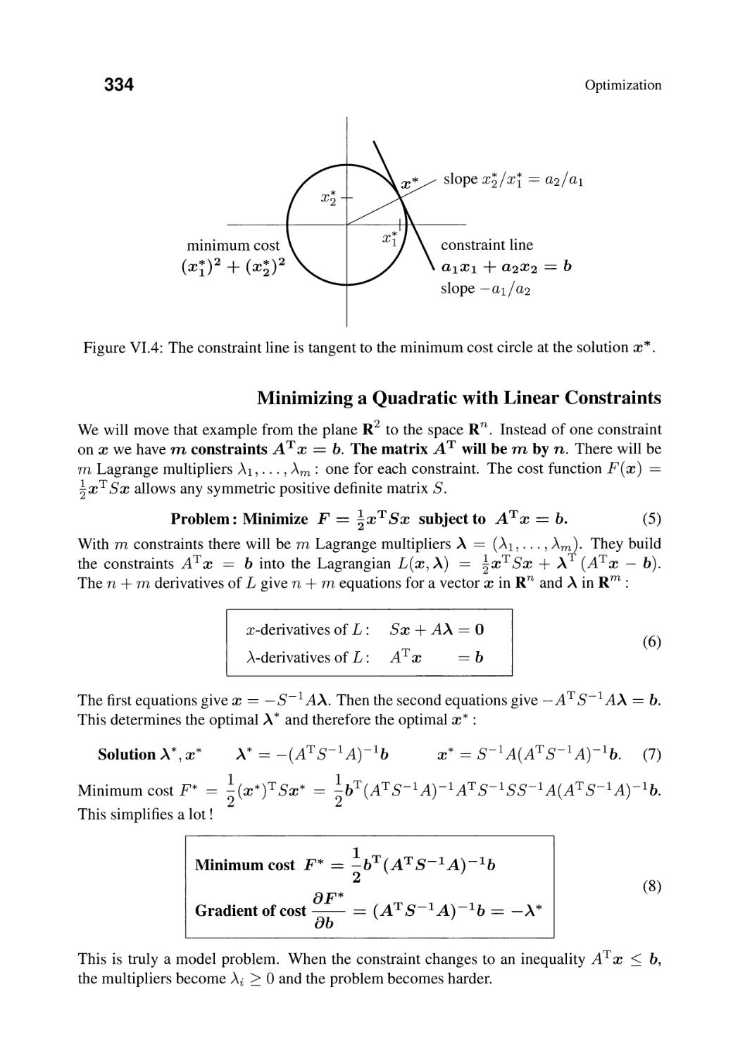
/


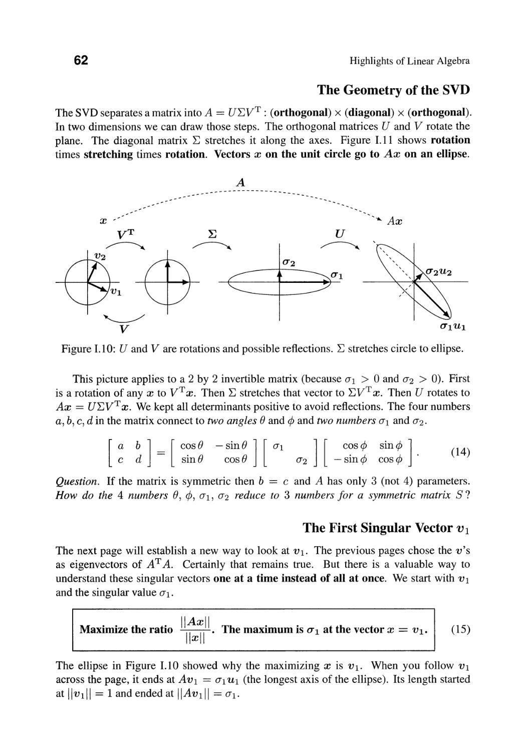


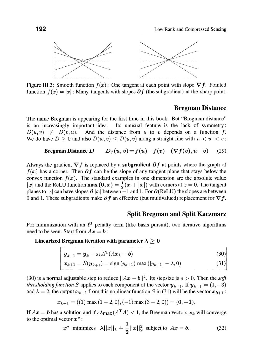


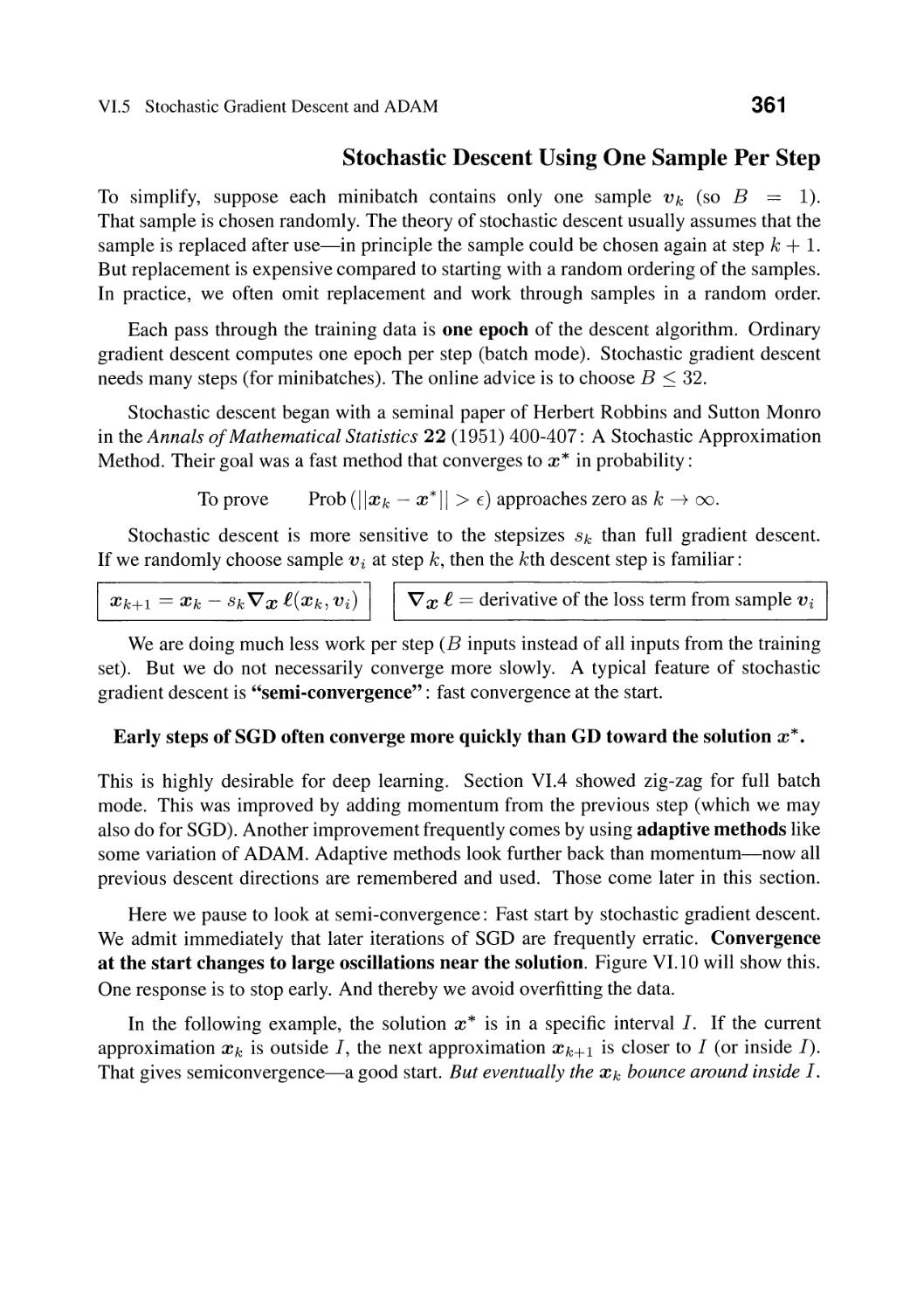


Text
LINEAR ALGEBRA
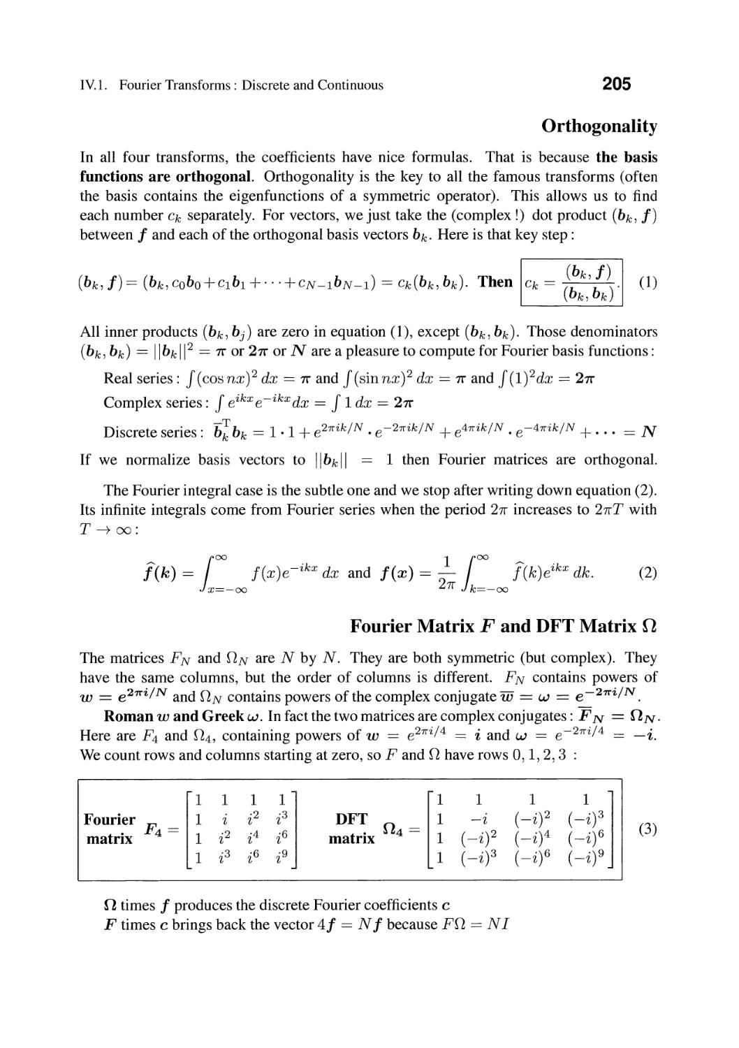
tllJ\,ol Le tl YlJ\,t lJ\,g
fyO
Dtlttl
'> .
:\
: ".
....."
,......"-...
,
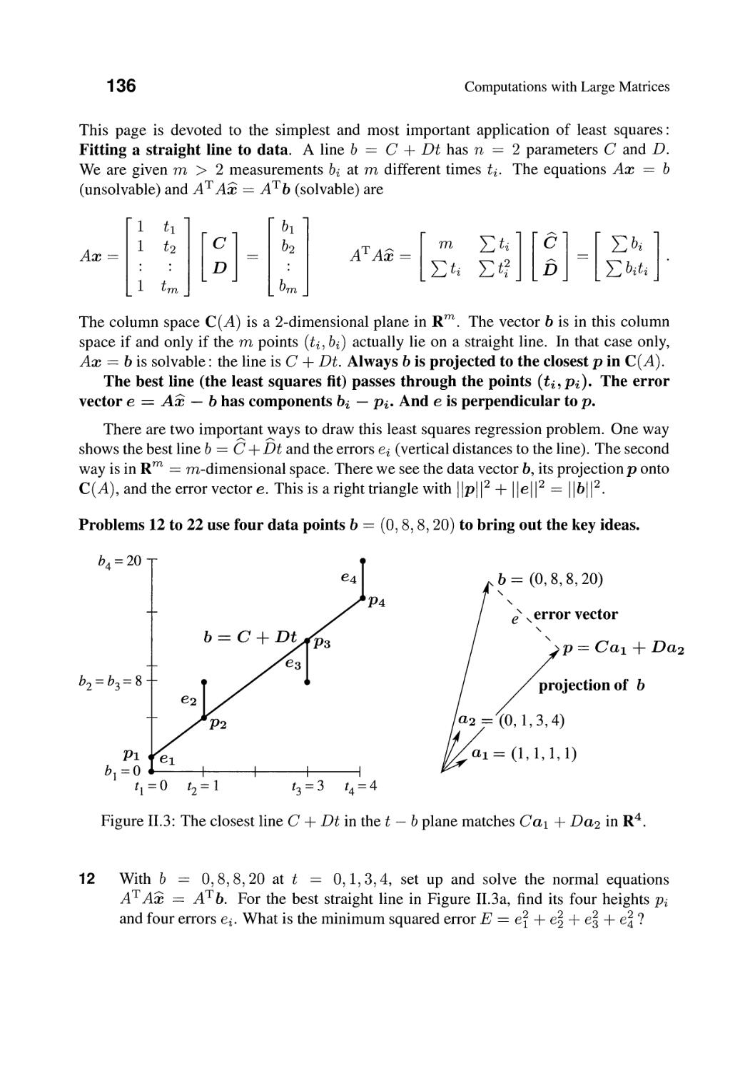
"'"
, \. ,,"
)
'r -
. _.. __.' .
___ I eWIJ I
"t /
...-r.--JI .......
""
.
,
,
"l
----
- -_:::::-,
-
- - -
- -
.' ,.. '....... -
_..... "
----
.:.---
_ _ -.0 _
-- -
--
.- -- -
.,. -
----
-- - -- -
.-
-.....;t.:
-
-
-
..
......... .-..
-
-
--- "'!I-a
- a
......
-=-- ---
-
. .
.
STRAN
-
-
LINEAR ALGEBRA AND
LEARNING FROM DATA
GILBERT STRANG
Massachusetts Institute of Technology
WELLESLEY - CAMBRIDGE PRESS
Box 812060 Wellesley MA 02482
Linear Algebra and Learning from Data
Copyright <92019 by Gilbert Strang
ISBN 978-0-692-19638-0
All rights reserved. No part of this book may be reproduced or stored or transmitted
by any means, including photocopying, without written permission from
Wellesley - Cambridge Press. Translation in any language is strictly prohibited -
authorized translations are arranged by the publisher.
BTEX typesetting by Ashley C. Fernandes (info@problemsolvingpathway.com)
Printed in the United States of America
987654321
Other texts from Wellesley - Cambridge Press
Introduction to Linear Algebra, 5th Edition, Gilbert Strang ISBN 978-0-9802327-7-6
Computational Science and Engineering, Gilbert Strang ISBN 978-0-9614088-1-7
Wavelets and Filter Banks, Gilbert Strang and Truong Nguyen ISBN 978-0-9614088-7-9
Introduction to Applied Mathematics, Gilbert Strang ISBN 978-0-9614088-0-0
Calculus Third edition (2017), Gilbert Strang ISBN 978-0-9802327-5-2
Algorithms for Global Positioning, Kai Borre & Gilbert Strang ISBN 978-0-9802327-3-8
Essays in Linear Algebra, Gilbert Strang ISBN 978-0-9802327-6-9
Differential Equations and Linear Algebra, Gilbert Strang ISBN 978-0-9802327-9-0
An Analysis of the Finite Element Method, 2017 edition, Gilbert Strang and George Fix
ISBN 978-0-9802327-8-3
Wellesley - Cambridge Press
Box 812060
Wellesley MA 02482 USA
www.wellesleycambridge.com
math.mit.edu/weborder.php (orders)
Iinearalgebrabook @ gmaiI.com
math.mit.edu/rvgs
phone (781) 431-8488 fax (617) 253-4358
The website for this book is math.mit.eduJIearningfromdata
That site will link to 18.065 course material and video lectures on YouTube and OCW
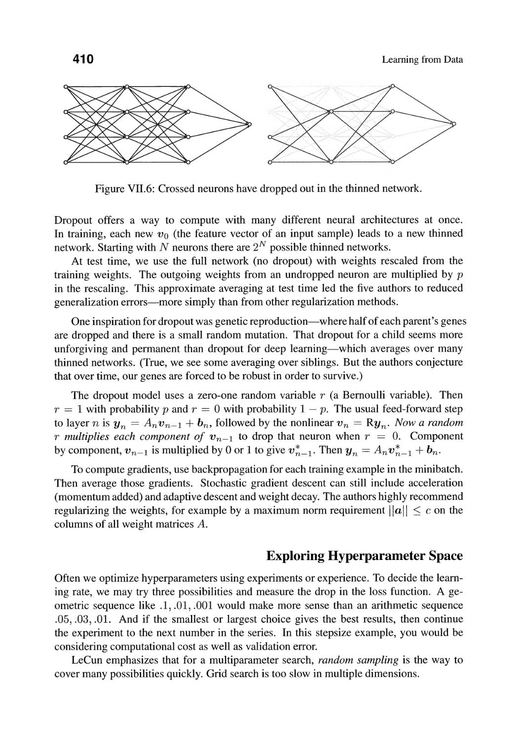
The cover photograph shows a neural net on Inle Lake. It was taken in Myanmar.
From that photograph Lois Sellers designed and created the cover.
The snapshot of playground.tensorflow.org was a gift from its creator Daniel Smilkov.
Linear Algebra is included in MIT's OpenCourseWare site ocw.mit.edu
This provides video lectures of the full linear algebra course 18.06 and 18.06 SC
Deep Learning and Neural Nets
Linear algebra and probability/statistics and optimization are the mathematical pillars
of machine learning. Those chapters will come before the architecture of a neural net.
But we find it helpful to start with this description of the goal: To construct a function
that classifies the training data correctly, so it can generalize to unseen test data.
To make that statement meaningful, you need to know more about this learning
function. That is the purpose of these three pages-to give direction to all that follows.
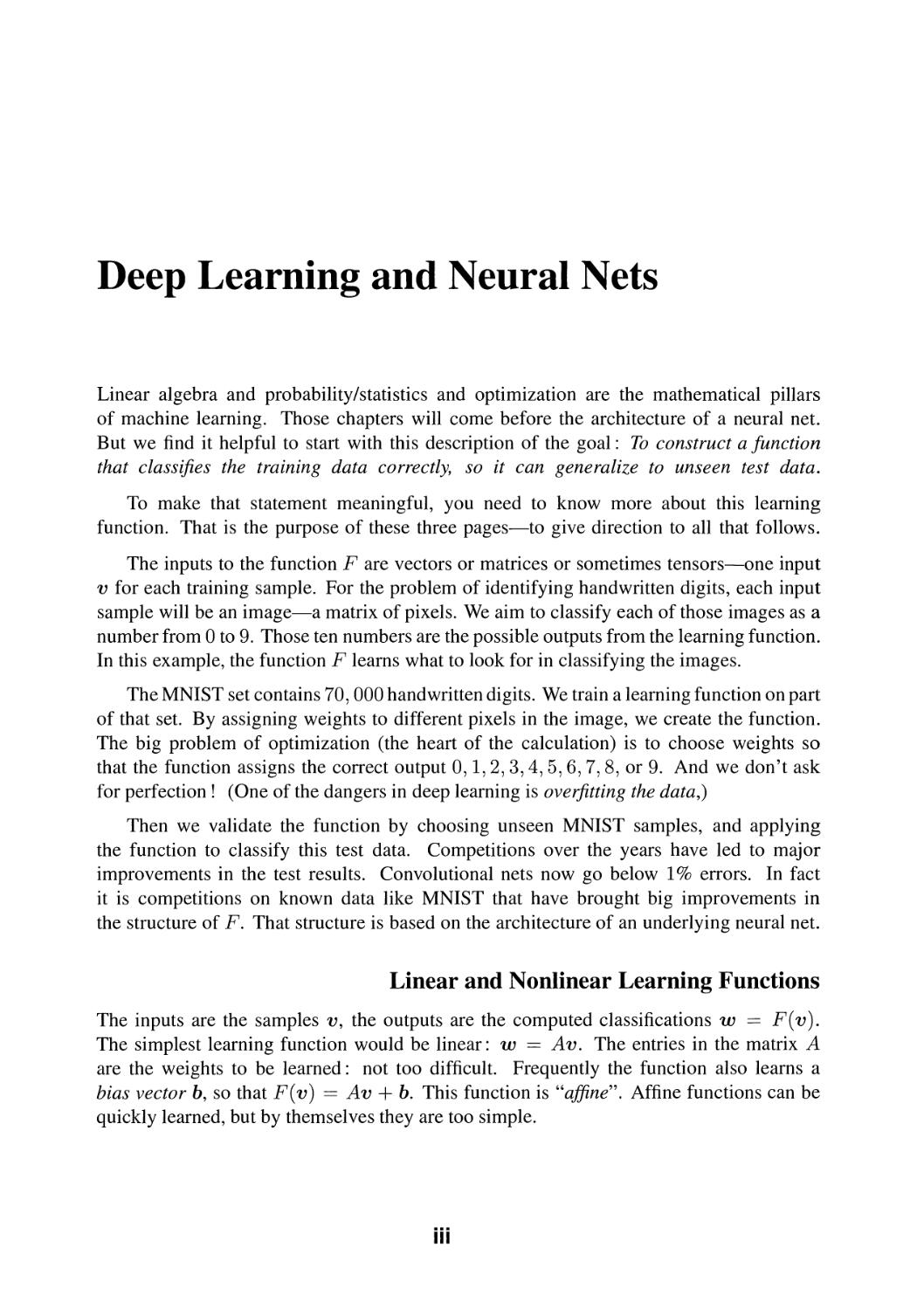
The inputs to the function F are vectors or matrices or sometimes tensors-one input
v for each training sample. For the problem of identifying handwritten digits, each input
sample will be an image-a matrix of pixels. We aim to classify each of those images as a
number from 0 to 9. Those ten numbers are the possible outputs from the learning function.
In this example, the function F learns what to look for in classifying the images.
The MNIST set contains 70, 000 handwritten digits. We train a learning function on part
of that set. By assigning weights to different pixels in the image, we create the function.
The big problem of optimization (the heart of the calculation) is to choose weights so
that the function assigns the correct output 0, 1,2,3,4,5,6,7,8, or 9. And we don't ask
for perfection! (One of the dangers in deep learning is overfitting the data,)
Then we validate the function by choosing unseen MNIST samples, and applying
the function to classify this test data. Competitions over the years have led to major
improvements in the test results. Convolutional nets now go below 1 % errors. In fact
it is competitions on known data like MNIST that have brought big improvements in
the structure of F. That structure is based on the architecture of an underlying neural net.
Linear and Nonlinear Learning Functions
The inputs are the samples v, the outputs are the computed classifications w == F ( v).
The simplest learning function would be linear: w == Av. The entries in the matrix A
are the weights to be learned: not too difficult. Frequently the function also learns a
bias vector b, so that F (v) == Av + b. This function is "affine". Affine functions can be
quickly learned, but by themselves they are too simple.
iii
iv
Deep Learning and Neural Nets
More exactly, linearity is a very limiting requirement. If MNIST used Roman numerals,
then II might be halfway between I and III (as linearity demands). But what would be
halfway between I and XIX? Certainly affine functions Av + b are not always sufficient.
Nonlinearity would come by squaring the components of the input vector v. That step
might help to separate a circle from a point inside-which linear functions cannot do.
But the construction of F moved toward "sigmoidal functions" with S -shaped graphs.
It is remarkable that big progress came by inserting these standard nonlinear S -shaped
functions between matrices A and B to produce A(S(Bv)). Eventually it was discovered
that the smoothly curved logistic functions S could be replaced by the extremely simple
ramp function now called ReLU(x) == max (0, x). The graphs of these nonlinear
"activation functions" R are drawn in Section VII.l.
Neural Nets and the Structure of F ( v )
The functions that yield deep learning have the form F( v) == L(R(L(R(... (Lv))))).
This is a composition of affine functions Lv == Av + b with nonlinear functions R-
which act on each component of the vector Lv. The matrices A and the bias vectors b
are the weights in the learning function F. It is the A's and b's that must be learned
from the training data, so that the outputs F (v) will be (nearly) correct. Then F can be
applied to new samples from the same population. If the weights (A's and b's) are well
chosen, the outputs F ( v) from the unseen test data should be accurate. More layers
in the function F will typically produce more accuracy in F( v).
Properly speaking, F(x, v) depends on the input v and the weights x (all the A's and
b's). The outputs VI == ReLU(A 1 v + b l ) from the first step produce the first hidden
layer in our neural net. The complete net starts with the input layer v and ends with the
output layer w == F ( v). The affine part L k ( V k-1) == A k V k-1 + bk of each step uses the
computed weights A k and b k .
All those weights together are chosen in the giant optimization of deep learning:
Choose weights A k and b k to minimize the total loss over all training samples.
The total loss is the sum of individual losses on each sample. The loss function for
least squares has the familiar form II F ( v) - true output I 1 2 . Often least squares is not
the best loss function for deep learning.
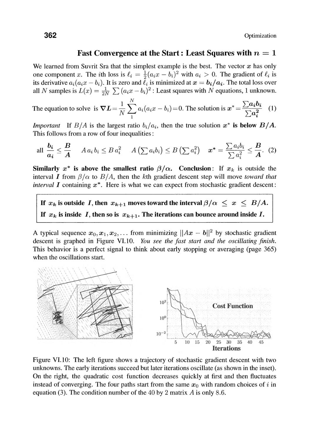
One input v ==
One output w == 2
Deep Learning and Neural Nets
v
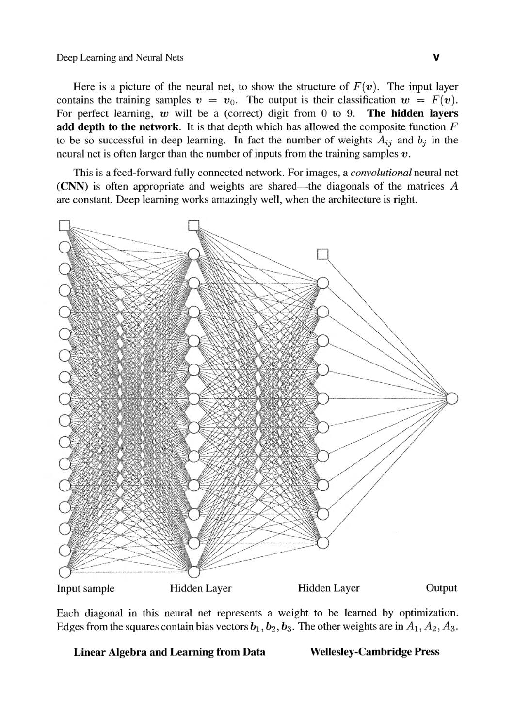
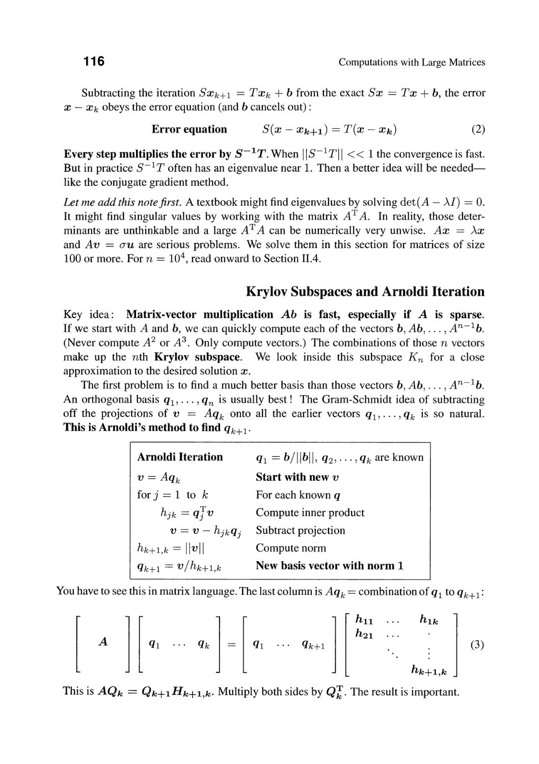
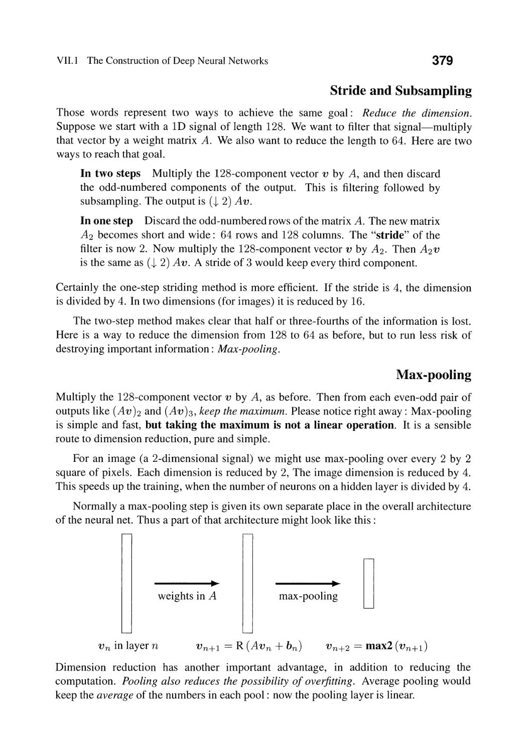
Here is a picture of the neural net, to show the structure of F ( v). The input layer
contains the training samples v == Vo. The output is their classification w == F ( v).
For perfect learning, w will be a (correct) digit from 0 to 9. The hidden layers
add depth to the network. It is that depth which has allowed the composite function F
to be so successful in deep learning. In fact the number of weights A ij and b j in the
neural net is often larger than the number of inputs from the training samples v.
This is a feed-forward fully connected network. For images, a convolutional neural net
(CNN) is often appropriate and weights are shared-the diagonals of the matrices A
are constant. Deep learning works amazingly well, when the architecture is right.
..;
\
l.
" \
\
1
\ i
, '
"
; :; 'l
Input sample
Hidden Layer
Hidden Layer
Output
Each diagonal in this neural net represents a weight to be learned by optimization.
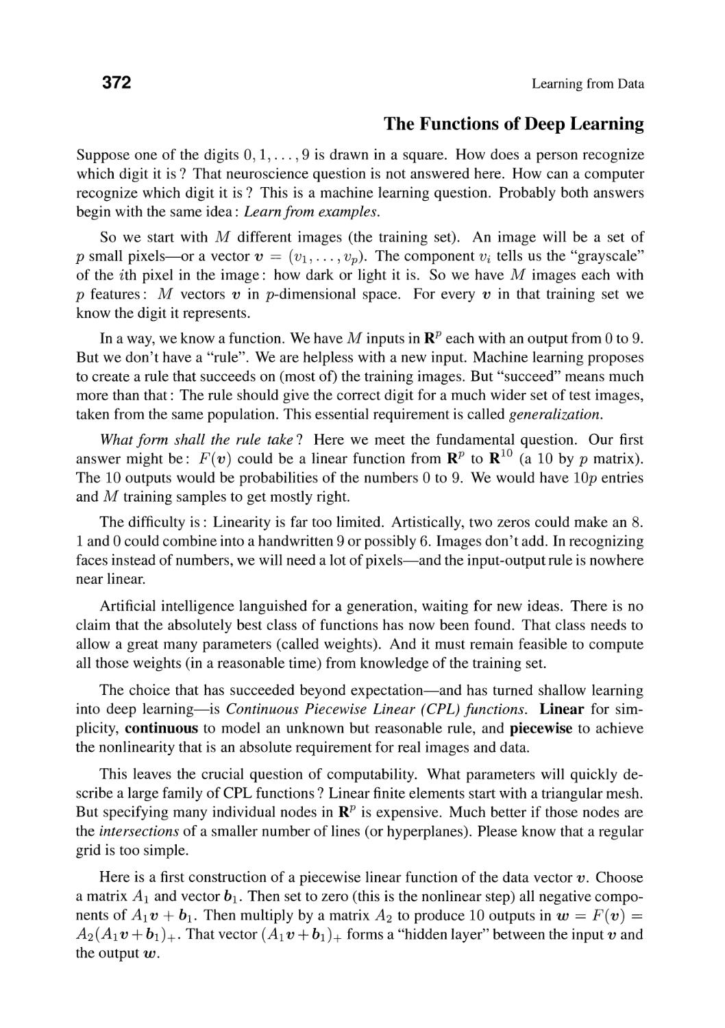
Edges from the squares contain bias vectors b 1 , b 2 , b 3 . The other weights are in AI, A 2 , A 3 .
Linear Algebra and Learning from Data
Wellesley-Cambridge Press
Preface and Acknowledgments
My deepest gratitude goes to Professor Raj Rao Nadakuditi of the University of Michigan.
On his sabbatical in 201 7, Raj brought his EECS 551 course to MIT. He flew to Boston
every week to teach 18.065. Thanks to Raj, the students could take a new course. He led
the in-class computing, he assigned homeworks, and exams were outlawed.
This was linear algebra for signals and data, and it was alive. 140 MIT students signed
up. Alan Edelman introduced the powerful language Julia, and I explained the four funda-
mental subspaces and the Singular Value Decomposition. The labs from Michigan involved
rank and SVD and applications. We were asking the class for computational thinking.
That course worked, even the first time. It didn't touch one big topic: Deep learning.
By this I mean the excitement of creating a learning function on a neural net, with the
hidden layers and the nonlinear activation functions that make it so powerful. The sys-
tem trains itself on data which has been correctly classified in advance. The optimization
of weights discovers important features-the shape of a letter, the edges in an image, the
syntax of a sentence, the identifying details of a signal. Those features get heavier weights-
without overfitting the data and learning everything. Then unseen test data from a similar
population can be identified by virtue of having those same features.
The algorithms to do all that are continually improving. Better if I say that they are
being improved. This is the contribution of computer scientists and engineers and
biologists and linguists and mathematicians and especially optimists-those who can
optimize weights to minimize errors, and also those who believe that deep learning
can help in our lives.
You can see why this book was written:
1. To organize central methods and ideas of data science.
2. To see how the language of linear algebra gives expression to those ideas.
3. Above all, to show how to explain and teach those ideas-to yourself or to a class.
I certainly learned that projects are far better than exams. Students ask their own questions
and write their own programs. From now on, projects!
vi
Preface and Acknowledgments
vii
Linear Algebra and Calculus
The reader will have met the two central subjects of undergraduate mathematics: Linear
algebra and calculus. For deep learning, it is linear algebra that matters most. We compute
"weights" that pick out the important features of the training data, and those weights go
into matrices. The form of the learning function is described on page iv. Then calculus
shows us the direction to move, in order to improve the current weights x k.
From calculus, it is partial derivatives that we need (and not integrals) :
Reduce the error L( x) by moving from Xk to Xk+l == Xk - Sk V L.
That symbol V L stands for the first derivatives of L( x). Because of the minus sign,
x k+ 1 is downhill from x k on the graph of L (x). The stepsize S k (also called the learning
rate) decides how far to move. You see the basic idea: Reduce the loss function L(x) by
moving in the direction of fastest decrease. V L == 0 at the best weights x* .
The complication is that the vector x represents thousands of weights. So we have
to compute thousands of partial derivatives of L. And L itself is a complicated function
depending on several layers of x's as well as the data. So we need the chain rule to find V L.
The introduction to Chapter VI will recall essential facts of multivariable calculus.
By contrast, linear algebra is everywhere in the world of learning from data. This is
the subject to know! The first chapters of this book are essentially a course on applied
linear algebra-the basic theory and its use in computations. I can try to outline how that
approach (to the ideas we need) compares to earlier linear algebra courses. Those are
quite different, which means that there are good things to learn.
Basic course
1. Elimination to solve Ax == b
2. Matrix operations and inverses and determinants
3. Vector spaces and subspaces
4. Independence, dimension, rank of a matrix
5. Eigenvalues and eigenvectors
If a course is mostly learning definitions, that is not linear algebra in action. A stronger
course puts the algebra to use. The definitions have a purpose, and so does the book.
Stronger course
1. Ax == b in all cases: square system-too many equations-too many unknowns.
2. Factor A into LU and QR and U:EyT and Cl\!I R: Columns times rows.
3. Four fundamental subspaces: dimensions and orthogonality and good bases.
4. Diagonalizing A by eigenvectors and by left and right singular vectors.
5. Applications: Graphs, convolutions, iterations, covariances, projections, filters,
networks, images, matrices of data.
viii
Preface and Acknowledgments
Linear algebra has moved to the center of machine learning, and we need to be there.
A book was needed for the 18.065 course. It was started in the original 2017 class,
and a first version went out to the 2018 class. I happily acknowledge that this book owes its
existence to Ashley C. Fernandes. Ashley receives pages scanned from Boston and sends
back new sections from Mumbai, ready for more work. This is our seventh book together
and I am extremely grateful.
Students were generous in helping with both classes, especially William Loucks and
Claire Khodadad and Alex LeN ail and Jack Strang. The project from Alex led to his online
code alexlenail.me/NN - SVGI to draw neural nets (an example appears on page v).
The project from Jack on http://www.teachyourmachine.com learns to recognize hand-
written numbers and letters drawn by the user: open for experiment. See Section VII.2.
MIT's faculty and staff have given generous and much needed help:
Suvrit Sra gave a fantastic lecture on stochastic gradient descent (now an 18.065 video)
Alex Postnikov explained when matrix completion can lead to rank one (Section IV.8)
Tommy Poggio showed his class how deep learning generalizes to new data
Jonathan Harmon and Tom Mullaly and Liang Wang contributed to this book every day
Ideas arrived from all directions and gradually they filled this textbook.
The Content of the Book
This book aims to explain the mathematics on which data science depends: Linear algebra,
optimization, probability and statistics. The weights in the learning function go into
matrices. Those weights are optimized by "stochastic gradient descent". That word
stochastic (== random) is a signal that success is governed by probability not certainty.
The law of large numbers extends to the law of large functions: If the architecture is
well designed and the parameters are well computed, there is a high probability of success.
Please note that this is not a book about computing, or coding, or software. Many books
do those parts well. One of our favorites is Hands-On Machine Learning (2017)
by Aurelien Geron (published by O'Reilly). And online help, from Tensorflow and Keras
and Math Works and Caffe and many more, is an important contribution to data science.
Linear algebra has a wonderful variety of matrices: symmetric, orthogonal, triangular,
banded, permutations and projections and circulants. In my experience, positive definite
symmetric matrices S are the aces. They have positive eigenvalues A and orthogonal
eigenvectors q. They are combinations S == Al q1 qI + A2q2q'f + . .. of simple rank-one
projections qq T onto those eigenvectors. And if Al > A2 > . . . then Al q1 q'f is the most
informative part of S. For a sample covariance matrix, that part has the greatest variance.
Preface and Acknowledgments
ix
Chapter I In our lifetimes, the most important step has been to extend those ideas from
symmetric matrices to all matrices. Now we need two sets of singular vectors, u's and v's.
Singular values (J replace eigenvalues A. The decomposition A == (J1 u] vI + (J2U2Vi +. . .
remains correct (this is the SVD). With decreasing (J's, those rank-one pieces of A still
come in order of importance. That "Eckart-Young Theorem" about A complements what
we have long known about the symmetric matrix AT A: For rank k, stop at (JkUkVI.
II The ideas in Chapter I become algorithms in Chapter II. For quite large matrices, the
(J's and u's and v's are computable. For very large matrices, we resort to randomization:
Sample the columns and the rows. For wide classes of big matrices this works well.
III-IV Chapter III focuses on low rank matrices, and Chapter IV on many important
examples. We are looking for properties that make the computations especially fast (in III)
or especially useful (in IV). The Fourier matrix is fundamental for every problem with
constant coefficients (not changing with position). That discrete transform is superfast
because of the FFT : the Fast Fourier Transform.
V Chapter V explains, as simply as possible, the statistics we need. The central ideas are
always mean and variance: The average and the spread around that average. Usually
we can reduce the mean to zero by a simple shift. Reducing the variance (the uncertainty)
is the real problem. For random vectors and matrices and tensors, that problem becomes
deeper. It is understood that the linear algebra of statistics is essential to machine learning.
VI Chapter VI presents two types of optimization problems. First come the nice problems
of linear and quadratic programming and game theory. Duality and saddle points are
key ideas. But the goals of deep learning and of this book are elsewhere: Very large
problems with a structure that is as simple as possible. "Derivative equals zero" is still
the fundamental equation. The second derivatives that Newton would have used are
too numerous and too complicated to compute. Even using all the data (when we take
a descent step to reduce the loss) is often impossible. That is why we choose only
a minibatch of input data, in each step of stochastic gradient descent.
The success of large scale learning comes from the wonderful fact that randolnization
often produces reliability-when there are thousands or millions of variables.
VII Chapter VII begins with the architecture of a neural net. An input layer is connected
to hidden layers and finally to the output layer. For the training data, input vectors v
are known. Also the correct outputs are known (often w is the correct classification of v).
We optimize the weights x in the learning function F so that F(x, v) is close to w
for almost every training input v.
Then F is applied to te5t data, drawn from the same population as the training data.
If F learned what it needs (without overfitting: we don't want to fit 100 points by 99th
degree polynomials), the test error will also be low. The system recognizes images and
speech. It translates between languages. It may follow designs like ImageNet or AlexNet,
winners of major competitions. A neural net defeated the world champion at Go.
x
Preface and Acknowledgments
The function F is often piecewise linear-the weights go into matrix mUltiplications.
Every neuron on every hidden layer also has a nonlinear "activation function". The
ramp function ReLU (x) == (maximum of 0 and x) is now the overwhelming favorite.
There is a growing world of expertise in designing the layers that make up F(x, v).
We start with fully connected layers-all neurons on layer n connected to all neurons on
layer n + 1. Often CNN's are better-Convolutional neural nets repeat the same weights
around all pixels in an image: a very important construction. Other layers are different.
A pooling layer reduces the dimension. Dropout randomly leaves out neurons. Batch
normalization resets the mean and variance. All these steps create a function that closely
matches the training data. Then F (x, v) is ready to use.
Acknowledgments
Above all, I welcome this chance to thank so many generous and encouraging friends:
Pawan Kumar and Leonard Berrada and Mike Giles and Nick Trefethen in Oxford
Ding-Xuan Zhou and Yunwen Lei in Hong Kong
Alex Townsend and Heather Wilber at Cornell
Nati Srebro and Srinadh Bhojanapalli in Chicago
Tammy Kolda and Thomas Strohmer and Trevor Hastie and Jay Kuo in California
Bill Hager and Mark Embree and Wotao Yin, for help with Chapter III
Stephen Boyd and Lieven Vandenberghe, for great books
Alex Strang, for creating the best figures, and more
Ben Recht in Berkeley, especially.
Your papers and emails and lectures and advice were wonderful.
THE MATRIX ALPHABET
A Any Matrix Q Orthogonal Matrix
C Circulant Matrix R Upper Triangular Matrix
C Matrix of Columns R Matrix of Rows
D Diagonal Matrix S Symmetric Matrix
F Fourier Matrix S Sample Covariance Matrix
I Identity Matrix T Tensor
L Lower Triangular Matrix U Upper Triangular Matrix
L Laplacian Matrix U Left Singular Vectors
JV[ Mixing Matrix Y Right Singular Vectors
JV[ Markov Matrix X Eigenvector Matrix
P Probability Matrix A Eigenvalue Matrix
P Projection Matrix Singular Value Matrix
Video lectures: OpenCourseWare ocw.mit.edu and YouTube (Math 18.06 and 18.065)
Introduction to Linear Algebra (5th ed) by Gilbert Strang, Wellesley-Cambridge Press
Book web sites : math.mit.edu/linearalgebra and math.mit.edu/learningfromdata
Table of Contents
Deep Learning and Neural Nets
Preface and Acknowledgments
Part I : Highlights of Linear Algebra
Hi
vi
1
1.1 Multiplication Ax Using Columns of A .............
1.2 Matrix-Matrix Multiplication AB . .
1.3 The Four Fundamental Subspaces
1.4 Elimination and A == LU . . . .
1.5 Orthogonal Matrices and Subspaces .
1.6 Eigenvalues and Eigenvectors . . . .
I. 7 Symmetric Positive Definite Matrices . . . . . . . . . . . . .
1.8 Singular Values and Singular Vectors in the SVD . . . . . . .
1.9 Principal Components and the Best Low Rank Matrix ....
1.10 Rayleigh Quotients and Generalized Eigenvalues . . . . . . . . .
1.11 Norms of Vectors and Functions and Matrices. . . . . . .
1.12 Factoring Matrices and Tensors: Positive and Sparse
2
9
14
21
29
36
44
56
71
81
88
97
Part II : Computations with Large Matrices
113
11.1 Numerical Linear Algebra . . . .
11.2 Least Squares: Four Ways . . . . . .
11.3 Three Bases for the Column Space. .
11.4 Randomized Linear Algebra .
115
124
138
146
xi
xii
Part III: Low Rank and Compressed Sensing
111.1 Changes in A -1 from Changes in A . . .
111.2 Interlacing Eigenvalues and Low Rank Signals
Table of Contents
111.3
Rapidly Decaying Singular Values
159
160
168
178
184
195
111.4 Split Algorithms for £2 + £1 . . . .
111.5 Compressed Sensing and Matrix Completion .
Part IV: Special Matrices
203
IV. 1 Fourier Transforms: Discrete and Continuous .
IV.2 Shift Matrices and Circulant Matrices
IV. 3 The Kronecker Product A 0 B . . .
IV.4 Sine and Cosine Transforms from Kronecker Sums .
IV. 5 Toeplitz Matrices and Shift Invariant Filters .
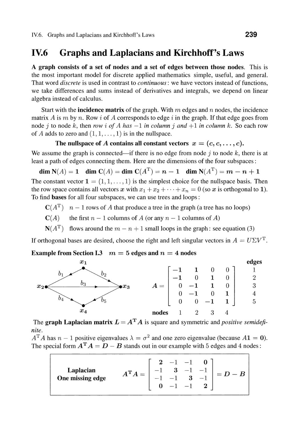
IV.6 Graphs and Laplacians and Kirchhoff's Laws
204
213
221
228
232
239
245
255
257
259
IV.7 Clustering by Spectral Methods and k-means
IV.8 Completing Rank One Matrices . . .
IV.9 The Orthogonal Procrustes Problem .
IV. 1 0 Distance Matrices ..........
Part V: Probability and Statistics
263
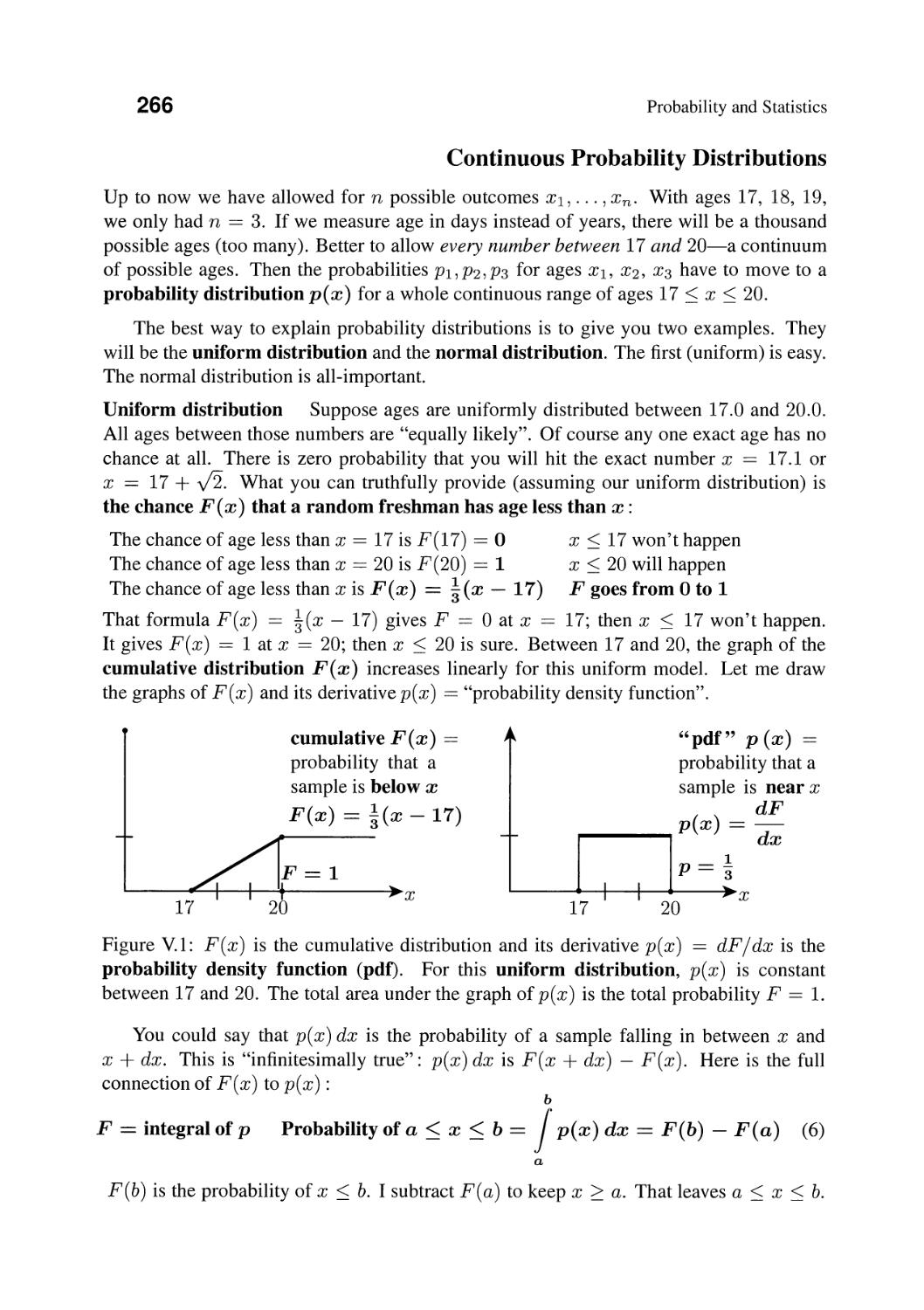
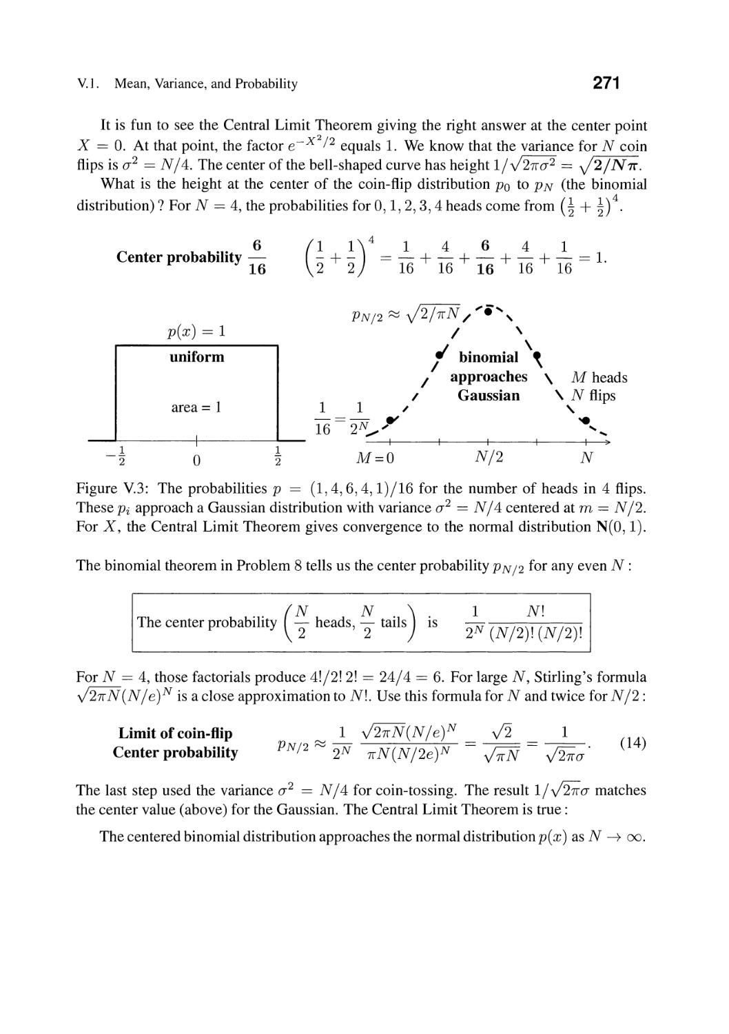
V.l Mean, Variance, and Probability. 264
V.2 Probability Distributions. 275
V.3 Moments, Cumulants, and Inequalities of Statistics. 284
V.4 Covariance Matrices and Joint Probabilities 294
V.5 Multivariate Gaussian and Weighted Least Squares. 304
V.6 Markov Chains . 311
Table of Contents xiii
Part VI: Optimization 321
VI. 1 Minimum Problems: Convexity and Newton's Method . . . . 324
VI.2 Lagrange Multipliers == Derivatives of the Cost . . 333
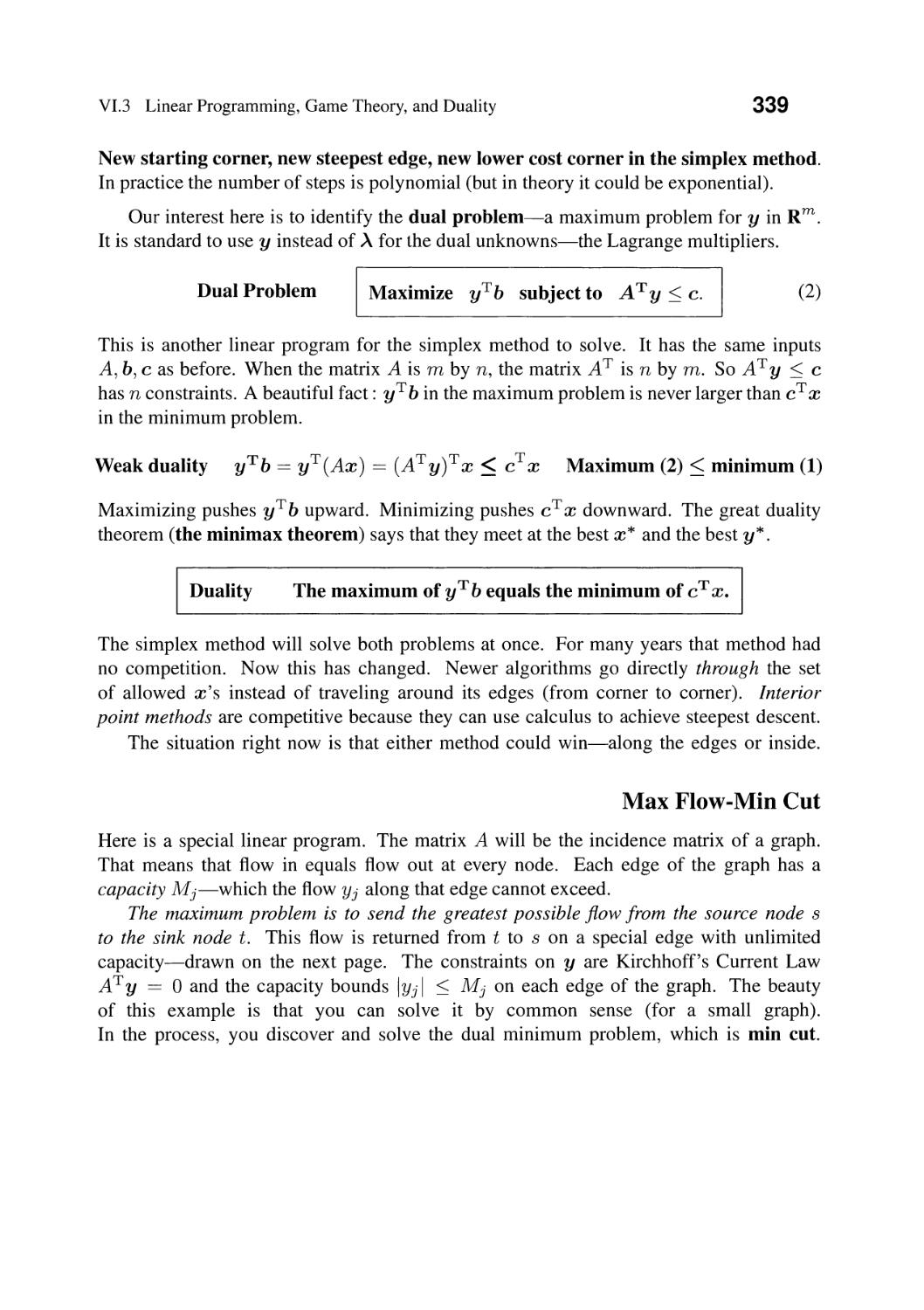
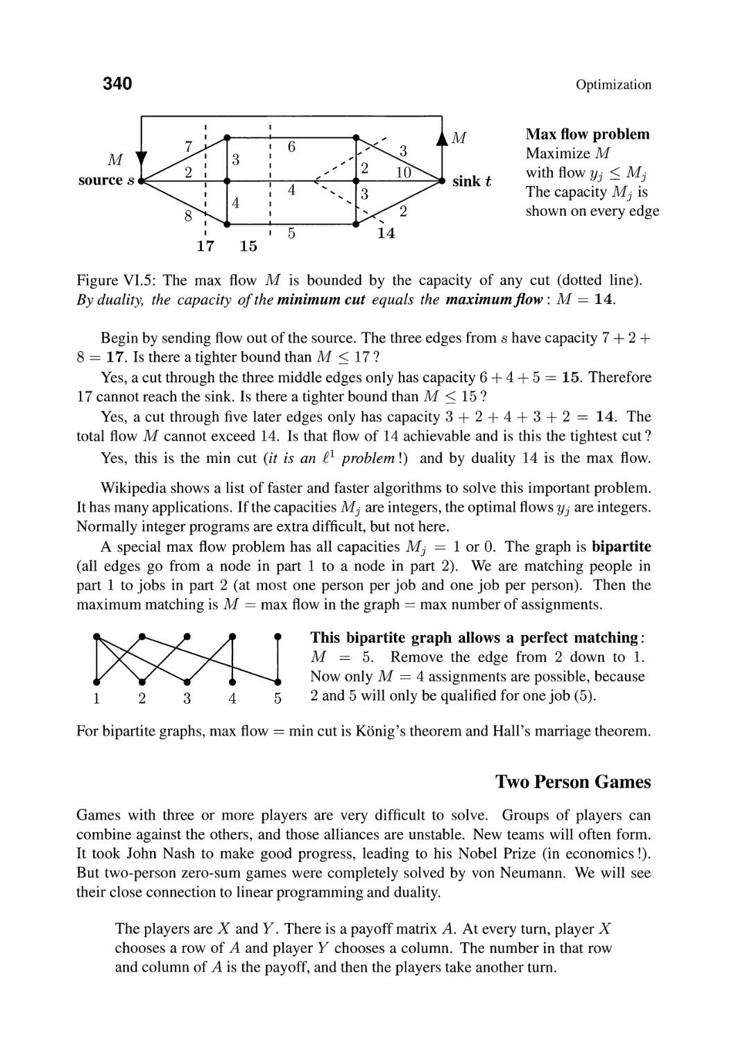
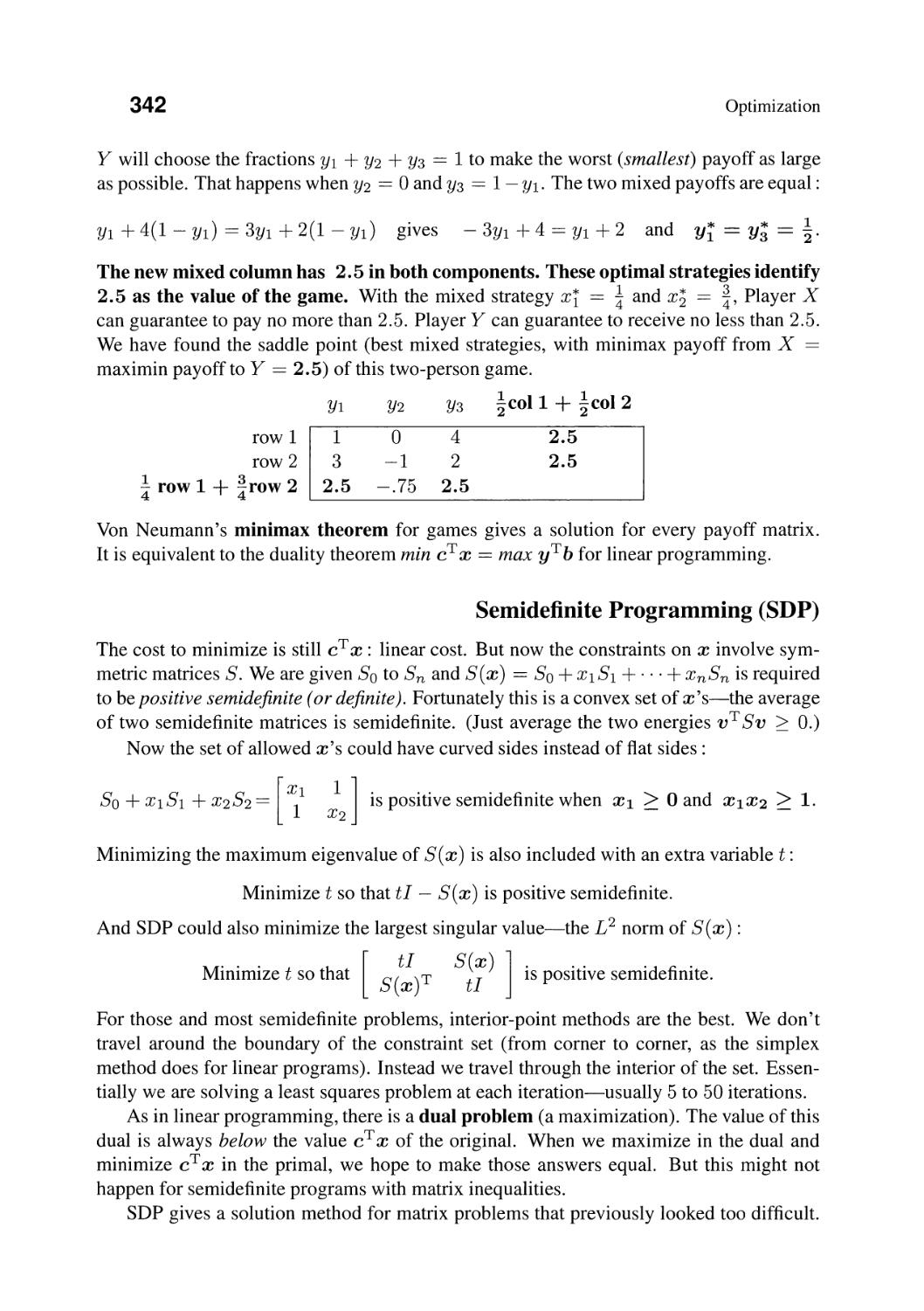
VI.3 Linear Programming, Game Theory, and Duality . . 338
VI.4 Gradient Descent Toward the Minimum. 344
VI.5 Stochastic Gradient Descent and ADAM . . . . . 359
Part VII: Learning from Data
371
VII. 1 The Construction of Deep Neural Networks
375
387
397
407
413
VII.2 Convolutional Neural Nets ......
VII.3 Backpropagation and the Chain Rule
VII.4 Hyperparameters: The Fateful Decisions
VII.5 The World of Machine Learning ....
Books on Machine Learning
416
Eigenvalues and Singular Values: Rank One
417
Codes and Algorithms for Numerical Linear Algebra
418
Counting Parameters in the Basic Factorizations
419
Index of Authors
420
Index
423
Index of Symbols
432
Part I
Highlights of Linear Algebra
1.1 Multiplication Ax Using Columns of A
1.2 Matrix-Matrix Multiplication AB
1.3 The Four Fundamental Subspaces
1.4 Elimination and A == LU
1.5 Orthogonal Matrices and Subspaces
1.6 Eigenvalues and Eigenvectors
1.7 Symmetric Positive Definite Matrices
1.8 Singular Values and Singular Vectors in the SVD
1.9 Principal Components and the Best Low Rank Matrix
1.10 Rayleigh Quotients and Generalized Eigenvalues
1.11 Norms of Vectors and Functions and Matrices
1.12 Factoring Matrices and Tensors: Positive and Sparse
Part I : Highlights of Linear Algebra
Part I of this book is a serious introduction to applied linear algebra. If the reader's
background is not great or not recent (in this important part of mathematics),
please do not rush through this part. It starts with multiplying Ax and AB using the
columns of the matrix A. That might seem only formal but in reality it is fundamental.
Let me point to five basic problems studied in this chapter.
Ax == b Ax == AX Av == au Minimize IIAx112/lIx112
Factor the matrix A
Each of those problems looks like an ordinary computational question:
Find x
Find x and A
Find v, u, and a
Factor A == columns times rows
You will see how understanding (even more than solving) is our goal. We want to know
if Ax == b has a solution x in the first place. "Is the vector b in the column space of A ?"
That innocent word "space" leads a long way. It will be a productive way, as you will see.
The eigenvalue equation Ax == AX is very different. There is no vector b-we are
looking only at the matrix A. We want eigenvector directions so that Ax keeps the
same direction as x. Then along that line all the complicated interconnections of A have
gone away. The vector A 2 x is just A 2 x. The matrix eAt (from a differential equation)
is just multiplying x by eAt. We can solve anything linear when we know every x and A.
The equation Av == (JU is close but different. Now we have two vectors v and u.
Our matrix A is probably rectangular, and full of data. What part of that data matrix is
important? The Singular Value Decomposition (SVD) finds its simplest pieces (Juv T.
Those pieces are matrices (column u times row v T). Every matrix is built from these
orthogonal pieces. Data science meets linear algebra in the SVD.
Finding those pieces (Juv T is the object of Principal Component Analysis (PCA).
Minimization and factorization express fundamental applied problems. They lead to
those singular vectors v and u. Computing the best x in least squares and the principal
component VI in PCA is the algebra problem that fits the data. We won't give codes-
those belong online-we are working to explain ideas.
When you understand column spaces and nullspaces and eigenvectors and singular
vectors, you are ready for applications of all kinds: Least squares, Fourier transforms,
LASSO in statistics, and stochastic gradient descent in deep learning with neural nets.
1
2 Highlights of Linear Algebra
1.1 Multiplication Ax Using Columns of A
We hope you already know some linear algebra. It is a beautiful subject-more useful
to more people than calculus (in our quiet opinion). But even old-style linear algebra
courses miss basic and important facts. This first section of the book is about matrix-vector
multiplication Ax and the column space of a matrix and the rank.
We always use examples to make our point clear.
Example 1 Multiply A times x using the three rows of A. Then use the two columns:
By rows
[ ] [ ] = [ 2x] + 3X2 ] inner products
Xl 2X1 + 4X2 of the rows
X2 3X1 + 7X2 with x == (Xl, X2)
[ ] [ ] [ ] [ ] combination
Xl +X2 of the columns
Xl
3 7 X2 a1 and a2
By columns
You see that both ways give the same result. The first way (a row at a time) produces
three inner products. Those are also known as "dot products" because of the dot notation:
row. column == (2, 3). (Xl, X2) == 2X1 + 3X2
(1)
This is the way to find the three separate components of Ax. We use this for computing-
but not for understanding. It is low level. Understanding is higher level, using vectors.
The vector approach sees Ax as a "linear combination" of a1 and a2. This is the funda-
mental operation of linear algebra! A linear combination of a1 and a2 includes two steps:
(1) Multiply the columns a1 and a2 by "scalars" Xl and X2
(2) Add vectors X1a1 + X2a2 == Ax.
Thus Ax is a linear combination of the columns of A. This is fundamental.
This thinking leads us to the column space of A. The key idea is to take all combina-
tions of the columns. All real numbers Xl and X2 are allowed-the space includes Ax for
all vectors x. In this way we get infinitely many output vectors Ax. And we can see those
outputs geometrically.
In our example, each Ax is a vector in 3-dimensional space. That 3D space is called
R 3 . (The R indicates real numbers. Vectors with three complex components lie in the
space C 3 .) We stay with real vectors and we ask this key question:
All combinations Ax == Xl a1 + X2a2 produce what part of the full 3D space?
Answer: Those vectors produce a plane. The plane contains the complete line in the
direction of a1 == (2,2,3), since every vector Xl a1 is included. The plane also includes
the line of all vectors X2 a2 in the direction of a2. And it includes the sum of any vector
on one line plus any vector on the other line. This addition fills out an infinite plane
containing the two lines. But it does not fill out the whole 3-dimensional space R 3 .
1.1. Multiplication Ax Using Columns of A
3
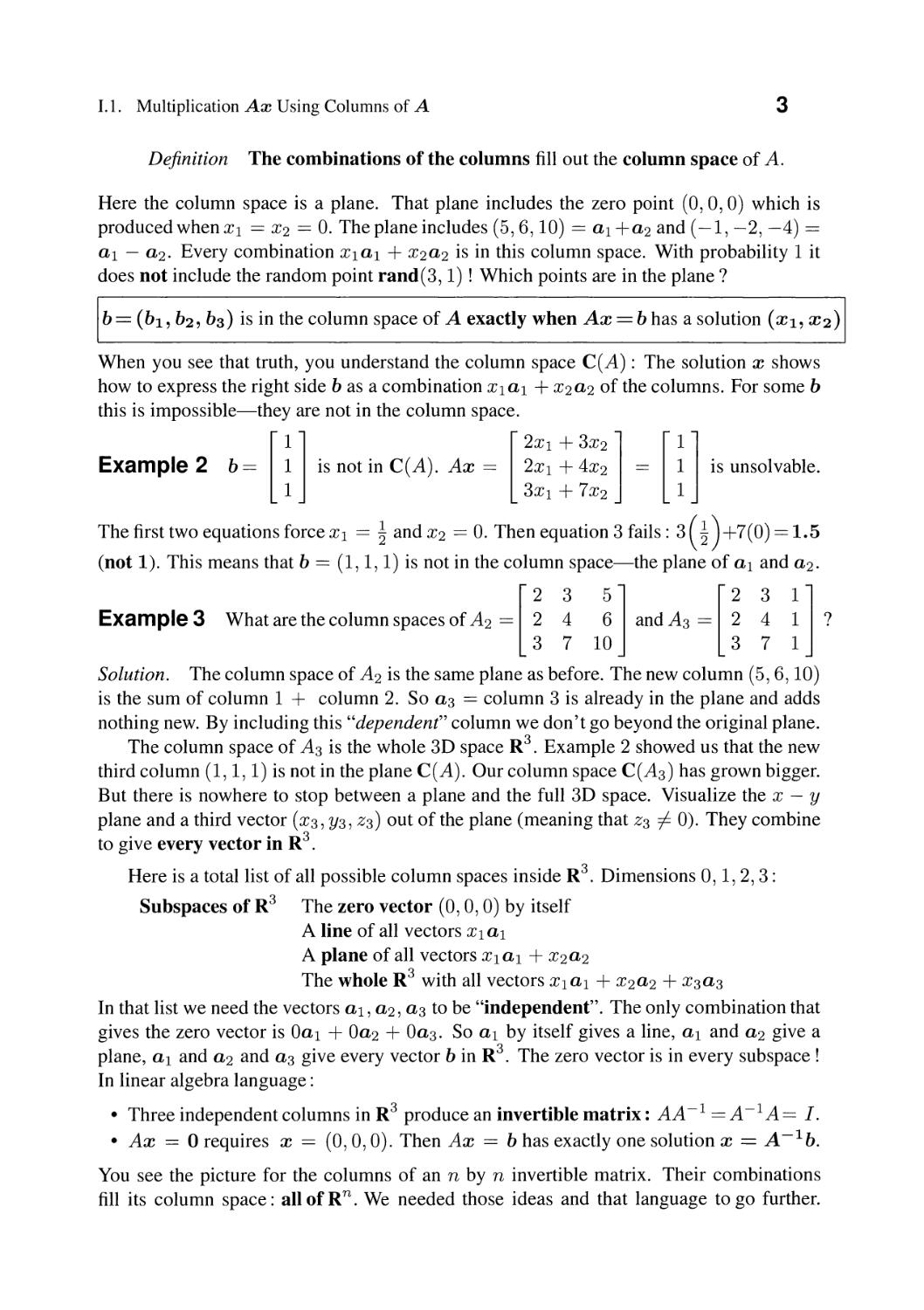
Definition The combinations of the columns fill out the column space of A.
Here the column space is a plane. That plane includes the zero point (0,0,0) which is
produced when Xl == X2 == O. The plane includes (5,6,10) == a1 +a2 and (-1, -2, -4) ==
a1 - a2. Every combination Xl a1 + X2a2 is in this column space. With probability 1 it
does not include the random point rand(3, 1) ! Which points are in the plane?
b == (b l , b 2 , b 3 ) is in the column space of A exactly when Ax == b has a solution (Xl, X2)
When you see that truth, you understand the column space C(A) : The solution X shows
how to express the right side b as a combination Xl a1 + X2a2 of the columns. For some b
this is impossible-they are not in the column space.
Example 2 b == [ ] is not in C(A). Ax == [ : ] == [ ] is unsolvable.
1 3X1 + 7X2 1
Thefirsttwoequationsforcexl = andx2 = O. Then equation 3 fails: 3( )+7(O)=1.5
(not 1). This means that b == (1, 1, 1) is not in the column space-the plane of a1 and a2.
Example 3 What are the column spaces of A 2 == [ ] and A 3 == [ 1 II]?
3 7 10 3 7
Solution. The column space of A 2 is the same plane as before. The new column (5,6,10)
is the sum of column 1 + column 2. So a3 == column 3 is already in the plane and adds
nothing new. By including this "dependent" column we don't go beyond the original plane.
The column space of A 3 is the whole 3D space R 3 . Example 2 showed us that the new
third column (1, 1, 1) is not in the plane C(A). Our column space C(A 3 ) has grown bigger.
But there is nowhere to stop between a plane and the full 3D space. Visualize the X - Y
plane and a third vector (X3, Y3, Z3) out of the plane (meaning that Z3 -=I 0). They combine
to give every vector in R 3 .
Here is a total list of all possible column spaces inside R 3 . Dimensions 0, 1,2,3 :
Subspaces of R 3 The zero vector (0,0,0) by itself
A line of all vectors Xl a1
A plane of all vectors Xl a1 + X2a2
The whole R 3 with all vectors Xl a1 + X2 a 2 + X3a3
In that list we need the vectors aI, a2, a3 to be "independent". The only combination that
gives the zero vector is Oa1 + Oa2 + Oa3. So a1 by itself gives a line, a1 and a2 give a
plane, a1 and a2 and a3 give every vector b in R 3 . The zero vector is in every subspace !
In linear algebra language:
· Three independent columns in R 3 produce an invertible matrix: AA -1 == A-I A == I.
· Ax == o requires x == (0,0,0). Then Ax == b has exactly one solution x == A-lb.
You see the picture for the columns of an n by n invertible matrix. Their combinations
fill its column space: all of R n . We needed those ideas and that language to go further.
4
Highlights of Linear Algebra
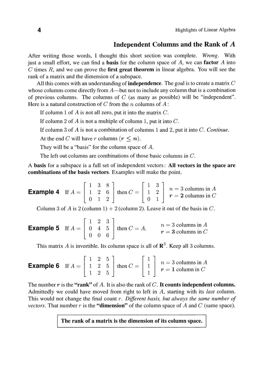
Independent Columns and the Rank of A
After writing those words, I thought this short section was complete. Wrong. With
just a small effort, we can find a basis for the column space of A, we can factor A into
C times R, and we can prove the first great theorem in linear algebra. You will see the
rank of a matrix and the dimension of a subspace.
All this comes with an understanding of independence. The goal is to create a matrix C
whose columns come directly from A-but not to include any column that is a combination
of previous columns. The columns of C (as many as possible) will be "independent".
Here is a natural construction of C from the n columns of A :
If column 1 of A is not all zero, put it into the matrix C.
If column 2 of A is not a multiple of column 1, put it into C.
If column 3 of A is not a combination of columns 1 and 2, put it into C. Continue.
At the end C will have r columns (r < n).
They will be a "basis" for the column space of A.
The left out columns are combinations of those basic columns in C.
A basis for a subspace is a full set of independent vectors: All vectors in the space are
combinations of the basis vectors. Examples will make the point.
Example 4 If A == [o ;1 2] then C == [ ] n == 3 columns n A
o 1 r == 2 columns In C
Column 3 of A is 2 (column 1) + 2 (column 2). Leave it out of the basis in C.
Example 5 If A ==
[ 1 2 3]
045
006
then C == A.
n == 3 columns in A
r == 3 columns in C
This matrix A is invertible. Its column space is all of R 3 . Keep all 3 columns.
Example 6 If A == [111 2 5] then C == [ ] n == 3 columns in A
1 r == 1 column in C
The number r is the "rank" of A. It is also the rank of C. It counts independent columns.
Admittedly we could have moved from right to left in A, starting with its last column.
This would not change the final count r. Different basis, but always the same number of
vectors. That number r is the "dimension" of the column space of A and C (same space).
The rank of a matrix is the dimension of its column space.
1.1. Multiplication Ax Using Columns of A
5
The matrix C connects to A by a third matrix R: A == CR. Their shapes are
(m by n) == (m by r) (r by n). I can show this "factorization of A" in Example 4 above:
A = [ ] [ ] [ ] = OR
(2)
When C multiplies the first column [ ] of R, this produces column 1 of C and A.
When C multiplies the second column [ ] of R, we get column 2 of C and A.
When C multiplies the third column [ ] of R, we get 2(column 1) + 2 (column 2).
This matches column 3 of A. All we are doing is to put the right numbers in R.
Combinations of the columns of C produce the columns of A. Then A == C R stores this
information as a matrix multiplication. Actually R is a famous matrix in linear algebra:
R == rref(A) == row-reduced echelon form of A (without zero rows).
Example 5 has C == A and then R == I (identity matrix). Example 6 has only one
column in C, so it has one row in R:
A=[l ] [lr 1
2 5]
== CR
All three matrices have rank r == 1
Column Rank == Row Rank
The number of independent columns equals the number of independent rows
This rank theorem is true for every matrix. Always columns and rows in linear algebra!
The m rows contain the same numbers aij as the n columns. But different vectors.
The theorem is proved by A == CR. Look at that differently-by rows instead of
columns. The matrix R has r rows. Multiplying by C takes combinations of those rows.
Since A == C R, we get every row of A from the r rows of R. And those r rows are
independent, so they are a basis for the row space of A. The column space and row space
of A both have dimension r, with r basis vectors-columns of C and rows of R.
One minute: Why does R have independent rows? Look again at Example 4.
A = [ ] = [ ] [ ]:= : ;: nt
ones and zeros
It is those ones and zeros in R that tell me: No row is a combination of the other rows.
The big factorization for data science is the "SVD" of A-when the first factor C
has r orthogonal columns and the second factor R has T orthogonal rows.
6
Highlights of Linear Algebra
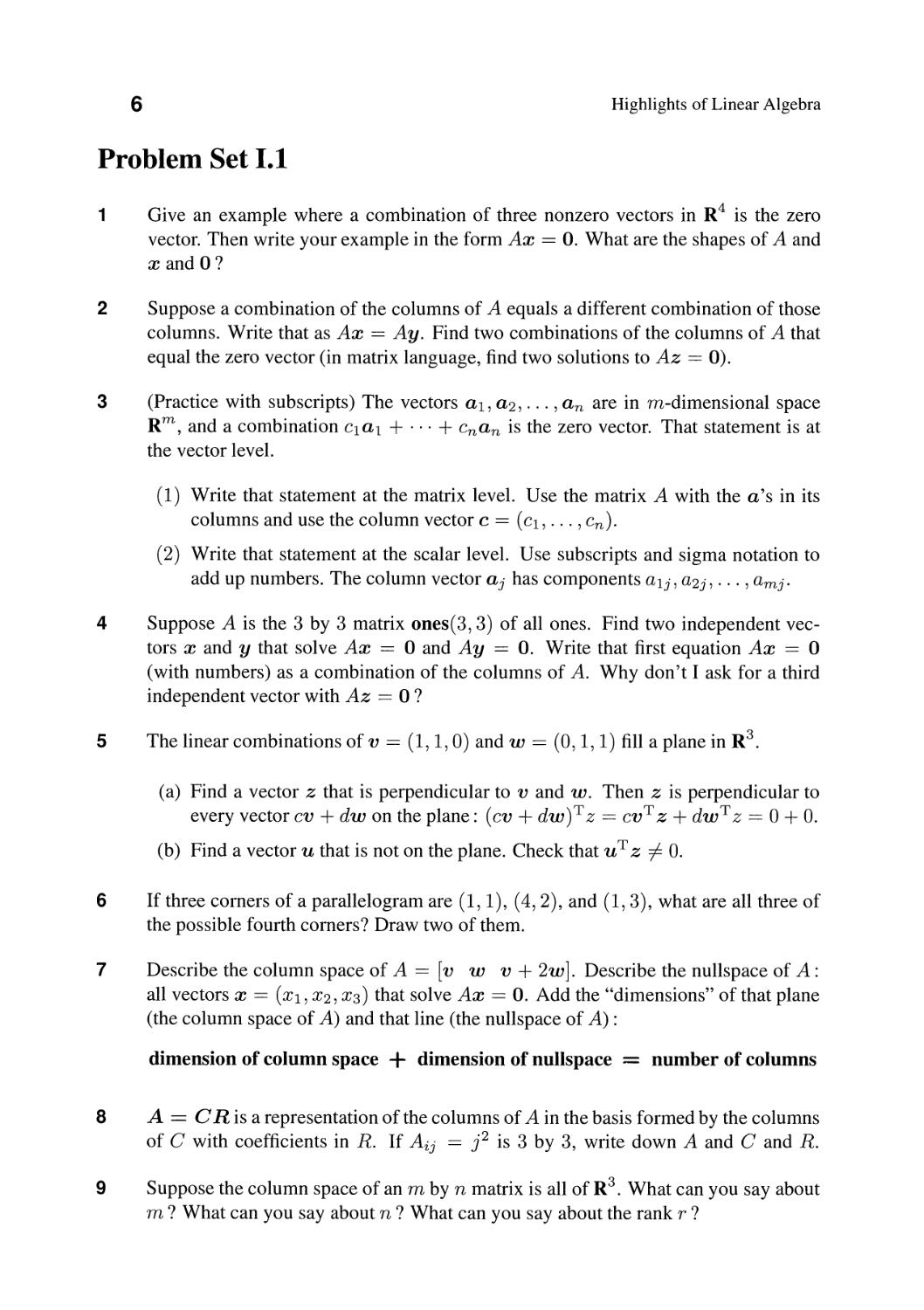
Problem Set 1.1
1 Give an example where a combination of three nonzero vectors in R 4 is the zero
vector. Then write your example in the form Ax == o. What are the shapes of A and
x and O?
2 Suppose a combination of the columns of A equals a different combination of those
columns. Write that as Ax == Ay. Find two combinations of the columns of A that
equal the zero vector (in matrix language, find two solutions to Az == 0).
3 (Practice with subscripts) The vectors aI, a2, . . . , an are in m-dimensional space
R m , and a combination e1 al + . . . + ena n is the zero vector. That statement is at
the vector level.
(1) Write that statement at the matrix level. Use the matrix A with the a's in its
columns and use the column vector c == (e1, . . . , en).
(2) Write that statement at the scalar level. Use subscripts and sigma notation to
add up numbers. The column vector aj has components a1j, a2j, . . . , amj.
4 Suppose A is the 3 by 3 matrix ones(3, 3) of all ones. Find two independent vec-
tors x and y that solve Ax == 0 and Ay == o. Write that first equation Ax == 0
(with numbers) as a combination of the columns of A. Why don't I ask for a third
independent vector with Az == 0 ?
5 The linear combinations of v == (1,1,0) and w == (0,1,1) fill a plane in R 3 .
(a) Find a vector z that is perpendicular to v and w. Then z is perpendicular to
every vector ev + dw on the plane: (ev + dw ) T Z == ev T z + dw T Z == 0 + o.
(b) Find a vector u that is not on the plane. Check that u T z -=I O.
6 If three corners of a parallelogram are (1,1), (4,2), and (1,3), what are all three of
the possible fourth corners? Draw two of them.
7 Describe the column space of A == [v w v + 2w]. Describe the nullspace of A:
all vectors x == (Xl, X2, X3) that solve Ax == o. Add the "dimensions" of that plane
(the column space of A) and that line (the nullspace of A) :
dimension of column space + dimension of nullspace = number of columns
8 A == C R is a representation of the columns of A in the basis formed by the columns
of C with coefficients in R. If A ij == j2 is 3 by 3, write down A and C and R.
9 Suppose the column space of an m by n matrix is all of R 3 . What can you say about
m ? What can you say about n ? What can you say about the rank r ?
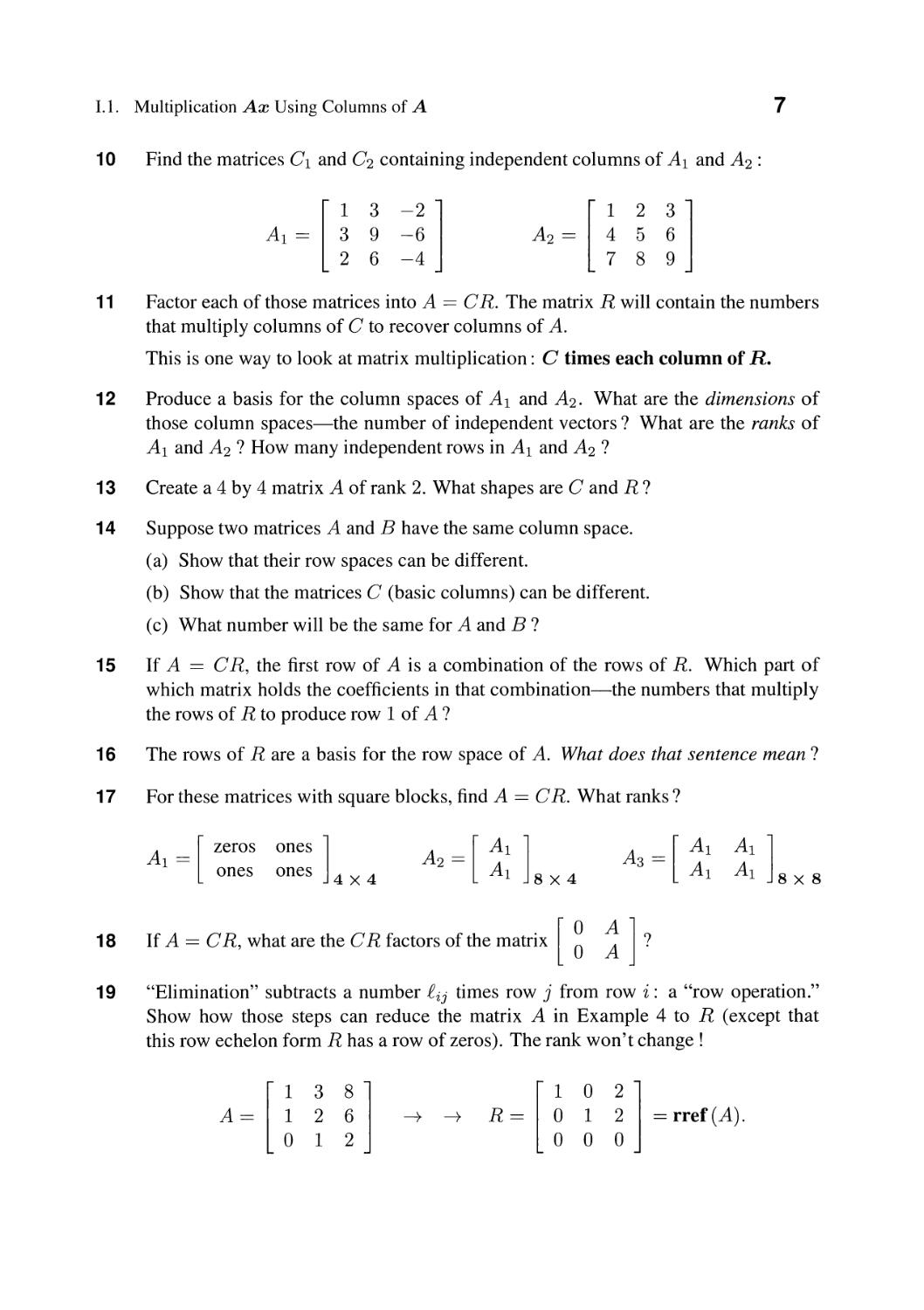
1.1. Multiplication Ax Using Columns of A
7
10 Find the matrices C 1 and C 2 containing independent columns of Al and A 2 :
Al == [ = ]
2 6 -4
A 2 == [ ]
7 8 9
11 Factor each of those matrices into A == CR. The matrix R will contain the numbers
that multiply columns of C to recover columns of A.
This is one way to look at matrix multiplication: C times each column of R.
12 Produce a basis for the column spaces of Al and A 2 . What are the dimensions of
those column spaces-the number of independent vectors? What are the ranks of
Al and A 2 ? How many independent rows in Al and A 2 ?
13 Create a 4 by 4 matrix A of rank 2. What shapes are C and R ?
14 Suppose two matrices A and B have the same column space.
(a) Show that their row spaces can be different.
(b) Show that the matrices C (basic columns) can be different.
(c) What number will be the same for A and B?
15 If A == CR, the first row of A is a combination of the rows of R. Which part of
which matrix holds the coefficients in that combination-the numbers that multiply
the rows of R to produce row 1 of A ?
16 The rows of R are a basis for the row space of A. What does that sentence mean?
17 For these matrices with square blocks, find A == CR. What ranks?
A _ [zeros ones]
1 - ones ones 4 x 4
A - [ Al ]
2 - Al 8 X 4
[ AI
A 3 ==
Al
Al ]
Al 8 X 8
18
If A = C R, what are the C R factors of the matrix [
A ] ?
A .
19 "Elimination" subtracts a number £ij times row j from row i: a "row operation."
Show how those steps can reduce the matrix A in Example 4 to R (except that
this row echelon form R has a row of zeros). The rank won't change!
A=[ ]
[ 1 001 0 22 ]
-+ --+ R == == rref (A).
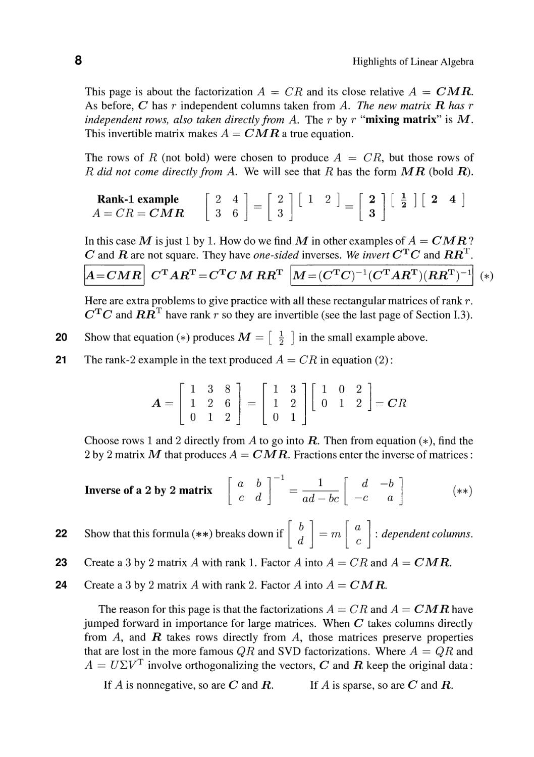
8
Highlights of Linear Algebra
This page is about the factorization A == C R and its close relative A == C lVl R.
As before, C has r independent columns taken from A. The new matrix R has r
independent rows, also taken directly from A. The r by r "mixing matrix" is lVl.
This invertible matrix makes A == C lVl R a true equation.
The rows of R (not bold) were chosen to produce A == C R, but those rows of
R did not come directly from A. We will see that R has the form Nl R (bold R).
Rank-l example
A == CR == CNlR
[ :]=[ ][1 2]=[ P ][2 4]
In this case Nl is just 1 by 1. How do we find Nl in other examples of A == C lVl R ?
C and R are not square. They have one-side d inverses. We invert cTe and RR T .
IA=CMRI C T ART =CTC M RR T 1 M = (C T C)-I(C T AR T )(RR T )-11 (*)
Here are extra problems to give practice with all these rectangular matrices of rank r.
cTe and RR T have rank r so they are invertible (see the last page of Section 1.3).
20 Show that equation ( *) produces Nl == [ ] in the small example above.
21 The rank-2 example in the text produced A == CR in equation (2):
A = [ ] [ ] [ ] = CR
Choose rows 1 and 2 directly from A to go into R. Then from equation (*), find the
2 by 2 matrix Nl that produces A == e Nl R. Fractions enter the inverse of matrices:
Inverse of a 2 by 2 matrix
[ ] -1 [ ]
a b 1 d-b
e d - ad - be - e a
(** )
22 Show that this formula (**) breaks down if [ ] = m [ ] : dependent columns.
23 Create a 3 by 2 matrix A with rank 1. Factor A into A == C R and A == C Nl R.
24 Create a 3 by 2 matrix A with rank 2. Factor A into A == e Nl R.
The reason for this page is that the factorizations A == C R and A == C lVl R have
jumped forward in importance for large matrices. When e takes columns directly
from A, and R takes rows directly from A, those matrices preserve properties
that are lost in the more famous Q Rand SVD factorizations. Where A == Q Rand
A == U VT involve orthogonalizing the vectors, C and R keep the original data:
If A is nonnegative, so are C and R. If A is sparse, so are C and R.
1.2. Matrix-Matrix Multiplication AB
9
1.2 Matrix-Matrix Multiplication AB
Inner products (rows times columns) produce each of the numbers in AB == C:
row 2 of A
column 3 of B
give C23 in C
[ a 1 a 2 a 3] [: · :] [
· · · b 33
C23 ]
(1)
That dot product e23 == (row 2 of A) · (column 3 of B) is a sum of a's times b's:
3
C23 == a2l b 13 + a22 b 23 + a23 b 33 == L a2k bk3
k=l
n
and Cij == L aik b kj .
k=l
(2)
This is how we usually compute each number in AB == C. But there is another way.
The other way to multiply AB is columns of A times rows of B. We need to see this!
I start with numbers to make two key points: one column u times one row v T produces a
matrix. Concentrate first on that piece of AB. This matrix uv T is especially simple:
"Outer
product"
uv T = [ ]
[346]=[
3 4
12 ]
12 == "rank one
matrix"
6
An m by 1 matrix (a column u) times a 1 by p matrix (a row v T) gives an m by p matrix.
Notice what is special about the rank one matrix uv T :
All columns of uv T are multiples of u = [ ] All rows are multiples of v T = [3 4 6]
The column space of uv T is one-dimensional: the line in the direction of u.
The dimension of the column space (the number of independent columns) is the rank
of the matrix-a key number. All nonzero matrices uv T have rank one. They are the
perfect building blocks for every matrix.
Notice also: The row space of uv T is the line through v. By definition, the row
space of any matrix A is the column space C(A T ) of its transpose AT. That way we stay
with column vectors. In the example, we transpose uv T (exchange rows with columns)
to get the matrix vu T :
(UVT)T = [: :
i ] T [I!
6
8
12
: ] [ : ]
[2 2
1 ]
== vu T .
10
Highlights of Linear Algebra
We are seeing the clearest possible example of the first great theorem in linear algebra:
Row rank == Column rank
r independent columns {:} r independent rows
A nonzero matrix uv T has one independent column and one independent row. All columns
are multiples of u and all rows are multiples of v T. The rank is r == 1 for this matrix.
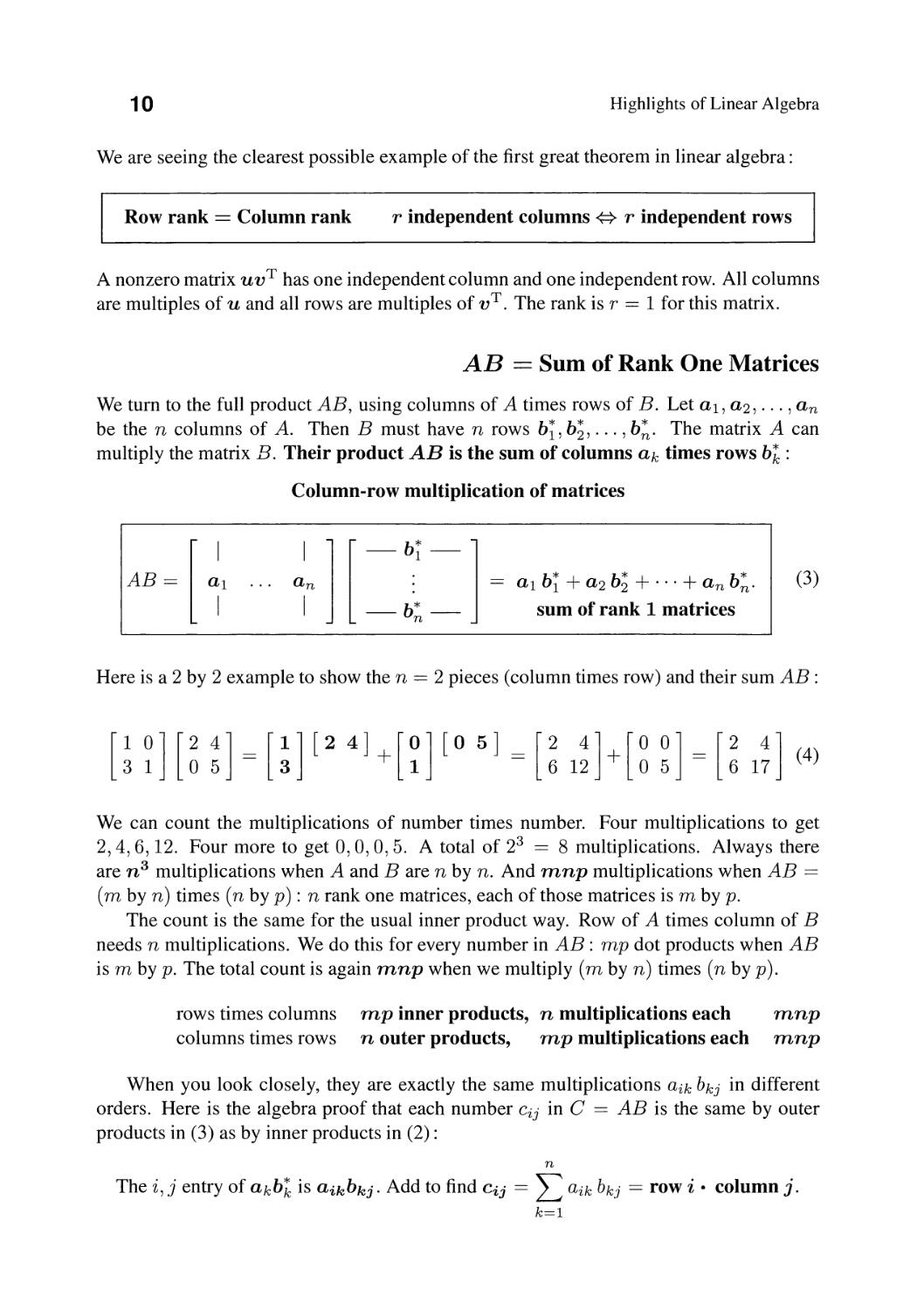
AB == Sum of Rank One Matrices
We turn to the full product AB, using columns of A times rows of B. Let aI, a2,..., an
be the n columns of A. Then B must have n rows b , b;, . . . , b . The matrix A can
multiply the matrix B. Their product AB is the sum of columns ak times rows b'k :
Column-row multiplication of matrices
- I I - - -b - -
AB == a1 an a1 b + a2 b; + . . . + an b . (3)
I -b*- sum of rank 1 matrices
- - _ n _
Here is a 2 by 2 example to show the n == 2 pieces (column times row) and their sum AB :
[ 1 0] [2 4] == [1] [2 4] [0] [0 5 ] == [2 4] [0 0] == [2 4] (4)
3 1 0 5 3 + 1 6 12 + 0 5 6 17
We can count the multiplications of number times number. Four multiplications to get
2, 4, 6, 12. Four more to get 0, 0, 0, 5. A total of 2 3 == 8 multiplications. Always there
are n 3 multiplications when A and Bare n by n. And mnp multiplications when AB ==
(m by n) times (n by p) : n rank one matrices, each of those matrices is m by p.
The count is the same for the usual inner product way. Row of A times column of B
needs n multiplications. We do this for every number in AB: mp dot products when AB
is m by p. The total count is again mnp when we multiply (m by n) times (n by p).
rows times columns
columns times rows
mp inner products, n multiplications each
n outer products, mp multiplications each
mnp
mnp
When you look closely, they are exactly the same multiplications aik b kj in different
orders. Here is the algebra proof that each number eij in C == AB is the same by outer
products in (3) as by inner products in (2) :
n
The i,.i entry of akb'k is aikbkj. Add to find Cij == L aik bkj == row i · column j.
k=l
1.2. Matrix-Matrix Multiplication AB
11
Insight from Column times Row
Why is the outer product approach essential in data science? The short answer is: We are
looking for the important part of a matrix A. We don't usually want the biggest number
in A (though that could be important). What we want more is the largest piece of A. And
those pieces are rank one matrices uv T. A dominant theme in applied linear algebra is :
Factor A into C R and look at the pieces ckr of A == CR.
Factoring A into C R is the reverse of multiplying C R == A. Factoring takes longer,
especially if the pieces involve eigenvalues or singular values. But those numbers have
inside information about the matrix A. That information is not visible until you factor.
Here are five important factorizations, with the standard choice of letters (usually A)
for the original product matrix and then for its factors. This book will explain all five.
I A=LU
A == QR
S == QAQT
A == XAX- l
A == U yT
At this point we simply list key words and properties for each of these factorizations.
1 A == LU comes from elimination. Combinations of rows take A to U and U back
to A. The matrix L is lower triangular and U is upper triangular as in equation (4).
2 A == Q R comes from orthogonalizing the columns a1 to an as in "Gram-Schmidt".
Q has orthonormal columns (QT Q == I) and R is upper triangular.
3 S == QAQT comes from the eigenvalues AI, . . . , An of a symmetric matrix S == ST.
Eigenvalues on the diagonal of A. Orthonormal eigenvectors in the columns of Q.
4 A == X AX -1 is diagonalization when A is n by n with n independent eigenvectors.
Eigenvalues of A on the diagonal of A. Eigenvectors of A in the columns of X.
5 A == U VT is the Singular Value Decomposition of any matrix A (square or not).
Singular values (}1 , . . . , () r in . Orthonormal singular vectors in U and V.
Let me pick out a favorite (number 3) to illustrate the idea. This special factorization
Q AQT starts with a symmetric matrix S. That matrix has orthogonal unit eigenvectors
q1, . . . , qn. Those perpendiculareigenvectors (dot products == 0) go into the columns of Q.
Sand Q are the kings and queens of linear algebra:
Symmetric matrix S ST == S All Sij == Sji
Orthogonal matrix Q QT == Q-l All qi. qj = { 0 for i-=lj
1 for ==J
12
Highlights of Linear Algebra
The diagonal matrix A contains real eigenvalues Al to An. Every real symmetric matrix
S has n orthonormal eigenvectors q1 to qn. When multiplied by S, the eigenvectors keep
the same direction. They are just resealed by the number A :
Eigenvector q and eigenvalue A
Sq == Aq
(5)
Finding A and q is not easy for a big matrix. But n pairs always exist when S is symmetric.
Our purpose here is to see how SQ == QA comes column by column from Sq == Aq:
Al
SQ == S q1 ... qn
A1q1 ... Anqn
q1 ... qn
== QA (6)
An
Multiply SQ == QA by Q-1 == QT to get S == QAQT == a symmetric matrix. Each
eigenvalue Ak and each eigenvector qk contribute a rank one piece AkqkqI to S.
Rank one pieces S == (QA)QT == (A1q1)q! + (A2q2)qI + ... + (Anqn)q (7)
All symmetric The transpose of qiq; is qiq; (8)
Please notice that the columns of QA are A1q1 to Anqn. When you multiply a matrix on
the right by the diagonal matrix A, you multiply its columns by the A's.
We close with a comment on the proof of this Spectral Theorem S == QAQT:
Every symmetric S has n real eigenvalues and n orthonormal eigenvectors. Section 1.6
will construct the eigenvalues as the roots of the nth degree polynomial Pn(A) == deter-
minant of S - AI. They are real numbers when S == ST. The delicate part of the proof
comes when an eigenvalue Ai is repeated- it is a double root or an Mth root from a factor
(A - Aj) M. In this case we need to produce M independent eigenvectors. The rank of
S - Aj I must be n - M. This is true when S == ST. But it requires a proof.
Similarly the Singular Value Decomposition A == U VT requires extra patience when
a singular value (J is repeated M times in the diagonal matrix . Again there are M
pairs of singular vectors v and u with Av == (JU. Again this true statement requires proof.
Notation for rows We introduced the symbols b , . . . , b for the rows of the second
matrix in AB. You might have expected bY, . . . , b and that was our original choice. But
this notation is not entirely clear-it seems to mean the transposes of the columns of B.
Since that right hand factor could be U or R or QT or X-lor V T , it is safer to say
definitely: we want the rows of that matrix.
G. Strang, Multiplying andfactoring matrices, Amer. Math. Monthly 125 (2018) 223-230.
G. Strang, Introduction to Linear Algebra, 5th ed., Wellesley-Cambridge Press (2016).
1.2. Matrix-Matrix Multiplication AB
13
Problem Set 1.2
1 Suppose Ax == 0 and Ay == 0 (where x and y and 0 are vectors). Put those two
statements together into one matrix equation AB == C. What are those matrices B
and C ? If the matrix A is m by n, what are the shapes of Band G ?
2 Suppose a and b are column vectors with components aI, . . . , am and b 1 , . . . , b p .
Can you multiply a times b T (yes or no)? What is the shape of the answer ab T ?
What number is in row i, column j of ab T ? What can you say about aa T ?
3 (Extension of Problem 2: Practice with subscripts) Instead of that one vector a,
suppose you have n vectors a1 to an in the columns of A. Suppose you have n
vectors bT, . . . , b in the rows of B.
(a) Give a "sum of rank one" formula for the matrix-matrix product AB.
(b) Give a formula for the i, j entry of that matrix-matrix product AB. Use sigma
notation to add the i, j entries of each matrix akbl, found in Problem 2.
4 Suppose B has only one column (p == 1). So each row of B just has one number.
A has columns a1 to an as usual. Write down the column times row formula
for AB. In words, the m by 1 column vector AB is a combination of the
5 Start with a matrix B. If we want to take combinations of its rows, we premultiply
by A to get AB. If we want to take combinations of its columns, we postmultiply by
G to get BG. For this question we will do both.
Row operations then column operations First AB then (AB)C
Column operations then row operations First BC then A(BC)
The associative law says that we get the same final result both ways.
Verify (AB)C = A(BC) for A = [ n B = [ ] C = [ n.
6 If A has columns aI, a2, a3 and B == I is the identity matrix, what are the rank one
matrices a1b and a2b; and a3b; ? They should add to AI == A.
7 Fact: The columns of AB are combinations of the columns of A. Then the column
space of AB is contained in the column space of A. Give an example of A and B
for which AB has a smaller column space than A.
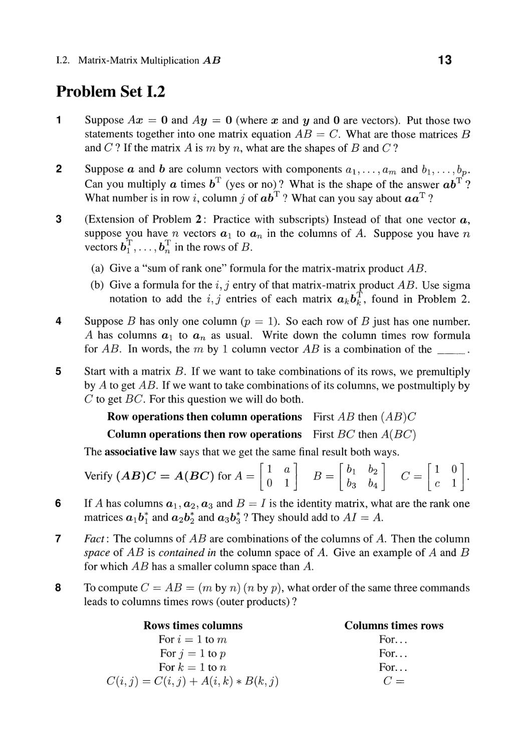
8 To compute G == AB == (m by n) (n by p), what order of the same three commands
leads to columns times rows (outer products) ?
Rows times columns
For i == 1 to m
For j == 1 to p
For k == 1 to n
C(i, j) == C(i, j) + A(i, k) * B(k, j)
Columns times rows
For.. .
For.. .
For.. .
G==
14 Highlights of Linear Algebra
1.3 The Four Fundamental Subspaces
This section will explain the "big picture" of linear algebra. That picture shows how every
m by n matrix A leads to four subspaces-two subspaces of R m and two more of R n .
The first example will be a rank one matrix uv T, where the column space is the line
through u and the row space is the line through v. The second example moves to 2 by 3.
The third example (a 5 by 4 matrix A) will be the incidence matrix of a graph.
Graphs have become the most important models in discrete mathematics-this example
is worth understanding. All four subspaces have meaning on the graph.
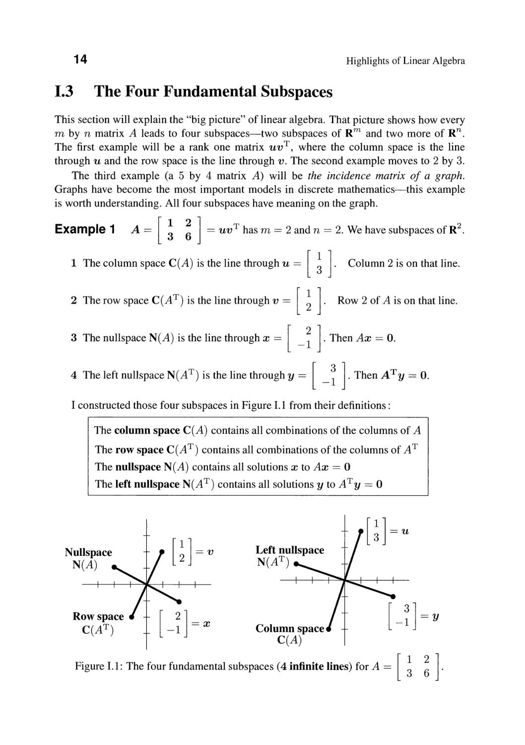
Example 1 A = [ ] = uv T has m = 2 and n = 2. We have subspaces of R 2 .
1 The column space C(A) is the line through u = [ ]. Column 2 is on that line.
2 The row space C(A T ) is the line through v = [ ; ]. Row 2 of A is on that line.
3 The nullspace N(A) is the line through x = [ _ ]. Then Ax = O.
4 TheleftnullspaceN(A T )is the line through y = [_ lThenATy=o.
I constructed those four subspaces in Figure 1.1 from their definitions:
The column space C(A) contains all combinations of the columns of A
The row space C(A T ) contains all combinations of the columns of AT
The nullspace N (A) contains all solutions x to Ax == 0
The left nullspace N(A T ) contains all solutions y to ATy == 0
Column space
C(A)
[ ]=u
Nullspace
N(A)
[;]=v
Left nullspace
N(A T )
Row space
C(A T )
[ _ ] = x
[ -n = y
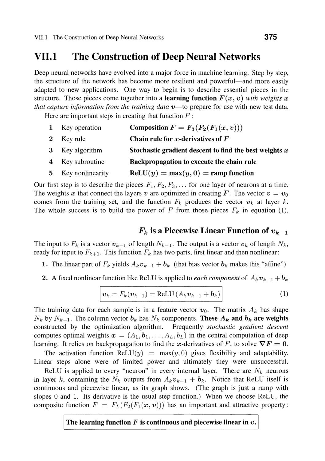
Figure 1.1: The four fundamental subspaces (4 infinite lines) for A ==
[ 1 2]
3 6 .
1.3. The Four Fundamental Subspaces
15
That example had exactly one u and v and x and y. All four subspaces were I-dimensional
Gust lines). Always the u's and v's and x's and y's will be independent vectors-they give
a "basis" for each of the subspaces. A larger matrix will need more than one basis vector
per subspace. The choice of basis vectors is a crucial step in scientific computing.
[ 1 -2 -2] 3 2
Example 2 B == 3 -6 -6 has m == 2 and n == 3. Subspaces in Rand R .
Going from A to B, two subspaces change and two subspaces don't change. The column
space of B is still in R 2 . It has the same basis vector. But now there are n == 3 numbers in
the rows of B and the left half of Figure 1.2 is in R 3 . There is still only one v in the row
space! The rank is still r == 1 because both rows of this B go in the same direction.
With n == 3 unknowns and only r == 1 independent equation, Bx == 0 will have
3 - 1 == 2 independent solutions Xl and X2. All solutions go into the nullspace.
Bx ==
[
-2
-6
-2
-6
] [ ] [ ] has solutions XI = [ ]
and X2 ==
[ ]
In the textbook Introduction to Linear Algebra, those vectors Xl and X2 are called
"special solutions". They come from the steps of elimination-and you quickly see that
BX1 == 0 and BX2 == O. But those are not perfect choices in the nullspace of B because
the vectors Xl and X2 are not perpendicular.
This book will give strong preference to perpendicular basis vectors. Section IL2 shows
how to produce perpendicular vectors from independent vectors, by "Gram-Schmidt".
Our nullspace N(B) is a plane in R 3 . We can see an orthonormal basis V2 and V3
in that plane. The V2 and V3 axes make a 90 0 angle with each other and with VI.
row of B
V2 = [ - ]
Row space == infinite line through VI
Nullspace == infinite plane of V2 and V3
n == 3 columns of B
r == 1 independent column
VI = [ = ]
[ VI
V3 = [ _ ]
V2
] orthonormal
V3 ==
basis for R 3
Figure 1.2: Row space and nullspace of B = [ = = ]: Line perpendicular to plane!
16
Highlights of Linear Algebra
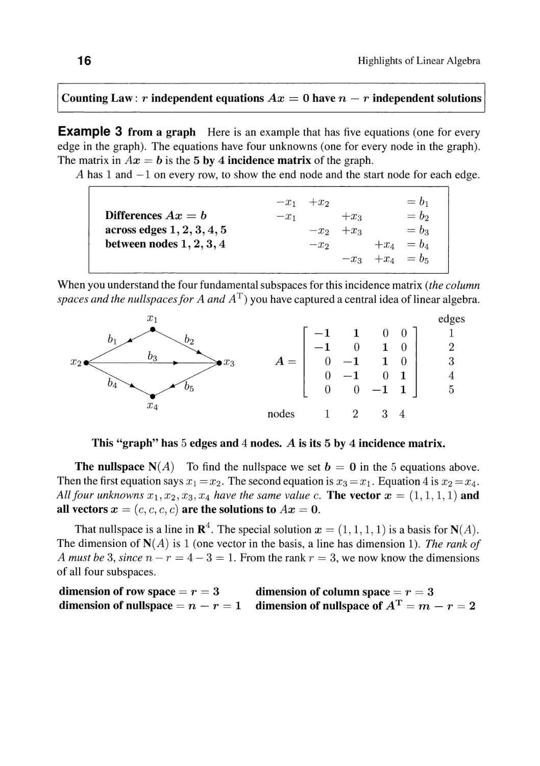
Counting Law: r independent equations Ax == 0 have n - r independent solutions
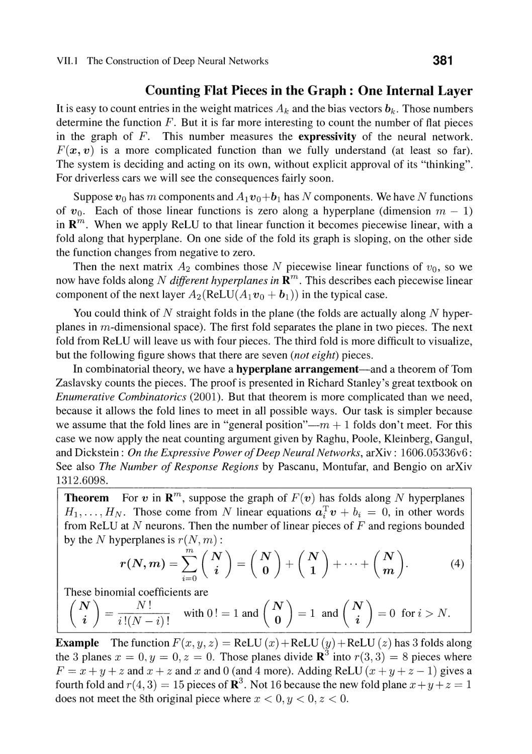
Example 3 from a graph Here is an example that has five equations (one for every
edge in the graph). The equations have four unknowns (one for every node in the graph).
The matrix in Ax == b is the 5 by 4 incidence matrix of the graph.
A has 1 and -Ion every row, to show the end node and the start node for each edge.
-Xl +X2 == b 1
Differences Ax == b -Xl +X3 == b 2
across edges 1, 2, 3, 4, 5 -X2 +X3 == b 3
between nodes 1, 2, 3, 4 -X2 +X4 == b 4
-X3 +X4 == b s
When you understand the four fundamental subspaces for this incidence matrix (the column
spaces and the nullspaces for A and AT) you have captured a central idea of linear algebra.
Xl edges
-1 1 0 0 1
-1 0 1 0 2
X2 X3 A == 0 -1 1 0 3
o -1 0 1 4
o 0 -1 1 5
X4
nodes
1
2
3 4
This "graph" has 5 edges and 4 nodes. A is its 5 by 4 incidence matrix.
The nullspace N (A) To find the nullspace we set b == 0 in the 5 equations above.
Then the first equation says Xl == X2. The second equation is X3 == Xl. Equation 4 is X2 == X4.
Allfour unknowns Xl, X2, X3, X4 have the same value e. The vector x == (1,1,1,1) and
all vectors x == (e, e, e, e) are the solutions to Ax == o.
That nullspace is a line in R 4 . The special solution x == (1,1,1,1) is a basis for N(A).
The dimension of N (A) is 1 (one vector in the basis, a line has dimension 1). The rank of
A must be 3, since n - r == 4 - 3 == 1. From the rank T == 3, we now know the dimensions
of all four subspaces.
dimension of row space == r == 3
dimension of nullspace == n - r == 1
dimension of column space == r == 3
dimension of nullspace of A T == m - r == 2
1.3. The Four Fundamental Subspaces
17
The column space C(A) There must be r == 4 - 1 == 3 independent columns.
The fast way is to look at the first 3 columns. They give a basis for the column space of A :
Columns -1 1 0 Column 4
-1 0 1
1,2,3 is a combination
0 -1 1
of this A are of those three
0 -1 0
independent basic columns
0 0 -1
"Independent" means that the only solution to Ax == 0 is (Xl j X2, X3) == (0,0,0).
We know X3 == 0 from the fifth equation OX1 + OX2 - X3 == O. We know .T2 == 0 from
the fourth equation OX1 - X2 + OX3 == O. Then we know Xl == 0 from the first equation.
Column 4 of the incidence matrix A is the sum of those three columns, times -1.
The row space C( AT) The dimension must again be r == 3, the same as for columns.
But the first 3 rows of A are not independent: row 3 == row 2 - row 1. The first three inde-
pendent ro",'s are rows 1, 2, 4. Those rows are a basis (one possible basis) for the row space.
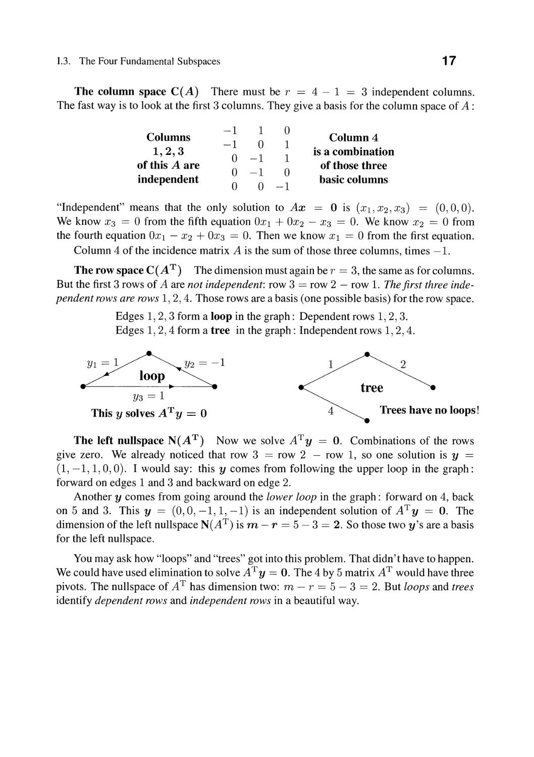
Edges 1,2,3 form a loop in the graph: Dependent rows 1,2,3.
Edges 1,2,4 form a tree in the graph: Independent rows 1,2,4.
1
Y3 == 1
This y solves ATy == 0
tree
Trees have no loops!
The left nullspace N(A T ) Now we solve ATy == o. Combinations of the rows
give zero. We already noticed that row 3 == row 2 - row 1, so one solution is y ==
(1, -1, 1,0,0). I would say: this y comes from follovving the upper loop in the graph:
forward on edges 1 and 3 and backward on edge 2.
Another y comes from going around the lower loop in the graph: forward on 4, back
on 5 and 3. This y == (0,0, -1, 1, -1) is an independent solution of ATy == o. The
dimension of the left nullspace N(A T ) is m - r == 5 - 3 == 2. So those two y's are a basis
for the left nullspace.
You may ask how "loops" and "trees" got into this problem. That didn't have to happen.
We could have used elimination to solve AT y == o. The 4 by 5 matrix AT would have three
pivots. The nullspace of AT has dimension two: m - r == 5 - 3 == 2. But loops and trees
identify dependent rows and independent rows in a beautiful way.
18
Highlights of Linear Algebra
The equations AT y == 0 give "currents" Y1, Y2, Y3, Y4, Y5 on the five edges of the graph.
Flows around loops obey Kirchhoff's Current Law: in == out. Those words apply
to an electrical network. But the ideas behind the words apply all over engineering and
science and economics and business. Balancing forces and flows and the budget.
Graphs are the most important model in discrete applied mathematics. You see graphs
everywhere: roads, pipelines, blood flow, the brain, the Web, the economy of a country
or the world. We can understand their incidence matrices A and AT. In Section 111.6,
the matrix AT A will be the "graph Laplacian". And Ohm's Law will lead to AT CA.
Four subspaces for a connected graph with m edges and n nodes: incidence matrix A
N (A) The constant vectors (e, e, . . . , e) make up the I-dimensional nullspace of A.
C( AT) The r edges of a tree give r independent rows of A : rank == r == n - 1.
C(A) Voltage Law: The components of Ax add to zero around all loops.
N(A T ) Current Law: AT y == (flow in) - (flow out) == 0 is solved by loop currents.
There are m - r == m - n + 1 independent small loops in the graph.
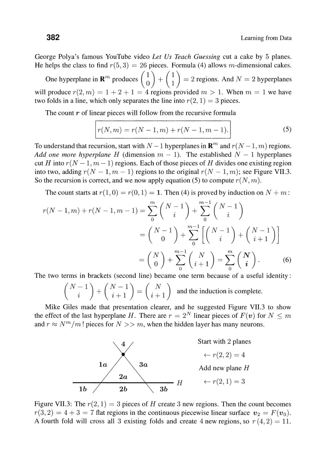
C(A T )
dimr
The big picture
N(A T )
dimension m - r
N(A)
dimension n - r
Figure 1.3: The Four Fundamental Subspaces: Their dimensions add to nand m.
1.3. The Four Fundamental Subspaces
19
The Ranks of AB and A + B
This page establishes key facts about ranks: When we multiply matrices, the rank
cannot increase. You will see this by looking at column spaces and row spaces. And there
is one special situation when the rank cannot decrease. Then you know the rank of AB.
Statement 4 will be important when data science factors a matrix into UV or CR.
Here are five key facts in one place: inequalities and equalities for the rank.
1 Rank of AB < rank of A
Rank of AB < rank of B
2 Rank of A + B < (rank of A) + (rank of B)
3 Rank of A T A == rank of AA T == rank of A == rank of AT
4 If A is m by rand B is r by n-both with rank r-then AB also has rank r
Statement 1 involves the column space and row space of AB :
C(AB) is contained in C(A)
C((AB)T) is contained in C(B T )
Every column of AB is a combination of the columns of A (matrix multiplication)
Every row of AB is a combination of the rows of B (matrix multiplication)
Remember from Section 1.1 that row rank == column rank. We can use rows or columns.
The rank cannot grow when we multiply AB. Statement 1 in the box is frequently used.
Statement 2 Each column of A + B is the sum of (column of A) + (column of B).
rank (A + B) < rank (A) + rank (B) is always true. It combines bases for C(A) and C(B).
rank (A + B) == rank (A) + rank (B) is not always true. It is certainly false if A == B == I.
Statement 3 A and AT A both have n columns. They also have the same nullspace.
(This is Problem 6.) So n - r is the same for both, and the rank r is the same for both.
Then rank(A T ) < rank(AT A) == rank(A). Exchange A and AT to show their equal ranks.
Statement 4 We are told that A and B have rank r. By statement 3, AT A and BB T have
rank r. Those are r by r matrices so they are invertible. So is their product AT AB B T . Then
r==rankof(ATABB T ) < rank of (AB) by Statement 1 :AT,BTcan'tincreaserank
We also know rank (AB) < rank A == r. So we have proved that AB has rank exactly r.
Note This does not mean that every product of rank r matrices will have rank r.
Statement 4 assumes that A has exactly r columns and B has r rows. BA can easily fail.
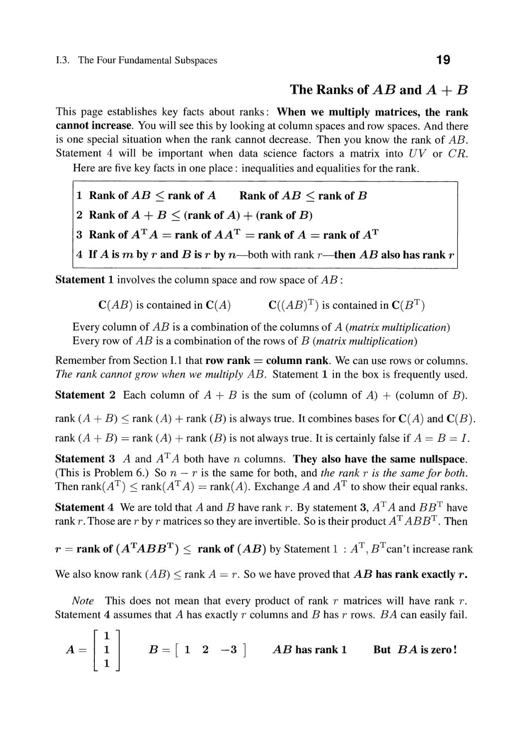
A=[ ]
B == [1 2 -3]
AB has rank 1
But BA is zero!
20
Highlights of Linear Algebra
Problem Set 1.3
1 Show that the nullspace of AB contains the nullspace of B. If B x == 0 then. . .
2 Find a square matrix with rank (A 2 ) < rank (A). Confirm that rank (AT A) == rank (A).
3 How is the nullspace of C related to the nullspaces of A and B, if C = [ ] ?
4 If row space of A == column space of A, and also N(A) == N(A T ), is A symmetric?
5 Four possibilities for the rank r and size m, n match four possibilities for Ax == b.
Find four matrices Al to A 4 that show those possibilities:
r==m==n
r==m<n
r==n<m
r < m, r < n
A 1 x == b has 1 solution for every b
A 2 x == b has 1 or ex:> solutions
A 3 x == b has 0 or 1 solution
A 4 x == b has 0 or ex:> solutions
6 (Important) Show that AT A has the same nullspace as A. Here is one approach:
First, if Ax equals zero then AT Ax equals . This proves N(A) C N(A T A).
Second, if AT Ax == 0 then x T AT Ax == IIAxl1 2 == O. Deduce N(A T A) == N(A).
7 Do A 2 and A always have the same nullspace? A is a square matrix.
8 Find the column space C(A) and the nullspace N(A) of A = [ ]. Remember
that those are vector spaces, not just single vectors. This is an unusual example
with C(A) == N(A). It could not happen that C(A) == N(A T ) because those two
subspaces are orthogonal.
9 Draw a square and connect its corners to the center point: 5 nodes and 8 edges.
Find the 8 by 5 incidence matrix A of this graph (rank r == 5 - 1 == 4).
Find a vector x in N(A) and 8 - 4 independent vectors y in N(A T ).
10 If N(A) is the zero vector, what vectors are in the nullspace of B == [A A A]?
11 For subspaces Sand T of RIO with dimensions 2 and 7, what are all the possible
dimensions of
(i) S n T == {all vectors that are in both subspaces}
(ii) S + T == {all sums s + t with s in Sand t in T}
(iii) SJ... == {all vectors in RIO that are perpendicular to every vector in S}.
1.4. Elimination and A == LU
21
1.4 Elimination and A == LU
The first and most fundamental problem of linear algebra is to solve Ax == b. We are given
the n by n matrix A and the n by 1 column vector b. We look for the solution vector x.
Its components Xl, X2, . . . , X n are the n unknowns and we have n equations. Usually
a square matrix A means only one solution to Ax == b (but not always). We can find
x by geometry or by algebra.
This section begins with the row and column pictures of Ax == b. Then we solve the
equations by simplifying them-eliminate Xl from n - 1 equations to get a smaller system
A2X2 == b 2 of size n - 1. Eventually we reach the 1 by 1 system Anx n == b n and we know
X n == b n / An. Working backwards produces X n -1 and eventually we know X2 and Xl.
The point of this section is to see those elimination steps in terms of rank 1 matrices.
Every step (from A to A 2 and eventually to An) removes a matrix £u *. Then the
original A is the sum of those rank one matrices. This sum is exactly the great factorization
A == LU into lower and upper triangular matrices Land U -as we will see.
A == L times U is the matrix description of elimination without row exchanges.
That will be the algebra. Start with geometry for this 2 by 2 example.
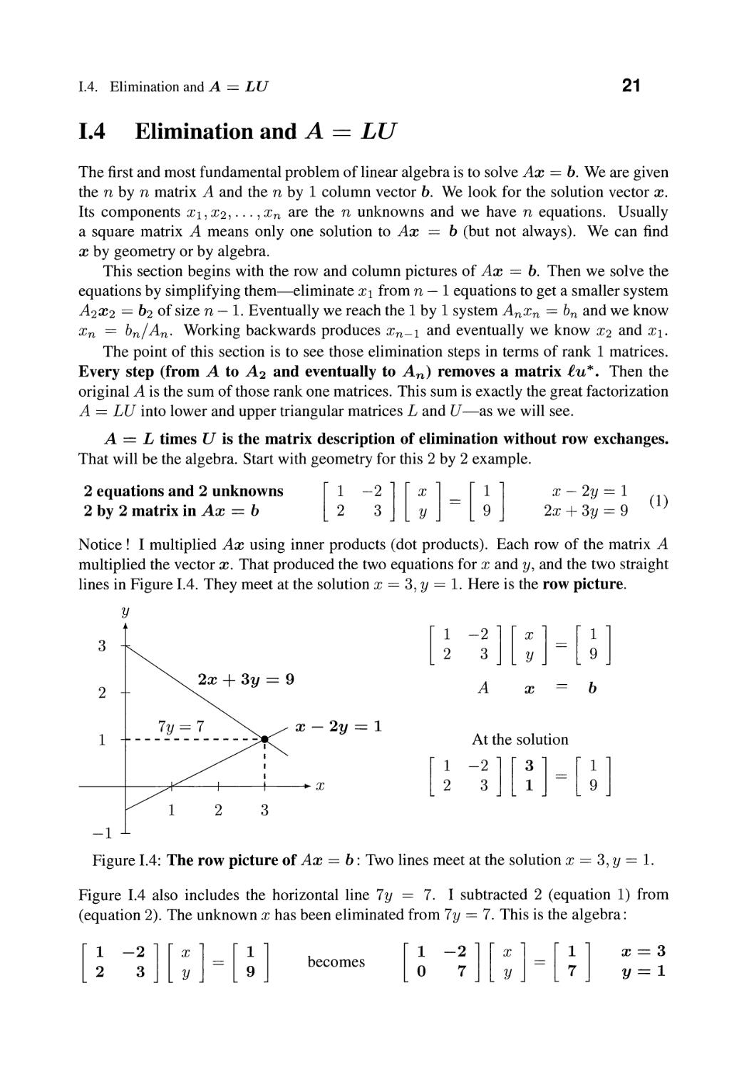
2 equations and 2 unknowns
2 by 2 matrix in Ax == b
[; - ] [ ] [ ]
X - 2y == 1
2x + 3y == 9
(1)
Notice! I multiplied Ax using inner products (dot products). Each row of the matrix A
multiplied the vector x. That produced the two equations for X and y, and the two straight
lines in Figure 1.4. They meet at the solution X == 3, y == 1. Here is the row picture.
y
3
[; - ] [ ] [ ]
A
x
b
2
x - 2y == 1
At the solution
1
[ ;
-2
3
][ ] [ ]
X
-1
Figure 1.4: The row picture of Ax == b: Two lines meet at the solution X == 3, y == 1.
Figure 1.4 also includes the horizontal line 7y == 7. I subtracted 2 (equation 1) from
(equation 2). The unknown X has been eliminated from 7y == 7. This is the algebra:
[
-2
3
][ ] [ ]
[ - ] [ ] [ ]
x==3
y==l
becomes
22
Highlights of Linear Algebra
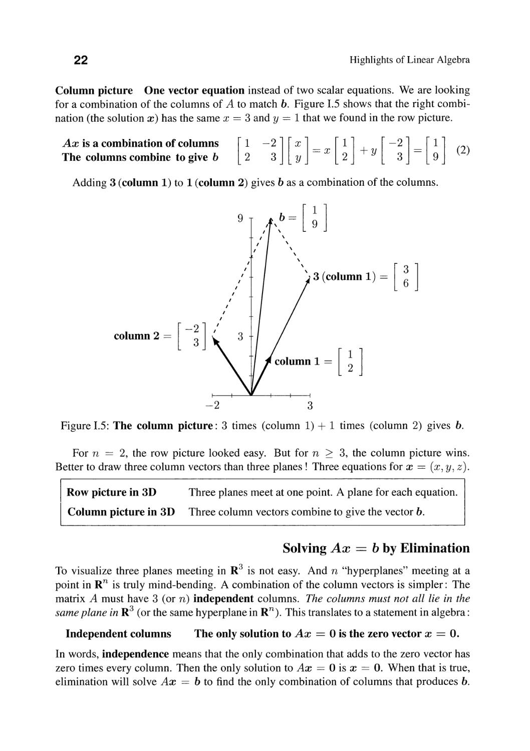
Column picture One vector equation instead of two scalar equations. We are looking
for a combination of the columns of A to match b. Figure 1.5 shows that the right combi-
nation (the solution x) has the same x == 3 and y == 1 that we found in the row picture.
Ax is a combination of columns
The columns combine to give b
[ ] [ ] = x [ ] + y [ - ] = [ ] (2)
Adding 3 (column 1) to 1 (column 2) gives b as a combination of the columns.
9
b==
[ ]
I
I
I
I
I
\
\
\
\
\
\
\
\
\
3 (column 1) ==
[ ]
column 2 = [ - ]
I
I
I
I
I
I
I
I
I
I
I
I
3
[ 2 1 ]
column 1 ==
-2
3
Figure 1.5: The column picture: 3 times (column 1) + 1 times (column 2) gives b.
For n == 2, the row picture looked easy. But for n > 3, the column picture wins.
Better to draw three column vectors than three planes! Three equations for x == (x, y, z).
Row picture in 3D Three planes meet at one point. A plane for each equation.
Column picture in 3D Three column vectors combine to give the vector b.
Solving Ax == b by Elimination
To visualize three planes meeting in R 3 is not easy. And n "hyperplanes" meeting at a
point in R n is truly mind-bending. A combination of the column vectors is simpler: The
matrix A must have 3 (or n) independent columns. The columns must not aU lie in the
same plane in R 3 (or the same hyperplane in R n ). This translates to a statement in algebra:
Independent columns
The only solution to Ax 0 is the zero vector x == o.
In words, independence means that the only combination that adds to the zero vector has
zero times every column. Then the only solution to Ax == 0 is x == o. When that is true,
elimination will solve Ax == b to find the only combination of columns that produces b.
1.4. Elimination and A == LU
23
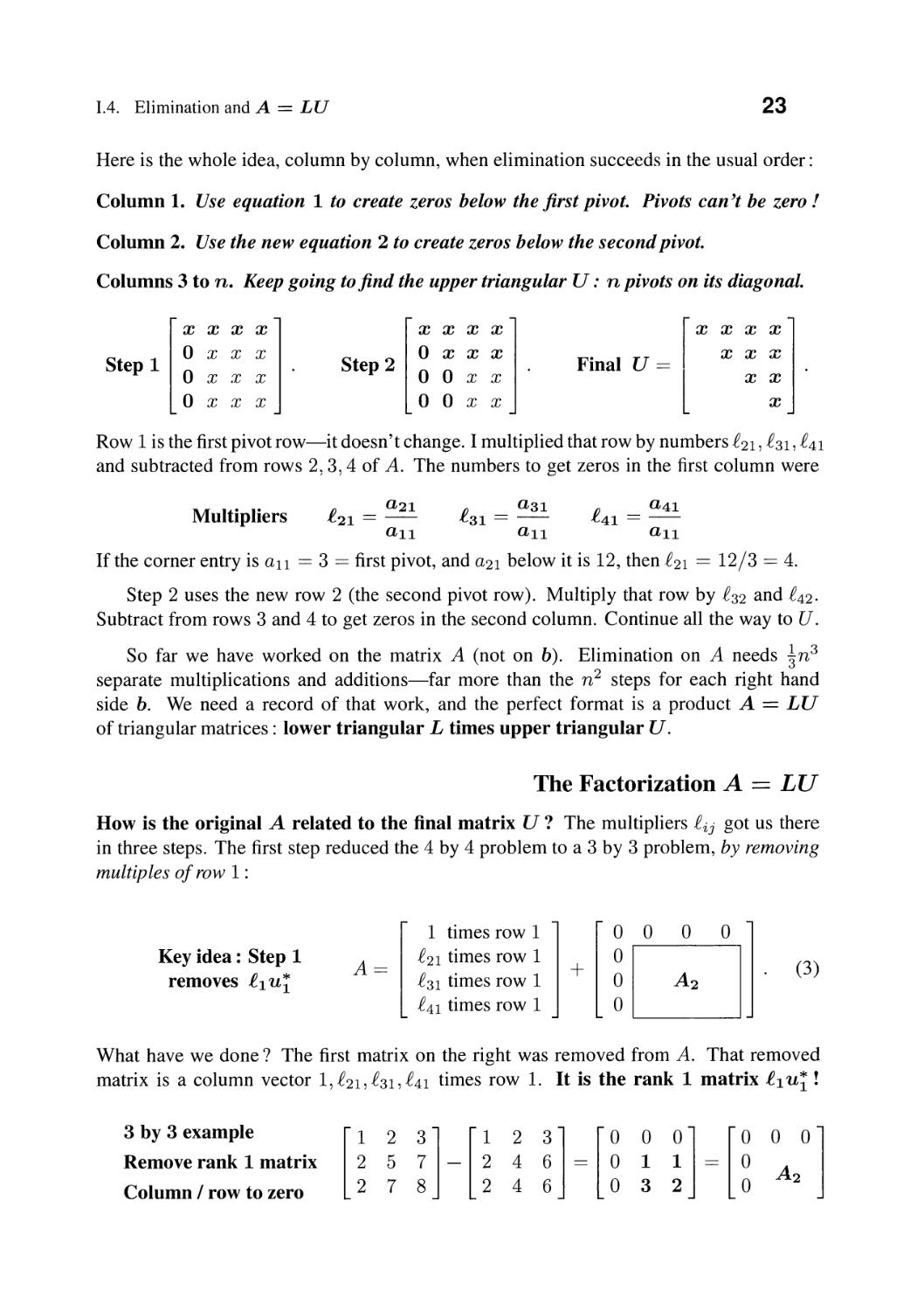
Here is the whole idea, column by column, when elimination succeeds in the usual order:
Column 1. Use equation 1 to create zeros below the first pivot. Pivots can't be zero!
Column 2. Use the new equation 2 to create zeros below the second pivot.
Columns 3 to n. Keep going to find the upper triangular U : n pivots on its diagonal.
Step 1
x x x x
0 x x x
0 x x x
0 x x x
Step 2
x x x x
o x x x
o 0 x x
o 0 x x
Final U ==
IX
l
x x x
x x x
x x
x
Row 1 is the first pivot row-it doesn't change. I multiplied that row by numbers £21, £31, £41
and subtracted from rows 2,3,4 of A. The numbers to get zeros in the first column were
Multipliers
f) _ a2l
.(,2l - -
all
f) _ a3l
.(,3l - -
all
f) _ a4l
.{,4l - -
all
If the corner entry is all == 3 == first pivot, and a21 below it is 12, then £21 == 12/3 == 4.
Step 2 uses the new row 2 (the second pivot row). Multiply that row by £32 and £42.
Subtract from rows 3 and 4 to get zeros in the second column. Continue all the way to U.
So far we have worked on the matrix A (not on b). Elimination on A needs in3
separate multiplications and additions-far more than the n 2 steps for each right hand
side b. We need a record of that work, and the perfect format is a product A == LU
of triangular matrices: lower triangular L times upper triangular U.
The Factorization A == LU
How is the original A related to the final matrix U? The multipliers £ij got us there
in three steps. The first step reduced the 4 by 4 problem to a 3 by 3 problem, by removing
multiples of row 1 :
1 times row 1 0 0 0 0
Key idea: Step 1 A== £21 times row 1 0
removes £1 u £31 times row 1 + 0 A 2
£41 times row 1 0
(3)
What have we done? The first matrix on the right was removed from A. That removed
matrix is a column vector 1, £21, £31, £41 times row 1. It is the rank 1 matrix £1 u !
3 by 3 example
Remove rank 1 matrix
Column / row to zero
u ] - U : n = [ ] = [ °A2 0 ]
24
Highlights of Linear Algebra
The next step deals with column 2 of the remaining matrix A 2 . The new row 2 is
u; == second pivot row. We multiply it by £12 == 0 and £22 == 1 and £32 and £42. Then
subtract £2U; from the four rows. Now row 2 is also zero and A 2 shrinks down to A 3 .
o times pivot row 2 0 0 0 0
Step 2 A == £lU + 1 times pivot row 2 0 0 0 0
£32 times pivot row 2 + 0 G
£42 times pivot row 2 0
(4)
That step was a rank one removal of £2U; with £2 == (0,1, £32, £42) and u; == pivot
row 2. Step 3 will reduce the 2 by 2 matrix A 3 to a single number A 4 (1 by 1). At this point
the pivot row u 3 == row 1 of A 3 has only two nonzeros. And the column £3 is (0,0,1, £43).
This way of looking at elimination, a column at a time, directly produces A == L U.
That matrix multiplication LU is always a sum of columns of L times rows of U :
1 0 0 0 pivot row 1
A == £1 U +£2 U ; +£3 U ; +£4 U : == £21 1 0 0 pivot row 2 ==LU. (5)
£31 £32 1 0 pivot row 3
£41 £42 £43 1 pivot row 4
Elimination factored A == LU into a lower triangular L times an upper triangular U
Notes on the LU factorization We developed A == LU from the key idea of elimina-
tion: Reduce the problem size from n to n - 1 by eliminating Xl from the last n - 1
equations. We subtracted multiples of row 1 (the pivot row). So the matrix we removed
had rank one. After n steps, the whole matrix A is a sum of n rank one matrices. That
sum-by the column times row rule for matrix multiplication-is exactly L times U.
This proof is not in my textbook Introduction to Linear Algebra. The idea there was to
look at rows of U instead of working with columns of A. Row 3 came from subtracting
multiples of pivot rows 1 and 2 from row 3 of A :
Row 3 of U == (row 3 of A) - £31 (row 1 of U) - £32 (row 2 of U). (6)
Rewrite this equation to see that the row [£31 £32 1] of L is multiplying the matrix U :
Row 3 of A == £31 (row 1 of U) + £32 (row 2 of U) + 1 (row 3 of U). (7)
This is row 3 of A == LU. The key is that the subtracted rows were pivot rows, and
already in U. With no row exchanges, we have again found A == LU.
1.4. Elimination and A == LU
25
The Solution to Ax == b
We must apply the same operations to the right side of an equation and to the left side.
The direct way is to include b as an additional column-we work with the matrix [A b].
Now our elimination steps on A (they multiplied A by L -1 to give U) act also on b:
Start from [A b] = [LU b] Elimination produces [u L -lb ] = [u c].
The steps from A to U (upper triangular) will change the right side b to c. Elimination
on Ax == b produces the equations U x == c that are ready for back substitution.
2x + 3y == 8 [ 2
4x + 7y == 18 --t 4
3
7
1 ] [
3
1
] [u c].
(8)
L subtracted 2 times row 1 from row 2. Then the triangular system U x
upwards-back substitution-from bottom to top:
c is solved
2x + 3y == 8
1y == 2
gives y == 2 and then x == 1. Ux == c gIves x == U- 1 c.
Looking closely, the square system Ax == b became two triangular systems:
Ax == b split into Lc == band U x == c. Elimination gave c and back substitution gave x.
The final result is x == U- 1 C == U- 1 L -1 b == A-I b. The correct solution has been found.
Please notice Those steps required nonzero pivots. We divided by those numbers.
The first pivot was all. The second pivot was in the corner of A 2 , and the nth pivot was in
the 1 by 1 matrix An. These numbers ended up on the main diagonal of U.
What do we do if all == O? Zero cannot be the first pivot. If there is a nonzero
number lower down in column 1, its row can be the pivot row. Good codes will choose the
largest number to be the pivot. They do this to reduce errors, even if all is not zero.
We look next at the effect of those row exchanges on A == LU. A matrix P will enter.
Row Exchanges (Permutations)
Here the largest number in column 1 is found in row 3: a31 == 2. Row 3 will be the first
pivot row ui. That row is multiplied by g21 == and subtracted from row 2.
A=[! l] [ !:]
u == row 3 of A
== first pivot row
(9)
26
Highlights of Linear Algebra
Again that elimination step removed a rank one matrix £1 ui. But A 2 is in a new place.
[ 011] [0 ][24 8J [01lIl]
1 3 7 == 1/2 + 0 +- A 2
248 1 000
(10)
Elimination on A 2 produces two more rank one pieces. Then A == LU has three pieces:
[ 1 ] [ 0
.elU +
1
1 J [0] [0 0 2 ] [0 1 0] [2 4 8]
+ 1 == 1/2 1 1 0 1 1 . (11)
o 100002
That last matrix U is triangular but the L matrix is not! The pivot order for this A was
3,1,2. If we want the pivot rows to be 1,2,3 we must move row 3 of A to the top:
Row exchange by
a permutation P
PA==[ ] [ ] [ i ]
010248 137
When both sides of Ax == b are multiplied by P, order is restored and P A == LU:
P A == [ i ] [ ] [ i ] == L U. (12)
1 3 7 1/2 1 1 0 0 2
Every invertible n by n matrix A leads to P A == LU: P == permutation.
There are six 3 by 3 permutations: Six ways to order the rows of the identity matrix.
1 exchange
(odd P)
P 213 = [ ]
[ 1 1 1]
P 123 ==
P 321 = [ ]
P 312 = [ ]
P 132 = [ n
P 231 = [ n
o or 2 exchanges
(even P)
The inverse of every permutation matrix P is its transpose pT. The row exchanges
will also apply to the right hand side b if we are solving Ax == b. The computer just
remembers the exchanges without actually moving the rows.
There are n! (n factorial) permutation matrices of size n: 3! == (3) (2) (1) == 6.
When A has dependent rows (no inverse) elimination leads to a zero row and stops short.
1.4. Elimination and A == LU
27
Problem Set 1.4
1 Factor these matrices into A == LU :
A=[ ]
A==
[: ::] A=[
2
-1
o
-1
2
-1
- ]
2 If all, . . . , a1n is the first row of a rank-1 matrix A and all, . . . , amI is the first
column, find a formula for aij. Good to check when all == 2,a12 == 3,a21 == 4.
When will your formula break down? Then rank 1 is impossible or not unique.
3 What lower triangular matrix E puts A into upper triangular form EA == U?
Multiply by E- 1 == L to factor A into LU:
A=[ ]
4 This problem shows how the one-step inverses multiply to give L. You see this
best when A == L is already lower triangular with 1 's on the diagonal. Then U == I :
Multiply A == [ ] by E 1 == [- 1 ]
bel -b 0 1
[ 1 _o 00 1 ]
and then E 2 ==
(a) Multiply E 2 E 1 to find the single matrix E that produces E A == I.
(b) Multiply Ell E:;l to find the matrix A == L.
The multipliers a, b, c are mixed up in E == L -1 but they are perfect in L.
5 When zero appears in a pivot position, A == LU is not possible! (We are requiring
nonzero pivots in U.) Show directly why these LU equations are both impossible:
[ ] = [ ] [ ;]
[: ] [1 J [d ; ]
These matrices need a row exchange by a permutation matrix P.
6 Which number e leads to zero in the second pivot position? A row exchange is
needed and A == LU will not be possible. Which e produces zero in the third pivot
position? Then a row exchange can't help and elimination fails:
A = [ : :]
28
Highlights of Linear Algebra
7 (Recolnmended) Compute Land U for this symmetric matrix A:
a a a a
A==
a b
a b
a b
e e
e d
b b
Find four conditions on a, b, e, d to get A == LU with four nonzero pivots.
8 Tridiagonal matrices have zero entries except on the main diagonal and the two adja-
cent diagonals. Factor these into A == LU. Symmetry further produces A == LD L T:
A = [ : ]
[ a a 0]
and A == a a + b b .
o b b+e
9 Easy but important. If A has pivots 5, 9, 3 with no row exchanges, what are the pivots
for the upper left 2 by 2 submatrix A 2 (without row 3 and column 3)?
10 Which invertible matrices allow A == LU (elimination without row exchanges)?
Good question! Look at each of the square upper left submatrices AI, A 2 , . . . , An.
All upper left submatrices A k must be invertible: sizes 1 by 1, 2 by 2, . . . , n by n.
because LU = [:k ] [ k : l
11 In some data science applications, the first pivot is the largest number laij I in A.
Then row i becomes the first pivot row ui. Column j is the first pivot column.
Divide that column by aij so £1 has 1 in row i. Then remove that £1 ui from A.
This example finds a22 == 4 as the first pivot (i == j == 2). Dividing by 4 gives £1 :
Explain that answer: A k factors into
[ 1 2] == [1/2] [3 4] [-1/2 0] == /} * /} * ==l f1/2 1] [3 4]
3 4 1 + 0 0 1 u 1 + 2u2 1 0 -1/2 0
For this A, both Land U involve permutations. PI exchanges the rows to give L.
P 2 exchanges the columns to give an upper triangular U. Then PlAP2 == LU.
Permuted in advance P AP _ [1 0] [4 3] _ [4 3]
1 2 - 1/2 1 0 -1/2 - 2 1
Question for A = [ :]: Apply complete pivoting to produce PIAP2 = LU.
12 If the short wide matrix A has m < n, how does elimination show that there are
nonzero solutions to Ax == O? What do we know about the dimension of that
"nullspace of A" containing all solution vectors x? The nullspace dimension is at
least
Suggestion: First create a specific 2 by 3 matrix A and ask those questions about A.
1.5. Orthogonal Matrices and Subspaces
29
1.5 Orthogonal Matrices and Subspaces
The word orthogonal appears everywhere in linear algebra. It means perpendicular.
Its use extends far beyond the angle between two vectors. Here are important extensions of
that key idea:
1. Orthogonal vectors x and y. The test is xTy == X1Y1 +... + XnYn == O.
If x and y have complex components, change to x T Y == X l Y1 + . . . + X nYn == O.
2. Orthogonal basis for a subspace : Every pair of basis vectors has v [ v j == O.
Orthonormal basis: Orthogonal basis of unit vectors: every V[ Vi == 1 (length 1).
From orthogonal to orthonormal, just divide every basis vector Vi by its length Ilvi II.
3. Orthogonal subspaces Rand N. Every vector in the space R is orthogonal to
every vector in N. Notice again! The row space and nullspace are orthogonal:
Ax == 0 means
each row · x == 0
[ row of A ] [x] [ 0 ]
rowmof A 0
(1)
Every row (and every combination of rows) is orthogonal to all x in the nullspace.
4. Tall thin matrices Q with orthonormal columns: QT Q I.
QTQ = [= : =] Ql" Qn
[ ] == I
001
(2)
If this Q multiplies any vector x, the length of the vector does not change:
IIQxl1 == Ilxll because (Qx)T(Qx) == xTQTQx == xTx (3)
If m > n the m rows cannot be orthogonal in R n . Tall thin matrices have Q QT -=I I.
5. "Orthogonal matrices" are square with orthonormal columns: QT Q-l.
For square matrices QT Q I leads to QQT == I
For square matrices Q, the left inverse QT is also a right inverse of Q.
The columns of this orthogonal n by n matrix are an orthonormal basis for R n .
The rows of Q are a (probably different) orthonormal basis for R n .
The name "orthogonal matrix" should really be "orthonormal matrix".
The next pages give examples of orthogonal vectors, bases, subspaces and matrices.
30
Highlights of Linear Algebra
1. Orthogonal vectors. The test x T y == 0 connects to right triangles by e 2 == a 2 + b 2 :
Pythagoras Law for right triangles IIx - yl12 == IIxll 2 + Ilyll2. (4)
The left side is (x - y)T (x - y). This expands to x T x + yT y - xTy - yT x . When
the last two terms are zero, we have equation (4): x == (1,2,2) and y == (2,1, -2) have
x T y == O. The hypotenuse is x - y == (-1,1,4). Then Pythagoras is 18 == 9 + 9.
Dot products x T y and y T X always equal II xliii y II cos e, where () is the angle
between x and y. So in all cases we have the Law of Cosines e 2 == a 2 + b 2 - 2ab cos e :
Law of Cosines
II x - y 11 2 == II X 11 2 + II Y 11 2 - 2 II x II II y II cos e.
(5)
Orthogonal vectors have cos e == 0 and that last term disappears.
2. Orthogonal basis. The "standard basis" is orthogonal (even orthonormal) in R n :
Standard basis i, j, k in R 3
i=[ ] j=[ ] k=[ ].
Here are three Hadamard matrices H 2 , H 4 , H s containing orthogonal bases of R 2 , R 4 , R S .
Hadamard matrices
Orthogonal columns
sizes 2, 4 and 8
[ - ]
1 1 1 1
1 -1 1-1
1 1 -1 -1
1 -1 -1 1
[ H 4 H4]
H 4 -H 4
Are those orthogonal matrices? No. The columns have lengths )2, A, V8. If we
divide by those lengths, we have the beginning of an infinite list: orthonormal bases
in 2, 4, 8, 16, 32, . . . dimensions.
The Hadamard conjecture proposes that there is a :::t 1 matrix with orthogonal columns
whenever 4 divides n. Wikipedia says that n == 668 is the smallest of those sizes without
a known Hadamard matrix. The construction for n == 16, 32, . . . follows the pattern above.
Here is a key fact: Every subspace of R n has an orthogonal basis. Think of a
plane in three-dimensional space R 3 . The plane has two independent vectors a and b.
For an orthogonal basis, subtract away from b its component in the direction of a :
aTb
Orthogonal basis a and c c == b - - a. (6)
aTa
The inner product aTe is aT b - aT b == O. This idea of "orthogonalizing" applies to any
number of basis vectors: a basis becomes an orthogonal basis. That is the Gram-Schmidt
idea in Section 11.2.
1.5. Orthogonal Matrices and Subspaces
31
3. Orthogonal subspaces. Equation (1) looked at Ax == o. Every row of A is multiplying
that nullspace vector x. So each row (and all combinations of the rows) will be orthogonal
to x in N (A). The row space of A is orthogonal to the nullspace of A.
Ax == [ ro 1 ] [ x ] == [ 0 ] AT Y == [ (colu n 1) T ] [ Y ] == [ ] (7)
ro rn 0 (colu n n)T 0
From AT y == 0, the columns of A are all orthogonal to y. Their combinations (the whole
column space) will also be orthogonal to y. The column space of A is orthogonal to the
nullspace of AT. This produces the "Big Picture of Linear Algebra" in Figure 1.6.
Notice the dimensions rand n - r adding to n. The whole space R n is accounted for.
Every vector v in R n has a row space component V r and a nullspace component V n with
v == V r + V n . A row space basis (r vectors) together with a nullspace basis (n - r vectors)
produces a basis for all of R n (n vectors).
Ax row == b
dimension
==r
row space to column space
.
AXnull == 0
nullspace to 0
.
dimension
==n-r
==m-r
Figure 1.6: Two pairs of orthogonal subspaces. The dimensions add to n and add to m.
This is the Big Picture-two subspaces in R n and two subspaces in Rm.
I will mention a big improvement. It comes from the Singular Value Decomposition.
The SVD is the most important theorem in data science. It finds orthonormal bases VI, . . . , V r
for the row space of A and U1, . . . , U r for the column space of A. Well, Gram-Schmidt
can do that. The special bases from the SVD have the extra property that each pair
(v and u) is connected by A :
Singular vectors
AV1 == (J1 U1
AV2 == (J2 U 2
AV r == (JrUr.
(8)
In Figure 1.6, imagine the v's on the left and the u' s on the right. For the bases from the
SVD, multiplying by A takes an orthogonal basis of v's to an orthogonal basis of u's.
32
Highlights of Linear Algebra
4. Tall thin Q with orthonormal columns: QTQ == I.
Here are three possible Q's, growing from (3 by 1) to (3 by 2) to an orthogonal matrix Q3.
Ql = [ _ ]
Q2 == [ - ]
3 -1 2
[ 2 2 -1]
Q3 == 2 -1 2 .
3 -1 2 2
(9)
Each one of those matrices has QT Q == I. So QT is a left inverse of Q. Only the last matrix
has Q3Qr == I. Then Qr is also a right inverse. Q3 happens to be symmetric as well as
orthogonal. It is a king and also a queen, truly a royal matrix.
Notice that all the matrices P == QQT have p 2 == P:
p2 == (QQT) (QQT) == Q (QTQ) QT == QQT == P. (10)
In the middle we removed QT Q == I. The equation p 2 == P signals a projection matrix.
If p 2 == P == pT then Pb is the orthogonal projection of b onto the column space of P.
Example 1 To project b == (3,3,3) on the Q1 line, multiply by PI == Q1 QI.
Prb = [ _ ]
[2 2 -1 ]
[ ] [- ]g=[- ]
projection
on a line
That matrix splits b in two perpendicular parts: projection PI b and error e == (I - PI) b.
line
b=[ ]
e = [ - ]
o
b=[ ]
error e = [ ]
Prb = [ _ ]
Ilel! == VIS
P 2 b = [ : ]
Ilell == J9
. s that line
contaln
plane
Figure 1.7: Projection of b onto a line by PI == Q1 QI and onto a plane by P 2 == Q2Qi.
Now project the same b == (3,3,3) on the column space of Q2 (a plane). The error vector
b - P 2 b is shorter than b - PI b because the plane contains the line.
P2b= [_ - ][ - - ][ ] [_ - ][ ]=[:]
1.5. Orthogonal Matrices and Subspaces
33
Question: What is P3 b == Q3QI b? Now you are projecting b onto the whole space R 3 .
Answer: P 3 b == b. In fact P 3 == Q3QI == identity matrix! The error e is now zero.
Projections lie at the heart of "least squares" in Section 11.2.
5. Orthogonal matrices: Now Q is square: QT Q == I and QQT == I. So Q-l == QT.
These Q's are truly important. For 2 by 2, they are rotations of the plane or reflections.
When the whole plane rotates around (0,0), lengths don't change. Angles between
vectors don't change. The columns of Q are orthogonal unit vectors, with cos 2 B-t-sin 2 e == 1 :
[ CDS f) - sin f) ] .
Qrotate == · f) f) == rotation through an angle e. (11)
SIn CDS
And if I multiply a column by -1, the two columns are still orthogonal of length 1.
[ CDS f) sin f) ] . e.
Q reflect == · f) f) == reflection across the - - lIne.
SIn - CDS 2
Now Q reflects every vector in a mirror. It is a reflection with determinant -1 instead of a
rotation with determinant + 1. The x-y plane rotates or the x-y plane flips over.
It is important that multiplying orthogonal matrices produces an orthogonal matrix.
(12)
Ql Q2 is orthogonal
(Q1 Q2)T(Q1 Q2) == Qi QI Q1Q2 == QiQ2 == I.
Rotation times rotation == rotation. Reflection times reflection == rotation. Rotation times
reflection == reflection. All still true in R n .
Q [n
[ -; :]
[ ]
Q [ ]
[ ]
[ C?S e ]
SIne
---
e .
- lIne
2
[ ]
Q [0] == [ sin e ]
1 - cose
Figure 1.8: Rotate the whole plane bye. Reflect every vector across the line at angle e /2.
The figure shows how the columns of Q come from Q [ ] and Q [ ].
34
Highlights of Linear Algebra
Orthogonal Basis == Orthogonal Axes in R n
Suppose the n by n orthogonal matrix Q has columns q1, . . . , qn. Those unit vectors are
a basis for n-dimensional space R n . Every vector v can be written as a combination of the
basis vectors (the q' s) :
v==e1q1+...+enqn (13)
Those e1q1 and e2q2 and enqn are the components of v along the axes. They are the
projections of v onto the axes! There is a simple formula for each number e1 to en :
C2=q'fV ... cn=q v I
(14)
Coefficients in
an orthonormal basis
I Cl = qlv
I will give a vector proof and a matrix proof. Take dot products with q1 in equation (13) :
q'[v == e1q'[q1 +... + enq'[qn == e1 (15)
All terms are zero except e1 q I q 1 == e1. So q I v == e1 and every q r v == ek.
If we write (13) as a matrix equation v == Qc, multiply by QT to see (14):
Q T V == Q T Qc == c gives all the coefficients ek == q r v at once.
This is the key application of orthogonal bases (for example the basis for Fourier series).
When basis vectors are orthonormal, each coefficient e1 to en can be found separately!
Householder Reflections
Here are neat examples of reflection matrices Q == H n . Start with the identity matrix.
Choose a unit vector u. Subtract the rank one symmetric matrix 2uu T. Then 1 - 2uu T
is a "Householder matrix". For ex ample, choose u == (1, 1, . . . , 1) / Vii.
Householder example I H n = I - 2uu T = I - ones (n, n).1 (16)
With uu T, H n is surely symmetric. Two reflections give H 2 == 1 because u T u == 1 :
H T H == H 2 == (1 - 2uu T ) (1 - 2uu T ) == 1 - 4uu T + 4uu TuuT == I. (17)
The 3 by 3 and 4 by 4 examples are easy to remember, and H 4 is like a Hadamard matrix:
H 3 = I - ones = [ - -2 -2] 1 -1 -1 -1
2 1 -1 1 -1 -1
1 -2 H 4 == 1 - - ones == - -1 -1 1 -1
3 3_ 2 -2 1 4 2
-1 -1 -1 1
Householder's n by n reflection matrix has Hnu == (1 - 2uu T )u == U - 2u == -u.
And Hnw == +w whenever w is perpendicular to u. The "eigenvalues" of Hare
-1 (once) and + 1 (n - 1 times). All reflection matrices have eigenvalues -1 and 1.
1.5. Orthogonal Matrices and Subspaces
35
Problem Set 1.5
1 If u and v are orthogonal unit vectors, show that u + v is orthogonal to u - v.
What are the lengths of those vectors?
2 Draw unit vectors u and v that are not orthogonal. Show that w == v - u( U Tv) is
orthogonal to u (and add w to your picture).
3 Draw any two vectors u and v out from the origin (0,0). Complete two more sides
to make a parallelogram with diagonals w == u + v and z == u - v. Show that
w T w + Z T Z is equal to 2u T U + 2v Tv.
4 Key property of every orthogonal matrix: IIQxl12 == IIxll 2 for every vector x.
More than this, show that (Qx) T (Qy) == X T Y for every vector x and y. So
lengths and angles are not changed by Q. Computations with Q never overflow!
5 If Q is orthogonal, how do you know that Q is invertible and Q-1 is also orthogonal?
If QI == Q 1 1 and Qi == Q"2\ show that Q1 Q2 is also an orthogonal matrix.
6 A permutation matrix has the same columns as the identity matrix (in some order).
Explain why this permutation matrix and every permutation matrix is orthogonal:
o 1 0 0
P == 0 0 1 0 has orthonormal columns so pT P ==
000 1
1 000
and p-1 ==
When a matrix is symmetric or orthogonal, it will have orthogonal eigenvectors.
This is the most important source of orthogonal vectors in applied mathematics.
7 Four eigenvectors of that matrix P are Xl == (1,1,1,1), X2 == (1, i, i 2 , i 3 ),
X3 == (1, i 2 , i 4 , i 6 ), and X4 == (1, i 3 , i 6 , i 9 ). Multiply P times each vector to find
AI, A2, A3, A4. The eigenvectors are the columns of the 4 by 4 Fourier matrix F.
1 1 1 1
F 1 1 2 -1 -2 -T
Show that Q == "2 =="2 1 i 2 1 -1 has orthonormal columns : Q Q = I
1 i 3 -1 2
8 Haar wavelets are orthogonal vectors (columns of W) using only 1, -1, and o.
n==4 1 1 1 0
1 1 -1 0 Find WTW and W- l and the
w==
1 -1 0 1 eight Haar wavelets for n == 8.
1 -1 0-1
J
l
36 Highlights of Linear Algebra
1.6 Eigenvalues and Eigenvectors
The eigenvectors of A don't change direction when you multiply them by A. The output
Ax is on the same line as the input vector x.
x == eigenvector of A
A == eigenvalue of A
Ax == AX
(1)
The eigenvector x is just multiplied by its eigenvalue A. Multiply again by A, to see that
x is also an eigenvector of A 2 : A 2 x == A 2 x.
x == same eigenvector
A 2 == squared eigenvalue
Certainly Akx == Akx for all k == 1,2,3,... And A-Ix == -l-x provided A -=I O.
These eigenvectors are special vectors that depend on A. Most n by n matrices have
n independent eigenvectors Xl to X n with n different eigenvalues Al to An. In that case
every n-dimensional vector v will be a combination of the eigenvectors :
A(Ax) == A(Ax) == A(Ax) == A 2 x .
(2)
Every v
Multiply by A
Multiply by A k
v == e1x1 + . . . + enx n
Av == e1A1x1 + . . . + enAnx n
Ak v == e1 A }x1 + . . . + enA xn
(3)
Here you see how eigenvalues and eigenvectors are useful. They look into the heart of
a matrix. If I All > 1 then the component e1 A1x1 will grow as n increases. If I A21 < 1
then that component e2A2'x2 will steadily disappear. Follow each eigenvector separately!
Example 1 S = [ ] has eigenvectors S [ ] = 3 [ ] and S [ _ ] = [ _ ]
Then Al == 3 and A2 == 1. The powers Sk will grow like 3 k . Those eigenvalues and
eigenvectors have four properties to notice:
(Trace of S) The sum Al + A2 == 3 + 1 equals the diagonal sum 2 + 2 == 4
(Determinant) The product Al A2 == (3) (1) == 3 equals the determinant 4 - 1
(Real eigenvalues) Symmetric matrices S == ST always have real eigenvalues
(Orthogonal eigenvectors) If Al -=I A2 then Xl · X2 == O. Here (1,1) · (1, -1) == O.
Symmetric matrices S are somehow like real numbers (every A is real). Orthogonal ma-
trices Q are like complex numbers e i8 == cos () + i sin e of magnitude 1 (every IAI == 1).
The powers of Q don't grow or decay because Q2, Q3, . . . are orthogonal matrices too.
1.6. Eigenvalues and Eigenvectors
37
Example 2 The rotation Q
[ 0 -1] h . . . I . d .
1 0 as ImagInary elgenva ues an - :
Q [ _ ] = [ - ] [ _ ] = (i) [ _ ] and Q [ ] = [ - ] [ ] = (-i) [ ]
Certainly Al + A2 == i - i agrees with the trace 0 + 0 from the main diagonal of Q.
And (AI) (A2) == (i) (-i) agrees with the determinant of Q == 1. The eigenvectors of Q
are still orthogonal when we move (as we should) to the dot product of complex vectors.
Change every i in Xl to -i. This produces its conjugate X l.
x i X2 = [1 i] [ ] = 1 + i 2 = 0 : orthogonal eigenvectors.
Warnings about eigenvalues and eigenvectors
The eigenvalues of A + B are not usually A(A) plus A(B).
The eigenvalues of AB are not usually A(A) times A(B).
A double eigenvalue Al == A2 might or might not have two independent eigenvectors.
The eigenvectors of a real matrix A are orthogonal if and only if AT A == AA T .
The matrix A also controls a system of linear differential equations duj dt == Au. The
system starts at an initial vector u(O) when t == O. Every eigenvector grows or decays or
oscillates according to its own eigenvalue A. Powers An are changed to exponentials eAt:
Starting vector u(O) == ClX1 + . . . + CnX n
Solution vector u(t) == cleAltx1 + . . . + cneAntxn
(4)
The difference between growth and decay is now decided by Re A > 0 or Re A < 0,
instead of I A I > 1 or I A I < 1. The real part of A == a + ib is Re A == a. The absolute
value of eAt is eat. The other factor e ibt == cos bt + i sin bt has cos 2 bt + sin 2 bt == 1.
That part oscillates while eat grows or decays.
Computing the Eigenvalues (by hand)
Notice that Ax == AX is the same as (A - AI)x == O. Then A - AI is not invertible:
that matrix is singular. The determinant of A - AI must be zero. This gives an nth
degree equation for A, and this equation det (A - AI) == 0 has n roots. Here n == 2 and
A = [ ] has two eigenvalues:
C
b = oX 2 - (a + d) oX + (ad - be) = 0
d-A
a-A
Determinant of A - AI ==
This quadratic equation might factor easily into (A - AI) (A - A2). The "quadratic formula"
will always give the two roots Al and A2 of our equation, from the + sign and the - sign.
38
Highlights of Linear Algebra
A = H a + d :l: J (a + d) 2 - 4 (ad - be) ] = H a + d ::l:: J (a - d) 2 + 4bc J.
You see that Al + A2 equals a + d (the trace of the matrix). The :I: square roots cancel out.
Notice also that the eigenvalues are real when A is symmetric (b == e). Then we
are not taking the square root of a negative number to find A. When be is very negative,
the eigenvalues and eigenvectors go complex!
Example 3 Find the eigenvalues and eigenvectors of A = [ ]: not symmetric.
8 - A 3
The determinant of A-AIls ==A 2 -15A+50==(A-I0)(A-5).
2 7 - A
[ 8- 2 10
Al == 10 has
[ 8- 2 5
A2 == 5 has
7 ! 10] [ ] [ ] Eigenvector XI = [ ] = [ ]
7 3 5 ] [ ] [ ] Eigenvector X2 = [ ] = [ _ ]
10 + 5 == 8 + 7. These eigenvectors are not orthogonal. Increase 3 to 30 for complex A's.
Question: If A is shifted to A + sI, what happens to the x's and A's?
Answer: The eigenvectors x stay the same. Every eigenvalue A shifts by the number s :
Shift in A =* shift in every A
(A + s1) x == AX + sx == (A + s) x
(5)
Similar Matrices
For every invertible matrix B, the eigenvalues of BAB- 1 are the same as the eigenvalues
of A. The eig envectors x of A are multiplied by B to give eigenvectors Bx o f BAB- 1 :
IIfAX = AX then (BAB- l ) (Bx) = BAx = BAX = A(Bx).1 (6)
The matrices BAB- 1 (for every invertible B) are "similar" to A: same eigenvalues.
We use this idea to compute eigenvalues of large matrices (when the determinant of
A - AI would be completely hopeless). The idea is to make BAB- 1 gradually into a
triangular matrix. The eigenvalues are not changing and they gradually show up on the
main diagonal of BAB- 1 :
The eigenvalues of any triangular matrix [ ] are Al = a and A2 = d. (7)
You can see that A - aI and A - dI will have determinant zero. So a and d are the
eigenvalues of this triangular matrix.
1.6. Eigenvalues and Eigenvectors
39
Diagonalizing a Matrix
Suppose A has a full set of n independent eigenvectors. (Most matrices do, but not all
matrices.) Put those eigenvectors Xl, . . . , X n into an invertible matrix X. Then multiply
AX column by column to get the columns A1X1 to Anx n . Important! That matrix splits
into X times A.
Al
A Xl .. X n
AX1 .. AX n
A1 X 1 .. Anx n
Xl .. X n
An
(8)
The eigenvalue matrix A goes on the right of X, because the A's in A multiply the columns
of X. That equation AX == XA tells us that A == X AX-I. If we know the eigenvalues
and eigenvectors, we know the matrix A. And we can easily compute powers of A :
A == diagonal eigenvalue matrix
X == invertible eigenvector matrix
A == XAX- 1
A2 == (X AX-I) (X AX-I) == X A2 X-I
A == XAX- l [8 3] [ 3 1 ] [ 10 ] 1 [1 1 ] (eigenvectors) times (A's)
in Example 3 2 7 == 2 -1 5 5 2 - 3 == times (left eigenvectors)
The equation A k == X A k X -1 is telling us what we already knew. The eigenvalues of A k
are A}, . . . , A . The eigenvectors of Ak are the same as the eigenvectors of A. Three steps
compute Ak v .
Step 1: X-IV
Step 2: A k X-IV
Step 3: XAk X-IV
This gives the e's in V == e1x1 + . . . + enx n
This gives the A's in e1A}x1 + ... + enA xn
This adds those pieces in Akv == e1A}x1 + . . . + enA xn
Example 4 If we divide Example 3 by 10, all eigenvalues are divided by 10. Then
Al == 1 and A2 == . In this case A is a Markov matrix, with positive columns adding to 1.
A == [ 0.8
0.2
0.3 ]
0.7
Ak V == e1(1)k x1 + e2( )kx2
As k increases, Akv approaches ClXl == steady state
We can follow each eigenvector separately. Its growth or decay depends on the eigenvalue
A. The action of the whole matrix A is broken into simple actions Gust multiply by A)
on each eigenvector. To solve a differential equation du/dt == Au we would multiply
each eigenvector by eAt.
40
Highlights of Linear Algebra
Nondiagonalizable Matrices (Optional)
Suppose A is an eigenvalue of A. We discover that fact in two ways:
1. Eigenvectors (geometric) There are nonzero solutions to Ax == AX.
2. Eigenvalues (algebraic) The determinant of A - AI is zero.
The number A may be a simple eigenvalue or a multiple eigenvalue, and we want to know its
multiplicity. Most eigenvalues have multiplicity M == 1 (simple eigenvalues). Then there
is a single line of eigenvectors, and det (A - AI) does not have a double factor.
For exceptional matrices, an eigenvalue can be repeated. Then there are two different
ways to count its multiplicity. Always GM < AM for each A:
1. (Geometric Multiplicity == GM) Count the independent eigenvectors for A.
Look at the dimension of the nullspace of A - AI.
2. (Algebraic Multiplicity == AM) Count the repetitions of A among the eigenvalues.
Look at the roots of det(A - AI) == o.
If A has A == 4,4, 4, then that eigenvalue has AM == 3 and GM == 1 or 2 or 3.
The following matrix A is the standard example of trouble. Its eigenvalue A == 0 is
repeated. It is a double eigenvalue (AM == 2) with only one eigenvector (GM == 1) .
AM == 2
GM == 1
[ 0 1] -A
A == 0 0 has det (A - AI) == 0
1 == \2
-A /\.
A == 0,0 but
1 eigenvector
There "should" be two eigenvectors, because A 2 == 0 has a double root. The double
factor A 2 makes AM == 2. But there is only one eigenvector x == (1,0). So GM == 1.
This shortage of eigenvectors when GM < AM means that A is not diagonalizable.
There is no invertible eigenvector matrix. The formula A == X AX -1 fails.
These three matrices all have the same shortage of eigenvectors. Their repeated eigen-
value is A == 5. Traces are 10 and determinants are 25:
A == [0 5 51] [6 -1]
and A == 1 4
and A = [_; ].
Those all have det(A - AI) == (A - 5)2. The algebraic multiplicity is AM == 2. But
each A-51 has rank r == 1. The geometric multiplicity is GM == 1. There is only one
line of eigenvectors for A == 5, and these matrices are not diagonaiizable.
1.6. Eigenvalues and Eigenvectors
41
Problem Set 1.6
1
. [ cos e
The rotatIon Q == . e
SIn
- sin e ] hi. I \ () -.L. . e
e as comp ex elgenva ues /\ == COS I 'l SIn :
COS
Q [ _ ] = (cas e + i sin e) [ _ ] and Q [ ] = (cas e - i sin e) [ ] .
Check that Al + A2 equals the trace of Q (sum Q11 + Q22 down the diagonal).
Check that (A 1) (A2) equals the determinant. Check that those complex eigenvectors
are orthogonal, using the complex dot product X l · X2 (not just Xl · X2 !).
What is Q-1 and what are its eigenvalues?
2 Compute the eigenvalues and eigenvectors of A and A -1. Check the trace!
A == [0 1 2 1 ] -1 [-1/2 1]
and A = 1/2 0 .
A -1 has the
has eigenvalues
eigenvectors as A. When A has eigenvalues Al and A2, its inverse
3 Find the eigenvalues of A and B (easy for triangular matrices) and A + B:
A = [i ] and B = [ ] and A + B = [i ].
Eigenvalues of A + B (are equal to )(are not equal to) eigenvalues of A plus eigen-
values of B.
4 Find the eigenvalues of A and Band AB and BA:
A = [ ] and B = [ i] and AB = [ ] and BA = [i i].
(a) Are the eigenvalues of AB equal to eigenvalues of A times eigenvalues of B?
(b) Are the eigenvalues of AB equal to the eigenvalues of BA?
5 (a) If you know that X is an eigenvector, the way to find A is to
(b) If you know that A is an eigenvalue, the way to find X is to
6 Find the eigenvalues and eigenvectors for both of these Markov matrices A and A (X) .
Explain from those answers why A 100 is close to A (X):
A == [.6 .2]
.4 .8
d A (X) [1/3 1/3]
an == 2/3 2/3 .
42
Highlights of Linear Algebra
7 The determinant of A equals the product A1A2 . . . An. Start with the polynomial
det(A - AI) separated into its n factors (always possible). Then set A == 0 :
det(A - AI) == (AI - A)(A2 - A) . . . (An .- A) so det A ==
Check this rule in Example 1 where the Markov matrix has A == 1 and .
8 The sum of the diagonal entries (the trace) equals the sum of the eigenvalues:
A = [ ] has det(A - AI) = A 2 - (a + d)A + ad - be = O.
The quadratic formula gives the eigenvalues A == (a+d+ V)/2 and A ==
Their sum is . If A has Al == 3 and A2 == 4 then det(A -- AI) ==
9 If A has Al == 4 and A2 == 5 then det(A - AI) == (A - 4)(A - 5) == A 2 - 9A + 20.
Find three matrices that have trace a + d == 9 and determinant 20 and A == 4,5.
10 Choose the last rows of A and C to give eigenvalues 4, 7 and 1,2,3:
Companion matrices
A = [ ;] C = [ ],
11 The eigenvalues of A equal the eigenvalues of AT. l'his is because det (A - AI)
equals det (AT - AI). That is true because __. Show by an example that the
eigenvectors of A and AT are not the same.
12 This matrix is singular with rank one. Find three A's and three eigenvectors:
A= [ ] [2 1 2] = [ ].
13 Suppose A and B have the same eigenvalues AI,. . ., An with the same independent
eigenvectors Xl,. . ., X n . Then A == B. Reason: Any vector X is a combination
e1X1 + . . . + enx n . What is Ax? What is Bx?
14 Suppose A has eigenvalues 0, 3, 5 with independent eigenvectors u, v, w.
(a) Give a basis for the nullspace and a basis for the column space.
(b) Find a particular solution to Ax == v + w. Find all solutions.
(c) Ax == u has no solution. If it did then would be in the column space.
15 (a) Factor these two matrices into A == XAX- 1 :
A = [ ] and A = [ ].
(b) If A == X AX -1 then A 3 == ( ) ( ) ( ) and A -1 == ( ) ( ) ( ) .
1.6. Eigenvalues and Eigenvectors
43
16 Suppose A == XAX- 1 . What is the eigenvalue matrix for A + 217 What is the
eigenvector matrix 7 Check that A + 21 == ( ) ( ) ( ) -1.
17 True or false: If the columns of X (eigenvectors of A) are linearly independent, then
(a) A is invertible
(c) X is invertible
(b) A is diagonalizable
(d) X is diagonalizable.
18 Write down the most general matrix that has eigenvectors [ J and [_ i ] .
19 True or false: If the eigenvalues of A are 2,2,5 then the matrix is certainly
(a) invertible
(b) diagonalizable
(c) not diagonalizable.
20 True or false: If the only eigenvectors of A are multiples of (1, 4) then A has
(a) noinverse (b) a repeated eigenvalue (c) nodiagonalizationXAX- 1 .
21 A k == XA k X-I approaches the zero matrix as k -+ 00 if and only if every A has
absolute value less than . Which of these matrices has A k -+ 07
Al == [.6 .9]
.4 .1
and
A == [.6 .9]
2 .1.6.
22 Diagonalize A and compute X A k X -1 to prove this formula for A k:
A == [ 2 -1]
-1 2
has
A k == [1+3 k
2 1 - 3 k
1 - 3 k ]
1 + 3 k .
23 The eigenvalues of A are 1 and 9, and the eigenvalues of Bare -1 and 9:
A = [ :]
and
B=[: ].
Find a matrix square root of A from R == X VA X-I. Why is there no real matrix
square root of B7
24 Suppose the same X diagonalizes both A and B. They have the same eigenvectors
in A == XA 1 X- 1 and B == XA 2 X- 1 . Prove that AB == BA.
25 The transpose of A == X AX -1 is AT == (X -1 ) T AX T . The eigenvectors in AT y ==
AY are the columns of that matrix (X- 1 )T. They are often called left eigenvectors of
A, because y T A == Ay T. How do you multiply matrices to find this formula for A 7
Sum of rank-l matrices A == XAX- 1 == A1x1yI +... + Anxny;;'.
26 When is a matrix A similar to its eigenvalue matrix A 7
A and A always have the same eigenvalues. But similarity requires a matrix B with
A == BAB- 1 . Then B is the matrix and A must have n independent
44 Highlights of Linear Algebra
1.7 Symmetric Positive Definite Matrices
Symmetric matrices S == ST deserve all the attention they get. Looking at their eigenvalues
and eigenvectors, you see why they are special:
1 All n eigenvalues A of a symmetric matrix S are real numbers.
2 The n eigenvectors q can be chosen orthogonal (perpendicular to each other).
The identity matrix S == 1 is an extreme case. All its eigenvalues are A == 1. Every
nonzero vector x is an eigenvector: 1 x == Ix. This shows why we wrote "can be cho-
sen" in Property 2 above. With repeated eigenvalues like Al == A2 == 1, we have a choice
of eigenvectors. We can choose them to be orthogonal. And we can rescale them to be
unit vectors (length 1). Then those eigenvectors q1, . . . qn are not just orthogonal, they are
orthonormal. The eigenvector matrix for S has QT Q == I : orthonormal columns in Q.
leads to
ql .. qn
1 0
o 1
o
o
T {O i -=I j
qi qj == 1 i == j
qf
o
1 0
o 1
q
o
We write Q instead of X for the eigenvector matrix of S, to emphasize that these
eigenvectors are orthonormal: QT Q == 1 and QT == Q-1. This eigenvector matrix is an
orthogonal matrix. The usual A == XAX- 1 becomes S == QAQT:
Spectral Theorem
Every real symmetric matrix has the form S == Q AQT .
Every matrix of that form is symmetric: Transpose Q AQT to get QTT A T QT == Q AQT.
Quick Proofs: Orthogonal Eigenvectors and Real Eigenvalues
Suppose first that Sx == AX and Sy == Oy. The symmetric matrix S has a nonzero
eigenvalue A and a zero eigenvalue. Then y is in the nullspace of S and x is in the column
space of S (x == SX/A is a combination of the columns of S). But S is symmetric:
column space == row space! Since the row space and nullspace are always orthogonal,
we have proved that x is orthogonal to y.
When that second eigenvalue is not zero, we have Sy == aYe In this case we look at
the matrix S - al. Then (S - al)y == Oy and (S - al)x == (A - a)x with A - a -=I O.
Now y is in the nullspace and x is in the column space (== row space!) of S - al.
So y T X == 0: Orthogonal eigenvectors whenever the eigenvalues A -=I a are different.
Those paragraphs assumed real eigenvalues and real eigenvectors. To prove this,
multiply Sx == AX by the complex conjugate vector x T (every i changes to -i). Then
x T Sx == A X T x. When we show that x T x and x T Sx are real, we know that A is real.
X TX== X 1X1+...+ Xn Xn and every X kXk is (a-ib)(a+ib)==a 2 +b 2 (real)
1.7. Symmetric Positive Definite Matrices
45
Also real: x T Sx == Sll X 1X1 + S12( X 1X2 + X1 X 2) + ... and again X 1X1 is real
X 1X2 + X1 X 2 == (a - ib)(e + id) + (a + ib)(e - id) == 2ae + 2bd == real
Since x T x > 0, the ratio A is real. And (S - AI)x == 0 gives a real eigenvector.
Complex comment: Transposing Sx == AX and taking complex conjugates gives
x T S T == A x T . For our real symmetric matrices, S T is exactly S. It is this double step,
transpose and conjugate, that we depend on to give back S. Since the proof only needs
S T == S, it allows for complex matrices too: When S T == S all eigenvalues of S are real.
[ 2 3 - 3i] -T
Complex example S == 3 + 3i 5 == S has real eigenvalues 8 and -1.
The key is 3 + 3i == 3 - 3i. The determinant is (2) (5) - (3 + 3i) (3 - 3i) == 10 -18 == -8.
The eigenvectors of this matrix are Xl == (1,1 + i) and X2 == (1 - i, -1). Those
vectors are orthogonal when we adjust complex inner products to x i X2. This is the
correct inner product for complex vectors, and it produces x i X2 == 0 :
T [1 1 + i ] [ _1 -1 i] -_ -2 to X T 1 X2 __ [ 1
Change xl X2 == IJ
l-i][I-i]==
-1 o.
Systems like MATLAB and Julia get the message: The vector x I and the matrix A I are
automatically conjugated when they are transposed. Every i changes to -i. Then x I is
T T
x and A I is A . Another frequently used symbol for x and A is a star: x* and A * .
Positive Definite Matrices
We are working with real symmetric matrices S == ST. All their eigenvalues are real.
Some of those symmetric matrices (not all) have a further powerful property that puts them
at the center of applied mathematics. Here is that important property:
Test 1
A positive definite matrix has all positive eigenvalues.
We would like to check for positive eigenvalues without computing those numbers A.
You will see four more tests for positive definite matrices, after these examples.
46
Highlights of Linear Algebra
1 S = [ ] is positive definite. Its eigenvalues 2 and 6 are both positive
2 S = Q [ ] QT is positive definite if QT = Q-l : same>. = 2 and 6
3 S = C [ ] C T is positive definite if C is invertible (not obvious)
4 S = [ ] is positive definite exactly when a > 0 and ac > b 2
5 S = [ ] is only positive semidefinite: it has A > 0 but not>' > 0
The Energy-based Definition
May I bring forward the most important idea about positive definite matrices? This new
approach doesn't directly involve eigenvalues, but it turns out to be a perfect test for A > O.
This is a good definition of positive definite matrices: the energy test.
S is positive definite if the energy x T S x is positive for all vectors x -=f. 0 (1)
Of course S == I is positive definite: All Ai == 1. The energy is x T I x == X T x, positive
if x -=I O. Let me show you the energy in a 2 by 2 matrix. It depends on x == (Xl, X2).
Energy xTSx= [XI X2] [ ] [ ] =2xi+8xIX2+9x
Is this positive for every Xl and X2 except (Xl, X2) == (0,0) ? Yes, it is a sum of squares:
X T Sx == 2xi + 8X1X2 + 9x == 2 (Xl + 2X2)2 + x == positive energy.
We must connect positive energy x T Sx > 0 to positive eigenvalues A > 0 :
If Sx == AX then x T Sx == Ax T x. So A > 0 leads to x T Sx > o.
That line only tested the energy in each separate eigenvector x. But the theory says that if
every eigenvector has positive energy, then all nonzero vectors x have positive energy:
If x T S X > 0 for the eigenvectors of S, then x T S X > 0 for every nonzero vector x.
Here is the reason. Every x is a combination e1X1 + . . . + enx n of the eigenvectors.
Those eigenvectors can be chosen orthogonal because S is symmetric. We will now show:
x T S x is a positive combination of the energies Ak x I x k > 0 in the separate eigenvectors.
I. 7. Symmetric Positive Definite Matrices
47
x T Sx == (e1xI + ... + enx ) S (e1x1 + ... + enx n )
== (e1 x f + ... + enx ) (e1 A 1 x 1 + ... + enAnx n )
== eIA1xIx1 +... + e;Anx xn > 0 if every Ai > O.
From line 2 to line 3 we used the orthogonality of the eigenvectors of S: xT Xj == O.
Here is a typical use for the energy test, without knowing any eigenvalues or eigenvectors.
If Sl and 8 2 are symmetric positive definite, so is Sl + S2
Proofby adding energies: X T (Sl + S2) x == x T Sl X + xTS2 X > 0 + 0
The eigenvalues and eigenvectors of Sl + S2 are not easy to find. Energies just add.
Three More Equivalent Tests
So far we have tests 1 and 2: positive eigenvalues and positive energy. That energy test
quickly produces three more useful tests (and probably others, but we stop with three) :
Test 3 S == A T A for a matrix A with independent columns
Test 4 All the leading determinants D l , D 2 , . . . , D n of S are positive
Test 5 All the pivots of 8 are positive (in elimination)
Test 3 applies to S == AT A. Why must columns of A be independent in this test?
Watch these parentheses:
S == AT A
Energy == xTSx == x T AT Ax == (Ax)T (Ax) == IIAxI1 2 .
(2)
Those parentheses are the key. The energy is the length squared of the vector Ax.
This energy is positive provided Ax is not the zero vector. To assure Ax -=I 0 when x -=I 0,
the columns of A must be independent. In this 2 by 3 example, A has dependent columns:
S = AT A = [: ] [
1 1] [2 3
2 3 == 3 5
4 7
] is not positive definite.
10
This A has column 1 + column 3 == 2 (column 2). Then x == (1, -2, 1) has zero energy.
It is an eigenvector of AT A with A == O. Then S == AT A is only positive semidefinite.
Equation (2) says that AT A is at least semidefinite, because xTSx == IIAxl12 is never
negative. Semidefinite allows energy / eigenvalues / determinants / pivots of 8 to be zero.
Determinant Test and Pivot Test
The determinant test is the quickest for a small matrix. I will mark the four "leading
determinants" D 1 , D 2 , D 3 , D 4 in this 4 by 4 symmetric second difference matrix.
48
Highlights of Linear Algebra
1 st determinant D 1 == 2
_ -1 2-1 2nd determinant D 2 == 3
s== has
-1 2 -1 3rd determinant D 3 == 4
-1 2 4th determinant D 4 == 5
The determinant test is here passed! The energy x T S x must be positive too.
Leading determinants are closely related to pivots (the numbers on the diagonal
after elimination). Here the first pivot is 2. The second pivot appears when (row 1)
is added to row 2. The third pivot appears when (new row 2) is added to row 3.
Those fractions f, , are ratios of determinants! The last pivot is .
D
The kth pivot equals the ratio k of the leading determinants (sizes k and k - 1)
D k - l
So the pivots are all positive when the leading determinants are all positive.
I can quickly connect these two tests (4 and 5) to the third test S == AT A. In fact
elimination on S produces an important choice of A. Remember that elimination ==
triangular factorization (8 == LU). Up to now L has had l's on the diagonal and
U contained the pivots. But with symmetric matrices we can balance S as LDL T :
[ - -1 -[ ] [ 1 ] [ 2 -1 - ]
2 1 1 3
2 2
-1 0 2 1
3
pull out =[ 1 ] [ 2 ] [ 1 1 0 ]
2
the pivots 1 1 3 1 2
2 2 3
in D 0 2 1 4 1
3 3
S == LU (3)
== LDL ' (4)
V2 V2 -.)1 0
share those pivots -.)1 ft ft -fj == ATA (5)
between A T and A
0 -fj Ii Ii
I am sorry about those square roots-but the pattern S == AT A is beautiful: A == v75 LT.
Elimination factors every positive definite 8 into AT A (A is upper triangular)
This is the Cholesky factorization S == AT A with V Pivots on the main diagonal of A.
1.7. Symmetric Positive Definite Matrices
49
The Test S == A T A : Two Special Choices for A
To apply the S == AT A test when S is positive definite, we must find at least one
possible A. There are many choices for A, including (1) symmetric and (2) triangular.
1 If S == QAQT, take square roots of those eigenvalues. Then A == Q/AQT == AT.
2 If S == LU == LDL T with positive pivots in D, then S == (LVi5) (Vi5L T ).
Summary The five tests for positive definiteness of S involve different parts of
linear algebra-pivots from elimination, determinants, eigenvalues, and S == AT A.
Each test gives a complete answer by itself: positive definite or semidefinite or neither.
Positive energy x T Sx > 0 is the best definition: it connects them all.
Positive Definite Matrices and Minimum Problems
Suppose S is a symmetric positive definite 2 by 2 matrix. Apply four of the tests:
s=[ ]
determinants a > 0, ae - b 2 > 0
eigenvalues Al > 0, A2 > 0
pivots a > 0, (ae - b 2 )/a > 0
energy ax 2 + 2bxy + ey2 > 0
I will choose an example with a == e == 5 and b == 4. This matrix S has A == 9 and A == 1.
Energy E == x T Sx
[x y ] [ :][ ] = 5 x 2 + 8 xy + 5 y2 > 0
The graph of that energy function E (x, y) is a bowl opening upwards. The bottom point
of the bowl has energy E == 0 when x == y == O. This connects minimum problems in
calculus with positive definite matrices in linear algebra.
Part VI of this book describes numerical minimization. For the best problems, the
function is strictly convex-like a parabola that opens upward. Here is a perfect test:
The matrix of second derivatives is positive definite at all points. We are in high dimen-
sions, but linear algebra identifies the crucial properties of the second derivative matrix.
For an ordinary function f (x) of one variable x, the test for a minimum is famous:
M . . .f fi d. . df 0 d d d. . d 2 f 0
lnlmum 1 rst envatIve dx == an secon erlvatIve dx 2 > at x == Xo
For f (x, y) with two variables, the second derivatives go into a matrix: positive definite!
Minimum a f _ 0 d a f _ 0 d [ 8 2 f / 8x 2 8 2 f / 8X8 Y ] is positive definite
-- an -- an 2 2 2
at xo, Yo ax ay 8 f / 8x8y 8 f / 8y at xo, Yo
The graph of z == f (x, y) is flat at that point xo, Yo because a f / ax == a f / ay == O.
The graph goes upwards whenever the second derivative matrix is positive definite.
So we have a minimum point of the function f (x, y).
50
Highlights of Linear Algebra
Second
derivatives
s=[: ]
y
f== xTSx>o
a > 0 and ac > b 2
The graph of 2f == ax 2 + 2bxy + cy2 is a bowl when S is positive definite.
If S has a negative eigenvalue A < 0, the graph goes below zero. There is a
maximum if S is negative definite (all A < 0, upside down bowl). Or a saddle point
when S has both positive and negative eigenvalues. A saddle point matrix is "indefinite".
Optimization and Machine Learning
Part VI of this book will describe gradient descent. Each step takes the steepest direction,
toward the bottom point x* of the bowl. But that steepest direction changes as we descend.
This is where calculus meets linear algebra, at the minimum point x* .
Calculus
The partial derivatives of 1 are all zero at x* :
81 == 0
8Xi
Linear algebra The matrix S of second derivatives 8 8 2 £ is positive definite
Xi Xj
If S is posItive definite (or semidefinite) at all points x == (Xl,..., x n ), then the
function f ( x) is convex. If the eigenvalues of S stay above some positive number fJ,
then the function f ( x) is strictly convex. These are the best functions to optimize.
They have only one minimum, and gradient descent will find it.
Machine learning produces "loss functions" with hundreds of thousands of variables.
They measure the error-which we minimize. But computing all the second derivatives
is completely impossible. We use first derivatives to tell us a direction to move-the error
drops fastest in the steepest direction. Then we take another descent step in a new direction.
This is the central computation in least squares and neural nets and deep learning.
The Ellipse ax 2 + 2bxy + cy2 == 1
Stay with a positive definite matrix S. The graph of its energy E == x T Sx is a bowl
opening upwards. Cut through that bowl at height x T S X == 1. Then the curve that goes
around the cut is an ellipse.
S = [ :] has>. = 9 and 1 Energyellipse 5x 2 + 8xy + 5 y 2 = 1 in Figure 1.9
1.7. Symmetric Positive Definite Matrices
51
y
y
1 (1 1)
- --
3 '
( ,o)
x
1
x
-1
-1
( ,- )
1
XTAX == 1
Al == 9 A2 == 1
x T Sx==1
Figure 1.9: The tilted ellipse 5x 2 + 8xy + 5 y 2 == 1. Lined up it is 9X 2 + y2 == 1.
The eigenvectors are q1 == (1,1) and q2 == (1, -1). Divide by J2 to get unit vectors.
Then S == Q AQT. Now multiply by x T == [x y] on the left and x on the right
to get the energy x T Sx == (x T Q)A( QT x). The eigenvalues of S are 9 and 1.
X T S X == sum of squares
( ) 2 ( )2
x+y x-y
5x 2 +8xy+5 y 2 = 9 J2 +1 J2 .
(6)
9 and 1 come from A. Inside the squares you see q1 == (1, 1) / J2 and q2 == (1, -1) / J2.
The axes of the tilted ellipse point along those eigenvectors of S. This explains why
S == Q AQT is the "principal axis theorem"-it displays the axes. Not only directions
(from the eigenvectors) but also the axis lengths (from the A's): Length == 1/ vx.
To see it all, use capital letters for the new coordinates X, Y that line up the ellipse:
Lined up
x+y ==X
J2
and
x-y
==y
J2
and
9X 2 + y2 == 1.
The largest value of X 2 is 1/9. The endpoint of the shorter axis has X == 1/3 and Y == o.
Notice: The bigger eigenvalue Al == 9 gives the shorter axis, of half-length 1/ A == 1/3.
The smaller eigenvalue A2 == 1 gives the greater length 1/ VX; == 1 : Y axis in Figure 1.9.
In the xy system, the axes are along the eigenvectors of S. In the XY system, the
axes are along the eigenvectors of A-the coordinate axes. All from S == QAQT.
S == QAQT is positive definite when all Ai > O. The graph of x T Sx == 1
is an ellipse, with its axes pointing along the eigenvectors of S.
Ellipse
[x Y]QAQT[ ] =[x Y]A[ ] =A 1 X 2 +A2 y2 =1.
(7)
52
Highlights of Linear Algebra
Problem Set 1.7
1 Suppose ST == Sand Sx == AX and Sy == ay are all real. Show that
yTSx==AyTx and xTSy==axTy and yTSx==xTSy.
Show that y T X must be zero if A -=I a : orthogonal eigenvectors.
2 Which of Sl, S2, S3, S4 has two positive eigenvalues? Use a test, don't compute the
A's. Also find an x so that x T SIX < 0, so Sl is not positive definite.
51 = [ ]
_ [-1 -2]
S2 - -2 -5
53 = [1
10]
100
54 = [1
10]
101 .
3 For which numbers band e are these matrices positive definite?
5 = [ ]
5 = [ ]
5=[ ].
With the pivots in D and multiplier in L, factor each A into LDL T .
4 Here is a quick "proof" that the eigenvalues of every real matrix A are real:
xTAx
A==
xTx
False proof Ax == AX gives x T Ax == AX T X so
real
real
Find the flaw in this reasoning-a hidden assumption that is not justified. You could
test those steps on the 90 0 rotation matrix [0 -1; 1 0] with A == i and x == (i, 1).
5 Write Sand B in the form A1x1xI + A2x2xi of the spectral theorem QAQT:
5 = [i ]
B = [1;
12]
16
(keep IIx111 == IIx211 == 1).
6 (Recommended) This matrix M is anti symmetric and also . Then all its
eigenvalues are pure imaginary and they also have lA' == 1. (11M xii == Ilxll for every
x so II AX II == II x II for eigenvectors.) Find all four eigenvalues from the trace of M:
0 1 1 1
M== -1 0 -1 1 can only have eigenvalues i or
V3 -1 1 0 -1 - .
-1 -1 1 0
7 Show that this A (symmetric but complex) has only one line of eigenvectors:
A = [; _ ] is not even diagonalizable: eigenvalues..\ = 0 and O.
AT == A is not such a special property for complex matrices. The good property is
A T == A. Then all eigenvalues are real and A has n orthogonal eigenvectors.
I. 7. Symmetric Positive Definite Matrices
53
8 This A is nearly symmetric. But its eigenvectors are far from orthogonal:
A = [
10- 15 ]
1 + 10- 15
has eigenvectors
[ ]
and
[?]
What is the angle between the eigenvectors?
9 Which symmetric matrices S are also orthogonal? Then ST == Sand ST == S-l.
(a) Show how symmetry and orthogonality lead to S2 == I.
(b) What are the possible eigenvalues of S ? Describe all possible A.
Then S == Q AQT for one of those eigenvalue matrices A and an orthogonal Q.
10 If S is symmetric, show that AT SA is also symmetric (take the transpose of AT SA).
Here A is m by nand S is m by m. Are eigenvalues of S == eigenvalues of AT SA ?
In case A is square and invertible, AT SA is called congruent to S. They have
the same number of positive, negative, and zero eigenvalues: Law of Inertia.
11 Here is a way to show that a is in between the eigenvalues Al and A2 of S :
s=[ ]
det (S - AI) == A 2 - aA - eA + ae - b 2
is a parabola opening upwards (because of A 2 )
Show that det (S - AI) is negative at A == a. So the parabola crosses the axis left
and right of A == a. It crosses at the two eigenvalues of S so they must enclose a.
The n - 1 eigenvalues of A always fall between the n eigenvalues of S = [:T :] .
Section 111.2 will explain this interlacing of eigenvalues.
12 The energy x T Sx == 2X1X2 certainly has a saddle point and not a minimum at (0,0).
What symmetric matrix S produces this energy? What are its eigenvalues?
13 Test to see if AT A is positive definite in each case: A needs independent columns.
A = [ ]
and A = [ ]
and A = U
1
2
] .
14 Find the 3 by 3 matrix S and its pivots, rank, eigenvalues, and determinant:
[ S ] [x Xx l]
[Xl X2 X3] == 4(X1 - X2 + 2X3)2.
54
Highlights of Linear Algebra
15 Compute the three upper left determinants of S to establish positive definiteness.
Verify that their ratios give the second and third pivots.
Pivots == ratios of determinants
s = [ ]
16 For what numbers e and dare Sand T positive definite? Test their 3 determinants:
s=[ :]
and
T = [ : :]
17 Find a matrix with a > 0 and e > 0 and a + e > 2b that has a negative eigenvalue.
18 A positive definite matrix cannot have a zero (or even worse, a negative number)
on its main diagonal. Show that this matrix fails to have x T Sx > 0:
[ Xl X2 X3 ] [ 4i 1 1] [X l]
is not positive when (Xl, X2, X3) == (
) .
19 A diagonal entry Sjj of a symmetric matrix cannot be smaller than all the A's. If it
were, then S - Sjj I would have eigenvalues and would be positive definite.
But S - sjjI has a on the main diagonal, impossible by Problem 18.
20 From S == QAQT compute the positive definite symmetric square root QVA.QT
of each matrix. Check that this square root gives AT A == S:
s = [ :]
and
s = [1 1 ].
21 Draw the tilted ellipse x 2 + xy + y2 == 1 and find the half-lengths of its axes from
the eigenvalues of the corresponding matrix S.
22 In the Cholesky factorization S == AT A, with A == JD L T, the square roots of the
pivots are on the diagonal of A. Find A ( upper triangular) for
s = [ ]
and
s = [: ]
23 Suppose C is positive definite (so y T Cy > 0 whenever y -=I 0) and A has indepen-
dent columns (so Ax -=I 0 whenever x -=I 0). Apply the energy test to x T ATCAx
to show that S == ATe A is positive definite: the crucial matrix in engineering.
1.7. Symmetric Positive Definite Matrices
55
The Minimum of a Function F(x, y, z)
What tests would you expect for a minimum point? First come zero slopes:
of of of . . .
First derivatives are zero 8x = 8y = 8z = 0 at the mllllmum POIllt.
Next comes the linear algebra version of the usual calCUlU[S ;:s d 2 x2 :]
Second derivative matrix H is positive definite H == F yx F yy F yz
F zx F zy F zz
H F 0 ( 0 F) 0 ( O F) F . ,. d" d d . .
ere xy == ox oy == oy ox == yx IS a mixe secon envatlve.
24 For F 1 (x, y) == :tx4 +x 2 y+y2 and F 2 (x, y) == x 3 +xy-x find the second derivative
matrices HI and H 2 (the Hessian matrices) :
Test for minimum
[ o2F / ox 2 o2F / oxo y ]
H = 8 2 F / 8y8x 8 2 F / 8 y 2 is positive definite
HI is positive definite so F 1 is concave up (== convex). Find the minimum point of Fl.
Find the saddle point of F 2 (look only where first derivatives are zero).
25 Which values of e give a bowl and which c give a saddle point for the graph of
z == 4x 2 + 12xy + ey2? Describe this graph at the borderline value of e.
(a) the determinant of S
( c) the eigenvectors of S
[ C?S () - sin ()] [2 0] [ C?S () sin ()], find
SIn () cos () 0 5 - SIn () cos ()
(b) the eigenvalues of S
(d) a reason why S is symmetric positive definite.
26
Without multiplying S ==
27 For which a and e is this matrix positive definite? For which a and e is it positive
semidefinite (this includes definite) ?
a a
a
All 5 tests are possible.
The energy x T S x equals
a (Xl + X2 + X3)2 + e (X2 - X3)2.
S==
a a+ e
a-e
a a - e
a+e
28 Important! Suppose S is positive definite with eigenvalues Al > A2 > . . . > An.
(a) What are the eigenvalues of the matrix Al I - S? Is it positive semidefinite?
(b) How does it follow that A1 X T x > X T Sx for every x?
(c) Draw this conclusion: The maximum value of x T Sx/x T x is A.
Note Another way to 28 (c) : lVIaximize x T Sx subject to the condition x T x == 1.
This leads to :x [x T S X -), (x T x-I)] = 0 and then S x =),x and ), = ), 1.
56 Highlights of Linear Algebra
1.8 Singular Values and Singular Vectors in the SVD
The best matrices (real symmetric matrices S) have real eigenvalues and orthogonal
eigenvectors. But for other matrices, the eigenvalues are complex or the eigenvectors
are not orthogonal. If A is not square then Ax == AX is impossible and eigenvectors
fail (left side in R m , right side in R n ). We need an idea that succeeds for every matrix.
The Singular Value Decomposition fills this gap in a perfect way. In our applications,
A is often a matrix of data. The rows could tell us the age and height of 1000 children.
Then A is 2 by 1000: definitely rectangular. Unless height is exactly proportional to age,
the rank is r == 2 and that matrix A has two positive singular values (}1 and (}2.
The key point is that we need two sets of singular vectors, the u's and the v's.
For a real m by n matrix, the n right singular vectors VI, . . . , V n are orthogonal in R n .
The m left singular vectors U1,..., U m are perpendicular to each other in R m .
The connection between n v's and m u's is not Ax == AX. That is for eigenvectors.
For sing ular vectors, each A v equals (TU :
IAvl = O"lUl .. AV r = O"rUr I I AVr+l = 0 .. AV n = 01 (1)
I have separated the first r v's and u' s from the rest. That number r is the rank of A, the
number of independent columns (and rows). Then r is the dimension of the column space
and the row space. We will have r positive singular values in descending order
(Tl > (T2 > . . . > (T r > o. The last n - r v's are in the nullspace of .A., and the
last m - r u' s are in the nullspace of AT.
Our first step is to write equation (1) in matrix form. All of the right singular vectors
VI to v n go in the columns of V. The left singular vectors U1 to U m go in the columns
of U. Those are square orthogonal matrices (V T == V-I and U T == U- 1 ) because
their columns are orthogonal unit vectors. Then equation (1) becomes the full SVD,
with square matrices V and U :
- - - - - -
(Tl
AY == U A 0
VI .. V r .. V n U1 .. U r .. U m a r
- - - - - 0 0_
(2)
You see AVk == (}kUk in the first r columns above. That is the important part of the SVD.
It shows the basis of v's for the row space of A and then u's for the column space.
After the positive numbers (}1, . . . , () r on the main diagonal of E, the rest of that matrix
is all zero from the nullspaces of A and AT.
The eigenvectors give AX == X A. But A V == UE needs two sets of singular vectors.
1.8. Singular Values and Singular Vectors in the SVD
57
Example 1
AY == U
[ 30] 1 [1
4 5 V2 1
-1 ] 1 [1
1 == JIO 3
-3
1
] [3 V5 V5]
The matrix A is not symmetric, so V is different from U. The rank is 2, so there are two
singular values (J1 == 3J5 and (J2 == J5. Their product 3 · 5 == 15 is the determinant of A
(in this respect singular values are like eigenvalues). The columns of V are orthogonal and
the columns of U are orthogonal. Those columns are unit vectors after the divisions by V2
and JIO, so Y and U are orthogonal matrices: V T == V -1 and U T == U -1 .
That orthogonality allows us to go from A V == U to the usual and famous
expression of the SVD : Multiply both sides of A V == UE by V-I == V T .
The Singular Value Decomposition of A is A == U y T .
(3)
Then column-row multiplication of UE times V T separates A into r pieces of rank 1 :
Pieces of the SVD
I A=U VT=l71UlvI+...+l7rurv;.1
(4)
In the 2 by 2 example, the first piece is more important than the second piece because
(J1 == 3J5 is greater than (J2 == J5. To recover A, add the pieces (J1 U1 vI + (J2U2Vi :
3J5 [l][ll J + J5 [-3][-11]== 3 [11]+ [ 3 -3]==[30]
JIO V2 3 JIO V2 1 2 3 3 2 -1 1 4 5
This simplified because J5 / JIO V2 equals 1/2 . Notice that the right singular vectors
(1, 1) and (-1, 1) in V are transposed to rows v I , vi of V T . We have not yet explained
how V and U and E were computed!
The Reduced Form of the SVD
The full form A V == UE in equation (2) can have a lot of zeros in E when the rank of A
is small and its nullspace is large. Those zeros contribute nothing to matrix multiplication.
The heart of the SVD is in the first r v's and u's and (J's. We can reduce AV == UE
to AV r == UrE r by removing the parts that are sure to produce zeros. This leaves the
reduced SVD where r is now square:
....
-
....
- ....
-
(J1
AYr == Ur r
A VI
v r
U1
U r
(5)
row space
L.. _
column space
L.. _ L..
(Jr
-
58
Highlights of Linear Algebra
We still have V r T V r == I r and U; U r == I r from those orthogonal unit vectors v's and u's.
But when V r and U r are not square, we can no longer have two-sided inverses: V r T -=I I
and U r U; -=I I.
[ 1/3 ] 1 [1 2 2 ]
V r == 2/3 and V r T == [ 1] but t 7 r V r T == - 2 4 4 == rank 1.
2/3 9 2 4 4
Example
Problem 21 shows that we still have A == U r r y r T . The rest of UE V T contributes
nothing to A, because of those blocks of zeros in E. The key formula is still A ==
(J1u1vI +... + (Jrurv;. The SVD sees only the r nonzeros in the diagonal matrix E.
The Important Fact for Data Science
Why is the SVD so important for this subject and this book? Like the other factorizations
A == LU and A == Q Rand S == Q AQT, it separates the matrix into rank one pieces.
A special property of the SVD is that those pieces come in order of importance.
The first piece (J1 U1 vT is the closest rank one matrix to A. More than that is true:
The sum of the first k pieces is best possible for rank k.
A k == (71 Ul vi + · · · + (7k U k V r is the best rank k approximation to A:
Eckart- Young
I If B has rank k then II A - A k II :S II A - B II. I
(6)
To interpret that statement you need to know the meaning of the symbol IIA - BII.
This is the "norm" of the matrix A - B, a measure of its size (like the absolute value
of a number). The Eckart-Young theorem is proved in Section 1.9.
Our first job is to find the v's and u's for equation (1), to reach the SVD.
First Proof of the SVD
Our goal is A == UEV T . We want to identify the two sets of singular vectors, the u's and
the v's. One way to find those vectors is to form the symmetric matrices AT A and AA T :
AT A == (VETU T ) (UEV T ) == y T yT
(7)
AA T == (UEV T ) (V TUT) == U TUT
(8)
Both (7) and (8) produced symmetric matrices. Usually AT A and AA T are different.
Both right hand sides have the special form QAQT. Eigenvalues are in A == ETE or
EE T . Eigenvectors are in Q == y or Q == U. So we know from (7) and (8) how V and
U and E connect to the symmetric matrices AT A and AA T .
1.8. Singular Values and Singular Vectors in the SVD
59
Y contains orthonormal eigenvectors of A T A
U contains orthonormal eigenvectors of AA T
(Ti to a; are the nonzero eigenvalues of both AT A and AA T
We are not quite finished, for this reason. The SVD requires that AVk == akuk.
It connects each right singular vector v k to a left singular vector Uk, for k == 1,..., r.
When I choose the v's, that choice will decide the signs of the u's. If Su == AU then
also S ( -u) == A( -u) and I have to know the correct sign. More than that, there is
a whole plane of eigenvectors when A is a double eigenvalue. When I choose two v's
in that plane, then Av == (}U will tell me both u's. This is in equation (9).
The plan is to start with the v's. Choose orthonormal eigenvectors VI,. . . , V r
of AT A. Then choose ak == A. To determine the u's we require Av == au:
v's then u's
T 2 AVk
A AVk == (TkVk and then Uk == - for k == 1,...,r (9)
(Tk
This is the proof of the SVD ! Let me check that those u's are eigenvectors of AA T :
AATUk==AAT( AVk ) ==A( ATAVk ) =A O" Vk =U%Uk (10)
(}k (}k (}k
The v's were chosen to be orthonormal. I must check that the u' s are also orthonormal:
U Uk == ( AVj )T( AVk ) = vJ(ATAvk) = O"k VTVk = { 1
J 0- . (}k () . (}k () . J 0
J J J
if j == k
if j -=I k
(11 )
Notice that (AAT)A == A(A T A) was the key to equation (10). The law (AB)C ==
A(BC) is the key to a great many proofs in linear algebra. Moving the parentheses is a
powerful idea. This is the associative law.
Finally we have to choose the last n - r vectors V r +1 to 'Un and the last m - r vectors
U r +1 to Urn. This is easy. These v's and u's are in the nullspaces of A and AT.
We can choose any orthonormal bases for those nullspaces. They will automatically be
orthogonal to the first v's in the row space of A and the first u's in the column space.
This is because the whole spaces are orthogonal: N(A) l- C(A T ) and N(A T ) l- C(A).
The proof of the SVD is complete.
Now we have U and V and E in the full size SVD of equation (1). You may have
noticed that the eigenvalues of AT A are in ETE, and the same numbers (}r to CJ; are
also eigenvalues of AA T in T. An amazing fact: BA always has the same nonzero
eigenvalues as AB : 5 pages ahead.
60
Highlights of Linear Algebra
Example 1 (completed) Find the matrices U, E, V for A = [: ].
With rank 2, this A has two positive singular values (J1 and (J2. We will see that (J1 is larger
than A max == 5, and (J2 is smaller than Amin == 3. Begin with AT A and AA T :
A T A==[2520]
20 25
AA T == [ 9 12]
12 41
Those have the same trace (50) and the same eigenvalues (Jr == 45 and (J == 5. The square
roots are (J1 == V45 and (J2 == VS. Then (J1 (J2 == 15 and this is the determinant of A.
A key step is to find the eigenvectors of AT A (with eigenvalues 45 and 5) :
[ ] [ ] = 45 [ ] [ ] [ - ] = 5 [ - ]
Then v 1 and V2 are those orthogonal eigenvectors resealed to length 1. Divide by J2.
R - - I 1 [1] 1 [-1] L f - I AVi
Ight smgu ar vectors VI = J2 1 V2 = J2 1 e t smgu ar vectors Ui = ---;:
Now compute AV1 and AV2 which will be (J1 U1 == J45 U1 and (J2 U 2 == VS U2 :
AV1
[ ]
[ - ]
J45 Jio [ ]
VS 1 [-3]
VIO 1
(J1 U1
AV2
(J2 U2
The division by J10 makes U1 and U2 orthonormal. Then (J1 J45 and (J2 VS
as expected. The Singular Value Decomposition of A is U times E times V T .
I u - [1 - ]
J103
=[J45 VS]
v = [ - ] I (12)
U and V contain orthonormal bases for the column space and the row space of A
(both spaces are just R 2 ). The real achievement is that those two bases diagonalize A :
AV equals UE. The matrix A == UEV T splits into two rank-one matrices,
columns times rows, with J2 J10 == J20.
T T V45 [II] VS [ 3
O"I U I V I +0"2 U 2 V 2 = V20 3 3 + V20 -1
-3] [3 0]
1 == 4 5 == A.
Every matrix is a sum of rank one matrices with orthogonal u's and orthogonal v's.
1.8. Singular Values and Singular Vectors in the SVD
61
Question: If S == QAQT is symmetric positive definite, what is its SVD?
Answer: The SVD is exactly UEV T == QAQT. The matrix U == V == Q is orthogonal.
And the eigenvalue matrix A becomes the singular value matrix E.
Question: If S == QAQT has a negative eigenvalue (Sx == -(t x), what is the singular
value and what are the vectors v and U ?
Answer: The singular value will be (T == +0 (positive). One singular vector (either U
or v) must be -x (reverse the sign). Then Sx == -(t x is the same as Sv == (JU.
The two sign changes cancel.
Question: If A == Q is an orthogonal matrix, why does every singular value equal 1 ?
Answer: All singular values are (J == 1 because AT A == QT Q == I. Then I.
But U == Q and V == I is only one choice for the singular vectors U and v :
Q == UEV T can be Q == QII T or any Q == (QQ1)IQI.
Question: Why are all eigenvalues of a square matrix A less than or equal to (Tl ?
Answer: Multiplying by orthogonal matrices U and V T does not change vector lengths:
IIAxl1 == IIUEVTxl1 == IIEVTxl1 < (J111V T xll == (TlIIXII for all x. (13)
An eigenvector has IIAxl1 == IAlllxll. Then (13) gives IAlllxl1 < (J1 Ilxll and IAI < (Tl.
Question: If A == xy T has rank 1, what are U1 and VI and (J1 ? Check that IAII < (Tl-
Answer: The singular vectors U1 == x/llxll and VI == y/llyll have length 1. Then 0"1 ==
Ilxllllyll is the only nonzero number in the singular value matrix E. Here is the SVD :
T x ( ) yT T
Rank 1 matrix xy = n;rr Ilxllllyll TIYfT = UIO"I V l.
Observation The only nonzero eigenvalue of A == xy T is A == Y T x. The eigenvector
is x because (xyT) X == x(yT x ) == AX. Then IA11 == lyTxl < (J1 == Ilyllllxll.
The key inequality I All < (J1 becomes exactly the Schwarz inequality.
Question: What is the Karhunen-Loeve transform and its connection to the SVD?
Answer: KL begins with a covariance matrix V of a zero-mean random process. V is
symmetric and positive definite or semidefinite. In general V could be an infinite matrix
or a covariance function. Then the KL expansion will be an infinite series.
The eigenvectors of V, in order of decreasing eigenvalues (JI > (J > . . . > 0, are the
basis functions Ui for the KL transform. The expansion of any vector v in an orthonormal
basis U1, U2,... is v == E(uTv)Ui.
In this stochastic case, that transform decorrelates the random process: the Ui are
independent. More than that, the ordering of the eigenvalues means that the first k terms,
stopping at (ur v )Uk, minimize the expected square error. This fact corresponds to the
Eckart- Young Theorem in the next section 1.9.
The KL transform is a stochastic (random) form of Principal Component Analysis.
62
Highlights of Linear Algebra
The Geometry of the SVD
The SVD separates a matrix into A == UEV T : (orthogonal) x (diagonal) x (orthogonal).
In two dimensions we can draw those steps. The orthogonal matrices U and V rotate the
plane. The diagonal matrix E stretches it along the axes. Figure 1.11 shows rotation
times stretching times rotation. Vectors x on the unit circle go to Ax on an ellipse.
A
----
---
-----
---
x'"
'"*' Ax
yT
V2
u
0"1
0"2
'---/
Y
O"lUl
Figure 1.10: U and V are rotations and possible reflections. E stretches circle to ellipse.
This picture applies to a 2 by 2 invertible matrix (because (}1 > 0 and (}2 > 0). First
is a rotation of any x to V T x. Then I: stretches that vector to I:V T x. Then U rotates to
Ax = UI:V T x. We kept all determinants positive to avoid reflections. The four numbers
a, b, c, d in the matrix connect to two angles () and 1J and two numbers (}1 and (}2.
[ a b] [C?S () - sin () ] [ (}1
C d SIn () cos ()
] [ cos 1J sin 1J ]
(}2 - sin 1J cos 1J .
(14)
Question. If the matrix is symmetric then b == e and A has only 3 (not 4) parameters.
How do the 4 numbers (), 1J, (}1, (}2 reduce to 3 numbers for a symmetric matrix S?
The First Singular Vector VI
The next page will establish a new way to look at v 1. The previous pages chose the v's
as eigenvectors of AT A. Certainly that remains true. But there is a valuable way to
understand these singular vectors one at a time instead of all at once. We start with VI
and the singular value (}1.
Maximize the ratio IIAxl1 Themaximumisul atthevectorx = VI- (15)
Ilxll ·
The ellipse in Figure 1.10 showed why the maximizing x is VI. When you follow VI
across the page, it ends at AV1 == (}1 U1 (the longest axis of the ellipse). Its length started
at IIv111 = 1 and ended at II Av 111 == (}1.
1.8. Singular Values and Singular Vectors in the SVD
63
But we aim for an independent approach to the SVD ! We are not assuming that we
already know U or or V. How do we recognize that the ratio IIAxll/llxll is a maximum
when x == VI ? Calculus tells us that the first derivatives must be zero. The derivatives will
be easier if we square our function:
Problem: Find the maximum value A f II Ax 11 2
o IIxl1 2
xTATAx
xTx
xTSx
xTx .
(16)
This "Rayleigh quotient" depends on Xl, . . . , X n . Calculus uses the quotient rule, so we
need
8 ( T) 8 ( 2 2 2) I
- X X ==- x 1 +...+x.+...+x ==2lx)i
8Xi 8Xi n
(17)
a , (xTSx) = a , (LL SijXi Xj ) = 2 L SijXj = 2 (SX)i
. . .
J J
(18)
The quotient rule finds 8/ 8Xi (x T S x/x T x). Set those n partial derivatives of (16) to zero:
(x T X)2(SX)i - (XTSX) 2 (X)i =0 for i=l,...,n
(19)
Equation (19) says that the best x is an eigenvector of S == AT A!
xTSx
2Sx == 2AX and the maximum value of
xTx
IIAxl1 2
is an eigenvalue A of S.
IIxl1 2
The search is narrowed to eigenvectors of S == AT A. The eigenvector that maximizes is
x == V 1. The eigenvalue is Al == (JI. Calculus has confirmed the solution (15) of
the maximum problem-the first piece of the SVD.
For the full SVD, we need all the singular vectors and singular values. To find V2
and (J2, we adjust the maximum problem so it looks only at vectors x orthogonal to VI.
Maximize III III under the condition vi x = O. The maximum is 0"2 at x = V2'
"Lagrange multipliers" were invented to deal with constraints on x like vI x == o.
And Problem 3 gives a simple direct way to work with this condition vI x == o.
In the same way, every singular vector v k+ 1 gives the maximum ratio over all vectors
x that are perpendicular to the first VI, . . . , V k. The left singular vectors would come from
maximizing IIATyll/llyll. We are always finding the axes of an ellipsoid and the
eigenvectors of symmetric matrices AT A or AA T .
64
Highlights of Linear Algebra
The Singular Vectors of A T
The SVD connects v's in the row space to u's in the column space. When we transpose
A == UEV T , we see that AT == y TUT goes the opposite way, from u's to v's:
ATUk == (J"kVk for k == 1,..., r
AT uk == 0 for k == r + 1, . . . , m
(20)
Multiply AVk == (}kUk by AT. Remember AT AVk == (} Vk in equation (9). Divide by (}k.
A Different Symmetric Matrix Also Produces the SVD
We created the SVD from two symmetric matrices AT A and AAT. Another good way
uses one symmetric block matrix S. This matrix has r pairs of plus and minus eigenvalues.
The nonzero eigenvalues of this matrix S are (}k and -(}k, and its size is m + n:
s = [;T ] has eigenvectors [ ] and [ -v: k ] .
We can check those eigenvectors directly, remembering AVk == (}kUk and AT uk == (}kVk :
[JT ] [ v:k ] = [ :k] = O"k [ ] and - O"k [ -v: k ] ,
That gives 2r eigenvalues. The eigenvectors are orthogonal: -ur Uk + vr Vk == -1 + 1.
Can you see the other (m - r) + (n - r) eigenvectors with A == 0 for that block matrix?
They must involve the remaining u's and v's in the nullspaces of AT and A.
(21)
AB and BA: Equal Nonzero Eigenvalues
If A is m by nand B is n by m, then AB and BA have the same nonzero eigenvalues.
Start with ABx == AX and A -=I O. Multiply both sides by B, to get BABx == ABx.
This says that Bx is an eigenvector of BA with the same eigenvalue A-exactly what we
wanted. We needed A -=I 0 to be sure that this eigenvector Bx is not zero.
Notice that if B is square and invertible, then B- 1 (BA)B == AB. This says that
BA is similar to AB : same eigenvalues. But our first proof allows A and B to be m by n
and n by m. This covers the important example of the SVD when B == AT. In that case
AT A and AA T both lead to the singular values of A.
If m > n, then AB has m - n extra zero eigenvalues compared to BA.
1.8. Singular Values and Singular Vectors in the SVD
65
Submatrices Have Smaller Singular Values
The approach to IIAII == (J1 by maximizing IIAxll/llxll makes it easy to prove this use-
ful fact. The norm of a submatrix cannot be larger than the norm of the whole matrix:
0"1 (B) < 0"1 (A).
If B keeps M < m rows and N < n columns of A, then IIBII < IIAII. (22)
Proof Look at vectors y with nonzeros only in the N positions that correspond to
columns in B. Certainly maximum of IIByll/llyll < maximum of IIAxll/llxll.
Reduce II By II further by looking only at the M components that correspond to rows
of B. So removing columns and rows cannot increase the norm (J1, and IIBII < IIAII.
The SVD for Derivatives and Integrals
This may be the clearest example of the SVD. It does not start with a matrix (but we will
go there). Historically, the first SVD was not for vectors but for functions. Then A is not
a matrix but an operator. One example is the operator that integrates every function.
Another example is the (unbounded) operator D that takes the derivative:
s
Ax (8) = j x (t) dt and Dx (t) = .
o
Those operators are linear (or calculus would be a lot more difficult than it is). In some
way D is the inverse of A, by the Fundamental Theorem of Calculus. More exactly D is a
left inverse with D A == I: derivative of integral equals original function.
But AD =1= I because the derivative of a constant function is zero. Then D has a
nullspace, like a matrix with dependent columns. D is the pseudoinverse of A! Sines
and cosines are the u's and v's for A == integral and D == derivative:
Operators on functions
Integral and derivative
(23)
1
Av == (JU is A( cos kt) == - (sin kt)
k
Then D(sinkt) == k (cos kt). (24)
The simplicity of those equations is our reason for including them in the book. We are
working with periodic functions: x (t + 21f) == X (t). The input space to A contains the
even functions like cos t == cos( -t). The outputs from A (and the inputs to D) are the
odd functions like sin t == - sin( -t). Those input and output spaces are like R n and R m
for an m by n matrix.
The special property of the SVD is that the v's are orthogonal, and so are the u's.
Here those singular vectors have become very nice functions-the cosines are orthogonal
to each other and so are the sines. Their inner products are integrals equal to zero:
27r 27r
VkVj= j(cOSkt) (cosjt)dt = 0 and UkUj= j(Sinkt)(Sinjt)dt=O.
o 0
66
Highlights of Linear Algebra
Notice that the inner product of functions x 1 and X2 is the integral of Xl (t) X2 (t).
This copies into function space (Hilbert space) the dot product that adds y · z == EYiZi.
In fact the symbol J was somehow created from E (and integrals are the limits of sums).
Finite Differences
The discrete form of a derivative is a finite difference. The discrete form of an integral
is a sum. Here we choose a 4 by 3 matrix D that corresponds to the backward difference
f(x) - f(x - x) :
D==
1
-1 1
-1 1
-1
with D T = [ 1
-1
1
-1 ]
1 -1 .
(25)
To find singular values and singular vectors, compute D T D (3 by 3) and D D T (4 by 4) :
DTD= [ -
-1
2
-1
]
and DD T ==
1 -1
-1 2
o -1
o 0
o 0
-1 0
2 -1
-1 1
(26)
Their nonzero eigenvalues are always the same! D D T also has a zero eigenvalue
with eigenvector U4 == ( , , , ). This is the discrete equivalent of the function
f ( x) == with df / dx == O.
The nonzero eigenvalues of both symmetric matrices D T D and D D T are
Al == ai (D) == 2 + V2
A2 == a (D) == 2
A3 == a; (D) == 2 - V2
(27)
The eigenvectors v of D T D are the right singular vectors of D. They are discrete sines.
The eigenvectors u of D D T are the left singular vectors of D. They are discrete cosines:
In 1 2n 1 3n 1
. 2n . 3n cos -- cos -- cos --
. n 2 4 2 4 2 4
SIll - Slll- Slll-
4 4 4 3n 3 2n 3 3n
COS -- COS -- Cos -- I
v!2y == . 2n 4n . 6n v!2u == 24 2 4 2 4
Slll- Slll- Slll-
4 4 4 5n 5 2n 5 3n 1
cos -- cos-- cos --
. 3n . 6n . 9n 24 2 4 2 4
Slll- Slll- Slll- 7n 72n 7 3n
4 4 4 cos -- COS -- COS -- I
24 2 4 2 4
These are the famous DST and DCT matrices-Discrete Sine Transform and Discrete
Cosine Transform. The DCT matrix has been the backbone of JPEG image compression.
Actually JPEG increases U to 8 by 8, which reduces the "blockiness" of the image.
8 by 8 blocks of pixels are transformed by a two-dimensional DCT-then compressed and
transmitted. Orthogonality of these matrices is the key in Section IV.4.
1.8. Singular Values and Singular Vectors in the SVD
67
Our goal was to show the discrete form of the beautiful Singular Value Decomposition
D (sin kt) == k (cos kt). You could correctly say that this is only one example. But Fourier
is always present for linear equations with constant coefficients-and always important.
In signal processing the key letters are L T I : Linear Time Invariance.
The Polar Decomposition A == Q S
Every complex number x + iy has the polar form re iO . A number r > 0 multiplies
a number e iB on the unit circle. We have x + iy == r cos () + ir sin () == re iB .
Think of these numbers as 1 by 1 matrices. Then e iB is an orthogonal matrix Q and
r > 0 is a positive semidefinite matrix (call it S). The polar decomposition extends the
same idea to n by n matrices: orthogonal times positive semidefinite, A == Q S.
Every real square matrix can be factored into A == QS, where Q is orthogonal
and S is symmetric positive semidefinite. If A is invertible, S is positive definite.
Polar decomposition
A == U yT == (UyT)(y yT) == (Q)(S).
(28)
The first factor UV T is Q. The product of orthogonal matrices is orthogonal. The second
factor VEV T is S. It is positive semi definite because its eigenvalues are in .
If A is invertible then and S are also invertible. S is the symmetric positive
definite square root of A T A, because S2 == V 2 V T == AT A. So the eigenvalues of
S are the singular values of A. The eigenvectors of S are the singular vectors v of A.
There is also a polar decomposition A == K Q in the reverse order. Q is the same but
now K == UEU T . Then K is the symmetric positive definite square root of AA T.
Example Find Q and S (rotation and stretch) in the polar decomposition of A = [ ] .
Solution The matrices U and E and V were found above equation (3) :
Q == UV T 1 [1
== VW 3
S = V VT = J5 [1
2 1
-n[- -n= [ - ]= [ -;]
- n [ 3 1] [- ] = J5 [ ; ] . Then A = Q S.
In mechanics, the polar decomposition separates the rotation (in Q) from the stretching.
The eigenvalues of S give the stretching factors in Figure 1.10. The eigenvectors of S
give the stretching directions (the principal axes of the ellipse). Section IV.9 on the
orthogonal Procrustes problem says that Q is the nearest orthogonal matrix to A.
68
Highlights of Linear Algebra
ProblelD Set 1.8
1 A symmetric matrix S == ST has orthonormal eigenvectors VI to V n . Then any
vector x can be written as a combination x == e1 VI + . . . + env n . Explain these two
formulas:
T 2 2
X X == e 1 + . . . + en
xTSx == A1 e i +... + Ane .
2 Problem 1 gives a neat form for the Rayleigh quotient x T Sx / x T x :
R(x) = xTSx = AIC +"'+AnC .
xTx e +... + e 2
1 n
Why is the maximum value of that ratio equal to the largest eigenvalue Al ?
This may be the simplest way to understand the "second construction" of the SVD
in equation (15). You can see why the ratio R(x) is a maximum when e1 == 1 and
e2 == C3 == . . . == en == o.
3 Next comes A2 when x == V2. We maximize R( x) == X T S x/x T x under the con-
dition that x T VI == O. What does this condition mean for e1 ? Why is the ratio in
Problem 2 now maximized when e2 == 1 and e1 == e3 == . . . == en == 0 ?
4 Following Problem 3, what maximum problem is solved by x == V3 ? The best c's are
e3 == 1 and e1 == e2 == e4 . . . == O.
The maximum of R(x) = xT;x is A3 subject to what two conditions on x?
x x
5 Show that AT has the same (nonzero) singular values as A. Then IIAII == IIATII
for all matrices. But it's not true that IIAxl1 == IIAT xii for all vectors. That needs
ATA == AA T .
6 Find the O"'s and v's and u's in the SVD for A = [ :]. Use equation (12).
7 What is the norm IIA - a1 U1 vI II when that largest rank one piece of A is removed?
What are all the singular values of this reduced matrix, and its rank?
8 Find the a's and v's and u's, and verify that A == [ ] == U"EV T . For this
000
matrix, the orthogonal matrices U and V are permutation matrices.
1.8. Singular Values and Singular Vectors in the SVD
69
9 To maximize xTSx with xTx == 1, Lagrange would work with L == xTSx +
A(x T x-I). Show that V L == (8L/8x1,..., 8L/8x n ) == 0 is exactly Sx == AX.
Once again max R( x) == AI.
10 Prove II B II < II A II in equation (22) by a slightly different approach. Remove first
the N - n columns of A. The new matrix has IICII < IIAII. (Why 7). Then transpose
C: no change in norm. Finally remove M - m columns of C T to produce B T
with no increase in norm. Altogether IIBII == IIB T II < IIC T II == IICII < IIAII.
11 Check that the trace of S = [JT ] from adding up its diagonal entries agrees
with the sum of its eigenvalues in equation (21). If A is a square diagonal matrix
with entries 1,2, . . . , n, what are the 2n eigenvalues and eigenvectors of S 7
12 Find the SVD of the rank 1 matrix A = [ ]. Factor AT A into QAQT.
13 Here is my homemade proof of the SVD. Step 2 uses the factorizations
AT A == V A V T and AAT == U AUT (same eigenvalues in A).
1 A(A T A) == (AAT)A
2 AVAV T == UAUTA
3 (U T AV)A == A(U T AV)
4 U T A V must be diagonal
Step 3 multiplied Step 2 on the left by and on the right by
Then the matrix U T A V commutes with the diagonal matrix A in Step 3. How
does this force the matrix U T A V == E to be also a diagonal matrix 7 Try 3 by 3.
[ (J11
A == (J21
(J31
] [AI A2 ] == [AI A2 ] [
(J32 (J33 A3 A3 (J31
] == A
(J32 (J33
Compare the first rows. When can you conclude that (J12 == 0 and (J13 == 07 This
shows the limitation on my proof: It needs the eigenvalues of AT A to be
The same bug appears in simple proofs of the spectral theorem S == QAQT.
This is easy when S has no repeated A's. The SVD is easy when A has no repeated (J's.
Both S == QAQT and A == UEV T remain true when A's or (J's happen to be
repeated. The problem is that this produces a whole plane of eigenvectors
or singular vectors. You have to choose the singular vectors u specifically as Av / (J-
which is the real proof in equation (9).
70
Highlights of Linear Algebra
14 Figure 1.10 showed how a 2 by 2 matrix with four entries a, b, e j d produces an SVD
with four parameters e, c/J, (Jl , (J2. Move to A == U VT == 2 by 3 with six entries.
How many (J'S for a 2 by 3 matrix? Then U (2 by 2) only needs one angle.
To recover A, that leaves how many angles for the 3 by 3 orthogonal matrix V ?
The row space of A is a plane in R 3 . It takes angles for the position of that plane.
It takes angle in the plane to find VI and V2. A total of angles for V.
15 Every 3 by 3 lllatrix has 9 entries. So UEV T must have 9 parameters. How many
parameters in U and E and V? Answer the same questions for 4 by 4. How many
parameters describe a rotation in 4-dimensional space?
16 numbers will give the direction of a unit vector VI in R 5 . Then the direction
of an orthogonal unit vector V2 takes numbers. How many for V3, V4, V5 ?
Total
17 If V is an eigenvector of A T A with A i: 0, then
18 If A == UEV T is square and invertible, then A-I ==
of AT A (not of A).
is an eigenvector of AA T .
. Find all singular values
19 If S == ST has orthogonal columns U1, U2, U3 in R 3 of lengths 2,3,4, find its SVD.
20 The reasons for the success of eigenvalues and eigenvectors are in A k == X A k X-I :
a) The eigenvalues of A k are A} j . . . , A
b) An eigenvector x of A is also an eigenvector of A k .
Show that a) and b) are false for singular values and singular vectors of [ -
21 Show that the singular values of AA T A are ((J1) 3 to ((J r ) 3 .
22 Equation (5) is AV r == UTEro Multiply by V r T to get A == Ur r V r T (reduced SVD).
-6]
2 ·
For that step we cannot use V r V r T == I (which is false when m > r). Show instead
that this matrix A == UTE T V r T satisfies equation (1).
23 Show that an m by n matrix of rank r has r( m + n - r) free parameters in its SVD :
A == UEV T == (m x r) (r x r) (r x n). Why do r orthonormal vectors U1 to U r
have (m - 1) + (m - 2) + . . . + (m - r) parameters?
Another approach uses A == C R == (m x r) (r x n) from Section 1.1. The matrix R
contains an r by r identity matrix, removing r 2 parameters from rm + rn. That
count is repeated in an appendix of this book.
1.9. Principal Components and the Best Low Rank Matrix
71
1.9 Principal Components and the Best Low Rank Matrix
The principal components of A are its singular vectors, the columns Uj and v j of the
orthogonal matrices U and V. Principal Component Analysis (PCA) uses the largest a's
connected to the first u' s and v's to understand the information in a matrix of data.
We are given a matrix A, and we extract its most important part A k (largest O"'s):
A k == crlUlVi +... + O"kUkVk with rank (A k ) == k.
A k solves a matrix optimization problem-and we start there. The closest rank k matrix
to A is A k . In statistics we are identifying the pieces of A with largest variance. This puts
the SVD at the center of data science.
In that world, PCA is "unsupervised" learning. Our only instructor is linear algebra-
the SVD tells us to choose A k . When the learning is supervised, we have a big set of
training data. Deep Learning (Section VII.1) constructs a (nonlinear!) function F that
correctly classifies most of that training data. Then we apply F to new data, as you will see.
Principal Component Analysis is based on matrix approximation by A k . The proof that
A k is the best choice was begun by Schmidt (1907). His theorem was written for operators
A in function space, and it extends directly to matrices in vector spaces. Eckart and Young
gave a new proof in 1936 (using the Frobenius norm for matrices). Then Mirsky found a
more general proof in 1955 that allows any norm IIAII that depends only on the singular
values-as in the definitions (2), (3), and (4) below.
Here is that key property of the special rank k matrix A k == (J1 U1 vI + . . . + (JkUk V I :
Eckart- Young
If B has rank k then II A - B II > II A - A k II.
(1)
Three choices for the matrix norm IIAII have special importance and their own names:
Spectral norm
IIAxl1
IIA112=ma x Ilxll =lTl (often called thef 2 norm)
Frobenius norm IIAIIF = J O"f +... + 0"; (12) and (13) also define IIAIIF (3)
(2)
Nuclear norm
IIAIIN == 0"1 + 0"2 + · · · + O"r (the trace norm)
(4)
These norms have different values already for the n by n identity matrix:
111112 == 1
IIIIIF == vn
IIIIIN == n.
(5)
Replace I by any orthogonal matrix Q and the norms stay the same (because all (Ji == 1):
IIQI12 == 1
IIQIIF == vn
IIQIIN == n.
(6)
More than this, the spectral and Frobenius and nuclear norms of any matrix stay
the same when A is multiplied (on either side) by an orthogonal matrix.
72
Highlights of Linear Algebra
The singular values don't change when U and V change to Q1 U and Q2 V. For complex
matrices the word unitary replaces orthogonal. Then Q T Q == I. These three norms are
unitarily invariant: II Q 1 A Q II == II A II. Mirsky's proof of the Eckart-Young theorem in
equation (1) applies to all unitarily invariant norms: IIAII is computable from E.
All three norms have IIQlAQill == IIAII for orthogonal Ql and Q2 (7)
We now give simpler proofs of (1) for the L 2 norm and the Frobenius norm.
Eckart- Young Theorem: Best Approximation by A k
It helps to see what the theorem tells us, before tackling its proof. In this example,
A is diagonal and k == 2 :
4 0 0 0 4 0 0 0
The rank two matrix closest to A == 0 3 0 0 A 2 == 0 3 0 0
0 0 2 0 IS 0 0 0 0
0 0 0 1 0 0 0 0
This must be true! You might say that this diagonal matrix is too simple, and not typical.
But the L 2 norm and Frobenius norm are not changed when the matrix A becomes Q1AQ2
(for any orthogonal Q1 and Q2). SO this example includes any 4 by 4 matrix with singular
values 4,3,2,1. The Eckart-Young Theorem tells us to keep 4 and 3 because they are
largest. The error in L 2 is IIA - A 2 /1 == 2. The Frobenius norm has IIA - A 2 11F == V5.
The awkward part of the problem is "rank two matrices". That set is not convex.
The average of A 2 and B 2 (both rank 2) can easily have rank 4. Is it possible that
this B 2 could be closer to A than A 2 ?
Could this B 2 be
a better rank 2
approximation to A ?
3.5 3.5
3.5 3.5
1.5 1.5
1.5 1.5
The errors A - B 2 are only 0.5 on the main diagonal where A - A 2 has errors 2 and 1.
Of course the errors 3.5 and 1.5 off the diagonal will be too big. But maybe there is
another choice that is better than A 2 ?
No, A 2 is best with rank k == 2. We prove this for the L 2 norm and then for Frobenius.
ECk :t ;oung If rank (B) < k then IIA - Ell = max II(A Ilx ) xii> O"k+l- (8)
I. 9. Principal Components and the Best Low Rank Matrix
73
We know that II A - A k II == (}k+ 1. The whole proof of II A - B II > (}k+ 1 depends on a
good choice of the vector x in computing the norm II A - B II :
k+1
Choose x -=I 0 so that Bx == 0 and x == L eiVi
1
(9)
First, the nullspace of B has dimension > n - k, because B has rank < k. Second, the
combinations of VI to Vk+1 produce a subspace of dimension k + 1. Those two subspaces
must intersect! When dimensions add to (n - k) + (k + 1) == n + 1, the subspaces must
share a line (at least). Think of two planes through (0, 0, 0) in R 3 -they share a line since
2 + 2 > 3. Choose a nonzero vector x on this line.
Use that x to estimate the norm of A - B in (8). Remember Bx == 0 and AVi == (}iUi :
k+1
II(A-B)xI1 2 == IIAxl1 2 == II L e i(}i U il1 2 == Le ();.
1
(10)
That sum is at least as large as (2: e;) (} +1' which is exactly IIxI12(} +1. Equation (10)
proves that II (A - B)xll > (}k+11Ixll. This x gives the lower bound we want for IIA - BII :
II (A - B) xii
Ilxll > O"k+l means that IIA - Ell > O"k+l = IIA - Akll. Proved!
(11)
The Frobenius Norm
Eckart- YoungFrobenius norm Now we go to the Frobenius norm, to show that A k is the best
approximation there too.
It is useful to see three different formulas for this norm. The first formula treats A as a
long vector, and takes the usual g2 norm of that vector. The second formula notices that the
main diagonal of AT A contains the g2 norm (squared) of each column of A.
For example, the 1,1 entry of AT A is lall1 2 + ... + la m l1 2 from column 1.
So (12) is the same as (13), we are just taking the numbers laij 1 2 a column at a time.
Then formula (14) for the Frobenius norm uses the eigenvalues (); of AT A. (The trace
is always the sum of the eigenvalues.) Formula (14) also comes directly from the SVD-
the Frobenius norm of A == U VT is not affected by U and V, so IIAII = 11:E11 .
Th .. 2 2
IS IS 0" 1 + · · · + 0" T .
IIAII == lall1 2 + la121 2 + . . . + la mn 1 2 (everya;j)
IIAII} == trace of AT A == (AT A)ll +... + (AT A)nn
IIAII} == O"I + O" +... + 0";
(12)
(13)
(14)
74
Highlights of Linear Algebra
Eckart-Young in the Frobenius Norm
For the norm IIA - BIIF, Pete Stewart has found and generously shared this neat proof.
Suppose the matrix B of rank < k is closest to A. We want to prove that B == A k .
The surprise is that we start with the singular value decomposition of B (not A) :
B = U [ ] V T where the diagonal matrix D is k by k. (15)
Those orthogonal matrices U and V from B will not necessarily diagonalize A :
A = U [ L + + R ] V T
(16)
Here L is strictly lower triangular in the first k rows, E is diagonal, and R is strictly upper
triangular. Step 1 will show that L, R, and F are all zero by comparing A and B with this
matrix C that clearly has rank < k :
c = U [ L + + R ] V T
(17)
This is Stewart's key idea, to construct C with zero rows to show its rank. Those
orthogonal matrices U and V T leave the Frobenius norm unchanged. Square all matrix
entries and add, noticing that A - C has zeros where A - B has the matrices L, R, F:
IIA - BII} == IIA - ell} + IILII} + IIRII} + IIFII}.
(18)
Since IIA - BII} was as small as possible we learn that L, R, F are zero! Similarly we
find G == O. At this point we know that U T A V has two blocks and E is diagonal (like D) :
u T AV = [ ] and U T BV = [ ].
If B is closest to A then U T BV is closest to U T A V. And now we see the truth.
The matrix D must be the same as E == diag (0-1, . . . , o-k).
The singular values of H must be the smallest n - k singular values of A.
The smallest error II A - B II F must be II H II F = V O" + 1 + . . . + 0": = Eckart-Young.
In the 4 by 4 example starting this section, A 2 is best possible: II A - A 2 11 F == )5.
It is exceptional to have this explicit solution A k for a non-convex optimization.
1.9. Principal Components and the Best Low Rank Matrix
75
Minimizing the Frobenius Distance II A - B II
Here is a different and more direct approach to prove Eckart-Young: Set derivatives
of IIA - BII} to zero. Every rank k matrix factors into B == C R == (m x k) (k x n).
By the SVD, we can require r orthogonal columns in C (so C T C == diagonal matrix D)
and r orthonormal rows in R (so RR T == I). We are aiming for C == UkE k and R == V k T .
Take derivatives of E == II A - C RII to find the matrices C and R that minimize E :
= 2(CR - A)R T = 0 = 2(R T C T - AT) C = 0 (19)
The first gives ART == CRR T == C. Then the second gives R T D == ATC == AT ART.
Since D is diagonal, this means:
The columns of R T are eigenvectors of AT A. They are right singular vectors Vj of A.
Similarly the columns of Care eigenvectors of AAT : AA T C == ART D == CD. Then C
contains left singular vectors Uj. Which singular vectors actually minimize the error E ?
E is a sum of all the (}2 that were not involved in C and R. To minimize, those should
be the smallest singular values of A. That leaves the largest singular values to produce
the best B == CR == A k , with IIA - CRII} == (} +1 + . . . + ();. This neat proof is in
Nathan Srebro's MIT doctoral thesis: ttic.uchicago.edu/-natilPublications/thesis.pdf
Principal Component Allalysis
Now we start using the SVD. The matrix A is full of data. We have n samples. For
each sample we measure m variables (like height and weight). The data matrix A o has n
columns and m rows. In many applications it is a very large matrix.
The first step is to find the average (the sample mean) along each row of A o . Subtract
that mean from all m entries in the row. Now each row of the centered matrix A has
mean zero. The columns of A are n points in R m . Because of centering, the sum of the
n column vectors is zero. So the average column is the zero vector.
Often those n points are clustered near a line or a plane or another low-dimensional
subspace of R m . Figure 1.11 shows a typical set of data points clustered along a line in R 2
(after centering A o to shift the points left-right and up-down for mean (0,0) in A).
How will linear algebra find that closest line through (0,0) ? It is in the direction of
the first singular vector Ul of A. This is the key point of PCA !
A is 2 x n (large nullspace)
AA T is 2 x 2 (small matrix)
AT A is n x n (large matrix)
Two singular values 0"1 > 0"2 > 0
Figure 1.11: Data points (columns of A) are often close to a line in R 2 or a subspace in R m .
76
Highlights of Linear Algebra
Let me express the problem (which the SVD solves) first in terms of statistics and
then in terms of geometry. After that come the linear algebra and the examples.
The Statistics Behind peA
The key numbers in probability and statistics are the mean and variance. The "mean" is
an average of the data (in each row of A o ). Subtracting those means from each row of
A o produced the centered A. The crucial quantities are the "variances" and "covariances".
The variances are sums of squares of distances from the mean-along each row of A.
The variances are the diagonal entries of the matrix AA T .
Suppose the columns of A correspond to a child's age on the x-axis and its height on the
y-axis. (Those ages and heights are measured from the average age and height.)
We are looking for the straight line that stays closest to the data points in the figure.
And we have to account for the joint age-height distribution of the data.
The covariances are the off-diagonal entries of the matrix AA T .
Those are dot products (row i of A) · (row j of A). High covariance means that increased
height goes with increased age. (Negative covariance means that one variable increases
when the other decreases.) Our example has only two rows from age and height: the
symmetric matrix AA T is 2 by 2. As the number n of sample children increases, we divide
by n - 1 to give AAT its statistically correct scale.
AA T
The sample covariance matrix is defined by S ==
n-l
The factor is n-1 because one degree of freedom has already been used for mean == O. Here
is an example with six ages and heights already centered to make each row add to zero:
A=[;
-4
-6
7
8
1
-1
-4
-1
-; ]
For this data, the sample covariance matrix S is easily computed. It is positive definite.
Variances and covariances
S == 1 AA T == [20 25].
6 - 1 25 40
The two orthogonal eigenvectors of S are U1 and U2. Those are the left singular vectors
(principal components) of A. The Eckart-Young theorem says that the vector Ul points
along the closest line in Figure 1.11. Eigenvectors of S are singular vectors of A.
The second singular vector U2 will be perpendicular to that closest line.
Important note PCA can be described using the symmetric S == AA T / (n - 1) or the
rectangular A. No doubt S is the nicer matrix. But given the data in A, computing S
would be a computational mistake. For large matrices, a direct S VD of A is faster and
more accurate.
1.9. Principal Components and the Best Low Rank Matrix
77
In the example, S has eigenvalues near 57 and 3. Their sum is 20 + 40 == 60, the trace
of S. The first rank one piece V57U1 vI is much larger than the second piece yl3u2vi.
The leading eigenvector U1 (0.6,0.8) tells us that the closest line in the scatter plot
has slope near 8/6. The direction in the graph nearly produces a 6 - 8 - 10 right triangle.
I will move now from the algebra of PCA to the geometry. In what sense will the line
in the direction of U1 be the closest line to the centered data?
The Geometry Behind PCA
The best line in Figure 1.11 solves a problem in perpendicular least squares. This is also
called orthogonal regression. It is different from the standard least squares fit to n data
points, or the least squares solution to a linear system Ax == b. That classical problem
in Section 11.2 minimizes IIAx - b11 2 . It measures distances up and down to the best line.
Our problem minimizes perpendicular distances. The older problem leads to a linear
system AT Ax == AT b. Our problem leads to eigenvalues (J2 and singular vectors Ui
(eigenvectors of S). Those are the two sides of linear algebra: not the same side.
The sum of squared distances from the data points to the Ul line is a minimum.
To see this, separate each column aj of A into its components along U1 and U2 :
n
n
n
L II a jl12 == L laJ u l1 2 + L laJ U 21 2 .
1 1 1
The sum on the left is fixed by the data. The first sum on the right has terms uI aja; U1.
It adds to uI(AA T )u1. So when we maximize that sum in PCA by choosing the top
eigenvector U1 of AA T , we minimize the second sum. That second sum of squared
distances from data points to the best line (or best subspace) is the smallest possible.
(20)
The Linear Algebra Behind PCA
Principal Component Analysis is a way to understand n sample points a1,..., an in
m/-dimensional space-the data. That data plot is centered: all rows of A add to zero
(AI == 0). The crucial connection to linear algebra is in the singular values (Ji and the
singular vectors Ui of A. Those come from the eigenvalues Ai == (J; and the eigenvectors
of the sample covariance matrix S == AA T j (n - 1).
The total variance in the data comes from the Frobenius norm (squared) of A :
Total variance T == IIAII /(n - 1) == (11al112 +... + Ila n I1 2 )j(n - 1). (21)
This is the trace of S-the sum down the diagonal. Linear algebra tells us that the trace
equals the sum of the eigenvalues 0"; / (n - 1) of the sample covariance matrix S.
78
Highlights of Linear Algebra
The trace of S connects the total variance to the sum of variances of the principal
components U1, . . . , U r :
Total variance
T == (O"i + · · · + 0";) / (n - 1).
(22)
Exactly as in equation (20), the first principal component U1 accounts for (or "explains")
a fraction (Jr IT of the total variance. The next singular vector U2 of A explains the next
largest fraction (J IT. Each singular vector is doing its best to capture the meaning in a
matrix-and together they succeed.
The point of the Eckart - Young Theorem is that k singular vectors ( acting together)
explain more of the data than any other set of k vectors. So we are justified in choosing U1
to Uk as a basis for the k-dimensional subspace closest to the n data points.
The reader understands that our Figure 1.11 showed a cluster of data points
around a straight line (k == 1) in dimension m == 2. Real problems often have k > 1
and m > 2.
The "effective rank" of A and S is the number of singular values above the point
where noise drowns the true signal in the data. Often this point is visible on a "scree plot"
showing the drop off in the singular values (Ji (or their squares (J;). Figure 1.12 shows
the "elbow" in the scree plot where signal ends and noise takes over.
In this example the noise comes from roundoff error in computing singular values of
the badly conditioned Hilbert matrix. The dropoff in the true singular values remains very
steep. In practice the noise is in the data matrix itself-errors in the measurements of A o .
Section 111.3 of this book studies matrices like H with rapidly decaying (J'S.
10 5
Singular values of hilb( 40 )
10- 5 -
10°l...
.
.
.
.
.
.
.
.
.
.
.
.
.
.
....
..................
.
1 1 1
2 3
1 1 1
2 3 4
H ij == 1 1 1 1
3 4 5 (i+j-1)
10- 10
10- 15 r
.
10-20 ________________________L_ _________ ____________
o 10 20 30 40
Figure 1.12: Scree plot of (J1, . . . , (J39 ((J 40 == 0) for the evil Hilbert matrix, with elbow
at the effective rank: r 17 and (Jr 10- 16 .
One-Zero Matrices and Their Properties
Alex Townsend and the author began a study of matrices with l's inside a circle and
O's outside. As the matrices get larger, their rank goes up. The graph of singular values
approaches a limit-which we can't yet predict. But we understand the rank.
1.9. Principal Components and the Best Low Rank Matrix
79
Three shapes are drawn in Figure 1.13: square, triangle, quarter circle. Any square
of l's will have rank 1. The triangle has all eigenvalues oX == 1, and its singular values are
more interesting. The rank of the quarter circle matrix was our first puzzle, solved below.
1 1 1 1 1 1
1 1 1 1 1 1
1 1 1 1 1 1
1 1 1 1 1 1
1 1 1 1 1 1
1 1 1 1 1 1
1
1 1
1 1 1
1 1 1 1
1 1 1 1 1
1 1 1 1 1 1
I
v'2 N
2
l's l's
Rank 1
v'2 N
2
Figure 1.13: Square and triangle and quarter circle of l's in matrices with N == 6.
RankN
RankCN?
Reflection of these figures in the x -axis will produce a rectangle and larger triangle
and semicircle with side 2N. The ranks will not change because the new rows are copies
of the old rows. Then reflection in the y-axis will produce a square and a diamond and a
full circle. This time the new columns are copies of the old columns: again the same rank.
From the square and triangle we learn that low rank goes with horizontal-vertical
alignment. Diagonals bring high rank, and 45 0 diagonals bring the highest.
What is the "asymptotic rank" of the quarter circle as the radius N == 6 increases?
We are looking for the leading term C N in the rank.
The fourth figure shows a way to compute C. Draw a square of maximum size in the
quarter circle. That square submatrix (all 1 's) has rank 1. The shape above the square has
N - V; N rows (about 0.3N) and the shape beside it has N - 4 N columns. Those rows
and those columns are independent. Adding those two numbers produces the leading term
in the rank-and it is numerically confirmed:
Rank of quarter circle matrix (2 - V2) N as N 00.
We turn to the (nonzero) singular values of these matrices-trivial for the square,
known for the triangle, computable for the quarter circle. For these shapes and others,
we have always seen a "singular gap". The singular values don't approach zero. All
the (J's stay above some limit L-and we don't know why.
The graphs show (J's for the quarter circle (computed values) and the triangle (exact
values). For the triangle of 1 's, the inverse matrix just has a diagonal of l's above a
diagonal of -1 's. Then (J" i == sin () for N equally spaced angles B i == (2i-1)7r / (4N +2).
Therefore the gap with no singular values reaches up to (J min sin == . The quarter
circle also has (J min . See the student project on math.mit.edullearningfromdata.
80
Highlights of Linear Algebra
fIJ 19 fIJ 25 0
Qj r Qj 10 0
:= 1 =
..... 10 1 . i .....
0
10- 5
J-e 0 J-e
«)
«)
..... 0 ..... 10- 10
= 0 004) =
eJ) 10 0 4) 0 0 eJ)
= =
.. 0.5 .. 2 3 -15
rJ:J. rJ:J. . e
0 5 10 15 20 25 30 0
"*..'---1
o 4) 0 ,0 0 0 0 0 0 0'0 0 0 CI 0'0 0' - - l
".l.. .., ,. ..._._:... . ._...:...._....:._... ... ...;_....-..-0--.0...0..-0..0..0-..0..0.-0-.0-..0-...
5 10 15 20 25 :50
Figure 1.14: The (nonzero) singular values for the triangle and quarter circle matrices.
ProbleDl Set 1.9
1 What are the singular values (in descending order) of A - Ak ? Omit any zeros.
2 Find a closest rank-l approximation to these matrices (£2 or Frobenius norm):
A=[ ]
A=[ ]
A=[ ]
3 F . d I k 1 ... h £2 A [COS () - sill () ]
In a c osest ran - apprOXImation In t e norm to == . () ()
SIll COS
4 The Eckart-Young theorem is false in the matrix norm IIAII(X) == max row sum:
A = [ ] has IIAlloo = max III II= = max(lal + Ibl, lei + Idl)
Find a rank-l matrix closer to A = [ ] than Al = [ l
5 Show that this norm IIAII(X) == max(lal + Ibl, lei + Idl) is not orthogonally invariant:
Find a diagonal matrix A where IIQAII(X) -=I IIAII(X) for Q == [c s()() - Sill()()].
SIll COS
6 If 8 == QAQT is a symmetric positive definite matrix, explain from Eckart-Young
why q1 AlqT is the closest rank-l approximation in the £2 matrix norm 118112.
7 Explain the derivatives BE / BC and BE / BR in equation (19) for size n == 2.
8 Which rank-3 matrices have IIA - A l 112 == IIA - A 2 112? A 2 is (}l U 1 V T + 0"2 U 2 V I.
9 Replace the quarter circle in Figure 1.13 by the parabola y == 1 - x 2 . Estimate
the rank CN with alII's under the parabola (N l's along the axes). First remove
a rectangle of l' s, touching the parabola where slope == -1.
10 If A is a 2 by 2 matrix with (}1 > (}2 > 0, find IIA -1112 and IIA -111 .
1.10. Rayleigh Quotients and Generalized Eigenvalues
81
1.10
Rayleigh Quotients and Generalized Eigenvalues
This section picks up and extends a theme from Section 1.8. There we connected the
eigenvalues and eigenvectors of a symmetric matrix S to the Rayleigh quotient R( x) :
R(x) = xT;x .
X X
(1)
The maximum value of R(x) is the largest eigenvalue Al of S. That maximum is
achieved at the eigenvector x == q 1 where S q 1 == Aq 1 :
R( ) _ qTSq1 _ qIA1q1 _,
q1 - T - T - AI.
q1 q1 q1 q1
Similarly the minimum value of R(x) equals the smallest eigenvalue An of S. That
minimum is attained at the "bottom eigenvector" x == q n. More than that, all the
eigenvectors x == qk of S for eigenvalues between An and Al are saddle points of R(x).
Saddles have first derivatives == zero but they are not maxima or minima.
Maximum
(2)
Saddle point
All 8R _- 0 Th R( ) _ qr Akqk - \
at x == qk en qk - T - /\k.
8Xi qk qk
(3)
These facts connected to the Singular Value Decomposition of A. The connection was
through S == AT A. For that positive definite (or semidefinite) matrix S, the Rayleigh
quotient led to the norm (squared) of A. And the largest eigenvalue of S is ()? (A) :
IIAxl1 2 x T AT Ax xTSx
IIAI1 2 = max II 11 2 = max T = max T = ),1(S) = O"r(A). (4)
x xx xx
In this way a symmetric eigenvalue problem is also an optimization: Maximize R( x).
Generalized Eigenvalues and Eigenvectors
Applications in statIstIcs and data science lead us to the next step. Applications in
engineering and mechanics point the same way. A second symmetric matrix M enters
the denominator of R( x) :
Generalized Rayleigh quotient
R(x) = xTSx
xTMx
(5)
In dynamical problems M is often the "mass matrix" or the "inertia matrix". In statistics
M is generally the covariance matrix. The construction of covariance matrices and
their application to classifying data will come in the chapter on probability and statistics.
82
Highlights of Linear Algebra
Here our goal is to see how the eigenvalue problem Sx == AX changes to Sx == AM x,
when R( x) becomes x T Sx / x T M x. This is the generalized symmetric eigenvalue problem.
If lVI is positive definite, the maximum of R( x) is the largest eigenvalue of lY1- l S.
We will reduce this generalized problem Sx == AM x to an ordinary eigenvalue problem
H y == AY. But you have to see that the choice H == M- 1 S is not really perfect. The
reason is simple: M- 1 S is not usually symmetric! Even a diagonal matrix M will make
this point clear. The square root M 1 / 2 of that same diagonal matrix will suggest the right
way to hold on to symmetry.
M- 1 S == [m 1 0 ]-1 [a b]
o m2 b e
[ a/m 1 b/m l ] is not symmetric
b/m2 e/m2
H == M- 1 / 2 S M- 1 / 2 == [ a /m1 b/ yl m lm2 ] is symmetric.
b/ yl mlm2 e/m2
Those matrices lVI-I Sand H == lVI- l / 2 SlVI- l / 2 have the same eigenvalues. This
H looks awkward, but symmetry is saved when we choose the symmetric square root of
M and M- 1 . Every positive definite lVI has a positive definite square root.
The diagonal example above had M 1 / 2 == diag (..;ml, -jm2). Its inverse is M- 1 / 2 .
In all cases, we just diagonalize M and take the square root of each eigenvalue:
If lVI == QAQT has A > 0 then lVI l / 2 == QA 1/2QT has A 1/2 > o. (6)
Squaring M 1 / 2 recovers QA 1/2QT QA 1/2QT == QAQT which is M. We will not use
M 1 / 2 or M- 1 / 2 numerically! The generalized eigenvalue problem Sx == AM x is solved
in MATLAB by the command eig(S, M). Julia and Python and R and all full linear
algebra systems include this extension to Sx == AM x.
A Rayleigh quotient with x T M x is easily converted to a quotient with Y T Y :
Set x == lVI- l / 2 y Then
xTSx
xTMx
yT(M- 1 / 2 )TSM- 1 / 2 y
yT y
yTHy
yT y .
(7)
This changes the generalized problem Sx == AM x to an ordinary symmetric problem
Hy == AY. If Sand M are positive definite, so is H == lVI- l / 2 SlVl- l / 2 .
The largest Rayleigh quotient still gives the largest eigenvalue AI. And we see the top
eigenvector Y1 of H and the top eigenvector Xl of M- 1 S:
yTHy
max T ==A1 when HYl==AlYl. Then SXl==AlVIxl for x1==M- 1 / 2 Y1.
y y
1.10. Rayleigh Quotients and Generalized Eigenvalues
83
Example 1 Solve Sx = )"Mx when S = [_ - ] and M = [ l
Solution Our eigenvalue problems are (S - AM) x == 0 and (H - AI) y == o. We will
find the same A'S from both determinants: det(S - AM) == 0 and det(H - AI) == o.
[ 4 - A -2] 2 . r;;
det(S - AM) == det -2 4 _ 2A == 2A -12A + 12 == 0 gives A == 3 ::I:: v 3 ·
If you prefer to work with one matrix H == M- 1 / 2 SM- 1 / 2 , we must first compute it:
H = [ 1/ ] [- - ] [ 1/ ] = [- -v:;].
Then its eigenvalues come from the determinant of H - AI :
[ 4 - A -J2] 2 r;;
det -J2 2 _ A == A - 6A + 6 == 0 also gives A == 3 ::f: y 3.
This equation is just half of the previous 2A 2 - 12A + 12 == O. Same A's for Hand M- 1 S.
In mechanical engineering those A's would tell us the frequencies w == for two
oscillating masses m1 == 1 and m2 == 2 in a line of springs. S tells us the stiffness in the
three springs that connect these two masses to fixed endpoints.
The differential equation is Newton's Law M d 2 u/ dt 2 == -Su.
Generalized Eigenvectors are M -orthogonal
A crucial fact about a symmetric matrix S is that any two eigenvectors are orthogonal
(when the eigenvalues are different). Does this extend to SX1 == AM Xl with two symmet-
ric matrices? The immediate answer is no, but the right answer is yes. For that answer,
we have to assume that 1\11 is positive definite, and we have to change from xi X2 == 0 to
"M-orthogonality" of Xl and X2. Two vectors are M-orthogonal if xi MX2 == o.
Xi MX2 == 0 if SXl = AlMxl and SX2 == A2 Mx 2 and Al =I A2. (8)
Proof Multiply one equation by xi and multiply the other equation by xI :
xi SX1 == Al xi M Xl and xl SX2 == A2 x I M X2
Because Sand M are symmetric, transposing the first equation gives xI SX2 == A1xI M X2.
Subtract the second equation:
(AI - A2) xl MX2 == 0 and with Al -=I A2 this requires xl MX2 == O. (9)
Then also xI SX2 == o. We can test this conclusion on the matrices Sand M in Example 1.
84 Highlights of Linear Algebra
Example 2 Find the eigenvectors for Al == 3+J3 and A2 == 3-J3. Test x T My == O.
The eigenvectors x and yare in the nullspaces where (S - A1M)X == 0 and (S - A2M)y == o.
(S-A1 M )X== [4-(3+J3)
-2
(S - A2 M ) y == [4 - (3 - J3)
-2
4 - 2 (3 V3)] [ ]
4 - 2 (3 J3)] [ ]
gIves x = c [1 +2 V3 ]
gives y = c [1 _2 V3 ]
Those eigenvectors x and yare not orthogonal. But they are M -orthogonal because
x T My = [2 1 + J3] [ ] [ 1 _2 J3 ] = o.
Positive Semidefinite M: Not Invertible
There are important applications in which the matrix M is only positive semidefinite.
Then x T J\;f X can be zero! The matrix M will not be invertible. The quotient
xTSxjxTMx can be infinite. The matrices M- 1 / 2 and H do not even exist. The
eigenvalue problem Sx == AM x is still to be solved, but an infinite eigenvalue A == 00
is now very possible.
In statistics M is often a covariance matrix. Its diagonal entries tell us the separate
variances of two or more measurements. Its off-diagonal entries tell us the "covariances
between the measurements". If we are foolishly repeating exactly the same observations-
or if one experiment is completely determined by another-then the covariance matrix M
is singular. Its determinant is zero and it is not invertible. The Rayleigh quotient (which
divides by x T M x) may become infinite.
One way to look at this mathematically is to write Sx == AM x in a form with 0: and f3.
o.Sx = (3Mx with 0. > 0 and (3 > 0 and eigenvalues A = (3 . (10)
Q
A will be an ordinary positive eigenvalue if 0: > 0 and f3 > O. We can even normalize those
two numbers by 0: 2 + f32 == 1. But now we see three other possibilities in equation (10):
0: > 0 and f3 == 0 Then .A == 0 and Sx == Ox: a normal zero eigenvalue of S
0: == 0 and f3 > 0 Then .A == 00 and M x == 0: M is not invertible
0: == 0 and f3 == 0 Then.A == is undetermined: M x == 0 and also Sx == o.
0: == 0 can occur when we have clusters of data, if the number of samples in a cluster is
smaller than the number of features we measure. This is the problem of small sample size.
It happens.
You will understand that the mathematics becomes more delicate. The SVD approach
(when you factor a data matrix into A == UEV T with singular vectors v coming from
eigenvectors of S == AT A) is not sufficient. We need to generalize the SVD. We need
to allow for a second matrix J\;f. This led to the GSVD.
1.10. Rayleigh Quotients and Generalized Eigenvalues
85
The Generalized SVD (Simplified)
In its full generality, this factorization is complicated. It allows for two matrices Sand M
and it allows them to be singular. In this book it makes sense to stay with the usual and
best case, when these symmetric matrices are positive definite. Then we can see the
primary purpose of the GSVD, to factor two matrices at the same time.
Remember that the classical SVD factors a rectangular matrix A into UEV T . It begins
with A and not with S == AT A. Similarly here, we begin with two matrices A and B.
Our simplification is to assume that both are tall thin matrices of rank n. Their sizes are
mA by nand mB by n. Then S == AT A and J\;f == B T Bare n by n and positive definite.
Generalized Singular Value Decomposition
AandBcanbefactoredinto A == UA AZ and B == UB BZ(sameZ)
U A and U B are orthogonal matrices (sizes rn A and m B)
A and B are positive diagonal matrices (with E1EA + EiJEB == I nxn )
Z is an invertible matrix (size n)
Notice that Z is probably not an orthogonal matrix. That would be asking too much.
The remarkable property of Z is to simultaneously diagonalize S == AT A and M == B T B :
ATA == z T E1uluAEAz == ZT ( 1 A) Z and BTB == ZT ( iJ B) Z. (11)
So this is a fact of linear algebra: Any two positive definite matrices can be diagonalized
by the same matrix Z. By equation (9), its columns can be Xl,..., X n ! That was known
before the GSVD was invented. And because orthogonality is not required, we can scale
Z so that E1EA + EiJE B == I. We can also order its columns Xk to put the n positive
numbers () A in decreasing order (in EA).
Please also notice the meaning of "diagonalize". Equation (11) does not contain Z-l
and Z, it contains ZT and Z. With Z-l we have a similarity transformation, preserving
eigenvalues. With ZT we have a congruence transformation ZT S Z, preserving symmetry.
(Then the eigenvalues of Sand ZT SZ have the same signs. This is Sylvester's Law of
Inertia in PSet 111.2. Here the signs are all positive.) The symmetry of S == AT A and the
positive definiteness of M == B T B allows one Z to diagonalize both matrices.
The Problem Set (Problem 5) will guide you to a proof of this simplified GSVD.
86
Highlights of Linear Algebra
Fisher's Linear Discriminant Analysis (LDA)
Here is a nice application in statistics and machine learning. We are given samples from
two different populations and they are mixed together. We know the basic facts about
each population-its average value m and its average spread () around that mean m. So we
have a mean m1 and variance (}1 for the first population and m2, (}2 for the second
population. If all the samples are mixed together and we pick one, how do we tell if it
probably came from population 1 or population 2 ?
Fisher's "linear discriminant" answers that question.
Actually the problem is one step more complicated. Each sample has several features,
like a child's age and height and weight. This is normal for machine learning, to have a
"feature vector" like f == (age, height, weight) for each sample. If a sample has feature
vector f, which population did it probably come from? We start with vectors not scalars.
We have an average age m a and average height mh and average weight m w for each
population. The mean (average) of population 1 is a vector ml == (mal, mhl, mWl).
Population 2 also has a vector m2 of average age, average height, average weight.
And the variance () for each population, to measure its spread around its mean, becomes a
3 X 3 matrix . This "covariance matrix" will be a key to Chapter V on statistics.
For now, we have ml, m2, E 1 , 2 and we want a rule to discriminate between the
two populations.
Fisher's test has a simple form: He finds a separation vector v. If the sample has
v T f > e then our best guess is population 1. If v T f < e then the sample probably came
from population 2. The vector v is trying to separate the two populations (as much as
possible). It maximizes the separation ratio R:
( xTm 1 - xTm2)2
Separation ratio R == ( 12)
x T E 1 x + xT 2X
That ratio R has the form xTSx/xTMx. The matrix S is (ml - m2)(ml - m2)T.
The matrix M is E 1 + E 2 . We know the rule Sv == AlVlv for the vector x v that
maximizes the separation ratio R.
Fisher could actually find that eigenvector v of M- 1 S. So can we, because the matrix
S == (ml - m2)(ml - m2)T has rank one. So Sv is always in the direction ml - m2.
Then M v must be in that direction, to have Sv == AM v. So v == lVl- l (ml - m2).
This was a nice problem because we found the eigenvector v. It makes sense that when
the unknown sample has feature vector f == (age, height, weight), we would look at the
numbers mi f and mi f. If we were ready for a full statistical discussion (which we are
not), then we could see how the weighting matrix M == Eo + 1 enters into the final test
on v T f. Here it is enough to say: The feature vectors f from the two populations are
separated as well as possible by a plane that is perpendicular to v.
Summary. We have two clouds of points in 3-dimensional feature space. We try to
separate them by a plane-not always possible. Fisher proposed one reasonable plane.
Neural networks will succeed by allowing separating surfaces that are not just planes.
1.10. Rayleigh Quotients and Generalized Eigenvalues
87
Problem Set 1.10
1
Solve (S - AM) x 0 and (H - AI) y
H == M- 1 / 2 SM- 1 / 2 :
s=[ i] M=[ ]
Step 1 is to find Al and A2 from det (S - AM) == O. The equation det (H - AI) == 0
should produce the same Al and A2. Those eigenvalues will produce two eigenvec-
tors Xl and X2 of S - AM and two eigenvectors Y1 and Y2 of H - AI.
Verify that x'f X2 is not zero but x'f M X2 == o. H is symmetric so y'f Y2 == o.
o after computing the matrix
2 (a) For x == (a, b) and y == (e, d) write the Rayleigh quotients in Problem 1 as
R*(x) = xTSx = (5a 2 +8ab+5b 2 ) andR(y)= yTHy = 5c 2 + 16cd+20d 2
xTMx (...+...+...) yT y (...+...)
(b) Take the e and d derivatives of R(y) to find its maximum and minimum.
(c) Take the a and b derivatives of R* (x) to find its maximum and minimum.
(d) Verify that those maxima occur at eigenvectors from (S - AM) x == 0 and
(H - AI)y == o.
3 How are the eigenvectors Xl and X2 related to the eigenvectors Y1 and Y2 ?
4 Change M to [ ] and solve Sx = AM x. Now M is singular and one of the
eigenvalues A is infinite. But its eigenvector X2 is still M -orthogonal to the other
eigenvector Xl.
5 Start with symmetric positive definite matrices Sand M. Eigenvectors of S fill an
orthogonal matrix Q so that QT SQ == A is diagonal. What is the diagonal matrix D
so that D T AD == I? Now we have DTQTSQD == I and we look at DTQT MQD.
Its eigenvector matrix Q2 gives QJ IQ2 == I and QJ DTQT MQDQ2 == A 2 .
Show that Z == Q DQ2 diagonaUzes both congruences ZT S Z and ZT M Z in the
GSVD.
6 (a) Why does every congruence ZT SZ preserve the symmetry of S?
(b) Why is ZT S Z positive definite when S is positive definite and Z is square and
invertible? Apply the energy test to ZT SZ. Be sure to explain why Zx is
not the zero vector.
7 Which matrices ZT I Z are congruent to the identity matrix for invertible Z ?
8 Solve this matrix problem basic to Fisher's Linear Discriminant Analysis:
If R( x) = x; Sx and S = uu T what vector x minimizes R( x) ?
x Mx
88 Highlights of Linear Algebra
1.11 Norms of Vectors and Functions and Matrices
The norm of a nonzero vector v is a positive number II v II. That number measures the
"length" of the vector. There are many useful measures of length (many different norms).
Every norm for vectors or functions or matrices must share these two properties of the
absolute value I el of a number:
Multiply v by c (Rescaling)
Ilcvll == Iclllvil
Ilv + wll < Ilvll + Ilwll
(1)
All norms
Add v to w (Triangle inequality)
(2)
We start with three special norms-by far the most important. They are the .e 2 norm and
.e l norm and .e oo norm of the vector v == (VI,..., v n ). The vector v is in R n (real Vi)
or in C n (complex Vi) :
.e 2 norm Euclidean norm II v l12 J IVll2 + .. · + Iv n l 2
.e l norm I-norm Il v lll IVII + I V 21 + ... + Ivnl
.e oo norm == maxnorm Ilvlloo == maximum of IVll,. .. , Ivnl
The all-ones vector v == (1, 1, . . . , 1) has norms II v 112 == vn and II viiI == n and II v II (X) == 1.
These three norms are the particular cases p == 2 and p == 1 and p == 00 of the gP norm
Ilv lip == (I V 1I P + . . . + IV n IP) l/p. This figure shows vectors with norm 1 : p == is illegal.
.e l norm
IVII + IV21 < 1
diamond
.e 2 norm
v 2 + v 2 < 1
12-
circle
V2
.e l / 2 norm
/fVJ + vrv;T < 1
not convex
(0,1)
( , )
(1,0)
.e 00 norm
IVII < 1, IV21 < 1
square
V2 == -1
Figure 1.15: The important vector norms II v I h, II V 112, II v II (X) and a failure (p == 0 fails too).
The failure for p == is in the triangle inequality: (1,0) and (0, 1) have norm 1, but their
sum (1,1) has norm 2 1 / p == 4. Only 1 < p < 00 produce an acceptable norm Ilvllp.
1.11. N orffiS of Vectors and Functions and Matrices
89
The Minimum of Ilv lip on the line al Vl + a2v2 == 1
Which point on a diagonal line like 3V1 + 4V2 == 1 is closest to (0, 0) ? The answer (and
the meaning of "closest") will depend on the norm. This is another way to see important
differences between gl and g2 and g(X). We will see a first example of a very special feature:
Minimization in £1 produces sparse solutions
To see the closest point to (0,0), expand the gl diamond and g2 circle and g(X) square
until they touch the diagonal line. For each p, that touching point v* will solve our
optimization problem:
Minimize II v II p among vectors (VI, V2) on the line 3V1 + 4V2 == 1
( 0, ) has II v * 111 ==
( 2 3 5 ' 2 ) has II v * 112 ==
( , ) has II v * 1100 ==
Figure 1.16: The solutions v* to the gl and g2 and g(X) minimizations. The first is sparse.
The first figure displays a highly important property of the minimizing solution to
the gl problem: That solution v* has zero components. The vector v* is "sparse".
This is because a diamond touches a line at a sharp point. The line (or hyperplane
in high dimensions) contains the vectors that solve the m constraints Av b. The
surface of the diamond contains vectors with the same gl norm. The diamond expands
to meet the line at a corner of the diamond! The Problem Set and also Section 111.4 will
return to this "basis pursuit" problem and closely related gl problems.
The essential point is that the solutions to those problems are sparse. They have few
nonzero components, and those components have meaning. By contrast the least squares
solution (using g2) has many small and non-interesting components. By squaring, those
components become very small and hardly affect the g2 distance.
One final observation: The "£0 norm" of a vector v counts the number of nonzero
components. But this is not a true norm. The points with Ilvllo == 1 lie on the x axis or
y axis-one nonzero component only. The figure for p == on the previous page becomes
even more extreme-just a cross or a skeleton along the two axes.
Of course this skeleton is not at all convex. The "zero norm" violates the fundamental
requirement that 112vll == 211vll. In fact 112vllo == Ilvllo == number of nonzeros in v.
The wonderful observation is that we can find the sparsest solution to Av == b
by using the gl norm. We have "convexified" that gO skeleton along the- two axes. We
filled in the skeleton, and the result is the gl diamond.
90
Highlights of Linear Algebra
Inner Products and Angles
The .e 2 norm has a special place. When we write Ilvll with no subscript, this is the norm
we mean. It connects to the ordinary geometry of inner products (v, w) == V T wand
angles 0 between vectors:
Inner product == length squared
v. v == vTv == IIvl1 2
(3)
Angle () between vectors v and w
vTw == Ilvllllwll cosO
(4)
Then v is orthogonal to w when 0 == 90 0 and cos 0 == 0 and v T w == O.
Those connections (3) and (4) lead to the most important inequalities in mathematics:
Cauchy-Schwarz Iv T wi < Ilvllllwll Triangle Inequality Ilv + wll < Ilvll + Ilwll
The Problem Set includes a direct proof of Cauchy-Schwarz. Here in the text we connect it
to equation (4) for the cosine: I cos 01 < 1 means that Iv T wi < Ilvllllwll. And this
in turn leads to the triangle inequality in equation (2)-connecting the sides v, w,
and v + w of an ordinary triangle in n dimensions:
Equality
Ilv+wl1 2 == (v+w,v+w) ==vTv+vTw+wTv+wTw
Inequality Ilv + wl1 2 < IIvl1 2 + 211vllllwil + IIwll 2 == (11vll + Ilwll)2 (5)
This confirms our intuition: Any side length in a triangle is less than the sum of the other
two side lengths: Ilv + wll < Ilvll + Ilwll. Equality in the g2 norm is only possible when
the triangle is totally flat and all angles have I cos 0 I == 1.
Inner Products and S-Norms
A final question about vector norms. Is g2 the only norm connected to inner products
(dot products) and to angles? There are no dot products for gl and g(X). But we can find
other inner products that match other norms:
Choose any symmetric positive definite matrix 8
Ilvll; == v T 8v gives a norm for v in Rn(called the 8-norm)
(v, w)s == V T 8w gives the 8-inner product for v, w in R n
(6)
(7)
The inner product (v,v)s agrees with Ilvll . We have angles from (4). We have
inequalities from (5). The proof is in (5) when every norm includes the matrix S.
We know that every positive definite matrix S can be factored into AT A. Then the
S-norm and S-inner product for v and ware exactly the standard g2 norm and the
standard inner product for Av and Aw.
1.11. Norms of Vectors and Functions and Matrices
91
(v,w)s == VTSW == (Av)T(Aw) because S == AT A
(8)
This is not an impressive idea but it is convenient. The matrices S and A are "weighting"
the vectors and their lengths. Then weighted least squares is just ordinary least squares in
this weighted norm.
Einstein needed a new definition of length and distance in 4-dimensional space-time.
Lorentz proposed this one, which Einstein accepted (c == speed of light) :
v == (x, y, z, t) IIvl1 2 == x 2 + y2 + Z2 - c 2 t 2 Is this a true norm in R 4 ?
Norms and Inner Products of Functions
A function f (x) is a "vector in function space". That simple idea gives linear algebra
an importance that goes beyond n-dimensional space R n . All the intuition associated with
linearity carries us from finite dimensions onward to infinite dimensions. The fundamental
requirement for a vector space is to allow linear combinations ev + dw of vectors v and
w. This idea extends directly to linear combinations ef + dg of functions f and g.
It is exactly with norms that new questions arise in infinite dimensions.
Think about the particular vectors V n == (1, , . . . , ( ) n ,0,0, . . . ) in the usual g2 norm.
Those vectors come closer together since IIv n - V Nil ---+ 0 as n ---+ 00 and N ---+ 00.
For a vector space to be "complete", every converging sequence V n must have a limit
V(X) in the space: Ilv n - v (X) II ---+ O.
1. The space of infinite vectors v == (VI,..., V N , 0, 0, . . .) ending in all zeros is
not complete.
2. The space of vectors with IIvl1 2 == IVl12 + IV212 +. . . < 00 is complete. A vector like
V(X) == (1, , , i,. . .) is included in this space but not in 1. It doesn't end in zeros.
Two famous names are associated with complete infinite-dimensional vector spaces:
A Banach space is a complete vector space with a norm Ilv II satisfying rules (1) and (2)
A Hilbert space is a Banach space that also has an inner product with (v, v) equal to II v 11 2
Those spaces are infinite-dimensional when the vectors have infinitely many components:
£1 is a Banach space with norm Ilv 111 == I V 11 + IV21 + . . .
£2 is a Hilbert space because it has an inner product (v, w) == VI WI + V2W2 + . . .
£00 is a Banach space with norm II v II 00 == supremum of the numbers I vII, I v21, . . .
Our special interest is in function spaces. The vectors can be functions f (x) for 0 < x < 1.
L 1 [0, 1] is a Banach space with Ilflh == Jo 1 If(x)ldx
L 2 [0, 1] is a Hilbert space with (f,g) == Jo 1 f(x) g(x) dx and Ilfll == Jo 1 If(x)1 2 dx
L oo [0, 1] is a Banach space with II f II (X) == supremum of If (x) I.
92
Highlights of Linear Algebra
Notice the parallel between sums of components in £1 and integrals of functions in L l .
Similarly for sums of squares in £2 and integrals of If (x) 1 2 in L 2 . Add or integrate.
Smoothness of Functions
There are many types of function spaces. This part of mathematics is "functional analysis".
Often a function space brings together all functions with a specific level of smoothness.
An outstanding example is the space C[O, 1] containing all continuous functions:
f belongs to C[O, 1] and Ilfllc == max I f(x) I if f(x) is continuous for all 0 < x < 1.
The max norm in the function space C is like the £00 norm for vectors. We can
increase the level of smoothness to C 1 [0, 1] or C 2 [0, 1]. Then the first derivative or
second derivative must also be continuous. These are Banach spaces but not Hilbert spaces.
Their norms do not come from inner products-compare (9) and (10):
df
Ilfll c l == Ilfllc + dx
c
d 2 f
IIfll c 2 == Ilfllc + dx 2
c
(9)
If we want a Hilbert space HI, then we build on the usual L 2 space (which is HO):
df 2 r l r l df dg
Ilfll 1=llfI12+ dx and (j,g)H 1 = i o f(x)g(x)dx+ io dxdx dx (10)
We bring this wild excursion in function space to an end with three examples.
1. The infinite vector v == (1, , , t, . ..) is in £2 and £(X). But it is not in £1.
The sum of its components is infinite.
2. A step function is in L 1 and L 2 and L (x), but not in C. The function has a jump.
3. The ramp function max (0, x) is in C and HI but not in C l . The slope has ajump.
Norms of Matrices: The Frobenius Norm
A space of matrices follows all the rules for a vector space. So a matrix norm II A II must
follow the three rules for a vector norm, and also a new rule when A multiplies B :
IIAII > 0 if A is not the zero matrix
IlcAII == IclllAl1 and IIA + BII < IIAII + IIBII
· New rule for a matrix norm IIABII < IIAIIIIBII
(11)
(12)
(13)
We need to verify (13) for the Frobenius norm, which treats matrices as long vectors.
1.11. N orffiS of Vectors and Functions and Matrices 93
IIAII == (Frobenius norm of A)2 == lall1 2 + . . . + la1nl 2 + . . . + la mn l 2 . (14)
Frobenius is the R? norm (Euclidean norm) for a vector with mr components. So (11)
and (12) are sure to be true. And when AB is a column vector a times a row vector b T -
in other words AB is a rank one matrix ab T -the norm inequality (13) is an exact
equality IlabTIlF == IlaIlFllbTIIF:
ab T ==
a1 [b 1 .. bpJ lal1 2 (lb l l 2 +... + Ib p l 2 )
hasllabTII == +...+ ==llall llbll .
la m l 2 (lb l l 2 +... + Ib p l 2 )
(15)
am
This leads to a first proof that IIABIIF < IIAIIF IIBII F . AB is a sum of rank-1 matrices.
II AB II F == II a1 bT + . . . + an b II F by column-row multiplication
< IlalbF IIF + . . . + Ilanb IIF by the triangle inequality (12)
== IIa111Fllb111F +... + IlanllFllbnllF by equation (15)
< (1I a 111} + . . . + Ilanll}) 1/2 (1Ib 1 11} + . . . + Ilbnll}) 1/2 by Cauchy-Schwarz
== IIAIIF IIBIIF by the definition (14) of the Frobenius norm
The Problem Set finds a different and quicker proof, multiplying AB by rows times columns.
When Q is an orthogonal matrix, we know that Qx has the same R? length as x :
Orthogonal Q IIQxl12 == IIxl12
Q multiplies columns of B IIQBIIF == IIBIIF
This connects the Frobenius norm of A == UEV T to its singular values in E:
IIAIIF = IIU VTIIF = II VTIIF = II IIF = v eri +... + er; (16)
Here is another way to reach that good formula for the Frobenius norm
Multiplying AT A brings all the numbers I aij 1 2 onto the main diagonal
II A II == trace of A T A == sum of eigenvalues == lJ" + · · · + lJ"; (17)
The Frobenius norm (squared) of A is easy to compute: Just square the entries and add.
The inequality IIABII < IIAIIIIBII will be built in for the matrix norms that come next.
94
Highlights of Linear Algebra
Matrix Norms IIAII from Vector Norms Ilvll
Start with any norm II v II for the vectors in R n. When we compare II Av II to II v II, this
measures the growth factor-the increase or decrease in size produced when we multiply
by A. If we choose the vector v with the largest growth factor, that gives an important
matrix norm IIAII.
Vector norm
leads to a
matrix norm
IIAII == max IIAvl1 == largest growth
v -=I 0 II v II factor
(18)
The largest ratio IIAII automatically satisfies all the conditions for a matrix norm-because
Ilv II satisfied all the conditions for a vector norm. The identity matrix will have 11111 == 1
because its growth factor is always III vll/llvll == 1. The key point of (18) is that
IIAvl1 < IIAllllvl1 because IIAII is the largest value reached by IIAvll/llvll.
Then IIABvl1 < IIAlIllBvl1 < IIAIIIIBllllvll. Therefore II A BII < IIAIIIIBII.
We think of IIvl12 and Ilvlh and Ilvll(X) as the important vector norms. Then (19),
(20), (21) produce the three matrix norms IIAII2 and IIAI hand IIAII(X). They all have
IIABII < IIAIIIIBII. For a given matrix A, how do we compute those three norms-
how do we maximize the ratio IIAvll/llvll ?
£2 norm IIAI12 == largest singular value 0"1 of A
£1 norm II AliI == largest £ 1 norm of the columns of A
£00 norm II A II (X) == largest £ 1 norm of the rows of A
(19)
(20)
(21)
This book has emphasized IIAI12 == largest ratio IIAv112/llv112 == (J1. That comes from
A == UEV T , because orthogonal matrices U and V T have no effect on g2 norms. This
leaves the diagonal matrix E which has g2 norm == (J1. Notice that AT A has norm (JI
(again no effect from U and V).
The three matrix norms have two especially beautiful connections:
IIAlloo == IIATlll
IIAII < IIAllliIAlloo.
(22)
The rows of A are the columns of AT. So II A II (X) == II AT 111 comes directly from (20)-(21).
For the inequality (22) that involves all three norms, look at the first singular vector
v of A. That vector has AT Av == (JIv. Take the gl norm of this particular v and use
IIAII(X) == IIA T I11:
(Ji Ilvlh == IIA T Avlh < IIA T I1111Avlh < IIAII(X) IIAlh Ilvlh.
Since (J1 == IIAII2, this tells us that IIAII < IIAII(X) IIAI h.
1.11. Norms of Vectors and Functions and Matrices
95
The Nuclear Norm
IIAllnuclear comes directly from the singular values of A. It is also called the trace norm.
Along with £2 and Frobenius, IIAIIN starts from A == U VT (the SVD). Those three
norms are not affected by U and V ("unitary invariance"). We just take the £1 and £2 and
£00 norms of the vector u == ((}1, (}2, . . . , () r) on the main diagonal of E :
IIAllnuclear == 0"1 + · · · + U r
IIAII} == ui + · · · + U;
IIAI12 == Ul
In 111.4, the nuclear norm is the key to matrix completion, when data is missing.
A remarkable fact: IIAIIN is the minimum value of IIUIIF IIVIIF subject to UV == A.
And a related but much easier fact: IIA T AIIN == IIAII}.
Notice that IIAII(X) == maxIIAvll(X)/llvll(X) is entirely different from IIIAIII(X) == maXlaij I.
We call IIIAIII(X) the medical norm because IliA - BIII(X) is small only when every entry
(every pixel) aij in A is close to b ij in B. Then IIA - BII(X) is also small.
Example 1 A =[ ] has IIAI12 =V50 because AT A = [1 ] hasAl =50.
The £1 and £00 norms are IIAlll == 8 (column sum) and IIAlloo == 9 (row sum).
A = [ ] has IIAI12 = VIO and IIAlll = 4 (column 2) and IIAIIex> = 3 (rows).
The.e 2 norm is JiO because AT A = [ ] has eigenvalues 0 and 10. And 10 < (4) (3).
Important The largest eigenvalue IAlmax of A is not on our list of matrix norms!
The Spectral Radius
That number IAlmax == max IAi I fails on all of the three main requirements for a norm.
A and B can have all zero eigenvalues when they are not zero matrices (A and B below).
The tests on A + Band AB (triangle inequality and IIABII < IIAIIIIBII) also fail for the
largest eigenvalue. Every norm has IIAII > IAlmax.
A=[ ] B=[ ]
Amax(A + B) == 1 > Amax(A) + Amax(B) == (0) + (0)
Amax(AB) == 1 > Amax(A) x Amax(B) == (0) x (0)
This number IAlmax is the "spectral radius". It is not a norm but it is important for this
reason: IIAnl1 -+ 0 exactly when IAlmax < 1.
When we multiply again and again by a matrix A (as we will do for Markov chains
in Section V.6) the largest eigenvalue I A I max of A begins to dominate. This is the basis
of the "power method" to compute I A I max.
96
Highlights of Linear Algebra
Problem Set 1.11
1 Show directly this fact about gl and g2 and g(X) vector norms: Ilvll < IIvl h Ilvll(X).
2 Prove the Cauchy-Schwarz inequality IvTwl < IIvll211wl12 for vectors in R n .
You could verify and use this identity for a length squared:
( vTw vTw) T Iv T wl 2
o < V - T W, V - T W == V V - T .
WW ww ww
3 Show that always IIvl12 < Vii Ilvll oo . Also prove Ilvlll < Vii IIvl12 by choosing a
suitable vector wand applying the Cauchy-Schwarz inequality.
4 The gP and gq norms are "dual" if p-1 + q-1 == 1. The gl and g(X) vector norms
are dual (and g2 is self-dual). Holder's inequality extends Cauchy-Schwarz to
all those dual pairs. What does it say for p == 1 and q == 00 ?
Holder's inequality
IvTwl < Ilvll p Ilwll q when p-l + q-l == 1.
5 What rules should be satisfied by any "inner product" of vectors v and w ?
6 The first page of 1.11 shows unit balls for the gl and g2 and g(X) norms. Those
are the three sets of vectors v == (VI, V2) with IIvl11 < 1, IIvl12 < 1, Ilvll(X) < 1.
Unit balls are always convex because of the triangle inequality for vector norms:
If II v II < 1 and II w II < 1 show that II + 'i!} II < 1.
7 A short proof of IIABIIF < IIAIIF IIBIIF starts from multiplying rows times columns:
I (AB)ij 1 2 < I I row i of AI1 2 Ilcolumn j of BI1 2 is the Cauchy-Schwarz inequality
Add up both sides over all i and j to show that IIABII} < IIAII} IIBII}.
8 Test IIABIIF < IIAIIF IIBIIF for A == B == I and A == B == "all ones matrix".
9 (Conjecture) The only matrices with IIABIIF == IIAIIF IIBIIF and no zero entries
have the rank one form A == uv T and B == vw T with a shared vector v.
10 The space of m by n matrices with the Frobenius norm is actually a Hilbert space-
it has an inner product (A, B) == trace(A T B). Show that IIAII == (A, A).
11 Why is (21) a true formula for IIAII (X) ? Which v with :1:1's has IIAv I I (X) == IIAII(X)?
12 Suppose A, B, and AB are m by n, n by p, and m by p. The "medical norm" of A
is its largest entry: IllAllloo == maXlaij I.
Show that IllABllloo < n IllAllloo IllBllloo (this is false without the factor n).
Rewrite that in the form (y0iPIIIABIII(X)) < ( y!mn ilIAIII(X))(vnPilIBIII(X)).
The resealing by those square roots gives a true matrix norm.
1.12. Factoring Matrices and Tensors: Positive and Sparse
97
1.12
Factoring Matrices and Tensors: Positive and Sparse
This section opens a wider view of factorizations for data matrices (and extends to tensors).
Up to now we have given full attention to the SVD. A == U yT gave the perfect factors
for Principal Component Analysis-perfect until issues of sparseness or nonnegativity
or tensor data enter the problem. For many applications these issues are important.
Then we must see the SVD as a first step but not the last step.
Here are factorizations of A and T with new and important properties:
CP Tensor Decomposition
min IIA - UYII
with U > 0 and V > 0
min IIA - UYII + -XIIUYIIN
with U > 0 and V > 0
R
min II T - L ai a b i a Ci II
i=l
Nonnegative Matrices
Sparse and Nonnegative
We will work with matrices A and then tensors T. A matrix is just a two-way tensor.
To compute a factorization A == UV, we introduce a simple alternating iteration.
Update U with Y fixed, then update Y with U fixed. Each half step is quick because
it is effectively linear (the other factor being fixed). This idea applies to the ordinary SVD,
if we include the diagonal matrix E with U. The algorithm is simple and often effective.
Section IJI.4 will do even better.
This UV idea also fits the famous k-means algorithm in Section IV.7 on graphs. The
problem is to put n vectors aI, . . . , an into r clusters. If ak is in the cluster around Uj,
this fact ak Uj is expressed by column k of A UY. Then column k of V is column
j of the r by r identity matrix.
Nonnegative Matrix Factorization (NMF)
The goal of NMF is to approximate a nonnegative matrix A > 0 by a lower rank product
UV of two nonnegative matrices U > 0 and V > O. The purpose of lower rank is
simplicity. The purpose of nonnegativity (no negative entries) is to produce numbers that
have a meaning. Features are recognizable with no plus-minus cancellation. A negative
weight or volume or count or probability is wrong from the start.
But nonnegativity can be difficult. When A > 0 is symmetric positive definite, we
hope for a matrix B > 0 that satisfies B T B == A. Very often no such matrix exists.
(The matrix A == AT with constant diagonals 1 + yI5, 2, 0, 0, 2 is a 5 x 5 example.) We are
forced to accept the matrix B T B (with B > 0) that is closest to A (when A > 0). The
question is how to find B. The unsymmetric case, probably not square, looks for U and V.
Lee and Seung focused attention on NMF in a letter to Nature 401 (1999) 788-791.
98
Highlights of Linear Algebra
The basic problem is clear. Sparsity and nonnegativity are very valuable properties. For
a sparse vector or matrix, the few nonzeros will have meaning-when 1000 or 100,000
individual numbers cannot be separately understood. And it often happens that numbers
are naturally nonnegative. But singular vectors in the SVD almost always have many small
components of mixed signs. In practical problems, we must be willing to give up the
orthogonality of U and V. Those are beautiful properties, but the Lee-Seung essay urged
the value of sparse PCA and no negative numbers.
These new objectives require new factorizations of A.
NMF
SPCA
Find nonnegative matrices U and Y so that A UV
Find sparse low rank matrices Band C so that A BC.
(1)
(2)
First we recall the meaning and purpose of a factorization. A == Be expresses every
column of A as a combination of columns of B. The coefficients in that combination are
in a column of C. So each column aj of A is the approximation c 1j b 1 + . . . + enjb n .
A good choice of BC means that this sum is nearly exact.
If C has fewer columns than A, this is linear dimensionality reduction. It is fundamental
to compression and feature selection and visualization. In many of those problems it can
be assumed that the noise is Gaussian. Then the Frobenius norm IIA - BCII F is a natural
measure of the approximation error. Here is an excellent essay describing two important
applications, and a recent paper with algorithms and references.
N. Gillis, The Why and How of Nonnegative Matrix Factorization, arXiv: 1401.5226.
L. Xu, B. Yu, and Y. Zhang, An alternating direction and projection algorithmfor structure-
enforced matrixfactorization, Computational Optimization Appl. 68 (2017) 333-362.
Facial Feature Extraction
Each column vector of the data matrix A will represent a face. Its components are the
intensities of the pixels in that image, so A > O. The goal is to find a few "basic faces" in
B, so that their combinations come close to the many faces in A. We may hope that a few
variations in the geometry of the eyes and nose and mouth will allow a close reconstruction
of most faces. The development of eigenfaces by Turk and Pentland finds a set of basic
faces, and matrix factorization A BC is another good way.
Text Mining and Document Classification
Now each column of A represents a document. Each row of A represents a word. A simple
construction (not in general the best: it ignores the ordering of words) is a sparse nonneg-
ative matrix. To classify the documents in A, we look for sparse nonnegative factors:
Document aj L(importance Cij) (topic b i )
(3)
Since B > 0, each topic vector b i can be seen as a document. Since C > 0, we are
combining but not subtracting those topic documents. Thus NMF identifies topics and
1.12. Factoring Matrices and Tensors: Positive and Sparse
99
classifies the whole set of documents with respect to those topics. Related methods are
"latest semantic analysis" and indexing.
Note that NMF is an NP-hard problem, unlike the SVD. Even exact solutions A == Be
are not always unique. More than that, the number of topics (columns of A) is unknown.
Optimality Conditions for Nonnegative U and V
Given A > 0, here are the conditions for U > 0 and V > 0 to minimize IIA - UVII :
y == UVV T -AV T > 0
Z == UTUV -UTA > 0
with Yij or U ij == 0 for all i, j
with Zij or Vij == 0 for all i, j
(4)
Those last conditions already suggest that U and V may turn out to be sparse.
Computing the Factors: Basic Methods
Many algorithms have been suggested to compute U and V and Band C. A central
idea is alternating factorization: Hold one factor fixed, and optimize the other factor.
Hold that one fixed, optimize the first factor, and repeat. Using the Frobenius norm, each
step is a form of least squares. This is a natural approach and it generally gives a good
result. But convergence to the best factors is not sure. We may expect further develop-
ments in the theory of optimization. And there is a well-established improvement of this
method to be presented in Section 111.4: Alternating Direction Method of Multipliers.
This ADMM algorithm uses a penalty term and duality to promote convergence.
Sparse Principal Components
Many applications do allow both negative and positive numbers. We are not counting or
building actual objects. In finance, we may buy or sell. In other applications the zero point
has no intrinsic meaning. Zero temperature is a matter of opinion, between Centigrade and
Fahrenheit. Maybe water votes for Centigrade, and super-cold physics resets 0 0 .
The number of nonzero components is often important. That is the difficulty with the
singular vectors u and v in the SVD. They are full of nonzeros, as in least squares. We
cannot buy miniature amounts of a giant asset, because of transaction costs. If we learn
500 genes that affect a patient's outcome, we cannot deal with them individually. To be
understood and acted on, the number of nonzero decision variables must be under control.
One possibility is to remove the very small components of the u's and v's. But if we
want real control, we are better with a direct construction of sparse vectors. A good number
of algorithms have been proposed.
H. Zou, T. Hastie, R. Tibshirani, Sparse principal component analysis, J. Computational
and Graphical Statistics 15 (2006) 265-286. See https://en.wikipedia.org/wiki/Sparse_PCA
100
Highlights of Linear Algebra
Sparse PCA starts with a data matrix A or a positive (semi)definite sample covariance
matrix S. Given S, a natural idea is to include Card (x) == number of nonzero components
in a penalty term or a constraint on x :
Maximize T
Ilxll = 1 x Sx - pCard (x)
Maximize T .
or Ilxll = 1 x Sx subject to Card (x) < k.
(5)
But the cardinality of x is not the best quantity for optimization algorithms.
Another direction is semidefinite programming, discussed briefly in Section VI.3. The
unknown vector x becomes an unknown symmetric matrix X. Inequalities like x > 0
(meaning that every Xi > 0) are replaced by X > 0 (X must be positive semidefinite).
Sparsity is achieved by including an £1 penalty on the unknown matrix X. Looking ahead
to IV.5, that penalty uses the nuclear norm IIXIIN : the sum of singular values (Ji.
The connection between £1 and sparsity was in the figures at the start of Section 1.11.
The £1 minimization had the sparse solution x == (0, i). That zero may have looked
accidental or insignificant, for this short vector in R 2 . On the contrary, that zero is the
important fact. For matrices, replace the £1 norm by the nuclear norm II X II N .
A penalty on II x 1/1 or /1 X II N produces sparse vectors x and sparse matrices X.
In the end, for sparse vectors x, our algorithm must select the important variables.
This is the great property of £1 optimization. It is the key to the LASSO:
n
LASSO
Minimize IIAx - bl1 2 + A L IXkl
1
(6)
Finding that minimum efficiently is a triumph of nonlinear optimization. The ADMM and
Bregman algorithms are presented and discussed in Section 111.4.
One note about LASSO: The optimal x* will not have more nonzero components than
the number of samples. Adding an £2 penalty produces an "elastic net" without this disad-
vantage. This £1 + ridge regression can be solved as quickly as least squares.
Elastic net
Minimize IIAx - bll + Allxl11 + f3llxll
(7)
Section 111.4 will present the ADMM algorithm that splits £1 from £2. And it adds a penalty
using Lagrange multipliers and duality. That combination is powerful.
1. R. Tibshirani, Regression shrinkage and selection via the Lasso, Journal of the Royal
Statistical Society, Series B 58 (1996) 267-288.
2. H. Zou and T. Hastie, Regularization and variable selection via the elastic net,
Journal of the Royal Statistical Society, Series B 67 (2005) 301-320.
1.12. Factoring Matrices and Tensors: Positive and Sparse
101
Tensors
A column vector is a I-way tensor. A matrix is a 2-way tensor. Then a 3-way tensor T
has elements T ijk with three indices: row number, column number, and "tube number".
Slices of T are two-dimensional sections, so the 3-way tensor below has three horizontal
slices and four lateral slices and two frontal slices. The rows and columns and tubes are the
fibers of T, with only one varying index.
We can stack m by n matrices (p of them) into a 3-way tensor. And we can stack
m by n by p tensors into a 4-way tensor == 4-way array.
vector
x in R 3
matrix
A in R 3 x 4
tensor
Tin R 3 x 4 X 2
Example 1 : A Color Image is a Tensor with 3 Slices
A black and white image is just a matrix of pixels. The numbers in the matrix are the
grayscales of each pixel. Normally those numbers are between zero (black) and 255 (white).
Every entry in A has 2 8 == 256 possible grayscales.
A color image is a tensor. It has 3 slices corresponding to red-green-blue. Each slice
shows the density of one of the colors RGB. Processing this tensor T (for example in
deep learning: Section VII.2) is not more difficult than a black-white image.
Example 2 : The Derivative aw / a A of w == A v
This is a tensor that we didn't see coming. The m x n matrix A contains "weights" to
be optimized in deep learning. That matrix multiplies a vector v to produce w == Av.
Then the algorithm to optimize A (Sections VI.4 to VII.3) involves the derivative of each
output Wi with respect to each weight A jk . So we have three indices i, j, k.
In matrix multiplication, we know that row j of A has no effect on row i of w == Av.
So the derivative formula includes the symbol 6ij, which is 1 if i == j and 0 otherwise. In
proper tensor notation that symbol becomes 6} (our authority on tensors is Pavel Grinfeld).
The derivatives of the linear function w == Av with respect to the weights A jk are in T :
8Wi
T ijk == == Vk ij
8A jk
as In TIll == VI and T 122 == 0
(8)
102
Highlights of Linear Algebra
Section VII.3 has a 2 x 2 x 2 example. This tensor T ijk == Vk6ij is of particular interest:
1. The slices k == constant are multiples Vk of the identity matrix.
2. The key function of deep learning connects each layer of a neural net to the next layer.
If one layer contains a vector v, the next layer contains the vector w == (Av + b )+.
A is a matrix of "weights". We optimize those weights to match the training data.
So the derivatives of the loss function L will be zero for the optimal weights.
U sing the chain rule from calculus, the derivatives of L are found by multiplying the
derivatives aw / a A from each layer to the next layer. That is a linear step to Av + b,
followed by the nonlinear ReLU function that sets all negative components to zero.
The derivative of the linear step is our 3-way tensor Vk6ij.
All this will appear again in Section VII.3. But we won't explicitly use tensor calculus.
The idea of backpropagation is to compute all the derivatives of L "automatically".
For every step in computing L, the derivative of that step enters the derivative of L.
Our simple formula (8) for an interesting tensor will get buried in backpropagation.
Example 3 : The Joint Probability Tensor
Suppose we measure age a in years and height h in inches and weight w in pounds.
We put N children into I age groups and J height groups and K weight groups.
So a typical child is in an age group i and a height group j and a weight group k-
where the numbers i, j, k are between 1,1,1 and I, J, K.
Pick a random child. Suppose the I age groups contain aI, a2, . . . , aI children
(adding to N children). Then a random child is in age group i with probability ail N.
Similarly the J height groups contain hi, h 2 , . . . , h J children and the K weight groups
contain WI, W2, . . . , W K children. For that random child,
Probability of height group j is
Probability of weight group k is v;:;
Now comes our real goal: joint probabilities Pijk. For each combination i,j, k we
count only the children who are in age group i and also height group j and also weight
group k. Each child has I times J times K possibilities. (Possibly PIll is zero-
no oldest children with the lowest height and weight.) Suppose N ijk children are found
in the intersection of age group i and height group j and weight group k :
N.. k
The joint probability of this age-height-weight combination is Pijk == 't J . (9)
N
We have I times J times K numbers Pijk. All those numbers are between 0 and 1.
They fit into a 3D tensor T of joint probabilities. This tensor T has I rows and J columns
and K "tubes". The sum of all the entries Nijk/N is 1.
To appreciate this I by J by K tensor, suppose you add all the numbers P2jk. You are
accounting for all children in age group 2 :
J K
L LP2jk == P == probability that a child is in age group 2. (10)
j=l k=l
1.12. Factoring Matrices and Tensors: Positive and Sparse
103
We are seeing a 2D slice of the tensor T. Certainly the sum PI + P2 + . . . + PI equals 1.
Similarly you could add all the numbers P2j5. Now you are accounting for all children
in age group 2 and weight group 5 :
J
L P2j 5 == P == probability of age group 2 and weight group 5. (11 )
j=l
These numbers are in a column of T. We could combine columns to make a slice of T.
We could combine slices to produce the whole tensor T :
I K I
L L pf == L pf == 1
i=l k=l i=l
By measuring three properties we were led to this 3-way tensor T with entries T ijk .
The Norm and Rank of a Tensor
In general a tensor is a d-way array. In the same way that a matrix entry needs two
numbers i, j to identify its position, a d-way tensor needs d numbers. We will concentrate
here on d == 3 and 3-way tensors (also called tensors of order 3). After vectors and matrices,
d == 3 is the most common and the easiest to understand. The norm of T is
like the Frobenius norm of a matrix: Add all Ti k to find IITI1 2 .
The theory of tensors is still part of linear algebra (or perhaps multilinear algebra).
Just like a matrix, a tensor can have two different roles in science and engineering:
1 A tensor can multiply vectors, matrices, or tensors. Then it is a linear operator.
2 A tensor can contain data. Its entries could give the brightness of pixels in an image.
A color image is 3-way, stacking RGB. A color video will be a 4-way tensor.
The operator tensor could multiply the data tensor-in the same way that a permutation
matrix or a reflection matrix or any orthogonal matrix operates on a data matrix.
The analogies are clear but tensors need more indices and they look more complicated.
They are. We could succeed with tensor multiplication (as for matrices, the operations
can come in different orders). We will not succeed so well for tensor factorization.
This has been and still is an intense research direction-to capture as much as possible
of the matrix factorizations that are so central to linear algebra: LU, Q R, Q AQT, UEV T .
Even the definition and computation of the "rank of a tensor" is not so simple or
successful as the rank of a matrix. But rank one tensors == outer products are still the
simplest and clearest: They are created from three vectors a, b, c.
3-way tensor T == a a b a c of rank one
T ijk == aibjCk
(12)
This outer product a a b a C is defined by the m + n + P numbers in those three vectors.
The rank of a tensor is the smallest number of rank-1 tensors that add to T.
104
Highlights of Linear Algebra
If we add several of these outer products, we have a convenient low rank tensor-
even if we don't always know its exact rank. Here is an example to show why.
T == u 0 u 0 v + u 0 v 0 u + v 0 u 0 u (three rank-l tensors with Ilull == IIvll == 1)
T seems to have rank 3. But it is the limit of these rank-2 tensors Tn when n -+ 00:
Tn=n(u+ v) 0 (u+ v) 0 (u+ v) -nuouou (13)
Why could this never happen for matrices? Because the closest approximation to A by
a matrix of rank k is fixed by the Eckart-Young theorem. That best approximation is A k
from the k leading singular vectors in the SVD. The distance from rank 3 to rank 2 is fixed.
Unfortunately there seems to be no SVD for general 3-way tensors. But the next
paragraphs show that we still try-because for computations we want a good low rank
approximation to T. Two options are CP and Tucker.
The CP Decomposition of a Tensor
A fundamental problem in tensor analysis and fast tensor computations is to approximate
a given tensor T by a sum of rank one tensors: an approximate factorization.
CP Decomposition
T a1 0 b 1 0 C1 + . . . + aR 0 bR 0 CR
(14)
This decomposition has several discoverers: Hitchcock, Carroll, Chang, and Harshman.
It also has unfortunate names like CANDECOMP and PARAFAC. Eventually it became
a CP Decomposition of T.
This looks like an extension to tensors of the SVD. But there are important differences.
The vectors aI, . . . , aR are not orthogonal (the same for b's and c's). We don't have
orthogonal invariance (which gave Q1AQ! the same singular values as A). And the
Eckart- Young theorem is not true-we often don't know the rank R tensor closest
to T. There are other approaches to tensor decomposition-but so far CP has been
the most useful. Kruskal proved that closest rank-one tensors are unique (if they exist).
If we change R, the best a, b, c will change.
So we are faced with an entirely new problem. From the viewpoint of computability,
the problem is N P-hard (unsolvable in polynomial time unless it turns out that P == N P,
which would surprise almost everyone). Lim and Hillar have proved that many simpler-
sounding problems for tensors are also N P-hard. The route of exact computations is closed.
C. Hillar and L.-H. Lim, Most tensor problems are NP-hard, J. ACM 60 (2013) Article 45.
We look for an algorithm that computes the a, b, c vectors in a reasonably efficient way.
A major step in tensor computations is to come close to the best CP decomposition.
A simple idea (alternating least squares) works reasonably well for now. The overall
problem is not convex, but the subproblems cycle in improving A then B then C-
and each subproblem (for A and B and C) is convex least squares.
1.12. Factoring Matrices and Tensors: Positive and Sparse
105
Alternate (a) Fix B, C and vary A
A, B, and C (b) Fix A, C and vary B
Minimize liT! - A(C 0 B)TII
(c) Fix A, B and vary C
(15)
This alternating algorithm is using the three matricized forms T 1 , T 2 , T 3 , described next.
CoB is the "Khatri-Rao product" coming in equation (17). Then (15) is all matrices.
Matricized Form of a Tensor T
Suppose A, B, C are the matrices whose columns are the a's and b's and c's in (14).
Each matrix has R columns. If the third order tensor T has dimensions I, J, K then the
three matrices are I by R, J by R, and K by R. It is good to "matricize" the tensor T,
so as to compute the CP decomposition.
Start by separating off the a's in the I by R matrix A. Then we look for an R by J K
matrix M 1 so that AMI expresses our sum (14) of rank-one tensors. M 1 must come from
the b's and c's. But in what way will a matrix product AMI express a 3-way tensor?
The answer is that we have to unfold the tensor T into a matrix T l . After that we can
compare T l with AMI.
An example of Kolda and Bader shows how tensors unfold into matrices. We have
I x J x K == 3 x 4 x 2 == 24 numbers in T. The matrix unfolding of T can be 3 x 8
or 4 x 6 or 2 x 12. We have three unfoldings T 1 , T 2 , T 3 , slicing T three ways:
First way [ 4 7 10 13 16 19 22 ]
Front and back slices T l == 5 8 11 14 17 20 23 (16)
IxJK==3x8 6 9 12 15 18 21 24
Second way 1 2 3 13 14 15
4 5 6 16 17 18
JxIK==4x6 T 2 == 7 8 9 19 20 21
Same 24 numbers 10 11 12 22 23 24
Third way T s = [ 11 3 2 3 4 5 6 7 8 9 10 11 12]
K x IJ == 2 x 12 14 15 16 17 18 19 20 21 22 23 24
Same 24 numbers
The Khatri-Rao Product A 8 B
Section IV.3 will introduce the Kronecker product K :=: A 0 B of matrices A and B.
It contains all the products aij times bkl of entries in A and B (so it can be a big matrix).
If A and B are just column vectors (J by 1 and K by 1 matrices) then A B is a long
column: J K by 1. First comes all times each entry in B, then a21 times those same
K entries, and finally aJ1 times those K entries. A 8 B has R of these long columns.
106
Highlights of Linear Algebra
Khatri-Rao multiplies all aijb 1j to find column j. A and B and A 8 B have R columns:
Khatri-Rao
Column j of A 0 B == (column j of A) (column j of B) (17)
Thus C and B (K by Rand J by R) produce C 8 B with R long columns (J K by R).
Summary T is approximated by L: ai 0 b i 0 Ci. We are slicing T in three directions
and placing the slices next to each other in the three matrices T 1 , T 2 , T 3 . Then we look
for three matrices M I , M 2 i M 3 that give us nearly correct equations by ordinary matrix
multiplication:
T 1 AMI and T 2 BM 2 and T 3 CM 3 .
(18)
Recall that A is 1 by R, with columns al to aRe T I is 1 by J K. So the correct M 1 must
be R by JK. This M 1 comes from the matrices Band C, with columns b j and Ck.
lVl l is the transpose of the Khatri-Rao product C 0 B which is J K by R.
The ith column of C 8 B comes from the ith columns of C and B (for i == 1 to R).
That ith column of C 8 B contains all of the J K numbers eki and b ji , for 1 < k < K
and 1 < j < J. C 8 B contains all J K R products of eki and b ji , coming from the
ith columns of C and B for i == 1 to R.
The three matricized forms T 1 , T 2 , T 3 of T are now approximate matrix products.
The Khatri - Rao definition was invented to make equation (19) true.
T 1 A(C8B)T
T 2 B(C 8 A)T
T 3 C(B 8 A)T
(19)
Computing the C P Decomposition of T
We aim to compute the a's and b's and c's in the approximation (14) to the tensor T.
The plan is to use alternating minimizations. With the b's and c's in the matrices
Band C fixed, we solve a linear least squares problem for the a's in A.
Put T in its matricized form T 1 . That matrix is 1 by JK. By equation (19), we are
aiming for T I A (C 8 B)T == (1 x R)(R x J K). Fix Band C for now.
Choose the best A in IIT I - A (C 8 B)TII == liT! - (C 8 B) ATII . (20)
Here C 8 B is the J K x R coefficient matrix. It multiplies each of the 1 columns of AT.
With the Frobenius norm, we have 1 ordinary least squares problems to solve for A:
one for every column of AT (== row of A).
Please note: A is not in its usual position Ax == b for least squares. The rows of A
are the unknowns! The coefficient matrix is C 8 B (not A). We expect that matrix
to be tall and thin, with J K > R. Similarly we will want 1 K > Rand 1 J > R when
the unknowns are alternated to become Band C.
1.12. Factoring Matrices and Tensors: Positive and Sparse
107
The solution to a least squares problem Ax == b is given by the pseudoinverse x == A + b.
If that matrix A has independent columns (as least squares often assumes),
A + is a left inverse (AT A) -1 AT of the matrix A. There you see the coefficient matrix
AT A in the usual normal equations for the best x. In our case that coefficient matrix is not
A but the Khatri-Rao product C 8 B. By good fortune the pseudoinverse of our coefficient
matrix C 8 B can be expressed as
(C 8 B)+ == [(CTC).* (B T B)]+(C 8 B)T.
(21)
This formula is borrowed from equation (2.2) of Kolda and Bader. It allows us to form
C T C and B T B in advance (R by R matrices). The symbol. * (or frequency 0) represents
the element-by-element product (the Hadamard product). Transposing, the least squares
problem (20) with fixed B and C is solved by the matrix
I A = TdC 8 B)(CTC.* B T B)+ I (22)
Next we use this A together with C to find the best B. One cycle of the alternating
algorithm ends by finding the best C, with A and B fixed at their new values.
The Thcker Decomposition
The SVD separates a matrix (a 2-tensor) into UEV T . The columns of U and V are
orthonormal. That decomposition is generally impossible for higher-order tensors. This
is the reason for the CP approximation and now the Tucker approximation.
Tucker allows P column vectors a p and Q column vectors b q and R column vectors Cr.
Then all rank-one combinations a p 0 b q 0 C r are allowed. A core tensor G with dimensions
P, Q, R determines the coefficients in those combinations:
Thcker decomposition of T
P Q R
T L L L gpqr a p 0 b q 0 C T
1 1 1
(23)
With this extra freedom in G-which was just a diagonal tensor in the CP decomposition-
we can ask that the a's and b's and c's be three sets of orthonormal columns. So Tucker is
a combination of PQR rank-one tensors, instead of only R.
Remember that (23) is an approximation and not an equality. It generalizes to d-way
tensors. The 3-way case has a matricized form, where T 1 , T 2 , T 3 and similarly G 1 , G 2 , G 3
are the unfolding matrices in equation (16). The CP matrices in (14) change to Tucker
matrices, and now we have Kronecker products instead of Khatri-Rao:
Thcker T 1 AG 1 (C @ B)T T 2 B G 2 (C @ A)T T 3 C G 3 (B @ A)T (24)
The higher-order SVD (HOSVD) is a particular Tucker decomposition. Its properties and
its computation are best explained in the work of De Lathauwer.
108
Highlights of Linear Algebra
Decomposition and Randomization for Large Tensors
This section has described basic steps in computing with tensors. Data is arriving in tensor
form. We end with two newer constructions (since CP), and with references.
1. Tensor train decomposition (Oseledets and Tyrtyshnikov) The problem is to handle
d-way tensors. The full CP decomposition would approximate T by a sum of rank-one
tensors. For large dimensions d, CP becomes unworkable. A better idea is to reduce T to a
train of 3-way tensors. Then linear algebra and CP can operate in this tensor train format.
2. CURT decompositions (Song, Woodruff, and Zhong) This is low rank approximation
for tensors. This paper aims to compute a rank k tensor within E of the closest to T.
For matrices, this is achieved (with E == 0) by the SVD and the Eckart-Young Theorem.
For tensors we have no SVD. Computations are based instead on a column-row CUR
approximation (Section IIL3) with a mixing tensor U.
The algorithm comes near the goal of nnz steps: equal to the number of nonzeros
in T. It uses randomized factorizations-the powerful tool in Section 11.4 for very large
computations. Tensors are at the frontier of numerical linear algebra.
1. T. Kolda and B. Bader, Tensor decompositions and applications, SIAM Review 52
(2009) 455-500.
2. M. Mahoney, M. Maggioni, and P. Drineas, Tensor-CUR decompositionsfor tensor-
based data, SIAM J. Matrix Analysis Appl. 30 (2008) 957-987.
3. B. Bader and T. Kolda, MATLAB Tensor Toolbox, version 2.2 (2007).
4. C. Andersson and R. Bro, The N-Way Toolbox for MATLAB (2000).
5. R. A. Harshman, http://www.psychology.uwo.ca/taculty/harshman
6. P. Paatero and U. Tapper, Positive matrix factorization, Environmetrics 5 (1994)
111-126.
7. D. D. Lee and H. S. Seung, Learning the parts of objects by non-negative matrix
factorization, Nature 401 (1999) 788-791.
8. L. De Lathauwer, B. de Moor, and J. Vandewalle, SIAM J. Matrix Anal. Appl. 21
(2000) 1253-1278 and 1324-1342 (and more recent papers on tensors).
9. S. Ragnarsson and C. Van Loan, Block tensor unfoldings, SIAM 1. Matrix Anal.
Appl. 33 (2013) 149-169, arXiv: 1101.2005,2 Oct 2011.
10. C. Van Loan, www.alm.unibo.it/ rv simoncin/CIME/vanloan1.pdf-vanloan4.pdf
11. L Oseledets, Tensor-train decomposition, SIAM J. Sci. Compo 33 (2011) 2295-2317.
12. Z. Song, D. P. Woodruff, and P. Zhong, Relative error tensor lovv rank approximation,
arXiv: 1704.08246, 29 Mar 2018.
13. P. Grinfeld, Introduction to Tensor Calculus and the Calculus of Moving Surfaces,
Springer (2013).
1.12. Factoring Matrices and Tensors: Positive and Sparse
109
Problem Set 1.12
The first 5 questions are about minimizing II A - UV II} when UV has rank 1.
2
Problem
Minimize
[ ] [ ] [ VI
V2 ]
F
1 Look at the first column of A - UV with A and U fixed:
2
Minimize
[ a - VI U1 ]
b - VI U2
== (a - V1U1)2 + (b - V1U2)2
Show by calculus that the minimizing number VI has (ui + u ) VI == U1a + u 2 b.
In vector notation u T u VI == U T a1 where a1 is column 1 of A.
2 Which point VI u in this picture minimizes IIa1 - VI ul1 2 ?
a1
o
The error vector a1 - VI U is to u.
From that fact, find again the number VI.
u
V1 U
3 The second column of A - UV is [ ] - [ ] V2 = a2 - V2U. Which number
V2 minimizes IIa2 - v2 u l1 2 ?
Vector form
The best v == [VI V2 ] solves (u T u) V == uTA
4 Problems 1 to 3 minimized IIA - UVII} with fixed U, when UV has rank 1.
With fixed V = [VI V2], which U = [ ] gives the minimum of IIA - UVII} ?
5 (Computer) Starting from any U o , does this alternating minimization converge
to the closest rank 1 matrix Al == (}1 U1 vI from the SVD?
Minimize IIA-UnVII} at V == V n A is 3 x 3
V
U is 3 x 1
Minimize IIA- UVnll} at U == U n + 1 V is 1 x 3
U
Note: These questions are also an introduction to least squares (Section 11.2). For
fixed V or fixed U, each minimization is a least squares problem-even when
the rank of UV increases beyond 1. But requiring nonnegativity or sparsity of
U and V makes each minimization more difficult and new methods are needed.
110
Highlights of Linear Algebra
Problems 6 to 11 are about tensors. We are not doing calculus (with derivatives)
or tensor algebra (with spaces of tensors). Our focus is on a single tensor T that
contains multidimensional data. If we have samples 1 to n and each sample is an
image (a matrix) then we have a tensor of order 3. How can we approximate this
tensor T by a combination of simple tensors? This is the data science question.
First we must decide: Which tensors are simple? Our answer: a Q9 b Q9 c is
a simple (rank 1) tensor. Its i, j, k entry is the number ai times b j times ek-just
as a rank-1 matrix ab T has entries aibj. A sum of simple tensors approximates T.
6 Given an m by n matrix A, how do you decide if A has rank 1 ?
7 Given an m by n by p tensor T, how do you decide if T has rank 1 ?
8 The largest possible rank of a 2 by 2 by 2 tensor is 3. Can you find an example?
9 (a) Suppose you know the row sums r1 to r m and the column sums e1 to en
of an m by n matrix A. What condition must be satisfied by those numbers?
(b) For an m by n by p tensor, the slices are n by p matrices and m by p matrices
and m by n matrices. Suppose you add up the entries in each of those m slices
and n slices and p slices. What conditions would be guaranteed to connect
those m numbers and n numbers and p numbers?
10 Suppose all entries are 1 in a 2 x 2 x 2 tensor T, except the first entry is TIll == O.
Write T as a sum of two rank-1 tensors. What is the closest rank-1 tensor to T
(in the usual Frobenius norm) ?
11 A 2 by 2 by 2 tensor T times a vector v in R 2 should produce a matrix A in R 2X2 .
How could you define that output A == Tv ?
Part II
Computations with Large
Matrices
11.1 Numerical Linear Algebra
11.2 Least Squares: Four Ways
11.3 Three Bases for the Column Space
11.4 Randomized Linear Algebra
II : Computations with Large Matrices
This part of the book discusses Ax == b in its many variations. Ordinary elimination might
compute an accurate x-or maybe not. There might be too many equations (m > n)
and no solution. A square matrix might be singular. The solution might be impossible
to compute (A is extremely ill-conditioned, or simply too large). In deep learning we
have too many solutions-and we want one that will generalize well to unseen test data.
These two pages will try to separate those sources of difficulty. We are like doctors
performing triage- identify the problem and suggest a course of action for each one. The
"pseudoinverse" of A proposes an inverse for every matrix-but this might not help.
o. Every matrix A == UEV T has a pseudoinverse A+ == Y +UT. For the diagonal
matrix the pseudoinverse E+ contains 1/ (Jk for each nonzero singular value. But the
pseudoinverse of 0 is O. To know when a number is exactly zero is an extremely rigid
requirement--impossible in many computations.
The pseudoinverse in Section 11.2 is one way to solve Ax == b. Here are other ways.
1. Suppose A is square and invertible, its size is reasonable, and its condition number
(}1 / () n is not large. Then elimination will succeed (possibly with row exchanges). We
have P A == LU or A == LU (row exchanges or no row exchanges) as in Section 1.4.
The backslash command A\b is engineered to make A block diagonal when possible.
2. Suppose m > n == r: There are too many equations Ax == b to expect a solution.
If the columns of A are independent and not too ill-conditioned, then we solve the
normal equations AT Ax == AT b to find the least squares solution x.
The vector b is probably not in the column space of A, and Ax == b is probably
impossible. Ax is the projection of b onto that column space in Section 11.2.
Those are two good problems to have-an invertible A or an invertible AT A, well
conditioned and not too large. r-rhe next page describes four computations (still linear
equations) that are more difficult.
113
114
Computations with Large Matrices
3. Suppose m < n. Now the equation Ax == b has many solutions, if it has one.
A has a nonzero nullspace. The solution x is underdetermined. We want to choose the
best x for our purpose. Two possible choices are x+ and Xl :
x == x+ == A+b. The pseudoinverse A+ gives the minimum .e 2 norm solution
with nullspace component == zero.
x == Xl == minimum .e l norm solution. This solution is often sparse (many zero
components) and very desirable. It comes from "basis pursuit" in Section 111.4.
4. The columns of A may be in bad condition. Now the ratio (}1 / () r is too large.
Then x is not well determined (as in high-order interpolation: Section 111.3). The usual
remedy is to orthogonalize the columns by a Gram-Schmidt or Householder algorithm.
Create orthonormal vectors q1, . . . , qn from the columns aI, . . . , an.
Section 11.2 explains two important forms of Gram-Schmidt. The standard way is to
orthogonalize each column ak+1 against the known directions q1 to qk. The safer way
orthogonalizes all the n - k remaining columns against q k as soon as that vector is found.
Then a small column k + 1 can be exchanged for a later column when necessary. The
very safest way picks the largest available column at each step.
5. A may be nearly singular (as in 4). In this case AT A will have a very large inverse.
Gram-Schmidt may fail. A different approach is to add a penalty term:
Minimize IIAx-bI1 2 +b 2 1Ixll 2 Solve (A T A+b 2 I)x<5==A T b
As the penalty b 2 approaches zero, (AT A + b 2 I) -1 AT approaches the pseudoinverse A +
(Section 11.2). We achieve invertibility by adding b 2 I to make AT A more positive. This
connects to ridge regression in statistics.
Penalty terms like b 2 11 x 11 2 are common in inverse problems, which aim to reconstruct
a system from knowledge of its outputs. Usually we know the system (like an electri-
cal network) and we find its outputs (currents and voltages). The inverse problem starts
with outputs (like CT or MRI scans). Reconstructing the system is ill-conditioned.
6. Suppose A is way too big. It spills outside fast memory. We can ask to see a few
columns but we cannot go forward with elimination. Multiplying AT times A would
be impossible, even on the petascale computer that is expected at Oak Ridge and the
exascale machine planned for Argonne (New York Times, 28 February 2018). What to do
for such a large matrix?
The best solution is random sampling of the columns (Section 11.4). If A is oversize
but reasonably coherent, each Ax will be a useful sample of the column space. The re-
sults from random sampling are never certain, but the probability of going wrong is low.
Randomized numerical linear algebra has led to algorithms with a secure statistical base.
This is a necessary evolution or revolution based on deep results in probability.
11.1. Numerical Linear Algebra
115
11.1 Numerical Linear Algebra
This section summarizes the central ideas of (classical) numerical linear algebra. They
won't be explained at length, because so many books do this well. Their aim is to solve
Ax == b or Ax == AX or Av == (JU. They are the foundation on which new computational
methods are built.
It is those new methods-aiming to extract information from the data in a matrix or
a tensor-that are the real goals of this part of the book. When a matrix or a tensor is
really large ("big data") we will often have to sample the matrix. It may seem impossible
that random sampling would give a reliable answer. But in fact this is highly probable.
The bible for numerical linear algebra is Matrix Computations. Its authors are Gene
Golub and Charles Van Loan. The fourth edition was published in 2013 by Johns Hopkins
University Press. Gene lectured at Johns Hopkins more than 30 years earlier and that led to
the first edition-I don't think the publisher had any idea of a 2013 book with 750 pages.
Many other books are listed on math.mit.edu/learningfromdata. Here we choose
one outstanding textbook: Numerical Linear Algebra by Trefethen and Bau. Its chapter
titles provide a good outline of the central ideas and algorithms:
I. Fundamentals (reaching the SVD and Eckart-Young)
II. Q R Factorization and Least Squares (all 3 ways: A + and (AT A) -1 AT and Q R)
III. Conditioning and Stability (condition numbers, backward stability, perturbations)
IV. Systems of Equations (direct elimination: P A == LU and Cholesky' s S == AT A)
V. Eigenvalues (reduction to tridiagonal-Hessenberg-bidiagonal; QR with shifts)
VI. Iterative Methods (Arnoldi, Lanczos, GMRES, conjugate gradients, Krylov).
Our plan in this section is to outline those important iterative algorithms from parts VI
and V. All these are included in major codes to solve Ax == band Sq == Aq and Ax == AX
and Av == (JU. That word "iterative" indicates that we repeat a simple and fast step,
aiming to approach the solution to a larger and more difficult problem.
A model for iteration (but not a specially fast algorithm !) is to split A into A == S - T :
Prepare for iteration
Rewrite Ax == b as Sx == Tx + b.
(1)
Start with any Xo and solve SX1 == Txo + b. Continue to SX2 == TX1 + b. A hundred
iterations are very common. If S is well chosen, each step SXk+l == TXk + b is fast.
116
Computations with Large Matrices
Subtracting the iteration SXk+1 == TXk + b from the exact Sx == Tx + b, the error
x - Xk obeys the error equation (and b cancels out):
Error equation
S(X - Xk+l) == T(x - Xk)
(2)
Every step multiplies the error by S-IT. When IIS- 1 TII < < 1 the convergence is fast.
But in practice S-lT often has an eigenvalue near 1. Then a better idea will be needed-
like the conjugate gradient method.
Let me add this note first. A textbook might find eigenvalues by solving det (A - AI) == O.
It might find singular values by working with the matrix AT A. In reality, those deter-
minants are unthinkable and a large AT A can be numerically very unwise. Ax == AX
and Av == (JU are serious problems. We solve them in this section for matrices of size
100 or more. For n == 10 4 , read onward to Section 11.4.
Krylov Subspaces and Arnoldi Iteration
Key idea: Matrix-vector multiplication Ab is fast, especially if A is sparse.
If we start with A and b, we can quickly compute each of the vectors b, Ab, . . . , An-lb.
(Never compute A 2 or A 3 . Only compute vectors.) The combinations of those n vectors
make up the nth Krylov subspace. We look inside this subspace K n for a close
approximation to the desired solution x.
The first problem is to find a much better basis than those vectors b, Ab, . . . , A n-1 b.
An orthogonal basis q1, . . . , qn is usually best! The Gram-Schmidt idea of subtracting
off the projections of v == Aq k onto all the earlier vectors q l' . . . , q k is so natural.
This is Arnoldi's method to find qk+1.
Arnoldi Iteration
v == Aqk
for j == 1 to k
h jk == qJv
V == V -hjkqj
hk+1,k == Ilvll
qk+1 == v/h k + 1 ,k
q1 == b/llbll, q2,..., qk are known
Start with new v
For each known q
Compute inner product
Subtract projection
Compute norm
New basis vector with norm 1
You have to see this in matrix language. The last column is Aqk == combination of q1 to qk+1:
A
q1
qk
h ll
h 2l
h lk
q1
(3)
qk+1
hk+l,k
This is AQk == Qk+lHk+l,k. Multiply both sides by Qr. The result is important.
11.1. Numerical Linear Algebra
117
QrAQk = QlQk+l H k+l,k = [hxk OkXl] [ row \ 1 ] = H k . (4)
The square matrix H k has lost the last row that was in equation (3). This leaves an upper
triangular matrix plus one subdiagonal containing h 21 to h k ,k-1. Matrices with only one
nonzero subdiagonal are called Hessenberg matrices. This H k has a neat interpretation:
H k == Qr AQk is the projection of A onto the Krylov space, using the basis of q's.
The Arnoldi process to find H k is one of the great algorithms of numerical linear
algebra. It is numerically stable and the q's are orthonormal.
Eigenvalues from Arnoldi
The numbers in H k == Qr AQk are computed during the Arnoldi process. If we go all the
way to k == size of A, then we have a Hessenberg matrix H == Q-1 AQ that is similar to
A: same eigenvalues. We compute those eigenvalues by the shifted Q R algorithm below,
applied to H..
In reality we don't go all the way with Arnoldi. We stop at a decent value of k. Then
the k eigenvalues of Hare (usually) good approximations to k extreme eigenvalues of A.
Trefethen and Bau emphasize for non-symmetric A that we may not want eigenvalues of A
in the first place! When they are badly conditioned, this led Trefethen and Embree to the
theory of pseudospectra.
Linear Systems by Arnoldi and GMRES
Arnoldi has given us a great basis (orthonormal q' s) for the growing Kry lov subspaces
spanned by b, Ab, . . . , A k - 1 b. So Arnoldi is the first step. In that subspace, the GMRES
idea for Ax == b is to find the vector Xk that minimizes lIb - AXkl1 : the Generalized
Minimum RESidual. With an orthonormal basis, we can compute accurately and safely:
GMRES with Arnoldi's basis q1,..., qk
Find Yk to minimize the length of Hk+l,k Y - (1Ibll, 0, . . . , O)T.
Then Xk == QkYk
Finding Yk is a least squares problem with a k + 1 by k Hessenberg matrix. The zeros
below the first subdiagonal of H k + 1 ,k make GMRES especially fast.
118
Computations with Large Matrices
Symmetric Matrices: Arnoldi Becomes Lanczos
Suppose our matrix is symmetric: A == S. In this important case, two extra facts are true.
1. H k == Qr SQk is also symmetric. Its transpose is clearly H k .
2. H k is tridiagonal: only one diagonal above because only one diagonal below.
A tridiagonal matrix H gives a major saving in cost-the Arnoldi iteration needs only one
orthogonalization step. The other orthogonalities are built in because H is symmetric
Hessenberg (so it is tridiagonal).
Here is Lanczos with simpler letters a1 to ak (on the main diagonal) and b 1 to bk-1 (on
the diagonals above and below). The a's and b' s in T replace the h' s of Arnoldi's matrix H.
Lanczos iteration for Sx == AX (symmetric Arnoldi)
qo == 0, q1 == b/llbll Orthogonalize b, Sb, Sb 2 ,...
For k == 1,2,3, . . .
v == Sqk
ak == qrv
v == v - b k - 1 qk-1 - ak qk
Start with new v
Diagonal entry in T is ak
Orthogonal to earlier q' s
Off-diagonal entry in T is b k
Next basis vector
bk==llvll
qk+1 == v /bk
Writing T for tridiagonal instead of H for Hessenberg, here are the key facts for Lanczos.
They are simply copied from Arnoldi:
Equations (3) and (4)
I Tk = Qr SQk and SQk = Qk+! Tk+l,k I
(5)
"The eigenvalues of Tk (fast to compute) approximate the eigenvalues of S." If only that
were exactly and always true! Trefethen and Bau create a diagonal matrix S with 201
equally spaced eigenvalues from 0 to 2, and also two larger eigenvalues 2.5 and 3.0.
Starting from a random vector b, Lanczos at step k == 9 approximates A == 2.5 and 3.0
exponentially well. T'he other 7 eigenvalues of T g == QJ SQg bunch near 0 and 2. But
they don't capture individual eigenvalues in that group of 201 A's.
The problem comes from non-orthogonal q's when exact Lanczos iterations would
guarantee orthogonal q's. Lanczos is valuable. But special care is needed to keep all
the q's orthogonal in practice-which was true also of Gram-Schmidt.
11.1. Numerical Linear Algebra
119
Eigenvalues of Tridiagonal T by the Q R Iteration
How to compute the eigenvalues of a symmetric tridiagonal matrix T ? This is the key
question for the symmetric eigenvalue problem. The original matrix S has been simplified
by Lanczos to the tridiagonal T == QT SQ == Q-1 SQ (no change in eigenvalues because
T is similar to S). Or those zeros could also come from 2 by 2 "Givens rotations".
At this point we have a tridiagonal symmetric matrix T == To. To find its eigenvalues,
an amazing idea appeared almost from nowhere:
1. By Gram-Schmidt or Householder, factor To into QR. Notice R == Q-lT o .
2. Reverse those factors Q and R to produce T l == RQ == Q-lToQ.
3. Repeat... Repeat... Repeat...
The new T 1 == Q- 1 T o Q is similar to T: same eigenvalues. More than that, the new
T 1 is still tridiagonal (Problem 1). So the next step and all the later steps are still fast.
And best of all, the similar matrices T, T l , T 2 , . . . approach a diagonal matrix A.
That diagonal matrix reveals the (unchanged) eigenvalues of the original matrix T.
The first eigenvalue to appear is in the last entry T nn.
This is the "QR algorithm" to compute eigenvalues. As it gradually became known, it
caused a sensation in numerical linear algebra. But numerical analysts are serious people.
If you give them a good algorithm, they immediately start to make it better. In this case
they succeeded triumphantly, because the improvements came at virtually no cost
(and they really worked).
The improved algorithm is shifted Q R, or Q R with shifts. The "shift" subtracts a
multiple skI of the identity matrix before the Q R step, and adds it back after the RQ step:
Q R algorithm
with shifts
to find eigenvalues
Choose a shift Sk at step k
Factor T k - skI == QkRk
Reverse factors and shift back: Tk+l == RkQk + skI
The T's all have the same eigenvalues because they are similar matrices. Each new
Tk+1 is Q;lT k Qk. It is still symmetric because Q;l == Qr :
Rk == Q;l(T k - skI) and then T k + 1 == Q;l(Tk - skI)Qk + skI == Q;lT k Qk. (6)
Well-chosen shifts Sk will greatly speed up the approach of the T's to a diagonal matrix A.
A good shift is S == T nn. A shift suggested by Wilkinson is based on the last 2 by 2
submatrix of Tk :
Wilkinson shift
h . I f [ a n -1
Sk == t e elgenva ue 0 b
n-1
b n - 1 ] closest to an.
an
Shifted QR achieves cubic convergence (very rare). In the example that follows,
the off-diagonal goes from sin 0 to - (sin 0)3. The n eigenvalues of a typical tridiagonal T
take only O( n 3 / E) flops for accuracy Eo
120
Computations with Large Matrices
== [ cos B sin e ] Shift == 0
o sinO 0
T - R Q _ [cose(l + sin 2 e)
1- 00- .3
- SIn 0
Q == [c s e - sin e ] R o == [1 sin e. cos e ]
o SIn B cos e 0 - SIn 2 e
- sin 3 e ] .
. 2 B e has cubed the error In one step.
- SIn COS
Computing the SVD
What is the main difference between the symmetric eigenvalue problem S x == AX
and A == U,,£yT? How much can we simplify S and A before computing A's and (J's ?
Eigenvalues are the same for Sand Q-1 SQ == QT SQ because Q is orthogonal.
So we have limited freedom to create zeros in Q-1 SQ (which stays symmetric).
If we try for too many zeros in Q-1 S, the final Q can destroy them. The good
Q-1 SQ will be tridiagonal: only three diagonals.
Singular values are the same for A and Q1AQi even if Q1 is different from Q2.
We have more freedom to create zeros in Q1AQi. With the right Q's, this will be
bidiagonal (two diagonals). We can quickly find Q and Q1 and Q2 so that
al b l t- for A's Cl d l
Q-lSQ == b l a2 b 2 QlAQi == 0 C2 d 2
b 2 0
for (J's -t
an 0 en
(7)
The reader will know that the singular values of A are the square roots of the
eigenvalues of S == AT A. And the unchanged singular values of Q1AQi are the
square roots of the unchanged eigenvalues of (Q1AQi)T(Q1AQi) == Q2 AT AQi.
Multiply (bidiagonal) T (bidiagonal) to see tridiagonal.
This offers an option that we should not take. Don't multiply AT A and find its eigen-
values. This is unnecessary work and the condition of the problem will be unnecessarily
squared. The Golub-Kahan algorithm for the SVD works directly on A, in two steps:
1. Find Q1 and Q2 so that Q1AQi is bidiagonal as in (8).
2. Adjust the shifted Q R algorithm to preserve singular values of this bidiagonal matrix.
Step 1 requires O(mn 2 ) multiplications to put an m by n matrix A into bidiagonal form.
Then later steps will work only with bidiagonal matrices. Normally it then takes O(n 2 )
mUltiplications to find singular values (correct to nearly machine precision). The full
algorithm is described on pages 489 to 492 of Golub-Van Loan (4th edition).
Those operation counts are very acceptable for many applications-an SVD is com-
putable. Other algorithms are proposed and successful. But the cost is not trivial (you can't
just do SVD's by the thousands). When A is truly large, the next sections of this book
will introduce methods which including "random sampling" of the original matrix A-this
approach can handle big matrices. With very high probability the results are accurate.
Most gamblers would say that a good outcome from careful random sampling is certain.
11.1. Numerical Linear Algebra
121
Conjugate Gradients for Sx == b
The conjugate gradient algorithm applies to symmetric positive definite matrices S.
It solves Sx == b. Theoretically it gives the exact solution in n steps (but those steps are
slower than elimination). Practically it gives excellent results for large matrices
much sooner than the nth step (this discovery revived the whole idea and now CG is one of
the very best algorithms). Such is the history of the most celebrated of all Krylov methods.
Key point: Because S is symmetric, the Hessenberg matrix H in Arnoldi becomes
the tridiagonal matrix T in Lanczos. Three nonzeros in the rows and columns of T makes
the symmetric case especially fast.
And now S is not only symmetric. It is also positive definite. In that case Ilxll ==
x T Sx gives a very appropriate norm (the S-norm) to measure the error after n steps.
In fact the kth conjugate gradient iterate x k has a remarkable property:
x k minimizes the error II x - x k II s over the kth Krylov subspace
Xk is the best combination of b, Sb, . . . , Sk-lb
Here are the steps of the conjugate gradient iteration to solve Sx == b:
Conjugate Gradient Iteration for Positive Definite S
Xo == 0, r 0 == b, do == r 0
for k == 1 to N
ak == (rr_1rk-1)/(dl-1Sdk-1)
Xk == Xk-1 + ak d k-1
rk == rk-1 - ak Sd k-1
{3k == (rrrk)/(rr_1rk-1)
d k == rk + {3k d k-1
step length Xk-1 to Xk
approximate solution
new residual b - SXk
improvement this step
next search direction
% Notice: only 1 matrix-vector multiplication Sd in each step
Here are the two great facts that follow (with patience) from those steps. Zigzags are gone!
1. The error residuals r k == b - S X k are orthogonal: r l r j == 0
2. The search directions d k are S-orthogonal: dr Sdj == 0
Notice Solving Sx - b == 0 is the same as minimizing the quadratic x T Sx - X T b.
One is the gradient of the other. So conjugate gradients is also a minimization algorithm.
It can be generalized to nonlinear equations and nonquadratic cost functions. It could be
considered for deep learning in Part VII of this book-but the matrices there are simply too
large for conjugate gradients.
We close with the cleanest estimate for the error after k conjugate gradient steps.
The success is greatest when the eigenvalues A of S are we ll space d.
( v Amax - J Amin)k
Ilx - xklls < 211x - xolls
V Amax + J Amin .
CG Method
(8)
122
Computations with Large Matrices
Preconditioning for Ax b
The idea of preconditioning is to find a "nearby" problem that can be solved quickly.
Explaining the idea is fairly easy. Choosing a good preconditioner is a serious problem.
For a given matrix A, the idea is to choose a simpler matrix P that is close to A. Those
matrices may be close in the sense that A - P has small norm or it has low rank. Working
with p- 1 A is faster:
Preconditioned
p- 1 Ax == P- 1 b instead of Ax == b.
(9)
The convergence test (for whichever algorithm is used) applies to p- 1 A in place of A.
If the algorithm is conjugate gradients (which works on symmetric positive definite
matrices) we likely change from A to p- 1 / 2 AP- 1 / 2 .
Here are frequent choices of the preconditioner P :
1 P == diagonal matrix (copying the main diagonal of A) : Jacobi iteration
2 P == triangular matrix (copying that part of A) : Gauss-Seidel method
3 P == LoU o omits fill-in from A == LU (elimination) to preserve sparsity: incomplete LU
4 P == same difference matrix as A but on a coarser grid: multigrid method
Multigrid is a powerful and highly developed solution method. It uses a whole sequence
of grids or meshes. The given problem on the finest grid has the most meshpoints (large
matrix A). Successive problems on coarser grids have fewer meshpoints (smaller matrices).
Those can be solved quickly and the results can be interpolated back to the fine mesh.
Highly efficient with fast convergence.
Kaczmarz Iteration
Equation (10) is fast to execute but not easy to analyze. Now we know that convergence
is exponentially fast with high probability when each step solves one random equation of
Ax == b. Step k of Kaczmarz gets the ith equation right:
b i - aTxk
Xk+l satisfies aT x = b i xk+l = Xk + Ilai W ai (10)
Each step projects the previous Xk onto the plane aT x == b i . Cycling through the m
equations in order is classical Kaczmarz. The randomized algorithm chooses row i with
probability proportional to Ilai 11 2 (norm-squared sampling in 11.4).
Kaczmarz iteration is an important example of stochastic gradient descent (stochastic
because equation i is a random choice at step k). We return to this algorithm in Section
VI.5 on optimizing the weights in deep learning.
T. Strohmer and R. Vershynin, A randomized Kaczmarz algorithm with exponential
convergence, J. Fourier Anal. Appl. 15 (2009) 262-278; arXiv: math/0702226.
11.1. Numerical Linear Algebra
123
Problem Set 11.1
These problems start with a bidiagonal n by n backward difference matrix D == 1 - S.
Two tridiagonal second difference matrices are DD T and A == -S + 21 - ST. The shift S
has one nonzero subdiagonal Si,i-1 == 1 for i == 2,..., n. A has diagonals -1,2, -1.
1 Show that D D T equals A except that 1 -=I 2 in their (1, 1) entries. Similarly
D T D == A except that 1 -=I 2 in their (n, n) entries.
Note Au corresponds to -d 2 uj dx 2 for 0 < x < 1 with fixed boundaries
u(O) == 0 and u(l) == 0 . DD T changes the first condition to dujdx(O) == 0 (free).
D T D changes the second condition to dujdx(l) == 0 (free). Highly useful matrices.
2 Show that the inverse of D == 1 - S is D- 1 == lower triangular "sum matrix" of l's.
D D- 1 == 1 is like the Fundamental Theorem of Calculus: derivative of integral of f
equals f. Multiply (D- 1 )T times D- 1 to find (DD T )-l for n == 4.
3 Problem 1 says that A == DD T + ee T where e == (1,0,...,0). Section 111.1 will
show that A-I == (DD T )-l - ZZT. For n == 3, can you discover the vector z?
Rank-one change in DD T produces rank-one change in its inverse.
4 Suppose you split A into -S + 21 (lower triangular) and -ST (upper triangular).
The Jacobi iteration to solve Ax == b will be (-S + 21) Xk+1 == ST Xk + b.
This iteration converges provided all eigenvalues of (-S + 21)-1 ST have IAI < 1.
Find those eigenvalues for sizes n == 2 and n == 3.
5 For b == (1,0,0) and n == 3, the vectors b, Ab, A 2 b are a non-orthogonal basis for
R 3 . Use the Arnoldi iteration with A to produce an orthonormal basis q l' q2, q3.
Find the matrix H that gives AQ2 == Q3H as in equation (3).
6 In Problem 5, verify that Qi AQ2 is a tridiagonal matrix.
7 Apply one step of the Q R algorithm to the 3 by 3 second difference matrix A.
The actual eigenvalues of A are A == 2 - J2, 2, 2 + J2.
8 Try one step of the QR algorithm with the recommended shift s == A 33 == 2.
9 Solve Ax == (1,0,0) by hand. Then by computer using the conjugate gradient
method.
124 Computations with Large Matrices
11.2 Least Squares: Four Ways
Many applications lead to unsolvable linear equations Ax == b. It is ironic that this is
such an important problem in linear algebra. We can't throw equations away, we need to
produce a best solution x. The least squares method chooses £ to make lib - A£11 2
as small as possible. Minimizing that error means that its derivatives are zero: those are
the normal equations AT Ax == AT b. Their geometry will be in Figure 11.2.
This section explains four ways to solve those important (and solvable!) equations:
1 The SVD of A leads to its pseudoinverse A +. Then x == A + b: One short formula.
2 AT Ax == AT b can be solved directly when A has independent columns.
3 The Gram-Schmidt idea produces orthogonal columns in Q. Then A == QR.
4 Minimize II b - Ax 11 2 + l5 2 11 X 11 2 . That penalty changes the normal equations to
(AT A + l5 2 I)x8 == ATb. Now the matrix is invertible and X6 goes to x as <5 -+ O.
AT A has an attractive symmetry. But its size may be a problem. And its condition
number-measuring the danger of unacceptable roundoff error-is the square of the
condition number of A. In \\'ell-posed problems of moderate size we go ahead to solve
the least squares equation AT Ax == AT b, but in large or ill-posed problems we find
another way.
We could orthogonalize the columns of A. We could use its SVD. For really large
problems we sample the column space of A by simply multiplying Av for random vectors
v. This seems to be the future for very big computations: a high probability of success.
First of all, please allow us to emphasize the importance of AT A and AT CA.
That matrix C is often a positive diagonal matrix. It gives stiffnesses or conductances or
edge capacities or inverse variances 1/ (}2- t he constants from science or engineering or
statistics that define our particular problem: the "weights" in weighted least squares.
Here is a sample of the appearances of AT A and AT CAin applied mathematics:
In mechanical engineering, AT A (or AT C A) is the stiffness matrix
In circuit theory, AT A (or AT C A) is the conductance matrix
In graph theory, AT A (or ATCA) is the (weighted) graph Laplacian
In mathematics, AT A is the Gram matrix: inner products of columns of A
In large problems, AT A is expensive and often dangerous to compute. We avoid it if
we can! The Gram-Schmidt way replaces A by QR (orthogonal Q, triangular R). Then
AT A is the same as R T QT Q R == R T R. And the fundamental equation AT Ax == AT b
becomes R T Rx == R T QT b. Finally this is R x == QT b, safe to solve and fast too.
Thus AT A and AT C A are crucial matrices-but paradoxically, we try not to compute them.
Orthogonal matrices and triangular matrices: Those are the good ones.
11.2. Least Squares: Four Ways
125
A + is the Pseudoinverse of A
I will first describe the pseudoinverse A + in words. If A is invertible then A + is A-I.
If A is m by n then A + is n by m. When A multiplies a vector x in its row space, this
produces Ax in the column space. Those two spaces have equal dimension r (the rank).
Restricted to these spaces A is always invertible-and A + inverts A. Thus A + Ax == x
exactly when x is in the row space. And AA + b == b when b is in the column space.
The nullspace of A + is the nullspace of AT. It contains the vectors y in R m with
AT y == o. Those vectors yare perpendicular to every Ax in the column space. For these
y, we accept x+ == A+y == 0 as the best solution to the unsolvable equation Ax == y.
Altogether A + inverts A where that is possible:
The pseudoinverse of A = [ ] is A+ = [1 2 ].
The whole point is to produce a suitable "pseudoinverse" when A has no inverse.
Rule 1 If A has independent columns, then A + == (A T A) -1 A T and so A + A == I.
Rule 2 If A has independent rows, then A + == A T (AA T) -1 and so AA + == I.
Rule 3 A diagonal matrix L: is inverted where possible-otherwise E+ has zeros:
1/0"1 0 0 On the four subspaces
o 1/0"2 0
o 0 0
o 0 0
[ 0"1
=
o
o
o
o
]
+ ==
+ == I
+ == 0
+ == I
+ == 0
0"2
o
All matrices
The pseudoinverse of A == U yT IS A + == y + U T .
(1)
A + A == [I 0] row space
o 0 nullspace
Figure 11.1: Vectors p == Ax+ in the column space of A go back to x+ in the row space.
A Row space to column space
A + Column space to row space
Reverse the 4 subspaces for A +
A+b == x+
...-
\ b
A+e == 0
I Pseudoinverse A + I
126
Computations with Large Matrices
This pseudoinverse A + (sometimes written A t with a dagger instead of a plus sign)
solves the least squares equation AT Ax == AT b in one step. This page verifies that x+ ==
A + b == VE+ U T b is best possible. At the end of this section, we look in more detail at A + .
Question: The formula A + == VE+ U T uses the SVD. Is the SVD essential to find A + ?
Answer: No, A + could also be computed directly from A by modifying the elimination
steps that usually produce A-I. However each step of arithmetic would have to be exact!
You need to distinguish exact zeros from small nonzeros. That is the hard part of A + .
The Least Squares Solution to Ax == b is x+ == A+b
I have written x + instead of x because the vector x + has two properties:
1 x == x+ == A + b makes II b - Ax 11 2 as small as possible. Least squares solution
2 If anoth r x achieves that minimum then Ilx+11 < Ilxll. Minimum norm solution
x+ == A+b is the minimum norm least squares solution. When A has independent
columns and rank r == n, this is the only least squares solution. But if there are nonzero
vectors x in the nullspace of A (so r < n), they can be added to x+. The error
b - A(x+ + x) is not affected when Ax == O. But the length Ilx+ + xl1 2 will grow
to Ilx+ 11 2 + Il x 11 2 . Those pieces are orthogonal: Row space --l nullspace.
So the minimum norm (shortest) solution of AT Ax == AT b is x+ == A + b,
x+ has a zero component in the nullspace of A.
Example 1 The shortest least squares solution to [ ] [ ] [ ] is x+
x+ = A+b = [1 3 ] [ ] = [ ]. All vectors [ 2 ] are in the nullspace of A.
All the vectors X /'-.. -- [ x22] .. . II b A/'-..I 1 2 64 B + [2]. h
mInImIze - x == . ut x == 0 IS S ortest.
That example shows the least squares solutions when A is a diagonal matrix like E.
To allow every matrix UEV T , we have to account for the orthogonal matrices U and V.
We can freely multiply by U T without changing any lengths, because UTU == I:
Squared error
lib - Axl1 2 == lib - UEV T xl1 2 == IIUTb - EV Tx I1 2 .
(2)
Set w == V T X to get IIU T b - Ew1l 2 . The best w is E+UTb. And finally x+ is A +b:
w == VTx+ == E+UTb and V T == V-I lead to x+ == Y +UTb == A+b. (3)
The SVD solved the least squares problem in one step A + b. The only question is the
computational cost. Singular values and singular vectors cost more than elimination.
The next two proposed solutions work directly with the linear equations AT Ax == AT b.
This succeeds when AT A is invertible-and then x is the same as x+.
11.2. Least Squares: Four Ways
127
When is A T A Invertible?
The invertibility (or not) of the matrix AT A is an important question with a nice answer:
A T A is invertible exactly when A has independent columns. If Ax == 0 then x == 0
Always A and AT A have the same nullspace ! This is because AT Ax == 0 always leads to
xTATAx == 0.ThisisllAxl12 == O.ThenAx OandxisinN(A).Forallmatrices:
N(A T A) == N(A) and C(AA T ) == C(A) and rank (AT A) == rank (AA T ) == rank (A)
We now go forward when AT A is invertible to solve the normal equations AT Ax == AT b.
The Normal Equations AT Ax == A Tb
Figure IL2 shows a picture of the least squares problem and its solution. The problem is
that b is not in the column space of A, so Ax == b has no solution. The best vector p == Ax
is a projection. We project b onto the column space of A. The vectors x and p == Ax
come from solving a famous system of linear equations: AT Ax == ATb. To invert AT A,
we need to know that A has independent columns.
The picture shows the all-important right triangle with sides b, p, and e.
e == b - p == error vector
p == projection of b
== Ax in the column space
Figure 11.2: The projection p == Ax is the point in the column space that is closest to b.
Everybody understands that e is perpendicular to the plane (the column space of A).
This says that b - p == b - Ax is perpendicular to all vectors Ax in the column space:
(AX)T(b-Ax)==xTAT(b-Ax) ==0 for all x forces AT(b-Ax) O. (4)
Everything comes from that last equation, when we write it as AT A x == AT b.
Normal equation for x
Least squares solution to Ax == b
Projection of b onto the column space of A
Projection matrix that multiplies b to give p
AT Ax == ATb (5)
x==(ATA)-lATb (6)
p == Ax == A(ATA)-lATb (7)
P==A(ATA)-lA T (8)
128
Computations with Large Matrices
A now has independent columns: r == n. That makes AT A positive definite and invertible.
We could check that our x is the same vector x + == A + b that came from the pseudoinverse.
There are no other x's because the rank is assumed to be r == n. The nullspace of A only
contains the zero vector.
Projection matrices have the special property p 2 = P. When we project a second
time, the projection p stays exactly the same. Use equation (8) for P :
p 2 == A (AT A)-l AT A (AT A)-l AT == A (AT A)-l AT == P. (9)
The Third Way to Compute x : Gram-Schmidt
The columns of A are still assumed to be independent: r == n. But they are not assumed
to be orthogonal! Then AT A is not a diagonal matrix and solving AT Ax == AT b needs
work. Our third approach orthogonalizes the columns of A, and then x is easy to find.
You could say: The work is now in producing orthogonal (even orthonormal) columns.
Exactly true. The operation count is actually doubled compared to AT Ax == AT b, but
orthogonal vectors provide numerical stability. Stability becomes important when AT A is
nearly singular. The condition number of AT A is its norm II AT A II times II (AT A) -111.
When this number (Jr / (J; is large, it is wise to orthogonalize the columns of A in advance.
Then work with an orthogonal matrix Q.
The condition number of Q is IIQII times IIQ- 1 11. Those norms equal 1 : best possible.
Here is the famous Gram-Schmidt idea, starting with A and ending with Q.
Independent columns a1,..., an lead to orthonormal q1,..., qn. This is a fundamental
computation in linear algebra. The first step is q1 == a1/lla111. That is a unit vector:
II q 111 == 1. Then subtract from a2 its component in the q 1 direction:
Gram-Schmidt step
Orthogonalize
Normalize
A 2 == a2 - (aT q1) q1
q2 == A 2 /IIA 2 11
(10)
(11)
Subtracting that component (aT q1) q1 produced the vector A 2 orthogonal to q1 :
(a2 - (ai q 1) q 1) T q 1 == ai q 1 - ai q 1 == 0 since q T q 1 == 1.
The algorithm goes onward to a3 and A 3 and q3, normalizing each time to make Ilqll == 1.
Subtracting the components of a3 along q1 and q2 leaves A 3 :
Orthogonalize
A 3 == a3 - (aj q1) q1 - (aj q2) q2
Normalize
A 3
q3 = IIA 3 11 (12)
Aj ql == Aj q2 == 0 and II q311 == 1
Each qk is a combination of al to ak. Then each ak is a combination of ql to qk.
a's from q's
a1 == II a 111 q1
a2 == (aT q1) q1 + IIA 2 11 q2
a3 == (aj q1) q1 + (aj q2) q2 + IIA 3 11 q3
(13)
11.2. Least Squares: Four Ways
129
Those equations tell us that the matrix R == QT A with ri,t == qT aj is upper triangular:
[ al a2 a3] [ql
q2
] [ rll
q3 0
o
:] is A == QR.
o r33
(14)
Gram-Schmidt produces orthonormal q's from independent a's. Then A == QR.
If A == QR then R == QT A == inner products of q's with a's! Later a's are not
involved in earlier q's, so R is triangular. And certainly AT A == R T QT Q R == R T R :
The least squares solution to Ax == b is x == R-lQTb.
The MATLAB command is [Q, R] == qr(A). Every rij == qT aj because R == QT A.
The vector x == (AT A)-l ATb is (R T R)-l RTQTb. This is exactly x == R-lQTb.
Gram-Schmidt with Column Pivoting
That straightforward description of Gram-Schmidt worked with the columns of A in their
original order aI, a2, a3, . . . This could be dangerous! We could never live with a code
for elimination that didn't allow row exchanges. Then roundoff error could wipe us out.
Similarly, each step of Gram-Schmidt should begin with a new column that is as
independent as possible of the columns already processed. We need column exchanges
to pick the largest remaining column. Change the order of columns as we go.
To choose correctly from the remaining columns of A, we make a simple change in
Gram-Schmidt:
Old Accept column aj as next. Subtract its components in the directions q1 to qj-1
New When qj-1 is found, subtract the qj-1 component from all remaining columns
This might look like more work, but it's not. Sooner or later we had to remove ( aT qj -1) qj-1
from each remaining column ai. Now we do it sooner-as soon as we know qj-1. Then
we have a free choice of the next column to work with, and we choose the largest.
Elimination Row exchanges on A left us with P A == LU (permutation matrix P)
Gram-Schmidt Column exchanges leave us with AP == QR (permutation matrix P)
Here is the situation after j - 1 Gram-Schmidt steps with column pivoting. We have
j - 1 orthogonal unit vectors q1 to qj-1 in the columns of a matrix Qj-1. We have the
square matrix R j -1 that combines those columns of Qj -1 to produce j - 1 columns of A.
They might not be the first j - 1 columns of A-we are optimizing the column order.
All the remaining columns of A have been orthogonaUzed against the vectors q1 to qj-1.
Step j. Choose the largest of the remaining columns of A. Normalize it to length 1.
This is qj. Then from each of the n - j vectors still waiting to be chosen, subtract the
component in the direction of this latest qj. Ready now for step j + 1.
130
Computations with Large Matrices
We will follow Gunnar Martinsson's 2016 course notes for APPM 5720, to express
step j in pseudocode. The original A is A o and the matrices Qo and R o are empty.
Step j is the following loop, which starts with A j -1 and ends at A j . The code stops
after j reaches min(m, n). Here is column pivoting in Gram-Schmidt:
't == argmax II A j -1 ( :, £) II finds the largest column not yet chosen for the basis
qj == A j -1 (:, i) / II A j -1 (:, i) II normalizes that column to give the new unit vector qj
Qj == [Qj-1 qj ] updates Qj-1 with the new orthogonal unit vector qj
rj == qJ A j - 1 finds the row of inner products of qj with remaining columns of A
R j = [ ;1 ] updates R j - l with the new row of inner products
A j == A j - 1 - qjr j subtracts the new rank-one piece from each column to give A j
When this loop ends, we have Q and R and A == Q R. This R is a permutation of an upper
triangular matrix. (It will be upper triangular if the largest columns in Step 1 come first,
so each i == j .) The actual output can be an upper triangular matrix plus a vector
with the numbers 1,.. . , n in the permutation order we need to know, to construct R.
In practice, this Q R algorithm with pivoting is made safer by reorthonormafizing:
qj == qj - Qj-1(QJ-1qj)
qj == qj / Ilqj II (to make sure!)
There is a similar reordering for "Q R with Householder matrices" to reduce roundoff error.
You have seen the essential point of pivoting: good columns come first.
Question: Both Q from Gram-Schmidt and U from the SVD contain an orthonormal basis
for the column space C(A). Are they likely to be the same basis?
Answer: No, they are not the same. The columns of U are eigenvectors of AA T . You
cannot find eigenvectors (or eigenvalues) in a finite number of exact "arithmetic" steps
for matrices of size n > 4. The equation det(A - AI) == 0 will be 5th degree or higher: No
formula can exist for the roots A of a 5th degree equation (Abel). Gram-Schmidt
just requires inner products and square roots so Q must be different from U.
In the past, computing a nearly accurate eigenvalue took a much larger multiple of n 3
floating point operations than elimination or Gram-Schmidt. That is not true now.
11.2. Least Squares: Four Ways
131
Another Way to Q : Householder Reflections
Without column exchanges, Gram-Schmidt subtracts from each vector aj its components
in the directions q1 to qj-1 that are already set. For numerical stability those subtractions
must be done one at a time. Here is q3 with two separate subtractionsfrom a3 :
Compute a3-(arq1)q1==a and a -(a Tq2)q2==A3 and q3==A 3 /IIA 3 11.
But still the computed q3 won't be exactly orthogonal to q1 and q2. That is just hard.
The good way to create an exactly orthogonal Q is to build it that way, as Householder did:
Householder reflection matrix
vv T
H = 1-2 IIvl1 2 = I -2uu T .
(15)
u is the unit vector v / II v II. Then u u T == VV T / II V 11 2 . H is symmetric and orthogonal.
H T H == (I - 2uu T )2 == I - 4uu T + 4u(u T u) u T == I. (16)
Key point: If v == a -r and Iiall == Ilrll then H a == r (see Problem 6). To produce zeros
in column k below the main diagonal, use this H k with v == (al ower - rl ower ) and
u == v / II v II. We are creating zeros in H A. And we have a choice of signs in r :
[ I ] [ ] [ au pper ]
Hk[ column k] = I _ 2uu T :upper = :I: I lalowerl I = Tk
lower n - k zeros
(17)
A 1 is the original matrix A. The first step produces HI A and the next step finds H 2 HI A.
By marching across the columns, the reflections HI to H n - 1 multiply to give Q. And
in opposite order, those reflections create zeros in A and produce a triangular matrix R :
H n - l . . . H 2 H I A = [ Tl T2 . . Tn ] becomes QT A = R. (18)
The key is to keep a record of the H j by storing only the vectors v j == aj - r j, not the
matrix. Then every H j == I - 2vjvJ /llvjl12 is exactly orthogonal. To solve Ax == b
by least squares, you can start with the matrix [A b] as in elimination. Multiply by all
the If's to reach [R QTb]. Then solve the triangular system Rx == QTb by ordinary
back substitution. You have found the least squares solution x == R-lQTb.
Example A = [ ] has a = [ ] and T = [ ] and Iiall = IITII
Choose v = a - T = [ - ] and u = II II = Jw [ - ]
T 1[4 3] T
Then H == I - 2uu == - == Q
5 3 -4
and H A = [ ] = R
132
Computations with Large Matrices
Least Squares with a Penalty Term
If A has dependent columns and Ax == 0 has nonzero solutions, then AT A cannot be
invertible. This is where we need A +. A gentle approach will "regularize" least squares:
Penaltyterm Minimize IIAx-bI12+621IxI12 Solve(A T A+l5 2 I)x==A T b (19)
This fourth approach to least squares is called ridge regression. We will show that x
approaches the shortest solution x+ == A+b as the penalty disappears (6 goes to zero).
Section 111.4 describes a different penalty: Add the £1 norm A II x 111. That has a
beautiful result: Instead of x+ with minimum norm, the gl norm leads to sparse solutions.
The Pseudoinverse A+ is the Limit of (AT A + ( 2 1)-1 AT
Equation (19) creates the pseudoinverseA+ from the positive definite matrices AT A + 6 2 I.
Those are invertible matrices up to the very last minute when 6 == O. At that moment we
have a sudden split in A +. You see it best if A is a 1 by 1 matrix (just a single number (J) :
For l5 > 0
(AT A + 6 2 I) -1 AT == [ (J" ] is 1 by 1
(J"2 + l5 2
Now let l5 -+ 0
1 1
The limit is zero if (J" == o. The limit is - if (J" i= o. This is exactly A + == zero or -.
(J" (J"
Now allow any diagonal matrix E. This is easy because all matrices stay diagonal.
We are seeing the 1 by 1 case at every position along the main diagonal. E has positive
entries (J1 to (J r and otherwise all zeros. The penalty makes the whole diagonal positive:
(J"'
(ETE + 6 2 I) -1 T has positive diagonal entries 2 't and otherwise all zeros.
(J" i + l5 2
Positive numbers approach :. . Zeros stay zero. When l5 -+ 0 the limit is again +.
't
To prove that the limit is A+ for every matrix A, bring in the SVD: A == UEV T .
Substitute this matrix A into (ATA + 6 2 I)-lA T . The orthogonal matrices U and V
move out of the way because U T == U- 1 and V T == v-I:
AT A + 6 2 I == VETUTUEV T + 6 2 I == V(ETE + 6 2 I)V T
(AT A + ( 2 1)-1 AT == V(ETE + 6 2 I)-lV T VE T U T == y [(ET + 6 2 I)-lET] U T
Now is the moment for 6 ---+ O. The matrices V and U T stay in their places. The diagonal
matrix in brackets approaches + (this is exactly the diagonal case established above).
The limit of (A T A + l5 2 I) -1 A T is our pseudoinverse A + .
limit
6 ---+ 0 Y [( T + l52I)-1 T] U T == Y +UT == A+. (20)
11.2. Least Squares: Four Ways
133
The difficulty of computing A + is to know if a singular value is zero or very small.
The diagonal entry in E+ is zero or extremely large! L:+ and A + are far from being
continuous functions of E and A. The value of A + is to warn us when A or () is very close
to zero- then we often treat it as zero without knowing for sure.
Here are small matrices and their pseudoinverses, to bring home the point that A + does
not follow all the rules for A -1. It is discontinuous at the moment when singular values
touch zero.
:o;:oo [ ] + [1 2 ]
but
[
o
2- 10
] + [1/2 0]
o 2 10
It is not true that (AB)+ == B+ A+. Pseudoinverses do not obey all the rules
of inverse matrices! They do obey (AT) + == (A +) T and (A T A) + == A + (A T ) + .
If A = [1 0] and B = [ ] then (AB)+ is not equal to B+ A+:
AB=[l] and (AB)+=[l] but B+=[ ] and A+=[ ] and B+A+=[ ].
If C has full column rank and R has full row rank then (CR)+ == R+C+ is true.
This is a surprisingly useful fact. It means that the pseudoinverse of any matrix
can be computed without knowing its SVD (and without computing any eigenvalues).
Here is the reasoning. The first step came in Section 1.1 , page 4 of the book.
Every 1m by n matrix A of rank r can be factored into A == C R == (m x r) (r x n).
The matrix C gives a column space basis. R gives a row space basis.
C+ == (C T C) -1 c T == left inverse of C and R+ == R T (RR T ) -1 == right inverse of R.
Then A == C R has A + == R+ C+ computed without eigenvalues or singular values.
The catch is that we need exact computations (no roundoff) to know the exact rank r.
The pseudoinverse is discontinuous when the rank suddenly drops. The large number 1/ ()
suddenly becomes zero. Always 0+ == O.
In the example above with (AB) + -=I B+ A +, you could verify that if we put those
matrices in reverse order then (B A) + == A + B+ is true.
The pseudoinverse is also called the Moore-Penrose inverse. In MATLAB it is pinv (A).
134
Computations with Large Matrices
Weighted Least Squares
By choosing to minimize the error II b - Ax 11 2 , we are implicitly assuming that all the
observations b 1 , . . . , b m are equally reliable. The errors in b i have mean == average value
== 0, and the variances are equal. That assumption could be false. Some b i may have less
noise and more accuracy. The variances o-? , . . . , o- in those m measurements might not
be equal. In this case we should assign greatest weight to the most reliable data (the b's
with the smallest variance).
The natural choice is to divide equation k by O-k. Then bk/o-k has variance 1. All
observations are normalized to the same unit variance. Note that 0- is the accepted notation
for the square root of the variance (see Section V.l for variances and V.4 for covariances).
Here 0- is a variance and not a singular value of A.
When the observations bk are independent, all covariances are zero. The only nonze-
ros in the variance-covariance matrix Care o-?, . . . o- on the diagonal. So our weights
l/o-k have effectively multiplied Ax == b by the matrix C- 1 / 2 .
Multiplying by C- l / 2 is still the right choice when C has nonzeros off the diagonal.
We are "Whitening" the data. The quantity to minimize is not II b - Ax 11 2 . That error
should be weighted by C- 1 .
Weighted least squares minimizes IIC- l / 2 (b - Ax) 11 2 == (b - Ax)T C-l(b - Ax).
Now the normal equation AT Ax == ATb for the best x includes C- 1 ==inverse covariances:
Weighted normal equation
AT C- l Ax == AT C-lb.
(21)
Example 2 Suppose x == b 1 and x == b 2 are independent noisy measurements of the
number x. We multiply those equations by their weights 1/0-.
Solve Ax = [ ] x = [ ] by weighted least squares. The weights are 1/0"1 and 1/0"2.
The equations become X/O"I = br/ 0"1 and X/0"2 = b 2 /0"2 : Uj ] x = [ j ]
[ 1 1] b l b 2
2"+ 2" x== 2"+2".
D" 1 D" 2 D" 1 D" 2
The statistically best estimate of x is a weighted average of b l and b 2 :
Weighted normal equation
(22)
x == ( o-? o- ) ( b 1 + b2 ) == D" b l + D"i b 2
0-2 + 0- 2 0- 2 0- 2 2 + 2
1 2 1 2 VI V2
11.2. Least Squares: Four Ways
135
Problem Set 11.2
1 (A new proof that N(A T A) == N(A)) Suppose AT Ax == o. Then Ax is in the
nullspace of AT. But always Ax is in the column space of A. Those two subspaces
are orthogonal, so if AT Ax == 0 then Ax == o.
Prove the opposite statement to reach N(AT A) == N(A).
2 Why do A and A + have the same rank? If A is square, do A and A + have the same
eigenvectors? What are the eigenvalues of A + ?
3
From A and A+ show that A+ A is correct and (A+ A)2
A + A == projection.
A == L (JiUi V ;
T
A + == """'" Vi u i
(Ji
A+A== LViV;
AA+ == L Ui U ;
4 Which matrices have A + == A ? Why are they square? Look at A + A.
5 Suppose A has independent columns (rank r == n; nullspace == zero vector).
(a) Describe the m by n matrix E in A == UEV T . How many nonzeros in E ?
(b) Show that E T E is invertible by finding its inverse.
(c) Write down the n by m matrix (E T E)-l E T and identify it as +.
(d) Substitute A == UEV T into (AT A) -1 AT and identify that matrix as A + .
A T Ax == A T b leads to A + == (A T A) -1 AT, but only if A has rank n.
6 The Householder matrix H in equation (17) chooses v == a - r with II a 11 2 == II r 11 2 .
Check that this choice of the vector v always gives H a == r :
(a-r)(a-r)T
Verify that H a = a - 2 ( )T( ) a reduces to r.
a-r a-r
7 According to Problem 6, which n by n Householder matrix H gives H a == [ II all ]?
zeros
8 What multiple of a == [t] should be subtracted from b == [6] to make the result
A 2 orthogonal to a? Sketch a figure to show a, b, and A 2 .
9 Complete the Gram-Schmidt process in Problem 8 by computing q1 == a/llall and
A 2 == b - (aT q1)q1 and q2 == A 2 /IIA 2 11 and factoring into QR:
[ 1 4] == [ ] [ila ll
1 0 q1 q2 0
111211] ,
10 If A == Q R then AT A == R T R == triangular times
Gram-Schmidt on A corresponds to elimination on AT A.
11 If QT Q == I show that QT == Q+. If A == Q Rfor invertible R, show that QQ+ == AA T.
On the last page 155 of Part II, this will be the key to computing an SVD.
triangular.
136
Computations with Large Matrices
This page is devoted to the simplest and most important application of least squares:
Fitting a straight line to data. A line b == C + Dt has n == 2 parameters C and D.
We are given m > 2 measurements b i at m different times tie The equations Ax == b
(unsolvable) and AT Ax == ATb (solvable) are
Ax ==
1 t1
1 t2
[ ]=
b 1
b 2
AT Ax = [£ti
L ti] [C] [L b i ]
L t; jj - L biti .
1 t m
b m
The column space C(A) is a 2-dimensional plane in R m . The vector b is in this column
space if and only if the m points (ti, b i ) actually lie on a straight line. In that case only,
Ax == b is solvable: the line is C + Dt. Always b is projected to the closest pin C(A).
The best line (the least squares fit) passes through the points (ii, Pi). The error
vector e == Ax - b has components b i - Pi. And e is perpendicular to p.
There are two important ways to draw this least squares regression problem. One way
.- .-
shows the best line b == C + Dt and the elTors ei (vertical distances to the line). The second
way is in R m == m-dimensional space. There we see the data vector b, its projection ponto
C(A), and the error vector e. This is a right triangle with IIpI1 2 + IIel1 2 == Ilb11 2 .
Problems 12 to 22 use four data points b == (0,8,8,20) to bring out the key ideas.
b 4 = 20
b 2 = b 3 = 8
P4
b == (0, 8, 8, 20)
,
,
e' , error vector
,
e4
,
P == Cal + Da2
projection of b
PI el
b I =0
t I = 0 t 2 = 1
t 3 = 3 t 4 = 4
Figure 11.3: The closest line C + Dt in the t - b plane matches C a1 + Da2 in R 4 .
12 With b == 0,8,8,20 at t == 0,1,3,4, set up and solve the normal equations
AT Ax == AT b. For the best straight line in Figure II.3a, find its four heights Pi
and four errors ei. What is the minimum squared error E == ei + e + e + e ?
11.2. Least Squares: Four Ways
137
13 (Line C + Dt does go through p's) With b == 0,8,8,20 at times t == 0,1,3,4,
write down the four equations Ax == b (unsolvable). Change the measurements to
p == 1,5,13,17 and find an exact solution to Ax == p.
14 Check that e == b - p == (-1, 3, - 5, 3) is perpendicular to both columns of the
same matrix A. What is the shortest distance Ilell from b to the column space of A?
15 (By calculus) Write down E == IIAx - bll 2 as a sum of four squares-the last one
is (C + 4D - 20)2. Find the derivative equations BE/BC == 0 and BE/BD == O.
Divide by 2 to obtain the normal equations AT Ax == ATb.
16 Find the height C of the best horizontal line to fit b == (0,8,8,20). An exact fit
would solve the unsolvable equations C == 0, C == 8, C == 8, C == 20. Find the
4 by 1 matrix A in these equations and solve AT Ax == AT b. Draw the horizontal
line at height x == C and the four errors in e.
17 Project b == (0,8,8,20) onto the line through a == (1,1,1,1). Find x == aTb/aTa
and the projection p == xa. Check that e == b - p is perpendicular to a, and find the
shortest distance II e II from b to the line through a.
18 Find the closest line b == Dt, through the origin, to the same four points. An exact
fi t would solve D · 0 == 0, D · 1 == 8, D · 3 == 8, D · 4 == 20. Find the 4 by 1
matrix and solve AT Ax == AT b. Redraw Figure II.3a showing the best line b == Dt.
19 Project b == (0,8,8,20) onto the line through a == (0,1,3,4). Find x == D and
p == xa. The best C in Problem 16 and the best D in Problem 18 do not
agree with the best (C,D) in Problems 11-14. That is because the two columns
(1,1,1,1) and (0,1,3,4) are perpendicular.
20 For the closest parabola b == C + Dt + Et 2 to the same four points, write down the
unsolvable equations Ax == b in three unknowns x == (C, D, E). Set up the three
normal equations AT Ax == AT b (solution not required). In Figure II.3a you are now
fitting a parabola to 4 points-what is happening in Figure II.3b?
21 For the closest cubic b == C + Dt + Et 2 + Ft 3 to the same four points, write down
the four equations Ax == b. Solve them by elimination. In Figure II.3a this cubic
now goes exactly through the points. What are p and e?
22 The averages of the ti and b i are I == 2 and b == 9. Verify that C + DI == b. Explain!
(a) Verify that the best line goes through the center point (I, b) == (2,9).
(b) Explain why C + DI == b comes from the first equation in AT Ax == AT b.
138 Computations with Large Matrices
11.3 Three Bases for the Column Space
This section touches on serious computational questions. The matrices get large. Their rank
is also large if there is random noise. But the effective rank, when the noise is removed,
may be considerably smaller than m and n. Modern linear algebra has developed fast
algorithms to solve Ax == b and Ax == AX and Av == o-u for large matrices.
Mostly we will leave special algorithms to the professionals. Numerical linear algebra
has developed quickly and well-we are safe with the experts. But you and I can recognize
some basic rules of common computational sense, including these two:
1. Don't use AT A and AA T when you can operate directly on A.
2. Don't assume that the original order of the rows and columns is necessarily best.
The first warning would apply to least squares and the SVD (and computational statistics).
By forming AT A we are squaring the condition number o-l/o-n. This measures the
sensitivity and vulnerability of A. And for really large matrices the cost of computing
and storing AT A is just unthinkable. It is true that the stiffness matrix of mechanics and
the conductance matrix of electronics and the graph Laplacian matrix for networks have
the form AT A or AT C A (with physical constants in C). But for data matrices we want
"square root algorithms" that work directly with the basic matrix A.
What do we really need from A ? Often the answer goes to the heart of pure and applied
algebra: We need a good basis for the column space. From that starting point we can do
anything! For Ax == b, we can find a combination of basic columns that comes near b.
For Av == o-u, we can compute accurate singular vectors.
Again, what we cannot do is to accept the first r independent columns of A as automat-
ically a good basis for computations in the column space C(A).
Three Good Bases
Let me reveal immediately the three bases that we propose to study. You may be tempted
to put them in the order gold, silver, bronze.
In part those three prizes represent the guaranteed quality of the three bases. But
they also suggest that the SVD has highest cost. All three are winners in the construction
of a basis for the column space.
1. Singular vectors Ul, . . . , U r from the SVD, with 0-1 > 0-2 > . . . > O"r.
2. Orthonormal vectors ql, . . . , qr from Gram-Schmidt. Use column pivoting!
3. Independent columns Cl, . . . , C r taken directly from A after column exchanges.
Each choice of basis for C(A) gives the column matrix in a "rank-revealing factorization"
A == column matrix times row matrix: (m by n) equals (m by r) (r by n).
11.3. Three Bases for the Column Space
139
1. The factors of A in the reduced SVD are U r times r yT
r
2. The factors of A in Gram-Schmidt are Qrnxr times R rxn
3. The factors of A in pivoted elimination are C rnxr times Zrxn
Let me comment right away on the properties of these three important factorizations
1. The column basis U] j . . . , U r in U is orthonormal. It has the extra property that also
the rows o-kV I of the second factor Er ! are orthogonal.
2. The column basis Q1, . . . , qr in Q is orthonormal. The rows of the second factor R
are not orthogonal but they are well-conditioned (safely independent).
3. The column basis C1, . . . , C r in C is not orthogonal. But both C and the second
factor Z can be well conditioned. This is achieved by allowing column exchanges.
(Not just allowing but insisting.) C contains r "good columns" from A.
The third factorization A == C Z can be called an Interpolative Decomposition
(ID rather than SVD or QR). Since this is the new idea for this section, I will focus now
on its properties. Notes and articles by Gunnar Martinsson and distinguished coauthors
are the basis for this exposition of ID.
The columns of C come directly from A, but the rows of Z do not. That is asking
too much. Later we will have C l\!l R with columns of A in C and rows of A in R-
and an invertible mixing matrix l\!l to make the product close to A.
Interpolative Decomposition == Column / Row Factorization
Here are four important advantages of CZ compared to QR and UEV T . Remember that
the columns of C are actual columns of A-thoughtfully chosen. That gives serious
advantages to A == C Z.
· A == C Z takes less computing time and less storage than A == UEV T and A == Q R.
· When A is sparse or nonnegative or both, so is C. C comes directly from A.
· When A comes from discretizing a differential or integral equation, the columns in
C have more meaning than the orthonormal bases in U and Q.
· When A is a matrix of data, the columns kept in C have simple interpretations.
Those last three points can make a major difference in our understanding of the output,
after the computations are complete. This has been a criticism of the SVD : the singular
vectors are algebraically and geometrically perfect but they are "humanly" hard to know.
When the numbers in A are intrinsically positive, the goal may be a Nonnegative
Matrix Factorization (NMF). Then both factors in A M N have entries > O. This is
important for moderate sizes but it is asking a lot in the world of big data.
A == C Z is right for large matrices when Z has small entries (say IZij I < 2).
140
Computations with Large Matrices
Factoring A into C Z
When C contains a basis for the column space of A, the factor Z is completely determined.
Every column of A is a unique combination of those basic columns in C :
(column j of A) == (matrix C) (column vector Z j ).
(1)
This is exactly the statement A == C Z, column by column. This idea was in Section 1.1
(with R instead of Z). It gave a neat proof of row rank == column rank. But the columns for
that C were possibly not very independent. This section will soon become serious about
choosing C quickly and well (but not yet).
First we can take a step beyond A == C Z, by looking at the row space of C. Somewhere
C has r independent rows. If we put those rows yI, . . . , y; into an r by r matrix B, then
B is invertible. Every row of C is a unique combination of those basic rows in B :
(row i of C) == (row vector y;) (invertible matrix B). (2)
This is exactly the statement C == Y B, row by row. Combine it with A C Z :
I A mxn = C mxr Zrxn = Y mxr B rxr Zrxn (3)
All those matrices have rank r.
Now use the fact that the columns of C came directly from A and the rows of B
came directly from C. For those columns and rows, the vectors Zj in (1) and y; in (2)
came from the identity matrix I r ! If you allow me to suppose that Zj and y; are the
first r columns and rows in A and C, then A == Y B Z has a special form:
Y _ [ IT ]
- C rn - r B- 1
B == submatrix of A
Z == [I r B-lZ n _ r ]
(4)
We are just supposing that the upper left r by r corner B of A is invertible. Every matrix
A of rank r has an invertible T by r submatrix B somewhere! (Maybe many such B's.)
When B is in that upper left corner, elimination finds Y and Z.
Example 1 This 3 by 4 matrix of rank 2 begins with an invertible 2 by 2 matrix B :
A=[ 2 4 2 ] [ ] [ 1 ] [ 0 0 ] = YBZ
1 2 1 0 1 2 (5)
3 6 3
(3 x 2)(2 x 2)(2 x 4)
11.3. Three Bases for the Column Space
141
Please understand. If C m - r or Zn-r or both happen to contain large numbers, the
factors in (5) are a bad choice. We are happiest if those other entries of Y and Z are small.
The best is IYij I < 1 and IZij I < 1. And we can find a submatrix B that makes this true!
Choose B as the r by r submatrix of A with the largest determinant.
Then all entries of Y and Z have I Yij I < 1 and I Zij I < 1.
Proof Those Yij and Zij are the numbers in C m _ r B- 1 and in B- 1 Zn-r. We start with
the Zij. Since B(B- 1 Zn-r) == Zn-r, we know that every column Zj of B- 1 Zn-r solves
this system of linear equations:
BZ j == column j of Zn-r.
By Cramer's Rule, the numbers Zij in the solution Zj are ratios of determinants:
det(B with its ith column replaced by that column j)
Zij == determinant of B
Remember that B is the r by r submatrix of A with largest determinant. The matrix in
the numerator is one of the many submatrices that we did not choose. Its determinant is
smaller than det B. So I Zij I < 1.
Similarly the rows of Y come from C m _ r B- 1 . Since (C m _ r B- 1 )B == C m - r '
those rows solve the linear equations y; B == row i of C m - r . When we transpose and use
Cramer's Rule, the components Yij of Y; are again ratios of determinants. And det B
is again the denominator! Since det B is as large as possible, we have I Yij I < 1.
We admit to one big problem. We said that "we can find B so that IYij I < 1 and
IZij I < I." This is not true. In reality, we can't find the submatrix B with maximum
determinant. Not without a quantum computer (which doesn't yet exist). B is somewhere
inside A, but we have no idea which submatrix it is.
The amazing thing is that by randomization we can identify a good submatrix B.
Then there is a very high probability (not a certainty) that all IYij I < 2 and IZij I < 2.
So the next section will complete this presentation of Interpolative Decomposition (when
columns or rows come directly from A). The selection of columns or rows will be random
with carefully chosen probabilities.
Example 2 The matrix in Example 1 has this B max with maximum determinant == 2.
Then !Yijl < 1 and IZijl < 1:
A= [ ] = [ ] [ ] [
o
-.5
o
1
-. ] = YB max Z
(6)
142
Computations with Large Matrices
eM R Factorization: Selecting C and R
Now we describe a recommended choice of columns and rows of A to go directly into C
and R. A mixing matrix M is always needed to achieve A C M R. This can be an
equality A == C M R if A actually has low rank. For large matrices that are approximately
low rank (this is what we assume) we can start with approximate singular vectors in A
UEV T . We will use U and V to achieve a rank r factorization C M R that is close to A.
Our guide is D. C. Sorensen and M. Embree, A DEIM induced CUR factorization,
arXiv: 1407.5516v2, 18 Sep 2015; SIAM J. Scientific Computing 38 (2016) 1454-1482.
The Discrete Empirical Interpolation Method chooses C and R. We write M in place of U.
It seems a little strange that C M R (which uses columns and rows directly from A)
begins with UEV T (which finds orthonormal combinations of those columns and rows).
And the approximate computation of UEV T often begins with Q R, to get one orthogonal
matrix Q in a fast way. So the bases C, U, Q for the column space of A (approximate !)
are all linked by fast algorithms.
The accuracy of the final approximation is controlled by the next singular value 0- r+ 1 in
A == UEV T -and the r columns of U and V corresponding to our choices for C and R :
(nn X r)(r X r) (r X m)
IIA - CAfRII < (1IU;lll + Ilyr-lll) O"r+l. (7)
Selection of Columns from A to Enter C
Start with the r columns of U mxr (the approximate left singular vectors of A). Suppose
s columns of E mxr come directly from I mxr . If ETU is an invertible matrix, then
1 P == U (E T U) -1 E T has p 2 == P == projection matrix
2 Px equals x in those s chosen positions, so P is an interpolatory projection
The crucial property is 2 (see Sorensen and Embree for all proofs). For s == 1, the DEIM
algorithm chooses the largest entry in the first singular vector U1. That leads to Pl. The
next choice (leading to P 2 ) is decided by the largest entry in U2 - PI U2. Every later P j
is decided by the largest entry in Uj - P j -1 Uj . This corresponds to maximizing
each pivot in ordinary elimination. A simple pseudocode is in [Sorensen-Embree].
The rows of A to enter R are selected in the same way. A big advantage comes from
this sequential processing, compared to norm-squared sampling based on all the row norms
of U and V. The next step is to estimate the error in interpolatory projection:
IIA-C(C T C)-lC T All < TJeo-r+1
and
IIA-AR T (RR T )-lRII < TJRo-r+1 (8)
In practice, those constants TJe and TJR are modest (of order less than 100). Again this is
similar to partial pivoting: fast growth is possible in theory but never seen in practice.
11.3. Three Bases for the Column Space
143
The Mixing Matrix M
The final decision is the mixing matrix in A C M R. Without that matrix M, the product
C R is normally not close to A. The natural choice for M is
M == (C T C) -1 C T ART (RR T ) -1 == [left inverse of C] A [right inverse of R]. (9)
On the last page of Section 1.1, this is the choice that produced equality in A == eM R.
On that page the rank of A was exactly r (we were innocent then). Now r is only the
approximate rank of a large matrix A.
For the randomized algorithms of the next section 11.4 (where A is too large for the
DEIM algorithm) you will see that Halko-Martinsson-Tropp and Mahoney-Drineas also
made this choice. The early analysis of Stewart (Numerische Math. 83 (1999) 313-323)
pointed the way to the error estimate in (8).
Starting from A :=: Q R with Column Pivoting
The Q R factorization is a favorite starting point for numerical linear algebra with large
matrices. At reasonable cost, it produces an orthonormal basis in Q for the column space
of A. From Q we can go quickly and accurately to the other two fundamental bases:
Columns of C (coming directly from A: Interpolatory Decomposition A == C l\!l R)
Columns of U (orthonormal vectors: Singular Value Decomposition A == U yT)
Please understand that good choices for C and U will depend on a good choice for Q.
Since that matrix is orthogonal (thus perfectly conditioned) it is the other factor R that
decides the quality of A == QR.
The ordinary Gram-Schmidt process in Section 11.2 kept the columns of A in their
original order. Pivoted Q R chooses the largest remaining column at the start of each new
step (column pivoting). This produces a permutation II so that the first k columns of All
(and Q) are the important columns:
An = QR = Qmxm [ ] with triangular A kxk (10)
A "strong rank-revealing factorization" has this form with extra conditions on the blocks:
0- i (A) is not small, 0- j (C) is not large, A-I B is not large. Those properties are valuable
in finding a basis for the (computational) nullspace of A. Allow us to assume that these
properties hold, and go forward to use the first k columns of Q in the C M R
and UEV T factorizations of A.
144
Computations with Large Matrices
Low Rank Approximation by a Partial Q R
The previous pages assumed that the rank r of the matrix A is relatively small. Often this
assumption is false but effectively true. We mean that
A == (matrix A r of low rank r) + (matrix E of small norm).
We want to find and compute with the low rank matrix A r . We can estimate the error in A r
that comes from ignoring the matrix E (large matrix, small norm).
Martinsson proposes that the low rank approximation A r can be computed using Q R.
The first r steps of that algorithm (with column pivoting) produce QrRr :
A == QrRr + E == (r columns qj)(r rows rJ)+(n-r columns orthogonal to those qj).
IIA n - r II is small! Since this algorithm includes column exchanges, those columns in
A n - r might not be the last n - r columns of A. But an n by n column permutation P will
move those columns to the back of AP. The r important columns are QrRr at the front:
lAP = [QrRr A n - r ] and A = [QrRr pT An_rP T ] .1 (11)
QrRrpT is the good rank r approximation to A. Fortunately the QR algorithm with
pivoting computes the column norms, so we know when IIA n - r IIF is below our preset
bound E. Then we stop.
This is an effective algorithm. But it surrendered on the goal of choosing columns
directly from A. It succeeded on the goal of orthonormal columns (in Q).
We come back to low rank approximation in 11.4 and in Part III of this book.
An Approximate SVD from the Partial Q R
To complete the circle we aim now for a good approximation to the SVD. This comes from
the close approximation in equation (11) to A == QR. The error matrix E has IIEIIF < E.
Small error E
(A) _ (Qr)
mxn mxr
(R r pT) + (E)
Txn mxn
(12)
Two quick steps are enough to produce an SVD very close to A, with the same error E :
First, find the SVD of the matrix RrP T with only r rows: RrpT == U r yT
Second, multiply Qr times U r to find U == QrUr == orthogonal times orthogonal:
Approximate SVD
with error E
I A = QrUr:EV T + E = U:EV T + E
(13)
So a small SVD and a large QR give a large (approximate) SVD.
11.3. Three Bases for the Column Space
145
Problem Set 11.3
1 The usual measure of danger from roundoff error is the condition number IIAIIIIA -111.
Show why that number is squared if we work with AT A instead of A.
2 Write down a 2 by 2 matrix A with condition number> 1000. What is A-I? Why
does A-I also have condition number> 1000?
3 The reason that IIAII and IIA -111 both appear is that we work with relative error.
If Ax == band A( x + x) == b + b then A x == b. Show that
II xll < IIAIIIIA-lll ll bll
IIxil - Ilbll.
4 Why does Amax/ Amin equal the condition number for positive definite A ?
5 Important What is the condition number of an orthogonal matrix Q ?
6 Suppose the columns of C contains an orthonormal basis for the column space of A
and the rows of R contains an orthonormal basis for the row space. Will those bases
contain the singular vectors v and u in the SVD ?
7 If C and R contain bases for the column space and row space of A, why does
A == C NI R for some square invertible matrix M ?
8 Here is a matrix whose nUlnerical rank is 2. The number E == machine epsilon
is 2- 16 . What orthonormal vectors q1 and q2 will give a good basis for the column
space-a basis that pivoted Q R will probably choose?
A = [ :
11]
1 + E 0
1 0
9 Approximate that matrix A as QRpT + (order E) for a permutation matrix P.
10 Which 2 by 2 submatrix B max of A (rank 2) has the largest determinant?
A=[ ]
Factor A == Y BmaxZ as in equation (6).
146 Computations with Large Matrices
11.4 Randomized Linear Algebra
This section on randomization will be incomplete. The first reason is that it is not
written by an expert. This book cannot be a detailed guide to computing the SVD or Q R.
Yet it still seems possible-and very worthwhile-to report on key ideas and algorithms
that have made those computations possible for large matrices.
Among those ideas are important new approaches that begin with random vectors x.
Then the products Ax are random samples from the column space of A. With r
of those vectors (or r + 10 to be on the safe side, protecting against random accidents)
we have a potentially thin matrix to compute. The speedup is impressive. (This is also
the starting point in Section IIL5 for "compressed sensing" that speeds up acquisition and
processing of digital signals.)
This section will introduce and describe the basic steps of randomized computations.
That idea has brought a revolution in numerical linear algebra for big matrices.
The first example is matrix multiplication. If A and Bare m by nand n by p, then
C == AB normally needs mnp individual multiplications: n multiplications for each of
the mp inner products in AB, or mp mUltiplications for each of the n outer products
(columns times rows). Multiplying very large matrices is expensive.
Suppose we just sample A and B instead of using the complete matrices. A few
entries aij and bjk don't tell us much. But s columns ak from A and s corresponding rows
bI from B will give us s rank one matrices akbI. If those are "typical" outer products,
we can multiply their sum by n/ s-to estimate the true AB == sum of n products.
Notice that this uses column-row products (highly recommended) and not row-column
inner products (low level).
There is more to this idea. Random sampling uses some basic statistics. Large products
akbI obviously make greater contributions to C == AB. We can and will increase the
chances of those larger samples by changing from uniform probability to "norm-squared
sampling". We have to compensate in our formulas, which aim to have the correct
expected value and the lowest variance. You will see the value of statistical ideas!
Our presentation will mostly follow Michael Mahoney's lecture notes for his course
at UC Berkeley. They are well organized and well written-a generous and important
contribution. The 2013 course notes were posted in 2016 and they begin with this
quick overview of random matrix multiplication:
A sampling matrix S will act on the columns of A and rows of B to produce C and R :
C == AS and R == ST Band CR == ASS T B AB. (1)
We multiply C and R instead of the full and correct matrices A and B. It will not be true
that SST is close to I. But it will be true that the expected value of SST is I. There you
see the key to randomization.
11.4. Randomized Linear Algebra
147
1 Column-row sampling Each column of S has one nonzero entry (call it Sk).
Then AS picks out individual columns ak directly from A, and ST B picks out the
corresponding rows bI of B. Multiplying AS times ST B gives a sum of column-
row products akbr weighted by the numbers s .
One product s akbI comes from one column of AS and one row of ST B :
[. ak
] [ S; ] = skak
[0 Sk 0 ] [
T
b k
] = skbI (2)
Altogether AB is approximated by the weighted sum CR == E s akbI of a random
selection of s rank-one matrices. The selection is random, but we choose the weights.
2 Sampling by random projections S The matrix S is still thin, so AS has many
fewer columns than A. The columns of S now contain multiple nonzeros, so AS
mixes columns as it projects C(A) into lower dimensions. Then ASS T B is a
more uniform approximation to AB.
We start with random sampling. Later we describe random projections. Those can produce
fast and useful preconditioners for the original matrix AB-and they may reduce the
computational cost of graph clustering.
Practice with Computing Mean and Variance
Here is a greatly simplified sampling problem. Instead of a matrix, we start with a vector
v == (a, b). We will sample it twice (2 independent trials). Then we compute the mean m
and the variance 0- 2 . Section V.1 will describe many more examples of m and 0- 2 .
First sample: With probabilities and , choose (a, 0) or (0, b)
Second sample: Repeat exactly. Then add the two samples to get (Xl, X2)
Computing the mean m == E[(X1, X2)] == expected value == average output (Xl, X2)
First way: The average value of sample 1 is (a, 0) + (O, b) == (a, b)
We have two independent identical trials (two samples). Add their means:
1 1
Overall mean m == E[(X1, X2)] == -(a, b) + -(a, b) == (a, b)
2 2
Our two-sample experiment was unbiased. The desired mean was achieved.
Second way: The experiment had the following 4 outcomes each with probability
(a,O)+(a,O) == (2a,0) (a,O)+(O,b) == (a,b) == (O,b)+(a,O) (O,b)+(O,b) == (0,2b)
The mean is the sum of all four outputs weighted by their probabilities (all ) :
111 1
Overall mean m == 4(2a, 0) + "4(a, b) + 4(a, b) + 4 (0, 2b) == (a, b) as before
148
Computations with Large Matrices
The variance (7"2 == weighted average of the squared distances from outputs to mean.
We will use two equivalent ways to compute 0- 2 == E [(x - mean)]2 == E [x 2 ] - (mean)2.
First way to find variance: Add all (outputs - mean)2 weighted by their probabilities
[(2a,0)-(a,b)r + [(a,b)-(a,b)r + [(a,b)-(a,b)r + [(0,2b)-(a,b)r
1 1 1 1 1
4 ( a 2 , b 2 ) + 4 (0, 0) + 4 (0, 0) + 4 ( a 2 , b 2 ) = 2 ( a 2 , b 2 )
Second way: Add all (outputS)2 weighted by their probabilities and subtract (mean)2
1 1 1 1
{T2 = 4(2a, 0)2 + 4(a, b)2 + 4(a, b)2 + 4(0, 2b)2 - (a, b)2
( 2 2 b 2 b 2 ) 1 ( )
2 a a 2 2 2 22
== a +-+-+O-a O+-+-+b -b ==- a b
44 ' 44 2'
(3)
Observation: If b is larger than a, we could keep the correct mean (a, b) and reduce the
variance 0- 2 by giving greater probability to choosing the larger samples (0, b).
Matrix sampling will do this (see Problem 7 at the end of this Section 11.4).
This page used s == 2 trials for n == 2 numbers a, b. Not useful, no time was saved. The
next pages use s < < n trials for a matrix with n columns. The mean of AB stays correct.
Random Matrix Multiplication with the Correct Mean AB
The n by s sampling matrix S will contain s columns. Each column of S has one nonzero.
For column j of S, the position of that nonzero is random! If the random choice is
row k == k(j), the nonzero in row k, column j of S is Skj. The sampled matrix is AS:
Columns 1 to S of AS are numbers Skj times columns k(l) to k(s) of A.
Here is an example with s == 2 trials. It samples columns k(l) == 1 and k(2) == 3 from A:
AS = [ al a2 a3 ] [Sf S 2] [sn a l S32 a 3]
The key question is: How do we choose those numbers Skj ? The answer is: They
come from probabilities! We intend to do random sampling. So we must choose those
s columns of A in a random way (allowing all columns a chance) in random multiplication:
Assign probabilities Pj to all of the n columns of A, with PI + . . . + Pn == 1
Choose S columns with replacement (so columns can be chosen more than once)
If column k of A is chosen (with row k of B), multiply both of those by 1/ "'/SPk
Then (column k of A) (row k of B)/ SPk goes into our random product AB.
11.4. Randomized Linear Algebra
149
Conclusion to be verified: The expected value of the n by n matrix S ST is I
Same conclusion in other words: The expected value of AS ST B is AB
Thus random sampling computes the matrix product with the correct mean AB
Proof There are S identical trials. Each trial chooses a column-row pair of A and B with
probabilities PI to Pn (column from A times row from B divided by ylsPj 2 == SPj).
Then the expected value == mean == average outcome from each trial is
(column 1 of A) (row 1 of B) (column n of A) (row n of B) (4)
PI +... + Pn .
SP1 SPn
The P's cancel. This is exactly AB / s. And since there are S trials, the expected value
for the randomized multiplication (AS) (ST B) is AB.
Conclusion All well so far-but we have to choose the probabilities PI to Pn.
Any choice (adding to 1) gives the correct expected value AB (the mean). But the choice
of the p's can strongly affect the variance!
Uniform sampling would choose equal probabilities P == 1/ n. This is reasonable if
the columns of A (and also the rows of B) have similar lengths. But suppose that
(column 1 of A) (row 1 of B) makes up most of AB-it dominates the other column-row
outer products. Then we don't want to randomly miss it.
Our approach here is to use unequal probabilities Pj. We now state and compute the
best p's. And we mention an entirely different option: Introduce a mixing matrix M
and work with AM and M- 1 B. Then use equal probabilities Pj for the randomly mixed
columns of A and rows of B.
Norm-squared Sampling Minimizes the Variance
Norm-squared sampling chooses the probabilities Pj proportional to the numbers
Ilcolumn j of A II Ilrow j of B II. In the important case B == AT, the Pj are proportional
to Ilcolumn j of A11 2 . The name "norm-squared" or "length-squared" is then natural.
We still have to scale all the probabilities Pj by a suitable constant C so they add to 1 :
1 IlajllllbTl1 n T (5)
Pj= C Ilcolumnj of All I I row j of BII= c J with C=l::j=lll a jllllb j II.
Now we will painstakingly compute the variance for randomized matrix multiplication
using any probabilities pj-and we will verify that the choice of P's in equation (5)
minimizes the variance. Best to choose large columns and rows more often. The line
after equation (4) showed that all choices give the correct mean E [ASS T B] == AB.
150
Computations with Large Matrices
Each of the S trials produces a matrix X j ajb; / SPj with probability Pj. Its i, k
entry is (X j )ik == aijb jk / SPj. In each trial we compute the mean: the Pj cancel.
Mean
n 1 n 1
E[X] == LpjX j == - L ajb; == -AB as in (4)
S S
j=l 1
The variance for one trial is by definition E [X 2 ] - (E [X]) 2. Adding the results for
S independent trials multiplies the one-trial mean and also the one-trial variance by s. The
mean becomes AB as we know. The variance will be computed in the Frobenius norm
(sum of squares of matrix entries). Compare the correct AB with the random C R :
Variance E [I lAB - CRII ] = t= t Pj a :fk - IIABII
n Ilaj11211b 112 1 2
(sum first over i and k) == " J - -II AB II F
sp. S
j=l J
Finally we choose probabilities PI, . . . , Pn to minimize this variance. Equation (5) reveals
the minimizing choice, proved below. For that choice Pj == Ilajllllb;II/C from (5),
the terms Ilaj 11 2 lib; 11 2 /Pj in equation (6) become Cllaj II lib; II. Their sum is C 2 .
The smallest variance (using those optimal Pj) is our final result:
(6)
E[I'AB-CR" ]= [t"aj""bJir - IIABII = : (C2_IIABII ). (7)
Here is the proof that (5) gives the probabilities Pj that minimize the variance in (6).
Multiply the constraint PI + . . . + Pn == 1 by a Lagrange multiplier A. Add it to the
function in (6). This is the key to Lagrange multipliers:
n lIaj11211 b ;11 2 1 2 ( n )
L(pl,...,Pn,A)=L s ' -;IIABIIF+A LPj-1
j=l PJ 1
Take the partial derivatives aLl apj to find the minimizing Pj (the optimal probabilities):
aL 1
-a == 0 becomes Ilaj11211 b ;11 2 == A
Pj SPj
(8)
This says that Pj == II aj IIII b; II / . Choose the Lagrange multiplier A so that E Pj == 1.
n n Ilajllllb 11 . Ilajllllb lI. .
LPj = L ) = 1 gIves = C andpj = C) as predIcted m (5).
1 1 SA
Norm-squared sampling uses the optimal probabilities Pi for minimum variance.
11.4. Randomized Linear Algebra
151
For very large matrices, stored outside of Random Access Memory (RAM), norm-squared
sampling may ask to read the matrix twice. The first pass computes the squared length
of each column of A and row of B. Then (inside RAM) the probabilities Pj are found,
and 8 columns and rows are chosen for sampling. The second pass puts the sampling
approximation C R into fast memory.
Applications of Randomized Matrix Multiplication
Norm-squared sampling == length-squared sampling can help to solve these central
problems of numerical linear algebra:
1 Interpolative approximation A C J.V[ R : C and R use columns and rows of A
2 Approximation of A by a low rank matrix
3 Approximation of the SVD of A
C NI R aims to produce an accurate "sketch" of A from k of its columns and its rows.
The columns will go into C and the rows wi]] go into R. Then a mixing matrix M connects
C with R to produce CM R A. The dimensions are (m x k) (k x k) (k x n) == (m x n).
If A is sparse then C and R will be sparse, because they come directly from A.
Notice the fast multiplication (C (J.V[ (Rv ) ) ). We never explicitly multiply C M R.
Understand first that A C R is probably not true. The column space of A wi]] be
accurately captured by C (we hope). The row space of A wi]] be captured by R.
"The spaces are right but not the matrix." Every matrix of the form C M R has the same
good column and row spaces (for invertible M). We want to choose M so that CM R is
close to A. We still avoid the notation CUR and reserve the letter U for the SVD.
To start, I will look for the mixing matrix M that is theoretically best. Good choices
of M have been developed and tested in the sampling literature. Here are six important
references to randomized linear algebra:
N. Halko, P. -G. Martinsson, and 1. A. Tropp, Finding structure with randomness: proba-
bilistic algorithms for constructing approximate matrix decompositions. SIAM Review 53
(2011) 217-288.
R. Kannan and S. Vempala, Randomized algorithms in numerical linear algebra, Acta
Numerica 26 (2017) 95-135.
E. Liberty, F. Woolfe, P. -G. Martinsson, V. Rokhlin, M. Tygert, Randomized algorithms
for the low-rank approximation of matrices, PNAS 104 (2007) no. 51,20167-20172.
M. W. Mahoney, Lecture Notes on Randomized Linear Algebra. arXiv:1608.04481.
P.-G. Martinsson, Compressing rank-structured matrices via randomized sampling,
arXiv:1503.07152.
D. P. Woodruff, Sketching as a tool for numerical linear algebra. Foundations and Trends
in Theoretical COlnputer Science 10 (2014) 1-157.
152
Computations with Large Matrices
Best M in A eM R : Frobenius Norm and L 2 Norm
We are given A, C, R. Suppose Qe contains an orthonormal basis for the column space
of C. Then QeQ is the projection matrix onto that subspace. Similarly Q R contains
an orthonormal basis for C(R T ) and Q RQ'lt is the projection matrix onto that row space.
Q contains an orthonormal basis for the nullspace N(R), and Q for N( C T ).
By definition, the projection of A into row/column spaces is A == Q AQR. The
purpose of these projections is to separate the subspaces where we choose M from
the subspaces that we cannot change. Yuji Nakatsukasa clarified and solved this problem
(conversations in Oxford). In the Frobenius norm, that solution is especially neat.
The orthogonal matrices [ Qe Q ] and [ Q R Q ] won't change the Frobenius and
L 2 norms of A - CM R. But they help us to see the optimal M to minimize this error.
[ Qc Q ]T (A - CMR) [ QR Q ] = [ ;] - [C R ], (9)
.......... .......... ..........
Should we choose 1Vl so that A == C 1Vl R? In the Frobenius norm, this is optimal!
Frobenius deals separately with every entry in each block of these matrices. The error
.......... .......... ..........
is smallest when the top corner is exactly right: C M R == A. This corner is the (only)
problem that we control. We have found the same M as in sections 11.3 and 1.1.
Frobenius norm
n IIA-CMRIIF = [ ;] F'
(10)
In the L 2 matrix norm, we might expect the same plan to succeed. But a zero block in the
corner may not give the smallest L 2 norm!
Example
[- ]
is smaller than
[ ]
L 2
(11 )
L 2
On the left, the columns are orthogonal with length yI2. Both singular values have 0- 2 == 2.
On the right, the larger singular value has o-r == (3 + VS) > 2. The zero submatrix
produced a larger L 2 norm for the whole matrix.
The optimal submatrix is a beautiful problep so ed bl Davis, Kahan, and Weinberger
in 1982. The optimal M often does not make C M R == A. But it reduces the L 2 norm to
the larger of II [Y Z] II and II [X T ZT] 11- a smaller L 2 norm is clearly impossible in (10).
In the example the smallest L 2 norm was achieved by that submatrix -1 (not zero).
Randomized Matrix Factorizations
Now we come to a summary of our subject. Orthogonal matrices are the goal in A == QR
and A == UL:V T . The matrix A is too large for exact factorizations-maybe too large to
read every entry aij. If we start from an (m x k) (k x n) approximation A C B, then
Halko-Martinsson- Tropp find the Q Rand UEV T factorizations quickly and accurately.
11.4. Randomized Linear Algebra
153
Here are fast decompositions starting from a randomized A C B.
(A QR)
(A U yT)
Factor C into Q1R1. Factor RIB into Q2R2. Then A (Q1 Q2)R 2 .
From C == Q1R1 factor RIB into U 2 L:V T . Choose U == Q1U2.
Projections J and Projection Matrices P
A "projection" of m-dimensional space R m to k-dimensional space R k is a k by m matrix.
In case that matrix J has full row rank k, then k < m and the projections fill all of R k .
A specially nice case is when the k rows of J are orthonormal. This means that
J JT == I. Then the rank is certainly k and the column space C( J) is all of R k .
Notice that a projection J is different from a projection matrix P. P is square
(m by m). Its rank is k < m (except when P == I). Its column space is a k-dimensional
subspace of R m (quite different from the vector space R k ). And the key property of the
projection matrix is p 2 == P. If we project perpendicularly onto the column space,
the projection Pb is closest to b in the usual norm lib - Pbll. Then P is also symmetric.
J and P have one nice connection. In case J has orthonormal rows, then JT J
is a symmetric projection matrix P. You see that p 2 == JT ( J JT) J == JT I J == P.
Example 1 Projection J == [ cos 0 sin 0 J with J JT == [cos 2 0 + sin 2 OJ == [1 J
.. . T [COs 2 0 COS 0 sin 0 ] 2
Projection matrix P == J J == 0 . 0 . 2 0 == P
COS SIn SIn
A symmetric P projects orthogonally onto its column space. Here that is C( JT).
Random Projections
Suppose the entries of a k by m projection J are independent random variables. In the
simplest case they are drawn from a normal distribution (a Gaussian) with mean m == 0
and variance 0- 2 == 1/ k. We will show that the expected value of P == JT J is the
identity matrix. In other words, the expected length of the projection v == J u equals
the length of u.
1. The (i, i) entry on the diagonal of JT J is the sum Jfi + . . . + Jfi. Those squares
are independent samples, each with mean 1/ k. (With zero mean for each entry of J,
the expected value of the square is the variance 0- 2 == 1/ k.) Then the mean (the
expected value) of the sum of k terms is k(l/ k) == 1.
2. The (i, j) entry off the diagonal of JT J is the sum J 1i J 1j + . . . + JkiJkj. Each of
those terms is the product of two independent variables with mean zero. So the mean
of each term is zero, and the mean of their sum (JT J)ij is also zero.
Thus E [ JT J] == I == identity matrix of size m.
154
Computations with Large Matrices
Using columns times rows, each matrix (row i of J)T (row i of J) has expectation I/k.
The sum has expectation I. Please notice what that means.
"In expectation" the m columns of J are orthonormal.
Therefore in expectation J x has the same length as x :
E [ II J x 11 2 ] == E [ x T JT J x ] == E [ X T X ] == "x 11 2 .
(12)
This random projection shows why linear algebra and probability sometimes seem to be
different worlds within mathematics. In linear algebra, a k by m matrix J with k < Tn
could not have rank m. Then JT J could not have rank m. But now take expected
values! E [ J] can be the zero matrix and E [ JT J ] can be the identity matrix. For 1 by 1
matrices this would be the most ordinary thing in the world: mean zero and variance one.
Here is the key point. On average, the squared distance between x and y in R m is the
same as the squared distance between J x and J y in R k. "The projection J into a lower
dimensional space preserves distances in an average sense." What we really want is to
preserve the actual distances within a factor 1 + E, for a set of n given points in R rn .
That property of J is the subject of the famous Johnson-Lindenstrauss Lemma.
It seems amazing that points in a high dimension can be transformed linearly to points
in a low dimension, with very small change in the distance between every pair of points.
How low can the low dimension be? This is a crucial question.
Dimension k == 1 is Too Low
Suppose we have n == 3 points Xl, X2, X3 in the plane R 2 . Is there a 1 by 2 matrix J that
nearly preserves their distances? We can certainly achieve II J Xl - J X211 == II x 1 - x211.
If the third point X3 == (x 1 + X2) is halfway between, then by linearity J X3 will be
(JX1 + JX2) and all distances are perfect. But if Xl, X2, X3 give an equilateral triangle,
then X3 has a component in the nullspace of J. That component will be lost (projected
to zero). The lengths II J Xl - J x311 and II J X2 - J x311 will be seriously reduced.
Johnson-Lindenstrauss looked at random k by m projections of n points in R rn .
They proved that if the dimension k is large enough, then one of those projections
(in fact most of them) will nearly preserve distances between the n points.
"In high dimensions, random vectors are orthogonal with probability near I."
The Johnson-Lindenstrauss Lemma
Suppose Xl, . . . , X n are any n points in R'm, and k > (8 log n) / E 2 . Then there is
a projection J from Rm to R k so that all distances between the n points are nearly
preserved:
(1 - E) IIXi - Xjl12 < IIJXi - JXjl12 < (1 + E) IIXi - xjl12
(13)
11.4. Randomized Linear Algebra
155
A key point is that the dimension k must grow like (log n) / E 2 . An amazing step in the
proof shows that a random k by 'm projection J is very likely to keep the n points apart.
Then there must be many specific J's that confirm equation (13) in the Lemma.
If a random choice has a positive probability
of success then a successful choice must exist.
Probabilistic hypothesis, deterministic conclusion.
That is the "probabilistic method". Multiple proofs of Johnson-Lindenstrauss are easily
found, and we liked the one on this website: cseweb.ucsd.edu/rvdasgupta/papers/jI.pdf.
One of the 18.065 class projects chose an example in which the Lemma requires
k > 2800. The accuracy of distances Ilxi - Xj II did break down for k == 2700. Also
interesting: Clustering of points survived even when distances went wrong.
Randomized Matrix Approximation
To summarize this topic we will follow Per-Gunnar Martinsson: Randomized methods for
matrix computations, arXiv: 1607.01649. First we identify the goals.
1 Rank k factorizations A y(y+ A) and S UDU T and A (QU)DyT.
2 Interpolative decompositions A C J.V[ R and A C Z using columns of A in C.
The randomized m by k factor Y is AG, for an n by k Gaussian random matrix G.
Always YY+ is the orthogonal projection onto the column space of Y. So YY+ A is
almost surely a very good rank k approximation to A. This is the random part.
How does an approximate SVD follow from A YY+ A ? For an orthonormal column
basis, first apply the Q R factorization to Y. QQT is the same projection as yy+. Then
find the SVD of the small matrix QT A == UDV T . The desired SVD is A (QU)DyT.
Notice the two-stage construction of that SVD. First we fix an approximate column
space, reducing the problem to "size k". Then any desired factorization is deterministic
and fast and essentially exact. Martinsson shows how those stages can combine into a
streaming algorithm that accesses each entry of A only once. The price is ill-conditioning
and the remedy is over-sampling.
For positive semidefinite S, an extra Nystrom step improves the factors at low cost.
Finally we look at A C Z or C M R, where C contains actual columns of A:
preserving sparsity and nonnegativity. The accuracy of a deterministic algorithm is the
same as pivoted AP Q R (not always as close as Eckart-Young). Randomized algo-
rithms are faster and better, if A has rapidly decaying singular values as in Section IIL3.
For a clear picture of randomized matrix algorithms, read Martinsson's paper and
Kannan- Vempala: Randomized algorithms in numerical linear algebra, Acta Numerica
(2017),95-135. These authors discovered norm-squared sampling.
156
Computations with Large Matrices
Problem Set 11.4
1 Given positive numbers aI, . . . , an find positive numbers PI . . . , Pn so that
2 2
d V a1 an h. .. ( )2
PI +.. .+Pn == 1 an == -+.. .+- reac es Its mInImum a1 +.. .+a n .
PI Pn
The derivatives of L(p, A) == V - A(P1 + . . . + Pn - 1) are zero as in equation (8).
2 (for functions) Given a(x) > 0 find p(x) > 0 by analogy with Problem 1, so that
1 1 p(x) dx = 1 and
r l (a(x)? dx is a minimum.
Jo p(x)
3 Prove that n(ai + ... + a;) > (a1 + ... + a n )2. This is Problem 1 with Pi == l/n.
Back in Problem Set 1.11 you proved that Ilalll < V7illaI12.
4 If M == 11 T is the n by n matrix of 1 's, prove that nI - M is positive semidefinite.
Problem 3 was the energy test. For Problem 4, find the eigenvalues of nI - M.
5 In case B == AT show that the "norm-squared" or "length-squared" probabilities Pj
in the text equation (5) are Ilaj 11 2 /IIAII}. Why is C == E lI a j 1IIIb j II == IIAII} ?
6 The variance computed in equation (7) cannot be negative! Show this directly:
IIABII} < (2: lI a jll II b JII)2.
Problem 7 returns to the example in the text of sampling (a, b) to get (a, 0) or (0, b).
If b > a then the variance will be reduced when b is chosen more often. This is
achieved by optimizing the probabilities P and 1 - P to minimize 0- 2 :
a 2 b 2
Variance (T2 = P 2" + (1 - p) ( )2 - (mean)2
P 1- P
7 Show that P == a / (a + b) and 1 - P == b / ( a + b) minimize that variance. (The mean
is the same for all p.) This optimal P agrees with equation (5) when applied to the
small matrix multiplication AB == [1] [a b]. In this case C == a + b in equation (5).
8 In the randomized construction on the previous page, show why (QU)DV T
(the approximate SVD in italics) is close to A. Use the steps A YY+ A and
Y QR and QT A == U DV T . Problem 11.2.11 on page 135 is a key.
Part III
Low Rank and Compressed
Sensing
III.! Changes in A -1 from Changes in A
111.2 Interlacing Eigenvalues and Low Rank Signals
111.3 Rapidly Decaying Singular Values
111.4 Split Algorithms for £2 + £1
III.S Compressed Sensing and Matrix Completion
Part III : Low Rank and Compressed Sensing
This part of the book looks at three types of low rank matrices:
1. Matrices that truly have a small rank (uv T is an extreme case with rank == 1)
2. Matrices that have exponentially decreasing singular values (low effective rank).
3. Inconlplete matrices (missing entries) that are completed to low rank matrices.
The first type are not invertible (because rank < n). The second type are invertible in
theory but not in practice. The matrix with entries (i + j - 1) -1 is a famous example.
How can you recognize that this matrix or another matrix has very low effective rank?
The third question-matrix completion-is approached in Section 111.5. We create
a minimization problem that applies to recommender matrices:
Minimize II A II N over all possible choices of the missing entries.
That "nuclear norm" gives a well-posed problem to replace a nonconvex problem:
minimizing rank. Nuclear norms are conjectured to be important in gradient descent.
The rank of a matrix corresponds in some deep way to the number of nonzeros in a
vector. In that analogy, a low rank matrix is like a sparse vector. Again, the number
of nonzeros in x is not a norm! That number is sometimes written as Ilxllo, but this
".eo norm" violates the rule 1/2xll == 211xll. We don't double the number of nonzeros.
It is highly important to find sparse solutions to Ax == b. By a seeming miracle,
sparse solutions come by minimizing the.e l norm Ilxlll == I X 11 + . . . + IX n I. This fact
has led to a new world of compressed sensing, with applications throughout engineering
and medicine (including changes in the machines for Magnetic Resonance Imaging).
Algorithms for.e 1 minimization are described and compared in 111.4.
Section 111.1 opens this chapter with a famous formula for (I - uv T)-l and
(A - UV T )-l. This is the Sherman-Morrison-Woodbury formula. It shows that the
change in the inverse matrix also has rank 1 (if the matrix remains invertible). This
formula with its extension to higher rank perturbations (A - UV T )-l is fundamental.
We also compute the derivatives of A(t)-l and A(t) and o-(t) when A varies with t.
159
160 Low Rank and Compressed Sensing
III.! Changes in A -1 from Changes in A
Suppose we subtract a low rank matrix from A. The next section estimates the change
in eigenvalues and the change in singular values. This section finds an exact formula
for the change in A-I. The formula is called the matrix inversion lemma by some
authors. To others it is better known as the Sherman-Morrison-Woodbury formula.
Those names from engineering and statistics correspond to updating and downdating
formulas in numerical analysis.
This formula is the key to updating the solution to a linear system Ax == b. The change
could be in an existing row or column of A, or in adding/removing a row or column.
Those would be rank one changes. We start with this simple example, when A == I.
The inverse of lVI == I - uv T
uv T
is lVI-I == I +
1 - vTu
(1)
There are two striking features of this formula. The first is that the correction to 1\1/-1 is
also rank one. That is the final term uv T / (l-v T u) in the formula. The second feature
is that this correction term can become infinite. Then lVI is not invertible: no M- 1 .
This occurs if the number v T u happens to be 1. Equation (1) ends with a division by
zero. In this case the formula fails. M == I - uv T is not invertible because M u == 0 :
Mu == (I - uvT)u == U - u(vTu) == 0 if vTu == 1.
The simplest proof of formula (1) is a direct multiplication of 1\1/ times M- 1 :
(2)
r ( uV T ) (I - uvT)uv T
MM- 1 ==(I-uv f ) 1+ ==I-uv T + ==I-uvT+uv T .
1 - vTu 1 - vTu
(3)
You see how the number v T u moves outside the matrix uv T in that key final step.
Now we have shown that formula (1) is correct. But we haven't shown where it came
from. One good way is to introduce an "extension" of I to a matrix E with a new row
and a new column:
Extended matrix
E = [:T ] has determinant D = 1 - V T U
Elimination gives two ways to find E- 1 . First, subtract v T times row 1 of E from row 2 :
[_ T ] E = [ ].
Then E- l = [ r l [
I
-v T
]
(4)
111.1. Changes in A -1 from Changes in A
161
The second way subtracts u times the second row of E from its first row:
[
-u] _ [I - uv T
E- T
1 v
n
[ T
Then E- l = I -v v
0] -1 [I -u]
1 0 1 .
(5)
Now compare those two formulas for the same E- l . Problem 2 does the algebra:
Two forms
of E- l
[ I + uD-lv T
D -1 T
- V
-UD- 1 ] [lVI- l
D- 1 - -v T M- 1
M- 1 ]
1 +-v™''.:.l u
(6)
The 1,1 blocks say that M- 1 == I + uD-1v T . This isformula (1), with D == 1 - vTu.
The Inverse of M == I - UV T
We can take a big step with no effort. Instead of a perturbation uv T of rank 1, suppose we
have a perturbation UV T of rank k. The matrix U is n by k and the matrix yT is k by n.
So we have k columns and k rows exactly as we had one column u and one row v T.
The formula for M- 1 stays exactly the same! But there are two sizes In and I k :
The inverse of lVI == In - UyT is lVI-I == In + U(I k - yTU)-l yT (7)
This brings out an important point about these inverse formulas. We are exchanging
an inverse of size n for an inverse of size k. Since k == 1 at the beginning of this section,
we had an inverse of size 1 which was just an ordinary division by the number 1 - v'T u.
Now VTU is (k x n) (n x k). We have a k by k matrix I k - VTU to invert, not n by n.
The fast proof of formula (7) is again a direct check that M M- 1 == I:
(In -UVT)(I n +U(I k - V'TU)-lV T ) == In -UV T +(I n - UyT)U(I k - V T U)-lV T .
Replace (In - UyT)U in that equation by U(I k - yTU). This is a neat identity!
The right side reduces to In - UV T + UV T which is In. This proves formula (7).
Again there is an extended matrix E of size n + k that holds the key:
E =[ ':r X] has determinant = det(In - UV T ) = det(Ik - VTU). (8)
If k < < n, the right hand side of (7) is probably easier and faster than a direct attack
on the left hand side. The matrix yTU of size k is smaller than UyT of size n.
Example 1 What is the inverse of M = 1-[: : :]? In this case u = v = [:].
Solution Here vTu = 3 and M- l = I + uv T . So M-l equals I - [ ].
1-3 2 1 1 1
162 Low Rank and Compressed Sensing
Example 2 If M = I - [ ] = I - UV T then M- 1 = [ :]
That came from writing the first displayed matrix as UV T and reversing to VTU:
[ 1 0] [0 1 1] [0 1
UV T = 0 Oland V T U = 0 0
[ ] -1
. -1 1 -1
ThenM- 1 above IS 1 3 + U [ 1 2 - yTu ] yT == 1 3 + U 0 1 V T .
The whole point is that the 3 by 3 matrix M- 1 came from inverting that bold 2 by 2.
] [ n=[ l
Perturbing any Invertible Matrix A
Up to now we have started with the identity matrix I == In. We modified it to I - uv T
and then to I - UV T . Change by rank 1 and then by rank k. To get the benefit of the full
Sherman-Morrison- Woodbury idea, we now go further: Start with A instead of I.
Perturb any invertible A by a rank k matrix UyT. Now M = A - UyT.
Sherman-Morrison- Woodbury formula
M- l == (A - UyT)-l = A-I + A- l U(1 - yT A-lU)-lyT A-I
(9)
Up to now A was In. The final formula (9) still connects to an extension matrix E.
Suppose A
is invertible
E = [:T ] is invertible when M = A - UV T is invertible.
To find that inverse of E, we can do row operations to replace V T by zeros:
Multiply row 1 by V T A-I and subtract from row 2 to get [ I _ V A-I U ]
Or we can do column operations to replace U by zeros:
Multiply column 1 by A-I U and subtract from column 2 to get [:T I _ V A -1 U ]
As in equation (6), we have two ways to invert E. These two forms of E- 1 must be equal.
[ A-1 + A- 1 UC- 1 V T A-I
-C- 1 VA- 1
-A- 1 UC- 1 ] _ [ NI- 1
C- 1 - V T B- 1
-M- 1 U ]
I k + V™-1U
(10)
Here C is I - V T A -] U and M is A - UV T . The desired matrix is M -1 (the inverse
when A is perturbed). Comparing the (1, 1) blocks in equation (10) produces equation (9).
Summary The n by n inverse of M == A - UV T comes from the n by n inverse of A and
the k by k inverse of C == I - V T A -1 U. For a fast proof, multiply (9) by A - UyT.
111.1. Changes in A -1 from Changes in A
163
This is a good place to collect four closely related matrix identities. In every case, a
matrix B or AT or U on the left reappears on the right, even if it doesn't commute with
A or V. As in many proofs, the associative law is hiding in plain sight: B(AB) == (BA)B.
B(I m + AB) == (In + BA)B
B(I m + AB)-l == (In + BA)-l B
AT (AA T + AI n )-l == (AT A + AI m )-l AT
U(I k - VTU) == (In - UVT)U
A is m by nand B is n by m. The second identity includes the fact that I + AB is invertible
exactly when I + BA is invertible. In other words, -1 is not an eigenvalue of AB exactly
when -1 is not an eigenvalue of BA. AB and BA have the same nonzero eigenvalues.
The key as in Section 1.6 is that (I + AB)x == 0 leads to (I + BA)Bx == o.
The Derivative of A-1
In a moment this section will turn to applications of the inverse formulas. First I turn to
matrix calculus! The whole point of derivatives is to find the change in a function f (x)
when x is moved very slightly. That change x produces a change f. Then the ratio of
f to x approaches the derivative df / dx.
Here x is a matrix A. The function is f (A) == A -1. How does A -1 change when
A changes? Up to now the change uv T or UV T was small in rank. Now the desired
change in A will be infinitesimally small, of any rank.
I start with the letter B == A + A, and write down this very useful matrix formula:
IB- l - A-I = B- 1 (A - B) A-II
( 11)
You see that this equation is true. On the right side AA-1 is I and B- 1 B is I. In fact
(11) could lead to the earlier formulas for (A - UV T )-l. It shows instantly that if A - B
has rank 1 (or k), then B- 1 - A-I has rank 1 (or k). The matrices A and B are assumed
invertible, so multiplication by B- 1 or A-I has no effect on the rank.
Now think of A == A(t) as a matrix that changes with the time t. Its derivative at
each time t is dA/ dt. Of course A-I is also changing with the time t. We want to find its
derivative dA -1/ dt. So we divide those changes A == B -A and A-1 == B- 1 - A-I
by t. Now insert A + A for B in equation (11) and let t -+ o.
A-1 A dA-l dA
= -(A + A)-1 -;\ A-I approaches = _A- I _A- l (12)
t tit dt dt
For a 1 by 1 matrix A == t, with dA/ dt == 1, we recover the derivative of l/t as -1/t 2 .
Problem 7 points out that the derivative of A 2 is not 2A dA/ dt !
164
Low Rank and Compressed Sensing
Updating Least Squares
Section 11.2 discussed the least squares equation AT Ax == AT b-the "normal equations"
to minimize lib - Ax 11 2 . Suppose that a new equation arrives. Then A has a new row r
(1 by n) and there is a new measurement b m + 1 and a new x:
[ AT rTJ [A] x..- __ [AT rTJ [b ]
IS [ATA+rTrJx==ATb+rTbm+1. (13)
r b m + 1
The matrix in the new normal equations is AT A + r T r. This is a rank one correction
to the original AT A. To update x, we do not want to create and solve a whole new set of
normal equations. Instead we use the update formula:
[AT A + rTr J- 1 ==(A T A)-l- c (A T A)-l rTr (A T A)-l with c == l/(l+r(A T A)-l r T )
(14)
To find c quickly we only need to solve the old equation (AT A) y == r T.
Problem 4 will produce the least squares solution xnew as an update of x. The same
idea applies when A has M new rows instead of one. This is recursive least squares.
The Kalman Filter
Kalman noticed that this update idea also applies to dynamic least squares. That word
dynamic means that even without new data, the state vector x is changing with time.
If x gives the position of a GPS satellite, that position will move by about x == v t
(v == velocity). This approximation or a better one will be the state equation for X n +1
at the new time. Then a new measurement b m + 1 at time t + t will further update that
approximate position to xnew. I hope you see that we are now adding two new equations
(state equation and measurement equation) to the original system Ax b:
Original
State update
Measurement update
Anew ==
[ -1 ] [X O ld ] [: t]
o r Xnew b m + 1
(15)
We want the least squares solution of (15). And there is one more twist that makes
the Kalman filter formulas truly impressive (or truly complicated). The state equation
and the measurement equation have their own covariance matrices. Those equations are
inexact ( of course). The variance or covariance V measures their different reliabilities.
The normal equations AT Ax == ATb should properly be weighted by V-I to become
A T V- 1 Ax == A T V- 1 b. And in truth V itself has to be updated at each step.
Through all this, Kalman pursued the goal of using update formulas. Instead of solving
the full normal equations to learn xnew, he updated xold in two steps.
The prediction Xstate comes from the state equation. Then comes the correction to
xnew, using the new measurement b m + 1 : zero correction.
K == Kalman gain matrix
xnew == Xstate + K(b m + 1 - r Xstate)
(16)
The gain matrix K is created from A and r and the covariance matrices Vstate and Vb.
You see that if the new b m + 1 agrees perfectly with the prediction Xstate, then there is a
zero correction in (16) from Xstate to xnew.
IlL!. Changes in A -1 from Changes in A
165
We also need to update the covariance of the whole system-measuring the reliability
of xnew. In fact this V is often the most important output. It measures the accuracy of the
whole system of sensors that produced xfinal.
For the GPS application, our text with Kai Borre provides much more detail:
Algorithms for Global Positioning (Wellesley-Cambridge Press). The goal is to estimate
the accuracy of GPS measurements: very high accuracy for the measurement of tectonic
plates, lower accuracy for satellites, and much lower accuracy for the position of your car.
Quasi-Newton Update Methods
A completely different update occurs in approximate Newton methods to solve f(x) == o.
Those are n equations for n unknowns Xl, . . . , X n . The classical Newton's method uses
the Jacobian matrix J ( x) containing the first derivatives of each component of f :
8fi
Newton J ik == - and Xnew == xold - J(x o ld)-l f(xold). (17)
8Xk
That is based on the fundamental approximation J ax == af of calculus. Here af ==
f (xnew) - f (xold) is - f (xold) because our whole plan is to achieve f (xnew ) o.
The difficulty is the Jacobian matrix J. For large n, even automatic differentiation
(the key to backpropagation in Chapter VII) will be slow. Instead of recomputing J at
each iteration, quasi-Newton methods use an update formula J (xnew) == J (xold) + aJ.
In principle aJ involves the derivatives of J and therefore second derivatives of f.
The reward is second order accuracy and fast convergence of Newton's method. But
the price of computing all second derivatives when n is large (as in deep learning)
may be impossibly high.
Quasi-Newton methods create a low rank update to J(xold) instead of computing
an entirely new Jacobian at Xnew. The update reflects the new information that comes
with computing Xnew in (17). Because it is J- 1 that appears in Newton's method, the
update formula accounts for its rank one change to Jni"w-without recomputing J- l .
Here is the key, and derivatives of 11, . . . , In are not needed:
Quasi-Newton condition J new (xnew - xold) == fnew - fold (18)
This is information J ax == af in the direction we moved. Since equation (17) uses
J- 1 instead of J, we update J- 1 to satisfy (18). The Sherman-Morrison formula will do
this. Or the "BFGS correction" is a rank-2 matrix discovered by four authors at the same
time. Another approach is to update the LU or the LD L T factors of J old.
Frequently the original n equations f (x) == 0 come from minimizing a function
F(X1, . . . , x n ). Then f == (8F / 8X1, . . . , 8F / 8x n ) is the gradient of this function F, and
f == 0 at the minimum point. Now the Jacobian matrix J (first derivatives of f) becomes
a Hessian matrix H (second derivatives of F). Its entries are Hjk == 8 2 F / 8xj 8Xk.
If all goes well, Newton's method quickly finds the point x* where F is minimized and
its derivatives are f(x*) == o. The quasi-Newton method that updates J approximately
instead of recomputing J is far more affordable for large n. For extremely large n (as in
many problems of machine learning) the cost may still be excessive.
166
Low Rank and Compressed Sensing
Problem Set III.!
1 Another approach to (I - uv T) -1 starts with the formula for a geometric series:
(1 - x)-l == 1 + x + x 2 + x +... Apply that formula when x == uv T == matrix:
(I - uvT)-l == I + uv T + uvTuv T + uvTuvTuv T +...
== I + u [1 + v T U + V T uv T U + . . . ] V T.
T
Take x == v T U to see I + uv T . This is exactly equation (1) for (I - uv T)-l.
I-v u
2 Find E- 1 from equation (4) with D == 1 - V T U and also from equation (5):
From (4) E-] == [I -UD- 1 ] [ I 0] [ ]
o D- 1 -v T 1 -
[ ( I - uv T)-l 0 1 ] [10 -l u ] [ ]
From (5) E- 1 ==
-vT(I - uv T )-l
Compare the 1,1 blocks to find M- 1 == (I - uvT)-l in formula (1).
3 The final Sherman-Morrison-Woodbury formula (9) perturbs A by UV T (rank k).
Write down that formula in the important case when k == 1 :
M- 1 == (A - uv T )-l == A-I +
Test the formula on this small example:
A=[ ]
u=[ ] v=[ ]
T [2 0]
A - uv == 0 2
4 Problem 3 found the inverse matrix M- 1 == (A - uv T)-l. In solving the equation
1\11 y == b, we compute only the solution y and not the whole inverse matrix 1\11- 1 .
You can find y in two easy steps:
Step 1 Solve Ax == band Az == u. Compute D == 1 - V T z.
T
Step 2 Then y = x + v D X z is the solution to My = (A - uvT)y = b.
Verify (A-uv T)y == b. We solved two equations using A, no equations using M.
5 Prove that the final formula (9) is correct! Multiply equation (9) by A - UyT.
Watch for the moment when (A - UVT)A -lU becomes U(I - V T A -lU).
6 In the foolish case U == V == In, equation (9) gives what formula for (A - 1)-1 ?
Can you prove it directly?
111.1. Changes in A -1 from Changes in A
167
7 Problem 4 extends to a rank k change M- 1 == (A - UV T )-l. To solve the equation
My == b, we compute only the solution y and not the whole inverse matrix M- 1 .
Step 1 Solve Ax == b and the k equations AZ == U (U and Z are n by k)
Step 2 Form the matrix C == I - VTZ and solve Cw == V T x. The desired
y == M- 1 b is y == x + Zw.
Use (9) to verify that (A - UyT) y == b. We solved k + 1 equations using A
and we multiplied yT Z, but we never used l\!l == A - UyT.
dA
8 What is the derivative of (A (t) ) 2 ? The correct derivative is not 2 A ( t) -.
dt
You must compute (A + A)2 and subtract A 2 . Divide by t and send t to O.
9
Test formula (12) for the derivative of A-I (t) when
A(t) = [ t:] and A- l (t) =
[ 1 -t 2 ]
o 1 .
10 Suppose you know the average Xald of b 1 , b 2 , . . ., b 999 . When b 1000 arrives, check
that the new average is a combination of Xald and the mismatch b 1000 - XaId:
x == b 1 + . . . + b 1000 == b 1 + . . . + b 999 (b _ b 1 + . . . + b 999 )
new 1000 999 + 1000 1000 999 .
This is a "Kalman filter" x new == Xald + 10 1 00 (b 1000 - XaId) with gain matrix 10 1 00 .
11 The Kalman filter includes also a state equation Xk+1 == F:£k with its own error
variance s2. The dynamic least squares problem allows x to "drift" as k increases:
[ - ; ] [ ] [ : ] with variances [ ; ]
With F == 1, divide both sides of those three equations by (J, s, and (J. Find XO and
Xl by least squares, which gives more weight to the recent b 1 .
Bill Hager's paper on Updating the Inverse of a Matrix was extremely useful in
writing this section of the book: SIAM Review 31 (1989).
168 Low Rank and Compressed Sensing
111.2 Interlacing Eigenvalues and Low Rank Signals
The previous section found the change in A -1 produced by a change in A. We could
allow infinitesimal changes dA and also finite changes A == - UV T . The results were an
infinitesimal change or a finite change in the inverse matrix:
dA-l = -A- l dA A-I and A-l = A- I U(I _ V T A- I U)-IV T A-I (1)
dt dt
This section asks the same questions about the eigenvalues and singular values of A.
How do each A and each 0" change as the matrix A changes?
You will see nice formulas for dA/ dt and dO" / dt. But not much is linear about
eigenvalues or singular values. Calculus succeeds for infinitesimal changes dA and do-,
because the derivative is a linear operator. But we can't expect to know exact values in
the jumps to A(A + A) or o-(A + A). Eigenvalues are more complicated than inverses.
Still there is good news. What can be achieved is remarkable. Here is a taste for a
symmetric matrix S. Suppose S changes to S + uu T (a "positive" change of rank 1).
Its eigenvalues change from Al > A2 > ... to Zl > Z2 > ... We expect increases
in eigenvalues since uu T was positive semidefinite. But how large are the increases?
Each eigenvalue Zi of S + uu T is not smaller than Ai or greater than Ai-I-
So the A's and z's are "interlaced" _ Each Z2, _ _ _ , Zn is between two A'S:
Zl > Al > Z2 > A2 > - - - > Zn > An-
(2)
We have upper bounds on the eigenvalue changes even if we don't have formulas for A.
There is one point to notice because it could be misunderstood. Suppose the change uu T
in the matrix is Cq2qi (where q2 is the second unit eigenvector of S). Then Sq2 == A2q2
will see a jump in that eigenvalue to A2 + C, because (S + Cq2qi)q2 == (A2 + C)Q2.
That jump is large if C is large. So how could the second eigenvalue of S + uu T
possibly have Z2 == A2 + C < Al ?
Answer: If C is a big number, then A2 + C is not the second eigenvalue of S + uu T !
It becomes Zl, the largest eigenvalue of the new matrix S + C q2 qi (and its eigenvector
is q2). The original top eigenvalue Al of S is now the second eigenvalue Z2 of the new
matrix. So the statement (2) that Z2 < Al < Zl is the completely true statement (in this
exalnple) that Z2 == Al is below Zl == A2 + C.
We will connect this interlacing to the fact that the eigenvectors between Al == Amax
and An == Amin are all saddle points of the ratio R( x) == X T S x / x T x.
111.2. Interlacing Eigenvalues and Low Rank Signals
169
The Derivative of an Eigenvalue
We have a matrix A(t) that is changing with the time t. So its eigenvalues A(t) are also
changing. We will suppose that no eigenvalues of A(O) are repeated-each eigenvalue
A(O) of A(O) can be safely followed for at least a short time t, as A(O) changes to an
eigenvalue A(t) of A(t). What is its derivative dA/ dt?
The key to dA/dt is to assemble the facts we know. The first is A(t)x(t) == A(t)x(t).
The second is that the transpose matrix AT (t) also has the eigenvalue A (t), because
det(A T - AI) == det(A - AI). Probably AT has a different eigenvector y(t). When
x is column k of the eigenvector matrix X for A, y is column k of the eigenvector matrix
(X- 1 )T for AT. (The reason is that A == X-I AX leads to AT == X T A(X- 1 )T). The
lengths of x and y are normalized by X-I X == I. This requires yT(t)x(t) == 1 for all t.
Here are these facts on one line with the desired formula for dAI dt on the next line.
Facts A(t) x(t) == A(t) x(t) yT(t)A(t) == A(t)yT(t) yT(t) x(t) == 1 (3)
dA dA
Formulas A(t) = yT(t)A(t) x(t) and dt = yT(t) dt x(t) (4)
To find that formula A == y T Ax, just multiply the first fact Ax == AX by y T and
use y T X == 1. Or multiply the second fact y T A == Ay T on the right side by x.
Now take the derivative of A == y TAx. The product rule gives three terms in dAI dt :
_ dyT A GdA"J T A dx (5)
- dt x+ +y dt
The middle term is the correct derivative dA/ dt. The first and third terms add to zero:
dyT T dx (d yT T dX) d ( T) d
-Ax+y A-==A -x+y - ==A- y x ==A-(l) ==0.
dt dt dt dt dt dt
(6)
There are also formulas for d 2 A/ dt 2 and dx / dt (but they are more complicated).
Example A = [ ] has.\2 -2(1 +t).\+2t = OandA = l+t:l:: V l +t 2 .
At t == 0, Al == 2 and A2 == 0 and the derivatives of Al and A2 are 1 ::l: t(l + t 2 )-1/2 1.
The eigenvectors for .\1 = 2 at t = 0 are yT = [0 1] and XI = [1{2].
The eigenvectors for .\2 = 0 at t = 0 are yI = [1 - ] and X2 = [ ] .
Now equation (5) confirms that d l = YT XI = [0 1] [ ] [1'2] = 1.
170
Low Rank and Compressed Sensing
The Derivative of a Singular Value
A similar formula for do- / dt (derivative of a non-repeated 0- (t)) comes from A v == o-u:
U T AY == u T (t) A(t) v(t) == u T (t) o-(t) u(t) == o-(t). (7)
The derivative of the left side has three terms from the product rule, as in (5). The first
and third terms are zero because Av == o-u and AT u == o-v and u T u == V T V == 1.
The derivatives of u T u and v T v are zero, so
du T du T dv dv
& A(t)v(t) = (T(t) &u(t) = 0 and uT(t)A(t) dt = o-(t)vT(t) dt = O. (8)
The third term from the product rule for u T Av gives the formula for do- / dt :
dA dO"
uT(t) di v(t) = ill
When A(t) is symmetric positive definite, O"(t) == A(t) and u == v == y == x in (4) and (9).
Derivative of a Singular Value
(9)
Note First derivatives of eigenvectors go with second derivatives of eigenvalues-not
so easy. The Davis- Kahan bound on the angle B between unit eigenvectors of Sand S + T
is sin B < IITII/ d (d is the smallest distance from the eigenvalue of S + T to all other
eigenvalues of S). Tighter bounds that use the structure of Sand T are highly valuable for
applications to stochastic gradient descent (see Eldridge, Belkin, and Wang).
C. Davis and W. M. Kahan, Some new bounds on perturbation of subspaces, Bull.
Amer. Math. Soc. 75 (1969) 863 - 868.
J. Eldridge, M. Belkin, and Y. Wang, Unperturbed: Spectral analysis beyond Davis-
Kahan, arXiv: 1706.06516v1, 20 Jun 2017.
A Graphical Explanation of Interlacing
This page owes everything to Professor Raj Rao Nadakuditi of the University of Michigan.
In his visits to MIT, he explained the theory and its applications to the 18.065 class.
His OptShrink software to find low rank signals is described in IEEE Transactions on
Information Theory 60 (May 2014) 3002 - 3018.
What is the change in the A's, when a low rank matrix euu T is added to a full rank
symmetric matrix S? We are thinking of S as noise and Buu T as the rank one signal.
How are the eigenvalues of S affected by adding that signal?
Let me make clear that all the eigenvalues of S can be changed by adding euu T,
not just one or two. But we will see that only one or two have changes of order B.
This makes them easy to find. If our vectors represent videos, and euu T represents a
light turned on or off during filming (a rank-one signal), we will see the effect on the A'S.
Start with an eigenvalue z and its eigenvector v of the new matrix S + Buu T :
(S + Buu T)v == zv.
(10)
Rewrite that equation as
(zI - S)v == eu(uTv) or v == (zI - S)-leu(u T v).
(11)
111.2. Interlacing Eigenvalues and Low Rank Signals
171
Multiply by u T and cancel the common factor u Tv. This removes v. Then divide by O.
That connects the new eigenval ue z to the change Ou u T in the symmetric matrix S.
I = uT(zI - S)-l u .1 (12)
To understand this equation, use the eigenvalues and eigenvectors of S. If Sqk == Akqk
then (zI - S)qk == (z - Ak)qk and (zI - S)-l qk == qk/(Z - Ak):
u = L ckqk leads to (zI - S)-l u = L ck(zI - S)-l qk = L zC q k ' (13)
Finally equation (12) multiplies (zI - S)-l u by u T == 'Lekqr. The result is I/O.
Remember that the q's are orthogonal unit vectors:
Secular
equation
1
o
uT(zI - S)-l U
n 2
" C k
Z - Ak
k==l
(14)
We can graph the left side and right side. The left side is constant, the right side blows
up at each eigenvalue z == Ak of S. The two sides are equal at the n points Zl, . . . , Zn
where the flat 1/ B line meets the steep curves. Those z's are the n eigenvalues of
S + Ouu T. The graph shows that each Zi is above Ai and below Ai-I: Interlacing.
The top eigenvalue Zl is most likely above AI. The z's will increase as B increases,
because the 1/ B line moves down.
Of course the z's depend on the vector u in the signal (as well as B). If u happened
to be also an eigenvector of S, then its eigenvalue Ak would increase by exactly B.
All other eigenvalues would stay the same. It is much more likely that each eigenvalue Ak
moves up a little to Zk. The point of the graph is that Zk doesn't go beyond Ak-l.
o
1/0
A4 z 4 A3 Z3 A2 Z2 Al Zl
Figure 111.1: Eigenvalues Zi of S + Buu T where the line meets the curves in (14).
Raj Rao Nadakuditi, When are the most informative components for inference
also the principal components? arXiv: 1302.1232,5 Feb 2013.
172
Low Rank and Compressed Sensing
The Largest Eigenvalue of S + T
The largest eigenvalue of a symmetric matrix S is the maximum value of x T Sx/x T x.
This statement applies also to T (still symmetric). Right away we know about the largest
eigenvalue of S + T.
i Amax(S + T) ::; Amax(S) + Amax(T) i
(15)
The left side is the maximum value of x T (S : T)x . That maximum is reached at an
x x
eigenvector v of S + T :
vT(S+T)v vTSv vTTv xTSx xTTx
AS+T == vTv == vTv + vTv < max xTx + max xTx == As + AT.
The eigenvector v of S + T maximizes that first ratio. But it probably doesn't maximize
the last two. Therefore As + AT can only increase beyond AS+T.
This shows that a maximum principle is convenient. So is a minimum principle
for the snlallest eigenvalue. There we expect Amin(S + T) > Amin(S) + Amin(T).
The same reasoning will prove it-the separate minimum principles for Sand T will bring
us lower than Amin (S + T). Or we can apply the maximum principle to -S and - T.
The difficulties come for the in-between eigenvalues A2 to An-I. Their eigenvectors
are saddle points of the function R( x) == X T Sx / x T x. The derivatives of R( x) are all
zero at the eigenvectors q2 to qn-1. But the matrix of second derivatives of R is indefinite
(plus and minus eigenvalues) at these saddle points. That makes the eigenvalues hard to
estimate and hard to calculate.
We now give attention to the saddle points. One reason is their possible appearance in
the algorithms of deep learning. We need some experience with them, in the basic problem
of eigenvalues. Saddle points also appear when there are constraints. If possible we want
to connect them to maxima of minima or to minima of n1axima.
Those ideas lead to the best possible bound for each eigenvalue of S + T:
Weyl upper bounds
Ai+j-l(S + T) < Ai(S)+Aj(T).
(16)
Saddle Points from Lagrange Multipliers
Compared to saddle points, computing a maximum or minimum of F (x) is relatively easy.
When we have an approximate solution X, we know that F(x) is not below the minimum
of F and not above the maximum: by definition. But we don't know whether F(x) is
above or below a saddle point value. Similarly, the matrix H (x) of second derivatives of
F is positive definite (or semidefinite) at a minimum and negative definite at a maximum.
The second derivative matrix H at a saddle point is symmetric but indefinite.
H has both positive and negative eigenvalues-this makes saddle points more difficult.
The conjugate gradient method is not usually available to find saddle points of x T H x.
111.2. Interlacing Eigenvalues and Low Rank Signals
173
Lagrange is responsible for a lot of saddle point problems. We start by minimizing
a positive definite energy x T Sx, but there are m constraints Ax == b on the solution.
Those constraints are multiplied by new unknowns Al . . . , Am (the Lagrange multipliers)
and they are built into the Lagrangian function:
1 T T
Lagrangian L(x, A) == -x Sx + A (Ax - b).
2
The 1m + n equations 8L/8x == 0 and 8L/8A == 0 produce an indefinite block matrix:
[ f ]=[ S ; A :A] and H[ ]=[ T] [ ]=[ ] (17)
A II I ld b H [ 1 1] . h . d . 1.. I
sma examp e wou e == 1 0 WIt negatIve eterminant - : Its eigenva ues
have opposite signs. The Problem Set confirms that this "KKT matrix" in equation (17)
is indefinite. The sol ution (x, A) is a saddle point of Lagrange's function L.
Saddle Points from Rayleigh Quotients
The maximum and minimum of the Rayleigh quotient R( x) == X T Sx / x T x are Al and An :
· qI Sq1 T
MaXimum T == q1 A1q1 == Al
q1 q1
M . · q Sqn T, ,
Inlmum T == qn /\nqn == An
qnqn
Our question is about the saddle points-the other points where all derivatives of the
quotient R( x) are zero. We will confirm that those saddle points occur at the other
eigenvectors q2 to qn-l of S. Our goal is to see A2 to An-l as maxima of minima.
That max-min insight is the key to interlacing.
Notice that the vectors x and 2x and ex (e -=I 0) all produce the same quotient R :
R (2x) = (2x)TS (2x) = 4 xTSx = xTSx = R (x).
(2x)T(2x) 4x T x xTx
So we only need to consider unit vectors with x T x == 1. That can become a constraint:
xTSx
max T is the same as maxxTSx subjecttox T x:=l. (18)
x x
The constraint x T x == 1 can be handled by one Lagrange multiplier!
Lagrangian
L(x, A) == x T Sx - A(x T x-I).
(19)
The max-min-saddle points will have 8L/8x == 0 and 8L/8A == 0 (as in Section 1.9):
8L
8x == 2Sx - 2Ax == 0 and
8L T
-==l-x x==O
8A .
(20)
This says that the unit vector x is an eigenvector with Sx == AX.
174
Low Rank and Compressed Sensing
Example Suppose S is the diagonal matrix with entries 5, 3, 1. Write x as (u, v, w) :
maximum value 5 at x == (1,0,0)
minimum value 1 at x == (0,0,1)
saddle point value 3 at x == (0, 1, 0)
xTSx
R==
xTx
5u 2 + 3v 2 + w 2
has a
u 2 + v 2 + w 2
By looking at R, you see its maximum of 5 and its minimum of 1. All partial derivatives of
R(u, v, w) are zero at those three points (1,0,0), (0,0,1), (0, 1,0). These are eigenvectors
of the diagonal matrix S. R( x) equals the eigenvalues 5, 1,3 at those three points.
Maxima and Minima over Subspaces
All the middle eigenvectors q2,..., qn-1 of S are saddle points of the quotient
x T Sx/x T x. The quotient equals A2,..., A n -1 at those eigenvectors. All the middle
singular vectors V2, . . . , V n -1 are saddle points of the growth ratio II Ax II / II x II. The ratio
equals a2, . . . , a n-1 at those singular vectors. Those statements are directly connected by
the fact that x T Sx == x T AT Ax == IIAxI1 2 .
But saddle points are more difficult to study than maxima or minima. A function moves
both ways, up and down, as you leave a saddle. At a maximum the only movement is down.
At a minimum the only movement is up. So the best way to study saddle points is to
capture them by a "max-min" or "min-max" principle.
Max-min for A2
A _ max min
2 - all 2D spaces Y x is in Y
xTSx
xTx
(21)
In the 5,3,1 example, one choice of the 2D subspace Y is all vectors x == (u, v, 0).
Those vectors are combinations of q1 and q2. Inside this Y, the minimum ratio x T Sx/ x T x
will certainly be A2 == 3. That minimum is at x == q2 == (0,1,0) (we understand minima).
Key point: Every 2D space Y must intersect the 2D space of all vectors (O,v,w).
Those 2D spaces in R 3 will surely meet because 2 + 2 > 3. For any x == (0, v, w)
we definitely know that x T Sx / x T X < A2. So for each Y the minimum in (21) is < A2.
Conclusion: The maximum possible minimum is A2 in (21) and Ai in (22).
max miD x T Sx
Ai (S) == dim V == i x in V x T X
max min IIAxl1
O"i(A)= dim W=i x in W Ilxll (22)
For i == 1, the spaces V and Ware one-dimensional lines. The line V through x == q1
(first eigenvector) makes x T Sx/xTx == Al a maximum. The line W through x == VI
(first singular vector) makes IIAxll/llxll == a1 a maximum.
For i == 2, the spaces V and Ware two-dimensional planes. The maximizing V con-
tains the eigenvectors q1, q2 and the maximizing W contains the singular vectors VI, V2.
The minimum over that V is A2, the minimum over that W is a2. This pattern continues
for every i. It produces the Courant-Fischer max-min principles in equation (22).
111.2. Interlacing Eigenvalues and Low Rank Signals
175
Interlacing and the Weyl Inequalities
For any symmetric matrices Sand T, Weyl found bounds on the eigenvalues of S + T.
Weyl inequalities
Ai+j-l(S + T) < Ai(S) + Aj(T)
Ak(S) + An(T) < Ak(S + T) < Ak(S) + Al(T)
(23)
(24)
The interlacing of the z's that we saw in Figure 111.1 is also proved by equation (23).
The rank one matrix T is Ouu T and its largest eigenvalue is Al (T) == O. All of the other
eigenvalues Aj (T) are zero. Then for every j == 2,3,... Weyl's inequality gives
Ai+l(S + T) < Ai(S). Each eigenvalue Zi+1 of S + T cannot go past the next
eigenvalue Ai of S. And for j == 1 we have Al (S + T) < Al (S) + (): an upper bound
on the largest eigenvalue of signal plus noise.
Here is a beautiful interlacing theorem for eigenvalues, when the last column and row
of a symmetric matrix S are removed. That leaves a matrix Sn-l of size n - 1.
The n -1 eigenvalues Qi of the matrix Sn-l interlace the n eigenvalues of S.
The idea of the proof is that removing the last row and column is the same as forcing all
vectors to be orthogonal to (0,...,0,1). Then the minimum in (22) could move below Ai.
But ai won't move below Ai+1, because Ai+1 allows a free choice with dim V == i + 1.
Example
Ai > Qi > Ai+l
[ 2 -1
-1 2
-1 -1
A == 3, 3,
-1 ]
-1
2
o
[ 2 -1]
-1 2
[ 2 ]
Q == 3, 1
3>2>1
Interlacing of Singular Values
Suppose A is not square and symmetric-so its singular values are involved. Each
column of A represents one frame in a video. We want to identify a rank one signal
j3xy T hidden in those columns. That signal is obscured by random noise. If a light
was turned on or off during the video, the goal is to see when that happened.
This leads us to ask: How much do the singular values change from A to A + B ?
Changes in eigenvalues of symmetric matrices are now understood. So we can study
AT A or AA T or this symmetric matrix of size m + n with eigenvalues ai and -ai :
[JT ] [ : ] = (Ti [ :] and [JT ] [ -:: ] = -(Ti [ -::] (25)
Instead we recommend the amazing notes by Terry Tao : https://terrytao.wordpress.coml
201 % 1/12/254a - notes-3a -eigenval ues-and -sums-of - hermitian - ma trices/
Weyl inequalities
i<m<n
D"i+j-l(A + B) < D"i(A) + D"j(B)
lD"i(A + B) - D"i(A) I < IIBII
(26)
(27)
176
Low Rank and Compressed Sensing
Problem Set 111.2
1 A unit vector u(t) describes a point moving around on the unit sphere u T u == 1.
Show that the velocity vector du / dt is orthogonal to the position: u T (du / dt) == o.
2 Suppose you add a positive semidefinite rank two matrix to S. What interlacing
inequalities will connect the eigenvalues A of S and a of S + uu T + VV T 7
3 (a) Find the eigenvalues Al (t) and A2 (t) of A = [ ] + t [ ] .
(b) At t = 0, find the eigenvectors of A(O) and verify dA = y T dA x.
dt dt
(c) Check that the change A(t) - A(O) is positive semidefinite for t > O. Then
verify the interlacing law Al (t) > Al (0) > A2(t) > A2(0).
4 S is a symmetric matrix with eigenvalues Al > A2 > ... > An and eigenvectors
q1, q2, . . . , qn. Which i of those eigenvectors are a basis for an i-dimensional
subspace Y with this property: The minimum of x T S x / x T x for x in Y is Ai.
5 Find the eigenvalues of A 3 and A 2 and A 1. Show that they are interlacing:
A 3 = [ - -:]
A 2 = [- - ]
Al == [ 1 ]
6 Suppose D is the diagonal matrix diag (1, 2,. . . , n) and S is positive definite.
1) Find the derivatives at t == 0 of the eigenvalues A(t) of D + tS.
2) For a small t > 0 show that the A's interlace the numbers 1,2, . . . , n.
3) For any t > 0, find bounds on Amin (D + tS) and Amax (D + tS).
7 Suppose D is again diag (1, 2, . . . , n) and A is any n by n matrix.
1) Find the derivatives at t == 0 of the singular values () (t) of D + tA.
2) What do Weyl's inequalities say about amax (D + tA) and amin (D + tA) 7
8 (a) Show that every i-dimensional subspace Y contains a nonzero vector z that is
a combination of qi, qi+1,..., qn. (Those q's span a space Z of dimension
n - i + 1. Based on the dimensions i and n - i + 1, why does Z intersect Y 7)
(b) Why does that vector z have z T S z / Z T Z < Ai 7 Then explain - :
max
Ai ==
dim Y == i
mln
zin Y
zTS Z
zT z
111.2. Interlacing Eigenvalues and Low Rank Signals
177
The Law of Inertia
Definition If S is symmetric and C is invertible, then the matrix C T S C is
"congruent to S". This is not similarity B- 1 SB! Eigenvalues of C T SC can change
from eigenvalues of S, but they can't change sign. That is called the "Law of Inertia" :
C T SC has the same number of (positive) (negative) (zero) eigenvalues as S.
My favorite proof starts with C == QR (by Gram-Schmidt). As R changes gradually to I,
C T SC changes gradually to QT SQ == Q- 1 SQ. Now we do have similarity (Q- 1 SQ
has the same eigenvalues as S). If R is invertible all the way to I, then no eigenvalues
can cross zero on the way. Their signs are the same for c T SC and Q- 1 SQ and S.
The max-min principles also prove the Law of Inertia.
9 If S == LD L T has n nonzero pivots in elimination, show that the signs of the pivots
of S (in D) match the signs of the eigenvalues of S. Apply the Law to Sand D.
10 Show that this 2n x 2n KKT matrix H has n positive and n negative eigenvalues:
S positive definite
C invertible
H=[t T ]
The first n pivots from S are positive. The last n pivots come from -C T S-lC.
11 The KKT matrix H is symmetric and indefinite-this problem counts eigenvalues:
H_[S
- A
n
T ] as in equation (17)
m
H comes from minimizing x T Sx (positive definite) with m constraints Ax == b.
Elimination on H begins with S. We know its n pivots are all positive.
Then elimination multiplies AS- 1 times [S AT ] and subtracts from [A 0 ]
to get [0 - AS- 1 AT J. That Schur complement - AS- 1 AT is negative definite.
Why? Then the last m pivots of H (coming from - AS- 1 AT) are negative.
12 If x T Sx > 0 for all x -=I 0 and C is invertible, why is (Cy) T S (Cy) also positive?
This shows again that if S has all positive eigenvalues, so does C T SC.
178 Low Rank and Compressed Sensing
111.3 Rapidly Decaying Singular Values
There are important matrices whose singular values have ak < Ce- ak . Those numbers
decay quickly. Often the matrices are invertible (their inverses are incredibly large).
And often we have a family of matrices of all sizes-Hilbert and Vandermonde matrices,
Hankel and Cauchy and Krylov and spectral difference matrices and more.
These matrices are at the same time easy and also hard to work with. Easy because
only a few singular values are significant. Not easy when the inverse has a giant norm,
increasing exponentially with the matrix size N. We will focus on two of many examples:
1 The nonuniform discrete Fourier transform (NUDFT) has U == A. * F in place of F.
2 The Vandermonde matrix Y fits a polynomial of degree N - 1 to N data points.
Actually those examples are connected. A standard DFT fits N values fa to f N -1 at the
N points w k == e-27rik/N. The Fourier matrix is a Vandermonde matrix! But instead of
real points between -1 and 1, the DFT is interpolating at complex points-equally spaced
around the unit circle /e i8 I == 1. The real case produces terrible Vandermonde matrices
(virtually singular). The complex case produces a beautiful Fourier matrix (orthogonal).
We start with that complex Fourier matrix F (equal spacing as usual). Multiplying by
F is superfast with the Fast Fourier Transform in Section IV. 1 : N log2 N operations.
For nonuniform spacing Xj # j / N, the special identities behind the FFT are gone.
But Ruiz-Antolin and Townsend showed how you can recover almost all of the speed:
Write the nonuniform U as AjkFjk where A is near a low rank matrix:
F . - e-27rikj/N and U' - e-27rikxj - A. p.
Jk - Jk - - Jk Jk
When U == F is the DFT with equal spacing, every A jk == 1. A has rank one. With un-
equal spacing, a low rank matrix virtually agrees with A, and fast transforms are possible.
Here are symbols for element by element multiplication AjkF jk and division Ujk/ F jk :
Multiplication U == A . * F == A 0 F
Division A == U 0 F.
(1)
The operation to execute quickly is the NUDFT: U times c. The Fast Fourier Transform
computes F times c. The ratios Ujk/ F jk give a matrix A that is nearly low rank.
So the nonuniform transform U comes from a correction A to the Fourier matrix F :
A ylzi + ... + Yrz; and Uc YlFZlc + ... + YrFZrc. (2)
Yi and Zi are diagonal N by N matrices with Yi and Zi along their main diagonals.
Equal spacing has U == F and A == ones and Y1 == Zl == (1,...,1) and Y1 == Zl == I.
For unequal spacing, r is determined by the nonuniformity of the sampling points Xi.
111.3. Rapidly Decaying Singular Values
179
Sample Points Xj near j IN
In this "lightly perturbed" case, we can match the unequally spaced x j with the equally
spaced fractions j/N for 0 < j < N. For each entry of U, A jk is a correction to Fjk:
U jk == AjkF jk is e-27rikxj == e- 27rik (xj-j/N) e-27rikj/N (3)
Then the key step for a fast algorithm is to find a close approximation to this matrix A
(we know F is fast). The Eckart-Young theorem would suggest to use the SVD of A.
But the SVD is a more expensive step than the rest of the fast unequally spaced transform.
A is an interesting matrix. All its entries in equation (3) have the form e i8 . If we replace
A jk == e- i8 by its power series 1 - iO + . .. then A will begin with the all-ones matrix.
The rest of this section finds low rank approximations by working with the Sylvester
equation. Here Townsend takes a different route: Approxinlate the function e- ixy .
The key idea is to replace the Taylor series for each of those matrix entries by a
Chebyshev expansion. This reflects a rule of great importance for numerical analysis:
Fourier series are good for periodic functions on an interval like I () I < 1r.
Chebyshev series are good for nonperiodic functions on an interval like I x I < 1.
The connection between Fourier and Chebyshev is cos () == x. The Fourier basis function
cosnB becomes the Chebyshev polynomial Tn(x) == cos(n arccosx). The Chebyshev
basis starts with To == 1 and T 1 == x and T 2 == 2x 2 - 1 because cos 20 == 2 cos 2 0 - 1.
All those basis functions have max ITn(x)1 == max I cosnOI == 1 from x == -1 to x == 1.
An important point is that the n solutions of Tn (x) == 0 are not equally spaced.
The zeros of cos nO are equally spaced, but in the x-variable those points come close
together near the boundaries -1 and 1. Interpolation at these x == cos( 1T(2k - 1) /2n)
is far more stable than equally spaced interpolation.
The highly developed computational system at chebfun.org is based on Chebyshev
polynomials (for functions in one or more dimensions). It computes a polynomial
very close to f (x). Then all operations on functions produce new polynomials as finite
Chebyshev series. The degree needed for high accuracy is chosen by the chebfun code.
This approach to the matrix A leads Ruiz-Antolin and Townsend to a proof of
low effective rank (close approximation to A by a low rank matrix). Their paper provides
a very efficient code for the nonuniform Fourier transform.
180
Low Rank and Compressed Sensing
The Sylvester Equation
We turn to the central problem of the subject: Which families of matrices have low
effective rank? The goal is to find a test that will reveal this property. To the
examples of the Hilbert matrix and the NUDFT matrix A we want to add Vandermonde.
And we hope for a test that can be applied to much wider classes of matrices-going
far beyond the Vandermonde example.
Here is the "Sylvester test" == "A, B, C test" developed by Beckermann and Townsend.
The words low displacement rank and structured matrix are often applied to X.
If AX - X B == C has rank r for normal matrices A, B with no shared eigenvalues,
then the singular values of X decay at an exponential rate decided by A, B, and C.
A matrix is normal if A T A == A A T . Then A has orthogonal eigenvectors: A == Q A Q T.
Symmetric and orthogonal matrices are normal, because the test gives S2 == S2 and I == I.
The Sylvester matrix equation AX - X B == C is important in control theory, and the
particular case when B == - A T is called the Lyapunov equation.
This Sylvester test requires us to find A, B, and C! That has been done for highly
important families of Toeplitz and Hankel and Cauchy and Krylov matrices (including
the Vandermonde matrix V). All those matrices solve Sylvester's equation for simple
choices of A, B, C. We take V as our prime example:
1 xI n-1
Xl Xl
1 x 2 n-1
Vandermonde matrix y== X2 2 x 2 (4)
1 X n x 2 n-1
n x n
V is the n by n "interpolation matrix". It is invertible as long as the points Xl, . . . , X n are
all different. We solve V c == f when we want the coefficients of a polynomial
p == eo + e1X + . . . + en_1xn-1. Multiplying V times c gives us the value of p at the
points X == Xl,..., x n . Then V c == f says that the interpolating polynomial
has the desired values 11, . . . , In at those n points. The polynomial exactly fits the data.
We noted that V becomes the Fourier matrix F when we choose complex points
Xl == W == e- 27ri / N and Xk == wk. This F has full rank. In that Fourier case A and B
(below) have the same eigenvalues w k : not allowed. A and B don't satisfy our require-
ment of well-separated eigenvalues and all the singular values have equal size: no decay.
It is Vandermonde matrices with real numbers Xl to X n that have exponential decay
in their singular values. To confirm this, apply the A, B, C test using these matrices:
A==
X2
B==
o
1
o
o
o
o
1
o
o
o
1
C==
o
o
o
o
o
o
o
o
o xl + 1
o x2: + 1
o
o
(5)
Xl
-1
X n
o
o
X n + 1
n
IIL3. Rapidly Decaying Singular Values
181
Those matrices A and B are certainly normal. (This requirement could be weakened but
here it's not necessary.) The eigenvalues of B are equally spaced around the unit circle.
Those A's are at angles 1r/n,31r/n,...,(2n - l)1r/n, so they are not real numbers
provided n is even. Then they don't touch the real eigenvalues Xl,..., x n of A.
And C has rank 1. The A, B, C Sylvester test is passed.
The graph of singular values confirms that V is highly ill-conditioned. So is K.
rI:J. 10 0 i 00 rI:J. 1 0° 0
QJ 0 00 QJ
= 0 = 0
0 0
0
10- 5 10- 5 0
0
0
0
10- 10 1 10- 10 ' ,0
'0
= 0 =
OJ:) OJ:) 0
= 10- 15 = 10- 15 ,
..,. 0 ..,.
rJ'J rJ'J 0
. ._-.,. , . .. .. - ._..:..... ." .
0 5 10 15 50 0 5 10 15 50
Figure 111.2: Vandermonde and Krylov singular values for V and K == [b Ab. . . An-1b].
Here b == all ones and A ij == random numbers (standard normal). V equals K when
A == diag (l/n, 2/n,. . .,1).
An Improved Sylvester Test
The requirement that AX - X B == C has low rank is much more strict than the conclusion
that X has rapidly decaying singular values. A perfect theorem would match the hypoth-
esis on the C n with the conclusion about X n . Certainly it is not true that Vandermonde
or Krylov matrices X n of increasing size n have bounded rank. So we have to weaken
that low rank requirement on Cn, while preserving the rapid singular value decay for X n .
Townsend has found such a theorem: "log-rank" for C leads to "log-rank" for X.
And a recent paper with Udell establishes that log-rank is a very widespread property.
Here is the definition (and many log-rank examples have q == 0 or q == 1).
A family of matrices C n has log-rank if I (C n - En)ij I < E
for nearby matrices En that have rank (En) < C (log n) q
(6)
Example 1 The radial basis function kernel is often used in support vector machines:
RBFKernel K(x,x') =exp (_ llx (T '112 )
For a set of feature vectors Xi, this produces the entries 0 < K ij < 1 of a full matrix K.
Calculating all of them is impossible. With good approximations, we solve nonlinear
classification problems by the "kernel trick" in VII.5. That matrix has low effective rank.
1. M. D. Buhmann, Radial basis functions, Acta Numerica 9 (2000) 1-38.
2. B. Fornberg and N. Flyer, A Primer on Radial Basis Functions, SIAM (2015).
3. T. Hofmann, B. Scholkopf, and A. J. Smola, Kernel methods in machine learning,
Annals of Statistics 36 (2008) 1171-1220 (with extensive references).
182
Low Rank and Compressed Sensing
ADI and the Zolotarev Problem
In a short paragraph we can point to two ideas that lead to fast decay for the singular
values of X. The first is an ADI iteration to solve Sylvester's equation AX - X B == C.
The Alternating Direction Implicit algorithm gives a computation ally efficient solution.
The second idea connects the eigenvalues of A and B (they are required not to overlap)
to a problem in rational approximation.
That "Zolotarev problem" looks for a ratio r( x) == p( x) j q( x) of polynomials that
is small at the eigenvalues of A and large at the eigenvalues of B. Approximating by
rational functions r( x) can be exponentially better than polynomials-a famous example
is Newman's approximation of the absolute value Ixl. The exponential accuracy of r(x)
becomes connected to the exponential decay of singular values of X.
Matrices X j + l / 2 and X j + l
X j + 1 / 2 (B - pjI) == C - (A - pjI) X j
(A - q j I)X j + 1 == C - X j + 1 / 2 (B - qjI)
ADI solves AX - X B == C
The good rational function r(x) == p(x)jq(x) has roots Pj in the numerator and qj in
the denominator. It was Zolotarev in 1877 (!) who found the best p's and q's in a model
problem. With A and B in the Sylvester test, the bound on a1+kr (X) is the "Z-number"
times a1 (X)-which means exponential decay of singular values.
Townsend and Fortunato developed this idea into a superfast Poisson solver on a square.
When X is the usual 5-point finite difference approximation to 8 2 uj8x 2 + 8 2 uj8 y 2,
fast solvers are already known. Their goal was a spectral method with optimal complexity.
1. B. Beckermann, The condition number of real Vandermonde, Krylov, and positive
definite Hankel matrices, Numerische Mathematik 85 (2000) 553-577.
2. B. Beckermann and A. Townsend, On the singular values of matrices with displace-
ment structure, SIAM J. Matrix Analysis, arXiv: 1609.09494v1, 29 Sep 2016.
3. P. Benner, R.-C. Li, and N. , On the ADI method for Sylvester equations,
J. Comput. Appl. Math. 233 (2009) 1035-1045.
4. D. Fortunato and A. Townsend, Fast Poisson solvers for spectral methods,
arXiv: 1710.11259v1, 30 Oct 2017.
5. D. Ruiz-Antolin and A. Townsend, A nonuniform fast Fourier transform based
on low rank approximation, arXiv: 1701.04492, SIAM J. Sci. Compo 40-1 (2018).
6. A. Townsend and H. Wilber, On the singular values of matrices with high
displacement rank, arXiv :17120.5864, Linear Alg. Appl. 548 (2018) 19-41.
7. A. Townsend, www.math.comell.edu/rv ajtlpresentationslLowRankMatrices.pdf
8. M. Udell and A. Townsend, Nice latent variable models have log-rank,
arXiv: 1705.0747 4v1, SIAM J. Math. of Data Science, to appear.
111.3. Rapidly Decaying Singular Values
183
Problem Set 111.3
1 Verify that a Krylov matrix K == [b Ab. . . An- 1 b] satisfies a Sylvester equation
AK - K B == C with B as in equation (6). Find the matrix C.
2 Show that the evil Hilbert matrix H passes the Sylvester test AH - H B == C
1
H..-
J - . +. 1
'l J-
A= diag(1,3,...,2n-l)
B ==-A
C == ones(n)
3 A Toeplitz matrix T has constant diagonals (IV.5). Compute AT - T AT == C :
to t-1
t1 to t-1
t1 to
A==
000
1 000
o 1 0 0
· 0 1
B == AT
T==
4 A Hankel matrix H has constant antidiagonals, like the Hilbert matrix. Then H ij
depends only on i + j. When H is symmetric positive definite, Beckermann and
Townsend show that H == K T K for a Krylov matrix K (as in Problem 1 above).
Then aj (H) == Io-j (K) 1 2 (why?) and the singular values of H decay quickly.
5 A Pick matrix has entries P jk == (8j + 8k)/(Xj + Xk) where x == (Xl,..., X n ) > 0
and 8 == (81'...' 8 n ) can be complex. Show that AP - P( -A) == 81 T + 1s T
where 1 T == [1 1... 1] and A == diag (Xl, . . . , x n ). A has positive eigenvalues,
B == -A has negative eigenvalues, and the Sylvester test is passed.
6 If an invertible matrix X satisfies the Sylvester equation AX - X B == C,
find a Sylvester equation for X-I.
7 If A == QA Q T has complex orthogonal eigenvectors q1, . . . , qn in the columns of Q,
verify that A T A == A A T: then A is normal. The eigenvalues can be complex.
8 If ST == Sand ZT == -Z and SZ == ZS, verify that A == S + Z is normal. Since
S has real eigenvalues and Z has imaginary eigenvalues, A == S + Z probably has
complex eigenvalues.
9 Show that equation (3) for U c follows from equation (2) for A.
184 Low Rank and Compressed Sensing
111.4 Split Algorithms for £2 + £1
These topics are truly important. They deserve a whole book. They include basis pursuit
and LASSO optimization-plus matrix completion and compressed sensing in 111.5.
What we can do here is to present basic ideas and successful algorithms.
Start with a linear system Ax == b. Suppose A has many more columns than rows
(m « n). Then AX n == 0 has many solutions (A has a large nullspace). If Ax == b has
one solution, then every x + X n is another solution. Which one to choose?
To minimize the £2 norm of x, we remove its nullspace component. That leaves the
minimum norm solution x+ == A + b, coming from the pseudoinverse of A. This is the
solution in 11.2 that uses the SVD. But x+ will generally have many small components-
it can be very difficult to interpret. In MATLAB, pinv(A) * b finds x+. Backslash A \b
finds a fairly sparse solution-but probably not the optimal x for basis pursuit.
A solution to Ax == b with many zero components (a sparse solution, if it exists)
comes from minimizing the £1 norm instead of the £2 norm:
Basis pursuit
Minimize Ilxlll == IXII +... + Ixnl subject to Ax == b. (1)
This is a convex optimization problem, because the gl norm is a convex function of x.
The gl norm is piecewise linear, unlike g2 and all other gP norms except II x II (X) == max I Xi I.
Basis pursuit is not solved by the SVD of A, which connects to the g2 norm. But gl
has become famous for giving sparse solutions, and fast algorithms have now been found.
The sparsest solution of Ax == b minimizes II x II 0 == number of nonzero components
of x. But this is not a true norm: 112xllo == IIxllo. The vectors with Ilxllo == 1 and only
one nonzero component lie along the coordinate axes, like i == (1,0) and j == (0,1).
So we "relax" or "convexify" the £ 0 problem to get a true norm-and that norm is £1 .
The vectors with Ilxl II == I X 11 + IX21 < 1 fill the diamond with corners at :f:i and :f:j.
A related problem allows for noise in Ax == b; an exact solution is not required.
Now the £1 norm enters as a penalty ,X II x 1/1 or a constraint II xiiI < t :
LASSO (in statistics)
Minimize IIAx - bll + 'xllxl11 or
Minimize IIAx - bll with IIxl11 < t
(2)
LASSO was invented by Tibshirani to improve on least squares regression. It has sparser
solutions than "ridge regression" which uses g2 norms in the penalty and the constraint.
Geometrically, the difference between II xiiI < 1 and II x 112 < 1 is in the shape of those
two sets: diamond for £1 versus sphere for £2. Please see both figures in Section 1.11.
A convex set IIAx - bll == C has a good chance to hit that diamond at one of its
sharp points. The sharpest points are sparse vectors. But the sphere has no sharp points.
The optimal x is almost never sparse in g2 optimization. Since that round convex set can
touch the sphere anywhere, the g2 solution has many nonzeros.
111.4. Split Algorithms for R? + /!,1
185
Split Algorithms for £1 Optimization
Sparse solutions are a key reason for minimizing in £1 norms. The small nonzeros
that appear in £2 will disappear in £1. This was frustrating to know, in the days when
£1 algorithms were very slow. Now the numerical implementation of £1 optimization
has essentially caught up with the theory.
Here is the picture. Many important optimization problems combine two terms:
Convex F l and F 2
Minimize F l (x) + F 2 (x) for x in a convex set K (3)
F 1 involves an £l-type norm and F 2 involves an £2_ type norm. Their convexity is very
valuable. But they don't mix well-the £2 iterations (ordinarily fast enough) are slowed
down waiting for £1 to learn which components should be nonzero.
The solution is to "split" the algorithm. Alternate between £2 steps and £1 steps.
In important cases, it becomes possible to solve £1 problems explicitly by a "shrinkage"
operation. The split iterations are much faster and more effective than a mixed £1_£2 step.
Among the leading algorithms are ADMM and split Bregman and split Kaczmarz
(all described below).
One way to start is to see key words that describe the development of the algorithms.
Those words describe forward steps that improved on the previous method-and made the
final ADMM algorithm a success:
Dual decomposition
Augmented Lagrangian
Method of multipliers
ADMM : Alternating direction method of multipliers
This step-by-step presentation is following the plan established by Boyd, Parikh, Chu,
Peleato, and Eckstein in their excellent online book on ADMM: Distributed Optimiza-
tion and Statistical Learning via the Alternating Direction Method of Multipliers. It was
published in Foundations and Trends in Machine Learning, 3 (2010) 1-122.
Those authors include a neat history (with references) for each of the four steps to ADMM.
Here is a statement of the problem, leaving ample freedom in the convex function f (x).
Minimize f ( x) subject to Ax == b: A is m by n
(4)
This is the primal problem for x == (Xl,..., x n ). The first step is to combine Ax == b
with the cost function f (x) by introducing Lagrange multipliers Y1, . . . , Ym :
Lagrangian
L(x, y) == f(x) + yT(Ax - b) == f(x) + yT Ax - yTb
(5)
186
Low Rank and Compressed Sensing
The combined solution x*, y* is a saddle point of L: mln max L == max min L.
x y y x
The equations to solve are 8LI8x == 0 and 8LI8y == O. In fact 8L/8y == 0 gives
us back exactly the constraint Ax == b. This is a fundamental idea in optimization with
constraints. In Chapter VI, the y's are seen as the derivatives 8L I 8b at the optimal x*.
Now comes the key step from the primal problem for x == (Xl,..., X n ) to the dual
problem for y == (Y1,..., Ym). Minimize L(x, y) over x. The minimum occurs at a
point x* depending on y. Then the dual problem is to maximize m(y) == L(x*(y), y).
Steepest Increase of m (y )
To maximize a function m(y), we look for a point y* where all the partial derivatives
are zero. In other words, the gradient is zero: Vm == (8mI8Y1,..., 8m18Ym) == o.
The present problem has a neat formula for those y-derivatives of m: V m == Ax* - b.
How to maximize a function m(y) when we know its first derivatives? This will be
the central question of Chapter VI, leading to the algorithm that optimizes the weights
in deep learning. There we will minimize a loss function; here we are maximizing m(y).
There we will follow the gradient downhill (steepest descent). Here we will follow the
gradient uphill (steepest ascent). In both cases the gradient tells us the steepest direction.
Steepest increase for max min L == max m
Find Xk+l and follow Vm == AXk+l - b
Xk+1 == argminL(x, Yk)
Yk+1 == Yk + Sk( Ax k+1 - b)
(6)
(7)
That number skis the stepsize. It determines how far we move in the uphill direction V m.
We do not expect to hit the maximum of m in one step! We just take careful steps upward.
It is a common experience that the first steps are successful and later steps give only small
increases in m. In financial mathematics that dual variable y often represents "prices".
Note that "argmin" in equation (6) is the point x where that function L is minimized.
This introduction of duality-minimizing over x and maximizing over y, in either
order-was not just a wild impulse. The reason comes next.
Dual Decomposition
Suppose that the original function I (x) is separable: I (x) == 11 (Xl) + . . . + IN (x N ).
Those Xi are subvectors of x == (Xl,..., X n ). We partition the columns of A in the
same way, so that A == [AI... AN]. Then Lagrange's function L(x,y) splits into
N simpler Lagrangians, L 1 to L N :
N N
f(x) + yT(Ax - b) = Li(Xi, y) = [fi(X i ) + yT AiXi - yTb] (8)
Now the x-minimization of L splits into N minimizations to be solved in parallel.
111.4. Split Algorithms for R? + /!,1
187
Decomposed dual problem
N dual problems in parallel
k+1 _ . L ( k)
Xi - argmln i Xi, Y
yk+1 == yk + sk(Ax k + 1 - b)
(9)
(10)
The N new x7+ 1 from (9) are gathered into AX k + 1 in (10). Then the resulting yk+1 is
distributed to the N processors that execute separate minimizations in the next iteration
of (9). This can give an enormous saving compared to one large minimization (6) when
f ( x) is not separable.
Augmented Lagrangians
To make the iterations (9)-( 1 0) more robust-to help them converge if f (x) is not strictly
convex-we can augment f (x) by a penalty term with a variable factor p :
Augmented Lagrangian Lp(x, y) = j(x) + yT(Ax - b) + p IIAx - bll . (11)
2
This is the Lagrangian for minimizing f( x) + p IIAx - bl1 2 with constraint Ax == b.
The same steps still lead to maximization as in (6)-(7). And the penalty constant p
becomes an appropriate stepsize s: We can show that each new (x k+ 1 , Y k+ 1) satisfies
V f(Xk+1) + AT Yk+1 == O. But there is a big drawback to adding the penalty term with p:
The Lagrangian L p is not separable even if f(x) is separable!
We need one more step to keep the advantage of separability (leading to N simpler
maximizations solved in parallel) together with the greater safety that comes from including
the penalty term p IIAx - b11 2 .
ADMM : Alternating Direction Method of Multipliers
The key new idea is splitting. The original f (x) is broken into two parts (possibly an
£1 part and an £2 part). We could call these parts f1 and f2, but to avoid subscripts they
will be f and g. And we allow 9 to have a new variable z (instead of x), but we recover
the original problem by adding the constraint x == z. This dodgy but legal maneuver
allows us to keep a separable problem, with the big advantage of parallel computations-
the pieces of x k+ 1 and z k+ 1 are distributed to separate computers.
That new constraint x == z joins the original Ax == b in a total of p linear constraints
Ax + Bz == c. We are now maximizing f(x) + g(z). And as before, we augment the
Lagrangian for safer convergence:
Lp(x, z, y) == f(x) + g(z) + yT(Ax + By - c) + p IIAx + By - c11 2 . (12)
Now we have an extra equation to update z at each step. As before, the stepsize s
can be the regularizing coefficient p. The key advantage of ADMM is that x and z are
updated sequentially and not jointly. The two functions f (x) and g(z) are alternated.
A separable f or 9 will allow the distribution of pieces, for minimization in parallel.
188
Low Rank and Compressed Sensing
Here are the three steps that reach a new x, z, y closer to x*, z*, y* :
Xk+1 == argmin L p (x, Zk, Y. ) (13)
x
ADMM Zk+1 == argmin L p (Xk+1, z, Yk) (14)
Z
Yk+1 == Yk + P ( AX k+1 + BZk+1 - c) (15)
In practice, ADMM can be slow to reach high accuracy-but surprisingly fast to achieve
acceptable accuracy. We mention here (looking ahead to Chapter VII on deep learning)
that modest accuracy is often sufficient and even desirable-in situations where overfitting
the training data leads to unhappy results on test data.
We continue to follow Boyd et al. by resealing the dual variable y. The new variable is
U == Y / P and the linear and quadratic terms are combined in the Lagrangian. This produces
a scaled ADMM that has advantages in practice.
Xk+1 == argmin (f(x) + p IIAx + BZk - C + uk11 2 )
X
Zk+1 == argmin (g(x) + P IIAxk+1 + Bz - c + uk11 2 )
Z
Uk+1 == Uk + AXk+1 + BZ k + 1 - C
(16)
(17)
(18)
In any optimization, and certainly in this one, we should identify the equations we are
solving. Those equations are satisfied (as we wanted) by the optimal x*, z* in the primal
problem and y* or u* in the dual problem:
0== Vf(x*) +ATy*
o Vg(z*) + BTy*
Gradients V f and V 9
o E 8f(x*) + ATy*
o E 8g(z*) + B T y*
Subdifferentials 8 f and 8g
(19)
(20)
A proper treatment of this problem (and a convergence proof for ADMM) would require
more convex analysis than we are prepared for. But the reader will see why each step
was taken, in reaching the scaled ADMM in (16)-(18). Convergence holds (see recent
papers of Hajinezhad) even if f and 9 are not strictly convex. (They must be closed and
proper. This allows f == 0 on a closed nonempty convex set and f == +00 otherwise.
Subdifferentials multivalued derivatives enter for such a function, at the edge of K.)
And the unaugmented Lagrangian must have a saddle point.
The next pages follow Boyd's ADMM book by developing four major examples.
1 D. P. Bertsekas, Constrained Optimization and Lagrange Multiplier Methods,
Athena Scientific (1986).
2 M. Fortin and R. Glowinski, Augmented Lagrangian Methods, North-Holland (1983-5)
3 D. Hajinezhad and Q. Shi, ADMM for a class of nonconvex bilinear optimization,
Journal of Global Optimization 70 (2018) 261-288.
III.4. Split Algorithms for R? + £1
189
Example 1 This classical problem of convex optimization will be the starting point
of Chapter VI. The function f (x) is convex. The set K is clo sed and convex.
I Minimize f(x) for x in K.I (21)
ADMM rewrites "x in K" as a minimization of g. It connects x t o z by a constraint.
I Minimize f(x) + g(z) subject to x - z = 0.1 (22)
9 is the indicator function of the set K: g(z) == 0 or +00 for z in or out of K.
So 9 == 0 at the minimum, which forces the minimizer to be in K. The indicator func-
tion g(z) is closed and convex, because the "cylinder" above its graph (above K) is closed
and convex. The scaled augmented Lagrangian includes the penalty term:
1
L(x, z, u) = f(x) + g(z) + 2 p Ilx - z + u11 2 . (23)
Notice how the usual AT (x - z) was folded into equation (23) by the scaling step.
Then ADMM splits (22) into a minimization alternated with a projection:
Xk+1 == argmin [f(x) + p Ilx - Zk + uk11 2 ]
Zk+1 == projection of Xk+1 + Uk+1 onto K
Uk+1 == Uk + Xk+1 - Zk+1
Example 2 Soft thresholding An important £1 problem has an exact solution.
f( x) == Allxl11 == Al x 11 + . . . + Alx n I splits into n scalar functions A Ixli.
Separation by AD MM leads to the minimization of each special function f 1 to f n :
fi(Xi) = ),Ixil + P (Xi - Vi)2 with Vi = Zi - Ui
The solution xi is the "soft thresholding" of Vi drawn in Section VI.4 :
ADMM
xi = (Vi - ) + - (-Vi - ) + = Vi ( 1 - P i I ) +
(24)
Not only is this thresholding function xi an explicit solution to an important nonlinear
problem, it is also a shrinkage operator: every Vi moves toward zero.
We will soon see this soft thresholding as a "proximal" operator.
190 Low Rank and Compressed Sensing
Example 3 Nonnegative Matrix Factorization A C R with C ij > 0 and R ij > 0
ADMM begins with an alternating minimization-our favorite way to factor a matrix.
Find C > 0
Find R > 0
Minimize IIA - CRII} with R > 0 fixed
Minimize IIA - CRII} with C > 0 fixed
Boyd et al. point out an equivalent problem with C and R in the constraint X == C R :
NMF
Minimize IIA - XII} + 1+ (C) + I+(R) with X == CR
ADMM adds a third step that updates the dual variable U. And it introduces a new variable
X constrained by X == C R > O. The indicator function 1+ (C) is zero for C > 0 and
infinite otherwise. Now ADMM splits into a minimization over X and C, alternating with
a minimization over R :
(X k + l , Ck+r) = argmin [IIA - Xllj" + p IIX - CRk + Ukllj,,] with X > 0, C > 0
Rk+1 == argmin Ilx k + 1 - Ck+1R + Ukll} with R > 0
Uk+1 == Uk + X k + 1 - Ck+1 R k+1
The rows of X k + 1 , Ck+1 and then the columns of Rk+1 can all be found separately.
The splitting promotes parallel computation.
Example 4 LASSO aims for a sparse solution to Ax == b by including an £1 penalty:
LASSO
Minimize
1
"2IIAx - bl1 2 + >'llxlll
(25)
Immediately that problem splits into f (x) + 9 (z) with the constraint x - z == o. The
subproblem for x is least squares so we meet AT A. Augment with p II Ax - b11 2 .
Scaled ADMM Xk+1 == (AT A + pI)-l(A T b + p (Zk - Uk))
Soft thresholding Zk+1 == SA/p(Xk+1 + Uk)
Dual variable
Uk+1 == Uk + Xk+1 - Zk+1
By storing the LU factors of AT A + pI, the first step reduces to back substitution.
Boyd et al remark that replacing IIxl11 == L IXil by II Fx lh == L I X i+1 - xii converts
this example into "total variation denoising". Their online book offers excellent and con-
vincing examples of ADMM.
111.4. Split Algorithms for R? + /!,1
191
Matrix Splitting and Proximal Algorithms
A first connection of Ax == b to ADMM comes from splitting that matrix into A == B + C.
In classical examples B could be the diagonal part of A or the lower triangular part of A
(Jacobi or Gauss-Seidel splitting). Those were improved by Douglas-Rachford and
Peaceman-Rachford, who regularized by adding a! and alternated between Band C:
(B + o.!)xk+1 == b + (a! - C)Zk
(C + o.!)zk+1 == b + (a! - B)Xk+1
(26)
This idea appeared in 1955, when problems were linear. It led to deeper nonlinear ideas:
proximal operators and monotone operators. A special feature is the appearance of exact
formulas for several important proximal operators-particularly the £1 minimization that
led to soft thresholding and shrinkage in Example 2. We will define the Prox operator and
connect it to ADMM.
In optimization, the analog to those matrix equations (26) has b == 0 and B == V F 2 .
Here F 2 is the £2 part and its gradient V F 2 (or its subgradient 8F 2 ) is effectively linear.
Then 8F 2 + a! corresponds to B + a! and its inverse is a "proximal operator":
PrOXF(V) = argmin (F(x) + llx - vll )
(27)
The key facts to justify this proximal approach (and the splitting into F 1 + F 2 ) are
1 The £2 problem is well understood and fast to solve
2 The £1 problem often has a closed form solution (by shrinkage).
The double-step combination-the analog for optimization of the double-step matrix
equations (26)-is the "proximal version" of ADMM with scaling factor a :
ADMM
Xk+l == (8F 2 + aI)-l(azk - aUk)
Zk+l == (8F l + aI)-l(aXk+l + aUk)
Uk+l == Uk + Xk+l - Zk+l
(28a)
(28b)
(28c)
Overall, proximal algorithms apply to convex optimization. For the right problems
they are fast. This includes distributed problems-minimizing a sum of terms in parallel
(as for ADMM). Parikh and Boyd remark that Prox compromises between minimizing a
function and not moving too far. They compare it to gradient descent x - a V F (x) in
which a plays the role of the stepsize. The fixed points of Prox are the minimizers of F.
Here are two excellent references and a website with source code for examples:
P. Combettes and J.- C. Pesquet, Proximal splitting methods in signal processing, in
Fixed-Point Algorithms for Inverse Problems, Springer (2011). arXiv: 0912.3522
N. Parikh and S. Boyd, Proximal algorithms, Foundations and Trends in Optimiza-
tion 1 (2013) 123-321.
Book and codes: http://stanford.edu/rvboyd/papers/pdf/prox_algs.pdf
192
Low Rank and Compressed Sensing
Figure IIL3: Smooth function f(x): One tangent at each point with slope V f. Pointed
function f(x) == Ixl : Many tangents with slopes 8 f (the sub gradient) at the sharp point.
Bregman Distance
The name Bregman is appearing for the first time in this book. But "Bregman distance"
is an increasingly important idea. Its unusual feature is the lack of symmetry:
D ( u, v) -=I D ( v, u). And the distance from u to v depends on a function f.
We do have D > 0 and also D( w, v) < D( u, v) along a straight line with u < w < v:
Bregman Distance D
Df(u, v) == f(u) - f(v) - (V f(v), u-v) (29)
Always the gradient V f is replaced by a sub gradient 8 f at points where the graph of
f ( x) has a corner. Then 8 f can be the slope of any tangent plane that stays below the
convex function f ( x). The standard examples in one dimension are the absolute value
Ixl and the ReLU function max (0, x) == (x + Ixl) with corners at x == O. The tangent
planes to Ixl can have slopes 8 Ixl between -1 and 1. For 8(ReLU) the slopes are between
o and 1. These sub gradients make 8f an effective (but multivalued) replacement for V f.
Split Bregman and Split Kaczmarz
For minimization with an £1 penalty term (like basis pursuit), two iterative algorithms
need to be seen. Start from Ax == b:
Linearized Bregman iteration with parameter -X > 0
Yk+1 == Yk - skAT(Axk - b)
Xk+1 == S(Yk+1) == sign (Yk+1) max (IYk+11 - ,x, 0)
(30)
(31)
(30) is a normal adjustable step to reduce IIAx - b11 2 . Its stepsize is S > O. Then the soft
thresholding function S applies to each component of the vector Yk+1. If Yk+l == (1, -3)
and A == 2, the output x k+ 1 from this nonlinear function S in (31) will be the vector x k+ 1 :
x k+ 1 == (( 1) max (1 - 2, 0), ( -1) max (3 - 2, 0)) == (0, -1).
If Ax == b has a solution and if sAmax(A T A) < 1, the Bregman vectors Xk will converge
to the optimal vector x * :
x* minimizes
1
-Xllxlll + -lIxll subject to Ax == b.
2
(32)
111.4. Split Algorithms for £2 + £1
193
Kaczmarz iteration is effective for big data with sparse vectors. The standard steps
solve Ax == b. They cycle sequentially or randomly through those n equations aT x == b i
(where aT is row i of A). Each step adjusts Xk by a multiple eai of one column of AT,
to satisfy the ith equation aT Xk+1 == b i :
b i - aTxk
Xk+1 == Xk + Il a il1 2 ai
solves
T T T b i - aTxk
a i X k+l =aiXk+aiai Il a il1 2 =b i . (33)
The sparse Kaczmarz steps combine (33) with the soft threshold in (31) :
Sparse Kaczmarz Yk+1 == Xk - Skai and Xk+1 == S(Yk+1). (34)
There is always freedom in the stepsize Sk. The choice Sk == (aTxk - bi)/llaiI12 is
consistent with Kaczmarz. Lin and Zhou have proposed an online learning algorithm
for the same problem. This means that the step k ---+ k + 1 is taken as soon as the new
observation bk and the new equation ar x == bk arrive to join the computation. Then the
learning algorithm (34) immediately computes Yk+1 and Xk+1.
1 T. Goldstein and S. Osher, The split Bregman method for L 1 regularized problems,
SIAM Journal of Imaging Sciences 2 (2009) 323 - 343.
2 W. Yin, S. Osher, D. Goldfarb, and J. Darbon , Bregman iterative algorithms for gl
minimization with applications to compressed sensing, SIAM J. Imaging Sciences 1
(2008) 143-168.
3 Y. Lei and D.-X. Zhou, Learning theory of randomized sparse Kaczmarz method,
SIAM J. Imaging Sciences 11 (2018) 547-574.
Bounded Variation: £1 Norm for the Gradient
Natural images have edges. Across those edges, the defining function u (x, y) can have
a jump. Its gradient Vu == (au/ax, au/ay) can be smooth in the edge direction, but
V u has a delta function in the perpendicular direction. The energy norm of u is infinite
but its bounded variation norm is finite:
IIVull J/ (U +U;)dXdY=OO but Il u IIBy=llV'ulll J/V U +U dXdY<OO
In one dimension u(x) could be a unit step function. Its derivative is a delta function 8(x).
The integral of 8(x)2 is infinite. But the integral of 8(x) is 1. We can't work with the
L 2 norm of the derivative 8(x), but the L l norm of 8(x) is good.
In applications to image denoising, that B V norm is a very successful penalty term.
We fit the data, and we use the BV norm to prevent wild oscillations. The image can be
smooth or piecewise smooth, but it can't have random "speckled" noise.
L. Rudin, S. Osher, and E. Fatemi, Nonlinear total variation based noise removal
algorithms, Physica D 60 (1992) 259-268. (This paper was fundamental in applying BV.)
194
Low Rank and Compressed Sensing
Problem Set 111.4
1 What vector x minimizes f(x) == IIxl1 2 for x on the line x T v == 1 ?
2 Following Example 1 in this section, write Problem 1 as a minimization of
f(x) + g(z) with x == z. Describe that 0-1 indicator function g(z), and take
one ADMM step starting from x == 0, z == 0, u == o.
3 Which vector x minimizes Allxl11 on the line x T W == 1 if w == (2,3) ?
4 Following Example 2, take one ADMM step in Problem 3 from x == (1,1).
5 What matrices C > 0 and R > 0 minimize IIA - CRII if A = [_ ]?
6 Following Example 3 in this section, take one ADMM step in Problem 5 :
FromA=[_ ] Ro=[ n Uo=[ n computeX l ,C l ,R l ,U l .
7 Find the LASSO vector x that minimizes IIAx - bll + Allxl11 with
A=[ ] b=[ ] A=2
8 Following Example 4, take one ADMM step in Problem 7 from Uo == (1,0) == Zo
with p == 2.
9 Find Proxp(v) == argmin ( llxI12 + llx - v11 2 ) in equation (27). This is the
proximal operator for F(x) == Ilx11 2 . It is a function of v.
Here are three function spaces (each contained in the next) and three examples of u( x, y) :
Smooth u(x,y) Lipschitz (slope can jump) Bounded variation (ucanjump)
Bowl x 2 +y2 Flat base max(x 2 +y2-1,0) Cylinder base (addstepupalongr==l)
A neat "coarea formula" expresses the BV norm of u as the integral of the lengths of
the level sets L(t) where u(x, y) == t. JJ I I grad ull dx dy == J(length of L(t)) dt.
Example Compute both sides of the coarea formula for a bowl: u( x, y) == x 2 + y2.
On the left side, I I grad ull == II (2x, 2y) II == 2r. The bowl area integrates from 0 to R:
IlullBV == IIgrad ulll == J J (2r) r dr dB == 41f R 3 /3.
On the right side, the level set where u == t is the circle x 2 + y2 == t with length 21f0.
The integral of that length L(t) from t == 0 to R 2 is J 21f0 dt == 41f R 3 /3.
10 What is IlullBV ifu(x, y) == x+y in the triangle with sides x == 0, y == 0, x+y == 1 ?
What is IlullBV if u == 0 in a unit square and u == 1 outside?
IIL5. Compressed Sensing and Matrix Completion
195
III.S
Compressed Sensing and Matrix Completion
The basic principle of compressed sensing is that a sparse signal can be exactly recovered
from incomplete data. It is a remarkable experience to see a perfect image emerging
from too few measurements. The geometry of an £1 diamond versus an £2 sphere is one
way to explain it. Now mathematical analysis has identified the conditions on A and the
minimum number of measurements. We will summarize.
The reader will understand that the Nyquist-Shannon theorem is still in force. To
recover a noisy signal exactly, you must sample with at least twice its top frequency.
Otherwise part of that signal is missed. But sparse signals are not noisy! If a signal
is expressed by a small number of sinusoids or wavelets, then that sparse signal can be
recovered (with probability extremely close to 1) by a small number of measurements.
It is important to remember: Sparsity depends on the basis VI, . . . , V n in which the
signal is represented. It uses only a few v's. And the signal can be sensed in a different
basis WI, . . . , W n . The v's are the columns of a representing matrix V, and the w's are the
columns of an acquiring matrix W. A common example: The v's are a Fourier basis and
the w's are a spike basis. Then V is the Fourier matrix F and W is the identity matrix I.
A key requirement for compressed sensing is "incoherence" of Y and W: the
entries of VTW are small. Those are the inner products V[Wj. Luckily we do have
low coherence for F and I: all entries of F have equal size. And even luckier:
Random matrices with Ilcolumnsil == 1 are almost sure to be incoherent with any fixed
basis. So randomness and probabilities close to 1 are key ideas in compressed sensing.
The sensing step produces only m < n nonzero coefficients Yk of the unknown signal f :
y == W T f. To reconstruct f* == V x* close to this f, we use £1 optimization to find x* :
Minimize II x 111 subject to W T V X == Y
(1)
This is a linear programming problem (it is basis pursuit). That tells us again to expect
a sparse solution x* (at a corner of the set of vectors with WTV x == y). So the simplex
method is a potential algorithm for locating x*. And there are faster ways to solve (1).
The basic theorem was established by Candes and Tao and Donoho:
Suppose V and Ware incoherent and x* is sparse « S nonzeros). The probability
is overwhelming that if m > C Slog n, the solution to (1) will reproduce f exactly.
Note One unusual situation arises when the true signal is supersparse in the basis of w's.
Maybe it is exactly one of the w's. Then probes might find only zeros and we totally
miss that W in x*. This is one reason that probability enters into compressed sensing.
196
Low Rank and Compressed Sensing
The basic theorem above is not the full story. The system will have noise. So we are
recovering a vector x that solves Ax == b + z, where z can be stochastic and unknown.
The sparse problem is nearby, but it doesn't perfectly match the noisy data. We want
stable recovery: Solve (1) with noisy data and obtain an x* that is near the sparse x**
« S nonzeros) that would have come from noiseless data.
This conclusion is true when A has the "restricted isometry property" with 6 < V2 - 1 :
(RIP)
(1 - 6) Ilxll < IIAxll < (1 + 6) Ilxll if x is S-sparse.
(2)
Fortunately, the matrix A can have columns chosen randomly on the unit sphere-
or chosen randomly from the normal distribution N(O,l/m)-or with independent
random entries equal to :f=1/ -jiii-or in other random ways. The RIP requirement is
almost surely satisfied if m > C Slog(n/ S).
This finally connects the number of measurements m with the sparsity S. And the
noisy data leads us to replace basis pursuit (where Ax exactly equals b) with LASSO:
LASSO with noise
Minimize Ilxl h subject to IIAx - bll 2 < E
(3)
This exposition of compressed sensing has followed the article by Candes and Wakin :
IEEE Signal Processing Magazine 21 (March 2008). That article refers to the early work
of Candes, Tao, and Donoho-which achieved a highly valuable goal. Instead of acquir-
ing massive accounts of data and then compressing it all (as a camera does), only m ==
O(S log n/ S) is acquired and used. A one-pixel camera becomes possible, with no lens,
as Rich Baraniuk has shown. Perhaps the medical applications are the most valuable-
we will start and end with those.
The start was an unexpected observation by Candes in 2004. The Logan-Shepp test
image (an abstract model of the human head) was corrupted by noise. It looked as if
Magnetic Resonance Imaging (MRI) had been stopped too soon. To improve the image,
Candes tried an idea using £1. To his surprise, the phantom image became perfect
(even though the data was incomplete). It was almost an online equivalent of Roentgen's
discovery of X-rays in 1895-an accident that gave birth to an industry.
Incredibly, in the week of writing these words, an essay by David Donoho appeared
in the online Notices of the American Math Society (January 2018). It describes how
compressed sensing has accelerated MRI. Scan times are reduced from 8 minutes to 70
seconds, with high quality images. Dynamic heart imaging becomes feasible even for
children. Michael Lustig was a pioneer in this MRI success, and a host of mathematicians
contributed to the theory and the algorithms. The FDA has approved a change that will
come gradually in the United States, as thousands of scanners are upgraded.
The purpose of Donoho's essay was to show that funding and collaboration and theory
and experiment (and a little luck) have produced something wonderful.
111.5. Compressed Sensing and Matrix Completion
197
Matrix Completion in the Nuclear Norm
The rank of a matrix is like the number of nonzeros in a vector. In some way the rank
measures sparsity. For low rank, the matrix E of singular values is literally sparse
(r nonzeros). Just as the number of nonzeros is a "O-norm" for vectors, the rank is a
"O-norm" for matrices. But Ilvlla and IIAlla are not true vector and matrix norms,
because Ilvllo == 112vllo and rank(A) == rank(2A). Multiplying by 2 doesn't change the
count of nonzeros or the rank-but it always doubles any true norm.
Nevertheless we often want sparsity for vectors and low rank for matrices. The matrix
completion problem starts with missing entries in a matrix A o . We want to complete A o
to A, keeping the rank as low as possible. We are introducing a minimum of unexplained
data. This problem of missing data is widespread in all areas of observational science.
Some assumption about the completed A is needed to fill in the blanks, and minimum rank
is a natural choice. Look at these examples:
AO=[ :]
B o = [ :]
C ==[12]
o 3 *
All can be completed with rank 1. A o allows any multiple of (1, 2) in the second row.
B o allows any numbers band e with be == 4. Co allows only 6 in its last entry.
With vectors, we relaxed the sparsity norm II v 110 to the £1 norm II v 111. With matrices,
we now relax the rank norm IIAlla to the nuclear norm IIAIIN. This nuclear norm is
the £1 norm of the diagonal of E. We are minimizing the sum of the singular values:
I Nuclear norm IIAIIN = 0"1 +0"2 +. .. +O"r I (4)
Now we have a convex norm, but not strictly convex: IIB 1 + B 2 11N == IIB 1 11N + IIB 2 11N
is possible in the triangle "inequality". In fact the example matrix B o could be completed
symmetrically by any b == e between -2 and 2. The nuclear norm IIBIIN stays at 5
(singular values == eigenvalues and II B II N == trace for this positive semidefinite B).
Rank one matrices are roughly analogous to sharp points in the diamond II xl/I == 1.
A famous example for matrix completion was the Netflix competition. The ratings
of m films by n viewers went into A o . But the customers didn't see all movies. Many
ratings were missing. Those had to be predicted by a recommender system. The
nuclear norm gave a good solution that needed to be adjusted for human psychology-
Netflix was not a competition in pure mathematics.
Another application is computing the covariance matrix from a lot of sampled data.
Finding all covariances () ij can be expensive (typical case: the covariances of all stocks
over 365 days). We may compute some and estimate the rest by matrix completion.
A scientific example: All the covariances in measuring the ocean surface at 10 4 positions.
Here is the "convex relaxation" of rank minimization to nuclear norm minimization:
Matrix completion
Minimize IIAIIN subject to A == A a in the known entries.
198
Low Rank and Compressed Sensing
The mathematical question is: By knowing K entries in an n by n matrix of rank r,
can we expect a perfect recovery of the whole matrix? The remarkable answer is yes-
provided K is large enough. Candes and Recht proved that if K > C n 5 / 4 r log n,
then with high probability (in a suitable model !) the recovery of A is perfect.
Here are a few comments on their 20-page proof, followed by references.
1. "With high probability" does not mean "certain". We must work with a model for ran-
dom matrices A. One choice takes U and V as random orthogonal matrices in A == UEV T .
2. The analysis and proof use matrix versions of the key inequalities of statistics in V.3.
3. Finding A with smallest nuclear norm can be expressed as a semi definite program:
M . .. h f [WI
lnlmlze t e trace 0 X
X ] X contains the known entries
W 2 WI, W 2 are positive semidefinite
1. D. Donoho, Compressed sensing, IEEE Trans. Inform. Th. 52 (2006) 1289-1306.
2. E. Candes, J. Romberg, and T. Tao, Robust uncertainty principles: Exact signal
reconstruction from highly incomplete Fourier information, IEEE Transactions on
Information Theory 52 (2006) 489-509.
3. E. Candes and B. Recht, Exact matrix completion via convex optimization, Founda-
tions of Compo Math. 9 (2009) 717 - 736; arXiv: 0805.4471 vI, 29 May 2008.
4. T. Hastie, B. Mazumder, J. Lee, and R. Zadeh, Matrix completion and low-rank SVD
via fast alternating least squares, arXiv: 1410.2596,9 Oct 2014.
Algorithms for Matrix Completion
We need an algorithm that completes the matrix A, with fixed entries Aknown.
Reference 4 above traces the development of three alternating iterations-each new
method improving on the previous algorithm. This is how numerical analysis evolves.
1 (Mazumder et. al) Soft-threshold the SVD of A k (see Section VI.5 for S)J :
A k == UkEk V k T and Bk == UkSA(Ek)VkT with SA(o-) == max (0- - A, 0)
SA sets the smaller singular values of B k to zero, reducing its rank. Then
Ak+l minimizes II(A - Bk)knownll} + AllBkllN (5)
The drawback is the task of computing the SVD of A k at each step. In the Netflix compe-
tition, A had 8 x 10 9 entries. The authors succeeded to reduce this heavy cost. And each
previous SVD gives a warm start to the next one. And new ideas kept coming.
2 (Srebro et. al) These authors write the solution matrix as CRT == (m x r) (r x n) :
Minimize
C and R
1 11 ( T 2 A 2 2
2 A - CR )knownllF + 2(IICIIF + IIRIIF)
(6)
111.5. Compressed Sensing and Matrix Completion
199
This is convex in C alone and in R alone (so biconvex). An alternating algorithm is natural:
Update C and then update R. Each problem is an £2 ridge regression for each column of
C and then each column of R. This produces a "maximum margin" factorization CR.
3 (Hastie et. ai, see 4 above) The third algorithm came in 2014. It is a variation on the
first-but it alternates between C and R as in the second. The minimization now includes
all entries of A - CRT, not only those in the known positions. This greatly simplifies
the least squares problem, to work with full columns of both known and unknown entries.
Start with this (alternating) least squares problem, when A is fully known:
Minimize
C and R
1 T 2 A 2 2
2 11A - CR IIF + 2(IICIIF + IIRIIF)
(7)
An explicit solution is C == UrSA (E r )1/2 and R == VrS A (E r )1/2. All solutions including
this one have CRT == UrSA(Er)VrT == soft SVD of A. The soft thresholding SA shows
the effect of the penalty term in (7). Amazingly and beautifully, that product B == CRT
solves this rank r nuclear norm problem:
Minimize
rank(B) < r
!IIA - BII + .\IIBIIN
2
(8)
This connection to (7) yields the following fast alternating computation of B == CRT.
For the moment assume all entries of A are known: none missing. Start with
C == random m x rand D == I r . Each step updates R, C, and D.
1. Minimize over R (n x r) IIA - CRTII} + AIIRII} (9)
2. Compute this SVD RD == UEV T Set D == and R new == V D
3. Minimize over C (m x r) IIA - CRTII} + AIICII} (10)
4. Compute this SVD CD == U1:V T Set D == and C new == U D
Repeat those steps until CRT converges to the solution B of (8).
N ow Hastie et. al return to the real problem, in which A has missing entries: not known.
At each iteration, those are taken from the current matrix CRT. This produces a very
efficient sparse plus low rank representation of A.
A == Aknown + (CRT)unknown == (A - CRT)known + CRT. (11)
The final algorithm is a slight modification of (9)-(10), by using A from equation (13).
The solutions to (9)-( 10) have remarkably simple forms, because those problems are
essentially ridge regressions (least squares) :
R T == (D 2 + AI)-l DU T A in (9)
C == AV D(D 2 + AI)-l in (10)
Altogether the algorithm is described as Soft-impute Alternating Least Squares.
Hastie et al analyze its convergence and numerical stability. They test an implementation
on the data for the Netflix competition-with success.
200
Low Rank and Compressed Sensing
Problem Set III.S
1 For one or more of these examples in the text, can you find the completion that
minimizes IIAIIN?
A ==[12]
o * *
B ==[1 *]
o * 4
C ==[12]
o 3 *
2 Corresponding to the important Figure 1.16 near the start of Section 1.11, can you
find the matrix with smallest "sum norm" IIAlls == lal + Ibl + lei + Idl so that
[ ] [ ]=[ ]?
3 For 2 by 2 matrices, how would you describe the unit ball II A II s < 1 in that sum
norm lal + Ibl + lei + Idl ?
4 Can you find inequalities that connect the sum norm to the nuclear norm for n by n
matrices?
IIAIIN < e(n) IIAlls and IIAlls < d(n) IIAIIN
5 If only one entry of a matrix A is unknown, how would you complete A to minimize
IIAlls or IIAIIN?
Here are two neat formulas for the nuclear norm (thank you to Yuji Nakatsukasa).
min min 1 2 1 2
IIAIIN == UV==A IIUllp IIVllp == UV==A "2IIUllp + "2IIVllp (*)
6 Start from A == UEV T == (UE 1 / 2 ) (E 1 / 2 V T ). If you rename those two factors
2 2
U* and V*, so that A == U*V*, show that IIU* lip == IIV* lip == IIAII N : equality in (*).
7 If A is positive semidefinite then IIAIIN == trace of A (why?). Then if A == UV,
explain how the Cauchy-Schwarz inequality gives
IIAIIN == trace (UV) == E Uij Vji < IIUllp IIVllp.
Part IV
Special Matrices
IV. 1 Fourier Transforms : Discrete and Continuous
IV.2 Shift Matrices and Circulant Matrices
IV.3 The Kronecker Product A Q9 B
IV.4 Sine and Cosine Transforms from Kronecker Sums
IV.5 Toeplitz Matrices and Shift Invariant Filters
IV.6 Graphs and Laplacians and Kirchhoff's Laws
IV.7 Clustering by Spectral Methods and k-means
IV.8 Completing Rank One Matrices
I 9 The Orthogonal Procrustes Problem
IV.10 Distance Matrices
Part IV : Special Matrices
This chapter develops two large topics: the key matrices for Discrete Fourier Transforms
and for graphical models. Both topics appear in machine learning when the problem has
special structure-which is reflected in the architecture of the neural net.
Fourier is for problems with shift invariance. The operations on one pixel of an image
are the same as the operations on the next pixel. In that case the operation is a convolution.
Each row of the underlying matrix is a shift of the previous row. Each column is a shift of
the previous column. Convolutional nets use the same weights around each pixel.
With that shift-invariant structure, a convolution matrix (a "filter" in image processing)
has constant diagonals. The N by N matrix in a I-dimensional problem is fully determined
by its first row and column. Very often the matrix is banded-the filter has finite length-
the matrix has zeros outside a band of diagonals. For 2-dimensional problems with repeated
one-dimensional blocks the saving is enormous.
This makes it possible to use a Convolutional Neural Net (CNN or ConvNet) when an
N 2 by N 2 matrix full of independent weights would be impossible. A major breakthrough
in the history of CNN's was this NIPS 2012 paper:
Alex Krizhevsky, Ilya Sutskever, and Geoffrey Hinton: ImageNet Classification with
Deep Convolutional Neural Networks. Their neural net had 60 million parameters.
Graphs have a different structure. They consist of n nodes connected by m edges.
Those connections are expressed by the incidence matrix A: m rows for the edges
and n columns for the nodes. Every graph is associated with four important matrices:
Incidence matrix A m by n with -1 and 1 in each row
Adjacency matrix JVl n by n with aij == 1 when nodes i and j are connected
Degree matrix D n by n diagonal matrix with row sums of M
Laplacian matrix L == AT A == D - JVl positive semidefinite matrix
From the viewpoint of deep learning, Fourier problems are associated with CNN's and
graphical models lead to graphical nets. Graph theory has become our most valuable tool
to understand discrete problems on networks.
203
204 Special Matrices
I l Fourier Transforms: Discrete and Continuous
The classical Fourier transforms apply to functions. The discrete Fourier transform (DFT)
applies to vectors:
Real Fourier series: real periodic functions I (x + 21f) == I (x)
Complex Fourier series: complex periodic functions
Fourier integral transforms: complex functions I (x) for - 00 < x < 00
Discrete Fourier series: complex vectors f == (10, 11, . . . , IN -1)
Our focus is on the last one-transforming vectors to vectors. That is achieved by an
N by N matrix. The inverse transform uses the inverse matrix. And all these transforms
share basis functions of the same type that Fourier used:
Real Fourier series: cosines cos nx and sines sin nx
Complex Fourier series: complex exponentials e inx for n == 0, =1::1, =1::2, . . .
Fourier integral transforms: complex exponentials e ikx for -00 < k < 00
Discrete Fourier series: N basis vectors b k with (b k ) j == e 27rij k / N == (e 27ri / N) j k .
Each function and each vector is expressed as a combination of Fourier basis functions.
What is the "transform"? It is the rule that connects I to its coefficients ak, bk, ek, f( k)
in these combinations of basis functions:
Real series f (x) == ao + a1 cos x + b 1 sin x + a2 cos 2x + b 2 sin 2x + . . .
Complex series f(x) == eo + e1 eix + e_1 e - ix + e2 e2ix + e_2 e - 2ix + ...
Fourier integrals f(x) = I: !(k)e ikX dk
Discrete series f == eob o + e1 b 1 + . . . + eN -1 b N -1 == Fourier matrix F times c
Each Fourier transform takes f in "x-space" to its coefficients in "frequency space".
The inverse transform starts with the coefficients and reconstructs the original function.
Computing coefficients is analysis. Reconstructing the original f (shown in the box)
is synthesis. For vectors the commands f f t and iff t produce c from f, f from c.
Those commands are executed by the Fast Fourier Transform.
IV.I. Fourier Transforms: Discrete and Continuous
205
Orthogonality
In all four transforms, the coefficients have nice formulas. That is because the basis
functions are orthogonal. Orthogonality is the key to all the famous transforms (often
the basis contains the eigenfunctions of a symmetric operator). This allows us to find
each number ek separately. For vectors, we just take the (complex!) dot product (b k , f)
between f and each of the orthogonal basis vectors b k . Here is that key step:
) ( ) (bk, f)
(bk,f)=(bk,Cobo+Clbl+"""+CN-lbN-l =Ck bk,b k . Then Ck= ( r
bk,b k
(1)
All inner products (bk, b j ) are zero in equation (1), except (b k , b k ). Those denominators
(b k , b k ) == Ilb k 11 2 == 1r or 21r or N are a pleasure to compute for Fourier basis functions:
Real series: J (cos nx)2 dx == 1r and J (sin nx)2 dx == 1r and J (1 )2dx == 21r
Complex series: J eikxe-ikxdx == J 1 dx == 21r
Discrete series: b b k == 1 · 1 + e21rik/N . e-21rik/N + e41rik/N . e-41rik/N + · .. == N
If we normalize basis vectors to II bk II == 1 then Fourier matrices are orthogonal.
The Fourier integral case is the subtle one and we stop after writing down equation (2).
Its infinite integrals come from Fourier series when the period 27f increases to 27fT with
T-+oo:
j(k) = 1:-00 f(x)e- ikX dx and f(x) = 2 1:-00 f(k)e ikX dk. (2)
Fourier Matrix F and DFT Matrix n
The matrices F N and ON are N by N. They are both symmetric (but complex). They
have the same columns, but the order of columns is different. FN contains powers of
w == e 27ri / N and ON contains powers of the complex conjugate w == w == e- 27ri / N .
Roman wand Greek w. In fact the two matrices are complex conjugates: F N == ON.
Here are F 4 and 0 4 , containing powers of w == e 21ri / 4 == i and w == e- 21ri / 4 == -i.
We count rows and columns starting at zero, so F and 0 have rows 0, 1,2,3
1 1 1 1 1 1 1 1
Fourier 1 2 -2 -3 DFT 0 == 1 -2 ( -i)2 ( -i)3
F 4 == 2 2 (3)
matrix 1 -2 -4 -6 matrix 4 1 (-i)2 ( -i)4 ( -i)6
2 2 2
1 -3 -6 -9 1 ( -i)3 ( -i)6 ( -i)9
2 2 2
o times f produces the discrete Fourier coefficients c
F times c brings back the vector 4f == N f because FO == N I
206
Special Matrices
If you multiply FN times ON, you discover a fundamental identity for discrete Fourier
transforms. It reveals the inverse transform:
I -1 1 1 -
F N ON = NI and therefore F N = IV ON = IV FN (4)
To see this, look closely at the N numbers 1, w, . . . , w N -1 in the second column of F.
Those numbers all have magnitude 1. They are equally spaced around the unit circle in the
complex plane (Figure IV.l). They are the N solutions to the Nth degree equation zN == 1.
Their complex conjugates 1, w, . . . , w N -1 are the same N numbers. These powers
of w go around the unit circle in the opposite direction. Figure IV. 1 shows 8 powers of
w = e 21ri / 8 and w = e- 21ri / 8 . Their angles are 45 0 and -45 o.
1,
1,
N == 8
1
w == e 27ri / 8 = e i {7r/4)
1
w = e- 27ri / 8 = e- i {7r/4)
w 8 = 1 and w 8 == 1
Figure IV. 1 : The powers of w are also the powers of w. They are the N solutions to zN == 1.
To prove that FNO N == N I, here is the property we need. The N points add to zero!
For every N the sum S = 1 + w + w 2 + · · · + w N -1 is zero. (5)
The proof is to multiply S by w. This produces w + . . . + w N . That is the same as S,
because w N at the end is the same as 1 (at the start). Then Sw == S. So S must be zero.
You see right away that the eight numbers around the circle in Figure IV.l add to
zero, because opposite pairs already add to zero. For odd N that pairing doesn't work.
This fact S == 0 tells us that every off-diagonal entry in FNO N is zero. The diagonal
entries (sum of 1 's) are certainly N. So F N ON = N I. If we divide F and 0 by m,
then the two matrices are inverses and also complex conjugates: they are unitary.
Unitary matrices ( FN) ( ON ) = ( FN) ( F N ) = I. (6)
Unitary matrices are the complex version of orthogonal matrices. Instead of QT == Q-1
we have Q T == Q-1. It is appropriate to take complex conjugates when you transpose a
complex matrix (and most linear algebra codes do that automatically). In the same way,
the complex version of a real symmetric matrix is a Hermitian matrix with S T == S.
IV.I. Fourier Transforms: Discrete and Continuous
207
The DFT Matrix n is a Permutation of the Fourier Matrix F
The matrices F and 0 have the same columns. So F and 0 are connected by a per-
mutation matrix. That permutation P leaves the zeroth columns alone: the column of l's
in both matrices. Then P exchanges the next column (1, w, w 2 , . . . , W N - 1 ) of F for its
last column (1, W, w 2 , . . . , w N -1 ). After the 1 in its zeroth row and column, P contains
the reverse identity matrix J (with l's on the antidiagonal):
P=[ ]=
100 0
000 1
001 0
010 0
p2 == I and n == F P and OP == F p 2 == F
Here are the full matrices for n == F P when N == 4 :
1 1 1 1 1 1 1 1 1 1 - 1
1 -'t ( -i)2 ( -i)3 1 2 -2 .3 1 -2 == i 3
0== 2 't because
1 ( -i)2 ( -i)4 ( -i)6 1 .2 -4 .6 1 (-i)2 == i 2
2 2 't
1 ( -i)3 ( -i)6 ( -i)9 1 .3 .6 .9 1 (-i)3 == i
2 2 't
These matrix identities lead to the remarkable fact that F 4 == 0 4 == N 2 I.
Four transforms bring back the original vector (times N 2 ). Just combine FO N I
and F P == 0 with p 2 == I :
I p 2 p = PO = NI so pp2 = NI and p4 = p 2 PPF 2 = N 2 I.1
From F 4 == N 2 I, it follows that the Fourier matrix F and the DFT matrix 0 have only
four possible eigenvalues! They are the numbers A == VN and i VN and - VN and
-iVN that solve A 4 == N 2 . For sizes N > 4 there must be and will be repeated A's.
The eigenvectors of F are not so easy to find.
The Discrete Fourier Transform
Start with any N-dimensional vector f == (10, . . . ,IN -1). The Discrete Fourier Transform
expresses f as a combination of eo b o + C1 b 1 +. . . + eN -1 b N -1 of the Fourier basis vectors.
Those basis vectors are the columns b (containing powers of w) in the Fourier matrix F N :
10
eo
f == FNc
C == FjV1 f
1
c == N ONf
(7)
b o ... b N - 1
IN-1
eN-1
The forward transform c == fft (f) multiplies f by the DFT matrix 0 (and divides by N).
That is the analysis step, to separate f into N orthogonal pieces. The DFT finds the coef-
ficients in a finite Fourier series f == eob o + ... + eN-1bN-1.
208
Special Matrices
The synthesis step is the inverse transform f == ifft ( c) == Fe. It starts with those
coefficients c == (eo,..., eN -1). It carries out the matrix-vector multiplication Fe to
recover f.
Thus ifft (fft (f)) == f. Examples will throw light on the two vectors f and c.
Example 1 The transform of f == (1,0, . . . ,0) is c == (1,1, . . . ,1).
That vector f with one spike is a discrete delta function. It is concentrated at one point.
Its transform c spreads out over all frequencies. Multiplying Of picks out the zeroth
column of O. Therefore c shows the same Fourier coefficients 1/ N from all frequencies.
Here N == 4:
1 . 1 1 1 1 1 1 1
1 1 1 0 1 1 1 1 'l .2 .3 0
. 'l 'l
c== -Of==- - f==Fc==- + .2 + .4 + -6
4 4 1 0 4 1 4 1 'l 'l 'l 0
1 0 1 1 -3 -6 .9 0
'l 'l 'l
This transform c of a "delta vector" f is like the continuous transform of a "delta function".
The delta function concentrates everything at x == O. Its Fourier transform spreads out flat:
(X). 1 j'IT . 1
t5(x) == Leke kX has Ck == - b(x)e- kXdx == - foreveryfrequency k.
27r -'IT 21r
-(X)
(8)
You see how 27r in the continuous transform matches N in the discrete transform.
Example 2 f == (1,1,...,1) will transform back to the delta vectorc == (N, 0,...,0).
Example 3 A shift in the delta vector to f == (0,1,0, . . . ,0) produces a "modulation"
in its transform. This shifted f picks out the next column (1, w, . . . , w N -1) of F:
1 1 1 1 1 0
1 1 w 1 1 W W N - 1 W 1
c == - ON f ==- and f == Fe ==-
N N N
N-1 1 W N - 1 w(N-1)2 N-1 0
W w
(9)
Fourier series would have a shift from f (x) to f (x - s). Each coefficient ek is
multiplied by e- iks . This is exactly like the multiplications of (1,1, . . . , 1) in Example 1
to produce (1, w,..., w N - 1 ) in Example 3.
Shift rule A shift in x-space is multiplication of the coefficients in k-space.
IV.I. Fourier Transforms: Discrete and Continuous
209
One Step of the Fast Fourier Transform
We want to multiply F times c as quickly as possible. Normally a matrix times a vector
takes N 2 separate multiplications-the matrix has N 2 entries. You might think it is im-
possible to do better. (If the matrix has zeros then multiplications can be skipped. But the
Fourier matrix has no zeros!) By using the special patterns w j k and w j k for their entries,
nand F can be factored in a way that produces many zeros. This is the FFT.
The key idea is to connect F N with the half-size Fourier matrix F N / 2 . Assume that
N is a power of 2 (for example N == 2 10 == 1024). F l024 connects to F 5l2 .
When N == 4, the key is in the relation between F 4 and two copies of F 2 :
1 1 1 1 1 1
1 2 -2 -3 F 2 1 '2
F 4 == 2 2 and 2
1 .2 .4 -6 F 2 1 1
2 2 2
1 -3 -6 -9 1 '2
2 2 2 2
On the left is F 4 , with no zeros. On the right is a matrix that is half zero. The work
is cut in half. But wait, those matrices are not the same. We need two sparse and simple
matrices to complete the FFT factorization:
The FFThas
three matrices
1 1 1 1
1 2 1 -2
F 4 == 2
1 -1 1 1
1 -2 1 -2
2
1
1
. (10)
1
1
The last matrix is a permutation. It puts the even e's (eo and e2) ahead of the odd e's (e1
and e3). The middle matrix performs half-size transforms F 2 and F 2 on the even e's and
odd e's separately. The matrix at the left combines the two half-size outputs-in a way that
produces the correct full-size output y == F 4 c.
The same idea applies when N == 1024 and M == N == 512. The number w is
e27Ti/1024. It is at the angle () == 27r /1024 on the unit circle. The Fourier matrix F 1024 is
full of powers of w. The first stage of the FFT is the great factorization discovered by
Cooley and Tukey (and foreshadowed in 1805 by Gauss):
F - [1 5 1 2 D 512 ] [F 5 l2
1024 - I D
512 - 512
F 512 ] [p:: :n] ,
(11 )
1 512 is the identity matrix. D 512 is the diagonal matrix with entries (1, w, . . . , w 511 ). The
two copies of F 512 are what we expected. Don't forget that they use the 512th root of unity
(which is nothing but w 2 !!) The permutation matrix separates the incoming vector c into
its even and odd parts c' == (eo, e2,. . ., e1022) and e" == (e1, e3,. . ., e1023).
210
Special Matrices
Here are the algebra formulas which say the same thing as that factorization of F 1024 :
(One step of the FFT) Set J.\;f == N. The first M and last M components of y == FNc
combine the two half-size transforms y' == FMC' and y" == FMc". Equation (11)
shows this step from N to M == N/2 as Iy' + Dy" and Iy' - Dy":
"- , + ( )j II . - 0 M - 1
YJ - Yj WN Yj' J - ,...,
" -' - ( )j II . - 0 M - 1
YJ+M - Yj WN Yj, J - ,..., .
(12)
Split c into c' and e". Transform them by F M into y' and y". Then (12) reconstructs y.
Those formulas come from separating eo . . . , eN-1 into even e2k and odd e2k+1 in (13).
N-l M-l M-l
,",,"k '"" 2 ok '"" "(2k+1) 1
Yj == w J ek == W J e2k + w J e2k+1 with M ==2N, W == WN.
000
(13)
Even e's go into c' == (eo, e2,. . .) and odd e's go into c" == (e1, e3,. . .). Then come
the transforms FMc' and FMc". The key is w7v == WM. This gives w'f.Jk == w{';.
Rewrite (13)
Yj == L(wM)jke + (WN)j L(wM)jke ' == y/ + (WN)jyj" (14)
For j > M, the minus sign in (12) comes from factoring out (w N ) M == -1 from (w N )j .
MATLAB easily separates even e's from odd e's and multiplies by Wive We use
conj(F) or equivalently MATLAB's inverse transform ittt to produce y == Fe. Remem-
ber that tft is based on w == W == e- 27Ti / N and it produces c from y using O.
FFTstep
fromNto N/2
inMATLAB
Transform even e's
Transform odd e's
Vector 1, w, . .. is d
Combine y I and y /I
Y' == ittt (e( 0 : 2 : N - 2)) * N /2;
y" == ittt (e(l : 2 : N - 1)) * N/2;
d == w.I\(O : N/2 - 1)';
Y == [Y' + d. * y" ; Y' - d. * y"];
The flow graph on the next page shows c' and e" going through the half-size F 2 . Those
steps are called "butterflies," from their shape. Then the outputs y' and y" are combined
(multiplying y" by 1, i from D and also by -1, -i from - D) to produce y == F 4 c.
This reduction from F N to two FM's almost cuts the work in half-you see the zeros
in the matrix factorization. That 50% reduction is good but not great. The complete FFT
is much more powerful. It saves much more than half the time. The key idea is recursion.
And the factorization of F applies equally to the conjugate matrix 0 == F.
IV.I. Fourier Transforms: Discrete and Continuous
211
00
eo
Yo
00
10
e2
Y1
10
01
e1
Y2
01
11
e3
Y3
11
-1
-'/;
The Full FFT by Recursion
If you have read this far, you probably guessed what comes next. We reduced F N to
F N / 2 . Keep on going to F N / 4 . Every F 512 leads to F 256 . Then 256 leads to 128. That is
recurSion.
Recursion is a basic principle of many fast algorithms. Here is step 2 with four copies
of F 256 and D (256 powers of W512). Evens of evens eo, e4, es, . . . come before e2, e6, e10, . . .
I D F pick 0,4,8,.. .
F 512 I -D F pick 2,6,10,.. .
F 512 I D F pick 1,5,9,.. .
I -D F pick 3,7,11,.. .
We will count the individual multiplications, to see how much is saved. Before the FFT
was invented, the count was the usual N 2 == (1024) 2 . This is about a million multiplica-
tions. I am not saying that they take a long time. The cost becomes large when we have
many, many transforms to do-which is typical. Then the saving by the FFT is also large:
The final count for size N == 2£ is reduced from N 2 to N £.
The number 1024 is 2 10 , so £ == 10. The original count of (1024)2 is reduced to
(5)( 1 024). The saving is a factor of 200. A million is reduced to five thousand. That is why
the FFT has revolutionized signal processing.
Here is the reasoning behind N g. There are £ levels, going from N == 2£ down to
N == 1. Each level has N /2 multiplications from the diagonal D's, to reassemble the half-
size outputs from the lower level. This yields the final count N g, which is N log2 N.
One last note about this remarkable algorithm. There is an amazing rule for the order
that the e's enter the FFT, after all the even-odd permutations. Write the numbers 0 to n-1
in binary (like 00,01,10,11 for n == 4). Reverse the order of those digits: 00,10,01,11.
That gives the bit-reversed order 0, 2, 1, 3 with evens before odds.
The complete picture shows the e's in bit-reversed order, the £ == log2 N steps of the
recursion, and the final output Yo, . . . , YN -1 which is FN times c.
The FFT recursion for the DFT matrix n == F uses exactly the same ideas.
212
Special Matrices
Problem Set I l
1 After S == 0 in equation (5), the text says that all off-diagonal entries of FnO N
are zero. Explain (row i of F). (column j of 0) == complex dot product == O?
Why is (1, Wi, W 2i , . . . , wCN -l)i) . (1, w j , w 2j , . . . , wCN -l)j) == 0 if i -=I j ?
You must use the dot product for complex vectors, not X1Y1 + . . . + XNYN.
2 If M == N show that (WN)M == -1. This is used in the FFT equation (12).
3 What are the matrices F 3 and 0 3 (using w == e 21ri / 3 and w == w )? What 3 by 3
permutation matrix P will connect them by 0 == F P and F == OP?
4 Find the Discrete Fourier Transform c of f == (0, 1, 0, 0). Verify that the inverse
transform of c is f.
5 Connect F 6 to two copies of F 3 by a matrix equation like (10) and (11).
6 For N == 6, how do you see that 1 + w + w 2 + w 3 + w 4 + w 5 == 0 ?
7 Suppose j(x) == 1 for Ixl < 1r/2 and j(x) == 0 for 1r/2 < Ixl < 1r. This function
is "even" because j( -x) == j(x). Even functions can be expanded in cosine series:
j ( x) == ao + a 1 COS x + a2 COS 2x + . . .
Integrate both sides from x == -1r to 1r, to find ao. Multiply both sides by cos x and
integrate from -1r to 1r, to find a1.
a Every real matrix A with n columns has AA T x == a1 (aT x) + . . . + an(a x).
If A is an orthogonal matrix Q, what is special about those n pieces?
For the Fourier matrix (complex), what is changed in that formula?
9 What vector x has F 4 x == (1,0,1,0)? What vector has F 4 y == (0,0,0,1)?
IV.2. Shift Matrices and Circulant Matrices
213
I\:2
Shift Matrices and Circulant Matrices
When this matrix P multiplies a vector x, the components of x shift upward:
Upward shift
Cyclic permutation
Px ==
010 0
o 0 1 0
o 0 0 1
1 0 0 0
Xl
X2
X3
X4
X2
X3
X4
Xl
(1)
The words "cyclic" and "circular" apply to P because the first component Xl moves to
the end. If we think of numbers Xl, X2, X3, X4 around a circle, P moves them all by one
position. And p 2 turns the circle by two positions:
o 100
p 2 x == 0 0 1 0
000 1
100 0
o 1 0 0
o 0 1 0
000 1
1 000
Xl
X2
X3
X4
o 0 1 0
000 1
100 0
o 1 0 0
Xl
X2
X3
X4
X3
X4
Xl
X2
(2)
Every new factor P gives one additional shift. Then p 4 gives a complete 360 0 turn:
p4 X == X and p4 == I. The next powers p 5 , p 6 , p 7 , p 8 repeat the pattern and cycle
around again. Notice that p3 is the inverse of P, because (P 3 ) (P) == p 4 == I.
The next matrix is called a circulant. It is simply a combination of P, p 2 , p3, and
p4 == I. It has constant diagonals:
,... -
eo Cl e2 e3
Circulant matrix C == coI + CIP + C2 P2 + C3 P3 == e3 eo Cl e2 (3)
e2 e3 eo Cl
Cl e2 e3 eo
-
Each diagonal in that matrix cycles around exactly like the l' s in P. The diagonal with
e1, e1 , e1 is completed by the fourth e1 at the bottom. Important: If you multiply two
circulant matrices C and D, their product CD == DC is again a circulant matrix.
When you multiply CD, you are multiplying powers of P to get more powers of P.
And DC is doing exactly the same. This example has N == 3 and p 3 == I :
CD == [ ] [ ] [
2 3 1 0 4 5 22 19
19 ]
22 == circulant
13
(4)
(I + 2P + 3p 2 ) (51 + 4p 2 ) = 51+lOP+(15+4)P2+8p3+12p4 = 13I+22P+19p2
(51 + 4p 2 ) (I + 2P + 3p 2 )
214
Special Matrices
At that last step, I needed and used the circular facts that p 3 == I and p4 == P. So the
vectors (1,2,3) for C and (5,0,4) for D produce the vector (13,22,19) for CD and DC.
This operation on vectors is called cyclic convolution.
To summarize: When we multiply N by N circulant matrices C and D, we take the
cyclic convolution of the vectors (eo, e1, . . . , eN -1) and (do, d 1 , . . . , d N -1). Ordinary con-
volution finds the coefficients when we multiply (eoI + e1 P +... + eN_lpN-I) times
(dol +d 1 P+. . .+d N _lpN -1). Then cyclic convolution uses the crucial fact that p N == I.
Convolution
(1,2,3) * (5,0,4) == (5, 10, 19, 8, 12)
(5)
Cyclic convolution (1,2,3) @) (5,0,4) == (5 + 8,10 + 12,19) == (13,22,19) (6)
Ordinary convolution is the multiplication you learned in second grade (made easier be-
cause there is no "carrying" to the next column) :
1 2 3
5 0 4
4 8 12
0 0 0
5 10 15
5 10 19 8 12 == c * d
The cyclic step combines 5 + 8 because p3 == I. It combines 10 + 12 because p4 == P.
The result is (13, 22, 19).
Practi ce (0, 1, 0) @ (do, d 1 , d 2 ) == (d 1 , d 2 , do)
(1,1,1) @ (do, d 1 , d 2 ) == (do + d 1 + d 2 , do + d 1 + d 2 , do + d 1 + d 2 )
(eo,e1,e2) @ (d o ,d 1 ,d 2 ) == (d o ,d 1 ,d 2 )@ (eo,e1,e2)
That last line means that CD == DC for circulant matrices and c @ d == d @ c for cyclic
convolutions. Powers of P in C commute with powers of P in D.
If you add 1 + 2 + 3 == 6 and 5 + 0 + 4 == 9, you have a quick check on convolution.
Multiply 6 times 9 to get 54. Then 54 should be (and is) equal to 5+ 10+ 19+8+ 12 == 54.
And also 13 + 22 + 19 == 54 for cyclic convolution.
The sum of the e's times the sum of the d's equals the sum of the outputs. That is
because every e multiplies every d in c * d and in c @ d.
IV.2. Shift Matrices and Circulant Matrices
215
Eigenvalues and Eigenvectors of P
With N == 4, the equation Px == AX leads directly to four eigenvalues and eigenvectors:
0 1 0 0 Xl X2 Xl X2 == AX1
Px == 0 0 1 0 X2 X3 ==A X2 X3 == AX2 (7)
0 0 0 1 X3 X4 X3 gIves X4 == AX3
1 0 0 0 X4 Xl X4 Xl == AX4
Start with the last equation Xl == AX4 and work upwards:
Xl == AX4 == A2x3 == A3x2 == A4x1 leading to A 4 == 1.
The eigenvalues of Pare thefourth roots of 1. They are all the powers i, i 2 , i 3 , 1 ofw == i.
A == i, A == i 2 == -1, A == i 3 == -i, and A == i 4 == 1. (8)
These are the four solutions to det(P - AI) == A 4 - 1 == O. The eigenvalues i, -1, -i, 1
are equally spaced around the unit circle in the complex plane (Figure IV.2).
When P is N by N, the same reasoning leads from p N == I to AN == 1. The N
eigenvalues are again equally spaced around the circle, and now they are powers of the
complex number w at 360/ N degrees == 21T / N radians.
The solutions to zN == 1 are A == W, w 2 , . . . , w N -1, 1 with w == e 27ri / N . (9)
In the complex plane, the first eigenvalue w is e i8 == cos () + i sin () and the angle () is 21f / N.
The angles for the other eigenvalues are 2(), 3(), . . . , N (). Since () is 21f / N, that last angle is
N () == 21f and that eigenvalue is A == e 21ri which is cos 21T + i sin 21T == 1.
For powers of complex numbers, the polar form with e i8 is much better than
using cos () + i sin ().
.. .
ImagInary aXIs
i 2 == -1
w 4 == -1
i 4 == 1 w 8 == 1
real axis
i 6 == -i
Figure IV.2: Eigenvalues of P N : The 4 powers of A == i for N == 4 will add to zero.
The 8 powers of A == W == e 21ri / 8 for N == 8 must also add to zero.
216
Special Matrices
Knowing the N eigenvalues A == 1, w, . . . , w N -1 of P N , we quickly find N eigenvectors :
Set the first component of q to 1. The other components of q are A and A 2 and A 3 :
1 1 1 1
Eigenvectors for 1 't .2 .3
't 't (10)
AI. .2 .3 qo == 1 q1== '2 q2 == '4 q3 == .6
== ,'l,'l,'l 't 't 't
1 .3 .6 .9
't 't 't
We have started the numbering at zero, as Fourier people always do. The zeroth eigenvector
has eigenvalue A == 1 == w O . The eigenvector matrix has columns 0,1,2,3 containing
qo, q1, q2, q3. That eigenvector matrix for P is the Fourier matrix.
Eigenvector matrix 1 1 1 1
1 't .2 .3 F T F == 41.
N == 4 't 't has (11)
1 -2 -3 -6
Fourier matrix 't 't 't
1 .3 .4 '9
't 't 't
The pattern stays the same for any size N. The kth eigenvalue is w k == (e 21ri / N )k ==
e 21rik / N. Again the count starts at zero: Ao == w O == 1, Al == w, . . . , AN -1 == w N -1.
The kth eigenvector contains the powers of wk. The eigenvector matrix contains
all N eigenvectors. It is the N by N Fourier matrix with F T F == N I.
1 1 1 1
1 W w 2 N-1
Fourier matrix w
F N == 1 w 2 w 4 w 2 (N-1) (12)
Eigenvectors of P
1 N-1 w 2 (N-1) w(N-1) (N-1)
w
We see again that the columns of the Fourier matrix are orthogonal. We must use the
complex inner product (x, y) == X T y. Here is the new proof of orthogonality:
Orthogonal matrices like P have orthogonal eigenvectors.
Then P == F AFT / N with its diagonal eigenvalue matrix A == diag (1, w, . . . , w N -1).
The next page moves from the special permutation P to any circulant matrix C.
IV.2. Shift Matrices and Circulant Matrices
217
Eigenvalues and Eigenvectors of a Circulant C
The eigenvectors of a circulant matrix C are especially easy. Those eigenvectors are the
same as the eigenvectors of the permutation P. So they are the columns qo, q1, . . . , qN-1
of the same Fourier matrix F. Here is C q k == Aq k for the kth eigenvector and eigenvalue:
(eo! + e1 P +... + eN_lpN-I) qk == (eo + e1 A k +... + eN_1A -1) qk. (13)
Remember that Ak == w k == e21rik/N is the kth eigenvalue of P. Those numbers are in
the Fourier matrix F. Then the eigenvalues of C in equation (13) have an almost magical
formula: Multiply F times the vector c in the top row of C to find the eigenvalues.
Ao(C)
Al (C)
A2(C)
eo + e1 + ... + eN-1
eo + e1w +... + eN_1 wN - 1
2 + 2(N-1)
eO+e1 w +... eN-1 w
==F
eo
e1
e2 == Fe. (14)
AN-1 (C)
+ N-1 + + (N-1) (N-1)
eo e1 W ... eN-1 W
eN-1
The N eigenvalues of C are the components of Fe == inverse Fourier transform of c .
Example for N == 2 with w == e 21ri / 2 == -1 in the Fourier matrix F
p=[ ]
and C == [ eo
e1
e1 ]
eo
and e = [ ]
and
F==[l 1]
1 -1
The eigenvectors of P and also C are the columns of F. The eigenvalues of Pare ::t1.
The eigenvalues of C == eo! + e1P are eo + e1 and eo - e1. These eigenvalues of Care
the components of F times c :
Eigenvalues of C
Fe = [ _ ] [ ] [ + : ] .
(15)
For any N, the permutation P is a circulant matrix C with c == (0,1,0, . . . ,0).
The eigenvalues of P are in the column vector Fe with this c.
That is the column (1, w, w 2 , . . . , w N -1) of the Fourier matrix F.
This agrees with the eigenvalues 1, i, i 2 , i 3 of P in equation (8), for N == 4.
218
Special Matrices
The Convolution Rule
This rule compares convolution with multiplication. Please understand that they are quite
different. But they are beautifully connected by the Fourier matrix F.
I will start with two circulant matrices C and D. Their top rows are the vectors c and d.
Equation (4) at the start of this section showed an example of the top row of CD:
Top row of CD == cyclic convolution == c @ d.
(16)
Then the eigenvalues of CD according to equation (14) are in the vector F(c@ d).
Now find those eigenvalues of CD in another way. The eigenvalues A(C) are in the
vector Fe. The eigenvalues A(D) are in the vector Fd. The eigenvectors qk are the same
for C and D! They are the columns of F. So each eigenvalue Ak (C D) is just Ak (C)
times Ak(D). This term by term "Hadamard product" is denoted in MATLAB by.*
Ao(CD)
Ao(C)Ao(D)
Ao(C)
Ao(D)
.*
==Fc .* Fd
AN-1(CD)
AN -1 (C)AN -1 (D)
AN-1(C)
AN-1(D)
That notation. * denotes component-by-component multiplication of two vectors.
The convolution rule compares our two formulas for the eigenvalues of CD:
Convolve vectors
Multiply transforms
Convolution Rule
F (c@ d) == (Fc).*(Fd). (17)
Left side
Right side
Convolve c and d first, then transform by F
Transform by F first, then multiply Fe times Fd component by component.
This is the fundamental identity of signal processing! Transforms are fast by the FFT.
Another way to see the convolution rule is by multiplying the diagonal matrices A ( C)
and A (D) that contain the eigenvalues of C and D. C is diagonalized by F- 1 C F == A (C) :
(F- 1 CF) (F- 1 DF) == F- 1 (CD)F is exactly A(C) A(D) == A(CD). (18)
This succeeds because all circulant matrices have the same eigenvectors (columns of F).
The convolution rule can be checked directly (Problem 1). Good to see it for N == 2:
F =U - ]
c@ d ==[cod o + e 1 d 1 ]
e O d 1 + e1 d O
Fe ==[e o + e 1 ]
eo - e1
Fd ==[d o + d 1 ]
do - d 1
The convolution rule (17) says that F(c @ d) is the component by component product.
F(c@ d) == [eod o + e1 d 1 + e O d 1 + e 1 d o ] == [(eo + e1)(d o + d 1 )] == (Fe). * (Fd)
eod o + e1 d 1 - e O d 1 - e1 d O (eo - e1)(d o - d 1 )
IV.2. Shift Matrices and Circulant Matrices
219
Multiplication and Convolution of Functions
If f (x) == :E Ckeikx and g( x) = :E drne irnx , what are the Fourier coefficients of
f(x) g(x) ? We are multiplying the 21f-periodic functions f and g.
The multiplication f 9 is in "x-space". By the convolution rule, we expect to convolve
C * d in "frequency space". These are periodic functions f and 9 (-1f < x < 1r) and their
Fourier series are infinite (k == 0, ::l:1, ::l:2, . . .). So cyclic convolution is gone and we are
multiplying two infinite Fourier series:
f(x) g(x) = C oo Ck eikX ) (m oo dme imx ) = n'f;oo hne inx . (19)
When does e ikx times e imx produce e inx ? The requirement is k + m = n.
The coefficient h n combines all products ekdm with k+m == n. Then m == n - k :
(X)
h n == L Ckdn-k is convolution h == C * d for infinite vectors.
k=-(X)
(20)
Next we multiply coefficients ekdk in k-space. So we convolve f * 9 in x-space!
Convolution of
27r-periodic functions
7r
(f * g) (x) = J f(t) g(x - t) dt
t=-7r
(21)
Convolution rule
for periodic functions
The Fourier coefficients of f * g are 27rCkdk
(22)
To see that f * g == g * f in equation (21), change variables to T == x - t and t == x - T.
I
The delta function ( x) is the identity for convolution-like I for multiplication:
(8 * g) (x) = J 8(t) g(x - t) dt = g(x) and (1,0,0) @ (a, b, c) = (a, b, c).
Cross-correlation and Autocorrelation
Cross-correlation is like convolution, but an important difference is indicated here by * *
[Not n - k] h n == L ekdn + k is cross-correlation h == C * * d for vectors (23)
k
(f * * g) (x) jf (t) g(x + t) dt =f(x) * g( -x) is cross-correlation for functions (24)
We are shifting the vector d and taking its dot products with c. We are sliding the function
9 along the x-axis and taking its inner products with f. These dot products will be largest
when the vectors c, d and the functions f, 9 are best aligned.
It is valuable to have this simple way to find the best alignment.
220
Special Matrices
The special cases c == d and f == 9 are the most important and certainly the best aligned. In
those cases, the cross-correlations c * * c and f * * f are called autocorrelations.
Convolution and cross-correlation correspond perfectly to matrix multiplications!
c * d gives the entries in CD (infinite constant-diagonal matrices)
c @ d gives the entries in CD (finite circulant matrices)
c * * d gives the entries in C T D and a * * a gives the entries in AT A
Problem Set IV.2
1 Find c * d and c@ d for c == (2,1,3) and d == (3,1,2).
2 Prove the convolution rule for N == 3: The kth component of F (c @ d) equals
(FC)k times (Fd)k. Start from (c@ d)p == eod p + e1dp-1 + e 2 d p - 2 .
Prove i w kp (c @ d)p = ( i= w km em ) ( i w kn d n ) with w 3 = 1
3 If c * d == e, why is (2:: ei) (2:: d i ) == (2:: ei)? Why was our check successful?
(1 + 2 + 3) (5 + 0 + 4) == (6) (9) == 54 == 5 + 10 + 19 + 8 + 12.
4 Any two circulant matrices of the same size commute: CD == DC. They have
the same eigenvectors qk (the columns of the Fourier matrix F). Show that the
eigenvalues Ak ( CD) are equal to Ak (C) times Ak (D).
5 What are the eigenvalues of the 4 by 4 circulant C == I + P + p 2 + p3 ? Connect
those eigenvalues to the discrete transform Fe for c == (1, 1, 1, 1). For which three
real or complex numbers z is 1 + z + z2 + z3 == 0 ?
6 "A circulant matrix C is invertible when the vector Fe has no zeros." Connect that
true statement to this test on the frequency response:
N-1
C( e i8 ) == L eje ij8 -=I 0 at the N points 0 == 21r / N, 41r / N, . . . ,21r.
o
7 How would you solve for d in a convolution equation c * d == e or c @ d == e?
With matrices this is CD == E and then D == C- 1 E. But deconvolution is
often faster using the convolution rule ( F c). * (F d) == (Fe). Then F d == ??
8 The nth component of the autocorrelation c * * c is the dot product of the vectors
c and sn c (the vector c shifted by n places). Why is c T sn c < c T c? Then the
largest component of c * * c is the zeroth component c T c (with no shift).
IV.3. The Kronecker Product A Q9 B
221
IV.3
The Kronecker Product A Q?) B
Section IV.l described the Discrete Fourier Transform of a I-dimensional signal f.
This section will describe the 2-dimensional DFT-which is needed for image processing.
When the I-dimensional transform uses a matrix of size N, the 2-dimensional transform
needs a matrix of size N 2 (and video will introduce a third dimension). The 2D matrices
will be large. We hope to construct them easily from the 1D Fourier matrices F and O.
This construction uses the Kronecker products F 0 F and 0 0 o. The earlier word
was tensor product. The MATLAB command is kron(F, F) and kron(O, 0).
This operation is extremely convenient for many purposes. So this section develops
the key ideas and operations on K == A @ B: to invert K, to solve (A @ B) x == y,
and to find the eigenvalues and eigenvectors and SVD of A @ B.
The first thing to know about Kronecker products is the size of A @ B == kron(A, B) :
1 If A and Bare n by n, then A 0 B is n 2 by n 2 .
2 If A is m by nand B is M by N, then A B has mNI rows and nN columns.
The entries of A @ B are (all mn entries of A) times (all M N entries of B).
The next fact is the position of those products in the large matrix. The rule is to
multiply each entry of A times the whole matrix B. Then A @ B is a block matrix.
Every block is a multiple of B :
-
allB
-
alnB
Kronecker product
A0B==
(1)
arnlB
-
arnnB
-
The simplest case has identity matrices for A and B : (2 by 2) @ (3 by 3) == 6 by 6.
1 2 Is == 1 6
[ ] 0 [ ] = [ : :] = 1 6 ,
(2)
A harder case (but not impossible) comes from multiplying two Kronecker products:
A0B
A0B
times C 0 D
times A-I 0 B- 1
equals AC 0 BD
equals 101
(3)
(4)
Equation (3) allows rectangular matrices. Equation (4) is for invertible square matrices.
I @ I is the identity matrix of size nN. So the inverse of A 0 B is A-I 0 B- 1 .
222
Special Matrices
The proof of equation (3) comes from block multiplication of Kronecker products:
[ a11B a 12 B] [e 11 D
a21 B a22 B e21 D
e 12 D] _ [( all ell + a12e21) BD
e22 D - (a21e11 + a22e21) BD
(all e12 + a12 e 22) BD] (5)
(a21e12 + a22e22) BD .
That is exactly AC@BD. A matrix of size N 2 times a matrix of size N 2 is still a matrix
of size N 2 . The final basic identity produces the transpose of A @ B :
(A@B)T==AT@B T
[ a11B
a21 B
a12 B ] T [a 11 B T
a22B a12 BT
a21 BT ]
a22 BT
(6)
Two-dimensional Discrete Fourier Transforms
Start with an N by N image. It could be a photograph with N 2 small pixels, taken by
your phone. It could be a painting by Chuck Close (who realized that your eyes merge the
small squares into a continuous image-this is how the phone camera works too).
We have N 2 numbers.
And we have a choice. We could unfold those numbers into a long vector of length N 2 .
Or we could keep them in an N by N matrix, so that pixels which are close in the image
remain close. The unfolding into a vector (by an operator called vee) will be described later
2
in this section. For now we think of a vector f in R n with its n 2 components in a square.
We intend to apply a 2D Discrete Fourier Transform to f. The result will be a
2D vector c. You could think of this process in two steps:
Row by row Apply the 1D DFT to each row of pixels separately.
Column by column Rearrange the output by columns and transform each column.
The matrix for each step is N 2 by N 2 . First think of the N 2 pixels a row at a time and
multiply each row in that long vector by the one-dimensional DFT matrix ON :
ON
ON
row 1
row 2
row 3
row 4
(f and Orow f have length N 2 )
(7)
Orowf ==
ON
That matrix is Orow == IN @ 0 N. It is a Kronecker product of size N 2 .
Now the output o row f is (mentally not electronically) rearranged into columns. The
second step of the 2D transform multiplies each column of that "halfway" image o row f
by ON. Again we are multiplying by a matrix 0column of size N 2 . The full 2D transform
is ON @ ON.
That matrix 0column is the Kronecker product ON IN-
The 2D transform puts the row and column steps together into ONXN.
ONXN == 0column Orow == (ON IN) (IN ON) == ON ON. (8)
IV.3. The Kronecker Product A Q9 B
223
Example 1 With N == 4 there are N 2 == 16 pixels in a square. The block matrix 04x4
for the 2D transform is 16 by 16:
0 4 0 4 0 4 0 4
0 4 -i 0 4 (-i)2 0 4 ( -i)3 0 4
°4X4 = 0 4 @ 0 4 = D 4 (-i)2 D 4 ( -i)4 D 4 (-i)6 D 4
0 4 ( -i)3 0 4 ( -i)6 0 4 ( -i)9 0 4
That matrix has to be divided by 4 times 4 == 16 to correctly match the 1D transform 0 4 /4.
Then the inverse of this 16 by 16 matrix gives the two-dimensional inverse DFT-
which is F 4 @ F 4 . Apply the inverse formula (4) for Kronecker products:
( 1 " -1
The 2D inverse is 16 04 @ 0 4 ) = F 4 @ F 4 = Kronecker product of 1D inverses.
The Kronecker Sum A EB B
The 2D Fourier transform is the product of two steps: transform by rows and transform
the result by columns. Those steps were I @ 0 and 0 @ I. In other problems we want the
sum instead of the product. That produces a different matrix. Its size is still N 2 or M N.
A is .M" by .M" .
BisNby N TheKroneckersumAEBB=A@IN+IM@BlsMNby MN. (9)
This construction is natural for Laplace's equation (or Poisson's equation) in 2D:
8 2 u 8 2 u
Laplace equation in a square -- - - == F(x,y) forO < x < 1,0 < Y < 1
8x 2 8 y 2 - - --
Divide that unit square into N 2 small squares with sides h == 1/ N. Put nodes or meshpoints
at the corners of those squares. There will be (N + 1)2 nodes. Then replace Laplace's
second order differential equation by a second order difference equation that connects the
values U j k at the nodes:
. a 2 u . -u(x + h) + 2u(x) - u(x - h)
In one dimensIon - ax 2 becomes a second dIfference h 2
For a line of N + 1 nodes those second differences go into a matrix of size N + 1 :
1 -1
N == 4 1 -1 2 -1
5== -1 2 -1 (10)
h == 1/4 (1/4)2
-1 2 -1
-1 1
Notice the first and last entries on the diagonal: 1 and not 2. Those reflect the bound-
ary conditions at the ends of the row. We are choosing the free condition au/ax == 0
in rows 1 and 5. (Fixed conditions u == 0 would lead to 2's on the whole diagonal.)
224
Special Matrices
The second difference matrix 5 is positive semidefinite. Its nullspace contains the
column vector 1 == (1,1,1,1,1).
This matrix 5 replaces -8 2 /8x 2 along each row and -8 2 /8 y 2 down each column.
We want the 25 x 25 matrix d row that finds second differences along all rows at once,
plus second differences dcolumn down all columns at once:
5
d row
== Is ds
5
dcolumn == (column at a time) == ds Is
So far this is like the discrete Fourier transform: all-row operation and all-column.
The difference is that we add these matrices. We are aiming to approximate -8 2 /8x 2
plus -8 2 / 8 y 2. The overall 2D finite difference matrix is the 25 x 25 Kronecker sum:
dS x s == Is @ s + s @ Is == d row + dcolumn.
(11)
The same matrix 5X5 comes from the finite element method (for linear finite elements).
This matrix is also a graph Laplacian! The graph is the 5 by 5 square array of 25
nodes. It has 20 horizontal edges and 20 vertical edges. Its incidence matrix A is 40 x 25.
Then its graph Laplacian AT A is the same 25 x 25 matrix 5 x 5. This matrix is positive
semi definite but not invertible. We study graph Laplacians in Section IV.6.
The nullspace of 5X5 contains the vector of 25 ones. That vector is 1 @ 1.
Eigenvectors and Eigenvalues of A @ B and A EB B
Suppose x is an eigenvector of A : Ax == AX. Suppose y is an eigenvector of B : By == jjy.
Then the Kronecker product of x and y is an eigenvector of A@B. The eigenvalue is AI-£ :
(A @ B)(x @ y) == (Ax) @ (By) == (Ax) @ (jjY) == Ajj(x @ y). (12)
Here A is n by nand B is N by N. Therefore x is n by 1 and y is N by 1. So A @ B
is a square matrix of size nN and x @ y is a vector of length nN. The same pattern also
succeeds for Kronecker sums-with the same eigenvector x @ y :
(A EB B)(x @ y) == (A @ IN )(x @ y) + (In @ B)(x @ y) == (A + jj)(x @ y). (13)
The eigenvalue of A EB B is A + 1-£. The vector y is certainly an eigenvector of
the identity matrix IN (with eigenvalue 1). The vector x is certainly an eigenvector of In
(with eigenvalue 1). So equation (13) for the Kronecker sum just comes from
two applications of equation (12) for the Kronecker product. A @ IN has eigenvalue A
times 1, and In @ B has eigenvalue 1 times jj. The eigenvector in both cases is x @ y.
So we add to see equation (13) with eigenvalue A + jj.
IV.3. The Kronecker Product A Q9 B
225
Separation of Variables
The last page was very formal. But the idea is simple and important. It is the matrix
equivalent of the most useful trick for eigenfunctions of Laplace's equation-and all similar
equations that have x-derivatives added to y-derivatives.
Eigenvalues Q of the Laplacian
8 2 u 8 2 u
8x 2 + 8 y 2 = exu(x,y).
(14)
The trick is to look for u in the separated form u(x, y) == v(x) w(y). Substitute vw foru
in Laplace's eigenvalue equation (14):
Separation of variables x and y ( : ) w(y) + v(x) : = exv(x) w(y). (15)
Ordinary derivatives instead of partials, v depends only on x and w depends only on y.
Divide equation (15) by v times w. The result on the left side is a function only of x
plus a function only of y.
d 2 v / dx 2 d 2 w / d y 2
+ == ex == constant.
v(x) w(y)
(16)
If this is true for every x and y then each term is a constant (think about this !) :
d 2 v d 2 w
Separated equations dx 2 = oX v and d y 2 = P, w with oX + P, = ex.
(17)
So A + f.1 is an eigenvalue of Laplace's equation (14). The Laplacian on the left side of
(14) is just the Kronecker sum of A == 8 2 /8x 2 and B == 8 2 / 8 y 2. The key point is
that the eigenfunction u(x, y) is the product of two 1D eigenfunctions v(x) and w(y),
This is continuous instead of discrete, with derivatives instead of difference matrices and
eigenfunctions instead of eigenvectors.
The partial differential equation is reduced to two ordinary differential equations (17).
The Matrix to Vector Operation vec(A)
We often want to vectorize a matrix. Starting with an m by n matrix A, we stack its n
columns to get one column vector vec(A) of length mn:
column n
vec([ ])=
a
e
b
d
(18)
column 1
vec(A) ==
226
Special Matrices
This vector of length N 2 is multiplied by the 2D Fourier matrix (a Kronecker product
of size N 2 ) to produce the vector of N 2 Fourier coefficients. And this vector of length
(N + 1) 2 is multiplied by the graph Laplacian matrix (a Kronecker sum) in the finite
difference approximation to Laplace's equation on a square.
So we need to see how this simple vec operation interacts with matrix multiplication.
Here is the key identity, when a matrix B is multiplied on the left by a matrix A and
on the right by a matrix C :
I vec(ABC) = (C T 0A)VeC(B).1 (19)
First check dimensions when all three matrices A, B, Care n by n. Then ABC is n by n
and vec makes it n 2 by 1. The Kronecker product is n 2 by n 2 and it multiplies the n 2 by 1
vector vec(B). So the right hand side of (19) also has length n 2 . And if ABC is m by p
then the matrix C T @ A has mp rows as it should. Good.
But notice a big difference in the operation count. In the n by n case, the two multi-
plications in ABC need 2n 3 separate multiply-adds. The Kronecker product on the right
has n 4 entries! So if we don't notice that it is a Kronecker product, this matrix-vector
multiplication needs n 4 multiply-adds. Reshaping is essential to take advantage of the
Kronecker structure:
A is m x nand mn == M N B == reshape (A, M, N) is M x N vec (B) == vec (A)
If A is 3 x 2 then B == reshape (A, 1,6) produces B == [all a21 a31 a12 a22 a32].
We need to understand the vec identity (19). Start with the case when B == [Xl X2] has
2 columns and C is 2 by 2. The right side of (19) is simply a matrix-vector multiplication
K X where X == vec (B) and we have recognized that K is a Kronecker product C T @ A.
That multiplication produces a vector y :
y==Kx== (cT@A) [Xl] == [e 1 1 A e 21 A] [Xl] == [e11AX1+e21AX2] (20)
X2 e12 A e22 A X2 e12 Ax 1 + e22 Ax 2
This vector y is exactly the left side of the identity (19) : vec (ABC) with B == [x 1 X2] is
vec ([ AXI AX2] [ ]) = vec [Cl1Axl + C21AX2 C12Axl + C22Ax2]
So if we have a linear system K X == b with a Kronecker matrix K, (19) will reduce its size.
The pixel values in a 2D image (n by n) are stacked by vec into a column vector
(length n 2 or 3n 2 with RGB color). A video with T frames has a sequence of images at T
different times. Then vec stacks the video into a column vector of length Tn 2 .
Reference
C. Van Loan, The ubiquitous Kronecker product, J. Compo Appl. Math. 123 (2000) 85-100.
Also The Kronecker Product, https://www.cs.comell.edu/cv/ResearchPDF/KPhist.pdt
IV.3. The Kronecker Product A Q9 B
227
Problem Set IV.3
1 A matrix person might prefer to see all n eigenvectors of A in an eigenvector matrix:
AX == X AA. Similarly BY == Y A B . Then the Kronecker product X @ Y of size
nN is the eigenvector matrix for both A @ B and A EB B :
(A@B)(X@Y) == (X@Y)(AA@A B ) and (AEBB)(X@Y) == (X@Y)(AAEBA B ).
The eigenvalues of A @ B are the nN products AifJ;j (every A times every fJ;).
The eigenvalues of A EB B are the nN sums Ai + J-Lj (every A plus every fJ;).
If A and Bare n by n, when is A EB B invertible? What if (eigenvalue of A) ==
- (eigenvalue of B) ? Find 2 x 2 matrices so that A EB B has rank 3 and not rank 4.
2 Prove: If A and B are symmetric positive definite, so are A @ B and A EB B.
3 Describe a permutation P so that P(A @ B) == (B @ A)P. Do A @ Band B @ A
have the same eigenvalues?
4 Suppose we want to compute y == (F @ G) x where x == vec(X). The matrix F is
m by nand G is p by q. The matrix F @ G is mp by nq, the matrix X is q by n,
the vector x is nq by 1. Show that this code finds the correct y == (F @ G) x :
Y==B@X@A T
y == reshape(Y, mp, 1)
5 Suppose we want to solve (F @ G) x == b when F and G are invertible matrices
(n by n). Then b and x are n 2 by 1. Show that this is equivalent to computing
X == G- 1 B(F- 1 )T with x == vec(X) and b == vec(B).
In reality those inverse matrices are never computed. Instead we solve two systems:
Find Z from GZ == B
Find X from X F T == Z or F X T == ZT
Show that the cost is now O(n 3 ). The larger system (F @ G) x == b costs O(n 6 ).
6 What would an image look like if its pixels produced a Kronecker product A @ B ?
7 How would you create a two-dimensional FFT? For an n by n image, how many
operations will your 2D Fast Fourier Transform need?
228 Special Matrices
IV.4 Sine and Cosine Transforms from Kronecker Sums
This section of the book presents an outstanding example of a Kronecker sum
K == I D + D @ I. The 1, - 2, 1 matrix D approximates the second derivative d 2 j dx 2
in one dimension (along a line). The Kronecker sum raises it to two dimensions (in a
square). This big matrix K of size N 2 approxirnates the Laplacian 8 2 j 8x 2 + 8 2 j 8 y 2.
For Kronecker, all is normal-a very convenient way to create an important matrix K.
The next steps make it practical to work with this large matrix. We are approximating
Laplace's partial differential equation by N 2 difference equations:
a 2 u a 2 u 1
Laplace 8x 2 + 8 y 2 = f ( x, y) Discrete Laplace h 2 KU = F (l)
The N 2 components of U will be close to the true u(x, y) at the N 2 points x == ph,
y == qh inside a square grid. Here p == 1 to N along a row of the grid and q == 1 to N up a
column, with h == x == y == meshwidth of the grid.
The difficulty is the size of the matrix K. The solution to this difficulty is to know
and use the N 2 eigenvectors of this matrix.
It is exceptional that we know those eigenvectors. It is even more exceptional (this is
virtually the only important example we have seen) that linear equations KU == h 2 Fare
quickly solved by writing h 2 F and U as combinations of the eigenvectors Vi of K:
h 2 F == b1V1 +b2V2+...
b 1 b 2
U== -V1+-V2+... Then KU==h 2 F.
Al A2
(2)
When K multiplies U, the A's cancel because each KVi == Aivi. So KU matches h 2 F.
The eigenvectors Uj of the one-dimensional 1, -2, 1 matrix D happen to be discrete
sine vectors. They are sample points taken from the eigenfunctions sinjJrx of d 2 / dx 2 :
Continuous d 2
and d 2 sinjJrx== _j2Jr2 sinjJrx
Discrete x
sinjJrhj(N + 1)
DUj == D == Ajuj (3)
sinjJrNhj(N + 1)
Eigenvectors v of the large matrix K == I @ D + D @ I were found in the Kronecker
section IV.3. Eigenvectors of K are Kronecker products Vjk == Uj @ Uk of the
sine eigenvectors of D. This is true in the continuous case (for eigenfunctions).
It remains true in the discrete case (for eigenvectors). The components of Vjk are
components of Uj times components of Uk :
Continuous VJ'k(X,y)== Discrete (. Jrjp)(. Jrk q )
V 'k (p q) == SIn SIn
eigenfunctions (sin j JrX ) (sin kJrY) eigenvectors J' N + 1 N + 1
The final step to success is the most crucial of all. We can compute with these eigen-
vectors using the Fast Fourier Transform. The Fourier matrix in Section IV. 1 had com-
plex exponentials. Its real part has cosines (which enter the Discrete Cosine Transforrn).
IV.4. Sine and Cosine Transforms from Kronecker Sums
229
The imaginary part of F produces the Discrete Sine Transform. That DST matrix contains
the eigenvectors U j of D. The two-dimensional DST matrix contains the eigenvectors v j k
of the Laplace difference matrix K.
The FFT executes the computational steps of equation (2) in O(N 2 1og 2 N) operations:
(1) A fast 2D transform FFT @ FFT to find the sine coefficients b jk of h 2 F
(2) A division of each b jk by the eigenvalue A,ik == A,i (D) Ak (D)
(3) A fast 2D inverse transform to find U from its sine coefficients b,ik/ A,ik.
This algorithm solves Laplace's equation in a square. Boundary values are given on
the four edges. It is coded in FISH PACK. That name is a terrible pun on the translation of
Poisson-who added a source term to Laplace's equation: a 2 u/ ax 2 +a 2 u/ a y 2 == f(x, y).
FISHPACK also allows the "free" or "natural" or "Neumann" boundary condition
auf an == 0 with cosine eigenvectors, as well as the "fixed" or "essential" or "Dirichlet"
boundary condition u == Uo with sine eigenvectors.
The difference between fixed and free appears in the first and last rows of D in one
dimension-and then in all the boundary rows of the Kronecker sum K == D EB D in two
dimensions:
D fixed ==
-2 1
1 -2 1
D free ==
-1 1
1 -2 1
(4)
1 -2
1 -1
The eigenvectors of D fixed led us to the Discrete Sine Transform. The eigenvectors of D free
would lead us to the Discrete Cosine Transform. But a different application is too interest-
ing to miss. Instead of solving Laplace's difference equation with free boundary conditions,
we will apply the two-dimensional Discrete Cosine Transform to image compression.
In that world the DCT-based algorithm is known as JPEG Uaypeg).
The Discrete Cosine Transform in JPEG
The letters JPEG stand for Joint Photographic Experts Group. This group established a
family of algorithms that start with pixel values (grayscale numbers from 0 to 255, or the
Red-Blue-Green intensities for each pixel). The code produces a compressed image file in
the .jpg format. The algorithm can be seen in two stages:
Step 1 is a linear transformation of the matrix of pixel values. At the start, grayscale
values are highly correlated-nearby pixels tend to have nearby values. The trans-
form produces numbers with more independent information.
Example: Take the average and difference of two neighboring values. When the difference
is small, we can transmit fewer bits and the human visual system will never know.
230
Special Matrices
Step 2 is a nonlinear compression and quantization of the transformed signal.
The compression keeps only numbers that are visually significant. The quantization
converts the compressed signal into a sequence of bits-to get ready for fast
transmission. Then the receiver uses those bits to reconstruct an image that is very
close to the original.
Step 1 most often uses a Discrete Cosine Transform. It acts separately on 8 x 8 blocks
of the image. (JPEG2000 offers a wavelet transform but this option has not been widely
adopted.) Each block of 64 grayscale values leads to a block of 64 cosine coefficients-
a lossless transform. The inverse transform will recover the original blocks of the image.
But before inverting we will compress and quantize those 64 numbers. This step
loses information that our eyes can't see anyway.
Discrete Cosine Transforms are described in SIAM Review for 1999 (volume 41,
pages 135-147). They differ in their boundary conditions. The most popular choice is
DCT- 2 with these 8 orthogonal basis vectors in each dimension:
DCT-2 The jth component of the kth vector is cos (j + ) k ; j, k = 1,.. .,8
Those 64 numbers go into an 8 by 8 matrix C. Then the matrix for the 2D cosine transform
is the Kronecker product C @ C of size 8 2 . Its columns are orthogonal. It acts on each 8 x 8
block of the image to give an 8 x 8 block of Fourier cosine coefficients-which tell us the
right combination of cosine basis vectors to reconstruct the original block in the image.
But we don't aim for perfect reconstruction. Step 2 discards information that we don't
need. Step 1 has produced cosine coefficients ejk of very different sizes-usually smaller
numbers e for higher frequencies j, k. The file https://cs.stanford.edulpeople/eroberts/
courses/soco/projects/data-compressionllossy/jpeg/dct.htm shows a typical 8 x 8 block
before and after the DCT step. The cosine coefficients are ready for Step 2, which is
compression and quantization.
First, each block of 64 coefficients goes into a 64 x 1 vector-but not by the vec
command. A zig-zag sequence is better at keeping larger coefficients first. If we end with
a run of near-zeros, they can be compressed to zero (and we only transmit the length of
the run: the number of zeros). Here is the start of the zig-zag order for the 64 coefficients:
1 267
/' /' /'
358
/' /'
4 9
/'
10
Higher frequencies come later in the zig-zag order and usually with smaller coefficients.
Often we can safely rescale those numbers before the rounding step gives qj k :
Quantization example
eOk
q Ok - J rounded to nearest integer
J - j+k+3
IV.4. Sine and Cosine Transforms from Kronecker Sums
231
Now each block is represented by 64 integers qjk. We transmit those numbers after encod-
ing for efficiency. The receiver reconstructs each block of the image-approximately.
In a color image, 64 becomes 192. Every pixel combines three colors. But Red-Green-
Blue are probably not the best coordinates. A better first coordinate tells us the brightness.
The other two coordinates tell us "chrominance". The goal is to have three statistically
independent numbers.
When the blocks are assembled, the full reconstruction often shows two unwanted
artifacts. One is blocking: the blocks don't meet smoothly. (You may have seen this
in an overcompressed printed image.) The second artifact is ringing: fast oscillations
along edges inside the image. These oscillations are famous in the "Gibbs phenomenon"
when eight cosines approximate a step function.
For a high quality picture after DCT compression, we can mostly cancel those blocking
and ringing artifacts. For high definition TV, compression is essential (too many bits to
keep up).
The DCT standard was set by the JPEG experts group. Then equipment was built and
software was created to make image processing into an effective system.
Problem Set IV.4
1 What are the eigenvalues A j of D in equation (3)?
2 What are the eigenvalues Ai and eigenvectors Vi of K == I @ D + D @ I == I EB D ?
3 What would be the Laplace operator K3 on a cubic grid in 3D ?
4 What would be the N 3 by N 3 Fourier matrix F3 in 3D ? In 2D it was F @ F.
232 Special Matrices
IV.5 Toeplitz Matrices and Shift Invariant Filters
A Toeplitz matrix has constant diagonals. The first row and column tell you the rest of
the matrix, because they contain the first entry of every diagonal. Circulant matrices are
Toeplitz matrices that satisfy the extra "wraparound" condition that makes them periodic.
Effectively e_ 3 is the same as e1 (for 4 x 4 circulants) :
ao a-I a-2 a-3 eo e3 e2 Cl
Toeplitz A== al ao a-I a-2 Circulant c== Cl eo e3 e2
matrix a2 al ao a-I matrix e2 Cl eo e3
a3 a2 al ao e3 e2 Cl eo
Circulant matrices are perfect for the Discrete Fourier Transform. Always CD == DC.
Their eigenvectors are exactly the columns of the Fourier matrix in Section IV.2.
Their eigenvalues are exactly the values of C( B) == L ekeik8 at the n equally spaced
angles B == 0, 21r In, 41r In, . . . (where e in8 == e 21ri == 1).
Toeplitz matrices are nearly perfect. They are the matrices we use in signal processing
and in convolutional neural nets (CNNs). They don't wrap around, so the analysis of A
is based on the two-sided polynomial A( B) with coefficients a1-n . . . ao . . . a n -1 :
Frequency response == symbol of A
A( 0) is real when A is symmetric
C ( 0) is nonzero when C is invertible
A( 0) == L ak e ikO
ak e ik8 + ak e- ik8 == 2ak cos kB
The symbol for C- 1 is l/C(B)
A( B) -=I 0 is not correct as a test for the invertibility of A! And A-I is not Toeplitz
(triangular matrices are the exception). Circulants C are cyclic convolutions. But Toeplitz
matrices are noncyclic convolutions with a == (a1-n... an-I) followed by projections:
x-space Ax == convolve a * x, then keep components 0 to n - 1
O-space Ax(B) == multiply A(B)x(O), then project back to n coefficients
We want to use the simple polynomial A( B) to learn about the Toeplitz matrix A.
In many problems the Toeplitz matrix is banded. The matrix only has w diagonals
above and below the main diagonal. Only the coefficients from a- w to a w can be nonzero.
Then the "bandwidth" is w, with a total of 2w + 1 nonzero diagonals:
Tridiagonal Toeplitz
Bandwidth w == 1
A==
ao a-I
a1 ao a-I
a1 ao a-I
a1 ao
We understand tridiagonal Toeplitz matrices (and their eigenvalues) for large size n by
studying the symbol A(B) == a_1e-i8 + ao + a1ei8. It is built from a-I, ao, a1.
IV.5. Toeplitz Matrices and Shift Invariant Filters
233
Toeplitz Matrices: Basic Ideas
In signal processing, a Toeplitz matrix is a filter. The matrix multiplication Ax in the time
domain translates into ordinary multiplication A( O)x (0) in the frequency domain. That is
the fundamental idea but it is not exactly true. So Toeplitz theory is on the edge of simple
Fourier analysis (one frequency at a time), but boundaries interfere.
A finite length signal x == (xo,.. . , x n ) has boundaries at 0 and n. Those boundaries
destroy a simple response to each separate frequency. We cannot just multiply by A( 0).
In many applications-but not all-this inconvenient fact can be suppressed. Then a
Toeplitz matrix essentially produces a convolution. If we want a bandpass filter that
preserves frequencies a < 0 < b and removes all other frequencies, then we construct
A( 0) to be near 1 in that band and near zero outside the band. (Again, an ideal filter
with A exactly 1 and 0 is impossible until n == 00.)
Linear finite difference equations with constant coefficients produce Toeplitz matrices.
The equations don't change as time goes forward (LTI == Linear Time Invariant).
They don't change in space (LSI == Linear Shift Invariant). The familiar -1, 2, -1
second difference matrix is an important example:
Tridiagonal - 1,2, -1 matrix with symbol A(O) == _e- ie + 2 - e ie == 2 - 2 CDS 0.
The fact that A( 0) > 0 tells us that A is symmetric positive semidefinite or definite.
The fact that A == 2 - 2 == 0 when 0 == 0 tells us that Amin ( A) will approach zero
as n increases. The finite Toeplitz matrix A is barely positive definite and the infinite
Toeplitz matrix is singular, all because the symbol has A( 0) == 0 at 0 == O.
The inverse of a Toeplitz matrix A is usually not Toeplitz. For example,
A-I = [ _ _ ] -1 [ ] is not Toeplitz
But Levinson found a way to use the Toeplitz pattern in a recursion-reducing the usual
O(n 3 ) solution steps for Ax == b to O(n 2 ). Superfast algorithms were proposed later,
but the "Levinson-Durbin recursion" is better for moderate n. Superfast algorithms give
accurate answers (not exact) for large n-one way is a circulant preconditioner.
One more general comment. It frequently happens that the first and last rows do not
fit the Toeplitz pattern of "shift invariance". The entries in those boundary rows can be
different from ao and a1 and a-I. This change can come from boundary conditions
in a differential equation or in a filter. When A multiplies a vector x == (Xl,..., x n ),
the Toeplitz matrix (sharp cutoff) is assuming Xo == 0 and X n +1 == 0 (zero-padding).
Zero padding may give a poor approximation at the endpoints. Often we change the
boundary rows for a better approximation. A close analysis of those changes can be
difficult, because the constant-diagonal pattern in the Toeplitz matrix is perturbed.
234
Special Matrices
Fast Multiplication by the FFT
For tridiagonal matrices, we don't need a special algorithm to multiply Ax. This requires
only 3n separate multiplications. But for a full dense matrix, the Toeplitz and circulant
properties allow major speedup in e-space by using the Fast Fourier Transform.
Circulants are cyclic convolutions. In e-space, the matrix-vector multiplication
Cx becomes (2: ekeik8)(2: Xkeik8). This product will give powers of e i8 that go outside
the range from k == 0 to k == n - 1. Those higher frequencies and negative frequencies
are "aliases" of standard frequencies-they are equal at every e == p21r / n :
Aliasing e inIJ = 1 and e i (n+l)IJ = e iIJ and ei(n+p)IJ = e ipIJ at e = 27f , 47f , . . .
n n
Cyclic convolution c @ x brings every term of (2: ekeik8) (2: Xkeik8) back to a
term with 0 < k < n. So a circulant multiplication Cx needs only O( n log2 n) steps
because of convolution by the Fast Fourier Transform.
Cyclic convolution
c @ x and c @ d give the entries of Cx and CD.
A Toeplitz matrix multiplication Ax is not cyclic. Higher frequencies in A(e)x(e)
don't fold back perfectly into lower frequencies. But we can use cyclic multiplication
and a circulant by a doubling trick: embed A into a circulant matrix C.
ao a-I · a1-n a n -1 · . a1
a1
ao a-I · . a1-n
a1 [ :] a-I a n -1
A== C== a n -1 . a1 ao a1-n
a1-n
a n -1 · a1
a-I
a-I · a1-n a n -1 · a1 ao
To compute Ax of size n, we can use this circulant matrix C of size 2n + 1.
1. Add n - 1 zeros to extend x to a vector X of size 2n - 1.
2. Multiply CX using the Fast Fourier Transform (cyclic convolution).
3. Then the first n components of CX produce the desired Ax.
If size 2n is preferred for C, a diagonal of ao's can go between a1-n and an-I.
Toeplitz Eigenvalues and Szego's Theorem
The exact eigenvalues of circulant matrices were found in Section IV.2. The eigenvectors
are known in advance-always the same! They are the columns of the Fourier matrix F.
The eigenvalues of C are the components of the vector Fe. They are the values of C (e) at
n equally spaced points. In other words, the eigenvalues are the discrete Fourier transform
of column 0 of the circulant matrix C.
IV.5. Toeplitz Matrices and Shift Invariant Filters
235
As always, circulant formulas are exact and Toeplitz formulas are close. You will see
integrals instead of point values of A( e). The formulas only become exact as the size of
the Toeplitz matrix becomes infinite. So there is a limit as n ----t 00 included in Szego's
Theorem about the eigenvalues of A. Two special cases and then the full theorem.
Szego As n ----t 00, the trace and the log determinant of a Toeplitz matrix A satisfy
1
- trace (A)
n
1 j'27r
== - A(e) de == ao
21r 0
(1)
1 1 1 27r
lim -log(det A) == - log(A(e)) de
n-+(X) n 21r 0
(2)
The trace and determinant of any matrix are the sum and product of the eigenvalues.
We are seeing their arithmetic mean in (1) and their geometric mean in (2) : log determinant
== sum of log Ak. Those two limits are the most important cases F (A) == A and F (A) == log A
of the full theorem, which allows any continuous function F of the eigenvalues of A:
Szego's Theorem
1 n-1 1 1 27r
limn-+(X) - L F(Ak) == - F(A(e)) de.
n 21r 0
k=O
(3)
The control on A(e) comes from Wiener's condition that L: lak I < 00. Excellent notes
are posted on the Stanford website ee.stanford.eduJ-gray/toeplitz.pdf.
Those notes by Professor Gray also develop a major application to discrete time
random processes. When the process is weakly stationary, the statistics stay the same
at every time step. The covariance matrix between outputs at times t and T depends only
on the difference T - t. Then the covariance matrix is Toeplitz == shift invariant.
Before applications, we mention three more key topics in Toeplitz matrix theory:
· The Gohberg-Semencul formula for A-I (Gohberg was truly remarkable)
· The Wiener-Hopf factorization of infinite systems A(X)x == b (so was Wiener!)
· The test for invertibility of A(X) is A (X) (e) -=I 0 and winding number == 0
An infinite one-step shift models the difficulties that come with n == 00. It has a
diagonal of l's above or below the main diagonal. Its symbol is just e iO or e- iO (never
zero). But e i8 winds around zero as e goes from 0 to 21r, and the infinite shift matrix
S(Xo, Xl,...) == (Xl, X2,...) or Sx == (0, Xo, Xl,...) is not invertible.
236
Special Matrices
Lowpass Filters in Signal Processing
A filter is a convolution: Multiply by a Toeplitz matrix. Going through a "lowpass
filter", the constant vector x == (..., 1, 1, 1, 1, . . .) can come out unchanged: Ax == x.
But an oscillating high-frequency signal like y == (..., -1, 1, -1, 1, . . .) has Ay o.
Those are the outputs if A( 0) == L;ak == 1 and A( 1r) O. Here is a lowpass example.
111
Lowpass averaging filter (Ax)n == - X n +1 + - X n + - X n -1.
4 2 4
That Toeplitz matrix A is symmetric. Its three diagonals have entries i, , i. Its symbol
A( B) (frequency response) is real and A( B) == 1 at frequency e == 0: lowpass filter.
A(O) = (e- iO + 2 + e iO ) = (1 + cosO) > o.
Frequency response
The highest frequency e == 1r produces the infinitely long plus-minus signal y ==
(. . . , -1, 1, -1, 1, . . .). That signal has Ay == O. It is filtered out. A typical component of
Ay is - i + - i == O. And we see this also from the symbol: A( 0) == (1 + cos 0)
is zero at 0 == Tr.
o
1
o
1 0 1
I
I
e
-1r
o
1r
-1r
o
1r
-1r
o
1r
Figure IV. 3 : Frequency responses A( e) : Short lowpass filter, ideallowpass, ideal highpass.
You see two ideal filters in Figure IV.3. They are achievable only with infinitely many
nonzero diagonals in the matrix A because an ordinary polynomial can't stay constant.
The numbers ak down the diagonals of A are the Fourier coefficients of A( e).
In practice, filters are a compromise between short and ideal. Equiripple filters are a
natural favorite-they oscillate around 1 and around O. The ripples (oscillations around
the ideal) all have the same height. That height decreases as we use more coefficients ak.
The filter gets sharper-the drop from 1 to 0 is steeper-but computing Ax takes longer.
Averages and Differences and Wavelets
Lowpass filters are running averages. Highpass filters are running differences. That word
"running" means that a window moves along the vector x. Suppose the window lets only
3 components of the signal x show through. The lowpass filter multiplies them by , ,
and adds, to find the averaged signal Ax. A highpass filter could alternate those signs to
produce - i, , - i. Then A is taking second differences instead of averages of averages.
IV.5. Toeplitz Matrices and Shift Invariant Filters
237
The moving window creates a convolution == Toeplitz matrix A or D :
111
(Ax)n == 4 X n -1 + 2 X n + 4 X n +1
111
(Dx)n == -4 X n -1 + 2 X n - 4 X n +1
The idea of "wavelets" is to use both filters: averages A and differences D.
Downsample the outputs: Delete (Ax)n and (Dx)n for odd n. Keep half-signals.
Now send the half-length signal (Ax )2n through both filters A, D. Downsample again.
Wavelet transform with downsampling (x)n .. (Ax )2n ----+(AAx )4n
A for low frequencies, D for high frequencies (Dx)2n (DAx)4n
The total signal length is unchanged by its wavelet transform (A 2 x )4n, (DAx )4n, (Dx )2n.
But the signal is separated into frequency blocks low-low, high-low, and high. We compress
those pieces separately-and the high frequencies are compressed most.
To invert the wavelet transform, go backwards in the flow chart. Upsample each piece
of the transform by inserting zeros. Then reverse the arrows and assemble the original
signal (x)n from the blocks AAx, DAx, Dx of its transform:
Inverse wavelet transform
( AAx ) 4n ----+ ( Ax ) 2n .. (x) n
(DAx)4n (Dx)2n
This process uses carefully chosen filters A and D to reduce the length of a signal
without losing the information that we want to see and hear. The best wavelet transforms
are adjusted so that A and D produce orthogonal matrices or symmetric matrices. The
Daubechies 4-coefficient filters are a favorite, with these diagonals in A and D :
ak == 1 + /3 3 + /3 3 - /3 1 - /3 dk == /3 - 1 3 - /3 - 3 - /3 /3 + 1
As always, finite Toeplitz matrices with these diagonal entries have to be adjusted at the
boundaries. Toeplitz has zeros outside the matrix, but good wavelets often use reflections.
238
Special Matrices
Problem Set 1\:5
1 Show that equations (2) and (3) are the same when F(A) == log A.
2 Suppose F(A) == A 2 . Then Szego's Theorem (3) gives the limit of the average
eigenvalue of A 2 .
(a) Show by squaring A with diagonals a-I, ao, a1 that the symbol of A 2 is (A( B))2 .
(b) Integrating that polynomial (A(B))2 from 0 to 21r produces its constant term.
What is that term for the -1, 2, -1 matrix?
The A == LU factorization of the -1, 2, -1 symmetric second difference matrix (n == 4) is
2 -1
-1 2 -1
-1 2 -1
-1 2
1
-1/2
2/1
-1
3/2 -1
4/3 -1
5/4
1
-2/3
1
-3/4 1
3 Verify that (LU)4 4 == 2 as required and det A == 5 == n + 1.
4 These factors of the -1, 2, -1 Toeplitz matrix are not Toeplitz matrices. But as n
increases the last row of L and the last column of U nearly end with -1, 1. Verify
that the limit symbols (_e- i8 + 1) and (_e i8 + 1) multiply to give the correct symbol
of A.
5 The symbol S - 2e i8 - 2e- i8 factors into 2 - e i8 times 2 - e- i8 . When the sym-
metric Toeplitz matrix S with diagonals -2,5, -2 is factored into S == AT A with
upper triangular A, what would you expect the last column to approach as n -+ CX) ?
(A will only have two nonzero diagonals.)
6 Use the Cholesky command A == chol(S) with the -2,5 - 2 matrix S in Problem 5,
to verify that the last row and column of AT and A approach the predicted limits.
IV.6. Graphs and Laplacians and Kirchhoff's Laws
239
IV.6
Graphs and Laplacians and Kirchhoff's Laws
A graph consists of a set of nodes and a set of edges between those nodes. This is
the most important model for discrete applied mathematics simple, useful, and general.
That word discrete is used in contrast to continuous: we have vectors instead of functions,
we take differences and sums instead of derivatives and integrals, we depend on linear
algebra instead of calculus.
Start with the incidence matrix of the graph. With m edges and n nodes, the incidence
matrix A is m by n. Row i of A corresponds to edge i in the graph. If that edge goes from
node j to node k, then row i of A has -1 in column j and + 1 in column k. So each row
of A adds to zero and (1, 1, . . . , 1) is in the nullspace.
The nulls pace of A contains all constant vectors x == (c, c, . . . , c).
We assume the graph is connected-if there is no edge from node j to node k, there is at
least a path of edges connecting them. Here are the dimensions of the four subspaces :
dim N(A) == 1 dim C(A) == dim C(A T ) == n - 1 dim N(A T ) == m - n + 1
The constant vector 1 == (1, 1, . . . , 1) is the simplest choice for the nullspace basis. Then
the row space contains all vectors x with Xl + X2 + . . . + X n 0 (so x is orthogonal to 1).
To find bases for all four subspaces, we can use trees and loops:
C(A T ) n - 1 rows of A that produce a tree in the graph (a tree has no loops)
C(A) the first n - 1 columns of A (or any n - 1 columns of A)
N(A T ) flows around the m - n + 1 small loops in the graph: see equation (3)
If orthogonal bases are desired, choose the right and left singular vectors in A UEV T .
Example from Section 1.3 m == 5 edges and n == 4 nodes
Xl edges
-1 1 0 0 1
-1 0 1 0 2
X2 X3 A== 0 -1 1 0 3
0 -1 0 1 4
0 0 -1 1 5
X4 nodes 1 2 3 4
The graph Laplacian matrix L == AT A is square and symmetric and positive semidefi-
nite.
AT A has n - 1 positive eigenvalues A == (}2 and one zero eigenvalue (because Al == 0).
The special form AT A == D - B stands out in our example with 5 edges and 4 nodes:
- -
2 -1 -1 0
Laplacian ATA == -1 3 -1 -1 ==D-B
One missing edge -1 -1 3 -1
0 -1 -1 2
- -
240
Special Matrices
The degree matrix is D == diag (2, 3, 3, 2). It counts the edges into nodes 1,2,3,4.
The adjacency matrix B has entries 0 and 1. An edge from j to k produces b jk == 1.
A complete graph (all edges present) has D == (n - 1) 1 and B == all ones minus 1.
If every pair of nodes is connected by an edge, the graph is complete. It will have
m == (n - 1) + (n - 2) + ... + 1 == n(n - 1) edges. B is the all-ones matrix (minus 1).
All degrees are n - 1, so D == (n - 1 )1. At the other extreme, there are only n - 1 edges.
In this case there are no loops in the connected graph: the graph is a tree. The number
m of edges in any connected graph is between m == n - 1 and m == n(n - 1).
1
CD
1
@
4
2
3
2
@
@
Pigure IV.4: Complete graph and two trees, all with n == 4 nodes: m == 6 or 3 edges.
The middle figure shows the numbering of the four nodes in all three graphs.
Those graphs are connected to linear algebra by their m by n incidence matrices A, A 2 , A 3
-1 1 0 0 [ -1 1 0 ] [ -1 1 0 ]
-1 0 1 0 -1 0 1 -1 0 1
0 -1 1 0 0 -1 0 -1 0 0
0 -1 0 1
0 0 -1 1 first tree second tree
-1 0 0 1 incidence matrix A 2 incidence matrix A 3
Our convention is that -1 comes before + 1 in each row. But these are not directed graphs!
Plows on the edges (the currents Y1 to Yrn) can be positive or negative. And all information
about a graph (its nodes and edges) is revealed by its incidence matrix.
The incidence matrix has n columns when the graph has n nodes. Those column vectors
add up to the zero vector. Say that in a different way: The all-ones vector x == (1, 1,1, 1) is
in the nullspace of all three incidence matrices. The nullspace of A is a single line through
that all-ones vector. Ax == 0 requires Xl == X2 == X3 == X4 so that x == (e, e, e, e).
-Xl +X2 == 0 (then Xl == X2)
-Xl +X3 == 0 (then Xl == X3)
-X2 +X3 == 0
-X2 +X4 == 0 (then X2 == X4)
-X3 +X4 == 0
+X4 == 0
[Ax=O I
(1)
-Xl
IV.6. Graphs and Laplacians and Kirchhoff's Laws
241
Kirchhoff's Current Law
The equation Ax == 0 is not very interesting. All its solutions are constant vectors. The
equation AT y == 0 is extremely interesting: a central equation of applied mathematics.
We need to see what it means and to find a full set of n - m + 1 independent solutions.
Y1
-1 -1 0 0 0 -1 Y2 0
Kirchhoff's Current Law 1 0 -1 -1 0 0 Y3 0
(2)
KCL is ATy == 0 0 1 1 0 -1 0 Y4 0
0 0 0 1 1 1 Ys 0
Y6
First, count the solutions. With m == 6 unknown y's and r == 3 independent equations,
there are 6 - 3 independent solutions. The nullspace of AT has dimension m - r == 3.
We want to identify a basis for that subspace of R 6 .
What is the meaning of the four equations in Kirchhoff's Current Law AT y == O?
Each equation is a balance law for currents going in or out of a node:
KCL == Balance of currents: Flow into each node equals flow out from that node.
At node 4, the last equation in (2) is Y4 + Ys + Y6 == O. The total net flow into node 4 is zero
(or electrons would pile up). This balance of currents or forces or money occurs everywhere
in engineering and science and economics. It is the balance equation of equilibrium.
The key to solving AT Y == 0 is to look at the small loops in the graph. A loop
is a "cycle" of edges-a path that comes back to the start. The first graph in Figure IV.4
has three small loops. Going around those loops are these edges:
loop 1: Forward on edge 2, backward on edges 3 and 1
loop 2: Forward on edges 3 and 5, backward on edge 4
loop 3: Forward on edge 6, backward on edges 5 and 2
Flow around a loop automatically satisfies Kirchhoff's Current Law. At each node in the
loop, the flow into the node goes out to the next node. The three loops in the graph produce
three independent solutions to AT Y == o. Each y gives six edge currents around a loop:
-1 0 0
1 0 -1
ATy==O for -1 and 1 and 0 (3)
Y1== 0 Y2 == -1 Y3 == 0
0 1 -1
0 0 1
There are no more independent solutions even if there are more (larger) loops!
The large loop around the whole graph is exactly the sum of the three small loops. So
the solution Y == (-1,0,0, -1,0,1) for that outer loop is exactly the sum Y1 + Y2 + Y3.
242
Special Matrices
The subspace dimensions lead to a fundamental identity in topology (discovered by Euler) :
(Number of nodes) - (Number of edges) + (Number of loops)
(n) - (m) + (m - n + 1) == 1.
(4)
The reader will already know that a tree has no loops. Our second and third graphs were
trees with 4 nodes and 3 edges. Then Euler's count is (4) - (3) + (0) == 1. And AT y == 0
has only the solution y o. The rows of A are independent for every tree.
A 2 = [
-1
-1
o
1
o
-1
o
1
o
]
[ -1
and A 3 == -1
-1
1
o
o
o
1
o
] .
The ATe A Framework in Applied Mathematics
Graphs are perfect examples for three equations that I see everywhere in engineering
and science and economics. Those equations describe a system in steady state equilibrium.
For flows in an electrical network (currents along the six edges of our first graph)
the three equations connect the voltages x == (Xl, X2, X3, X4) at the four nodes and the
direct currents y == (Y1, Y2, Y3, Y4, Ys, Y6) along the six edges.
Voltage differences
across edges
Ohm's Law
on each edge
Kirchhoff's Law
with current sources
e == Ax
e 1 == voltage at end node 2
- voltage at start node 1
current Y1 == e1 times e1
== (conductance) (voltage)
current sources f into nodes
balance the internal currents y
y == Ce
f==ATy
Those three equations e == Ax and y == Ce and f == AT y combine into one
equilibrium equation AT C Ax == f. This is the form of so many fundamental laws.
The beauty is in the appearance of both A and AT. The result is that the governing
matrix AT C A is symmetric. AT C A is positive semi definite because Ax == 0 has the
all-ones solution x == (1, . . . , 1).
With a boundary condition such as X4 == 0 (which grounds node 4 and removes the
last column of A) the reduced matrix AT C A becomes symmetric positive definite.
The grounded network has n - 1 == 3 unknown voltages (X4 == 0 is known)
The reduced incidence matrix A is now 6 by 3 : full rank 3.
The system matrix ATCA is (3 x 6)(6 x 6)(6 x 3) == 3 x 3
The energy is positive: xTATCAx == (Ax)TC(Ax) > Oifx -=I 0
Now AT C A is symmetric and invertible and positive definite.
IV.6. Graphs and Laplacians and Kirchhoff's Laws
243
This AT C A framework is the foundation of my MIT course 18.085 on Computational
Science and Engineering. It is the point where linear algebra has an important message for
large-scale computations (like the finite element method). The video lectures and textbook
emphasize the applications of AT A and A T CA.
By preserving the symmetric positive definite structure of the governing equations-
which are often partial differential equations-the format of AT C A fits the laws of science.
Kirchhoff's Current Law AT y == 0 becomes a model for all balance laws: conservation
of charge, balance of forces, zero net income in economics, conservation of mass and
energy, continuity of every kind.
The same AT C A matrix enters in linear regression (least squares applied to Ax == b).
AT AX == ATb
ATCAx == ATCb
minllb - Axll
Normal equation for the vector x that best fits the data b
Least squares weighted by the inverse covariance matrix C == V-I
Minimum squared error (b - Ax)TC(b - Ax)
Deep learning in the final chapter will again be an optimization problem. Find the
weights between each layer of neurons so the learning function F correctly classifies
the training data. In the 20th century, when F was linear, this was not so successful.
In this century, each neuron also applies a nonlinear activation function like ReLU ( x)
(the larger of 0 and x). Deep learning has now become amazingly powerful.
The overall function F that classifies the data is continuous and piecewise linear.
Its graph has an astonishing number of small flat pieces. Every application of ReLU (x)
adds a fold to the graph of F. That fold crosses the other folds to divide feature space
into many many pieces. Please see Section VII.t on deep neural nets.
Constructing all these flat pieces provides the mathematical power for deep learning.
The Graph Laplacian Matrix
K == A T C A is a weighted graph Laplacian-the weights are in C. The standard
Laplacian matrix is G == AT A, with unit weights (C == I). Both Laplacians are crucial
matrices for theory and applications. The main facts about AT A and AT C A apply to every
connected graph. K can be a stiffness matrix or a conductance matrix in engineering.
1 Every row and column of G and K adds to zero because x == (1, . . . , 1) has Ax == O.
2 G == AT A is symmetric because edges go both ways (undirected graph).
3 The diagonal entry (AT A) ii counts the edges meeting at node i : the degree.
4 The off-diagonal entry is (AT A) ij == -1 when an edge connects nodes i and j.
5 G and K are positive semidefinite but not positive definite (because Ax == 0 in 1).
AT A == diagonal + off-diagonal == degree matrix - adjacency matrix == D - B.
244
Special Matrices
Problem Set I 6
1 What are the Laplacian matrices AT A for a triangle graph and a square graph?
The incidence matrix A reverses sign if all arrows are reversed-but signs in AT A
don't depend on arrows.
2 What is AT A for a complete graph (all ten edges between n == 5 nodes)?
3 For a triangle graph with weights e1, e2, e3 on edges 1 -+ 2, 1 -+ 3, 2 -+ 3, show
by matrix multiplication that
K == AT C A == [Cl_: I C 2 Cl:lc3 = ]
-e2 -e3 e2 + e3
4 That matrix K == AT C A is the sum of m == 3 "element matrices" :
K = Cl [ -
-1
1
o
] +C2 [
1 0
o 0
-1 0
- ] + e3 [ - ]
1 0 -1 1
Show that those rank -1 matrices come from K == AT ( C A) == columns times rows.
5 Draw a tree with n == 4 nodes and m == 3 edges. There should be m - n + 1 == 0
solutions to the current law AT w == o. Explain this conclusion: Rows of A that
correspond to a tree in the graph are independent.
6 A complete graph with n == 4 nodes and m == 6 edges apparently can't be drawn in
a plane. Can you prove (after experiment) that edges will intersect?
7 (a) For that complete graph with 4 nodes and 6 edges, find the matrix AT A.
(b) Also find 6 - 4 + 1 solutions (from loops) to Kirchhoff's Law AT w === O.
8 Explain Euler's formula (the beginning of topology) for any graph in a plane:
(number of nodes) - (number of edges) + (number of small loops) == 1
9 For a triangle graph, find the eigenvalues and eigenvectors of G == AT A. The
eigenvectors are not completely determined because G has a repeated
Find one choice for the SVD : A == UEV T .
IV.7. Clustering by Spectral Methods and k-means
245
I 7
Clustering by Spectral Methods and k-means
How to understand a graph with many nodes (and not all possible edges)? An important
starting point is to separate the nodes into two or more clusters-like groups of friends.
Edges are more likely within the clusters than between different clusters. We hope the
clusters have similar size so that we are not just picking off a few loners. Identifying
these clusters will give a first rough understanding of our graph.
A key step in decoding genetic data is to cluster genes that show highly correlated
(and sometimes anti-correlated!) expression levels. Clustered genes may lie in the same
cellular pathway. The great achievement of the Human Genome project was to tell us the
pieces in the puzzle of life: the rows of G. We now face the greater problem of fitting those
pieces together to produce function: such as creating proteins.
An Example with Two Clusters
The figure below shows n == 5 nodes. Those nodes are separated into k == 2 clusters.
The points marked by * are the centroids (2,1) and (-1,2/3) of the two clusters. The
first centroid is the average (1, 1) + (3, 1) of the two points, and the second centroid is
the average k [( 0, 0) + (- 3, 0) + (0, 2)]. Those centroids C1 and C2 minimize the sum of
squared distances lie - aj 11 2 to the points aj in the clusters.
These clusters were produced by the famous k-means algorithm with k == 2. This is
a simple way to cluster the nodes-but not the only way. (And probably not the fastest or
best way for a large set of nodes.) Before using eigenvalues and cuts to produce clusters,
we show how k-means is one more excellent example of a central theme in this book:
Approximate an m X n matrix A by CR == (m X k)(k X n) (1)
The rank of C R is low because C has only k columns and R has k rows. In the k-means
approximation, the columns ofC are the centroids of the clusters. What is R?
Each column of R has a single 1 and k - 1 zeros. More exactly, R ij == 1 (or 0) if
centroid i is closest (or not) to the point Xj. Then the l's in row i of R tell us the cluster
of nodes around the centroid (marked by *) in column i of C.
For 5 nodes and 2 clusters, R has only two different columns (centroids) in A CR.
(0,2) [0 1 3 0 -3] [-1 2 2 2/ 2/ ]
o 1 1 2 0 2/3 1 1
. * .
/
/
/ [ -1 2 ] [ 1 0 0 1 1 ]
/
(-3,0) (0,0) (1,1) (3,1) A CR= 2/3 1 0 1 1 0 0
246
Special Matrices
Four Methods for Clustering
Out of many applications, we start with this one: to break a graph in two pieces.
Those pieces are clusters of nodes. Most edges should be inside one of the clusters.
1. Each cluster should contain roughly half of the nodes.
2. The number of edges between clusters should be relatively small.
For load balancing in high performance computing, we are assigning equal work to
two processors (with small communication between them). For social networks we are
identifying two distinct groups. We are segmenting an image. We are reordering rows
and columns of a matrix to make the off-diagonal blocks sparse.
Many algorithms have been and will be invented to partition a graph. I will
focus on four successful methods that extend to more difficult problems: Spectral
clustering (using the graph Laplacian or the modularity matrix), minimum cut,
and weighted k-means. Here are those four methods:
I. Find the Fiedler vector z that solves AT C Az == ADz. The matrix AT C A is the
graph Laplacian. Its diagonal D contains the total weights on edges into each of the
nodes. D normalizes the Laplacian. The Fiedler vector has
The eigenvector for Al == 0 is (1, . . . , 1). The Fiedler eigenvalue comes next: A == A2.
Positive and negative components of its eigenvector indicate the two clusters of nodes.
II. Replace the graph Laplacian matrix ATe A by the modularity matrix lVl. Choose
the eigenvector that comes with the largest eigenvalue of M. Again it will be the
positive and negative components that indicate the two clusters:
Modularity matrix
M = (adjacency matrix) - dd T
2m
The vector d gives the degrees of the n nodes (the number of edges adjacent to the
nodes). Each row and column of M == M T adds to zero, so one eigenvector of M is
again (1,1, . . . , 1). If its eigenvalue A == 0 happens to be the largest-so M has no
positive eigenvalues- then all nodes will and should go into one cluster.
The article by Mark Newman in PNAS 103 (2006) 8577-8582 makes a strong case
for the modularity matrix in clustering the nodes.
III. Find the minimum normalized cut that separates the nodes in two clusters P and
Q. The unnormalized measure of a cut is the sum of edge weights Wij across that
cut. Those edges connect a node in P to a node outside P:
Weight across cut links(P) == L Wij for i in P and j not in P. (2)
By this measure, a minimum cut could have no nodes in P. So we normalize
by the sizes of P and Q. These are SUlTIS of weights inside clusters:
Size of cluster
size(P) == L Wij for i in P.
(3)
IV.7. Clustering by Spectral Methods and k-means
247
Note that an edge inside P is counted twice, as Wij and Wji. The unweighted size
would just count the nodes, and lead to "ratio cut." Here we divide weight across the
cut by the weighted sizes of P and Q, to normalize the key quantity Ncut:
Normalized cut weight
N (P Q) _ links(P) links(Q)
cut , - + .
size(P) srize( Q)
(4)
Shi and Malik found that minimizing Ncut(P, Q) gives a good partitioning of the graph.
That application was to segmentation of images. They uncovered the connection to the
Laplacian L.
The definition of Ncut extends from two clusters P and Q to k clusters PI, . . . , P k :
Normalized K-cut
links(P i )
Ncut(P l ,..., P k ) = L..t . ( )
i=l szze Pi
(5)
We are coming close to k-means clustering. Start with k == 2 clusters (P and Q).
IV. k-means Represent the nodes in the graph as vectors aI, . . . , an. The clusters P
and Q have centers Cp and cQ. We minimize the total squared distance from nodes
to those "centroids".
2-means clustering
Cp, cQ == centroids
Minimize E== 2:: Il a i- c pI12+ 2:: Ilai-cQl12 (6)
i in P i in Q
The centroid is the average Cp == (2:: ai)/IPI of the vectors in cluster P.
The vector ai mayor may not represent the physical location of node i. So the clustering
objective E is not restricted to Euclidean distance. The more general kernel k-means
algorithm works entirely with a kernel matrix K that assigns inner products K ij == a; aj.
Distances and means are computed from a weighted K.
The distance measure E will also be weighted, to improve the clusters P and Q.
The Normalized Laplacian Matrix
The first step to L is AT A. This A is the m by n incidence matrix of the graph. Off the
diagonal, the i, j entry of AT A is -1 if an edge connects nodes i and j. The diagonal
entries make all row sums zero. Then (AT A)ii == number of edges into node i == degree
of node i. With all weights equal to one, AT A == degree matrix - adjacency matrix.
The edge weights in C can be conductances or spring constants or edge lengths.
They appear on and off the diagonal of ATe A == D - W == node weight matrix-
edge weight matrix. Off the diagonal, the entries of - Ware minus the weights Wij.
The diagonal entries d i still make all row sums zero: D == diag( sum(W)).
248
Special Matrices
The all-ones vector 1 == ones( n, 1) is in the nullspace of AT C A, because Al == O.
Each row of A has 1 and -1. Equivalently, Dl cancels WI (all row sums are zero).
The next eigenvector is like the lowest vibration mode of a drum, with A2 > o.
For the normalized weighted Laplacian, multiply AT C A on the left and right by
D- 1 / 2 , preserving symmetry. Row i and column j are divided by y!di and /dj, so the i, j
entry of ATCA is divided by Jdid j . Then L has di/d i == I-along its main diagonal.
Normali.zed La lacian L L == D- l / 2 AT C A D- l / 2 == I - N
NormalIzed weights nij
nij ==
Wij
J didj
(7)
A triangle graph has n == 3 nodes and m == 3 edge weights e1, e2, e3 == W12, W13, W23:
[ W12 + W13
-W21
-W31
-W12
W21 + W23
-W32
-W13 ]
-W23
W31 + W32
L == [- 21 - 12 = : ]
-n31 -n32 1
L == D- l / 2 ATCA D- l / 2
(8)
ATCA == D - W
The normalized Laplacian L == I - N is like a correlation matrix in statistics, with unit
diagonal. Three of its properties are crucial for clustering:
1. L is symmetric positive semidefinite: orthogonal eigenvectors, eigenvalues A > o.
2. The eigenvector for A == 0 is u == (yId;, . . . , -J(I;;). Then Lu== D- 1 / 2 AT CAI == O.
3. The second eigenvector v of L minimizes the Rayleigh quotient on a subspace:
A2 == smallest nonzero eigenvalue of L
Minimize subject to x T U == 0
.
mIn
xTLx
xTx
vTLv
vTv
== A2 at x == v
(9)
The quotient x T Lx / x T x gives an upper bound for A2, for any vector x orthogonal to the
first eigenvector D 1 / 2 1. A good lower bound on A2 is more difficult to find.
Normalized versus Unnormalized
The algorithms of clustering could use the unnormalized matrix AT CA. But L usually
gives better results. The connection between them is Lv == D- 1 / 2 A T CAD- 1 / 2 v == AV.
With z == D- 1 / 2 v this has the simple and important form ATCAz == ADz:
Normalized Fiedler vector z
ATCAz == ADz with I T Dz == O.
(10)
For this "generalized" eigenvalue problem, the eigenvector for A == 0 is still the all-ones
vector 1 == (1, . . . , 1). The next eigenvector z is D-orthogonal to 1, which means 1 T D z ==
IV.7. Clustering by Spectral Methods and k-means
249
o (Section 1.10). By changing x to D 1 / 2 y, the Rayleigh quotient will find that second
eigenvector z:
SameeigenvalueA2 . yTATCAy L:L: w ij(Yi-Yj)2
Fiedlerz = D- 1 / 2 V mm TD = L:d 2 =A2 at y=Z.
lTDy = 0 Y Y i Yi
(11)
In Ay, the incidence matrix A gives the differences Yi - Yj. C multiplies them by Wij.
Note For some authors, the Fiedler vector v is an eigenvector of AT CA. We prefer
z == D- 1 / 2 v. Then ATCAz == A2Dz. Experiments seem to give similar clusters from v
and z. Those weighted degrees d i (the sum of edge weights into node i) have normalized
the ordinary AT C A eigenvalue problem, to improve the clustering.
Why would we solve an eigenvalue problem Lv == AV (usually expensive) as a first
step in reordering a linear system Ax==b? One answer is that we don't need an accurate
eigenvector v. A "hierarchical" multilevel method combines nodes to give a smaller L
and a satisfactory v. The fastest k-means algorithms coarsen the graph level by level, and
then adjust the coarse clustering during the refinement phase.
Example 1 A 20-node graph has two built-in clusters P and Q (to find from z). The
MATLAB code creates edges within P and within Q, with probability 0.7. Edges between
nodes in P and Q have smaller probability 0.1. All edges have weights Wij == 1, so C == I.
P and Q are obvious from the graph but not from its adjacency matrix W.
With G == AT A, the eigenvalue command [V, E] == eig(G, D) solves AT Ax == ADx.
Sorting the A's leads to A2 and its Fiedler vector z. Des Higham's third graph shows how
the components of z fall into two clusters (plus and minus), to give a good reordering.
He provided this MATLAB code.
N == 10; W == zeros(2*N, 2*N) ;
rand('state',100)
for i == 1: 2*N -1
forj==i+1:2*N
p == 0.7-0.6 * mod(j-i, 2);
W(i,j) == rand < p;
end
end
W == W + W'; D == diag(sum(W));
G == D- W; [V, E] == eig(G, D);
[a, b] == sort( diag( E)) ; z == V (:, b(2)) ;
plot ( sort ( z ), '. - ') ;
% Generate 2N nodes in two clusters
% rand repeats to give the same graph
% p == 0.1 when j - i is odd, 0.7 else
% Insert edges with probability p
% The weights are Wij == 1 (or zero)
% So far W is strictly upper triangular
% Adjacency matrix W, degrees in D
% Eigenvalues of Gx == ADx in E
% Fiedler eigenvector z for A2
% Show + - groups of Fiedler components
250
Special Matrices
Graph
Adjacency matrix W
o .. . .... ..
.. ... .
.. . .... . ...
. . ...
5 .. .. ..
. ... .. ..
.. .....
... .. ...
10 · · .. · ...
.. .. .
. ... . . .
. ... ...
. . ...
15 .. .. ... ·
. . . . . .. .
. ... . .
.. ... . .
.. . . .
20 · ... .... ·
.. . . . . .
2
1
o
-1
-2
-2
-1
o
1
2
o 10 20
nz = 142
Reordered Matrix W
o .. ... .
. ....
. .. ....
... ..
5 .... .. . .
.... .. .
. .. . .
.. .. ..
. .... . ..
10 ... .. ...
... .. ......
. .... ....
.... .....
. .. ..
15 . .. . ...
.... ...
... ...
... ... ..
20 .. ..... ·
. ......
o 10 20
nz = 142
Fiedler components
0.2
,
0.1 000 o 0
o 0 0 0 0
0
* *
-0.1 * * * * *
* *
-0.2
0 5 10
Application to Microarray Data
Microarray data comes as a matrix M from m genes and n samples. Its entries mij record
the activity (expression level) of gene i in sample j. The n by n weight matrix M T M
measures the similarity between samples (the nodes in a complete graph).
The off-diagonal entries of M T Menter W. The row sums of W go into D. Then
D - W is the weighted Laplacian matrix ATCA. We solve ATCAz == ADz.
Higham, Kalna, and Kibble report tests on three data sets. Those involve leukemia
(m == 5000 genes, n == 38 patients), brain tumors (m == 7129, n == 40), and lymphoma.
"The normalized spectral algorithm is far superior to the unnormalized version at revealing
biologically relevant information."
The experiments also show how the next eigenvector after Fiedler helps to produce
k == 3 clusters. The k lowest eigenvalues provide eigenvectors to identify k clusters.
IV.7. Clustering by Spectral Methods and k-means
251
Cuts Connected to Eigenvectors
How is the graph cut separating P from Q related to the Fiedler eigenvector in ATe Az ==
ADz? The crucial link comes from comparing Ncut(P, Q) in (5) with the Rayleigh quo-
tient yT ATCAy/yT Dy in (11). The perfect indicator of a cut would be a vector y with
all components equal to p or -q (two values only) :
Two values
Node i goes in P if Yi == p
Node i goes in Q if Yi == -q
1 T Dy will multiply one group of d i by p and the other group by -q. The first d i add to
size(P) == sum of Wij (i in P) == sum of d i (i in P). The second group of d i adds to
size(Q). The constraint 1 T Dy == 0 becomes p size(P) == q size(Q).
When we substitute this y into the Rayleigh quotient, we get exactly N cut( P, Q) ! The
differences Yi - Y j are zero inside P and Q. They are p + q across the cut:
Numerator yT ATCAy == L L Wij (Yi - Yj)2 == (p + q)2links(P, Q) (12)
Denominator y T Dy == p2 size(P)+q2 size( Q) == p (p size(P) )+q (p size(P)). (13)
That last step used p size(P) == q size( Q). Cancel p + q in the quotient:
Rayleigh (p + q) links(P, Q) = p links(P, Q) + q links(P, Q) = Ncut(P Q).
quotient p size(P) p size(P) q size( Q) , (14)
The Ncut problem is the same as the eigenvalue problem, with the extra constraint that
Y has only two values. (This problem is NP-hard: there are so many choices of P and Q.)
The Fiedler vector z will not satisfy this two-value condition. But its components in that
specially good example clearly separated into two groups. Clustering by z is a success if
we can make it efficient.
Clustering by k-means
The most basic problem begins with n points a1,..., an in d-dimensional space.
The goal is to partition those points into k clusters. The clusters PI, . . . P k have centroids
C1, . . . , Ck. Each centroid C minimizes the total distance L II C - aj 11 2 to points aj in its
cluster. The centroid is the mean (the average) of those nj points:
C -d f P sum of a's . .. '" II 11 2 f ,. I P
entrol 0 j Cj == mInImIzes 0 C - a or a s In custer j.
number of a's
The goal is to find the partition PI, . . . , P k with minimum total distance D to centroids:
Clustering
Minimize D == D 1 +... + D k == L Ilcj - ail1 2 for ai in Pj. (15)
252
Special Matrices
Key idea Each clustering into PI, . . . , P k of the nodes produces k centroids (step 1).
Each set of centroids produces a clustering (step 2), where a moves into P j if Cj is
the closest centroid to a. (In case of equally close centroids, choose one arbitrarily.)
The classical "batch k-means algorithm" iterates from a clustering to its centroids to
a new clustering. In eqn. (1) it is a factorization A == C R by alternating least squares!
k-means
1. Find the centroids Cj of the (old) clustering PI, . . . , Pk.
2. Find the (new) clustering that puts a in P j if Cj is the closest centroid.
Each step reduces the total distance D. We reset the centroids Cj for each P j , and then
we improve to new P j around those Cj. Since D decreases at both steps, the k-means
algorithm converges. But it might not converge to the global minimum.
It is hard to know much about the limit clusters. Non-optimal partitions can give
local minima. Better partitions come from weighted distances.
Step 1 is the more expensive, to compute all the distances II Cj - ai 11 2 . The complexity
is normally O(n 2 ) per iteration. When the algorithm is extended below to kernel k-means,
generating a kernel matrix K from the data can cost O(n 2 d).
Step 2 is the "Voronoidal idea" of finding the set closest to each centroid.
Weights and the Kernel Method
When we introduce weights in the distances, they appear in the centroids:
Distances d(x,ai) == Wi Ilx-ail12
C .d f P l: Wi ai ( . P) 6)
entrOi 0 j Cj = l: ai In j (l
Wi
The weighted distance D j == l: Wi II X - ai 11 2 is minimized by x == Cj in step 1. To reduce
the total D == D 1 + . . . + D k , step 2 resets the clusters. Each ai goes with the closest
centroid. Then iterate step 1 (new centroids) and step 2 (new clusters).
A key point is that distances to centroids only require dot products ai . aj :
Each i in P j II Cj - ai 11 2 == Cj . Cj - 2 Cj . ai + ai . ai (1 7)
Kernel method The weighted kernel matrix K has entries ai . a.e. Those vectors ai
need not be actual positions in space. Each application can map the nodes of the graph
to vectors ai in a linear or nonlinear way, by its own rule. When the nodes are points Xi
in input space, their representing vectors ai == cjJ( Xi) can be points in a high-dimensional
feature space. Three kernels are commonly used:
In statistics
In neural networks
Sigmoid
Kif- == (Xi. x.e + e)d
Kif- == exp( -llxi - x.e11 2 /2(}2)
Kif- == tanh( e Xi . X.e + 0)
In vision
Polynomial
Gaussian
The distance in (17) needs only the kernel matrix because of the centroid formula (16).
IV.7. Clustering by Spectral Methods and k-means
253
. "II 11 2 LLWiWRKiR LWiKiR"
Sum overnodesm P j Cj-ai = 2 -2 L + Kii' (18)
(L Wi) Wi
The kernel batch k-means algorithm uses the matrix K to compute this total distance.
For large data sets, k-means and eig(ATCA, D) will be expensive. Here are two
approaches that create a sequence of more manageable problems. Random sampling
finds the best partition for a sample of the nodes. Use its centroids to partition all nodes,
by assignment to the nearest centroid. Sampling has become a major research direction,
aiming to prove that with high probability the partition is good.
Dhillon's graclus code uses multilevel clustering: graph coarsening, then clustering
at the base level, and then refinement. Coarsening forms supernodes with the sum of edge
weights. For the small supergraph at base level, spectral clustering or recursive 2-means
will be fast. This multilevel approach is like algebraic multigrid.
Applications of Clustering
The reason for this section is the wide variety of applications. Here is a collection that
goes far beyond clustering. This part of applied mathematics has grown very quickly.
1. Learning theory, training sets, neural networks, Hidden Markov Models
2. Classification, regression, pattern recognition, Support Vector Machines
3. Statistical learning, maximum likelihood, Bayesian statistics, spatial statistics, kriging,
time series, ARMA models, stationary processes, prediction
4. Social networks, small world networks, six degrees of separation, organization theory,
probability distributions with heavy tails
5. Data mining, document indexing, semantic indexing, word-document matrix, image
retrieval, kernel-based learning, Nystrom method, low rank approximation
6. Bioinformatics, microarray data, systems biology, protein homology detection
7. Cheminformatics, drug design, ligand binding, pairwise similarity, decision trees
8. Information theory, vector quantization, rate distortion theory, Bregman divergences
9. Image segmentation, computer vision, texture, min cut, normalized cuts
10. Predictive control, feedback samples, robotics, adaptive control, Riccati equations.
254
Special Matrices
Problem Set I 7
1 If the graph is a line of 4 nodes, and all weights are 1 (C == I), the best cut is down
the middle. Find this cut from the ::t components of the Fiedler vector z:
1 -1 Zl 1 Zl
ATCAz == -1 2 -1 Z2 == A2 2 Z2 == A2 Dz .
-1 2 -1 Z3 2 Z3
-1 1 Z4 1 Z4
Here A2 == . Solve for z by hand, and check [1 1 1 1] Dz == O.
2 For the same 4-node tree, compute links(P) and size(P) and N eut(P, Q) for the
cut down the middle.
3 Starting from the same four points 1, 2, 3, 4 find the centroids c p and cQ and the
total distance D for the clusters P == {I, 2} and Q == {3, 4}. The k- means algorithm
will not change P and Q when it assigns the four points to nearest centroids.
4 Start the k-means algorithm with P == {I, 2,4} and Q == {3}. Find the two centroids
and reassign points to the nearest centroid.
5 For the clusters P == {I, 2, 3} and Q == {4 }, the centroids are e p == 2 and
eQ == 4. Resolving a tie the wrong way leaves this partition with no improvement.
But find its total distance D.
6 If the graph is a 2 by 4 mesh of 8 nodes, with weights C == I, use eig (AT A, D) to find
the Fiedler vector z. The incidence matrix A is 10 by 8 and D == diag( diag(A T A)).
What clusters come from the ::t components of z ?
7 Use the Fiedler code with probabilities narrowed from p == 0.1 and 0.7 to
p == 0.5 and 0.6. Compute z and plot the graph and its partition.
Problems 8-11 are about the graph with nodes (0, 0), (1, 0), (3, 0), (0,4), (0,8).
8 Which clusters P and Q maximize the minimum distance D* between them?
9 Find those best clusters by the greedy algorithm. Start with five clusters, and combine
the two closest clusters. What are the best k clusters for k == 4,3,2 ?
10 The minimum spanning tree is the shortest group of edges that connects all nodes.
There will be n - 1 edges and no loops, or the total length will not be minimal.
Dijkstra's algorithm Start with any node like (0,0). At each step, include the
shortest edge that connects a new node to the partial tree already created.
11 The minimum spanning tree can also be found by greedy inclusion. With the edges
in increasing order of length, keep each edge unless it completes a loop.
IV.8. Completing Rank One Matrices
255
I 8
Completing Rank One Matrices
Filling up missing entries in a rank -1 matrix is directly connected to finding (or not finding)
cycles in a graph. This theory of rank -1 completion developed from the following question:
We are given m + n - 1 nonzero entries in an m by n matrix A.
When does the requirement rank (A) == 1 determine all the other entries?
The answer depends on the positions of those m + n -1 nonzeros. Here are three examples:
Al = [ :
x
x ] A 2 = [ :
: x]
x
x
x
x
x
A 3 ==
x
x
success
failure
failure
In AI, we are given column 1 with no zeros. Columns 2 and 3 must be multiples of
column 1, if A has rank 1. Since we are given the first entries in columns 2 and 3, those
columns are completely determined.
Here is another approach to AI. In any rank 1 matrix, every 2 by 2 determinant must
be zero. So the 2, 2 entry of Al is decided by a22a11 == a12a21.
In A 2 , the first four entries might not satisfy determinant == O. Then we are doomed
to failure. If that determinant is zero, we could choose any a31 -=I 0 in column 1, and
complete A 2 to rank 1. This is the usual situation: no solution or infinitely many solutions.
That example shows failure whenever we know all four entries of a 2 by 2 submatrix.
Does every failure occur this way? No, A 3 has a different failure.
In A 3 , that leading 3 by 3 submatrix has too many specified entries. There are 6 instead
of 3 + 3 - 1 == 5. For most choices of those 6 entries, rank 1 is impossible for a 3 by 3 :
[: ;]
leads to
[
1
1
2
l ]
and the rank is 2.
Spanning Trees in a Graph
Alex Postnikov explained the right way to look at this problem of rank -1 completion.
He constructed a graph with m nodes for the m rows and n nodes for the n columns.
For each prescribed entry A ij , the graph has an edge connecting row node i to column
node j. Then the pattern of x' s in the matrices above becomes a pattern of edges in their
row-column graphs (next page).
256
Special Matrices
The Al and A 3 examples produce these two graphs:
1 1 1 1
rows 2 2 columns 2 2
3 3 rows 3 columns
3
Prescribed nonzeros in Al and A 3 4 . . 4
These are bipartite graphs because all their edges go from one part to the other part.
Success for Al and failure for A 3 can be explained by these graphs.
Graph Al The 5 edges form a spanning tree. It is a tree because that graph has no
closed loop (no cycle). The tree is spanning because it connects all 6 nodes. If we want
to discover the 3,3 entry of Al (in a rank-1 completion), we add that dotted line edge to
complete a cycle. Then A 33 is determined by All, A 13 , and A 31 in the cycle. Those four
numbers produce a zero determinant.
Graph A 3 The 7 edges do not form a spanning tree. It is not a tree because there is
a cycle (in the top six edges). The cycle imposes a requirement on those six entries of A 3 :
T .. . A11A22A33 (Ul VI) (U2 V 2) (U3 V 3)
If A 3 = uv has rank 1, Its entnes must satIsfy A A A = ( ) ( ) ( ) = 1.
12 23 3] U1 V2 fU2V3 U3 V 1
If this condition happens to hold, there are infinitely many ways to complete A 3 with rank 1.
Conclusion The partial matrix A has a unique rank-1 completion if and only if the
m + n - 1 prescribed entries A ij produce m + n - 1 edges (row i to column j) that
form a spanning tree in the row-column graph. The tree reaches all nodes with no loops.
Open problem Which (m + n - 2)2 entries of A can be specified, to allow a unique com-
pletion to a rank-2 matrix? Appendix C to this book confirms (m + n - 2)2
as the correct number of independent parameters for a rank 2 matrix.
Problem Set IV.8
1 Draw the bipartite graph with 3 row and column nodes for the example matrix A 2 .
Do the 5 edges from A 2 make up a spanning tree?
2 Construct a 5 by 5 matrix A 4 with 5 + 5 - 1 == 9 nonzeros in a cycle of length 8.
What equation like A11A22A33 == A12A23A31 must hold for completion to a rank-1
matrix?
3 For a connected graph with M edges and N nodes, what requirement on M and N
comes from each of the words spanning tree?
4 How do you know that a graph with N nodes and N - 1 edges is a spanning tree?
IV.9. The Orthogonal Procrustes Problem
257
IV.9
The Orthogonal Procrustes Problem
Here is a neat (and useful) application of the SVD. It starts with vectors Xl, . . . , X n and
Y1, . . . , Y n . Which orthogonal matrix Q will multiply the y's to come as close as
possible to the x's? This question turns up in a surprising number of applications.
Notice the limitation to an orthogonal matrix Q. That doesn't allow for translation and
it doesn't allow for resealing. If the mean of the y's equals the mean of the x's, then no
translation is needed. Otherwise most codes will subtract those mean values to achieve new
x's and y's with L: Xi == L: Yi == zero vector. Then the two sets are centered with mean
zero. And if we allow resealing of the vectors to equalize their lengths in advance, that
leads to the "generalized Procrustes problem".
I have to tell you about Procrustes and the myth. Procrustes himself was famous
for resealing. He invited passing strangers to spend a comfortable night in his
special bed. He claimed that the bed would adjust its length to match the visitor.
But the reality was that Procrustes adjusted the length of the visitor to fit the bed.
(Short visitors were stretched on the rack, tall visitors had their legs chopped
off. I am not sure what this myth tells us about the Greeks, but it isn't good.)
Theseus was up to the challenge, and he adjusted Procrustes to fit his own bed.
Unfortunately fatal.
They solved the generalized problem and we solve the standard problem: orthogonal Q.
Solution 1. Construct matrices X and Y with columns Xl, . . . , X n and Y1, . . . , Y n
2. Form the square matrix y T X
3. Find the singular value decomposition yT X == UEV T
4. The orthogonal matrix Q == yTU minimizes IIX - YQII
Discussion
The distance between the columns X k and Y k Q is the usual Euclidean length
Ilxk - YkQII. For the (squared) distance from all the x's to all the yQ's, it is natural
to add up the squares of those column lengths. This produces the (squared) Frobenius
norm IIX - YQII}. We must show that Q == yTU in Step 4 minimizes this norm-
it is the best possible Q.
Three small observations will be helpful in the proof:
(i) The squared Frobenius norm II A II} is the trace of AT A.
(ii) The trace of AT B equals the trace of B T A and also the trace of BAT.
(iii) The squared norm "All} is the same as IIAQII} and IIATII}.
258
Special Matrices
The trace of a square matrix is the sum of the entries on the main diagonal. It is also
the sum of the eigenvalues. Then the three observations are easily explained.
(i) The diagonal entries of AT A are the squared column lengths-so they add to II A II}.
(ii) AT B and its transpose B T A have the same diagonal-and therefore the same trace.
AT B and BAT have the same nonzero eigenvalues. Their diagonals include all aijb ij .
(iii) AQ has the same column lengths as A, because Q is an orthogonal matrix.
Both IIAII} and IIA T II} add up the squares of all the entries of A, so they are equal.
Proof that Q == yTU is the orthogonal matrix that minimizes IIX - YQII .
We minimize trace (X -YQ)T(X - YQ) == trace (X T X)+trace (y T Y)-2 trace (QTyT X).
X T X and yTy are fixed. So we maximize that last trace. This is the moment for the
SVD: yT X == U yT.
trace (QTyTX) == trace (QTUEV T ) == trace(VTQTU ) == trace(Z ). (1)
The matrix Z == V T QT U is a product of orthogonal matrices and therefore orthogonal.
is a diagonal matrix of positive numbers 0-1, . . . , 0- r. So the trace of that matrix Z
is Zllo-l + . . . + ZrrO-r. To maximize that number, the best choice is Z == I.
Z == yT QTU == I means that Q == UyT solves the Procrustes problem
In case the original X and Y were orthogonal matrices, the perfect rotation to produce
X == YQ (with zero error X - YQ) is clearly Q == y T X. This agrees with the answer
Q == UV T . The singular values of an orthogonal matrix are all 1, so the decomposition
y T X == UEV T in equation (1) is exactly UV T .
Notes The Procrustes problem was originally solved in Schoneman's 1964 thesis.
Procrustes Problems by Gower and Dijksterhuis (Oxford University Press, 2004)
develops many of its applications. We have borrowed the proof given above from
Golub and Van Loan (Matrix Computations 4th edition, page 328). That page also begins
the important applications of the SVD to angles between subspaces.
Problem Set IV.9
1 Which orthogonal matrix Q minimizes IIX - YQII}? Use the solution Q == UV T
above and also minimize that norm as a function of 0 (set the O-derivative to zero) :
x=[; ]
y=[ ]
Q == [ c s 0
Sin 0
- sin 0 ]
cos 0
IV.tO. Distance Matrices
259
IV.tO
Distance Matrices
Suppose n points are at positions Xl to X n in d-dimensional space. The n by n distance
matrix D contains the squared distances D ij == IIxi - Xj 11 2 between pairs of points.
Thus D is symmetric. The main diagonal of D has zeros from Ilxi - xil1 2 == O. Here is
the key question about extracting information from D :
Can we recover the positions Xl, . . . , X n from the Euclidean distance matrix D?
The immediate answer is no. Suppose we find one solution-one set of possible positions
Xi. Then we could shift those positions by a constant Xo. We could multiply all x's
by any orthogonal matrix. Those are rigid motions and they don't change the distances
Ilxi - Xj II. Recognizing that one solution will lead to this family of equivalent solutions,
the key question remains (and we answer it) :
Are there always positions Xl to X n consistent with the distance matrix D? Yes.
There is always a position matrix X (with columns Xl to x n ) that produces the given
distances in D. The matrix X has d rows when the points are in d-dimensional space
(d == 2 for a map, d == 3 for our world, d > 3 is allowed and it happens). One problem is
to determine the minimum dimension d.
This problem of finding X from D has a long history. At first this was a purely
mathematical question. But applications soon appeared. We mention just three of them:
1. Wireless sensor networks: Measuring the travel times between pairs of sensors
yields D. Then we solve for the sensor positions X (the network topology).
2. Shapes of molecules: Nuclear magnetic resonance gives distances between atoms.
Then we know the matrix D. We solve for position matrices X. This example
and many others will involve noise (errors in D) and even missing entries.
3. Machine learning: The examples in a training set are converted to feature vectors
in high dimensions. Those vectors might lie close to a plane or a curved surface
that has much lower dimension. Finding that surface (approximately) is a giant step
toward understanding the data and classifying new examples. Then the kernel trick
reduces the dimension. Again this can involve a very noisy environment.
In preparing this section of the book, we relied on a wonderful paper "Euclidean Dis-
tance Matrices" posted in 2015 to the arXiv: 1502.07541 v2 [cs.OH]. Its authors are Ivan
Dokmanic, Reza Parhizkar, Juri Ranieri, and Martin Vetterli. This paper is full of ideas,
algorithms, codes, and many applications. They are clearly explained! Please find it on the
Web to learn more.
260
Special Matrices
Positions X from Distances D
Here is the key observation that simplifies the problem. It connects each (distance)2 in D
to four entries in the matrix X T X (dot products of the desired vectors Xi and X j) :
IIXi - xjl12 == (Xi - Xj)T(Xi - Xj) == X;Xi - X;Xj - XJXi + xJXj (1)
The first term xi Xi produces a matrix with constant rows (no dependence on j). The last
term xJ Xj produces a matrix with constant columns (no dependence on i). The numbers
IIxil12 and IIxjl12 in both of those matrices are on the main diagonal of G == XTX.
Those are the numbers in the column vector diag (G).
The middle terms -2xi Xj in (1) are exactly the numbers in -2G == -2X T X.
So we can rewrite (1) as an equation for the matrix D, using the symbol 1 for the
column vector of n ones. That gives constant columns and 1 T gives constant rows.
I D = I diag(G)T - 2G + diag(G) IT. I (2)
Our problem is to recover G from D. Then the positions in X will come from
X T X == G. You see that a solution X can be multiplied by any orthogonal matrix Q,
and still (QX)T(QX) == G. Rotations are expected and allowed by Q.
Solving X T X == G for the d by n matrix X will tell us that the points Xl to X n
can be placed in the space Rd. The rank of G will be the spatial dimension-this is the
smallest dimension consistent with the given distance matrix D.
Since two terms in equation (2) are rank 1 matrices, we learn that D has rank at most
d + 2. Note that our points could all be shifted by a constant vector without changing
squared distances in D. So D is an affine dimension (shift allowed) instead of a subspace
dimension.
Now we solve equation (2) for G == X T X. Place the first point at the origin:
Xl == o. Then every Ilxi - x1/1 2 is just IIXi 11 2 . The first column d 1 of D (which is given)
is exactly the same as diag(X T X) == diag( G) == (1IxlI12, Ilx2112, . . . , Ilx n I1 2 ).
diag(G) == d 1 and diag(G) IT == d 1 1 T .
(3)
Now G comes from D. G will be positive semi definite provided the distances in Dobey
the triangle inequality (see Menger: Amer. J. Math. 53; Schoenber g: Annals Math. 36):
IXTX = G = - (D -Idi - d 1 I T ).1 (4)
Once we know G we find X from X T X == G. Use elimination on G or use its eigenvalues
and eigenvectors. Both of those give a position matrix X with Xl == 0 :
If G == QAQT (eigenvalues and eigenvectors) then X can be VAQT
If G == UTU (elimination == Cholesky factorization) then X can be U (upper triangular)
In both cases we can keep only rank(G) rows in X. The other rows are all zero, coming
from zero eigenvalues in A or from an early end to elimination.
IV.10. Distance Matrices
261
We remove zero rows from X to see the dimension d of the point set of x's.
If the squared distances in D include measurement noise, set small eigenvalues to zero.
This is the classical MDS algorithm: MultiDimensional Scaling with first point Xl == o.
Centering X or Rotating to Match Anchor Points
Centering: Often we might prefer to place the centroid of the x's at the origin.
The centroid of Xl, . . . , X n is just the average of those vectors:
1 1
Centroid c == -(Xl + ... + X n ) == - X 1. (5)
n n
Just multiply any position matrix X by the matrix 1- 11 T to put the centroid at o.
Anchor points: Possibly a few of the positions have been selected in advance:
N anchor points Yi in a matrix Y. Those positions may not agree with the computed Xi.
So we choose the corresponding N columns from the computed position matrix X,
and then find the rotation Q that moves those columns closest to Y.
The best orthogonal matrix Q solves the Procrustes problem in Section 111.9.
It is found from the singular value decomposition X N yT == UEV T . The orthogonal
matrix Q that moves the N positions in X N closest to the anchor points in Y is Q == VU T .
J. C. Gower, Properties of Euclidean and non-Euclidean distance matrices, Linear Algebra
and Its Applications 67 (1985) 81-97.
Problem Set I 10
1 IIx1 - x211 2 == 1 and IIx2 - x311 2 == 1 and IIx1 - x311 2 == 6 will violate the triangle
inequality. Construct G and confirm that it is not positive semidefinite: no solution
X to G == XTX.
2 IIx1 - x211 2 == 9 and IIx2 - x311 2 == 16 and IIx1 - x311 2 == 25 do satisfy the
triangle inequality 3 + 4 > 5. Construct G and find points Xl, X2, X3 that match
these distances.
3 If alllixi - xjll2 == 1 for Xl, X2, X3, X4, find G and then X. The points lie in R d
for which dimension d ?
Part V
Probability and Statistics
V.I Mean, Variance, and Probability
V.2 Probability Distributions
V.3 Moments, Cumulants, and Inequalities of Statistics
V.4 Covariance Matrices and Joint Probabilities
V.5 Multivariate Gaussian and Weighted Least Squares
V.6 Markov Chains
Part V : Probability and Statistics
These subjects have jumped forward in importance. When an output is predicted, we need
its probability. When that output is measured, we need its statistics. Those computations
were restricted in the past to simple equations and small samples. Now we can solve
differential equations for probability distributions (master equations). We can compute the
statistics of large samples. This chapter ainls at a basic understanding of these key ideas:
1 Mean m and variance (}2 : Expected value and sample value
2 Probability distribution and cumulative distribution
3 Covariance matrix and joint probabilities
4 Normal (Gaussian) distribution: single variable and multivariable
5 Standardized random variable (x - m) / ()
6 The Central Limit Theorem
7 Binomial distribution and uniform distribution
8 Markov and Chebyshev inequalities (distance from mean)
9 Weighted least squares and Kalman filter: x and its variance
10 Markov matrix and Markov chain
263
264 Probability and Statistics
\:1 Mean, Variance, and Probability
We are starting with the three fundamental words of this chapter: mean, variance, and
probability. Let me give a rough explanation of their meaning before I write any formulas:
The mean is the average value or expected value
The variance (72 measures the average squared distance from the mean m
The probabilities of n different outcomes are positive numbers PI, . . . , Pn adding to 1.
Certainly the mean is easy to understand. We will start there. But right away we have two
different situations that you have to keep straight. On the one hand, we may have the results
(sample values) from a completed trial. On the other hand, we may have the expected
results (expected values) from future trials. Let me give examples of both:
Sample values Five random freshmen have ages 18,17,18,19,17
Sample mean (18 + 17 + 18 + 19 + 17) = 17.8
Probabilities The ages in a freshmen class are 17 (20%),18 (50%), 19 (30%)
A random freshman has expected age E [x] == (0.2) 17 + (0.5) 18 + (0.3) 19 == 18.1
Both numbers 17.8 and 18.1 are correct averages. The sample mean starts with N samples
Xl, . . . , X N from a completed trial. Their mean is the average of the N observed samples:
Sample mean
1
m == M == -(Xl + X2 +... + XN)
N
(1)
The expected value of X starts with the probabilities PI, . . . , Pn of the ages Xl, . . . , X n :
Expected value m == E[x] == PlXl + P2X2 + · · · + PnXn. (2)
This is P · x. Notice that m == E[x] tells us what to expect, m == J-L tells us what we got.
A fair coin has probability Po == of tails and PI == of heads. Then E[x] == ( ) O+ (1).
The fraction of heads in N flips of the coin is the sample mean, expected to approach
E[x] == . By taking many samples (large N), the sample results will come close to the
probabilities. The "Law of Large Numbers" says that with probability 1, the sample mean
will converge to its expected value E[x] as the sample size N increases.
This does not mean that if we have seen more tails than heads, the next sample is likely
to be heads. The odds remain 50-50. The first 100 or 1000 flips do affect the sample mean.
But 1000 flips will not affect its limit-because you are dividing by N -+ 00.
V.I. Mean, Variance, and Probability
265
Variance (around the mean)
The variance (72 measures expected distance (squared) from the expected mean E [x].
The sample variance S2 measures actual distance (squared) from the actual sample mean.
The square root is the standard deviation (7 or S. After an exam, I email J-L and S to the
class. I don't know the expected mean and variance because I don't know the probabilities
PI to P100 for each score. (After teaching for 50 years, I still have no idea what to expect.)
The deviation is always deviation from the mean-sample or expected. We are looking
for the size of the "spread" around the mean value x == m. Start with N samples.
Sample variance
2 1 [2 2]
S == (Xl - m) +... + (XN - m)
N-l
(3)
The sample ages x == 18,17,18,19, 17have mean m == 17.8. That sample has variance 0.7 :
8 2 = [(.2? + (-.8)2 + (.2)2 + (1.2)2 + (-.8)2] = (2.8) = 0.7
The minus signs disappear when we compute squares. Please notice! Statisticians divide
by N - 1 == 4 (and not N == 5) so that S2 is an unbiased estimate of (}2. One degree of
freedom is already accounted for in the sample mean.
An important identity comes from splitting each (x - m)2 into x 2 - 2mx + m 2 :
sum of (Xi - m)2 == (sum of x;) - 2m(sum of Xi) + (sum of m 2 )
== (sum of x;) - 2m(Nm) + Nm 2
sum of (Xi - m)2 == (sum of x;) - Nm 2 . (4)
This is an equivalent way to find (Xl - m)2 +... + (XN - m 2 ) by adding xi +... + x'jy.
To find the sample variance S2, divide this by N - 1.
Now start with probabilities Pi (never negative !) instead of samples. We find expected
values instead of sample values. The variance (}2 is the crucial number in statistics.
Variance (72 == E [(X - m)2] == Pl(Xl - m)2 +... + Pn(X n - m)2. (5)
We are squaring the distance from the expected value m == E[x]. We don't have samples,
only expectations. We know probabilities but we don't know experimental outcomes.
Example 1 Find the variance (}2 of the ages of college freshmen.
Solution The probabilities of ages Xi == 17,18,19 were Pi == 0.2 and 0.5 and 0.3.
The expected value was m == I: PiXi == 18.1. The variance uses those same probabilities:
(72 == (0.2)(17 - 18.1)2 + (0.5)(18 - 18.1)2 + (0.3)(19 - 18.1)2
== (0.2)(1.21) + (0.5)(0.01) + (0.3)(0.81) == 0.49.
The standard deviation is the square root (7 == 0.7.
This measures the spread of 17,18,19 around E[x], weighted by probabilities 0.2,0.5,0.3.
Equation (4) gi ves another way to compute the variance (}2 :
10"2 = E [x 2 ] - (E [X])2 = I: Pi x; - (I: Pi Xi)21
266
Probability and Statistics
Continuous Probability Distributions
Up to now we have allowed for n possible outcomes Xl, . . . , x n . With ages 17, 18, 19,
we only had n == 3. If we measure age in days instead of years, there will be a thousand
possible ages (too many). Better to allow every number between 17 and 20-a continuum
of possible ages. Then the probabilities PI, P2, P3 for ages Xl, X2, X3 have to move to a
probability distribution p( x) for a whole continuous range of ages 17 < X < 20.
The best way to explain probability distributions is to give you two examples. They
will be the uniform distribution and the normal distribution. The first (uniform) is easy.
The normal distribution is all-important.
Uniform distribution Suppose ages are uniformly distributed between 17.0 and 20.0.
All ages between those numbers are "equally likely". Of course anyone exact age has no
chance at all. There is zero probability that you will hit the exact number X == 17.1 or
X == 17 +.J2. What you can truthfully provide (assuming our uniform distribution) is
the chance F ( x) that a random freshman has age less than x :
The chance of age less than X == 17 is F(17) == 0 x < 17 won't happen
The chance of age less than x == 20 is F(20) == 1 x < 20 will happen
The chance of age less than x is F ( x) == (x - 1 7) F goes from 0 to 1
That formula F(x) == k(x - 17) gives F == 0 at x == 17; then x < 17 won't happen.
It gives F(x) == 1 at x == 20; then x < 20 is sure. Between 17 and 20, the graph of the
cumulative distribution F (x) increases linearly for this uniform model. Let me draw
the graphs of F (x) and its derivative p( x) == "probability density function".
cumulative F (x) ==
probability that a
sample is below x
F(x) == (x - 17)
17
20
x
17
" pdf" p (x )
probability that a
sample is near x
dF
p(x) == -
dx
p==
x
20
Figure V.1: F (x) is the cumulative distribution and its derivative p( x ) dF / dx is the
probability density function (pdf). For this uniform distribution, p( x) is constant
between 17 and 20. The total area under the graph of p(x) is the total probability F == 1.
You could say that p( x) dx is the probability of a sample falling in between x and
x + dx. This is "infinitesimally true": p(x) dx is F(x + dx) - F(x). Here is the full
connection of F(x) to p(x) :
b
F = integral of p Probability of a < x < b = J p(x) dx = F(b) - F(a) (6)
a
F(b) is the probability of x < b. I subtract F( a) to keep x > a. That leaves a < x < b.
V.I. Mean, Variance, and Probability
267
Mean and Variance of p( x )
What are the mean m and variance (}2 for a probability distribution? Previously we added
PiXi to get the mean (expected value). With a continuous distribution we integrate xp( x) :
Mean
20
m = E[x] = J xp(x)dx = J (x) ( ) dx = 18.5
m=17
For this uniform distribution, the mean m is halfway between 17 and 20. Then the proba-
bility of a random value x below this halfway point m == 18.5 is F(m) == .
In MATLAB, x == rand (1) chooses a random number uniformly between 0 and 1.
Then the expected mean is m == . The interval from 0 to x has probability F(x) == x.
The interval below the mean m always has probability F(m) == .
The variance is the average squared distance to the mean. With N outcomes, (}2 is the
sum of Pi(Xi - m)2. For a continuous random variable x, the sum changes to an integral.
Variance
(72 = E [(x - m)2] = J p(x) (x - m)2 dx
(7)
When ages are uniform between 17 < x < 20, the integral can shift to 0 < x < 3 :
20 3 ] x=3
2 1 2 1 2 1 3 2 3 3
() == J -(x - 18.5) dx == J -(x - 1.5) dx == -(x - 1.5) == -(1.5) ==-.
3 3 9 9 4
17 0 x=o
That is a typical example, and here is the complete picture for a uniform p( x), 0 to a.
Uniform distribution for 0 < x < a
1 x
Density p( x) == - Cumulative F (x) == -
a a
a
Mean m == - halfway
2
a 1 ( a) 2 a 2
Variance (72 == J - x - - dx == -
o a 2 12
(8)
The mean is a multiple of a, the variance is a multiple of a 2 . For a == 3, (}2
For one random number between 0 and 1 (mean ) the variance is (}2 == 11 2 .
9
12
3
4.
Normal Distribution: Bell-shaped Curve
The normal distribution is also called the "Gaussian" distribution. It is the most important
of all probability density functions p( x). The reason for its overwhelming importance
comes from repeating an experiment and averaging the outcomes. The experiments have
their own distribution (like heads and tails). The average approaches a normal distribution.
268
Probability and Statistics
Central Limit Theorem (informal) The average of N samples of "any" probability
distribution approaches a normal distribution as N -+ CX) (proved in Section V.3).
Start with the "standard normal distribution". It is symmetric around x == 0, so its mean
value is m == O. It is chosen to have a standard variance 0"2 == 1. It is called N (0,1).
Standard normal distribution
p(x) == 1 -x 2 /2
V21T e .
(9)
The graph of p( x) is the bell-shaped curve in Figure V.2. The standard facts are
Total probability == 1
(X) (X)
J p( x) dx = vk J e _x 2 /2 dx = 1
-(X) -(X)
(X)
m = vk J xe- x2 / 2 dx = 0
-(X)
(X)
a 2 == J (x - 0)2 e -x 2 /2 dx == 1
V2K
-(X)
Mean E [x] == 0
Variance E [x 2 ] == 1
The zero mean was easy because we are integrating an odd function. Changing x to -x
shows that "integral == - integral". So that integral must be m == O.
The other two integrals apply the idea in Problem 12 to reach 1. Figure V.2 shows
a graph of p(x) for the normal distribution N (0, 0") and also its cumulative distribution
F(x) == integral of p(x). From the symmetry of p(x) you see mean == zero. From F(x)
you see a very important practical approximation for opinion polling:
2
The probability that a random sample falls between -0- and 0- is F(a) - F( -a) -.
3
(j (j -(j
This is because J p(x) dx equals J p(x) dx - J' p(x) dx == F(o-) - F( -0-).
-(j
-(X)
-(X)
Similarly, the probability that a random x lies between - 20" and 20" ("less than
two standard deviations from the mean") is F(20") - F( -20") 0.95. If you have an
experimental result further than 20" from the mean, it is fairly sure to be not accidental:
chance == 0.05. Drug tests may look for a tighter confirmation, like probability 0.001.
Searching for the Higgs boson used a hyper-strict test of 50- deviation from pure accident.
The normal distribution with any mean m and standard deviation 0- comes by shifting
and stretching the standard N (0, 1). Shift x to x - m. Stretch x - m to (x - m) / a.
Gaussian density p( x )
Normal distribution N (m, a)
p(x) = 1 e-(x - m)2/2(T2 (10)
aV21T
V.l. Mean, Variance, and Probability
269
The integral of p(x) is F(x )-the probability that a random sample will fall below x.
The differential p(x) dx == F(x + dx) - F(x) is the probability that a random sample
will fall between x and x + dx. There is no simple formula to integrate e- x2 /2, so
this cumulative distribution F(x) is computed and tabulated very carefully.
.98
x
.84 I
F(x) =. p(x) dx
-00
F(O) =
2
-20- -0-
o
0-
20-
.16
.02
-20-
-a
o
0-
20-
Figure V.2: The standard normal distribution p (x) has mean mJ == 0 and 0- == 1.
N Coin Flips and N -+ 00
Example 2 Suppose x is 1 or -1 with equal probabilities PI == P-l == .
The mean value is m == (1) + (-1) == o. The variance is (7"2 == (1)2 + (-1)2 == 1.
The key question is the average AN == (Xl + ... + xN)/N. The independent Xi
are :!=1 and we are dividing their sum by N. The expected mean of AN is still zero.
The law of large numbers says that this sample average approaches zero with probability 1.
How fast does AN approach zero? What is its variance (7"'fv ?
a 2 a 2 0- 2 a 2 1
By linearity (7"2 == - + - +... + - == N- == - sincea 2 == 1. (11)
N N2 N2 N2 N2 N
Example 3 Change outputs from 1 or -1 to x == 1 or x == o. Keep PI == Po == .
The new mean value m == falls halfway between 0 and 1. The variance moves to (7"2 == :
1 1 1
m == -(1) + -(0) == -
2 2 2
1 ( 1)2 1 ( 1)2
and (7"2 == 2 1 - 2 + 2 0 - 2
1
4
1 111
The average AN now has mean 2 and variance 4N2 + . . . + 4N2 = 4N = a'fv. (12)
This o-N is half the size of o-N in Example 2. This must be correct because the new range
o to 1 is half as long as -1 to 1. Examples 2-3 are showing a law of linearity.
270
Probability and Statistics
The new 0 - 1 variable Xnew is xold + . So the mean m is increased to and
the variance is multiplied by ( ) 2. A shift changes m and the resealing changes (}2 .
Linearity X new == aXold + b has m new == amold + band (72 new == a 2 (72 01d (13)
Here are the results from three numerical tests: random 0 or 1 averaged over N trials.
[48 l's from N == 100] [5035 l's from N == 10000] [19967 l's from N == 40000].
The standardized X == (x - m) / () == (AN - ) / 2m was [-.40] [.70] [-.33].
The Central Limit Theorem says that the average of many coin flips will approach a
normal distribution. Let us begin to see how that happens: binomial approaches normal.
The "binomial" probabilities Po, . . . , P N count the number of heads in N coin flips.
For each (fair) flip, the probability of heads is . For N == 3 flips, the probability
of heads all three times is ( ) 3 == k. The probability of heads twice and tails once is
i, from three sequences HHT and HTH and THH. These numbers and are pieces of
( + ) 3 == + + + == 1. The average number of heads in 3 flips is 1.5.
1 3 3 3 6 3
Mean m == (3 heads) "8 + (2 heads) "8 + (1 head) 8 + 0 == "8 + "8 +"8 == 1.5 heads
With N flips, Example 3 (or common sense) gives a mean of m == XiPi == N heads.
The variance (}2 is based on the squared distance from this mean N /2. With N == 3
the variance is (}2 == (which is N/4). To find (}2 we add (Xi - m)2 Pi with m == 1.5:
(T2 = (3 _ 1.5)2 ! + (2 _ 1.5)2 + (1-1.5)2 + (0 _ 1.5)2 ! = 9 + 3 + 3 + 9 = 3 .
8 8 8 8 32 4
For any N, the variance for a binomial distribution is (7Fv == N/4. Then aN == m /2.
Figure V.3 shows how the probabilities of 0, 1,2,3, 4 heads in N == 4 flips come close
to a bell-shaped Gaussian. That Gaussian is centered at the mean value m == N /2 == 2.
To reach the standard Gaussian (mean 0 and variance 1) we shift and rescale that graph.
If x is the number of heads in N flips-the average of N zero-one outcomes-then x is
shifted by its mean m == N/2 and resealed by () == m /2 to produce the standard X:
Shifted and scaled
X==
x-m x-!N
_ 2
(7 VN/2
(N == 4 has X == x - 2)
Subtracting m is "centering" or "detrending". The mean of X is zero.
Dividing by (7 is "normalizing" or "standardizing". The variance of X is 1.
V.l. Mean, Variance, and Probability
271
It is fun to see the Central Limit Theorem giving the right answer at the center point
X == O. At that point, the factor e- X2 / 2 equals 1. We know that the varian ce fo r N coi n
flips is 0- 2 == N/4. The center of the bell-shaped curve has height 1/ V 21fo- 2 == J 2/N1r.
What is the height at the center of the coin-flip distribution Po to PN (the binomial
distribution)? For N == 4, the probabilities for 0,1,2,3,4 heads come from ( + ) 4.
6
Center probability -
16
( 1 1)4 1 4 6 4 1
2 + 2 == 16 + 16 + 16 + 16 + 16 == 1.
p(x) == 1
uniform
PN/2 J 2/1fN / ;e',
/ \
f binomial \,
/ approaches \ M heads
/ Gaussian , N flips
1/,
2 N ",W'
"
I I )
M=O N/2 N
area = 1 1
-
I 16
1 I 1
2 0 2
Figure V.3: The probabilities P (1,4,6,4,1) /16 for the number of heads in 4 flips.
These Pi approach a Gaussian distribution with variance 0- 2 == N /4 centered at m == N /2.
For X, the Central Limit Theorem gives convergence to the normal distribution N(O, 1).
The binomial theorem in Problem 8 tells us the center probability P N /2 for any even N :
The center probability ( heads, tails) is
1 N!
2 N (N/2)! (N/2)!
F or N == 4, those factorials produce 4!/2! 2! == 24/4 == 6. For large N, Stirling's formula
V 21f N(N / e)N is a close approximation to NL Use this formula for N and twice for N /2 :
Limit of coin-flip
Center probability
1 V21fN(N/e)N
PN/2 2N 1fN(N/2e)N
V2
V1rN
1
V'2Ko-.
(14)
The last step used the variance 0- 2 == N /4 for coin-tossing. The result 1/ V'2Ko- matches
the center value (above) for the Gaussian. The Central Limit Theorem is true:
The centered binomial distribution approaches the normal distribution p( x) as N -+ 00.
272
Probability and Statistics
Monte Carlo Estimation Methods
Scientific computing has to work with errors in the data. Financial computing has to work
with unsure numbers and predictions. So much of applied mathematics meets this problem:
accepting uncertainty in the inputs and estimating the variance in the outputs.
How to estimate that variance? Often probability distributions p(x) are not known.
What we can do is to try different inputs b and compute the outputs x and take an average.
This is the simplest form of a Monte Carlo method (named after the gambling palace
on the Riviera, where I once saw a fight about whether the bet was placed in time).
Monte Carlo approximates an expected value E[x] by a sample average (Xl +. . . +XN) / N.
Please understand that every Xk can be expensive to compute. We are not flipping coins.
Each sample comes from a set of data b k . Monte Carlo randomly chooses this data b k ,
it computes the outputs Xk, and then it averages those x's. Decent accuracy for E[x]
often requires many samples b and huge computing cost. The error in approximating E[x]
by (Xl +... + xN)/N is usually of order l/vIN. Slow improvement as N increases.
That l/vIN estimate came for coin flips in equation (11). Averaging N independent
samples X k of variance a 2 reduces the variance to a 2 / N.
"Quasi-Monte Carlo" can sometimes reduce this variance to a 2 / N 2 : a big difference!
The inputs b k are selected very carefully-not just randomly. This QMC approach is
surveyed in the journal Acta Numerica 2013. The newer idea of "Multilevel Monte Carlo"
is outlined by Michael Giles in Acta Numerica 2015. Here is how it works.
Suppose it is simpler to simulate another variable y(b) which is close to x(b). Then
use N computations of y(b k ) and only N* < N computations of x(b k ) to estimate E[x].
2-level Monte Carlo
1 N 1 N*
E[x] - L y(b k ) + - L [x(b k ) - y(b k )]
N 1 N* 1
The idea is that X - Y has a smaller variance ()* than the original x. Therefore N* can
be smaller than N, with the same accuracy for E[x]. We do N cheap simulations to find
the y's. Those cost C each. We only do N* expensive simulations involving x's. Those
cost C* each. The total computing cost is N C + N* C* .
C alculu s minimizes the overall variance for a fixed total cost. The optimal ratio N* / N
is J C / C* a* / a. Three-level Monte Carlo would simulate x, y, and z:
N N* N**
111
E[x] ::::; N L z(b k ) + N* L [y(b k ) - z(b k )] + N** L [x(b k ) - y(b k )] .
1 1 1
Giles optimizes N, N*, N**, . . . to keep E[x] < fixed Eo, and provides a MATLAB code.
V.I. Mean, Variance, and Probability
273
Review: Three Formulas for the Mean and the Variance
The formulas for m and (}2 are the starting point for all of probability and statistics. There
are three different cases to keep straight: sample values Xi, expected values (discrete Pi),
expected values (continuous p(x)). Here are the mean m and the variance S2 or (}2:
Samples Xl to X N
Sum of outputs Xi
times probabilities Pi
m== X 1 +...+X N S2== (X 1 -m)2+...+(X N -m)2
N N-1
n
m == E PiXi
1
n
(J"2 == E Pi(Xi - m)2
1
Integral of outputs X
. m==Jxp(x)dx
with probability density
(J"2 == J (x - m) 2 P ( x) dx
Problem Set 1
1 The previous table has no probabilities P on line 1. How can these formulas be
parallel? Answer: We expect a fraction Pi of the samples to be X == Xi. If this is
exactly true, X == Xi is repeated times. Then lines 1 and 2 give the same m.
When we work with samples, we just include each output X as often as it comes.
We get the "empirical" mean (line 1) instead of the expected mean.
2 Add 7 to every output x. What happens to the mean and the variance? What are the
new sample mean, the new expected mean, and the new variance?
3 We know: k of all integers are divisible by 3 and of integers are divisible by 7.
What fraction of integers will be divisible by 3 or 7 or both?
4 Suppose you sample from the numbers 1 to 1000 with equal probabilities 1/1000.
What are the probabilities Po to P9 that the last digit of your sample is 0,. . . , 9?
What is the expected mean m of that last digit? What is its variance (}2 ?
5 Sample again from 1 to 1000 but look at the last digit of the sample squared. That
square could end with x == 0,1,4,5,6, or 9. What are the probabilities Po, PI, P4, P5,
P6, P9? What are the (expected) mean m and variance (}2 of that number x?
6 (a little tricky) Sample again from 1 to 1000 with equal probabilities and let x be the
first digit (x == 1 if the number is 15). What are the probabilities PI to P9 (adding
to 1) of x == 1, . . . ,9? What are the mean and variance of x?
7 Suppose you have J\l == 4 samples 157,312,696,602 in Problem 5. What are the
first digits Xl to X4 of the squares? What is the sample mean J-L ? What is the sample
variance S2 ? Remember to divide by N - 1 == 3 and not N == 4.
274
Probability and Statistics
8 Equation (4) gave a second equivalent form for S2 (the variance using samples):
1 1
S2 == sum of (Xi - m)2 == [(sum of x;) - Nm 2 J .
N-1 N-1
Verify the matching identity for the expected variance (}2 (using m == E Pi Xi) :
(J"2 == sum of Pi (Xi - m)2 == (sum of Pi X;) - m 2 .
9 If all 24 samples from a population produce the same age X == 20, what are the
sample mean JL and the sample variance S2 ? What if x == 20 or 21,12 times each?
10 Computer experiment: Find the average A1000000 of a million random 0-1 samples!
What is your value of the standardized variable X == (AN - ) /2VN ?
11 The probability Pi to get i heads in N coin flips is the binomial number b i = ( )
divided by 2 N . The b i add to (1 + l)N == 2 N so the probabilities Pi add to 1.
( 1 l)N 1 . N!
Po + . . . + PN = 2' + 2' = 2N (b o + . . . + bN) with b i = i! (N - i)!
24 24 24 1
N =4 leads to b o = 24 ' b l = (1)(6) = 4, b 2 = (2)(2) = 6, Pi = 16 (1,4,6,4,1).
Notice b i == b N -i. Problem: Confirm that the mean m == Opo + . . . +N P N equals .
12 For any function f(x) the expected value is E[f] == Pi f(Xi) or J p(x) f(x) dx
(discrete or continuous probability). The function can be x or (x - m)2 or x 2 .
If the mean is E[x] == m and the variance is E[(x - m)2] == (}2 what is E[x 2 ]?
13 Show that the standard normal distribution p( x) has total probability J p( x ) dx == 1
as required. A famous trick multiplies J p( x) dx by J p(y) dy and computes the
integral over all x and all y (-00 to (0). The trick is to replace dx dy in that double
integral by r dr dO (polar coordinates with x 2 + y2 == r 2 ). Explain each step:
00 00 00 21r 00
21f jp(x) dx jp(y) dy = j j e-Cx2+y2)/2dx dy = j j e- r2 /2 r dr de = 21r.
-00 -00 -00 0 == 0 r == 0
V.2. Probability Distributions
275
V.2 Probability Distributions
The applications of probability begin with the numbers Po, PI , P2 . .. that give the
probability of each possible outcome. For continuous probability we have a density
function p( x). The total probability is always L: Pi == 1 or J p( x) dx == 1.
There are dozens of famous and useful possibilities for p. We have chosen seven
that are specially important: two with discrete probabilities Po, PI, P2 . . . and five with
continuous probabilities p( x) or p( x, y).
Binomial
Poisson
Exponential
Gaussian == Normal
Log-normal
Chi-squared
Multivariable Gaussian
Tossing a coin n times
Rare events
Forgetting the past
Averages of many tries
Logarithm has normal distribution
Distance squared in n dimensions
Probabilities for a vector (in V.5)
Each of those has a mean, and a variance around that mean. You will want to know those
fundamental numbers JL and (}2. On this topic, Wikipedia is organized in a useful way-
with graphs of p( x) and its integral <I> (x) (the cumulative distribution == total probability
up to x). There is a systematic list of other properties of those seven special probability
distributions, and others too.
1. Binomial distribution
For each trial the outcome is 1 or 0 (success or failure, heads or tails). The probability of
success is PI, 1 == p. The probability of failure is Po, 1 == 1 - P == q. A fair coin has P == .
The probabilities of 0, 1, 2 successes in n == 2 trials are
PO,2 == (1 - p)2 P1,2 == 2p(1 - p) P2,2 == p 2 (1)
The probability of exactly k successes in n trials involves the binomial coefficient ( ) :
Pk,n= ( )pk(l_p)n-k with
( n) n!
k - k!(n-k)!
and O! == 1
(2)
For n == 2 those binomial coefficients are 1, 2, 1 as shown in equation (1) :
( 2) 2!
- -1
o -O! 2!-
( 2) 2!
- -2
1 -1!1!-
( 2) 2!
2 == 2! 0! ==1
For a fair coin, k == 0, 1, 2 successes in n == 2 trials have PO,2 == and P1,2 == and P2,2 == .
276
Probability and Statistics
Mean value in one trial J-L == (O)po + (1)P1 == (0)(1 - p) + (l)p J-L == E[x] == p (3)
Binomial distribution Mean value J-Ln in n trials is nJ-L J-Ln == np (4)
Variance in one trial (J" 2 == E [ (X - I-l) 2 ] == (1 - P ) (0 - I-l) 2 + P (1 - I-l) 2
== (1 - P ) p 2 + P (1 - P ) 2 == P (1 - p) (p + 1 - p) (J"2 == P (1 - p) (5)
Binomial distribution Variance (J" in n trials is n(J"2 (J" == np(l- p) (6)
The answers for n independent trials came quickly: Multiply by n. The same answers
come more slowly from the binomial probabilities Pk,n in equation (2) for k successes.
The sum of kPk,n is still J-Ln == np and the sum of (k - I-ln)2 Pk,n is (J" == np(1 - p).
2. Poisson Distribution
The Poisson distribution is fascinating, because there are different ways to approach it.
One way is to connect it directly to the binomial distribution (probability P of success in
each trial and Pk,n for k successes in n trials). Then Poisson explains this limiting situation
of rare events but many trials with A successes:
p ---+ 0 The success probability P is small for each trial (going to zero)
n ---+ (X) The number of trials n is large (going to infinity)
np == A The average (expected) number of successes in n trials is A == np == constant
What are the probabilities of 0,1,2 successes in n trials when P 0 and np == A ?
n failures, 0 successes Probability PO,n = (1 _ p)n = (1 _ ) n --+ e-'x
n - 1 failures, 1 success Probability PI n = np(l- p)n-l = ,\ (1- A )n Ae- A
, 1-p n
n - 2 failures, 2 successes Probability P2,n = n(n - 1) p 2 (1 - p)n-2
== (A 2 - Ap) (1 _ A )n 1 A 2 e- A
2 (1 - p)2 n 2
At every step we applied the same key facts from a calculus course:
(1+ )n --+e
( 1 + ) n --+ e'x
(1- ) n --+ e-'x
V.2. Probability Distributions
277
For k successes in n trials with probability p == AI n each time, the binomial probability
Pn,k approaches the Poisson probability Pk == Ake- A Ik!
A k
Poisson probability R k == - e- A
k!
(7)
The sum of those Poisson probabilities Pk is verified to equal 1 :
( A2 A 3 )
Po + PI + P 2 + P 3 + ... == e- A 1 + A + - + - +...
2! 3!
== e-Ae A == 1.
Now comes the calculation of the Poisson mean (A) and the variance (also A).
The mean of the Poisson distribution is A. The slow way to find it is
( A2 A 3 )
J-Lp == OP o + 1P 1 + 2P 2 + . . . == e- A 0 + A + - + - + . . . == e-A(Ae A ) == A
I! 2!
Fast way: Poisson mean J-L p == limit of binomial mean np. So J-L p == A
Variance 0";' == limit of binomial variance np( 1 - p). So 0";' == A
Applications of Poisson
We associate Poisson with rare events (they have p ---+ 0). But we wait a long time,
or we include a large population, to produce a decent chance that one or more events
will actually occur. Poisson is not for the probability that you will be struck by lightning:
say one in a million, over your lifetime. It is for the probability that someone in a city of
100, 000 will be struck. In this case A == pn == 100, 000/1, 000, 000 == /0 . This is the
expected number of lightning strikes.
The Poisson distribution is often applied to counting rare events over a long time:
The number of big meteors striking the Earth
The number of campers attacked by mountain lions
The number of failures of big banks
Poisson assumes independent events! Those examples might not fit. One of the most
difficult aspects of applied probability is to estimate the dependence of one event on
other events. One bank failure may mean more bank failures.
The assumption i i d means independent and identically distributed-not always true.
278
Probability and Statistics
3. Exponential distribution
The exponential distribution is continuous (not discrete). It describes the waiting time in a
Poisson process. How long until lightning strikes your city? The key assumption is :
The waiting time is independent of the time you have already waited.
The future is independent of the past. Is this true for a television set to fail? It is true
for a computer to fail? If failure depends on a random disaster, the waiting time has
exponential distribution. The failure rate A is constant. If failure comes from slow decay,
the independence requirement will not hold.
The probability density function (pdt) for an exponential distribution is
p( x) == Ae- Am for x > 0 (8)
The cumulative distribution (probability of an event before time t) is the
integral of p :
F(t) = I t Ae- AX dx = [ - e-AX]:: t = 1 - e->.t
The mean of p( x) is the average waiting time:
1 (X) 1 (X) 1
J-L == x p(x) dx == xAe- Ax dx == -
o 0 A
The variance of p( x) is the expected value of (x - JL)2:
f(X) ( 1) 2 1
(T2 = i o x - A Ae- AX dx = A 2
(9)
(10)
(11)
That equation for the mean JL == 1/ A is not a surprise. If tables at a restaurant open up at an
average rate of 3 tables per hour (night and day) then the average wait (expected waiting
time) is 20 minutes.
1
Note that this number (3 == - is often used instead of A itself.
A
1
Exponential distribution p(x) == -e-A/ Mean J-L == {3. (12)
{3
The exponential distribution has no memory: The probability of waiting at least
y hours more for a table is unfortunately not affected by already having waited x hours:
No memory Prob{t> x + y given that t > x} == Prob{t > y}. (13)
This reduces to a simple statement about integrals of p(t) == Ae- At :
rOO Ae-At dt / roo Ae- At dt = 1 00 Ae- At dt IS e-A(x+y) Ie-AX = e- AY .
lx+y lx y
V.2. Probability Distributions
279
Another remarkable fact. What if your phone and computer have failure rates A p and
A c ? Assume that their failures are independent. What is the probability distribution p(tmin)
of the time tmin of the first failure? Answer: This distribution is exponential with failure
rate A p + A c . Look at survival instead of failure in equation (9), and multiply:
Prob{ tfirst > t} == [Prob{ tphone > t}] [Prob{ tcomputer > t}] == e- Apt e- Act == e-(Ap+Ac)t.
If failures only occur at integer times t == 0,1,2,3, . . . then the exponential distribution
(which has continuous time) is replaced by the geometric distribution (discrete time).
The probability of failure at time n is Pn = (1 - Q) Q n . (14)
The factor 1 - a is included so that Po + PI +... == (1 - a) + (a - a 2 ) +... == 1. The
total probability is 1.
4. Normal Distribution (Gaussian Distribution)
The normal distribution is right at the center of probability theory. It is produced when we
average the results from another distribution. At the same time it leads to new distributions
that we will see next: log-normal and multivariate normal and "chi-squared".
Nice formulas are often possible, even though the integral of e- x2 is not an elementary
function. That integral (from 0 to x) cannot be expressed in terms of exponentials and
powers of x. The saving grace is that integrals from -00 to +00 do have simple forms.
The integral of e- x2 /2 is , so we divide by that number.
Mean 0, variance 1
1 e- m2 / 2
The standard normal distribution N(O, 1) has p(x) ==
V21r
1
The distribution N(JL, 0'"2) has p(x) == e-(m-/-t)2/ 2 0- 2 (15)
V21r0'"
Mean JL, variance 0'"2
These distributions are symmetric around the point x == JL. The function p( x) increases up
to that point and decreases for x > 11. The second derivative is negative between x == 11- (J
and JL + (J. Those are points of inflection where d 2 p/ dx 2 == O. Outside that interval the
function is convex (d 2 p/ dx 2 > 0). 67% of the area under p(x) is in that interval. So the
probability of Ix - JLI < (J is 0.67.
The probability of Ix - 111 < 2(J is 95% (x is less than 2 standard deviations from its
mean value 11). This is the famous bell-shaped curve (Figure V.2). It is not heavy-tailed.
Question If p(x) == e-ax2+bx+c is a probability distribution, what are 11 and (J?
Answer Complete that exponent -ax 2 + bx + e to a square -a (x - 2 b a ) 2 plus a con-
stant. In this form we identify the mean 11 as b/2a. The number a outside the parentheses
is 1/ (2(J2). The role of the constant e is to make J p( x) dx == 1.
Normal distributions are symmetric around their center point x == 11. So they are not
suitable for variables x that are never negative. A log-normal distribution might succeed.
The cumulative distribution is the integral from - 00 to x of p( x ). When p( x) is
standard normal (11 == 0 and (J2 == 1), its integral from - 00 is often written <I> (x) :
280
Probability and Statistics
1 jX
4>(x) == - e- t2 / 2 dt
-(X)
This is very closely related to the well-tabulated "error function" erf( x) :
Cumulative distribution
(16)
2 [X 2
Error function erf( x) = Vi Joe - S ds
(17)
We can change that variable s to tf y'2, and add for the integral from -00 to O. Then
Integral of p( x) = <t> (x) = [1 + erf ( )] = shifted and scaled error function
For the normal distribution N(/1, (J) just change x to (x - /1)/(J.
The next pages will describe two more probability distributions-important in their
own right-that come directly from this one-variable normal distribution p( x) :
1. When x has a normal distribution, the exponential eX has a log-normal distribution.
2. If x has the standard N(O, 1) distribution, then x 2 has a chi-squared distribution.
If Xl, . . . , X n are independent normals with mean zero and variance 1, then
3. Their sum Xl + . . . + X n has a normal distribution with mean zero and variance n
4. xI + . . . + x; has the chi-squared distribution X with n degrees of freedom.
Ratios of sums of squares have the F -distribution (not studied here).
What we want most is to allow random variables that are not independent. In this
situation we will have covariances as well as variances. The mean values are /11, . . . , /1n :
Variances == expected values of (Xi - /-Li)2
Covariances == expected values of (Xi - /-Li) (X j - /-Lj)
Those numbers fill the variance-covariance matrix C in Section V.5. When the variables
Xl, . . . , X n are independent, the covariances are zero and C is diagonal. When the vari-
ables are not independent, like stocks and bonds, C is symmetric and positive definite
(in an extreme case, semidefinite). Then the joint distribution of Gaussian variables
." It. · t G."
Xl, X2, . . . , X n IS mu Ivarla e ausslan :
( ) ( ) 1 e-(X-/-L)TC- 1 (X-/-L)
p X == P Xl, . . . , X n ==
(V21r)n V det C
(18)
For n == 1, the 1 by 1 covariance matrix is C == [(J2] and p(x) is the usual Gaussian.
V.2. Probability Distributions
281
5. Log-normal Distribution
The distribution of x is log-normal when the distribution of y == log x is normal. This
requires x > o. The log-normal distribution only enters for positive random variables.
The normal distribution appears (from the central limit theorem) when you average
many independent samples of a random variable y. You center and rescale by (x - f.1),
to approach the standard normal N(O, 1) with f.1 == 0 and (J2 == 1. Similarly the log-
normal distribution appears when you take the product of many positive sample values.
The arithmetic mean for normal compares with the geometric mean for log-normal.
To see the formula for p( x ), start with a normal distribution for y == log x. The total
probability must be 1. Change variables and remember that dy == dx / x. This brings a
factor 1/ x into the log-normal distribution p( x) :
1 == 1 00 1 e-(Y-J.L)2/ 2O' 2 dy = roo 1 e-(logx-J.L)2/ 2O' 2 dx = ['X) p(x) dx.
-(X) (J/'Fff J o (J/'Fff x J o
(19)
The applications of log-normal distributions always involve the requirement that x > O.
6. Chi-squared Distribution
Start with this question: If x has a standard normal distribution with f.1 == 0 and (J"2 == 1,
what is the probability distribution of s == x 2 ? This will be the XI distribution of s,
where the Greek letter chi and the subscript 1 tell us that we are squaring one standard
normal variable x. Certainly s == x 2 > O.
We need the probability that s is betwee n y and y + dy. This h appens two ways.
Either yIS is between VY and V y + dy or yIS is between - V y + dy and -vy.
Those are equ ally likely since the standard normal is symmetric across zero.
And V y + dy == VY + dy/2VY + terms in (dy)2 :
Prob {y < s < y + dy} == 2 Prob {/Y < JS < /Y + -.!!JL.} == e-(vy)2 /2-.!!JL.
2VY /'Fff 2VY
This answers our first question. The distribution of probabilities for s == y2 is PI (s) :
xi distribution
1
Pl(S) == e- s / 2 , S > 0
y'21rs
(20)
Note: We mention that the cumulative distribution for s == x 2 connects directly to the
standard normal cumulative distribution <P (x) in equation (16) :
Prob{s < y} == Prob{ -/Y < x < /Y} == <I>(/y) - (1 - <I>(/y)).
By definition the derivative at y == s is the XI probability distribution, agreeing with (20) :
New approach
Same formula
d [ ] == e-S/2
PI (8) = dy 2<1>( /Y) - 1 yIS /'Fff .
282
Probability and Statistics
Move now to the sum of two squares. This is 82 == xi + x . The standard normal
variables Xl and X2 are independent. We have to look at all combinations xI == 8 and
x == 82 - 8 that add to 82. The probability distribution P2 for 82 is the integral over all
those combinations:
f S 2
P2(S2) = io PI (S) PI (S2 - s) ds = "convolution of PI with PI".
(21)
Then formula (20) for PI (8) leads to (22) for P2 (82 )-it is an exponential distribution!
Chi-squared with n = 2 is exponential: 82 = xi + x
1
P2(82) == _e- s2 / 2 (22)
2
This convolution gives a successful approach to X; for every n == 3,4,5, . . . The vari-
able 8 n is the sum of squares of n independent standard normals. We can think of 8 n as
81 + 8 n -1 == one square plus n - 1 squares. Then use the same idea as in equation (21):
fSn
Pn(sn) = io PI (s) Pn-l (Sn - s) ds = "convolution of PI with Pn-l"
This integral Pn has the form C 8 n-2) /2 e -Sn/ 2 . The number C must make the total prob-
ability J Pn d8 n equal to 1. Integration by parts will steadily reduce the exponent (n - 2) /2
until we reach -1/2 or O. Those are the two cases we have completed (for n == 1 and
n == 2). So we know how to find C - and we have the X; probability distribution for
8 n == xI + . . . + x; :
8 n == x == sum of squares
of n standard normals
Pn(8 n ) == C8 n-2)/2e-8n/2
Integral of
Pn must be 1
1
C==
2 n / 2 r(n/2)
1
2 n / 2 ( ; -I)!
(23)
The Gamma function f( n) == (n-1 )f( n-1) is (n-1) ! and for n == this is f ( ) == .
Typical Application of X 2
We manufacture something. Then we test it. We have sample values Xl, . . . , X n of its
thickness. We compute the average thickness X and the sample variance S2 :
1 n
X == - LXi
n 1
and
1
S2== "(Xi- X )2.
n-1
1
n
S2 is a sum of squares with n - 1 degrees of freedom. One degree of freedom was used
by the mean x . For n == 1, X is Xl and S == O. For n == 2, X is (Xl + X2) and
S2 == (Xl - X2)2. S2 has the probability distribution Pn-1 for X;-l given by (23).
V.2. Probability Distributions
283
Problent Set 2
1
1 2/ 2 1 2/ 2
If P1(X) == e- x 20"1 and P2(X) == e- x 20"2 show that P1P2
V2i (J1 V2i (J2
is also a normal distribution: mean == zero and variance == (J2 == (Jr eJ / ((Jr + eJ ).
The product of Gaussians is Gaussian. If PI and P2 have means m1 and m2 then
P1P2 will have mean (m1(J + m2(Jr)/(eJr + (J ).
Important: The convolution of those Gaussians PI (x) and P2 (x) is also Gaussian:
2
j (X) 1 2/ (2 2)
(PI * P2) (x) == P1(t)P2(X - t) dt == e- x 2 0"1+0"2
-(X) J 21T( (Jr + (J )
A good proof takes Fourier transforms F and uses the convolution theorem:
F [p 1 (x) * P2 ( X )] == F (p 1 (x) ) F (P2 ( X ) ) .
This is a success because the transforms F(Pi(X)) are multiples of exp (-(J;k 2 /2).
Multiplying those transforms gives a product as in Problem 1. That product involves
eJr + (J . Then the inverse Fourier transform produces PI * P2 as another Gaussian.
Question What is the variance (J; for the convolution of n identical Gaussians N(O, (J2) ?
3 Verifythattheconvolution P(x) = jp(t)P(x-t)dt has j P(x)dx=l:
1:-= P(x) dx = 11 p(t) p(x - t) dt = 11 p(t) p(x - t) dt =
4 Explain why the probability distribution P(x) for the sum of two random variables
is the convolution P == PI * P2 of their separate probability distributions.
An example comes from rolling two dice and adding the results:
Probabilities for sum
( 1 1 1 1 1 1) (1 1 1 1 1 1)
6'6' 6 '6'6'6 * 6'6'6' 6 '6'6 =
( 1 2 3 4 5 6 5 4 3 2 1)
36'36' 36' 36' 36' 36' 36' 36'36' 36' 36
Probabilities of 2 to 12
284 Probability and Statistics
3 Moments, Cumulants, and Inequalities of Statistics
Suppose we know the average value (the mean X == E[X]) of a random variable X.
What we want to know is something about its probabilities: the probability that X is
greater than or equal to a. A larger cutoff a will make that probability smaller.
Markov found a simple bound X /a on the probability that X > a, for any nonnega-
tive random variable X. As an example we could choose a == 2X. Then Markov says:
A random sample will be larger than or equal to 2 X with probability not greater than .
Markov's inequality assumes that X > 0: no samples are negative
E[X] mean of X X
Then the probability of X ( s) > a is at most == == -
a a a
An example will show why Markov's inequality is true (and what it means). Suppose
the numbers 0, 1, 2, . . . (all nonnegative!) appear with probabilities Po, PI, P2, . .. And
suppose that this distribution has mean E [X] == X == 1 :
Mean value
X == Opo + 1P1 + 2P2 + 3P3 + 4P4 + 5ps + . . . == 1.
(1)
Then Markov's inequality with a == 3 says that the probability of X > 3 is at most -k :
Markov
1
P3 + P4 + Ps + · · · < 3 .
(2)
Proof of Markov: Write equation (1) in a more revealing way:
Opo + 1P1 + 2P2 + 3(P3 + P4 + Ps + · · · ) + P4 + 2ps + . . . == 1. (3)
Every term in equation (3) is greater than or equal to zero. Therefore the bold term could
not be larger than 1 :
3(P3 + P4 + Ps + · · · ) < 1 which is Markov's inequality (2). (4)
Equation (3) tells us even more. When could P3 + P4 + Ps + · .. be equal to ?
Now the bold term in equation (3) is equal to 1, so every other term must be zero:
PI == 0
2P2 == 0
P4 == 0
2ps == O. . .
This leaves only Po and P3. So it forces P3 == -k and Po == because the p's must add to 1.
Conclusions First, Markov is correct. Second, if there is equality and Prob{ x > a} is
equal to E[x]/ a, then all probabilities are actually zero except for these two:
Prob{x = a} = E[x] and Prob{x = O} = 1 _ E[x] .
a a
N ow we gIve a formal proof, allowing continuous as well as discrete probabilities.
V.3. Moments, Cumulants, and Inequalities of Statistics
285
The proof of Markov's inequality takes four quick steps.
X == E [X] == L X(s) times (Probability of X(s))
all s
> L X (s) times (Probability of X (s ))
X(s) a
> L a times (Probability of X (s ))
X(s) a
== a times (Probability that X (s) > a)
Dividing by a produces Markov's inequality: (Probability that X (s) > a) < X /a.
The second useful inequality is Chebyshev's. This applies to all random variables X (s),
not just to nonnegative functions. It provides an estimate for the probability of events that
are far from the mean X -so we are looking at the "tail" of the probability distribution.
For "heavy-tailed" distributions a large deviation I X (s) - X I has higher than usual
probability. The probability of IX - X I > a will decrease as the number a increases.
Chebyshev's inequality for any probability distribution X (s )
__ a 2
The probability of I X (s) - X I > a is at most 2"
a
The proof is to apply Markov's inequality to the nonnegative function Y (s) == (X (s) - X )2.
By the definition of variance, the mean of that function Y is a 2 ! We are interested in
the events with IX(s) - X I > a. Square both sides to get Y(s) > a 2 . Then use Markov:
Chebyshev from Markov
mean ofY (}2
Prob (Y(s) > a 2 ) < 2 == 2.
a a
(5)
Those are easy inequalities. They could be improved. Sometimes they are enough to estab-
lish that a particular randomized algorithm will succeed. When they are not enough, you
generally have to go beyond the mean and variance to higher "moments" and "cumulants".
Often the key idea (as in Chernoff's inequality) is to use a generating function, which
connects all those moments.
Connecting a list of numbers to a function is a powerful idea in mathematics.
One real function f(x) == :E anx n or one complex function F(x) == :E ane inx contains
(in a different form) the information in all the numbers an. Those numbers could be
probabilities or "moments" or "cumulants". Then f will be their generating function.
286
Probability and Statistics
Moments and Central Moments
The mean and variance are fundamental numbers, for a discrete set of probabilities Pi
and for probability density functions p( x). But the basic theory of statistics goes further.
For every n, the moments are m n == E [x n ]. So far we know mo, m1, m2 :
Zeroth moment = 1 Pi == 1 or J p(x) dx == 1
First moment == mean == E [x] iPi == m or J xp(x) dx == m
Second moment (around 0) i 2 pi or J x 2 p(x) dx == (72 + m 2 == E [x 2 ]
Second central moment (around m) (i - m)2 Pi == (72 or J(x - m)2 p(x) dx == (72
The nth moment m n is inpi or J x n p(x) dx. But the central moments (around m)
are more useful. They are }.Ln == expected value of (x - m) n .
nth central moment J.Ln == (i - m)n Pi or J(x - m)n p(x) dx (6)
nth normalized central moment == J.Ln/ (7n (7)
Every symmetric distribution with Pi == P-i or p( x) == p( - x) will have mean zero.
All odd moments will be zero, because the terms left of zero and right of zero will cancel.
When p(x) is symmertic around its mean value, the odd central moments }.L1, }.L5,. . .
will all be zero. [Best example == normal distribution.] The normalized third central
moment I == J.L3 / (73 is called the skewness of the distribution.
Question: What is the skewness of Bernoulli's coin flip probabilities Po == 1 - P and
PI == p?
Answer: First, the mean isp. Thevarianceis}.L2 == (}2 == (1-p)p2+ p (1-p)2 == p(1 - p).
The third central moment is }.L3, and it depends on distances from the mean p:
skewness T = It = 1 - 2p
() Vp (l - p)
J.L3 == (1-p)(0-p)3+ p (1-p)3 == p(1-p)(1-2p)
Moments are larger when you are far from the "center". For a seesaw, that is the center
of mass. For probability, the center is the mean m. A heavy-tailed distribution will have a
large value of }.L4. We generally use the fourth moment of a normal distribution (it is 3(}4)
as a basis for comparison. Then the kurtosis of any distribution is called kappa:
Kurtosis
==
J.L4 - 3(74 J.L4
== - - 3.
(74 (74
(8)
V.3. Moments, Cumulants, and Inequalities of Statistics
287
Generating Functions and Cumulants
Four key functions are created from the probabilities and the moments and the cumulants.
We start with a discrete random variable X. The event X == n has probability Pn. Those
numbers Pn lead to the first three functions. Then K(t) == log M(t).
ex:>
Probability generating function G(z) == L Pn zn
o
(9)
ex:>
Characteristic function cjJ(t) == L Pn eitn
o
ex:> t n
Moment generating function M ( t) == L mn,
o n.
ex:> t n
Cumulant generating function K ( t) == L n,
o n.
(10)
( 11)
(12)
All probabilities Pn and moments m n and cumulants /<l;n can be recovered from the
nth derivatives of the functions G, M, K at z == 0 and t == 0 :
1 dnG
Pn == - (0)
n! dz n
dnM
m n == (0)
dtn
dnK
n == (0)
dtn
(13)
And there is a very revealing way to connect the four generating functions to expectations:
G(z) == E [zX] cjJ(t) == E [e itX ] M(t) == E [e tX ] K(t) == logE [e tX ] (14)
Of course there must be a purpose behind these four functions. We are capturing an infinite
set of coefficients in each function. The key point of cumulants is that they lead to this
property of K(t) == log M(t) :
K x + y ( t) == K x ( t) + K y ( t ) for independent random variables X and Y.
Examples One coin flip gives the Bernoulli distribution with probabilities Po == 1 - P
and PI == p. Thenp == E [x] == E [x 2 ] == E [x 3 ] == ... and M(t) == 1 - P + pet.
Cumulative generating function K(t) == log(1 - P + pet).
dK [ pet ]
The first cumulant is 1 == - == t == p.
dt 1 - P + pe t=O
For the binomial distribution (N independent coin flips) multiply every cumulant by N.
For the Poisson distribution Pn == e-AA n In! the function K(t) is A(e t - 1). All /<l;n == A.
288
Probability and Statistics
Generating Functions for Continuous Distributions
We cannot leave out the normal distribution! For a continuous distribution, all the
generating functions have integrals involving p( x) instead of sums involving Pn :
rjJ(t) = I: p(x) e itrx dx
M(t) = I: p(x) e trx dx
K(t) == logM(t). (15)
The moment generating function for a normal distribution (mean 11, variance (J2) is M (t) ==
ef.-Ltea2t2/2. The cumulant generating function is its logarithm K(t) == J.Lt + (72t 2 /2.
So the normal distribution is highly exceptional with only those two nonzero cumulants :
Normal distribution
1',1 == J.L
1',2 == (72
1',3 == 1',4 == . . . == 0
Key facts about 3 cumulants 1',1 == mean 1',2 == variance 1',3 == third central moment
Because the cumulants of independent processes can be added, they appear throughout
combinatorics and statistics and physics. Higher cumulants are more complicated than /<l;3.
The Central Limit Theorem
In a few lines, we can justify the great limit theorem of probability. It concerns the
standardized averages Zn == 2:(X k - m)/(JViV of N independent samples Xl,..., X N
with mean m and variance (J2. The central limit theorem says: The distribution of Zn
approaches the standard normal distribution (mean zero, variance 1) as N ---+ 00.
The proof uses the characteristic function of the standardized variable Y == (X - m) / (J :
E [e itY ] = E [1 + itY - t2y2 + O(t 3 )] = 1 + 0 - t 2 + O(t 3 ) (16)
Certainly Z N == (Y 1 + Y 2 + . . . + Y N ) / ViV. So its characteristic function is a product of
N identical characteristic functions of Y / ViV: the number t is fixed.
[E(eitY/v'N)]N = [1- ( ) 2 + 0 ( ) 3] N -+ e-t2/2 as N -+ 00. (17)
That limit e- t2 / 2 is the characteristic function of a standard normal distribution N (0,1).
Chernoff's Inequality for Sums
The mean value of a sum X == Xl + ... + X n is always X == Xl + ... + X n .
If those variables are independent, then also the variance (J2 of X is (J2 == (Jr + . . . + (J;.
At the start of this section, Chebyshev's inequality gave a bound on the probability of
samples Xi that are far from their means X i. It applies also to their sums X and X .
V.3. Moments, Cumulants, and Inequalities of Statistics 289
(72 + . . . + (72
Chebyshevforasum Prob(IX- X I > a) < 1 n (18)
a 2
The inequality is tight for n == 1. Can the inequality be improved for a sum? I would have
guessed no. Chernoff says yes. There is a subtle point here. Chernoff assumed not just
independence of each pair Xi and X j , but joint independence of all the Xi together:
Multiply probabilities P(X1,..., x n ) == P1(X1)... Pn(x n ). (19)
A diagonal covariance matrix only needs pairwise independence. Equation (19) says more.
And it leads to much stronger bounds (20) for a sum than Chebyshev's inequality (18).
The key point about Chernoff's inequality is its exponential bound. Sums X that are
far from their mean X are exponentially unlikely. That is because an exceptional sum
X == Xl + . . . + X n usually needs several Xi to be far from their means Xi.
An example is the number of heads in tossing n coins. Then Xi == Pi for each coin.
The total number X of heads will have mean value X == PI + . . . + Pn.
Upper Chernoff
Lower Chernoff
Prob (X > (1 + 8) X ) < e- X 82 /(2+8)
Prob (X < (1 - 8) X ) < e- X 82 / 2
(20)
In his online notes for the MIT class 18.310, Michel Goemans points out how strong this
is. Suppose we have n flips of a fair coin. Then X == n/2 (half heads and half tails).
Now take a small <5 2 == (4 log n) / n, and compare the Chernoff bounds (20) for <5 and 2<5.
The probability that X < (1 - 2(5) X is very much smaller than the probability
of X < (1 - (5) X . By doubling <5, the <5 2 in Chernoff's exponent changes to 4<5 2 .
The probability drops from l/n to 1/n 4 :
X <5 2 /2 ==logn gives abound e- 1ogn ==1/n
X (2<5)2/2 == 410g n gives a bound e- 4log n == l/n 4
Chebyshev would have had 1/ 4n where Chernoff has 1/ n 4 : an exponential di ffer ence!
We can point to the key step in proving Chernoff bounds. First center X so that X == 0:
Usual Chebyshev Prob (IXI > a) == Prob (X 2 > a 2 )
< E [X 2 ]/a 2
Upper Chernoff Prob (X > a) = Prob (e sX > e sa ) < E [e SX ] lesa
Lower Chernoff Prob (X < a) = Prob (e- sX > e- sa ) < E [e- SX ] Ie-sa
We need both exponentials (plus and minus). Especially we need the moment generating
function. This tells us M(s) == E [esxJ and M(-s) == E [e-sxJ. Then Chernoff will
follow from a careful choice of s. It has many applications in randomized linear algebra.
To work with non-independent samples we need covariances as well as variances.
And we also need Markov-Chebyshev-Chernoffinequalities for matrices. Those come now.
290
Probability and Statistics
Markov and Chebyshev Inequalities for Matrices
Stochastic gradient descent (Section VI.5) is the established algorithm for optimizing the
weights in a neural net. Stochastic means random-and those weights go into matrices.
So an essential step in the statistics of deep learning is to develop inequalities for the
eigenvalues and the trace of random matrices.
We will not aim for an exhaustive presentation: just the basic facts. We will write
X < A when A - X is positive semidefinite: energy > 0 and all eigenvalues > o.
Otherwise X i A. In this case A - X has a negative eigenvalue.
Markov's inequality Suppose X > 0 is a semidefinite or definite random matrix
with mean E [X] == X . If A is any positive definite matrix, then
Prob {X i A} == Prob { A - X is not positive semidefinite } < Trace of X A -1. (21)
If X and A are scalars x and a, compare with Markov's inequality Prob {x > a} < x /a.
Proof If A 1/2 is the positive definite square root of A, here is the key step:
(Trace of A- 1 / 2 XA- 1 / 2 ) > 1 if X i A.
(22)
When A - X is not positive semidefinite, there must be a vector v with negative energy
v T (A - X)v < o. Set w == A 1/2 v so that w T w < W T A -1/2 X A -1/2 W . Then the largest
eigenvalue of A -1/2 X A -1 /2 is Amax > 1 :
yTA-1/2XA-1/2y
Rayleigh quotient Amax == max T > 1
y Y
No eigenvalues of A -1/2 X A -1/2 are negative, so its trace is larger than 1. This is (22).
Then taking expectations of both sides of (22) will produce Markov's inequality (21):
Prob {X i A} < E[trace (A -1/2 X A -1/2)] == trace (A -1/2 X A -1/2) == trace ( X A -1).
Now we turn to Chebyshev's inequality Prob {I X - X I > a} < (}2 / a 2 . For a
symmetric matrix A == QAQT, we will use a fact about its absolute value IAI == QIAIQ T :
If A 2 - B 2 is positive semidefinite then IAI - IBI is also positive semidefinite.
The proof is not completely simple. The opposite statement is not true. We save examples
for the Problem Set and use this fact now:
Chebyshev's inequality for a random matrix X with mean 0
If Aispositivedefinitethen Prob{IXI i A} < trace(E[X 2 ]A- 2 ). (23)
If A -IXI is not positive semidefinite then A 2 - X 2 is not positive semidefinite (as above):
Prob {IXI i A} < Prob {X 2 i A 2 } < trace (E [X 2 ]A -2).
That last step was Markov's inequality for the positive semidefinite matrix X 2 .
V.3. Moments, Cumulants, and Inequalities of Statistics
291
Wikipedia offers a multidimensional Chebyshev inequality for a random x in R N .
Suppose its mean is E [x] == m and its covariance matrix is V == E [( x - m) (x - m) T] :
If V is positive definite and t > 0 then Prob {(x - m) T V-I (x - m) > t 2 } < N/t 2 .
Matrix Chernoff Inequalities
Chernoff inequalities deal with a sum Y of random variables Xk-previously scalars
and now n by n positive semidefinite (or positive definite) matrices. We look at the
smallest and largest eigenvalues of that sum. The key point of Chernoff is that for
a sum to be far from its mean value, it normally needs several terms in the sum to be
fairly far off-and that combination of unusual events is exponentially unlikely.
So we get exponentially small bounds for tail probabilities (distances from the mean).
Matrix Chernoff Suppose each matrix X k in Y == Xk has eigenvalues 0 < A < C.
- -
Let JLmin and JLmax be the extreme eigenvalues of the average sum Y == X k. Then
E [Amin(Y)] > (1 - ) JLmin - Clogn (24)
E[Amax(Y)] < (e-1) JLmax+Clogn
Eigenvalues of the sum Y far from their mean are exponentially unlikely:
(25)
Prob {A . (Y) < t II. . } < n e-(1-t)2 iL m in/ 2e (26)
mln - r-vmln -
( e) tiLmaX/ e
Prob { Amax (Y) > t JLmax} < n t for t > e (27)
Joel Tropp's online textbook is an excellent presentation of matrix inequalities. His book
proves sharper estimates for the expectations and exponential bounds in (24-27).
Joel Tropp, An Introduction to Matrix Concentration Inequalities, arXiv :1501.01591.
There are many more inequalities after Chernoff! We stop with an application of the
inequality (26) to the probability that a graph with edges at random is connected.
Erdos-Renyi Random Graphs
This is a chance to define random graphs. Start with n nodes. Each edge is present with
probability p. Then the question is: For which p is the graph likely to be connected?
The n by n adjacency matrix has M jk == Mkj == 1 when nodes j and k are connected.
The random variable Xjk for that two-way edge is 0 or 1, with probability 1 - p and p:
Adjacency matrix M == sum of random matrices == L xjk(E jk + E kj ). (28)
j<k
E jk is the matrix with a single 1 in position (j, k). The Laplacian matrix is L == D - M.
Row sums minus M
L == LXjk(E jj + Ekk - Ejk - Ekj)
j<k
(29)
292
Probability and Statistics
For every edge (meaning Xjk 1), the degree matrix D has two l's from E jj + Ekk.
The adjacency matrix M has two l's from Ejk + Ekj. Together those four entries
have A == 2 and O. So L is positive semidefinite and A == 0 has the eigenvector (1, . . . , 1).
The second smallest eigenvalue of L will be positive when the graph is connected.
With two pieces, we can number nodes in one part before nodes in the other part. Then
L has separate blocks from the two parts. Each block has an all-ones eigenvector, and
L has Al == A2 == 0 (two zero eigenvalues with separate eigenvectors of 1 's).
We need a random matrix Y of size n-1 whose smallest eigenvalue is Al (Y) == A2 (L).
Then a connected graph will have Al (Y) > O. A suitable Y is U LU T , where the n - 1
rows of U are orthogonal unit vectors that are perpendicular to the all-ones vector 1.
Y is like L, but with that all-ones eigenvector and its zero eigenvalue removed.
We now apply the matrix Chernoff theorem to discover when Amin (Y) > 0 and
the graph is connected. Y is the sum of random matrices Xjk (for all j < k) :
Y == U LU T == L Xjk U (E jj + E kk - E jk - Ekj) U T == L X jk (30)
Each Xjk is semidefinite with eigenvalues < 2 as above, since IIUII == IIUTII == 1.
Then C == 2 in the Chernoff theorem. We also need the smallest eigenvalue JLmin
of the average matrix Y. The expected value of each random number Xjk is p-the proba-
bility of including that edge in the graph. The expected value of Y == L Xjk is p n I n - 1 :
Y == p U [L(E jj + Ek k - E jk - Ek j )] U T
j<k
== p U[(n - l)I n - (11 T - In)]U T == p n I n - l
(31)
That term (n - l)I n came from adding all the diagonal matrices E jj and Ek k . The off-
diagonal matrices Ejk and E kj add to 11 T - In == all-ones matrix with zero diagonal.
UU T == I n - 1 producedp n In-I, and we have found the smallest eigenvalue JLmin == P n.
Now apply the inequality (26) in Chernoff's theorem with C == 2 :
Prob { A2 (L) < t P n} == Prob { Al (Y) < t P n} < (n - 1) e - (1- t) 2 pn / 4 . (32)
As t -t 0, the crucial quantity is (n - 1)e- pn / 4 . This is below 1 if its logarithm is below
zero.
1 41og(n - 1)
10g(n-1)--pn<0 or p> .
4 n
(33)
Edges in the random graph are included with probability p. If p is large enough to satisfy
(33), the graph is probably connected. A tighter argument would remove the factor 4.
That produces the optimal cutoff value of p for connected random graphs.
V.3. Moments, Cumulants, and Inequalities of Statistics
293
Problem Set V.3
1 Find the probability generating function G (z) for Poisson's Pn == e - A An / n !
2 Independent random variables x and y have p(x, y) == p(x) p(y). Derive the
special property K x + y (t) == K x (t) + K y (t) of their cumulant generating functions.
3 A fair coin flip has outcomes X == 0 and X == 1 with probabilities and . What
is the probability that X > 2X? Show that Markov's inequality gives the exact
probability X /2 in this case.
4 Throwing two ordinary dice has an outcome between X == 2 and X == 12 (two l's or
two 6's). The mean value is 7. What is the actual probability P that X > 12? Show
that Markov's X /12 overestimates that probability P in this case where a == 12.
5 Here is another proof of Markov's basic inequality for a nonnegative variable X.
For a > 0, the random variable Y = {
if X < a ?
.f X - has Y < X. Why.
1 >a
Explain the final step a Prob [X > t] == E [Y] < E [X] to Markov's bound E [X]/ a.
6 Show that the largest eigenvalue of a random Y == y T is a convex function of Y :
Amax( Y )==Amax(P1 Y 1+.. .+Pn Y n) < P1 A max(Y 1 )+.. .+PnAmax(Yn)==E[Amax(Y)].
7 Show that A - B is positive semi definite but A 2 - B 2 is not:
A=[ ]
B=[ ]
8 Prove this amazing identity when random samples 0 < Xl < X2 < ... < X n have
probabilities PI to Pn :
mean = E[x] = t PiXi = 1 00 (Probability that x > t) dt.
1 t=O
Hint: That probability is L Pi == 1 up to t == Xl and then it is 1 - PI as far as t == X2.
294 Probability and Statistics
4 Covariance Matrices and Joint Probabilities
Linear algebra enters when we run M different experiments at once. We might measure
age and height and weight (M == 3 measurements of N people). Each experiment has
its own mean value. So we have a vector m == (m1, m2, m3) containing the M mean
values. Those could be sample means of age and height and weight. Or m1, m2, m3
could be expected values of age, height, weight based on known probabilities.
A matrix becomes involved when we look at variances. Each experiment will have
a sample variance S; or an expected (J; == E [(Xi - mi)2] based on the squared
distance from its mean. Those M numbers (JI, . . . , (J will go on the main diagonal
of the "variance-covariance matrix". So far we have made no connection between the
M parallel experiments. They measure different random variables, but the experiments
are not necessarily independent!
If we measure age and height and weight (a, h, w) for children, the results will be
strongly correlated. Older children are generally taller and heavier. Suppose the means
m a , mh, m w are known. Then (J , (J , (J are the separate variances in age, height, weight.
The new numbers are the covariances like 0" ah, which measures the connection of age
to height.
Covariance 0" ah == E [(age - mean age) (height - mean height)] . (1)
This definition needs a close look. To compute (J ah, it is not enough to know the
probability of each age and the probability of each height. We have to know the joint
probability of each pair (age and height). This is because age is connected to height.
Pah = probability that a random child has age == a and height == h: both at once
Pij = probability that experiment 1 produces Xi and experiment 2 produces Yj
Suppose experiment 1 (age) has mean mI. Experiment 2 (height) has mean m2. The
covariance in equation (1) between experiments 1 and 2 looks at all pairs of ages Xi and
heights Yj. We multiply by the joint probability Pij of that pair.
Expected value of
(x - ml)(Y - m2)
Covariance 0"12 == I: I: Pij(Xi - ml)(Yj - m2) (2)
all i, j
To capture this idea of "joint probability Pij" we begin with two small examples.
Example 1 Flip two coins separately. With 1 for heads and 0 for tails, the results can
be (1,1) or (1,0) or (0,1) or (0,0). Those four outcomes all have probability ( )2 == .
For independent experiments we multiply probabilities:
Pij == Probability of ( i, j) == (Probability of i) times (Probability of j).
V.4. Covariance Matrices and Joint Probabilities
295
Example 2 Glue the coins together, facing the same way. The only possibilities are
(1,1) and (0,0). Those have probabilities and . The probabilities P10 and POI are zero.
(1, 0) and (0, 1) won't happen because the coins stick together: both heads or both tails.
Joint probability matrices
for Examples 1 and 2
p=[! ;J
and P = [ J .
Let me stay longer with P, to show it in good matrix notation. The matrix shows the
probability Pij of each pair (Xi, Yj )-starting with (Xl, Y1) == (heads, heads) and (Xl, Y2) ==
(heads, tails). Notice the row sums PI, P2 and column sums PI, P 2 and the total sum == 1.
P b b -I-t t - P [P11 P12] P11 + P12 == PI (first)
roallymarlx == .
P21 P22 P21 + P22 == P2 COIn
(second coin) column sums PI P 2 4 entries add to 1
Those sums PI, P2 and PI, P 2 are the marginals of the joint probability matrix P:
PI == P11 + P12 == chance of heads from coin 1 (coin 2 can be heads or tails)
PI == P11 + P21 == chance of heads from coin 2 (coin 1 can be heads or tails)
Example 1 showed independent random variables. Every probability Pij equals Pi times Pj
( times gave Pij == in that example). In this case the covariance 0"12 will be zero.
Heads or tails from the first coin gave no information about the second coin.
Zero covariance 0"12
for independent trials
v= [
O 2 ] == diagonal covariance matrix Y.
0"2
Independent experiments have (}12 == 0 because every Pij equals (Pi) (Pj) in equation (2):
0"12 = l( )Pi)(Pj )(Xi- m l)(Yj- m 2) = [l((Pi) (Xi- m l)] [ )Pj )(Yj-m 2 )] = [0][0].
Example 3 The glued coins show perfect correlation. Heads on one means heads on
the other. The covariance (}12 moves from 0 to 0"1 times 0"2. This is the largest possible
value of (}12. Here it is ( ) ( ) == (}12 == (:t), as a separate computation confirms:
1
Means == -
2
lT12 = (1 - ) (1 - ) + 0 + 0 + (0 - ) (0 - ) = :
Heads or tails from coin 1 gives complete information about heads or tails from the glued
coin 2:
Glued coins give largest possible covariances
Singular covariance matrix: determinant == 0
[ 0"2
Y g1ue == 1
0"10"2
0"10"2 ]
0"2
2
296
Probability and Statistics
Always (J"i (J" > «(J"12) 2 . Thus (}12 is between -(}1 (}2 and (}1 (}2. The matrix V
is positive definite (or in this singular case of glued coins, V is positive semidefinite).
Those are important facts about all M by M covariance matrices V for M experiments.
Note that the sample covariance matrix S from N trials is certainly semidefinite.
Every new sample X == (age, height, weight) contributes to the sample mean X (a vector).
Each rank-one term (Xi - X ) (Xi - X ) T is positive semidefinite and we just add to reach
the matrix S. No probabilities in S, just actual outcomes:
- X 1 +...+X N
X==
N
s= (XI - X) (XI X)T +... + (X N - X)(X N - X)T (3)
N-1
The Covariance Matrix V is Positive Semidefinite
Come back to the expected covariance (}12 between two experiments 1 and 2 (two coins) :
(}12 expected value of [(output 1 - mean 1) times (output 2 - mean 2)]
(J"12
Pij (Xi - ml) (Yj - m2). The sum includes all i, j.
(4)
Pij > 0 is the probability of seeing outputs Xi in experiment 1 and Yj in experiment 2.
Some pair of outputs must appear. Therefore the N 2 joint probabilities Pij add to 1.
Total probability (all pairs) is 1
LLPij == 1.
all i, j
(5)
Here is another fact we need. Fix on one particular output Xi in experiment 1. Allow
all outputs Yj in experiment 2. Add the probabilities of (xi, Y1), (xi, Y2),..., (xi, Yn):
n
Row sum Pi of P Pij == probability Pi of Xi in experiment 1. (6)
j==1
Some Yj must happen in experiment 2 ! Whether the two coins are completely separate or
glued, we get the same answer for the probability PH == PH H + P HT that coin 1 is heads:
1 1 1 1 1
(separate) P HH + P HT == - + - == - (glued) P HH + P HT == - + 0 == -.
4 4 2 2 2
That basic reasoning allows us to write one matrix formula that includes the covariance
(}12 along with the separate variances ()? and () for experiment 1 and experiment 2.
We get the whole covariance matrix V by adding the matrices Vij for each pair (i, j) :
Covariance matrix
Y == sum of all Vij
_ (Xi - m1)2 (Xi - m1)(Yj - m2) (7)
Y - Pij ( ) ( ) ( ) 2
11 " Xi - m1 Yj - m2 Yj - m2
a ,J
V.4. Covariance Matrices and Joint Probabilities
297
Off the diagonal, this is equation (2) for the covariance (J12. On the diagonal, we are
getting the ordinary variances (J? and (J . I will show in detail how we get VII == a?
by using equation (6). Allowing all j just leaves the probability Pi of Xi in experiment 1 :
Y ll == LLPij(Xi - m1)2 == L (probability of xi) (xi - m1)2 == (J"i. (8)
all i, j all i
Please look at that twice. It is the key to producing the whole covariance matrix by
one formula (7). The beauty of that formula is that it combines 2 by 2 matrices Vij.
And the matrix Vij in (7) for each pair of outcomes i, j is positive semidefinite :
Vij has diagonal entries Pij (xi -m1)2 > 0 and Pij (Yj -m2)2 > 0 and det(Vij) == O.
That matrix Vij has rank 1. Equation (7) multiplies Pij times column U times row U T :
[ (Xi-m1)2
(Xi - m1)(Yj - m2)
(Xi - ml)(Yj -; m 2 )] == [Xi - m 1 ] [Xi - m1 Yj - m2]
(Yj - m2) Yj - m2
(9)
Every matrix PijUU T is positive semidefinite. So the whole matrix V (the sum of
those rank 1 matrices) is at least semidefinite--and probably V is definite.
The covariance matrix Y is positive definite unless the experiments are dependent.
Now we move from two variables X and Y to M variables like age-height-weight.
The output from each trial is a vector X with M components. (Each child has an age-
height-weight vector X with 3 components.) The covariance matrix V is now M by M.
The matrix Y is created from the output vectors X and their average X == E [X] :
Covariancematrix V=E[(X- X ) (X- X )T]=I.:Pij (X- X ) (X_ X )T (10)
--T
Remember that X X T and X X == (column) (row) are M by M matrices.
For M == 1 (one variable) you see that X is the mean m and V is the variance (J2.
For M == 2 (two coins) you see that X is (m1, m2) and V matches equation (7). The
expectation always adds up outputs times their probabilities. For age-height-weight
the output could be X == (5 years, 31 inches, 48 pounds) and its probability is P5,3l,48 .
N ow comes a new idea. Take any linear combination c T X == e1 Xl + . . . + eM X M .
With c == (6,2,5) this would be c T X == 6 x age + 2 x height + 5 x weight. By linearity
we know that its expected value E [c T X] is cTE [X] == c T X :
E [c T X] == cTE [X] == 6 (expected age) + 2 (expected height) + 5 (expected weight).
298
Probability and Statistics
More than the mean of e T X, we also know its variance (7"2 == cTy c:
Variance of e T X = E [(e T X - e T X) (e T X - e T X ) T]
= eTE [(X - X) (X - X )T] e= eTVe
(11 )
Now the key point: The variance of c T X can never be negative. So cTy c > o.
New proof: The covariance matrix V is positive semidefinite by the energy test cTy c > o.
Covariance matrices V open up the link between probability and linear algebra:
y equals QAQT with eigenvalues Ai > 0 and orthonormal eigenvectors q1 to qM.
Diagonalizing the covariance matrix Y means finding lVl independent
experiments as combinations of the originallVl experiments.
Confession I am not entirely happy with that proof based on cTy c > O. The expectation
symbol E is hiding the key idea of joint probability. Allow me to show directly that the
covariance matrix V is positive semi definite (at least for the age-height-weight example).
The proof is simply that Y is the sum of the joint probability Pahw of each combination
(age, height, weight) times the positive semi definite matrix UU T . Here U is X - X :
y == L Pahw U U T with
all a,h,w
[ age ] [mean age ]
U == hei ht - mean hei ht
weIght mean weIght
(12)
This is exactly like the 2 by 2 coin flip matrix V in equation (7). Now M == 3.
The value of the expectation symbol E is that it also allows pdf's: probability density
functions like p( x, y, z) for continuous random variables x and y and z. If we allow all
numbers as ages and heights and weights, instead of age i == 0,1,2,3. . ., then we need
p( x, y, z) instead of Pij k. The sums in this section of the book would all change to integrals.
But we still have V == E [UU T ] :
[ X-X]
Covariance matrix V = J J J p(x, y, z) UU T dx dy dz with U = y - y .
z-z
(13)
Always J J J P == 1. Examples 1-2 emphasized how P can give diagonal V or singular V:
Independent variables x, y, z
Dependent variables x, y, z
p(x, y, z) == Pl(X) P2(Y) P3(Z).
p(x, y, z) == 0 except when ex + dy + ez == O.
V.4. Covariance Matrices and Joint Probabilities
299
The Mean and Variance of z == x + y
Start with the sample mean. We have N samples of x. Their mean (== average) is the
number mx. We also have N samples of Y and their mean is my. The sample meaD of
z == x + y is clearly mz == mx + my:
Mean of sum == Sum of means
1 N 1 N 1 N
N 2:(Xi + Yi) = N 2: Xi + N 2: Yi. (14)
1 1 1
Nice to see something that simple. The expected mean of z == x + Y doesn't look so simple,
but it must come out as E [z] == E [x] + E [y]. Here is one way to see this.
The joint probability of the pair (Xi, Yj) is Pij. Its value depends on whether the experi-
ments are independent, which we don't know. But for the expectation of the sum z == x+y,
dependence or independence of x and Y doesn't matter. Expected values still add:
E[x + y] == 2: 2:Pij(Xi + Yj) == 2: 2:Pij X i + 2: 2:PijYj. (15)
i j
i j
i j
All the sums go from 1 to N. We can add in any order. For the first term on the right side,
add the Pij along row i of the probability matrix P to get Pi. That double sum gives E[x] :
2: 2:Pij X i == 2:(Pi1 + ... + PiN )Xi == 2:Pi X i == E[x].
i j i i
For the last term, add Pij down column j of the matrix to get the probability P j of Yj.
Those pairs (Xl, Yj) and (X2, Yj) and. . . and (x N, Yj) are all the ways to produce Yj :
2: 2:PijYj == 2:(P1j + ... + PNj)Yj == 2: PjYj == E[y].
i j j j
Now equation (15) says that E[x + y] == E[x] + E[y]. Mean of sum == Sum of means.
What about the variance of z == x + y? The joint probabilities Pij and the covariance
(J xy will be involved. Let me separate the variance of x + Y into three simple pieces:
0"; == L: L:Pij (Xi + Yj - m x - m y )2
== L: L:Pij(Xi - m x )2 + L: L:Pij(Yj - m y )2 + 2 L: L:Pij(Xi - mX)(Yj - my)
The first piece is 0";. The second piece is O"z. The last piece is 20" xy.
The variance of z == x + y is 0"; == 0"; + o"z + 20"xy. (16)
300
Probability and Statistics
The Covariance Matrix for Z == AX
Here is a good way to see (J when z == x + y. Think of (x, y) as a column vector X.
Think of the 1 by 2 matrix A == [1 1 ] multiplying that vector X == (x, y). Then AX is
the sum z == x + y. The variance 0-; in equation (16) goes into matrix notation as
iT; = [1 1 J[ :y r] [ ]
which is 0- 2 - AY AT
z- .
(17)
You can see that (J; == A V AT in (17) agrees with (J; + (J; + 2(J xy in (16).
Now for the main point. The vector X could have M components coming from M
experiments (instead of only 2). Those experiments will have an M by M covariance
matrix Y x . The matrix A could be K by M. Then AX is a vector with K combinations
of the M outputs (instead of one combination x + y of 2 two outputs).
That vector Z == AX of length K has a K by K covariance matrix V Z. Then the great
rule for covariance matrices-of which equation (17) was only a 1 by 2 example-is this
beautiful formula: The covariance matrix of AX is A (covariance matrix of X) AT:
The covariance matrix of Z :=: AX is Y Z :=: A Y X AT (18)
To me, this neat formula shows the beauty of matrix multiplication. I won't prove this
formula, just admire it. It is constantly used in applications.
The Correlation p
Correlation Pxy is closely related to covariance (J xy. They both measure dependence or
independence. Start by resealing or "standardizing" the random variables x and y
The new X == x / 0- x and Y == y / 0- Y have variance o-.k == o-ir == 1. This is just like
dividing a vector v by its length to produce a unit vector v / II v II of length 1.
The correlation of x and y is the covariance of X and Y. If the original covariance
of x and y was (J xy, then resealing to X and Y will divide by (J x and (J y :
o-xy X Y
Correlation Pxy == == covariance of - and -
o-xo-y o-x o-y
Always -1 < Pxy < 1
Zero covariance gives zero correlation. Independent random variables produce Pxy == O.
We know that always (Pxy)2 < (J;(J; (the covariance matrix V is at least positive
semidefinite). Then (0- xy ) 2 < 1. Correlation near P == + 1 means strong dependence in
the same direction: often voting the same. Negative correlation means that y tends to be
below its mean when x is above its mean: Voting in opposite directions when P is near -1.
V.4. Covariance Matrices and Joint Probabilities
301
Example 4 Suppose thaty isjust -x. A coin flip has outputs x == 0 or 1. The same flip
has outputs y == 0 or -1. The mean m x is for a fair coin, and my is - . The covariance
of x and y is (J xy == - (J x (J y. The correlation divides by (J x (J y to get Pxy == -1. In this
case the correlation matrix R has determinant zero (singular and only semidefinite):
Correlation matrix R = [p y p y]
R==[ 1
-1
-1 ]
1 when y == -x
R always has l's on the diagonal because we normalized to G" x == G"y == 1. R is the
correlation matrix for x and y, and it is also the covariance matrix for X == x / (J x and
Y==y/(Jy.
That number Pxy is also called the Pearson coefficient.
Example 5 Suppose the random variables x, y, z are independent. What matrix is R?
Answer R is the identity matrix. All three correlations Pxx, Pyy, pzz are 1 by definition.
All three cross-correlations Pxy, Pxz, Pyz are zero by independence.
The correlation Inatrix R comes from the covariance matrix V, when we rescale every
row and every column. Divide each row i and column i by the ith standard deviation (Ji.
(a) R== DY D for the diagonal matrix D == diag [1/ (J1, . . . , 1/ (JM]. Then every R ii == 1.
(b) If covariance V is positive definite, correlation R == DV D is also positive definite.
· WORKED EXAMPLE ·
Suppose x and yare independent random variables with mean 0 and variance 1. Then
the covariance matrix Y x for X == (x, y) is the 2 by 2 identity matrix. What are the
mean m z and the covariance matrix Y z for the 3-component vector Z == (x, y, ax + by) ?
Solution
Z is connected to X by A
z = [ ax bY] [ ] [ ] = AX.
The vector mx contains the means of the M components of X. The vector mz contains
the means of the K components of Z == AX. The matrix connection between the means
of X and Z has to be linear: mz == A mx. The mean of ax + by is am x + bm y .
302
Probability and Statistics
The covariance matrix for Z is Y z == AA T , when Y x is the 2 by 2 identity matrix:
covariance matrix for
Y z ==
Z == (x, y, ax + by)
[ :][ ]=[ :
a ]
b .
a 2 + b 2
Interpretation: x and yare independent with covariance (J xy == O. Then the covariance of
x with ax + by is a and the covariance of y with ax + by is b. Those just come from
the two independent parts of ax + by. Finally, equation (18) gives the variance of ax + by :
Use Y z == AYxA T
2 2 2 2 2 b 2 0
(J ax+by == (J ax + (Jby + (J ax,by == a + +.
The 3 by 3 matrix Y z is singular. Its determinant is a 2 + b 2 - a 2 - b 2 == O. The third
component z == ax + by is completely dependent on x and y. The rank of Y z is only 2.
GPS Example The signal from a GPS satellite includes its departure time. The receiver
clock gives the arrival time. The receiver multiplies the travel time by the speed of light.
Then it knows the distance from that satellite. Distances from four or more satellites will
pinpoint the receiver position (using least squares !).
One problem: The speed of light changes in the ionosphere. But the correction will be
almost the same for all nearby receivers. If one receiver stays in a known position, we can
take differences from that one. Differential G PS reduces the error variance by fixing one
receIver:
Difference matrix
A==[1 -1]
Covariance matrix
Y z == AYxA T
Y z
== [1 - 1 ] [ (Jf
(J12
- 2 2 + 2
- 0'"1 - 0'"12 0'" 2
(J12
(J2
2
] [ - ]
Errors in the speed of light are gone. Then centimeter positioning accuracy is achievable.
(The key ideas are on page 320 of Algorithmsfor Global Positioning by Borre and Strang.)
The GPS world is all about time and space and amazing accuracy.
Problem Set 4
1 (a) Compute the variance (J2 when the coin flip probabilities are P and 1 - P
(tails == 0, heads == 1).
(b) The sum of N independent flips (0 or 1) is the count of heads after N tries.
The rule (16-17-18) for the variance of a sum gives (J2 ==
2 What is the covariance (Jkl between the results Xl, . . . , X n of Experiment 3 and the
results Y1, . . . , Yn of Experiment 5 ? Your formula will look like (J12 in equation (2).
Then the (3, 5) and (5, 3) entries of the covariance matrix V are (J35 == (J53.
3 For M == 3 experiments, the variance-covariance matrix V will be 3 by 3. There
will be a probability Pijk that the three outputs are Xi and Yj and Zk. Write down a
formula like equation (7) for the matrix V.
V.4. Covariance Matrices and Joint Probabilities
303
4 What is the covariance matrix V for M == 3 independent experiments with means
d . 2 2 2?
m1, m2, m3 an varIances (J1, (J2, (J3 .
5 When the covariance matrix for outputs X is Y, the covariance matrix for outputs
Z == AX is A Y AT. Explain this neat formula by linearity:
Z == E [(AX - AX )(AX - AX )T] == AE [(X - X )(X - X )T] AT.
Problems 6-10 are about the conditional probability that Y == Yj when we know X = Xi.
Notation: Prob (Y == Yj IX == Xi) == probability of the outcome Yj given that X == Xi.
Example 1 Coin 1 is glued to coin 2. Then Prob (Y == heads when X == heads) is 1.
Example 2 Independent co in flips : X gives no information about Y. Useless to know X.
Then Prob (Y == heads IX == heads) is the same as Prob (Y == heads).
6 Explain the sum rule of conditional probability:
Prob (Y == Yj) == sum over all outputs Xi of Prob (Y == Yj IX == Xi).
7 The n by n matrix P contains joint probabilities Pij == Prob (X == Xi and Y == Yj).
p" Pi]'
Explain why the conditional Prob (Y == Yj IX == Xi) equals ]
Pi1 + . . . + Pin Pi
8 For this joint probability matrix with Prob (Xl, Y2) == 0.3, find Prob (Y2Ix1) and Prob (Xl).
P == [ P11
P21
P12 ] == [ 0.1 0.3]
P22 0.2 0.4
The entries Pij add to 1.
Some i, j must happen.
9 Explain the product rule of conditional probability:
Pij == Prob (X == Xi and Y == Yj) equals Prob (Y == Yj IX == Xi) times Prob (X == Xi).
10 Derive this Bayes Theorem for Pij from the product rule in Problem 8:
( _. _ .)_ Prob(X==xiIY==Yj)Prob(Y==Yj)
Prob Y - y] and X - x, - Prob (X = Xi)
"Bayesians" use prior information. "Frequentists" only use sampling information.
304 Probability and Statistics
5 Multivariate Gaussian and Weighted Least Squares
The normal probability density p(x) (the Gaussian) depends on only two numbers:
Mean m and variance (J"2
p(x) = e-(x - m)2 /20- 2 .
21t" (J"
(1)
The graph of p( x) is a bell-shaped curve centered at x == m. The continuous variable x
can be anywhere between -00 and 00. With probability close to , that random x will lie
between m - (J and m + (J (less than one standard deviation (J from its mean value m).
<X)
J p(x) dx = 1
-<X)
m+(J" 1
and J p(x)dx= vk J e-X2/2dX . (2)
m - (J" -1
That integral has a change of variables from x to X (x - m) / (J. This simplifies
the exponent to - X 2 /2 and it simplifies the limits of integration to -1 and 1. Even
the 1/ (J from p( x) disappears because dX equals dx / (J. Every Gaussian becomes a
standard Gaussian with mean m == 0 and variance (J2 == 1 :
ThestandardnormaldistributionN(O,l) has p(x) = e-x2/2. (3)
21t"
Integrating p( x) from - 00 to x gives the cumulative distribution F (x): the probability
that a random sample is below x. That probability will be F == at x == 0 (the mean).
Two-dimensional Gaussians
Now we have M == 2 Gaussian random variables x and y. They have means m1 and m2.
They have variances (Jr and (J . If they are independent, then their probability density
p( x, y) is just PI (x) times P2 (y). Multiply probabilities when variables are independent:
Independent x and y
p(x,y) = 1 e-(x mr)2/20"ie-(y-m2)2/20" (4)
27f(J1 (J2
The covariance of x and y will be (J"12 == O. The covariance matrix V will be diagonal.
The variances (Jr and (J are always on the main diagonal of V. The exponent in p( x, y) is
just the sum of the x-exponent and the y-exponent. Good to notice that the two exponents
can be combined into - (x - m) T y-l (x - m) with the inverse covariance matrix
V-I in the middle. This exponent is -[x - m]TV- 1 [x - m]/2:
(x - m1)2
2(J2
1
(y- m 2)2 ==- [X- m 1
2(J2 2
2
[ (J2
Y - m2] 0 1
rl [ = : ]
(5)
V.5. Multivariate Gaussian and Weighted Least Squares
305
Non-independent x and y
We are ready to give up independence. The exponent (5) with V-I is still correct when V is
no longer a diagonal matrix. Now the Gaussian depends on a vector m and a matrix Y.
When M == 2, the first variable x may give partial information about the second
variable y (and vice versa). Maybe part of y is decided by x and part is truly independent.
It is the M by M covariance matrix V that accounts for dependencies between the M
variables x == Xl, . . . , X M. The inverse covariance matrix y-l goes into p( x) :
Multivariate Gaussian
probability distribution
p(x) = 1 e-(x-m)TV- 1 (x-m)/2 (6)
( )M V det V
The vectors x == (Xl, . . . , X M ) and m == (m1, . . . , m M ) contain the random variables and
their means. The M square roots of 27f and the determinant of V are included to make the
total probability equal to 1. Let me check by linear algebra. I use the eigenvalues A and the
orthonormal eigenvectors q of the symmetric matrix V == QAQT. SO y-l == QA -lQT :
X==x-m
(x - m)Ty-l(x - m) == XTQA -lQT X == yT A -1 Y
Notice! The combinations Y == QT X == QT (x - m) are statistically independent.
Their covariance matrix A is diagonal.
This step of diagonalizing V by its eigenvector matrix Q is the same as "uncorrelating"
the random variables. Covariances are zero for the new variables Y1,. . . Y M. This is
the point where linear algebra helps calculus to compute multidimensional integrals.
The integral of p( x) is not changed when we center the variable x by subtracting m
to reach X, and rotate that variable to reach Y == QT X. The matrix A is diagonal!
So the integral we want splits into M separate one-dimensional integrals that we know:
f ... f e- yT A -1 Y / 2 dY = (- I e- y f! 2A l d Yl ) ... (-I e- Y 'it/ 2A M d YM )
= ( J 21rA l) ... ( J 21rAM ) = ( ) M V det V. (7)
The determinant of V (also the determinant of A) is the product (AI)... (AM) of
the eigenvalues. Then (7) gives the correct number to divide by so that p( Xl , . . . , X M )
in equation (6) has integral == 1 as desired.
The mean and variance of p( x) are also M -dimensional integrals. The same idea
of diagonalizing V by its eigenvectors q1 to qM and introducing Y == QT X will find
those integrals:
Covariance matrix Y
f...f xp(x)dx= (ml,m2,...) =rn (8)
f...f(x-m)p(x)(x-rn)Tdx=v (9)
Vector m of means
306
Probability and Statistics
Conclusion: Formula (6) for the probability density p( x) has all the properties we want.
Weighted Least Squares
In Chapter 4, least squares started from an unsolvable system Ax == b. We chose x to
minimize the error II b - Ax 11 2 . That led us to the least squares equation AT Ax == AT b.
The best Ax is the projection of b onto the column space of A. But is this squared distance
E == lib - Axl12 the right error measure to minimize?
If the measurement errors in b are independent random variables, with mean m == 0
and variance (J2 == 1 and a normal distribution, Gauss would say yes: Use least squares.
If the errors are not independent or their variances are not equal. Gauss would say no:
Use weighted least squares,
This section will show that the good measure of error is E == (b - Ax ) T Y -1 (b - Ax ).
The equation for the best x uses the covariance matrix V :
Weighted least squares
ATy-l Ax == ATy-lb.
(10)
The most important examples have m independent errors in b. Those errors have
variances (Jr,..., (J . By independence, V is a diagonal matrix. The good weights
1/ (Jr, . . . , 1/ (J come from V-I. We are weighting the errors in b to have variance == 1
(and covariance == 0).
Weighted least squares
Independent errors in b
M . .. E (b - Ax):
lnlmlze == L...J 2 "
i=l (Ji
(11 )
By weighting the errors, we are "Whitening" the noise. White noise is a quick description
of independent errors based on the standard Gaussian N(O, 1) with mean zero and (J2 == 1.
Let me write down the steps to equations (10) and (11) for the best x :
Start with Ax == b (m equations, n unknowns, m > n, no solution)
Each right side b i has mean zero and variance (J;. The b i are independent
Divide the ith equation by (Ji to have variance == 1 for every b i / (Ji
That division turns Ax == b into V- 1 / 2 Ax == V- 1 / 2 b with V- 1 / 2 == diag (1/ (J1, . . . , 1/ (Jm)
Ordinary least squares on those weighted equations has A ---+ V- 1 / 2 A and b ---+ V- 1 / 2 b
(V- 1 / 2 A)T(V- 1 / 2 A)x == (V- 1 / 2 A)TV- 1 / 2 b is ATy-l Ax == ATy-lb. (12)
Because of 1/ (J2 in V-I, more reliable equations (smaller (J) get heavier weights.
This is the main point of weighted least squares.
Those diagonal weightings (uncoupled equations) are the most frequent and the
simplest. They apply to independent errors in the b i . When these measurement errors are
not independent, V is no longer diagonal-but (12) is still the correct weighted equation.
In practice, finding all the covariances can be serious work. Diagonal V is simpler.
v.s. Multivariate Gaussian and Weighted Least Squares
307
The Variance in the Estim ted x
One more point: Often the important question is not the best x for a particular b.
This is only one sample! The real goal is to know the reliability of the whole experiment.
This is measured (as reliability always is) by the variance in the estimate x.
First, zero mean in b gives zero mean in x. Then the formula connecting variance Y
in the inputs b to variance W in the outputs x turns out to be beautiful:
Variance-covariance matrix for x W ==E[(x - x)(x - x)T] == (ATy- l A)-I. (13)
That smallest possible variance comes from the best possible weighting, which is V-I.
This key formula is a perfect application of Section V.4. If b has covariance matrix
V, then x == Lb has covariance matrix LY LT. The matrix L is (A T V- 1 A)-l A T V- 1 ,
because x == Lb solves the weighted equation (A T V- 1 A) x == A T V- 1 b. Substitute
this into LV L T and watch equation (13) appear:
LY L T == (A T V- 1 A)-l A T V- 1 V V-I A (A T V- 1 A)-l == (ATy- l A)-I.
This is the covariance W of the output x. It is time for an example.
Example 1 Suppose a doctor measures your heart rate x three times (m == 3, n == 1) :
x == b 1
X == b 2
X == b 3
[ 1 ]
IS Ax == b with A ==
[ (J2
and V = 1
o
(J2
2
o
; ]
The variances could be (JI == 1/9 and (J == 1/4 and (J == 1. The weights are 3 then 2
then 1. You are getting more nervous as measurements are taken: b 3 is less reliable than
b 2 and b 1 . All three measurements contain some information, so they all go into the best
(weighted) estimate x :
3x == 3b 1
V- 1 / 2 Ax == V- 1 / 2 b IS 2x == 2b 2 leading to ATy-l Ax == ATy-lb
Ix == 1b 3
[ 1
1
1 ]
[9 41 ] [:]x=
[ 1
1
1 ] [9 4 1] [ :: ]
.-
x==
9b l + 4b 2 + b g
14
is the best weighted average of b l , b 2 , b g
308
Probability and Statistics
Most weight is on b 1 since its variance (}1 is smallest. The variance of x has the beautiful
formula W == (ATV-lA)-l. That variance W == 11 4 went down from! by including
b 2 and b 3 :
Variance of x
( [1 1 1] [9 4 1] [ : ]) -1
1
14
is smaller than
1
9
The BLUE theorem of Gauss (proved on the website) says that our x == Lb is the
Best Linear Unbiased Estimate of the solution to Ax == b. For any other unbiased choice
x * == L * b, the variance W* == L * V L *T will be greater than our W == LV LT.
Note: Greater means that W* - W will be positive semidefinite. Unbiased means
L * A == I. So an exact Ax == b will produce the right answer x == L * b == L * Ax.
I must add that there are reasons not to minimize squared errors in the first place. One
reason: This x often has many small components. The squares of small numbers are very
small, and they appear when we minimize. It is easier to make sense of sparse vectors-
only a few nonzeros. Statisticians often prefer to minimize unsquared errors: the sum
of I (b - AX)i I. This error measure is gl instead of g2. Because of the absolute values,
the equation for x using the,e1 norm becomes nonlinear.
Fast new algorithms are computing a sparse x quickly and the future belongs to ,e1 .
Section IV.4 on compressive sensing was an impressive application of regression in ,e1.
The Kalman Filter
The "Kalman filter" is the great algorithm in dynamic least squares. That word dynamic
means that new measurements b k keep coming. So the best estimate Xk keeps changing
(based on all of b o , . . . , b k ). More than that, the matrix A is changing. So X2 will be
our best least squares estimate of the latest solution to the whole history of observation
equations and update equations (state equations). Up to time 2, there are 3 observations
and 2 state equations:
Aoxo == b o
Xl == Foxo
A 1 X 1 == b 1
X2 == F 1 X 1
A 2 X 2 == b 2
(14)
The Kalman idea is to introduce one equation at a time. There will be errors in each
equation. With every new equation, we update the best estimate Xk for the current Xk. But
history is not forgotten! This new estimate Xk uses all the past observations b o to b k - 1 and
all the state equations X new == Fold Xold. A large and growing least squares problem.
One more important point about (14). Each least squares equation is weighted using
the covariance matrix V k for the error in b k . There is even a covariance matrix C k for
errors in the update equations Xk+1 == FkXk. The best Xl then depends on b o , b 1 and F 1
and V o , VI and C 1 . The good way to write Xl is as an update to the previous Xl.
V.5. Multivariate Gaussian and Weighted Least Squares
309
Let me concentrate on a simplified problem, without the matrices Fk and the covari-
ances Ck. We are estimating the same true x at every step. How do we get Xl from Xo ?
OLD A o Xo == b o leads to the weighted equation AJ V O - 1 A o Xo == AJ -1 boo (15)
NEW [ ] XI = [ ] leads to the following weighted equation for Xl :
[A6' AT] [VO 1 V l - l ][ ] XI = [A6' AT] [V O - l V l - l ][ l (16)
Yes, we could just solve that new problem and forget the old one. But the old solution Xo
needed work that we hope to reuse in Xl. What we look for is an update to Xo :
Kalman update gives Xl from Xo
Xl == Xo + K 1 (b 1 - Al xo).
(17)
The update correction is the mismatch b 1 - A1Xo between the old state Xo and the new
measurements b 1 -multiplied by the Kalman gain matrix K 1 . The formula for K 1 comes
from comparing the solutions Xl and Xo to (15) and (16). And when we update Xo to Xl
based on new data b 1 , we also update the covariance matrix W o to WI.
Remember W o == (AJ V O - 1 A O )-l from equation (13). Update its inverse from W O - 1
to W 1 - 1 :
Covariance WI of errors in Xl
W l - l == W O l + AI V l - l Al
K l == WI AI V l - l
(18)
(19)
Kalman gain matrix K l
This is the heart of the Kalman filter. Notice the importance of the covariance matrices Wk.
Those matrices measure the reliability of the whole process, where the vector Xk estimates
the current state based on the particular measurements b o to b k .
Whole chapters and whole books are written to explain the dynamic Kalman filter,
when the states Xk are also changing (based on the matrices F k ). There is a prediction of
x k using F, followed by a correction using the new data b. Perhaps best to stop here!
This page was about recursive least squares: adding new data b k and updating the
best current estimate x k based on all the data-and updating its covariance matrix Wk.
The updating idea began with the Sherman- Morrison-Woodbury formula for (A - UV T )-l
in Section IlL 1. Numerically that is the key to Kalman's success-exchanging inverse
matrices of size n for inverse matrices of size k.
310
Probability and Statistics
Problem Set 5
1 Two measurements of the same variable x give two equations x == b 1 and x == b 2 .
Suppose the means are zero and the variances are (Jr and (J , with independent
errors: V is diagonal with entries (Jr and (J . Write the two equations as Ax == b
(A is 2 by 1). As in the text Example 1, find this best estimate x based on b 1 and b 2 :
- b 1 1 (Jr + b 2 1 (J
x==
II (Jr + 1/ (J
( ) -1
_ -T 1 1
E [x x ] = O"i + O" .
2 (a) In Problem 1, suppose the second measurement b 2 becomes super-exact and its
variance (J2 ---+ O. What is the best estimate x when (J2 reaches zero?
(b) The opposite case has (J2 ---+ 00 and no information in b 2 . What is now the best
estimate x based on b 1 and b 2 ?
3 If x and yare independent with probabilities PI (x) and P2 (y), then p(x, y) ==
PI (x) P2 (y). By separating double integrals into products of single integrals
(-00 to (0) show that II p(x, y) dx dy== 1 and II(x+y) p(x, y) dx dy==ml + m2.
4 Continue Problem 3 for independent x, y to show that p( x, y) == PI (x) P2 (y) has
J J (x - mr)2 p(x, y) dx dy = (T J J (x - mr)(y - m2) p(x, y) dx dy = O.
So the 2 by 2 covariance matrix V is diagonal and its entries are
5 Suppose Xk is the average of b 1 , . . . , b k . A new measurement b k + 1 arrives. The
Kalman update equation (17) gives the new average Xk+1 :
Verify that Xk+l = Xk+ k 1 (b k + l - Xk) is the correct average of b l . . . ,bk+l'
+1
Also check the update equation (18) for the variance W k + 1 == (J2 I (k + 1) of this
average x assuming that W k == (J2 / k and b k + 1 has variance V == (J2.
6 (Steady model) Problem 5 was static least squares. All the sample averages Xk were
estimates of the same x. To make the Kalman filter dynamic, include also a state
equation Xk+1 == FXk with its own error variance 8 2 . The dynamic least squares
problem allows x to "drift" as k increases:
[ - ; ] [ ] [ ] with variances [ ; ] .
With F == 1, divide both sides of those three equations by (J,8, and (J. Find
XO and Xl by least squares, which gives more weight to the recent b 1 . The Kalman
filter is developed in Algorithms for Global Positioning (Borre and Strang).
V.6. Markov Chains
311
V.6 Markov Chains
The key facts about Markov chains are illustrated by rental cars! Start with 100 cars in
Chicago. Every month, cars move between Chicago and Denver.
80% of the Chicago cars stay in Chicago 30% of the Denver cars move to Chicago
20% of the Chicago cars move to Denver 70% of the Denver cars stay in Denver
In matrix language, the movement of cars from month n to n+ 1 is given by Y n +1 == PYn :
1 == [ Chicago cars] == [0.8 0.3] [ Chicago cars] == P (1)
Yn+ Denver cars n + 1 0.2 0.7 Denver cars n Yn
Every month we multiply by that "Markov matrix" P. Both columns add to 1. After n
months the distribution of cars is Yn == pn yo . Our example has Yo == (100,0) since all
cars start in Chicago:
_ [ 100 ] Yl = [ ] Y2 = [ ] Y3 = [ ] . .. Y 00 = [ : ] .
Yo - 0 Suppose that all 100 cars start in Denver instead of Chicago:
Yo = [ 1 0 ] Yl = [ ] Y2 = [ : ] [ 52.5 ] . .. Y oo = [ : ] .
Y3 == 47.5
Both ways lead to the same 60-40 limiting distribution. It doesn't matter where the cars
start. Since we are looking at powers pn of the matrix P, this is a problem for the
eigenvalues and eigenvectors of P :
Eigenvalues
det [ : -,\ : _ ,\] = ,\2 - 1.5,\ + 0.5 = (,\ - 1)('\ - 0.5)
[ 0.8 0.3] [ .60 ] == [ .60 ]
0.2 0.7 .40 .40
A == 1
A == 0.5
Eigenvectors
[ 0.8 0.3] [ 1] == [ 1]
0.2 0.7 -1 2-1
Those explain everything. The limiting 60-40 distribution of cars is the steady state:
eigenvalue Al == 1. So Yn == (60,40) gives Y n +1 == (60,40). Then A2 == means:
Every month the distance to steady state is multiplied by .
You see that in the numbers above: 100,80,70,65 in Chicago has multiplied the distance
to 60 (steady state) by every month. Similarly 0,20,30,35 in Denver is halving the
distance to 40 (steady state). In matrix notation, P is diagonalized as X AX- 1 by using
its eigenvectors and eigenvalues. Then pn == (X AX-I) . . . (X AX-I) == X An X-I:
pn==XA n X- 1 ==[.6 _l][l n l. n ][l _1]==[.6 .6]+( I )n[_A -.6]
.4 1 (2) .4 .6 .4.4 2 .4.6
312
Probability and Statistics
For n == 1 we have P. For n == 00 the limiting matrix p(X) has .6, .4 in both columns.
The 100 cars could start in the Chicago column or the Denver column-always a 60-40
split as n ---+ 00. This is the outstanding feature of positive Markov matrices like P.
The requirements for a positive Markov matrix are:
All Pij > 0 and each column of P adds to 1 (so no car is lost). Then 1 T P == 1 T
The matrix P has Al == 1 (largest eigenvalue) and Xl > 0 (positive eigenvector).
It is the Perron-Frobenius Theorem for positive matrices that guarantees Al > 0 and Xl > O.
Then the fact that columns add to 1 tells us that p T 1 == 1 and Al == 1. And this produces
the steady state y (X) as a multiple of Xl. Remember that row 1 of X -1 is the left eigenvector
[1 1 ... 1]:
Convergence
pn == XAn X-I
[XI X2. . . xn] [1 A 2 ...J [ X-I ] -+ [XI XI... XI ]
As n ---+ 00, only the 1 in that diagonal matrix A n will survive. Columns times rows become
column Xl of X times [1 1 ... 1]. The limiting matrix p(X) has Xl in every column!
The steady state Y(X) == P(X)Yo has to be a multiple of that column vector Xl.
The multiple was (60,40) in our example because we started with 100 cars. A Markov
chain doesn't destroy old cars or add new cars-it eventually distributes them according
to the leading eigenvector X 1 of P.
Now we look at P as a matrix of probabilities. Then comes Perron-Frobenius.
'fransition Probabilities
Markov chains are perfect examples of linear algebra within probability theory. The
fundamental numbers are the probabilities Pij of moving from state j at time n to state i
at time n + 1:
Transition probabilities Pij == Probability that X (n + 1) == i if X (n) == j. (2)
There are two key points hidden in that simple statement. First, the probability Pij does not
depend on n. The rules stay the same at all times. Second, the probabilities Y n+ 1 for the
new state x( n + 1) depend only on the current state x( n )-not on any earlier history.
One question is still to answer: What are the possible "states" of the Markov chain?
In the example the states are Chicago and Denver (sorry, cities). Here are three options:
Finite Markov Chain Each state x(n) is one of the numbers 1,2,..., N
Infinite State Markov Chain Each state x(n) is an integer n == 0,1,2, . . .
Continuous Markov Chain Each state x(n) is a real number.
V.6. Markov Chains
313
We mostly choose finite chains with N possible states. The initial state x(O) could be
given. Or we may only know the vector Yo of probabilities for that initial state. Unlike
differential equations, x(O) does not determine x(l). If x(O) == j, that only determines the
N probabilities in Y 1 for the new state x (1). That new state is a number from 1 to N.
The probabilities for those new states are the numbers P1j, P2j, . . . , P N j . Those
probabilities must add to 1 :
Columni of P
Plj + P2j + · · · + P N j == 1.
(3)
Those numbers go naturally into a matrix P == N by N matrix of probabilities Pij.
Those are called transition probabilities and P is the transition matrix. It tells us
everything we can know (only probabilities, not facts!) about the transition from state
x(O) == j to state x(l) == i. And this same matrix P applies to the transition from x(n) to
x( n + 1) at every future time.
Transition Pro b { x (n + 1) == 1 } Pll PIN Pro b { x ( n ) == 1 }
matrix P Y n +1 ==
Y n +1 == PYn Prob{x(n + 1) ==N} PNl... PNN Prob{ x( n) == N}
(4)
All entries of the matrix P have 0 < Pij < 1. By equation (3), each column adds to 1 :
1 T == row vector of Nones 1 T P == 1 T and p T 1 == 1 1 == column vector of Nones
So p T is a nonnegative matrix with eigenvalue A == 1 and eigenvector 1 == (1, 1, . . ., 1).
And P is also a nonnegative matrix with eigenvalue A == 1. But we must find the eigenvec-
tor with Pv == v :
Example 1 P == [0.8 0.3] [1 1] P == [1 1] Pv == [0.8 0.3] [0.6] == v
0.2 0.7 0.2 0.7 0.4
Thus v == (0.6,0.4). The trace is 0.8 + 0.7 == 1.5. So the second eigenvalue is A2 == 0.5.
The second eigenvector V2 of P is always orthogonal to the first eigenvector (1, 1) of pT.
We return to the transition equation Y n +1 == PYn for the probabilities. Those vectors
Y nand Y n+ 1 contain the probabilities for the N different states, at time n and at time n + 1.
At all times, the columns of pn add to 1 (and so do the probabilities in Yn):
I T Yn+1 == I T (PYn) == (I T p)Yn == I T Yn == 1.
(5)
Here is the fundamental question for a Markov chain. The transition matrix P is fixed
and known. The starting state x(O) or the vector Yo of probabilities for that state may be
known or unknown. Key question: Do the probability vectors Yn == pnyo have a limit
Yoo as n ---+ CX)? We expect Yoo to be independent of the initial probabilities in Yo. We
will see that Yoo often exists, but not for every P. When it exists, Yoo tells us how often
we expect to be in each state.
314
Probability and Statistics
E I 2 Th . . . b P [0 1] · h. ·
xamp e e transItIon matnx can e == 1 0 == SWltC Ing matrix.
This means: The system changes its state at every time step. State 1 at time n leads to State
2 at time n + 1. If the initial probabilities were in Yo == (i, ) then Y1 == PYo == ( , i).
The probabilities go back and forth between those two vectors. No steady state.
Our matrices P always have the eigenvalue A == 1. Its eigenvector would be a steady
state (nothing changes when we multiply by P). But this particular P also has the eigen-
value A == -1. Its effect will not die out as n --t 00. The only steadiness will be seen
in Yo == Y2 == Y4.. . and separately in Y1 == Y3 == Ys . . . The powers of this matrix P
oscillate between P and I.
Other matrices P do have a steady state: pn --t poo and Y n --t Y (X) . Notice that the
actual states x are still changing-based on the probabilities Pij in P. The vector Yoo tells
us the fraction (Yloo, . . . , YNoo) of time that the system is eventually in each state.
Positive P or Nonnegative P
There is a clear difference between our two examples: PI > 0 and P 2 > o.
PI = [ : :;] has eigenvalues 1 and . The powers ( ) n approach zero.
P 2 = [ ] has eigenvalues 1 and -1. The powers ( -1 t don't approach zero.
Every column of P adds to 1. Then A == 1 is an eigenvalue, because the rows of P - I
add to the zero row. And no entry of P is negative. The two properties together ensure that
no eigenvalue can have IAI > 1. But there is an important difference between PI and P 2 .
P 2 has zero entries. This opens the possibility that the magnitude of A2 could be 1.
PI has strictly positive entries. This guarantees that the magnitude of A2 has I A21 < 1.
The Perron-Frobenius Theorem for PI > 0 (strictly positive entries) guarantees success:
1. The largest eigenvalue Al of P and its eigenvector VI are strictly positive.
2. All other eigenvalues A2, . . . , AN have IAI < AI. Markov matrices have Al == 1.
A third example P 3 shows that zeros in P don't always ruin the approach to steady state:
Example 3 P a = [ 1] has A = 1, with VI = [ ] and V2 = [ _ ].
Even with that zero In P 3 , all columns of (P 3 )n approach VI first eigenvector:
(Pa)n = [ 1 r [ 1 ( vn ] [ ]. (6)
This is the steady state that we want and expect. Then Y n == (P 3 )n yo approaches that same
eigenvector VI == [1 0 J. This Markov chain moves everybody to state 1 as n --t 00.
V.6. Markov Chains
315
Convergence to Steady State as n -+ CX)
For strictly positive Markov matrices, the best way to see the convergence pn --t poo
is by diagonalizing P. Assume for now that p has n independent eigenvectors.
The eigenvalue matrix A starts with Al == 1. Its eigenvector matrix X has the leading
eigenvector VI in its first column. As n increases, that eigenvector VI will appear in every
column of pn.
p == XAX- 1 means that pn == (XAX- 1 )... (XAX- 1 ) == XAn X-I
The columns of X are the eigenvectors VI, . . . , V n of P. The rows of X-I are the
eigenvectors of pT (starting with the all-ones vector IT). Because Al == 1 and all other
eigenvalues have lA' < 1, the diagonal matrix An will approach A (X) with just a single "I"
in the top corner:
pn=XAnX-lapproachesp==[ VI V2 ...J [1 0 0 .J [l: T J = [VI VI ...J
Here are P, p2 , p3 , . . . converging to the rank one matrix poo
columns:
VII T with VI in all
[ .80
.20
.30]
.70
[ .70
.30
.45]
.55
[ .65
.35
.525] [.60
.475 approach .40
.60] == [.6] [1
.40 .4
IJ
At this point we state and prove the Perron-Frobenius Theorem. Actually we prove
Perron's part (strictly positive matrices). Then Frobenius allows zeros in P. This brings
the possibility that IA21 equals AI. In that case pn will not converge (unless P I)
to the usual p(X) == vII T .
Perron-Frobenius Theorem
One matrix theorem dominates this subject. The Perron-Frobenius Theorem applies when
all aij > O. There is no requirement that all columns add to 1. We prove the neatest form,
when all aij > O. Then the largest eigenvalue Amax and also its eigenvector x are positive.
Perron-Frobeniusfor A > 0
All numbers in Ax == Amax x are strictly positive.
Proof Start with A > O. The key idea is to look at all numbers t such that Ax > tx for
some nonnegative vector x (other than x == 0). We are allowing inequality in Ax > tx
in order to have many small positive candidates t. For the largest value tmax (which is
attained), we will show that equality holds: Ax == tmax x. Then t max is our eigenvalue
Amax and x is the eigenvector-which we now prove.
316
Probability and Statistics
If Ax > tmaxx is not an equality, multiply both sides by A. Because A > 0,
that produces a strict inequality A 2 x > tmaxAx. Therefore the positive vector y == Ax
satisfies Ay > tmax y. This means that t max could be increased. This contradiction
forces the equality Ax == tmaxx, and we have an eigenvalue. Its eigenvector x is positive
because on the left side of that equality, Ax is sure to be positive.
To see that no eigenvalue can be larger than tmax, suppose Az == AZ. Since A and z
may involve negative or complex numbers, we take absolute values: IAlizl == IAzl < Aizi
by the "triangle inequality." This Izi is a nonnegative vector, so this IAI is one of the
possible candidates t. Therefore 'AI cannot exceed tmax-which must be Amax.
Finer Points of Markov Theory
Returning to Markov, we left two cases unresolved in proving pn -t p(X) == [VI VI . . . VI].
1. P > 0 could be strictly positive, but it might not have n independent eigenvectors.
2. p > 0 might have zero entries. Then I A21 == 1 becomes a possibility-not a certainty.
Case 1 is a technical problem. The important fact pn -t p(X) is still true even if we don't
have an invertible eigenvector matrix X. We do have separation between Al == 1 and all
other eigenvalues. As long as the eigenvector with PV1 == VI goes in the first column
of X, the first column of X-I P X will still be (1,0, . . . ,0). The submatrix A in the last
rows and columns of X-I P X has the other eigenvalues of P. They all have IAI < 1 by
Perron-Frobenius. We will prove that An -+ o.
Main point from algebra: X-I P X can always be made triangular (usually diagonal).
If 1'\21 < 1 then pn --+ poo
We want to prove that pn -+ poe == [VI VI ... VI ] whenever IA21 < 1. The ma-
trix P > 0 could contain zeros, as in Example 3. The matrix P might not have n indepen-
dent eigenvectors, so we can't diagonalize P. But we can separate Al == 1 from the rest of
the matrix with I A I < 1. This will be enough to prove that pn approaches p(X) :
X-I PX = [ ] and the eigenvalues of A have IA21 < 1,..., IAnl < 1.
By isolating that matrix A, we get a clean result with many applications.
pn = X(x- l px)nX- l = X [ 1 n ] X-I convergestovI 1T and An -+ O.
If all eigenvalues of A have I A I < 1, then An -+ 0 as n -+ CX)
Step 1 Find an upper triangular matrix S == M- 1 AM that has small norm IISII < 1.
Step2 Then An == (MSM- 1 )n == MsnM- 1 has IIAnl1 < IIMllllSlln IIM- 1 11-t o.
V.6. Markov Chains
317
We need to find that triangular matrix S-then the proof is complete. Since S == M- 1 AM
is similar to A, S will have the same eigenvalues as A. But the eigenvalues of a triangular
matrix are seen on its main diagonal:
[ A2
s=
a
A3
o
] has IISII < 1 if a, b, e are very small
A4
Key point: The largest eigenvalue is not a norm! If a, b, e are large then the powers
S2 , S3, S4 will start to grow. Eventually A2', A 3 , A4 do their part and sn falls back toward
the zero matrix. If we want to guarantee no growth at the beginning then we want the norm
of S to be IISII < 1. Then Iisn II will stay below IISlln and go directly toward zero.
We know that IA21 < 1,IA31 < 1, IA41 < 1. If a, b, e are small the norm is below 1:
IISII < Iidiagonal partll + I I off-diagonal partll < 1.
We reach this triangular S == M- 1 AM in two steps. First, every square matrix A is similar
to some upper triangular matrix T == Q-1 AQ. This is Schur's Theorem with an orthogo-
nal matrix Q. Its proof is straightforward, on page 343 of Introduction to Linear Algebra.
Then we reduce A, B, C in T by a diagonal matrix D to reach small a, b, e in S:
D- I TD = [1
] [ A2 A
l/d 0 A3
1/ d 2 0 0
][1 d d2]=[
dA d 2 B]
A3 dC == S.
o A4
For small d, the off-diagonal numbers dA and d 2 Band dC become as small as we want.
Then S is D- 1 (Q-1 AQ)D == M- 1 AM, as required for Step 1 and Step 2.
If P > 0 is not strictly positive, everything depends on the eigenvalues of P. We face
the possibility that I A21 == 1 and the powers pn do not converge. Here are examples:
p == [ O 5 O 5] (A == 1,1,0)
o 0.5 0.5
p = [ ] (A 3 = 1)
"Gambler's Ruin"
This matrix P is a classic Markov example. Two gamblers have $3 between them. The
system has four states (3,0), (2, 1), (1,2), and (0,3). The absorbing states are (3,0) and
(0,3), when a player has won all the money-the game is over and there is no way to leave
either of those states. With those two steady states we must expect A == 1 twice.
The transient states are (2, 1) and (1,2), when a $1 game is played-with probability p
that Player 1 will win and probability q == 1 - p that Player 2 will win. The 4 by 4 transition
matrix P has those numbers p and q in its middle columns, where Player 1 has $2 or $1.
318
Probability and Statistics
p==
1 p
o 0
o q
o 0
o 0
p 0
o 0
q 1
Question: What are the four eigenvalues of P ?
Answer: A == 1,1, yPq, and -yPq. SO IA21 == 1 and there is no unique steady state.
Question: What is the probability that the game will continue forever with no winner?
Answer: Zero. With probability 1 this game will end.
Question: If the game starts at (2, 1), what is the probability p* that Player 1 wins?
Answer: Good question! Player 1 will win immediately in round 1 with probability p. The
probability is q == 1 - p that Player 2 will win round 1 and change the status to ($1, $2).
Then the probability is p that Player 1 will win round 2 and return the status back to ($2, $1).
From there Player 1 eventually wins with probability p*. From this we can find p* :
p* == p + qpp*
p
and p* ==
1- qp
Master Equations: Continuous Markov Processes
Master equations are blessed with an impressive name. They are linear differential equa-
tions dp/ dt == Ap for a probability vector p(t) (nonnegative components that sum to 1).
The matrix A is special: negative or zero on the diagonal, positive or zero off the diag-
0nal, columns add to zero. This continuous Markov process has probabilities eAtp(O).
The probability of being in state j at time t is Pj (t). The probability for the state to
change from j to i in a small time interval dt is aij dt. Given p(O), the solution comes
from a matrix exponential p(t) == etAp(O). That matrix eAt will be a Markov matrix.
Proof If n is large, 1 + (tA/ n) is an ordinary Markov matrix. Its columns add to 1. Then
(1 + t ) n converges to P == etA which is also Markov. And as t -+ 00, etA converges in
the usual way to a limit p(X) .
An example is the matrix A with diagonals 1, -2, 1, except that All == ANN == -1.
This is minus the graph Laplacian on a line of nodes. Finite difference approximations
to the heat equation with Neumann boundary conditions use that matrix.
This A appears in the master equation for the bimolecular reaction A + B -+ C.
A molecule of A chemically combines with a molecule of B to form a molecule of C.
@ CD @ CID @
@ -16 1 0 0 0
CD 16 -10 2 0 0 Columns of A add to zero
A== @ 0 9 -6 3 0 Columns of I + tA add to one
n
CID 0 0 4 -4 4 Then P == eAt is Markov
@ 0 0 0 1 -4
V.6. Markov Chains
319
Problent Set 6
1 Find a Markov matrix P > 0 that has a zero entry but p 2 is strictly positive.
The columns of P add to 1 so Amax == 1. How do you know that the other eigenval-
ues of P have IAI < 1 ? Then pn approaches p(X) with VI in every column.
2 If A has all positive entries then AT A and AAT have all positive entries. Use
Perron's theorem to show: The rank 1 matrix (}1 U1 Vf closest to A is also positive.
3 These matrices have II A II > 1 and II M II > 1. Find matrices Band C so that
IIBAB- 1 11 < 1 and IICMC- 1 11 < 1. This is surely possible because the
of A and M are below 1 in absolute value. Why is it impossible if M is Markov?
A=[ 1]
[ .8 .1]
M==
.8 .1
4 Why is IIBZB- 1 11 < 1 impossible for any B but IICYC- 1 11 < 1 is possible?
z=[ ]
y=[ 1]
5 If you take powers of A, what is the limit of An as n ---t 00 ?
A = [ ; ; ] and also A = [: i]
6 Suppose that every year 99% of the people in New York and Florida go to Florida
and New York-but 1 % die off (I am sorry about this question). Can you create
a 3 by 3 Markov matrix P corresponding to the three states New York-Florida-dead.
What is the limit of the matrices pn as n ---t 00 ?
Part VI
Optimization
VI.t Minimum Problems: Convexity and Newton's Method
VI.2 Lagrange Multipliers == Derivatives of the Cost
VI.3 Linear Programming, Game Theory, and Duality
VI.4 Gradient Descent Toward the Minimum
VI.S Stochastic Gradient Descent and ADAM
Part VI : Optimization
The goal of optimization is to minimize a function F(X1,... , xn)-often with many
variables. This subject must begin with the most important equation of calculus:
Derivative == Zero at the minimum point x*. With n variables, F has n partial derivatives
8 F / 8Xi. If there are no "constraints" that x must satisfy, we have n equations 8 F / 8Xi :=: 0
for n unknowns xi, . . . , x .
At the same time, there are often conditions that the vector x must satisfy. These
constraints on x could be equations Ax == b or inequalities x > o. The constraints
will enter the equations through Lagrange multipliers AI, . . . , Am. Now we have m + n
unknowns (x's and A's) and m + n equations (derivatives == 0). So this subject combines
linear algebra and multivariable calculus. We are often in high dimensions.
This introduction ends with key facts of calculus: the approximation of F (x + x)
by F(x) + xTV F + xT Hx. Please see that important page.
Evidently this is part of mathematics. Yet optimization has its own ideas and cer-
tainly its own algorithms. It is not always presented as an essential course in the math-
ematics department. But departments in the social sciences and the physical sciences-
economics, finance, psychology, sociology and every field of engineering-use and teach
this subject because they need it.
We have organized this chapter to emphasize the key ideas of optimization:
VI.t The central importance of convexity, which replaces linearity. Convexity involves
second derivatives-the graph of F( x) will bend upwards. A big question com-
putationally is whether we can find and use all those second partial derivatives
8 2 F / 8Xi8xj. The choice is between "Newton methods" that use them and
"gradient methods" that don't: second-order methods or first-order methods.
Generally neural networks for deep learning involve very many unknowns. Then
gradient methods (first order) are chosen. Often F is not convex! The last
sections of this chapter describe those important algorithms-they move along
the gradient (the vector of first derivatives) toward the minimum of F ( x).
VI.2 The meaning of Lagrange multipliers, which build the constraints into the
equation derivative == zero. Most importantly, those multipliers give the
derivatives of the cost with respect to the constraints. They are the Greeks
of mathematical finance.
321
322
Optimization
VI.3 The classical problems LP, QP, SDP of "mathematical programming". The
unknowns are vectors or matrices. The inequalities ask for nonnegative vectors
x > 0 or positive semidefinite matrices X > o. Each minimization problem has
a dual problem-a maximization. The multipliers in one problem become the
unknowns in the dual problem. They both appear in a 2-person game.
VI.4 First-order algorithms begin with gradient descent. The derivative of the cost
in the search direction is negative. The choice of direction to move and how
far to move- this is the art of computational optimization. You will see crucial
decisions to be made, like adding "momentum" to descend more quickly.
Levenberg-Marquardt combines gradient descent with Newton's method. The
idea is to get near x* with a first order method and then converge quickly with
(almost) second order. This is a favorite for nonlinear least squares.
VI.S Stochastic gradient descent. In neural networks, the function to minimize is
a sum of many terms-the losses in all samples in the training data. The learning
function F depends on the "weights". Computing its gradient is expensive.
So each step learns only a minibatch of B training samples-chosen randomly
or "stochastically". One step accounts for a part of the data but not all. We hope
and expect that the part is reasonably typical of the whole.
Stochastic gradient descent-often with speedup terms from "ADAM" to account
for earlier step directions-has become the workhorse of deep learning.
The partial derivatives we need from F are computed by backpropagation.
This key idea will be explained separately in the final chapter of the book.
Like so much of applied mathematics, optimization has a discrete form and a continuous
form. Our unknowns are vectors and our constraints involve matrices. For the calculus
of variations the unknowns are functions and the constraints involve integrals. The vector
equation "first derivative == zero" becomes the Euler-Lagrange differential equation
"first variation == zero".
That is a parallel (and continuous) world of optimization but we won't go there.
The Expression "argmin"
The minimum of the function F(x) == (x - 1)2 is zero: min F(x) == O. That tells us how
low the graph of F goes. But it does not tell us which number x* gives the minimum.
In optimization, that "argument" x* is the number we usually solve for. The minimizing
x for F == (x - 1)2 is x* == argminF(x) == 1.
argmin F ( x) == value(s) of x where F reaches its minimum.
For strictly convex functions, argmin F (x) is one point x*: an isolated mInImum.
Multivariable Calculus
323
Multivariable Calculus
Machine learning involves functions F (Xl, . . . , x n ) of many variables. We need basic facts
about the first and second derivatives of F. These are "partial derivatives" when n > 1.
The important facts are in equations (1)-(2)-(3). I don't believe you need a whole course
(too much about integrals) to use these facts in optimizing a deep learning function F (x).
One function F
One variable x
dF 1 d 2 F
F(x + x) F(x) + x - (x) + - ( X)2 - (x)
dx 2 dx 2
(1)
This is the beginning of a Taylor series-and we don't often go beyond that second-order
term. The first terms F(x) + ( x)( dF / dx) give afirst order approximation to F(x + x),
using information at x. Then the ( X)2 term makes it a second order approximation.
The x term gives a point on the tangent line-tangent to the graph of F(x). The
( x ) 2 term moves from the tangent line to the "tangent parabola". The function F will
be convex-its slope increases and its graph bends upward, as in y == x 2 -when the second
derivative of F(x) is positive: d 2 F / dx 2 > o. Equation (2) lifts (1) into n dimensions.
O e function F F(x + x) F(x)+( X)T V F+ 1 ( X)T H ( x) (2)
Variables Xl to X n 2
This is the important formula! The vector V F is the gradient of F -the column vector
of n partial derivatives a F / aX1 to a F / ax n . The matrix H is the Hessian matrix.
H is the symmetric matrix of second derivatives H ij == a 2 F / aXi aXj == a 2 F / aXj aXi.
The graph of y == F(X1,..., x n ) is now a surface in (n + I)-dimensional space.
The tangent line becomes a tangent plane at x. When the second derivative matrix H
is positive definite, F is a strictly convex function: it stays above its tangents.
A convex function F has a minimum at x* if f == V F(x*) == 0: n equations for x*.
Sometimes we meet m different functions 11 (x) to 1m (x): a vector function f :
m functions f == (fl, · · · , f Tn)
n variables x == (Xl, . . . , x n )
f (x + x) f(x) + J(x) x
(3)
The symbol J(x) represents the m by n Jacobian matrix of f(x) at the point x.
The m rows of J contain the gradient vectors of the m functions 11 (x) to 1m (x).
8fl 8fl
(V fl)T 8Xl. · · 8x n
Jacobian matrix J ==
(4)
(V frn)T
8frn 8frn
8Xl
8x n
The Hessian matrix H is the Jacobian J of the gradient f == V F ! The determinant of J
(when m == n) appears in n-dimensional integrals. It is the r in the area formula J J r dr dO.
324 Optimization
VI.t Minimum Problems: Convexity and Newton's Method
This part of the book will focus on problems of minimization, for functions F (x) with
many variables: F (x) == F (x 1, . . . , x n ). There will often be constraints on the vectors x :
Linear constraints Ax == b (the set of these x is convex)
Inequality constraints x > 0
(the set of these x is convex)
Integer constraints Each Xi is 0 or 1 (the set of these x is not convex)
The problem statement could be unstructured or highly structured. Then the algorithms to
find the minimizing x range from very general to very specific. Here are examples:
Unstructured Minimize F(x) for vectors x in a subset K ofR n
Structured Minimize a quadratic cost F ( x) == X T S x constrained by Ax == b
Minimize a linear cost F ( x) == C T x constrained by Ax == b and x > 0
Minimize with a binary constraint: each Xi is 0 or 1
We cannot go far with those problems until we recognize the crucial role of convexity.
We hope the function F( x) is convex. We hope the constraint set K is convex. In the
theory of optimization, we have to live without linearity. Convexity will take control
when linearity is lost. Here is convexity for a function F (x) and a constraint set K:
K is a convex set If x and yare in K, so is the line from x to y
F is a convex function The set of points on and above the graph of F is convex
F is smooth and convex F(x) > F(y) + (V F(y), x - y)
That last inequality says that the graph of a convex F stays above its tangent lines.
A triangle in the plane is certainly a convex set in R 2 . What about the union of two
triangles? Right now I can see only two ways for the union to be convex:
1) One triangle contains the other triangle. The union is the bigger triangle.
2) They share a complete side and their union has no inward-pointing angles.
outside K
x y
y
y
x
y
Figure VI. 1 : Two convex sets and two non-convex sets in R 2 : Inward-pointing at P.
VI. 1 Minimum Problems: Convexity and Newton's Method
325
For functions F there is a direct way to define convexity. Look at all points px + (1- p) y
between x and y. The graph of F stays on or goes below a straight line graph.
F is convex F(px + (1 - p)y) < pF(x) + (1 - p)F(y) for 0 < p < 1. (1)
For a strictly convex function, this holds with strict inequality (replace < by <). Then
the graph of F goes strictly below the chord that connects the point x, F(x) to y, F(y).
Interesting that the graph stays above its tangent lines and below its chords.
Here are three examples of convex functions. Only F 2 is strictly convex:
F 1 == ax + b
F 2 == x 2 (but not - x 2 )
F 3 == max(F 1 ,F 2 )
The convexity of that function F 3 is an important fact. This is where linearity fails but
convexity succeeds! The maximum of two or more linear functions is rarely linear.
But the maximum F(x) of two or more convex functions Fi(X) is always convex.
For any z == px + (1 - p)y between x and y, each function F i has
Fi(z) < pFi(x) + (1 - p)Fi(y) < pF(x) + (1- p) F(y).
(2)
This is true for each i. Then F(z) == max Fi(z) < pF(x) + (1 - p)F(y), as required.
The maximum of any family of convex functions (in particular any family of linear
functions) is convex. Suppose we have all the linear functions that stay below a convex
function F. Then the maximum of those linear functions below F is exactly equal to F.
linear F 3
linear F 2
linear F 1
Figure VI.2: A convex function F is the maximum of all its tangent functions.
A convex set K is the intersection of all half-spaces that contain it. And the intersection
of any family of convex sets is convex. But the union of convex sets is not always convex.
Similarly the maximum of any family of convex functions will be convex. But the
minimum of two convex functions is generally not convex-it can have a "double well".
Here are two useful facts about matrices, based on pos def + pos def == pos def:
The set of positive definite n by n matrices is convex.
The set of positive semidefinite n by n matrices is convex.
The first set is "open". The second set is "closed". It contains its semi definite limit points.
326
Optimizati on
The Second Derivative Matrix
An ordinary function f (x) is convex if d 2 f / dx 2 > O. Reason: The slope df / dx is
increasing. The curve bends upward (like the parabola f == x 2 with second derivative == 2).
The extension to n variables involves the n by n matrix H (x) of second derivatives.
If F( x) is a smooth function then there is an almost perfect test for convexity:
F (Xl, . . . , x n ) is convex if and only if its second derivative matrix H (x) is positive
semidefinite at all x. That Hessian matrix is symmetric because 8 2 F / 8Xi8xj ==
8 2 Fj8xj8xi. The function F is strictly convex if H(x) is positive definite at all x.
.
: ]
8 2 F
H ij == == H ji
8Xi8xj
[ 82 F/8xI
H(x)= (J2F/ X2aXl
82F/8x18x2
8 2 F/8x
A linear function F == c T X is convex (but not strictly convex). Above its graph is a half-
space: flat boundary. Its second derivative matrix is H == 0 (very semidefinite).
A quadratic F == x T Sx has gradient Sx. Its symmetric second derivative matrix is
S. Above its graph is a bowl, when S is positive definite. This function F is strictly convex.
Convexity Prevents Two Local Minima
We minimize a convex function F(x) for x in a convex set K. That double convexity has
a favorable effect: There will not be two isolated solutions. If x and yare in K and they
give the same minimum, then all points z on the line between them are also in K and give
that minimum. Convexity avoids the truly dangerous situation when F has its minimum
value at an unknown number of separate points in K.
This contribution of convexity is already clear for ordinary functions F(x) with one
variable x. Here is the graph of a non-convex function with minima at x and y and z.
x
y
't
z
F is not convex. It is concave after the inflection point i, where 8 2 F / 8x 2 goes negative.
And F is not defined on a convex set K (because of the gap between x and y). To fix both
problems, we could connect x to y by a straight line, and end the graph at i.
For a convex problem to have multiple solutions x and y, the interval between them
must be filled with solutions. Never two isolated minima, usually just a single point.
The set of minimizing points x in a convex problem is convex.
The CVX system provides MATLAB software for "disciplined convex programming".
The user chooses least squares, linear and quadratic programming,. .. See cvxr.com/cvx.
VI. 1 Minimum Problems: Convexity and Newton's Method
327
The £1 and £2 and £00 Norms of x
Norms F(x) == Ilxll are convex functions of x. The unit ball where Ilxll < 1 is a
convex set K of vectors x. That first sentence is exactly the triangle inequality:
Convexity of Ilxll lip x + (1 - p) yll < pllxll + (1 - p) Ilyll
There are three favorite vector norms £1, £2, £ex:>. We draw the unit balls Ilxll < 1 in R 2 :
(0,1)
(0,1)
(0,1)
£1 norm
(1,0)
(1,0)
(1,0)
£2 norm
£ex:> norm
IIxlll == I X 11 + I X 21
IIxll2 == J XI + X
II x II ex:> == max (I x 11, I X21)
Figure VI.3: For all norms, the convex "unit ball" where II x II < 1 is centered at x == o.
Newton's Method
We are looking for the point x* where F(x) has a minimum and its gradient V F(x*) is
the zero vector. We have reached a nearby point Xk. We aim to move to a new point Xk+1
that is closer than Xk to x* == argmin F( x). What is a suitable step Xk+1 - Xk to reach
that new point x k+ 1 ?
Calculus provides an answer. Near our current point Xk, the gradient V F is often
well estimated by using its first derivatives-which are the second derivatives of F ( x ).
Those second derivatives 8 2 F / 8Xi8xj are in the Hessian matrix H:
V F(Xk+1) V F(Xk) + H(Xk)(Xk+1 - Xk).
(3)
We want that left hand side to be zero. So the natural choice for x k+ 1 comes when the
right side is zero: we have n linear equations for the step Xk == Xk+1 - Xk :
Newton's Method
H(Xk)( Xk) == - V F(Xk) and Xk+1 == Xk + Xk
(4)
Newton's method is also producing the minimizer of a quadratic function built from F and
its derivatives V F and its second derivatives H at the point x k :
TIT
Xk+1 mInImIzes F(Xk) + VF(Xk) (x - Xk) + 2" (x - Xk) H(Xk)(X - Xk). (5)
328
Optimization
Newton's method is second order. It uses second derivatives (in H). There will still be
an error in the new Xk+1. But that error is proportional to the square of the error in Xk :
Quadratic convergence
IIXk+1 - x*11 < C Ilxk - x*11 2 .
(6)
If x k is close to x*, then x k+ 1 will be much closer. An example is the computation of
x* == V4 == 2 in one dimension. Newton is solving x 2 - 4 == 0:
Minimize
F(x) == X3 - 4x with VF(x) == x 2 - 4 and H(x) == 2x
One step of Newton's method: H(Xk)( Xk) == 2Xk(Xk+1 - Xk) == -x + 4.
Then 2XkXk+l = x + 4. So Newton chooses Xk+l = 1 (Xk + ).
2 Xk
Guess the square root, divide into 4, and average the two numbers. We can start from 2.5 :
Xo == 2.5
Xl == 2.05
X2 == 2.0006
X3 == 2.000000009
The wrong decimal is twice as far out at each step. The error Xk - 2 is squared:
1( 4) 1 2
Xk+1 - 2 == - Xk + - - 2 == - (Xk - 2)
2 Xk 2Xk
Ilxk+l - x*11 Ilxk - x*11 2
Squaring the error explains the speed of Newton's method-provided Xk is close.
How well does Newton's method work in practice? At the start, Xo may not be
close to x *. We cannot trust the second derivative at Xo to be useful. So we compute the
Newton step xo == Xl - xo, but then we allow backtracking:
Choose a < and f3 < 1 and reduce the step x by the factor f3 until we
know that the new Xk+1 == Xk +t x is producing a sufficient drop in F(x) :
Reduce t until the drop in F satisfies F(Xk + t x) < F(Xk) + a t V F T x. (7)
We return to backtracking in Section V1.4. It is a safety step in any search direction,
to know a safe choice of x k+ 1 after the direction from x k has been set. Or we can
fix a small stepsize-this is the hyperparameter-and skip the search in training a large
neural network.
Summary Newton's method is eventually fast, because it uses the second derivatives
of F(x). But those can be too expensive to compute-especially in high dimensions.
Quasi-Newton methods in Section 111.1 allow the Hessian H to be built gradually
from information gained as the algorithm continues. Often neural networks are simply
too large to use H. Gradient descent is the algorithm of choice, to develop in VI.4-5.
The next two pages describe a compromise that gets better near x* .
VI. 1 Minimum Problems: Convexity and Newton's Method
329
Levenberg-Marquardt for Nonlinear Least Squares
Least squares begins with a set of m data points (t i , Yi). It aims to fit those m points as
well as possible by choosing the parameters p == (PI,.. .Pn) in a fitting function Y (t,p).
Suppose the parameters are the usual p == (C, D) for a straight line fit by Y == C + Dt.
Then the sum of squared errors depends on C and D :
E (C, D) == (Y1 - C - Dt 1 )2 +... + (Ym - C - Dt m )2.
(8)
The minimum error E is at the values C and fj where 8E/8C == 0 and 8E/8D == O.
Those equations are linear since C and D appear linearly in the fitting function y == C + Dt.
We are finding the best least squares solution to m linear equations J p == y :
m equations
2 unknowns
no solution
.... - -
1 tl Y1
J[g] [ g ] ==y
1 t m L.. Ym _
.... -
JTJ [ ] == JT Y for the best parameters p == [; l
2 equations
2 unknowns
This is linear least squares. The fitting function fj is linear in C and D. J would normally
be called A. But for nonlinear least squares the fitting function fj (p) depends in a
nonlinear way on the n parameters p == (PI,... ,Pn). When we minimize the total error
E == sum of squares, we expect n nonlinear equations to determine the best parameters:
m
E (p ) == L (Yi - Yi) 2 == (y - fj (p) ) T (y - fj (p) )
i=l
(9)
== yT y _ 2 y Tfj(p) + fj(p)Tfj(p).
This is the "square loss" error function to minimize by choosing the best parameters p.
Applications can include a weighting matrix or whitening matrix W. Often W is a
diagonal matrix of inverse variances 1/ (Jr , . . . , 1 / (J . Those enter the total error
E == (y - fj)TW(y - fj). Therefore they enter the normal equations JTW Jp == JTWy.
This gives more weight to data with smaller variance (J i: the data that is more reliable.
For simplicity we go forward with W == I : unit weights.
Our problem is to minimize E(p) in equation (9). So we compute its gradient vector
8 E / 8p == V E. This gradient is constant for linear least squares-but V E depends
on p for our nonlinear problem. The next page describes an algorithm to minimize E-
approximating Newton but avoiding second derivatives of E.
330
Optimization
V E = 2JT(y - fj (P n ))= 0 with m by n Jacobian matrix J = : at p. (10)
J was a constant m by 2 matrix when the fitting function fj == C + Dt was linear in the
parameters P == (C, D). The least squares equation for minimum error is V E == O. In
the linear case this was JT Jp == JT fi. In the nonlinear case we have a first order method
(gradient descent) and an approximate Newton's method to solve (10):
Gradient descent
P n +1 - P n == -sJ T (y - fj (P n ))
JT J (Pn+1 - P n ) == JT (y - fj (P n ))
(11)
Newton (approximate)
(12)
That symmetric matrix JT J is an approximation to the second derivative matrix H
(the Hessian of the function E). To see this, substitute the first order approximation
fj (p + t::,.p) fj (p) + J P into the loss function E in (9) :
E(p + p) (y - fj (p) - J p) T (y - fj (p) - J p).
(13)
The second order term is t::,.p T JT J t::,.p. So 2J T J is acting like a Hessian matrix.
The key idea of Levenberg and Marquardt was to combine the gradient descent
and Newton update rules (11)-(12) into one rule. It has a parameter A. Small values
of A will lean toward Newton, large values of A will lean more toward gradient descent.
Here is a favorite (and flexible) method for nonlinear least squares problems:
Levenberg-Marquardt
(JT J + AI) (P n +1 -P n ) == JT(y_fj (P n )).
(14)
You start with a fairly large A. The starting Po is probably not close to the best choice p*.
At this distance from the minimizing point p*, you cannot really trust the accuracy of
JT J-when the problem is nonlinear and the Hessian of E depends on p.
As the approximations PI , P2, . . . get closer to the correct value p*, the matrix JT J
becomes trustworthy. Then we bring A toward zero. The goal is to enjoy fast convergence
(nearly Newton) to the solution of V E (p*) == 0 and the minimum of E(p).
A useful variant is to multiply AI in (14) by the diagonal matrix diag (JT J). That
makes A dimensionless. As with all gradient descents, the code must check that the error
E decreases at each step-and adjust the stepsize as needed. A good decrease signals that
A can be reduced and the next iteration moves closer to Newton.
Is it exactly Newton when A == 0 ? I am sorry but I don't think it is. Look back at (13).
The quadratic term suggests that the second derivative matrix (Hessian) is 2J T J.
But (13) is only a first order approximation. For linear least squares, first order was exact.
In a nonlinear problem that cannot be true. The official name here is Gauss-Newton.
To say this differently, we cannot compute a second derivative by squaring a first derivative.
Nevertheless Levenberg-Marquardt is an enhanced first order method, extremely useful
for nonlinear least squares. It is one way to train neural networks of moderate size.
VI. 1 Minimum Problems: Convexity and Newton's Method
331
Problem Set VI.t
1 When is the union of two circular discs a convex set? Or two squares?
2 The text proposes only two ways for the union of two triangles in R 2 to be convex.
Is this test correct? What if the triangles are in R 3 ?
3 The "convex hull" of any set S in R n is the smallest convex set K that contains S.
From the set S, how could you construct its convex hull K ?
4 (a) Explain why the intersection KIn K 2 of two convex sets is a convex set.
(b) How does this prove that the maximum F 3 of two convex functions F 1 and F 2
is a convex function? Use the text definition: F is convex when the set of points
on and above its graph is convex. What set is above the graph of F 3 ?
5 Suppose K is convex and F(x) == 1 for x in K and F(x) == 0 for x not in K.
Is F a convex function? What if the 0 and 1 are reversed?
7
6 From their second derivatives, show that these functions are convex:
(a) Entropy x log x
(b) log (eX + e Y )
(c) gP norm Ilxllp == (I X 1I P + I X 2I P )1/ p , P > 1
(d) Amax (S) as a function of the symmetric S
xTSx x 2 + 2 y 2
R( x) == T == 2 2 is not convex. It has a maximum as well as a minimum.
x x x +y
At a maximum point, the second derivative matrix H is
8
.. mIn max max mIn
ThIS chapter Includes statements of the form K (x, y) == K (x, y).
x y y x
But minimax == maximin is not always true! Explain this example:
. .
mIn max max mIn
(x+y) and (x+y) are +00 and -00.
x y y x
9 Suppose f(x, y) is a smooth convex function and f(O, 0) == f(l, 0) == f(O, 1) == O.
(a) What do you know about f ( , ) ?
(b) What do you know about the derivatives a == 8 2 f / 8x 2 , b == 8 2 f / 8x8y,
e == 8 2 f /8 y 2 ?
10 Could any smooth function f (x, y) in the circle x 2 + y2 < 1 be written as the
difference g(x, y) - h(x, y) of two convex functions 9 and h? Probably yes.
332
Optimization
The next four problems are about Newton's method.
11 Show that equation (5) is correct: Newton's x minimizes that quadratic.
12 What is Newton's method to solve x 2 + 1 == o? Since there is no (real) solution,
the method can't converge. (The iterations give a neat example of "chaos".)
13 What is Newton's method to solve sin x == o? Since this has many solutions,
it may be hard to predict the limit x* of the Newton iterations.
14 From Xo == (uo, vo) find Xl == (U1, VI) in Newton's method for the equations
u 3 - V == 0 and v 3 - U == O. Newton converges to the solution (0,0) or (1,1)
or ( -1, -1) or it goes off to infinity. If you use four colors for the starting points
( UQ, vo) that lead to those four limits, the printed picture is beautiful.
15 If f is a convex function, we know that f(x/2 + y/2) < f(x) + f(Y). If this
"halfway test" holds for every x and y, show that the "quarterway test"
f (3x / 4 + y / 4) < f (x) + f (y) is also passed. This is a test halfway between
x and x /2 + y /2. So two halfway tests give the quarterway test.
The same reasoning will eventually give f (px + (1 - p)y) < P f (x) + (1 - p) f (y)
for any fraction p == m/2 n < 1. These fractions are dense in the whole interval
o < p < 1. If f is a continuous function, then the halfway test for all x, y leads to
the px + (1 - p)y test for all 0 < P < 1. So the halfway test proves f is convex.
16 Draw the graph of any strictly convex function f (x).
Draw the chord between any two points on the graph.
Draw the tangent lines at those same two points.
Between x and y, verify that tangent lines < f(x) < chord.
VI.2 Lagrange Multipliers == Derivatives of the Cost
333
VI.2
Lagrange Multipliers == Derivatives of the Cost
Unstructured problems deal with convex functions F (x) on convex sets K. This section
starts with highly structured problems, to see how Lagrange multipliers deal with con-
straints. We want to bring out the meaning of the multipliers AI, . . . , Am. After introducing
them and using them, it is a big mistake to discard them.
Our first example is in two dimensions. The function F is quadratic. The set K is linear.
Minimize F(x) == xi + x on the line K: alXl + a2X2 == b
On the line K, we are looking for the point that is nearest to (0, 0). The cost F (x) is
distance squared. In Figure V1.4, the constraint line is tangent to the circle at the winning
point x* == (xi, x;). We discover this from simple calculus, after we bring the constraint
equation a1X1 + a2x2 == b into thefunction F == xI + x .
This was Lagrange's beautiful idea.
Multiply alXl + a2X2 - b by an unknown multiplier A and add it to F(x)
Lagrangian L(x, A) == F(x) + A(a1x1 + a2x2 - b)
== xi + x + A(alxl + a2X2 - b) (1)
Set the derivatives 8L / 8Xl and 8L / 8X2 and 8L / 8A to zero.
Solve those three equations for Xl, X2, A.
8L / 8Xl == 2Xl + Aal == 0 (2a)
8L/8X2 == 2X2 + Aa2 == 0 (2b)
8L / 8A == alXl + a2X2 - b == 0 (the constraint!) (2c)
The first equations give Xl == - Aa1 and X2 == - Aa2. Substitute into a1x1 + a2X2 == b:
1 2 1 2 -2b
-2>.a l - 2>.a 2 = b and A = a 2 + a 2 . (3)
1 2
Substituting A into (2a) and (2b) reveals the closest point (xi, x;) and the minimum cost
(xi)2 + (x;)2 :
X*l = - >.al = al b 2
2 ai + a 2
* 1 a2b
x 2 == -- Aa 2 == 2 2
2 a l + a 2
b 2
(X*)2 + (X*)2 ==
1 2 a 2 + a2
1 2
The derivative of the minimum cost with respect to the constraint level b is minus
the Lagrange multiplier:
d ( b 2 )
db ai + a
2b
(4)
== -A.
ai + a
334
Optimization
minimum cost
(X )2 + (X;)2
slope x 2 1 xi == a21 a1
constraint line
alXl + a2X2 == b
slope -all a2
Figure V1.4: The constraint line is tangent to the minimum cost circle at the solution x* .
Minimizing a Quadratic with Linear Constraints
We will move that example from the plane R 2 to the space R n . Instead of one constraint
on x we have m constraints AT X == b. The matrix AT will be m by n. There will be
m Lagrange multipliers AI, . . . , Am: one for each constraint. The cost function F (x) ==
x T Sx allows any symmetric positive definite matrix S.
Problem: Minimize F == x T Sx subject to AT x == b. (5)
With m constraints there will be m Lagrange multipliers ,\ == (AI,..., Am). They build
the constraints ATx == b into the Lagrangian L(x,'\) == xTSx +,\T (ATx - b).
The n + m derivatives of L give n + m equations for a vector x in R n and ,\ in R m :
x-derivatives of L :
A-derivatives of L :
Sx + A,\ == 0
AT X == b
(6)
The first equations give x == - S-l A'\. Then the second equations give - AT S-l A,\ == b.
This determines the optimal ,\ * and therefore the optimal x* :
Solution A*, x* ,\* == -(A T S- 1 A)-lb x* == S-l A(A T S- 1 A)-lb. (7)
Minimum cost F* = (X*)T Sx* bT (AT S-1 A)-1 AT S-1 SS-1 A(A T S-1 A)-lb.
This simplifies a lot!
1
Minimum cost F* == _b T (AT S- l A)-lb
2
8F*
Gradient of cost == (ATS-lA)-lb == -,\*
8b
(8)
This is truly a model problem. When the constraint changes to an inequality AT x < b,
the multipliers become Ai > 0 and the problem becomes harder.
VI.2 Lagrange Multipliers == Derivatives of the Cost
335
May I return to the "saddle point matrix" or "KKT matrix" in equation (6) :
M[ ] [IT :][ ] [ ].
(9)
That matrix M is not positive definite or negative definite. Suppose you multiply the first
block row [S A] by AT S-l to get [AT AT S-l A]. Subtract from the second block row
to see a zero block:
[
A
-ATS-IA
] [ ] [ ].
(10)
This is just elimination on the 2 by 2 block matrix M. That new block in the 2,2 position
is called the Schur complement (named after the greatest linear algebraist of all time).
We reached the same equation - AT S-l AA == b as before. Elimination is just an
organized way to solve linear equations. The first n pivots were positive because S is
positive definite. Now there will be m negative pivots because -A T S- 1 A is negative
definite. This is the unmistakable sign of a saddle point in the Lagrangian L (x, A).
That function L == xT Sx + AT (AT X - b) is convex in x and concave in A !
Minimax == Maximin
There is more to learn from this problem. The x-derivative of L and the A-derivative
of L were set to zero in equation (6). We solved those two equations for x* and A *.
That pair (x*, A *) is a saddle point of L in equation (7). By solving (7) we found the
minimum cost and its derivative in (8).
Suppose we separate this into two problems: a minimum and a maximum problem.
First minimize L(x, A) for each fixed A. The minimizing x* depends on A. Then find the
A* that maximizes L(X*(A), A).
Minimize L at x* = - S-'1 A A At that point x*, min L = - A T AT S-1 A A - AT b
Maximize that minim um A* = -(A T S-l A)-lb gives L = bT(AT S-1 A)-lb
I m x m n L = bT(A T S-1 A)-1 b I
This maximin was x first and A second. The reverse order is minimax: A first, x second.
1 T { +00 if AT x -=I b
The maximum over A ofL(x,A) == -XTSX+A (ATx-b)is 1 T . T
2 2X Sx If A x == b
The minimum over x of that maximum over A is our answer bT (AT S-l A)-l b.
I m n m x L = bT(A T S-1 A)-1 b I
8L 8L ..
At the saddle point (x*, A*) we have 8x = 8A = 0 and m x m n L = m n m x L.
336
Optimization
Dual Problems in Science and Engineering
Minimizing a quadratic x T Sx with a linear constraint AT x == b is not just an abstract
exercise. It is the central problem in physical applied mathematics-when a linear
differential equation is made discrete. Here are two major examples.
1 Network equations for electrical circuits
Unknowns: Voltages at nodes, currents along edges
Equations: Kirchhoff's Laws and Ohm's Law
Matrices: AT S-l A is the conductance matrix.
2 Finite element method for structures
Unknowns: Displacements at nodes, stresses in the structure
Equations: Balance of forces and stress-strain relations
Matrices: AT S-l A is the stiffness matrix.
The full list would extend to every field of engineering. The stiffness matrix and the
conductance matrix are symmetric positive definite. Normally the constraints are equa-
tions and not inequalities. Then mathematics offers three approaches to the modeling of
the physical problem:
(i) Linear equations with the stiffness matrix or conductance matrix or system matrix
(ii) Minimization with currents or stresses as the unknowns x
(iii) Maximization with voltages or displacements as the unknowns A
In the end, the linear equations (i) are the popular choice. We reduce equation (9) to
equation (10). Those network equations account for Kirchhoff and Ohm together.
The structure equations account for force balance and properties of the material.
All electrical and mechanical laws are built into the final system.
For problems of fluid flow, that system of equations is often in its saddle point form.
The unknowns x and A are velocities and pressures. The numerical analysis is well
described in Finite Elements and Fast Iterative Solvers by Elman, Silvester, and Wathen.
For network equations and finite element equations leading to conductance matrices
and stiffness matrices AT C A, one reference is my textbook on Computational Science and
Engineering. The video lectures for 18.085 are on ocw.mit.edu.
In statistics and least squares (linear regression), the matrix AT E -1 A includes
E == covariance matrix. We divide by variances (J2 to whiten the noise.
For nonlinear problems, the energy is no longer a quadratic x T Sx. Geometric non-
linearities appear in the matrix A. Material nonlinearities (usually simpler) appear in
the matrix C. Large displacements and large stresses are a typical source of nonlinearity.
VI.2 Lagrange Multipliers == Derivatives of the Cost
337
Problem Set VI.2
1 MinimizeF(x) == xTSx == xI + 2x subject to ATx == Xl + 3X2 == b.
(a) What is the Lagrangian L(x, A) for this problem?
(b) What are the three equations "derivative of L == zero" ?
(c) Solve those equations to find x* == (xi, x 2 ) and the multiplier A * .
(d) Draw Figure VI.4 for this problem with constraint line tangent to cost circle.
(e) Verify that the derivative of the minimum cost is 8 F* j 8b == - A * .
2 Minimize F( x) == (xI + 4x ) subject to 2X1 + X2 == 5. Find and solve the three
equations 8Lj8x1 == 0 and 8Lj8x2 == 0 and 8Lj8A == O. Draw the constraint line
2X1 + X2 == 5 tangent to the ellipse (xI + 4x ) == F min at the minimum point
(xi, X2).
3 The saddle point matrix in Problem 1 is
M=[;T ]
[ ]
Reduce M to a triangular matrix U by elimination, and verify that
u==[So A ]
-A T S- 1 A .
How many positive pivots for M ? How many positive eigenvalues for M ?
4 For any invertible symmetric matrix S, the number of positive pivots equals the
number of positive eigenvalues. The pivots appear in S == LDL T (triangular L)
The eigenvalues appear in S == QAQT (orthogonal Q). A nice proof sends Land Q
to either I or - I without becoming singular part way (see Problem Set 111.2). The
eigenvalues stay real and don't cross zero. So their signs are the same in D and A.
Prove this "Law of Inertia" for any 2 by 2 invertible symmetric matrix S:
S has 0 or 1 or 2 positive eigenvalues when it has 0 or 1 or 2 positive pivots.
1. Take the determinant of LDL T == QAQT to show that det D and det A have
the same sign. If the determinant is negative then S has _ positive eigenvalue
in A and _ positive pivot in D.
2. If the determinant is positive then S could be positive definite or negative defi-
nite. Show that both pivots are positive when both eigenvalues are positive.
S Find the minimum value of F(x) == (xI + x + x ) with one constraint
Xl + X2 + X3 == 3 and then with an additional constraint Xl + 2X2 + 3X3 == 12.
The second minimum value should be less than the first minimum value: Why?
The first problem has a _ tangent to a sphere in R 3 . The second problem has a _
tangent to a sphere in R 3 .
338 Optimization
VI.3 Linear Programming, Game Theory, and Duality
This section is about highly structured optimization problems. Linear programming comes
first-linear cost and linear constraints (including inequalities). It was also historically first,
when Dantzig invented the simplex algorithm to find the optimal solution. Our approach
here will be to see the "duality" between a minimum problem and a maximum-
two linear programs that are solved at the saIne time.
An inequality constraint x k > 0 has two states-active and inactive. If the minimizing
solution ends up with x'k > 0, then that requirement was inactive-it didn't change any-
thing. Its Lagrange multiplier will have A'k == O. The minimum cost is not affected by that
constraint on Xk. But if the constraint Xk > 0 actively forces the best x* to have x'k == 0,
then the multiplier will have A'k > O. So the optimality condition is xZ:AZ == 0 for each k.
One more point about linear programming. It solves all 2-person zero sum games.
Profit to one player is loss to the other player. The optimal strategies produce a saddle point.
Inequality constraints are still present in quadratic programming (QP) and semidefinite
programming (SDP). The constraints in SDP involve symmetric matrices. The inequality
S > 0 means that the matrix is positive semi definite (or definite). If the best S is actually
positive definite, then the constraint S > 0 was not active and the Lagrange multiplier
(now also a matrix) will be zero.
Linear Programming
Linear programming starts with a cost vector c == (e1, . . . , en). The problem is to minimize
the cost F (x) == e1 Xl +. . . + enx n == c T x. The constraints are m linear equations Ax == b
and n inequalities Xl > 0, . . . , X n > o. We just write x > 0 to include all n components:
Linear Program
Minimize c T x subject to Ax == b and x > 0
(1)
If A is 1 by 3, Ax == b gives a plane like Xl + X2 + 2X3 == 4 in 3-dimensional space.
That plane will be chopped off by the constraints Xl > 0, X2 > 0, X3 > O. This leaves
a triangle on a plane, with corners at (Xl j X2 j X3) == (4,0,0) and (0,4,0) and (0,0,2).
Our problem is to find the point x* in this triangle that minimizes the cost c T x.
Because the cost is linear, its minimum will be reached at one of those corners.
Linear programming has to find that minimum cost corner. Computing all corners is
exponentially impractical when m and n are large. So the simplex method finds one
starting corner that satisfies Ax == b and x > o. Then it moves along an edge of the
constraint set K to another (lower cost) corner. The cost c T x drops at every step.
It is a linear algebra problem to find the steepest edge and the next corner (where that
edge ends). The simplex method repeats this step many times, from corner to corner.
VI.3 Linear Programming, Game Theory, and Duality
339
New starting corner, new steepest edge, new lower cost corner in the simplex method.
In practice the number of steps is polynomial (but in theory it could be exponential).
Our interest here is to identify the dual problem-a maximum problem for y in R m .
It is standard to use y instead of A for the dual unknowns-the Lagrange mult ipliers.
I Maximize y T b subjectto A T Y :::; c. I
Dual Problem
(2)
This is another linear program for the simplex method to solve. It has the same inputs
A, b, c as before. When the matrix A is m by n, the matrix AT is n by m. So AT Y < c
has n constraints. A beautiful fact: y T b in the maximum problem is never larger than c T x
in the minimum problem.
Weak duality y Tb == yT (Ax) == (AT y)T X < c T x Maximum (2) < minimum (1)
Maximizing pushes y T b upward. Minimizing pushes c T x downward. The great duality
theorem (the minimax theorem) says that they meet at the best x* and the best y*.
Duality
The maximum of y T b equals the minimum of c T x.
The simplex method will solve both problems at once. For many years that method had
no competition. Now this has changed. Newer algorithms go directly through the set
of allowed x's instead of traveling around its edges (from corner to corner). Interior
point methods are competitive because they can use calculus to achieve steepest descent.
The situation right now is that either method could win-along the edges or inside.
Max Flow-MiD Cut
Here is a special linear program. The matrix A will be the incidence matrix of a graph.
That means that flow in equals flow out at every node. Each edge of the graph has a
capacity Nlj-which the flow Yj along that edge cannot exceed.
The maximum problenl is to send the greatest possible flow from the source node s
to the sink node t. This flow is returned from t to s on a special edge with unlimited
capacity-drawn on the next page. The constraints on yare Kirchhoff's Current Law
AT y == 0 and the capacity bounds IYj I < M j on each edge of the graph. The beauty
of this example is that you can solve it by common sense (for a small graph).
In the process, you discover and solve the dual minimum problem, which is min cut.
340
Optimizati on
6 M Max flow problem
M 3 , Maximize M
, 2
, with flow Yj < M j
,
source s , sink t
4 "- 3 The capacity M j is
"-
4 "-
"-
shown on every edge
5
17 15
Figure VI.5: The max flow M is bounded by the capacity of any cut (dotted line).
By duality, the capacity of the minimum cut equals the maximumflow: M == 14.
Begin by sending flow out of the source. The three edges from s have capacity 7 + 2 +
8 == 17. Is there a tighter bound than M < 17?
Yes, a cut through the three middle edges only has capacity 6 + 4 + 5 == 15. Therefore
1 7 cannot reach the sink. Is there a tighter bound than M < 15?
Yes, a cut through five later edges only has capacity 3 + 2 + 4 + 3 + 2 == 14. The
total flow M cannot exceed 14. Is that flow of 14 achievable and is this the tightest cut?
Yes, this is the min cut (it is an £1 problem!) and by duality 14 is the max flow.
Wikipedla shows a list of faster and faster algorithms to solve this important problem.
It has many applications. If the capacities M j are integers, the optimal flows Yj are integers.
Normally integer programs are extra difficult, but not here.
A special max flow problem has all capacities M j == 1 or O. The graph is bipartite
(all edges go from a node in part 1 to a node in part 2). We are matching people in
part 1 to jobs in part 2 (at most one person per job and one job per person). Then the
maximum matching is M == max flow in the graph == max number of assignments.
3
4
This bipartite graph allows a perfect matching:
M == 5. Remove the edge from 2 down to 1.
Now only M == 4 assignments are possible, because
2 and 5 will only be qualified for one job (5).
1
2
5
For bipartite graphs, nlax flow == min cut is Konig's theorem and Hall's marriage theorem.
Two Person Games
Games with three or more players are very difficult to solve. Groups of players can
combine against the others, and those alliances are unstable. New teams will often form.
It took John Nash to make good progress, leading to his Nobel Prize (in economics !).
But two-person zero-sum games were completely solved by von Neumann. We will see
their close connection to linear programming and duality.
The players are X and Y. There is a payoff matrix A. At every turn, player X
chooses a row of A and player Y chooses a column. The number in that row
and column of A is the payoff, and then the players take another turn.
VI.3 Linear Programming, Game Theory, and Duality
341
To match with linear programming, I will make the payment go from player X to Y.
Then X wants to minimize and Y wants to maximize. Here is a very small payoff matrix.
It has two rows for X to choose and three columns for Y.
Payoff matrix
Y1
I
Y2
o
-1
Y3
2
4
Y likes those large numbers in column 3. X sees that the smallest number in that column
is 2 (in row 1). Both players have no reason to move from this simple strategy of column 3
for Y and row 1 for X. The payoff of 2 is from X to Y :
2 is smallest in its column and largest in its row
This is a saddle point. Y cannot expect to win more than 2. X cannot expect to lose
less than 2. Every play of the game will be the same because no player has an incentive
to change. The optimal strategies x* and y* are clear: row 1 for X and column 3 for Y.
But a change in column 3 will require new thinking by both players.
New payoff matrix
Y1
XI 1 1
X2 3
Y2
o
-1
Y3
I
X likes those small and favorable numbers in column 2. But Y will never choose that
column. Column 3 looks best (biggest) for Y, and X should counter by choosing row 2
(to avoid paying 4). But then column 1 becomes better than column 3 for Y, because
winning 3 in column 1 is better than winning 2.
You are seeing that Y still wants column 3 but must go sometimes to column 1. Sim-
ilarly X must have a mixed strategy: choose rows 1 and 2 with probabilities Xl and X2.
The choice at each turn must be unpredictable, or the other player will take advantage.
So the decision for X is two probabilities Xl > 0 and X2 > 0 that add to Xl + X2 == 1.
The payoff matrix has a new row from this mixed strategy:
row 1
row 2
Xl (row 1) + x2(row 2)
o
-1
1
3
Xl + 3X2
-X2
4
2
4Xl + 2X2
X will choose fractions Xl and X2 to make the worst (largest) payoff as small as possible.
Remembering X2 == 1 - Xl, this will happen when the two largest payoffs are equal:
Xl + 3X2 == 4Xl + 2X2 means Xl + 3(1 - Xl) == 4Xl + 2(1 - Xl).
Thatequationgivesx == and x; == . The new mixed row is 2.5, -.75,2.5.
Similarly Y will choose columns 1,2,3 with probabilities Y1, Y2, Y3. Again they add to 1.
That mixed strategy combines the three columns of A into a new column for Y.
column 1 column 2 column 3 mix 1, 2, 3
1 0 4 Yl + 4Y3
3 -1 2 3Yl - Y2 + 2Y3
342
Optimizati on
Y will choose the fractions Y1 + Y2 + Y3 == 1 to make the worst (smallest) payoff as large
as possible. That happens when Y2 == 0 and Y3 == 1 - Y1. The two mixed payoffs are equal:
Y1 + 4(1 - Y1) == 3Y1 + 2(1 - Y1) gIves - 3Y1 + 4 == Y1 + 2 and y == y; == .
The new mixed column has 2.5 in both components. These optimal strategies identify
2.5 as the value of the game. With the mixed strategy xi == and x2 == , Player X
can guarantee to pay no more than 2.5. Player Y can guarantee to receive no less than 2.5.
We have found the saddle point (best mixed strategies, with minimax payoff from X
maximin payoff to Y == 2.5) of this two-person game.
Y1 Y2 Y3 coll + col 2
1 0 4 2.5
3 -1 2 2.5
2.5 -.75 2.5
row 1
row 2
row 1 + row 2
Von Neumann's minimax theorem for games gives a solution for every payoff matrix.
It is equivalent to the duality theorem min c T x == max y T b for linear programming.
Semidefinite Programming (SDP)
The cost to minimize is still c T x: linear cost. But now the constraints on x involve sym-
metric matrices S. We are given So to Sn and S ( x) == So + XIS 1 + . . . + X n Sn is required
to be positive semidefinite (or definite). Fortunately this is a convex set of x's-the average
of two semidefinite matrices is semidefinite. (Just average the two energies v T Sv > 0.)
Now the set of allowed x' s could have curved sides instead of flat sides:
[ Xl
So + X1 S 1 + X2 S 2 == 1
;2] is positive semidefinite when Xl > 0 and XIX2 > 1.
Minimizing the maximum eigenvalue of S (x) is also included with an extra variable t :
Minimize t so that tf - S (x) is positive semidefinite.
And SDP could also minimize the largest singular value-the L 2 norm of S (x) :
M . .. h [ tf S(X)]. . . .d fi .
InImIze t so t at S (x) T tf IS posItIve semI e nlte.
For those and most semidefinite problems, interior-point methods are the best. We don't
travel around the boundary of the constraint set (from corner to corner, as the simplex
method does for linear programs). Instead we travel through the interior of the set. Essen-
tially we are solving a least squares problem at each iteration-usually 5 to 50 iterations.
As in linear programming, there is a dual problem (a maximization). The value of this
dual is always below the value c T x of the original. When we maximize in the dual and
minimize c T x in the primal, we hope to make those answers equal. But this might not
happen for semidefinite programs with matrix inequalities.
SDP gives a solution method for matrix problems that previously looked too difficult.
VI.3 Linear Programming, Game Theory, and Duality
343
Problem Set VI.3
1 Is the constraint x > 0 needed in equation (3) for weak duality? Is the inequality
ATy < c already enough to prove that (AT y)T x < c T x? I don't think so.
2 Suppose the constraints are Xl + X2 + 2X3 == 4 and Xl > 0, X2 > 0, X3 > o.
Find the three corners of this triangle in R 3 . Which corner minimizes the cost
cTx == 5X1 + 3X2 + 8X3?
3 What maximum problem for y is the dual to Problem 2 ? One constraint in the primal
problem means one unknown y in the dual problem. Solve this dual problem.
4 Suppose the constraints are x > 0 and Xl + 2X3 + X4 == 4 and X2 + X3 - X4 == 2.
Two equality constraints on four unknowns, so a corner like x == (0,6,0,4) has
4 - 2 == 2 zeros. Find another corner with x == (Xl, X2, 0, 0) and show that it costs
more than the first corner.
5 Find the optimal (minimizing) strategy for X to choose rows. Find the optimal
(maximizing) strategy for Y to choose columns. What is the payoff from X to Y
at this optimal minimax point x* , y* ?
Payoff
matrices
[ ]
[ ;]
6 If AT == -A (antisymmetric payoff matrix), why is this a fair game for X and Y
with minimax payoff equal to zero?
7 Suppose the payoff matrix is a diagonal matrix E with entries (}1 > (}2 > . . . > (}n.
What strategies are optimal for X and Y ?
8 Convert II(x1, X2, x3)lh < 2 in the £1 norm to eight linear inequalities Ax < b.
The constraint II x II < 2 in the £00 norm also produces eight linear inequalities.
9 In the £2 norm, Ilxll < 2 is a quadratic inequality xI + x + x < 4. But in
semidefinite programming (SDP) this becomes one matrix inequality X X T < 41.
Why is this constraint X X T < 41 equivalent to x T X < 4 ?
Note Duality offers an important option: Solve the primal or the dual.
That applies to optimization in machine learning, as this paper shows:
F. Bach, Duality between subgradient and conditional gradient methods,
SIAM Journal of Optimization 25 (2015) 115-129; arXiv: 1211.6302.
344 Optimization
VI.4 Gradient Descent Toward the Minimum
This section of the book is about a fundamental problem: Minimize a function
f (Xl, · · · , x n ). Calculus teaches us that all the first derivatives 8 f/ 8Xi are zero at the
minimum (when f is smooth). If we have n == 20 unknowns (a small number in
deep learning) then minimizing one function f produces 20 equations 8 f / 8Xi == O.
"Gradient descent" uses the derivatives 8 f / 8Xi to find a direction that reduces f (x).
The steepest dire ction, in which f (x) decreases fastest, is given by the gradient - V f :
I Gradientdescent Xk+l = Xk - sk"Vf(Xk) I (1)
The symbol V f represents the vector of n partial derivatives of f: its gradient.
So (1) is a vector equation for each step k == 1,2,3,... and Sk is the stepsize or the
learning rate. We hope to move toward the point x* where the graph of f (x) hits bottom.
We are willing to assume for now that 20 first derivatives exist and can be computed.
We are not willing to assume that those 20 functions also have 20 convenient derivatives
8/8xj(8f /8Xi). Those are the 210 second derivatives of f-which go into a 20 by 20
symmetric matrix H. (Symmetry reduces n 2 == 400 to n2 + n == 210 computations.)
The second derivatives would be very useful extra information, but in many problems
we have to go without.
You should know that 20 first derivatives and 210 second derivatives don't multiply the
computing cost by 20 and 210. The neat idea of automatic differentiation-rediscovered
and extended as backpropagation in machine learning-makes those cost factors much
smaller in practice. This idea is described in Section VII.2.
Return for a moment to equation (1). The step -Sk V f(xk) includes a minus sign
(to descend) and a factor Sk (to control the the stepsize) and the gradient vector V f
(containing the first derivatives of f computed at the current point Xk). A lot of thought
and computational experience has gone into the choice of stepsize and search direction.
We start with the main facts from calculus about derivatives and gradient vectors V f.
The Derivative of f ( x) : n == 1
The derivative of f (x) involves a limit-this is the key difference between calculus and
algebra. We are comparing the values of f at two nearby points x and x + Llx, as Llx
approaches zero. More accurately, we are watching the slope Llf / Llx between two points
on the graph of f(x) :
Derivative of f at x
df ==limitof f ==limitof [ f(X+ X)-f(X) ]. (2)
dx x x
This is a forward difference when Llx is positive and a backward difference when Llx < O.
When we have the same limit from both sides, that number is the slope of the graph at x.
The ramp function ReLU(x) == f(x) == max(O, x) is heavily involved in deep learning
(see VII. 1). It has unequal slopes 1 to the right and 0 to the left of x == O. So the derivative
df / dx does not exist at that corner point in the graph. For n == 1, df / dx is the gradient V f.
VI.4 Gradient Descent Toward the Minimum
345
ReLU == x for x > 0
o for x < 0
slope 1:11 = 1(0 + I:1x) - 1(0) = 1!..x/1!..x = 1 if I:1x > 0
Llx Llx 0 / x == 0 if Llx < 0
For the smooth function f (x) == x 2 , the ratio Llf / Llx will safely approach the
derivative df / dx from both sides. But the approach could be slow Gust first order).
Look again at the point x == 0, where the true derivative df / dx == 2x is now zero:
. Llf . f(Llx) - f(O) (Llx)2 - 0
The ratio at x == 0 IS Ll == Ll == x Then limit == slope == o.
uX X X
In this case and in almost all cases, we get a better ratio (closer to the limiting slope df / dx)
by averaging the forward difference (where Llx > 0) with the backward difference
(where Llx < 0). The average is the more accurate centered difference.
Centered [ f(X + Llx) - f(x) + f(x - Llx) - f(X) ] == f(x + x) - f(x - x)
at x 2 Llx - Llx 2 x
For the example f(x) == x 2 this centering will produce the exact derivative df / dx == 2x.
In the picture we are averaging plus and minus slopes to get the correct slope 0 at x == O.
For all smooth functions, the centered differences reduce the error to size (Llx)2. This is
a big improvement over the error of size Llx for uncentered differences f (x + Llx) - f (x).
x)=x
ope 0 ope 1
centered 2
-Z 1(x)=x
backward
forward
Figure V1.6: ReLU function == ramp from deep learning. Centered slope of f == x 2 is exact.
Most finite difference approximations are centered for extra accuracy. But we are still
dividing by a small number 2 Llx. And for a multivariable function F(X1, X2, . . . , x n ) we
will need ratios LlF / LlXi in n different directions-possibly for large n. Those ratios
approximate the n partial derivatives that go into the gradient vector grad F == V F.
( 8F 8F)
The gradient of F(Xl' . . . , x n ) is the column vector V F == -,..., - .
8Xl 8x n
Its components are the n partial derivatives of F. V F points in the steepest direction.
Examples 1-3 will show the value of vector notation (V F is always a column vector).
Example 1 For a constant vectora== (a1'...' an), F(x) ==a T X has gradient V F== a.
The partial derivatives of F == a1x1 + ... + anX n are the numbers 8F/8xk == ak.
346
Optimization
Example 2 For a symmetric matrix S, the gradient of F( x) == X T Sx is V F == 2 Sx.
To see this, write out the function F(X1, X2) when n == 2. The matrix S is 2 by 2:
F == [Xl
X2 ] [a b] [Xl] == aXI + ex
b e X2 + 2bx1X2
[ 8 f / 8X1] == 2 [ aX 1 + b X 2] == 2S [Xl] .
8f /8 X 2 bX1 + eX2 x2
Example 3 For a positive definite symmetric S, the minimum of a quadratic
F(x) == x T Sx - aT x is the negative number F miD == - aT Sa at x* == S-la.
This is an important example! The minimum occurs where first derivatives of F are zero:
[ 8Fj8xl ]
VF == : == Sx - a == 0 at x* == S-la == argminF.
8Fj8x n
(3)
As always, that notation arg min F stands for the point x* where the minimum of
F( x) == x T Sx - aT x is reached. Often we are more interested in this minimizing x*
than in the actual minimum value F min == F(x*) at that point:
1 1 1
Fmin is 2"(S-l a )TS(S-l a ) - a T (S-l a ) = 2"a T S- 1 a - a T S- 1 a = - 2 aTS-Ia.
The graph of F is a bowl passing through zero at x == 0 and dipping to its minimum at x*.
Example 4 The determinant F( x) == det X is a function of all n 2 variables Xij.
In the formula for det X, each Xij along a row is multiplied by its "cofactor" C ij . This
cofactor is a determinant of size n - 1, using all rows of X except row i and all columns
except column j-and multiplied by ( -1 )i+ j :
The partial derivatives O( :::) = C ij in the matrix of cofactors of X give V F.
Example 5 The logarithm of the determinant is a most remarkable function:
L(X) == log (det X) has partial derivatives 8 0L = d C ij = j, i entry of X-I.
Xij et X
The chain rule for L == 10gFis (8L/8F) (8F/8xij) == (1/F)(8F/8xij) == (l/detX) Oij.
Then this ratio of cofactors to determinant gives the j, i entries of the inverse matrix X-I.
It is neat that X-I contains the n 2 first derivatives of L == log det X. The second
derivatives of L are remarkable too. We have n 2 variables Xij and n 2 first derivatives in
V L == (X- 1 )T. This means n 4 second derivatives! What is amazing is that the matrix
of second derivatives is negative definite when X == S is symmetric positive definite.
So we reverse the sign of L: positive definite second derivatives => convex function.
- log (det S) is a convex function of the entries of the positive definite matrix S.
VI.4 Gradient Descent Toward the Minimum
347
The Geometry of the Gradient Vector V f
Start with a function f(x, y). It has n == 2 variables. Its gradient is V f == (a f / ax, a f / ay).
This vector changes length as we move the point x, y where the derivatives are computed:
Vf == ( Of , Of )
ox oy
( Of) 2 (8 f ) 2
Length = II V f II = ox + oy = steepest slope of f
That length IIV fll tells us the steepness of the graph of z == f(x, y). The graph is normally
a curved surface-like a mountain or a valley in xy z space. At each point there is a slope
of / ox in the x-direction and a slope 8 f / oy in the y-direction. The steepest slope is in
the direction of V f grad f. The magnitude of that steepest slope is II V f II.
Example 6 The graph of a linear function f (x, y) == ax + by is the plane z == ax + by.
The gradient is the v ector V f = [ ] of partial derivatives. The length of that vector is
II V f II == J a 2 + b 2 == slope of the roof. The slope is steepest in the direction of V f.
That steepest direction is perpendicular to the level direction. The level direction
z == constant has ax + by == constant. It is the safe direction to walk, perpendicular to
V f. The component of V f in that flat direction is zero. Figure VI.7 shows the two
perpendicular directions (level and steepest) on the plane z == x + 2y == f (x, y).
negative gradient - V f
slope is - J5 in this direction
steepest direction [ ] = V f
slope is II V f II == vIS in this direction
level direction [ _ ] = (V f) J...
f == x + 2y is constant in this direction
Figure VI. 7: The negative gradient - V f gives the direction of steepest descent.
For the nonlinear function f (x, y) = ax 2 + b y 2, the gradient is V f = [ :].
That tells us the steepest direction, changing from point to point. We are on a curved
surface (a bowl opening upward). The bottom of the bowl is at x == y == 0 where the
gradient vector is zero. The slope in the steepest direction is II V f II. At the minimum,
V f == (2ax, 2by) == (0,0) and slope == zero.
348
Opti mizati on
The level direction has z == ax 2 + by 2 == constant height. That plane z == constant
cuts through the bowl in a level curve. In this example the level curve ax 2 + b y 2 == e is an
ellipse. The direction of the ellipse (level direction) is perpendicular to the gradient vector
(steepest direction). But there is a serious difficulty for steepest descent:
The steepest direction changes as you go down! The gradient doesn't point to the bottom!
z
steepest direction V f up and down the bowl ax 2 + b y 2 == Z
flat direction (V f)J... along the ellipse ax 2 + b y 2 == constant
y
the steepest direction is perpendicular to the flat direction but
the steepest direction is not aimed at the minimum point
Figure VI.8: Steepest descent moves down the bowl in the gradient direction [ == : ] .
Let me repeat. At the point xo, Yo the gradient direction for f == ax 2 + b y 2 is along
V f == ( 2ax o, 2byo). The steepest line through xo, Yo is 2axo (y - Yo) == 2byo (x - xo).
But then the lowest point (x, y) == (0,0) does not lie on the line! We will not find that
minimum point in one step of "gradient descent". The steepest direction does not lead
to the bottom of the bowl-except when b == a and the bowl is circular.
Water changes direction as it goes down a mountain. Sooner or later, we must change
direction too. In practice we keep going in the gradient direction and stop when our cost
function f is not decreasing quickly. At that point Step 1 ends and we recompute the
gradient V f. This gives a new descent direction for Step 2.
An Important Example with Zig-Zag
The example f (x, y) == (x 2 + b y 2) is extremely useful for 0 < b < 1. Its gradient
V f has two components of/ax == x and of / ay == by. The minimum value of f is zero.
That minimum is reached at the point (x* , y*) == (0, 0). Best of all, steepest descent with
exact line search produces a simple formula for each point (Xk, Yk) in the slow progress
down the bowl toward (0,0). Starting from (xo, Yo) == (b, 1) we find these points:
X k ==b( b-l )k
b+l
( 1 - b ) k
Yk == 1 + b
( 1 - b)2k
f(Xk, Yk) = 1 + b f(xo, Yo)
(4)
VI.4 Gradient Descent Toward the Minimum
349
If b == 1, you see immediate success in one step. The point (Xl, Y1) is (0,0). The bowl
is perfectly circular with I == (x 2 + y 2 ). The negative gradient direction goes exactly
through (0, 0). Then the first step of gradient descent finds that correct minimizing point
where I == Q.
The real purpose of this example is seen when b is small. The crucial ratio in
equation (4) is r == (b - l)/(b + 1). For b == 11 0 this ratio is r == -9/11. For b == 160
the ratio is - 99/101. The ratio is approaching -1 and the progress toward (0, 0) has
virtually stopped when b is very small.
Figure VI.9 shows the frustrating zig-zag pattern of the steps toward (0,0). Every
step is short and progress is very slow. This is a case where the stepsize skin x k+ 1 ==
Xk - Sk V f(Xk) was exactly chosen to minimize I (an exact line search). But the direction
of - V f, even if steepest, is pointing far from the final answer (x*, y*) == (0,0).
The bowl has become a narrow valley when b is small, and we are uselessly crossing
the valley instead of moving down the valley to the bottom.
!
1<
!
i
\
\
1
I
/;
I
I
The first descent step starts out perpendicular to the level
set. As it crosses through lower level sets, the function
I (x, y) is decreasing. Eventually its path is tangent to
a level set L. Descent has stopped. Going further will
increase I. The first step ends. The next step is perpen-
dicular to L. So the zig-zag path took a 90 0 turn.
J
i
Figure VI.9: Slow convergence on a zig-zag path to the minimum of I == x 2 + b y 2.
For b close to 1, this gradient descent is faster. First-order convergence means that the
distance to (x*, y*) == (0, 0) is reduced by the constant factor (1 - b) / (1 + b)
at every step. The following analysis will show that linear convergence extends to all
strongly convex functions I-first when each line search is exact, and then (more
realistically) when the search at each step is close to exact.
Machine learning often uses stochastic gradient descent. The next section will
describe this variation (especially useful when n is large and x has many components).
And we recall that Newton's method uses second derivatives to produce quadratic
convergence-the reduction factor (1 - b) / (1 + b) drops to zero and the error is squared at
every step. (Our model problem of minimizing a quadratic !x T Sx is solved in one step.)
This is a gold standard that approximation algorithms don't often reach in practice.
350
Optimization
Convergence Analysis for Steepest Descent
On this page we are following the presentation by Boyd and Vandenberghe in Convex
Optimization (published by Cambridge University Press). From the specific choice of
f (x, y) == (x 2 + b y 2), we move to any strongly convex f (x) in n dimensions.
Convexity is tested by the positive definiteness of the symmetric matrix H == V 2 f of
second derivatives (the Hessian matrix). In one dimension this is the number d 2 f / dx 2 :
Strongly convex 8 2 f
m > 0 Hij == has eigenvalues between m < A < 1VI at all x
8Xi8xj - -
The quadratic f == (x 2 + b y 2) has second derivatives 1 and b. The mixed derivative
8 2 f / 8x8y is zero. So the matrix is diagonal and its two eigenvalues are m == band
M == 1. We will now see that the ratio m /1VI controls the speed of steepest descent.
The gradient descent step is Xk+1 == Xk - sV fk. We estimate f by its Taylor series:
T M 2
f(Xk+1) < f(Xk) + Vf (Xk+1 - Xk) + 211xk+1 - xkll
= f(Xk) - sllVfl1 2 + s2 11Vf112
(5)
(6)
The best s minimizes the left side (exact line search). The minimum of the right side is at
s == 1/ M. Substituting that number for s, the next point Xk+1 has
1 2
f(Xk+1) < f(Xk) - 2M 11Vf (xk)11 . (7)
A parallel argument uses m instead of M to reverse the inequality sign in (5).
f(x*) > f(Xk) - 2 IIVf(Xk)112. (8)
Multiply (7) by M and (8) by m and subtract to remove II V f (x k) 11 2 . Rewrite the result as
Steady drop in f
f(Xk+d f(x*) < (1 - ;; ) (f(Xk) f(x*))
(9)
This says that every step reduces the height above the bottom of the valley by at least
e == 1 - ;; . That is linear convergence: very slow when b == m / M is small.
Our zig-zag example had m == band M == 1. The estimate (9) guarantees that the
height f(Xk) above f(x*) == 0 is reduced by at least 1 - b. The exact formula in that
totally computable problem produced the reduction factor (1 - b)2 / (1 + b)2. When b is
small this is about 1 - 4b. So the actual improvement was only 4 times better than the
rough estimate 1 - b in (9). This gives us considerable faith that (9) is realistic.
VI.4 Gradient Descent Toward the Minimum
351
Inexact Line Search and Backtracking
That ratio m / M appears throughout approximation theory and numerical linear algebra.
This is the point of mathematical analysis-to find numbers like m / M that control the rate
of descent to the minimum value f(x*).
Up to now all line searches were exact: x k+ 1 exactly minimized f (x) along the line
x == Xk - sV fk. Choosing s is a one-variable minimization. The line moves from Xk
in the direction of steepest descent. But we can't expect an exact formula for minimizing
a general function f (x), even just along a line. So we need a fast sensible way to find an
approximate minimum (and the analysis needs a bound on this additional error).
One sensible way is backtracking. Start with the full step s == 1 to X == Xk - V f k .
Test If f(X) < f(Xk) - iiiV' h11 2 , with s = 1, stop and accept X as xk+l.
Otherwise backtrack: Reduce s to and try the test on X == Xk - V f k.
If the test fails again, try the stepsize s == . Since V f is a descent direction, the test
is eventually passed. The factors! and could be any numbers a < and f3 < 1.
Boyd and Vandenberghe show that the convergence analysis for exact line search
extends also to this backtracking search. Of course the guaranteed reduction factor
1 - (m/ M) for each step toward the minimum is now not so large. But the new factor
1 - min (2ma, 2maf3 / M) is still below 1. Steepest descent with backtracking search
still has linear convergence-a constant factor (or better) at every step.
Momentum and the Path of a Heavy Ball
The slow zig-zag path of steepest descent is a real problem. We have to improve it. Our
model example f == (x 2 + b y 2) has only two variables x, y and its second derivative
matrix H is diagonal-constant entries fxx == 1 and fyy == b. But it shows the zig-zag
problem very clearly when b == Amini A max == ml M is small.
Key idea: Zig-zag would not happen for a heavy ball rolling downhill. Its momentum
carries it through the narrow valley-bumping the sides but moving mostly forward. So we
add momentum with coefficient {3 to the gradient (Polyak's important idea). This gives
one of the most convenient and powerful ideas in deep learning.
The direction Z k of the ne w step remembers the previous direction Z k-1.
Descent with momentum I Xk+l = Xk - SZk with Zk = V' !(Xk) + {3zk-l I (10)
Now we have two coefficients to choose-the stepsize s and also {3. Most important,
the step to Xk+1 in equation (10) involves Zk-1. Momentum has turned a one-step method
(gradient descent) into a two-step method. To get back to one step, we have to rewrite
equation (10) as two coupled equations (one vector equation) for the state at time k + 1 :
Descent with
momentum
Xk+1
Zk+1 - V f(xk+1)
== Xk - SZk
{3zk
(11 )
352
Optimization
With those two equations, we have recovered a one-step method. This is exactly like re-
ducing a single second order differential equation to a system of two first order equations.
Second order reduces to first order when dy / dt becomes a second unknown along with y.
2nd order equation
1st order system
:; +b +ky=O becomes :t [dY/dt]=[ - ] [dY/dt]'
Interesting that this b is damping the motion while f3 adds momentum to encourage it.
The Quadratic Model
When f (x) == x T Sx is quadratic, its gradient V f == Sx is linear. This is the model
problem to understand: S is symmetric positive definite and V f(xk+1) becomes SXk+1
in equation (11). Our 2 by 2 supermodel is included, when the matrix S is diagonal with
entries 1 and b. For a bigger matrix S, you will see that its largest and smallest eigenvalues
determine the best choices for f3 and the stepsize 8-S0 the 2 by 2 case actually contains
the essence of the whole problem.
To follow the steps of accelerated descent, we track each eigenvector of S. Suppose
Sq == Aq and Xk == ek q and Zk == d k q and V f k == SXk == A ek q. Then our equation
(11) connects the numbers ek and dk at step k to ek+ 1 and d k + 1 at step k + 1.
Following the ek+ 1 == ek - 8 d k
eigenvector q - A ek+ 1 + dk+ 1 == f3 d k
[_ ][ :: ] = [ -;][ :] (12)
Finally we invert the first matrix ( - A becomes + A) to see each descent step clearly:
Descent step
multiplies by R
[ ek+1 ] _ [1 0] [1 -8] [ e k ] _ [ 1 -s] [ek] _ R [e k ]
d k + 1 - A 1 0 f3 dk - A {3 - AS d k - d k
(13)
After k steps the starting vector is multiplied by R k . For fast convergence to zero
(which is the minimum of f == x T Sx) we want both eigenvalues e1 and e2 of R to be
as small as possible. Clearly those eigenvalues of R depend on the eigenvalue A of S.
That eigenvalue A could be anywhere between Amin (S) and Amax (S). Our problem is :
Choose sand j3 to minimize max [le 1 (A)I, le 2 (A)I] for Amin(S) < A < Amax(S).
(14)
It seems a miracle that this problem has a beautiful solution. The optimal 8 and f3 are
s = ( JAmax : JAmin ) 2
and
( ) 2
(3 = JAmax - JAmin
V Amax + J Amin
(15)
VI.4 Gradient Descent Toward the Minimum
353
Think of the 2 by 2 supermodel, when S has eigenvalues Amax == 1 and Amin == b:
s = C +2 Vb r and (3 = ( ) 2 (16)
These choices of stepsize and momentum give a convergence rate that looks like the
rate in equation (4) for ordinary steepest descent (no momentum). But there is a crucial
difference: b is replaced by Vb.
Ordinary
descent factor
( 1 _ b ) 2
l+b
Accelerated
descent factor
( 1- Vb ) 2
I+Vb
(17)
So similar but so different. The real test comes when b is very small. Then the ordinary
descent factor is essentially 1 - 4b, very close to 1. The accelerated descent factor is
essentially 1 - 4Vb, much further from 1.
To emphasize the improvement that momentum brings, suppose b == 1/100. Then
Vb == 1/10 (ten times larger than b). The convergence factors in equation (17) are
( .99)2 (.9)2
Steepest descent - == .96 Accelerated descent - == .67
1.01 1.1
Ten steps of ordinary descent multiply the starting error by 0.67. This is matched by
a single momentum step. Ten steps with the momentum term multiply the error by 0.018.
Notice that Amax/ Amin == l/b == /'1; is the condition number of S. This controls
everything. For the non-quadratic problems studied next, the condition number is still
the key. That number /'1; becomes L / J-l as you will see.
A short editorial This is not part of the expository textbook. It concerns the rate
of convergence for gradient descent. We know that one step methods (computing Xk+1
from Xk) can multiply the error by 1 - 0 (1/ /'1;). Two step methods that use Xk-1 in
the momentum term can achieve 1- O( ). The condition number is /'1; == Amax/ Amin
for the convex quadratic model f == x T Sx. Our example had 1/ K == b.
It is natural to hope that 1 - CK -1 / n can be achieved by using n known values
Xk, Xk-1,..., Xk-n+1. This might be impossible-even if it is exactly parallel to finite
difference formulas for dx / dt == f (x). Stability there requires a step size bound on !It.
Stability in descent requires a bound on the stepsize s. MATLAB's low order code ODE15S
is often chosen for stiff equations and ODE45 is the workhorse for smoother solutions.
Those are predictor-corrector combinations, not prominent so far in optimization.
The speedup from momentum is like "overrelaxation" in the 1950's. David Young's
thesis brought the same improvement for iterative methods applied to a class of
linear equations Ax == b. In those early days of numerical analysis, A was separated into
S - T and the iterations were SXk+1 == TXk + b. They took forever. Now overrelaxation
is virtually forgotten, replaced by faster methods (multigrid). Will accelerated steepest
descent give way to completely different ideas for minimizing f (x) ?
This is possible but hard to imagine.
354
Optimization
Nesterov Acceleration
Another way to bring Xk-1 into the formula for Xk+1 is due to Yuri Nesterov. Instead of
evaluating the gradient V f at Xk, he shifted that evaluation point to Xk + rk(Xk - Xk-1).
And choosing r == (3 (the momentum coefficient) combines both ideas.
Gradient Descent
Stepsize s (3 == 0
Stepsize s Momentum (3
Stepsize s Momentum (3
,==0
,==0
shift \7 f by r x
Heavy Ball
Nesterov Acceleration
Accelerated descent involves all three parameters s, (3, , :
Xk+1 == Xk + (3 (Xk - Xk-1) - S V f (Xk +, (Xk - Xk-1)) (18)
To analyze the convergence rate for Nesterov with r == (3, reduce (18) to first order:
Nesterov
Xk+1 == Yk - sV f(Yk) and Yk+1 == Xk+1 + (3(Xk+l - Xk).
(19)
Suppose j(x) == xTSx and V f == Sx and Sq == Aq as before. To track this eigenvector
set Xk == Ckq and Yk == dkq and V f(Yk) == Adkq in (19):
Ck+1 == (1- sA)dk and d k + 1 == (1 + (3)Ck+1 - (3ck == (1 + (3) (1- sA)dk - (3ck becomes
[ :: ] = [!f3 (1 + ; sA) ] [ : ] = R [ : ] (20)
Every Nesterov step is a multiplication by R. Suppose R has eigenvalues e1 and e2,
depending on sand (3 and A. We want the larger of leI I and le21 to be as small as possible
for all A between Amin (S) and An1ax (S). These choices for sand (3 give small e' s :
1 V Amax - . f A . V Amax - . f A .
s == and (3 == V mln givemax(l e 11, le21) == V mln (21)
Amax V Amax + vl Amin V Amax
When S is the 2 by 2 matrix with eigenvalues Amax == 1 and Amin == b, that convergence
factor (the largest eigenvalue of R) is 1 - Vb.
This shows the same highly important improvement (from b to Vb) as the momentum
(heavy ball) formula. The complete analysis by Lessard, Recht, and Packard discovered
that Nesterov's choices for sand (3 can be slightly improved. Su, Boyd, and Candes
developed a deeper link between a particular N esterov optimization and this equation:
Model for descent
d 2 y 3 dy
dt 2 +i dt +\7j(t) ==0.
VI.4 Gradient Descent Toward the Minimum
355
Functions to Minimize: The Big Picture
The function f (x) can be strictly convex or barely convex or non-convex. Its gradient can
be linear or nonlinear. Here is a list of function types in increasing order of difficulty.
1. f(x, y) == (X2 + by 2 ). This has only 2 variables. Its gradient V f == (x, by) is
linear. Its Hessian H is a diagonal 2 by 2 matrix with entries 1 and b. Those are the
eigenvalues of H. The condition number is 1'lJ == l/b when 0 < b < 1. Strictly convex.
2. f(xl'...' x n ) == xT Sx - c T x. Here S is a symmetric positive definite matrix.
The gradient V f == Sx - c is linear. The Hessian is H == S. Its eigenvalues are
Al to An. Its condition number is 1'lJ == A max / Amin. Strictly convex.
3. f (Xl, . . . , x n ) == smooth strictly convex function. Its Hessian H (x) is positive
definite at all X (H varies with x). The eigenvalues of H are Al (x) to An (x), always
positive. The condition number is the maximum over all x of Amax/ Amin.
An essentially equivalent condition number is the ratio L / Amin (x) :
L=="Lipschitzconstant" in IIVf(x)-Vf(y)11 < Lllx-yll. (22)
This allows corners in the gradient V f and jumps in the second derivative matrix H.
4. f (Xl, . . . , x n ) == convex but not strictly convex. The Hessian can be only semi-
definite, with Amin == o. A small example is the ramp function f == ReLU(x) ==
max (0, x). The gradient V f becomes a "subgradient" that has multiple values
at a corner point. The subgradient of ReLU at x == 0 has all values from 0 to 1.
The lines through (0,0) with those slopes stay below the ramp function ReLU (x).
Positive definite H is allowed but so is Amin == O. The condition number can be infinite.
The simplest example with Amin == 0 has its minimum along the whole line x + y == 0:
f(x, y) = (x + y)2 = [x y] [ ] [ ] with a semidefinite matrix S
This degeneracy is very typical of deep learning. The number of weights used by the
network often far exceeds the number of training samples that determine those weights.
(The "MNIST" data set can have 60,000 training samples and 300,000 weights.)
Those weights are underdetermined but still gradient descent succeeds. Why do its weights
generalize well-to give good answers for unseen test data?
When strict convexity is lost (Case 4), a convergence proof is still possible.
But the condition number is infinite. And the rate of convergence can become sublinear.
356
Optimization
Note. We speak about linear convergence when the error Xk - x* (the distance to the
minimizing point) is reduced by an approximately constant factor 0 < 1 at each step:
Linear convergence
IIXk+1 - x*11 0 Ilxk - x*ll.
(23)
This means that the error decreases exponentially (like Ok or e k log e with log 0 < 0).
Exponential sounds fast, but it can be very slow when 0 is near 1.
In minimizing quadratics, non-adaptive methods generally converge to minimum
norm solutions. Those solutions (like x+ == A + b from the pseudoinverse A +) have
zero component in the row space of A. They have the largest margin.
Here are good textbook references for gradient descent, including the stochastic version
that is coming in VI.5 :
1. D. Bertsekas, Convex Analysis and Optimization, Athena Scientific (2003).
2. S. Boyd and L. Vandenberghe, Convex Optimization, Cambridge Univ. Press (2004).
3. Yu. Nesterov, Introductory Lectures on Convex Optimization, Springer (2004).
4. J. Nocedal and S. Wright, Numerical Optimization, Springer (1999).
Four articles coauthored by Ben Recht have brought essential new ideas to the analysis of
gradient methods. Papers 1 and 2 study accelerated descent (this section). Papers 3 and 4
study stochastic descent and adaptive descent. Video 5 is excellent.
1. L. Lessard, B. Recht, and A. Packard. Analysis and design of optimization algorithms
via integral quadratic constraints, arXiv: 1408.3595v7, 28 Oct 2015.
2. A. C. Wilson, B. Recht, and M. Jordan, A Lyapunov analysis of momentum methods
in optimization, arXiv: 1611.02635v3, 31 Dee 2016.
3. A. C. Wilson, R. Roelofs, M. Stern, N. Srebro, and B. Recht, The marginal value of
adaptive gradient methods in machine learning, arXiv : 1705.08292v 1, 23 May 2017.
4. C. Zhang, S. Bengio, M. Hardt, B. Recht, and O. Vinyals, Understanding deep
learning requires rethinking generalization, arXiv: 1611.03530v2, 26 Feb 2017,
International Conference on Learning Representations (2017).
5. https://simons.berkeley.edu/talks/ben-recht-2013-09-04
Section VI.5 on stochastic gradient descent returns to these papers for this message:
Adaptive methods can possibly converge to undesirable weights in deep learning.
Gradient descent from Xo == 0 (and SGD) finds the minimum norm solution to least squares.
Those adaptive methods (variants of Adam) are popular. The formula for Xk+1 that
stopped at Xk-1 will go much further back-to include all earlier points starting at Xo. In
many problems that leads to faster training. As with momentum, memory can help.
When there are more weights to determine than samples to use (underdetermined prob-
lems), we can have multiple minimum points for f(x) and multiple solutions to V f == o.
A crucial question in VI.5 is whether improved adaptive methods find good solutions.
VI.4 Gradient Descent Toward the Minimum
357
Constraints and Proximal Points
How does steepest descent deal with a constraint restricting x to a convex set K?
The projected gradient and proximal gradient methods use four fundamental ideas.
1 Projection onto K The projection Ilx of x onto K is the point in K nearest to x.
If K is curved then II is not linear. Think of projection onto the unit ball II x II < 1.
In this case Ilx == proj K (x) == x/II x II for points outside the ball. A key property is
that 11 is a contraction. Projecting two points onto K reduces the distance between them:
Projection 11 == projK 1111 x - 11 z II < Ilx - zll for all x and z in R n . (24)
2 Proximal mapping Proxf(x) is the vector z that minimizes llx - zl12 + f(z).
In case f == 0 inside K and f == 00 outside K, Prox f (x) is exactly the projection Ilx.
Important example If f (x) == ell x 111 then Prox f is the shrinkage function in statistics.
The ith component of x leads to
the ith component of Prox f (x)
This is soft thresholding S ( x )
S(Xi) == sign (Xi) · max (Xi - e, 0)
Proxf(x )i
Xi
Xi - e
e
We are denoising and regularizing, as in the £1 LASSO construction of Section 111.4.
The graph shows how small components are set to zero-producing zeros is the effect
that the £1 norm already achieves compared to £2.
3 Projected gradient descent takes a normal descent step (which may go outside the
constraint set K). Then it projects the result back onto K: a basic idea.
Projected descent
Xk+1 == projK(xk - Sk V f(xk))
(25)
4 Proximal gradient descent also starts with a normal step. Now the projection onto K
is replaced by the proximal map to determine s == S k : a subtle idea.
Proximal descent
Xk+1 == proxs(xk - sVf(xk))
(26)
The LASSO function to minimize is f(x) == llb - Axll + Allxlh.
mapping decides the soft thresholding and the stepsize s at x by
1
proxs(x) arg lln 2s llx - zl12 + Allxllr
1
arg m 211x - zl12 + Asllxllr = Ss,\(x)
That produces the soft-thresholding function S in the graph above as the update Xk+1.
The proximal
(27)
Proximal gradients for LASSO (fast descent) Xk+1 == SAs (Xk +sA T (b - AXk))
358
Optimization
Problem Set VI.4
1 For a 1 by 1 matrix in Example 3, the determinant is just det X == XII.
Find the first and second derivatives of F(X) == -log( det X) == -log XII for
XII > o. Sketch the graph of F == - log X to see that this function F is convex.
2 The determinant of a 2 by 2 matrix is det(X) == ad - bc. Its first derivatives are
d, -c, -b, a in V F. After dividing by det X, those fill the inverse matrix X-I.
That division by det X makes them the four derivatives of log( det X) :
Derivatives V F == [ d - c ]
of F==det X -b a
Inverse == 1 [d
of X detX-c
-b]== (VF)T
a detX
Symmetry gives b == c. Then F == -log(ad - b 2 ) is a convex function of a, b, d.
Show that the 3 by 3 second derivative matrix of this function F is positive definite.
3 Show how equations (7) and (8) lead to the basic estimate (9) for linear convergence
of steepest descent. (This extends to backtracking for another choice of c.)
4 A non-quadratic example with its minimum at X == 0 and y == +00 is
1
f(x,y) = 2 X2 + e- Y
Vi = [ _:-Y ]
H==[l 0]
o e- Y
1
"" == -
e- Y
5 Explain why projection onto a convex set K is a contraction in equation (24).
Why is the distance II x - y II never increased when x and yare projected onto K ?
6 What is the gradient descent equation Xk+1 == Xk - Sk \7 f(Xk) for the least squares
problem of minimizing f(x) == IIAx - b11 2 ?
VI.5 Stochastic Gradient Descent and ADAM
359
VI.S
Stochastic Gradient Descent and ADAM
Gradient descent is fundamental in training a deep neural network. It is based on a step of
the form Xk+1 == Xk - Sk V L(Xk). That step should lead us downhill toward the point
x* where the loss function L(x) is minimized for the test data v. But for large networks
with many samples in the training set, this algorithm (as it stands) is not successful!
It is important to recognize two different problems with classical steepest descent:
1. Computing V L at every descent step-the derivatives of the total loss L with
respect to all the weights x in the network-is too expensive. That total loss adds
the individual losses R(x, Vi) for every sample Vi in the training set-potentially
millions of separate losses are computed and added in every computation of L.
2. The number of weights is even larger. So V xL == 0 for many different choices x*
of the weights. Some of those choices can give poor results on unseen test data.
The learning function F can fail to "generalize". But stochastic gradient descent
(SGD) does find weights x* that generalize-weights that will succeed on unseen
vectors V from a similar population.
Stochastic gradient descent uses only a "minibatch" of the training data at each step.
B samples will be chosen randomly. Replacing the full batch of all the training data by
a minibatch changes L( x) == E R i (x) to a sum of only B losses. This resolves both
difficulties at once. The success of deep learning rests on these two facts:
1. Computing V li by backpropagation on B samples is much faster. Often B == 1.
2. The stochastic algorithm produces weights x* that also succeed on unseen data.
The first point is clear. The calculation per step is greatly reduced. The second point is
a miracle. Generalizing well to new data is a gift that researchers work hard to explain.
We can describe the big picture of weight optimization in a large neural network.
The weights are determined by the training data. That data often consists of thousands
of samples. We know the ''features'' of each sample-maybe its height and weight, or
its shape and color, or the number of nouns and verbs and commas (for a sample of text).
Those features go into a vector V for each sample. We use a minibatch of samples.
And for each sample in the training set, we know if it is "a cat or a dog" -or if
the text is "poetry or prose". We look for a learning function F that assigns good weights.
Then for v in a similar population, F outputs the correct classification "cat" or "poetry".
We use this function F for unidentified test data. The features of the test data are
the new inputs v. The output from F will be the correct (?) classification-provided
the function has learned the training data in a way that generalizes.
Here is a remarkable observation from experience. We don't want to fit the training data
too peifectly. That would often be overfitting. The function F becomes oversensitive.
It memorized everything but it hasn't learned anything. Generalization by SGD is the
ability to give the correct classification for unseen test data v, based on the weights x
that were learned from the training data.
360
Optimization
I compare overfitting with choosing a polynomial of degree 60 that fits exactly
to 61 data points. Its 61 coefficients ao to a60 will perfectly learn the data. But that
high degree polynomial will oscillate wildly between the data points. For test data at a
nearby point, the perfect-fit polynomial gives a completely wrong answer.
So a fundamental strategy in training a neural network (which means finding a func-
tion that learns from the training data and generalizes well to test data) is early stopping.
Machine learning needs to know when to quit! Possibly this is true of human learning too.
The Loss Function and the Learning Function
Now we establish the optimization problem that the network will solve. We need to define
the "loss" L (x) that our function will (approximately) minimize. This is the sum of the
errors in classifying each of the training data vectors v. And we need to describe the
form of the learning function F that classifies each data vector v.
At the beginning of machine learning the function F was linear-a severe limitation.
Now F is certainly nonlinear. Just the inclusion of one particular nonlinear function
at each neuron in each layer has made a dramatic difference. It has turned out that with
thousands of samples, the function F can be correctly trained.
It is the processing power of the computer that makes for fast operations on the data.
In particular, we depend on the speed of GPU's (the Graphical Processing Units
that were originally developed for computer games). They make deep learning possible.
We first choose a loss function to minimize. Then we describe stochastic gradient
descent. The gradient is determined by the network architecture-the "feedforward"
steps whose weights we will optimize. Our goal in this section is to find optimization
algorithms that apply to very large problems. Then Chapter VII will describe how the
architecture and the algorithms have made the learning functions successful.
Here are three loss functions-cross-entropy is a favorite for neural nets. Section VII.4
will describe the advantages of cross-entropy loss over square loss (as in least squares).
N
1 Squareloss L(x) = LIIF(x,vi)-trueI12:sumoverthetrainingsamPlesvi
1
1 N
2 Hinge loss L(x) = N L max(O, 1 - tF(x)) for classification t = 1 or -1
1
N
3 Cross-entropy loss L( x) = - L [ydog Yi + (l-Yi) log (l-Yi)] for Yi = 0 or 1
1
Cross-entropy loss or "logistic loss" is preferred for logistic regression (with two
choices only). The true label Yi == 0 or 1 could be -lor 1 (Yi is a computed label).
For a minibatch of size B, replace N by B. And choose the B samples randomly.
This section was enormously improved by Suvrit Sra's lecture in 18.065 on 20 April 2018.
VI.5 Stochastic Gradient Descent and ADAM
361
Stochastic Descent Using One Sample Per Step
To simplify, suppose each minibatch contains only one sample Vk (so B == 1).
That sample is chosen randomly. The theory of stochastic descent usually assumes that the
sample is replaced after use-in principle the sample could be chosen again at step k + 1.
But replacement is expensive compared to starting with a random ordering of the samples.
In practice, we often omit replacement and work through samples in a random order.
Each pass through the training data is one epoch of the descent algorithm. Ordinary
gradient descent computes one epoch per step (batch mode). Stochastic gradient descent
needs many steps (for minibatches). The online advice is to choose B < 32.
Stochastic descent began with a seminal paper of Herbert Robbins and Sutton Monro
in the Annals of Mathematical Statistics 22 (1951) 400-407: A Stochastic Approximation
Method. Their goal was a fast method that converges to x* in probability:
To prove
Prob (!IXk - x* II > E) approaches zero as k -+ 00.
Stochastic descent is more sensitive to the stepsizes S k than full gradient descent.
If we randomly choose sample V i at step k, then the kth descent step is familiar:
I Xk+l = Xk - Sk V X f(Xk, Vi) ] V x f = derivative ofthe loss term from sample Vi
We are doing much less work per step (B inputs instead of all inputs from the training
set). But we do not necessarily converge more slowly. A typical feature of stochastic
gradient descent is "semi-convergence": fast convergence at the start.
Early steps of SGD often converge more quickly than GD toward the solution x*.
This is highly desirable for deep learning. Section VI.4 showed zig-zag for full batch
mode. This was improved by adding momentum from the previous step (which we may
also do for SGD). Another improvement frequently comes by using adaptive methods like
some variation of ADAM. Adaptive methods look further back than momentum-now all
previous descent directions are remembered and used. Those come later in this section.
Here we pause to look at semi-convergence: Fast start by stochastic gradient descent.
We admit immediately that later iterations of SGD are frequently erratic. Convergence
at the start changes to large oscillations near the solution. Figure VI. 1 0 will show this.
One response is to stop early. And thereby we avoid overfitting the data.
In the following example, the solution x* is in a specific interval I. If the current
approximation x k is outside I, the next approximation x k+ 1 is closer to I (or inside I).
That gives semiconvergence-a good start. But eventually the Xk bounce around inside I.
362
Optimization
Fast Convergence at the Start: Least Squares with n == 1
We learned from Suvrit Sra that the simplest example is the best. The vector x has only
one component x. The ith loss is gi == (aix - b i )2 with ai > O. The gradient of gi is
its derivative ai(aix - b i ). It is zero and gi is minimized at x == b i / ai. The total loss over
all N samples is L(x) == 2iv L (aix - b i )2: Least squares with N equations, 1 unknown.
N
1" ( b ) I.. * 'Lai b i ( 1 )
The equation to solve is V L == - ai aix - i == O. The so ution IS x == 2
N 'La.
1
Important If B / A is the largest ratio b i / ai, then the true solution x* is below B / A.
This follows from a row of four inequalities:
b i B
all - <-
ai - A
Aa-b. < Ba
-
A (2:: aibi) < B (2:: a;)
* 'Laibi B
x == 2 < -. (2)
'Lai - A
Similarly x* is above the smallest ratio {3/ Q. Conclusion: If Xk is outside the
interval I from (3/ a to B / A, then the kth gradient descent step will move toward that
interval I containing x*. Here is what we can expect from stochastic gradient descent:
If Xk is outside I, then Xk+l moves toward the interval {3 / Q < X < B / A.
If Xk is inside I, then so is Xk+l. The iterations can bounce around inside I.
A typical sequence XO,X1,X2,... from minimizing IIAx - bl1 2 by stochastic gradient
descent is graphed in Figure VI. 1 O. You see the fast start and the oscillating finish.
This behavior is a perfect signal to think about early stopping or averaging (page 365)
when the oscillations start.
10-2
10°
5
25 30 35 40 45
Figure VI. 1 0: The left figure shows a trajectory of stochastic gradient descent with two
unknowns. The early iterations succeed but later iterations oscillate (as shown in the inset).
On the right, the quadratic cost function decreases quickly at first and then fluctuates
instead of converging. The four paths start from the same Xo with random choices of i in
equation (3). The condition number of the 40 by 2 matrix A is only 8.6.
VI.5 Stochastic Gradient Descent and ADAM
363
Randomized Kaczmarz is Stochastic Gradient Descent for Ax == b
Kaczmarz for Ax == b with random i ( k )
b i - aTxk
Xk+1==Xk+ Il a il1 2 ai
(3)
We are randomly selecting row i of A at step k. We are adjusting Xk+1 to solve equation i
in Ax == b. (Multiply equation (3) by aT to verify that aT Xk+1 == b i . This is equation i
in Ax == b.) Geometrically, Xk+1 is the projection of Xk onto one of the hyperplanes
aT x == b i that meet at x* == A -lb.
This algorithm resisted a close analysis for many years. The equations aI x == b 1 ,
ai x == b 2 . . . were taken in cyclic order with step s == 1. Then Strohmer and Vershynin
proved fast convergence for random Kaczmarz. They used SGD with norm-squared sam-
pling (importance sampling) as in Section 11.4: Choose row i of A with probability Pi
proportional to IlaT 11 2 .
The previous page described the Kaczmarz iterations for Ax == b when A was N by 1.
The sequence Xo, Xl, X2, . . . moved toward the interval I. The least squares solution x*
was in that interval. For an N by K matrix A, we expect the K by 1 vectors Xi to move
into a K -dimensional box around x*. Figure VI. 1 0 showed this for K == 2.
The next page will present numerical experiments for stochastic gradient descent:
A variant of random Kaczmarz was developed by Gower and Richtarik, with no less
than six equivalent randomized interpretations. Here are references that connect the many
variants from the original by Kaczmarz in the 1937 Bulletin de l' Academie Polonaise.
1 T. Strohmer and R. Vershynin , A randomized Kaczmarz algorithm with exponential
convergence, Journal of Fourier Analysis and Applications 15 (2009) 262-278.
2 A. Ma, D. Needell, and A. Ramdas, Convergence properties of the randomized
extended Gauss-Seidel and Kaczmarz methods, arXiv: 1503.08235v3 1 Feb 2018.
3 D. Needell, N. Srebro, and R. Ward, Stochastic gradient descent, weighted sam-
pling, and the randomized Kaczmarz algorithm, Math. Progr. 155 (2015) 549-573.
4 R. M. Gower and P. Richtarik, Randomized iterative methods for linear systems,
SIAM J. Matrix Analysis. 36 (2015) 1660-1690; arXiv: 1506.03296v5 6 Jan 2016.
5 L. Bottou et ai, in Advances in Neural Information Processing Systems, NIPS 16
(2004) and NIPS 20 (2008), MIT Press.
6 S. Ma, R. Bassily, and M. Belkin, The power of interpolation: Understanding the
effectiveness of SGD in modern over-parametrized learning, arXiv: 1712.06559.
7 S. Reddi, S. Sra, B. Poczos, and A. Smola, Fast stochastic methods for nonsmooth
nonconvex optimization, arXiv: 1605.06900, 23 May 2016.
364
Optimization
Random Kaczmarz and Iterated Projections
Suppose Ax* == b. A typical step of random Kaczmarz projects the current error Xk - x*
onto the hyperplane aT x == b i . Here i is chosen randomly at step k (often with impor-
tance sampling using probabilities proportional to Ilai 11 2 ). To see that projection matrix
aiaT / aT ai, substitute b i == aT x* into the update step (3):
b T T
* * i - a i Xk ( *) ai a i ( *) 4)
X k+ 1 - X == X k - X + II .11 2 ai == x k - X - T . X k - X (
a a i a
Orthogonal projection never increases length. The error can only decrease. The error
norm Ilxk - x* II decreases steadily, even if the cost function IIAxk - bll does not. But
convergence is usually slow! Strohmer- Vershynin estimate the expected error:
E[llx k -x*11 2 ] < (1- :2 r Il x o-x*11 2 , c= conditionnumberofA. (5)
This is slow compared to gradient descent (there c 2 is replaced by c, and then ..;c with
momentum in VI.4). But (5) is independent of the size of A: attractive for large problems.
The theory of alternating projections was initiated by von Neumann (in Hilbert space).
See books and papers by Bauschke-Borwein, Escalante-Raydan, Diaconis, Xu,...
Our experiments converge slowly! The 100 by 10 matrix A is random with e 400.
The figures show random Kaczmarz for 600, 000 steps. We measure convergence by the
angle Ok between Xk - x* and the row ai chosen at step k. The error equation (4) is
IIXk+1 - x* 11 2 == (1 - cos 2 Ok) IIXk - x* 11 2
(6)
The graph shows that those numbers 1 - cos 2 Ok are very close to 1: slow convergence.
But the second graph confirms that convergence does occur. The Strohmer- Vershynin
bound (5) becomes E [cos 2 Ok] > 1/c 2 . Our example matrix has 1/c 2 10- 5 and
often cos 2 Ok 2 · 10- 5 , confirming that bound.
00 10- 10
o
tJ
...:....:"..". ...._........: 'l/'"'_!
N
10- 5
10- 15
r.
t
1:-
10° t-
F-'
f
10- 2 [
f""
!;
.,
_ _ ..... _.. ....... _.. . i _... . .._....._. .._..._....__.. .__ ,__.. ._.. .'-.__'. ......_ .._ . _ _ ....,_ ._._..'. .___.1.. ..,
,
_0_. _ ... ._. .... .:.... ...
N 10 2
600,000
k==6x
Figure Vl.l1: Convergence of the squared error for random Kaczmarz. Equation (6) with
1 - cos 2 Ok close to 1 - 10- 5 produces the slow convergence in the lower graph.
VI.5 Stochastic Gradient Descent and ADAM
365
Convergence in Expectation
For a stochastic algorithm like SGD, we need J a convergence proof that accounts for
randomness-in the assumptions and also in the conclusions. Suvrit Sra provided us
with such a proof, and we reproduce it here. The function f (x) is a sum E fi ( x) of
n terms. The sampling chooses i(k) at step k uniformly from the numbers 1 to n (with
replacement!) and the stepsize is s == constant/ n. First come assumptions on f (x)
and V f(x), followed by a standard requirement (no bias) for the random sampling.
1 Lipschitz smoothness of V f(x) IIV f(x) - V f(y) II < L Ilx - yll
2 Bounded gradients IIVfi(k)(x)II < G
3 Unbiased stochastic gradients E [V fi(k) (x) - V f(x)] == 0
From Assumption 1 it follows that
1 2 2
f(Xk+1) < f(Xk) + (Vf(xk),xk+1 - Xk) + 2 Ls IIVfi(k)(xk)11
1 2 2
f(Xk+1) < f(Xk) + (V f(xk), -s V fi(k) (Xk)) + "2 Ls IIV fi(k) (xk)/I
Now take expectations of both sides and use Assumptions 2-5:
1
E [f ( X k+ r)] < E [j ( X k)] - 8 E [ II v f ( X k) 11 2 ] + 2 L8 2 C 2
2 1 . 1 2 2
=} E [IIV f(xk)II ] < E [f(Xk) - !(Xk+1)] + 2 Ls G . (7)
Choose the stepsize s == e/ n, and add up (7) from k == 1 to T. The sum telescopes:
E [IIV f(x _ )11 2 ] < ( f(X 1 ) - f(x*) + Le G 2 ) = .£. (8)
T k n e 2 n
k=l
Here f (x*) is the global minimum. The smallest term in (8) is below the average:
l<kl T E[IIVf(xk)11 2 ] < cln. (9)
- -
The conclusion of Sra's theorem is convergence in expectation at a sublinear rate.
Weight Averaging Inside SGD
The idea of averaging the outputs from several steps of stochastic gradient descent
looks promising. The learning rate (stepsize) can be constant or cyclical over each group
of outputs. Gordon Wilson et al have named this method Stochastic Weight Averaging
(SWA). They emphasize that this gives promising results for training deep networks,
with better generalization and almost no overhead. It seems natural and effective.
P. Izmailov, D. Podoprikhin, T. Garipov, D. Vetrov, A. Gordon Wilson, Averaging
weights leads to wider optima and better generalization, arXiv: 1803.05407.
366
Optimization
Adaptive Methods Using Earlier Gradients
For faster convergence of gradient descent and stochastic gradient descent, adaptive
methods have been a major direction. The idea is to use gradients from earlier steps.
That "memory" guides the choice of search direction D and the all-important stepsize s.
We are searching for the vector x* that minimizes a specified loss function L( x).
In the step from Xk to Xk+1, we are free to choose D k and Sk :
Dk==D(VLk,VLk-1,...,VLo) and sk==s(VL k ,VL k - 1 ,...,VL o ). (10)
For a standard SGD iteration, D k depends only on the current gradient V L k (and Sk might
be s/ Jk). That gradient V L k ( Xk, B) is evaluated only on a random minibatch B of the
test data. Now, deep networks often have the option of using some or all of the earlier
gradients (computed on earlier random minibatches) :
Adaptive Stochastic Gradient Descent
Xk+1 == Xk - SkDk
(11 )
Success or failure will depend on D k and Sk. The first adaptive method (called
ADAGRAD) chose the usual search direction Dk == V L(xk) but computed the stepsize
from all previous gradients [Duchi-Hazan-Singer]:
ADAGRAD stepsize Sk = ( ) [ diag ( IIV Li112) f/2 (12)
a / Jk is a typical decreasing stepsize in proving convergence of stochastic descent.
It is often omitted when it slows down convergence in practice. The "memory factor"
in (12) led to real gains in convergence speed. Those gains made adaptive methods
a focus for more development.
Exponential moving averages in ADAM [Kingma-Ba] have become the favorites.
Unlike (12), recent gradients V L have greater weight than earlier gradients in both Sk and
the step direction D k . The exponential weights in D and S come from 6 < 1 and f3 < 1 :
D k = (1- 0) t, Ok-i V L( Xi) Sk = ( ) [(1 - /3) diag t, /3k-i IIV L (Xi) 11 2 ] 1/2 (13)
Typical values are 6 == 0.9 and f3 == 0.999. Small values of 6 and f3 will effectively kill off
the moving memory and lose the advantages of adaptive methods for convergence speed.
That speed is important in the total cost of gradient descent! The look-back formula for
the direction D k is like including momentum in the heavy ball method of Section VI.4.
The actual computation of D k and Sk will be a recursive combination of old and new:
D k == 6D k - 1 + (1 - 6)V L(xk)
S == f3s -l + (1 - f3) IIV L (Xk) 11 2
(14)
For several class projects, this adaptive method clearly produced faster convergence.
VI.5 Stochastic Gradient Descent and ADAM
367
ADAM is highly popular in practice (this is written in 2018). But several authors have
pointed out its defects. Hardt, Recht, and Singer constructed examples to show that its
limit X(X) for the weights in deep learning could be problematic: Convergence may fail or
(worse) the limiting weights may generalize poorly in applications to unseen test data.
Equations (13)-( 14) follow the recent conference paper of Reddi, Kale, and Kumar.
Those authors prove non-convergence of ADAM, with simple examples in which the
stepsize Sk increases in time-an undesired outcome. In their example, ADAM takes the
wrong direction twice and the right direction once in every three steps. The exponential
decay scales down that good step and overall the stepsizes S k do not decrease. A large f3
(near 1) is needed and used, but there are always convex optimization problems on which
ADAM will fail. The idea is still good.
One approach is to use an increasing minibatch size B. The NIPS 2018 paper proposes
a new adaptive algorithm YOGI, which better controls the learning rate (the stepsize).
Compared with ADAM, a key change is to an additive update; other steps are unchanged.
At this moment, experiments are showing improved results with YOGI.
And after fast convergence to weights that nearly solve V L( x) == 0 there is still the
crucial issue: Why do those weights generalize well to unseen test data?
References
1. S. Ruder, An overview of gradient descent optimization algorithms, arXiv :1609.04747.
2. J. Duchi, E. Hazan, and Y. Singer. Adaptive subgradient methods for online learning
and stochastic optimization. J. of Machine Learning Research 12 (2011) 2121-2159.
3. P. Kingma and J. Ba, ADAM: A method for stochastic optimization, ICLR, 2015.
4. M. Hardt, B. Recht, and Y. Singer, Trainfaster, generalize better: Stability of stochastic
gradient descent, arXiv: 1509.01240v2, 7 Feb 2017, Proc. ICML (2016).
5. A. Wilson, R. Roelofs, M. Stern, N. Srebro, and B. Recht, The marginal value of
adaptive gradient methods in machine learning, arXiv: 1705.08292, 23 May 2017.
6. S. Reddi, S. Kale, and S. Kumar, .On the convergence of ADAM and beyond,
ICLR 2018 : Proc. IntI. Conference on Learning Representations.
7. S. Reddi, M. Zaheer, D. Sachan, S. Kale, and S. Kumar, Adaptive methods for noncon-
vex optimization, NIPS (2018).
We end this chapter by emphasizing: Stochastic gradient descent is now the leading method
to find weights x that minimize the loss L(x) and solve V L(x*) == o. Those weights
from SGD normally succeed on unseen test data.
368
Optimization
Generalization: Why is Deep Learning So Effective?
We end Chapter VI-and connect to Chapter VII-with a short discussion of a central
question for deep learning. The issue here is generalization. This refers to the behavior of
a neural network on test data that it has not seen. If we construct a function F (x, v) that
successfully classifies the known training data v, will F continue to give correct results
when v is outside the training set?
The answer must lie in the stochastic gradient descent algorithm that chooses weights.
Those weights x minimize a loss function L ( x, v) over the training data. The question is :
Why do the computed weights do so well on the test data?
Often we have more free parameters in x than data in v. In that case we can expect
many sets of weights (many vectors x) to be equally accurate on the training set. Those
weights could be good or bad. They could generalize well or poorly. Our algorithm chooses
a particular x and applies those weights to new data Vtest.
An unusual experiment produced unexpectedly positive results. The components
of each input vector v were randomly shuffled. So the individual features represented
by v suddenly had no meaning. Nevertheless the deep neural net learned those randomized
samples. The learning function F (x, v) still classified the test data correctly. Of course
F could not succeed with unseen data, when the components of v are reordered.
It is a common feature of optimization that smooth functions are easier to approximate
than irregular functions. But here, for completely randomized input vectors, stochastic
gradient descent needed only three times as many epochs (triple the number of iterations)
to learn the training data. This random labeling of the training samples (the experiment
has become famous) is described in arXiv: 1611.03530.
The Kaczmarz Method in Tomographic Imaging (CT)
A key property of Kaczmarz is its quick success in early iterations. This is called semi-
convergence in tomography (where solving Ax == b constructs a CT image, and the method
produces a regularized solution when the data is noisy). Quick semi-convergence for noisy
data is an excellent property for such a simple method. The first steps all approach the
correct interval from a/ {3 to A/ B (for one scalar unknown). But inside that interval,
Kaczmarz jumps around unimpressively.
We are entering here the enormous topic of ill-conditioned inverse problems (see the
books of P. C. Hansen). In this book we can do no more than open the door.
VI.5 Stochastic Gradient Descent and ADAM
369
ProbleDl Set VI.S
1 The rank-one matrix P == aa T / aT a is an orthogonal projection onto the line through
a. Verify that p 2 == P (projection) and that Px is on that line and that x - Px is
always perpendicular to a (why is aT x == aT Px 7)
2 Verify that equation (4) which shows that Xk+1 - x* is exactly P(Xk - x*).
3 If A has only two rows a1 and a2, then Kaczmarz will produce the alternating
projections in this figure. Starting from any error vector eo == Xo - x*, why does ek
approach zero 7 How fast 7
e3
e1
o
a1
eo == Ilxo - x*11
a2
4 Suppose we want to minimize F(x,y) == y2 + (y - x)2. The actual minimum
is F == 0 at (x*, y*) == (0, 0). Find the gradient vector V F at the starting point
(xo, Yo) == (1,1). For full gradient descent (not stochastic) with step s == , where
is (Xl, Y1) 7
5 In minimizing F( x) == IIAx - b11 2 , stochastic gradient descent with minibatch size
B == 1 will solve one equation aT x == b i at each step. Explain the typical step for
mini batch size B == 2.
6 (Experiment) For a random A and b (20 by 4 and 20 by 1), try stochastic gradient
descent with minibatch sizes B == 1 and B == 2. Compare the convergence rates-
the ratios rk == Il x k+1 - x* 11/ Ilxk - x* II.
7 (Experiment) Try the weight averaging on page 365 proposed in arXiv: 1803.05407.
Apply it to the minimization of IIAx - bl1 2 with randomly chosen A (20 by 10) and
b (20 by 1), and minibatch B == 1.
Do averages in stochastic descent converge faster than the usual iterates x k 7
Part VII
Learning from Data
VII.t The Construction of Deep Neural Networks
VII.2 Convolutional Neural Nets
VII.3 Backpropagation and the Chain Rule
VII.4 Hyperparameters: The Fateful Decisions
VII.S The World of Machine Learning
Part VII: Learning from Data
This part of the book is a great adventure-hopefully for the reader, certainly for the author,
and it involves the whole science of thought and intelligence. You could call it
Machine Learning (ML) or Artificial Intelligence (AI). Human intelligence created it
(but we don't fully understand what we have done). Out of some combination of ideas
and failures, attempting at first to imitate the neurons in the brain, a successful approach
has emerged to finding patterns in data.
What is important to understand about deep learning is that those data-fitting computa-
tions, of almost unprecedented size, are often heavily underdetermined. There are a great
many points in the training data, but there are far more weights to be computed in a deep
network. The art of deep learning is to find, among many possible solutions, one that will
generalize to new data.
It is a remarkable observation that learning on deep neural nets with many weights
leads to a successful tradeoff: F is accurate on the training set and the unseen test set.
This is the good outcome from minibatch gradient descent with momentum and the
hyperparameters from Section VII.4 (including stepsize selection and early stopping).
This chapter is organized in an irregular order. Deep learning comes first. Earlier
models like Support Vector Machines and Kernel Methods are briefly described in VII. 5 .
The order is anhistorical, and the reader will know why. Neural nets have become the
primary architecture for the most interesting (and the most difficult) problems of
machine learning. That multi-layer architecture often succeeds, but by no means always!
This book has been preparing for deep learning and we simply give it first place.
Sections VII.l- 2 describe the learning function F ( x, v) for fully connected nets and
convolutional nets. The training data is given by a set of feature vectors v. The weights
that allow F to classify that data are in the vector x. To optimize F, gradient descent
needs its derivatives of/ox. The weights x are the matrices AI, . . . , A L and bias vectors
b 1 , . . . , b L that take the sample data v == Vo to the output w == v L.
Formulas for a F / a A and a F / ab are not difficult. Those formulas are useful to see.
But real codes use automatic differentiation (AD) for backpropagation (Section VII.3).
Each hidden layer with its optimized weights learns more about the data and the population
from which it comes-in order to classify new and unseen data from the same population.
371
372
Learning from Data
The Functions of Deep Learning
Suppose one of the digits 0,1, . . . ,9 is drawn in a square. How does a person recognize
which digit it is? That neuroscience question is not answered here. How can a computer
recognize which digit it is? This is a machine learning question. Probably both answers
begin with the same idea: Learn from examples.
So we start with M different images (the training set). An image will be a set of
p small pixels-or a vector v == (VI,..., v p ). The component Vi tells us the "grayscale"
of the ith pixel in the image: how dark or light it is. So we have M images each with
p features: M vectors v in p-dimensional space. For every v in that training set we
know the digit it represents.
In a way, we know a function. We have M inputs in RP each with an output from 0 to 9.
But we don't have a "rule". We are helpless with a new input. Machine learning proposes
to create a rule that succeeds on (most of) the training images. But "succeed" means much
more than that: The rule should give the correct digit for a much wider set of test images,
taken from the same population. This essential requirement is called generalization.
What form shall the rule take? Here we meet the fundamental question. Our first
answer might be: F( v) could be a linear function from RP to RIO (a 10 by p matrix).
The 10 outputs would be probabilities of the numbers 0 to 9. We would have lOp entries
and M training samples to get mostly right.
The difficulty is: Linearity is far too limited. Artistically, two zeros could make an 8.
1 and 0 could combine into a handwritten 9 or possibly 6. Images don't add. In recognizing
faces instead of numbers, we will need a lot of pixels-and the input-output rule is nowhere
near linear.
Artificial intelligence languished for a generation, waiting for new ideas. There is no
claim that the absolutely best class of functions has now been found. That class needs to
allow a great many parameters (called weights). And it must remain feasible to compute
all those weights (in a reasonable time) from knowledge of the training set.
The choice that has succeeded beyond expectation-and has turned shallow learning
into deep learning-is Continuous Piecewise Linear (CPL) functions. Linear for sim-
plicity, continuous to model an unknown but reasonable rule, and piecewise to achieve
the nonlinearity that is an absolute requirement for real images and data.
This leaves the crucial question of computability. What parameters will quickly de-
scribe a large family of CPL functions? Linear finite elements start with a triangular mesh.
But specifying many individual nodes in RP is expensive. Much better if those nodes are
the intersections of a smaller number of lines (or hyperplanes). Please know that a regular
grid is too simple.
Here is a first construction of a piecewise linear function of the data vector v. Choose
a matrix Al and vector b 1 . Then set to zero (this is the nonlinear step) all negative compo-
nents of Al v + b 1 . Then multiply by a matrix A 2 to produce 10 outputs in w == F( v) ==
A 2 (A 1 V + b 1 ) +. That vector (A 1 V + b 1 ) + forms a "hidden layer" between the input v and
the output w.
The Functions of Deep Learning
373
(AV)l
[(Av + b)l]+
VI
C[Av + b]+ == W
Inputs
(Av)q
[(Av + b)q]+
r( 4,3) == 15 linear pieces
in w == F(v)
V p
Actually the nonlinear function called ReLU (x) == x+ == max (x, 0) was originally
smoothed into a logistic curve like 1/ (1 + e- X ). It was reasonable to think that continuous
derivatives would help in optimizing the weights AI, b 1 , A 2 . That proved to be wrong.
The graph of each component of (AI v + b 1 )+ has two halfplanes (one is flat, from
the zeros where Al v + b 1 is negative). If Al is q by p, the input space RP is sliced by
q hyperplanes into r pieces. We can count those pieces! This measures the "expressivity"
of the overall function F ( v). The formula from combinatorics uses the binomial coeffi-
cients (see Section VII.l:;q,p) = ( ) + ( ) +... + (; )
This number gives an impression of the graph of F. But our function is not yet sufficiently
expressive, and one more idea is needed.
Here is the indispensable ingredient in the learning function F. The best way to create
complex functions from simple functions is by composition. Each F i is linear (or
affine) followed by the nonlinear ReLU : F i ( v) == (Ai V + b i ) +. Their composition is
F( v) == F L (F L - 1 (. . . F 2 (F 1 (v)))). We now have L - 1 hidden layers before the final
output layer. The network becomes deeper as L increases. That depth can grow quickly for
convolutional nets (with banded Toeplitz matrices A).
The great optimization problem of deep learning is to compute weights Ai and b i
that will make the outputs F( v) nearly correct-close to the digit w( v) that the image v
represents. This problem of minimizing some measure of F( v) - w( v) is solved by
following a gradient downhill. The gradient of this complicated function is computed by
backpropagation-the workhorse of deep learning that executes the chain rule.
A historic competition in 2012 was to identify the 1.2 million images collected in
ImageNet. The breakthrough neural network in AlexNet had 60 million weights. Its
accuracy (after 5 days of stochastic gradient descent) cut in half the next best error rate.
Deep learning had arrived.
Our goal here was to identify continuous piecewise linear functions as powerful
approximators. That family is also convenient-closed under addition and maximization
and composition. The magic is that the learning function F( Ai, b i , v) gives accurate
results on images v that F has never seen.
This two-page essay was written for SIAM News (December 2018).
374
Learning from Data
Bias vs. Variance: Underfit vs. Overfit
A training set contains N vectors VI, . . . , V N with m components each (the m features of
each sample). For each of those N points in R m , we are given a value Yi. We assume there
is an unknown function f (x) so that Yi == f (Xi) + Ei, where the noise E has zero mean and
variance 0- 2 . That is the function f ( x) that our algorithms try to learn.
Our learning algorithm actually finds a function F(x) close to f(x). For example,
F from our learning algorithm could be linear (not that great) or piecewise linear (much
better) - this depends on the algorithm we use. We fervently hope that F( x) will be close
to the correct f (x) not only on the training samples but also for later test samples.
The warning is often repeated, and always the same: Don't overfit the data. The
option is there, to reproduce all known observations. It is more important to prevent large
swings in the learning function (which is built from the weights). This function is going
to be applied to new data. Implicitly or explicitly, we need to regularize this function F.
Ordinarily, we regularize by adding a penalty term like A II x II to the function that we
are minimizing. This gives a smoother and more stable solution as the minimum point.
For deep learning problems this isn't always necessary! We don't fully understand
why steepest descent or stochastic steepest descent will find a near minimum that
generalizes well to unseen test data-with no penalty term. Perhaps the success comes
from following this rule: Stop the minimization early before you overfit.
If F does poorly on the training samples with large error (bias), that is underfitting
If F does well on the training samples but not well on test samples, that is overfitting.
This is the bias-variance tradeoff. High bias from underfitting, high variance from
overfitting. Suppose we scale f and F so that E [F(x)] == 1.
Bias == E [f(x) - F(x)] Variance == E [(F(X))2] - (E [F(X)])2
We are forced into this tradeoff by the following identity for (Bias)2 + (Variance) + (Noise)2 :
E [(y - F(X))2] == (E [f(x) - F(X)])2 + E [(F(X))2] - (E [F(X)])2 + E [(y - f(X))2]
Again, bias comes from allowing less freedom and using fewer parameters (weights).
Variance is large when we provide too much freedom and too many parameters for F.
Then the learned function F can be super-accurate on the training set but out of control
on an unseen test set. Overfitting produces an F that does not generalize.
Here are links to six sites that support codes for machine learning:
Caffe: arXiv: 1408.5093 Keras: http://keras.io/
MatConvNet: www.vlteat.org/matconvnet Theano: arXiv: 1605.02688
Torch: torch.ch TensorFlow: www.tensortlow.org
VII.! The Construction of Deep Neural Networks
375
VII.t
The Construction of Deep Neural Networks
Deep neural networks have evolved into a major force in machine learning. Step by step,
the structure of the network has become more resilient and powerful-and more easily
adapted to new applications. One way to begin is to describe essential pieces in the
structure. Those pieces come together into a learning function F (x, v) with weights x
that capture information from the training data v-to prepare for use with new test data.
Here are important steps in creating that function F :
1 Key operation Composition F == F 3 (F 2 (F l (x, v) ) )
2 Key rule Chain rule for x-derivatives of F
3 Key algorithm Stochastic gradient descent to find the best weights x
4 Key subroutine Backpropagation to execute the chain rule
5 Key nonlinearity ReLU(y) == max(y, 0) == ramp function
Our first step is to describe the pieces F 1 , F 2 , F 3 , . . . for one layer of neurons at a time.
The weights x that connect the layers v are optimized in creating F. The vector v == Va
comes from the training set, and the function F k produces the vector v k at layer k.
The whole success is to build the power of F from those pieces Fk in equation (1).
F k is a Piecewise Linear Function of Vk-l
The input to F k is a vector v k-1 of length N k-1. The output is a vector v k of length N k,
ready for input to F k + 1. This function F k has two parts, first linear and then nonlinear:
1. The linear part of F k yields AkVk-1 + b k (that bias vector bk makes this "affine")
2. A fixed nonlinear function like ReLU is applied to each comp onent of AkVk-1 + b k
I Vk = Fk(Vk-l) = ReLU (A k V k-l + b k ) I (1)
The training data for each sample is in a feature vector Va. The matrix A k has shape
N k by N k - 1 . The column vector b k has N k components. These A k and b k are weights
constructed by the optimization algorithm. Frequently stochastic gradient descent
computes optimal weights x == (AI, b 1 , . . . , A L , b L ) in the central computation of deep
learning. It relies on backpropagation to find the x-derivatives of F, to solve V F == o.
The activation function ReLU(y) == max(y,O) gives flexibility and adaptability.
Linear steps alone were of limited power and ultimately they were unsuccessful.
ReLU is applied to every "neuron" in every internal layer. There are N k neurons
in layer k, containing the N k outputs from AkVk-1 + b k . Notice that ReLU itself is
continuous and piecewise linear, as its graph shows. (The graph is just a ramp with
slopes 0 and 1. Its derivative is the usual step function.) When we choose ReLU, the
composite function F == F L (F 2 (F 1 (x, v) )) has an important and attractive property:
The learning function F is continuous and piecewise linear in v.
376
Learning from Data
One Internal Layer (L == 2)
Suppose we have measured m :=: 3 features of one sample point in the training set.
Those features are the 3 components of the input vector v == Vo. Then the first function F 1
in the chain multiplies Vo by a matrix Al and adds an offset vector b 1 (bias vector).
If Al is 4 by 3 and the vector b 1 is 4 by 1, we have 4 components of Aovo + boo
That step found 4 combinations of the 3 original features in v :=: Vo. The 12 weights
in the matrix Al were optimized over many feature vectors Vo in the training set, to choose a
4 by 3 matrix (and a 4 by 1 bias vector) that would find 4 insightful combinations.
The final step to reach v 1 is to apply the nonlinear "activation function" to each of the
4 components of Al Vo + b 1 . Historically, the graph of that nonlinear function was
often given by a smooth "S -curve". Particular choices then and now are in Figure VIl.l.
ReLU(x)
tanh(x/2)
2
1
-1
+1
4
o
o
,... ._.__. .._.. .t_. .. _. ._, .._.__. ___..1.._. ._.__. . .
d/dx ReLU(x)
d/dx tanh(x/2)
1
0.5
0.5
0.25
o
o
2
4
o
-4
o
2
4
........_. .. .:..-.. ,_ . _.__ __.. ___ .._-1._.._.._._.,__... _._.._._._ ._..
Figure VII. 1 : The Rectified Linear Unit and a sigmoid option for nonlinearity.
Previously it was thought that a sudden change of slope would be dangerous and pos-
sibly unstable. But large scale numerical experiments indicated otherwise! A better result
was achieved by the ramp function ReLU(y) == max(y,O). We will work with ReLU:
Substitute Al Vo + b l into ReLU to find VI
(VI)k:=: max((A1vo+b1)k,0). (2)
Now we have the components of VI at the four "neurons" in layer 1. The input layer held
the three components of this particular sample of training data. We may have thousands or
millions of samples. The optimization algorithm found Al and b 1 , possibly by stochastic
gradient descent using backpropagation to compute gradients of the overall loss.
Suppose our neural net is shallow instead of deep. It only has this first layer of 4
neurons. Then the final step will multiply the 4-component vector VI by a 1 by 4 matrix
A 2 (a row vector). It can add a single number b 2 to reach the value V2 == A2V1 + b 2 .
The nonlinear function ReLU is not applied to the output.
Overall we compute V2 == F (x, vo) for each feature vector Vo in the training set.
The steps are V2 == A2V1 + b 2 :=: A 2 (ReLU (AI Vo + b 1 )) + b 2 == F(x, vo).
(3)
VII. 1 The Construction of Deep Neural Networks
377
The goal in optimizing x == AI, b 1 , A 2 , b 2 is that the output values VR V2 at the
last layer g == 2 should correctly capture the important features of the training data Vo.
4 x 3 matrix Al 1 x 4 matrix A 2
Add 4 x 1 vector b 1
ReLU
ReLU
ReLU
ReLU
Feature vector Vo Y1 == Al Vo + b 1 VI at layer 1
Three components for Y1 at layer 1 VI == ReLU (Y1)
each training sample Four components of Y1 and VI
Figure VII.2: A feed-forward neural net with 4 neurons on one internal layer.
The output V2 (plus or minus) classifies the input Vo (dog or cat). Then V2 is a composite
measure of the 3-component feature vector Vo. This net has 20 weights in A k and b k .
Output w == V2
V2 == A 2 V 1
For a classification problem each sample Vo of the training data is assigned
1 or -1. We want the output V2 to have that correct sign (most of the time).
For a regression problem we use the numerical value (not just the sign) of V2.
We do not choose enough weights A k and b k to get every sample correct. And we
do not necessarily want to ! That would probably be overfitting the training data.
It could give erratic results when F is applied to new and unknown test data.
Depending on our choice of loss function L(x, V2) to minimize, this problem
can be like least squares or entropy minimization. We are choosing x == weight
matrices A k and bias vectors b k to minimize L. Those two loss functions-
square loss and cross-entropy loss-are compared in Section VII.4.
Our hope is that the function F has "learned" the data. This is machine learning.
We don't want to choose so many weights in x that every input sample is sure to be
correctly classified. That is not learning. That is simply fitting (overfitting) the data.
We want a balance where the function F has learned what is important in recognizing
dog versus cat-or identifying an oncoming car versus a turning car.
Machine learning doesn't aim to capture every detail of the numbers 0,1,2 . . . , 9.
It just aims to capture enough information to decide correctly which number it is.
378
Learning from Data
The Initial Weights Xo in Gradient Descent
The architecture in a neural net decides the form of the learning function F(x, v). The
training data goes into v. Then we initialize the weights x in the matrices A and vectors b.
From those initial weights xo, the optimization algorithm (normally a form of gradient
descent) computes weights Xl and X2 and onward, aiming to minimize the total loss.
The question is: What weights Xo to start with? Choosing Xo == 0 would be a disaster.
Poor initialization is an important cause of failure in deep learning. A proper choice of the
net and the initial Xo has random (and independent) weights that meet two requirements:
1. Xo has a carefully chosen variance 0- 2 .
2. The hidden layers in the neural net have enough neurons (not too narrow).
Hanin and Rolnick show that the initial variance 0- 2 controls the mean of the computed
weights. The layer widths control the variance of the weights. The key point is this:
Many-layered depth can reduce the loss on the training set. But if 0- 2 is wrong or width
is sacrificed, then gradient descent can lose control of the weights. They can explode to
infinity or implode to zero.
The danger controlled by the variance 0- 2 of Xo is exponentially large or exponentially
small weights. The good choice is 0- 2 == 2/fan-in. The fan-in is the maximum nUluber of in-
puts to neurons (Figure VII.2 has fan-in == 4 at the output). The initialization "He uniform"
in Keras makes this choice of 0- 2 .
The danger from narrow hidden layers is exponentially large variance of x for deep
nets. If layer j has nj neurons, the quantity to control is the sum of l/(layer widths nj).
Looking ahead, convolutional nets (ConvNets) and residual networks (ResNets)
can be very deep. Exploding or vanishing weights is a constant danger. Ideas from physics
(mean field theory) have become powerful tools to explain and also avoid these dangers.
Pennington and coauthors proposed a way to stay on the edge between fast growth
and decay, even for 10,000 layers. A key is to use orthogonal transformations: Exactly as
in matrix multiplication Q1 Q2Q3, orthogonality leaves the size unchanged.
For ConvNets, fan-in becomes the number of features times the kernel size (and not
the full size of A). For ResNets, a correct (J2 normally removes both dangers. Very deep
networks can produce very impressive learning.
The key point: Deep learning can go wrong if it doesn't start right.
K. He, X.Zhang, S. Ren, and J. Sun, Delving deep into rectifiers, arXiv: 1502.01852.
B. Hanin and D. Rolnick, How to start training: The effect of initialization and architec-
ture, arXiv: 1803.01719,19 Jun 2018.
L. Xiao, Y. Bahri, J. Sohl-Dickstein, S. Schoenholz, and J. Pennington, Dynamical isometry
and a meanfield theory ofCNNs: How to train 10,000 layers, arXiv: 1806.05393, 2018.
VII.] The Construction of Deep Neural Networks
379
Stride and Subsampling
Those words represent two ways to achieve the same goal: Reduce the dimension.
Suppose we start with a 1D signal of length 128. We want to filter that signal-multiply
that vector by a weight matrix A. We also want to reduce the length to 64. Here are two
ways to reach that goal.
In two steps Multiply the 128-component vector v by A, and then discard
the odd-numbered components of the output. This is filtering followed by
subsampling. The output is (t 2) Av.
In one step Discard the odd-numbered rows of the matrix A. The new matrix
A 2 becomes short and wide: 64 rows and 128 columns. The "stride" of the
filter is now 2. Now multiply the 128-component vector v by A 2 . Then A 2 v
is the same as (t 2) Av. A stride of 3 would keep every third component.
Certainly the one-step striding method is more efficient. If the stride is 4, the dimension
is divided by 4. In two dimensions (for images) it is reduced by 16.
The two-step method makes clear that half or three-fourths of the information is lost.
Here is a way to reduce the dimension from 128 to 64 as before, but to run less risk of
destroying important information: Max-pooling.
Max-pooling
Multiply the 128-component vector v by A, as before. Then from each even-odd pair of
outputs like (AV)2 and (AV)3, keep the maximUln. Please notice right away: Max-pooling
is simple and fast, but taking the maximum is not a linear operation. It is a sensible
route to dimension reduction, pure and simple.
For an image (a 2-dimensional signal) we might use max-pooling over every 2 by 2
square of pixels. Each dimension is reduced by 2, The image dimension is reduced by 4.
This speeds up the training, when the number of neurons on a hidden layer is divided by 4.
Normally a max-pooling step is given its own separate place in the overall architecture
of the neural net. Thus a part of that architecture might look like this:
.
weights in A
.
max-pooling
v n in layer n
V n +1 == R (Av n + b n )
V n +2 == max2 (V n +1)
Dimension reduction has another important advantage, in addition to reducing the
computation. Pooling also reduces the possibility of overfitting. Average pooling would
keep the average of the numbers in each pool: now the pooling layer is linear.
380
Learning from Data
The Graph of the Learning Function F ( v )
The graph of F( v) is a surface made up of many, many flat pieces-they are planes
or hyperplanes that fit together along all the folds where ReLU produced a change of slope.
This is like origami except that this graph has flat pieces going to infinity. And the
graph might not be in R 3 -the feature vector v == Vo has No == m components.
Part of the mathematics of deep learning is to estimate the number of flat pieces
and to visualize how they fit into one piecewise linear surface. That estimate comes after
an example of a neural net with one internal layer. Each feature vector Vo contains
m measurements like height, weight, age of a sample in the training set.
In the example, F had three inputs in Vo and one output V2. Its graph will be a piecewise
flat surface in 4-dimensional space. The height of the graph is V2 == F( vo), over the
point Vo in 3-dimensional space. Limitations of space in the book (and severe limitations
of imagination in the author) prevent us from drawing that graph in R 4 . Nevertheless
we can try to count the flat pieces, based on 3 inputs and 4 neurons and 1 output.
Note 1 With only m == 2 inputs (2 features for each training sample) the graph of F
is a surface in 3D. We can and will make an attempt to describe it.
Note 2 You actually see points on the graph of F when you run examples on
playground.tensorflow.org. This is a very instructive website.
That website offers four options for the training set of points Vo. You choose the number of
layers and neurons. Please choose the ReLU activation function! Then the program counts
epochs as gradient descent optimizes the weights. (An epoch sees all samples on average
once.) If you have allowed enough layers and neurons to correctly classify the blue and
orange training samples, you will see a polygon separating them. That polygon shows
where F == O. It is the cross-section of the graph of z == F( v) at height z == o.
That polygon separating blue from orange (or plus from minus: this is classification)
is the analog of a separating hyperplane in a Support Vector Machine. If we were limited
to linear functions and a straight line between a blue ball and an orange ring around it,
separation would be impossible. But for the deep learning function F this is not difficult. . .
We will discuss experiments on this playground.tensorflow site in the Problem Set.
Important Note: Fully Connected versus Convolutional
We don't want to mislead the reader. Those "fully connected" nets are often not the most
effective. If the weights around one pixel in an image can be repeated around all pixels
(why not ?), then one row of A is all we need. The row can assign zero weights to faraway
pixels. Local convolutional neural nets (CNN's) are the subject of Section VII.2.
You will see that the count grows exponentially with the number of neurons and layers.
That is a useful insight into the power of deep learning. We badly need insight because
the size and depth of the neural network make it difficult to visualize in full detail.
VII.] The Construction of Deep Neural Networks
381
Counting Flat Pieces in the Graph: One Internal Layer
It is easy to count entries in the weight matrices A k and the bias vectors b k . Those numbers
determine the function F. But it is far more interesting to count the number of flat pieces
in the graph of F. This number measures the expressivity of the neural network.
F(x, v) is a more complicated function than we fully understand (at least so far).
The system is deciding and acting on its own, without explicit approval of its "thinking".
For driverless cars we will see the consequences fairly soon.
Suppose Vo has m components and Al vo+b 1 has N components. We have N functions
of Vo. Each of those linear functions is zero along a hyperplane (dimension rn - 1)
in R m . When we apply ReLU to that linear function it becomes piecewise linear, with a
fold along that hyperplane. On one side of the fold its graph is sloping, on the other side
the function changes from negative to zero.
Then the next matrix A 2 combines those N piecewise linear functions of vo, so we
now have folds along N different hyperplanes in R m . This describes each piecewise linear
component of the next layer A 2 (ReLU(A 1 Vo + b 1 )) in the typical case.
You could think of N straight folds in the plane (the folds are actually along N hyper-
planes in 1m-dimensional space). The first fold separates the plane in two pieces. The next
fold from ReLU will leave us with four pieces. The third fold is more difficult to visualize,
but the following figure shows that there are seven (not eight) pieces.
In combinatorial theory, we have a hyperplane arrangement-and a theorem of Tom
Zaslavsky counts the pieces. The proof is presented in Richard Stanley's great textbook on
Enumerative Combinatorics (2001). But that theorem is more complicated than we need,
because it allows the fold lines to meet in all possible ways. Our task is simpler because
we assume that the fold lines are in "general position"-m + 1 folds don't meet. For this
case we now apply the neat counting argument given by Raghu, Poole, Kleinberg, Gangul,
and Dickstein: On the Expressive Power of Deep Neural Networks, arXiv: 1606.05336v6:
See also The Number of Response Regions by Pascanu, Montufar, and Bengio on arXiv
1312.6098.
Theorem For v in R m , suppose the graph of F( v) has folds along N hyperplanes
HI, . . . j H N. Those come from N linear equations aT v + b i == 0, in other words
from ReLU at N neurons. Then the number of linear pieces of F and regions bounded
by the N hyperplanes is r(N, rn) :
r(N,rn) = ( ) = C ) + ( ) +... + ( ). (4)
These binomial coefficients are
( ) = i!(: i)! WithO!=1and( ) =1 and( ) =0 fori>N.
Example The function F(x, y, z) == ReLU (x) + ReLU (y) + ReLU (z) has 3 folds along
the 3 planes x == O y == 0, z == O. Those planes divide R 3 into r(3, 3) == 8 pieces where
F == x + y + z and x + z and x and 0 (and 4 more). Adding ReLU (x + y + z - 1) gives a
fourth fold and r( 4,3) == 15 pieces of R 3 . Not 16 because the new fold plane x + y + z == 1
does not meet the 8th original piece where x < 0, Y < 0, z < O.
382
Learning from Data
George Polya's famous YouTube video Let Us Teach Guessing cut a cake by 5 planes.
He helps the class to find r(5, 3) == 26 pieces. Formula (4) allows m-dimensional cakes.
One hyperplane in R m produces ( ) + ( ) = 2 regions. And N = 2 hyperplanes
will produce r (2, m) == 1 + 2 + 1 == 4 regions provided m > 1. When m == 1 we have
two folds in a line, which only separates the line into r(2, 1) == 3 pieces.
The count r of lin ear pieces will follow from the recursive formu la
I r(N, m) = r(N - 1, m) + r(N - 1, m - 1).1 (5)
To understand that recursion, start with N - 1 hyperplanes in R rrL and r( N - 1, m) regions.
Add one more hyperplane H (dimension m - 1). The established N - 1 hyperplanes
cut H into r (N - 1, m - 1) regions. Each of those pieces of H divides one existing region
into two, adding r(N - 1, m - 1) regions to the original r(N - 1, m); see Figure VII.3.
So the recursion is correct, and we now apply equation (5) to compute r(N, m).
The count starts at r(l, 0) == r(O, 1) == 1. Then (4) is proved by induction on N + m:
m (N 1) m-1(N 1)
r(N -I,m) + r(N - I,m -1) = ; + ;
= (N 1 ) + [( N ; 1 ) + ( ;11 )]
( N) m-1 ( N) m (N)
= 0 + i+l = i .
(6)
The two terms in brackets (second line) became one term because of a useful identity:
( N ; 1 ) + ( ; / ) = (i 1) and the induction is complete.
Mike Giles made that presentation clearer, and he suggested Figure VII.3 to show
the effect of the last hyperplane H. There are r == 2 N linear pieces of F ( v) for N < rn
and r Nm / m ! pieces for N > > m, when the hidden layer has many neurons.
Start with 2 planes
+- r(2, 2) == 4
Add new plane H
H +-r(2,1) ==3
Ib
3b
Figure VII.3: The r(2, 1) == 3 pieces of H create 3 new regions. Then the count becomes
r(3,2) == 4 + 3 == 7 flat regions in the continuous piecewise linear surface V2 == F( vo).
A fourth fold will cross all 3 existing folds and create 4 new regions, so r (4, 2) == 11.
VII. 1 The Construction of Deep Neural Networks
383
Flat Pieces of F ( v) with More Hidden Layers
Counting the linear pieces of F ( v) is much harder with 2 internal layers in the network.
Again Vo and Vl have m and N 1 components. Now Al VI + b 1 will have N 2 components
before ReLU. Each one is like the function F for one layer, described above. Then appli-
cation of ReLU will create new folds in its graph. Those folds are along the lines where a
component of Al VI + b 1 is zero.
Remember that each component of Al vI + b 1 is piecewise linear, not linear. So it
crosses zero (if it does) along a piecewise linear surface, not a hyperplane. The straight
lines in Figure VII.3 for the folds in VI will change to piecewise straight lines for the folds
in V2. In m dimensions they are connected pieces of hyperplanes. So the count becomes
variable, depending on the details of vo, AI, b 1 , A 2 , and b 2 .
Still we can estimate the number of linear pieces. We have N 2 piecewise straight lines
(or piecewise hyperplanes in R m ) from N 2 ReLU's at the second hidden layer. If those
lines were actually straight, we would have a total of N 1 + N 2 folds in each component of
V3 == F( vo). Then the formula (4) to count the pieces would have N 1 + N 2 in place of N.
This is our estimate (open for improvement) with two layers between Vo and V3.
Composition F 3 (F 2 (F 1 (v)))
The word "composition" would simply represent "matrix multiplication" if all our
functions were linear: F k ( v) == A k v. Then F ( vo) == A 3 A 2 A 1 vo: just one matrix.
For nonlinear F k the meaning is the same: Compute VI == F 1 ( vo), then v 2 == F 2 ( VI),
and finally V3 == F 3 ( V2). This operation of composition F 3 (F 2 (F l ( vo) )) is far more
powerful in creating functions than addition!
For a neural network, composition produces continuous piecewise linear functions F ( vo).
The 13th problem on Hilbert's list of 23 unsolved problems in 1900 asked a question about
all continuous functions. A famous generalization of his question was this:
Is every continuous function F (x, y, z) of three variables the composition of
continuous functions G 1 , . . . , G N of two variables? The answer is yes.
Hilbert seems to have expected the answer no. But a positive answer was given in 1957
by Vladimir Arnold (age 19). His teacher Andrey Kolmogorov had previously created
multivariable functions out of 3-variable functions.
Related questions have negative answers. If F(x, y, z) has continuous derivatives, it
may be impossible for all the 2- variable functions to have continuous derivatives
(Vitushkin). And to construct 2-variable continuous functions F(x, y) as compositions
of I-variable continuous functions (the ultimate 13th problem) you must allow addition.
The 2-variable functions xy and :J.;Y use I-variable functions exp, log, and log log:
xy == exp(logx + logy) and x Y == exp(exp(logy + log log x)). (7)
So much to learn from the Web. A chapter of Kolmogorov's Heritage in Mathematics
(Springer, 2007) connects these questions explicitly to neural networks.
Is the answer to Hilbert still yes for continuous piecewise linear functions on R m ?
384
Learning from Data
Neural Nets Give Universal Approximation
The previous paragraphs wandered into the analysis of functions 1 ( v) of several variables.
For deep learning a key question is the approximation of 1 by a neural net-when the
weights x are chosen to bring F ( x, v) close to 1 ( v).
There is a qualitative question and also a quantitative question:
1 For any continuous function l(v) with v in a cube in R d , can a net with enough
layers and neurons and weights x give uniform approximation to 1 within any
desired accuracy E > O? This property is called universality.
If f(v) is continuous there exists x so that IF(x, v) - l(v)1 < E for all v. (8)
2 If 1 (v) belongs to a normed space S of smooth functions, how quickly does the
approximation error improve as the net has more weights?
Accuracy of approximation to f
m n IIF(x,v) - l(v)11 < 0111115 (9)
Function spaces S often use the L 2 or L l or Loo norm of the function 1 and its
partial derivatives up to order r. Functional analysis gives those spaces a meaning
even for non-integer r. 0 usually decreases as the smoothness parameter r is
increased. For continuous piecewise linear approximation over a uniform grid
with meshwidth h we often find 0 == O(h 2 ).
The response to Question 1 is yes. Wikipedia notes that one hidden layer (with
enough neurons!) is sufficient for approximation within E. The 1989 proof by
George Cybenko used a sigmoid function rather than ReLU, and the theorem is
continually being extended. Ding-Xuan Zhou proved that we can require the A k to be
convolution matrices (the structure becomes a CNN). Convolutions have many
fewer weights than arbitrary matrices-and universality allows many convolutions.
The response to Question 2 by Mhaskar, Liao, and Poggio begins with the degree
of approximation to functions 1( VI, . . . , Vd) with continuous derivatives of order r.
For n weights the usual error bound is On -r / d. The novelty is their introduction
of composite functions built from 2- variable functions, as in 1 ( VI, V2, V3, V4) ==
13 (11 ( VI, V2), 12 ( V3, V4)). For a composite function, the approximation by a
hierarchical net is much more accurate. The error bound becomes en -r /2.
The proof applies the standard result for d == 2 variables to each function 11, 12, 13.
A difference of composite functions is a composite of 2-variable differences.
1 G. Cybenko, Approximation by superpositions of a sigmoidal function,
Mathematics of Control, Signals, and Systems 7 (1989) 303-314.
2 K. Hornik, Approximation capabilities of multilayer feedforward networks,
Neural Networks 4 (1991) 251-257.
3 H. Mhaskar, Q. Liao, and T. Poggio, Learning functions: When is deep better
than shallow, arXiv: 01603.00988v4, 29 May 2016.
VII.] The Construction of Deep Neural Networks
385
4 D.-X. Zhou, Universality of deep convolutional neural networks, arXiv: 1805.
10769,20 Jul 2018.
5 D. Rolnick and M. Tegmark, The power of deeper networks for expressing
natural functions, arXiv: 1705.05502,27 Apr 2018.
Problem Set VII.t
1 In the example F == ReLU (x) + ReLU (y) + ReLU (z) that follows formula (4)
for r(N, m), suppose the 4th fold comes from ReLU (x + y + z). Its fold plane
x + y + z == 0 now meets the 3 original fold planes x == 0, y == 0, z == 0 at a
single point (0,0, O)-an exceptional case. Describe the 16 (not 15) linear pieces of
F == sum of these four ReLU's.
2 Suppose we have m == 2 inputs and N neurons on a hidden layer, so F(x, y)
is a linear combination of N ReLU's. Write out the formula for r(N, 2) to show
that the count of linear pieces of F has leading term N 2 .
3 Suppose we have N == 18 lines in a plane. If 9 are vertical and 9 are horizontal,
how many pieces of the plane? Compare with r(18, 2) when the lines are in general
position and no three lines meet.
4 What weight matrix Al and bias vector b 1 will produce ReLU (x + 2y - 4) and
ReLU (3x - y + 1) and ReLU (2x + 5y - 6) as the N == 3 components of the first
hidden layer? (The input layer has 2 components x and y.) If the output w is the
sum of those three ReLU's, how many pieces in w(x, y) ?
5 Folding a line four times gives r (4, 1) == 5 pieces. Folding a plane four times gives
r (4, 2) == 11 pieces. According to formula (4), how many flat subsets come from
folding R 3 four times? The flat subsets of R 3 meet at 2D planes (like a door frame).
N
6 The binomialtheorem finds the coefficients ( ) in (a + b)N = ( ) akb N -k.
For a == b == 1 what does this reveal about those coefficients and r (N, m) for m > N?
7 In Figure VI!.3, one more fold will produce 11 flat pieces in the graph of z == F(x, y).
Check that formula (4) gives r (4, 2) == 11. How many pieces after five folds?
8 Explain with words or show with graphs why each of these statements about
Continuous Piecewise Linear functions (CPL functions) is true:
J.V[ The maximum M (x, y) of two CPL functions F 1 (x, y) and F 2 (x, y) is CPL.
S The sum S(x, y) of two CPL functions F 1 (x, y) and F 2 (x, y) is CPL.
C If the one-variable functions y == F 1 (x) and z == F 2 (y) are CPL,
so is the composition C(x) == z == (F 2 (F 1 (x)).
386
Learning from Data
9 How many weights and biases are in a network with m == No == 4 inputs in each
feature vector Vo and N == 6 neurons on each of the 3 hidden layers? How many
activation functions (ReLU) are in this network, before the final output?
10 (Experimental) In a neural network with two internal layers and a total of 10 neurons,
should you put more of those neurons in layer 1 or layer 2 ?
Problems 11-13 use the blue ball, orange ring example on playground.tensorflow.org
with one hidden layer and activation by ReLU (not Tanh). When learning succeeds,
a white polygon separates blue from orange in the figure that follows.
11 Does learning succeed for N == 4 ? What is the count r ( N, 2) of flat pieces in F ( x) ?
The white polygon shows where flat pieces in the graph of F(x) change sign as they
go through the base plane z == O. How many sides in the polygon?
12 Reduce to N == 3 neurons in one layer. Does F still classify blue and orange cor-
rectly? How many flat pieces r(3, 2) in the graph of F( v) and how many sides in
the separating polygon?
13 Reduce further to N == 2 neurons in one layer. Does learning still succeed? What is
the count r (2, 2) of flat pieces? How many folds in the graph of F ( v) ? How many
sides in the white separator?
14 Example 2 has blue and orange in two quadrants each. With one layer, do N == 3
neurons and even N == 2 neurons classify that training data correctly? How many
flat pieces are needed for success? Describe the unusual graph of F ( v) when N == 2.
15 Example 4 with blue and orange spirals is much more difficult! With one hidden
layer, can the network learn this training data? Describe the results as N increases.
16 Try that difficult example with two hidden layers. Start with 4 + 4 and 6 + 2 and
2 + 6 neurons. Is 2 + 6 better or worse or more unusual than 6 + 2 ?
17 How many neurons bring complete separation of the spirals with two hidden layers?
Can three layers succeed with fewer neurons than two layers?
I found that 4 + 4 + 2 and 4 + 4 + 4 neurons give very unstable iterations for that
spiral graph. There were spikes in the training loss until the algorithm stopped trying.
playground.tensortlow.org (on our back cover!) was a gift from Daniel Smilkov.
18 What is the smallest number of pieces that 20 fold lines can produce in a plane?
19 How many pieces are produced from 10 vertical and 10 horizontal folds?
20 What is the maximum number of pieces from 20 fold lines in a plane?
VII.2 Convolutional Neural Nets
387
VII.2
Convolutional Neural Nets
This section is about networks with a different architecture. Up to now, each layer was
fully connected to the next layer. If one layer had n neurons and the next layer had m
neurons, then the matrix A connecting those layers is m by n. There were mn independent
weights in A. The weights from all layers were chosen to give a final output that matched
the training data. The derivatives needed in that optimization were computed by backprop-
agation. Now we might have only 3 or 9 independent weights per layer.
That fully connected net will be extremely inefficient for image recognition. First, the
weight matrices A will be huge. If one image has 200 by 300 pixels, then its input layer has
60,000 components. The weight matrix Al for the first hidden layer has 60, 000 columns.
The problem is: We are looking for connections between faraway pixels. Almost always,
the important connections in an image are local.
Text and music have a 1D local structure: a time series
Images have a 2D local structure: 3 copies for red-green-blue
Video has a 3D local structure: Images in a time series
More than this, the search for structure is essentially the same everywhere in the image.
There is normally no reason to process one part of a text or image or video differently from
other parts. We can use the same weights in all parts: Share the weights. The neural net of
local connections between pixels is shift-invariant: the same everywhere.
The result is a big reduction in the number of independent weights. Suppose each
neuron is connected to only E neurons on the next layer, and those connections are the
same for all neurons. Then the matrix A between those layers has only E independent
weights x. The optimization of those weights becomes enormously faster. In reality
we have time to create several different channels with their own E or E 2 weights. They
can look for edges in different directions (horizontal, vertical, and diagonal).
In one dimension, a banded shift-invariant matrix is a Toeplitz matrix or a filter.
Multiplication by that matrix A is a convolution x * v. The network of connections
between all layers is a Convolutional Neural Net (CNN or ConvNet). Here E == 3.
Xl Xo X-I 0 0 0 v == (VO,V1,V2,V3,V4,VS)
A== 0 Xl Xo X-I 0 0 Y == Av == (Y1,Y2,Y3,Y4)
0 0 Xl Xo X-I 0
0 0 0 Xl Xo X-I N + 2 inputs and N outputs
It is valuable to see A as a combination of shift matrices L, C, R: Left, Center, Right.
Each shift has a diagonal of l's A == xlL + xoC + x_lR
Then the derivatives of y == Av == xlLv + xoCv + x_lRv are exceptionally simple:
8y == Lv
8X1
8y == Cv
8xo
8y == Rv
8X-1
(1)
388
Learning from Data
Convolutions in Two Dimensions
When the input v is an image, the convolution with x becomes two-dimensional. The
numbers X-I, XO, Xl change to E 2 == 3 2 independent weights. The inputs Vij have two
indices and v represents (N + 2)2 pixels. The outputs have only N 2 pixels unless we pad
with zeros at the boundary. The 2D convolution x * v is a linear combination of 9 shifts.
[ XII
Weights X10
X1-1
X01
XOO
XO-1
X-II ]
X-10
X-1-1
Input image Vij i,j from(O,O) to(N + 1,N + 1)
Outputimage Yij i,jfrom (l,l)to(N,N)
Shifts L, C, R, U, D == Left, Center, Right, Up, Down
A==X11LU +X01 CU +X-11RU +x10L+xooC+X-10R+X1-1LD+xO-1CD+x-1-1RD
This expresses the convolution matrix A as a combination of 9 shifts. The derivatives
of the output y == Av are again exceptionally simple. We use these nine derivatives
to create the gradients V F and V L that are needed in stochastic gradient descent
to improve the weights Xk. The next iteration Xk+1 == Xk - sV L k has weights that
better match the correct outputs from the training data.
These nine derivatives of y == Av are computed inside backpropagation :
ay == L Uv
aXIl
ay == CUv
aX01
ay == RUv
aX-II
ay == RDv
aX-1-1
(2)
CNN's can readily afford to have B parallel channels (and that number B can vary as
we go deeper into the net). The count of weights in x is so much reduced by weight sharing
and weight locality, that we don't need and we can't expect one set of E 2 == 9 weights
to do all the work of a convolutional net.
Let me highlight the operational meaning of convolution. In 1 dimension, the formal
algebraic definition Yj == I: XiVj-i == I: Xj-kVk involves a "flip" of the v's or the x's.
This is a source of confusion that we do not need. We look instead at left-right shifts L
and R of the whole signal (in 1D) and also up-down shifts U and D in two dimensions.
Each shift is a matrix with a diagonal full of 1 's. That saves us from the complication
of remembering flipped subscripts.
A convolution is a combination of shift matrices (producing a filter or Toeplitz matrix)
A cyclic convolution is a combination of cyclic shifts (producing a circulant matrix)
A continuous convolution is a continuous combination (an integral) of shifts
In deep learning, the coefficients in the combination will be the "weights" to be learned.
VII.2 Convolutional Neural Nets
389
Two-dimensional Convolutional Nets
Now we come to the real success of CNN's: Image recognition. ConvNets and deep
learning have produced a small revolution in computer vision. The applications are to
self-driving cars, drones, medical imaging, security, robotics-there is nowhere to stop.
Our interest is in the algebra and geometry and intuition that makes all this possible.
In two dimensions (for images) the matrix A is block Toeplitz. Each small block
is E by E. This is a familiar structure in computational engineering. The count E 2 of
independent weights to be optimized is far smaller than for a fully connected network.
The same weights are used around all pixels (shift-invariance). The matrix produces a
2D convolution x * v. Frequently A is called a filter.
To understand an image, look to see where it changes. Find the edges. Our eyes look
for sharp cutoffs and steep gradients. Our computer can do the same by creating a filter.
The dot products between a smooth function and a moving filter window will be smooth.
But when an edge in the image lines up with a diagonal wall, we see a spike. Those dot
products (fixed image) · (moving image) are exactly the "convolution" of the two images.
The difficulty with two or more dimensions is that edges can have many directions. We
will need horizontal and vertical and diagonal filters for the test images. And filters have
many purposes, including smoothing, gradient detection, and edge detection.
1 Smoothing For a 2D function I, the natural smoother is convolution with a Gaussian:
G !(:£, y) = 1 e-(x 2 +y2)/20- 2 * ! = 1 e-x2/20-2 * 1 e- y2 / 2 0- 2 * !(x, y)
21f 0- 2 J21f 0- J21f 0-
This shows G as a product of 1D smoothers. The Gaussian is everywhere positive, so it is
averaging: G I cannot have a larger maximum than I. The filter removes noise (at a price
in sharp edges). For small variance 0- 2 , details become clearer.
For a 2D vector (a matrix lij instead of a function I (x, y)) the Gaussian must become
discrete. The perfection of radIal symmetry will be lost because the matrix G is square.
Here is a 5 by 5 discrete Gaussian G (E == 5) :
1 4 7 4 1 1 [ 1 4 7 4 1 ]
1 4 16 26 16 4 1 4
G == 273 7 26 41 26 7 7
-
4 16 26 16 4 289 4
1 4 7 4 1 1
(3)
We also lost our exact product of 1D filters. To come closer, use a larger matrix G == xx T
with x == (.006, .061, .242, .383, .242, .061, .006) and discard the small outside pixels.
2 Gradient detection Image processing (as distinct from learning by a CNN) needs
filters that detect the gradient. They contain specially chosen weights. We mention some
simple filters just to indicate how they can find gradients-the first derivatives of f.
390
Learning from Data
One dimension
E=3
(XI, Xo, x_r) = ( - , 0, ) [ ( , 0, - ) in convolution form]
In this case the components of Av are centered differences: (A v) i == Vi+ 1 - Vi-I.
When the components of v are increasing linearly from left to right, as in Vi == 3i,
the output from the filter is 3 (i + 1) - 3 (i - 1) == 3 == correct gradient.
The flip to ( , 0, - ) comes from the definition of convolution as 'E Xi-kVk.
Two dimensions These 3 x 3 Sobel operators approximate a/ax and a / ay :
E=3
8 [-1 0 1]
ax =
8 1 [-1 -2 -1]
- - 0 0 0
8y 2 1 2 1
(4)
For functions, the gradient vector 9 == grad f has II 9 11 2 == I a f / ax 1 2 + I a f / ay 1 2 .
Those weights were created for image processing, to locate the most important features
of a typical image: its edges. These would be candidates for E by E filters inside a 2D
convolutional matrix A. But remember that in deep learning, weights like and - are
not chosen by the user. They are created from the training data.
Sections IV.2 and IV.5 of this book studied cyclic convolutions and Toeplitz matrices.
Shift-invariance led to the application of discrete Fourier transforms. But in a CNN,
ReLU is likely to act on each neuron. The network may include zero-padding-as well
as max-pooling layers. So we cannot expect to apply the full power of Fourier analysis.
3 Edge detection After the gradient direction is estimated, we look for edges-the most
valuable features to know. "Canny Edge Detection" is a highly developed process.
Now we don't want smoothing, which would blur the edge. The good filters become
Laplacians of Gaussians :
E f(x,y) == \72[g(x,y) * f(x,y)] == [\7 2 g(x,y)] * f(x,y).
The Laplacian \72 G of a Gaussian is (x 2 + y2 - 20- 2 ) e-(x 2 +y2)/2o- 2 /1ro- 4 .
(5)
The Stride of a Convolutional Filter
Important The filters described so far all have a stride S == 1. For a larger stride, the
moving window takes longer steps as it moves across the image. Here is the matrix A
for a I-dimensional 3-weight filter with a stride of 2. Notice especially that the length
of the output y == Av is reduced by that factor of 2 (previously four outputs and now two) :
Stride S == 2 A == [Xl Xo X-I 0 0 ] (6)
o 0 Xl Xo X-I
Now the nonzero weights like Xl in L are two columns apart (S columns apart for stride S).
In 2D, a stride S == 2 reduces each direction by 2 and the whole output by 4.
VII.2 Convolutional Neural Nets
391
Extending the Signal
Instead of losing neurons at the edges of the image when A is not square, we can extend the
input layer. We are "inventing" components beyond the image boundary. Then the output
y == Av fits the image block: equal dimensions for input and output.
The simplest and most popular approach is zero-padding: Choose all additional
components to be zeros. The extra columns on the left and right of A multiply those zeros.
In between, we have a square Toeplitz matrix as in Section IV.5. It is still determined by a
much smaller set of weights than the number of entries in A.
For periodic signals, zero-padding is replaced by wraparound. The Toeplitz matrix
becomes a circulant (Section IV.2). The Discrete Fourier Transform tells its eigenvalues.
The eigenvectors are always the columns of the Fourier matrix. The multiplication Av is
a cyclic convolution and the Convolution Rule applies.
A more accurate choice is to go beyond the boundary by reflection. If the last component
of the signal is v N , and the matrix is asking for v N + 1 and v N + 2, we can reuse v N and v N -1
( or else v N -1 and v N - 2). Whatever the length of v and the size of A, all the matrix entries
in A come from the same E weights X-I to Xl or X-2 to X2 (and E 2 weights in 2D).
Note Another idea. We might accept the original dimension (128 in our example) and
use the reduction to 64 as a way to apply two filters C l and C 2 . Each filter output
is downsampled from 128 to 64. The total sample count remains 128. If the filters are
suitably independent, no information is lost and the original 128 values can be recovered.
This process is linear. Two 64 by 128 matrices are combined into 128 by 128: square.
If that matrix is invertible, as we intend, the filter bank is lossless.
This is what CNN's usually do: Add more channels of weight matrices A in order to
capture more features of the training sample. The neural net has a bank of B filters.
Filter Banks and Wavelets
The idea in those last paragraphs produces a filter bank. This is just a set of B different
filters (convolutions). In signal processing, an important case combines a lowpass filter
C 1 with a highpass filter C 2 . The output of C 1 v is a smoothed signal (dominated by low
frequencies). The output C 2 v is dominated by high frequencies. A perfect cutoff by ideal
filters cannot be achieved by finite matrices C 1 and C 2 .
From two filters we have a total of 256 output components. Then both outputs are
subsampled. The result is 128 components, separated approximately into averages and
differences-low frequencies and high frequencies. The matrix is 128 by 128.
Wavelets The wavelet idea is to repeat the same steps on the 64 components of
the lowpass output (t 2) C 1 x. Then (t 2) C 1 (t 2) C 1 x is an average of averages. Its
frequencies are concentrated in the lowest quarter (Iwl < 1f /4) of all frequencies. The
mid-frequency output (t 2) C 2 (t 2) C 1 x with 32 components will not be subdivided.
Then 128 == 64 + 32 + 16 + 16.
In the limit of infinite subdivision, wavelets enter. This low-high frequency separation
is an important theme in signal processing. It has not been so important for deep learning.
But with multiple channels in a CNN, frequency separation could be effective.
392
Learning from Data
Counting the Number of Inputs and Outputs
In a one-dimensional problem, suppose a layer has N neurons. We apply a convolutional
matrix with E nonzero weights. The stride is S, and we pad the input signal by P zeros at
each end. How many outputs (M numbers) does this filter produce?
N-E+2P I
J.V[ == + 1
S
(7)
I Karpathy's formula
In a 2D or 3D problem, this 1D formula applies in each direction.
Suppose E == 3 and the stride is S == 1. If we add one zero (P == 1) at each end, then
M==N-3+2+1==N
(input length == output length)
This case 2P == E - 1 with stride S == 1 is the most common architecture for CNN's.
If we don't pad the input with zeros, then P == 0 and M == N - 2 (as in the 4 by 6
matrix A at the start of this section). In 2 dimensions this becomes M 2 == (N - 2)2.
We lose neurons this way, but we avoid zero-padding.
Now suppose the stride is S == 2. Then N - E must be an even number. Otherwise
the formula (4) produces a fraction. Here are two examples of success for stride S == 2,
with N - E == 5 - 3 and padding P == 0 or P == 1 at both ends of the five inputs:
Stride
2
[ -1
Xo
o
Xl
X-I
o
o ] [ -1
Xl 0
Xo
o
o
o
o
o
o
]
Xl
Xo
Xl
X-I
o
Xo
o
Xl
X-I
Xo
Again, our counts apply in each direction to an image in 2D or a tensor.
A Deep Convolutional Network
Recognizing images is a major application of deep learning (and a major success). The
success came with the creation of AlexNet and the development of convolutional nets.
This page will describe a deep network of local convolutional matrices for image recog-
nition. We follow the prize-winning paper of Simonyan and Zisserman from ICLR 2015.
That paper recommends a deep architecture of L == 16-19 layers with small (3 x 3) filters.
The network has a breadth of B parallel channels (B images on each layer).
If the breadth B were to stay the same at all layers, and all filters had E by E local
weights, a straightforward formula would estimate the number W of weights in the net:
w LBE 2
L layers, B channels, E by E local convolutions
(8)
Notice that W does not depend on the count of neurons on each layer. This is because A
has E 2 weights, whatever its size. Pooling will change that size without changing E 2 .
But the count of B channels can change-and it is very common to end a CNN with
fully-connected layers. This will radically change the weight count W !
VII.2 Convolutional Neural Nets
393
It is valuable to discuss the decisions taken by Simonyan and Zisserman, together with
other options. Their choices led to W 135,000,000 weights. The computations were on
four NVIDIA GPU's, and training one net took 2-3 weeks. The reader may have
less computing power (and smaller problems). So the network hyperparameters Land B
will be reduced. We believe that the important principles remain the same.
A key point here is the recommendation to reduce the size E of the local convolutions.
5 by 5 and 7 by 7 filters were rejected. In fact a 1 by 1 convolutional layer can be a way
to introduce an extra bank of ReLU's-as in the ResNets coming next.
The authors compare three convolution layers, each with 3 by 3 filters, to a single layer
of less local 7 by 7 convolutions. They are comparing 27 weights with 49 weights, and
three nonlinear layers with one. In both cases the influence of a single data point spreads
to three neighbors vertically and horizontally in the image or the RGB images (B == 3).
Preference goes to the 3 by 3 filters with extra nonlinearities from more neurons per layer.
Softmax Outputs for Multiclass Networks
In recognizing digits, we have 10 possible outputs. For letters and other symbols, 26 or
more. With multiple output classes, we need an appropriate way to decide the very last
layer (the output layer w in the neural net that started with v). "Softmax" replaces the
two-output case of logistic regression. We are turning n numbers into probabilities.
The outputs WI, . . . , W n are converted to probabilities PI, . . . , Pn that add to 1 :
Softmax
1
Pj==- e Wj
S
n
where S== L e Wk
k=l
(9)
Certainly softmax assigns the largest probability Pj to the largest output Wj. But e W is
a nonlinear function of w. So the softmax assignment is not invariant to scale: If we
double all the outputs 'iJ)j, softmax will produce different probabilities Pj. For small w's
softmax actually deemphasizes the largest number Wmax.
In the CNN example of teachyourmachine.com to recognize digits, you will see how
softmax produces the probabilities displayed in a pie chart-an excellent visual aid.
CNN We need a lot of weights to fit the data, and we are proud that we can compute them
(with the help of gradient descent). But there is no justification for the number of weights to
be uselessly large-if weights can be reused. For long signals in 1D and especially images
in 2D, we may have no reason to change the weights from pixel to pixel.
1. cs231 n.github.io/convolutional-networks/ (karpathy@cs.stanford.edu)
2. K. Simonyan and A. Zisserman, Very deep convolutional networks for large-scale
image recognition, ICLR (2015), arXiv: 1409.1556v6, 10 Apr 2015.
3. A. Krizhevsky, I. Sutskever, and G. Hinton, ImageNet classification with deep
convolutional neural networks, NIPS (2012) 1106-1114.
4. Y. LeCun and Y. Bengio, Convolutional networks for images, speech, and time-series,
Handbook of Brain Theory and Neural Networks, MIT Press (1998).
394
Learning from Data
Support Vector Machine in the Last Layer
For CNN's in computer vision, the final layer often has a special form. If the previous layers
used ReLU and max-pooling (both piecewise linear), the last step can become a difference-
of-convex program, and eventually a multiclass Support Vector Machine (SVM). Then
optimization of the weights in a piecewise linear CNN can be one layer at a time.
L. Berrada, A. Zisserman, and P. Kumar, Trusting SVM for piecewise linear CNNs,
arXiv: 1611.02185, 6 Mar 2017.
The World Championship at the Game of Go
A dramatic achievement by a deep convolutional network was to defeat the (human) world
champion at Go. This is a difficult game played on a 19 by 19 board. In turn, two players
put down "stones" in attempting to surround those of the opponent. When a group of one
color has no open space beside it (left, right, up, or down), those stones are removed from
the board. Wikipedia has an animated game.
AlphaGo defeated the leading player Lee Sedol by 4 games to 1 in 2016. It had trained
on thousands of human games. This was a convincing victory, but not overwhelming.
Then the neural network was deepened and improved. Google's new version AlphaGo
Zero learned to play without any human intervention-simply by playing against itself.
Now it defeated its former self AlphaGo by 100 to O.
The key point about the new and better version is that the machine learned by itself.
It was told the rules and nothing more. The first version had been fed earlier games,
aiming to discover why winners had won and losers had lost. The outcome from the
new approach was parallel to the machine translation of languages. To master a language,
special cases from grammar seemed essential. How else to learn all those exceptions?
The translation team at Google was telling the system what it needed to know.
Meanwhile another small team was taking a different approach: Let the machine figure
it out. In both cases, playing Go and translating languages, success came with a deeper
neural net and more games and no coaching.
It is the depth and the architecture of AlphaGo Zero that interest us here. The hy-
perparameters will come in Section VII.4: the fateful decisions. The parallel history of
Google Translate must wait until VII.5 because Recurrent Neural Networks (RNN's)
are needed-to capture the sequential structure of text.
It is interesting that the machine often makes opening moves that have seldom or never
been chosen by humans. The input to the network is a board position and its history. The
output vector gives the probability of selecting each move-and also a scalar that estimates
the probability of winning from that position. Every step communicates with a Monte Carlo
tree search, to produce reinforcement learning.
VII.2 Convolutional Neural Nets
395
Residual Networks (ResNets)
Networks are becoming seriously deeper with more and more hidden layers. Mostly these
are convolutional layers with a moderate number of independent weights. But depth brings
dangers. Information can jam up and never reach the output. The problem of "vanishing
gradients" can be serious: so many mUltiplications in propagating so far, with the result
that computed gradients are exponentially small. When it is well designed, depth is a good
thing-but you must create paths for learning to move forward.
The remarkable thing is that those fast paths can be very simple: "skip connections"
that go directly to the next layer-bypassing the usual step V n == (A n V n -1 + b n )+.
An efficient proposal of Veit, Wilber, and Belongie is to allow either a skip or a normal
convolution, with a ReLU step every time. If the net has L layers, there will be 2£ possible
routes- fast or normal from each layer to the next.
One result is that entire layers can be removed without significant impact. The nth layer
is reached by 2 n - 1 possible paths. Many paths have length well below n, not counting
the skips.
It is hard to predict whether deep ConvNets will be replaced by ResNets.
K. He, X. Zhang, S. Ren, and J. Sun, Deep residual learning for image recognition, arXiv:
1512.03385, 10 Dee 2015. This paper works with extremely deep neural nets by adding
shortcuts that skip layers, with weights A == I. Otherwise depth can degrade performance.
K. He, X. Zhang, S. Ren, and 1. Sun, Identity mappings in deep residual networks,
arXiv: 1603.05027,25 Jul 2016.
A. Veit, M. Wilber, and S. Belongie, Residual networks behave like ensembles of relatively
shallow networks, arXiv: 1605.06431,27 Oct 2016.
A Simple CNN : Learning to Read Letters
One of the class projects at MIT was a convolutional net. The user begins by drawing
multiple copies (not many) of A and B. On this training set, the correct classification
is part of the input from the user. Then comes the mysterious step of learning this data-
creating a continuous piecewise linear function F( v) that gives high probability to the
correct answer (the letter that was intended).
For learning to read digits, 10 probabilities appear in a pie chart. You quickly discover
that too small a training set leads to frequent errors. If the examples had centered numbers
or letters, and the test images are not centered, the user understands why those errors appear.
One purpose of teachyourmachine.com is education in machine learning at all levels
(schools included). It is accessible to every reader.
These final references apply highly original ideas from signal processing to CNN's :
R. Balestriero and R. Baraniuk, Mad Max: Affine spline insights into deep learning,
arXiv: 1805.06576.
S. Mallat, Understanding deep convolutional networks, Phil. Trans. Roy. Soc. 374 (2016);
arXiv: 1601.04920.
C.-C. J. Kuo, The CNN as a guided multilayer RECOS transform, IEEE Signal Proc. Mag.
34 (2017) 81-89; arXiv: 1701.08481.
396
Learning from Data
Problem Set VII.2
1 Wikipedia proposes a 5 x 5 matrix (different from equation (3)) to approximate a
Gaussian. Compare the two filters acting on a horizontal edge (all l's above all O's)
and a diagonal edge (lower triangle of 1 's, upper triangle of O's).
2 What matrix-corresponding to the Sobel matrices in equation (4)-would you use
to find gradients in the 45 0 diagonal direction?
3 (Recommended) For image recognition, remember that the input sample v is a matrix
(say 3 by 3). Pad it with zeros on all sides to be 5 by 5. Now apply a convolution as
in the text (before equation (2)) to produce a 3 by 3 output Av. What are the 1, 1 and
2,2 entries of Av ?
4 Here are two matrix approximations L to the Laplacian 8 2 u / 8x 2 + 8 2 u / 8 y 2 == \l2 u :
[ - ]
and
[
41]
-20 4 .
4 1
What are the responses LV and LD to a vertical or diagonal step edge?
v==
2 2 2 6 6 6
2 2 2 6 6 6
2 2 2 6 6 6
2 2 2 6 6 6
D==
00001 1
00011 1
00111 1
01111 1
5 Could a convolutional net learn calculus? Start with the derivatives of fourth degree
polynomials p( x). The inputs could be graphs of p == ao + a1 x + . . . + a4x4 for
o < x < 1 and a training set of a's. The correct outputs would be the coefficients
0, aI, 2a2, 3a3, 4a4 from dp/dx. Using softmax with 5 classes, could you design and
create a CNN to learn differential calculus?
6 Would it be easier or harder to learn integral calculus? With the same inputs, the six
outputs would be 0, ao, a1' a2, a3' t a4 .
7 How difficult is addition of polynomials, with two graphs as inputs? The training
set outputs would be the correct sums ao + b o , . . . , a4 + b 4 of the coefficients. Is
multiplication of polynomials difficult with 9 outputs aob o , a O b 1 + a1 b o , . . . , a4b4 ?
The inputs in 5-7 are pictures of the graphs. Cleve Moler reported on experiments:
https://blogs.mathworks.com/cleve/2018/08/06/teach i n g- cal cu I us-to-a-deep-Iearner
Also .. 2018/1 0/22/teaching-a-newcomer-about-teaching-calculus-to-a-deep-learner
A theory of deep learning for hidden physics is emerging: for example see arXiv: 1808.04327.
VII.3 Backpropagation and the Chain Rule
397
VII.3
Backpropagation and the Chain Rule
Deep learning is fundamentally a giant problem in optimization. We are choosing
numerical "weights" to minimize a loss function L (which depends on those weights).
L (x) adds up all the losses £ (w - true) == g (F (x, v) - true) between the computed
outputs w == F (x, v) and the true classifications of the inputs v. Calculus tells us the
system of equations to solve for the weights that minimize L :
The partial derivatives of L with respect to the weights x should be zero.
Gradient descent in all its variations needs to compute derivatives (components of
the gradient of F) at the current values of the weights. The derivatives of/ox lead to
o L / ox. From that information we move to new weights that give a smaller loss.
Then we recompute derivatives of F and L at the new values of the weights, and repeat.
Backpropagation is a method to compute derivatives quickly, using the chain rule:
Chain
rule
dF d (dF3) (dF 2 ) (dF 1 )
dx = dx (F 3 (F 2 (F 1 (x)))) = dF 2 (F 2 (F 1 (x))) dF 1 (F 1 (x)) dx (x)
One goal is a way to visualize how the function F is computed from the weights
Xl, X2, . . . , X N. A neat way to do this is a computational graph. It separates
the big computation into small steps, and we can find the derivative of each step (each
computation) on the graph. Then the chain rule from calculus gives the derivatives of
the final output w == F (x, v) with respect to all the weights x. For a standard net, the
steps in the chain rule can correspond to layers in the neural net.
This is an incredibly efficient improvement on the separate computation of each deriva-
tive of / OXi. At first it seems unbelievable, that reorganizing the computations can make
such an enormous difference. In the end (the doubter might say) you have to compute
derivatives for each step and multiply by the chain rule. But the method does work-and
N derivatives are computed in far less than N times the cost of one derivative of / aX1.
Backpropagation has been discovered many times. Another name is automatic
differentiation (AD). You will see that the steps can be arranged in two basic ways:
forward-mode and backward-mode. The right choice of mode can make a large difference
in the cost (a factor of thousands). That choice depends on whether you have many
functions F depending on a few inputs, or few functions F depending on many inputs.
Deep learning has basically one loss function depending on many weights. The right
choice is "backward-mode AD". This is what we call backpropagation. It is the
computational heart of deep learning. We will illustrate computational graphs and back-
propagation by a small example.
The computational graphs were inspired by the brilliant exposition of Christopher Olah,
posted on his blog (colah.github.io). Since 2017 he has published on (https://distill.pub).
And the new paper by Catherine and Desmond Higham (arXiv: 1801.05894, to appear in
SIAM Review) gives special attention to backpropagation, with very useful codes.
398
Learning from Data
Derivatives a F / ax of the Learning Function F ( x, v )
The weights x consist of all the matrices AI, . . . , A£ and the bias vectors b 1 , . . . , b £.
The inputs v == Vo are the training data. The outputs w == F(x, vo) appear in layer L.
Thus w == v £ is the last step in the neural net, after VI, . . . , V £-1 in the hidden layers.
Each new layer V n comes from the previous layer by R (b n + A n V n -1). Here R
is the nonlinear activation function (usually ReLU) applied one component at a time.
Thus deep learning carries us from v == Vo to w == V £. Then we substitute w into
the loss function to measure the error for that sample v. It may be a classification error:
o instead of 1, or 1 instead of O. It may be a least squares regression error Ilg - w /1 2 ,
with w instead of a desired output g. Often it is a "cross-entropy". The total loss L (x) is
the sum of the losses on all input vectors v.
The giant optimization of deep learning aims to find the weights x that minimize L.
For full gradient descent the loss is L (x). For stochastic gradient descent the loss at each
iteration is g (x )-from a single input or a minibatch of inputs. In all cases we need the
derivatives ow/ox of the outputs w (the components of the last layer) with respect to
the weights x (the A's and b's that carry us from layer to layer).
This is one reason that deep learning is so expensive and takes so long-even on GPU's.
For convolutional nets the derivatives were found quickly and easily in Section VII.2.
Computation of a F / ax : Explicit Formulas
We plan to compute the derivatives 8F / 8x in two ways. The first way is to present the
explicit formulas: the derivative with respect to each and every weight. The second way
is to describe the backpropagation algorithm that is constantly used in practice.
Start with the last bias vector b £ and weight matrix A£ that produce the final
output v £ == w. Th ere is no nonlinearity at this layer, and we drop the layer index L :
I VL = b L + A L vL-l or simply w = b + Av.1 (1)
Our goal is to find the derivatives OWi/obj and oWi/oAjk for all components of b + Av.
When j is different from i, the ith output Wi is not affected by b j or A j k. Multiplying
A times v, row j of A produces Wj and not Wi. We introduce the symbol d which is 1 or 0 :
dij == 1 if i == j dij == 0 if i -=I .i The identity matrix I has entries dij.
Columns of I are I-hot vectors! The derivatives are 1 or 0 or Vk (Section 1.12):
Fully connected layer
Independent weights A jk
8Wi
- -d.. and
8b. - 'I,J
J
8Wi
== dijVk
8A jk
(2)
[ Ww12 ]
Example There are six b's and a's In
[ bbl ] + [ all VI + a12 v 2 ].
2 a21 VI + a22 V 2
OWl OWl OWl OWl OWl OWl
Derivatives of WI 8b 1 = 1, 8b 2 = 0, 8all = VI, 8a12 = V2, 8a21 = 8a22 = O.
VII.3 Backpropagation and the Chain Rule
399
Combining Weights b and A into M
It is often convenient to combine the bias vector b and the matrix A into one matrix M :
Matrix of weights
M= [i ]
has
M [ ] = [b +1 Av ]. (3)
For each layer of the neural net, the top entry (the zeroth entry) is now fixed at 1.
After multiplying that layer by M, the zeroth component on the next layer is still 1.
Then ReLU(l) == 1 preserves that entry in every hidden layer.
At the beginning of this book (page v), the big image of a neural net had squares
for zeroth entries and circles for all other entries. Every square now contains a 1.
This block matrix M produces a compact derivative formula for the last layer w == M v.
M=[ 0;]
and
8Wi
8M j k = ijVk
for i > o.
(4)
Both v and w begin with l's. Then k == 0 correctly gives owojoM jo == 0 for j > O.
Derivatives for Hidden Layers
Now suppose there is one hidden layer, so L == 2. The output is w == V £ == V2, the
hidden layer contains VI, and the input is Vo == v. The nonlinear R is probably ReLU.
VI == R (b 1 + Al vo) and w == b 2 + A 2 V 1 == b 2 + A 2 R (b 1 + Al vo).
Equation (2) still gives the derivatives of w with respect to the last weights b 2 and A 2 .
The function R is absent at the output and V is VI. But the derivatives of w with respect
to b 1 and Al do involve the nonlinear function R acting on b 1 + Al vo.
So the derivatives in owjoA 1 need the chain rule oj jox == (oj jog) (ogjox) :
Chain rule
ow _ 0[A 2 R(b 1 +A 1 V o)] _ A '(b A ) 0(b 1 +A 1 V o) (5)
oA 1 - oA 1 - 2 R 1 + 1 Vo oA 1 .
That chain rule has three factors. Starting from Vo at layer L - 2 == 0, the weights b 1
and Al bring us toward the layer L - 1 == 1. The derivatives of that step are exactly like
equation (2). But the output of that partial step is not V £-1. To find that hidden layer we
first have to apply R. So the chain rule includes its derivative R '. Then the final step (to w)
multiplies by the last weight matrix A 2 .
The Problem Set extends these formulas to L layers. They could be useful. But with
pooling and batch normalization, automatic differentiation seems to defeat hard coding.
Very important Notice how formulas like (2) and (5) go backwards from w to v.
Automatic backpropagation will do this too. "Reverse mode" starts with the output.
400
Learning from Data
Details of the Derivatives aw / aA 1
We feel some responsibility to look more closely at equation (5). Its nonlinear part R /
comes from the derivative of the nonlinear activation function. The usual choice is the
ramp function ReLU (x) == (x)+, and we see ReLU as the limiting case of an S-shaped
sigmoid function. Here is ReLU together with its first two derivatives:
ReLU(x) == max (0, x) == (x)+
{ 0 x<O
dR/ dx == 1 x > 0
d2 R/ dx 2 == { 0 x -=I 0
1 integral over all x
Ramp function R(x)
Step function
H(x) == dR/dx
Delta function
5(x) == d 2 R/ dx 2
The delta function represents an impulse. It models a finite change in an infinitesimal time.
It is physically impossible but mathematically convenient. It is defined, not at every point
x, but by its effect on integrals from -00 to 00 of a continuous function g(x) :
J 8(x) dx = 1 J 8(x) g(x) dx = g(O) J 8(x - a) g(x) dx = g(a)
With ReLU, a neuron could stay at zero through all the steps of deep learning. This
"dying ReLU" can be avoided in several ways-it is generally not a major problem.
One way that firmly avoids it is to change to a Leaky ReLU with a nonzero gradient:
{ X x>O
LeakyReLU(x)== .01x x < 0 Always ReLU(ax)==aReLU (x)
(6)
Geoffrey Hinton pointed out that if all the bias vectors b 1 , . . . , b £ are set to zero at every
layer of the net, the scale of the input v passes straight through to the output w == F( v).
Thus F(Av) == aF( v). (A final softmax would lose this scale invariance.)
100
100
Leaky ReLU
ReLU
o
-1
-50
o
50
100
o
50
100
Figure VII.4: The graphs of ReLU and Leaky ReLU (two options for nonlinear activation).
Returning to formula (5), write A and b for the matrix A£-l and the vector b £-1 that
produce the last hidden layer. Then ReLU and A£ and b £ produce the final output w == v £.
Our interest is in ow /0 A, the dependence of w on the next to last matrix of weights.
w = AdR(Av + b)) + bL and = ALR'(Av + b) 8(A;A+ b) (7)
VII.3 Backpropagation and the Chain Rule
401
We think of R as a diagonal matrix of ReLU functions acting component by component
on Av + b. Then J == R' (Av + b) is a diagonal matrix with l's for positive components
and O's for negative components. (Don't ask about zeros.) Formula (7) has become (8) :
w==ALR(Av+b) and ow ==A J o(Av+b)
oA L oA
We know every component (Vk or zero) of the third factor from the derivatives in (2).
When the sigmoid function R a replaces the ReLU function, the diagonal matrix
J == R (Av + b) no longer contains l's and O's. Now we evaluate the derivative dRa/dx
at each component of Av + b.
In practice, backpropagation finds the derivatives with respect to all A's and b's.
It creates those derivatives automatically (and effectively).
(8)
Computational Graphs
Suppose F(x, y) is a function of two variables x and y. Those inputs are the first two nodes
in the computational graph. A typical step in the computation-an edge in the graph-
is one of the operations of arithmetic (addition, subtraction, multiplication,. . .). The final
output is the function F (x j y). Our example will be F == x 2 (x + y).
Here is the graph that computes F with intermediate nodes e == x 2 and 8 == X + y :
.G=x
(F = c0
=x+V
When we have inputs x and y, for example x == 2 and y == 3, the edges lead to c == 4 and
s == 5 and F == 20. This agrees with the algebra that we normally crowd into one line:
F == x 2 (x + y) == 2 2 (2 + 3) == 4(5) == 20.
G= "'(.G=X2 =
(F = cs = 20
= .0=x+y=Y
Now we compute the derivative of each step-each edge in the graph. Begin with the
x-derivative. At first we choose forward-mode, starting with the input x and moving
toward the output function x 2 (x + y). So the first steps use the power rule for e == x 2
and the sum rule for 8 == X + y. The last step applies the product rule to F == e times 8.
oe
- == 2x
Ox
08 == 1
Ox
of
- ==8
oe
of
- ==e
08
Moving through the graph produces the chain rule!
402
Learning from Data
8F of oe of os
-==--+--
8x oe ox os ox
== (s) (2x) + ( e) (1) == (5) ( 4) + (4) (1) == 24
The result is to compute the derivative of the output F with respect to one input x.
You can see those x-derivatives on the computational graph.
Forward
mode
8F
to-
8x
oe == 2x
ox
of
-==s==5
oe
os == 1
ox
os == 1
oy
of
-==e==4
os
There will be a similar graph for y-derivatives-the forward mode leading to of I oy.
Here is the chain rule and the numbers that would appear in that graph for x == 2 and
y == 3 and e == x 2 == 2 2 and s == x + y == 2 + 3 and F == es :
8F of oe of os
-==--+--
8y oe oy os oy
== (s)(O) + (e)(l) == (5)(0) + (4)(1) == 4
The computational graph for of / oy is not drawn but the point is important: Forward mode
requires a new graph for each input Xi, to compute the partial derivative of I OXi.
Reverse Mode Graph for One Output
The reverse mode starts with the output F. It computes the derivatives with respect to
both inputs. The computations go backward through the graph.
That means it does not follow the empty line that started with oy I ox == 0 in the forward
graph for x-derivatives. And it would not follow the empty line ox / oy == 0 in the forward
graph (not drawn) for y-derivatives. A larger and more realistic problem with N inputs
will have N forward graphs, each with N - 1 empty lines (because the N inputs are
independent). The derivative of Xi with respect to every other input Xj is oXiloxj == O.
Instead of N forward graphs from N inputs, we will have one backward graph
from one output. Here is that reverse-mode computational graph. It finds the derivative
of F with respect to every node. It starts with of I of == 1 and goes in reverse.
A computational graph executes the chain rule to find derivatives. The reverse mode
finds all derivatives of I OXi by following all chains backward from output to input.
Those chains all appear as paths on one graph-not as separate chain rules for
exponentially many possible paths. This is the success of reverse mode.
VII.3 Backpropagation and the Chain Rule
403
oe == 0
oy
of
- ==s
oe
os == 1
oy
of
- ==e
os
os == 1
ox
. d. f h d. (OF OF)
FIgure VII.S: Reverse-mo e computatIOn ate gra lent ax ' ay at x = 2, y = 3.
Product of Matrices ABC: Which Order?
The decision between forward and reverse order also appears in matrix multiplication!
If we are asked to multiply A times B times C, the associative law offers two choices
for the multiplication order:
AB first or BC first?
Compute (AB) C or A(BC)?
The result is the same but the number of individual multiplications can be very different.
Suppose the matrix A is m by n, and B is n by p, and C is p by q.
First way
AB == (m x n) (n x p) has mnp mUltiplications
(AB)C == (m x p) (p x q) has mpq mUltiplications
BC == (n x p) (p x q) has npq multiplications
Second way
A(BC) == (m x n) (n x q) has mnq multiplications
So the comparison is between mp( n + q) and nq( m + p). Divide both numbers by mnpq :
. 1 1. 1 1
The first way IS faster when - + - IS smaller than - + -.
q n m p
Here is an extreme case (extremely important). Suppose C is a column vector: p by 1.
Thus q == 1. Should you multiply BC to get another column vector (n by 1) and then
A(BC) to find the output (m by I)? Or should you multiply AB first?
The question almost answers itself. The correct A(BC) produces a vector at each step.
The matrix-vector multiplication BC has np steps. The next matrix-vector multiplication
A(BC) has mn steps. Compare those np + mn steps to the cost of starting with the
matrix-matrix option AB (mnp steps !). Nobody in their right mind would do that.
404
Learning from Data
But if A is a row vector, (AB)C is better. Row times matrix each time.
This will match the central computation of deep learning: Training the network ==
optimizing the weights. The output F( v) from a deep network is a chain starting with v :
F(v) == A L vL-1 == A L (RA L - 1 (... (RA 2 (RA 1 v)))) is forward through the net.
The derivatives of F with respect to the matrices A (and the bias vectors b) are easiest
for the last matrix A L in A L v L-1. The derivative of Av with respect to A contains V's:
8F i
8A jk = Oij Vk. Next is the derivative of A L ReLU (A L - 1 VL-r) with respect to A L - 1 .
We can explain how that same reverse mode also appears in the comparison of
direct methods versus adjoint methods for optimization (choosing good weights).
Adjoint Methods
The same question of the best order for matrix multiplication ABC comes up in a big
class of optimization problems. We are solving a square system of N linear equations
Ev == b. The vector b depends on design variables p == (PI,..., PM). Therefore the
solution vector v == E- 1 b depends on p. The matrix 8v / 8p containing the derivatives
8Vi/8Pj will be N by lVl.
To repeat: We are minimizing F (v). The vector v depends on the design variables p.
So we need a chain rule that multiplies derivatives 8F / 8Vi times derivatives 8Vi/8Pj.
Let me show how this becomes a product of three matrices-and the multiplication order
is decisive. Three sets of derivatives control how F depends on the input variables Pi :
A == 8F / 8Vi The derivatives of F with respect to VI, . . . , V N
B == 8Vi /8b k The derivative of each Vi with respect to each b k
C == 8bk/8Pj The derivative of each b k with respect to each Pj
To see 8Vi/8pj we take derivatives of the equation Ev == b with respect to the Pj :
E 8v _ 8b
8pj - 8pj '
. 8x _18b
J = 1,..., M so 8p = E 8p '
(9)
It seems that we have M linear systems of size N. Those will be expensive to solve
over and over, as we search for the choice of p that minimizes F ( v ). The matrix 8v / 8p
contains the derivatives of VI, . . . , V N with respect to the design variables PI, . . . , PM.
Suppose for now that the cost function F( v) == c T V is linear (so 8F / 8v == c T ).
Then what optimization actually needs is the gradient of F( v) with respect to the p's.
The first set of derivatives 8 F / 8v is just the vector c T :
8F == 8F 8v == c T E- 1 8b
8p 8v 8p 8p
has three factors to be multiplied.
(10)
VII.3 Backpropagation and the Chain Rule
405
This is the key equation. It ends with a product of a row vector c T times an N by N
matrix E- 1 times an N by M matrix 8b/8p. How should we compute that product?
Again the question almost answers itself. We do not want to multiply two matrices.
So we are not computing 8v / 8p after all. Instead the good first step is to find c T E- 1 .
This produces a row vector AT. In other words we solve the adjoint equation E T A == c:
Adjoint equation
ETA == c gives ATE == c T and AT == c T E- 1 .
(11 )
Substituting AT for c T E- 1 in equation (10), the final step multiplies that row vector
times the derivatives of the vector b (its gradient) :
Gradient of the cost F
8F == AT 8b
8p 8p
(1 by N times N by M).
(12)
The optimal order is (AB) C because the first factor A is actually the row vector AT.
This example of an adjoint method started with Ex == b. The right hand side b
depended on design parameters p. So the solution x == E- 1 b depended on p. Then
the cost function F( x) == C T x depended on p.
The adjoint equation AT A == c found the vector A that efficiently combined the last
two steps. "Adjoint" has a parallel meaning to "transpose" and we can apply it also to
differential equations. The design variables PI, . . . , PM might appear in the matrix E,
or in an eigenvalue problem or a differential equation.
Our point here is to emphasize and reinforce the key idea of backpropagation :
The reverse mode can order the derivative computations in a faster way.
Adjoints and Sensitivity for Deep Layers
Coming closer to the problem of deep learning, what are the derivatives 8w / 8x j of the
outputs w == (WI,... W M) at layer L with respect to the parameters x == (Xl,. . . , X N ) ?
That output w == v L is seen after L steps from the input Vo. We write step n as
v n == F n (V n -1, x n ) where F n depends on the weights (parameters) x n . (13)
(13) is a recurrence relation. And the same P parameters x could be used at every step.
Deep learning has new parameters for each new layer-which gives it "learning power"
that an ordinary recurrence relation cannot hope for. In fact a typical recurrence (13)
is just a finite difference analog of a differential equation dv / dt == f ( v, x, t).
The analogy is not bad. In this case too we may be aiming for a desired output v(T),
and we are choosing parameters x to bring us close. The problem is to find the
matrix of derivatives J == 8v N / 8x M. We have to apply the chain rule to equation (13),
all the way back from N to O. Here is a step of the chain:
VN == FN(VN-1,XN) == F N (FN-1(VN-2,XN-1),XN). (14)
406
Learning from Data
Take its derivatives with respect to x N -1, to see the rule over the last two layers:
OVN
OXN-1
OFN OVN-1
OVN-1 OXN-1
OVN
OXN-2
oF N OVN-1
OVN-1 OXN-2
OFN OVN-1 OVN-2
OVN-1 OVN-2 OXN-2
That last expression is a triple product ABC. The calculation requires a decision:
Start with AB or start with BC? Both the adjoint method for optimization and the
reverse mode of backpropagation would counsel: Begin with AB.
The last two pages developed from class notes by Steven Johnson: Adjoint methods
and sensitivity analysis for recurrence relations, http://math.mit.edu/ rv stevenj/18.336/
recurrence2.pdf. Also online: Notes on adjoint methods for 18.335.
For deep learning, the recurrence relation is between layers of the net.
Problem Set VII.3
1 If x and y are column vectors in R n , is it faster to multiply x(yT x) or (xyT)x?
2 If A is an m by n matrix with m > n, is it faster to multiply A(A T A) or (AAT)A ?
3 (a) If Ax == b, what are the derivatives OXilobj with A fixed?
(b) What are the derivatives of oXil OAjk with b fixed?
4 For x and y in R n , what are o( x T y) IOXi and o(xy T) IOXi ?
5 Draw a computational graph to compute the function f(x, y) == x 3 (x - y). Use the
graph to compute f(2, 3).
6 Draw a reverse mode graph to compute the derivatives of I ox and of I oy for
f == x 3 (x - y). Use the graph to find those derivatives at x == 2 and x == 3.
7 Suppose A is a Toeplitz matrix in a convolutional neural net (CNN). The number ak
is on diagonal k == 1 - n, . . . , n - 1. If w == Av, what is the derivative oWiloak ?
8 In a max-pooling layer, suppose Wi == max (V2i-1, V2i). Find all OWiloVj.
9 To understand the chain rule, start from this identity and let x ---+ 0 :
f(g(x + x)) - f(g(x))
x
f(g(x + x)) - f(g(x))
g(x + x) - g(x)
g(x + x) - g(x)
x
Then the derivative at x of f (g (x)) equals df I dg at 9 (x) times dg I dx at x.
Question: Find the derivative at x == 0 of sin ( cos (sin x) ).
Backpropagation is essentially equivalent to AD (automatic differentiation) in reverse mode:
A. Griewank and A. Walther, Evaluating Derivatives, SIAM (2008).
VII.4 Hyperparameters: The Fateful Decisions
407
VII.4
Hyperparameters: The Fateful Decisions
After the loss function is chosen and the network architecture is decided, there are still
critical decisions to be made. We must choose the hyperparameters. They govern the algo-
rithm itself-the computation of the weights. Those weights represent what the computer
has learned from the training set: how to predict the output from the features in the input.
In machine learning, the decisions include those hyperparameters and the loss function and
dropout and regularization.
The goal is to find patterns that distinguish 5 from 7 and 2-by looking at pixels. The
hyperparameters decide how quickly and accurately those patterns are discovered. The
stepsize skin gradient descent is first and foremost. That number appears in the iteration
Xk+1 == Xk - Sk V L (Xk) or one of its variants: accelerated (by momentum) or adaptive
(ADAM) or stochastic with a random minibatch of training data at each step k.
The words learning rate are often used in place of stepsize. Depending on the author,
the two might be identical or differ by a normalizing factor. Also: TJk often replaces S k.
First we ask for the optimal stepsize when there is only one unknown. Then we point to
a general approach. Eventually we want a faster decision.
1. Choose sk==I/L"(xk). Newton uses the second derivative of L. That choice
accounts for the quadratic term in the Taylor series for L (x) around the point x k.
As a result, Newton's method is second order: The error in Xk+1 is proportional
to the square of the error in x k . Near the minimizing x* , convergence is fast.
In more dimensions, the second derivative becomes the Hessian matrix H (x) ==
V 2 L(Xk). Its size is the number of weights (components of x). To find Xk+1,
Newton solves a large system of equations H(Xk) (Xk+1 - Xk) == - V L(Xk).
Gradient descent replaces H by a single number 1/ Sk.
2. Decide Sk from a line search. The gradient V L(Xk) sets the direction of the line.
The current point Xk is the start of the line. By evaluating L( x) at points on the line,
we find a nearly minimizing point-which becomes Xk+1.
Line search is a practical idea. One algorithm is backtracking, as described
in Section V1.4. This reduces the stepsize S by a constant factor until the decrease
in L is consistent with the steepness of the gradient (again within a chosen factor).
Optimizing a line search is a carefully studied I-dimensional problem.
But no method is perfect. We look next at the effect of a poor stepsize s.
Too Small or Too Large
We need to identify the difficulties with a poor choice of learning rate:
skis too small Then gradient descent takes too long to minimize L (x)
Many steps Xk+1 - Xk == -Sk V L (Xk) with small improvement
skis too large
We are overshooting the best choice x k+ 1 in the descent direction
Gradient descent will jump around the minimizing x* .
408
Learning from Data
Suppose the first steps 80 and 81 are found by line searches, and work well. We may
want to stay with that learning rate for the early iterations. Normally we reduce s as the
minimization of L (x) continues.
Larger steps at the start Get somewhere close to the optimal weights x*
Smaller steps at the end Aim for convergence without overshoot
A learning rate schedule Sk :=: sol vfk or Sk :=: sol k systematically reduces the steps.
After reaching weights x that are close to minimizing the loss function L (x, v) we may
want to bring new v's from a validation set. This is not yet production mode. The purpose
of cross-validation is to confirm that the computed weights x are capable of producing
accurate outputs from new data.
Cross-validation
Cross-validation aims to estimate the validity of our model and the strength of our learning
function. Is the model too weak or too simple to give accurate predictions and classifi-
cations? Are we overfitting the training data and therefore at risk with new test data?
You could say that cross-validation works more carefully with a relatively small data set,
so that testing and production can go forward quickly on a larger data set.
Note Another statistical method-for another purpose-also reuses the data. This is the
bootstrap introduced by Brad Efron. It is used (and needed) when the sample size is small
or its distribution is not known. We aim for maximum understanding by returning to the
(small) sample and reusing that data to extract new information. Normally small data sets
are not the context for applications to deep learning.
A first step in cross-validation is to divide the available data into K subsets. If K == 2,
these would essentially be the training set and test set-but we are usually aiming for more
information from smaller sets before working with a big test set. K -fold cross-validation
uses each of K subsets separately as a test set. In every trial, the other K - 1 subsets form
the training set. We are reworking the same data (moderate size) to learn more than one
optimization can teach us.
Cross-validation can make a learning rate adaptive: changing as descent proceeds.
There are many variants, like "double cross-validation". In a standardized m by n least
squares problem Ax == b, Wikipedia gives the expected value (m - n - 1) / (m + n - 1)
for the mean square error. Higher errors normally indicate overfitting. The corresponding
test in deep learning warns us to consider earlier stopping.
This section on hyperparameters was influenced and improved by Bengio's long chapter
in a remarkable book. The book title is Neural Networks: Tricks of the Trade (2nd edition),
edited by G. Montavon, G. Orr, and K.-R. Muller. It is published by Springer (2012) with
substantial contributions from leaders in the field.
VII.4 Hyperparameters: The Fateful Decisions
409
Batch Normalization of Each Layer
As training goes forward, the mean and variance of the original population can change
at every layer of the network. This change in the distribution of inputs is "covariate shift".
We often have to adjust the stepsize and other hyperparameters, due to this shift in the
statistics of layers. A good plan is to normalize the input to each layer.
Normalization makes the training safer and faster. The need for dropout often disap-
pears. Fewer iterations can now give more accurate weights. And the cost can be very
moderate. Often we just train two additional parameters on each layer.
The problem is greatest when the nonlinear function is a sigmoid rather than ReLU.
The sigmoid "saturates" by approaching a limit like 1 (while ReLU increases forever
as x ---+ (0). The nonlinear sigmoid becomes virtually linear and even constant when
x becomes large. Training slows down because the nonlinearity is barely used.
It remains to decide the point at which inputs will be normalized. Ioffe and Szegedy
avoid computing covariance matrices (far too expensive). Their normalizing transform
acts on each input VI, . . . , V B in a minibatch of size B :
variance
J-t ==(V1+...+ V B)/B
(j2 == (11 v 1 - J-t11 2 +... + IlvB - J-t11 2 ) / B
Vi == (V i - J-t) / V (j2 + E for small E > 0
Yi == "Y V i + {j ("Y and {j are trainable parameters)
mean
normalize
scale/shift
The key point is to normalize the inputs Yi to each new layer. What was good for the
original batch of vectors (at layer zero) is also good for the inputs to each hidden layer.
S. Ioffe and C. Szegedy, Batch normalization, arXiv: 1502.03167v3,2 Mar 2015.
Dropout
Dropout is the removal of randomly selected neurons in the network. Those are components
of the input layer Vo or of hidden layers V n before the output layer v L. All weights in
the A's and b's connected to those dropped neurons disappear from the net (Figure VII.6).
Typically hidden layer neurons might be given probability p == 0.5 of surviving, and
input components might have p == 0.8 or higher. The main objective of random dropout
is to avoid overfitting. It is a relatively inexpensive averaging method compared to
combining predictions from many networks.
Dropout was proposed by five leaders in the development of deep learning algorithms:
N. Srivastava, G. Hinton, A. Krizhevsky, I. Sutskever, and R. Salakhutdinov. Their paper
"Dropout" appears in: Journal of Machine Learning Research 15 (2014) 1929-1958.
For recent connections of dropout to physics and uncertainty see arXiv: 1506.02142 and
1809.08327.
410
Learning from Data
Figure VII.6: Crossed neurons have dropped out in the thinned network.
Dropout offers a way to compute with many different neural architectures at once.
In training, each new Vo (the feature vector of an input sample) leads to a new thinned
network. Starting with N neurons there are 2 N possible thinned networks.
At test time, we use the full network (no dropout) with weights resealed from the
training weights. The outgoing weights from an undropped neuron are multiplied by p
in the resealing. This approximate averaging at test time led the five authors to reduced
generalization errors-more simply than from other regularization methods.
One inspiration for dropout was genetic reproduction-where half of each parent's genes
are dropped and there is a small random mutation. That dropout for a child seems more
unforgiving and permanent than dropout for deep learning-which averages over many
thinned networks. (True, we see some averaging over siblings. But the authors conjecture
that over time, our genes are forced to be robust in order to survive.)
The dropout model uses a zero-one random variable r (a Bernoulli variable). Then
r == 1 with probability p and r == 0 with probability 1 - p. The usual feed-forward step
to layer n is Yn == A n V n -1 + b n , followed by the nonlinear V n == RYn. Now a random
r multiplies each component of V n -1 to drop that neuron when r == o. Component
by component, V n -1 is multiplied by 0 or 1 to give V -l. Then Y n == AnV _l + b n .
To compute gradients, use backpropagation for each training example in the minibatch.
Then average those gradients. Stochastic gradient descent can still include acceleration
(momentum added) and adaptive descent and weight decay. The authors highly recommend
regularizing the weights, for example by a maximum norm requirement Iiall < c on the
columns of all weight matrices A.
Exploring Hyperparameter Space
Often we optimize hyperparameters using experiments or experience. To decide the learn-
ing rate, we may try three possibilities and measure the drop in the loss function. A ge-
ometric sequence like .1, .01, .001 would make more sense than an arithmetic sequence
.05, .03, .01. And if the smallest or largest choice gives the best results, then continue
the experiment to the next number in the series. In this stepsize example, you would be
considering computational cost as well as validation error.
LeCun emphasizes that for a multiparameter search, random sampling is the way to
cover many possibilities quickly. Grid search is too slow in multiple dimensions.
VII.4 Hyperparameters: The Fateful Decisions
411
Loss Functions
The loss function measures the difference between the correct and the computed output
for each sample. The correct output-often a classification Y == 0,1 or y == 1,2,..., n-
is part of the training data. The computed output at the final layer is w == F( x, v) from the
learning function with weights x and input v.
Section VI.5 defined three familiar loss functions. Then this chapter turned to the
structure of the neural net and the function F. Here we come back to compare square
loss with cross-entropy loss.
1. Quadratic cost (square loss): £(y, w) == lly - w11 2 .
This is the loss function for least squares-always a possible choice. But it is not a favorite
choice for deep learning. One reason is the parabolic shape for the graph of g (y, w), as
we approach zero loss at w == y. The derivative also approaches zero.
A zero derivative at the minimum is normal for a smooth loss function, but it frequently
leads to an unwanted result: The weights A and b change very slowly near the optimum.
Learning slows down and many iterations are needed.
1 n
2. Cross-entropy loss: £(y, w) == - - L [Yi log Zi + (1 - Yi) log (1 - Zi)] (1)
n 1
Here we allow and expect that the N outputs Wi from training the neural net have been
normalized to Z ( w ), with 0 < Zi < 1. Often those Zi are probabilities. Then 1 - Zi is also
between 0 and 1. So both logarithms in (1) are negative, and the minus sign assures that
the overall loss is positive: g > o.
More than that, the logarithms give a different and desirable approach to Z == 0 or 1.
For this calculation we refer to Nielsen's online book Neural Networks and Deep Learning,
which focuses on sigmoid activation functions instead of ReLU. The price of those smooth
functions is that they saturate (lose their nonlinearity) near their endpoints.
Cross-entropy has good properties, but where do the logarithms come from? The first
point is Shannon's formula for entropy (a measure of information). If message i has prob-
ability Pi, you should allow -logPi bits for that message. Then the expected (average)
number of bits per message is best possible:
m
Entropy == - L Pi log Pi. For m == 2 this is -P logp - (1 - p) log (1 - p). (2)
1
Cross-entropy comes in when we don't know the Pi and we use Pi instead:
m
Cross-entropy == - L Pi log Pi. For m == 2 this is -P log P - (1 - p) log (1 - ]i). (3)
1
(3) is always larger than (2). The true Pi are not known and the Pi cost more. The difference
is a very useful but not symmetric function called Kullback-Leibler (KL) divergence.
412
Learning from Data
Regularization: £2 or £1 (or none)
Regularization is a voluntary but well-advised decision. It adds a penalty term to the loss
function L( x) that we minimize: an £2 penalty in ridge regression and £1 in LASSO.
RR Minimize Ilb-Axll +A21Ixll LASSO Minimize Ilb-Axll +A1 L IXil
The penalty controls the size of x. Regularization is also called weight decay.
The coefficient A2 or Al is a hyperparameter. Its value can be based on cross-validation.
The purpose of the penalty terms is to avoid overfitting (sometimes expressed as fitting the
noise). Cross-validation for a given A finds the minimizing x on a test set. Then it checks
by using those weights on a training set. If it sees errors from overfitting, A is increased.
A small value of A tends to increase the variance of the error: overfitting. Large A
will increase the bias: underfitting because the fitting term II b - Ax 11 2 is less important.
A different viewpoint! Recent experiments on MNIST make it unclear if explicit
regularization is always necessary. The best test performance is often seen with A == 0
(then x* is the minimum norm solution A+b). The analysis by Liang and Rakhlin
identifies matrices for which this good result can be expected-provided the data leads
to fast decay of the spectrum of the sample covariance matrix and the kernel matrix.
In many cases these are the matrices of Section 111.3: Effectively low rank.
Similar ideas are increasingly heard, that deep learning with many extra weights
and good hyperparameters will find solutions that generalize, without penalty.
T. Liang and A. Rakhlin, Just interpolate: Kernel "ridgeless" regression can generalize,
arXiv: 1808.00387, 1 Aug 2018.
The Structure of AlphaGo Zero
It is interesting to see the sequence of operations in AlphaGo Zero, learning to play Go :
1. A convolution of 256 filters of kernel size 3 x 3 with stride 1 : E == 3, S == 1
2. Batch normalization
3. ReLU
4. A convolution of 256 filters of kernel size 3 x 3 with stride 1
5. Batch normalization
6. A skip connection as in ResNets that adds the input to the block
7. ReLU
8. A fully connected linear layer to a hidden layer of size 256
9. ReLU
Training was by stochastic gradient descent on a fixed data set that contained the
final 2 million games of self-played data from a previous run of AlphaGo Zero.
The CNN includes a fully connected layer that outputs a vector of size 19 2 + 1. This
accounts for all positions on the 19 x 19 board, plus a pass move allowed in Go.
VII.5 The World of Machine Learning
413
VII.S
The World of Machine Learning
Fully connected nets and convolutional nets are parts of a larger world. From training data
they lead to a learning function F (x, v). That function produces a close approximation
to the correct output w for each input v (v is the vector of features of that sample). But
machine learning has developed a multitude of other approaches-some long established-
to the problem of learning from data.
This book cannot do justice to all those ideas. It does seem useful to describe Recurrent
Neural Nets (and Support Vector Machines). We also include key words to indicate the
scope of machine learning. (A glossary is badly needed! That would be a tremendous
contribution to this field.) At the end is a list of books on topics in machine learning.
Recurrent Neural Networks (RNNs)
These networks are appropriate for data that comes in a definite order. This includes time
series and natural language : speech or text or handwriting. In the network of connections
from inputs v to outputs w, the new feature is the input from the previous time t - 1.
This recurring input is determined by the function h( t - 1).
Figure VII. 7 shows an outline of that new step in the architecture of the network.
time t
time t - 1
Figure VII. 7: The computational graph for a recurrent network finds loss-minimizing out-
puts w at each time t. The inputs to h(t) are the new data v(t) and the recurrent data
h( t - 1) from the previous time. The weights multiplying the data are xin and Xrecur
and Xout, chosen to minimize the loss L(y - w). This network architecture is universal:
It will compute any formula that is computable by a Turing machine.
Key Words and Ideas
1 Kernel learning (next page) 5 Graphical models
2 Support Vector Machines (next page) 6 Bayesian statistics
3 Generative Adversarial Networks 7 Random forests
4 Independent Component Analysis 8 Reinforcement learning
414
Learning from Data
Support Vector Machines
Start with n points VI, . . . , V n in m-dimensional space. Each Vi comes with a classification
Yi == 1 or Yi == -1. The goal proposed by Vapnik is to find a plane w T V == b in m
dimensions that separates the plus points from the minus points-if this is possible. That
vector w will be perpendicular to the plane. The number b tells us the distance Ibl/llwll
from the line or plane or hyperplane in R m to the point (0, . . . ,0).
V2 , This separating line w T V == b
, , maximizes the equal distance
,
" (the margin) to + and - points.
, ' If v 4 is inside the triangle,
" ' , , , separation will be impossible
· V4 has Y4 == -1
VI
Problem Find wand b so that w T Vi - b has the correct sign Yi for all points i == 1, . . . , n.
If VI, V2, V3 are plus points (y == + 1) in a plane, then v 4 must be outside the triangle of
VI, V2, V3. The picture shows the line of maximum separation (maximum margin).
Maximummargin Minimize Ilwll under the conditions Yi(wTvi - b) > 1.
This is a "hard margin". That inequality requires Vi to be on its correct side of the separator.
If the points can't be separated, then no wand b will succeed. For a "soft margin" we go
ahead to choose the best available wand b, based on hinge loss + penalty:
Soft margin Minimize [ : max (0,1 - Yi(W T Vi - b))] + A Ilw11 2 . (1)
That hinge loss (the maximum term) is zero when Vi is on the correct side of the separator.
If separation is impossible, the penalty Allwl1 2 balances hinge losses with margin sizes.
If we introduce a variable hi for that hinge loss we are minimizing a quadratic function
of w with linear inequalities connecting w, b, Yi and hi. This is quadratic programming in
high dimensions-well understood in theory but challenging in practice.
The Kernel Trick
SVM is linear separation. A plane separates + points from - points. The kernel trick
allows a nonlinear separator, when feature vectors V are transformed to N ( v). Then the
dot product of transformed vectors gives us the kernel function K ( Vi, V j ) == N ( Vi) T N ( V j ).
The key is to work entirely with K and not at all with the function N. Infact we never
see or need N. In the linear case, this corresponds to choosing a positive definite K and
not seeing the matrix A in K == AT A. The RBF kernel exp( -Ilvi - Vj 11 2 /20- 2 ) is in IIL3.
M. Belkin, S. Ma, and S. Mandai, To understand deep learning we need to understand ker-
nellearning, arXiv:1802.01396. "Non-smooth Laplacian kernels defeat smooth Gaussians"
T. Hofmann, B. Scholkopf, and A. J. Smola, Kernel methods in machine learning,
Annals of Statistics 36 (2008) 1171-1220 (with extensive references).
VII.5 The World of Machine Learning
415
Google Translate
An exceptional article about deep learning and the development of Google Translate ap-
peared in the New York Times Magazine on Sunday, 14 December 2016. It tells how
Google suddenly jumped from a conventional translation to a recurrent neural network.
The author Gideon Lewis-Kraus describes that event as three stories in one: the work
of the development team, and the group inside Google that saw what was possible, and
the worldwide community of scientists who gradually shifted our understanding of how to
learn: https://www.nytimes.com/2016/12/14/magazine/the-great-AI-awakening.html
The development took less than a year. Google Brain and its competitors conceived the
idea in five years. The worldwide story of machine learning is an order of magnitude longer
in time and space. The key point about the recent history is the earthquake it produced in
the approach to learning a language:
Instead of programming every word and grammatical rule and exception in both
languages, let the computer find the rules. Just give it enough correct translations.
If we were recognizing images, the inputs would be many examples with correct
labels (the training set). The machine creates the function F(x, v).
This is closer to how children learn. And it is closer to how we learn. If you want to teach
checkers or chess, the best way is to get a board and make the moves. Play the game.
The steps from this vision to neural nets and deep learning did not come easily.
Marvin Minsky was certainly one of the leaders. But his book with Seymour Papert
was partly about what "Perceptrons" could not do. With only one layer, the XOR function
(A or B but not both) was unavailable. Depth was missing and it was needed.
The lifework of Geoffrey Hinton has made an enormous difference to this subject.
For machine translation, he happened to be at Google at the right time. For image recog-
nition, he and his students won the visual recognition challenge in 2012 (with AlexNet).
Its depth changed the design of neural nets. Equally impressive is a 1986 article in Nature,
in which Rumelhart, Hinton, and Williams foresaw that backpropagation would become
crucial in optimizing the weights: Learning representations by back-propagating errors.
These ideas led to great work worldwide. The "cat paper" in 2011- 2012 described train-
ing a face detector without labeled images. The leading author was Quoc Le: Building
high-level features using large scale unsupervised learning: arxiv.org/abs/1112.6209.
A large data set of 200 by 200 images was sampled from YouTube. The size was managed
by localizing the receptive fields. The network had one billion weights to be trained-
this is still a million times smaller than the number of neurons in our visual cortex.
Reading this paper, you will see the arrival of deep learning.
A small team was quietly overtaking the big team that used rules. Eventually the
paper with 31 authors arrived on arxiv.org/abs/1609.08144. And Google had to switch
to the deep network that didn't start with rules.
Books on Machine Learning
1 Y. S. Abu-Mostafa et ai, Learningfrom Data, AMLBook (2012).
2 C. C. Aggarwal, Neural Networks and Deep Learning: A Textbook, Springer (2018).
3 E. Alpaydim, Introduction to Machine Learning, MIT Press (2016).
4 E. Alpaydim, Machine Learning: The New AI, MIT Press (2016).
5 C. M. Bishop, Pattern Recognition and Machine Learning, Springer (2006).
6 F. Chollet, Deep Learning with Python and Deep Learning with R, Manning (2017).
7 B. Efron and T. Hastie, Computer Age Statistical Inference, Cambridge (2016).
https://web.stanford.edu/rvhastie/CASI_tiles/PDF /casi .pdt
8 A. Geron, Hands-On Machine Learning with Scikit-Learn and TensorFlow, O'Reilly
(2017).
9 I. Goodfellow, Y. Bengio , and A. Courville, Deep Learning, MIT Press (2016).
10 T. Hastie, R. Tibshirani , and J. Friedman, The Elements of Statistical Learning:
Data Mining, Inference, and Prediction, Springer (2011).
11 M. Mahoney, J. Duchi, and A. Gilbert, editors, The Mathematics of Data, American
Mathematical Society (2018).
12 M. Minsky and S. Papert, Perceptrons, MIT Press (1969).
13 A. Moitra, Algorithmic Aspects of Machine Learning, Cambridge (2014).
14 G. Montavon, G. Orr, and K. R. Muller, eds, Neural Networks: Tricks of the Trade,
2nd edition, Springer (2012).
15 M. Nielsen, Neural Networks and Deep Learning, (title).com (2017).
16 B. Recht and S. Wright, Optimization for Machine Learning, to appear.
17 A. Rosebrock, Deep Learningfor Computer Vision with Python, pyimagsearch (2018).
18 S. Shalev-Schwartz and S. Ben-David, Understanding Machine Learning: From
Theory to Algorithms, Cambridge (2014).
19 S. Sra, S. Nowozin, and S. Wright, eds. Optimization for Machine Learning, MIT
Press (2012).
20 G. Strang, Linear Algebra and Learningfrom Data, Wellesley-Cambridge Press (2019).
21 V. N. Vapnik, Statistical Learning Theory, Wiley (1998).
416
Eigenvalues and Singular Values: Rank One
A rank one matrix has the simple form A == xy T. Its singular vectors U1, VI and its only
nonzero singular value (}1 are incredibly easy to find:
x y
Ul = n;rr VI = TIYfT 0"1 = Ilxllllyll.
You see immediately that A == xyT == u1(}lvI. One nonzero in the m x n matrix E.
All other columns of the orthogonal matrices U and V are perpendicular to U1 and VI.
The decomposition A == UEV T reduces to the first term A == U1(}1 vI because rank == 1.
Eigenvalues and eigenvectors are not quite that easy. Of course the matrix A must be
square. To make life simple we continue with a 2 by 2 matrix A == xy T. Certainly x is an
eigenvector!
Ax == xyT x == A1X so Al is the number yT X . (2)
The other eigenvalue is A2 == 0 since A is singular (rank == 1). The eigenvector X2 == y
must be perpendicular to y, so that AX2 == xy T y == o. If y == ( a, b) then y is its
90 0 rotation (b, -a).
The transpose matrix AT == yx T has the same eigenvalues y T X and O. Its eigenvectors
are the "left eigenvectors" of A. They will be y and x (because xy T has eigenvectors
x and y ). The only question is the scaling that decides the eigenvector lengths.
The requirement is (left eigenvector)T(right eigenvector) == 1. Then the left eigenvec-
tors are the rows of X -1 when the right eigenvectors are the columns of X : peifection !
In our case those dot products of eigenvectors now stand at y T X and (x ) T y . Divide
both left eigenvectors y and x by the number y T x, to produce X -1 X == X X-I == I:
xyT = XAX- 1 = [ X y-L ] [y x ] [ ;-L ] / yT x (3)
Finally there is one more crucial possibility, that y T x == o. Now the eigenvalues of
A == xy T are zero and zero. A has only one line of eigenvectors, because y is in the
same direction as x. The diagonalization (2) breaks down because the eigenvector matrix
X becomes singular. We cannot divide by its determinant y T X == o.
This shows how eigenvectors can go into a death spiral (or a fatal embrace x == y ).
Of course the pairs of singular vectors x, x and y, y remain orthogonal.
Question In equation (2), verify that X-I X = [ ;;:T ] [ x y.L ] = (yT x) [ l
Question When does A == xy T have orthogonal eigenvectors ?
417
Codes and Algorithms for Numerical Linear Algebra
LAPACK is the first choice for dense linear algebra codes.
ScaLAPACK achieves high performance for very large problems.
COIN/OR provides high quality codes for the optimization problems of operations research.
Here are sources for specific algorithms.
Direct solution of linear systems
Basic matrix-vector operations
Elimination with row exchanges
Sparse direct solvers (UMFPACK)
QR by Gram-Schmidt and Householder
Eigenvalues and singular values
Shifted QR method for eigenvalues
Golub-Kahan method for the SVD
Iterative solutions
Preconditioned conjugate gradients for S x == b
Preconditioned GMRES for Ax == b
Krylov-Arnoldi for Ax == AX
Extreme eigenvalues of S
Optimization
Linear programming
Semidefinite programming
Interior point methods
Convex Optimization
Randomized linear algebra
Randomized factorizations via pivoted QR
A == C M R columns/mixing/rows
Interpolative decomposition (ID)
Fast Fourier Transform
Repositories of high quality codes
ACM Transactions on Mathematical Software
BLAS
LAPACK
SuiteSparse, SuperLU
LAPACK
LAPACK
LAPACK
Trilinos
Trilinos
ARPACK, Trilinos, SLEPc
see also BLOPEX
CLP in COIN/OR
CSDP in COIN/OR
IPOPT in COIN/OR
CVX, CVXR
users.ices.utexas.edu/
rvpgm/main_codes.html
FFTW.org
GAMS and Netlib.org
TOMS
Deep learning software (see also page 374)
Deep learning in Julia Fluxml.ai/Flux.jl/stable
Deep learning in MATLAB Mathworks.com/learn/tutorials/deep-Iearning-onramp.htmI
Deep learning in Python and JavaScript Tensorflow.org, Tensortlow.js
Deep learning in R Keras, KerasR
418
Counting Parameters in the Basic Factorizations
A == LU A == QR S == QAQT A == XAX- 1 A == QS A == U VT
This is a review of key ideas in linear algebra. The ideas are expressed by those factor-
izations and our plan is simple: Count the parameters in each matrix. We hope to see
that in each equation like A == LU, the two sides have the same number of parameters.
For A == LU, both sides have n 2 parameters.
L: Triangular n x n matrix with l's on the diagonal n(n - 1)
U: Triangular n x n matrix with free diagonal n (n + 1)
Q: Orthogonal n x n matrix n(n - 1)
S: Symmetric n x n matrix n(n + 1)
A: Diagonal n x n matrix n
X : n x n matrix of independent eigenvectors n 2 - n
Comments are needed for Q. Its first column q1 is a point on the unit sphere in R n . That
sphere is an n - I-dimensional surface, just as the unit circle x 2 + y2 == 1 in R 2 has
only one parameter (the angle B). The requirement IIq111 == 1 has used up one of the n
parameters in q1. Then q2 has n - 2 parameters-it is a unit vector and it is orthogonal
to q1. The sum (n - 1) + (n - 2) +... + 1 equals n(n - 1) free parameters in Q.
The eigenvector matrix X has only n 2 - n parameters, not n 2 . If x is an eigenvector
then so is ex for any e -=I O. We could require the largest component of every x to be 1.
This leaves n - 1 parameters for each eigenvector (and no free parameters for X-I).
The count for the two sides now agrees in all of the first five factorizations.
For the SVD, use the reduced form A rnxn == Urnxr rxr Vr n (known zeros are
not free parameters!) Suppose that m < n and A is a full rank matrix with r == m. The
parameter count for A is mn. So is the total count for U, E, and V. The reasoning for
orthonormal columns in U and V is the same as for orthonormal columns in Q.
1 1
U has - m(m - 1) E has m V has (n-1)+.. .+(n-m) == mn - - m(m + 1)
2 2
Finally, suppose that A is an m by n matrix of rank r. How many free parameters
in a rank r matrix? We can count again for UmxrErxr Vr n:
1 1
U has (m-1)+.. .+(m-r) == mr - - r(r + 1) V has nr - - r(r + 1) E has r
2 2
The total parameter count for rank r is (m + n - r) r.
We reach the same total for A == C R in Section 1.1. The r columns of C were taken
directly from A. The row matrix R includes an r by r identity matrix (not free !). Then
the count for C R agrees with the previous count for UEV T , when the rank is r :
C has mr parameters R has nr - r 2 parameters Total (m + n - r) r.
419
Index of Authors
(For most living authors, the page includes a journal or book or arXiv reference)
Abu-Mostafa,416 Borre, 165, 302 Daubechies, 237 Flyer, 181
Aggarwal, 416 Bottou,363 Davis, 152, 170 Fornberg, 181
Alpaydim, 416 Boyd, 185, 188, De Lathauwer, Fortin, 188
Andersson, 108 191, 350, 354, 107 Fortunato, 182
Arnold, 383 356 de Moor, 108 Fourier, 178, 179,
Arnoldi, 115-117, Bregman, 185, Dhillon, 253 204,207,216,
123 192 Dickstein, 381 222,391
Bro, 108 Dijksterhuis, 258 Friedman, 416
Ba,366,367 Buhmann, 181 Dokmanic, 259 Frobenius, 71, 73,
Bach, 343 Donoho, 195-198 93,257,312,
Bader, 105, 108 Candes, 195, 196, Douglas, 191 315
Bahri,378 198,354 Drineas, 108, 143
Balestriero, 395 Canny, 390 Duchi, 366, 367, Geron, 416
Banach, 91 Carroll, 104 416 Gangul,381
Baraniuk, 196, Cauchy, 90, 178, Durbin, 233
395 200 Garipov,365
Bassily, 363 Chang, 104 Eckart- Young, 58, Gauss, 122, 191,
Bau, 115, 117 Chebyshev, 179, 71,72,74,179 209, 268, 304,
Bayes, 253, 303 263, 285, 289, Eckstein, 185 308
Gibbs, 231
Beckermann, 180, 290 Efron, 408, 416
182, 183 Chernoff, 285, Einstein, 91 Gil bert, 416
Belkin, 170, 363, 289,291 Eldridge, 170 Giles, 272, 382
414 Cholesky, 48, 54, Elman, 336 Gillis, 98
Belongie, 395 115,238 Embree, 117, 142 Givens, 119
Ben- David, 416 Chollet, 416 Erdos, 291 Glowinski, 188
Bengio, 356, 381, Chu, 185 Euclid, 259 Goemans,289
393,408,416 Combettes, 191 Euler, 242, 244, Gohberg, 235
Benner, 182 Cooley, 209 322 Goldfarb, 193
Bernoulli, 286, Courant, 174, 176 Goldstein, 193
287,410 Courville, 416 Fatemi, 193 Golub, 115, 120,
Berrada, x, 394 Cybenko,384 Fiedler, 246, 248, 258
Bertsekas, 188, 254 Goodfellow, 416
356 Dantzig,338 Fischer, 174, 176 Gordon Wilson,
Bishop, 416 Darbon, 193 Fisher, 86, 87 365
420
Index of Authors 421
Gower, 258, 261, Householder, 34, Lagrange, 69, 173, Menger, 260
363 131,135 185,322,333 Mhaskar,384
Gram-Schmidt, Lanczos, 115, 118 Minsky, 415, 416
30, 116, Ioffe,409 Laplace, 223, 225, Mirsky, 71, 72
128-130 Izmailov, 365 228,239,248 Moitra,416
Gray, 235 Lathauwer, 108 Moler, 396
Griewank, 406 Jacobi, 122, 123, Le,415 Monro, 361
Grinfeld, 108 191,323 LeCun,393,410 Montavon, 408,
Johnson, 154 Lee, 97, 108, 198 416
Haar,35 Johnson, 406 Lei, 193 Montufar, 381
Hadamard, 30, Jordan, 356 Leibler, 411 Moore- Penrose,
107,218 Lessard, 354, 356 133
Hager, 167 Kaczmarz, 122, Levenberg, 329 Morrison, 160,
185, 193, 363,
Hajinezhad, 188 368 Levinson, 233 162,309
Halko, 143, 151 Kahan, 120, 152, Lewis- Kraus, 415 Muller, 408, 416
Hall, 340 170 Li, 182 Nakatsukasa, 152,
Hanin,378 Kale, 367 Liang, 412 200
Hankel, 178, 183 Kalman, 164, 167, Liao,384 Nash, 340
Hansen, 368 263,308,309 Liberty, 151 Needell, 363
Hardt, 356, 367 Kalna,250 Lim, 104 Nesterov, 354, 356
Harmon, viii Kannan, 151, 155 Lindenstrauss, Neumann, 318
Harshman, 104, Karpathy, 392 154 Newman, 182,
108 Khatri-Rao, 105, Lipschitz, 355 246
Hastie, 99, 100, 106 Logan, 196 Newton, 165, 327,
198,199,416 Kibble, 250 Lorentz, 91 330,332
Hazan, 366, 367 Kingma, 366, 367 Lustig, 196 Nielsen, 411, 416
He, 378, 395 Kirchhoff, 18, Lyapunov, 180 Nocedal, 356
Hermite, 206 241,243,336 Nowozin,416
Hessenberg, 115, Kleinberg, 381 Ma, 363,414 Nyquist, 195
117 Kolda, 105, 108 Maggioni, 108 Nystrom, 253
Higgs, 268 Konig, 340 Mahoney, 108,
Higham, 249, 250, Kolmogorov,383 143,146,151, Ohm, 18, 242, 336
397 Krizhevsky, 203, 416 Olah,397
Hilbert, 78, 91, 393,409 Malik, 247 Orr, 408, 416
96, 159, 178, Kronecker, 105, Mallat,395 Oseledets, 108
183,383 221, 223, 224, MandaI, 414 Osher, 193
Hillar, 104 226 Markov, 253, 263,
Hinton, 203, 393, Kruskal, 104 284, 290, 293, Paatero, 108
409,415 Krylov, 115-117, 311,318 Packard, 354, 356
Hitchcock, 104 121,178,181, Marquardt, 329 Papert, 415, 416
Hofmann, 414 183 Martinsson, 130, Parhizkar,259
Holder, 96 Kullback,411 139,143,151, Parikh, 185, 191
Hopf,235 Kumar, 367, 394 155 Pascanu,381
Hornik, 384 Kuo,395 Mazumder, 198 Peaceman, 191
422 Index of Authors
Pearson, 301 Ruder, 367 Strohmer, 122, Vershynin, 122,
Peleato, 185 Rudin, 193 363 363
Pennington, 378 Ruiz-Antolin, 178, Su,354 Vetrov,365
Pentland, 98 179,182 Sun, 378, 395 Vetterli, 259
Perron, 312, 315, Rumelhart, 415 Sutskever, 203, Vinyals, 356
319 393,409 Vitushkin, 383
Pesquet, 191 Sachan,367 Sylvester, von Neumann,
Pick, 183 Salakhutdinov, 180-183 340
Poczos,363 409 Szego,235
Schmidt, 71 Wakin, 196
Podoprikhin, 365 Szegedy,409
Poggio,384 Schoenberg, 260 Walther, 406
Poisson, 223, 229, Schoenholz, 378 Tao, 175, 195, 198 Wang, 170
276,287 Scholkopf, 414 Tapper, 108 Ward, 363
Polya,382 Schoneman, 258 Taylor, 179, 323, Wathen, 336
Polyak, 351 Schur, 177, 335 407 Weyl, 172, 175
Poole, 381 Schwarz, 61, 90, Tegmark, 385 Wiener, 235
Postnikov, 255 96,200 Tibshirani, 99, Wilber, 182, 395
Procrustes, 67, Seidel, 122, 191 100,184,416 Wilkinson, 119
257 Semencul, 235 Toeplitz, 183, 232, Williams, 415
Pythagoras, 30 Seung,97,108 235,387,389 Wilson, 356, 367
Shalev-Schwartz, Townsend, 78, Woodbury, 160,
Rachford, 191 416 178-183 162,309
Raghu,381 Shannon, 195,411 Trefethen, 115, Woodruff, 108,
Ragnarsson, 108 Shepp, 196 117 151
Rakhlin, 412 Sherman, 160, Tropp, 143, 151, Woolfe,151
Ramdas,363 162,309 291 Wright, 356,416
Ranieri, 259 Shi, 188, 247 Truhar, 182
Rao Nadakuditi, Silvester, 336 Tucker, 107 Xiao,378
170, 171 Simonyan, 392, Tukey,209 Xu, 98
Rayleigh, 68, 81, 393 Turing, 413 Yin, 193
87, 173, 249, Singer, 366, 367 Turk, 98 Young, 353
290 Smilkov, 386 Tygert, 151 Yu,98
Recht, 198, 354, Smola, 363, 414 Tyrtyshnikov, 108
356,367,416 Sohl- Dickstein, Udell, 181, 182 Zadeh, 198
Reddi, 363, 367 378 Zaheer,367
Ren, 378, 395 Song, 108 Van Loan, 108, Zaslavsky,381
Renyi,291 Sorensen, 142 115, 120,226, Zhang, 98, 356,
Riccati, 253 Sra, viii, 360, 363, 258 378,395
Richtarik,363 365,416 Vandenberghe, Zhong, 108
Robbins, 361 Srebro, 75, 198, 350,356 Zhou, 193, 384,
Roelofs, 356, 367 356,363,367 Vandermonde, 385
Roentgen, 196 Srivastava, 409 178,180,181 Zisserman,
Rokhlin, 151 Stanley, 381 Vandewalle, 108 392-394
Rolnick, 378, 385 Stern, 356, 367 Vapnik, 414, 416 Zolotarev, 182
Romberg, 198 Stewart, 74, 143 Veit,395 Zou,99,100
Rosebrock, 416 Vempala, 151, 155
Index
Accelerated descent, 352, 353
Accuracy, 384
Activation, iv, 375, 376
AD, 397,406
ADAGRAD,366
ADAM, 322, 356, 366
Adaptive, 407
Adaptive descent, 356, 361
ADI method, 182
Adjacency matrix, 203, 240, 291
Adjoint equation, 405
Adjoint methods, 404
ADMM, 99,185,187,188
Affine, iii
AlexNet, ix, 373,415
Aliasing, 234
AlphaGo Zero, 394, 412
Alternating direction, 185, 191
Alternating minimization, 97, 106, 199,
252
Antisymmetric, 52
Approximate SVD, 144, 155
Approximation, 384
Architecture, 413
Argmin, 186, 322
Arnoldi, 116, 117
Artificial intelligence, 371
Associative Law, 13, 163
Asymptotic rank, 79
Augmented Lagrangian, 185, 187
Autocorrelation, 220
Automatic differentiation, 371, 397, 406
Average pooling, 379
423
Averages, 236,365
Back substitution, 25
Backpropagation,102,344,371,397
Backslash, 113, 184
Backtracking, 328,351
Backward difference, 123
Backward-mode, 397
Banach space, 91
Banded, 203,232
Bandpass filter, 233
Basis, 4, 5, 15, 204, 239
Basis pursuit, 184, 195
Batch mode, 361
Batch normalization, x, 409, 412
Bayes Theorem, 303
Bell-shaped curve, 279
Bernoulli, 287
BFGS (quasi-Newton), 165
Bias, iii, 375
Bias-variance, 374,412
Bidiagonal matrix, 120
Big picture, 14, 18, 31
Binomial, 270, 271, 275, 287
Binomial theorem, 385
Bipartite graph, 256, 340
Block Toeplitz, 389
BLUE theorem, 308
Bootstrap, 408
Boundary condition, 229
Bounded variation, 193, 194
Bowl, 49
Bregman distance, 192
424
Index
Caffe, viii, 374
Cake numbers, 382
Calculus, 396
Calculus of variations, 322
Canny Edge Detection, 390
Cauchy-Schwarz, 90, 96, 200
Centered difference, 345
Centering (mean 0), 75, 270
Central Limit Theorem, 267, 271, 288
Central moment, 286
Centroid, 247, 261
Chain rule, 375, 397,406
Channels, 388
Chebyshev series, 179
Chebyshev's inequality, 285, 290
Chernoff's inequality, 285
Chi-squared, 275, 280-282
Chord, 332
Circulant, x, 213, 220, 234
Circulants CD == DC, 220
Classification, 377
Closest line, 136
Clustering, 245, 246
CNN, v, 203, 232, 380
Coarea formula, 194
Codes, 374
Coin flips, 269
Column pivoting, 129, 143
Column space, 1-5, 13, 14
Combinatorics, 373, 381
Companion matrix, 42
Complete graph, 240, 244
Complete spaces, 91
Complex conjugate, 205, 215
Complex matrix, 45
Composite function, 384
Composition, iv, 373, 375, 383
Compressed sensing, 146, 159, 196
Compression, 230
Computational graph, 397, 401
Computing the SVD, 120, 155
Condition number, 145,353
Conductance matrix, 124, 336
Congruent, 53, 85, 87, 177
Conjugate gradients, 121
Connected graph, 292
Constant diagonal, 213
Continuous Piecewise Linear, 372, 375
Contraction, 357, 358
Convergence in expectation, 365
Convex, 293, 321,324,325
Convex hull, 331
ConvNets, 378
Convolution, 203, 214, 220, 283, 387
Convolution in 2D, 388
Convolution of functions, 219
Convolution rule, 218, 220
Convolutional net, 380, 387
Corner, 338, 343
Correlation, 300, 301
Cosine series, 212
Counting Law. 16
Courant-Fischer, 174
Covariance, 76, 289, 294
Covariance matrix, 81, 134, 295-297
CP decomposition, 97, 104
CPL, 372, 385
Cramer's Rule, 141
Cross-correlation, 219
Cross-entropy, 360
Cross-entropy loss, 411
Cross-validation, 408, 412
Cubic convergence, 119
Cumulant, 287, 288
Cumulative distribution, 266, 269
Current Law, 18, 241
CURT, 108
CVX,326
Cycle, 256
Cyclic convolution, 214, 218, 234
Cyclic permutation, 213
Data science, vi, 11, 71
DCT, 66, 230, 231
Deep Learning, iii, vi, 371
Degree matrix, 203, 240
DEIM method, 142
Delta function, 193, 219
Index
425
Derivative, 101, 344, 398, 399
Derivative dA/ dt, 169
Derivative do- / dt, 170
Derivative of A 2 , 167
Derivative of A-I, 163
Descent factor, 353
Determinant, 36, 42, 47, 48, 346
DFT matrix, 205, 207
Diagonalization, 11, 43, 52, 298
Diamond, 88, 89, 184
Difference equation, 223
Difference matrix, 16, 39, 238
Digits, iii
Dimension, 4, 6
Discrete Fourier Transform, 203-207
Discrete Gaussian, 389
Discrete sines and cosines, 66
Discriminant, 86, 87
Displacement rank, 182
Distance from mean, 284
Distance matrix, 259
Document, 98
Driverless cars, 381
Dropout, 409, 410
DST matrix, 66, 229
Dual problem, 186, 190, 322, 339
Duality, ix, 96, 339, 340, 342, 343
Dying ReLU, 400
Entropy, 411
Epoch, 361
Equilibrium, 242
Equiripple filter, 236
Erd6s- Renyi, 291
Error equation, 116, 364
Error function, 280
Euclidean, 88, 259
Even function, 212
Expected value, 149, 264
Exploding weights, 378
Exponential distribution, 278
Expressivity, 373, 381
Early stopping, 360
Eckart-Young, 58, 71, 72, 74, 75
Eigenfaces, 98
Eigenfunction, 228
Eigenvalue, 1, 12, 36, 39
Eigenvalue of A EB B,224
Eigenvalue of A Q9 B,224
Eigenvalues of AT and A k, 42, 70
Eigenvalues of AB and BA, 59, 64
Eigenvector, 12, 36, 39, 216
Eigenvectors, viii, 11, 217
Element matrix, 244
Elimination, 11, 21, 23
Ellipse, 50, 62
Energy, 46, 49
Factorization, 5, 11
Fan-in, 378
Fast Fourier Transform, 178
Fast multiplication, 234
Feature space, 86, 252, 375
FFT, ix, 204,209,211,229,234
Fiedler vector, 246, 248, 249, 254
Filter, 203, 233, 236, 387
Filter bank, 391
Finance, 321
Finite element, 336
Five tests, 49
Fold plane, 381
Forward mode, 401, 402
Foursubspaces,18
Fourier integral, 204, 205
Fourier matrix, ix, 35, 180, 204, 205,
216
Fourier series, 179, 204
Free parameters, 419
Frequency response, 232, 236
Frequency space, 219
Frobenius norm, 71, 257
Fully connected net, v, x, 371, 380
Function space, 91,92
Fundamental subspaces, 14
Gain matrix, 164
Gambler's ruin, 317
Game theory, 340
GAN,413
426
Index
Gaussian, 271, 275, 389
Generalize, 359, 367, 368, 372
Generalized eigenvalue, 81
Generalized SVD, 85
Generating function, 285, 287
Geometry of the SVD, 62
Gibbs phenomenon, 231
Givens rotation, 119
GMRES,117
Go, ix, 394, 412
Golub-Kahan, 120
Google,394
Google Translate, 415
GPS, 165,302
GPU,393
Gradient, 323, 344, 345, 347
Gradient descent, 322, 344, 349
Gradient detection, 389
Gradient of cost, 334
Gram matrix, 124
Gram-Schmidt, 114, 128
Grammar, 415
Graph, 16,203,239
Graph Laplacian, 124, 224, 239, 243,
246
Grayscale, 229
Greedy algorithm, 254
Hilbert matrix, 78, 183
Hilbert space, 66, 91
Hinge loss, 360
Householder, 131, 135
Hyperparameters,407-412
Hyperplane, 381, 382
Holder's inequality, 96
Haar wavelet, 35
Hadamard matrix, 30
Hadamard product, 107, 218
Half-size transforms, 209
Halfway convexity test, 332
Hankel matrix, 183
Hard margin, 414
He uniform, 378
Heavy ball, 351, 366
Heavy-tailed, 285
Hermitian matrix, 206
Hessenberg matrix, 117
Hessian, 55, 323, 326
Hidden layer, 371, 372,387, 399
Hilbert 13th problem, 383
i i d, 277
ICA,413
Identity for 0- 2 , 265, 274
Ill-conditioned, 113
Image recognition, 387, 389
ImageNet, ix, 373
Importance sampling, 363
Incidence matrix, 16, 203, 239, 240
Incoherence, 195
Incomplete LU, 122
Incomplete matrices, 159
Indefinite matrix, 50, 172
Independent, 3-5, 289
Indicator function, 189
Infinite dimensions, 91
Informative component, 171
Initialization, 378
Inner product, 9, 10,91
Interior-point methods, 342
Interlacing, 53, 168, 170, 171, 175
Internal layer, 377
Interpolation, 180, 363
Interpolative decomposition, 139, 155
Inverse Fourier transform, 217
Inverse of A - UV T , 162
Inverse of A @ B, 221
Inverse problems, 114
Inverse transform, 204
Isolated minimum, 322
Jacobian matrix, 323
Johnson-Lindenstrauss, 154
Joint independence, 289
Joint probability, 102, 294
JPEG, 66,229
Kaczmarz, 122, 193, 363-364
Kalman filter, 164, 167,308-310
Index
427
Karhunen-Loeve,61
Keras, viii, 374,418
Kernel function, 414
Kernel matrix, 247
Kernel method, 181,252
Kernel trick, 414
Khatri-Rao product, 105, 106
Kirchhoff, 241, 242, 336
KKT matrix, 173, 177, 335
Kriging, 253
Kronecker product, 105, 221, 227
Kronecker sum, 223-225,228
Krylov, 116, 183
Kullback-Leibler,411
Kurtosis, 286
Linear Time Invariance, 67, 233
Lipschitz constant, 194, 355, 365
Local structure, 387
Log-normal, 275, 280, 281
Log-rank, 181
Logan-Shepp test, 196
Logistic curve, 373
Logistic regression, 393
Loop, 17,241
Loss function, 360, 377, 411
Low effective rank, 159, 180
Low rank approximation, 144, 155
Lowpass filter, 236, 391
LTI,233
Lagrange multiplier, 150,321,333
Lagrangian, 173, 333
Lanczos, 118
Laplace's equation, 229
Laplacian matrix, 203
Laplacian of Gaussian, 390
Large deviation, 285
Largest determinant, 141
Largest variance, 71
LASSO, 100, 184, 190, 357
Latent variable, 182
Law of Inertia, 53, 177, 337
Law of large numbers, 264
Leaky ReL U, 400
Learning function, iii, vi, 373, 375
Learning rate, vii, 344, 407
Least squares, iv, 109, 124, 126
Left eigenvectors, 43
Left nullspace, 14, 17
Left singular vectors, 60
Length squared, 47, 149
Level set, 194
Levenberg-Marquardt, 329, 330
Line of nodes, 223
Line search, 351
Linear convergence, 350, 356
Linear pieces, 373, 381
Linear programming, 338
Machine learning, 371, 413
Machine learning codes, 374, 418
Machine translation, 394
Margin, 414
Marginals,295
Markov chains, 311
Markov matrix, 39, 311-313, 318
Markov's inequality, 284,290,293
Mass matrix, 81
Master equation, 263, 318
Matricized tensor, 105
Matrix calculus, 163
Matrix Chernoff, 291
Matrix completion, viii, 159, 197, 198,
255
Matrix identities, 163
Matrix inversion lemma, 160
Matrix multiplication, 7, 10, 13
Matrix norm, 92, 94
Max-min,174
Max-pooling, 379, 406
Maximum flow, 339, 340
Maximum of R(x), 81,172
Maximum problem, 62, 63, 68
MDS algorithm, 261
Mean, 75,147,264,267
Mean field theory, 378
Mean of sum, 299
Medical norm, 95, 96
428
Index
Method of multipliers, 185
Microarray, 250
Minibatch, ix, 322, 359, 367
Minimax, 174,335,342
Minimum, 49, 55, 338
Minimum cut, 246, 340
Minimum norm, 126, 356
Minimum variance, 150
Missing data, 1 97
Mixed strategy, 341
Mixing matrix, 8, 142, 143, 152, 155
MNIST, iii, 355
Modularity matrix, 246
Modulation, 208
Moments, 286
Momentum, 351, 366
Monte Carlo, 272, 394
Morrison-Woodbury, 160, 162
Moving window, 237, 390
MRI,196
Multigrid, 122, 353
Multilevel method, 249
Multiplication, 2, 10, 214
Multiplicity, 40
Multivalued, 192
Multivariable, 275, 280, 304, 305
Normal matrix, 180, 183
Normalize, 128,270,409
Normalized Laplacian, 248
NP-hard,99
Nuclear norm, 71, 95,100,159,197,
200
N ullspace, 6, 14
Nyquist-Shannon, 195
Ohm, 336
One-pixel, 196
One-sided inverse, 8
One-Zero matrices, 78
OpenCourseWare, x
Optimal strategy, 341, 343
Optimization, 321
Orthogonal, 11, 29, 52, 128
Orthogonal eigenvectors, 44
Orthogonal functions, 205
Orthogonal matrix, 29, 33, 35, 36, 257
Orthogonal subspaces, 29
Orthonormal basis, 34, 130
Outer product, 9, 10, 103
Overfitting, iii, vi, ix, 359, 360, 409
Overrelaxation, 353
Netflix competition, 199
Neural net, iii, v, 377
Neuron, 375
Newton's method, 165,327,332
NMF, 97, 98,190
Node, 16
Noise, 184
N ondiagonalizable, 40
Nonlinear least squares, 329
Nonnegative, 8, 97
Nonuniform DFT, 178, 182
Norm of tensor, 103
Norm of vector, 88
Norm-squared sampling, 122, 146, 149,
156,363
Normal distribution, 268, 279, 288
Normal equation, 113, 127
Parameters, 70, 419
Payoff matrix, 341, 343
PCA, 1,71,75-77
Penalty, 100, 114
Perceptrons, 415
Periodic functions, 204
Permutation, 26, 28, 35
Perron- Frobenius, 314, 315
Pieces of the SVD, 57
Piecewise linear, x, 375, 381, 385
Pivot, 23, 25,47,48
Playground, 386
Poisson, 182, 275, 276, 287
Polar decomposition, 67
Polar form, 215
Pooling, x, 379
Positions from distances, 260
Positive definite, viii, 45-49
Positive matrix, 315
Index
429
Positive semidefinite, 46, 290
Power method, 95
Preconditioner, 122, 147
Primal problem, 185
Principal axis, 51
Principal components, 71
Probability density, 266, 273, 278
Probability matrix, 295
Probability of failure, 279
Procrustes, 257, 258, 261
Product rule, 303
Projection, 32, 113, 127, 136, 153,357
Projection matrix, 127, 153
Projects, vi, viii, 155, 366, 395
Proof of the SVD, 59, 69
Proximal, 189, 191
Proximal descent, 357
Pseudoinverse, 113, 124,125,132,184
Pseudo spectra, 117
Rank revealing, 138, 143
Rank two matrix, 176
Rare events, 277
Rational approximation, 182
Rayleigh quotient, 63, 68, 81, 87, 173,
251
RBF kernel, 181, 414
Real eigenvalues, 44
Rectified Linear Unit, 376
Recurrence relation, 405
Recurrent network, 394, 413
Recursion, 382
Recursive least squares, 164, 309
Reduced form of SVD, 57
Reflection, 33, 34, 131, 237, 391
Regression, 77, 377
Regularization, 132, 410, 412
Reinforcement learning, 394, 413
Relax, 184
ReLU, iv, x, 375, 376,400
Repeated eigenvalue, 12, 69
Resealing, 300
Reshape, 226, 227
Residual net, 395
ResNets,378
Restricted isometry, 196
Reverse mode, 399,402,403,405
Ridge regression, 132, 184
Right singular vectors, 60
Rigid motion, 259
RNN, 394,413
Rotation, 33,37,41,62,67
Roundoff error, 145
Row exchange, 26
Row picture, 21
Row space, 5, 14
Quadratic x T Sx, 326
Quadratic convergence, 328
Quadratic cost, 411
Quadratic formula, 38
Quadratic model, 352
Quantization, 230
Quarter circle, 79, 80
Quasi-Monte Carlo, 272
Quasi-Newton, 165,328
Radial basis function, 181
Ramp function, 376, 400
Random forest, 413
Random graph, 291, 292
Random process, 235
Random projection, 153
Random sampling, 114, 120, 148, 253,
410
Randomization, ix, 108, 146, 155, 368
Randomized Kaczmarz, 363
Rank, 4, 5, 10,20
Rank r, 419
Rank of AT A and AB, 19
Rank of tensor, 103, 104
Rank one, 61,110,160,255,417
Saddle point, ix, 50, 81, 168, 172, 174,
186,335,341
Sample covariance, viii, 76, 296
Sample mean, 264, 296
Sample value, 264
Sample variance, 265
Saturate, 409, 411
430
Index
Scale invariance, 400
Schur complement, 177, 335
Schur's Theorem, 317
Scree plot, 78
Second derivatives, 49, 50, 326
Second difference, 123
Secular equation, 171
Semi-convergence, 361
Semidefinite, 47
Semidefinite program, 198, 342
Sensitivity, 406
Separable, 187
Separating hyperplane, 380
Separation of Variables, 225
SGD, 359, 361, 367
Share weights, 387
Sharp point, 89, 184
Sherman-Morrison- Woodbury, 162
Shift, 213, 235
Shift invariance, 203
Shift matrix, 387
Shift rule, 208
Shift-invariant, 387
Shrinkage, 189, 191, 357
SIAM News, 373
Sigmoid, iv, 252
Signal processing, 191, 211, 218
Similar matrices, 38, 43, 85, 119
Simplex method, 338
Sine Transform, 229
Singular gap, 79
Singular Value Decomposition, see SVD
Singular values, 56
Singular vectors, ix, 56, 59
Sketch, 151
Skewness, 286
Skip connection, 412
Skip connections, 395
Slice of tensor, 101
Smoothing, 389
Smoothness, 92
Sobel, 390, 396
Soft thresholding, 189, 192, 357
Softmax, 393
Solutions to zN == 1, 206, 215
Spanning tree, 256
Sparse, 8, 89, 184, 195
Sparse PCA, 98-1 00
Spectral norm, 71
Spectral radius, 95
Spectral Theorem, 12, 44
Speech, 413
Spirals, 386
Spline, 395
Split algorithm, 185, 191
Split Bregman, 192, 193
Square loss, 360, 411
Square root of matrix, 67
Standard deviation, 265
Standardized, 263, 270, 288
State equation, 167
Steady state, 311
Steepest descent, 186, 347, 348, 350
Step function, 193
Stepsize, vii, 186, 344, 407
Stiffness matrix, 124, 336
Stochastic descent, viii, 359, 361, 398
Straight line fit, 136
Stretching, 62, 67
Strictly convex, 49, 323, 325, 355
Stride, 379, 390
Structured matrix, 180
Subgradient, 188, 191, 192, 355
Submatrix,65
Subsmpling, 379
Sum of squares, 51
Support Vector Machine, 394
SVD, vi, ix, 1,5, 11,31,56,57,60,144
SVD for derivatives, 65
SVM, 181, 394, 413, 414
SWA,365
Sylvester test, 180, 181, 183
Symbol, 232, 238
Symmetric matrix, 11, 36
Szego,235
Tangent line, 324, 325, 332
Tay lor series, 323
Index
431
Tensor, x, 101, 110
Tensor train, 108
Tensor unfolding, 105
Tensorflow, viii, 374,418
Test, 47,412
Test data, iii, ix, 359
Tex t mining, 98
Three bases, 138
Toeplitz matrix, 183, 232, 233, 373, 387,
406
Total probability, 268, 274
Total variance, 77
Total variation, 190, 193
Trace, 36, 77
Training, 412
Training data, iii, 359
Transition matrix, 313, 314
Tree, 17, 240, 244
Triangle inequality, 88, 260
Tridiagonal, 28, 118, 232
Tucker form, 107
Turing machine, 413
Two person game, 340
Upper Chernoff, 289
Upper triangular, 23, 129
Vandermonde, 178, 180
Vanishing weights, 378
Variance, ix, 76, 134, 147, 150, 264,
265,267
Variance of X, 307
Variance of sum, 299
Vector norm, 327
Vectorize (vec), 225
Video, 226
Voltage Law, 18
Unbiased, 308
Underfitting,374
Unfolding, 108
Uniform distribution, 266, 267
Unit ball, 89, 96, 200
Unitarily invariant, 72
Unitary matrix, 206
Universality, 384
Unsupervised, 71
Updating, 164-166
Wavelet, 391
Wavelet transform, 237
Weak duality, 339, 343
Weakly stationary, 235
Weight averaging, 365
Weight decay, 412
Weight sharing, 388
Weighted, 134, 243
Weighted average, 306, 307
Weights, 375
Weyl inequalities, 172, 175, 176
White noise, 134, 306
Wiener-Hopf,235
Wikipedia, 30, 275, 394, 408
Wraparound, 391
YOGI, 367
Zero padding, 233,391
Zig-zag, 348, 349
Zolotarev, 182
Index of Symbols
(AB) C or A(BC),403
-1,2, -1 matrix, 238
18.06-18.065, vi, viii, x, 155
A == CMR, 8,142,151,156
A == CR, 5, 7, 245
A == LU, 11, 24, 27
A == QR, 11, 129, 143, 156
A == QS, 67
A == UV, 97
A == UEV T , 11,57,64,69,120
A==XAX- 1 ,11,39
AB, 9, 10,64
AV == UE, 56
AV r == UrE r , 57
A EB B, 223
A @ B, 221
ATCA, 242,243
A+ == At == VE+U T , 125,132
A k == XAk X-I 39
,
Hk == QrAQk, 117
M -orthogonal, 83
QQT,32
Q R algorithm, 119, 123
QTQ,32
QT == Q-1, 29
S-curve,376
S-norm,90
S==ATA 47 48
, ,
S == ATCA 54
,
432
S == QAQT, 11, 12,44,51
V F, 323,347
a * *a, 220
c * d, 214,220
c@ d, 214,218
x T Sx, 46, 55
gO norm, 89, 159
gl vs. g2, 308
gl, g2, gCXJ norms, 88,94, 159,327
uv T ,9
C(A), 3
N (0, 1), 288, 304
N (m, 0-),268
S + T,S n T,S ,20
Kron(A, B), 221
vec,225-227
C(A T ),9
N(A), 14
N(A T A) == N(A), 20,135
log( det X), 346, 358
8, 105
IA11 < 0-1,61
IIAxll/llxll,62
Ilflle,92
k-means,97,245,247,251,252,254
MATLAB,45,82,108,221,249,418
Julia, 45, 82,418
.* or 0, 107,218