/

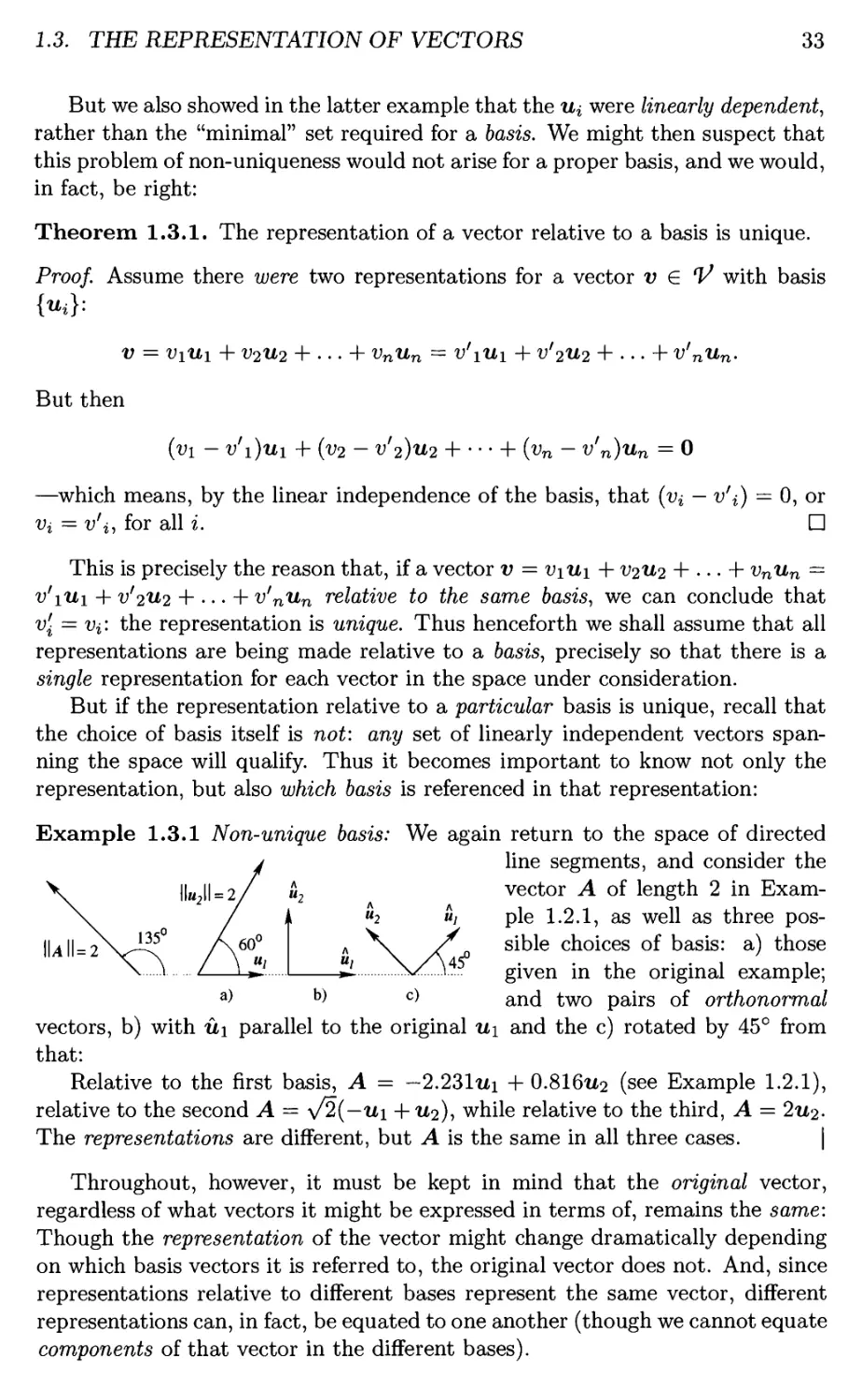


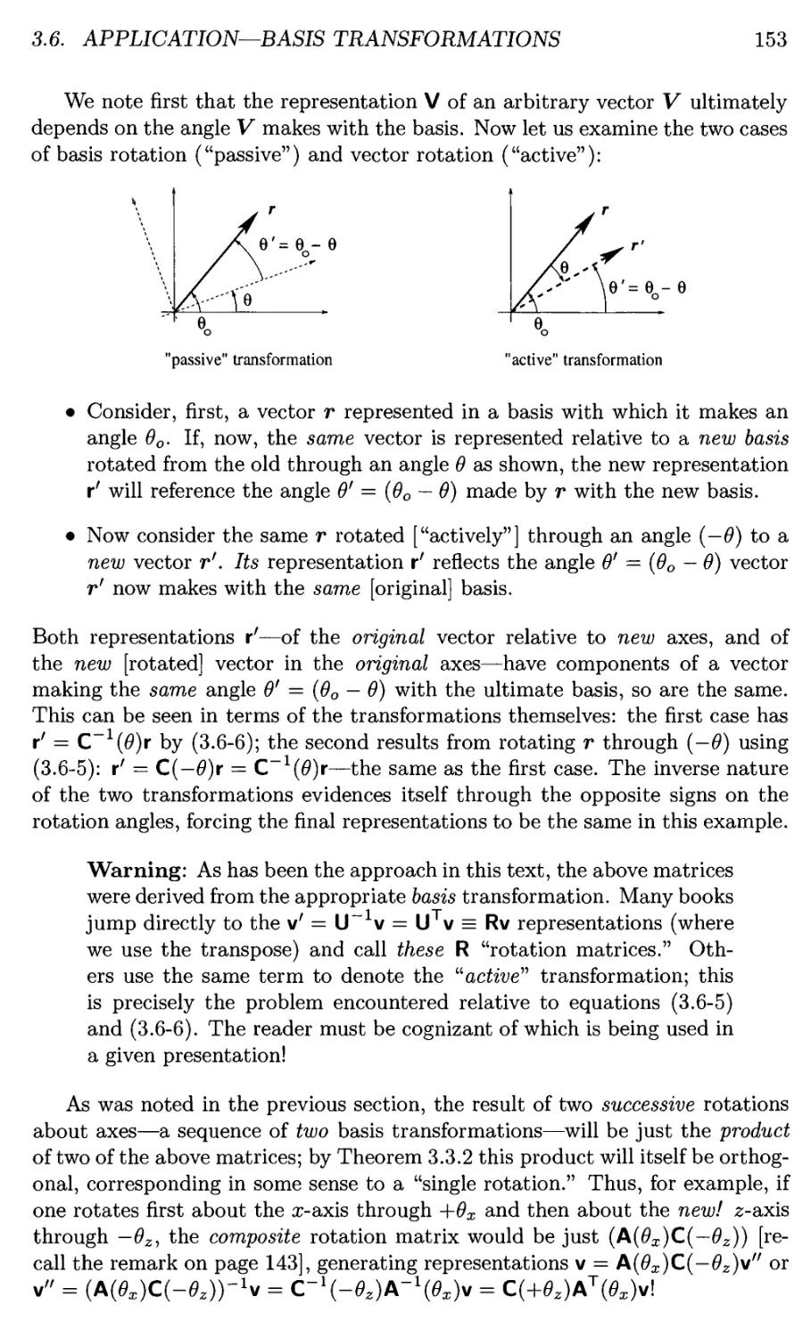


Text
Mechanical Engineering Series
Frederick F. Ling
Editor-in-Chief
Mechanical Engineering Series
J. Angeles, Fundamentals of Robotic Mechanical Systems:
Theory, Methods, and Algorithms, 2nd ed.
P. Basu, C. Kefa, and L. Jestin, Boilers and Burners: Design and Theory
J.M. Berthelot, Composite Materials:
Mechanical Behavior and Structural Analysis
I.J. Busch-Vishniac, Electromechanical Sensors and Actuators
J. Chakrabarty, Applied Plasticity
K.K. Choi and N.H. Kim, Structural Sensitivity Analysis and Optimization 1:
Linear Systems
K.K. Choi and N.H. Kim, Structural Sensitivity Analysis and Optimization 2:
Nonlinear Systems and Applications
G. Chiyssolouris, Laser Machining: Theory and Practice
V.N. Constantinescu, Laminar Viscous Flow
G.A. Costello, Theory of Wire Rope, 2nd Ed.
K. Czolczynski, Rotordynamics of Gas-Lubricated Journal Bearing Systems
M.S. Darlow, Balancing of High-Speed Machinery
J.F. Doyle, Nonlinear Analysis of Thin-Walled Structures: Statics,
Dynamics, and Stability
J.F, Doyle, Wave Propagation in Structures:
Spectral Analysis Using Fast Discrete Fourier Transforms, 2nd ed.
P.A. Engel, Structural Analysis of Printed Circuit Board Systems
A.C. Fischer-Cripps, Introduction to Contact Mechanics
A.C. Fischer-Cripps, Nanoindentations, 2nd ed.
J. Garcia de Jalon and E. Bayo, Kinematic and Dynamic Simulation of
Multibody Systems: The Real-Time Challenge
W.K. Gawronski, Advanced Structural Dynamics and Active Control of
Structures
W.K. Gawronski, Dynamics and Control of Structures: A Modal Approach
G. Genta, Dynamics of Rotating Systems
(continued after index)
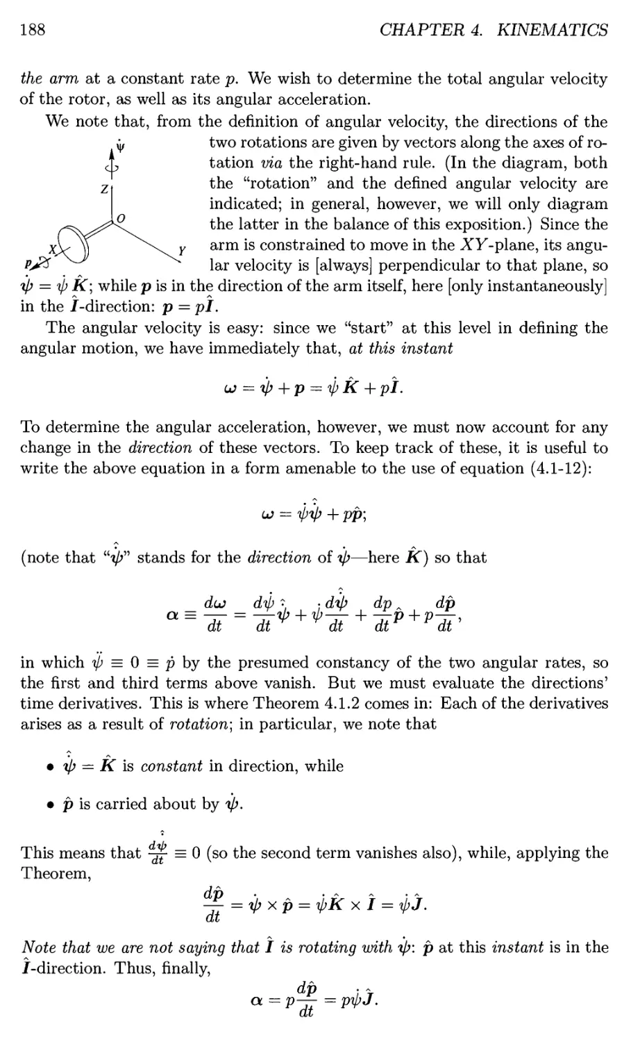
R. A. Howland
Intermediate Dynamics:
A Linear Algebraic Approach
^Spri
nnger
R. A. Howland
University of Notre Dame
Editor-in-Chief
Frederick F. Ling
Earnest F. Gloyna Regents Chair Emeritus in Engineering
Department of Mechanical Engineering
The University of Texas at Austin
Austin, TX 78712-1063, USA
and
Distinguished William Howard Hart
Professor Emeritus
Department of Mechanical Engineering,
Aeronautical Engineering and Mechanics
Rensselaer Polytechnic Institute
Troy, NY 12180-3590, USA
Intermediate Dynamics: A Linear Algebraic Approach
ISBN 0-387-28059-6 e-ISBN 0-387-28316-1 Printed on acid-free paper.
ISBN 978-0387-28059-2
© 2006 Springer Science+Business Media, Inc.
All rights reserved. This work may not be translated or copied in whole or in part without
the written permission of the publisher (Springer Science+Business Media, Inc., 233 Spring
Street, New York, NY 10013, USA), except for brief excerpts in connection with reviews or
scholarly analysis. Use in connection with any form of information storage and retrieval,
electronic adaptation, computer software, or by similar or dissimilar methodology now
known or hereafter developed is forbidden.
The use in this publication of trade names, trademarks, service marks and similar terms,
even if they are not identified as such, is not to be taken as an expression of opinion as to
whether or not they are subject to proprietary rights.
Printed in the United States of America.
98765432t SPIN 11317036
springeronline.com
Dedicated to My Folks
Mechanical Engineering Series
Frederick F. Ling
Editor-in-Chief
The Mechanical Engineering Series features graduate texts and research monographs to
address the need for information in contemporary mechanical engineering, including
areas of concentration of applied mechanics, biomechanics, computational mechanics,
dynamical systems and control, energetics, mechanics of materials, processing,
production systems, thermal science, and tribology.
Advisory Board/Series Editors
Applied Mechanics
Biomechanics
Computational Mechanics
Dynamic Systems and Control/
Mechatronics
Energetics
Mechanics of Materials
Processing
Production Systems
Thermal Science
Tribology
F.A. Leckie
University of California,
Santa Barbara
D. Gross
Technical University of Darmstadt
V.C. Mow
Columbia University
H.T. Yang
University of California,
Santa Barbara
D. Bryant
University of Texas at Austin
J.R. Welly
University of Oregon, Eugene
I. Finnie
University of California, Berkeley
K.K. Wang
Cornell University
G.-A. Klutke
Texas A&M University
A.E. Bergles
Rensselaer Polytechnic Institute
W.O. Winer
Georgia Institute of Technology
Series Preface
Mechanical engineering, and engineering discipline born of the needs of the
industrial revolution, is once again asked to do its substantial share in the call for
industrial renewal. The general call is urgent as we face profound issues of
productivity and competitiveness that require engineering solutions, among others.
The Mechanical Engineering Series is a series featuring graduate texts and
research monographs intended to address the need for information in contemporary
areas of mechanical engineering.
The series is conceived as a comprehensive one that covers a broad range of
concentrations important to mechanical engineering graduate education and
research. We are fortunate to have a distinguished roster of consulting editors, each
an expert in one of the areas of concentration. The names of the consulting editors
are listed on page vi of this volume. The areas of concentration are applied
mechanics, biomechanics, computational mechanics, dynamic systems and control,
energetics, mechanics of materials, processing, thermal science, and tribology.
Preface
A number of colleges and universities offer an upper-level undergraduate course
usually going under the rubric of "Intermediate" or "Advanced" Dynamics—
a successor to the first dynamics offering generally required of all students.
Typically common to such courses is coverage of 3-D rigid body dynamics and
Lagrangian mechanics, with other topics locally discretionary. While there are
a small number of texts available for such offerings, there is a notable paucity
aimed at "mainstream" undergraduates, and instructors often resort to
utilizing sections in the first Mechanics text not covered in the introductory course,
at least for the 3-D rigid body dynamics. Though closely allied to its planar
counterpart, this topic is far more complex than its predecessor: in kinematics,
one must account for possible change in direction of the angular velocity; and
the kinetic "moment of inertia," a simple scalar in the planar formulation, must
be replaced by a tensor quantity. If elementary texts' presentation of planar
dynamics is adequate, their treatment of three-dimensional dynamics is rather
less satisfactory: It is common to expand vector equations of motion in
components—in a particular choice of axes—and consider only a few special instances
of their application (e.g. fixed-axis rotation in the Euler equations of motion).
The presentation of principal coordinates is typically somewhat ad hoc, either
merely stating the procedure to find such axes in general, or even more
commonly invoking the "It can be shown that..." mantra. Machines seem not to
exist in 3-D! And equations of motion for the gyroscope are derived
independently of the more general ones—a practice lending a certain air of mystery to
this important topic.
Such an approach can be frustrating to the student with any degree of
curiosity and is counterproductive pedagogically: the component-wise expression of
vector quantities has long since disappeared from even Sophomore-level courses
in Mechanics, in good part because the complexity of notation obscures the
relative simplicity of the concepts involved. But the Euler equations can be
expressed both succinctly and generally through the introduction of matrices.
The typical exposition of principal axes overlooks the fact that this is precisely
the same device used to find the same "principal axes" in solid mechanics
(explicitly through a rotation); few students recognize this fact, and, unfortunately,
few instructors take the opportunity to point this out and unify the concepts.
And principal axes themselves are, in fact, merely an application of an even
more general technique utilized in linear algebra leading to the diagonalization
X
of matrices (at least the real, symmetric ones encountered in both solid
mechanics and dynamics). These facts alone suggest a linear algebraic approach to the
subject.
A knowledge of linear algebra is, however, more beneficial to the scientist
and engineer than merely to be able to diagonalize matrices: Eigenvectors and
eigenvalues pervade both fields; yet, while students can typically find these
quantities and use them to whatever end they have been instructed in, few can
answer the simple question "What is an eigenvector?" As the field of robotics
becomes ever more mainstream, a facility with [3-D] rotation matrices becomes
increasingly important. Even the mundane issue of solving linear equations is
often incomplete or, worse still, inaccurate: "All you need is as many equations
as unknowns. If you have fewer than that, there is no solution." (The first of
these statements is incomplete, the second downright wrong!) Such fallacies are
likely not altogether the students' fault: few curricula allow the time to devote
a full, formal course to the field, and knowledge of the material is typically
gleaned piecemeal on an "as-need" basis. The result is a fractionated view with
the intellectual gaps alluded to.
Yet a full course may not be necessary: For the past several years, the
Intermediate Dynamics course at Notre Dame has started with an only 2-3
week presentation of linear algebra, both as a prelude to the three-dimensional
dynamics to follow, and for its intrinsic pedagogical merit—to organize the bits
and pieces of concepts into some organic whole. However successful the latter
goal has been, the former has proven beneficial.
With regard to the other topic of Lagrangian mechanics, the situation is
perhaps even more critical. At a time when the analysis of large-scale systems
has become increasingly important, the presentation of energy-based
dynamical techniques has been surprisingly absent from most undergraduate texts
altogether. These approaches are founded on virtual work (not typically the
undergraduate's favorite topic!) and not only eliminate the need to consider the
forces at interconnecting pins [assumed frictionless], but also free the designer
from the relatively small number of vector coordinate systems available to
describe a problem: he can select a set of coordinate ideally suited to the one at
hand.
With all this in mind, the following text commits to paper a course which
has gradually developed at Notre Dame as its "Intermediate Dynamics"
offering. It starts with a relatively short, but rigorous, exposition of linear systems,
culminating in the diagonalization (where possible) of matrices—the foundation
of principal coordinates. There is even an [optional] section dealing with Jordan
normal form, rarely presented to students at this level. In order to understand
this process fully, it is necessary that the student be familiar with how the
[matrix] representation of a linear operator (or of a vector itself) changes with a
transformation of basis, as well as how the eigenvectors—in fact the new axes
themselves—affect this particular choice of basis. That, at least in the case
of real, symmetric, square inertia matrices, this corresponds to a rotation of
axes requires knowledge of axis rotation and the matrices which generate such
rotations. This, in turn, demands an appreciation of bases themselves and,
XI
particularly, the idea of linear independence (which many students feel deals
exclusively with the Wronskian) and partitioned matrix multiplication. By the
time this is done, little more effort is required to deal with vector spaces in
general.
This text in fact grew out of the need to dispatch a [perceived]
responsibility to rigor (i.e.proofs of theorems) without bogging down class presentation
with such details. Yet the overall approach to even the mathematical material
of linear algebra is a "minimalist" one: rather than a large number of arcane
theorems and ideas, the theoretical underpinning of the subject is provided
by, and unified through, the basic theme of linear independence—the echelon
form for vectors and [subsequently] matrices, and the rank of the latter. It can
be argued that these are the concepts the engineer and scientist can—should—
appreciate anyhow. Partitioning establishes the connection between vectors and
[the rows/columns of] matrices, and rank provides the criterion for the solution
of linear systems (which, in turn, fold back onto eigenvectors). In order to avoid
the student's becoming fixated too early on square matrices, this fundamental
theory is developed in the context of linear transformations between spaces of
arbitrary dimension. It is only after this has been done that we specialize to
square matrices, where the inverse, eigenvectors, and even properties of
determinants follow naturally. Throughout, the distinction between vectors and tensors,
and their representations—one which is generally blurred in the student's mind
because it is so rarely stressed in presentation—is heavily emphasized.
Theory, such as the conditions under which systems of linear equations have
a solution, is actually important in application. But this linear algebra Part is
more than mere theory: Linear independence, for example, leads to the
concept of matrix rank, which then becomes a criterion for predicting the number
of solutions to a set of linear equations; when the cross product is shown to
be equivalent to a matrix product of rank 2, indeterminacy of angular
velocity and acceleration from the rotating coordinate system equations in the next
Part becomes a natural consequence. Similarly, rotation matrices first appear
as an example of orthogonal matrices, which then are used in the diagonaliza-
tion of real symmetric matrices culminating the entire first Part; though this
returns in the next Part in the guise of principal axes, its inverse—the rotation
from principal axes to arbitrary ones—becomes a fundamental technique for the
determination of the inertia tensor.
Given the audience for which this course is intended, the approach has been
surprisingly successful: one still recalls the delight of one student who said that
she had decided to attack a particular problem with rotation matrices, and "It
worked!" Admittedly, such appreciation is often delayed until the part on rigid
body dynamics has been covered—yet another reason for trying to have some
of the more technical detail in the text rather than being presented in class.
This next Part on 3-D dynamics starts with a relatively routine exposition of
kinematics, though rather more detail than usual is given to constraints on the
motion resulting from interconnections, and there is a perhaps unique
demonstration that the fundamental relation dr = dO x r results from nothing more
than the fixed distance between points in a rigid body. Theory from the first
Xll
Part becomes integrated into the presentation in a discussion of the
indeterminacy of angular velocity and acceleration without such constraints. Kinetics is
preceded by a review of particle and system-of-particles kinetics; this is done
to stress the particle foundation on which even rigid body kinetics is based as
much as to make the text self-contained. The derivation of the Euler
equations is also relatively routine, but here the similarity to most existing texts
ends: these equations are presented in matrix form, and principal coordinates
dispatched with reference to diagonalization covered in the previous Part. The
flexibility afforded by this allows an arbitrary choice of coordinates in terms of
which to represent the relevant equations and, again, admits of a more
transparent comprehension than the norm. 3-D rigid body machine kinetics, almost
universally ignored in elementary presentations, is also covered: the emphasis
is on integrating the kinematics and kinetics into a system of linear equations,
making the difference between single rigid bodies and "machines" quantitative
rather than qualitative. There is also a rather careful discussion of the forces at
[ball-and-socket] connections in machines; this is a topic often misunderstood
in Statics, let alone Dynamics! While the gyroscope equations of motion are
developed de nuvo as in most texts, they are also obtained by direct
application of the Euler equations; this is to overcome the stigma possibly resulting
from independent derivation—the misconception that gyroscopes are somehow
"special," not covered by the allegedly more general theory. There is a brief
section detailing the use of the general equations of motion to obtain the
variational equations necessary to analyze stability. Finally, a more or less routine
treatment of energy and momentum methods is presented, though the
implementation of kinetic constants and the conditions under which vanishing force
or moment lead to such constants are presented and utilized; this is to set the
scene for the next Part, where Analytical Dynamics employs special techniques
to uncover such "integrals of the motion."
That next Part treats Analytical Mechanics. Lagrangian dynamics is
developed first, based on Newton's equations of motion rather than functional
minimization. Though the latter is mentioned as an alternative approach, it seems
a major investment of effort—and time—to develop one relatively abstruse
concept (however important intrinsically), just to derive another almost as bad by
appeal to a "principle" (Least Action) whose origin is more teleological than
physical! Rather more care than usual, however, is taken to relate the concepts
of kinematic "constraints" and the associated kinematical equations among the
coordinates; this is done better to explain Lagrange multipliers. Also included
is a section on the use of non-holonomic constraints, in good part to introduce
Lagrange multipliers as a means of dealing with them; while the latter is
typically the only methodology presented in connection with this topic, here it is
actually preceded by a discussion of purely algebraic elimination of redundant
constraints, in the hopes of demonstrating the fundamental issue itself. Withal,
the "spin" put on this section emphasizes the freedom to select arbitrary
coordinates instead of being "shackled" by the standard vector coordinate systems
developed to deal with Newton's laws. The discussion of the kinetic constants
of energy and momentum in the previous Part is complemented by a discussion
Xlll
of "integrals of the motion" in this one; this is the springboard to introduce Ja-
cobi's integral, and ignorable coordinates become a means of uncovering other
such constants of the motion in Lagrangian systems—at least, if one can find
the Right Coordinates! The Part concludes with a chapter on Hamiltonian
dynamics. Though this topic is almost universally ignored by engineers, it is
as universal in application as Conservation of Energy and is the lingua franca
of Dynamical Systems, with which every modern-day practitioner must have
some familiarity. Unlike most introductions to the field, which stop after
having obtained the equations of motion, this presentation includes a discussion of
canonical transformations, separability, and the Hamilton-Jacobi Equation: the
fact that there is a systematic means of obtaining those variables—"ignorable"
coordinates and momenta—in which the Hamiltonian system is completely
soluble is, after all, the raison d'etre for invoking a system in this form, as opposed
to the previous Lagrangian formulation, in the first place. Somewhat more
attention to time-dependent Hamiltonian systems is given than usual.
Additionally, like the Lagrangian presentation, there is a discussion of casting time
as an ordinary variable; though this is often touched upon by more advanced
texts on analytical mechanics, the matter seems to be dropped almost
immediately, without benefit of examples to demonstrate exactly what this perspective
entails; one, demonstrating whatever benefits it might enjoy, is included in this
chapter.
A Note on Notation. We shall occasionally have the need to
distinguish between "unordered" and "ordered" sets. Unordered sets will be denoted
by braces: {a, b} = {fo,a}, while ordered sets will be denoted by parentheses:
(a, b) ^ (6, a). This convention is totally consistent with the shorthand notation
for matrices: A = (a^).
Throughout, vectors are distinguished by boldface: V\ unit vectors are
distinguished with a "hat" and are generally lower-case letters: i. Tensor/matrix
quantities are written in a boldface sans-serif font, typically in upper-case: I
(though the matrix representation of a vector otherwise denoted with a
lowercase boldface will retain the case: v ~ v).
Material not considered essential to the later material is presented in a
smaller type face; this is not meant to denigrate the material so much as to
provide a visual map to the overall picture. Students interested more in
applications are typically impatient with a mathematical Theorem/Proof format,
yet it surely is necessary to feel that a field has been developed logically. For
this reason, each section concludes with a brief guide of what results are used
merely to demonstrate later, more important results, and what are important
intrinsically; it is hoped this will provide some "topography" of the material
presented.
A Note on Style. There have been universally two comments by students
regarding this text: "It's all there," and "We can hear you talking." In
retrospect, this is less a "text" than lectures on the various topics. Examples are
unusually—perhaps overwhelmingly!—complete, with all steps motivated and
XIV
virtually all intermediate calculations presented; though this breaks the "one-
page format" currently in favor, it counters student frustration with "terseness."
And the style is more narrative than expository. It is hoped that lecturers do
not find this jarring.
R.A. Howland
South Bend, Indiana
Contents
Preface ix
I Linear Algebra 1
Prologue 3
1 Vector Spaces 5
1.1 Vectors 6
1.1.1 The "Algebra" of Vector Spaces 7
1.1.2 Subspaces of a Vector Space 12
1.2 The Basis of a Vector Space 13
1.2.1 Spanning Sets 14
1.2.2 Linear Independence 16
A Test for Linear Independence of n-tuples: Reduction to
Echelon Form 18
1.2.3 Bases and the Dimension of a Vector Space 28
Theorems on Dimension 28
1.3 The Representation of Vectors 32
1.3.1 n-tuple Representations of Vectors 34
1.3.2 Representations and Units 37
1.3.3 Isomorphisms among Vector Spaces of the Same Dimension 38
2 Linear Transformations on Vector Spaces 41
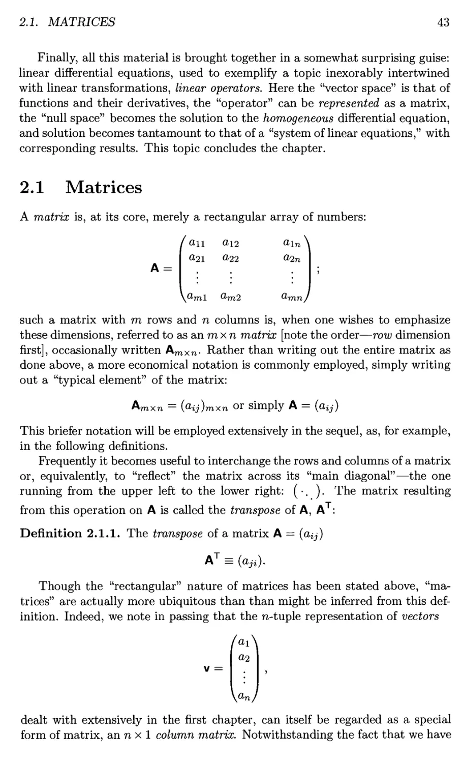
2.1 Matrices 43
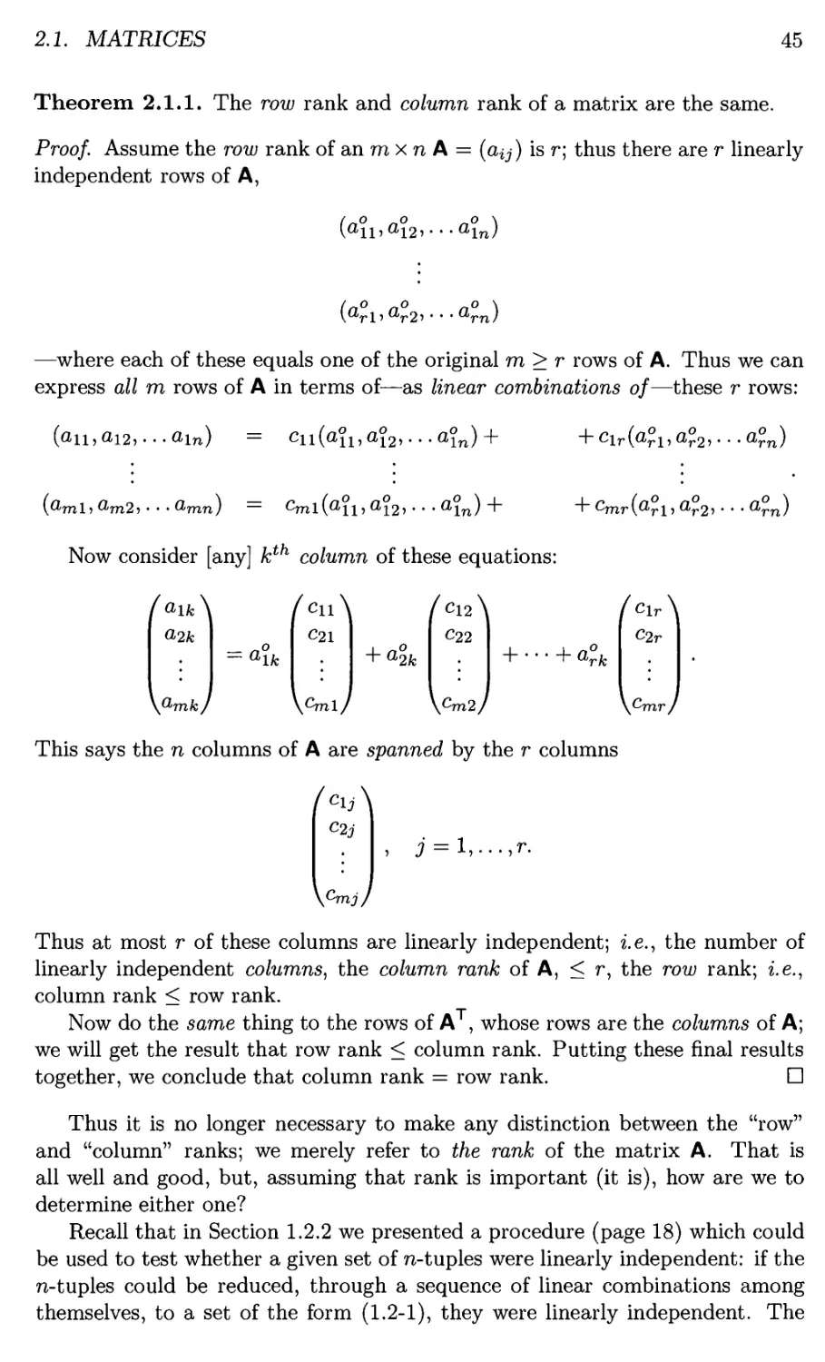
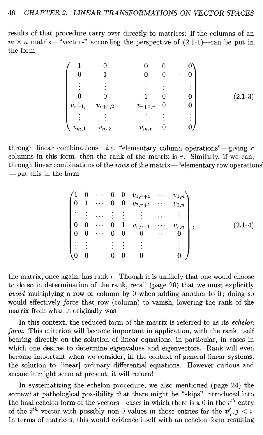
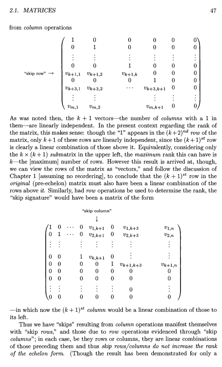
2.1.1 The "Partitioning" and Rank of Matrices 44
The Rank of a Matrix 44
2.1.2 Operations on Matrices 48
Inner Product 49
Transpose of a Matrix Product 51
Block Multiplication of Partitioned Matrices 52
Elementary Operations through Matrix Products 54
2.2 Linear Transformations 61
XVI
CONTENTS
Domain and Range of a [Linear] Transformation and their
Dimension 64
2.2.1 Linear Transformations: Basis and Representation .... 65
Dyadics 68
2.2.2 Null Space of a Linear Transformation 72
Dimension of the Null Space 74
Relation between Dimensions of Domain, Range, and Null
Space 74
2.3 Solution of Linear Systems 77
"Skips" and the Null Space 82
2.3.1 Theory of Linear Equations 84
Homogeneous Linear Equations 84
Non-homogeneous Linear Equations 85
2.3.2 Solution of Linear Systems—Gaussian Elimination .... 88
2.4 Linear Operators—Differential Equations 90
3 Special Case—Square Matrices 97
The "Algebra" of Square Matrices 98
3.1 The Inverse of a Square Matrix 99
Properties of the Inverse 102
3.2 The Determinant of a Square Matrix 103
Properties of the Determinant 105
3.3 Classification of Square Matrices Ill
3.3.1 Orthogonal Matrices—Rotations 113
3.3.2 The Orientation of Non-orthonormal Bases 115
3.4 Linear Systems: n Equations in n Unknowns 116
3.5 Eigenvalues and Eigenvectors of a Square Matrix 118
3.5.1 Linear Independence of Eigenvectors 123
3.5.2 The Cayley-Hamilton Theorem 128
3.5.3 Generalized Eigenvectors 131
3.5.4 Application of Eigenvalues/Eigenvectors 137
3.6 Application—Basis Transformations 140
3.6.1 General Basis Transformations 141
Successive Basis Transformations—Composition 144
3.6.2 Basis Rotations 151
3.7 Normal Forms of Square Matrices 156
3.7.1 Linearly Independent Eigenvectors—Diagonalization . . . 157
Diagonalization of Real Symmetric Matrices 162
3.7.2 Linearly Dependent Eigenvectors—Jordan Normal
Form 163
Epilogue 171
CONTENTS
xvii
II 3-D Rigid Body Dynamics 173
Prologue 175
4 Kinematics 177
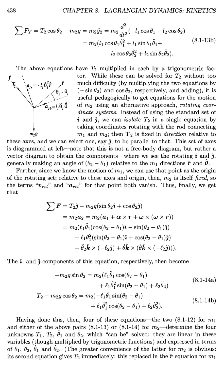
4.1 Motion of a Rigid Body 177
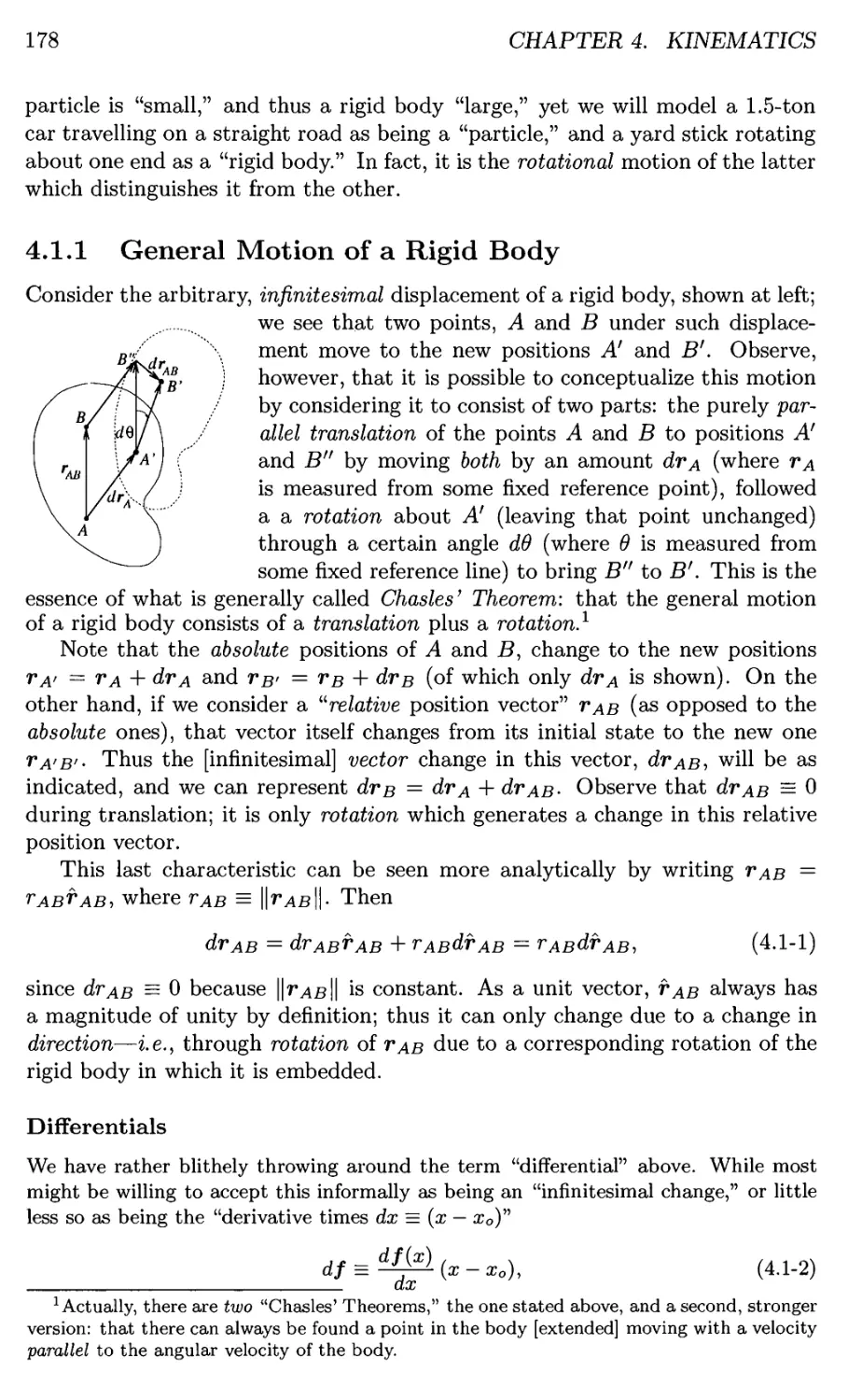
4.1.1 General Motion of a Rigid Body 178
Differentials 178
4.1.2 Rotation of a Rigid Body 180
Differential Rigid Body Rotation 181
Angular Velocity and Acceleration 185
Time Derivative of a Unit Vector with respect to Rotation 187
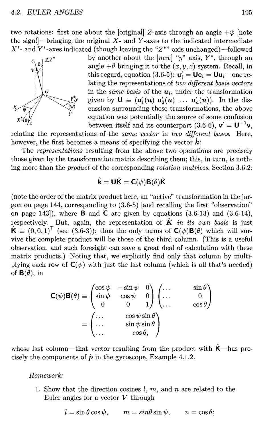
4.2 Euler Angles 191
4.2.1 Direction Angles and Cosines 192
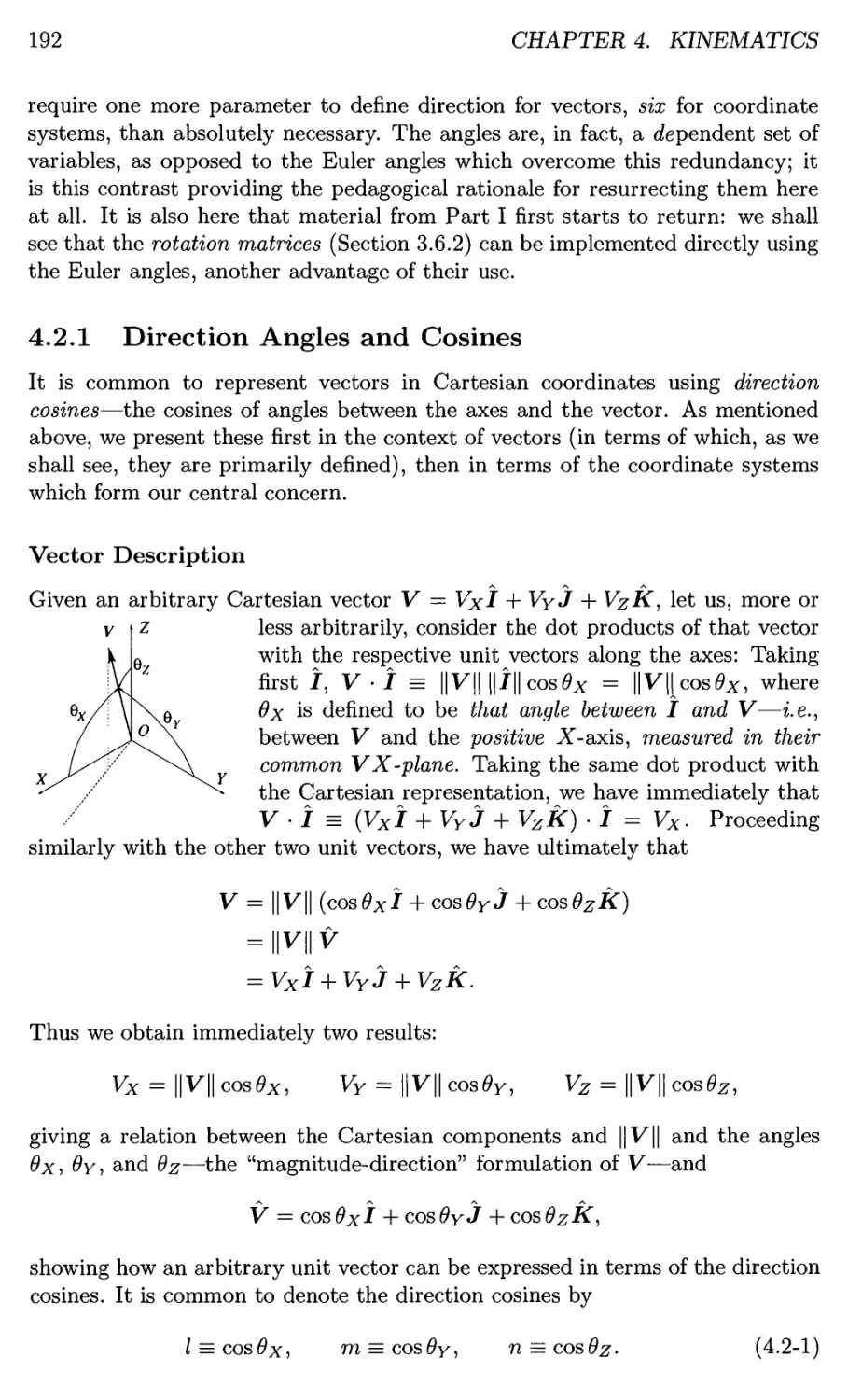
Vector Description 192
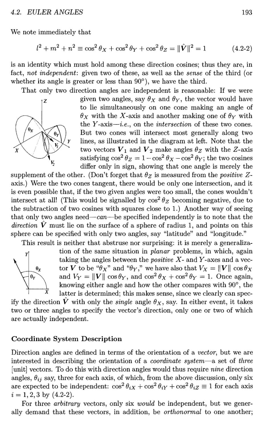
Coordinate System Description 193
4.2.2 Euler Angles 194
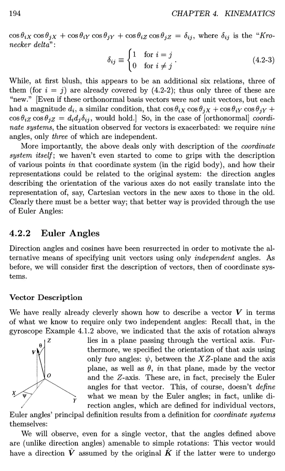
Vector Description 194
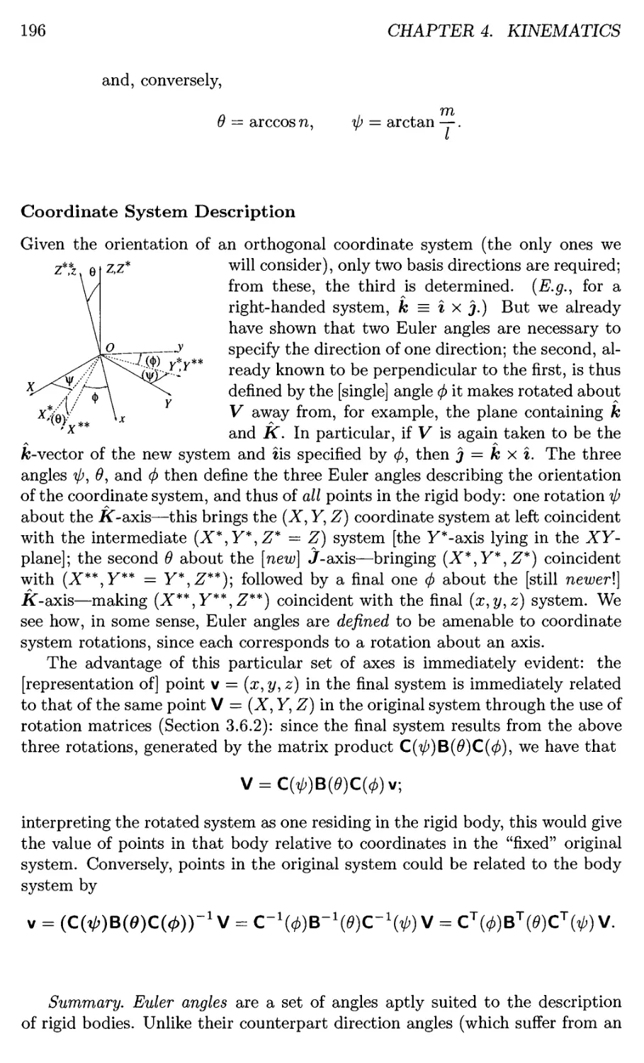
Coordinate System Description 196
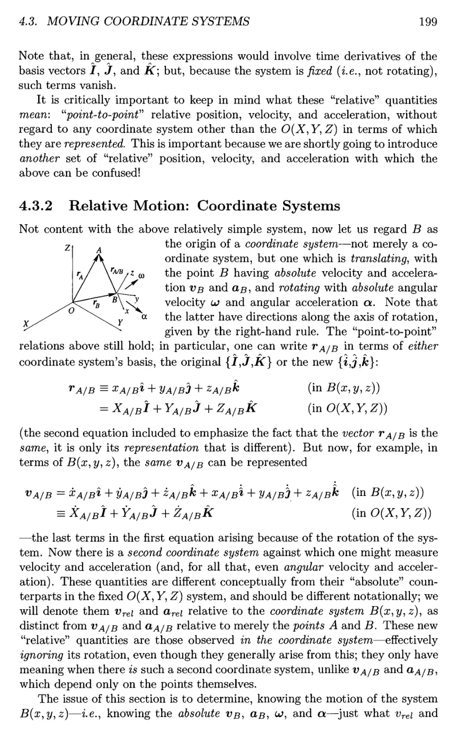
4.3 Moving Coordinate Systems 197
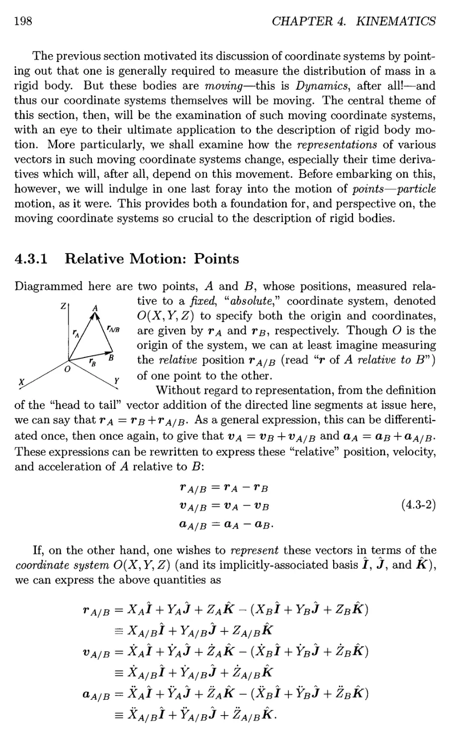
4.3.1 Relative Motion: Points 198
4.3.2 Relative Motion: Coordinate Systems 199
Time Derivatives in Rotating Coordinate Systems .... 200
Applications of Theorem 4.3.1 201
Rotating Coordinate System Equations 202
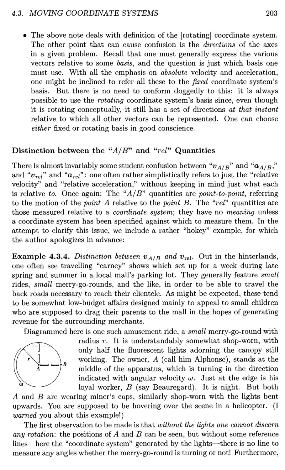
Distinction between the "A/B" and "re/" Quantities . . . 203
The Need for Rotating Coordinate Systems 209
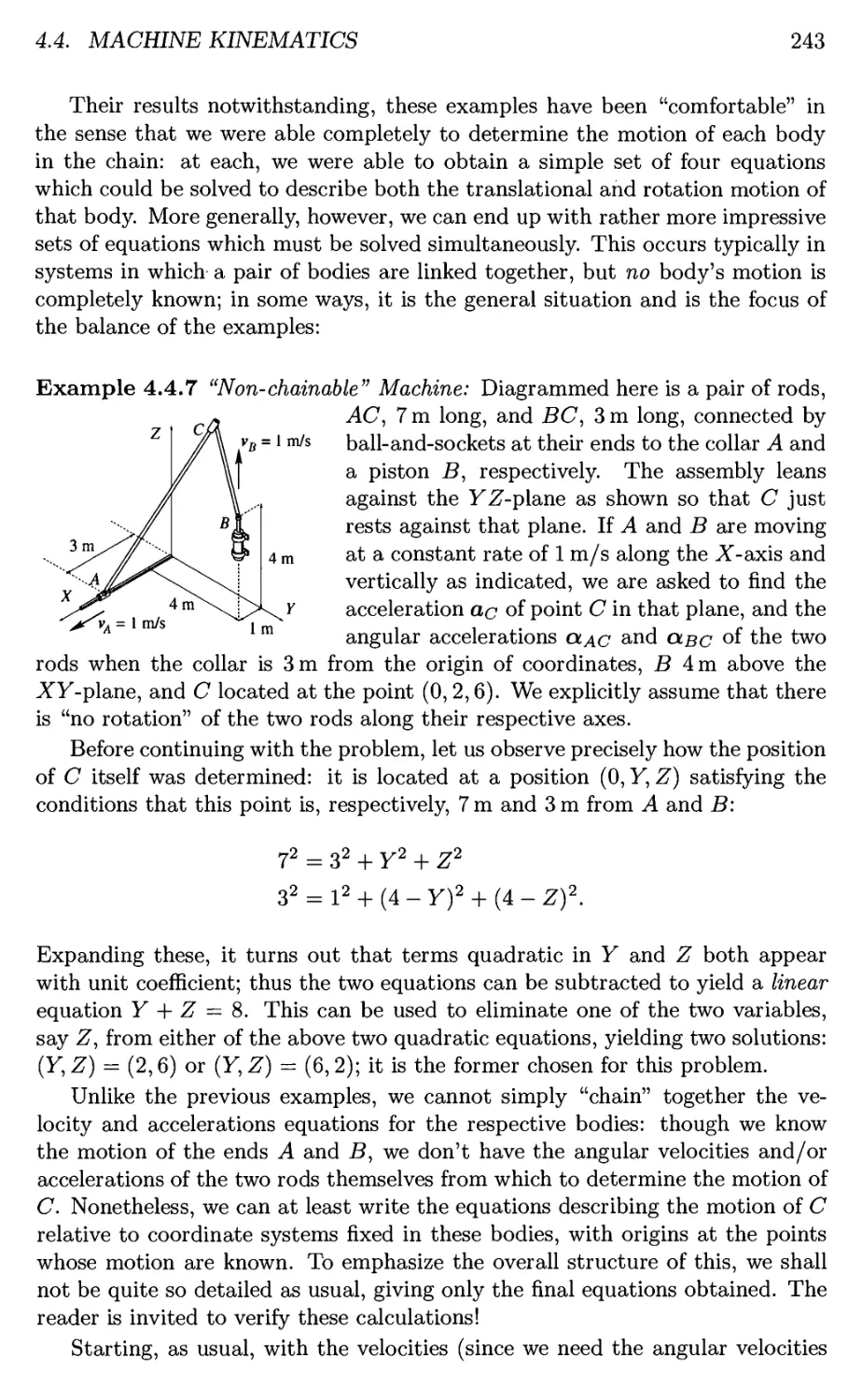
4.4 Machine Kinematics 210
4.4.1 Motion of a Single Body 211
A Useful Trick 218
The Non-slip Condition 220
The Instantaneous Center of Zero Velocity 225
4.4.2 Kinematic Constraints Imposed by Linkages 228
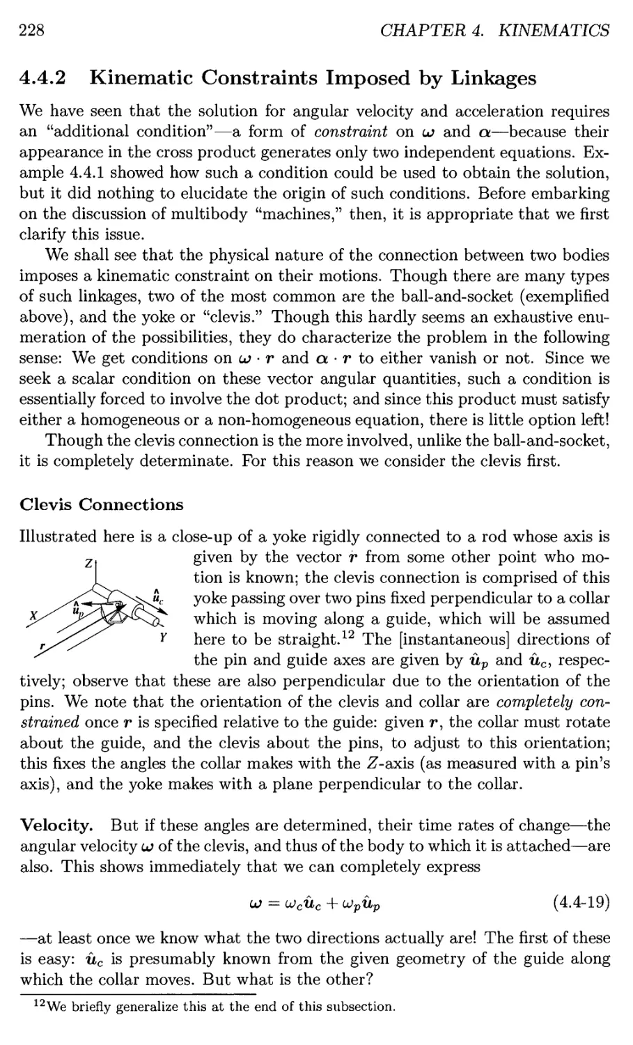
Clevis Connections 228
Ball-and-socket Connections 237
4.4.3 Motion of Multiple Rigid Bodies ("Machines") 238
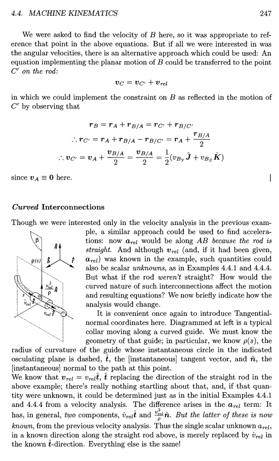
Curved Interconnections 247
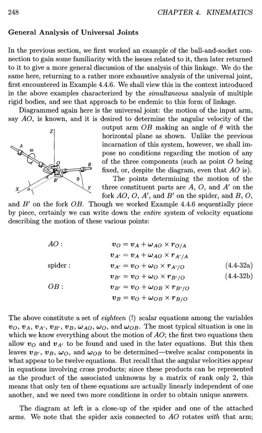
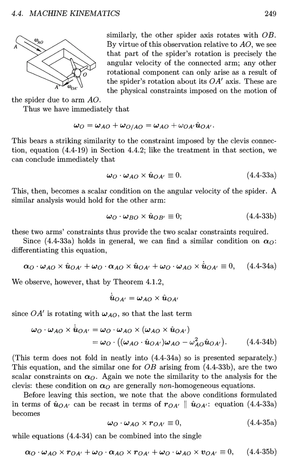
General Analysis of Universal Joints 248
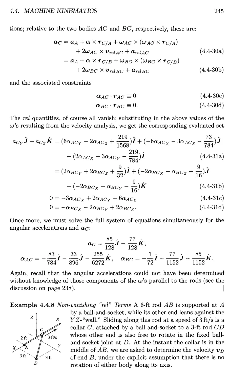
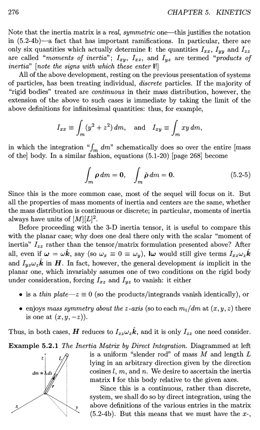
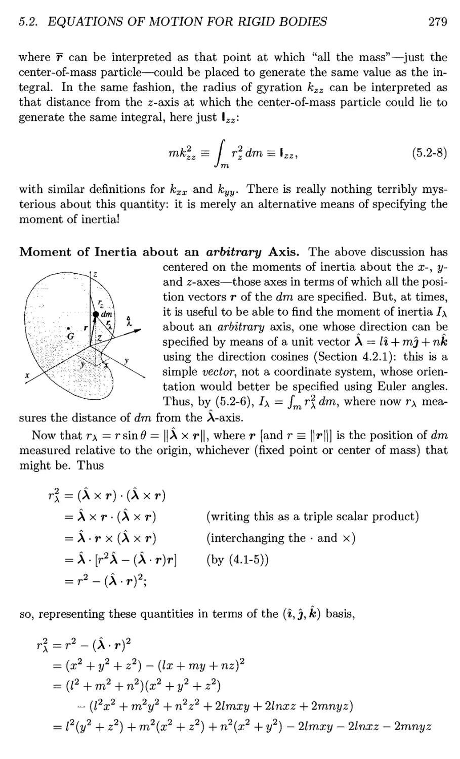
5 Kinetics 253
5.1 Particles and Systems of Particles 255
5.1.1 Particle Kinetics 255
Linear Momentum and its Equation of Motion 255
Angular Momentum and its Equation of Motion 257
Energy 258
A Caveat regarding Conservation 262
XV111
CONTENTS
5.1.2 Particle System Kinetics 263
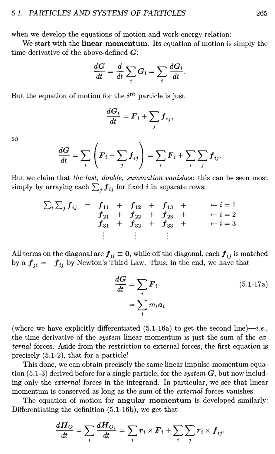
Kinetics relative to a Fixed System 264
Kinetics relative to the Center of Mass 267
5.2 Equations of Motion for Rigid Bodies 272
5.2.1 Angular Momentum of a Rigid Body—the Inertia Tensor 273
Properties of the Inertia Tensor 280
Principal Axes 287
5.2.2 Equations of Motion 304
Forces/Moments at Interconnections 312
Determination of the Motion of a System 325
5.2.3 A Special Case—the Gyroscope 327
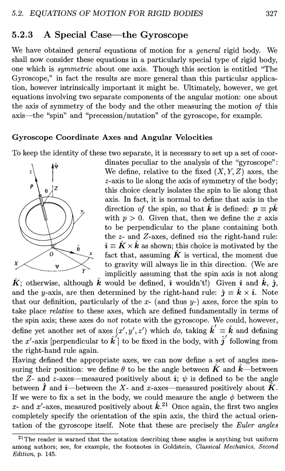
Gyroscope Coordinate Axes and Angular Velocities .... 327
Equations of Motion 328
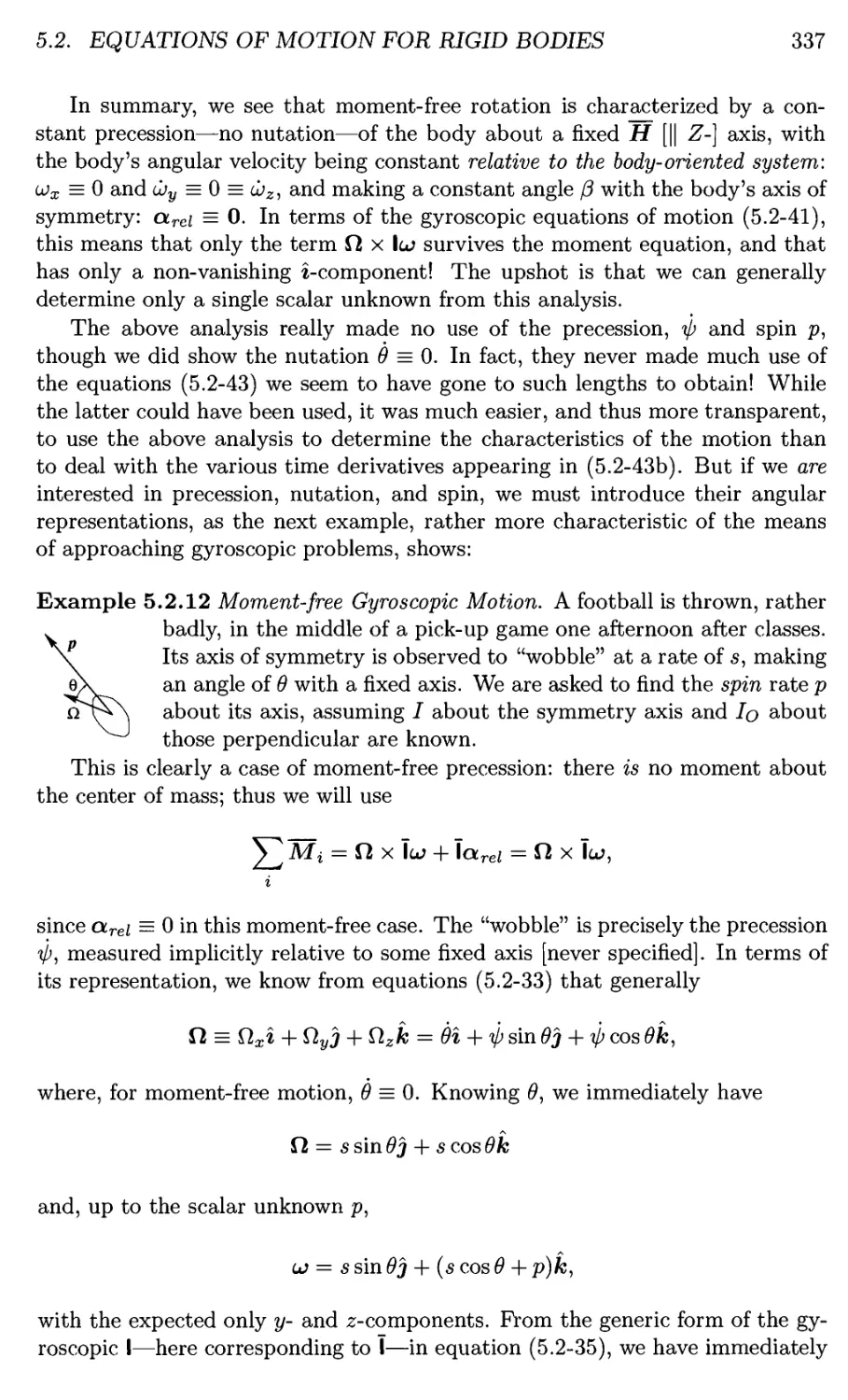
Special Case—Moment-free Gyroscopic Motion 333
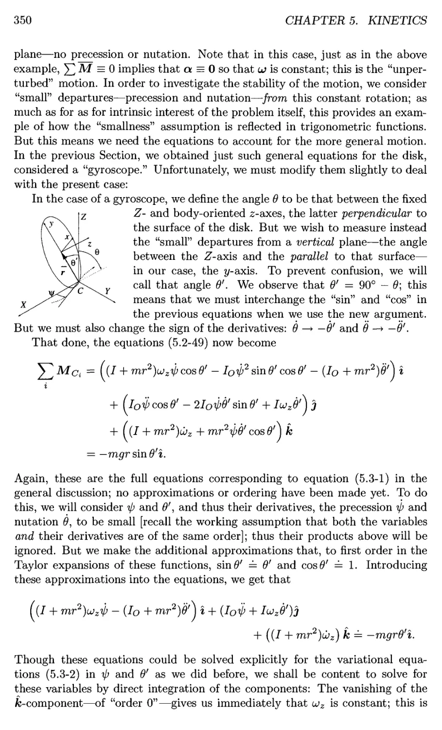
General Case—Gyroscope with Moment 338
5.3 Dynamic Stability 346
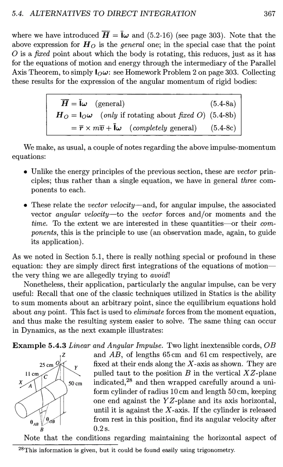
5.4 Alternatives to Direct Integration 352
5.4.1 Energy 353
Kinetic Energy 353
Work 355
Energy Principles 357
5.4.2 Momentum 366
5.4.3 Conservation Application in General 372
Epilogue 381
III Analytical Dynamics 383
Prologue 385
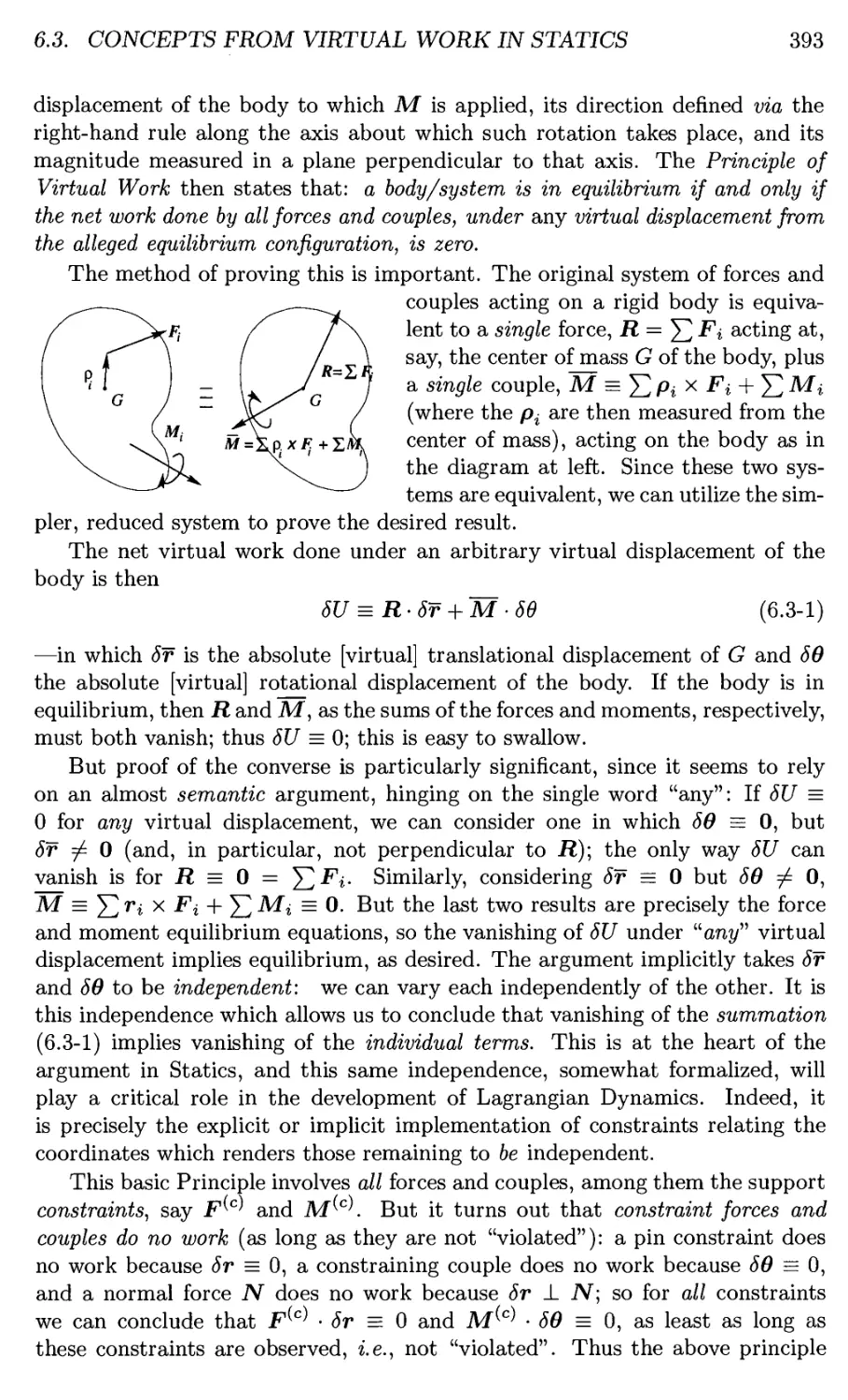
6 Analytical Dynamics: Perspective 389
6.1 Vector Formulations and Constraints 389
6.2 Scalar Formulations and Constraints 391
6.3 Concepts from Virtual Work in Statics 392
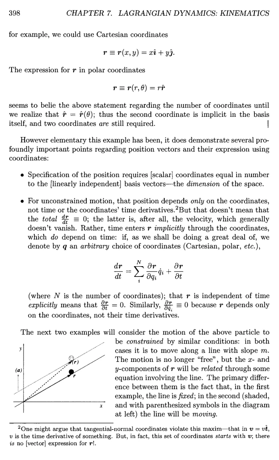
7 Lagrangian Dynamics: Kinematics 397
7.1 Background: Position and Constraints 397
Categorization of Differential Constraints 403
Constraints and Linear Independence 405
7.2 Virtual Displacements 408
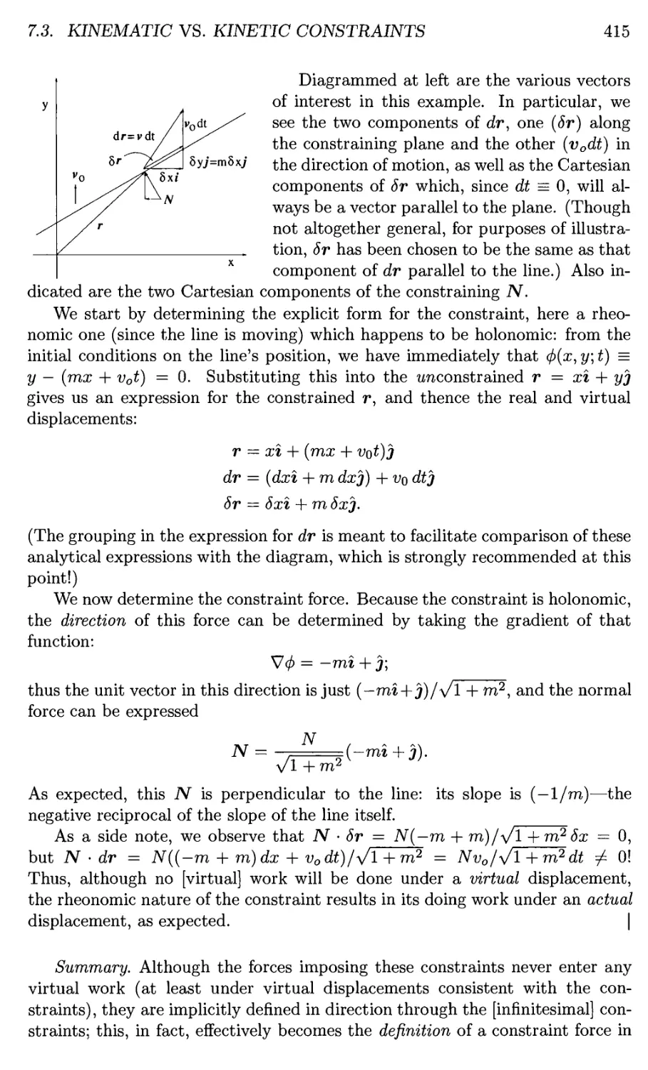
7.3 Kinematic vs. Kinetic Constraints 412
7.4 Generalized Coordinates 416
Derivatives of r and v with respect to Generalized
Coordinates and Velocities 420
CONTENTS
xix
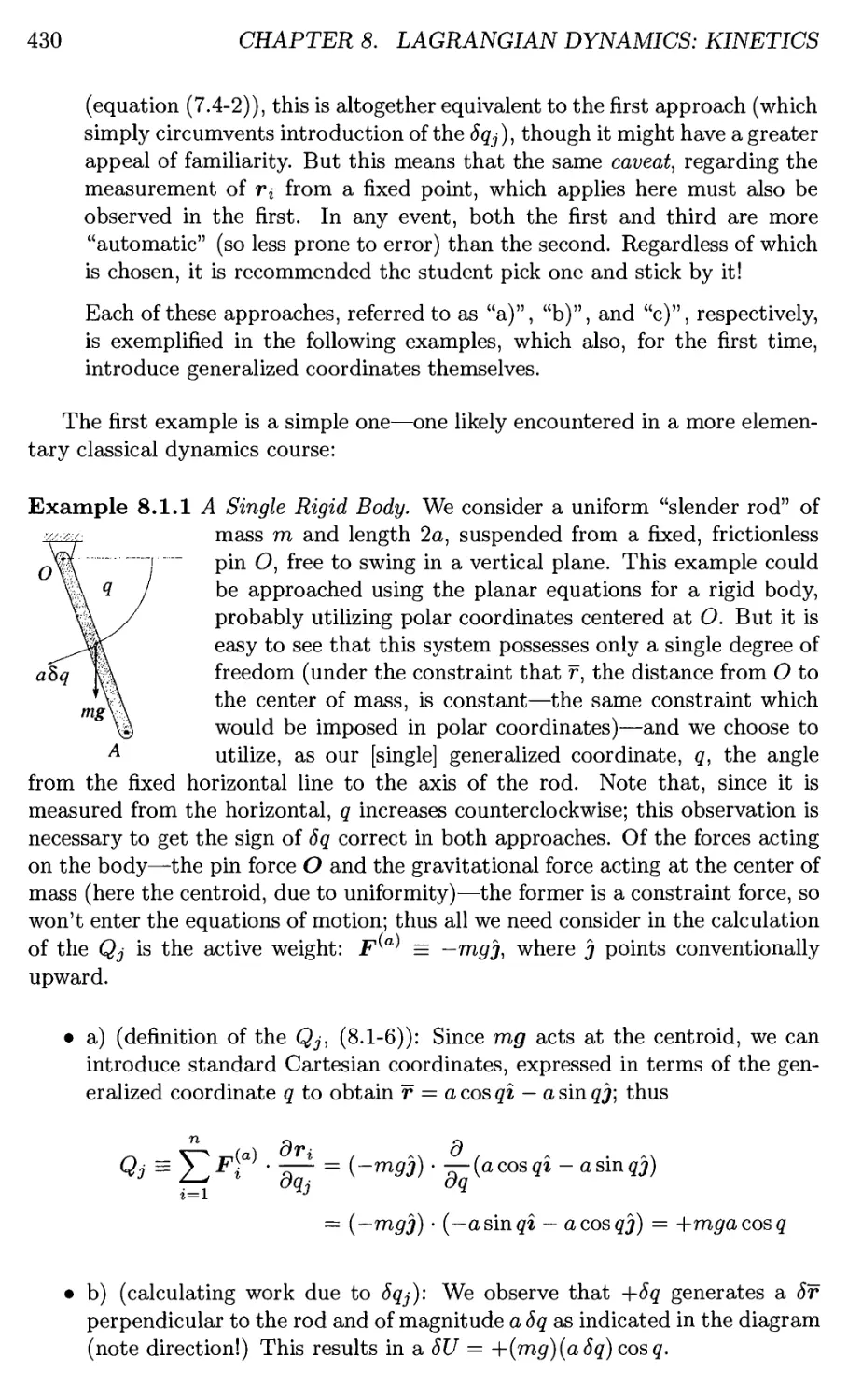
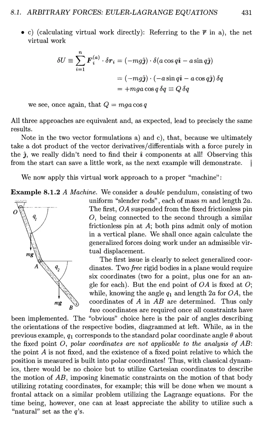
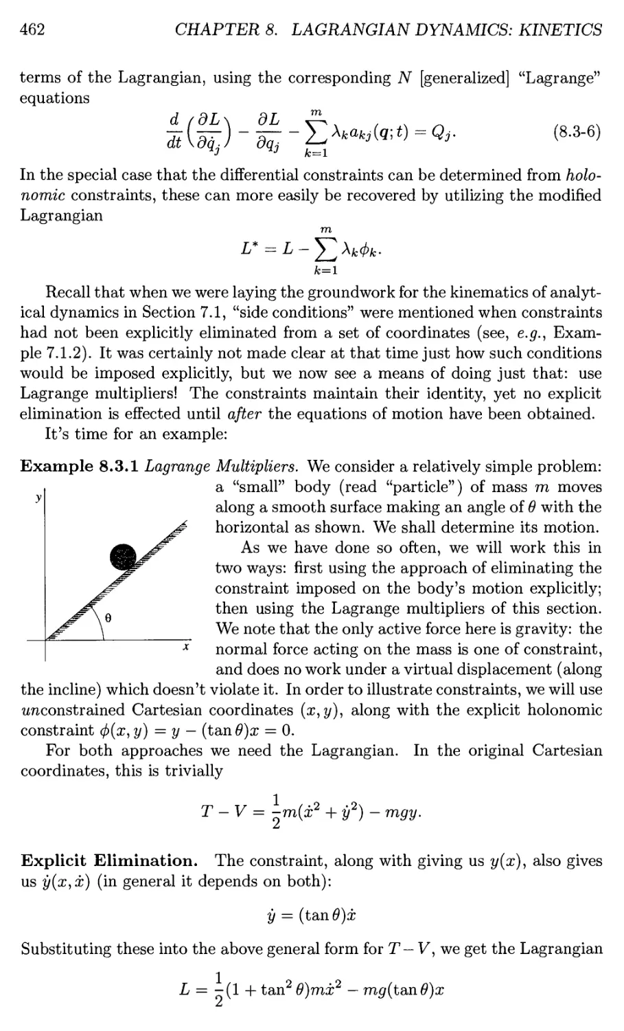
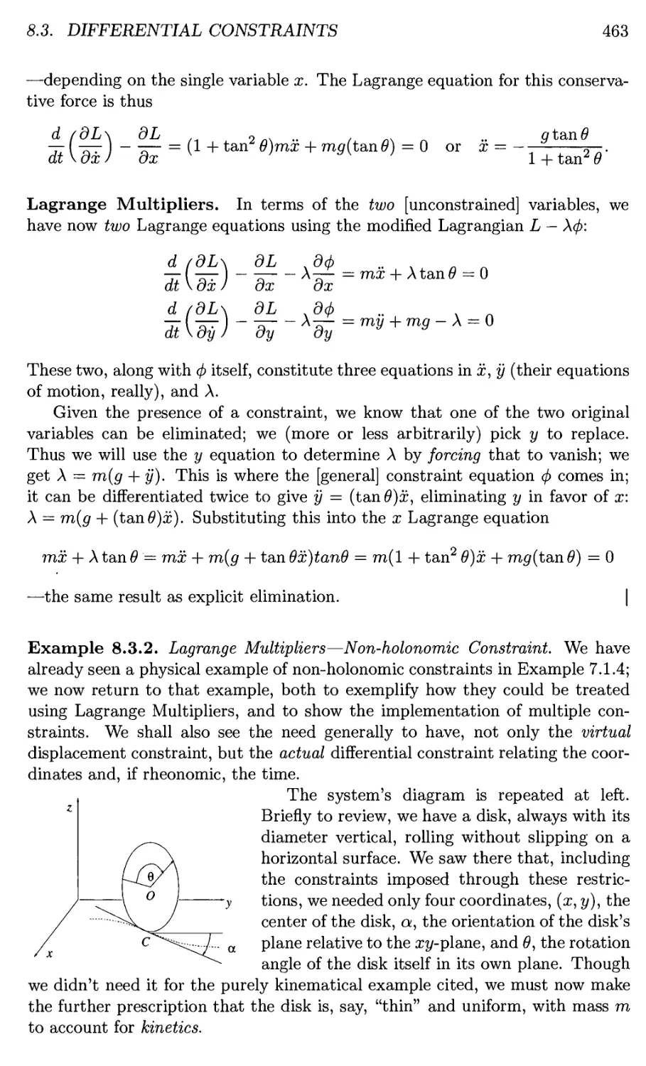
8 Lagrangian Dynamics: Kinetics 423
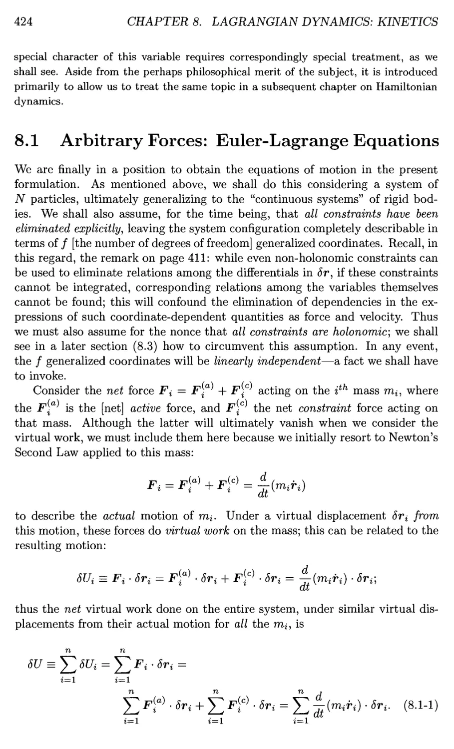
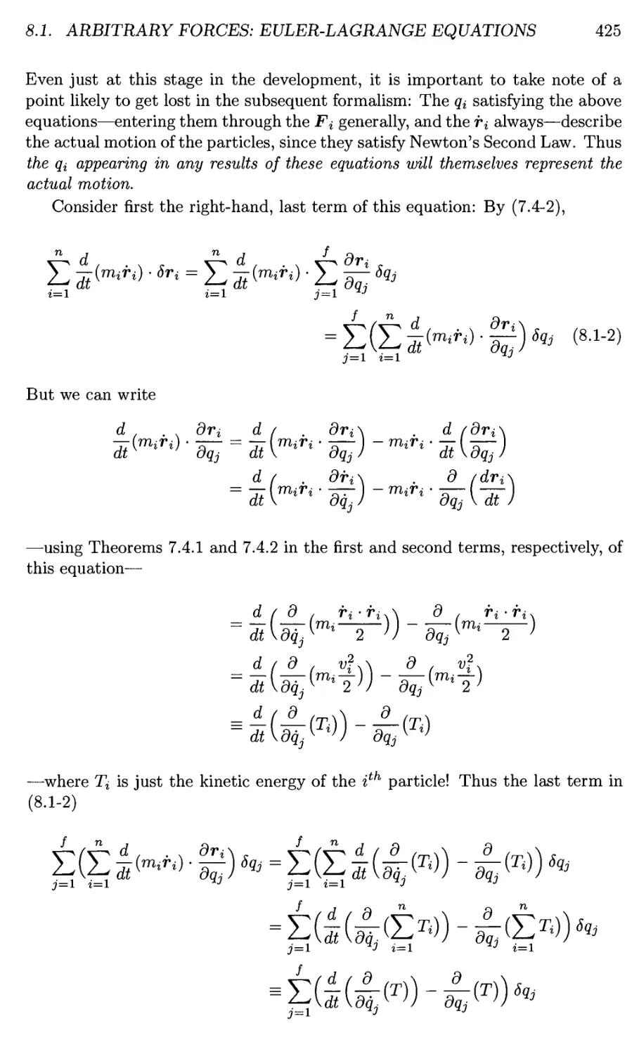
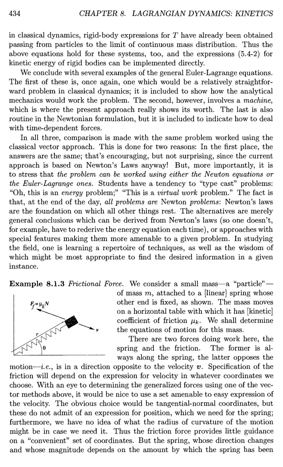
8.1 Arbitrary Forces: Euler-Lagrange Equations 424
Notes on the Euler-Lagrange Equations 427
8.2 Conservative Forces: Lagrange Equations 443
Properties of the Lagrangian 453
8.3 Differential Constraints 455
8.3.1 Algebraic Approach to Differential Constraints 456
8.3.2 Lagrange Multipliers 458
Interpretation of the Lagrange Multipliers 465
8.4 Time as a Coordinate 467
9 Integrals of Motion 471
9.1 Integrals of the Motion 471
9.2 Jacobi's Integral—an Energy-like Integral 473
9.3 "Ignorable Coordinates" and Integrals 478
10 Hamiltonian Dynamics 483
10.1 The Variables 483
Solution for q(q,p]t) 484
10.2 The Equations of Motion 486
10.2.1 Legendre Transformations 488
10.2.2 q and p as Lagrangian Variables 490
10.2.3 An Important Property of the Hamiltonian 492
10.3 Integrals of the Motion 495
10.4 Canonical Transformations 497
10.5 Generating Functions 503
10.6 Transformation Solution of Hamiltonians 509
10.7 Separability 517
10.7.1 The Hamilton-Jacobi Equation 517
10.7.2 Separable Variables 519
Special Case—Ignorable Coordinates 519
10.8 Constraints in Hamiltonian Systems 522
10.9 Time as a Coordinate in Hamiltonians 524
Epilogue 533
Index
535
Part I
Linear Algebra
Prologue
The primary motivation for this part is to lay the foundation for the next one,
dealing with 3-D rigid body dynamics. It will be seen there that the
"inertia," I, a quantity which is a simple scalar in planar problems, blossoms into a
"tensor" in three-dimensional ones. But in the same way that vectors can be
represented in terms of "basis" vectors t, J, and fc, tensors can be represented as
3x3 matrices, and formulating the various kinetic quantities in terms of these
matrices makes the fundamental equations of 3-D dynamics far more
transparent and comprehensible than, for example, simply writing out the components
of the equations of motion. (Anyone who has seen older publications in which
the separate components of moments and/or angular momentum written out
doggedly, again and again, will appreciate the visual economy and conceptual
clarity of simply writing out the cross product!) More importantly, however,
the more general notation allows a freedom of choice of coordinate system.
While it is obvious that the representation of vectors will change when a
different basis is used, it is not clear that the same holds for matrix representations.
But it turns out that there is always a choice of basis in which the inertia tensor
can be represented by a particularly simple matrix—one which is diagonal in
form. Such a choice of basis—tantamount to a choice of coordinates axes—is
referred to in that context as "principle axes." These happen to be precisely
the same "principle axes" the student my have encountered in a course in Solid
Mechanics; both, in turn, rely on techniques in the mathematical field of "linear
algebra" aimed at generating a standard, "canonical" form for a given matrix.
Thus the following three chapters comprising this Part culminate in a
discussion of such canonical forms. But to understand this it is also necessary
to see how a change of basis affects the representation of a matrix (or even a
vector, for that matter). And, since it turns out that the new principle axes
are nothing more than the eigenvectors of the inertia matrix—and the inertia
matrix in these axes nothing more than that with the eigenvalues arrayed along
the diagonal—it is necessary to understand what these are. (If one were to walk
up to you on the street as ask the question "Yes, but just what is an
eigenvector?", could you answer [at least after recovering from the initial shock]?) To
find these, in turn, it is necessary to solve a "homogeneous" system of linear
equations; under what conditions can a solution to such a system—or any other
linear system, for that matter—be found? The answer lies in the number of
"linearly independent" equations available. And if this diagonalization depends
4
on the "basis" chosen to represent it, just what is all this basis business about
anyhow?
In fact, at the end of the day, just what is a vector?
The ideas of basis and linear independence are fundamental and will pervade
all of the following Part. But they are concepts from the field of vector spaces,
so these will be considered first. That "vectors" are more general than merely
the directed line segments—"arrows"—that most scientists and engineers are
familiar with will be pointed out; indeed, a broad class of objects satisfy exactly
the same properties that position, velocity, forces, et al (and the way we add and
multiply them) do. While starting from this point is probably only reasonable
for mathematicians, students at this level from other disciplines have developed
the mathematical sophistication to appreciate this fact, if only in retrospect.
Thus the initial chapter adopts the perspective viewing vectors as those objects
(and the operations on them) satisfying certain properties. It is hoped that this
approach will allow engineers and scientists to be conversant with their more
"mathematical" colleagues who, in the end, do themselves deal with the same
problems they do!
The second chapter then discusses these objects called tensors—"linear
transformations" between vector spaces—and how at least the "second-order" tensors
we are primarily interested in can be represented as matrices of arbitrary (non-
square) dimension. The latter occupy the bulk of this chapter, with a discussion
of how they depend on the very same basis the vectors do, and how a change
of this basis will change the representations of both the vectors and the tensors
operating on them. If such transformations "map" one vector to another, the
inverse operation finds where a given vector has been transformed from; this is
precisely the problem of determining the solution of a [linear] equation.
Though the above has been done in the context of transformations between
arbitrary vector spaces, we then specialize to mappings between spaces of the
same dimension—represented as square matrices. Eigenvectors and eigenvalues,
inverse, and determinants are treated—more for sake of completeness than
anything else, since most students will likely already have encountered them at this
stage. The criterion to predict, for a given matrix, how many linearly
independent eigenvectors there are is developed. Finally all this will be brought together
in a presentation of normal forms—diagonalized matrices when we have
available a full set of linearly independent eigenvectors, and a block-diagonal form
when we don't. These are simply the [matrix] representations of linear
transformations in a distinguishing basis, and actually what the entire Part has been
aiming at: the "principle axes" used so routinely in the following Part on 3-
D rigid-body dynamics are nothing more than those which make the "inertial
tensor" assume a diagonalized form.
Chapter 1
Vector Spaces
Introduction
When "vectors" are first introduced to the student, they are almost universally
motivated by physical quantities such as force and position. It is observed
that these have a magnitude and a direction, suggesting that we might define
objects having these characteristics as "vectors." Thus, for most scientists and
engineers, vectors are directed line segments—"arrows," as it were. The same
motivation then makes more palatable a curious "arithmetic of arrows": we
can find the "sum" of two arrows by placing them together head-to-tail, and
we can "multiply them by numbers" through a scaling, and possibly reversal
of direction, of the arrow. It is possible to show from nothing more than this
that these two operations have certain properties, enumerated in Table 1.1 (see
page 7).
At this stage one typically sees the introduction of a set of mutually
perpendicular "unit vectors" (vectors having a magnitude of 1), i, j, and k—themselves
directed line segments. One then represents each vector A in terms of its [scalar]
"components" along each of these unit vectors: A = Axi + Ayj + Azk. (One
might choose to "order" these vectors i, j, and fc; then the same vector can be
written in the form of an "ordered triple" A = (Ax,Ay,Az).) Then the very
same operations of "vector addition" and "scalar multiplication" defined for
directed line segments can be reformulated and expressed in the Cartesian (or
ordered triple) form. Presently other coordinate systems may be introduced—in
polar coordinates or path-dependent tangential-normal coordinates for example,
one might use unit vectors which move with the point of interest, but all
quantities are still referred to a set of fundamental vectors.
[The observant reader will note that nothing has been said above regarding
the "dot product" or "cross product" typically also defined for vectors. There
is a reason for this omission; suffice it to point out that these operations are
defined in terms of the magnitudes and (relative) directions of the two vectors,
so hold only for directed line segments.]
6
CHAPTER!. VECTOR SPACES
The unit vectors introduced are an example of a "basis"; the expression of
A in terms of its components is referred to as its representation in terms of that
basis. Although the facts are obvious, it is rarely noted that a) the representation
of A will change for a different choice of i, j, and fc, but the vector A remains the
same—it has the same magnitude and direction regardless of the representation;
and b) that, in effect, we are representing the directed line segment A in terms
of real numbers AXi Ayi and Az. The latter is particularly important because it
allows us to deal with even three-dimensional vectors in terms of real numbers
instead of having to utilize trigonometry (spherical trigonometry, at that!) to
find, say, the sum of two vectors.
In the third chapter, we shall see how to predict the representation of a vector
given in one basis when we change to another one utilizing matrix products.
While talking about matrices, however, we shall also be interested in other
applications, such as how they can be used to solve a system of linear equations.
A fundamental idea which will run through these chapters—which pervades all
of the field dealing with such operations, "linear algebra"—is that of "linear
independence." But this concept, like that of basis, is one characterizing vectors.
Thus the goal if this chapter is to introduce these ideas for later application.
Along the way, we shall see precisely what characterizes a "basis"—what is
required of a set of vectors to qualify as a basis. It will be seen to be far more
general than merely a set of mutually perpendicular unit vectors; indeed, the
entire concept of "vector" will be seen to be far broader than simply the directed
line segments formulation the reader is likely familiar with.
To do this we are going to turn the first presentation of vectors on its ear:
rather than defining the vectors and operations and obtaining the properties in
Table 1.1 these operations satisfy, we shall instead say that any set of objects,
on which there are two operations satisfying the properties in Table 1.1, are
vectors. Objects never thought of as being "vectors" will suddenly emerge
as, in fact, being vectors, and many of the properties of such objects, rather
than being properties only of these objects, will become the common to all
objects (and operations) we define as a "vector space" It is a new perspective,
but one which, with past experience, it is possible to appreciate in retrospect.
Along the way we shall allude to some of the concepts of "algebra" from the
field of mathematics. Though not the sort of thing which necessarily leads
to the solution of problems, it does provide the non-mathematician with some
background and jargon used by "applied mathematicians" in their description
of problems engineers and scientists actually do deal with, particularly in the
field of non-linear dynamics—an area at which the interests of both intersect.
1.1 Vectors
Consider an arbitrary set of elements V. Given a pair of operations
[corresponding to] "vector addition," 0, and "scalar multiplication," 0, V and its
two operations are said to form a vector space if, for v, vi, V2, and v$ in V,
and real numbers a and 6, these operations satisfy the properties in Table 1.1.
LI. VECTORS 7
vector addition:
(Gl) Vi®v2ecV (closure)
(G2) (vi 0 v2) 0 vs = v\ 0 («2 0 W3) (associativity)
(G3) 30 G ^ : v 0 0 = v for all v G V (additive identity element)
(G4) for each v e V, 3v e V :v © v = 0 (additive inverse)
(G5) v\ © v2 = v2 © vi (commutativity)
scalar multiplication:
(VI) aQvef (closure)
(V2) a 0 (wi 0 v2) = (a 0 Vi) 0 (a 0 v2) (distribution)
(V3) (a + b) 0 v = (a 0 v) © (6 0 v) (distribution)
(V4) (a • 6) 0 v = a 0 (b 0 v) (associativity)
(V5) 1 0 v = v
Table 1.1: Properties of Vector Space Operations
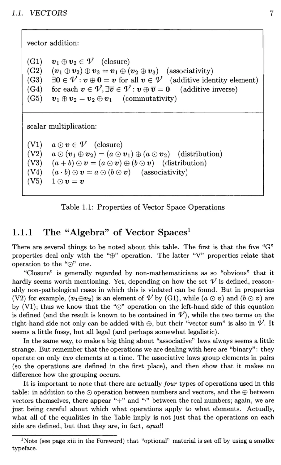
1.1.1 The "Algebra" of Vector Spaces1
There are several things to be noted about this table. The first is that the five "G"
properties deal only with the "0" operation. The latter "V" properties relate that
operation to the "0" one.
"Closure" is generally regarded by non-mathematicians as so "obvious" that it
hardly seems worth mentioning. Yet, depending on how the set V is defined,
reasonably non-pathological cases in which this is violated can be found. But in properties
(V2) for example, (vi©V2) is an element of V by (Gl), while (a 0 v) and (b 0 v) are
by (VI); thus we know that the "0" operation on the left-hand side of this equation
is defined (and the result is known to be contained in 1/), while the two terms on the
right-hand side not only can be added with ©, but their "vector sum" is also in V. It
seems a little fussy, but all legal (and perhaps somewhat legalistic).
In the same way, to make a big thing about "associative" laws always seems a little
strange. But remember that the operations we are dealing with here are "binary": they
operate on only two elements at a time. The associative laws group elements in pairs
(so the operations are defined in the first place), and then show that it makes no
difference how the grouping occurs.
It is important to note that there are actually four types of operations used in this
table: in addition to the 0 operation between numbers and vectors, and the 0 between
vectors themselves, there appear "+" and "•" between the real numbers; again, we are
just being careful about which what operations apply to what elements. Actually,
what all of the equalities in the Table imply is not just that the operations on each
side are defined, but that they are, in fact, equall
1Note (see page xiii in the Foreword) that "optional" material is set off by using a smaller
typeface.
8
CHAPTER!. VECTOR SPACES
Property (V5) appears a little strange at first. What is significant is that the
number "1" is that real number which, when it [real-]multiplies any other real number,
gives the second number back—the "multiplicative identity element" for real numbers.
That property states that "1" will also give v back when it scalar multiplies v.
It all seems a little fussy to the applied scientist and engineer, but what is really
being done is to "abstract" the structure of a given set of numbers, to see the essence
of what makes these numbers combine the way they do. This is really what the term
"algebra" (and thus "linear algebra") means to the mathematician. While it doesn't
actually help to solve any problems, it does free one's perspective from the prejudice of
experience with one or another type of arithmetic. This, in turn, allows one to analyze
the essence of a given system, and perhaps discover unexpected results unencumbered
by that prejudice.
In fact, the "G" in the identifying letters actually refers to the word "group" —
itself a one-operation algebraic structure defined by these properties. The simplest
example is the integers: they form a group under addition (though not multiplication:
there is no multiplicative inverse; fractions—rational numbers—are required to allow
this). In this regard, the last property, (G5), defined the group as a "commutative" or
"Abelian" group. We will shortly be dealing with the classic instance of an operation
which forms a group with appropriate elements but which is not Abelian: the set of
n x n matrices under multiplication. The [matrix] product of two matrices A and B
is another square matrix [of the same dimension, so closed], but generally AB ^ BA.
One last note is in order: All of the above has been couched in terms of "real
numbers" because this is the application in which we are primarily interested. But,
in keeping with the perspective of this section, it should be noted that the actual
definition of a vector space is not limited to this set of elements to define scalar
multiplication. Rather, the elements multiplying vectors are supposed to come from a
"field"—yet another algebraic structure. Unfortunately, a field is defined in terms of
still another algebraic structure, the "ring":
Recall that a vector space as defined above really dealt with two sets of elements:
elements of the set 1/ itself, and the [set of] real numbers; in addition, there were
two operations on each of these sets: "addition," "0" and "+" respectively, and
"multiplication," "•" on the reals and "0" between the reals and elements of V. In
view of the fact that we are examining the elements which "scalar multiply" the vectors,
it makes sense that we focus on the two operations "+" and "•" on those elements:
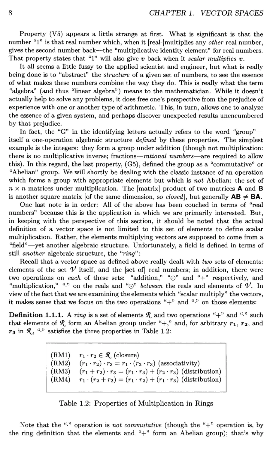
Definition 1.1.1. A ring is a set of elements ^ and two operations "+" and "•" such
that elements of ^ form an Abelian group under "+," and, for arbitrary n, r2, and
rz in ^, "•" satisfies the three properties in Table 1.2:
(RM1)
(RM2)
(RM3)
(RM4)
r\
(ri
ri € ^ (closure)
• r2) • r3 =
(ri + r2) • rz
r\
(r2 + r3)
r\ • (r2
• r3) (associativity)
= (ri • r3) + (r2
= (n • r2) + (r\
• r3) (distribution)
• r3) (distribution)
Table 1.2: Properties of Multiplication in Rings
Note that the "•" operation is not commutative (though the "+" operation is, by
the ring definition that the elements and "+" form an Abelian group); that's why
1.1. VECTORS
9
there are two "distributive" laws. Again we return to the example of square matrices:
we can define the "+" operation to be an element-wise sum, and the "•" operation
to be ordinary matrix multiplication; then matrices, under these two operations, do
in fact form a ring (in which, as noted above, the multiplication operation is non-
commutative) .
Now that we have dispatched the ring, we can finally define the field:
Definition 1.1.2. A field is a ring whose non-0 elements form an Abelian group under
multiplication ("•").
Recall that "0" is the additive identity element—that which, when "added" to any
element returns that same element; thus, in effect, this definition is meant to ensure
that the "reciprocal" of an element exists while precluding division by 0. Clearly, real
numbers (under the usual definitions of addition and multiplication) form a field; so do
the rational numbers (fractions). On the other hand, the set of integers (positive and
negative ones—otherwise there is no "additive inverse" for each) form a ring under the
usual operations, but not a field: there is no multiplicative inverse without fractions.
Having finally sorted out what a "field" is, we are ready to view vector spaces
from the most general perspective: The elements used to scalar multiply element of
the vector space must arise from a field, jF. In this context, we refer to the vector
space as consisting of elements from one set, 1/, on which vector addition is defined,
in combination with another set, ^F, from which the "scalars" come in order to define
scalar multiplication; the resulting vector space is referred to as a vector space over the
field J when we wish to emphasize the identity of those elements which scalar multiply
the "vectors." In all the below examples, and almost exclusively in this book, we shall
be talking about vector spaces over the reals. Again, while a vector space consists
technically of the set 1/ of "vectors," the field 7 of "scalars" [and the operations
of "addition" and "multiplication" defined on it\] and the two operations, "0" and
"0" of "vector addition" on V and "scalar multiplication" between J and V—which
really comprises another set of two spaces and two operations (1/, ff, 0,0)—we shall
typically employ the more economical [and perhaps abusive] description of simply "the
vector space 1/" where the field and operations are all implicitly understood. This is a
reasonably common practice and exactly what was done in the examples below. One
must keep in mind, however, that there are really four types of elements required to
define a vector space completely, and that the various operations on the sets 1/ and
jF are distinct.
Now having this general definition of a vector space, we are armed to see how
many familiar mathematical quantities actually qualify as such a space. Recall
that in order to define the space in question, we are obliged to define 1) the
elements and 2) the [two] operations; if they satisfy the properties in Table 1.1,
they are, in fact, a vector space. Though these examples will be identified by
the elements comprising the space, the actual vector space involves both the
elements and the operations on it.
Example 1.1.1. Directed Line Segments: under the operations of head-to-tail
"addition" and "scalar multiplication" by the reals. This is the classic case,
characterized by position, velocity, force, etc. |2
2To set off the Examples, they are terminated by the symbol "|."
10
CHAPTER 1. VECTOR SPACES
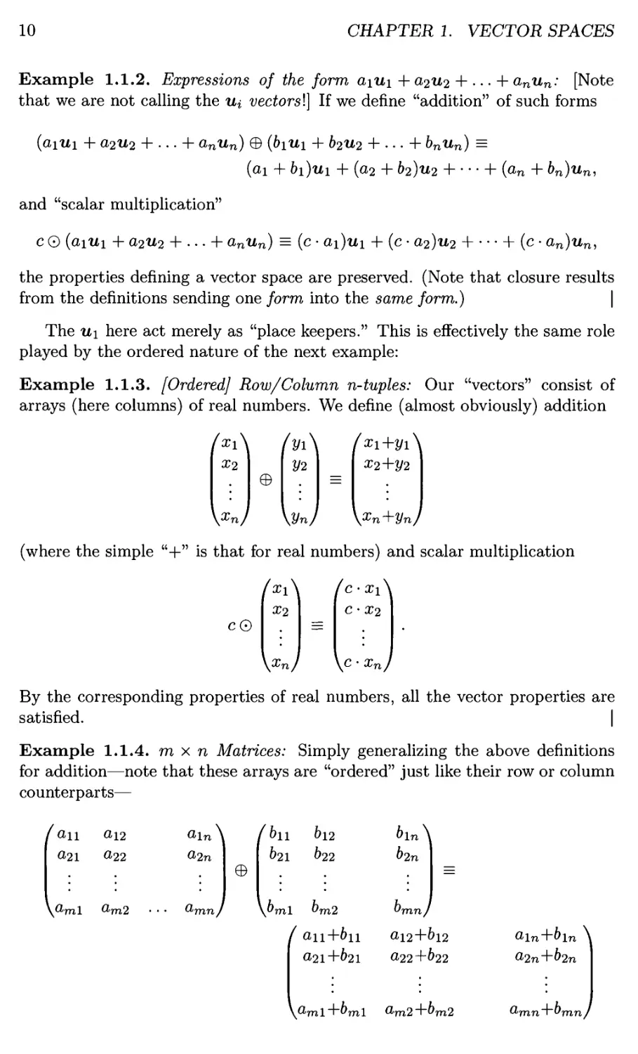
Example 1.1.2. Expressions of the form a\U\ 4- (X2U2 + ... + anun: [Note
that we are not calling the Ui vectors^] If we define "addition" of such forms
(aiiii 4- a2U2 4- •. • 4- anun) 0 {b\U\ 4- b2u2 + ... + bnun) =
(ai 4- h)ui 4- (a2 4- b2)u2 H 4- (an 4- bn)un,
and "scalar multiplication"
c 0 (aiiii 4- a2u2 4- ... 4- anun) = (c • ai)iii 4- (c • a2)u2 -\ \-(c- an)un,
the properties defining a vector space are preserved. (Note that closure results
from the definitions sending one form into the same form.) \
The tti here act merely as "place keepers." This is effectively the same role
played by the ordered nature of the next example:
Example 1.1.3. [Ordered] Row/Column n-tuples: Our "vectors" consist of
arrays (here columns) of real numbers. We define (almost obviously) addition
X2
/Vi\
V2
/a?i+2/i\
#2+2/2
\Xn/ \ynj \Xn+Vn/
(where the simple "+" is that for real numbers) and scalar multiplication
c0
X2
\xn)
(c-xi\
C-X2
\c. xn)
By the corresponding properties of real numbers, all the vector properties are
satisfied. |
Example 1.1.4. m x n Matrices: Simply generalizing the above definitions
for addition—note that these arrays are "ordered" just like their row or column
counterparts—
/flu
021
\flml
ai2
«22
0>m2 •
«ln\
&2n
Q"mn/
0
/611
621
bu
b22
\bjnl bm2
( aii+in
G21+&21
&ln\
b2n
Omn/
CL12+1
a22+l
>12
>22
Gln+^ln \
fl2n+&2n
\flml+^ml G>m2+bm2
Q"mn\Vmn/
1.1. VECTORS
11
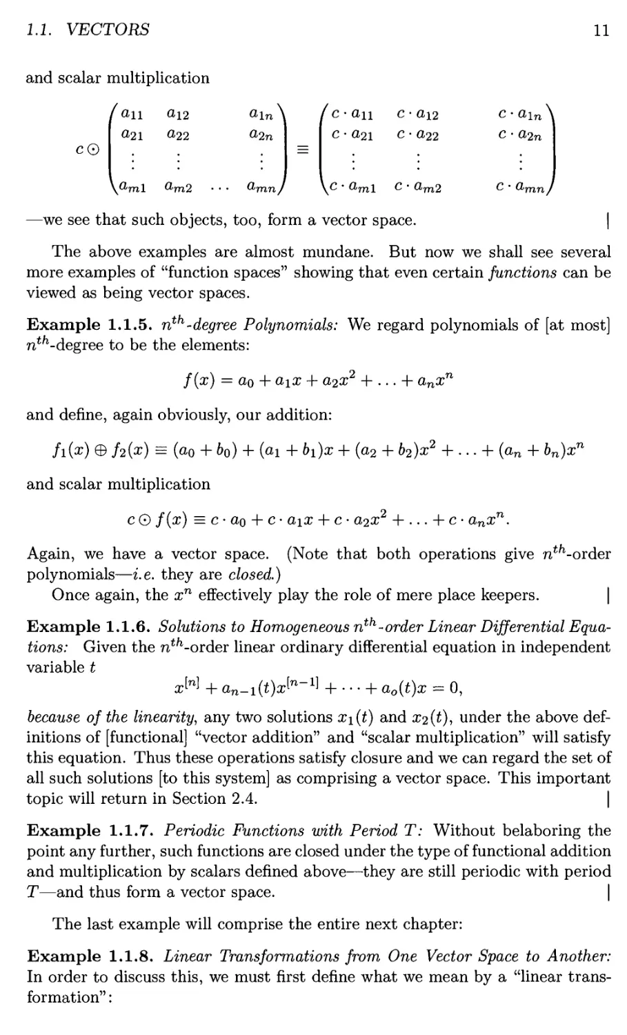
and scalar multiplication
fan
Q>21
\ami
an
a22
am2 •
Gln\
a2n
amn/
=
( c-an
c-a2i
\c - ami
c-a\2
C'd22
c- am2
c-ain\
c- a2n
C ' aynnj
C0
—we see that such objects, too, form a vector space. |
The above examples are almost mundane. But now we shall see several
more examples of "function spaces" showing that even certain functions can be
viewed as being vector spaces.
Example 1.1.5. nth-degree Polynomials: We regard polynomials of [at most]
nth-degree to be the elements:
f(x) = ao 4- aix 4- a2x2 4- ... 4- anxn
and define, again obviously, our addition:
fi(x) 0 f2(x) = (a0 4- 60) + (ai 4- &i)x + (a2 + b2)x2 + ... + (an 4- bn)xn
and scalar multiplication
c 0 f(x) = c • ao + c • aix + c • a2x2 + ... + c • anxn.
Again, we have a vector space. (Note that both operations give n^-order
polynomials—i.e. they are closed.)
Once again, the xn effectively play the role of mere place keepers. |
Example 1.1.6. Solutions to Homogeneous nth-order Linear Differential
Equations: Given the nth-order linear ordinary differential equation in independent
variable t
M
+ an-i(t)x[n-^ + • • • + a0(t)x = 0,
because of the linearity, any two solutions #i(£) and x2(t), under the above
definitions of [functional] "vector addition" and "scalar multiplication" will satisfy
this equation. Thus these operations satisfy closure and we can regard the set of
all such solutions [to this system] as comprising a vector space. This important
topic will return in Section 2.4. |
Example 1.1.7. Periodic Functions with Period T: Without belaboring the
point any further, such functions are closed under the type of functional addition
and multiplication by scalars defined above—they are still periodic with period
T—and thus form a vector space. |
The last example will comprise the entire next chapter:
Example 1.1.8. Linear Transformations from One Vector Space to Another:
In order to discuss this, we must first define what we mean by a "linear
transformation" :
12
CHAPTER 1. VECTOR SPACES
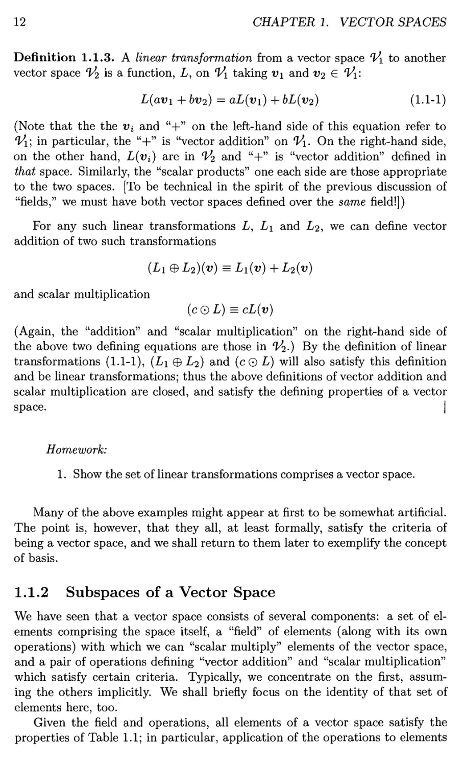
Definition 1.1.3. A linear transformation from a vector space V\ to another
vector space V2 is a function, L, on V\ taking V\ and v2 G V\\
L(avi + bv2) = aL(vi) + bL(v2) (1-1-1)
(Note that the the vi and "+" on the left-hand side of this equation refer to
V\\ in particular, the "+" is "vector addition" on V\. On the right-hand side,
on the other hand, L(vi) are in V2 and "+" is "vector addition" defined in
that space. Similarly, the "scalar products" one each side are those appropriate
to the two spaces. [To be technical in the spirit of the previous discussion of
"fields," we must have both vector spaces defined over the same field!])
For any such linear transformations L, L\ and L2, we can define vector
addition of two such transformations
(Lx ® L2)(v) = Lx(v) + L2(v)
and scalar multiplication
(c©L) = cL(v)
(Again, the "addition" and "scalar multiplication" on the right-hand side of
the above two defining equations are those in cl?2.) By the definition of linear
transformations (1.1-1), (L\ 0 L2) and (c 0 L) will also satisfy this definition
and be linear transformations; thus the above definitions of vector addition and
scalar multiplication are closed, and satisfy the defining properties of a vector
space. I
Homework:
1. Show the set of linear transformations comprises a vector space.
Many of the above examples might appear at first to be somewhat artificial.
The point is, however, that they all, at least formally, satisfy the criteria of
being a vector space, and we shall return to them later to exemplify the concept
of basis.
1.1.2 Subspaces of a Vector Space
We have seen that a vector space consists of several components: a set of
elements comprising the space itself, a "field" of elements (along with its own
operations) with which we can "scalar multiply" elements of the vector space,
and a pair of operations defining "vector addition" and "scalar multiplication"
which satisfy certain criteria. Typically, we concentrate on the first,
assuming the others implicitly. We shall briefly focus on the identity of that set of
elements here, too.
Given the field and operations, all elements of a vector space satisfy the
properties of Table 1.1; in particular, application of the operations to elements
1.2. THE BASIS OF A VECTOR SPACE
13
of the vector space result in other elements in the vector space—the closure
properties (Gl) and (VI) in the Table. But it might happen that a certain
subset of elements in the space, identified by some criterion to be a "proper
subset" of that space (so forming a "smaller" set not equal to the original
space) will, when operated upon by the same operations, give back elements in
the subset. A brief example might be in order to illustrate this idea:
Example 1.1.9. Consider the space of row 4-tuples—elements of the form
(v\, ^2, t>3, v*)—under the operations defined for such elements in Example 1.1.3.
Elements of the form (vi,^2,0,^4) are clearly elements of this space; but the
results of vector addition and scalar multiplication on such elements return an
element of exactly the same form. \
Clearly such elements satisfy properties (G2)-(G5) and (V2)-(V5) in the
Table: they inherit these properties by virtue of being elements of the vector
space in the large. But they also enjoy a unique closure property in that they
remain in the subset under the general operations. Such elements then, through
this closure property, form a vector space in their own right: they satisfy all the
properties of the Table including closure. Elements which retain their identity
under the general operations seem special enough to warrant their own category:
Definition 1.1.4. A [proper] subset of elements of a vector space which remains
closed under the operations of that vector space are said to form a [vector]
subspace of that space.
Though at this stage such elements and the "subspace" they comprise might
seem merely a curiosity, they are relatively important, and it is useful to have
a criterion to identify them when they occur. Since it is the closure property
which characterizes them, it is no surprise that the test depends only on closure:
Theorem 1.1.1. A subset of a vector space forms a subspace if and only if
((a® vi) ©(&<£> V2)), for all "scalars" a and b and all v\ and V2 in the subspace,
is itself an element of the subspace.
Homework:
1. Prove this.
1.2 The Basis of a Vector Space
This chapter has been motivated by appeal to our experience with "Cartesian"
vectors, in which we introduce the fundamental set of vectors i, j, and fc in terms
of which to represent all other vectors in the form A = Ax% + Ayj + Azk. [Note
that after all the care exercised in the previous section to differentiate between
the scalar "+" and "•" and vector "0" and "0," we are reverting to a more
14
CHAPTER 1. VECTOR SPACES
common, albeit sloppier, notation. The distinction between these should be
clear from context.] In terms of the "algebra" discussed in the previous section,
we see that each part of this sum is the scalar products of a real with a vector (so
a vector by Property (VI) in Table 1.1), and the resulting vectors are summed
using vector addition, so yielding a vector (by Property (Gl) of the same Table);
this is the reason the two defining operations on vectors are so important. Such
a vector sum of scalar products is referred to as a linear combination of the
vectors.
While these fundamental vectors i, j, and k form an "orthonormal set"—
mutually perpendicular unit vectors—we shall examine in this section the
question of how much we might be able to relax this convention: Do the vectors
have to be unit vectors? Or perpendicular? And how many such vectors are
required in the first place? All of these questions revolve around the issue of a
basis for a vector space.
In essence, a basis is a minimal set of vectors, from the original vector space,
which can be used to represent any other vector from that space as a linear
combination. Rather like Goldilocks, we must have just the right number of
vectors, neither too few (in order to express any vector), nor too many (so that
it is a minimal set). The first of these criteria demands that the basis vectors
(in reasonably descriptive mathematical jargon) span the set; the second that
they be linearly independent. The latter concept is going to return continually
in the next chapter and is likely one of the most fundamental in all of linear
algebra.
1.2.1 Spanning Sets
Though we have already introduced the term, just to keep things neat and tidy,
let us formally define the concept of linear combination:
Definition 1.2.1. A linear combination of a set of vectors {vi, V2,..., vn} is
a vector sum of scalar products of the vectors: a\V\ + 02^2 + ... + anvn.
We note three special cases of this definition given the set {vi, V2,..., vn}:
1. Multiplication of a [single] vector by a scalar: v% can be multiplied by a
scalar c by simply forming the linear combination with a* = c and dj = 0
for j ^ i.
2. Addition of two vectors: Vi + Vj is just the linear combination in which
<Xi = a j = 1 and a& = 0 for k ^ i,j.
Thus far, there's nothing new here: the above two are just the fundamental
operations on vector spaces, cast in the language of linear combinations.
But:
3. Interchange of two vectors in an ordered set: If the set is an ordered set of
vectors (vi,..., Vi,..., Vj,...). The claim is that we can put this into the
1.2. THE BASIS OF A VECTOR SPACE
15
form (vi,..., Vjy..., Vj,...) through a sequence of linear combinations:
(Vi, . . . , VU . . . , Vj, ...)-> (Wi, . . . , Wi, . . . , Vj + W», ... )
-> (vi,...,-^,...,^+«»,...)
-> (vi,...,-^-,...,^,...)
-> (vi,...,Vj,...,«»,...).
Thus the concept of "linear combination" is more general that the definition
alone might suggest.
With this, it is easy to formalize the concept of spanning:
Definition 1.2.2. A set of vectors {tti, ti2, •. •, un} in a vector space V is said
to span the space iff every v E 1/ can be written as a linear combination of the
it's: v = viU\ + V2U2 + ... 4- vnun.
We give two examples of this. The first is drawn from the space of directed
line segments. We purposely consider non-orthonormal vectors:
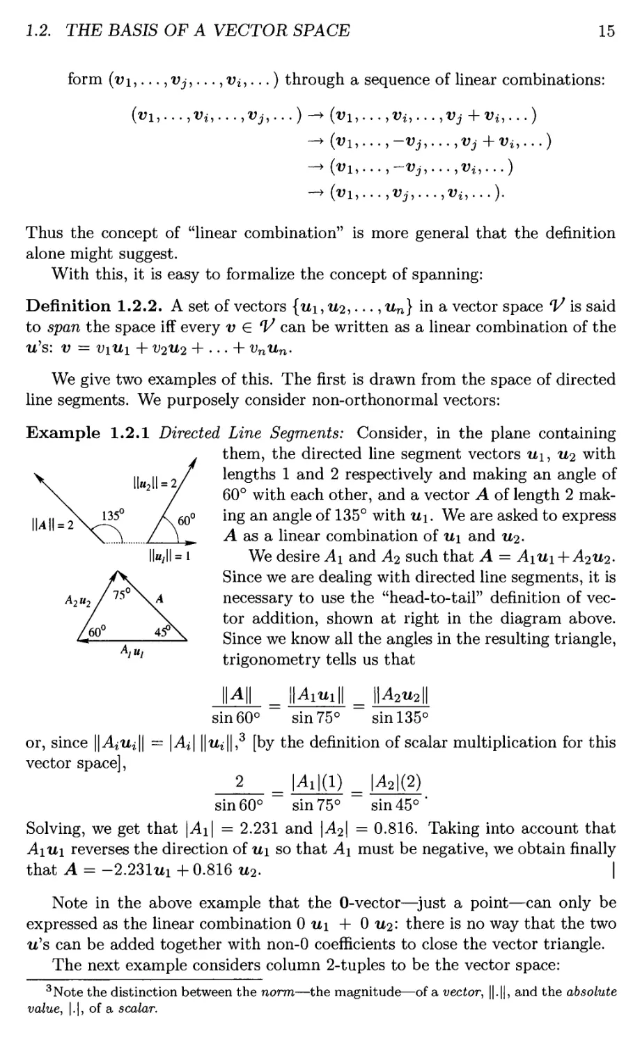
Example 1.2.1
Directed Line Segments: Consider, in the plane containing
them, the directed line segment vectors u\, u<i with
lengths 1 and 2 respectively and making an angle of
60° with each other, and a vector A of length 2
making an angle of 135° with u\. We are asked to express
A as a linear combination of U\ and 112.
We desire A\ and A<i such that A = A\U\-\- A^ui.
Since we are dealing with directed line segments, it is
necessary to use the "head-to-tail" definition of
vector addition, shown at right in the diagram above.
Since we know all the angles in the resulting triangle,
trigonometry tells us that
Pltilll _ P2«2||
or, since ||^i^|| = \A%
vector space],
sin 60° sin 75° sin 135°
|t^||,3 [by the definition of scalar multiplication for this
l^il(l) _ I4>1(2)
sin 60° sin 75° sin 45°
Solving, we get that \A\\ = 2.231 and \A<±\ = 0.816. Taking into account that
A\U\ reverses the direction of u\ so that A\ must be negative, we obtain finally
that A = -2.231m + 0.816 ti2. I
Note in the above example that the 0-vector—just a point—can only be
expressed as the linear combination 0 u\ + 0 u<i'. there is no way that the two
it's can be added together with non-0 coefficients to close the vector triangle.
The next example considers column 2-tuples to be the vector space:
3Note the distinction between the norm—the magnitude—of a vector, ||.||, and the absolute
value, |.|, of a scalar.
16
CHAPTER!. VECTOR SPACES
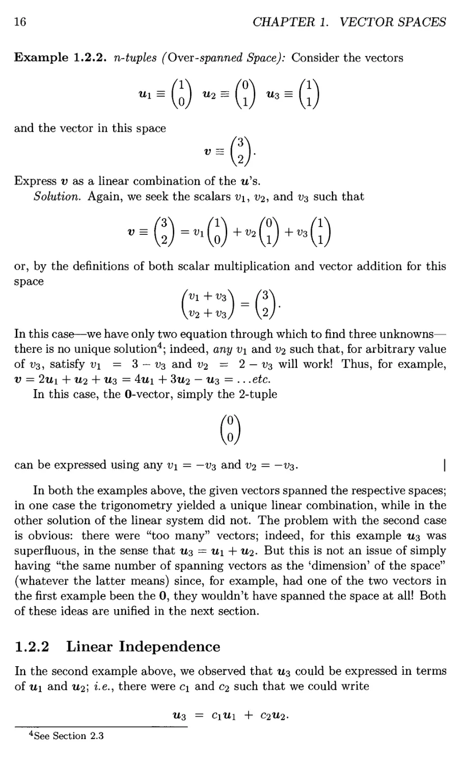
Example 1.2.2. n-tuples (Ovex-spanned Space): Consider the vectors
ui s G)u2 s (i)u3 s G)
and the vector in this space
•■©■
Express v as a linear combination of the it's.
Solution. Again, we seek the scalars v\, v2, and vs such that
v=Q=viQ+v20+v3§
or, by the definitions of both scalar multiplication and vector addition for this
space
\V2+V3j V2/
In this case—we have only two equation through which to find three unknowns—
there is no unique solution4; indeed, any V\ and v2 such that, for arbitrary value
of V3, satisfy v\ = 3 — ^3 and v2 = 2 — vs will work! Thus, for example,
v = 2u\ + u2 + ti3 = 4tti + 3tt2 - tt3 = .. .e£c.
In this case, the O-vector, simply the 2-tuple
W
can be expressed using any v\ = —Vs and v2 = — V3. \
In both the examples above, the given vectors spanned the respective spaces;
in one case the trigonometry yielded a unique linear combination, while in the
other solution of the linear system did not. The problem with the second case
is obvious: there were "too many" vectors; indeed, for this example U3 was
superfluous, in the sense that Us = u\ + U2. But this is not an issue of simply
having "the same number of spanning vectors as the -dimension' of the space"
(whatever the latter means) since, for example, had one of the two vectors in
the first example been the 0, they wouldn't have spanned the space at all! Both
of these ideas are unified in the next section.
1.2.2 Linear Independence
In the second example above, we observed that U3 could be expressed in terms
of tti and U2; i.e., there were c\ and c2 such that we could write
tt3 = ciiii + c2tt2.
4See Section 2.3
1.2. THE BASIS OF A VECTOR SPACE
17
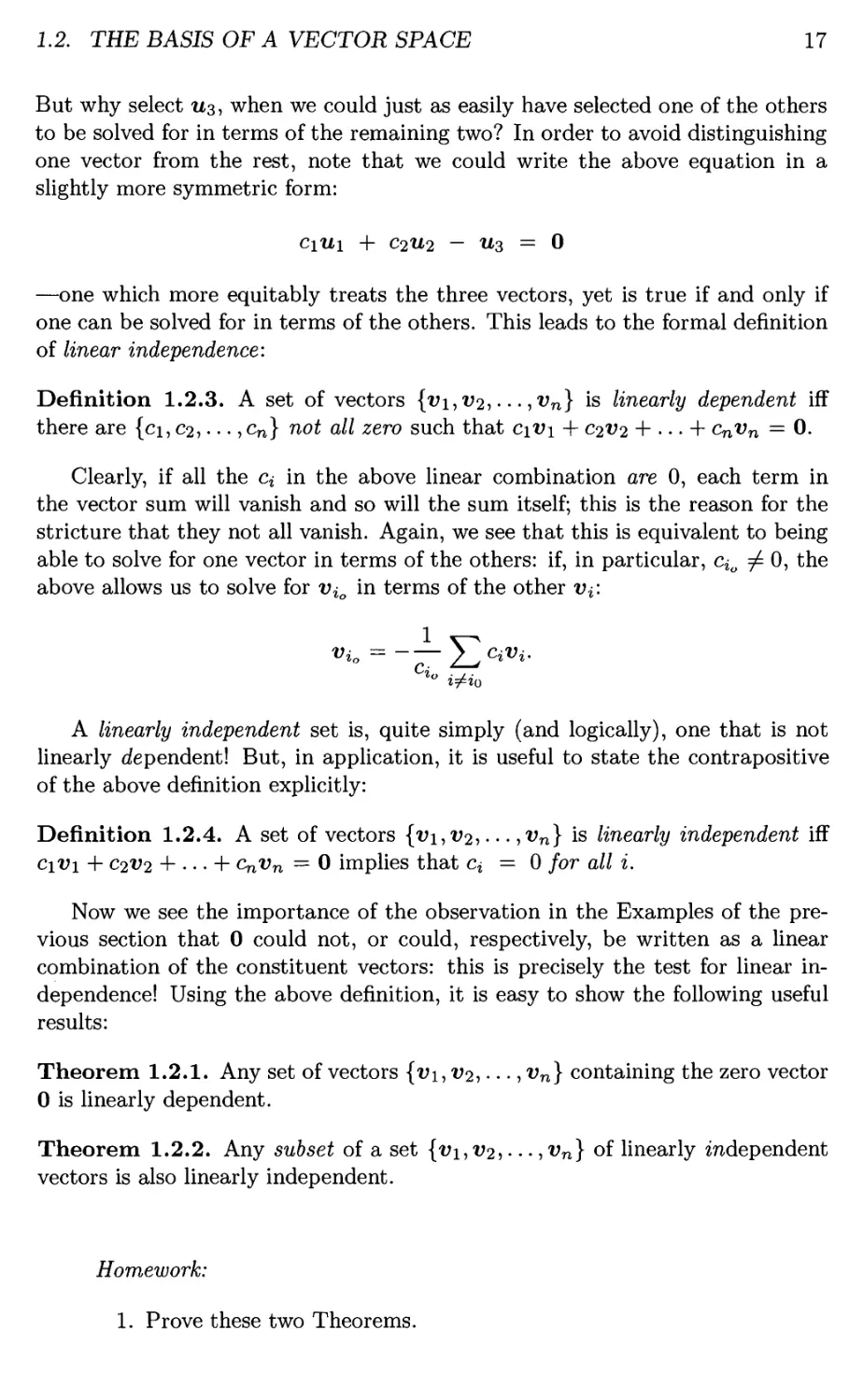
But why select 113, when we could just as easily have selected one of the others
to be solved for in terms of the remaining two? In order to avoid distinguishing
one vector from the rest, note that we could write the above equation in a
slightly more symmetric form:
c\U\ + C2U2 - u3 = 0
—one which more equitably treats the three vectors, yet is true if and only if
one can be solved for in terms of the others. This leads to the formal definition
of linear independence:
Definition 1.2.3. A set of vectors {v\, V2,..., vn} is linearly dependent iff
there are {ci, C2,..., cn} not all zero such that c\V\ + C2V2 + ... 4- cnvn = 0.
Clearly, if all the c* in the above linear combination are 0, each term in
the vector sum will vanish and so will the sum itself; this is the reason for the
stricture that they not all vanish. Again, we see that this is equivalent to being
able to solve for one vector in terms of the others: if, in particular, qo ^ 0, the
above allows us to solve for Vi0 in terms of the other vf.
vio = — y^c^i.
A linearly independent set is, quite simply (and logically), one that is not
linearly dependent! But, in application, it is useful to state the contrapositive
of the above definition explicitly:
Definition 1.2.4. A set of vectors {vi, V2,..., vn} is linearly independent iff
c\Vi + C2V2 4- ... 4- CnVn = 0 implies that c$ = 0 for all i.
Now we see the importance of the observation in the Examples of the
previous section that 0 could not, or could, respectively, be written as a linear
combination of the constituent vectors: this is precisely the test for linear
independence! Using the above definition, it is easy to show the following useful
results:
Theorem 1.2.1. Any set of vectors {vi, V2,..., vn} containing the zero vector
0 is linearly dependent.
Theorem 1.2.2. Any subset of a set {t>i, V2, • • • > vn} of linearly independent
vectors is also linearly independent.
Homework:
1. Prove these two Theorems.
18
CHAPTER!. VECTOR SPACES
Warning: Many students may first have seen "linear dependence"
in a course on differential equations, in connection with the "Wron-
skian" in that field. Reliance on that criterion alone as a "quick-and-
dirty" criterion for linear independence is shortsighted however: In
the first place, it evaluates the determinant of numbers, useful only
in the case of row or column n-tuples, Example 1.1.3 above; how, for
example, could we have used this to show the linear independence of
directed line segments, Example 1.2.1? Secondly, even if our vector
space does consist of such n-tuples with numerical components, the
determinant is only defined for a square matrix; what if one is
examining the linear independence of fewer (or more) than n vectors?
The above definitions, however, work in both cases.
We shall now consider another criterion for linear independence. Unlike the
above definition, however, it will be applicable only to the n-tuple row or column
vectors, and thus be apparently limited in scope. Actually, as we shall see, it
can be applied to any vectors (Theorem 1.3.2); and in the discussion of matrices
[of real numbers], it is of fundamental utility.
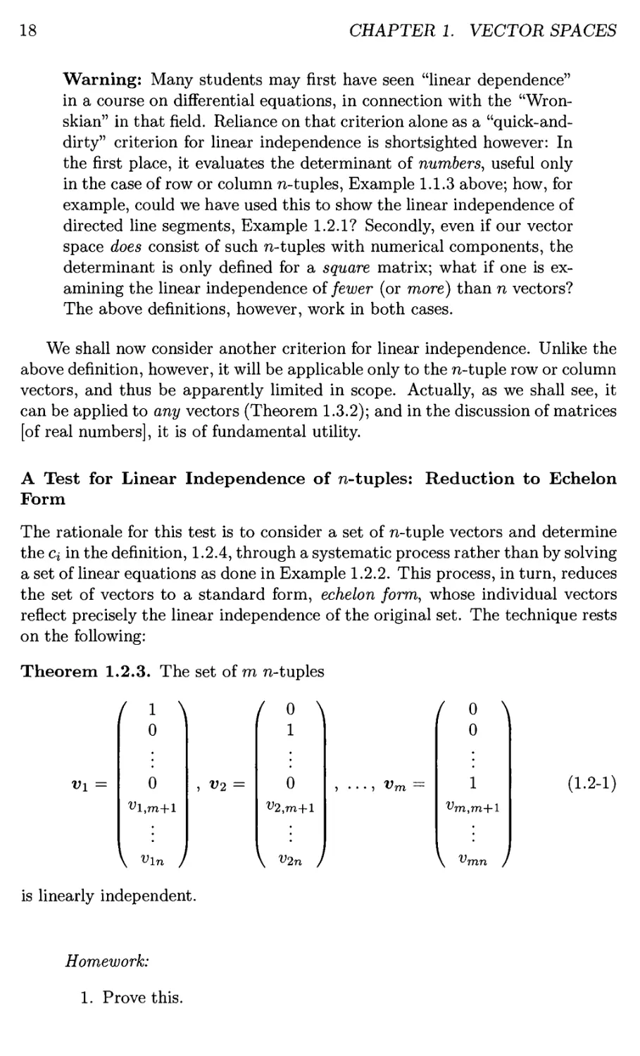
A Test for Linear Independence of n-tuples:
Form
Reduction to Echelon
The rationale for this test is to consider a set of n-tuple vectors and determine
the Ci in the definition, 1.2.4, through a systematic process rather than by solving
a set of linear equations as done in Example 1.2.2. This process, in turn, reduces
the set of vectors to a standard form, echelon form, whose individual vectors
reflect precisely the linear independence of the original set. The technique rests
on the following:
Theorem 1.2.3. The set of m n-tuples
vi
(
\
1
0
0
\ Vln j
is linearly independent.
/
, V2
\
0
1
0
^2,m+l
\ V2n )
, . . . , Vm —
/ 0 \
0
1
Vm,m+1
\ ^mn /
(1.2-1)
Homework:
1. Prove this.
1.2. THE BASIS OF A VECTOR SPACE
19
The idea is to examine the linear independence of the set of vectors by trying
to reduce it, through a sequence of linear combinations of the vectors among
themselves, to the above "ec/ie/on"5 form. This can best be seen by an example:
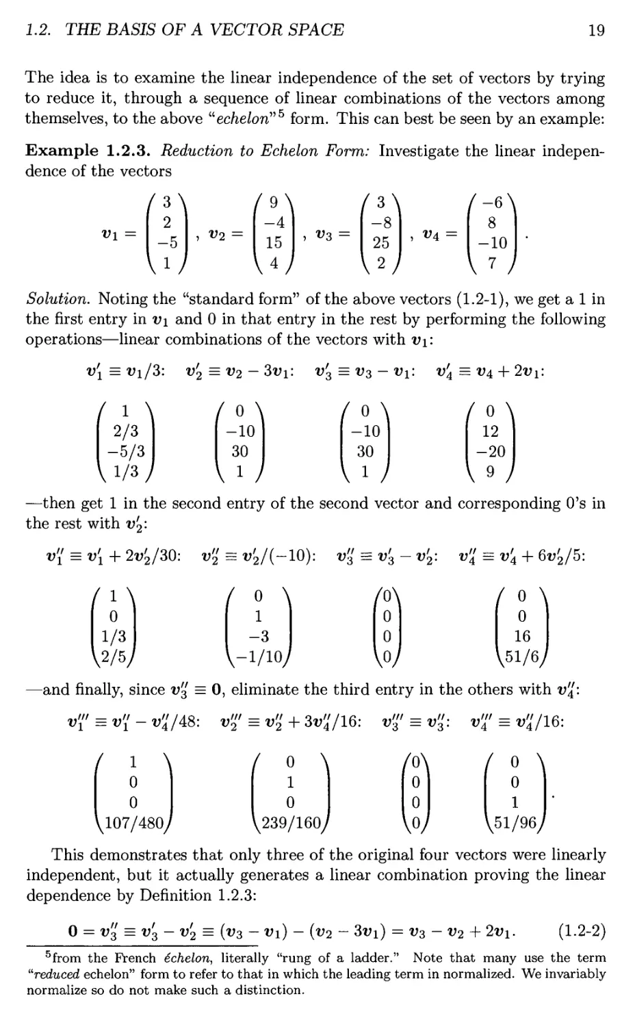
Example 1.2.3. Reduction to Echelon Form: Investigate the linear
independence of the vectors
Vi
/3\
2
-5
W
V2
/9\
-4
15
W
V3
/3\
-8
25
V2/
V4
/-6\
8
-10
V 7 J
Solution. Noting the "standard form" of the above vectors (1.2-1), we get a 1 in
the first entry in v\ and 0 in that entry in the rest by performing the following
operations—linear combinations of the vectors with V\:
v[ = wi/3:
vf2 = V2 — 3v\:
v'3 = v3- vi:
v\ = W4 + 2wi:
/ 1 \
2/3
-5/3
(° ^
-10
30
^ l J
( ° "\
-10
30
I 1 )
( ° \
12
-20
^ 9 /
—then get 1 in the second entry of the second vector and corresponding 0's in
the rest with v'2:
v'{ = v[+2v'2/30: „» = „'2/(-io): v'3' = v'3 - v'2: v'{ = v'A + 6v'2/5:
I 1 \
0
1/3
V2/5/
/ 0 \
1
-3
V-i/ioy
M
0
0
w
(° ^
0
16
\51/6j
-and finally, since v3 = 0, eliminate the third entry in the others with v'l:
v'{' = v'l - </48: < = v'l + 3</16: < = v%: < = </16:
/ 1 \
0
0
\107/480/
This demonstrates that only three of the original four vectors were linearly
independent, but it actually generates a linear combination proving the linear
dependence by Definition 1.2.3:
1 ° ^
1
0
\239/16(y
M
0
0
w
( ° \
0
1
^51/96/
0 = v3 = v3 - v2 = (v3 - vi) - (v-z - 3«i) = v3-v2 + 2«i.
(1.2-2)
5from the French Echelon, literally "rung of a ladder." Note that many use the term
"reduced echelon" form to refer to that in which the leading term in normalized. We invariably
normalize so do not make such a distinction.
20
CHAPTER 1. VECTOR SPACES
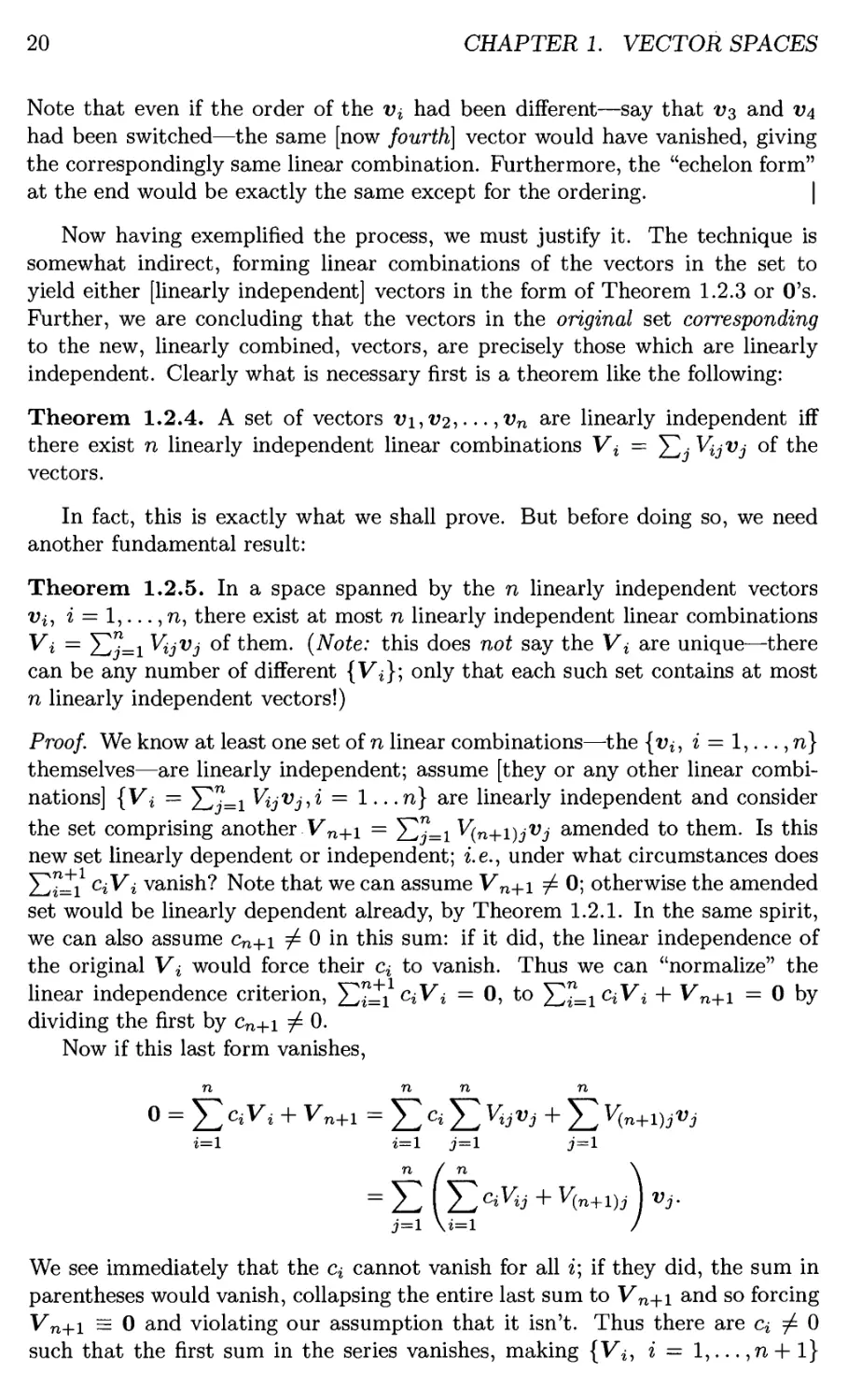
Note that even if the order of the Vi had been different—say that Vs and V4
had been switched—the same [now fourth] vector would have vanished, giving
the correspondingly same linear combination. Furthermore, the "echelon form"
at the end would be exactly the same except for the ordering. |
Now having exemplified the process, we must justify it. The technique is
somewhat indirect, forming linear combinations of the vectors in the set to
yield either [linearly independent] vectors in the form of Theorem 1.2.3 or O's.
Further, we are concluding that the vectors in the original set corresponding
to the new, linearly combined, vectors, are precisely those which are linearly
independent. Clearly what is necessary first is a theorem like the following:
Theorem 1.2.4. A set of vectors vi, V2,..., vn are linearly independent iff
there exist n linearly independent linear combinations V* = ]T\- Vijvj °f the
vectors.
In fact, this is exactly what we shall prove. But before doing so, we need
another fundamental result:
Theorem 1.2.5. In a space spanned by the n linearly independent vectors
v$, i = 1,..., n, there exist at most n linearly independent linear combinations
Vi — Sj=i Vijvj °f them. (Note: this does not say the Vi are unique—there
can be any number of different {Vi}; only that each such set contains at most
n linearly independent vectors!)
Proof. We know at least one set of n linear combinations—the {vi, i = 1,..., n)
themselves—are linearly independent; assume [they or any other linear
combinations] {Vi = X^j=i Vijvj->i — 1.. .n} are linearly independent and consider
the set comprising another Vn+i = ]C?=i V(n+i)jvj amended to them. Is this
new set linearly dependent or independent; i.e., under what circumstances does
Sr=^i ciVi vanish? Note that we can assume Vn+i 7^ 0; otherwise the amended
set would be linearly dependent already, by Theorem 1.2.1. In the same spirit,
we can also assume cn+i 7^ 0 in this sum: if it did, the linear independence of
the original Vi would force their c* to vanish. Thus we can "normalize" the
linear independence criterion, Ya=i ci^i = 0> to Yl7=i c^* + ^n+i = 0 by
dividing the first by cn+i ^ 0.
Now if this last form vanishes,
n n n n
Q = Y; °iVi + Vn^ = 5ZC*5Z Vi0V3 + 51 V(n+l)3V3
i=l i=l j=l j=l
n / n \
= 2 w2CiVi3 + V(n+l)j I Vj.
j=l \i=\ /
We see immediately that the c* cannot vanish for all i; if they did, the sum in
parentheses would vanish, collapsing the entire last sum to Vn+i and so forcing
Vn+i = 0 and violating our assumption that it isn't. Thus there are Ci ^ 0
such that the first sum in the series vanishes, making {Vi, i = 1,... ,n + 1}
1.2. THE BASIS OF A VECTOR SPACE
21
linearly dependent, and proving that the original n are the most which can be
linearly independent. □
Note: This is a fundamental result—one which will return in our discussion
of "dimension" of a vector space in Section 1.2.3.
We are now ready to prove the above theorem:
Proof of Theorem 1.2.4- The "implication" is trivial: Assume the {vi} are
linearly independent; then the linear combinations
Vi = (i)vi + (o)v2 + • • • + (ok
V2 = (0)«i + (l)v2 + ■ • ■ + (OK
vn = (oK + (o)v2 + --- + (iK
are linearly independent.
Conversely, assume the set {V* = ^jVijVj,i = l...n} are linearly
independent, and consider the two spaces
V = {all vectors spanned by the Vi, i = 1,..., n}
V = {all vectors spanned by the Vi, i — 1,..., n}.
While all n of the Vi are linearly independent by hypothesis, at most n of the Vi
are; whatever number are is also the maximum number of linearly independent
linear combinations V can support, by the above Theorem. But the vectors
{Vi, i = l,..,,n}C^; and linear combinations of linear combinations of the
Vi are themselves linear combinations of the Vi, so V C v. Thus the nV\ E. V,
so at least n of the spanning Vi must be linearly independent, or Theorem 1.2.5
is violated. Thus all n of the Vi must be linearly independent. □
This shows that, in the Example 1.2.3 above, having obtained three linearly
independent linear combinations (the v1") of the original vectors v», three of
the latter were, in fact, linearly independent. But it doesn't show that the first,
second, and fourth were the linearly independent ones. This is a result of the
systematic way the echelon form was obtained:
Recall that we seek to have the ith vector have a 1 in its ith row, with O's
above and below. But the O's above the ith row result from linear combinations
of vectors preceding the ith vector, while those below come from linear
combinations with those following it. If a vector is "cleared" in the process of trying
to zero out entries above the ith, such as the the third vector was in the second
iteration in Example 1.2.3 was, it is the result of linear combinations with
vectors only preceding it] we have yet to operate on entries below the ith using the
following ones. This is shown explicitly in (1.2-2) in the example. Thus Vs is
linearly dependent on V\ and v<i but not on v\ [yet].
5Following common practice, proofs are set off by terminating them with a symbol, here
22
CHAPTER!. VECTOR SPACES
But if we are not interested in which vectors are linearly independent (and
typically, in application, we aren't), all that is necessary is to obtain the number
of linearly independent linear combinations, regardless of the order in which the
original set was presented. This means that we can "switch" the order of vectors
at will in order to standardize that order. (Recall the remark on page 14: such
an interchange is itself a linear combination!) In particular, this "standardized
order" in the present context is one in which the ith vector is reduced to a "1" in
its ith row, with O's below, precisely that in Theorem 1.2.3. This is the approach
that will be followed in the sequel.
Having exemplified the procedure and stated the theory on which it rests,
we can now organize it into a systematic technique for examining the linear
independence of a set of m vectors. This will be done inductively, assuming
that we have already reduced i vectors in the set to the form (1.2-1) through
row:
the ith
( 1 \
0
0
vi,*+i
/ o \
1
0
^2,2+1
^2,2+2
/o\ /
0
\ Vln / \ V2n /
1
Vi,i+2
0
0
0
UM-l,z+l
\
\ Vin ) \ ^i+l,n /
/ o \
0
0
*W+2
\ Vmn /
i in standard form
i+1 linearly independent
(in which the jth component of Vi is Vij), and are dealing with putting the
(i + l)st vector in standard form. (Initially, i = 0.) If Vi+i^+i ^ 0, we proceed
as usual. By performing linear combinations of the preceding i vectors, this set
gets reduced to an echelon form
/ 1 \
0
0
0
yi,i+2
V v[n J
( 0 \
1
0
0
^2,2+2
\< J
( o \ /
0
yt,<+2
0
0
0
1
/
i+l,i+2
\
/ o \
0
0
0
\ V'in I \ «i+lfn /
7TM+2
V v'mn J
It might be the case that the (i -f l)st component of v*+i, ^+i^+i, is, in fact, 0;
in fact, it might be the case that Vi+ij = 0 for all j > i—i.e., that Vi+\ = 0—
as happened with V3 in Example 1.2.3 above, in which case Vi+i is a linear
combination of the Vj,j < i to the left of v*+i, and we have shown that only i
1.2. THE BASIS OF A VECTOR SPACE
23
of the z + l vectors thus far put in standard form are linearly independent. In
any event, if we are only interested in how many linearly independent vectors
there were originally, we are free to reorder the set by switching v^+i with one
of the Vj in which Vj^+\ ^ 0. (Note that the two vectors being transposed have,
to this point, been operated on only by those to the left of v*+i.) We then
normalize that entry and use it to eliminate the (i + l)st entries in the other
vectors.
But it is conceivable that, in fact, there is no other such vector with a non-0
(i + l)st entry; that, at this stage in the procedure, the vectors have assumed
the form
0
0
vl,i+l
\ Vin J
•)
( ° ^
1
0
^2,2+1
^2,2+2
\ v2n )
i ' ' • i
( ° ^
0
1
Viti+2
\ Vin J
7
( ° ^
0
0
0
^2+1,2+2
\ vi+iiU J
, . . . ,
( ° \
0
0
0
Vm,i+2
\ vmn )
i in standard form
2+1 linearly independent using row i+2!
with a 0 in the (i-\-l)st row of not only the (i + l)st vector, but also in all others
to its right. We briefly sketch an example of such a case:
Example 1.2.4. "Skip" case: Reduce the vectors
vi =
/1\
1
-1
0
11
V5/
>V2 =
/1\
4
-7
-3
14
V8/
,«3 =
/1\
0
1
4
34
W
,v4 =
/1\
3
-5
-4
-3
,«5
/1\
3
-5
0
29
V 9/
to [reduced] echelon form.
Results of the obvious operations using, respectively,
vi:
/1\
1
-1
0
11
\5/
> ^2
3
-6
-3
3
\3/
> "3
-1
2
4
23
V2/
>v4 =
/ 0 \
2
-4
-4
-14
V 0 /
v* =
2
-4
0
18
V4/
24
CHAPTER 1. VECTOR SPACES
then «2:
v, =
/1\
0
1
1
10
W
1
-2
-1
1
V1/
>v3
0
0
3
24
,v4
( 0 \
0
0
-2
-16
-v
V
o
0
2
16
V2/
yield a "pathological" case: though v% is not voided out altogether, neither it
nor v'l nor v§ have any entry in their third rows; thus we cannot eliminate
terms of this row in the vectors to the left. To continue at all, we must go to
the fourth: now operating on V3, it turns out that the last two vectors both
void out altogether:
/1\
0
1
0
2
W
i v2 —
/o\
1
-2
0
9
VV
(0\
0
0
1
8
W
'v4 —
/0\
0
0
0
0
w
>v? =
(Q\
0
0
0
0
w
We thus have that only three of these column 6-vectors are linearly independent;
more importantly (for purposes of this example, in any event), we note the
signature "skip form" for these vectors. |
In this case we cannot eliminate those components in the {% + l)st entry
to the left, because we don't have anything to form linear combinations with!
Nevertheless, we can look to the (i + 2)nd "row" of entries for a non-0 value
and, assuming we find one, continue the process from there. This introduces a
"skip" in the final form at the end of this step, yielding a set
/ 1 \
0
vi,*+i
0
V < /
/ o \
1
^2,2+1
0
\ ^2n 7
/ o \
0
0
V*4 /
/ o \
0
0
0
1
\vi+l,J
( o \
0
0
0
0
\v'mn)
but the resulting i + 1 vectors are still linearly independent. Note that such a
skip manifests itself in these column n-tuples by having a 0 instead of a 1 in
the ith entry of the ith vector along with generally non-0 ith entries to the left
(though still 0's to the right).
The process continues until we either a) run out of vectors, b) run out of
non-0 "rows," or c) run out of rows altogether. The final set assumes a form in
1.2. THE BASIS OF A VECTOR SPACE
25
which v\ has either a 1 or a 0 in its ith entry. In the former case, all other vectors
have a 0 in this entry; in the latter, either v\ = 0 (showing that the original Vi
is a linear combination of those to its left), or Vjti = 0 for j > i (though with
possibly non-0 entries for j < i)—the "skip case" above. In either event, the
number of linearly independent vectors is the number of "diagonal l's".
Thus, given a set of m n-tuple vectors, there are three possible relations
between the two numbers:
1. m < n: If there are fewer vectors than the number of entries in each, the
"best" we can hope for—that we avoid the "0 row syndrome" mentioned
above—is that the final product of this process will be of the form (1.2-1):
0
0
Ul,m+1
•)
( ° ^
1
0
\ V2n J
, . . . ,
( ° \
0
1
^771,771+1
\ vin J
i.e., that all m are linearly independent. This is case "a)" above. Even
if there are the "skips" mentioned above, there is still the possibility that
the original set is linearly independent; but if there are too many skips, we
might run out of "rows" first, giving even fewer than m linearly
independent combinations of the original ones. In the pathological limit of such
a situation, there is no non-0 element in any of the lower rows from Vi+\
on; then all the remaining vectors are linearly dependent on the preceding
ones (case "b)" above).
2. m = n: The "best case scenario" here is that we end up with a set of
vectors
0
w
>
1
W
, ...,
f \
0
W
i.e., that all m vectors are linearly independent. But "skips" would reduce
this number to less than m.
3. m > n: Now the best we can hope for is a final set of the form
HO • • • O
^y
•)
}
1
w
, . . . ,
0
v)
j
o ••• o c
, . . . ,
o ••• o c
26
CHAPTER!. VECTOR SPACES
the maximum number of linearly independent columns is n (case "c)").
"Skips" would reduce this number even further, since we would run out
of rows earlier.
While all of the above has been couched in terms of column vectors,
analogous results are obtained for row vectors: in particular, the above three "best"
cases of final form become:
1. m<n: (1,0,... ,0,*>i,m+i,... ,vin) ,
(0,l,...,0,i^,m+i,...,i^n) ,
(U, U, . . . , 1, t>m)m_|_i, . . . , Vin) 7
2. m = n: (1,0,...,0) ,
(0,1,...,0),
(0,0,...,1,),
and
3. m >n: (1,0,...,0) ,
(0,1,...,0),
(0,0,...,1),
(0,0,...,0),
(0,0,...,0),
respectively. We observe that, in the case of row n-tuples, "skips" manifest
themselves again by having a 0 in the ith entry in the ith row and generally
non-0 entries above this; those below still vanish, however.
There is one last comment which must be made regarding this procedure
for determining the linear dependence/independence of a set of vectors: In
forming the intermediate linear combinations c^Vi + CjVj in the ith vectors, we
clearly cannot allow Ci — 0; to do so would eliminate Vi from the set altogether,
replacing it by 0 which, by Theorem 1.2.1, would make the resulting set linearly
dependent, even if the original set wasn't. However trivial this observation
might seem, it is important to make it (with a view of later application of the
criterion in what follows).
This section appears long, primarily because of the detailed discussion
regarding the "echelon test." In point of fact, however, there have been only two
fundamental ideas: that of linear dependence and independence, and the test
itself for linear independence among a set of row/column vectors; the major
theorem in this section merely supports the latter. The key points are what
linear independence is (and what it isn't—the "Wronskian"!), and the fact that
linear independence of a set of row/column vectors is equivalent to reduction
1.2. THE BASIS OF A VECTOR SPACE
27
of that set of vectors to "echelon form." Despite its apparently rather narrow
application, this criterion will become fundamental when applied to matrix
algebra in the next chapter. But the importance of linear independence cannot
be overstated: the concept will pervade all of the sequel. It should be firmly in
mind.
Homework:
1. Theorem 1.2.5 emphasizes the fact that there are generally
many sets of linearly independent linear combinations of the
original linearly independent vi. Show, for example, that the
set {Vi = J2)=i vi} (e-9-> V\ = vi, V2 = «i + v2, etc.) form
a linearly independent set.
2. Show that if a vector v £ {vectors spanned by linearly
independent Vj, i = 1,..., n}, then the set {vi, V2, •.., vn, v} are
linearly independent.
3. Show that
and
are linearly independent.
4. Show that
are linearly dependent.
5. Show that
and
-6
are linearly dependent.
6. Investigate the linear independence of the vectors
1
-1
/3\
5
2
W
and
/6\
7
7
v-v
using
(a) the definition of linear independence, and
(b) reduction to "echelon form."
(c) If it turns out the above vectors are linearly dependent,
find a linear combination of them which vanishes.
28
CHAPTER 1. VECTOR SPACES
7. Show that the matrices (viewed as a vector space)
(4 2) ' (e -2)
are linearly independent.
1.2.3 Bases and the Dimension of a Vector Space
Knowing now the criteria that a given set of vectors is large enough (that it is
a spanning set) and that it is not too large (that vectors in the set are linearly
independent) we are prepared to define a basis:
Definition 1.2.5. A basis for a vector space V is a linearly independent set of
vectors from 1/, {tii, U2,. •., un} which span V\ i.e., for any v G V, v can be
written as a linear combination of the u^. v = v\U\ + V2U2 + ... + vnun.
The vectors need be neither "normalized" to unit magnitude nor
"orthogonal" like most systems with which the reader is familiar (though this choice
does have certain conveniences); in fact, the concept of orthogonality only has
meaning for vectors of the class of directed line segments (though a related
criterion, the "inner product," can be used more generally). In this regard, the
set of non-orthonormal vectors in Example 1.2.1, since they both spanned the
planar space considered and were linearly independent, constitute a basis for
that space. A point not often emphasized, however, is that the basis vectors
must be from the space itself
With the concept of basis in hand, we are ready to define the concept of
dimension of a vector space:
Definition 1.2.6. The dimension of a vector space is the number of vectors in
a basis for that space.
The concept of dimension is important, in that it characterizes the vector
space in a sense we shall discuss below. For the time being, however, we shall
obtain some important results regarding dimension; in particular, we must
explain why the above definition states merely "a basis." Though we mention one
example of a vector space of infinite dimension, the following will characterize
finite-dimensional vector spaces:
Theorems on Dimension
The first of these is really just a restatement of Theorem 1.2.5 in the present
context. In that theorem we considered "a space spanned by the n linearly
independent vectors"—precisely what we now define to be a basis. Though we
could leave it at that, we will give an alternate proof:
Theorem 1.2.6. The dimension of a vector space is the maximum number of
linearly independent vectors in that space.
1.2. THE BASIS OF A VECTOR SPACE
29
Proof. Assume the space has dimension n—i.e., it has a basis {txi, U2,..., un}
of linearly independent vectors which spans it. We claim that there is no other
vector v independent of the {ui}.
For assume there were a v such that {txi, 1x2, • • •, un, v) were linearly
independent. We must take v/0 (for otherwise, by Theorem 1.2.1, the set would
be linearly dependent from the start). Since the {ui} span the space already,
we can write v = ]T ViUi—where the Vi are not all zero, since otherwise v is!
But this means that the linear combination (l)v — Ylviui — 0, violating the
linear independence assumed. □
Theorem 1.2.7. The dimension of a vector space is unique; i.e., given two
bases, {u\,U2,... ,um} and {vi, i>2> • • • > vn}> then m = n.
Proof. If m ^ n, then either m < n or m > n, both violating the above
maximality of the number of linearly independent vectors! D
Theorem 1.2.8. Any set of n linearly independent vectors forms a basis for a
vector space of that dimension.
Proof. Assume {u\, U2,..., un} are linearly independent (so none is 0!) Then,
for any v in the space, the set of n + 1 vectors {u\,U2,... ,un,v} must be
linearly dependent, since there are only n linearly independent ones. Thus
^2ciUi + cn+iv = 0, where not all the Ci = 0. In particular, cn+i ^ 0: if it
were, the ^CiUi = 0, meaning (by the linear independence of the {Ui}) that
all the Ci = 0 for i < n; but then all the Ci vanish. Thus we can solve for v:
v =—y^ciUi,
showing that the {u^ span the space. Since they are already linearly
independent, they form a basis. □
This last theorem explains why, in the definition of dimension above, we can
use any basis whatsoever.
Now let us return to the examples of vector spaces given in Section 1.1:
Example 1.2.5. Directed Line Segments: Any pair of non-parallel directed line
segments in 2-D, or any three non-coplanar, non-parallel directed line segments
in 3-D form a basis. The dimensions of these two spaces are (not surprisingly)
2 and 3 respectively! |
Example 1.2.6. Expressions of the form a\U\ + a2tt2 + ... + anun: The
vectors {u\, ti2,. • •, un} form a basis. These are elements of the space: u^ = liii.
The space is of dimension n. \
Example 1.2.7. [Ordered] Row/Column n-tuples: In keeping with this example
earlier, we will consider columns. One convenient basis for these is the so-called
30
CHAPTER 1. VECTOR SPACES
"natural basis" :
ei =
/1\
0
W
, e2 =
M
l
W
/°\
W
(1.2-3)
any v = (ci, C2,.. •, cn) = ciei -f C2e2 + ... + cnen.6 Once again, to specify a
basis for a vector space, that basis must come from the space; here our space
is of columns, so the basis must be, too. And, once again, this space is of
dimension n. |
Example 1.2.8. mxn Matrices: We can form a "natural basis," analogous to
the above, for these, too—[matrix] elements of the original space
En =
(I 0
0 0
\0 0
0
0/
0 0
E12SS
\0 0
0
0/
Ein =
/o 0
0 0
\0 0
1\
0
0/
(1.2-4)
/o 0
0 0
Eml =
0
/o 1
0 0
Em2 =
0
0/
, . . . , Cttj,^ —
/o 0
0 0
\0 0
dimension n + 1.
1\
0
1/
\1 0 0/ \0 1
Here the space is of dimension ran. |
Example 1.2.9. nth-degree Polynomials: Here the basis is {x0,^1,... ,xn}, of
1
Example 1.2.10. Solutions to Homogeneous nth-order Linear Differential
Equations: We have already seen (1.1.6) that the solutions of a given n^^-order linear
differential equation
x{n) + an-i{t)x{n-l) + • • • + a0(t)x = 0
constitute a vector space; it is rather less obvious what the dimension of that
space will be. Observe, however, that we can write the above equation as one
involving a column n-tuple x = (x^n ^ x^n 2)
..*)T:
dx
~dt ~~
_ d
" dt
/x(n-l)\
x(n-2)
(-
\ x J \
/-On-iWx'"-1' a0(t)x\
x(n-2) >
rr(D
= f(x;t);
J
6The superscript "T" on a row/column vector v, vT, denotes the transpose of v: if v
is a row vector, vT is that column vector with the same components and conversely. See
Definition 2.1.1 below. It is introduced here just for compactness.
1.2. THE BASIS OF A VECTOR SPACE
31
thus, in fact, the solution to this equation is itself an n-tuple—i.e., it lies in a
space of dimension n. The basis for this space would then consist of any set of
n linearly independent solutions of the associated equation.
This construction might, at first, appear somewhat contrived and artificial;
such reservation likely results from viewing the original differential equation as
one in the scalar "unknown" x. But recall that, in addition to the differential
equation that x satisfies, the solution also invokes the initial conditions on not
only x but all its derivatives (up to the nth, which, once the values of the lower
derivatives are specified, is itself known). In effect, we can conceive of a point
x in the n-dimensional space of x and its derivatives, evolving from the point
x(0) (given by its initial conditions) along the solution x(t). In this context,
the n-dimensional space of x is referred to as the phase space.
This perspective is actually quite fruitful: the theory of ordinary differential
equations—even non-linear ones—rests on the foundation that, as long as the
function / is continuous7, the first-oider equation x = f(x) not only has a
solution satisfying its initial conditions ("existence"), but that solution is unique.
These results are immediately applicable to the case in which the right-hand side
in the above is independent of t—i.e., that the system is "autonomous." But
we can treat the more general non-autonomous case easily by simply regarding
t itself as one component of the unknown vector x' = (x t) : It is trivially the
case that
dx'
dt
d
dt
/x(n-l)\
x(n-2)
X
\ * )
/
\
/-an-i^"-1' a0(t)x\
a.(n-2)
1 /
= /V)
satisfies both the original differential equation and the hypotheses of the
fundamental theorem: if f(x-,t) is continuous in x and f(t) in t, then the above
f'{x') is clearly continuous in x'. The (n + l)-dimensional space of [the original]
x and t is referred to as the extended phase space. |
Example 1.2.11. Periodic Functions with Period T: This example is a rather
less prosaic than the preceding ones. By Fourier's theorem, we know that any
periodic function can be expanded in a generally infinite series of sines and
cosines in the argument 27rx/T; thus the set of all such functions—themselves
periodic of period T—form an in/im£e-dimensional space! |
The observant reader will note that the last example in Section 1.1,
Example 1.1.8, has been omitted. This is not a oversight. While the first two
"function" vector spaces above are somewhat "concrete" with regard to
establishing a basis, the last is more general and difficult to pin down. And since
7Actually, the result is shown for a somewhat less restrictive condition that / satisfy a
"Lipschitz condition" but continuous or piecewise continuous functions are the norm in most
physical applications.
32
CHAPTER 1. VECTOR SPACES
such transformations are dignified by their own chapter, it seems appropriate
to forestall discussion of their basis until that point.
We note in passing that all the above, which has been applied to "vector
spaces" will clearly also hold for subsp&ces of a vector space: as vector spaces in
their own right, subspaces will have their own bases and dimensions, with the
latter generally less than the space in which they are contained. Note, however,
that the basis of the full space will have, among its elements, basis elements of
its subspaces; conversely, knowing the existence of a subspace and its basis, it is
possible to build up a basis for the full space by augmenting the subspace basis
with other, linearly independent, vectors.
Summary. This section has been, admittedly, a little technical. The key
points, however, are terribly important: A basis is any set of linearly
independent vectors from the space which span it; i.e., any vector can be expressed as
a linear combination of the basis vectors. The dimension of the space is the
number of vectors in a basis, or, equivalently, the maximum number of linearly
independent vectors in that space. While the basis may not be unique, the
dimension is.
As mentioned in the Prolog to this Part, the concept of linear independence
is important and has already assumed a central position in the development.
This section also presents a procedure, the echelon test, to ascertain whether
a given set of vectors are linearly independent or not. This, too, will return in
the sequel.
1.3 The Representation of Vectors
We have earlier observed that writing vectors in the form
v = viUx + v2u2 + ... + vnun (1-3-1)
is more than a mere convenience: it allows us to operate on the v's through
manipulation of the Vi rather than the original vectors or even the Ui. If the v%
are real (or even complex) scalars, such manipulation becomes effectively trivial
compared with, say, the original operations on the original vectors. Thus, as a
matter of almost necessary convenience, this is the methodology employed. In
order to discuss this approach, it is necessary to introduce a little jargon:
Definition 1.3.1. We call the right-hand side of (1.3-1) the representation of
v relative to the {u^}] the {v^} are called the components of v relative to the
{Ui}.
Note that in order to be able to write any vector in the form (1.3-1), it is
necessary that the Ui span the space—see Section 1.2.1. But in Example 1.2.2
of that section, we saw that such a representation might not be unique; this fact
would certainly make it more difficult to identify vectors in a given
representation, greatly complicating the very process we are trying to simplify!
1.3. THE REPRESENTATION OF VECTORS
33
But we also showed in the latter example that the Ui were linearly dependent,
rather than the "minimal" set required for a basis. We might then suspect that
this problem of non-uniqueness would not arise for a proper basis, and we would,
in fact, be right:
Theorem 1.3.1. The representation of a vector relative to a basis is unique.
Proof. Assume there were two representations for a vector v G V with basis
{tii}:
V = ViUi + V2U2 + . . . + VnUn = v'iUi + Vf2U2 + . . . + v'nUn.
But then
(vi - v'i)ui 4- (v2 - v'2)u2 H 4- On - v'n)un = 0
—which means, by the linear independence of the basis, that (vi — v'i) = 0, or
Vi — v'i, for all i. D
This is precisely the reason that, if a vector v = v\Ui 4- v2u2 + ... 4- vnun —
v'\U\ 4- v'2u2 + ... 4- v'nun relative to the same basis, we can conclude that
v[ = Vi'. the representation is unique. Thus henceforth we shall assume that all
representations are being made relative to a basis, precisely so that there is a
single representation for each vector in the space under consideration.
But if the representation relative to a particular basis is unique, recall that
the choice of basis itself is not: any set of linearly independent vectors
spanning the space will qualify. Thus it becomes important to know not only the
representation, but also which basis is referenced in that representation:
Example 1.3.1 Non-unique basis: We again return to the space of directed
j line segments, and consider the
V IIm2II = 2/ «2 vector A of length 2 in Exam-
^v / \ "2 «y pie 1.2.1, as well as three pos-
IIaII=2\^^ /\60° a ^\ AcO S1^e cn°ices of basis: a) those
\ ^ ^—i-^7 I ^ \Z...\4.^ given in the original example;
a> b> c) and two pairs of orthonormal
vectors, b) with U\ parallel to the original Ui and the c) rotated by 45° from
that:
Relative to the first basis, A = -2.231tti + 0.816ti2 (see Example 1.2.1),
relative to the second A — y/2(—U\ + u2), while relative to the third, A = 2u2.
The representations are different, but A is the same in all three cases. |
Throughout, however, it must be kept in mind that the original vector,
regardless of what vectors it might be expressed in terms of, remains the same:
Though the representation of the vector might change dramatically depending
on which basis vectors it is referred to, the original vector does not. And, since
representations relative to different bases represent the same vector, different
representations can, in fact, be equated to one another (though we cannot equate
components of that vector in the different bases).
34
CHAPTER 1. VECTOR SPACES
1.3.1 n-tuple Representations of Vectors
Heretofore we have considered the basis to be an arbitrary collection of
vectors {ui}. But if we choose to order the set and form (tti,tt2,... ,ttn) so
that U\ corresponds to the first element of the set, U2 corresponds to the
second, etc., it is possible to express the representation much more
economically by simply expressing the components in a similarly-ordered set—i.e., an
n-tuple. Thus, relative to the ordered set (tti,tt2,... ,ttn), the vector v =
v\Ux + V2U2 + ... + vnun can be expressed simply as
(vi\
V2
(For reasons which will become clearer in the next chapter, we generally express
vectors as column n-tuples rather than as rows.) Thus, for example, in the above
Example 1.3.1, the three representations of A could themselves be represented
as
(mis1) ' {~jt) ' and
respectively. Again, keep in mind that all three represent the same vector, even
though they "look" different, and could be equated (though not
componentwise).
This is all well and good for most vectors, but if the original vector space itself
consisted of n-tuples, some confusion can arise: one n-tuple becomes represented
as yet another n-tuple! Thus it becomes critical to know whether, in such a
space, it is the original vector one is talking about, or its representation relative
to other vectors, themselves of the same form.
It is reasonable to ask why we even consider this possibility in the first place:
We have motivated the entire issue of representations as a means of simplifying
the vector operations on vectors; instead of operating on the original vectors
(whatever they might be), we operate on the scalar components—most often
real numbers—of those vectors relative to a given basis. It would seem, given the
inherent simplicity of operation on n-tuples, that it would hardly be necessary
to introduce any basis different from the "natural basis" (see (1.2-3)) in terms
of which such n-tuples are all implicitly defined in the first place. But there are
problems in the next chapter in which this is done, just to engrain the issue of
which basis a given vector is referred to. We illustrate this idea with an example:
Example 1.3.2. Consider, in the space of 2-tuples, the vector
v={o)
Note that this is already represented in terms of the "natural basis" [of 2-tuples]
Cl ee (J) , e2 ee (j) ;
1.3. THE REPRESENTATION OF VECTORS
35
indeed,
v = 2e\ + Qe2 or, as a 2-tuple: I j .
Now consider this same vector in, as it were, an -unnatural basis
1\ A
*i = [^ , u2 _ VQ
[These are, indeed, linearly independent. Using the definition 1.2.4:
c\Ui + c2u2 = f X 2 1 = 0
iff ci, and therefore C2, both vanish.]
To represent v in terms of u\ and u2, we must have
Solving, again c\ = 0 but now C2 — 2; thus, in terms of U\ and u2,
v = 0u\ + 2tt2 or, as a 2-tuple: I 9 1
Note the dramatically different representations of the vector relative to the two
bases! |
A rather superficial reading of this example might suggest that
(1.3-2)
but this would be wrong: the first is the original vector v [in the natural basis],
while the second is its representation in terms of u\ and u2. The way out of
this confusion could be notation to suggest what signifies what. To the extent
it is possible, the distinction between a vector (of whatever ilk) and its [n-tuple]
representation will be to denote the first with Roman boldface and the latter
with sans-serif bold; thus, in the above example,
(1.3-3)
This doesn't completely obviate the confusion: strictly speaking, the
representation would also have to specify the particular basis (itself specified in terms
of the natural one!) in which that representation was valid, but doing so would
soon become cumbersome. Thus we will finesse this fussy practice, being
satisfied with merely indicating when a given n-tuple is a representation.
A simple but important instance of these ideas—one unfortunately liable to
misinterpretation—is the representation of the basis vectors themselves. Since
36
CHAPTER 1. VECTOR SPACES
each basis vector in the [ordered] set (1*1,1*2, • • • ,un) can be represented 1*; =
(0)i*i + (0)i*2 H + (l)i*i + • • • 4- (0)i*n, that vector's n-tuple representation
u^ [note notation] in terms of that basis will always be of the form
M
0
= "i,
(1.3-4)
0
1
0
w
regardless of the nature of the i*^. The confusion can arise because of the identity
of form with the natural basis of n-tuples, equation (1.2-3): that equation is a
basis for any n-tuple, the above is the representation of any basis vector in
terms of such n-tuples. In any event, neither is [necessarily] the Cartesian basis
(i, j, fc) (though (1.3-4) is assuredly the n-tuple representation of these vectors).
As if all that weren't bad enough, one, can certainly write, in comparison with
equations (1.3-2) and (1.3-3), that e* = e*!
The student should be certain the above distinctions are understood.
Representations allow us to deal with n-tuples rather than the original
vectors. They also allows application of the "echelon test" in Section 1.2.2 to any
class of vectors—to the extent that vectors whose [n-tuple] representations are
linearly independent are themselves linearly independent. We now show that:
Theorem 1.3.2. A set of vectors {vi, V2> • • •)%} is linearly independent iff
their n-tuple representations relative to an arbitrary basis are.
Proof. Assume the {t>i, V2> • • • > vm} are in a space with basis (1*1,1*2,..., un)\
i.e., we can represent each
Vi = $Z vsiU3
3
and consider the column representation of each:
(vu\
V2i
\VniJ
We show the "implication" by assuming the {v*} are linearly independent.
Now if a linear combination of their representations were to vanish,
£
CiVi
/Cl\
C2
= 0,
(1.3-5)
1.3. THE REPRESENTATION OF VECTORS
37
then the same linear combination of the {vi} would:
0 = YCou3 = J2 \Hcivn ) uj = J2Ci Y2vHui = Y
CiVi
But, by the assumed linear independence of the {vi}, this means that each c* = 0
here and in (1.3-5), showing that the {v^} in the latter are linearly independent.
Conversely, assume the {v^} are linearly independent. Were a linear
combination of the {v^ to vanish,
* i \ 3 ) 3 V i I 3
then, by the linear independence of the basis vectors (uj), each Cj would have
to vanish. But then
0 =
fCi\
c2
\CnJ
\E CiVniJ
= £
fvu\
V2-
\VniJ
= YCiyU
which would mean the c* = 0 here and in (1.3-6), by the assumed linear
independence of the {v^}. Thus the {Vi} are linearly independent. □
1.3.2 Representations and Units
Most physical quantities are not purely numerical; they require one or another
set of units in terms of which to measure them. Thus units must somehow enter
the representation of vector quantities demanding units. There is a somewhat
subtle point, rarely mentioned, regarding just how this is to be done.
Consider and arbitrary v = v\Ui 4- V2U2 + ... 4- vnun. We have two options
regarding where the units for this vector are to be introduced: we can either
• attach units to the components, v^ leaving the basis vectors unitless, OR
• attach units to the basis vectors, leaving the components unitless.
The former is almost invariably the tack taken: it allows vectors of various
physical type (position, velocity, etc.) to be expressed in a single vector space,
laying the burden of unit identification on the components. Thus, for example,
the familiar Cartesian 3-D basis (i, j, and k) consists of unitless unit vectors.
The alternative, attaching units to the basis vectors, would identify the
vector space with a certain physical quantity; thus we could speak of the "position
space," the "angular velocity space," etc., in which the respective quantities
would have unitless components. But implementing this would soon lead to
chaos: were one to attach, say, length units to a basis, the components of position
38
CHAPTERS VECTOR SPACES
vectors would be unitless, while those of velocity would have units [T_1], while
moments' components would have units of force and forces units of [M/T2]—a
situation lacking any aesthetic appeal whatsoever. And that doesn't even begin
to address the issue of what happens if we choose to change our length units!
The point is that basis vectors will here universally be chosen to be unitless.
And any change of basis will thus require no reference to whatever units are
chosen to measure any physical quantity expressed in terms of that basis.
1.3.3 Isomorphisms among Vector Spaces of the Same
Dimension
We have now seen how any vector in an n-dimensional vector space (one with n basis
vectors, recall) can be represented as an n-tuple if we order the basis by simply
arraying the components of a given vector relative to that basis in the same order. In effect,
then, to each vector in the original space there is a representation—a unique
representation by Theorem 1.3.1—in terms of the basis, and thus in its n-tuple representation.
But this means that there is a one-to-one relation between vectors in an n-dimensional
space and the n-tuples. Further, relating the vector operations in the [original] vector
space to those of the n-tuple space using Example 1.1.2 (where now we do mean the
Ui to be vectors!) and Example 1.1.3, we see that the the result of operations in the
original space correspond to those in the n-tuple space. Such a relationship between
the elements and operations on two [different] vectors spaces is called an isomorphism
between them. What we have observed, then, is that any n-dimensional vector space
is isomorphic to that of n-tuples. But that means that any two different n-dimensional
vector spaces are isomorphic to [the same] space of n-tuples, and thus to each other.
Thus we have all but proved the following:
Theorem 1.3.3. All vector spaces of the same dimension are isomorphic to each
other.
In a highfalutin mathematical fashion, this simply says in regard to vector spaces
of a given dimension, that "once you've see one vector space you've seen them all"—
that you can operate in any vector space of the same dimension and get the same
results (at least with regard to the fundamental operations on such spaces). This is
the reason one often sees vector properties "proven" in Cartesian form, with results
extended to vectors in, say, polar form. And it is the sense in which the dimension of
a vector space characterizes it, as mentioned on page 28.
The isomorphisms among all the finite-dimensional vector spaces exemplified in
Section 1.1 can be exhibited explicitly, again with reference to the space of n-tuples:
The directed line segments in terms of their basis (i,j,k) as v=vxi + vyj + v2fc, or as a
row 3-tuple as (vXivyivz)^ the "forms" in Example 1.1.2 as (ai,a2,.. • ,an), the mxn
matrices as a [/onp!] mn-tuple (an,ai2,... ,aim,Q>2i,Q>22, • • • ,a>mn), and nth-degree
polynomials as (ao,ai,... ,an)—all n-tuples of various lengths. In particular, if the
various lengths happen to be the same, they are all isomorphic to each other!
It is important to recognize that it is really just this isomorphism which allows
us to operate on the n-tuple representation in the first place: we can identify each
vector with its n-tuple representation, and then the result of n-tuple vector addition
and scalar multiplication with the corresponding result in the original space. This is
really the thrust of Theorem 1.3.2.
1.3. THE REPRESENTATION OF VECTORS
39
Summary. The scalars Vi in writing v = v\Ui + V2U2 + ... + vnun relative to
a basis {u^ are called the components of v relative to that basis, and are unique
for a given v. If we order the basis, (t^), those scalars can themselves be arrayed
in a [ordered] n-tuple v, the representation of v; this representation is then also
unique relative to that basis. In particular, the basis vectors themselves can be
represented by elements of the natural basis. But if we represent v relative to
a different basis, its representation will change, even though the original vector
remains the same. This distinction must be kept in mind, particularly when the
original vectors are themselves n-tuples!
The fact that we can represent vectors of any ilk as unique n-tuples becomes
significant because the linear independence of the original vectors is reflected
precisely in that of it n-tuples. Thus the echelon test, originally developed only
for n-tuples, now can be applied to the n-tuple representations of arbitrary
vectors.
The units of physical quantities can be carried by either the basis vectors or
the components of vectors relative to that basis. The latter is far less confusing,
and it is the practice followed explicitly in this book (and implicitly in most
others).
Since the n-tuple representation of any vector in an n-dimensional space is unique
relative to its basis, there is a one-to-one relationship between arbitrary n-vectors
and n-tuple vectors. In particular, the n-tuples provide an identification—an
isomorphism—among the vectors of arbitrary n-dimensional spaces.
Summary
In view of the fact that the student allegedly "knows vectors," there has been
quite a bit of new information—at least a new perspective—contained in this
chapter. The key points are that:
• vectors are any elements which, along with the defined operations of
"vector addition" and "scalar multiplication," satisfy the properties in
Table 1.1
• for any vector space there is a basis of vectors in that space which
- span the space
- are linearly independent
- can uniquely represent any vector as a linear combination of the basis
vectors, whose scalar factors are components of the vector relative to
the given basis
- will generally have a different representation relative to a different
basis, even though the original vector remains the same
• the dimension of a vector space is the number of vectors in any basis
• vector spaces of the same dimension are equivalent ("isomorphic")
40
CHAPTER,!. VECTOR SPACES
• we can represent vectors as n-tuples of the components, so that
• linear independence of a set of vectors can be determined by putting their
representations [in the same basis!] in "echelon form"
Chapter 2
Linear Transformations on
Vector Spaces
Introduction
Despite the somewhat daunting title of this chapter, we are going to be primarily
concerned with matrices. But in the same way that we saw in the last chapter
that we could represent vectors as n-tuples, it will turn out that we can also
represent linear transformations as matrices. And in the same way that we can
easily manipulate a vector of any type by operating on its n-tuple representation
of real numbers, we can similarly deal most easily with linear transformations
on an arbitrary set of vectors by using their matrix representations. In fact, at
the end of the day, even an n-tuple is really a matrix—a column matrix (or row
matrix, if we choose).
We have already seen that the representation of a vector changes with the
choice of basis; in some way, this is almost obvious. What is less obvious is that,
when we change the basis in terms of which we express vectors, we also change
the representation of linear transformations operating on those vectors. Here
is the central issue in this chapter: how do the representations of both vectors
and linear transformations change with a change of basis?
This becomes important in the next Part, where we deal with 3-D rigid
body motion. It turns out there that the angular momentum of a rigid body is,
effectively, a linear transformation on the angular velocity, one which [linearly]
transforms the angular velocity to an angular momentum; thus, from what
we said above, it can be represented as a matrix—the inertia matrix. But it
also happens that, because of the special form of this matrix, there is always a
particular set of axes—in fact, orthogonal axes—in terms of which this matrix
representation is particularly simple: a diagonal matrix. This choice of axes is
called the "principle axes" and is, in the language employed heretofore, simply
a change of basis resulting in this simple representation. Thus the next chapter
culminates in the process by which we can diagonalize matrices, the conditions
42 CHAPTER 2. LINEAR TRANSFORMATIONS ON VECTOR SPACES
under which it can be done in the first place, and what can be done if these
conditions are not met.
That process is bound up with the eigenvectors and eigenvalues of the
matrix, and whether those eigenvectors are linearly independent; this is why vector
independence was emphasized so much in the last chapter. But the
determination of eigenvectors hinges on the solution to a "homogeneous" vector equation;
under what conditions can such a solution be found? Indeed, under what
conditions can the solution to a "non-homogeneous" equation (whatever either of
these terms means) be found? This question itself is of intrinsic interest even
outside the present context and, once again, rests on the idea of linear
independence.
So how is the material organized?
In the last chapter, we presumed sufficient experience with "vectors" that we
could immediately consider them from a general perspective; expecting that the
student is likely to have had rather less exposure to matrices, however, we shall
start this chapter with a brief review of the operations on matrices: Though we
have seen that matrices themselves form a vector space under obvious definitions
of vector addition and scalar multiplication, it is a new operation, peculiar to
matrices, which really gives them their utility in application: matrix
multiplication. We discuss operations employing it, and introduce a perspective which will
return throughout the chapter, "partitioning": how matrices, originally simply
an array of numbers, can be viewed as an array of vectors, and how we quantify
the linear independence of such vectors through the rank of the matrix they
comprise. Determination of the rank will return, under this interpretation, to
the echelon test for linear independence of vectors presented in the last chapter,
where now the "vectors" are simply the rows or columns of the matrix. Using
the idea of partitioning, we also demonstrate the block operations on matrices,
in which entire sub-blocks of a matrix are treated as if they were scalars.
We then move onto the contact point with "linear transformations" around
which this chapter is organized—what they are and how they can be represented
in terms of matrices. We have seen in the previous chapter [Example 1.1.8] that
such transformations—functions, if you will—themselves form a vector space
and thus must posses a basis; in this chapter we will explicitly exhibit that basis
[of arbitrary linear transformations]. We shall see there the reason that such
transformations can be represented as matrices, and the first inklings of how
the basis of the space on which the transformations act affects the basis of the
transformations themselves. Just as any other functions, linear transformations
have a domain and a range; we will see that these form vector spaces in their
own right, examine a particular si/frspace of the domain, the null space, and
obtain an important result regarding the dimensions of all these [vector] spaces.
With an eye toward the determination of eigenvectors and eigenvalues, we
then discuss the essentially inverse operation to "transformation," solution of
linear systems of equations, both homogeneous and non-homogeneous. Once
again the ideas of linear dependence and independence become central, as do
the echelon test for linear independence and the null space we have regarded
earlier.
2.1. MATRICES
43
Finally, all this material is brought together in a somewhat surprising guise:
linear differential equations, used to exemplify a topic inexorably intertwined
with linear transformations, linear operators. Here the "vector space" is that of
functions and their derivatives, the "operator" can be represented as a matrix,
the "null space" becomes the solution to the homogeneous differential equation,
and solution becomes tantamount to that of a "system of linear equations," with
corresponding results. This topic concludes the chapter.
2.1 Matrices
A matrix is, at its core, merely a rectangular array of numbers:
/an an o>in\
0*21 Q>22 &2n
A = : : ;
\ami am2 G>mn/
such a matrix with m rows and n columns is, when one wishes to emphasize
these dimensions, referred to as an m x n matrix [note the order—row dimension
first], occasionally written Amxn. Rather than writing out the entire matrix as
done above, a more economical notation is commonly employed, simply writing
out a "typical element" of the matrix:
Amxn = (aij)mxn Or Simply A = (dij)
This briefer notation will be employed extensively in the sequel, as, for example,
in the following definitions.
Frequently it becomes useful to interchange the rows and columns of a matrix
or, equivalently, to "reflect" the matrix across its "main diagonal"—the one
running from the upper left to the lower right: (•. ). The matrix resulting
from this operation on A is called the transpose of A, A :
Definition 2.1.1. The transpose of a matrix A — {cl%j)
AT = (CLji).
Though the "rectangular" nature of matrices has been stated above,
"matrices" are actually more ubiquitous than than might be inferred from this
definition. Indeed, we note in passing that the n-tuple representation of vectors
(ai\
a2
V= : '
\anJ
dealt with extensively in the first chapter, can itself be regarded as a special
form of matrix, an n x 1 column matrix. Notwithstanding the fact that we have
44 CHAPTER 2. LINEAR TRANSFORMATIONS ON VECTOR SPACES
continually pointed out that matrices themselves comprise a vector space (see
Example 1.1.4), we shall generally reserve the term "vector" [representation] for
just such a column matrix throughout this text.
We now introduce a perspective which will be utilized extensively in the
sequel.
2.1.1 The "Partitioning" and Rank of Matrices
We have frequently employed the convention that vectors can be represented as
column n-tuples. With this in mind, it is not too much of a stretch to view a
matrix as a catenation of such n-tuples:
fan
Q>21
ai2
^22
\0"ml 0>m2
Q>ln\
0>2n
(ai,a2,...an) for a^
d2j
(2.1-1)
\Q>mj /
or
A =
fan
Q>21
a\2
«22
a>in\
a>2i
I -r 1
for Bi =
(an\
a>%2
(2.1-2)
\ami am2 • • • amn/ \a^/ \ainJ
Note that the identity of the "a^" is different in the above two equations.
Thus, rather than considering the matrix as a whole, we can view it as being
made up of a set of row or column n-tuples—"vectors" in their own right. But
this means that we can consider linear combinations of these "vectors." In the
context of matrices, we refer to such linear combinations as elementary row (or
column) operations.
From this perspective, it makes sense to consider the linear independence of
the constituent "vectors" in a matrix. We characterize this particular aspect of
a matrix through a measure called the rank:
The Rank of a Matrix
Definition 2.1.2. The column rank of a matrix is the number of linearly
independent columns [or, more exactly, n-tuple column vectors] in the matrix.
Definition 2.1.3. The row rank of a matrix is the number of linearly
independent rows [or, more exactly, n-tuple row vectors] in the matrix.
These definitions reference, respectively, the columns and rows of a matrix;
it is perfectly reasonable to expect that, in a rectangular matrix whose row
and column dimensions are different, the number of linearly independent rows
[n-tuple vectors] might be different from the number of linearly independent
columns. In fact, however, this is not the case: the number of linearly
independent rows and columns in a matrix are exactly the samel This rather remarkable
result is contained in the following theorem:
2.1. MATRICES
45
Theorem 2.1.1. The row rank and column rank of a matrix are the same.
Proof. Assume the row rank of an m x n A = (a^) is r; thus there are r linearly
independent rows of A,
(an,a12,. • -aln)
(arl,ar2,... a°n)
—where each of these equals one of the original m> r rows of A. Thus we can
express all m rows of A in terms of—as linear combinations of—these r rows:
(an,ai2,.. .ain)
cn(afi,a?2,...ai„) +
+ cir«1X2,...<J
(ami, am2? • • • ^mn) — cml(an> ai2> • • • aln) ~^~ ~^~ cmrKl' ar2> ■ * • arn)
Now consider [any] kth column of these equations:
( Q>ik\
&2k
\a>mk)
— a
Ik
(cn\
C21
\Cml/
+ <%
C22
\Cm2/
+ • • • + a.
rk
fclr\
C2r
\Cmr /
This says the n columns of A are spanned by the r columns
( cij\
c2j
\cmj/
, j = l,...,r.
Thus at most r of these columns are linearly independent; i.e., the number of
linearly independent columns, the column rank of A, < r, the row rank; i.e.,
column rank < row rank.
Now do the same thing to the rows of AT, whose rows are the columns of A;
we will get the result that row rank < column rank. Putting these final results
together, we conclude that column rank = row rank. □
Thus it is no longer necessary to make any distinction between the "row"
and "column" ranks; we merely refer to the rank of the matrix A. That is
all well and good, but, assuming that rank is important (it is), how are we to
determine either one?
Recall that in Section 1.2.2 we presented a procedure (page 18) which could
be used to test whether a given set of n-tuples were linearly independent: if the
n-tuples could be reduced, through a sequence of linear combinations among
themselves, to a set of the form (1.2-1), they were linearly independent. The
46 CHAPTER 2. LINEAR TRANSFORMATIONS ON VECTOR SPACES
results of that procedure carry over directly to matrices: if the columns of an
m x n matrix—"vectors" according the perspective of (2.1-1)—can be put in
the form
/ 1
0
0
*V+l,l
\ Vmti
0
1
0
Vr+1,2
Vm,2
0
0
1
^vn^r
0
0 •
0
0
0
o\
• 0
0
0
oj
(2.1-3)
through linear combinations—i.e. "elementary column operations"—giving r
columns in this form, then the rank of the matrix is r. Similarly, if we can,
through linear combinations of the rows of the matrix—"elementary row operations'
— put this in the form
/l 0
0 1
0 0
0 0
\o o
0
0
0
0
0
0
1
0
Vl,r+1 •
^2,r+l '
0
* * v'2tn
Vr,n
•• 0
0 0
0
o /
(2.1-4)
the matrix, once again, has rank r. Though it is unlikely that one would choose
to do so in determination of the rank, recall (page 26) that we must explicitly
avoid multiplying a row or column by 0 when adding another to it; doing so
would effectively force that row (column) to vanish, lowering the rank of the
matrix from what it originally was.
In this context, the reduced form of the matrix is referred to as its echelon
form. This criterion will become important in application, with the rank itself
bearing directly on the solution of linear equations, in particular, in cases in
which one desires to determine eigenvalues and eigenvectors. Rank will even
become important when we consider, in the context of general linear systems,
the solution to [linear] ordinary differential equations. However curious and
arcane it might seem at present, it will return!
In systematizing the echelon procedure, we also mentioned (page 24) the
somewhat pathological possibility that there might be "skips" introduced into
the final echelon form of the vectors—cases in which there is a 0 in the ith entry
of the ith vector with possibly non-0 values in those entries for the v'pj < i.
In terms of matrices, this would evidence itself with an echelon form resulting
2.1. MATRICES
47
from column operations
"skip row"
0
0
0
0
0
Vfe+l,fc
0
0
0
^fe+3,1 ^fc+3,2
\ Vm,l
Vm,2
0 0
0 0
1 0
0
0
0
0
0
0/
As was noted then, the k + 1 vectors—the number of columns with a 1 in
them—are linearly independent. In the present context regarding the rank of
the matrix, this makes sense: though the "1" appears in the (k-\-2)nd row of the
matrix, only k +1 of these rows are linearly independent, since the (k-\- l)st row
is clearly a linear combination of those above it. Equivalently, considering only
the k x (fc + 1) submatiix in the upper left, the maximum rank this can have is
k—the [maximum] number of rows. However this result is arrived at, though,
we can view the rows of the matrix as "vectors," and follow the discussion of
Chapter 1 [assuming no reordering], to conclude that the (k -\- l)st row in the
original (pre-echelon) matrix must also have been a linear combination of the
rows above it. Similarly, had row operations be used to determine the rank, the
"skip signature" would have been a matrix of the form
/I
0
0
0
0
0
vo
o .
1 •
0
0
0
0
0
"£
• 0
• 0
1
0
0
0
0
kip column"
1
^1,/c+l
^2,/c+l
^fe,fe+l
0
0
0
0
0
0
0
1
0
0
0
*>l,fc+3
V2,k+3
^fc+l,fc+3
0
0
0
0
Vltn \
V2,n
Vk+l,n
0
0
o /
—in which now the (fc + l)st column would be a linear combination of those to
its left.
Thus we have "skips" resulting from column operations manifest themselves
with "skip rows" and those due to row operations evidenced through "skip
columns"; in each case, be they rows or columns, they are linear combinations
of those preceding them and thus skip rows/columns do not increase the rank
of the echelon form. (Though the result has been demonstrated for only a
48 CHAPTER 2. LINEAR TRANSFORMATIONS ON VECTOR SPACES
single such skip, in fact it clearly would hold for any number.) This observation
will prove useful when we discuss the solution of systems of linear equations in
Section 2.3.
We note in passing that, in order to determine the rank of a matrix, such
skips can be eliminated by using both row and column operations
simultaneously; in this regard, recall Theorem 2.1.1. We adopt the convention, however,
of using only one type of operation in a given case.
2.1.2 Operations on Matrices
Though we have already discussed a means of defining "vector addition" and
"scalar multiplication" on matrices (Example 1.1.4), we restate them here, both
to get all the relevant material in this chapter, and to illustrate again the above
shorthand notation:
Definition 2.1.4. Given two arbitrary matrices A = (a^) and B — (6^) of the
same dimension, we define the [sector] sum of A and B
A©Be (aij +bij)
and the the scalar product of a scalar c with A
c0Ae(c- a»j).
We have already pointed out that such definitions allow the set ofmxn
matrices to be regarded as a vector space; we have even displayed a basis for
that space, (1.2-4) in Example 1.2.8, of dimension ran. If this were all there is
to matrices, little would be made of them. But the importance of matrices in
application rests on a third operation on matrices, matrix multiplication:
Definition 2.1.5. Consider an m x k matrix A = (an) and a k x n matrix
B = (bij). We define the matrix product C = AB to be the m x n matrix
(Cij)= r^aubtA. (2.1-5)
Note that each term in the sum for Cij is a product of terms whose "outer
indices" are i and j; summation is on the "inner" ones. This observation is of
more than incidental importance, as we shall see presently when we consider
the transpose of a matrix product.
In computation, few people use (2.1-5) directly; rather they consider the rows
of the first matrix (holding i fixed) and columns of the second (holding j fixed)
and think "(->)( J )•" However one thinks about it, however, it is important
to note that matrix multiplication is defined only for matrices whose number of
columns of the first equals the number of rows of the second. Thus, although
we have AB above, BA is generally not even defined! But, even in the case of
square matrices (which we will consider in some detail in the next chapter), in
which multiplication on the reverse order is defined, in general BA ^ AB.
2.1. MATRICES
49
Homework:
1. For two square matrices show by example that BA ^ AB.
2. Assume two compatible matrices A and B are functions of a
scalar variable s. Show that ^p=^fB+A^j, where we define,
for A = (<■«),£ = (*$&).
3. (Eigenvectors and Eigenvalues) Consider the matrix
(a) Show that the product Av, for v = (0,1, — 1) , yields a
vector along v.
(b) Now [magic trick!] pick [almost!] any vector v' other than
v and show that Av' isn't along that vector.
Clearly, vectors which, when multiplied by a matrix, give a
vector along (parallel or antiparallel to) themselves are
distinguished and called eigenvectors of the corresponding matrix.
Since the resulting vector is parallel or antiparallel to the
original, say £, it can be represented in the form A£, where A is a
[positive or negative] scalar; such A is called the eigenvalue
associated with £. These topics will form the subject of the whole
of Section 3.5; their applications in science and engineering are
numerous!
Now having defined, in particular, matrix multiplication, we shall discuss
some applications of the concept:
Inner Product
The first application of matrix multiplication gives us an operation reminiscent
of the "dot product" familiar from vectors:
Definition 2.1.6. Given two n x 1 column matrices vi and V2 consisting of
real1 numbers, we define the inner product
<vi,v2)=viTv2 (2.1-6)
Several remarks are in order about this definition: In the first place, it is
obvious that the inner product results in a scalar:
viTv2 = (i>n,i>i2,...vin)
fv2l\
\V2nJ
= 5^viiV2i. (2.1-7)
lrThe definition changes for complex numbers; see equation (3.5-3).
50 CHAPTER 2. LINEAR TRANSFORMATIONS ON VECTOR SPACES
But this means that the inner product commutes:
V2TVi = (v2UV22,..>V2n)
^12
= 51 V2iVli = 5Z VliV2i = VlTv2- l2'1"8)
*=1
i=l
V>ln/
It also means that the the inner product is linear in its two entries; e.g.,
(Vn + Vi2) V2 = (Vi^ + Vi2l, Vll2 + ^122, • • • ,^11„. + ^12n )
/*>2l\
^22
\V2n/ (2.1-9)
5^(^11* +Vl2i)V2i = ^VlliV2t H-^^12^2*
i=l
2=1
ViiTV2+Vi2TV2,
*=1
and similarly for viT(v2i + V22). (This is sometimes called a "bilinear mapping"
since it is linear in both its arguments).
The second point is that the product of two matrices can be cast in terms
of inner products: referring to equations (2.1-1) and (2.1-2), we see that we can
write
/ai\
AB =
w
(bi,b2,...bn) = ((a;,bj))
(2.1-10)
—the matrix of inner products (recall the shorthand notation indicated on
page 43). Thus, in effect, the matrix product AB is nothing more than the
aggregation of inner products of the column vectors of A and B. [Note that
the curious product above is defined: the first "matrix" has the same number of
"columns," 1, as the second has "rows"! This anticipates the next subsection.]
Finally, inner product was described above as being reminiscent of the dot
product; it is important to realize that the two operations are different: In the
first place, the dot product A• B = \\A\\ \\B\\ cos#, as mentioned in Section 1.1,
is defined only for directed line segments, since it references the magnitudes
and directions [through "the angle between them"] of the two vectors; the inner
product, on the other hand, is defined only for [column] n-tuples. And of the
former, it is always true that || A\\2 = A-A; but, in general, it is not true, even for
the representations A of directed line segment vectors A, that ||A||2 = (A, A).
Notwithstanding this caveat, we can at least borrow a term, "orthogonal,"
which is normally associated with [the perpendicularity of] directed line
segments, and apply it to matrices (and thus, by extension to the representations
of vectors, to any vector space):
2.1. MATRICES
51
Definition 2.1.7. Two column matrices vi and V2, of the same dimension, are
said to be orthogonal if their inner product vanishes: (vi, V2) = 0.
In the same fashion, it is no greater abuse to use the inner product to define
a length:
Definition 2.1.8. The length ||v|| of a column matrix v is the square root of
its inner product with itself: ||v||2 = (v,v).
Homework:
1. Consider two [directed line segment] basis vectors, U\ and U2,
not necessarily perpendicular or even unit vectors! For any
vector v lying in their plane, we can find the components, v%,
of v relative to that basis:
V = V\U\ + V2U2
by forming a vector triangle. (It is helpful to draw the
triangle, noting that the lengths of its sides parallel to the Ui are
||qi^|| = \ci\ \\ui\\.) Show that
(a) ||v||2 is, indeed, equal to the dot product v • v,
(b) the result of (a) gives just the Law of Cosines (careful of
the definition of the angle here!), and that
(c) ||v||2 is not the inner product of the component column
vector (C1C2) unless
i. the Ui are perpendicular and
ii. the 11 it; 11 are both 1.
2. Show, by example, that the dot and inner product don't
generally give the same result.
Transpose of a Matrix Product
This entire topic consists of relating the transpose of a matrix product to the
product of its transposed constituents:
Theorem 2.1.2. Given two multiplication compatible matrices A and B,
(AB)T = BTAT (2.1-11)
The reversal of order seems curious initially, but makes sense when we consider
the dimensions of the two matrices. If A is m x k and B is k x n, their transposes
will be fc x m and n x fc respectively; thus the reversal of order not only makes
the product on the right-hand side above defined, it is necessary to make the
second product compatible!
52 CHAPTER 2. LINEAR TRANSFORMATIONS ON VECTOR SPACES
Proof. Initially keeping track of both the dimensions and the ranges of the
indices, to show how these carry through the transpose.
(AB)T= IfcaubtA
\\*=1 / mxn)
i == l,...,m; j = l,...,n
mxn/
= ( 5Z a^hu ) i = 1,..., n; j = 1,..., m
= fe«W (4)^AT, (^)^BT
= BTAT
The fourth equation appears arbitrary until one recalls the remark following
the equation (2.1-5) defining matrix multiplication: summation is on the inner
indices; thus we must write the previous equation in this form to conclude the
last. □
Block Multiplication of Partitioned Matrices
In Section 2.1.1, we pointed out that we could "partition" a matrix into row or
column "vectors." We now extend that device to a larger granularity: Rather
than dividing the matrix into individual rows or columns, we can divide it into
rectangular blocks:
A= ( A11.: A12.
V A21 : A22
—where An is mi x fci, Ai2 is mi x k<i, A21 is 1712 x k\ and A22 is m2 x /c2.
We note parenthetically that the transpose of such a block-partitioned matrix
is the transpose of the transposed blocks; i.e.,
If, now, we do the same to another matrix B:
Bn . Bi2
B21 B22
—where Bn is k\ x m, Bi2 is k\ x n2, B2i is k>2 x m and B22 is /c2 x n2 (so
that the number of columns in each submatrix of A is "compatible" with the
corresponding number of rows in each of B), it is easy (if somewhat inelegant)
2.1. MATRICES
53
to show, by keeping track of each of the indices in the respective products in
(2.1-5), that,
^g _ /AiiBn + A12B21 A11B12 + A12B22\ /2 1.13^
\A21Bn + A22B21 A21B12 + A22B22/
—exactly as if the matrix blocks were scalarsl Note that, just as for scalars,
the "outside indices" of each product correspond to its entry in the "product."
And the dimensions of the block products are of dimension
mi x rii mi x n>2
7712 x ni m2 x 77,2
since each of the separate block products in the sums are of corresponding
dimension.
Once established, this approach becomes a powerful tool for the analysis of
operations involving matrix multiplication. Thus, for example, we can prove
the associativity of matrix multiplication (matrix multiplication being defined
initially as a binary operation between only two matrices): assuming that A,
B, and C are "multiplication compatible"—i.e., B has the same number of rows
as A has columns, with a similar relation between C and B—we obtain, with
remarkable efficiency, that matrix products are associative—
(AB)C - A(BC) (2.1-14)
—by simply treating the matrices as "scalars." Similarly, we obtain the
distributive laws of matrix multiplication over matrix addition: if A and B are of
the same dimension, and both are multiplication compatible with C,
(A + B)C = AC + BC, (2.1-15)
and, again assuming appropriate dimensioning,
A(B + C) = AB + AC. (2.1-16)
There are limits to this device, however; in particular, one must retain the order
of multiplication and not try to infer that matrix multiplication is commutative
just because the multiplication of real numbers is!
Homework:
1. Prove equation (2.1-13).
2. Consider the 3x2 and 2x4 matrices A and B:
J D .10 0 5
andB=( 2;2 Q x
54 CHAPTER 2. LINEAR TRANSFORMATIONS ON VECTOR SPACES
(a) Ignoring, for the time being, the partitioning indicated,
simply find the product matrix AB.
(b) Assume the partitioning indicated defines four submatrices
for each A and B. Multiplying the two matrices using block
partitioning, show the result is the same as for the above.
(c) Now consider the entire matrix A but consider B to be
partitioned into four column matrices: B = (b^bab^.
Then show that that AB = (AbiAb2Ab3Ab4).
Elementary Operations through Matrix Products
Though marginally interesting in application, the results of this section will
provide the theoretical underpinning for a great deal of this chapter and the
next. Recall that, in Section 2.1.1, we pointed out that the "vectors" formed
by "partitioning" a matrix could be combined in linear combinations, effecting
"elementary row/column operations" on the matrix. At the end of that section
we translated the vector echelon test (page 18) to a similar test on matrices to
examine the linear independence of these rows or columns. It was pointed out
that this test corresponds to applying such elementary operations to the matrix.
We shall now show how such elementary operations can, in fact, be represented
as a product of that matrix with another, mundanely rudimentary one. Before
considering matrices, however, we shall first examine what happens when we
pre- or post-multiply a matrix by certain elementary vectors.
Back in Section 1.2.3, Example 1.2.7 exhibited a basis for n-tuple vectors,
the natural basis, with O's everywhere except for a "1" in a single row/column:
M
0
= e(«)
— et
0
1
0
If an arbitrary rax n matrix A is post-multiplied by this vector, the result will
obviously be an ra x 1 column vector. What is likely not so obvious initially,
however, is that this product column vector will be nothing more than the ith
column of A: as each row of the product is determined, only the ith entry of
A's row survives the "inner product" operation used to find the corresponding
row in the product vector. Symbolically, using the notation of (2.1-1),
Aej(n) = (a1a2...an)e|n)=ai.
Similarly, if we pre-multiply A by one of the row n-tuple basis vectors, which
can be written as just the transpose of one of the above e's (now of length ra
2.1. MATRICES
55
so that the multiplication is defined in the first place), and use (2.1-2) [with
different "a*"],
(e!"")TAE(e|m))T
a2
W
= a.
utilizing block multiplication of the two quantities. Thus
• pre-multiplication by ej picks off the ith row,
• ^^-multiplication by e^ picks off the ith column.
of A.
We now consider similar operations with matrices. In Example 1.2.8 we
exhibited a basis for m x n matrices, consisting of matrices of that dimension,
Eij consisting of all 0's except for a 1 in the ith row and jtfl column. Consider,
for the time being, such a square basis matrix of dimension n x n:
/°
j
i
0 0 0
o\
0
0
0
0 0 0
0 1 0
0 0 0.
0
0
. 0
Vo
0 0 0
= (n)
"ij '
0/
Let us first examine what happens if we pre-multiply an arbitrary raxn matrix A
by E- : We note, in the first place, that the dimensions of the two matrices are
compatible with multiplication, and that this will give another product matrix
of dimension raxn. Clearly all rows above and below the ith row in the product
E^j A will be zero, since each element of the columns of A will be multiplied by
the 0's in those rows of E\™ , thus it suffices to consider only the ith row of the
product. When the ith row of E\j multiplies the kth column of A (in order to
find the element lying on the ith row and kth column of the product), only the
jth entry in the kth column survives: all other entries in that column are 0-ed
out by the 0's in the ith row of E^"\ But this puts the element (j, k) of A in
the position (i, k) of the product. Doing this for all k = 1,... ,n, we finally see
that this product has the net effect of putting the jth row of A in the ith of the
product E^A; i.e., pre-multiplication by the matrix E\j moves the jth row
of A into the ith of the product.
56 CHAPTER 2. LINEAR TRANSFORMATIONS ON VECTOR SPACES
The same analysis applies to ^^-multiplication: Now we must post-multiply
by E^ in order to make the two matrices amenable to multiplication, but the
product will still be an m x n matrix. Now the 0 columns of E^ will make all
columns of the product vanish except the jth. When the kth row of A multiplies
this column (to find the (k,j)th element of the product), only the ith [column]
element of that row in A will survive, all other vanishing because of the O's in
the jth column of E^J , thus (for all fc), the net effect is to take the ith column
of A and put it in the jth column of the product.
Let us summarize: Given an m x n matrix A,
• pre-multiplication by E\j gives a product with the jth row of A in the
ith of the product,
• ^^-multiplication by E\j gives a product with the ith column of A in
the jth of the product;
all other elements in the product vanish. Clearly, if either E^ were multiplied
by a scalar constant c, the products would yield a matrix with ex either the
row or column in the final product.
Now let us introduce an n x n matrix which will become of major import
when we specialize to the discussion of square matrices in Chapter 3 below: the
nth-order identity matrix,2
l(n) =
(\ 0 0
0 1 0
0 0 1
\0 0 0
0
0
1/
= (ei e2
Sn)
(2.1-17)
—the "blockwise" catenation of the e^, with l's on the main diagonal and O's
elsewhere. Observe that we can write
1 — cll "+- c22 "> •" t-nn >
The analysis above demonstrates that each of the matrices in the right-hand
sum, when it pre- (or post-) multiplied an arbitrary m x n A [with appropriate
dimension], would yield a matrix with the ith row (column) of A. When summed,
this would just return the original matrix A:
Al(n) = 1(m)A = A^
With the two matrices above, now consider their sum,
Ejn)(c)S(lW+cES?>),
(2.1-18)
(2.1-19)
2We denote the identity matrix by "1" rather than the more usual "I" to prevent confusion
with the inertia matrix, universally denoted I, in the next Part.
2.1. MATRICES
57
which can be written explicitly
*(n)
(c)
/I
0
\o
0
1
0
i
0
0
c
0
0
0
V
(2.1-20)
—where the arrows point to the ith row and jth column to indicate the only non-
0 element aside from the l's on the diagonal. When, say, E*jm)(c) pre-multiplies
an arbitrary mxn matrix A:
Egm)(c)A
(l<m) + cEJf) A = l(m>A + cEJ^A = A + CEJ?°A
—the last equation resulting from multiplication distribution over summation,
(2.1-15). But the [vector] sum of the two matrices at the end is nothing more
than A with c times the jth row in that matrix added to its ith—i.e., what we
referred to above as an elementary row operation! Similarly, ^^-multiplication
by E*j(c) would give a matrix with c times the ith column of A added to
its jth—an elementary column operation. (We note that this also covers the
elementary operation of multiplying a row or column by a constant c, using
E^(c — 1). This also points up the fact that E^(-l) will make the ith row or
column vanishl)
The above results have been obtained through a brute force examination of
the matrix products involved. But there is another means of determining the
[composite] E£- matrix required to effect a given row or column operation—or
even a sequence of them: Assume we start with an arbitrary mxn matrix A on
which we wish to perform such operations; let us perform the same operations on
the identity matrix of appropriate ordei—Vm' if we wish to do row operations,
vn* for column:
A 1 .
Now perform an arbitrary sequence of all row operations:
£*(m)£*(m) ^ ^ £*(m)£
Injii In—ljn—l
j(ra) _> E*(ra)j(m) _ g*(m)
or all column operations:
. _*(n)c*(n)
hji iih
= AE*(n)
l(n) _» i(n)£*(n) _ £*(™\
We see that, by doing the same operations on 1 we want on A generates the
appropriate E^ • directly! Once more, however, note that we must restrict our
operations to be all row or column ones.
58 CHAPTER 2. LINEAR TRANSFORMATIONS ON VECTOR SPACES
Example 2.1.1. For the matrix
find what matrices will effect adding twice the first column to the second, then
subtracting three times that second column from the third.
Solution: Though A is not square, since we are going to do column operations
(requiring ^^-multiplication by appropriate elementary matrices) on it, we will
use 1^ to mimic these, in order to ensure dimensional compatibility:
:)
The last matrix is the composite "E*" which will effect the desired column
operations on A through post-multiplication, as can be verified by direct calculation.
Note the order in which operations on 1 are done: it is only after the [new]
second column has been determined that this new column is subtracted from the
third.
Though column operations were exemplified here, had row operations been
specified, we would pre-multiply by an E*, building this up on r I |
Thus we have shown that elementary row and column operations can be
obtained by matrix multiplication with one of the E* matrices. But, by the
remarks at the beginning of this topic, this means that examination of the
linear independence of the rows or columns of a matrix—reduction to echelon
form, recall—is tantamount to pre- or post-multiplication by a multiplicative
combination of these matrices—validated by the associative property of matrix
multiplication, (2.1-14). It also means that multiplication by an elementary
matrix leaves the rank of the matrix unchanged—at least as long as we don't use
E^(—1) (which would make a row or column disappear, artificially reducing the
rank), since the latter is obtained through exactly the row/column operations
these matrices effect! We shall return to these facts repeatedly in order to
obtain important results below, but this observation is primarily of interest in
the proofs.
(—) g;
(-—) fx!
2.1. MATRICES
59
Homework:
1. Consider the matrix
12 3 4
5 6 7 8
(a) Pre-multiply by (e^ ) , then
(b) post-multiply by e^ . What is n in each case?
(c) What would n be if the above matrix is pre-multiplied by
l(n)? Post-multiplied?
(d) Form E34 and thence AE34 , by direct multiplication. Is
the effect of the latter what was is expected?
(e) Form E^ and thence E^ A by direct multiplication. Is
the effect of the latter what was is expected?
Returning to the matrices of Problem 2 on page 53, we consider
the matrices
A = 1 -1 and B =
10 0 5
2 2 0 1
Find those matrices which would be multiplied with
(a) A to add twice its second row to its third, and
(b) B to subtract the last column from 3 times its second,
verifying each by direct multiplication.
3. (Multiplication by Diagonal Matrices) Consider the two
matrices
fan a>i2 ai3\ /di 0 0'
&2i a22 «23 J and D = I 0 cfe 0
\a3i a32 a33/ \0 0 d3/
(a) Show that multiplication in the order AD multiplies each
column of A by the corresponding element of the diagonal
matrix D, while
(b) multiplication in the order DA multiplies each row by the
corresponding diagonal element.
(c) Convince yourself, using block multiplication, and
[independently] by expressing D in terms of the E^ (di)
matrices, that this result holds in general.
60 CHAPTER 2. LINEAR TRANSFORMATIONS ON VECTOR SPACES
4. (Multiplication by Matrices with Off-diagonal Terms) Consider
the three matrices
fan an ai3y
&21 a22 &23
^31 &32 a^j
'0 0 0>
U = | 0 0 1 I , L=[l 0 0
\0 1 0>
(a) Show, perhaps using E^ matrices as in the above problem,
that
i. posi-multiplication by the upper off-diagonal matrix,
AU, yields a matrix shifting each column of A to the
right by one, leaving the first column 0, and
ii. pos^-multiplication by the lower off-diagonal matrix,
AL, yields a matrix shifting each column of A to the
left by one, leaving the last column 0.
(b) and that
i. pre-multiplication by the upper off-diagonal matrix,
UA, yields a matrix shifting each row of A up by one,
leaving the last row 0T, and
ii. pre-multiplication by the lower off-diagonal matrix, LA,
yields a matrix shifting each row of A down by one,
leaving the first row 0 .
Summary. This entire section has been involved with matrices, what they
are, and the operations on them, particularly important among them being
matrix multiplication. We have defined the transpose of a matrix and obtained a
result involving the transpose of the product of two matrices. Similarly, we have
defined on column matrices (which, recall, are for us useful as the representation
of vectors) the operation of the inner product—one reminiscent of, but distinct
from, the dot product of directed line segment vectors.
Perhaps the most powerful idea introduced, however, was the concept of
partitioning a matrix: By "partitioning" the matrix into a series of row or
column matrices—"vectors" in their own right, recall—we introduced the concept
of elementary row/column operations on matrices, which correspond to linear
combinations of the resulting vectors. But this idea also carries through to block
multiplication of matrices—a technique which allows us, without actually
calculating the indicated products, to tell something about the results of matrix
multiplication.
Finally, we showed that the elementary operations on matrices could
themselves be represented in term of matrix multiplication. This result will be used
to demonstrate many of the important properties of matrices in what follows.
2.2. LINEAR TRANSFORMATIONS
61
2.2 Linear Transformations
We have introduced matrices and some of the operations on them. We now
consider their prime utilization, linear transformations. But that means we must
first know just what a "linear transformation" is! Though this has already been
defined in Example 1.1.8, we repeat that definition here for sake of completeness.
In essence, such a transformation is one which transforms linear combinations
in one space into linear combinations in another [ "over the same field"; see the
discussion following the definition in that Example]:
Definition 2.2.1. A linear transformation on a vector space V\ to another
vector space V2 is a function, L, on V\ taking v\ and v2 G V\\
L(avi + bv2) = aL(vi) + bL(v2) (2.2-1)
Note that the "+" on the left-hand side applies to V\ while that on the right is
in V2.
There is occasionally some confusion between the ideas of a "linear
transformation" and the "equation of a line." We observe that, from the above
definition, L must necessarily take 0 G V\ to its counterpart Oe^: for arbitrary
veVu
1,(0) = L(v -v) = L(v) - L(v) = 0. (2.2-2)
Compare this with the general equation of a line, y = mx + b which, in general,
takes x = 0 to b ^ 0. Note, too, that the "vector spaces" mentioned above
are arbitrary■; in particular, we can talk about linear transformations on, say,
matrices just as well as on [n-tuple] "vectors."
For purposes of concreteness, as well as their intrinsic interest, we give a
number of examples of such transformations. Many of these might surprise the
reader!
Example 2.2.1. Scalar Product of a Vector: If a pair of vectors (of the same
dimension, so that they can be added) is multiplied by a scalar, Properties (V2)
and (V4) of Table 1.1 state that
c{a\V\ + a2v2) — a\cv\ + a2cv2\
i.e., the scalar product can be regarded as a linear transformation of a vector
space onto itself. |
Example 2.2.2. Angular Momentum of a Rigid Body: (This is the prime
example of such "transformations" in the next Part.) In a more elementary
dynamics course, the angular momentum of a rigid body is expressed
H0 = low,
where \o is the moment of inertia of the body about either a fixed point about
which the body is rotating, or the [non-fixed] center of mass of the body; in
62 CHAPTER 2. LINEAR TRANSFORMATIONS ON VECTOR SPACES
planar dynamics, this quantity is a scalar. But if there are two components to
u>: u) = u)\ + CJ2, in fact
H0 = low = lo(^i +^2) = lo^i + lo^2,
while the above example shows that the same would hold true for a linear
combination of the u;'s, demonstrating that the "transformation" is, indeed,
linear. With reference to the discussion on page 37, this transformation could
be viewed as one between two different spaces: the u space, in which the basis
is "measured" in terms of inverse time units [T]_1, and the Ho space, whose
basis vectors have units of angular momentum, [m][r][v] = [M][L]2[T]_1; in
both spaces the components would have no units. Alternatively, it could be
interpreted as a transformation between vectors in the same space, one spanned
by dimensionless basis vectors, with the components of each physically different
type of vectors carrying the units. |
Example 2.2.3. Inner Product: In the vector space of n-dimensional column
matrices, any such n-tuple, v, can be selected to form the inner product with
all other elements of the space:
fv(x) = (v,x).
By (2.1-9), this is a linear transformation (in fact, a "bilinear" one). It takes an
element from the n-dimensional space and maps it into a scalar; such functions
are generally referred to as "linear Junctionals" \
Example 2.2.4. Cross Product of Directed Line Segments: Among the
properties of the cross product (defined in 3-D space), we have that
{aidi + 0*20,2) x 6 = aidi x 6 + ^2^2 x 6,
demonstrating that the cross product is a linear transformation on its first
component as "argument." (Clearly the same could be shown for the second
component vector; this is another example of a bilinear mapping, like the inner
product.) I
Example 2.2.5. "Vector" Representations under Change of Basis: Consider
a vector v which, relative to a basis {tii,ti2,..., un}, has a representation
v = Y^i ViUi. If, now, one changes to a different basis {u^u^,... ,uln} [note
that the number of basis vectors is the same, the dimension of the vector space],
v assumes a new representation v = Y^iviu'i- Expressing the respective
representations as n-tuples
(vi\
V2
M\
v' = T(v) =
W
w
we allege that the transformation T from v to v; is, in fact, a linear one.
2.2. LINEAR TRANSFORMATIONS
63
Note first that, since the two bases lie in the same space, spanned by both
the {u^ and the {tx^}, we can express, in particular, the original basis vectors
in terms of the new basis:
n
3
But then
= £t*yuV (2.2-3)
v = J2 viui = YlViYl Uiou'i = Yl (J2 ViUii) u'j= Yl vju'j
i i 3 j \ i / j
—since the representation of a vector relative to the basis {u'i} is unique
(Theorem 1.3.1); i.e.,
n
t>} = 53t><u«. (2-2-4)
%
This gives us the explicit relation between the two representations.
From here, it is merely tedious to demonstrate the linearity: Given two
vectors' representations vi and V2, the linear combination
avi + b\i2 =
avu + bv22
\avln + bv2nj
(by the definition in Example 1.1.3). By (2.2-4), the jth element of the new
representation of this n-tuple
n n n
v'j = ^2(avu + bv2i)uij = a^vuUij ^-b^v^u^
i i i
—which is immediately recognized as the jth component of aT(vi) + bT(\f2).
Note that the Uij above came from (2.2-3), relating the bases; this is an
important observation which will return when we consider arbitrary linear
transformations in Theorem 2.2.1 below, particularly in the remarks following it.
Note, however, that that equation expresses the "old" basis in terms of the
"new" one; typically one expresses the "new" in terms of the "old," and it is
the latter approach which will be used when we finally consider general basis
transformations in Section 3.6. |
Example 2.2.6. Derivatives ofnth Degree Polynomials: This might be a novel
perspective, but recall that the derivative of the polynomial f(x) = ao + a\x +
a2x2 + ... 4- anxn is just the (n - l)£/l-degree polynomial f'(x) = a\ + 2a2x +
h nanxn~l. But differentiation is inherently linear:
-{afl(x) + bf2(X))=a-+b-
64 CHAPTER 2. LINEAR TRANSFORMATIONS ON VECTOR SPACES
Thus the operation of differentiation on such polynomials can be considered
to effect a linear transformation from the space of nth-degree polynomials to
that of (n — l)£/l-degree ones! (Actually, one normally hears the phrase "linear
operator" applied to differentiation; see Section 2.4.) |
Domain and Range of a [Linear] Transformation and their Dimension
Let us introduce a little more jargon used to describe transformations (linear or
otherwise):
Definition 2.2.2. Given a linear transformation L from a vector space V\ to
another, V2, the set of vectors in V\ on which L acts is called the domain of L;
the set of vectors in V2 to which they transform is called its range.
The domain of a transformation is typically V\ itself; as a vector space,
that domain has a dimension.3 Assuming the domain of the transformation is
a vector space, then its range is also a vector space: We have closure: for any
yx = L(x\) and y2 = L(x2) for the Xi in the domain of L, we claim that the
linear combination ayi + by2 is itself in the range of L. Indeed,
&V\ + by2 = aL(xi) + bL(x2) = L{ax\ + bx2),
where, since the domain is a vector space, {ax\ + bx2) is in it, so the linear
combination lies in the range of L. All other algebraic properties in Table 1.1
are inherited from the linearity as shown in Example 2.2.5, and the range of L
is a vector space as alleged. Thus one commonly refers to the range of a linear
transformation as the range space. As a vector space, it, too, has a dimension.
Though the domain be all of l^, the range may not be all of CU2. In such
cases it would be called a "proper subset" of <V2. Consider, for example, the
transformation y = Ax generated by a matrix
A 3\
2 -4
0 0
7 3
\0 0/
taking elements in the space V\ of 2-tuples to those of the space V2 of 5-tuples.
Every vector y in the range of this transformation will be of the form
2/2
0
ys
W
3One might artificially limit the domain of a given transformation, for example, by
specifying that it operate only on vectors below a certain magnitude. In this case, linear combinations
of vectors in the domain could easily fall outside it; then the domain would not qualify as a
vector space, and the concept of dimension would be undefined. Such pathological cases are
generally not encountered in practice, however!
2.2. LINEAR TRANSFORMATIONS
65
This is clearly a proper subset of the set of all 5-tuples; further, it is, in fact, a
vector space—a "subspace" of V2.
It it enticing to say this subspace has a dimension of 3—that it is spanned
by the vectors, say,
/1\
0
0
0
w
1
M
1
0
0
w
, and
(o\
0
0
1
w
but, upon closer examination, this turns out not to be the case: The three
non-0 rows of A are 2-tuples, elements of a space of dimension 2; thus only
two of the three are linearly independent—there are c^, not all 0, such that
ci(l,3) +c2(2,-4) +c3(7,3) = 0. In fact, cx = 17, c2 = 9, and c3 = -5, or
c\ — 3.4, C2 = 1.8, and C3 = -1 are possible q; thus
/ x\ + 3#2 \
2#i - 4x2
0
7xi + 3x2
=
/
Xi + 3x2 ^
2xi - 4x2
0
3.4(a;i + 3x2) + 1.8(2xi - 4x2)
,
^ 0 / V 0 )
/i\ /o\
= (xi + 3x2)
0
0
3.4
\V)
+ (2xi - 4x2)
1
0
1.8
^0/
and the range is only of dimension 2: regardless of the values of the x*, all
vectors in the domain are linear combinations of these two 5-tuples!
2.2.1 Linear Transformations: Basis and Representation
The careful reader might recall that in the examples in Section 1.2.3, we
purposely omitted exhibiting a basis for the "vector space" of linear
transformations, forestalling that until the present chapter. Having now given some
concrete examples of such transformations, we shall finally get to the business of
establishing a basis for them.
Recall that the basis for a vector space is comprised of elements from that
space; in the present instance, then, our basis must, in fact, consist of
certain linear transformations—i.e., functions. And though the above examples
give some evidence of these objects called "linear transformations" in particular
circumstances, it is not clear that, for an arbitrary vector space, such
transformations even exist! The following theorem demonstrates both the existence
of such transformations for any space, and exhibits the basis for such linear
transformations:
66 CHAPTER 2. LINEAR TRANSFORMATIONS ON VECTOR SPACES
Theorem 2.2.1. Consider two vector spaces, V\ of dimension m with [a] basis
{til, tt2, • • •, iim}, and V2 of dimension n with [a] basis {u[, uf2,. •., u'n}. For
arbitrary v = v\U\ + V2U2 + ... 4- vnum in 1^, define the functions
Lij(v) = Viu'y, (2.2-5)
i.e., Lij(v) multiplies the jt/l basis vector in the range space by the ith
component of the domain's v.4 Then
1. the Lij are linear transformations, and
2. they form a basis for the set of all linear transformations from V\ to ty-
Proof. We begin by showing the first contention: For two arbitrary vectors
vi = vnui 4- ^12^2 4-... 4- v^Um and v2 = v2\Ui -f ^22^2 4- • • • + v2num in V\
Lij(avi 4- bv2) = avuu'j 4- bv2iUfj = aL^-(vi) + bLij(v2)
and 1. is proved. (Thus we have at least one linear transformation at our
disposal!)
Now address the second part: We claim that the L^ form a basis for any
linear transformation; i.e., for any linear transformation L, we can write
77i n
* 3
We first prove the L^ above span the "space" of linear transformations. This
means that, for any v = Y^k vkuk in 1^1,
TTin m n / m \7nnm
i j i j \ k / i j k
by the linearity of the L^-. But, by the definition of the Lij, (2.2-5),
Lij(ui) = Up while Lij(uk) = 0 for k ^ i\ (2.2-7)
thus the only non-0 Lij{uk) terms are those for which i = fc, and the above
collapses to "merely"
n 77i
L(u) = HH ^kjLkjiuk), (2.2-8)
j &
and this is what we must show. But, after all these preliminaries, that is
relatively easy: since
(m \ m
^2vkUk = 5^VfcL(tifc), (2.2-9)
k / k
4 We clearly are assuming that both spaces have scalar multiplication defined over the same
"field"; see Definition 1.1.2 and the discussion surrounding it regarding vector spaces.
2.2. LINEAR TRANSFORMATIONS
67
and, since L(uk) £ %, we can express
n n
L(ufc) = JVfcX = ^J^K) (2.2-10)
(again by (2.2-7)), we conclude that
m n
k j
But this is precisely (2.2-8): the £kj in that equation are just the ufk- in (2.2-10).
We have proven that the L^ span the space, but we must still show they are
linearly independent to demonstrate they form a basis for the space of linear
transformations. Assume they weren't; i.e., there are c^, not all 0, such that
m n
* 3
—the zero linear transformation from V\ to %• But then, applying this linear
combination to, in particular, each of the basis vectors {u\, ti2, •. ♦, um} in turn,
we get that
m n n
0 = ^^CijLijiuk) = ^Ckju'j
i 3 3
—again by (2.2-7), which means that [each] Ckj = 0, by the linear independence
ofthe{iijJ. □
We note several important points about this theorem—points in some ways
more important than the theorem itself!—in passing: In the first place, there
are ran L^'s—n corresponding to each of the i = 1,..., m in (2.2-7); thus the
dimension of this vector space is precisely mn.
In the second place, the final remark in the proof points out that the £^ in
(2.2-8)—and thus in (2.2-6), the equation defining the linear combination of the
Lij—are precisely the u'k- in (2.2-10). But the last equation shows that these
quantities are simply the components of the representations of the transformed
original basis vectors in the new space! This is of fundamental importance:
what effectively determines a given linear transformation between vector spaces
is what that transformation does to the basis vectors of the original space; once
that is established, the transformation of any other vector is simply the same
linear combination of the transformed basis vectors as that vector's representation
in terms of the original basis. This is precisely what (2.2-9) above demonstrates.
The £ij, on the other hand, are just the "components" of the "vector" L in
terms of the "basis" {L^}—i.e., the representation of the linear transformation!
This observation, however, has profound implications: it indicates that, when we
change the basis for V\, then we change the ufk- in (2.2-10), and thus the £ij in
(2.2-8); i.e., the representation changes. Just how it changes is a central theme
68 CHAPTER 2. LINEAR TRANSFORMATIONS ON VECTOR SPACES
in the next chapter, but the key point for the present is that the representation
of a linear transformation does depend on the basis of the vectors on which it
operates.
But the last point is of even greater import in application: We have shown
that, from the properties of matrices, matrix products are inherently linear
transformations. Conversely, in the same way that any vector can be expressed
in terms of its representation relative to a certain basis, these linear
transformations, as "vectors," can be defined through their representations relative to a
basis (such as the one in the above Theorem). But that representation requires
mn ^j's, the very form of which almost begs to be represented as a matrix.
Thus we have stumbled on, and all but proved, the fundamental idea:
Theorem 2.2.2. Any linear transformation can be represented as a matrix.
In the same way that a "vector" v [in the common sense of the word] can
be represented as an n-tuple column matrix v, any linear transformation L can
be represented as an m x n matrix L—a matrix of real numbers making it easy
to manipulate such linear transformations easily, regardless of the type of linear
transformation (such as the L^ above) involved. But, as noted above, when the
basis of the vector space on which the linear transformation operates changes,
so does its representation.
The study of linear transformations is tantamount to the study of matrices.
Homework:
1. Consider the two linear transformations A and (B:
Vi = fon^i + 6i2x2
y2 = 62iXi + 622X2.
Vs = 631X1 + 632X2
SI: yi=a"xi+*ux* and 0: 2/2 = 621X1+622X2-
y2 = CL21X1 + a22X2
(a) By direct substitution of y = (y\y2) in Ji for x = (X1X2)
of *B, find the composite transformation (BoJ2L(x) = $}(2L(x)).
(b) Representing the transformations A and # by matrix
products y = Ax and y = Bx, show that the same composite
transformation is given by the matrix product BAx.
Dyadics
Though occasionally ventured into by scientists, the field of dyadics is one almost
universally ignored by engineers. This is unfortunate, because once one gets past
the somewhat dicey notation, they provide an immediate generalization from vectors
to matrices and even tensors, and they explicitly demonstrate the fundamental issue
above: that the representation of a linear operator on a vector space depends on the
basis of that vector space.
2.2. LINEAR TRANSFORMATIONS
69
Recall that we have been ubiquitous in the representation of vectors relative to
a basis (tii,ti2, • • •»un)'- v = V1U1 + V2U2 + ... + vnun\ in the present context, the
basis vectors would be called first-order dyads; scalar quantities would be referred to
as zeroth-order dyads. Given such a basis in which an inner/dot product is defined, we
define the second-order dyad formal juxtaposition of two basis vectors. This
expression is non-commutative: UjUi ^ UiUj\ furthermore, there is no multiplication
implied. We can turn the set of such forms into a vector space by defining scalar
multiplication and vector addition in the obvious fashion (elements and
in different order, can be added together, they just can't be collected into a single
term). The vector sum ^dijUiUj is then referred to as a dyadic.
We now augment these basic operations with two operations of dyadic
multiplication:
• outer multiplication: the outer product of two basis vectors is simply their dyad,
UiUj. Thus the product of two first-order dyads is a second-order one; the
operation is non-commutative.
• inner multiplication: the inner product of two basis vectors is the dot/inner
product of the vectors:
Ui Uj = (Ui,Uj)
—generating a scalar, a zeroth-order dyad. Unlike the outer product, this
operation is commutative.
Thus the outer product increases the order of the result, while the inner product
reduces—or contracts—it. We note that these operations enjoy no closure unless one
considers the set of dyadics of all orders.
Now let us consider the inner product of two dyadics, one of second order and
the other of first: if the basis vectors happen to be orthogonal (in the sense of
Definition 2.1.7),
]T CiijUiUj 1 * I XI V0U0 ) - X aiJVj(UiUj) ' U3' = X a^V0U^
i,j / \ 3 / i,j 3
we get precisely the definition, but along with the basis vectors, of the matrix product,
Definition 2.1-5 (which, recall, gives only the n-tuple representation of the components
of the m). But this is simply a representation of an arbitrary linear transformation,
which we see can also be represented as a second-order dyadic. Even if the basis
vectors don't happen to be orthogonal, however, this becomes the generalization of
equation (2.1-10).
The defined operations on dyadics may seem curious, even arbitrary; but, in
retrospect, they are really no more so than those for the corresponding matrix operations.
And, as mentioned above, they are really just a consistent generalization of those for
vectors, and they explicitly show the dependence of the linear operator on the basis
of the vectors.
But they have another advantage: if one swallows the above definitions for first-
and second-order dyadics, it is clear that outer multiplication can generate third-order
dyadics (or those of any order); the inner product of such a dyadic with a first-order
one would then result in one of second order. Such higher-order generalization of
vectors, and now matrices, are referred to as tensors; in the same way that vectors
can be represented as first-order dyadics, and linear operators as second-order dyadics,
higher-order "tensors" can be represented as dyadics of corresponding order. In this
70 CHAPTER 2. LINEAR TRANSFORMATIONS ON VECTOR SPACES
context, all these quantities are really tensors, just of different order. The important
point is once again representation: the physical quantity—the tensor—has an identity
independent of the coordinates used to represent it The intent is to keep separate that
quantity and its representation.
We now demonstrate this ability to express linear transformation in terms of
matrices. Of the examples given in the previous section (page 61), we shall deal
with only the last three: scalar multiplication in Example 2.2.1 can formally
be represented as a matrix c\ for appropriately-dimensioned identity matrix
1, but this seems a little contrived; and the transformation from u to Ho in
Example 2.2.2 will occupy the entire next Part!
Example 2.2.7. Cross Product of Directed Line Segments: We have shown
previously that a x b is effectively a linear transformation on the first
component, a. Prom the above discussion, we should be able to represent this
operation as some matrix multiplying the representation of a. And, indeed, for
b = (fei, &2,&3)T (& column matrix, as we represent all "common vectors")
a x b =
0
-63
b2
h
0
-h
-b2\
h
0/
(a\
1 a>2
\«3
= ba
as expected.
Homework:
1. Show this.
2. Show that the rank of the b matrix is only 2 if all three bi ^ 0.
3. Show that, rather remarkably, even if two of the three bi = 0,
the rank of b is still 2!
Example 2.2.8. "Vector" Representations under Change of Basis: Recall that
in the presentation of Example 2.2.5, we obtained an equation explicitly giving
the components of the new representation under a change of basis, (2.2-9).
Though it might have been overlooked then, this is nothing more than the
equation defining matrix multiplication, (2.1-5), in this case written as an inner
product (equations (2.1-6) and (2.1-7)):
n
Vj = ^2,ViUij = \tTUj = UjTV
i
since the inner product commutes (equation (2.1-8)). Thus, expressing v' as a
[column] vector,
/U1TV\ /UlT\
U2 V
V»nV
U2
V«nV
2.2. LINEAR TRANSFORMATIONS
71
(where we have made use of "block multiplication," page 52). But the
second matrix above is that whose rows are the u^—the representations of the
original basis vectors Ui in terms of the new basis u'i, equation (2.2-3). Once
again we see the importance of the remark on page 67: what is relevant in a
transformation is what happens to the basis vectors.
As noted in Example 2.2.5, this approach is not the one ultimately to be
followed, where we will generally express the "new" basis vectors in terms of
the "old" ones, but it does demonstrate the fact that the linear transformation
from one representation to another can be expressed as a matrix product. |
Example 2.2.9. Derivatives of nth Degree Polynomials: Recalling that our
basis for polynomials is just the set of n +1 powers of x, {x°, xl,..., xn},
differentiation effectively transforms from the representation of /(#), (ao, ai,..., an)T
to the representation of f'(x) (in the space of (n — l)th degree polynomials),
(ai, 2a2,..., nan). But this can be represented as the product of an (n — 1) x n
matrix and the f(x) representation:
2a2
\nan)
/0 1 0
0 0 2
\0 0 0
o\
nj
/a0\
\anj
as desired.
I
We conclude these examples with one not "set up" by the previous
"Examples of Linear Transformations." It is meant to drive home the fact that a linear
transformation is defined in terms of what it does to the basis vectors, but has
the practical result of, knowing explicitly what this effect on the basis vectors is,
being able obtain the matrix representation of the transformation matrix itself
in an almost trivial fashion! We start with a general discussion of the technique
and then provide a more numerical example.
Example 2.2.10. Explicit Determination of the Matrix Representation of a
Linear Transformation: Consider an arbitrary transformation A which operates
on the ordered basis vectors (ui,U2,... ,um). In particular, if these transform
to a vector space spanned by (u[, u'2,..., u'n):
til
Atti = unu[ + U2iu'2 H h un\u'n
un
Aum = UimUi + U2mUf2 H hi
%Un
In terms of the n-tuple representations of the basis vectors {u^u^ ..., u'n) (cf
72 CHAPTER 2. LINEAR TRANSFORMATIONS ON VECTOR SPACES
equation (1.3-4)), these relations become:
Aui = un
Aum — uin
o
W
0
W
+ \-unl
M
o
M
o
H \-un
w
Thus, setting up the matrix of vectors of transformed basis vectors, and using
block multiplication,
(Aui Au2 ... Aum) =
U21
U\2
U22
\Unl Un2
U>lm\
U2m
A(ui u2 . ..um) = Al = A
Thus, in fact, the matrix A is nothing more than the matrix of the coefficients
of the basis vectors' transformations! This is precisely what was shown by
Theorem 2.2.1: these are the £ij obtained there.
As an example of this, consider the transformation from a 2-D space to a
5-D space such that
Aui = u\ + 2uf2 + 7u'4
Au2 = Su[ — 4u'2 + 3tt4
Then the matrix representation of this transformation is just
/l 3\
2 -4
A= 0 0
7 3
\0 0/
This is, in fact, nothing more than the example on page 64, where the
transformation was from the space of 2-tuples to the space of 5-tuples; but this matrix
would be the representation of this transformation between any spaces of those
dimensions! |
2.2.2 Null Space of a Linear Transformation
We observed, in equation (2.2-2), that any linear transformation takes the 0
vector from the first space into the 0 vector in the other one. We now examine
2.2. LINEAR TRANSFORMATIONS
73
the question of whether there are any other, non-0 vectors which transform to 0.
This apparently arcane issue actually has important ramifications in application,
such as the solution of linear systems, the topic of eigenvectors, and even the
solution of differential equations (see Section 2.4 below).
We start with a brief example of what we are talking about. While this will
be a matrix example, from what we have just discussed, it would occur for any
linear transformation represented as a matrix.
Example 2.2.11. Consider the matrix
/ 1 -2-4 2
A = I 0 1 2-1
\-l 5 10 -5
find those column vectors v such that Av are 0.
Since A is a 3 x 4 matrix, we wish to find the v = (vi,V2,vs,v^)T such that
vi-2^2- 4^3+2^4—0 (a)
V2+ 2v3- V4 = 0 (b)
-^1+5^2 + 10^3-5^4 = 0 (c)
We solve the system:
(a)+2(b): vx =0 (a')
(c)+(a): 3v2 + 6v3 - 3v4 = 0 (b')
(b')-3(b): 0-0
so that (a') and (b') give the answer:
/ o \
-2v3 + V4
v = \ ;
\ V4 J
i.e., for any values of ^3 and v\—even non-0 values—Av = 0. We note in
passing that the process of "solution" for this system involves adding and
subtracting "rows" of equations; in the context of matrices, this is equivalent to the
"elementary row operations" encountered earlier. |
Having exemplified this concept, we now introduce the term used to describe
it:
Definition 2.2.3. The null space of a linear transformation is that set of
elements which transform into the 0 vector.
The term "null space" arises because the elements do, in fact, define a vector
space—in fact, a si/frspace of the original space on which the transformation acts.
Clearly, if v\ and V2 are elements of the null space—i.e., A(vi) = 0 under the
linear transformation A, then
A(av± + bv2) = aA(v\) + 6^4(^2) - 0,
and, by Theorem 1.1.1, this forms a subspace of the original.
74 CHAPTER 2. LINEAR TRANSFORMATIONS ON VECTOR SPACES
Dimension of the Null Space
As a [vector] space, it makes sense to talk about the basis and/or dimension of
the null space. If we call that dimension "n" and the dimension of the domain
"d," we have immediately that n < d, since the null space is, itself, a subspace of
the domain. In the above example, there were the two [independent] parameters
^3 and V4 determining the form of v in the null space. We can allow each to
assume the value of, say, 1 while the other(s) are 0 and get two vectors
til =
/0\
-2
1
u2 =
M
i
o
W
resulting in two linearly independent vectors. They always will be linearly
independent, due to their positions in the final "null space vector" form. Any
other vectors in the null space will be linear combinations of these; thus they
comprise a basis for the null space, and we see that, in this case, the null space
has a dimension of 2.
Important Note: Even though the above example was cast in terms
of matrices, the results carry over to arbitrary linear
transformations on arbitrary vector spaces: It is necessary only to work with
the matrix representation of the linear operator; the column
matrix v solved for then becomes the representation of the element of
the null space relative to the basis—of whatever elements comprise
that vector space—in terms of which both are expressed. Thus, in
the above example, the null space consists of linear combinations of
—2u2 + Us and u2 + U4 relative to the basis U\, u2,..., 114.
This discussion leaves open the matter of what to call the dimension of the
null space consisting only of the 0 element itself! While one might be tempted
to call it "1," since there is only one element, this would clearly be at odds with
null spaces which could be defined by only a single parameter, say V4 in the
above example. Little reflection makes obvious the definition of the null space
{0} as having dimension 0; this is consistent with Theorem 1.2.1.
Relation between Dimensions of Domain, Range, and Null Space
We have mentioned above that we can assign a dimension to the domain and
range of a transformation from V\ and V2\ typically the domain dimension
is that of V\, though the range may have one less than that of V2 (see the
example on page 64). We now establish an important relationship between
these dimensions and that of the null space (which is, recall, in l/i):
Theorem 2.2.3. If a linear transformation L has domain of dimension d, range
of dimension r, and null space of dimension n, then r = d — n.5
5By above discussion, r is immediately > 0
2.2. LINEAR TRANSFORMATIONS
75
Proof. Since the null space has dimension n, there is a basis {111,112, • • • , ^n}
in V\ which spans it. Since n < d, we can augment these vectors with others,
{tin+i,..., v>d}, in V\ to form a basis for all of the domain of L.
Now consider the effect of L on each of these basis vectors, L(Ui); from the
remark on 67, these are precisely what determine the transformation itself. But,
on those vectors in the null space basis, L(ui) ~ 0; it is only the L(ui), i —
n + 1,..., d—(d — n) in number—which are non-0. We claim that these latter
form a basis in ^ for the range of L proving the assertion.
In the first place, these span the range space of L: For any y in the range,
y — L(x) for some x in the domain of L; i.e., x = J2i xiui f°r some {xi}. But
then
(d \ d d
^XiUi) =^2xiL(ui) = ^ XiL(ui),
2=1 / 2=1 2=n+l
since the {txi,U2,...,un} are in the null space. (Note that 0 in the range can
be expressed in terms of {tin+i,... , ltd} even though these vectors are not in
the null space: simply set the Xi = 0!) Thus the vectors {L(tin+i),..., L(ud)}
span the range of L.
But they are also linearly independent. For if there are {q} such that
d / d \
2=71 + 1 \ 2 = 71+1 /
J2i=n+i ciui must itself be an element of the null space, so it can be expressed
in terms of the {tii,ti2,. • • ,un}\
d n n d
y^ c^i = ^2 ziui °r ^2ziUi ~ ^2 °iUi = °
2=71 + 1 2=1 2=1 2=71+1
—a linear combination of the linearly independent {tii,ti2, • • • ^d] which, to
vanish, demands that the {q} (and, for all that, the {^}, too) vanish.
Thus linear independence of the {L(ui), i = n + 1,..., d} which span the
range space has been established, they form a basis of that space, and are d — n
in number. The proof is complete. □
This theorem has been couched in terms of general linear transformations,
but we are typically interested in the matrix representation of such
transformations, to which we now specialize the above result. It turns out that
the rank of the matrix once more emerges as an important measure of such
transformations—that in fact the dimension of the range space, r above, is
nothing more than the rank! Before establishing that, however, we must make
an important observation about matrix transformations which will justify the
proposition:
Consider a linear transformation generated by a matrix [representation] A,
y = Ax. We claim that if any two rows of A are linearly dependent, then the
76 CHAPTER 2. LINEAR TRANSFORMATIONS ON VECTOR SPACES
corresponding components of Ace are also [for arbitrary x\. Indeed, expressing
the matrix product in terms of inner products, (2.1-10), we can write
Ax
K\
w
cc =
(aj.a)
If the jth row of A is a linear combination of the other rows:
i±3
then the jth component of Ace,
(aj,a>) = (y^CiaJ.x) = ]Tci(a7,a)
\ i^j I &j
(from the "bilinearity" of the the inner product, (2.1-9)), so that this component
is not only a linear combination of the other components, it is the same linear
combination as the corresponding row of A! This is precisely what was observed
in the example of range space on page 64.
Once this is established, we see that the number of linearly independent
entries of Ace is exactly the same as the number of linearly independent rows
of A. But the former is precisely the dimension of the range space, while the
latter is just the [row] rank of the matrix. Thus:
Theorem 2.2.4. The dimension of the range space of a matrix transformation
Ace is the rank of A.
With this in place, we are ready to establish the matrix analog of
Theorem 2.2.3:
Theorem 2.2.5. The null space of the transformation y = Ax generated by
the M x N matrix A with rank r has dimension n = N — r.
Note that "r," the rank, denotes a quantity different from that in Theorem 2.2.3
(where "r" is the range dimension); don't confuse them! Further, since r < N,
n = N -r >0.
Proof. For this transformation, the range space has dimension r by
Theorem 2.2.4, the domain dimension N (from the size of the matrix, operating
on an iV-entry column vector6); thus the dimension of the null space is N — r
by Theorem 2.2.3. □
6 If the domain is artificially limited to a subspace of this TV-dimensional domain by, say,
forcing certain entries to vanish, then r would be the rank of the submatrix of A resulting
from eliminating the associated columns.
2.3. SOLUTION OF LINEAR SYSTEMS
77
This apparently arcane theorem actually has important application when it
comes to the solution of linear systems (Section 2.3), and as a predictor for the
number of eigenvectors available to a given matrix (Section 3.5), to come later.
But it also appears in the theory of differential equations (Section 2.4). In all
these, what becomes central is the fact that the dimension of the null space
tells the number of linearly independent vectors spanning it; i.e., the number of
linearly independent solutions. It is clearly more than merely "arcane"!
Summary. We have defined linear transformations and exemplified their
broad application to a number of important areas, including basis
transformation and general rigid-body dynamics—both topics to which we shall return—
and even differential equations. We have also discussed their domain, range, and
null space, and obtained an important result relating the dimensions of these
three. We have also gone into some detail regarding the basis of linear
transformations (which do, after all, qualify as a vector space) and seen that these bases
are inexorably intertwined with those of the vector spaces of both their domain
and range. Most importantly to our purposes, however, we have seen that we
can represent any such transformation as a matrix—one whose columns are just
the representations in the range space of each basis vector in the domain. Thus
the matrix representation of a given linear transformation does not exist in a
vacuum; it depends on the bases used to represent the vectors themselves. Just
how it depends on the latter, and particularly how it might change when the
respective bases change, is the subject of a subsequent section.
2.3 Solution of Linear Systems
Though this is sectioned off from the previous topic, in point of fact it is just
the other side of the same coin: "Linear transformations" consider the equation
Ax = y where x is known and we desire y; in some sense, y is given explicitly in
terms of x. The "solution of linear systems," on the other hand, considers the
same equation in which y is known and we wish to find x; x is given implicitly
by this equation. It is obvious that the "system" of equations
anXi + ai2#2 + h ainXn = b\
a2\X\ + a22#2 + 1" Ci2nXn = &2
Q>mlXl + «m2^2 H h ^mnXn = bn
can be written in the form Ax = b, where
/an ai2 o>in\
0>21 ^22 «2r
\0>ml am2 0>mn/
and b
b2
\bmJ
78 CHAPTER 2. LINEAR TRANSFORMATIONS ON VECTOR SPACES
In this equation, the quantity "x" plays a subordinate role: the system is the
same if we replace that variable by "z." Thus what really defines the system is
the "coefficient matrix" A and the right-hand side b. "Solution" of the system
consists in adding and subtracting equations from one another in the attempt
to isolate as many of the n unknowns X\ on one side as possible. Given the fact
that it is really only A and b which are important, in practice this manipulation
of the two sides of the equation is often effected by operating on entire rows of
the "augmented matrix"
(Ab)
/an
«21
din h\
0>2n b2
(2.3-1)
bm/
But what exactly do we mean by "solution"? If, for example, m < n, the
situation is often described by saying that there is "no solution"; the best we
can hope for is to express m of the x's in terms of the remaining n — m:
Xl = b[ + ci)m+i#m+i H + ci,nxn
X2 = b'2 + C2,m+l#m+l ^ + C2,n^n
while if m = n we would hope for
xi = b[
x2 = &2
xm — bm
But what happens if m > n? And when are n equations really "n equations"?
And if m < n, is it really the case that there is "no solution" ? These are the
questions we shall address in this section.
Before considering the problem generally, however, let us first review the
types of situation that might arise in practice through a few simple examples:
Example 2.3.1. Consider the algebraic system
x + y = 3
x + y = 3
Clearly we have not two, but only one equation in the two unknowns. Even
if the second equation had read "2x -\- 2y = 6," we still would have had only
a single equation: the last is simply 2x the original one. This is obvious and
means that it is simplistic merely to count the "number of equations." |
2.3. SOLUTION OF LINEAR SYSTEMS
79
Example 2.3.2. Let us consider a slightly more optimistic set:
#4 2/+ 2= - 1 (a)
x-3 y+2z= - 3 (b)
x+l3y-2z=5 (c)
Though these "look" different, closer examination reveals that there are really
only two "different" equations here: the last is just 4 times the first minus
3 times the second—i.e., it is a linear combination of the first two! If one
hadn't observed this fact and naively proceeded in "solving" the system, first
by eliminating "x" from the last two:
(b)-(a): -4y+z = -2 (b')
(c)-(a): 12y-3z = 6 (c')
and then "y" from the third:
(c')+3(b'): 0 = 0,
the last would vanish identically. This is not at all surprising: we have already
seen that the third original equation is a linear combination of the first two,
and solution involves taking linear combinations of the equations! One might,
um, smell "rank" here, and that is just the point: there are only two linearly
independent equations—rows of the original augmented matrix (2.3-1). In fact,
temporarily viewing this system in its matrix representation, we could
investigate the rank of that matrix by performing row operations mimicking the above
solution process (giving the "row rank" = rank):
1
1
1
-3
13
1
2
-2
-M
-3
5/
—>
A
0
Vo
i
-4
12
1
1
-3
-2
6
—so that the rank of the [augmented] matrix is, in fact, only 2. Simply dropping
the last column shows that the coefficient matrix also has a rank of 2:
(2.3-3)
This is precisely one of the "skip" cases considered in the discussion of the
echelon test in Section 1.2.2: we have a 0 on the diagonal with non-0 entries
above it characteristic of such skips in row n-tuples. Observe the values of those
entries; they will return!
But if, undaunted, we forge ahead and try to "solve" this system, we continue
to make some interesting observations: (b') can be written
z 1
80 CHAPTER 2. LINEAR TRANSFORMATIONS ON VECTOR SPACES
which, when substituted into (a) yields
5z 3
Thus the "solution" is
X+ 4
3 hz \ z
2 4 7 * 2 4
-for arbitrary z. Thus we can write the overall solution:
—where we have added "z" to both sides of the "0 = 0" equation obtained above
to amend the equation "z = z" to the "solution. (Cf the first two coefficients of
z in the last term with the "skip" entries in (2.3-3)!) We have already seen that
we have only "two equations" in the "three unknowns," but far from having no
solution, we have too many: any value of z can be substituted into this equation
to give a different value for the solution.
But we can get even one more interesting facet of this problem: The solution
consists of two parts, a numerical value and the one depending on the parameter
z. Just for interest, let us substitute each of these parts into the original equation
to see what it yields. In terms of the matrix product:
while
(2.3-4)
—i.e., it is the "particular" numerical part which gives the constant values on
the right-hand side of the original equation, while the "general" part
depending on z is in the null space of the coefficient matrix! This observation is of
fundamental importance, as we shall see. |
While this example has been provocative, we shall undertake one more before
attempting to bring all these ideas together:
Example 2.3.3. Let us consider almost the same system as above, but changing
the value of the right-hand side of the last equation:
x+ y+ z= - 1 (a)
x-3 y+2z= - 3 (b)
x+l3y-2z=8 (c*)
2.3. SOLUTION OF LINEAR SYSTEMS
81
The left-h&nd side of the last equation is still the linear combination of the
first two, but the right-h&nd side isn't. We concentrate on this equation in
tracing the "solution" process: In eliminating x from the equation we would
get, corresponding to "(c')" in the above example,
12y - 3z = 9;
then eliminating y from this just as before, by taking this equation and adding
3 x (b') from above, we get
0 = 3
—a rather inauspicious result. Clearly something is wrong: there is, in fact no
solution to this system—no set of x, y, and z satisfying it—due to an
inconsistency on the constant side of the system. Having mentioned the importance
of rank in the preceding example, it makes sense to investigate that issue here:
The coefficient matrix is exactly the same, so its rank (see (2.3-3)) is still 2. But
considering the augmented matrix, the calculations (2.3-2) now becomes
[again a "skip" form]—demonstrating that the augmented matrix has a rank of
3\ The additional order of rank has come from precisely the "inconsistency"
cited above and clearly becomes useful as a criterion for investigating such
pathological cases. |
Let us pause here briefly to review what the above examples demonstrate:
In the first place, the process of "solution" of a linear system consists in
performing row operations on the coefficient or augmented matrix. But, recall
(page 54), such row operations are equivalent to pre-multiplying by a certain
form of "elementary matrix" E*^; by the associative property of matrix
multiplication (2.1-14), the product of such elementary matrices can be lumped
together into a single matrix, say E*. But applying these row operations to
the entire equation is then the same as multiplying both sides of the original
equation by E*. Thus the net effect of these operations is to bring the original
system Ax = b into a form E*Ax = E*b. The solution to the latter system is
the same as the solution to the original one.
These operations are directed toward isolating each unknown; equivalently,
we attempt to bring the associated coefficient matrix A into a form reminiscent
of the "identity matrix," equation (2.1-17):
E*Ax =
/l 0 ...\
0 1 -.
o o "•
\i i i/
Xl
x = I *2 I = E*b
82 CHAPTER 2. LINEAR TRANSFORMATIONS ON VECTOR SPACES
—precisely the echelon form of the matrix A—providing the solution. In this
regard, then, the process of solution is tantamount to reduction of the matrix
system to echelon form. But this process also exhibits the rank of the matrix,
which we have seen is the real measure of just "how many equations" we actually
have.
Note that such operations may include [row] reordering; this doesn't change
the solution, since the order of the individual equations—the rows of the
augmented matrix—is irrelevant. And such reordering may be necessary if, in the
process of solution, a given element on the diagonal of the coefficient matrix
happens to be 0. Recall, however, that it might be the case that no
subsequent row has a non-0 value in that column to switch with the offending row;
this introduces "skips" into the final form (page 47), observed in the examples
above. However annoying their presence might be, they in fact have a significant
bearing on the solution, which we shall now examine.
"Skips" and the Null Space
In the discussion of Example 2.3.2, we observed that the solution to that non-
homogeneous system consisted of two parts, a "particular," numerical, part
giving the right-hand side, and a "general" part which, at least in that example,
turned out to belong to the null space of the coefficient matrix. The latter part,
in turn, was just the variable z multiplied by the negative of that "skip column"
in the coefficient matrix corresponding to z—but with its signature diagonal
replaced by a 1. We shall now show a generalization of this interesting result.
Though "skip" cases have thus far been modelled with a single such column,
it is clear that, in general, such skips might occur more than once. Thus we must
consider the possibility that there is more than one "skip column" in the reduced,
echelon form of the matrix; e.g., with somewhat elaborate "partitioning" of the
echelon matrix (indicating the columns k\ and fe in which the skips occur, and
span of rows/columns by right/over-braces),
E*A =
We shall show that certain vectors xn, derived from the "skip columns" are, in
point of fact, elements of the null space of the coefficient matrix A; i.e., such
that Accjv = 0. By virtue of the fact that solutions to this system are precisely
the same as those to the reduced matrix system E*Accjv = E*0 = 0, we shall
actually show that they are in the null space of the matrix E*A.
Consider the first skip column; we claim that the vector
fcl-l
' l(fel-l)
0
o
i
0
0
&2 —fcl —1
0
1(fc2-fcl-l)
0
k2
i
£22
0
« Wi
(2.3-5)
2.3. SOLUTION OF LINEAR SYSTEMS
83
—in which the bottom of the vector is "padded" with sufficient O's to make it
an n-vector—is a member of the null space of E*A; i.e., E*A#jvi = 0. Indeed,
by direct [block] multiplication of the matrices,
E*A;r
'l(*i-i)(_
Ni
<1
0
o /
.;
\o
Before considering the next skip column, in order to lend an air of con-
creteness to this proposition, let us compare this with the corresponding
equation (2.3-4) in Example 2.3.2. In that example, the skip was in the third column,
£n was a 2-vector. The element of the null space was
z =
l
z,
showing the "1" amended to the — £n vector in (2.3-5); because the matrix E*A
had as many rows as x had unknowns, it was unnecessary to further "pad" the
vector with 0 in this instance, z, the variable corresponding to the third column
in the coefficient matrix, was a free parameter; it is the vector multiplying it—an
element of the null space—which made their product an element of that space.
Now consider the second skip column. We here claim that the vector
0
XN2 = -£22
1
V 0 /
is an element of the null space of E*A (and so of A). Indeed,
E*Acciv2 =
-£21 + ° - ° + £21 + 0>
0 + 0-$22 + ^22 + 0
0
as expected. Having hurdled this more general instance of skip column, it is
clear how to construct subsequent Xn\ thus the allegation is proven.
Before leaving this topic, let us make one final observation. All of this
analysis has been couched in the contexts of "skips." But the above demonstration
depends only the the "£" vectors in the [reduced] matrix, not on the O's below
them. Thus, in the case in where there are no such O's—that the matrix has
84 CHAPTER 2. LINEAR TRANSFORMATIONS ON VECTOR SPACES
the form
/I 0 0 ai,m+i ain\
0 1 0 a2,m+i a2n
E*A =
(2.3-6)
\0 0 1 am>m+i a^ny
—exactly the same results would apply. In particular, the columns to the right
would generate elements of the null space of E*A, and thus of A itself (since,
again, the solutions of E*A# = 0 and Ace = 0 are exactly the same).
2.3.1 Theory of Linear Equations
With the background from these examples, as well as from the previous material,
we can approach all these issues quite comprehensively. We have learned from
the above examples that
• Solution is tantamount to reducing the coefficient and/or augmented
matrix to echelon form.
• The rank of the appropriate matrix is a measure of the actual number of
[independent] equations we have in the system.
• "Skips" in the matrix signal members of the null space of that matrix.
Recall the last example above, 2.3.3. We saw there that an inconsistency
on the right-hand, "constant," side of the equation led to a system with no
solution; had the constant side been the 0 vector, this would not have arisen,
since linear combinations of 0 are still 0. This suggests that the two cases must
be analyzed separately—that systems of equations Ax = 0 and Ax = b ^ 0 are
somehow fundamentally different. Thus we classify systems of linear equations
according to their constant sides, as being homogeneous if that side is 0, and
(reasonably) non-homogeneous if it isn't. Note that the former, homogeneous,
case is precisely the problem of determining the null space of the transformation
generated by the coefficient matrix!
Homogeneous Linear Equations
We have already observed that the issue of consistency which caused the
problem in Example 2.3.3 will not arise in homogeneous equations: homogeneous
equations are always consistent. Since we don't have to worry about the
constant side of the equation at all, we shall examine merely the m x n coefficient
matrix, and what the form of the [row-] reduced system indicates. We consider
three cases, according to the rank, r:7
7In the event r < ra, the number of equations, there would be additional rows of 0's in
each example (see (2.1-4)). But these result in 0-rows in Acc, so are ignored for purposes of
clarity. The issue of "skips" doesn't enter, since their effect is already accounted for in the
rank; see page 24.
2.3. SOLUTION OF LINEAR SYSTEMS
85
1. r < n: Here our coefficient matrix, in reduced form, becomes
E*A
/l
0
a'
M,r+1
/
2,r+l
\0 0
1 a!
r,r+l
(C/. (2.3-6)). We obtain here solutions for only r of the n unknowns;
the remaining n — r variables simply become parameters, transposed to
the "solution" side of the equation, which can be chosen freely and still
satisfy the equation. In particular, they can independently be assigned
non-0 values, resulting in non-0 solutions to the homogeneous equations.
In any event, there are an infinite number of possible solutions.
2. r = n: Now the reduced coefficient matrix becomes simply
E*A
(\ 0
0 1
0
\0 0 l)
which results in the single solution x = 0. The solution is unique.
3. r > n: This situation does not arise: the maximum rank can only be n,
the number of columns in the coefficient matrix.
This is the point at which Theorem 2.2.5 becomes useful practically: The
process of determining the solution to a homogeneous equation Ax — 0 is
precisely that of finding vectors in the null space of A. x = 0 is always a solution;
the real issue is whether there are any x ^ 0 which are. If 0 is the only solution,
the dimension of the null space is [defined to be] 0; this is precisely the reason for
this definition. Non-0 solutions are signalled by a null space dimension n > 0,
giving the number of linearly independent elements in the basis spanning the
null space, of which all other solutions are linear combinations. But, by
Theorem 2.2.5, n — m — r, where m is the number of equations, and r the rank of
the coefficient matrix A. If r — m, n = 0: the only solution is x = 0. But if
r < m, n > 0: there are n linearly independent solutions to the homogeneous
equation.
Non-homogeneous Linear Equations
Now the issue of consistency can arise: it is possible that the right-hand sides of
the equations result in an impossible solution. But we saw in Example 2.3.3 that
this was signalled when the rank of the augmented matrix (2.3-1) was greater
than that of the coefficient matrix. (It can't be less: the minimum rank of the
augmented matrix is that of the coefficient matrix, which comprises part of the
augmented one.) Thus we have all but proven the
86 CHAPTER 2. LINEAR TRANSFORMATIONS ON VECTOR SPACES
Theorem 2.3.1. If the rank of the augmented matrix of a non-homogeneous
system of equations is greater than that of the coefficient matrix, there is no
solution.
Once this is recognized, the number of variables which can be solved for when
there is a solution follow immediately in the same fashion as above, according
to the rank of the coefficient matrix:
1. r < n: It is possible to solve for r of the unknowns in terms of the
remaining n — r variables. There are an infinite number of such solutions.
2. r ~w. It is possible to solve for all n variables. The solution is unique.
3. r > n: Again, this situation cannot arise.
The first of these cases, in which the rank of the coefficient matrix is less than
the number of unknowns, is precisely the one encountered in Example 2.3.2. We
noted there that the solution consisted of two parts: one giving the constant
side of the matrix, and the other being an element of the null space. This is
characteristic of such systems in the sense of the following theorem:
Theorem 2.3.2. The general solution of the non-homogeneous system Ax =
b 7^ 0 is x = xp 4- xjv, where
Axp = b
and xjv is an element of the null space.
Proof. Assume there are two solutions, xi and X2 to the system Ax = b ^ 0.
Thus Axi — Ax2 = A(xi — X2) = 0 (by the linearity of A); i.e., (xi — X2) is
an element of the null space of A, say xjy. Thus, immediately xi = X2 4- xjv,
proving the assertion. □
Now we have come full circle: Solution of linear systems is tantamount
to reduction of the coefficient matrix (the augmented matrix, too, for non-
homogeneous systems) to echelon form. The rank of the matrix is reduced by
"skips" and can lead to systems in which the rank of the coefficient matrix is less
than the number of unknowns. These result in columns generating vectors in
the null space of the coefficient matrix—parts of the solution for homogeneous
equations, and the xjv above in non-homogeneous ones.
Homework:
1. In Example 2.2.7 on page 70, we showed that cross product
of two 3-D vectors a and b could be represented as the
product of a matrix b with a column matrix a. The Homework
following demonstrated that b only has rank 2. Consider the
non-homogeneous system of linear equations for b
a x b = c,
SOLUTION OF LINEAR SYSTEMS
and, in view of Theorem 2.3.1, give the conditions on the
components of b and c such that this system, in fact, has a solution.
Hint: Clearly all three components of b cannot vanish, or b
itself does! Assume, say, by ^ 0, and then find conditions under
which the second row of the augmented matrix vanish. Does
the result change if both bx and bz vanish identically?
2. Verify Theorem 2.3.2 with regard to solving the above system.
What is the general element of the null space of the matrix b?
3. (Solutions to Linear Equations) For each pair matrix A and
[column] vector b following, tell how many variables can be
solved for in the system Ax = b, and how many of these
solutions exist for each. It is not necessary to solve the systems
explicitly!
a)
Ans. single solution for 3 variables.
2
3
-4
5
9
-19
8 \
-6
92/
and b =
/3
-i
\27
b) A =
Ans. infinite solutions for 2 variables.
c) A =
Ans. no solution.
d)
1
-2
-1
5
-10
-5
-3\
6
3/
and b —
/3
h6
V-3
Ans. infinite solutions for 1 variable.
88 CHAPTER 2. LINEAR TRANSFORMATIONS ON VECTOR SPACES
2.3.2 Solution of Linear Systems—Gaussian Elimination
Echelon form has been the tool used for the analysis of systems of linear
equations, but, at the end of the day, one is generally at least as interested in solving
them! We here briefly describe possibly the most common practical method of
doing so, Gaussian Elimination.
It is certainly quite proper to reduce an arbitrary system of linear equations
to echelon form: having obtained a matrix equation of the form, say,
E*Ax =
/I
0
0 a'
0 a:
l,r+l
'2,r+l
\0 0
1 a:
r,r-f 1
a'in\
«2n
<W
x = b'
(in which n> r), one has immediately that
X2\ _\b>2~ ^W+l °2,JXJ
W W-£?>r+l<,W
giving the solution for r of the x's in term of the remaining (n—r). This approach
is generally called the Gauss-Jordan Method8 for solving linear systems. Though
straightforward, there is a great deal of effort involved, first in normalizing each
coefficient on the "diagonal," and then subtracting off products of each row from
the others in order to make the off-diagonal terms vanish.
As system almost as easy to solve, however, would be the one
/<
0
*12
Z22
a'lr\
l2r
x = b';
V 0 0 a'rJ
-so-called "upper triangular form" x can be found first by obtaining
xr — br/ar r,
from which
xr-\ — \br_i — ar_i rxr)/ar.
■l,r-l>
with other components being found similarly—a process called the "back
solution" In comparison with the above method of explicitly putting A in echelon
form, this approach, Gaussian Elimination, avoids dividing each coefficient in
each row by its diagonal term (this is effected by the single division by that term
8Actually, the Gauss-Jordan method generally also involves "pivotting," described below.
2.3. SOLUTION OF LINEAR SYSTEMS
89
in the back solution) and certainly eliminates clearing of the upper off-diagonal
terms; thus it is somewhat more efficient than the Gauss-Jordan approach.
Though this describes the essence of Gaussian Elimination, any such method
is clearly directed ultimately towards numerical solution, and it is here that
subtleties of numerical analysis enter: It may occur that, in the process of
eliminating the coefficients below a certain diagonal term, one of these coefficients is
very large (typically orders of magnitude) compared with the diagonal term. In
this case, numerical roundoff error, imposed either by choice or, in the [likely]
case of computer implementation, by hardware limitations, can become a major
problem. We demonstrate this with a simple example:
Consider the system of equations
W~5x + y = 2
x + y = 3;
clearly y is approximately 2, so x will be close to 1. Now let us say that this
is being run on a very bad computer—one with only three significant figures in
the floating-point mantissa and, say, two in the exponent. When we eliminate
x from the second equation, it should be
(1 - 105)y = 3 - 2 x 10⁵,
But, because of the limited accuracy of our computer, it assumes the internal
form
-I05y = -2 x 10⁵.
resulting in y = 2.00. Not bad so far. But, when we back-solve, the first
equation now becomes
10"5x + 2 = 2
yielding x = 0, not 1, even to the accuracy of our machine. This just isn't
acceptable! If, however, we were simply to reorder the equations
x + y = 3
10~5x + </ = 2,
elimination of x in the [now] second equation would give
(l-10"5)y = 2-3 x 10"5,
or, internally, "y — 2.00," whose back solution would give the desired x = 1.
This example suggests the utility of always having the largest term in a given
column be on the diagonal, advising a reordering of the rows so this is assured—
a device referred to a "pivotting." (Actually, this is called "partial pivotting,"
since we only examine elements in a given column; "full pivotting" would also
examine other columns, but the benefits of this approach are still an issue of
some debate.)
90 CHAPTER 2. LINEAR TRANSFORMATIONS ON VECTOR SPACES
Neither this section nor this book is intended to be a discourse on numerical
analysis; this topic warrants an entire course. But the above is meant at least
to introduce the reader to considerations in the field.
Summary. Though the examples used to motivate the results of this section
involved a great deal of detail, we have finally begun to bring together previous
topics: The process of "solving" a system of linear equations is merely the
"inverse" operation to a linear transformation and is tantamount to bringing the
coefficient matrix to echelon form. In particular, finding a homogeneous solution
is precisely the determination of vectors in the null space of the transformation,
whose dimension is related to the number of linearly independent rows—i.e., the
rank—of the matrix representation of that linear transformation; this allows us
to predict whether any more than the 0 vector comprises such a solution. In the
case of non-homogeneous equations, there is the additional issue of consistency
among the equations, where rank once again plays a role: this is assured if and
only if the ranks of both the coefficient matrix and the "augmented" matrix are
the same. Assuming they are, then the general solution to the non-homogeneous
equations consists of two parts: a "particular" part, giving the value of the
right-hand side, and a "general" part, consisting of elements of the null space
multiplied by some corresponding parameters.
The end result of these considerations is given by the corresponding pair of
practical criteria: Given an m x n coefficient matrix A for the system Ax = b,
• a solution exists for any homogeneous system (b = 0), or for any non-
homogeneous system (b ^ 0) in which the ranks of A and the augmented
matrix (Ab) are the same; and
• if the rank, r, of A is less than n, there are an infinite number of solutions,
while if r = n the solution is unique.
2.4 Linear Operators—Differential Equations
The entire chapter thus far has been devoted to linear transformations—the
mapping of one element in a vector space into another. We now shift the
emphasis to a closely allied topic of linear operators, as exemplified by nth order
linear ordinary differential equations.
"Closely allied" is an apt description: The material here was originally going
to be sorted out as examples in previous sections, illustrating how their ideas
were reflected in differential equations. But, in view of the "operator" nature of
the present subject, and as a means to bring together virtually all the concepts
presented thus far, it seemed expedient pedagogically to break off this particular
topic into its own section.
Solutions of Linear Differential Equations as a Vector Space. We have
already observed (Example 1.1.6) that the set of solutions to the homogeneous
2.4. LINEAR OPERATORS—DIFFERENTIAL EQUATIONS 91
nth,-ovdev linear ordinary differential equation
x[n| + an-i(t)xIn~1] + • • • + a0{t)x = 0 (2.4-1)
constitute a vector space, in the sense of being closed under the customary
definitions of "vector addition" and "scalar multiplication." Further, as a
vector space, it has a dimension: Example 1.2.10 demonstrated that this
dimension is simply n. The latter relied on associating with the scalar solution x(t)
an n-vector function x = (x^n~^(t) x^n~2\t) ... x(t)) , comprised of x itself
and its derivatives up to order n — 1—the so-called phase space. Recall
(Example 1.2.10) that such differential equations are called autonomous (or
"homogeneous"'); in the non-autonomous case, one typically introduces a vector
x' = (x^n~^(t) x^n~2\t) ... x(t) t) in the extended phase space. (Note that
primes will be used to denote the addition of t as a component of the vector, not
the derivative!) For purposes of generality, it is the latter we will consider here,
with in-line remarks addressing the case in which the equation is homogeneous.
Linear Differential Equations as Linear Operators. We now adopt a
slightly different perspective—not to be confused with the previous one—in
which we view this equation as a linear operator on the elements of a vector
space of functions, to each of which we identify a vector of the function and
its derivatives. Note that, unlike the above formulation, this space is infinite in
dimension, even though it consists of finite n-tuples: there are an infinite number
of [n-difTerentiable] functions x(t); that this is a n-tuple is merely a vestige of the
number of derivatives we include. It satisfies Definition 2.2-1, being linear in its
argument due to the inherently linear nature of differentiation. And it operates
on one [n-tuple] function x in that space to return another; in this regard
it could be viewed as a "linear transformation" of functions. In fact, although
there is a palpably different "flavor" to operators vis-a-vis transformations, they
are clearly fundamentally related—so much so that most texts tend to avoid
a rigorous definition to differentiate one from the other! Generally, however,
operators are distinguished from transformations by being applied to functions9
(though the author has seen at least once the term "operator" reserved merely
for "transformations" from a space into itself).
We note in passing that the above equation can be written in the form of an
inner product (shown above in Example 2.2.3 to be a linear transformation) of
two (n + l)-tuples (not to be confused with the above n-tuple functions)
(a,x) = f(t), (2.4-2)
in which a = (1 an-\(t) an-2 ••• a0) and x = (x'n' x^n~^ ... x) . (Again,
tildes will denote derivatives up to order n to distinguish the variable from
the original x.) Thus we see that the fundamental equation 2.4-1, much like
algebraic linear systems, is a non-homogeneous {homogeneous, in the case that
Kreyszig, Advanced Engineering Mathematics, 1982, §2.5
92 CHAPTER 2. LINEAR TRANSFORMATIONS ON VECTOR SPACES
f(t) = 0) "linear equation" implicitly defining that x satisfying the equation.
(We begin to see the emergence of "linear systems" considered in the previous
section already!)
Matrix Representation of the Linear Operator. As a linear
transformation/operator, the differential equations should be expressible using matrices
(Theorem 2.2.2). The governing equation 2.4-1 can easily be expressed as a
matrix product with, generally, an additional additive term:
dx' _ d
~dT = di
/-
V
= /
w
X
2]
\ t J
Q>n-i(t) -an-2(t)
1 0
0 0
0 0
+
(f(t)\
0
0
V i J
>»' + .
ft(
t).
-ai(t)
0
1
0
-a0(t)
0
0
0
0
/x[n-l]\
x[n-2)
X
\ * J
(The student should be careful to understand the form of the A(t)!) Here A(t) is
an (n + 1) x (n + 1) matrix, but if the system is autonomous—f(t) = 0—the last
row on each side reduces to "1" and becomes superfluous, and all dimensions
reduce to n.
The "operator" nature of this equation can be emphasized by introducing a
"matrix derivative operator" D—note its form—and writing the system as the
product of the matrix "linear operator" (D — A(t)) times x'\
x
- A{t)xf
(D - A{t))x'
(
/A.
( dt
0
\0
0
A
dt
0 0\
0 0
A
dt
0
<L1
dt'
2.4. LINEAR OPERATORS—DIFFERENTIAL EQUATIONS 93
(~an-i(t) -an-2(t)
1 0
-ai{t) -a0(t) 0\\
/(
V
dt t an.
-1
0
0
V
i(*))
0
0
0>n-2{t)
dt
ai{t)
0
1
0
a0(t)
0
si
dt
0
0\
0
0
A.
dt'
0 0
0 0/
/x[n-l]>y
x[n-2]
V * /
fx[n-l]\
.[n-2]
- /*(*);
the linearity in the argument x' is then rather more explicit. But this also allows
a further correspondence to be made between it and the "linear system" nature
of such operators, as we shall see below. In this regard, note that if we explicitly
invoke the identities that ^- = x^+1^ in the above equation, it reduces to
/$t+an-i(t) an-2(t)
(D-A(t))x' =
ai(t)
0
aQ{t)
0
0\
0 0 0
0 n A.
0 ft)
/x[n-l]\
Jn-2]
X
\ t )
ft(t).
Again (accounting for ^| = 1 in the last row), all rows are identical on both
sides except the first, which is (allowing for notation) precisely the form of
equation (2.4-2) above.
In fact, the relationship between the above equations—the form usually
implemented in the study of differential equations—and (2.4-2) can be made clearer
by considering not x or x' (with derivatives only up to the (n - l)st) as the
unknown function, but rather, say, x or xf, that vector with all derivatives up
to the nth; the above equation then assumes the form
A
o
0
Q>n-l(t)
0
0
0
ai(t)
0
0
0
a0{t)
0
0\
0
±1
dt/
( zM \
x[n-l]
\
X
t
J
0
0
V i /
(2.4-3)
or A(t)x' = ft(t)9
where now the [square] matrix A and vectors have dimension n + 2; this, just as
with any other differential equation, is a relation among the derivatives of the
function. Like A(t) above, the rank of A(t) is only 2; in the event the system is
94 CHAPTER 2. LINEAR TRANSFORMATIONS ON VECTOR SPACES
autonomous, the superfluous last row would be dropped, and this matrix would
then have rank 1.
Null Space of the Linear Operator. We further develop the
correspondence between linear "operators" and "transformations." Given their reflexive
nature, we would expect there to be a "null space" associated with this operator;
it is nothing more than the set of x' such that A(t)xf — 0—i.e., the
homogeneous solution to this equation! But there's more: the fact that the rank of
A is only 2 (1 if the system were autonomous) means (by Theorem 2.2.3) that
the null space of this matrix has dimension n—precisely the number of linearly
independent homogeneous solutions to the original differential equation!
Once again, then, the distinction between transformations and operators
becomes blurred.
Linear Differential Equations as "Linear Systems". We have already
characterized the original differential equation as a "system of linear equations,"
and have even applied the terminology "homogeneous" and "non-homogeneous"
to such systems according as to whether the right-hand side vanishes or not.
Continuing the connection in the language of the previous section, we note that
this "linear equation" in fact does have a solution: due to the placement of the
O's in both A and /£, and the fact that the last row of both A(t)xf and ft is
independent of the others, the rank of the augmented matrix (A ft) is the same
as that of A. Furthermore, by Theorem 2.3.2, the general solution consists of
two parts: the particular part xp satisfying this equation, plus an element xjv of
the null space. But the latter is precisely a solution to the homogeneous equation
Ax' = 0; thus we have the familiar result that the general solution to a linear
non-homogeneous differential equation consists of the "homogeneous" part plus
the "particular" part. And, as we pointed out previously, the dimension of the
null space of A is, by Theorem 2.2.3, just n—the number of linearly independent
solutions to the homogeneous equation!
Summary. We have seen that nt/l-order linear ordinary differential equations
are an instance of "linear operators"—just "linear transformations" of functions.
These operate on elements of the n-dimensional vector space of scalar functions
and their derivatives to return such elements, and are, in effect, systems of
"linear equations," homogeneous or non-homogeneous, implicitly defining the
desired function. The null space of such transformations, seen to have
dimension n, consists of just the "homogeneous" solutions to the differential equation;
like algebraic linear systems, the most general solution to a non-homogeneous
differential equation consists of this homogeneous part plus a "particular"
solution to the equation.
None of this helps one actually to solve the equation, but it does give some
indication of how pervasive the theory of linear systems actually is!
2.4. LINEAR OPERATORS—DIFFERENTIAL EQUATIONS 95
Summary
This chapter has dealt with general linear transformations between vectors
spaces, though we have quickly established the association between such
transformations and matrices: in the same way that a vector can be represented
as an n-tuple, linear transformations can be represented as matrices. Thus we
spent a great deal of time early on discussing the partitioning of matrices into
vectors and "blocks," their transpose, and operations on them: matrix
addition and scalar multiplication—operations which qualify matrices as a vector
space—but, most importantly, matrix multiplication, that operation on which
most applications, including the inner product, of matrices depend. We show
how partitioning can be implemented in block multiplication and the transpose.
Further, we demonstrate how the elementary operations on matrices (viewed as
partitioned vectors) can be implemented through matrix products.
We then return to the primary topic of the chapter, linear transformations:
those satisfying the property L(avi + 6^2) = aL(vi) + bL(v2). We consider
a number of examples of such transformations, most importantly vector
representations under a change of basis and, for purposes of the next Part, the
transformation between angular velocity and angular momentum. We discuss
the domain and range of such transformations, as well as their null space—the
set of vectors in the domain which transform to the 0 vector in the range—and
establish a fundamental relation between the dimensions of these three spaces.
We have already seen that linear transformations themselves comprise a vector
space; we now exhibit the basis and dimension of that space. We establish that
what really defines the transformation is what it does to the basis vectors in
the domain space: any other vector, a linear combination of the domain's basis
vectors, is simply the same linear combination of the transformed basis vectors.
But we also see that the the linear transformation, since it relies on the effect on
its domain's basis, will change when that basis changes. All these observations
culminate in the equivalence between linear transformations and matrices—that
one can always be expressed as the other. Finally there is a brief introduction
to dyadics—a fruitful formulation of linear transformations which exhibits the
effect of basis explicitly.
If we generally view "linear transformations" as determining the element in
the range space knowing that in its domain, the inverse problem of establishing
which element in the domain is mapped to a known element in the range is
generally described as the "solution of linear systems." We categorize such
systems according to whether the range element is 0 ("homogeneous") or not
(non-homogeneous). After establishing how "skips" in the matrix representation
of linear transformations are reflected in the null space, we finally confront a
general theory of linear equations, established by recognizing that "solution,"
effected through row operations—equivalent to premultiplication by elementary
[non-singular]10 matrices and ultimately to reduction of the coefficient matrix
to echelon form—really hinges on the rank of that matrix. If the system is
'See Definition 3.1.1.
96 CHAPTER 2. LINEAR TRANSFORMATIONS ON VECTOR SPACES
homogeneous, solution amounts to determination of vectors in the null space of
the coefficient matrix: if that rank is less than the "number of equations" (the
number of rows in the coefficient matrix), the null space has non-0 dimension,
and there are an infinite number of solutions; while if it is the same, the 0 vectors
is the only solution. (The case in which the number of rows is greater than the
rank cannot occur.) For non-homogeneous systems, the analysis is similar, but
now we must consider the consistency of the system: that the augmented matrix
of the coefficient matrix catenated with the right-hand side vector be the same.
If this is satisfied, the number of solutions depends on the rank of the coefficient
matrix in the same way it does for homogeneous equations; otherwise there is
no solution. We also show that the most general form of non-homogeneous
solution consists of the sum of two parts: a particular part satisfying the non-
homogeneous equation, plus an element of the null space. This section concludes
with a brief discussion of the most common practical means of solving such
equations, Gaussian elimination, and some numerical considerations regarding
its implementation.
Finally we regard an application of virtually all the foregoing theory, the
solution of n^-order linear differential equations, and that operation related to
linear transformations, linear operators—linear "transformations" of functions.
We see that solution to such systems themselves constitute an n-dimensional
vector space; that the null space of this operator is just the homogeneous
solutions of the differential equation; that, as a linear operation, these equations can
be represented as a matrix; and that the rank of the associated matrix indicates
that the null space is just n. Finally, by viewing the differential equation as
"transformation" on the space of vectors obtained from a scalar function and
its n derivatives—the phase space or, in the case of non-homogeneous
equations, the extended phase space including t as an additional component—and
the resulting differential equation as a "linear system," homogeneous or not
according as to whether there is a non-0 f(t), we see that the previous theory can
be applied here too; in particular, the general solution to a non-homogeneous
differential equation consists of a "particular" part satisfying the equation, and
the "homogeneous" part residing in the null space.
While the above traces the development of linear transformations in general,
the key points to recur continually are
• matrix partitioning, particularly the block multiplication it effects,
• the fact that an arbitrary linear transformation can be represented, relative
to a given basis, as a matrix, and thus that this representation will change
when the basis changes,
• the null space of a transformation, particularly how it relates to the rank
of that matrix [representing the] linear transformation, and
• ability to predict the number of solutions to a system of linear equations.
These are the concepts which will be required in the sequel.
Chapter 3
Special Case—Square
Matrices
Introduction
All matrices up to this point have been arbitrary rectangular arrays; we now
specialize to the case of square matrices. After a brief presentation of the
"algebra" of such matrices, we then discuss their inverses, determinants (and
a standard technique for determining the linear independence of the vectors
comprising these matrices), and some terms classifying them.
This done, we are in a position to consider eigenvectors: what they are,
when the they will be linearly independent and, if not, how to find "generalized
eigenvectors" to supplement the standard ones. We then consider the basic
theme of the chapter: how the representations of either vectors or matrices in a
given vector space change explicitly with a change of basis. Since basis vectors
are elements of the vector space, we can represent a new basis in terms of the
original one as linear combinations of the original basis vectors. Thus it should
not come as a surprise that that a basis change can itself be expressed as a
linear transformation—through yet another matrix! How that transformation
can be applied to vectors and matrices to get their new representations is then
revealed. We shall also consider a particularly important application of such
basis transformation: rotation matrices.
Finally, we will have attained sufficient background to treat the subject
toward which all the above has been directed: "normal" or "canonical" forms
of matrices. If the form—i.e. the representation—of a matrix depends on its
basis, is there a "standard" form of a given matrix which most simply reflects the
essence of that matrix? The answer, of course, is "yes," or the question wouldn't
have been posed in the first place! It turns out that, if the eigenvectors of the
matrix are linearly independent, it can be diagonalized] if not, it can be put in
a 6/ocfc-diagonalized form, "Jordan normal form," generalizing the diagonalized
one. All this depends on the basis chosen in terms of which to represent the
98
CHAPTER 3. SPECIAL CASE—SQUARE MATRICES
matrix. In the case of the inertia matrix of 3-D kinetics, it can always be
diagonalized, and the new basis comprises the "principle axes," which turn
out to be nothing more than a set rotated from the original ones. Virtually
everything covered up to that point converges on this topic.
In the preceding, we have been discussing arbitrary mxn matrices—matrices
which would generate linear transformations on m-tuple [representations] to
result in an n-tuple [representation]. The observant reader might have noted,
particularly after a somewhat lengthy discussion of the "algebra" of vectors in
the first Chapter, that little has been made of that regarding matrices. That
is because one of the primary properties discussed in algebra, the closure of
operations defined on the elements of a vector space, just isn't satisfied for the
central operations unique to matrices, matrix multiplication: except in the most
general sense that the product of two matrices is another matrix, the product
of a general m x k matrix and a k x n matrix is an m x n matrix—one whose
dimension is neither of its constituents!
If we specialize to the topic of square matrices—n x n matrices, as it were—
closure under matrix multiplication is satisfied. And, regarding such matrices
as the [representation of a] linear transformation, this would correspond to the
transformation of an n-tuple [representation of a] vector in an n-dimensional
space V into the same space. This is, in fact, the primary application of such
matrices: They will ultimately be utilized to effect "basis transformations"—
or more correctly, the change in the representations of both vectors and other
matrices—under a change of basis, including the important special case of
rotation of axes. In this context we will examine just how one can select the basis
to force a square matrix to assume a particularly simple form—the culmination
of both this chapter and this Part.
But, aside from its intrinsic importance, the raison d'etre for this study of
linear algebra is to set the stage for the next Part on 3-D rigid body dynamics:
As was mentioned in Example 2.2.2, the angular momentum of a 3-D rigid
body—and thus the equations of motion for such a body—can itself be regarded
as a transformation between two vectors, u and H, in 3-space:
H = \uj.
There the moment of inertia will be represented as a matrix—one amenable to
"simplification" resulting from a particular choice of axes in terms of which to
represent it. This choice is precisely what is called the "principal axes" in both
dynamics and solid mechanics.
The "Algebra" of Square Matrices
We have already remarked a number of times that, insofar as the operations of "vector
addition" and "scalar multiplication," as defined in Example 1.1.4, any mxn matrices
form a vector space; in particular, under "vector addition" for matrices, the set of
square matrices—let us refer to them as M—will form an Abelian group, properties
(G1)-(G5) in Table 1.1, under this operation. But we have also observed that, under
3.1. THE INVERSE OF A SQUARE MATRIX
99
matrix multiplication, square matrices satisfy the following properties for A, B, and C
in M:
(RM1)
(RM2)
(RM3)
(RM4)
(RM5)
(RMA)
AB 6 M (closure)
(AB)C = A(BC) (associativity)
(A + B)C = AC + BC (distribution)
A(B + C) = AC + AC (distribution)
1A = Al = A (identity element)
c(AB) = (cA)B = A(cB)
Table 3.1: Properties of Multiplication on Square Matrices
—where the first follows from the definition of matrix multiplication, the second
through the fourth are just equations (2.1-14)-(2.1-16) obtained in the section on
block multiplication of matrices, the fifth is (2.1-18), defined for the nth-order identity
matrix, defined in (2.1-17)
1 = l(n) =
/l 0 0 0\
0 10 0
0 0 1 0
\0 0 0
1/
and the last follows from the "scalar multiplication" part of the vector space property
of [square] matrices.
But the first four properties, along with the structure of an Abelian group under
vector addition, are precisely those defining a ring, Table 1.1.1! The fifth, not in that
table, is an additional property defining a special ring, a ring with identity element
The last, "(RMA)," relating the scalar multiplication [over a "field"] to this matrix
multiplication, is that which makes this into what mathematicians call an "algebra":
Definition 3.0.1. An associative ring over a field, scalar multiplication with which
satisfies property (RMA), is called an algebra.
Thus square matrices form analgebra with unit element, (RM5)—a linear algebra, if
we focus on the linear nature of matrix multiplication, central to the above properties.
There are a number of operations and classifications peculiar to square
matrices. We now consider them:
3.1 The Inverse of a Square Matrix
The identity matrix above is significant in its form: it is precisely the target
echelon form of an n x n square matrix. If the rank of the matrix A is n, it can
be reduced to this form through either a sequence of row operations or column
operations. But the former result from a series of pre-multiplications by the E*^
100
CHAPTER 3. SPECIAL CASE—SQUARE MATRICES
matrices (page 54) which can be associatively combined into a single matrix,
say L, to reduce it to this form:
LA = 1;
similarly, column operations result from post-multiplication by the E*^, which
can be combined into a single matrix, say R, to reduce it to this echelon form:
AR = 1.
The first might reasonably be called, in analogy with real numbers, a "left
inverse," the second a "right inverse." While, conceptually, these might be
expected to be different, in the case of matrices at least, they are the same:
Theorem 3.1.1. If both the left inverse, L, and right inverse, R, exist for a
square matrix A, they are equal.
Proof.
L = LI - L(AR) = (LA)R = 1R = R.
(Note that the fundamental property leading to this result is the
associativity of matrix multiplication; thus we would expect this result to hold for any
associative operation, not just matrices.) □
In this case we refer simply to the inverse of A, generally written A-1.
AA1 =A_1A = 1. (3.1-1)
Definition 3.1.1. A non-invertible matrix is called singular', one which can be
inverted is called non-singular.
Calculation of the Inverse. The inverse of a matrix at least seems
possibly important (it is), and it would be useful to have a means of calculating it.
Certainly one way would be to find the rank of the matrix using row or column
operations, keeping tabs of the corresponding E*, matrices which generate such
operations, then find their product directly; this is just the approach used to
motivate the left and right inverses above (which, by the Theorem, are both
equal to the inverse). There is, however, an alternative which does effectively
the same thing, but which doesn't require explicit introduction of the E*^:
Assume we have a matrix A whose inverse we are trying to find. If we perform
the same matrix pre- or post-products—elementary row and column operations
are equivalent to matrix products, recall—to both A and the identity matrix 1,
then what started as the identity matrix will end as that single matrix which,
when pre- or post-multiplying A, generates the final form of A. In essence, this
says that, starting with
3.1. THE INVERSE OF A SQUARE MATRIX
101
A 1,
then, using L, the aggregate row operation matrix,
A ^ LA = 1 1^L1-L
or R, the final column operation matrix,
A^AR-1 1^1R = R.
This appears similar to the procedure on page 57 for finding an E* to effect
the appropriate row or column operations on a matrix. Like that procedure, it
only works for all left products or all right products', it is not possible to mix
them, since the result of such operations on A could not be effected through a
single left- or right-multiplication! In application, one doesn't perform matrix
products at all, but simply performs the same row or column operations (not
bothl) on both A and 1; the latter then becomes that matrix which generates
the same sequence of operations through a matrix product. This can best be
illustrated by an example:
Example 3.1.1. Find the inverse of the matrix
Solution: We start with the matrices A and 1 side-by-side and then operate on
both simultaneously. In this example, row operations are used on A.
The last matrix is A *, as can be verified directly. Note that no actual matrix
products using the E*^ were used; the results of such products, elementary row
102 CHAPTER 3. SPECIAL CASE—SQUARE MATRICES
operations, are merely reflected in both matrices. Since row operations were
used [exclusively], the matrix is, strictly speaking, the left inverse of A; but,
since echelon form could be arrived at through column operations—i.e., through
^^-multiplication by what would turn out to be the right inverse—the inverse
exists and is equal to both (Theorem 3.1.1). |
Working under the assumption that the inverse of a square matrix is
important (it is), it would appear useful to have some properties of the inverse. These
are contained in the following theorems:
Properties of the Inverse
Theorem 3.1.2. (Uniqueness): If it exists, the inverse, A-1, of a square matrix
A is unique.
Proof. Assume A_1A = 1 = CA; we claim that A-1 — C. Indeed, since A_1A =
1 = AA"1,
C - CI = CAA1 - 1A1 = A1 □
Theorem 3.1.3. (Inverse of a Product): (AB)_1 = B_1A_1.
Proof
(B"1A-1)(AB) - B-1(A"1A)B - B_1B = 1
(Cf the transpose of a product, Theorem 2.1.2.) □
Theorem 3.1.4. (Inverse of an Inverse): (A-1)-1 = A
Proof
A = Al = A(A"1(A"1)-1) = 1(A~1)-1) = (A"1)"1 □
We conclude these results with a criterion to determine when the inverse of
a square matrix actually exists in a given instance. We have observed already
that determination of the inverse of an n x n matrix is equivalent to being able
to reduce that matrix to an echelon form which is itself the identity matrix;
but this is possible if and only if all n rows or columns are, in fact, linearly
independent. Thus we have obtained the following important result:
Theorem 3.1.5. The inverse of n x n A exists if and only if all of its rows or
columns are linearly independent; i.e., if and only if the rank of A is n.
In terms of Definition 3.1.1, a matrix is non-singular iff all of its rows or columns
are linearly independent.
Summary. After introducing the concept of "left-" and "right-" inverses, we
show that, for associative operations, these two coalesce into "the" matrix. We
show how this can be calculated in practice, and obtain its properties.
3.2. THE DETERMINANT OF A SQUARE MATRIX
103
3.2 The Determinant of a Square Matrix
Associated with a square matrix A is a real number referred to as the
determinant of A, denoted |A|. Though it can be defined rather elegantly in terms
of things like "permutation operators," the definition is curious to the point of
being dicey! It is rather more straightforward (if only little less dicey) to define
the determinant in a somewhat more mundane fashion due to Laplace:
Calculation of the Determinant—Expansion in Minors: The procedure
proceeds in a series of steps, at each of which we express the determinant of
a matrix in certain linear combinations of determinants of subm&tnces of that
matrix; thus, if the original matrix were of dimension nxn, the linear
combinations would involve determinants of (n — 1) x (n — 1) submatrices. The process
continues iteratively until we have reduced the submatrices to dimension 2x2,
whose determinant we define to be
a b\
c d\
= ad-bc. (3.2-1)
In order to explain the approach, it is necessary first to establish a couple of
preliminaries:
• Given any element of an n x n square matrix, there is associated with it
another determinant, called the minor of that element; it is simply the
determinant of the submatrix obtained from the elements remaining after
striking out the row and column of the [original] matrix containing the
element in question. Because of this "striking out" operation, the minor
becomes the determinant of an (n — 1) x (n — 1) matrix.
• Associated with the matrix is a sign matrix, consisting of alternating +-
and —signs, obtained by starting in the upper left-hand corner of the
matrix with a +:
/+ - + -.\
_ + _ ...
\\ \ \ ■■■)
The minor associated with a given element a^, multiplied by the
appropriate sign from this sign matrix, is referred to as the cofactor of the
element, cof(ajj).
With this in hand, we now describe the process in more detail: Given an
n x n matrix, we choose to "expand in minors of" an arbitrary row or column
by taking each element of that row or column and multiplying
1. the element (with its associated sign), times
2. the associated sign from the above "sign matrix" (so that, if the associated
sign is "-," the sign of the element is reversed), times
3. the minor of that element.
104
CHAPTER 3. SPECIAL CASE—SQUARE MATRICES
—note that the last two steps generate the cofactor of the element—and
summing it with the results of similar products from the other elements of that row
or column. Symbolically,
|A| = 2j(a^ • cof(aifc)) (expansion on ith row) (3.2-2a)
n
= 2_j(aki ' c°f(afo)) (expansion on ith column). (3.2-2b)
k=i
Each of the minors is the determinant of a square matrix one order less than the
original matrix, giving a linear combination of n terms involving determinants
of (n - 1) x (n - 1) matrices.
The process is now repeated on the individual determinants in this sum;
now each such generates a linear combination consisting of n — 1 determinants
of order n — 2—a total of n(n — 1) terms.
We now operate on each of these determinants, continuing at each step until
we ultimately end up with (n(n — 1)... 2) 2 x 2 determinants, which we finally
evaluate using the definition (3.2-1).
Warning: If one us accustomed to the expansion of, say, 3x3
determinants by taking products of triples first to the lower right,
and then to the lower left (with the opposite sign), he should be
aware that this device will not work for higher-order determinants!
Though the above procedure lacks any degree of elegance, it is at least
straightforward and likely the best for hand calculation for reasonably small
matrices. Clearly, however, the amount of effort is proportional to n! in the
order of the matrix, so, in general (and particularly for even semi-large
matrices), one uses a dodge: rather than using this definition, the matrix is reduced
to the "upper-triangular" form already encountered in connection with Gauss
Elimination (Section 2.3.2), with zeros below the main diagonal:
A =
/an ai2
&21 a22
\0"nl 0"n2
Q>ln\
a>2>>
Q"nn/
A'ee
Mi
0
Vo
*12
X22
0
l2n
(3.2-3)
J
We note explicitly that this triangular form does not normalize the diagonal
entries; doing so would simply multiply the determinant of the resulting tri-
angularized matrix (now with l's along the diagonal) by the product of the
normalizing factors (Theorem 3.2.3 below). Thus it will have the same
determinant: by the above definition (expanding successively in minors of respective
columns, starting with the first, say), is just
|A'|
an a
llcx22 '
3.2. THE DETERMINANT OF A SQUARE MATRIX
105
The matrix A' is arrived at through elementary row/column operations,
involving only n2 multiplications. We shall show below (Theorem 3.2.5) that such
operations, in fact, do leave the determinant unaltered.
There is still one loose end to be tied up regarding the above definition of
the determinant: it was couched in terms of expansion in minors of any row or
column, and it hardly evident that the resulting number would be independent
of this choice! But some reflection indicates that is is:
Consider first the form of each term in the final summation giving the
determinant—a product of n elements of the matrix. When each element, on
the row/column in terms of which the expansion is made, multiplies its minor
at each intermediate step in the reduction, it no longer appears in any
subdeterminants thus
• each element, in turn representing one row/column, appears in only one
term of the linear combination of subdeterminants.
Further, however, recall that we "strike out" the row and column in which
that element appears, in order to determine the submatrix whose determinant
will be multiplied by the element; thus each term in the linear combination of
subdeterminants contains no other terms in that element's row or column; i.e.,
• each term in the final linear combination of products of elements of the
original matrix contains exactly one element from each row and column
of that matrix.
Since there is one element from each row [and column] in each term of the
final summation, it will have the form a\j1a2j2 ... anjn-i.e., we can order terms
in the product by at least their row index, even though the column indices
will contain [exactly one of] the numbers 1,... ,n in any order. But there are
exactly n! possible such terms (corresponding to the choice of the jk)—exactly
the number of products in the definition as stated. Thus the products of elements
in the final sum giving the defined value of the determinant are independent of
whether one expands in minors of a row or column.
The only thing left is the sign assigned to this particular product. But
that comes from the sign matrix, applied whether expansion is done in rows or
columns. Thus, in fact, the definition for the determinant is well-defined.
Having now defined the determinant, it should come as no surprise that
we will examine some of its properties. These are contained in the following
theorems:
Properties of the Determinant
Theorem 3.2.1. {Determinant of Transpose): |AT| — |A|.
Proof. Since the expansion of |A| can be made in terms of either rows or columns,
and expanding, say, |A| in columns corresponds to expanding |A | in rows, the
result will be the same in either case. □
106
CHAPTER 3. SPECIAL CASE—SQUARE MATRICES
Theorem 3.2.2. {Interchange): The interchange of any two rows/columns of
A reverses the sign on |A|.
Proof. We note first that the interchange of two adjacent rows/columns of A
changes the sign of |A|: if we expand this in terms of a given row/column,
then switch and re-expand in terms of the same row, the signs on the second
expansion will be reversed because the adjacent row's sign matrix reverses.
Now consider two row/columns, say i and j where, without loss of generality,
we can assume j > i: j = i + m,ra > 1. To interchange these, it takes
• (m — 1) interchanges below (or to the right) of the ith to bring the jth to
row/column (i + 1),
• 1 interchange to switch these, and
• m — 1 interchanges to bring the new {i + l)st row/column to the jth,
—a total of 2m - 1 interchanges (an odd number)—each of which changes the
sign of |A| by the above Theorem 3.2.2. □
Theorem 3.2.3. {Row/Column Multiplication by a Constant): Multiplication
of a row/column of A by a number c changes |A| to c|A|.
Proof. If one expands |A| in terms of that row/column, each term in the initial
reduction, using elements of the row/column, will be multiplied by c; thus so
will |A|. □
Theorem 3.2.4. {Proportional Row/Columns): If two row/columns of A are
proportional, then |A| =0.
Proof. If, say, row j is k times row i, then, by the above theorem,
Q>n Q>i2 Clin
kan kai2 kain
= k
an ai2 a
an ai2 a
= 0,
since if we expand |A| in all other rows except i and j at each step, using these
to expand the final 2x2 minors at the end of the reduction, each of the latter
will be of the form
l^H-t Q>i\
0
so that the total determinant vanishes.
□
Note that, as a special case of this, a 0 row or column—just 0 times a row
or column—will generate a 0 determinant.
The next theorem appears at first to directly contradict Theorem 3.2.3, but
note that we add a constant times the row/column to another row/column; we
don't simply multiply it!
3.2. THE DETERMINANT OF A SQUARE MATRIX
107
Theorem 3.2.5. (Addition of [Constant times] Row/Column to another Row/
Column): Adding a c times a row/column to another row/column of A leaves
|A| unchanged.
Proof Expanding the altered matrix' determinant first in terms of the row ii,
say, that ex (row ^2) has been added to, yielding terms a^j +cai2j, each cof actor
M^j of these terms is multiplied by that element; thus the resulting determinant
is
n n n
3 3 3
But the first of these is | A| itself, while the second is the determinant of a matrix
whose rows i\ and ^2 are proportional (in fact equal), so vanishes, by the above
theorem. □
(This result justifies the procedure alluded to for the determination of
determinants of large matrices on page 104, particularly equation 3.2-3: if we merely
add a constant times one row/column to another row/column—effectively
reducing it to echelon form but without normalizing [which, by Theorem 3.2.3,
would scale the determinant], the determinant remains unchanged.)
Before continuing with these important results, let us illustrate the usefulness
of the above theorem with an example, which will also be used in the following
theorem:
Example 3.2.1. Find the determinant of an arbitrary elementary matrix
Kit)
(I
0
\o
0
1
0
3
1
0
0
c
o\
0
0
0
1/
—where the arrows point to the ith row and jth column to indicate the only
non-0 element aside from the l's on the diagonal.
Solution: While the determinant is not too difficult to evaluate using its
definition above, a more more elegant means is to notice that E*j(c) is defined
to be the identity matrix 1, c times whose jth row has been added to its ith
(equation (2.1-19)). From the above theorem, the determinant will be simply
the same as |l|, namely 1, for i ^ j; if i = j, adding c times the ith row to itself
puts the number (c + 1) in the ith term on the diagonal—(c + 1) times the ith
row of 1 which, by Theorem 3.2.3, has a determinant of just (c-h 1) • 1 = (c+1):
iWi
(3.2-4)
108
CHAPTER 3. SPECIAL CASE—SQUARE MATRICES
Note that the determinant of an elementary matrix will vanish for i = j if
c = -1—the very case mentioned on page 57, amounting to multiplying the ith
row or column by 0! |
Note that the operations addressed in Theorems 3.2.3 and 3.2.5 give us a
means of analyzing the effect of linear combinations on the determinant. If, for
example, one wishes to perform column operations on a matrix denoted as an
ordered collection of column matrices—"vectors" a^ so that A = (aia2 • •. an)—
the linear combination cia* + C23j = ci(a* + (c2/ci)aj) can be formed in the ith
column by first adding {02/c\) times aj to that column and then multiplying the
result by c\. Thus we see that such a linear combination in fact changes the value
of the determinant: the first operation does nothing (by Theorem 3.2.5), but the
second multiplies the value of the original determinant by c\ (Theorem 3.2.3).
Multiplication of a column by a constant, for example to normalize it, will
similarly multiply the determinant by that constant.
Thus linear combinations change the determinant; what they do not do is to
make the determinant vanish—at least as long as one avoids multiplication of a
row/column by the constant 0. In particular, the linear combinations utilized to
determine the rank of a matrix A (which also avoid O-multiplication, page 46)—
i.e., to bring the matrix to echelon form—cannot zero out the determinant |A|:
lAechl =c|A|, c/0. (3.2-5)
But, if a particular row/column of the original matrix was itself a linear
combination of other row/columns—i.e., the rank of the matrix is less than n—the
result of such operations will be an Aec/i with a 0 row or column. Expansion
of the determinant in terms of this will thus make |bech\ vanish, not because of
the operations but because of the linear dependence. Thus, by (3.2-5), |A| = 0,
and we have immediately a test for linear independence of the rows or columns
of a square matrix:
Theorem 3.2.6. The determinant of a square matrix A vanishes if and only if
the rows and columns of A are linearly dependent.
Corollary. The rank of a matrix A is less than n if and only if |A| = 0.
But, then, by Theorem 3.1.5 we have immediately a corresponding test for
the existence of the inverse of matrix:
Theorem 3.2.7. The inverse of a square matrix A exists if and only if | A| 7^ 0.
As a particular instance of this, consider the matrix E*j (c) again; we have
already seen that |E*^(c)| ^ 0 as long as c ^ — 1 (equation (3.2-4)); thus it has
an inverse. In fact, it is obvious that
(E^c))-1 = E£(-c)! (3.2-6)
In particular, we observe that the inverse of an elementary matrix is itself an
elementary matrix.
We are now ready to prove the final property of determinants:
3.2. THE DETERMINANT OF A SQUARE MATRIX
109
Theorem 3.2.8. (Determinant of a Product): |AB|=|A||B|.
To do this, we will first prove a special case of the theorem, applicable when
one of the two matrices in the product is an elementary matrix:
Lemma. For arbitrary matrix B, |E^-(c)B| = |E^-(c)||B|.
Proof. As in Example 3.2.1, we consider two cases: If i ^ j, E^-(c)B simply
adds c times the jth row of B to the ith; but, by Theorem 3.2.5, this leaves the
determinant of the matrix unchanged. If, on the other hand, i = j, this product
effectively multiplies the ith row by (c 4- 1), just as in the above example; thus,
again by Theorem 3.2.3, the determinant itself is just multiplied by (c + 1):
IF*^\RI JlBl iz£3
|E«(C)B| = {(C + 1)|B| i = j-
This proves the lemma. □
With this in hand, we are finally ready to prove the ultimate result:
Proof of the Product Determinant Theorem. Observe that we can always bring
an arbitrary square matrix A to its echelon form by performing, say, row
operations—tantamount to pre-multiplying by appropriate E^-(c) matrices (to
simplify the notation, simply labelled "EJ," "E2," etc., in what follows):
*ech
E^...EJA = E*A
[note the order]. But, precluding the pathological case c — — 1, each of the E*
has an inverse (see (3.2-6)), so that we can write
A = (El)-1...(E^)-1Aech
—where we have used Theorem 3.1.3 recursively, or, by the Lemma (also applied
repeatedly),
|A| = |(EI)-1|...|(E^)-1||Aech|. (3.2-7)
There are now two possible cases:
1. If the rank of A is n, then Aech = 1, and
AB = (EI)-1... (E*NA)-'AechB = (E?)-1... (E^J^B;
thus, by repeated application of the Lemma (noting that the inverses are
each themselves elementary matrices),
|AB| = I(EI)-1 • • • (E^J-^I = l(Ei)-1!... KE^niBI = |A||B|
by (3.2-7), and the fact that \Aeck\ = |l| = 1.
110 CHAPTER 3. SPECIAL CASE—SQUARE MATRICES
2. If, on the other hand, the rank of A is less than n, Aec/i has at least one 0
row (using row operations to give the row rank), and thus so does AechB,
and thus |AechB| = 0. But then, again by the Lemma,
|AB| = l(Et)-1... (E^J^IlAecfcBI = 0 = |A||B|.
since |A| = 0 by Theorem 3.2.7.
This important theorem is proven. □
As an important consequence of this theorem, we have the following:
Theorem 3.2.9. Determinant of an Inverse: If the inverse, A-1, of a matrix
A exists, then |A_1| = 1/|A|.
Proof. Since A-1 exists, we can form
|A_1||A| = |AA_1| = |1| = 1.
But, by Theorem 3.2.7, since the inverse exists, |A| ^ 0; thus we can divide
both sides of this equation by it, to get the desired result. □
There is one last fundamental result involving determinants, not always given
in their exposition:
Theorem 3.2.10. Derivative of a Determinant: The derivative of the
determinant of a square matrix A is
|A|' = |(aia2 ...an)r
= |(ai a2 ... an)| + |(ai a2 ... an)| + • • • + |(ai a2 ... afn)\.
Though this has been posed in terms of the columns of A, clearly the same
result holds for rows, by Theorem 3.2.1.
Proof Though this is difficult to show if one straightforwardly expresses the
determinant and then differentiates directly, it can be demonstrated fairly easily if
the arguments on page 105 regarding the well-defined nature of Laplace'
definition are understood: Since each term in the determinant's summation contains
exactly one element from each row and column of the matrix, the derivative this
summation would be a sum of terms, each of which contains only one
derivative from each row and column. Gathering together the terms corresponding
to the ith column, say, these terms are nothing more than the determinant of
|(ai ... a£ ... an)|, and the above result follows immediately. □
We conclude this section with an equation giving the inverse of a matrix explicitly
using its determinant:
3.3. CLASSIFICATION OF SQUARE MATRICES
111
Theorem 3.2.11. Let Ca = (cij) be the transpose of the matrix of cofactors of each
element of the n X n matrix A:
CA
/cof(an) cof(a2i) cof(ani)\
I cof(ai2) cof(a22) cof(an2) 1
\cof(ain) cof(a2n) cof(ann)/
Note the ordering of terms arising from the transpose: Cij is the signed determinant of
the submatrix formed by striking out the jth row and ith column of A = (aij). Then
Proof. If we denote the right-hand side of the above equation by V, then we wish
to show that AV — 1. Writing AV = (&ij)> the definition of matrix multiplication,
Definition 2.1-5, gives us immediately that
1 n 1 n
bi* = ]a| *l2(aikCkj} = |a| ^2^aik ' cof(ai*))
We consider first the off-diagonal terms of this product, i ^ j: recalling the
definition of the determinant, (3.2-2), this is the determinant of that matrix obtained
by replacing the jth row of A by its ith—i.e., the determinant of a matrix whose ith
and jth rows are identical! But, by Theorem 3.2.4, the determinant of such a matrix
vanishes (the constant of proportionality is 1!), so bij = 0, i ^ j.
Now consider the diagonal terms of this product, i — j:
I n 1 n
bii = ]a[ ^(a**Cfc<) - ]a| "52(aik ' cof(a^))
But the summation part of this is nothing more than the expansion of |A| in cofactors
of the ith row; thus, after division by |A|, we have that bu = 1.
Thus we have shown that AV = (bij) = 1, as desired. D
Recall that we have already given a reasonably straightforward method of
calculating the inverse of a matrix (see Example 3.1.1). To be brutally frank, this theorem
is of little utility: no one calculates the inverse of a matrix this way! The only reason
it is given here is to use the result in a later section on the Cay ley-Hamilton Theorem,
though it is also cited in Section 3.4 in connection with Cramer's Rule.
Summary. We introduce a scalar associated with a square matrix, its
determinant, and also enumerate its properties.
3.3 Classification of Square Matrices
We categorize square matrices according to certain properties they might enjoy:
Definition 3.3.1. A square matrix A such that AT — A is called symmetric.
112
CHAPTER 3. SPECIAL CASE—SQUARE MATRICES
Observe that, though we can talk about the transpose of an arbitrary matrix, it
is only square matrices that have any hope of being symmetric: the transpose
of a general m x n matrix will be an n x m matrix which clearly cannot be the
same as the original!
Definition 3.3.2. A square matrix A such that AT = -A is called skew- [or
anti-] symmetric.
Definition 3.3.3. A square matrix A such that AT = A-1 is called orthogonal
Orthogonal matrices enjoy a very special form:
Theorem 3.3.1. The columns of an orthogonal matrix A = (ai,a2,... ,an)
form a set of "orthogonal" n-tuples with unit length, in the sense that their
inner products satisfy:
/ \ I1 i=3
<a"a'> = {o iff
(Cf. Definitions 2.1.7 and 2.1.8.)
Proof. Using the interpretation afforded by equation (2.1-10),
/al\
a J
AA= . (ai,a2,...an) = ((ai,aj»
w
= A_1A = 1
from which, equating the right hand sides of each line, the result follows
immediately. □
In this sense, it is likely that a better name for "orthogonal" matrices might
be "orthonormal" matrices! It is also the case that the product of two orthogonal
matrices is itself orthogonal:
Theorem 3.3.2. If A and B are orthogonal, AB is orthogonal.
Proof. If A"1 = AT and B"1 = BT, then, by Theorems 3.1.3 and 2.1.2
(AB)"1 = B^A1 = BTAT = (AB)T
as desired. D
Thus orthogonal matrices are "closed" under matrix multiplication, with
which they form a "group."
Homework:
1. Show that, for an arbitrary matrix A, ATA is a symmetric
matrix. (Hint: Use Theorem 2.1.2.)
3.3. CLASSIFICATION OF SQUARE MATRICES
113
2. Show that, for a non-singular n x n matrix A, |A| = — | — A| if
and only if n is odd.
3. Show that the determinant of any nxn skew-symmetric matrix,
for n odd, vanishes. \Cf homework on page 70, problems 2-3.]
3.3.1 Orthogonal Matrices—Rotations
"Symmetric" square matrices seem intuitively to be a Good Thing; it is not so
clear why "orthogonal" ones might be any more than a curiosity. But consider
the results of operating on an arbitrary vector [representation] v by such an
orthogonal matrix A. If, perchance, we should happen to consider the inner
product of the result of this operation on two n-tuples
(Avi, Av2) = (AVl)TAv2 = v[ATAv2 - vjlv2 = (vi, v2), (3.3-1)
(where we have used Theorem 2.1.2 to "unpack" (Av)T), we see that inner
products are preserved under the transformation generated by an orthogonal matrix.
This is important in application when we are transforming representations of
vectors relative to orthonormal bases of directed line segments:
Recall that, in general, the inner product and the dot product are different
(page 50). But, when the v above corresponds to the representation of a vector
in terms of an orthonormal basis, the two operations coalesce; this is precisely
the reason that the dot product of two vectors v\ and v2 in their Cartesian
representations V\xi + v\yj 4- v\zk and v2xi + V2yj -\-v2zk can be calculated
Vi • V2 = VlxV2x + ViyV2y + VlzV2z.
Thus, in fact, what equation (3.3-1) shows is that, when an orthogonal matrix
operates on the orthonormal representation of a [single] vector, it preserves dot
products] thus it preserves magnitudes—|v|2 — v • v—and the transformations
represented by such matrices will change the vector, at worst, through some
form of rotation.
Note the qualification "some form of" in the above statement: preservation
of the dot product of two directed line segment vectors means that the magnitude
of a directed line segment vector is preserved and that the cosine of the angle
between two of them is, but it doesn't mean that the angle itself is: cos(0) =
cos(27r — 0), so it is at least possible that the angle between the two vectors has
been altered, from 6 to 27r — 0.
This fact becomes important when one considers what happens not just to
a single vector, or a pair of vectors, but to all the basis vectors under such an
orthogonal transformation. To indicate the problem we are trying to address,
consider first a standard Cartesian basis (J, j, fc)—note that these are ordered—
under a transformation [represented by a matrix] A which leaves the first two
vectors unchanged, but which reflects the vector fc:
i—> i = i, j —► j = j, fc —> fc = -fc.
114
CHAPTER 3. SPECIAL CASE—SQUARE MATRICES
In terms of the n-tuple representation of the basis vectors (see the discussion
on page 36), this means that
&
^rHB ■ ^HHMiH HI
Cartesian vectors are defined to be ordered (in the sense of the ordered set we use
to express their n-tuple representation) in "right-hand orientation": k = i x j.
But the new set is a /e/i-hand orientation: k = j x i . Thus this transformation
reverses the orientation of the original basis. What would signal this potentially
unfortunate circumstance?
A similar situation would hold if, rather than explicitly multiplying one of
the original basis vectors by a negative, we had simply interchanged the order
of the original [ordered] set:
t
i = h 3 ~> 3 = k, k -> fc = j.
or
once again, the cross product of the first two transformed vectors gives —k .
And again we ask what criterion might be used to determine when this might
occur.
Note that the above two transformations in one case multiplied a basis vector
by a negative number, in the other simply interchanged the order of the original
set—precisely the operations which, when applied to determinants, change their
sign\ This at least suggests the criterion which indicates a reversal of orientation:
that the determinant of the matrix of the [representations of the] transformed
basis vectors is negative. Indeed, applying this somewhat ad hoc criterion to
the above two examples' transformed bases,
= -1.
While this goes a long way to showing what is happening, it would be nice
to have a criterion which could be applied to the matrix A itself, since, after all,
it is this matrix which really determines the transformations in the first place!
But both of the above examples are really of the form, writing the indicated
matrices as column vectors,
1 0
0 1
0 0
0
0
-1
= -i;
1 0 0
0 0 1
0 1 0
\i'j'k I = I At Aj Afc| = |A (Jjfc)| = |A||(i?fc)|
(3.3-2)
—where we have applied Theorem 3.2.8 to the block multiplication of (ijk) by
the "scalar" A. Thus we make the important observation: the sign on \i'j'k |
will change that on \ijk\ if and only if |A| is negative.
3.3. CLASSIFICATION OF SQUARE MATRICES
115
We can see this explicitly in the above examples by exhibiting the respective
transformation matrices explicitly. In the first case
(1 0 0\
A= 0 1 0 ,
\0 0 -1/
in the second
/l 0 0\
A= 0 0 1 ;
\o 1 0/
(see Example 2.2.10); in both |A| = -1.
Actually we can say a little more about orthogonal matrices. In terms of
their determinants:
Theorem 3.3.3. The determinant of an orthogonal matrix is ±1.
Proof.
|A|2 = |A||A| - |AT||A| = |A_1||A| = |A^A| = |1| = 1;
—where we have used Theorem 3.2.1, the definition of orthogonal matrices, and
Theorem 3.2.8 in the second through fourth equalities, respectively. □
The above examples demonstrate this.
We have seen that orthogonal matrices correspond to a "rotation" of the
vectors on which it acts. From the above theorem, they will have a determinant
of ±1; further, from what we have observed in equation (3.3-2) and the examples
preceding it, |A| — +1 preserves the orientation of the basis when A is applied
to it, while |A| = —1 reverses it. Thus it appears useful to categorize such
matrices:
Definition 3.3.4. When the determinant of an orthogonal matrix is +1, the
basis rotation it generates are referred to as proper; when it is -1, they are
called improper.
3.3.2 The Orientation of Non-orthonormal Bases
The above has been couched in terms of orthonormal [directed line segment] bases,
both because these are the ones—specifically Cartesian vectors—we shall be primarily
interested in in terms of applications; and they are the ones for which the inner
product, which is always preserved under orthogonal transformations, can be interpreted as
the dot product on which the above interpretation was based. But we can generalize
the results of this discussion if we mandate the intermediate step of expressing even
non-orthonormal basis vectors in terms of Cartesian ones: the dot product of vectors
in such a basis can still be found in terms of the inner product of their representations
and the results of operating on them through an orthogonal transformation will still
correspond to rotations.
116
CHAPTER 3. SPECIAL CASE—SQUARE MATRICES
This is useful in interpreting the sign of the determinant as giving the orientation of
a basis. Let us consider an arbitrary basis in three dimensions on which an orthogonal
transformation "reflects" the basis vector 1x3 across the plane determined by the [non-
parallel] first two: if originally 1x3 made an angle 0 with this plane above it, the
reflection will carry it across the plane to make the same angle with the plane, but
now from below it. (Recall that, to preserve the cos of this angle, 6 —> 2tt — 0 or, in
this case, 6 —> — 0, which also enjoys the same value of the cos.)
Though the transformation does this reflection "instantaneously," it is useful to
visualize it as doing so continuously from its initial angle 6 to its final orientation — 9.
As it does so, 1x3 eventually lies in the plane of the other two; but then the three
vectors are coplanar, so that the triple scalar product ui • 112 x 1x3 = 0. But the triple
scalar product of Cartesian vectors can be calculated by taking the determinant of their
representations. Further, in order for the sign reversal of the vectors' orientation to
change under this conceptually continuous transformation, it must go through 0 in
order to pass from a positive to a negative value.
This is effectively the connection between orientations and determinants (and their
signs), observed above in a somewhat ad hoc manner. It does show, however, how the
discussion can be applied to even more general bases: orientation is a concept which
can be applied to an arbitrary basis, and the determinant remains a measure of it.
Summary. We categorize square matrices as being symmetric and/or
orthogonal. The latter become of particular significance, since they preserve inner
products and correspond to rotations of basis. We show the determinant of any
such orthogonal matrix is ±1 and introduce the concept of orientation of such
rotations—whether they preserve the "handedness" of the original basis.
3.4 Linear Systems: n Equations in n Unknowns
In Section 2.3 we discussed arbitrary systems of linear equations—an arbitrary
number of equations in an arbitrary number of unknowns. In the same way that
we are specializing to square matrices in this chapter, we will consider the case
in which the number of equations and unknowns are the same.
In this case, solution of the system Ax = b is tantamount to finding
x = A"1^ (3.4-1)
We observe that we can only talk about A-1 (whether it exists or not) in the case
that A is square—i.e., that there are as many [formal] equations as unknowns.
We can only find x if A-1 exists, i.e., if and only if |A| ^ 0 and/or A has
rank n (Theorem 3.1.5); in this regard, the present treatment is equivalent to
that in Section 2.3. But, unlike the more general case considered previously,
the distinction between homogeneous and non-homogeneous equations becomes
moot: both cases are treated by this single equation.
Theorem 3.2.11 gives us an explicit expression for A-1:
3.4. LINEAR SYSTEMS: N EQUATIONS IN N UNKNOWNS 117
in which Ca is the transpose of the matrix of cofactors of each element in A.
Substituting this expression into (3.4-1), writing Ca = (qj;), we get the solution
as a column matrix
—where Ckj is the cofactor of ajk due to the transposition—using the definition
of the matrix product, equation (2.1-5). We claim that the last summation,
the kth component of x, is nothing more than the determinant of that matrix
obtained by replacing the kth column of A by b. Indeed, consider that matrix,
b
(k) _ jaij, 3 ^k
a* ~\bj, j = k
From the equation defining the determinant in minors of a column, (3.2-2b), if
we choose to expand |a£ | in minors of the kth column,
i=i
by the definition of A^ itself, and the fact that the cofactors of the kth column
are the same for that matrix and A (since they involve only elements of the
respective matrices off the kth column). This is precisely what was alleged
above.
Thus we have established Cramer's Rule: that the kth component of x,
IA(fc)l
Once again, in order that a solution be found, it is necessary that |A| ^ 0, for
otherwise we divide by 0 in each component.
Cramer's Rule seems to be one of those things the student remembers from
high school: it is neat and tidy, resulting in a certain intellectual comfort. But
it is rather de-emphasized in this book: In the first place, it only holds when
there are as many [independent] equations as unknown, whereas we are viewing
these systems somewhat more generally. But the primary reason for ignoring
it is its gross inefficiency: We have noted that it requires approximately n!
calculations to evaluate an n x n determinant, and to find all n components
of x would require (n + 1) determinants (one for the denominator plus one for
the numerator of each component)—a total of (n + 1)! calculations! Gaussian
elimination (Section 2.3.2), on the other hand, can be shown to require fewer
118
CHAPTER 3. SPECIAL CASE-SQUARE MATRICES
than n3/3 calculations to solve the entire system, and is always a more efficient
method. In fact, the only reason we even mention Cramer's Rule, aside from
completeness and the desire to demystify it, is in connection with the following
point:
The perspicacious student might have observed that the non-vanishing of
this determinant is at least consistent with the more general theory outlined in
Section 2.3. But the latter made a great deal of the fact that we also had to be
sure that the augmented matrix, (A b), not have rank greater than that of A
itself. Yet nothing has been said about that here, either regarding (3.4-1) or in
Cramer's Rule. Are we leaving something out?
In point of fact, we aren't: Assuming the determinant of the coefficient
matrix doesn't vanish, that matrix must have rank n (by Theorem 3.1.5). But
forming the augmented matrix cannot increase the rank: the rank is the number
of linearly independent rows or columns [Theorem 2.1.1], and although the
augmented matrix has (n +1) columns, it still has only n rows; thus the maximum
rank that matrix can have is n (which it does). Thus, in effect, examination
of the coefficient matrix itself is sufficient in this case to prove sufficiency of
uniqueness, and we have a special criterion for solution in this case:
Theorem 3.4.1. A unique solution to a system of n equations in n unknowns
exists if and only if the coefficient matrix has rank n; i.e., if and only if its
determinant doesn't vanish.
Of course, by the general theory, if the determinant does vanish, we have an
infinite number of solutions.
Summary. In the special case that we have the same number of equations as
unknowns, it is unnecessary to examine the augmented matrix: a unique solution
exists if and only if the determinant of the coefficient matrix is non-zero. If it
vanishes, it is necessary to revert to the more general theory of Section 2.3 to
determine just how many parameters the infinite number of possible solutions
depend on.
3.5 Eigenvalues and Eigenvectors of a Square
Matrix
Eigenvalues and eigenvectors of a matrix are oftentimes introduced in the course
of presentation of other material: they are defined and immediately applied,
but rarely is the luxury given to explain just what they are or why—or even
whether—they are special. But they are useful, and it seems appropriate to
explain briefly just why an eigenvector is a distinguished vector associated with
a linear transformation.
For the time being, let us consider "vectors" as being the directed line
segments with which we are all familiar. In general, if one takes an arbitrary vector
v with representation v, and multiplies that by the [matrix representation of]
3.5. EIGENVALUES AND EIGENVECTORS OF A SQUARE MATRIX 119
the linear transformation A, the matrix product Av will not represent a vector
parallel to v:
Avjfv.
Vectors which are, then, are indeed distinguished.
We pause here for a brief legalism: Were we to have been somewhat precious
and taken v = 0 above, the result would have been satisfied (whatever "parallel"
means for 0); thus we will explicitly preclude this possibility in the following
definition:
Definition 3.5.1. Given a linear transformation [represented by] A, those
vectors [represented by] £ ^ 0 on which it acts such that A£ = A£ are called
eigenvectors; the corresponding A are the eigenvalues associated with £.
Though we explicitly prohibit 0 from being an eigenvector, it may be the
case that 0 is an eigenvalue: if £ ^ 0 happens to belong to the null space
(Section 2.2.2) of the matrix A, then A£ = 0 = 0£.
Notice, too, that if £ is an eigenvector, then so is c£.
We observe that eigenvectors and eigenvalues are not unique: for any scalar
c, if £ is an eigenvector, so is c£; if A is an eigenvalue, so is cX.
Assuming eigenvectors and eigenvalues am important (they are), is there a
systematic means of finding them? The answer of course is "yes": In order to
find £ and A satisfying the definition 3.5.1, it is necessary that A£ — A£ = 0;
i.e., that (A — Al)£ = 0. But this says that £ lies in the null space of the matrix
(A - Al), and we have already seen (Section 2.3.1) that, although £ = 0 is
always a solution to this homogeneous equation, the only way to get a £ ^ 0 is
for the rank of (A — Al) to be less than n. But, by Theorem 3.2.6, the only way
this can happen is for |A — Al| = 0. This equation depends only on A; it will
be a polynomial of degree n in the variable A, and is called the characteristic
equation. This determines the eigenvalue, whose value can be used to find £ by
solving the equation (A - Al)£ = 0 for £.
Actually, given the theory we have obtain earlier, we can tell a little more
about the eigenvectors associated with A: Theorem 2.2.3 allows us to predict
the dimension of the null space of |A — Al|—i.e., the number of [linearly
independent] vectors in the null space. But this is nothing more than the number
of eigenvectors available to A corresponding to A.
We illustrate these ideas with an example:
Example 3.5.1. Find the eigenvectors of the matrix
/2 1 1\
A= 2 3 2
\l 1 2/
Solution: We must first find the eigenvalues: the characteristic equation
120
CHAPTER 3. SPECIAL CASE—SQUARE MATRICES
corresponding to this matrix is
p(A) = |A-Al| =
2-A 1 1
2 3-A 2
1 1 2-A
-A3 + 7A2-llA + 5
—the third-degree polynomial expected. It has three roots: A = 5, 1, and 1; in
this case, one of the roots is repeated—a root of multiplicity 2.
We now find the eigenvectors: writing £ = (£i,£2>£3)T> for either of the A,
(A-A1)£
1
2
(2-A)
(2-A)£i+6+6
26 + (3 - A)& + 2& I = 0.
£i+6 + (2-A)&
5: Here
A-51
1
2
-3
—a matrix of rank 2 (the third row is minus the sum of the first two), so
having a null space dimension of 3 — 2 — 1, so giving only a single eigenvector;
equivalently, we expect to be able to solve for only two of the & in terms of the
third (recall Case 1. of the "Homogeneous Linear Equations" in Section 2.3.1).
Solving the system, we get that
(where we have solved for £i and £2 in terms of £3). We see exhibited explicitly
the "multiplicative constant" up to which £t can be determined. Having done
so, however, we will simply set £3 = 1.
A = 1 (the "repeated root"): Now
A-(1)1
—a matrix clearly only of rank 1, with a null space of dimension 2, and a system
(A - Al)£ = 0 which allows for only 1 unknown to be solved for in terms of
the other two; in fact, the single equation embodied in the above system is just
£1 = —£2 — £3- Observe that, although £2 and £3 can be chosen independently, if
we are so indiscreet as to select pairs of values which are proportional, then the
3.5. EIGENVALUES AND EIGENVECTORS OF A SQUARE MATRIX 121
resulting components will be also, leading to linearly dependent eigenvectors,
which we would like to avoid. Likely the easiest way to do this is to take, for
example, (£2^3) = (1,0) and then (0,1): these choices yield
, and £3
The resulting eigenvectors are, indeed, linearly independent:
ci I 2 I + c2 I 1 + c3
can only be true for c\ = c2 = c3 = 0.
Let us make a couple of notes about this example:
1. Since c£ is always an eigenvector if £ is, we can normalize the above
eigenvectors, by dividing each by its magnitude, so that ||£]| = 1.
2. If the above happen to take place in a space of directed line segments (so
that the inner product is the same as the dot product), the above three
vectors are not orthogonal: though $~[£3 = 0, but $~[%2 ¥" 0 and £2 £3 ¥" 0-
Nonetheless, we can at least find new eigenvectors £2 and £3 corresponding
to the repeated root orthogonal to each other: We note first that any linear
combination of these two eigenvectors is also an eigenvector corresponding
to the root A = 1:
A(si£2 + ^£3) = xi A^2 + ^A£3 = xiA£2 + x2A£3 = A(xi£2 + x2£3)
(This would clearly hold for any set of eigenvectors corresponding to a
repeated root of the characteristic equation.) The idea is to find an
appropriate linear combination of these two eigenvectors such that £2 ^3 — 0-
In this case, because £3 is already orthogonal to £x, we choose to leave it
alone—£3 = £3—and instead modify £2:
£2 = o£2 + £3 =
We then select a such that the inner product of these vectors vanishes:
£2T£3 = (<* + l) + l=<* + 2 = 0,
or a = — 2. Substituting this into the above equation for £2,
*2
In the end, £x and £3 are orthogonal as are £2 and £3, but £x and £2 are
still not.
122
CHAPTER 3. SPECIAL CASE—SQUARE MATRICES
The technique implemented in the second note is called "Gram-Schmidt Orthog-
onalization" \
We conclude this section with a useful observation: If a matrix happens to
be upper triangular,
(an Q>vz a>in\
0 a22 a2n
V ° ° &nn)
(cf. page 104), the eigenvalues can be uncovered by inspection: Forming (A—Al)
would simply amend -A to each term on the diagonal, and the expansion of
the characteristic equation, the determinant of that matrix, would be merely
the product of these terms (as remarked on the above-cited page). Thus the
eigenvalues of an upper- [or lower-] triangular matrix are just the numbers on
the diagonal This is useful to look for. But note that the technique cited on
that page to find the determinant—performing row/column operations (without
"scaling") to reduce A to it upper-diagonal form, A' = BA—will not work to
find the characteristic equation: A satisfying |A — Al| = 0 are not necessarily
the same as those satisfying |BA — Al| =0!
Homework:
1. Given matrix A, pick [almost] any vector v and show that Av
is not parallel to v.
2. Prove that, if £ and A are, respectively, an eigenvector and
eigenvalue of a matrix, then so are, respectively, c£ and cA.
3. Prove that if a given eigenvalue happens to be 0, then the
matrix itself must be singular.
4. (Linearly Independent Eigenvectors Associated with Repeated
Eigenvalues) For the matrix
(a) find the eigenvalues and eigenvectors, and
(b) show that these eigenvectors are linearly independent.
[Partial] Answer: A — -1,2,2.
5. (Repeated Eigenvalues without Linearly Independent
Eigenvectors) Find the eigenvalues and eigenvectors of the matrix
3.5. EIGENVALUES AND EIGENVECTORS OF A SQUARE MATRIX 123
[Partial] Answer: A = 1,1,3. Note that in the above
problem, there were two linearly independent eigenvectors
associated with the repeated root A = 2; here there is only one
associated with A = 1. This is generally the case with repeated
roots; it is only if the eigenvalues are distinct that the
associated eigenvalues are assured to be linearly independent. (See
Theorem 3.5.1.)
( "Generalized Eigenvectors") Problem 5. resulted in only a
single eigenvector, say £x, associated with the eigenvalue A = 1.
But it is possible to find a second, "generalized," eigenvector,
£i, associated with this value by solving the equation
(A-AlKi^i-1
(See Section 3.5.3.)
(a) Solve for £[ in this case and
(b) show that this generalized eigenvector is linearly
independent of the first.
(c) Attempt to find a second generalized eigenvector
corresponding to the first:
(A-Al)tf = €i,
showing that this leads to an impossible condition on £'/,
thus terminating the procedure with one "real"
eigenvector and one "generalized" eigenvector corresponding to the
eigenvalue A = 1 [of "multiplicity 2"].
Note: £i is not a true "eigenvector": the latter are defined to
be solutions to the homogeneous equation (A —Al)^ = 0, while
the "generalized" eigenvector satisfies the non-homogeneous
equation (A - Al)£i = £x ^ 0!
3.5.1 Linear Independence of Eigenvectors
Given all the attention which has been paid to the linear dependence and
independence of vectors, it is no surprise that we might be interested in this
characteristic in reference to eigenvectors. We give here a couple of predictive
tests allowing us to tell a priori whether the eigenvectors associated with a
given matrix might be linearly independent, without resorting to find any linear
combinations, or even the eigenvectors themselves!
1Note that, multiplying each wide of this equation by (A — Al) gives:
(A - Al)2£ = (A - Al)& = 0
—the form in which this equation is normally shown.
124
CHAPTER 3. SPECIAL CASE-SQUARE MATRICES
Theorem 3.5.1. Eigenvectors corresponding to distinct eigenvalues of a matrix
A are linearly independent.
Proof. Assume that A has eigenvalues {Ai, A2,..., An} which are distinct—i.e.,
Xi ^ Xj for i ^ j—and associated eigenvectors {£i,£2> • • • >£n}- The claim is
that the eigenvectors are linearly independent; i.e.,
n
E ci€i =0 => fy = 0 for all i.
Indeed, assume they are not linearly independent; i.e., there are some Ci ^
0 such that Ylci€i = 0. ^n particular, then, there is some i0, 2 < i0 < n
such that {£i,£2> • •• >£i0-i} are linearly independent but {£i,£2> - - ->€i0} are
linearly dependent; i.e.,
io io — l
Ec*£* = 0 or - a0£io = Y^ c^
thus
-^ - E f^ (3-5-1)
<=i c*°
(Note that we can assume that c*0 7^ 0, since otherwise £io wouldn't enter at
all!) But, then,
io — 1 io-1
^i • j. x ^ Ci
H-tJ = -^io = E 7T*ti = E 7~x& (3-5"2)
Multiplying equation 3.5-1 by Xio,
i=i ^ i=i Q«
ip-1
and subtracting (3.5-2) from this,
*=i Cio
But {^i,^2»---»^i -1} are Nearly independent, so ^-(A^ — A*) = 0 for all
i < io — 1. And since A*o 7^ A^ by the distinctness hypothesis, this means that
Ci — 0 (for all i); thus, by (3.5-1), £io = 0, violating the defining characteristic
that eigenvectors not be 0. This contradiction proves the assertion. □
The above characteristic is precisely what was observed in Example 3.5.1:
the eigenvector corresponding to A = 5 in that example was linearly independent
of those corresponding to A = 1.
3.5. EIGENVALUES AND EIGENVECTORS OF A SQUARE MATRIX 125
It is important to note just what this theorem says and what it doesn't:
it says that eigenvectors corresponding to distinct eigenvalues are linearly
independent; it doesn't say that eigenvectors associated with a repeated root are
linearly dependent. Again, this is exactly what happened in Example 3.5.1:
we were able to find two linearly independent eigenvectors corresponding to
A = 1—a fact predicted by the rank of the matrix A — (1)1.
But that doesn't mean that all eigenvectors corresponding to a repeated
root will be linearly independent:
Example 3.5.2. (Linearly Dependent Eigenvectors of Repeated Root): Find
the number of linearly independent eigenvectors of the matrix
/2 1 0\
A= 0 2 1 .
\0 0 2/
Solution: The characteristic equation for this matrix is just p(X) = (2 — A)3, so
we have a repeated root, 2, "of multiplicity 3." (We would have the same result
by noting that this is in "upper triangular form"—see page 122.) Forming the
matrix
/0 1 0\
A -21- 0 0 1 ,
\0 0 0/
we see that we have one of rank 2; thus there is only a single eigenvector.
Observe that had one of the "1" 's in A been a "0," p(X) would have been
the same, but A — 21 would only have had a rank of 1, and there would have
been two linearly independent eigenvectors. |
Thus, relative to the number of linearly independent eigenvectors
corresponding to a repeated root, anything can happen; each case must be considered
on its own. In order to find anything like linearly independent eigenvectors, we
must resort to "generalized eigenvectors," considered below.
We now obtain a powerful result pertaining to a special form of square
matrix, a real, symmetric matrix. This might seem so special that it would only
arise under very curious circumstances. In point of fact, however, it happens
to be precisely the case we are going to be using in the next Part: the "inertia
tensor" is (more correctly, can be represented as) a real symmetric matrix.
Before doing so, however, we must take note of the character of roots
of the characteristic equation. In general, the roots of this polynomial—the
eigenvalues—will be complex numbers. But if the coefficients of this polynomial
are real, precisely the case that will apply if the matrix is real, any complex roots
will occur in complex conjugate pairs.
Now if the eigenvalues of a matrix are complex, then so generally will be
the eigenvectors. In fact for a real matrix, they necessarily must be complex, in
order that the equation A£ = A£ be satisfied! With an eye towards applications
(in, one hopes, real space!), this will require some adjustment in our definition
of the inner product:
126
CHAPTER 3. SPECIAL CASE—SQUARE MATRICES
Recall that we have pointed out that, at least in the space of directed line
segments with an orthonormal basis (for example the common Cartesian space
spanned by the unit vectors i, j, and fc), the inner product and dot product
coalesce. But the dot product of a vector with itself gives the magnitude of that
vector squared: v • v = \v\2. It would clearly be an awkward development to
have the magnitude of a vector be the square root of a complex number, as it
would be if the dot product (i.e. the inner product in this case) of a complex
vector were taken: for real u and v we can write the dot product of an arbitrary
complex vector,
(u + iv) - (u 4- iv) = (u 4- zv, u + iv)
= (U + 2V)T(U +l\l)
— (uTu - vTv) 4- i(uT\f 4- vTu)
= (|u|2- |v|2) + 2zuTv.
(Note that we have used the commutativity of the transpose product to combine
the last two terms.) Thus in this case (and by extension to the reals, merely a
special case of the complex numbers), we define the inner product for complex
vectors to be
(vi,v2)=vjv2, (3.5-3)
in which v denotes the complex conjugate of [complex] v. Note, in this regard,
properties of the complex conjugate: for two complex numbers z\ and z2,
z\z2 ~'z\Z2 (3.5-4a)
Y[Z2 = Z1Z2 (3.5-4b)
f = z (3.5-4c)
Furthermore, we observe that the only time a [complex] number can equal its
conjugate, z = z, is if that number is itself real.
In this case, the above equation now becomes
(u + iv) - (u + iv) = (u + zv, u + iv)
= (U + 2V)T((U + 2V)
= (u + 2v)T(u-zv) (3.5-5)
= (uTu + vTv) + z(-uTv + vTu)
= (|u|2 + H2).
This is rather more in keeping with what we expect: the magnitude squared
is precisely a real number, equal to the hypotenuse of the triangle whose sides
are the real and complex parts in the complex plane. We note that this inner
product has a peculiar form of commutativity for different [complex] vectors:
(v2, vi> = vjvi = (v}v2)T = v}v2 = v|v2 = (vi, v2), (3.5-6)
3.5. EIGENVALUES AND EIGENVECTORS OF A SQUARE MATRIX 127
where the transpose equals its untransposed counterpart because the inner
product is a scalar, and the last equation results from (3.5-4a). But, as we showed
above, if we take the inner product of a complex vector with itself, we end up
with a real number.
Observe that for any complex scalars z\ and z2, because of the linearity of
the inner product,
(zivi + 22v2,v3) =*i(vi,v3) +z2(v2,v3). (3.5-7)
We remark, in passing, that any vector space with a %)" satisfying the above
properties (3.5-5), (3.5-6), and (3.5-7) is called an inner product space over the
complex numbers.
We note that the properties of complex conjugates, equations (3.5-4), will
apply to each term in the products comprising a matrix product. Thus the
above definition of the inner product for complex numbers can be applied to
the situation in which one of the vectors is itself the product of a matrix and
another vector:
(Avi,v2) = (Avi)TvJ
= v}ATvJ
T=T_
= v{A v2
= vjA v2
= (vi,A v2>
In particular, for matrices A such that
A = AT
—so-called Hermitian matrices—we have that (Avi,v2) =(vi,Av2). Observe
that the real, symmetric matrices we are ultimately to deal with (lest we forget!)
enjoy this property. Note, too, that we could repeat the above sequence of
equations in the case that A was a "1 x 1 matrix"—a scalar, say A; then A = A
and
(Avi,v2) = (vi,Av2),
or, factoring this scalar outside the inner products, obtain
A(vi,v2) = A(vi,v2) (3.5-8)
With this background in hand, we are finally ready to obtain the desired
result:
Theorem 3.5.2. If A is a real, symmetric matrix, then its eigenvalues are real
and its eigenvectors are orthogonal.
(by Theorem (2.1.2))
(by (3.5-4c))
(by (3.5-4b))
128
CHAPTER 3. SPECIAL CASE—SQUARE MATRICES
Proof. We first show the eigenvalues are real: If A£ = A£, then we can form the
inner product
<A*,*> = <*&*> = *&*>• (3.5-9)
But, as observed above, real symmetric matrices satisfy the property that A =
A ; thus
(by the curious commutativity property (3.5-6) of complex inner products).
But this means that (A£,£) is real; further (£,£) is already real, since the inner
product of a [complex] number with itself is real. Thus A in (3.5-9) is the
quotient of two real numbers, so itself real. Thus the eigenvalues are real.
We now demonstrate the orthogonality. Assume that £x and £2 are two
eigenvectors of A with different associated eigenvalues Ai and A2; i.e.,
A£i = Ai£i and A£2 = A2£2.
We wish to show that (£i,£2) — 0 (*?/• Definition 2.1.7). We can once again
form inner products:
<A«1,€2) = <Ai€1,€2) = A1«1,€2),and
«i,A€2> = <«i,A2€2) = A;«1,C2)
But, from the oft-cited Hermitian property, (A^1,^2) = (£x, A£2); thus
Ai(£1,£2} = A2"(€1,£2)=A2<£1,£2)
because the eigenvalues of a Hermitian matrix are real, or
(Ai-A2)(^,^2)=0.
But Ai and A2 are different; thus (£i,£2) = 0> as desired.
There is still one loose end to be tied up: the orthogonality proof depended
on the two different eigenvectors having different eigenvalues; this was so that
we knew (Ai — A2) ^ 0 and thus the above inner product had to vanish. But it is
at least conceivable that these different eigenvectors might belong to the same
eigenvalue; ie., that they are [linearly independent] eigenvectors corresponding
to a repeated root. But in this case we can carry out the Gram-Schmidt Or-
thogonalization noted at the end of of Example 3.5.1 and force the eigenvectors
to be orthogonal! □
3.5.2 The Cayley-Hamilton Theorem
We now obtain a curious, and even marginally interesting, result uniformly described
as "fundamental" in texts on linear algebra. It deals with a polynomial equation a
matrix satisfies. Thus we must briefly set the stage for such matrix polynomials:
3.5. EIGENVALUES AND EIGENVECTORS OF A SQUARE MATRIX 129
The product of an n x n matrix with itself is another n x n matrix; this product
can then be multiplied again by A to yield yet another n x n matrix. This suggests
that we can recursively define the power of a matrix:
An = AAn_1.
But we have made a great deal about the non-commutativity of [square] matrix
multiplication, and the thoughtful reader might ask whether this definition is well-defined
in the sense that, for example, the power An+1 can be calculated as either
An+1 = AAn or An+1 = AnA.
It can be shown inductively that this product is well-defined no matter which way
An+1 is found: It certainly is true for n = 1: AA = A A! And if it is true for all powers
up to n, then
An+1 = AAn = A(An_1A) = (AAn_1)A = AnA
by the associativity of matrix multiplication. Thus we can speak simply of "An+1."
n x n matrices are closed under the "vector addition" and "scalar multiplication"
of matrices; thus one can form a "matrix polynomial" resulting in yet another n x n
matrix:
p(A) = ao + aiA + a2A2 + ... + anAn.
On the other hand, it is at least possible to conceive of a matrix whose elements are
polynomials:
Q(A) = (gy(A));
such matrices could reasonably be called "polynomial matrices." Thus one must be
careful which he is talking about, and we are going to use both in this section!
In essence, what the Cayley-Hamilton Theorem says is that a matrix satisfies its
characteristic equation:
Theorem 3.5.3 (Cayley-Hamilton Theorem). If the characteristic equation of a
square matrix A is p(X) = |A — Al|, then p(A) = 0.
One must be careful to observe that the "0" in this statement is the 0 matrixl
In order to prove this, it will be necessary to use a fact from algebra:
Lemma. xn — yn is always divisible by x — y.
Proof, (by induction) This is clearly true for n = 1. Assume it is for all orders up to
n\ we must show it true for xn+1 — yn+1. But, writing
xn + l _ yn + l = xn+l + ^ _ xyn _ yn + l __ ^ + xyn
= (x + y)(xn - yn) - xy(xn~x - yn~x),
both products in the sum are divisible by x — y by the induction hypothesis. □
As a consequence, we have what we really need:
Corollary. For an arbitrary polynomial P(x), P(x) — P(y) is divisible by x — y.
Proof. When one forms P(x) — P(y), any constant in P(x) subtracts out, leaving a
polynomial with the same [remaining] coefficients a* multiplying (x1 — yl). But each
of these, by the Lemma, is divisible by x — y. □
130
CHAPTER 3. SPECIAL CASE—SQUARE MATRICES
This means that we can write P(x) — P(y) = (x — y)P\x, y), where P' is of degree
1 less than that of P.
With this in hand, we are finally ready to prove the Cay ley-Hamilton Theorem:
Proof of Cayley-Hamilton Theorem. Consider thenxn matrix A —Al, from which the
characteristic equation p(X) = |A — Al| is obtained. Form the matrix Q(A) consisting
of the transpose of the matrix of cof actors of each element of A — Al (c/. the proof
of Theorem 3.2.11!); this is a "polynomial matrix" introduced above, with elements
themselves polynomials in A. By Theorem 3.2.11—this is the only reason we presented
(A-Al)-1 = ^Q(A) = ?lyQ(A);
i.e.,
(A - Al)Q(A) = p(A)l. (3.5-10)
Now, by the above Corollary, we can form p(a) — p(A) and write it as p(a) — p(A) =
(a — X)p'(a, A), or p(a) = p(\) + (a — X)p'(a, A), where p'(A) is a polynomial in A of
degree n — 1. Forming the "matrix polynomial" of this (where the scalar A is replaced
by Al):
p(A)=p(Al) + (A-Al)p'(A,Al)
= p(A)l + (A-Al)p'(A,Al)
= (A - Al)Q(A) + (A - Al)p'(A, Al)
= (A-Al)(Q(A) + p'(A,Al))
= A (Q(A) + p'(A, Al)) - A (Q(A) + p'(A, Al))
—where (3.5-10) has been introduced in the third equality. Examining this equation,
we note that the left-hand side, p(A), must be a constant, and thus so must the
right. But, whereas the first term on that side has the quantity (Q(A) + p'(A, Al))
multiplied by [the constant] A, the second has this same quantity factored by A,
so there is no way the right-hand side can be independent of that variable—unless
(Q(A) + p'(A, Al)) = 0! But if that is the case, then the right-hand side vanishes
altogether, and thus p(A) = 0—precisely the assertion to be proved.2 □
We conclude this section with a simple example of the above Theorem, also
demonstrating matrix polynomials:
Example 3.5.3. Cayley-Hamilton Theorem We consider the matrix of Example 3.5.1:
A =
We have already obtained the characteristic equation: p(\) — —A3 + 7A2 — 11A -f- 5.
Forming the matrix products
'32 31 31>
62 63 62
6 7/ \31 31 321
A2 = 12 13 12 , A3 = 62 63 62
2The suspicious reader might note that, since |A — Al| =0 for eigenvalues, the (A — Al)-1,
corresponding to Q(A) above, might not even exist! But we are dealing here with matrix
polynomials here, not those matrices resulting from substituting a particular value for A.
3.5. EIGENVALUES AND EIGENVECTORS OF A SQUARE MATRIX 131
and substituting into the matrix polynomial [note that 5 —► 51!]:
p(A) = -A3 + 7A2 - 11A + 51
/32 31 31\ /49 42 42\
= - I 62 63 62 + 84 91 84
\31 31 32/ \42 42 49/
22
22
11
11
33
11
U\
22
22/
+
r
p
Vo
o <?
5 0
0 5
—as expected!
Note that we can also write the characteristic equation in terms of its factors:
p(A) = — (A — 1)2(A — 5). This suggests another means of calculating p(A): using the
expressions for (A - 11) and (A — 51) obtained in Example 3.5.1,
/4 4 4\
(A-ll)2= 6 6 6 ;
^4 4 4)
thus
p(A) = (A-ll)2(A-51)
Note that, since we can order the characteristic equation p(X) = —(A — 5)(A — l)2, we
could also find p(A) = (A - 51)(A - ll)2.
It is important to note that, in saying p(A) = 0, this does not say that either
factor vanishes; see the above calculations. I
3.5.3 Generalized Eigenvectors
We have noted above that, for distinct eigenvalues, we have distinct, linearly
independent eigenvectors. We also observed that for repeated eigenvalues—roots of the
characteristic equation with multiplicity greater than 1—we might have distinct
eigenvectors, or we might just as easily not In the latter case, there is clearly a deficiency
in eigenvectors; the question is, what to do to come up with the balance. We now
address that issue.
Consider, for example, the case that A0 is a repeated root—one with multiplicity
m0—of the characteristic equation for an n x n matrix A:
|A-Al|=p(A) = (A-Ao)m"p,(A)I
where p' is of degree (n — m0) in A. Further, let us say that (A — A01) is of rank n — 1;
i.e., there is only one eigenvector, since the dimension of the null space is 1:
(A-Aol)^ =0. (3.5-11)
What are we to do in this case?
Well, in the first instance, there are no more eigenvectors: £x is it\ But, as in
Problem 6 on page 123, consider the possibility that there is another vector, £2,
132
CHAPTER 3. SPECIAL CASE—SQUARE MATRICES
satisfying the non-homogeneous equation (since, by the definition of eigenvectors, we
only accept £x ^ 0)
(A-A01){2 = {1. (3.5-12)
£2 is not an eigenvector: eigenvectors satisfy only the appropriate homogeneous
equation (3.5-11). Observe, however, that it satisfies something like that equation:
(A-Aol)2^2 = (A-Aol)^=0
Such a vector is referred to as a generalized eigenvector, here of order 2. Similarly,
any vector £k satisfying
(A-Aol)*-1^^.!^, (A-Aol)fc^ = 0 (3.5-13)
is called a generalized eigenvector of order k. In this context, normal, proper
eigenvectors might be categorized as "generalized eigenvectors of order 1." This might all
appear somewhat desperate, and, to a certain extent, it is. But, to the extent we can
find such non-0 vectors, they do enjoy at least one property we have come to value
highly:
Theorem 3.5.4. Any set of non-0 vectors £fc,/c < m0 satisfying (3.5-13) are linearly
independent.
Proof. Assume we have a set {£;l,£2, • • • >£fc} satisfying (3.5-13) for k < m0. Were
Et*=i^i = °.then
(A - \0\)k-1 J2 ati = £ C*(A " ^l)"-1^ + cfc(A - A0l)fc-^fc = 0.
But the first term on the right-hand side—the summation—vanishes identically, since,
for each j < (k — 1),
(A - Aol)*"1^. = (A - Aol)*-1-'^ - Xoiytj = 0
by (3.5-13). But this means that cfc(A- Aol)fc_1£fc = 0 which, since (A- Aol)fc_1£fc ^
0, means that Ck vanishes. With this shown, we can repeat the process with (A —
A0l)fc~2 applied to the sum J2i=ici£n now l>2iZi CiZn showing that Ck-i — 0, and
continue back until ending with c\ = 0. Thus the {£^} are linearly independent. □
// we can find any, it is tempting to expect that we can find a infinite number;
after all, we are solving a homogeneous equation (A — A0l)fc£fc = 0, and the rank of
(A — A0l)fc is always less than n by the Corollary on page 108:
|(A-Aol)fc| = |A-A„l|fc = 0
by Theorem 3.2.8. But, in point of fact, the process eventually terminates: while we
might be able to find £ satisfying (A — A0l)fc£fc = 0, £ is only an n-dimensional vector,
and thus there can be at most n of them which are linearly independent.
In fact, the number of linearly independent eigenvectors corresponding to an
arbitrary eigenvalue A* is just m*, the multiplicity of its root in the factored form of the
characteristic equation
P(A) = n(A-A,)mi=0
3.5. EIGENVALUES AND EIGENVECTORS OF A SQUARE MATRIX 133
—where n\ is the number of distinct eigenvalues of p(A). This is certainly suggested
by the corresponding form the the Cayley-Hamilton Theorem
p(A) = n(A-A4l)roi=0
t=l
which, in fact, is central to the proof of this assertion, which we now sketch. [For
details, see A.D. Myskis, Advanced Mathematics for Engineers]. We warn the reader
that it is a bit "technical"!
The set of all vectors £^—normal and generalized—such that (A — \il)k£^ =
0 for some k < rrii form a subspace: given two such, £^ and £2» ^ ls trivial to
show that ciSi0 + c2£2° satisfies (A - Ail)fe(ci£(1i) + c2£20) = 0 for some k < m*.
It is not surprising, in view of the fact that standard eigenvectors corresponding to
distinct eigenvalues are linearly independent, that these subspaces are disjoint: that
£^ corresponding to A* will not satisfy (A — Ajl)fc£w = 0 for k < rrijii i ^ j. One
can then show craftily that any n-tuple can be expressed as a linear combination of
the vectors in these subspaces corresponding to the different eigenvalues,
where
cj = cji[(A-\kirk
so that, by the Cayley-Hamilton Theorem,
(A - AilpQv = Cj(A - Ajl)™' I](A - Afcl)mfcv = 0;
thus CjV is in the subspace generated by Xj. In particular, then, for v in that subspace
resulting from Ai, the vj = 0 for j ^ i, showing that (A — \il)kv for such vectors will
terminate for k = m*; i.e., there is no £fc for k > mi linearly independent of the others,
since any vector will satisfy (A — Ail)m'£ = 0£ = 0.
This is, admittedly, all a little involved. The bottom line is this: in such cases that
a given eigenvalue \t has a multiplicity mi greater than 1 (if it is 1, its associated
eigenvector is already linearly independent of all others, remember), it is possible to
find rrii linearly independent, standard or generalized, eigenvectors associated with that
eigenvalue. In practice, the details take care of themselves, as the following examples
show.
Example 3.5.4. Eigenvectors of Repeated Roots We return to the matrices of
Example 3.5.2, which we have already seen to be deficient in normal eigenvectors.
Solution: The characteristic equation for this matrix is just p(A) = (2 — A)3, so we
have a repeated root, 2, "of multiplicity 3." Forming the matrix
134
CHAPTER 3. SPECIAL CASE-SQUARE MATRICES
we see that we have one of rank 2; thus there is only a single eigenvector. Though we
did not do it in the example cited, we now proceed to find that eigenvector, say £x:
(A-"*'-(ss 3(1)-(!)"-«■-($)
According to the above discussion, we expect there to be two other generalized
eigenvectors satisfying equation (3.5-13), for k = 2,3. Consider the first:
'•-""■-(si j)(D-(!)-**-(s)
In terms of the theory of linear equations, we see that the coefficient matrix has a rank
of two, while the augmented matrix
/0 1 0 1\
0 0 10
\0 0 0 0/
has the same rank; thus a solution exists. But, since the rank of both is only two, we
can, at best, solve for two in terms of a third; indeed,
«•-(!)•■■"■-(;)
[we could have taken a non-0 value for the first component]. As alleged by the above,
this is linearly independent of £x. (It automatically satisfies (A — 21)2£2 = 0 by
(3.5-12).)
Finally, we find £3:
(A-21)€3= Ul\ = £2 = 111
Again, both coefficient and augmented matrices have rank 2, and we can solve for two
components in terms of the third. Because of our selection ofO for the first component
°f £2* £2 = 0, but £1 can be arbitrary; we take it to be 0:
£3 =
which is, as expected, linearly independent of the others. Note that choices of the
arbitrary component propagated forward to the later solutions at each step.
Now consider the possibility mentioned at the end of Example 3.5.2: that one of
the l's were a 0. Say
/2 1 0\
A- 0 2 0 ;
\0 0 2/
b\
0
1/
. say £3 =
P
°
\1.
3.5. EIGENVALUES AND EIGENVECTORS OF A SQUARE MATRIX 135
the characteristic equation is the same, but now
0 1 0\
A-21= 0 0 0 ,
\0 0 0/
with rank 1, suggesting the existence of two linearly independent eigenvectors. Indeed,
writing
'0
A-21=|0 0 0 1 £ = | 0
^0
we get that
s =
say €i =
and £2 =
We now have a choice to make: do we find £3 such that (A — 21)£3 = £x or £2? Here
the theory we have obtained for linear equations in Section 2.3.1 comes to our aid:
were we to select £2, there would be no solution, since the augmented matrix
/0 1 0 0\
(A-21)£2= 0 0 0 0
\0 0 0 1/
has rank 2, while, as observed, (A — 21) only has rank 1. Thus we must use the first:
(A-21)£3= f 0 j =£1= loj =*£3= 111 ,
independent of the first two, as expected. Note that the above two [standard]
eigenvectors have a different character: though £x remains "single," £2 has started a "family"
of generalized eigenvector offspring. |
We now consider an example on a somewhat grander scale:
Example 3.5.5. Consider the matrix
/5 1 0 0 0\
0 5 10 0
A= 0 0 5 0 0
0 0 0 5 1
\0 0 0 0 5/
Again (cf. page 122), we have a repeated eigenvalue A = 5 of multiplicity 5; thus
A-51
fo i o o o\
0 0 10 0
0 0 0 0 0
0 0 0 0 1
\o o o o o/
136
CHAPTER 3. SPECIAL CASE-SQUARE MATRICES
has rank 3, predicting two linearly independent [standard] eigenvectors. Direct
calculation of (A - 51 )£ = 0 yields
/6\
Is
0
Is
\o)
= 0 or, say, £x =
(X\
0
0
0
w
and £2 —
(°\
oj
0 !
1
w
We note that the augmented matrices of both of these vectors with (A — 51) will
have rank 3; thus each can be used to establish the other three linearly independent
eigenvectors predicted by the theory. We consider these in turn; to keep the genealogies
of the two families straight, we shall introduce a double subscripting for the generalized
eigenvectors:
£x: Let us solve for, say, £u:
(A-51)€u =
/6\
Is
0
Is
v<v
= ll =
(*\
0
0
0
w
In
i
0
U
W
. say £n
0
0
There is no reason not to continue with this; let us seek £x
(A - 51)£12 =
PA
6
0
Is
w
=in =
l
o
o
w
€l2 =
o
l
w
say €12 =
0
1
0
•and |13:
(A -51)^3 =
/IA
'is'
0
= ll2 =
(0\
0
1
0
Oops! We've hit a snag: there is no solution to this! If we'd been fussy about keeping
track of the augmented matrices, we'd have seen that the augmented matrix here
would have had rank 4, even though the coefficient matrix has rank of only 3! Thus
this "family" consists of only £x and its two offspring £n and £12.
£2- Now let us find £21. We will be a little more careful about whether such solutions
exist! The augmented matrix (A — 51 £2) still has rank 3:
0
(A - 51)£21 = I 0 I = £2 = I 0 I =» |21 = 0 , say £21 =
I4
W
but if we [foolishly!] look for, say, £22> the augmented matrix ((A
4 again; thus there is no solution.
PA
|3
0
Is
w
= l2 =
(°\
0
0
1
w
=
ffl
0
0
•
W
51)
€21
) has rank
3.5. EIGENVALUES AND EIGENVECTORS OF A SQUARE MATRIX 137
Thus we have the five linearly independent vectors, in two families, {£i,£n,£i2}
and {£2, £2i}- Note that different choices of the free parameters £1 and £4 right at
the determination of the [standard] eigenvectors would have changed the form of the
generalized ones; similarly, such a choice in determining the first of these would have
propagated to later progeny. But, at the end of the day, it was never necessary to muck
about in all the details of the theory; with the assurance that it was worth looking for
such eigenvectors in the first place, the math "bailed us out." |
Let us summarize the results of this rather extensive section: To find
eigenvectors, we first solve the characteristic equation |A —Al| = 0 for the eigenvalues
A; having those we determine the eigenvectors £ such that (A — A1)£=0, but the
details of this solution diverge depending on the multiplicity of the eigenvalues:
• If the eigenvalues are distinct—each has a multiplicity of 1—then we know
the £ are linearly independent.
• If a given eigenvalue has a multiplicity m greater than 1, then
— it might be the case that there is still a full set of m linearly
independent [true] eigenvectors corresponding to that A; these would
be linearly independent of eigenvectors corresponding to the other
eigenvalues. OR
— there might be fewer than m eigenvectors, in which case there are m
linearly independent standard and generalized eigenvectors corresponding
to A.
3.5.4 Application of Eigenvalues/Eigenvectors
Eigenvalues and eigenvectors pervade all of science and engineering, at least
when dealing with linear systems. We briefly mention several examples:
Example 3.5.6. Solution of Systems of Linear Ordinary Differential Equations
with Constant Coefficients: We can represent any system of this form as a
vector /matrix system
x = Ax
where A is the matrix of [constant] coefficients and "'" stands for, say,
differentiation with respect to the time t. Recalling that the solution of the corresponding
scalar system x = a x is x = c eat for some constant c, we try for a solution of
the same form, x = £eXt for some constant £ and some value of A; then
x = A£eA* = A£eA*
or, since eXt ^ 0, we can divide it out, giving A£ = A£—precisely the defining
equation for eigenvalue/eigenvectors!
138
CHAPTER 3. SPECIAL CASE—SQUARE MATRICES
For example, consider the second-order equation for scalar x: x+ax+bx = 0.
This can be put in the form of a first-order equation by putting it in vector form
by defining the components of x by x\ = x and #2 = %'-
*=@)-("°V)-(r ?)&)-*■■•
Trying x = £eA*, we get, as above, the eigenequ&tion (A - Al)£ = 0, with
characteristic equation
-a — A —b
1 -A
A2 + aX + b = 0
—precisely the "characteristic equation" of the theory of such differential
equations for the original system! |
Example 3.5.7. Generalized Eigenvectors and the Solution of Linear
Differential Equations with Constant Coefficients: Again we consider the differential
equation
x - Ax (3.5-14)
in which x is [the representation of] an n-vector and A a constant matrix. We
know that, for scalar differential equations of order greater than 1, if A is a
root of the characteristic equation with multiplicity m > 1, then the functions
teXt, yeA*, ... are also solutions of the original equation which are linearly
independent. We now generalize that case to one in which there are eigenvalues
A^ of multiplicity ra^ > 1 to vector systems of ordinary differential equations:
Assume that A* is an eigenvalue but that the null space of A — Ajl only has
dimension 1; ie., there is only a single eigenvector ^ /0 associated with A^.
Clearly, by our discussion above, x(t) = £^eAi* is one solution to (3.5-14); we
claim (assuming that m^ > 3) that the next two linearly independent solutions
are
xi(t) = ^teXit + £aeXit = fat + (-a)eXit (3.5-15a)
in which (A — A^l)^a = £^, and
*2(*) = (*«|i + tut + <-i2)eXit (3.5-15b)
in which (A — \V)£i2 — £a (so that
(A - \DHi2 = (A - A,l)2£a = (A - A4)* = 0
and £a and £i2 are generalized eigenvectors of orders 2 and 3, respectively).
Clearly these are linearly independent: if cx(t) + c\Xi{t) + C2X2(t) = 0,
then, in order for the successive powers of t to vanish in the above, the c's must
3.5. EIGENVALUES AND EIGENVECTORS OF A SQUARE MATRIX 139
vanish. That these are additional solutions can be demonstrated directly: for
example, differentiation of (3.5-15a) gives that
xi(t) = KiSit + tiJe^+t^1 = (Ma + £i)eXit + tXi^ieXit,
while
A^i =t*ZieXit + A£ileXit.
But A^e*** = \i£ieXit by the definition of the eigenvector £^, so the terms
factored by t1 satisfy equation (3.5-14); and, by the definition of the generalized
eigenvector £a, A£aeAi* = (A^u +^)eA**, so that factored by t° does. Thus
xi(t) is a solution, as desired.
One of the reasons for talking about scalar differential equations in the lead-
in to this example was to emphasize the distinction between these and systems
in general: Inducing from the scalar case, one might expect a second linearly
independent solution associated with A^ to be t^e^*; it isn'tl3
Though the above has implicitly presumed there to be on a single "family"
of generalized eigenvectors associated with A*, the generalization to multiple
families is obvious. I
Homework:
1. Show that #2(£), equation (3.5-15a), does, indeed, satisfy (3.5-14).
Diagonalization of Matrices: This is the primary result we are aiming for in
the Part; it will be treated later in its own section.
Stability Analysis: This will also be considered later.
Summary. We come finally to a central, albeit often unfortunately
ill-understood, concept of square matrices, their eigenvectors. These are distinguished
vectors £ whose orientation is preserved under transformation by the original
matrix: A£ = A£, the corresponding A being referred to as the eigenvalue. We
note that such eigenvector/value pairs satisfy the equation (A - Al)£ = 0—the
"eigen equation" of A—and thus the £ are solutions of a homogeneous equation,
determined only up to a constant, and members of the null space of (A — Al);
the dimension of that null space thus predicts the number of linear independent
eigenvectors available to the associated eigenvalue A.
3 A nice presentation of this and motivation for the correct form of such solutions can be
found in Boyce Sz DiPrima, Elementary Differential Equations and Boundary Value Problems,
in the Example in §7.8 in the Third Edition.
140
CHAPTER 3. SPECIAL CASE—SQUARE MATRICES
We investigate the linear independence of eigenvectors, showing, in
particular, that eigenvectors corresponding to distinct eigenvalues are linearly
independent—an only sufficient, not necessary, condition; thus even repeated
eigenvalues may have associated linearly independent eigenvectors. We then obtain a
result associated with the apparently very special case of real, symmetric
matrices: that its eigenvalues are real and its eigenvectors are not only linearly
independent, but orthogonal!
We also discuss the Cayley-Hamilton Theorem, which states that the matrix
polynomial of a matrix satisfies its characteristic equation. This is of importance primarily
in the discussion of generalized eigenvectors—"eigenvectors" satisfying not the
homogeneous equation (A - Al) = 0, but the non-homogeneous equation (A — A0l)£fc =
£fc_i 7^ 0. It turns out that, even if there are not a full complement of linearly
independent true eigenvectors, there are of true and generalized eigenvectors, shown with
the Cayley-Hamilton Theorem.
Finally, we discuss the applications of these curious eigenvectors and their
eigenvalues. These include the solution of linear systems of differential
equations, the diagonalization [and "Jordan normal form"] of matrices, and stability
analysis, the latter of which will be discussed presently.
3.6 Application—Basis Transformations
We now come to the one of the primary applications of linear transformations
and their representations, here as a square matrix: basis transformations. In
what follows it is essential that the reader make the distinction between the
vector, v, and its representation, v: the first may be an element of any vector
space—of directed line segments, n-tuples, even functions—while the second is
invariably a n-tuple of real (or complex) numbers of the components oiv relative
to a given basis.
The issue which will be addressed in this section is this: Consider an
arbitrary vector v in an n-dimensional space spanned by two different, ordered
bases, say (iii,U2,... ,un) and (u[,uf2,... ,u'n). These two bases give rise to
two different representations, though the original vector remains unchanged:
^2viui = J2vfiufi,
whose representations can be expressed as two different n-tuples:
«2
7^V' =
w
w
Knowing the relation between the (ui) and the (i^), the question is: What is the
relation between v and v'? Furthermore, we have already pointed out (page 67)
3.6. APPLICATION—BASIS TRANSFORMATIONS
141
that the representation of an arbitrary linear transformation also changes when
we change the basis for vectors on which the transformation acts] thus we are
also interested in how, given such a transformation [representation] A applied
to vectors in the (Ui), what is the new representation, A', relative to (i^)?
Actually, we have already dealt with how the vector representations change
in Example 2.2.5. But, as remarked at the end of that example, we
considered there the representation of the original basis in terms of the new basis,
whereas typically one represents the new in terms of the old. Nonetheless,
essentially what we do here is just what we did in the original example, and,
as demonstrated by that example, the effect of a change of basis on a vector's
representation is, in fact, given by a linear transformation. We shall consider
two instances of basis transformation: arbitrary basis transformations, and the
special case of those resulting from a rotation.
3.6.1 General Basis Transformations
We pointed out on page 67 that the effect of any linear transformation is really
defined by what it does to the basis vectors; thus it is natural to determine
the transformation that relates the representations of the basis vectors (ui) and
(u'i). Since both sets of vectors lie in the same space, we can use either set to
express the other; let us express the primed basis in terms of the unprimed one:
We can write each u^ in terms of the (Ui):
Ui = U^Ux + u'2iU2 + • • • + u'niUn = J2 UjiUj]
(3.6-1)
i.e., the representation of the basis vector u\ relative to the basis (u^
«\
= uj(ti). (3.6-2)
«sm
This business of the representations is important. Recall (page 36) that the
representation of u^ itself in its own basis is always given by equation (1.3-4),
repeated here for reference:
/«\
0
= ">
0
1
0
w
which could be written u^(ti') in the notation of (3.6-2).
(3.6-3)
142
CHAPTER 3. SPECIAL CASE-SQUARE MATRICES
We now carry out the representations (3.6-2) for all the u\ and form the
matrix obtained by catenating these column n-matrix representations side-by-
side:
U = (u[(u) u'2(u) ... u'n(u)) (3.6-4a)
(u'xx u'l2 u'ln\
U2\ U22 V>2n
(3.6-4b)
\u'nl u'n2 u'nn)
Note that U is simply the matrix ofu'^u)—the representations of the u\ in terms
of the (Ui). We also observe a rather remarkable relation that exists between
the representations u^ and the u^ in the {u} basis:
u[{u) = Ue* = Uui(tt) (3.6-5)
(where we have applied (3.6-3) to the Ui(u) in the latter equation); note that
this relates [the representations of] two different vectors \ u\ and u^ in the same
basis of the (ui)—the very opposite of what we are trying to do, namely relate
the representations of the same vector v in two different bases (ui) and (i^)!
But it holds nonetheless.
We now effect what we are trying to do: For [arbitrary] vector v
j=l i=l i=l \j=l J j=l \i=l /
Setting the coefficients of Uj in the second and last expressions equal, we get
immediately that Vj = Y%=i ujivi\ but, by the definition (2.1-5), this is nothing
more than the jth row of the matrix product Uv;. Thus we have that
v - IV.
We note, however, that since the (u^) form a basis, they are linearly independent;
thus their representations are (by Theorem 1.3.2); thus the rank of U is n; thus,
by Theorem 3.1.5, U has an inverse, and we can write
v; = U_1v (3.6-6)
—the form in which we will normally use the basis transformation matrix, U.
Note that by (3.6-4), U is the matrix whose columns are the representations of
the new basis vectors in terms of the old, the order in which such transformations
are usually specified.
At first blush, we expect that we should be able to apply this to any vectors,
including the basis vectors themselves; in particular, then, we should be able to
write u^ = U-1u^ (We canl) But this seems to run directly counter to (3.6-5)!
(It does.) This is an error which can result from the thoughtless application of
3.6. APPLICATION—BASIS TRANSFORMATIONS
143
mere equations without consideration of what they mean. Once again: (3.6-5)
relates the representations of two different [basis] vectors, u and u' in the same
basis; (3.6-6) relates the representations of the same vector v in two different
basesl Thus, for example, the [correct] equation u7 = U_1u^ would relate the
representations u^ and u^ of the same basis vector Ui in the ("new" and "old")
{u^} and {u^ bases respectively. (Note the distinctions implied by the notations
"v" and "v" throughout this paragraph!). The student must keep this critical
difference in mind.
With this in hand, we are now ready to determine a similar relation holding
between the representations of a [single] linear transformation in the two
different bases. Once again, however, we must specify exactly what we mean by this:
If a matrix A [representing a linear transformation] is applied to a
representation of the vector v, \i, relative to the basis (Ui), we seek that representation
A7 such that, when it is applied to the representation, v', of [the same] v in the
new basis (i^), it will return that representation in the new basis
corresponding to the same vector as Av; in other words, if the representation v —► v', we
want the new representation A —► A7 such that (Av) —► (Av)' = AV. But,
by (3.6-6), the last is simply U_1(Av) = U_1Av by the associative property of
matrix multiplication. Thus we require that AV = A'U_1v = U_1Av hold for
any v, so that
UA;U_1 = A
or
A' = U^AU. (3.6-7)
A matrix transformation of the form (3.6-7) is called a similarity
transformation, and we have shown that the relation between the representations of an
arbitrary linear transformation in two different bases is given by such a
transformation. Conversely, any relation between two representations of a linear
transformation given by a similarity transformation can be interpreted as one
resulting from a basis transformation given by the matrix U, whose columns
are nothing more than the representations of the new basis in terms of the
old. We shall have occasion to implement just such an interpretation when we
diagonalize matrices.
Homework:
1. Show that the determinant of a matrix under a similarity
transformation remains unchanged: |U_1AU| = |A|.
Let us make two general observations concerning this:
• If there is a sequence of two basis transformations, say {u} —► {uf},
generated by U, and then another such that {uf} —> {u"}, generated
by U7, the first transformation would give v' = U~'1v while the second
would give v" = (U7)-V = (U'^ITS/ = (UU')_1v; thus the composite
transformation would be generated by the matrix UU' (which, if you think
about it, seems backwardsl).
144
CHAPTER 3. SPECIAL CASE—SQUARE MATRICES
• The above transformation formulae were predicated on having specified
the new basis vectors in terms of the old; that's where the equation U =
(u'i(u) uf2(u) ... ufn(u)) comes from. If we were given the transformation
in the opposite order—old basis vectors in terms of the new—we would
have the inverse of the above U matrix, U' = (ui(u') 1*2(11') ... un(u')) =
U_1, and the equations would then be v' = l)fv and A' = U/A(U/)~1.
Successive Basis Transformations—Composition
We have already made explicit the confusion which might arise between
equations (3.6-5) and (3.6-6), repeated here for reference:
v' = Uv (3.6-5')
v' = U_1v, (3.6-6)
where we have intentionally written the first equation in a form closer to that
of the second in order to highlight the similarities. We have also indicated
that the former relates the representation of two different vectors in the same
basis, whereas the latter relates the representations of the same vector in two
different bases. We observe, too, that the first can be interpreted as giving a
new vector [representation] resulting from the application of the matrix U to
v—an "active" transformation, carrying one vector to another; as opposed to
the second, in which the vector v remains "passive" under a change of basis
used to represent it. But it is beneficial, at this juncture, to examine these two
apparently contradictory equations in more detail, particularly as regards the
composition of such transformations:
Though the above relations have been derived through direct appeal to the
matrices involved, we must not lose sight of the fact that this chapter itself is
actually about "linear transformations." The matrices are merely introduced to
represent such linear transformations, using Theorem 2.2.2; and such
representations depend on the basis which they reference. From this perspective, let us
now examine these equations.
In the first place, we might better emphasize the "two vector" nature of
(3.6-5') by writing it in the form
v2(u) = U(ti)vi(u), (3.6-8)
where the arguments of the various matrix representations (as in (3.6-6))
invoke the common [incorrect!4] notation to signify "the variables on which the
function depends." Here they suggest the basis relative to which the respective
representations are cast and emphasize that the underlying basis remains the
same for both vectors. On the other hand, (3.6-6) retains its notation, with only
the addition of the arguments:
v/(ti/) = U-1(tx)v(ti). (3.6-9)
4It actually means the value of the function at that value of argument.
3.6. APPLICATION—BASIS TRANSFORMATIONS
145
Observe, in both of the above expressions for a single transformation, that
all quantities on each side of the equals are expressed in the same basis.
Furthermore, in both cases we utilize the same transformation matrix, U, describing
the basis transformation from (ui) —► (t^), equation (3.6-4):
U(«) = (ui(ti) u'2(ti) ... u»).
Now let us consider the simple composition of two ("passive") basis
transformations, already discussed above, but looking more closely at the bases involved
in the representations: In addition to the above transformation (m) —► (i^), we
now make a second one (uf{) —► (u") with associated matrix U':
uV) = KV) uS(«') ...">'))•
Here
v"(«") = (uV))-V(u'),
—now all bases on the right-hand side involve the (u1)—and thus, substituting
in (3.6-9) (which gives precisely the representation v'(tt'))
= (uvjr^-^ttMti)
= (uutv
as already obtained before.5
But now regard a second "active" transformation resulting from the [same]
U' above:
v3(ti) = \J'(uf)\t2{u). (3.6-10)
It is enticing not to track the bases involved at each step, merely substituting
into V3 = U;V2 that V2 = Uvi, to get v3 = U'Uvi. Unfortunately, this approach
is too simplistic, because the right-hand side of (3.6-10) (representing a single
transformation, just like (3.6-8)) does not involve just the (u^ but also the
(u[) through U'! In order to bring these representations to the same basis
fai) (v2(i0 already necessarily represented in that basis), we must transform
Uf(uf) to that basis—effectively re-representing U' resulting from the ["passive"]
transformation (u[) —> (tx*), the inverse of (U{) —► (u^): by (3.6-7),
U'(ti) = UU'U"1,
so that
v3(ti) - U;(ti)v2(ti) = (UU'U"1^^)
5Though it might appear that the first of the above equations involves a mismatch of the
bases, referencing both the (u) and the (tx'), this, unlike (3.6-8), involves more than a single
transformation.
146
CHAPTER 3. SPECIAL CASE—SQUARE MATRICES
into which we can substitute (3.6-8):
= (UU/U"1)Uvi(u)
= (UU>i(ti).
We note that, in the same way that the matrices representing single "active"
and "passive" transformations are inverses of one another, those representing
the compose of such transformations, UU' and (UU')-1, are also.
We now give two examples of such basis transformations. The second,
presenting basis rotations, is sufficiently important to warrant its own section. The
first, though relatively more routine, deals with the vector space of n-tuples;
the critical distinction between such n-tuple vectors and their [n-tuple]
representations must be clearly observed, as well just which basis all calculations are
being done in terms of, or the example will be more confusing than elucidating!
Example 3.6.1. Consider two bases in the space of triples:
(1*1,1*2,1*3) : 1*1 =
(i*i, 1*2,1*3) : v>i =
U2
IXo =
—each of which is expressed in terms of the natural basis.
We note first that each of these sets of vectors truly is a basis: the constituent
vectors span the space and are linearly independent by Theorem 3.1.5:
Til U2 1*3|
1 0 0
1 1 0
1-11
1^0;
1*1 1*9 l*o
2
0
1
0 0
1 1
0 1
2^0. (3.6-11)
Now consider a vector in the [original] n-tuple space [using the natural basis],
We find its representations—yet other triples—in terms of the two new bases.
Considering the first basis, we wish to find the {vi} such that v = v\U\ -\-v2U2 +
^31*3. Expressing both v and the {1*^} in the natural basis, then, we wish
vi
+ V2
+ V3
Note that this can be written as the linear system
3.6. APPLICATION—BASIS TRANSFORMATIONS
147
whose solution exists if and only if
0 0|
7^0
1
1
0
0 0
1 0
-1 1
(see Section 3.4)—the condition included in equation (3.6-11) above. Solving
the separate components—three equations in the v\—for these variables we get
that v\ = 2, v2 = 1, and ^3 — 0. Similarly, for the {v^},
v =
from which v[ = 1, v2 = 5, and v3 = —2. Thus the two representations are,
respectively,
Perhaps a little more should be said regarding the role of the natural basis
in this step. In order even to be able to write the above equations for the
determination of the {v^ and {v^} in the first place, both sides of the equation
had to be expressed in terms of the same basis. This is because what we are
really doing here is to conclude, from
viUi + v2u2 + ... 4- vnun = a\U\ + a2u2 + ... 4- anun
that Vi = di for all i; this, in turn, can only be done in the assurance that both
sides are expressed relative to the same basis. In the present case, the natural
basis is that in terms of which both the vector and the two bases are expressed
in the first place; it becomes the "basis of last resort" in such problems.
We now find the transformation matrix U = (u'i(u) u2(u) ... ufn(u))
between the two bases; thus we seek the representations of the {u^} in terms of
the {ui}] i.e., the {u^} satisfying equation (3.6-1):
+■
J2ujtuJ = uu 111 +*4 I 1 I +t4 I ° I = I < + M2i
(Again, all vectors are expressed in terms of the original, natural basis.) For
i = 1, this equation becomes
/oX ' , u'n ,
L\\ +^21
K-u'2l + u'31/
from which ufn = 2, uf2i = -2, and uf31 = —1. Proceeding similarly for u'2 and
uf3 we get u[2 = 0, uf22 = 1, and uf32 = 1 and u'l3 = 0, u23 = 1, and ^33 = 2.
148
CHAPTER 3. SPECIAL CASE—SQUARE MATRICES
Thus
V = (u[(u) u'2(u) ... <(«)) =
—that matrix whose columns are just the components of the u\ relative to the
Ui.
Having determined U, we can verify equation (3.6-6), or, equivalently, the
equation from which it came, v = Uv':
—as expected. Note here that we deal here with the representations of v in
the respective, different bases. We can also verify (3.6-6) directly: Determining
U_1 using the procedure in Example 3.1.1 (as opposed to the result in
Theorem 3.2.11!),
i l\ ° °
U_1= f 2-1
V4 -i i
(It can be verified—in fact, is generally a good idea to verify after the calculation
of the inverse!—that UU_1 = 1.) thus
U_1v =
Finally we consider the representations of a linear transformation in the two
bases. Consider that transformation, represented by a matrix in the {u} basis
This transforms v—more correctly, its representation v—into a vector in {u}
/12N
w = Av =
But, under the basis transformation {u} —> {uf} generated by U, A —► A7 given
by (3.6-7):
A' = U_1AU
3.6. APPLICATION—BASIS TRANSFORMATIONS
149
We claim that A7 transforms the {u1} representation, v', into w' = AV which
is exactly the same vector represented by w in {u}\ indeed,
w' = A V
But, according to (3.6-6), w and w' should be related by
(\ ° °
w' = U_1w= | 2-1
V\ -1 1
—as expected.
The simultaneous solution for the Uij in the determination of U here was
necessitated by the fact that, in the interests of generality, we expressed both bases
relative to yet a third (the natural basis); had we had the basis transformation
giving the new directly in terms of the old—the form of equation 3.6-1—we
could have read off the entries in U directly; e.g., if we knew that
u[ = 3tii-h5ii2+8ii3
u'2 =—2ui+5u2+3v,3
V>3 = Ui+8U2 — 2U3,
then the transformation matrix would be simply
1
U
-2 j
This is usually the form of the basis transformation given.
Homework:
1. Consider the pairs of [column matrix] vectors (given in the
natural basis)
2\ , / 0
"i = (^h U'2=W.
(a) Show the pairs in each set are linearly independent.
(b) Express the vector V = I J (again, given in the natural
basis) in terms of both the {ui} and the {u^}.
Ans:V=(-A, V = (^
150
CHAPTER 3. SPECIAL CASE—SQUARE MATRICES
(c) Find the matrix U = (Uj) such that
11 j — Zj tijUi
-1
and its inverse, U
Ans:U=(\ _\) , U1 = ±U.
(d) Show that, indeed, V = UV' and V' = U_1V.
(e) Consider the linear transformation on vectors in the {u^
basis:
' 1 -5
A = .
\-2 3
Find its representation, A', in the {u^} basis, and verify
that A' takes V' into the same vector (in the {u^} basis)
that A takes V to.
(f) Now consider a second transformation, U': {u^} —► {u"},
generated by the matrix
(Note: this is represented in the {u^} basis!)
i. Find the vectors v!{ and v!^
A. in terms of the {u^} basis, and
B. in terms of the natural basis.
ii. Find V", the representation in the {u"} basis of V,
and check that V = U'V" holds.
iii. Show that, under the transformation generated by U" =
UU',
A. the {ui} are transformed to the {u"} [i.e., u^ =
U"u"—be careful what this means!]] thus that U"
is precisely the transformation from the {ui} to the
B. Verify that the coordinate transformation satisfies
V = U'V as expected. Note that this means that
V" = (UU')_1V = U/_1U_1V, which is consistent
with the coordinate transformations done separately:
v'^u^v'^u'V.
2. Find that transfomation taking {i,j,fe} into the vectors {i+2j,-
z+3fc,j}.
3.6. APPLICATION—BASIS TRANSFORMATIONS
151
3.6.2 Basis Rotations
As mentioned above, rotations are sufficiently important a topic that they are
given their own section here. The very concept of "rotation" virtually demands
that we be dealing with the vector space of directed line segments; their
application in almost invariably to Cartesian vectors i, j, and fc. Thus we will first
develop rotations relative to such an orthonormal set.
Consider first the rotation to a new basis (%' ,j' ,k ) resulting from rotation
v z through an angle (+a)—positive in the right-hand sense about
\a\ f the [old] i direction—about the z-axis: From the figure—note
\\ fl^\a tnat we are looking "down" the positive z-axis, defining the
k'X* y positive sense of rotation—we see that the new basis vectors
are related to the old by
%'' = «
j = cos aj 4- sin ak
k = — smaj 4- cosafc.
Thus we have immediately that the vectors transform representations
0 0 \
cos a —sin a v' (3.6-12)
sin a cos a J
We claim that this matrix is, in fact, orthogonal. In view of our discussion of
such matrices as being tantamount to rotations, this should come as no surprise,
but it can be shown directly: noting that the reverse rotation through (—a) is
just the inverse of this matrix:
/l 0 0 \
A l(a) = A(—a) — 0 cosa sina = AT(a),
yO — sin a cos a J
we see that A satisfies the definition of such matrices. But this means that, in
the form in which we normally express the new representation, v; = A~ (a)v =
AT(a)v. We note too that |A(a)| = 4-1; i.e., this corresponds to a proper
rotation.
In a similar fashion, it is easy to show that, corresponding to a rotation
about the y-axis through (+/?), we get a rotation matrix
(cos/? 0 sin/ft
0 10], (3.6-13)
— sin /? 0 cos
and about the z-axis through (+7),
''cos 7 -sin 7 0^
C(7) = ( sin7 COS7 0 ) . (3.6-14)
0 0 1;
152
CHAPTER 3. SPECIAL CASE—SQUARE MATRICES
Both are also orthogonal matrices generating proper rotations. The new
representations will be given by the transposes of these matrices applied to the old
representations.
Homework:
1. Derive B(/3) and Cfr).
2. Show that, under a rotation of basis, a symmetric matrix [the
representation of a linear operator] remains symmetric.
3. Express
(a) the vector representation v = 2% 4- 3j + 5fc, and
(b) the linear operator, represented as a matrix relative to the
(zj,fc) basis
/ 0 1 3>
A- 2 0 0
V-i l oy
in terms of a new basis obtained by rotating about the [old]
y-axis through an angle of 20°.
Ans:
/0.16928^
a) v' = I 3
\5.38250y
/-0.64279 0.59767 2.76604^
b) A' = 1.87939 0 0.68404
\-1.23396 1.28171 0.64279;
(c) Now consider two basis rotations, H(x the +20° y-axis
rotation above and %2 one about the z-axis through an angle
of-10°. Find the [single] matrices generating the
composite rotations in the order ^1^2 and then ^2^1, showing
that these are different. Of course they are expected to
be: matrix multiplication doesn't, in general, commute.
But this demonstrates that rotations through finite angles
don't either.
Note: The use of one of computer mathematics/algebra
packages is strongly recommended!
In the previous section, we proposed the interpretations of "active" and
"passive" transformations on a vector, the former generating a new vector from
the old (in the same basis), the latter merely a new representation of the same
vector (in a new basis). We also pointed out the inverse nature of these two forms
of transformation relative to one another. Rotations [of magnitude/direction
vectors] provide a ready example of this, particularly easy to visualize in 2-D:
3.6. APPLICATION—BASIS TRANSFORMATIONS
153
We note first that the representation V of an arbitrary vector V ultimately
depends on the angle V makes with the basis. Now let us examine the two cases
of basis rotation ("passive") and vector rotation ("active"):
e'= e - e
" 0o
"passive" transformation
"active" transformation
• Consider, first, a vector r represented in a basis with which it makes an
angle 0O. If, now, the same vector is represented relative to a new basis
rotated from the old through an angle 0 as shown, the new representation
r' will reference the angle 0f = (0O — 0) made by r with the new basis.
• Now consider the same r rotated ["actively"] through an angle (—0) to a
new vector r'. Its representation r' reflects the angle 0f — (0O — 0) vector
rf now makes with the same [original] basis.
Both representations r'—of the original vector relative to new axes, and of
the new [rotated] vector in the original axes—have components of a vector
making the same angle 0f = (0O — 0) with the ultimate basis, so are the same.
This can be seen in terms of the transformations themselves: the first case has
r' = C_1(0)r by (3.6-6); the second results from rotating r through (—0) using
(3.6-5): r' = C(—0)r = C_1(0)r—the same as the first case. The inverse nature
of the two transformations evidences itself through the opposite signs on the
rotation angles, forcing the final representations to be the same in this example.
Warning: As has been the approach in this text, the above matrices
were derived from the appropriate basis transformation. Many books
jump directly to the v' = U~1v = UTv = Rv representations (where
we use the transpose) and call these R "rotation matrices."
Others use the same term to denote the "active" transformation; this
is precisely the problem encountered relative to equations (3.6-5)
and (3.6-6). The reader must be cognizant of which is being used in
a given presentation!
As was noted in the previous section, the result of two successive rotations
about axes—a sequence of two basis transformations—will be just the product
of two of the above matrices; by Theorem 3.3.2 this product will itself be
orthogonal, corresponding in some sense to a "single rotation." Thus, for example, if
one rotates first about the x-axis through -\-0x and then about the new! 2-axis
through —0Z, the composite rotation matrix would be just (A(0x)C(—0z))
[recall the remark on page 143], generating representations v = A(0x)C(—0z)vff or
v" = (aow-**))-1* = c-l(-e,)A-\ex)v = c(+ez)AT(ex)v\
154
CHAPTER 3. SPECIAL CASE-SQUARE MATRICES
In this regard, recall that, even though multiplication of these square
matrices is defined in either order, matrix multiplication is not commutative; i.e.,
B(/?)A(a) 7^ A(a)B(/?). This means that two finite rotations result in different
rotations. This has an important ramification: Vectors, recall, are defined to be
commutative under addition, but we have just shown that finite rotations do
not commute under addition; thus finite rotations are not vectors.
But, if the angles are small, so that sin a = a, sin/? = /?, and cos a = 1 =
cos/?, then in fact
B(/?)A(q) =
while
/l 0 0
A(a)B(/?) = 0 1 -a
\0 a 1
In the limit of really small angles, aj3 —> 0, and the above products are equal
("to first order"):
B(/?)A(a) = I 0 1 -a ) = A(a)B(/?)
1
0
-P
0
1
a
/?
—a
1
and "infinitesimal rotations" do commute: infinitesimal rotations are vectors.
(We recall that Theorem 3.3.2 alleges that the product of these two matrices
should be orthogonal. Though this doesn't "look" orthogonal, it is to first
order, as can be seen either by multiplying the above matrix by its transpose
directly, or by examining the individual columns of the matrix and showing they
are orthonormal (using Theorem 3.3.1); in either approach, second-order terms
must be set to 0 to remain consistent with the first-order approach used to get
the above product in the first place.)
We now illustrate the use of explicit rotation matrices with a couple of
examples.
Example 3.6.2. The first example is drawn from the area of Solid Mechanics:
Consider the stress matrix
(G x 1~xy T
TXy 0~y Tyz
Txz TyZ C
—note that it is a real, symmetric matrix—in the special case of plane stress:
txz = Tyz — az = 0. We examine how this matrix—the representation of a given
transformation—changes under a rotation about the z-axis through an angle,
3.6. APPLICATION—BASIS TRANSFORMATIONS
155
say 6. From the discussion above, its representation will be transformed into
the form
S/ = C_1SC = CTSC
cos# sin# 0\ (gx rxy 0\ /cos 0 — sin 6 ti\
- sin 6 cos 6 Q I \ rxy ay 0 I sin 6 cos 6 0
0 0 1 \ 0 0 0/ \ 0 0 1>
in which
afx = ax cos2 6 + ay sin2 0 + 2rxy sin 0 cos 0 (3.6-15a)
Txy = (ax -<7y)(-sm6cos6) + Txy(cos26-sm26) (3.6-15b)
Gy = ax sin2 6 + Gy cos2 0 - 2rxy sin 0 cos 6 (3.6-15c)
Clearly, different choices for 6 will result in different forms of S', a fact returned
to below in Example 3.7.2. |
Example 3.6.3. We illustrate the above ideas with an example anticipating
the material of the next Part. It deals with the description of a gyroscope—
an assumed axially-symmetric body moving about a fixed point at the base of
that axis. Though one possible mode of motion of the gyroscope simply keeps
that axis vertical, the really interesting motion occurs when that axis goes off-
vertical: in that case (as anyone getting a toy gyroscope as a child knows), the
top "precesses" about the vertical. The question is just how we might describe
that motion; i.e., its orientation in time.
Even that issue requires some judgment: Since the body (here simplified to
a top) is moving about a fixed point, its position can be completely specified by
three coordinates—those of some point on its rim, say. But, at the end of the
day, we are not as interested in the specific orientation
of the top about its axis of symmetry as we are in that
of its axis. And the latter can be specified by giving two
angles: the angle 6 between the spin axis and the
vertical; and that, ip, between the plane containing both the
vertical Z reference axis and the spin axis, and the XZ-
plane—one which will, in fact, measure the precession.6
In fact, it is customary to set up a set of axes spinning
not with the gyroscope itself, but rather with its spin
axis (suppressing the spin itself): the z-axis is oriented along the top's axis of
symmetry, and the x-axis is taken to be perpendicular to the plane containing
the moving z-axis and the fixed Z one, thus lying in the XY-plane; the y axis
then follows from the right-hand rule. The result is that the angle between the
fixed Z-axis and the moving z is precisely 6, and that between the fixed X-axis
and the moving x is (V> 4- 90°).
6These are precisely the "Euler angles" described in Section 4.2 in the next Part.
156
CHAPTER 3. SPECIAL CASE—SQUARE MATRICES
With all that in hand, we come to the real issue of this example: How can
one relate quantities measured in the xyz coordinate system to the fixed XYZ?
The answer is clearly through the use of rotation matrices: we go from the set of
axes xyz (the "old") to the set XYZ (the "new"), where the latter are obtained
from the former through a pair of rotations. We must, however, obtain those
rotations in the correct order and direction. The key is to recognize that the
above rotations are defined in such a fashion to bring the "old" system (really
its basis vectors!) coincident with the "new" through the relevant rotations.
In the present case, such coincidence can be effected through first a rotation
about the ["old"} x-axis through an angle of (—6)—note the rotation in the
negative sense—bringing the z and Z axes coincident, and then one about the
[intermediate] 2-axis through — (ijj + 90°), bringing in a single operation the
y and Y and x and X axes together; note that rotating first about the 2-axis
through -(V> + 90°) would not bring the x- (or any otherl) axes coincident. The
composite of these basis transformations would thus be A(-0)C(-(V> + 90°)) =
A-^C"1^ + 90°) = AT(<9)CT(V> + 90°) - (C(</> + 90°)A(<9))T. Thus the
ultimate transformation giving the representation V in the XYZ coordinates of
a vector with representation v in the xyz system would be given by
V = ((Cty + 90°)A((9))T)-1v - C(</> + 9O°)A(0)v.
Facility with the relations among inverses, transposes, and negative values
of transformation matrices is strongly recommended! |
Summary. Given a specific basis {u\, u<i,..., un} of an n-dimensional space
in terms of which vectors and linear transformations are represented by
column vectors v and matrices A, respectively, their representations v' and A7 in
a different basis {u[,uf2,... ,u'n} are given by v' = U_1v and A7 = U_1AU, in
which U is just the matrix whose columns are the representations of the {u[}
in terms of the original basis: U = (u[(u), u'2(u),..., ufn(u)). Such
transformations, in which one vector is represented in two bases, is referred to as "passive";
the corresponding "active" transformation, between two different vectors in the
same basis, is given by the inverse of the above: v' = Uv and A7 = UAU~ .
We showed, in particular, how we could form sequences—compositions—of such
transformations. As a specific case of such basis transformation, we consider
rotation matrices—matrices corresponding to finite (so non-commutative)
rotations around each of the original orthonormal basis vectors.
3.7 Normal Forms of Square Matrices
We finally embark on the last section of this subject. It really forms the
culmination of all the previous material, which possibly seems to have gone on at
greater length than necessary. But it provides the foundation for all of the next
part and is presumed in the subsequent exposition.
3.7. NORMAL FORMS OF SQUARE MATRICES
157
Let us first summarize the knowledge base to date: We have seen that linear
transformations (among them, the physically important case of that
"transformation" which carries an angular velocity u> to an angular momentum H) can
be represented as matrices; that, as expected, this representation depends on
the basis to which it is referred; that, rather less obviously, the basis for such
linear transformations ultimately refers back to the basis used to represent the
vectors (of whatever ilk) on which such transformations operate; and that the
transformation matrix to a new basis, vectors of the new basis' representation
in terms of the old, predicts the representations of both vectors and
transformations, the former through multiplication by, and the latter through a "similarity
transformation" involving, that matrix.
But if the representation—i.e., the form—of such a transformation depends
on the basis, it is reasonable to ask whether there might be a "simplest"
representation the transformation representation can assume. The answer [of course,
or the question wouldn't have been posed in the first place!] is "yes," and the
"simplest representation" is referred to as the normal form of the matrix
[representation]. Since this form is dependent on the basis, determination of that form
is tantamount to determination of the corresponding basis—that basis in terms
of which both the transformation and the vectors on which it operates—which
most simplifies the form of the transformation matrix.
What might be the "simplest form" of a matrix? For a vector, if the basis
is chosen to have one axis along that vector, its simplest form has only a single
component; but it is too much to expect matrices to be so simple. It is
perhaps easy to accept, however, that there's not a much simpler matrix than one
consisting mostly of O's, with any non-0 entries on its diagonal. To anticipate
the outcome of this discussion, let it be said that the new basis is nothing more
than the set of eigenvectors of the matrix. And it cannot then come as too great
a surprise that the corresponding eigenvalues of the matrix play a pivotal role,
appearing as the primary entries in the simplified, normal form of the original
matrix; in fact, the diagonal entries just referred to are nothing more than the
eigenvalues of the matrix.
It was remarked before that this section is the "culmination" of the study
thus far. A brief review of the above "set-up" indicates just why this is the case:
the topics mentioned include eigenvectors, eigenvalues (both of which require
the solution of homogeneous linear equations), rotations, basis transformations,
and ultimately representation, basis, and linear independence—all key concepts
which have been covered; in fact, the proof of the diagonalizing methods will
also utilize block multiplication and the properties of inverses. The reader is
expected to have reasonable facility with all these ideas, which will appear with
some rapidity!
3.7.1 Linearly Independent Eigenvectors—Diagonalization
Let us assume that the nxn matrix A in question enjoys a full set of n linearly
independent eigenvectors £x, £2> • • •»£n- ^n tn^s case, consider the matrix formed
158
CHAPTER 3. SPECIAL CASE—SQUARE MATRICES
of the side-by-side catenation of these vectors,
H = (*i€2---a
Now, more or less arbitrarily, consider the matrix product
A= = Afo & ... O = (A^i Afc ... A£J = (Arfi A2£2 ... An£J
—where we have utilized block multiplication [treating A as a "scalar"] in the
second equation and the definition of eigenvector/values in the third (noting the
order in which the eigenvalues appear, the same as that of the eigenvectors in
E). The last term can be written
(Ai€1A2$2...An*n) = (*i*2 •••*»)
Ai
0
0
A2
\0 0
o\
0
A„/
HA,
in which A is just that matrix consisting of the eigenvalues of A arrayed along
its diagonal, in the same order as the ^i in E. (This equation can be verified
either directly; by noting that each ^ — Eej , where e\ is the nxl natural
basis vector—dropping the superscript, it being understood that we are talking
of n-dimensional vectors here—so
(Ai£x A2£2 • • • An£n) = (AiEei A2Ee2 ... AnEen) = E(Aiei A2e2 ... Anen),
from which the above relation follows; or by using block multiplication of the
"1 x n" row matrix E by the "n x n" matrix A.) Collecting the above two
equations into one, we conclude that
AE - EA,
or, since the columns of E are linearly independent, its inverse exists (by
Theorem 3.2.7), so we can write simply
E_1AE = A.
(3.7-1)
Thus we have the rather remarkable result that the above product—a
similarity transformation (3.6-7)—is precisely that which puts the matrix A in a
diagonal form A—one in which the entries on the diagonal are nothing more
than the eigenvalues of the original matrix A! But recall that, in the remarks
following (3.6-7), on page 143, we observed that such a transformation can be
interpreted as a basis transformation, with the columns of the transformation
matrix (here E) being [representations of] the new basis in terms of the old.
In the present case, those columns are just the £^, the eigenvectors of A; thus
these eigenvectors are nothing more than the new basis [representations relative
to the old]. Thus we have shown that: the eigenvectors of a matrix A are just
the basis vectors in terms of which the linear transformation [represented by] A
3.7. NORMAL FORMS OF SQUARE MATRICES 159
is [represented by] a diagonal matrix, whose entries are the eigenvalues arrayed
in the same order as the eigenvectors in the transformation matrix!
(3.7-1) is the point at which the linear independence of the eigenvectors
becomes important: All the equations up to this one would have been true
even if there had been some linear dependence among the eigenvectors. But in
order to be able to take the inverse of the matrix of eigenvectors E, they must
be linear independent (Theorem 3.1.5). We recall the results of Theorem 3.5.1:
that eigenvectors corresponding to distinct eigenvalues are linearly independent;
on the other hand, eigenvectors associated with multiple eigenvalues—repeated
roots of the characteristic equation—may or may not be linearly independent,
as the examples related to this Theorem demonstrate.
Before proceeding further, let us consider a simple example of this technique:
Example 3.7.1. Diagonalization of a Matrix. Consider again the matrix of
Example 3.5.1,
/2 1 1\
A= 2 3 2
V 1 V
(In the absence of any other information, this matrix is implicitly assumed
expressed in terms of the "natural basis"!) We have already seen in that example
that the eigenvalues are Ai = 5 and a multiple eigenvalue A2 = A3 — 1. Though
we cannot conclude that the eigenvectors associated with the repeated root are
linearly independent, we have shown that the corresponding eigenvectors are
«, - g) , «, - p) , «. = ("o1)
and, indeed, linearly independent. This means that the transformation matrix
from the original [natural] basis to that diagonalizing A is given by
Using the techniques of Section 3.1.1 we obtain in a straightforward fashion that
=-1 _ (}i ? \\
\ 4 4 4' /
and just as straightforward (if tedious) multiplication results in
/5 0 0
E_1AE = 0 10
\0 0 1
as expected: the eigenvalues are arrayed along the diagonal in the same order
as their corresponding eigenvectors in E. In this regard, switching the last
160
CHAPTER 3. SPECIAL CASE—SQUARE MATRICES
two columns of E would have made no difference, but if we had defined that
matrix instead to have the first two columns interchanged, the result of the final
product would have been
/l 0 0\
=_1A== 0 5 0 .
We note in passing that these matrix multiplications are both
"straightforward" and "tedious"! It is useful for the engineer/scientist to be familiar with
one of the many excellent algebra/math programs available to expedite these
calculations, and their use is highly recommended in working both these and
other problems. |
The discussion of ordering in the above example simply dramatizes the
arbitrary nature of the basis transformation. Though not as "neat and tidy" as
one might like, this character is actually useful in application: We have pointed
out (Section 3.3.1) that [orthogonal] rotations (and, more generally, even non-
orthogonal transformations) can be classified as "proper" or "improper,"
according to the sign of the determinant of the transformation matrix; for example, the
above non-orthogonal transformation has |E| = +5, so would be "proper." But,
ever if it were not, switching the columns of this matrix would switch the sign of
its determinant (Theorem 3.2.2); thus we have the freedom to force the above
transformation to be proper simply by selecting the order of the eigenvectors
correctly.
In the same vein, we recall that if £ is an eigenvector, then so is c£—
eigenvectors are only determinable up to an arbitrary constant. This means
that we also have the freedom to normalize the eigenvectors and make the new
basis above consist of unit vectors. Both this and the ability to make the
transformation proper will be important in the following special case, characterizing
the inertia matrix in the next Part.
To motivate the importance of this case, we make an observation regarding
this procedure: Recall that in the discussion of eigenvalues and eigenvectors,
we pointed out that the eigenvalues, roots of a general polynomial equation—
even one with real coefficients—were in general going to be complex; thus the
associated eigenvectors could be—if the matrix were real, would be—complex.
However appealing aesthetically the concept of matrix diagonalization might
be, this eventuality would certainly put a damper on any enthusiasm one might
generate for the technique, at least when applied to "real, physical" problems.
The following addresses precisely this issue, particularly as it relates to the
inertia matrix of primary interest in this book.
Homework:
1. For the matrix
(2 -3 3 \
A = 0 5 -3
\0 6 -4/
3.7. NORMAL FORMS OF SQUARE MATRICES
161
we have already shown (Problem 4, page 122) that,
corresponding to the eigenvalues Ai = — 1, A2 =2, A3 = 2 are three linearly
independent eigenvectors; for example,
€1 =
respectively. Diagonalize this matrix, and show that the
elements on the diagonal are, indeed, the above eigenvalues,
arranged in order corresponding to that of the eigenvectors.
The matrix
/2 -3 3
A= 0 5 -3
\0 6 -Aj
has already been shown (Problem 5, page 122) to have
eigenvalues A = 3,1,1. Corresponding to the first is the eigenvector
[say] ,12], while corresponding to the eigenvalue A — 1 one
W
can find only the single eigenvector 1
(a) Show that the vector £' — I 1 is a generalized eigen-
v-v
vector (Section 3.5.3) for the root A = 1, satisfying the
equation (A - ll)2£' = 0, but that it is not a true
eigenvector: (A - ll)£'! = 0.
(b) Show that the above three vectors—the two real
eigenvectors and the [bogus] generalized eigenvector in a)—are
linearly independent.
(c) Show that the same diagonalization procedure used above,
where there are three linearly independent eigenvectors,
almost works here; in particular, show that, for P the matrix
formed by concatenating the two normal eigenvectors and
the generalized eigenvector in part a), the matrix
product P_1AP still has the eigenvalues on the diagonal, but
that, corresponding to the repeated root A = 1, there is
now an additional "1" on the upper off-diagonal. This
[almost] diagonalized form is called Jordan normal form
(Section 3.7.2 below), and is that resulting from repeated
eigenvalues lacking the full complement of linearly
independent true eigenvectors.
162
CHAPTER 3. SPECIAL CASE—SQUARE MATRICES
Diagonalization of Real Symmetric Matrices
Despite their apparently over-special nature, real symmetric matrices are
actually quite common in physical application: as mentioned above, the stress
matrix from solid mechanics is real and symmetric, and the inertia matrix in
the next Part will be shown to be. We now consider the above procedure of
diagonalization in the particular case that the original matrix is of this form.
According to the above exposition, a matrix can be diagonalized when it is
expressed relative to a basis given by its eigenvectors. But, in the discussion
of eigenvectors, we had occasion to prove Theorem 3.5.2: that the eigenvalues
of a real, symmetric matrix are real, and its eigenvectors orthogonal. The
former property assures us that the diagonalized matrix will always be real. It
also, accounting for the real nature of the matrix, means the eigenvectors—the
new basis vectors—will be real. And the latter property, along with the above
observation that we can always normalize the eigenvectors, means that we can
always force the diagonalizing basis to be orthonormaL If the basis in terms of
which the matrix was originally expressed is also orthonormal, we would expect
that this diagonalization could be carried out by means of a mere rotation of
axes from the original to the new, diagonalizing, ones. And, except for a couple
of technical details, this is precisely the case:
In the first place, we claim that the above E matrix is orthogonal for
orthonormal eigenvectors, £^, resulting from the diagonalization of a real
symmetric matrix and normalization of its eigenvectors; indeed, for
H = (€i£2---0
we can directly compute
(*i€2---a = (&,*i» = i;
thus E is, in fact, orthogonal. And (Section 3.3.1) orthogonal matrices in an
orthonormal basis correspond to a rotation. This rotation may be proper or
improper; but, by the discussion leading into this section above, we can always
force the matrix—i.e., the basis transformation—to be proper simply by
ordering the eigenvectors correctly: if it turns out that the determinant of the
transformation [representation] is -1, we merely switch a pair of vectors to
make the determinant +1, and we are done!
Thus we have proven the important result:
Theorem 3.7.1. Any real, symmetric matrix represented relative to an
orthonormal basis can be diagonalized to a real matrix by a [proper] rotation to
a new set of orthonormal axes.
Example 3.7.2. Diagonalization of Real Symmetric Matrix through Rotation.
We illustrate this concept by returning to a previous example, 3.6.2, in which we
3.7. NORMAL FORMS OF SQUARE MATRICES
163
explicitly showed the form, equations (3.6-15) of the planar stress matrix—itself
a real symmetric matrix, as noted there—under a rotation through arbitrary 0
about the 2-axis. It happened in that case that the new form of the matrix,
S', was also symmetric; in particular, the off-diagonal term in that matrix,
(3.6-15b), is reproduced here:
Txy = (ax — Gy){— sm # cos &) + Txy(COS2 0 — sin2 0).
We observe that if we choose 0:
sin 0 cos 0 | sin 20 rxy 2rxy
—^ 5T = —7Z7T = — or tan2(9= y—,
cos^ 0 — sin 0 cos 20 ox — ay ox — oy
this off-diagonal term will vanish, and the resulting S' will be diagonalized by
means of a simple rotation through the angle 0. \
3.7.2 Linearly Dependent Eigenvectors—Jordan Normal
Form
Recall that the technique in the above section worked precisely because the original
matrix had a full set of linearly independent eigenvectors. This meant that the E
matrix of these eigenvectors had an inverse, allowing the similarity transformation—
i.e., the basis transformation—to be formed. As has been pointed out repeatedly, if the
eigenvalues of a matrix are distinct, then its eigenvectors will be linearly independent; if
there is any multiplicity associated with a given eigenvalue, the associated eigenvectors
may or may not be linearly independent (in the above example, they were). But in
general the eigenvectors corresponding to a repeated root of the characteristic equation
will be linearly dependent, in which case the above approach fails. What would be
the "simplest" matrix corresponding to such a case?
It turns out that, aside from a certain accommodation required, the situation in
this case is remarkably similar to that for the less pathological one: the only difference
is that, instead of "normal" eigenvectors, we utilize the generalized eigenvectors (see
page 131). In order to set the scene, let us briefly review the conditions surrounding
the case in which there is not a full set of linearly independent eigenvectors and we
must resort to those of the generalized variety:
Consider an n x n matrix A for which we have no < n distinct eigenvalues
Ai,... j Xno lacking a full set of linearly independent eigenvectors (since, if there were
a full set, the above technique is applicable). Let us denote the multiplicity of each
Xi by rrii > 1; note that ^2 mi — n. Then, for each nn, one of the following two cases
holds: either
1. tuj = 1: (A — Ail)^ = 0; i.e., A£^ = A*^ ("normal" eigenvectors)
2. raj > 1: There are Ni < rrii linearly independent eigenvectors £^1,^2, • • • > £*n
associated with A*. Again, there are two possible cases to be considered: either
(a) Nj = tUj: We have a full set of linearly independent eigenvectors
£^.: (A - Xil)^i:j = 0; i.e., A£i>?. = A^ ("normal" eigenvectors)
associated with A; despite the multiplicity. For all intents and purposes,
this is equivalent to the above case.
164
CHAPTER 3. SPECIAL CASE—SQUARE MATRICES
(b) Nj < rrn: For each j = 1,..., Ni there is a "family" of linearly independent
generalized eigenvectors, {£^'}:
^1}: ("normal" eigenvectors) For fc = 1, (A - Xil)^ = 0; i.e., A^1} =
£$: ("generalized" eigenvectors) For fc > 1, (A - AJ)^*0 = €i*_1); i.e.,
A€y} = Ai^if + 4fc_1)' ^ j = 1,..., Ny , Ny denoting the number
of linearly independent generalized eigenvectors in the jth "family" of
Xi. Note that ^ . Nij = rrii.
Note the structure implied by the index notation: subscripts in the absence of
superscripts denote "normal" eigenvectors; a double subscript indicates a repeated root of
the characteristic equation. Superscripts are introduced when a repeated root is
deficient in the number of linearly independent eigenvectors: the "(1)" indicates, again,
the "normal" eigenvector; higher values its "offspring."
As mentioned above, we regard cases "1." and "2(a)" as equivalent; thus we
consider case "2(b)." Let, then, rid denote the number of eigenvalues which are deficient
in the number of linearly independent eigenvectors: N% < rrii for i = 1,..., ra<*. Having
developed the process of diagonalization for a full set of ["normal"] linearly
independent eigenvectors, we now try to apply the same procedure to the generalized variety:
More or less arbitrarily, let us form the matrix of eigenvectors, now both "normal"
and generalized:
Nn N12 Nl/Vi N2i N22 11 1
- = ((£ll ) (£12) ••• (£lATi) (£21) (£22) ••• €nd + l £nr/+2 ••• £n0J
Observe that we have started with the families of generalized eigenvectors, catenated
within their own submatrices; the numbered brace over each entry indicates the
number of columns occupied by that family or eigenvector.
As before, we shall apply A to E:
AE = A(««>) (*«>) ... {£%) (&>) (€«>) ... |nj + 1 e„i+2 ••• Ino)
= (A«K)) A(tfa>) ... A(^) A««>) A«&>) ... A£n<1+1 A^+2 ... A£no).
To see what happens in this case, consider the first Nn columns of the E matrix,
(£11). As before, block multiplication, use of ^i = Ee^n) [see page 56], and the
equations satisfied by the [generalized] eigenvectors yield
Afcff) = (A&> A€8> ... *<?»>)
= (AiEei AiEe2 + Eei AiEe3 + Ee2 ...)
= E(Aie-i Aie2 + ei Aie3 + e2 ...)
3.7. NORMAL FORMS OF SQUARE MATRICES
165
/Ai 1 0
0 Ai 1
0 0 Ai
0
0\
0
0 Ai 1
0 Ai
: 0
= *( J" V
\0 : : : : 0/
where Jn is a square NuxNu matrix with the eigenvalue Ai arrayed along its diagonal
and l's along the upper off-diagonal, and 0mXn denotes the rectangular rnxn matrix
of 0's, acting here as a "filler" to make the matrix post-multiplying EannxNn one.
Jn is called a Jordan block; in the special case that its dimension (here iVn) is 1, it
reduces to the lxl "matrix" of the eigenvalue itself.
In a similar fashion (noting that £i2 = — e(Nn+.?))>
A (&>) = (*£> A€<? ... *£»>)
= (AiEe(Nll+i) AiEe(Nll+2) + =e(Nll+i) AiEe(Nll+3) + Ee(Ar11+2) •••)
= E (Aie(7v11+i) Aie(jvn+2)+ e(wn+i) Aie(Aril+3) + e^Nlx+2) •••)
/
\
1
0
0 Ai 1
0 0 Ai
0
\o
0
0 Ai 1
0 Ai
0
0/
0jVuXNi2
Jl2
5(n-N1i-Ni2)xNi2/
—E post-multiplied by an n x A/12 matrix consisting of the A/12 x N12 Jordan block
J12—Ai still goes along the diagonal, since £i2 is still a [true] eigenvector of that
eigenvalue—filled above and below by rectangular blocks of 0's.
166
CHAPTER 3. SPECIAL CASE-SQUARE MATRICES
This procedure proceeds similarly for all the remaining families (£^ ), generating
subsequent rectangular n x Nij submatrices of AE. Isolated eigenvectors £nd+j at the
end are treated exactly the same, generating only a single n x 1 column instead.
Thus, finally, catenating side-by-side the above intermediate results for each sub-
matrix of the product, we get that
/Jn 0 0 0 \
0 J12 0 :
1:00
• '• JlNi '
And+1 •
\ Ano/
—J being a diagonalized matrix of Jordan blocks extending upward off the main
diagonal, or degenerate "blocks" consisting of the single eigenvalue corresponding to
the isolated, linearly independent eigenvectors of the original matrix. The structure
of these blocks reflects the nature of each linearly independent eigenvector spawning
its "family": the dimension of that block indicates the size of the family (including
the parent linearly independent eigenvector), and again these block are arrayed in the
same order as the eigenvectors, normal and generalized, in the matrix E.
Recall that the matrix E is constructed of the linearly independent set of
eigenvectors, both "normal" and "generalized"; thus it has an inverse (just as the corresponding
E for the case of a full set of "normal" eigenvectors); thus we can ultimately write the
above equation in the same form:
E_1AE = J. (3.7-2)
Again we have a similarity transformation, so again the columns of E correspond to
the [representations, relative to the original basis, of] new basis in terms of which A
is brought to this 6/ocfc-diagonalized form J—the Jordan normal form of A. Again
we observe the generalizing nature of this construction: in the case all the ["normal"]
eigenvectors of A are linearly independent, J simply collapses to the truly diagonal
form A obtained in the previous section.
Example 3.7.3. We have already laid the groundwork for this in the previous
Example 3.5.5: corresponding to the repeated eigenvalue A = 5 there were only two linearly
independent eigenvectors, each of which spawned a self-terminating family of
generalized eigenvectors. In fact, in that case the matrix A was already in Jordan form; the
generalized eigenvectors
£ii = ei €12 = e2 €13 = e3 £21 = e4 £22 = e5
would generate the matrix E = 1, the identity matrix, so that E_1AE = A. But the
structure of A exhibits the structure of the families corresponding to the two [true]
3.7. NORMAL FORMS OF SQUARE MATRICES
167
eigenvectors: A consists of two Jordan blocks, the 3x3 block corresponding to the
[true] eigenvector £n and its two offspring, and the 2x2 block associated with £12
and its single child, £22. |
Thus we have rounded out the possible normal forms of an arbitrary matrix. Either
its [true] eigenvectors are linearly independent or they aren't. In the former case, the
matrix can be diagonalized; in the latter, it can't, though it can be 6/ocA;-diagonalized
to Jordan normal form. There is no other case.
Summary. We have investigated the "normal forms" of a matrix (the
representation of a linear transformation, recall). In particular, if the eigenvectors
of the matrix are linearly independent, its normal form is a diagonalized
matrix, with the eigenvalues arrayed along the diagonal. [If they are not, the
normal form is 6/ocfc-diagonalized Jordan normal form.] Such normal forms are
arrived at through a similarity transformation—a change of basis—from that
in which the linear transformation was originally represented. The columns of
the similarity transformation's matrix are just the eigenvectors [or generalized
eigenvectors] of the original matrix; thus they are nothing more than the new
basis vectors, represented in terms of the original basis.
It is too easy to be caught up in the techniques—the formalism—of the above
"normal forms" and miss the importance of these forms. In point of fact,
however, they are actually quite significant: the normal form contains, in a very real
sense, the essence of a given matrix and the linear transformation it represents.
Yet the monicer "normal" (or "standard") form is really a misnomer: it is not so
much the form which is standard as it is the basis in which the matrix
representation of a linear transformation assumes that form. Recall, in this regard, the
observation (on page 67) that what defines a linear transformation on a vector
space is what it does to the basis vectors. The basis vectors bringing a linear
transformation to normal form are just the eigenvectors ("real" and/or
generalized). And, in this basis' representation, the transformation merely stretches
these eigenvectors by a factor of the corresponding eigenvalue—A^i = A^,
independently of the other basis vectors—in the case the eigenvectors are linearly
independent; or transforms them to a simple linear combination of generalized
eigenvectors—A£^-' = A*£^ 4- £^-~ , almost independently of other
"eigenvectors" and certainly independent of the other "families"—if they aren't.
Though the normal form is arrived at in the above approaches through a
similarity transformation, recall that such transformations represent nothing
more than a change of basis. Conversely, any other representation of this linear
transformation would result from another similarity transformation—a change
of basis—of this normal form; in this regard, then, any other matrix resulting
from a similarity transformation of the normal form is truly equivalent to it,
merely representing the same linear transformation in another, non-standard,
basis.
168 CHAPTER 3. SPECIAL CASE—SQUARE MATRICES
Summary
This has been an extended chapter, because however "special" the case of square
matrices might be, it comprises the one of most practical importance. We
discussed the inverse of such a matrix, obtaining various properties and showing
finally that the inverse will exist if and only if its rows/columns are linearly
independent; i.e., the matrix of the n x n matrix is itself n.
We then discussed determinant of a given square matrix, enumerating its
properties formally in a series of theorems. In particular, the echelon test
determining the rank of a [square] matrix was recast in terms of determinants:
that the rows/columns of such a matrix are linearly independent if and only if
its determinant is non-0; this, in turn, led to the fact that the inverse existed
under the same criterion, completing a circle of equivalences connecting linear
independence, inverses, and determinants.
After briefly introducing the classification of such matrices as being
"symmetric" and/or "orthogonal," we then discussed the importance of the latter,
showing that they were equivalent to [the representation of] rotations, briefly
introducing the concepts of "proper" and "improper" rotations [and, more
generally, transformations].
We applied the results of linear system solution in general to that of the
case in which the number of equations and unknowns were the same. As in the
general case, this was tantamount to reducing the coefficient matrix to echelon
form, but in the present case, the matrix was square, and the echelon form was
nothing more than the identity matrix. A brief discussion of Cramer's Rule
followed, leading to the simplified criterion for the unique solution to a system
of linear equations was that the determinant of the coefficient matrix [a/one!]
not vanish.
We then turned to the determination of eigenvalues and eigenvectors—a
procedure involving homogeneous systems of equations, providing a useful criterion
to predict when the eigenvectors of a given square matrix would be linearly
independent. In particular, we showed that eigenvectors corresponding to distinct
eigenvalues were always linearly independent, though in the case an eigenvalue
had multiplicity greater than one, nothing could be said. But, since the
eigenvectors of A corresponding to an eigenvalue A satisfies the homogeneous equation
|A — Al| = 0, the dimension of the null space of A - Al could predict the
number of linearly independent eigenvectors even in the case of a repeated root of
the characteristic equation. [In the case they weren't linearly independent, we
could still generate a full set of linearly independent generalized eigenvectors—
"families" of vectors spawned by the [true] eigenvectors of the original matrix,
related to them through the solution of a non-homogeneous "eigenvector-like"
equation.] We also showed how, in the case A was real and symmetric, the
eigenvectors were not only linearly independent, they were actually orthogonal
(and the eigenvalues are all real). This special case of apparently only academic
interest is precisely the one that holds for both the stress matrix and the inertia
matrix.
We then considered a critically important application of square matrices:
3.7. NORMAL FORMS OF SQUARE MATRICES
169
just how the representations of both vectors and linear transformations in an
n-dimensional vector space would change under a transformation of that space's
basis, explicitly introducing matrices which would effect a rotation of orthonor-
mal basis in three dimensions. Finally we considered "normal forms" of a square
matrix—"simplified" forms of a matrix resulting from an appropriate choice of
basis in terms of which to represent them. It turned out that, if the eigenvectors
of the matrix were linearly independent, those eigenvectors were nothing more
than the representation of the new basis (in terms of the original) in which
the matrix representation was diagonalized. [In the case the matrix was
deficient in linearly independent (true) eigenvectors, the same procedure gave a
6/ocA:-diagonal form, the Jordan normal form.]
The length of this chapter merely reflects the importance of the subject
to the material in this book, particularly the next Part, where we consider
3-D rigid-body dynamics. There the inertia matrix will be a real, symmetric
one; thus all its eigenvectors are linearly independent and, in fact, form an
orthonormal set comprising a basis simply a rotation from the original set.
These are the principal axes in which the matrix becomes diagonalized—the
very same principal axes likely already encountered in Solid Mechanics. The
orthogonal nature of this basis will often allow us to determine the principal
axes without resorting to the diagonalization described above; the important
thing is that, even though we might not be able to determine principal axes by
inspection, they nevertheless always exist!
With these ideas in mind, those concepts to be used in the sequel include:
• Any matrix—the representation of a linear operator, recall—can be brought
into a "standard form," either diagonalized (if the matrix' eigenvectors are
linearly independent) or "Jordan normal form" (if they are not). This fact
allows the analysis of all matrices, and thus the linear transformations they
represent, in terms of just these two forms!
• As a special case of the above, real, symmetric matrices can always be
diagonalized; in the event the original basis relative to which it was
represented is orthonormal, this can be effected through a mere [proper] rota-
tion of axes. The latter axes are referred to as principal axes, and become
fundamental in the study of 3-D rigid body motion in the next part.
• Though the thrust of this Chapter has been on putting an arbitrary matrix
in standard form, once that has been done, it can be represented relative to
an arbitrary set of axes through a basis transformation, particularly those
effected through rotation matrices. This approach will be particularly
fruitful in the following Part.
Epilogue
This entire part has been concerned with linear systems (as in "Linear
Algebra"). It is too easy to become comfortable with linear systems, particularly
given the amount of material devoted to it thus far. Yet, at the end of the day,
physical systems are inherently nonlinear, starting with that problem which
launched the modern study of mechanics, the "two-body problem" of celestial
mechanics, in which the law of gravitation varies as the inverse square of the
distance (itself a non-linear function of the coordinates) between the two particles.
There are just about as many physically linear systems as there are frictionless
pins—try to get one of those at your local hardware store!
So why this emphasis on linear systems in the face of contrary physical
evidence? The reason, quite frankly, is purely a practical one: we can solve
linear systems of equations; we can solve linear differential equations of any
order (including the second-order equations resulting from Newton's Second
Law). In general we can't solve nonlinear systems (at least not analytically).
So how can we reconcile the physical reality of nonlinear systems with the
practical inability to solve them? Certainly one possibility is to resort to purely
numerical solution—numerical integration of the equations of motion for a given
system. This is an effective (if somewhat inelegant) means of determining what
an arbitrary system is going to do, and is limited only by the accuracies of the
analytical model and computational hardware employed. But in order to
ascertain just how a given system depends on its various parameters it is necessary to
make multiple runs—effectively to make "numerical experiments"—and analyze
the results in exactly the same way one does in the laboratory.
A second possibility—and this characterizes "classical" (read
"undergraduate" ) physics and engineering—is to force the system to be linear by explicitly
linearizing it: thus undergraduates study "Vibrations" by studying linear
vibrations; "Solid Mechanics" relies on the linear Hooke's Law relating stress
and strain; typical problems in "Fluid Mechanics" generally give conditions
which linearize the resulting Navier-Stokes equations, precisely to enable
solution. There may occasionally be nonlinear problems encountered at the lower
levels, but these are soluble cases whose results apply only to these special cases.
(We note, however, that such nonlinearities arise only on the force/moment
kinetic side of the equations of motion; the derivatives of linear and angular
momentum on the kinematic side of these equations are inherently linear.) The
172
CHAPTER 3. SPECIAL CASE—SQUARE MATRICES
resulting equations at least have the virtue of being able to be solved (as
mentioned above); the question remains, however, of whether the process of
linearization effectively "throws the baby out with the [nonlinear] bathwater." If
nonlinearities are "small" (whatever that means precisely), however, one
implicitly assumes that the full system will behave "basically" like its linearized
one—that the system primarily behaves in the way its linearized model predicts.
(And then there's always the "safety factor"—factor of ignorance?—which one
invokes to cover any inaccuracies the linearization might introduce.)
To the extent the above assumptions hold, however, linear systems are
applicable, justifying the emphasis placed on such systems in this Part. In any event,
the linear kinematic side of the equations of motion must be dealt with, and
in three dimensions—the subject of the next Part—the [linear] "inertia matrix"
will be employed extensively.
In the case the nonlinearities are "small," there is a third approach which
can be employed to give some analytical handle on the system, perturbation
analysis. This, however, makes the same implicit assumption that linearization
does, albeit more subtly; namely, that the nonlinear system behaves qualitatively
like the "unperturbed" solution does; if the latter is taken to be linear, however,
this may well not be the case.
But the latter suggests a slightly more abstract approach which,
nonetheless, has proven valuable in the analysis of physical systems: a purely qualitative
analysis of the equations of motion. Here we lower our sights somewhat,
becoming less interested in the exact nature of the solution than in whether it
evolves to a stable final state, effectively escapes the system altogether ("blows
up"), or something else. While this may initially seem less satisfying than a
full-blown solution, if one is designing a piece of machinery which will explode,
he is less concerned with the details of just how it does than the fact that it
does\ And this approach has a well-founded tradition: in [linear] vibrations, for
example, one typically invokes the truism that friction is always present and will
damp out any "transient solution" before finally settling to "the steady-state
solution," on which primary attention is focussed. This "qualitative approach"
has proven most fruitful and is the object of most current research in mechanics.
It, too, will be the subject of a later chapter.
Part II
3-D Rigid Body Dynamics
Prologue
In a Statics course, one generally covers both 2- and 3-dimensional equilibrium
of both "particles" and "rigid bodies." Two-dimensional equilibrium of particles
is easy: one has merely that ^2 Fi = 0—a pair of equations typically involving
the support forces as unknowns, whose components are commonly easy to obtain
by inspection. That of rigid bodies is little harder: in addition to the above two
equations, there is a moment equation, that Yl^M = 0 about an arbitrary
point A in the body. The moments are not too difficult to calculate in this case,
since they are invariably assumed to be in a direction perpendicular to the forces,
and one can find the magnitude using the fact that \\r x F\\ = ||r|| ||.F|| sin0 =
||n_|| H-Fll = IMI ||-F!l||» and the direction by, effectively, "hand waving"; again,
these can be found by inspection.
TTiree-dimensional equilibrium of "particles" is also a straightforward
generalization of the 2-D problem: one has merely an additional component of force
to include. But that of "rigid bodies" is somewhat more involved: although the
force equations are the same as for the "particle" problem, now one must, in
one way or another, calculate the cross products defining the moments. At that
stage in the student's career, it does pose somewhat of a challenge.
In Dynamics, however, the right-hand sides of the above equilibrium
equations no longer vanish, although the left-hand sides are precisely the same. That
of the force equation, giving the translational motion of the particle/rigid body,
is just ma—or ma for a rigid body—in whatever coordinate system one chooses
to express this acceleration; again, this is not too difficult in either two or three
dimensions, as long as vector coordinate systems are well understood. The
moment equation, giving the rotational motion of a rigid body, is again reasonably
straightforward for planar, 2-D motion: the moments can be calculated in the
same way they are in Statics, and the right-hand side involves a scalar expression
for the "moment of inertia," J, calculated about an appropriate point.
But experience with tfiree-dimensional motion in Statics at least suggests
that the generalization of the moment equation to the higher dimension in
Dynamics will be a little more involved than simply adding an additional equation,
and this is, in fact, correct: In the first place, the moment of inertia is no longer
a scalar, but a matrix—the "linear transformation" from u> to H = \u> alluded
to in Example 2.2.2. The other difficulty is the fact that we no longer have
a simple equation of the form "£^ M — la" as might be expected from
experience with planar motion: in the previous material, u>, so its time derivative
176
a, were always assumed to be in a fixed direction; in general three-dimensional
motion, however, the direction of u> is no longer fixed—a fact appreciated if one
considers the motion of a gyroscope, for example, which generally "precesses."
These, then, are the primary issues to be considered in this Part:
determination of the angular acceleration in the case in which the angular acceleration
is no longer fixed in direction; how this changing direction of angular velocity
affects the angular momentum, whose equation of motion is precisely that given
by the moment equation; and the form of the "moment of inertia" in general
three-dimensional motion. The matrix nature of the last, in fact, is the primary
reason for the first Part of this book: as a linear transformation, its
representation will change with a change of basis, and we shall see that this representation
in a Cartesian basis is precisely a real, symmetric matrix—that special case
considered in Theorem 3.5.2 and ultimately culminating in Section 3.7.1.
As is customary in the presentation of dynamics, we shall first consider
"kinematics"—the mathematical field dealing with the expression of transla-
tional and rotational velocities and accelerations, and the relations among them;
then we shall examine kinetics—the effect of the physical forces and/or couples
acting on a given system. Aside from merely organizing the material, this
division of labor is actually quite necessary: we can't even write down the equations
of motion without a vector coordinate system in terms of which to do so, and
having done so, we cannot solve the resulting equations (second-order ordinary
differential equations) without knowing how these derivatives interrelate.
Chapter 4
Kinematics
Introduction
As mentioned in the Prologue to this Part, kinematics is effectively the
description of motion, here the motion of three-dimensional rigid bodies. The primary
distinction between that of a rigid body and a particle is rotation: the former
rotate, while the latter do not. Thus we discuss this first, showing that it is the
rigid nature of a "rigid" body which leads to the single quantities of "angular
velocity" lc and "angular acceleration" a characterizing such motion. These
are vectors so can be added vectorially, while finite rotations are not.
But if rotation—the time rate of change of an angle—is so central to the
motion of rigid bodies, just how do we measure such angles in three dimensions?
In planar motion, all such angles are confined to remain in the plane of motion,
but in general, how can we measure angular orientation? The answer is Euler
angles, which are introduced next, as contrasted with direction angles.
We then consider a primary theme recurring continually in this Part, rotating
coordinate systems. These will allow us to determine the velocity and
acceleration of any point in a rigid body (or system of rigid bodies—a "machine") given
that of a single point and the rotational motion of the body itself.
The inverse problem—that of determining the angular velocity and
acceleration of a body, either isolated or in a machine—generally goes under the
rubric of "machine kinematics." This relies on rotating coordinate systems,
already considered. One of the primary considerations in such analysis is that of
constraints on the motion; these will occupy a great deal of attention in this
Section, which concludes the discussion of the Chapter.
4.1 Motion of a Rigid Body
It has been mentioned that it is rotation which characterizes the motion of a
"rigid body" vis-a-vis that of a "particle." These classifications are traditional,
so observed here, but they can be somewhat misleading: one might infer that a
178
CHAPTER 4. KINEMATICS
particle is "small," and thus a rigid body "large," yet we will model a 1.5-ton
car travelling on a straight road as being a "particle," and a yard stick rotating
about one end as a "rigid body." In fact, it is the rotational motion of the latter
which distinguishes it from the other.
4.1,1 General Motion of a Rigid Body
Consider the arbitrary, infinitesimal displacement of a rigid body, shown at left;
we see that two points, A and B under such
displacement move to the new positions A and Bf. Observe,
however, that it is possible to conceptualize this motion
by considering it to consist of two parts: the purely
parallel translation of the points A and B to positions A!
and B" by moving both by an amount drA (where Va
is measured from some fixed reference point), followed
a a rotation about A! (leaving that point unchanged)
X. J through a certain angle d8 (where 8 is measured from
some fixed reference line) to bring B" to Bf. This is the
essence of what is generally called Chasles' Theorem: that the general motion
of a rigid body consists of a translation plus a rotation.1
Note that the absolute positions of A and B, change to the new positions
ta> = va + drA and rs1 = tb + drs (of which only drA is shown). On the
other hand, if we consider a "relative position vector" tab (as opposed to the
absolute ones), that vector itself changes from its initial state to the new one
rA'B'> Thus the [infinitesimal] vector change in this vector, drAB, will be as
indicated, and we can represent drs = dra + drAB- Observe that drAB = 0
during translation; it is only rotation which generates a change in this relative
position vector.
This last characteristic can be seen more analytically by writing rab =
tabTab-, where rAB = \\vabW- Then
drAB = drABTAB + rABdrAB = rABdrAB-, (4.1-1)
since drAB = 0 because I^abU ls constant. As a unit vector, t*ab always has
a magnitude of unity by definition; thus it can only change due to a change in
direction—z.e., through rotation of rAB due to a corresponding rotation of the
rigid body in which it is embedded.
Differentials
We have rather blithely throwing around the term "differential" above. While most
might be willing to accept this informally as being an "infinitesimal change," or little
less so as being the "derivative times dx = (x — xoy
df = ^-(x-Xo), (4.1-2)
1 Actually, there are two "Chasles' Theorems," the one stated above, and a second, stronger
version: that there can always be found a point in the body [extended] moving with a velocity
parallel to the angular velocity of the body.
4.1. MOTION OF A RIGID BODY
179
—at least for functions of a scalar variable—in point of fact there is a rather more
rigorous definition with which the student should be familiar:
For a start, we note that the above traditional "definition" of the differential allows
us to approximate the function f(x) at a point x0 by a linear function:
/(*) = /(*„) + df = f(x„) + ^^ (x - x0)
in the sense that the approximation becomes identity in the limit as x —> x0
lim f{x) = f(Xo) + l£p± (x - x0).
x—>x0 ax
But the latter definition can immediately be generalized to vector functions of a vector
variable:
^lim f(x) = f(x0)+df
= f[xo) + ^^ (x - xo)
= f(x0) + Df(Xo)(x-Xo).
It is this last which can be recast to define the differential:2
Definition 4.1.1. The differential of a vector function f(x) of a vector x is that
function df = Df(Xo)(x — x0) satisfying
lim /(«>-/(*o)-P/<->(«-«») = 0) (4.1-3)
x-*xa ||X-X0||
where Df(Xo) is a linear transformation on (x -x0) (though Df(Xo) is not necessarily
linear in x). In particular, then, if / is an m-vector function and x an n-vector variable,
Df(Xo)(x — x0) can be represented as the product of a constant mxn matrix Df(Xo)
with a column n-matrix (x — x0)-
In effect, what this somewhat austere definition says is that we can approximate the
function f(x) by (f(x0) 4- Df(Xo)(x — x0))—a "straight line" tangent to / at x0. If
we slightly rewrite the above definition, we get an equivalent formulation
lim fW - '(*»> = lim P/<-->(*-*'> = DHxo)u, (4.1-4)
x->x0 ||®-®o|| x^*o \\x-Xo\\ f{ o) y }
where u is in the direction of [the limit as x —► x0 of] (x — x0)—the directional
derivative of / in the w-direction: the term on the left is essentially the derivative of
/ at x0, with the denominators involving the scalar distance between the two vectors
x and y to preserve the same vector direction of the approximating differential as the
original function / has.
In all the discussion leading up to this, note that our "relative position" r is really
a function of the scalar variable £, allowing the definition to make sense. In this case
the definition (4.1-3) becomes simply
Hm f(t + *)-f(t)-df= nm f(t + M)-m-Df(t)At =
At^o ||Atl| At^o sgn(At) At v J
2and hence the derivative—that entity multiplying (x — x0)- On the other hand, consider
the difficulties trying to generalize the limit quotient definition of the derivative with respect
to a scalar variable to a vector one!
180
CHAPTER 4. KINEMATICS
in which sgn(a;) is the sign of the scalar x—note that At ^ 0 in the definition of the
limit, so this is well-defined—while the equivalent form (4.1-4) becomes
lim f(t + At)-f(t) ^ dl
At^o At dt u 4,v
Df(t)At { }
= lim —^p— =Df(t)
At-o At /( ;
—demonstrating that the term multiplying At in the definition (4.1-3'), in fact,
corresponds to nothing more than the derivative of / at t; in the general vector case
(4.1-4), Df(Xo) is just the Jacobian matrix of partial derivatives of the components
of / with respect to the components of cc, evaluated at x0\ ( q* }•> i and j
being the row and column indices, respectively "Multiplying both sides" of (4.1-
4') by dt clearly reduces to the more popular definition of differential as (4.1-2):
limAt->o Df(t)At = Df(t)dt = df, from the above definition (4.1-3').
4.1.2 Rotation of a Rigid Body
Rotation, then, is characteristic of the motion of rigid bodies. But how do
we measure such "rotation"? Rotation involves the change in an angle. And
angles are measured between lines, such as AfB" and A'Bf in the discussion
introducing the previous section. Thus, in order to measure the rotation of
a body, we must have a line fixed in the body against which to measure any
possible rotation. This, in turn, requires that the body have extent: a "point
mass"—conceptualize it as an infinitesimal point—might well be "rotating," but
without some line attached to this mass we cannot discern any rotationl This
is precisely the sense in which particles5 motion does not involve rotation, but
rigid bodies' does: without extent, we cannot draw a "relative position vector"
between two points in the body in the first place.
The concept of "rotation" relates merely to the [angular] motion of a line in
the body. The rectangular body to the left, for example,
is moving with its center located on a circle about the
fixed point O, but it is not rotating: a line fixed in the
body—its orientation is not important—always remains
at a fixed angle to, say, the horizontal. We say the body
is revolving about O, "revolution" being a translational
motion rather than a rotational one.
Students will often describe a rotating body as
"rotating about [thus and such] a point." While there is, in
fact, always some such point about which a body is instantaneously rotating, the
"instantaneous center of zero velocity," one should not become too fixated on
it: this "point about which the body is rotating" is fixed only instantaneously,
changing as the body moves. Trying to ascertain the location of such a point is
conceptually irrelevant and misleading—a sort of "red herring"—and altogether
a waste of time. Don't bother.
4.1. MOTION OF A RIGID BODY
181
Differential Rigid Body Rotation
Consider a pair of points in a rigid body; the position of one relative to the other
can be specified by a vector r, as was done above in Section 4.1.1. When that
body moves infinitesimally, the positions of the two points change, resulting in
a change, dr in this relative position vector. As mentioned above, the general
[infinitesimal] motion of a body can be broken up into its translational and
rotational components. But under translation, dr = 0: r merely moves parallel
to itself. It is only rotation which can result in a dr ^ 0.
We shall here obtain a fundamental result: that this infinitesimal change in
the relative r resulting from a differential rotation can be characterized through
the use of a cross product with another infinitesimal vector: dr = dO x r, where
dO is a single, unique vector for all points in the body. What is notable about
this result is the fact that it relies only on the stricture that all points remain a
fixed distance apartl We first present a formal statement of this important fact:
Theorem 4.1.1. The differential of the relative position r\ between any points
in a rigid body can be expressed dri ~ dO x r^, where dO is the same for all
points.
Note that, in introducing the cross product, we have implicitly characterized
the n as being a directed line segments; thus it will be possible to assess the
"parallel" and/or "perpendicular" nature of all vectors under consideration.
Such geometrical characteristics will become central to the arguments of the
proof:
Proof. We present a constructive proof, exhibiting explicitly the dO predicted by
the theorem. We warn the reader that this is one of those that goes on and on,
riddled with technicalities. On the other hand, remember that we're not going
on very much: all we're starting with is the scalar fixed-distance hypothesis,
and we're trying to prove a vector uniqueness result! Bear with us.
Copious use from here on will be made of a fundamental vector identity
expressing the triple vector product in terms of vector dot products and scalar
multiplication: Since (unlike the triple scalar product) the operation is defined
regardless of the grouping of vectors used to find the first cross product, we
must consider two possible cases of such triple vector products. The identities
in each case are
A x (B x C) = (A ■ C)B - (A • B)C (4.1-5a)
(A x B) x C - (A • C)B ~ (B • C)A\ (4.1-5b)
note that this means that the different groupings lead to different results. But
there is also a pattern in both the above identities: the right-hand side of each
starts with the middle term multiplied by the dot product of the other two,
from which is subtracted the other term in the parentheses multiplied by the
dot product of the two remaining; this provides a neat mnemonic to remember
these. The triple vector product will return repeatedly in this Part; it is useful
to remember the above identities.
182
CHAPTER 4. KINEMATICS
We consider a rigid body, in which three arbitrary points, O, A, and B are
chosen, subject only to the stricture that the relative positions
i"i = To a and V2 = r<jB not be parallel, and that their
differentials dr\ and dr2 also not be parallel. (In particular, the
last hypothesis means the body must be rotating in the first
place: if the relative motion differential dri = 0 for all pairs
of points in the body, it must be purely translating.)
By virtue of the fact that the body is rigid, we have
immediately that the ||r*i||2 = Vi • Vi = d? are constant. But this
means that d||ri||2 = 2r^ -dr^ = 0—i.e., that ri and dri are perpendicular (note
again that we are dealing with "vectors" as being directed line segments here).
It might be possible that one of the dri = 0, but not both (since the r% aren't
parallel) unless there's no motion at all. We will assume initially that both
dri ^ 0.
The above hypotheses on the non-parallel nature of the ri and dri might
seem at first to be overly restrictive: is it even possible to find such points O,
A, and B satisfying them? In point of fact, it is: If, given two non-parallel
r^ it turns out that dri \\ dr^, then we consider, rather than r2) the vector
7*2 = 1*1 x V2- Clearly this is not parallel to n; furthermore, its differential
change, drf2 = dr\ xr2 + ri x dr2, is not parallel to dri:
drf2 x dri = (dri x r2) x dri + (r\ x dr2) x dri
= (dri * dr2)r2 — (dr\ • r2)dri
+ (ri • dri)dr2 — (dri * dr2)r\
= (dr\ -dr2)(r2 - n)
—the terms multiplying the dri in the second line vanishing because dri -ri = 0
while, by the hypothesis on this situation, dri || dr2, so its dot product with
r2 also vanishes. But the last term doesn't vanish, again by the parallelism of
the two differentials, and the fact that the n are presumed not to be parallel
(the reason for this assumption). Note that it is conceivable that r'2 might lie
outside the body if it doesn't happen to extend that far in this direction (e.g.,
"thin plates"); in this case we consider the "body extended."
The fact that each dri is perpendicular to its r% means that we can represent
it as a cross product of some arbitrary vector with r%. Recall that the dri are
differential quantities; this motivates our using a similarly differential vector,
d$i, in the indicated cross products:
dn = dOi x n dOi Ifri (4.1-6a)
dr2 = d02 x r2 d02 ^r2 (4.1-6b)
The above dOi are here arbitrary, in both magnitude and direction. But we
claim that we can get an explicit expression for both:
The differential dri have directions; in particular, we can write dri = driiti.
We allege that we can express dOi = d6iU\ x u2\ indeed, substituting these into
4.1. MOTION OF A RIGID BODY
183
(4.1-6) and expanding the resulting triple cross products using (4.1-5), we get a
consistent set
dr\ = driiii = d8i[(iii • r\)U2 — {ii2 * r{)u\} = —d8i{ii2 • ri)iii (4.1-7a)
dr2 = dr2ii2 = d62[(ui • ^2)^2 - (^2 * 1*2)61] = d02(ui • r2)u2 (4.1-7b)
—a pair of equations for the d6i, all other quantities being known since the r\
and dri are.
But more than that, we claim that dB\ — d62\ s.e., that d8\U\ x 112 =
d02Ui x ii2. Clearly these are parallel (or antiparallel), but it remains to show
that the dOi are equal. But consider the vector (r2 — 1*1) going from A to B:
this has a fixed length, so, by the same reasoning that led to equations (4.1-6),
we get that
0 = d(r2 - 1*1) • (r2 - 1*1) = (dr2 - dr\) • (r2 - 1*1)
= (d62{u\ - r2)ii2 + d8\(u2 • r\)ui) • (r2 - r\)
= d02(Ul ' V2)U2 ' ^2 - d02(Ul ' T2)U2 ' T\
+ d6i{ii2 - r{]u\ - V2 - d6\{u2 * r*i)tii • r\
= {d9i - d62){ui • r2)(it2 • rx)
—the second line resulting from substitution of equations 4.1-7 into the [end of
the] first, and the first and last terms in the penultimate line vanishing because
the iii || dri, so Ui-ri = 0. This implies that d0\ — d&2 as long as neither of the
other two dot products vanishes. But the quantity r\ • V2 = \\ri\\ \\r2W cos612 is
a constant since, again, both A and B are fixed in the body; thus
d(r\ • V2) — dr\ • V2 + 1*1 • dr2 — 0
.-. dr\ii\ • r2 = -dr2ii2 ■ 1*1;
thus either both vanish, or neither vanishes. But if one (so both) vanishes, then
so do both of the dri in (4.1-7), violating the preliminary hypothesis that both
don't. This demonstrates the fact that the d0i are, in fact, equal, as desired.
Thus we can write that
dOi = dOiiii xu2 = dQiii xii2= dQO (4.1-8)
—an equation essentially defining the vector dO desired. We observe that this
vector is perpendicular to the plane determined by the directions of the dri.3
Lest we forget, recall that the above was derived under the assumption, not
only that the dri weren't parallel, but also that neither vanished. It might be
3Note that, viewing equations (4.1-6) as a pair of non-homogeneous equations for the dOi,
we have found only the -particular solutions of each; the general solutions would include an
element of the null space of [the matrix—see Homework 2.2.7 on page 70—corresponding to]
the xri'.
dOi = dO + XiVi
(see Theorem 2.3.2). But the only solutions such that dQ\ ~ d$2 require that Airi = A2T2—
i.e., that the v% be parallel, thus violating the hypotheses of the Theorem.
184
CHAPTER 4. KINEMATICS
the case that one of them vanishes, however. In this case we merely define
the direction of dO to be parallel to the corresponding vanishing Vi (violating
one of the conditions in equations (4.1-6), but at least giving the appropriate
dri = 0); the value of d6 then follows from the non-vanishing equation in (4.1-6).
(It might be the case that dO is actually an^-parallel to the offending r; in this
case the scalar d9 obtained from the last will be negative, but the sense of the
vector will be correct.) □
Recall that we have noted that the dri above will be non-0 only as a result of
rotation. The above proof is constructive, giving an expression, (4.1-8), for the
characteristic dO explicitly. The direction of dO defines the [instantaneous] axis
of rotation. In fact, this direction gives that of the rotation via the right-hand
rule, just as with moments due to forces.
Equation (4.1-1) can be combined with the results of Theorem 4.1.1 to give
an important result: dropping the subscripts in that equation and equating it
to the expression for dr in the Theorem, we have
dr = rdr = dO x r = dO x rr = r dO x r, (4.1-9)
from which we get immediately that dr = dO x r. Here r is the unit vector
giving the direction of a relative position r, but clearly this result would hold
for any unit vector undergoing a rotation. Thus we have
Corollary, The differential change of a unit vector u under a rotation given by
dO is dit = dO x it.
Note that, in contrast with the Theorem, in which, given the r* and dr^, we
determined the <20, this Corollary presumes we know dO and determine du. This
result will prove fundamental in what is to follow.
The reader will note that we have been emphasizing the differential nature
of the vector rotations dO. This is because, as we noted in the discussion of
rotation matrices on page 154, finite rotations are not vectors. The results of
Theorem 4.1.1 gives another demonstration of this fact and the same result
utilized previously using rotation matrices. Once again, in order to be able even
to observe a rotation, we need some line against which to measure an angular
change, even though we are interested only in the angular change itself; let such
a line be given by the vector r. Just to be contrary, let us attempt to apply the
results of the Theorem to finite rotations, A0, whose direction could certainly
be defined according to the above paragraph. Were we to do so—this would be
incorrect!—the vector r under the sequence of rotations A0i and A02 would
then become
under A0i: r —> r[ = r 4- A0i x r
under A02: r[ -> r'2 = r[ + A02 x r[
= (r + A0i x r) + A02 x (r + A0i x r)
= r + A0i x r 4- A02 x r + A02 x (A0i x r).
4.1. MOTION OF A RIGID BODY
185
On the other hand, doing the operations in the opposite order:
under A02: r —> r[ = r 4- A02 x r
under A0i: r^ —> r'2 = r[ 4- A0i x r[
= r-\- A02 x r + A0i x r + A0i x (A02 x r).
We see that the two results differ in the last term of each: A02 x (A0i x r) ^
A0i x (A02 x r). But if we consider differential quantities d0\ and d02, where
we retain only first-order terms in such products,4 the results would be the
same: r —> rf2 = r + {d0\ 4- d02) x r. How does this demonstrate that finite
rotations are not vectors and infinitesimal ones are? Recall that we have defined
vector addition to be commutative—Property (G5) of Table 1.1 in Chapter 1. If
we attempt to call such finite rotations vectors under the "addition" operation
of rotations, the above demonstrates that we don't get the same result—that
such addition is not commutative; the same operation on infinitesimal rotations
is.
The non-vector nature of finite rotations can easily be demonstrated: Laying
a book flat on a table, it can be rotated about directions through the bottom of
the book (the "x-axis") and its spine (the "?/-axis"). Rotating about these two
axes through an angle of +90°in opposite orders will result in different
orientations of the book: the finite additions of such rotations are not commutative.
Angular Velocity and Acceleration
The above section has characterized the rotational motion of a rigid body
through the differential change in relative position vectors in the body—lines
against which such rotation can be observed. These differential changes in both
dr and dO will occur over a similarly differential interval in time, on which both
these must depend; in particular, then, we can define the angular velocity u:
implicitly:
dr dO
v = —- = — x r =uj x r. (4.1-10)
dt dt
The above informal "derivation" is pretty typical of ones involving differentials. But
a more rigorous demonstration of this fact returns to our discussion of differentials
above: Knowing that the differential dr = dO x r means, in terms of Definition 4.1.1,
that dr, so dO x r, must satisfy equation 4.1-3:
r(t + At) - r(t) - dr At _ r(t + At) - r(t) - dO x r At
At—o \\At\\ ~~ At—o sgn(At)At
s lim r(t + At)-r(t)-De{t) x r At = Q
~ At—o sgn(A£)A£
4Ignoring "second-order" terms in the differential can be justified by examining
equation (4.1-47), where such terms in At in the numerator will be reduced to only first order
upon division by the denominator; thus, in the limit, these terms vanish.
186
CHAPTER 4. KINEMATICS
But, then,
lim v(t + At) - r(t) _ dr_
At—o A* dt
De(t)xrAt dO
= A At = De(t)xr = -xr = u>xr,
the penultimate equality by (4.1-4').
We observe that the direction of lj, o>, is the same as that of d0\ this effectively
defines the direction of the angular velocity: u: = u>u>,. Note, however, that we
do not attempt to define this through the normal definition of the derivative,
dO ,. A0
— = lim -r—,
dt At->o At
since, as we have already noted, A0 is itself not a vector; we start with the
derivative (the angular velocity). The situation is rather like the definition of
tangential-normal coordinates, in which position is not defined: such coordinates
start with the definition of v = vi = ^t, defining the i-direction to be parallel
to the differential change in [absolute] position, dr.
Since the angular velocity is defined in terms of the vector dO, uj itself is a
vector; thus angular velocities add vectorially. In particular, the net result of
imposing two components of angular velocity, an absolute w\ and Ct?2 measured
relative to uj\, on a rigid body is a single, absolute angular velocity
UJ = UJ\+ UJ2> (4.1-11)
Thus, for example, in gyroscopic motion, the total angular velocity of the rotor
would be the [vector] sum of its spin and any precession about a vertical axis.
Having established angular velocity, we can now define the angular
acceleration:
du d(u(b) duo „ d& , A , ..
a = -— = v, J = —uj + u;—. (4.1-12)
dt dt dt dt
The last term above, resulting from a change in the direction of the angular
velocity, vanishes in planar problems: u> = uok is defined to be fixed in direction,
so that Cj = k = 0. In general however, particularly in 3-D motion, it isn't. For
example, the gyroscopic spin of the rotor precesses about a vertical axis; thus,
even if both these components were constant in magnitude, there would be a
contribution to a due to the change in direction of the spin axis. As with the
vector angular velocity, angular accelerations also add:
a = ai+a2. (4.1-13)
(though, if we start with the angular velocities, the individual accelerations will
include the effects of changes in the directions of both angular velocities).
An examination of (4.1-12) is instructive: In the fist place, we see that
W -L 6, s^ce
4.1. MOTION OF A RIGID BODY
187
thus we see that a in general has two components: The first, ^a>, is parallel to
u: and corresponds to a change in a; = ||a;||; the other, u>^f, will be perpendicular
to the first, and arises from a change in direction of lj. Clearly, a known ot can
always be split up into components parallel and perpendicular to lj:
ol = (a • a>) a> 4- (a — (a • a>)a>),
with the first term corresponding to ^a> in (4.1-12).
Homework:
1. Given a and u, find ^.
Time Derivative of a Unit Vector with respect to Rotation
We have already seen in (4.1-12) that the change in direction of a vector will
contribute to its time derivative; what has yet to be shown is how to evaluate
this contribution. But we already have the mechanism to do this: We have seen,
in the Corollary, on page 184, to Theorem 4.1.1, that the differential change, dii
of a unit vector ii under a differential rotation dO is just dii = dOx ii. "Dividing
by eft" 5 we have immediately that
Theorem 4.1.2. The time rate of change of a unit vector ii due to an angular
velocity u: is u = u> x ii.
Homework:
1. Assume axes are rotating with [absolute] angular velocity u> =
uj\ + ll>2, where uj2 is measured relative to uj\. Denoting the
time derivative of vector V observed with respect to a
coordinate system rotating with Ui by "^jr|w.»" show that these
time derivatives are related:
dV
dt
U>l+U>2
dV
dt
■ bj2 x V.
ui
With all this in hand, we are now ready to apply it to a couple of "practical"
problems:
Example 4.1.1 A Simple Rotating System. We consider a rotor attached
perpendicularly to the end of an arm. The arm rotates about the fixed origin O in
the XY-plane with at a constant rate of ip, while the rotor rotates relative to
5This can be done rigorously in precisely the same way as showing that v = lj x r on
page 185: simply replace "r" in those equations by "it."
188
CHAPTER 4. KINEMATICS
the arm at a constant rate p. We wish to determine the total angular velocity
of the rotor, as well as its angular acceleration.
We note that, from the definition of angular velocity, the directions of the
two rotations are given by vectors along the axes of
rotation via the right-hand rule. (In the diagram, both
the "rotation" and the defined angular velocity are
indicated; in general, however, we will only diagram
the latter in the balance of this exposition.) Since the
arm is constrained to move in the XY-plane, its
angular velocity is [always] perpendicular to that plane, so
ip = ip K\ while p is in the direction of the arm itself, here [only instantaneously]
in the /-direction: p = pi.
The angular velocity is easy: since we "start" at this level in defining the
angular motion, we have immediately that, at this instant
u — -0+p — <ip K -\- pi.
To determine the angular acceleration, however, we must now account for any
change in the direction of these vectors. To keep track of these, it is useful to
write the above equation in a form amenable to the use of equation (4.1-12):
uj = ipjp + pp\
(note that "-0" stands for the direction of ip—here K) so that
du dip ? • dip dp ^ dp
OL= = —Ip + 1p —- + —P+P—,
dt dt dt dt dt
in which ip = 0 = p by the presumed constancy of the two angular rates, so
the first and third terms above vanish. But we must evaluate the directions'
time derivatives. This is where Theorem 4.1.2 comes in: Each of the derivatives
arises as a result of rotation] in particular, we note that
• 'ip — K is constant in direction, while
• p is carried about by i/>.
This means that -^ = 0 (so the second term vanishes also), while, applying the
Theorem,
-—= xp xp = ipK x I = ipj.
dt
Note that we are not saying that I is rotating with xp: p at this instant is in the
/-direction. Thus, finally,
dp . y
OL = p— = pip J.
4.1. MOTION OF A RIGID BODY
189
We observe that a _L u>; in light of the discussion on page 187, this is the result
completely of a change in the direction of u>, as hypothesized in the example
itself.
Again, it must be emphasized that all these results hold only at this instant,
since the rotor arm will continue to rotate from its present position, changing
the direction of p (if not tp). |
The above example was intentionally a simple "starter." The next is rather
more impressive, but no less "practical":
Example 4.1.2 Gyroscopic Motion. Diagrammed here is the gyroscope first
encountered in Example 3.6.3 in the section on rotation
matrices. But now we have included the possibility that
the body is rotating: It will have a certain spin, p, along
its own axis; note that this axis always lies in a plane
passing through the Z-axis: since one end lies on the
origin, its other will determine a unique plane through
that point and the coordinate axis. But in addition,
there can be a precession of this axis about the K axis
(assumed fixed), as well as a nutation or "nodding" of
that axis relative to the Z-axis. From the definition of
angular velocity, each of these will be a vector parallel
to its axis of rotation. If the angle between the spin and Z axes is 6, and
that between the plane containing the spin axis and the XZ-plane is ip, we
can express these angular velocities relative to the basis vectors I, J, and K.
These will be p = pp = p (sin 6 cos tpl 4- sin 9 sin ipj 4- cos 8K), tp = ip K, and
0 = 0 (— sin ipl + cos tp J), the direction of the latter following from the fact that
it is perpendicular to the plane containing both K and the rotor, so lies in the
XY-plane.
Since these angular velocities are vectors, they can be added together
immediately to obtain the total angular velocity of the gyroscope:
us = p-\-xp + 0
= (p sin 6 cos tp — 6 sin tp) I + (p sin 6 sin ip + 6 cos ip) J + (p cos 6 -\-ip) K;
again, the relatively straightforward nature of this addition results from the fact
that our description of angular motion starts from the "velocity level." But when
it comes to determination of the angular acceleration, we must now account for
the changes in direction of these vectors: Writing the angular velocity in terms
of each contribution's component and its direction,
u> = pp + ip^ + 00,
190
CHAPTER 4. KINEMATICS
the angular acceleration will be the total time derivative of this quantity:
duj dp ^ dp dip • -dip d6 ? -dO
oc = — = — p + p— + —-rj) + ip—- h—e + e—
dt dt dt dt dt dt dt (a i ia\
dp ••• -dxb ••? -dO
= PP + p-£ + ipip + ^ + 00 + 0—.
The time derivatives of p, ip, and #, measuring the rates of change of the
various components of u> along their directions, are presumably known, but it is
necessary to evaluate these directions' time derivatives. Again, we note that
• ip is constant,
• 6 is carried about by ip, while
• p is carried about by both ip and 0;
thus, applying Theorem 4.1.2,
= (ip K) x (- sin ipl + cos ipJ)
= — sin ipipj — cos tpipl
while, since the angular velocity of p is the vector sum of its constituent parts,
— (ip K + 6 (- sin ipl + cos ipJ)) x (sin 6 cos ipl + sin 6 sin -0 J + cos 6K)
— sin 8 cos t/jt/jJ — sin 6 sin -0^7 — sin 6 sin2 -00X + cos 6 sin -00 J
— sin 6 cos2 -00.K" 4- cos 6 cos -00 J.
These, along with the values for p, ip, and #, are substituted into equation (4.1-14)
to get the final answer. (This will not be done here: the point of this example
is merely to demonstrate the technique for a somewhat general problem.) The
procedure, though tedious, is reasonably straightforward, at least once the
application of (4.1-14), and the reasoning bulleted above, is understood. Note that,
in contrast with the previous example, in which the spin direction was specified
only instantaneously, here the directions of the various rotations are given in
terms of arbitrary values of the angles; thus the result would hold generally. \
Summary. In general, the displacement of a rigid body consists of two
components: translation and rotation; it is the latter which distinguishes its motion
from that of "particles." The infinitesimal change in a relative position vector
4.2. EULER ANGLES
191
r in a rigid body, due only to the constraint that this position have a constant
length, is given by dr — d6 x r, for some characteristic "rotation" dO which
is the same for all pairs of points in the body. This infinitesimal rotation is a
vector, though finite rotations generally aren't. As a result of this fact, the
angular velocity u> = ^| and angular acceleration oc = ^ are also vectors, so add
vectorially; furthermore, the time derivative of any unit vector it (which is itself
fixed in magnitude) can only arise from rotation u>, and is given by u = uj x it.
In particular, given the angular velocity itself, expressed as uj = ujuj, the
corresponding angular acceleration will generally have two terms, including one due
to the change in direction, due to some rotation ft, of u>:
a = loCj + ljCj = CjCj 4- uoft x a> = loCj + ft x u>.
Since a can always be split up into components parallel and perpendicular to
uj, this provides us with a means of determining the separate contributions due
to Co and ft.
4.2 Euler Angles
As mentioned in the Prologue to this Part, there are a number of non-trivial
generalizations required to go from planar, two-dimensional motion to general
three-dimensional motion of rigid bodies. One of the most notable is merely
how to describe the motion in 3-D: while the higher-dimensional formulations
of the standard vector coordinate systems are easy to apply to the description of
[3-D] points, it is rotation—the angular motion—which primarily distinguishes
"rigid bodies" from "particles," as discussed in the previous section. While that
section focussed on the time derivatives of such angles, we never quite came to
grips with just what angles might be used to describe the orientation of a rigid
body. That is the topic of the present section.
But what ultimately do we have to describe? It is the position and
orientation of a rigid body which are required to specify its configuration; these, in
turn, could be given by the position of a point in the body, and the rotation of
the body relative to some axes. Both of these, in turn, can be expressed using a
coordinate system fixed in the body: the origin of that system gives a reference
point for position, while the directions of its axes determine its rotation. More
importantly, we are ultimately interested in describing the positions of various
other points in the body, since, as we shall see, the distribution of mass in the
system affects the motion through the "inertia tensor" measuring this
distribution; again, this requires a coordinate system. Thus, in the end, what we are
interested in specifying is such coordinate systems.
In order to elucidate this topic, we first consider the angular description of
mere vectors, utilizing ideas from this simple case to motivate the specification of
coordinate systems. In both cases, we will consider two alternatives: direction
angles and their cosines (the "direction cosines," appropriately enough), and
then uEuler angles" more generally used for this purpose. As we shall see,
the reason for preferring the latter is the fact that direction angles actually
192
CHAPTER 4. KINEMATICS
require one more parameter to define direction for vectors, six for coordinate
systems, than absolutely necessary. The angles are, in fact, a dependent set of
variables, as opposed to the Euler angles which overcome this redundancy; it
is this contrast providing the pedagogical rationale for resurrecting them here
at all. It is also here that material from Part I first starts to return: we shall
see that the rotation matrices (Section 3.6.2) can be implemented directly using
the Euler angles, another advantage of their use.
4.2,1 Direction Angles and Cosines
It is common to represent vectors in Cartesian coordinates using direction
cosines—the cosines of angles between the axes and the vector. As mentioned
above, we present these first in the context of vectors (in terms of which, as we
shall see, they are primarily defined), then in terms of the coordinate systems
which form our central concern.
Vector Description
Given an arbitrary Cartesian vector V = Vxl + VyJ + VzK, let us, more or
less arbitrarily, consider the dot products of that vector
with the respective unit vectors along the axes: Taking
first J, V I = \\V\\\\i\\cosOx = HV^cosflx, where
Ox is defined to be that angle between I and V—ie.,
between V and the positive X-axis, measured in their
common VX-plane. Taking the same dot product with
the Cartesian representation, we have immediately that
V I = (VXI + VyJ + VZK) .I = VX. Proceeding
similarly with the other two unit vectors, we have ultimately that
V = ||Vr||(cos(9xi' + cos(9rJ + cos(9zK)
= ||V||V
= vxi + vYj + vzK.
Thus we obtain immediately two results:
Vx = \\V\\ cosOx, Vy = \\V\\ cos#y,
Vz = \\V\\cos6z,
giving a relation between the Cartesian components and ||V|| and the angles
Ox, 6y, and Qz—the "magnitude-direction" formulation of V—and
V = cosOxI -\-cosOyJ + cosOzK,
showing how an arbitrary unit vector can be expressed in terms of the direction
cosines. It is common to denote the direction cosines by
cos#
x,
m = cos By, n = cos Oz.
(4.2-1)
4.2. EULER ANGLES
193
We note immediately that
I2 + m2 + n2 = cos2 6X + cos2 6Y + cos2 6Z = || V||2 = 1 (4.2-2)
is an identity which must hold among these direction cosines; thus they are, in
fact, not independent: given two of these, as well as the sense of the third (or
whether its angle is greater or less than 90°), we have the third.
That only two direction angles are independent is reasonable: If we were
♦ z given two angles, say 8x and 0y, the vector would have
to lie simultaneously on one cone making an angle of
S—-s. 9x with the X-axis and another making one of By with
/ / "Nl ^^r--\ the Y-axis—i.e., on the intersection of these two cones.
\ / /^T^\A ) ^u^ ^wo cones wiU intersect most generally along two
>\^ \ V^oCY lmes> as illustrated in the diagram at left. Note that the
x \ ic--^ ^wo vect°rs V± and V2 make angles 6z with the Z-axis
^-—^\ satisfying cos2 Bz — \— cos2 Ox — cos2 By; the two cosines
2 differ only in sign, showing that one angle is merely the
supplement of the other. (Don't forget that 6z is measured from the positive Z-
axis.) Were the two cones tangent, there would be only one intersection, and it
is even possible that, if the two given angles were too small, the cones wouldn't
intersect at all! (This would be signalled by cos2 8z becoming negative, due to
the subtraction of two cosines with squares close to 1.) Another way of seeing
that only two angles need—can—be specified independently is to note that the
direction V must lie on the surface of a sphere of radius 1, and points on this
sphere can be specified with only two angles, say "latitude" and "longitude."
This result is neither that abstruse nor surprising: it is merely a
generalization of the same situation in planar problems, in which, again
taking the angles between the positive X- and Y-axes and a
vector V to be "6>x" and "0y," we have also that Vx = \\V\\ cos(9x
and Vy = ||V|| cos#y, and cos2 6x + cos2#y = 1. Once again,
knowing either angle and how the other compares with 90°, the
latter is determined; this makes sense, since we clearly can
specify the direction V with only the single angle #x> say. In either event, it takes
two or three angles to specify the vector's direction, only one or two of which
are actually independent.
Coordinate System Description
Direction angles are defined in terms of the orientation of a vector, but we are
interested in describing the orientation of a coordinate system—a set of three
[unit] vectors. To do this with direction angles would thus require nine direction
angles, 9ij say, three for each axis, of which, from the above discussion, only six
are expected to be independent: cos2 8ix + cos2 8iy + cos2 8iz = 1 for each axis
t = 1,2,3 by (4.2-2).
For three arbitrary vectors, only six would be independent, but we
generally demand that these vectors, in addition, be orthonormal to one another;
194
CHAPTER 4. KINEMATICS
cosOixcosOjx + cosOiYcosQjy + cos9izcos9jz = Sij, where 5ij is the "Kro-
necker delta":
10 for i ± 3
While, at first blush, this appears to be an additional six relations, three of
them (for i = j) are already covered by (4.2-2); thus only three of these are
"new." [Even if these orthonormal basis vectors were not unit vectors, but each
had a magnitude d$, a similar condition, that cos^x cos#jx + cos^y cosfyy 4-
cos Biz cos 6 jz = did j Sij, would hold.] So, in the case of [orthonormal]
coordinate systems, the situation observed for vectors is exacerbated: we require nine
angles, only three of which are independent.
More importantly, the above deals only with description of the coordinate
system itself; we haven't even started to come to grips with the description
of various points in that coordinate system (in the rigid body), and how their
representations could be related to the original system: the direction angles
describing the orientation of the various axes do not easily translate into the
representation of, say, Cartesian vectors in the new axes to those in the old.
Clearly there must be a better way; that better way is provided through the use
of Euler Angles:
4.2.2 Euler Angles
Direction angles and cosines have been resurrected in order to motivate the
alternative means of specifying unit vectors using only independent angles. As
before, we will consider first the description of vectors, then of coordinate
systems.
Vector Description
We have really already cleverly shown how to describe a vector V in terms
of what we know to require only two independent angles: Recall that, in the
gyroscope Example 4.1.2 above, we indicated that the axis of rotation always
lies in a plane passing through the vertical axis.
Furthermore, we specified the orientation of that axis using
only two angles: ip, between the XZ-plane and the axis
plane, as well as #, in that plane, made by the vector
and the Z-axis. These are, in fact, precisely the Euler
\. angles for that vector. This, of course, doesn't define
K^vy ^- what we mean by the Euler angles; in fact, unlike
direction angles, which are defined for individual vectors,
Euler angles' principal definition results from a definition for coordinate systems
themselves:
We will observe, even for a single vector, that the angles defined above
are (unlike direction angles) amenable to simple rotations: This vector would
have a direction V assumed by the original K if the latter were to undergo
4.2. EULER ANGLES
195
two rotations: first one about the [original] Z-axis through an angle +ip [note
the sign!]—bringing the original X- and Y-axes to the indicated intermediate
X*- and Y*-axes indicated (though leaving the "Z*" axis unchanged)—followed
by another about the [new] "y" axis, Y*, through an
angle +# bringing it to the (x,y,z) system. Recall, in
this regard, equation (3.6-5): u^ = Ue^ = Uu^—one
relating the representations of two different basis vectors
in the same basis of the u^, under the transformation
given by U = (u[(u) u'2(u) ... ufn(u)). In the
discussion surrounding these transformations, the above
equation was potentially the source of some confusion
between itself and its counterpart (3.6-6), v' = U_1v,
relating the representations of the same vector in two different bases. Here,
however, the first becomes a means of specifying the vector fc:
The representations resulting from the above two operations are precisely
those given by the transformation matrix describing them; this, in turn, is
nothing more than the product of the corresponding rotation matrices, Section 3.6.2:
k = UK = C(^)B(0)K
(note the order of the matrix product here, an "active" transformation in the
jargon on page 144, corresponding to (3.6-5) [and recalling the first "observation"
on page 143]), where B and C are given by equations (3.6-13) and (3.6-14),
respectively. But, again, the representation of K in its own basis is just
K = (0,0,1)T (see (3.6-3)); thus the only terms of C(^)B(0) which will
survive the complete product will be those of the third column. (This is a useful
observation, and such foresight can save a great deal of calculation with these
matrix products.) Noting that, we explicitly find only that column by
multiplying each row of C(tp) with just the last column (which is all that's needed)
of B(0), in
C(V>)B(0) =
f cos tp — sin tp 0 >
sin ip cos ip 0
0 0 1,
cos 'ip sin 9^
sin ip sin 8
cos 0,
whose last column—that vector resulting from the product with K-
cisely the components of p in the gyroscope, Example 4.1.2.
-has pre-
Homework:
1. Show that the direction cosines /, m, and n are related to the
Euler angles for a vector V through
I = sin 9 cos ip, m — sin8 sin ip,
n ■
cos 9:
196
CHAPTER 4. KINEMATICS
and, conversely,
9 = arccosn,
V-
m
arctan —.
Y*Y*
Coordinate System Description
Given the orientation of an orthogonal coordinate system (the only ones we
will consider), only two basis directions are required;
from these, the third is determined. (E.g., for a
right-handed system, fc = i x j.) But we already
have shown that two Euler angles are necessary to
specify the direction of one direction; the second,
already known to be perpendicular to the first, is thus
defined by the [single] angle 0 it makes rotated about
V away from, for example, the plane containing fc
and K. In particular, if V is again taken to be the
fc-vector of the new system and iis specified by 0, then j = fc x i. The three
angles ip, 0, and (j) then define the three Euler angles describing the orientation
of the coordinate system, and thus of all points in the rigid body: one rotation ij)
about the X-axis—this brings the (X, Y, Z) coordinate system at left coincident
with the intermediate (X*,Y*,Z* = Z) system [the Y*-axis lying in the XY-
plane]; the second 6 about the [new] J-axis—bringing (X*,Y*,Z*) coincident
with (X**,Y** = Y*,Z**); followed by a final one (j) about the [still newerl]
K-axis—making (x**, Y**,Z**) coincident with the final (x,y,z) system. We
see how, in some sense, Euler angles are defined to be amenable to coordinate
system rotations, since each corresponds to a rotation about an axis.
The advantage of this particular set of axes is immediately evident: the
[representation of] point v = (x, y, z) in the final system is immediately related
to that of the same point V = (X, Y, Z) in the original system through the use of
rotation matrices (Section 3.6.2): since the final system results from the above
three rotations, generated by the matrix product C(<0)B(0)C(0), we have that
V = C(V)B(0)C(flv;
interpreting the rotated system as one residing in the rigid body, this would give
the value of points in that body relative to coordinates in the "fixed" original
system. Conversely, points in the original system could be related to the body
system by
v = (C(^)B(8)CW)-1V = C-^B-^C-1^) V = CT(flBT(0)CT(VO V.
Summary. Euler angles are a set of angles aptly suited to the description
of rigid bodies. Unlike their counterpart direction angles (which suffer from an
4.3. MOVING COORDINATE SYSTEMS
197
interdependence), precisely the "right number" of such angles are required to
describe the orientation of vectors (2) and coordinate systems (3). Furthermore,
since these can be interpreted as simple rotations, they are amenable to the use
of rotation matrices to relate coordinates in the rigid body to a fixed system.
4.3 Moving Coordinate Systems
Time derivatives pervade all of mechanics: time is the ultimate variable on
which all others depend, and Newton's Second Law involves the acceleration
of the particle—a second time derivative. More importantly, this time
derivative is defined to be the absolute time derivative, measured relative to a fixed6
frame: clearly, chaotic non-uniqueness would result if we could measure such
time derivatives relative to moving systems! We have already obtained a rather
general expression for such time derivatives: equation (4.1-12), for the angular
acceleration, involves a term accounting for the change in direction of lj. There
is nothing special about the form of this equation pertaining to the angular
velocity; any vector can be written in the form V = VV, for which the time
derivative would then be
in which the last term, arising from a rotation, say fi, would involve the use of
Theorem 4.1.2:
This equation is, in some sense, generic: nothing is said regarding how V is
expressed, and the result is independent of this. But, as a practical matter,
we are almost invariably forced to utilize not the vectors themselves, but their
representations in terms of some basis; this is precisely what was done in
Examples 4.1.1 and 4.1.2.
But there is more than a basis involved in these examples: their very
statement is predicated on knowing the [absolute] rates at which the various angles
are changing; this, in turn, requires the existence of some fixed lines or planes
relative to which such changes can be measured in the first place. In a similar
fashion, the measurement of accelerations, velocities, and ultimately position
itself, demand some fixed point from which these quantities can be measured.
Once again, the concept of absolute time derivative emerges. Implicit in all of
these, then, is some form of coordinate system. It is important to note that
such a coordinate system is not required for the vectors intrinsically; these
require only a basis in terms of which to represent them. Rather, the coordinate
system is implicit in the definition of the quantities themselves—positions
measured relative to some point, or [differential] angles from some line—which, in
turn, happen to be vectors.
6 Actually, Newton's Second Law, giving the acceleration, demands only that the frame be
"inertial"—non-accelerating. But we are interested in this section in velocities, also, so will
require the frame to be fixed.
198
CHAPTER 4. KINEMATICS
The previous section motivated its discussion of coordinate systems by
pointing out that one is generally required to measure the distribution of mass in a
rigid body. But these bodies are moving—this is Dynamics, after all!—and
thus our coordinate systems themselves will be moving. The central theme of
this section, then, will be the examination of such moving coordinate systems,
with an eye to their ultimate application to the description of rigid body
motion. More particularly, we shall examine how the representations of various
vectors in such moving coordinate systems change, especially their time
derivatives which will, after all, depend on this movement. Before embarking on this,
however, we will indulge in one last foray into the motion of points—particle
motion, as it were. This provides both a foundation for, and perspective on, the
moving coordinate systems so crucial to the description of rigid bodies.
4.3.1 Relative Motion: Points
Diagrammed here are two points, A and B, whose positions, measured rela-
zt tive to a fixed, "absolute" coordinate system, denoted
A 0{X,Y,Z) to specify both the origin and coordinates,
rA/ \*m are given by va and ra, respectively. Though O is the
7 \ origin of the system, we can at least imagine measuring
J^\~*T*^ the relative position rA/B (read "r of A relative to B")
/^ ^^ Y of one point to the other.
^ ^ Without regard to representation, from the definition
of the "head to tail" vector addition of the directed line segments at issue here,
we can say that va = Tb+Va/b- As a general expression, this can be
differentiated once, then once again, to give that va = vB-\- Va/b an(l aA = a>B + Q>a/b-
These expressions can be rewritten to express these "relative" position, velocity,
and acceleration of A relative to B:
Ta/b =rA~rB
va/b =va-vb (4.3-2)
<*>a/b — aA — Q>b>
If, on the other hand, one wishes to represent these vectors in terms of the
coordinate system 0(X,Y, Z) (and its implicitly-associated basis J, J, and K),
we can express the above quantities as
rA/B = XAI + YAJ + ZAK - (XBI + YBJ + ZBK)
= XA/bI + Ya/b J + za/bk
vA/B = XAI + YAJ + ZAK - (XBI + YBJ + ZBK)
= XA/BI + YA/BJ + Za/bK
aA/B = XAI + YAJ + ZAK - (XBI + YBJ + ZBK)
= XA/bI + YA/BJ + ZA/BK.
4.3. MOVING COORDINATE SYSTEMS
199
Note that, in general, these expressions would involve time derivatives of the
basis vectors J, J, and K\ but, because the system is fixed (i.e., not rotating),
such terms vanish.
It is critically important to keep in mind what these "relative" quantities
mean: "point-to-point" relative position, velocity, and acceleration, without
regard to any coordinate system other than the 0(X,Y,Z) in terms of which
they are represented. This is important because we are shortly going to introduce
another set of "relative" position, velocity, and acceleration with which the
above can be confused!
4*3.2 Relative Motion: Coordinate Systems
Not content with the above relatively simple system, now let us regard B as
the origin of a coordinate system—not merely a
coordinate system, but one which is translating, with
the point B having absolute velocity and
acceleration vB and aB, and rotating with absolute angular
velocity uj and angular acceleration a. Note that
the latter have directions along the axis of rotation,
given by the right-hand rule. The "point-to-point"
relations above still hold; in particular, one can write rA/B m terms of either
coordinate system's basis, the original {I,J,K} or the new {i,j,fc}:
rA/B = xa/bi + Va/bJ + zA/Bk (in B(x, y, z))
= XA/BI + YA/BJ + ZA/BK (in 0(X, Y, Z))
(the second equation included to emphasize the fact that the vector r A/B is the
same, it is only its representation that is different). But now, for example, in
terms of B(x,y,z), the same vA/B can be represented
vA/B = xA/Bi + Va/bJ + ZA/Bk + xA/Bi + yA/Bj + za/b& (in B(x, y, z))
= xA/Bi + ya/bj + zA/Bk (in o(x, y, z))
—the last terms in the first equation arising because of the rotation of the
system. Now there is a second coordinate system against which one might measure
velocity and acceleration (and, for all that, even angular velocity and
acceleration). These quantities are different conceptually from their "absolute"
counterparts in the fixed 0(X, Y, Z) system, and should be different notationally; we
will denote them vTe\ and aTe\ relative to the coordinate system B(x,y,z), as
distinct from vA/B and aA/s relative to merely the points A and B. These new
"relative" quantities are those observed in the coordinate system—effectively
ignoring its rotation, even though they generally arise from this; they only have
meaning when there is such a second coordinate system, unlike vA/B and aA/B,
which depend only on the points themselves.
The issue of this section is to determine, knowing the motion of the system
B(x,y,z)—i.e., knowing the absolute vB, aB, u>, and a—just what vre\ and
200
CHAPTER 4. KINEMATICS
arei are. We shall return to that presently, but in order to obtain the desired
result, we need another of arguably even more fundamental import: the relation
generally between absolute time derivatives and those observed from a rotating
system. Though presented here as a means of dealing with the kinematics of
arbitrary motion of coordinate systems, this result will have profound implications
for the kinetics in the next Chapter.
Time Derivatives in Rotating Coordinate Systems
Rather than dealing with the above question of velocities and accelerations in
coordinate systems, we will treat the more general question of the time derivative
of an arbitrary vector quantity A =Axi 4- Ayj + Azk represented relative to a
coordinate system rotating with absolute angular velocity and acceleration uj
and a. The absolute time derivative
dA .... . . a
— = (Axi + Ayj + Azk) + (Axi + Ayj + Azk).
The first set of terms is that observed in the rotating system, ignoring its
rotation: were A a position, for example, this would just be the velocity in these
Cartesian coordinates. We denote this derivative in a couple of ways:
A = —
rel = IT
= Axi + Ayj + Azk. (4.3-3)
rel
Note that, operationally, Are\ merely differentiates its components with respect
to time, leaving the basis vectors "fixed."
The second set of terms arises from time derivatives of the basis vectors; i.e.,
because of rotation—the only way, recall, unit vectors can change. But this is
precisely the case treated by Theorem 4.1.2: from that theorem % — u: x i, with
similar results for j and fc. Thus
Ax% + Ayj -f Azk = Axu;xi + Ay<x>xj + Az<jjxk
= <jj x (Axi + Ayj + Azk)
= uj x A.
Thus we have the fundamental result:
Theorem 4.3.1. The absolute time derivative A of a vector A is related to
the relative time derivative Arei observed in a coordinate system rotating with
absolute angular velocity u through A-wxA + Arei.
This is likely one of the most important propositions in this entire Part: it
will be used immediately and will return in the next Chapter, and should be
thoroughly understood.
We now apply this theorem to a number of examples, ultimately answering
the question of how the "A/5" and "re/" quantities are related:
4.3. MOVING COORDINATE SYSTEMS
201
Applications of Theorem 4.3.1
Example 4.3.1. Absolute and Relative Angular Acceleration. Letting "A"
above correspond to the [absolute] angular velocity <*>, we get immediately that
CO = OJ X CjJ + 0Jrel
or, since the cross product vanishes identically,
a = OLrel.
This rather remarkable result says that the angular acceleration observed from
the rotating system is unaffected by the rotation—either angular velocity or
acceleration—itself! Clearly, the same result would hold for any vector parallel
to u>; it does not depend on the special character of u). \
Example 4.3.2. vA/B. Noting that rA/B = xA/Bi + Va/b3 + zA/Bk is, in
fact, a quantity measured relative to the rotating system B(x,y,z), we simply
substitute this in for "A" in the general Theorem:
va/b
drA/B , d
-ux rA/B +
dt
dt
rel
rA/B-
But the last term, by the definition of the "re/" derivative (note the alternate
notation), is precisely the derivative of Va/b as observed from B(x,y,z)—i.e.,
the elusive vre\ we have been seeking! Thus
va/b =ux rA/B + vreh
relating the point-to-point va/b and the coordinate system vrei. \
Example 4.3.3. aA/B- We play much the same game we have before, but now
we substitute the above result in for Va/b:
&A/B
dvA/B , d
= UX VA/B +
dt
dt
= U> X (u> X VA/B + Vrel) +
rel
dt
va/b
= [u x (u> x vA/b) +^x vrei]
rel
(u X VA/B + Vrel)
+
^ x ta/b + <*> x
rel
dt
rel
^a/b +
dt
Vrel
rel
—where the results of each term in the second line is bracketed in the third;
note the application of the derivative product rule to the rel differentiation. But
d_
dt
UJ = OtT
a,
rel
d
dl
rel
nA/B
and
d_
dt
Vrel
ar
rel
202
CHAPTER 4. KINEMATICS
the first by Example 4.3.1, and the second and third by the "re/" definitions.
Thus, finally,
o>a/b = w x (u> x ta/b) + 2u> x vrei + a x rA/B + arei
—an equation corresponding to the previous example's, but now relating the
two types of acceleration. |
Rotating Coordinate System Equations
We now collect the last two examples' results with those of equations (4.3-2) for
the system at the beginning of this section, to relate the absolute velocity and
acceleration of the point A, to those measured relative to a coordinate system
whose origin B moves with absolute velocity and acceleration vb and as, and
which rotates with absolute angular velocity and acceleration u> and a:
Velocity:
VA =VB +VA/B
= VB+UXr-\- Vrei
Acceleration:
a a = <*>b + aA/B
= a,B-\-OLXr + (jJx(b;xr)-\-2b;x vTe\ + arei
(4.3-4a)
(4.3-4b)
(4.3-5a)
(4.3-5b)
Let us make several observations regarding this important set of equations:
• Note in these relations that the second and following terms on the right-
hand side of each "b" equation correspond to the "A/B" term in the "a"
line. In each case, the latter quantity is the same; it is only represented
in terms of quantities related to the absolute and rotating systems,
respectively. Further, all quantities—the v's, a\ u>, and a—are absolute,
themselves implicitly measured relative to a fixed system 0(X,Y,Z)
except for the two terms vrei and Otrei-, which are measured relative to the
coordinate system B(x,y,z) rotating with [absolute] u and a.
• We have dropped the somewhat cumbersome A/B subscript on r for
reasons of economy: it is measured from the origin of the rotating system,
whose velocity and acceleration start the "b" equations. This bears on
a point important in application: any coordinate system is defined given
two parameters—its origin and how it's rotating—both of which are given
relative, implicitly, to some fixed system. Students will often start
problems dealing with rotating coordinate systems by going to great lengths
to define a fixed system. But it's already there: without it, there would
be no velocities and accelerations of the various points to begin with!
4.3. MOVING COORDINATE SYSTEMS
203
• The above note deals with definition of the [rotating] coordinate system.
The other point that can cause confusion is the directions of the axes
in a given problem. Recall that one must generally express the various
vectors relative to some basis, and the question is just which basis one
must use. With all the emphasis on absolute velocity and acceleration,
one might be inclined to refer all these to the fixed coordinate system's
basis. But there is no need to conform doggedly to this: it is always
possible to use the rotating coordinate system's basis since, even though
it is rotating conceptually, it still has a set of directions at that instant
relative to which all other vectors can be represented. One can choose
either fixed or rotating basis in good conscience.
Distinction between the "A/B" and "re/" Quantities
There is almost invariably some student confusion between "va/b" and "o>a/b"
and "vrei" and "are/": one often rather simplistically refers to just the "relative
velocity" and "relative acceleration," without keeping in mind just what each
is relative to. Once again: The UA/B" quantities are point-to-point, referring
to the motion of the point A relative to the point B. The "re/" quantities are
those measured relative to a coordinate system; they have no meaning unless
a coordinate system has been specified against which to measure them. In the
attempt to clarify this issue, we include a rather "hokey" example, for which
the author apologizes in advance:
Example 4.3.4. Distinction between va/b an<i ^rei- Out in the hinterlands,
one often see travelling "carney" shows which set up for a week during late
spring and summer in a local mall's parking lot. They generally feature small
rides, small merry-go-rounds, and the like, in order to be able to travel the
back roads necessary to reach their clientele. As might be expected, these tend
to be somewhat low-budget affairs designed mainly to appeal to small children
who are supposed to drag their parents to the mall in the hopes of generating
revenue for the surrounding merchants.
Diagrammed here is one such amusement ride, a small merry-go-round with
radius r. It is understandably somewhat shop-worn, with
only half the fluorescent lights adorning the canopy still
working. The owner, A (call him Alphonse), stands at the
middle of the apparatus, which is turning in the direction
indicated with angular velocity u. Just at the edge is his
loyal worker, B (say Beauregard). It is night. But both
A and B are wearing miner's caps, similarly shop-worn with the lights bent
upwards. You are supposed to be hovering over the scene in a helicopter. (I
warned you about this example!)
The first observation to be made is that without the lights one cannot discern
any rotation: the positions of A and B can be seen, but without some reference
lines—here the "coordinate system" generated by the lights—there is no line to
measure any angles whether the merry-go-round is turning or not! Furthermore,
204
CHAPTER 4. KINEMATICS
assuming the truck on which the ride is situated is not moving, the absolute
velocity va of A is zero. With that in hand, we now consider two scenarios:
1. B stands off the merry-go-round. Now the absolute vb = 0. But, due to
the rotation, there is a non-zero velocity of B relative to the coordinate
system, vrei, which A observes of B: it has a magnitude of ru, and points
down in the diagram.
Now consider this situation in the light of equations (4.3-4): The first of
these states that Vb/a [note the notation] is vb — va = 0. But this is
allegedly supposed to equal the last two terms of (4.3-4b):
wxr-f vrei = ru] -\-ru[= 0
and we see that, indeed, vb/a = <*> x r + vrei, as expected.
2. B stands on the edge of the merry-go-round. Now va is still 0, but vb,
the absolute velocity of B, has a magnitude of rw and points up, while
the velocity of B relative to the merry-go-round—the coordinate system
in this case—vanishes. Thus, once again
vb/a = vB - vA = ru] - 0
= wxr + vrei = ru] + 0,
and the relation holds.
As embarrassing as this example might be for a college text, it is hoped
that it points up somewhat more precisely what the terms in equations (4.3-4)
and (4.3-5) actually mean. \
The next example actually applies virtually all the kinematics we have
learned up to this point to a "real-life" problem. This is a situation in which
we know, or can find, all angular motion and determine the absolute velocity
and acceleration of a point utilizing the rotating coordinate systems—something
which might be called the "forward" problem. This point is made to contrast the
example with those in the next section, where we know [something about] the
velocities and accelerations of the points, and determine the angular velocities
and accelerations—the "inverse" problem.
Example 4.3.5 We consider a b x a plate with one corner always at the fixed
point O undergoing a sort of "tumbling" motion: it
rotates about its diagonal OA—which always maintains the
angle 6 with the Z-axis—at a rate of p, while that axis
rotates about the vertical at a rate ip—both angular rates
considered constant. Sliding in a track along one edge,
^|||p^b"\^ AB, of the plate is a small particle B, which moves with
J}r constant speed vb = v in the track. We are asked to de-
*v termine the absolute acceleration, ag, of B.
Aside from the fact that this is allegedly supposed to exemplify rotating co-
4.3. MOVING COORDINATE SYSTEMS
205
ordinate systems, why is that technique implemented in this problem? Observe
that we are given v relative to the plate; this almost begs to be identified with
a "vre/"-type velocity—i.e., one measured relative to a coordinate system. The
only issue remaining is to choose just what that coordinate system is; aside from
the fixed 0(XYZ)-system, no other is indicated. This is done intentionally:
someone once said that "Coordinate systems are a device of Man, not of God,"
meaning that, aside from the fixed, absolute coordinate system against which
all other quantities are measured, any other systems are introduced merely at
convenience. Just to emphasize that point, this problem is going to worked
utilizing three different rotating systems; this is done to show that the final
answer is the same for all three—it is, after all, the absolute acceleration we are
trying to find—as well as to drive home the meaning of the various terms in the
general rotating coordinate system equations. Recall, in this regard, just what
is needed to define a rotating coordinate system: the motion of its origin, and
just how it is rotating. Thus each choice carefully starts by declaring just what
the coordinate system is. Such a declaration, conceptualized explicitly from the
start, is useful when problems arise regarding the identity of the various terms
in the rotating coordinate system equations.
Coordinate System with Origin at A, Rotating with the Plate. We
consider a system A{x, y, z) fixed in the 'plate with the stated origin, and whose
basis vectors i, j, and fc are instantaneously parallel to the I, J, and K vectors
in the fixed 0(X, Y, Z) system. From this declaration of coordinate system, in
particular its origin, the rotating coordinate system equation becomes
aB = aA + & x r + uj x (us x r) + 2<jj x vrei + arei, (4.3-6)
where the angular velocity is
Lj = ipK + p(sin 81^ + cos OK),
in which the changing direction of p is emphasized by expressing it in terms of i^,
a horizontal vector in the Z0^4-plane rotating with -0, while its /if-component
is fixed. Note, however, that at the instant considered, i^ (if not %$) can be
replaced by I. All that remains is to evaluate the various terms in (4.3-6):
a A'. We actually have a couple of options here: One is to utilize cylindrical
coordinates centered, say, at the fixed point O, 0(r,8,z), with the [fixed] z-
axis parallel to the Z-axis; then the acceleration of A can be found using these
coordinates' acceleration:
aA = (r - r62)r + (2r<9 + r6)0 + zk
= -bip2I
—since r = b and 8 = —ip are constant, while r — I. The latter is, in effect, a
basis transformation from the vectors r, 0, and fc to their equivalents I, J, and
206
CHAPTERS KINEMATICS
K, respectively; in particular, choosing k = K, and the cylindrical coordinate
direction r = I by definition, makes 0 = k x r = J (imposed to keep the
cylindrical coordinates right-handed), producing the minus sign in 0 = —ip.
Alternatively, we can introduce an intermediate rotating coordinate system
with origin at O and rotating with u>f ~ ipK; then
a a = Q>o + ctf x rf + ul x (u/ x rf) + 2u/ x vfrel + a!Tel
= 0 + 0 + ^x (iPK x (bl + aK)) + 0 + 0 - -^2i",
since u;' is constant in both magnitude and direction, while v'rel = 0 = afrel
because A is fixed in this [intermediate] system.
a x r: Recalling that a is the absolute angular acceleration of our coordinate
system, we must calculate it in the same fashion as we have before:
a = — = — UJ)K + p(sin Oi^ + cos OK) J
= p sin Oiif, = p sin 0(ipk x I)
— pip sin 6 J
—since the angular rates are constant, and only i changes its direction, rotating
with ipk; and, at that instant, i^ — I—leading to the final result in terms of
the fixed system's basis.
r is measured from the origin of the rotating coordinate system, here A; thus
r = — ak which equals -~ak at this instant, and so, finally,
ax r = ptpsinOJ x (—ak) = —apips'mOI.
u> x (u> x r): This is relatively straightforward, if a little tedious:
u> x (u> x r) = (ipK + p(sin 6%^ + cos OK) J
x ((ipK + p(sm6iTp +cos6K) x (-ak)\
= Cij)k+p(sm0i + cos9k)\ xapsmOJ
— ap2 sin2 9k — ap(ip + p cos 0)1.
2uj x vrei: vrei is, recall, defined to be measured relative to the coordinate
system, here the plate; thus, in fact, vTe\ = vK for our choice of coordinate
system:
2u> x vrei = 2 (ipK + p(sin0i7p +cosOK)j x vK
— —2pvsin0J.
Orel} Since vk = vrei is constant, we have immediately that arei = 0.
4.3. MOVING COORDINATE SYSTEMS
207
Finally, collecting all the results of the above calculations, we get that
Q>B = ~(bih2 + 2apiLsinO + ap2 sin 0 cos 0)1
- 2pv sin OJ + ap2 sin2 OK.
Coordinate System with Origin at O, Rotating with the Plate. Now
the expression for acceleration becomes, with the new origin,
aB = ao + ol x r + LJ x (u: x r) + 2lj x vre\ + are/, (4.3-8)
in which the angular velocity, and acceleration, will be precisely those obtained
in the previous coordinate system, since this one has the same rotation. This
allows us to condense the calculations, with reference back to the preceding
incantation of this problem:
ao= 0 .
ax r: Although a is the same, now r is measured from the new origin, O.
Utilizing the previous calculation for a,
a x r = pip sin 0 J x bl — —bpip sin OK.
Lj x (u: x r): Again, this is almost the same as above, but with a new r:
u: x (u: x r) = (ipK + p(sin 0%^ + cos OK) J
x ((ipK + p(sinOii) + cos OK) x (bl)\
= (ipK + p(sin01 + cos0K)\ xb(ip + pcos0)J
= pb sin 0(ip +p cos 0)K — b(ip +pcosO)2I.
2u x vrei= —2pvs'mOJ as before.
arei= 0 as before.
Thus, collecting these results (expanding the square in the /-component of
u x (u: x r)), we get that
aB = -b(ip2 + 2pip cos 0 + p2 cos2 0)1 - 2pv sin OJ + bp2 sin 0 cos OK. (4.3-9)
A comparison of this result with that obtained from the previous choice of
coordinate system, equation (4.3-7), exhibits a disturbing inconsistency: though
the J term is the same, the K-term, and the second and third terms in the I-
component aren't! This unsettling development can be reconciled if we recognize
that the angle 0 appearing above satisfies the equations
208
CHAPTER 4. KINEMATICS
substituting these relations into, say, the X-component of equations (4.3-7)
and (4.3-9), respectively, we get that
oh2
ap2 sin2 8 = -^—-rp2 = bp2 sin 6 cos 6,
az + bz
with similar results for the other two offending terms in the /-component. Thus,
in fact, the results are the same.
Coordinate System with Origin at O, Rotating with ipK. Now the
expression for acceleration is still
a>B = a>o + ol x r + u) x (u x r) + 2a; x vrei + areu (4.3-10)
but with Lj = tpK and a = 0. Calculations start off the same:
ao= 0 .
a x r= 0, since a = 0.
Lj x (u: x r): r is the same as in the second try, but now uj is different:
lj x (lj x r) = tpK x (ipK x bl) = -bip2I
(cf. the expression for a a in the first coordinate system).
Up to this point, calculations have been, if anything, easier than either
of the previous choices. But here is where things begin to get a little more
"interesting":
2lj x vrei: uj = TpK is no problem. But what is vre{! Recall that this
is defined to be the velocity of B relative to the coordinate system] this, in
turn, arises due to rotation of the plate about the 0^4-axis which is fixed in the
coordinate system we have chosen, along with the motion of B along the slot
AB. To measure this, it is useful to introduce, again, an intermediate coordinate
system, this time rotating with the plate in the original system, and with its
origin at O:
Vrel = V'0+LJ' X r' + v'reh
in which now all quantities are relative to the ipK-rotating coordinate system;
in particular, rf = r = bl, and we have angular velocity and acceleration
u/ = p(sin 9i^ + cos 8K)
ol' = 0,
because a/ is constant in both magnitude and direction relative to the original
rotating coordinate system. Since v'Q = 0 in this [original] system,
Vrel = v'0 + J X r' + v'rel
= 0 + p(sm 6%^ + cos 9K) xbl + vK
= pb cos 6 J + vK
4.3. MOVING COORDINATE SYSTEMS
209
so that, finally,
2u x vrei = 2ipK x (pbcos 0J + vK) = -2bpip cos 01.
Orel} This is calculated similarly to the vrei, using the same intermediate
coordinate system:
Q>rei = a'0 + a' xrf + a/ x (u/ x r') + 2d x i/rd + a'rd
= 0 + 0 + p(sin 0%^ + cos 0K") x (p(sin 0%^ + cos OK) x 6J J
+ 2p(sin 0%^ + cos OK) x vK + 0
= p(sin ^ + cos 9k) x pfr cos 0 J - 2pt; sin 0 J
= 6p2 sin (9 cos OK - bp2 cos2 01 - 2pv sin 0 J.
Again, collecting results, we get finally that
aB = -(bip2 + 2bpip cos 0 + bp2 cos2 0)1 - 2pv sin 0J + 6p2 sin 0 cos 0Jf
—matching exactly the second coordinate system's result, equation (4.3-9).
The above presentation of alternate choices of coordinate systems may seem
at first to be "overkill"; but, once again, it is presented to demonstrate that
the correct result will be obtained no matter what rotating coordinate system is
selected: there is no "correct" coordinate system. It gives some idea, however,
of the complexity of various choices, and also attempts to reinforce the meaning
of the various terms in the rotating coordinate system equations. Finally, the
freedom of selection of basis—fixed or rotating—in terms of which to express
the various vector quantities is demonstrated. |
The major problem students have with these rotating systems is a tendency
to wander off the particular one they have chosen to use. There is, however,
a certain commitment—a pledge of faithfulness, in some sense—one implicitly
makes when he chooses to refer quantities to a given system. This, perhaps
human, inclination towards unfaithfulness should be discouraged in Dynamics,
as well as in Life.
The Need for Rotating Coordinate Systems
Given their somewhat daunting form, the student might ask whether rotating
coordinate systems are actually necessary. In point of fact, they are: Recall
that we have stated that Newton's Second Law prescribes that the acceleration
it embodies be the absolute one; in fact, one can interpret ^ F = ma as
demonstrating that we observe the existence of [kinetic] forces through the [kinematic]
acceleration they produce. This makes sense when one realizes that many of
the most important physical forces—gravity, for example—aren't even visible]
Thus, if we observe an [absolute] acceleration, we infer the existence of a force
generating it. But we are always observing various phenomena from a rotating,
210
CHAPTER 4. KINEMATICS
accelerating coordinate system: we are on a rotating earth which revolves about
the Sun in a non-straight-line path, so is accelerating.7
One can certainly argue that, over the time scales of most observations, the
accelerations resulting from this motion has little practical effect, and it is, for
all but the most precise experiment, admissible to ignore them. But rotating
coordinate systems furnish a tool for the analysis of systems accelerating relative
to the earth itself, exemplified below. And they will provide the basis for the
next section on "machine kinematics," which does have practical importance.
They are more than merely academic.
For the time being, however, we shall apply these rotating coordinate system
equations (4.3-4) and (4.3-5) in the context of the way that they were derived:
that we know (or can find simply) the motion of the "rotating system" and
desire to find the absolute velocity and/or acceleration of some other point.
This is, in some sense, the "forward" problem of rotating coordinates.
Summary. Translational velocity and acceleration are time rates of change
of a vector measured from some point; rotational velocity and acceleration are
those measured from a line. Such points and lines implicitly define coordinate
systems. If this system is fixed, the time rates are absolute, but if it is moving,
one measures quantities "vrei" and "arej," or "a;re/" and "arej." The theme
of this section has been to relate these two types of quantities through general
rotating coordinate systems.
In order to develop these relations, we considered first only points, A and B,
say, in terms of which which we measured the "point-to-point" velocity va/b
and acceleration a^/#; such quantities required no coordinate system other than
the absolute one, in order to be able to measure the respective absolute motions.
We then allowed one of these itself to be the origin of a coordinate system—one
which itself was rotating with a given angular velocity and acceleration. We
obtained a fundamental relation between the time derivatives of quantities in
the absolute and rotating systems, Theorem 4.3.1. Though this will return in
the next Chapter, in the present context its primary significance was to obtain
equations relating the absolute velocity and acceleration of a point and that
observed in the rotating coordinate system, vre\ and are\. Such relations are
useful when one knows only these observed quantities and wants the absolute
ones—particularly the absolute acceleration, required by Newton's Laws.
4.4 Machine Kinematics
The previous section dealt with "moving coordinate systems"—coordinate
systems whose motion (more precisely, whose origin's translation and axes' rota-
7This doesn't even begin to scratch the surface regarding the motion of our reference frame:
The Sun revolves about the center of our Milky Way galaxy. But "our" galaxy congregates
with other galaxies constituting our "Local Group," which all move, more or less together,
in a "cluster" of galaxies. These clusters, in turn, have been observed to form superclusters
similarly moving together, and there is no reason to expect this clustering to stop at that
level. It's all "fleas on fleas" on a literally cosmic scale!
4.4. MACHINE KINEMATICS
211
Hon) are known, allowing us to determine the absolute velocities and
accelerations and/or those observed in the system. Though the present section goes
under the rubric of "machine kinematics," it, too, will involve such coordinate
systems; the difference is that now uj and a will be considered as unknowns
to be determined from the velocities and accelerations. If the approach of the
previous section was described at its end as the "forward" problem, that of the
current section might similarly be characterized as the "inverse" problem.
This distinction is significant because of the manner in which lj and a
actually enter the rotating coordinate system equations; namely, through cross
products. If these quantities are known, it is straightforward merely to evaluate
the indicated products and include them with the balance of the terms in the
equations. But if they are unknown, it is necessary somehow to "undo" these
cross products to recover the desired quantities.
The fundamental approach taken here is to fix a coordinate system in a given
body; the motion (particularly the rotational motion) of the coordinate system
then mimics that of the body itself. In particular, if some point is known to
move with a certain velocity, or at least in a certain direction (things which
typically are known about a machine, which is designed to move in a certain
way), that point makes a good candidate for the origin of the coordinate system:
since its [translational] motion is known, there remains only the rotation of the
coordinate system—i.e., of the body—to determine. This procedure applies to
a single body; if this is part of a proper "machine"—a system of interconnected
rigid bodies, then the process is merely applied recursively. This brief outline
of the methodology is mirrored in the current presentation: we shall consider
first single rigid bodies to ensure the procedure is thoroughly understood; then
"machines" will be dealt with. Along the way we shall consider precisely what
kinematical constraints are imposed on the motion of various bodies by the
connections between them.
There remains, however, the question if just why one even wants to determine
the angular velocity and acceleration of various members in a machine. The
answer is reasonably straightforward: To design a machine, the first criterion
for successful operation is that it stay together! This, in turn, demands an
analysis of the forces and moments acting on the various members; and that
requires knowledge of rotational and center-of-mass translational motion—i.e.,
kinetics—which we shall pursue in the next Chapter.
4.4.1 Motion of a Single Body
Consider an arbitrary body, diagrammed at left, in which
two points, A and 5, have velocities va and vb and
accelerations a a and a^, respectively. If we choose to fix a
coordinate system in the body at, say, the point B, then
the angular velocity and angular acceleration of the
coordinate system are precisely those of the body itself. In
particular, it is possible to describe the motion of point
A relative to that coordinate system through the rotating
212
CHAPTER 4. KINEMATICS
coordinate system equations obtained in the previous section, equations (4.3-4b)
and (4.3-5b):
vA=vB+u*r + vrei
o>a — a>B + ol x r + u x (u x r) + 2u x vrei + aTe\
—in which lc and a are the angular velocity and acceleration of the body. Note
that if the body is rigid, then viewed from the coordinate system there is no
motion of A relative to B—i.e., vrei = 0 = aTe\. These terms can be non-0 only
if the body itself admits of a changing distance between the two points, e.g.,
through a "telescoping" construction.
It might be thought that the motions of A and B can be arbitrary, but this
is generally not the case: If the body is rigid (as it often is), then the above
equations can be written
va — vb = u x r
a,A — Q>b — u x (lj x r) = a x r.
The first of these says that the vector va — vb must be perpendicular to r,
since it is expressed as a cross product with r as one component; the second
says the same thing with regard to a a — Q>b — u x (<*> x r). Since r is completely
determined by the positions of A and B, these conditions will only hold true
under special circumstances; the only way that the motions of A and B can be
arbitrary is for there to be an additional non-0 vrei and aTe\ to "take up the
slack." Using exactly the same arguments demonstrating that both left-hand
sides must be perpendicular to r, they must also be perpendicular to uj and a,
respectively.
Recall that we are primarily interested in determination of lj and a. These
can be isolated by rewriting the rotating coordinate system equations in the
form
u x r = vA - vB - vrei = V (4.4-la)
ol x r = a,A — Q>b — u x (<*> x r) — 2u x vrei — arei = A; (4.4-lb)
just as above, V must simultaneously be perpendicular to r and uj, and A
perpendicular to both r and a. At first blush, it might be expected that these
equations would completely determine the three components of uj and a, but
this, too, is not correct: Using Example 2.2.7, we can represent the two cross
products as products of a matrix r with the column matrices w and a and write
the above equations
XOL = A.
These can be viewed as systems of linear equations—they may be homogeneous
or non-homogeneous, depending on the values of V and A—for w and a in
which each is multiplied by a "coefficient matrix" r. But, from the homework
4.4. MACHINE KINEMATICS
213
problem 3 on page 70, this matrix always has rank only two 2 for r ^ 0;8 thus,
by the theory of systems in Section 2.3, there are an infinite number of possible
values of uj and a: the solution is not unique unless there is some additional
constraint equation on these unknowns! There is a geometrical interpretation
of this malady: Dotting the two vector equations with u: and a, respectively,
bj-bjxr~0 = bj-V (4.4-2a)
a.'(xxr = Q = (X'A, (4.4-2b)
showing that the two angular variables lie in planes perpendicular to V and A;
but there are an infinite number of such vectors, and these equations alone do
not specify which direction the unknowns have. Once these directions uj and
& were established, however, any component of the equations would determine
the scalar u and a to fix u> = ujuj and a = act. However it is viewed, this
means that we must have a minimum of 4 equations: the three components
of the above rotating coordinate system equations, plus the fourth additional
condition on the unknowns lc and a.
The student with experience in planar problems might ask why the necessity
of such an "additional condition" never arose there. In point of fact, there
was such an additional condition implicit in the planar nature of the problem
itself: since u> is always assumed to be perpendicular to the plane of motion—
in the fc-direction, say—there were two additional conditions assumed: that
ujx = 0 = ujy. These, along with the fact that there were only two components
of the rotating coordinate system equations surviving the calculations, gave
unique results for u>: we had two fewer components to find, but only one less
equation.
Three of the unknowns which can be found are the components of angular
velocity and acceleration; what is the fourth? In the case the body is rigid—
vrei = 0 = arei—we noted above that the motion of both A and B cannot be
arbitrary; in fact, if, say, Vb and as are given completely, only the directions
of va and a a can be specified; the scalar components va and aA along these
directions then typically comprise the last unknowns. On the other hand, if the
body is not rigid, va and aA can be specified completely and the directions
of vrei and are\ specified, leaving the components vre\ and are\ to be found.
These are the typical cases, and they comprise the elusive fourth unknown in
the respective circumstances. But it must be kept in mind that one generally
cannot find all three components of the angular velocity and acceleration
without a fourth equation for each, and that there are generally four unknowns, of
whatever ilk, to be found from these.
There is another important observation to be made with regard to actually
using these rotating coordinate system equations to determine the angular
motion of a body: Note that the equation for a itself involves lj through the triple
8This, of course, assumes the equation has a solution in the first place! By the theory in
Section 2.3.1, it always will if the equation is homogeneous, but if V # 0 and/or A/0,
the rank of the augmented matrix, (r V) or (r A), must also be less than 2. See Homework
Problem 2 on page 218.
214
CHAPTER 4. KINEMATICS
cross product uj x (u> x r); thus a cannot be determined without knowing a;!
Even though one might be interested only in the value of the angular
acceleration, it is necessary to solve for u> from the velocity equation in order to find a.
Similar considerations hold with regard to vrei and are\ in the case the body is
not rigid.
The mathematics notwithstanding, there remains the practical question of
just which points "A" and UB" to consider in these equations. Clearly if one
knows completely the velocity and acceleration of a point, there is a certain
psychological security generated by picking that as the origin of the rotating
system, though this is not a necessary practice: if one interchanges the identities
of "A" and "£," r = r^/B —> Tb/Ai effectively reversing the sign on the cross
products in the original assignment and leaving the final lj and a the same. But
what would be the other point? At the end of the day, the motion of certain
points—generally only two such—ultimately determine the motion of the body
as a whole; the other points in the body simply "come along for the ride." It
is more than merely expedient to determine such points from the start—this
requires only a minimal sense of physical intuition—use them to determine the
angular motion of the body, and then determine the motion of other points
from the known motion of one and the angular motion of the body, using now
the "forward" rotating coordinate system equations. This is exemplified in the
following:
Example 4.4.1. Ball-and-socket Connection. We treat here a fairly general
example, one in which the body is not rigid. As noted above, this allows us to
specify completely the motion of the two end points, in the assurance that the
"re/" quantities will adjust for it.
We consider a piston AB, connected by balls-and-sockets at each end to
collars which move along two rods, one of which
m/s is aligned with the X-axis and the other of which
moves along one parallel to the Y-axis and 2 m
above the first as shown. If end A moves with a
constant speed va = 2 m/s while B moves with
constant vb = 1 m/s, find the acceleration, a, of
the center of mass G of the piston, assumed always to lie 0.47 of the length of
AB from A, at the instant A and B are 1 m and 2 m, respectively, away from
the Z-axis. Assume there to be no rotation of the piston about its axis.
The reader will recall our discussion of the "additional condition" required to
determine angular velocity and acceleration. The final sentence above, regarding
the rotational motion (or lack of motion) about the piston's axis is precisely
such a statement. This particular choice may appear to be somewhat ad hoc at
present; we shall shortly see the rationale for this. For the present we merely
accept it as a given condition and solve the problem.
In view of the fact that the rotating coordinate equations are the approach
to determine these quantities, we will, more or less arbitrarily, consider a
coordinate system with origin at B and rotating with AB; then w and a correspond
to ujab and olab, respectively, while r will be Va/b- Though this defines our
4.4. MACHINE KINEMATICS
215
coordinate system, we have yet to declare the directions of the basis vectors in
that system: for convenience, we will assume the rotating system has directions
instantaneously the same as the fixed system's, expressing all quantities in terms
of I, J, and K.
Since we know the accelerations of both A and B, we can express
a = a,B + OLxr + b;x (u; xr) + 2u; x vrei + ~areu (4.4-3)
where r measures the position of G from the rotating system's origin, here B,
and vrei and arei account for any motion of G in the rotating system. This
requires that we know both u: and a, the former demanding a previous velocity
analysis. Both angular quantities, in turn, are determined by the motion of
A and B, so we shall initially focus attention on these points rather than G.
Furthermore, even though we are not interested in them, it will be necessary
to include the rel quantities resulting from the expandable nature of the piston
just to find the angular quantities. In summary, even though we wish to find
the acceleration of G, we must start with the velocities of A and B, contending
along the way with apparently "extraneous" vre\ and are\. [Actually, we shall
need even these, as we shall see.]
We consider the velocity first: From our choice of coordinate system, we
have immediately that
vA = vB+uxr + vrei. (4.4-4a)
Unlike the above equation, vre\ in this one stands for the motion of A measured
relative to our coordinate system. Since in this coordinate system vre\ is directed
along the line from A to B, and writing uj = uxl + u>yJ + wzK,
21 = 1J + (uxI + uYJ + oJzK) x (1/ - 2 J - 2K)
U -2J -2K
+ Vrei ^
(the sign on vrei will determine the actual vector direction of the last term).
Carrying out the indicated cross products and collecting terms, we get three
component equations
1
2 = -2uY+2uJz+-vrei
2
-1 = 2uX + Uz~-Vrel
2
0 = -2(jJX- UY ~^Vrel
[The vrei terms are necessary: if they were absent, the coefficient matrix
determining the components of uj would have rank of only 2, while that of the
augmented matrix, including the non-homogeneous column, would have rank 3;
thus the equations would be inconsistent, and there would be no solution. See
Section 2.3.] This is a set of three equations in the three components of lj as
(4.4-4b)
216
CHAPTER 4. KINEMATICS
well as vrei; clearly there is yet another equation required. This is the condition
that there be no component of u: along AB:
0 = u-r (4.4-5a)
or
0 = ux - 2vy - 2vz. (4.4-5b)
The "b" equations of (4.4-4) and (4.4-5) constitute a set of four equations in
four unknowns. Solving these—note that we will need vre\ as well as u in the
acceleration equation—we get that
2 4 14
u>x = ~
thus
UX = -g, Wy = --, LOz = ", Vrei =
^ = —zl ~ t:j + -K, vrd = -I --J - -K
9 9 3 9 9 9
—quantities which are needed following.
We briefly interject the fact that, knowing now uj and va (or vb), we could
find the velocity of the center of mass:
v = vA + w x rG/v4 + vre<
= vA + w x 0.47rB/A + 0A7vrehj/A
since G is located 0.47 the distance along AB from A, and thus its rel velocity
is the same fraction of Vb/a-
We now consider the acceleration: Once again taking B to be the origin of
the system rotating with the piston, we use
Q>a = Q>b + ol x r + LJ x (u: x r) + 2u x vrej + arej. (4.4-6a)
Since both A and 5 move with constant speeds, so [because their directions
don't change] velocities, their accelerations vanish; taking a = axI-hay J+azK
and noting that, once again, are\ is along Tab, this equation becomes
0 = 0 + (axI + aY J + azK) x (1/ - 2 J - 2K)
+ <-§* -1*+i*>x (<-§* - ^+i*>x <" -2j -2^
+ 2(4/ - 1J + I*) x (1J - | J - §*) + aj1-2"3-™.
v 9 93;v9 9 9 ; 3
Again carrying out the indicated calculations, we get that
83 1
-— = -2aY+2az + -a>rei
50 2
-— - 2ax + az-^arei (4.4-6b)
122 2
4.4. MACHINE KINEMATICS
217
Again, the fact that there is supposed no motion along the piston means that
ctr = ax— 2ay - 2o>z = 0; (4.4-7)
this, along with (4.4-6b) constitute the four equations in the variables ax, oly,
olz, and arei. The solution is
16 32 8 29
ax =
so that
ax=81' ay=8l' az = "27' a"<=27;
16 ~x 32 ~ 8 ~ 29 9. 58 ~ 58 ~
81 81 27 ' re* 81 81 81
Again, it was necessary to include the rel terms in order to find a.
The above would be the procedure required to determine the angular
motion of the rod alone. But, lest we forget, the example asked us to determine
the acceleration of the center of mass! This is now relatively straightforward,
implementing rotating coordinate systems in the "forward" direction using
equation (4.4-3) in which og is known [to vanish], and we have determined uj and a
above. From the assumed placement of the center of mass 0.47 of the distance
from ,4—0.53 that from B—we get that r = 0.53/ - 1.06 J - 1.06K. But what
will we use for vrei and are{! Again, the presumed placement of G along tab
allows us to conclude that these quantities for that point are just 0.53 the values
for A obtained above. Substituting these into (4.4-3), we get that
a = -2.80/ + 1.20J - 1.40*: x 10-10 m/s2.
It is not so surprising that this so small (the accelerations of the ends of the
piston are both zero, recall), but that there is one at all (rather like Johnson's
dog walking on its hind legs)!
This might seem an awfully lot of work to get such a small number, but
in actual problems it would be necessary to find that acceleration in order to
determine the forces acting at ends A and B\ this will be the subject of the next
Chapter. But however small this acceleration might be, the forces acting on the
piston will sum to the mass of the piston times this value; and the piston is [at
least] 3 m long, recall!
Before we leave this example, let us briefly consider how it would change if
AB were not telescoping—i.e., it were a rigid body. In the first place, vrei =
0 = arei- But, more importantly, complete specification of both va and vb,
and/or both q,a and as would be impossible: the system would then become
over deter mined. Thus let us assume that only the motion of A is known; the
fact that B moves along the bar means that vb = vbJ and a5 = as J, and the
scalars vb and 0,3 replace vre\ and are\ above, all other quantities remaining the
same.
Corresponding now to Equations (4.4-4), we have
va = vb + u; x r
218
CHAPTER 4. KINEMATICS
(since vre\ = 0), or
2 = ~2uy-\-2uz
0 =vb+2u>x + wz
0 = —2cjx— ^y ;
while (4.4-5) still holds:
0 = u>x — 2uy — 2u)z-
Solving these four [component] equations for u> and vb, we get, finally, that
Compare this with the previous answer. The acceleration is similar and will not
be worked. |
Homework:
1. Show that, indeed, were the vre\ terms absent from (4.4-4b),
the coefficient matrix has the expected rank of 2, while that of
the augmented matrix is 3.
2. In equations 4.4-2 we showed that u> and a must each be
perpendicular to the vectors V ^ 0 and A ^ 0, respectively, in
equations 4.4-1. A similar condition regarding V and A can
be obtained involving the vector r in these [latter] equations,
a) Obtain that condition, and b) reconcile it with the results of
Homework 1 on page 86. Again, note that at least one
component of r must be non-0 or r = 0!
A Useful Trick
As we have seen above, one typically has four unknown to solve: the three
components of the angular variable under consideration, as well as that of either an
absolute or "re/" quantity in known direction. Most generally one is interested
in the angular motion, but it might be the case that only the single latter type
of variable is desired. Though one might expect it still to be necessary to solve
a system of four equations just to find that value, it turns out that that can be
determined from a single equation independent of the angular variable:
Consider first the velocity equation, (4.3-4b):
Va = Vb+UX r + Vrei.
If we dot this equation with r,
VA'r = VB'r + u>xr-r + vrei • r
= vb r + vrei • r
4.4. MACHINE KINEMATICS
219
since the triple scalar product of three vectors, two of which are parallel,
vanishes. This equation eliminates the variable u> from the equation, leaving just
the fourth unknown, be it va, vb, or vrei (in known direction). This can be
exemplified in the above Example, where, dotting the velocity equation (4.4-4a)
with r we get that 2 = — 2 + 9vrei/3, yielding vrei = 4/3 as before.
In a similar fashion, dotting the acceleration equation (4.3-5b) with r,
a a - v = as - r + a x r • r + [lj x (u> x r)] • r 4- 2u> x vTe\ • r + arei • r.
The triple scalar product in a vanishes in the same way the corresponding term
in Lj did before, but what about the third and fourth terms, which seem to
depend on u>?
Let us consider first the third term: It is useful for this analysis to break up
u) into two components:
u> = u>|| +u>_l, (4.4-8a)
in which u>|| is parallel to r and u± [in a plane] perpendicular to r. This can
always be done; indeed,
u\\ = (u> • f)f, u>± = u — u\\. (4.4-8b)
We note from the start that
u x r = (cj|j + u>_l) x r = u± x r (4.4-9)
by virtue of the fact that the parallel component vanishes in the cross product.
This shows that it is only u± which enters the velocity equation, and only that
which can be determined from the equation; it is just another way of looking at
the fact that the rank of the matrix representation of the cross product is only 2,
and that it does not determine a unique value of lj. (Still another way is to note
that the general solution to equation (4.4-la), u> x r = V, involves an element
of the null space of r [Theorem 2.3.2 and the Homework on page 87)]—here
called u>||.)
Expanding now the triple vector product using (4.1-5)
lj x (u> x r) = (u>|| + u>±) x (cc?_l x r)
= ((u>|| + u>_l) • r) u>_l - ((u>y + o;_l) • u>_l) r (4.4-10)
= (uj\\ - r)oj± — J\r
since the dot product retains only components parallel to its constituents. Now
let us consider what happens to this term when we dot it with r:
[u> x (u> x r)] - r — [(u>\\ • r)u>± - w]_r] • r = —J]_r2\
thus we see that the only part of u: which survives the dot product is uj±—
precisely, incidentally, that part remaining from the cross product in the velocity
equation! [Though the triple cross product has been expanded to show the
220
CHAPTER 4. KINEMATICS
need for u>, it is usually most straightforward to calculate it directly in a given
problem.]
Now consider the fourth term, 2u> x vrei: In general, this will vary depending
on the nature of vre\, and impossible to predict which parts of uj will be required
to evaluate it; thus we cannot make any sweeping statements regarding what
happens when this term is dotted with r. However, it is common for vrei to
be parallel to r itself, as we saw in the previous example. In this case, then,
the term 2u> x vrei • r vanishes once again because two components of the triple
scalar product are parallel. Even in the full equation, however, only u)± will
survive the cross product 2u> x vrei\
We conclude that, in general,
aA'r = aB-r- uj2Lr2 + 2u x vret • r + aret • r, (4.4-11)
requiring that we know u>. But we note also that third term on the right-hand
side drops out if vrei \\ r. As noted above, this is precisely what happens in
the previous example, where, substituting the value of u> = —|i"-|j + ^X
and vrei = |l—|j — |lf into (4.4-6a), we get that 0 = —1| + 3arej, yielding
arei = §f, again as before.
Despite the fact that we must still solve the full velocity equation set, this
does provide a useful means of finding the fourth acceleration unknown: instead
of solving six equations in six unknowns, we need obtain the solution to only
four equations in four. It is at least an efficient means of finding the fourth
velocity unknown in a single equation.
The Non-slip Condition
We now give another example of single-body "machine" kinematics, this time
one whose results are of intrinsic importance: the "non-slip condition." This
ultimately will serve to relate the velocities and accelerations of points in a
rigid body to the angular velocity and acceleration of the body itself (and, if
the surface on which the body is moving, the velocity and acceleration of the
surface itself).
In order to develop this subject, we will first treat an absurdly simple
example: the motion of a sphere. But before we can even do this, we shall state
formally exactly what the "non-slip condition" is; this, in effect, becomes the
definition of that condition. That done, we shall obtain the ramifications of this
condition: relations among the velocities and accelerations of the center of the
sphere, those of the surface on which the body is moving without slipping, and
the angular velocity and acceleration of the sphere—relations which,
unfortunately are also informally referred to in practice as "non-slip conditions."
Definition 4.4.1 (Non-slip Condition). Consider an arbitrary body
contacting a surface at a single point C. Associated with the point of contact on
the surface, there is a point C in the body itself. The non-slip condition says
that the relative velocity vc/c an(l acceleration ac/c tangent to the surface,
4.4. MACHINE KINEMATICS
221
vlc, ,c and tlc, ,c, both vanish:
v^/c = 0 (4.4.12a)
a*c7c = 0 (4.4.12b)
Note that nothing is said regarding the component of these quantities normal
to the surface.
Example: Motion of a Sphere under the Non-slip Condition. Now
consider a sphere of radius r moving without slipping on a surface. The velocity
of the center O of the sphere can be expressed in terms of the motion of the
point of contact C in that sphere through rotating coordinates:
v0 = vc> +ux r0/c + vrei = (vc + vc>/c) + ^ x ro/c■> (4.4-13)
since vrei = 0. Clearly vc is tangent to the surface at that point, but so is vo-
Both will be in a plane tangent to the surface (in tangential-normal coordinates
at C); and it is possible to break vc/c UP mt° two components, one [in a plane]
tangent to the surface and one normal to it:
vc/c = v^/ci + t#,/cn = v%,/cn
by the non-slip definition (4.4-12a). Furthermore, u> x ro/c ls perpendicular
to Tq/c , so perpendicular to h. In particular, then, the component of
equation (4.4-13) in the tangent plane reads
vo = vc + u x r0/c\ (4.4-14a)
while the n-component gives that vg, ,c = 0 so that vc/c = 0^ and we Set an
equivalent formulation for the non-slip condition on vc = vc + vc/c:
vC' = vc] (4.4-14b)
i.e., the point of contact in the sphere moves with the same [absolute] velocity
as the surface. This latter has a rather remarkable consequence: it says that,
as one is travelling down the highway,9 four points in the car—those in contact
with the [stationary] pavement—aren't moving!
We now obtain an analogous result for acceleration: The acceleration of O
can be referred to coordinates in the sphere centered at Cf:
ao = aC' + ol x r0/c + tc? x (a; x r0/c)
= (ac + a>c/c) + ol x r0/c + ^ x (a; x r0/c)-
Now, however, a little more is involved in sorting out the directions of the various
components: As above, a x ro/c wiU ne m a plane parallel to the tangent plane
9at precisely the speed limit!
222
CHAPTER 4. KINEMATICS
at C. But now ac no longer lies completely in a plane tangent to the surface;
rather it has a component normal to that plane, as does ac/c:
ac>/c = ac'/c + a<c'/crn = Q>c'/cnn-
—again, by the non-slip definition (4.4-12b). Furthermore, ao also has two
components: using tangential-normal coordinates at O,
ao = vot H -—n,
Pc+r
where t is in the plane parallel to the tangent plane at C, and pc is the radius
of the "osculating sphere" approximating the surface at C, so pc + r is the
radius of the path of point O.
The fact that the radius of curvature is pc 4- r is initially "obvious," but more
reflection can generate some doubts. Consider, however, a pair
of geometrically similar curves at left. Measuring the two
vectors r and rf from some fixed point 0, we can clearly express
rf = r — rn (note that, in tangential-normal coordinates, n is
the inward normal to the curve; due to the similarity of the
two curves, both t and n are the same for both at the points
indicated).
Taking differentials of this general relation we get that dr' = dr — rdn, since the
distance r between the two curves is constant. But dr = pdpi, where p is the radius
of curvature of the instantaneous osculating circle to the inner curve as indicated, and
n = n(/5), where f3 is measured from the center of the osculating circle, which, due
to the similarity of the two curves, is the same for both. Using Corollary 4.1.2 and
noting the direction of positive /5, we get that
dn=^dp = -tdp,
dp
so that
dr = pd(3i + r dpi = (p + r) dpi
as desired.
The term uj x (u x ro/c) presents a special problem. Expanding this
using (4.1-5),
LJ x (u x r0/c) = (^ * ro/c)w - u>2r0/c'-
While the last term on the right-hand side is in the n-direction, the first is in
the direction of lj and generally has both a tangential and a normal component
[unlike the planar case, in which it is always perpendicular to the plane of
motion]. Perhaps the best that can be done to separate out its contributions in
the two directions is to say
u: x (lj x r0/c) = (^ * (^ * r0/c) - (tc? x (a; x r0/c) • n) n)
+ (u x (u x r0/c) 'fi)h\
4.4. MACHINE KINEMATICS
223
the first is in a plane tangent to the surface, while the second is in the
redirection.
Again taking the components of the acceleration equation in the tangent
plane,
v0i* =atc + ax r0/c
+ (lj x (lj x r0/c>) - (lj x (lj x r0/c)' n) n), (4.4-15a)
while the n-component of the equation gives that
v2
a>c/c ft = —7— ft - aCnn - (lj x (lj x r0/c)' n) ™
1 pc + f
so that
v2
ac> = Oc H —n - (lj x (lj x r0/c)' n) n (4.4-15b)
pc 4. r
—the pair of equations (4.4-15) corresponding respectively to the above
equations (4.4-14) for the velocities. Unlike velocity, the acceleration of C" does not
match that of C, but has an additional component in the normal direction.
Such generality is all well and good, but let us consider a common case in
which these simplify: the situation in which the "surface" is flat: There pc —> 00
so that ao = voi and alc = ac\ thus equations (4.4-15) become "simply"
do = CLC + OL X Tq/c
+ (lj x (lj x r0/c) - (lj x (lj x r0/c) -n)n) , (4.4-16a)
ac = ac — (lj x (lj x ro/c) ' ^) ^ (4.4-16b)
equations bearing so little resemblance to (4.4-14) to be of little practical use,
even though similar simplification for ac = 0 also holds. Their primary utility is
to demonstrate the presence of a normal component of acceleration for Cf—and
to use them to obtain the equations of motion for a rigid body in the non-slip
case in the next Chapter.
But if the above demonstrates how not to find ao, how do we impose
the non-slip condition? Certainly we can deal with the velocity using
equations (4.4-14) above, but that still leaves ao to determine. Likely the best way
to deal with this quandary is, rather than implementing the rotating coordinate
system equations we did above to find accelerations, to go one step back and use
the foundation on which these equations rest in the first place, Theorem 4.3.1:
that A = lj x A + Are[. In particular, then, we can obtain vo from (4.4-14),
and then obtain the acceleration by considering a system moving with the body.
We illustrate this in the following example:
Example 4.4,2 Non-slip Motion A thin disk of radius r rolls without slipping
over a fixed horizontal plane. If the orientation of the disk is described by the
angles 0 it makes with the vertical and ij) its path makes with the X-axis, obtain
224
CHAPTER 4. KINEMATICS
expressions for the velocity and acceleration of the center O of the disk, vo and
ao-
With an eye towards the determination of the
acceleration, we consider a coordinate system (x, y, z) fixed in
and rotating with the disk. In particular, we take O as its
center, with k perpendicular to the disk, i in the direction
of the vector from the point of contact CtoO, and then
define j = k x i which, we observe, will thus be parallel to
the XY-plane. Note that these directions are all defined
at the instant of interest: all will change as the disk moves.
In these directions we can represent u: = uxi+u)yj+uzk, where, in particular,
ujy = 9 and uz is the spin of the disk about its axis. Since the surface is not
moving, (4.4-14) reduces to just
vo = u x r0/c = (vxi> + uyj + uzk) xri = ruzj - rujyk.
That's easy. Now, to find ao, we return to Theorem 4.3.1: the desired
acceleration ao = vo = (vo)rei +wxvo. in which, recall, the "re/" time derivative
only differentiates the components of the vector. Thus, since rrei = 0,
ao = (ru>zj - rujyk) +
* 3
UJX LUy
0 rujz
uz
-ruA
= (ruizj - rujyk) + (-r(uJy + w2z)i - (-ru>xujy)j + ruoxujzk\
= -r(u)y + Ji)i + (ruxUy + ruz)j + {ruxujz - rujy)k.
At this stage, values of the components of w could be substituted in; similarly,
this representation could be transformed to one in 2, J, and K. Neither will
be done here, but the advantage of this approach relative to the one above is
obvious! I
Motion of an Arbitrary Body under the Non-slip Condition, While
the above study of non-slip motion of a sphere was clearly a special case, its
results can be applied immediately to the motion of an arbitrary body contacting
a surface at a single point C. Obviously, we must know the geometry of the
body; in particular, we have the radius of the osculating sphere approximating
the body at the point of contact C. This radius then replaces "r" in the above
equations, and the rest of the analysis goes through directly.
Why is all this useful? Recall that, once we know the velocity and
acceleration of one point in the body, then the velocity and acceleration of any other
point can be found from w and a using rotating coordinates centered at the
point whose motion is known. In particular, then, motion of the center of mass
of a rigid body—a quantity central to the analysis of the dynamics of such
bodies—can be determined.
4.4. MACHINE KINEMATICS
225
The Instantaneous Center of Zero Velocity
An idea which gets a great deal of attention in planar, rigid body kinematics
is the "instantaneous center of zero velocity"—a point10 about
which the body actually is rotating at a particular instant. If,
in planar systems, this provides a useful alternative to the more
direct vector approach espoused here, it does not generally in
3-D motion.
Let us first briefly review the concept itself: Consider an
arbitrary rigid body diagrammed at left. If two points A and
B have velocities vA and vb respectively, we seek a point Z, in
the body or "body extended," with zero velocity such that the
body will appear instantaneously to rotate about that point.
What does that mean?
By the hypotheses on this point, we can express the velocity of each point
A and B in the form Vi = vz + u x r\ 4- vTe\ = u x n (in which the Vi are
measured from Z), since vz = 0 = vrei:
vA=ux rA/z (4.4-17a)
vb = u x Vb/z- (4.4-17b)
But, as cross products, the Vi must be simultaneously perpendicular to their
respective n and the common uj\ equivalently, the r\ and uj must be
perpendicular to the Vi—they must lie in planes perpendicular to the velocities. Though
the Vi are different, uj is common and thus must lie in both planes; i.e., lo lies on
the [common] intersection of these two planes, and this intersection forms the
desired axis. Any point on this axis then serves as the "instantaneous center."
Clearly the planes must intersect in the first place; thus the Vi must be non-
parallel—unless both points share a common [perpendicular] plane, in which
case the intersection is not unique. Assuming it is, however, the uj thus found
will necessarily be perpendicular to the Vi.
Since the bodies are rigid, one typically knows one velocity completely and
has Lj and the other velocity in known direction to find (see the modification of
Example 4.4.1 at the end). Having located the instantaneous center and knowing
the direction u>, it then becomes an easy matter to determine the magnitude u
from the known velocity, and, from that, the second velocity:
|M = l^SM (4.4-18)
\\VA\\ ||tc>X7\4||
The above is a more complete development than typically given in an
introductory Dynamics course. It shows an important point universally ignored in
such presentations: instantaneous centers rely on the rotating coordinate
equations alone! The latter, in turn, utilize only that component of the angular
10 Actually, it should likely be called an "instantaneous axis of zero velocity: any point on
such an axis would serve as an "instantaneous center."
226
CHAPTER 4. KINEMATICS
velocity perpendicular to the r vector; they neither reference any component
along the rod, nor can they find it.
We now consider both Planar and 3-D formulations of the concept, in order
to show why it may be useful in the former, but not in the latter:
Planar Motion. Equations (4.4-17) provide the foundation for a geometrical
approach useful in 2-D problems: Since the points A and B, and their velocities
(assumed non-parallel for the nonce), are known to lie in a common plane—
say the x?/-plane, those planes perpendicular to the v's and through the two
points will intersect in the fc-direction; u: is then also in the fc-direction, and it
suffices (though is not necessary) to take the instantaneous center to lie in the
xy-pl&ne. Knowing the directions of the two velocities, then, one merely takes
lines perpendicular to the v's, and where those lines intersect gives the position
of Z. (Refer again to the diagram on page 225.)
We observe that the Vi = u> x n, coupled with the fact that w is known
to be perpendicular to the plane of the motion (and so to the r*), means that
equation (4.4-18) becomes
||ug|| __ ||cij x rB\ _ ||q;|| ||rg|| _ ||rg|l
Knowing either of the v's, along with knowledge of the corresponding r from
the determined point Z, enables us to find ||il?||; the direction of a; can then be
determined by inspection, and the velocity of the other point calculated. But
all this is predicated on being able to locate Z in the first place, and in the
pathological event the v's happen to be parallel, this is not generally possible.
If they are equal but not sharing a common perpendicular, this corresponds to
pure translation:
0 = vB - vA = w x (rB - va),
uj = 0 because (rB — va) neither vanishes nor is parallel to lj; otherwise the
method fails.11
Note the central role the assumption that uj is perpendicular to the r's
plays here: it means that "a;" determined by the procedure is always the "o;_l"
utilized by the rotating coordinate equations.
3-D Motion. As with the planar case, equations (4.4-17) provide a useful tool
in simple cases: Assuming the velocities to be non-parallel, the intersection of
planes, perpendicular to them and through the two points, will give both the
desired axis and the direction of lj. (If the v's are parallel, on the other hand—
assuming both points lie on the same plane perpendicular to these—the problem
is reduced to a 2-D case in that plane containing the velocities themselves.)
The angular velocity so obtained will generally have a component along r
(see Example below). But, as we have observed several times, such a component
11 The position of Z can be found for parallel v's if both are known, simply by using the
above ratio and similarity of the r/v triangles.
4.4. MACHINE KINEMATICS
227
is meaningless in terms of the motion of [the endpoints of] r, which, as noted
above, depends only on that component of u: perpendicular to r. Furthermore,
such an analysis examines only the motions of the points in a body; it does not
make any accommodation regarding the constraints imposed on its motion by
connections. In the next section we examine these conditions in more detail;
for present purposes, however, it suffices to note that there are two possibilities:
either uj is completely determined (as exemplified by the "clevis" in the next
section), or (as with the ball-and-socket joints in Example 4.4.1) we can only
find that component, lj±, perpendicular to Va/b sucn that lj_\_ • rA/s ~ 0.
In the former case, it is quite possible that the uj determined by the clevis is
not perpendicular to the r's in (4.4-17); in such case there is no instantaneous
center of zero velocity.
In sum, then, we see that the instantaneous axis of zero velocity can only be
found if LJ of the body is perpendicular to the known v's; this is not known a
priori, of course, and generally is not even the case! Generally we are limited,
at best, to finding only lj±—that component of u: perpendicular to the r's.
Example 4.4.3. Instantaneous Center of Zero Velocity. We briefly return to
Example 4.4.1, particularly the rigid-body modification at the end, where vb
is regarded as unknown. The planes perpendicular to va — 2/m/s and vb
(whose direction is known) obviously intersect along a vertical line through
rz = I 4- 2J, say, making u: = IKs"1 to produce the given va- This turns
out to give the correct vb = u x i*b/z — — lJm/s, yet it is not the lj± —
|j-|j+|Ks_1 found previously. But, decomposing u into components
parallel and perpendicular to Va/b:
-I + 2J + 2k\ -J + 2J + 2K
3 J 3
_ -21 + 4J + AK
9
2 9- 4 r 5 r>
w_l=w-W|| = -I--J + -K
—precisely the value found before. |
It is not surprising that we cannot utilize such a methodology alone: as the
above example shows, to be able to do so would allow determination of the
velocities without regard to the kinematic constraints imposed by the linkagesl
This clearly flies in the face of the previously-presented theory.
The upshot of all this is the fact that instantaneous centers of zero velocity
are essentially useless in general motion. And they don't apply to accelerations
even in planar problems. And they only apply to rigid bodies. For present
purposes, it's likely best simply to ignore them altogether!
U|| = (u • Va/B^A/B
228
CHAPTER 4. KINEMATICS
4.4.2 Kinematic Constraints Imposed by Linkages
We have seen that the solution for angular velocity and acceleration requires
an "additional condition"—a form of constraint on u: and a—because their
appearance in the cross product generates only two independent equations.
Example 4.4.1 showed how such a condition could be used to obtain the solution,
but it did nothing to elucidate the origin of such conditions. Before embarking
on the discussion of multibody "machines," then, it is appropriate that we first
clarify this issue.
We shall see that the physical nature of the connection between two bodies
imposes a kinematic constraint on their motions. Though there are many types
of such linkages, two of the most common are the ball-and-socket (exemplified
above), and the yoke or "clevis." Though this hardly seems an exhaustive
enumeration of the possibilities, they do characterize the problem in the following
sense: We get conditions onw-r and a r to either vanish or not. Since we
seek a scalar condition on these vector angular quantities, such a condition is
essentially forced to involve the dot product; and since this product must satisfy
either a homogeneous or a non-homogeneous equation, there is little option left!
Though the clevis connection is the more involved, unlike the ball-and-socket,
it is completely determinate. For this reason we consider the clevis first.
Clevis Connections
Illustrated here is a close-up of a yoke rigidly connected to a rod whose axis is
z. given by the vector r from some other point who mo-
I tion is known; the clevis connection is comprised of this
^VT^T^^l yoke passing over two pins fixed perpendicular to a collar
^^ J^y^^^ which is moving along a guide, which will be assumed
r^y^ Y nere to be straight.12 The [instantaneous] directions of
the pin and guide axes are given by uv and uc,
respectively; observe that these are also perpendicular due to the orientation of the
pins. We note that the orientation of the clevis and collar are completely
constrained once r is specified relative to the guide: given r, the collar must rotate
about the guide, and the clevis about the pins, to adjust to this orientation;
this fixes the angles the collar makes with the Z-axis (as measured with a pin's
axis), and the yoke makes with a plane perpendicular to the collar.
Velocity. But if these angles are determined, their time rates of change—the
angular velocity u> of the clevis, and thus of the body to which it is attached—are
also. This shows immediately that we can completely express
u> = u>cuc + ujpiip (4.4-19)
—at least once we know what the two directions actually are! The first of these
is easy: iic is presumably known from the given geometry of the guide along
which the collar moves. But what is the other?
2We briefly generalize this at the end of this subsection.
4.4. MACHINE KINEMATICS
229
Up is already known to be perpendicular to the collar, and thus to uc. But,
since the yoke swings in a plane perpendicular to the pins, up must also be
perpendicular to r\ Since up is simultaneously perpendicular to iic and r, we
can write that, up to a sign, up || iic x r so that
up = li^^ir. (4.4-20)
||uc x r\\
If uc and r are parallel, up vanishes making the pin direction indeterminate—a
circumstance making sense physically. As long as they aren't, this equation
determines up\ it along with (4.4-19) fixes the direction of a;.
That's all well and good, but how are we to cajole a scalar equation out
of this to give the additional condition on a;? Equation (4.4-19) shows that uj
must lie in the plane determined by iic and up\ thus a vector perpendicular to
this plane must be perpendicular to u>. And such a vector perpendicular to the
plane containing itc and uv is just their cross product, itc x iip:
u: uc x iiv = 0. (4.4-21)
[This same equation can be obtained directly by dotting u> expressed in
equation (4.4-19) with iicx iip: the resulting triple scalar products will vanish
identically because of two identical constituent vectors.] We note that this equation
says that u> lies in a plane perpendicular to the vector iic x up; geometrically,
then, LJ lies simultaneously on this plane and that perpendicular to the right-
hand side "V" of the velocity equation—i.e., on their intersection—fixing the
actual direction Cj.
We can investigate the pathology that there be no such intersection—that these
two planes be parallel: This will occur only if the normals to the two planes, V and
Uc x up, are parallel; i.e., that V x (uc x up) = 0. But
V = u x r — (ujcUc 4- WpUp) x r,
so
V x (uc x Up) = (oJcUc x r 4- wPup x r) x (uc x up)
= Vc[(uc x r) x (uc x Up)] 4- wp[(iip x r) x (&c x tip)]
= (jc[((«c x r) - Up)uc - ((uc x r) • ttc)tip]
4- u;p[((up x r) • ttp)ttc - ((Up x r) • ttc)ttP]
by the use of identities (4.1-5),
= uc[((uc x r) - Up)uc - 0] + cjp[0 - ((up x r) • uc)iip),
the vanishing terms being triple scalar products with two vectors parallel. Now
consider the bracketed expressions in these two terms: by (4.4-20),
uc x r • Up = ||iic x r\\up • up — \\uc x r||,
230
CHAPTER 4. KINEMATICS
while, interchanging the x and • in the triple scalar product in the second,
iip x r - uc = up • r x uc = up • (—||tic x r\\up) — ~\\uc x r||;
thus finally
V x (uc x Up) = ujc\\uc x r\\uc + ujp\\uc x r\\up = ||&c x r||u>!
This vanishes—i.e., the two planes will be parallel—if and only if either \\uc x r\\ =0
(the situation in which uv is indeterminate because uc \\ r) or a; itself vanishes (in
which case V — u: x r = 0 already).
With the direction o> established, then, any component of the velocity
equation is sufficient to determine a;, so uj, uniquely. In application, one simply
solves the four equations simultaneously, first finding up using (4.4-20),
calculating ucxiip, and then implementing (4.4-21) as the fourth, condition, equation
for u>. (Since the last is a homogeneous equation, it is not really necessary to
normalize up as in (4.4-20) for the velocity analysis; we shall see, however, that
this is necessary for the acceleration.)
Acceleration. In general, the angular acceleration of the clevis is found from
the time derivative of (4.4-19):
a = ucuc + Upiip + ivcuc + cjpiip.
For the straight guide presumed in this discussion, however, iic = 0; while, since
the pin is rotating with the collar's angular velocity ujciic, iip = ujcuc x wp, so
LOpiip = u)pU)cuc x iip. Thus
ol = Cjcuc + Cjpiip + u)cujpUc x iip.
We note that up, by (4.4-20), must be perpendicular to iic\ by this, iic x up is
itself a unit vector perpendicular to them both; thus the above expression for a
expresses it relative to an orthonormal set of vectors. This observation allows
us to get a scalar expression giving a condition on a rather similar to that on
<*>, equation (4.4-21): taking a cue from the form of that equation and dotting
a with iic x tip,
a • iic x zip = u)cu>p, (4.4-22)
each of the first two terms vanishing as a triple scalar product with two parallel
vectors. Geometrically, this says that a makes an angle of 9a = arccos(u;cu;p/||a||)
with the vector ucxup; thus d lies simultaneously on this cone with vertex angle
9a about uc x tip and the plane perpendicular to the right-hand side "A" of the
acceleration equation, generally giving two possible lines of intersection. This
means that we generally need both the independent components of a x r = A
(expressing the components of a in terms of ||a||). Again, in practice, one
merely solves the four equations—three components of the acceleration rotating
coordinates plus the additional condition (4.4-22)—simultaneously. u> at this
4.4. MACHINE KINEMATICS
231
point has been determined from the velocity analysis, but it remains to find the
separate components uc and up in order to implement the condition equation.
Because of the perpendicularity of uc and up, this is basically trivial:
u)c = lc - iic and up = u> • up.
Though the above is a "direct" approach to obtaining equation (4.4-22)
through the straightforward differentiation of u: and evaluation of the various
time derivatives arising due to rotation, there is another, more "elegant," so
more austerely abstruse, means of deriving it—one which we employ extensively
in the sequel: Since the velocity constraint (4.4-21) is a general condition, we
can differentiate it to obtain
ol - [uc x up] 4- (jj - [iic x up + iic x iip] = 0.
But the bracketed term
uc x iip + itc x iip = 0 4- uc x u>c(uc x uP),
since iic is fixed and up rotates with u)cuc\ expanding this using (4.1-5),
= wc[(uc • itp)uc - (uc • uc)up] = -u)cup
because uc and iip are perpendicular by (4.4-20). Thus, finally,
uj • [iic x up + itc x iip] = (u>cuc + upiip) • (-ucup) = -u>pu)c
so
a • [uc x Up] — a;pa;c = 0,
precisely the condition (4.4-22).
The two conditions on u> and a, equations (4.4-21) and (4.4-22), are
remarkably similar in form: that for lj is homogeneous while that for a is non-
homogeneous. We note that is is necessary to normalize uc x up, however.
guide is curved♦ If the collar is not moving along a straight
guide, we can no longer say that its angular velocity is just
Uc = cjcc«>c for fixed u>c: there will be an additional
component due to its changing orientation along the track. How will
this complicate the analysis?
Clearly, we must know the geometry of the guide; otherwise
the problem is indeterminate. In particular, then, we must
know the shape of the curve; this means we can determine
its radius of curvature p at each point along its arc length s:
p = p(s). We will also know the tangent to the track t,
corresponding to uc above, as well as the normal n to the curve (in
the "osculating plane"), and its radius of curvature p, at the
particular instant considered; these quantities are indicated in
the diagram at left, with the instantaneous osculating plane
and approximating circle of radius p dotted. From the two
What to do if the
232
CHAPTER 4. KINEMATICS
directions, we can calculate the binomial vector b = i x n. These are just the basis
vectors for three-dimensional tangential-normal coordinates.
We assume the collar is small—it almost has to be to follow a curved guide!. This
means that any rotational motion of the collar will be mimicked by its translational
motion in the following sense: any component of angular velocity of the collar in the
6-direction must be accompanied by motion around the path's instantaneous circle of
curvature, and any rotation in the n-direction must correspond to translation out of
the osculating plane. (Rotation in the i-direction is precisely what has been dealt with
above.) But there is no binormal component of translational motion, in either velocity
or acceleration; thus there will be no n-component of rotation. This leave only the
additional binormal component of angular motion to be accounted for.
For velocity, 6 gives the direction of this added rotation of uc:
uc = (jjti + u)bb
in the total angular velocity
t x v
U> = Uc+UJpUp, Up = -r -,
ll*xr||
the last supplanting equation (4.4-20). uj\j is then related to the velocity through
tangential-normal coordinates expressed in terms of coordinates p and fi, where f3
measures the rate at which the radius-of-curvature vector rotates about the
instantaneous center of curvature: ojb = fi, where v = vt = pfit. In terms of the previous
discussion, one would likely write
u = ujti 4- fib 4 oJpUp = u1 + fib = u/ + -b (4.4-23)
P
with a/ taking the place of the unknown u; above: since it has only t- and uv-
components, we have
w''txup = 0, (4.4-24)
corresponding to (4.4-21) above. If v were known in the problem, - would be also,
leaving one more quantity, typically a vn:i, to find. If v were unknown, it would enter
u> through only linearly, through u xr; v would be the fourth unknown, with any vr<d
necessarily known.
For acceleration, the situation becomes much more complicated: now we must
account for (3 or v, as well as b above. Differentiating (4.4-23), we get a daunting
expression:
a — tbti 4- uti 4- CjpUv -h upup 4- fib 4- fib. (4.4-25)
While it would be possible to evaluate the various terms in this expression as was
done above initially for the clevis, we will take the alternate approach for analysis of
the angular acceleration there, differentiation of the condition on u> itself. From the
general expression for u?, equation (4.4-23), we can separate that quantity into two
parts,
a = a 4- fib 4- fib
Working backwards, we see immediately that the last term drops out, since 6 = 0.
Furthermore, we claim that we can express fi:
4.4. MACHINE KINEMATICS
233
If $ above was related to i>, it is not surprising that J3 must be determined in
conjunction with the acceleration of the collar, ac- In the tangential-normal components
used,
ac = vt-\ n,
P
in which v is known either a priori or from the velocity analysis; this leaves v, in the
known ^-direction as either already known (if ac is given), or to determine from the
acceleration equation. This is related to $ through
v =-^(pp) = pp + pp.
p is known from the geometry, and $ either known from known v or determined from
the velocity analysis, yet to find /3, we must know p. But, recall, the geometry is
known well enough to know p(s), where $ = $(t); thus
dp ds dp
in which v is known, so that, finally,
ds dt ds
v = v^f-p + pp.
as
Again, v is either known from ac (allowing us to determine ft) or not. In the former
case, so is /3, and there is a fourth variable, typically an arc/, to find. In the latter,
p =
y-y^P
can be substituted into a; v enters linearly through the term a x r, as well as in its
2
ac = vt 4- —n expression. It is thus totally a linear unknown which "can" be solved
for.
This leaves us with a' to determine. It will enter the acceleration equation through
axr, resulting in its appearance as components of a' x r. As with any cross product,
it is necessary to have an additional condition to uniquely determine the unknown.
This condition can be found by differentiation of (4.4-24)
a - i x Up 4- u' • [i x up + i x up] = 0.
But the first term in brackets can be found immediately: since t rotates with /56, we
have that t = fib x i = /5n, so i x up — 0n x up. And since the pin rotates with the
collar's angular velocity so that up = (ujtt 4- uj\>b) x up,
i x tip = i x [uti x tip 4- Ubb x up]
= ut[(i • uv)t — (i • i)up] 4-ujb[(i • up)b — (i • b)up]
= —UJtUp
since t is perpendicular to both up and b. Thus, finally,
ol' -ixiip + J > (-LJtUp) = 0, (4.4-26)
in which u' has been determined from the velocity analysis above, becomes the
"additional condition" on ol' .
234
CHAPTER 4. KINEMATICS
It's not pretty, but at least it can be done!
We note in passing that the "right" way to do this—one not requiring the
assumption that the collar is "small" (an assumption implicit in even the normal analysis)—is
to consider motion of the contact points of the collar with the guide, relating these to
the motion of, say, the center of the collar and its angular motion.
1 m/s
Example 4.4.4 Clevis Connection: We conclude this section with an example
of this type of connection—merely a restatement
of Example 4.4.1 with the ball-and-socket end B
replaced by a clevis, though we shall be content
with finding only u: and a here. This reprise is
done for pedagogical reasons: In the first place,
we shall see the similarities with the previous
example, as well as the differences between the
two. Just as importantly, however, it gives us the opportunity to discuss the
correspondence between the two [different] answers obtained, at the end of the
example.
We note that the velocity rotating coordinate system equations for this
problem, equations (4.4-4), remain unchanged, since it is only the constraint
equation which depends on the additional condition. Just for easy reference, the
calculated "b" form of the original incantation of the system's velocity equation
is reproduced here:
2 =
-1 =
0 — — 2(jJx— Wy
2u>Y+2vz+^vrei
2U)X + ^Z-~^Vr
;Vrei.
The constraint equation 4.4-21, u> • iic x iip ~ 0, on u: requires that we know itc
of the collar's rotational axis, and itp of the pin's. The former is immediately
recognized to be J; the latter is perpendicular to the plane containing itc and
r and must be normalized:
un
uc x r
\\uc x r\\
Jx (1I-2J-2K)
||Jx(lJ-
-2i -k
2J -2K)\\
2x/5 9- a/5
K:
thus
C*/-> ^n cXrj
5 5
4.4. MACHINE KINEMATICS
235
so that finally the condition on lc is
v^ 2x/5
LJ • uc x up = -—u>x H — wz = 0.
o o
Amending this to the three component equations for the velocity above, we get
finally that
2 4 14
a,x = __ u* = --, "* = --, vrel = -.
Comparing these with the answers to Example 4.4.1, we are not surprised to see
that u: is different: the above additional condition on this variable is, after all,
different. But vre\ is the same! In some ways, this is to be expected physically: if
the velocities of A and B are the same, regardless of how the piston is connected,
it must be expanding at the same rate in order to "keep up" with its endpoints.
Yet LJ is radically different, and that, too, goes into the v's. On the other hand,
we know that vrei could be found using the "useful trick" on page 218, and that
gives a result independent of uj because it eliminates that unknown from the
equation. So it isn't really so surprising after all!
A similar situation holds for the accelerations, though now, due to the
different value for lj, the terms w x (u> x r) and 2lj x vre\ change the constant
side:
271
405 ~
38
405 ~
826 _
405 ~
1
—2ay-\-2az-\--arei
2
2ax + OLZ-^rel
2
-2aX~ OLY -oflreJ.
Now we must obtain the additional condition on a, equation (4.4-22), that
a • itc x iip = ujcti)p. The left-hand side will be identical in form to that for lc
above, but we need the two components uc and up of (4.4-19): u = ujcuc+u)pup.
But, since iic and iip are perpendicular, we have immediately that uc = u-uc =
— | and up = u: • iip = ^. Substituting these values into the condition on a,
we get
y/E 2a/5 4x/5
aucxup = --—ax + -7— az = ucwp = --—.
Amending this equation to the three above yields a solution
692 16 256 29
ax = 20^5' aY = 25> az = 2025> ^ = 27'
Once again a is drastically different, while arei is precisely the same. While a
similar result was able to be rationalized with regard to the velocity equation
above, and it again certainly makes sense physically that the expansion rate
along the piston should match what's happening at the ends, our discussion of
the "useful trick" points out that the [different] angular velocity does enter the
236
CHAPTER 4. KINEMATICS
acceleration equation through the triple cross product u: x (u: x r) as well as
through the term 2u x vrei, and these terms survive the dot product with r
there. So what's going on?
Again we appeal to the device of dotting the acceleration equation with r,
as expanded in equation (4.4-11). In the summary following that expression, we
observe that if vre\ || r, the term 2a; x vre\ • r = 0; this is precisely the situation
in the present example. And if we explicitly determine the value of lj± in this
problem using (4.4-8b),
U||
(«•■
((■
k'
r)r
-h>-
-%>
p-
16
45'
1
'45
k
k
I-2J -2K\\ I-2J-2K
U)± = bJ — U»||
= l-ii-±j-lk]-(^i-™j-^k
45 45 45 J V45 45 45
2- 4 - 1 -
— i'-j' + S*
Lj± is exactly the same value as obtained for "a;" in Example 4.4.1. a a, Q>b,
and r are the same in both examples, lj± is the same, and 2u> x vre\ • r = 0
for both; thus the right-hand side of (4.4-11) is the same, and the arei obtained
from each will be identical, just as observed above.
We make one more remark regarding this: We explicitly calculated u>_l here
in order to exemplify the use of equations (4.4-8). But we should have known
from the start that lj± would be the same for both problems: the value of uj in
each satisfied the same velocity equation and, as pointed out in the discussion
regarding the "useful trick," this leads to both having the same lj± . Everything
hangs together.
On the other hand, if we calculate the component of a perpendicular to r
in the two problems, we get that
, „ 16 9. 32 ~ 8 ~
ball-and-socket: a± = — I + — J - —K
81 81 27
, . 14969. 104-v 1352^
clevis: a_L = ;r——i - —— J — -r—rzK.
2025 675 2025
These are not the same because a is determined from the full acceleration
equation, not just that component remaining when that equation is dotted with
r. And the total value of uj is folded into this equation through both the terms
ljx (uxr) and 2ujxvrei (the different constant side of the acceleration equation).
Although we pointed out in the "trick" discussion that only lj± affects the first
(so that term is the same for both cases), equation (4.4-10) demonstrates the
ash enters the second. For the ball-and-socket, uj\\ = 0, since we enforced the
4.4. MACHINE KINEMATICS
237
condition that u: • r = 0; but for the clevis, we have explicitly calculated u\\ ^ 0
above. I
Ball-and-socket Connections
It was mentioned that this analysis is rather more simple than that of the clevis
preceding. We shall see, however, that what becomes a practical simplification
also generates a conceptual conundrum.
We pointed out, in the development of the kinematic constraint imposed
on the motion of the body due to the clevis, that the orientation of the body
was completely specified physically knowing r and the tangential direction of the
guide. This led to a constraint completely specifying the direction of a;, and this,
in turn, resulted in a condition on a. But the ball-and-socket enjoys no such
constraint: physically it is possible to rotate the body freely about the r axis—
this corresponds to what we have been calling "cc>||"—without violating any
conditions on the motion of the end points of the body itself. This observation
is completely consistent with the mathematics involved: the velocity analysis
invoking the rotating coordinate systems determines u: by solving for it from its
appearance in uj x r = u>± x r—i.e., it is only the perpendicular component of
uj which can be found from this condition, and any further component of that
vector is determined by the additional [scalar] condition imposed. The analysis
for ol is similar, in that any angular acceleration along r will have no effect on
the accelerations of the endpoints.
As a result of these observations, it is often the practice to admit defeat
regarding determination of the components of lj and a parallel to the rod, u:\\
and ay, and determine only the perpendicular components lj± and ql±. These
conditions can be stated simply as
Lj - r = o;_l • r = 0 and otr = aj_ • r = 0 (4.4-27)
—precisely those used in Example 4.4.1—effectively forcing u and a to be
perpendicular to r. Geometrically, these conditions describe a plane perpendicular
to r; w and a lie on the intersections of this plane with those perpendicular
to the right-hand sides "V" and "A" of the velocity and acceleration
equations (4.4-1), just as with the angular velocity in the clevis. The same
condition for indeterminacy—that the normals to these planes, r, and V or A be
parallel—applies. But now this simplifies somewhat: V = uxr and A = otxr
are always perpendicular to r, never parallel, so the only way these planes are
"parallel" is if a; or a vanishes.
There is, however, a subtle problem, rarely stated explicitly, regarding this
practice: equation (4.4-10)
u x (u) x r) = (ct?|| • r)uj± - u\r
shows that the value of Cc?j| enters the acceleration equation in the determination
of a (if not of the acceleration of an endpoint or the arei); the direction of that
238
CHAPTER 4. KINEMATICS
term involving u;\\ is that of lj±—i.e., perpendicular to r itself, and thus in the
direction of the equation determining even a± from axr. We saw this, in fact,
at the end of Example 4.4.4, where, although the u± were the same for both
that example and Example 4.4.1, the non-0 u;\\ in the latter altered even the
value of a±. Thus the ignorance made explicit in the above conditions (4.4-27)
comes at a cost: not only can we determine only u>_l, we can't even obtain
all of aj_! This rather remarkable circumstance means that it is necessary to
have determined lj\\ by observation or some independent means; it cannot be
determined from a kinematic analysis alone. This stricture does not hold in
planar problems: there u: = cok ± r [by hypothesis], so lj\\ = 0 from the start!
4.4.3 Motion of Multiple Rigid Bodies ("Machines")
With the nature of constraints imposed by connections between various bodies
[one hopes!] well in hand, we can embark on the study systems of interconnected
rigid bodies—ie., "machines" As mentioned in the prologue to this section,
the basic idea to the analysis of such a system is to "chain" together the velocity
and/or acceleration analyses of those for a single rigid body by fixing a rotating
coordinate system in each. Just as with the analysis of single bodies, the points
chosen for this description will be those determining the motion of each body—
points invariably including the points of connection between pairs of bodies.
This technique will typically involve expressing the motion of points in one
body in terms of those in another and equating the components of the vector
velocity and acceleration equations; to expedite this equating, it is useful—and
this is really the only "new" idea in this application—to utilize the same basis
for all bodies. We exemplify this in the following:
Example 4.4.5 "Chainable" Machine. Diagrammed here is a 4-ft rod OA,
making a fixed 30° angle with the vertical, rotating around
that axis at a constant rate u: = uK. It is attached by
means of a ball-and-socket to a second 4-ft rod AB, whose
other end B is attached to a collar sliding along the X-axis
by means of a second ball-and-socket joint. It is desired
to examine the acceleration of point B as it varies with
the angle 6 made by the vertical plane through A with the XZ-plane.
This becomes a relatively straightforward application of the single-body
approach discussed previously: In effect we "know everything" about the motion
of OA; from that we can determine, in particular, the motion of point A—that
point connecting the two bodies and common to both—in that member, which
is precisely the same as the absolute velocity of the corresponding point in AB.
Between that and the constraint imposed on the motion of B due to the collar,
we can solve for og. The situation is slightly muddied due to this business
regarding determination of the angle #, but, if we express all quantities in terms
of general #, we will then have a^^).
That is precisely the strategy employed: We want a#, so will need the a/s,
requiring a velocity analysis. Looking first to OA, we see immediately that the
4.4. MACHINE KINEMATICS
239
velocity of A satisfies
VA=V0+UX rAj0 + Vrei
= 0 + uK x (2 cos 81 + 2 sin 8J + 2V3K) + 0
= — 2u sin 81 4- 2a; cos # J (relative to OA)
= vB-\- uAb x rA/B + vret
= vBi
+ (u)abx I + ojaby J + wabz K)x (-2 cos (97 + 2 sin 6J + 2v/3A') + 0
= (vB + 2v/3o;v4By - 2l>abz sin0)1 - (2u;abz cos(9 4- 2V3uAbx)J
+ (2u>abx sin# + 2u>aby cos 8)K (relative to AB),
rA/Bx being found by solving (2 cos6 - XB)2 + (2sin0)2 + (2\/3)2 = 42 for
either Xb = 4cos#—so that r^/^ = 2cos# — 4cos^, or Xb = 0—in which
case rA/B — +2 cos 8.
This "machine" is going to arise again in a couple of guises, so it is beneficial to
examine the actual motion of the system in some more detail. Assuming that AB has
end B pulled in the positive X-direction—by a spring, say—then, for 0 € [0,7r/4),
Xb is, indeed, 4cos#; it starts at 4a and is drawn toward 0 as 8 —► 7r/4. When it
reaches that limit, however, AB lies along OA and cannot XB
pass "through" it; thus AB becomes carried coincident with 4a
the latter arm until 0 —► 37r/4, when the spring gradually
pulls end B away from O until its Xb = 4a again at 0 = 2tt.
While end A moves in the circle described by that end of OA,
end B traces out the motion given by Xb at right. For that
reason, we will implicitly be assuming that 0 € (—7r/4,7r/4) 0 n/2 ic 3rc/2 2n
in the subsequent analysis. At the same time, it should be recognized that, although
Xb is continuous, it is not differentiable: there is a discontinuity in slope-the velocity—
at 7r/2 and 37r/2 which carries through to the acceleration.
In addition, we have the constraint on AB that we can find only the
component of ojab perpendicular to va/b:
uab - tab = -Zvabx cos# + 2ujAby sin# + 2^0^52 = 0.
Note that we have expressed a pair of vector equations represented in terms of
the same basis vectors I, J, and K. This allows us to utilize either or both sides
of both equations (relative to OA and AB) with impunity. The above is a set of
seven scalar equations in the unknown components of Va, wab>> and the scalar
vb> But we don't really care about va (though in this case its "solution" is
just the OA equation!); because both sets are relative to the same basis, we can
simply set the right-haxid sides of the equations equal and use the resulting set of
240
CHAPTER 4. KINEMATICS
four equations13 (the first three, along with the above equation liab • tab — 0)
to find ojab necessary for the acceleration analysis:
vb = -4cj sin 6\ ljab = tW cos 61 H—— u sin 6 J —:uK,
4 4 4
completing the velocity analysis.
We are now ready to tackle the acceleration analysis. In precisely the same
way as above, we get that
aA = a0 + oloa x rA/0 + u> x (u> x rA/0) + 2u x vrei + arei
= 0-\-0-\-uK x (cok x (2cos(9i" + 2sin(9J-h2v/3K)-hO + 0
= 2a;2 cos (9/ + 2a;2 sin 6J (relative to OA)
= aB + a^B x rA/B + u>ab x (o^ab x rA/B) + 2cc?ab x vrei + ard
= asl
+ {olaBx I + ^BkJ + aABz K)x(-2 cos 0 J + 2 sin 6 J + 2^^)
+ ( —a; cos 0J H—— cj sin 6 J uK)
V 4 4 4 /
x ( (-—-u cos 61 -\- —usm6J - j^Kj
x (-2 cos61 + 2 sin6J + 2^*0] +0 + 0
= (as + 2v/3o^AJBr - 2(^,45^ sin# + -a;2cos#)J
- (2cos6aABz +2aABx — -a;2sin#)J
+ {2aABx sin# + 2aABY cos6 — J1 sin2 6)K (relative to AB)\
once more we have to make olAb be perpendicular to rAs'-
olAb * rAs = -2cusx cos (9 + 2aABY sin (9 + 2v/3q;abz = 0.
Again, we can obviate solution for aA by simply setting the right-hand sides
of the above expressions for that variable equal and including the ball-and-socket
condition on clAb- The solution for the desired variables is
A 2sm26 >/3 2 . ^9- \/3 2l + sin20v 1 2 ~
aB = —4a; -; a^B = —a; sin 01 + ——a; —J--a; tanfl/v.
cos# 4 4 cos0 2
We observe that, although as vanishes at 6 = 0 and # = 7r, it becomes singular
at 0 = ±f. This is a rather remarkable result, almost counterintuitive, and
13This is rather similar to the device in planar machine kinematics, where it typically results
in a pair of scalar components with the angular velocity or acceleration as unknowns. But in
planar problems, there is only one component of such angular quantities to find; here there
are three.
4.4. MACHINE KINEMATICS
241
would not have been uncovered without the above analysis. We also note, in
passing, similar behavior for a through its Y- and Z-components. |
If the above example was marginally interesting, we now discuss a system
both larger and of intrinsic practical import:
Example 4.4.6 Universal Joint. The universal joint, schematized here, is
really itself another form of linkage between rigid
bodies—one designed to change the direction of
rotational motion. It consists, however, of a
system of three rigid bodies, two forked-shaped
assemblies, enclosing a "spider" suspended between
the arms of each fork. Here the width of the forks
on both AO and OB is 2a; the shaft of each is
held in place by pillow blocks fixed, respectively,
parallel to the XY- and YZ-planes, with the
latter arm making an angle of 6 with the Y-axis, If AO is rotating with an angular
velocity of u> about its axis, we wish to determine the angular velocity of the
second arm, loob>
As has been mentioned before, it is useful to assess exactly what is actually
driving the motion of the system: in this case arm AO drives the spider OA'B'
which, in turn, drives OB. Thus it makes intuitive sense to analyze the system
in this order, and this is, indeed, a judicious approach. In particular, we shall
first determine the angular motion of the spider by implementing the fact that
the point Af on the spider has the same [absolute] velocity as that point on AO;
the angular velocity of the spider will then give the velocity of point B' on that
member, which in turn will be used to determine the final angular velocity of
OB.
We know that A! is one point driving the spider, but what other point do
we use for the latter? The key to this body's motion is the observation that,
since the center O of the spider always lies on the axes of the two shafts, and
since those are fixed, vo = 0. In this case, that point can serve as the origin of
rotating coordinates for both AO and the spider. Fixing such systems in both
OA'B' and AO, we have immediately that
va> =vo+ uao x rAi/o + vreiAO (relative to AO)
= v0+ uoa'B' x rAi/o + VreiOAiB, • (relative to OA'B')
As noted, vo = 0, and, in this case, both vre^s vanish because the A! does
not move relative to the respective coordinate systems] thus all that remains to
determine is ojoa'B'- Representing these in terms of the fixed basis,
vAi = 0 + ujJ x al + 0 = -aujK
= 0 4- (uxl + uyJ + u>zK) x al + 0 = auzJ - awyK
[The fact that the first equation has only a If-component results from the
special position of point A': in general there would be components in both the
242
CHAPTER 4. KINEMATICS
I- and X-directions.] The first equation will completely determine va', since
u> is known, but the second only allows determination of uy and the fact that
uz = 0; there is nothing said about u>x\ Looking at this equation carefully,
we note that u>x doesn't even appear, due to the cross product with al in the
first equation! But the cross product wxr has, recall, only two independent
components, demanding some additional scalar to find u>; how are we do get an
additional condition here?
Once again, we note that uoa'B' has two components: one corresponds to
motion about the J-direction due to AO, the other about OS's axis of rotation,
cos 8J + sin 8K. Thus a vector perpendicular to this plane—one parallel to
J x (cos 8 J + sin 8K) = sin 81—will be perpendicular to lj; thus, just as with
the clevis (to which the universal joint is related),
u> • sin 81 — —u>x sin 8 = 0,
becomes the determining condition onw. But this just means that uox = 0 for
8^0. (Observe that if 6 — 0, then all of uj is in the "K-direction, and uox still
vanishes!) Thus uox is determined and, equating the remaining components
in the velocity equation, we have immediately that ojoa'B' = &J—a rather
remarkable result, if you think about it! Note that this equating of components
assumed the representations on both sides were relative to the same basis—the
reason this was mentioned in the remarks beginning the section.
We are now prepared to determine mob'- The motion of OB is a consequence
of the fixed nature of its shaft supports and the motion of B'\ the latter, in turn,
results from the spider's rotation, now known, about the fixed point O. Again
fixing coordinates systems in these two bodies,
vB> =vo + uoa'B' x TB'io + vreiOAfli, (relative to OA'B')
= vo+ uob x rB>/o + vreiAO, (relative to OB)
Once again, O doesn't move, and the vre^s both vanish. Substituting in the
above-determined value for looa'B', and noting that the direction of ujob is
known: ujob = u>ob (cos 0J +sin 0-RT), uoob becomes the only [scalar] unknown,
despite the alleged three-dimensional nature of the problem. But when the
calculations are actually carried out,
vb' = 0 + uoJ x a(sin 0J + cos 0K) + 0 = au> cos 01
= 0 + loob (cos 0 J + sin 8K) x a( - sin 8 J + cos OK) + 0
= au;os (cos2 8 + sin2 0)1,
so that only a single component remains, and u>ob = v cos 0.
Note that there is a singularity in this solution when 8 — 90°; what does this
tell us? This occurs when the two shafts are 'perpendicular, but at that point, the
system would "lock up," and there would be no rotation! The student should
always be sensitive to such pathological circumstances, since they invariably
indicate something potentially terribly, terribly wrong. |
4.4. MACHINE KINEMATICS
243
Their results notwithstanding, these examples have been "comfortable" in
the sense that we were able completely to determine the motion of each body
in the chain: at each, we were able to obtain a simple set of four equations
which could be solved to describe both the translational and rotation motion of
that body. More generally, however, we can end up with rather more impressive
sets of equations which must be solved simultaneously. This occurs typically in
systems in which a pair of bodies are linked together, but no body's motion is
completely known; in some ways, it is the general situation and is the focus of
the balance of the examples:
Example 4.4.7 "Non-chainable" Machine: Diagrammed here is a pair of rods,
AC, 7 m long, and BC, 3 m long, connected by
:! m/s ball-and-sockets at their ends to the collar A and
a piston B, respectively. The assembly leans
against the YZ-plane as shown so that C just
rests against that plane. If A and B are moving
4m at a constant rate of 1 m/s along the X-axis and
vertically as indicated, we are asked to find the
^ acceleration ac of point C in that plane, and the
* *A l llu* l m angular accelerations olac and olbc of the two
rods when the collar is 3 m from the origin of coordinates, B 4 m above the
XY-plane, and C located at the point (0, 2,6). We explicitly assume that there
is "no rotation" of the two rods along their respective axes.
Before continuing with the problem, let us observe precisely how the position
of C itself was determined: it is located at a position (0, Y, Z) satisfying the
conditions that this point is, respectively, 7 m and 3 m from A and B:
72 = 32 + Y2 + Z2
32 = l2 + (4-Y)2 + (4-Z)2.
Expanding these, it turns out that terms quadratic in Y and Z both appear
with unit coefBcient; thus the two equations can be subtracted to yield a linear
equation Y + Z = 8. This can be used to eliminate one of the two variables,
say Z, from either of the above two quadratic equations, yielding two solutions:
(Y, Z) = (2,6) or (Y, Z) — (6, 2); it is the former chosen for this problem.
Unlike the previous examples, we cannot simply "chain" together the
velocity and accelerations equations for the respective bodies: though we know
the motion of the ends A and B, we don't have the angular velocities and/or
accelerations of the two rods themselves from which to determine the motion of
C. Nonetheless, we can at least write the equations describing the motion of C
relative to coordinate systems fixed in these bodies, with origins at the points
whose motion are known. To emphasize the overall structure of this, we shall
not be quite so detailed as usual, giving only the final equations obtained. The
reader is invited to verify these calculations!
Starting, as usual, with the velocities (since we need the angular velocities
244
CHAPTER 4. KINEMATICS
in order to determine the accelerations):
vc = vA + uac x rC/A + VreiAC (relative to AC) (4.4-28a)
= vB + ubc x rc/s + Vre/BC (relative to BC) (4.4-28b)
augmented by the fact that the respective angular velocities are purely normal
to the two rods, due to assumption that there be no rotation along the rods:
uac -rAC = 0 (4.4-28c)
ubc -rBC = 0 (4.4-28d)
These constitute a set of eight linear equations in the eight unknowns vcY»
vcz (vcx = 0 because motion is constrained to be in the YZ-plane), and the
three components of each uac and ljbc- Recognizing the fact that the vrej's
both vanish in this problem and substituting in the values for the r's, we get
evaluated equations corresponding to the above:
VCyJ + VCzK = (1 + §UACy - 2uAC7)I + (~6VACx ~ 3u>ACx)J
+ {2u>acx + 3u>ACY )K (4.4-29a)
= (2u>BCY +2UBCz)I + (-2u>BCK -VBCz)J
+ (1 - 2u)Bcx + ubcy )K (4.4-29b)
0 = -3u>acx + 2u>acy + Gvacz (4.4-29c)
0 = -uscx ~ 2uBcY + 2uBcir (4.4-29d)
In the first example, we set the right-hand sides of the equations giving the
motion of the interconnecting point equal to one another; the resulting equation,
along with the perpendicularity condition on ljab, allowed us to solve directly
for that angular variable. But if we try that trick here, we see that we will have
three component equations from the right-hand side equality, along with two
perpendicularity conditions—a total of only five equations for the six unknown
components of the angular velocities u:ac and ubc* Thus we are forced to
introduce the additional equation on vc, adding three more equations
(including the fact that vcx = 0) with only two accompanying unknowns, the non-0
components of vc- That done, the solutions are "immediate":
13 9, 51 ~ 43 * 1-1*1 -
AC 98 392 392 ' BC 2 8 8
Were there to have been any components of the o/s along their respective rods—
these would have to have been determined by some analysis independent of this
purely kinematical one, recall—they would be added in at this point.
The angular velocities, in particular, are needed in the acceleration equa-
4.4. MACHINE KINEMATICS
245
tions; relative to the two bodies AC and BC, respectively, these are:
ac = aA + ol x rC/A + ^ac x (uac x rc/A)
+ 2cc?ac x «reUC + areUC (4.4-30a)
= aA + a x rc/jB + u>bc x (cj^c x rc/s)
+ 2(x?bc x vreiBC + arejBC (4.4-30b)
and the associated constraints
olac • vac = 0
olbc - tec = 0.
(4.4-30c)
(4.4-30d)
The rel quantities, of course all vanish; substituting in the above values of the
o/s resulting from the velocity analysis, we get the corresponding evaluated set
219 - 73 -
aCvJ + aCzK = {6aAcY ~ 2aACz + J^)1 + {~QaACx - 3&acz - f^)J
219 ~
+ (2aACX + ^OLACy ~ T^)I
(4.4-31a)
9 - 9 -
= (2aBcy + IolbCz + ~) J + (-2q;bcx - aBCz + t^) J
Jz lb
+ (-2olbcx + ^BCy - r~£)K
lb
0 = -3aACx + 2®acy + 6^ACZ
0 = -olbCx ~ 2aBCY + %aBCx-
(4.4-31b)
(4.4-31c)
(4.4-31d)
Once more, we must solve the full system of equations simultaneously for the
angular accelerations and ac-
olac
83 ,
"784j
_33_
896 *
ac =
255
128 128 '
6272^' a*c = -k*'
77 y-^Lk.
1152
1152
Again, recall that the angular accelerations could not have been determined
without knowledge of those components of the u>'s parallel to the rods (see the
discussion on page 238). |
Example 4.4.8 Non-vanishing "rel" Terms A 6-ft rod AB is supported at A
by a ball-and-socket, while its other end leans against the
YZ-"wall." Sliding along this rod at a speed of 3 ft/s is a
collar C, attached by a ball-and-socket to a 3-ft rod CD
whose other end is also free to rotate in the fixed ball-
and-socket joint at D. At the instant the collar is in the
middle of AB, we are asked to determine the velocity vb
of end B, under the explicit assumption that there is no
rotation of either body along its axis.
246
CHAPTER 4. KINEMATICS
Similarly to Example 4.4.7, we can find the position of collar C in this one;
in particular, we select the solution re = I + 2J + 2Kit here.
Body CD is simple, with velocity equation
vc = vD + ucd x rC/D + vrei
= 0 + (u>cdxI + vcdyJ + ojcdzK) x (-2/ - J + 2K) + 0
= (2u;cDy + 2u;cDz)i" - (2u;cdz + 2uCdx)J - (^cdx - 2ujCdy)K.
The same point can be referred to AB: since vrei = vreirrei where the latter
vector is along AB,
= VA + UAB X rC/A + Vrei
= 0 + (U>ABXI + VABYJ + UABZK) X (-J + 2 J + 2K)
o-I + 2J + 2K
+ 3 3
= (2uJABy - 2u>ABz ~ IK - Kb2 + 2u>ABx ~ 2) J
+ (2uubx + ^b, + 2) A".
As in the previous example, we see that there is little benefit in trying to set
the right-hand sides of these equations equal: even with the perpendicularity
conditions on the angular velocities, we have only five equations to find the o/s.
But we know a further condition on the motion of the system: since end B is
constrained to move along the "wall,"
vb = vbyJ + vbzK
= VA + UAB X rB/A + Vrei
= 0 + (U>ABXI + VAByJ + UAByK) X (-2/ + U + 4K) + 0
= (4u>ABy ~ 4u>ABz)I ~ (2u)ABz + 4u>ABx ) J
+ (4wABx +2uABy)K>
This introduces another three equations with only two additional unknowns,
the components of vb- Amending to the above the perpendicularity condition
on the angular velocities:
uab - tab = -2uAbx + *uaby + ^abz = 0
&CD ' TCD = 2u>CDx + UCDy - 2UJCDZ = 0?
we finally get the solution
16- 4 ~ 4 - 22- 2 - 23 -
AB 27 27 27 ' CD 27 27 27
9- 10t 2f, 8- 8r>
^ = -/+TJ+3K' VB=3J-ZK-
4.4. MACHINE KINEMATICS
247
We were asked to find the velocity of B here, so it was appropriate to
reference that point in the above equations. But if all we were interested in was
the angular velocities, there is an alternative approach which could be used: An
equation implementing the planar motion of B could be transferred to the point
C on the rod:
VC = VC> + Vrei
in which we could implement the constraint on B as reflected in the motion of
Cf by observing that
rB =rA + rB/A = rc> + rB/c
.'. re = rA + rB/A ~ rB/c = rA + 2
. VB/A VB/A 1 y ~
.'.vc =vA + -j- =="-7"= 2(VByJ + VBzK>
rB/A
since vA = 0 here.
Curved Interconnections
Though we were interested only in the velocity analysis in the previous
example, a similar approach could be used to find
accelerations: now arei would be along AB because the rod is
straight And although vrei (and, if it had been given,
arei) was known in the example, such quantities could
also be scalar unknowns, as in Examples 4.4.1 and 4.4.4.
But what if the rod weren't straight? How would the
curved nature of such interconnections affect the motion
and resulting equations? We now briefly indicate how the
analysis would change.
It is convenient once again to introduce Tangential-
normal coordinates here. Diagrammed at left is a typical
collar moving along a curved guide. We must know the
geometry of that guide; in particular, we know p(s), the
radius of curvature of the guide whose instantaneous circle in the indicated
osculating plane is dashed, t, the [instantaneous] tangent vector, and n, the
[instantaneous] normal to the path at this point.
We know that vrei = vreii, i replacing the direction of the straight rod in the
above example; there's really nothing startling about that, and, if that
quantity were unknown, it could be determined just as in the initial Examples 4.4.1
and 4.4.4 from a velocity analysis. The difference arises in the arei term: It
has, in general, two components, i)reit and ^ft. But the latter of these is now
known, from the previous velocity analysis. Thus the single scalar unknown are\,
in a known direction along the straight rod above, is merely replaced by vrei in
the known t-direction. Everything else is the same!
248
CHAPTER 4. KINEMATICS
General Analysis of Universal Joints
In the previous section, we first worked an example of the ball-and-socket
connection to gain some familiarity with the issues related to it, then later returned
to it to give a more general discussion of the analysis of this linkage. We do the
same here, returning to a rather more exhaustive analysis of the universal joint,
first encountered in Example 4.4.6. We shall view this in the context introduced
in the above examples characterized by the simultaneous analysis of multiple
rigid bodies, and see that approach to be endemic to this form of linkage.
Diagrammed again here is the universal joint: the motion of the input arm,
say AO, is known, and it is desired to determine the angular velocity of the
output arm OB making an angle of 9 with the
horizontal plane as shown. Unlike the previous
incarnation of this system, however, we shall
impose no conditions regarding the motion of any
of the three components (such as point O being
fixed, or, despite the diagram, even that AO is).
The points determining the motion of the
three constituent parts are A, O, and A! on the
fork AO, O, Af, and Bf on the spider, and B, O,
and B' on the fork OB. Though we worked Example 4.4.6 sequentially piece
by piece, certainly we can write down the entire system of velocity equations
describing the motion of these various points:
AO : v0 = vA + u>ao x r0/A
VA< = VA + UAO X TA*/A
spider : vA> =v0+uo>< rA'/o
vb' = vo +uo x rB'/o
OB : vB> =v0+ uob x rB'/o
vB = v0 +uob x rB/o
The above constitute a set of eighteen (!) scalar equations among the variables
vo, vA, va1, vb', vg, uao, uo, and ljob- The most typical situation is one in
which we know everything about the motion of AO\ the first two equations then
allow vo and va' to be found and used in the later equations. But this then
leaves vb'<> ^5, u>o> and uob to be determined—twelve scalar components in
what appear to be twelve equations. But recall that the angular velocities appear
in equations involving cross products; since these products can be represented
as the product of the associated unknowns by a matrix of rank only 2, this
means that only ten of these equations are actually linearly independent of one
another, and we need two more conditions in order to obtain unique answers.
The diagram at left is a close-up of the spider and one of the attached
arms. We note that the spider axis connected to AO rotates with that arm;
(4.4-32a)
(4.4-32b)
4.4. MACHINE KINEMATICS
249
similarly, the other spider axis rotates with OB.
By virtue of this observation relative to AO, we see
that part of the spider's rotation is precisely the
angular velocity of the connected arm; any other
rotational component can only arise as a result of
the spider's rotation about its OA! axis. These are
the physical constraints imposed on the motion of
the spider due to arm AO.
Thus we have immediately that
UO = U>AO + U0/AO = <+>AO 4- OJOA'UOA' •
This bears a striking similarity to the constraint imposed by the clevis
connection, equation (4.4-19) in Section 4.4.2; like the treatment in that section, we
can conclude immediately that
u>o • wao x u>oa' = 0. (4.4-33a)
This, then, becomes a scalar condition on the angular velocity of the spider. A
similar analysis would hold for the other arm:
u>o • ubo x u0b> = 0; (4.4-33b)
these two arms' constraints thus provide the two scalar constraints required.
Since (4.4-33a) holds in general, we can find a similar condition on olo'-
differentiating this equation,
olo ' uao x uoa> + uo ' olAo x u0a> + u0 • ^ao x u0a> = 0, (4.4-34a)
We observe, however, that by Theorem 4.1.2,
ilOA' = UAO X V>OA'
since OAf is rotating with loao, so that the last term
UO ' UAO X ilOA' = UO ' UAO X (UJAO x UOA>)
- ujo • ((uao ' uoa>)uao - v2aoU>oa>)- (4.4-34b)
(This term does not fold in neatly into (4.4-34a) so is presented separately.)
This equation, and the similar one for OB arising from (4.4-33b), are the two
scalar constraints on oto- Again we note the similarity to the analysis for the
clevis: these condition on olo are generally non-homogeneous equations.
Before leaving this section, we note that the above conditions formulated
in terms of iioA' can be recast in terms of voa1 II uoa'- equation (4.4-33a)
becomes
ojo ' uao x r0A' = 0, (4.4-35a)
while equations (4.4-34) can be combined into the single
olo - uao x r0A' + u0 - olao x r0A' + u0 - uao x voa' = 0, (4.4-35b)
250
CHAPTER 4. KINEMATICS
in which voa' is the relative va> — vo.
How does the present analysis compare with the previous working of this
problem, Example 4.4.6, particularly in light of never having had to invoke, in
the latter, the additional constraints we gone to such pains to obtain above? The
fact is that these constraints were already implicit in the problem itself: Because
vo = 0 in the statement of the problem, the equations (4.4-32) involving u>o
for the spider above, become simply
vA> =^0x rA>/o
vB> = ojo x rBi/0\
but this means that u>o * va' = 0 = ljo * vb'—precisely the condition on loo-,
equation (4.4-35a). In this case, the two conditions reduce to ljo ' (-K) = 0 =
Do - (—-0, showing that u>o = ^oJ-, just as observed in the Example. And,
although we did not do it there, had we chosen to determine the accelerations,
the terms in equation (4.4-35b)
UO ' OLAO X TO A' = U0 J ' OCAoJ X T0A' = 0
uo • uao x voa' = uoJ - ooaoJ x voa' = 0,
since both are triple scalar products with two vectors parallel; thus the
acceleration condition would be simply
olo - uao x r0A' = 0
showing olo to be perpendicular to K. On the other hand, applying the
condition analogous to (4.4-35b) to B\ only
ojo - olob x roB' = uoJ - otOBQ>J = 0;
the other two terms
OLO ' UOB X VOB' + Uo ' UOB X VOB'
— olo ' a(jjcos8(—I) +uJ • au;2cos#(— sin^J + cos8K)
= olo • cllj cos 0(—I) — aco3 cos 6 sin 6 = 0,
showing that ceo does, in fact, have an /-component! (In fact, solving the full
system, olo is entirely in the X-direction!)
If these conditions were redundant in Example 4.4.6, one can reasonably
question the need for their development here. But vo vanished in that example,
leading to the equivalent conditions above; furthermore, the rotational directions
of AO and OB were also fixed. More generally—e.g., in the analysis of "trailing
arms" so popular in British sports cars—OB might itself be rotating, and olob
would have an additional component due to the rotation of uob>
Note that, in any event, there are still required two additional scalar
equations on the bodies even to carry that off! These can assume any form: for
4.4. MACHINE KINEMATICS
251
example, knowing the direction of one of the u>'s reduces the originally three
unknown variables to only one; i.e., it imposes two implicit constraints on the
motion. The need for such a constraint makes sense physically: the above set
of kinematic equations hold for any system, and we must ultimately tie down
the specific system with which we are working.
Summary. This section has been long, primarily because of the extensive
number of examples (and the length of each of these). Yet, overall, the basic
idea is quite simple: a rotating coordinate system fixed in each body reflects the
angular motion of that body through the coordinate system's u> and a. The
determination of these variables—the "undoing" of the cross products through
which these angular quantities enter—is effected through the simultaneous
solution of these rotating coordinate system equations, written for those points
which determine the motion of each body. Though the resulting set may grow
impressively, at the end of the day, the technique reduces "simply" to the
solution of a system of linear equations.
Summary
We started this chapter by discussing the distinction between "particles" and
"rigid bodies": that while the former can only translate, the latter can both
translate and rotate. Since the first is presumably (certainly hopefullyl) well
understood, the emphasis here has been on the latter. After pointing out that
rotation involves merely the change in orientation of a line fixed in an [extended]
rigid body, we then showed that the differential change in the relative position of
any point in that body could be expressed as dr — dOxr, where the infinitesimal
dO was the same vector for all points in the body; thus it characterizes the
rotational motion of the body as a whole. We then introduced angular velocity
u> = ^| and acceleration ot = ^, the latter, in particular, generally involving
the change in direction of u>—something which could be found by utilizing the
results to that point: u = ft x o>, where ft measured the rate at which u> rotates.
We then introduced the Euler Angles. We first compared them with a
parallel development of the more familiar direction angles (which suffer from a
somewhat extravagant redundancy). Then we showed how the Euler angles
were so much better suited to the description of vector coordinate systems and
were amenable to the direct application of rotation matrices discussed in the
previous Part.
We then moved to the discussion of moving coordinate systems, first
presenting how velocity and acceleration could be described relative either to points—
we denote such relative velocity and acceleration v^/b and aA/B—or coordinate
systems—denoted vrei and arei—the latter, in particular, involving rotation
once more. We obtained a fundamental result relating the absolute time
derivative V of a vector V to that observed in a coordinate system rotating with 17,
Vrei'. V = Vrei 4- ft x V, pointing out that that meant, in particular, that
the angular acceleration of a coordinate system as observed from that coordi-
252
CHAPTER 4. KINEMATICS
nate system, otrei, was precisely the same as its absolute angular acceleration a.
Using this fact, we finally obtained a pair of equations for each velocity and
acceleration, relating both the "point-to-point" "A/5" quantities and [coordinate
system] "relative" "re/" quantities:
VA = VB + VA/B
= VB + U X r + t>re/
= aJB+axr + tt>x(o;xr) + 2u>x vre/ + are/
—a set of equation which would become central in what followed. We concluded
with a brief discussion of just why anyone really needs such relations in the first
place!
The first reason they are important surfaced immediately: If these equations
can be used to find, say, va and a a knowing the balance of the quantities—
particularly u> and a—they can also be used to determine the angular quantities
knowing something about the v's and a's. This "inverse" problem, involving
somehow "undoing" the cross products through which the angular variables
enter the equations, generally goes under the rubric of "machine kinematics." We
developed this by first discussing in some detail the motion of a single body,
showing how it might be possible to find the velocity and acceleration of points
in a rigid body without resorting to finding the angular velocity and
acceleration explicitly and ultimately developing the non-slip condition relating the
motion of the point of contact, or of the center of the osculating sphere
approximating the geometry of the body at an instant, to that of the surface on
which the body moves. We then presented "kinematic conditions" resulting from
the connections of the body with other moving points, particularly the clevis
(whose rotational motion is completely determinate), and the ball-and-socket
(only whose component perpendicular to the line between the points
determining the motion can be determined). We concluded with a discussion of proper
"machines"—systems of interconnected rigid bodies which can be treated by
sequential application of the approach of a single body. This generally resulted
in impressive, albeit normally linear systems of equations to solve
simultaneously. As a particular application of this technique, we looked at an important
application, the universal joint, obtaining kinematic constraints on the angular
velocity and acceleration of the connecting "spider."
But just what is the place of rigid body kinematics in the scheme of things—
why is it Good For You? The analysis of this section demonstrates that, once
the rotational motion of the body and the translational motion of any point in
the body are known, then the [translational] motion of all points are (see, e.g.,
Example 4.4.1, where the center-of-mass acceleration of the piston was obtained
from the known motion of end A and the angular acceleration obtained from
the kinematic analysis). But this is precisely what kinetics, introducing forces
for the first time, does: it gives the angular acceleration of the body and the
acceleration of the mass center! This is the subject of the next Chapter.
Chapter 5
Kinetics
Introduction
After finally having completed the description of the general 3-D motion of
rigid bodies in the previous Chapter, we now discuss the issue of how forces and
moments actually affect this motion—that study which generally goes under
the rubric of "kinetics." If Newton's Second Law is the determining equation
relating the physical forces and kinematical acceleration for the motion of a
single particle, it is not too surprising that it is for the motion of a rigid body,
too. But a rigid body is not a "particle" at all; rather it is a collection of
such particles—oftentimes a continuous collection of ["infinitesimal"] particles—
moving together as a "rigid" unit, with a single angular velocity and/or angular
acceleration describing its rotational motion, as described in Section 4.1.2. So
how does Newton's Law actually come to bear on the motion of such a body?
The answer to this comes from the analysis of systems of particles—a "gas"
of particles each moving independently of one another, and not a rigid body at
all. Though this topic is invariably covered in a course of planar rigid body
dynamics, it appears there as almost a curiosity—a brief interlude between the
more extensive "particle dynamics" and the "good stuff" of [planar] rigid-body
dynamics. But, in fact, it plays a central role in the development of rigid body
dynamics, providing a touchstone between the dynamics of a single particle and
the motion of rigid bodies. Given its importance—one which should be
appreciated for any students having gotten to this level in the field of dynamics—this
subject is presented again here, both as a review and to make the exposition
self-contained. In particular, we shall see: how the fundamental "kinetic
quantities" of linear momentum, angular momentum, and energy, first developed
for [single] particles, are generalized into corresponding quantities for a system;
that the "equations of motion" for the first two are precisely the same as for a
single particle (with energy virtually the same); and that, in fact, the last two
are themselves a consequence of the first.
That done, we are ready to consider, in particular, the motion of rigid bodies.
254
CHAPTER 5. KINETICS
If the equations of motion are the foundation on which all of kinetics is based,
it is reasonable that we first consider the equations of motion for such a body.
Recall that it has two modes of motion: translation and rotation. It is not too
surprising that the first is measured by linear momentum, and little more so that
the second is by angular momentum. If translation becomes a direct carryover
from particle motion, however, the second, requiring the preceding system of
particle analysis, requires rather more care: in fact, the angular momentum of
a rigid body turns out generally to be expressed as the product of a tensor
with the angular velocity—one which reduces to a scalar only in the special
case of planar motion. This characteristic of angular momentum is precisely the
rationale for the development of linear algebra, of which tensors are the most
general component, in the first Part of this treatise. But, as we showed there, it
is a matter of practical necessity to represent both vectors and tensors in order
to be able to work with them: vectors can be represented as column n-tuples of
numbers, and [second-order] tensors as matrices; for three-dimensional motion,
the inertia tensor will be [represented as] a 3 x 3 matrix, generally having nine
elements. Just what these are and how to calculate them is clearly important
and will be discussed. But we also noted in the first Part that the form of such
representations changes with respect to the basis used to represent them; thus,
in particular, the form of the inertia matrix/tensor will be changed for different
choices of axes. In fact, that matrix happens to be real and symmetric, and
thus there is always a basis in which it can be diagonalized; this basis, which
can be obtained from whichever one used initially to represent the inertia tensor
by a mere rotation, is called the principal axes, and is clearly of interest in the
practical dealings with rigid body motion. In fact, such axes can be the starting
point for the determination of the inertia matrix—the representation of the
inertia tensor, in exactly the same way columns vectors represent vectors—in
arbitrary axes, arrived at through translation and/or rotation from the principal
ones.
With the inertia tensor firmly in hand, we will finally be in the position to
obtain the equations of motion for a rigid body. These equations are obtained
from the system of particles analysis and are, just as for particles, instantaneous
second-order ordinary differential equations; in the case of three-dimensional
motion, then, we have a system of such differential equations, generally coupled
among the coordinates. In order to get some idea of how the body or bodies
actually behave in time, however, it is necessary to integrate these equations
over a finite time interval. As a special application of the equations of motion,
we will consider the case of a symmetric body's motion—the gyroscope, where we
will see how the forces determine its rotational motion, particularly "precession"
and "nutation."
While the equations of motion are of intrinsic interest, they also have
application in another important topic: stability. Let us say that we have
somehow managed, by hook or by crook, actually to integrate the above equations.
While one justifiably gets a certain sense of self-satisfaction from having done
so, there is always a nagging questions: how valid is this solution? In theory,
for example, a pencil should stand on its tip, since this solution "satisfies" the
5.1. PARTICLES AND SYSTEMS OF PARTICLES
255
equilibrium equations; but it never happens, because there is always some form
of disturbance to knock it over. The issue, then, is how such disturbances—
"perturbations"—affect the solution, and the answer lies in finding how these
perturbations themselves develop in time. But these means we need the
equations they satisfy, and these are found using the equations of motion.
Is there a means of obtaining information about the system without resorting
to explicit integration of these equations? The answer is yes (otherwise, the
question would likely not have been posed in the first place): through the use
of conservation of just the kinetic quantities developed, again, in systems of
particles and specialized tot he case of rigid-body motion. These actually do
involve integration, but it's done once and for all, generally, rather than for each
specific problem. What information these integrated equations give us, and how
we can determine when a certain quantity is conserved at all, are the subject
of the last section.
5.1 Particles and Systems of Particles
We develop here the equations governing "systems of particles," on which those
for rigid bodies are based. This is allegedly a review and will be done as briefly
as possible. But, to establish a perspective on that fundamental law on which
all of dynamics is based, Newton's Second for particles, we shall present them
de nuvo.
5.1.1 Particle Kinetics
This section reviews in some detail the first appearance of linear momentum,
angular momentum, and energy for particles. It is done to lead into the next
section on systems of particles, but also to show the entire development of
dynamics in a relatively short space—most importantly, to demonstrate how all
of kinetics rests on Newton's Second Law! Certain parts, particularly the general
discussion of Conservation of Energy or the "Conservation Caveat" might be
new, yet are presumed in the sequel. But, with either an already firm grasp
of Particle Dynamics, or a lack of interest in a presentation aimed as much at
aesthetic appreciation as Dynamics, it could likely be skipped!
Linear Momentum and its Equation of Motion
One generally states Newton's Second Law as "F=mo," but this is not actually
the form in which Newton himself presented it. In fact, he starts defining the
"quantity of motion" to be the product of "mass" (which he merely described
as the "quantity of matter") and "motion" (which corresponds to our velocity)',
thus, in effect, Newton's "quantity of motion is nothing more than our linear
momentum'.
G = mv. (5.1-1)
256
CHAPTER 5. KINETICS
(It is important to note that the 'V here is the absolute velocity, measured
relative to a conceptually fixed system.) He then states that the "fluxion"—the
term Newton uses to describe the time derivative1—of "motion" equals the net
force2 acting on a particle; in modern parlance,
This means that
£*•
dt
d(mv)
—-— = mv + mv — ma
dt
only when rh = 0, and it isn't when one must invoke relativity. The distinction is
unimportant for most Engineering work, but the startling thing is that Newton
got it right, over two centuries before the Theory of Relativity was even a gleam
in Einstein's eye! In any event, we see that ^ introduces a (and v in the
relativistic case)—kinematic quantities.
Again, a is the absolute acceleration, measured relative to an "inertial"—
i.e., non-accelerating—system. In an accelerating system, we observe not a but
what was called in the previous Chapter "arej." If we measure the latter, we
might ascribe to it a net force
marei
= ^2Fi- m(a xr + ux(ujxr)-\-2LJX vrei) = ^ Feff
—an "effective" force summation, consisting of the actual, physically-applied
forces, along with "fictitious forces" due not to any actual forces, but the non-
inertial quality of the observing system. It is better not to invoke such
"fictitious" forces at all, but rather to stick to inertial systems from the start.
It is common to describe the time derivatives of "kinetic quantities" such
as G as "equations of motion." Thus Newton's Second Law is the "equation
of motion for linear momentum." Though philosophers of science occasionally
describe this as a "definition of mass," it is likely most fruitful to view this
as a relation between [primitives of] the [many] forces and [resulting, single]
acceleration—between the kinetics and the kinematics, as it were, with the
kinetics on one side of (5.1-2) and the kinematics on the other. This pattern
will re-emerge continually.
It is important to note that Newton's Second Law is an instantaneous
formulation: it holds at an instant in time. But it is, at least conceptually, possible
1 Newton actually never uses calculus in the Principia: all his Propositions make use of
purely geometrical arguments—some of them rather arcane! It is the author's understanding
that Newton regarded the calculus as a secret he was unwilling to divulge, and he was clever
enough to reformulate all his fundamental ideas in terms of geometry. When the
contemporary Leibniz actually did publish his work on calculus, Newton accused him of stealing
his proprietary technique, and the two were on the outs until Leibniz died in 1716 (Newton
surviving until 1727). In fact, vestiges of both authors' work remain to this day: the symbols
"£," ux" (and x' and x") etc. are Newton's; the notation "^f" and "4rf" are Leibniz'.
2 Note that only forces, not couple moments, act on a particle.
5.1. PARTICLES AND SYSTEMS OF PARTICLES
257
to integrate (5.1-2) through a simple separation of variables:
rt2
L
J2Fidt = G(t2) - G{ti) = G2- Gi. (5.1-3)
The integral on the left is generally referred to as the linear impulse. We note
that this Principle of Impulse and Linear Momentum, unlike the Newton Law
from which it is derived, holds over an interval But, as aesthetically pleasing
as this might appear, it involves no more than a [first] time integration of the
equation of motion for G, including all the forces acting on the particle over the
interval [ti,^]; there's really nothing new here.
Nonetheless, we can get an interesting perspective from this equation: If
the linear impulse—the integral of the net force over time—happens to
vanish, then we see immediately that G2 = G\—the Principle of Conservation
of Linear Momentum. To show the impulse vanishes would normally demand
explicit integration of the net force, which is tantamount to partial solution of
the differential equations afforded us by Newton's Second. But if the integrand
^ Fi = 0 over the entire time interval, we know a priori that the impulse
vanishes so that linear momentum must be conserved. (Identical vanishing of
the net force, of course, is precisely the condition for Statics; this is a course in
Dynamics, so such an eventuality is regarded as "uninteresting.") Since G is
a vector, this can also be applied component-wise in the event forces vanish in
only certain directions (though note the "caveat" on page 262).
Angular Momentum and its Equation of Motion
Given a body of mass m moving with [absolute] velocity v, we define the angular
momentum relative to a fixed3 point O:
Ho =r x G = mr x v, (5.1-4)
where r is measured from O to the position of the particle. Though many
students seem to identify this with motion in a curved path around O, in fact
angular momentum is defined even for particles moving in a straight one!
We can obtain an equation of motion for this quantity too: by taking its
time derivative to establish such an equation, we get that
dHo d(r x G) dr „ dG /r 1 e,
—r-^ = -^—: = — xG + rx —. (5.1-5)
dt dt dt dt
But r — v || G, so the first term vanishes identically; while, by Newton's Second,
rx — =rx^2Fi = ^2rxFi
3While it is possible to define angular momentum relative to moving points, and many
authors do so, one can get into arguments involving just what such a quantity means. Such
a concept is really unnecessary to develop the equations of motion anyway, and the author
prefers to avoid contentiousness!
258
CHAPTER 5. KINETICS
because, since it is a particle, r is the same for each F in the summation. Thus,
most simply,
^ = £m0„ w
i
where Moi is the moment about O due to Fi—the "equation of motion" for
angular momentum. Once again, Ho will involve the kinematics:
dHo d(mr x v) , N
—— = —— = m(v x v -\-r x a) = mr x a,
at at
and we have the kinetic moments on one side of (5.1-6) and the resulting
kinematics on the other.4
As with linear momentum, the equation of motion for angular momentum is
an instantaneous principle. As with linear momentum, however, we can separate
variables and integrate (5.1-6) to obtain
rt2
Jtl
^M0i dt = Ho(t2) ~ Ho(ti) = Hq2 - H0l, (5.1-7)
to obtain the Principle of Angular Impulse and Momentum. The quantity on
the left is, appropriately enough, the angular impulse, and this is once again
simply a first time integration of all the moments acting on the particle over the
interval [ti, ^2].
Just as with linear momentum, if the angular impulse vanishes, then we have
the Conservation of Angular Momentum: Ho2 = -H"oi- Though this certainly
holds if J^F = 0 (the "uninteresting" Statics case), it also holds under less
trivial conditions. In particular, if there is some [fixed] point O through which
all the forces happen to pass, then Yl^o = 0, the angular impulse vanishes,
and angular momentum is conserved even if the linear impulse doesn't.
Energy
Work and Kinetic Energy. Before talking about energy, we must first talk
about work, U, which is actually defined in terms of a differential: given a
particle of mass m, to which there is applied a net force J^ F, we define the
differential of work
dU = J2Fi'dr^ t5-1"8)
i
where dr is the absolute5 [differential] displacement of the mass. This might be
expected to be integrable, too, but to do so will involve the evaluation of a line
integral:
r2
[dU = U1->2= f 2J2Fi'dr-
J Jri *
4It is interesting to note that (5.1-5), and thus its consequent (5.1-6), hold even if m is
not constant: any rh term is accounted for in G in the first equation. Ho = rnr x a, on the
other hand, presumes m once again to be constant, just as does (5.1-2), that G = ma, does.
5 See footnote on page 257.
5.1. PARTICLES AND SYSTEMS OF PARTICLES
259
To do this, in turn, demands parameterization of the path over which the particle
happens to move with respect to some scalar parameter. Fortunately, we have
one immediately available: since r = r(t), t itself will serve, and the differential
dr = jfc dt. Thus
Jri i
dt
-note that we have changed the variable of integration to t, where r{U) = tv
ft2 d2r dr ,
Jtl dt2 dt
m^-r i -r ' -r ) dt
~ Jtl m2dt \dt ' dt J
ft2ld_ f dr_ dr\
~ Jtl 2 dt y dt ' dt J
= Itl Jt {\mv2) dt = \mv2{t2) ~ \mv2^
i2 1 d ( dr dr\ .... , ,.
-— I m— - — J at i) m is constant]
or simply
rV2
C/1_2 = / yjFi-dr = T2-Tu for T{ = ^mv2^), (5.1-9)
where T is called the kinetic energy, and this equation named the Principle of
Work and [Kinetic] Energy. It is important to note that we explicitly presume
m to be constant; this principle would not apply to relativistic cases without
modification. Once again, we have the kinetics entering on one side of the
equation through the work, and the resulting kinematics on the other, through
the speed in T. Just as important to the present development, however, we note
that it is inherently yet another integrated form—this time a line integral—of
Newton's Second. Everything we have obtained to date starts with Newton's
Second Law. That's all one needs to know about Dynamics!
Conservation of Energy. The nature of line integrals is a major
inconvenience: in order to evaluate one in practice, it is necessary to express the Fi
and r in some vector coordinate system, select a particular path between the
points, parameterize that path with respect to t, and then, taking the indicated
dot product with the parameterized form of dri, evaluate the resulting scalar
integral. The Fi generally depend on position, the dri definitely depend on the
path chosen, so the work done is generally dependent on the path—different
path, different work.
260
CHAPTERS. KINETICS
But it is at least possible to conceive of forces whose work might be
independent of the path—that such work, if different for different endpoints, doesn't
depend on how one gets from r\ to r2. This would be the case if the integrand
of the line integral were an exact differential: J2^i * ^ri — _dV(r), sav> f°r
then
/ar»2
'X ' (5-1"1°)
r \-dV(r)) = -V(r2) + V{n) =T2- Tx,
nV2
or, for Vi = V(ri), simply
-V2 + V1=T2-T1.
But this says that T2 + V2 = T\ + Vi, or denning the [total] energy E = T + V,
that
E2 = E1. (5.1-11)
(The minus sign in writing the integrand of equation (5.1-10) as "—dV" is simply
to allow writing E = T + V rather than E = T - V!) This is referred to as
the conservation of energy;6 V(r) is referred to in this context as the potential
energy.
Although, as the above sketch of the derivation demonstrates, "conservation
of energy" is merely a special case of the more general "work-energy" relation,
there is a major advantage to use of the potential energy: rather than having
to calculate the work through a line integral (with all its parameterizations,
etc.), the work is determined by evaluating a simple scalar function of position.
Little reflection (and little more experience with line integrals!) verifies this
assessment.
Equation (5.1-11) hinges on work due to the force being path-independent;
those forces enjoying this property warrant their own classification, conservative
forces. Clearly it would be nice to recognize a priori whether a given force is
conservative or not; in point of fact, there is a chain of equivalences associated
with such forces:
F conservative iffF = -VV iff V x F ~ 0. (5.1-12)
V is the "del" operator, which depends on the coordinates chosen to describe
a given force, and V = V(r) is precisely the potential energy. The second
expression in the chain, F = -VV, essentially allows us to write F • dr =
—Wdr = —dV as in the above equations. The last expression is particularly
useful, since it gives a criterion to establish whether or not a given force is
conservative; it is a vector form of the test for exact differentials.
6Mechanicians tend to take a somewhat parochial viewpoint with regard to "energy,"
regarding only the mechanical energy; when this form is converted to others, particularly heat,
they will accuse energy of having been lost. Thermodynamicists, on the other hand, adopt a
much more catholic perspective!
5.1. PARTICLES AND SYSTEMS OF PARTICLES
261
There is an important observation, rarely made, regarding equation (5.1-12):
The criterion that F be conservative, V x F = 0, takes derivative only with
respect to position, not time. In particular, it is quite conceivable that a time-
dependent force, F(r;t), might satisfy this equation; e.g., F(r;t) = R(r)T(t)
in which V x R = 0 would, under this criterion, be regarded as "conservative,"
though with some abuse of terminology! Thus, by the equivalence of the
conditions in this equation, there would be a V such that F = — VV, where now
V = V(r\t). We could still form an "energy" (more abuse!) E = T + V, but
now, through V, E = E(r, v; £); in particular, E is no longer constant. But the
time-dependent force can still be put into this "potential."
Although we have already obtained the "conservation of energy," both to
reinforce the idea in the above paragraph, and to stress what we mean by
"conservation," it is useful briefly to reexamine energy itself. Assuming there
is a potential energy V—we will write it as V(r\ t) for the time being to cover
the possibility of a time-dependent potential—the energy for a particle can be
written in the form
E = T + V = hmv) • v + V(r\ t).
To say that energy is "conserved," what we really mean is that it is constant in
time; i.e., E = 0. Differentiating the above expression with respect to time, we
see that
— =ma-v+ (VV • v + -^-) = (ma + W) • v + —. (5.1-13)
at \ ot / ot
But the first term in the last expression vanishes by virtue of the fact that
W = -J]F, and the second will vanish as long as t does not appear in
V] on the other hand, if t does appear in V, energy is not conserved. Many
define V to be independent of time, and they might be uncomfortable with
the generalization presented here; but it is useful, and will be implemented in
several examples to follow.
The above conservation of energy, and the advantages of scalar functions vs.
line integrals, relies on all forces being conservative. In practice, one is rarely
so lucky. But it is possible to generalize the technique used to obtain energy
conservation to allow scalar functions to be used for conservative forces, while
admitting the flexibility to use line integrals for the balance of non-conservative
forces: if we divide the forces in equation (5.1-10) into the conservative Fc and
non-conservative Fjv,
Ui-
Jrx i Jri i
= r^Fir-dn + i-v^ + vin))
= (UN)^2 + (-V(r2) + V(n)) =T2- Tu
262
CHAPTER 5. KINETICS
—where we have used (5.1-10) to express the integral of the Fic in the second
equation—and then bring the V's over to the right-hand side in the last equation
to form Ei = Ti 4- V\, we get
(UN)i^2 = E2 - Eu (5.1-14)
—where E includes conservative forces (the only ones for which there is a V
in the first place), and (E/jv)i-»2 involves all non-conservative forces and any
conservative forces that one, by choice or ignorance, doesn't put into a
potential energy. This hybrid is the most general form of energy: if all forces are
conservative (and one chooses to put them into potential energy), then the left-
hand side vanishes and we have the conservation of energy (5.1-11); if V = 0, all
forces' work is included in the work term, and we have the work-energy principle
(5.1-10), applicable to all forces, conservative or not.
Thus we have developed the three "kinetic quantities" of G, Ho, and T (or
£"), the instantaneous "equations of motion" for the first two, integrated forms
for all three, holding over an interval of time (for the impulses) or space (for
energy), and criteria to know when G, Ho, or E might be conserved.
A Caveat regarding Conservation
Conservation is an important tool in the repertoire of techniques for analyzing
dynamics. That energy or a momentum—or even a component of momentum—
is conserved amounts to having effected a partial integration of the system
without actually having to carry out the integration! With enough of these
"integrals," the system can be solved completely, albeit only implicitly.
There is, however, a subtle point regarding the application of conservation,
particularly of [components of] momentum: In one problem, it might be the case
that the sum of the forces, chosen to be represented in Cartesian coordinates,
vanishes in the vertical Jf-direction because, say, a normal force exactly balances
the weight force. One interprets equation (5.1-3) to imply that G is conserved
in that direction; i.e., that (mvz)2 — (wwz)i—and gets the problem correct.
In another problem, represented in polar coordinates, it might be the case that
the sum of the forces vanishes in the ©-direction; one concludes that Gq is
conserved—{mve)2 = {tmve)i—and get the problem wrong. What's going on
here, and "why does it work in one case and not the other?"
Let's analyze exactly what we're saying here: Gz = G • K, so to argue
that "the vanishing of forces in the Jf-direction means this component of linear
momentum is conserved" is actually to say that
Now, in point of fact,
dGz _ d(G ■ K)
dt ~ dt
d(G-K) =dG k | c dK _dG k
dt dt dt dt
5.1. PARTICLES AND SYSTEMS OF PARTICLES
263
because K is fixed in direction. And, indeed, simply dotting Newton's Second
Law by K shows that this is true:
^ dt
as alleged.
On the other hand, attempting to apply the same reasoning to the polar
example is to say that
whereas
dGe _ d(G • 9)
dt ~ dt '
d(G-0) = dG b]C dO.
dt dt dt '
so, dotting Newton's Second with 0, we get that
because 0^0. In fact, what we do know is that
E«
^ = mae = m(2r0 + r0) = ~^-(mr2e) - 1 dH°z
r dt r dt
i.e., the sum of forces vanishing in the ^-direction doesn't mean that G$ is
conserved, but rather that Hoz is! This example demonstrates that such
"peeling off" of components of a momentum can be done only in a fixed direction
[or, more generally, one whose time derivative is perpendicular to the kinetic
quantity whose conservation is being alleged, as shown by (5.1-15)].
5.1.2 Particle System Kinetics
Having introduced the momenta and energy of a single particle, we now
formulate exactly the same three quantities for a "system of particles." What is
such a system? Fundamentally, it is anything we want it to be: we identify
an arbitrary group of independently-moving particles—a "gas," as it were—as
being a "system" simply by conceptually enveloping them and maintaining the
identity of this particular set of particles as being part of the system, regardless
of how they move.
Having done that, however, has important ramifications on the kinetics of
the system: it simultaneously divides the forces acting on the various particles
into two categories, those arising from outside the system—the external forces,
and those from within—the internal ones.
The system and resultant force categorization is a fundamental concept
transcending just Dynamics: it is exactly what the free body diagram in Statics
264
CHAPTER 5. KINETICS
effects, and is essentially the "control volume" in fluid mechanics. We shall
return to the former construct shortly.
Having defined the system, we will now return immediately to the
fundamental kinetic quantities defined above for a single particle, defining a single
linear momentum, and single angular momentum, and a single energy—kinetic
energy, really—characterizing the system as a whole. Clearly some information
regarding the individual motion of the particles will be lost, but that is of no
consequence. More remarkably, we will obtain equations of motion and
integrated forms almost exactly the same for the entire system as we did above for
a single particle; it is the latter which we need ultimately to study the kinetics
of rigid bodies. Recall that the above development emphasized the absolute
nature of the v's and a's that entered it; thus we first consider such an inertial
reference.
Kinetics relative to a Fixed System
Shown here is just a system of particles as modelled above, enclosed by an
envelope—a "baggie" as it were—identifying just which
• particles constitute the system. We see a typical particle,
mL^Fft mi, whose position relative to the fixed point O is given
*^V ; by ri- That particle is moving with [absolute] velocity
@ / Vi and is acted upon by two forces: Fi, the net external
Jy^ " ,^>\ force arising from outside the system, and the internal
^ .* .---"" ^ force /^-, resulting from the effect on mi due to m^,
another particle in the system. By Newton's Third Law /-$ = —fij\ further it
is obviously the case that fu = 0. We also explicitly assume of these internal
forces that they are directed along the line joining the two particles. Note that
this last assumption is independent of Newton's Third, which says merely that
the two forces are parallel, not that they are along the defined line. Gravitational
forces satisfy this stricture; electromagnetic ones do not.
The Kinetic Quantities. We start by defining linear and angular momentum,
and kinetic energy, for this system as a whole. The most naive such definition
would be that these quantities are nothing more than the sum of the
corresponding quantities for all the particles, and this is precisely the tack followed:
G = Y^ Gi = Y2 miVi
i i
ro = ^2 H°> = !l,miTi x Vi
i i
T=ET* = £§m^2
(5.1-16a)
(5.1-16b)
(5.1-16c)
Equations of Motion and Energy. We can define anything we want, but
do these definitions make any sense? In point of fact, they do, as we will see
5.1. PARTICLES AND SYSTEMS OF PARTICLES
265
when we develop the equations of motion and work-energy relation:
We start with the linear momentum. Its equation of motion is simply the
time derivative of the above-defined G:
dG d ^—y ^-> dGi
~dT = di^ i = ^~dT'
i i
But the equation of motion for the ith particle is just
dGi
dt
^+E^>
so
dG
~dt
Eh+EAi =5>+££/«-
But we claim that the last, double, summation vanishes: this can be seen most
simply by arraying each V • /^ for fixed i in separate rows:
fij - /ll + /l2 + /l3
/21 + /22 + /23
/31 + /32 + /33
+
+
+
<-t = l
*-i = 2
4-$ = 3
All terms on the diagonal are fu = 0, while off the diagonal, each f ^ is matched
by a fjt = —fij by Newton's Third Law. Thus, in the end, we have that
dt
(5.1-17a)
y^mjCii
(where we have explicitly differentiated (5.1-16a) to get the second line)—i.e.,
the time derivative of the system linear momentum is just the sum of the
external forces. Aside from the restriction to external forces, the first equation is
precisely (5.1-2), that for a particle!
This done, we can obtain precisely the same linear impulse-momentum
equation (5.1-3) derived before for a single particle, for the system G?, but now
including only the external forces in the integrand. In particular, we see that linear
momentum is conserved as long as the sum of the external forces vanishes.
The equation of motion for angular momentum is developed similarly:
Differentiating the definition (5.1-16b), we get that
dHo v^ dHoi
dt
= E^ = E^^+EE^4'
266
CHAPTER 5. KINETICS
Prom our experience with linear momentum, we expect the double summation
to vanish again, and it does. But the reasoning is a little more subtle this time:
From the arraying of this sum we see that the diagonal terms will be of the form
Ti x fu = 0. But now the off-diagonal terms pair up
n x fid + rj x fdi = (n - rj) x f{j
by Newton's Third, which is not sufficient by itself to make these terms vanish.
But because we have assumed the f ^ to act along the line joining the particles,
the two parallel vectors in the cross product literally "cross out." Thus we have
that
? = E^^ = E^ (5.1-17b)
i i
= ^2 rriiVi x m
i
(differentiating (5.1-16b) in the second line)—that the time derivative of the
angular momentum is the sum of the moments, due to external forces once again.
And, just as for the system linear momentum above, we can obtain an angular
impulse-momentum equation and conservation principle, both examining only
the moments due to external forces.
We remarked on how free-body diagrams are really just an implementation
of the concept of systems. This fact is demonstrated by the above equations
of motion: since only the external forces and moments change the linear and
angular momentum of the system, it is precisely external agents which enter
the equations; and it is also those included on the free-body diagram. In fact,
in order to find any internal forces or moments, it is necessary to break up the
free body in order to externalize these forces.
Finally we come to energy. The most general formulation of energy is
the general work-energy relation (5.1-9), precisely the reason we defined an
expression for the kinetic energy of the system, rather than a "total" energy.
We get that
T2-T^ £(Ti2 -Tix) = Y, I'" (Fi + £'**) • dr- (5'1"17c)
We expect initially that the last terms' double summation on the internal forces
will vanish. But it doesn't: The terms for i = j certainly do because fH = 0;
but the pairing of terms for i ^ j, f^ • dri + f ^ • drj, don't because, although
fjt = —fij, dri needn't be the same as drj due to the independent motion of
these particles. Thus, unlike linear and angular momentum, both external and
internal forces do work on a system. Thus in the two-body problem of Newton,
in which the only force in the problem is the internal gravitational one between
the two bodies (so linear and angular momentum of this system of two bodies
are conserved), the gravity does work on the bodies, changing the kinetic energy
of that system.
5.1. PARTICLES AND SYSTEMS OF PARTICLES
267
As for a single particle, the forces doing work, be they external or internal,
may themselves be conservative. It is then possible to define a potential energy
for such forces and, if all the forces, external and internal, doing work are
conservative, the total energy of the system is conserved.
Thus, aside from the delicate negotiation between external and internal
forces when it comes to energy, the fundamental kinetic principles for systems
are little different from those for single particles!
Kinetics relative to the Center of Mass
While we should perhaps be self-satisfied and leave well enough alone, we are
now going to do something potentially very perilous:
reformulate all the above results in terms of the center of
mass of the system. The reason this is risky is because
the center of mass is generally an accelerating point, and
thus a patently non-inertial system, not the stable fixed,
inertial point relative to which all the above relations
were defined. But it will turn out that it is these latter
relations which will be the primary governing equations for rigid bodies.
We diagram here once again the system motivating the previous section, but
now indicate the position, G, of its center of mass. Note that the position r of
this point, measured relative to the inertial system, satisfies the equation
mr = y^m^,
i
m = 2_\ mi
(5.1-18a)
—an equation holding generally and thus able to be differentiated7 to yield an
expression for v and a, the velocity and acceleration of the center of mass:
i
ma
(5.1-18b)
(5.1-18c)
We certainly can measure positions relative to this new reference point, even
though it is moving; the position of m^ relative to the center of mass will be
uniformly denoted as pi. These are related to the positions, r^, relative to O
through the equation
n ^r + Pi,
which can also be differentiated to yield
Vi=V + f)t.
(5.1-19a)
(5.1-19b)
7Note that we once again assume the m^, so m, to be constant.
268
CHAPTER 5. KINETICS
(Note that pi = Vi—v can be written "Vi/G>" the velocity of m^ relative to [the
point] G.) Substituting this into equation (5.1-18a), we get that
i i
from which, immediately,
^rriipi-O (5.1-20a)
i
—a relation making perfectly good sense, saying merely that the center of mass,
measured in center-of-mass coordinates, is just at the origin! This, too, is general
and can be differentiated to yield
5]m,p^0. (5.1-20b)
i
(A similar relation could be obtained for the p^ but we don't need it.)
The Kinetic Quantities. We now express the same G, Ho and T defined
by relations (5.1-16) in terms of the new center-of-mass variables:
The system linear momentum
G = 53m*v* — mv, (5.1-21a)
i
by (5.1-18b). This says that the linear momentum is the same as that of a
single particle with mass m (the total mass) moving with the center-of-mass
velocity—the "linear momentum of the center-of-mass particle," as it were.
The angular momentum of the system
Ho = 53rniVi x Vi = 53mi(¥ + ft) x vi (bv (5.1-19a))
i i
= rx Y^ rniVi + 53 miPi x Vi = r x mv + .H",
i i
where the first term in the final expression is just the "angular momentum
of the center of mass particle" and the second, H = YlimiPi x vu can be
interpreted as the "angular momentum about the center of mass," even though
we are mixing the pi with the absolute Vi. But it turns out that this apparently
bogus mismatch can be corrected:
h = 53 mipix vi = 53 m*pix (*+ft) (by (5-i-i9b))
i i
= 53 m*ftx ^+53 m*ftx ft = 53 m^ftx ft
5.1. PARTICLES AND SYSTEMS OF PARTICLES 269
by (5.1-20a). So H has exactly the same form as any angular momentum; it
merely uses the p's and p's in place of the r's and v's. Thus we have, finally,
that
H0 = rxmv-\-l¥ (5.1-21b)
H = ^2m^xPi' (5.1-21c)
i
Unlike the linear momentum expressed in terms of center-of-mass quantities, the
angular momentum has two parts: one, like the linear momentum, consisting
of angular momentum of the center-of-mass particle, and the other, new, one,
consisting of motion about the center of mass. [Actually, we could effect a
similar division for linear momentum—writing G = mv + G—by defining a
"linear momentum about the center of mass" G = ^JirniPi-> ^'s Just that the
latter vanishes identically, by (5.1-20b).]
Finally we come to kinetic energy: Again by the definition (5.1-16c),
T = 12 2miVt = 12 2m^ + ^ * ^ + ^
i i
= 2 12 m^ * v + * ' Ylm*h + H 2miPi ' Pi
i i i
= -miJ2+0 + ^-m^2,
i
the second term vanishing, again by virtue of (5.1-20b). But, in the spirit of the
H we defined above, we can call the last term the "kinetic energy about the
center of mass," and write this equation as
T= ^mv2 + T (5.1-21d)
T = Y,\mif>l (5.1-21e)
i
Like the angular momentum (but not the linear), kinetic energy consists of two
parts: the "center of mass particle" part, and one "about the center of mass."
Thus we have, once again, obtained expressions for the linear and angular
momentum, and energy, but now in terms of center-of-mass quantities; their
reasonably simple form is a result of the special character of the pi and the pi
in equations (5.1-20). It must be emphasized that these are the same quantities
defined in equations (5.1-16), merely written differently. Thus we can use the
same kinetic equations (5.1-17) to describe them, precisely what we do now:
Equations of Motion and Energy. We start with the linear momentum.
Simply substituting in (5.1-2la) into (5.1-17a), we get immediately that
E„ d(mv) _ /^ . ^^ x
Fi = v J = ma (5.1-22a)
i
270
CHAPTER 5. KINETICS
—an equation saying that the "center-of-mass" particle moves as if all the forces
were acting there. This can actually be observed on the Fourth of July, when
one can visually follow the center of mass of the individual particles after a
skyrocket has exploded, seeing that it merely continues the arc of the rocket on
its ascent.
Once again, we can, just as for a single particle obeying an equation of
motion of the same form, obtain a linear impulse-momentum equation, leading
to similar considerations regarding the conservation of this quantity. But we
consider only the impulse due to external forces.
Now consider angular momentum. Recall that we have seen that, when
expressed in terms of center-of-mass quantities, this kinetic quantity has two
components, one due to the center-of-mass particle, the other due to motion
of the individual particles about the center of mass. When we examine the
equations of motion for angular momentum, (5.1-17b), a rather remarkable thing
happens: substituting (5.1-2lb) into (5.1-17b), we get
£M0i =J2rixFi = ]£(r + Pi) x F, (by (5.1-19a))
i i i
i i
_ dHo _ d(r x mv) dH
dt dt dt
But the first term in the second line,
rx^Fi^rxma (by (5.1-22a))
i
d(r x mv)
dt
so all that's left of the above equation
(5.1-22b)
^xF.^M^^. (5.1-22c)
i i
Thus, in the same way that the angular momentum itself separates into two
parts, the equation of motion separates into two corresponding parts, one giving
the center-of-mass particle's motion, the other motion about the center of mass!
Now we can formulate two angular impulse-momentum principles, one for the
center-of-mass "particle," the other for angular momentum about the center of
mass; these will be generally independent of one another. And the resulting
conservation principles will hold, again independently.
Finally we examine energy. Again substituting (5.1-21d-e) into (5.1-17c),
we get
E f'2 (pt+E /«) •dri = E f2 (F*+E /«) • (^+dPi)
5.1. PARTICLES AND SYSTEMS OF PARTICLES
271
(taking the differential of (5.1-19a))
Jri i j
Pi!
-T
2""~z ' *) V2
3
lmv22 + T2 ) - (\mvl-\-Ti ).
But
i j i i j i
since we have already shown that the double summation £^ J2j fij vanishes due
to Newton's Third Law—this is the argument leading up to (5.1-17a). Then, in
exactly the same way we derived the work-energy relation (5.1-9),
f* v- ., ,- ft2 d2r dr , ft2 1 d ( dr dr\ 1
/ > Fi-dr= m—7T • — dt = -— m- ) dt
M V Jti dt dt Jtx 2dt\ dt dt)
= -rnv22 - -mvl (5.1-22d)
and, once again, all that's left of the original equation is
rPi>
i Jpn j
(5.1-22e)
Thus, just as with angular momentum, the work-energy relation splits up into
two parts, one involving the work done on the center-of-mass particle, done only
by the external forces (the only ones affecting this "particle's" motion, recall),
and those due to both external and internal forces, changing the kinetic energy
about the center of mass. (Again, Newton's Third Law does not eliminate the
internal forces, since the independent motions of the mi allow the dpi to be
"different.") And, in the same way we have done for particles, then systems of
particles, we can talk about energy conservation; but now there are two such
formulations, one for the center-of-mass particle, the other for motion about the
center of mass.
Thus we have once again formulated the "kinetic quantities" of linear
momentum, angular momentum, and [kinetic] energy—the same quantities
expressed in terms of center-of-mass coordinates: we see that the linear
momentum consists only of a "center-of-mass particle" part, while both angular
momentum and kinetic energy consist of both a center-of-mass particle part and
one about the center of mass. The equations of motion for the two momenta
272
CHAPTER 5. KINETICS
split up the same way: the external forces act as if they were all acting on the
center of mass particle for linear momentum, while the equation of motion for
angular momentum splits up into two parts: the moments due to the external
forces on the center-of-mass particle change that "particle's" angular
momentum, while the moments about the center of mass due to the external forces
change the angular momentum about the center of mass. And the work-energy
relation also divides up along the same lines: the work, due to only the external
forces acting at the center of mass, change the kinetic energy of that
"particle," while both external and internal forces, doing work relative to the center
of mass, change the " about center of mass" kinetic energy.
Summary. This summary will be brief, since the two subsections have each
ended with their own summaries. But we have, starting only with Newton's
Second Law, obtained "kinetic quantities" of linear momentum, angular
momentum, and [kinetic] energy. This has been done first for a single particle,
and then for systems of particles—particles merely identified as a group, with
a concomitant categorization of the forces acting on the individual particles as
being "external" and "internal"; this is precisely what the free-body diagram
does. Only the former forces change the two momenta, while the latter also
change the kinetic energy of the system. Along the way, we have introduced
impulse—the time integral of the forces—for the two momenta, leading to
conservation principles for both these quantities over the interval of integration;
this is analogous to energy conservation, resulting from a special case of the
work-energy principle, which inherently is applied over an interval [in space].
For systems, we have also expressed the two momenta and energy both in terms
of an absolute, inertial reference, and relative to the non-inertial center of mass.
The latter will be the fundamental reference for rigid bodies in the next section.
5.2 Equations of Motion for Rigid Bodies
One of the primary ideas developed in the previous Chapter was that fact
that the motion of rigid bodies vis-a-vis particles included not only
translation, but also rotation. At the same time, given the motion of any point in
the body, and its rotation, it is possible to find the motion of any other point
in the body through the implementation of rotating coordinate systems. Thus
what is needed now is to determine how the physical agents—forces and couple
moments—acting on a given body can determine the translational motion of
some point and the rotational motion of the body as a whole. Having been
quite careful to point out where the mass of the particles was assumed constant
above, we shall here make the sweeping assumption that we are talking about
rigid bodies with constant mass.
Consider first the translation. What point should we reference, and just
how do the kinetic forces affect it? The results of the previous Section provide
the answer immediately: The equation of motion for linear momentum G =
5.2. EQUATIONS OF MOTION FOR RIGID BODIES
273
Y^i THiVi = mv of a system of particles, equation (5.1-22a)
i
states that the "center-of-mass particle" acts as if all the forces were acting on
it; thus, with no further development, we have the motion of one point in the
body, the center of mass.
But that leaves the rotational motion of the body to be determined. This
will require a little more consideration, since the motion of particles, to which
the development has been limited to date, is inherently translational! The key to
this is the observation that, in general, rotation generates a transverse motion of
one point relative to another: in the particular case of a rigid body considered
in Section 4.1.2, this was demonstrated explicitly in Theorem 4.1.1, where it
was shown that the relative motion of one point relative to another could be
expressed as dri = dO x n. As a cross product, the dri will necessarily be
perpendicular to the particular r% measuring the relative position of one point
to the other. That vector operation which picks off the transverse component
of a vector is the cross product, and the cross product is the essence of angular
momentum: H = ^ ri x mvi [in a generic form]. Thus it is not too surprising
that, in the same way linear momentum's equation of motion provides the
translational component of motion of a rigid body [point], angular momentum,
and its equation of motion, will provide the basis for analysis of the rotational
motion of the body.
Linear momentum is relatively straightforward, and carries over without
modification from systems of particles to rigid bodies. But just what is the
angular momentum in the particular case of a rigid body? That is the subject
of the following section:
5.2.1 Angular Momentum of a Rigid Body—the Inertia
Tensor
We have been rather cavalier in our discussion of angular momentum leading into
this section, carefully avoiding being too specific about details of the angular
momentum of a rigid body. This is because there are, in fact, two possible
formulations of angular momenta and their equations of motion for a system of
particles:8 relative to a, fixed point O, equations (5.1-17b) and (5.1-16b)
J TT
J2MOi = —jf-, Ho^^rmnxvi, (5.2-la)
i i
8Actually, Theorem 5.2.5 allows the equation of motion for Ho to be obtained from that
for H, and this is the tack taken subsequently with regard to expressions for T and Ho,
derived from T and H, respectively. ("G" vanishes identically.) But, in view of the insistence
that angular momentum be defined relative to a fixed point—H just "happens" to be of the
same form as Ho—Ho is retained and the two developed in parallel for the nonce.
274
CHAPTER 5. KINETICS
or equations (5.1-22c) and (5.1-21c), about the [generally accelerating] center of
mass
i i
These two equation are of precisely the same "generic" form:
J TT
^Mi=—, H^^minxvi, (5.2-lc)
i i
where "Mi" corresponds to either Moi or Mi, and "if" to either if o or if,
depending on which case we are considering; furthermore, the if's themselves
are of the same form, "r" and "v" in if o merely being replaced by pi and pi
to get if. Thus it suffices to consider this general form in the sequel, keeping
in mind the replacements to be made for each case. But it turns out that this
analogy is maintained in the special case of present interest, the rigid body:
In the first case, dealing with motion about fixed O, if the body is
rotating about that point, we can express the Vi using a rotating coordinate system
rotating with the body's w about O: since Vi is measured from that point,
Vi = vo + w x n + vrei = 0 + uj x ri + 0.
Similarly, in the evaluation of the p{, a system rotating with lj can be fixed at
the center of mass G, so that
Pi = vi/G = ux ri/G + vrei = w x pi + 0. (5.2-2)
Thus both uVi" are of exactly the same form, and we can write the generic if,
in the special case of rigid body motion, as
if = ^2/mlri x (u x n); (5.2-3)
i
this, then, is the generic form we will use to analyze the angular momentum of
a rigid body.
We see that if is sum of triple vector products (multiplied by the mz).
Though these are generally rather obnoxious to deal with, we have already
introduced a vector identity, equations (4.1-5), which allow us to express such
a product as the difference of two vectors; the applicable one here is (4.1-5a),
Ax (B xC) = (A- C)B - (A • B)C , so that equation (5.2-3) becomes
H = ^mi{{ri'ri)u- (n • u)ri) = E]m» (IWI2^ ~ (r* * w)r0 •
i i
In order to evaluate this quantity, let us set up a Cartesian coordinate
system at the appropriate origin (O or G), so that the vectors r^ and lj will be
represented relative to this basis
ri = x%i + ya + Zik, u: = uxi + uyj + ujzk,
5.2. EQUATIONS OF MOTION FOR RIGID BODIES
275
where r^ is, recall, measured from that origin. Then the above H becomes
H =^mi[(xl + Vi + zi) fax* + uyj + uzk)
i
- {xiLOx + yiUy + ZiUz) (xii + ytj + ztk)\
= 51 m*[(^ + ^V* ~ xiViVy ~ XiZiUz]i
i
+ 51 m4~^^^ + (x? + z1)ujy - yiZiUz]j
i
+ 5^ ™>i[-XiZiWx - yiZiUJy + (x? 4- ^2)a;2]fc.
This is a somewhat awkward form, but it is here that the material from Part I
begins to come into play: In section 2.2.1, we introduced curious quantities called
dyadics—linear combinations of juxtaposed basis vectors J2 ai2...n^i^2 • • -wn,
along with the operations of "inner''' and "outer" multiplication. Such objects
were a means of representing tensors of the appropriate "order" the value of n.
We claim that the above expression for H can itself be represented as the inner
product of a dyadic of second order with one of first order: H = lu>, where
I = ^2 m%[{Vi + zi)™ - XiViij - XiZitk]
i
+ ^2m*[-^2/# + (xl + zi)jJ - ViZijk]
i
+ ^2mi[-XiZikt - yizikj + (x* + yf)kk\
i
and
u: = toxi + ujyj + ujzk.
(Recall that these formal vector juxtapositions are not commutative: ij ^ ji.)
This shows that I is a second-order tensor—the "inertia tensor"—and u> one of
first order. As such, H can be represented as the product of a matrix I with a
column matrix representing u: H = la; for
{Y,imi{y1 + zi) -YjimixiVi ~Yjimixizi \
1 = ( - Ei ™>%x%y% J2i ™>i(xi + zi) - Hi ™iVizi (5.2-4a)
- £\ miXiZi - £V myizi Ei m*(x? + vT))
(5.2-4b)
fux
kuz
■'II
~lxy
~*xz
~lxy
lyy
~lyz
J-xz
~Iyz
hz
-the "inertia matrix"—and
276
CHAPTER 5. KINETICS
Note that the inertia matrix is a real, symmetric one—this justifies the notation
in (5.2-4b)—a fact that has important ramifications. In particular, there are
only six quantities which actually determine I: the quantities Ixx, Iyy and Izz
are called "moments of inertia"; Ixyi IXZi and Iyz are termed "products of
inertia" [note the signs with which these enter I!]
All of the above development, resting on the previous presentation of systems
of particles, has been treating individual, discrete particles. If the majority of
"rigid bodies" treated are continuous in their mass distribution, however, the
extension of the above to such cases is immediate by taking the limit of the
above definitions for infinitesimal quantities: thus, for example,
Ixx —
= / (y2 + z2)dm, and Ixy = / xydm,
Jm Jm
in which the integration "Jm dm" schematically does so over the entire [mass
of the] body. In a similar fashion, equations (5.1-20) [page 268] become
/ pdm = 0, / pdm = 0. (5.2-5)
Jm Jm
Since this is the more common case, most of the sequel will focus on it. But
all the properties of mass moments of inertia and centers are the same, whether
the mass distribution is continuous or discrete; in particular, moments of inertia
always have units of [Af][L]2.
Before proceeding with the 3-D inertia tensor, it is useful to compare this
with the planar case; why does one deal there only with the scalar "moment of
inertia" Izz rather than the tensor/matrix formulation presented above? After
all, even if u> = uk, say (so ux = 0 = u)y), \uj would still give terms Ixzujzk
and Iyzujzk in H. In fact, however, the general development is implicit in the
planar one, which invariably assumes one of two conditions on the rigid body
under consideration, forcing Ixz and Iyz to vanish: it either
• is a thin plate—z = 0 (so the products/integrands vanish identically), or
• enjoys mass symmetry about the z-axis (so to each mi/dm at (x, y, z) there
is one at (#,?/, —z)).
Thus, in both cases, H reduces to Izzu)zk, and it is only Izz one need consider.
Example 5.2.1 The Inertia Matrix by Direct Integration. Diagrammed at left
is a uniform "slender rod" of mass M and length L
lying in an arbitrary direction given by the direction
cosines /, m, and n. We desire to ascertain the inertia
matrix I for this body relative to the given axes.
Since this is a continuous, rather than discrete,
system, we shall do so by direct integration, using the
above definitions of the various entries in the matrix
(5.2-4b). But this means that we must have the #-,
dm = A, ds
5.2. EQUATIONS OF MOTION FOR RIGID BODIES
277
y-, and z-components of the mass element dm = Xds, where A is the [uniform]
"linear density" of the rod per unit length (whatever that is), and s is that
variable measuring the distance along the rod from the origin, ranging from 0
to L. In particular, because we know the direction cosines of the rod's direction,
it is an easy matter to obtain r = s(IHm}+nfe), from which we get immediately
the Cartesian components we require.
That done, it is a straightforward matter to obtain the various moments and
product of inertia in the inertia matrix:
Ixx= / (y2+z2)dm= / (m2 + n2)s2(Xds)
Jm JO
= (m2 + n2)X— = (m2 + n2)—^-,
in which we have craftily multiplied the penultimate result by 1 in the clever
guise 1 = M/XL in order to introduce the mass, M. Iyy and Izz follow the same
pattern. Similarly,
c r
Ixy = / xydm = / lms2(Xds) = Im-
Jm Jo
ML1
with Ixy and Iyz following suit. Thus, finally,
—Im
(/2 + n2)
—mn
Note the signs on the products of inertia; this is likely the most common mistake
to make! If the rod had happened to lie along an axis, say the x-axis, then the
direction cosines would be / = 1 and m = n = 0; in that case all off-diagonal
terms vanish, as does Ixx.
Were the rod to have been non-uniform, A would not have been a constant
but rather a function of s: X — X(s) would have to be a known function in the
integrand, but it would be impossible to introduce M = J X(s) ds. \
Homework:
Oftentimes, a mass moment or product of inertia might not
be in tables, but one of area is. Show that if the body is
uniform and has a density per unit area of o~, then the mass
moment/product is merely a times the areal moment/product.
Show that, for a thin triangular plate of
mass m, altitude h, base 6, lying in the xy-
plane with its vertex a distance a from the
2/-axis as shown, the inertia matrix
Io =
(b+2a)h
12
0
(b+2a)h
o 12 o
a2+ab+b2
6
0
0
0
q2+qfr+b2+/i2
6
m.
278
CHAPTER 5. KINETICS
We will now discuss briefly some of the properties of both the moments and
products of inertia as individual quantities. Then we shall enumerate the
important properties of the inertia matrix/tensor—despite the technical distinction
between the representation of this object and the object itself, we tend to use
the two terms interchangeably—as a whole.
Moments of Inertia. Moments of inertia are precisely the same "moments
of inertia" discussed in Statics, though there they are
moments of inertia of area, while here they are moments
of inertia of mass. Properties, however, are precisely
the same for the two cases, since the only difference [for
continuous systems] is the variable over which the
integration is done, and the properties of these quantities
depend only on the properties of the integrals themselves,
not the variable with respect to which the integration is
carried out. We shall demonstrate the various properties
of Izz; clearly, the same ones will hold for Ixx and J3
yy -
We can reformulate the mass moment of inertia integral
Izz =
Jm
x2 + y2) dm = /
Jrr
rz dm,
(5.2-6)
m
where rz is just the distance from the z-axis. We see immediately one property
of moments of inertia: as integrals with positive—or at least non-negative—
integrands, they can never be negative:
hz > 0.
(5.2-7)
In fact, they only way they can vanish is for x = 0 = y—an infinitesimally thin
rod lying along the z-axis; this is precisely what happened in the above example,
there relative to the x-axis.
In planar moments of inertia, of both area and mass, one often will use the
identity that "Izz = Ixx + Iyy" The student should be warned that this is
generally not the case:
/v
Jm
L
-\-y2)dm
L
^ / (y2 + z2)dm+ / (x2 + z2) dm = Ixx + I}
yy
unless z = 0 for all dm—i.e., the body is a "plate" with infinitesimal thickness
in the z-direction.
The student is likely familiar with the radius of gyration associated with
moments of inertia. This, in some ways, an analog to the equation for centers
of mass, here also generalized to continuous systems from equation (5.1-18a) for
discrete systems:
rdm,
mr
-L
J m
5.2. EQUATIONS OF MOTION FOR RIGID BODIES
279
where r can be interpreted as that point at which "all the mass"—just the
center-of-mass particle—could be placed to generate the same value as the
integral. In the same fashion, the radius of gyration kzz can be interpreted as
that distance from the z-axis at which the center-of-mass particle could lie to
generate the same integral, here just \zz:
mk2zz = J r2zdm~\zz, (5.2-8)
with similar definitions for kxx and kyy. There is really nothing terribly
mysterious about this quantity: it is merely an alternative means of specifying the
moment of inertia!
Moment of Inertia about an arbitrary Axis. The above discussion has
centered on the moments of inertia about the #-, y-
and z-axes—those axes in terms of which all the
position vectors r of the dm are specified. But, at times,
it is useful to be able to find the moment of inertia I\
about an arbitrary axis, one whose direction can be
specified by means of a unit vector A — 114- mj + nfc
using the direction cosines (Section 4.2.1): this is a
simple vector, not a coordinate system, whose
orientation would better be specified using Euler angles.
Thus, by (5.2-6), I\ = Jmv\ dm, where now r\
measures the distance of dm from the A-axis.
Now that r\ = r sin# = ||A x r||, where r [and r = ||r||] is the position of dm
measured relative to the origin, whichever (fixed point or center of mass) that
might be. Thus
r2 = (A x r) • (A x r)
= A x r • (A x r) (writing this as a triple scalar product)
= A • r x (A x r) (interchanging the • and x)
= A • [r2A - (A • r)r] (by (4.1-5))
= r2-(A-r)2;
so, representing these quantities in terms of the (£, j, k) basis,
r2=r2-(A-r)2
= (x2 + y2 + z2) - (Ix + my + nz)2
= (/2+m2 + n2)(x2+?/2 + z2)
— (/2x2 + m2y2 + n2z2 + 2lmxy + 2lnxz + 2mnyz)
= l2(y2 + z2) + m2(x2 + z2) + n2(x2 + y2) - 2lmxy - 2lnxz - 2mnyz
280
CHAPTER 5. KINETICS
—where we have used (4.2-2) in the third line. Thus, integrating this over all
of m,
h = / rldm = l2Ixx + m2Iyy + n2Izz - 2lmlxy - 2lnlxz - 2mnlyz. (5.2-9)
Jm
We see that not only the moments of inertia enter this equation, but also the
products. The clever reader might have seen the connection here between this
development and rotations: Euler angles could have been used to specify A, and,
as pointed out in Section 4.2, these not only can be used to specify vectors; they
also are amenable to the implementation of rotation matrices. We shall shortly
see an alternative means of obtaining this same result using such an approach.
Products of Inertia Though most students have likely had moments of
inertia in Statics and Strength of Materials, products of inertia may be new to
many. They are fundamentally different from moments of inertia: In the first
place, the definition [for continuous systems] of, say
Ixy = I xy dm,
Jm
shows that products of inertia can assume any value, positive or negative or even
zero, depending on how the dm and the signed x— and y-coordinates of the mass
element conspire together when integrated over the entire body. Secondly, we
point out that even the notation of products of inertia, vis-a-vis moments, is
somewhat inconsistent; e.g.,
hz 7^ / zzdml
Jm
In the previous section we obtained equation (5.2-9) giving the moment
of inertia about an arbitrary axis u, specified there in terms of its direction
cosines. One might reasonably expect a parallel development here, but a little
reflection shows the difficulty in as straightforward an approach as used above:
the products of inertia reference two axes, and it would be necessary to specify
both in terms of the (i, j, k) basis, requiring two sets of direction cosines! But this
is precisely the place where Euler angles—inherently amenable to rotations—
became so useful, and thus we will forestall discussion of the products of inertia
under such rotations until the end of the next section.
Properties of the Inertia Tensor
Certainly the inertia tensor is made up of its individual components, the
moments and products of inertia discussed separately above. But ultimately we
are interested in the matrix itself, rather the individual entries, and this is the
perspective adopted here, even though we often return to the separate elements
of that matrix. We will discuss two important properties of the matrix, both
5.2. EQUATIONS OF MOTION FOR RIGID BODIES
281
of which ultimately enable the use of tables to evaluate the inertia tensor of an
arbitrary body.
Such tables will typically include centroids and moments of inertia, though
occasionally one finds tables including products, too. Such tables are limited to
common, regular figures such as triangular blocks, rectangular ones, circles and
spheres, and the like. But few bodies of physical interest are so simple, generally
being composed of parts which themselves might be more elementary in nature.
The first Theorem deals with how the inertia tensor of such a composite body
could be found:
Theorem 5.2.1 (The Composition Theorem). Assume the body of interest
is made up—composed—of a series of smaller bodies: m — m\ -\-rri2 + Then,
relative to a given set of axes,
l = li+l2 + ....
[The student should not confuse this with the corresponding Composition
Theorem for centers of mass, which is a weighted sum of the separate centers of
mass:
mr = m\fi + m<2Xi + ...
m = mi +m2 4- ]
Proof. Consider, for example, the moment of inertia Izz; the other two would
be similar:
Izz = / (x2 + y2) dm = (x2 + y2) dm+ (x2 +y2)dm + ...
Jm Jm\ Jnri2
= J-ZZi \ J-ZZ2 ~T • • •
since integrals sum over the domains of integration; i.e., the moment of inertia
of a body about a given axis is just the sum of the moments of inertia of its
component parts. Since the proof here hinges on the property of integrals
themselves, rather than on the particular integrand, the same holds for products of
inertia; e.g.,
Ixy — -Lxyi ~r Ixyi + • • • ,
with similar results for the other two products. Assembly of the various terms
into the bodies' matrices leads to the above result. □
The next results treat how to deal with changes in the reference axes. There
are two ways in which these axes may change: either through a translation of
axes or through a rotation. In the first case, the axis directions, i.e., the basis,
remain unchanged, and only the origin changes; in the second, the basis changes,
but the origin remains fixed. Most generally, of course, both change, but such
general alteration can be broken up into the two constituent moves: rotation,
followed by translation. Thus it suffices to consider the two separately.
282
CHAPTER 5. KINETICS
Translation. In this form of axis change, the basis remains the same; and, in
view of our discussion in Part I, where we discussed only how a matrix changes
[the representation of] a linear operator under a change of basis, one might
reasonably question why a mere translation would have any effect on a matrix.
The reason in the present case is the fact that the inertia matrix is itself defined
in terms of the coordinates, and changing the origin changes the coordinates.
Thus translation will alter the form of the matrix.
The first result, the Parallel Axis Theorem, is oftentimes somewhat
mysterious to students. At its foundation, it relates the moment of inertia of a body
about an axis to that about a parallel axis through the center of mass of the
body; this is the translational change in axis:
Theorem 5.2.2 (The Parallel Axis Theorem). If the center of mass of a
body with mass m is located at a position r = xi 4- yj 4- ~zk relative to arbitrary
axes, the moment of inertia I relative to these axes is related to I, the moment
of inertia relative to parallel axes with origin at the center of mass, through
I = l + m
(5.2-10a)
where dx, dy and dz are the distances between the respective pairs of [parallel]
#-, y-, and z-axes.
Though this result, expressed as a matrix sum in the spirit of the presentation
emphasizing the matrix itself, may at first appear daunting, one should not be
put off by this! In practice, the elements of I are found individually, and this is
precisely how the proof is made. In any event, we note that the added matrix is
itself, like the inertia matrix, real and symmetric, assuring that the final I will
be.
Proof Consider first the moment of inertia components
of I. For example, we can again find Izz in terms of the
original coordinates measuring the position r = xi-hyj +
zk of dm from O. But now measure the position of dm
relative to parallel axes through G, the center of mass
at r = xi 4- yj + ~zk [relative to O]: p = £i 4- r]j + (k.
Since r = r + p, these two sets of coordinates are related:
x = x + £, y = y + 1), and z = ~z 4- £. In particular,
Izz = [ (x2 + y2) dm= f ((ir + £)2 + (y + r,f) dm
Jm Jm
= x2 dm + 2x £dm+ £2 dm
Jm Jm Jm
+ y2 / dm + 2y rjdm-\- rf
Jm Jm Jm
dm.
5.2. EQUATIONS OF MOTION FOR RIGID BODIES
283
But fm£dm = 0 = fm7]dm, since these integrals are just, respectively, ra£
and rrirj for a continuous system, giving the £- and //-coordinates of the center
of mass with respect to the center of mass [see equations (5.2-5)]. Thus, since
f dm = m,
Jm '
I
= x2m + / (£ + r? ) dm + y m = Izz + mdz,
Jm
where Izz = Jm(£2 + V2) dm is the moment of inertia about the parallel center-
of-mass £-axis, and d2z = x2 + y2 is the square of the distance between the z—
and £-axes. Thus the moment of inertia about an axis is that about a parallel
axis through the center of mass plus the mass times the square of the distance
between the two [parallel] axes.
As a byproduct of this part of the proof, we also have a
Corollary. The minimum value of the moment of inertia about an axis in a
given direction is that about a parallel axis through the center of mass [where
each d = 0].
Now consider a typical product of inertia, say
Ixy = / xydm= / (x + £)(y + r?) dm
Jm Jm
= xy / dm-\-x / t]dm + y / £dm+ / £r]dm
Jm Jm Jm Jm
= mxy + ~\xy
in the same way we obtained the result for moments of inertia.9 The negative
signs in the added matrix in (5.2-10) then result from the fact that the products
of inertia enter the inertia matrix with that sign.
Note the importance of having the parallel axes pass through the centroid:
this was required to make the two integrals which did vanish in each case do
so! □
Although equation (5.2-10) is the normal statement of this principle, it is
instructive to write the result of the above Theorem in a slightly different form
by substituting the definitions of dx, dy, and dz\
(y2 -\-~z2 —xy -xz \
-xy x2-\-z2 -yz (5.2-10b)
-xz -yz x2-\-y2)
—one which echoes the form of the sums/integrands in the definition (5.2-4a).
9Though we have been strictly observant of the definitions of x, y, and 1, as being the
coordinates of the center of mass relative to the original axes, in point of fact, product of
inertia translation is rather forgiving of the distinction: had we used the coordinates of the
original origin relative to the center of mass, this would simply change the signs of each in
the integrand, leading to the same net result!
284
CHAPTER 5. KINETICS
In planar problems (as noted on page 276), the matrix I in la; reduces to
a scalar Izz. Any application of the Parallel Axis Theorem there involves only
distances dz between perpendicular axes in the direction of u and a measured
in the ;n/-plane; as a practical issue, neither the vector nature of r, nor the
tensor nature of I—let alone the fact that the representation of each (as a
column n-tuple or matrix) depends on the basis chosen—really matters. But
in 3-D problems, it does. In particular, one must carefully observe that the
components of r = (x,y, ~z) and the values of the variables £, 77, and £ in the
above sums/integrands are measured along the same directions; i.e., the bases
for I and r must be the same; this fact will become important in Examples 5.2.6
and 5.2.7 below.
There is a Composition Theorem for centers of mass; one might well wonder
why there is not a "parallel axis theorem" for these. In point of fact, there "is,"
but it's so trivial that it's never stated explicitly: the center of mass r of a body
in arbitrary axes is the origin of a set of parallel axes through its center of mass!
Homework:
1. Show that, writing the Parallel Axis Theorem in the form I =
I + mD, the matrix D can be written
D = r2l-FFT,
in which r is the column matrix [representation] of r from the
origin to the center of mass. Note that the last product, frJ,
will thus be a matrixl
Rotation. The matrix nature of the inertia matrix—its representation relative
to a given coordinate system—means that all the formalism we have developed
for matrices in Part I can be brought to bear on I. In particular, if the vector
basis changes, meaning that the new basis is rotated from the original in a
known way, we can determine a rotation matrix R, using the methodology of
Section 3.6.2. Then, in fact, the representation \' of the moment of inertia in
the new basis will simply be given by equation (3.6-7):
r = R_1iR.
Recall that I is a [real] symmetric matrix; thus (Homework 2 on page 152) \f
will be also, just as it should. This observation is useful as either a means of
expediting the calculations, or of checking them.
We illustrate this with a couple of examples. The first of these is likely more
typical of the application of this technique, where we first find the inertia matrix
relative to a special set of axes in which that matrix is simplified, then rotate to
the desired set. The second illustrates how these rotation matrices can be used
5.2. EQUATIONS OF MOTION FOR RIGID BODIES
285
to obtain a result determined previously; though one would probably never use
the approach, it is perhaps interesting nonetheless.
Example 5.2.2 A Simple Example. Diagrammed here is a "thin" uniform
semicircular plate of mass m and radius a, inclined by an angle 0 with the ?/z-plane
and having its diameter along the y-axis. We are asked to determine its inertia
matrix relative to the given axes.
In the spirit of the practical calculation of the various elements in the matrix,
we note that tables give immediately the moments
of inertia about both the y-axis and one
perpendicular to y in the plate—call these the "yfn and "zfn
respectively—are \ma2, while that about one
perpendicular to the plate through O—the "#'" axis—
is -via2. This observation suggests using such axes
in which to determine the inertia matrix, then
simply rotate from these axes to the desired ones. Yet
nothing is given regarding the products of inertia of such a body, even relative
to this set referenced to the plane; thus it is necessary to find these directly.
But that is not too difficult: Ixiyi = fmx'y'dm has xf = 0 for all dm due
to the "thin" nature of the plate, so this product vanishes; similarly, Ix>z' = 0.
This leaves only Iyizi to find. But, due to the symmetry about the z'-axis, to
each dm at (0,y\zf) there is the same dm at (0, -yf,zf) [we have to introduce
the uniform nature of the plate explicitly here]; thus, although the integrand
of Iy>z> doesn't vanish identically, its integral over the entire mass will. The
products of inertia for this particular set of axes vanish!
Thus we have the inertia matrix relative to these axes:
/2 0 0\ 2
,<= o i o IS.,
\0 0 1/ 4
where we have factored out the fraction to make the subsequent calculation
easier. We observe that we can go from the (#', yf, z') axes to the desired
(x,y,z) through a simple rotation through positive 9 about the ["old"] ?/-axis:
using equation (3.6-13) from Part I in the basis transformation (3.6-7),
\ = B-1(9)\fB(9) = BT (9)\fB(9)
/cos 9 0 -sin0\ /2 0 0\ / cos 9 0 sin 9
= I 0 1 0 0100 1 0
\sin0 0 cos (9 / \0 0 1/ \-sin0 0 cos0
(l + cos20 0 sin 0 cos 0
0 1 0
sin 0 cos 0 0 1 + sin2 0
As expected, I is, indeed, symmetric; this acts as a check on our calculations.
The technique implemented here—finding a special set of axes in which the
inertia matrix is especially simple, then transforming back to the desired axes—
is precisely the general approach to determining that matrix. The intermediate
ma
ma*
286
CHAPTER 5. KINETICS
(xf,yf,zf) axes were indeed special (though their choice here was "obvious"):
they are an example of principal axes to be discussed presently. |
As a second example, we provide an alternative derivation of the equation
giving the moment of inertia about an arbitrary axis, equation (5.2-9). Here,
however, we use rotation matrices:
Example 5.2.3 Moment of Inertia about an Axis from Rotation Matrices. We
will regard 7a to be the moment of inertia Ix>x> about
the x'-axis resulting from that final rotation about
the original (x, ?/, 2)-axes to (#', y\ z')-axes resulting
from two successive rotations: first, one about the
z-axis through an angle of -\-0z to intermediate axes
(#", y", z" = z)\ and second, one about the [new] yn-
axis through an angle of {—0y») to the final (#', yf =
yfl', z')-axes. (Note the directions of these rotations
indicated on the diagram, as well as the signs of the
rotation angles, relative to the indicated axes!)
In terms of the rotation matrices given on page 154, we are going from the
"old" (x,y,z) system/basis to the "new" (xf,yf,zf)] the net effect of these two
rotations is a single rotation matrix R = C(+0z)B(—0y»), so that the final
inertia matrix will be given by
r = R_1iR:
RTIR,
since rotation matrices are orthogonal. But now it is necessary to calculate the
individual entries in the two matrices. Noting the x- and ^/-components of A are
I and m on the diagram,
sin 0Z
sin 0ytt
m
J'
n,
cos #2
COS Oyll = 6,
in which b = VI2 + m2 (and recalling that ||A|| = 1!); substituting these into
the rotation matrices, we get immediately that
c(ez) =
so that
and
R = C(0*)B(-!V) =
m
m
b
0
(We note that the first column of this matrix, the components of i relative to
the original basis, is just (l,m,ri) as expected.)
Though we doggedly calculated all nine elements of R for pedagogical
purposes, a little foresight (and planning) would have shown that the first column
5.2. EQUATIONS OF MOTION FOR RIGID BODIES
287
of that matrix was really all that's required: the desired IxtX', that in the first
row and column of the transformed I', will result from the product of the first
row of R , I itself, and the first column of R:
/ m
|' = RT|R =
m
J-xx xy
~lxy lyy
~*xz ~*yz
Hxx Ynixy
l>lxy 1 TTLlyy
ll-xz YTllyz
-Ixz\
-Ixz]
Izz )
-nlxz
-nIyZ
+ nlzz
1
m
\n
resulting in precisely the same expression we got for I\ before.
Translation and Rotation. As mentioned in setting up this topic, we can
consider an arbitrary change of axes to be made up of a translation and a
rotation. We have seen above that a translation schematically makes I —> I + P
(where P is that matrix added onto the original I by the Parallel Axis Theorem),
while a rotation makes I —» R_1IR. This means that the order in which these
two operations are applied is important—the two are not "commutative":
translation, then rotation: I —> I + P —> R_1(l + P)R
rotation, then translation: I —> R_1IR —> R_1IR + P,
and the end results are not the same! What is the reason for this, and which of
the two orders is correct?
The key to this is realization of the fact that, in the above translations, given
by the Parallel Axis Theorem, r and I must be in the same basis (page 284).
If they are not, it is generally necessary to rotate the basis of one or the other
to match them before the translation is done. On the other hand, it may be
that the bases match, but that these are not parallel to the finally-desired ones;
in that case, one can translate first, then rotate back to the ultimate axes.
Examples of such considerations follow (5.2.6 and 5.2.7).
Principal Axes
In Example 5.2.2 we first obtained the inertia matrix relative to a particular
set of axes in which that matrix assumed an especially simple form—that of a
diagonalized matrix. This is precisely the subject of Section 3.7.1, in which we
showed that, if the eigenvectors of a matrix were linearly independent, there
was a particular choice of axes—a particular basis, in fact just the eigenvectors
of the matrix—in which that matrix could be diagonalized. This culminated
in Theorem 3.7.1, where we showed that any matrix, real and symmetric in an
orthonormal basis, could be diagonalized through a simple [proper] rotation to
a new orthonormal basis.
We have repeatedly stressed the real, symmetric nature of the inertia matrix,
and the results of this Theorem can be brought to bear directly on such a matrix.
288
CHAPTER 5. KINETICS
In the present context, this means that there is always a new set of Cartesian
axes in which the [originally Cartesian] inertia matrix is diagonalized; i.e., in
which the products of inertia vanish. This basis, and the axes whose directions
are given by that basis, are called the principal axes of the inertia matrix. Before
proceeding further, let us give an example to review just how such axes could
be found:
Example 5.2.4. Principal Axes of Example 5.2.2. Recall that in the cited
example, we ultimately obtain the final matrix
ma2
f 1 + cos2 0 0 sin 0 cos 0\
0 1 0
^sin#cos(9 0 1 + sin2 0)
by transforming from what we now know to be the principal axes using
rotation matrices. We now work that problem in the opposite order, starting with
the above I and obtaining the principal axes in which this matrix would be
diagonalized.
Recall (Section 3.7.1) that the directions of these axes—the basis vectors—
are precisely the eigenvectors of the matrix desired to be diagonalized if the
eigenvectors are linearly independent] thus we must find these, which means
finding first the eigenvalues of the matrix I. Despite all the trig functions, it is
a surprisingly easy matter to find the characteristic equation for this matrix:
|l - Al| = [A3 - (3 + sin2 6 + cos2 0)X2
2
+ (3 + 2 sin2 6 + 2 cos2 0)\ - (1 + sin2 9 + cos2 6)] ^j-
= [A3-4A2 + 5A-2]^=0
with eigenvalues Ai = 2 and a degenerate value A2 = A3 = 1; thus we cannot
immediately conclude that the eigenvectors will be linearly independent, though
the fundamental Theorem 3.7.1 on which all this is based assures us that they
will be!
Plugging the value for Ai = 2 into the above I—note the fortuitous "1"
along the diagonal—we get that £x = (cos 0,0, sin 0) . On the other hand, for
A2 = A3 = 1, we get that
2 / cos20 0 sin 0 cos 0\ /fi
I - Ail - -— 0 0 0
\sin 0 cos 0 0 sin2 0
—a linear homogeneous equation with rank 1, so having two linearly
independent solutions (elements of the null space—see Theorem 2.2.5). From the
component equations we conclude that £2 is arbitrary and that cos 0£i + sin #£3 =
0, with two linearly independent solutions £2 ~ (sin0,1, — cos0) and £3 =
(0,1,0) , the middle component chosen to ensure linear independence of £v
5.2. EQUATIONS OF MOTION FOR RIGID BODIES
289
These eigenvectors, the representations relative to the (x,y,z) axes of the
directions of the principal axes guaranteed by the Theorem [they haven't been
normalized!], show that the ?/-axis (£3) is already a principal axis, as is £x,
along the x'-axis in Example 5.2.2. Furthermore, the fact that the inner
products of £x with the other two vanish shows that these are orthogonal so linearly
independent, just as they should be, since each pair consists of eigenvectors of
distinct eigenvalues (Theorem 3.5.1). And all three eigenvectors are linearly
independent: using Theorem 3.2.6, the determinant of that matrix composed of
the three eigenvectors
|£i £2 £3
cos 9 sin 0 0
0 1 1
sin 6 — cos 6 0
+1.
That's the good news. But recall that Theorem 3.7.1 guaranteed that the di-
agonalizing axes would themselves be orthonormal, and, although £2 is
perpendicular to the other two, £2 and £3 aren't: £2 * £3 — 1 7^ 0» this is precisely the
possibility pointed out at the end of the proof of that Theorem.
But it was also pointed out there that the Gram-Schmidt procedure,
exemplified at the end of Example 3.5.1, ensured that we could force these two
eigenvectors, corresponding to their common eigenvalue, to be orthogonal:
recognizing that a linear combination of eigenvectors corresponding to the same
eigenvalue are also an eigenvector, we choose to retain £3 with its appealing
form and replace £2 by the linear combination £2 = a^2 + £3 (which will thus
also be an eigenvector for A2 = 1) such that it is perpendicular to £3:
Thus a — — 1 so that the desired £2 = (— sin 0,0, cos#) . This vector is still
perpendicular to £x (£x -£2 = 0), so the three vectors form an orthogonal—now
even orthonorraa/—set. In fact, the matrix comprised of the three vectors,
H = (*i £3 £2)
the new basis represented in terms of the old, is orthogonal—E E=l, so
corresponds to a rotation (Section 3.3.1). And |E| = +1 (this is the reason the
vectors were slightly reordered in E), so that this ordering of the three
eigenvectors describes a proper rotation (Definition 3.3.4).10
We have already pointed out that £x = 1 and £3 = j = jf in Example 5.2.2;
we now observe that £2 is just k in the Example. Thus these three vectors
comprise precisely those basis directions diagonalizing the I—the principal axes
predicted. Though we could continue and show explicitly that the product
cos#
0
sin#
0
1
0
-sin#
0
cos#
10In fact, — can be recognized to be nothing more than the rotation matrix B(—0)—that
matrix bringing the (xyy,z) axes to the principal (x'yy'yzf).
290
CHAPTER 5. KINETICS
— x\=. = =.T\=. diagonalizes the matrix, with the three eigenvalues 2, 1, and 1
along the diagonal in that order, this will not be done here.
Before leaving this example entirely, we point out that the same procedure
could be applied to Example 5.2.1. But now the characteristic polynomial, after
simplification using I2 + m2 + n2 = 1, becomes
||-A1| =A3-2A2 + A = 0,
an equation giving A = 0 as an eigenvalue—precisely the possibility mentioned at
the end of Definition 3.5.1! The corresponding eigenvalue £ ^ 0 must therefore
be an element of the null space of I — 01 = I, and, in fact, turns out to be
£ = (/,ra, n) = A, the direction of the rod. This corresponds to the principal
"Ixx = 0" in the remark regarding this Example on page 277. |
Homework:
1. Show that £ = (/, m,ri) — A is, indeed, an element of the null
space of the I in Example 5.2.1.
A point rarely emphasized strongly enough is the fact that principal axes for
a given body are more than merely a matter of the directions of the axes, even
though they are ultimately determined by a simple rotation of axes from those
in which I is originally expressed. This is because I fundamentally depends on
the coordinates used to express it—the values of the x, y, and z in the various
integrals making up the elements of the matrix, and not only the directions
in which they are measured—and thus the origin of such coordinates (see the
remark on page 282). This fact is illustrated in the following:
Example 5.2.5 Principal Axes dependent on Origin. We have at left a
simple thin, uniform, rectangular plate of mass m, lying in
the :n/-plane, whose center is located at the origin of
coordinates. We claim that the given axes are in fact
principal: by virtue of the fact that z = 0 to all dm
in the plate, we have immediately that the products of
inertia Ixz = Iyz = 0; further, Ixy = 0 because, to each
dm at (x, ?/, 0) there is one at (—x, y, 0), so the net integral Jm xy dm = 0. This
means that there remain only the moments of inertia of the plate to determine.
These can be found easily in the tables, leading to the matrix I (to distinguish
its being through the center of mass)
a/2
G
C
•
V
h/2
X
±mb2
0
0
0
j^ma2
0
0
0
±m(a2 + b2)
5.2. EQUATIONS OF MOTION FOR RIGID BODIES
291
Now let us consider the inertia matrix \c relative to the parallel axes at the
point C. A straightforward application of the Parallel Axis Theorem gives
■Ixx ~ J- xx "T TYICLX
■Lyy — *yy + widy
hz = Izz + md2.
In the same way,
±xz == ■*■ xz i TYIXZ
with Iyz vanishing similarly. But when it comes to the last product of inertia,
-= ^ /6\ /a\ mab
Ixy = Ixy + mxy = 0 + m ( - J (^-J - —,
which doesn't vanish! Thus the parallel axes at C are not principal. While it
would be possible to determine what the principal axes at C are, this will not be
done here; the point is that even simple translations can destroy the principal
nature of the axes' directions. I
Homework:
1. Find directions of the principal axes at C in the above example,
comparing these with those at O.
While these examples verify the existence of principal axes (and also bring
together a great deal of the material of Part I!), the practical importance of
such axes is demonstrated by Examples 5.2.2 and 5.2.5: if we can determine
such principal axes by inspection, it becomes a simple matter to find only the
moments of inertia in such axes, then translate and/or rotate from these axes
to those in which the inertia matrix is ultimately desired, giving the complete
inertia matrix in the desired coordinates. Given the advantages of such an
approach, it is useful to be able to recognize in a given problem just what the
principal axes might be. There are two useful criteria to apply:
Principal axes are generally regarded as the entire set of axes in which the
inertia matrix is diagonalized. But we can also consider a single "principal axis"
to be one whose two products with the other coordinates vanish; for example,
if Ixy and Ixz both vanish, then we can regard x as a principal axis. This is the
thrust of the first criterion:
1 l2 (by mb2
-mb +ml-\ = —
1 2
—ma + m
&=
ma
= £(a' + *) + m((f)
+ T
m(a2 + b2)
0 + m [ - 1 0 = 0,
292
CHAPTER 5. KINETICS
Theorem 5.2.3 (Symmetry.). A principal axis of a rigid body is
perpendicular to a plane of symmetry.
Proof. Assume that a body is symmetric with respect to, say, the x?/-plane.
We claim that the z-axis is principal; i.e., that Ixz = 0 = Iyz. This
follows immediately from the definitions of the latter products. For example,
Ixz = fm xzdm = 0 because to each dm at (x, y, z) there is an identical one at
(x,y,-z). □
We remark that this phenomenon was demonstrated in the above
Example 5.2.5: even though the x- and t/-axes were not principal at C, the z-axis still
was, because it was perpendicular to a plane of symmetry. Furthermore, in the
event that there are two such axes of symmetry—they themselves will have to
be perpendicular, by Theorem 3.7.1—the third, also perpendicular to the first
two, is then completely determined.
The second criterion deals with translation along a principal axis,
particularly one of the set through the center of mass:
Theorem 5.2.4 (Translation along Center of Mass Principal Axes). A
parallel translation to a new origin along a principal axis through the center of
mass leaves the axes principal.
Proof Consider, for example, translation along the principal x-axis. The
products of inertia calculated about such a new origin at (x, 0,0) will be
Ix'y' = Ix'y' + rrix'y' = 0 + mxf 0 — 0
Ix'z' — Ix'z' + rnxf"zf = 0 + mxf 0 — 0
Iy'z' = Ty'z' + rny'z' = 0 + m00 = 0,
since the original center-of-mass axes were principal themselves. □
In the event we move off the principal axes altogether, however, the original
axes relative to the new point will, in general, not be principal, since non-
vanishing products will be introduced by the Parallel Axis Theorem for these
products; this is just what happened in Example 5.2.5. And, even though new
axes remain principal in the above cases so the products of inertia are unchanged,
in general the moments of inertia will have to be recalculated using the Parallel
Axis Theorem.
We are now ready for a couple of examples showing how the inertia matrix
would generally be determined in practice. We recall that this matrix will
usually have both moments and products of inertia, yet few tables give the
latter! The reason for this is the fact that the moments of inertia given in
these tables are almost invariably along principal axes, and we have shown on
page 284 how we can rotate from such [principal] axes in which there are no
products to an arbitrary set of axes in which there are. This is the procedure
we exemplify in the following:
Example 5.2.6 Translation plus Rotation on Single Body. We return to the
5.2. EQUATIONS OF MOTION FOR RIGID BODIES
293
uniform slender rod of mass m and length a. It is
located in the YZ-plane, with one end located 2a
along the Y-axis from O, and makes an angle of
0 with the Z-axis as shown. We desire to find the
inertia matrix of this rod relative to the point O
in the given axes.
Clearly we are going to have to undergo a
translation to get the matrix relative to the
origin at O; this means we will have to know the matrix [representation] relative
to the center of mass of the rod G, lying at its middle. Tables give the moments
of inertia about axes perpendicular to the rod through its center as being y^ma2,
while, from the definition of the moment of inertia, that about the rod's axis
vanishes ("r = 0"). From our discussion of principal axes, it is clear that one of
these is the axis of the rod itself: the body is symmetric about a plane through
G (remember that the identity of principal axes depends on their origin). But
the rod is similarly symmetric to any plane through that axis, making the other
two principal axes any pair of mutually perpendicular axes also perpendicular to
the rod's axis (remember that principal axes always form an orthogonal set, by
Theorem 3.7.1); for convenience we take one of these axes parallel to the X-axis,
with the other perpendicular to the first two selected—the centroidal (£, 77, £) on
the diagram. These axes are precisely the ones cited in the tables, so we have
immediately the inertia matrix relative to these center-of-mass principal axes:
0>
|M = [ 120 JLma2 0
0 0 0
The center of mass is located at the point r = (2a — ~ sin 0) J + | cos 6K
relative to the origin. But this representation is in terms of the original (J, J, K)
basis, whereas 1 is expressed in the principal axis (u^, uv, u^) basis. According
to the remark on page 284, however, these must be in the same basis in order
to invoke the Parallel Axis Theorem.
One means of overcoming this basis mismatch is to transform the principal
~(p)
axis representation 1 to its representation I parallel to the original axes; then
we can apply the Parallel Axis Theorem to the resulting I. With our knowledge
of how matrix representations transform, this is easy: to bring the principal
axes parallel to the original ones, we merely rotate about the x'-axis through
an angle of -0 [note the sign!] using the matrix A(—0), equation (3.6-12), and
the fact that A_1(0) = A(-0) = AT(0):
I
lb)*
A~1(-0)I^A(-0)
fl 0 0
0 cos 0 - sin 0
i0 sin0 cos 1
: A(0)T(P)AT
(0)
12'
0 0
cos 0 sin 0
-sin0 cos0)
294
CHAPTER 5. KINETICS
±ma2 0 0
0 j2 ma2 cos2 9 -^ ma2 sin 9 cos 9
0 ^ ?na2 sin 9 cos # ^ ma2 sin2 #
That done, we translate along these parallel axes to 0 using the Parallel Axis
Theorem, using the components of r cited above and equation (5.2-10b):
'a2(^-2sin0) 0 0 \
J + m[ 0 a2^cos20 a2 (\sin9 - l) cos#
0 a2 (± sm9- l) cos0 a2 (4 - 2sin0 + ^)
'^-2sin0 0 0
0 |cos20 (|sin0-l)cos<9 \ma2. (5.2-11)
0 (±sin<9-l)cos# 4 - 2 sin 9 + ± sin2 0/
But there is another way of attacking this problem: Rather than expressing
~(p) —
I in the original axes, we can instead express r in the principal ones; this
means we transform the representation F in the original axes to its representation
rp) in the principal ones by means of a basis rotation about the x-axis through
an angle of +9:
t(p) =A-1(9)r = AT(6)r
'10 0 \ / 0 \ / 0
0 cos# sin# [2a-±sin6M = I 2acos9
\0 -sin# cos 9J \ |asin# / \^a-2asin#y
Now we apply the Parallel Axis Theorem along these directions, using the
components of r ^:
l^=T(p)+
/a2(-^-2sin0) 0 0
m 0 a2{\ -2 sin (9+ 4 sin2 (9) a2 (4 sin# — 1) cos#
\ 0 a2 (4 sin 9-1) cos 9 4a2 cos2 9 j
(a2(^-2sm9) 0 0 \
0 a2(|-2sin(9 + 4sin2(9) a2 (4sin9 - 1) cos6 .
0 a2 (4 sin 0-1) cos 0 4a2 cos2 9 )
But this is \o represented in principal coordinates; to represent it in terms of
the original basis, we merely rotate it back through an angle of —6 to bring the
principal axes coincident with the original:
\o = A"1(-(9)l^)A(-e) = A(0)I^AT(0),
obtaining precisely the result (5.2-11) above. (Yes, it actually does work!)
The primary reason for the second approach was more pedagogical than
practical: the intent was to show how these representations interact and to
5.2. EQUATIONS OF MOTION FOR RIGID BODIES
295
reinforce the directions in which the various rotations and translations should
be implemented. Though the reader is, perhaps, invited to verify the above
calculations, the important thing is less the details and actual results than
gaining some facility with the approach and, again, the various relations between
rotation matrices, their inverses and transposes, and the signs of the angular
arguments. |
Example 5.2.7 Inertia Matrix for a Composite Body. The last example in this
section deals with the inertia matrix of a simple
composite body: The body ABC diagrammed at left consists of
two [again!] "uniform slender rods," AB and BC, welded
together at a right angle at the point B. The mass of
AB is 2m and it has a length of 1200 mm; BC, on the
other hand, has mass and length of m and 600 mm,
respectively.11 The body is positioned with A at a point
1200 mm along the Y-axis, with BC parallel to the X-
axis and AB making an angle of 30° with the vertical.
We are again to determine the inertia matrix relative to the origin of
coordinates, O.
The statement of the problem is obviously meant to illustrate the
Composition Theorem 5.2.1. But, as with a number of other examples presented, we
shall work this problem two ways: first obtaining the desired inertia matrix of
the entire body by finding each of the two parts relative to O separately, then
by finding that for the body as a whole and translating the single inertia matrix
to O using the Parallel Axis Theorem.
The first approach is relatively simple: We shall invoke the Composition
Theorem in the form
■o = 'Oa/j +*Obc-
We observe that the original basis directions are center-of-mass principal axes
for BC: the body is symmetric about a plane through its center and parallel to
the FZ-plane, so the i-direction is principal; and planes through the rod's axis
parallel to the other two [original] coordinate planes are also ones of symmetry.
Thus we can invoke the Parallel Axis Theorem for this body directly using
rBC = SI + .6 J + .6 VSK m:
"m" is left in literal form to separate its effect from that of the various dimensions.
296
CHAPTER 5. KINETICS
The inertia matrix due to AB is found similarly to the previous example: The
directions for the (x\yfizf) axes through the center of mass are principal, so
that, since the moments of inertia Ixix> = Iy'y> = ^(2m)(2a)2 = |ma2 and
Iz'z* = 0,
/fma2 0 0\ /.24m 0 0>
•ab = ° lma2 ° I = I ° -24m °
\ 0 0 0/ \ 0 0 Oy
this representation in principal axes can be expressed relative to the original
axes through a rotation about the x'-axis through the angle —30°:
\AB = A-^-30°)T^A(-30°) = A(30°)T(^AT(30°)
'.24m 0 0
0 .18m My/Sm
0 .06V3m .06m
and finally we get \oAb through a parallel translation to the center of mass
rAB = .9 J + .3y/3K [note the "2m"]:
/1.08 0 0 \ /2.4 0 0 \
\oAB=\AB + '2m[ 0 .27 -.27^3 ) = (o .72 -.48^3 m.
\ 0 -.27\/3 .81 / \ 0 -ASy/3 1.68 /
Thus, finally, the total inertia matrix about O is, by the Composition Theorem,
/ 3.84 -.18 -.18>/3\
\o = \oAb + *oBC = --18 1.92 -.84^/3 m. (5.2-12)
\-.18>/3 -My/3 2.16 /
The above approach required two Parallel Axis translations, one for each
part of the body as well as a rotation of axes for one of them, whose principal
axes were not parallel to the primary reference axes. This is fairly typical of the
general application of the Composition Theorem: sub-bodies of a composite will
rarely be assembled with their individual principal axes parallel to one another;
thus an axis rotation is almost unavoidable, somewhere along the way, to find
the inertia matrix for the whole.
An alternative means would be to find the inertia matrix for the entire body
about some point (and relative to some basis), followed by a single translation;
that is what will be done next:
The (xf,y\zf) principal axes at point B are also principal for each body:
this is a point lying on a principal axis of each through its center of mass
(Theorem 5.2.4). Thus, again by the Composition Theorem,
(lma2 0 0\ /0 0 0
'^ = iK„ + i&L = I ° §™2 ° + ° ^2 °
\ 0 0 0/ \0 0 \ma2
m.
5.2. EQUATIONS OF MOTION FOR RIGID BODIES
297
It is tempting to rotate from these principal axes to the original ones and
translate back immediately using the Parallel Axis Theorem. But this would be
wrong: the Parallel Axis Theorem only applies to translations from the center
of mass! Thus it is necessary first to find its representation I relative to this
point: Since, relative to B, the center of mass rp) in these principal coordinates
satisfies
(tuab + mBc)^v) = 3rar(p) = mAB*AB + rnBc*BC = 2m(-.6fc ) + m(.3i/),
we get that r^ = .1% - Ak . Thus, applying the Parallel Axis Theorem
"backwards,"
/.16 0 .04\ / .48 0 -.12\
|(p) = |<p> - 3m 0 .17 0 = 0 -.51 0 m.
\.04 0 .01/ \-.12 0 .09 /
Again, however, this representation is relative to the principal axis directions;
thus it is necessary to rotate back to the original ones:
T= A-1(-30°)T(p)A(-30°) = A(30°)T(P)AT(30°)
/ .48 .06 -.06\/3\
.06 .45 A2y/3 m.
V-.Oev^ .12^/3 .21 /
Finally, we are ready to translate back to O using the fact that the center of
mass of the entire body is located atF=.lJ + .8J + &y/%K:
I 1.12 -.08 -.04>/3\
lo=T + 3m -.08 .49 -.32^3 ,
V-^v^ -.32^3 .65 /
which does, in fact, give the same result, (5.2-12)!
Again, less important than the actual results above, one should focus on the
sequence of steps required to get to each solution. It is also important to note
just which angles and rotation matrices were used, as well as the values of the
masses multiplying each parallel translation matrix. |
The above examples have explicitly utilized rotation matrices to effect the
transformation from principal axes; this is done to drive home the fact that it
is simple rotations which take one from non-principal to principal axes—and
the other way around. Though the last two examples required only a single
rotation, in general several such, about different axes, are required, necessitating
the use of matrix products; see, for example, Example 5.2.3. In that case, we
were given not the angles explicitly, but rather coordinate information
regarding the unit vector A, and it was necessary to go to some lengths to obtain the
requisite angles. (It is also necessary to find the inverse of such products in
order to transform the inertia tensor, of course, by equation (3.6-7). But, for
298
CHAPTER 5. KINETICS
the rotation matrices guaranteed by the real, symmetric nature of that tensor
[representation] [Theorem 3.7.1], the inverse is itself just the transpose
[Theorem 3.3.2]).
Yet, as neatly as such rotations fit into the scheme expounded thus far to
diagonalize—i.e., find the principal axes of—the inertia matrix, it does seem
superfluous to have to find rotation angles when the very same information
would appear to be contained in specification of the coordinates given. We thus
present an alternative approach obviating the need for the matrix products
required for the composition of such rotations—at least when the appropriate
information is given:
Inertial Matrices from Dimensional/Coordinate Data. In the previous
Example 5.2.3, we knew I in the original reference axes and found I' in the newly
rotated ones; this entailed a rotation from the (x, y, z) to (#', yf, z') system. Now
we will implement exactly the same philosophy of Section 3.6—finding the basis
transformation matrix—but doing so directly, rather than finding them through
rotation matrices (Section 3.6.2).
Recall that we argued in that Example that, in order to obtain 7X/X/ of—
there—I' — R IR, it was necessary only to have the product of the first row of
R and the first column of R. A great deal of effort was still required, however,
to determine those angles necessary to effect even this partial rotation.
But we already have the direction cosines necessary to describe the direction
A there; indeed, that unit vector is nothing more than the representation of the
new rr'-axis, which will be the first column of a transformation matrix going
from the (i, j, fc) basis to (£',}', fc ):
Us(: :::)•
This will then determine the desired
r = u-1iu = uTiu,
where we know U-1 = U precisely because rotations are generated by
orthogonal matrices. Thus we get exactly the same result we had in the previous
incantation of that Example, but without the need to find R = C(#2)B(—8y>>)
and their requisite sin#2, cos0z, sin#y//, and cos8y>>.
But, more generally, we have the principal axes' representation vv' (or I )
and must rotate back to the reference axes. In the first place, it is clearly
necessary to know the orientation of the body. Knowing that and the body's
principal axes, then, the orientation of the principal axes is also known; from
this information we have the representations of the principal axes, i, }, fc in
5.2. EQUATIONS OF MOTION FOR RIGID BODIES
299
terms of the fundamental I, J, and K:
i(i,j,k)
j(i,j,k)
k(i,J,k)
If, now, we form the matrix
U = (i(J, J, K),](/, J, K), k(J, J, K)), (5.2-13)
this is precisely the matrix U defined in equation (3.6-4)—that matrix generating
the transformation from the (J, J, K) basis to the (£, j, fc) one. Thus to go from
vp* in principal axes to the base set—from the latter basis to the former—it is
necessary to apply the inverses of those in (3.6-7):
^(U-1)-1!^)-1
= UI(P)U"1,
in which, recall, the transformation itself is merely a rotation, thus orthogonal,
and having an easy inverse:
= Ul(p)UT
Thus, rather than using the rotation angles to generate the rotation
matrices and their [product] composite transformation, we jump immediately to the
matrix composite by having the new basis vectors' representations directly—
information available from their coordinate representations.
Now let us look at another example of both approaches:
Example 5.2.8 Determination of I Given only Dimensions. We consider a
slight generalization of Example 4.4.5—one which
will return in Example 5.2.11: A "uniform slender
rod" AC [we ignore the mass of the clevis
connection at end C] of length 2a has end A located on a
circle of radius a, parallel to the XY-plane and
oriented parallel to that plane V%a above it. Its other
end C is constrained to move along the X-axis. We
are asked to determine the centroidal inertia matrix I
relative to the reference XYZ-axes when the angle in
the XY-plane between the X-axis and the line from
O to the projection of A in that plane is 9.12 We shall work this problem two
ways: first using the explicit rotation matrices used heretofore, then by directly
determining the transformation matrix from [known] directions of the principal
axes. The thrust will be on the rotation transformations; we shall not find vp>
300
CHAPTER 5. KINETICS
itself explicitly.
Clearly the information given fixes the orientation of AC. But no angles are
given relative to which to perform the appropriate rotations to the reference
axes from the principal ones. In fact, the axial symmetry of the rod makes
such principal axes non-unique—a fact which we will use to our advantage. We
will take the principal z-axis to be along the rod; then any pair of orthogonal
axes perpendicular to this will also be principal, due to its very symmetry. For
convenience we take the centroidal x-axis [instantaneously] to be along the
intersection of two planes through the centroid of the member: one perpendicular
to the rod and the other perpendicular to K:
i || K x vac'-,
thus it is parallel to the XY-plane, and perpendicular to the plane determined
by these two directions. In particular, then, there is an angle in this latter plane
between the Z-axis and the rod, denoted by 8\; there is also an angle [in a plane
parallel to the XY-plane] between the x- and X-axes, which we call #2- With
fc and % determined, j is also (though we won't need this one).
This choice of xyz-ax.es can easily be brought coincident (or, more correctly,
parallel) with the XYZ reference axes through a pair of rotations:
1. a rotation about the x-axis through +#1, bringing the z- and Z-ax.es
coincident, followed by
2. a second rotation about the [new] z-axis through —62, bringing the x- and
X-axes—and thus y and Y—coincident.
~(p)
Thus the rotation matrix bringing the centroidal principal inertia tensor I
to its representation in the reference axes is just A(#i)C(—62) = A(#i)C (#2)
(recall the remark regarding the composition of two rotations on page 143).
It remains "merely" to determine 8\ and 82- The first is easy: since AC has
length 2a and Za = a/3^ while Zb = 0,
, \/3a v^
8\ is at a constant 30°!—rather surprising until one recognizes the symmetry
inherent in the problem. The second is little more difficult: Once we know
the actual direction of i, then i • I = cos 82- But va = a cos 81 + a sin 6 J +
y/SaK; while, in precisely the same way we found tabx m Example 4.4.5,
re = 2a cos 81. Thus vac — vc~va ~ a cos 81 — a sin 8 J — y/3aK [note this is
from AtoC], so that i = K x vac = a sin 81 + a cos 8 J—a vector of magnitude
a, and
i • I = (K x vac) -1 = \\I\\ \\K x t\4c|| cos 82 = (l)(a)cos82 = a sin 8
.-. cos 82 = sin 8, sin 82 = cos 8.13
12Relative to the remark concerning the motion of Example 4.4.5, we implicitly assume that
0e (-37r/2,7r/2).
5.2. EQUATIONS OF MOTION FOR RIGID BODIES
301
This done, we are now prepared to determine the composite rotation matrix,
R:
R = A(0i)CT(02) = A(3O°)CT(02)
0 0
cos 30° -sin 30°
sin 30° cos 30°
0\
0
2
I
2
sin#
2 /
-^COS0
-^cos#
^sin<9
(5.2-14)
from which we calculate I = R vp'R.
Now consider the same problem, but determining the transformation matrix
U = (i(J, J, K),j(I, J, K),k(I, J, K)) directly; this means we must calculate
the respective representations explicitly:
From the diagram,
k
re a — a cos 61 + a sin 6 J + V3aK
WvcaW 2a
cos 6 - sin 6 - \/3 -
since ||t*ca|| = 2a. Thus we get
i =
K xrAc
\\K XrAc\\
s'm6I + cos#J,
since, as already observed, ||-RT x vac\\ = a. Thus, finally,
j = fc x i =
cos V
2
sin#
sin#
K
4_V3
^ 2
0
2 2 2
13Just to be fussy, we note that, since 0 G (—37r/2,7r/2), sin 02 and cos$2 are both positive
for 0 G [0,7r/2), while sin6>2 > 0 and cos6>2 < 0 on 0 G (-37r/2, 0]; the first case give 02 < 7r/2
for 0 G [0,tt/2), while 6>2 G [7r/2,7r) for 6> G (~3tt/2, 0]. Thus <92 G (0, tt) over the entire region
of interest.
302
CHAPTER 5. KINETICS
Collecting these vectors as n-tuple column vectors in the transformation matrix,
/sin<9 -^cos<? -|cos<?\
U=|cos0 ^sin6» ±sin# |. (5.2-15)
/sin<9 -^cos<? -|cos<?\
cos# ^sin6> |sin#
V 0 ~\ 4 J
Note that this matrix U gives the "new " /principal/ vectors' representations
(i, j, k) in terms of the "old" /reference/ (I, J, K). But we wish to go from the
"new" to the "old," whose transformation matrix is given by the inverse—i.e.,
transform—matrix U :
l = UI(p)UT.
rather than I = RTI^R. Thus U = RT—as examination of equations (5.2-14)
and (5.2-15) verifies—as expected.
Comparing the two approaches, we see that the first demanded finding 6\
and #2, followed by explicit calculation of the product A(#i)CT(#2), while the
second required only determination of j = k x i. \
Observe that much of the internal calculation above was necessitated by not
having explicit expressions for the principal axes' directions. For a body without
symmetry, on the other hand, such directions would already be determined.
As this example demonstrates, direct calculation of the transformation
matrix is arguably more straightforward than going back through rotation matrices—
at least, if the appropriate data are provided—for composite rotations. On the
other hand, for single rotations—e.g., Examples 5.2.2, 5.2.6, and 5.2.7—it's at
least a toss-up. Use your judgment.
The primary thrust of this section has been determination of the matrix
representation of the inertia tensor, which appears continually throughout the
study of 3-D rigid body dynamics. But, lest we forget, the whole point of these
inertia matrices is to calculate the angular momentum [in generic form] H — la;!
Let us make a few remarks regarding this:
• In the event that we undergo a rotation to bring I to diagonalized form
I' = R-1IR = R IR, we have to express all other vectors v in terms
of the new basis: v' = R-1v = R v; this is just what was done above
in Examples 5.2.6 and 5.2.7 in determining r. In particular, we would
also have to transform the angular velocity to a;' = RTu. We observe,
in passing, that this makes H' = I'u/ = RTIRRTo; = RTlo;—or simply
H' = RTH = R_1H, the transformed vector H!
• Recall that, in general the product la; is not parallel to a;: only if a; is an
eigenvector of I—i.e., a; is itself parallel to a principal axis of I—will this
occur. The last is precisely what happens in planar rigid-body motion,
where I reduces to the scalar Izz, so that la; = Izzu> \\ lj.
• All the above has focussed on a "generic" H = la;, where "H" is either H
or Ho and "I" T or \q, respectively. But the latter holds only if the body is
5.2. EQUATIONS OF MOTION FOR RIGID BODIES
303
rotating about the fixed point O; more generally, the angular momentum
about an arbitrary [fixed] point O is given by equation (5.1-2lb):
Ho = rrir xv + H = rrir x v + \u. (5.2-16)
Homework:
1. Show that if O is fixed and the body is rotating about it, the
term rrir x v in equation (5.2-16) can be written
rrif xv = m[f2uj - (r • ui)r\.
2. In a manner similar to that leading to equations (5.2-4), show
that when the body is rotating about the fixed point O,
m[f2uj — (r • Lj)r] = mDw,
in which D is that same matrix in Problem 1 on page 284 using
which the Parallel Axis Theorem can be written in the form
\o = I + mD. This demonstrates that, in the special case
that the body is rotating about the fixed point O, the general
expression (5.2-16) for Ho reduces to just \ou.
3. Show that
m[r2a. — (r • ct)r] + la = \oct.
4. What are the eigenvalues of any inertia matrix?
Summary. This section has been rather extensive, and there has been a slow
shift in emphasis toward the end. The primary conclusion, however, is that,
given merely the moments of inertia in principal axes (in which the products
of inertia are defined to vanish), it is possible to obtain the inertia matrix
relative to coordinates with an arbitrary origin and orientation: from the inertia
matrix represented in center-of-mass principal coordinates, one simply invokes
translation (using the Parallel Axis Theorem) and rotation (using the rotation
matrices on page 154). The approach enables the use of tables of such moments
of inertia; a composite body made up of shapes included in such tables can be
similarly composed using the Composition Theorem for the inertia matrix. In
the event a body doesn't happen to be in the tables, it is necessary to resort to
direct integration (as in, for example, Example 5.2.1).
304
CHAPTER 5. KINETICS
5.2.2 Equations of Motion
The previous section is so long that it is easy to lose sight of its place in the
development. But we are attempting to obtain the equations of motion for a
rigid body. And Systems of Particles (Section 5.1.2) form the touchstone—
the bridge—between single particles covered by Newton's Second Law and the
present rigid bodies (which are just a special case of Systems). As was pointed
out on the lead-in to these two sections, the center-of-mass formulation of the
equation of motion for linear momentum of systems, equation (5.1-22a), carries
over immediately to rigid bodies:
s>
dG_
dt '
mv:
thus
^2 Fi = ma>
giving the translational motion of the [center of mass of the] body. This suggests
that we need such center of mass; it can be determined from equation (5.1-18a)
for a system of particles, or, for a composite rigid body made up of constituent
sub-bodies, using the analogous
mr
i
= J2™i¥i' (5.2-17)
i
Y.<
m= y mi,
i
when each of the individual centers of mass 7^ is known.
Occasionally for a composite body we might happen to know the
accelerations of its various parts' centers of mass; e.g., when the body is known to
rotate about a fixed axis, such accelerations are in circles of known radius. In
this case we can bypass calculation of the single composite center of mass and
use the analog to equation (5.1-18c) to utilize this information directly:
y^ Fi = ma = ^^ mi<*i' (5.2-18)
i i
We would expect that, in the same way that linear momentum determines
the translational motion of the body, angular momentum would govern the
rotational motion, and this is correct: Retaining, for the nonce, the "generic"
form of equation (5.2-lc) H = la;,
^2 Mi = —fT, H = 5Z niiVi XVi== la;'
i i
we see that, in general, the right-hand side will yield the derivative
d(\u>) .
at
5.2. EQUATIONS OF MOTION FOR RIGID BODIES
305
These are absolute time derivatives—derivatives taken with respect to a fixed
[inertial] system; in particular, then, Cj = a, but I ^ 0 because the body is
rotating, so that, relative to the fixed system, I is continuously changing! This
is a remarkably awkward development, forcing us to evaluate this derivative.
If, rather than considering a fixed coordinate system to reference the body's
motion, we introduced a rotating system, particularly one rotating with the body,
the time derivative of I as observed relative to the rotating system, \rei, would
vanish: the coordinate system would rotate with the body, and there would be
no change in I relative to that system. But the time derivative relative to a
rotating coordinate system is precisely the quantity studied on page 200, and
the derivative of H observed in that system is precisely what we called "Hrei,"
vanishing in the present case. And we can relate the time derivative of H in
that system to the absolute time derivative required in the above equation of
motion through the use of Theorem 4.3.1: since the current rotating system
moves with the angular velocity, a;, of the body, we have immediately from that
Theorem that
dH dl\u) , d
dt dt dt
The second term
A I
(lu) = IrelU + IdJrel-
(lu,).
re I
d_
dt
I rel
But, since the system rotates with the body, \rei = 0, while, from Example 4.3.1,
djrei = otrei — a; thus, in the end,
dH
—-— = (jj x la; + la,
at
so
J2 Mi = ^p = u x la; + la; (5.2-19)
i
this is referred to as Euler's equation.14"
Homework:
1. Assume that a rigid body rotates with [absolute] angular
velocity u: with two components: u> = £2 + p, where p is measured
relative to £2. Show that the equation of motion for angular
momentum satisfies the equation
dH _ d
~dt~ ~ ~dt
la; + n x la;, (5.2-20)
14This is the name given by Goldstein [Classical Mechanics, Second Edition^ p. 204], and he
should know. But the reader is warned that is it common, particularly in introductory
Engineering texts, to apply the term only to these equations represented in principal coordinates.
Such a distinction seems over-nice to the author, and runs counter to the coordinate-free
thrust of this exposition, so is not observed in this text.
It is most not common not to expand ^- as is done here. The present practice is chosen for
two reasons: it is closer in form to the equation "J^ M = lot" familiar from planar dynamics,
and it stresses the fact that the moments determine the angular acceleration.
306
CHAPTER 5. KINETICS
where "^|n" denotes the derivative observed in the system
rotating with ft as in Homework 1 on page 187.
Students coming to this subject after a course in planar rigid body dynamics
will recognize the second term on the right-hand side, but the first term comes
as a bit of a shock. But, actually, it has been there all along, even in the special
case of planar rigid body motion: We remarked on page 302 that when I is a
tensor, \u> |f u;. But in scalar problems, I becomes the scalar Izz, so that la; || u>,
and the cross product a; x la; = 0.
If, to this point, we have been focussing on the "generic" form H = la;, in
which "H" corresponds either to H about the center of mass or "Ho" about
a fixed point O about which the body is rotating—cases (5.2-la-b), we shall
now begin to be more specific about the equations of motion. The first case
translates to
Y^ M0i = —rr^ = w x l0o; + \0oc;
*—' at
i
again let us emphasize that this is only a special case, corresponding to that
in which the body itself is rotating about the fixed point O! The second case,
however, is more general, holding for any type of motion:
V M * = —- = u x To; + Ta;
*—' at
as a general equation, it can be used in any situation. Given the similarity
between the above equations, it is not uncommon for students to conclude,
inductively,15 that summing moments about an arbitrary point A means
^2 MAi = —^ = u) x \Aw + Ua;
i
but this is wrong. We now prove the correct means of summing moments about
an arbitrary point:
Theorem 5.2.5 (Moment Equation about an Arbitrary Point). The
summation of moments about an arbitrary point A satisfies the equation of
motion
y^ M.Ai = tG/a x m~a> + H = r<j/A x ma + u x To; + Ta.
Proof. We now prove the above assertion by considering a system of forces and
[couple] moments acting on an arbitrary body. Shown here is such a body acted
upon by a typical indexed force F{ and couple Mi. The center of mass is located
Induction is one of the classic examples of erroneous reasoning in Logic.
5.2. EQUATIONS OF MOTION FOR RIGID BODIES
307
at G; as we have tried to do consistently, positions relative
to this point are denoted as p{. Positions to the points of
application of the Fi from the point A are denoted as r^;
in particular, the position of G relative to that point is just
rG/A- Though the couple moment has the same effect on all
points in the body, the moment generated by Fi depends on
the point about which it is calculated:
Y,ri xFi + Y,Mi = Y,^G/A + Pi) *Fi + Y,Mi
i i i i
rG/A xJ2Fi + ^lPix Fi + 12Mi-
i i i
But, from the force equation, J2i Fi = ma, while
Y^ pz x Fi + Y2 Mi = ]C ^=^=u x 'w+Ta'
i i i
from which the Theorem is proven. □
This is the most general form of the moment equation: If A is the center of
mass G itself, then rG/A = 0, and this reduces to just J2i Mi = u x \lj + la.
On the other hand, if A happens to be a fixed point O about which the body is
rotating, then if r is the position of the center of mass relative to O,
a = ao + OLxr + LJx(bjxr) = 0 + axr + (bJ- r)uj - to2r
—where we have once again utilized the triple vector product expansion, 4.1-5;
thus the term rG/o x ma in the general moment equation becomes
r x ma = m[r x (a x r) + (lj • r)r x u: - w2r x r]
= m[f2a - (a • r)r - lj x (u> • r)r - 0] (5.2-21a)
= mf2OL - m{oi - r)r + cjx mf2u — uj x m(u • r)r, (5.2-21b)
where the third term in the last line is a thinly-disguised 0! Thus the general
moment equation above becomes
y^ Moi = r x ma + u x \u: + Ta
i
= u: x (\u + mf2u: — m(u> • r)r) + (Ta + mf2ot — m{ot • r)r).
But, by Homework Problem 2 on page 303, the first is nothing more than
Lj x Iqo;, while, from Problem 3 on the same page, the second is \ool. Thus
the general moment equation reduces to the special case of rotation about a
fixed point. While these facts regarding the generality of Theorem 5.2.5 would
appear to render the other two equations obsolete, the machinations required
£mA;
308
CHAPTER 5. KINETICS
to get them makes these special cases, particularly the one dealing with motion
about a fixed point, useful to remember. But the general one is a profoundly
useful form, and the freedom to take moments about any point makes it the
most powerful. We shall make more and more use of it as time goes on.
What really made the general case "collapse" to that about O was the fact
that rx ma reduced to equation (5.2-21a), which then was cajoled to be put into
form (5.2-21b), ultimately leading to the desired result. Now consider a radially-
symmetric body rolling without slipping on a flat, horizontal surface: we have
obtained, on page 223, an expression for the acceleration of the [geometrical]
center O of a sphere but with a surface acceleration of a<?:
ao = ac + a x r0/c + (a; x (a; x r0/c) - (w x (a; x r0/c) -n)h).
From the symmetry, a = ao in the kinetic equations, suggesting setting ro/c —
r; and, since the surface is fixed, ac = 0; thus the "correction" term in the
general moment equation becomes
r x ma = rx mao = r x m [a x r + (uj x {u x r) - {u x (u x r) • ft) ft))
— m[r2ct - (a • r)r - lj x (u: • r)r - 0 - 0]
—the last term vanishing because n || r. From here on out, the derivation
proceeds in exactly the same way as above, demonstrating that
y^ Md = u x \qu + \col
i
even though C is not fixed, and the body isn't "rotating about" it! This equation
is used often in such special situations, particularly in elementary courses, yet
there's virtually no justification for its introduction. As helpful as it is, however,
one must remember the conditions limiting its application.
We now bring all the basic equations of motion together in one place:
Translation:
i
Rotation:
i
i
- ma
= u x
- U X
= rG//
To;+Ta
(general)
\ow + \oOL {only if rotating about fixed 0)
[ x ma +
u x \u + la
{completely general)
(5.
(5.2
(5.2
(5.2
2-22)
-23a)
-23b)
-23c)
5.2. EQUATIONS OF MOTION FOR RIGID BODIES
309
As usual, we make several remarks regarding these equations:
• Each equation is of precisely the same form: as written above, the left-
hand side of each contains the [several] applied forces and/or moments—
the kinetics—while the right-hand side has the [single] translational
acceleration and/or [single] rotational acceleration—the kinematics—resulting
from these applied agents. This is precisely what occurred in the
corresponding equations in Section 5.1.
• The equations are inherently instantaneous, relating the forces and/or
moments at each instant to the resulting acceleration. In particular, if
we desire to know the motion of the body/system as a function of time,
it is necessary that these be cast in general form, resulting in a generally
coupled set of second-order ordinary differential equations which must be
integrated.
• The set of equations for a rigid body will constitute a set of at most
six scalar equations, which can thus be used to solve for [at most] six
unknowns.
• As pointed out in Section 5.1.2, the forces and moments entering the
equations of motion are those external to the "system," however that's
chosen. In particular, given a system of several rigid bodies—a "machine,"
it is necessary to "break up" the system to consider the individual bodies
separately, since each has its individual center-of-mass a and rotational a;
then included on each will be the forces and/or moments resulting from the
interconnections between the body and its neighbors—a situation precisely
the same as in the Static analysis of "frames and machines." Like that
analysis, the assumed directions of such forces or moments on one body
due to another will have to be reversed on the second body in order to
account for Newton's Third Law. And like that analysis, one generally will
have to deal with a set of 6iV equations in 6N unknowns coupled through
these interconnecting forces or moments.
• In the desire to generate additional equations, students will occasionally
take moments about an additional point. But there is no new information
to be derived from such a practice: applying the general moment equation
(5.2-23c) to two such points A and B, we see that their difference (any
common couple moments cancelling out) is
iii i
= ^2(rAi -rBi) xFi
i
= j2((TBi + TA/B>> ~ r^ X Fi
i
= rA/B xY2Fi = VaIb x m^5
i
310
CHAPTERS. KINETICS
thus, in fact, the difference between any two such moment equations is
nothing more than the force equation (5.2-22) cross-multiplied by rB/A—
a linear combination of the force equation's components. Thus the new
equation components are linearly dependent on the original basic six
equations.
• These equations involve forces/moments and translational/rotational
accelerations. However trivial that observation might seem, in the vast
majority of cases, if one wants one or the other of these types of quantities,
the equations of motion are the way to go!
• In line with the above observation, we note that it is necessary to know the
[instantaneous] angular velocity u> of the body in order to find the forces
(moments) and accelerations.
• For a rigid body, a and a are related: from the rotating coordinate system
equations involving the acceleration of an arbitrary point A,
a = aA + cxx rG/A + uj x (w x r) + 2u x vrei + arel.
While the rel terms will vanish in most cases, Example 4.4.1 demonstrates
that this is not always the case!16
The last point, in particular, shows that generally we have not six, but nine
equations associated with each rigid body: the six equations of motion, plus
the three components relating a and a. If we know a and a,A (and, of course,
a;), a is determined, and the equations of motion allow determination of [up
to] six forces and/or couple moments entering linearly on the left-hand sides of
equations (5.2-22) and (5.2-23); this, in effect, would determine the forces and
moments required to enforce a given motion.
A slightly more quirky case would arise with knowledge not of a a and a, but,
say, a a and a: Since the angular acceleration enters the kinematic equations
for a rigid body through a cross product, there result only two independent
equations for its three components (see Section 4.4.1); consequently, there is
some additional condition required to find a in this case. Alternatively,
equations (5.2-22) and (5.2-23) allow determination of only five scalar unknowns.
On the other hand, it might be the case that we know the forces/moments,
and desire to determine the resulting accelerations; this situation is a little more
complicated: a can be found immediately from (5.2-22)—as long as m ^ 0, i.e.,
the body is not "light." In the latter case, the appropriate I also vanishes,
and neither acceleration a nor ot can be determinedl In fact, the forces and
moments acting on the body satisfy equilibrium equations, not because there is
no acceleration, but because the right-hand sides vanish by virtue of the fact
terms multiplying these accelerations vanish!
16Actually, the kinematics in this case would be applied not to a single rigid body, but the
system of rigid bodies consisting of the two sleeves of the piston. The forces of each sleeve on
the other would be "internalized," preventing their determination, but the external forces at
the ends of the complete piston could be found.
5.2. EQUATIONS OF MOTION FOR RIGID BODIES
311
But, even absent that "pathological" case, there can be some subtle
complications involving determination of the angular acceleration: Most generally, a
satisfies equation (5.2-23c), which can be written
\a = 2^ Ma* - Tq/a x rria — u: x To;.
i
This is a non-homogeneous system of three linear equations in the three
components of a; we know from Theorem 3.4.1 that a unique solution exits if and
only if the determinant of the coefficient matrix, here I, doesn't vanish. But
certain inertia matrices, notably the "slender rod" in its principal axes [see the
remark on page 277], have a vanishing moment of inertia; thus |I| = 0, so there
is no unique solution in this case. And this circumstance is not merely because
of the use of principal axes: any other axes' representation of I would be
obtained from the principal axes' by a coordinate transformation—i.e., a similarity
transformation, equation (3.6-7)—and by Homework 1 on page 143, |I| remains
unchanged under such a transformation. Thus the situation is endemic to the
body itself.
But this development isn't as bad as it might appear: A vanishing moment
of inertia will, at least for a body with mass, occur only if there is no mass
distribution about the corresponding axis—the "slender rod" case above. But
this means that any forces acting on this body must themselves be applied along
that axis] i.e., the moment about this axis due to forces vanishes identically,
too. If, however, there happens to be a couple applied about this axis, a will
be indeterminate.
Machines have even more problems: Again, it is not too bad if we know the
accelerations: The requisite forces and moments on each individual body will
satisfy the equations of motion for that body, with Newton's Third applied at
each interconnections; once more, impressive systems of simultaneous equations
generally result. A machine consisting of n bodies will thus generate a system
of 6n scalar equations—three components of both force and moment equations
for each body. A sometimes useful form of force equation isolates those forces
external to the machine as a whole: since all the interconnecting forces are
purely internal to the machine, they will not appear in a machine analog to
5.2-18
^ Fexti = y^rojat,
i i
in which the right-hand side is known since the bodies' [center of mass]
accelerations are. Note that this equation is not independent of the individual bodies'
force equations: it is, after all, merely their sum! But, just as with frames and
machines in statics, it can occasionally be a useful addition to the more general
equations.
But if the accelerations are unknown, such systems must include the
additional kinematical constraints imposed on the system relating the individual o^
and ai resulting from the known motion of various points in the machine. Now
the resulting systems of simultaneous equations transcend being merely
"impressive," they become downright tedious! But this development is more a practical
312
CHAPTER 5. KINETICS
one than conceptual; at the end of the day, we are still fundamentally utilizing
only the standard equations of motion, along with the kinematical constraints
discussed in the previous Chapter. And, with the exception of u: (which enters
the kinematical equations through the triple cross product w x (lj x r)—and,
as remarked above, this value must be known anyway), all variables enter the
equations of motion linearly, so it is always a linear system of equations which
must be solved, however large it may be.
A final note is in order: It is common, in elementary texts, to formulate
the equations of motion in principal axes exclusively; certainly this leads to
great simplification in form. But [typically unknown] reactions may be more
amenable to non-principal axes (see, e.g., Example 5.2.9); or one might simply
prefer them. Most generally, however, one deals with multi-body machines,
and axes principal for one body are almost certainly not principal for the others
(e.g., Example 5.2.11). It is precisely the flexibility afforded by representing the
inertia matrix in any choice of axes that justifies the present approach.
Forces/Moments at Interconnections
While on the subject of "machines," there is a point given unfortunately little
attention in Mechanics texts: what to do if there is a force applied at a ball-
and-socket joint connecting two components of a machine. This is the norm
for "trusses" in a Statics course, and it is dealt with there using either the
Method of Joints (in which the connecting joint is itself the free body) or the
Method of Sections (in which the joint is included in the subsection used to
find the member forces). But when "frames and machines" are covered in that
course, the question is either touched only only briefly [the author recalls one
text recommending merely to "include the force on one of the members"], or
ignored altogether. The present exposition seems an appropriate time to discuss
this important topic.
To start with a simple case, we consider two bodies, "1" and "2," connected
by a ball-and-socket at their common end O. Diagrammed at top left are the
free-body diagrams for each, along with that for the joint considered as a
separate body, we include the forces F applied at the joint, as well as those forces
"internal" when the machine is assembled, fQ1 and f02
on O due to the respective members, as well as their op-
posites f1Q and f20 acting on the individual members,
opposite by Newton's Third.
Below is an alternative free body, where now we have
included the joint in member 1. This operation
internalizes the forces fQ1 and flQ, and there remain only
fQ2 and f2Q—forces which might be designated "/2i"
and "/12" if we were to start with this diagram. As the
maxim to "include the force in one of the members"
suggests, F is applied to the chosen member, and we have
/ "°2 precisely the forces expected.
Now consider three bodies: As before, we start with the free-body diagrams
5.2. EQUATIONS OF MOTION FOR RIGID BODIES
313
of the three individual bodies, along with the separate free body of the joint 0.
The diagram is the same, with the exception of the additional pair of opposite
forces /03 and fso due to the third member. There seems to be nothing new
here.
But when we once again consider the joint to be made part of member 1,
effectively "applying the force F to a member," something rather unexpected
happens: while it is not surprising that we have the forces f02 and fos acting
on the chosen member, and their opposites f20 an(l fso
on the others—"/2i" and "/31" if one prefers—there are
no forces "f2S " and "fS2 " which might be expected from
a thoughtlessly naive application of Newton's Third!
All of the above has been motivated by the application
of an external force at the interconnecting joint. But
say there were no such force—i.e., that F = 0.
Nothing would change: there would still not be forces "f2S "
and "f32 "! The easiest way to avoid such an error is to
do precisely what was done above: consider the ball-and-
socket joint to be its own free body and apply the
internalization explicitly, or, perhaps better still, to avoid the
internalization altogether.
Though the latter practice introduces additional free bodies to consider, it
preserves a certain symmetry in the equations of motion: We invariably
consider these pins/ball-and-sockets to be light, of negligible mass; as remarked on
page 310, such joints will satisfy the equilibrium equations. In particular, then,
J2i Fi = 0> an(i> in the second example, we would have, in addition to the /^
acting on members i, a force equation for the joint:
F + foi + fo2 + fos = 0.
But there is no [non-trivial] moment equation: ^i Mot = 0 because the forces
all pass through the [infinitesimal] joint. Thus, accepting the suggested
approach of considering the connecting joint to be its own rigid body, we garner
an additional three "equations of motion" (equilibrium, really) at each.
A similar consideration applies to clevis connections: For one attached to
a collar free to slide along a track, for example, there would be exerted forces
perpendicular to the track at that interconnection. But, recall, the angular
acceleration of the body is completely determined by a clevis; in particular, the
kinematics can determine [a component of] angular acceleration about the axis
between connecting points in the body. But what physically produces such
an acceleration? The very nature of a clevis generates a couple moment due
to the fork-type connection characterizing it. This, then, must be included in
the free-body diagram of bodies acting under such interconnections and will be
encountered in Example 5.2.11.
314
CHAPTER 5. KINETICS
Examples
With all this background in hand, we are now ready to give a number of
examples. Most will be worked entirely analytically, not because this is a Good
Thing, but because it makes it easier to follow the roles played by the individual
parameters and to keep them separate.
Example 5.2.9 Simple Single Rigid Body. We start with the "simple" case of
a single rigid body OAB, consisting of a uniform "slender rod"
of mass m and length 3a, bent one-third of its length from end
B to make a 30° angle at O as shown. The resulting body is
held with BO vertical by a "shallow cup" at B and a "narrow
strap" at O, both assumed to be frictionless. We are asked to
determine the couple moment Mo applied at O to make OAB
rotate with an angular acceleration a = aK about the vertical
Z-axis with an [instantaneous] angular velocity uj = uK when
the plane containing OAB makes an angle of 6 with the XZ-
plane as shown, as well as the forces applied at O and B at that instant.
This is an instance of what is generally referred to as "fixed-axis rotation"
about the fixed K-direction. The fact that the forces due to
the band at O lie in the XY-plane recommend use of the XYZ
coordinate system shown. We know a, and thus a and desire the
forces and moments acting on the body—an obvious application
of the equations of motion for the body. J^ Fi = ma is always
with us; since O (or B) is a fixed point about which the body
is rotating, we shall use the moment equation in the form (5.2-
23b):
y^ Mo-, ~ u x low + Iock-
We note that the six [component] equations of motion can be used to determine
the six [scalar] unknowns Fo (2 unknowns), Fb (3 unknowns) and Mo (1
unknown, in the If-direction). To implement these equations, however,
need a and lo-
Knowing a, the first of these is easy: Using rotating coordinates,
we
a — ao -hot x r -hu: x (oj x r) -h2u: x vrei -h are/,
(5.2-24)
in which ao = 0, a and u are given, and, relative to the [rotating coordinate
system] origin O, r satisfies the equation
_ m a -
2m
(a cos 61 -ha sin 6 J -h aV3K)
or
2 -2 - 4\/3-
-a cos 61 + -a sin 6J H —
O d O
-aK.
5.2. EQUATIONS OF MOTION FOR RIGID BODIES
315
Substituting these values into (5.2-24), we get finally that
2 2
a = —-a(a sin # + u;2cos#)J + -a(aicos# - u;2sin#)J.
But now we must find \o'- The given axes are principal for part £?0, and, in
fact,
(I 0 0\
lollo = 0 | 0 ma2.
\0 0 0/
But these axes are not principal for OA, so a little more is involved. Introducing
the indicated principal (x, y, z) axes for this part, we have that
|W= 0 § 0 ma2.
\0 0 0/
From this it is straightforward to rotate back to the (X, Y", Z) axes, first through
a rotation about the [original] x-axis through (-30°) and then about the [new]
z-axis through (-((9 + 90°)):
\0oa = C_1(-(# + 90°))A-1(-30o)I^A(-30°)C(-(^ + 90°))
= C(0 + 9O°)A(3O°)I^AT(3O°)CT(0 + 90°)
'§-§cos2<9 -§sin(9cos<9 -|V3cos(9\
-§sin(9cos(9 § + § cos2 (9 -|V3sin(9 ma2,
-|V3cos(9 -§V3sin0 f /
so that, finally,
(l-§cos2<9 -|sin(9cos(9 -§>/3cos0\
-§sin(9cos<9 |-hfcos20 -|V3 sin (9 ma2.
-|V3cos(9 -§V3sin(9 | /
Determination of the six unknowns is now straightforward: The force
equations become
2
Y^Fx = Ox + Bx = max = — -ma(asm9 + u2 cos9) (5.2-25a)
2
^2 Fy = Oy 4- By — may = -ma(a cos 6 - u2 sin 6) (5.2-25b)
3
^2 Fz = Bz - mg = maz = 0, (5.2-25c)
316
CHAPTER 5. KINETICS
while the moment equations about the fixed point O involve only
M0(B) = rB/o x B = (-ak) x (BXI + BYJ + BZK)
= aByl - aBxJ (5.2-26a)
(C\ C\ A /o -1 \
-acos#J-h -a sin0J H aK ) x (-mgK)
3 3 6 1
2 ~ 2
— ~ 7;m9a sm 81 + q m9a cos ®J (5.2-26b)
and
Mo(M0) = M0K\ (5.2-26c)
this is the left-hand side of (5.2-23b). The right-hand side is easy to calculate:
/l-§cos20 -|sin(9cos(9 -fV3cos0\ /O
uj x l0w = u>K x ma2 I -§ sin (9 cos(9 | + §cos20 -§V3sin<9 J JO
V -§V3cos6> -fv^sintf | / y*;,
(2 2 2 - \
--\/3ma2u;cos0i" - -\/3ma2a; sin (9 J + ~ma2toK I
2 2
= - \/3ma2a;2 sin 61 - - VZma2u2 cos 6J (5.2-27a)
(note that we have used matrix/column vector representations for the product
lo^), while
2 2 2
loa = --\/3ma2acos0J - -v^ma2asin(9J + -ma2aK. (5.2-27b)
Summing the three components of the sum of equations (5.2-26) with those of
the sum of equations (5.2-27), we get the final set of three moment equations:
2 2 2
aBy — -mgasinO = -V3ma2u2 sinO — -y/3ma2acos9 (5.2-28a)
2 2 2
~aBx + -mga cos 6 = --VZma2uj2 cos 6 - -y/3ma2a sin 6 (5.2-28b)
2
M0 = ~ma2a (5.2-28c)
With the six equations (5.2-25) and (5.2-28) we get the answers immediately:
'2
B
vSmauj2cos9 + -vSmaasin6 + -mgcos6 I I
9 o j
(2 2 2 \
-v3mow2sin9 — -yZmaacos6 + -m#sin0 I J + m#A"
9 9 o J
5.2. EQUATIONS OF MOTION FOR RIGID BODIES
317
O
2 2 \
- (3 4- \/3)ma (a;2 cos 8 + a sin 6) + -m# cos 9 J J
+ ( - (3 + \/3)ma (a;2 sin # + a cos #) - -m# sin 8 ) J
2 o -
Mo = -mazaK
It is useful to step back briefly and take an overview of what has been done
here: although, knowing a, we explicitly solved for a in equation (5.2-24) and
substituted the result into the Y^F = ma equation to get equations (5.2-25),
in essence, we actually solved nine equations: the kinematic (5.2-25)
a = aoJr(xxr + u:x (u xr) + 2a; x vrei + are/,
the force equation (5.2-22)
i
and the moment equation (5.2-23b)
y^ Moi = u x \ou + \ool
i
in nine unknowns, consisting of the components of a, F^, Fo, and Mo (the
last two having only two and one non-zero components, respectively). This
perspective is useful if we consider the problem in which Mo was given but
not a: Now a, F#, and Fo remain unknown, but we have an additional
three unknown components of the angular acceleration—a total of 11 [scalar]
unknowns, yet only nine equations. [Admittedly, we know a has only a K-
component in this problem, but in general we would not have such knowledge.]
Where would we get an additional set of equations?
In fact, we have such a set, one not utilized explicitly above—the kinematical
condition that the point B is also fixed:
aB =ao + a x rB/Q +wx(wx rB/o) + 2a; x vrei + are/,
in which we know aB = 0 as are vrei and are[. Although this appears initially
to have three components, in fact only two of them are non-trivial: since rB/o,
appearing in both of the only non-vanishing terms, has only a Z-component
which doesn't vanish, the right-hand side of this equation has a vanishing K-
component, matching the corresponding one in aB. Thus the above four vector
equations have only 11 non-zero scalar components, and the system is not over-
determined.
Before leaving this, we make one final observation: Though a above was
considered known and Mo unknown, the same relation Mo = ^rna2a would
hold if their roles were reversed. In particular, knowing that Mo was constant,
a would be, too. |
318
CHAPTER 5. KINETICS
Example 5.2.10. A Not-so-simple Single Rigid Body. The next example is
superficially like the previous one, but there are a number of additional points
involved. The basic idea is the same as before: simply write down both
kinematic and kinetic equations and solve the resulting system of linear equations.
It's just that there are several new features here.
We consider a uniform "thin" rectangular a x b rectangular plate OAB of
mass m supported by ball-and-sockets at its diagonal
corners A and B as shown. The latter, in turn, are attached
to one arm, OA, of a Y-shaped frame whose other arm, OB
is always vertical. At the instant represented, OB rotates
with an angular velocity ft = flK and angular
acceleration ft = flK; the plate rotates about its diagonal axis
OA with angular velocity lj\ — w\d, where d is directed
along the diagonal. (What's making it move like this is not
indicated; it just is\ Though we might expect pins at the
points A and O to enforce this, we would be wrong, as we shall see shortly.) We
are asked to determine the angular acceleration of the plate about the OA axis.
That's the first point: the rotational motion of the plate has two components,
the absolute ft and uji measured relative to ft. This is precisely the situation
presented in Section 4.1.2; in particular, equation (4.1-11) in that section shows
that the total, absolute angular velocity of the plate will thus be u> = ft + Wi.
More importantly for present purposes, however, that Section also discussed the
fact that the [absolute] angular acceleration a would have components due not
only to ft and any acceleration, say ai, about OA, but also one due to the
change in direction of uj\ this was the thrust of Examples 4.1.1 and 4.1.2. In
the present situation, that means that
a
— Iftk + u\d) = QK + aid + u>id =
at
■■ QK + aid + uift x d.
If we take our coordinate system (x, y, z)—one rotating with the body, recall—
for convenience to be aligned with the fixed (X,Y,Z) at the instant shown,
d = cos 0 J + sin 0K, and the angular quantities expressed in terms of this basis
then become
a
u> = cji cos 0J + (ft 4- cji sin 0)k
-flu\ cos61 + ai cos 8J + (ft 4- ai sin 0)k,
in which
cos# =
sin# =
(5.2-29)
V^TF' """ yja2 + b2'
ai then assumes the role of an unknown needed to determine the total a;
note that this cannot be found from a kinematic analysis of O and B, since it
measures the motion of a rigid body, not just of points.
We know everything about the motion of the line OB so, in particular, can
find the center-of-mass acceleration, a, of the plate, necessary for the kinetic
5.2. EQUATIONS OF MOTION FOR RIGID BODIES
319
analysis:
a = ao + ctxr + u:x(u>xr)+2u>x vrei + arei
= 0+ (-Qui cos 61 + ax cos 6 J + (ft + ai sin 0)A")
-J+b,k
+ ^i cos (9 J + (fi + a;i sin 0)k\ x
[ ui cos 6 J + (ft + ui sin 0)k\
P + \k
+ 0 + 0
--atll
2
-atfj
2
(5.2-30)
Thus we now focus on the kinetics.
This is where the second point comes in: The equations of motion will
comprise six scalar components of the force and moment equations —the latter
surely to be taken about the fixed point O. A naive application of the ball-
and-sockets at each O and A would thus lead to three unknown components at
each which, along with oil, would comprise seven unknowns, with only the six
equations to determine them! So what's wrong here?
Nothing, actually, though it does introduce the concept of "dynamic
indeterminacy" analogous to static indeterminacy familiar from Statics. The fact
is that we don't need three constraints at both O and B: the Y-component of
force, required to generate the centripetal acceleration to keep the center of mass
moving in a circle, could be provided by a single force at either O or A. Again,
similar situations arose in Statics, in which, for example, a shaft supported by
pillow blocks at its ends would be modelled as having an axial force at only
one of them; not to do so resulted in an indeterminate force in the axial
direction. And, like classical Statics, classical Dynamics determines the minimum
number of constraints required to enforce a given motion. While such dynamic
indeterminacy can certainly be treated through the
introduction of Solid Mechanics as is done in static
cases, we shall be satisfied to take the more simplistic
approach of merely eliminating the superfluous force
FoY'17 But, clearly, this must be considered before
drawing the free-body diagram, given at left.
Once this is done, the balance of the problem becomes routine. The
components of the force equation, into which (5.2-30) has been substituted, become
simply
Ox + Ax = max = —m-a£l
may
-m-aQ2
2
Oz + Az — mg = maz = m • 0.
17Physically, such reaction force could be generated, e.g., by having a pin at O connected
to a rod freely sliding in the F-direction. The choice of this particular variable is somewhat
arbitrary: we could also have picked Fqz or one of the corresponding components at A.
320
CHAPTER 5. KINETICS
The moment equation is little harder. As suggested above, we will take moments
about the fixed point O: J^Mo = u x \ow + \ot. But this means we need lo,
which is relatively easy because the basis directions are principal relative to the
center of mass; thus we can apply the Parallel Axis Theorem, which gives
f±m(a2 + b2)
\o= [ 0 ±mb2
V 0
f\m{a2 + b2)
0
0
(Note that, as in Example 5.2.5 [which is the same body], axes at O are not
principal, even though parallel axes through the center of mass are.) Components
of the moment equation become
1 (a;?(a2-62) + 3J2?(o2 + 62))mo6 Q^mab2
aAz-bAY--amg= ^fl + W) ^_=
bAx
mab2a.\ mabtl
12\/a2 + b2 4
ma2ba.\ ma2Q,
-aAx=12Va> + b>+^-
In all the above equations, 0 has been eliminated in favor of a and b
using (5.2-29). As expected, they are linear in the desired unknowns. The
solutions are
5 a 9- f2g-b£l2 bu2{a2-b2) b2Qu)\ \ ~
24 V 4 12(a2 + 62) 6Va2 + 62/
7 1
A = — —matll — -maQ?J
24 2
[2g + bQ2 bu)\{a2-b2) b2Qu% \ f
+ m I 4 12(a2 + b2) + Gv^+W
ai = zb~^
from the last of which
yja2 + b2 26 2
That q;i ^ 0 is at first surprising, since there is no moment being applied
about the OA-axis. But its generation can be argued heuristically as follows:
If we regard the two separate triangular portions of the plate above and below
the diagonal, the respective centers of mass are at different distances, | and ^,
from the OS-axis. These distances, multiplied by the Sl-terms, in effect result in
5.2. EQUATIONS OF MOTION FOR RIGID BODIES
321
"forces" which are themselves different, giving a net moment about the OA-axis
observed.
It is instructive to view this example from the perspective of kinematics,
particularly the discussion of the ball-and-socket joints on page 237, bringing
us to the final point demonstrated by this example: Despite the nature of the
connections at O and A, we have never introduced the kinematical constraints,
equations (4.4-27) u • r = u>± • r = 0 and a r = cx± • r = 0, imposed on
the angular motion by such constraints when such motion is unknown. The
first is unnecessary: uj = fl + c^i, where both components are known. But,
even though a is not [entirely] known, attempting to implement the second
would be wrong: both of these constraints merely make explicit our inability to
determine components of the desired angular motion along the axis of rotation
purely kinematically; the desired ot\ is in just that direction, and any attempt to
introduce this constraint would result in a set of inconsistent equations! Ending
the above-cited discussion, on page 238, we pointed out that such components
"cannot be determined from a kinematic analysis." But in the present case, we
were able to determine [all of] a, not from a kinematical analysis, but from a
kinetic one.
This example was presented by first determining a from the kinematic
equation (5.2-30), then solving the force and moment equations separately. But we
note again that this could be regarded as a complete system of nine equations
(three each for a, ^2F, and J^Mo) in the nine unknowns a (3), Fo (2), Fa
(3), and a\ (1); the system could be written down in toto from the beginning,
then solved simultaneously. The latter perspective is useful in unifying the
approach to all problems, regardless of the details in each. |
Example 5.2.11. A "Simple" Machine. We have been conscientious about
giving all the details of most problems, showing all intermediate calculations and
getting final answers. This will not be done in the present case, because the final
system is impressive and, although the answers have been obtained, the tens of
terms which most contain add little to the ultimate intent of the problem—can,
in fact, obscure the points the problem is attempting to illustrate. Thus we
shall be content merely to indicate which equations would be used to solve it.
This problem differs from the previous ones in that here it is the applied
moment which is known, with the resulting angular
motion being totally unknown (and, of course, it
is a "machine"). We consider two "slender" rods
composed of the same stock: OAB, of length
3a and mass m with a 30°-bend one-third of
its length from B—the same body considered in
Example 5.2.9—connected to AC of length 2a
and thus of mass ^ by a ball-and-socket. The
other end of AC is attached to a collar free to
slide along the X-axis by a clevis. OB is held
vertical by a "narrow strap" at O and a "cup" at B—both frictionless, and has
applied to it a couple moment Mq at O. We are asked to determine the angular
322
CHAPTER 5. KINETICS
acceleration of OAB, oloa, assuming that we know the angular velocities loab
and uac, as a function of the angle 8 from the X-axis to the line projected
from OA into the XY-plane.
As suggested in the discussion of interconnected bodies on page 312, we find
it safest to consider the "ball" of a ball-and-socket joint as a separate free body;
thus we consider three free-body diagrams and the kinematic/kinetic equations
on each: OAB, AC, and the ball A. To emphasize the parallels with the cited
discussion, upper case F and lower case / will denote the external and internal
forces, respectively.
We first consider the free-body diagram of the bent rod OAB. We show the
weight mg—note that it acts at the center of mass of the
entire body—and three components of the force Fb at the
"small cup" at B. Also shown are the two components of the
force at O, Fo, and the applied couple moment Mo- None
of this is anything new. What is new, however, is the set of
forces at A: Jax » /ay » and Iaz are tne components of the
force f Aoa at ^ne ball-and-socket joint generated by the ball
f r ^ itself \ these are not the "force of AC on OAB" and, in any
^~tt^M- event, are not directed along AC.18
These cataloged, the equations of motion are immediate:
The force equation is always the same:
F0 + FB + fAAB +mg = maAB- (5.2-31a)
Since the body rotates about the fixed point O—B could have been chosen
as well—we will sum moments about that point: denoting the position of the
center of mass of this body relative to O by tab,
tbio x FB + rA/o x f aab + ?ab x rng =
uab x \0abuab + IoabO-ab- (5.2-31b)
(This equation demands determination of \oAC, but we have already done this as
part of Example 5.2.9.) The above pair comprises a set of six scalar equations in
the unknowns Fo (2 components), Fb (3), f aab (3)» ~Q>ab (3) and olab (1)—a
total of 12 unknown scalar components. Clearly we need more equations!
One set of these is immediately suggested by those above: the kinematical
relations between ciab and olab'- since ao = 0, as are vrei and arei,
Q>ab = olab x Tab + ^ab x {uAb x Tab)- (5.2-31c)
These three vector equations—nine scalar equations—are the standard set of
equations for a single rigid body. While the last introduces no new unknowns,
18 Light rigid bodies formally satisfy the equilibrium equations even if they are accelerating:
the mass, so both m and I, and thus ma and lot, will vanish. Were AC "light," then, it would
be in "equilibrium" under the two forces at A and C, and thus a "two force member" under
either tension or compression. But here rriAC ¥" 0-
5.2. EQUATIONS OF MOTION FOR RIGID BODIES
323
it only furnishes us with three more scalar equations; we're still short. This
is precisely the situation with frames and machines in Statics: each separate
body's equations of equilibrium are always deficient in the number of equations
available.
While on body ABB, there is one more equation which will turn out to be
necessary for another part of the machine: the motion of A, used to determine
the motion of AC. That is also routine:
aA = olab x rA/o + ojab x (uab x rA/o). (5.2-31d)
We note that, while this gives us three more equations, it also introduces another
three unknown components of cla- Thus far, then, we have 12 equations in 15
unknowns.
Now consider the ball at A: Along with the three components of f aab ^~
ready accounted for—but now with the opposite sign by New-
fAC ton's Third, we have additionally the three components due to
f0A k body AC, f AAr- Thus the force equations comprise the three
^X^ °A* scalar components of
f ^Cn
JACx f JACY
f(Uz -fAAB+fAAO = 0 (5-2-31e)
—the right-hand side vanishing because the ball is "light."
There is no moment equation: it vanishes identically since all forces pass through
A and 1,4 = 0. Thus we have picked up three new equations, but at the expense
of three new unknowns, the components of f aac- The totals: 15 equations in
18 unknowns.
Finally we consider the clevis-ended rod AC: Once again the forces of the
ball on end A, —f' aac ls deluded, reversed from its direction on A above.
Because the rod along which the collar at C slides is smooth, there is no reaction
force in the X-direction. And there is the ubiquitous weight, here only \mg
because of the shorter length of this member.
But there is additionally a couple moment due to the clevis at end C: what
direction is it in? At first [see the remark on page 313] one might expect it to
be along AC, but this is wrong, as a more careful analysis indicates: In the first
place, the collar is free to rotate about the rod—denoted
"uc" in the kinematic analysis of these connections on
page 228; thus any couple moment must be perpendicular
to iic: Mc -L iic- Similarly, Mc -L up, the direction of
the pin connecting the fork to the collar. Thus Mc is
mutually perpendicular to both these vectors: Mc || ucxup,
or Mc — Mc nsS'^u! this is the direction indicated in
\\uc xUp\\
uc x ur,
tt; tms
the free-body diagram at left.19 Note, however, that Mc
corresponds to only a single unknown in known direction.
Observe that, by equation (4.4-21), this makes Mc -L ^ACy-
324
CHAPTER 5. KINETICS
The kinetic equations are little less immediate than they were before: The
force equation is
2 2 _
Fc - SAac - 3m# = ^naAc, (5.2-31f)
where the mass of this body is only two-thirds that of AB, due to its shorter
length. The moment equation is different from what it was before, however:
since there is no fixed point about which the body rotates, we effectively default
to taking moments about the center of mass: conventionally denoting vectors
measured from that point with p's, we get that
Pa x (-Saac) +Pcx fc + Mc = uc>< Iac^c -\-\acolAc- (5.2-31g)
(Once again, we need \ac, but this is precisely the inertia matrix determined
in Example 5.2.8. Note that we ignore the pathological geometry which could
be introduced by the clevis at C, engaging in the standard Engineering
approximation that this is "small.") The three scalar components of this equation
introduce the new unknowns Fc (2 components), ~q>ac (3), olac (3), and Mc
(1); now 21 equations, but 27 unknowns. We need more equations—badly!
Again, the kinematics comes to our aid: we can relate ~clac and olac,
aac = aA + olac x rAc + uac x (ljAc x rAc)\ (5.2-31h)
Three more equations to give 24, no new unknowns [for the first time]! But,
unlike AB, the center-of-mass motion is itself determined by the kinematical
constraints on end A and C:
ac = aA + olac x rC/A + ^ac x (uac x rc/A). (5.2-31i)
But this introduces a 28th unknown, ac, since ac is known to be only in the
X-direction: 27 equations, 28 unknowns. Where to get that last equation?
End C is a clevis, and we know that the rotation about the connection axis,
here AC, is kinematically determined by the scalar equation (4.4-22):
olac • Ac x &p = u>cVp, (5.2-31J)
in which the various quantities are obtained as explained in the section on these
connections, page 228. This is one of the important points of this Example: the
unknown Mc and this equation come together "in a brace," one embodying
the kinetic ramification of the clevis, the other the kinematic one; both must be
implemented. Had there been a ball-and-socket at C, on the other hand, neither
a moment nor the kinematic condition (4.4-27) would have been included, as
the previous example demonstrated.
This last equation closes the circle, and the system is soluble: all unknowns
appear only linearly, and, although the system of equations is impressive, it can,
"in theory," be solved. Just to show this, the desired olab = &abK = ^^>
where 6 is the angle in the XY-plane between the X-axis and the vertical plane
through OA and the Z-axis:
3 num (^o^o\
aAB 4 ma2(32 + 32 cos2 6 - 22 cos4 6 + 3 cos6 6)' [ *}
5.2. EQUATIONS OF MOTION FOR RIGID BODIES
325
in which
num = (48 - 24 cos2 9 + 3 cos4 9)M0 +
mo? J1 sin 9 (64 cos (9-31 cos3 (9 + 4 cos5 6) (5.2-32b)
—and that's one of the shorter answers!20 |
The primary reason for getting this answer is the following:
Determination of the Motion of a System
We have pointed out that the equations of motion are instantaneous in nature,
giving the kinetic forces and moments consistent with a given kinematic trans-
lational and rotational motion. And, like most presentations of this material,
all the above examples have analyzed the motion at a particular instant.
But it is too easy to overlook a fundamental point: the classic problem in
dynamics considers the kinetics as given and desires to find the kinematics, not
at an instant, but over an interval of time. The equations of motion govern this
motion; how would such instantaneous principles yield a solution over a finite
time?
The answer, of course, is that these equations involve [translational and
rotational] accelerations—second [time] derivatives—and thus determine the second-
order, ordinary differential equations governing the motion. In particular, if we
have general expressions giving the accelerations at each instant, these
equations "can" be integrated to yield the subsequent motion. For instance, in
Example 5.2.9 we found that
„ _ 2 o 2 odd
M0 = -ma a = -ma -^\
if we regarded the couple moment as being a known constant, then we would
have the angular motion immediately:
9 = 4^2Mot2 + 0ot + 0O,
in which 90 and 90 were the values of the first and zeroth time derivatives of 9
at t = 0.
Unfortunately, the differential equations are rarely so simple. In the
preceding Example 5.2.11, even though there is only one component to a—and that
one parallel to the applied Mo—the equation of motion governing this rota-
tion could most politely only be described as "daunting": qlab = ^? satisfies
20No, this wasn't done by hand! Like most of the examples in this book, it was solved with
a MAPLE routine. MAPLE and its ilk become a boon to the analytic solution of a vast array
of problems, but it is particularly useful in large systems of linear equations such as these.
326
CHAPTER 5. KINETICS
equations (5.2-32), in which now "num" becomes
num = (48 - 24 cos2 9 + 3 cos4 0)MO +
ma2 sin (9 (64 cos (9-31 cos3 (9 + 4 cos5 (9)
—an expression which, recall, is divided by another polynomial in cos 8, making
it wildly non-linear! Even if Mo is constant, this is virtually impossible to
solve analytically, and one must resort to a numerical integration. And this
was a single equation for the single variable 8, which happened to be able to be
decoupled from the other 27 unknowns in that Example; more generally, these
differential equation are coupled, with variables, and their derivatives, appearing
in the second-order equations for one another.
The Good News is that there are alternatives to this "brute force" approach
to solving the fundamental differential equations directly—alternatives which
involve already-integrated forms of these equations applicable in many, if not
all, problems. We shall discuss these in Section 5.4
Homework:
1. Rod on frictionless horizontal surface, resting against friction-
less vertical one, released from rest. Find a, normal forces.
2. [Computer project] Numerically solve the above problem for a
of one end (2 components) and plot the path. Maybe indicate
intervals of time with bigger dots?
Summary. Though this section has been extensive, much of its length
results from the level of detail in the Examples. We ultimately developed the
fundamental equations of motion (5.2-22) and (5.2-23)—instantaneous
principles governing the motion of such bodies, and relating the kinetic forces and/or
[couple] moments and kinematic translational and rotational accelerations. We
discussed how these equations applied to the motion of both single rigid
bodies and machines, in particular indicating how to deal with the forces and/or
moments at interconnections, recommending that ball-and-sockets, in
particular, be treated as separate bodies, and how to deal with the couple moments
introduced by a clevis connection.
These forces, moments, and accelerations enter the equations of motion
purely linearly] it is only the angular velocities which enter non-linearly through
the oj x (u> x r) term. To the extent the last are known, the balance can thus be
found through the simultaneous solution of a purely linear system of equations
embodying both the kinetics and the kinematics of the problem at a particular
instant However grand these systems might be—and even for the relatively
simple case of just two rigid bodies above, they were—in principle they are all
"merely" linear systems. To find the motion over an interval, however, it is
necessary to integrate these instantaneous equations of motion—a task that is
generally difficult.
5.2. EQUATIONS OF MOTION FOR RIGID BODIES
327
5.2.3 A Special Case—the Gyroscope
We have obtained general equations of motion for a general rigid body. We
shall now consider these equations in a particularly special type of rigid body,
one which is symmetric about one axis. Though this section is entitled "The
Gyroscope," in fact the results are more general than this particular
application, however intrinsically important it might be. Ultimately, however, we get
equations involving two separate components of the angular motion: one about
the axis of symmetry of the body and the other measuring the motion of this
axis—the "spin" and "precession/nutation" of the gyroscope, for example.
Gyroscope Coordinate Axes and Angular Velocities
To keep the identity of these two separate, it is necessary to set up a set of
coordinates peculiar to the analysis of the "gyroscope":
We define, relative to the fixed (X, Y, Z) axes, the
z-axis to lie along the axis of symmetry of the body;
this choice clearly isolates the spin to lie along that
axis. In fact, it is normal to define that axis in the
direction of the spin, so that fc is defined: p = pk
with p > 0. Given that, then we define the x axis
to be perpendicular to the plane containing both
the z- and Z-axes, defined via the right-hand rule:
i = K x fc as shown; this choice is motivated by the
fact that, assuming K is vertical, the moment due
to gravity will always lie in this direction. (We are
implicitly assuming that the spin axis is not along
K\ otherwise, although fc would be defined, % wouldn't!) Given % and fc, j,
and the ?/-axis, are then determined by the right-hand rule: j = fc x i. Note
that our definition, particularly of the x- (and thus y-) axes, force the spin to
take place relative to these axes, which are defined fundamentally in terms of
the spin axis; these axes do not rotate with the gyroscope. We could, however,
define yet another set of axes (xf,yf,zf) which do, taking fc = fc and defining
the x'-axis [perpendicular to fc ] to be fixed in the body, with j following from
the right-hand rule again.
Having defined the appropriate axes, we can now define a set of angles
measuring their position: we define 6 to be the angle between K and fc—between
the Z- and z-axes—measured positively about i; ip is defined to be the angle
between I and i—between the X- and x-axes—measured positively about K.
If we were to fix a set in the body, we could measure the angle 0 between the
x- and x'-axes, measured positively about fc.21 Once again, the first two angles
completely specify the orientation of the spin axis, the third the actual
orientation of the gyroscope itself. Note that these are precisely the Euler angles
21 The reader is warned that the notation describing these angles is anything but uniform
among authors; see, for example, the footnotes in Goldstein, Classical Mechanics, Second
Edition, p. 145.
328
CHAPTER 5. KINETICS
describing the orientation of axes, introduced in Section 4.2. In particular,
[vector] points relative to the (x, y, z) axes could be expressed relative to the fixed
axes through the pre-multiplication of the rotation matrices C~1(-'0)A-1(-^);
matrices; see Example 3.6.3. Transforming the inertia matrix would also require
post-multiplication by the inverse of their product. (Points relative to (#', yf, zf)
would require an additional first C_1(—0)-rotation.)
The motion of the body is described through the time derivatives of these
three angles. In particular, we can define vector angular velocities and the
names used to describe them:
• p ~ 0fc = pk, p > 0—the spin,
• 9 = 6i—the nutation, and
• t/> = ipK = tjj(sm8j 4- cos0fc)—the precession.
Note that the spin p = <j> is defined to be measured relative to the (x, y, z) axes.
Absolute motion of the spin axis is given by
Q == <0 + 0 = 0$ + ip sin 6j + ip cos Ok (5.2-33a)
= Qxi + Qyj + Qzk, (5.2-33b)
while the total angular velocity of the body
u = ft + p = 6i + ip sin 0j + (^ cos 0 + p)k (5.2-34a)
= Qxi + tlyj + (Qz + p)k (5.2-34b)
= uoxi + Wyj + u)zk. (5.2-34c)
Equations of Motion
It is customary to derive the relevant equations of gyroscopic motion
independently of the more general Euler equations; this will also be done here, because
it serves better to identify the relevant quantities of interest. But we shall also
show how these equations can be derived from the more general ones, just to
emphasize that there's really nothing new—nothing different—about this case.
There is no change in the force equation (5.2-22): Y^i^i ~ m** no m&tter
what the system is! But the moment equations (5.2-23) we have been using
to this point were, recall, derived using rotating coordinates rotating with the
body and its angular velocity uj.
The most general form of moment equation is given by Theorem 5.2.5:
y^ MAi = rG/A x ma + H.
We shall focus attention on the H first, obtaining other variants of this equation
from it.
5.2. EQUATIONS OF MOTION FOR RIGID BODIES
329
Note that H = To;, and it is useful to examine briefly the inertia matrix itself:
The assumed symmetry makes any planes through the spin axis principal, and
so the spin axis itself; thus the (x,y,z) axes themselves are principal, and the
inertia matrix will be diagonalized relative to these axes from the start. The
center of mass is clearly located on the spin axis, so I will be diagonalized; and,
as long as a fixed point O about which the gyroscope spins is located along one
of these axes—in practice, it invariably is—so will l<> Thus the "generic" form
of the inertia matrix, with the coordinates chosen, is
(5.2-35)
where, again, symmetry makes Ixx = Iyy = Io>
Direct Derivation of the Gyroscopic Equations of Motion. To compare
these with the present ones, it is useful briefly to review the previous
derivation: If we denote the time derivative measured relative to a coordinate system
rotating with angular velocity u: by " ^ | ," as in Homeworks 1 on page 187
and 1 on page 305, the derivation of the moment equation, Euler's equation on
page 305, uses Theorem 4.3.1:
dt
dt
\(jJ + UJ X \UJ
ll»+l£
u> -\-u> x \lj
= 0 + la + u x he?
because the axes are rotating with the body, and, again by Theorem 4.3.1,
a =
du:
IF
d_
dt
u + ux u■
d^
dt
lj.
But consider the present system, axes rotating with the axis of symmetry-
with ft, not o;-inside which the gyroscope rotates with p: Now
H =
\u; + ft x \uj.
(5.2-36)
But
d_
dt
n
"•"^
n
"-+<i
<*>,
n
in which the first term vanishes, not because the axes are rotating with the
body, but rather because of the assumed symmetry of that body. Thus
dt
LJ.
n
330
CHAPTER 5. KINETICS
Gyroscopic Equations of Motion from Euler's Equations. As was
mentioned at the beginning of this section, the gyroscope equations are invariably
developed de nuvo without any reference to the more general Euler equations.
This is unfortunate, because it can lend a certain air of mystery about these
equations, as if they are somehow "different" from the general ones. In fact,
they're not, as the following shows:
Expressing Euler's equations using the fact that u = ft + p,
H = u> x \lj + la
= (n + p)x i<x> + i—
at
= (ft x Lc?+px k>) +T(— tc? + ftxa;J, (5.2-37)
where we have, more or less arbitrarily, expressed a in terms of a time derivative
relative to an ft-rotating system. Now
p x \lj = p x T(ft + p)
= px\n + px]p
— p x Tft
because p is defined to be along a principal axis, so \p || p and the cross product
vanishes; this is, in effect, analogous to the observation that ^LT = 0 in the
above classical derivation. And
I(ft xw)=i(Ox (ft + p))
= I(ft x ft) + I(ft x p) - T(ft x p)
= (Tft) x p = —p x Tft.
The passage from the second line to the last, T(ft x p) = (Tft) x p (where the
parentheses indicate the grouping of multiplication), requires some explanation,
because this is not true in general. Here it is the result of the very special
matrix and vectors involved: the form of T (equation (5.2-35)), and the fact that
p = pfc, gives the result for arbitrary ft.
Homework:
1. Show that, for T satisfying (5.2-35) and p = pfc, T(ft x p) =
(Tft) x p for arbitrary ft.
Thus the second and fourth terms in (5.2-37) cancel out, and we end up with
the same equation above:
— T d
H = ft x \u + I —
at
5.2. EQUATIONS OF MOTION FOR RIGID BODIES
331
Though this latter derivation makes direct reference to Euler's equations, the
first, more classical, one is more in the spirit of the development of those
fundamental equations and stresses the application of the ft-rotation of the (x,y,z)
axes, here introduced more or less formally. The present derivation does,
however, point out the importance of the principal nature of these axes and the
axial symmetry presumed in the rigid body.
However the expression for H is obtained, if we write the time derivative in
its last term
d\ ,
u = ocreU (5.2-38)
\n
dt
—the angular acceleration relative to the Q-rotating axes (x, y, z)—then
equation (5.2-36) becomes
Tl = n x L> + !areZ, (5.2-39)
analogous to the result of Theorem 5.2.5, in which u: x To; —> Q x To; and
ol —> otrei\ thus the most general moment equation for the gyroscope becomes
/] Mal — vq/a x m& + H = vq/a x ™^ + £2 x Tu> + \otrei.
i
Although the derivation dealt with finding H in which H = To;, if we
instead had used angular momentum relative to a fixed point O, Ho = low,
all the above would have carried through with I —> lo; thus we can conclude
immediately that
^2 MOi =ttX low + \oOLreh
i
And, of course, summing moments about the center of mass would give the H
already obtained. Thus, bringing all the equations of motion for a gyroscope
together in one place, we have, analogous to equations (5.2-22) and (5.2-23) the
set
Translation:
y^ Fi = ma
i
Rotation:
y^ Mi = tt x \uj + \cxrei (general)
V^ Moi =fix low + \o<*rei {only if rotating about fixed O)
Y^ MA.-, — tg/a x ma + £2 x \uj + lare/ {completely general)
i
(5.2-40)
(5.2-41a)
(5.2-41b)
(5.2-41c)
332
CHAPTER 5. KINETICS
In the desire to obtain equations analogous to those we have been using
for more general motion, we have been rather cavalier regarding precisely what
the term "are/" actually is; it was merely defined, somewhat facilely, in
equation (5.2-38), and then we barged ahead to get the above. We now examine
that term more closely:
Again, what it stands for is the angular acceleration relative to the ft-rotating
axes (x, ?/, z). Note that we can no longer conclude that this term is the absolute
OCrel
dt
u±
n
d_
dt
u: — a.
But it is
d_
dt
lj = —
,(n+p>=d*
rt +
dt
n
°+i
by the same reasoning that led before to ^ = J^| <*>. The first term ft is
precisely the absolute precessional acceleration. [By rights, this could be written
as a capital a, but it is too easily confused with "A"!] This leaves us with only
the last term, ^ | fi p, to interpret.
p is the spin which is, recall, always along the axis of symmetry and thus
fixed to be in the fc-direction: p = pk\ thus, recalling that the "re/" time
derivative operates only on the components of the expression, relative to the
fl-rotating axes,
-n\ p = pk,
the spin acceleration, so that
arel ~ dt
u: = ft + pk.
(5.2-42a)
n
This can also be written in terms of the time derivatives of the [Euler]
angles 8 and -0, in terms of which fl was expressed in equations (5.2-33): since
J^Lo; is the "reV time derivative relative to the f2-rotating axes, and since
such time derivatives differentiate only the components of the vector
representations in their [rotating] basis (equation (4.3-3))—here i, j, and fc—we can use
equations (5.2-34) to obtain
= uxi + LOyj + Cozk (5.2-42b)
= Qxi + tlyj + — (Qz + p)k (5.2-42c)
= 6i + 00 sin 0 + ip9 cos 6)3 + —(ipcos6+p)k. (5.2-42d)
dt
The form of the generic inertia matrix, equation (5.2-35), means that la; and
la will both be of the form Iq i + Iq 3 + Iq fc> where the underscores
5.2. EQUATIONS OF MOTION FOR RIGID BODIES
333
would be either u or a. Substituting the expressions for ft and uj from (5.2-33b)
and (5.2-34b) into la; in the last row of the cross product
ft x la; =
i 3 k
tig aby iL^
Io&x Io^y I(Slz+p)\
= (my(Qz + p)- iotoytoz) i - (itox(nz +p)- Io&xq,z) j
—note that there is no fc-component; writing
\OLrel = Io&xt + Io&y3 + I~JI^lz + P)k
and substituting the expressions for these in terms of the Euler angles, (5.2-34a)
and (5.2-42d); we get ultimately
ft X la; + iOLrel — (lSly(Slz +p)~ Io(ttyftz ~ &x)) i
- (jSlx(Slz + p) - I0(^x^z + (ly)) 3
+ /^(^2+p)fc (5.2-43a)
= (io (0 - ip2 sin 6 cos 6) + lip sin 6(ip cos 6 + p)\ i
(lo(i>sin 8 + 2ip6cos6) - I6(ipcos 6 + p)\ 3
+
+ I—(ipcos6 +p)k. (5.2-43b)
at
Note that, despite their separate development, these equation are nothing more
than a special case—in the principal axes of an axially-symmetric body—of
Euler1 s equations (5.2-23); this was the intent of the alternate derivation on
page 330. What they do, however, is to break out the separate components
of angular velocity due to spin, precession, and nutation. They should not be
memorized! In the first place, they are written relative to only a specific, albeit
useful, set of axes in the gyroscope. More importantly, however, the thrust of
this text is to minimize the material to be memorized. In fact, this is the first
time full-blown general equations have been expanded in components at all;
the only reason for doing so here is to show the form the matrix products will
assume in this particular formulation, and to enable a general analysis of the
gyroscope in Example 5.4.5. Specific examples will rely on setting up specific
representations of the general equations (5.2-40) and (5.2-41), as we shall see.
Special Case—Moment-free Gyroscopic Motion
We consider at first what might seem to be an altogether too special case: the
motion of a "gyroscope" (in the generalized sense used in this section) free of
any external moments. Any support located other than the center of mass of
334
CHAPTER 5. KINETICS
a spinning body will generate a moment. Yet such a situation can arise in
practice: an axially-symmetric body—a football, for example—going through
the air [in the absence of friction, at least] has only a gravitational force passing
through its center of mass, and the same holds for bodies in space. In both
these conditions, then, the moment about the center of mass vanishes. Almost
invariably, then, we use the center-of-mass formulation of the moment equation,
(5.2-41a),
^2/Mi = ft x \lj + \oLrei.
i
Before turning to a specific example, let us consider the general properties of
bodies obeying this law of motion:
We must first establish a non-rotating reference system. To do so, we use
the fact that: since there is no moment about the center of mass, relative to
any such inertial basis H must be a constant, in both magni-
| A tude and direction; thus define the Jf-direction to be parallel
00 a] to this constant:
y<jJ /y _. _
* xrQ-^/ h =H^> H constant-
I ^C^J That done, we set up our gyroscopic axes as usual, taking fc
\ 7/ along the body's axis of symmetry, making an angle 9^0
with K, and thence i = K x fc and j = k x i. This is the
system diagrammed at left.
Now consider H represented both relative to the fixed and body-oriented
basis vectors:
H = Hk
= HX i + Hy j + Hz fc
= 0 -\-Hsm9j-\-Tl cos 9 fc (5.2-44a)
—an equation relating H and 6—or, multiplying out H — \lj using (5.2-35)
and (5.2-34b),
= I0ttxi + IoVy 3 + I(toz + P)k. (5.2-44b)
Note that this tells us immediately that £lx = ux = 0; ie., that u: always lies
in the t/z-plane. This observation has an important side effect: it means that
both ft and u: have only y- and z-components; so that la; [expressed in principal
axes] does also, and thus £2 x To; has only an i-component
To this point, 8 could be varying: though K is fixed, j and fc are rotating,
recall. But we have just shown that £lx = 0, where Qx = 6 from equations (5.2-33).
Thus we see immediately that 6 is a constant, so the (x, y, z)-axes rotate about
K at a constant angle—there is no nutation—and the spin axis' motion,
equation (5.2-33a), specializes to
ft — ClK = ip sin 9 j + ip cos 9k = Qyj + £lzk
5.2. EQUATIONS OF MOTION FOR RIGID BODIES 335
—there is only precession, Ct = -0, of the spin axis.
Finally, since by equations (5.2-44) and (5.2-34),
iJ sin0 — Io&y = Io^y and iJ cos0 = I(ftz -\-p) = Iuz, (5.2-45)
we can determine toy and wz—at least if we know H. But even if we don't,
we can find the [constant] angle /? these components make with the [rotating]
z-axis from uj:
iJ sin 0 I0fty IoUy Io ^ n
t3,n9 — = = ———^-— = ——- =■- -—tanp.
iJ cos 0 I(ftz+p) Iu>z I
[It is perhaps useful to refer to the above diagram to see the geometry.] These
equations relate 0 and /? to the components of uj and the physically characteristic
moments of inertia of the body; in particular, they show that 8 and /? (both
< 90°) must lie in the same quadrant.
Equations (5.2-45) giving uy and cj2, since H and 8 are constant, mean that
these components of uj are constant—ux = 0 already is! Alternatively, the
constant ^/-component, Hs'md = lofty, shows that fty = ips'mS, so ip = \\ft\\,
is constant—£1 = K already is—and £2 is constant; similar constancy of the
z-component Hcos8 = I(ftz + p) shows that p = ||p|| is constant. In either
event, otrei = tl + pk (see (5.2-42a-b)) in the equations of motion vanishes
identically! Thus, ultimately, the moment equation of motion for the moment-
free gyroscope, using the fact that 8 = 0, becomes merely a special case of
equation (5.2-43b):
^Mi^nxla;^ ((J-Jo )^ cos 0 + Jp)^ sin 0i = O. (5.2-46)
i
(Again, it needn't be memorized, coming out automatically as a result of the
indicated multiplication!) This is effectively an equation relating the angle 6—
still non-0 by hypothesis—and ip ^ 0, the precession—the only motion of the
spin axis, recall:
Ip
ipcos8 — Qz — -.
Io - J
The equation is written in this form to avoid the apparently pathological
problem if 8 = 90°: in this case [non-0] precession is taking place about an axis
perpendicular to the axis of symmetry, and the above moment equation
becomes Iptp = 0—i.e., p = 0 and there can be no spin!
We can easily find the angle 8* between the spin axis p and the precession
i\> (generally different from 8 between p and K || H)\ since 0 = 0,
v • V> = IIpII IIVHI cos0*
= pk • (^(sin 8j + cos 8k)) = pip cos 0
ip2
Io-I'
In particular, then, the angle between the two axes will be less than, or greater
than, 90° depending on the sign of Io — J-
336
CHAPTERS, KINETICS
• if Io > I, 0 < 90°; this case is referred to as "direct" precession, since it
is "in the same direction" (more or less) as the spin. Similarly,
• if Io < I, 0 > 90°, referred to as "retrograde" precession. Finally,
• if Io = I the moment equation above, 5.2-46, reduces to IpipsinO — 0
and, assuming p ^ 0—8 ^ 0 by definition of the entire problem, recall—ip
must vanish: there is no precession!
The utility of this analysis lies in being able to predict the easily-observable spin
(symmetry) and precessional axis directions knowing the relative magnitudes
of the two moments of inertia. In particular, if a body is long and thin—
approaching a "slender rod," the moment about the spin axis, "7," will be
smaller than that about a perpendicular axis, "To"; conversely, if the body is
"flat"—more or less plate-shaped, I > Io-
Above it was mentioned that 8 and /? must lie in the same quadrant. An
approach similar to the above allows us to predict that quadrant, depending
only on the relative sizes of the two moments of inertia: Again noting that uj
has no component due to nutation,
p - u = \\p\\ \\lj\\ cos/3
— pk - (ip sin 8j + (ip cos 8 + p)k) = p ( + p I
= IoV2
io-r
We see that this angle depends only the direct or retrograde nature of the
precession.
Before continuing, let us briefly make a note regarding the explicit hypothesis
that 8, between the fixed K and symmetry axis fc be non-0: This was required
initially in order to define i, and thence j, from the cross product of these two.
But if the angle between them happens to vanish, K and fc are coincident and
j can be arbitrarily fixed relative to k/K. Then the reader should confirm that
there is no pathology in any of the above equations—sin 8 always entering in the
numerators of the various expressions—except for (5.2-46), where the following
expression for ipcosS presumes sin# ^ 0. But if that angle vanishes, p || K
and ip = 0, and 8 still vanishes by equations (5.2-44), which remain valid in this
special case.
If p and ft are relatively easy to observe, the total angular velocity uj = tt-\-p
is less so. But it is nevertheless possibly interesting to note that, although the
angle 6 between p and fl can be anywhere between 0° and 180°, the angle
a = 8 — p [again, see diagram] between uj and Ct \\ H must always be less than
a right angle:
||o;|| ||ff|| cosa = lj • H
= (vxi + uy3 + cu2fc) • (IoUxi + IoUyJ + Iuzk)
= I0u>l + Io^l + Iw2z > 0.
5.2. EQUATIONS OF MOTION FOR RIGID BODIES
337
In summary, we see that moment-free rotation is characterized by a
constant precession—no nutation—of the body about a fixed H [|| Z-] axis, with
the body's angular velocity being constant relative to the body-oriented system:
u)x = 0 and uy = 0 = o;2, and making a constant angle /? with the body's axis of
symmetry: otrci = 0. In terms of the gyroscopic equations of motion (5.2-41),
this means that only the term fl x la; survives the moment equation, and that
has only a non-vanishing ^-component! The upshot is that we can generally
determine only a single scalar unknown from this analysis.
The above analysis really made no use of the precession, ip and spin p,
though we did show the nutation 9 = 0. In fact, they never made much use of
the equations (5.2-43) we seem to have gone to such lengths to obtain! While
the latter could have been used, it was much easier, and thus more transparent,
to use the above analysis to determine the characteristics of the motion than
to deal with the various time derivatives appearing in (5.2-43b). But if we are
interested in precession, nutation, and spin, we must introduce their angular
representations, as the next example, rather more characteristic of the means
of approaching gyroscopic problems, shows:
Example 5.2.12 Moment-free Gyroscopic Motion. A football is thrown, rather
badly, in the middle of a pick-up game one afternoon after classes.
Its axis of symmetry is observed to "wobble" at a rate of s, making
an angle of 9 with a fixed axis. We are asked to find the spin rate p
about its axis, assuming I about the symmetry axis and Io about
those perpendicular are known.
This is clearly a case of moment-free precession: there is no moment about
the center of mass; thus we will use
^Mi = Q x To; + \ocrei = Q x To;,
i
since otrei = 0 in this moment-free case. The "wobble" is precisely the precession
-0, measured implicitly relative to some fixed axis [never specified]. In terms of
its representation, we know from equations (5.2-33) that generally
ft = Qxi + Qyj + Q.zk = 9i + ip sin 9j + ip cos #fc,
where, for moment-free motion, 9 = 0. Knowing #, we immediately have
ft = s sin 9j + s cos 9k
and, up to the scalar unknown p,
u = s sin 9 j + (s cos 9 + p)fc,
with the expected only y- and z-components. Prom the generic form of the
gyroscopic I—here corresponding to I—in equation (5.2-35), we have immediately
338
CHAPTERS. KINETICS
that
\i 3 k
nxlw= 0 s sin 6 s cos 6
|0 7ossin# I(s cos #+p) |
= ((/-Jo)s2 sin0cos0 + Js sin0p) J = 0,
featuring only the expected i-component. Solving, we obtain p = (JQ~Jjgcos m
Note that, since p > 0 by definition, and, for a football, Io > i", cos0 > 0 so
that 0 < 90°: precession must be directl \
General Case—Gyroscope with Moment
We have seen that the moment-free gyroscope equations ultimately give a simple
precession—no nutation—of the axis of symmetry about some fixed direction,
ultimately leading to only a single non-vanishing component of the [vanishing]
moment equation. Furthermore, the angular velocity w is fixed in the body-
centered axes, forcing otrei = 0. More generally, however, there will be some
moment, and we must return to the full-blown equations (5.2-40) and (5.2-41)—
the latter of which, in particular, generally involves all three components.
Yet even in the presence of a moment, certain simplifications can arise, the
most common involving the case in which ft happens to lie along a principal
axis of the body: Note that, in general, ft makes an arbitrary angle 0 with the
spin axis; thus the term involving this quantity,
ft x \lj = ft x \(ft + p) = ft x in + ft x ip,
will have a contribution due to £2 x I ft. But in the special case that ft itself
happens to be along a principal axis—i.e., ft _L p22 (since p is defined to be
along a principal axis, and the symmetry means any axis perpendicular to the
spin will be principal)—then Ift \\ ft and this term drops out; thus, for example,
^ Mi = ft X \bJ + \OLrel = ft X \p + \OLrei.
If, in addition, the second term otrei — ft + pk by (5.2-42), happens to vanish,
this becomes simply
5^Mi = nxTp,
i
in which, because p is along a principal axis, \p || p. This means that the
set (flipi^2iMi) forms a right-handed triad, and some interesting
qualitative information can be gleaned from just that. Even if otrei doesn't vanish,
22In the case of a moment-free gyroscope, this could not happen: we saw above that there
can be no spin for a body precessing about an axis perpendicular to that of symmetry! But
here there is a moment, and such precession can occur.
5.2. EQUATIONS OF MOTION FOR RIGID BODIES
339
however—say in the case that the spin axis rotates with a constant angular
velocity: ft = 0—the moment equation is still surprisingly simple in form:
^2 ~Mi = n x 'P + IP*-
i
Even these simple equations can lead to some surprising results:
Example 5.2.13. Qualitative Analysis of "Gyroscopic" Motion. A plane
moving with constant speed is at the bottom of a vertical circle of constant radius
moving in the direction shown. Find the effect of this maneuver on the plane.
We consider the "gyroscopic" component of the plane: the propeller. Taking
m i, j, and fc in the customary directions, we see that,
in the body-oriented axes, p = —pi and ft = —flk.
Since both these quantities are constant, p in magnitude
and ft in magnitude and direction, otrei = 0; thus the
[couple] moment required to enforce this motion, predicted by ^ Mi — ft x Tp,
is M || ft x p || j because \p \\ p. But this is the couple moment applied to the
propeller; by Newton's Third, this applies an equal but opposite moment to the
plane. Thus the plane feels a moment in the — j-direction—ie., to the right as
it is travelling. Thus the plane must "yaw" to the left in order to keep moving
in this vertical circle!
Clearly, some care is required in accounting for Newton's Third Law! And,
although the above example was qualitative in nature, had we been given values
for spin, precession, and the symmetric axis1 moment of inertia, we could find
the value of that required moment. |
Of course, ft needn't be perpendicular to the spin axis. The next example23
is a rather more general example of the gyroscope equations
Example 5.2.14 A uniform cylinder with mass m, radius a, and length I, spins
with constant angular velocity p about its spin axis at
the same time it is carried in a light frame about the
vertical Z-axis through fixed point O with constant
angular velocity ft. Find the couple moment M about the
vertical axis required to do this, assuming that the end
of the cylinder's axis is a height b directly above O, and
that the axis makes an angle 0 with the horizontal as
shown.24
oz We note that the support for the frame itself
consists of a full complement of three components of both forces O and [couple]
moment M (though, to prevent clutter, only the former are diagrammed). We
are given the two components of the total angular velocity lc = ft + p of the
cylinder, and this is supposed to exemplify gyroscopic motion, so we will use
the equations of motion appropriate to this.
23From several editions of Meriam, Engineering Mechanics: Dynamics.
24 Adapted from a problem in Meriam, Dynamics, 2nd ed., 1986.
340
CHAPTER 5. KINETICS
But this means we must set up the body-oriented axes utilized by these
equations: First comes k in the direction of p—so 9 — 90° + 0 > 90° as shown;
this defines i = K x k and thus j ~ k x i.
Since we care only about M, we can eliminate the O forces by summing
moments about that point. But O is not a fixed point about which the body
is rotating (to be fussy), nor is it the center of mass; thus we will use the
generalized form of the gyroscope equations
y^ Mo.t = rG/o x ma + ft x To; + \oLrei.
We note that, since both p and ft are constant, otrei = 0; any ft = ftK would
enter here.
From here on out, we merely enter the known values into this equation: It is
likely easiest to calculate the first term in the fixed system, then convert back:
- cos 0 J + f b + - sin 0 ) K
m2
COS 01,
_ b £ \ o ~ (b I i o
x ma = m \ - + - sin 0 I Ifl cos 0J = m I - + - sin 0 ) £fl cos 0i.
a = a0 + flx rG/0 + ftx (ftx rG/0) +0 + 0
= o + o + nk x (nkx
from which we get immediately that
rG/o
Then, since in terms of the favored gyroscopic basis
ft = fl(cos 03 - sin 0fc)
so that
u: = ft + p = ft cos 0j + (p — ft sin 0)fc,
it is easy, in the principal gyroscopic coordinates, to write down immediately
the term
ft x \lj
I 3 k
0 Qcos0 —ft sin cj)
0 loft cos 0 I(p — ft sin 0)
= (ip + (Iq — I)&2 sin 0 cos 0) i,
in which, from tables,
Io = -ma2 + — mf
4 12
and
7 J- 2
i = -ma .
2
Thus, in the end, we get that
M = m[ ~a2p-\- \—zP - ja2 ) ft2 sin 0 cos 0+ f - + - sin0 ) ^2cos0 ) i
— m I oa2P +
—I2 - -a2 jsin0+ ( — + —sin0) ) ^]2cos0 ) J.
5.2. EQUATIONS OF MOTION FOR RIGID BODIES
341
ft x \lj had only an ^-component here, just as with the moment-free gyroscope
considered previously. But this is only because there was no nutation, only
precession, in this problem. Similarly, it is only coincidence that the additional
Vq/o x m& was also m that direction; it could generally be in any. \
Homework:
1. Work the above example using Euler's equations, rather than
the gyroscopic formulation used here.
In the above example, the motion—the kinematics—was known, and we
found the forces/moments—the kinetics. Clearly the problem might be cast
in the other direction, in which known forces and moments would generate
an unknown motion. We now turn to this aspect of gyroscopic systems with
moments.
In the first place, we note that it is generally possible to find either any
p or f2, knowing the other and ft; the situation is rather similar to the Elder
equations, requiring knowing u> to determine a. Indeed, since (in "generic"
form for moment summation about the center of mass or a fixed point about
which the body is rotating),
^Mi = nx \u> + \arel
i
-fix \(n + p) + \(ti + pk)
= ct x \n + ct x ipk + \n + ipk.
[Note that we have observed the fact that \p = Ipk in the last two lines.] In
particular, then, p is isolated in the ^-component of that equation:
p = j I^Mi-nx \n-n xipk-\n) .
To find tl is, in principal, little harder:
n = r1 f ^Mi-fi x \n-n x \(n + p)-ipk).
Again, these equations are merely meant to indicate how these quantities can
be found from the general equations; they are not regarded as otherwise overly
important!
We now consider a more general analysis of gyroscopic motion in the presence
of a moment; the latter is assumed given, and it is the resulting motion we wish
to ascertain. We have already observed the purely precessional motion of such
a system in the absence of a moment; we here examine this case with one. Such
342
CHAPTER 5. KINETICS
motion is characterized by the absence of any nutation, a component which
has, to this point, gotten rather short shrift! We will consider this, but in
Section 5.4.5, where we view it as an application of conservation to rigid body
motion in general.
Steady-state Precession of Gyroscope with Moment. By "steady-state
precession," we enforce two primary conditions on the motion:
• nutation vanishes: this means that * = £lx = 0
• both precession and spin are constant in magnitude: \\Q\\ = \\tpW = ip and
||p|| — p are constant, so -0 and p both vanish.
In particular, the former means that
UJ = rLJrp = tl> + p,
while this and the latter implies ocrei = 0 [see equation (5.2-42d)], so the [generic]
moment equation reduces to
y^ Mi = ft x hi?
i 3 fc
o ny nz
0 I0£ly I(QZ+P)
((i -io)nynz + Kiyp)i
—i.e., only the ^-component of the moment equation survives, as in the moment-
Tree case! (This also means that, in general, only a single scalar unknown can be
determined in this circumstance.) Substituting in the values for the components
of ft in terms of the non-vanishing Euler angles' time derivatives, this becomes,
then,
Y^Mi* = (I - Io)ip2s'm6cos6 + Iippsm6, (5.2-47)
i
involving tp quadratically and p linearly.
Let us first consider the case in which p is known and we wish to determine
the precession: Solving the above equation for tp, we get
; -7psin*± v/(7psin*)2 + 4M(7-70)sin*cos* /rn^0,
* = 2(7-70) sin*cos* (5-2"48)
Note that, in order to have real roots to this equation—i.e., to have precession
at all!—we must have
(7psin*)2 + AM (I - 70) sin* cos* > 0, i.e.
2 4M(7-7p)cot*
P — j2 '
otherwise there is no precession at all!
For large p, the radical in (5.2-48) is approximated by 7psin*, and we have
two solutions:
Ip
V>i = 0 and V>2 = 77 ^ ^
(Io — 7) cos *
5.2. EQUATIONS OF MOTION FOR RIGID BODIES
343
Consider the latter solution first: since p ^> 1, so will be tp2, corresponding to
a high rate of precession. This "high energy" state tends to be mechanically
unstable and hard to observe in practice. For example, if p « ip, it is possible
for p and ip to be [nearly] commensurate: ^ = ^ for relatively small integral
values of m and n; in this case any imbalance in the rotor—there is always
somel—will quickly cause the gyroscope to topple due to a "resonant" forcing.
Thus it is the first, "slow" precession we will examine more closely. Since
p > 1 [still], equation (5.2-47) becomes approximated by
M = ^2 Mi* = i1 ~ Io)ip2 sin 8cos8 + Iippsin8 = Iippsin8\
i
thus
/ • M
varies inversely with p and is, for large such values, indeed "small."
As mentioned above, it is this "slow precession" most commonly observed
as in, for example, the common gyroscope, which precesses at a far slower rate
than its spin! If one considers such ipi in the standard body-oriented gyroscopic
axes, the only moment about the fixed support, of magnitude mgf sin 8 (f being
the distance to the center of mass from the support point), will thus generate a
precession of
• . mgf sin 6 gf
Ip sin 8 k2p'
where we have used the radius of gyration I = mk2 to eliminate m. All
quantities are fixed except for p, and a simple experiment will verify that, the faster
p is, the slower the [steady] precession.
Again, just to focus the thrust of the above discussion, all the results will fall
out naturally from the moment equation; this is meant just to give an overview
of the problem and point out that it is the lesser of the two ^'s one accepts as
"the precession" when this is being solved for.
If, on the other hand, ip is known, the single value of p which must have led
to that is found immediately from equation (5.2-47). There is little left to be
said!
We end this section with a very general analysis of a symmetric body not
moving about a fixed point. Although, as always, it could be worked using
Euler's equations, we treat it as a "gyroscope" because of this symmetry. More
than an example of these equations, however, it also serves as one demonstrating
acceleration under the non-slip condition.
Example 5.2.15 Non-slip motion of a Thin Disk. A thin disk rolls without
344
CHAPTER 5. KINETICS
slipping on the horizontal XY-plane. At the instant
represented, its z-axis of symmetry makes an angle 9 with
the vertical Z-axis, and the tangent to its path makes an
angle ^ with the X-axis as shown. Find the equations of
motion describing its angular motion.
We note that, in order to enforce the non-slip
condition, there must be friction at the point of contact, C.
We could sum forces and take moments about, here, the
center of mass, obtaining a set of equations giving a and a (related through the
non-slip condition), as well as the friction and normal forces. However, since
we are interested only in the angular motion, we would like to sum moments
about C to eliminate these forces, that we really don't care about! But C is
neither the center of mass nor a fixed point about which the body is rotating; in
fact, the point is generally accelerating. This is where the most general form
of moment equation (5.2-41c) becomes useful: it allows moments to be taken
about any point, fixed or not! That, then, is the route we shall follow here:
That moment equation is, in this case,
y^ Md = rG/c x rna 4- ft x L> + \arei,
i
where we will denote rG/c = r. The centroidal gyroscopic body-oriented
(x, y, z) axes are as shown for the orientation given in the diagram. It remains
only to determine the various parameters in this equation. We note that the
precession
£1 = 9% + V> sin 9j + ip cos 9k
while the total angular velocity of the body
u: = 9i + ip sin 9j 4- (ip cos 9 + p)k
= Qxi + QyJ + (tiz + p)k
= ujxi -\-u)yj -\-u>zk.
We shall work most of the problem in components of ft and u: to keep the
expressions tidy.
The first problem, of course, is determination of a under the non-slip
constraint. Something similar was done in Example 4.4.2, but there we used axes
rotating with the disk u>; here we wish to use those rotating with the symmetry
axis ft. But that's not a major alteration:
v = u> x r = (u>xi + uoy3 + wzk) x rj — -rtozi + ruxk.
5.2. EQUATIONS OF MOTION FOR RIGID BODIES
345
From that we obtain, just as in the Example cited [noting that the "re/"
derivatives differentiate only the components],
Q> = vrei + ft x v
= (-ruzi + rujxk) +
i
-ruz
J
ily
0
fc
rw
= r ((u>xQy - <bz)i - (vxQx + uzQz)j + (vzSly + ux)k\ .
Thus, finally,
r x ma
rj x ma — mr2 ((uzQy 4- ux)i — (ux£ly — uz)k J
mr
((u>zipsin8 + 8^i +(uz - ip8sin
Calculation of the other two terms is straightforward: noting that uj and £1
are the same in the x- and y-directions,
I i 3 fc
fl x Iw = flj Qy Qz
\lo&>x Io&y Iwz
= (ifc^fij, - /o^j/^z)^ - (IVz&x ~ Io&x&z)3
= (Iu>zip sin 8 — Ioip2 sin # cos 8)1 + (IoipO cos # - Iu>z9)j]
loLrei = IoOi -\- Io(^sin8 + tp8 cos 8) j 4- iu^fc.
Note that we have not expanded uz or its time derivative. This is motivated by
the fact that uz appears only in the z-components here, and there is no moment
in that direction. Maintaining the identity of ujz will expedite its eventual
integration; we do this in what follows. (By rights, we could substitute in the
values of I and Io for the thin disk under discussion, but the equations are
completely general as they stand for any shape body. We retain that generality.
Note, however, that if the disk were "thick," the non-slip would still hold, but
with some adjustment in the value of r, which would no longer be in the j-
direction.) Collecting components in the above three terms, we get that
^2MCi = ((I + mr2)uzij)sin8 - I0ip2sin8cos8 + (Io + mr2)8\ i
i
(loi>sin8 + 2I0ip9cos8 - Iuz9\ j
((I + mr2)ujz - mr2ip9 sin 8J fc
+
+
-mgf cos 9i.
(5.2-49)
Granted, it's not a pretty sight! But less important than the angular equations of
motion themselves is the relatively mundane, even routine, calculation sufficient
346
CHAPTER 5. KINETICS
to get them. That is the major point to the example, as well as a review of
how to deal with the non-slip condition kinematically. But the final equations
provide an example of stability later. |
Summary. This section has treated a special formulation of the equations
of motion to treat an axially-symmetric body, the gyroscope. In order to keep
separate the angular velocity of the axis—itself consisting of precession and
nutation—and the spin about that axis, a canonical set of body-oriented
coordinates is set up, with fc along the symmetric axis and measured in the direction
of the spin, and i = K x fc. This forces these axes to be principal, so the inertia
matrix is always diagonalized. The equations of motion leave the force equation
unchanged, but the moment equation in these axes assumes a new form (5.2-41).
We then considered cases in which moments were actually applied or not. In
the latter case, motion was characterized by constant precession of the symmetry
about a fixed line (the direction of constant angular momentum); in the former,
similar motion was examined, with more general motion forestalled until a later
section.
Again, it must be emphasized that the gyroscope equations are merely a
special formulation of the Euler equations for an axially-symmetric body. Their
primary utility is precisely the ability to separate out the two components of
angular motion of the body.
5.3 Dynamic Stability
We leave basic kinetics to examine briefly an application of the equations of
motion we have developed to this point: dynamic stability. What do we mean
by this? In fact, what do we really mean by the term "stability" at all?
In theory, a pencil standing on its tip on a horizontal surface should stay
there: it satisfies all the equilibrium equations. Yet such a configuration is
rarely observed in practice. Why is this? Life being what it is, the pencil will
inevitably suffer some slight displacement from this position—someone walking
by, or a puff of air (generally from a bothersome confederate). Once displaced
from this position, the pencil falls: the [couple] moment about its tip due to
gravity generates a moment which brings it down. On the other hand, if the
pencil is hung by its tip and displaced from its equilibrium vertical position, a
similar displacement from this orientation generates a moment which brings it
back to the vertical. There is clearly an important qualitative difference between
these two equilibrium "solutions": one is unstable, the other stable. A similar
analysis is commonly applied to the stability of bodies floating in a fluid—
hydrostatic stability; analogous conditions regarding the couple generated by
the weight and, here, the buoyant force lead to the idea of "righting" moments
and "tipping" moments.
Despite the existence of a [couple] moment in both the above examples,
the concept of stability is not a kinetic idea, but a kinematic one: if the body is
displaced from a solution "a bit," will it return to, or diverge from, that solution.
5.3. DYNAMIC STABILITY
347
In our choice of words we have cleverly provided a bridge between statics and
dynamics: the issue isn't whether it "remains in place" but whether it "returns
to its solution'1—the latter formulation being as applicable to Dynamics, where
we ultimately consider the solutions to the differential equations resulting from
Newton's Second, as it is to Statics.
That bridge, then, allows us to firm up the idea mathematically in the jargon
of Differential Equations: It suffices to consider the first-order vector differential
equation x = f{x\i), since any higher-order equation can be cast in this form
through the common device of introducing each order of differentiation as a
component of the vector (see, e.g., Section 2.4). Let us say, then, that we have
a solution, x(t), to this equation; in the present context, this would represent
the solution to Newton's Second or the Euler equations. A displacement from
this solution could be represented by, say, £(t), where, to investigate stability,
it suffices to regard this as small.23 (The "small" £(t) is commonly described as
being "of first order" in contrast to x(t) "of zeroeth order.") Thus the motion is
now given, not by x(t), but by x(t) +£(£). The question is, then, how does £(t)
behave: does it remain small or even go to 0 so that x(t) + £(£) —> x(t)—x(t)
then being stable, or does it diverge—meaning that the original solution x(t) is
unstable?
But this means that we must somehow determine £(£) itself. What handle do
we have on this; in particular, what equation does it satisfy? The "perturbed"
solution x(t) + £(t) is, recall, a solution to the original differential equation
x = f{x\t); i.e.,
^(x + £) = x + S = f(x + &t); (5.3-1)
note that this reduces to the original "unperturbed" equation x = f(x; t) when
£ —> 0. / can be any function, arbitrarily complicated, depending on the
original system, which makes the prospect of determining f(x + £;£) somewhat
unappealing. But recall that a stability analysis admits £(£) to be small,
suggesting immediately the technique of expanding f(x + £;£) in a Taylor Series
about [the "unperturbed" solution] x: if x (and thus /) are n-vectors, the
components of this expansion become
f2(x + t,t)
\fn(x + £;t)/
//i(*;0 + £r=i^fi& +
• \
/2(*;*) + £?=i
n df2(x\t)
dxi
& + ■
\fn(x;t) + Z7=1
n dfn(x;t)
dxi
& + .../
in which the higher-order terms in the &, and accompanying higher-order
partial derivatives, are not written explicitly. But the & are small; thus the full,
"perturbed," differential equation can be approximated by
* + £ = /(* + &*) = /(*; 0 + D/(*;t)&
25Even stable solutions can be upset by a large displacement!
348
CHAPTER 5. KINETICS
in which Df(x.t) is the Jacobian matrix of partial derivatives ( q^ ), i and
j being the row and column indices, respectively, each partial being evaluated
at the [known] original solution (see page 180). But, recall, x(t) satisfies the
original differential equation x = f(x;t); thus the equation which the unknown
£(t) must satisfy is "simply"
£ = D/(a,;t)£ (5.3-2)
—a linear equation, sometimes called the "variational equation," in that
variable which can, in principle, be solved. In practice, it may or may not be
necessary to form the Jacobian explicitly; the above is merely meant to show
that, in general, this analysis always reduces to a linear equation.
In the particularly appealing case that the matrix multiplying £ is a constant,
we know the solutions for each component will be: exponentially decaying to, or
expanding from, 0—stable or unstable respectively; purely periodic
("indifferently" stable); or one itself factored by t—this occurs when there are repeated
eigenvalues—so unstable. But recall (Section 3.5.4) that the presumption that
the solution of this linear system is of the form £(t) = £0eXt ultimately yields
the eigenvalues A^ of the matrix multiplying £ (and the eigenvectors £0). Thus
stability in such cases is tantamount to determining the eigenvalues of the
[constant] matrix: if any eigenvalue is positive (or, if complex, has a positive real
part,), then the overall solution is unstable.
There is, in practice, one implicit working assumption invariably made which
might require a little explicit elucidation: that if a quantity £ is small, then so
are its derivatives £ and £. Intuitively, this makes sense: if a quantity is small,
then its change A£ in ^| = limA*->o -^f should be also. While this assumption
is fairly easy to expect relative to £, its veracity relative to £, which can be
affected by external forces or moments of arbitrary magnitude (e.g., impact; see
page 370), is somewhat more tenuous. It is the assumption made nonetheless!
In order to "flesh out" all the above theory, we now consider a couple of
examples:
Example 5.3.1. Stability of Moment-free Motion. Let us first examine the
moment-free rotation of an arbitrary body for stability about each of its three
principal axes:
We note first that this rotation remains constant: the Euler equation (5.2-
23a)—this is not a gyroscope, since we don't know that any principal axis is
one of symmetry—is simply
i
But, for cj about a principal axis, \u> || u>, so the first term "crosses out" and
we are left with Ta = 0—constant angular velocity.
Now let us consider a perturbed rotation about, say, the [arbitrary] z-axis:
u: + £ = £xi + £yj + (to + £2)fc, in which the £'s are presumed small. The above
equation becomes, noting that a = otrei (differentiating only the components)
5.3. DYNAMIC STABILITY
349
for axes rotating with the body by Example 4.3.1,
0 = u> x \u> + la
i 3 fc
£>x €y U + £2
Ix£x Iyky Iz(v + £z)
+ hixi + ^4i + 7*(^ + £z)i*
= (/*& + a;(72 - Jy)fy) t + (jyiy - u{Iz - /*)&.) 3 + Iz(lj + 6)fc,
in which, following the ground rules for the "small" quantities, we have dropped
second-order products in them. This is, to the order 1 retained, equation (5.3-1);
note that, again, it reduces to the "unperturbed" Euler equation above when
the & —> 0. We have carried £2 through in the last component to make a point:
since it is "small" compared to the "0-th order" a;, it too is dropped in the sum,
showing that, once again, u is constant: 0 = Iz(Cj + £z) = Izu => u — 0.
The remaining two components, the first-order part of the above, can be put
in the form of a matrix differential equation with constant coefficients:
i (t) = (sujU
these are the equations the two small displacements must satisfy, corresponding
to the variational equation (5.3-2), obtained here without recourse to calculation
of the Jacobian. The solutions for this will involve exponentials with t times
the eigenvalues of the matrix, the latter satisfying the equation
x2 _ \Iz ~ Iy)\Iz — Ix) 2
II
■Lx1y
If the right-hand side is positive—since the 7's are all positive, this means that
the differences (Iz — Iy) and (Iz — Ix) have different signs—then A will be ±a for
some constant a and, in particular, will have a positive eigenvalue.26 Thus there
is a divergent solution possible for u: + £, and we regard the original system to
be unstable. Conversely, if both have the same sign, A is purely imaginary; £xi
and £yj will be oscillatory, but at least with their "small" amplitudes, about lj.
What this means physically is that if Ix < Iz < Iy—"z" is the axis with
the intermediate moment of inertia—then motion is unstable; while as long as
this axis has one of the extreme values, motion is stable. This is exactly what
happens! (Try it with a book. Not this one.) |
For the second example, we consider the "thin disk" with which we concluded
the previous section:
Example 5.3.2. Stability of Thin Disk Rolling without Slipping. We consider
a thin disk rolling without slipping on a horizontal surface in a fixed vertical
26The general solution, C\eat ~\-C2C~at, certainly admits of a stable solution if C\ = 0. But
this solution is singular in the sense that any slight change in the initial conditions will force
C\ 7^ 0 and the solution to go unstable. Thus it is dismissed from consideration here!
350
CHAPTER 5. KINETICS
plane—no precession or nutation. Note that in this case, just as in the above
example, ^T,M = 0 implies that a = 0 so that u is constant; this is the
"unperturbed" motion. In order to investigate the stability of the motion, we consider
"small" departures—precession and nutation—from this constant rotation; as
much as for as for intrinsic interest of the problem itself, this provides an
example of how the "smallness" assumption is reflected in trigonometric functions.
But this means we need the equations to account for the more general motion.
In the previous Section, we obtained just such general equations for the disk,
considered a "gyroscope." Unfortunately, we must modify them slightly to deal
with the present case:
In the case of a gyroscope, we define the angle 0 to be that between the fixed
Z- and body-oriented z-axes, the latter perpendicular to
the surface of the disk. But we wish to measure instead
the "small" departures from a vertical plane—the angle
between the Z-axis and the parallel to that surface—
in our case, the y-axis. To prevent confusion, we will
call that angle 0'. We observe that 0f = 90° - 0\ this
means that we must interchange the "sin" and "cos" in
the previous equations when we use the new argument.
But we must also change the sign of the derivatives: #—►—#' and 0 —> — 0'.
That done, the equations (5.2-49) now become
Y^ MCi = ((I + mr2)u>zip cos 0' - I0ip2 sin 0' cos 0' - (I0 + mr2)0f\ i
i
+ (lo4> cos 0f - 2I0ipdf sin 0' + lwz0'\ j
+ ((I + mr2)uz + mr2ip0f cos 0'\ k
= —mgrsin0fi.
Again, these are the full equations corresponding to equation (5.3-1) in the
general discussion; no approximations or ordering have been made yet. To do
this, we will consider ip and 0'', and thus their derivatives, the precession ip and
nutation 0, to be small [recall the working assumption that both the variables
and their derivatives are of the same order]; thus their products above will be
ignored. But we make the additional approximations that, to first order in the
Taylor expansions of these functions, sin#' = 0' and cos#' = 1. Introducing
these approximations into the equations, we get that
((/ + mr2)coziP - (I0 + mr2)0'^ i + (Ioi> + W)5
+ ((/ + mr2)uz) k = -mgr0fi.
Though these equations could be solved explicitly for the variational
equations (5.3-2) in ip and 0' as we did before, we shall be content to solve for
these variables by direct integration of the components: The vanishing of the
fc-component—of "order 0"—gives us immediately that uz is constant; this is
5.3. DYNAMIC STABILITY
351
the very reason we kept it separate in the original derivation of the equations!
In point of fact, however, this is just a vestige of the original unperturbed
solution, where lc = u>zk is itself constant. We just didn't explicitly subtract that
solution off here.
The other two components of this equation comprise the first-order
variational equations (5.3-2): Similar integration of the j-component gives that
Ioip + Iojz9' = C, a constant; this shows that the "precession" ip is linear in
[small] 8f. Thus, finally, the ^-component becomes
(t _l 2w , fl(l + mr2)u2z \ C(I + mr2)uz
(Io + mr')8 + I — '-^ - mgr I 8 = — —
—a non-homogeneous linear differential equation in 8''. The particular part of its
solution is just a constant, but the part that interests us is the homogeneous part:
if the coefficient of 8' is positive, we will have periodic oscillation in 8' about the
z-axis. But if that coefficient is negative, then we have exponential growth in
8'. The boundary between the two occurs when that coefficient vanishes; i.e.,
when
= / Iprngr
Uz Y 7(7+ mr2)*
For u)z greater than this value, the motion is stable—a quickly rolling coin
(or bicycle wheel) will not keel over; if it's too small, the presumed motion is
unstable and it will. For the thin disk announced, 7 = \mr2 and Io = \mr2;
then loz = yf^s, from which the [unperturbed] critical speed for stability would
be, r being nearly vertical, v = ||u> x r\\ = y/^p- But—and this is the advantage
of using general 7 and Io—we could also use, for example, parameters for a
"thin" hoop to approximate a bicycle wheel; then uz = \yfij5—smaller than
that for the disk, due to the greater concentration of mass at r, and thus greater
angular momentum. |
The above has been cast purely in terms of the ramifications of small
physical disturbances from a solution to the equations of motion. But they have a
profound impact on the solution itself when the latter has been obtained
numerically—a practice which must generally be resorted to: Numerical calculation
is invariably limited by that fixed precision used to obtain a result. But these
are forms of numerical "perturbation"—a variation from the "actual" solution
taking place generally in the innards of a computer, "roundoff error." But it is
also limited by the particular technique of numerical integration used to arrive
at the final result, "truncation error." If a system is physically unstable, this
instability will surely evidence itself in the numerical output; conversely, if it is
stable, the numerical solution will be so as well (though likely not "exactly" the
right one, due to the numerical issues). If the numerical and "actual" solutions
are the same qualitatively, however, stability issues clearly make the solution for
an inherently unstable system highly suspect.
Roundoff error can be mitigated by hardware/software techniques: modern
computers, for example, will often round internal calculations before storing
352
CHAPTER 5. KINETICS
them for later steps; older machines tended merely to truncate the solution at
a given fixed accuracy—systematically "rounding down." But truncation error
is endemic, since numerical integration implicitly uses a Taylor-series
approximation which, practically, must itself be stopped—"truncated"—at some order.
In order to get some measure of confidence in a numerical answer, it is
useful to continually make side calculations of, say, kinetic constants like energy
and/or momentum which might be known to be conserved: these provide an
independent check on the calculations and can be used to halt the process when
the error in one of these quantities has exceeded an acceptable tolerance. Just
because it comes out of a computer doesn't make it right With all the advances
in speed made in computer technology, one can merely generate garbage more
efficiently.
Homework:
1. [Computer project) Numerically integrate the single-degree-of-
freedom simple harmonic oscillator equation x + u2x = 0 using
your favorite integrator, printing out the energy (which should
be conserved) at each 1000 steps. See what happens.
Summary. Stability analysis mathematically introduces small variation from
a known solution. By considering the general equations of motion for this altered
case, we invariably obtain linear differential equations in these "perturbations."
More important than their actual solution is their qualitative behavior,
particularly whether they diverge or not from the original, unperturbed solution. If
they do, the original motion is regarded as unstable; otherwise it is stable (or,
in the case of purely periodic motion, uindifferently stable").
5.4 Alternatives to Direct Integration
We have seen that, just as with particles, the equations of motion for rigid
bodies give rise to second-order ordinary differential equations in the instantaneous
translational and rotational components. Unless such acceleration-type
quantities are all that's desired, at some point we are going to have to confront the
problem of integrating these—of obtaining information of how the system will
behave over an interval of time. While it would be possible to do this directly
on a case-by-case basis, it would be nice to be able to predict which such
integration could be done, and even to obtain general expressions corresponding to
just such integrated forms of the equations of motion.
In fact, this very possibility has already been hinted at: in Section 5.1, we
saw recurring the "kinetic quantities" of linear momentum, angular momentum,
and energy. At that time we alluded to conditions under which these quantities,
or even just separate components of the vector momenta, would be "conserved"
over an interval. In that Section, we formulated these very quantities initially
5.4. ALTERNATIVES TO DIRECT INTEGRATION
353
for single particles, then extended their definitions to systems of particles. But
rigid bodies are, at the end of the day, simply systems of particles constrained to
move in such a way that their inter-particle distances remain constant, and thus
Section 5.2 started by expressing linear and angular momentum in this special
case. In fact, it was precisely the equations of motion for linear and angular
momentum for such systems which ultimately led to the equations of motion
for rigid bodies in that Section.
One is justified, then, in hoping that conservation laws analogous to those
for particles and systems of them would hold for rigid bodies, albeit likely
formulated to account for the special type of motion such bodies pursue. This is
precisely the case. We shall consider first the scalar energy, the form [kinetic]
energy assumes for rigid bodies, and what changes—or doesn't change—this
energy. We then do the same for the two varieties of vector momenta (though
their forms for rigid bodies have already been obtained above).
5.4.1 Energy
On page 258, we obtained the most fundamental form of energy equation, the
Principle of Work and [Kinetic] Energy, equation (5.1-9); it was this on which
the formulations of Conservation of Energy, (5.1-11) and the most general form
of work and total energy, (5.1-14) were ultimately based. This will form the
starting point here, too, with the later results following from it. But that
means that we must consider precisely what might be different about work and
kinetic energy in the special case of rigid bodies. This we do now (though in
the opposite order):
Kinetic Energy
As might be expected from the above discussion, we must start the investigation
of kinetic energy in rigid bodies by considering what it is for systems of particles:
Though we defined T as simply the sum of the separate particles' kinetic energies
in equation (5.1-16c), we ultimately expressed it in terms of the center-of-mass
motion and motion about the center of mass in equations (5.1-21d-e), which are
repeated here:
T=imtJ2+T, T = Y,\m^
i
in view of the prominent role the center of mass has played to date, it is not
surprising that this is the formulation we will focus on.
In particular, we desire to express T in the special case of rigid-body motion:
Noting that the above p\ — pi- pi, and that we have already obtained a general
expression (5.2-2), pi — uj x p{, in the development of the equations of motion
for the special case of rigid-body motion, we can immediately find
Pi =Pi'Pi = (ux Pi) '(wxpi)=u>xpi.(ux p^
354
CHAPTER 5. KINETICS
(nothing magical about this: we are simply dropping the parentheses in the
definition of the triple scalar product A x B • C = (A x B) • C)
= W'ftX(w Xft),
since we can interchange the dot and cross products in the triple scalar product.
Thus
? = J2 2miU 'Pix(°JX Pi) = 2U 'J2miPi x(^x Pi)>
i i
factoring \lo, which doesn't depend on i, out of the summation. But the term
after the dot product is precisely the ["generic"] H, equation (5.2-3)/
Accounting for the fact that all quantities are measured relative to the center of mass,
then, we see that
T=\u-'H = \u-\u. (5.4-1)
A A
Thus the general expression for kinetic energy is
nn ! 2 7* 1 2 1 T
T = -mv2 + T = -mr + -u • la;.
We note the marginally interesting fact that this can be written symmetric in both
momenta:
T = ]-v • G + i<*> • To;.
The reader will recall that in developing the equations of motion on page 307,
we showed how the most general form of the moment equation (5.2-23c) reduced
to that in the special case of motion about a fixed point, (5.2-23b), through
the intercession of the Parallel Axis Theorem. We shall now show a similar
circumstance holds for energy: // the body is rotating about a fixed point O,
we can write v = u> x r where r is measured from O, so
-mv2 = -m(u? xr)-(u>xr)
— -mu> x r - (uj x r)
— -mu> - r x (u x r)
2 v ;
= -u; • m[r2u) - (u> • r)r],
using the ubiquitous equations (4.1-5) once again to expand the triple vector
product. Thus
T = ~mv2 + -u> • \u> = -u> - [m[f2uj - (u; • r)r] + Tu;] = -u • lo^,
AAA A
once again using Problem 2 on page 303 to show that the bracketed terms are
nothing more than a matrix formulation of the Parallel Axis Theorem
transferring the origin from the center of mass to O.
5.4. ALTERNATIVES TO DIRECT INTEGRATION
355
In developing the equations of motion, we noted at this point that, for
radially-symmetric spherical bodies moving over a fixed, flat plate, we could
employ the "trick" of summing moments about the contact point, treating it
as if it were a fixed point about which the body rotates. We now show that,
somewhat more generally, the same device can be applied to energy. Again,
examination of how the general expression for energy, equation (5.4-2a), reduces
to (5.4-2b) shows that this rests on the fact that v = u> x r. But, if the
surface is fixed, this is precisely the velocity non-slip condition (4.4-13), since, due
to the mass symmetry, v = t>o, the velocity of the geometrical center O, and
r = r0/c-
In sum, we have the kinetic energy expressed
T = -mv2 + -u> - \u> (completely general) (5.4-2a)
= -u> • \qu> (only if rotating about fixed O) (5.4-2b)
Work
Recall that the work done by a force is defined through a differential quantity,
equation (5.1-8):
i
where dr is the absolute differential translational displacement of the point at
which Fi acts; certainly the same definition would hold for work done by forces
on a rigid body. That's all well and good when talking about particles, whose
only motion is translational, and thus on which only forces show any effect, but
on an extended rigid body, couple moments can also act, since the pair of forces
generating such a couple can act over a non-vanishing moment arm. What,
then, would be the work done by a couple?
Though, having introduced force couples, one immediately abstracts their
effect to the "pure twist" of a couple, since work is defined in terms of forces, it
makes sense to return to the basic definition of a couple as a pair of opposing
forces of equal magnitude with non-vanishing moment arm.
Thus, in determining the force due to a couple M, we
reintroduce a pair of forces, F and — F positioned with relative
points of application separated by r such that M = r x F\
the actual values of F and r are unimportant as long as they
generate M. In particular, so are their points of application
on the body, since the couple moment's effect is independent
of its placement; thus we will choose to place -F at the
center of mass, G, with r being measured from that point to the other force's
position A.
Using the [force] definition of work, the net work done by these two forces
is dll = F - drA + {-F) • drc- Now dr a — dro + dr^/d but we can get an
356
CHAPTER 5. KINETICS
expression for the relative displacement dra/q by invoking (4.1-9): drA/G —
dO x r, where dO is the infinitesimal rotation of r, here that of the body as a
whole. Thus
dU = F-drA + (-F) • drG = F • (drG + dO x r) + (-F) • drG
= F • d6 x r - -F • r x d0 = -F x r • d0
= +r x F • d0 = M • d0
Thus, corresponding to the [definition of the] work done by a force under a
translation, we see that the work done by a couple under a rotation is simply
dU = M • dO. (5.4-3)
Note that 9 here must be measured in [unitless] radians.
We now know how to calculate the work done by both forces and couples,
but which of those forces and couples acting on a rigid body actually do work?
We shall answer this question in the negative giving a brief (though hardly
exhaustive) list of those which don't:
• internal forces and moments: For an action/reaction pair of couples, this
is immediate: dU = M • dO + (—M) • dO = 0 because the dO is the same
for both. And for such a pair of forces, acting at, say, T\ and r2,
dU = f-dn + (-/) -dr2 = f- (drx - dr2)
= f - d(n -r2) = f -d6x (n - r2) = 0,
since the last is a triple scalar product in which / || (r\ - r2)-
Contrast this with the systems of particles on which rigid-body analysis is
based: for systems, both external and internal forces can do work, due to
the independent motion possible for points at which the forces act. But
for rigid bodies this is precluded.
• frictionless machine connections: Forces on the "ball" are opposite to
those on the members it connects, and the dr is the same for all (see
page 312).
• normal forces: They are perpendicular to the displacement of the point of
contact.
• friction imposing a non-slip condition at a fixed surface: v, so dr, of that
point vanishes altogether (equation (4.4-14b)).
This greatly simplifies the problem by reducing the number of forces which need
to be considered.
5.4. ALTERNATIVES TO DIRECT INTEGRATION
357
Energy Principles
From here on out, everything we have said regarding energy, its conservation,
and the generalized principle of work and energy, equation (5.1-14)
(t/jv)i—2 = E2 - Ei,
holds in the case of rigid bodies: if all forces doing work are conservative—the
criteria for which being given by equation (5.1-12), then E is conserved, the
work done these forces being accounted for in the potential energy V in the
total energy E = T + V.
Since we are now going to make use of energy, it is appropriate to make
several remarks regarding it:
• This is a generally integrated form of the original Newton equations for a
particle, now generalized to rigid bodies; thus, unlike the latter's
instantaneous nature, these hold over an interval of time. In particular, if E is
conserved, that function has the constant value over the interval.
• One need account only for those forces actually doing work, be they in the
work term or potential energy, over the entire interval.
• It is a scalar formulation; this has both good and bad points:
— Only a single scalar unknown can be found; in particular, absent any
other equations, it can be applied only to "single degree of freedom"
systems—those in which the entire orientation of the system can be
specified with a single variable (that's maybe bad).
— v, in particular, is the speed of the center of mass: v2 = v^ + Vy + v^]
the same considerations apply to to. It is not possible to "break out"
components of this as it is with vector formulations! (Very bad if
you try it!) And directions can't be found, either.
— As a scalar, its expression is independent of the vector coordinate
system in terms of which forces and velocities are specified', in particular,
it is admissible to "mix" coordinates in terms of which we express
the various quantities (that's good).
— In line with the above observation, T = \u • To;, despite the vector
nature of its constituents, can be expressed in any basis (that's very
good).
• It is a relation between speed, linear and angular, (through T) and position
(through U and/or V); this distinguishes it from the equations of motion
which relate forces and accelerations. Now that we are beginning to build
a repertoire of principles to solve problems, observations such as this can
often guide one in the choice of which to use.
358
CHAPTER 5. KINETICS
The observant reader will recall that, in the discussion of systems of particles (on
which the analysis of rigid bodies is based), we also referred kinetic energy to center-of-
mass coordinates. In particular, we obtained work-[kinetic] energy relations (5.1-22d)
and (5.1-22e):
2mv2 ~ 2mv*>
A J D..
But we have already argued that the internal forces /i ■ do no work in a rigid body;
thus, in that case, this reduces to just
„• J Pi.
dpi = T2-T1.
The center-of-mass formulation has been fundamental to the equations of motion, yet
we seem to ignored the above relations altogether. We now correct that apparent
oversight:
It is, in principle, certainly possible to reformulate all the above discussion
regarding the energy of a rigid body in terms of these relations. The first is effectively the
energy principle for a particle—the center-of-mass particle—on which all the applied
forces act, and separates out the translational motion of the rigid body. The last, on
the other hand, is a measure of purely rotational motion: T = \w ■ \u>. So far, so
good. But now consider the nature of the work terms in the above relations:
df is the absolute displacement of the center of mass. dpi, on the other hand,
measures the displacement of the point at which Fi is applied relative to the center of
mass; this, too, will only occur if the body rotates: by equation (4.1-9), dpi = dO x pt.
We consider a couple of simple examples to illustrate the differences between these
and the previous "absolute" work:
1. a flat plate drawn over a horizontal plane with friction: Here p
both forces, P and Ft, appear in Y\ F • dr. but neither enters \H\'i--^L'r-^ff
^2 F ' dp because there is no rotation!
2. a cylinder drawn without slipping on a horizontal plane: Here
only P appears in ^ F • dr because of the non-slip at the point
of contact, but only Ff—which actually generates the rotation—
enters ^2 F • dp because P passes through the center of mass.
In both cases, however, both forces enter ^2 F ' c^-
With this background in hand, it is possible to apply all the above principles
including the concept of "conservative" forces doing work, now limited to the above
considerations. There is some minor advantage to the translational form, but one
must involve all the forces, whereas one appealing feature of energy is the ability to
eliminate forces! The rotational work-energy form, however, seems to be little used in
practice.
We now provide a couple of examples of the use of energy:
Example 5.4.1 A Simple Example—Single Rigid Body. Consider a thin uni-
5.4. ALTERNATIVES TO DIRECT INTEGRATION
359
form right-triangular plate of mass m and sides a
and b (OA the hypotenuse!) as shown, free to pivot
about the fixed OA-axis relative to the vertical Z-
axis. It is released from rest in a position at which
the edge AB has been rotated 90° about the OA-
axis upward from the vertical; during the time it
falls, a constant couple moment M = M(—K) is applied at O. We are asked
to determine its angular velocity when it passes the vertical position shown.
This is clearly an instance in which energy would be useful: we are asked to
determine its angular velocity after its position has changed, but this "system"
has only a single degree of freedom—its complete orientation can be specified
knowing only the angle it assumes about the OA-axis—and thus, up to its sense,
the velocity is determined by its speed. In this case, we are interested in the
value of the energy at the endpoints of the interval.
The forces and moments acting on it are whatever constrains it along the
OA-axis, its weight, and the moment. But the first does no work, since there is
no displacement of its hypotenuse, leaving only the weight and the couple. The
first of these is known to be conservative: V = mgZ, but we're not sure about
the couple. In fact, since the criteria for "conservative" applies only to forces,
the issue becomes moot; thus we choose to put only the work done by gravity
into a potential, leaving that done by the couple in a work term:
C/i_2(M) = E2-EU
in which E = T + V = T + mgZ. This leaves us with T to determine; since the
body rotates about the fixed point O, we shall use T = \w • lou>.
Such "thin triangular plates" are not necessarily common in tables of
moments of inertia, but we have craftily determined the inertia matrix for such a
plate about the origin in Homework Problem 2 on page 277; if they were not
given, we would have to determine them from first principles as in that problem.
We note that the axes given there are not principal, or even through the center
of mass; but as noted above, this does not matter: we can use any convenient
system because T is a scalar. We're given the appropriate matrix in that set, so
they qualify as "convenient." Noting that, the first impulse is simply to start
writing, filling in the entries in the inertia matrix and start calculating. But a
little foresight can save us a great deal of work:
We note in the first place that, in the chosen axes, u is represented u? = ui,
so u)y and uz both vanish. This means that the only terms in the inertia matrix
which survive the multiplication Iqu; are those in the first column, so all we
need are Ixx, Ixy, and Ixz: loo; = Ixx(jOxi + hy^xj + hz^xk. But, when we
form the dot product with u>, the only term which remains after this is Ixx^x-
Thus all we really need is Ixx, and T = ^Ixxco2\
We're not out of the woods yet, however: as seems usual with tables, the
360
CHAPTER 5. KINETICS
parameters "a," "6," and "ft" given there do not correspond
to those here. But that's just a minor annoyance: from the
%" diagram at left we see that "a" in the tables is just acosfl =
a , « , "6" is \/a2 + &2, and "ft" is asm0 = a-^~
(Though only "ft" is necessary for Ixx, we shall need the
others to find Z in the potential energy presently.) Thus
E = T + V = -Ixxu2 + mgZ = ^-^"72 w2 + mgZ.
Now we must find the work due to M: by equation (5.4-3), and noting that
dcj) = (cos 0 J + sin 0K) d<j> as the plate falls, we have that
dU(M) = M-d<j> = M(-K) • (cosflJ + sin0K)d<j) = -Msm0d<j)
(using "d</>" so as not to confuse with "0" above), in which M (and 0\) are
constant Thus, finally, we have that
/ 7i *\ Mb 7T
All that's left is to calculate are the two values of Z for the potential energy:
Zi is the height of the centroid when the plate is rotated up, Z2 when it reaches
its final position. Though we could find r in the (x, y, z)
coordinates and then use rotation matrices to find its Z-
'**&}.JL-:z components, we will use a more elementary means by
^■^'-w-^k-j observing that the difference in vertical heights of the
b' y center of mass is simply ycos6 = ^f- cos#—"y" and "0"
the same as in the above Table diagram, the latter also
being the angle between OA and the horizontal:
- - "ft" ab a a2b
Zi-Z2 = ^-cosfl
3 3Va2 + b2 Va2 + b2 3(a2 + b2)
(note the sign).
Finally, substituting into the energy equation,
,__. Mb 7T
U^M) = -
Vat+tfZ
„ „ / 1 ma2b2 n \
2-1 = V 12a2 + fr2^ + mff 2J " (0 + m#Zl)
1 ma262 9 a2 b
ju2 - mg
or
12a2 + b2 2 *3(a2 + 62)
/12(a2 + 62)/ a2b nMb
^2 = 4/ ^75— m9-
ma2b2 V 3(a2 + 62) 2y/oTTb*
Note that this places a condition on M: it must be small enough so that the
radicand is non-negative, a zero value corresponding to the maximum value
5.4. ALTERNATIVES TO DIRECT INTEGRATION
361
allowing the plate to fall completely. Furthermore, we cannot determine the
sense in which the plate is rotating from this analysis, since energy involves only
the speeds—the magnitudes of the desired velocities—rather than their vector
components. But this can be determined from "intuition" (hand-waving).
Although we presumed M known and determined u>, this same approach
could also be used to find the M required to raise the plate from rest: now
^2 = 0 would be known, and M unknown, but still determinable from a single
equation.
As much as anything else, this example demonstrates how to coerce tables
into doing what you want them to! |
The above example was a relatively simple one in which there was only a
single body whose direction of rotation was known. In the next one, we consider
a machine in which the rotations are not known:
Example 5.4.2 A Machine, and Kinematical Considerations. A pair of
uniform slender rods, AB of length 310 mm, and
BC of length 260 mm, and of masses—we shall
assume them to be of the same stock—say, .31
and .26 kg, respectively, are connected together
by a "small" 50-g collar at B. Point A is fixed
in the YZ-plane, and B supported by the
horizontal XY-plane. End C has another 50-g collar
sliding along a spiral track whose radius is given
by r = ^-0 m, where the angle is measured from
the negative Z-axis as shown. Applied to the collar is a force F of magnitude
F = ||F||, directed radially outward from O, and to AB a couple M = 2XN-m.
If the collar C is moving with a speed vq — 5 m/s when C is on the X-axis
(0 = §), we are asked to find F to just bring that collar to the positive Z-axis
(0 = 7r), ignoring any friction.
The topic of this section notwithstanding, it is fairly clear that we desire to
use energy here: the question asks to find a relation between speed and position:
we know vc initially and wish vc to vanish at the end, and we are once again
interested in the values of the energy at its endpoints. Furthermore, the system
has only a single degree of freedom: since the lengths of the rods are fixed, once
we know the position of C—and thus the length AC—the size of the resulting
triangle is known, and its orientation is determined by C and the fact that B
must lie on the given plane. What is not so obvious is that we shall consider
the energy of the system of the two bodies together:
The agents doing work are the weights, F, and M: the support at A does
none because that point is fixed, while that acting on the collar C due to the
spiral rod does none because it is always perpendicular to drc—at least as
long as the collar doesn't break the spiral rod! Nor, despite the fact it moves,
is work done by the ball-and-socket forces at £?, since the opposite forces it
exerts on each rod move through the same drsl the desire to "internalize" this
work is precisely the reason we considered the system as a whole. We note
362
CHAPTER 5. KINETICS
further, however, that weight does no work on AB, since its center of mass
moves perpendicularly to the weight, remaining at a constant height of 210 mm
above the horizontal plane; similarly, the collar at B remains at Zb = 0. Thus
we consider only the weight acting on BC and the collar at C, choosing to put
them into a potential energy [of the system]. The couple moment isn't a force
at all, so we put it in a work term.
This leaves us with the issue of how to deal with F which, although constant
in magnitude, is not constant in direction. We actually have a couple of options,
depending on whether we account for the work due to F as:
• work: Since F = Fr in polar coordinates, we can find the "line element"
dr = ^dt = drr + rd60:
Ui^2(F)= f * F-dr
Jr\
rr2
= Fr . (drr + r d66) = Fdr = F(r2 - n).
Jr\ J r\
•
potential energy: This is a slightly more sophisticated approach, but we
note that the criterion for a force to be conservative, equation (5.1-12),
VxF--
r
r rO k
A. A. A.
dr d0 dz
F 0 0
= 0
is satisfied. Thus, by the same criterion, there is a scalar function V:
„ „. ^Tr dV ^ ldV* dVf
F = Fr = -W = -—r - -—0 - —fc,
or r ov oz
from which we get immediately that V = -Fr; we needn't worry about
any additive constant, since we consider only the difference of any
potential energy.
Note that, in the first case we will have a +F(r2 — n) on the work side, in the
second we will get, in E2 — E\, —F(r2 — n) on the energy side; the approaches
are equivalent. We chose the second option in the following, so that, including
the potential energy of the collar,
V = rriBcgZBC + rncgZc - Fr.
Observe that we use three different coordinates, Zbc, Zc>> and r, to measure
the potential energy; this is an instance of the "mixing" of coordinates possible
with the scalar principle of energy mentioned above in the notes.
This leaves us with T to find: Since AB moves about the fixed point A while
5.4. ALTERNATIVES TO DIRECT INTEGRATION
363
BC doesn't, we express the system
T = Tab + Tbc + Tc
= 7>UAB ' lABAUAB +
{ -ubc • \bcubc + ^rnBcv2Bc ) + ^mcvc^ (5.4-4)
where we choose to leave the "small collar" at B part of body AB itself. (Note
that "small" bodies—particles—such as the collar at C have no rotational
kinetic energy, only translational. Putting collar B in body AB does not violate
this; it merely "reconstructs" the kinetic energy of the particle B from the
inertia matrix of the rigid body AB when the latter is multiplied by u>!) But
we don't know either angular velocity, suggesting a kinematic analysis. And
there is the further problem to deal with that, in such analysis, we will only be
able to determine that component of angular velocity perpendicular to each rod,
u>±; the parallel component u>|| is indeterminate (see page 237). While the first
has its own wrinkles, the second can be dispatched immediately: we note that
the moment of inertia along the rod—that which would multiply u>\\ in
principal axes—itself vanishes, so that component of angular velocity never even
enters the energy. This suggests that it might be necessary explicitly to find the
principal axes to evaluate the kinetic energy, but, carrying this principal axis
concept one step further, we note that we can imagine that we have obtained
these with z along the rod and the perpendicular principal x-axis along u>±;
then the expression for kinetic energy reduces to simply ^Ixxuj\. Once again
we see how helpful the scalar nature of energy becomes: we can, and here do,
utilize entirely different bases in the evaluation of the I's and u>'s!
We are finally ready to calculate. We start with the two rods' [scalar]
moments of inertia about a perpendicular axis: since the collar B is attached to
AB, and noting that a point ("small") mass has moment of inertia rar2—this
was the original formulation of the inertia tensor, recall—we get that
IABa = i(0.31)(0.31)2 + (0.05)(0.31)2 = 1.474 x 10"2kg-m2
Tbc = t^(0.26)(0.26)2 = 1.465 x l(T3kg-m2.
These are necessary to find Ti; but so is quite a bit more, since we don't know
the angular velocities at this point. But we do have the kinematical constraints
relating the motions of A, B, and C:
vb = vA + u>ab x rB/A + 0 = u>ab x rB/A (5.4-5a)
vc = vB+ u>bc x rC/B + 0 (5.4-5b)
364
CHAPTER 5. KINETICS
as well as the constraints on the angular velocities arising from the ball-and-
socket connections:
0 = ujab ■ rBiA (5.4-5c)
0 = UBC-rc/B- (5.4-5d)
[Even though the angular velocities will each have three components, the last
two conditions ensure that these will be perpendicular to the corresponding
positions.] We note that vbz = 0; and vci — vciVcd where we can find
the direction i)c1 from the polar coordinate representation of the spiral in the
XZ-plane:
24 • • - . / 2 -
vCl = rifi + rtfiOi = '—Oiri + (.12)^01 = .1201 ( -I + (1)K
so
-I + K
vCl = T = 0.5370/ + 0.8436K.
Thus, since vc\ — 5m/s, vcx = vcxvc\ — 2.685/ +4.218/f m/s.
But we still need to know the two r's. Using the same approach we did in
Example 4.4.7 to find the position of B (assumed to have positive X-components),
we get that rBl = 0.22J + 0.24Jm so that rB/A = 0.22/ - 0.06 J - 0.21Km
while Tq/b — —0.10/ — 0.24Jm. Substituting these values and the vc found
before into the above equations (5.4-5), we get ultimately the set corresponding
to those:
VBx = -SlUABy + -06LOABZ
vBy = .21vabx + .22vabz (5.4-6a)
0 = -.Q6vAbx - .22^5^
2.685 = vBx + •24u;jBCz
0 = vBy - O.IdbCz (5.4-6b)
4.218 = -.24ubcx + OAuBCy
0 = .22uABx - -OQuABy ~ .21uAbz (5.4-6c)
0 = -0.1ubcx ~ .24u>BCY- (5.4-6d)
Solving [we don't bother checking rank and all, just seeing if a solution is
possible], we get
u>ab = 2.195/ - 0.5987 J + 2.471KS"1
u>bc = -14.97/+ 6.239J + 10.05KS"1
vB = 0.2740/ + 1.005Jm/s,
allowing us to find the requisite
vBc = vb+ u>bc x rBc = 1.480/ + 0.5023J + 2.109K m/s,
5.4. ALTERNATIVES TO DIRECT INTEGRATION
365
which, when substituted into equation (5.4-4), give T\ = 1.8703 J.
After all that, V\ is easy: since Zbc = %c = 0 initially, the only contribution
to that term is the potential energy due to F, and V\ = — .12F. Thus, finally,
Ex=Ti + Vi = 1.8703 - .12F J.
E2 is essentially trivial: since nothing is moving, T2 = 0, Zbc = -12 m,
Zc = .24 m, and "r" in the potential energy of F is .24 m, so
E2 = T2 + V2 = 0 + (((0.12)(0.26) + (0.24)(0.05)) 9 - (0.24)F) = 0.4238 - .24F.
Finally, we have the effect of the moment to find. Since
dU^2(M) = M • d0AB = MK • {MABxi + dOABYJ + d6ABz(-K))
where M is constant, U\^2 — —MA6Abz and we need A6Abz. But this is the
angle between the projections of rB/A in the XY-plane t\ = 0.22J — 0.06 J and
t2 = 0.06/ - 0.22 J; solving
ti • t2 = 2.640 x 10"2 = ||ti||||t2|| cosA6ABz = (2.280 x lO"1)^^,
we get finally that A6ABz = 1.455 [rad], so that C/i_>2 = -2.910 N-m.
The generalized work-energy equation thus becomes
C/i_2 = -2.910 = E2-Ei = (0.4238 - .24F) - (1.8703 - .12F)
= -1.447-.12F,
solving which we get F = 19.12 N.
This example has been rather more "busy" than normal: in addition to the
energy principle it was meant to illustrate, there were also details regarding the
kinetic energy of slender rods, a reminder regarding the moment of inertia of
point masses, determination of the direction of motion from a path, calculation
of the relevant angle in the moment's work term, and ultimately the kinematics
necessary to reduce the various variables in a single-degree-of-freedom system
to a single independent one. Though the last is a general technique often
required in even single-body problems, one should not lose sight of the basic
point regarding the implementation of energy; the rest are just details! |
The above examples have utilized the values of the energy at its endpoints:
finding information about a system's motion after it has changed its orientation.
While this is its typical application, there is another useful aspect to energy: the
fact that it is an a/read^-integrated form of the equations of motion, whether this
integration is done numerically or analytically, and that this integrated form—a
function, remember—holds over the interval in question. In particular, then,
this means that what start out as generally second-order equations of motion
will, upon integration to an energy form, become first-order ones involving v
and u>. And one would much rather integrate the latter than the former!27
27Note, however, that solution for v or lj will invariably involve a square root, making the
resulting first-order equations non-linear.
366
CHAPTER 5. KINETICS
There remains, of course, the fact that there is still only a single component to
such an energy equation, and it is thus necessary to reduce everything to a single
variable to be found from this procedure. This important aspect is exemplified
presently in Example 5.4.5, regarding general motion of the gyroscope.
Summary. Energy, a generally-integrated form of the equations of motion
which relates speed and position, is as useful in three-dimensional systems—
perhaps even more useful—as it is in planar problems: the fact that it is a scalar
formulation makes it very forgiving of both signs and coordinate systems, and
the elimination of forces which do no work greatly reduces the number to be
considered. At the same time, its application is limited by the fact that it is
only a scalar, so separate components of the motion cannot be found, and its
ability to determine even speed is limited to single-degree-of-freedom systems
in the absence of other equations. Furthermore, it is generally necessary to use
a kinematical analysis to relate the various variables in such systems to a single
one.
It is most often used in finding the value of various quantities at the end-
points of the interval over which it is examined. But it can be used more
generally to find the first-order differential equations involving the quantities
entering the energy, which are at the root of this integrated form.
5.4.2 Momentum
In Section 5.1, we pointed out that the impulse was defined to be just the time-
integrated form of the equations of motion. Applying this approach to the case
of rigid bodies, we get immediately that the linear impulse
f2^2Fidt = G2-Gu
Jti i
in which, introducing the linear momentum for a system/rigid body,
equation (5.1-21a),
G = mv (5.4-7)
There is only one such. But there are two forms of angular momentum, that
relative to a fixed point O, Ho, and that relative to the center of mass, H\
integrating their equations of motion, (5.1-17b) and (5.1-22c), we get the respective
angular impulses
f 2 J2 ~M*dt = *** - Hi, H = Tto
Jti i
/ Y^MOidt = Ho2-H0l, H0=rxmv + \u>,
Jti i
5.4. ALTERNATIVES TO DIRECT INTEGRATION
367
where we have introduced H = Tu> and (5.2-16) (see page 303). Note that the
above expression for Ho is the general one; in the special case that the point
O is a fixed point about which the body is rotating, this reduces, just as it has
for the equations of motion and energy through the intermediary of the Parallel
Axis Theorem, to simply \o^: see Homework Problem 2 on page 303. Collecting
these results for the expression of the angular momentum of rigid bodies:
H
Ho
= ~\u>
= \o<*>
= r x
(general)
(only if
mv + \u?
(5.4
rotating about fixed O) (5.4
(completely general)
(5.4
-8a)
-8b)
-8c)
We make, as usual, a couple of notes regarding the above impulse-momentum
equations:
• Unlike the energy principles of the previous section, these are vector
principles; thus rather than a single equation, we have in general three
components to each.
• These relate the vector velocity—and, for angular impulse, the associated
vector angular velocity—to the vector forces and/or moments and the
time. To the extent we are interested in these quantities—or their
components, this is the principle to use (an observation made, again, to guide
its application).
As we noted in Section 5.1, there is really nothing special or profound in these
equation: they are simply direct first integrations of the equations of motion—
the very thing we are allegedly trying to avoidl
Nonetheless, their application, particularly the angular impulse, can be very
useful: Recall that one of the classic techniques utilized in Statics is the ability
to sum moments about an arbitrary point, since the equilibrium equations hold
about any point. This fact is used to eliminate forces from the moment equation,
and thus make the resulting system easier to solve. The same thing can occur
in Dynamics, as the next example illustrates:
Example 5.4.3 Linear and Angular Impulse. Two light inextensible cords, OB
and AB, of lengths 65 cm and 61cm respectively, are
fixed at their ends along the X-axis as shown. They are
pulled taut to the position B in the vertical XZ-plane
indicated,28 and then wrapped carefully around a
uniform cylinder of radius 10 cm and length 50 cm, keeping
one end against the YZ-plane and its axis horizontal,
until it is against the X-axis. If the cylinder is released
from rest in this position, find its angular velocity after
0.2 s.
Note that the conditions regarding maintaining the horizontal aspect of
28This information is given, but it could be found easily using trigonometry.
368
CHAPTER 5. KINETICS
the cylinder's axis is not unreasonable: if the center of the
cylinder is rolled against the line BC, then the amount of
each cord wrapped around the cylinder is the same because
the tangents make the angles 6ob and 6ab with the cylinder:
dsoB cos 60 b — dr = dsAB cos 6ab'-
This is not the sort of problem in which one would like to
integrate the equations of motion directly! These do provide us with a couple of
useful facts however: The only forces acting on the cylinder are the tensions in
the cords and gravity. Since the cylinder is initially against the XZ-plane, the
cord forces lie in the XZ-plane at that instant; thus all the forces are initially
in vertical planes. There is no horizontal force—the normal force the XZ-plane
could generate has nothing to react against—or velocity in the J-direction to
change that, so the forces remain in this planes, and we see that the center
of mass moves purely vertically. In fact, the kinematical condition imposed by
the wrapped cord shows that there is no acceleration in the /-direction, so the
center of mass moves purely vertically parallel to BC and the X-components of
the two tensions must vanish.
This deals with the translational motion of the center of mass, but what
about the rotational motion of the body? Here we come to the key point about
this problem: from the above, the forces Tob o>nd Tab will always pass through
the [fixed] point B; thus, if we sum moments about that point, both forces will
have been eliminated from that moment equation. The process is precisely the
same as in Statics. This leaves us with only the known gravitational force to deal
with. Let us tentatively assume that u; = —u; J; from that moment equation—
about neither a fixed point about which the body is rotating nor the center of
mass—
]P MBi = rG/B xmg = (0.1 J + ZK) x (-mgk) = -O.lmgl
— r
g/b x ma + cj x lu; + la
= (0.1 J + ZK) x m(~ak) + 0 + Ta
= -O.lmaJ + Ta, (5.4-9)
the term u x \u> vanishing because u is along a principal axis, so \u> \\ u. But
this shows that the only a is in the /-direction; thus u retains its direction, and
there is also no rotation of the cylinder out if its initial orientation. [Note that,
had the center of mass lain off the line BC, then it would generate a moment
and resulting angular acceleration component in the J-direction, and all our
kinematic assumptions would be invalid, with one cord immediately becoming
slack.]
Thus the central equation we will use involves the angular impulse about B:
/
Jo
0.2s
r x mgdt = -0.02mgl
0
Hb2 - HBl = (rG/B xmv + \u>) -0
5.4. ALTERNATIVES TO DIRECT INTEGRATION
369
= (0.1 J + ZK) x m(-ui x 0.1 J) + Ixx(-loI),
v replaced by the "non-slip" motion along the cords, and the principal nature
of these axes used to find
Icj = lxx{-u)I = - (o.Olmu + -m(0.1)2u; J J,
from which we conclude that u> = 13.08 [rad]/s.
Note that, in the above, we assumed that u; = —a;/, a = — a J, and a =
—aK, so that the non-slip conditions v = u> x r and a = a x r gave that
tj = +fo; and a = +ra. We could just as easily (and just a validly) presumed
u) = +ujI and/or a = +al—<j and a are unknowns, recall—in which case we
would obtain v = — ru and a — —fa. But whichever is chosen, one must remain
consistent.
Clearly, the impulse approach is nothing more than an integration of the
moment equation of motion, (5.4-9). But it does tend to emphasize the kinetic
aspect a bit more and is useful to look for in cases in which it can be applied.
There is an interesting sidelight to this example: The above analysis was
based on the assumption that the cords, enforcing both the non-slip motion
and the moment itself, remained taut. But do they? Or, as the cylinder spins
faster, does the cylinder spin so fast that the cords become slack? (They do this
simultaneously, since J^Fx = Tobx + ^abx — 0-)
In fact, they don't: Summing forces in the vertical direction,
^2 Fz = Tobz + Tabz ~mg= -ma or m(g -a)= T0bz + tabz > 0;
(where we have once again taken a > 0), so that a < g, equality occurring when
the tensions go to zero. But, again by the non-slip condition, assuming that
a — —a/, a = -t-O.la;, so (5.4-9)—which holds whether the cords are taut or
not—tells us that a = ^-g, a constant. In particular, then, a = \g < g, also
constant, so never allowing the cords to slacken. |
Homework:
1. For Example 5.4.3,
(a) find the radius of the cylinder for which the cords would
not exert a moment on it as it fell, and
(b) describe the motion of the cylinder under these conditions.
There is one other useful aspect to the impulse equations: just as in
Section 5.1.1, when an impulse vanishes, then the corresponding momentum is
conserved. While, as pointed out there, this generally requires the very sort of
integration we are trying to avoid, there are easy sufficiency conditions which
370
CHAPTER 5. KINETICS
obviate this: if the integrand, or a component of the integrand, happens to
vanish, then the corresponding kinetic quantity, or component of that quantity, is
conserved—at least subject to the constraints of the caveat on page 262. In
particular, if there is no [net] force in a certain [fixed] direction, that component of
linear momentum is conserved, while if there is no moment in such a direction,
the angular momentum component is conserved.
In the above example, use of angular impulse was an optional means of
eliminating unknown forces from an equation of motion; had we chosen to sum
moments about, say, the mass center, the resulting equations would have been
equivalent (see the remark regarding this on page 309), but not so convenient to
solve, generally requiring the use of the force equations, too. But in certain cases,
use of impulse/momentum—particularly its angular form—becomes absolutely
essential:
Impactive forces are large forces acting over a very short period of time.
Over that period At, such forces, F/, say, exert a far greater effect than more
general forces, say Fq: Fj ^> Fq- But this means the impulse these forces
generate is also much greater:
/t+At pt+At pt+At
]TF7<ft+/ ^2FGdt= / YlFldt>
in fact, because of their "small" magnitude, the latter effectively produce no
impact over the short At (though they would over a longer interval of time).
A similar equation would hold for the angular impulse. The upshot is that, in
the presence of such impactive forces, we can effectively consider only impactive
forces, and any moments they might generate.
We need consider only those impactive forces external to the rigid body—the
"system"—because, of the equations of motion for systems. But these external
forces can be either applied or reaction forces. Thus, for example, when one
hammers a block of wood resting atop a concrete floor, the block jumps up, due
to the impactive, reaction normal force exerted by the floor against it!
For a rigid body, these forces result in qualitatively discontinuous jumps in
the velocity v — G/m, as can be see from the above
equation. Yet they are also considered to take place
over so short a period of time that the position remains
unchanged. (If this seems a little far-fetched, consider
what happens when a bat hits a baseball: the ball
instantaneously changes its velocity, in fact, reversing its
direction, all while the ball "remains" at home plate
during the encounter.) This situation is schematically
diagrammed at left.
The nature of impact—a "S-function," having
negligible "width" but non-vanishing "area"—make its
integration mathematically difficult to deal with explicitly,
and mechanicians go to great length to avoid this if at all possible. Thus, for
example, in the analysis of frictionless particle impact covered in an elementary
a=t
5.4. ALTERNATIVES TO DIRECT INTEGRATION
371
Dynamics course, the linear momentum of the system is considered in order to
internalize this force.29 In the case of rigid body motion, if such an impactive
force is localized to a point, it can be eliminated by saying that angular
momentum is conserved about that point: we need consider only the impactive forces
and their moments during impact, and summing [impactive] moments about
this point of impact eliminates it even there. We should note, however, that
although momentum may be conserved during impact, energy virtually never is:
the mechanical energy inherent in its motion is invariably converted to other,
non-mechanical forms. This is the thrust of the next example:
Example 5.4.4 Impact—Angular Momentum Conservation. A uniform thin
rectangular plate, lmx2m in size, falls against the
stationary corner of the horizontal XY-plane at the origin with
center-of-mass velocity v = -lKm/s and angular velocity
u) = 2K [rad]/s as shown. Assuming no rebound of the
corner during the encounter, find the angular velocity of the
plate after impact.
Even though gravity is operative in this example, we
never consider it: in the presence of impact, such normal-magnitude forces are
ignored compared with the effect of the large impactive forces. We observe that
that force (one of reaction) is concentrated at the corner O; this means that the
sum of the impactive moments—that's all we have to consider during impact—
about O vanishes, and thus angular momentum is conserved: Ho2 = Hox •
It remains only to calculate the initial and final angular momentum. Since
the plate is not initially rotating about O, we must use the general form of
angular momentum; the orientation of the plate is gratifyingly principal relative
to the reference axes:
HOt = rG/0 x mv + Tu>
= (-lI-0.5J) xm(-lK)
■+ 0 >(2)2
\ 0 0
After the impact, however, the plate is rotating about O, due to the lack of
rebound; these axes are not principal, though the Z-axis is:
Ho2 = low'
/^(1)2 +(o.5)2 _(0#5)(1) 0 x i^\
= m -(0.5)(1) ^(2)2 + (l)2 0 u,U
\ 0 0 i(l2+22) + (0.52 + l2)y \^z)
29Then, of course, the presentation turns right around and introduces it explicitly, cleverly
eliminating it through the linear impulse relation.
0
0
^m(l2 + 22)
372
CHAPTER 5. KINETICS
= (fax ~ \<*)l+ far ~ \^x)j + \^zk) m.
Solving the above three vector component equations in the three unknown
components of a/, we get that
J = 0.857/ - 0.429J + 0.5X".
We mentioned above that energy is almost never conserved during impact;
from previous experience with particle impact we would expect it not to be here,
since there is no rebound (the coefficient of restitution e = 0), while energy in
the particle case is conserved if and only if e = 1. This is precisely the case:
since the position is posited not to change during impact, the position-dependent
potential energy does not change, and we need find only
1 o 1 -
Ti = -rriv2 + -u; • lu; = 1.333m
and
T2 = -J • \ou? = -J • Ho2 = 0.637m.
Thus we have an energy change ^£ = (—)52.2%. In fact, the vertical motion of
the center of mass of the plate is stopped "dead in its tracks": if we calculate
v' = J x r = -0.251 - 0.5J,
the Z-component vanishes identically! |
Summary. Just as for particles and systems, we can conceptually integrate
the linear and angular momentum equations for a rigid body to obtain the
linear and angular impulse, giving the change in the respective momenta over
an interval. However appealing these are to write, there is really nothing new
here, since they are just first time-integrations of those equations of motion. But
there are vector quantities, so can give up to three scalar equations each to assist
in the solution of the original equations of motion. In particular, if any of these
quantities is conserved—the associated impulse vanishes—in a fixed direction
(relative to the oft-cited caveat on page 262), we can conclude immediately that
that quantity is a constant.
5.4.3 Conservation Application in General
In the two previous sections, we have carefully used only one conservation
principle in the examples; this is a routine pedagogical device to exemplify the
concepts being presented. But, more generally, more than a single kinetic quantity
may be conserved. In the hopes of forestalling integration of the equations of
motion as long as possible, all possible quantities should be examined for possible
5.4. ALTERNATIVES TO DIRECT INTEGRATION
373
conservation: energy, and each component—at least subject to the
considerations of the "caveat" on page 262—of linear and angular momentum. Doing so
will uncover already-integrated forms of the equations of motion.
In some problems, the desired information can be found without recourse to
the equations of motion at all; thus, in Example 5.4.4, the results of angular
momentum were used to calculate the [kinetic] energy and post-impact center-of-
mass velocity, which themselves could be used as input to an energy analysis—all
without ever invoking the full equations of motion. We conclude this section,
however, with an example not only of intrinsic interest, but also demonstrating
how already-integrated, conserved quantities can be useful in the analysis of the
equations of motion from which they were derived:
Example 5.4.5 General Motion of the Gyroscope—Nutation. In the previous
Section, we made an analysis of the motion of a
standard gyroscope supported at one fixed point, under
the action of its own weight. But this was explicitly
limited to the case of "steady-state precession." We
now consider the most general case of that system,
diagrammed again at left.
Being primarily interested in the angular motion
of the gyroscope, we will try to effect the analysis
using only the moment equation. Once again, we
will take moments about the fixed support point
at the origin of coordinates—call it O. And, since
we are interested in an analysis of precession and
nutation, we shall also utilize those equations
introducing those specific quantities, equations (5.2-43b).
Now, however, we have no simplifications resulting from the previously-
presumed steady-state motion, and our equations become
y] Moi = Tvag sin 61
= ft X \oU + \00Lrel
= (l0 (0 - ip2 sin 0 cos 6) + lip sin 6(ip cos 6 + p)\ i
+ (l0 (^ sin 6 + 2ip8 cos 0) - I0(ip cos 6 + p)) j
+ 1—(ipcosQ+p)k,
at
(5.4-10a)
(5.4-10b)
(5.4-10c)
in which r represents the distance to the center of mass of the gyroscope from
O. The last of these equations tells us immediately that
ip cos 8 + p = ujz , a constant.
(5.4-11)
While vanishing of the second, (5.4-10b), looks promising, unlike (5.4-10c), it is
not the total time derivative of a function; the best that can be done is to write
374
CHAPTER 5. KINETICS
it in the form
Io J. (^ sin 0) + (IQ - I)6{ip cos 0+p)- Ip{ip cos 6 + p) = 0,
which cannot be integrated as it stands.
Recalling that conservations of energy and momenta are already-integrated
forms of these equations, we now consider which of these might be conserved:
• Linear Momentum. Not conserved: [external] applied forces due to the
fixed support and gravity appear generally in all three components.
• Angular Momentum. Not conserved: there is a moment generated about
O. But: relative to the fixed (X, Y, Z)-system, that moment is generated
by the weight, in the X-direction; thus that moment must be
perpendicular to K. Since Hz = Yl Moz = 0 in the fixed Z-direction (in the context
of the "caveat" on page 262), we can conclude in this case that Hz is
conserved, even though the other two components of H aren't.
It is certainly the case that all forces pass through the body-oriented z-
axis, and it is tempting to conclude that Hz is also conserved. But that
would be attempting to apply conservation to a rotating axis' component,
so would be specious (even though, as it turns out, the end result would
be the same)!
• Energy. Since O is fixed, the only force doing work is gravity—a
conservative force. Thus energy is conserved.
Now let us implement the conserved quantities we have discovered above:
Hz = Hy sin 0 + Hz cos6 = (Io^P sin 8) sin 0 + (Iuz) cos 0
= I0tp sin2 9 + Iljz cos 6 (5.4-12)
—where he have introduced (5.4-11)—is constant. [Note that this is not what
we did above, where we concluded directly from the differential equation Iujz = 0
that ujz was constant, rather than saying Hz = J2^-Oz = 0 implies that
Hz = Iujz is constant.] This illustrates the advantages of considering the
possible conservation of kinetic quantities in this problem allegedly dealing with
the equations of motion: even though the former are derived from the latter,
it is unlikely that a mere examination of the equations of motion would
uncover the particular combination (5.4-12) as being one of their integrals!
Equations (5.4-11) and (5.4-12) provide us with two first-order equations in the first
derivatives 8, ip, and p = 0, but we need a third in order to be able to solve for
all three.
That, of course [given the conservation analysis above] is energy. Kinetic
energy in principal gyroscopic coordinates is easy: T = To = ~(Io(^x + lo^y +
Iu)2) — -(IqO2 + Io(ip sin 0)2 + Iu)1)\ if we define the potential energy to vanish
5.4. ALTERNATIVES TO DIRECT INTEGRATION
375
when 9 = 0 and eliminate ip using Hz from equation (5.4-12), we get that
-mgr(l -cos8) (5.4-13)
—an equation in 8 alone—is also constant. This is where energy has been
particularly useful: it is still a first-order equation in the variables, particularly
here, 8. Note that, unlike the previous examples of energy, we are applying its
conservation throughout the interval, rather than just at the endpoints. Writing
this in slightly different form to solve for that derivative, we get
sin2* P = (^(E + mgr)-!^ ^ ^^ ^ g
_(B*-l£<*»^\ (5.4-14)
which doesn't look too promising until we note that dc^e = — sm88. This
suggests writing the above equation entirely in terms of cos 8; introducing the
identity sin2 8 — 1- cos2 8, in particular into the second term on the right-hand
side, demonstrates that this is a cubic equation in cos#:
dcos8\2 _ (2(E + mgr)-Iuj2 H2\ , o (HzIuz mgf\
dt ) -{ Io I2o) \ Q> to )COSd
(2(E + mgf) - I.2 + P£\ ^ Q + 2_rngr ^ Q
\ 7o I20 J Io
= /(cos0), (5.4-15)
in which all coefficients are constants depending on the initial conditions. If we
can integrate this equation to find cos 8{t), then equations (5.4-12) and (5.4-11)
determine ip and p = 0, which are no longer constant but depend on 8(t):
W) = "v'j^Ts = T~ZT«2' (5-4-16)
Hz - Iu)z cos 8{t) _ Hz — Iu)z cos 6(t)
Io sin2 8(t) ~ I0(l - cos2 8(t))
:. p(t) =uz- ip(t) cos 6{i). (5.4-17)
We can, in theory, actually find 8{t): equation (5.4-15) is a first order
equation, and thus we have, as the saying goes, "reduced the problem to
quadratures," which is generally a phrase to indicate that we just don't now how to
find the solution! In this case, however, we actually can: writing u = cos 8 and
simply separating variables, we get that
pu
t-t0 =
Ju0
du
7Wy
376
CHAPTER 5. KINETICS
where cos 6(t0) = u0. But f(u) is a cubic in u, not a quadratic such as would lead
to the "elementary" trig substitutions familiar from a second Calculus course.
In fact, however, there is a whole area of so-called "elliptic functions"—having
nothing, incidentally, to do with ellipses—which allow such integration of square
roots of cubic and even quartic functions. These involve the introduction of new
functions "sn" and "en" which are, like their more elementary counterparts sin
and cos, periodic in nature.30 In fact, in this case the solution would involve
the sn of the sin of a constant times £, so the solution is assured to be periodic!
That's all we'll say about the subject, but the periodicity will be important.
Rather than finding the actual solution, however, we shall be content with a
rather more qualitative analysis of it: Clearly, to be real—and it is real
mechanics we're interested in, after all!—(dc^°) = f(cos@) must be non-negative. In
particular, when u = cos0 = —1, equation (5.4-15) shows that
< 0, (5.4-18a)
and, similarly,
/(+i) = -# ■
1o
I2w2 HzIuz
io 1o
I2u2 HzIwz
~ I2o II -
(Hz - Iuz)2
I2
1o
(Hz + Iuz)2
II
</(-!) <0; (5.4-18b)
differentiation of the same equation also yields
HzIu)z + 4I0mgf +2I0E + 1(1 - I0)u>\
/'(-1) = 2-
I2
1o
_ nHzIuz + Ip(2E + 4mffF - Ijj) + I2u>2z
~ I2
> 0, (5.4-18c)
the only negative term How2z being balanced through multiplication of the
inequalities resulting from (5.4-13)
2E + 4mgr >2E + 2mgf(l - cos 9) = 2T > Iu2z
by Jo- Furthermore we have that
lim f(u) = —oo while lim f(u) = +oo. (5.4-18d)
u—> — cx^ u—>+oo
(5.4-18d) shows immediately that the cubic f(u) goes from —oo on the left to
+oo on the right; while (5.4-18a-b) (particularly that /(+1) < /( —1)), and the
fact that f(u) is still rising at (-1) by (5.4-18c) (and, of course, continuity of its
derivative from the polynomial nature of/(u)), mean that the function assumes
a maximum somewhere on the interval (—1, +1).
30In fact, they are doubly periodic: there are two distinct periods. The classic reference
on the subject is by Byrd and Friedman, Handbook of Elliptic Integrals for Engineers and
Physicists.
5.4. ALTERNATIVES TO DIRECT INTEGRATION 377
Thus we see that the cubic f(u) is qualitatively as at left: assuming that
fmax(u) > 0 for some u ~ cos0 G (-1,1), there are
three roots, two inside the open interval ( — 1,1)
bounding u itself—call them u\ and U2—and the other
outside.31 Those two inside the interval are the points at
which d°2le = -sin86 must vanish—i.e., at which
0 = 0; they bound the region in which v? > 0 and thus of admissible
motion. This means that 6(t), periodic due to its elliptic functional nature, varies
between the two values Gi = arccosu^—the nutation observed of a gyroscope.
It is, of course, possible that the two distinct roots above coalesce into a
single, repeated root if the initial conditions make the coefficients of f(u) give
such; then there is only a single angle at which such precession takes place.
But, then, by equations (5.4-12) and (5.4-16), ip and p are also constant since
G is. This is precisely the case of steady-state precession studied at the end of
Section 5.2.3, where we started with the conditions that nutation vanished while
spin and precession were constant in magnitude; here we investigate the origins
of those conditions.
The above is meant as much to describe a method of analysis and to verify
mathematically a phenomenon familiar physically as to provide an example
of "conservation." But what the analysis also shows is something likely not
expected from physical intuition—that the precession is related to the nutation
by equation (5.4-16). In particular, depending on the values of the various
parameters in the problem, the periods of G—recall that the elliptic functions are
also periodic—and ip can be in any ratio to one another, generating "Lissajous"-
like figures in the trace of 6 vs. ip if the two variables are plotted (mod 2tt). \
Summary. Though we tend to compartmentalize linear momentum, angular
momentum, energy, and the equations of motion as being separate, in point of
fact they are all different facets of the same basic equations of motion. Thus
each of the "kinetic quantities" can be brought to bear on the analysis of the
system, including the equations of motion themselves.
Summary
This is likely the longest chapter in the book, since it is essentially the
culmination of all that has gone before: We first reviewed particles, defining linear
momentum, angular momentum—obtaining their "equations of motion" and
impulse, and energy—obtaining the work-[kinetic] energy principle. Then we
considered systems of particles, where we defined the same [single] "kinetic
quantities" for such a system, both in terms of their definition relative to a fixed,
inertial system, and then relative to the non-inertial center-of-mass system.
31 It is not immediately obvious from what has been said thus far that, in fact, f(u)
actually goes positive in the interval ( — 1,1). But, on physical grounds, this must be so:
equation (5.4-15) demonstrates that, as a square [of a presumably real number!], f(u) > 0.
378
CHAPTER 5. KINETICS
Rather remarkably, it turned out that the equations of motion for momenta,
and work-energy principle for energy, were essentially identical for systems to
those for particles.
Systems were important, because they provided the touchstone between rigid
body on the one hand—the last being just a special "system of particles," in
which the inter-point distance remains fixed—and the fundamental Newtonian
equations of motion, formulated only for single particles on the other. The trans-
lational motion of a rigid body was given by the system equation of motion for
linear momentum: ^ F = G = ma. Similarly, the rotational motion resulted
from the system equation of motion for angular momentum, in which now that
assumed (relative to the center of mass) the form H = \u>. I is the inertia tensor
or [its representation] matrix—a real, symmetric matrix. The latter depends
not only on the basis vectors, but also the coordinates in terms of which the
individual entries in the matrix are represented; like any other linear
transformation, it could be transformed to other bases through rotation matrices; but it
could also be translated to other coordinates—other origins—through the
Parallel Axis Theorem. In particular, as a real symmetric matrix, it was possible to
diagonalize this matrix through a simple proper rotation; the axes in which it
was diagonalized were called principal axes, and the inertia matrix could then
be represented only in terms of its moments of inertia, the off-diagonal
products of inertia vanishing because of the diagonalization. That done, we then
considered the equations of motion themselves, comprising most generally
equations (5.2-22) and (5.2-23), the latter being forms of Euler's equations. These
could be applied to single rigid bodies or systems of rigid bodies—machines—
demanding special care at the interconnections. In the special case the body
had an axis of symmetry about which spin could take place—a gyroscope, these
assumed a special form, particularly the moment equation (5.2-41), separating
out the spin component of the gyroscope's angular velocity about its axis from
the precession and nutation of that axis.
We briefly discussed stability, showing that the stability of motion could be
investigated mathematically the same way it is conceptually: by taking small
disturbances—"perturbations"—from the motion and examining their solutions
to see whether they amplified, died away, or merely oscillated about the original
solution. Fortuitously, the variational equations of motion for such
perturbations are invariably linear, as a result of considering only first-order departures
from the unperturbed solution.
Finally, we considered alternatives to direct integration of the second-order
equations of motion—generally-integrated forms of those equations. These came
back to the original kinetic quantities of energy and momenta, both linear and
angular; the former is purely scalar, allowing its representation in arbitrary
"mixed" coordinates, while the latter are vectors, demanding their
representation relative to a particular basis. As with particles, we can talk of the possible
conservation of these quantities, energy begin conserved if all the forces
[doing work] are themselves conservative, and the momenta being conserved along
fixed basis directions if the corresponding impulse vanishes. In general, we can
profitably bring all these tools—equations of motion and conservation—to bear
5.4. ALTERNATIVES TO DIRECT INTEGRATION 379
on a given problem, with conservation often uncovering integrals of the motion
which would elude discovery by examining the equations of motion alone.
Epilogue
Given its length, comments on this Part are going to be uncharacteristically
brief! But we have considered both the kinematics and kinetics of the motion
of rigid bodies, showing how the first is invariably required just to describe the
second, which then determines the first.
The kinetics, in particular, is founded on Newton's Laws, particularly the
Second and (in the case of interconnected rigid bodies) the Third. These laws
are a vector formulation, so must be expressed relative to a given basis—a
given coordinate system. In a typical introductory course on planar motion,
one is introduced to three or four of these—Cartesian, cylindrical, tangential-
normal, and perhaps spherical coordinates. It is pointed out there that it is
expeditious to select a coordinate system best suited to a particular problem:
for motion in a straight line, for example, a basis similarly fixed in direction,
Cartesian coordinates, are most useful, while for motion in a circle, cylindrical
or tangential-normal are best. One can envision more complicated problems
in which it might be nice to have a coordinate system particularly well-suited
to that problem; but there just aren't many more than those already
enumerated, and, in such cases, one invariably defaults to the "system of last resort,"
Cartesian coordinates.
One's choices are limited with regard to vector coordinate systems.
The next Part removes those limitations, allowing us to define any
coordinates convenient to a given problem, free of the constraints imposed by the
classic vector coordinate systems. The situation is similar to that observed in
energy, where point was made of the freedom to "mix" coordinates due to the
scalar nature of energy itself: scalar quantities, unlike vector quantities, are
invariant under vector transformations. In fact, we have already let the cat
out of the bag: The next Part deals with an energy-based formulation of
Mechanics, rather than the vector-based formulation of Newton. Yet we can't just
ignore Newton; Nature seems inherently vector-based, and his Laws are, after
all, that foundation on which all motion rests. How, then, can we separate out
the various components of motion from a scalar?
Read on
Part III
Analytical Dynamics
Prologue
Newton's laws, on which all of mechanics is based, are a vector formulation:
the forces and moments, and resulting linear and angular accelerations, are
all vectors. Thus, in order to implement them, it is necessary to express—to
represent—these laws in a given vector coordinate system. This is the reason
that courses in a given area will typically start with a discussion of kinematics—
the mathematical expression of position, velocity, and acceleration (hence the
vector coordinate systems), and the relations among them, before introducing
kinetics—the physical laws governing motion and their ramifications.
In Statics, of course, the kinematics is trivial: a = 0 = a; thus Cartesian
coordinates are totally adequate to the description of the non-motion, and the
primary focus of that field is the kinetics. But when one studies Dynamics, it
is necessary to express the various accelerations and velocities, so a great deal
of time is spent developing vector expressions for these, too. And other
coordinates systems are introduced in addition to the Cartesian: polar, tangential-
normal, and often spherical coordinates are presented as alternatives to the "old
standby". Though as [absolute] vector formulations, the physical laws should
not need such a variety, it turns out to be expeditious to use one or another
of these systems in a given problem, the choice being guided typically by the
type of motion—the kinematical constraints—imposed on the movement of the
system. Yet even when this can be implemented, the [kinetic] constraint forces
still appear in the equations of motion, despite the fact these constraints are
already implicit in the [kinematical] expressions of velocity and acceleration.
While the use of these fundamental vector laws turns out to be altogether
adequate to analyze the motion of a single particle or rigid body, when it comes
to systems of such objects, this approach soon becomes burdensome: Different
parts have different motions generally not amenable to the special features of
alternative coordinates systems; one must usually doggedly default to the
"coordinate system of last resort", Cartesian, expressing the kinematic relations
among the parts using rotating coordinate systems. And the forces
interconnecting parts must be included in the separate equations of motion for each,
resulting in a ponderous system of equations in which both the accelerations
and forces as unknowns—a system endemically coupled by the latter.
The same problem holds in Statics, of course, though the system of equations
is simpler, due to the absence of accelerations. But an alternative approach
is presented there, virtual work, which eliminates not only the coupling pin
386
forces (assuming they're frictionless), but also the external supports; the only
forces remaining in the equations of equilibrium are the "active" forces—the
ones doing [virtual] work under a "virtual displacement" ("consistent with the
constraints") from the equilibrium position assumed. In a very real sense, the
"redundancy" inherent in accounting for constraint forces in both the kinetics
and the kinematics in equations of motion is eliminated: the constraint forces
never appear, the constraint being implicit in selecting a [kinematical] virtual
displacement "consistent with the constraints". In addition to this elimination
of constraint forces, however, there is also a subtle advantage to be gained from
the use of virtual work: work is a scalar, so its description can be made in any
coordinates, since scalars retain their value regardless of coordinate system.
Thus it is common to select any convenient coordinates in terms of which to
express work, and even to mix coordinates in its evaluation. The other side of
this coin, however, is the necessity ultimately to relate the various coordinates
in the final scalar expression, which can only be solved for a single unknown.
And, of course, since the constraint forces never appear in the virtual work
expression, this approach cannot be used to find the support or pin forces.
"Work" is a fundamental quantity in dynamics, too, and it seems reasonable
that some form of Principle of Virtual Work should be applicable to that field.
Presumably, once again, constraint forces would be eliminated from
consideration, and one would have the freedom to select any set of convenient coordinates
in terms of which to describe the system. Yet, to this point, Dynamics has had
little to say on the possibility. Clearly this would be a somewhat delicate
matter, for since the body is moving, any "virtual displacements" would involve the
motion of the bodies in question, and somehow we would have to conceptualize
displacements from this [actual] motion. And there's still the issue of how one
might relate any "mixed" coordinates introduced for convenience. But if we
could somehow overcome these obstacles, the major advantage of such a
formulation would be the ability to express the motion of systems in any coordinates,
chosen at convenience, bursting unshackled from the customary sets one must
use in a vector formulation.
This is precisely the approach taken by analytical dynamics: It considers a
virtual displacement, from the actual motion satisfying Newton's laws of motion,
consistent with the constraints imposed by supports and frictionless
interconnecting pins. But these constraints, originally kinetic in nature, only evidence
themselves through kinematic constraints on the motion: they never enter the
equations themselves, since they do no work! Such kinematic constraints on the
motion, in turn, are reflected in the choice of coordinates we make, just as they
were in the vector coordinate systems exemplified above. But here the
similarity ends: Because the foundation of this formulation is work, and since work is
a scalar able to be expressed in any convenient coordinates, such coordinates
can be completely arbitrary—chosen at will—subject only to the stricture that
they be able to describe the configuration of the system. Such generalized
coordinates, rather than being chosen from the standard set of vector coordinate
systems, are completely at our discretion, and the most "natural" set according
to personal taste. Only the non-constraint, active, forces enter the equations of
387
motion; the constraint forces are implicit in the coordinates themselves.
To develop this subject, we first briefly review how constraints are treated in
the classical vector formulation, and the concepts fundamental to Virtual Work
in Statics. In order to motivate the balance of the discussion, several simple
examples of constraints and how they affect the form of the position, r, are
presented.
We then focus on the kinematics, discussing precisely what a "virtual
displacement" is in the context of dynamics: a differential displacement from the
actual motion at a given time. This is motivated by a detailed examination of
constraints as differential quantities, describing how they relate the components
of such a virtual displacement, regardless of what coordinates we use to describe
them, categorizing them according to integrability and time dependence, and
finally relating them to the kinetic forces generating them in the first place.
We then come to the central idea in Lagrangian dynamics, generalized
coordinates—an arbitrary set of independent coordinates, from which all relations
have been explicitly removed, describing the configuration of the system; it is
these in terms of which the motion is ultimately described.
With this in hand, we discuss the kinetics, obtaining the general form of the
equations of motion in these variables, the Euler-Lagrange equations, utilizing
virtual displacements from the actual motion satisfying Newton's laws, and the
accompanying virtual work done. Since they are based on work, it is not
surprising to see that this form is strongly reminiscent of the general work/energy
relation from dynamics; just as in the more classical field, there is a special form
of of these equation holding if all forces are conservative, Lagrange's equations.
And in the same way that energy conservation can be put in a form generalized
to include non-conservative forces, Lagrange's equations are so generalized. We
shall then briefly touch on the case in which one might choose to use a set other
than a canonical one of independent coordinates, and how Lagrange multipliers
might be used to determine "constraint forces" imposing those constraints not
explicitly eliminated.
We then introduce a perhaps new perspective on the solution of problems
in dynamics, "integrals of the motion". As a particular instance of these, we
introduce a generalization of the energy integral familiar from dynamics, Ja-
cobi 's integral. We then show how the solution to the system is, in some ways,
tantamount to the selection of the "right set" of coordinates.
Finally we provide an introduction to an alternative form of Lagrange's
equations, the Hamilton equations, pointing out how this concept of the "right"
coordinates can be used to solve the complete problem.
A word of advice here: The student will likely recall the reception given to
Virtual Work in Statics. Some of this might result from its typically unfortunate
placement at the end of the course. But some is inherent in the subject itself: if
forces and moments are easy to visualize, work, particularly virtual work, is far
less so; furthermore, the fundamental idea seems almost philosophical, rather
than physical, in nature—something "done with mirrors" rather than "common
sense". Both of these impressions are, unfortunately, somewhat justified, but
the only way to overcome the stigma attached to virtual work is to understand
388
it and look back to its foundations after some rudimentary facility has been
gained with the procedure.
If this is true with Statics, it is possibly even more so in the context of
dynamics. Analytical dynamics (the name given to these scalar, work-based
formulations of mechanics) is initially somewhat arcane: there is a lengthy
discourse with a lot of mathematics, some philosophy, and apparently unrelated
facts; then, suddenly, there appears the dens ex machina—a remarkably simple
formulation almost routine in application, precisely as back in Statics! But, as
with virtual work, any time taken to review the development, particularly after
working some problems, will result in a far less jaundiced view of the subject
and the feeling that, in fact, it does rest on a solid foundation conceptually.
This approach is encouraged.
Chapter 6
Analytical Dynamics:
Perspective
Introduction
In order to provide a perspective on the issues dealt with by scalar Analytical
Dynamics, we briefly discuss them from the viewpoint of vector Classical
Dynamics. Central is the subject of constraint: a given motion is reflected both
in the forces—the kinetics and the [vector] coordinates used to describe this—
the kinetics. Yet Virtual Work in Statics manages to eliminate the forces of
constraint (as well as those of interconnection in frictionless machines) because
they do no work. And Virtual Work somehow manages, from a scalar
principle (work), to get "components" of the balance of the forces. These issues
become central to that generalization of Virtual Work to Dynamics that we call
Analytical Dynamics.
6.1 Vector Formulations and Constraints
Newton's Second Law, the foundation of all of mechanics, is a vector
principle; one must express it—in particular, the various forces, moments, and
accelerations—in a vector coordinate system. Thus, in the kinematics of
dynamics, one typically studies Cartesian, polar, tangential-normal and
possibly spherical coordinates systems, giving expressions for r (at least in all but
tangential-normal coordinates, which start with velocity), v, and a in these
systems. There is immediately a justifiable question: Why is it necessary to have
all these systems? In a very real sense, it isn't; physical laws involve physical
quantities, not mathematical ones, and one should be able to express a physical
principle in any coordinate system.
A body free to move in two- or three-dimensional space requires coordinates
equal in number to the corresponding dimension to specify its motion. But
390
CHAPTER 6. ANALYTICAL DYNAMICS: PERSPECTIVE
motion which is not free—which is constrained to move in a certain direction—
imposes relations among its coordinates. The implementation of such kinemati-
cal constraints can be facilitated by an appropriate choice of coordinate system:
If a particle is moving in a straight line the constraint imposed on this motion
can easily be imposed by taking Cartesian basis vectors with one parallel to the
motion, and saying that the coordinate^] in the direction^] perpendicular to
that basis vector are constant; thus if we take i in the direction of motion, the
kinematical constraints are that y = y0,z = z0, and
r = xi + y0j + z0fe, v = xi, a = xi
provide reasonably simple expressions for these quantities.
We could use, say, polar coordinates (evidencing at least some wisdom by
taking the reference plane through the polar origin and
the line, so that z = 0), but then our constraint
imposing straight-line motion would be that rcos6 = d, where
d is the perpendicular distance between the chosen origin
of the polar coordinates and the motion's trajectory; this
would have to be solved for r(0); then differentiated, and o
explicitly solved for, say, r(0,0); then differentiated again and solved for, say
f (0, 0,0); finally expressing
r = r(6)r, v = r(0,0)f + r(0)00,
a = (r(0,0,0) - r(6)62)r + (2r(0,0)0 + r(0)6)0
—not a pleasant sight!
Conversely, if motion were in a circle, the constraint that r = a is easy to
implement in polar coordinates; but the above process would have to be carried
out on the corresponding constraint x2 ~\-y2 — a2, expressing, say, y(x), y(x,i),
and y(x,x,x) if one used Cartesian coordinates. (If, of course, the motion is
neither straight nor circular—along a curve y = f{x), say—there is no recourse
but to use [here] Cartesian coordinates, utilizing this constraint explicitly by
taking its time derivatives as discussed.)
The above deals only with the kinematics of the problem. When we come to
the kinetics, it is necessary to express the forces imposing the above constraints
in whichever coordinate system has been chosen, as motivated by the
kinematics. But the best choice for the kinematic constraints is mirrored in that for the
kinetics enforcing these: Again in the straight-line case, if Cartesian coordinates
were selected, the normal force would have components in the j- and fe-
directions, and friction would have simply an i component. But if polar coordinates
were invoked, each of these would have to be resolved in terms of 0 along the
basis vectors r and 0 (with at least the fc-component cooperating!)1
1A feature bearing on the choice of coordinates, rarely emphasized, is the fact that the polar
coordinate r and 6 are undefined at the origin. Thus these presumably should be avoided in
cases in which such motion is possible.
6.2. SCALAR FORMULATIONS AND CONSTRAINTS 391
There is an important observation regarding these examples: a kinetic
constraint (the normal forces enforcing the above motions) reflects itself in a
kinematic constraint imposed on the expressions for position, velocity, and
acceleration. In this regard, the two are equivalent—a constraint force leads to a certain
type of motion, and a given motion must result from some force; this reflexive
nature will play a pivotal role in the present Part. But both must be accounted
for in Newton's Second Law, one in the expression for a in ma, and the other
in the ^ F side; it almost seems redundant.
If the above dealt with a single particle, motion of a single rigid body would
involve similar considerations. But what if we were given a system of rigid
bodies—a "machine" in engineering parlance? Because of the different motions
of the various centers of mass, it would be necessary to break up the system
into its constituent parts, writing equations of motion for each. While one
body might possess an axis about which fixed rotation occurs, admitting the
use of polar coordinates to describe its motion, others would not. For the
latter we typically resort to "the coordinate system of last resort", Cartesian
coordinates; now the kinematical constraints are enforced through the use of
rotating coordinate systems, while the kinetic forces generating these constraints
including the supports and pin forces holding the machine together must still
appear in the force side of the equation of motion. There results an impressive
system of linear equations in the accelerations and these forces, coupled with
one another through both the pin forces and accelerations, which must be solved
simultaneously.
6.2 Scalar Formulations and Constraints
"Machines" are also treated in what is typically the first engineering course,
Statics. The problem there is simplified by the fact that all accelerations
vanish, though the mathematical nature of the linear system of equation resulting
from such problems remains. But an alternative approach to the analysis of
machines is generally presented (typically the last topic in the course—"Is this
going to be on the final?"): virtual work. There one considers, not work in
the normal sense of dynamics, but virtual work—work thought about but not
done.2 Rather than considering the [vector] forces/moments acting on a body
or system, virtual work considers the work these do under a virtual displacement
from the equilibrium configuration. Further, since it is based on work, one need
consider only those forces/moments doing (virtual] work, unlike the Newtonian
formulation, where one must consider all agents acting on a body; those doing
work are generally only a subset of the totality of all forces and couples. In
particular, the supports do no work as long as displacements are "consistent"
with such constraints; neither do frictionless interconnecting pins in a machine.
The only forces which end up doing work are the applied, "active" forces and/or
couples.
2 Given the propensity for this practice among students, it is surprising virtual work is not
more popular with them.
392
CHAPTER 6. ANALYTICAL DYNAMICS: PERSPECTIVE
Work, of course, is a scalar. There is an important ramification of this fact
which transcends merely the distinction between "vectors" and "scalars": Scalar
quantities are independent of vector coordinate systems—they retain their value
regardless of the vector system in which they are embedded. For example, the
distance between two points is the same, whether those points' positions are
measured in Cartesian coordinates or polar. This means that we can use any
convenient [scalar] coordinates to measure them. This evidences itself in
dynamics, where work/energy problems will often "mix" various scalar coordinates in
the measurement of the work and/or potential energy in a given system—though
it is necessary, either explicitly or implicitly, to relate these coordinates to one
another.
Analytical dynamics, particularly Lagrangian dynamics, is based on the
principle of virtual work; we shall see this in the derivation of the Lagrange
equations. But now we consider "virtual displacements" from the actual motion of
the dynamical system, rather than from its static equilibrium. (Still left open
is the question of just what such a "virtual displacement" actually entails in a
moving body.) Like the Statics Principle of Virtual Work, constraint forces of
support will do no work (as long as they're not violated), so they won't enter
the equations of motion. Like the Principle of Virtual Work, interconnecting pin
forces in a system will similarly not enter (as long as they're frictionless); it is
merely the active forces on which we focus our attention. And like the Principle
of Virtual Work, its scalar nature allow us to use any convenient coordinates
in terms of which to formulate our problems; in fact, the entire dynamics of a
system is contained in a scalar function. This is likely the major advantage of
analytical dynamics: we are no longer shackled by the relatively small number
of vector coordinate systems at our disposal and can select any coordinates of
convenience, or preference, in terms of which to describe the problem. There is
an additional advantage to the analytical formulations of dynamics: the
equations of motion generally depend on whether or not a given coordinate (or, in
Hamiltonian dynamics, a momentum) actually appears in the scalar function
describing the system, alluded to above. This fact makes it possible to solve
the system (at least implicitly) without resorting to the solution of differential
equations! We shall see this in Chapter 9.
In view of this conceptual heritage common to both virtual work in Statics
and the present subject, it is useful briefly to review the former, since these
ideas will recur continually in what is to follow.
6.3 Concepts from Virtual Work in Statics
For a body in static equilibrium the actual displacement, dr, of every point is
zero: dr = 0; thus no actual work is done by any force which might act at that
point: dU = F-dr = 0. But one can consider an arbitrary virtual displacement,
denoted Sr, from that actual [non]-motion: Sr ^ dr = 0. If a force F acts
at r, then F generally does virtual work SU = F • Sr ^ 0. Similarly, any
couple moment, M, does work 5U = M • SO, where SO is the [virtual] angular
6.3. CONCEPTS FROM VIRTUAL WORK IN STATICS
393
displacement of the body to which M is applied, its direction defined via the
right-hand rule along the axis about which such rotation takes place, and its
magnitude measured in a plane perpendicular to that axis. The Principle of
Virtual Work then states that: a body/system is in equilibrium if and only if
the net work done by all forces and couples, under any virtual displacement from
the alleged equilibrium configuration, is zero.
The method of proving this is important. The original system of forces and
couples acting on a rigid body is equiva-
rFj / /\ lent to a single force, R = ^Fi acting at,
say, the center of mass G of the body, plus
a single couple, M = ^ Pi x F% + S Mi
(where the pi are then measured from the
M=^p».xf +ZA^ center of mass), acting on the body as in
the diagram at left. Since these two
systems are equivalent, we can utilize the
simpler, reduced system to prove the desired result.
The net virtual work done under an arbitrary virtual displacement of the
body is then
5U = R-5r+~M -56 (6.3-1)
—in which 5r is the absolute [virtual] translational displacement of G and 50
the absolute [virtual] rotational displacement of the body. If the body is in
equilibrium, then R and M, as the sums of the forces and moments, respectively,
must both vanish; thus 5U = 0; this is easy to swallow.
But proof of the converse is particularly significant, since it seems to rely
on an almost semantic argument, hinging on the single word "any": If 5U =
0 for any virtual displacement, we can consider one in which 56 = 0, but
5r ^ 0 (and, in particular, not perpendicular to R)\ the only way 5U can
vanish is for R = 0 = J^i*V Similarly, considering 5r = 0 but 50 ^ 0,
M = Y^ri x Fi + J2^i = 0. But the last two results are precisely the force
and moment equilibrium equations, so the vanishing of 5U under "any" virtual
displacement implies equilibrium, as desired. The argument implicitly takes 5r
and 50 to be independent: we can vary each independently of the other. It is
this independence which allows us to conclude that vanishing of the summation
(6.3-1) implies vanishing of the individual terms. This is at the heart of the
argument in Statics, and this same independence, somewhat formalized, will
play a critical role in the development of Lagrangian Dynamics. Indeed, it
is precisely the explicit or implicit implementation of constraints relating the
coordinates which renders those remaining to be independent.
This basic Principle involves all forces and couples, among them the support
constraints, say F^c' and M^c\ But it turns out that constraint forces and
couples do no work (as long as they are not "violated"): a pin constraint does
no work because 5r = 0, a constraining couple does no work because 50 — 0,
and a normal force JV does no work because 5r _L iV; so for all constraints
we can conclude that F^ • 5r = 0 and M^ • 50 = 0, as least as long as
these constraints are observed, i.e., not "violated". Thus the above principle
394
CHAPTER 6. ANALYTICAL DYNAMICS: PERSPECTIVE
specializes to: a body/system is in equilibrium if and only if the net work done
by all applied forces and couples, under a virtual displacement "consistent with
the constraints" from the alleged equilibrium configuration, is zero.
While this Principle can be applied to a single rigid body, it turns out to be
more involved to do this than merely to invoke the standard vector conditions
for equilibrium. But if one considers a "machine", virtual work comes to the
fore: assuming the interconnecting pins are frictionless (as one invariably does),
they do no net work: the pin force on one body is precisely opposite to that on
the other (Newton's Third Law), while the [virtual] displacement of the points
at which this force is applied is the same. Thus the Principle of Virtual Work
applied to such "ideal machines" simplifies to the equilibrium being imposed by
only the applied forces and moments: an ideal machine is in equilibrium if and
only if the net work done by all applied forces and couples, excluding the
interconnecting pins, under a virtual displacement "consistent with the constraints
from the alleged equilibrium configuration, is zero. This is a major coup: it
eliminates from consideration the interconnecting pins—the very forces coupling the
vector equilibrium conditions in that approach.
Work is a scalar; this means that we can use any convenient [scalar]
coordinates to measure it. Recall, in this regard, how the [scalar] potential energy due
to gravity is customarily measured utilizing [Cartesian] height y, while that due
to a spring typically uses its [polar] length r — r0 measured from its fixed end
(or some reasonable facsimile)—both in the same expression for energy: it is not
necessary to hold doggedly to a particular set of coordinates as one must do in
a vector coordinate system. Virtual work, based on work, is thus also scalar in
nature, enjoying the advantages of this freedom. There is a down side to this
fact, however: Since it is a scalar principle, we get only a single equation by
invoking it; thus it is really only useful when the virtual displacements considered
can be parameterized by a single scalar quantity—when the system has only a
"single degree of freedom"—and all these variables we have chosen to express
the work must ultimately be expressed in term of this parameter. Furthermore,
since the constraint forces—often the very forces one is interested in finding in
Statics!—do no work, they can't be found using this Principle! Nonetheless,
having information regarding the system that virtual work gives us, we can often
return to the vector formulation with an easier system to solve, now that some
of the unknown quantities have been determined independently of the vector
form.
Summary
Vector formulations of mechanics demand that one express each equation of
motion in terms of a vector coordinate system. Further, all forces and couples
acting on the bodies must be accounted for, both in the kinetic force/moment
side of the equations, and in the kinematic acceleration side.
Yet Statics proposes a scalar alternative based on energy, the Principle of
Virtual Work. There entire classes of forces and moments—constraining sup-
6.3. CONCEPTS FROM VIRTUAL WORK IN STATICS
395
ports and interconnecting frictionless pins in a machine—do no work as long as
they are not "violated", and therefore do not appear in the expression for the
virtual work done under any virtual displacement of the system one considers.
In this formulation, such "constraints" are merely kinematical, implicit in the
allowable choice of virtual displacement. As a scalar principle, this can be
expressed in terms of any scalar variables. The demonstration of this principle
rests on the conceptual independence of the virtual displacements: though the
net [virtual] work done under such displacements is a [scalar] summation, this
independence allows us to conclude that the vanishing of the sum implies the
vanishing of the individual terms in the sum.
Chapter 7
Lagrangian Dynamics:
Kinematics
Introduction
As is done with classical dynamics, we shall start by examining the kinemat-
ical considerations in analytical dynamics. The primary focus of this chapter
will be a discussion of virtual displacements and what they are in the context
of dynamics, as well as generalized coordinates and what might qualify as an
appropriate set of such coordinates. But, in view of the relationship between
kinetic constraints and their kinematical manifestation, we also see how the first
effect the latter, particularly with regard to possible [virtual] displacements. In
order to put this all into some perspective, however, we start with a brief
discussion of how constraints affect the specification of of position—used to describe
the configuration of a system—in the first place.
7.1 Background: Position and Constraints
Newton's Second Law for a particle is ^F = ma.1 This involves the
acceleration of the particle, but we are almost invariably less interested in the
acceleration that we are in the position, r. Nonetheless, we can get an equation
for a by merely differentiating—getting the second total time derivative, r = a.
But this derivative depends on the form which r assumes; thus we will examine
this question more closely through some simple, even prosaic, 2-D examples, in
order to motivate the discussion to follow.
Example 7.1.1. Unconstrained Motion of a Particle. For motion in two
dimensions, it requires generally two, independent coordinates to specify r. Thus,
Actually, it isn't. See Section 5.1.1.
398
CHAPTER 7. LAGRANGIAN DYNAMICS: KINEMATICS
for example, we could use Cartesian coordinates
r = r(x, y) = xi + yj.
The expression for r in polar coordinates
r = r(r, 0) = rf
seems to belie the above statement regarding the number of coordinates until
we realize that r = r{6); thus the second coordinate is implicit in the basis
itself, and two coordinates are still required. |
However elementary this example has been, it does demonstrate several
profoundly important points regarding position vectors and their expression using
coordinates:
• Specification of the position requires [scalar] coordinates equal in number
to the [linearly independent] basis vectors—the dimension of the space.
• For unconstrained motion, that position depends only on the coordinates,
not time or the coordinates' time derivatives.2But that doesn't mean that
the total ^ = 0; the latter is, after all, the velocity, which generally
doesn't vanish. Rather, time enters r implicitly through the coordinates,
which do depend on time: if, as we shall be doing a great deal of, we
denote by q an arbitrary choice of coordinates (Cartesian, polar, etc.),
dr _ y-^ dr . dr
<fe = Y dq~iQi + 'dt
(where N is the number of coordinates); that r is independent of time
explicitly means that ^ = 0. Similarly, &- = 0 because r depends only
on the coordinates, not their time derivatives.
The next two examples will consider the motion of the above particle to
be constrained by similar conditions: in both
cases it is to move along a line with slope m.
ffir'j' /^ The motion is no longer "free", but the x- and
...-;;;'' m^^ ^/-components of r will be related through some
, /\y^r equation involving the line. The primary differ-
s'\s^ ence between them is the fact that, in the first
/^ example, the line is fixed] in the second (shaded,
T and with parenthesized symbols in the diagram
at left) the line will be moving.
2 One might argue that tangential-normal coordinates violate this maxim—that in v = vi>
v is the time derivative of something. But, in fact, this set of coordinates starts with v; there
is no [vector] expression for r!.
7.1. BACKGROUND: POSITION AND CONSTRAINTS
399
Example 7.1.2. Motion with Fixed Constraint. Assume the particle is
constrained to move along the fixed line passing through the origin of coordinates.
The x- and y-components of r are related through the equation y = mx. Thus
we can either represent r as above, with the side condition that this constraint
be satisfied:
r = r(x, y) = xi + yj, where (/>(#, y) = y — mx = 0
.*. t> = ±i + yj, where </>(#, y) — y — mx = 0 (7-1-1)
a = H + yj, where 0(x, y) = y — mx = 0
—in which case the two coordinates are no longer independent, due to the
additional constraint; or we can explicitly eliminate the constraint:
r = r(x) = xi + mxj
.-. t> = #2 + mar/, a = xi + mxj
In this latter case, the position is no longer a function of x and r/, but only x,
due to the explicit elimination of the constraint: only one coordinate is required
to specify the position of the particle, even though motion allegedly takes place
in 2-D space.
We note in passing that 4>(x^y) = 0 in equation (7.1-1) can be differentiated
to give a relation between the differentials of these coordinates:
d0(x, y) — dy — mdx = 0;
conversely, knowing the expression for v in (7.1-2), the same relation could
be obtained by multiplying the j component of v = xi + mxj = xi + yj—that
component in which the constraint is introduced above—by dt. The significance
of this fact will become clear below. |
The first example showed that the number of coordinates required to specify
an unconstrained r is equal to the dimension of the space. This one shows that
a [kinematic] constraint reduces that number (by one for each such constraint).
Note, however, that time has yet to enter the r expression.
Example 7.1.3. Motion with Moving Constraint. Now let us assume that the
above constraining line, though still having a fixed slope m, is moving in the
^-direction with constant acceleration a; thus, assuming that the line passes
through the origin at t = 0, now y = mx + \at2!, which can be expressed as
a scalar function 4>(x,y\t) = y — (mx + \at2) = 0. We could get an equation
like (7.1-1) by simply carrying this constraint along; or, analogously to (7.1-2),
we could eliminate it. But now, unlike any of the previous cases, the time t is
introduced explicitly:
r = r(x; t) = xi + (mx + ~at2)j
.-. v = xi + (mx + at)jy a = xi + (mx + a)j
400
CHAPTER 7. LAGRANGIAN DYNAMICS: KINEMATICS
Observe that, in contrast to (7.1-2), there is an additional term corresponding
to VQt in r, and an additional term in the total time derivative a = r.
Once more, we can differentiate 0(x, y\ t) = 0:
d<f>(x, y\t) = dy - mdx - at dt — 0,
yielding a relation involving not only x and y, but now again also £, due to
the moving nature of the constraint in this case. As in the previous example,
knowing v we could merely multiply the j component of v by dt to get this
same result. |
Even in the presence of a time-independent constraint relating the
coordinates, r = r(q) and ^ = 0. But if the constraint is a moving one, r depends
on the time, and ^ ^ 0 for the first time. This is the only way t can enter the
expression for r explicitly.
These two examples have been intentionally straightforward. In both we
were able to embody the kinematic constraint in a function, 0 = 0, expressed
in terms of the coordinates themselves (and, in the case of a moving constraint,
also involving the time explicitly). The next, example, however, cannot be so
written:
Example 7.1.4 Motion with Differential Constraints. We consider a
surprisingly prosaic example: A disk, with its diameter
always vertical, rolls without slipping on a
horizontal plane. We can completely specify its
configuration with four coordinates: x and y, such
that (x, y) is the position of the disk's center O;
■y a, the orientation of the disk's plane (measured
between that plane and the yz-plane); and 0, the
a rotation of the disk relative to the horizontal. We
allege that, despite the relative simplicity of this
system, constraints relating the above variables satisfy only non-integrable
differential constraints.
Before getting to the bulk of the problem, it is interesting to see just why
only four coordinates are required to specify the motion of this system: As a
rigid body in three dimensions, we would normally expect there to be required
six coordinates—three for the center, say, plus three Euler angles. Clearly,
however, O will always have a ^-coordinate equal to the radius of the disk, say
r, with associated constraint 0i = z — r = 0, leaving only the (x, y) cited above
to specify the position of the center. And the orientation of the disk requires
only two Euler angles: axes with, say, zf along that radius making the angle 8
with the horizontal, and x' perpendicular to the disk (yf then determined by
the right-hand rule) can be brought coincident with the (x,y,z) system by only
two rotations, one around xf through 8 — 90° (bringing k' and k coincident),
followed by a second around the [new] z'-axis through a, generating a composite
rotation matrix R = A(0 - 90)C(a). Yet there are generally three Euler angles,
with rotations through each, first about one axis, then about a second, and
7.1. BACKGROUND: POSITION AND CONSTRAINTS 401
finally one about the first again. Where is that third angle in this case, and how
can it be specified by a constraint?
The answer to this comes from the observation that each of the three rotation
matrices reduces to the identity matrix 1 when the rotation angle is 0. The
pattern of rotations "first/second/first", then, will be maintained if we simply
"dummy in" an initial rotation angle of ipz' = 0 about the 2/-axis, or a final one
of i\)x> = 0 about #', the associated constraint then becoming either 02 = ipzt = 0
or 02 = i)x> — 0. This constraint, along with the first, then reduces the number
of coordinates to four.3 Note that both of these constraints are integrable; we
now return to the problem to exemplify two others which aren't:
In the previous problems, we obtained constraints relating the coordinates,
then used time derivatives of these constraints to obtain velocity and
acceleration. Here we reverse that procedure: By the non-slip condition, we can relate
the velocity of its center to its [absolute] angular velocity, ft: Vo = ft x r,
where r is measured from the point of contact to the center and, in this case,
is always vertical. Here ft = 0 + d, where 0 is measured about an axis 0,
always horizontal, through O, and a about a vertical one; because of the latter,
however, a. x r = 0. Thus
vo = 0 x r,
relating the translational velocity vo = xi + yj and the angular 0 = 60, and
thus the time derivatives of these coordinates.
We can relate the differentials of the coordinates by multiplying vo = 0 x r
by dt—the same device noted at the end of the previous two examples:
dro = d0 x r.4
But, since the direction of rotation is given by (— cos ai + sinaj), we have
immediately that d0 = d0(- cos ai + sinaj), so that
dro = dxi + dyj
= d0 x r
= d6{— cos ai + sin aj) x rk
= r sin a d8i + r cos a d6j.
Thus we have two relations among the differentials of the chosen coordinates:
dx — r sin a d6 = 0
dy — r cos a d6 = 0.
3Though these are the customary sets of coordinates—position of one point plus a
rotation—another pair of conditions is possible: for example, that the point of contact
always have zc = 0, and that the diameter be vertical so that zo = r.
4It might appear that we have "forced" a differential form here, by taking an already
integrated form and differentiating it! But note that, without knowing the solution t*oW—
and at this stage, we don't—we cannot relate 0 to x and y. [On a more subtle level, the
relation cj = dO/dt involves the vector cj, which can't be integrated to a vector "0": finite
rotations are not vectors! See the remark on page 154.]
402
CHAPTER 7. LAGRANGIAN DYNAMICS: KINEMATICS
Recall that, in the previous examples, we were able to write such relations
in terms of a [scalar] relation among the coordinates q: faq; t) = 0. It is natural
to ask whether we can do the same in the present case. To be able to do so
would require that each of the above two relations be exact differentials of a
function—that each would be dfa for some functions fa. But this is true if and
only if the "mixed partials" of the above sums be the same; e.g., for the first
relation
(l)dx + (0)dy + (—r sin a) d6 + (Q)da = a\\dx + audy + aizd6 + auda,
it would be necessary that, for example
dais da\4
~da~ = ~df'
But if we try to verify this:
dais , n dau
so this differential constraint is not an exact differential.
Thus we see that, in the spirit of the previous examples, it is possible to
relate velocities and accelerations. Yet, even in this relatively simple, non-
general example, we cannot directly relate the four coordinates (x,y,8,a) or
express any relation of the form fax, y, 6, a) = 0. Instead we get a constraint
involving the differentials of the coordinates. |
The above are meant to exemplify constraints, how they enter the expressions
for r, v, and a in Newtonian dynamics, and the effect of time dependency in the
constraint on these expressions. Most importantly, however, we note that the
most general form of constraint is a differential one: though we have obtained
such a differential form from the differentiation of scalar constraints relating the
coordinates, the last example demonstrates that, in general, we cannot go in the
other direction!
Constraints, in some sense, relate the coordinates in a problem. In the first
examples above, this could be done explicitly because we had an explicit [scalar]
relation among the coordinates, and the latter could be used to eliminate the
"superfluous" ones and reduce the number of actual coordinates required. In
such a case it is possible to express r = r(q\t), where q is some reduced set
of coordinates, written for convenience as a vector. (Use of the semicolon to
separate the two arguments is meant to emphasize that t, rather than being
simply another parameter in the problem, is that parameter on which q
generally depends.) We see that t enters explicitly on the presence of moving—i.e.,
time-dependent—constraints which have been explicitly eliminated from the
expression for r. In the last example, however, such elimination couldn't be done,
since the relation was only on the differential level. Yet even such a differential
relation somehow relates the coordinates themselves, if only implicitly.
7.1. BACKGROUND: POSITION AND CONSTRAINTS
403
Categorization of Differential Constraints
If the above demonstrates how a function relating the coordinates can be used
to obtain one relating the differentials, it points out more significantly that, in
general, we have a relation among the differentials of both the coordinates and
time
^2 a*(<?; t) dqi + at{q; t)dt = ^ a*(^ *) d(H = ° l7-1"3)
i=l i=0
(where, for convenience, we take q0 = t). This most general form of constraint
is called its Pfaffian form and is the ultimate relation among differentials of the
coordinates and time. Although we can always obtain such relations by taking
the differential of a scalar relation among the variables themselves, this is really
just a very special case of the Pfaffian form; indeed, as we saw in Example 7.1.4,
only if the mixed partials of the coefficients in (7.1-3) are equal:
daj(q;t) _ daj(q\t)
dqj ~ dqi
can we conclude that the Pfaffian form reduces to the exact differential of some
scalar function 0:
^ai{q\t)dqi = d<j)(q;t) - 0. (7.1-5)
i=i
This distinction between integrable and non-integrable constraints is
actually quite fundamental: In general, we start with a non-integrable form
(Example 7.1.4). If there is such a 0—if the constraint is integrable—then we
can recover a relation among the coordinates themselves, which is part of the
solution involving these variables; otherwise we can't. This observation, if
nothing else, justifies the classification of differential constraints according to such
integrability:
Definition 7.1.1. A [Pfaffian] constraint (7.1-3) satisfying (7.1-4) (so there
is a 4>(q\t), (7.1-5)), is called holonomic; otherwise, it is described as being
non-holonomic.
There is an important fact regarding these two categories of constraints: If
the constraint is holonomic, it might be possible to express one coordinate in
terms of the others and thus reduce the number of differentials and coordinates;
but if it is non-holonomic, we can't even do that. Even if the constraint is
holonomic, however, the relation among the coordinates is generally non-linear; so,
even though solution for some variable in terms of the others should be possible
in principle, this is often "inconvenient," or even mathematically impossible.5
The general differential constraint, on the other hand, is always linear in the
differentials, as above, always allowing solution for one differential in terms of
the others. One might argue that this merely suppresses the problem—that the
5The Implicit Function Theorem says this can be done under reasonable conditions, but
only locally. And Galois Theory in Modern Algebra demonstrates that, in general, fifth-degree
polynomials are insoluble.
(7.1-4)
404
CHAPTER 7. LAGRANGIAN DYNAMICS: KINEMATICS
ai(q;t) in (7.1-3) still involve all the coordinates (even though one coordinate's
differential has been eliminated), that these still generally enter non-linearly,
and that we are no better off than we were before: though we have eliminated
a differential, the coordinates themselves still remain! The result: a general
Pfaffian constraint yields a dqi expressed in terms of not only the remaining
n — 1 differentials, but also in terms of all n "independent" coordinates! But
this was not a problem in energy, where—since it is a scalar—potential energy
can be expressed in any number of, generally, related coordinates. In the end, it
is assumed that we know the values of all the coordinates, [differentially] related
or not, and we can substitute in these values at the end.
Even if a constraint is holonomic, however, the overall situation is still
murky: there might exist symmetries in the problem, such as x2 + y2 + z2 =
constant. It is difficult to choose which variable should be eliminated here;
indeed, such symmetries are intrinsically important, and one might prefer they be
protected rather than eliminated! We shall return to these issues in Section 8.3.
If non-integrable constraints are the norm, some integrable ones are quite
important:
Example 7.1.5. Fixed Distance Constraint. We provide another example of
constraint, this one holonomic, of fundamental importance to the study of rigid-
body motion: Two particles of masses mi and rri2 are fixed to the end of a rigid
rod of length d. We shall obtain the constraint that fixed distance imposes on
the system.
Taking the positions of the two masses to be at r* = xfi + yrf + Z{k, the
vector from, say, rri\ to rri2 is just 7*12 = (#2 — xi)i + (2/2 — y{)3 + (22 — z{)k.
Thus the condition that the two particles be a fixed distance 7*12 = |ri2| — d
apart is just that r\2 = (#2 — ^l)2 + (2/2 - Vi)2 + (22 — ^l)2 = d2. While this
is a holonomic constraint, we are interested here in how it affects the virtual
displacement. Since the latter follows the same rules as differentials, we find
that
d(rn)2 = d(r 12 • ri2) = 2ri2 • dri2 = 0 (7.1-6)
where dr 12 = (dx2 — dx\)i + (dr/2 — dy\)j + (dz2 — dz\)k. Note that this
demonstrates that any dr 12 consistent with the fixed distance must be orthogonal to
7*12 itself, already used in the proof of Theorem 4.1.1. |
The above classification described the integrability of the [differential]
constraint. We conclude this topic with one more categorization, now dealing with
whether or not the constraint depends on time:
Definition 7.1.2. If a constraint is independent of time, it is called scleronomic;
if it is time-dependent, it is described as rheonomic.
When it comes to problems which actually have to be solved, this
classification seems rather academic, compared with the "practical" holonomic character
of the constraint. But it has profound ramifications relative to the process
described in Example 7.1.6, particularly equation (7.1-8)—which, recall, involves
only coordinate differentials, not the time. This will be exemplified in
Example 7.1.7.
7.1. BACKGROUND: POSITION AND CONSTRAINTS
405
Constraints and Linear Independence
There is an important interpretation to be given to any form of differential
constraint: in the language of vector spaces, (7.1-3) says that the differentials
of the various coordinates are linearly dependent. In Section 1.2.2 we
introduced the idea of linear dependence among a set of vectors {vi}: that there are
{ci, C2,..., cn} such that c\V\ + c^v2 + ... + cnvn = 0—a definition essentially
saying that one V{ can be solved for in terms of the others. While this concept
has been applied uniformly to vectors (and is stated here in terms of vectors),
it was first motivated by being able to express one vector in terms of the others
in the set—an idea which applies equally well to scalar coordinates (or their
differentials). From this perspective, (7.1-3) is precisely Definition 1.2.3 cast in
terms of differentials.
This means that certain of these differentials are, in some sense, redundant
and can be eliminated in favor of the others. When such "redundant"
differentials have been eliminated, however, those remaining are linearly independent,
so that we can conclude of any equation involving the balance that
y^ Ci(q\ t) dqi = 0=> d(q; t) = 0 for all i (7.1-7)
—precisely the definition of linear independence, Definition 1.2.3. In general,
we would not be justified in concluding that the coefficients of the various dqi
vanish just because their sum vanishes; it is the independence of the dqi which
admits that result. Just to illustrate the situation, we consider an example:
Example 7.1.6. Explicit and Implicit Introduction of Constraint. Assume we
have a set of n coordinates {#1, #2, • • •, qn} linearly independent in their
differentials in the above sense: that
^2ci(q\t)dqi = 0
means that all Ci = 0. If there is imposed on this system a constraint of the
form (7.1-3) in which, although time appears, its differential does not,
n
5^(0;*)^ = 0, (7.1-8)
i=l
this equation states that the original differentials are now linearly dependent, by
definition: certainly not all a* can vanish, so this is a linear combination of the
dqi which vanishes even though not all coefficients (the a^) themselves vanish.
Thus far the constraint has not been eliminated; it must be carried as a "side
condition" imposed after all coordinate manipulations have been performed. We
might try to introduce it explicitly: Since not all coefficients can vanish, say that
aio ^ 0. Then, solving for
1 n
406
CHAPTER 7. LAGRANGIAN DYNAMICS: KINEMATICS
and substituting this into the left-hand side of the linear combination criterion
(7.1-7),
n n
= J2ci(q;t)dqi+ciAq;t)J2(-^l)dqi
By Theorem 1.2.2, this subset of a linearly independent set is also linearly
independent, so if the sum vanishes, the coefficients of the dqi must also; in
particular, for i ^ i0,
ci(q;t)=ai{q]t);i°{J't)^o
in terms of [arbitrary] cio(q',t), and we have a linear combination of the dqi
with non-0 coefficients which vanishes; i.e., a linearly dependent set. But this
is merely ^V*\l times the constraint equation; in testing linear dependence
of the set of differentials, we have actually recovered the constraint condition!
Alternatively, we can eliminate the associated differential implicitly, restricting
our consideration to the s^&set of differentials {dqi, dq^,..., dqn, i ^ i0} ignoring
Qio—dqi0 can be expressed using (7.1-9); this subset is linearly independent.
Observe that the ai(q; t) generally depend on all the qi, so though we may
have eliminated dqio using (7.1-9), the associated coordinate qio itself will
generally remain in the a*. |
It is important to note that these two concepts—independence of the
coordinates and [linear] independence of the differentials of these coordinates—are
distinct: The differential of a holonomic constraint will yield a Pfaffian form,
but consider a non-holonomic one; by definition, there is no relation among the
variables, just among the differentials of these variables. The differentials are
linearly dependent, but the coordinates themselves aren't, linearly or otherwise;
else there would be some function relating them, and, by hypotheses, there
isn't! Q.E.D. A purely semantic argument, but one showing it possible to have
linearly dependent coordinate differentials without a corresponding dependence
among the coordinates themselves!
Example 7.1.7. Time-dependent Constraint. Consider a single particle in 3-D.
In Cartesian coordinates (x,y,z), linear independence of coordinates (actually,
the coordinates' differentials), equation (7.1-7), becomes
c\ dx + C2 dy + cs dz = 0. (7.1-10a)
The presumed linear independence of the three coordinates means that the
d = 0 above.
7.1. BACKGROUND: POSITION AND CONSTRAINTS
407
Now assume the particle is constrained to move on the surface of a parabolic
sheet z = ax2—one moving with velocity v0k which has passed through the
origin at t = 0; this imposes the constraint [function] <j)(x, y, z) = z — {ax2 +
v0t) = 0. Put in terms of actual coordinate differentials, this becomes
dz = 2ax dx + v0 dt. (7.1-10b)
While this is the solution for dz, let us (somewhat more perversely) solve
instead for dx = (dz - v0 dt)/(2ax) [assuming x ^ 0], just to illustrate that such
constraints generally depend on the coordinates—even those being "eliminated."
Now the linear independence criterion, equation (7.1-10a), becomes
dz-v0dt . f . / ci \ , c\v0 . rx /n , _ N
c\— V c2dy + c3dz = c2dy + ( h c3J dz - -—dt = 0. (7.1-lOc)
If the coefficients of dx, dy, and dz must vanish due to their assumed linear
independence, what of those of dy, dz, and dt? Those of dy and dt force c2
and c\, respectively, to vanish; the latter (from the coefficient of dz) then makes
Cs = 0. That these are the same in terms of the new equation is not surprising:
it is merely a restatement of the linear independence of the original variables,
now recast (through the constraint) in terms of the new.
But if we implicitly choose dx to have been eliminated by the constraint, we
say from the start that only dy and dz are linearly independent; the constraint
itself never even appears, and the linear independence criterion becomes
c2 dy + c3dz = 0,
which, to vanish, requires c2 = 0 = c3.
Note that it was presence of the dt term in (7.1-10c) that forced C\, and
thus C3, to vanish. That term, in turn, resulted from the [differential] relation
resulting from a time-dependent, "rheonomic," constraint. Had the constraint
been time-independent—v0 = 0, say—then (7.1-10c) would have been
C2dy+{^t+C3)dz = 0-
In particular, choosing any C\ ^ 0, c2 = 0 and cs = — ^ ^ 0—note that
this still depends on that variable, x, whose differential has been eliminated—
will allow the linear dependence criterion to be satisfied for non-0 coefficients;
indeed,
0 = c\ dx + c2 dy + cs dz = c\(dx) + 0 + (--—)dz = c\ I dx - -— J ,
which is precisely the constraint equation (7.1-10b) for v0 = 0, just as predicted
by Example 7.1.6. But such recovery of the constraint equation—indeed, of the
linear dependence itself—holds only for time-independent constraints! This is
the thrust of the concept of virtual displacements considered next. |
408
CHAPTER 7. LAGRANGIAN DYNAMICS: KINEMATICS
Independence of the coordinate differentials is fundamental: The ability,
independently, to vary these was what enabled the conclusion in the [Statics]
Principle of Virtual Work in Section 6.3, and their linear independence is what
will ultimately allow us to obtain multiple "component" equations from a scalar
differential in Section 8.1. In the short term, we will make the assumption
that, in fact, superfluous differentials have been eliminated from all expressions;
thus the remaining differentials are independent. We subsequently show how
to deal with non-holonomic constraints (with a smaller number of independent
differentials than coordinates) using "Lagrange Multipliers" (Section 8.3.1).
Summary. Constraints are scalar relations among the differentials of the
coordinate variables. When such a relation exists, the differentials are linearly
dependent; only if all such differential constraints have been explicitly eliminated
can we regard the remaining ones as linearly independent, and can conclude
that the vanishing of a linear combination of such differentials implies that the
coefficients of the differentials must vanish separately.
In general such relations are not exact differentials—integrable functions of
the coordinates. If they are, they are termed holonomic; otherwise, they are
non-holonomic. Similarly, constraints are categorized as scleronomic or rheo-
nomic, according as to whether they are time-independent or not; the latter
result from moving constraints. The elimination of redundant variables
utilizing holonomic constraints before differentiation renders the differentials of the
remaining variables linearly independent.
7.2 Virtual Displacements
As discussed in the discussion of virtual displacements in Statics, we categorize
infinitesimal displacements of points in a body according to whether they are
the real, actual displacements, dr, or imagined, virtual displacements, 5r. That
seems an awfully great burden to place on notation, but there it is! In
particular, in Statics, dr = 0; there is no actual displacement whatsoever, and any
displacement from the equilibrium position of a point is a virtual one. That's
all well and good for Statics, but how are we to treat such virtual displacements
in dynamics, where things do move?
This is where things begin to get a little "philosophical". We craftily
introduced, in the previous section, the fact that the time t plays a distinguished
role in mechanics: it is that variable on which all other variables ultimately
depend. It may enter the expression for r explicitly (if one goes to the
trouble of eliminating a moving constraint relating the variables) or it may not, as
the examples above demonstrate. But whether it does or not, the coordinates
ultimately depend ont, so t enters the expression for r implicitly through q.
Recall that Newton's Second Law is an instantaneous one: when we write
Y^F — ma, we write it at a particular instant in time. If we are lucky, and can
manage to integrate up the resulting second-order differential equation, we will
7.2. VIRTUAL DISPLACEMENTS
409
get the solution r(t) over an interval in £, but it must be remembered that this
results from an equation that holds, generally, at each instant.
If we are going to try to uncover an alternative formulation of mechanics
utilizing [virtual] displacements from the actual, we can't just ignore Newton;
we must ultimately refer back to his fundamental Law! But that Law holds at a
particular [fixed] instant t\ thus it makes sense that, in considering them, virtual
displacements from the actual motion take place at a fixed t. Thus we are finally
in a position to define what me mean by a virtual displacement in the context
of dynamics:
Definition 7.2.1. A virtual displacement 8r is any displacement different from
the actual displacement dr at a fixed time.
The distinction between the real and virtual displacements becomes clear
when we consider what this means mathematically, but such a demonstration
becomes merely formal—even arbitrary—unless we understand the above
background. We saw in the previous section that, most generally, r = r(q; t) (where,
again, the semicolon emphasizes the special nature of the variable t). Thus the
actual infinitesimal displacement, dr, is simply the total differential of r:
dr = dr(q; t) = J2 g-dqi + —dt. (7.2-1)
i
On the other hand, the virtual displacement, Jr, holds at a particular instant;
thus in the above, dt = 0:
6r = 6r(q;t) = '£f£-6qi (7.2-2)
—where we have used "&&" rather than "dqf to emphasize the virtual nature
of the displacement of each coordinate. It is tempting to indicate the distinction
between the two by writing simply
dr
dr = 8r + —dt.
at
To the extent that this ignores the difference between 8qi in Sr and dqi in dr, it
is misleading; but, at least informally, it does suggest the contrast we are trying
to draw.
The distinction between "real" and virtual [differential] displacements can
be applied directly to constraints of the previous Section. There Example 7.1.7
showed how differential constraints could be introduced. The series of equations
(7.1-10) involving true differentials could be expressed in terms of virtual ones:
Equation (7.1-10a) would read
c\8x + ci8y + csSz — 0
—almost the same as its corresponding number. But now Sx = 8z/(2ax)
(accounting for the fact that 8t = 0 for virtual displacements), and Equation (7.1-
10b) becomes
8z — 2ax 8x.
410
CHAPTER 7. LAGRANGIAN DYNAMICS: KINEMATICS
In the same way, (7.1-10c) is now
while, assuming we have only implicitly eliminated dx (Sx), (7.1-10d) is just
c^Sy + csSz = 0.
This is precisely what was pointed out in Example 7.1.7: by forcing dt (or St)
to vanish—here through the definition of virtual displacements—we similarly
force the constraint among the coordinates to be reflected in linear dependence
among their differentials. Had dt ^ 0, the need to make the term involving it to
vanish would have resulted in linear independence among the differentials, just
as it did in the Example—certainly not what we want!
Note that we have blithely calculated 5r above as if it were a differential. In
fact it is, and there is an important point to be noted regarding this practice:
Like any other differential, the derivative part must be evaluated at a particular
point. In this case, because Sr is taken from the actual motion, all the J^
above are evaluated at the "actual" position r. In particular then, the q in
r(q\t) above corresponds to the solution for these variables.
To serve as examples, we can calculate dr and Sr for those in the previous
section. We only briefly cite the results in order to show the differences between
the real and virtual displacements in the three cases:
Example 7.1.1: dr — dxi + dyi (7.2-3a)
Sr = Sxi + Syj (7.2-3b)
Example 7.1.2: dr = dxi + m dxj (7.2-3c)
Sr = 6xi + m Sxj (7.2-3d)
Example 7.1.3: dr = dxi + (m dx + at dt)j (7.2-3e)
Sr = 6xi + m Sxj (7.2-3f)
Example 7.1.4: dr0 = dxi + dyj (7.2-3g)
= r sin a d8i — r cos a d8j (7.2-3h)
Sro = r sin a 58i — r cos a S6j (7.2-3i)
The reader should be certain these examples are understood. In particular,
it is only when r is explicitly dependent on t, such as occurs when there is a
"moving", time-dependent constraint, that there is a critical distinction—more
than one of mere notation—between dr and Sr.
These ideas can be schematized diagrametrically: Let us consider the
motion taking place in two dimensions. In order
to emphasize the "fixed t" nature of virtual
displacements, it is useful initially to
imagine the system evolving in time, as shown at
left, where a point starting at t = 0 moves in
a t/iree-dimensional space (r^(t),ry(t); t). At
each value of t there will be a two-dimensional
7.2. VIRTUAL DISPLACEMENTS
411
"slice" describing the position, r = rxi + ryj, of the point at that instant.
Despite the "three-dimensional" nature of the motion, this is the plane in which
we actually observe r and v, and thus, particularly, dr = vdt: we don't see the
"third" dimension of t any more than we do the "fourth dimension" t advocated
by relativity in our own [3-D] world.
Now we examine such a "slice", with the basis vectors %
plane we see the actual, two-dimensional
displacement dr, along with a typical virtual
displacement 5r t£ dr, at that instant.
Assuming r depends on the two coordinates q\ and
q2—not necessarily the Cartesian coordinates
"x" and "y"—as well as t, the former is
expressed dr = (dr)t + (dr)q, where, using the
notation common to the description of partial
derivatives, subscripts indicate which variables
are held constant while partial differentiation is
being done with the others, here q and t, respectively:
and j. In that
dr=(dr)t + (dr)
(dr)t
(dr)q
dr . dr .
^—dqi + — dq2
dqi dq2
dr
dt.
Note here that the dqi are the actual [infinitesimal] changes in the two
coordinates during the actual motion; the virtual displacement
dr dr
dqi dq2
looks like (dr)t (since dt = 0) but involves arbitrary 5qi. Were t to have been
absent explicitly from the expression for r, (dr)q would vanish identically and
(dr)t would be the same as dr. The virtual displacement is one different from
(dr)t in this case, and, in any event, generally different from dr itself.
[Differential] constraints can be holonomic or non-holonomic. We have seen
above that non-holonomic constraints—at least thus far—are not all that
inconvenient: due to the linearity in the differentials of such constraints, we can
still solve for dependent variables' differentials and express the differential 5r
in terms of a reduced set. There is, however, a major problem with such
constraints, dealing not with the differential 5r, but rather with quantities which
depend on the coordinate variables themselves, particularly forces (which, in
general, depend on position). And any solutions obtained will presumably give
only the reduced set, yet still expressed in the "redundant" set which cannot be
related to the smaller one.
We can get some feel for the problem even at this point: In point of fact,
even for a general differential constraint of form (7.1-3), the qi are related:
^2ai(q]t)qi-\-at(q\t) = ]Pat(g;*)& = 05
i=l
i=0
412
CHAPTER 7. LAGRANGIAN DYNAMICS: KINEMATICS
The difficulty is the fact that we can't similarly relate the coordinates. We shall
see this later in the derivation of the equations of motion (Section 8.1), and
ultimately develop a technique to deal with this situation (Section 8.3).
Summary. A virtual displacement Sr (as opposed to the actual displacement
dr), is any from r at a specific instant in time—i.e., holding t fixed.
Operationally, it is a differential quantity, but in cases in which r depends explicitly
on time (due to moving constraints), we must set dt = 0.
7.3 Kinematic vs. Kinetic Constraints
The Prologue pointed out that, in the vector Newtonian formulation of
mechanics, kinetic forces and moments enforced kinematic constraints, yet both had to
be present in the equations of motion; this was described as "redundant" there.
All the above "constraints", however, have been kinematic in nature; and, when
it comes to examining virtual work, the forces generating such constraints will
not appear precisely because they do no work! What we shall briefly describe
here is just how, even though kinetic constraints don't enter explicitly in the
ultimate equations, they are implicit in the [differential] constraints themselves.
Let us consider such a constraint force, F^c' (similar considerations holding
for constraint couples). In the Statics formulation of Virtual Work, these do no
work either because Sr = 0 (in a fixed pin, for example), or because Sr J_ F^c>
(with normal forces); in either case F^c' • Sr = 0 and such forces don't enter the
virtual work equation.
In the present context, we turn that argument around, effectively defining a
[kinetic] constraint force as that enforcing a [kinematical] constraint:
Definition 7.3.1. Given an arbitrary virtual displacement Sr ^ 0 consistent
with a scalar constraint, we associate a constraint force F^c' to be any force
doing no work under that virtual displacement: F^ • 5r = 0.
In effect, what we are saying is that, given any constraint, there must be a
[kinetic] constraint force F^c' generating that [kinematical] constraint!
Though we don't know its magnitude (any more than we know the magnitude
of the associated normal force in Statics), its direction must satisfy F^c> -Sr = 0.
Thus, for example, if a constraint states that motion of a given point is restricted
to a particular surface, the associated constraint force must be normal to that
surface in order that it do no work under any virtual displacement along the
surface. And in Example 7.1.5, equation (7.1-6) (particularly the part that
?*12 * dr 12 = 0) says that the force associated with the constraint maintaining
mi and rri2 at a fixed distance must be along ri2-
In the particular case that a constraint is holonomic—that it is associated
with a [scalar] function </> = 0 of the coordinates—this observation makes it
particularly easy to determine the direction of the force: taking the differential
of this function
*-£&«* + £*-<>■
7.3. KINEMATIC VS. KINETIC CONSTRAINTS
413
But at fixed £, using the defining property of the gradient of a scalar (which,
recall, takes derivatives only with respect to the coordinates), this reduces to
6<l> = V<l>-6r = 0,
and we see that V0 is in the direction of the constraint force generating that
constraint. We note, however, that in the event the constraint, even though
holonomic, is scleronomic, work is done under an actual displacement: since we
can write F^ = F*V0 for some scalar F*,
d0(g; t) = V</> • dr + ^ dt = 0 => F(c) • dr = F*V0 • dr = ~F*^dt ^ 0.
The constraint still does no work, however, under a virtual displacement, since
V</> • 5r still vanishes identically.
To drive these points home, let us consider three examples, with holonomic,
non-holonomic, and rheonomic constraints, respectively:
Example 7.3,1. Holonomic Constraint. Consider a body constrained to move
on the surface of a hemispherical bowl of radius a. Though this would most
appropriately be worked using spherical coordinates, just to demonstrate the
effect of constraints, let us consider Cartesian ones. The most convenient set of
such coordinates would have their origin at the center of the hemisphere; thus
the coordinates (x, y, z) satisfy the constraint 0(x, y, z) = x2 + y2 + z2 — a2 = 0.
(Note the "standard form" in which such holonomic constraints are customarily
written, so we can conclude immediately that 5(f) = 0.) We can use this relation
to eliminate, say, Sx from the general form for Sr = 5x1 + Syj + 5zk:
Sr=(-y-^±^)i + Syj + Szk. (7.3-1)
We note that this constraint has reduced the number of coordinates from three
to two. This makes sense: if we had been rational and chosen to use spherical
coordinates in the first place, only the two angular variables would have been
necessary. Even there, however, we would be imposing the constraint that the
radial coordinate p was a constant.
If, now, we take the gradient of 0, V0 = 2(xi + yj + zk), we see that this is
in the direction radially outward from the origin—normal to the surface of the
hemisphere—as expected. This is not actually the force or the direction, since
the units are wrong for both; but we can at least find the unit vector in this
direction by dividing by its magnitude:
P _ xi + yj + zk
a
A direct calculation verifies that V</> • Sr — 2(-(ySy + z5z) + y5y + z5z) = 0,
as expected. |
414
CHAPTER 7. LAGRANGIAN DYNAMICS: KINEMATICS
Example 7.3.2. Non-holonomic Constraint. Let us consider an arbitrary non-
holonomic (though scleronomic) constraint ax(x,y,z)Sx + az{x,y,z)Sz = 0.
Subject to this constraint, the allowable virtual displacement
Sr — (—-Sz)i + Syj + Szk.
We can associate with this constraint the force F^ = Fxi + Fyj + Fzk by
enforcing the fact that, for any 5r, F^ • Sr = 0:
F(c) • Sr = Fy5y + (Fz - —Fx)Sz = 0
&x
which must hold for any Sy and Sz. (Note that y and z are, at this stage,
independent) The only way this can happen is for the coefficients of 5y and 5z
to vanish identically:
y = ' z = x
&x
or
F(C) = F^+—Fxfe.
Non-holonomic constraints are clearly more general than holonomic ones;
thus we expect that we should be able to use this approach to get the F^ even
for holonomic constraints. This is, in fact, true, as can be seen by applying the
present methodology to the previous, holonomic example. In that case, using
Sr from (7.3-1),
F^c) • 5r = (Fy - ^Fx)5y + (Fz - -Fx)5z = 0
x x
for any Sy and Sz. Thus
Fy — ~rxi Fz — — rx
X X
or
F<c> = Fx(i + |j) + Z-Fxk = ^(xi + yj + zk)
—again a force (the units do work out in this case) in the direction of the result
in the previous example. |
Example 7.3.3. Rheonomic Constraint. We conclude this section with an
example which manages to bring together "virtually" all the concepts discussed
to date: A particle is constrained to move along a line, moving with velocity
v0 — v0j and having a [constant] slope m; the line initially passes through
the origin at time t — 0. At a particular instant of time, the point is located
at r relative to the origin as shown. We shall determine expressions for the
actual displacement dr, the virtual displacement Sr, and the constraint force
N enforcing the given constraint.
7.3. KINEMATIC VS. KINETIC CONSTRAINTS
415
Diagrammed at left are the various vectors
of interest in this example. In particular, we
see the two components of dr, one (Sr) along
the constraining plane and the other (v0dt) in
the direction of motion, as well as the Cartesian
components of Sr which, since dt = 0, will
always be a vector parallel to the plane. (Though
not altogether general, for purposes of
illustration, Sr has been chosen to be the same as that
component of dr parallel to the line.) Also
indicated are the two Cartesian components of the constraining N.
We start by determining the explicit form for the constraint, here a
rheonomic one (since the line is moving) which happens to be holonomic: from the
initial conditions on the line's position, we have immediately that 0(x, y\ t) =
y - (mx + v0t) = 0. Substituting this into the unconstrained r = xi + yj
gives us an expression for the constrained r, and thence the real and virtual
displacements:
r — xi + {mx + vot)j
dr = (dxi + m dxj) + vq dtj
Sr — Sxi + m Sxj.
(The grouping in the expression for dr is meant to facilitate comparison of these
analytical expressions with the diagram, which is strongly recommended at this
point!)
We now determine the constraint force. Because the constraint is holonomic,
the direction of this force can be determined by taking the gradient of that
function:
V0 = -mi + j;
thus the unit vector in this direction is just (—mi-\- j)/vl + m^, and the normal
force can be expressed
N
N =
\/l + ra'
:(-m£ + j).
As expected, this N is perpendicular to the line: its slope is ( —1/m)—the
negative reciprocal of the slope of the line itself.
As a side note, we observe that N • Sr = N(-m + m)/\/l + m2 Sx = 0,
but N • dr = N((-m + m)dx + v0dt)/Vl + m2 = Nv0/Vl + m2dt ^ 0!
Thus, although no [virtual] work will be done under a virtual displacement,
the rheonomic nature of the constraint results in its doing work under an actual
displacement, as expected. |
Summary. Although the forces imposing these constraints never enter any
virtual work (at least under virtual displacements consistent with the
constraints), they are implicitly defined in direction through the [infinitesimal]
constraints; this, in fact, effectively becomes the definition of a constraint force in
416 CHAPTER 7. LAGRANGIAN DYNAMICS: KINEMATICS
the current context. In the particular case that the constraint is holonomic, this
direction becomes merely that of V0.
7.4 Generalized Coordinates
We finally come to what is likely the most fundamental concept in analytical
dynamics, that of generalized coordinates. Recall that in the Prologue for this
Part, note was made of the obligation to hold to those coordinates associated
with a vector coordinate system. This can be a bother, and downright
inconvenient in cases involving multiple bodies, as was alluded to there. The campaign
is ultimately to allow any choice of coordinates, most particularly those best
suited to a given problem.
Recall that, at the beginning of Section 7.1, we pointed out that, once a form
for the position r has been chosen, then a = r is determined; thus we shall focus
our attention on the specification of position. In finally obtaining the equations
of motion for Lagrangian dynamics, using virtual work (as has been mentioned
continually), we shall follow the lead of classical dynamics, doing this first for
a system of particles, then (unfortunately, somewhat informally) passing to the
limit of continuous systems—i.e., rigid bodies. But this means that we shall
generally require more than a single position, and we shall denote the position
vector to a given particle of mass nrii as r^.
But the specification of r\ requires a set of coordinates, and it is here that
the generalized coordinates enter: we allege that we can pick any such set, as
long as we can completely specify the orientation—the configuration—of the
system. But how many such coordinates are required? For a set of N particles
in two dimensions we generally require 2N such coordinates, 3N in three. But
recall that we typically have constraints on the system, certain points which
are fixed, or prescribed to move in a certain direction due to external supports.
Such constraints evidence themselves through scalar relations among the
coordinates or, more generally, the coordinates' differentials (see Section 7.1); such
constraints mean that the original coordinates are, in fact, linearly dependent.
If these constraints are holonomic, we can use these relations successively to
express each coordinate in terms of the balance, ultimately ending up with a
reduced set of linearly independent coordinates in terms of which we can
describe the problem. In particular, if there are k scalar constraints among the
coordinates, only 2N - k or 3N - k remain after all the constraint dependencies
have been explicitly eliminated. Those which do are precisely the generalized
coordinates:
Definition 7.4.1. Generalized coordinates are any independent set completely
specifying the configuration of the system.
Note, in this regard, that by "independent" we mean independent in the sense of
equation (7.1-7): that the vanishing of any [scalar] linear combination of the dqi
or Sqi means that we can conclude that the coefficient of each such differential
7.4. GENERALIZED COORDINATES
417
must vanish. Thus, even though the discussion leading to this Definition entailed
holonomic constraints, it would hold even for non-holonomic ones.
The number of such coordinates, 2N - k or 3AT - k in 2- or 3-dimensional
space subject to k constraints, is also given a name:
Definition 7.4.2. The number of generalized coordinates required completely
to specify the configuration of a system is called the number of degrees of
freedom.
In most of the [particle] examples to this point, there has been only one
constraint; thus all 2-D problems required only a single coordinate, while
Example 7.3.1, a 3-D problem, required two (x and z chosen there). On the other
hand Example 7.1.4 started with six coordinates (the position, r, of O, and
three Euler angles, say), but two holonomic and two non-holonomic constraints
reduced the number of independent coordinates to two. Each of these describes
the number of degrees of freedom for the corresponding system. We shall
consider one more example of this idea of fundamental importance:
Example 7.4.1. Degrees of Freedom in Rigid Body Motion. The constraints
required to describe the orientation of a body will be reduced by the number
of constraints on the system. Generally we conceive of such constraints as
limiting the motion of specific points in the body—those sliding over a surface or
connected to other bodies with pin connections; there are no others if one is
discussing the motion of a "particle"—a "point" in its own right. But merely to
qualify as a "rigid body"—in this example meaning a system of particles moving
as a unit—implicitly imposes further constraints on the system; these, in turn,
are precisely of the type discussed in Example 7.1.5: constraints maintaining
the inter-particle distance. It is this type of constraint, and the resulting
number of generalized coordinates required to describe the motion of a rigid body
independent of the former "point constraints", which we shall examine here.
As noted above, that number will be either 2N — k or 3N — fc, depending on
whether we are addressing 2- or 3-D dynamics; thus it is not surprising that we
must treat these two cases separately. But the real issue is what k is; i.e., how
many constraints are required to enforce the condition of being a "rigid body".
We now examine this equation for the two cases.
Planar Motion. The simplest rigid system consists of two particles connected
by a "light rigid rod" with fixed length. Here there are four coordinates required
to specify the unconstrained motion of the particles; this number is reduced to
three generalized coordinates by the single constraint.
Now consider three particles. These would form a triangle—itself an
inherently rigid structure6—connected by three rods; thus the six unconstrained
coordinates are reduced again to three by the three inter-particle distances.
When we go to four particles, however, simply specifying the four lengths of
418
CHAPTER 7. LAGRANGIAN DYNAMICS: KINEMATICS
the sides of the resulting quadrilateral is not enough,
as anyone who has tried to construct a bookcase by
merely nailing four boards together knows: the
resulting structure is not rigid! To make it rigid, one
must specify an additional inter-particle distance—a
diagonal as it were—in effect forming two [rigid] tri-
| x angles with a common side. This suggests the general
inductive mode for building up a planar rigid structure with more than three
particles: one attaches the ith particle to the rigid system of (i — 1) particles
using two rods of fixed length. The two additional [unconstrained] coordinates
required to specify the position of that particle are then eliminated by the
additional two constraints imposed by the lengths of the connecting rods, and the
net number of generalized coordinates remains at three.
Thus in all these cases, three generalized coordinates are sufficient—the
coordinates of one particle (or the center of mass of the system) plus the angle
specifying the orientation of the entire rigid body relative to some fixed line,
say—and planar rigid bodies have three degrees of freedom.
"Space" Motion. Now we consider motion in three dimensions, generally
requiring three coordinates to specify the position of each particle. Again we
start with the pair of two particles connected by a rigid rod: here the six
unconstrained coordinates are reduced by the single constraint maintaining the
inter-particle distance to five generalized coordinates.
Three particles, however, require six generalized coordinates: nine
[unconstrained] coordinates to specify the positions of each of the three particles,
reduced by the three inter-particle distances.
Now consider four particles. Our experience with the planar model sug-
I gests the approach to attach the fourth to the pre-
,# vious three: to maintain rigidity, we must connect it
/ / \ with three additional rods to form a tetrahedron. Thus
we now have six constraints—the original three for
the base triangle, plus the additional three to fix the
fourth particle—reducing the number of generalized
coordinates from twelve to six again. Further points
will be added similarly: each additional requires three
additional coordinates, reduced by three constraints.
So the number of degrees of freedom remains at six: three coordinates of one
particle (or the center of mass) plus three Euler angles (see Section 4.2)
specifying the rotations required to bring the body coordinates from the reference
system to its instantaneous orientation. This holds for all systems of iV > 3.
But why does it require only five coordinates for two particles? This is a
degenerate case, insensitive to rotation about the interconnecting rod itself. The
angular orientation of the rod, measuring the position of one particle relative to
the other, will effectively trace out a sphere as that first particle moves around
6Note that triangles are rigid because any two with equal sides are congruent.
7.4. GENERALIZED COORDINATES
419
its companion; but this orientation requires only two angles, say "latitude" and
"longitude", in addition to the three coordinates specifying the position of the
reference particle.
The student might perceive a familiar ring in the above arguments. In point
of fact, they are precisely the ones used to describe the geometry of trusses,
both 2- and 3-D, in Statics (where they are also often categorized as "planar"
and "space"). The number of members in such structures required to maintain
rigidity lead to a relation which must hold between the number of joints in the
truss (corresponding here to the masses) and the number of members (here the
interconnecting "rods"). |
We are thus finally ready to describe the various positions in a system.
Each Vi will generally depend on its [arbitrary] generalized coordinates, equal
in number to the number of degrees of freedom. But, to cover all possible
eventualities, we must allow for the possibility that some of these constraints be
rheonomic, time-dependent, in character; in that case, r* will generally depend
on the time t. Thus in the end, r% = r{(q;t), where each ^ — qi(t). Note that,
although V{ depends on q and t, it does not on q.
If we denote the number of degrees of freedom (and thus the number of
independent qi) by /, we can express various quantities of interest in terms of
these (/'s: corresponding to r* is the velocity
_ drj(q;t) ^ dr{ dr{
Udq*
(We could similarly find a^, but it will turn out not to be needed.) We observe
that Vi = Vi(q,q;t); in particular, vi is linear in the q^. And, with an eye to
the distinction between the infinitesimal real and virtual displacements, we note
that
A ^dV* A , dr* A+
dri = l^»Zdqi + -Wdt
3=
f-f dqj ^J ' dt
.7=1 J
while, since dt = 0 for virtual displacements,
^ = £^, (7.4-2)
3 = 1 Qj
Both to illustrate these results and to set up further examples in this section,
we consider a brief example:
Example 7.4.2. Consider "Cartesian" coordinates r = xi + yj expressed in
terms of "polar" variables (r, 6): since x = rcosO and y = rsinfl, we have
immediately that r = r cos 0i + r sin 6j; thus
dv dr ' „ „
v = — r + — 8 — (cos0z + sinflj) f + (—rsmOl + rcosOj) 0
or 66
420
CHAPTER 7. LAGRANGIAN DYNAMICS: KINEMATICS
and
dr dr
Sr = -— 5r + —- 56 — (cos 6% + sin 0j) 5r + (-r sin 6i + r cos 6j) 66.
or 66
(Here, since r is independent of t, no extra terms appear in v due to partial
derivatives of that variable.) |
The time derivatives of generalized coordinates, the qj, are called
"generalized velocities" (even though they are scalars!) Note that although the Vi
will always have units [L/T], the generalized velocities need not: 6 above, for
example, has units simply [T]-"1.
Derivatives of r and v with respect to Generalized Coordinates and
Velocities
We now prove two important properties of generalized coordinates and their
velocities:
Theorem 7.4,1. For Vi(q;t),
dqk dqk'
This property relates derivatives of the position with respect to coordinates to
those of the velocity with respect to the generalized velocities; it is sometimes
informally described by saying "dots cancel"!
Proof. This property follows immediately from (7.4-1):
dri _ dv _ d / <^ dri . dri \ _ dri
dqk ~ dqk " dqk V^ dq5 Qj dt ) ~ Dqk
since r is explicitly a function only of q and t—not q—so the qj enter only
explicitly as above. □
This result can be exemplified by returning to the above Example 7.4.2; in
particular
dv d dv
—r = -rsinfli + rcos#7 = —-(rcos6i + rsinflj) = —-.
d6 d6K J' 86
Theorem 7.4.2. For Ti{q\t),
JL-($11±\ - d (9ri\
dqk V dt J dt\ dqk J'
The essence of this property is that "-£- and ^ commute" on r. It is really a
non-trivial result: one side of the equation is the partial of a total derivative,
the other is the total of a partial.
7.4. GENERALIZED COORDINATES
421
Proof. Again referring to (7.4-1),
Wk " ^ " Wk V ^ % *" + ^T J
j^dqkKdqj)*** dqk\&t )
(§ff = °since ^ = tf*W only)
_ v-^ ® (dri\ . d (dri\
= p{Wk\dq~) q° +"dtVd^J
(assuming the partials commute on the last term)
dt \ dqk /
Again this is verified in Example 7.4.2:
~dO\~dt) = ~Qg((cosei + sin°3) r + (~r sin6i + r cos6j) 0)
= (—sin#£ + cos#j)r + (—r cos 6i + rs'm6j)6)
d fdr\ d . . _ _..
d-Ade) = Tti-rsm9l + rcos93))
= - (r sin 6 + r cos 00)£ + (r cos 0 - r sin 00)j
Summary. Generalized coordinates are an arbitrary set of independent
variables sufficient completely to describe the orientation of the system; the number
of such coordinates is called the number of degrees of freedom. The
independence of these coordinates is important: it means that all constraints among
the variables have been explicitly eliminated—something conceptually requiring
the constraints to be holonomic, though we allow such constraints to be even
non-holonomic in practice—and that the vanishing of any linear combination
of [the differentials of] these variables allows us to conclude that the coefficients
of those variables must vanish individually. The time derivatives of these
generalized coordinates, even though they are scalars, are referred to as generalized
velocities.
We have obtained, in terms of such generalized coordinates and velocities,
expressions for velocity, as well as differentials of the actual and virtual motions.
Finally we have determined two important properties of derivatives of r with
respect to these variables. Virtually all of these will return in the next section,
where we determine the equations of motion of an arbitrary system in terms of
this arbitrary set of coordinates.
422
CHAPTER 7. LAGRANGIAN DYNAMICS: KINEMATICS
Summary
Constraints on the motion of a particle generally reduce the number of [scalar]
coordinates required to specify its position. Such constraints can most generally
expressed in the form of scalar relations among the differentials of the
coordinates and the time (Pfaffian form). In the event such differential relations are
integrable to get a [scalar] relation among the coordinates themselves, they are
called holonomic; otherwise they are non-holonomic. Similarly, if they are time-
dependent, generally arising from constraints which are moving, they are called
rheonomic] otherwise scleronomic. The number of independent coordinates—
those from which all constraints have been eliminated—is called the number of
degrees of freedom.
A virtual displacement Sr is one away from the actual displacement dr,
conceived to occur at the same time as the actual one; thus, in terms of differentials,
dt ~ 0; conceptually, they are differential in nature, so one can can obtain Sr
from dr by simply taking dt = 0. But this same contemporaneous character
must be observed with regard to constraints; in particular, if r = r(q;t), the
differential constraint on the virtual Sqi arising from a rheonomic constraint on
the dqi must set dt = 0, too.
Since constraints are imposed on the coordinates, they are kinematic in
nature. But such constraints must be generated by kinetic forces (or couples).
In fact, they are equivalent in the sense that a constraint force F^c' imposing a
virtual displacement Sr at a point must satisfy F^c' • Sr ~ 0—that constraint
forces do no work under displacements consistent with them; this condition can,
in fact, be used as a definition of such constraint forces, which otherwise will
never appear in any expressions involving work.
Chapter 8
Lagrangian Dynamics:
Kinetics
Introduction
The previous chapter discussed the fundamental kinematical concepts associated
with Lagrangian dynamics: virtual displacements and generalized coordinates,
are and their relation to constraints. The present chapter now moves to the
kinetics—the introduction of forces and how they effect the motion.
Given the fact that analytical dynamics is based on virtual work, itself a
concept from energy, it is not surprising that features of the latter pervade the
current discussion: in particular, in cases in which the forces are conservative,
certain simplifications to the general Principle of Work and [Kinetic] Energy
arise in dynamics, and a similar simplification will occur here. But one must
always have the more general Principle to fall back on in the event all forces aren't
conservative, and thus we start with the most general formulation of Lagrangian
dynamics, the Euler-Lagrange Equations. We then discuss the special case of
conservative forces, obtaining the Lagrange Equations, ultimately generalizing
them to a form which allows even non-conservative forces to be included.
The derivations will demonstrate the critical role that independence of the
[differentials of the] coordinates plays in the present context: just as in the
derivation of the Principle of Virtual work in Section 6.3, we ultimately
conclude that the vanishing of a sum of terms in the virtual work—done by the
applied forces under an arbitrary virtual displacement from the actual motion—
implies that each term must vanish separately. These demonstrations presume
initially that any constraints are holonomic. But we have already seen
(Example 7.1.4) that non-holonomic constraints can arise quite naturally; thus the
subsequent section discusses just how these could be implemented, culminating
in a discussion of Lagrange multipliers and their interpretation.
The chapter concludes with a discussion of how even time—that ultimate variable
on which all others depend—can be regarded as just another coordinate! Yet the
424 CHAPTER 8. LAGRANGIAN DYNAMICS: KINETICS
special character of this variable requires correspondingly special treatment, as we
shall see. Aside from the perhaps philosophical merit of the subject, it is introduced
primarily to allow us to treat the same topic in a subsequent chapter on Hamiltonian
dynamics.
8.1 Arbitrary Forces: Euler-Lagrange Equations
We are finally in a position to obtain the equations of motion in the present
formulation. As mentioned above, we shall do this considering a system of
N particles, ultimately generalizing to the "continuous systems" of rigid
bodies. We shall also assume, for the time being, that all constraints have been
eliminated explicitly, leaving the system configuration completely describable in
terms of / [the number of degrees of freedom] generalized coordinates. Recall, in
this regard, the remark on page 411: while even non-holonomic constraints can
be used to eliminate relations among the differentials in <5r, if these constraints
cannot be integrated, corresponding relations among the variables themselves
cannot be found; this will confound the elimination of dependencies in the
expressions of such coordinate-dependent quantities as force and velocity. Thus
we must also assume for the nonce that all constraints are holonomic; we shall
see in a later section (8.3) how to circumvent this assumption. In any event,
the / generalized coordinates will be linearly independent—a fact we shall have
to invoke.
Consider the net force Fi = F^ + F\c' acting on the ith mass m^, where
the Fr1' is the [net] active force, and F± the net constraint force acting on
that mass. Although the latter will ultimately vanish when we consider the
virtual work, we must include them here because we initially resort to Newton's
Second Law applied to this mass:
F| = Fj->+lf> = !(«,*,)
to describe the actual motion of m;. Under a virtual displacement Sri from
this motion, these forces do virtual work on the mass; this can be related to the
resulting motion:
SUi = Fi • 6ri = F\a) • 6n + F\c) • 5n = j^rriiri) • toy,
thus the net virtual work done on the entire system, under similar virtual
displacements from their actual motion for all the m^, is
n n
*=1 »=1
J2 Ff] -6ri + J2 *f} -Sn = J2 j^mm) ■ Sr,. (8.1-1)
i=l i=l i—1
8.1. ARBITRARY FORCES: EULER-LAGRANGE EQUATIONS 425
Even just at this stage in the development, it is important to take note of a
point likely to get lost in the subsequent formalism: The qi satisfying the above
equations—entering them through the Fi generally, and the f $ always—describe
the actual motion of the particles, since they satisfy Newton's Second Law. Thus
the qi appearing in any results of these equations will themselves represent the
actual motion.
Consider first the right-hand, last term of this equation: By (7.4-2),
d , ... x^ d , . x v-^ dri
£ -(mm) •*■, = £ £(m,r,) • £ ^ Sq,
f , n
d , . , dr
E(E|(-a)-^)^ (8.i-2)
,-l<-l- d"l
But we can write
d , . x dri d ( . dri\ . d /dri\
d ( . dvi\ . d (dri
a ( . ovi\ . a tari\
—using Theorems 7.4.1 and 7.4.2 in the first and second terms, respectively, of
this equation—
d ( d , ft-fi.\ d , ft-fix
did. vh\ d "2
,9^/ "2V dq
-sG|w)-&(7l>
—where X^ is just the kinetic energy of the ith particle! Thus the last term in
(8.1-2)
ht !<-'•> • g) * - ht K^W) - £<*)) *
^? = 1 z=l ^7 ^ = 1 z=l V J
-£(l(£m)-4^)*
426
CHAPTER 8. LAGRANGIAN DYNAMICS: KINETICS
—where now T = Ym=i T% is the total kinetic energy of the system. Thus
equation (8.1-1) reads that:
i=\ j=\ 3j ^J
We now consider the penultimate term in (8.1-1), involving the virtual work
done by the applied and constraint forces. That done by the constraint forces
vanishes, however, as long as we take the Sri consistent with these constraints;
this is precisely the definition 7.3.1! Assuming such virtual displacements, then,
SU = J2F(ia)-Sri. (8.1-4)
We once again invoke (7.4-2):
i=l i=l j=l q3
-tit*?-®*
j=l t=l HJ
f
= ^2QjSqj
i.e.,
n /
SU = ^2^a)'Sri = ^2QjSqj (8.1-5)
t=l j=l
—where the
i=i aqi
are called generalized forces. Like the generalized velocities, these, too, are
scalars! Note that, while the F^a) always have units [F], and the r* always have
units [L], the ^, and thus the Sqj, can have any units whatsoever. Thus, for
example, if qj happens to be an angle, the corresponding Qj by (8.1-6) would
have units of [F][L]—i.e., units of moment; only if [qj] = [L] will the partial
|^f be unitless, making [Qj] = [F].
We now set the two expressions for 8U, (8.1-3) and (8.1-5), equal to one
another:
«-£(l(f)-©^X>^'
j=\ ^3 *•> j=l
8.1. ARBITRARY FORCES. EULER-LAGRANGE EQUATIONS 427
or, just to be fussy,
This says that the above sum must vanish. But recall that the generalized
coordinates {<ji, q2,..., q/} have had all constraints eliminated from among them;
thus they are linearly independent; i.e., by equation (7.1-7), we can conclude
that the coefficients of the Sqj must vanish separately, not just in the above sum.
There results a set of / equations
m)-w,-Q'-'-^-'^
These are referred to as the Euler-Lagrange equations. They are the fundamental
equations, and, in view of their rather remarkable character, some discussion of
them is warranted:
Notes on the Euler-Lagrange Equations
First a few conceptual observations regarding these equations:
• The virtual displacements above were presumed consistent with all the
constraints; that is the reason only the F^ entered the virtual work term.
But since the F^c' don't enter, constraint forces cannot be determined.1
This is precisely what obtained in the Statics presentation of virtual work.
• The above development considered virtual displacements from the actual
motion; Newton's Second Law was used right from the start. Thus the qj
satisfying (8.1-8) satisfy the actual motion of the system.
• The equations were derived through the use of [virtual] work; thus it
is not surprising that what results involves the energy, particularly the
kinetic energy, T. It is otherwise completely general; there is no restriction
placed on the type of [applied] forces which can be considered. In all
these regards, (8.1-8) is somewhat analogous to the Principle of Work and
[Kinetic] Energy in classical dynamics.
We now consider the form of these equations in some detail:
• There is an interesting division of labor between the kinetic energy and
generalized forces: The former involves the speed of the particles; the
expression for this, in turn, depends purely on the coordinates chosen, as
1Well, actually, they can be found using this technique, but only if one selects a virtual
displacement violating a given constraint.
428
CHAPTER 8. LAGRANGIAN DYNAMICS: KINETICS
well as the constraints. The latter, though, also dependent on coordinates,
are where any active forces are described. Thus, in some sense, the
kinematics of the problem is contained in T, while the kinetics relies on the
Q's.
• The kinetic energy T for a system, is defined by
N
2'
N 1
i=l
uVi" in this equation is the speed—the magnitude of the actual velocity—of
nrii. But, using equation (7.4-1),
J fc ^ 3
(8.1-9)
(Note that the last two terms in this somewhat obnoxious sum result
from time-dependent—i.e., rheonomic—constraints] in particular they will
vanish if the constraints are scleronomic.) Thus we can write
/ /
r-E^si;
3 k
dqj dqk
QjQk +
Eyr-^ dVi dVi . Al dVi dVi
3 J
f f ( n 1
9r; 9r
(8.1-10)
2 dqj dqk
V^/V^ dri dri\ . , v^ 1 dri dri
Note that the terms multiplying the qj involve derivatives of Vi(q;t) so
are themselves functions only of q and t. We see, then, that T is generally
quadratic in the qj\ thus *S- will be linear in the (fy; thus Jj(f|-) will
give an expression in q times #j—a second order differential equation for
qj (which, however, will generally be non-linear).
It will prove useful for later development to write this as a summation of
matrix products.
T = qTT2q + qTTi + T0 (8.1-11)
8.1. ARBITRARY FORCES: EULER-LAGRANGE EQUATIONS 429
—in which q is the / x 1 column vector of the <&, T2 is an / x / matrix (of
sums of the individual terms for each m^)—note that this is symmetric—
Ti is a simple / x 1 column matrix (also a sum), and To a scalar. Again,
all these are functions of q and t only, just as in (8.1-10).
• The generalized forces, (8.1-6),
Qi = 2^Fi '9a-
^=l J
are, if generally straightforward to calculate, admittedly a little involved.
Note that one deals with vectors, so it is necessary to introduce basis
vectors to express the F^ and r^, though these can be expressed in
whatever qj have been selected for the particular problem.
But there are actually a couple of alternatives: The fact that QjSqj is just
the work done under a virtual displacement 5qj suggests that this might
be an alternative method for determining the Qj-. simply take the virtual
5qj—at fixed t, and holding all other generalized coordinates fixed—and,
"by inspection", determine what work is done; the coefficient of the 5qj
is then the desired Qj. In this method, it is necessary to be consistent
with regard to signs of both the 5qj and the resulting 5Uj = QjSqj. To
help enforce this, it is wise to take 5qj positive; this will assure that the
5Uj, and thus the corresponding Qj, will have appropriate signs. While
such an approach has a certain simplistic appeal, and is certainly useful
in simple problems (see first example below), it is quite possible that
varying one coordinate alone will result in rather intense "inspection" for
the associated work (see second example).
Still another alternative, likely most popular among those who remember
their virtual work from Statics, is merely to take the same [vector]
virtual displacements used there—simple differentials, as they have been all
along—of the r* and calculate the total virtual work
n /
6U = J2F{a)-6ri^^Qj5qj,
equation (8.1-5), directly. The [net] coefficient of 8qj is then just Qj. It is
important in this regard, to note that we are calculating the "absolute"
work done under the <5r^, be that virtual or not. This means that the
generating r* must be measured from a fixed point; otherwise the resulting
SU would be different, depending on which [moving] point r* is chosen to
be measured from! By virtue of the fact that
430
CHAPTER 8. LAGRANGIAN DYNAMICS: KINETICS
(equation (7.4-2)), this is altogether equivalent to the first approach (which
simply circumvents introduction of the 8qj), though it might have a greater
appeal of familiarity. But this means that the same caveat, regarding the
measurement of r* from a fixed point, which applies here must also be
observed in the first. In any event, both the first and third are more
"automatic" (so less prone to error) than the second. Regardless of which
is chosen, it is recommended the student pick one and stick by it!
Each of these approaches, referred to as "a)", "b)", and "c)", respectively,
is exemplified in the following examples, which also, for the first time,
introduce generalized coordinates themselves.
The first example is a simple one—one likely encountered in a more
elementary classical dynamics course:
Example 8.1.1 A Single Rigid Body, We consider a uniform "slender rod" of
mass m and length 2a, suspended from a fixed, frictionless
pin O, free to swing in a vertical plane. This example could
be approached using the planar equations for a rigid body,
probably utilizing polar coordinates centered at O. But it is
easy to see that this system possesses only a single degree of
freedom (under the constraint that f, the distance from O to
the center of mass, is constant—the same constraint which
would be imposed in polar coordinates)—and we choose to
utilize, as our [single] generalized coordinate, q, the angle
from the fixed horizontal line to the axis of the rod. Note that, since it is
measured from the horizontal, q increases counterclockwise; this observation is
necessary to get the sign of Sq correct in both approaches. Of the forces acting
on the body—the pin force O and the gravitational force acting at the center of
mass (here the centroid, due to uniformity)—the former is a constraint force, so
won't enter the equations of motion; thus all we need consider in the calculation
of the Qj is the active weight: F^a' = —mgj, where j points conventionally
upward.
• a) (definition of the Qj, (8.1-6)): Since mg acts at the centroid, we can
introduce standard Cartesian coordinates, expressed in terms of the
generalized coordinate q to obtain r = a cos qi - a sin qj; thus
Qj =J2F^] ' ~df. = ("m93)' Triacosqi ~ asin^?)
= {—mgj) - (—asmqi ~ a cos qj) = +mgacosq
• b) (calculating work due to Sqj): We observe that +5q generates a Sr
perpendicular to the rod and of magnitude a 5q as indicated in the diagram
(note direction!) This results in a 5U = +(mg)(a 5q) cos q.
8.1. ARBITRARY FORCES: EULER-LAGRANGE EQUATIONS 431
• c) (calculating virtual work directly): Referring to the r in a), the net
virtual work
n
SU = 2_2^i ' $ri — (—™>93)' S(a cos qi - asmqj)
i=l
= (~mgj) • (—a sin qi - acosqj)Sq
= +mga cos qSq = Q5q
we see, once again, that Q = mga cos q
All three approaches are equivalent and, as expected, lead to precisely the same
results.
Note in the two vector formulations a) and c), that, because we ultimately
take a dot product of the vector derivatives/differentials with a force purely in
the j, we really didn't need to find their i components at all! Observing this
from the start can save a little work, as the next example will demonstrate. |
We now apply this virtual work approach to a proper "machine" :
Example 8.1.2 A Machine. We consider a double pendulum, consisting of two
uniform "slender rods", each of mass m and length 2a.
The first, OA suspended from the fixed frictionless pin
O, being connected to the second through a similar
frictionless pin at A\ both pins admit only of motion
in a vertical plane. We shall once again calculate the
generalized forces doing work under an admissible
virtual displacement.
The first issue is clearly to select generalized
coordinates. Two free rigid bodies in a plane would require
six coordinates (two for a point, plus one for an
angle for each). But the end point of OA is fixed at 0\
while, knowing the angle q\ and length 2a for OA, the
coordinates of A in AB are determined. Thus only
two coordinates are required once all constraints have
been implemented. The "obvious" choice here is the pair of angles describing
the orientations of the respective bodies, diagrammed at left. While, as in the
previous example, q\ corresponds to the standard polar coordinate angle 6 about
the fixed point O, polar coordinates are not applicable to the analysis of AB:
the point A is not fixed, and the existence of a fixed point relative to which the
position is measured is built into polar coordinates! Thus, with classical
dynamics, there would be no choice but to utilize Cartesian coordinates to describe
the motion of AB, imposing kinematic constraints on the motion of that body
utilizing rotating coordinates, for example; this will be done when we mount a
frontal attack on a similar problem utilizing the Lagrange equations. For the
time being, however, one can at least appreciate the ability to utilize such a
"natural" set as the q's.
432
CHAPTER 8. LAGRANGIAN DYNAMICS: KINETICS
As in the previous example, the pin at O does no work under an admissible
displacement. But neither does that at A: this can be seen either by appeal
to its "constraint" nature, or by noting that the forces the pin exerts on each
member are opposite, but that the [virtual] displacements of the points in the
respective rods are the same, resulting in a net virtual work of zero. Thus the
only forces doing work under a displacement [from the actual] not violating
the constraints are the two weights. The work done by the upper rod's has
already been obtained above; allowing for the change in notation, this is just
mga cos qi—a term which will have to be added to any additional contribution
to Qi we obtain from the lower rod. Thus we concentrate our attention on work
done by gravity on AB.
• a) (definition of the Qj): Again mg acts at the centroid of the lower rod—
a point whose [vector] position we must now express. The first inclination
might be to measure this from the point A, but that would be wrong:
in order to measure the absolute displacement of the point, it must be
measured from a fixed point. O provides an obvious choice; utilizing a
Cartesian basis in the customary directions, and noting once again that
the force is purely in the j direction, we get that r2 = 2a(... i — sinqij) +
a(... i - sin#2J)- Then, since
dr2 0 , . .. , dr2 , . .,
-— = 2a(...i-cosqij) and —— = a{... 1 - cosq2j)
oqi dq2
we obtain immediately (accounting for the contribution due to OA)
Qi = 3mga cos qi and Q2 = mga cos q2
• b) (calculating work due to qj): Actually, we will not carry out the
calculations for this method; rather we will only sketch what would have to be
done to find the generalized forces "by inspection". (In fact, this segment
is included primarily to show why not to depend on this approach!)
When qi changes holding q2 fixed [virtual] work is done not only by the
upper bar (whose orientation q\ measures), but also the lower; this is
precisely the additional term to Q\ above. The amount by which its
center is displaced is going to be pSqi, where upn is the distance from O
to the lower bar's center. That is not an easy thing to calculate: it is
the third side of a triangle whose other two have lengths 2a and a, and
we don't have explicitly any of the angles in that triangle! Likely the
easiest way to find them is to resort to finding the horizontal and vertical
distances from O to the rod's center—but this is essentially all we had to
do in a)! It is not a pleasant thing to contemplate, particularly given the
relatively straightforward—even automatic—techniques available.
• c) (calculating virtual work directly): We shall approach this as if we never
8.1. ARBITRARY FORCES: EULER-LAGRANGE EQUATIONS 433
had the previous example's results, since this is typically the situation:
SU = {-mgj) • Sri + (-mgj) • Sr2
= (-mgj) •5(...i-asmq1j)+
{-mgj) -S(...i- (2asingi -asmq2)j)
= (-™>93) ' {••.i-acosqi5qij) +
(-™>93) •(...?- (2acosqiSqi - a cos q2 5q2)j)
= mga cos q\ 5q\ + 2mga cos q\ 8q\ + mga cos q2 Sq2
= QiSqi +Q25q2
—from which we get the same results as in a).
We leave whatever conclusions are to be drawn to the reader. |
There is one final note to be made regarding the above derivation in
general. We have considered a system of particles—a "gas" of particles subject to
some constraints, but otherwise free to move relative to one another. This is
a stepping stone on the way to developing the rigid body equations of motion
in classical dynamics, where, in presenting "systems", the distinction is made
between external forces—those arising from outside the system, and internal
ones—those due to forces particles in the system exert on one another. It is
shown there that, while only the external forces affect the linear and
angular momentum of a system, both external and internal forces do work; thus,
in the "two-body problem"—two point masses subject only to their mutual
gravitation—there are no external forces (so the center of mass of the system
moves with constant velocity), but the internal gravitational force appears in
the energy of the system.
We have been focusing here on the applied/constraint division between
forces; but these, too, can each be either "external" or "internal" (though
the classification for constraint forces becomes moot, since they do no work
anyway). Considering the applied forces, however, both internal and external
applied forces do [virtual] work. And even though the internal f^, the force on
rrii due to rrij, say, is equal in magnitude but opposite in direction to f^ (by
Newton's Third Law), the net virtual work done by these two forces on their
respective masses will generally not vanish, due to the unconstrained nature of
this "gas" of particles (see the remark on page 266).
But now consider such a system of particles in which they move as a unit,
having their inter-particles distances fixed; i.e., as a rigid body. This is precisely
the situation examined in Example 7.1.5, where we observed that the imposition
of such fixed distances is tantamount to putting constraints—holonomic ones,
at that—on the system. These [internal] forces, rather than being active, now
become constraint forces which do no work. Thus, in considering the motion of a
rigid body, we can ignore internal forces. This is, in the context of constraints in
Analytical Mechanics, precisely the result obtained for rigid bodies on page 356.
Finally, with regard to the motion of rigid bodies, we note that "T" in the
above equations was simply the kinetic energy of the system [of particles]. But,
434
CHAPTER 8. LAGRANGIAN DYNAMICS: KINETICS
in classical dynamics, rigid-body expressions for T have already been obtained
passing from particles to the limit of continuous mass distribution. Thus the
above equations hold for these systems, too, and the expressions (5.4-2) for
kinetic energy of rigid bodies can be implemented directly.
We conclude with several examples of the general Euler-Lagrange equations.
The first of these is, once again, one which would be a relatively
straightforward problem in classical dynamics; it is included to show how the analytical
mechanics would work the problem. The second, however, involves a machine,
which is where the present approach really shows its worth. The last is also
routine in the Newtonian formulation, but it is included to indicate how to deal
with time-dependent forces.
In all three, comparison is made with the same problem worked using the
classical vector approach. This is done for two reasons: In the first place, the
answers are the same; that's encouraging, but not surprising, since the current
approach is based on Newton's Laws anyway! But, more importantly, it is
to stress that the problem can be worked using either the Newton equations or
the Euler-Lagrange ones. Students have a tendency to "type cast" problems:
"Oh, this is an energy problem;" "This is a virtual work problem." The fact is
that, at the end of the day, all problems are Newton problems: Newton's laws
are the foundation on which all other things rest. The alternatives are merely
general conclusions which can be derived from Newton's laws (so one doesn't,
for example, have to rederive the energy equation each time), or approaches with
special features making them more amenable to a given problem. In studying
the field, one is learning a repertoire of techniques, as well as the wisdom of
which might be most appropriate to find the desired information in a given
instance.
Example 8.1.3 Frictional Force. We consider a small mass—a "particle" —
, of mass m, attached to a [linear] spring whose
Ff=\L,N other end is fixed, as shown. The mass moves
" on a horizontal table with which it has [kinetic]
coefficient of friction ///-. We shall determine
v the equations of motion for this mass.
There are two forces doing work here, the
spring and the friction. The former is al-
ways along the spring, the latter opposes the
motion—i.e., is in a direction opposite to the velocity v. Specification of the
friction will depend on the expression for velocity in whatever coordinates we
choose. With an eye to determining the generalized forces using one of the
vector methods above, it would be nice to use a set amenable to easy expression of
the velocity. The obvious choice would be tangential-normal coordinates, but
these do not admit of an expression for position, which we need for the spring;
furthermore, we have no idea of what the radius of curvature of the motion
might be in case we need it. Thus the friction force provides little guidance
on a "convenient" set of coordinates. But the spring, whose direction changes
and whose magnitude depends on the amount by which the spring has been
8.1. ARBITRARY FORCES: EULER-LAGRANGE EQUATIONS 435
stretched, virtually begs the use of classical polar coordinates; thus we will use
those.
In order to calculate the generalized forces, we will express both these forces
as vectors:
spring: Fs = -k(r - r0)r
friction: Ff = —\xkmgv
(r0 being the unstretched length of the spring) where, in polar coordinates
v fr +r60
v =
M J+2 + (r0)2
In terms of these coordinates, the Euler-Lagrange equations can be written
dt\df) dr 'Wr' dt\de) 90 ~W*'
we must determine, then, T, Qr and Qq.
T is easy: either dotting the polar coordinate v = fr + r60 with itself, or
utilizing the orthogonal character of these [vector] coordinates, we get that
T = -mv2 = -m(f2 + (r6)2)
We now find the generalized forces, for example, by calculating the virtual
work done under a virtual displacement: The expression for Sr can most easily
be found noting that, since r = v = fr + r60, the differential Sr = Srr + rSOO,
so
5U = 8U(Fa)+5U(Ff)
= -k(r - r0)r • (Srr + rSOO) + ~^k7n9^r + r66) . (Srr + rS60)
v
likmgf iikmgrO
= -k(r - r0) Sr Sr r SO
v v
= QrSr + QeS6
—in which, for brevity, we write v = \v\ = \if2 + (rQ)2. Thus
d (dT\ dT d . .. -2 .. .2
-— —— —— — —(mr) — mrO = mr — mrv
dt\df) dr dty }
= Qr = -k(r-ro)-^^
* f^L) -^ = ±(mr28) - 0 = 2mrf8 - mr26
dt\dO' 96 dtK }
(jLkmgr20
Qe = •
436
CHAPTER 8. LAGRANGIAN DYNAMICS: KINETICS
Note that above we made direct appeal to the polar coordinates we chose as
our "generalized" ones in order to get expressions for v and Sr. A more general
approach, and one which would work without foreknowledge of the necessary
quantities, would be to set up quasi-C&rtesia,n coordinates in, say, the directions
in the diagrams. Then, expressing the Cartesian coordinates in terms of our
choice of generalized coordinates,
r = xi + yj = r cos 6i + r sin 6j\
thus
5r = (cos 61 + sin 6j) 5r + (—r sin 6i + r cos 6j) 56
and
v2 = x2 + y2 = (rcos0- rsin66)2 + (rsinfl + rcos60)2
= f2+r262.
—the cross terms in sin 6 cos 6 cancelling, and the others both multiplying
(cos2 6 + sin2 6) = 1.
Two things are notable about this example: In the first place, after all the
ponderous development leading up to this point, the final procedure is
surprisingly straightforward; the most involved thing above was calculation of the Q's!
The other point refers to the classical vector approach to this problem: As
noted above, we would likely pick polar coordinates in terms of which to work
it; then the resulting equation would be
EFr = —k(r - r0) = mar = m(r - r62)
v
yFe = _mw± = mae = m{2r9 + r§)
—precisely the equations obtained above (mod the extra factor of r in the 6
equation). Comparing the proposed approach with the classical one, we see
we've got to find the vector forces to find the Q's anyhow, and the Newtonian
formulation avoids the extra step of determining these. In point of fact, this
example has done little to demonstrate any advantage! The next one probably
does. |
The next example involves a system—a "machine" of sorts:
Example 8.1.4 System of Particles. We return to the double pendulum of
Example 8.1.2, with some generalizations, but the significant simplification that,
rather than using slender rods ("rigid bodies"), we consider two point masses,
mi and m2. Each is fixed to the end of a "light" rigid rod, of lengths l\ and
I2 respectively; the first is suspended from the fixed point O while the second
attached to mi, both connections using those "frictionless pins". (We choose
8.1. ARBITRARY FORCES: EULER-LAGRANGE EQUATIONS 437
different generalized coordinates, too—four free [two planar particles] reduced
by two fixed-distance constraints—but that is of little consequence.)
Included in the picture are the
free body diagrams of the two masses
(don't confuse the tensional forces
"Ti" with kinetic energy!); this is
done because, in order to drive home
the point that there is nothing
"special" about the Euler-Lagrange
equations, as well as to compare the
effort and features involved in both
the classical the present approaches,
the problem will first be at least set
up using Newtonian dynamics, but
measured using the generalized
coordinates 6\ and 02 we shall be using
m2g
later, just to facilitate comparison.
Newtonian Equations We note first that, since the rods are light, the forces
exerted on them, and thus which they exert on the two masses, are along the
respective rods. Further, it will be necessary to write individual equations of
motion for each mass.
The first body's motion is amenable to the use of polar coordinates, using
O as the fixed origin, and choosing to have 0 increasing in the same direction as
0i. That done, the equations of motion for mi are relatively straightforward:
^Fr = -Ti +r2cos(02-0i)+mi0cos0i
= miar = rai(r'i — r\0\) — —m\li9\
Y^Fe = T2 sin(02 - 0i) - nag sin 0x
= mi<LQ ~ rai(2ri0i + n0i) = miliOi.
(8.1-12a)
(8.1-12b)
Description of the second mass's motion becomes rather more interesting. Since
it doesn't move in a circle, and we have no clue regarding its radius of curvature,
we default to the "coordinates of last resort", Cartesian.2 Taking the customary
direction for such coordinates, we get that
^2Fx = _^2sin02 = m2x2 = rc^-rj^i sin0i +/2sin02)
= m2(—/1 sin0i02 + li cos0i0i-
Z2 sin 0202+ /2 cos 0202)
(8.1-13a)
2Lest we be accused of "mixing coordinates", note that we will ultimately be getting scalar
component equations in the various unknowns; how those are obtained then becomes moot.
438
CHAPTER 8. LAGRANGIAN DYNAMICS: KINETICS
d2
2jFy = T2COS02 — rri2g = m2V2 = r^-r-^-Zi cos#i - l2cos02)
= m2(/icos^i^i + h sin^1^1 +
Z2 cos ^2+^2 sin 62^2).
(8.1-13b)
*ye=/yeye
™2g
The above equations have T2 multiplied in each by a trigonometric
factor. While these can be solved for T2 without too
much difficulty (by multiplying the two equations by
(-sin62) and cos#2, respectively, and adding), it is
useful pedagogically to get equations for the motion
of nri2 using an alternative approach, rotating
coordinate systems. Instead of using the standard set of
i and j, we can isolate T2 in a single equation by
taking coordinates rotating with the rod connecting
mi and vri2\ then T2 is fixed in direction relative to
these axes, and we can select one, say j, to be parallel to that. This set of axes
is diagrammed at left—note that this is not a free-body diagram, but rather a
vector diagram to obtain the components—where we see the rotating i and j,
generally making an angle of (62 — 0\) relative to the m\ directions r and 0.
Further, since we know the motion of mi, we can use that point as the origin
of the rotating set; relative to these axes and origin, then, m2 is itself fixed, so
the terms "t>re/" and "are/" for that point both vanish. Thus, finally, we get
that
^2 F — ^2j - rn2g{sm 821 + cos 62j)
= m2C&2 = rri2(ai + a x r + u> x (u; x r))
= m2(^i<9i(cos(02 - Oi)i - sin(02 - 91)3)
+ *i0?(sin(02 - Bi)% + cos(02 - 61)3)
+ 02k x (-e2j) +0kx (0k x (-£23)))'
The i- and j-components of this equation, respectively, then become
-m2#sin#2 = rri2(h6i cos(#2 - 0i)
+ *ie?sm(02-0i)+4^2)
T2 - rri2gCOS62 = m2{-£i0i sin(02 - 0i)
+ e16lcoB(62-9i)+e262).
(8.1-14a)
(8.1-14b)
Having done this, then, four of these equations—the two (8.1-12) for mi
and either of the above pairs (8.1-13) or (8.1-14) for m2—determine the four
unknowns 7\, T2, 0\ and 62, which "can be" solved: they are linear in these
variables (though multiplied by trigonometric functions) and expressed in terms
of 0i, 02, 0\ and 02. (The greater convenience of the latter for m2 is obvious:
its second equation gives T2 immediately; this replaced in the r equation for mi
8.1. ARBITRARY FORCES: EULER-LAGRANGE EQUATIONS 439
then gives 7\.) In particular, we obtain differential equations for the 0's which
must be solved.
Note that, as is necessary in Newtonian mechanics, Xi and T2 had to be
included in these equations, even though we might not be so interested in them
as in the motion, 0i(t). In any event, the resulting four unknowns had to be
solved for from the four equations to obtain the differential equations for the
0's.
Euler-Lagrange Equations We shall use the equations
dt\dej dex~Vu dt\d02) 902 ~V2
for the Oi, where T is the kinetic energy of the system] we get that first. Recall
that, for a system of particles,
T = ^Ti = -mxv\ + -m2v\
The v's are scalars here; we can use any coordinates we choose to determine
them, vi is easy: since mi moves in a circle about O, we could use the results
from polar coordinates [based on mi] we have invoked previously:
«i = rifi + r16101 = l16101 =* v\ = \\v^2 = \\Q\
—fi and 0\ being the polar coordinate unit vectors for mass mi—or use the
more general approach utilized above of expressing v\ in Cartesian coordinates
but using the present variables: taking I and J in the customary directions,
v\ = ||ri||2 = \\jt(h sinSi! - h cosfli J)||2
= ||/icos^i<9il + /isin^i6>iJ||2
= (/icosMi)2 + (/isin0i<9i)2
= l\0l
While cited for purpose of completeness, the latter approach is included here
because it must be used if we choose to find v2 using Cartesian coordinates:
v\ = ||r2||2 = || —([/isin0i + /2sin02]l- [/icosfli + /2cos02]J)||2
= ||[/icos^i(9i + /2cos^2i92]i + [/isin^i<9i + l2 sin 0202] J ||2
= (/icosfliSi + /2cos0202)2 + (/isin^i<9i + /2sin0202)2
= l\9\ + \\B\ + 2/i/2(cos(9i cos02 + sin6>i sin02)0i02
= l\0\ + l\B\ + 2/1/2 cos(02 - ei)0iO2.
440
CHAPTER 8. LAGRANGIAN DYNAMICS: KINETICS
(The excruciating detail in the above is included merely to indicate the type of
calculations one might expect, as well as the simplification in form afforded by
the use of elementary trigonometric identities.)
Once again, however, rotating coordinates provide an alternative, arguably
more convenient, means of finding v2: using the rotating (i,j) basis above and
finding components of V\ with respect to this,
V2 = Vi +U>2 X r2
= £l6l{{cos{62 - B{)% - sin(02 - B{)3) + 02k x {-£2j)
= (iJi cos(62 - 0i) + £262)i ~ iiBi sin(02 - 0i)j,
whose components squared give the above t>2. In either event, note that this
is not merely (^i#i)2 + (i202)2; the latter would hold if and only if the angle
between the two rods was 90°!
With the above two expression for the u's—compare them with the general
ViiQi&t)) equation (8.1-9)—it is an easy matter to find
T = -(mi + m2)l\Q\ + -m2l\b\ + m2hl2 cos(02 - 0i)di82-
Now it is necessary to determine the Qi which do work under a virtual
displacement not violating the constraints. Under such a displacement, the pin
force at O ("Ti" above) and the connection between the lower rod and mi ("T2"
above) are both constraint forces which do no work; thus the only forces doing
"active" work are the two m^'s, both in the vertical direction. We find the Qi
using the standard virtual work approach:
SU = 5U{mig) + 5U(m2g) = Qx 50i + Q2 561
in which [noting we need only the J-component of 8r]
SU(mig) = -migJ • S(- • • - l\ cosBiJ)
= —migJ •(••• — l\ sin#i 8B\J)
= —mighsmBi 86\
and, noting that we must measure the position at which m2g acts from a fixed
point,
8U(m2g) — —m2gJ •<?(••• — (/i cos Q\ + l2 cos 62)J)
= ~m2gJ •(••• + (/! sin Qx 8Q\ + l2 sin 82 862)J)
= -m2g(li sin 9\ 86i + l2 sin 62 862)\
thus
8U = -(mi +m2)glisin6i 86\ - m2gl2sin62 862
= Q186i+Q2862.
8.2. ARBITRARY FORCES: EULER-LAGRANGE EQUATIONS 441
Finally we calculate the two equations of motion: For 8\,
*(w) - w= i [(mi+m2)'^+m2hh cos('2 - *H
- m2hl2 sin(02 - #i)0i#2
= [(mi + m2)/i^i + rrh2hl2 cos(02 - 9i)02
- m2hh sin(^2 - 9i)02 ~ 0i)62]
- m2l\l2 sin(02 - 0i)6i62
= (mi + m2)ll0i + m2l\l2 cos(62 - 6i)92
-m2lil2sm(62 -6i)Ql
— Q\ = -{mi +m2)glisin8i.
In a similar fashion, for 62,
d /dT\
dt\dej
dT
W2
j _ _
-r-\m2l292 + m2lil2cos(62 - OAOA
at i J
+ m2lil2sm(62 -Oi)0i02
l2n
m2l292 + m2lil2 cos(62 - 9\)6i + m2l\\2 sin(#2 - 9\)9\
Q2
-m2gl2 sin 62.
Here we have only two equations to solve for the two quantities 6\ and 92; the
solution is not trivial, but the unknowns still appear only linearly (albeit again
multiplied by trigonometric functions) and at least it's easier than in the
Newtonian system! These equations are altogether equivalent to the equations for
0i(t) obtained above using the Newtonian approach: the 62 equation is
precisely the ^-component of the rotating coordinate set's (8.1-14) for m2, and the
6\ equation can be shown to be a linear combination of the rotating i- and
j-equations (8.1-13), and the 0-equation for mi, (8.1-12b). The T$, forces at
the connections, do not appear because they do no [virtual] work; thus they
couldn't be found using this method in which such "constraints" are not
violated. But oftentimes one is merely interested in the motion of the system, and
these equations give it; if one really wants the T^, they can now be found with
the Newtonian [polar coordinate] equations, but now in only two unknowns. |
F(t)=F(t)r
Example 8.1.5 Time-dependent Force. In order to indicate how time-
dependent forces can be dealt with using the
Euler-Lagrange equations, we include a brief
example of such a system. We consider one
similar to Example 8.1.3, but now, rather than
a [kinetic] frictional force—we will assume the
horizontal table to be "frictionless"—we apply
a radial time-dependent force. T will remain
the same, but the generalized forces will be dif-
442 CHAPTER 8. LAGRANGIAN DYNAMICS: KINETICS
ferent. Thus the first step required is calculation of these forces.
We already have that associated with the spring, so we here find that
resulting from F(t). Again, it is necessary to introduce a temporary vector coordinate
system in order to evaluate the virtual work. Given the "polar" nature of the
problem, the easiest choice is likely to express F(t) = Fr(t)r. In terms of these
(and again obtaining Sr from dr = j£ dt = vdt in polar coordinates),
SU = F(t) • Sr = Fr(t) Sr = QrSr
—which will be added onto the corresponding terms for the spring in
Example 8.1.3. Prom here, application of the Euler-Lagrange equations is routine:
Jt Uf) ~~& = mf~ mr§2 = Qr = ~k{r ~Vo)+Fr{t)
d (dT\ dT „ . • ,•• ^
—again equations obtained by writing the Newtonian equations of motion in
polar coordinates. |
Of the above examples, Example 8.1.4 is likely more typical of the types of
problems where the features of analytical dynamics becomes a powerful
technique for analysis: systems of interconnected bodies—"machines"—for which
one wishes to determine the motion (as opposed to the connection forces
required to support this motion). Actually, this is not too surprising: even in
Statics, using virtual work to solve a problem involving a single rigid body/particle
involves an order of magnitude more work than simply writing out the
equilibrium equations; it is in the analysis of machines that virtual work really shows
its stuff! And if one does require the internal connection or support forces, it is
always possible to revert afterwards to the Newtonian formulation to find them,
where now the [kinematic] motion is known; then there are only the kinetic
forces or moments to find, instead of both: we get two independent pairs, say,
of equations in two unknowns each, rather than a single system oifour equations
in four unknowns for the two-degree-of-freedom system of Example 8.1.4.
As is typical in mechanics, the interconnecting pins were assumed to be
frictionless. But friction in pins manifests itself through a couple moment M,
and, in the presence of such an effect, it could be accounted for by merely
including a term —M • SO under a [virtual] rotation SO.
Clearly the complexity of the equations would become greater as the number
of bodies increased, but it would increase doubly if Newtonian mechanics was
used (and that doesn't even begin to address the issue of keeping track of the
vector coordinate systems required to express the Newtonian equations in the
first place). But the Euler-Lagrange equations have the major advantage of
being scalar in character and allowing the descriptive variables of interest to
be chosen at will. As a practical matter, obtaining the equations for these
variables is straightforward—almost tediously mundane—if a little "busy" (as
demonstrated in the second example): one requires only the speeds of various
8.2. CONSERVATIVE FORCES: LAGRANGE EQUATIONS 443
points, and this means that only the first time derivative, instead of the second
required to obtain accelerations in Newtonian mechanics, need be found. The
only other bookkeeping required is determination of the generalized forces, but
this, too, is relatively routine.
It is an important feature of these equations that they deal with all types of
forces, including dissipative ones—a characteristic they share with their
counterpart from classical dynamics, the work-[kinetic] energy principle. In that, too,
calculation of the work done by various forces over an interval was somewhat
tedious, at least when compared with the relative simplicity of energy
conservation, where the forces doing work entered through their potential energies
rather than work. Given the energy nature of the Euler-Lagrange equations,
and their correspondence with the Principle of Work and [Kinetic] Energy, it
might be suspected that analytical mechanics has a similar formulation, with
similar simplicities, in the special case that all forces [doing virtual work] are
conservative. This is in fact true, and it will be dealt with in the next section.
Summary. We have developed the Euler-Lagrange equations
dtKdqJ % ^
for systems in which all constraints are holonomic and have been eliminated
among the generalized coordinates; the latter was required in order that linear
independence among the resulting / differentials, equal in number to that of the
degrees of freedom, could be assumed. The equations are otherwise completely
general, applicable to any system of forces.
T in this equation is the total energy of the system, expressed in terms of
the generalized coordinates and their [generalized] velocities; this turns out to
be a purely quadratic function of the latter. The Qi are the active "generalized
forces", themselves calculated using virtual work. Constraint forces never
appear, at least as long as they are not violated; thus the Euler-Lagrange equations
cannot be used to obtain the forces of constraint. (These can be found, however,
by solving for the qi(t) obtained from the Euler-Lagrange equations, then
substituting these solutions back into the Newtonian formulation; this procedure
decouples the solution of the motion from that of solution for constraints.) The
resulting equations yield / second-order ordinary differential equations in the
qi\ the qi satisfying these equations are then precisely those giving the actual
motion of the system according to Newton's Laws, from which these equations
have been derived in the first place.
8.2 Conservative Forces: Lagrange Equations
It has been mentioned several times that the Euler-Lagrange Equations are
reminiscent of the Principle of Work and [Kinetic] Energy in classical dynamics.
To explain that, aid in the development of a special case of the Euler-Lagrange
Equations, and show the correspondence between that new formulation and
444
CHAPTER 8. LAGRANGIAN DYNAMICS: KINETICS
the conservation of energy, let us briefly review the development of energy in
Section 5.1:
We start by integrating the differential [definition] of work, dU = F-dr
(equation 5.1-8) to get the Principle of Work and [Kinetic] Energy, equation (5.1-9)3
U^2 = P Y, Fi * dri = T2 - Ti. (8.2-1)
The net work U\^2 ls thus a line integral, generally dependent on the path
to get from r\ to r2, but we consider the possibility that this work might be
independent of the path—i.e., dependent only on [positions of] the endpoint, n
and r2. This would be the case if the integrand of the line integral were an
exact differential. ^Fi • dri = —dV(r), say, for then
Ui^2= f J2Fi'dri
;;2 (8.2-2)
= / (-dV(r)) = -V(r2) + V(n) = T2- 7\,
or, for Vi = V(ri), simply
-V2 + V1=T2-T1.
But this says that T2 + V2 = T\ + V\, or defining the [total] energy E = T + V,
that (equation (5.1-11))
E2 = EU (8.2-3)
the conservation of energy. Forces whose work is path-independent are called
conservative, and we have a set of equivalences, (5.1-12), furnishing both a
criterion for F to be conservative, and giving an equation for the above V(r),
the potential energy. This has the major advantage over the Work/[Kinetic]
Energy Principle that the work can be calculated from a scalar function V(r),
rather that by evaluating a line integral. We even point out that this can be
applied to time-dependent forces to give a time-dependent "potential energy",
thus making E itself be time-dependent (see page 261).
But conservation of energy demands that all forces do path-independent
work; if any doesn't, we must revert to the Work/[Kinetic] Energy Principle
with its line integrals. To keep the advantages of the scalar potential energy
while allowing certain forces to be non-conservative, we ultimately obtain a
"hybrid" form of Work and Energy,
(UN)^2 = E2 - Eu (8.2-4)
—where E includes conservative forces (the only ones for which there is a V
in the first place), and (Un)i->2 involves all non-conservative forces and any
conservative forces that one, by choice or ignorance, doesn't put into a potential
energy
3We renumber these equations in this Section for convenience.
8.2. CONSERVATIVE FORCES: LAGRANGE EQUATIONS 445
What has all this got to do with analytical dynamics? The Euler-Lagrange
equations in the previous section put all [active] forces into generalized forces,
Qi, forces which required a separate step to obtain. But these equations are
based on energy—virtual work is used to get them in the first place, recall—and
it seems plausible that, at least in the case of conservative forces, we might be
able to bypass this separate step, perhaps even using potential energy. This
is indeed the case, and the above review was included to show the parallels
between classical energy arguments and the ones to follow, where we consider
first the case in which all forces are conservative, and then obtain the most
general form of the equations with "mixed" forces.
Recall that the Euler-Lagrange equations resulted from equation (8.1-3),
reproduced here:
W = E^(^^)-^ = E(1(S)-||)^.
in which the virtual work, assuming done through virtual displacements
consistent with the constraints,
su^F^.Sn
i=i
Assume, now that the F\ are [all] conservative. By the conditions (5.1-12) for
this to hold, just as in the classical analysis, this means that
7 = 1 ^3
i=l j =
Substituting this into the above [reproduced equation (8.1-3)] and putting all
terms on one side, we get that
3=1 I
d_(dT\_ dT\ dV_
dt\dqj dqJ + dq3- ( "°
+ -z->8qj=Q. (8.2-5)
._ | \az \uqA/ uq<j /
Again we invoke the linear independence of the J(/'s, allowing us to conclude
that, for each j [separately]
\dt\dqjJ dqj) dq3-
But recall that V = V(r; £), and r = r(q; t); in particular, both are independent
of the qj\ thus j¥- = 0 and we can write, at least formally, that
\dt \dq.) dq3 ) + dqj ~ \dt \dqj) dqj) \dt\dqj dqj)'
4Note that, because the "6" varies only the coordinates, this equation holds even if -^- ^ 0,
i.e.,\idV±8V.
446 CHAPTER 8. LAGRANGIAN DYNAMICS: KINETICS
This motivates our tidying things up a bit by defining the Lagrangian
L = T-V, (8.2-6)
resulting in the final form
d fdL\
dl\dq~J '
dL
dqj '
= 0
3 ■■
= 1,2,.
•,/
(8.2
-7)
—the Lagrange Equations.
The Lagrange equations—merely the Euler-Lagrange equations applied to a
conservative system—can be obtained by invoking the Principle of Least Action: that the
variation, 6, of the action, A = jt2 Ldt, vanish:
6 / L(qtq\t)dt = 0,
effectively "minimizing" this integral (more appropriately, extremizing it).5
"Variation" here is precisely the variation we have been considering: it involves varying the
path by varying the values of the coordinates, and hence the value of the integral,
at a fixed time. But the integral itself imposes the further stricture that, whatever
various paths are chosen, they must have the same starting and ending points: q(t\)
and qfo) are held constant. The Euler-Lagrange equations, in this context, are simply
the conditions on the integrand that the integral be extremized.
This is a common approach to developing the Lagrange equations, but it is not
utilized here for several reasons:
• It requires a long time just to develop the theory of the calculus of variations,
that field of mathematics dealing with the minimization of such integrals.
However important this is intrinsically, students invariably never see the topic again,
making it a sort of "hanger" in the course.
• Having developed this theory, one apparently simply posits the Principle of Least
Action as a fundamental law—an approach many find unsatisfying.
• Since the Lagrangian is defined only for conservative systems, the introduction
of non-conservative forces, endemic in the Real World, becomes problematic! In
fact, many books starting from the Lagrangian itself can be, perhaps justifiably,
accused of a somewhat ad hoc approach to general forces.
The approach used here does not require any more than the most rudimentary
knowledge of variations, no variational calculus, no deus ex machina in the form of curious
philosophical propositions, and immediate application to all forces. Nonetheless, the
reader should be aware of the alternative, since many of the classic texts in the field
do develop the subject this way.
5The first sentence in C.L. Siegel's book Lectures on Celestial Mechanics (1971), as
translated by Moser, reads "Ours, according to Leibniz, is the best of all possible worlds, and the
laws of nature can therefore be described in terms of extremal principles."
8.2. CONSERVATIVE FORCES: LAGRANGE EQUATIONS 447
Equation (8.2-7) presumes that all forces are conservative, so that we can
write (8.2-5); but, as with the classical development, if some forces are
conservative and others aren't (or aren't chosen to be put into V), we can get the
most general form of Lagrange's equations,
Kt)-£-<J"-1's--/(s">
—generalized Lagrange equations. In a very real sense, the Euler-Lagrange
equations (8.1-8), Lagrange equations (8.2-7), and generalized Lagrange
equations (8.2-8) stand to one another in exactly the same way the classical work-
[kinetic] energy equation (8.2-1), conservation of energy (8.2-3), and generalized
work-energy (8.2-4) do: (8.2-1) and (8.1-8) are the original, general forms from
which their respective special cases in which all forces are conservative,
equations (8.2-3) and (8.2-7), are derived; both of the latter can be generalized to
their most general forms (8.2-4) and (8.2-8), allowing use of both work and
potential energy in the same equation. As with the classical equations, V = 0 in
(8.2-8) reduces to the Euler-Lagrange equations, while Qj ~ 0 for all j reduces
to the standard Lagrange equations. Like the classical generalized energy
equations, this allows one to use potential energy functions for those forces which
are conservative, obviating the need to calculate generalized forces in such cases,
while admitting of their use for non-conservative forces.
Note that the equations (8.2-8) are just an alternative form of the Euler-
Lagrange equations: we have merely introduced the potential energy where
possible. Thus, as with the earlier formulation, these will give us a set of /
second-order ordinary differential equations in the qj. (See the remarks related
to T in the Euler-Lagrange equations, page 428.)
We illustrate these equations, first by briefly returning to the previous
examples of the Euler-Lagrange equations, merely indicating the modifications in the
procedure; the point here is that, just as in the classical case of the work-energy
principle, the Euler-Lagrange equations always work; it's just usually simpler
to utilize potential energy wherever possible. We then present an entirely new
problem, exemplifying (for the first time) rigid body motion; as with previous
examples, the analysis required classically will be presented, in order that the
advantages of the present approach can be appreciated.
Example 8.2.1. Example 8.1.3 using Lagrange Equations. We return to the
cited example, which the reader is recommended to review: only the
modifications to that example are given here.
We shall now use the generalized Lagrange equations, (8.2-8). Here we need
L ~ T - V and any necessary Qj. T — \mv2 = ^m(f2 + (r0)2) is easy,
using polar coordinates or a more general approach. In this case, of the two
active forces (the spring and friction), only the spring is conservative; thus we
can put its effect into a potential energy V = \k{r - r0)2. But friction is not
448
CHAPTER 8. LAGRANGIAN DYNAMICS: KINETICS
conservative; thus it must remain the generalized force terms as in that example,
and be determined in the same way. There results the Lagrangian
L = T - V = ^m(f2 + (r6)2) - ifc(r - r0)2.
Substitution into the Lagrange equations yield
for r:
d (dL\ dL d -2 .. -2
— I —- J — -7-— = —{mr) — [mrO — «(r — r0)) = mr — mru + «(r — r0)
_ _ (Jikmgr
— Vr —
V
while for 0:
d fdL\ dL d , 2 • ^ • 2«
dt\dO' 96 dty }
likmgr2e
= Qe — •
v
The 8 equation is exactly the same as before: V is independent of 0, so it never
enters. The r equation has the spring force transferred to the left-hand side
with opposite sign; this is precisely what happens when potential energy, rather
than work, is used in energy problems in classical dynamics. |
Example 8.2.2. Example 8.1.4 using Lagrange Equations. Again, we need
L = T - V and any Q's. T must still be found in the same way it was before
T = g (mi + m2)*i»? + ^rn2l22622 + m2hl2 cos(62 - 8l)6l82')
it is merely cited here (see the previous incantation of this example). All active
forces are conservative; this suggests putting them into potential energy, leaving
the Qj = 0 ("Lagrange's equations"):
V = ,mgyl 4- mgy2 = —migli cos 8\ — m2g(li cos 8\ + l2 cos 92)
Thus the Lagrangian in this problem is just
L = T-V = l(mi + m2)l\e2 + X~m2\\e\ + m2lihcos(02 - 0i)0i92
— (—migliCos6i — m2g(li cos#i + l2cos62).
Calculating the Lagrange equations:
"jTlTT") ~ ^7T = (mi +m2)ll0i +m2lil2cos(62 -81)62
dt \d0l' 081
- m2lil2sm(82 - 8\)8\ + (mi + m2)gli sin#i = 0
~Z\Tr) ~ ~^~ = m2h82 + m2lil2cos(82 - 81)61
dt\d82J 982
+ m2lil2sm(62 - 0i)#i + m2gl2sin82 — 0
8.2. CONSERVATIVE FORCES: LAGRANGE EQUATIONS 449
—again, the same as before, with the force terms transposed. |
Example 8.2.3 Rigid Body Motion. We introduce, for the first time, rigid
, av body motion into the Lagrangian
formalism. Recall, in this regard,
the remarks on page 433: that,
although we have derived the
Lagrangian equations for a system of
particles, T represents the kinetic
energy of the system, which has
already been determined for rigid
bodies in classical mechanics. We shall
use that here.
We consider a "uniform slender rod" AB, of mass m and length I. It is
attached by a frictionless pin at A to a light collar which, in turn, moves along a
horizontal rod with acceleration a as shown. We desire to determine the motion
of AS, which is assumed to be constrained to be in the vertical plane.
Newtonian Equations. As was mentioned in the introduction to these
examples, we will work this first using classical dynamics, in order that comparison
with the Lagrangian approach can be made; thus there is a free body diagram
above. Now matter how it is worked, however, it must be noted that, since the
point A is accelerating, there must be some force applied to the rod at A, even
though it is not drawn in the original statement's diagram.
There is no available fixed point, due to the acceleration of A\ thus we
will utilize rotating Cartesian coordinates in the customary directions. The
equations of motion for this planar problem are
E^
—where we choose to take moments about A in order to eliminate the pin force
there; but, since this is not the center of mass or a fixed point about which the
body is rotating, it is necessary to use the moment transfer to get the moment
equation. Unlike the others, this is written in vector form for later calculation.
Though these are three equations in the five unknowns Ax, Ay, ax, ay, and
a, we can get two more equations by relating a and a through the rotating
coordinate equations, using the fact that cla = at: defining a = -9k, and
u> = —0fc, we finally get (after tedious but straightforward calculation!) that
7j, = aA + ctxr + wx (u> xr)
( al . n U2\, ( al n Iuj2\,
= ^a-_mfl-_jt+^_C0Sfl + _jJ.
J\x — TYlCLx
Ay — mg = may
mgl
cos 9k = tq/a x mo> + lot
450
CHAPTER 8. LAGRANGIAN DYNAMICS: KINETICS
But this means that (after more calculation!)
/ al2 al . \t
rG/A x ma = m I —— -f — sin 8 I fc.
Finally, replacing a and w by 0 and 9, respectively, and \a = —r]^-6k we get
I $ ■ a l°2 a\
Ax = m I a - —- sin 9 — cos 6
( W n W2 • n\
Ay — mg = m I — — cos 0 + — sin v
mal „ ml2 •• mal . ^ ml2 •• ml2 •• mal . ^
—f^cos^ = —6 + ——sinO- -r^0 = — 6 + —— sin^
2 42 12 32
—three equations in Ax, Ay, and ^, which must be solved simultaneously just
to get the last. (They are linear in those three unknowns, so they can be solved.
And, of course, these do give A.)
Lagrange Equations. We observe that there are two degrees of freedom in
this problem: the normal two (for the collar "particle") plus three (for rigid
AB) being reduced by the fact that the positions of the collar and A are the
same (two constraints) and that the y-coordinate of both is constant, knowing,
for example, where A is, we can measure the orientation of the rod from that
point. Thus we choose to use, as our generalized coordinates, the variables x
and 6 shown on the diagram. (Note that these do not correspond to any vector
coordinate system whatsoever. But they are convenient, and we are at liberty
to pick convenient coordinates!)
As usual, we first determine the Lagrangian function itself. This requires
expressions for T and V (if any) in terms of our chosen coordinates. For general
planar rigid body motion T = ^mv2 + \lw2\ we must now find the two
component parts. Again using Cartesian coordinates relative to the fixed point at the
end of the horizontal rod,
A 1 I
v = — ((x'+-cos6»)i- -sinflj)
= (x - - sin 66)1 - - cos 66j.
(The same result could have been obtained using rotating coordinates, centered
at A and rotating with the rod, having instantaneously the same %- and j-
directions:
v = va + u; x r
= xi + {—Ok) x -(cos0£ - sin0j);
8.2. CONSERVATIVE FORCES: LAGRANGE EQUATIONS 451
note the sign given to u;(0), due to the direction of positive 0.) Thus, after slight
simplification,
l202
v2 — x2 - I sin 0x0 -\——,
so that, finally, multiplying by \m and adding on \lu2 = ^tf2,
T = -mx2 - -ml sin 9x9 + -ml292.
(The presence of x is somewhat troubling: we are only given a, not v. And,
although we normally wouldn't have it available, the above Newtonian solution
didn't need it!)
We now consider the active forces. The weight is conservative, with V =
—mg^ sin9 (in these coordinates), and, though the vertical component of the
pin force at A does no work for a virtual displacement consistent with the
motion, Ax does; thus we need its generalized force expression. Just to be
fussy, we include both components of A and note that the only possible virtual
displacement which does not violate the pin constraint at A is a horizontal one:
SU = {Axi + Ayj) • 5xi = AxSx = Qx5x
so that Qx = Ax itself in this case.
Thus we finally have our system: with the above V,
L = T -V = -mx2 - -ml sin 9x9 + -ml292 +mg- sin 9
2 2 6 y2
and, with the above Qx, we get our final [generalized] Lagrangian equations of
motion:
for x:
i r\ t O T J -1 -1
— [ -r— ) - -rr— = — (mx - -ml9sin 9) - 0 = mx - -mi(sin69 + cos992)
dt\dx) dx dty 2 J 2 y }
= ma - -ml(sin 99 + cos 992)
while, after intermediate simplification, for 9:
d fdL\ dL d , 1 , . „. 1 ^ax /I , *.* mQl „\
— —- - ttt- = -r( —-ml sm Ox + -mid) - (--ml cos 0x0 -\——- cost?
dt\d9' 90 dty 2 3 J y 2 2 y
1 ... 1 l2'- ra#£
— ~~ o m*sln Ox -\- -mlO — cos 0
= --m/sin(9 + -mrt -f-cos0 = 0.
452
CHAPTER 8. LAGRANGIAN DYNAMICS: KINETICS
(The time derivative generates a term - -ml cos 6x6 when sin 6 is differentiated;
this is what eliminates the awkward x term we complained about above.) The
x-equation here is precisely the x-component of the Newtonian example, while
the 0-equation is just the Newtonian moment. (Ay, of course, doesn't enter the
Lagrange equations, since it is a constraint force.) |
Example 8.2.4. Example 8.1.5 using Lagrange Equations. Once again we
return to a previous problem, but now the emphasis is on the "time-dependent
potential energy" mentioned above. The spring's potential energy is "clean":
V = \k(r - r0)2. But we note of F(t) = F(t)r that, since it is independent of
coordinates altogether and lies only in the r-direction, it trivially satisfies the
condition of equations (5.1-12) that VxFeO. Thus, by those equations, there
is a V (= V(t)) such that F = —VV; the appropriate V expressed in the
generalized "polar" coordinates of choice, either by solving the partial differential
equation
dV ldV~
F{t) = Fr(t)r = -VV = --f---e,
or the equivalent approach using the definition of VV in polar coordinates
- VV • dr = -dV =-^-dr-^-d6 = F(t) • dr = Fr(t) dr,
or 66
we get a "potential energy" V(t) = -Fr(t)r; thus the Lagrangian
L = T - V = ^m(f2 + (r6)2) - ^k(r - r0)2 + rFr(t).
Taking the Lagrange equations—the system now being "conservative"—
s(#)-£-5<™'>-<■»*-*<'-■-.> + *<.>>
= mr - mr62 + k(r - r0) - Fr(t) = 0
d fdL\ dL d . 2-N _
dt\d6' 96 dV }
= 2mrf6 - r26 = 0
Again, these are precisely the same equations resulting previously. |
Having obtained the above generalized Lagrange equations and assessed their
advantages, we shall supplant the earlier Euler-Lagrange set with them: the
latter can be obtained from the Lagrange form; and the ability to be able to use
potential energy (where applicable), rather than having continually to rederive
the generalized forces, is just too good to pass up. The choice to do so warrants
examining these Lagrange equations, and the Lagrangian function itself, in a
little more detail:
8.2. CONSERVATIVE FORCES: LAGRANGE EQUATIONS 453
Properties of the Lagrangian
Clearly, if one selects a different set of generalized coordinates in terms of which
to express the Lagrangian, the form of L will change. But one might expect
that, given a choice of coordinates, that form would be determined—that L
would be unique. The following asserts that this is not quite the case, at least
insofar as the equations of motion are concerned:
Theorem 8.2.1. Given a set of coordinates {tfi,#2> • • • ,Qn}, and an arbitrary
function W = W(q\t), the equations of motion for a Lagrangian L(q, q;t) and
another Lagrangian L'(q, q\ t) — L(q, q\ t) + ^t are the same.
Note that W does not depend on q, since otherwise ^- would introduce terms
in q, affecting the equations of motion!
Proof. This is so if and only if
it d (dW(q;t)\\ 8 (dW(q;t)\_
dtVa^A dt )) dqj\ dt )-
—«-e., ^- satisfies the Lagrange equations identically—which is straightforward
to demonstrate:
dW(q;t) =TpdW(q;t). dW(q;t)
dt V d1k dt
k
. 8 /dW(q;t)\dW(q;t)
' ' dqj V dt ) dqj
and the rest follows from Theorem 7.4.2. □
Homework:
1. Prove this.
2. Show that a Lagrangian L and another V = L + qiqi + \q2Q2
give the same equations of motion by
(a) showing the added terms are the total time derivative of
some function, W, and
(b) taking the operation
d / 8 fdW(g;t)\\ 8 (dW(q;t)\_
dtKdqjK dt J J dqj\ dt )
Hint: use Theorems 7.4.1 and 7.4.2.
The next result holds even if one goes to a different set of generalized
coordinates, at least for conservative systems (where the "generalized" Lagrange
equations go to the Lagrange equations):
454
CHAPTER 8. LAGRANGIAN DYNAMICS: KINETICS
Theorem 8.2.2. The Lagrange equations of motion are invariant in form
under an arbitrary coordinate transformation qi —> qi(Q\t)\ i.e., under such a
transformation, the equations of motion in terms of the new variables for the
transformed Lagrangian L*(Q,Q\t) = L(q(Q;t),q(Q,Q;t)]t) are
d/9i/S 8L*
0.
Again, note that the transformation depends only on the Q's, not their time
derivatives; further, this result applies only to Lagrange's equations, not the
generalized form in which the Q's do not vanish.
Proof. Assume that L(q, q; t) satisfies
0.
d fdL\ dL
dt V dq, ) dqj
Then
- d (X~* d£ dqk \ _ d /y^ dL dqk \
~dt\^ dQk qq, J' dt\L. dqk dQj )
(since "dots cancel", by Theorem 7.4.1)
Ed (9L\ dqk y> dL d / dqk\_
k dt \8qk JdQj 2f dqk dt KdQjP
Similarly,
dL* d
dQj dQ.
L(q(Q;t),q(Q,Q;t);t)j
■sr^ dL dqk \-^ dL dqk
-Z^dq^Q.+l^d^OQ.
EdL dqk sr^ dL d t dqk \
k d~q~k~dQ~ + Y dqkdt\dQj)
(since "& and Jy commute", by Theorem 7.4.2). Subtracting these two
subexpressions, the last sums in each cancel, leaving
±L(®IlL\ -2IlL- vf— (—\ dL \dqk - o
dl\dQj ~ dQj ~X\dt \dqk) dqk) dQj ~
—since the term in parentheses satisfies the Lagrange equation (for each k). □
8.3. DIFFERENTIAL CONSTRAINTS
455
In a very real sense, the above theorem and proof are superfluous: it is clear
that, had we started with either the {#i, #2> • • •, Qn} °r the {Qi, Q2,..., Qn}, we
would have ended up with equations of motion in standard Lagrangian [non-
generalized] form. But this is included to stress the idea of transformation of
coordinates—a concept which will return.
Summary. We have seen that, in the same way that the Euler-Lagrange
equations are related to the Principle of Work and Energy, we can obtain, in
the case that the active forces are conservative, a specialized form related to
the Conservation of Energy, the Lagrange equations. And in the same way
that energy conservation can be cast in a "mixed" form, utilizing both work
and potential energy, the Lagrange equations can be put in a form using both
generalized forces and potential energy. The latter preserves the advantages
of potential energy (obviating the need to determine the associated generalized
forces), while allowing it to be applied to cases in which the forces are not
all conservative. Given the importance of the Lagrangian, we also obtained a
couple of results pertaining to that function.
8.3 Differential Constraints
Though we have introduced both holonomic and non-holonomic constraints in
Section 7.1, we have limited our discussion to those of the former variety,
particularly in the derivation of the Euler-Lagrange and Lagrange equations of
motion. But where was that limitation actually imposed in an important way?
A review of the derivations shows that it was invoked only at the last step in
each, where equations (8.1-7) and (8.2-5), involving the vanishing of a sum in the
Sqi, implied the ultimate equations (8.1-8) and (8.2-8), respectively, the separate
vanishing of coefficients of the 5qi. These conclusions were justified because of
the assumed linear independence of the [differential] Sqi, not the integrability
of the constraints generating these differentials!
And, aside from the psychological security which might arise from dealing
with coordinates rather than their differentials, holonomic constraints are not
necessarily such a Good Thing: As a practical issue, even though there might be
a relation among the coordinates, this relation is generally going to be nonlinear,
and the process required to express some of these in terms of the others
introduces its own difficulties. But, on an almost aesthetic level, certain constraints
may introduce symmetries into the problem—for example, the [holonomic]
constraint 4>{x,y,z) = x2 + y2 + z2 - a2 = 0 of Example 7.3.1, forcing the point
to move on the surface of a hemisphere, is symmetric in all three variables—a
symmetry which is broken when one chooses, more or less arbitrarily, which to
solve for. Such symmetries are often an important feature of a system, and one
would like to preserve them, not destroy them!
Thus the present section will examine these issues more closely, focussing
on the differential nature of the constraints, independent of whether they are
holonomic or not; its results, then, will be applicable to any constraint, holo-
456
CHAPTER 8. LAGRANGIAN DYNAMICS: KINETICS
nomic or non-holonomic. And, although most of the examples thus far have
demonstrated single constraints, we shall put this in the more general context
of problems involving systems of constraints. In particular, we will consider a
system describable with N [unconstrained] coordinates {tfi, <?2> • • • > <Zw}> subject
to a set of m differential constraints:
N
]Tatj(g;*)d?j
3=1
N
■ ait(q\t) dt \
0, i=l,...,m
—in which, for compactness, we write qo = t. (Though these are in Pfaffian
form, (7.1-3), they might have resulted from the differential of a holonomic
constraint.) Clearly m < N, for otherwise the system is overconstrained; generally
m < N, or all coordinates are already determined by the constraints,
independent of any equations of motion! We will assume (reasonably) that these
constraints (if not the coordinates themselves) are [linearly] independent—that
none of them can be written as a linear combination of the others. This set
of constraints immediately yields a similar set of constraints on the virtual
displacements:
N
J=l
ai3{q\t)5qj = 0, i=l,...,m,
(8.3-1)
also independent.
We shall first consider these from a purely algebraic viewpoint, showing how
one might explicitly solve for the dependent differentials, making the balance
independent. We shall then introduce the technique of "Lagrange multipliers",
which obviates this solution process and admits of a rather elegant
interpretation.
8.3.1 Algebraic Approach to Differential Constraints
Recall that, in Example 7.1.7, we indicated how explicit introduction of the
differential constraints among the variables rendered the resulting virtual
differentials of the coordinates independent; this is the procedure to be followed
here, generalized to multiple constraints. The above relations (8.3-1) are linear]
thus we can write these as a [matrix] system of algebraic equations, with the
AT-vector unknown Sq is multiplied by an m x N matrix A (whose elements are
themselves generally functions of q and t):
A5q =
(an
Q>2\
\ami
a>i2
Q>22
Q>m2
Q>1N
&2N
a<mN/
fsqi\
Sq2
\SqN/
0.
The presumed independence of the coordinates means that the rank of A is m;
thus (see page 84) we can solve for m of the <%, say {Sq^i = (N—m+1),..., N},
8.3. DIFFERENTIAL CONSTRAINTS
457
as linear combinations of the (N — m) remaining ones:
Sqj = 5qj{qi,q2,...,qN',t)
N-m
= ^2 cjk(q;t)5qk, j = N - m + 1,...,N. (8.3-2)
fe=i
Now consider the derivation of the Euler-Lagrange equations, on which that
for the generalized Lagrange equations was based: The various summations
X/L:i there arose because we had eliminated all dependent variables from the
start, leaving us with / degrees of freedom, and such summations resulted from
the substitution of equation (7.4-2) into equations (8.1-1) and (8.1-4). But the
upper limit / in equation (7.4-2) came from the posited number of degrees
of freedom; more generally, it would extend to N for the general differential
form (here on N variables) on which the equation is based. In this case,
equation (8.1-7) becomes
and still holds, having come from manipulations among the various quantities;
it's just that we cannot conclude that the separate coefficients of the Sqi vanish.
But this sum can be broken up into two parts:
+jL{<i®-©-<*}*
-£{(i(f)-£)-*}*
* t {(l(f)-©-«ff^>
j=N-m+l \ ^3 *J ) k=l
+ E E ^\{jAw)-d^rQk\^
j=l fc=JV-m+l l Hk Hie )
458
CHAPTER 8. LAGRANGIAN DYNAMICS: KINETICS
♦„l*((i(©-©-*)}*-
(Note that we have merely switched indices from the introduction of (8.3-2)
in the third, going to the fourth, equation above to make "folding" into the
last equation more transparent.) These 5qj are linearly independent, and we
can conclude that each coefficient vanishes identically; this is precisely what
happened in the simpler Example 7.1.7. Clearly the result would obtain for the
generalized Lagrange equations, since the only difference is to include those Qk
which are conservative in a potential energy in L.
This procedure demonstrates that what is important to the [derivation of
the] fundamental equations of analytical dynamics is linear independence of
the differentials of the coordinates, rather than of the coordinates themselves.
We observe that the equations are expressed in terms of all N coordinates,
rather than just the f = N - m remaining after all constraints have been
eliminated, so that any symmetries among the variables would be preserved. But
the technique, if conceptually straightforward, requires explicit solution for the
m differentials as well as explicit substitution into the original set of equations,
and lacks a certain elegance, particularly when compared to the alternative:
8.3.2 Lagrange Multipliers
The reader has likely noted that all constraints, both holonomic and non-
holonomic, are typically written in a "standard form", with the scalar function,
or linear combination of differentials, always being set equal to 0. The reason
for this will become clear here.
Though we will return to the systems of constraints (8.3-1), in order to
clarify the procedure, let us once again consider a single [PfafRan] constraint
N
^aj(q;t)5qj = 0
3=1
for the time being, and return to the place in the derivations, equation (8.3-3),
g{(i($-®-«}*-
at which we must be assured of linear independence in order to get separate
equations. We know that the constraint vanishes; thus we can subtract 0, in
the clever guise of A times that constraint, from the above equation:
±{^-®-Q>h-xb'"«
8.3. DIFFERENTIAL CONSTRAINTS
459
Note that it is A times the coefficient of Sqj which enters each term in brackets.
The N variables are still linearly dependent, since no elimination to reduce
the set to the constrained set of (N — 1) variables has been done, explicitly or
implicitly; in particular, we cannot conclude that the coefficients of Sqj vanishes
for all j.
A is a free variable, apparently introduced capriciously. At least two of
the aj ^ 0 in the constraint, for otherwise there is no relation among the
differentials! Assume, say, that a^ ^ 0 in the constraint; then let us determine
A so that the j = N term of this sum vanishes:
d / dT\ dT
dt \dqM) 8qn
note that this will yield a A depending generally on the qi, <^, and the qj. Then
the above sum reduces to
*(&)-£)-«-M*-
using the above-determined value for A. These variables can be considered
linearly independent, since they are only (N — 1) in number; in effect, we have
eliminated the constraint implicitly by using A to force the j = N term vanish,
rather than any assumption on linear independence. But that equation (used
to determine A initially) then becomes the equation of motion for qpj, while
the previous (N — 1) equations (the coefficients of the Sqj vanishing separately
because they are linearly independent) become those for the Sqj, j < N. All
have the same form, though one is used to find A. In effect we have (N + 1)
equations—the (N - 1) [independent] equations for j < AT, the equation forcing
the coefficient of q^ to vanish, and the constraint itself—in (iV + 1) unknowns—
the N equations of motion, plus A.
Observe that the equations of motion in this case assume the form
d(dT\ dT
dt V dq\j ) dq
—the standard Euler-Lagrange equations, but with Xaj on the derivative side.
Again, these can be recast immediately in terms of the generalized Lagrange
equations
d /8L\ 8L
aX-d^)-^- J=Qi
—once more, with Xaj on the left-hand side.
If all this has been presented in differential form, useful for non-holonomic
constraints, it is immediately applicable to holonomic ones, too, since the aj are
merely the partial derivatives of the constraint <j>:
86
460
CHAPTER 8. LAGRANGIAN DYNAMICS: KINETICS
But rather than carry out that differentiation and then substitute into the above
equations, it is conceptually easier simply to subtract A0 from the Lagrangian
itself: since </> = </>(q]t) (and not qr),
d fdL\ dL _ d /dL\ dL d(j)
dt \ dqj J dqj 3 dt\ dq^ J dqj dqj
d (d(L-\4>)\ _ d(L - A0) =
dt\ d^ ) dqj W
3
—tantamount to using a "modified Lagrangian" L* = L - A0.
Before moving to the case in which there is more than a single constraint, it
is useful to see how the Lagrange multiplier technique and the earlier algebraic
approach relate to one another in this simpler case: Assuming that a^ ^ 0, we
can solve for that variable from the [single] constraint equation above:
iV — 1
j=i aN'
corresponding to (8.3-2) in the algebraic method. Substituting this into (8.3-3),
we get the linear combination of the N - 1, now linearly independent, 5qji
Qj } sQj
♦{(5(£)-£)-«»}S1(-«)'*
= g({(l(^
(8.3-4)
which must vanish for each j = 1,..., iV — 1.
If the above has given the result from the algebraic perspective, the Lagrange
multiplier approach would determine, using a^ from the [single] constraint in
the form of the coefficient of 5q^ to determine the [single] A,
d / 8T n 8T ^ _ Q
dt V dqN J dqN
or A
aN
8.3. DIFFERENTIAL CONSTRAINTS
461
This value of A is then used in the [now, linearly independent] coefficients of
5qj, j = 1,..., N — 1 to get the equations of motion:
d /dT\ dT
\dt\dq) da J Qi
Ao,
\dt\3qj dqj) Qj aN\\dt\dqN) dqN J Qn)~"
—precisely the result obtained above in (8.3-4).
With this special case of a single constraint in hand, it is easy to generalize
to the system of m constraints, (8.3-1): Now the "clever disguise" for 0 is not
just the single Pfaffian form of constraint multiplied by the single A, but the
sum of such terms:
m N
^ Afc^a^(q; *)<%=(). (8.3-5)
fc=i j=i
The N equations we use, coefficients of the 6qj in the sum, now become
d (dT\ dT ^V . . ^
k=l
once again it is the coefficients of 5qj, each multiplied by its own A/c, which
enter the equation for the jth coordinate. Of these, we use, say, the last m to
determine the A^:
37 (^ ) ~~ q Z.^kO>k(N-m+l)(Q\t) — Q(N-m+l)
-T ( o^ ) ~ ^7 " - Yl Xbak(N-m+2) (g; t) = Q(N-m+2)
at \0q{N_rnJt2) J dg(Ar_m+2) ^
a ( or \ oi y-^
TtKWN)~^~hXkakN{q't) = QN
—itself a system of to linear equations in the to A^. The remaining (AT - to)
equations with the above values o/Afe,
J K — 1
in the now linearly independent #i,#2> • • • ^Q(N-m)—n°te that (N — m) = /,
the number of degrees of freedom once again—are then the equations of motion
for these variables. We get the AT equations of motion and the m A^ from the
above N "Euler-Lagrange" equations and m constraints. These can be cast in
462
CHAPTER 8. LAGRANGIAN DYNAMICS: KINETICS
terms of the Lagrangian, using the corresponding N [generalized] "Lagrange"
equations
d (dL\ dL ^ _ ,
jAw)-wr^XkakM]t)=Qr (8-3"6)
In the special case that the differential constraints can be determined from holo-
nomic constraints, these can more easily be recovered by utilizing the modified
Lagrangian
m
L* = L- }^\k(t>k-
k=l
Recall that when we were laying the groundwork for the kinematics of
analytical dynamics in Section 7.1, "side conditions" were mentioned when constraints
had not been explicitly eliminated from a set of coordinates (see, e.g.,
Example 7.1.2). It was certainly not made clear at that time just how such conditions
would be imposed explicitly, but we now see a means of doing just that: use
Lagrange multipliers! The constraints maintain their identity, yet no explicit
elimination is effected until after the equations of motion have been obtained.
It's time for an example:
Example 8.3.1 Lagrange Multipliers. We consider a relatively simple problem:
j a "small" body (read "particle") of mass m moves
along a smooth surface making an angle of 6 with the
J> horizontal as shown. We shall determine its motion.
jgfo j^ As we have done so often, we will work this in
^Spr two ways: first using the approach of eliminating the
^^ constraint imposed on the body's motion explicitly;
^^ then using the Lagrange multipliers of this section.
\^^ \ We note that the only active force here is gravity: the
* normal force acting on the mass is one of constraint,
and does no work under a virtual displacement (along
the incline) which doesn't violate it. In order to illustrate constraints, we will use
unconstrained Cartesian coordinates (#,?/), along with the explicit holonomic
constraint 0(x, y) = y — (tan#)x = 0.
For both approaches we need the Lagrangian. In the original Cartesian
coordinates, this is trivially
T - V = -m{x2 + y2) - mgy.
Explicit Elimination. The constraint, along with giving us y(x), also gives
us y(x,x) (in general it depends on both):
y = (tan0)ir
Substituting these into the above general form for T— V, we get the Lagrangian
L = -(1 + tan2 6)mx2 — mg(ta,n6)x
8.3. DIFFERENTIAL CONSTRAINTS
463
—depending on the single variable x. The Lagrange equation for this
conservative force is thus
d fdL\ dL /H 9 „x .. / „x .. otanfl
*fe)-^ = (1+tan')mx + m*(tan*) = 0 or x = -T^Te-
Lagrange Multipliers. In terms of the two [unconstrained] variables, we
have now two Lagrange equations using the modified Lagrangian L — \<fi:
d (dL\ dL a<j> .. x n n
at \ ox J ox ox
d (dL\ dL 8<f> .. x n
jAw-^-x^ = mv+m9-x = Q
These two, along with cj) itself, constitute three equations in x, y (their equations
of motion, really), and A.
Given the presence of a constraint, we know that one of the two original
variables can be eliminated; we (more or less arbitrarily) pick y to replace.
Thus we will use the y equation to determine A by forcing that to vanish; we
get A = m(g + y). This is where the [general] constraint equation 0 comes in;
it can be differentiated twice to give y = (tan 6)x, eliminating y in favor of x:
A = m(g + (tan0)x). Substituting this into the x Lagrange equation
mx + A tan 6 — mx + m(g + tan Ox)tanO = ra(l + tan2 9)x + m#(tan 9) = 0
—the same result as explicit elimination. |
Example 8.3.2. Lagrange Multipliers—Non-holonomic Constraint. We have
already seen a physical example of non-holonomic constraints in Example 7.1.4;
we now return to that example, both to exemplify how they could be treated
using Lagrange Multipliers, and to show the implementation of multiple
constraints. We shall also see the need generally to have, not only the virtual
displacement constraint, but the actual differential constraint relating the
coordinates and, if rheonomic, the time.
The system's diagram is repeated at left.
Briefly to review, we have a disk, always with its
diameter vertical, rolling without slipping on a
horizontal surface. We saw there that, including
the constraints imposed through these
restrictions, we needed only four coordinates, (x, ?/), the
center of the disk, a, the orientation of the disk's
plane relative to the xy-plane, and 0, the rotation
angle of the disk itself in its own plane. Though
we didn't need it for the purely kinematical example cited, we must now make
the further prescription that the disk is, say, "thin" and uniform, with mass m
to account for kinetics.
464
CHAPTER 8. LAGRANGIAN DYNAMICS: KINETICS
In the previous kinematical example, we have already determined the [actual]
constraints on the motion, that
dro = r sin a dQi + r cos a dOj
= dx% + dyj,
from which we obtained the virtual constraints
Sx — r sin a SO = 0
8y - r cos a 56 = 0.
But now we must also determine the Lagrangian of the system. This requires
the calculation of T; this is three-dimensional, with Ct = 0 + a, but, since we are
dealing with scalars here, we can take any set of convenient coordinates—that
means principal axes (xf)yf)zf)) rotated from the reference system by a—to
express the vector quantities:
T= \mv2 + \n-\n
1 1 • - 1 • 1
= -m(x2 + y2) + -(0% + ah') • (-mr26i + -mr2ak')
= -m(x2 + y2) + -{-mr202 + -mr2a2)
We note that, under the strictures in the problem, V = mgr is constant, so it will
not affect the equations; in fact, if we took the height datum for gravitational
potential energy to be 0 at the center of the disk, potential energy would vanish
altogether! Thus the above T is all there is to the Lagrangian function L. The
only other force in the problem is the frictional force at the point of contact;
but, by the non-slip condition, Sr = 0 for this point, so it doesn't enter, either.
Corresponding to the above differential virtual constraints are the "clever
forms"
Ai (Sx — r sin a S6) = Ai (a\xSx + a\eS9) = 0
\2(Sy - r cos a S6) = \2(o>2ySy -\-a2eSO) = 0,
with the balance of the a^ terms vanishing identically. Subtracting the
appropriate portion of these relations from each of the Lagrange equations of motion
gives the four equations for x, y, 0, and a:
d fdL\ dL v-^ x x
k=l
d fdL\ dL y-^ x x
d fdL\ dL v^ . 1 2- . x
37h^"^" > A*afe0 = -mr 0 + Airsina + A2rcosa = 0
dt V 80 / 90 f-^ 2
96 - *-i
8.3. DIFFERENTIAL CONSTRAINTS
465
d fdL\ dL v^ x 1 o..
/e=l
It is clear which of these we will use to solve for the A's! We get that Ai = mx
and A2 = my, implicitly choosing to eliminate x and y. The last equation,
already free of these variables, immediately gives us that a is constant, while
the third becomes
-mr29 + rmx sin a + myr cos a = 0.
But this equation still involves the variables x and y, which we allegedly
eliminated through our choice of equations used to determine the A^! This is where
the knowledge of the actual (rather than virtual) differential constraint becomes
important. Using the differentials (8.3-7), we get that
x — r sin a 9 — 0
y - r cos a 9 — 0
from which
x — r cos a a6 — r sin a 6 = 0
y + r sin a aO — r cos a 6 = 0
so that the equation for 9 is just
1 . 3
~mr29 + mr2 [(cos a sin a — sin a cos a) a9 + (sin2 a + cos2 a) 0] = -mr29 = 0.
That's an awful lot of work to get what we could have by consideration of the
torqueless system (and a little hand-waving), but it's really meant to indicate
how such non-holonomic constraints could be implemented! Note, however, that
knowledge of the actual differentials in the variables was required, since, for a
rheonomic constraint, there would generally be an additional term arising from
the differential in t. This term, absent from the virtual displacement in which
dt = 0, could not otherwise be determined. |
Note that, in both of the above examples, the "equations of motion" (8.3-6)
maintain their form for all N /dependent/ variables. We merely select m of
these equation to determine the A's (implicitly solving for the associated
variables' virtual differentials in terms of the rest), then the balance (with these A
values) to obtain equations of motion for the now independent variables.
Interpretation of the Lagrange Multipliers
Thus far, Lagrange multipliers have been introduced merely as a means of
accounting for differential (or, in the case of holonomic constraints, even non-
differential) constraints. However, they admit of a rather elegant interpretation:
466
CHAPTER 8. LAGRANGIAN DYNAMICS: KINETICS
We observe that, in the above equations of motion where they are employed, the
terms \kO>kj (or ^/e^~- for holonomic constraints) must have the same units as
the generalized force associated with q^ since, wherever the latter appear, those
term enters additively. Furthermore, the kth constraint in equation (8.3-5),
N
^2^kakj(q]t)8qj = 0,
can be interpreted as saying that the "vector generalized force", with
components \kQ>kj{q]t) (whose units may be different from one another, depending
on those of <fy?!), does no work. But this is precisely the criterion defining
constraint forces in Section 7.3! Thus, in effect, the Lagrange multipliers (times the
terms in the differential constraints) are just the [generalized] constraint forces.
We can see this where we used Lagrange multipliers in the above
Example 8.3.1: There we determine
x / n \ / tan2 6 2 n
A = m(q + tante) = mail t^—) = ma cos 6:
v* ; *v l+tan20; y
thus, since the constraint in this problem is the holonomic <j) = y — (tan6)x = 0,
\a\ —> A— = (ra#cos20)(-tan0) = -mgsmOcosO
\a2 -> Xt~ = (mgcos2 0)(1).
8y
But these can be recognized as just the x- and y-components of the normal force
N = mg cos 6(— cos 6i + sinflj) producing that constraint in the first place. (In
this case the qj both have [L], so their generalized forces will, in fact, have [F].)
Similarly, the two multipliers in Example 8.3.2 are just mx and m?/, the friction
enforcing non-slip—the only unbalanced force, giving the center of mass motion.
Summary. We have noted that what is important in the derivation of the
Euler-Lagrange/generalized Lagrange equations of motion is not so much the
ability to find a set of independent coordinates as it is to find such a set whose
differentials are independent; it is this which allows us to conclude that the
various summations ^CiSqi = 0 implies that the separate C{ = 0. More to
show conceptually that this is so than for its practical importance, we first used
a purely algebraic approach to eliminate dependent differentials.
We then introduced the technique of Lagrange multipliers to effect the same
thing: By factoring each of the m [differential] constraints by such a term,
and subtracting the results from the Lagrangian, we got a full set of
generalized Lagrange equations in all N variables; though only (N — m) of these
were independent, we used the remaining equations to determine the
multipliers. The latter had the added advantage of giving the [generalized] constraint
forces themselves. In the particular case that the constraints were holonomic,
we showed that the same result could be achieved by simply modifying the
8.4. TIME AS A COORDINATE 467
Lagrangian itself, subtracting the constraint functions, times their respective
multipliers, from the unconstrained Lagrangian and applying the equations of
motion to the altered function.
But ultimately we have obtained a technique which can be applied to any
system, holonomic or not—one which implicitly reduces the original set of N
[unconstrained] coordinates to (N — m) — f whose differentials are linearly
independent. Once again, we recover a set in number equal to the number of
degrees of freedom.
8.4 Time as a Coordinate
This section will obtain a result possibly interesting in its own right, but more
important conceptually for what is to follow than for its practical significance. We shall
devise a means to consider time, up to now the fundamental variable in mechanics, as
merely another coordinate.
In this regard, we shall consider it, as well as all the other generalized coordinates,
to be functions of some arbitrary variable—a parameter—r. In particular, for t = £(r),
/ _ dt i. N
so that derivatives with respect to t can be expressed in terms of those with respect
to r:
d _ dr d _ 1 d
dt dt dr V dr
and, for qi = ^(i(r)),
qt = ^=qit,
and thus the Lagrangian
L(q,q;t) = L(q^;t).
(Note that we have admitted the possibility that there are rheonomic constraints or a
time-dependent potential in L.)
We shall first obtain the Lagrange equations, originally derived from Newton's
Laws, and thus tied to i, now expressed rather in terms of r. We have
dL(q>q\t) = 8L(q,£;t) = 8L(q,£;t) f, = d(L(q,£;t)t')
dQi d<ii Ni dq'i
—since t' = t\r) only. Thus
d (dL(q,q;t)\ = 1 d /d(L(q,£;t)t')\
dt\ Bq. ) V dr\ dql )'
Furthermore, we can write
468
CHAPTER 8. LAGRANGIAN DYNAMICS: KINETICS
for the same reason. Thus, finally,
and we see that Lagrange equations in t for L vanish if and only if the Lagrange
equations in r for the modified Lagrangian Lt' do. Thus under such a change of
variable from t to £(r), the Lagrangian transforms from L to Lt' (expressed in the new
variables and derivatives).
Now consider a Lagrangian like that above, but also regard t as a coordinate:
t — t(r) = q0. Then we can write the modified Lagrangian
L(q,q;t)t' = L{q,jF\q0)t' = ~L(qiqf),
—note that L is independent of the variable r itself—in which the generalized
coordinates and their velocities are now
q = (<?o,...,tf/)
q - (<7o,...,<7/J , q0 = t .
These will satisfy the Lagrange equations (8.4-1) in r for the modified Lagrangian
Though we have not yet encountered the term, it is traditional to assign a name to
the derivative of L with respect to the generalized velocities: we define the generalized
momentum to be pi = ^, and it will become of increasing importance in the sequel.
For present purposes, however, we note merely that there is a generalized momentum
associated with the "coordinate" t — q0\ namely, because the t' enter L only through
the / arguments q' /t\
dL{q,q') _ d(L(q,f,t)t') _ / X dL_ U\,,
P°- dq'0 ~ 8f ~ +\^dq'dt>)
f
= L - ^Piqi
since
^ = -&- - a
1 d^
In particular, if t—i.e., q0—happens to be absent from the Lagrangian L, then the
Lagrange equation for qQ,
d (d(Lt')\ _ d(Lt') = dpo__Q = Q
dr \ dt' ) dqQ dr
i.e., p0 = L — ^2piqi is a constant in r (whatever that might happen to be).
8.4. TIME AS A COORDINATE
469
Both the argument used above regarding the constancy of p0, and the function
L — ^piqi (or, more exactly, its negative) will return in the next chapter. The function,
in particular, happens to be precisely what we will define there as Jacobi's function,
which will also reappear as the Hamiltonian in a later chapter!
Summary. We have seen that it is possible to regard time itself as a generalized
coordinate, of no greater significance than any other coordinate, if we view them all as
functions of yet another independent variable, here called r. From that perspective,
then, there is a generalized momentum associated with t, the function L — Y^PiQi- ^n
particular, if t is absent from the Lagrangian, this function is constant.
Summary
We have ultimately obtained the most general form of Lagrange equations—ones
which encourage use of potential energy where possible, while admitting of use
of generalized forces where necessary:
d (dL\ dL .
in which L = T — V and / is the number of degrees of freedom, so the number
of [independent] generalized coordinates available. V includes only potential
energies due to conservative forces F:
F conservative iffF = - W iff VxFeO.
(the only ones for which it is defined in the first place); Qi is that generalized
force arising from non-conservative forces
o^XX^ or ^ = X>la)-^ = £Q^
2=1 W 2=1 j=l
(or any conservative ones not, by choice or ignorance, included in V). In
character, it is very much like the most general form of energy principle: that
f/i_>2 = E2 — Ei, in which E includes the potential forces and U the rest. The
only forces which need be included in this formulation are those doing virtual
work (on which the principle is based); namely, the active forces—assuming
that the virtual displacement from the actual motion is consistent with the
constraints, which then do no work.
The function L is not unique: the equations of motion remain the same if a
total time derivative of an arbitrary function W(q;t) is added onto L, because
W satisfies the Lagrange equations with Qi = 0. Further, the equations—for
Qi = 0—retain their form under an arbitrary transformation to new coordinates,
Though the equations are initially derived assuming all constraints to be
holonomic and eliminated among the original set of coordinates, all that is really
470 CHAPTER 8. LAGRANGIAN DYNAMICS: KINETICS
required to obtain them is linear independence among the virtual differentials,
Sqi. The latter can be imposed either explicitly through algebraic solution, or
(more elegantly) implicitly through the introduce of Lagrange multipliers; in
the latter case, the multiplier, times its associated [kinematic] constraint, is
nothing more than the [kinetic] constraint enforcing that constraint. In fact,
the [generalized] Lagrange equations appear in exactly the same form as for
independent coordinates; one just uses a number, equal to the number of
constraints, to determine the multipliers, with the balance of the equations (using
those multiplier values) then holding as independent coordinates. Though, for
purposes of generality, non-holonomic constraints are used in the derivation,
holonomic constraints (j>k{Q\t) can be accounted for automatically by using a
modified Lagrangian L* = L — Y^k=i ^k<t>k>
Despite its distinguished character, even time can be regarded as just another
variable: it is necessary only to introduce another independent variable r on which all
variables, including t, depend, and utilize a slightly different Lagrangian L = Li' =
Chapter 9
Integrals of Motion
Introduction
Recall that, for each degree of freedom, the [generalized] Lagrange equations
(8.2-8) give us a second order ordinary differential equation for each qj (see
pages 447 and 428). Though we have been focussing on obtaining the
equations, at some point they must be solvedl The same thing occurred in rigid-body
motion in the previous Part; there we ultimately invoked conservation laws to
glean information about the system at hand. This chapter will introduce a new
perspective on that process, "integrals of the motion". We will then obtain a
particular such integral, energy-like in character, Jacobi's integral, which holds
generally for conservative systems and which reduces to the classical energy in
a certain case. Finally, we will discuss an approach to "solution" of the system,
resulting not from solving a given set of differential equations, but rather from
finding a set of coordinates in which the Lagrangian function assumes a
particular form in which the problem is already half-solved without any integration of
differential equationsl
9.1 Integrals of the Motion
What is meant by the "solution" to a problem in dynamics? We have already
seen that the Lagrange equations, just like the Newtonian equations on which
they are based, result in a system of second-order ordinary differential equations.
Though such a system can always be solved if they are linear, and though the
qj certainly enter linearly, the balance of the derivatives generally aren't; thus,
unless he is lucky, one must usually resort to approximations to get an analytical
solution, or just give up and get a numerical one.
But any of these techniques, because of the second-order nature of the
system, must ultimately somehow effect two integrations, each of which introduces
an [additive] constant generally used to match the conditions of the system at
a given time. In particular, for a system with / degrees of freedom, we require
472
CHAPTER 9. INTEGRALS OF MOTION
2/ such integrations introducing 2/ associated constants.
The integrations themselves rarely give an explicit solution qi = &(£), any
more than they do in the analytical integration of differential equations; rather
they yield an implicit solution—a relation among the variables and their [first]
derivatives, generally of the form fi(qi, #2> • • • ,gn, <?i, <?2, • • •> Qn\ t) = Ci. It's not
that this is the best system, or certainly the most desirable one (that would
likely be an explicit solution), but, with differential equations, one is just happy
with what he gets!
In the present context, such a relation is referred to as an "integral of the
motion'''. Aside from the jargon introduced here, such [general] integrals have
already been encountered in the previous Part; in particular, for particles, they
include
• energy: E = T-\-V = T(r) + V(r) (one constant), holding if all forces are
conservative
• angular momentum: Ho = var x v (three constants), holding if ^j^2- =
£Mo=0
• linear momentum: G = mv (three constants), holding if ^ = £F = 0
—"conserved" under the given conditions, and yielding the indicated number of
[scalar] "constants", the constants of integration alluded to above. And there are
corresponding integrals of the motion for systems of particles and rigid bodies,
too.
It is significant that the last two of these integrals result from the
vanishing of the time derivatives—the "equations of motion"—of the corresponding
quantities Ho and G; the energy principle, on the other hand, has no such
time derivative E (though, to be conserved, quite clearly E = 0, and we have
obtained an expression for E in equation (5.1-13)). Equations of motion are
generally regarded as time derivatives.
But no matter what they're called, to completely solve a system with /
degrees of freedom, one must obtain 2/ integrals of the motion, explicit or implicit.
In some sense, then, the solution to a problem in [Lagrangian] dynamics is
tantamount to discovering a full set of such integrals. Even if they are all implicit,
one can presumably solve the resulting system in order to obtain the values of
the qi and qi at any (or each) time t.
The classical integrals of classical dynamics cited above are known to hold
under the conditions given; in particular, if one knows those conditions hold,
then the corresponding functions of r and v are known to be constant without
explicitly solving the differential equations. Given the initial conditions on the
system, the values of the "constants" E and/or Ho and/or G are known, and
we are already on our way to a full solution of the problem. (Sometimes only
one or two components of the vector integrals are known to be conserved; that's
still better than nothing.) Oftentimes, one of these integrals is enough to get the
information desired; that's the approach taken in typical undergraduate
problems in dynamics, which necessarily present these general integrals piecemeal.
9.2. JACOBFS INTEGRAL—AN ENERGY-LIKE INTEGRAL 473
But, at the end of the day, we ultimately want to know the full solution to the
full problem, and the number of available integrals of the motion allows us to
measure how far along the process we are.
All the examples of integrals of the motion thus far have been taken from
the realm of classical dynamics. We shall now obtain such an integral in the
present context of Lagrangian dynamics.
Summary. "Integrals of the motion" are simply relations among the
unknowns which are constant in time; i.e., if the time derivative of a certain
quantity vanishes, that quantity is one of the requisite integrals. In particular,
if we have as many [independent] integrals for each degree of freedom in the
system as the order of the differential equation describing its motion, the problem
is solved, albeit implicitly.
9.2 Jacobi's Integral—an Energy-like Integral
We shall assume all active forces are conservative and have been put into a
potential energy. Then Lagrange's equations hold, and, for L = T - V =
L{q, q\ t), we have that
d_(dL\ dL _
dt \ dqj J dqj
for all j = 1,...,/.
We shall now examine the [total] time derivative of the function L—its
equation of motion:
dL v- 9L . ^ dL .. dL
By the Lagrange equations, however, J^- in the first term can be replaced by
^■(f^)i furthermore, q\ = -$*■ in the second; thus
dL _tt^( d (dL\ . dLdqi\ dL
~dl = ^-f\di\ddJ9i +~da~~d7 I +~dt
-l^dt Kdq*) + dt ~ dt V2-- d<uqi) + dt
Thus we get finally that
d/^dL. \ dL
■di\l^Wiqi-L)--W
2=1 %
We shall now further assume that ^ =0, i.e., that L does not depend on
time explicitly (it still does implicitly through the qi and qi). Then, just as
474
CHAPTER 9. INTEGRALS OF MOTION
occurred in the classical conservations of linear and angular momentum, where
the corresponding equation of motion vanished, we get that
f BT
& = %,,) = £_&-£ (9.2-1)
i=l y*
is a constant (in time). Thus we have uncovered what appears to be another
integral of the motion—Jacobi 's integral The function h could be evaluated at a
particular time, and the resulting form—a relation among the qi and qi—would
then always assume that value. Note the perhaps overly cautious remark that
this "appears to be another integral of the motion". The emphasis here is on
the word "another": is this truly a new integral, or is it merely contained in the
above classical ones? The facts that this is a scalar, and it requires all active
forces to be conservative—both characteristics of the energy integral—make us
even more suspicious. We now examine that issue.
Remember that L = L(q,q)—not t!—in the above function. But how can
t enter L = T — V? Consider first V: We have seen (page 261) that V can be
an explicit function of t if there is a time-dependent F(t) such that V x F = 0.
In this case, even if T were to be time-dependent, it would be impossible for
^-dependent terms between T and V to cancel because V = V(r;t) doesn't
depend on q but T does; thus any accompanying t in these terms arising from
time-dependent constraints would remain (see equation (8.1-10)). So L would
be dependent on £, violating the conditions for Jacobi's Integral.
Thus let us assume that V = V(r) only. Recall that, in general, r* =
Vi(q;t). so Vi = Vi(q,q;t), and thus T = ^ ^rriiVi'Vi = T(q,q-,t); furthermore,
V = V{ri) = V(ri(q\t)). Now T depends on the if, and we have obtained a
general expression for T, equation (8.1-10), which we can examine to see where
t enters explicitly. Doing so reveals that this can happen only if r% explicitly
depends on time; that, in turn, occurs only if r* is subject to time-dependent—
i.e., rheonomic—constraints; if the constraints are scleronomic, on the other
hand, the discussion surrounding (8.1-9) points out that T is a purely quadratic
function of the qi. And certainly if r% depends on time, so does V(ri(q; t)). This
suggests consideration of the special case that r = r(q) alone to see whether
it might lead to one of the classical integrals; this turns out to be precisely the
case:
Theorem 9.2.1. If r = r(g), then Jacobi's integral (9.2-1) reduces to the
energy integral.
Proof. We note that V — V(ri(q)) alone (for "time-dependent potentials" it
might depend on t, too, but it doesn't depend on q\); thus the qi enter L only
through T, which we will now examine.
We have already cited the general expression for T, equation (8.1-10). In
9.2. JACOBFS INTEGRAL—AN ENERGY-LIKE INTEGRAL 475
the hypothesized case that ^ = 0, that equation reduces to
We can write T in a form isolating the qi terms:
/ / /
T = J2C52 t2ix Wk + t2ji qj4i) + (]T t2ih Mk + t2ii 42)
j-^Li k-^i ky£i
(where the second term in parentheses is just the j = i term left out in the first
such). Thus
dL dT
M~ = B^ = ^{° + t2» 4j) + (^t2ik 4k + 2t2i< 4i)
q* ** fri k^i
f f
j k
(where we have allocated the 2t2ii 4i between the two summations). Thus,1
8L
f f
f f
^2qt^ = YH2 t2a **■+ J2 Y, *** 4m = 2r
i ^ i j
i k
It is instructive to carry out the above manipulations with the matrix
expression for T, equation (8.1-11): We note that we can write
v-9L. (dL_ 8L_ 8L\
^dq^-yw^w^'-'^Wf)
/«i\
Q2
W
xThis is a special case of "Euler's Theorem". If there are nearly as many "Euler's
Theorems" as there are fields of mathematics, this one deals with homogeneous functions—
functions satisfying the condition
/(Axi,Ax2,...,Axn) = An/(xi,x2,... ,xn).
Loosely, this merely states that the exponents of each term in a polynomial sum to the same
value; thus x2t/2 + y 2 is homogeneous [of degree |], while x2y + y 2 isn't. In this context,
Euler's Theorem states that
5Zxi a— =n/(xi,X2,...,x„
and is proven by simply differentiating the homogeneity condition with respect to [the general]
A and setting that parameter to 1 in the result.
476
CHAPTER 9. INTEGRALS OF MOTION
Again, T is a purely quadratic function of the qy, thus (8.1-11) reduces to
T = qTT2q
—where, recall, T2 is symmetric (see discussion relating to (8.1-11)).
Differentiating this with respect to qi (see Homework 2, Section 2.1.1),
dQi dq{ (9.2-2)
- 2qTT2e,,
since (eTT2q)T = qTT^ei (by Theorem 2.1.2), which is just qTT2ei, by the
symmetry of T2. Thus
/ dL
Y^ ~^Qi = 2qTT2(ei,e2,... ,e/)q = 2qTT2lq = 2T
(using block multiplication)—just as before. Note that, aside from the appealing
compactness of this approach, it avoids all the annoying index bookkeeping
necessary when one uses the above explicit summations.
In either event, Jacobi's integral
BL
h = Y TT^ft -L = 2T-(T-V)=T + V = E
in this case, as desired. □
We can collect all these results into a single theorem:
Theorem 9.2.2 (Jacobi's Integral). If all active forces in a system are
conservative, and if the resulting Lagrangian function is [explicitly] independent of
time, then the quantity
f qt
t=i qi
is conserved. Furthermore, if the system is subject to only scleronomic
constraints, h is nothing more than the energy function.
Actually, the above can be stated in a slightly more general form: if we
define Jacobi's function
h(q,q;t) = £ 2^lM& _ L(qtq;t)t (9.2-3)
the conditions of this theorem become that all forces are conservative and ^ =
0; under those conditions Jacobi's function becomes a constant of the motion,
9.2. JACOBI'S INTEGRAL—AN ENERGY-LIKE INTEGRAL 477
reducing to the energy [function] if all constraints are scleronomic. This function
will return in the next chapter.
So we have shown that Jacobi's integral reduces to the classical energy
integral if r = r(q) alone; i.e., if all constraints are scleronomic. But it holds
in the more general case of rheonomic constraints, too; it is a generalization of
the energy integral, not strictly one of the classical ones. Note, however, that
we have expressed L in terms of its / generalized coordinates (and their
generalized velocities); in particular, all constraints have already been eliminated.
Thus, at least as presented here, this demands that the constraints be holonomic
in character; the devices in the previous chapter cannot be applied.
Example 9.2.1. Jacobi's Integral. To illustrate Jacobi's integral in a non-
trivial fashion, it is necessary to pick an example embodying rheonomic [and
holonomic] constraints; as shown in the above theorem, scleronomic constraints
reduce to simply the energy integral. Furthermore, the active forces must
themselves be conservative in order to satisfy the hypotheses of the general Theorem.
Yet the Lagrangian must be independent of time. It would seem to be a
somewhat delicate matter to bring all these restrictions together in a problem! In
point of fact, however, Jacobi's integral arose originally in connection with a
problem in celestial mechanics, the "restricted three-body problem",2 in which
variables are referred to a rotating coordinate system. Thus we shall present a
similar example.
We consider a [linear] spring with unextended
?y& length r0, with one end connected to a fixed point
\ /$T O, and the other to a particle of mass m moving
\ /Ja e ^ on a horizontal plane without friction (so that the
\ /\^ ^^\ * on*y active force is conservative). We shall obtain
V^>-^^^ W an integral of the motion involving the two gener-
^o\ x~ alized coordinates r and 9 measured relative to a
coordinate system rotating with constant angular
velocity u as shown.
We must first obtain the Lagrangian. Taking fixed Cartesian coordinates
(X, Y) centered at O, we get that the components of the mass are
X = r cos(0 + art), Y = r sin(0 + cot).
Note that the rotating coordinates introduce a "rheonomic constraint" due not
to a constraint force per se, but rather to the rotation itself. This is not
surprising in retrospect: we are observing the motion relative to a non-inertial
coordinate system, introducing intrinsic accelerations due to the rotation. From
the above, we obtain immediately that
X = f cos(0 + wt) - r sin(0 + wt) (6 + u)
Y = fsm(6 + vt) +rcos(0 + wt)(0 + w)\
2See, e.g., Danby, Fundamentals of Celestial Mechanics, 1962, §8.1.
478
CHAPTER 9. INTEGRALS OF MOTION
substituting these into v2 = X2 + Y2 and subtracting off the potential energy
due to the spring, we get finally that
L = T - V = ]-m{f2 + r2{6 + a;)2) - )-k(r - r0)2. (9.2-4)
(The same result could be obtained with polar or rotating coordinates, where
6 —> 6 + cj.) Note that, even though r = r(q;t), the time dependence vanishes
in the Lagrangian! Then calculating the two terms in the Jacobi function
9L. .2
—— r = mr
or
~0 = m{r2(6 + u)))9 = m{r202 + r2u>9),
uu
we get that
h = t— r + ^6 ~L= -m(r2 -f r262 - r2u2) + ~k(r - r0)2.
This is not the energy integral
E = T + V = \m(r2 + r2{6 + w)2) + \k{r - r0)2
but an independent one. |
Thus we have obtained, under only the conditions that active forces be
conservative and the resulting Lagrangian be independent of time, a new general
integral of the motion. We consider in the next section an approach for finding
others.
Summary. We have uncovered a general integral in the context of Lagrangian
dynamics—that Jacobi's function, equation (9.2-3), is constant if the system
is conservative and the Lagrangian time-independent. Under certain
circumstances, it reduces to the classical energy integral, though is truly independent
of it.
9.3 "Ignorable Coordinates" and Integrals
We shall once again, from the start, assume all forces are conservative, so that
the [non-generalized] form of Lagrange's equations holds. Let us say that, when
the Lagrangian is expressed in a certain set of coordinates, it is independent of,
say, qi; then
(where the second part of this results from Lagrange's equations). This is not
so uncommon a result as might be expected; in fact, it occurred in the previous
9.3. "IGNORABLE COORDINATES" AND INTEGRALS
479
Example 9.2.1, in which the Lagrangian L = ~m(f2 -\-r2(6-\-u)2) - ~k(r -r0)2,
equation (9.2-4), happens to be free of the variable 6\ But the last term above
is itself an "equation of motion"—the time derivative of |£. Note that, since
L = L{q,qt\t), this partial derivative will itself be a function of the various
coordinates and their time derivatives; the fact its time derivative vanishes, just
as in the case of the classical and Jacobi integrals, means that this function is
an integral of the motion. Thus in the Lagrangian of the previous example,
9L 9/-
— = mr2(0 + u))
86
is constant throughout the motion. Such a coordinate which does not appear in
the Lagrangian of a system is called an "ignorable coordinate", and we see that
its absence in a conservative system immediately implies the existence of an
integral of the motion. (Before going any farther, it should be noted that the same
does not apply to "ignorable velocities": the absence of a generalized velocity
in a conservative Lagrangian means that its corresponding coordinate must be
absent, too, by (9.3-1)—"you can't have a coordinate without its velocity"!)
In the same way that analytical dynamics talks about scalar "generalized
coordinates", "generalized velocities", and "generalized forces"—these are often
not "real" velocities and forces, recall—one can define the partial derivative
*.££ (9.3-2)
to be the generalized momentum corresponding to <ft. The terminology is
motivated by the observation that, in Cartesian systems, in which the kinetic
energy (in conservative systems, the only term containing the qi) is of the form
T - \m(x2 + y2), so that
dL dL
px = — = mx and py = — = my.
Note, however, that once again in polar coordinates, where T = ^m(f2 + (r6)2),
9L dL 2-
pr = -r-r = mr and p$ = —- = mr 0,
Or 86
the latter is the angular momentum: just as with its counterparts, these
quantities are scalars, and do not necessarily have the expected units. In terms of
these, the above discussion regarding ignorable coordinates can be expressed
by saying that if a coordinate is ignorable, then its corresponding momentum is
constant
We have already noted one example of this above. We now provide another:
Example 9.3.1. Ignorable Coordinate. Consider the "one body problem" of
celestial mechanics: A mass m moves under an inverse-square law towards a
fixed focus; in terms of its position r relative to this point, the force law is
480
CHAPTER 9. INTEGRALS OF MOTION
where r = \r\. Using the criteria collected in equation (5.1-12), V x F = 0, so
this is a conservative force; thus there is an associated potential energy V such
that F = - W. In fact,
r
If we consider only planar motion, and express the Lagrangian in terms of
Cartesian coordinates, we get that
L = -mix2 + y2) H . ^
and no coordinates are ignorable. But if we use polar coordinates to write it,
L = ±m(f2 + (r6)2) + £
—in which, as above, 0 is ignorable; thus we conclude that p$ — mr20, the
angular momentum, is conserved. A not overly perspicacious choice of coordinate
system has generated an integral, without any integration! |
What is the importance of this? We note that
• whether a coordinate is ignorable or not depends on the form of the
Lagrangian, and
• the form of the Lagrangian depends on the coordinates used to express it.
And now we pull together all of the ideas in this chapter: We desire to find
integrals of the motion. If coordinates are ignorable, their corresponding momenta
are integrals of the motion. But this depends on the form of the Lagrangian,
and the form depends on the coordinates chosen. In particular, if we could
find a set of coordinates in which the Lagrangian [form] renders them all ignor-
able, we would immediately have half the required integrals of the motionl We
wouldn't have to find such integrals by integration; rather we find them by
seeking the "right" coordinates in terms of which to cast the Lagrangian. The onus
is shifted from solving differential equations to discovering coordinates. This is
where Theorem 8.2.2 comes in: it says that, given a Lagrangian in one set of
coordinates, we can transform to any other set and the form of the equations of
motion will be the same in the new coordinates. Thus we can search for such a
transformation, concentrating only on the form the Lagrangian assumes in the
new coordinates, in the assurance that the equations of motion will still be of
the same form.
Examination of the above arguments explains why we are restricting our
attention to conservative systems: The existence of integrals of the motion
according to this criterion depends on only the presence or absence of given
generalized coordinates in the Lagrangian, not on where they might appear in any
generalized forces; this, in turn, relies on the right-hand side of equations (8.2-8)
being 0. A coordinate transformation would likely change the form of any Qj
there, but it generally won't make it vanish.
9.3. "IGNORABLE COORDINATES" AND INTEGRALS
481
Unfortunately, there is no practical means of uncovering just the "right"
set of coordinates in Lagrangian problems. But the possibility of avoiding the
explicit solution of differential equations, even after little experience with them,
does have some appeal. And, although there isn't a general means of finding
coordinates to get half the integrals in Lagrangian problems, there is one in the
allied field of Hamiltonian dynamics—one which gets them all\ This will be the
subject of the next, and final, section in this Part.
Summary. If a generalized coordinate is absent from the Lagrangian—if it
is an "ignorable coordinate"—the "generalized momentum" corresponding to
that variable is an integral of the motion. But this depends on the form of the
Lagrangian, which, in turn, depends on the coordinates chosen to describe it.
Thus, if we could find a set of coordinates in which the Lagrangian depends only
on the generalized velocities, we would immediate have / of the 2/ integrals of
motion required to solve the system [implicitly].
Summary
This chapter has generally been involved with uncovering integrals of the
motion—functions of the qi and qi which are constant in time. We have produced
a function, the Jacobi integral, which is generally known to be such a constant
under the proviso that all active forces be conservative and the Lagrangian is
free of time; this function is shown to reduce to the energy integral under scle-
ronomic constraint. Finally we discussed how the discovery of up to half the
required integrals of the motion was tantamount to selection of the appropriate
coordinates—an achievement signalled by the presence (or absence) of ignorable
coordinates.
Chapter 10
Hamiltonian Dynamics
Introduction
We shall, in this chapter, develop to Lagrangian dynamics a companion
formulation, Hamiltonian dynamics. If the former utilizes the Lagrangian function,
the latter makes fundamental use of the Hamiltonian [function], which enjoys
a sort of reflexive relationship with the Lagrangian; in fact, much of the
development relies on results from Lagrangian dynamics. Like the Lagrangian, the
Hamiltonian equations of motion depend on the form of that function.
Hamiltonian dynamics, however, also has a number of unique characteristics, as we
shall see, among them the ability to find coordinates in which the Hamiltonian
assumes a desired form—a property not shared by the Lagrangian—a form in
which the entire problem is solved.
10.1 The Variables
The Lagrangian, recall, utilizes / generalized coordinates which, along with
their time derivatives (the generalized velocities) and the time itself, appear in
the Lagrangian:
L = L(q,q;t)=T-V.
In the previous section we introduced, almost offhandedly, the / generalized
momenta associated with generalized coordinates:
. dL(q,q\t)
Pi = Pi(q> <?; t) = —^t—.
These quantities, merely a sidelight previously, will become fundamental to
Hamiltonian dynamics. In fact, the Hamiltonian, a function in this formulation
playing the same role as the Lagrangian in the previous one, is expressed not
in terms of the q and <j, but rather the [same] q and these p.1 These sets are
1This choice is possibly the origin of the phrase that "You must watch your p's and g's"?
484
CHAPTER 10. HAMILTONIAN DYNAMICS
called conjugate variables, with each q± said to be [the variable] conjugate to its
Pi (and conversely).
The above definition of the pi is, effectively, a set of / equations in the 3/
variables p, q, and q explicitly defining the Pi\ given values of q and q, we
immediately have a corresponding value for pit But we might then also expect
that, given values of the q and p, say, the value for q would be determined—
that, in essence, q is defined implicitly by this same set of equations, and that
we might be able to "solve" this system for g(cj,p;t)—at least under certain
conditions. This is indeed the case, and we now examine the conditions required
to ensure the ability to find this solution.
Solution for q(q,p;t)
Once more we note that the g's enter only through T and return to the matrix
expression for that quantity, equation (8.1-11) (repeated here):
T = qTT2q + qTT! + T0
—in which the various terms, except for the q, are all functions only of q and
t. Thus each
8L 8T 8 /(Tt . .T_ _ .
dq{ dqi dq^ (10.1-1)
= 2eTT2q + eTTi,
using the results of (9.2-2). Note that pi is a linear function in the qj (though
its dependence on the qj, through Tj(g,q;t), in generally non-linear). These
can be "stacked" into a column /-vector (more block multiplication):
P =
/e!\
W/
(2T2q + Ti) =2T2q + Ti,
the "stacked" ej being just 1, the identity matrix. But this is a linear equation
in q, which can be solved
q=^T2-1(p-T1) (10.1-2)
as long as T^"1 exists—i.e., as long as |T~2| ^ 0. We note, in this regard, that
(10.1-1) gives us
82L d2T o Tt
where T2 = (^2^); i.e., 2T2 is just the matrix of the d^.h., the so-called Hessian
matrix of L with respect to the <fe. This is the form in which the condition for
10.1. THE VARIABLES
485
q solution is usually cast:
d2L
dqidqj
^0
(10.1-3)
—since it makes direct reference to the definition of pi = ^. Equivalently, it
also shows that the p^, regarded as functions of the (fy, are linearly independent
of one another:
d2L
dqidqj
8pj_
7^0
(actually, that their partial derivatives, so their directional derivatives, are
linearly independent). Regardless of how this condition is expressed, however, we
note that q will itself be linear in p (though, again, arbitrarily complicated in
the g's), by equation (10.1-2).
It's all well and good to obtain this criterion for solution, but we have to show
that the condition is met for the Lagrangian systems of interest. To do this,
we will return to the topic of matrix diagonalization, Section 3.7.1, not so much
for the diagonalization itself, as to reduce T2 to a diagonalized form, Tf2, whose
determinant we can find easily. Then using the fact that this diagonalization
is effected through a similarity transformation, which leaves the determinant of
the matrix to which it is applied unchanged, we have that of T2 (which we are,
recall, trying to find).
We note first that, in fact, T2 above can be diagonalized: its entries are
real, and it is symmetric, so its eigenvectors will be linearly independent
(Theorem 3.5.2). We must be careful about what basis we are diagonalizing with
respect to, however: confusion can arise because this matrix, as defined in
equation (8.1-11), was just the representation of equation (8.1-10), shown above to
be the Hessian,
T2 = (t2ii)
drk
and, in some sense, we've got two sets of vectors, ri and q (whose basis is that
of the q), in play here. But, since T2 is applied to the latter, it is with respect
to their basis (the natural basis of column /-tuples) we will diagonalize.
Carrying out the procedure in Section 3.7.1, we see that, through a change
of basis, represented here by the matrix S (so as not to confuse it with the T's),
T2 and q assume the new representations
T^S-h^S and q' = S_1q.
But this represents the same T2 relative to the new q basis:
, / v^ 1 dri
dri dvi
2 X6A 8q'k
^ 1. 9r£ dr\
^^dq'/dti
dri
dq'
486
CHAPTER 10. HAMILTONIAN DYNAMICS
—since the matrix is diagonalized; thus each of its diagonal terms is non-
negative, and there must be at least one non-0 ^-h, or the r* don't depend
on the g's at all! Thus, since the determinant of a diagonalized matrix is simply
the product of its diagonal terms, we have that
0<mi = |S-1||T2||S| = |T2|,
by Theorems 3.2.8 and 3.2.6. Thus IT2I 7^ 0, and it is always possible to solve
for q{q,p;t).
Before leaving this topic, there is one interesting comparison to be made
regarding the variables q and q in the Lagrangian formulation, and those q and
p in the Hamiltonian one: In the former, selection of q immediately determines
the q\ in effect, specification of the Lagrangian is determined completely by
choice of the q. In the Hamiltonian systems, on the other hand, p is defined as
the partial derivatives of L(q,q;t), determined not only by q, but also by the
system itself \ Conceptually, p is linked to the system. To the extent that, in
any Lagrangians of physical interest, q enters only through the kinetic energy,
and potential energy depends purely on the coordinates chosen—i.e., q—this
distinction is moot, but it interesting nonetheless.
Summary. The generalized momenta Pi = Pi{q,q\t) = |£ are variables
fundamental to the Hamiltonian formulation of dynamics, which utilizes the 2/
variables q and p. We can always invert this relation to find q(q,p; t).
10.2 The Equations of Motion
Just as in obtaining the Euler-Lagrange and Lagrange equations, we will assume,
at least initially, that we have eliminated all constraints explicitly from the start;
i.e., that the system is holonomic. (We shall consider a technique analogous
to that for non-holonomic constraints in Lagrangian systems in Section 10.8.)
Having obtained q(q,p; t), we now form, from the Lagrangian, the Hamiltonian:
H{q,p;t) = p • q(q,p;t) - L(q,q(q,p;ty,t). (10.2-1)
This might seem somewhat arbitrary, but in point of fact, we have already
encountered this function: the first term in this definition of H is just
f f dL
Mi = -L dfqj
i i 3
3 3
thus, comparing the definition of the Hamiltonian with equation (9.2-3), we see
that the Hamiltonian is just JacobVs function, merely expressed in terms of q,
p, and t, rather than q, q and t\ In particular, then, under the conditions that
this function be an integral of the motion—namely, that all active forces be
conservative, and that ^ = 0 (so ^ = 0)—the Hamiltonian itself will be a
10.2. THE EQUATIONS OF MOTION
487
constant; if constraints are scleronomic, H is nothing more than the energy of
the system (Theorem 9.2.2).
We will now obtain the equations of motion for this Hamiltonian formulation.
Differentiating H with respect to each of its 2/ + 1 arguments:
dq%
_ \^ dqj dL ^ dL dqj _ u±j
~ 2Ls pJ 7>Z ~ ~nZ ~ 2Lj ^T 7)^7 ~~ ~ ^7
dp
dH
dt
dqi dqi
dqj_
}dPl
. dqj dqi
dqi
dH _ . y^ dqj v^ dL dqj _ .
dq, dpi
_ sr^ dqj y-~^ dL dqj dL _ dL
dq, dt dt
—where the final simplification in each case results from the definition of the
Pj = ||p But, in the first equation, the [generalized] Lagrange equations tell
us that
dqi~^1 dt\dqJ-Qi dtPi
Thus, we get finally the equations of motion with a slight reordering,
ft= — (10.2-2a)
OPi
dH
Pi = -1-+Qi (10.2-2b)
(the last being simply a restatement of the time dependence of the Jacobi
function).
We see that, rather than getting / second-order differential equations in the
qi as in the Lagrangian formulation, we get 2/ first-order equations in each the
qi and Pi. Actually, this fact is not really all that remarkable by itself: employing
the standard technique of defining a new variable
x=(q
we can formally represent even the second-order Lagrangian equations as a set
of first-order ones:
—where the top half of / is obtained from the Lagrange equations (expressed
in terms of the components of x) and the bottom is just the top half of x itself.
What is notable, however, is that each equation of motion depends on the
partial derivative with respect to its "conjugate" variable—on the form of the
488
CHAPTER 10. HAMILTONIAN DYNAMICS
Hamiltonian—just as occurred in the Lagrangian formulation, but now holding
with respect to both sets of variables. That is a significant observation, as we
shall see in Section 10.3.
Clearly the Hamiltonian depends on the Lagrangian—it's defined in terms
of the Lagrangian! But in the introduction to this section, it was mentioned
that there was a "reflexive relationship" between these two functions. We briefly
examine this.
10.2.1 Legendre Transformations
Rather than talking about either Lagrangians or Hamiltonians, consider for the
time being an arbitrary scalar function F(w, x) of the 2n variables ui, U2,..., un
and #i, #2, • • •, xn. Now introduce two new sets of variables vi, i>2, • • •, vn and
2/i,2/2,.-.,2/n defined by
dF dF
Vi = Vi{u,x) = —, yi = yi(u,x) = —; (10.2-3)
subject to the condition that the Hessian of F,
d2F ,
1 ^ 0, (10.2-4)
duiduj
the resulting Vi will be linearly independent, and the inversion giving u{v,x)
can be carried out.
Now consider a function
G{v,x) = u{v,x)-v- F(u{v,x),x). (10.2-5)
By direct calculation,
dG ^ duj Y^ ®F ®uj
dvi ^ dvi J % *-? duj dvi
3 3
and
8G__^dui y, 8F 8u3 dF
dxi ^ dxi J £-? duj dxi dxi
3 3 J
Eduj y^ ®u3 ®F
~dx~Vj ~ ^Vj~dx~ " dx~'
3 3
or
dG 8G „rtrt/.x
wr** ^r~m- (10-2-6)
10.2. THE EQUATIONS OF MOTION
489
The symmetry in equations (10.2-3) and (10.2-6), as well as the fact that (10.2-5)
is itself symmetric in form:
F(u, x) = u • v(u, x) - G(v(u, x))
exhibit an almost incestuous relation—a duality—between the functions and the
variables in terms of which they are expressed. We note the parallels in form
between the above and the definitions of p and H; we return to this shortly.
Examples of such relations, other than the above transformation from La-
grangian to Hamiltonian, are not so far-fetched as might initially be thought.
In classical thermodynamics, the enthalpy H(S, P) (not to be confused with the
Hamiltonian H\) is defined in terms of entropy S and pressure P such that
dH(S,P)
dS
T(S,P), and V=dHfpP) =V(S,P),
where T (not to be confused with kinetic energy T) and V (not to be confused
with potential energy V) are temperature and volume, respectively. Again, we
assume we can invert T to get S = S(P,T). The Gibbs free energy (not to be
confused with G above!)
G(P, T) = H(S(P, T), P) - TS(P, T)
so that
S(P,T) = -
8G{P,T)
and V(P, T) =
dG(P,T)
DT v ' ' dP '
(V playing the role of the parameter "x" above) is the [sign-modified] dual
function, as can be verified directly.
What does this have to do with Lagrangians and Hamiltonians? The
situation is somewhat muddied here due to the presence of additional variables, but
in point of fact, the transformation between the Lagrangian and Hamiltonian is
just a Legendre transformation insofar as the q\i and Pi are concerned. In order
to dramatize this, we will briefly notationally suppress the variables q and t by
merely keeping their places; then the above four equations become
(10.2-3) -► (9.3-2): p,
(10.2-4) -> (10.1-3):
(10.2-5) -> (10.2-1):
(10.2-6) -> (10.2-2a):
(-»<z; -)
d2L
dqidqj
dL
'dq,
7^0
H(.,p;.)=p
d.
* = a
H
p.qf(-,p;-)-L(-,qf(-,p;-);.)
In particular, then, the last equation above, (10.2-2a) in the set of Hamiltonian
equations of motion, is merely a result of the Legendre transformation from L to
H. There is no dynamics involved—L could be anything!—and the fact that we
490
CHAPTER 10. HAMILTONIAN DYNAMICS
get q is the result of having chosen to use that variable as one of the Legendre
ones, nothing deeper. This set is almost tautological in character, with q and
t playing the role of "free parameters". Equation (10.2-2b) for p, on the other
hand, is an equation of motion, obtained independently of the other one; here
p does play an important role, being a variable used in favor of, but to account
for the effects of, q in the Lagrangian. Equation (10.2-2c), still different, is
just a result of the calculus. But since the first of these equations is obtained
independently of the second, in Hamiltonian dynamics, q and p are treated as
independent variables. The Hamilton equations (10.2-2) are truly a set of 2/4-1
first-order equations in 2/ + 1 independent variables q, p, and t.
We remark that this duality goes in the other direction, too: defining the
Legendre "variable" q:
BH
qM,P\t) = —, (10.2-7)
OPi
subject to the condition that
I d2H I
| dpidpj I
and defining
L(q, <?; t) = p(<7, q;t)q- H(q, p(q, q; *); t)
we get that
dL
Pi = ~^-
We can pass freely between the two functions and their corresponding
formulations (as long as the appropriate equations of motion are observed).
10.2.2 q and p as Lagrangian Variables
Above we pointed out that the equations of motion for q and p were derived
independently—one merely from the Legendre transformation, the other from
the Lagrangian equations of motion—so could be regarded as "independent
variables". In view of the foundation that Lagrangian dynamics provides for
Hamiltonian dynamics, it is reasonable to return to that function briefly.
In reinforcing the idea of the "duality" between the Lagrangian and
Hamiltonian systems, we showed how L could be obtained from H through the Legendre
transformation: given H(q,p\t), we could obtain the Lagrangian by "reinvert-
ing" to find p{q,q',t) and then substituting into the Legendre transformation
L{q, <?; t) = p{q, q\t) • q - H(q, p(q, <?; *); t).
But, for sake of argument, say we didn't bother to solve for p in terms of the
other variables—that we merely expressed the Legendre transformation in terms
of q, p, and q:
L(q,q,p;t)=p.q-H(q,p;t). (10.2-8)
10.2. THE EQUATIONS OF MOTION
491
Then a couple of remarkable things happen: In the first place, L is independent
of the value of p, since
jr = * - ^ 0 (10.2-9)
dpi dpi
by virtue of nothing more than the Legendre transformation, (10.2-7); but this
means that L is truly independent of p\
But this result leads to an equally remarkable second one: from (10.2-9),
and the fact that p doesn't occur in L at all,
d /dl\ dl
) - !=■ = 0; (10.2-10)
dt V dpi J dp,
i.e., L satisfies the Lagrange equations in p\ There's no dynamics here—this is
really just J^0 — 0 = 0!—and no 5p\ in fact, there's not even much left of the
Legendre transformation, aside from the definition of the Hamiltonian and the
fact that q\i = |^ used to obtain equation (10.2-9), and those could be viewed
as independent definitions. That's all well and good for p, but do the Lagrange
equations for L still hold for the original qr, or, in going from L to L, have we
"thrown out the baby with the bathwater"? In point of fact, they do: going
back to the definition of Z, equation (10.2-8),
dlL_ 9L
dl _ dH _ dL
dqi dqi dqi
(the last equation resulting from the definition of H itself), so that
_d_/9L\ _ dl_ _ rf_/9L\ dL _
dt \ d^ J dqi dt V dq • / dqi
Thus, in fact, L satisfies the Lagrange equations in both q and p\
And this result provides an even more significant one: Now returning to the
definition of L and applying to it the Lagrange equations in both q and p, we
obtain the 2/ equations
d_(dl\ <&__£( ( dH\ _n
dt \Wj ~dq~~ di{Pl) ~ \~dq~) ~
±(dl\ _dl__ d_,nv /. 9H\ __n
dAdpJ dPi~dt{0} \Qi dPl)~°
—precisely the Hamiltonian equations of motion (10.2-2a and b). (The last of
those, equation (10.2-2c), follows as before from the Jacobi function results.)
Note that there are no generalized forces associated with the p\.
492
CHAPTER 10. HAMILTONIAN DYNAMICS
10.2.3 An Important Property of the Hamiltonian
When the Lagrangian was first introduced in Section 8.2, we presented two
theorems: Theorem 8.2.1 said that an arbitrary time derivative of the
coordinates [only] could be added to the Lagrangian without affecting its equations of
motion; the other, Theorem 8.2.2, said these equations were invariant under a
coordinate transformation. We shall obtain similar results in this Chapter, but
the latter warrants its own section (10.4), so we restrict our attention here to
an analog to the former.
In Section 10.2.2, we showed that if we didn't explicitly eliminate p in going
from the Hamiltonian back to its dual Lagrangian with a Legendre
transformation, we could obtain the Hamiltonian equations of motion by applying the
Lagrange equations in both q and p to that Lagrangian we called there L(q, g, p\ t).
Just as W(q\t) satisfies the Lagrange equations [in q] identically, a W(q,p;t)
will satisfy the Lagrange equations in q and p identically. But this means that,
in exactly the same way that W(q; t) could be added onto L without changing
its equations of motion in ej, W(q, p; t) can be added onto L without changing
its equations of motion in q and p. This result is formalized in the following:
Theorem 10.2.1. Given a set of coordinates {tfi, #2, • • • »#/} and their
conjugate momenta {pi,P23 • • • >P/}> and an arbitrary W = W(q,p;t), the equations
of motion in these two sets of variables for a Lagrangian L(q, q, p; t) and another
Lagrangian L'{q,q,p\t) = L(q,q,p;t) H dt are ^e same-
The reason this result is notable is the observation made with regard to
Theorem 8.2.1: that W there could not depend on q\ Yet in Hamiltonian systems,
V — P(QiQ'->t)> so anY W(q,p\t) will generally introduce [implicitly] not only g,
but also q into the expression for W.
The reason this result is significant is the fact that the Hamiltonian equations
of motion result from application of the Lagrange equations of motion (in both
q and p) to L. The Hamiltonian equations, in turn, apply to the original H,
not to H + W. We demonstrate what this theorem says (and what it doesn'tl)
with a simple example:
Example 10.2.1. We consider a one-degree-of-freedom system H(q,p; t). Take
W(q,p) = pq; then W = pq + pq, so L ~ pq - H(q,p\t), and LI = L + W =
2pq + qp - H. Then the Lagrangian equations become
d fdV\ dV d /ft . .. 9ff . 8H rt
A^)-^ = ti{2p)-{p-^)=P+^q-=°
d fdL'\ dV d , x /rt. 8H, . 8H „
di{^)-^ = -Tt{q)-{2q-^) = -q + ^ = 0>
exactly as we would get with the Hamilton equations for H. Note, however, that
had we tried to apply the Hamiltonian equations to H' = H + W = H + pq+pq,
10.2. THE EQUATIONS OF MOTION
493
we would get
ich are very peculiar,
Q =
P =
indeed
dH'
dp
8Hf
8q
dH
dp
= -
We end this section with an example:
+ q
dH
dq
p,
5*
Example of Hamiltonian Dynamics
To show the correspondence between these two formulations, we consider an
example worked previously in Lagrangian dynamics, Example 8.1.3, now using
the Hamiltonian approach. This is one involving a non-conservative force,
friction, to which Hamiltonian's equations are not generally applied, for reasons to
be cited later. But it is introduced here just to show a) that Hamiltonian can
be used in such problems, and b) that the results are the same as obtained with
the Lagrangian approach (which, in turn, jibes with the classical one).
Example 10.2.2 Hamiltonian Dynamics—Non-conservative system. To
review the problem briefly: A particle of mass ra
F= N is attached to a linear spring with constant k
"*<^ and unextended length r0, whose other end is
fixed. The mass moves on a horizontal table
v with which it has friction, given by a kinetic
friction coefficient of //£. We take, as
generalized coordinates in terms of which to formulate
— the Lagrangian (required by the above
discussion to express the Hamiltonian) the same variables r and 8 we did previously.
Unlike that example, however, meant to exemplify the Euler-Lagrange
Equations, we will now introduce the potential energy to account for the spring
(though the friction must be left in generalized force terms).
Our first task is to define the Hamiltonian: The Lagrangian should, by this
time, have become almost routine:
L = T - V = l-m{r2 + (rO)2) - l-k{r - r0)2.
This defines the generalized momenta
dL . dL 2-
pr = —— = mr and pe = —- = mr 6
df ^ d6
(linear, as expected, in the qi) which can easily be inverted to express the q in
terms of the p:
Pr A A P0
r — — and 0 = —tt\
m
494
CHAPTER 10. HAMILTONIAN DYNAMICS
thus, finally, the Hamiltonian is found by replacing the q by these expressions
in terms of p in
tf = p.g-£=^ + f^-X(5) +r'(^)2\ + 1-k(r-r0)2
oh
8pr
oh
dpe
Pr
m
Pe
mr2
(10.2-11)
Observe that, in the absence of friction, this would be the time-independent
Hamiltonian for a conservative system with scleronomic constraints—the Jacobi
function equal to the energy, but expressed in terms of q and p.
We now take the equations of motion: For the g's,
(10.2-12a)
0=^- = JZ- (10.2-12b)
ope mrz
—simply the relation between the q and p, just as expected from the Legendre
duality; nothing new here. But, in the present context, they must be
interpreted as being a relation, not between the original Lagrangian q and the new
Hamiltonian p (which they are, after all), but between the Hamiltonian p and
time derivatives of the Hamiltonian q. That's a subtle distinction, but unless
it's understood, one feels he's chasing his tail in all this formalism!
For the equations of motion for the p's, we need the generalized forces.
These would normally have to be found de nuvo, using the same techniques as
for Lagrangians. But, from the previous incantation of this example, omitting
the terms due to the spring (which are now included in the potential energy
in the Lagrangian/Hamiltonian) and expressing in terms of the current set of
variables, they are
_ Hkmgr _ \xkgpT
Wr — —
and
fj,k7ngr2d iikgpe
Qe = = ,
v v
where, recall, v is the speed, here expressed in q and p:
<=M
2+ ( Pe )2
\mrJ
Thus
pr = -¥L + Qr = +4* " Hr ~ r0) - ^^ (10.2-13a)
or mr6 v
9i7 \xkgpe
Pe = —Qg- +Qe = 0 — • (10.2-13b)
10.3. INTEGRALS OF THE MOTION
495
Right! We've got these first-order equations in the four variables r, 0, pr,
and pq. How do we begin to get a solution? Equations (10.2-12) give a relation
between the Hamiltonian p's and the time derivatives of the [Hamiltonian] g's.
Differentiating them,
pr = mr and po — m(2rf9 + r26)
and substituting both these and the p(q) from (10.2-12) into equations (10.2-13),
returns a pair of second-order differential equations for the [Hamiltonian] g's:
.. (mr2d)2 fik9(mr)
mr — ^ k(r - r0)
mr6 v
= mr6> - k(r - r0) - ^^
V
and
V
These are precisely the equations obtained in the Euler-Lagrange treatment of
this problem, Example 8.1.3. |
Summary. The Hamiltonian equations of motion, equation (10.2-2), are a
set of 2/ first-order differential equations for the q and p. They result from
two independent lines: the Legendre transformation, in the variables q and p,
from the Lagrangian to its "dual" Hamiltonian, plus the Lagrangian equations
of motion. In this sense, we regard the "conjugate" variables q and p, in terms
of which the Hamiltonian is defined, to be independent insofar as the equations
of motion are concerned. But this independence is more than merely technical:
in fact, the Lagrangian associated with a Hamiltonian, expressed in terms of
ej, p, t and q, is insensitive to the value of p. Thus it turns out that this
form of the Lagrangian formally satisfies the Lagrangian equations of motion
in both q and p, resulting in the Hamiltonian equations. In turn, it also allows
the time derivative of a function in both sets of variables to be added onto
this Lagrangian without affecting its Lagrangian equations of motion [in both
variables], and thus the Hamiltonian ones.
10.3 Integrals of the Motion
Integrals of the motion were introduced in the previous chapter, where we also
saw that "ignorable coordinates" signalled the existence of such integrals in
conservative Lagrangian systems. In particular, if a given coordinate were absent
from the Lagrangian—if the partial derivative of L with respect to that
coordinate vanished—its corresponding "generalized momentum" was constant—i.e.,
496
CHAPTER 10. HAMILTONIAN DYNAMICS
an integral. But the presence or absence of coordinates in the Lagrangian
depended on which coordinates were chosen to express it: if we could find a set of
coordinates whose Lagrangian for a system was free of all coordinates, then we
would immediately have / of the 2/ integrals required to obtain a complete
solution [implicitly]. Though we showed that the Lagrangian equations of motion
were invariant under a coordinate transformation from q to q(Q), unfortunately,
as was noted there, there is no practical systematic means of discovering the
appropriate transformation to such sets of coordinates.
We now apply the same type of argument to conservative Hamiltonian
systems. Like Lagrangian ones, the Hamiltonian equations of motion depend on
the presence or absence of the variables. In fact, although it was not pointed
out then, if there were no friction in Example 10.2.2—i.e., \x^ = 0 in that
problem—the Hamiltonian (10.2-11) would be independent of 0; thus we could
conclude immediately that pe = mr20 is a constant of the motion. (Of course
it isn't in the problem as stated: the generalized force Qq arising from the
friction invalidates any such result.) But, unlike Lagrangians, where only the
time derivatives of the momenta depended on the coordinates in the problem,
in Hamiltonian dynamics, the equations of motion for all variables depend on
their conjugate variables being in the Hamiltonian function. In Lagrangian
dynamics, only the absence of a coordinate can signal the existence of an integral;
in Hamiltonian dynamics, the absence of either a coordinate or a momentum
implies its conjugate is an integral of the motion.
Thus, in the same way that we can at least imagine a set of coordinates in
which the Lagrangian is half-solved, we can consider the possibility that there
might be a set of coordinates and their conjugate momenta which are totally
absent from the Hamiltonian—that the Hamiltonian is constant:
0 => qi = Qi0, constant
= 0 => pi = Pi0, constant;
in this case all 2/ integrals of the motion would be available, again, not through
explicit solution of the differential equations, but only by virtue of the
coordinates (and associated momenta) in terms of which the Hamiltonian is expressed.
Actually, we don't even have to aim for an ideal form H = constant: if H
depends on only one set of conjugate variables, qr, say, the Hamiltonian equations
of motion tell us that
q{ = —i^- = 0 => q{ = Qi0 constant (10.3-1)
opt
dH(q^) dH{Q„.) .
Pi = o => Pi{t) = o 1 + Fio; (10.3-2)
oq% oq%
i.e., the pi are linear in the time, since the partial derivatives in pi(t) are
evaluated at constant values. In either event, one focuses on the form of the
Hamiltonian to solve the problem.
8H _
dpi ~
dH
Pi = -
dqi
10.4. CANONICAL TRANSFORMATIONS
497
From this discussion, we see why we are continually restricting our Hamilto-
nians to those of conservative systems: like Lagrangian systems, any generalized
force in the equations of motion (10.2-2) could certainly be expressed in terms
of the new variables, but these would be added to the partial derivatives we are
counting on to give us the integrals, and the above arguments, relying on merely
the presence or absence of variables in the Hamiltonian itself, would no longer
be valid.
The reader may have noticed that the concept of "transformation" has been
stressed in this discussion. Unless one is very lucky, it is unlikely that the first set
of coordinates selected to express the Hamiltonian will yield one of the desired
[constant] form. Thus generally one starts with a particular set of coordinates
in which the Lagrangian/Hamiltonian is not of "ideal form" and transforms
to a set in which it is. With the Lagrangian, whose form depends only on
the generalized coordinates, this is straightforward: any transformation to new
coordinates—which implicitly transforms the generalized velocities on which the
Lagrangian also depends—will leave the form of the Lagrangian equations of
motion unchanged (Theorem 8.2.2), so the form of the transformed Lagrangian
is all we need. Of course, as has been mentioned repeatedly, there is no general
means of uncovering the desired transformation. And, even if it's found, we still
have only / integrals—half the number we need.
With Hamiltonians, if such a transformation can be found, all 2/ integrals
are manifest immediately. And it turns out that there is a systematic means
of ascertaining it. On the other hand, the situation is rather more convoluted:
Here one has two sets of variables, coordinates and momenta, which must be
transformed; the equations of motion depend on both, and it is not at all obvious
that an arbitrary transformation of these variables will leave the form of the
equations of motion invariant. And it is maintenance of the form of the equations
of motion on which the desired form of the Hamiltonian is predicated. In point
of fact, the form of transformation to new variables in which the Hamiltonian
equations of motion preserve their form is not arbitrary; this will be discussed
in the next section.
Summary. As with Lagrangians, the form of the Hamiltonian function in
conservative systems enables us to uncover integrals of the motion. Unlike the
former, however, "ignorable" coordinates or momenta will each correspond to
integrals. In particular, in that case in which the Hamiltonian is entirely free
of either set of conjugate variables, or free of the both, the system is already
"solved".
10.4 Canonical Transformations
If we seek to transform the [conservative] Hamiltonian to one amenable in form
to one of the above trivial solutions, we must be assured that the form of the
equations of motion remains unchanged under the transformation. We saw
(Theorem 8.2.2) that this was true for any transformation q —> Q : q = q(Q\t)
498
CHAPTER 10. HAMILTONIAN DYNAMICS
in Lagrangian systems; we now investigate what conditions, if any, might be
necessary for the form to be maintained under a transformation in Hamiltonian
ones. We will assume such transformations are of similar form q = q(Q,P)
and p = p(Q,P)—i.e., that they are time independent. (It turns out that
this condition can be relaxed, but forestall consideration of that until the next
section.) We start with a bit of jargon to describe such transformations:
Definition 10.4.1. A transformation (q,p) —> (Q, P) which preserves the form
of the Hamiltonian equations of motion—i. e.
dH(q,p-t) dH(q,nt)
Qi = ^ and pi =
dpi dqi (10.4-1)
• 9#*(Q,P;Q p dH*(Q,P;t) y ]
^Qi = ^5 and Ft = ^7;
dPi dQi
in which H*{Q,P\t) = H{q(Q,P),p{Q,P);t)—is called canonical Note that
the notation "jj*" is used merely to express the difference in functional form
from H (one doesn't just replace q and p by Q and P, which would be
H{Q,P\t))\ they are, however, equal "in value".
Thus we shall find in this section the criterion that a transformation (q,p) —>
(Q, P) be canonical.
It will turn out to be convenient to express this transformation in a matrix
formulation, but this means we must express the equations of motion in such
a form. We shall use a single 2/-tuple to express the entire set of conjugate
variables
v
and denote the derivative of a scalar function with respect to an n-vector variable
by
In terms of these, then, we can write the Hamiltonian equations of motion in
the form
(10.4-3)
—in which the matrix J, consisting of / x / blocks of 0's and diagonal blocks of
±1, is called the symplectic matrix. We wish to find the conditions that, under
the above transformation to Q and P, the new equations of motion are
«= it =J 1$ • (10-4-4)
10.4. CANONICAL TRANSFORMATIONS
499
Since we are dealing with [partial] derivatives, here, it is not surprising that
we shall make use of the Jacobian matrix of the transformation2
(dQ 3QN
Ik fc
dq dp >
/ dQl dq2
dQ2 dQ2
dqi dq2
dP
dPj_
\ dqi dq2
dQi
dpf
dQ2
dPf
\
dPf /
(10.4-5)
[which seems to run counter to the above notation (10.4-2)—we'll see why this
is chosen below], assumed to have non-vanishing determinant so that the
transformation is, in fact, invertible. Using this in the expression of (10.4-3) in terms
of the new variables (using block multiplication again),
da dp \ (Q\ —
Oq Up
dP dP , I rr,
Kdq dp I \p
= JS
(by (10.4-4)) [now we see the reason for notation (10.4-5)!]
f dH* (dQ\T , dH* (dP\T^
do \da ) ^ dp \ da )
= TJ I dQ dq ~ dP dq
dH* (dQ\T , dH* (dP\T
dQ \dv > ^ dP \dv )
dp \ dp>
= TJ
'(d£\T (dP_\T\ /d/T>
(where the transposes enter because we are summing on the Q's and P's—the
rows of T)
= TJT'
Thus we have proven the
Theorem 10.4.1 (Symplectic Condition). A time-independent
transformation from (q,p) to (Q,P) with Jacobian matrix J, (10.4-5), is canonical if and
only if the symplectic condition, that
TJTT = J,
(10.4-6)
is satisfied.
2Note that, unlike previous transformations, the Jacobian presumes new variables
expressed in terms of the old.
500
CHAPTER 10. HAMILTONIAN DYNAMICS
Actually carrying out the indicated [block] multiplications in this condition,
\dq){dp> \dp>\dq) \dq)\dp' \ dp'\ dq> \_ I " 1
(dR\(d9.\V _ (dR\(d<l\V (dP_\(dP_\T _ (dP_\(dP_\T )
\\dq)\dp) \dp)\dq> \ dq A dp > \ dp >\ dq > /
we see that the upper right and lower left blocks are just negative transposes of
each other, so identical in content. There remain three different block equations:
<f>'f)T-<fxf)T-
—the so-called Poisson conditions that a transformation be canonical.
Expanding these, noting that the second factor in each involves the transpose, so that
summation will be on p's and g's (which we must watch!), we get a corresponding
set
d^^_dQidPl\ =g
dqk dpk dpk dqk )
13
(10.4-8b)
S^(dPi,dPj__ d^dPA _
^\dqk dpk dpk dqk J
—where Sij is the Kronecker delta (see equation (4.2-3)). We point out that
the above equations (10.4-8) are nothing more than the (ij)th element in the
matrix TJT .In fact, this form of differentiation
_y^/9t£ dv du dv \
is called the Poisson bracket of u(q,p) and v(q,p). Aside from mere name-
calling, however, this operation actually is quite useful: {u, H} = ^M Thus
10.4. CANONICAL TRANSFORMATIONS
501
the determination of integrals is equivalent to finding functions whose Poisson
brackets with H vanish (though we will not pursue this approach here).
There is an equivalent form for the symplectic condition which will prove
useful below. If we take the transpose of equation (10.4-6), and using the fact
(from homework 2 on page 502) that JT = —J,
TTJT = J.
Expanding this as we did leading up to equations (10.4-7), we get now,
corresponding to those equations, the set
<£>T<£>-<£>T<£>-
<f>T(f)-<f>T<f>-
Now the expansions corresponding to (10.4-8), due to transposes on the first
factors, and the resultant summation on the Q's and P's, become
8Qk 8Pk 8Pk 8Qk
dqi dqj
dQk dPk
dqi dp.
dQk dPk
dqi dqj
dPk dQk
dqi dpj
dPk dQk
dqk dpj dpi dpj
= 0 (10.4-10a)
- Sij (10.4-10b)
= 0. (10.4-10c)
Again, this is an equivalent criterion to the previous one, each holding if and
only if the transformation is canonical. The corresponding forms,
[w>4i,p = £(
dq^dp^ _ dpk dqk
du dv du dv
are called Lagrange brackets, the above criteria for canonicity called the
Lagrange conditions.
We observe that, in the not uncommon case of a single degree of freedom (/,
z, and j all 1), both statements of the symplectic condition, Equations 10.4-8
and 10.4-10, simplify: conditions a) and c) are satisfied identically, and the b)
forms each reduce to
dQ_dP_^8Q_dP_
dq dp dp dq
It must be emphasized that only transformations satisfying these equations
will preserve the form of the Hamiltonian equations. And while the symplectic
502
CHAPTER 10. HAMILTONIAN DYNAMICS
condition is useful to determine whether a given transformation is canonical or
not, it does not actually help us to find such a transformation. That is the topic
of the next section.
Summary. Unlike Lagrangian systems, whose equations of motion remain
invariant under an arbitrary coordinate transformation, q and p must transform
together in order that their equations of motion retain Hamiltonian form. We
obtain a pair of symplectic conditions enabling us to evaluate the canonical
nature of a given transformation.
Homework:
1. Show that J"1 = -J.
2. Show that JT = -J.
3. Show that {u,H} = $.
4. Show that J is an orthogonal matrix.
5. Show that | - J| = |J|, not -|J|! (Hint: use Theorem 3.2.3.)
6. Show that |J| = 1.
7. In Example 10.6.1, we shall show that
H=hp2 + \k{x-x°f
is the Hamiltonian for the "simple harmonic oscillator" (the
undamped spring-mass system).
(a) Find the [Hamiltonian] equations of motion for this system.
A transformation (x,p) <-+ (X,P) which brings H(x,p) to a
"simple form" for H*(X,P) is given by
V = V2mX cos r.
Verify this allegation by
(b) explicitly calculating H* and thence
(c) finding the Hamiltonian equations for X and P.
Unfortunately, these results are incorrect. Show this by
(d) solving—"inverting"—the above transformation for X(x, p)
and P(x,p) and then differentiating these directly to find
X(x,p,a:,p) and P(x,p,x,p), finally
(e) substituting in the expressions for x and p found above in
part (a). These are the correct X and P, but not those
found in (c). The given transformation, then, is not
canonical.
(f) Now show this transformation to be non-canonical using
the Poisson conditions.
10.5. GENERATING FUNCTIONS
503
10.5 Generating Functions
Above we examined an already-existing transformation to determine whether it
was canonical; this section will develop a means of producing a transformation
in the assurance that it will be canonical. If the symplectic condition is both
necessary and sufficient ("if and only if"), the method presented here will be
only sufficient; in that regard, then, it does not deal with the entire class of all
canonical transformations, but only a subset of them. Notwithstanding, it will
give us a means of finding those variables in which the Hamiltonian assumes
an "ideal form"—i.e., of solving the system. The method, if appealing in its
generality, is not without fault: in particular, it will give the canonical
transformation only implicitly, and the issue of how we get an explicit transformation
will be conveniently brushed aside. But we will show that an arbitrary
function of "mixed"—"old" and "new"—variables will, in fact generate a canonical
transformation.
We first obtain a result on which the balance of this section is based:
Theorem 10.5.1. A transformations (q,p) —> (Q,P) is canonical if and only
if the differential J2(Pk d>Qk — Pk dQk) is exact; i.e., if and only if
/
Y^Pk dqk - Pk dQk) = dW (10.5-1)
k
for some function W.
Before proving this, let us make a couple of observations regarding it:
In the first place, no arguments are stated for W. At first blush, we might
expect that W = W(q,Q), in order that the differentials on the left "match"
those on the right when dW is taken. But what of p and P on the left: where
are they to come from? Actually, we are assuming implicitly that these, too, be
functions of the same variables W is. But, in point of fact, the above relation
could be expressed in terms of any set of 2/ conjugate variables (see the example
below). In any event, we see already the "mixed" nature of the variables on
which W depends.
Let us also make an observation to motivate the significance of the particular
form (10.5-1): Though we are dealing with the Hamiltonian formulation in this
chapter, its legacy ultimately traces back to Lagrangians, from which Hamilto-
nians are derived (equation (10.2-1)). In fact, in Section 10.2.2, we showed how
the Hamiltonian equations of motion could be obtained by consideration of the
Lagrangian, applying the Lagrange equations in both the independent q and p
to L = p • q — H. [We are purposely suppressing arguments here, for the same
reasons alluded to in the above paragraph.]
Now let us consider something we did not there, the transformation of
variables. If such a transformation (q,p) —> (Q, P) is applied, H will assume a new
form H*; clearly H — H* ["in value"]. This will generate a new Lagrangian
L* ~ P • Q — H*. At first blush, one might expect that it is necessary that
L* = L, which would then also require that p • q = P • Q. But we desire
504
CHAPTER 10. HAMILTONIAN DYNAMICS
only that the equations of motion for L* remain invariant] we don't really care
about its "value"! And Theorem 10.2.1 says that the Lagrangian equations of
motion remain invariant if one adds the time derivative of a function W(QyP]t)
onto the Lagrangian; thus the equations of motion will be the same for L* and
L* + W. But this says that we can transform the Lagrangians:
L = pq-H = L*=PQ-H* + W
or, equivalently, using the fact that H — H*,
p-q-P-Q = W;
this is, except in [total] differential form, precisely what (10.5-1) says—at least
for W = W(Q, P) (We treat the more general case in which W depends
explicitly on t below). From the new L*, we can obtain its equations of motion—the
equivalent Hamiltonian equations of motion in the new variables. But those
equations depend only on the form of L*, which is (except for the irrelevant W)
precisely the same as that for L. Thus the Hamiltonian equations of motion
will retain their form, and (10.5-1) is nothing more than the condition that this
hold.
Having observed that, let us finally get on with the formal proof of the above
theorem:
Proof Let us assume that we have expressed Q and P in terms of (ej,p). This
means, in particular, that
"Y dqi *-f dpi
so that (10.5-1) becomes
E(^-E^^)^-E(E^^f)^-E^^+E^^-
The condition that a differential form be exact is that its "crossed partial
derivatives" are the same. Here we have two sets of variables with respect to which
to find these partials:
dJU^dA^ QPkdQk fp^d'2Qk
dqj dqi ' ^ dqj dqi 2-f k dqjdqi
0PkdQk v4 82Qk
-E^-E^
dqi dqj ^ dqidq^
k ^ ^ k
10.5. GENERATING FUNCTIONS
505
the second sum on each side drops out, leaving terms which satisfy this equation
if and only if (10.4-10a) holds. Similarly
8Aj dBi _ ^dPk8Qk J^„ d2Qk
v Z^ a„, a„, Z^rk
dpi dqj *-? dpi dqj ^ dpidq.
yj ^~ uvi ^hj
ydPkdQk ^p^ d2Qk
^ dqj dpi ?--< kdqjdpi
(the Sij entering because pi only appears in Aj if i = j); again, the second par-
tials cancel, leaving a condition true if and only if (10.4-10b) is. (The condition
that -q-£- = ^± is similar to the first of the above, so is omitted.) □
We note that we can write
/ / /
^2(Pk dqk - Pk dQk) = - ^2(qk dpk + Pk dQk) -\-d^2pkqk (10.5-2a)
/ /
- Y^iPk dQk + Qk dPk) -dJ2 pkQk (10.5-2b)
k k
f f
= ~^2(Qkdpk -QkdPk)+d^(pkqk -PkQk)\
k k
(10.5-2c)
since each of the first differential forms on the right-hand side of the above
equations differs from the original (10.5-1) by an exact differential, by the above
theorem, the transformation is canonical if and only if any one of them is an
exact differential. This is the form in which we shall apply the Theorem.
Pollard3 makes an important point—"a subtlety, often overlooked" he
describes it—which, along with his example, is paraphrased here: For sake of
argument, we shall take / = 2. To say that, for example, the differential form
in (10.5-2a), q\ dp\ +#2 dp2 + P\ dQ\ + P2 dQ2, is exact does not mean that there
is a function W(pi,p2,Qi,Q2) such that
qi dpi + q2 dp2 + P\ &Q\ + P2 d<?2 =
dw 1 dw f dw _ dw _
-— dpx + —- dp2 + ^- dQi + —— dQ2
dpi dp2 dQi dQ2
in the sense we can simply equate coefficients:
dw dw dw „ dw n /1APO,
dpi op2 0Q1 oQ2
3 Mathematical Introduction to Celestial Mechanics (1966), p. 67
506
CHAPTER 10. HAMILTONIAN DYNAMICS
For example, consider the transformation (ej,p) —> (Q,P) given by
(Qi, Q2, A, ^2) = (gi,P2,Pi, -92);
expressing the Q and P in terms of the q and p in the differential form cited
above,
/
XIte dPfe + Pfc d^fe) = 4i dPi + ^2 d]?2 + Pi dqi - q2 dp2 = d(qipi)
k
is, indeed, exact, so this transformation is canonical, by the above Theorem.
Note, however, that this exact differential involves #i, a variable not appearing
[explicitly] in W(pi,P2>Qi>Q2); m fact, this differential depends on both the
old coordinates and momenta. But there is no W such that (10.5-3) is satisfied.
Consider for example, the second component of that:
dW(pup2,QuQ2) _ p
— = q2 = -k>2\
0P2
this is impossible since P2, allegedly the result of this differentiation, doesn't
even appear in the function being differentiated! In fact, as Goldstein points out
regarding this example,4 this transformation can be derived from the function
<Zi-Pi +^2^2 = W(qi, <j2> -Pi? Q2)—a "mixed function" of the mixed coordinates!
But if there is such a function—a "generating function"—for a given
canonical transformation, then the above equations (10.5-1) and (10.5-2) allow us to
conclude, respectively, that
„ dW(q,Q) dW{q,Q)
Pk = o Pk = w^ (10.5-4a)
dqk dQk
„~*52&s> ft .-mgm (10.5-4b)
OPk OQk
= dW(g,P) = dW(q>P)
Pk dqk Wk dPk y '
qk = —d^r Qk=+ dPk ' (10-5-4d)
conversely, for any function W of mixed variables, the transformations implicitly
defined by these equations will be canonical. It is the latter fact we utilize in
order to transform the Hamiltonian to an "ideal" form in the next section. Thus,
even though all the conditions thus far have been of the "if and only if" variety,
to the extent that we use only functions of this type, we are dealing with only
a subset of all canonical transformations.
Clearly the precise signs on the above equations are less important than
whether those for a given transformation have the same or different ones: both
would be switched simply replacing W by — W. To remember whether a given
4Classical Mechanics, 2nd ed. (1980), p. 388
10.5. GENERATING FUNCTIONS
507
generating function's transformations should have alternating signs,
examination of these equations verifies the mnemonic: "Like arguments of the generating
function [both coordinates or both momenta] have unlike signs in the
transformations" (and conversely).
Once again, note the "mixed" nature of these functions W, all of which
involve conjugate variables from both the original and transformed sets. But that
means that each of those variables resulting from the indicated partial
derivatives are also in terms of both old and new variables; i.e., the transformation is
only implicitly defined. In order to get an explicit transformation, some form
of inversion is required. Thus, though we are assured such transformations are
canonical, they can hardly be described as convenient*.
Example 10.5.1. Generating Functions. As a very simple example of the above
ideas, consider a function W = pQ + p2 = W(p, Q). Since the arguments are
"different", we know the corresponding transformation equations will involve
the partials of this function with "like" signs:
9W „ n „ 8W
The transformation is, indeed, only implicit, but in this case it is a trivial matter
to solve for the explicit one:
Q = q-2p P = p.
We note that, in this case, the fundamental differential form (10.5-1)
pdq - PdQ = pdq - p(dq - 2dp) = 2pdp = d(p2)
is verified. |
Homework:
1. Show that the other three differential forms in equations (10.5-2)
are verified in the above Example.
There is one more point to be made regarding (10.5-1): Theorem 10.2.1
admits the possibility that W depend on time, so that there would generally be
an additional term in dW corresponding to ^~ dt. And there is no "dtn on
the left-hand side to "match" with this! What to do? Again we return to the
Lagrangian foundation of the Hamiltonian formulation: there we regarded
virtual displacements, holding t fixed. Thus in the same way that non-holonomic
constraints—themselves differential forms—were implemented using their
virtual differentials in the equations of motion for Lagrangians, (10.5-1) will, most
generally, be cast in the form of virtual differentials:
/
J2(Pk5qk-Pk6Qk) = 5W.
508
CHAPTER 10. HAMILTONIAN DYNAMICS
Equivalently, in terms of the generalized velocities appearing in the Hamiltonian,
the derivative form can be expressed
V^/ • r, A ^ dW dW
l^{Vkqk-PkQk) = 1[r--^.
k
We can now summarize our results for this most general case that W
depends explicitly on t: Given a Hamiltonian H(q,p\t) and a transformation
(QiP) ~^ (Q>-P;*)> yielding the transformed H*(Q,P;t), the associated
Lagrangian functions (from which we obtain the Hamiltonian equations of motion
for these Hamiltonians) are
l(q, p; *) = p • <?(<?, p; t) - H(q, v\ t)
and
L*(Q,P;t) = P- Q{Q,P,t) - H*{Q,P;t)
which yield the Hamiltonian equations of motion (as in the above discussion)
of the same form
8H 8H
dpi dqi
6 - ^— P - dH*
Qi~ dPi l~~ DQi *
But the Lagrangian equations of motion for Q and P are exactly the same if
we add W to L*; i.e., rather than using the above L*, these equations remain
unchanged if we use
L =pQ-H * + ir = p-Q-H +(-^--df) + -df
Thus the Hamiltonian equations of motion remain unchanged under this
addition!
It is at this point that the canonical nature of the transformation comes in:
if such a transformation transforms L above to L* = L [ "in value" ]
L = p.q-H = L* sp.Q-*- + (_-_)+_
in the particular way that
(condition (10.5-1), modified as above to account for ^-dependent W's), then we
see the canonical property is preserved. But we also get the form for the new
H*:
dW
-H = -JT + ^L
at
10.6. TRANSFORMATION SOLUTION OF HAMILTONIANS 509
or
This, then, is the form of the new H* in that case in which the generating
function W is explicitly dependent on t. Note that now H ^ H*: since W depends
explicitly on t, evaluation of H* is more than a matter of merely substituting
in the old variables expressed in terms of the new.
All the above discussion has been cast in the language that "W depends
on tn. But if it does, since the condition (10.5-5) is equivalent to the
condition (10.5-1), the transformation to new coordinates will satisfy the same
equations derived from the latter, namely equations (10.5-4). But these involve
partial derivatives of W, which now depends on t; thus the transformations
themselves are time-dependent; i.e., a time-dependent generating function is
precisely that defining a time-dependent transformation (q,p) —> (Q,P;t).
As a final remark, we note the critical role that Theorem 10.2.1 has played
in the above discussion of generating function, both depending, or not, on t.
But that theorem relies on the independence of q and p in applying the
Lagrange equations to [the Legendre transformation] L = pq- H. Without this
conceptual foundation, the entire structure of generating functions collapses.
Summary. We have seen that any function of "old" and "new" variables—
effectively corresponding to that function in these variables whose time
derivative can be added to the Hamiltonian—generates an implicit canonical
transformation. These are endemically "mixed" in nature (requiring some form of
inversion to recover the explicit transformation), and do not encompass all canonical
transformations.
10.6 Transformation Solution of Hamiltonians
We finally have the formalism developed to give a general approach to the
solution of conservative Hamiltonian systems: Rather than attempting to solve
the original system, we solve a transformed system whose solution is easy to
find—one of the "ideal" systems referred to above. This is determined merely
by the form of the Hamiltonian as long as the transformation preserves the form
of the equations of motion; i.e., as long as the transformation is canonical. The
solution of the original system is then found "merely" by expressing its variables
in terms of the new, soluble system's. In a very real sense, this implements the
philosophy that "If you don't like the system you have, convert it into one you
do!"
This is where the previous section's topic comes in: In order to enforce the
canonical nature of the transformation, we utilize generating functions, in the
assurance that the result will be canonical; e.g., for W = W(q,P;t),
substituting the appropriate transformations from equations (10.5-4) ["unlike" variables],
510
CHAPTER 10. HAMILTONIAN DYNAMICS
this process results in
—where ^f results from the time dependence of W, as at the end of the last
section.
The process of finding the solution of the original system is thus supplanted
by that of finding the transformation—the generating function—to bring the
Hamiltonian into a soluble form. There are some problems surrounding just
that: since the transformations are expressed as partial derivatives of the
generating function, we end up with partial differential equations to solve. But
the major difficulty is at the final step, where we express the original variables
in terms of the soluble ones—the "inversion" problem arising from the mixed
nature of the generating function. We illustrate this process with an example:
Example 10.6.1. We consider a classic example of the transformation
technique, the single-degree-of-freedom undamped linear spring-mass system. We
must first find the Hamiltonian of the system. It is time-independent and
conservative, and there are no rheonomic constraints; thus we know that the
Hamiltonian will be nothing more than the energy. But this must be expressed in
terms of the generalized momentum of the problem, and for that we still need
the Lagrangian. That is trivial to find: for unextended length x0,
L = T - V = -mx2 - -k(x - x0f\
thus
dL . p
p = —- = mx => x = —.
ox m
In terms of this we find the Hamiltonian
H = E
T + V = \m(^)\\k{x-x0f
2 \mJ 2
Now we must decide on the desired "ideal form" for the transformed
Hamiltonian, if*, to assume. Noting (though this is more or less "cheating"!) that
H is constant suggests setting it equal to a new variable whose solution will
also be constant; let us take H*(X, P) = X (See equation 10.3-1; we could just
as easily have set it equal to P.) And H is independent of t\ this suggests a
generating function also independent of t. These two observations motivate a
W = W(_, X), but we must pick the "old" variable for W. The rather generic
expression for T, and the fact that V depends on x, suggest we take the latter:
W = W(x,X). In terms of these "like" arguments for W, we have immediately
that the signs for the generating function transformation will be of the form
__dW_ p_dW
P ~ ~ Ox " dX
10.6. TRANSFORMATION SOLUTION OF HAMILTONIANS 511
(or their opposites). Substituting this into the equation saying that H = H*
(again, because of the ^-independence of W), we get
noting that X > 0.
We must now solve the system for W, satisfying the equation
8W
dx
l~2X
= yJlmX - mk(x - x0)2 = VmkJ — - (x - x0)2; (10.6-1)
the solution is
W = V^kl ^Y^J^f -(*- Xo? + j arcsin j X-^ ) } (10.6-2)
—a function of x and X, as expected. (We can take the indicated square root in
the argument of the inverse trig function, since, as noted above, X > 0. Further,
since the transformation depends only on the derivatives of W, we dispense with
any additive constants.)
We need at least one more relation among the variables to solve for x and p:
we only have p = ^~ from (10.6-2), which is precisely (10.6-1)! We could solve
for P = —Qf%- by direct differentiation, but W is notably ugly, and we invoke
the useful dodge of Leibniz7 rule:
8 fdW _ f ^_dW_, _ [ 0 frn 1
dXj ~dx~dX-J dX^X~dX-j ^J /2_X_{x^~2
m . / x — x0
— \ -r arcsin
k \ Fix I
x V k
(10.6-3)
This is immediately soluble for—this is the "inversion" step cited above—
fiX . fk'
x — x0 + \ —— sin \ —P,
V A; V m
which, when substituted back into (10.6-1)—another inversion—yields
9W r-r 2X 2X . 2 /T /—— / fc „ .
p= -^r— = -Vmk\ — —sin"5 \ —P = -V2mXcos\ — P. b
ox )j k k \ m V m
It is easy to lose sight of the solutions for X and P in the above manipulations,
but, from the form for JFP, the former is constant, while the latter is just P =
5The minus sign here could be avoided by taking the negative square root in (10.6-1).
512
CHAPTER 10. HAMILTONIAN DYNAMICS
-t + P0. Thus, in fact, the above solutions for x and p show a fundamental
[circular] frequency of J^, as expected from this system. But, often ignored,
there is the fact that we must know the values of X and P0 in order to have the
full solution! These are certainly defined implicitly by the above expressions for
x and p at, say, t = 0:
Equivalently, they could be found explicitly by performing the last inversion,
expressing X and P in terms of x and p:
substituting this back into (10.6-3) gives
The values of x(0) and x(0) = P0/m will then give the corresponding values for
X and P0. In either event, some form of inversion is required to match initial
conditions. I
Homework:
1. Use the Poisson conditions to show that the transformation
(x,p) <-> {X,P) used in Example 10.6.1 is canonical.
The above was meant to show the general idea of implementing canonical
transformations through generating functions. It doesn't really go very far to
demonstrate the benefits of the approach: the solution of the ordinary
differential equation mx + k(x — x0) = 0 can effectively be found by inspection, not with
two pages of calculus! In a similar vein, the next example is meant merely to
show how these canonical transformations could be applied to time-dependent
Hamiltonians.
Example 10*6.2, Time-dependent Generating Function. Again, we consider
a single-degree-of-freedom system subject to a time-dependent forcing function
F(t) = At. As was noted on page 261, and utilized in Example 8.2.4, if such
forces satisfy VxFeO, then they can be included in a time-dependent
potential; in this case V = —Axt. Thus the Lagrangian is L(x, t) = ^mx2 + Axt, the
10.6, TRANSFORMATION SOLUTION OF HAMILTONIANS 513
corresponding generalized momentum p = mi, so the Hamiltonian—effectively
the time-dependent "energy" for this "conservative" system—
P2
H = px - L = -f Axt.
F 2m
As is generally done in time-dependent problems, we are going to use a canonical
transformation to transform this Hamiltonian to the new one H* = 0; thus all
new coordinates and momenta will be constant. The explicit appearance of t
in the Hamiltonian suggests that our generating function W will depend on
£, but what other variables will it depend on? Though above we used the
transformation to eliminate the momentum from the Hamiltonian, the fact that
the coordinate x is only linear, while the momentum quadratic, suggests that
we eliminate x: W — W(p,-\t). Since H* = 0, this doesn't give any guidance
for the choice of the new variable in terms of which to express the variables; we
more or less arbitrarily pick X as the other variable; thus the transformations,
now including the Hamiltonian's, will be given by [note "unlike" arguments of
W]
_dW(p,X;t) 8W(p,X;t)
x dp dx
H*=H , dW(p,X;t)^
dt
We then substitute these into the expression
dt 2m dp dt K J
to get an equation for W.
So now we've got to find W to solve this problem. Despite the simple linear
nature of the above equation, it is, like all partial differential equations, a
somewhat delicate matter to solve. This, fortunately, is only of first order; we will
use probably the most general approach to such partial differential equations,
Lagrange's method. We note that X doesn't appear in this equation at all; thus
we shall not carry this superfluous variable in what follows.
Setting up the Lagrange auxiliary equations:
dW __dp__.
p2/2m At
the last equation gives immediately p = —At2 + C\\ thus the solution can be
expressed as an arbitrary function of the function 0i = p + At2. Unfortunately,
this doesn't help very much:
p2 ^80! , 8<l>1(p,X;t)_n
1m M dp + dt "U'
i.e., 0i is the homogeneous solution! The first of the auxiliary equations above
must contain the non-homogeneous one.
514
CHAPTER 10. HAMILTONIAN DYNAMICS
More unfortunately, that one contains, in addition to W and p, the term
At, and there seems to be no linear combination of the differentials which
eliminates this without reducing to the equation already solved. In the hopes that
the next solution we [hope to] obtain, 02, is independent of 0i, we resort to
eliminating t in favor of p through the solution relating those variables above:
t — y/2{C\ — p)/A. Then the first equation, writing W as "Wp" for reasons
which will become clear presently, becomes
dw. = -?dp- p2dp ■
p 2m At 2V2Amy/G\-p'
therefore
1 f p2 dp
Wp = — r-i I r*
2s/2AmJ y/Ci ~P
I
1 2(8C? + 4ClP+3p?) r- -
2V2Am 15
p2t Apt3 A2tb „
= -- + C2
2m 3m 15m
—in which C\ is eliminated in favor of C\ = p + At2. Though the final
solution depends on an arbitrary function of 02 = Wp + fm "*~ "3m~ ^~ f^m' direct
substitution verifies that, in fact, Wp is the solution to the non-homogeneous
equation (10.6-4), also verifying its independence of <j>\. This is what we were
looking for! But we're not out of the woods yet:
Wv is independent of X; we forced that when we noted above that it doesn't
appear in the equation equating H and H*. But as things stand now, we have
that P = -Qjf- = 0—a somewhat awkward result! Somehow, we've got to
introduce X into W explicitly.
We might try to patch this up by assuming that W is separable in p:
W(p, X; t) = Wp(p; t) + Wx(p, X; t)
—we have already implicitly done that above by finding that part of W
dependent on p (and t) only—and then noting that, since P doesn't appear in #*, it
is constant, concluding that
dWx
P - -JjT- =P0 =» WX= P0X.
But this would be an unproductive tack, for two reasons: In the first place, the
whole argument flies in the face of the philosophy that the transformation is, in
some sense, independent of the solution for H*—the solution arising from H* is
substituted into the transformation in order to find x(t) and p(t)—whereas here,
we have used the solution—in particular, the fact that P is constant—in order
to determine the transformation. In the second, it doesn't satisfy the original
differential equation (10.6-4) which defines W in the first place!
10.6. TRANSFORMATION SOLUTION OF HAMILTONIANS 515
The way out of this is to note that the Wp we have determined above is the
solution to the non-homogeneous [partial] differential equation (10.6-4); on the
other hand, if the additive part Wx happens to be a solution to the homogeneous
equation
AidWx(p,X;t) dWx(p,X;t) _
~M dp~ + Ft = °'
then our hard-won Wp will still give the non-homogeneity in (10.6-4), so that
W — Wp + Wx will satisfy that equation. Yet the solution to the homogeneous
part obtained above:
At2
0i =P+ ~y
still doesn't contain X\ But if 0 is a solution to the homogeneous equation,
then so is f(X)</>, for any f(X). Thus, finally, we have a generating function of
appropriate form:
W(p,X;t) = Wp(p;t) + Wx(p,X;t) =
pH Apt3 A2t5 ,,„,/ At2*
2m 3m 15m
+ /(X)(p+^-),
where, for pedagogical reasons, we leave f{X) unspecified for the moment.
We are now presumably at the point we can recover the solution for x(t) and
p(t). We have that, from the original canonical transformation,
dW pt At*
op m 3m
and
dW fl//_/ At2^
_ aw Ht„.( Ar\
When we finally get to the equations of motion for H*, we will have immediately
that X is constant; this is why f{X) was left unspecified: regardless of what it
is, x will merely be changed by an additive constant, while P will have p — At2/2
times another constant added onto it. There is no particular virtue in taking /
to be complicated; let us, more or less arbitrarily, select f(X) = X. Then the
specific transformation is
-r Pt A^ 4- Y
x= — +X
m 3m
and
At2
P = P+-y.
"Inverting" these—i.e., solving for x and p in terms of X, P, and t—we get that
„ At2 t / At2\ At3 v At* Pt v
p = P-— => x = (P- —-) - —- +X = +X;
2 m \ 2 / 3m 6m m
516
CHAPTER 10. HAMILTONIAN DYNAMICS
conversely, getting X in x, p, and t (P already is, above!) to match initial
conditions,
X = £+ —.
m 3m
At this point we introduce the fact that, from the equations of motion for #*,
X = X0 and P = P0, both constant, in the above transformations, giving the
solution to the problem. Recognizing that p = mx in this case, we have precisely
(with allowance for the values of the constants) those for mx = At. \
Neither of the above examples has done much to press the case for Hamil-
tonian dynamics: either could be solved much more simply in the Newtonian
formulation—typically in one line rather than multiple pagesl
Notwithstanding, one can at least recognize that we have complete control over the form of
the transformed Hamiltonian, and the above machinations are, in some sense,
just the price to be paid for such freedom. It should also be pointed out that,
however simpler the Lagrangian material in this Part might have seemed, the
thrust there was merely to obtain the equations of motion: we never solved the
resulting differential equations. What has occupied most of the volume above
has been the solution of the Hamiltonian equations of motion, not obtaining
them in the first place.
Having defended the study to that extent, however, there is an additional
point which must be made: The method of solution above is qualitatively quite
distinct from that in Lagrangian dynamics. In the latter, we had to resort to
brute-force solution of the system of second-order ordinary differential
equations resulting from the equations of motion: even though we showed these are
invariant under a coordinate transformation, there is no practical, systematic
means of uncovering the appropriate set of ignorable coordinates in Lagrangian
dynamics. And even if we could find such coordinates, they would only give
us half the number of integrals of motion required to solve the problem. In
the present formulation, on the other hand, canonical transformations provide
a systematic means of discovering the appropriate set of coordinates and
momenta—of solving the entire problem. After having mentioned continually that
the form of the Lagrangian or Hamiltonian functions can be used to obtain
integrals of the motion, we finally have a means of implementing that approach.
Given that fact, it is not too surprising that we must contend with a more
powerful formalism and the resulting partial differential equations.
But there is even an observation to be made with regard to that To a
certain extent, the difficulty of solution, particularly in multi-degree-of-freedom
systems, depends very much on how the transformed Hamiltonian is "broken
up" in the partial differential equations resulting from the canonical
transformations generated by the function. If this can be done mathematically in a
way conforming to the physical system, we presumably have a greater chance
of obtaining a mathematically tractable system—and conversely, as we shall see
in further examples. Some of this is, frankly, just insight, and that's something
which comes with brute experience: it can't merely be taught. But a great deal
rests on the truism that mathematical simplicity generally results from picking
10.7. SEPARABILITY
517
the "right" system to solve in the first place, and that is often guided by the
physics of the problem!
Summary. Hamiltonians can be expressed in any desired form through a
canonical transformation resulting from a generating function, used to ensure
its canonicity. Mere substitution of the generating function transformations
into the original and transformed Hamiltonians results in a generally non-linear
partial differential equation. Having the solution in the new variables, the
solution of the original system is embodied in the transformation between the
sets of variables themselves. Since that transformation is only implicit in the
generating function formulation, the mixed-variable relations must be inverted
explicitly, both to get the solution of the original variables, and to match initial
conditions on the original variables to values of the new ones.
10.7 Separability
In Example 10.6.2 we had to resort to assuming—hoping—that the generating
function we sought was separable—that it could be written as a sum of terms,
some of which depended on only a single variable (and, in that case, because of
the time-dependence, on t). We could do it there with Wp(p;t)) but Wx was
still a function of both p and X. In such circumstances, p is referred to as a
separable variable. Though we were able to find Wx even though it depended
on both variables, this was primarily because its p-dependence was a solution
to the homogeneous partial differential equation, which we could multiply by
any function of X while retaining that property. Clearly, this is just a special
situation and does not hold in general.
As a matter of practicality, one normally counts on such separability just
to be able to solve the partial differential equations resulting from canonical
transformation generated by an unknown function. In fact, one generally hopes
for complete separability among, say, the various [old] coordinates and [new]
momenta:
W=J2Wi(qi,P;t)
i
—in which it is implicitly assumed the new momenta will be constants, due to
the form of the desired H*. Though there are, in fact, criteria to predict when
such separability can be effected (the Staeckel conditions', see, e.g., Goldstein,
Classical Mechanics, 2nd ed, p. 453), these are somewhat technical, even a little
"fussy". There are, however, fairly general situations in which separability can
be assured relative to a particular variable.
10.7.1 The Hamilton-Jacobi Equation
Recall that the first example in the previous section used a time-independent
generating function and transformed to an H* depending on the coordinates,
while the second's allowed W to depend on t and chose H* = 0. Equations
518
CHAPTER 10. HAMILTONIAN DYNAMICS
determining the generating functions to effect a vanishing transformed Hamil-
tonian are generally referred to as the Hamilton-Jacobi Equation:
8W a dW
tt( 0W A
dqi ' / dt
What we intend to show here is that, if H is independent of time (i.e., the type
in Example 10.6.1), then
• this equation still holds, reducing to the form we utilized in the first
example, and
• that the equation is, in fact, separable in t.
The two features are interrelated, and we shall actually consider them in the
opposite order:
If H — H(q,p) is independent of £, then the Hamilton-Jacobi equation for
a time-dependent generating function, W = W(q,P;t), say,
u( dW\
dW\ dW
can be solved assuming W is separable in t:
W(q,P;t) = W0(q,P) + Wt(t).
Goldstein refers to the time-in dependent W0(q^P) as Hamilton's characteristic
function. Indeed, under this assumption,
/ dW\ 8W / 8W0\ dWt „
where the first term is independent of t altogether. Thus, using a separation of
variables argument, the most general solution is
ow0^ ^ dwt
constant =
v( ow°\
dqi J dt
The right-hand equation gives us immediately that Wt = (constant) £, while the
left-hand simply says that H is itself constant—just the form used in
Example 10.6.1. The argument is reminiscent of that demonstrating constancy of the
Jacobi function—precisely the Hamiltonian, recall. In a very real sense, then,
W can always be regarded as a function of t; it's just that, when 4^- = 0, the
generating function includes an additive term linear in the time. This blurs the
distinction between the time-dependent and time-independent cases, and makes
the Hamilton-Jacobi equation conceptually general in application.
10.7. SEPARABILITY
519
10.7.2 Separable Variables
The reasoning applied above can be put in a more general context: Let us
say that a given variable qj and its conjugate pj appear together in a group,
fj(QjiPj)y ^dependent of the other variables. Then, writing q' = (qk,k ^ j)
and pf = (pky k ^ j), and assuming that H doesn't depend explicitly on t—i.e.,
that t is itself separable—the Hamilton-Jacobi equation becomes
__/ dW0\ I , dW'( dWj\\
H(* -d^)=H[q> ^q~J^ ^q~)) = ^^
—in which we seek a separable generating function
W0(q,P) = W^q',P)+Wj(qj,P).
As Goldstein [op. cit.) argues, the above Hamilton-Jacobi equation can, at least
in principle, be inverted to give
f(a dWi\-F(„> 9W'o\
But the left-hand side depends only on qj while the right depends only on
q'; thus, most generally, both must equal some constant. We have, indeed, an
independent Hamilton-Jacobi equation for qj, and separability has, in fact, been
effected.
Special Case—Ignorable Coordinates
If qj is altogether absent from H, then the fj = fj(Pj) alone, and the above
inversion of separability reduces to the Hamilton-Jacobi equation
dW-
hi-*-1) = constant. (10.7-1)
As a result of the above, such ignorable coordinates in the Hamiltonian can
always be separated. (Presumably the same would hold for "ignorable momenta",
too, but these are unlikely to arise without a corresponding coordinate!) This is,
of course, just another way of looking at the conservation of the corresponding
momentum.
The above Hamilton-Jacobi equation has, as its immediate solution, Wj =
(constant) qj; in particular, we can identify the constant with Pj, the [new]
momentum, yielding Wj — Pjqj. This is precisely the form, P0X, we had when we
tried a "cheap" means of working X into Wx on page 514; there it was regarded
as a Bad Thing! Why is it valid in the present context? In Example 10.6.2,
recall, we attempted to use the constant solution of the transformed Hamiltonian
to justify such a term in the generating function; consequently, the variable P
never appeared in W, and, in fact, the trial W didn't even satisfy the partial
differential equation defining it. Here the variable is absent from the start, and
520
CHAPTER 10. HAMILTONIAN DYNAMICS
it's the original system we utilize to obtain the [part of the] Hamilton-Jacobi
equation (10.7-1) which is satisfied; in effect, we are merely trying not to tamper
with a variable that's already constant!
Finally, just to bring everything together, the similarity of all the above
arguments, particularly with regard to ^-separability in the Hamilton-Jacobi
equation for time-independent Hamiltonians, suggests that one could almost
regard t itself as an "ignorable coordinate". In view of the special character t plays
in dynamics, viewing it as "just another coordinate" seems mildly heretical, but
we shall justify it in [optional] Section 10.9.
We conclude this section with an example of the above ideas:
Example 10.7,1. Three-dimensional "One-body Problem" We shall examine
the problem of a body, subject to a force of magnitude ^ when it is distance r
from a fixed point, in three dimensions. The problem is conservative: V = — ^.
Using spherical coordinates (r, 0, 0), the Lagrangian (from which we must obtain
the Hamiltonian) is
L = T - V = \mv2 - V = \m(f2 + (r0)2 + (rsin00)2) + -.
2 2 r
We obtain immediately
dL . dL 2 • dL o . 2 .
pr = -— = mr, P6 — —- — mr• <z>, pe = —- = mr sin 00,
dr Fq> 90 ^ * 30
from which, since this is conservative and time-independent, so H equals the
energy,
2m V rz r2sin 0/ r
We note immediately that 0 is an ignorable coordinate (though 0 isn't); thus
we know p$ will correspond to an integral—a constant. Once that is done, we
see that we can write the last terms in the parentheses as
r2 r2sin20 r2 VP* + sin2 0 J'
thus, accounting for the constancy of p$, this means that the (0,p^) pair will
be separable, and the above group itself a constant. The remaining terms will
then depend on r alone, as well as the terms shown above to be constants.
Having examined the separability of this system, it is time to commit to the
variables we will use, as well as the transformed form of the Hamiltonian, H*.
Let us use W = W(r, 0,0, Pr, Pe> -P*) this time, where the P's will be constant;
from the above strategy detailing the separation, we shall take
W(r,e,<f>,PR,Pe,P9) = Wr(r,P) + We(6,P) + W4(4>,P).
10.7, SEPARABILITY
521
From the transformations generated by this function [of "unlike" variables], we
get that
*N(
9W^ | p|
d<f> J sin2 <j)
2m V dr ) r2
or
dw
86
dW
d<j)
dW _
dr
dWe
do
d<t>
_ dWT
dr
= Pe
= Jp2 _ Pe
y * sin24>
V rz r
We have craftily restrained from predicting the form for the transformed
H* to this point; we see now that the above transformations will result in just
H* = i?, so that Pr is linear in time. On the other hand, the variables P@
and P$ are altogether absent from this, but that's no problem: they are still
constant, as are their associated conjugate coordinates, G and $! The entire
solution process has been "reduced to quadratures"—the determination of first
integrals. Of course, we will ignore the details of inversion of this
transformation! But it should be pointed out that the device utilized in Example 10.6.1—of
integrating the [partial] derivatives of W, rather than finding W explicitly and
then differentiating—is of major benefit in actually finding the explicit
transformations themselves. |
This example does begin to show the power of the Hamiltonian approach, as
well as the use of generating functions resulting in what we know to be canonical
transformations. It also demonstrates just how critical the separability was,
and reinforces the maxim that one should examine the system before starting
to write\
Summary. Actual solution for the generating function is expedited—usually
necessitated^.—by the ability to separate the function into a sum of terms, each
of which depends on only a single coordinate/momentum pair. Although there
are general conditions for such separability, it is assured if the Hamiltonian
groups such pairs naturally, particularly if a particular coordinate is ignorable
altogether.
522
CHAPTER 10. HAMILTONIAN DYNAMICS
10.8 Constraints in Hamiltonian Systems
The reader will recall how much attention was paid to constraints in the
Lagrangian chapters; it seemed that every other sentence somehow had that word
in it! Yet we have been strangely silent regarding this topic in the present
context. In some ways this is understandable: the implementation of constraints in
the Lagrangian context arose from consideration of the work done under virtual
displacements, yet here there has been nary a word regarding these. At the
same time, since the Hamiltonian is derivable from the Lagrangian, an
understanding of how constraints enter the latter will explain their introduction into
the former. That is precisely the approach we will take in this brief discussion of
constraints in Hamiltonian systems, which is included for sake of completeness
as much as anything else.
Recall that when we considered these in Section 8.3, particularly with the
introduction of Lagrange multipliers, the independence of the 5qi played a
critical role: because constraints are most generally non-holonomic—differential
relations among the coordinates—we had to return to the differential level to
introduce them. Yet we have never used virtual displacements directly in
derivation of the Hamilton equations, so how can we introduce them now? The key
lies in the observation that independence of the Sqi were used merely to obtain
the [Euler-] Lagrange equations, and we have seen, in the discussion surrounding
Theorem 10.2.1, that we can utilize the Lagrange equations directly to obtain
the Hamiltonian ones, if we regard both q and p as independent in the function
Thus we return once again to the Lagrangian
L=pq-H
and the general form for the Lagrangian equations of motion, equation (8.3-6), in
the special case that all generalized forces have been derivable from a potential:
Qj = 0. Then, given general constraints of the form
/
Y2akj(q\t)Sqj = 0, k = l,...,m
j=i
and applying these Lagrange equations, now in both q and p (regarding them
as independent again), we get
d/dL\ dL ^V . x . dH ^x
jAw)~wrhkakM',)=Pj+^+hkakj =
10.8. CONSTRAINTS IN HAMILTONIAN SYSTEMS
523
or
*J k=l
dH
Qj = W,'
Just as in Section 8.3, in the special case that the above constraints are holo-
nomic
4>k{q',t) =0, k = l,...,m,
the above reduce to the special form
P>~ dQj y^dq, - dgj
dH
—i.e., we can use the modified function Hf = H + SfcLi ^k<t>k as our Hamilto-
nian, similar to the modified Lagrangian we used before.
The above assumed constraints among the coordinates alone, as discussed in
connection with Lagrangian dynamics. But, to the extent that we are viewing
q and p as independent, there is no reason that we couldn't at least conceive of
a similar set of constraints involving p, too:
/ /
^akjiqiP^^Sqj + ^bkjiqiP'i^Spj = 0, h= l,...,m;
j=i j=i
then the Hamiltonian equations of motion would include terms in the fe's
P3 = --^-2^xk°>kj
k=i
8q3-
dpj
If these were holonomic, </>/c(ej,p; t) = 0, we would get
dqj
a*
BPj
While we have merrily obtained equations, we must not forget that, at some
point, it is necessary actually to obtain the A^! But, just as in the Lagrangian
524
CHAPTER 10. HAMILTONIAN DYNAMICS
presentation in Section 8.3—the above are obtained from the Lagrangian
formulation, after all—we will use m of the above equations to determine the m
Afc; then the balance actually to derive their equations of motion.
We note a significant advantage to holonomic constraints in the Hamiltonian
formulation: Recall that the major feature of Hamiltonian dynamics is the
ability to obtain systematically those variables in which the Hamiltonian function
assumes an "ideal" form. This rests on the observation that the Hamiltonian
equations of motion depend on the presence or absence of variables in the
Hamiltonian function itself, and the generating function approach to solution looks
only to the form of the Hamiltonian under a canonical transformation; indeed,
"canonical transformations" themselves are defined [Definition 10.4.1] only in
terms of what they do to the Hamiltonian, not to any additional terms. Though
non-holonomic constraints can be included in the Hamiltonian equations, even
canonical transformations will not generally eliminate their additive nature from
the transformed equations of motion. But holonomic constraints satisfy the
same equations of motion the Hamiltonians do; thus one uses canonical
transformations on the modified Hamiltonian H' = H + Y^k=i ^k<t>k>> effectively
ignoring the fact that constraints are a part of that function, and retaining the
canonical approach to solution.
As was mentioned in the opening to this section, it is included for
completeness, as much because it was considered in the context of Lagrangian dynamics
as anything else, though clearly the advantages of leaving constraints in the
Hamiltonian rather than eliminating them are the same as in the Lagrangian:
symmetries, in particular, are preserved. But it turns out that we will use
these very ideas in the next section, where, again analogous to the Lagrangian
presentation, we deal with time as a coordinate.
Summary. It is possible to introduce constraints into the Hamiltonian
formulation in much the same way as in the Lagrangian one: non-holonomic
constraints merely get appended to the Hamiltonian equations of motion, while
holonomic ones can be simply added to the Hamiltonian function itself; the
latter circumstance is then amenable to canonical transformations applied to the
modified Hamiltonian. In both cases, the constraints are generally multiplied
by appropriate Lagrange multipliers, just as for the Lagrangian formulation.
10.9 Time as a Coordinate in Hamiltonians
Recall that, in Section 8.4, we introduced the possibility that we might regard t as
a coordinate, effectively reducing its otherwise special nature as the Ultimate
Independent Variable to one of no greater significance than any other. This required the
introduction of some other Ultimate Variable, r, in terms of which all others were
determined; the exact nature of r has been left purposely vague, and will remain so
here.
With regard to Lagrangians, this fact was more an oddity than anything else:
there was no major advantage to adopting this perspective in Lagrangian dynamics,
and, even from the point of view of the present Chapter, this was really done there
10.9. TIME AS A COORDINATE IN HAMILTONIANS
525
only to introduce the generalized momentum conjugate to t. But viewing t as "just
another variable" could have a practical advantage in the Hamiltonian formulation:
Canonical transformations resulting from generating functions are presented as the
primary means of solution of an arbitrary Hamiltonian system. But if // depends on
£, so will the generating function, and this requires special treatment (as pointed out
at the end of Section 10.5); this is just another manifestation of the special status of
time. But if time could be reduced to the status of an "ordinary variable", this would
be unnecessary, and there might be advantages to this approach.
And we seem to have all the formalism at hand to do this: we know that
/
H = pq- L(q,p;t) = ]Tpi^ - L(q,p;t),
i=l
can call t "<?0'\ and even have a momentum conjugate to £, equation (8.4-2). Blithely
substituting this into the above definition for the Hamiltonian to obtain one in which
t is a dependent variable, however, one obtains
_ /
f
= Poio + 22 PiQi ~ L(Q)Prf)
i=l
f f
i=l i=\
—in which we have substituted (8.4-2) for p0 and noted that q0 = 1—
= 0
—a result bizarre beyond words: simply by renaming £, we have suddenly caused
the Hamiltonian to vanish identicallyl While this is just what we want in, say, a
transformed Hamiltonian, in the present context it says that q and p are all constant
in the original one. Clearly something is dreadfully, dreadfully wrong here.
Actually, there are two things wrong here. In the first place, this naive, even
mindless, manipulation blissfully ignored the fact that H is that relative to r, not
t. And, as noted above, r is a somewhat shadowy variable, whose identity remains
unspecified even to now. But that's precisely the point: r is an arbitrary parameter,
yet the equations of motion relative to that variable must remain valid regardless of
what it is. In some sense, the power of r is precisely its anonymity!
The other error above takes a little more digging, but is once again connected
to the identity of r as the independent variable: The above value for pQ came from
the Lagrangian in r, shown in Section 8.4 to be the modified Lagrangian Lt\ where
t' = j£ = q'0. Thus the above Hamiltonian should really be
— f / - / f q'
H = ^PiQi ~ L(Q><t) = ^Prti - L(Q> —\Qo)q0
i=o <=o q°
in which q and q' are the n + 1 vectors including t = q0 and t' = q'0,
,_dqi , , _ dL(q,£;t)t
ft = — and Pi = ^ ,
526
CHAPTER 10. HAMILTONIAN DYNAMICS
The latter equation is solved for q'(q,p'\t) in order to express H in terms of p\ H
still vanishes: this is effectively no more than the Jacobi function (Section 9.2) in / +1
coordinates g, in which the Lagrangian is independent of "time", r.
But we can't solve for the q[: Recall that, at the end of Section 10.1, we obtained
the condition to be able to do this, namely that the Hessian of L with respect to the
q not vanish, equation (10.1-3); we claim that that for L relative to the qf it does.
This is shown by direct calculation. In the new "extended" variables ~q and p, the new
momenta satisfy, for i ^ 0,
_ = dZ(q,q') = d{L{q,*r\t)t') dL(l\ff = M
Pi~ d% dql dqSt') Oq,'
Thus we have the derivatives in the Hessian (for i ^ 0!), for j = 0:
d2L __ d ,dL(q,£;t)s_' d2L , ^ x J, d2L q,
d^M'o 9t'\ dqi ) fr[dqidqj\ t'2) fridqidqjt'' K ' '
while, for j ^ 0:
dm* = h (—*t~)= *m (?) (ia9~lb)
—where, again, -ft = (jj. Similarly, for i = 0, writing the penultimate expression for
pQ in equation (8.4-2) as
we get, for j = 0:
dPLjqrf) _ 9 ( q' 'dL{q^;t)(q'^
dq'o2 ~d¥\(q,T'} ^ dQi \t'J
while, for j # 0:
_&
>2I d { q' ' dL^j^WxA
Wo = H\L{q^t)-h 9qt \J))
= ^.(L) -y(#lL)(4.) - 9Jl(L\ (10.9.3b)
yL d2L /gj\ =_^ . d2L /i\
f^ dqtdqj \t'J ^ Qxdqtdqj \t')'
10.9. TIME AS A COORDINATE IN HAMILTONIANS
527
We observe that the equations in (10.9-3) are just linear combinations of the respective
ones in (10.9-1), each of the latter multiplied by its corresponding — q\i\ thus the 0th
row in the Hessian for L is a linear combination of the others, and its determinant
vanishes (Theorem 3.2.6). We cannot solve for all f + 1 q'i in this case. But the / x /
stt&matrix with entries given by equation (10.9-lb) is just the normal Hessian matrix
divided by t\ and we have shown (at the end of Section 10.1) that that matrix has
a non-vanishing determinant; thus the rank of the Hessian for L is /, and the above
linear combination is the only one among the entries in this matrix.
The original / pi are linearly independent; the / + 1 pi aren't. Thus there is
some relation among them, particularly between p0 and the others, since it is the
introduction of that variable which forces the entire set to go dependent. That relation
is precisely equation (10.9-2), defining p0 and differentiated to get the above results,
that
/
Po = L~Y^PiQi = ~H(q,p\t)\
i=l
i.e.—and this is something we recognize explicitly for the first time—the momentum
conjugate to t in the r equations of motion is nothing more than the [negative] Hamil-
tonian in terms of the original q and p itself! This relation among the q and p is
thus a constraint on these variables, and we are ultimately implementing Hamiltonian
equations of motion relative to the constraint
<j> = po + H(q,p;t) = 0
—precisely the situation discussed in the previous section. (Note that this is a case
in which the constraint depends on p, too!) Since this constraint is holonomic, rather
than eliminating it explicitly, we can include it in the Hamiltonian
#' = tf + A<£ = 0 + \{p0 + H(q,p; q0))>
in which A is the Lagrange multiplier. The Hamiltonian equations of motion in the
2/ + 2 variables q and p are just:
i = 0:
i> 1
/
Qo =
i
Po =
1
Qi =
/
Pi =
dH' _
dp0
dH'
dqQ
d7? __
dpi
_dir_
dqi
X
dq0
dpi
dqi
And now the flash of the wand: q0 = £, so q0 = X = t'. And r is, recall, arbitrary,
in particular, we can select it to make t' = X = 1. Doing so, using the fact that
-— — jr -jr = -£-, and substituting H for pQ explicitly at this stage, the above equations
528
CHAPTER 10. HAMILTONIAN DYNAMICS
become
/ _ dt dt
~~ dr dt
, _dH _ dH
dr dt
, _ dqi dqi
1 ~ dr dt
f dpi dpi
Pi ~ dr ~ dt
1
dH
dt
_ dH
dpi
dH
~ dqi '
The first equation is merely a reflection of our choice of r, the second is just
equation (10.2-2c), while the last two are just equations (10.2-2a-b) (in the special case
that Qi = 0)! In effect, the Hamiltonian H = p0 + H(q,p; q0) in the 2/ + 2 variables
q and p in which q0 = t—note that if is a function of only the original 2f variables q
and p—give precisely the equations of motion [in r] of the original system [in t] when
jfc = 1! And H is always conservative^ since it doesn't depend on r.
Now for the test to see what, if any, advantages might accrue from this approach:
Example 10.9.1. Hamiltonian with t as Coordinate. For sake of comparison, we shall
again treat the problem in Example 10.6.2, with Hamiltonian
V2
H = f- - Axt.
2m
In the previous presentation of this example, we took advantage of the linear nature of
the coordinate x, choosing to eliminate this term through a transformation W(p> X\ t)
in which x — ^-. This put the Hamilton-Jacobi equation in the form (10.6-4):
Alternatively, we could (though perhaps not "just as easily") have used, say, W{x, X\ t)
in which now p = ^-; this would have led to the equation
1 /dW\2 dW
Now let us implement the approach of this section: We conceptually introduce the
independent variable r, making t a function of that variable. As we have observed,
the new Hamiltonian H = 0 in this approach, but we get around this by viewing the
equation for the momentum conjugate to t as a constraint <j> = p0 + H — 0. Adding
this with its Lagrange multiplier onto H we get what we called above
f / 2
H' = H + \(j> = \(p0 + H(x,p;q0)) = \[p0 + | Atx),
where, recall, we will ultimately take A = 1. This is now truly a two-degree-of-freedom
system in the conjugate pairs (x,p) and (^o>Po).
For purposes of comparison, let us transform this to H* = 0 and use a generating
function of the form W(x,q0,X,Q0); then the Hamilton-Jacobi equation becomes
dW J_(dW_\2 _ A
dqQ 2m \ dx )
10.9. TIME AS A COORDINATE IN HAMILTONIANS
529
—precisely the form (10.9-4) we get from the normal Hamilton-Jacobi equation for this
form of function. We note, however, that this device does allow an alternative, not
available to the standard Hamilton-Jacobi equation: if, rather, we use W(p,p0) X,Q0),
for example, then the equation becomes different in form:
p2 AdWdW-0
2m dq0 dp
—a flexibility which might be appealing in certain cases. |
After all this work, there seems to be little if any practical advantage to interpreting
t as "just another coordinate" in the Hamiltonian formulation, either. But there is a
conceptual advantage6 we won't go into here.
Summary. Much like with Lagrangians, time can be regarded as a dependent
variable, if one considers it and all the other variables to be functions of an arbitrary
parameter; the momentum conjugate to t is then nothing more than the original
Hamiltonian itself. Doing so makes the Hamiltonian in the resulting 2/ + 2 variables
vanish identically, and if one tries to express the q' in terms of the / + 1 p's, the
defining equations are dependent. In fact, this dependency is contained precisely in
the equating of the time's momentum with the Hamiltonian—a relation which,
however, can be introduced as a constraint without explicitly eliminating it. Doing so,
and taking ~ = 1 (which makes the Lagrange multiplier A = 1), recovers the original
2/ Hamiltonian equations in the original variables, as well as the time derivative of
that Hamiltonian.
Summary
Given a Lagrangian L(q,q\t), we define the generalized momentum conjugate
to qi
_ 8L
9<li
—a relation which can always be inverted to obtain q = q(q,p,t). This done,
we form the Hamiltonian (the Legendre transform of L)
H(Q,P;t)=p- q{q,p;t) - L(q,q(q,p;t);t)
which enjoys equations of motion
dH
q.% =
p% =
dH
dt
dpi
oh
dqi
dL
dt
+ Q:
6See Lanczos, The Variational Principles of Mechanics, 3rd ed., pp 189-192.
530
CHAPTER 10. HAMILTONIAN DYNAMICS
—a set of 2/ first-order equations in the variables g and p, along with an
equation describing the time variation of H. Despite the fact that q —► q in
Lagrangian dynamics, the variables q and p are truly independent; in fact, the
equations of motion can be obtained by applying the Lagrange equations to
L(q, q,p;t) = p • g — H(q,p; t) in both sets of variables.
The form of these equations of motion is significant: it demonstrates that,
like the Lagrangian, integrals of the motion depend only on the form of the
function; but, unlike the Lagrangians, that form affects the equations for all 2/
variables. In particular, if H is free of both sets of variables, they are constant;
if it depends on only one set, that set is constant and its conjugate variables
are linear in the time. In either event, the complete solution of the system is
known.
Since the form of the Hamiltonian depends on the variables chosen, this
suggests the possibility that we might find such a set—effect a transformation
of coordinates—to bring H to a soluble form H*. But such an approach is
predicated on the form of the equations of motion being invariant under such a
transformation. This is true if and only if the transformation satisfies the sym-
plectic conditions; transformations satisfying this stricture are called canonical
It turns out that these conditions are satisfied by that transformation
resulting from partial derivatives of an arbitrary function—the generating function—
of "mixed", old and new, variables. Unfortunately, the transformation is defined
only implicitly and must be inverted to get the explicit transformation. And
such transformations are only a [proper] subset of the class of all such canonical
transformations.
Nonetheless, implementation of this approach is a powerful tool for the
solution of such Hamiltonian systems—at least as long as the systems are
conservative—since, unlike Lagrangian systems, they provide a systematic means
of uncovering the "right variables" to make the Hamiltonian assume a
soluble form. This approach generally requires the solution of a partial differential
equation, the Hamilton-Jacobi equation, and ultimate inversion of the resulting
transformation, both to get the solution and to match initial conditions.
Solution of the Hamilton-Jacobi equation is expedited if the variables are
separable: if, most generally, they appear in groups independent of all the others.
In that case, solution of the governing equation reduces to simple quadratures—
integrals in a single variable.
In the same way that constraints in Lagrangian systems can be
implemented by either explicit or implicit elimination—the latter utilizing Lagrange
multipliers, Hamiltonian systems can be. Like Lagrangian systems, holonomic
constraints are particularly appealing, since it is possible simply to apply the
standard Hamiltonian equations of motion to the modified Hamiltonian H' =
Like Lagrangian systems, time can be considered to be merely another
coordinate, itself dependent on yet another, arbitrary parameter. This, of course, requires
a momentum conjugate to t; it turns out that momentum is nothing more than the
negative of the original Hamiltonian itself! Appropriate conditions on the nature of
the "arbitrary parameter" ultimately lead to precisely the equations of motion for the
10,9, TIME AS A COORDINATE IN HAMILTONIANS 531
original Hamiltonian.
Epilogue
We have considered in some detail two energy-based formulations of mechanics,
Lagrangian and Hamiltonian dynamics. The former is explicitly based on the
Principle of Virtual Work, where virtual displacements are taken from the
motion of the particle being considered; the latter, in major degree, is a by-product
of the former. Both enjoy the heritage of virtual work: Constraint forces never
enter the equations (as long as they're not violated). Pins connecting members
of a machine never enter the equations (as long as they're frictionless). And, as
least as important, any coordinates can be used (as long as the orientation of
the system can be specified in terms of those chosen).
So how does one decide which of these two formulations to utilize in a given
problem? To a certain extent, this depends on what one intends to do with the
result. Though one might argue simplistically that the Hamiltonian
formulation gives only first-order equations, even the Lagrangian ones can be put in
a formally first-order form through the simple device of doubling the number
of variables by introducing the first derivatives themselves as variables. Yet
the Hamilton equations are true first-order equations, while doubling the
number of variables to solve the Lagrangian systems merely disguises their truly
second-order nature. In particular, one likely has a better chance at solving
the Hamiltonian system analytically than the Lagrangian one. In fact, that is
where the Hamiltonian formulation shows true superiority over the Lagrangian:
in solution—the determination of "integrals of the motion". Hamiltonian
dynamics has a means of determining those variables in which its fundamental
function assumes a soluble form, however cumbersome it might appear to be
on the surface. But that mechanism endemically presumes the system to be
conservative: if there are any generalized forces which cannot be included in
the Hamiltonian function itself, this approach fails, and one might just as well
revert to the Lagrangian formalism.
In fact, if ultimately one is interested in the equations of motion merely
to obtain a numerical solution, Lagrangian equations likely have the edge:
one get immediately equations in the variables <& and their time derivatives,
rather than having to go through the intermediary p calculations. And, as
pointed out above, the ability of Lagrangian equations of motion to deal with
any type of force, conservative or non-conservative, gives them a generality not
enjoyed—even viewing canonical transformations as "practical"—by
Hamiltonian systems.
534
CHAPTER 10. HAMILTONIAN DYNAMICS
But the appealing symmetry of the Hamiltonian equations, and the ability
to utilize the canonical formalism, make them the formulation of choice for the
examination of general non-linear equations, of current major interest. Those
with an interest in this field should have at least a nodding acquaintance with
this approach, one of the primary reasons it was included in this text.
But these are details. The major advantage of analytical dynamics is the
ability to deal with systems of bodies, and to introduce arbitrary coordinates
of choice. The first of these is tedious in Newtonian mechanics, the second
impossible. It stands to Dynamics as the Principle of Virtual Work (on which it
is based) does to Statics, and should be co-equal in the repertoire of dynamical
techniques to the Newtonian formulation.
!ndex
alicized pages indicate primary references or definitions; "Hw" denotes Home-
ork problems, "Ex" examples, and "Thrm" theorems.
gebra, 99
linear, 99
with unit, 99
igular momentum, see kinetics, of
particles, systems of
particles, rigid bodies
as linear transformation, 61
ssociativity, 7
asis transformation, 140-156
composition, 143
rotation, see rotation
inary operations, 7
ilculus of variations, 446
ayley-Hamilton Theorem, 128-131,
133
mter of zero velocity, 225-227
laracteristic equation, see matrix
(square): eigenvalues,
eigenvectors
hasles' Theorem, 178
osure, 7
omposition Theorem, see inertia
tensor
)nservation caveat, 257, 262-263,
370, 374
)nservative forces, criterion for, 260,
362
3nstraint force, J^12, see also
kinematic constraints: and
kinetic constraints
constraints, see differential constraints;
Hamiltonian dynamics; kine-
matical constraints; Lagrangian
dynamics: differential
constraints;
coordinate system, relative motion,
197-210
points, 198-199
rotating system equations, 202,
202-210
absolute and rel derivatives,
203-204
utility of, 209-210
systems, 199-210
time derivatives in, 200-202
cross product
as linear transformation, 62
as matrix product, 70
rank, 70-Hw.2, 212-213
degrees of freedom, 394, 417, 417-
419, 443, 457, 461
derivatives of polynomials
as linear transformation, 63
as matrix product, 71
determinant, see matrix (square)
differential constraints, see also
Lagrangian dynamics
and linear independence, 405,
405-408, 458
categorization, 403-408
holonomic, 40 S
non-holonomic, 403
536
INDEX
Pfaffian, 403
rheonomic, 4 04
scleronomic, 404
differential equations, 90-94
as linear operator, 91, 92
null space, 94
as linear systems, 94
as vector space, 11, 90
differentials, 179, 178-180, 185-186
of relative position under
rotation, 181
of unit vector under rotation,
184
direction angles, cosines, 192-194
for coordinate systems, 193-194
for vectors, 192-193
redundancy in, 193, 194
domain, see linear transformation:
domain and range
dyadics, 68
inner and outer products, 69
echelon form, see matrix; vector
eigenvalues, eigenvectors, see matrix
(square)
energy, see kinetics, of particles,
systems of particles, rigid
bodies
Euler angles, 194-197, see also
gyroscope: coordinates
and rotation matrices, 195, 196
for coordinate systems, 196
for vectors, 194-196
Euler equations, see kinetics—rigid
bodies
Euler-Lagrange equations, see La-
grangian dynamics
exact differential, 402, 403, 444
field, 9
Gaussian elimination, see linear
systems, solution
generalized coordinates, forces,
velocities, see Lagrangian
dynamics
generalized momenta, see Hamilto-
nian dynamics, coordinates
and momenta; Lagrangian
dynamics
Gram-Schmidt orthogonalization, 122,
128, 289
group, 8
Abelian, 8
gyroscope, 327-346, 373-377
coordinates, 327-328
equations of motion, 328-346
moment-free, 333-338
precession under moment
steady-state, 342-346
with nutation, 373-377
Hamiltonian dynamics, 483-531
canonical transformations, 497-
502
constraints, 522-524
coordinates and momenta, 483-
486
generalized momenta, 4&%
independence, 490-491
equations of motion, 486-495
invariant under additive time
derivative, 492-493
generating functions, 503-509
Hamilton-Jacobi equation, 518,
517-518
ignorable coordinates, 519-521
integrals of motion, 495-497
separability, 517-521
separable variables, 519-521
time as coordinate, 524-529
transformation solution, 509-517
Hermitian, see matrix (square):
Hermitian
identity matrix, 56
impactive forces, 370-371
impulse
angular, 258, 266, 270, 366, 367
linear, 257, 258, 265, 270, 366
inertia matrix, see inertia tensor
inertia tensor, 275, 273-303
INDEX
537
2-D vs. 3-D, 276
Composition Theorem, 281
moments of inertia, 278-280
Parallel Axis Theorem, 282, 282-
284, 303-Hw.2, 354, 367, Ex-
5.2.7
by direct integration, Ex-5.2.0
determination of centroidal from
non-centroidal, Ex-5.2.7
matrix form, 283
Parallel Axis theorem, 303
principal axes, 291, 287-303
by symmetry, Thrm-5.2.3
dependence on origin, Ex-5.2.4
translation along center-of-mass,
Thrm-5.2.4
products of inertia, 280
properties, 280-287
rotation, 284-287, 303
inner product, see matrix
inner product space, 127
instantaneous center of zero
velocity, see center of zero
velocity
integrals of the motion, 471-481, see
also Hamiltonian
dynamics; Lagrangian dynamics:
ignorable coordinates
Jacobi's integral, 474, 476, 473-
478
reduction to energy integral,
474
Newtonian dynamics, 471-473
number required for solution, 472
Jacobi's function, ^7tf, 486
Jacobi's integral, see Hamiltonian
dynamics: integrals of the
motion
Jacobian (matrix), 180, 348
Jordan form, see matrix (square),
normal form: Jordan
kinematic constraints, 389-416
and choice of vector coordinate
system, 389-390
and kinetic constraints, 390-391,
412-416
machines, 391
differential, 402, see also
differential constraints; Lagrangia:
dynamics
linkages, 228-238
ball-and-socket, 237-238
clevis, 228-237
vis-a-vis actual displacements,
397
kinetic energy, see Lagrangian
dynamics; kinetics, of
particles, systems of particles,
rigid bodies: energy
kinetics—particles, 255-263
angular momentum, 257, 257-
258
conservation, 258
energy, 260, 258-262
conservation, 259-261, 444
kinetic, 259
linear momentum, 255, 255-257
conservation, 257
kinetics—rigid bodies, 272-346, see
also inertia tensor
angular momentum, 273-303, 36rt
366-372
conservation, 370
energy, 357, 353-366
conservation, 357
kinetic, 355, 353-355
equations of motion, 304-346
general, 304-326
gyroscope, 328-346
"light" bodies, 310
moment about arbitrary point,
306, 331
Euler equations, 305
linear momentum, 272, 366
conservation, 370
machine interconnections, 312—
313
momentum, 366-372
work, 355-356, 358
done by couple, 355-356
538
forces, couples not doing, 356
kinetics—systems of particles, 263-
272
angular momentum, 264, 265-
266, 268-270
conservation, 266
energy, 266-267, 269-271
conservation, 267
kinetic, 264
linear momentum, 264, 265, 268,
269
conservation, 265
work, done by internal forces,
266
Lagrange brackets, 501
Lagrange conditions, 501
Lagrange equations, see Lagrangian
dynamics
Lagrange multipliers, see Lagrangian
dynamics, differential
constraints
Lagrangian, see Lagrangian
dynamics
Lagrangian dynamics
differential constraints, see also
differential constraints, 455-
467
algebraic approach, 456-458
Lagrange Multipliers, 458-466
Euler-Lagrange equations, 4^7,
424-443
generalized coordinates, ^i^, 416-
421
generalized forces, 4%6, 427, 429-
433
generalized momenta, ^7P
generalized velocities, 4%0
ignorable coordinates, ^7P, 478-
481
kinetic energy, 426, 427-429, 434
Lagrange equations, 446, 443-
455
generalized, 44^
invariant under additive time
derivative, 453
INDEX
Lagrangian, 44$
properties, 453-455
time as coordinate, 467-469
Legendre transformations, 488-489
and Hamiltonian dynamics, 489-
490
linear combination, 14
and determinant, 108
linear dependence, independence, 393,
see also vectors
linear momentum, see kinetics, of
particles, systems of
particles, rigid bodies
linear systems, solution, 77-94, 213
n x n systems, 116-118
and determinant, 118
and inverse, 116
Cramer's rule, 117
examples, 78
Gaussian elimination, 88, 104
numerical considerations, 89
"pivotting", 89
homogeneous, 84
non-homogeneous, 85
linear transformation, 61, 61-77
basis and representation, 65-72,
see also basis
transformation
domain and range, 64, 64-65
dimension, 64, 74
examples, 61
null space, 73, 72-77
dimension, 74, 76
representation as matrix, 68, 70
machine kinematics, 211, 210-251,
see also kinematic constraints
and kinetic constraints
u> required for a, 213
additional constraint required for
u> and a, 213
multiple bodies, 238-251
non-slip, see non-slip condition
single body, 211-227
matrix, 43, 43-60
as vector space, 48
INDEX
539
basis, Ex-1.2.8
column echelon form, 46
echelon form, 46
"skips", 46, see matrix,
echelon form, 82
"skips" and null space, 82-84
elementary operations, 44
as matrix product, 54
inner product, ^P, 49-51, 113,
115
as linear transformation, 62
distinct from "dot product",
50, 51-Hw.l
of complex vectors, 125-127
properties, 49
multiplication, 4$
as inner product, 50, 54, 70
block, 52
non-singular, 100
partitioning, 44
rank, 44, ^5
column rank, 44
determination, 45
row rank, 44
row echelon form, 46
singular, 100
transpose, 43
of product, 51, 112-Hw.l
matrix (square), 97-169
algebra, 98-99
anti-symmetric, 112
classification, 111-116, 127, see
also matrix (square): Her-
mitian, orthogonal,
symmetric
cofactor of element, 103
determinant, 103, 105, 103-111,
143-Hw.l
and inverse, 108, 110, 111
and linear independence, Thrm-
3.2.6
of upper triangular matrix,
104
properties, 105-111
eigenvalues, eigenvectors, 119,
118-140, 348
and rank of matrix, 119
applications, 137-139,157, 348
calculation, 119-122
characteristic equation, 119,
125
generalized eigenvectors, 132,
131-137, 163
linear independence, 119, 123-
128
of upper triangular matrix,
122
Hermitian, 127
inverse, 100, 99-102, see also
linear systems, solution: nx
n systems
and determinant, 108, 110, 111
and linear independence, 102
left- and right-, 100
properties, 102
minor of element, 103
normal form, 156-167
diagonalized, 157-163
Jordan, 163-167
orthogonal, 112-116
and rotations, 113, 151
properties, 112
real, symmetric, 127, 162-163
skew-symmetric, 112
symmetric, 111
matrix polynomial, 128
matrix, identity, see identity matrix
moments of inertia, see inertia
tensor
non-slip condition, 220, 220-224, 344,
369, 401
acceleration, 223, 223-224
velocity, 221
null space, see linear transformation
orthonormal, 14, 113, 151, 162
Parallel Axis Theorem, see inertia
tensor
Poisson bracket, 500
Poisson conditions, 500
540
INDEX
polynomial matrix, 129
potential energy, 260, 260-261, 357,
362, 444
Principle of Least Action, 44$
products of inertia, see inertia
tensor
range, see linear transformation:
domain and range
rank, see matrix
rigid-body motion, 178-191
rotation, 178, 180-191
angular velocity, acceleration,
185-190
differential, 181-185
translation, 178
ring, 8, 99
properties, 8
with identity, 99
rotation
finite and infinitesimal, 153, 184-
186
through matrices, 113, 162, see
also rotation matrices;
matrices (square), orthogonal:
and rotations
proper, 115, 152, 162
rotation matrices, 151-156, 284-287
Siegel, 446n
similarity transformation, 143, 143-
Hw.l, 158, 163, 166, 167
spanning, 15, 14-16
stability, dynamic, 346-352
indifferently stable, 348
order of terms, 347
stable, unstable, 347, 348
stress tensor, 154
tensor, 69
time derivative
in rotating coordinate system,
200-202
of unit vector with respect to
rotation, 187
triple cross product, identity, 181
truss (Statics), 419
universal joint, 241, 248-251
vector, 6-13
as column matrix, 43
length, 51
"natural" basis, 30, 147
orthogonality, 51
echelon form, 18-28
linear dependence, 17
linear independence, 17, 16-28
vector space, 5-40
algebra, 7-9
basis, 28, 13-32
examples, 29
dimension, 28, 28-29
examples, 12
isomorphisms, 38, 38
properties, 7
representation, 32, 32-39
and units, 37-38
under basis transformation, 62,
70
subspace, 13, 12-13
virtual displacements, 409, 408-412
independence of, 393
vis-a-vis actual displacements,
411
Statics, 392
virtual work, 391-394
Principle of
machine, 394
single body, 393
work, 258, 394, see also kinetics, of
rigid bodies, systems of
particles
Mechanical Engineering Series (continued from page a)
K.C. Gupta, Mechanics and Control of Robots
J. Ida and IP. A. Bastos, Electromagnetics and Calculations of Fields
M. Kaviany, Principles of Convective Heat Transfer, 2nd ed.
M. Kaviany, Principles of Heat Transfer in Porous Media, 2nd ed.
E.N. Kuznetsov, Underconstrained Structural Systems
P. Ladeveze, Nonlinear Computational Structural Mechanics:
New Approaches and Non-Incremental Methods of Calculation
P. Ladeveze and J.-P. Pelle, Mastering Calculations in Linear and
Nonlinear Mechanics
A. Lawrence, Modern Inertial Technology: Navigation, Guidance, and
Control, 2nd ed.
R.A. Layton, Principles of Analytical System Dynamics
F.F. Ling, W.M. Lai, D.A. Lucca, Fundamentals of Surface Mechanics:
With Applications, 2nd ed.
C.V. Madhusudana, Thermal Contact Conductance
D.P. Miannay, Fracture Mechanics
D.P. Miannay, Time-Dependent Fracture Mechanics
D.K. Miu, Mechatronics: Electromechanics and Contromechanics
D. Post, B. Han, and P. Ifju, High Sensitivity and Moire:
Experimental Analysis for Mechanics and Materials
F.P. Rimrott, Introductory Attitude Dynamics
S.S. Sadhal, P.S. Ayyaswamy, and J.N. Chung, Transport Phenomena with
Drops and Bubbles
A. A. Shabana, Theory of Vibration: An Introduction, 2nd ed.
A. A. Shabana, Theory of Vibration: Discrete and Continuous Systems, 2nd ed.