FOUNDATIONS
OF AERODYNAMICS
Bases of
Aerodynamic Design
FIFTH EDITION

FOUNDATIONS
OF AERODYNAMICS
Bases of
Aerodynamic Design
FIFTH EDITION
Arnold M. Kuethe
Department of Aerospace Engineering
University of Michigan
Chuen-Yen Chow
Department of Aerospace Engineering Sciences
University of Colorado at Boulder
John Wiley & Sons, Inc.
New York • Chichester • Weinheim • Brisbane • Singapore • Toronto

ACQUISITIONS EDITOR Regina Brooks
MARKETING MANAGER Karen Allman
PRODUCTION EDITOR Ken Santor
ILLUSTRATION Gene Aiello
This book was set in Times Roman by GGS Information Services.
Recoginizing the importance of preserving what has been written, it is a
policy of John Wiley & Sons, Inc. to have books of enduring value published
in the United States printed on acid-free paper, and we exert our best
efforts to that end.
The paper on this book was manufactured by a mill whose forest management programs include sustained
yield harvesting of its timberlands. Sustained yield harvesting principles ensure that the number of trees
cut each year does not exceed the amount of new growth.
Copyright © 1998, by John Wiley & Sons, Inc.
All rights reserved. Published simultaneously in Canada.
No part of this publication may be reproduced, stored in a retrieval system or transmitted
in any form or by any means, electronic, mechanical, photocopying, recording, scanning
or otherwise, except as permitted under Sections 107 or 108 of the 1976 United States
Copyright Act, without either the prior written permission of the Publisher, or
authorization through payment of the appropriate per-copy fee to the Copyright
Clearance Center, 222 Rosewood Drive, Danvers, MA 01923, (508) 750-8400, fax
(508) 750-4470. Requests to the Publisher for permission should be addressed to the
Permissions Department, John Wiley & Sons, Inc., 605 Third Avenue, New York, NY
10158-0012, (212) 850-6011, fax (212) 850-6008, E-Mail: PERMREQ@WILEY.COM.
Library of Congress Cataloging in Publication Data:
Kuethe, Arnold M. (Arnold Martin), 1905-
Foundations of aerodynamics : bases of aerodynamic design / Arnold
M. Kuethe, Chuen-Yen Chow. — 5th ed.
p. cm.
Includes bibliographical references and index.
ISBN 0-471-12919-4 (cloth : alk, paper)
1. Aerodynamics. I. Chow, Chuen-Yen, 1932- II. Title.
TL570.K76 1998
629.132'3—dc21 98-15257
CIP
10 987654321

Preface
Our objective in the preparation of this fifth edition of Foundations of Aerodynamics is
the same as that for the first four editions: that is, to provide the material for an
understanding of the concepts and a working knowledge of their applications consistent with
the physics and mathematics background of junior/senior level engineering students.
Courses in advanced calculus, mechanics, thermodynamics and computational methods
should be co-requisites. A course in elementary fluid mechanics with laboratory
experiments would be very helpful. To help the student understand and visualize the physical
concepts, An Album of Fluid Motion by Van Dyke [Parabolic Press, Stanford, CA, 1982]
and Illustrated Experiments in Fluid Mechanics [MIT Press, Cambridge, MA, 1972] are
highly recommended. The latter comprises descriptions and explanatory material on
experiments in many half-hour films (available from Encyclopedia Britannica Educational
Corp., 425 N. Michigan Avenue, Chicago, IL 60611).
In the fifth edition, vector manipulations are used more often than in previous editions.
For easier access to the related formulas, a section on vector notation and vector algebra
is added in Chapter 2. Added also in that chapter are the Eulerian and Lagrangian
descriptions of flow fields. The early part of Chapter 3 is reorganized by introducing first a
general formulation for the acceleration vector of a fluid particle before the equation of
motion is derived. Applications of Bernoulli's equation are delayed until various forms
of Bernoulli's equation have been obtained.
More illustrative examples and problems of practical interest are added in the present
edition, with the inclusion of a new section on supersonic wind tunnels in Chapter 9. On
the other hand, to keep the total pages about the same as before, the previous
hydrostatic analyses in Chapter 1, the method of characteristics in Chapter 10, and Appendix C
on prototypes in nature, have been eliminated.
Simplified derivations and improvements appear throughout the text, with the addition
of more recent references and the updated FORTRAN listings in the computer programs
shown in Chapters 5 and 6. Navier-Stokes equations in cylindrical coordinates, which are
needed in several problems, are added in Appendix B.
The problems that were previously grouped near the end of the book are now placed
at the end of their respective chapters for the convenience of the student.
The authors gratefully acknowledge the advice and assistance of colleagues and others
on the sources and interpretation of data and analyses. We especially would like to thank
Professor Bram van Leer of the University of Michigan for supplying new problems in
Chapters 4 and 6, Professor Allen Plotkin of San Diego State University for helpful
discussions on the effect of the ground on airfoil lift, and Dr. Xiao-Yen Wang of the Uni-
v

vi Preface
versity of Colorado for valuable assistance in preparation of the manuscript. We are
grateful to the reviewers of the present edition who offered many useful comments and
constructive suggestions. We express our special thanks to Patti Gassaway for her skillful
editing and typing of the manuscript.
Arnold M. Kuethe
Chuen-Yen Chow

Contents
Chapter 1 • The Fluid Medium 1
1.1 Introduction 1
1.2 Unit 1
1.3 Properties of Gases at Rest 2
1.4 Fluid Statics: The Standard Atmosphere 4
1.5 Fluids in Motion 6
1.6 Analogy between Viscosity and Other Transport Properties 10
1.7 Force on a Body Moving through a Fluid 11
1.8 The Approximate Formulation of Flow Problems 13
1.9 Outline of Chapters That Follow 14
Chapter 2 • Kinematics of a Flow Field 16
2.1 Introduction: Fields 16
2.2 Vector Notation and Vector Algebra 17
2.3 Scalar Field, Directional Derivative, Gradient 22
2.4 Vector Field: Method of Description 27
2.5 Eulerian and Lagrangian Descriptions, Control Volume 30
2.6 Divergence of a Vector, Theorem of Gauss 32
2.7 Conservation of Mass and the Equation of Continuity 34
2.8 Stream Function in Two-Dimensional Incompressible Flow 37
2.9 The Shear Derivatives: Rotation and Strain 43
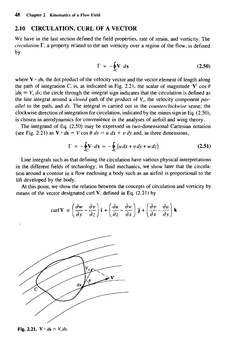
2.10 Circulation, Curl of a Vector 48
2.11 Irrotational Flow 50
2.12 Theorem of Stokes 51
2.13 Velocity Potential 53
2.14 Point Vortex, Vortex Filament, Law of Biot and Savart 57
2.15 Helmholtz's Vortex Theorems 59
2.16 Vortices in Viscous Fluids 61
Chapter 3 • Dynamics of Flow Fields 68
3.1 Introduction 68
3.2 Acceleration of a Fluid Particle 68
3.3 Euler's Equation 72
vii

viii Contents
3.4 Bernoulli's Equation for lrrotational Flow 75
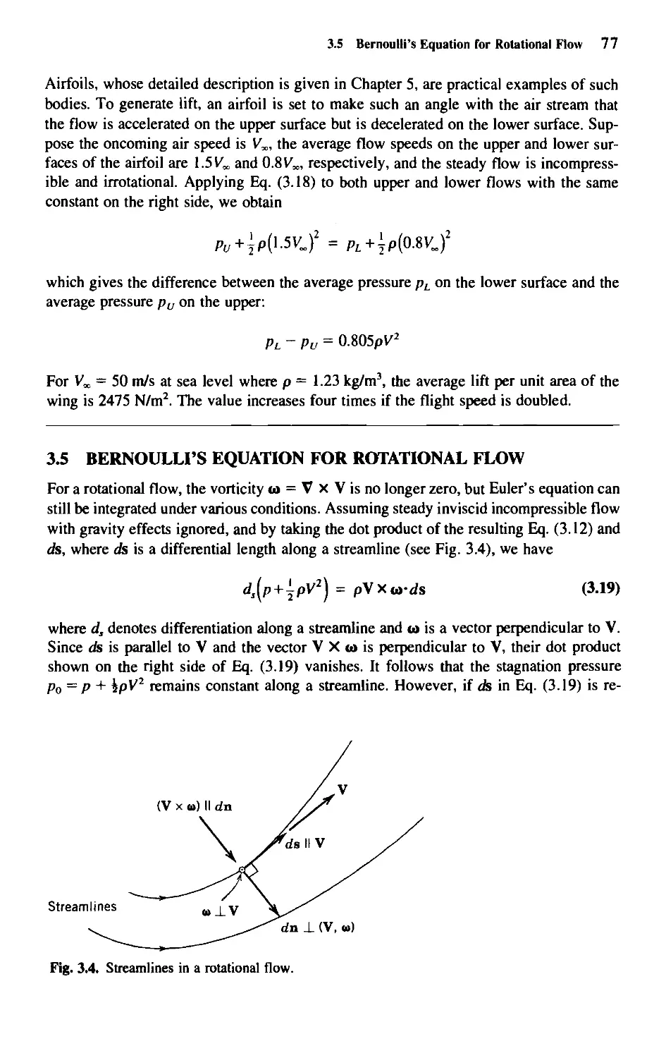
3.5 Bernoulli's Equation for Rotational Flow 77
3.6 Applications of Bernoulli's Equation in Incompressible Flows 79
3.7 The Momentum Theorem of Fluid Mechanics 81
Chapter 4 • lrrotational Incompressible Flow About
Two-Dimensional Bodies 93
4.1 Introduction 93
4.2 Governing Equations and Boundary Conditions 94
4.3 Superposition of Flows 96
4.4 Source in a Uniform Flow 96
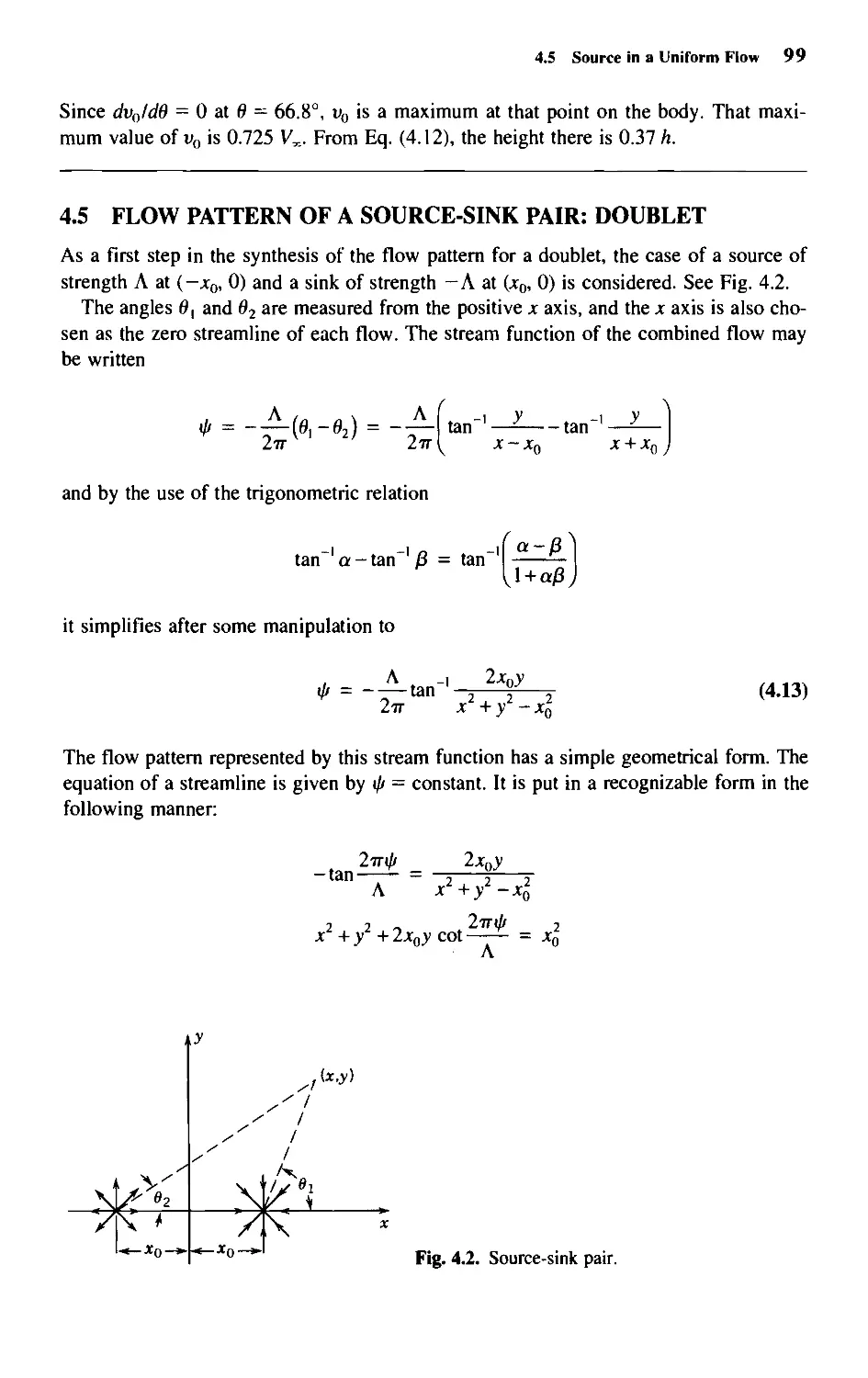
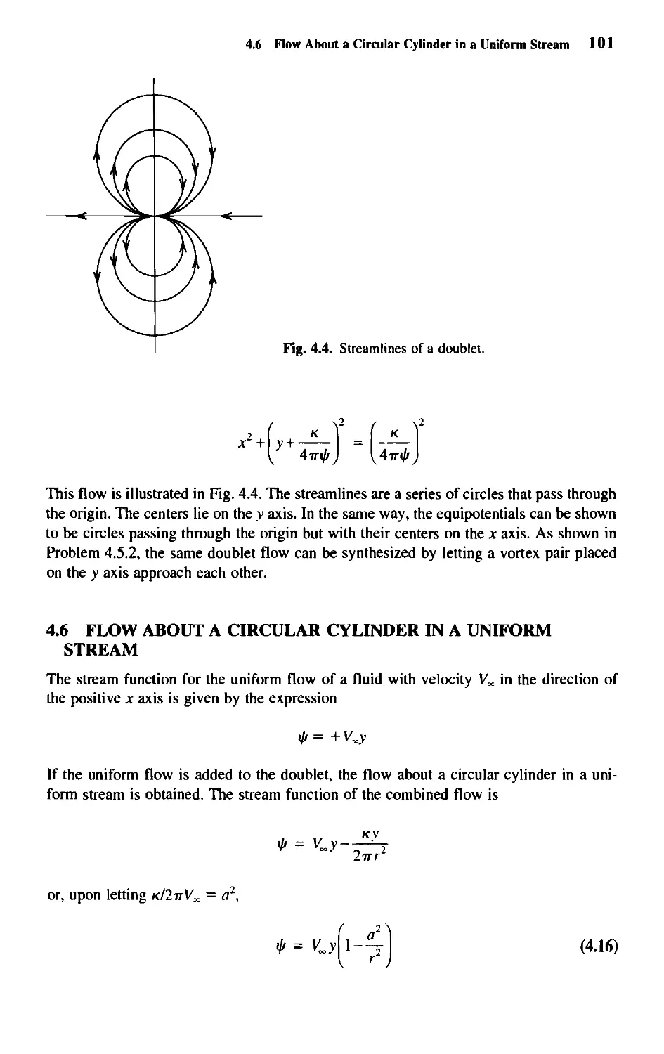
4.5 Flow Pattern of a Source-Sink Pair: Doublet 99
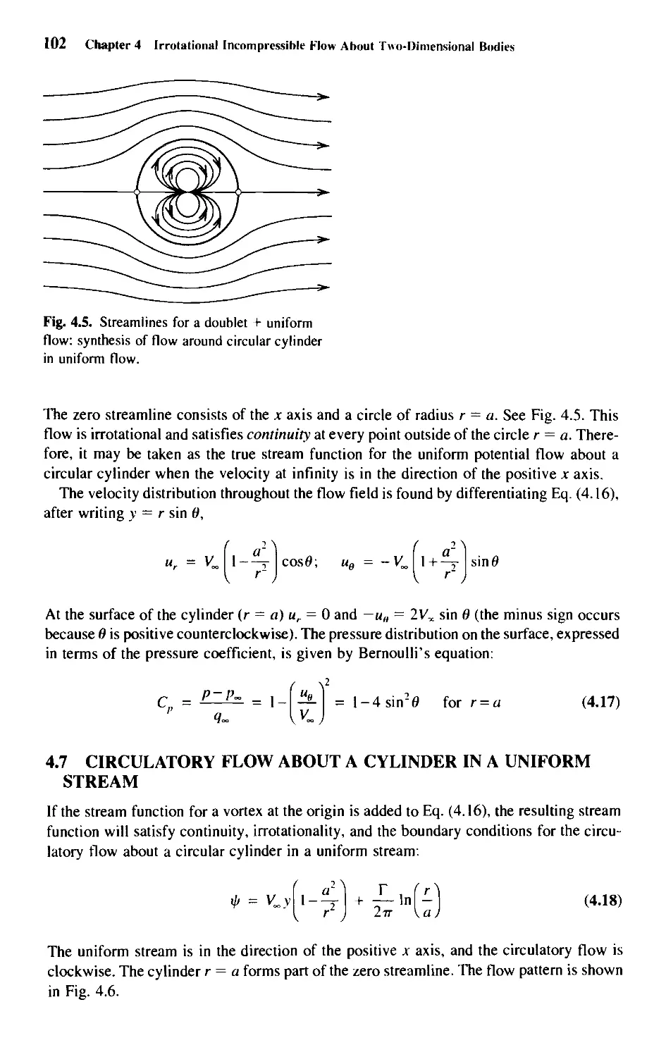
4.6 Flow about a Circular Cylinder in a Uniform Stream 101
4.7 Circulatory Flow about a Cylinder in a Uniform Stream 102
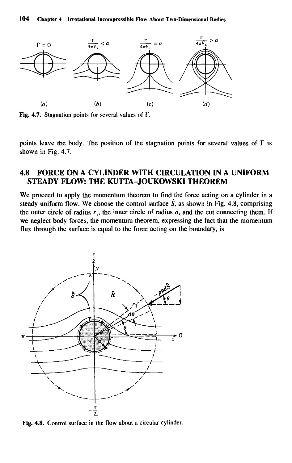
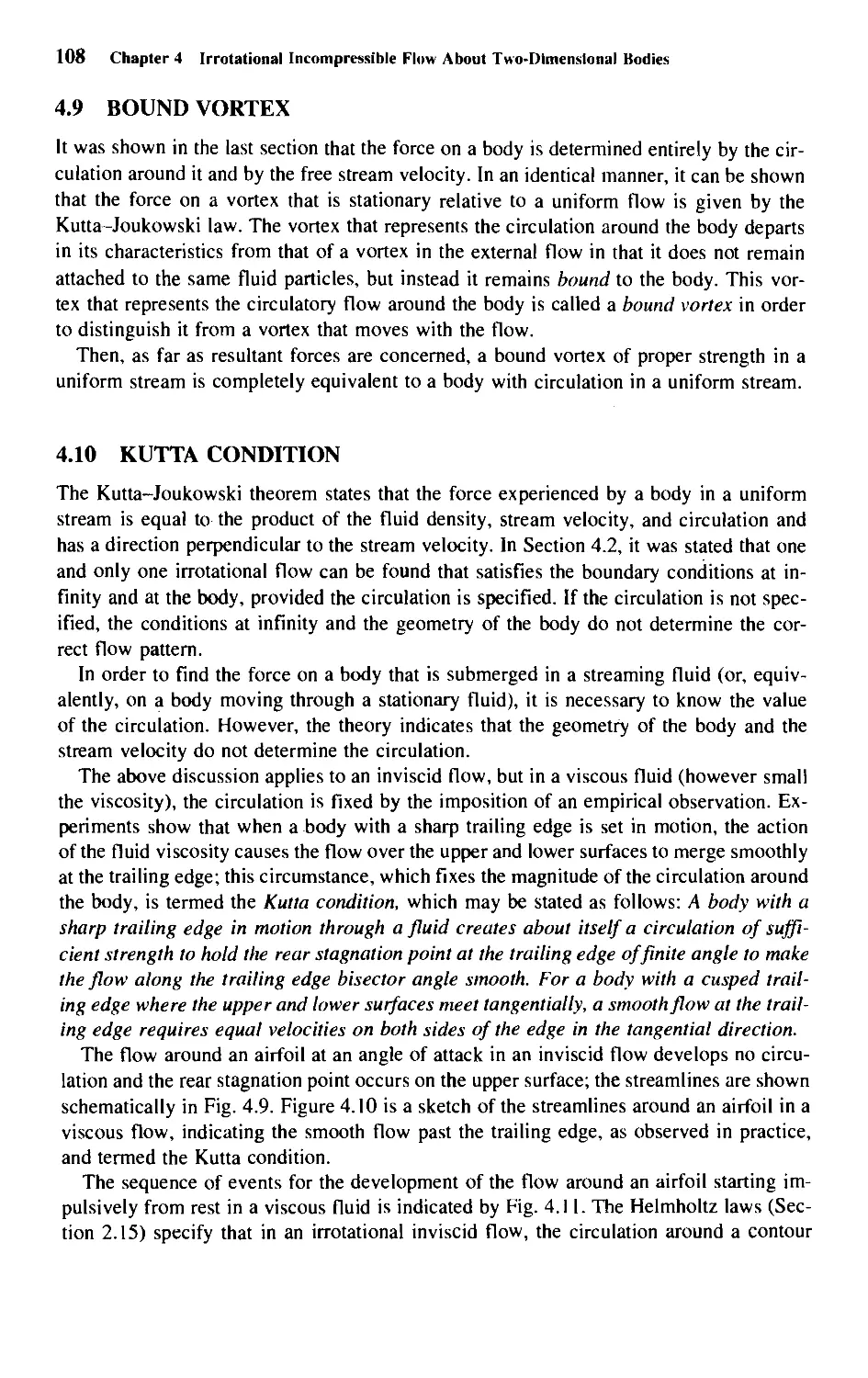
4.8 Force on a Cylinder with Circulation in a Uniform Steady
Flow: The Kutta-Joukowski Theorem 104
4.9 Bound Vortex 108
4.10 Kutta Condition 108
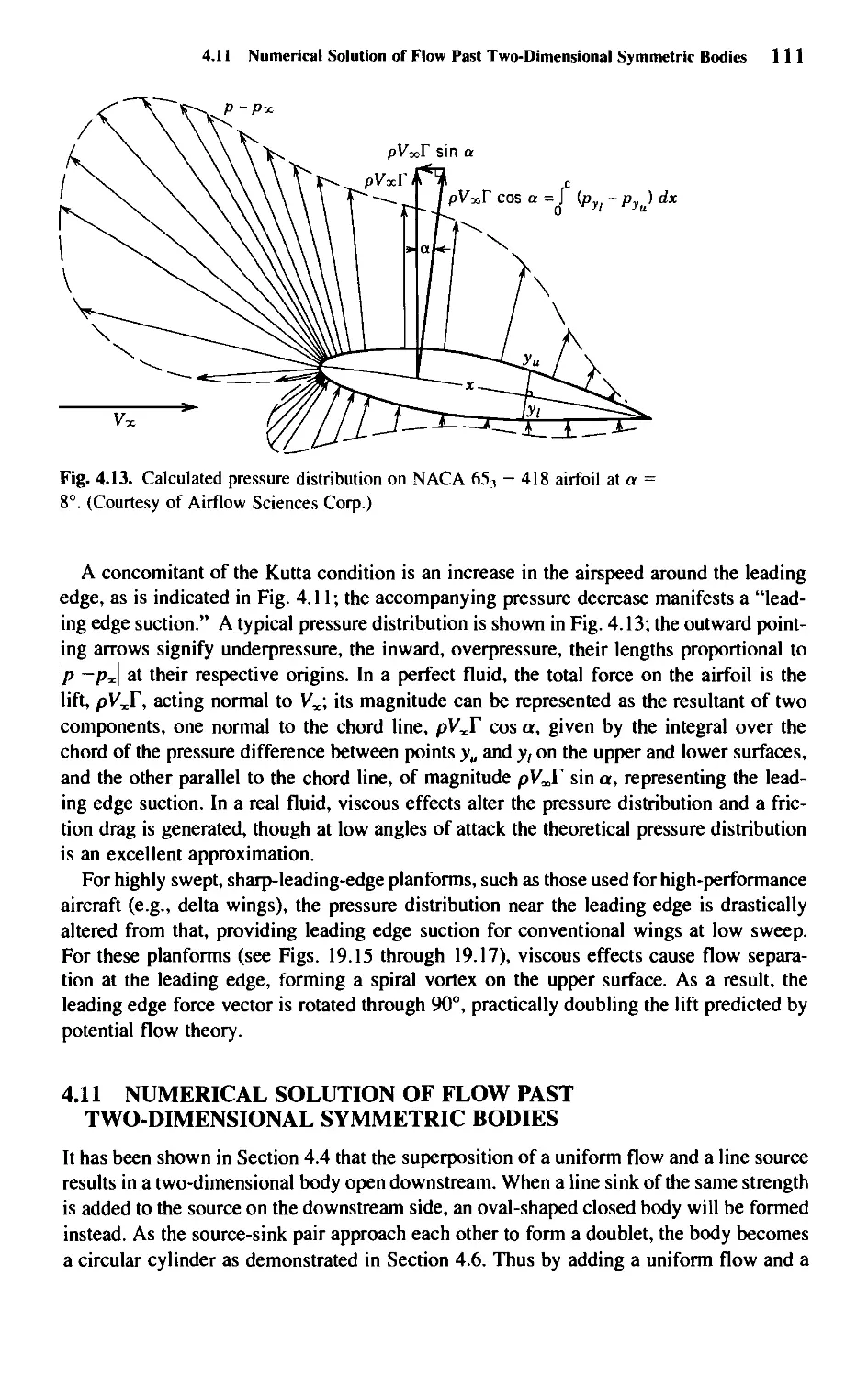
4.11 Numerical Solution of Flow Past Two-Dimensional
Symmetric Bodies 111
4.12 Aerodynamic Interference: Method of Images 115
4.13 The Method of Source Panels 119
Chapter 5 • Aerodynamic Characteristics of Airfoils 132
5.1 Introduction 132
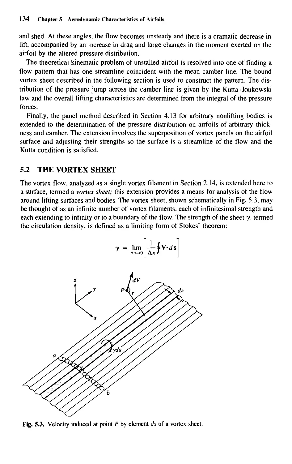
5.2 The Vortex Sheet 134
5.3 The Vortex Sheet in Thin-Airfoil Theory 136
5.4 Planar Wing 138
5.5 Properties of the Symmetrical Airfoil 138
5.6 Vorticity Distribution for the Cambered Airfoil 142
5.7 Properties of the Cambered Airfoil 144
5.8 The Flapped Airfoil 150
5.9 Numerical Solution of the Thin-Airfoil Problem 154
5.10 The Airfoil of Arbitrary Thickness and Camber 156
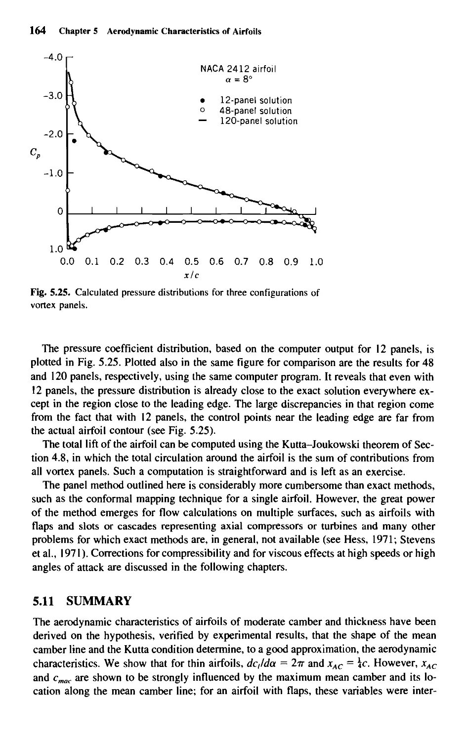
5.11 Summary 164
Chapter 6 • The Finite Wing 169
6.1 Introduction 169
6.2 Flow Fields around Finite Wings 169
6.3 Downwash and Induced Drag 172

Contents IX
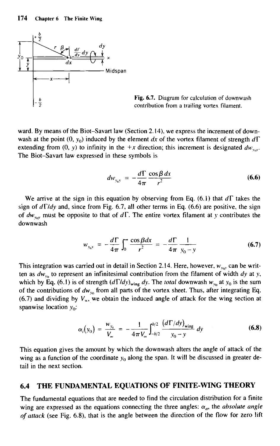
6.4 The Fundamental Equations of Finite-Wing Theory 174
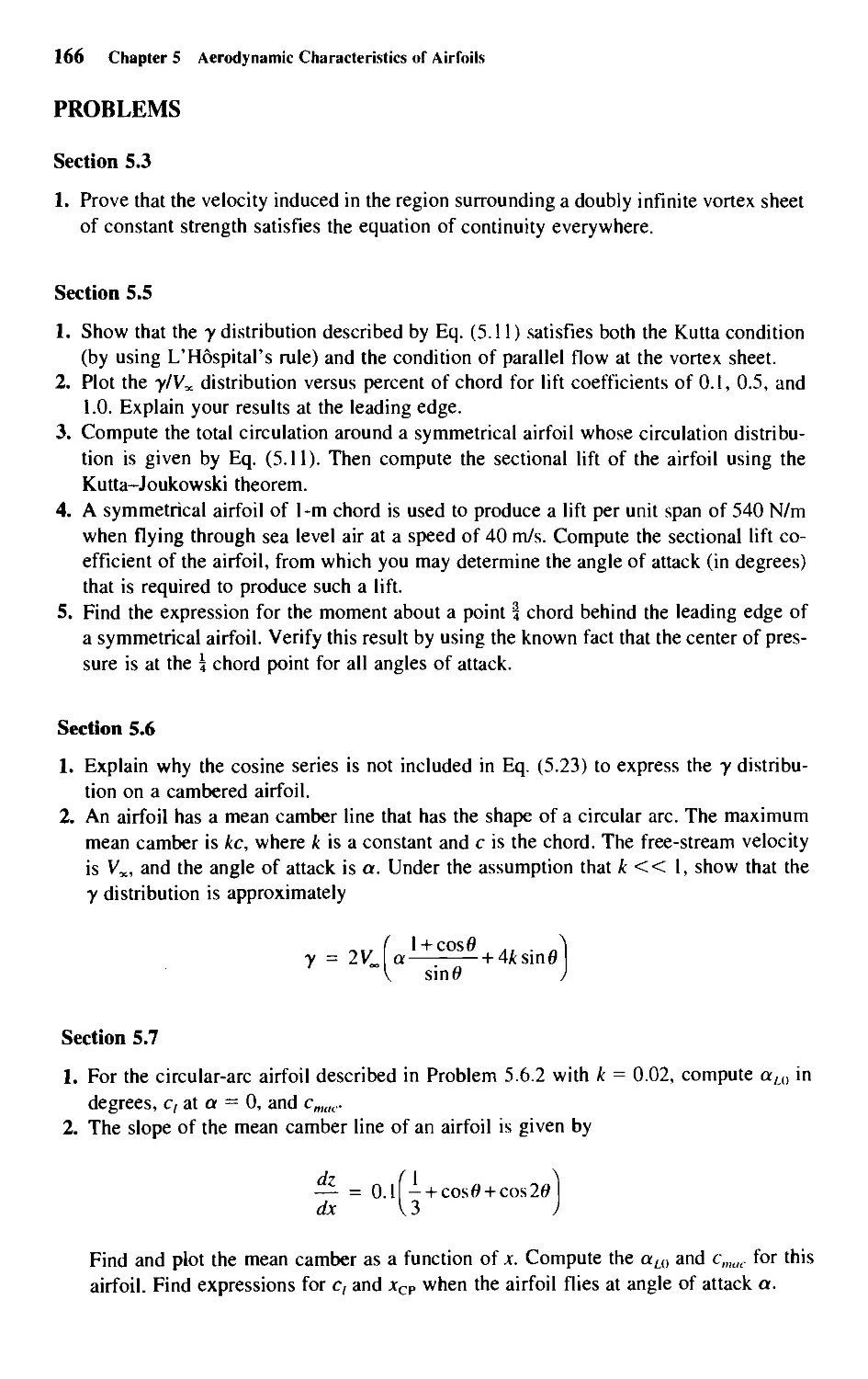
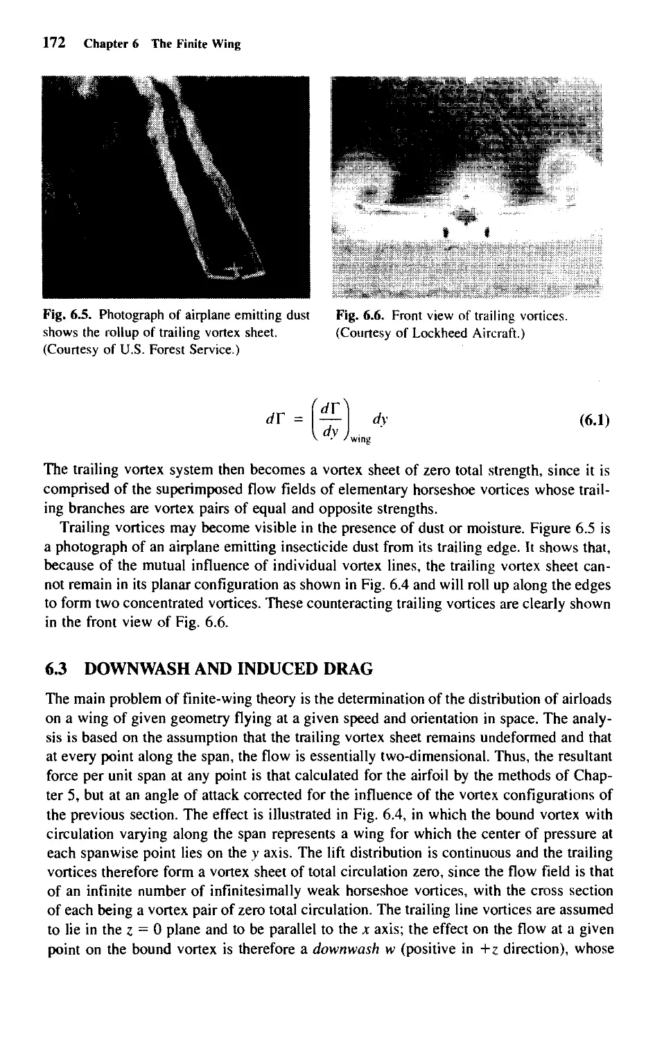
6.5 The Elliptical Lift Distribution 176
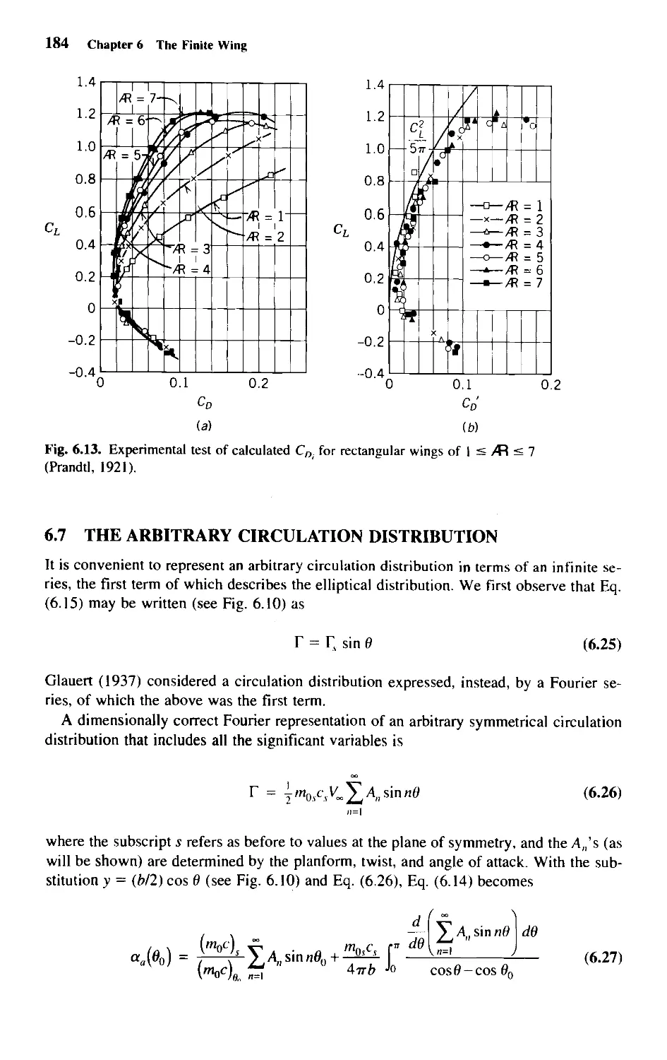
6.6 Comparison with Experiment 182
6.7 The Arbitrary Circulation Distribution 184
6.8 The Twisted Wing: Basic and Additional Lift 188
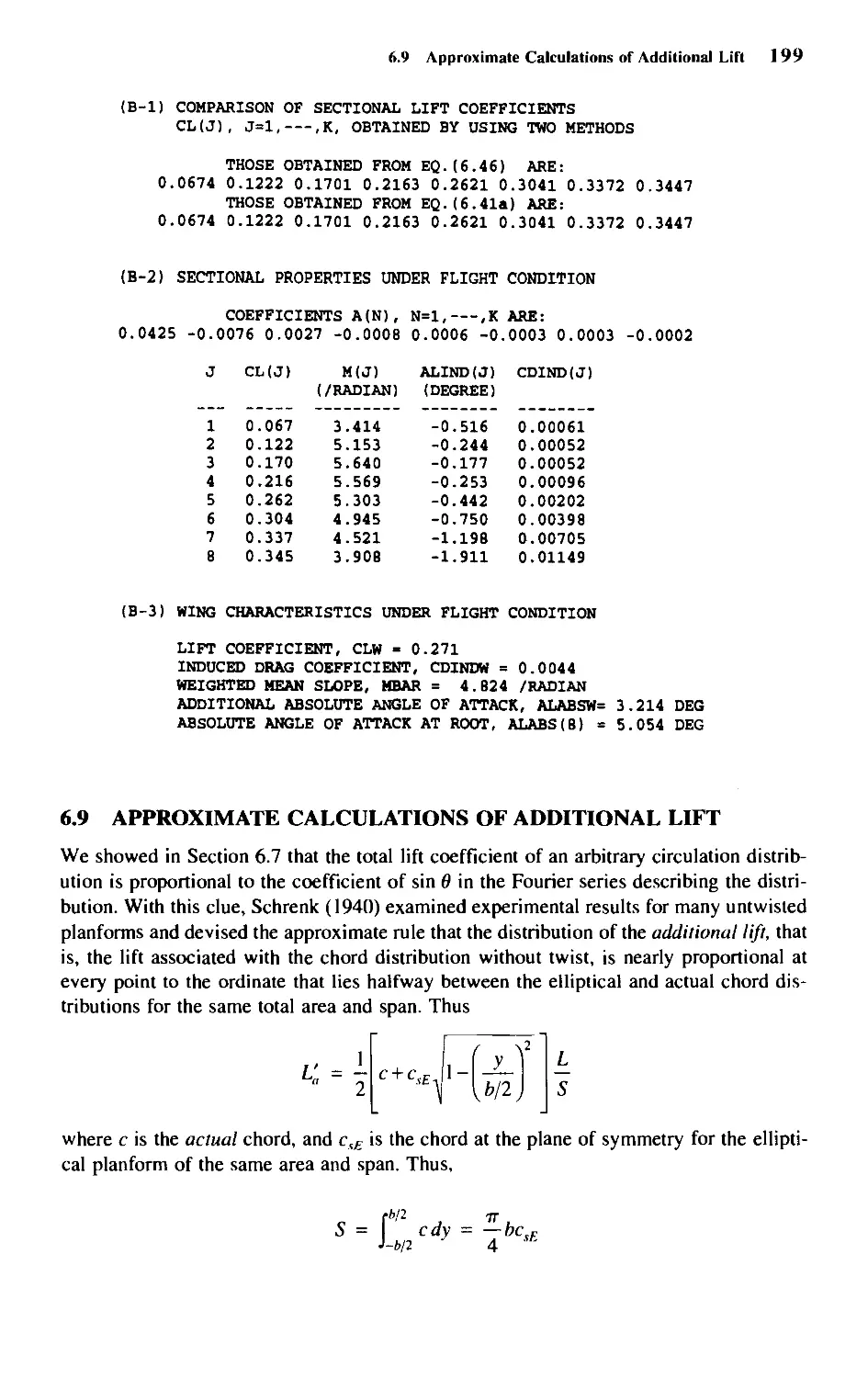
6.9 Approximate Calculations of Additional Lift 199
6.10 Winglets 200
6.11 Other Characteristics of a Finite Wing 202
6.12 Stability and Trim of Wings 203
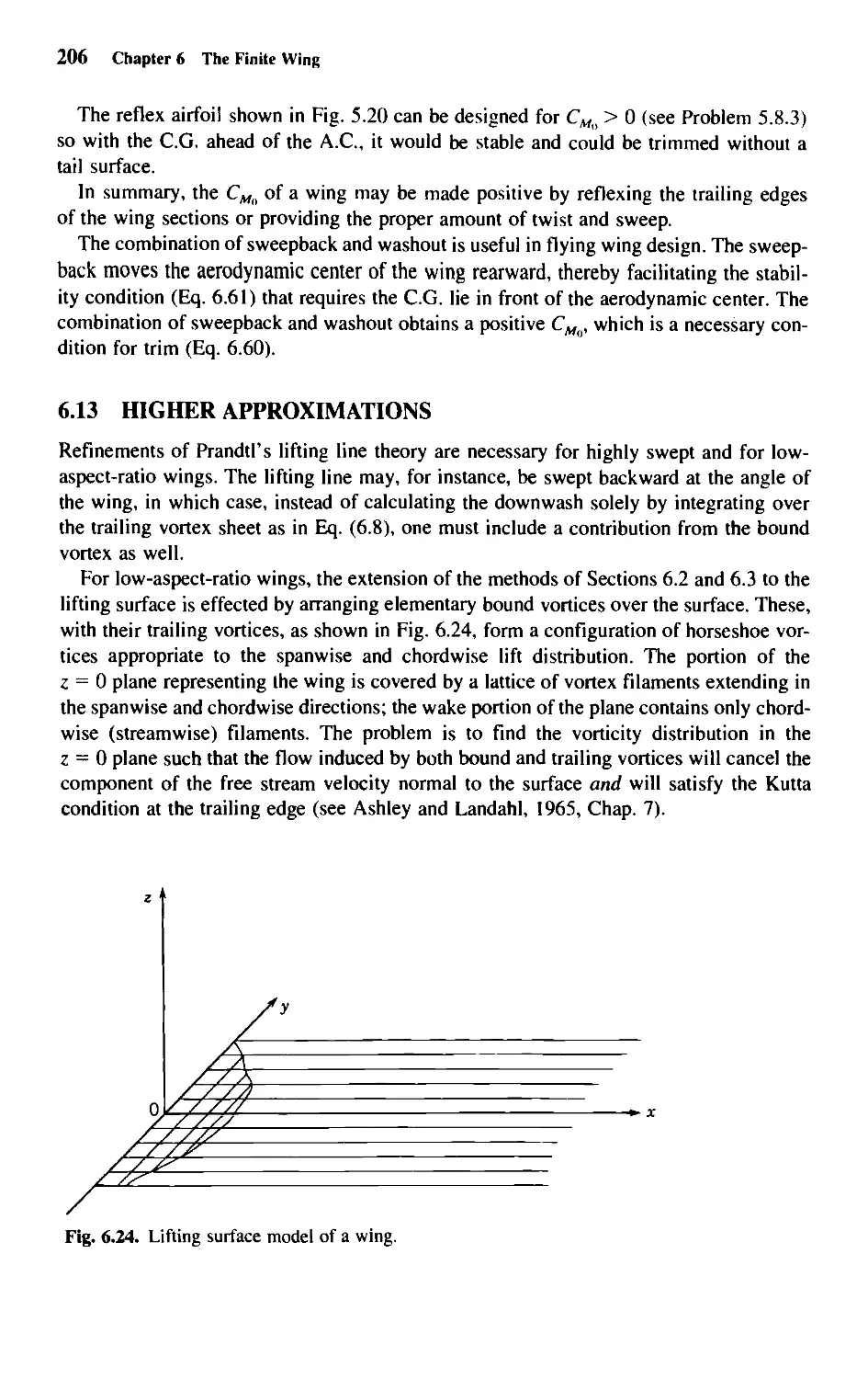
6.13 Higher Approximations 206
6.14 The Complete Airplane 207
6.15 Interference Effects 207
6.16 Concluding Remarks 210
Chapter 7 • Introduction to Compressible Fluids 220
7.1 Scope 220
7.2 Equation of Continuity: Stream Function 221
7.3 Irrotationality. Velocity Potential 222
7.4 Equation of Equilibrium: Bernoulli's Equation 222
7.5 Criterion for Superposition of Compressible Flows 223
Chapter 8 • Energy Relations 225
8.1 Introduction 225
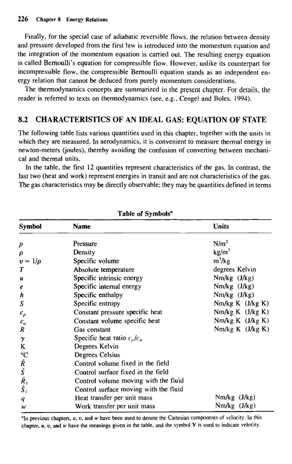
8.2 Characteristics of an Ideal Gas: Equation of State 226
8.3 First Law of Thermodynamics 229
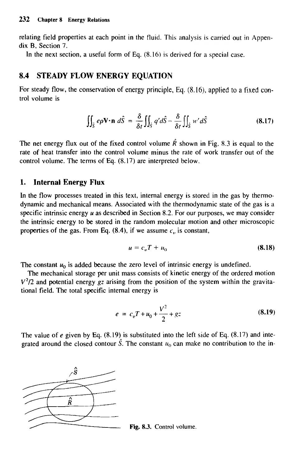
8.4 Steady Flow Energy Equation 232
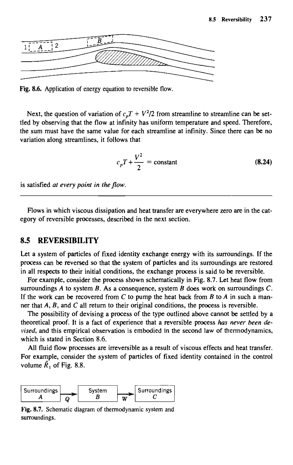
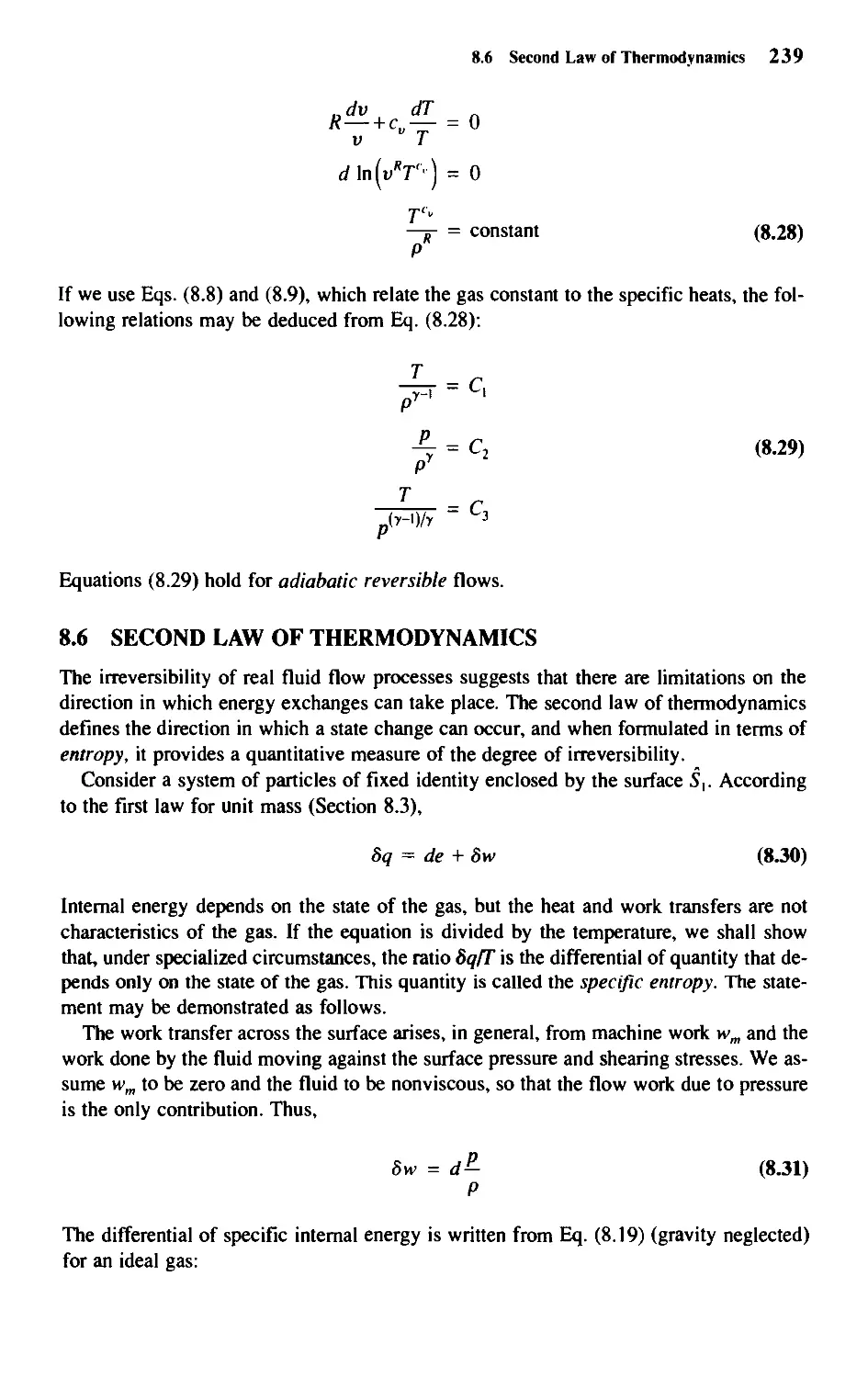
8.5 Reversibility 237
8.6 Second Law of Thermodynamics 239
8.7 Bernoulli's Equation for Isentropic Compressible Flow 241
8.8 Static and Stagnation Values 242
Chapter 9 • Some Applications of One-Dimensional
Compressible Flow 246
9.1 Introduction 246
9.2 Speed of Sound 246
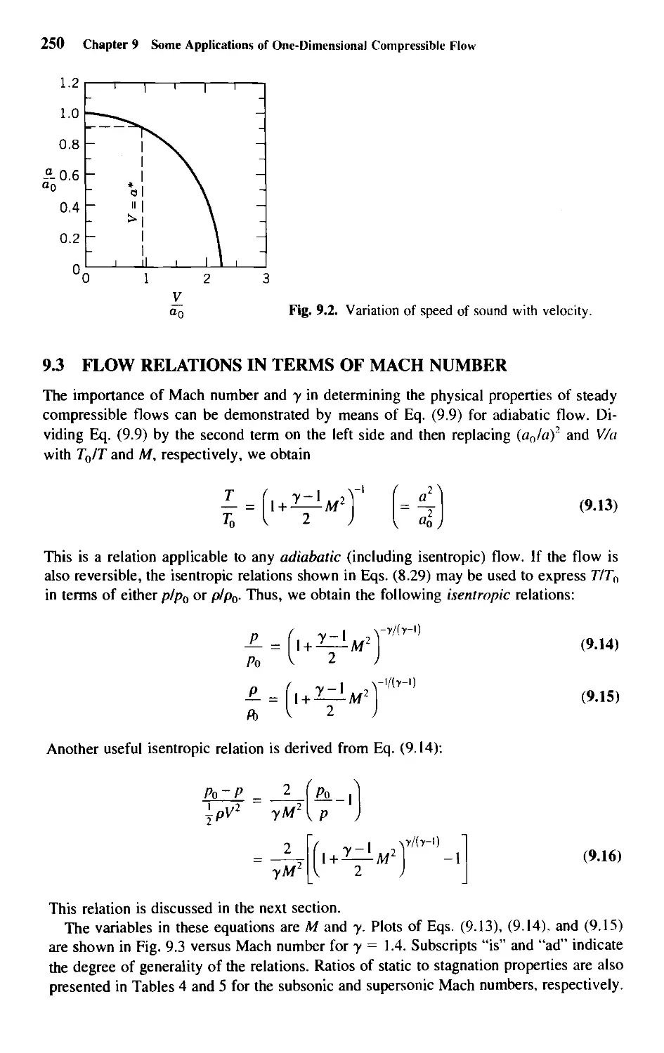
9.3 Flow Relations in Terms of Mach Number 250
9.4 Measurement of Flight Speed (Subsonic) 252
9.5 Isentropic One-Dimensional Flow 252
9.6 The Laval Nozzle 255

X Contents
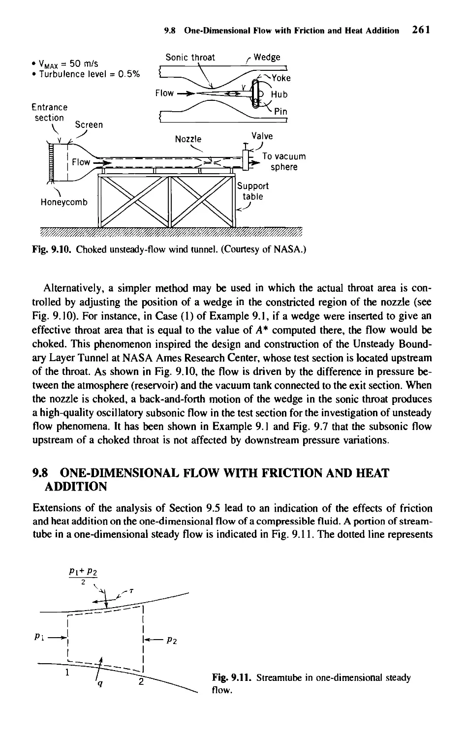
9.7 Supersonic Wind Tunnels
9.8 One-Dimensional Flow with Friction and Heat Addition
9.9 Heat Addition to a Constant-Area Duct
259
261
263
Chapter 10 • Waves
270
10.1 Establishment of a Flow Field
10.2 Mach Waves
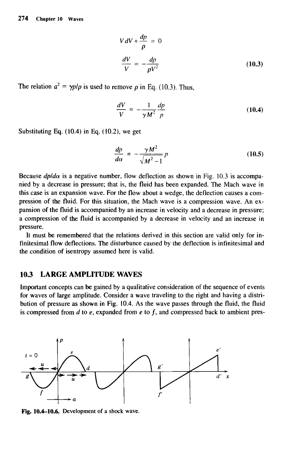
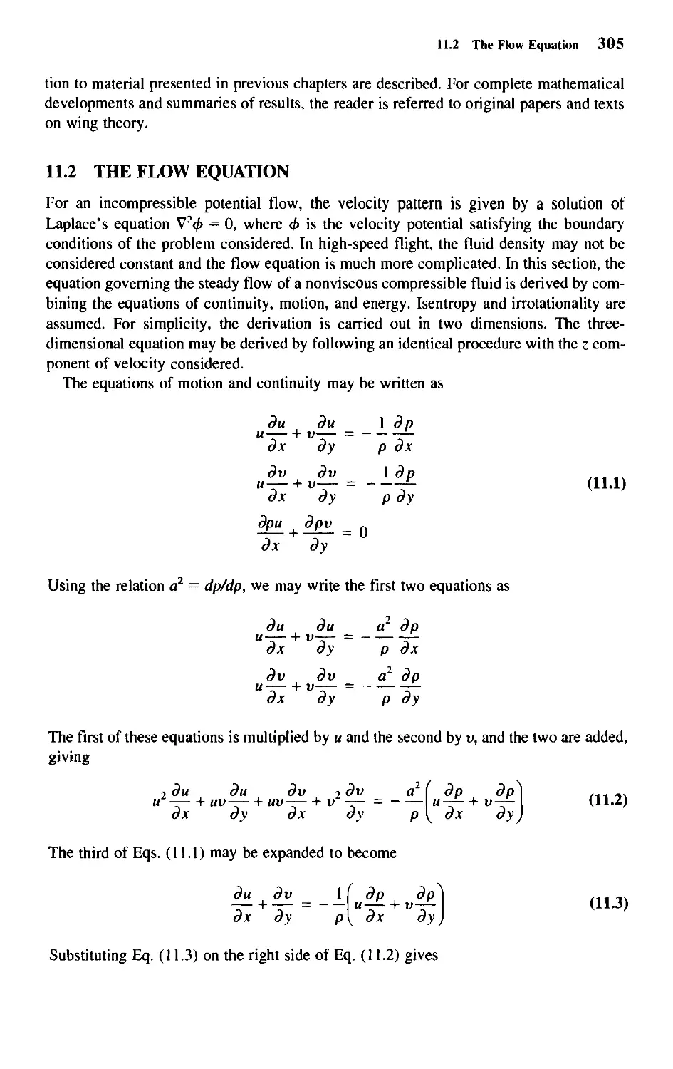
10.3 Large Amplitude Waves
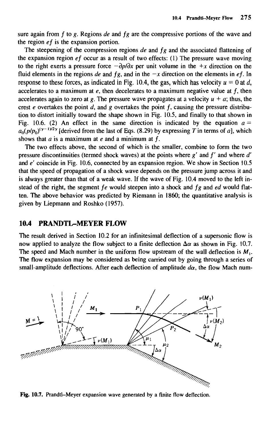
10.4 Prandtl-Meyer Flow
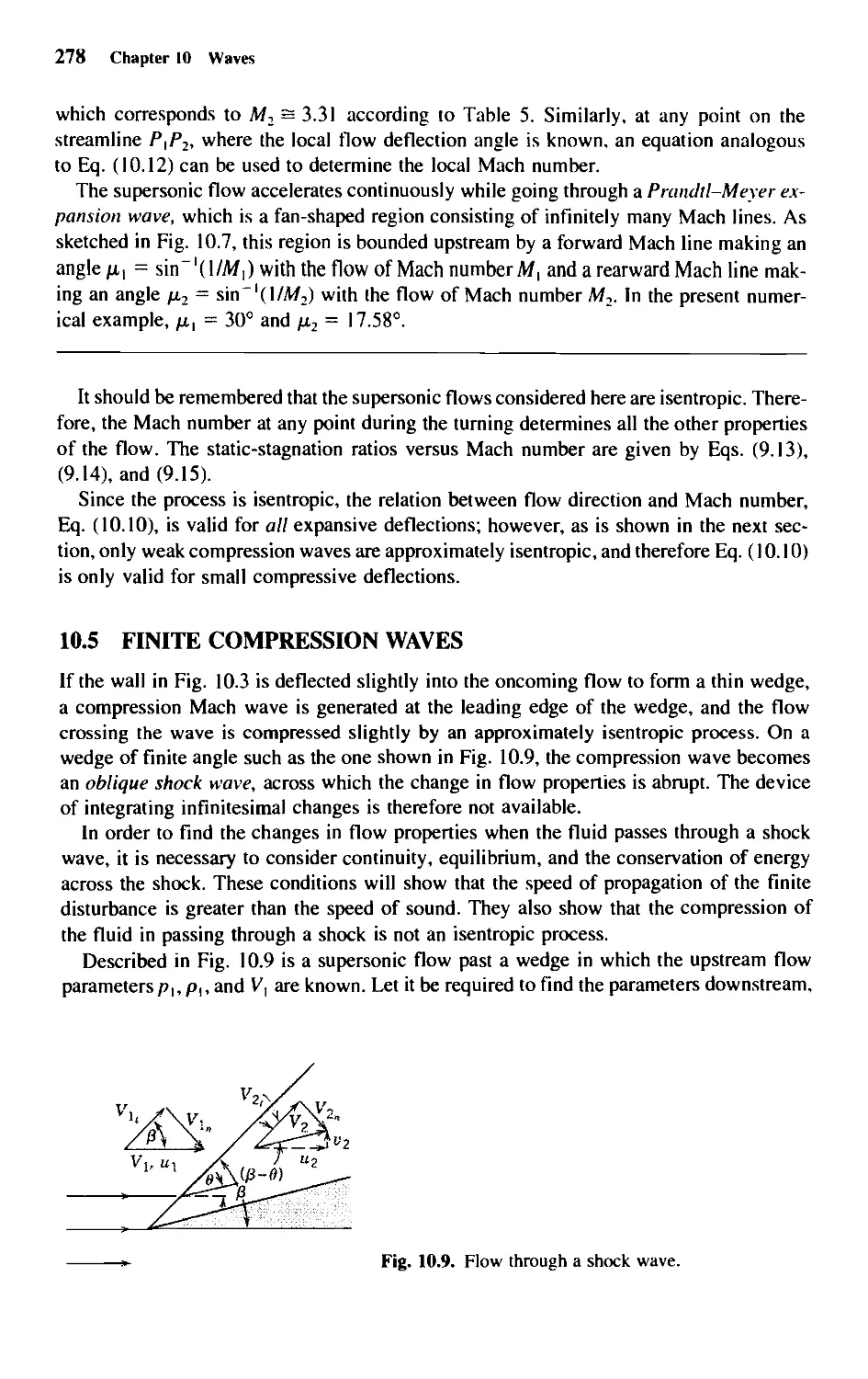
10.5 Finite Compression Waves
10.6 The Characteristic Ratios as Functions of Mach Number
10.7 Normal Shock Wave
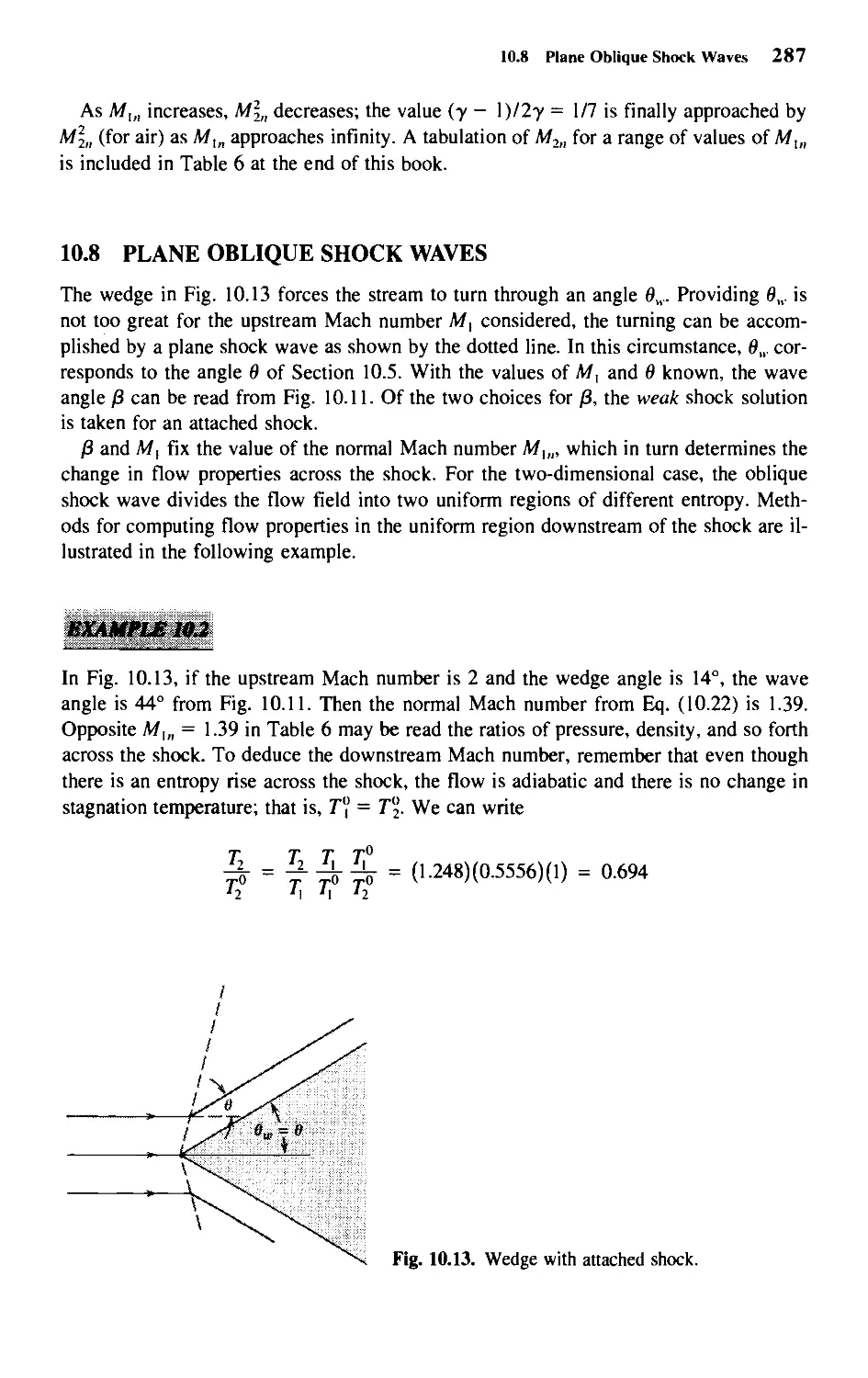
10.8 Plane Oblique Shock Waves
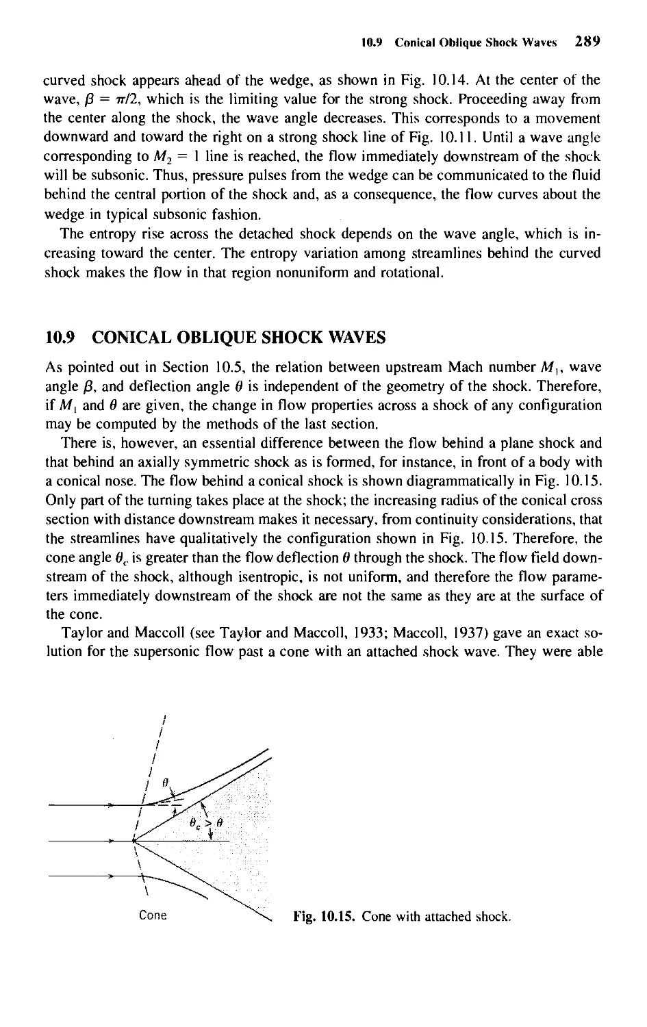
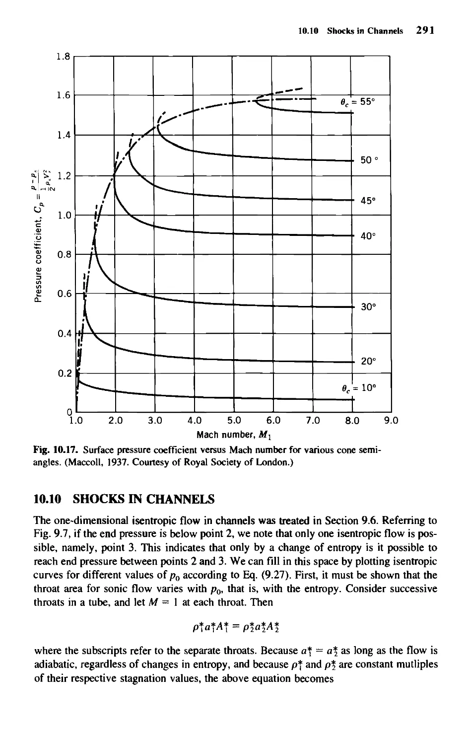
10.9 Conical Oblique Shock Waves
10.10 Shocks in Channels
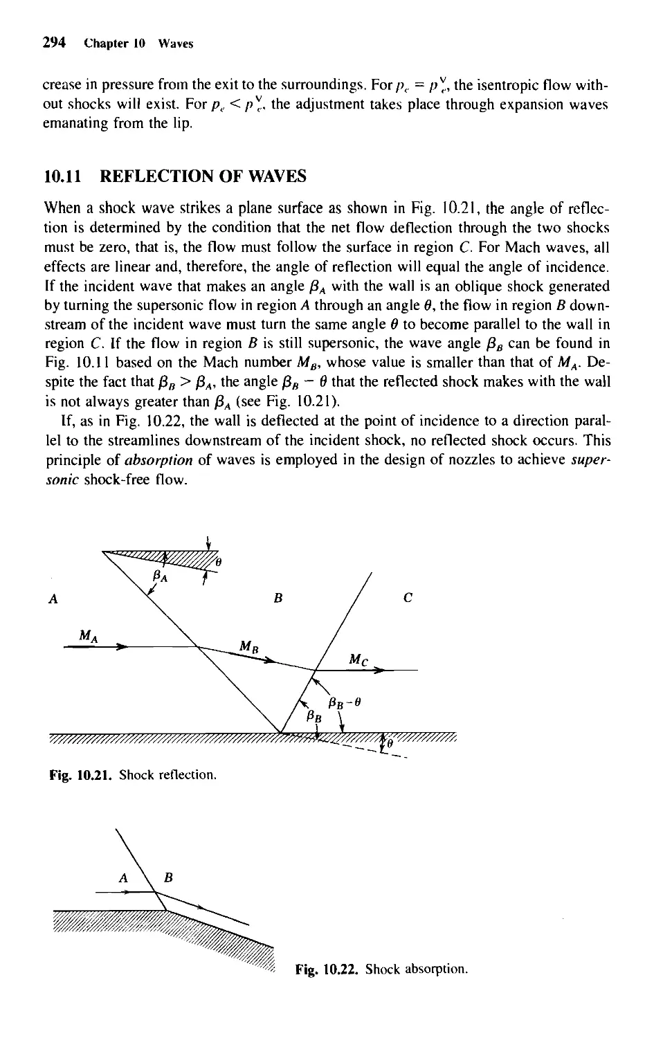
10.11 Reflection of Waves
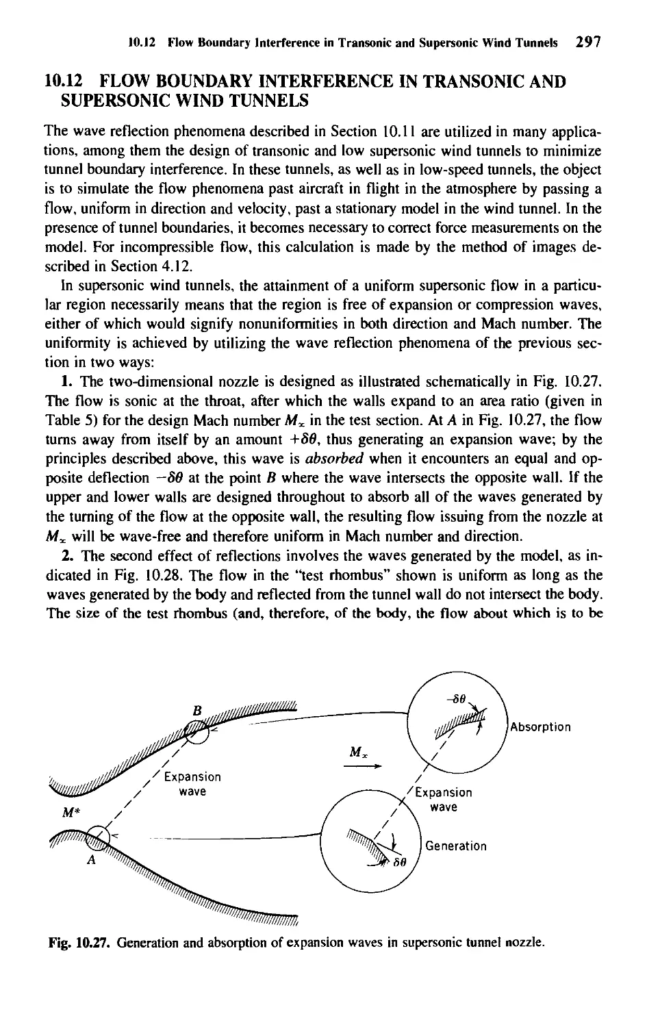
10.12 Flow Boundary Interference in Transonic and Supersonic
Wind Tunnels
270
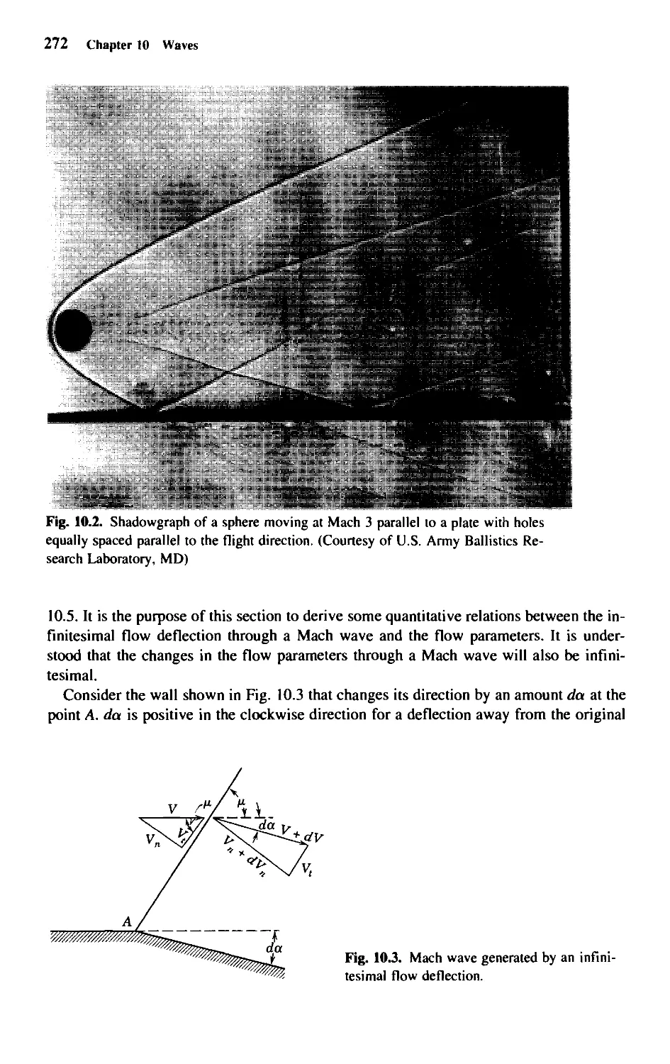
271
274
275
278
283
286
287
289
291
294
297
Chapter 11 • Linearized Compressible Flow
304
1.1 Introduction
1.2 The Flow Equation
1.3 Flow Equation for Small Perturbations
1.4 Steady Supersonic Flows
1.5 Pressure Coefficient for Small Perturbations
1.6 Summary
304
305
306
308
310
311
Chapter 12 • Airfoils in Compressible Flows
313
12.1 Introduction 313
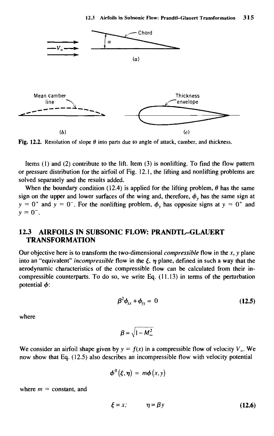
12.2 Boundary Conditions 313
12.3 Airfoils in Subsonic Flow: Prandtl-Glauert Transformation 315
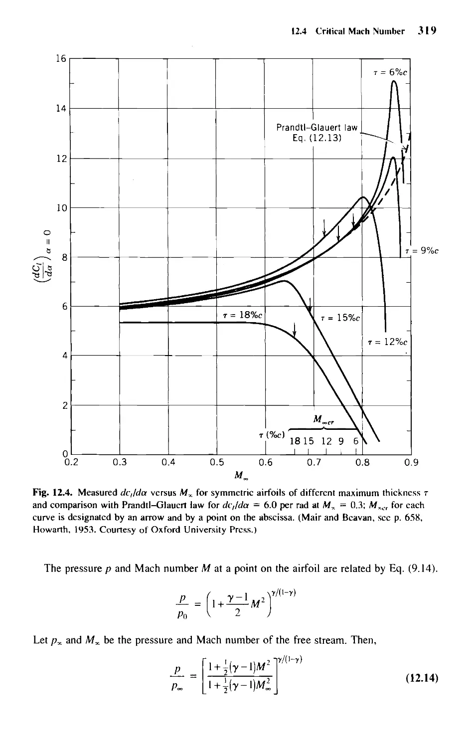
12.4 Critical Mach Number 318
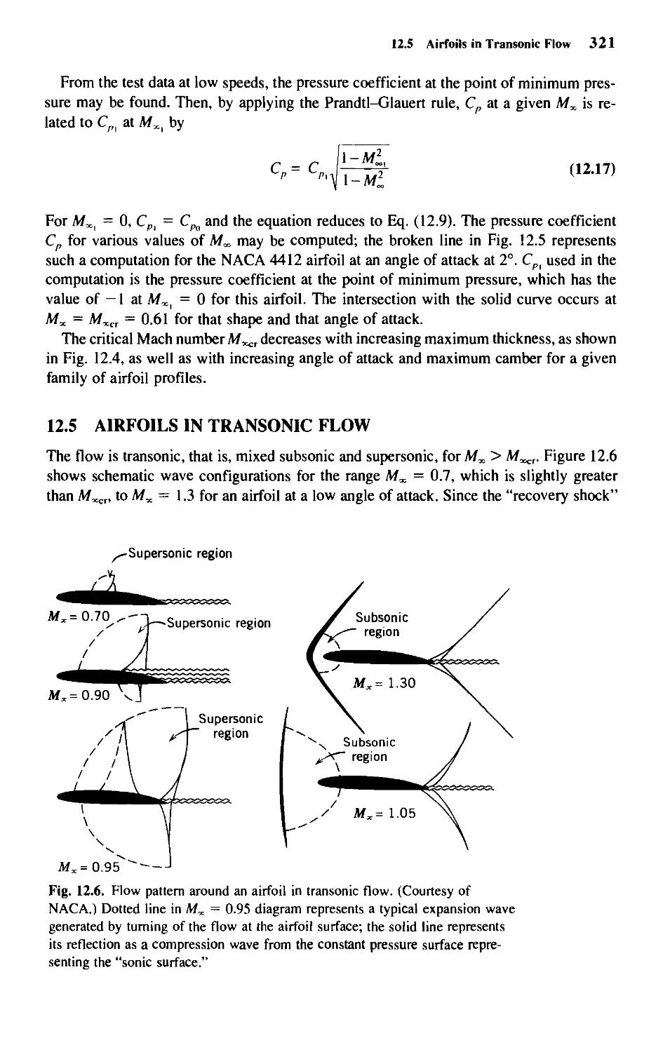
12.5 Airfoils in Transonic Flow 321
12.6 Airfoils in Supersonic Flow 324
Chapter 13 • Wings and Wing-Body Combinations
in Compressible Flow 332
13.1 Introduction 332
13.2 Wings and Bodies in Compressible Flows: The Prandtl-Glauert-
Goethert Transformation 332

Contents XI
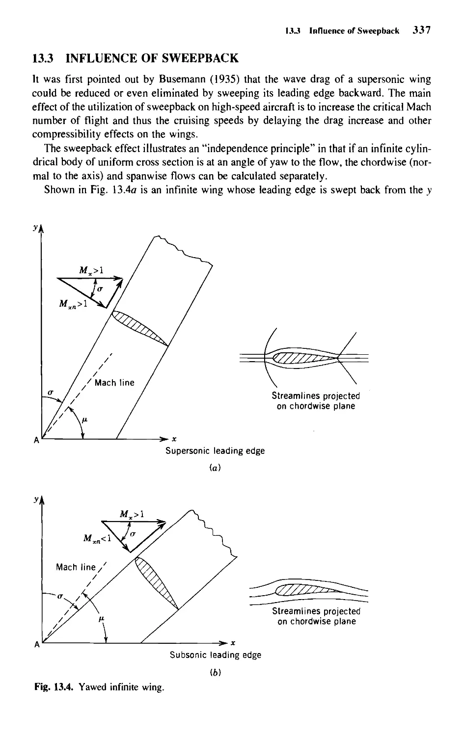
13.3 Influence of Sweepback 337
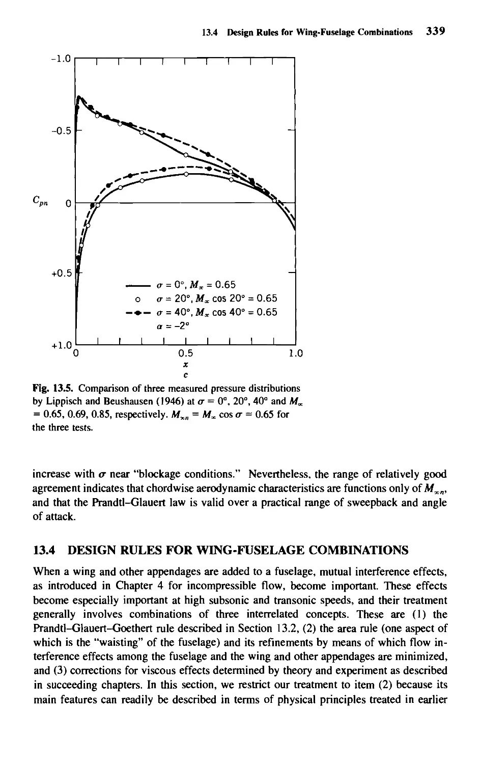
13.4 Design Rules for Wing-Fuselage Combinations 339
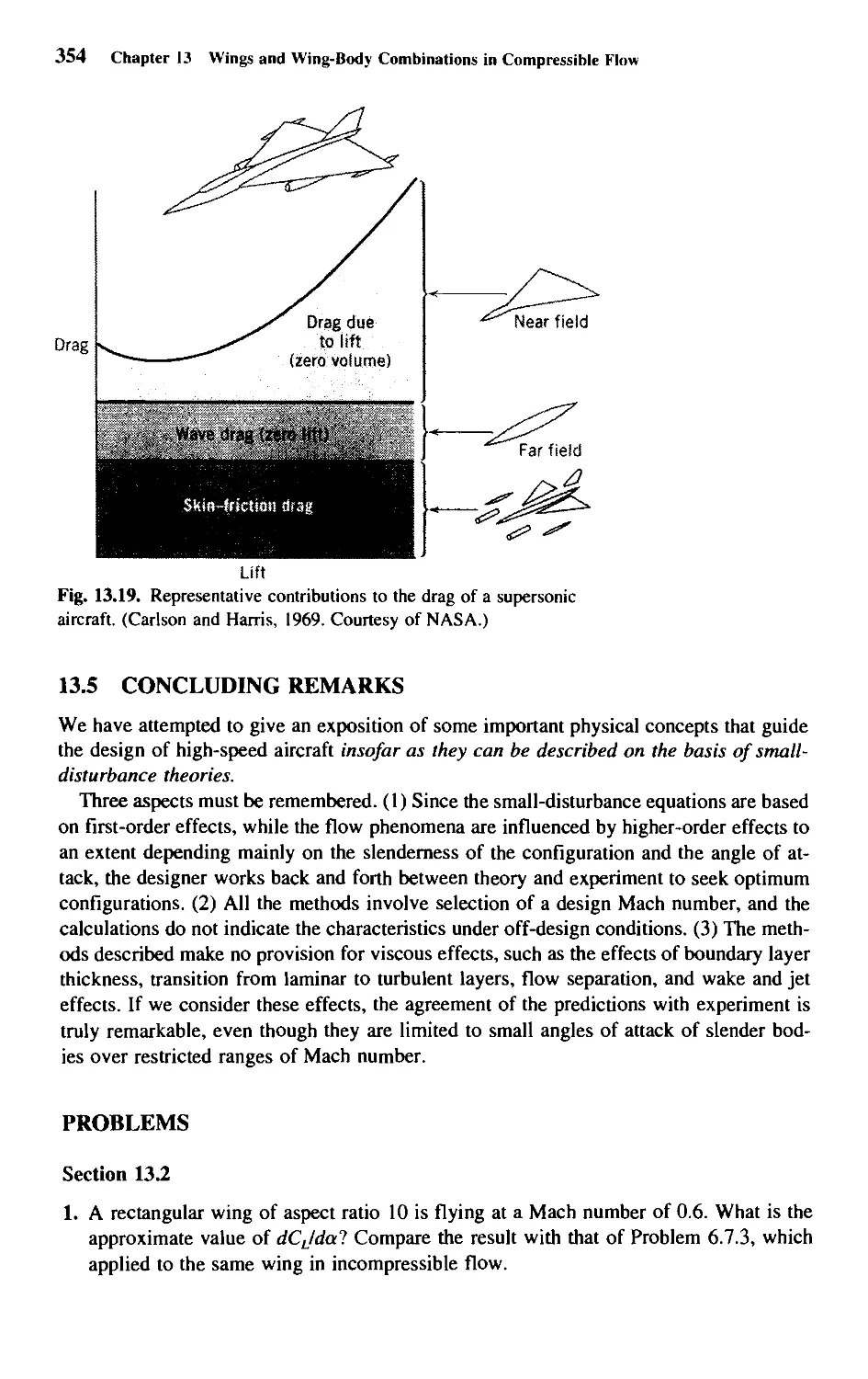
13.5 Concluding Remarks 354
Chapter 14 • The Dynamics of Viscous Fluids 357
14.1 Introduction 357
14.2 The No-Slip Condition 358
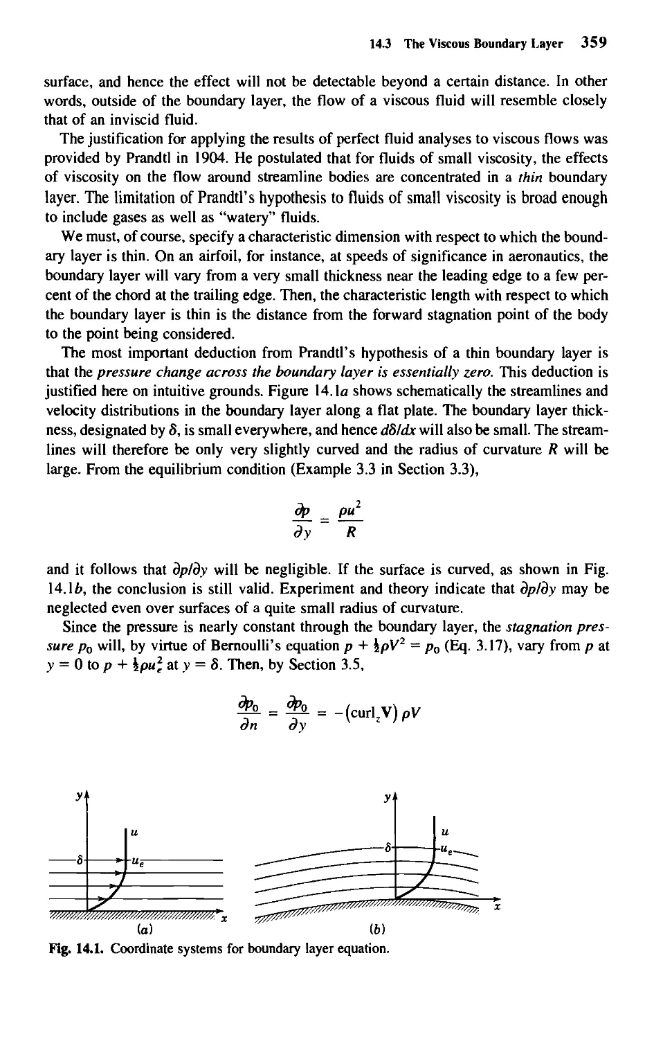
14.3 The Viscous Boundary Layer 358
14.4 Viscous Stresses 360
14.5 Boundary Layer Equation of Motion 361
14.6 Similarity in Incompressible Flows 362
14.7 Physical Interpretation of Reynolds Number 364
Chapter 15 • Incompressible Laminar Flow in Tubes
and Boundary Layers 367
15.1 Introduction 367
15.2 Laminar Flow in a Tube 367
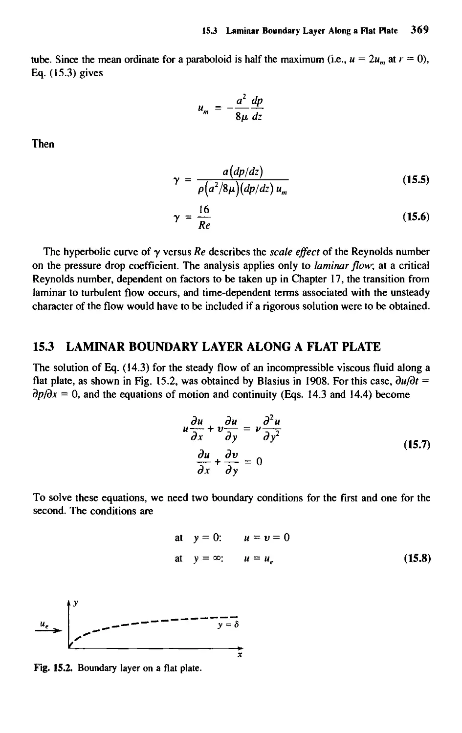
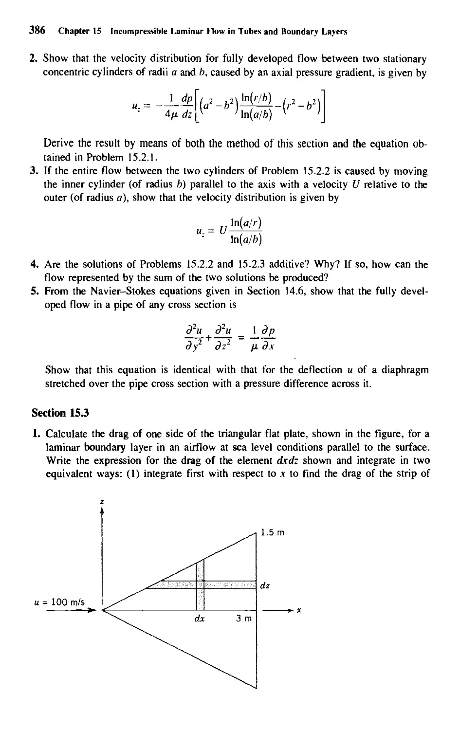
15.3 Laminar Boundary Layer along a Flat Plate 369
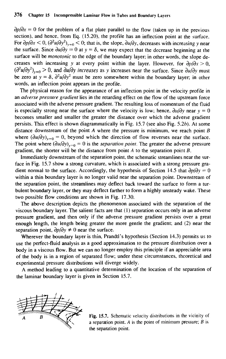
15.4 Effect of Pressure Gradient: Flow Separation 375
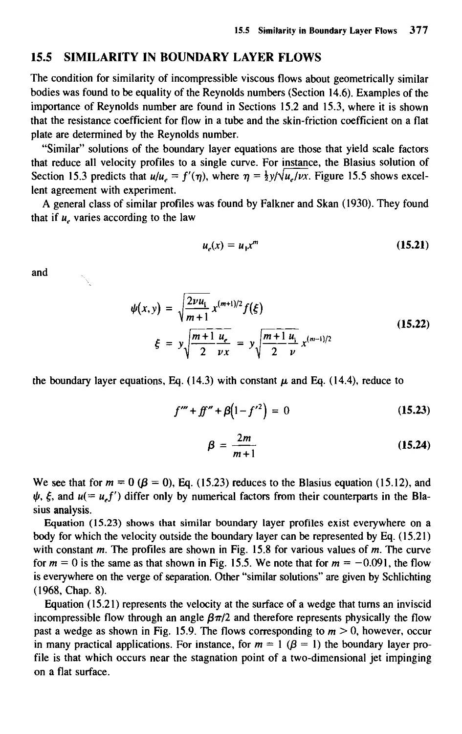
15.5 Similarity in Boundary Layer Flows 377
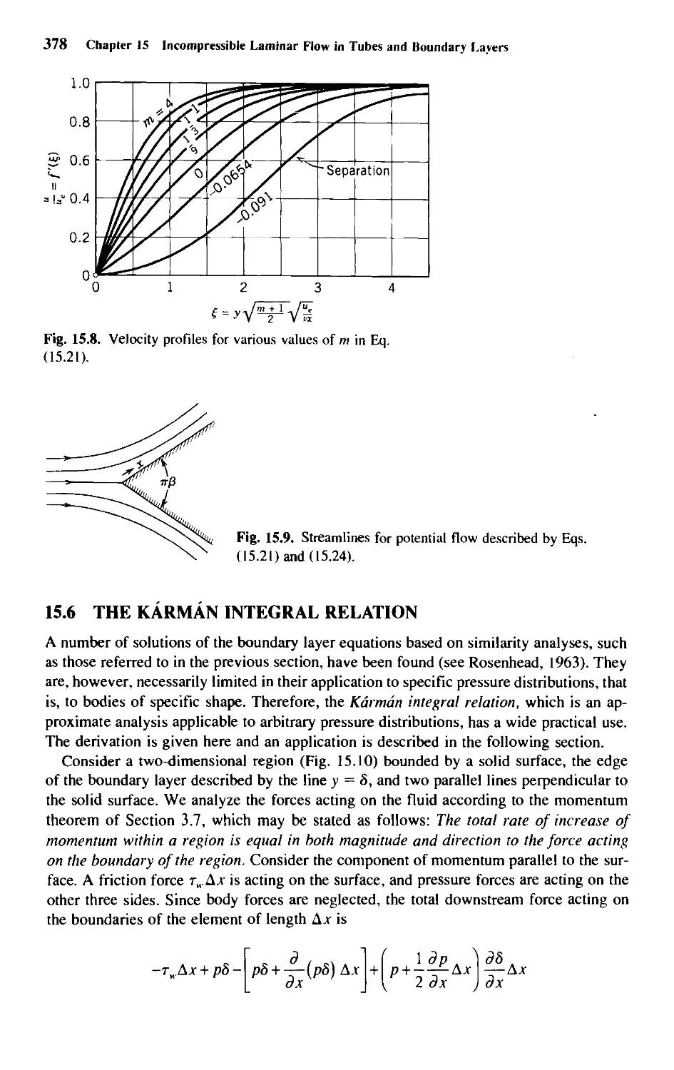
15.6 The Karman Integral Relation 378
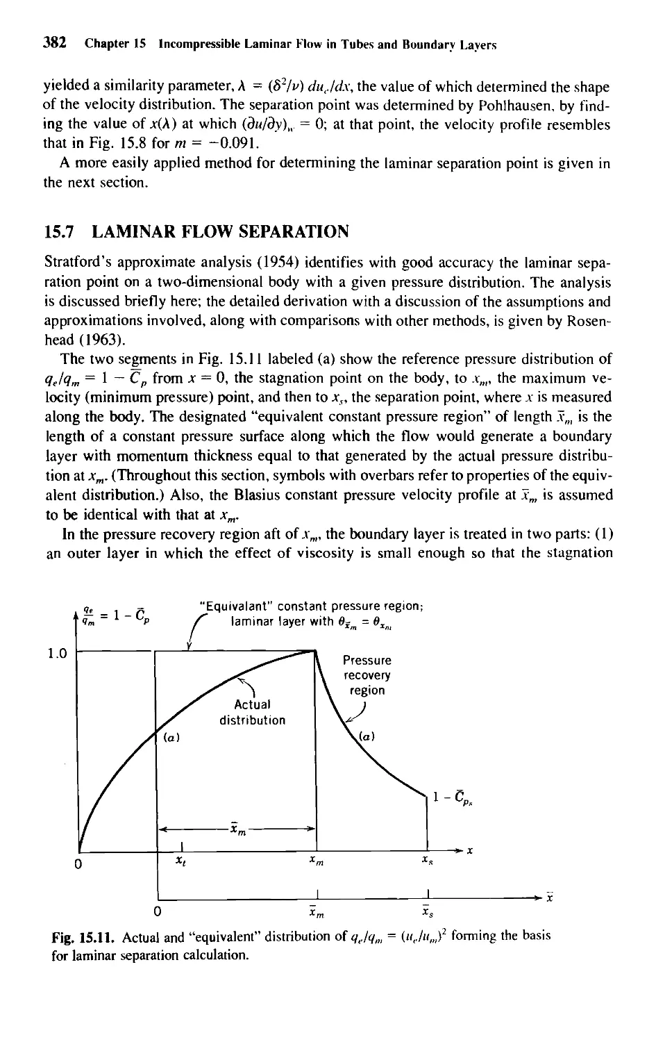
15.7 Laminar Flow Separation 382
Chapter 16 • Laminar Boundary Layer in Compressible Flow 390
16.1 Introduction 390
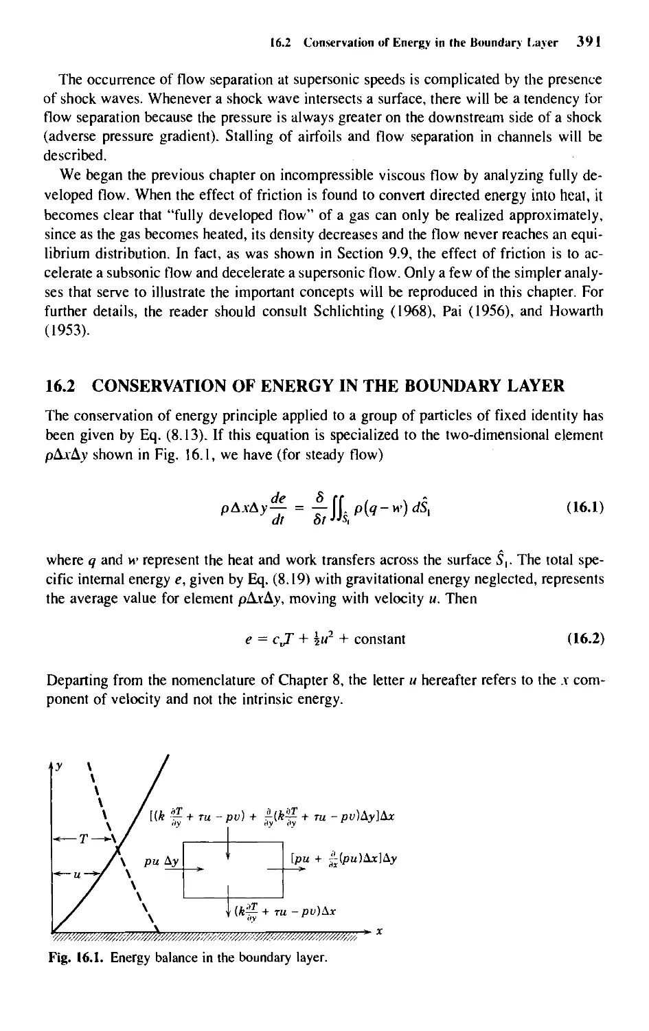
16.2 Conservation of Energy in the Boundary Layer 391
16.3 Rotation and Entropy Gradient in the Boundary Layer 393
16.4 Similarity Considerations for Compressible Boundary Layers 394
16.5 Solutions of the Energy Equation for Prandtl Number Unity 395
16.6 Temperature Recovery Factor 399
16.7 Heat Transfer versus Skin Friction 402
16.8 Velocity and Temperature Profiles and Skin Friction 405
16.9 Effects of Pressure Gradient 407
Chapter 17 • Flow Instabilities and Transition from
Laminar to Turbulent Flow 413
17.1 Introduction
17.2 Gross Effects
413
414

xii Contents
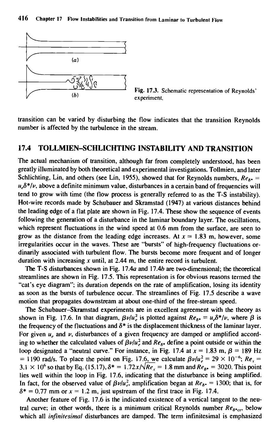
17.3 Reynolds Experiment 415
17.4 Tollmien-Schlichting Instability and Transition 416
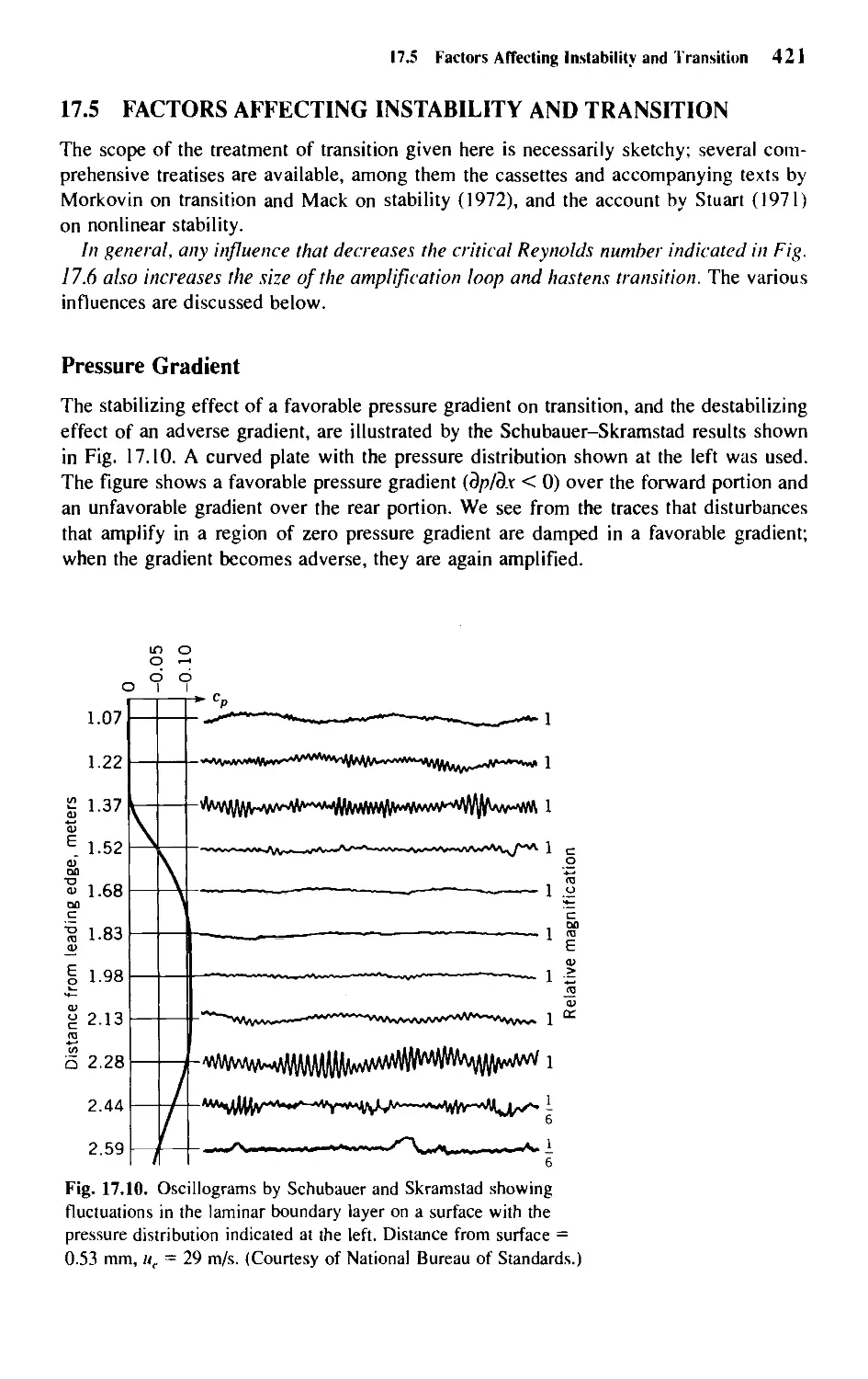
17.5 Factors Affecting Instability and Transition 421
17.6 Natural Laminar Flow and Laminar Flow Control 432
17.7 Stratified Flows 433
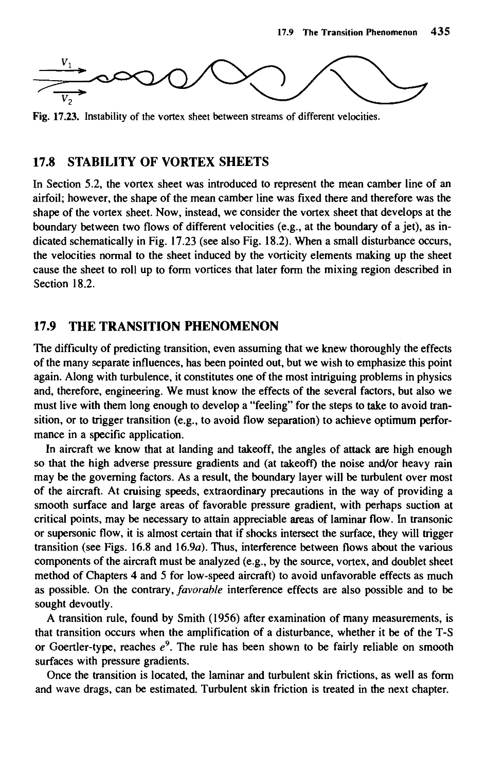
17.8 Stability of Vortex Sheets 435
17.9 The Transition Phenomenon 435
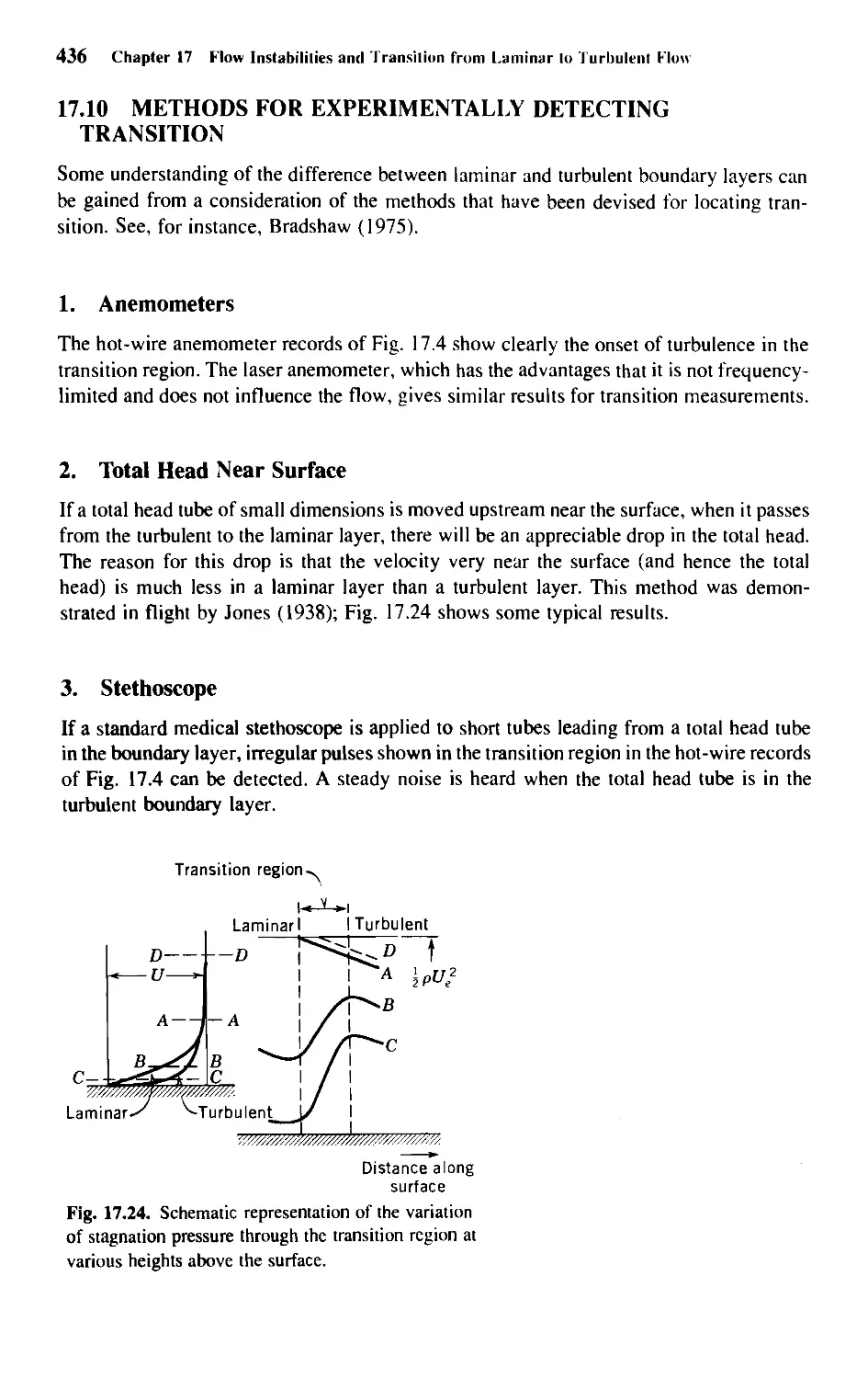
17.10 Methods for Experimentally Detecting Transition 436
17.11 Flow around Spheres and Circular Cylinders 437
17.12 Concluding Remarks 441
Chapter 18 • Turbulent Flows 443
18.1 Introduction 443
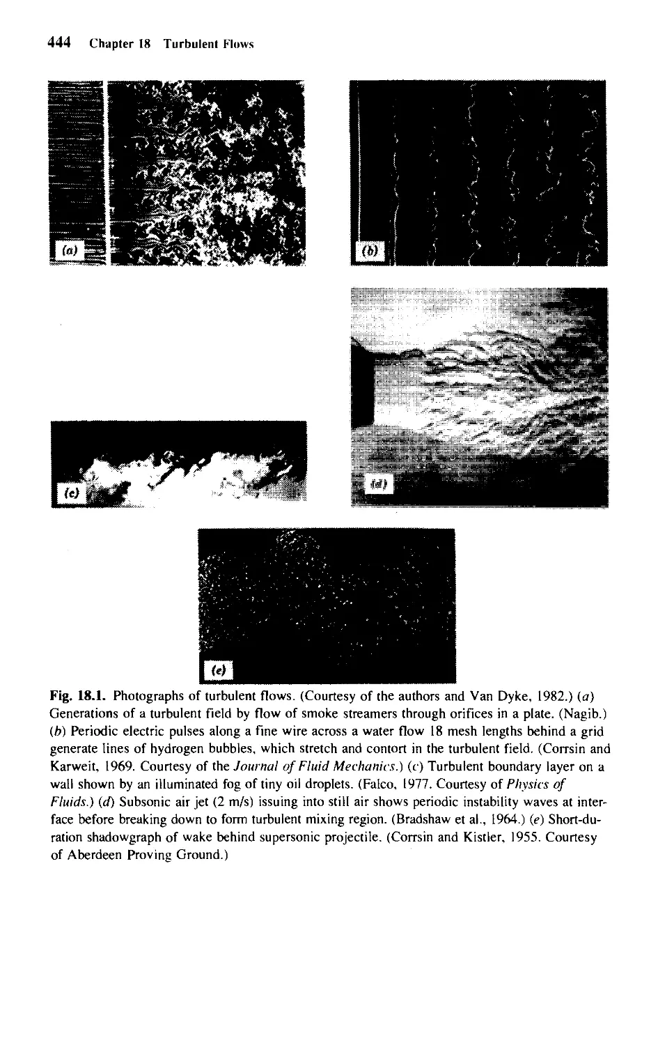
18.2 Description of the Turbulent Field 443
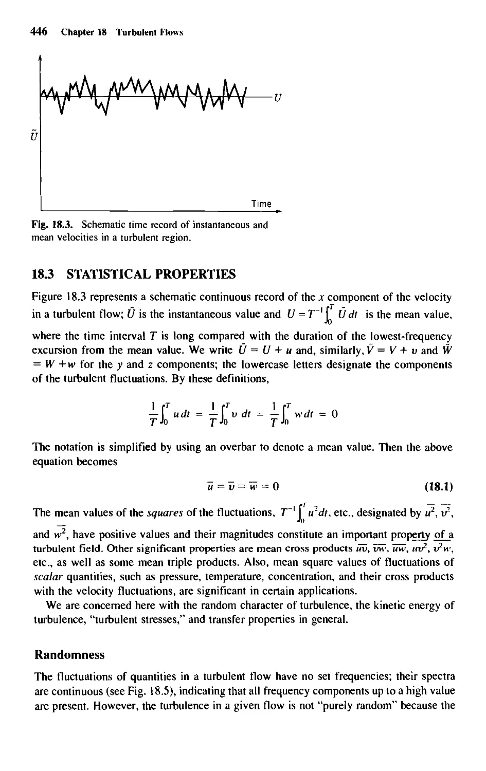
18.3 Statistical Properties 446
18.4 The Conservation Equations 453
18.5 Laminar Sublayer 455
18.6 Fully Developed Flows in Tubes and Channels 457
18.7 Constant-Pressure Turbulent Boundary Layer 461
18.8 Turbulent Drag Reduction 468
18.9 Effects of Pressure Gradient 469
18.10 The Stratford Criterion for Turbulent Separation 472
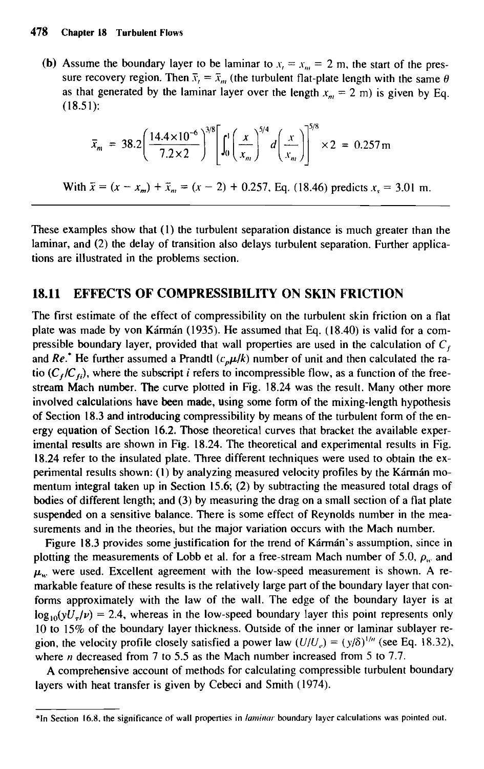
19.11 Effects of Compressibility on Skin Friction 478
18.12 Reynolds Analogy: Heat Transfer and Temperature
Recovery Factor 479
18.13 Free Turbulent Shear Flows 480
Chapter 19 • Airfoil Design, Multiple Surfaces, Vortex Lift,
Secondary Flows, Viscous Effects 486
19.1 Introduction 486
19.2 Airfoil Design for High c,_ 486
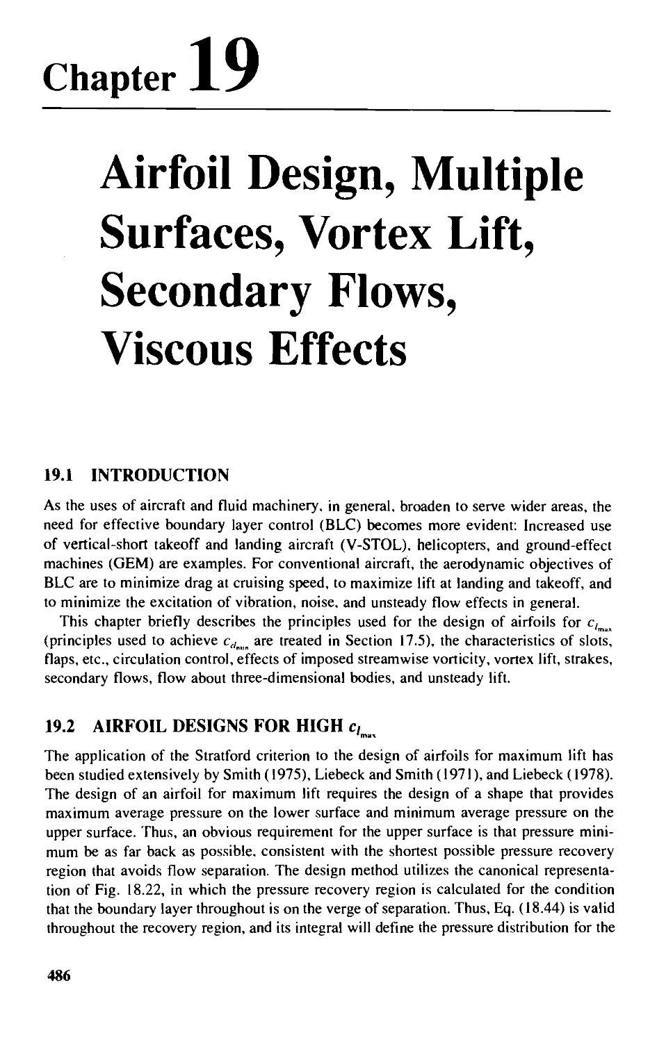
19.3 Multiple Lifting Surfaces 490
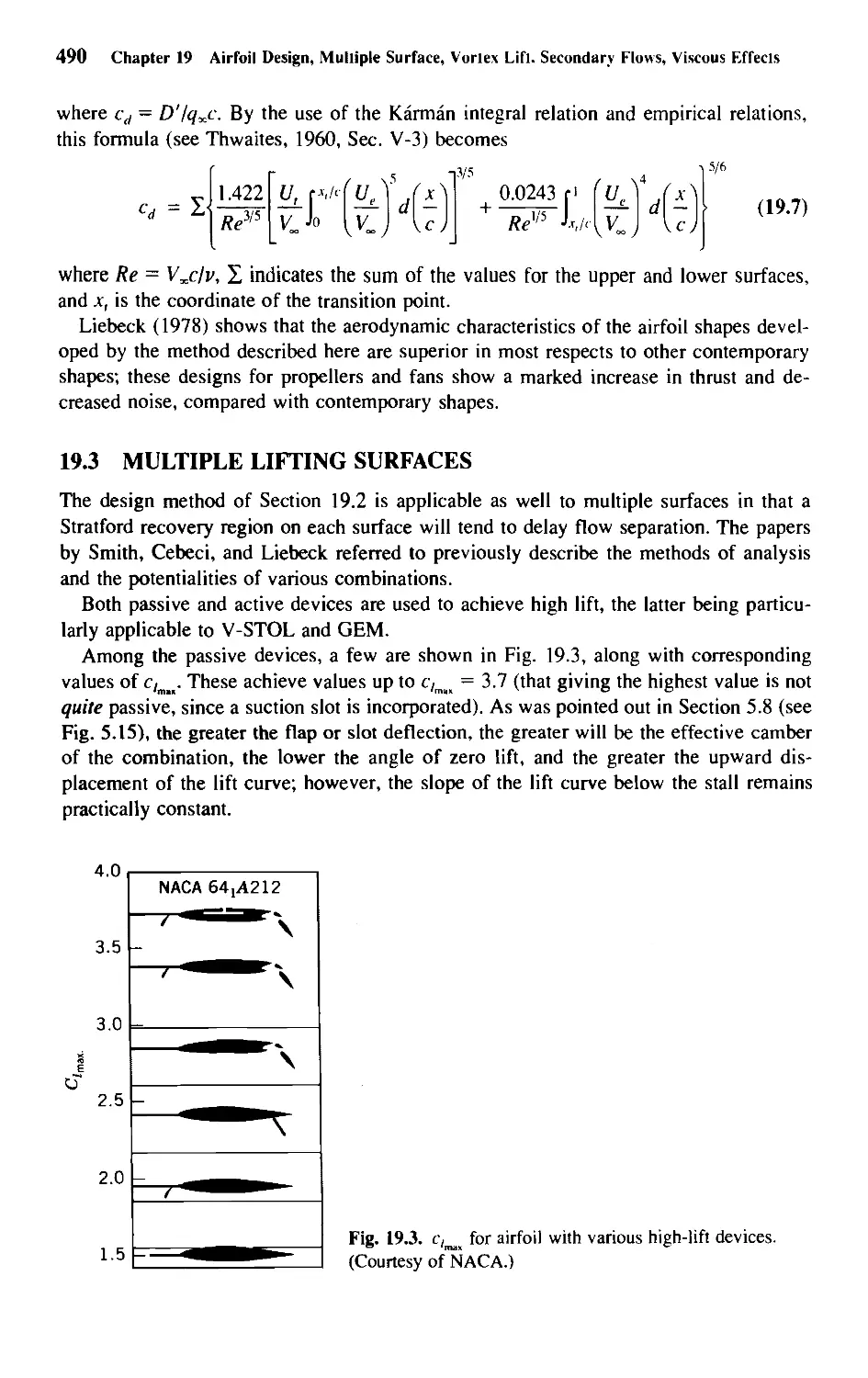
19.4 Circulation Control 493
19.5 Streamwise Vorticity 493
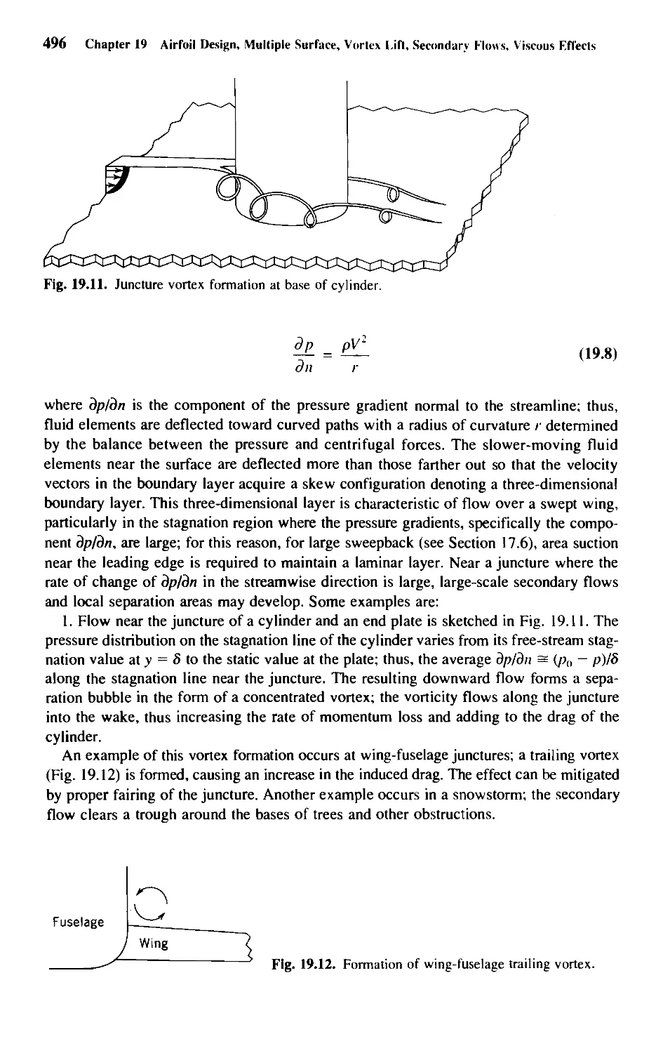
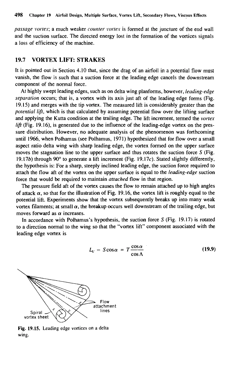
19.6 Secondary Flows 495
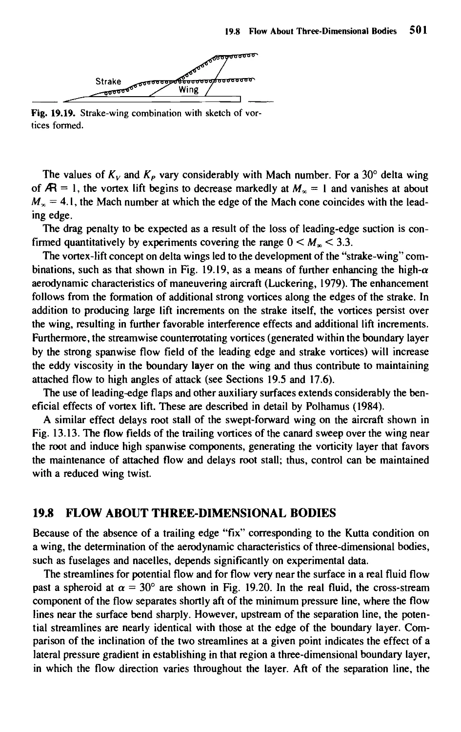
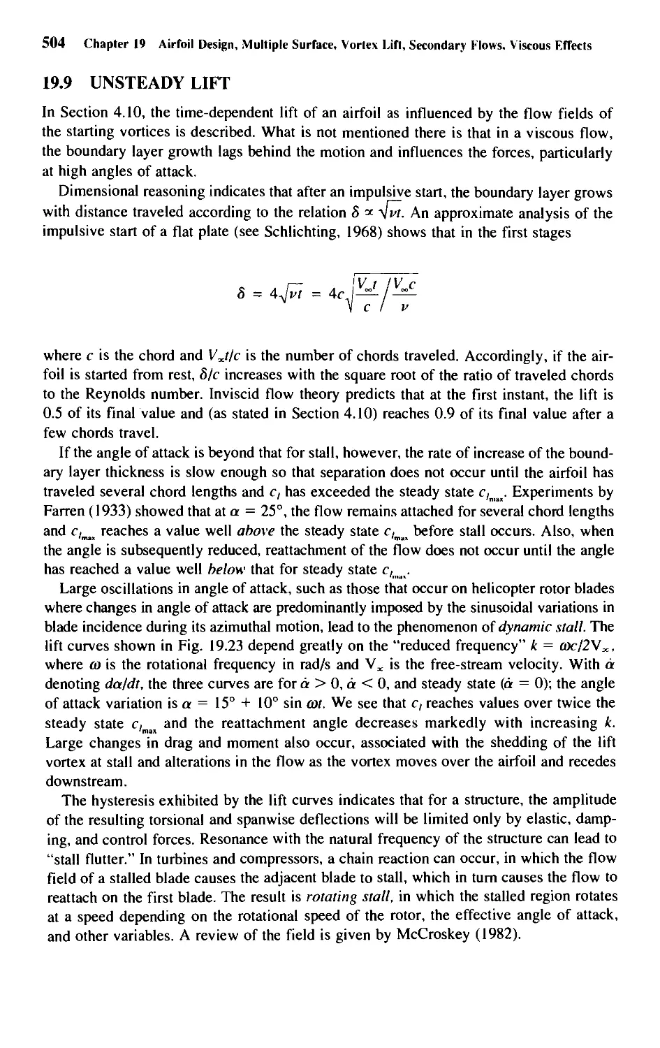
19.7 Vortex Lift: Strakes 498
19.8 Flow about Three-Dimensional Bodies 501
19.9 Unsteady Lift 504
Appendix A • Dimensional Analysis
508

Contents xiii
Appendix B • Derivation of Navier-Stokes and the Energy
and Vorticity Equations 513
Tables 531
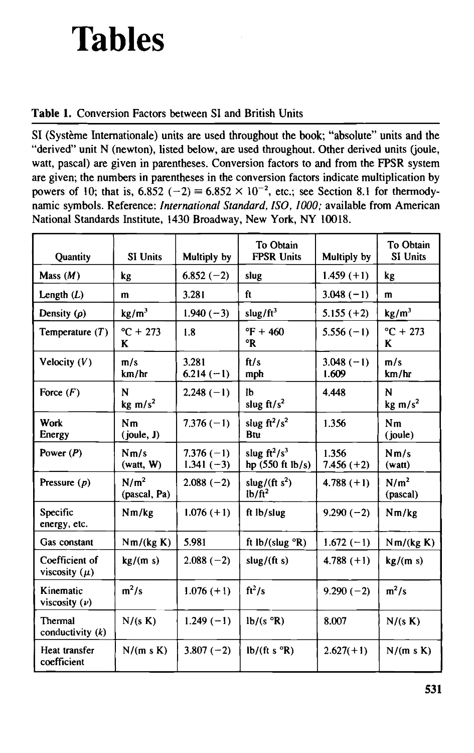
1. Conversion Factors between SI and British Units 531
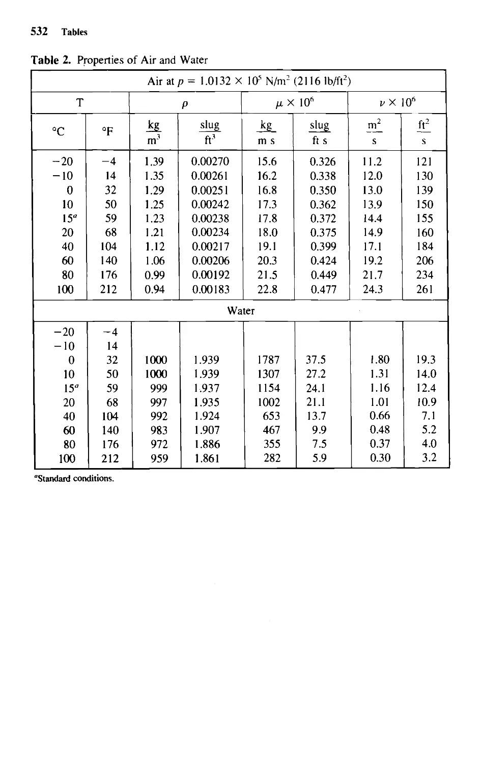
2. Properties of Air and Water 532
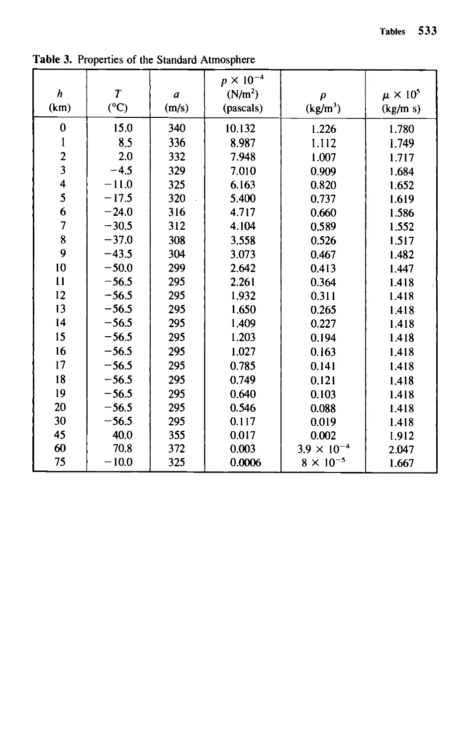
3. Properties of the Standard Atmosphere 533
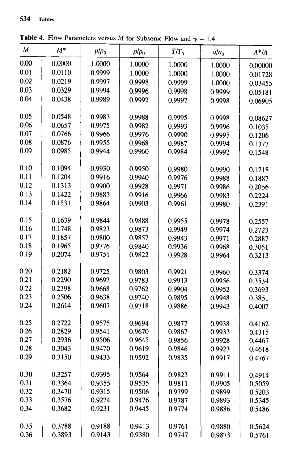
4. Flow Parameters versus M for Subsonic Flow and -y = 1.4 534
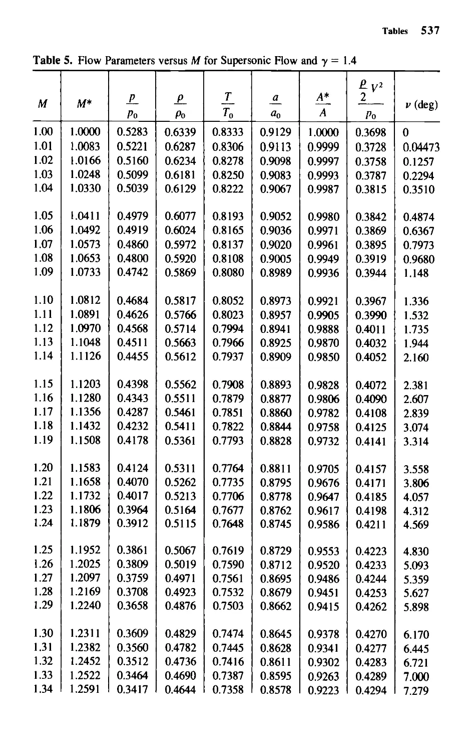
5. Flow Parameters versus M for Supersonic Flow and y = 1.4 537
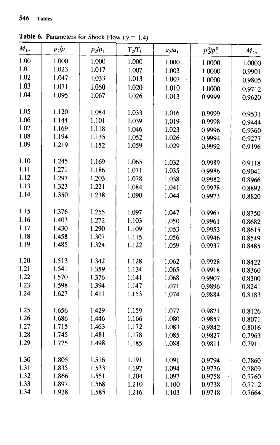
6. Parameters for Shock Flow {y = 1.4) 546
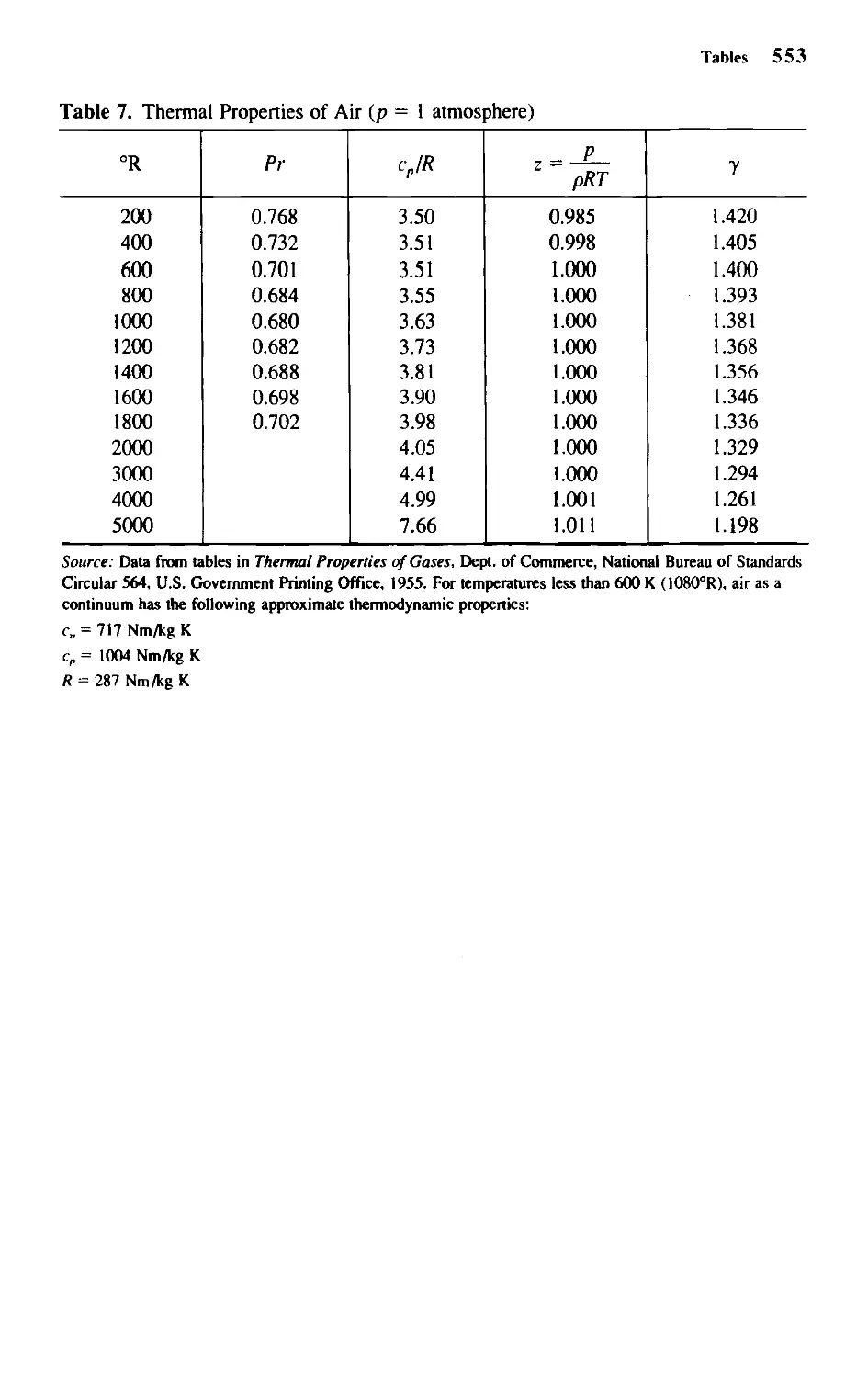
7. Thermal Properties of Air 553
Oblique Shock Chart 554
References 555
Index
563

Chapter
The Fluid Medium
1.1 INTRODUCTION
The objective of this book is to present the fluid flow concepts leading to the design of
flow surfaces and passages with the goal of achieving optimum performance over the
widest feasible range of the significant parameters in their respective fields of
application.
A clear understanding of the fundamental concepts is necessary since, owing to
mathematical complexities and often hypothetical physical premises, we are constantly
dealing with approximations to the actual problems we are attempting to solve. Therefore,
many of the more difficult problems involve in their solution an intuitive approach that
is facilitated by full comprehension of those concepts shown by experiment to be valid.
This chapter deals with the properties of the fluid medium, which we define as a
material that is at relative rest only when all forces acting on it are in equilibrium. Although
the concepts treated are of primary interest in aerospace engineering, applications in other
fields are also mentioned. These applications are generally described through analogies
and illustrative examples.
The fluid properties we discuss here are the pressure, temperature, density, elasticity,
and transport properties, especially viscosity—all related to the molecular structure of the
fluid. Numerical data are given for both air and water. The chapter closes with brief
descriptions of some aspects of dimensional analysis and a discussion of the subdivisions
of aerodynamics according to altitude and speed of flight.
1.2 UNITS
The SI (Systeme Internationale) system of units is used throughout this book. In this
system, the unit of force, the newton, is defined by the equation
1 newton (N) = 1 kilogram (kg) X 1 m/s2
The British system, in FPS units, is based on the definition of 1 pound as the unit of force
given by
1 pound (lb) = 1 slug X 1 ft/s2
If the first equation above is multiplied by the acceleration of gravity, g ( = 9.807 m/s2),
we see that a mass of 1 kg weighs 9.807 newtons in the "gravitational" MKS system. The
1
1

2 Chapter 1 The Fluid Medium
gravitational system is commonly used in nontechnical fields. Similarly, in the British
system (g = 32.174 ft/s2), we see that a mass of 1 slug weighs 32.174 lb.
The only other fundamental unit we need is that of absolute temperature T, expressed
in "degrees Rankine" in the British system, or in "degrees Kelvin" in the SI system. In
terms of the Fahrenheit and "Celsius" (degrees Centigrade) scales, these units are defined
by
T (°R) = °F + 460
T (K) = °C + 273
°C = (°F-32)/1.8
Conversion factors relating the British and SI factors are given in Table 1 at the end
of the book and inside the front cover.
1.3 PROPERTIES OF GASES AT REST
A gas consists of a large number of molecules moving in a random fashion relative to
one another. The "number density" of molecules is determined by Avogadro's law, which
states that a gas contains 6.025 X 1026 molecules/kg-mole" (8.79 X 1027/slug-mole). For
air under standard conditions (see Section 1.4), the number density is 2.7 X 1019 mole-
cules/cc (4.4 X 1020/in3). The ideal gas is one in which intermolecular forces are
negligible. Its bulk properties, which closely approximate those of real gases (except at very
low and very high temperatures and densities), can be expressed in terms of its
molecular properties: the mass m of the molecule, the average random speed c of the molecule,
and the mean distance the molecule travels between collisions with other molecules,
namely, the mean free path A.
1. Density The density of matter is defined as the mass per unit volume—thus, the
total mass of the molecules per unit volume. The dimensions of density are, then, force X
(time)2/(length)4; it is designated by p and has dimensions of kilograms per cubic meter
(kg/m1) in SI units and slugs per cubic foot (slugs/ft1) in FPS units. Table 2 gives its
variation with temperature for air at sea level pressure and for water; in Table 3, values of
the density in SI units are given for the "standard atmosphere."
2. Pressure When molecules strike a surface they rebound and by Newton's second
law, a force is exerted on the surface equal to the time rate of change of momentum of
the rebounding molecules. That is, the force is equal to the sum of the changes in
momentum experienced by all the molecules striking and rebounding from the surface per
second. Pressure is defined as the force per unit area exerted on a surface immersed in
the fluid and at rest relative to the fluid. It is expressed in newtons per square meter [N/m2
(pascals)] or pounds per square foot (lb/ft2). Experiment indicates that the collisions among
molecules and with surfaces are elastic so that the mean change in momentum is a
vector normal to the surface, regardless of the angle of incidence of the collision. Therefore,
we conclude that fluid pressure acts normal to a surface.
*One kg-mole is the number of kilograms of gas numerically equal to the atomic weight. Thus, 1 kg-mole of
air has a mass of 28.97 kg. Avogadro's number has the same value for all gases.

1.3 Properties of Gases at Rest 3
In order to show that the fluid pressure is proportional to the kinetic energy of
molecules of the gas, we do the following. We compute the force exerted on the walls of a
unit cube of gas (Fig. ].l), and, since we wish to identify only the combination of gas
properties that determine the pressure, we adopt the following simplified model of the
molecular motion: All of the N (N is the number density) molecules in the unit cube are
assumed to have identical masses m and identical speeds c. They are assumed to travel
parallel to the coordinate axes, AV3 parallel to, and N/6 in the positive direction of, each
axis. The (N/6)Ax molecules in the thin layer shown in Fig. 1.1 will strike the right x face
in time Af = Ax/c. The collisions are assumed to be elastic so that the momentum of each
molecule is changed by 2mc. Newton's second law then predicts that a force equal to the
product of 2mc and the number of molecules striking the surface per second will be
exerted on the right face. The number striking per second will be (AV6)c and since Nm = p,
the fluid density, the force acting on the right face (in fact, on each face) is given by the
formula
p = — -2mc = £- (1.1)
6 3
The pressure p has the dimensions of force/area. Physically, Eq. (1.1) states that the
pressure is proportional to the kinetic energy of the molecular motion. Since the pressure
is equal on all faces, the cube is at rest relative to the surrounding fluid. That is, either
the flow speed is zero or the cube is moving at the flow speed. Also, since the speed of
the molecules varies, the pressure is actually proportional to the mean of the square of
the speed rather than to the square of the mean speed (see Problem 1, Section 1.3). This
approximation, however, affects only the magnitude of the proportionality in Eq. (1.1).
3. Temperature According to the kinetic theory of gases, the absolute temperature is
proportional to the mean translational kinetic energy of the molecules. It can be
interpreted in terms of the equation of state for an ideal gas
p = pRT (1.2)
where T is the absolute temperature and R, the gas constant, has a specific value depending
only on the composition of a gas. For air, R = 287 m2/s2 K. For systems in which the
mass per unit volume remains constant, any process (e.g., the addition of heat) that
increases the kinetic energy of the random motion will increase the temperature and
pressure by proportional amounts.
I- 1 -
Ax
Fig. 1.1. Model for interpretation of pressure.

4 Chapter 1 The Fluid Medium
4. Elasticity When a pressure is applied to a gas, its volume per unit mass changes.
Elasticity is defined as the change in pressure per unit change in specific volume v.
E = -
dp
dvlv
dp
dp
(1.3)
in which v = 1/p. It will be shown later that dp/dp is the square of the speed of sound
through the medium. Therefore, the density and speed of sound define the elasticity.
1.4 FLUID STATICS: THE STANDARD ATMOSPHERE
In order to establish uniformity in the presentation of data, standard atmospheric
conditions have been adopted and are in general use. Commonly referred to as sea-level
conditions, these are
p = 1.013 X 105 N/m2 or pascals (2116 lb/ft2)
p = 1.23 kg/m1 (0.002378 slugs/ft1)
T = 273 + 15°C = 288 K (520°R)
Under these standard conditions, the speed of sound a is 340 m/s.
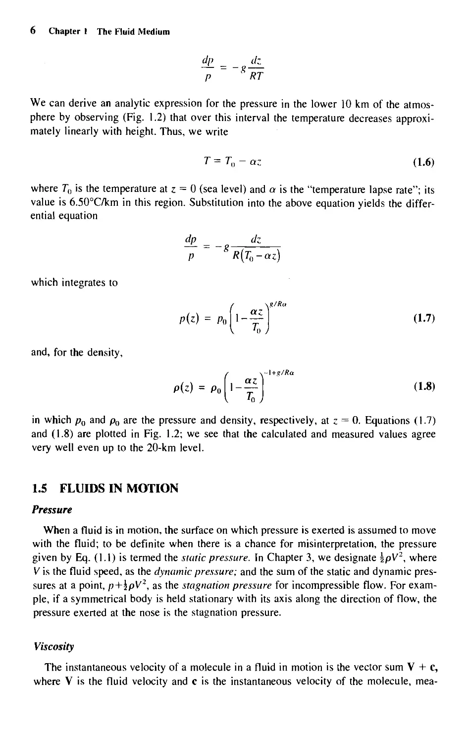
The temperature, pressure, and density in the atmosphere vary with altitude; their
magnitudes up to 20 km above sea level are plotted in Fig. 1.2, and the properties extended
to a much higher level are tabulated in Table 3 at the end of the book. The mean free path
of the air molecules is also plotted in Fig. 1.2, up to an altitude of 250 km.
We will now show that the variations of pressure and density shown in Fig. 1.2 are
consistent with the measured temperature distribution under the hypothesis that no net
20
15K
E
10
0
\
Eq.(
1.6)
\
II
1
A
\
Eq.(
1.7)
\
11
V
v
Eq.d
8)
200
150
100
50
n
10"
-60 -40 -20 0 20 0 5 10 0 0.5 1.0 1.5 lCr8 10~4 10°
TCC) pxlO-4(N/m2) p(kg/m3) A (m)
Fig. 1.2. Variations of temperature, pressure, density, and mean free path with height in the
standard atmosphere. The approximate relations (Eqs. 1.6, 1.7, and 1.8) are plotted as dashed lines.

1.4 Fluid Statics: The Standard Atmosphere 5
lp(z) + ^ AzlAxAy
Ay/
Az
Ax
/•--
/ A
pgAxAyAz
p(z)AxAy
mmmmmmmmmmmmmmmmmmmzm>
Fig. 13. Force balance on fluid element.
force acts on any element of the fluid; the atmosphere is then in static equilibrium.
Figure 1.3 shows a cube of fluid of volume AxAyAz oriented with its base AxAy at a height
z above an arbitrary datum—for example, sea level. The pressures are equal on all
vertical faces of the cube, so the pressure p varies only with z. Under the assumed equilibrium
conditions, the weight of the element pgAxAyAz, where p is the average density of the
cube, is balanced by the difference between the pressure forces on the lower and upper
faces.
pAxAy-
P +
Az
AxAy = pgAxAyAz
As the volume of the cube approaches zero, p —> p, the density at z, we obtain the
equation of aerostatics
dp
Tz=~pg
(1.4)
We may take g as constant, but both p and p vary with z, as shown in Fig. 1.2. Then the
pressure variation as expressed by the integral of Eq. (1.4) is
P = Po~lQP8dz
(1.5)
where p0 is the pressure at z = 0.
If we use Eq. (1.2) and express p
p/RT, Eq. (1.4) becomes

6 Chapter 1 The Fluid Medium
p g RT
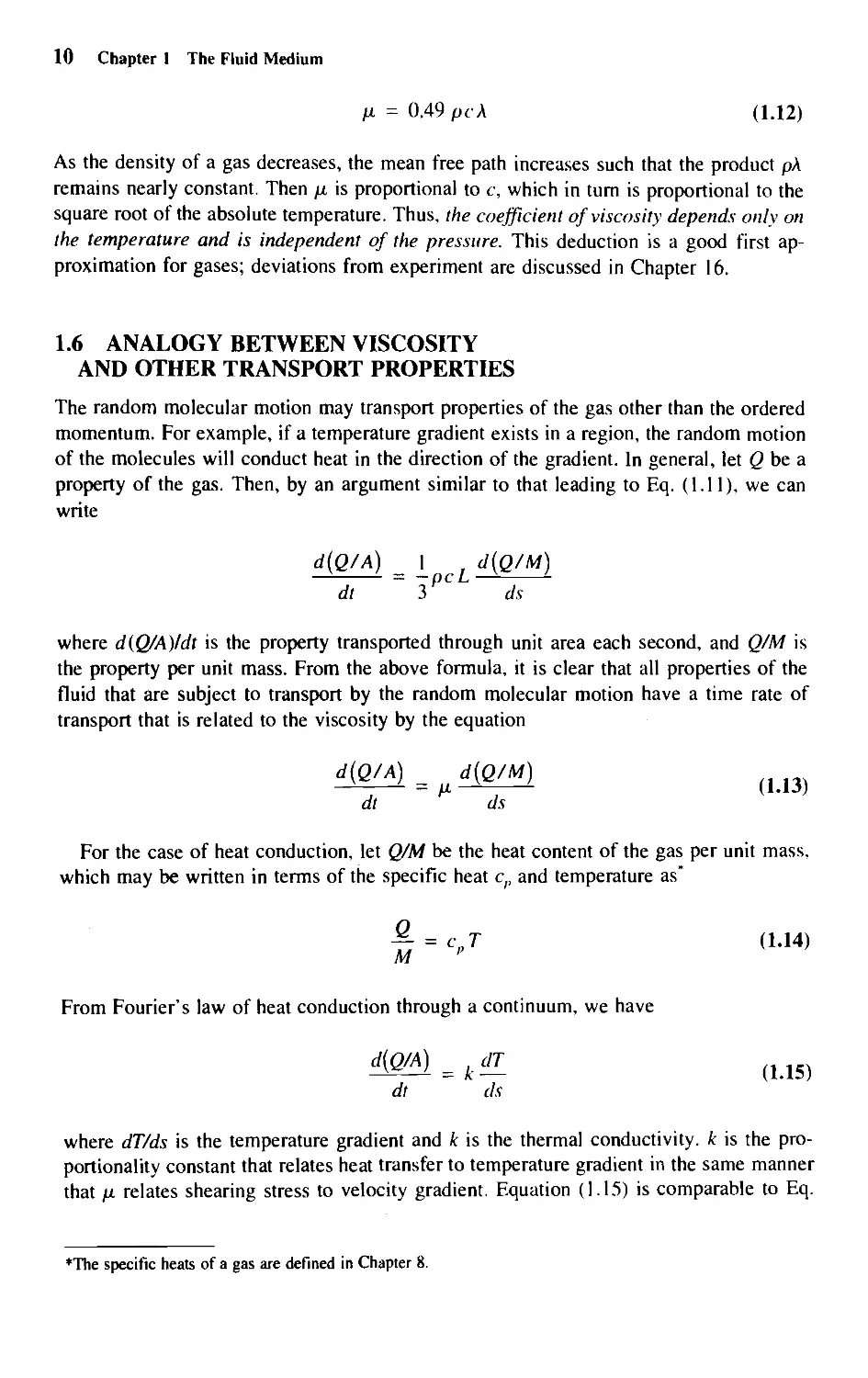
We can derive an analytic expression for the pressure in the lower 10 km of the
atmosphere by observing (Fig. 1.2) that over this interval the temperature decreases
approximately linearly with height. Thus, we write
T = T0 - az (1.6)
where 7",, is the temperature at z = 0 (sea level) and a is the "temperature lapse rate"; its
value is 6.50°C/km in this region. Substitution into the above equation yields the
differential equation
dp dz
= ~8
p R{T0-az)
which integrates to
and, for the density,
P(z) = Po
P(z) = P0
1-
az
(1.7)
az ' (1.8)
1
To J
in which pQ and p0 are the pressure and density, respectively, at z = 0. Equations (1.7)
and (1.8) are plotted in Fig. 1.2; we see that the calculated and measured values agree
very well even up to the 20-km level.
1.5 FLUIDS IN MOTION
Pressure
When a fluid is in motion, the surface on which pressure is exerted is assumed to move
with the fluid; to be definite when there is a chance for misinterpretation, the pressure
given by Eq. (1.1) is termed the static pressure. In Chapter 3, we designate hpV2, where
V is the fluid speed, as the dynamic pressure; and the sum of the static and dynamic
pressures at a point, p+^pV2, as the stagnation pressure for incompressible flow. For
example, if a symmetrical body is held stationary with its axis along the direction of flow, the
pressure exerted at the nose is the stagnation pressure.
Viscosity
The instantaneous velocity of a molecule in a fluid in motion is the vector sum V + c,
where V is the fluid velocity and c is the instantaneous velocity of the molecule, mea-

1.5 Fluids in Motion 7
Fig. 1.4. Flow in an annulus.
sured by an instrument that moves with the fluid. Since the molecular velocity in the fluid
at rest is random in magnitude and direction, its mean value is zero, so that the fluid
velocity at a given point is the mean vector sum of the velocities of the molecules passing
that point.
If the flow velocities are different on two layers aligned with the flow, the exchange
of molecules between them tends to equalize their velocities; that is, the random
molecular motion effects a transfer of downstream momentum between them. The process of
momentum transfer by the molecular motions is termed viscosity. The viscous force per
unit area, termed the shearing stress, is defined as the rate at which the molecules
accomplish the cross-stream transfer of downstream momentum per unit area. The stress is
thus a force per unit area and is characterized by an equal and opposite reaction, in that
positive momentum is transferred from the higher to the lower speed layer, and vice versa.
A consequence of the existence of fluid viscosity is the "no-slip condition" at the solid
surface, as illustrated in Fig. 1.4 for the flow between coaxial cylinders, one of which is
rotating with angular velocity o>. The velocity distribution, designated schematically by
the vectors, is established as a result of the random motions of the molecules with the no-
slip condition as a constraint at each surface; that is, the monomolecular layer adjacent to
a surface has zero velocity relative to it. Molecules rebounding from the outer
(stationary) surface will have zero averaged ordered velocity, whereas those rebounding from the
inner (moving) surface will have an average ordered tangential velocity of magnitude u>R.
The mean free path between collisions, as shown in Fig. 1.2 for air, will, under the great
majority of practical conditions, be much smaller than the gap A/?, so that the molecules
will, on average, carry their ordered velocities only a very short distance before they
collide with molecules of slightly different ordered velocities. The large number of collisions
constitutes an effective mixing process, resulting in the continuous velocity distribution
shown in Fig. 1.4. If the gap AR < R,& small segment of the flow will approximate flow
between parallel planes in relative motion, as shown in Fig. 1.5. The lower plane will
have a speed V = toR, and the transfer of momentum across the intervening space will
tend to drag the upper plane to the right. For A/? <S R, experiment shows that the stress,
Fig. 1.5. Shearing stress in a fluid.

8 Chapter 1 The Fluid Medium
t, exerted on the upper plane, varies directly as the relative speed V and inversely as the
distance between the planes. Thus,
T = fl
AR
where \i is the coefficient of viscosity of the fluid. Returning momentarily to the coaxial
flow of Fig. 1.4, we see that the torque on the outer cylinder will be 2ir{R + A/?)2t per
unit length. The above formula may be generalized by considering the shearing stress
exerted between the two adjacent layers of fluid, say, the layers immediately above and
immediately below the section AA in Fig. 1.5. In this example, the relative speed of the
layers is an infinitesimal dV, and the distance between layers is also an infinitesimal ds. Then
we may write
dV
T =
fids
(1.9)
It is understood that the derivative in Eq. (1.9) is always in a direction perpendicular to
the plane on which the shearing stress is being computed. When air is flowing with a
velocity u over a solid surface, the mixing by the random molecular motion results in the
formation of a thin boundary layer, as identified by Ludwig Prandtl (1875-1953) and
shown schematically in Fig. 1.6. Each infinitesimal section of the boundary layer can be
visualized as two planes in relative motion, and so the shearing stress at any point is given
by Eq. (1.9). At the surface, the shearing stress is given by
T„. = M
(1.10)
The velocity gradient du/dy is large at the surface and becomes substantially zero at y =
S, where S is defined as the thickness of the boundary layer.
The coefficient of viscosity may be interpreted in terms of the molecular properties of
a fluid by evaluating the shearing stress associated with it. The shearing stress exerted by
the fluid below AA in Fig. 1.6 on that above AA is a retarding effect; it is equal to the rate
of loss of momentum of the fluid above AA resulting from the exchange of molecules
across unit area of the plane AA.
Fig. 1.6. Boundary laye

1.5 Fluids in Motion 9
To calculate the shearing stress, we evaluate the rate of transport of ordered
momentum through unit area of AA by the random motion of the molecules. If our frame of
reference moves with the fluid velocity at AA and we restrict our consideration to the
immediate vicinity of AA, we may postulate the linear velocity distribution shown in the
blowup in Fig. 1.7. Thus, the velocities above AA are positive, and those below are
negative. A molecule originating at yl and moving downward through AA will carry with it
a positive momentum m(du/dy)yl. Similarly, a molecule moving upward through AA and
originating at y2 will carry with it a negative momentum m(du/dy) y2. Both these
excursions represent a transfer of ordered momentum across AA, and it is the sum of such losses
that occur in unit time through unit area of AA that equals the shear stress t.
As in the pressure calculation of Section 1.3, the random molecular motion is assumed
to be split equally among the three coordinate directions. Then, if there are N molecules
per unit volume, if their average speed is c, and if one-third of them have a motion
perpendicular to AA, then Nc/3 molecules will pass through AA per unit time. Each of these
molecules will carry with it a momentum corresponding to the position y at which it
originates. The sum of these momenta is the shear stress. There is an effective height at which
all the molecules could originate with the same resulting shear stress. If we call this height
L, the shear stress becomes
-Nc\m
(d^
The product Nm is the density p; therefore,
1 , du
T = - OCL
3 dy
(1.11)
A comparison of Eqs. (1.9) and (1.11) indicates that
fi = -pcL
The effective height L is related to the mean free path A, and more accurate calculations
show that
Fig. 1.7. Kinetic interpretation of coefficient of
viscosity.

10 Chapter 1 The Fluid Medium
p = 0.49 pr A (1.12)
As the density of a gas decreases, the mean free path increases such that the product pA
remains nearly constant. Then p is proportional to c, which in turn is proportional to the
square root of the absolute temperature. Thus, the coefficient of viscosity depends only on
the temperature and is independent of the pressure. This deduction is a good first
approximation for gases; deviations from experiment are discussed in Chapter 16.
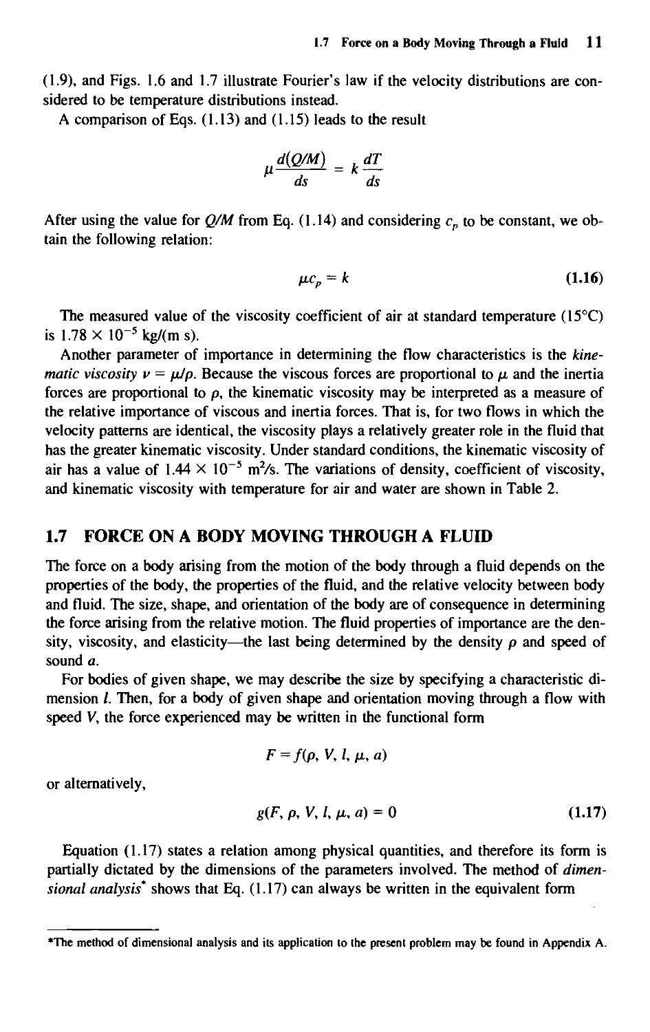
1.6 ANALOGY BETWEEN VISCOSITY
AND OTHER TRANSPORT PROPERTIES
The random molecular motion may transport properties of the gas other than the ordered
momentum. For example, if a temperature gradient exists in a region, the random motion
of the molecules will conduct heat in the direction of the gradient. In general, let Q be a
property of the gas. Then, by an argument similar to that leading to Eq. (1.11), we can
write
d(Q/A) 1 d{Q/M)
— = —pcL— '-
dt 3 ds
where d(Q/A)/dt is the property transported through unit area each second, and Q/M is
the property per unit mass. From the above formula, it is clear that all properties of the
fluid that are subject to transport by the random molecular motion have a time rate of
transport that is related to the viscosity by the equation
mA^m^i (1.13)
dt ds
For the case of heat conduction, let Q/M be the heat content of the gas per unit mass,
which may be written in terms of the specific heat cp and temperature as*
£ . crr O.M)
From Fourier's law of heat conduction through a continuum, we have
dm^dT
dt ds
where dT/ds is the temperature gradient and A' is the thermal conductivity, k is the
proportionality constant that relates heat transfer to temperature gradient in the same manner
that p relates shearing stress to velocity gradient. Equation (1.15) is comparable to Eq.
♦The specific heats of a gas are defined in Chapter 8.

1.7 Force on a Body Moving Through a Fluid 11
(1.9), and Figs. 1.6 and 1.7 illustrate Fourier's law if the velocity distributions are
considered to be temperature distributions instead.
A comparison of Eqs. (1.13) and (1.15) leads to the result
^d(Q/M) =kdT
ds ds
After using the value for Q/M from Eq. (1.14) and considering cp to be constant, we
obtain the following relation:
ficp = k (1.16)
The measured value of the viscosity coefficient of air at standard temperature (15°C)
is 1.78 X l(T5kg/(ms).
Another parameter of importance in determining the flow characteristics is the
kinematic viscosity v = fi/p. Because the viscous forces are proportional to fx and the inertia
forces are proportional to p, the kinematic viscosity may be interpreted as a measure of
the relative importance of viscous and inertia forces. That is, for two flows in which the
velocity patterns are identical, the viscosity plays a relatively greater role in the fluid that
has the greater kinematic viscosity. Under standard conditions, the kinematic viscosity of
air has a value of 1.44 X 10~5 m2/s. The variations of density, coefficient of viscosity,
and kinematic viscosity with temperature for air and water are shown in Table 2.
1.7 FORCE ON A BODY MOVING THROUGH A FLUID
The force on a body arising from the motion of the body through a fluid depends on the
properties of the body, the properties of the fluid, and the relative velocity between body
and fluid. The size, shape, and orientation of the body are of consequence in determining
the force arising from the relative motion. The fluid properties of importance are the
density, viscosity, and elasticity—the last being determined by the density p and speed of
sound a.
For bodies of given shape, we may describe the size by specifying a characteristic
dimension /. Then, for a body of given shape and orientation moving through a flow with
speed V, the force experienced may be written in the functional form
F=/(p, V,Z,M,«)
or alternatively,
g(F, p, V, Z, m, a) = 0 (1.17)
Equation (1.17) states a relation among physical quantities, and therefore its form is
partially dictated by the dimensions of the parameters involved. The method of
dimensional analysis* shows that Eq. (1.17) can always be written in the equivalent form
*The method of dimensional analysis and its application to the present problem may be found in Appendix A.

12 Chapter 1 The Fluid Medium
\pV I p. a)
where each of the three combinations of parameters is a dimensionless quantity. The above
equation may be solved for the first dimensionless combination, and then we have the
fundamental relation
-TJ2J2 = 8\ — •- <1-18)
pV I { p a)
To interpret Eq. (1.18), consider a body of a given shape and orientation in motion in a
fluid such that the quantities F/(pV2l2), pVI/p, and V/a have certain definite values. Then,
if a geometrically similar body with the same orientation is moved through the same or
another fluid such that pVl/p, and V/a have the same values as for the first body, then
F/(pV2l2) will also have the same value.
Assume for the moment that p. and a in Eq. (1.17) have no influence on the force F.
Then an application of dimensional analysis will lead to the result
the solution of which is
F = CFpV2l2 (1.19)
where CF is a dimensionless constant. Equation (1.19) states that, for a body of given
orientation and shape in motion through a fluid, the force experienced is proportional to the
kinetic energy of the relative motion per unit volume of the fluid pV2/2 and to a
characteristic area I2. For example, if the force on an airplane of given shape, orientation, and
size is known at a given flight speed and altitude, the force on another airplane of a
geometrically similar shape at the same orientation and flying at a different speed and
altitude can be predicted from Eq. (1.19). This result was given by Isaac Newton (1642-1727),
and the dimensionless constant CF is sometimes referred to as the Newtonian coefficient.
CF is a dimensionless quantity that characterizes the force, and in the following chapters
will be called the force coefficient. The force coefficient is of great importance in
experimental aerodynamics, for it makes possible the prediction of forces on full-scale airplanes
at various altitudes and flight speeds from data obtained on models tested in wind
tunnels.
Newton's result (Eq. 1.19) is an approximation that is accurate only under specialized
conditions to be described later. The viscosity and elasticity of the fluid are important in
general, and Eq. (1.18) shows that the force coefficient is not a constant for a body of
given shape and orientation. It is a function of the combinations pVl/p and V/a, which
bear the names Reynolds number and Mach number, respectively, after Osborne Reynolds
(1842-1912) and Ernst Mach (1838-1916), who investigated the effects of these
parameters in flow problems.

1.8 The Approximate Formulation of Flow Problems 13
Dimensional analysis has shown that the force coefficient for a body of a given
orientation and shape is a function of the Reynolds number and the Mach number. The
accuracy of this result depends entirely on the accuracy of the initially chosen parameters
governing the force. If important properties of the flow are omitted from the initial choice of
parameters, the method of dimensional analysis will not expose this fact. Possible
neglected properties that influence the force on the body could include surface roughness,
turbulence of the stream, the presence of other bodies in the vicinity, heat transfer through
the body surface, and so forth. In applying data from model tests to the full-scale airplane,
these facts must be considered.
Finally, if the geometries of the two flows are similar (geometric similarity), and if the
Mach numbers are equal and the Reynolds numbers are equal, the flows are said to be
dynamically similar. Dynamically similar flows have equal force coefficients. The Mach
and Reynolds numbers are called similarity parameters.
1.8 THE APPROXIMATE FORMULATION OF FLOW PROBLEMS
Strictly speaking, a gas is a compressible, viscous, inhomogeneous substance, and the
physical principles underlying its behavior are expressed in the form of nonlinear partial
differential equations. Solutions of those equations are obtainable nowadays on high speed
computers by means of numerical techniques, whose validities are to be checked by
comparison with experiment. On the other hand, analytical methods are still applicable to
many flow problems if various approximations are made to those equations.
In order to render the problems of aerodynamics tackled in this book tractable, we
consider three different fluid flows, each of which provides a good approximation for airflow
problems of particular types.
1. Perfect fluid flow The fluid of this flow is homogeneous (not composed of
discrete particles), incompressible, and inviscid, corresponding to that of a flow at zero Mach
number and infinite Reynolds number. The assumption of a perfect fluid gives good
agreement for flow experiments that are outside the boundary layer and wake of
well-streamlined bodies moving with velocities of less than -400 km/hr (111 m/s), at altitudes under
~30 km. The scale effect is neglected for problems treated by perfect-fluid theory, and
the force coefficient given by Eq. (1.19) is constant.
2. Compressible, inviscid fluid flow This flow differs from the perfect fluid flow in
that the compressibility, characterized by the finite speed of sound, is taken into account
(nonzero Mach number, infinite Reynolds number). It provides a good approximation for
problems involving the flow outside the boundary layer and wake of bodies at high
Reynolds numbers at altitude below -30 km.
3. Compressible, viscous fluid flow This flow differs from that described under (2)
in that the viscosity is taken into account (nonzero Mach number, finite Reynolds
number). Although it is not feasible to treat the entire flow around a body, that part of the
flow within the boundary layer and wake is amenable to accurate analysis, provided the
flow is laminar; turbulent flow has so far yielded only to semiempirical analyses. The
agreement of the analyses with experiment is good for all speeds at altitudes below -30 km.
At altitudes above -60 km, the mean free path of the molecules will generally not be
small compared with a significant dimension of the body. Therefore, as the altitude in-

14 Chapter 1 The Fluid Medium
creases further, the characterization of air as a fluid becomes more and more approximate.
Finally, at altitudes above approximately 150 km, the flow (if it can even be termed a
flow) consists simply of the collision of the body with those molecules directly in its path.
1.9 OUTLINE OF CHAPTERS THAT FOLLOW
The objective as stated in Section 1.1 may, in view of the intervening discussion, be
rephrased as follows: To provide a background of concepts of use in finding approximate
solutions to problems involving the flow of a compressible, viscous, inhomogeneous gas.
The approximations that may be made depend on the particular aspect of the flow being
investigated. For instance, it has been abundantly demonstrated experimentally that the
lift and moment acting on aircraft at flight speeds under ~400 km/hr (250 mph) are very
slightly affected by compressibility and viscosity. Therefore, the first six chapters of this
book are devoted to a study of the flow of a perfect fluid and to the application of
perfect-fluid theory to the prediction of the lifting characteristics of wings.
Chapters 7 to 13 will deal with the compressible inviscid fluid and its application to
the flow through channels and about wings. Both subsonic and supersonic flow problems
are formulated, and the basic differences between the two regimes are discussed in
physical terms. In some cases, exact solutions of the equations are given; in others, useful
approximations that neglect the nonlinear terms are introduced.
The effects of viscosity on the flow of incompressible and compressible fluids are
addressed in Chapters 14 through 19. Here we are concerned with the flow in boundary
layers and in tubes. The main objectives are to understand the approximations that have been
made, and to analyze the problems of viscous drag and flow separation.
Two appendices, tables, and a bibliography appear at the end of the book. In
Appendix A, a brief treatment of dimensional analysis is given. The equations of motion and
energy for a viscous, compressible fluid are given in Appendix B, and the reduction to
the boundary layer equations is illustrated there.
PROBLEMS
Section 13
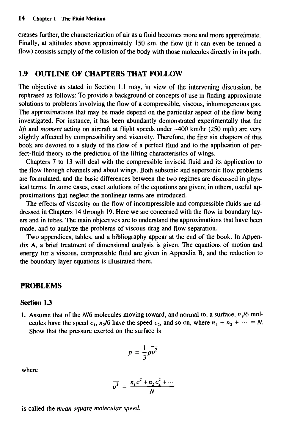
1. Assume that of the N/6 molecules moving toward, and normal to, a surface, n,/6
molecules have the speed c,, «2/6 have the speed c2, and so on, where «, + n2 + •■■ = N,
Show that the pressure exerted on the surface is
1 ~
p = -pv
where
-j _ «, cf + n2 c2 H—
~ N
is called the mean square molecular speed.

Problems 15
Section 1.4
1. Show that for an isothermal atmosphere, the pressure distribution is described by
p = p0 exp(-gz/RT)
2. In an isentropic atmosphere, the relationship between pressure and density is governed
by
P_
Po
( V
P_
ft.
where y is the ratio of the specific heat of air at constant pressure to that of air at
constant volume. Show that the pressure distribution in such an atmosphere is described by
V'(t-i)
P = Po
, 7-1 Po
y Po
Section 1.7
1. For F = 500 lb, V = 100 mph, and / = 3 ft, show that the Reynolds number and force
coefficient (Eqs. 1.18 and 1.19) have the same values in FPS and SI units. Calculate
for both air and water under standard conditions. Tables 1 and 2 give conversion
factors and numerical values.

Chapter
Kinematics of
a Flow Field
2.1 INTRODUCTION: FIELDS
In this and the following chapter, we develop equations that describe the properties of
incompressible, inviscid flows in regard to (I) field properties, that is, the velocity,
pressure, temperature, and the like at any point in space; and (2) particle properties, that is,
the variations of those properties experienced by a fluid element as it moves along its path
in the flow. In Chapter 2, we restrict ourselves to the kinematic properties, those that
follow from the indestructibility of matter. The dynamic properties, those that follow from
the application of Newton's laws to the individual (tagged) fluid elements, are discussed
in Chapter 3. The dynamics and thermodynamic properties of compressible viscous and
inviscid flows are reserved for later chapters.
The term field denotes a region throughout which a given quantity is a function both
of time and of the coordinates within the region. Examples are pressure, density, and
temperature fields, within which these properties can be represented as functions of
Cartesian coordinates x, y, z, and time /. These are scalar fields, in that the magnitude of the
quantity at any point at a given instant of time is represented completely by a single
number. Vector fields (such as velocity, momentum, or force fields), on the other hand, each
require, at every point, three numbers for their complete description; that is, the vector
field results from the superposition of three scalar fields.
The empirical laws on which fluid dynamics are based are applicable to fluid elements
of fixed identity—that is, to small regions that still comprise an inordinately large
number of tagged molecules. As any given element moves through a flow field along a path
determined by the force field, the principle of conservation of mass states that its mass
remains constant. This indestructibility of matter is thus a particle property. Other
conservation laws, such as momentum and energy (taken up later), also apply to particle
properties. Then, the application of these conservation laws to the particle properties defines
a flow field in which each fluid element moves in conformity with these laws.
In most problems, rather than solve for the particle properties, it is more convenient to
derive the field properties, that is, the flow properties as functions of the spatial
coordinates at any given instant. When the conservation laws are applied, we show that the
particle properties so derived determine the field properties.
2
16

2.2 Vector Notation and Vector Algebra 17
Flows are classified according to their dependence on time and spatial coordinates. If
the properties of a flow vary with spatial coordinates but not with time, the flow is steady
or stationary; if not, the flow is unsteady. On the other hand, if the properties vary in all
three directions in space, the flow is called a three-dimensional flow. An example of
steady, three-dimensional flow is the flow about a wing of finite span to be studied in
Chapter 6. When a wing of identical cross sections is placed across a wind tunnel with
the wing tips flush with the tunnel side walls, the flow around the wing does not vary
along the span and thus becomes a two-dimensional flow field, which is the subject
matter thoroughly analyzed in Chapter 5. The plane sound wave described in Section 9.2 is
an example of one-dimensional flow fields, in which the fluid properties vary only in the
direction of wave propagation.
2.2 VECTOR NOTATION AND VECTOR ALGEBRA
The analyses shown in this book are often expressed more conveniently in vector form.
Vectors in a three-dimensional space are constructed using three mutually perpendicular
unit vectors. In Cartesian coordinates, the unit vectors are i, j, and k, having unit length
along the positive x, y, and z axes, respectively. In terms of these unit vectors, the
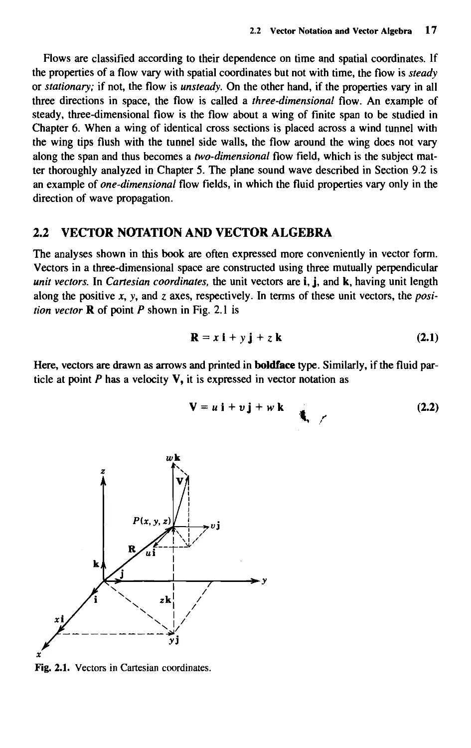
position vector R of point P shown in Fig. 2.1 is
R = xi + yj + zk
(2.1)
Here, vectors are drawn as arrows and printed in boldface type. Similarly, if the fluid
particle at point P has a velocity V, it is expressed in vector notation as
V = wi + uj + M'k
*,
(2.2)
**y
Fig. 2.1. Vectors in Cartesian coordinates.

18 Chapter 2 Kinematics or a Flow Field
where u, v, and w are the velocity components in the x, v, and z directions, respectively:
they are each scalar functions of x, v, z and t, in general. The magnitude of the velocity
vector V, being a scalar quantity called the speed V, is computed as the length of the
vector:
V = V
= V"2
+ v' + w~
(2.3)
Alternatively, the location of point P may be represented by r, 0, z in cyclindrical
coordinates, with its radial and angular coordinates r and d measured in the xy plane as
shown in Fig. 2.2. With the z coordinate remaining the same in both coordinate systems,
the transformations between cylindrical and Cartesian coordinates deduced directly from
Fig. 2.2 are
-i
2 ">
X + V
= tan
-i >'
(2.4)
and
x — r cos i
y — r sin i
(2.5)
Three unit vectors are defined at point P, of which e,. is in the outward radial direction;
ee is in the direction of increasing 9 and is thus tangent to the circle of radius r with its
center on the z axis; and e. is in the direction of increasing z. As the angular position of
P changes, the orientations of er and eg will both vary accordingly, whereas that of e_ will
not be affected. Based on these unit vectors, the velocity V at point P is constructed:
*-y
Fig. 2.2. Vectors in cylindrical coordinates.

2.2 Vector Notation and Vector Algebra 19
V = «,.e,. + wHeH + M.e. (2.6)
whose magnitude is, similar to that shown in Eq. (2.3),
V = |V| = yjuj + ul+u2. (2.7)
where «,., m„, and u, are, respectively, the radial, circumferential, and axial velocity
components.
For problems in which flow properties do not vary with z, the cylindrical coordinate
system is simplified to a two-dimensional system consisting of polar coordinates r and 0
only.
Between two vectors A and B expressed in any coordinate system, there are two
product manipulations besides addition and subtraction. One of them is called the dot, or scalar,
product, which is defined as a scalar given by
AB = |aI'b|cos<£ (2.8)
where <f> is the angle between the two vectors. To be interpreted geometrically through
Fig. 2.3, A • B is equal to either the projection of A onto B multiplied by the length of
B; or the projection of B onto A multiplied by the length of A. The value of the dot
product of A and B remains unchanged if the order of A and B is reversed; that is, A • B =
B • A. For 90° < <f> < 270°, the dot product becomes negative, indicating that the
projection of one vector is in the direction opposite to that of the other vector. Furthermore,
the relation A • B = 0 is required for the perpendicular of two nonvanishing vectors A
andB.
Letting A and B in Eq. (2.8) be one of the three unit vectors in Cartesian coodinates,
we obtain
and
i • i = j ■ j = k • k = 1 (2.9)
i-j = i-k = j-k = 0 (2.10)
Fig. 2.3. Dot product of A and B.

20 Chapter 2 Kinematics of a Flow Field
By the use of Eqs. (2.9) and (2.10), the dot product of A = Aj + AJ + Ak and B = #vi
+ BJ + S.k is
A • B = A3S + KBy + AS. (2.11)
Similarly, the magnitude of vector A is obtained by replacing B with A in Eq. (2.8) to
give
A = |A| = ^A-A = ^4; + A; + A: (2.12)
whose equivalents are shown in Eqs. (2.3) and (2.7). Expressions analogous to Eqs. (2.9)
through (2.12) can be derived for other coordinate systems.
The second product manipulation, called the cross, or vector, product, is defined as a
vector C given by
C = A x B = JAMB! sin <f> e± (2.13)
where e± is the unit vector normal to the plane containing both A and B, whose direction
is determined by the motion of a right-hand screw when A is rotated toward B through
an angle <f> (see Fig. 2.4). The magnitude of C represents the area S of a parallelogram
with sides A and B, whose value is equal to the product of base length |AJ and height
|Bj sin 4> as shown in Fig. 2.4.
Based on the definition of Eq. (2.13), the cross product of A and B changes sign if their
order is reversed, that is, B x A = -A x B. For parallel vectors A and B, A x B = 0
and, in particular, A X A = 0. The following relationships are deduced from Eq. (2.13)
in Cartesian coordinates:
ixi=jxj = kxk = 0 (2.14)
and
C = AXB
->
Fig. 2.4. Cross product of A and B.

2.2 Vector Notation and Vector Algebra 21
i x j = k = -j x i
j x k = i = -kx j
kxi = j = -ixk
(2.15)
For any two vectors A and B in Cartesian coordinates, the cross product can be expressed
in the form of a determinant and its expression is obtained by an appropriate expansion:
AxB =
i J k
At \ \
B, B, B,
(\Bz-AzBy)i
= + {AzBx-AxBz)j
+ (AxBy-AyBx)k
(2.16)
In cylindrical coordinates, Eqs. (2.14) and (2.15) are still valid if i, j, and k are replaced
with and e„ ee, and ez, respectively, so that the cross product has the form
AxB =
Ar \ Az
Br Bg Bz
{AeBz-AzBe)er
= +(AzBr-ArBz)eg
+ {ArBe-AeBryz
(2.17)
At this point, it is appropriate to introduce the vector differential operator del, denoted
by V, which is defined in Cartesian coordinates as
V = — i + — • + — k
dx dy dz
(2.18)
When V operates on a scalar field Q(x, y, z), the resultant vector expression is called the
gradient of Q and is sometimes written as grad Q:
i„ „~ dQ. dQ. dQ,
grad Q = V0 = -^i + -^-j + -^-k
dx dy dz
(2.19)
V may operate on a vector field, say, the velocity vector \(x, y, z), in two different ways.
The result of a dot product is a scalar quantity called the divergence of V:
j. ., *7 ., <^" dv dw
divV = V-V = — + — + —-
dx dy dz
whereas that of a cross product is a vector called the curl of V:
curl V = V X V
(2.20)
fdw__dv^
dy dz
1 +
du dw
dz dx,
J +
dv du
K d* dy
(2.21)

22 Chapter 2 Kinematics or a Flow Field
which is obtained following the expansion procedure described in Eq. (2.16), with the
elements in the second row of the determinant replaced by the three components of the
operator V.
Note that unlike the dot product of two vectors shown in Eq. (2.11), the order of the
operator V and the operant V in the dot product shown in Eq. (2.20) cannot be reversed,
since
d a d
V-V =u——+v—+w—
ax d\ dz
(2.22)
represents a scalar differential operator whose meaning is completely different from that
of V • V.
Expressions for gradient, divergence, and curl in cylindrical coordinates are quite
different from those in Cartesian coordinates; they are shown or derived in later sections of
this chapter.
2.3 SCALAR FIELD, DIRECTIONAL DERIVATIVE, GRADIENT
In the previous section, a scalar field was defined as one in which a property, such as
temperature, pressure, and the like, at a given point in space at a given instant is
represented completely by a single number. We will abbreviate the analyses by postulating that
the field is steady. Then the property Q is defined in Cartesian coordinates by
Q = Q(*. y. z)
We thus describe scalars as single-valued functions of position. They and their
derivatives are also generally continuous so that a Taylor expansion can be used to relate
magnitude QB at a neighboring point B in terms of QA, the value at a given point A. Thus,
Qb
*♦(»<■
—Hf)
dQ
(>■->'*)+ ~r (zb-za)
dx2
{xb~xa)2
2!
+ •••
Let B —> A. Then (QB - QA) —> dQ, (xB - xA) —> dx, and so on, and in the limit the terms
multiplying the higher derivatives vanish and the equation becomes
dQ = d-Qdx + d-Qdy + d4dZ
dx dy az
(2.23)
The equation may be expressed alternatively in vector notation as
dQ = V£ • ds
(2.24)
in which VQ is the gradient vector already defined in Eq. (2.19), and

2.3 Scalar Field, Directional Derivative, Gradient 23
Q(x + dx, y + dy, z + dz)
= Q(x, y, z) + dQ
/da = dx'\ + dyj + dzk
K /
Q(x, y, z) Fig. 2.5. Change of Q due to displacement.
ds = dxi + dyj + dzk (2.25)
is the displacement vector shown in Fig. 2.5.
The physical meaning of Eq. (2.23) can be interpreted as follows: dQ/dx, dQ/dy, and
dQ/dz are the partial derivatives evaluated at a given point (x, y, z), which represent
increases of Q per unit distance in the x, y, and z directions, respectively. When moving
away from the point (jc, y, z) with infinitesimal displacements (dx, dy, dz), the increment
in Q due to the change of position in the x direction is (dQ/dx) dx and, similarly, those in
the y and z directions are (dQ/dy) dy and (dQ/dz) dz, respectively. Thus, the total
increment dQ at the new position is the sum of the three individual contributions, which is
further expressed in a more compact form of Eq. (2.24) in vector notation.
Equation (2.23) can now be extended to define the directional derivative, that is, the
rate of change of Q with respect to the distance in a specified direction. For geometrical
simplicity, the problem is reduced to two dimensions, as illustrated in Fig. 2.6. Let ds be
Fig. 2.6. Directional derivative; isolines and
gradient lines.

24 Chapter 2 Kinematics of a Flow Field
the magnitude of ds, then
dQ_ _ dQ ^v dQdy_
ds dx ds d\- ds
in which the geometrical derivatives are, with a being the angle between ds and the x
axis,
dx dx
— = cosa; — = sin a
ds ds
so that
dQ dQ dQ .
-~- = -^ cosa + -2- sin a (2.26)
ds dx d\~
This relationship can also be derived by dividing Eq. (2.24) by ds:
^ = V0-e, (2.27)
ds
where ev = ds/ds = cos a i + sin a j is the unit vector in the direction of ds. dQIds is
defined as the directional derivative of Q in the direction of ev.
EXAMPLE 2.1
To demonstrate the use of the preceding analysis, we consider a two-dimensional field
Q = x2 + y1
and compute its directional derivative at the point (1, 1) in the direction of the straight
line y — x = 0.
The slope of the straight line is dyldx = 1 = tan a, so that a = 45° and the unit vector
in that direction is
i j
et = cosai + sinai = -7= + —j=
J V2 4i
At (1, 1), VQ = 2x\ + 3yj = 2i + 3j. Substitution of these two vectors into Eq. (2.27)
yields
dQ = _2_ J_ = J_
ds ' ■& 4l ' 4l

2.3 Scalar Field, Directional Derivative, Gradient 25
For a two-dimensional scalar field Q, VQ at a given point (x, v) is a vector pointing in
a known direction as shown in Fig. 2.6. The directional derivative of Q at that point in
the direction of ds that makes an angle <j) with VQ is
^ = |V0|cos<* (2.28)
ds ' '
which is obtained by expressing the right-hand side of Eq. (2.27) according to the
definition of dot product shown in Eq. (2.8). Equation (2.28) indicates that the directional
derivative varies with the direction of ds relative to the direction of VQ. In particular, when
4> = 90°, ds 1 VQ and dQ = 0; in other words, the value of Q will remain unchanged in
this particular direction. The curves on which Q assumes different constant values are
called isolines. The slope of the isoline passing through (jc, v) is thus determined from Eq.
(2.26) by setting the left-hand side to zero:
dy\_ dQIdx (229)
dxJi dQ/dy
in which the subscript / is used to denote isoline. In arriving at this form, we have
realized that the slope is equal to tan a„ where a, is the angle between the tangent ds, to the
isoline and the x axis. The solid curves sketched in Fig. 2.6 are used to represent isolines.
On the other hand, the value of dQ/ds is shown to become a maximum when <f) = 0 in
Eq. (2.28). A physical interpretation of the gradient of Q is thus found as follows: VQ at
a given point gives both the direction and magnitude of the maximum spatial rate of
increase of Q, which is a vector perpendicular to the isoline passing through that point.
Curves that are everywhere in the direction of the greatest rate of change of Q are called
gradient lines. Some gradient lines are shown in Fig. 2.6 as dashed curves.
Orthogonality of the gradient line and isoline at (x. y) requires that their slopes are negative
reciprocals, from which we obtain the slope of the gradient line by use of Eq. (2.29):
dx)x dQ/dx
With the right-hand side expressed as a known function of x and y, an integral of Eq.
(2.30) will yield the general equation of gradient lines containing an arbitrary constant.
We can see from Fig. 2.6 that the distribution of a scalar throughout a two-dimensional
region is defined by a family of isolines or by an orthogonal family of gradient lines.
EXAMPLE 2.2
The equations of the two orthogonal families of lines are related by Eqs. (2.29) and (2.30).
For instance, assume that the scalar is distributed according to the equation
Q = xy
(A)

26 Chapter 2 Kinematics of a Flow Field
That is, the isolines are members of a family of rectangular hyperbolas asymptotic to the
x and y axes, each one corresponding to a different value of Q. Then dQ/dx = y and dQIdy
= x so that, by Eq. (2.30), the slope of the gradient line is given by
dy x
tana. = — = —
* dx v
and the equation of the gradient line is the solution of the differential equation
y dy - x dx = 0
which integrates to
y2 — x2 = constant (B)
This equation also represents a family of rectangular hyperbolas, orthogonal to those of
Eq. (A), and asymptotic to axes at 45° to the x and y axes.
If we were given instead the equation for the gradient lines, Eq. (B), we would
differentiate and take the negative reciprocal to find the differential equation
x dy + y dx = 0
for the isolines. The integral is Eq. (A). We show later that the hyperbolas of Eq. (A)
trace the approximate paths of fluid elements in the immediate neighborhood of a
"stagnation point," that is, for instance, the point on an airfoil where the incident flow divides
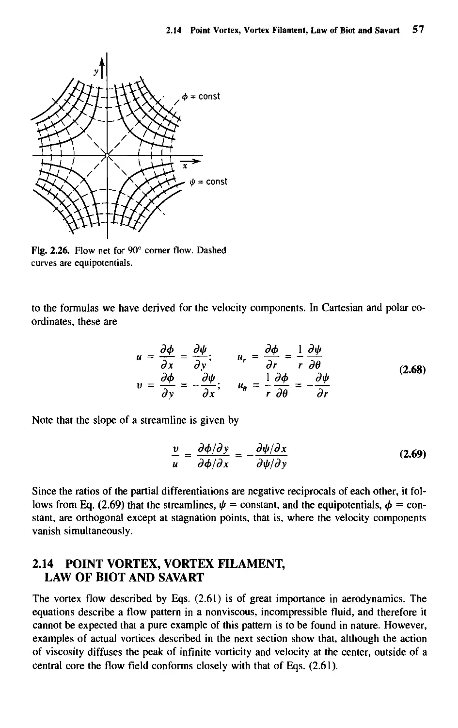
(see Fig. 2.26).
Consider a long heated wire along the z axis in a stagnant fluid and neglect gravity forces.
Then convection currents would be absent and the temperature T would be constant on
circular cylindrical surfaces. Conservation of energy requires that
C C
where C = constant.
Then dTldx = -Cxltf + y2)3'2 and dT/dy = -Cy/(x2 + y2f'2 and, by Eq. (2.30), the
differential equation for the gradient lines is dyly — dx/x, the solution of which is y = kx
where Jk is a constant. The gradient lines are therefore radial lines through the origin,
orthogonal to the circular isolines.
It follows from Eqs. (2.29) and (2.30), and is evident in the two examples, that since
the two families are orthogonal, their designations as isolines or gradient lines are inter-

2.4 Vector Field: Method of Description 27
changeable. Thus, in Example 2.2, if Eq. (B) describes the isolines, Eq. (A) describes the
gradient lines; in Example 2.3, if the lines y = kx are specified as isotherms, the gradient
lines are concentric circles.
2.4 VECTOR FIELD: METHOD OF DESCRIPTION
There are several vector fields that appear frequently in the analysis of fluid flows, such
as the fluid velocity and pressure gradient. The latter, being a vector designated as grad
p or Vp, is obtained by replacing Q with the pressure p in Eq. (2.19):
. dp . dp . dp .
gradp = 3J1 + 31 J + ^k
ox ay oz
The vector has the magnitude
2
+
2
+
<dzj
\\dx) ydy) \dz
Its direction is determined in the same way shown in Fig. 2.1 from the projections of Vp
on the three coordinate axes.
In cylindrical coordinates, we may write
. dp I dp dp
gradP = -e, + --ee+-e:
in which the second term on the right side represents the increase of p per unit arc length
on the circle shown in Fig. 2.2. The magnitude of this vector is
|gradp| =
[dr) [rdej
fdp_
U
Similarly, as already shown in Eq. (2.2), a velocity field having components u, v, and
w is represented in vector notation by
V = Mi + vj + H,k
where u, v, and w are each scalar functions of x, v, z and time t. They are field
properties; that is, they represent the velocity components of the field element passing through
a given point (x, y, z) at a given instant of time. At a later instant, the element will have
moved to a new position and its velocity will correspond to the field position it occupies
at the later instant. The magnitude of the velocity vector is computed in the manner
described in Eq. (2.3).
Rather than specifying the components as functions of spatial coordinates, a steady
velocity field is sometimes described by specifying its magnitude and direction as functions

28 Chapter 2 Kinematics of a Flow Field
Streamline
Fig. 2.7. Tangent of velocity to streamline.
of position with the introduction of streamlines. A streamline is defined as a path whose
tangent at any point is aligned with the velocity vector at that point. A velocity field may
then be described alternatively in terms of equations of the streamlines and the absolute
value of the velocity.
Frequently, something will be known about the streamlines and the magnitude of the
velocity. For mathematical operations, however, the velocity components are needed as
functions of spatial coordinates, and a conversion from the second method of
representation to the first is necessary. In treating the two-dimensional case described in Fig. 2.7,
the conversion is readily performed by remembering that vlu is the slope dy/dx of a
streamline and the magnitude of the velocity vector is yju2 4- ir. These values provide two
equations in two unknowns:
dx v . . — r
-^- = —; |V| = \ ir + v
dx it
from which u, v can be computed if dy/dx and V are given, and vice versa. These two
methods of representing a velocity field are demonstrated in the following two examples.
EXAMPLE 2.4
For a two-dimensional velocity field given by
u = v, v =.v
the slope of the streamline passing through the point (x, v) is
dy _ v _ .v
dx u v
It can be written as
x dx - v dx = 0

2.4 Vector Field: Method of Description 29
whose integral yields the equation of streamlines:
x2 - y2 = C (A)
It represents a family of hyperbolas by varying the value of the integration constant C
and has the same form as that of the gradient lines described in Example 2.2.
To find the equation of a particular steamline passing through the point (2, 1), we first
compute the value of C at that point, which is 3 from Eq. (A). Thus, the equation of that
streamline is x2 - y2 = 3.
Alternatively, assume it is known that the streamlines are circular and the magnitude of
the velocity is constant on a given streamline. Then the equation of the streamline is
x2 + y2 = constant
and the magnitude of the velocity is
|V| = fix2 + y2)
From the first equation above,
dy _ x _ v
dx y u
and from the second,
V7T7 = T+(»)2=/('!+/)
Substituting — x/y for v/u and solving for u, we obtain
u_ ^f{*2+y2) _ {yf{r)
where x2 + y2 = r2. Similarly,
xf(x2+y2) xf{r]
The signs on u and v must be opposite in order to satisfy the condition v/u = -x/y. The
sense of V, that is, the sign of f(r), determines the flow direction, as shown in Fig. 2.8
for a positive /. The direction of the velocity vector is reversed if / is negative.

30 Chapter 2 Kinematics of a Flow Field
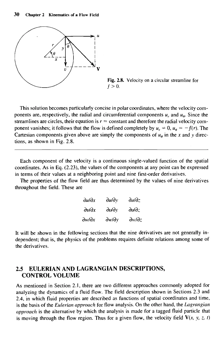
V
Fig. 2.8. Velocity on a circular streamline for
/>0.
This solution becomes particularly concise in polar coordinates, where the velocity
components are, respectively, the radial and circumferential components «,. and uH. Since the
streamlines are circles, their equation is r = constant and therefore the radial velocity
component vanishes; it follows that the flow is defined completely by ur = 0, uH = -/(r). The
Cartesian components given above are simply the components of uti in the x and .y
directions, as shown in Fig. 2.8.
Each component of the velocity is a continuous single-valued function of the spatial
coordinates. As in Eq. (2.23), the values of the components at any point can be expressed
in terms of their values at a neighboring point and nine first-order derivatives.
The properties of the flow field are thus determined by the values of nine derivatives
throughout the field. These are
du/dx du/dy du/dz
dv/dx dv/dy dv/dz
dw/dx dw/dy dw/dz
It will be shown in the following sections that the nine derivatives are not generally
independent; that is, the physics of the problems requires definite relations among some of
the derivatives.
2.5 EULERIAN AND LAGRANGIAN DESCRIPTIONS,
CONTROL VOLUME
As mentioned in Section 2.1, there are two different approaches commonly adopted for
analyzing the dynamics of a fluid flow. The field description shown in Sections 2.3 and
2.4, in which fluid properties are described as functions of spatial coordinates and time,
is the basis of the Eulerian approach for flow analysis. On the other hand, the Lagrangian
approach is the alternative by which the analysis is made for a tagged fluid particle that
is moving through the flow region. Thus for a given flow, the velocity field \{x, y, z, t)

2.5 Eulerian and Lagrangian Descriptions, Control Volume 31
in the Eulerian description becomes V(r) in the Lagrangian description; the latter
represents the velocity of a selected fluid particle moving along its own particular path, on
which the coordinates x, y, and z of the particle are given functions of time. Basic laws
of fluid dynamics can be derived based on either the Eulerian or Lagrangian method of
description.
When the Eulerian approach is followed to derive the laws of conservation of mass,
momentum, and energy, the analyses are performed by considering a group of fluid
material that is confined instantaneously within a region called the control volume. It is an
imaginary volume of a properly selected shape, which is ordinarily fixed in space but may
deform as required in some problems. The control volume is bounded by a control
surface, through which the fluid can move freely without friction or any other restrictions.
In the flow region shown in Fig. 2.9, let R be a control volume fixed in space and S be
its bounding control surface. Consider an infinitesimal surface area dS, at which the unit
vector n normal to the surface and pointing away from the volume is known for a given
shape of R. If the local fluid velocity V makes an angle <f> with n, it can be decomposed
into a component V cos <j> normal to the surface and a component V sin <f> tangent to it.
Since the volume of fluid flowing per unit time from the control volume, or the volume
efflux dq, through dS is not affected by the tangential velocity component, it is computed
as the product of the normal velocity component V„ and the area, that is, V cos $ dS,
which, after we invoke Eq. (2.8), is written as
dq = V • n dS = V„ dS (2.31)
At a surface point where V points away from the control volume, such as the point shown
in Fig. 2.9, the sign of dq is positive, indicating that fluid is leaving the control volume
through that surface element. On the contrary, a negative dq signifies that fluid is
entering the control volume locally.
Fig. 2.9. Control volume and control surface.

32 Chapter 2 Kinematics of a Flow Field
2.6 DIVERGENCE OF A VECTOR, THEOREM OF GAUSS
The three derivatives on the diagonal extending from the upper left-hand corner to the
lower right-hand corner of the matrix shown at the end of Section 2.4 have a property in
common. Each represents the rate of change of a component of the velocity in the
direction of that component. As defined in Eq. (2.20), the sum of these extension derivatives
is called the divergence of the velocity and is written
du dv dw
dx dy dz
divV = — + — +
(2.32)
The divergence of the velocity vector can be interpreted physically as the efflux per
unit volume from a point. To see this, consider^ the velocity vector V, which is a field
property, let A^ be the small control volume shown in Fig. 2.10, and let AS be the
control surface enclosing A^?. At any instant of time, a fluid particle in the control volume
has the field velocity at the point it occupies at that instant. In Fig. 2.10, the control
volume A^? has been oriented for convenience with its edges parallel to the x, y, z axes; the
velocity components at its center are indicated by u, v, and w. To find the volume of fluid
flowing per second, or the volume flux, through the control surface enclosing A^?,
contributions of the velocity components normal to each of the six faces of the control
surface have been indicated on the figure according to Eq. (2.31). For a negative dq, an
inward pointing arrow is drawn to denote an inflow.
The magnitudes of the normal components have been derived from their values at the
center of the control volume by the argument of Section 2.3. For example, the value of
the x component of the velocity on an x face of the cube (i.e., on one of the faces normal
to the x axis) differs from that at the center of the control volume by an increment
(3m/3jc)(Ajc/2); it will be remembered from the discussion in Section 2.3 that this is an
exact statement when Ajc is vanishingly small. Consequently, for a control volume of
infinitesimal proportions, the average value of the velocity component on the right-hand x face
is u + (duldx)(kx/2). Since the area of an x face is AvAz, the rate of volume flow out of
. ciu A*.. .
, dv dVw ,_
w+ — -^-)AxA2
dy 2
(u>- - ^)AxAv
oz 2
».(B+__)V42
W+ —■ — )A*Ay
9y 2
Fig. 2.10. Volume effluxes through faces of a cubical control
volume.

2.6 Divergence of a Vector, Theorem of Gauss 33
the right-hand a- face is [u + (du/dx) A.y/2] AyAz; that into the left-hand face is [u - (du/dx)
/W2] AyAz. Thus, the net outflow from the x faces is (du/dx) AxAyAz per unit time.
The efflux of fluid volume per unit control volume enclosing a point is, by definition,
lim
AR-*0
volume outflow/s - volume inflow/s
AR
With the aid of Fig. 2.10, the above expression becomes du/dx + dv/dy + dw/dz for the
net outflow per second from the three pairs of faces of the cube; this is precisely the
definition of div V given in Eq. (2.32). It is a scalar and its magnitude is the rate at which
fluid volume is leaving a point per unit control volume.
In a similar manner, the expression for divergence of a vector can be derived in other
orthogonal coordinate systems. Figure 2.11 shows a control volume in cylindrical
coordinates, ;\ 0, z. It can be shown (Problem 2.6.1) that
divV
dur 1
^7 + 7
( du, ^
K +
\
dd )
du:
dz
(2.33)
We return to the consideration of flow through a finite control volume for the purpose
of deriving an important integral relation and thus gaining further insight into the mean-
(ur+ jf ~~){r+ yJAOAz
i)u.t &z
l* Hz 2
)r\0\r
Fig. 2.11. Volume effluxes through faces of a polar control volume.

34 Chapter 2 Kinematics of a Flow Field
Fig. 2.12. Control volumes.
ing of divergence. We consider a finite control volume R as shown in Fig. 2.12. The
region R is divided into elementary cubes and div V is found for each cube. The flux through
common faces of adjacent cubes cancel because the inflow through one face is equal to
the outflow through the other. Now, if we sum the fluxes for all cubes, only the flow rate
through the faces of the surface enclosing the entire region will contribute to the
summation. In the limit, therefore, as the cubes approach infinitesimal volume, the integral of
div V over R is equal to the net flux through S, the surface enclosing R, that is,
JJJ^div V dR = jj. V • n dS (2.34)
This equation is a specialized form of an integral theorem applying to vector fields in
general. It is useful in many fields of technology and is referred to as the divergence
theorem; it is generally attributed to Carl Friedrich Gauss (1777-1855).
In the next section, we treat the conservation of matter applied to fluid flows. All the
analyses by which we identified div V in the present section as the flux of volume at a
point carry over to the flux of mass by substituting pV for V in Eq. (2.34).
2.7 CONSERVATION OF MASS AND
THE EQUATION OF CONTINUITY
One of the empirical laws that forms the basis of "Newtonian mechanics" states that mass
can neither be created nor destroyed. This conservation principle applies to fluid elements
of fixed identity and, in order to express the principle in terms of field properties of a
flow, we apply a physical reasoning following the Eulerian approach.
Consider a control volume R fixed in the field, as shown in Fig. 2.12. The total mass
within R is
E"*
where p dR is the infinitesimal contribution of the mass at a given point to the total within
the region R. Through any incremental area dS of the control surface, the mass flow per
unit time is pV • n dS, which is obtained by multiplying the volume efflux shown in Eq.

2.7 Conservation of Mass and the Equation of Continuity 35
(2.31) by the density. If more mass flows out of than into R per unit time, the mass within
R must be decreasing. Specifically, the net efflux of mass through S is equal to the time
rate of decrease within R. The conservation of mass principle stated in terms of field
properties is then
JJ.pV.„^ = -JJJ.^ (2.35)
As a simple application of the above principle, consider the steady flow of a fluid
through the shaded stream-tube shown in Fig. 2.12. The control volume is contained within
the two neighboring streamlines and the dotted lines. There is no flux through the
streamlines because they are everywhere tangent to the local fluid velocities, and it is assumed
that p, and V, are average values across the area At, and p2 and V2 are average values
across A2. Because the flow is steady, the right-hand side of Eq. (2.35) is zero and the
conservation of mass principle becomes
PiViA2- p,V,A, =0
The surface integral in Eq. (2.35) may be transformed into a volume integral by
application of the divergence theorem, Eq. (2.34):
JJ. pV-n dS = HI. div p V dR
Thus, Eq. (2.35) is written in the form
E(f+divpV)^ = 0 (2,36)
Equation (2.36) must hold for all control volumes regardless of size, and therefore the
integrand must be identically zero. Then the equation of continuity, which is a statement
of the conservation of mass principle in terms of field properties at a point, is obtained
in the form of a partial differential equation
4^ + divpV = 0 (2.37)
dt
This equation is satisfied in a physically possible flow, that is, a flow in which mass is
conserved. When the flow is steady, the field properties are not functions of time, and
continuity reduces to
div pV = 0 (2.38)
If the fluid is incompressible, p is a constant and continuity becomes, regardless of whether
the flow is steady or unsteady,
div V = 0 (2.39)

36 Chapter 2 Kinematics of a Flow Field
A given velocity field is physically possible only if continuity (as defined by the
particular one of these equations appropriate to the flow being considered) is satisfied.
The most elementary example of a physically possible flow is one in which the fluid
velocity is constant everywhere. There, regardless of the orientation of the x, y, z axes,
the separate terms in div V vanish identically, and the continuity is satisfied for uniform
incompressible flow.
Another example occurs in the incompressible flow in which the streamlines radiate
from the origin; for simplicity, we assume that the radial velocity ur depends only on the
distance r from the origin, and we determine its variation such that continuity is satisfied.
For the two-dimensional problem, the formula for div V is given in Eq. (2.33), and
since u„ = 0 everywhere, the condition for continuity, Eq. (2.39), becomes
^ + ^ = 0 (2.40)
dr r
and the solution is rur = k, that is,
k
«,. = —
r
The constant k is evaluated by writing A = 2-irru,. = 2irk for the rate of volume flow
through the circle of radius r. Then k = A/2ir and the two-dimensional flow radiating
uniformly in all directions from the origin and satisfying continuity is described by
A ; «» = o (2.41)
2irr
These equations describe a source flow of strength A. A > 0 for flow outward, and A <
0 for flow inward; the latter is called a sink flow. A has dimensions of lengtlr/time.
The same result will be obtained by the use of Eq. (2.35) for a steady flow if we choose
R as the annular region shown in Fig. 2.13, bounded by circular cylinders of radii r, and
U<2
Fig. 2.13. Control surface for volume flux from a
source.

2.8 Stream Function in Two-Dimensional Incompressible Flow 37
r2, with r2 > rt. For flow outward, fluid volume enters unit length of cylinder r, at the
rate 2-n rxun and leaves unit length of cylinder r2 at the rate 2nr2un. The surface 5
enclosing R comprises the surfaces of the two cylinders and a connecting "corridor" of
infinitesimal width, as indicated in Fig. 2.13. We arbitrarily choose the positive direction
of integration so that the region R is always on the left. Then, since the outward drawn
normal is positive, and V • n = -ur< and +«„, respectively, on the inner and outer
surfaces and V • n vanishes on the boundaries of the corridor. Then Eq. (2.35) becomes
2Trr2uri - 2nrlun = 0
Since rt and r2 are arbitrary, we may let r2 approach r,. Then r2 = r, + Ar and «r, = un
+ Aur, and the equation becomes
(r, + Ar)(un + Aur) - rtur, = 0
As Ar and Aur both approach infinitesimal, we obtain Eq. (2.40), which integrates to Eqs.
(2.41).
We note that in the preceding analyses the region R excluded the origin. Now we take
the region R as including the origin and proceed to evaluate div V at r = 0, where Eqs.
(2.41) indicate that ur becomes infinite. To this end: Since div V vanishes everywhere
except at r = 0, the volume integral on the left-hand side of Eq. (2.34) becomes in the limit
the product of div V and a volume Ay?, which approaches zero as r —> 0; therefore, since
both integrals in the equation must be equal to the constant efflux represented by the right-
hand side of Eq. (2.34),
l\-ndS
(divV),_n = lim J -— = o°
v "*' ak-o AR
A source flow is thus physically possible everywhere except at the center where div V is
unbounded.
We discuss separately these elementary flows, such as uniform flow, sources, sinks,
and vortices (see Section 2.11), as a prelude to demonstrating that they are "building
blocks" for more complicated flows. Later we show the methods by which the details of
the flow around, and the fluid pressures acting on, a body of a given shape that is in
motion through a fluid can be determined by adding the contributions from these building
blocks, whose respective strengths are actually determined from the body shape.
In the following sections, quantitative methods are developed for describing these flows
to facilitate their application to practical problems.
2.8 STREAM FUNCTION IN TWO-DIMENSIONAL
INCOMPRESSIBLE FLOW
As a consequence of the conservation of mass, it is possible to define uniquely a
function of the field coordinates from which the velocity in both magnitude and direction is
derivable for two-dimensional incompressible flow. In Fig. 2.14, let ab and cd represent

38 Chapter 2 Kinematics of a Flow Field
Fig. 2.14. Streamlines and velocity in a stream tube.
streamlines in a two-dimensional incompressible flow.* As defined in Section 2.4, a
streamline is a curve whose tangent at every point coincides with the direction of the
local velocity vector. Therefore, no fluid can cross cd or ab. Incompressible flow has been
assumed, the density of the fluid within the boundary efgh does not vary with time, and,
therefore, the same mass of fluid must cross ef per unit time as crosses hg, or any other
path connecting the streamlines. If the streamline ab is arbitrarily chosen as a base, every
other streamline in the field can be identified by assigning to it a number ip, called the
stream function; its magnitude is the volume of fluid passing per unit time between an
arbitrary base streamline and the one passing through the given point, per unit distance
normal to the plane of the motion. Isolines of ip are the streamlines with the isoline ip =
0 chosen as the base streamline.
The fluid velocity can be derived from a stream function with the following
considerations. Let rfs in Fig. 2.14 be the infinitesimal displacement vector going from the
streamline ip to a neighboring streamline ip + dip, and V be the average velocity in the stream
tube bounded by the two streamlines. According to the definition of stream function, the
rate of volume flow through the tube is dip, which is computed as the product of !vl and
the area \ds\ sin <p of the tube normal to |v|, where <f> is the angle between V and ds as
indicated in Fig. 2.14:
dip = |V| \ds\ sin <f> = V x ds\
The second equality is a result of Eq. (2.13), the definition of the cross product.
♦Such a function can also be found in three dimensions for flows with axial symmetry, for example, the flow
about a body of revolution (see Karamcheti. 1966). For a two-dimensional compressible flow, the stream
function is derived in Section 7.2.

2.8 Stream Function in Two-Dimensional Incompressible Flow 39
Carrying out the product of V = u\ + vj and ds = dxi + dy\ in the manner described
in Eq. (2.16), we have V X ds = k(u dy - vdx). Thus,
dip = u dy — v dx
Mathematically, we may also write, according to Eq. (2.23),
.. dip . difi .
dip = -^-dx + ^-dy
ox ay
Since these two equations are identical everywhere in the flow field, the coefficients of
dx and dy must, respectively, be identical in the two equations. It therefore follows that
u = -^; v = --£• (2.42)
ay ox
From Eqs. (2.42), a general rule can be drawn: The velocity component V in any
direction is found by differentiating the stream function in the direction of n, which is a
displacement vector at right angles to the left of that velocity component; that is,
dn
It follows from the above equation that the dimensions of i/' are length2/time.
In polar coordinates, in which the counterclockwise direction is positive for 9, the
application of the above general rule gives
• dip dip
"' = 7^: U°=~Tr (2'43)
The use of the stream function in describing a two-dimensional incompressible fluid
flow becomes clear if we substitute Eqs. (2.42) or (2.43) for the terms in Eq. (2.32) or
(2.33) for div V, to obtain
.. „, du dv du. 1
d.vV = 3" + -r- = Y + "
ax ay or r
( 3„ ^
u.+-
\
dUg
36 ,
= 0
We find that the continuity equation (2.39) is satisfied identically and therefore that
continuity is identically satisfied by the "existence" of a stream function, that is, by the
existence of an analytic expression ip from which the velocity components can be found by
partial differentiation according to the above rule.
Introduction of the stream function simplifies the mathematical description of a two-
dimensional flow because the two velocity components can thereby be expressed in terms
of the single variable ip.

40 Chapter 2 Kinematics of a Flow Field
EXAMPLE 2.6
For a uniform flow, Eqs. (2.42) give
u = -£- = A; v = --J- = B
ay ox
where A and B are given constants. Since the derivatives are partials with respect to y and
x, respectively, we find two expressions for i// by integrating the first equation, keeping x
constant, and the second keeping y constant. Thus, with C, and C2 being the integration
constants,
4> = Ay + f(x) + Ct; .// = -Bx + g(y) + C2
where f(x) is a function only of x and g(y) only of y; they are evaluated from the
condition that the two equations must give identical expressions for <//. This identity condition
requires that f(x) = -Bx and g(y) = Ay. Thus, the stream function
ijj = Ay - Bx + C (A)
describes a uniform flow with speed |V, = Va2 + Br, inclined at an angle tan~'(5/A) to
the x axis.
Although the integration constant C does not have any influence on the velocity field,
its numerical value determines the constant i/> values on the individual streamlines in the
flow. The value of C is usually determined from the requirement that the base streamline
passes through a conveniently selected point. For example, if we require that the base
streamline i// = 0 goes through the origin where x = 0 and y = 0, then the value of C is
zero as computed from Eq. (A). Thus for this particular case of C = 0, the stream
function is 4> = Ay — Bx, the equation of the base streamline is Ay — Bx = 0, the equation of
the streamline on which if = 1 is Ay — Bx = 1, etc.
In the same way, by the integration of Eq. (2.43) for the source flow of Section 2.7
[ur = A/277T, u„ = 0], we find
,/, = A0
2tt
for the stream function, in which the constant of integration has been set to zero so that
the base streamline coincides with the straight line 9 = 0. Differentiation according to
Eqs. (2.43) yields the velocity components of Eq. (2.41):
v = -z—; ue = °
iirr

2.8 Stream Function in Two-Dimensional Incompressible Flow 41
It follows that the existence of a stream function is a necessary condition for a physically
possible two-dimensional incompressible flow, that is, one that satisfies mass
conservation. Or, in other words, and as illustrated in the following example, a stream function
cannot be found for any flow that does not satisfy the mass conservation principle.
EXAMPLE 2.7
An assumed incompressible flow that does not satisfy continuity is described by the
components m = -4, v = By, where -4 and B are constants. In accordance with Eqs. (2.42),
dip/dy - A and dip/dx = -By. Thus, with integration constants ignored, we obtain
\\i = Ay + f(x) and ifr = -Bxy + g(y)
Since no choice of /(x) will reconcile these two expressions, we must conclude that the
assumed flow cannot be described by a stream function as defined in Eqs. (2.42). In other
words, a stream function does not exist for the assumed flow. Furthermore, it follows from
,. ,r du dv
divV = —+ — = B
ox ay
that the assumed flow would require the creation, at the rate of B cubic meters of fluid
per cubic meter of the control volume at every point of the field. Thus, the assumed flow
field is not physically possible and, as was shown above, it cannot be described by a
stream function.
Two different methods have been introduced for finding the equation of streamlines.
The first method is the one described in Section 2.4 based on the tangency of fluid
velocity on the streamline, from which the slope of the streamline is obtained as a function
of velocity components. The second method shown in the present section is based on the
conservation of fluid mass between two streamlines through which fluid cannot cross.
Since the volume flow rate ifr of an incompressible fluid between a given streamline and
the base streamline is required to be a constant, say, C, the equation of this streamline is
obtained by looking for the curve on which ifr = C. To demonstrate that the results from
these two methods are equivalent, the problem that has been solved in Example 2.4
using the first method is reconsidered in the following example.
'EXAMPLE M
With m = y and v = x, Eqs. (2.42) become

42 Chapter 2 Kinematics of a Flow Field
If we keep in mind that these are partial differential equations, their integrated forms are
<{f = —>''+/(*) + £, and tjf = x2 +g(y) + k:. Reconciliation of the two
expressions gives
* - w
in which the constant of integration disappears if the base streamline tjj = 0 is required to
pass through the origin. Since <{/ = 3/2 at the point (2, 1), the equation of the streamline
passing through that point is y2 — x2 = 3, which is in agreement with the result of
Example 2.4.
A physical interpretation of the individual terms in the continuity equation for an
incompressible flow can be made by considering a small two-dimensional fluid element
AjcAv at time /, as shown at the left of Fig. 2.15. If the vertical surface on the right side
of the element moves with a horizontal velocity that is faster than that on the left side by
an amount (du/dx) Ajc, at time / + A/ the horizontal dimension of the element becomes
Ajc + (du/dx) AjcA/, as described at the right of Fig. 2.15. Thus, the time rate of
elongation per unit length of the element in the x direction is du/dx. Similarly, if the surface on
the top of the element moves with a vertical velocity faster than that on the bottom by
(dv/dy) Ay, the vertical dimension of the element at / + A/ becomes Ay + (dv/dy) AyA/,
so that dv/dy represents the time rate of elongation per unit length of the element in the
y direction.
Furthermore, for an incompressible fluid the area of the element on the xy plane must
remain unchanged; that is,
A* + t-- Ax \t
Ox
Av + Q- Av \t
dy
f i (u + ^ A.r) \t H
-1 ■ ox
Fig. 2.15. Elongation and contraction of a fluid element.

2.9 The Shear Derivatives: Rotation and Strain 43
A 3" A A
A* + —-AxAt
ox
a dv ^ ,
Av + —-AyAt
dy
= A*Av
By letting A/—»0 with (A/)2 diminishing much faster, we obtain
du dv
ox oy
which is the same continuity equation, Eq. (2.39), that was derived by applying the
principle of conservation of mass of fluid through a fixed control volume. Note that for a
positive duldx that causes an elongation of the fluid element in the x direction, the preceding
equation shows that dvldy is negative, corresponding to a contraction in the v direction as
illustrated in Fig. 2.15.
2.9 THE SHEAR DERIVATIVES: ROTATION AND STRAIN
We have so far identified the sum of the derivatives along the diagonal of the matrix in
Section 2.5 as the divergence of the vector V and, physically, as the flux of fluid volume
from a point. The six remaining derivatives, those o/f the diagonal, are distinguished by
the fact that they represent rates of change of the velocity components in directions
normal, respectively, to these components. These are called the cross or shear derivatives;
this section describes the roles they play in identifying further physical properties of flows.
The derivative du/dy, for instance, measures the rate at which the x component of the
velocity changes with position normal to the xz plane. Consider the distortion of an
element as a function of time as it transverses a flow in which u is the total velocity and
du/dy is the only nonzero shear derivative. Figure 2.16 shows schematically the changes
in the shape of the element with time. These changes can be described in terms of (1) the
rate of deformation or strain defined in terms of the rate of change of the included
angles, and (2) the angular velocity or rate of rotation of the diagonal.
->'!
,
/ ±y
u /
uto
/
/
/
/
/
Ax
%-Ayto
<)y
40 h/ s'l
!/ '' l
Fig. 2.16. Fluid element in a shear flow.

44 Chapter 2 Kinematics of a Flow Field
In a general three-dimensional flow, the coplanar pairs of shear derivatives in each of
the three orthogonal planes determine three components of the rate of strain and of the
angular velocity of an element. These coplanar sets are du/dy and dvldx for the xy plane,
du/dz and dw/dx for the xz plane, and dv/dz and dw/dy for the yz plane. The rate of strain
and angular velocity are thus identifed as vectors; the three components are designated
respectively by subscripts indicating the axes normal to the planes on which they act.
For purposes of illustration, we choose the xy plane and thus derive expressions for the
z components of the rate of strain and angular velocity, respectively y, and e_; the
corresponding vectors are designated y and e.
In the simplified case of the shear flow described in Fig. 2.16, consider a small fluid
element AxAy whose vertical and horizontal sides are orthogonal at a given instant t. The
horizontal velocities at the two ends of the vertical wall on the left of the element are u
and u + (du/dy) Ay, respectively. After a short time period A/, the velocity difference
causes a horizontal displacement (du/dy) AyAr of the upper end relative to the lower end,
as shown on the distorted fluid element in Fig. 2.16, resulting in an angular displacement
A/3 = (du/dy) A/ of the vertical side. In arriving at the last expression, we have replaced
the arctangent of a function by its small argument. The corresponding angular velocity is
obtained by taking the limit:
dp ,. A/3 du
—£- - lim —£- = —
dt a/->o A/ dy
We have thus shown that a positive du/dy represents a clockwise angular velocity of the
vertical side of a fluid element about the z axis.
In a similar manner it can be shown, for a general flow, that & positive dv/dx represents
a counterclockwise angular velocity daldt of the horizontal side of a fluid element about
the z axis (obtained from Aa/A/ by letting A/-* 0), where Aa is the angular displacement
in the interval A/ as shown in Fig. 2.17.
Referring to the corner of a fluid element sketched in Fig. 2.17, we see that the
component y. of the rate of strain vector y is defined as the rate at which the included angle
is decreasing; that is,
da dB dv du ,_ . „
y, = — + -*- = — + — (2.44)
dt dt dx dy
On the other hand, the component e, of the angular velocity e of the fluid element is de-
sp
j Fig. 2.17. Strain and rotation of a fluid element.

2.9 The Shear Derivatives: Rotation and Strain 45
fined as the average of the angular velocities of the two bounding sides, which is
considered positive for a counterclockwise rotation:
e, = —
2
da
It
dp
dt)
' dv__du_
ydx dy,
to,
2
(2.45)
where w, is defined as the component of the vorticity normal to the xy plane. The
magnitude of the vorticity vector, <a, is twice that of the angular velocity of the fluid element,
and it is directed along its axis of rotation. A general mathematical expression for the
vorticity is defined later in Section 2.10.
EXAMPLE 2.9
■ ■—■'—— * * - -
These two flow properties can be illustrated in terms of the "plane Couette flow" u = Ky,
v = 0, which is a special case of the flow, shown in Fig. 2.16 with a linear velocity
profile. Here, dv/dx = 0, so that yz = du/dy = K and u)z = -du/dy = —K.
We consider next the rate of strain and angular velocity of a fluid element in polar
coordinates, but only for those flows whose streamlines are concentric circles. Shown in
Fig. 2.18 is a small fluid element that, at time instant t, is bound by two radial lines and
two neighboring streamlines separated by a distance Ar. In the interval A/, the upper
circumferential side rotates by the amount A0, that is, by ue Ar/r. The amount the left radial
side rotates depends on the difference in velocity between its upper and lower ends, that
i&0 + A<t>)
Fig. 2.18. Rate of strain and angular velocity in polar coordinates.

46 Chapter 2 Kinematics of a Flow Field
is, (dug/dr) &r. The difference in the displacement of these two ends is then (dujdr) ArAt
that, after being divided by Ar, gives the angular displacement A</> = (duu/dr) A/. The
mean angular displacement Ae. of the fluid element in the interval At is (A0 + A</>)/2 so
that the vorticity of the element is given by
(>). = lim
Ar-»0
A<(> + A# _ due Ug
At dr r
(2.46)
Recalling that a positive rate of strain is defined as the rate of decrease of the included
angle, we obtain
y. - lim
Ar-»0
A(j)-A8
At
dr
(2.47)
Note that in a general flow ur does not vanish; its influences would appear in Eqs. (2.46)
and (2.47) in such a case. One example is given by Eq. (2.55).
Figure 2.19 shows a flow in which the two intersecting edges of an element rotate at the
same rate but in opposite directions. Thus, the diagonal of the element has vanishing
angular velocity, but is subjected to a pure strain. This flow is called a two-dimensional
vortex, whose velocity field ue is derived in Section 2.11 as k/r, where k is a constant.
Fig. 2.19. Fluid element in a vortex flow.

2.9 The Shear Derivatives: Rotation and Strain 47
After substituting in Eqs. (2.46) and (2.47) and using the method of Section 2.8 to find
the stream function i/>, we note that the flow field of a two-dimensional vortex has the
following properties (see Eqs. 2.43)
k
ur = 0; ue = —; /. i/> = -k\nr
2k (2>48)
a)z = 0 (at/■*()); yz = -^-(atr^O)
Figure 2.20 shows a flow in solid-body rotation about a point 0. The two intersecting
edges rotate at the same angular velocity, causing a pure rotation of the element without
any deformation. In this case, ue is given by Or, where Q is the constant angular speed
of the flow. If we use Eqs. (2.46) and (2.47), and the method of Section 2.8 to find the
stream function i/f, the flow field of a fluid in a solid-body rotation has the following
properties:
ur = 0; ue = Qr; :.^i
w, = 2Q; y, = 0
Fig. 2.20. Fluid element in a flow in solid-body
rotation.
2 (2.49)

48 Chapter 2 Kinematics or a Flow Field
2.10 CIRCULATION, CURL OF A VECTOR
We have in the last section defined the field properties, rate of strain, and vorticity. The
circulation I\ a property related to the net vorticity over a region of the flow, is defined
by
-♦V-rfs
(2.50)
where V • ds, the dot product of the velocity vector and the vector element of length along
the path of integration C, is, as indicated in Fig. 2.21, the scalar of magnitude VJ cos 6
\ds\ = Vx ds; the circle through the integral sign indicates that the circulation is defined as
the line integral around a closed path of the product of Vx, the velocity component
parallel to the path, and ds. The integral is carried out in the counterclockwise sense; the
clockwise direction of integration for circulation, indicated by the minus sign in Eq. (2.50),
is chosen in aerodynamics for convenience in the analyses of airfoil and wing theory.
The integrand of Eq. (2.50) may be expressed in two-dimensional Cartesian notation
(see Fig. 2.21) as V • ds = V cos 6 ds = u dx + v dy and, in three dimensions,
f = -»V-ds = -f(udx + vdy+wdz)
(2.51)
Line integrals such as that defining the circulation have various physical interpretations
in the different fields of technology; in fluid mechanics, we show later that the
circulation around a contour in a flow enclosing a body such as an airfoil is proportional to the
lift developed by the body.
At this point, we show the relation between the concepts of circulation and vorticity by
means of the vector designated curl V, defined in Eq. (2.21) by
curlV
dw
K dy dz
dv). I du dw
Kdz dx
J +
dv du
dx dy
Fig. 2.21. V • ds = V,ds.

2.10 Circulation, Curl of a Vector 49
The respective components are seen to be exactly the components of the vorticity, that is,
, .. dw dv
curlA V = —--— = &>v
dy dz
, ,7 du dw
curlvV = — = &>v
dz dx
dv du
curl.V = = &).
dx dy
(2.52)
In vector notation
to = curl V
(2.53)
The vector is directed along the axis of rotation of the fluid element.
The components of w at a given point are identified with the limit of the circulation
around a contour enclosing the point. For example, by carrying out the line integral of
Eq. (2.51) around the element of Fig. 2.22, one can verify that
lim
AS->0
b(udx + vdy)
AS
(2.54)
where AS is the area enclosed by the path about which the line integral is taken. The
directions of a)x, wv, and coz are determined according to the "right-hand rule."
In cylindrical polar coordinates (r, 0, z) (Problem 2.10.1), the vorticity component in
the z direction is found to be
dua 1 ( dur
(2.55)
Fig. 2.22. V, on the sides of an element.

50 Chapter 2 Kinematics of a Flow Field
2.11 IRROTATIONAL FLOW
In 1904, Ludwig Prandtl hypothesized that the flow of gases and "watery liquids" around
streamlined bodies can be assumed to have zero vorticity, that is, to be irrotational,
except in a thin boundary layer and a narrow wake behind the body. In other words, at the
Reynolds numbers of flight for aircraft or for the motion of many devices and animals
through fluids, a good approximation to the flow field, outside of the immediate
neighborhood of the body, can be found by assuming irrotationality. In terms of Eqs. (2.52),
an irrotational flow is characterized by
o)x = wv = a). = 0
that is,
dv du
dx dy
dw dv
dy dz'
du dw
dz dx
(2.56)
In cylindrical polar coordinates, a two-dimensional irrotational flow (Eq. 2.55) is expressed
by
du„ d i \ du,
r-*+*MTrM = li (2'57)
EXAMPLE 2.12
The simplest and most obvious irrotational flow is, of course, a uniform flow. In Section
2.8, we identified the flow t/t = Ay — Bx as a uniform flow inclined at the angle tan" \B/A)
to the x axis. By Eqs. (2.42), u = A, v = B, and by Eqs. (2.52), w = wjk. = 0, so the flow
is irrotational.
EXAMPLE 2.13
Consider the flow described by the stream function
i/i = Axy
This example was used to identify iso- and gradient lines in Section 2.3, where it was
pointed out that the rectangular hyperbolas described by t/f = constant represent the
approximate paths of fluid elements, that is, the streamlines, in the neighborhood of a
"stagnation point." By Eqs. (2.42), u = Ax and v = —Ay. Both dvldx and du/dy vanish, so that,
by Eqs. (2.52), the flow is irrotational.
In general, the vorticity has a definite magnitude and direction, expressed by Eq. (2.53),
at each point in the flow field. We see from Eqs. (2.52) that any component of the vor-

2.12 Theorem of Stokes 51
ticity vanishes if the shear derivatives in the normal plane vanish (as in the illustrative
examples above) or if coplanar pairs are equal to each other. This latter condition, which
seems highly restrictive, is actually fulfilled by a large class of flow fields of importance
in fluid mechanics.
Of special importance is the two-dimensional irrotational flow in which the streamlines
are concentric circles and the speed is constant on each streamline. We will solve for the
velocity distribution as a function of the radius. Since ur = 0 and ug is a function only of
r, the condition for irrotationality, Eq. (2.57), may be written as an ordinary differential
equation:
d(rue) = 0
dr
and the integral is
ue = - (2.58)
r
where k is a constant. This result was referred to in Section 2.9, Eqs. (2.48), where it was
shown that the stream function for this flow is ip = —k In rand that the vorticity vanishes
but the strain does not.
As was mentioned, this flow is termed a "vortex flow," and we have shown above that
the flow is irrotational everywhere except at r = 0, where the derivative dug/dr becomes
infinite and Eq. (2.55) indicates that the vorticity at that point must be evaluated by other
means; this is carried out in the next section by the application of Stokes' theorem.
2.12 THEOREM OF STOKES
A theorem connecting the integral over a surface with the line integral around it is
indicated by the definition of vorticity given in Eq. (2.54). In terms of the vorticity component
normal to an arbitrarily oriented surface, the definition may be expressed as
w„ = curLV = lim <
AS->0
where the subscript n designates the component of w normal to AS.
In a given flow, a continuous surface of arbitrary shape and orientation, shown
schematically in Fig. 2.23, is chosen and subdivided into k segments. If the flow is known, the
component of the vorticity normal to each segment can be determined by resolution of
the components defined by Eqs. (2.52). The above relation, applied to segment 1 of Fig.
2.23, reads
$Xds
AS

52 Chapter 2 Kinematics of a Flow Field
Fig. 2.23. Stokes' theorem.
and, if we sum over the k segments.
k k■
2(o>„AS). = XtfV'H (2-59)
i=i i=i '
In summing the line integrals on the right-hand side of the equation, it will be observed
that the integrals over paths common to any two segments can make no contribution to
the summation. Therefore, the sum of the line integrals about the segments A5, is just
equal to the line integral along the closed curve C around the entire surface 5. Equation
(2.59) becomes a better and better approximation as each AS, approaches zero, and it is
exact in the limit. Under these conditions, the summation becomes a surface integral and
Eq. (2.59) may be written
\\.w„dS = jxds = -r (2.60)
The relation between the double integral and line integral in Eq. (2.60) bears the name of
Sir George Stokes (1819-1903). The negative sign on T arises because circulation is
counted positive clockwise, but the positive sense for curl is counterclockwise.
It is evident from Eq. (2.60) that the circulation around any contour is zero if the flow
is irrotational within the contour of integration. However, for a vortex flow described by
u„ = k/r, Eq. (2.58), the flow was shown to be irrotational everywhere except at r = 0,
so that Eq. (2.60) will not vanish unless the origin r = 0 is outside of the contour of
integration. If the origin is within the contour, however, the value of — T will be the
limiting value of w„A5 as AS approaches zero, and hence w„-»^asc-* 0. Thus, the vortex
flow ue = k/r is irrotational everywhere except at the origin where the vorticity is
infinite.
We evaluate k in terms of the circulation by integrating Eq. (2.60) along a streamline,
that is, along a circle r = constant. The product V • ds is simply (k/r)r dd and the
circulation becomes
r = -j\-ds = -^{k/r)rd6 = -2irk
If k is replaced with its equivalent -172-77, the equation that describes the vortex flow
becomes

2.13 Velocity Potential 53
-r
ue =
27rr (2.61)
d/ = lnr
2tt
Thus, the intensity or strength of a vortex is measured by the circulation around it; the
sense of the velocity is clockwise when T is a positive number.
In summary, vortex flow is irrotational everywhere except at the center of the vortex
itself, where the vorticity is infinite; it satisfies the equation of continuity everywhere and
therefore represents a physically possible flow.
This important flow is discussed at greater length in Section 2.14.
2.13 VELOCITY POTENTIAL
From Stokes' theorem, it is apparent that the line integral of V • ds around a closed path
in an irrotational flow is zero. Then, if A and B of Fig. 2.24 represent two points on a
closed path in an irrotational field, the line integral from A to B along either branch must
be the same. Since an infinite number of closed paths may be drawn through A and B,
around each one of which the line integral is zero, it necessarily follows that the line
integral along any path connecting A and B is independent of the path; its value is
therefore a function only of its integration limits, that is,
<fB X-ds = i\udx + vdy+wdz) = f{A, B) (2.62)
Ja Ja
However, a line integral can be independent of the path of integration only if the
integrand is an exact differential. Therefore, Eq. (2.62) requires that V • ds be an exact
differential of some function of the field coordinates. This function is given the symbol
<£(*, y, z) and called the velocity potential.
Fig. 2.24. Integration paths between points in a
flow.

54 Chapter 2 Kinematics of a Flow Field
We accordingly expand the total differential dd> and set it equal to the integrand V • <r/s
in Eq. (2.62):
u dx + v d\< + wdz = dc}) = Q dx + ^-dy + ^-dz (2.63)
ox dy dz
Since these expressions must be identical, the coefficients of dx, dy, and dz must
respectively be equal, that is,
(2.64)
d<p
*
dx
d(})
\J — ' "
dy
d<p
w - —t-
dz
In cylindrical polar coordinates (/•, 6, z),
"' = -j~; "» = ~-jz'- ".- = ~ir (2-65)
or r dd dz
and, in vector notation,
V = grad <f> = V<£ (2.66)
We note that, unlike the stream function, the velocity potential is defined in three
dimensions; its dimensions are length2/time.
Thus in a flow that is irrotational everywhere (containing neither isolated vortices nor
regions of distributed vorticity), since the circulation around any contour vanishes, the
integrand of Eq. (2.62) must be everywhere a perfect differential, which we call d<p. Then,
for this flow, a velocity potential (f>(x, v, z) = JV/</> "exists," and <p has the property that
its partial derivative in any direction is the velocity component in that direction. It
follows that the existence of 4> is the sole criterion for irrotationality, since when we
substitute the expressions for u, v, w in Eqs. (2.64) into Eqs. (2.52), we find that each
component of the vorticity, w,, wv, w., vanishes identically. Thus, an irrotational flow is termed
a potential flow. The usefulness of the velocity potential in flows of practical significance
derives from the circumstances that, for a body in relative motion in an originally
irrotational flow, the circulation vanishes around any contour that does not include the body or
does not intersect the boundary layer or the wake; therefore, a velocity potential can be
found to describe the flow everywhere outside of the boundary layer and the wake.
The stream function and the velocity potential have some analogous features: The
existence of the velocity potential implies irrotationality, and in a three-dimensional flow
the three velocity components can be derived from a single variable, <p(x, y, z). The
existence of the stream function, on the other hand, implies continuity in a two-dimensional
flow, and the two velocity components can be derived from a single variable, tp(x, y).
Both (p and ip have the dimensions length2/time.
In Section 2.9, it was shown that the components of the velocity determine the stream
functions for uniform flow, sources, and sinks. We can use the same method to find the
velocity potential. For instance, by the use of Eqs. (2.65), Eqs. (2.61) give, for the
potential vortex,

2.13 Velocity Potential 55
d4> , 1 <ty -r
u, — = U; »s = =
dr r d6 2irr
The first equation states that <£ is a function only of 0, so that the partial differentiation
in the second equation can be replaced as an ordinary differentiation. If we set the
integration constant equal to zero, the resulting equation integrates to
-r
4> = —e
277-
The "equipotentials" are thus straight lines radiating from the origin. If the same method
is applied to a rotational flow, such as the plane Couette flow of Fig. 2.16 in which u =
Ay, v = 0 (ip = \Ay2), we can easily prove the nonexistence of a velocity potential. We
do this by first assuming that a function <j>(x, v) exists, such that
d4> d<S>
u = —— = Av; v = = 0
dx ' dy
We then integrate the first equation keeping v constant, the second keeping x constant,
and let the integration constants vanish. The two solutions are
4> = Axy + /(v); </> = g(Jf)
The function g(x) is an arbitrary function of x only, so the term Axy in the first
expression cannot possibly occur in the second. The two expressions for (f> are therefore
irreconcilable. Thus, we conclude that, contrary to the original assumption, a velocity
potential does not exist for the flow.
EXAMPIM 2.14
The velocity potential of an irrotational flow can be found alternatively by the method of
line integration. As an illustrative example, consider the flow u = v and v =jt, which
represents an irrotational flow of an incompressible fluid. Let us integrate Eq. (2.63) from
the origin (0, 0) to an arbitary point (jc. y), with the assumption that 0(0, 0) = 0:
<b(x,v) = [ iudx + vdy)- \ '(\dx + xd\)
v • ; J(o.o)v ' ; J(o.o)v" • ;
We may integrate first along a horizontal path on the x axis from (0, 0) to (x, 0), on which
y = 0 and dy = 0 so that the integral vanishes, and then along a vertical path from (x, 0)
to (x, y), on which x remains constant and dx = 0. Thus,
4> (x, y) = x \ dy = xy
It can be shown that the same result is obtained no matter what path is chosen for inte-

56 Chapter 2 Kinematics of a Flow Field
gration. Similarly, the stream function of a two-dimensional flow defined in Section 2.8
may be computed by line integration.
Application of the above methods to the other irrotational flows treated earlier yields
the velocity potential functions given along with the stream functions in the first four
entries in Eqs. (2.67). For the rotational flows, the method shows, as indicated in the last
two entries, that velocity potential does not exist.
Flow
Vortex
Source
Uniform flow
90° corner flow
Solid body rotation
Plane Couette flow
*
(17277) In r
(A/2tt) 0
Ay- Bx
Axy
far2
\Af
*
(-17277)0
(A/277) In r
Ax+By
Uix2 - y2)
Does not exist
Does not exist
(2.67)
The first two entries in Eqs. (2.67) indicate that the circles in Fig. 2.25 represent
streamlines of a vortex or equipotentials of a source, whereas the radial lines represent equipo-
tentials of a vortex or streamlines of a source. Uniform flow is represented by a network
of orthogonal straight lines. The streamlines and equipotentials of the flow in 90° corners
are shown in Fig. 2.26; they are orthogonal families of hyperbolas and are the isolines
and gradient lines of Example 2.2, Section 2.3. The curves in each quadrant describe the
flow in a corner and those in adjacent quadrants describe the flow against a plane surface
or in the immediate neighborhood of a stagnation point. Since the two families are
orthogonal, except at the stagnation point, their designations are interchangeable; that is, the
streamlines for the flow in one quadrant are the equipotentials for the flow in the
quadrant at 45°.
We show that this orthogonality condition is general for irrotational flows by reference
X /
1 \ t Y
-x/ ' i
^x/ /
--' X
^.** X
Fig. 2.25. Flow net for source or vortex.

2.14 Point Vortex, Vortex Filament, Law of Biot and Savart 57
<f> = const
ij> = const
Fig. 2.26. Flow net for 90° corner flow. Dashed
curves are equipotentials.
to the formulas we have derived for the velocity components. In Cartesian and polar
coordinates, these are
d<f> dip
v =
dx
d<f>
dv
dip.
d<f> _
dr
1 d<f>
r dd
1 dip
r dd
dip
dr
(2.68)
Note that the slope of a streamline is given by
v _ d(f>/dy _ dip/dx
u d(f>/dx dip/dy
(2.69)
Since the ratios of the partial differentiations are negative reciprocals of each other, it
follows from Eq. (2.69) that the streamlines, ip = constant, and the equipotentials, <f> =
constant, are orthogonal except at stagnation points, that is, where the velocity components
vanish simultaneously.
2.14 POINT VORTEX, VORTEX FILAMENT,
LAW OF BIOT AND SAVART
The vortex flow described by Eqs. (2.61) is of great importance in aerodynamics. The
equations describe a flow pattern in a nonviscous, incompressible fluid, and therefore it
cannot be expected that a pure example of this pattern is to be found in nature. However,
examples of actual vortices described in the next section show that, although the action
of viscosity diffuses the peak of infinite vorticity and velocity at the center, outside of a
central core the flow field conforms closely with that of Eqs. (2.61).

58 Chapter 2 Kinematics of a Flow Field
We therefore treat the properties and motion of a theoretical vortex as an irrotational
flow with infinite vorticity at the center. The center point is referred to as a point vortex
whose strength is defined as the circulation about that point. It is customary to speak of
the point vortex as inducing a flow in the surrounding region. However, it should be
remembered that the point vortex and the flow in the surrounding region simply coexist.
One is not actually the cause of the other.
The two-dimensional velocity field described by Eqs. (2.61) is a vortex flow in the xy
plane with the point vortex at the origin of the coordinates. Two-dimensional flow means
the pattern is identical in all planes parallel to the xy plane. This point vortex, then, must
be duplicated in every parallel plane that has the configuration of a straight line
perpendicular to the xy plane and extending from —& to +*. In three dimensions, such a line is
called a vortex filament and may be defined as a line coinciding with the axis of rotation
of successive fluid elements.
It is convenient to speak of the velocity induced in the region surrounding a vortex
filament by an element ds of the filament as shown in Fig. 2.27. The increment of velocity
induced at P by element ds of the filament is given by the Biot-Savart Law:
duu
T cos Bds
(2.70)
where V is the strength of the vortex filament, r is the distance between the filament and
Qr
Fig. 2.27. Velocity increment du„ induced by
vortex element ds.

2.15 Helmholtz's Vortex Theorems 59
the point P, and /3 is the angle between the length r and the normal to the filament. The
direction of the velocity increment induced by ds is perpendicular to a plane containing
the length ds and the point P. [In electromagnetism, with T the direct current and uH the
magnetic field, Eq. (2.70) expresses the proportionality between the strength of a
magnetic field induced in a region surrounding a wire that is carrying a current, and the
current.] The velocity at P induced by the entire filament is obtained by integration:
477 J^» r
r = hsec/3; 5 = /itan/3 (2.72)
The h in Eqs. (2.72) is the perpendicular distance between the filament and the point
P. If Eqs. (2.72) are substituted in Eq. (2.71) and the integration with respect to /3
between the limits ±7r/2 is performed,
(2.73)
2irh
This is precisely the velocity induced at P, arising from a point vortex at the origin in a
two-dimensional flow.
The concept of the vortex filament is extended by lifting the restriction that it must be
a straight line perpendicular to the plane of the two-dimensional point vortex. The
picture now is one of a line curving arbitrarily in space in such a manner that it coincides
with the axis of rotation of successive fluid particles. The Law of Biot and Savart as given
by Eq. (2.70) is applicable to the curved filament.
2.15 HELMHOLTZ'S VORTEX THEOREMS
It is readily shown by the following method that the strength of a vortex filament is
constant along its length. Enclose a segment of the vortex filament with a sheath from which
a slit has been removed, as pictured in Fig. 2.28. Since the vorticity at every point on the
Fig. 2.28. Split sheath control surface around vortex filament.

60 Chapter 2 Kinematics of a Flow Field
curved surface enclosed by the perimeter of the split sheath is zero, it follows, from Stokes'
theorem, that the line integral of the velocity along the perimeter is also zero. In
traversing the perimeter, the contributions to the total circulation of the line integrals from b to
c and d to a will be of equal magnitude and opposite sign, providing the slit is very
narrow. In order for the total circulation to be zero, therefore, the line integral around the
sheath from a to b and that from c to d must be of equal magnitude and an opposite sign.
This means that the vorticity enclosed by the top and bottom perimeters of the cylinder
must be identical, which demonstrates the truth of Helmholtz's first theorem:
The strength of a vortex filament is constant along its length.
Carrying the demonstration a step further, presume the split sheath so placed that the
filament ends midway between the top and bottom edges. The line integrals around the
sheath from a to b and c to d can no longer be of equal magnitude, and the condition that
the circulation around the perimeter be zero is therefore violated. Hence, the vortex
filament cannot end in space; this conclusion is embodied in Helmholtz's second theorem:
A vortex filament cannot end in a fluid; it must extend to the boundaries of
the fluid or form a closed path.
A third Helmholtz theorem follows by the use of the fact that in an inviscid, incompressible
flow, only pressure forces are exerted on a fluid element; since pressure forces act
normal to all surfaces of the element, it can be shown that their resultant passes through the
centroid of the element and therefore can cause no rotation, that is, no vorticity. In
mathematical terms, the curl of the force vanishes and the law is stated as follows:
In the absence of rotational external forces, a fluid that is initially irrotational
remains irrotational.
From the theorem of Stokes, a corollary may be written immediately:
In the absence of rotational external forces, if the circulation around a path
enclosing a definite group of fluid particles is initially zero, it will remain zero.
A further corollary may be written:
In the absence of rotational external forces, the circulation around a path
that encloses a tagged group of fluid elements is invariant.
It follows from these laws that an element is set in rotation only by a contiguous
rotating element; in other words, whereas pressure changes propagate throughout the flow
field with the speed of sound, vorticity propagates only through contiguous fluid elements.
It should be noted that the vortex theorems are proved for inviscid fluid flows; they are
therefore valid to a good approximation in viscous-tluid flows in regions where the
viscosity may be neglected.

2.16 Vortices in Viscous Fluids 6 !
2.16 VORTICES IN VISCOUS FLUIDS
We have shown that the potential vortex w„ = — Ylltrr (Eqs. 2.61) is a physically
possible flow field of an inviscid, incompressible fluid with a point of infinite vorticity at r =
0. In a real fluid, however, viscosity causes diffusion of the vorticity to form instead a
core within which the vorticity is approximately constant; in Section 2.9, Eqs. (2.49), we
showed that if the vorticity is constant, the fluid is in solid body rotation with m„ = Qr.
As time goes on, this core spreads; that is, the vortex decays from within. The process is
illustrated in Fig. 2.29, where theoretical velocity distributions are shown for three
values of the parameter vt, along with those for solid body rotation with the same total
circulation. The calculated curves are all asymptotic to that for / = 0; they indicate further
that the vortex may be represented approximately by a core of solid body rotation joined
to the theoretical distribution for a vortex with circulation given by — T = 7rrfw,, where
r, and w, are, respectively, the radius of and the vorticity everywhere in the core.
The atmosphere is a field of flow in which vortices over a wide range of sizes and
strengths are generated by fluid- and thermodynamics processes, and the Earth's rotation.
The configurations of the high- and low-pressure isobars on a weather chart are
associated with large-scale vortices. Moving down the scale, hurricanes with vortex flow fields
I
I
11 = 0
\
\
\ r/2-rrr
F!g. 2.29. Decay of a vortex filament in a viscous
fluid. At the initial instant / = 0, «„ = -Yllnr.
Prandtl (1943) showed that the important nondi-
mensional parameter is rlvt, where v is the
kinematic viscosity (dimensions l2lt). Velocity
distributions for three values of vt are shown, along with
linear distribution of uH corresponding roughly to
cores of solid body rotation (dashed lines) with
radii proportional to Vw.

62 Chapter 2 Kinematics of a Flow Field
covering areas of hundreds of square kilometers, tornadoes covering less than 1 km2,
thunderstorms, on down to the gusts caused by surface variations of temperature, moisture, and
topography, consist mainly of vortices that determine the large- and small-scale rainfall
and temperature fields over the globe.
Discrete vortices and vorticity fields are the most significant features of flow around
aircraft. Figures 4.11 and 4.12 illustrate the traces of vortices in the flow behind a wing
as its motion starts and stops, and Figs. 6.4, 6.5, and 6.6 show the vortex field and
trailing tip vortices behind an airplane. In Chapters 17 through 19, the roles of vortices in
specific flows are described.
PROBLEMS
Section 2.3
1. A two-dimensional pressure field is defined by the expression
p = x2y + v2
Find the derivative of p in the direction of a line that makes an angle of 45° with the
positive x axis. What is the value of this derivative at the point (3, 2)?
2. For the pressure field described in Problem 2.3.1, what is the derivative at the point
(3, 2) in the direction of the curve
3/ - 4jc = 0
At the same point, what is the derivative in the direction for which the derivative of p
is the maximum? What is the direction of this derivative?
3. A temperature field is described by the equation
At the point (1,2), what are the magnitude and direction of grad Tl Write the
equations of the gradient line and isotherm passing through the point (1,2).
Section 2.4
1. A two-dimensional velocity field is described in terms of its Cartesian components:
m = .ry; v = —xy2
Write the equation of the streamline passing through the point (1, 2).
2. In a flow field, the absolute value of the velocity is constant along circles that are
concentric about the origin. The streamlines are straight lines passing through the origin.
In functional form, write the Cartesian components of the velocity w and v and write
the polar components w,. and uH.
3. The absolute value of the velocity and the equation of the streamlines in a velocity
field are given, respectively, by

Problems 63
|V| = 1/x2 + 2xy + ly1; v2 + Ixy = constant
Find expressions for u and v.
4. In the flow field of Problem 2.4.3, in what direction is the rate of change of u the
maximum? Does it make sense to speak of the gradient of m? If so, what is its value?
Section 2.5
1. The velocity components of a flow are given by
u = —x\ v ~ y
Compute the volume of fluid flowing per unit time per unit area through a small
surface at (1, 2) whose normal makes an angle of 60° with the positive x axis.
Section 2.6
1. In cylindrical polar coordinates (r, 6, z) shown in Fig. 2.11, show that the divergence
of the velocity vector V is
,. ,. du, 1
div V = —'-■¥-
dr r
du„ | du,
u'+1kYTz
2. The streamlines of a two-dimensional velocity field are straight lines through the
origin described by the equation
y = mx
The absolute value of the velocity varies according to the law
|V| = ^
Using both Cartesian and polar coordinates, find the value of div V at all points in the
field except at the origin. What can be said about div V at the point (0, 0)?
3. In the three-dimensional flow from a point source, the streamlines radiate in all
directions from a point. If we designate the strength of the source by A', show that
|V| = A747rr2
Note the dimensions of A' compared with A (for a line source).
Section 2.7
1. Which of the following flows satisfy conservation of mass for the flow of an
incompressible fluid?
(a) u = -x5 sin y (b) u = x* sin y
V—3X2 cos y v = 3JC2 cos y

64 Chapter 2 Kinematics of a Flow Field
(c) «,. = 2r sin 6 cos 6 (d) V = £/r2
ue = —2r sin20 x2 + y2 = c (streamlines)
2. The * and _y components of the velocity field of a three-dimensional incompressible
flow are given by
u = xy; v = — y2
Find the expression for the z component of the velocity that vanishes at the origin.
3. For a certain flow field, the absolute value of the velocity and the equation of the
streamlines are given, respectively, by
;V! = /(/-); y = mx
Show that /(r) must have the form for source flow (and no other) if the pattern is to
satisfy conservation of mass for the flow of an incompressible fluid.
Hint: Apply the condition div V = 0 and solve the resulting differential equation for
f(r).
4. A flow field is described by
jV! = /(r); x2 + y2 = c (streamlines)
What form must /(r) have if continuity is to be satisfied? Explain your results.
5. A flow field is described by
|V| = f(r, 9); x2 + y2 = c (streamlines)
Is there any function f(r, 6) for which this field satisfies continuity? Explain your answer.
Section 2.8
1. Solve Problem 2.4.1 by using the stream function that vanishes at the origin.
2. The stream function of a two-dimensional incompressible flow is given by the
equation
ip = x2 + 2y
(a) What are the magnitude and direction of the velocity at the point (2, 3)?
(b) At the point (2, 3), what is the velocity component in the direction that makes an
angle of 30° with the positive x axis?
3. The existence of a stream function depends on the flow satisfying continuity.
Therefore, any velocity field derived from a stream function automatically satisfies
continuity. Prove the latter statement.
4. An incompressible two-dimensional flow is described by the stream function
ip = x2 + y3
Write the equation of the streamline that passes through the point (2, I). Show that at
any point the magnitude of V is equal to the absolute value of grad ip. Show that the
direction of the velocity is perpendicular to the direction of grad ip.

Problems 65
5. A two-dimensional incompressible flow is described by the velocity components
u = 2x; v= —6x — 2v
Does the flow satisfy continuity? If so, find the stream function.
6. The r component of the velocity of a two-dimensional incompressible flow is given
by ur = r sin 0.
(a) Find the expression for the 8 component of the velocity that vanishes at r = 0.
Discard the part of the solution that represents a revolving flow.
(b) Find the stream function that vanishes at r — 0.
(c) Find the equation of the streamline passing through the point (1, it).
Section 2.9
1. The streamlines of a certain flow are concentric circles about the origin, and the
absolute value of the velocity varies according to the law
JV| = kr"
Show that the angular speed of any fluid element in the flow is described by
ez = i.*(n+l)r"-'
and that the corresponding rate of strain of the element is y. = —2k.lt2 if e. = 0.
2. Consider a "boundary layer" of thickness S at a distance *(>> 5) from the leading
edge of a flat plate. Assume the velocity components are
s2"
u = 2ue
Find e. and y. for 0 < _y < 8.
S) 2\8
v = 0
Section 2.10
1. In two-dimensional polar coordinates, show that the curl of the velocity vector V is
curLV = —2- + - m« ~
dr r{H 96 ,
Hint: Apply Eq. (2.54) to a region formed by two circular arcs and two radius
vectors.
2. When n = 1 for the flow of Problem 2.9.1, find the circulation along a circular path
of radius r with its center at the origin.
3. The stream function of a two-dimensional incompressible flow is given by
i/r = —lnr
2tt

66 Chapter 2 Kinematics of a Flow Field
Show that the circulation about a closed path enclosing the origin is T and is
independent of r.
Section 2.11
1. Does the irrotational velocity field of a two-dimensional vortex flow satisfy continuity!
Section 2.12
1. The components of V are given by the expressions
u = x2 + y2; v = — 2xy
Find the integral along the path s between the points (0, 0) and (1, 2) of V • ds for the
following three cases:
(a) s is a straight line.
(b) s is a parabola with its vertex at the origin and opening to the right.
(c) s is a portion of the x axis and a straight line perpendicular to it.
2. The absolute value of the velocity and the equation of the streamlines in a two-
dimensional velocity field are given by the expressions
|V| = a/*2 + 4xy + 5y2; y2 + xy = c
By two different methods, find the value of the integral of curl, V over the surface
shown.
y
........ ,(2,1)
X
3. The velocity components of a flow are given by
ur = >2 cos B\ u„ = — 3r sin 6
Compute the total vorticity contained in the shaded area by the method of line integration
Section 2.13
1. A velocity field is described by the following components:

Problems 67
u = 2x\\
v = x2 + 1
Beginning with these expressions, find the velocity potential.
2. Does a potential exist for the field described by
-3xy\
v = x2 4- 1
Show that every field derived from a potential is necessarily irrotational.
3. A two-dimensional velocity field is described in the following manner:
u = x2 — y2 + x\
v = ~(lxy + y)
Show that this field satisfies continuity and is also irrotational. Find the velocity potential.
Find the line integral of V • ds along a straight line connecting (0, 0) and (2, 3).
Check this answer by computing the value of the line integral directly from the potential.
4. A two-dimensional potential field is described in the following manner:
i -* 2 2 2
4> = — -x2-xy2+y2
Find the velocity component in the direction of the path x2y = -4 at the point
(2,-1).
5. If a velocity field has a potential, are we guaranteed that the conservation of mass
principle is satisfied?
6. Show that the two fields described below are identical:
i/r = 2xy + y; 4> = x2 + x — y2
7. By examining the dot product of grad i/r and grad <t>, show that streamlines and equipo-
tentials are orthogonal except at stagnation points.
Section 2.14
1. Find the velocity induced at the center of a circular vortex filament of strength T and
radius R.
2. A rectangular vortex filament of strength 4tt X 104 m2/s is shown in the figure below.
Find the magnitude of the velocity at point A induced by 0.01 m of filament at point
B. What is the direction of that induced velocity? What is the velocity induced at point
A by 0.01 m of filament at C?

Chapter
Dynamics of Flow Fields
3.1 INTRODUCTION
In the last chapter, methods for describing simple flow fields were developed without
regard to the forces generating them. The basic flow fields treated were those of uniform
flow, sources, and vortices. We found, in general, that the continuity and irrotationality
conditions uniquely determine a velocity field by identifying a network of orthogonal
families of curves, representing, respectively, the streamlines and equipotentials of the flow.
This description is, however, incomplete in that the pressure field required to calculate
the fluid dynamic force on a body in relative motion in the fluid is still not known.
The dynamics of the flow field determines this pressure distribution, for which the
governing equations are dictated by Newton's law expressing conservation of momentum.
This chapter is devoted to deriving the equations expressing momentum conservation that,
together with mass conservation (continuity), determines all the details of an
incompressible inviscid flow field. The analysis will be carried out first for a moving fluid
particle following the Lagrangian description and then for a control volume fixed in space
following the Eulerian description. Both approaches are described in Section 2.5. It will
be shown that the results obtained from these two different methods are equivalent by
taking a proper limiting process.
3.2 ACCELERATION OF A FLUID PARTICLE
Before deriving the general equations of fluid dynamics, we need to examine the
acceleration of a "tagged" elementary mass, termed a fluid particle or element. The element is
defined such that its dimensions are small compared with a characteristic dimension of
the flow, but large enough to contain an inordinately large number of molecules. At any
time, a fluid particle moves with the local flow velocity at that instant, so its position
varies continuously with time even if the flow is steady.
Let us first consider a steady velocity field \(x, y, z), whose components (m, v, w) are
also functions only of spatial coordinates and are independent of time. At time t, we tag
the fluid particle located at (x, y, z) as shown in the two-dimensional version of Fig. 3.1,
whose instantaneous velocity is V. The particle will move along the local streamline in a
short period Ar to a new position (x + Ax, y + Av, z + Az), where its velocity becomes
V + AV. Since the incremental velocity AV is caused by the change of particle position,
each of its three components can be computed using Eq. (2.23). For example, the x
component of the incremental velocity is computed as
3
68

3.2 Acceleration of a Fluid Particle 69
V + AV
u, y, z
Fig. 3.1. Motion of a tagged particle on a streamline.
ou . du . du
Am = —A* + —A;y + —Az
ox ay az
in which the three displacements are the distances traveled during At by the particle with
its own velocity in the three coordinate directions; that is, Ax = uAt, Ay = vAt, and
Az = wAt. Taking the limit of Au/At as At —* 0, we obtain an expression for ax, the x
component of the particle acceleration a:
Au du du du
at = hm— = u— + V—+W—
a»-»o At ax ay az
(3.1)
The equation can be written in a simpler form by introducing an operator to represent that
defined in Eq. (2.22):
dt
d_ d_ d_
dx dy dz
(3.2)
The other two components of the acceleration vector are derived in a similar manner.
Thus, when expressed in terms of the operator shown in Eq. (3.2), the x, y, and z
components of a are, respectively,
ar =
dt
a,. =
4i
dt
dw
It
(3.3)
A vector sum of the three components gives
a =
d\
dt
(3.4)
which describes a procedure for computing the acceleration of a tagged fluid particle in
a steady flow. The operator d/dt computes the time rate of change of a particle property
that is caused by the position change of a moving particle; for this reason, d/dt is called
the convective derivative. When operating on the velocity, the resultant acceleration shown

70 Chapter 3 Dynamics of Flow Fields
in Eq. (3.4) is called the convective acceleration of a fluid particle, d/clt may operate on
any other field variables. For example, dp/dt represents the pressure change per unit time
that is experienced by a fluid particle in a steadily moving flow. Note that even in a steady
flow in which all field properties are stationary with respect to time, the flow properties
as seen by a moving fluid particle will generally vary in time since its location changes
from one time instant to another.
We consider next a general unsteady velocity field \(x, y, z, t). A fluid particle in such
a flow will experience, in addition to the acceleration caused by change in position,
another acceleration attributed to the unsteady behavior of the flow even if the location of
the particle remains fixed in space. As sketched in Fig. 3.2, at time / the instantaneous
streamline passing through the point (x, y, z) is represented by a solid curve, and the
velocity of a fluid particle at that point is \(x, y, z, t). After a time increment A/, the local
streamline may change to look like the one represented by the dashed curve, and, even
without considering its displacement, the fluid particle will have a different velocity \(x,
y, z, t + Af)- The so-called local acceleration is computed as
lim
\(x, y, z, t + At)-\(x, v, z, t)
At
dt
(3.5)
Thus in an unsteady flow, the total acceleration of a fluid particle, designated by 9)V/2)f,
is the sum of the local acceleration (Eq. 3.5) and convective acceleration (Eq. 3.4); that
is,
9lV _ d\ d\
%t dt dt
= —+ V-V
[dt
(3.6)
The operator as defined for an unsteady flow by
Fig. 3.2. Change of velocity at a fixed point in an unsteady
flow.

3.2 Acceleration or a Fluid Particle 71
2)/
dt
- + V-V
= i. A A i.
<?/ <?jc <?y <?z
(3.7)
is termed th^ particle or substantial derivative; it computes the time rate of change of a
flow property following a tagged fluid particle by summing the contributions from the
local derivative d/dt and the convective derivative V • V.
EXAMPLE 3.1
Consider an unsteady two-dimensional stagnation-point flow with velocity components
u = xt and v = —yt, whose representative flow pattern at any instant is displayed in Fig.
2.26. For a fluid particle located at (jc, y) at time /, the local acceleration is
d\
.du .dv
dt dt dt
which happens to be time-independent for this particular flow. The convective
acceleration is
( d d\
(V-V)V = u-^- + v—\(iu + jv) = ijt/2 + j;y/2
^ dx dy)
Thus, the total acceleration of the fluid particle is
■ - f - '('♦'VJH+fy
EXAMPLE 3.2
When the substantial derivative operates on a scalar field such as the temperature T, the
result 2)772)/ is a scalar representing the time rate of change of T as seen by a particle
moving with velocity V. Let T = x2 + y2 be the temperature distribution and V = i + j2
be the constant velocity of a thermometer. The time rate of change of the temperature
reading on the thermometer is computed as
%t
— + K-T- + V —
dt dx dy
—+ —+ 2—'
dt dx dy y
(*2V)
= 2x + 4y
which varies with the position of the thermometer.

72 Chapter 3 Dynamics of Flow Fields
3.3 EULER'S EQUATION
Knowing the correct formulation for the acceleration of a fluid particle, we now proceed
to derive the equation of motion by applying Newton's law to a small fluid element
following the Lagrangian method of description. Newton's law of motion, in general terms,
is: The rate of change of momentum of a tagged element in a flow is equal in both
magnitude and direction to the resultant force acting on the element. Applied to an element
of mass pAjtAyAz, it gives
3?
(pAxA.vAzV) = FA.xA.yAz
where F is the resultant of the forces per unit volume acting on the element; they arise
through viscous stresses, pressure gradients, gravity forces, and, for an electrically
conducting fluid, electromagnetic stresses. The left-hand side is the substantial rate of change
of momentum of the element. Since the mass of the element pAxAyAz is fixed, the
vector equation reduces to
n^ -F
p = r
a/
(3.8)
which is then valid for compressible or incompressible flow.
The force on an element arising from pressure gradients in the flow is obtained from
a consideration of Fig. 3.3. It is to be noted that the element shown is in motion along a
streamline of the flow, and the pressures designated are static pressures; that is, they are
the barometric pressures indicated by an instrument moving with the flow. The pressure
at the center of the element is p, and the pressures acting on the six faces of the cube are
designated in the figure. The resultant force in the positive direction of x, y, and z axes
are, respectively, -Op/3jt)Ax • AyAz, -(3p/3;y)A.y • AjtAz, and -(3p/3z)Az • AxAy, where
p -
r?X 2
:n ? I I-
lip ii
P +
A2
Ay 2
;ix 2
Fig. 3.3. Variation of pressure on a fluid element.

3.3 Kuler's Equation 73
AvAz and so forth are the areas of the appropriate faces of the cube. In vector notation,
the pressure force may be written
.dp .dp .dp
l—- + }—L + k—L
dx dy dz,
AxAyAz = - VpAjrAyA;
and, thus, — Vp is, in magnitude and direction, the pressure force per unit volume acting
on a fluid element. Let g represent the acceleration due to gravity. The weight of the fluid
element is (pAxAyAz) g. Then the total external force on the element is
FAxAyAz = (pg ~Vp)AxAyAz
and Eq. (3.8) becomes
p-^- = p%-vp (3.9)
This equation, known as Euler's equation of motion, is named after Leonhard Euler
(1707-1783), who was responsible for its formulation. It is applicable to compressible or
incompressible flows. In Cartesian form, in which the substantial derivative is expanded
to show the local and convective accelerations (see Eqs. 3.7), the three component
equations are
du du du du 1 dp
\-u \-v \-w— = gx —
dt dx dy dz p dx
dv dv dv dv 1 dp ., ,_
-r + u — + v — + w— = gy-—J- (3.10)
dt dx dy dz p dy
dw dw dw dw 1 dp
— + U— + V-—+W— = g -- —
dt dx dy dz p dz
where gr, gy, and gz are the three components of the gravitational acceleration. The
development of Euler's equation has assumed the fluid to be nonviscous. For cases in which
viscous shearing stresses cannot be neglected, further terms must be added to the force F
of Eq. (3.8). This subject is treated in Chapter 14 and Appendix B.
Euler's equation may appear in many different forms. For example, upon substitution
from Eq. (3.6), Eq. (3.9) becomes
—+ (V-V)V
dt
= pg-Vp (3.11)
The term (V • V) V is a "pseudo-vector" expression, of which a direct expansion holds
only in Cartesian coordinates. Sometimes, it is preferable to express this term in true
vector form so that it becomes valid in any coordinate system. By the use of a vector iden-

74 Chapter 3 Dynamics of Flow Fields
tity that can be found in a typical vector analysis book, Eq. (3.11) is rewritten in more
general form:
Vx(VxV)+V
dt
= pg-Vp (3.12)
It can be verified that the three components of Eq. (3.12) in Cartesian coordinates are
those shown in Eqs. (3.10). Of particular interest is the polar form of this equation (with
the gravitational force term omitted), whose r and 6 components are, respectively,
dur dur ue dur ul _ I dp
dt ' dr r dd r p dr
(3.13)
dt "r dr r dd r p r dd
due due ue due uru# _ 1 1 dp
Note that these equations cannot be obtained by a direct expansion of Eq. (3.11) in polar
coordinates. There are two nonderivative terms on the left sides of Eqs. (3.13), of which
—ul/r is the centripetal acceleration in the radial direction and m,#«A 's tne Coriolis
acceleration in the circumferential direction.
EXAMPLE 3.3
If the velocity field of a flow is given, its pressure field can be determined by the use of
Euler's equation. Consider the flow in solid body rotation with constant angular velocity
ft (see Section 2.9), in which ur = 0 and ue = Q.r. For an axisymmetric flow such as this,
the second equation in Eqs. (3.13) vanishes and the first becomes
± = ?£ = prfr
dr r
It indicates that a radial pressure gradient will be established in the flow to balance the
centrifugal force per unit volume. An integral of the differential equation yields
P = (/>)r=0+%£iV
The pressure in this flow increases quadratically with radial distance from the center of
rotation. The integration constant represents the pressure at the center.
In spite of its seeming complexity, Euler's equation can be integrated; the resulting
scalar equation is called Bernoulli's equation, named after Daniel Bernoulli (1700-1782).
Various forms of Bernoulli's equation are derived in the following for incompressible
fluids.

3.4 Bernoulli's Equation for Irrotational Flow 75
3.4 BERNOULLI'S EQUATION FOR IRROTATIONAL FLOW
For an irrotational flow, V X V = 0 and, as described in Section 2.13, a velocity
potential <f> exists such that V = V<f>. Similarly, since V X g = 0 we can define a gravitational
potential U so that
g = VU (3.14)
Under the assumption of constant density and after d\/dt is replaced with V(d<f>/dt), every
nonvanishing term in Eq. (3.12) is now in the form of a gradient of a certain scalar
function. Performing the dot product of the resultant vector equation with ds, which is an
incremental displacement from a given point with arbitrary direction, we obtain a scalar
equation
v(*£-+rL+£-t,U = o
[dt 2 p )
which, according to Eq. (2.24), is reduced to
[dt 2 p )
It states that the sum of all scalar terms contained in the parentheses remains a constant
along ds. In other words, since ds is an arbitrary displacement vector, the sum is
invariant in spatial coordinates but may vary with time. Thus,
% + £ + *-U = f<f) (3.15)
dt 2 p
which is the form of Bernoulli's equation for unsteady, incompressible, and irrotational
flow.
Considered in the remainder of this section are steady flows, for which the unsteady
term on the left side of Eq. (3.15) vanishes and the integration constant on the right side
is a pure constant instead of a function of time.
The role played by gravity in Bernoulli's equation is now examined. In Cartesian
coordinates, if z is the conventional upward vertical coordinate whose direction is opposite
to that of gravitational acceleration g, then, according to Eq. (3.14), the corresponding
gravitational potential is U = —gz. For a steady flow at height z that is decelerated to
V = 0 at a so-called stagnation point at height Zq where the pressure is p0, with the right
side evaluated at the stagnation point, Eq. (3.15) has the form
/> + 7pV2+P*(z-Zo) = Pb <3-16)
The terms in Eq. (3.16) have the dimensions of pressure. Each is associated with a
particular aspect of the flow as follows: p, the static pressure, is the pressure measured by
an infinitesimal barometer attached to a given fluid element in the flow; \pV2, called the

76 Chapter 3 Dynamics of Flow Fields
dynamic pressure, is the pressure identified with the fluid motion; pg(z - z()) is the change
in hydrostatic pressure between two points at different heights in a fluid of density p;
then p0, the total pressure or the sum of the three pressures, is a constant at every point
in the flow field.
In gas flows in which the variation in height of a streamline is not large, the
magnitude of the term pg(z ~ zn) will be negligibly small compared with that of the static
pressure. For instance, for air under standard sea level conditions, p - 101,320 N/m2, while
Pg(z - Zo) = 1-23 X 9.81 = 12.07 N/m2 per meter change in height, which is only 0.01%
of the static pressure. With the hydrostatic pressure term omitted for aerodynamic
analyses, Bernoulli's equation as expressed by Eq. (3.16) is simplified to
P + ^pV2= Po (3.17)
It signifies that, in a steady, incompressible, and irrotational flow of a gaseous fluid, the
sum of the static and dynamic pressures (or the total pressure p0) remains a constant. Since
p0 is the static pressure at a stagnation point, it is also called the stagnation pressure of
the flow. On the other hand, for flows of high-density fluids, such as the hydraulic flows,
Eq. (3.16) is the appropriate form of Bernoulli's equation.
In practical measurements on flow around bodies, data are generally presented in terms
of the pressure coefficient, Cp. To define C,„ we assume irrotational flow so that p0 is
constant everywhere and we identify /?» and V^ as values far from the body; then Eq.
(3.17) yields
P + ~pV2= p„ + \pVl (3.18)
Using what has become a standard abbreviation, q - \pV2. we define the pressure
coefficient for incompressible flows:
r - p~p" - l
fv\
V
\ » j
(3.19)
where q^ = ipV*. Then, in an incompressible flow, C,, = 1 at a stagnation point where
V = 0, and Cp = 0 far from the body where V = Vx.
It is to be noted that for flight through the atmosphere, p^ is the barometric pressure at
a given altitude and remains constant during flight at the same level, whereas the
stagnation pressure pQ measured in the aircraft increases with flight speed. On the other hand,
when we are considering an inviscid incompressible flow in a tube of varying cross
section, the stagnation pressure p0 is constant at every station in the tube, while the static
pressure varies with the speed as indicated by Eq. (3.17).
EXAMPLE 3.4
Equation (3.17) describes a physical principle that the static pressure increases at a point
where the local flow speed is decreased, and vice versa. Based on this principle, forces
in the desired direction can be generated on bodies of a properly designed configuration.

3.5 Bernoulli's Equation Tor Rotational Flow 77
Airfoils, whose detailed description is given in Chapter 5, are practical examples of such
bodies. To generate lift, an airfoil is set to make such an angle with the air stream that
the flow is accelerated on the upper surface but is decelerated on the lower surface.
Suppose the oncoming air speed is V„, the average flow speeds on the upper and lower
surfaces of the airfoil are 1.5 V„ and 0.8^, respectively, and the steady flow is
incompressible and irrotational. Applying Eq. (3.18) to both upper and lower flows with the same
constant on the right side, we obtain
Pu + \p{\.5V„)2 = Pt+ip(0.8V„)2
which gives the difference between the average pressure pL on the lower surface and the
average pressure py on the upper:
pL - Pu = 0.805pV2
For V,, = 50 m/s at sea level where p = 1.23 kg/m3, the average lift per unit area of the
wing is 2475 N/m2. The value increases four times if the flight speed is doubled.
3.5 BERNOULLI'S EQUATION FOR ROTATIONAL FLOW
For a rotational flow, the vorticity ta = V x V is no longer zero, but Euler's equation can
still be integrated under various conditions. Assuming steady inviscid incompressible flow
with gravity effects ignored, and by taking the dot product of the resulting Eq. (3.12) and
ds, where ds is a differential length along a streamline (see Fig. 3.4), we have
ds(p + {PV2) = pVxwds (3.19)
where ds denotes differentiation along a streamline and to is a vector perpendicular to V.
Since ds is parallel to V and the vector V X to is perpendicular to V, their dot product
shown on the right side of Eq. (3.19) vanishes. It follows that the stagnation pressure
p0 = p + ipV2 remains constant along a streamline. However, if ds in Eq. (3.19) is re-
(V x m) II dn
Streamlines «i>J_V
' dn J_ (V, m)
Fig. 3.4. Streamlines in a rotational flow.

78 Chapter 3 Dynamics of Flow Fields
placed by a differential length dn in a direction normal to both the streamline and vor-
ticity, as shown in Fig. 3.4, the result becomes
dn(p + ~PV2) = pVXwdn (3.20)
in which d„ denotes differentiation in the direction of the normal vector dn. Note that the
increment of dn leads to a displacement from one streamline to a neighboring streamline.
Figure 3.4 shows that V X w, just like dn, is perpendicular both to V and w and thus is
a vector of magnitude Va> parallel to dn. In this case, the right side of Eq. (3.20) is
expressed by pVo) dn, which is a nonvanishing scalar for rotational flow. The equation is
then written in terms of the stagnation pressure as
^ = PVa> (3.21)
dn
Care must be taken when evaluating the expression on the right; its sign is to be
determined according to the vectorial manipulations described in both Eq. (3.20) and Fig. 3.4.
The conclusion we draw from the analyses shown in the present and preceding sections
is: In steady, inviscid flow, the stagnation pressure p(„ defined in Eq. (3.17), is constant
throughout an irrotational flow; in a rotational flow, p0 is constant along any streamline
but changes from streamline to streamline.
EXAMPLE 3.5
The flow in solid body rotation that was described in Section 2.9 is a rotational flow
characterized by ur = 0, u„ = Qr, and o). = 2Q (Eqs. 2.49). The stagnation pressure that
remains invariant on a circular streamline of radius r is
p0 = p + \pul = p+^pQ2r2 (A)
To see how the stagnation pressure varies among streamlines, we replace dn with er dr
in Eq. (3.20) to get
dPo = p(e80r)x(e.20)-(ePdr)
= p(er2Q.2ry(erdr) = Iptfrdr
in which the cross product in cylindrical coordinates is carried out according to Eq. (2.17).
The integrated form is
p{){r) = pg + pflV (B)
where the constant of integration, p%, represents the stagnation pressure at the center of
rotation, at which r = 0 and the flow speed is zero. Thus in this particular flow, the
stagnation pressure is constant on a streamline but increases quadratically with the radius of
the streamline.

3.6 Applications of Bernoulli's Equation in Incompressible Flows 79
Equating the right-hand sides of Eqs. (A) and (B) yields the static pressure distribution
that is equivalent to the expression obtained in Example 3.3 from the integration of Euler's
equation.
EXAMPtE 3.6
If the horizontal velocity in the shear flow depicted in Fig. 2.16 is a linear function of
height, the flow is termed "plane Couette flow." With u = Cy and v = 0, the vorticity is,
by Eq. (2.53),
, (dv du\
<o = k =-kC
\dx dy)
The streamlines are straight lines parallel to the x axis. Invariant along the streamline at
height _>', the stagnation pressure is
Po = p + \PC2y2 (A)
When going from this streamline to another at distance dy above, the change in
stagnation pressure is, by Eq. (3.20),
dp0 = p(lCy)x{-kC)-(idy) = PC2y dy
which integrates to
Po = Po+~pC2y2 (B)
where p% is the value of p0 at y = 0. A comparison between Eqs. (A) and (B) concludes
that the static pressure p = pJ5 is constant traversing the Couette flow. This result is
predicted by the conditions of the problem, since the streamlines are rectilinear; for if p were
to vary with y, dp/dy would not vanish and the resulting force on the fluid elements would
cause the streamlines to curve in order to generate a balancing centrifugal force.
3.6 APPLICATIONS OF BERNOULLI'S EQUATION IN
INCOMPRESSIBLE FLOWS
Numerous applications of Bernoulli's equation are found in engineering practice. As
illustrative examples, two instruments that are designed based on Bernoulli's principle for
the measurement of flow speed are described in this section.
The Pitot-static tube shown schematically in Fig. 3.5 is a device that depends on
Bernoulli's equation for its usefulness. The tube is of cylindrical cross section, and the U

80 Chapter 3 Dynamics of Flow Fields
V *~ pQ »■
P,P
Fig. 3.5. Pitot-static tube.
tube manometer attached to it measures the difference between the stagnation pressure
p0 at the point where the streamline intersects the body and the static pressure p at the
station behind the nose where the pressure is equal to that in undisturbed flow. In order
to avoid errors resulting from small misalignment, static pressure orifices are distributed
around the circumference. For the tube shown, known as the "Prandtl tube," the nose is
hemispherical in form and the static pressure orifices are three diameters behind the nose;
calibration shows that at or behind this station, the pressure at the tube surface is very
nearly equal to the static pressure far from the body; in other words, the flow interference
due to the nose extends about three diameters along the body.
The U tube manometer indicates a difference in level A/i and thus the pressure
difference, which is equal to the weight of the column of the manometer liquid of unit cross
section and height A/i, gives
A> - P = PiE^h
(3.22)
where p, is the mass density of the manometer liquid. Then, after we substitute p0- p =
pV2/2 from Eq. (3.17) and solve for V, Eq. (3.22) becomes
V =
2p,gM
(3.23)
The venturi tube is another device for measuring the flow speed; it is shown
schematically in Fig. 3.6. We assume that the area change is gradual enough so the speeds are
constant across the cross sections at stations 1 and 2, and their magnitudes are V, and V2.
We assume also that p{ = p2- P- The flow is assumed irrotational, so that by Eq. (3.17),
Px-Pi= jp{v?~Vl2) = p,gAh
Since mass is conserved and the density is constant,
V2A2 =ViA1

3.7 The Momemtum Theorem of Fluid Mechanics 81
Fig. 3.6. Venturi tube.
we can solve, for instance, for V2:
i p i-(a,/a)
The accuracy of Eqs. (3.23) and (3.24) depends on the assumption that the
compressibility of the fluid can be neglected, that is, on the relation
Po-P _ ,
In Chapter 9, we find that the accuracy of this relation depends on the Mach number of
the flow. For instance, at a Mach number of 0.4, that is, a flow velocity of 136 m/s,
under standard conditions the ratio is about 1.04; it follows that the velocity calculated by
Eq. (3.23) (if we assume constant density) would be about 2% high.
On aircraft or in modern laboratories, pressure difference is measured more
conveniently by an instrument called the pressure transducer instead of the liquid manometer
shown in Figs. 3.5 and 3.6. A simple pressure transducer is an open-ended cylindrical
tube containing an elastic diaphragm at the middle. Deformation of the diaphragm in
response to the difference of pressures at the two ends is converted into an electrical
signal by means of strain gages bonded to the diaphragm, which is then displayed properly
on a meter.
3.7 THE MOMENTUM THEOREM OF FLUID MECHANICS
Euler's equation, developed in Section 3.3 according to the Lagrangian description of fluid
motion, is a statement of the conditions that must be fulfilled at each point in the field if
the fluid is to be in dynamic equilibrium. Frequently in aerodynamics, the details of a
flow field are too complicated to deal with and a gross relation involving a group of field
points is desired. The momentum theorem of fluid mechanics provides this relation. It is

82 Chapter 3 Dynamics of Flow Fields
formulated following the Eulerian method of description by applying Newton's law of
motion to the fluid contained instantaneously in a control volume /?, which is fixed in
space and enclosed by surface S (see Fig. 3.7). Newton's law in this case may be stated
as follows: The time rate of change of momentum of the fluid within R, plus the rate at
which momentum is carried out of R through S, is equal in both magnitude and direction
to the total force acting on the fluid.
Each part of the statement will be transformed into a mathematical expression. The
momentum of a fluid element of volume dR having density p and velocity V is p\ dR, from
which the time rate of change of momentum of all fluid contained with R is obtained:
\\\^dk = Jt\\\^dR (3-25)
in which d/dt is an ordinary differentiation. By Eq. (2.31), the volume efflux of fluid
through an elementary surface dS (where the outward drawn unit normal vector is n) is
V • n dS, which carries with it a momentum of amount pV(V • n) dS out of the control
volume per unit time. Summing the contributions from all parts of the bounding surface
gives the rate at which net momentum is carried out of R through S, expressed in the form
of a surface integral as
jj.p\{\-n)dS (3.26)
Let F be the total force acting on the fluid in R. Since most of the practical applications
of the momentum theorem involve finding the force F, exerted by the fluid on a body
within a control volume, it is convenient to break this force F into three parts: a force
-F, exerted by the body on the fluid, a pressure force - f Jipn dS exerted on the control
Fig. 3.7. Control volume for momentum theorem.

3.7 The Momemtum Theorem of Fluid Mechanics 83
surface by the fluid outside the surface, and a body force (gravity or electromagnetic)
acting on the fluid within R. If the body force is gravitational, its expression is ///« pg dR.
Then
F = - Ff - JJ. pn dS + JJj^. pg dR (3.27)
and, for the mathematical formulation of the momentum theorem, we combine the terms
(3.25) and (3.26) with Eq. (3.27) to get
TMpWdk+iispY^'n^ = -^-gPndS + jjj.PgdR (3.28)
The two terms on the left measure the momentum gained per unit time by the fluid
streaming through the region; the three terms on the right measure the force that was exerted to
cause that increase in momentum. There are two contributions to the momentum increase.
The first term is the rate of increase of momentum of the fluid within R at a given instant
and will vanish in a steady flow (it would be nonzero, for instance, for the flow near an
accelerating or maneuvering aircraft). The second term is the steady flow contribution and
measures the flux of momentum through S, that is, the amount by which the momentum
leaving S per unit time is greater than that entering. The first term on the right, -F„ is
the force that is needed to hold a body within 5 against a force +F, exerted by the fluid
on the body, as would be the case, for instance, if the body experienced a drag D; then
the force on the fluid would be upstream and the first term on the right would be -D.
The second term on the right is the resultant contribution of pressure on the control
surface to the force on the fluid; the sign is negative because the unit normal vector is
positive outward (as shown in Fig. 3.7); this term vanishes if the pressure is constant on S.
The third term on the right represents a net body force on the fluid within R.
An important aspect of the momentum theorem, and one that makes it so extremely
useful in engineering computations, is that one needs to know only the flow properties at
the control surface boundary and the magnitude and direction of any external and body
forces acting across the boundary.
In the applications treated here, we neglect gravity forces. Then the three Cartesian
components of Eq. (3.28) are
fMpu dk+& pu{y • ■)d* = -F* -ft' (n • *)d*
jiJjjkpvdR+jj.Pv(\>n)dS = -Fy-gp(n-j)dS (3.29)
j-Jjj.pwdR+jj.pW(\-n)dS = -Ft-jj.p(n-k)dS
where Fx, Fy, and Fz are, respectively, the magnitudes of the components of F, in the
direction of the x, y, and z axes. It can be shown (Problem 3.7.1) that the momentum
equations (3.29) derived from the Eulerian description of fluid motion are equivalent to the
Euler's equations (3.10) derived from the Lagrangian description.

84 Chapter 3 Dynamics of Flow Fields
Fig. 3.8. Pressure forces on a small surface area.
Evaluation of the pressure integrals on the right sides of Eqs. (3.29) can be simplified
by considering the physical meaning of the integrands. We take the pressure integral in
the first equation as an example and use it to compute the x component of the pressure
force exerted on the surface n dS as shown in Fig. 3.8. Since n • i = cos cf> where cf> is the
angle in between as defined in Eq. (2.8) and Fig. 2.3, the pressure force -pn dS has an
jc component -pn • idS, which can be written as —pdSx, where dSx = dS cos (f> is the
projection of the area dS in the direction of jc.
The procedure just described is now generalized for an arbitrary surface configuration
as follows. On a surface dS with outward unit normal vector n and exposed to pressure
p, the magnitude of the pressure force in the •+-* direction is p dSv where dSx is the
projection of the area dS in the direction of jc; its sign is in concurrence with the sign of
— n • i. Thus, if the pressures on the right and left bounding surfaces of the strip shown
in Fig. 3.8 are p, and p2, respectively, the net pressure force exerted on the strip in the
+x direction is [p2 ~ pt) dSx. The same general rule applies in determining the y or z
component of the pressure force if i is replaced by j or k and dSx is replaced by dSy or dS:,
the projection of dS in the v or z direction. It follows that, in the absence of gravity, the
resultant pressure force is zero on a closed body surrounded by a constant surface
pressure.
Because of the importance of the momentum theorem, three examples of applications
of Eq. (3.28) for steady flows are given below. Other examples are given in later chapters.
A practical means of determining the drag of a body from velocity measurements in its
wake is used as the first illustration of the momentum theorem. Although the method
involves a number of approximations, good results can be obtained.
Because of its viscosity effects, a wake of retarded flow exists behind the cylinder of
Fig. 3.9. In the wake region, the velocity is less than the upstream value, as illustrated by
the profile at the right.
The control volume is bounded by the streamlines far from the body and the lines
normal to the streamlines labeled station 1 and station 2, respectively, far upstream and far

3.7 The Momemtum Theorem of Fluid Mechanics 85
downstream of the body. Then the pressure on the control surface is constant and the
pressure integral in Eq. (3.28) vanishes. We assume steady incompressible flow and
negligible gravity forces. Then the force exerted by the fluid on the body follows from Eq. (3.28):
K =-\\.p\(\-n)dS
To evaluate the surface integral we choose, as shown in Fig. 3.9, a cross-hatched stream
tube bounded by two neighboring streamlines that are separated by differential distances
dy, and dy2 at stations 1 and 2, respectively. In view of the fact that V • n = 0 along a
streamline, integration is needed only at stations 1 and 2. Thus, for n, = -i and
n2 = i,
f, = -JP(iv;)[(i^)-(-i)]^1-Jp(iv2)[(iv2)-(i)]<v2
= \\v{{pVxdyi)-\\v2(PV2dy2)
¥e is the drag of the cylinder per unit length, \D', pV, dy{ is the rate at which fluid
enters the control volume through dy„ and pV2 dy2 is the rate at which fluid leaves dy2.
The practical use of the equation is facilitated by combining the two integrals into one
to be evaluated at station 2 in the wake. Conservation of mass for flow through the stream
tube requires that
pV, dyx = pV2 dy2
and when this relation is introduced, the above vector equation may be written as
DT = \PV2{Vi-V2)dy2
The physical meaning of this equation becomes clear when we note that pV2 dy2 is the
mass of fluid leaving dy2 per unit time, and during its flow around the body, its velocity
is decreased from V, to V2. The integrand is therefore the momentum lost by the fluid
leaving the control volume through dy2 per unit time. In the absence of pressure forces
on the control surface, the integral is the loss of momentum suffered by the fluid passing
© ©
Fig. 3.9. Drag of a body from wake measurements.

86 Chapter 3 Dynamics of Flow Fields
through the downstream plane per unit time, which, by the momentum theorem, is
exactly equal to the drag per unit length of the cylinder.
The equation is used practically, for instance, to determine the contribution of a
particular spanwise station to the total drag of a wing; then V, is the flight speed and V2 is
the measured velocity as a function of position along a line normal to the trailing edge.
The location of the measurement plane behind the trailing edge, at which the
contribution of the pressure integral in Eq. (3.28) can be neglected, must be determined by
experiment. Measurements behind airfoils at low angles of attack (see Goldstein, 1938,
p. 262) show that if the measurement plane location is 0.12 chord behind the trailing edge,
pressure variation is small enough so that the above integral gives the drag to within a
few percent of its correct value.
EXAMPLE 3.8 FOXCE £># A PIPE BEND
We calculate the force required to cause a change in flow direction by applying the
momentum theorem to the flow in a pipe bend as shown in Fig. 3.10.
Fluid enters the pipe bend with pressure pt, density p,, and velocity V, parallel to the
x axis, and leaves with pressure p2, density p2, and velocity V2 parallel to the y axis. The
bend is connected with the rest of the piping through perfectly flexible bellows so that
the external force F, is exerted only at the support B. A control surface S is drawn as
shown, coincident with the outer surface of the pipe and normal to the flow at stations 1
and 2. The pressure acting on the pipe surface is the constant external pressure p„.
With n, = -i and n2 = -j, the pressure integral and momentum integral in Eq. (3.28)
are evaluated, respectively, as
Pi. Pi
*► nj^—JAj
y *
Bellows
Fig. 3.10. Flow through a pipe bend.

3.7 The Momemtum Theorem of Fluid Mechanics 87
'lis pn dS = "(^ "/7"^' + J^2 ~ P«)A2
and
jj.PV(V-n)</S = -ftjV2[(-jV2)-(-j)]/l2 + ^[(iV^H)]/!,
= -ftV^AzJ-p.VJ^i
Finally, if we postulate steady flow, neglect gravity forces, and use the above relations in
Eq. (3.28), the force on the support is expressed in the form
*", = *[P I * M2 +{P~ Pa) Al]+ S{P 2*2^2 +{l> 2- Pa) Al]
Mass conservation provides an additional relation between the properties at stations 1
and 2; that is,
P|V|/4, = p2V2A2 = m
Then the equation for the external force may be written as
Ff = i[inVl+(pl-pa)y*l] + j[inV2+(p2-pfl)y42]
The two-dimensional cascade of identical vanes shown in Fig. 3.11 deflects the flow
through an angle and changes the pressure from p, to p2. Fx and Fy are the force
components acting on a single vane normal to and parallel to the plane of the cascade.
Fig. 3.11. Flow through cascade of vanes.

88 Chapter 3 Dynamics of Flow Fields
The cascade is taken to comprise an infinite number of vanes with constant gap /;, so
that all corresponding streamlines, such as those designated AB and CD. are identical.
The control surface S could be made up of the streamlines AB and CD and the surfaces
AC and BD. Assume steady incompressible flow with /?,, V, and p2, V2, respectively,
constant along AC and BD. The first term in Eq. (3.28) vanishes since the flow is steady, and
since AB and CD are streamlines, continuity requires that the mass flow rate p«,/? = pu2h
= m. Therefore, «, = «2 and, if we neglect gravity, the remaining terms of Eq. (3.28) are
\\.p\{\-n)dS = i-0 + jpw2/i(u2-u,)
~\\spnd^ = 'l(p~pi)h
and the force exerted by the fluid on a single vane is
F<. = i{P\-P2)h+'i™{v\-vl)
The flow is irrotational so that p0 = constant, and
P\ + ^PVf = P2+jPV2
But, since u, = u2 and V\ — V2 = \?2 — \i\,
F, = iFx+}Fs = iip/j(u22-ur) + jm(u,-u2)
Thus,
Fx = ^ph[v22-v^) = [p\-p2)h\ Fy = w(u,-u2)
It should be pointed out that in this example u, is positive and v2 is negative according to
their directions shown in Fig. 3.11.
The flow through the cascade resembles roughly that through a turbine stator or rotor
far from the axis of rotation if the flow is viewed from the moving blade. Then Fx and
Fv are analogous, respectively, to the thrust and torque per unit span of the blade; they
are functions of the fluid density, the spacing h (determined by the number of blades in
the wheel), the pressure increase, the mass flow rate m, and the change in peripheral speed
(u, — v2) through the wheel.
PROBLEMS
Section 3.2
1. Consider a velocity field described in the following manner:
u = xy + 20/; v = x-~y2+t2

Problems 89
Find expressions for the local acceleration, convective acceleration, and total
acceleration of a fluid particle in this flow.
2. Flow in a right angle corner is described by the stream function i/r = Axy, where A is
a constant. (See Example 2.2.)
Show that as the fluid elements move along the streamlines, their speed increases
at the rate
ay _ A2(x2-y2)
2)/ r
where r is the radial distance from the origin. What is the curve along which 23V/2)/
varies inversely as r? Distinguish between acceleration 23V/23/ and 23V/2)/.
3. For flow along elliptical streamlines described by i/r = ax1 + by2, show that the stream
speed of a fluid element increases at the rate
m_ _ 4xyab{a-b)
For what values of a and b (or the relation between them) does 2) V/2)/ = 0? What are
the shapes of the streamlines for these flows?
4. The velocity potential of a steady flow field is given by the expression
$ = 2xy+v
The temperature is the following function of the field coordinates:
T = x2+3rv + 2
Find the time rate of change of temperature of a fluid element as it passes through the
point (2, 3).
Section 33
1. Find the acceleration vector of a fluid particle in the steady two-dimensional flow field
described by i/r = xy + y2. Then find the pressure field for this flow.
2. Show that in a steady flow the radial acceleration of a fluid element at a distance r
from a line source is — A^itV1, and that for a point source (see Problem 2.6.3), the
value is -A'2/87rV.
3. Find the direction and magnitude of the acceleration of a fluid particle in the vortex
flow described by ue = k/r. If the pressure far away from the vortex center is p0, find
the pressure field in the flow.
4. A two-dimensional incompressible flow is described by the stream function i/» = x2 -
V2. Find Vp/p at the point (1,2).
5. Find an expression for Sip/2)/ in the source flow whose stream function is given by i/r
= (a/2tt) e.

90 Chapter 3 Dynamics of Flow Fields
Section 3.4
1. An airfoil is traveling through sea-level air at a speed of 180 km/hr. Find the pressure
at a stagnation point on the airfoil. Consider a point on the airfoil where the velocity
of the air relative to the airfoil is 60 m/s. What are the pressure and pressure
coefficient at that point?
2. Sea-level air is being drawn into a vacuum tank through a duct, as shown in the
accompanying diagram. The static pressure at station AA in the duct measures 9.33 X
104 N/m2. What is the velocity at station AA? Assume an incompressible nonviscous
flow.
3. In part a of the figure, sea-level air is being drawn into a vacuum tank through a duct.
In b, the airfoil is moving through sea-level air at a speed of 30 m/s. In both cases, the
relative velocity between airfoil and air at point A is 60 m/s and the air is
incompressible. Find the static pressure at point A in each case.
W
30 m/s
fc^
(6)
4. A flow of constant density p enters a nozzle of area A with a speed of V and discharges
at the atmospheric pressure pu through the exit where the area is All. To maintain a steady
flow through the converging nozzle, what is the required pressure p at the entrance?
Pa
Section 3.5
1. A fluid is rotating as a solid body according to the law |VJ = Clr. Find the difference
in stagnation pressure between streamlines whose radii are 5 and 6 m, respectively.
The density of the fluid is p.

Problems 91
Section 3.7
1. Derive Euler's equations (Eqs. 3.10) from the momentum integrals (Eqs. 3.29) by
letting R -> 0.
Note: Use the divergence theorem (Section 2.6) to express the surface integrals of
Eqs. (3.29) as volume integrals, then let R —* 0. (In Appendix B, this transformation
is carried out for a viscous fluid.)
2. Air at a pressure of 1.08 X 105 N/m2 and a velocity of 30 m/s enters the tank shown
in the figure at A and B. The entrance areas are each 5 cm2. The air discharges at
atmospheric pressure at C through an area of 10 cm2. Steady conditions are assumed at
the entrances and exit, and the density of the air may be considered to have the sea-
level value everywhere. Find the reactions R] and R2 in the directions shown in the
figure.
Let the body shown in Fig. 3.9 be a symmetrical airfoil of chord c flying at zero
angle of attack at speed Ux. Measurements at a distance of 0.4 chords behind the airfoil
reveal that the wake is bounded between y = ±bl2 with b = 0.2 chords, and the
velocity distribution in the wake is given approximately by the formula
U = U.
1-0.83 cos2
ny
Find the drag coefficient of the airfoil cd = D'l\pU\c.
4. A fire engine with a high speed nozzle is shown schematically. The nozzle exit
diameter is 7.5 cm and the water flow rate is 8000 L/min. The pressure at the nozzle exit
is atmospheric. The diameter of the inlet pipe is 30 cm and the inlet pressure is 2 X
105N/m2.
Determine the components of the force F, in addition to the weight of the engine,
required to hold the fire engine in place. Express your results in newtons. Water and
air are at standard conditions.

92 Chapter 3 Dynamics of Flow Fields
p = 2 x 105 N/m2
30 cm
5. A liquid jet of density p and cross-sectional area A entering a vane with velocity iV is
deflected in such a way that its direction is reversed, while the speed remains
unchanged. Both the jet and vane are exposed to atmospheric pressure. Determine the
force that is required to hold the vane stationary.
iV-
6. Referring to the flow described in Problem 3.4.4 in which the pressure at the entrance
was computed, determine the force that is required to hold the nozzle stationary.

Chapter
Irrotational
Incompressible Flow
About Two-Dimensional
Bodies
4.1 INTRODUCTION
It has been shown in Chapters 2 and 3 that variations of flow properties of any physically
possible inviscid flow must obey the laws as described by the continuity equation (2.37)
and Euler's equation (3.9), which are derived from kinematical and dynamical
considerations, respectively. For an incompressible fluid of given p, those equations (consisting
of four scalar equations) form a complete set of governing equations that are sufficient to
solve for the four unknowns, namely, p, u, v, and w. In the case of a compressible fluid
with p and T added to the list of unknowns, additional equations are needed as is shown
later in Chapter 7.
Even for a simplified class of problems concerning steady incompressible flow with far
field conditions given, finding solutions to the governing equations is usually difficult
because of the nonlinearity of Euler's equation. However, if an additional kinematical
condition of irrotational flow is imposed, the flow field equation (in terms of either stream
function or velocity potential) becomes decoupled from the equation of motion and can
be determined by solving a linear partial differential equation with prescribed boundary
conditions. Upon substitution of the velocity components so obtained into Bernoulli's
equation, which is an integrated version of Euler's equation expressed in the form of an
algebraic equation containing nonlinear terms of the velocities, the pressure can be
computed directly. Thus, the difficulties of solving nonlinear partial differential equations are
avoided.
Considered in this chapter are the problems of steady irrotational flow about bodies in
an incompressible inviscid fluid, whose solution procedure has just been outlined. Since
the governing flow equation for this class of problems is linear, various flows may be
constructed by the synthesis of some simple flows, such as the uniform flow, sources,
sinks, and vortices treated in Chapter 2.
4
93

94 Chapter 4 Irrotational Incompressible Flow About Two-Dimensional Bodies
Once the flow field is known, we can, by Bernoulli's equation, calculate the pressure
distribution on the surface of the body; the forces and moments acting on the body
follow from the integration of pressures over the surface.
We describe the flow about an airfoil and the manner in which the viscosity is
responsible for generating a circulation that causes the fluid to flow smoothly past the sharp
trailing edge. It turns out that the circulation is directly proportional to the lift. After this
condition of smooth flow at the trailing edge (called the Kutta condition) is imposed, the
methods of inviscid fluid analysis enable calculation of the aerodynamic characteristics
of airfoils; however, this calculation and a comparison with experiment are reserved for
later chapters.
Approximate methods that utilize numerical techniques for representing the flow around
complicated bodies are described for two- and three-dimensional configurations, and are
shown to be in excellent agreement with experiment.
4.2 GOVERNING EQUATIONS AND BOUNDARY CONDITIONS
The analyses of the present chapter apply to two- and three-dimensional flows that
satisfy the equations for continuity and irrotationality. The equation for continuity, that is,
conservation of mass,
div V = 0 (4.1)
for incompressible flow is identically satisfied in a two-dimensional flow by the existence
of a stream function i/> (Section 2.8). The vector equation expressing irrotationality, with
all three components of the vorticity (Eqs. 2.52 and 2.56) vanishing, is
curl V = 0 (4.2)
for compressible or incompressible flow; it is satisfied identically by the existence of a
velocity potential $, that is, V = V$.
The equations for the velocity components in a two-dimensional flow are (Eqs. 2.68):
_ cty _ d<A. _ d^ _ \_dji_
dx dv' ' dr r dd
(4.3)
- itt - -^L- - -Q - -^t.
dy dx r d9 dr
If we substitute for u and ufrom Eqs. (4.3), Eqs. (4.1) and (4.2) become, respectively,
for two-dimensional flows:
V2<j> = 0
(4.4)
vV=o
In these Laplace's equations, named after Pierre de Laplace (1749-1827), the operator

4.2 Governing Equations and Boundary Conditions 95
r-,~< o" d" d" 1 d 1 d~ /A _.
V" = T-+ r- = T + + — T (4.5)
dx2 dy2 dr2 rdr r2 dd2
(termed the Laplacian) is important in fluid flow field theory, as well as in electromag-
netism and other fields of physics.
It follows from the foregoing that either of the following two pairs of conditions:
<j> exists and V~$ = 0
„2 (4'6)
if/ exists and V if/ = 0
gives identical information: The flows they describe satisfy both continuity and irrota-
tionality. Also (Section 2.13), the curves <j> = constant and i/f = constant are orthogonal
families. Which of the two pairs of Eqs. (4.6) is used to solve a specific flow problem is
a matter of which pair enables the equations to be put in the most convenient form for
solution.
In addition to Eqs. (4.6), we must have suitable boundary conditions to enable us to
choose the solution that describes the particular problem. For instance, to find the flow
field about a specific body situated in a uniform stream of speed V, in the x direction, we
must impose the conditions that the surface of the body is a streamline of the flow, that
is,
if/ = constant or — = 0 (4.7)
dn
at the surface, on which n is the distance in the direction of the outward-pointing normal,
and at a great distance the velocity of the fluid relative to the body is VJ. In Cartesian
coordinates, the velocity components far from the body are
u = ^=# _v
dX ^ " (4.8)
dy dx
which give the far field stream function and velocity potential as
i/> = V^y and <j> = V^x (4.9)
It can be shown that a solution of either of Eqs. (4.4) is unique if it satisfies (4.7) at
the surface of a given body, about which a circulation is given, and Eqs. (4.8) at infinity;
in other words, the uniqueness of the irrotational flow about a given body is established
if the boundary conditions at infinity and at the body are both satisfied and, in addition,
i/ the magnitude of the circulation around the body is specified.
Thus, the kinematical problem of finding the flow pattern of an incompressible invis-
cid flow about a body is reduced to the purely mathematical one of finding a suitable
particular solution of Laplace's equation. The incompressible, inviscid, irrotational flows
derived in Chapter 2 are summarized in Eqs. (2.67), only the first three entries of which are

96 Chapter 4 Irrotational Incompressible Flow About Two-Dimensional Bodies
used in this chapter. The first two entries are for the vortex and source flows, respectively,
and the third for an arbitrary uniform flow is replaced with Eq. (4.9) for a special case in
which the flow is in the x direction. Each of the stream functions and velocity potentials
in Eqs. (2.67) is expressed in the coordinate system in which it takes its most concise
form; the system used to solve a specific problem is chosen on the basis of conciseness
and tractability.
In the next section, we show how these simple flows may be superimposed to describe
the flow about bodies of arbitrary shape.
4.3 SUPERPOSITION OF FLOWS
We show in this section that since Eqs. (4.4) are linear, we can "superimpose" flows in
the sense that, given two or more flows with stream functions i//,, i//2,..., i//„ such that
V2i//, = 0 for each, the resulting flow described by i// = i//, + i//2 + ••• + i//„ also satisfies
V2i/i = 0. Thus, the flow resulting from the superposition of incompressible, irrotational
flows is also incompressible and irrotational.
Since the first of Eqs. (4.4) is also linear, the velocity potentials are additive under the
same rules as for the stream functions.
The fact that the linearity of Eqs. (4.4) in <f> and <// is the key to the validity of the
superposition process can easily be seen from the nature of the equation. Consider a
representative term of V2(i//, + i//2) as
ox ax ox
and a similar term for the v derivative. This expansion shows that a point-by-point
addition of I//, and 1A2 describes a new flow that is also incompressible and irrotational. This
superposition principle can obviously be extended to the addition of any number of flows.
Since Eqs. (4.1) and (4.2) are also linear, the velocity components and therefore the
velocity vectors, given by the derivatives of <f> and ip (Eqs. 4.3), are also additive. That is,
V = V, + V2 = («, +u2)\ + (v, + u,)J
(4.10)
u = m, + u2; v = v, + v2
where u and v are the components of V.
It is important to note that the pressures in the component flows cannot be
superimposed, because they are nonlinear (in fact, quadratic) functions of the velocity (see for
instance, Eqs. 3.10 and 3.17).
In the following sections, we superpose elementary flows and in this way synthesize
the flow fields about specific bodies.
4.4 SOURCE IN A UNIFORM FLOW
The stream function for the uniform flow of a fluid with velocity VK in the direction of
the negative x axis is given by the expression

4.4 Source in a Uniform Flow 97
0, = -Vx.v
If, at the origin, a source of strength A with stream function ip2 = (A/27r) 6 is
superimposed on the uniform flow, the resultant stream function is
(4.11)
where ft = A/2\C_ is a "characteristic length" of the combined flow. Some streamlines
plotted for V^ = h = 1 are shown in Fig. 4.1. If the region enclosed by the curve BAB'
of the streamline ifi = 0 is considered a solid surface that encloses the source, the flow
exterior to the surface satisfies continuity everywhere and is irrotational. The flow field
Fig. 4.1. Streamlines for ifi = uniform flow (i//,) + source (i//2) for V^ = 1 and h =
kllV^ = 1. Note, for instance, that the i// = 0 streamline (0,4 and BAB') is the locus of
the intersections of the streamlines i//2 anc' "Ai (= —W- Similarly, for the i/> = 0.1
streamline, i//, + i//2 = 0.1, and so forth.

98 Chapter 4 Irrotational Incompressible Flow About Two-Dimensional Bodies
may be visualized as that of a horizontal wind past a cliff, whose shape (v„, 6) is described
by the equation tf/ = 0, that is,
hf)
y0 = rosin0 = — , O<0<tt (4.12)
in which r0 is the radial distance of a point on the cliff at height y0 above the x axis. Thus,
h represents the height that the cliff approaches asymptotically when 6 tends to -n; that
is, when x tends to —».
The velocity components, obtained by differentiating the stream function given in Eq.
(4.11) with the substitution 6 = tan~~'(yjr), have the expressions
dip v ^ Vmh x
v =
y tt x' + y
_dip_ _ V„h v
X V X' + V"
We see from these equations that the velocity vanishes (w = v = 0) at the point (Mtt, 0),
that is, at (A/lvV^, 0). In other words, the velocity vanishes at the point A on the x axis
where the velocity from the source, A/2irx, just cancels Vx.
EXAMPLE 4.1
To remain aloft in a light wind, a glider will seek the point in the flow field where the
vertical wind speed is a maximum. To locate this position, the vertical wind speed on the
hill is written as
h sin d,
7rrn
"o= V~
On the cliff \jt = 0, whose shape is given by Eq. (4.12),
r0 = h
7rsin0
After eliminating r0 from the above two equations, we obtain
sin*0
and the derivative
dv0 _ singcosg(20-tang)

4.5 Source in a Uniform Flow 99
Since dvJdQ = 0 at 6 = 66.8°, v0 is a maximum at that point on the body. That
maximum value of u0 is 0.725 V^. From Eq. (4.12), the height there is 0.37 h.
4.5 FLOW PATTERN OF A SOURCE-SINK PAIR: DOUBLET
As a first step in the synthesis of the flow pattern for a doublet, the case of a source of
strength A at (-jc0, 0) and a sink of strength -A at (jc0, 0) is considered. See Fig. 4.2.
The angles 0, and 62 are measured from the positive x axis, and the x axis is also
chosen as the zero streamline of each flow. The stream function of the combined flow may
be written
*-£<*-«■>"£
tan
-i y
x-xn
■tan
-i y
x + x.
and by the use of the trigonometric relation
tan 'a-tan '/3 = tan"
l + a/3
it simplifies after some manipulation to
A _| 2x0y
•A = tan '-= f__
277 JC2 + /-JC^
(4.13)
The flow pattern represented by this stream function has a simple geometrical form. The
equation of a streamline is given by i/> = constant. It is put in a recognizable form in the
following manner:
-tan
2TTlfl
2*0y
*2+y2-4
x + y + 2x0y cot
2TTlfl
= Xn
>>
V
I
LfV
\ *
*-x0-*.
y
/
/
/
/
/
N
/
■*— xo —*■
'7
1
1
L ^n
\
Fig. 4.2. Source-sink pair.

100 Chapter 4 Irrotational Incompressible Flow About Two-Dimensional Bodies
Completing the square on the left-hand side, we obtain
2 I 27Tl/»
X + >' + JC()COt —
2-rnp
(4.14)
The equation is seen to represent a family of circles with centers on the y axis. When
y = 0, x = ±x0 for all values of ip. The flow pattern is shown in Fig. 4.3.
An especially useful flow pattern results when the distance between a source and a sink
of equal strengths approaches zero, while their strengths approach infinity in such a way
that their product remains a constant value of k = 2x0 A. The resulting stream function is
given by the limit of Eq. (4.13) as x{) approaches zero, by which the argument of the
arctangent function becomes small. Thus,
i/» = lim
A -i
-tan
2*0 y
= lim
•v„-»0
2*o y
277 x" + y
In the limit, the stream function and velocity potential are
k sin0
277 XL + V
<A =
4> = +
277 JT+.V
K COS 6
277 r
(4.15)
277
The equation for <f> can be verified using Eqs. (4.3) to show that the velocity components
calculated from both functions are identical.
The flow described by Eqs. (4.15) is called a doublet of strength k, whose axis is
pointing in the negative x direction. The streamlines of the doublet flow (lines of constant i/0
given by the first of Eqs. (4.15) are circles, as is readily seen if it is rearranged in the
following form:
Fig. 4.3. Streamlines of a source-sink pair.

4.6 Flow About a Circular Cylinder in a Uniform Stream 101
Fig. 4.4. Streamlines of a doublet.
x~ +
y+
AlTifl
4-mli /
This flow is illustrated in Fig. 4.4. The streamlines are a series of circles that pass through
the origin. The centers lie on the y axis. In the same way, the equipotentials can be shown
to be circles passing through the origin but with their centers on the x axis. As shown in
Problem 4.5.2, the same doublet flow can be synthesized by letting a vortex pair placed
on the y axis approach each other.
4.6 FLOW ABOUT A CIRCULAR CYLINDER IN A UNIFORM
STREAM
The stream function for the uniform flow of a fluid with velocity Vx in the direction of
the positive x axis is given by the expression
If the uniform flow is added to the doublet, the flow about a circular cylinder in a
uniform stream is obtained. The stream function of the combined flow is
* = v-y~z—i
lirr
or, upon letting kIIttV^ = a1,
* = K.y 1
,2 A
(4.16)

102 Chapter 4 Irrotational Incompressible Flow About Two-Dimensional Bodies
Fig. 4.5. Streamlines for a doublet + uniform
flow: synthesis of flow around circular cylinder
in uniform flow.
The zero streamline consists of the x axis and a circle of radius r = a. See Fig. 4.5. This
flow is irrotational and satisfies continuity at every point outside of the circle r = a.
Therefore, it may be taken as the true stream function for the uniform potential flow about a
circular cylinder when the velocity at infinity is in the direction of the positive x axis.
The velocity distribution throughout the flow field is found by differentiating Eq. (4.16),
after writing v = r sin 0,
w, = V_
I 2 \
V r
cos0; ug = -VL,
1+ —
V r
sin0
At the surface of the cylinder (r = a) u,. = 0 and -u„ — 2V-^ sin 0 (the minus sign occurs
because 0 is positive counterclockwise). The pressure distribution on the surface, expressed
in terms of the pressure coefficient, is given by Bernoulli's equation:
C„ =
P-P~
1-
= 1-4 sin"0 for r = a
(4.17)
4.7 CIRCULATORY FLOW ABOUT A CYLINDER IN A UNIFORM
STREAM
If the stream function for a vortex at the origin is added to Eq. (4.16), the resulting stream
function will satisfy continuity, irrotationality, and the boundary conditions for the
circulatory flow about a circular cylinder in a uniform stream.
>P = V„y
( 2 \
+ f ln[l
2-n-
(4.18)
The uniform stream is in the direction of the positive x axis, and the circulatory flow is
clockwise. The cylinder r = a forms part of the zero streamline. The flow pattern is shown
in Fig. 4.6.

4.7 Circulatory Flow About a Cylinder in a Uniform Stream 1 03
Fig. 4.6. Doublet + vortex + uniform flow:
synthesis of flow around circular cylinder with
circulation.
The points where the x axis intersects the circle (x = ±a) are stagnation points of the
flow for T = 0. When circulation in the clockwise sense is added, the stagnation points
move downward until they coincide at the position x = 0, y = —a. For further increases
in T, the two stagnation points merge to become one lying below the cylinder.
To investigate the location of these stagnation points, the velocity components are found
by differentiating Eq. (4.18):
r d0
-M
COS0
Ma = -
dlj.
= -V sinfl
J\
1 + -
(4.19)
2irr
On the surface of the cylinder, r = a and ur vanishes. The resultant velocity is
u„ = -2K sin0 --
27ra
For the stagnation value of 0, u# must vanish:
sinfl, =
4-n-aV,
Since sin 0 = y/r, the stagnation position in Cartesian coordinates is
k — ±Ja — v ; v =
(4.20)
From Eqs. (4.20), it is apparent that, as Y becomes large, the stagnation points move
downward until (r/477^)2 equals a2; for this condition, the stagnation points coincide on the
>■ axis at (0, -a). For (r/47r^)2 > a2, Eqs. (4.20) no longer hold because the stagnation

104 Chapter 4 Irrotational Incompressible Flow About Two-Dimensional Bodies
(a) (6) (e) (d)
Fig. 4.7. Stagnation points for several values of T.
points leave the body. The position of the stagnation points for several values of T is
shown in Fig. 4.7.
4.8 FORCE ON A CYLINDER WITH CIRCULATION IN A UNIFORM
STEADY FLOW: THE KUTTA-JOUKOWSKI THEOREM
We proceed to apply the momentum theorem to find the force acting on a cylinder in a
steady uniform flow. We choose the control surface 5, as shown in Fig. 4.8, comprising
the outer circle of radius r,, the inner circle of radius a, and the cut connecting them. If
we neglect body forces, the momentum theorem, expressing the fact that the momentum
flux through the surface is equal to the force acting on the boundary, is
Fig. 4.8. Control surface in the flow about a circular cylinder.

4.8 Force on a Cylinder with Circulation in a Uniform Steady Flow 105
jj\(p\-n)dS = -jjpndS
(4.21)
The direction of the integrations, indicated by the arrows, which keeps the region R
always to the left of the path, is counterclockwise around r, and clockwise around a. When
the width of the cut approaches zero, the two integrals along that part of the path vanish,
and if we take into account that V • n = ur = 0 at the streamline r = a, Eq. (4.21) may
be expressed (as in Eq. 3.28)
£*Vp«,/i d0 = -
el*
F.-J Pnrxd8
(4.22)
where -Fe = —$\„ pna dd = ~iFx - jFv is the force exerted on the fluid by the unit
length of the inner cylinder. If one considers any segment of width dy parallel to the x
axis, it is clear from Fig. 4.8 that since the streamline configuration and therefore the
pressures acting on the boundaries are symmetrical about the y axis, Fx must vanish. Thus,
the x component of the momentum of an element of fluid entering the contour at the left
must equal that when it leaves at the right, and the force acting on the inner cylinder
becomes
F, = jFv
2 r. p sin 0d6-\ pr,urvd0
J-ir/2 Jo '
0)
(U)
(4.23)
where v is the y component of the velocity.
We evaluate first the pressure integral (1) by the use of Bernoulli's equation:
1 1/2
P = P0~iPV
When this equation is substituted in (I) above, since the flow is irrotational, p0 is constant
X7T/2
/70r, sin 6 dd vanishes. Thus,
(I) = PI I
■x/2
nil
Vz sin 6 dd
(4.24)
V2 can be found from Eqs. (4.19):
V2 =u2r+u2
l>4"
\
n
cos20 + VJ
( ->\
sin20
Virsin0
irr.
1+-
2irr,

106 Chapter 4 Irrotational Incompressible Flow About Two-Dimensional Bodies
Since
cos"0sin8 d6 = sin36cl6 = sin0dO = 0
J-ff/2 J-jt/2 J-ff/2
Eq. (4.24) can be written
fir/2 V T
(I) = P'.J /2—
( 2\
V
sin" 6 d8
-pv„r
'I J
1 \
1 a
1 + —
(4.25)
If r, = a, the calculation gives the force components simply by an integration of the
pressure force over the body surface. That is, since ur = 0 at rt = a, the term (II) in Eq. (4.23)
vanishes, and by the symmetry conditions above and Eq. (4.25), the force components are
Fv = pVjT; Fv = 0
(4.26)
Equations (4.26) give the force on the circular cylinder. The remainder of the analysis
consists of evaluating term (II) of Eq. (4.23) over the outer boundary with r{ > a and
reasoning that, since the result is again Eqs. (4.26) even as r, —> ■*, the force acting on a
cylinder is independent of its cross section.
At r = r, we find, from Eq. (4.18),
dtp _ 2a'xy
_T_ x_
2ir r{
,., a . T cosfl
= -2VC—cosfl sin0 - —
n 2tt r,
(4.27)
'i
'i
Then, by the use of Eqs. (4.19) and (4.27), term (II) of Eq. (4.23) becomes
(II) = P'.K.
1-^v
JO
„,, a ■> n . „ I cos 6
2V„ — cos" 6 sinfl +
r, 2tt r.
\
'i
'i
dd
The first integral makes no contribution, so that
1
(II)
:pK.r
With the above equation and Eq. (4.25), Eq. (4.23) becomes
F, = pVS; F, = 0
(4.28)
In vector notation,

4.8 Force on a Cylinder with Circulation in a Uniform Steady Flow 107
F = pV, x r (4.29)
where T is the circulation vector; its direction is determined by the right-hand-screw rule.
The force acts normal to T and Vx.
We may conclude from the following reasoning that, since Eqs. (4.26) and (4.28) are
identical, the force acting on a cylinder is independent of its cross section. The shape of
the zero streamline conforming with the surface of a given closed body is matched in a
flow field by the superposition of the uniform flow and a unique configuration of sources,
sinks, and vortices of various strengths within the body. For a closed body, continuity
demands that the net source strength be zero and, for r» a, where a is a characteristic
length of the body (e.g., chord of an airfoil, diameter of a cylinder, etc.), the flow field
of the resulting source-sink pairs and vortices approaches that of a cluster of doublets and
vortices near the origin. As r -»°°, the distances between the doublets and vortices
become insignificant and the flow field there approaches that generated by a single doublet
with circulation equal to the sum of the vortex strengths within the body. Another
example of this limiting process occurs when Eq. (4.13) is viewed from a great distance, so
that x0 becomes negligible and the resulting form for i/r is that of the doublet (Eqs. 4.15).
Thus, in the limit, the forces acting are given by Eqs. (4.29), independent of the shape of
the body; this conclusion is expressed by the Kutta-Joukowski theorem, which may be
stated: The force acting per unit length on a cylinder of any cross section is equal to
p\x x r.
If the cross section is an airfoil and Vx is the relative velocity in the x direction, the
Kutta-Joukowski theorem yields
V = pVj; D' = 0
where L' and D' are the lift and drag, respectively, in the y and x directions per unit span-
wise length of the airfoil.
The prediction of zero drag may be generalized to apply to a three-dimensional body
of any shape in an entirely irrotational, steady, subsonic flow. This result was long known
as "d'Alembert's paradox." However, its explanation in terms of the pressure
distribution belies its connotation as a paradox. For an airfoil, for instance, the zero drag results
simply from the circumstance that at an angle of attack, the high speed and therefore the
low pressure in the flow around the leading edge (termed leading edge suction) generate
a thrust that just balances a rearward force over the aft regions.
We show in the next chapter that airfoil theory based on the Kutta-Joukowski law and
the "Kutta condition" described below predicts with remarkable accuracy the magnitude
and distribution of the lift of airfoils up to angles of attack of around 15° at flight Reynolds
numbers. The prediction of zero drag is, of course, at total variance with reality, which is
not surprising if we consider that viscosity and compressibility have been neglected;
contributions from these effects to the drag are described in later chapters.
A circulation is established around a body (such as a circular cylinder or a sphere) when
it is given a spin in a real fluid with viscosity. In a translational motion, the spinning body
will experience a side force normal to its path according to the Kutta-Joukowski
theorem. This phenomenon is called the Magnus effect which, for example, causes the
trajectory of a spinning baseball to curve.

108 Chapter 4 Irrotational Incompressible Plow About Two-Dimensional Bodies
4.9 BOUND VORTEX
It was shown in the last section that the force on a body is determined entirely by the
circulation around it and by the free stream velocity. In an identical manner, it can be shown
that the force on a vortex that is stationary relative to a uniform flow is given by the
Kutta-Joukowski law. The vortex that represents the circulation around the body departs
in its characteristics from that of a vortex in the external flow in that it does not remain
attached to the same fluid particles, but instead it remains bound to the body. This
vortex that represents the circulatory flow around the body is called a bound vortex in order
to distinguish it from a vortex that moves with the flow.
Then, as far as resultant forces are concerned, a bound vortex of proper strength in a
uniform stream is completely equivalent to a body with circulation in a uniform stream.
4.10 KUTTA CONDITION
The Kutta-Joukowski theorem states that the force experienced by a body in a uniform
stream is equal to the product of the fluid density, stream velocity, and circulation and
has a direction perpendicular to the stream velocity. In Section 4.2, it was stated that one
and only one irrotational flow can be found that satisfies the boundary conditions at
infinity and at the body, provided the circulation is specified. If the circulation is not
specified, the conditions at infinity and the geometry of the body do not determine the
correct flow pattern.
In order to find the force on a body that is submerged in a streaming fluid (or, equiv-
alently, on a body moving through a stationary fluid), it is necessary to know the value
of the circulation. However, the theory indicates that the geometry of the body and the
stream velocity do not determine the circulation.
The above discussion applies to an inviscid flow, but in a viscous fluid (however small
the viscosity), the circulation is fixed by the imposition of an empirical observation.
Experiments show that when a body with a sharp trailing edge is set in motion, the action
of the fluid viscosity causes the flow over the upper and lower surfaces to merge smoothly
at the trailing edge; this circumstance, which fixes the magnitude of the circulation around
the body, is termed the Kutta condition, which may be stated as follows: A body with a
sharp trailing edge in motion through a fluid creates about itself a circulation of
sufficient strength to hold the rear stagnation point at the trailing edge of finite angle to make
the flow along the trailing edge bisector angle smooth. For a body with a cusped
trailing edge where the upper and lower surfaces meet tangentially, a smooth flow at the
trailing edge requires equal velocities on both sides of the edge in the tangential direction.
The flow around an airfoil at an angle of attack in an inviscid flow develops no
circulation and the rear stagnation point occurs on the upper surface; the streamlines are shown
schematically in Fig. 4.9. Figure 4.10 is a sketch of the streamlines around an airfoil in a
viscous flow, indicating the smooth flow past the trailing edge, as observed in practice,
and termed the Kutta condition.
The sequence of events for the development of the flow around an airfoil starting
impulsively from rest in a viscous fluid is indicated by Fig. 4.11. The Helmholtz laws
(Section 2.15) specify that in an irrotational inviscid flow, the circulation around a contour

4.10 Kutta Condition 109
Fig. 4.9. Flow around an airfoil with zero circulation.
enclosing a number of tagged fluid elements is invariable throughout its motion; thus, the
circulation around a contour that includes the airfoil and its "wake," being zero before the
motion began, must remain zero. The establishment of the Kutta condition, therefore,
requires the formation of the so-called starting vortices (see Fig. 4.11) with a combined
circulation equal and opposite to that around the airfoil. The induced flow caused by the
bound vorticity, added to that caused by the starting vortices in the wake, will be just
sufficient to accomplish the smooth flow at the trailing edge.
The starting vortices are left behind as the airfoil moves farther and farther from its
starting point, but during the early stages of the motion, Fig. 4.11 indicates that their
induced velocities assist those induced by the bound vortex, to satisfy the Kutta condition.
It follows that the bound vortex will not be as strong in the early stages, when it is being
helped by the starting vortices, as it is after the flow is fully established when the bound
vorticity must be strong enough by itself to move the rear stagnation point to the trailing
edge. In fact, unsteady flow theory and experiment show that the bound vortex at the
initial instant of uniform impulsive translation is only about half as intense as it is finally
(see Goldstein, 1938, p. 460), when steady flow is achieved. Thus, the lift begins with
half its steady flow value; it reaches 90% of its steady value after it has traveled about
three chord lengths. One of the many practical examples of this phenomenon occurs
during the passage of an aircraft through a sharp gust; fortunately, the effect is to attenuate
the unsteady forces one would calculate if the velocities induced by the starting vortices
are neglected.
If an airfoil is started and stopped impulsively, the bound vortex is shed into the fluid
and we have, as in Fig. 4.12, a vortex pair of equal and opposite strengths. This flow will
be discussed further in connection with Fig. 4.18.
Fig. 4.10. Flow past an airfoil in a real fluid.

110 Chapter 4 Irrotational Incompressible Flow About Two-Dimensional Bodies
Fig. 4.11. Paths of aluminum particles on water surface when airfoil has traveled 0.3
chords after impulsive start (Prandtl and Tietjens, 1934).
Fig. 4.12. Particle paths after sudden stop of the airfoil in Fig. 4.11 (Prandtl and
Tietjens, 1934).

4.11 Numerical Solution of Flow Past Two-Dimensional Symmetric Bodies 111
Fig. 4.13. Calculated pressure distribution on NACA 65, - 418 airfoil at a =
8°. (Courtesy of Airflow Sciences Corp.)
A concomitant of the Kutta condition is an increase in the airspeed around the leading
edge, as is indicated in Fig. 4.11; the accompanying pressure decrease manifests a
"leading edge suction." A typical pressure distribution is shown in Fig. 4.13; the outward
pointing arrows signify underpressure, the inward, overpressure, their lengths proportional to
p —p-\ at their respective origins. In a perfect fluid, the total force on the airfoil is the
lift, pVJ", acting normal to V^; its magnitude can be represented as the resultant of two
components, one normal to the chord line, pV-S cos a, given by the integral over the
chord of the pressure difference between points yu and yt on the upper and lower surfaces,
and the other parallel to the chord line, of magnitude pVJ? sin a, representing the
leading edge suction. In a real fluid, viscous effects alter the pressure distribution and a
friction drag is generated, though at low angles of attack the theoretical pressure distribution
is an excellent approximation.
For highly swept, sharp-leading-edge planforms, such as those used for high-performance
aircraft (e.g., delta wings), the pressure distribution near the leading edge is drastically
altered from that, providing leading edge suction for conventional wings at low sweep.
For these planforms (see Figs. 19.15 through 19.17), viscous effects cause flow
separation at the leading edge, forming a spiral vortex on the upper surface. As a result, the
leading edge force vector is rotated through 90°, practically doubling the lift predicted by
potential flow theory.
4.11 NUMERICAL SOLUTION OF FLOW PAST
TWO-DIMENSIONAL SYMMETRIC BODIES
It has been shown in Section 4.4 that the superposition of a uniform flow and a line source
results in a two-dimensional body open downstream. When a line sink of the same strength
is added to the source on the downstream side, an oval-shaped closed body will be formed
instead. As the source-sink pair approach each other to form a doublet, the body becomes
a circular cylinder as demonstrated in Section 4.6. Thus by adding a uniform flow and a

112 Chapter 4 Irrotational Incompressible Flow About Two-Dimensional Bodies
distribution of doublets (or sources and sinks of zero total strength), closed bodies of
various shapes can be generated.
Consider a stream of uniform horizontal velocity Vx and a continuous distribution of
doublets, of strength 2ttk per unit length along the x axis, within the range between x =
a and x = b. The distribution k{x) will determine the shape of a symmetrical body such
as shown in Fig. 4.14. The quantity 2itk is termed the doublet density, so that the total
doublet strength K within the body is J* Ittk dx. At a given point P{x, y), the doublets
contained within the small interval d£, located at a distance £ from the origin, contribute
dip to the stream function at that point. We find from the first of Eqs. (4.15) that
# = -
x{t)ydt
The stream function at P, for the superposition of the uniform flow and the doublet
distribution, is, therefore,
>!> = V„y-
<€) y
. f K(£J .V
)°{x-tf+y
<%
(4.30)
The shape of the body described by ifi = 0 is controlled by varying the distribution k(£).
The distance between the leading edge of the body and the first doublet at x = a, and
that between the last doublet at x = b and the trailing edge, must be nonzero if the radii
of curvature at these points are finite. For a prescribed body contour, the determination
of the function k(£) requires the solution of the integral equation, Eq. (4.30), which is
usually difficult. However, such a problem can be solved numerically to any desired
degree of accuracy.
An approximate numerical solution of the flow about the symmetrical body (Fig. 4.15)
of length L is obtained by representing the "exact" doublet distribution k(x) along the
■*• o
y
V ^
x = a S ^»
* i-
i// = 0
1 f1
—>-
-<
P(x
x-e—
\
A J
>-
■y)
'
X
Fig. 4.14. Continuous distribution of doublets in a uniform stream.

4.11 Numerical Solution of Flow Past Two-Dimensional Symmetric Bodies 113
-*- 0
Fig. 4.15. Scheme of numerical method. In the figure, / = 6, j — 3, for n = 10
segments.
centerline by the stepwise distribution, comprised of n doublet segments, each of length
A£, where A£/L << 1. For purposes of the calculation, the segment of strength k,A£,
assumed to be concentrated at £•, will contribute
M>i =
Kj&typ
(xp-tj) +yp
to the stream function at the point P; then, after we superimpose a uniform flow V^, the
approximate formula corresponding to the exact form, Eq. (4.30), is
+p = V„yP-%
KjA£yF
j=i(xp-£j)~ + y2p
(4.31)
We now apply this formula to n points on a body of prescribed shape; we know that if/
= 0 everywhere on the body. Thus, we have only to apply Eq. (4.31) at these points to
obtain a set of n simultaneous linear algebraic equations, the solution of which yields the
doublet densities k„ ..., k„; the velocity and pressure distributions over the body follow
immediately.
We designate PfjCj, y,) as any one of the n points on the surface and, with more
convenient notation, write
<A, =0= V.y,-J^cuKj
(4.32)
where the "influence coefficient"
C;. =
yte
' {*,-€$+*

114 Chapter 4 Irrotational Incompressible Flow About Two-Dimensional Bodies
is the contribution of a doublet of unit density (k, = 1) at £, to the stream function at the
point P) on the body.
Equations (4.32) may be expanded into n simultaneous equations as follows:
cnK, + c,2k, + ••• + cu,k„ = Vxy,
C2,K, + C22K, + ••• + C2nK„ = Vxy2
(4.33)
C„,K, + C„2K2 + ■■■ + C„„K„
v*yn
As n approaches infinity, the numerical result for the doublet density distribution, k-,
approaches the exact solution. By utilizing a program for solving simultaneous linear
equations, the solution for a reasonably large number of segments can readily be found on a
digital computer.
Once the doublet strength distribution is known, the stream function at any point in the
flow can be computed by Eq. (4.31). Successively, the velocity and pressure fields can
be obtained by taking derivatives of i/» and then substituting into Bernoulli's equation.
As an example, the dimensionless pressure distribution on the surface of a nonlifting
airfoil, based on a numerical computation with 52 segments, is given in Fig. 4.16. It
demonstrates excellent agreement with the exact solution.
The numerical method described here for two-dimensional configurations is
applicable, through the use of "point sources," to the solution of axisymmetric flow problems.
A computer program for computing the flow around bodies of revolution, together with
the subprograms for solving simultaneous linear equations of the form of Eqs. (4.33), is
given by Chow (1979).
1.0
0.8
0.6
Cr
H
a. 0.2
i
3,
0
-0.2
[
-0.4 -
-0.6 L
° Numerical result
— Exact solution
Fig. 4.16. Distribution of pressure coefficient on a symmetric airfoil at zero angle of
attack. (Courtesy of P.E. Rubbert, Boeing Company.)

4.12 Aerodynamic Interference: Method of Images 115
For a uniform flow past an asymmetric body producing zero circulation, a similar
numerical computation can be carried out by distributing doublets or source segments along
a curved path. However, because of the asymmetry, the points />,(*,•, >',) leading to Eqs.
(4.32) and (4.33) must be distributed over both the upper and lower surfaces; as a result,
acceptable accuracy generally requires that n, the number of segments, be increased over
that for a symmetrical body.
Instead of the stream function, we may use the velocity potential of the combined flow
and require that the flow be tangent, that is, that d<p/dn = 0 (Eq. 4.7), at the surface of
the body. The two methods are equivalent, but the boundary conditions for the velocity
potential are generally more involved.
By the Kutta-Joukowski theorem, a body will generate lift only if there exists a
circulation around it. In the next chapter, a numerical method is described for determining the
lift of a planar wing.
4.12 AERODYNAMIC INTERFERENCE: METHOD OF IMAGES
To this point, we have dealt with features of the flow about single bodies in an infinite
fluid. Although these are of practical interest by themselves, they often designate the
starting point of more practical problems, in which there are many bodies and there is mutual
interference among the flows, to an extent depending on the bodies' sizes and their
distances from each other. Some examples are the effect of the proximity of the ground and
the flow fields of other aircraft or obstructions on aircraft performance; the effect of the
wind tunnel boundaries on the measured aerodynamic characteristics of a model under
test; flight characteristics as affected by mutual flow interferences among the various
component parts of an aircraft. The "method of images" in one form or another is used to
determine the magnitude of these interferences.
A simple example shown in Fig. 4.17 illustrates the distortion of the flow generated by
a source at y = a in the presence of a plane wall at y = 0. The boundary condition im-
Fig. 4.17. A source near a plane wall.

116 Chapter 4 Irrotational Incompressible Flow About Two-Dimensional Bodies
posed by the wall is v = 0 at v = 0, and its influence is calculated by observing that the
effect of a wall is identical with that of an "image source" of equal strength at v = —a.
The velocity vector diagram shows that the superposition of the two sources results in a
flow everywhere tangent to the wall at y = 0. The stream function of the combined flow
is obtained by the method analogous to that used to obtain Eq. (4.13) for the source-sink
pair. Thus, for the source and its image.
«/,=
A
2tt
_if v-a \ -if y + a
tan +tan " J
where A is the strength of each source. If the flow is established without external
constraints on the sources, each of the sources will move away from the median plane at a
velocity initially equal to A/(2tt • 2a). The origin (0, 0) is a stagnation point. The flow
velocity along the y axis [use the polar coordinate form from the second entry in Eqs.
(2.67) with Eqs. (43)] is
«o = (u),=o =
1
1
• v a + v
The first term in the parentheses is the velocity in the absence of the image, that is, in the
absence of the plane at y = 0, and the second term is the velocity generated by the
image. The formula shows that the flow from the image decreases v at y < a and increases
it at y > a. If we imagine the fluid issuing at y = a from a pipe of small, finite radius,
having the same density as the fluid, the pipe is in an updraft from the image and, if it is
not constrained, its upward velocity is A/(2v ■ 2a). Bernoulli's equation shows that the
velocity distribution from the image contributes a downward pressure gradient and
therefore an upward force on a body in the field.
The arrangement is roughly similar to that for an air cushion vehicle in which a
downward-blowing air jet is deflected by the ground or by a water surface. The high-pressure
region so created is confined under a casing whose upper surface is exposed to the
atmosphere. The resulting pressure force that can be analyzed quantitatively as an image
effect plays an essential role in sustaining the vehicle at a given altitude.
When a line vortex of circulation T is placed parallel to and at a distance a above a
ground plane at y = 0, the stream function is the sum of that associated with the vortex
itself and that of its image. After substituting the proper values for r into the first entry
in Eqs. (2.67), the stream function of the flow is
iff = ^- | ln^ + (y-a)2 -In^jx2+{y + af
2tt
_T_
A-rr
In
x2+{y-af
x2+(y + a)2
(4.34)
Some streamlines are plotted in Fig. 4.18. In the absence of constraints, the vortex and
the image will move parallel to the plane to the left at a velocity T/(2tt • 2a), the
velocity induced at the center of one vortex by the other.

4.12 Aerodynamic Interference: Method of Images 117
Fig. 4.18. A vortex near a plane wall.
If another vortex of equal and opposite circulation is placed parallel to the first and at
the same height above the plane surface, the flow configuration is that of the impulsive
starting and stopping of an airfoil (see Fig. 4.12) in the presence of the wall. The
equivalent actual and image vortex configuration is shown in Fig. 4.19, where it is shown to
approximate a cross section of the trailing vortex system of an airplane wing near the
ground. Each vortex moves along the path indicated in the figure because of the
velocities induced at its center by the other three.
Another example of the image effect demonstrates that the singularities introduced to
achieve a given streamline shape must take into account other singularities in the flow.
Q
<P
i
i
i
Fig. 4.19. Motion of a vortex pair near the ground.

118 Chapter 4 Irrotational Incompressible Flow About Two-Dimensional Bodies
<\\\\\\\\\\\\\\\\\\\\\\\\\\V\^V\\\V\\V-n\- >-\ ; v S\\v x
Fig. 4.20. A doublet near a plane wall parallel to a uniform flow.
For instance, although the doublet of Eq. (4.15) added to a uniform flow generates the
flow (Eq. 4.16) about a circular cylinder moving in an undisturbed fluid, Fig. 4.20 shows
the effect of placing the doublet near a wall parallel to the axis of the doublet. The
velocities induced by the image doublet required to simulate the effect of the wall are seen
to distort significantly the streamline defining the closed body shown in Fig. 4.20.
It is necessary to add singularities and, necessarily, their images to preserve the
circular shape of the cylinder or, indeed, the shape of any body in the vicinity of the wall or
other bodies. The entire system including the images then establishes the pressure
distribution and the force acting on the body.
Since the total circulation around the body and images is zero, so is the total force
acting on the body and the wall. The force acting on the cylinder alone is therefore equal
and opposite to that exerted on the wall.
It must be emphasized that the method of images as presented here is based on the
superposition principle described in Section 4.3. It follows that in appreciable areas of
rotational flow, such as in the large wakes behind bluff bodies, its use is impaired. Other
examples of flow interference and the validity of their treatment by the image method are
described in succeeding chapters.
EXAMPLE 4.2
The configuration of images shown in Fig. 4.18 can be used to compute the effect of the
proximity of the ground on the lift of an airfoil and to demonstrate that the weight of an
aircraft must ultimately be exerted on the surface of the Earth. The flow field about an
airfoil situated at y = a above the plane y = 0 in a flow field with uniform velocity V-j, at
infinity is simulated by the superposition of the uniform flow and the bound vortex and
image configuration of Fig. 4.18. Let V be the circulation around the airfoil, which is
different from the circulation T0 in the absence of the ground. The stream function \p of the
resultant flow is obtained by adding V„v to the expression shown on the right side of Eq.
(4.34). After differentiating, we obtain the velocity distribution at the ground plane y =
0:
tt x' + a'

4.13 The Method of Source Panels 119
The pressure at infinity, px, and /?„. at the plane y = 0 are related by Bernoulli's equation:
A, +iP"h = P~+\pVl
Upon substitution of «„. into the above equation, the pressure increment on the ground
plane caused by the presence of the airfoil becomes
PW~P~
paT
ir(x2+a2)
V -
aT
2ir(x2+a2)
The lift acting on the vortex per unit span is equal and opposite to the force acting on the
ground per unit distance along the z axis. Thus, the integrated pressure force on the ground
plane becomes, after simplification,
i' = £(pw-A.)d* = PK.r
47raV
The same expression may be derived using the Kutta-Joukowski theorem by realizing the
fact that the image-induced velocity YIAira at the bound vortex is in the direction against
that of Vx, which effectively causes a negative lift of magnitude p(I747ra)r.
On the other hand, the circulation around an airfoil of chord c is increased when
flying at a fixed angle of attack in ground proximity. It has been shown (see Katz and Plotkin,
1991, p. 137) that
2 \
r„ i +
16a'
Thus, the airfoil lift becomes
L' = pKXo
1 + -
r0
16a' 47raV
The result indicates that the effect of the ground is to decrease the lift when the airfoil is
above a certain height; below that height, the ground effect becomes reversed and the lift
will increase rapidly as the ground is approached.
The effect of the ground on the lift of a finite wing, caused by the presence of the
"trailing vortices," is to increase the lift. The effect is described in Chapter 6.
4.13 THE METHOD OF SOURCE PANELS
It was shown in Section 4.11 that flow about a given nonlifting body can be generated
by distributing singularities (sources, sinks, doublets) within its enclosure at specific
locations such that the body surface becomes a streamline of the flow. Alternatively, this
flow may be achieved by replacing the surface by a "source sheet," the strength of which
varies over the surface in such a manner that at every point the normal velocity
generated by the source sheet just balances the normal component of the free stream velocity.

120 Chapter 4 Irrotational Incompressible Flow About Two-Dimensional Bodies
If the body generates lift, vortex sheets (Chapter 5) may also be introduced to provide
circulation (Hess and Smith, 1967). In this section, we introduce the panel method in its
simplest form, that of determination of the flow about a nonlifting body; flow around lifting
bodies will be treated in the next two chapters.
The source sheet method may be adapted to computer methods by replacing the body
by a finite number of "source panels," each of constant strength (see Fig. 4.22), instead
of by a source sheet of continuously varying strength.
The step-by-step process by which a number of discrete line sources arranged along a
line normal to a flow evolve into a source panel forming a streamline of the flow is
illustrated in Fig. 4.21. The complex flow pattern of Fig. 4.21a is the upper half of the
,*'°l .^T
(a)
(b)
(O
id)
V, A/2
-v»
Source
panel
A/2
Source
panel
(c) if)
Fig. 4.21. Flow pattern resulting from distributing m identical line sources along the dashed
line in the presence of a uniform flow. Because of symmetry, only the upper half of the flow
is shown. Circles indicate the locations of the line sources, (a) m = 5. (b) m = 11, while the
total source strength is kept the same as in the previous case, (c) m = 101 with the same total
source strength, (d) m = 101, but the source strength is reduced, (e) m —> °° with A/2 = V*. (/)
Boundary conditions at inclined panel.

4.13 The Method of Source Panels 121
streamline pattern resulting from the superposition of a uniform flow VK and five
identical lines sources, each of strength A„, located at equal intervals along a line normal to Vx.
the method is identical to that used to construct Fig. 4.1, except that in Fig. 4.21a four
more sources are placed on the y axis: two above and two below the jc axis. The (equal)
source strengths are chosen great enough so that the zero streamline (i/» = 0) encloses all
the sources and thus may be visualized as the surface of a rigid body, since the external
flow contains no singularities. If the same total source strength (5A„) is distributed among
11 equally spaced sources of equal strength, the streamline pattern changes to that shown
in Fig. 4.21/?; the waviness exhibited by the zero streamline in Fig. 4.21a is not evident,
but further downstream the contributions of the individual sources can still be detected.
If the total source strength is distributed instead among 101 equally spaced sources of
equal strength, all the streamlines shown in Fig. 4.2If have lost the waviness identifiable
with individual sources. Then if the strength of each source is reduced uniformly, the zero
streamline, that is, the body surface, will approach the line along which the sources are
located; one example is shown in Fig. 4.2Id. We see that the zero streamline approaches
the line of sources as the strength decreases.
Although the computer does not enable passage to the limit of an infinite number of
sources of finite total strength, it is clear that, for the example of Figs. 4.21a through d,
that limit will be the source panel shown in Fig. 4.2 le, in which the streamline
emanating from the upper edge is depicted schematically. The panel is characterized by a
uniform "source density" A, defined as the volume of fluid discharged per unit area, of the
panel. The discharge velocities will be ±A/2, and A/2 = V^ is the boundary condition
required in Fig. 4.21e to make the source panel a streamline of the flow. In Fig. 4.21/, the
source panel is at an angle to the flow and the velocity at the surface for the single source
panel is shown. For a closed body being approximated by several source panels, the sum
of the contributions from each to the normal velocity component must balance V* cos /3
at each panel.
We consider now a two-dimensional body in a uniform flow of speed V^. The body
surface is replaced by m source panels of different lengths Sj and uniform strengths \j. As
shown in Fig. 4.22, adjacent panels intersect at "boundary points" of the surface; "con-
Fig. 4.22. Replacement of a body with source panels.

122 Chapter 4 Irrotational Incompressible Flow About Two-Dimensional Bodies
trol points," or the points at which the resultant flow is required to be tangent to the panel
surfaces, are chosen to be the midpoints of the panels, as designated in the figure. The
mathematical questions that arise because external velocities approach infinity along the
lines of intersection of two panels are resolved by Hess and Smith (1967); this aspect is
illustrated in the example in Section 5.10.
The source distribution on the/th panel causes an induced flow field whose velocity
potential at any point in the flow (jc„ y,) is, according to Eqs. (2.67), expressed by
JJ ITT
where A; dsj is the source strength for the element dsj at the point (xp yj) on the panel.
That is, it is the area flow rate, or the rate of volume flow through dsj per unit length
along the z axis, from the source, and rtJ = yj(x, — Xj)2 + (yt — v;)2; the path of
integration covers the entire length of the/th panel. Thus, the velocity potential for the flow
resulting from superposition of the uniform flow and the m source panels is given by
<f>{Xj ,y,)= V„xt + X-L[ In r& dSj (4.35)
in which the constant factor \jl2v has been taken out of the integral. Since Eq. (4.35) is
valid everywhere in the flow field, we now let (jc„ >,) be the coordinates of the control
point on the ith panel where the outward normal vector is n,. The angle between n, and
V,, is /?,- as shown in Fig. 4.22. The approximate boundary condition at the body surface
is that at each control point the resultant normal velocity from all the superimposed flows
vanishes; thus,
;T-*(vy,)=o
establishes that the control panel of each panel is on a streamline of the flow.
Accordingly, we differentiate Eq. (4.35) to obtain
Each term under the summation represents the integrated contribution of the yth panel to
the normal velocity component at the ith panel. The term representing the contribution of
the ith panel is simply A,/2, in line with the discussion of Figs. 4.2\e and 4.21/ (see
Problem 4.13.1), and the above equation becomes
2 ~-i2ttjj dn,;V '
where the summation is carried out for all values of/ except/ = i.

4.13 The Method of Source Panels 123
For a given panel configuration, both n, and ft, are specified at each control point.
After the evaluation of the integrals in Eq. (4.36) for all values of i, a set of m
simultaneous algebraic equations is obtained that enables us to solve for A;. With known panel
strengths, the velocity and pressure at any point in the flow can be computed by taking
derivatives of </> expressed in Eq. (4.35) and using Bernoulli's equation.
As a specific example, the source panel technique is applied to solving the problem of
a uniform flow past a circular cylinder, whose exact solution has been found analytically
in Section 4.6. As sketched in Fig. 4.23, the surface of the cylinder is replaced by eight
source panels of equal widths, whose orientations are so arranged that the first panel is
facing the oncoming flow.
As a sample calculation, let us compute the contribution to the normal velocity at panel
3 by the source distribution on panel 2. This contribution is the product of X3/2tt and the
integral
/32SI,T_ (lnr32)^2
J2 dn3
We let (*-,, y3) be the coordinates of the control point on panel 3 (the origin is at the
center of the cylinder) and (x2, y2) be those of an arbitrary point on panel 2;
(x2, y2) is at a distance s2 from the lower end of the panel (see Fig. 4.24). Thus,
r32 — V(*3 ~~ x2)2 + (y3 — y2)2 and the integral becomes
= M*i-*2p*^)+(yi-y2)(fy,/<)nJ)
-3
Fig. 4.23. Pressure coefficient on a circular cylinder in a uniform
stream obtained by using eight source panels (marked by X) in
comparison with the exact solution.

124 Chapter 4 Irrotational Incompressible Flow About Two-Dimensional Bodies
(-0.9239, 0.3827)
Fig. 4.24. Designations for a sample calculation.
in which l2 (= 0.7654) is the total length of panel 2, dx3/dn? = cos j33 = 0, and 9v,/9«,
= sin /33 = 1. Panel 2 makes an angle 82( = 45°) with the x axis; therefore, sin 62 = cos
02 = 0.7071. With the substitutions that
xy = 0; v, = 0.9239
x2 = -0.9239 + 0.707 l.v,; v\ = 0.3827 + 0.707 Is,
the right-hand side of Eq. (4.37) is expressed in terms of s2 only and, after some
manipulation, the integral may be written in the form
- b ■
" Jo s; - es-, +
-ds-,
where a = 0.7654, b = 0.5412, c = 0.7071, e = 2.0720, and / = 1.1464. The form of the
result is determined by the constants in the denominator. For the present case, (4/ - e2)
= b2>0:
/32=-J[ln(*22-«2+/)J +
= 0.3528
2b-ce
tan
_. (2s-, -e
The remaining integrals contained in Eq. (4.36) can be evaluated in a similar fashion for
every combination of /and j. Thus, by letting A- = A ,7277-^ and /' = 1, 2,..., 8, Eq. (4.36)
becomes (when expressed in the more convenient matrix form):

4.13 The Method of Source Panels 125
3.1416 0.352*
i 0.4018
0.3528 3.1416 0.3528
0.4018 0.352*
0.4074 0.401*
i 3.1416
i 0.3528
0.4084 0.4074 0.4018
0.4074 0.4084 0.4074
0.4018 0.4074 0.4084
0.3528 0.4018 0.4074
( l.oooo'
0.7071
0.0000
-0.7071
-1.0000
-0.7071
0.0000
0.7071
0.4074
0.4018
0.3528
3.1416
0.3528
0.4018
0.4074
0.4084
0.4084
0.4074
0.4018
0.3528
3.1416
0.3528
0.4018
0.4074
0.4074
0.4084
0.4074
0.4018
0.3528
3.1416
0.3528
0.4018
0.4018
0.4074
0.4084
0.4074
0.4018
0.3528
3.1416
0.3528
0.3528
0.4018
0.4074
0.4084
0.4074
0.4018
0.3528
3.1416
a;
a;
a,
a;
a;
a;
a;
A8
The above set of equations has the solution
A; =0.3765; A 2 = 0.2662;
a;
0.3765; AI
A3 = 0; A; - -0.2662
0.2662; A^ = 0; A J, = 0.2662
the sum of the A's is zero, as it must be to represent a closed body, since all the panels
are of the same length.
With only eight panels, the pressure coefficient computed at the control points is shown
in Fig. 4.23 to be in coincidence with the theoretical distribution shown in Eq. (4.17). A
computer program for the source-panel method described in this section is given by Chow
(1979).
This example demonstrates the power of the panel method, although the excellent
agreement with the exact distribution can be misleading. The panel method is, after all, a method
of approximation, and its accuracy depends on the shape of the body and on the panel
configuration chosen. For example, when eight source panels of unequal lengths are used
to approximate the surface of an elliptical cylinder, the resultant pressure distribution does
not coincide with the analytical curve at all control points; the errors can be reduced by
increasing the number of panels.
In a similar manner, the panel method can be applied to a two-dimensional nonlifting
airfoil. In the case of a lifting body, vortex panels or those in addition to source panels
are needed to generate a circulation around the body, and the Kutta condition has to be
satisfied. The numerical technique is discussed in detail in Section 5.10.
Three-dimensional nonlifting bodies can be represented by the use of finite source
panels as illustrated in Fig. 4.25. The boundary points (which are the intersections of the
source panels with the body surface) and control points are indicated. The computational
procedure is more complicated in that more panels are needed and the line integrals in

Flow
Streamlines Stream Function f
Velocity Potential 4,
Uniform flow
in x direction
Source at
the origin
Vortex at
the origin
Source-sink
pair
Doublet at
the origin
Uniform flow past
source
Uniform flow
past doublet
Uniform flow past
circle with circulation
Source above
a wall
Vortex above
a wall
*
-0-
Vmy
2ir 2v x
^-\nr; ^- In tx? + v*)
2w 4ir
A [ .v/U - x0) -ylix + x0)
' 2ir 1 ♦ lj-2/U - xa)lx +*„)] :
k y k sinfl
V»z
x* +(.v - o)z
4ir
x? +(.v + a)2
2w Air
2ir
A . tx
—- In —
47T (X
It X
2n x2 +
V*x (l +
Vxx (l +
-
+ x0>*
-x0)2
y2'
In r -
r
2ir
tan
+ >>2
■)
r
2ir
2^
0
1 y
X
cost)
r
4w
ln([*2 + ly - a)2)lx2 + (y + a)2U
2-rr
tan
l(zf£)— '(4-')l

Problems 127
Fig. 4.25. Source panel representation of a three-dimensional body.
Eq. (4.36) become surface integrals; however, no new concepts are involved. Application
to lifting three-dimensional bodies is discussed in Chapter 6.
PROBLEMS
Section 4.2
1. Let G(x, y) be a solution of the two-dimensional Laplace equation. Show that G(x, y)
may represent the velocity potential or stream function of a two-dimensional, nonvis-
cous, incompressible flow.
2. State clearly what boundary conditions are required to describe a particular solution
of Laplace's equation.
Section 4.4
1. Show that at 6 = 66.8°, the wind speed on the cliff described by i/f = 0 in Fig. 4.1 is
the same as that far upstream.
2. Superimpose a vortex flow and a source flow with centers at the origin. Show that the
result is a spiral flow in which the velocity is everywhere inclined at the same angle
to the radius vector from the origin, the angle being tan~'(-i7A).
3. Using the momentum theorem of Section 3.7, prove that the drag of the half body,
shown in Fig. 4.1, generated by superimposing a source of strength A on the uniform
stream of speed V», is zero.
Section 4.5
1. Show that a source-sink pair (source and sink of equal strength) when viewed from
infinity look like a doublet.

128 Chapter 4 Irrotational Incompressible Flow About Two-Dimensional Bodies
2. A vortex of strength T is located at (0, y0) and a vortex of strength -T is located at
(0, _.v0)- We let v0 approach zero while keeping the product py,, a constant. Show that
the stream function for the resulting flow has the same form as that for a source-sink
doublet on the x axis.
Section 4.6
1. A source of strength A located on the x axis at x = —a and a sink of the same strength
located at x = +a are in the presence of a uniform stream of speed V^ in the direction
of the positive x axis.
(a) There are two stagnation points in the combined flow. Show that they lie on the x
axis at
jr., = ±(«2 + ciA/ttVJU2
(b) Show that the equation of the streamline (other than y = 0) that contains the
stagnation points is
2 ■> i 2a v
JT+)'--<T= ; : r
tan(2wK.v/A)
Plot the body shape for a = Vr_ = AJ2tt = 1. The closed body described by the if/ =
0 streamline is called the Rankine oval.
2. Let the locations of the source and sink in Problem 4.6.1 be interchanged.
(a) Show that the possible stagnation points on the x axis lie at
.vv = ±(«2 - aA/77-V,)"2
(b) Sketch the streamline pattern for each of the three cases in which a is either greater
than, equal to, or less than A/ttVk.
3. A source of strength A is located at (0, 0) and a doublet of strength k (whose axis is
pointing in the negative x direction) is located at («, 0). Find the locations on the x
axis of the two stagnation points in the combined flow.
Passing through these stagnation points, a closed body enclosing the doublet is
generated, whose contour is described by the i/f = 0 streamline. Sketch the body contour
and some streamlines outside the body. The following phenomenon will be observed
in the sketch.
The faster flow speed on the left side of the body, signified by the more crowded
streamlines there, indicates that the local pressure is less than the pressure on the right
side of the body. In the absence of viscous forces, the resultant pressure force will push
the body in the direction toward the source. The result of this problem serves as one
example to show that in an incompressible potential flow, a force can also be
generated on a body even in the absence of a circulation around the body.
4. Plot the polar pressure coefficient distribution about the circular cylinder described in
this section. The plot will show that C,, is positive (representing overpressure) in the

Problem!. 129
front and back regions of the cylinder, vanishes at 0 = ±30° and ±150°, and becomes
negative (representing underpressure) over the top and bottom surfaces.
Under such a pressure distribution, a cylinder of flexible surface would deform.
Sketch the shape of the deformed cylinder. This is also the shape of a falling raindrop,
since the pressure distribution about a sphere is qualitatively similar to that about a
circular cylinder (see Blanchard, 1967).
A pressure distribution similar to that shown in the plot is found around a
swimming fish. It has been observed (see Vogel, 1983, p. 50) that fish gills are situated in
the negative Cp region for easier ventilation, and the eyes are located in the region
where Cp = 0 so that vision will not be distorted by flow-induced pressures.
Section 4.7
1. Show that the pressure coefficient on the surface of a circular cylinder of radius a in
a uniform stream, with a circulation Y around the cylinder, has the form
(
C;; = l-4sin20
1 + -
4iraV„ sin0
2. A circular cylinder of 1-m radius is moving in the direction of the negative x axis with
a velocity of 10 m/s. The circulation around the cylinder is 20i7 nr/s. Plot the polar
pressure coefficient distribution about the cylinder.
3. A velocity field is described by the stream function
«A = I00v (l-^J J
628 , r
+ In -
2i7 5
Find (a) the shape of the zero streamline, (b) the locations of the stagnation points, (c)
the circulation around the body, (d) the velocity at infinity, (e) the force acting on the
body, and (f) the pressure coefficient at the point (6, -1).
Section 4.8
1. A uniform stream is flowing past a bound vortex at the origin. Using the momentum
theorem, show that the force per unit length on the vortex is
F = pVxxr
where T is a vector formed from the circulation by using the right-hand rule.
Hint: In this problem, the inner boundary may be taken as a point at the origin.
2. The Magnus effect was utilized cleverly by the British Royal Air Force during World
War II in the bombing of German dams. A special cylindrical bomb, 50 in. in
diameter, 60 in. long, and weighing almost 10,000 lb, was developed for such missions. The
bomb was given a fast backspin before it was released from a Lancaster bomber at 240
mph, 60 ft above water, and 800 yd ahead of the dam as shown in the sketch. When

130 Chapter 4 Irrotational Incompressible Flow About Two-Dimensional Bodies
it hit the water, the spinning bomb skimmed like a skipping rock on the surface to
avoid the underlying torpedo nets until it hit the dam. Then the Kutta-Joukowski force
on the still rotating bomb pressed it against the wall while it crawled downward until
it exploded on a hydrostatic fuse set for 30 ft below the water surface.
Assuming that the circulation generated on a cylinder of radius R rotating with
angular speed O rad/s is 2irR2il, compute the rpm of the spinning bomb that is required
to generate a lift equal to its weight when it is released from the airplane at sea level.
Then determine the instantaneous locations of the stagnation points around the
cylinder.
Section 4.12
1. If the source in Fig. 4.17 is not constrained, it would move away from the wall. Find
the initial speed of this motion.
2. Show that the stream function of the flow shown in Fig. 4.20, obtained by placing a
doublet of strength k in a uniform flow of speed V,. at a height a above a plane wall,
has the expression
<l> = V„y-
2/r
y-a
v + a
x2+(y-a) x2+(y + a)
On the closed body formed by a constant ip curve, find the force per unit spanwise
length acting in the direction toward the wall.
Hint: Compute the force acting on the plane wall.
Section 4.13
1. Consider a source panel of length / and of uniform strength A per unit length lying on
the y axis. Show that the velocity potential at a point (x, y) caused by the source panel
is
<t>{x, v) = — P'+ InL2 +(v-y„)2| dy
where yt is the distance of the lower end of the panel from the x axis. Then verify that
the velocity components at that point are

Problems 131
u(x,y) = — tan-
\ y-yi
-tan
-i(y-y\-i
w(x>y) = A{jn[^+(y_yi)J]_ta[x»+(y_yi_/)J]}
From the above relations, show that on the surface of this panel (except at the end
points), the normal velocity induced by the source distribution is A/2, and that the
induced tangential velocity at the midpoint is zero.
For the source panel arrangement around a circular cylinder shown in Fig. 4.23,
verify that for i = 4, they = 6 term in the summation of Eq. (4.36) is 0.4018 \J2ir.

Chapter
Aerodynamic
Characteristics of
Airfoils
5.1 INTRODUCTION
The history of the development of airfoil shapes is long and involves many names in
philosophy and the sciences (Giacomelli, 1943). By the beginning of the twentieth century,
the methods of classical hydrodynamics had been successfully applied to airfoils, and it
became possible to predict the lifting characteristics of certain airfoil shapes
mathematically. These special shapes, which lent themselves to precise mathematical treatment, did
not represent the optimum in airfoil performance, and workers in the field resorted to
experimental methods guided by theory to determine the characteristics of arbitrarily shaped
airfoils.
In 1929, the National Advisory Committee for Aeronautics (NACA) began studying
the characteristics of systematic series of airfoils in an effort to find the shapes that were
best suited for specific purposes. Families of airfoils constructed according to a certain
plan were tested and their characteristics recorded. The airfoils were composed of a
thickness envelope wrapped around a mean camber line in the manner shown in Fig. 5.1. The
mean camber line lies halfway between the upper and lower surfaces of the airfoil and
intersects the chord line at the leading and trailing edges.
The various families of airfoils are designed to show the effects of varying the
geometrical variables on the important aerodynamic characteristics, such as lift, drag, and
moment, as functions of the geometric angle of attack. The geometric angle of attack a
is defined as the angle between the flight path and the chord line of the airfoil, as depicted
in Fig. 5.1. The geometrical variables include the maximum camber z(. of the mean
camber line and its distance xv behind the leading edge; the maximum thickness tm.M and its
distance x, behind the leading edge; the radius of curvature r0 of the surface at the
leading edge; and the trailing edge angle between the upper and lower surfaces at the trailing
edge. Theoretical studies and wind tunnel experiments show the effects of these variables
in a way to facilitate the choice of shapes for specific applications. The reader is referred
to Abbott and von Doenhoff (1949) for means of identifying the various families of air-
5
132

5.1 Introduction 133
Thickness envelope
Mean camber line
/
Trailing edge
angle
Fig. 5.1. Airfoil geometrical variables.
foil shapes; we are concerned here with geometrical features insofar as they have an
important effect on the aerodynamic characteristics of airfoils.
The lifting characteristics of an airfoil below the stall are negligibly influenced by
viscosity. Further, the resultant of the pressure forces on the airfoil (magnitude, direction and
line of action) is only slightly influenced by the thickness envelope, provided that the
ratio of maximum thickness to chord tmax/c is small, the maximum mean camber zt. is small,
and the airfoil is operating at a small angle of attack. These three conditions are usually
fulfilled in the normal operation of the usual types of airfoils.
The theory given in this chapter shows that in an inviscid fluid of constant density, the
lift is proportional to the angle of attack and to the dynamic pressure q^ = hpVl; the
pressure distribution has the characteristics shown in Fig. 4.13. In a real fluid the lift is within
about 10% of theory up to an angle of attack aL m.M of 12 to 15°, depending on the
geometric factors of Fig. 5.1; Fig. 5.2a shows that at these low angles, the streamlines
follow the surface smoothly, although (particularly on the aft portion of the upper surface),
the boundary layer causes some deviation. At angles of attack greater than a, ,„.1X, called
the stalling angle, the flow separates on the upper surface, as shown in Fig. 5.2b at
a = 20°; the Kutta condition no longer holds, and large vortices are intermittently formed
Fig. 5.2. Streamlines of the flow around an airfoil (a) at low a, and (b) at a > a, showing
flow separation near the leading edge. (Smoke filament photographs by D. Hazen for FM film
on Boundary Layer Control.)

134 Chapter 5 Aerodynamic Characteristics of Airfoils
and shed. At these angles, the flow becomes unsteady and there is a dramatic decrease in
lift, accompanied by an increase in drag and large changes in the moment exerted on the
airfoil by the altered pressure distribution.
The theoretical kinematic problem of unstalled airfoil is resolved into one of finding a
flow pattern that has one streamline coincident with the mean camber line. The bound
vortex sheet described in the following section is used to construct the pattern. The
distribution of the pressure jump across the camber line is given by the Kutta-Joukowski
law and the overall lifting characteristics are determined from the integral of the pressure
forces.
Finally, the panel method described in Section 4.13 for arbitrary nonlifting bodies is
extended to the determination of the pressure distribution on airfoils of arbitrary
thickness and camber. The extension involves the superposition of vortex panels on the airfoil
surface and adjusting their strengths so the surface is a streamline of the flow and the
Kutta condition is satisfied.
5.2 THE VORTEX SHEET
The vortex flow, analyzed as a single vortex filament in Section 2.14, is extended here to
a surface, termed a vortex sheet; this extension provides a means for analysis of the flow
around lifting surfaces and bodies. The vortex sheet, shown schematically in Fig. 5.3, may
be thought of as an infinite number of vortex filaments, each of infinitesimal strength and
each extending to infinity or to a boundary of the flow. The strength of the sheet y, termed
the circulation density, is defined as a limiting form of Stokes' theorem:
y = lim —»V*ds
A.v->0 AS J
Fig. 5.3. Velocity induced at point P by element ds of a vortex sheet.

5.2 The Vortex Sheet 135
where As is the width of the sheet enclosed by the contour. If the circulation is
clockwise, y is a positive number having the dimensions of a velocity and y ds is the
circulation about the element ds.
If the elements of the sheet are straight, doubly infinite vortex filaments, then the
velocity induced in the surrounding field at any point P by an element ds of the sheet, as in
Eq. (2.73), is
dV = 2* (5.1)
2irr
where r is the distance of P measured on the xz plane from the vortex element, and dV
is normal to r as depicted in Fig. 5.3.
It is apparent that the velocity field induced by a vortex sheet will satisfy continuity at
all points in the field because each element individually induces a flow that satisfies
continuity at all points. Irrotationality is satisfied at all points in the field by the same
argument. The argument fails at the sheet itself, where the value of curl V is nonzero.
It easily can be seen that the velocity is finite at all points in the field, excluding the
end points of the sheet, by realizing that the velocity at point P induced by any finite
increment of the sheet is finite, and therefore the velocity at P induced by the entire sheet
is finite. For points on the sheet, it can be shown that the velocity induced there by the
entire sheet is also finite, except for the points a and b, that is, at the edges of the sheet.
At these points, the velocity is infinite.
No discontinuities in the velocity occur anywhere in the field except at the sheet itself.
We will show that the velocity component parallel to the sheet jumps by an amount equal
to the strength of the sheet at the point where the contour crosses the sheet. We consider
the cross section of the sheet shown in Fig. 5.4 and evaluate the circulation Ar along a
closed path around the area AsAn to obtain
yAs = i\-ds = ulAs-v2An-u2As + vlAn
where y is the average circulation density over As. In the limit, as As —> 0, w, and v2
become identical so that (u, - v2) —> 0; then, as An —> 0, ut and u2 become, respectively,
the velocities on the upper and lower surfaces of the vortex sheet that are used to
approximate the airfoil. Thus, the expression above reduces to y ds, where y is the
circulation density at a point x on the sheet. It follows that
I i f
I I.
-As-
Fig. 5.4. Contour for evaluating circulation density.

136 Chapter 5 Aerodynamic Characteristics of Airfoils
y(x) = u, - w, (5.2)
which is the jump in tangential velocity across the sheet.
5.3 THE VORTEX SHEET IN THIN-AIRFOIL THEORY
In thin-airfoil theory, the airfoil is replaced with its mean camber line. The flow pattern
is built up by placing a bound vortex sheet on the camber line and adjusting its strength
so that the camber line becomes a streamline of the flow. Points on the camber line (and
therefore on the vortex sheet) lie outside the field of flow. The velocity pattern, then, is
composed of a uniform stream plus the field induced by the vortex sheet.
Continuity and irrotationality are both satisfied at every point in the field. The
velocity at infinity is that of the uniform stream because a vortex sheet of finite length can
make no contribution at infinity. At the camber line, the resultant velocity of the uniform
stream and the field induced by the sheet is parallel to the camber line.
According to the discussion of Section 4.2, in order to establish the uniqueness of an
irrotational flow, it is necessary to specify not only the velocity at infinity and the
direction of the velocity at the body but also the circulation around the body. It is apparent
that the circulation around the sheet is simply the strength of the entire sheet. It follows
that for a sheet of given total strength, there is only one distribution of vortex strength
that will make the sheet a streamline when the field of the sheet is combined with the
uniform stream. It is this distribution that is sought.
The circulation around the body is established by the Kutta condition. In Section 4.10,
it was shown that the Kutta condition means that there can be no velocity discontinuity
at the trailing edge. In terms of the vortex strength distribution along the mean camber
line, the Kutta condition must be interpreted as fixing the strength of the vorticity at the
trailing edge at zero. Therefore, the Kutta condition removes the difficulty of an infinite
velocity at the trailing edge of the vortex sheet. The infinite velocity at the leading edge
remains, which means that the flow pattern at the leading edge predicted by the theory is
only approximately correct.
In summary, it can be said that the resultant of the uniform stream and the velocity
induced by a vortex sheet satisfies continuity and irrotationality and has a value at infinity
equal to that of the uniform stream. One and only one distribution of vortex strength can
be found of given total strength, which, when combined with a uniform stream, makes
the vortex sheet a streamline. The total strength of the sheet is fixed by the Kutta
condition:
7(TE) = 0 (5.3)
In order for the resultant of the uniform stream and the velocity induced by the sheet
to be parallel to the sheet, the normal components of the uniform stream and induced
velocity must sum to zero. The geometry, drawn out of scale for clarity, is shown in Fig.
5.5. It should be remembered that, for wings in common use, the maximum mean
camber is of the order of 2% of the chord. An increment of induced velocity is given by Eq.
(5.1). The normal component of the increment at a surface point P at distance x0 from the
leading edge, induced by the vortex sheet of length ds at distance ,v, is

5.3 The Vortex Sheet in Thin-Airfoil Theory 137
2n
L.E.
"'\ f
Mean camber line "j /
z = z(x) ^\hh^
I /
a-tan-i(^)
Fig. 5.5. Velocity components establishing boundary condition.
,., / \ y{x) ds
lirr
(5.4)
The negative sign is used because clockwise circulation and V,„ along the outward unit
vector n normal to the upper surface are considered positive. Using the relations
r —
ds =
_ Ao
cosS2
dx
cos 8,
and integrating from the leading edge to the trailing edge, we obtain
1 c y{x) dx cos 82 cos 83
v'-w - -i^i-
xn-x
cosS,
(5.5)
The three angles S„ S2, and S3 are functions of jc, and c is the chord of the airfoil.
The component of the free stream normal to the mean camber line at P is given by
V„n(*0) = V.sin
a-tan"
dz
dxj0
(5.6)
The angle of attack a is taken as positive, and (dz/dx)0, the slope of the mean camber line
1 = z(x) at the chordwise station jc0, is negative at P as shown in Fig. 5.5.
The sum of Eqs. (5.5) and (5.6) must be zero at any point x0 between the leading and
trailing edges if the mean camber line is to be a streamline of the flow:
v,„ + v.„ = 0
(5.7)

138 Chapter 5 Aerodynamic Characteristics of Airfoils
The central problem of thin-airfoil theory is to find a y distribution that satisfies Eqs.
(5.3) and (5.7). In the next section, a simplification of Eq. (5.7) is introduced that leads
to the concept of the planar wing.
5.4 PLANAR WING
The three angles 8,, 82, and 8, in Eq. (5.5) are small if the maximum mean camber is
small. This is the usual situation in practical airfoils, and so to a good approximation the
cosines of the three angles can be set equal to unity. Then Eq. (5.5) becomes
M„(*o) = -fj;^ (5.8)
ITT J0 JC0 - X
But Eq. (5.8) represents the velocity induced on the x axis by a vortex sheet lying on the
x axis. Therefore, the simplification introduced above is equivalent to satisfying
boundary conditions on the x axis instead of at the mean camber line.
The same order of approximation is made in Eq. (5.6), the additional assumption
being that the angle of attack is small. If we set the sine and tangent equal to the angle in
radians, Eq. (5.6) becomes
K..K)
dxJ0.
The boundary condition at the airfoil corresponding to Eq. (5.7) becomes
dz
1 p y(x)dx = y
277-Jo Xn-x
dx)0.
forO<x0<c (5.9)
Equation (5.9) represents the condition of zero flow normal to the mean camber line. The
condition is applied at the x axis, however, instead of at the mean camber line.
This technique, referred to as the planar wing approximation, is used throughout thin-
wing theory. It appears again in Chapter 6 in connection with the finite wing and in
Chapter 12 in the development of supersonic-wing theory.
The integral of Eq. (5.9) has an infinite integrand at x = xn. The induced velocity is the
principal value of this integral. For a discussion of the limiting process involved in
taking the principal value of an integral, see Kaplan (1984). Integrals of this type occur
frequently in the present and the following chapter. In each instance, it is the principal value
to which reference is being made.
5.5 PROPERTIES OF THE SYMMETRICAL AIRFOIL
The distribution that satisfies Eqs. (5.3) and (5.9) will be found first for the case dz/dx =
0. This corresponds to a symmetrical airfoil or one in which the chord line and mean
camber line are coincident. It is convenient to change coordinates, as illustrated in Fig. 5.6,
by letting

5.5 Properties of the Symmetrical Airfoil 139
0 x
Leading
edge
Fig. 5.6. Plot of x = \c(\ - cos 61).
Trailing
edge
x = ic(l — cos 6)
where c is the chord of the airfoil. 6 becomes the independent variable and 60 corresponds
to jc0. Then the conditions to be satisfied are, from Eqs. (5.3) and (5.9),
y(ir) = 0
1 t* y(8)sm8d8
2irJo cos0-cos0n
(5.10)
V„a for 0 < 60 < ir
It can be readily verified that the y distribution that satisfies both of Eqs. (5.10) is
y{6) = 2a V„
1+COS0
sinfl
(5.11)
To verify that Eq. (5.11) satisfies the second of Eqs. (5.10), it is necessary to show that
1+COS0
f
Jo
COS0-COS&,
-de = it
This can be done with the help of the definite integral (Glauert, 1937, p. 92):
I
cosnfl ,. sin«0n
dd = it -
sin ft,
o cosfl-cosft,
(5.12)
Then, with n = 1, Eq. (5.11) satisfies the second of Eqs. (5.10). This integral occurs
several times in both thin-airfoil theory and finite-wing theory. An evaluation of it may be
found in other textbooks on aerodynamics (Glauert, 1937, p. 2; von Mises, 1945, p. 208;
von Karman and Burgers, 1943, p. 173).
That Eq. (5.11) satisfies the first of Eqs. (5.10) can be shown by evaluating the
indeterminate form as 6 -* it (Problem 5.5.1).

140 Chapter 5 Aerodynamic Characteristics of Airfoils
In terms of x, Eq. (5.11) becomes
— (5.13)
x
A direct method for finding the y distribution consists of transforming the flow about
a circle into the flow about a flat plate by conformal mapping. See von Karman and
Burgers (1943).
The lift per unit area at a given location is given by
&P = pV^y (5.14)
and is numerically equal to the difference in pressure between the upper and lower
surfaces at the point. Figure 5.7 shows chordwise plots of the pressure coefficients (Eq. 3.19),
CPl, CPu for the lower and upper surfaces, and
AC = C -C - P °°^
aS Si. Si
Too
for an NACA 0012 airfoil at an angle of attack of 9°.
Fig. 5.7. Distribution of pressure coefficient and
AC, on NACA 0012 airfoil at a = 9°.
y{x) = 2a V„

5.5 Properties of the Symmetrical Airfoil 141
The lift per unit span V follows from Eq. (5.14):
L' = VApdx = pvS ydx
Jo Jo
and for the distribution of Eq. (5.11),
(5.15)
1 + COS0C .
r/ ., f" „ ., 1 + COSW C . - ,.
L' = pV„ 2a V. , -smddd
Jo sinfl 2
sin0 2
The appropriate dimensionless parameter is the sectional lift coefficient defined by
L'
(5.16)
q~c
(5.17)
After we evaluate the integral, Eqs. (5.16) and (5.17) lead to the simple result:
c, = lira = m0a (5.18)
where m0 is the slope of the c, versus a curve and the angle a is in radians. Thus, thin-
airfoil theory indicates that the sectional lift coefficient for a symmetrical airfoil is
directly proportional to the geometric angle of attack. Further, when the geometric angle of
attack is zero, the lift coefficient is zero. The moment of the lift about the leading edge
of the airfoil is given by
Kb
Apxdx
A stalling moment is taken as positive (clockwise in Fig. 5.8). Again if we use Eqs. (5.11)
and (5.14) and define a sectional moment coefficient cm = MlE/qxc2, its value becomes
ira
M LE = -\Q&pxdx
Fig. 5.8. Moment about leading edge.

142 Chapter 5 Aerodynamic Characteristics of Airfoils
or, in terms of the lift coefficient,
C = -=*■
4
(5.19)
The center of pressure on the airfoil is the point of action of the resultant pressure force
(or the lift), whose chordwise location ^CP is determined from the requirement that, about
any given point, the moment caused by the lift must be the same as that caused by the
distributed pressure on the airfoil. Taking the leading edge as the point about which
moments are computed, we have
L'xCP = -M'IF
and, by the use of Eqs. (5.18) and (5.19),
*CP
- (5.20)
4
at all angles of attack.
The lifting characteristics have now been completely determined in magnitude,
direction, and line of action. Summarizing, for a symmetrical airfoil we have the following:
1. The sectional lift coefficient is directly proportional to the geometric angle of attack
and is equal to zero when the geometric angle of attack is zero.
2. The lift curve slope m() equals 27T.
3. The center of pressure is at the quarter chord for all values of the lift coefficient.
5.6 CIRCULATION DISTRIBUTION FOR THE CAMBERED AIRFOIL
The method of determining the properties of a cambered airfoil is essentially the same as
that for the symmetrical airfoil. However, because of the dependence of these properties
on the mean-camber-line shape, the actual computations are more involved. The
properties of the cambered airfoil must include those of the symmetrical airfoil as a special case.
Again, the central problem is finding a y distribution that satisfies Eqs. (5.3) and (5.9).
Using the transformation (Fig. 5.6)
x = |c(l - cos 0)
Eqs. (5.3) and (5.9) become
yiir) = 0 (5.21)
1 r» y(6) sinddd
27T J0 COS0-COS0O
dx A,
for 0 < 0O < 77 (5.22)
The y distribution that satisfies Eq. (5.22) may be represented as the sum of two parts.
One part involves the shape of the mean camber line and the angle of attack, and has the

5.6 Circulation Distribution for the Cambered Airfoil 143
form of the y distribution for the symmetrical airfoil as given by Eq. (5.11). This part is
written
sin0
It will be shown later that A0- a when the airfoil is symmetrical; that is, when dzldx =
0. The other part of the y distribution depends only on the shape of the mean camber line
and is finite everywhere including the point at the leading edge. It is convenient to
express this part as a Fourier series and, following the form used for the first part, we write
2V„JTA„sinH0
n=l
for the contribution of the camber.
The total y distribution is the sum of the two parts and may be written
7(0) = 2V„
A 1 + COS0 V" . -
A0——- + 2/„sinH0
(5.23)
When 0 = it, y = 0 for all values of the coefficients; thus, Eq. (5.21) is satisfied.
It remains to find the values of A0 and An that will make Eq. (5.23) satisfy Eq. (5.22).
To this end, Eq. (5.23) is substituted in Eq. (5.22), giving
^f 1+cosg de + f^r sin"gsing de = «-(*!
77 J0 COS0-COS0O ~l IT J0 COS0-COS0O \dx J0
The first integral on the left-hand side is of the form of the relation shown in Eq. (5.12).
The second infinite series of integrals may also be evaluated by Eq. (5.12) if the
trigonometric identity sin nO • sin 0 = ^[cos (n — 1)0- cos (n + 1) 0] is used. After we perform
these integrations and rearrange terms, the equation above becomes
■j- = (a-Ao) + X^„cos«0 (5.24)
The station subscript has been dropped, for it is understood that Eq. (5.24) applies to any
chordwise station. The coefficients A0 and An must satisfy Eq. (5.24) if Eq. (5.23) is to
represent the y distribution that satisfies the condition of parallel flow at the mean
camber line.
It will be observed that Eq. (5.24) has the form of the cosine series expansion of dzldx.
For a given mean camber line, dzldx is a known function of 0 and, therefore, the values
of A0 and An may be written directly as
A0= a-
1 r" dz
f 2±de (5.25)
Jo dx

144 Chapter 5 Aerodynamic Characteristics of Airfoils
A„= — P — cosnOdO forn>\ (5.26)
Equations (5.23), (5.25), and (5.26) determine the y distribution of the cambered airfoil
in terms of the geometric angle of attack and the shape of the mean camber line. For zero
camber, A0 = a and An = 0. Equation (5.23) reduces to the y distribution for the
symmetrical airfoil shown in Eq. (5.11).
5.7 PROPERTIES OF THE CAMBERED AIRFOIL
The lift and moment coefficients for the cambered airfoil are found in the same manner
as for the symmetrical airfoil:
ct =
\CoApdx
ay
where A/7 equals pV^y and y is given by Eq. (5.23). After we perform the integrations,
the lift and moment coefficients become
c, = 2ttA0+ttA, (5.27)
cmiJE=-W(A0 + A1-\A2) (5.28)
The moment coefficient in terms of the lift coefficient may be written
<WE= ~ic, + W{A2-Al) (5.29)
The center-of-pressure position behind the leading edge is found by dividing the
moment about the leading edge by the lift:
c 7tcA2-A,
4~~4 ~q
*cp = T " ^f^^^J- (5.30)
From Eq. (5.26), it can be seen that A, and A2 are independent of the angle of attack. They
depend only on the shape of the mean camber line. Therefore, Eq. (5.30) shows that the
position of the center of pressure will vary as the lift coefficient varies. The line of
action of the lift, as well as the magnitude, must be specified for each angle of attack.
It will be observed from Eq. (5.29) that, if the load system is transferred to a point
behind the leading edge by a distance equal to 25% of the chord, the moment coefficient
about this point will be independent of the angle of attack:
cmM= W(A2-A,) (5.31)

5.7 Properties of (he Cambered Airfoil 145
M'le =[-C/ + T-t^-^lUi q^c2
(f f.A.C. ____A£^
■ A
L' L'
M'LE/L'-
Fig. 5.9. Equivalent load systems at the leading edge, the aerodynamic center
(A.C.), and the center of pressure (C.P.)
Equivalent load systems for the three locations, the leading edge, the quarter chord
point, and the center of pressure are shown in Fig. 5.9. Note that (1) M'c/4 is dependent
only on the geometry of the section, and (2) M'CP = 0, but the location of the center of
pressure can vary between ±^c as the lift varies (see Eq. 5.30).
The load system is commonly specified as a lift and a constant moment acting on the
quarter chord. The point about which the moment coefficient is independent of the angle
of attack is called the aerodynamic center of the section, and the moment coefficient about
the aerodynamic center is given the symbol cmm.. Because this moment is a constant for
all angles of attack, including the angle of attack that gives zero lift, it is frequently called
the zero-lift moment. A moment in the absence of a resultant force is a couple. The zero-
lift moment, therefore, is a couple. According to thin-airfoil theory, the aerodynamic
center is at the quarter chord point and, therefore, the moment coefficient about the
aerodynamic center is given by Eq. (5.31). After A2 and A, are replaced with their equivalents
from Eq. (5.26), the c„wi. becomes
l r17 dz
~2
T—(cos20-cos0)d0
(5.32)
The influence of the mean-camber-line shape on the cmw is shown later. For symmetrical
airfoils, cmac is zero.
If we replace the coefficients A0 and >4, with their equivalents from Eqs. (5.25) and
(5.26), the lift coefficient becomes
cz = 2tt
a + J_ (" -*(COS0-1) dd
77 Jo dxK '
(5.33)
The lift coefficient varies linearly with the geometric angle of attack, and the slope of the
lift curve m0 is 2tt (see Fig. 5.10). The lift coefficient, however, is not zero when the
geometric angle of attack is zero, as it is for the symmetrical airfoil. The value of the
geometric angle of attack that makes the lift coefficient zero is called the angle of zero lift
aL0. From Eq. (5.33),

146 Chapter 5 Aerodynamic Characteristics of Airfoils
Fig. 5.10. c, and cmrf4 versus a curves for a symmetric (NACA 0009) airfoil and a
cambered (NACA 2408) airfoil. Re = 9 X 106.
aL0 = -- T —(cos0- \)d6 (5.34)
Experimental results such as those shown in Fig. 5.10 indicate remarkable agreement
with the foregoing formulas based on thin-wing theory. The experiments were carried out
on a symmetrical airfoil (NACA 0009) of 9% maximum thickness and on a cambered
airfoil (NACA 2408) with a maximum mean camber of 2% located at x = 0.4c and a
maximum thickness of 8%. We note the following points of comparison between theory and
experiment: (1) The c, versus a curves show that dc,lda = 27T, in good agreement with
Eqs. (5.18) and (5.27) in the range -10° < a < +10° for both sections, though for the
cambered section c, continues to increase for a short range. (2) When the c, curves depart
markedly from the linear relation, the airfoils "stall" and the theory becomes invalid
because, as we show in later chapters, viscous effects cause failure of the Kutta condition.
(3) The aerodynamic center and center of pressure coincide for the symmetrical section
(in the unstalled range), as follows from cm/i = 0 (Eqs. 5.19 and 5.20). (4) For positive

5.7 Properties of the Cambered Airfoil 147
Z.L.L.
Fig. 5.11. Orientation of airfoil at zero lift.
camber, c„V/4 = constant and is negative, as is predicted by Eq. (5.31). (5) The angle of
zero lift aLQ is zero for the symmetrical section and negative for positive camber, as is
indicated by Eq. (5.34).
In Fig. 5.11, an airfoil is shown set at a geometric angle of attack equal to the angle of
zero lift. A line on the airfoil parallel to the flight path Vx and passing through the
trailing edge when the airfoil is set at the orientation of zero lift is called the zero-lift line
(Z.L.L.) of the airfoil. For symmetrical airfoils, the zero-lift line coincides with the chord
line.
The absolute angle of attack is defined as the angle included between the flight path
and the zero-lift line and is given the symbol aa. From Fig. 5.12,
a„ = a - a,
(5.35)
The negative sign occurs because aM is itself a negative number on normal airfoils. From
Eqs. (5.34) and (5.35), the absolute angle of attack is
1
dz
aa = a + — [" — (cosd-l)dd
TTJ0 dx
Then Eq. (5.33) may be written
c, = 2iraa = 2ir(a - au)
(5.36)
(5.37)
The meanings of Eqs. (5.18), (5.35), and (5.37) are presented in the c, versus a plot of
Fig. 5.10 for the NACA 0009 and NACA 2408 airfoils.
Airfoil characteristics for symmetrical (dzldx = 0) and cambered sections may be
summarized as follows:
(a) m0 = 27T.
(b) aL0 = -{\Itt)\1 (dzldx) (cos0-\)dB.
(c) Aerodynamic center is c/4 behind the leading edge, as it is for the symmetrical
airfoil.
Z.L.L.
Fig. 5.12. Absolute angle of attack.

148 Chapter 5 Aerodynamic Characteristics of Airfoils
W) cmttC=cmiii=^(dztdx)[cos26-cosO)de .
(e) Center of pressure (Eq. 5.30) is at x = c/4 for the symmetrical airfoil (A2 = A, = 0)
and varies with c, for a cambered section.
EXAMPIM SJ
Consider an airfoil whose mean camber line is represented by the parabola
z = 4z„,
X I X
c \c
where z,„ is the maximum height of the camber at the midchord. The slope of this
camber line is
*L = 4i"Lf|_2£l = 4^COS0
dx c \ c J c
and from Eqs. (5.25) and (5.26),
AQ=a; A ,= 4^-; A„=0 for n>2
Then from Eqs. (5.27) through (5.31),
aL0 = -2^; c; = 2ira + 2^
c \ c
c«u=-Ha+4^) c>""<=-^
xCP —-
1+-
\ + !L *m.
2/ c
This last expression shows that the center of pressure is at the midchord at zero angle of
attack, and moves toward the aerodynamic center as a or (c,) increases.
A quantitative comparison between tests and theory of the dependence of the moment
coefficient about the aerodynamic center (c„„„.) on the maximum mean camber and
position of maximum mean camber for the NACA five-digit sections is shown in Fig. 5.13.
The sections with the reflexed mean lines were calculated to give zero values of cmat. (see
Section 5.8); the agreement with experiment for these sections as well as those with
simple camber is quite good.

5.7 Properties of the Cambered Airfoil 149
0.02
£ -0.02
Theoretical cmac (simple mean line)
Fig. 5.
on cm„
0 0.05 0.10 0.15 0.20 0.25
Maximum camber position in fraction of chord
13. Theory versus experiment for effect of camber
..(Courtesy of NASA.)
Representative experimental data of those sectional characteristics that are mainly
dependent on the potential flow have been tabulated in Fig. 5.14, in which the NACA five-
digit and 6-series airfoils as well as the previously described four-digit airfoils are shown.
The NACA 23012 section has the same 2% maximum camber and 12% maximum
thickness as the NACA 2412 section, but its maximum camber is located at a more forward
position of 15 (=30/2)% of the chord in comparison with the 40% position on the NACA
2412 section. In the 6-series numbering system, some aerodynamic properties in addition
to the geometric configurations are included. Its meaning is illustrated by using the NACA
643 - 418 airfoil as an example. The first digit represents the series designation. The
second digit denotes that the minimum pressure is at 0.4c for the basic symmetrical section
at zero lift. The third subscribed digit signifies that the drag coefficient is near its
minimum over a range of lift coefficients of 0.3 above and below 0.4, the design lift
coefficient that is represented by the fourth digit. The last two digits indicate that the maximum
thickness is 0.18c. Among the three 6-series airfoils, listed in the order of 643 - 418, 653
- 418, and 663 - 418 in Fig. 5.14, differences are found only in the second digit. Since
Section
Designation
0009
2412
2415
2418
2421
2424
4412
23012
64,-
65,-
663-
418
418
418
m0
2^
0.995
0.985
0.97
0.935
0.925
0.895
0.985
0.985
1.06
1.03
1.00
"to
(degrees)
0
-1.9
-1.9
-1.85
-1.85
-1.8
-3.9
-1.2
-2.9
-2.5
-2.5
a.c.
- aft of L.E.
c
0.25
0.243
0.246
0.242
0.239
0.228
0.246
0.241
0.271
0.266
0.264
^mac
0
-0.05
-0.05
-0.05
-0.045
-0.04
-0.095
-0.015
-0.07
-0.06
-0.065
Fig. 5.14. Representative experimental values of the section characteristics.

150 Chapter 5 Aerodynamic Characteristics of Airfoils
the point of minimum pressure occurs in the neighborhood of maximum thickness, it can
be concluded that the section of maximum thickness on each of these three airfoils is
located farther and farther away from the leading edge.
All the airfoils shown in Fig. 5.14 are cambered except the first one. Experimental data
taken on those airfoils are found to be in support of the thin-airfoil theory as evidenced
by the following observations:
1. The lift-curve slope and position of the aerodynamic center are closely predicted by
the thin-airfoil theory; the considerably small 10% disagreements for the thick NACA
2424 airfoil are not expected as that airfoil can no longer be classified as thin.
2. The basic assumption in the theory that sectional characteristics are only slightly
influenced by the thickness is justified by measured data for airfoils of a range of
thickness values. Varying the chordwise location of the thickest section of an
airfoil results only in small changes in airfoil performance as shown in the last three
entries for the 6-series airfoils.
3. Despite the fact that theoretical results for respective camber shapes of the concerned
airfoils have not been computed here, qualitative comparisons can be made on the
trend of the effects caused by varying the magnitude and location of the maximum
camber. The theory predicts (see Example 5.1) that aL(, and cmu. are both directly
proportional to the maximum camber of a parabolic camber line. In agreement, those
values shown in Fig. 5.14 for the NACA 4412 airfoil are nearly doubled as
compared with those for the NACA 2412 airfoil. On the other hand, experimental
results indicate that after shifting the location of maximum camber forward, from 0.4c
(NACA 2412) to 0.15c (NACA 23012), the absolute values of aL0 and cmm. are
significantly reduced. The same phenomenon is observed by comparing the values of
alM and c„uu. computed in Example 5.1 for a parabolic camber, whose maximum
height occurs at 0.5c, with those computed in Problem 5.7.4 for two joined
parabolas having the same maximum camber but located at 0.4c instead.
The above discussion summarizes the behavior of wing sections in low-speed flow
when the wing is in an unstalled position; that is, when the angle of attack is sufficiently
low so that the boundary layer remains attached to the body and thus the Kutta condition
can be satisfied. A discussion of the maximum lift coefficient and the character of the
stall is reserved for later chapters.
5.8 THE FLAPPED AIRFOIL
The term (cos 8 - 1) in Eq. (5.34) vanishes at the leading edge where 0 = 0; and its
absolute value reaches maximum at the trailing edge where 8 = it. Thus, the portion of the
mean camber line in the vicinity of the trailing edge powerfully influences the value of
aL0. It is on this fact that the aileron as a lateral-control device and the flap as a high-lift
device are based. A deflection downward of a portion of the chord at the trailing edge
effectively makes the ordinates of the mean camber line more positive in this region. As a
consequence, aU) becomes more negative and the lift at a given geometric angle of attack
is increased. These results are shown in Fig. 5.15. The lift curve is displaced to the left
as a result of an increase in a,„ negatively. The gain in lift at the given geometric angle

5.8 The Flapped Airfoil 151
Flap
deflected \
Fig. S.1S. Effect of flap deflection on lift curve.
of attack is shown as Ac,. If the rear portion of the trailing edge is deflected upward, an
opposite displacement of the lift curve results and the lift at a given geometric angle of
attack is decreased.
The success of the flap as a high-lift device is based on the fact that, although the
stalling angle as is reduced by the deflection of a flap, the reduction is not great enough
to remove the gain arising from the shift of the curve as a whole. The increase in
maximum lift coefficient, Ac, , is shown in Fig. 5.15.
'max C3
The influence of small flap deflections on the section properties can be predicted by
thin-airfoil theory (Glauert, 1924, 1927). Because all angles are small, it is sufficient to
find the properties of a symmetrical airfoil at zero angle of attack with flap deflected.
These may be added directly to the properties of the cambered airfoil at any angle of
attack. In Fig. 5.16, the mean camber line of a symmetrical airfoil at zero angle of attack
is shown with a trailing-edge flap deflected through an angle tj. If the leading and
trailing edges are connected by a straight line and if this is treated as a fictitious chord line,
the problem reduced to that of a cambered airfoil at an angle of attack a' (see Fig. 5.17).
Let E be the ratio of the flap chord to the total chord of the airfoil, he is the length shown
in Fig. 5.17. From the leading edge to the hinge line, the slope of the mean camber line
is /i/(l — E). From the hinge line to the trailing edge, the slope is — hIE.
The formulas of Sections 5.6 and 5.7 apply directly. From Eqs. (5.25) and (5.26),
1 r* dz
° 77 Jo dx
" 77-1(1 dx
de
cos nddd
The integrals must be evaluated in two parts: from the leading edge to the hinge line 0,„
and from the hinge line to the trailing edge. A0 becomes
-»- L.E.
~\^
T.E. Fig. 5.16. Airfoil with flap deflected.

152 Chapter 5 Aerodynamic Characteristics of Airfoils
T.E.
Fig. 5.17. Geometry of flapped airfoil.
^o= «'"
7T
\-E
7T
±8
E
After we substitute in the limits and use the relations
h h
: + - = V
the value of An becomes
\-E E
a H— = tj
E
_ v(ir-eh)
IT
In a similar manner, the values of A„ are found to be
_ 217 sin n0h
mr
(5.38)
(5.39)
These equations, when substituted into Eqs. (5.27) and (5.31), yield incremental
aerodynamic characteristics Ac, and AcmflC due to the flap deflection:
Ac, = 2[(tt - 0h) + sin 0,,] tj
bcmac = [isin 0„(cos 0„ - 1)] 17
By reference to Fig. 5.15, Aa^, is given by the formula
AalJ0 = -Ac,/27r = -[(it - dh) + sin 0,,] -ql-rr
(5.40)
(5.41)
(5.42)
These equations show that the incremental values of c„ c,„„c, and a/0 vary linearly with
the flap deflection. The magnitudes are shown to be strong functions of 0h, which is
related to the distance xh of the hinge line behind the leading edge by the expression

5.8 The Flapped Airfoil 153
x,, = k(l - cosfl,,)
so that, as 0 < 6,, < it, 0 < xhlc < 1 (see Fig. 5.17). The flap-chord ratio follows from E
= 1 - x,,lc.
A comparison between theory and experiment for -AaL0/r] versus E is shown in Fig.
5.18. The cross-hatched band includes all the experimental results collected from various
sources by Abbott and von Doenhoff (1949) for 21 airfoil sections with maximum
thicknesses up to 0.21c. The gaps at the hinge line were sealed and the flaps contoured to the
shape of the section for zero flap deflection. Near E = 0, the agreement between theory
and experiment is poor but improves steadily until at E = 0.4, where the theoretical curve
is only 7% too high. The poor agreement for low E is ascribed to the boundary layer,
which attains a thickness of a few percent of the airfoil chord near the trailing edge; for
small flap-chord ratios, the entire flap chord is immersed in this relatively thick layer of
retarded fluid, so that the response to flap deflection will be significantly less than that
predicted by theory.
Equation (5.41), plotted in Fig. 5.19, shows that the effect of flap deflection is also to
increase c„mc negatively. It follows from an examination of Eqs. (5.33) and (5.34) that
positive flap deflection has qualitatively the same effect on a^, and cmaK as either an
increase in the camber or a rearward movement of the position of maximum camber of the
mean line. Negative flap deflection, of course, has the opposite effect. The experimental
results show, as with those for a^ in Fig. 5.18, that the agreement with theory improves
as E increases. Again, as with Aa^, the experimental results for Acm„c are limited to
deflection angles 0 < tj < 20°. However, as we show later with a slot at the flap leading
edge, stall is delayed and -Ac,„„(. continues its increase to higher flap angles.
Perring (see Allen, 1938), by representing a given mean camber line as the
superposition of many flaps, showed that the aerodynamic characteristics of a given mean camber
0.8
0.6
AaL0
V
0.4
Eq. (5.42)^'
s' /fExperiment
_L
0.4
0.5
0.2 0.3
E
Fig. 5.18. Experiment versus theory for effect of flap-chord ratio
E on AaM/7j based on flap deflection range from 0 to 10°.
(Courtesy of NASA.)

154 Chapter 5 Aerodynamic Characteristics of Airfoils
-0.8
-0.6
Ae„
/ s
<^.-~ — .
\
\
\\
\
n -0.4
(radr1
-0.2
0 0.2 0.4 0.6 0.8 1.0
E
Fig. 5.19. Effect of flap-chord ratio E on Ac,„U( /r).
---Experiment (Gothert, 1940).
line can be determined. Also, by deflecting the flaps near the trailing edge negatively,
c„ulc and a^o can be made to vanish or become positive. The concept is illustrated in Fig.
5.20. Figure 5.13 shows measurements of cmm. for an airfoil with such a "reflexed mean
camber line."
As is indicated in Fig. 5.15, the effect of the flap is to increase the maximum lift and
decrease the angle of stall.
5.9 NUMERICAL SOLUTION OF THE THIN-AIRFOIL PROBLEM
The analytical method of Sections 5.5 and 5.6 requires the use of Eq. (5.11) as a starting
point for determining the circulation density for a thin airfoil. In addition to the
mathematical analyses, we described here, without recourse to Eq. (5.11), an approximate
numerical method, the results of which show excellent agreement with the analytical
solution; the method is easily adapted to machine calculation.
As a first step in the method, the vortex sheet situated on the mean camber line z(x) is
replaced by n discrete vortices with strengths yp located at xp where j — 1, 2,... , n, as
indicated in Fig. 5.21. At points on the mean camber line but midway between the line
vortices, n control points are chosen having abscissas jc0„ / = 1, 2,..., n. After
evaluating Eq. (5.9) at these control points and replacing the integral by a summation, we obtain
n simultaneous algebraic equations.
If the intervals between vortices near the trailing edge are small enough, the
application of Eq. (5.9) at the last control point will satisfy approximately the Kutta condition.
L.E.'
Camber
/"line
Chord
Negative
ordinates^
Fig. 5.20. Reflexed mean camber line
representing a multiple flap system with 17 > 0 in the
front and tj < 0 near the trailing edge.

5.9 Numerical Solution of the Thin-Airfoil Problem 155
-z(x)
J2
r-e-r-e-*-
L.E. xi | x2
I
*01 ^02 x0i x0n
Fig. 5.21. Vortex configuration for numerical method of solution of planar wing problem.
Figure 5.22 gives a comparison of the increment of lift coefficient Ac, for a symmetrical
airfoil approximated by 40 equally spaced vortices along the chord line.
For numerical computations, the Kutta condition may be approximated in various forms.
An example is given in Chow (1979, p. 151) by requiring that the flow in the wake at a
short distance from the trailing edge be parallel to the surface of a flat-plate airfoil. A
solution, with accuracy comparable to that shown in Fig. 5.22, is obtained by using 25
vortex panels.
4.0 ■-,
Fig. 5.22. Distribution of Ac, = Ap/qx. Numerical solution is obtained by using
40 line vortices. (Courtesy of P. E. Rubbert, Boeing Company.)

156 Chapter 5 Aerodynamic Characteristics of Airfoils
5.10 THE AIRFOIL OF ARBITRARY THICKNESS AND CAMBER
The analytical method of Sections 5.4 and 5.6 and the numerical method of Section 5.9
give remarkably accurate results for the thin, slightly cambered airfoils of conventional
aircraft. On the other hand, the determination of the aerodynamic characteristics of thick,
highly cambered, slotted surfaces, with single or multiple flaps and mutual interference
effects among wings, fuselages, nacelles, and so forth, require, in general, the use of
numerical methods such as the source panel representation described in Section 4.13. Since
the method as described there applies only to nonlifting bodies, to treat lifting bodies it
is necessary to introduce circulation, the strength of which is fixed by the Kutta
condition. The accuracy of the method in practical flow problems is limited only by the skill
of the designer in representing adequately the surface by source and vortex panels, by the
number of simultaneous linear algebraic equations the computer can handle expeditiously,
and by the accuracy to which the effects of viscosity and, at high flow speeds,
compressibility can be included in the computation.
The following method is only one variation of the use of the panel method (Stevens et
al., 1971); it involves representation of the airfoil by a closed polygon of vortex panels.
The airfoil and wing problems can be solved by means of a vortex-panel distribution alone,
but the calculation of fuselage and nacelle characteristics and their interference flows
dictates the use of source and, possibly, doublet as well as vortex panels. Results of an
analysis of a multiple-flap configuration using vortex panels only are given in Section 19.3.
The vortex-panel method introduced here has the feature that the circulation density on
each panel varies linearly from one corner to the other and is continuous across the
corner, as indicated in Fig. 5.23. The Kutta condition is easily incorporated in this
formulation, and the numerical computation is stable unless a large number of panels is chosen
on an airfoil with a cusped trailing edge. The panels, in in number, are assumed to be
planar and are named in the clockwise direction, starting from the trailing edge. The
"boundary points," selected on the surface of the airfoil, are the intersections of contiguous
vortex panels; the condition that the airfoil be a streamline is met approximately by applying
the condition of zero normal velocity component at "control points," specified as the
midpoints of the panels.
<V
i
iv v\ ith control point (x^y^
Fig. 5.23. Replacement of an airfoil by vortex panels of linearly varying strength.

5.10 The Airfoil of Arbitrary Thickness and Camber 157
In the presence of a uniform flow V^ at an angle of attack a and m vortex panels, the
velocity potential at the ith control point (jc„ y:) is, from Eqs. (2.67),
?<*;>.--/
<l>{xi<yi) = V^(xiCosa + yiSinaj-Y [ —^-tan
,=i ' 2lT
where
yi-ji
X- — X
dsj (5.43)
y(sj) = yj+(yj+i-yj)i- <5-44>
As defined in Fig. 5.23, (jc,, y^ represent coordinates of an arbitrary point on the 7th panel
of length Sj, which is at a distance Sj measured from the leading edge of the panel. The
integration is performed along the entire panel from (Xp Yj) to (XJ+I, YJ+l). Here, capital
letters are used to denote the coordinates of boundary points. The (m + 1) values of y, at
boundary points are unknown constants to be determined numerically.
The boundary condition requires that the velocity in the direction of the unit outward
normal vector n, be vanishing at the ith control point, so that
j-4>{xhy) = Q- i = l,2,...,m
Carrying out the involved differentiation and integration in a manner similar to that shown
in Section 4.13 for source panels, we obtain
YXC^y'i + C";M = Mei-<*)> '" = 1.2 m (5.45)
in which y' = yl2irVx is a dimensionless circulation density, 0, is the orientation angle
of the /th panel measured from the x axis to the panel surface, and the coefficients are
expressed by
C„h = 0.5DF +CG- Cn2ij
C„2,. = D + 0.5QF/Sj - (AC + DE) G/5,
The constants shown in these and some later expressions are defined as
A = -(xi-Xj)Cosej-(y,-Yi)Smej
* = (*,-Xj)2+(y,-Yj)2
C = sin(0,-0y)
D = cos(0,-0;)
E = (xi-Xj)smej-(yi-Yj)cosej

158 Chapter 5 Aerodynamic Characteristics of Airfoils
F = In
' S;+2AS,A
1 + J '-
\
G = tan
-i
B
_ESL
B+AS
j J
P = (jr(. -X.) sin(0,. -20y) + (y; - /,) cosffl, -20,)
Q = (x, - Xj) cos(0; -20j)-(yi - K;) sinjfl, -20.)
Note that these constants are functions of the coordinates of the ith control points, those
of the boundary points of the y'th vortex panel, and the orientation angles of both ith and
yth panels. They can be computed for all possible values of i and./ once the panel
geometry is specified.
The expression in the parentheses on the left side of Eq. (5.45) represents the normal
velocity at the ith control point induced by the linear distribution of vortices on the jth
panel. The form of Eq. (5.45) corresponding to constant-strength vortex panels is shown
in Chow (1979, Section 2.8). For i = j, the coefficients have simplified values
C„, = -1
and
C„2„ = 1
which describe the self-induced normal velocity at the ith control point.
To ensure a smooth flow at the trailing edge, the Kutta condition (Eq. 5.3, which
demands that the strength of the vorticity at the trailing edge be zero) is applied that, in the
present notation, becomes
y\ + y;„+,=o
5.46)
There are (m + 1) equations after combining Eqs. (5.45) and (5.46); they are sufficient
to solve for the (m + 1) unknown y\ values. We may rewrite this system of simultaneous
equations in a more convenient form:
£^y; = RHS;; i = 1, 2, .... m + l
(5.47)
H
in which, for i < m + 1:
RHS,= sin(0,-a)
y = 2, 3, ..., m
and, for i = m + 1:

5.10 The Airfoil of Arbitrary Thickness and Camber 159
A,„ = a = l
A,,, = °; 7=2,3,..., m
RHS, = 0
Except for i = m + 1, A may be called the normal-velocity influence coefficients
representing the influences of -y,' on the normal velocity at the i'th control point.
After the determination of the unknown circulation densities, we now proceed to
compute the velocity and pressure at the control points. At such a point, the velocity has only
a tangential component at the panel surface because of the vanishing of the normal
component there. Thus, if we let t, designate the unit tangential vector on the /th panel (see
Fig. 5.23), the local dimensionless velocity defined as (d^/dt^/V^ can be computed, which
has the expression
"i .
Vt = cosfo.-aJ + ^Q^ + C,^,); i = l, 2, ..., m (5.48)
;='
in which
C„ = 0.5CF-DG-C,
Cl2 = C+0.5 PF/Sj+(AD-CE)G/Sj
c/i„. = C/2„ = -"72
The expression in the parentheses following the summation symbol has the physical
meaning of the tangential velocity at the /'th control point induced by the vortices distributed
on the 7th panel. To facilitate computer programming, Eq. (5.48) is further rewritten as
m+l
V, = cos(61,. -a) + ^A,.?;; i = l, 2, ..., m (5.49)
where the tangential-velocity influence coefficients are defined as follows:
A, - C„ + C,2..,; 7 = 2, 3, ..., m
A,„„, = ^(2^,
The pressure coefficient at the /th control point is, according to the definition of Eq.
(3.19),
Cpt =l-V* (5.50)
The use of the vortex panel method just described is illustrated in the following
example to compute the flow around a NACA 2412 airfoil flying at a = 8°. Figure 5.24

160 Chapter 5 Aerodynamic Characteristics of Airfoils
\ 1
\l s'
X
\
\
\
1 /
1 /
1 /
1 /
1 /
/
/
h\ !/
/
/
/
/
Fig. 5.24. Determination of panel boundary points on an airfoil. Hollow circles
represent control points at centers of vortex panels.
shows a simple and yet reliable method for selecting boundary points on the airfoil. A
circle centered at the midchord is drawn, which passes through both leading and trailing
edges. When 12 panels are used in the present example, the circumference of the circle
is divided into 12 arcs of equal length. Projection of the points on the circle gives 12
boundary points on the surface of the airfoil. The trailing edge is named twice as both the
first and thirteenth boundary points, as shown in Fig. 5.24. A closed polygon of 12
panels is thus formed by connecting these boundary points. In this way, relatively short
panels are automatically obtained in the leading- and trailing-edge regions, where changes in
surface curvature are large.
Computations are performed on the computer by the use of a program written in
FORTRAN language. This program can easily be modified to handle airfoils of arbitrary shape.
The input of the program is a set of coordinates of the boundary points determined in the
manner shown in Fig. 5.24 based on a smooth NACA 2412 airfoil, whose shape is
obtained using a cubic-spline routine to fit the data points published by Abbott and von
Doenhoff (1949), but with a minor modification to make the trailing edge close.
In this program, {X, Y) and {XB, YB) are used to represent coordinates of control and
boundary points, respectively, and GAMA is the name used for y'. Other names in the
program are the same as those appearing in the analysis. Two subprograms, namely
CRAMER and DETERM, are attached for solving a set of simultaneous algebraic
equations using Cramer's rule.

5.10 The Airfoil of Arbitrary Thickness and Camber 161
PROGRAM AIRFOIL
THIS PROGRAM COMPUTES VELOCITY AND PRESSURE COEFFICIENT
AROUND AN AIRFOIL, WHOSE CONTOUR IS APPROXIMATED BY M
VORTEX PANELS OF LINEARLY VARYING STRENGTH.
PARAMETER) M = 12 )
DIMENSION XB(M-t-l) , YB(M+1) , X(M) , Y(M) , S(M) , SINE(M) ,COSINE (M) ,
THETA(M),V(M),CP(M),GAMA(M),RHS(M),CN1(M,M),
CN2(M,M),CT1(M,M),CT2(M,M),AN(M+1,M+1),AT(M,M+1)
SPECIFY COORDINATES (XB.YB) OF BOUNDARY POINTS ON AIRFOIL
SURFACE. THE LAST POINT COINCIDES WITH THE FIRST.
DATA XB
11.. .933, .750, .500,
DATA YB
/0.,-.005,-.017,-.033,-
.250, .067,0.,.067,.250,.500,.750,.933,1./
.042,-.033,0.,.043,.076,.072,.044,.013,0./
MP1 = M+l
PI = 4.0 * ATAN(l.O)
ALPHA = 8. * PI/180.
COORDINATES (X,Y) OF CONTROL POINT AND
COMPUTED FOR EACH OF THE VORTEX PANELS
THE RIGHT-HAND SIDE OF EQ.(5.47)
DO I = 1, M
IP1 =1+1
X(I) = 0.5*(XB(I)+XB(IP1))
Y(I) = 0.5*(VB(I)+TB(IPD)
S(I) = SQRT( (XB(IPl)-XB(I))'
= ATAN2( (YB(IPl)-YB(I)), (XB(
= SIN( THETA(I) )
COS( THETA(I) )
SIN( THETA(I)-ALPHA )
PANEL LENGTH S ARE
RHS REPRESENTS
2 + (YB(IF1)-YB(I))**2 )
THETA(I) = ATAN2( (YB(IPl)-YB(I)), (XB(IPl)-XB(I)) )
SINE(I)
COSINE(I)
RHS(I)
END DO
DO I = 1, M
DO J = 1, M
IF ( I .EQ. J ) THEN
CNl(I.J) = -1.0
CN2(I,J) = 1.0
CTKI.J) = 0.5*PI
CT2(I,J) = 0.5*PI
ELSE
A = -(X(I)-XB(J))*COSINE(J) - (Y(I)-YB(J))*SINE(J)
B= (X(I)-XB(J))**2 + (Y(I)-YB(J))**2
C = SIN( THETA(I)-THETA(J) )
D = COS( THETAd)-THETA(J) )
E = (X(I)-XB(J))*SINE(J) - (Y(I)-YB(J))*COSINE(J)
F = ALOG( 1.0 + S(J)*(S(J)+2.*A)/B )
G = ATAN2( E*S(J), B+A*S(J) )
P = (X(I)-XB(J)) * SIN( THETA(I)-2.*THETA(J) )
+ (Y(I)-YB(J)) * COS( THETA(I)-2.*THETA(J) )
Q - (X(I)-XB(J)) * COS( THETA(I)-2.*THETA(J) )
- (Y(I)-YB(J)) * SIN( THETA(I)-2.*THETA(J) )
CN2(I,J) = D + .5*Q*F/S(J) - (A*C+D*E)*G/S(J)
CNl(I.J) = .5*D*F + C*G - CN2(I,J)
CT2(I,J) = C + .5*P*F/S(J) + (A*D-C*E)*G/S(J)

162 Chapter 5 Aerodynamic Characteristics of Airfoils
CTKI.J) = .5*C*F - D*G - CT2(I,J)
END IF
END DO
END DO
C COMPUTE INFLUENCE COEFFICIENTS IN EQS.(5.47) AND (5.49),
C RESPECTIVELY.
DO I = 1, M
AN(I,1)
AN(I,MP1) =
AT(I,1)
AT(I,MP1) =
DO J = 2,
AN(I,J) =
AT(I,J) =
END DO
END DO
AN(MP1,1)
AN(MPl.MPl)
DO J = 2, M
AN(MP1,J) =
END DO
RHS(MPl) =
CNl(I.l)
CN2(I,M)
CT1(I,1)
CT2(I,M)
M
CNl(I.J)
CTKI.J)
= 1.0
= 1.0
0.0
0.0
+ CN2(I,J-1)
+ CT2(I,J-1)
C SOLVE EQ.15.47) FOR DIMENSIONLESS STRENGTHS GAMA USING
C CRAMER'S RULE. THEN COMPUTE AND PRINT DIMENSIONLESS
C VELOCITY AND PRESSURE COEFFICIENT AT CONTROL POINTS.
WRITE (6,6)
6 F0RMAT(1H1///11X,1HI.4X,4HX(I),4X,4HY(I),4X,8HTHETA(I),
* 3X,4HS(I).3X,7HGAMA(I),3X,4HV(I),6X,5HCP(I)/
* 10X, 3H—, 3X, 4H , 4X, 4H , 4X, 8H ,
* 3X, 4H , 3X, 7H , 3X, 4H , 6X, 5H )
CALL CRAMER( AN, RHS, GAMA, MP1 )
DO I = 1, M
V(I) = COS( THETA(I)-ALPHA )
DO J = 1, MP1
V(I) = V(I) + AT(I,J)*GAMA(J)
CP(I) = 1.0 - V(I)**2
END DO
WRITE(6,9) I,X(I),Y(I),THETA(I),S(I),GAMA(I),V(I),CP(I)
END DO
9 FORMAT(10X,I2,F8.4,F9.4,F10.4,F8.4,2F9.4,F10.4)
WRITE(6,10) MP1,GAMA(MP1)
10 FORMAT(10X,I2,35X,F9.4)
STOP
END
SUBROUTINE CRAMER( C, A, X, N )
C THIS SUBROUTINE SOLVES A SET OF ALGEBRAIC EQUATIONS
C C(I,J)*X(J) =A(I), 1=1,2,-—,N
C IT IS TAKEN FROM P.114 OF CHOW(1979)
PARAMETER) M = 12 )
DIMENSION C(M+1,M+1),CC(M+1,M+1),A(M+1),X(M+1)
DENOM = DETERM( C, N )
DO K = 1, N
DO I = 1, N
DO J = 1.

5.10 The Airfoil of Arbitrary Thickness and Camber 163
CC(I,J) = C(I,J)
END DO
END DO
DO I = 1, N
CC(I,K) = A(I)
END DO
X(K) = DETERM( CC, N ) / DENOM
END DO
RETURN
END
FUNCTION DETERM( ARRAY, N )
C DETERM IS THE VALUE OF THE DETERMINANT OF AN N*N
C MATRIX CALLED ARRAY, COMPUTED BY THE TECHNIQUE
C OF PIVOTAL CONDENSATION. THIS FUNCTION IS TAKEN
C FROM PP.113-114 OF CHOW(1979)
PARAMETER( M = 12 )
DIMENSION ARRAY(M+l,M+l),A(M+1,M+1)
DO I = 1, N
DO J = 1, N
A(I,J) = ARRAY(I,J)
END DO
END DO
L = 1
1 K = L + 1
DO I = K, N
RATIO = A(I,L)/A(L,L)
DO J = K, N
A(I,J) = A(I,J) - A(L,J)*RATIO
END DO
END DO
L = L + 1
IF( L .LT. N ) GO TO 1
DETERM = 1.
DO L = 1, N
DETERM = DETERM * A(L,L)
END DO
RETURN
END
I
1
2
3
4
5
6
7
8
9
10
11
12
13
X(I)
0.9665
0.8415
0.6250
0.3750
0.1585
0.0335
0.0335
0.1585
0.3750
0.6250
0.8415
0.9665
Y(I)
-0.0025
-0.0110
-0.0250
-0.0375
-0.0375
-0.0165
0.0225
0.0605
0.0740
0.0580
0.0285
0.0065
THETA(I)
-3.0671
-3.0761
-3.0777
-3.1056
3.0925
2.6839
0.5914
0.1678
-0.0160
-0.1115
-0.1678
-0.1916
S(I)
0.0672
0.1834
0.2505
0.2502
0.1832
0.0747
0.0807
0.1856
0.2500
0.2516
0.1856
0.0682
GAMA(I)
-0.0823
-0.1403
-0.1422
-0.1413
-0.1334
-0.0981
0.2170
0.2785
0.2401
0.2098
0.1843
0.1578
0.0823
V(I)
-0.8585
-0.8962
-0.8890
-0.8563
-0.7276
0.0840
1.6763
1.5839
1.3905
1.2288
1.0811
0.9125
CP(I)
0.2630
0.1969
0.2097
0.2667
0.4707
0.9929
-1.8101
-1.5088
-0.9334
-0.5099
-0.1688
0.1674

164 Chapter 5 Aerodynamic Characteristics or Airfoils
Fig. 5.25. Calculated pressure distributions for three configurations of
vortex panels.
The pressure coefficient distribution, based on the computer output for 12 panels, is
plotted in Fig. 5.25. Plotted also in the same figure for comparison are the results for 48
and 120 panels, respectively, using the same computer program. It reveals that even with
12 panels, the pressure distribution is already close to the exact solution everywhere
except in the region close to the leading edge. The large discrepancies in that region come
from the fact that with 12 panels, the control points near the leading edge are far from
the actual airfoil contour (see Fig. 5.25).
The total lift of the airfoil can be computed using the Kutta-Joukowski theorem of
Section 4.8, in which the total circulation around the airfoil is the sum of contributions from
all vortex panels. Such a computation is straightforward and is left as an exercise.
The panel method outlined here is considerably more cumbersome than exact methods,
such as the conformal mapping technique for a single airfoil. However, the great power
of the method emerges for flow calculations on multiple surfaces, such as airfoils with
flaps and slots or cascades representing axial compressors or turbines and many other
problems for which exact methods are, in general, not available (see Hess, 1971; Stevens
et al., 1971). Corrections for compressibility and for viscous effects at high speeds or high
angles of attack are discussed in the following chapters.
5.11 SUMMARY
The aerodynamic characteristics of airfoils of moderate camber and thickness have been
derived on the hypothesis, verified by experimental results, that the shape of the mean
camber line and the Kutta condition determine, to a good approximation, the aerodynamic
characteristics. We show that for thin airfoils, dc,lda = 27r and xAC = \c. However, xAC
and cmm. are shown to be strongly influenced by the maximum mean camber and its
location along the mean camber line; for an airfoil with flaps, these variables were inter-

5.11 Summary 165
preted, respectively, in terms of magnitude of flap deflection and flap-chord ratio (i.e.,
location of the hinge line). Experimental results are shown to indicate that the airfoil
thickness may be as high as 0.2c and the maximum mean camber as high as 0.04c without
affecting significantly the accuracy of the characteristics predicted.
These limitations do not exist, however, for the panel method taken up in the
foregoing section. The method is effective for airfoils of any thickness or camber.
Compressibility and viscous effects can be introduced, as is pointed out in the following chapters.
It must be kept in mind that the correctness of the panel method for determining the
flow properties around arbitrary bodies requires that the flows induced by the several
panels be superposable, that is, their kinematic properties must satisfy linear differential
equations. This condition is satisfied for incompressible irrotational flows that are governed
by Laplace's equation (Section 4.2).
The following table lists the most important formulas derived in the text.
Symmetric Airfoil
Cambered Airfoil
Chordwise circulation
distribution, y
2aV„
2aV.
1 + cos 6
sin 8
c — x
where jc = |c(l - cos 6)
2V„
1 + cos 6 "
A„ ;—; 1- 2_, An sin nd
sin 6
where A
1 f
0="-—I
TT J0
_ 2 c* dz
TT Jq OX
dz
TT J0 dx
d6
cos nd dd
Lift coefficient, c,
Slope of c, vs. a
curve, m„
Chordwise location of
center of pressure, xCP
Moment coefficient about
leading edge, c,„lf
Aerodynamic center
2ira
2ir
c
1
va
~^2~'
c
c,
~~\
1 (" dz
2ir[a + — — (cos 8 - 1) dd]
TT J0 dx
2v
c ttc A2- Ax
4 4 c,
ic,+ 1MA2-Al)
c
7
Moment coefficient about
aerodynamic center, cmll
1 (" dz
— — (cos 26 - cos 6) dd
2 Jq dx
Angle of zero
lift, aL0
1 r dz
- —(cos 0-1)
TT Jn nt
dd

166 Chapter 5 Aerodynamic Characteristics or Airfoils
PROBLEMS
Section 5.3
1. Prove that the velocity induced in the region surrounding a doubly infinite vortex sheet
of constant strength satisfies the equation of continuity everywhere.
Section 5.5
1. Show that the y distribution described by Eq. (5.11) satisfies both the Kutta condition
(by using L'Hospital's rule) and the condition of parallel flow at the vortex sheet.
2. Plot the y/Vx distribution versus percent of chord for lift coefficients of 0.1, 0.5, and
1.0. Explain your results at the leading edge.
3. Compute the total circulation around a symmetrical airfoil whose circulation
distribution is given by Eq. (5.11). Then compute the sectional lift of the airfoil using the
Kutta-Joukowski theorem.
4. A symmetrical airfoil of 1-m chord is used to produce a lift per unit span of 540 N/m
when flying through sea level air at a speed of 40 m/s. Compute the sectional lift
coefficient of the airfoil, from which you may determine the angle of attack (in degrees)
that is required to produce such a lift.
5. Find the expression for the moment about a point \ chord behind the leading edge of
a symmetrical airfoil. Verify this result by using the known fact that the center of
pressure is at the \ chord point for all angles of attack.
Section 5.6
1. Explain why the cosine series is not included in Eq. (5.23) to express the y
distribution on a cambered airfoil.
2. An airfoil has a mean camber line that has the shape of a circular arc. The maximum
mean camber is kc, where k is a constant and c is the chord. The free-stream velocity
is Vx, and the angle of attack is a. Under the assumption that k « 1, show that the
y distribution is approximately
V sin0 )
Section 5.7
1. For the circular-arc airfoil described in Problem 5.6.2 with k = 0.02, compute aU) in
degrees, c, at a — 0, and cmac.
2. The slope of the mean camber line of an airfoil is given by
.* = O.lf- + cos0 + cos26> |
dx U J
Find and plot the mean camber as a function of x. Compute the aL0 and c„,M. for this
airfoil. Find expressions for c, and xCP when the airfoil flies at angle of attack a.

Problems 167
3. NACA 2510 is a 10% thick airfoil whose maximum camber of 0.02c occurs at the
midchord position, where c is the chord. We assume that the mean camber line can be
represented approximately by a parabola.
Suggest a modification to this airfoil configuration for doubling the lift at a = 0.
What is the NACA designation of the modified airfoil?
4. The mean camber line of an airfoil consists of two parabolas joined at their vertices
as shown. The maximum mean camber kc (where k is a constant and c is the chord)
is located at 0.4c behind the leading edge. For this airfoil, find the values of aLl) and
cmac in terms of k.
\ T.E.V
\ ^
5. Let the shape of the mean camber lines of the NACA four-digit airfoils be
approximated by that of the two joined parabolas described in Problem 5.7.4. Using the
results obtained there, plot c, and cmuc versus a (in degrees) for each of the NACA 1412,
2412, and 4412 airfoils. Explain the differences between the predictions based on thin-
airfoil theory and the experimental curves (for the highest Reynolds number) shown
in Appendix IV of Abbott and von Doenhoff (1949).
Compute the theoretical values of aL0 and c,„av for NACA 2412 and 4412 airfoils
and compare them with the experimental values shown in Fig. 5.14.
6. Explain why reinforced structures are in presence near the leading edge of the wings
of a flying animal, such as those on the wings of a dragonfly.
Bird feathers have a common structure with a shaft separating interlocked barbs on
either side. Explain why the feathers on the wing (which are individually
lift-generating elements with cambered airfoil cross sections) show an asymmetrical pattern with
the shaft situated at a nearly quarter chord distance behind the leading edge, whereas
the feathers on the nonlifting body and tail show a symmetrical pattern with the shaft
situated at the middle.
In the structural design of an airplane wing having slightly cambered airfoil
sections, where is the proper location of the main spar? Explain why.
Section 5.8
1. From Eqs. (5.41) and (5.42), show that
-AcmJV = 2(1-E) J E(\-E)
-TrAaL0/-n = tt-cos'1{2E-1) + 2^E(1-E)
where E is the ratio of the flap length to the total chord of the airfoil. Figures 5.18 and
5.19 are plotted based on these two relations.
2. Consider the double-flapped airfoil shown in the figure; xhl- 0.2c and x,,2 = 0.8c
deflected, respectively, at angles tj, and tj2 . We will show that for proper values of tj,
and tj2, this mean camber line will resemble roughly a "reflex" profile; for a given tj,
> 0 (simulating positive camber), the sign and magnitude of tj2 will govern cmac. Show

168 Chapter 5 Aerodynamic Characteristics of Airfoils
that tj2 = —0.2577, is the condition that c,mlc = 0 for the combination. Show that with
tj2 = 0 and tj, > 0, Acm,„. < 0 corresponds to a diving moment, but a very slightly
negative tj2 will make the cmuc of the combination vanish.
3. A mean camber line with a reflexed trailing edge must have a point of inflection and,
therefore, the simplest equation that can describe it is cubic. Satisfying the condition
of zero camber at the leading and trailing edges, a reflexed mean camber line may be
represented by the following dimensionless cubic equation containing two arbitrary
constants:
z = a[(b- l)x3 -bx2 + x]
where z = z/c and x = x/c, c being the chord.
What are the values of b and cmac if the angle of zero lift of the airlift is zero? What
is the value of b that makes cmac vanishing? Plot the mean camber line in each case.
Section 5.10
1. Add statements in the computer program shown in Section 5.10 for calculating the
total lift of an airfoil based on the Kutta-Joukowski theorem. What is the lift of the
NACA 2412 airfoil when flying at a = 8°?
2. Compute and plot surface pressure distributions on an NACA 0012 airfoil flying at a
= 0°, 4° and 8°, respectively. The plot will reveal the effect of the angle of attack on
the pressure on the upper and lower surfaces, as well as its effect on the airfoil lift that
is represented by the area enclosed by the pressure curve.
3. Compare the pressure distribution on the cambered NACA 2412 airfoil, plotted in Fig.
5.25, and that obtained in Problem 5.10.2 for the symmetric NACA 0012 airfoil at
a = 8° to see the effect of camber on the pressure distribution around a 12% thick
airfoil.

Chapter O
The Finite Wing
6.1 INTRODUCTION
It was shown in Section 4.8, from momentum considerations, that a vortex which is
stationary with respect to a uniform flow experiences a force of magnitude pVxT in a
direction perpendicular to V^. The resulting Kutta-Joukowski theorem states that the force
experienced by unit span of a right cylinder of any cross section whatever is pV^T and it
is directed perpendicular to V^. It follows that a stationary line vortex normal to a
moving stream is the equivalent of an infinite span wing (an airfoil) as far as the resultant
force is concerned.
The airfoil-vortex analogy also forms the basis for calculating the properties of they?-
nite wing. However, since the lift (and therefore, the circulation) is zero at the tips of a
wing of finite span and varies throughout the wing span, flow components appear that
were not present in the airfoil theory of Chapter 5; in this chapter, we treat these
components and show their effect on the local airfoil section properties along the span.
We show further how the section properties and the Helmholtz vortex theorems of
Section 2.15 enable us to describe and calculate the flow field and aerodynamic
characteristics of finite wings.
6.2 FLOW FIELDS AROUND FINITE WINGS
Consider a wing of span b in a uniform flow of velocity Vx represented by a bound
vortex (AB of Fig. 6.1) of constant circulation T; by the Kutta-Joukowski law, a force pVxT
normal to Vx is exerted on the vortex. The Helmholtz laws require, however, that the
bound vortex cannot end at the wing tips; it must form a complete circuit, or it must
extend to infinity or a boundary of the flow. As was described in Section 4.10, these laws
require further that at the beginning of the motion, a starting vortex of strength equal and
opposite to that of the bound vortex, indicated by CD in Fig. 6.1, be formed. The vortex
laws are satisfied by including the trailing vortices BD and AC of strength T.
The resulting velocity field of Fig. 6.1 is comprised of the uniform flow V*. with a
superimposed downward flow within the rectangle ABDC and an upward flow outside. The
flow, however, is unsteady since the starting vortex moves downstream with the flow, and
the trailing vortices AC and BD are therefore increasing in length at the rate Vx.
The objective of a study of the finite wing is to modify the airfoil characteristics
derived in Chapter 5 to take account of the velocities induced at the wing by the starting
and trailing vortices.
169

170 Chapter 6 The Finite Wing
Bound
Fig. 6.1. Vortex configuration soon after start of
flow past bound vortex AB.
We note first (Section 2.14) that the velocity induced by a given vortex varies with the
reciprocal of the distance from the vortex. Therefore, as time goes on, the starting vortex
recedes from the wing position and, relatively soon after the start, the velocities it induces
at the wing are negligible compared with those induced by the portions of the trailing
vortices near the wing. Quantitatively, in practice b « Vj for steady flight and the
configuration becomes essentially a horseshoe vortex fixed to the wing and extending to
infinity.
Actual finite wings are made up of a superposition of horseshoe vortex elements of
various strengths as shown schematically in Fig. 6.2. An infinite number of these lead to a
continuous distribution of circulation and therefore of the lift as a function of y
extending over -b/2 < y < bll. In steady flight, the vortices will in general be symmetrically
placed, as in Fig. 6.2; the deflection of ailerons, for instance, would be represented by the
addition of a horseshoe vortex of one sign near +b/2 and one of opposite sign near — b/2.
The trailing vortex lines lying on the xy plane form a vortex sheet of width b extending
from the trailing edge of the wing to infinity.
From a physical standpoint, we can visualize the formation of the trailing vortices with
the help of the head-on view of the wing in Fig. 6.3. The flow field that develops as a
consequence of the circulation around the wing is initiated by an underpressure ( —) over
Fig. 6.2. Superposition of horseshoe vortices in
steady flow.

6.2 Flow Fields Around Finite Wings 171
*rr7/r///////////////////////7rr>* J Fig. 6.3. Formation of trailing vortices at wing
"-+ + + + + + + +-/ tips.
the upper surface and an overpressure (+) over the lower surface. The indicated flow from
high to low pressure at the wing tips signifies the formation of the trailing vortices.
We can describe the formation of the trailing vortices in the terminology of the vortex
laws of Section 2.15 and the Kutta condition of Section 4.10. The circulation about the
wing is generated as a consequence of the action of viscosity in establishing the Kutta
condition at the trailing edge. The boundary layer that forms adjacent to the surface is a
rotational flow resulting from the viscous shearing action; the rotating fluid elements spill
over the wing tips as indicated in Fig. 6.3 at the rate required to form trailing vortices
with circulation equal to that around the wing. After leaving the wing tips, the trailing
vortices follow the streamlines of the flow and, in conformity with the vortex laws, the
circulation around them remains constant.
The superposition of several horseshoe vortices then leads to the trailing vorticity field
of Fig. 6.2; we see that at each point on the wing where the lift changes, a trailing
vortex is generated, equal in strength to the change in circulation about the wing at that point.
In the limit when the circulation distribution becomes continuous, as in Fig. 6.4, the change
in circulation at any point is an infinitesimal and the strength dY of the trailing vortex
sheet of width dy starting at a given point on the wing is given by
Fig. 6.4. Downwash velocity w induced by the trailing vortices. Resultant velocity V and
forces V and D' per unit span.

172 Chapter 6 The Finite Wing
Fig. 6.5. Photograph of airplane emitting dust
shows the rollup of trailing vortex sheet.
(Courtesy of U.S. Forest Service.)
Fig. 6.6. Front view of trailing vortices.
(Courtesy of Lockheed Aircraft.)
dT =
(d£
dy
d\
(6.1)
' wing
The trailing vortex system then becomes a vortex sheet of zero total strength, since it is
comprised of the superimposed flow fields of elementary horseshoe vortices whose
trailing branches are vortex pairs of equal and opposite strengths.
Trailing vortices may become visible in the presence of dust or moisture. Figure 6.5 is
a photograph of an airplane emitting insecticide dust from its trailing edge. It shows that,
because of the mutual influence of individual vortex lines, the trailing vortex sheet
cannot remain in its planar configuration as shown in Fig. 6.4 and will roll up along the edges
to form two concentrated vortices. These counteracting trailing vortices are clearly shown
in the front view of Fig. 6.6.
6.3 DOWNWASH AND INDUCED DRAG
The main problem of finite-wing theory is the determination of the distribution of airloads
on a wing of given geometry flying at a given speed and orientation in space. The
analysis is based on the assumption that the trailing vortex sheet remains undeformed and that
at every point along the span, the flow is essentially two-dimensional. Thus, the resultant
force per unit span at any point is that calculated for the airfoil by the methods of
Chapter 5, but at an angle of attack corrected for the influence of the vortex configurations of
the previous section. The effect is illustrated in Fig. 6.4, in which the bound vortex with
circulation varying along the span represents a wing for which the center of pressure at
each spanwise point lies on the y axis. The lift distribution is continuous and the trailing
vortices therefore form a vortex sheet of total circulation zero, since the flow field is that
of an infinite number of infinitesimally weak horseshoe vortices, with the cross section
of each being a vortex pair of zero total circulation. The trailing line vortices are assumed
to lie in the z = 0 plane and to be parallel to the x axis; the effect on the flow at a given
point on the bound vortex is therefore a downwash w (positive in +z direction), whose

6.3 Downwash and Induced Drag 173
magnitude at each point is given by the integrated effect of the circulation distribution on
the semiinfinite vortex sheet over the range -b/2 < y < b/2.
Before proceeding with the detailed calculation of the downwash, we may easily see
its qualitative effect on the forces, as shown in the lower portion of Fig. 6.4. The
resultant velocity at the wing has two components V„ and w(y) at each point; these define an
induced angle of attack:
i \ -l w
aAy) = tan y
(We note from Fig. 6.4 that w < 0 for L' > 0.) By the Kutta-Joukowski law, the force
on the bound vortex per unit span has the magnitude pVT and is normal to V; that is, it
is inclined to the z axis at the angle a,. This force has a lift component normal to Vx given
by
L' = pVT cos a, = pVj? (6.2)
and a drag component, termed the induced drag,
Dl = -pVT sin a, = -pwT (6.3)
The primes in these formulas designate the forces per unit span. In most practical
applications, the downwash is small, that is, |w| << V*,. It follows that a, is a small angle and
the above formulas become
°i{y) = y (6-4)
D\ = -L'a, (6.5)
We note particularly that the induced drag D,' is a component of the Kutta-Joukowski
force in the direction of Vm that is, in the plane of flight. In later chapters, we calculate
drag contributions due to viscosity and compressibility.
Although the trailing vortex sheet induces a downwash along the span of a lifting wing,
on the other hand, it induces an upwash velocity field in the regions beyond the wing tips.
When another wing flies in such a region, the oncoming flow is effectively tilted upward
by the upwash, so that the resultant aerodynamic force will cause a forward thrust instead
of a backward drag on the second wing. To take advantage of this phenomenon, birds
usually fly in a V-shaped formation during long-distance flights, since each bird in such
a formation flies in the upwash region of its neighbors on both sides. In proper
configurations of the formation, savings higher than 50% in the total power required for the flight
can be achieved as compared to that when birds are flying far apart at the same speed
(Lissaman and Shollenberger, 1970).
We now calculate the downwash and induced angle of attack at a wing section,
according to the diagram shown in the upper part of Fig. 6.4, the essential features of which
are shown in the top view of the z = 0 plane in Fig. 6.7; the downwash w is positive out-

174 Chapter 6 The Finite Wing
y,o
dx V~f
Midspan
b Fig. 6.7. Diagram for calculation of downwash
2 contribution from a trailing vortex filament.
ward. By means of the Biot-Savart law (Section 2.14), we express the increment of down-
wash at the point (0, y0) induced by the element dx of the vortex filament of strength dY
extending from (0, y) to infinity in the +x direction; this increment is designated dwynr
The Biot-Savart law expressed in these symbols is
, dY cos Bdx ,, ,.
dw = -- ^— (6.6)
477- r
We arrive at the sign in this equation by observing from Eq. (6.1) that dY takes the
sign of dYldy and, since from Fig. 6.7, all other terms in Eq. (6.6) are positive, the sign
of dwVnV must be opposite to that of dY. The entire vortex filament at y contributes the
downwash
f- cos Hdx _ dY 1
Jo r Ait v„ - v
This integration was carried out in detail in Section 2.14. Here, however, wyny can be
written as dwyn to represent an infinitesimal contribution from the filament of width dy at y,
which by Eq. (6.1) is of strength (dI7dy)wing dy. The total downwash wyn at y0 is the sum
of the contributions of dwyo from all parts of the vortex sheet. Thus, after integrating Eq.
(6.7) and dividing by Vx, we obtain the induced angle of attack for the wing section at
spanwise location y0:
„Xy0) = ^ = --i-r^^* (6-8)
,V-0/ K. 47TVJ-A/2 y0-y ■
This equation gives the amount by which the downwash alters the angle of attack of the
wing as a function of the coordinate y„ along the span. It will be discussed in greater
detail in the next section.
6.4 THE FUNDAMENTAL EQUATIONS OF FINITE-WING THEORY
The fundamental equations that are needed to find the circulation distribution for a finite
wing are expressed as the equations connecting the three angles: a„, the absolute angle
of attack (see Fig. 6.8), that is the angle between the direction of the flow for zero lift

6.4 The Fundamental Equations of Finite-Wing Theory 175
Chord line
Z.LL.
Flight path f
Fig. 6.8. Fundamental diagram of finite-wing theory.
(Z.L.L.) at a given _y0 and the flight velocity vector V*; the induced angle of attack a,;
and the effective angle of attack a0. These equations are
a„ = a„ ~ a, = a - a,
(6.9)
The latter relation connects the "aerodynamic angles of attack" a(), a, with the
"geometric," a and aL0, that is, those measured relative to the chord line at a given spanwise
station. The effective angle of attack a0 is a section property and thus must satisfy the
formula derived in Chapter 5:
C, = fflnOn
(6.10)
where m0 = 2ir according to thin wing theory; actually m0 varies slightly according to the
airfoil shape. The meaning of m„a0 given in Eq. (6.10) for a finite wing is shown in Fig.
6.9. If the airfoil section were on a wing of infinite span, the sectional lift coefficient there
ict) Infinite span
(c;) Finite wing
Fig. 6.9. Graphic representation of Eqs. (6.10) and (6.11).

176 Chapter 6 The Finite Wing
would have a higher value of m^a^ Alternatively, the sectional lift coefficient on the
finite wing may be expressed in terms of the absolute angle of attack, which is determined
by the wing geometry. As shown in Fig. 6.9, we define another lift curve slope by
writing
c, = maa (6.11)
where by Eqs. (6.9), m is a function of a,. The relation between m0 and m follows from
the substitutions of Eqs. (6.10) and (6.11) into the first of Eqs. (6.9). Thus,
c, c,
— = ——a i
m itiq
m = "*> = —*— (6.12)
X-m^aJc, \-aJa0
We note from these equations that m :£ m0 for c, > 0.
Equations (6.9) may be put in a form for the solution of a given problem by first
writing
L' = pVS = ni(fic0hpVic
from which,
2r
«o = —rr (6.13)
This equation indicates that the sectional circulation T on a finite wing (which is
proportional to a0) is smaller than that on a wing of infinite span (which is proportional to aj
because of the induced angle of attack a, caused by the downwash (see Fig. 6.8). Then,
the fundamental equation in its final form is obtained by substituting Eqs. (6.8) and (6.13)
into the first of Eqs. (6.9), for -bll < y0 < b/2:
<*„U = —rr + TIT) hn dy <6-14)
y°-y
The only unknown in this integro-differential equation is the circulation I\ and its
solution for all spanwise stations y0 solves the airload distribution problem for a given wing.
Unfortunately, its solution can be obtained in a straightforward manner for only a few
special cases; the most important of these, the elliptical lift distribution, is taken up in the
next section.
6.5 THE ELLIPTICAL LIFT DISTRIBUTION
Equation (6.14) is readily solved if the T distribution is assumed to be known and the
chord distribution c(y) is taken as the unknown. This problem of finding a chord distrib-

6.5 The Elliptical Lift Distribution 177
ution that corresponds to a given circulation distribution simply involves the solution of
an algebraic equation. A very important special case is the elliptical circulation
distribution, for, as will be shown, this distribution represents the wing of minimum induced drag.
Fortunately, the properties of wings of arbitrary planforms that do not differ radically from
the usual shapes are close to those of the elliptical wing. It is therefore customary to write
the properties of wings of arbitrary planform in terms of the properties of the elliptical
wing and a correction factor. In this section, the properties of a wing with an elliptical
circulation distribution are analyzed.
If r, represents the circulation in the plane of symmetry, the elliptical variation of
circulation with span is written
r = r.ji-
i \2
y
U/2.
(6.15)
The induced angle of attack for an elliptical T distribution is found by substituting Eq.
(6.15) in Eq. (6.8):
ai{y0) = -
y0-y
The integral is evaluated easily if the trigonometric substitution (Fig. 6.10) y = (b/2) cos 8
is made. The equation becomes
«,K) =
2iTbV„ J"
r.
—sin0
dd
—&■ d0
cos 0o-cos0
tv cos Odd
2-nbV„ Jo cos0o-cos0
The integral will be recognized as that which occurred in Eq. (5.12).
The case at hand corresponds to n = 1. The value of the induced angle of attack then
becomes
a,- = -T./2bV,
(6.16)
-6/2
y b/2 Fig. 6.10. Plot of y = \b cos 6.

178 Chapter 6 The Finite Wing
Equation (6.16) indicates that a, at any point along the lifting line is constant if the Y
distribution is elliptical. Therefore, if the absolute angle of attack a' at every spanwise
station is the same, the first of Eqs. (6.9) indicates a constant effective angle of attack.
Thus, from Eqs. (6.9), (6.10), and (6.5), respectively,
D'
«o = «„+«/; c, = m0a0; cd = —^- = -c^ (6.17)
where cdi is the sectional-induced drag coefficient. Thus, if the sectional-lift curve slopes
are independent of y, the sectional-lift coefficients and induced drag coefficients will be
independent of _y. To summarize, for wings with an elliptical T distribution and constant
lift curve slope and absolute angle of attack, the nondimensional section properties will
not vary along the span.
If we use these conditions, the product m(fit0c must vary elliptically, for
= '"o«oTPVic (6.18)
m^c = -f-.\- f- (6.19)
It should be observed that Eq. (6.19) indicates an elliptical planform only if the product
niffliQ is independent of _y. On the other hand, for a nonelliptical planform, since m0 is
nearly constant, a0 must be a specific function of v; that is, the wing must be twisted if
the equation is to be satisfied. This condition could occur only at a specific attitude of the
wing. Thus, only an untwisted elliptical planform will yield an elliptical lift distribution
at all angles of attack up to the stall.
The wing properties are found by integrating the section properties across the span. The
wing-lift coefficient CL is defined as the total wing lift L divided by the product of the
dynamic pressure q^ and the wing area S. Then, since the lift per unit span for a wing with
an elliptical T distribution is given by the first of Eqs. (6.18), we can write the wing-lift
coefficient and integrate to find
1 :+h'2.,, T,irb
1 ~l/2
, , L'dy = -s 6.20
The wing-lift coefficient and sectional-lift coefficient are equal when the sectional-lift
Ml
coefficients are constant along the span; thus, with constant c, and S= \ cay, we have
1 ffc/2
CL = —l)l.nC>q-Cdy = C> (6-21)
If Eq. (6.20) is solved for f, and this value is used in Eq. (6.16), the expression for the

6.5 The Elliptical Lift Distribution 179
induced angle of attack becomes, for an elliptical V distribution under the condition
described by Eq. (6.21),
a< = —%■ = —%T (6-22)
where >fl is the aspect ratio of the wing and is defined as
S
The wing-induced drag coefficient (Eqs. 6.17) is given by
CDi = cdj = -Qa, = A- (6.23)
7T/H
The expression for the lift curve slope for a section of a finite wing of constant sectional-
lift coefficient may now be completed. The value of a,/*:, is - \lirfi\. Therefore, Eq. (6.12)
becomes
m = 29— (6.24)
I + Wq/tt/R
Thus for the elliptical V distribution, the c, versus aa curve has the same slope at every
span wise section; its magnitude is equal to that for the CL versus a curve.
An untwisted wing with an elliptical planform and an elliptical lift distribution has an
aspect ratio of 6 and a span of 12 m. The wing loading (defined as the lift per unit area of
the wing) is 900 N/m2 when flying at a speed of 150 km/hr (41.67 m/s) at sea-level. We
shall compute the induced drag for this wing.
The projected area and the total lift of the wing are, respectively,
b2
S = —- = 24 m2; L = 21,600 N
The dynamic pressure is
qx = 1(1.226) (41.67)2 = 1064 N/m2
Since the lift distribution is elliptical, both the sectional-lift and sectional-drag
coefficients are constant along the span (Eqs. 6.21 and 6.23) and are equal to the wing-lift and
wing-drag coefficients, respectively. Thus,

180 Chapter 6 The Finite Wing
c, = CL = UqrS = 0.846
cdl = C„, = C2l/tt/R = 0.038
The induced drag is
D, = LCD/CL = 970 N
which is 4.49% of the total lift.
The additional power that is required to compensate for the induced drag of this finite
wing is
P = D<VX = 40,420 Nm/s (54.2 hp)
The induced angle of attack (Eqs. 6.23) and the constant downwash (Eq. 6.4) are,
respectively,
a, = -CDICL = -0.045 rad (-2.58°)
w = a,V-, = -1.88m/s
The effective angle of attack and the absolute angle of attack also become constant
along the span and are computed from Eqs. (6.10) and (6.9), respectively:
a(, = c/m„ = 0.135 rad (7.73°)
a„ = a0 - a, = 0.18 rad (10.31°)
The lift curve slope defined in Eq. (6.11) is then computed by using Eq. (6.12):
in = m()/(l — a,/a0) = 0.75 m0
which shows that the finite wing considered in this example generates only 75% of the
lift that would be generated by the same wing if the effect of induced downwash were
ignored.
The result of Example 6.1 illustrates the role played by downwash on the performance
of a finite wing. It shows that the extra power needed to compensate the induced drag is
quite significant even at a low flight speed. Since for a given lift coefficient the induced
drag is inversely proportional to the aspect ratio (Eq. 6.23), this extra power can be made
smaller by increasing the aspect ratio of the wing. For this reason, slender wings of
large aspect ratio are often observed on gliders, low-power light planes, long-duration
reconnaissance military airplanes, as well as birds migrating over long distances. The
aerodynamic properties of a representative slender wing are computed in the following
example.

6.5 The Elliptical Lift Distribution 181
EXAMPLE 6.2
Massachusetts Institute of Technology's Light Eagle is a human-powered aircraft that held
the Federation Aeronautique Internationale closed-course world distance record of 36.4
miles (58.58 km), established in 2 hr, 14 min on January 23, 1987. Some specifications
of the Light Eagle are shown in Fig. 6.11, taken from Drela (1988).
With limited power that could be provided by a human being, the demand for the
design to have the lowest possible drag was critical. Although a small viscous drag was
achieved by careful design of the cabin and airfoil profiles, the induced drag was greatly
reduced by utilizing a slender wing, whose aspect ratio is A^ = b2/S = 39.4 based on the
data shown in Fig. 6.11.
The average speed in the record-breaking flight was 7.29 m/s (16.3 mph) that, at sea-
level, gives a dynamic pressure qx = 32.58 N/m2. In a level flight, the gross weight
W (= 1076.4 N) of the aircraft is balanced by the wing lift L. Thus, the corresponding
wing-lift coefficient is (with 5 = 30.66 m2)
CL= W/qxS= 1.08
Fig. 6.11. The human-powered aircraft Light Eagle. (Courtesy of American Institute of
Aeronautics and Astronautics.) Copyright © 1988 AIAA—Reprinted with permission.

182 Chapter 6 The Finite Wing
Assuming an elliptical lift distribution, we obtain the wing-induced drag coefficient (Eq.
6.23)
CD. = C2lIttM = 0.0094
which is much smaller than the value 0.038 computed in Example 6.1 for a wing with an
aspect ratio of 6. The induced drag force is
D,■, = CDiqxS = 9.39 N (2.111b)
To overcome this drag a power of 0.092 hp is required, which is about one-third of the
total power of 0.3 hp available from the pilot. It leaves room for 0.208 hp to compensate
a maximum allowable profile (or viscous) drag of 21.3 N, corresponding to a maximum
profile drag coefficient CD(1 = 0.021. This stringent demand for a low viscous drag
resulted in an efficient structural design of the Light Eagle in which the pilot is enclosed in
a streamline-shaped pod as shown in Fig. 6.11.
6.6 COMPARISON WITH EXPERIMENT
To check the validity of a previous statement that the properties of wings of arbitrary
planform can be approximated by those of the elliptical wing, some of the results derived
in Section 6.5 based on elliptical wing theory are now compared with experiment.
We consider an untwisted wing having identical symmetrical airfoil sections along the
span. With the assumption of elliptical lift distribution, all the angles of attack shown in
Eqs. (6.9) are invariant along the wing span and aw = 0. Thus, from the second of Eqs.
(6.9) and upon substitution of Eq. (6.22) for a„ the geometric angle of attack of the wing
becomes
Q
Seven rectangular wings of aspect ratios (b2/S = b/c) varying from 1 to 7 were tested in
a wind tunnel, as reported by Prandtl (1921). The measured wing-lift coefficient CL is
plotted versus the geometrical angle of attack a for each of those wings in Fig. 6.12a.
According to the second of Eqs. (6.17), for a given C,, wings of different aspect ratios
will have the same effective angle of attack a0. Under such a condition and by referring
to the fi\ = 5 wing whose geometrical angle of attack is a', the above equation yields
a = a + —- —
Based on this conversion formula, the experimental data points for different A\ values
shown in Fig. 6.12a collapse onto a single curve when C, is plotted versus a' in Fig.
6.12b. The phenomenon may be interpreted as follows: For the same lift coefficient CL,

6.6 Comparison with Experiment 183
1.4
1.2
1.0
0.8
0.6
0.4
0.2
0
-0.2
-0.4
-10
*',
A
/R =
/R = 7N
= 6s
= 5N
X\
V
\
x'
<R
i
-1
<
<R
i
\
i
X
/
\
' K
3
>
X
/
1
? - ^
.
0'
10°
20'
1.4
1.2
1.0
0.8
0.6
L
0.4
0.2
0
-0.2
-0.4
-•St,—
,£
^
c
#3-
^*
l£
-10°
0'
10°
20"
(a) (6)
Fig. 6.12. Experimental test of calculated a, for rectangular wings of 1 < A^ < 7 (Prandtl,
1921).
the wing of aspect ratio fi\ flying at angle of attack a is equivalent to an >fl = 5 wing at
angle of attack a'.
The plots in Fig. 6.13 are termed "polar plots" for the wing. In Fig. 6.13a, CL is
plotted against CD, defined by
where CD() is the viscosity-caused profile drag coefficient consisting of skin friction and
pressure drag, which is not influenced by the aspect ratio. CD is a minimum at small CL,
increases slowly until the stall, after which it increases very rapidly. In Fig. 6.13&, the
points are corrected to fi\ = 5 by the use of Eq. (6.23); these corrected results are
plotted against the new drag coefficient C'D for fi\ = 5 given by
Q) — Q) +
C2f
77
_[ 1_
5 /R
The CD. curve for an elliptical lift distribution at aspect ratio 5 is shown for comparison.
Figures 6 Alb and 6.13b verify, therefore, that significant departures from the
elliptical distribution can be tolerated without causing appreciable corrections to the induced
drag and angle of attack in the range ls^<7. We note, however, that in Fig. 6.12a
the CL versus a plot for A\ = 1 has a noticeable curvature; the curvature becomes more
pronounced as the aspect ratio decreases further, so the assumption that the slope m is
independent of angle of attack becomes more hazardous.

184 Chapter 6 The Finite Wing
1.4
1.2
1.0
0.8
0.6
0.4
0.2
0
-0.2
-0.4
c
.IT
□
2
L
t
K
»
a
C"i
•o
-d-/R = 1
—x—/R = 2
—c^/R = 3
—♦— /« -4
—o—/R = 5
-^-/R = 6
—•—/R = 7
0
0.1
Co
ib)
0.2
Fig. 6.13. Experimental test of calculated Cn. for rectangular wings of
(Prandtl, 1921).
M
6.7 THE ARBITRARY CIRCULATION DISTRIBUTION
It is convenient to represent an arbitrary circulation distribution in terms of an infinite
series, the first term of which describes the elliptical distribution. We first observe that Eq.
(6.15) may be written (see Fig. 6.10) as
r = r. sin e
(6.25)
Glauert (1937) considered a circulation distribution expressed, instead, by a Fourier
series, of which the above was the first term.
A dimensionally correct Fourier representation of an arbitrary symmetrical circulation
distribution that includes all the significant variables is
T = {m0scsV^Ans'inn6
(6.26)
where the subscript 5 refers as before to values at the plane of symmetry, and the A„'s (as
will be shown) are determined by the planform, twist, and angle of attack. With the
substitution y = (b/2) cos 0 (see Fig. 6.10) and Eq. (6.26), Eq. (6.14) becomes
la \ (m°C)s V A ■ a , m"'C
aM = Tir^z<A»smn0» +
K4, £
— V A^sinn^
■nh Jo
de
Attb
cos 0- cos 60
(6.27)

6.7 The Arbitrary Circulation Distribution 185
In this equation, 0O refers to a specific spanwise station. After performing the
differentiation and integration, with the aid of Eq. (5.12), we may drop the subscript on 6 and Eq.
(6.27) reduces to
«M = ^XA,Sin*0 + ^5>4.^r (6-28)
mnc *r Ab , sin0
a,, -a,
As is indicated in the derivation of Eq. (6.14), at a given station 6, the first group on the
right of Eq. (6.28) is the effective section angle of attack a0, and the second is the
induced section angle of attack a,. In Section 6.8, we outline the numerical solution of Eq.
(6.28) for practical cases.
The sectional lift and induced drag coefficients are readily found by substituting from
Eqs. (6.26) and (6.28):
= pV^ = m^f ^ (629)
1~P c „=,
Abe
-2 2/°° A
( °° • ta\
V a ■ a V i a sin M
Vn=l )
V*=i ™e J
(6.30)
where in the last series in Eq. (6.30) the subscript is changed to k to avoid confusion when
multiplying the two series.
The coefficient of total lift of the wing is given by the weighted integral of Eq. (6.29),
that is,
= p cju^ = m^ p fAaS{nn6.!Ls{n0de (6.31)
J-*/2 q„S S Jo j^ " 2
The integration is carried out easily by interchanging the orders of the integration and the
summation and by the use of the definite integrals (Pierce Tables No's. 488 and 489):
[0 for n* it
J sin n0 sin kO dO = \rr_ (6.32)
Thus, since k = 1 in Eq. (6.31), all the integrals except that for n = 1 vanish, and the
wing-lift coefficient becomes
= m^nb_ 3
L AS '
We note therefore that the wing-lift coefficient for an arbitrary symmetrical circulation
distribution is proportional to Ax and thus is independent of all other Fourier coefficients.
We note from Eq. (6.20) that for an elliptical lift distribution, CL is proportional to T,

186 Chapter 6 The Finite Wing
that, as is shown by Eq. (6.25), is also the first Fourier coefficient. In Section 6.9, an
empirical rule is described, showing that for nonelliptical planforms the spanwise
distribution of ct can also be related to the elliptical distribution.
The coefficient of total induced drag for the wing is calculated by using Eq. (6.30) and
expressing dy in terms of dd. Thus,
= fb/2 cJ&Ld = ^^- f" XYk^smnOsmkOdO (6.34)
A J-"/2 q„S ■ 8S Jo ££ " *
As we did with Eq. (6.31), we interchange the orders of the integration and the
summations, and since the factor kA,,Ak is independent of 6, the multiplication of the terms in
the two series leaves us with an infinite number of integrals of the exact form of Eq.
(6.32). Since only the squared terms (k = n) survive the integration, Eq. (6.34) simplifies
to
CD = <&fnA; (6.35)
i6s ~ "
We can now prove that, for a given lift coefficient and aspect ratio, the induced drag
coefficient is a minimum for the elliptical lift distribution. For the elliptical lift distribution,
designated by the subscript el, Eq. (6.23) is
u -
7T/R
If this equation, with the expression for CL from Eq. (6.33), is substituted into Eq. (6.35),
we get for an arbitrary symmetrical lift distribution:
nAl
11=1 n\
where
o- = IKM2) (6-37)
n=2
Since the correction factor a, comprising only squared terms, is always positive, it
follows that the induced drag coefficient is a minimum for the elliptical lift distribution at a
given lift coefficient and aspect ratio. Equation (6.36) is sometimes expressed in an
alternative form
CD = -2- (6.38)
D' ire/ft
where e = 1/(1 + a) is called the span efficiency factor, and e/R represents the effective
aspect ratio of an equivalent wing having an elliptical lift distribution.

6.7 The Arbitrary Circulation Distribution 187
Similarly, we can use the general relation Eq. (6.12) to show that the slope of the
section lift curve slope m for an arbitrary lift distribution can be related to the elliptical
distribution by a correction factor t, that is,
m = m° = ^ (6.39)
c, TrMK '
The expression for t in terms of the Fourier coefficients is found easily by the use of Eq.
(6.29) and a, designated in Eq. (6.28). (See Problem 6.6.2.)
Glauert (1937) tabulated values for the correction factors a and t. He found that the
corrections are small even for appreciable departures from the elliptical distribution, as is
demonstrated below for a rectangular planform. General methods of solution of Eq. (6.28)
are outlined in Section 6.8.
It is important to keep in mind that the above analyses are based on replacing the wing
by a single bound vortex. For low aspect ratio or highly swept wings, as pointed out in
Section 6.2, the lift distribution is represented by a number of bound vortices at different
chordwise locations. For this configuration, Eqs. (6.30) and (6.39) do not describe the
spanwise variations of cd and m.
EXAMPLE 6.3
The analysis of this section is now applied to compute the characteristics of an untwisted
rectangular wing of aspect ratio 6 flying at an angle of attack a. Assume that the airfoil
is uncambered so that the absolute angle of attack aa is equal to a everywhere along the
span (see Fig. 6.8). Furthermore, since the wing sections do not vary with the spanwise
location, we have c = cs and m = m0 = 2-n-. Thus, Eq. (6.28) becomes
/ jAH sin nO
f
1 +
2/Rsin0
For a symmetrically loaded wing, the coefficients A„ vanish for even values of n (see
Problem 6.6.1). If four values of n are taken and we chose /R = 6, every station 0 —
cos~'(2y/fo) satisfies the equation
A, sin^f 1 + —^—|+A,sin30( 1+—— )+A5sin50|l +
+ A7sin70 1 +
12sin0j - V 4sin07 V 12sin0
7tt
12sin0
It is sufficient to choose four stations along one-half of the span because of the
symmetry of the rectangular wing. For 0 = 7r/8, it/4, 37r/8, and 7r/2, we obtain a set of four
simultaneous linear equations for the coefficients A„:

188 Chapter 6 The Finite Wing
0.6445/1, + 2.82004, + 4.08414, + 2.215347 = a
0.9689/1, + 1.49254, - 2.01614, - 2.539747 = a
1.18574, - 0.70804, - 0.92494, + 2.756547 = a
1.26184, - 1.78544, + 2.309045 - 2.832647 = a
The solution of the set of equations is
4, = 0.9174a; 4, = 0.1104a; 45 = 0.0218a; 47 = 0.0038a
The wing-lift coefficient is from Eq. (6.33)
Q = tt24,/2 = 4.5273a
Based on the values
(CD)et = C;?/7J7R = 1.0874a2
and
a - M±M±M = 0.0464
A?
the induced drag coefficient for the wing is computed from Eq. (6.36):
CDi = (CD)el(l +o-)= 1.1378a2
which is approximately 5% higher than (CD)el. On the other hand, in comparison with the
lift coefficient of a wing of the same aspect ratio but with an elliptical lift distribution,
which is calculated using Eqs. (6.11), (6.21), and (6.24),
(Q), = ^T = !-57ra = 4.7124a
v Uel 1 + mo/TT/R
so that the slope of the lift coefficient curves, dCJda, of the rectangular wing is
approximately 4% lower.
The result verifies the statement at the beginning of Section 6.5, that the properties of
wings of arbitrary planforms are close to those of the elliptical wing.
6.8 THE TWISTED WING: BASIC AND ADDITIONAL LIFT
In order to obtain desirable aerodynamic force and moment distributions along the span,
the wing is often twisted, geometrically or aerodynamically, or both. These terms are
defined as follows: (1) Geometric twist is achieved by twisting the axis of the wing so that
the geometric angle of attack a varies spanwise; geometric washout signifies that a de-

6.8 The Twisted Wing: Basic and Additional Lift 189
creases from root to tip. (2) Aerodynamic twist is achieved by changing the airfoil
section from root to tip, effecting a spanwise variation of camber and position of maximum
camber; these changes affect the spanwise variation of the absolute angle of attack and
the center of pressure (see Section 5.8). For a fixed chordwise position of maximum mean
camber, aerodynamic washout could be achieved by decreasing the camber from root to
tip.
For a wing of given twist and planform in steady motion along a given rectilinear path,
the spanwise distributions of absolute angle of attack a„ and of chord c are known. To
determine numerically the spanwise distributions of sectional lift and drag, we select k
spanwise stations 0, 9k, at which wing chords are, respectively, c,,..., ck. Then,
after changing the upper limits of the summations in Eq. (6.28) from °° to k, we write for
thej'th station,
Oa&.j'A.stoinej + H^\nA„S-^l = aaJ (6.40)
In general, the accuracy of a given calculation is increased by increasing k or by decreasing
the relative spanwise interval
yj+, - \j = \b(cos 9J+1 - cos 0,)
in those regions where the sectional properties are expected to change rapidly, such as
near the wing tips and in the vicinity of nacelles or engine pods.
The application of Eqs. (6.40) to the k spanwise stations yields a set of k simultaneous
equations, which is solved for the coefficients Alt...,Ak.
The local values of the effective and induced angles of attack at they'th station are, by
reference to Eq. (6.28), given by the first and second summations of Eq. (6.40):
a0j=^^-^Ans\nndj (6.41)
4b % sinfl,.
With reference to Eq. (6.12), the local slope of the c, versus aa curve is given by
i»j=, m°'l (6.43)
l-a,j/a0J
The substitution of Eqs. (6.41) and (6.42) into Eq. (6.43) gives the slope at each of the k
stations for the aa distribution represented by Eq. (6.40), that is, for one given attitude of
the wing relative to the flight path.
The above calculation outlines the procedure for finding the distributions of
aerodynamic characteristics for a given aa(y). Calculations covering the entire range of aa (if
we assume the wing is unstalled at every section) are facilitated with the help of Fig. 6.14.

190 Chapter 6 The Finite Wing
Fig. 6.14. Zero-lift line of wing
Chord line
In this figure, which supplements Fig. 6.8, angles are expressed relative to the direction
designated Z.L.L.W., the "zero lift line of the wing," that is, the direction of V^ for which
the total lift of the wing is zero. The angle a„ can, by this terminology, be expressed as
a„ = a
ab ' "«W
(6.44)
where aab, termed the basic absolute angle of attack, is the local absolute angle of attack
for zero total lift of the wing and thus depends at a given station only on the wing twist;
aaW, termed the additional absolute angle of attack, is measured from Z.L.L.W. to the
flight path.
The corresponding spanwise circulation contributions designated, respectively, Th and
Ta are shown schematically along with their sum
in Fig. 6.15. They satisfy the relations
fh/2 rh/2
rh>2 _ rh/2
-ft/2 " " J-b/2
V = L'„ + L[, = PVJXh + r„)
Fig. 6.15. "Basic" and "additional" contributions to the
circulation.

6.8 The Twisted Wing: Basic and Additional Lift 191
The corresponding lift coefficients are defined by
/' /'
L ~ ' '„ ~~
The local lift coefficient c, is expressed by
c, = clh + ch (6.45)
where clb depends on aab, that is, on the twist of the wing, and is thus independent of aaW;
clu (the additional lift coefficient) is dependent on otilW and is thus independent of wing
twist. Equation (6.45) may be written as
c, = ch + c',CL (6.46)
where c',a is introduced for the ease of presentation of data. Determination of the
aerodynamic characteristics for a given wing at any angle of attack within the range of
completely unstalled flow resolves itself into finding clh and c,'u as functions of y. The
procedure is given below.
Equations (6.40) are solved for two angles of attack, that is, for two sets of aaj,
designated aaJl and a0y„ to obtain two sets of coefficients A,,,..., Akl and/\,2,... ,Ak2. Within
the limitations of the lifting line representation (Eq. 6.43)
dc,
' dani
(6.47)
is a constant at a given station, independent of aa, but varying from station to station.
Thus, to a good approximation, mh = mh = nij and
H. "V"«yi'
(6.48)
If these coefficients are integrated spanwise with respect to y, we obtain (see Eqs. 6.31
and 6.33)
C = - \b'2 c cdv - mo^'irb,\
C^ SL/2Vdy- 45 "
G = — c, cdy =
0 " A
S i-b/i -''""■' 45 '2
(6.49)
Then we write Eq. (6.46) for the two angles of attack:
\ , r (6-50)
%=%+cL1Cl2
After we substitue for ch, clj2, CL|, and CL, from Eqs. (6.48) and (6.49), the solution of
the simultaneous equations (6.50) yields clh and c,' as functions of y. Thus, the equations

192 Chapter 6 The Finite Wing
can be solved for these coefficients and c, versus a„ determined throughout the range of
angles of attack for which the wing is unstalled at all sections.
The spanwise distribution of induced drag can be found by means of Eqs. (6.17):
c,i, = -Q«,- (6.51)
and a, can be obtained easily by Eqs. (6.9), (6.10), and (6.11):
ai = ao~a<, = — L
mn in
so that
(-;,. - c,
num
(6.52)
We may also define a "weighted mean slope" for the entire wing as
l r*/2
m =
[ mcdv (6.53)
J-W2
so that
CL = matlW (6.54)
It must be emphasized that these results were derived for wings of large enough aspect
ratio and small enough sweepback so that they can be represented by a lifting line
normal to the flight path. In particular, Eqs. (6.51) and (6.52) are restricted to such plan-
forms; thus, wings with appreciable sweepback or small aspect ratio must be treated by
other methods, such as the source-doublet-vorticity panel representation treated briefly in
Sections 4.13. 5.10, and 6.14.
EXAMPLE 6.4
This example demonstrates the use of the analysis for computing the performance of a
twisted wing of finite span. The symmetrical trapezoidal wing shown in Fig. 6.16 is
considered, which has the following properties:
Aspect ratio: & = 6.
Taper ratio: A = (tip chord c,)/(root chord c,) = 0.55.
The wing has a geometric twist that varies linearly from zero at the root to —4° at the tip.
A negative twist denotes washout.
There is no aerodynamic twist.
Airfoil shapes are identical and m0 has a constant value of 27T per radian along the span.

-* ct »>
«----, j = l
/
r:::c:::
\ \
\ \ \
-^ ^ \
/X \ \ \ \ eA
/ X \ \ \
\ \
\
^ \- — -v-—^—\—i-i
\ \ \ \
_^_ v -A_yH
— ^ \ x\\w
^ —- ^^xV\
Fig. 6.16. A trapezoidal wing with a geometric twist.
Twist = -4°
(Chord line)roolf (ZLL)tlp
/
("Lo'tip = ("Ld'root
be
Q.
3
a
3
Q.
>
Q.
Q.

194 Chapter 6 The Finite Wing
(a) Compute sectional aerodynamic properties c,, and cj for this wing.
(b) When flying at sea level at speed V of 250 km/hr, the wing loading WIS is 800 Him2.
Compute c, and crf. along the span and the wing characteristics for this flight
condition.
As shown in Fig. 6.16, eight spanwise stations are selected on one side of the wing, so
that k = 8 in Eq. (6.40). We defined dimensionless spanwise distance Y as y/0.5b and di-
mensionless chord C as c/cr At the y'th station on a linearly tapered wing,
0,.=— -; K=cos0;; and C, =1-(1-A) cos 0;
' 2 k ' ' ' '
It can also be verified that
mn.c,
O.vS _
TT
4b /R(l + A)
Because the coefficients A„ vanish for even values of n for a symmetrical wing, it is
more convenient to replace An by AN in Eq. (6.40) and to replace n by 2N - 1 elsewhere
in that equation, where N = 1, 2,..., k. Thus, Eq. (6.40) can be written in a simplified
form
Y,Djnan = V .7 = 1.2,...,*
(6.40a)
in which, for a uniform distribution of m0 = 2tt,
DJN =
J_ (2/V-l)7T
Cj /R(l + A)sin0;
s\n(2N-l)0j
DJN is a function of geometry only and can readily be computed for given values of j and
N.
Similarly, Eqs. (6.35), (6.41), (6.42), and (6.53) are rewritten as
■n ^,„„ n . sin(2N-l)^
°»=-^(iTA)S( )Aw sin0y
1 f1
m = \ mCdY
1 + A Jo
(6.35a)
(6.41a)
(6.42a)

6.8 The Twisted Wing: Basic and Additional Lift 195
The integral in the last equation can be evaluated numerically using the trapezoidal rule:
1 *"'
m = 27i7a) ^MjCj+mJ«c»)(YJ ~ Y») (6'53a)
It is more efficient and more accurate to have the finite-wing computations carried
out on the computer. For this purpose, a computer program is constructed, which is
written in Fortran language. For solving simultaneous algebraic equations, subprograms
CRAMER and DETERM are borrowed from the computer program shown in Section
5.10. Their listings are referred to that section and are not repeated here. Only eight wing
stations are used in the program to illustrate the computational procedure. The student
needs only to increase the value of it and to make some related minor changes in this
program to obtain a result of desired accuracy. Whenever applicable, the formulas modified
for the present wing configuration will be used in the program to replace those derived
originally for a general finite wing. To clarify the notation used in the main program,
definitions of some major variable names are listed below:
Program Symbol Definition
A(N)
ALABS(J)
ALABSW
ALIND(J)
AL1, AL2
ALF
AR
C(J)
CDIND(J)
CDINDW
CL(J), CL1(J), CL2(J)
CLA(J)
CLB(J)
CLW1.CLW2
CLWF
D(J, N)
M(J)
MBAR
THETA(J)
WLOAD
Y(J)
nN
<*aj
<*aW
aU
Two values of aa at root
aa at root under flight condition
Aspect ratio
cjlcs
Co,
Q.l> W.2
CL under flight condition
DjN
»j
Wing loading
y}IQ.Sb

196 Chapter 6 The Finite Wing
PROGRAM FNTWING
C
C **************************************************
c *
C * THIS PROGRAM COMPUTES AERODYNAMIC PROPERTIES *
C * OF A TRAPEZOIDAL WING WITH A GEOMETRIC TWIST *
C
C *********************************.*****,**..**«*.*
parameter; k = 8 )
dimension a(k),alabs(k),alind(k),c(k),cdind(k),cl(k),cl1(k),
* cl2(k),cla(k),clb(k),costh(k),sinth(k),d(k,k),theta(k),y(k)
REAL LAMBDA,MBAR,M(K)
C DESCRIBE WING SPECIFICATIONS
DATA AR, LAMBDA, RHO, TWIST, V, WLOAD
/ 6., 0.55, 1.226, -4., 250., 800. /
C FOR K EQUALLY SPACED INTERVALS IN THE RANGE PI/2, COMPUTE
C THETA(J), Y(J), AND C(J), J-1,2,—-,K, AND STORE THETA(J) ,
C SIN(THETA(J)), AND COS(THETA(J)) FOR LATER USE
PI = 4.0 * ATAN(l.O)
DO 5 J = 1, K
THETA(J) * PI * J / (2.*K)
COSTH(J) « COS( THETA(J) )
SINTH(J) = SIN( THETA(J) )
Y(J) - COSTH(J)
5 C(J) = 1. - (1.-LAMBDA)*COSTH(J)
C COMPUTE COEFFICIENTS D(J,N) IN EQS.(6.40a)
DO 10 J = 1, K
Dl = 1. / C(J)
D2 = PI / (AR*(l.+LAMBDA)*SINTH(J))
DO 10 N = 1, K
I - 2*N -1
10 D(J,N) * ( Dl + D2*I ) * SIN(I*THETA(J))
C PART (A) : LET US CHOOSE TWO VALUES, AL1 = 3 DEG AND AL2 = 6 DEG, FOR
C ABSOLUTE ANGLE OF ATTACK AT THE ROOT
C FOR AL1, CALCULATE ABSOLUTE ANGLE OF ATTACK (IN RADIANS) AT
C ALL WING STATIONS, SOLVE EQS.(6.40a) FOR A(N) USING CRAMER'S
C RULE, AND THEN COMPUTE WING LIFT COEFFICIENT CLWl AND SECTIONAL
C LIFT COEFFICIENTS CL1(J) USING EQS.(6.33) AND (6.41a)
DATA AL1.AL2/ 3., 6. /
DO 15 J = 1, K
15 ALABS(J) = ( AL1 + TWIST*COSTH(J) ) * PI/180.
CALL CRAMER! D, ALABS, A, K )
CLWl * PI**2 * A(l) / (l.+LAMBDA)
DO 25 J = 1, K
SUM » 0.0
DO 20 N = 1, K
20 SUM = SUM + A(N) * SIN((2*N-1)*THETA(J))
CL1(J) » 2.*PI/C(J) * SUM
25 CONTINUE
C FOR AL2, REPEAT THE SAME PROCEDURES AS FOR AL1
DO 30 J = 1, K
30 ALABS(J) = ( AL2 + TWIST*COSTH(J) ) * PI/180.
CALL CRAMER( D, ALABS, A, K )
CLW2 = PI**2 * A(l) / (l.+LAMBDA)
DO 40 J - 1, K
SUM =0.0

6.8 The Twisted Wing: Basic and Additional Lift 197
C SOLVE EQS. (6.50) FOR CLA(J) ANDCLB(J), J=l,2,—-,K
DO 45 J = 1, K
CLA(J) = (CL2(J)-CL1(J)) / (CLW2-CLW1)
CLB(J) = CL1(J) - CIA(J)*CLW1
45 CONTINUE
C PRINT RESULT FOR PART (A)
WRITE (6,50)
50 F0RMAT(1H1///5X,41HPART(A) SECTIONAL PROPERTIES OF THE WING//
* 15X.43H J Y(J)/(B/2) C(J)/C(K) CLB(J) CLA(J)/
* 15X.43H— — - )
WRITE (6,55) ( J,Y(J),C(J),CLB(J),CLA(J), J=1,K),
* CLW1,AL1, CLW2,AL2
55 FORMAT) 8(15X,I2,F10.3,F13.3,F10.4,F8.4/)/
* 14X,49HLIFT COEFFICIENT OF THIS WING BEHAVES AS FOLLOWS:/
* 16X,5HCLW =,F6.3,17H FOR ROOT-ALABS *,F6.3,8H DEOREES/
* 16X,5HCLW »,F6.3,17H FOR ROOT-ALABS =,F6.3,8H DEGREES )
C PART(B): TO COMPUTE WING CHARACTERISTICS FOR FLIGHT CONDITION, WE
C FIRST DETERMINE THE CORRESPONDING WING LIFT COEFFICIENT
CLWF « WLOAD / (0.5*RHO*(V*1000./3600.)**2)
WRITE (6,60) V,WLOAD
60 FORMAT) ///5X,36HPART(B) FOR A FLIGHT CONDITION THAT/14X,
* 3HV =,F6.1,23H KM/HR, WING LOADING =,F6.1,7H N/SQ.M )
C ASSUMING A LINEAR RELATION BETWEEN CLW AND THE ABSOLUTE ANGLE
C OF ATTACK AT THE ROOT, THAT ANGLE UNDER FLIGHT CONDITION IS
ALF = AL1 + (AL2-AL1)*(CLWF-CLW1)/(CLW2-CLW1)
C SECTIONAL LIFT COEFFICIENTS CL(J) MAY BE COMPUTED BY USING
C EITHER EQ.(6.46) OR EQ.(6.41a). LET US COMPARE THESE TWO RESULTS
C WE FIRST USE EQ.(6.46) AND PRINT THE RESULT
DO 65 J « 1, It
65 CL(J) » CLB(J) + CLA(J)*CLWF
WRITE (6,70) ( CL(J), J»1,K )
70 FORMAT(//9X,47H(B-l) COMPARISON OF SECTIONAL LIFT COEFFICIENTS/
* 15X,47HCL(J), J-l,—,K, OBTAINED BY USING TWO METHODS//
* 20X,35HTHOSE OBTAINED FROM EQ.(6.46) ARE:/12X, 8F7.4 )
C THEN WE USE EQ.(6.41a). WE CAN SEE THAT THESE TWO SETS ARE
C IDENTICAL UP TO FOURTH DECIMAL PLACE
DO 75 J = 1, K
75 ALABS(J) = ( ALF + TWIST*COSTH(J) ) * PI/180.
CALL CRAMER( D, ALABS, A, K )
DO 85 J = 1, K
SUM = 0.0
DO 80 N = 1, K
80 SUM ■ SUM + A(N) * SIN((2*N-1)*THETA(J))
85 CL(J) = 2.*PI/C(J) * SUM
WRITE (6,90) ( CL(J), J=1,K )
90 FORMAT) 20X,35HTHOSE OBTAINED FROM EQ.(6.41a) ARE:/12X,8F7.4 )
C WE NOW COMPUTE SECTIONAL INDUCED ANGLES OF ATTACK USING
C EQ.(6.42a), SECTIONAL INDUCED DRAG COEFFICIENTS USING EQ.(6.51),
C AND SECTIONAL LIFT CURVE SLOPE USING EQS.(6.48), AND THEN PRINT
C THE RESULT. ANGLES ARE PRINTED IN DEGREES.
DO 100 J = 1, K
SUM =0.0
DO 95 N = 1, K
I = 2*N - 1
95 SUM = SUM + I*A(N)*SIN(I*THETA(J))/SINTH(J)

198 Chapter 6 The Finite Wing
ALIND(J) = -PI/(AR*(1.+LAMBDA)) * SUM
CDIND(J) = -CL(J)*ALIND(J)
M(J) = CL(J) / ALABS(J)
100 ALIND(J) = ALIND(J) * 180./PI
WRITE (6,105) ( A(N), N=1,K ),
( J,CL(J),M(J),ALIND(J),CDIND(J), J=1,K )
105 FORMAT(//9X,49H(B-2) SECTIONAL PROPERTIES UNDER FLIGHT CONDITION
* //20X,33HCOEFFICIENTS A(N), N=l,---,K ARE:/8X,4(F7.4,F8.4)//
17X.41H J CL(J) M(J) ALIND(J) CDIND(J)/
* 29X,19H(/RADIAN) (DEGREE)/
* 17X.41H— /
* 8(17X,I2,F8.3,F9.3,F11.3,F10.5/) )
C
C
C
C
110
115
120
FINALLY, WE COMPUTE INDUCED DRAG COEFFICIENT, CDINDW,
WEIGHTED MEAN SLOPE,MBAR, AND THE ADDITIONAL ABSOLUTE
ANGLE OF ATTACK, ALABSW, OF THE WING USING EQS. (6.35a) ,
(6.53a), AND (6.54), RESPECTIVELY, AND PRINT THE RESULT
SUM =0.0
DO 110 N = 1, K
SUM = SUM + (2*N-1)*A(N)**2
CDINDW = PI**3/(AR*(1.+LAMBDA)**2) * SUM
SUM =0.0
KM1 = K - 1
DO 115 J = 1, KM1
SUM = SUM + (M(J)*C(J)+M(J+1)*C(J+1))*(Y(J)-Y(J+D)
MBAR - SUM / (l.+LAMBDA)
ALABSW = CLWF / MBAR * 180./PI
"WRITE (6,120) CLWF,CDINDW,MBAR,ALABSW,ALF
FORMAT( /9X,49H(B-3) WING CHARACTERISTICS UNDER FLIGHT CONDITION/
/15X.23HLIFT COEFFICIENT, CLW »,F6.3
/15X.34HINDUCED DRAG COEFFICIENT, CDINDW =,F7.4
/15X.27HWEIGHTED MEAN SLOPE, MBAR =,F7.3,8H /RADIAN
/15X.44HADDITIONAL ABSOLUTE ANGLE OF ATTACK, ALABSW=,
F6.3.4H DEG
/15X.44HABSOLUTE ANGLE OF ATTACK AT ROOT, ALABS(8) =,
F6.3.4H DEG )
STOP
END
PART (A) SECTIONAL PROPERTIES OF THE WING
J
1
2
3
4
5
6
7
Y(J)/(B/2)
0.981
0.924
0.831
0.707
0.556
0.383
0.195
C(J)/C(K)
0.559
0.584
0.626
0.682
0.750
0.828
0.912
CLB(J)
-0.0582
-0.0874
-0.0862
-0.0630
-0.0260
0.0164
0.0564
CLA(J)
0.4642
0.7744
0.9473
1.0321
1.0644
1.0632
1.0375
8
0.000
1.000
0.0789 0.9824
LIFT COEFFICIENT OF THIS WING BEHAVES AS FOLLOWS:
CLW = 0.104 FOR ROOT-ALABS = 3.000 DEGREES
CLW = 0.347 FOR ROOT-ALABS = 6.000 DEGREES
PART(B)
FOR A FLIGHT CONDITION THAT
V = 250.0 KM/HR, WING LOADING = 800.0 N/SQ.M

6.9 Approximate Calculations of Additional Lift 199
(B-l) COMPARISON OF SECTIONAL LIFT COEFFICIENTS
CL(J), J=l,-— ,K, OBTAINED BY USING TWO METHODS
THOSE OBTAINED FROM EQ.(6.46) ARE:
0.0674 0.1222 0.1701 0.2163 0.2621 0.3041 0.3372 0.3447
THOSE OBTAINED FROM EQ.(6.41a) ARE:
0.0674 0.1222 0.1701 0.2163 0.2621 0.3041 0.3372 0.3447
(B-2) SECTIONAL PROPERTIES UNDER FLIGHT CONDITION
COEFFICIENTS A(N), N=l,—-,K ARE:
0.0425 -0.0076 0.0027 -0.0008 0.0006 -0.0003 0.0003 -0.0002
J CL(J) M(J) ALIND(J) CDIND(J)
(/RADIAN) (DEGREE)
1 0.067 3.414 -0.516 0.00061
2 0.122 5.153 -0.244 0.00052
3 0.170 5.640 -0.177 0.00052
4 0.216 5.569 -0.253 0.00096
5 0.262 5.303 -0.442 0.00202
6 0.304 4.945 -0.750 0.00398
7 0.337 4.521 -1.198 0.00705
8 0.345 3.908 -1.911 0.01149
(B-3) WING CHARACTERISTICS UNDER FLIGHT CONDITION
LIFT COEFFICIENT, CLW = 0.271
INDUCED DRAG COEFFICIENT, CDINDW = 0.0044
WEIGHTED MEAN SLOPE, MBAR = 4.824 /RADIAN
ADDITIONAL ABSOLUTE ANGLE OF ATTACK, ALABSW= 3.214 DEG
ABSOLUTE ANGLE OF ATTACK AT ROOT, ALABS(B) = 5.054 DEG
6.9 APPROXIMATE CALCULATIONS OF ADDITIONAL LIFT
We showed in Section 6.7 that the total lift coefficient of an arbitrary circulation
distribution is proportional to the coefficient of sin 6 in the Fourier series describing the
distribution. With this clue, Schrenk (1940) examined experimental results for many untwisted
planforms and devised the approximate rule that the distribution of the additional lift, that
is, the lift associated with the chord distribution without twist, is nearly proportional at
every point to the ordinate that lies halfway between the elliptical and actual chord
distributions for the same total area and span. Thus
" 2
c + c,
',*
6/2
where c is the actual chord, and csE is the chord at the plane of symmetry for the
elliptical planform of the same area and span. Thus,
cdy = — fcc,f
J-W2 4 st

200 Chapter 6 The Finite Wing
^
(a) (fc)
Fig. 6.17. Schrenk approximation for additional
lift.
By the use of the relations
l:
we find Schrenk's approximate relation
and
_ S
c = —
b
t .. Y
b/2)
(6.55)
This relation shows clearly the effect of taper on the spanwise lift distribution. The
dotted lines in Fig. 6.17 are drawn halfway between the actual chord distributions and that
for an ellipse of the same area and semispan.
It can be seen that the effect of taper is to increase the load in the outboard portion
above that which would occur if the additional lift were proportional to the chord. For
stress analysis purposes, the assumption of a lift distribution proportional to the chord is
unconservative if the ratio of tip chord to root chord is less than 1/2.
6.10 WINGLETS
We have seen in Fig. 6.3 that the vortices trailing behind a finite wing are formed by the
communication of the high- and low-pressure regions across the lifting surface through
the wing tips. Analyses in the previous sections of this chapter show that the trailing
vortices induce a downwash velocity field at the wing, which in turn causes an induced drag
on the wing.
Mounting end plates would not prevent the pressure communication through the wing
tips because, as sketched in Fig. 6.1, the circulation of the trailing vortices is the same as
that about the wing. Thus during a steady, level flight, the strength of the trailing vortices
is proportional to the weight of the airplane; it will remain the same with or without the
end plates. Experiments (Chigier, 1974), with a small vertical "spoiler" plate mounted on
the upper surface of a wing tip, indicate that the spoiler could reduce the maximum
circumferential velocity of a rolled-up trailing vortex, but with a corresponding increase in

6.10 Winglets 201
the diameter of the core. The total circulation of the vortex appeared to be the same as
that of the vortex trailing behind a wing tip without a spoiler.
Although the total strength of the trailing vortices of an airplane cannot be changed, it
is possible, nevertheless, to decrease the induced drag of a given airplane by using
properly designed end plates, called winglets, to redistribute the strength of the trailing
vortex sheet. Flat end plates are not efficient in that they may cause viscous drag that is large
enough to offset the reduction in induced drag. To be fully effective, the vertical surface
at the tip must efficiently produce significant side forces that are required to reduce the
lift-induced inflow above the wing tip or the outflow below the tip.
A typical winglet is shown in Fig. 6.18. It is a carefully designed lifting surface mounted
at the wing tip, which can produce a gain in induced efficiency at a small cost in weight,
viscous drag, and compressibility drag. The geometry of a winglet is primarily determined
by the toe-in (or toe-out) angle, cant angle, leading-edge sweep angle, and the chord and
aspect ratio of the winglet, as shown in Fig. 6.18. Flow surveys behind the tip of a wing
with and without winglets, by Flechner et al. (1976), indicate that the basic effect of the
winglets is a vertical diffusion of the tip vortex flow just downstream of the tip, which
leads to drag reduction.
The gain in induced efficiency for a winglet is greater for a wing that has larger loads
near the tip. If the winglet was set vertically on the wing tip, it would behave like an end
plate, that is, its own normal force would contribute nothing to lift. On the other hand, if
the winglet lay in the plane of the wing, its effect would be that of an irregular extension
of the wing span, causing a large increase in the bending moment at the wing root and
therefore a weight penalty for the wing structure. In practice, the winglet generally has
an outward cant angle so that its influence is a mixture of both effects. The best cant
angle will be a compromise between induced efficiency and the drag caused by mutual
interference at the junction of the wing tip and the winglet. Winglet toe-in angle provides
design freedom to trade small reductions in induced efficiency increment for larger
reductions in the weight penalties caused by the increased bending moment at the wing root.
Fig. 6.18. Three views of a winglet.

202 Chapter 6 The Finite Wing
For high effectiveness of the winglet for cruise conditions, the leading edge of the
winglet is placed near the crest of the wing-tip section with its trailing edge near the
trailing edge of the wing, as shown in Fig. 6.18. In front of the upper winglet mounted above
the wing tip, a shorter lower winglet may also be mounted below the wing tip. A lower
winglet in combination with a larger upper winglet produces relatively small additional
reductions in induced drag at cruising speeds, but may improve overall winglet
effectiveness at both high-lift and supercritical conditions.
The combined upper and lower winglets mounted on a jet transport wing were
investigated in the wing tunnel by Whitcomb (1976). A typical result, at a Mach number of
0.78 and wing lift coefficient of 0.44, shows that adding the winglets reduces the induced
drag by about 20% and increases the wing lift-drag ratio by approximately 9%. This
improvement in lift-drag ratio is more than twice as great as that achieved by the wing-tip
extension. Similar experimental results have been obtained by Heyson et al. (1977),
showing the advantages of the upper winglets over wing-tip extensions.
6.11 OTHER CHARACTERISTICS OF A FINITE WING
The center of pressure, aerodynamic center, and moments about finite wings are
calculated as the weighted mean averages of the section characteristics.
The fore and aft location of the center of pressure (see Fig. 6.19), an important design
parameter, will then be the weighted average of jccp, the location for the sections. The
distance from a reference line to the center of pressure line for the entire wing, Xcp, for a
given angle of attack is
V =-^£L (6.56)
tp L
where AfRL, the moment about the reference line, is given by
th/2 rb/2 r/»/2
Mrl - -\_hn L\pdy = -lhj2 L',x dy + lb/2 M'K dy
Reference line
Fig. 6.19. Moments about a reference line.

6.12 Stability and Trim of Wings 203
In this equation, x^ and M^ are functions only of v, since they are independent of the
angle of attack; however, V is a function of y, therefore of the sectional absolute angle of
attack, aa. It follows that AfRL will be (Fig. 6.14) a function of aaW, the absolute angle of
attack of the wing (see Eq. 6.54), and Eq. (6.56) shows that XCP will also be a function
of otaw If we express L' in terms of the basic and additional contributions, Eq. (6.56)
becomes
ffc/2
J_ J-(c;,, +<Q) V + cmflCc2] dy
7*72
J-b/2 '« L
ACP — ^2 (6.57)
We see from Fig. 6.19 that we may describe the loading at a section in terms of the
sectional lift L', acting at the a.c, and M'ac or, in terms of L' acting at the c.p. (since M'cp =
0). Then XAC, the distance from the reference line to the wing aerodynamic center, is
given by
fh/2
I hnclcx*dy
*ac = -^i (6-58)
c',cdy
J-b/2 '«
This equation states that the aerodynamic center of the wing (A.C.) is located at the cen-
troid of the additional lift.
It follows that the ch and cmac terms in Eq. (6.57) must determine MAC, the moment
about the A.C; this follows from the definition of MAC as independent of the angle of
attack and, therefore, of the additional lift. Thus, if we define Axac as the distance from the
A.C. line to the section aerodynamic center (a.c), and we define CMAC = MhClqJ:S (where
c = Sib is the mean chord), we have
c^.^L^^fJl^)
The integrand of this equation can also be interpreted as the result of the transfer of
moments, from the a.c. at a given y to the A.C, the centroid of the additional lift of the wing.
Thus,
MAC = 0AC-^Ax,c)^£)
6.12 STABILITY AND TRIM OF WINGS
A wing is termed statically stable if, as a result of a small angular disturbance from
equilibrium in steady flight, an aerodynamic moment is generated tending to return the wing
to equilibrium. In Fig. 6.20, a wing cross section is shown with the load system acting at
the aerodynamic center. If we consider the wing a rigid body, any unbalanced moments
will cause it to rotate about its center of gravity (C.G.). If, as in Fig. 6.20, the C.G. is be-

204 Chapter 6 The Finite Wing
Fig. 6.20. Load system on rigid wing.
hind the aerodynamic center and AfCG is zero or balanced externally, the increment of lift,
+AL, that results from an increment in the angle of attack will cause a moment + AAfCG
(in the direction of the stall). Conversely, if the angle of attack decreases, the resulting
AL and AAfCG will both be negative. In either case, dMcc/dL > 0; thus, since the moment
generated is in the direction to increase the deviation from equilibrium, this inequality
identifies the configuration of Fig. 6.20 as unstable. Therefore, the wing is stable if
*ac > ^cg so tnat dMcJdL < 0.
For most configurations, the C.G. lies behind the aerodynamic center, as in Fig. 6.20,
and stability is generally achieved by placing a horizontal stabilizer behind the wing. From
Fig. 6.21, it can be seen that the tail contributes a stabilizing moment when the wing-tail
configuration is disturbed from equilibrium, and by a proper adjustment of the tail area
and tail length /„ this stabilizing moment can be made easily to outweigh the
destabilizing effect of the wing.
Stability is not the entire consideration. For steady equilibrium flight, the airplane must
be trimmed, meaning that the net moment acting must vanish. In view of the above
discussion, the airplane is stable if dMCG/dL < 0; if trim is also to be achieved in steady
flight (L > 0), it is necessary that AfCG = 0 at L = Llrim. Thus, to satisfy both conditions,
it is required that Mca > 0 at L < L,rim. In terms of the coefficients, the two conditions,
trim and stability, for steady equilibrium flight are, respectively,
C„cc > 0
at
ct = o
dC,
MCC
dCL
<0
(6.60)
(6.61)
These conditions are illustrated in Fig. 6.22 [note that at C^ — 0. the Cmcg (—^mac^ ^
designated CMo], which shows schematically the dependence of CMCC on CL for the wings
with the C.G. ahead of and behind the A.C., for the tail (behind A.C.), and for the wing-
tail combination. We see that the wing A alone trims but is unstable if the C.G. is behind
Fig. 6.21. Tail stabilizer.

6.12 Stability and Trim of Wings 205
\NingA{XCG>XAC)
Fig. 6.22. Stability and trim for conventional wing normal to
flight path {CMn < 0), for tail, and for wing + tail.
the A.C., and the wing B alone is stable but does not trim if the C.G. is ahead of the A.C.
For both these wings, stability and trim are achieved by adding the tail. For a
conventional wing (wing B) with positive camber, CMo < 0 so that the tail is required for steady
equilibrium flight.
The contribution of the basic lift to CMn may be either positive or negative, depending
on the twist and sweep of the wing. Consider the sweptback wing shown in Fig. 6.23.
The direction of sweep of a wing is determined by the inclination of the line of
aerodynamic centers. Presume that the wing is set at C, — 0 so that the lift acting at any section
is the basic lift. Then, if the wing is washed out at the tips, the lift acting on the outboard
sections will be down, whereas the lift acting on the inboard sections will be up. This is
a consequence of the fact that the integral of the basic lift must be zero. The basic lift
thus distributed will cause a positive moment about the aerodynamic center.
By the same argument, it can be shown that a combination of sweepforward and washin
at the tips will also result in a positive contribution to the CMAC by the basic lift.
Fig. 6.23. Sweptback wing.

206 Chapter 6 The Finite Wing
The reflex airfoil shown in Fig. 5.20 can be designed for CMn > 0 (see Problem 5.8.3)
so with the C.G. ahead of the A.C., it would be stable and could be trimmed without a
tail surface.
In summary, the CM(1 of a wing may be made positive by reflexing the trailing edges
of the wing sections or providing the proper amount of twist and sweep.
The combination of sweepback and washout is useful in flying wing design. The sweep-
back moves the aerodynamic center of the wing rearward, thereby facilitating the
stability condition (Eq. 6.61) that requires the C.G. lie in front of the aerodynamic center. The
combination of sweepback and washout obtains a positive CM(), which is a necessary
condition for trim (Eq. 6.60).
6.13 HIGHER APPROXIMATIONS
Refinements of Prandtl's lifting line theory are necessary for highly swept and for low-
aspect-ratio wings. The lifting line may, for instance, be swept backward at the angle of
the wing, in which case, instead of calculating the downwash solely by integrating over
the trailing vortex sheet as in Eq. (6.8), one must include a contribution from the bound
vortex as well.
For low-aspect-ratio wings, the extension of the methods of Sections 6.2 and 6.3 to the
lifting surface is effected by arranging elementary bound vortices over the surface. These,
with their trailing vortices, as shown in Fig. 6.24, form a configuration of horseshoe
vortices appropriate to the spanwise and chordwise lift distribution. The portion of the
z = 0 plane representing the wing is covered by a lattice of vortex filaments extending in
the spanwise and chordwise directions; the wake portion of the plane contains only chord-
wise (streamwise) filaments. The problem is to find the vorticity distribution in the
z - 0 plane such that the flow induced by both bound and trailing vortices will cancel the
component of the free stream velocity normal to the surface and will satisfy the Kutta
condition at the trailing edge (see Ashley and Landahl, 1965, Chap. 7).
^
%3£
/¥-
7ZL
Fig. 6.24. Lifting surface model of a wing.

6.15 Interference Effects 207
6.14 THE COMPLETE AIRPLANE
Theoretical and experimental studies along with advances in computer technology in
recent years have culminated in the capability of panel methods in determining with
remarkable accuracy the aerodynamic characteristics of complete aircraft. The three
significant developments that have led to this capability are (1) the concepts of source and
doublet panels and their utilization, along with vorticity panels, to determine the irrota-
tional velocity and pressure distributions over the aircraft; (2) advances in semiempirical
methods for introducing viscous boundary layer and wake effects; (3) development of
computers that can handle expeditiously literally thousands of simultaneous linear
algebraic equations. The general method for the use of source panels to establish an arbitrary
nonlifting shape as a stream surface in a flow was described in Section 4.13; the
superposition of vorticity panels to satisfy the Kutta condition for two-dimensional lifting
airfoils was described in Section 5.10.
The determination of the effects of the trailing vorticity field of the lifting surfaces and
mutual aerodynamic interference effects among fuselage, wing, tail, engines, and so forth,
introduce considerable complication into the calculations but, to the extent that the flows
are incompressible and inviscid so that the superposition is justified, no new concepts are
involved. The effects of compressibility and viscosity, which are described in the
following chapters, must still be introduced in the computations. For subsonic aircraft, these
effects are introduced as corrections that do not alter significantly the general scheme of
the calculations.
Details of the method are described elsewhere (Hess and Smith, 1967; Hess, 1971,
1972; Rubbert and Saaris, 1969, 1972; Katz and Plotkin, 1991). Figure 6.25 shows a
perspective view of the surface panel representations of the Boeing 737, and the comparison
between theory and experiment for CL versus a and for pressure distributions at four span-
wise stations.
6.15 INTERFERENCE EFFECTS
A few of the significant interference effects involving finite wings, so far not mentioned,
are given below.
1. Ground Effect
In Example 4.2 in Section 4.12, the image effect was used to calculate the lift force per
unit length of a vortex parallel to a plane surface (Fig. 4.18) and normal to a flow along
the surface. The configuration is similar to that used to calculate the ground effect on an
infinite wing. As was pointed out there, the ground effect on a finite wing must take into
account the effect of not only the bound vortex but also the trailing vortices. To
visualize this effect, one may consider Fig. 4.19 as the cross section of the trailing vortices and
their images near the ground. It is clear that the images induce an upwash between the
vortices above ground; its effects will be to decrease the downwash at the wing and to
increase the lift at the same angle of attack, so that dCJda will be increased accordingly
by an amount that decreases with height above the ground. The effect is shown in Fig.

208 Chapter 6 The Finite Wing
(a) Surface panel representation .^>
-2.0 i-
-2.C 0.0 2.0 4.0 6.0
a (Degrees)
(6) Lift variation with angle of attack
-2.0
1.0L
(c) Wing surface pressure distributions
Fig. 6.25. Comparison of numerical and experimental results for a Boeing 737 wing-body
model. (Courtesy of P. E. Rubbert and G. R. Saaris, The Boeing Company.)
6.26, where the subscript h refers to values at heights 2Mb above the ground (Goranson,
1944). The modeling of ground effect on a finite wing based on the panel method can be
found in Katz and Plotkin (1991, p. 387).
2. Wind T\innel Boundary Effect
When a model of an aircraft is placed in a wind tunnel, the measured characteristics must
be corrected for the velocities induced by the images required to establish the boundary
condition of no flow through the solid boundaries.

6.15 Interference Effects 209
1.28
1.24
1.20
1.16
1.12
1.08
1.04
1.00
\
\
>
\ \
\>'
/R
•3
-4
.—5
"6
0 0.2 0.4 0.6 0.8 1.0 1.2 1.4 1.6 1.8
2hlb Height of quarter-chord above ground (semispans)
Fig. 6.26. Ground effect on lift-curve slope (Goranson, 1944). (Courtesy of NASA.)
2.0
EXAMPLE 6.5
Consider a wing of span b with circulation T in an airstream of radius R with impervious
walls, as shown in the cross section in Fig. 6.27. A and B are the trailing vortices of the
wing; A' and B' are images of A and B calculated to establish the circle R as a
streamline of the flow. As far as the flow components in the plane of the paper are concerned,
the vortices originate at the points shown and extend to infinity into the paper. The reader
may verify that, if the circulations of A' and B' are of equal and opposite magnitudes,
respectively, to those of A and B, and with OA = OB = b/2, OA' = OB' = R2l\b, the circle
Fig. 6.27. Trailing vortices and images of wing AB in circular wind
tunnel.

210 Chapter 6 The Finite Wing
r = R is a streamline of the flow. At the center of the wing, the upwash induced by the
(semiinfinite) image vortices is, from Eq. (2.73),
Ah- = 2 V = r-
4tt R2 4ttR2
In terms of the equation for the lift coefficient, with
CLSW ■ hpVl = pVjb
where Sw is the area of the wing, the upwash becomes
Ah- = L w
85r
where ST = ttR2, the cross-sectional area of the tunnel. The correction to the angle of
attack of the wing may be written as
Aa = ^L = £^
It follows that the correction to the drag coefficient is
ACD = &*L
D 8ST
The calculation assumes, in addition to a circular cross section and concentrated trailing
vortices separated by the wing span, that bllR, SW/ST, and CL be small enough that new
variables, such as blockage of the tunnel airstream, interference with the wall boundary
layers, and excessive deflection of the airstream do not exert significant effects.
Many other interference effects—for instance, those between the blades of rotors,
between appendages and lifting surfaces, between viscous wakes and nearby
surfaces—affect the aerodynamic characteristics, and each can exert a predominant effect for some
configurations.
6.16 CONCLUDING REMARKS
The preceding sections are intended to show the basis of finite-wing theory and to show
some of the methods used for determining the spanwise lift distribution; this distribution,
along with the section properties calculated by the methods of Chapter 5, determines the
complete aerodynamic characteristics of the wing.
The source, doublet, and vortex panel method is generally considered to be a powerful
tool for accurate flow computations, although it is remarkable how effectively and easily
the elliptical lift distribution can be used for preliminary design purposes. The real power
of the panel method lies in its capability to evaluate aerodynamic interference effects and

Arbitrary Lift Distribution
Elliptical Lift Distribution
Spanwise circulation
distribution,
^m0,c,Vx ^ An sin nd
n=\
r.sinfl; r. Jl-
*/2,
Sectional induced
angle of attack, a,-
mftx.
X "^
sin /i0
4ft ~"{ sin0
7T/R
Sectional lift
coefficient, c,
Sectional induced
drag coefficient, cd
m0scs
—- ^ /4„ sin nd
*''l/lBsin/.fl 2>t-
4/>c
n=1
*=1
sin 8
Sectional lift curve
slope, m
mn
w0a,
mn
1 + mJirfiK
Wing lift
coefficient, CL
4S
20
Wing induced drag
coefficient, CD
16S
5>2
eg
7T/R

212 Chapter 6 The Finite Wing
in the framework that has been developed by means of which thickness, compressibility,
and viscous effects can be introduced. Also, this method has been applied effectively to
flow through channels and complicated passages, evaluation of boundary-layer control
methods, characteristics of flow past multiple surfaces, jet interference effects, and other
flow problems over a range of engineering fields.
The effects of compressibility and viscosity were passed over lightly in the above
paragraph. Their introduction into the panel method or into any of the analyses of this
chapter can be effective only if carried out in the light of a thorough understanding of
compressible and viscous fluid flows. In terms of the pertinent dimensionless parameters, the
calculated results become highly suspect over the range of Mach numbers (within which
shock waves occur) and over the range of Reynolds numbers and angles of attack (within
which viscosity effects are significant). The following chapters are designed to provide a
background for the evaluation of compressibility and viscous effects and their influence
on the design of aircraft and fluid flow devices.
Another effect that is not mentioned is the determination of the lift of three-dimensional
bodies, for example, the fuselage. The difficulty lies in the circumstance that the Kutta
condition of smooth flow at the trailing edge is a two-dimensional concept, and we still have
nothing to replace it for a three-dimensional body. Fortunately, the lift of the fuselage is
small and the lift of the wing may be calculated as if it extends into the fuselage body.
PROBLEMS
Section 6.2
1. Comparing with Fig. 2.27 and using Eqs. (2.71) and (2.72), show that the velocity
induced at point P by a finite vortex filament ab of strength Y is
w = —— (sin ft,-sin ft,)
4irh
/
l
l
l
l
l
l
l
l
l

Problems 213
in which h is the perpendicular distance between point P and the filament, and the /3
angles are denoted in the accompanying figure, w is in the direction normal to and out
of the plane containing both the point P and the vortex filament. This general formula
is useful in that it involves only the location of P relative to the vortex filament and
thus is valid in any coordinate system. In the case of an infinitely extended line
vortex described in Fig. 2.27 with /3fr = 7r/2 and /3„ = -7r/2, the result shown in Eq. (2.73)
is immediately verified.
The bound vortex AB shown in the accompanying figure is in the presence of a sea-
level stream of speed equal to 100 m/s. The total force on the vortex is 10,000 N. At
the end of 1/5 s, the vortex formation in the fluid is shown in the figure. Using the
result of Problem 6.2.1, find the induced downward velocity at the point E.
F= 104 N
The mechanism of drag reduction by formation flight of birds migrating over long
distances is examined based on a crude three-bird model, in which each bird of span b is
approximated by a single horseshoe vortex of circulation T. The downwash is
computed only at the midspan of each wing using the formula derived in Problem 6.2.1,
whose magnitude is proportional to the induced drag of that wing.
For a bird flying alone, show that the velocity induced at the midspan by the two
trailing line vortices is w0 = —Ylirb with the negative sign denoting a downwash. When
the three birds fly abreast with small distances between neighboring wing tips, the
velocities induced by the two trailing vortices at each of the two gaps are effectively
canceled, so that the combined vortex system may be represented by a single horseshoe
vortex of width 3b as shown in the sketch.
L
A
<: .
^ z*
I I
Li I
o
^=
M
A
I
CD
CD
^ z*
11 r
Li
^=-
A
.—■■/ ^
I i
Li
CD
CD
^
CD

214 Chapter 6 The Finite Wing
Show that the downwash velocities at the midspan of birds L, M, and R are equal
to 3w0/5, w0/3, and 3w„/5, respectively. The result indicates that the total induced drag
would be decreased significantly by flying abreast. It also shows that the bird in the
middle experiences the lowest drag and thus could be the weakest among the three
birds.
4. If the three birds described in Problem 6.2.3 are rearranged in a V-formation with the
middle bird flying at a distance d ahead of the others, the combined vortex system may
be represented by a broken vortex line of strength T as shown in the sketch. Defining
r = dlb, show that the midspan downwash at bird M is
1 1 Va ^
-+-V4+r
3 2
-44 + 9r~
wn
and those at bird L and bird R are
L R 15 4 12
If the total power required to compensate the induced drag is proportional to 3h0 when
the three birds fly separately, that power would be proportional to the sum of the
individual downwash velocities when they fly in a formation. Let e = 3w„/(wM
wR) be the induced drag efficiency of the formation flight; then
+ H'L +
i 15 i r.—^ i r. _ _-,
- = — + — V4 + r V4 + 9r
e 45 12 36
represents the ratio of the induced power for the group flight to that without a
formation. The role played by the stagger distance d in the analysis of formation flight of
three birds is examined in the following:

Problems 215
(a) As d decreases toward zero, r —> 0 and the result obtained in Problem 6.2.3 is
recovered. In the present abreast flight, the induced drag of the middle bird is 5/9
times that of the bird on either side. The value of e is 1.956 and e~' = 0.511,
giving a 48.9% saving in induced power.
(b) When d increases from zero to infinity, the induced drag is redistributed in such a
way that the drag saving is shifting continuously from the middle bird to the other
two, whereas the efficiency e decreases monotonously from 1.956 to 1.608.
(c) Show that when d = 0.209b, the drag savings are evenly distributed and all birds
experience the same downwash velocity 0.51 lw0. The efficiency is e = 1.852 and
the saving in induced power is 46%. A further increase in d will make the bird at
the middle a leader, in the sense that it needs to provide more power than the
followers.
The result of an analysis based on elliptical wing theory for up to 25 birds flying
with a finite wing tip spacing is given by Lissaman and Shollenberg (1970).
Section 6.3
1. Show that on a lifting line of span b and constant circulation T, the drag induced by
the starting vortex filament alone is expressed by
2tt
1 +
^2
where / is the distance between the starting vortex and the lifting line. In finite-wing
calculations, this drag is neglected. Why?
2. The downwash on the tail resulting from the wing wake is almost twice as great as the
downwash on the wing resulting from the wing wake. Why?
3. Show that the downwash velocity, induced at the wing tip (point A) by a small area
of the vortex sheet that forms the wake, has a magnitude (per unit area)
4 L'r
(nf2 npvy
The small area is downstream of the lifting line by a distance b and off the centerline
of the wing by a distance blA. Assume that the vorticity is constant over the small area
and equal to the value at the center of the area. The lift distribution varies linearly from
root to tip according to the equation
A
T
t
b
2
L

216 Chapter 6 The Finite Wing
Section 6.4
1. For the lift distribution described in Problem 6.3.3, show that the induced angle of
attack at the spanwise station y0, which is neither at the root nor at the tips of the wing,
has the expression
a(y) = ^ in 4—_
Section 6.5
1. A wing with an elliptical planform is flying through sea-level air at a speed of 45 m/s.
The wing loading W/S = 1000 N/m2. The wing is untwisted and has the same section
from root to tip. The lift curve slope of the section m0 is 5.7. The span of the wing is
10 m, and the aspect ratio is 5. Find the sectional-lift and induced-drag coefficients.
Find also the effective, induced, and absolute angles of attack. What is the power that
is required to overcome the induced drag of the wing?
2. Two identical wings having the same weight and flying at the same speed are arranged
in tandem. Which wing requires the greater horsepower?
Hint: Consider the velocities induced by one wing on the other.
3. Design an untwisted elliptical wing to fly at 200 km/hr in sea-level air with the
following specifications:
lift = 45,000 N
planform area = 30 m2
wing span < 12 m
The absolute angle of attack a„ cannot exceed 12° to avoid stall. For the wing of
minimum induced drag, specify its aspect ratio, wing span, maximum chord, the design
au, and the power required to compensate induced drag.
If the wing span is limited to within 10 m, can a wing be designed to meet all other
specifications? Explain.
4. Shown in the accompanying photograph is the Gossamer Condor, a human-powered
aircraft designed and built by Paul MacCready (Burke, 1980). On August 23, 1977, it
completed a required figure-eight course around two turning points 0.5 miles apart to
win the Kremer Prize of £50,000. The aircraft parameters are listed below:
Rectangular wing: area S = 1056 ft2, span b = 96 ft
Weight without pilot: IV = 84 lb
Cruise speed: V = 15 ft/s at sea-level
Profile drag coefficient: CDn = 0.025 (estimated)

Problems 217
Gossamer Condor. (Courtesy of American Institute of Aeronautics and
Astronautics.) Copyright © 1980 AIAA—Reprinted with permission.
It is assumed that the effects of the canard (the front steering airfoil) have been
absorbed in the above data.
(a) In the winning flight, the total weight of pilot Bryan Allen and equipment was 140
lb. Based on elliptical wing analysis, compute the power that was required to fly
the Gossamer Condor at the cruise speed, and then determine whether Allen was
able to carry out the mission. Ground tests revealed that he could deliver 0.4 hp in
a period comparable to that of the mission.
(b) Can a 120-lb person whose power output is 0.3 hp fly the aircraft at the same cruise
speed? If not, redesign the main wing without changing 5, W, and V, assuming that
the value of C0n remains the same as before.
What is the span of the redesigned wing if its planform is still rectangular? If,
from structural considerations, the wing span is not allowed to exceed 100 ft,
select a proper wing planform for the new design, with its dimensions given, that
will satisfy all design specifications.
Section 6.6
1. Verify the curves in Figs. 6.12b and 6.13b by correcting those in Figs. 6.12a and 6.13a
to fi\ = 5.

218 Chapter 6 The Finite Wing
Section 6.7
1. Show that for a symmetrically loaded wing, An in Eq. (6.26) vanish for even values
of n.
2. Show that in Eq. (6.39)
Y nAn%mnBjs\x\Q
2_, Aism "0
where c is the mean chord.
3. For an untwisted rectangular wing of aspect ratio 10 flying at an angle of attack a,
find the expressions for C, and CD, What is your conclusion after comparing the
result with that computed in Example 6.3 for the rectangular wing of aspect ratio 6?
Section 6.8
1. The equation for a twisted wing (6.46) is solved twice. At a station midway between
the root and tip, the sectional-lift coefficient is found to be 0.8 when the wing-lift
coefficient is 0.85. For the second solution, the sectional-lift coefficient is found to be
0.5 when the wing-lift coefficient is 0.52. The wing loading W/S is 1000 N/m2. Find
the sectional-lift coefficient at this station when the wing is flying at a speed of 30 m/s
through sea-level air.
2. Show that the induced-drag coefficient is the sum of a constant term, a term
proportional to C,., and a term proportional to C2.
3. A wing having the properties described below is flying through sea-level air at a speed
of 300 km/hr. The wing loading W/S = 770 N/m2. Plot c,h and cj versus span. Plot c,
and cd. versus span. Solve for at least eight values of A„. Notice that for a
symmetrically loaded wing, A„ vanish for even values of n.
Wing Properties
Taper ratio = tip chord / root chord = 0.6.
Aspect ratio = 7.
Twist = 0° at root and decreases linearly to -3° at tip (geometric washout).
Root section NACA 23012: aL0 = -1.2°, m0 = 0.1/deg.
Tip section NACA 2412: aL0 = -2°, m0 = 0.098/deg.
Assume a linear variation in properties from root to tip.
4. Keeping all other conditions the same for the wing described in Example 6.4 of
Section 6.8, vary the twist angle at the tip from -4° to 4° at 1° increments and compute
wing characteristics for each of the twisted wing geometries. Plot the results to find
how a linear twist affects C0., m, aaW, and aa at the root of the wing.
Section 6.11
1. For the wing described in Problem 6.8.3, assume that the trailing edge is
perpendicular to the plane of symmetry. Find the aerodynamic center of the wing behind the lead-

Problems 219
ing edge of the root section, the moment coefficient about the aerodynamic center, and
the angle of zero lift of the wing measured from the chord line of the root section.
If the wing weighs 28,600 N, the induced drag is 113.5 N when it is flying through
sea-level air at 300 km/hr.
2. For a linearly tapered symmetrical wing of taper ratio A that has a constant value of
the sectional cmac, show that the second integral on the right-hand side of Eq. (6.59)
has the expression
4Cma[.(l + A + A2)
3(1 +A)2

Chapter
Introduction to
Compressible Fluids
7.1 SCOPE
Chapters 7 through 13 describe the changes that occur in the aerodynamic characteristics
of bodies in high-speed flight. In the preceding chapters, the basic concepts of the flow
of a perfect fluid past solid bodies were studied. Agreement with theory and
discrepancies between theory and experiments were pointed out. Some of these discrepancies
result from treating the fluid as nonviscous. Others arise as a consequence of assuming air
to be incompressible.
The similarity parameter* characterizing compressible flows is the Mach number, which
is the ratio of the airspeed to the speed of sound. Whereas incompressible fluid
considerations are a good approximation to low Mach number flows, as the Mach number
increases, density variations throughout the flow become greater and greater and the
approximation involved in taking the density constant becomes poorer and poorer.
Since air is both viscous and compressible, the flow will depend on the Mach number,
Reynolds number, and other similarity parameters to be defined in Chapter 14. It is
permissible, however, to postulate that the effect of viscosity is confined to a thin boundary
layer (except where flow separation occurs) so that the main flow is approximately
dependent only on the Mach number. Accordingly, the analysis in these chapters will
generally be limited to compressible nonviscous flows; experimental tests demonstrate the
extent to which viscosity alters these results.
The physical quantities that were considered constant in previous chapters and now
must be treated as variables are density and temperature (see Section 4.1). The two
additional unknowns require additional equations for the solution of compressible flow
problems, and these are obtained from empirical information associated with energy concepts
and the behavior of an ideal gas. The empirical principles are described briefly in
Chapter 8 and the necessary mathematical equations are developed from them. In Chapters 9
and 10, the equations are manipulated to expose the nature of subsonic and supersonic
flows. The section on compressibility is concluded with an introduction to wing theory
in Chapter 12.
♦Similarity parameters are discussed in Chapter 1 and Appendix A.
7
220

7.2 Equation of Continuity: Stream Function 221
In Chapters 2 and 3, the principles of conservation of mass and momentum, which
apply to elements of fixed identity, were formulated in terms of field properties. The
resulting equations are perfectly general and apply whether the fluid is compressible or not.
From these conservation principles, the equations of continuity, equilibrium, irrotational-
ity, and the associated concepts of stream function and velocity potential were derived.
The remainder of this chapter is devoted to a brief discussion of each of the derived
relationships from the viewpoint of compressible flow application.
7.2 EQUATION OF CONTINUITY: STREAM FUNCTION
The equation of continuity for the general case of unsteady, compressible flow is given
by Eq. (2.37):
^ + divpV = 0 (7.1)
dt
It may be readily verified, by expansion into Cartesian form, that Eq. (7.1) may be
written as
^ + pdivV = 0 (7.2)
For p constant, the substantial derivative is zero, and Eq. (7.2) takes the familiar form of
incompressible-flow theory.
A stream function for two-dimensional steady compressible flows may be defined,
provided that the density p is included in the definition. In accordance with the argument of
Section 2.8, a stream function t//' can be found such that the velocity components at any
point in the flow are given by
u = —f-\ v = f- (7.3)
p ay p ax
so that Eq. (7.1) is satisfied, and the direction of the velocity is given by the family of
i/»' = constant (7.4)
The component of velocity in any direction s is given by differentiating the stream
function at right angles to the left:
K - {-S~f (7.5)
p an
where the direction of n is normal to that of s.

222 Chapter 7 Introduction to Compressible Fluids
7.3 IRROTATIONALITY: VELOCITY POTENTIAL
The vorticity vector to defined in Section 2.9 does not involve density and, therefore, the
three components of vorticity of a flow, compressible or incompressible, are
dw dv
ay a i
du dw
wv = — - — (7.6)
dz dx
dv du
dx dy
In the absence of viscosity, the vorticity of a flow that was originally at rest is always
zero, that is,
(o = curl V = 0 (7.7)
for irrotational velocity fields. It follows that a velocity potential <f> exists, such that
V = grad <f> (7.8)
or, in Cartesian form,
u = -2-; v = -^-; w = -^ (7.9)
dx dy dz
The existence and implications of the existence of a velocity potential <f> were shown in
Section 2.13. The compressibility of the fluid in no way alters that discussion.
7.4 EQUATION OF EQUILIBRIUM: BERNOULLI'S EQUATION
Euler's equation (3.9) expressing dynamic equilibrium of an element of mass of an in-
viscid, compressible or incompressible, fluid was derived in Section 3.3. Compressible
fluids are invariably gases, for which gravity forces may be neglected, so that the
equation may be written as
°^1 + ^P = o (7.10)
%t p
For irrotational flow, the dot product of terms in Euler's equation (3.12) with an
incremental displacement ds led to the following result, for steady flow:
d^ + ^ = 0 (7.11)
2 o

7.5 Criterion for Superposition of Compressible Flows 223
Equation (7.11) is the equilibrium equation in differential form. If p is constant, an
integration of Eq. (7.11) leads to the familiar form of Bernoulli's equation. If p is variable, a
relation between p and p must be found before the second term can be integrated.
7.5 CRITERION FOR SUPERPOSITION OF COMPRESSIBLE
FLOWS
In Section 4.2, it was shown that the irrotationality condition in terms of the stream
function for an incompressible flow leads to the Laplace equation
V24> = 0
(7.12)
and, similarly, the equation of continuity in terms of the velocity potential leads to the
Laplace equation
V2<f> = 0
(7.13)
Thus, the velocity field for an incompressible flow is completely determined by a linear
differential equation with one dependent variable, the scalar <j> or ip. Therefore, solutions
can be added (superimposed) to form new solutions, and, in this way, complicated flows
can be analyzed as the sum of a number of simple flows. For instance, in Section 4.6, the
flow around a circular cylinder was obtained by superimposing a uniform flow and a
doublet, which is itself a superposition of source and sink flow.
An analogous procedure is not justified for compressible flows unless, as is pointed out
below, the density variation is small enough to be neglected. For a compressible flow, the
irrotationality condition in terms of the stream function leads to (z component)
curl.V = - —
ox
(\d<P') d(\dip
\P dx )
dy
,\
\P dy )
= 0
(7.14)
Similarly, the equation of continuity for steady flow in terms of the velocity potential
leads to
divpV - ——
ox
d<f>
= 0
(7.15)
Since the density in a compressible flow is a variable, Eqs. (7.14) and (7.15) are
nonlinear equations. Therefore, separate solutions <f>(x, y) or >f/'(x, y) cannot be added to
obtain new solutions, except for flows in which the density variation can be neglected.
The expansion of Eq. (7.15) indicates in more detail the circumstances under which the
superposition is justified. This expansion becomes, after we substitute for u and v from
Eqs. (7.9),
dx dy
(7.16)

224 Chapter 7 Introduction to Compressible Fluids
The last two terms in this equation, expressed vectorially by (V • V) p, are nonlinear; they
represent the convective derivative of the density, that is, the rate of change of the
density of a fluid element as it is convected along a streamline in a steady flow. Accordingly,
if
(V-V)p « pY-<f> (7.17)
Eq. (7.16) is nearly linear and superposition is justified.
For flows that are everywhere subsonic, condition (7.17) is shown to be satisfied to a
good enough approximation to enable the linearization of Eq. (7.16); as a result, we show
that compressible flow problems in this flow range can be solved by applying a simple
"stretching" factor, dependent on the "local" Mach number, to an equivalent
incompressible flow. For flows everywhere supersonic past slender bodies, condition (7.17) is
satisfied to the extent that superposition is again justified if the Mach number is not too
high or the shock waves are not too intense.
PROBLEMS
Section 7.2
1. Show that for a compressible fluid:
div V=
v 3r
where v is the specific volume, and the term on the right-hand side of the above
equation is called the dilatation. Interpret the physical meaning of div V from the point of
view of this equation.
Section 7 3
1. Verify that the velocity field represented by Eqs. (7.9) is irrotational, causing the right-
hand sides of Eqs. (7.6) to vanish.

Chapter
Energy Relations
8.1 INTRODUCTION
In Section 3.4, it was pointed out that Bernoulli's equation for an incompressible invis-
cid flow expresses the conservation of mechanical energy. If we neglect the effect of
gravity (as we do for gas flows), the equation (Eq. 3.16) becomes
p + \pV2 = A), a constant (8.1)
The terms on the left may be regarded as the kinetic energies per unit volume of the
random and ordered mean motions of the gas molecules, respectively, and the equation states
that their sum p0 is the total mechanical energy per unit volume. A decrease in ordered
kinetic energy per unit volume, according to Eq. (8.1), is accompanied by an equal
increase in pressure so that the sum of the two energies is conserved. Thus, mechanical
energy is conserved. Equation (8.1) represents simply one more implication of conservation
of momentum as expressed by Euler's equation.
When the fluid is compressible, mechanical energies are not conserved, and it is no
longer possible to deduce an energy relation from the momentum principle. An entirely
separate empirical fact, the first law of thermodynamics, must be introduced. Intrinsic
energy, a concept derived from the first law, enters the energy balance. Furthermore, the
first law encompasses other energies in addition to mechanical work, thereby
generalizing the energy conservation principle. The energy forms of interest in aerodynamics are
thermal and mechanical. The laws governing the transfer from one form to the other are
derived and applied in this and the following chapters to problems of practical
importance.
Intrinsic energy involves temperature, a gas characteristic that has not been considered
so far. To relate temperature to density and pressure requires another empirical fact, the
equation of state (discussed in Section 8.2), together with other characteristics of an ideal
gas.
In Sections 8.3 and 8.4, the first law of thermodynamics is formulated and used to
develop an equation that expresses the conservation of energy for a gas in motion. The use
of the energy equation with and without viscous dissipation and heat addition is illustrated
by examples. In Section 8.5, the concept of reversibility is introduced, and special
relations among temperature, pressure, and density are derived for adiabatic reversible flows.
The direction in which an energy exchange may proceed is governed by the second law
of thermodynamics, also an empirical observation. The second law is formulated in terms
of entropy in Section 8.6.
8
225

226 Chapter 8 Energy Relations
Finally, for the special case of adiabatic reversible flows, the relation between density
and pressure developed from the first law is introduced into the momentum equation and
the integration of the momentum equation is carried out. The resulting energy equation
is called Bernoulli's equation for compressible flow. However, unlike its counterpart for
incompressible flow, the compressible Bernoulli equation stands as an independent
energy relation that cannot be deduced from purely momentum considerations.
The thermodynamics concepts are summarized in the present chapter. For details, the
reader is referred to texts on thermodynamics (see, e.g., Cengel and Boles, 1994).
8.2 CHARACTERISTICS OF AN IDEAL GAS: EQUATION OF STATE
The following table lists various quantities used in this chapter, together with the units in
which they are measured. In aerodynamics, it is convenient to measure thermal energy in
newton-meters (joules), thereby avoiding the confusion of converting between
mechanical and thermal units.
In the table, the first 12 quantities represent characteristics of the gas. In contrast, the
last two (heat and work) represent energies in transit and are not characteristics of the gas.
The gas characteristics may be directly observable; they may be quantities defined in terms
Table of Symbols"
Symbol
P
P
v =
T
u
e
h
S
cp
Cv
R
y
K
°C
R
S
K,
s,
<?
w
1/P
Name
Pressure
Density
Specific volume
Absolute temperature
Specific intrinsic energy
Specific internal energy
Specific enthalpy
Specific entropy
Constant pressure specifi
ic heat
Constant volume specific heat
Gas constant
Specific heat ratio cp/cv
Degrees Kelvin
Degrees Celsius
Control volume fixed in
Control surface fixed in
Control volume moving
Control surface moving
the field
the field
with the fluid
with the fluid
Heat transfer per unit mass
Work transfer per unit mass
Units
N/m2
kg/m1
mVkg
degrees Kelvin
Nm/kg (J/kg)
Nm/kg (J/kg)
Nm/kg (J/kg)
Nm/kg K (J/kg
Nm/kg K (J/kg
Nm/kg K (J/kg
Nm/kg K (J/kg
Nm/kg (J/kg)
Nm/kg (J/kg)
"In previous chapters, u, v, and w have been used to denote the Cartesian componenls of velocity. In this
chapter, u, v, and w have the meanings given in the table, and lhe symbol V is used to indicate velocity.

8.2 Characteristics of an Ideal Gas: Equation of State 227
of observable characteristics; or they may be quantities deduced from experiment. The
state of a gas is fixed when all its characteristics have definite values. It will be seen later
that not all the characteristics are independent, and therefore the state of the gas may be
fixed by specifying a limited number of characteristics.
In addition to the thermodynamic characteristics listed in the table, there are
mechanical characteristics such as displacement and velocity that determine the potential and
kinetic energies of the gas as a whole. In the following material, the term state is used to
mean the thermodynamic state. The thermodynamic characteristics are described briefly
in the following sections.
1. Equation of State and Gas Constant R
The ideal or thermally perfect gas in equilibrium (described in Section 1.3) obeys the
equation of state
p = PRT (8.2)
where the gas constant R depends on the molecular weight of the gas being considered.
For a gas of fixed composition, R is constant. For air, based on 21 % oxygen and 79%
nitrogen by volume,
R = 287 Nm/kg K (J/kg K)
In terms of a universal gas constant, R' = nR, where n is the number of kilograms of gas
equal to the molecular weight of the gas (n = 28.97 for air). Then R' = 8314 in SI units.
At the extremely high temperatures encountered in very high Mach number flight,
dissociation, ionization, and the formation of new compounds cause the average molecular
weight of air to decrease with an attending rise in the gas constant R. In this text, R is
considered to have the constant value given above unless stated otherwise.
The state of a gas of given molecular weight (and therefore all its thermodynamic
characteristics) is, according to Eq. (8.2), fixed when any two of the three state variables p,
p, T are known.
2. Intrinsic Energy and Constant Volume Specific Heat
The intrinsic energy is a characteristic deduced from experiment and is discussed in
Section 8.3 in connection with the first law of thermodynamics. Determined by the state of
the gas, the specific intrinsic energy, or the intrinsic energy per unit mass of the gas, may
be written
u = u(v, T)
du =
du , du
dv
dv +
T
w„
dT
The notation (du/dv)T indicates that u has been differentiated with respect to v while
holding T constant.

228 Chapter 8 Energy Relations
The Joule-Thomson experiments show that for an ideal gas
fdu\
= 0
Kdvh
and therefore the intrinsic energy depends only on temperature. By definition, the
constant volume specific heat is
c„ =
du
V^,„
so that a change in specific intrinsic energy is given by
Au = \T'cvdr
(8.3)
(8.4)
Because c„ is defined in terms of characteristics u and T, it is itself a characteristic of the
gas. For temperatures less than 600 K, c„ for air is practically constant and has the value
c„ = 717Nm/kgK (J/kg K)
For the very high temperatures encountered in hypersonic flight, cv can rise to several
times the value indicated above. Unless stated otherwise, cv in this text will be treated as
a constant.
3. Enthalpy and Constant Pressure Specific Heat
The specific enthalpy h is a characteristic defined as
h = pv + u
Also by definition, the constant pressure specific heat is
fdh^
cp =
dT
(8.5)
(8.6)
Equations (8.2), (8.4), and (8.5) show the enthalpy to be a function only of temperature
so that a change in specific enthalpy is given by
Ah
£
cpdT
(8.7)
c„ is a characteristic of the gas because it is defined in terms of the characteristics h and
T. For temperatures less than 600 K, cp for air is practically constant and has the value
c„ = 1004 Nm/kg K (J/kg K)
The comments made about c„ concerning its variation with temperature also apply to cp.

8.3 First Law of Thermodynamics 229
It should be noted that an absolute value of intrinsic energy u is not defined, and
therefore it is appropriate to speak only of changes in intrinsic energy as indicated in Eq. (8.4).
Because h is defined in terms of «, an absolute value of h does not exist, either.
4. Relation between Gas Constant and Specific Heats
From the definition of enthalpy, Eq. (8.5), and equation of state (8.2),
dh = RdT + du
Using Eqs. (8.3) and (8.6) in the above, we obtain
cp = R +c„ (8.8)
5. Ratio of Specific Heats
The specific heat ratio
y = CjL (8.9)
occurs frequently in compressible flow theory. For air, at 288 K
y = 1.4
y is close to this value for temperatures under 600 K. As the temperature rises, y decreases
toward unity. In this text, y is assumed to be equal to 1.4 unless stated otherwise.
8.3 FIRST LAW OF THERMODYNAMICS
The principle of conservation of energy is now applied to a group of fluid particles of
fixed identity. In thermodynamic terminology, the group of particles of fixed identity is
called a system and everything outside the group of particles is called the surroundings
of the system. The first law of thermodynamics stems from the fundamental experiments
of Joule that demonstrated heat and work are entities of the same kind. If a system goes
through a succession of states such that the initial and final states are the same, the net
heat transferred across the boundary is equal to the net work transferred across the
boundary. Considering unit mass of the gas and adopting the standard convention that work
transferred out of the system and heat transferred into the system are positive, we may
formulate the first law:
j(Sq-Sw) = 0 (8.10)
where the line integral represents a succession of state changes in which the initial and
final states are identical. The increments are expressed as 8q and Sw for the reason that

230 Chapter 8 Energy Relations
v Fig. 8.1. p-v diagram.
q and w are not unique functions of p and v, and they therefore cannot be expressed as
differentials dq and dw in the p, v plane. As indicated in Section 8.2, the state of an ideal
gas is completely determined by the two variables p and v. Therefore, Eq. (8.10) applies
to a succession of states represented by the locus of points from A to B to A in the p-v
diagram of Fig. 8.1.
Because by the first law the line integral around a closed path is zero, the line integral
of dq — dw between any two states A and B depends only on A and B and therefore a new
characteristic e is defined.
JB
A(8q-Sw)
(8.11)
e is called the specific internal energy of the gas. The absolute value of e is not defined,
but the difference in internal energy Ae between any two states A and B can be found by
measuring the net heat and work transfers across the boundaries of the system as the
system changes from state A to state B by any path whatever.
Consider the control surface S in Fig. 8.2. At time /, the control surface S, which is
fixed in space, encloses a region R containing a tagged set of fluid particles. At time /,,
these particles will have moved to the region R, enclosed by the dotted surface S,.
The rate of increase of energy within the elementary volume AV? enclosed by the
surface AS may be written as
Fig. 8.2. Conversion to fluid representation.

8.3 First Law of Thermodynamics 231
—lep) AR =
'8q' 8w'^
< 8t 8t
AS
(8.12)
where q' and w' are defined, respectively, as the heat and work transfer per unit area in
N • m/m2, and the notation dldt is to be interpreted as a derivative in the ordinary sense.
Applied to the volume R{ enclosed by the surface S,, Eq. (8.12) becomes
jA^^-jM&'-')^
(8.13)
where R{ comprises particles of fixed identity that are originally contained in R.
Let EA, EB, and Ec be the internal energy of the fluid in regions A, B, and C,
respectively. At time t, the particles have internal energy EA(t) + EB(t) and, at time tu internal
energy £B(f,) + £c(0- The change of internal energy during the interval f, —t is
[£B(M + Ec(r,)] - [EB(t) + EA(t)]
(8.14)
Ec(t,) is the internal energy of the fluid that has passed through S during the interval, and
EA(t) is the internal energy of the fluid that has entered S, during the interval. The time
rate of change of internal energy is given by the limit of expression (8.14) as t{ -> t:
lim
£„(;,)-EB(Q | E^-E.it)
t,-t
ti-t
(8.15)
In the limit as f, -> t, S, coincides with S, and the first term in expression (8.15) becomes
the time rate of change of internal energy of the fluid in region R enclosed by S. This is
written as the integral
d_
dt
\\\kePdR
The second term in expression (8.15) is the energy flux through S, with outward being
counted positive. In integral form, the second term is written as
jj.ep\-ndS
where n is the unit normal vector pointing outward from R on an infinitesimal surface dS.
The conservation of energy principle. Eq. (8.13), is finally written as
Jt\\l eP « +Ji'PV-" dS = £//.(*'- W) <« (8.16)
All terms in the above equation are field properties. The heat transfer term can be
written in terms of the temperature gradient at the surface and the work transfer term in terms
of general surface stresses. Equation (8.16) can then be reduced to a differential equation

232 Chapter 8 Energy Relations
relating field properties at each point in the fluid. This analysis is carried out in
Appendix B, Section 7.
In the next section, a useful form of Eq. (8.16) is derived for a special case.
8.4 STEADY FLOW ENERGY EQUATION
For steady flow, the conservation of energy principle, Eq. (8.16), applied to a fixed
control volume is
JJ^pv-^ = Ajf^ *jj ,^
St-
(8.17)
The net energy flux out of the fixed control volume R shown in Fig. 8.3 is equal to the
rate of heat transfer into the control volume minus the rate of work transfer out of the
control volume. The terms of Eq. (8.17) are interpreted below.
1. Internal Energy Flux
In the flow processes treated in this text, internal energy is stored in the gas by
thermodynamic and mechanical means. Associated with the thermodynamic state of the gas is a
specific intrinsic energy u as described in Section 8.2. For our purposes, we may consider
the intrinsic energy to be stored in the random molecular motion and other microscopic
properties of the gas. From Eq. (8.4), if we assume c„ is constant,
m = c„T + u„
(8.18)
The constant m0 is added because the zero level of intrinsic energy is undefined.
The mechanical storage per unit mass consists of kinetic energy of the ordered motion
V2/2 and potential energy gz arising from the position of the system within the
gravitational field. The total specific internal energy is
e = cvT + u^ + -
■ + .?=
(8.19)
The value of e given by Eq. (8.19) is substituted into the left side of Eq. (8.17) and
integrated around the closed contour S. The constant ua can make no contribution to the in-
z
Fig. 8.3. Control volume.

8.4 Steady Flow Energy Equation 233
tegral, and in the problems that we are concerned with, gz changes so slightly over the
contour S that its contribution is essentially zero. The left-hand side of Eq. (8.17) becomes
ft(y«-'
p\-ndS (8.20)
2. Rate of Heat Transfer
If a temperature gradient exists across the control surface, there will be a rate of heat
transfer that is easily expressed in integral form. This is done in Appendix B, Section 7.
Heat may also be transferred to the control volume at a specific rate by a combustion
process. In this chapter, the total rate of heat addition to the fluid inside the control
volume is designated Q = Mq, where M is the mass within the control volume and q is the
heat transferred per unit mass per unit time.
The thermal conductivity of air is small and unless temperature gradients are large, the
heat transfer can frequently be considered negligible. This circumstance arises when the
control surface lies outside regions of viscous dissipation, such as the boundary layer of
bodies or shock waves. If the rate of heat transfer across the control surface is zero, the
flow is adiabatic.
3. Work Rate
Pressure and shearing stresses at the control surface boundary lead to a work rate that is
developed in detail in Appendix B. There may also be a work rate through the control
surface if a propeller, turbine, or other device is present. Work of this nature will be called
machine work per unit mass wm, and the total machine work rate is given the symbol
Wm = Mwm.
In many applications involving viscous dissipation, it is possible to choose the control
surface in such a way that the surface shearing stresses can be neglected. This leads to a
great simplification in formulating the work rate due to surface stresses. Under these
conditions, the surface stress is entirely pressure, whose direction is opposite to that of the
unit outward normal vector n at surface dS. Work is done by the fluid when it flows from
the control volume through dS against the local pressure p. With a volume flow rate of
V • n dS, the work rate is p\ • n dS locally and is
\l
S-pW-ndS (8.21)
for the entire control surface. The expression pip represents the flow work per unit time
per unit mass of the fluid. If we recall that a work done by the system on the
surroundings is considered positive, the flow work is positive at a surface location where the fluid
is leaving the control volume (V • n being positive), and is negative where the fluid is
entering the control volume.
The steady flow energy equation applied to a fixed control volume is written by
substituting expressions (8.20) and (8.21) in Eq. (8.17):

234 Chapter 8 Energy Relations
Us
+ CJ + Z-
p)
pX-ndS = Q-Wm
(8.22)
where Q represents the rate at which heat is transferred into the control volume through
the bounding surface, and Wm represents the rate at which machine work is transferred
out of the control volume.
It is understood that the control surface must be chosen in such a way that the surface
shearing stresses may be neglected. If we use Eq. (8.5), which shows that the sum of
specific intrinsic energy and specific flow work rate is equal to the specific enthalpy, the
energy equation can be simplified further to read
Three applications of Eq. (8.23) follow.
pX-ndS = Q-Wn
(8.23)
EXAMPLE 8.1
A turbo machine is indicated schematically in Fig. 8.4. Air enters the machine at 288 K
with a speed of 150 m/s. The specific enthalpy drop across the machine is 6000 Nm/kg,
and the exhaust velocity is 300 m/s. Heat is added at the rate of 50,000 Nm/kg.
How much work per kilogram of air passing through the machine is delivered to the
compressor?
SOLUTION
Choose a control surface indicated by the dotted line in Fig. 8.4 and assume that the exit
and entrance conditions are steady and uniform over the areas At and A2, respectively.
Equation (8.23) for this case may be written as
Heat added by
burning fuel
^T
' Work delivered }
A A„
ni to compressor 2
Fig. 8.4. Application of energy equation to a flow with
heat and work transfer.

8.4 Steady Flow Energy Equation 235
fv2 „
—+CJ
2 p
(PVA)2~
h
rV2 „
2 "
(pVA). = Q-Wa
h
From the conservation of mass, the flux into the machine (pVA)t is equal to the mass flux
out (pVA)2- Dividing through the mass flux and rearranging, we obtain
W„
Q
(y? v^
pVA pVA
+c,tt-r2)
The left-hand side of the equation is the work per unit mass:
Work per unit mass = 50,000 +
1502 3002
2 2
= 22,250 Nm/kg
+ 6000
EXAMPLE 82
The shock wave at the nose of the wedge shown in Fig. 8.5 is a region in which viscous
dissipation results in a change of flow properties. If the wedge is traveling through sea
level air at a supersonic speed of 600 m/s, and the temperature of the air behind the shock
is 390 K, what is the speed of the air behind the shock measured relative to the shock?
/**- Shock wave
Wedge
Fig. 8.5. Application of energy equation to a flow in
which viscous dissipation occurs.

236 Chapter 8 Energy Relations
SOLUTION
Let the axis of reference be attached to the wedge. Then sea level air appears to approach
the shock at a uniform steady velocity of 600 m/s. Choose a control surface whose
lateral sides coincide with two streamlines, as indicated by the dotted box shown in Fig. 8.5.
If we assume viscosity effects to be small everywhere except at the shock itself, there will
be no machine work and no heat conducted across the control surface, and Eq. (8.23) may
be written as
(v2 }
— + cnT
2 p
(PVA\ =
i
(v2 )
— + cj
2 '
Using the conservation of mass principle and rearranging, we obtain
V,2 ,_. ., V-
or, after substituting in the numbers,
V2 = 394 m/s
where V2 is an average value across A2. Because of the two-dimensional nature of the
problem, V2 has the same value only if A2 is behind the shock. Therefore, it is correct to
identify V, as the velocity upstream of the shock and V2 as the velocity downstream of
the shock.
An essential feature of the application of Eq. (8.23) illustrated above is the fact that
viscous dissipation within the control volume is permissible. It is only required that
shearing stresses and heat transfer across the control surface be zero. Within the boundary layer,
where viscous dissipation is general, a control surface that satisfies these requirements
cannot be drawn. On the other hand, in flows containing isolated regions of viscous
dissipation, a control surface approximately satisfying the above requirements is easily drawn.
EXAMPLE 83
As a final example of the application of Eq. (8.23), consider a flow in which viscous
dissipation and heat conduction are everywhere zero. Such a flow is approximated by the
region outside the boundary layer of a body moving through air at constant speed, as shown
in Fig. 8.6. The control surface at A in the figure has equal values of cpT + V2/2 over
faces 1 and 2. Because the control surface could have been drawn anywhere on the stream
tube (e.g., at B), it follows that cpT + V2/2 has the same value at every point on the stream
tube, or in the limit, on a streamline. This result could have been obtained in a
mathematical fashion by applying the divergence theorem to Eq. (8.23).

8.5 Reversibility 237
Fig. 8.6. Application of energy equation to reversible flow.
Next, the question of variation of cpT + V2/2 from streamline to streamline can be
settled by observing that the flow at infinity has uniform temperature and speed. Therefore,
the sum must have the same value for each streamline at infinity. Since there can be no
variation along streamlines, it follows that
V2
c„T + —= constant (8.24)
p 2
is satisfied at every point in the flow.
Flows in which viscous dissipation and heat transfer are everywhere zero are in the
category of reversible processes, described in the next section.
8.5 REVERSIBILITY
Let a system of particles of fixed identity exchange energy with its surroundings. If the
process can be reversed so that the system of particles and its surroundings are restored
in all respects to their initial conditions, the exchange process is said to be reversible.
For example, consider the process shown schematically in Fig. 8.7. Let heat flow from
surroundings A to system B. As a consequence, system B does work on surroundings C.
If the work can be recovered from C to pump the heat back from B to A in such a
manner that A, B, and C all return to their original conditions, the process is reversible.
The possibility of devising a process of the type outlined above cannot be settled by a
theoretical proof. It is a fact of experience that a reversible process has never been
devised, and this empirical observation is embodied in the second law of thermodynamics,
which is stated in Section 8.6.
All fluid flow processes are irreversible as a result of viscous effects and heat transfer.
For example, consider the system of particles of fixed identity contained in the control
volume R, of Fig. 8.8.
Surroundings
A
Q
System
B
W
Surroundings
C
Fig. 8.7. Schematic diagram of thermodynamic system and
surroundings.

238 Chapter 8 Energy Relations
Fig. 8.8. Control volume.
Viscous dissipation resulting from shearing stresses at the surface and heat transfer
through the surface S, are responsible for the fact that after an elapsed interval, the
system and surrounding flow can never return to their original condition. This is true no
matter how small the volume /?,. Therefore, it is true for every vanishingly small subsystem
within Rf. Then it may be said, if there are any viscosity or heat transfer effects within
or on the surface S,, the system will undergo an irreversible change of state.
If the control surface of Fig. 8.8 lies outside the boundary layer and contains no shock
wave, the requirement for reversibility is very nearly met. Under these conditions,
special relations exist among the state variables p, p, and T that are useful in the following
chapters. They may be derived from the momentum and energy equations in the
following manner.
The energy equation (8.24) is satisfied at every point in an adiabatic reversible flow.
Therefore, its differential form may be written as
cp dT+VdV = 0 (8.25)
The first term is the differential of the enthalpy, which may be written from Eqs. (8.5)
and (8.4) as
cpdT = pdv + vdp + cv dT (8.26)
Equations (8.25) and (8.26) give the result
pdv + cvdT + ^- + d — = 0 (8.27)
P 2
The differential form of the equilibrium equation for a nonviscous fluid (gravity neglected)
is given by Eq. (7.11):
dV- + ^ = 0
2 P
Therefore, the sum of the first two terms of Eq. (8.27) is independently zero. Replacing
p with its equivalent from the equation of state and dividing through by T leads to

8.6 Second Law of Thermodynamics 239
R— + cv— = 0
v T
d\n(vRT'-) = 0
Tc-
— = constant (8.28)
P
If we use Eqs. (8.8) and (8.9), which relate the gas constant to the specific heats, the
following relations may be deduced from Eq. (8.28):
J--C
4 = C2 (8-29)
P
T -c.
p(y-\)h ~ 3
Equations (8.29) hold for adiabatic reversible flows.
8.6 SECOND LAW OF THERMODYNAMICS
The irreversibility of real fluid flow processes suggests that there are limitations on the
direction in which energy exchanges can take place. The second law of thermodynamics
defines the direction in which a state change can occur, and when formulated in terms of
entropy, it provides a quantitative measure of the degree of irreversibility.
Consider a system of particles of fixed identity enclosed by the surface S,. According
to the first law for unit mass (Section 8.3),
8q = de + Sw (8.30)
Internal energy depends on the state of the gas, but the heat and work transfers are not
characteristics of the gas. If the equation is divided by the temperature, we shall show
that, under specialized circumstances, the ratio Sq/T is the differential of quantity that
depends only on the state of the gas. This quantity is called the specific entropy. The
statement may be demonstrated as follows.
The work transfer across the surface arises, in general, from machine work wm and the
work done by the fluid moving against the surface pressure and shearing stresses. We
assume wm to be zero and the fluid to be nonviscous, so that the flow work due to pressure
is the only contribution. Thus,
8w = d^- (8.31)
The differential of specific internal energy is written from Eq. (8.19) (gravity neglected)
for an ideal gas:

240 Chapter 8 Energy Relations
de = c-dT + d-
(8.32)
Substituting Eqs. (8.31) and (8.32) into (8.30) and dividing through by T yield
dT p dp
§1 - 1
T ~ T
'<*-+*>
+ c,
pT p
The term in the parentheses must vanish in a steady nonviscous flow (Eq. 7.11) and the
remainder can be written as
Sq
= £/(lnr»-ln/)
(8.33)
Thus, for an ideal gas, Sq/T becomes an exact differential of the state variables T and p.
The assumption that allowed the work term to be written in differential form was
precisely the assumption of reversibility. Therefore, 8q/T is an exact differential of state
variables only if the flow is reversible. Under these conditions, 8q/T is defined as the
differential of the specific entropy:
dS =
' ''rev
s7-s,
m
v l /rev
(8.34)
As with internal energy, the entropy has no absolute base, and therefore we cannot give
values to entropy unless an arbitrary base is assigned.
From Eqs. (8.33) and (8.34), the change in entropy AS between states 1 and 2 for a
reversible process is
^rev
m
( „ "\
P2
(8.35)
The second law of thermodynamics is a completely independent physical principle and is
one of the empirical laws on which aerodynamics is based. It states that the incremental
change in specific entropy dS is equal to (8q/T)Tcy plus a contribution £/Sirrev from the
irreversible processes of viscosity, heat transfer, and mass diffusion occurring within the
system, that is,
dS
^1 +<&,
(8.36)
in which dSinev > 0.

S.7 Bernoulli's Equation for Isentropic Compressible Flow 241
For a system of particles at state 1 exchanging energy with its surroundings and
passing into state 2, Eq. (8.36) may be written as
AS > £f^] (8.36a)
V ' /rev
the right-hand side of which can be computed using Eq. (8.35). The equal sign
corresponds to a reversible process.
For adiabatic processes, the entropy rule reduces to
AS > 0 (8.37)
If the process is adiabatic and reversible,
AS = 0 (8.38)
Such processes are called isentropic.
8.7 BERNOULLI'S EQUATION FOR ISENTROPIC COMPRESSIBLE
FLOW
At each point in an isentropic flow, the energy relation given by Eq. (8.24) must be
satisfied:
cT + — = c-7i+^- (8-39)
Station 1 is a position at which all flow properties are assumed known. From the last of
Eqs. (8.29),
T T,
- ! (8.40)
_(y-0/y Jy-O/y
P P\
Substituting Eq. (8.40) in Eq. (8.39) and replacing T, with pt/p,R from the equation of
state, we obtain
(c n'M ■ ■■ "2
p P\
* p. J
Finally, from Eqs. (8.8) and (8.9),
(y-')/y + X_ = EjlK + YL
2 R p, 2
^ = —Cs— = -1— (8.41)
R cp-cv 7-1
and the energy equation in terms of p and V becomes

242 Chapter 8 Energy Relations
7 Pi
7-1 Pt{Pi
+ T = . +^T <8-42>
2 7-1 p, 2
Equation (8.42) is called Bernoulli's equation for compressible flow, and, unlike its
incompressible counterpart, it cannot be deduced from the conservation of momentum
principle alone. It will be recalled that Eq. (8.39) is valid for adiabatic flows, whereas Eq.
(8.42) has the additional restriction of isentropy, imposed by the use of Eq. (8.40). For
this reason, Eq. (8.39) is frequently referred to as the strong form of the energy equation,
and Eq. (8.42) as the weak form.
Equation (8.42) can also be obtained by integrating the differential form of the
momentum equation, provided we use the relation between p and p for isentropic flow
(Eqs. 8.29):
■~ = "T (8.43)
P p]
But Eq. (8.43) was derived from the first law of thermodynamics. Therefore, its use in
integrating the momentum equation makes the result a consequence of the first law. The
derivation is carried out starting with Eq. (7.11), gravity omitted:
d— + ^- = 0 (8.44)
2 p
From Eq. (8.43),
■dp
P 7-1 Pi
fffc = 7 Pi
J n *v — 1 n.
( \(y-0/y
P_
(8.45)
If we substitute Eq. (8.45) in Eq. (8.44) and integrate, an equation is obtained that is
identical to Eq. (8.42).
8.8 STATIC AND STAGNATION VALUES
The pressure, density, and temperature of a gas at rest were discussed in Section 1.3. The
same interpretation of these properties applies to a gas in motion, provided the
measuring instrument moves with the gas. For example, in Eq. (8.39), in order to measure T, the
thermometer must move with the velocity V. Relative to the thermometer, the gas is at
rest and the temperature recorded will be the static value of the flow. The same argument
applies to the pressure in Eq. (8.42). Whenever a term such as temperature, pressure, or
density is used without a modifying adjective, the static value is implied.
To arrive at the meaning of a stagnation value, we must visualize a hypothetical flow
in which the ordered velocity is reduced to zero isentropically. The position of zero
ordered velocity is called a stagnation point and the values of the gas characteristics at a
stagnation point are called stagnation values. Stagnation values will be given a subscript

8.8 Static and Stagnation Values 243
or superscript (0). If station 1 in Eqs. (8.39) and (8.42) is a stagnation point, then the two
equations would be written as
cpT + ^ = c,T0 (8-46)
y Po
_p
Po)
\(t-i)/t
,2
v y Po
+ ^- = ^7— (8.47)
2 y-\ Po
The stagnation pressure, density, and temperature in an isentropic flow have the same
values at every point in the flow. In a nonisentropic flow, the stagnation values vary from
point to point.
The restriction of isentropy for constant stagnation temperature T0 may be lightened
from the following consideration. Equation (8.39) applies to adiabatic flows with viscous
dissipation, provided T, V, T{, and V, are interpreted as average values over a properly
constructed control surface, as explained in Section 8.4. Therefore, it follows that Eq.
(8.46) applies to adiabatic irreversible flows with the terms interpreted as averages.
EXAMPLE 8.4
Find the stagnation temperature, pressure, and density in the upstream flow of Example
8.2, Section 8.4. Assume an entropy rise across the shock of 26 Nm/kg K. Compute both
static and stagnation properties of air behind the shock, and compare their magnitudes
with those upstream of the shock.
SOLUTION
Speed and static properties of the flow upstream of the shock are given:
From Eq. (8.46)*,
v,
Pi
Pi
r,
To
*l
= 600m/s
= 1.013 X 105N/m2
= 1.226 kg/m3
= 288K
V2
= T.+-*- = 467
2c,
*When subscripts are used to denote positions in the fluid, the symbol 0 indicating stagnation value is appended
as a superscript.

244 Chapter 8 Energy Relations
From Eq. (8.29),
7-,/pr1 = wir-'
I t-o A
K^J
i/(r-
4.10 kg/m3
pi = pM = 5.50 X 105 N/m2
Downstream of the shock:
From Eq. (8.35),
T2 = 390 K > 7",
1*1 = PI = 467 K
AS = 26 Nm/kg K
P2= Pi
fT \'/(r-')
f /
A C
exp— = 2.39 kg/m3 > p.
From Eq. (8.2),
From Eqs. (8.29),
p2 = p2RT2 = 2.68 X 10s N/m2 > p,
P2 = P:
7?
= 3.75 kg/m3 < p"
From Eq. (8.2),
pS = p'^r1,' = 5.03 X 10? N/m2 < p{\
The result shows that after a shock the static temperature, density, and pressure all
increase. If we keep the stagnation temperature unchanged in an adiabatic process, the
entropy rise causes a reduction in downstream stagnation density and stagnation pressure.
PROBLEMS
Section 8.3
1. Derive the energy equation in integral form, Eq. (8.16), following the Eulerian method
of description using a control volume fixed in space, in a procedure similar to that for
the derivation of the momentum theorem, Eq. (3.28).

Problems 245
Section 8.4
1. Air enters a tank at a speed of 100 m/s and leaves it at 200 m/s. If no heat is added to
and no work is done by the air, what is the temperature of the air at the exit relative
to that at the entrance?
2. Air enters a machine at 373 K with a speed of 200 m/s and leaves it at standard sea-
level atmosphere temperature. In order to have the machine deliver 100,000 Nm/kg of
air without any heat input, what is the exit air speed? What is the exit speed when the
machine is idling with Wm = 0?
3. Two jets of air of equal mass flow rate mix thoroughly before entering a large
reservoir. One jet is at 400 K and 100 m/s, and the other is at 200 K and 300 m/s. In the
absence of heat addition or work done, what is the temperature of the air in the
reservoir?
4. Sea-level air flowing at 500 m/s is slowed down to 300 m/s by a shock wave. What is
the temperature of the air behind the shock?
Section 8.7
1. Show that Bernoulli's equation for an isothermal flow of a compressible fluid, derived
by integrating Eq. (8.44), has the form
W2 + RT In p = constant
Section 8.8
1. When air is released adiabatically from a tire, the temperature of the air at the nozzle
exit is 37°C below that inside the tire. What is the exit speed of air?
2. A stream of air drawn from a reservoir is flowing through an irreversible adiabatic
process into a second reservoir in which the pressure is half that in the first. Find the
entropy difference between the two reservoirs.

Chapter
Some Applications of
One-Dimensional
Compressible Flow
9.1 INTRODUCTION
In one-dimensional flow theory, the ordered velocity is assumed to be unidirectional, and
the equations that describe the flow may be written as though the flow consists of one
component only. As a result, the theory is simplified greatly, and it is possible to deduce
relatively simple relations that expose the fundamental nature of compressible flow.
Many important flow phenomena approximate one-dimensional flow closely enough to
make the theory developed here applicable. In the first two sections, the speed of sound
is defined and the isentropic flow parameters are expressed in terms of Mach number.
Application is made to the basic one-dimensional flow represented by the Laval nozzle
in Section 9.6. The last two sections deal with the influence of friction and heat addition
in one-dimensional flows.
9.2 SPEED OF SOUND
Consider the propagation of a disturbance of infinitesimal proportions through a fluid that
is at rest. The geometry of the disturbance (whether plane or spherical) does not
influence the following argument. Chapter 10 will show that because the disturbance is
infinitesimal, the compression or expansion of the fluid in response to the disturbance's
passage is accomplished reversibly. The speed with which such a disturbance travels through
a fluid is established by the properties of the fluid. Because a sustained sound is simply
a succession of small disturbances of this nature, the speed with which a small
disturbance travels is called the speed of sound. In contrast, a large disturbance such as an
explosion wave does not compress the fluid reversibly as it passes through the fluid, and
the speed of propagation is very different from that of sound. The speed of propagation
of large disturbances is treated in the next chapter.
The speed with which a spherical sound wave is propagated through a fluid is the same
as that with which a plane sound wave is propagated. For simplicity, the plane wave is
treated. Consider a portion of a plane wave contained within the channel shown in Fig.
9.1. Let the wave be traveling to the left with a velocity u, and let it be required to find
9
246

9.2 Speed of Sound 247
P
P
p +Ap
p + Ap
u + Au
Fig. 9.1. Plane wave in a tube.
the relation between the speed of propagation u and the properties of the fluid. In order
to make the flow steady, attach the coordinate of reference to the moving plane wave so
that the wave becomes stationary, through which the fluid passes from left to right. In the
steady isentropic flow through a tube of constant cross section, a continuous change in
the properties of the fluid does not occur because nothing about the system will promote
such a change. However, a discontinuity in the flow properties may be premised; the
mechanism by which a discontinuity develops is discussed in the next chapter. The point
of view is taken that the wave is a region at which discontinuities in the flow properties
occur. Upstream of the wave, the fluid velocity, pressure, and density have the constant
values u, p, and p, respectively. Downstream of the wave, the properties are also constant
and equal to u + Ah, p + Ap, and p + Ap, in which the incremental quantities are small
in comparison with the undisturbed values. The properties upstream and downstream of
the wave are related by the equations of continuity and momentum that, when applied to
the example illustrated in Fig. 9.1, become
pu = (p+ Ap)(« + Ah)
(9.1)
p - (p + Ap) = (p + Ap)(u + Ah)2 - pu2
Upon expanding, dropping the much smaller second-order term ApAu, and using the
continuity relation in the momentum equation, Eqs. (9.1) become
Ah
u
u Au =
P
p
Dividing the second of the above equations by the first yields
„2 = ±E. (9.2)
Ap
In the limit of very small discontinuities, u becomes the speed of sound a, and
a = W- (9.3)
Because the process is isentropic, the density and pressure are related by
p
— = constant
Py

248 Chapter 9 Some Applications of One-Dimensional Compressible Flow
from which
a=\$- = !y^ (9.4)
idP Vp
and, by using the equation of state, Eq. (8.2),
a = JyRT (9.5)
Equation (9.5) shows that the speed of sound is a function only of the temperature. For
air with y = 1.4,
a = 20.04 Vr m/s (9.6)
where T is in degrees Kelvin. At sea-level, a = 340 m/s.
In the atmosphere, since the temperature decreases with height (up to 11 km altitude)
so does the speed of sound. (See Fig. 1.2 and Table 3 at the end of the book.)
It was stated in Section 1.3 that if pressure changes within a flow are great enough the
elasticity of the fluid must be considered, together with the viscosity and the density, as
physical properties entering into the derivation of similarity parameters governing the
flow. The elasticity is defined in Eq. (1.3) as the change in pressure per unit change in
specific volume, that is, p dp/dp. Hence by Eq. (9.4) the elasticity is given by pa2, and so
we may take the speed of sound a as a physical property, which along with the density
determines the elasticity.
We now examine the energy equation (8.47) for an adiabatic flow:
cpT+W2 = cpT0 (9.7)
The two terms on the left side represent, respectively, the kinetic energy of the random
motion and that of the ordered motion of molecules per unit mass of the gas. Equation
(9.7) states that these two forms of energy are interchangeable, whereas their sum remains
a constant if there is no exchange of heat and work between the gas and surroundings.
Thus, the gas may accelerate and become cooler by converting its enthalpy (thermal
energy) into kinetic energy of the flow, and vice versa. After we use Eq. (9.5), the ratio of
these two terms in Eq. (9.7) becomes
c,7- \a)
The ratio on the right side is defined as the Mach number after Ernst Mach.
M = - (9.8)
a
which is a measure of the relative importance of kinetic and thermal energies in a flow.
The Mach number is a fundamental dimensionless parameter in compressible flow analy-

9.2 Speed of Sound 249
sis and is generally used to classify flow speed regimes. When M = 1 at a point where
the flow speed is equal to the local speed of sound, the flow there is called sonic. When
M < 1 or M > 1, it is called a subsonic or supersonic flow. In addition, the term
transonic flow is used to designate flow whose Mach number is in the neighborhood of unity,
and hypersonic flow is named when the Mach number is much higher than unity. Note
that the condition M = 0 is sometimes used to denote incompressible flow, since the speed
of sound in an incompressible fluid tends to infinity, according to Eq. (9.3).
Equation (9.7) is then recast in terms of the speed of sound. After we replace T and T0
with a2/yR and a^lyR, respectively, and use the relation
cn _ cn _ I
yR y(c„-cv) y-i
Eq. (9.7) becomes
11 1
—+ -^— = -A_ (9.9)
2 y-\ y-\
The speed of sound varies with the local flow speed; it decreases from a0 at V = 0 to zero
at the speed
V"< = tTa° (= 2.236 a0 for air) (9.10)
V,„ is, therefore, the maximum flow speed that is approached as the temperature decreases
toward absolute zero. When flow speed becomes equal to the speed of sound, we set
V = a = a* in Eq. (9.9) to obtain
— a0 (=0.9130,, for air) (9.11)
y +1
which is the speed of sound corresponding to a Mach number of unity and bears a
definite relation to a0. a* is called the critical speed of sound and is a characteristic speed for
the flow. It is often convenient to express the right side of Eq. (9.9) in terms of a* or V,„
rather than a0. Thus,
V2 a2 _ al _ y + \ ^ _ V2
- + -
2 y-\ y-\ 2(y-l)
a*2 = -*- (9.12)
It is noteworthy, for the analyses which follow, that Eq. (9.12) is not restricted to isen-
tropic flows. It applies as well to steady adiabatic irreversible flow.
Variation of the speed of sound with flow speed in an adiabatic flow (described by Eq.
9.9), together with the values of Vm and a* (given by Eqs. 9.10 and 9.11) is shown in Fig.
9.2, in which a/a0 is plotted versus V/a0 for air with y = 1.4.

250 Chapter 9 Some Applications of One-Dimensional Compressible Flow
1.2
1.0
0.8
-5-0.6
0.4
0.2
0
- * i \
0
a0
Fig. 9.2. Variation of speed of sound with velocity.
9.3 FLOW RELATIONS IN TERMS OF MACH NUMBER
The importance of Mach number and y in determining the physical properties of steady
compressible flows can be demonstrated by means of Eq. (9.9) for adiabatic flow.
Dividing Eq. (9.9) by the second term on the left side and then replacing (a0/a)2 and V/a
with TQ/T and M, respectively, we obtain
L = [i+r
V
^\
uoJ
(9.13)
This is a relation applicable to any adiabatic (including isentropic) flow. If the flow is
also reversible, the isentropic relations shown in Eqs. (8.29) may be used to express T/Tn
in terms of either p/p0 or p/p0. Thus, we obtain the following isentropic relations:
P_
A>
1 + ^V
P_ ^
ft
-E- = 1 +
2
y-1
M*
->/(>-')
■V(i-0
Another useful isentropic relation is derived from Eq. (9.14):
(9.14)
(9.15)
Po-P _
>2
yMz
2
Es..
P
yMz
1+^V
*/(i-0
(9.16)
This relation is discussed in the next section.
The variables in these equations are M and y. Plots of Eqs. (9.13), (9.14). and (9.15)
are shown in Fig. 9.3 versus Mach number for y - 1.4. Subscripts "is" and "ad" indicate
the degree of generality of the relations. Ratios of static to stagnation properties are also
presented in Tables 4 and 5 for the subsonic and supersonic Mach numbers, respectively.

9.3 Flow Relations in Terms of Mach Number 251
1.0
0.8
«la°
5 0.6
Me?
S 0.4
0.2
V Ug/ad.
1*3 )'s-
\ir0iad
Wis-
1
3
M
Fig. 9.3. Flow parameters versus Mach number of adiabatic (ad.)
and isentropic (is.) flows.
In the isentropic relations just derived, the flow speed V is made dimensionless by
referring to the local speed of sound a, and the resulting dimensionless speed is called the
Mach number M. Sometimes, it is more convenient to define an alternative
dimensionless speed
M * =
(9.17)
by using the critical speed of sound a*, defined in Eq. (9.11), as the reference speed. The
advantage of using M* is that a* depends only on the reservoir temperature and therefore
does not vary from one point to another.
There is a definite relation between M* and M. Dividing Eq. (9.12) by a*2, we get
V/a"
7-U V/a
7 + 1
which gives
or
M
^2 (y + \)M2
2+(y-l)M2
(9.18)
Af2=^
— M*2
y~l >,*i
(9.19)
1-
7 + 1
M*

252 Chapter 9 Some Applications of One-Dimensional Compressible Flow
Equation (9.18) shows that M* g 1 for M = 1, and
M* = \-^— as M-^oo (9.20)
The right-hand side of Eq. (9.20) has the value of V6, or 2.449, for y = 1.4. Values of
M* as a function of Af are listed in Table 4 for subsonic range and in Table 5 for the
supersonic range. In particular, when M = M* = 1, the flow properties under this critical
condition have the following definite relations with the stagnation properties:
T*/T0 = 0.833, a*/a0 = 0.913
(9.21)
p*/p0 = 0.528, p*/Po = 0.634
9.4 MEASUREMENT OF FLIGHT SPEED (SUBSONIC)
Equation (9.16), the right side of which is unity for an incompressible fluid flow with
M = 0, provides a ready means for determining the error involved in neglecting
compressibility in determining speed of flight or of gas flows in general. At Mach 0.5, for
instance, the right side of the equation is equal to 1.064. Thus, for a given density, neglect
of the compressibility leads to an underestimation of the pressure coefficient by 6.4%.
As the speed of flight increases, two main difficulties arise: (1) the measurement of p
and p0 (as given by the pitot-static tube) now determines, according to Eq. (9.14), the
Mach number instead of the airspeed; (2) the flow interference due to adjacent parts of
the aircraft grows rapidly with the Mach number so that the position error also increases.
If the Mach number is obtained by means of pitot tube measurements of p and p0, the
speed can be computed, if we can obtain the speed of sound. The easiest way to do this
is to measure T0 by a suitable stagnation temperature thermometer. Once the Mach
number is known, compute the ambient temperature 7" by Eq. (9.13). The speed of flight then
follows from the formula V = Ma.
Since compressibility effects on the aerodynamic characteristics are functions of the
Mach number, an indispensable instrument for high-speed aircraft is the Machmeter.
Equation (9.14) is the fundamental equation on which this device operates; p and p0 are
measured by means of a pitot tube, and through a computer network the Mach number is
displayed.
The above method is applicable only to the measurement of subsonic speeds. At
supersonic speeds, a shock wave forms ahead of the pitot tube, and the isentropic formulas
derived in the present chapter are not applicable.
9.5 ISENTROPIC ONE-DIMENSIONAL FLOW
In a channel with a small rate of cross-sectional change or between nearly parallel
streamlines, the velocity components normal to the mean flow direction are small compared to
the total velocity. As a consequence, the flow may be analyzed as though it were one-
dimensional. This means that the flow parameters are constant in planes that are

9.5 Isentropic One-Dimensional Flow 253
normal to the mean flow direction. In many practical problems, the conditions for one-
dimensional flow are very nearly fulfilled.
Simple considerations of the equilibrium and continuity equations for isentropic flow
lead to important conclusions regarding the nature of isentropic subsonic and supersonic
flows. The flow through the streamtube of Fig. 9.4 is such as to obey the continuity
equation
pVA = constant (9.22)
as long as the angle between the streamlines is small enough so that we may consider the
flow substantially one-dimensional. If we take the logarithmic derivative, Eq. (9.22)
becomes
W + dp + dA = 0 (923)
V p A
In order to eliminate the second term to obtain an equation that relates change of speed
to area variation, we invoke Eq. (7.11), the differential form of the equilibrium equation
with gravity neglected:
2 P
It may be written, for isentropic flow,
VdV+dR± = VdV + a2dp=0
p dp p
By substituting for dplp from Eq. (9.23), and after dividing through by a2 and collecting
terms, we get
^V-i) = ^i
V V ' A
After we introduce ds, the element of length along a streamline, the above equation
becomes
(Af'-i)l^ = 14! (9.24)
V > V ds A ds
r
A I
P
L
Fig. 9.4. Streamtube for one-dimensional flow analysis.

254 Chapter 9 Some Applications of One-Dimensional Compressible Flow
There are four possible channel configurations, as shown in Fig. 9.5, depending on the
manner in which the cross-sectional area varies in the flow direction. In a converging
channel, the downstream area decreases (dAlds < 0), whereas in a diverging channel, it
increases {dAlds > 0). At a section where dAlds = 0, the area there may be either a local
maximum or a local minimum; in the latter case, the channel section is called a throat.
The behaviors of various Mach number flows through these four channels are examined
using Eq. (9.24).
1. Subsonic Flow, M < 0
dV/ds and dAlds are opposite in sign. Hence a subsonic flow, similar to an
incompressible flow, accelerates in a converging channel and decelerates in a diverging channel. Flow
speed remains unchanged at sections of constant area.
2. Supersonic Flow, M > 0
In this case, dAlds and dVlds have the same sign. Hence, a supersonic flow decelerates
in a converging channel and accelerates in a diverging channel. Such behavior is
opposite to that of a subsonic flow. On the other hand, the conclusion for sections of constant
area remains the same as before.
3. Sonic Flow, M = 1
When a subsonic flow accelerates to become supersonic, it must first reach sonic speed.
We need to determine the configuration of the channel section at which a sonic flow can
occur. After we set M = 1, Eq. (9.24) indicates that for Finite dAlds, dV/ds = x is a con-
Subsonic flow
M< 1
Supersonic flow
M> 1
Sonic flow
M= 1
Converging
channel
ds
"*—«^
M~*ds
Accelerating
ds
Decelerating
ds
Impossible
dV
—— = x
ds
Diverging
channel
dA >Q
ds
Decelerating
as
Accelerating
ds
Impossible
dV
= X
ds
Constant-ar
dA
ds
Area maximum
ea sections
= 0
Throat
-*\
No speed change
ds
No speed change
ds
Physically
impossible
dV Vanishing
ds or finite
Fig. 9.5. Various channel flows.

9.6 The Laval Nozzle 255
dition ruled out on physical grounds. Thus, sonic flow is not possible in a converging or
diverging channel. However, it may occur at a section where dAlds = 0; only under this
condition, dVlds can be expressed in the indeterminate zero-over-zero form and may
assume a finite value. We can rule out the section of maximum area by remembering that
a supersonic flow accelerates and a subsonic flow decelerates in a diverging channel;
hence, the flow could never reach sonic speed at the end of a divergence. We conclude,
therefore, that the sonic flow can occur only at a throat. The M = 1 flow at the throat can
be achieved by either accelerating a subsonic flow or decelerating a supersonic flow
through the converging channel upstream of the throat. After passing the throat, however,
the sonic flow may become either subsonic or supersonic depending on the pressure
downstream of the diverging channel.
Results of the preceding discussion are summarized in Fig. 9.5.
9.6 THE LAVAL NOZZLE
Consider a nozzle of varying cross section whose one end is connected to a large
reservoir, the stagnation gas properties in which are p0, p0, and 7"0. When the other end of the
nozzle is maintained at a pressure that is lower than p0, a steady flow will finally be
established in the nozzle. Assuming isentropic flow and for slowly varying cross-sectional
area, we shall develop the one-dimensional Laval nozzle equations that express the local
flow properties at any given nozzle section of area A in terms of the stagnation
properties. Let m be the rate of mass flow through the nozzle. Then, from continuity relation
Eq. (9.22),
m = pVA = p^VA-P- = PoVa\-2-
Po lPo,
\i/y
Substitution of V for an expression that is obtained by solving Eq. (8.47) yields
m
A
\y-\
PoPo
( \2^
—
PoJ
1-
_P_
Po
(t-0/t
(9.25)
This is known as the St. Venant equation.
It is convenient to write Eq. (9.25) in terms of the ratio of the local area to the critical
area A*, that is, the throat area corresponding to sonic speed for the given mass flow. If
we introduce M = 1 in Eq. (9.14), the critical value of the pressure ratio is
/ 2 \t/(t-0
Po
u+u
Substituting this value in Eq. (9.25) yields
/ 2 >(ni)/(r-i)
u+u
PoPo
(9.26)

256 Chapter 9 Some Applications of One-Dimensional Compressible Flow
from which, after eliminating m from Eqs. (9.25) and (9.26), we get
( A V
A*
y-1
( 2 N^'IA?-')
y + l
1-
Po,
i \2>y
Po
(9.27)
Substituting for p/p0 in terms of M from Eq. (9.14), we obtain
1 (7+0/(7-1)
_A_
A*
M1
Y + \\ 2
(9.28)
These are the fundamental equations connecting the pressure ratio and Mach number
with the area ratio. They are plotted in Fig. 9.6 and the numerical data are tabulated in
Tables 4 and 5 at the end of the book.
Several features of these curves should be noted. The curves consist of a subsonic and
a supersonic branch, so that A/A* is double-valued except at M = I, where p*lp0 = 0.528
for air (from Eqs. 9.21). Since isentropic flow must follow these curves, in order to
obtain subsonic flow in one part of the channel and supersonic in another, a throat of area
A* must intervene. If a throat of area A* does not occur in the channel, the flow remains
supersonic or subsonic throughout. Downstream of a throat of area A*, the flow can
either accelerate supersonically or decelerate subsonically, depending on the pressure ratio
at the exit of the channel. These features are demonstrated by the use of the following
example.
Fig. 9.6. Area ratio versus pressure ratio and Mach number.

9.6 The Laval Nozzle 257
EXAMPLE 9.1
We use the Laval nozzle shown in Fig. 9.7 to illustrate the procedure by which Tables 4
and 5 are used for solving isentropic compressible flow problems. The stagnation values
p0, p0, and T0 are assumed to be constant in the large reservoir on the left, and the area
Ae at the exit is used as an area of reference. If the exit pressure pe is held at a value lower
than p0, a steady flow is established in the nozzle. Row properties will be computed at
the following four nozzle sections, ordered in the flow direction: section a (Aa = 0.9244,);
the throat (A, = 0.8806A,,); section b (Ab — Aa); and the exit. Shown in the following are
the results obtained for four different exit pressures.
Case (]). For pe/p0 = 0.99, the small pressure difference between the reservoir and exit
induces a flow through the nozzle, whose mass flow rate m may be computed by
replacing p and A in Eq. (9.25) with pe and Ae, respectively. If this flow were accelerated to
Po
T,
^S^"-r ^^^1
o ^^rfrrrmrTbrmrrm.
™^^
Fig. 9.7. Laval nozzle.

258 Chapter 9 Some Applications of One-Dimensional Compressible Flow
reach sonic speed, a throat would be needed whose area A* is determined from Eq. (9.26)
if m is known, or from Eq. (9.27) if both p,, and Ae are given. More practically, the value
of A* is obtained by using Table 4 or 5, in which Eq. (9.27) is tabulated for subsonic or
supersonic air speeds. The value pe/p{) = 0.99 is found only in the subsonic Table 4, which
gives A*IAe = 0.2056 and Me = 0.12. Since the geometric throat area/4, of the given
nozzle is larger than the critical area A* required for the present flow, the flow cannot reach
the speed of sound at the throat. Although A* cannot be found physically in the nozzle,
it represents an important parameter in determining flow properties. For example, upon
substitution of A* into Eq. (9.26) we obtain the mass flow rate m = 0.\4\Ae^popo. To
find the conditions at the selected nozzle sections, the area ratios there are computed first
to give A*/A„ = A*IAh = 0.2225 and A*IA, = 0.2335. The local pressure ratios and Mach
numbers (described by Eq. 9.28) are then found in Table 4:
pJPo = PM = 0.988, p,/Po = 0.987
M„ = Mh = 0.13, M, = 0.14
Variations of pressure and Mach number along the nozzle of this entirely subsonic flow
are qualitatively sketched and represented by curves 1 in Fig. 9.7.
Case (2). The exit pressure is now lowered to pe/pn = 0.7528, for which Table 4 gives
A*IAe = 0.8806 and Me = 0.65, and Eq. (9.26) yields m = 0.603,4,, VPoPo In this case,
the throat area A, becomes equal to A* and a sonic flow is expected at the throat. From
the area ratios A*IAU = A*IAh = 0.953 and A*/A, = 1, we obtain from Table 4:
pJPo = PJPo = 0.672, p,/p0 = 0.528
Mu = M„ = 0.776, M, = 1
Note that although the area ratio of 0.953 at section b also appears in the supersonic Table
5, that table was not used because a supersonic flow is not possible in the diverging
section b that connects to a downstream subsonic flow at the exit. As sketched by curves 2
in Fig. 9.7, the flow accelerates subsonically to M = 1 at the throat and then decelerates
subsonically toward the exit.
Case (3). The exit pressure is lowered further to pjpn = 0.30, a value that appears only
in Table 5. We obtain A*IAe = 0.8806, which is the same as in Case (2), and Me = 1.437,
denoting a supersonic exit speed. Thus, the mass flow rate m as well as all area ratios
remain the same as those computed in Case (2), yielding the same subsonic upstream flow
up to the throat. However, due to the supersonic flow at the exit, the flow at section b
must also be supersonic. The local pressure and Mach number are found, for A*IAh =
0.953 in Table 5, to be p,,lp0 = 0.382 and M„ = 1.258. The solution is represented
qualitatively by curves 3 in Fig. 9.7.
It is pointed out in Chapter 10 that for exit pressure ratios in the range between points
2 and 3 in Fig. 9.7, the resultant flows can no longer be isentropic and a normal shock
wave will appear somewhere downstream of the throat, whereas for exit pressure ratios
below point 3, a complex wave system will develop outside the exit section.
Nevertheless, once the throat flow reaches sonic speed, the subsonic upstream flow properties and
the mass flow rate will all remain unchanged by lowering the exit pressure to a value be-

9.7 Supersonic Wind Tunnels 259
low that at point 2. Such a nozzle flow, characterized by M — 1 at the throat, is called a
choked flow. For given reservoir conditions, the mass flow rate increases with decreasing
exit pressure and reaches a maximum after the flow becomes choked.
Case (4). This case illustrates that a completely supersonic isentropic flow is possible
if the exit pressure is lowered from that at point 3 in Fig. 9.7, say, to phlpQ = 0.1996.
Table 5 gives A*/Ae = 0.7423 and Me= 1.71. The mass flow rate is m = 0.508 Ae VaiPo-
which is lower than the maximum amount shown in Cases (2) and (3) that can be passed
through a choked nozzle. Since the critical area A* is smaller than the throat area A„ the
flow speed at the throat cannot be sonic. It cannot be subsonic either because the flow
connects divergently to a supersonic flow at the exit (see Fig. 9.5). Thus, the flow speed
at the throat, as well as those upstream and downstream of the throat, must be supersonic.
If this flow is drawn from a reservoir, a throat of area equal to A* (or 0.7423 Ae) must be
inserted between the reservoir and the nozzle. With A*IA„ = A*/Ah = 0.8034 and A*IA,
= 0.8429, and by using Table 5 (not Table 4), we obtain pjp0 = pblpu = 0.236, p,lp„ =
0.263, and Ma = Mh = 1.596, and M, = 1.515, which are sketched as curves 4 in Fig. 9.7.
The computed results are summarized as follows. Curves 1 and 4 in Fig. 9.7 show
completely subsonic and completely supersonic flows, respectively; the throat area is greater
than A* for the mass flow rates involved in these cases. In Cases (2) and (3), the throat
area equals the critical value A* so that the flow speed at the throat becomes sonic. The
choked flows described by curves 2 and 3 have the same subsonic flow behavior in the
region upstream of the throat; they split downstream of the throat to form a subsonic and
a supersonic branch, respectively. Curves 1, 2, and 3 are possible flows from a reservoir
for the end pressure ratios indicated on the right of those curves. The flow described by
curve 4 must have a throat area of A* somewhere upstream, or supersonic flow would
never have been reached in the nozzle.
9.7 SUPERSONIC WIND TUNNELS
One of the practical applications of the Laval nozzle analysis is the design of supersonic
wind tunnels, which are needed for model testing of high-speed vehicles and their
components. Shown in Fig. 9.8 is the schematic drawing of a 4 ft X 4 ft blowdown (or
intermittent) wind tunnel, through which the flow is discharged into the atmosphere instead
of being recirculated. Large tanks of compressed air are connected in parallel to serve as
the reservoir of this trisonic wind tunnel that can provide a subsonic, transonic, or
supersonic flow in the test section. During a run, air is drawn from the reservoir at a controlled
rate into a settling chamber fitted with honeycomb and screens to damp turbulence. The
laminar flow is then passed through a convergent-divergent nozzle to be accelerated to a
supersonic (or any desired) speed in the constant-area test section in which test models
are mounted. Further downstream of the test section, the supersonic flow is guided through
a diffuser (which is another convergent-divergent nozzle containing a second throat to be
described in Section 10.10) to return to a subsonic speed. The low-speed flow is muffled
before it is finally discharged from an exhaust stack.
It has been shown in Section 9.6 that the throat region of a nozzle plays a critical role
in controlling the mass flow rate and determining whether the flow downstream can
become supersonic. Rather than the built-in nozzles of fixed configurations that are found

260 Chapter 9 Some Applications of One-Dimensional Compressible Flow
Acoustical
treatment
Fig. 9.8. 4 ft X 4 ft trisonic blowdown wind tunnel. (Courtesy of
FluiDyne Engineering Corporation.)
in many conventional tunnels, some modern wind tunnels (such as the one shown in Fig.
9.8) incorporate the adaptive-wall technology to vary the flexible wall contours by
adjusting the heights of a large number of supporting jacks as shown in Fig. 9.9. Such
facilities enable researchers to design test sections that best meet their specified
experimental needs.
Fig. 9.9. Adjustable nozzle walls of a supersonic
wind tunnel. (Courtesy of FluiDyne Engineering
Corporation.)

9.8 One-Dimensional Flow with Friction and Heat Addition 261
1 VMAX = 50 m/s
■ Turbulence level = 0.5% I
Sonic throat
Wedge
Entrance
section
i Screen
Nozzle
Valve
[z To vacuum
sphere
Fig. 9.10. Choked unsteady-flow wind tunnel. (Courtesy of NASA.)
Alternatively, a simpler method may be used in which the actual throat area is
controlled by adjusting the position of a wedge in the constricted region of the nozzle (see
Fig. 9.10). For instance, in Case (1) of Example 9.1, if a wedge were inserted to give an
effective throat area that is equal to the value of A* computed there, the flow would be
choked. This phenomenon inspired the design and construction of the Unsteady
Boundary Layer Tunnel at NASA Ames Research Center, whose test section is located upstream
of the throat. As shown in Fig. 9.10, the flow is driven by the difference in pressure
between the atmosphere (reservoir) and the vacuum tank connected to the exit section. When
the nozzle is choked, a back-and-forth motion of the wedge in the sonic throat produces
a high-quality oscillatory subsonic flow in the test section for the investigation of unsteady
flow phenomena. It has been shown in Example 9.1 and Fig. 9.7 that the subsonic flow
upstream of a choked throat is not affected by downstream pressure variations.
9.8 ONE-DIMENSIONAL FLOW WITH FRICTION AND HEAT
ADDITION
Extensions of the analysis of Section 9.5 lead to an indication of the effects of friction
and heat addition on the one-dimensional flow of a compressible fluid. A portion of stream-
tube in a one-dimensional steady flow is indicated in Fig. 9.11. The dotted line represents
P1+P2
Fig. 9.11. Streamtube in one-dimensional steady
flow.

262 Chapter 9 Some Applications of One-Dimensional Compressible Flow
a fixed control surface on which pressure and shearing stresses act as indicated. The
shearing stress is assumed to act only on the streamwise faces and has an average value t. The
area over which the shear stress acts is /. The pressure stress on the lateral faces is taken
to be the average of the pressure stresses on the normal faces. The heat per unit mass
added between stations 1 and 2 is q. The equations that determine the flow are given
below.
1. Conservation of Mass
P2V2A2-PlVtA^Q
A(pVA) = 0
2. Conservation of Momentum
PjV^-ptfA^ = pA-PlA2-7f + ?^{A2-A{)
pVAAV = -A(pA)-Tf+Pl+P2 AA
3. Conservation of Energy
,2\
CnT2 + —
2
-\c„Ti +
/2\
/2A
CPT+-
/ 2)
= q
4. Equation of State
Pi
P\
P2T2 Pi7!
\
= 0
41 £
If we ignore higher-order effects, these four equations may be expanded to read
Ap =
P
p
AT _
T
AV AA
V A
rf
- VAV - —
pA
q WAV
(9.29i
(9.30)
(9.31)

9.9 Heat Addition to a Constant-Area Duct 263
^ = *£ - *L (9.32)
p p T
Equation (9.30) can be written as
P±P=-VAV-ll
P P pA
and using the relation a2 = yp/p, we obtain
^P=.VAVJL_JLll (9.33)
p a a pA
Equating expressions (9.29) and (9.32) and eliminating &T/T and Ap/p with Eqs. (9.31)
and (9.33), respectively, lead to
AV
V
( 2^
-yM2 + \ + —
cpTJ
y rf a AA
-T-7 + ^7-— (9.34)
a pA c 1 A
Using the relation T = a2/yR in the left-hand side of Eq. (9.34) leads to the final result
(9.35)
AV 1
V M2-\
A/4 q yrf
A cpT pAa2)
This equation shows that the convergence of the streamtube (A/4 < 0), friction, and heat
addition cause acceleration of a subsonic flow and deceleration of a supersonic flow.
Further, in the presence of heat addition or friction, sonic flow is reached in a slightly
divergent channel, rather than at the throat.
The postulation of one-dimensional viscous flow is to a certain extent anomalous, since
in channel flow friction acts at the walls and destroys the one-dimensional nature of the
flow. No difficulty arises, however, if we assume fully developed flow in the sense that
velocity profiles remain similar so that cross components of the velocity do not exist; then
each elementary streamtube is subject to the above analysis. The measurements of Keenan
and Neuman (1945) and Froessel (1938) indicate that departures from
one-dimensionality are not of great importance in fully developed high-speed flow through a tube.
9.9 HEAT ADDITION TO A CONSTANT-AREA DUCT
Quantitative relations for the flow changes across a frictionless constant-area duct
resulting from the introduction of heat are of interest in the study of aerothermodynamic power
plants. The subject is treated here because it represents a simple application of the
conservation principles applied to one-dimensional diabatic flow.* The conservation equa-
*In an actual combustion chamber, the cross-sectional areas will vary, and frictional effects will not be entirely
absent. Also, the introduction of fuel changes the mass flow slightly and the products of combustion will have
some effect on the gas constant R. However, these effects generally are small enough to make the results of this
analysis applicable as a guide to the behavior of a combustion chamber.

264 Chapter 9 Some Applications of One-Dimensional Compressible Flow
tions set down at the beginning of the last section when specialized to constant-area fric-
tionless flow may be written as:
P.V, = P2V2
P\~ Pi = PiV\- P\V
cpT, + \V] + q = cpT2 + \V\
Pi = _P2_
P\T\ PiT2
(9.36)
(9.37)
(9.38)
(9.39)
Stations 1 and 2 in Eqs. (9.36) through (9.39) refer to the entrance and exit of the
constant area duct shown in Fig. 9.12.
Eliminating density from Eqs. (9.36) through (9.39), we obtain
't; ~t2
From Eq. (9.37),
El
Pi
Ml R
(9.40)
- _£Ll/2 P\ „2
RT2 RT, '
£1 - l+yM\
P\
1 + yM\
(9.41)
Equating the expressions for p2/p, given by Eqs. (9.40) and (9.41) and solving for the
temperature ratio yield
7; M?
2\
1 + yM,
{1 + yM;)
(9.42)
From Eq. (9.38),
Pi
I—
L.
■t
"~l
pi
v,
Fig. 9.12. Constant-area duct.

9.9 Heat Addition to a Constant-Area Duct 265
Cn+ +
yP 27; Tx)
= T,
'2 _
1 +
y-1
Mf+-
V
crT*J.
c„+ —
p 2j
1 + ^tf
Equating the expressions for T2ITX given by Eqs. (9.42) and (9.43), we get
Af, 1 +
y-i
M
M
M2\l + 1Z1M2
(l + yA/,2) (l + yA/,2) cpT\ (l + TA/22)
By defining a function <f>(M) as
a/2[1+1z!a/2
(f>(M) =
(l + yM2)
Eq. (9.44) can be written as
</>( A/2 ) = </>( A/,) +
A/2
(l + yMf) cpTx
(9.43)
(9.44)
(9.45)
A knowledge of the entrance Mach number and temperature and the heat per unit mass
added between entrance and exit is sufficient to compute the exit Mach number from Eq.
(9.45). The pressure and temperature ratios can then be computed from Eqs. (9.41) and
(9.42), respectively. The Mach number and static characteristics at the exit can be used
to calculate the stagnation characteristics at the exit. In this manner, all exit
characteristics can be found.
A plot of <t>(M) is shown in Fig. 9.13. The figure indicates that heat added subsonically
0.3
0.2
4>W
0.1
//
ft
Q 1
^L-1
2 3
M
Fig. 9.13. Heat addition diagram.

266 Chapter 9 Some Applications of One-Dimensional Compressible Flow
will raise the Mach number and heat added supersonically will lower it. This conclusion
was found in the qualitative analysis of Section 9.8. At any Mach number, there is a
critical amount of heat that will drive the stream Mach number to unity. This is the
condition for thermal choking. Heat added in excess of the critical amount will cause a
decrease in mass flux through the duct.
PROBLEMS
Section 9.2
1. Newton assumed that the process for very small discontinuities was isothermal and
found an expression for the speed of sound in the form
a = jRT
Verify this result and show that at sea-level the indicated speed of sound is 287 m/s,
which is low compared with the correct (isentropic) value given by Eq. (9.5).
2. Sea-level air is drawn from the atmosphere through a duct and into a vacuum tank. If
the air remains a perfect gas at all temperatures, and if it can be expanded reversibly,
what is the maximum speed that the air can attain? If a maximum air speed of 1000
m/s is desired, what is the temperature to which the air must be heated before
entering the duct?
Section 9.3
1. A surface temperature of 500 K is recorded for a missile that is flying at an altitude
of 15 km. Assume that the conditions at the surface are the same as those at a
stagnation point. Find the speed of the missile.
Note: The no-slip condition at the surface of a body requires that the flow velocity
be zero at the surface. The full stagnation temperature is not reached, however,
because the fluid is not brought to rest adiabatically. See Section 16.6 for a discussion
of this.
2. Equation (9.4) shows that the flow of incompressible fluid corresponds to that of a
fluid with y - =». Show that, by letting y-» =», Eqs. (9.14) and (9.16) reduce to the
familiar expressions for incompressible flow.
3. An intermittent wind tunnel is designed for a Mach number of 4 at the test section.
The tunnel operates by sucking air from the atmosphere through a duct and into a
vacuum tank. The tunnel is located in Boulder, Colorado (altitude 1650 m, p = 1.044
kg/m3), and the flow is assumed isentropic. What is the density at the test section?
4. Show that for adiabatic flow, local and free-stream temperatures are related by
r. 2 -[ [v.)

Problems 267
Section 9.4
1. An airplane is flying through sea-level air at M = 0.6 (V = 204 m/s; 734 km/hr). What
pressure will be recorded at the head of a pitot tube that is directed into the stream? If
the recorded total pressure were used to calculate the flight speed from Bernoulli's
equation for incompressible fluids, what would the speed be? What is concluded from
the result?
Section 9.S
1. Show that in a one-dimensional channel at a section where dA/ds = 0 but M =£ 1, the
quantities dV/ds, dp/ds, and dp/ds must all be zero.
Section 9.6
1. Near a Mach number of unity, small variations in the free cross-sectional area of a
wind tunnel (tunnel cross-sectional area minus model cross-sectional area) cause large
variations in the flow parameters. Corresponding to a 1 % change in free area at test
Mach numbers of 1.1, 1.2,1.5, and 2.0, respectively, what are the percentages of change
in Mach number?
2. Sea-level air is being drawn isentropically through a duct into a vacuum tank. The
cross-sectional areas of the duct at the mouth, throat, and entrance to the vacuum tank
are 2 m2, 1 m2, and 4 m2, respectively. What is the maximum mass flow rate of air that
can be drawn into the vacuum tank?
3. If the maximum flow rate is to be attained for the duct-tank configuration of Problem
9.6.2, what is the pressure in the supersonic flow at the entrance to the vacuum tank?
4. The geometry of a Laval nozzle is shown in the accompanying figure. The cross-
sectional diameters vary linearly from the reservoir entrance to the throat and from the
throat to the exit. The throat area A, = 1 m2. The ratio of the entrance area to the throat
area (Ar/A,) = 20. The ratio of the exit area to the throat area (AJA,) = 4. The length
of the collector Lr = 1 m. The diffusion angle is 7°. For numerical computation,
select a section of 2.5 m2 area upstream of the throat and a section of equal area
downstream of the throat.
(a) For a Mach number of 0.5 at the throat, compute and tabulate M and p/p0 at the
five sections where the local areas are given. Then sketch their distribution along
the nozzle.
(b) Do the same for a Mach number of unity at the throat, while the flow downstream
of the throat is either subsonic or supersonic.
Diffuser 7°

268 Chapter 9 Some Applications of One-Dimensional Compressible Flow
5. Consider a manned orbital laboratory (MOL) circling the earth at an altitude such that
the external pressure is very nearly zero. A small meteorite punches a hole in the wall
of the laboratory and the air within the laboratory starts to leak out. The astronauts
within the laboratory initially are not wearing pressure suits. Determine the time the
astronauts have to put their pressure suits on. Assume:
(a) Size of MOL: Diameter = 3.66 m
Length = 12.2 m
(b) Diameter of hole in MOL wall = 5.9 cm.
(c) Gas in MOL is air, y = 1.4.
(d) Initial pressure in MOL = pressure equivalent to that at 2000-m altitude.
(c) Pressure at which astronauts fail to function in a rational manner without oxygen
= pressure at 12,000-m altitude.
(f) Sonic flow through the hole in the MOL wall.
(g) The air within the tank follows a reversible isothermal process.
(h) The air flowing through the hole in the wall follows an isentropic process,
(i) The temperature within the MOL is 15°C.
( C
Section 9.7
1. A mobile supersonic wind tunnel (MSWT) is constructed by mounting a Laval nozzle
on a truck as shown in the accompanying figure. This continuous-flow wind tunnel is
designed for operating at an altitude of 2 km above sea level.
(a) When the MSWT is moving at the designed speed of 23.24 m/s (or 52 mph), a
uniform flow of the same speed is assumed to enter the entrance at the local
atmospheric pressure. Determine the Mach number and stagnation pressure of the
incoming flow as measured by instruments on the vehicle.
(b) If the entrance area is ^4, = 1 m2 and the flow is isentropic, determine the throat
area A, that is required to choke the flow.

Problems 269
(c) Determine the cross-sectional area A2 of the test section in which a Mach 2 flow
is desired.
(d) A round glass window of 10-cm diameter is to be mounted at the test section for
flow visualization. If the outer surface of the window is exposed to the local
atmospheric pressure, determine the net pressure force acting on the glass window
when the Mach number in the test section is 2.
(e) Going through a second throat, the supersonic flow leaving the test section is
decelerated to a subsonic speed, which is then drawn into a vacuum tank in the truck
through a tube of area /43 = 0.3 m2. Ignoring the entropy increase in the test
section caused by shock waves, determine the pressure at the entrance of the vacuum
tank. Is the pressure so obtained lower or higher than the realistic value when the
entropy change is included in the computation?
(f) What is the Mach number at the throat when the MSWT is moving at 52 mph at
sea level? Determine the truck speed that is required to choke the flow at sea level.
Section 9.9
1. Sea-level air moving at a speed of 170 m/s enters a constant-area duct in which heat
is added at the rate of 1 X 105 Nm/kg. Determine the temperature, pressure, density,
and velocity for the air after heat addition.
2. In Problem 9.9.1, find the heat rate that will produce thermal choking.
3. In the tube shown, sea-level air enters at M = 0.68 and reaches a value of M = 0.25
at the exit of the diffuser (station B). The entrance area is 1 m2.
(a) Assuming no dissipative losses in the diffuser, what is the area of station B? Will
the area be larger or smaller if losses occur?
(b) Assuming no losses, find the static pressure and density at station B. If losses are
present, will the stagnation pressure rise or fall from station A to station B? Will
the stagnation density rise or fall? Why?
(c) Heat is added at M = 0.25 between station B and station C until thermal choking
occurs. How much heat is added and what is the stagnation temperature at station
C?
M = 0.68
Sea level
air

Chapter
10
Waves
10.1 ESTABLISHMENT OF A FLOW FIELD
The disturbance caused by a body that is in motion through a fluid is propagated
throughout the fluid with the speed of sound. The speed of sound in an incompressible flow
(p = constant) must be infinite according to the expression a2 = dp/dp, and therefore the
pressure variations in the fluid caused by the motion of the body are felt instantaneously
at all points in the fluid. It follows that when the speed of motion of a body is much less
than the speed of sound, the flow will closely resemble in all details that of an
incompressible fluid, in which the flow field extends to infinity in all directions.
The pressure field generated by a pressure source such as occurs at the nose of a pointed
body moving at various speeds relative to the speed of sound is illustrated in Fig. 10.1;
the curves are the circular (or spherical) wave fronts of the pressure disturbances
generated at five equally spaced instants, at intervals Af previous to the instant of observation.
The pressure source is stationary in Fig. 10.1a, moves at M = 0.5 in Fig. 10.\b, at M =
1,0 in Fig. 10.1c, and at M — 2.0 in Fig, 10.Id. In Fig. 10.1a, the field, designated by the
concentric circles, extends uniformly in all directions; Figs. 10. \b through 10. Id indicate
the distorted pressure fields as seen by an observer moving with the source at the same
Mach numbers. At M = 0.5, there is some distortion of the field. At M = 1, the wave
fronts propagate at the same speed as the source so that they do not extend beyond the
vertical plane; thus, a "zone of silence" results, which is the limiting "Mach cone" shown
in Fig. 10.Id for M = 2. In Fig. 10. Id, we define the "Mach angle" /a, which we can
describe quantitatively as the envelope of the wave fronts, or the Mach wave, generated by
the moving source; during the previous interval 5Af, the source moved from —5 to 0 at
speed V, while the wave front, moving at speed a, arrived at the point -5'. After
drawing the radius perpendicular to the wave front, we see that
• -i aAt ■ -i ' nm\
a = sin = sin — (10.1)
VAt M
Figure 10.2 is a shadowgraph of a sphere moving (in a firing range) at Mach 3 over a
plate with equally spaced holes along the line of flight. We see that the waves generated
by the passage of the shock over the holes form an envelope inclined at the Mach angle
to the flight direction. We shall refer to this photograph in various later sections to point
out many other flow phenomena that it illustrates.
270

10.2 Mach Waves 271
Zone of action
(c)
Fig. 10.1. Point source moving in compressible fluid, (a) Stationary source, {b) Source moving
at half the speed of sound, (c) Source moving at the speed of sound, (d) Source moving at twice
the speed of sound. (Adapted from von (Carman, 1947.)
From Eq. (10.1), it can be seen that as the Mach number decreases toward unity, the
Mach angle becomes larger and larger, finally becoming 90° as the Mach number reaches
unity. For Mach numbers of less than unity, the waves travel ahead of the body and Eq.
(10.1) has no meaning.
The above description is independent of whether the flow is two- or three-dimensional;
that is, the body may be a razor blade or needle parallel to the flow. The Mach wave will
be conical in the latter case and wedge-shaped in the former.
10.2 MACH WAVES
It was shown in the last section that the fluid surrounding a cone or wedge that is
moving at a supersonic velocity can be divided into two parts. The part ahead of the Mach
wave can receive no signals from the body. Consequently, any deflection of the stream
due to the presence of the body must begin at the Mach wave. In the preceding treatment,
it was specified that the cone or wedge be extremely thin; that is, the deflection of the
stream due to the body is infinitesimal. If the deflection is finite, the line of wave fronts
is a shock wave rather than a Mach wave. The subject of shocks is discussed in Section

272 Chapter 10 Waves
Fig. 10.2. Shadowgraph of a sphere moving at Mach 3 parallel to a plate with holes
equally spaced parallel to the flight direction. (Courtesy of U.S. Army Ballistics
Research Laboratory, MD)
10.5. It is the purpose of this section to derive some quantitative relations between the
infinitesimal flow deflection through a Mach wave and the flow parameters. It is
understood that the changes in the flow parameters through a Mach wave will also be
infinitesimal.
Consider the wall shown in Fig. 10.3 that changes its direction by an amount da at the
point A. da is positive in the clockwise direction for a deflection away from the original
Fig. 10.3. Mach wave generated by an
infinitesimal flow deflection.

10.2 Mach Waves 273
flow direction. If the fluid is to follow the wall, then its direction will also change by da
at the point A. The disturbance to the flow will not be felt ahead of the Mach line
originating at A. This case is comparable to that of a wedge moving through a fluid at rest if
the axis of reference is attached to the wedge. It is different from the wedge case in that
the flow deflection is in the opposite sense. The wall is assumed to extend to infinity in
a direction normal to the plane of the paper. If the only bend in the wall is at the point
A, then all the turning will occur at the Mach line springing from A. The two-dimensional
nature of the problem dictates that the turning must be identical at all points on the wave
from A to infinity. Therefore, the change in flow properties across the wave must be the
same at all points along the wave.
Because there is no pressure differential along the wave, the tangential component of
the velocity cannot change in crossing the wave. This follows from considerations of
continuity and equilibrium and is proved in the next section. Thus, the change in the
velocity of the fluid in crossing the wave results entirely from the change in the component of
the velocity normal to the wave. The changes in the magnitude and direction of the
velocity are functions of the change in the normal component and, therefore, they are
related to each other. The rate of change of magnitude with direction is found in the
following manner.
Equating the tangential velocity components (deduced from Fig. 10.3 on the upstream
and downstream sides of the wave) gives
V, = V cos n = (V + dV) cos(/i + da)
= (V + dV) (cos fi cos da - sin fi sin da)
= V cos ft + dV cos ft — V sin ft da — sin p dV da
The last expression is obtained after replacing cos da with unity and sin da with da for
an infinitesimal deflection angle da. Furthermore, by dropping the term containing the
product of small increments dV and da, we have
dV _ sinfi
da cos ft
From Eq. (10.1), sin fi = 1/A/andcos/i = Va/2- l/A/, the equation is finally expressed
in terms of the Mach number in the undisturbed region:
dV V
t = _n= (10-2)
The above is a scalar equation that relates the change in speed to a change in the
velocity direction. From Fig. 10.3, it can be seen that an increase in speed is associated with a
clockwise change in direction, and therefore the positive sense must be counted
clockwise. The flow about a wedge corresponds to a deflection opposite to that shown in Fig.
10.3. For such deflections, the speed of the stream is decreased.
Pressure variation dp across the Mach wave is found with the aid of the differential
form of the equilibrium equation (Eq. 7.11):

274 Chapter 10 Waves
VdV +
dp
0
dV_
V
dp
(10.3)
The relation a = yplp is used to remove p in Eq. (10.3). Thus,
dV \_dp_
V yM~ p
Substituting Eq. (10.4) in Eq. (10.2), we get
(10.4)
da
yM2
4
(10.5)
M-\
Because dp/da is a negative number, flow deflection as shown in Fig. 10.3 is
accompanied by a decrease in pressure; that is, the fluid has been expanded. The Mach wave in
this case is an expansion wave. For the flow about a wedge, the deflection causes a
compression of the fluid. For this situation, the Mach wave is a compression wave. An
expansion of the fluid is accompanied by an increase in velocity and a decrease in pressure;
a compression of the fluid is accompanied by a decrease in velocity and an increase in
pressure.
It must be remembered that the relations derived in this section are valid only for
infinitesimal flow deflections. The disturbance caused by the deflection is infinitesimal and
the condition of isentropy assumed here is valid.
10.3 LARGE AMPLITUDE WAVES
Important concepts can be gained by a qualitative consideration of the sequence of events
for waves of large amplitude. Consider a wave traveling to the right and having a
distribution of pressure as shown in Fig. 10.4. As the wave passes through the fluid, the fluid
is compressed from d to e, expanded from e to /, and compressed back to ambient pres-
,
t = 0
u
g\ J
(
P
e
/ \d
1
/ \ g'
t
/^
V
i
s'
1
d' x
Fig. 10.4-10.6. Development of a shock wave.

10.4 Prandtl-Meyer Flow 275
sure again from / to g. Regions de and fg are the compressive portions of the wave and
the region ef is the expansion portion.
The steepening of the compression regions de and fg and the associated flattening of
the expansion region ef occur as a result of two effects: (1) The pressure wave moving
to the right exerts a pressure force —dp/dx per unit volume in the +x direction on the
fluid elements in the regions de and fg, and in the —x direction on the elements in ef. In
response to these forces, as indicated in Fig. 10.4, the gas, which has velocity w = 0 at d,
accelerates to a maximum at e, then decelerates to a maximum negative value at /, then
accelerates again to zero at g. The pressure wave propagates at a velocity u + a; thus, the
crest e overtakes the point d, and g overtakes the point /, causing the pressure
distribution to distort initially toward the shape shown in Fig. 10.5, and finally to that shown in
Fig. 10.6. (2) An effect in the same direction is indicated by the equation a =
flo(p/A>)<y ')/2y [derived from the last of Eqs. (8.29) by expressing T in terms of a], which
shows that a is a maximum at e and a minimum at /.
The two effects above, the second of which is the smaller, combine to form the two
pressure discontinuities (termed shock waves) at the points where g' and /' and where d!
and e' coincide in Fig. 10.6, connected by an expansion region. We show in Section 10.5
that the speed of propagation of a shock wave depends on the pressure jump across it and
is always greater than that of a weak wave. If the wave of Fig. 10.4 moved to the left
instead of the right, the segment fe would steepen into a shock and fg and ed would
flatten. The above behavior was predicted by Riemann in 1860; the quantitative analysis is
given by Liepmann and Roshko (1957).
10.4 PRANDTL-MEYER FLOW
The result derived in Section 10.2 for an infinitesimal deflection of a supersonic flow is
now applied to analyze the flow subject to a finite deflection Aa as shown in Fig. 10.7.
The speed and Mach number in the uniform flow upstream of the wall deflection is Mt.
The flow expansion may be considered as being carried out by going through a series of
small-amplitude deflections. After each deflection of amplitude da, the flow Mach num-
/ /
v . / /
\ ! / / ;
v(Ux)
Fig. 10.7. Prandtl-Meyer expansion wave generated by a finite flow deflection.

276 Chapter JO Waves
ber is increased by an infinitesimal amount dM. The process is repeated until the flow
finally becomes parallel to the deflected wall, along which the flow becomes uniform again
but with Mach number M2(= Mt + AAf). The expansion is completed within a fan-shaped
region bounded by an upstream Mach line that makes an angle /i|[= sin~'(l/M,)] with
M, and a downstream Mach line that makes an angle /a-,[= sin" \\IM2)] with M2 (see Fig.
10.7).
The relation between speed change and flow deflection across any one of these
infinitesimal waves has been given by Eq. (10.2), which may be written in the form
da
n/m2-1
dV
(10.6)
The total deflection through the fan is the integral of Eq. (10.6). The integration can be
performed if dV/V is expressed in terms of M in the following manner.
The fluid speed is related to the local speed of sound a through the adiabatic energy
equation, Eq. (9.9):
'V^
\"0j
1-
a
\"0j
(10.7)
in which (a0/a)2 has been given by Eq. (9.13). Substituting this value in Eq. (10.7) yields
M2
<y\
\"oj
\ + ^-M2
(10.8)
After differentiating Eq. (10.8) and dividing the result by the same equation, we obtain
dV_
V
dM
M\ \ + ^-M:
Thus, Eq. (10.6) becomes
da -
4m2
1 dM
1 +
7-1
ML
M
(10.9)
To generalize the analysis, we imagine that the supersonic flow field in Fig. 10.7 is
generated from an M = 1 flow by deflecting it successively away from its original
direction. At a point where the Mach number is M, the flow direction there is specified by the
angle v measured from the fictitious M = 1 flow. Equation (10.9) is then integrated from
the upstream flow where v = 0 and M = 1 to an arbitrary location where those values are
v and M. The result shows that the angle v is solely determined by the local Mach
number through the relation

10.4 Prandtl-Meyer Flow 277
140
120
100
80
60
40
20
v= 130.5° at M = x
11
M
13
15 17
19
21
Fig. 10.8. Prandtl-Meyer function versus Mach number.
,(A/) = Jl±|tan-'J^i(^-l)
■1
\y
tan"
a/a/^1
(10.10)
The function v(M) is called the Prandtl-Meyer function.
For M = 1, v = 0. As M increases, v increases. Finally, when M becomes infinite, v
reaches the value 130.5°. A plot of v versus M for y — 1.4 appears in Fig. 10.8 and is
tabulated in Table 5 at the end of the book. Since the finite angle v in Eq. (10.10) is
obtained by summing infinitesimal contributions under a reversible adiabatic process, the
flow is isentropic.
For a finite wall deflection such as Aa shown in Fig. 10.7,
v(M2) = v(My) + Aa
(10.11)
in which Aa and Mx are given, so that M2 can be determined with the help of Fig. 10.8
or Table 5.
EXAMPLE 10J
To illustrate the use of Eq. (10.11), we let A/, = 2 and Aa = 29° in Fig. 10.7.
Substitution of the value v(M{) = 26.38° from Table 5 into Eq. (10.11) gives
v(Mj) = v{M\) + Aa = 55.38°
(10.12)

278 Chapter 10 Waves
which corresponds to M2 = 3.31 according to Table 5. Similarly, at any point on the
streamline P\P2, where the local flow deflection angle is known, an equation analogous
to Eq. (10.12) can be used to determine the local Mach number.
The supersonic flow accelerates continuously while going through a Prandtl-Meyer
expansion wave, which is a fan-shaped region consisting of infinitely many Mach lines. As
sketched in Fig. 10.7, this region is bounded upstream by a forward Mach line making an
angle jli, = sin-'(I/Af,) with the flow of Mach number Af, and a rearward Mach line
making an angle \x2 = sin~'(l/A/2) with the flow of Mach number M2. In the present
numerical example, /n, = 30° and \x2 — 17.58°.
It should be remembered that the supersonic flows considered here are isentropic.
Therefore, the Mach number at any point during the turning determines all the other properties
of the flow. The static-stagnation ratios versus Mach number are given by Eqs. (9.13),
(9.14), and (9.15).
Since the process is isentropic, the relation between flow direction and Mach number,
Eq. (10.10), is valid for all expansive deflections; however, as is shown in the next
section, only weak compression waves are approximately isentropic, and therefore Eq. (10.10)
is only valid for small compressive deflections.
10.5 FINITE COMPRESSION WAVES
If the wall in Fig. 10.3 is deflected slightly into the oncoming flow to form a thin wedge,
a compression Mach wave is generated at the leading edge of the wedge, and the flow
crossing the wave is compressed slightly by an approximately isentropic process. On a
wedge of finite angle such as the one shown in Fig. 10.9, the compression wave becomes
an oblique shock wave, across which the change in flow properties is abrupt. The device
of integrating infinitesimal changes is therefore not available.
In order to find the changes in flow properties when the fluid passes through a shock
wave, it is necessary to consider continuity, equilibrium, and the conservation of energy
across the shock. These conditions will show that the speed of propagation of the finite
disturbance is greater than the speed of sound. They also show that the compression of
the fluid in passing through a shock is not an isentropic process.
Described in Fig. 10.9 is a supersonic flow past a wedge in which the upstream flow
parameters/?,, p,, and V, are known. Let it be required to find the parameters downstream,
Fig. 10.9. Flow through a shock wave.

10.5 Finite Compression Waves 279
/ Fig. 10.10. Equilibrium in shock wave.
p2, p2, and V2.* Two more parameters enter the problem: the deflection angle 9 and the
wave angle /3. It will be shown presently that four equations are available for solving the
problem and therefore four unknowns may be determined. In addition to p2, p2, and V2,
either /3 or 6 can be taken as an unknown. In the following, it is assumed that the wave
angle /3 is known and the deflection angle that corresponds to this wave angle and the
upstream conditions will be determined.
The four equations available for the solution of the unknowns follow. Reference should
be made to Fig. 10.9 for the notations used.
1. Equation of Continuity
Conservation of mass requires that, for any unit area of the wave, the mass flux
entering must equal the mass flux leaving:
P,V„, = p2V2„ (10.13)
2. Equations of Equilibrium
The pressure and velocity changes across the wave are related by the momentum
theorem, which is given by Eq. (3.28). Consider the region R shown in Fig. 10.10. Let the
faces parallel to the wave be of unit area. According to the momentum theorem,
equilibrium normal to the wave is expressed by
Pi-P2 = fhVL-ptvin (io-i4)
Parallel to the wave, there is no change in pressure, and the equilibrium is expressed by
0 = p2V2„V2,-PlV„y1, (10.15)
3. Energy Equation
The energy equation for a gas in motion as given by Eq. (9.12) is applicable to any adi-
abatic flow whether or not it is reversible, and therefore the value of a* is constant through-
*Equally important applications occur where the downstream parameters are known and the upstream
parameters are the unknowns. For example, in wind tunnel work, the downstream parameters are frequently measured
and the upstream values are computed.

280 Chapter 10 Waves
out the flow. Then the following energy equations are applicable, where a* has the same
value in both equations:
K. + K , y P\
vin + vj,, y p.
7+1
T-lp, 2(7-1)
7+1
(10.16)
2 y-\p2 2(7-l)
From Eqs. (10.13) and (10.15), it follows that
V = V
(10.17)
The tangential component of velocity is the same on both sides of a shock. This fact was
utilized in the treatment of infinitesimal waves in Section 10.2.
Since the tangential components of the velocity do not change when the fluid passes
through the wave, the velocity downstream is established once V2n is determined. From
Eqs. (10.13) and (10.14),
P2 ~ Pi = PiVJV,,, - V2„)
(10.18)
Again using continuity, we get
Jh
P\
f^2„ P,K,
vlH-v2>
p2/p2 and P\lpx may be eliminated by employing the energy equations (10.16). The
station subscript is dropped from V, because V„ = V2l.
y + 1 *2
j—af
2y
1
I
V *2n 'In )
7-1
2y
f v*\
K + —
which rearrange to the form
y + 1 a*
y-i vr
7 + '
27 VlHV2„ 2y Vh,V2n 2y J
K-v2B) = o
The above equation is satisfied when either factor is zero. The solution that V,,, — V2n
= 0 corresponds to a shock wave of zero intensity or a Mach wave. Setting the first
factor equal to zero gives a nontrivial solution:
V V = a*2-^-V2
v1hv2« " , , I
7 + 1
(10.19)
From Fig. 10.9, V,„ = V, sin/3 and V, = V, cos/3. These expressions are substituted into
Eq. (10.19) with the result

10.5 Finite Compression Waves 281
V,. =
i*2 y -1 cos" P
Vjsin^ y+1 ' sin0
which may be written as
Vm =
sin/3
^cos2/3
7 + 1
or, after we replace a*la0 and ai)/Vl with expressions obtained from Eqs. (9.11) and (9.12),
V =-*
sin/3
y-K:
sin'^
1
7+1 7 + 1 M, j
From Fig. 10.9, V2„ is related to the wave angle p and deflection angle 0 by
V2n = V, tan(/3 - 6) = V, cos P tan(/3 - 0)
which may be equated to the value of V2„ given by Eq. (10.20) with the result
(10.20)
tan(/3-0) = -
1
sin/3cos/3l 7+1
7'-1sin^+ 2
1
7 + 1 A/,'J
From the above, it can be seen that only two of the variables /3, 0, and M, are
independent. An explicit solution for the deflection angle in terms of the upstream Mach
number and wave angle is
0 = /3-tan~
1
sin fi cos fi
sin fl +
7 + 1
1
7+1 M{
(10.21)
From Eq. (10.21), it may be readily verified that when the wave angle is equal to the
Mach angle
, 1
P = /j, = sin" —-
M,
the deflection goes to zero as is to be expected, because under these conditions the wave
is of infinitesimal strength. When p = tt/2 in Eq. (10.21), corresponding to a shock wave
normal to the flow, the deflection again goes to zero.
A plot of Eq. (10.21) for the complete range of Mach numbers is shown in Fig. 10.11.
Two points should be observed:
1. For any value of A/,, there are two wave angles that produce the same deflection 9.
The wave represented by the larger value of p (dashed curve) is termed a strong shock.
The smaller value of p (solid curve) corresponds to the weak shock. The waves are so
named because the strong shock produces the greater entropy rise.

282 Chapter 10 Waves
0 4 8 12 16 20 24 28 32 36 40 44 48 52
Deflection angle, 0, degrees
Fig. 10.11. Variation of shock angle /3 with flow deflection angle 6. Perfect gas, y — 1.4.
(Courtesy of the National Advisory Committee for Aeronautics). A more versatile chart for rough
calculations is included with the tables ai the end of the book.
2. For any value of A/,, there is a maximum deflection angle. The maximum occurs
along the solid curve that separates the strong and weak shocks. Flow deflections in
excess of the maximum are not consistent with the basic relations, Eqs. (10.13) through
(10.16), used in the derivation of Eq. (10.21). Waves that are attached to the leading edge
of a wedge are the weak shocks. If the wedge angle is higher than the maximum
deflection angle that the M, flow can turn, the shock becomes detached from the wedge and in
the meantime the shock configuration becomes curved. Passing through the strong shock
region in front of the wedge, the flow is decelerated to a subsonic speed and thus can turn
the wedge angle that is otherwise too large for the supersonic flow. A detailed
description of the detached shock is given in Section 10.8.
A shock chart that gives more information on oblique shocks than Fig. 10.11 is
included with the tables in the back of the book, although it is restricted to M, < 5.5 and
the resolution is not as great.

10.6 The Characteristic Ratios as Functions of Mach Number 283
Equation (10.21) is applicable to conical shocks as well as plane shocks. In the case of
the plane shock illustrated in Fig. 10.9, the deflection angle 0 is the same as the angle of
the wedge that produces the shock. In the three-dimensional case, the deflection angle 0
is not the same as the cone angle that generates the conical shock. This point is discussed
in greater detail in Section 10.9.
10.6 THE CHARACTERISTIC RATIOS AS FUNCTIONS OF MACH
NUMBER
This section will show that the pressure, density, temperature, and stagnation pressure
ratios across a shock wave are functions of the normal component of the upstream Mach
number only. From Fig. 10.9, it can be seen that the normal component of the upstream
Mach number is given by
Af]„ = M, sin/3
(10.22)
Mu in the following is referred to as the normal Mach number.
The pressure ratio can be derived from Eq. (10.18), which after substitution from Eq.
(10.19) for VU,V2„ becomes
^ =1 + ^
P\
P\
v£_fl.z + id.K2
y + \
(10.23)
Pi/p, is replaced by its equivalent yla] and V,2by V] — V}„. Then Eq. (10.23) becomes
^ = 1+ 2y
P\
(x, V
y+\
( .\2
-y
y(y-0
y + ]
M
(10.24)
(fl*/a,)2 can be obtained from the first of Eqs. (10.16). Then, with (Vl(/V,) = sin /3, Eq.
(10.24) becomes
El
P\
ly_
y+\
Mi
y-i
y + \
(10.25)
The density ratio across the shock may be found by multiplying the right-hand side of
Eq. (10.18) by (V,„ + V2„). Equation (10.18) becomes
P^„
l\A \A\ P|V
lh~P\ = \vu,-V2„)T—
By using the equation of continuity, Eq. (10.26) becomes
,„-^,
(10.26)
%1-vl = {p2-Pl
— + —
Pi Pi
(10.27)

284 Chapter 10 Waves
But, from Eqs. (10.16),
v.z-v? =
2y
y-1
El
P:
El
Pi,
(10.28)
Equations (10.27) and (10.28) are equated, and after some rearrangement, we have
Pz
Pi
T+l + Pi
y-1 p2
' l + y + 1 "
(10.29)
y-\ p2
Equation (10.29) is known as the Rankine-Hugoniot relation. From Eqs. (10.29) and
(10.25), it can be seen that p2lpx is a function only of M,„. The expression for the
temperature ratio follows directly from the equation of state:
?i
Pi Pi
(10.30)
Pressure, density, and temperature ratios across a shock wave in air (y = 1.4) are plotted
against the normal Mach number in Fig. 10.12. The numerical data are included in Table
6 at the end of the book. From Eqs. (10.25), (10.29), and (10.30), it can be seen that the
pressure and temperature ratios become infinite and the density ratio approaches 6 as M,„
becomes infinite.
AS
R
4
3
2
1
0
"°2
"i
1.0
0.9
0.8
0.7
0.6
0.5
0.4
0.3
0.2
0.1
0
T2
12
11
10
9
8
7
6
5
4
3
2
1
"2
"i
6
5
4
3
2
1
"2
60
55
50
45
40
35
30
25
20
15
10
5
0
H
- p1 ■
"2
Pi
"2
"l
A
Tl
•AS/i
?
2 3 4 5 6 7
Mi-
Fig. 10.12. Characteristic ratios across a shock wave versus normal Mach number.

10.6 The Characteristic Ratios as Functions of Mach Number 285
The change in entropy between the thermodynamic states on the two sides of a shock
wave AS is given by Eq. (8.35):
AS = In
f T \
'2
P\
VT\) {P2)
= flln
( t V/(t-0
kTxj
( \
El
(10.31)
With the aid of Eqs. (10.25), (10.29) and (10.30), Eq. (10.31) may be expressed in terms
of the normal Mach number. It can be readily verified that for normal Mach numbers less
than unity, Eq. (10.31) indicates an entropy loss and Eq. (10.25) a pressure decrease in
passing through the shock. An entropy loss is ruled out by the second law of
thermodynamics, and a pressure decrease means that the wave is an expansion discontinuity.
Equations (10.25) and (10.31), therefore, prove that expansion discontinuities cannot exist. This
is the same conclusion reached in the discussion of Section 10.3.
Since when we compare the stagnation with the static (or ambient) properties of the
gas we assume that the gas is brought to rest isentropically, we may substitute in Eq.
(10.31) the stagnation properties on the two sides of the shock. Thus, Eq. (10.31) may be
written as
AS = R In
V(t-'V „o "i
Pi
This equation is simplified by noting that, since the flow through the shock is adiabatic,
T\ = r°, and as a consequence, the equation of state shows that p°\lp\ = p°\lp°2- Then the
last equation becomes
AS = R\n(pi\lpl)
(10.32)
The ratio of the stagnation pressures across the shock follows immediately from the
comparison of Eqs. (10.31) and (10.32):
P\
fT V/(t-')(
h
Pi
Tt
Pi
{P2
l/(y-\)f v/(7-0
Pi
Pi)
(1033)
A crucial point in the analysis of supersonic flow over thin bodies is the circumstance
that the entropy increase through weak shock waves is small. To demonstrate this result,
Eq. (10.31) is expressed in terms of Mln by means of Eqs. (10.24), (10.29), and (10.30).
The resulting expression can be expanded in a series in powers of {M]„ - 1) (see Liep-
mann and Roshko, 1957, p. 60). The result is
AS _ 2y K~l)3
R ~ {y + \f 3
(10.34)
Equation (10.32), plotted in Fig. 10.12 as a function of Mu, for y = 1.4, shows that for
A/,„ less than about 1.5, the entropy increase through a shock wave is very small. The in-

286 Chapter 10 Waves
crease, by Eq. (10.34), is proportional to the cube of the deviation of M]„ from unity. This
relation signifies that the flow is isentropic through Mach waves and is very nearly isen-
tropic through weak shocks. As the value of Mu, increases, the loss in stagnation
pressure increases. It is evident, therefore, that energy is dissipated within a shock wave just
as it is dissipated in the flow through a tube with friction or in a boundary layer or wake.
Finally, it remains to interpret the normal Mach number. By changing the axes of
reference so that the wave is traveling through a stationary fluid with a speed
corresponding to a Mach number M,, it can be seen that M,„ is simply the ratio of the velocity of
propagation of the wave to the speed of sound. When the normal Mach number is unity,
the shock is a Mach wave and there are no discontinuities in the flow parameters across
it. As the speed of propagation becomes greater, the discontinuity in the flow parameters
becomes greater. Thus, the intensity of the discontinuity or shock is a function of the
speed of propagation of the wave.
10.7 NORMAL SHOCK WAVE
If the shock is normal to the flow, /3 = 7r/2, and because V, = 0, Eq. (10.19) becomes
Vi„V2„ = a*2 (10.35)
Equation (10.35) indicates that if V,„ is greater than a*, V2ll must be less than a*. Entropy
considerations have shown that the flow upstream of a shock must be supersonic.
Therefore, for normal shock waves, the flow downstream of the shock is subsonic.
Equation (10.35) may be written as
a, a,, a2 a0
a*
V fl<> )
(10.36)
From Eq. (9.12), (a*la0)2 = 21 (y + 1). From Eq. (9,13).
*-v+r"
2
These values are substituted in Eq. (10.36). Then
M2n _ 2 VH7-1)^, + 1
1(7-1)^ + 1 y
+ 1 M
in
This is readily solved for M\„:
: = (y-l)< + 2
"" 2yMl-(y-\)
Equation (10.37) holds for both normal and oblique shock waves.

10.8 Plane Oblique Shock Waves 287
As MUl increases, M\n decreases; the value (y - l)/2y = 1/7 is finally approached by
M\n (for air) as Mu, approaches infinity. A tabulation of M2n for a range of values of Mln
is included in Table 6 at the end of this book.
10.8 PLANE OBLIQUE SHOCK WAVES
The wedge in Fig. 10.13 forces the stream to turn through an angle d„. Providing 9K is
not too great for the upstream Mach number Mt considered, the turning can be
accomplished by a plane shock wave as shown by the dotted line. In this circumstance, d„.
corresponds to the angle 6 of Section 10.5. With the values of M{ and 6 known, the wave
angle /3 can be read from Fig. 10.11. Of the two choices for /3, the weak shock solution
is taken for an attached shock.
P and M, fix the value of the normal Mach number MUl, which in turn determines the
change in flow properties across the shock. For the two-dimensional case, the oblique
shock wave divides the flow field into two uniform regions of different entropy.
Methods for computing flow properties in the uniform region downstream of the shock are
illustrated in the following example.
EXAMPLE 10.2
In Fig. 10.13, if the upstream Mach number is 2 and the wedge angle is 14°, the wave
angle is 44° from Fig. 10.11. Then the normal Mach number from Eq. (10.22) is 1.39.
Opposite Mu, = 1.39 in Table 6 may be read the ratios of pressure, density, and so forth
across the shock. To deduce the downstream Mach number, remember that even though
there is an entropy rise across the shock, the flow is adiabatic and there is no change in
stagnation temperature; that is, 7"° = T°2. We can write
S4H = (1-248)(0.5556)(1) = 0.694
Fig. 10.13. Wedge with attached shock.

288 Chapter 10 Waves
TJT{] corresponds to M, =2 and was read from Table 5 at the end of the book. From
the same table, corresponding to TJT{2 = 0.694, the value of M2 is found to be 1.48.
The downstream Mach number can be computed alternatively by first finding its
normal component M2n = 0.744 from Table 6 based on Eq. (10.37) for a normal shock. Then,
dividing the velocities behind the shock shown in Fig. 10.9 by a2, we have
M,
M„,
0.744
sin(j8-0) sin(44°-14°)
1.488
The small deviation between the two numerical values of M2 is caused by the fact that an
accurate value of ]3 cannot be obtained visually from Fig. 10.11.
Note that when the upstream velocities in Fig. 10.9 are divided by a, to form a Mach
number diagram, unlike the tangential velocity components, the tangential Mach numbers
across the shock are no longer of the same magnitude.
The Mach number downstream of a weak oblique shock is supersonic for all turning
angles up to a degree of the maximum turning angle. In the example above, for M, =2
the maximum turning angle is 23°. M2 is sonic for 6 = 22.7° and supersonic for 6 less
than this value. For 8 between 22.7° and 23°, the oblique shock wave is still weak but M2
becomes subsonic. The boundary between subsonic and supersonic downstream Mach
numbers is indicated by the dashed line marked M2 = 1 in Fig. 10.11. The Mach number
downstream of strong oblique shocks is subsonic.
The above discussion assumes the wedge angle does not exceed the maximum turning
angle for the M, considered. If the wedge angle exceeds the maximum, then a detached
M, > 1
Fig. 10.14. Wedge with detached shock.

10.9 Conical Oblique Shock Waves 289
curved shock appears ahead of the wedge, as shown in Fig. 10.14. At the center of the
wave, /3 = ttI2, which is the limiting value for the strong shock. Proceeding away from
the center along the shock, the wave angle decreases. This corresponds to a movement
downward and toward the right on a strong shock line of Fig. 10.11. Until a wave angle
corresponding to M2 = 1 line is reached, the flow immediately downstream of the shock
will be subsonic. Thus, pressure pulses from the wedge can be communicated to the fluid
behind the central portion of the shock and, as a consequence, the flow curves about the
wedge in typical subsonic fashion.
The entropy rise across the detached shock depends on the wave angle, which is
increasing toward the center. The entropy variation among streamlines behind the curved
shock makes the flow in that region nonuniform and rotational.
10.9 CONICAL OBLIQUE SHOCK WAVES
As pointed out in Section 10.5, the relation between upstream Mach number A/,, wave
angle /3, and deflection angle 8 is independent of the geometry of the shock. Therefore,
if A/1 and 8 are given, the change in flow properties across a shock of any configuration
may be computed by the methods of the last section.
There is, however, an essential difference between the flow behind a plane shock and
that behind an axially symmetric shock as is formed, for instance, in front of a body with
a conical nose. The flow behind a conical shock is shown diagrammatically in Fig. 10.15.
Only part of the turning takes place at the shock; the increasing radius of the conical cross
section with distance downstream makes it necessary, from continuity considerations, that
the streamlines have qualitatively the configuration shown in Fig. 10.15. Therefore, the
cone angle 8C is greater than the flow deflection 8 through the shock. The flow field
downstream of the shock, although isentropic, is not uniform, and therefore the flow
parameters immediately downstream of the shock are not the same as they are at the surface of
the cone.
Taylor and Maccoll (see Taylor and Maccoll, 1933; Maccoll, 1937) gave an exact
solution for the supersonic flow past a cone with an attached shock wave. They were able
/
Fig. 10.15. Cone with attached shock.

290 Chapter 10 Waves
80
70
60
50
DO
= 40
30
20
10
r
1
/
K.I
/ /
1 [..-
Mach a
/
ngle-'
f'
.*-"""
»c
0c
= 55°
^50°
■ 40°
" 30°
■ 20°
■ 10°
= 0°
0
1.0
2.0
3.0
7.0
8.0
4.0 5.0 6.0
Mach number, Af]
Fig. 10.16. Shock angle versus Mach number for various cone semi-angles.
(Maccoll, 1937. Courtesy of Royal Society of London.)
9.0
to patch an isentropic flow about a cone with a shock flow such that the flow parameters
immediately downstream of the shock had the same values from the two solutions. The
results of their work are summarized in Figs. 10.16 and 10.17, which give the shock wave
angle and the pressure coefficient at the surface of the cone as functions of Mach
number and cone angle. As for the wedge, there is a maximum cone angle, which is a
function of Mach number, beyond which a conical shock will not form. Here again, a detached
shock will exist. In keeping with previous remarks, it can be seen that, for a given A/,,
the maximum cone angle is greater than the maximum wedge angle. Figure 10.18 shows
an attached and a detached shock on a body with a conical nose at a Mach number of
1.9.*
♦Interferometer, schlieren, and shadowgraph are three devices for detecting shock waves optically. They detect
the density, density gradient, and rate of change of density gradient, respectively. The photographs of Fig. 10.18
were taken with a schlieren system. For a description of these techniques, see Bradshaw (1964).

10.10 Shocks in Channels 291
1.8
1.6
1.4
1.2
1.0
0.8
0.6
0.4
0.2
/
,7
'/
A
f
A
1
~
1
, >
1/
'4
--■—
-^£
• —
ec
ec
= 55°
■ 50°
■ 45°
■ 40°
■ 30°
■ 20°
= 10°
0
1.0 2.0
3.0
7.0 8.0 9.0
4.0 5.0 6.0
Mach number, Mx
Fig. 10.17. Surface pressure coefficient versus Mach number for various cone semi-
angles. (Maccoll, 1937. Courtesy of Royal Society of London.)
10.10 SHOCKS IN CHANNELS
The one-dimensional isentropic flow in channels was treated in Section 9.6. Referring to
Fig. 9.7, if the end pressure is below point 2, we note that only one isentropic flow is
possible, namely, point 3. This indicates that only by a change of entropy is it possible to
reach end pressure between points 2 and 3. We can fill in this space by plotting isentropic
curves for different values of p0 according to Eq. (9.27). First, it must be shown that the
throat area for sonic flow varies with p0, that is, with the entropy. Consider successive
throats in a tube, and let M = 1 at each throat. Then
p*a*A*\ = p%a*A%
where the subscripts refer to the separate throats. Because a*x = a\ as long as the flow is
adiabatic, regardless of changes in entropy, and because pj and p\ are constant mutliples
of their respective stagnation values, the above equation becomes

292 Chapter 10 Waves
Fig. 10.18. Schlieren photographs of attached and detached shock waves for flow
past cones of different vertex angles. M = 1.90. (Courtesy of University of
Michigan Aerospace Laboratories.)

10.10 Shocks in Channels 293
Fig. 10.19. Nonisentropic flow through a channel.
Because T°, = 7°, the equation of state enables us to write
(10.38)
Pi
N
Then, for flow through a tube, if a shock occurs, Eq. (9.27) also represents the flow
downstream of a shock in which the new p0 and A* are related to the former values through
Eq. (10.38). The result is a series of isentropic curves as shown in Fig. 10.19. The vertex
of each curve occurs at that point in the channel where A = A%; the upper portion
represents a subsonic flow, the lower a supersonic flow.
Since the flow changes from supersonic to subsonic through a normal shock, an end
pressure p] can be reached if a shock occurs at A and the flow downstream of the shock
is isentropic. As pe decreases, the shock will move downstream until for pe - p" it is at
the exit. The adjustment to still lower exit pressures may take place outside the channel,
as shown in Fig. 10.20. As long as pe > pvr, oblique shocks can provide the necessary in-
UZZZZZzzz^
Pe
YZZZZZZZzz^
^^tr
Pe Pe
Fig. 10.20. Adjustments to ambient pressure near
lip of a jet.

294 Chapter 10 Waves
crease in pressure from the exit to the surroundings. For/),, = pi, the isentropic flow
without shocks will exist. For p., < p*. the adjustment takes place through expansion waves
emanating from the lip.
10.11 REFLECTION OF WAVES
When a shock wave strikes a plane surface as shown in Fig. 10.21, the angle of
reflection is determined by the condition that the net flow deflection through the two shocks
must be zero, that is, the flow must follow the surface in region C. For Mach waves, all
effects are linear and, therefore, the angle of reflection will equal the angle of incidence.
If the incident wave that makes an angle /3A with the wall is an oblique shock generated
by turning the supersonic flow in region A through an angle 0, the flow in region B
downstream of the incident wave must turn the same angle 6 to become parallel to the wall in
region C. If the flow in region B is still supersonic, the wave angle /3B can be found in
Fig. 10.11 based on the Mach number MB, whose value is smaller than that of MA.
Despite the fact that j8B > j8A, the angle ]8B - 8 that the reflected shock makes with the wall
is not always greater than ]8A (see Fig. 10.21).
If, as in Fig. 10.22, the wall is deflected at the point of incidence to a direction
parallel to the streamlines downstream of the incident shock, no reflected shock occurs. This
principle of absorption of waves is employed in the design of nozzles to achieve
supersonic shock-free flow.
Fig. 10.21. Shock reflection
92sW^^p
li"///////////A
Fig. 10.22. Shock absorption.

10.11 Reflection of Waves 295
mm
Fig. 10.23. Mach reflection.
Fig. 10.24. Shock reflection from a
free surface.
If the Mach number in region B is so low that the turning required is greater than the
maximum deflection angle 8,„ for that Mach number, a so-called Mach reflection as shown
in Fig. 10.23 may be formed. In this event, the reflected shock as well as that which
connects the intersection with the wall may be curved. However, at the point where the shock
strikes the wall, it must be normal so that no turning will result. The flow in at least a
portion of region C is subsonic and the streamlines are not parallel to each other.
When a shock wave reflects from a free surface, such as that at the boundary of a jet
(see Fig. 10.20), the boundary condition requires that the pressure be constant and equal
to its ambient value in the surrounding space. Figure 10.24 shows the wave configuration
for the case when the surrounding pressure is less than that in the jet. Expansion waves
originate at the lip, and the jet expands. When these waves reach the opposite boundary
of the jet, they must reflect as compression waves if the pressure at the boundary is to be
constant. As a result, the "rocket plumes" are formed, comprised of the expanding and
contracting jet flow with the wavelength of the expansions and contractions depending on
the Mach number and pressure of the issuing jet and on the ambient pressure. However,
viscosity causes the jet boundaries to become more and more blurred with distance from
the jet lip. (See the review by Adamson, 1964.)
A schlieren photograph of an "under-expanded" axisymmetric jet with sonic flow at
the lip is shown in Fig. 10.25. The curved shock that forms at the boundary is continu-
Fig. 10.25. The expansion of an axisymmetric flow showing the
expansion fan, the viscous spreading of the free boundary, and
the "Mach disk." The Mach number of the flow at the lip is
unity; the ratio of static pressure at the lip to the external
pressure, plpc = 18.5. (Courtesy of Gas Dynamics Laboratory,
Aerospace Engineering Dept., University of Michigan.)

296 Chapter 10 Waves
ously reenforced by the compression waves generated at the free boundary, and the "Mach
disk" provides the downstream adjustment to the ambient pressure.
example ms
Figure 10.26 illustrates a method by which a supersonic flow entering the inlet of an
airplane engine is decelerated to a subsonic speed after having gone through a series of shock
waves that are successively reflected between a two-dimensional wedge and the engine
cowl plate. Computations are carried out for an entering Mach number M, = 2.2 and a
wedge angle of 0 = 10°. From Fig. 10.11, the incident wave attached to the wedge makes
an angle /3, = 36° with the free stream. The Mach numbers normal to the shock are Af,„
= M, sin /3, = 1.29 on the upstream side and M2„ = 0.7911 on the downstream side, as
found in Table 6. Following the method described in Example 10.2, the Mach number of
the downstream flow is computed:
M2 =
M
In
J36°-10o)
= 1.8
sin
The M2 flow is deflected inward through a 10° angle to be parallel to the cowl plate,
causing a reflected shock that makes an angle /32 = 44° with the direction of M2. Repeating
the previous procedure, we obtain the normal Mach numbers across the reflected shock;
they are M2„ sin /32 = 1.25 and M,„ = 0.8126. Then
M3 =
M
3«
in(44°-10°)
= 1.45
sin!
Similarly, the wave reflected from the wedge is found to make an angle /33 = 62° with
the horizontal and the Mach number downstream of it is M4 = 1.01. This flow can no
longer turn a 10° angle; a Mach reflection similar to that shown in Fig. 10.23 will appear
on the cowl plate. The flow finally becomes subsonic before it is further compressed by
a downstream compressor.
02=44'„_--r10-
'■*//7&//////////////k'/////
44"-10'
^4=1-01 subsonic
V77777777777777>
01=36 „_
Fig. 10.26. Successive shock reflection at the inlet of a supersonic jet engine.

10.12 Flow Boundary Interference in Transonic and Supersonic Wind Tunnels 297
10.12 FLOW BOUNDARY INTERFERENCE IN TRANSONIC AND
SUPERSONIC WIND TUNNELS
The wave reflection phenomena described in Section 10.11 are utilized in many
applications, among them the design of transonic and low supersonic wind tunnels to minimize
tunnel boundary interference. In these tunnels, as well as in low-speed tunnels, the object
is to simulate the flow phenomena past aircraft in flight in the atmosphere by passing a
flow, uniform in direction and velocity, past a stationary model in the wind tunnel. In the
presence of tunnel boundaries, it becomes necessary to correct force measurements on the
model. For incompressible flow, this calculation is made by the method of images
described in Section 4.12.
In supersonic wind tunnels, the attainment of a uniform supersonic flow in a
particular region necessarily means that the region is free of expansion or compression waves,
either of which would signify nonuniformities in both direction and Mach number. The
uniformity is achieved by utilizing the wave reflection phenomena of the previous
section in two ways:
1. The two-dimensional nozzle is designed as illustrated schematically in Fig. 10.27.
The flow is sonic at the throat, after which the walls expand to an area ratio (given in
Table 5) for the design Mach number Mx in the test section. At A in Fig. 10.27, the flow
turns away from itself by an amount +88, thus generating an expansion wave; by the
principles described above, this wave is absorbed when it encounters an equal and
opposite deflection —86 at the point B where the wave intersects the opposite wall. If the
upper and lower walls are designed throughout to absorb all of the waves generated by
the turning of the flow at the opposite wall, the resulting flow issuing from the nozzle at
M^ will be wave-free and therefore uniform in Mach number and direction.
2. The second effect of reflections involves the waves generated by the model, as
indicated in Fig. 10.28. The flow in the "test rhombus" shown is uniform as long as the
waves generated by the body and reflected from the tunnel wall do not intersect the body.
The size of the test rhombus (and, therefore, of the body, the flow about which is to be
Fig. 10.27. Generation and absorption of expansion waves in supersonic tunnel nozzle.

298 Chapter 10 Waves
M
Fig. 10.28. Model in supersonic stream with waves defining the
test rhombus.
independent of boundary interference) will depend on the intensity of the shock waves it
generates and on the Mach number.
At Mach numbers near unity, the shock angles will be near 90° and the rhombus
therefore will be so short (or the tunnel must be so large) that other methods of eliminating
boundary effects must be found. "Slotted wall" tunnels have been developed that obviate
the reflection shows in Figs. 10.21 and 10.24. Figure 10.21 shows that when a wave
intersects a solid plane boundary, it reflects without change in sign. In other words, a
compression reflects as a compression and an expansion as an expansion. Figure 10.24 shows
the opposite, that a wave intersecting a constant pressure boundary reflects with a change
in sign. A slotted or porous boundary, as shown in Fig. 10.29, provides a compromise
between solid and constant pressure boundaries that effectively absorb both compression
and expansion waves generated by the body surface. This description is, of course,
idealized, but the use of the method has yielded reasonably satisfactory test results near Mach
unity.
"Blockage" is still a serious problem in this range because, however small the model
is, at Mach unity the test section becomes a second throat (see Section 9.6).
As mentioned in the previous section, viscous effects on the model and along the
tunnel boundaries must be taken into account.
Tunnel wall
Y///////////////////////////////^/^///////////^ gleeve
Mx
v///////////////////////////////;///////////////,
Fig. 10.29. Model in supersonic tunnel
indicating absorption of waves by slotted boundaries.

Problems 299
PROBLEMS
Section 10.2
1. Sea-level air moving at a Mach number of 1.5 is turned isentropically in an expansion
direction through an angle of 5°. By treating M as a constant in Eqs. (10.2) and (10.5),
what are the percentages of velocity increase and pressure drop? How can this result
be improved?
2. Using the approximate velocity obtained in Problem 10.2.1 and the energy equation
(Eq. 9.9), find the approximate Mach number of the flow after turning through 5°.
3. In Problem 10.2.1, the air is turned in an expansion direction through an angle of 15°.
By dividing the tum into three 5° increments, find the approximate Mach number
after turning.
Section 10.3
1. Sea-level air moving at a Mach number of 1.5 is turned isentropically in a
compressive direction through an angle of 5°. Following the approximation procedure used in
Problems 10.2.1 and 10.2.2, find the approximate Mach number of the flow after
turning. Why is your answer approximate?
2. A small amplitude wave on a shallow water surface is propagating in the direction of
the negative x axis at a constant speed u. The accompanying figure shows the picture
as seen by an observer moving with the wave front. Ignoring the effect of surface
tension, we see that the pressure is a constant at all points on the water surface.
(a) Using the equation before Eq. (3.15), the Bernoulli equation in differential form,
show that udu = —gdh.
(b) Show that for small increments, the conservation of mass requires that hdu = — u
dh. From the above two equations, show that the propagation speed of a shallow-
water surface wave of small amplitude has the expression u = ^[gh. This wave
phenomenon is the basis for the "surface analogy" used in practice to identify the two-
dimensional wave configurations around complicated shapes.
f/j0%0%0%0ffi0/ffl/
^^^^
h h +dh
,
j
v^//00////y00//0/^^^//^^/^^//
Section 10.4
1. Sea-level air moving at a Mach number of 1.5 is turned isentropically in a
compressive direction through an angle of 5°. Find the exact Mach number of the flow after
turning, and compare your answer with that obtained in Problem 10.3.1.

300 Chapter 10 Waves
2. For the flow of Problem 10.4.1, what are the static values of the pressure, density, and
temperature after 5° of turning?
3. Sea-level air moving at a Mach number of 1.5 is turned isentropically in an expansive
direction through an angle of 15°. Find the exact Mach number at the end of 5°
turning and at the end of 15° turning. Compare your answers with those obtained in
Problems 10.2.2 and 10.2.3.
4. For the flow of Problem 10.4.3, what are the static values of the pressure, density, and
temperature after 15° of turning?
5. The upper surface of the projectile photographed in Fig. 16.7 is sketched as shown.
Assume that the projectile is a two-dimensional wedge and the concave surface is an
arc of a circle of radius 3.236L centered above the tip A, where L is the horizontal
distance of point D at the shoulder measured from the tip. Neighboring points marked on
the arc are separated by the same distances.
For a free-stream Mach number of 2, compute the Mach number and the orientation
of the Mach line at each of the marked points on the surface. Draw those Mach lines
and the bounding Mach lines of the fan wave at the shoulder.
3.236L
Mr
Section 10.5
1. Using the procedure of Section 10.5, derive the following relation among u,, u2, and
v2 (see Fig. 10.9):
v\ = (U]-u2)2—3
M|U2 -<l
2Mf/(-y + l)-U|U2 + a*2
A plot of the above equation using the dimensionless variables u* — u,/a*, u*- = u2la*,
and v\ = v2/a* is the shock polar diagram illustrated below. The polar has been drawn
for a particular value of u*.
Interpret the points A, B, and C corresponding to the turning angle 6. Interpret the
two points on the polar corresponding to 6 = 0 in terms of the waves produced. How
does the maximum turning angle d„, vary with it*)?

Problems 301
"2*
1
_
\
\
^^Tv
V
Ui* Uo* = 1
/
/
/
^\K
]\
1
/
/
-^J3
'1 \
1
"1*
c/^
Section 10.6
1. Using a value of 1.4 for y, show that the ratios of the flow parameters across an oblique
shock wave in terms of the normal Mach number may be written as
P\
Pt_
P\
7M..-1
6<
Ml,+5
'2 _
(7<-!)(< +5)
^' 6A#,
™.V
1
2 \
3.5
M., + 5.
2. A body with a conical nose is traveling through sea-level air at a Mach number of 2.
The shock wave at the nose is observed to make an angle of 50° with the flow
direction. Find the pressure, density, temperature, and stagnation pressure immediately
downstream of the shock.
3. Other conditions remaining unchanged, what is the influence of altitude on the
quantities computed in Problem 10.6.2?
4. Verify that, for (p2/p\) < 1, Eqs. (10.29) through (10.31) indicate a decrease in entropy
across an expansion shock. Thus, the existence of an expansion shock is precluded by
the second law of thermodynamics.
Section 10.7
1. Show that if (V,/a*) > 1 ,then V,/a, is also greater than unity; that is, show that (V,/a*)
> 1 means the flow ahead of a shock wave is supersonic.

302 Chapter 10 Waves
2. Sea-level air at a Mach number of 3 passes through a normal shock wave. What are
the static pressure and flow speed of the air in passing through the shock? What do
you think of the normal shock wave as a pressure-recovery device? Reserve your
judgment until you have worked out Problem 10.7.3.
3. Let the stream of Problem 10.7.2 be compressed between the initial and final Mach
numbers isentropically. What is the pressure rise? This is the maximum pressure
recovery that can be obtained.
4. Sea-level air at a Mach number of 3.2 passes through:
(a) a single normal shock wave
(b) an oblique shock with /3 - 30°, followed by a normal shock
Compute the stagnation pressure behind the shock structure in each of the two cases.
Which shock wave arrangement is more efficient (i.e., with a smaller drop in
stagnation pressure) in decelerating a supersonic flow, such as that at the inlet of a jet
engine, to subsonic speeds?
5. Suppose one wishes to produce a normal shock wave, traveling at M = 1.5 through
stationary sea-level air in a tube, by pushing a piston at a constant velocity. Determine
the required piston speed.
Section 10.8
1. Sea-level air moving at a Mach number of 1.5 is turned in a compressive direction
through an angle of 5°. What is the Mach number after the turning? What is your
conclusion after comparing the present problem with that of Problem 10.3.1?
2. A symmetrical wedge having a total vertex angle of 60° is traveling at a Mach
number of 3 at an altitude of 15 km. What are the static values of the pressure, density,
and temperature downstream of the shock, and what are the stagnation values of those
quantities? What is the percentage loss of the stagnation pressure across the shock
wave?
3. If the total vertex angle of the wedge is 30° instead of 60° in Problem 10.8.2, what is
the loss in stagnation pressure across the shock?
4. In order to maintain an oblique shock attached to the nose, what is the minimum speed
of the wedge of Problem 10.8.2?
5. At the speed just before the shock detaches from the nose, what is the static pressure
immediately behind the shock of Problem 10.8.4, and what is the wave angle? What
is the pressure acting on the surface of the wedge? What is the stagnation pressure loss
in crossing the shock?
6. A wedge of wedge angle 0M. = 8° is flying at an altitude of 15 km with a Mach
number of 6. Find the wave angle (3 and compute the wedge surface temperature. The
results depict some features of hypersonic flight, in which the shock wave is close to the
body and the body is exposed to high temperatures. Note that the melting points of
iron and tungsten are 1540°C and 3400°C, respectively.
Section 10.9
1. What is the cone angle of the cone that will have the same critical speed as the wedge
of Problem 10.8.4? At this critical speed, what is the pressure at the surface of the
cone?

Problems 303
2. What is the pressure immediately downstream of the shock of Problem 10.9.1? What
is the direction of the flow there?
Section 10.10
1. Sea-level air is being drawn into a reservoir through a duct, as shown in the
accompanying figure. The cross-sectional areas at the mouth, throat, and entrance to the
vacuum tank are 2 m2, 1 m2, and 4 m2, respectively. By schlieren photography, a normal
shock is detected at a position in the duct where the cross-sectional area is 3 m2. What
is the pressure at the entrance to the vacuum tank?
A = 2 A-3\
A = 4
Section 10.11
1. A shock wave that makes an angle of 30° with the upstream flow is produced by
holding a wedge in a stream of sea-level air traveling at a Mach number of 3. The wave
strikes a plane surface as shown in Fig. 10.21. What is the angle that the reflected
shock wave makes with the wall?
2. In order that the incident shock wave of Problem 10.11.1 not be reflected, how should
the wall be deflected at the point of incidence?
3. The free surface at the exit shown in Fig. 10.24 deflects through a 5° angle when a
Mach 3 channel flow discharges into the atmosphere. Find approximately the Mach
number and orientation angle of the flow behind the first shock wave reflected from
the free surface.
Section 10.12
1. Assume that the model shown in Fig. 10.28 is so thin that the waves generated on its
surface are Mach waves and 2L is the total height of the wind tunnel. Determine the
allowed maximum length of the model when M = 1.1.

Chapter
Linearized Compressible
Flow
11.1 INTRODUCTION
The analyses of the preceding chapters have shown the essential differences between
compressible and incompressible flows. These differences stem from the circumstances that
as gas speed increases, the accompanying density decrease becomes significant well
before sonic speed is reached locally; then when the flow becomes completely supersonic,
the entire flow configuration is altered. Thus, in subsonic flow any modification of the
surface (flap or elevator deflection, etc.) influences the pressure distribution over the
entire wing. Disturbances in a supersonic flow, on the other hand, have a limited "zone of
action." For instance, in Section 5.8 we showed that in incompressible flow, deflection
of a flap alters the entire pressure distribution over the wing, whereas in supersonic flow,
the analyses of Sections 10.4 and 10.5 indicate that only the pressure in the immediate
vicinity of the flap would be altered.
In some cases of interest, pressure distributions in supersonic flow may be calculated
by means of the shock and Prandtl-Meyer theory of Chapter 10. Generally, however,
exact solutions of the finite wing and body problems are not feasible and recourse is made
to approximations. By assuming a wing geometry that disturbs the flow only slightly, it
is possible to approximate the flow field by the solution of a linear differential equation
over much of the Mach number range.
In this chapter, the equation governing the steady flow of a nonviscous compressible
fluid is derived and then approximated in accordance with small perturbation theory. In
the subsonic range, the equation may be linearized and solved by means of a
transformation of variables that converts the problem to an equivalent one in incompressible flow.
In the supersonic range, the linearized equation is also a good approximation and
solutions may be found by superimposing elementary solutions in a manner that will satisfy
the boundary conditions of the problem. The procedures used closely follow those
introduced earlier in the text in connection with incompressible wing theory. In transonic and
hypersonic flows, the linearization is invalid but special methods permit approximate
solutions to design problems.
The material presented in the following sections is meant as an introduction to some
of the methods of wing and body theory. The underlying principles as well as their rela-
11
304

11.2 The Flow Equation 305
tion to material presented in previous chapters are described. For complete mathematical
developments and summaries of results, the reader is referred to original papers and texts
on wing theory.
11.2 THE FLOW EQUATION
For an incompressible potential flow, the velocity pattern is given by a solution of
Laplace's equation V2$ = 0, where <f> is the velocity potential satisfying the boundary
conditions of the problem considered. In high-speed flight, the fluid density may not be
considered constant and the flow equation is much more complicated. In this section, the
equation governing the steady flow of a nonviscous compressible fluid is derived by
combining the equations of continuity, motion, and energy. Isentropy and irrotationality are
assumed. For simplicity, the derivation is carried out in two dimensions. The three-
dimensional equation may be derived by following an identical procedure with the z
component of velocity considered.
The equations of motion and continuity may be written as
du du
dx dy
dv
dx
dpu
dx
dv
¥ V
dy
dpv
dy
= -
= -
= 0
1 dp
p dx
1 dp
pdy
(11.1)
Using the relation a2 = dp/dp, we may write the first two equations as
du du
dx dy
dv dv
dx dy
a2 dp
p dx
a1 dp
p dy
The first of these equations is multiplied by u and the second by v, and the two are added,
giving
a2( dp dp^
2du du dv 2 dv
u —— -I- uv—— + uv~- + v -r—
dx dy dx dy
^ dx dy
(11.2)
The third of Eqs. (11.1) may be expanded to become
du dv
dx dy
dp <?p
dx dy
(11.3)
Substituting Eq. (11.3) on the right side of Eq. (11.2) gives

306 Chapter 11 Linearized Compressible Flow
( 2 \
Vi
VC>'
du u v
dx a
du dv
Kdy dx,
dv
(11.4)
If we introduce the irrotationality condition {dvldx - du/dy) = 0 and the velocity
potential, Eq. (11.4) becomes
J2* + (W|_^+
dx \ a' J dxd\
(2 \ i2
dy
(11.5)
Equation (11.5) is the steady flow equation for a nonviscous compressible fluid. Its three-
dimensional counterpart is
fu2 ^
^T-l
a
d2<f>
dx2
-t 1
d2<f>
dy
)2
a"
<?>
2j. A
d'<b d <b d <b
+ vw. + hm
<9.r<9
dvdz
dzdx )
= 0
(H.6)
The sonic speed a is a variable. It may be put in terms of the flow speed by using the
energy relation, Eq. (9.9), in the form
a2^-{y-\)V2=al+l{y-\)V2
(H.7)
All velocities may, of course, be written in terms of the velocity potential. Equations (l 1.5)
and (l 1.6) may therefore be written with (j> as the only dependent variable. Because of
the great complexity of the resulting potential equation, an analytical solution for
boundary conditions corresponding to shapes of interest in aerodynamics is not possible.
Fortunately, many practical flow problems can be approximately represented by a linearized
form of the flow equation. This form is developed in the next section.
It should be observed that for an incompressible fluid, a is infinite and Eqs. (11.5) and
(l 1.6) reduce to Laplace's equation (see earlier chapters for solutions to these equations).
11.3 FLOW EQUATION FOR SMALL PERTURBATIONS
In general, a thin body at a small angle of attack in motion through a fluid disturbs the
fluid only slightly, that is, the perturbation caused by the body is small compared to the
velocity of the body.
Consider a thin body moving with speed —Vx through a fluid. An observer stationed
on the body will see a uniform stream V^ on which are superimposed perturbation
components w', v', and w'. The perturbation components, except at stagnation points, will be
small compared to V^. If we assume Vx to be in the direction of the x axis, the total
velocity at any point will be given by the three components:

11.3 Klow Equation for Small Perturbations 307
v„ + u' = v„+<t>y
w' = (j>.
(11.8)
The partial derivatives of <j> are indicated by the appropriate subscripts. Thus, Eqs. (11.8)
are substituted in Eq. (11.5), and for simplicity the analysis is restricted to two
dimensions. Equation (11.5) then becomes
fVl+2u'V„ + u'2 ^
A,+2\ 2 %v +
7-
A, = o (u-9)
Since V^ is a constant, the second derivative of its potential is zero, and therefore <j> in
Eq. (11.5) may be regarded as either the perturbation potential or the total potential of the
flow. In this chapter, <j> is taken as the perturbation potential. It will be shown that under
certain conditions the bracketed coefficients are constants and Eq. (11.9) becomes a
linear equation in the perturbation potential.
If the velocity is written as the sum of free-stream and perturbation parts in Eq. (11.7),
the local sonic ratio becomes
/ \
= 1-^V
/
V V2 V2
or, if we neglect higher-order forms in the perturbation to free-stream ratio,
( \2
a
= l-(y-l)Af«
2 "
(11.10)
Now, if we multiply Eq. (11.9) by (ala^f, neglect in the parentheses all terms of second
order in the perturbations, and substitute (ala^)2 from Eq. (11.10), we obtain
A
[Ml-l) + (y + \)Ml&
**,+
2m:
*.)
*„-&,= o
This equation is correct to the second order in the perturbations. The middle term is
nonlinear, since it involves the product <j>y<j>xy; for slender bodies, lateral velocity
perturbations are small, so this term is neglected. The equation thus reduces to
(Ml-\) + (y + \)Ml$-
4\,-4>w=o
(ii.il)
This equation is termed the transonic small perturbation potential flow equation
because in near-sonic flows, the second term in the brackets cannot be neglected compared
to (Mi - 1). Thus, transonic flow is governed by a nonlinear differential equation in the

308 Chapter 11 Linearized Compressible Flow
velocity perturbations; the equation becomes effectively linear in Mach number ranges
for which
|A^-i|»(y+i)A*:^r (11.12)
When the Mach number of the flow for a given body is such that this condition is
satisfied, Eq. (11.11) reduces to
(l-Ml)<fc,, + <k,. = 0 (11.13)
and, if the reduction is carried out in three dimensions, the equation is
(I -Ml) e/>„ + <*>,, + 4>„ = 0 (11.14)
As Af* —» 0, the equation approaches Laplace's equation, as it must, since the flow
becomes incompressible. At the higher Mach numbers, angles of attack, or thickness-chord
ratios, the resulting increase in Ml<j>s in the inequality (11.12) tends to invalidate Eq.
(11.14), so that Eq. (11.11) must be used as the governing equation. Quantitatively, for
flows in which M^a or M^r (where t is the maximum thickness-chord ratio) reaches a
value of 0.5 to 0.7, significant errors occur in the solutions of Eq. (11.14). For example,
in a Mx = 5 flow, if a - 0.1 rad or t = 10%, the errors involved in the use of linear
theory will be appreciable.
Since M^ is constant, the coefficients of <j>xx in Eqs. (11.13) and (11.14) are constants,
and as we show in the next chapter, an appropriate stretching of the coordinates reduces
a compressible subsonic flow problem to that about an "equivalent" body in an
incompressible flow, to which the methods of Chapters 4 and 5 are again applicable. The
results can then be converted to those for the actual body in a compressible flow.
11.4 STEADY SUPERSONIC FLOWS
In incompressible flows (Chapters 1 to 6), we discussed flows about arbitrary bodies in
terms of the superposition of source, doublet, and vortex panels and uniform flows; in
completely supersonic linearized flow, the linearity of Eq. (11.14) validates superposition
of flows about slender bodies as well. However, since solutions of Eq. (11.14) are
expressed in terms of /3 = yl—Ml (which becomes imaginary for M x > 1), these
solutions are valid for subsonic flow only. Therefore, for supersonic applications, Eq. (11.14)
is written in the form
(Ml- !)£„-*„. -*.-, = 0 (11.15)
Instead of/3, the quantity A = ^Ml - 1 occurs importantly in these solutions. Physically,
the change from Eq. (11.14) to (11.15) with Mx > 1 signifies essential changes between
supersonic and subsonic compressible flow fields. The differences can be exemplified by
considering the supersonic counterparts of the above elementary solutions for incom-

11.4 Steady Supersonic Flows 309
pressible flows, all of which must satisfy Laplace's equation V2$ = 0, instead of Eq.
(11.15).
These elementary supersonic solutions with centers at the origin are
Source (f> -
Doublet (with vertical axis) <f> =
2-nh
C\2z
2-nti
Vortex
<f> =
Cxz
2ir(y2+z2)h
(11.16)
where
h = Vjc2 - A V + z2)
(11.17)
and C is a constant. The reader may verify that these are solutions of Eq. (11.15).
These solutions and their superposition to solve specific problems are discussed by
Heaslet and Lomax (1954). We shall discuss here only the first of the above solutions,
that for the supersonic source; the others are referred to in Chapter 13.
At Mx = 0, Eq. (11.15) reduces to Laplace's equation, the exact equation for
incompressible flow, V2(j> = 0, and the source solution of Eqs. (11.16)
<f> =
2irjx2+y2+z2
C
2irr
describes a point source in incompressible flow (see Problem 2.6.3).
The elementary supersonic solutions Eqs. (11.16) will be referred to in Chapter 13 in
connection with aircraft configurations for transonic and supersonic flow. They are
characterized particularly by the so-called hyperbolic radius h of Eq. (11.17), illustrated in
Fig. 11.1; we note that h = 0 on the surface of the cone with the axis along x, and with
the semiapex angle
/j. = sin
J_
cot/j.
= 4Ml~{ = A
Inside the cone, h is real; outside, it is imaginary.
The term source is carried over to the supersonic case, although the previous physical
interpretation (that of an incompressible fluid issuing from a point) must be revised. The
properties of this linearized source can be described by reference to Fig. 11.1, which for
a given M„, represents the Mach cones with apices at the source. However, the influence
of a supersonic source cannot extend upstream in a supersonic flow, and since
A^/y2 +z2 > x outside the Mach cone
< x within the Mach cone

310 Chapter 11 Linearized Compressible Flow
-(x,y,z)
Fig. 11.1. Supersonic point source.
h is real within and imaginary outside the Mach cones. For these reasons C, the strength
of the source, doublet, or vortex in Eqs. (11.16) is replaced by zero everywhere outside
the downstream Mach cone, and within that cone the velocity components of its flow field
are <£A, 0V, $..
It follows that the supersonic flow about a slender, nonlifting body of revolution can
be analyzed by superposing on the main flow the perturbation velocities of a line of
supersonic sources, of strength C(x), whose Mach cones intersect the body surface upstream
of any given surface point. This problem was solved by von Karman and Moore in 1934
(see Liepmann and Roshko, 1957, Chap. 9).
Another noteworthy feature of the supersonic flow past a body of revolution emerges
when we compare the perturbation velocities, given by superposition of the supersonic
source fields, with those for two-dimensional linearized flows. For two-dimensional flows,
(j> and its derivatives, that is, the perturbation velocities (Eqs. 11.8), are constant at every
point on a given Mach line. On the other hand, the perturbation velocities given by Eq.
(11.16) decrease with distance from the x axis within the Mach cone.
11.5 PRESSURE COEFFICIENT FOR SMALL PERTURBATIONS
For small perturbations, the difference between the pressure p at any point in the flow
and the free-stream pressure px is given to first order of approximation by Eq. (7.11)
(gravity neglected):
P~P~= dp = -pel
(11.18)
p may be expressed as the sum of a free-stream part p.,. and a perturbation part p . Also.
d(V2/2) is interpreted as the difference
k(V2 - Vi) = V-y + i(«'2 + v'2 + w'2)

11.6 Summary 311
Making these substitutions in Eq. (11.18) leads to
p-px= -(p. + p') [V^u + \(u'2 + v'2 + w'2)]
After we neglect all terms greater than first order in the perturbations, the above equation
becomes
p - px= -p.V.u'
which leads to the pressure coefficient
rsf^% = -^ = -^ (11.19)
For the flow past slender "fuselagelike" bodies, Lighthill pointed out that the term
\{v'2 + w'2) is no longer negligible (see Liepmann and Roshko, 1957) compared with
Vxu' and, as a consequence, Eq. (11.19) must be replaced by
C. = -2-"' V'2 + W'2
'" K. K2
If the flow is supersonic, this result can be expressed in terms of 6, the local angle of
inclination of the surface to Vx. For small inclinations, we may write Eq. (10.5) as
dp _ p-p„ yMlp„
dd 0
V^TT
where the sign has been changed because 6, as used here, is positive in the
counterclockwise direction. But yp^Ml, = p^V2,, so that the pressure coefficient becomes, for
supersonic flow,
26
C„ = ,—— (11-20)
p
11.6 SUMMARY
The differential equation governing compressible flows is linearized so that its
application is limited to slender bodies. The various neglected terms are discussed and reasons
for the nonapplication of the equations to transonic and hpersonic flows are pointed out.
Some elementary solutions for sources, doublets, and vortices are given. The formula for
the pressure coefficient in linearized flow is derived.

312 Chapter 11 Linearized Compressible Flow
PROBLEMS
Section 11.2
1. Combine the basic equations of steady compressible flow theory into the form
V = a divV
dt
Using the relation curl V = 0, show that the Cartesian form of the above is Eq. (11.5).
d/dt is the steady-state substantial derivative.
Section 11.3
1. Prove that the linearized potential equation for three-dimensional steady compressible
flow
x ' ox ay' oz~
is a valid approximation, provided
Mi — «1; Af; — «1; Mi — «1; -^ «1
K. K. K. Mi -1 V„
2. Show that Eq. (11.10) is the linearized form of Eq. (11.7).
Section 11.4
1. Verify that Eqs. (11.16) satisfy Eq. (11.15).
Section 11.5
1. From the development of Section 11.5, the perturbation density appears only in
combination with perturbation velocities, and therefore in the linear problem it can make
no contribution to the pressure coefficient. With this in mind, show that the pressure
coefficient could have been derived from Bernoulli's equation for incompressible flow:
P-, + \p,Vl =p + \p.y2

Chapter
12
Airfoils in Compressible
Flows
12.1 INTRODUCTION
As a prelude to the consideration of finite wings with sweepback, as well as wing-body
combinations in Chapter 13, this chapter is concerned with the application of the linear
equation, Eq. (11.13), to the two-dimensional compressible flow past airfoil shapes and
their agreement with experiment. Consider first an airfoil shape of zero camber at zero
angle of attack in a compressible flow. The pressure coefficient
Cp(.v) = C
L{x),t,M„
c
[where t/c is the distribution of relative thickness as a function of position along the chord,
and t designates (t/c)ma%\ characterizes a given "family" of airfoil shapes (a single
proportionality factor relates the thickness distribution of one member to any other member
of a family). Our first analyses will be confined to subsonic flow and will be concerned
with (1) Cp at a given x/c for a given t/c distribution, and (2) Cp at a given x/c and Mx as
a function of r. Then we will define, mainly on the basis of experiment, the limits of
validity of the result.
Transonic flow, that is, a subsonic main flow with an embedded supersonic flow
region or a supersonic main flow with an embedded subsonic flow region, is treated mainly
on the basis of experiment and the physical principles involved.
Supersonic flow past airfoil shapes is treated completely on the basis of linearized flow
theory. Comparison with experiment is presented and discussed.
12.2 BOUNDARY CONDITIONS
When an airfoil is placed in a uniform stream, the flow will move along the airfoil
contour so that the body surface effectively becomes one of the streamlines of the flow. If
the y coordinate of the airfoil contour is described by a given function of .v, then
(according to the definition of streamline shown in Section 2.4) the tangent at any point on
the body surface is in the direction of the velocity at that point. Thus,
313

314 Chapter 12 Airfoils in Compressible Flows
—V,
Fig. 12.1. Section geometry.
dx
v
u
(12.1)
With reference to Fig. 12.1, which represents a thin airfoil section with exaggerated
thickness, camber, and angle of attack, the small perturbation approximations described
in Section 11.3 are applicable. If the tangent to the surface makes a small angle 8 with
the x axis, its slope is approximated by
^ = tan0 = 8
dx
Similarly, the right-hand side of Eq. (12.1) is approximated by
(12.2)
V _ V V
(12.3)
Upon substitution from Eqs. (12.2) and (12.3), Eq. (12.1) becomes
(*L-
ve
(12.4)
In this equation, v has been expressed in terms of the perturbation potential <f>, and, within
the scope of linearized theory, it is evaluated on the .v axis with y = 0.
For situations in which small perturbation theory is applicable, 8 is small and to close
approximation it may be taken as the sum of the following three parts (Fig. 12.2): (1)
angle between the free stream and the chord line, that is, the angle of attack a; (2) angle
between the chord line and the tangent to the mean camber line; (3) angle between the
tangent to the mean camber line and the tangent to the surface.
As a consequence of the additive character of the three contributions, the flow field
may be treated as the superposition of a flat plate at an angle of attack, the mean camber
line at zero angle of attack, and a symmetrical thickness envelope at zero angle of attack.
(The mean camber line and thickness envelope were defined in Chapter 5.)

12.3 Airfoils in Subsonic Flow: Prandtl-Glauert Transformation 315
■Chord
(a)
Mean camber
line ~X
^---"""" "*"^
Thickness
envelope
(6) (c)
Fig. 12.2. Resolution of slope 9 into parts due to angle of attack, camber, and thickness.
Items (1) and (2) contribute to the lift. Item (3) is nonlifting. To find the flow pattern
or pressure distribution for the airfoil of Fig. 12.1, the lifting and nonlifting problems are
solved separately and the results added.
When the boundary condition (12.4) is applied for the lifting problem, 6 has the same
sign on the upper and lower surfaces of the wing and, therefore, <£v has the same sign at
_y = 0+ and _y = 0~. For the nonlifting problem, <£,. has opposite signs at _y = 0+ and
y = 0~.
12.3 AIRFOILS IN SUBSONIC FLOW: PRANDTL-GLAUERT
TRANSFORMATION
Our objective here is to transform the two-dimensional compressible flow in the x, y plane
into an "equivalent" incompressible flow in the £, tj plane, defined in such a way that the
aerodynamic characteristics of the compressible flow can be calculated from their
incompressible counterparts. To do so, we write Eq. (11.13) in terms of the perturbation
potential <f>:
^+^=0
(12.5)
where
p=V,-a/-
We consider an airfoil shape given by y = f(x) in a compressible flow of velocity V^. We
now show that Eq. (12.5) also describes an incompressible flow with velocity potential
*°(f.i|) - m4>{x,y)
where m — constant, and
£ = *;
r) = Py
(12.6)

316 Chapter 12 Airfoils in Compressible Flows
Then
<fcv =
A11
m
The transformation of the _y derivative will be carried out in steps:
1 defy0 _ 1 d(t>° di) 0 d(t>°
dy
d2<t>
dy2
m dy m d-q dy m d-q
m dr\
(d4t
<>N
di]
dj]
dv
)32 <?V
m dr\~
Substituting in Eq. (12.5), we obtain
which shows that <£>° satisfies the Laplace equation in the £, 17 plane. Therefore, the
incompressible flow represented by $"(£, 17) is a solution of Eq. (12.5) if <f>° ~ m<f>, and the
coordinates are related as shown in Eqs. (12.6). The boundary condition Eq. (12.4),
however, describes a new airfoil shape in the incompressible flow. For the compressible flow,
0 = df(x)/dx is the inclination of the surface at a given point on the surface. For the
incompressible flow, we set 6n = dg(£,)ld£, and use thin airfoil approximations to evaluate
the relation between 0 and 0o as follows:
VJB
~dx
m
fL(?±
o\
dy Jv=0 m{dT,)
)3Vi dg
m d%
m
(12.7)
so that, from the definitions of / and #,
e = U
m
(12.8)
Equations (12.6) through (12.8) represent the essential features of the "Prandtl-Glauerf
transformation relating subsonic compressible and incompressible two-dimensional flows.
So far, the constant m is free. We now evaluate it for two practical cases.
1. Consider identical airfoils in compressible and incompressible flows. Then, by Eq
(12.8),
m = P
so that
♦M - *f*

12.3 Airfoils in Subsonic Flow: Prandtl-Glauert Transformation 317
Then the x perturbation velocities it' and «,', are
* P P
and by Eq. (11.19), Cp — ~2u'/Vx, so the pressure coefficients for the identical shapes
are related by
r - p°
P~ ft
where Cp refers to the pressure coefficient for incompressible flow.
2. For two geometrically similar shapes such that
<Mjc, y) = <fr°(& i?)
(12.9)
so that m = 1 and «' = «o»tne pressure coefficients are then also equal, provided the
corresponding inclinations of the surfaces are related by Eq. (12.8):
e = e0p
(12.10)
Figure 12.3 shows two similar symmetrical airfoil shapes with identical Cp distributions,
one in an Mx = 0 flow and the other in an Mx = 0.8 flow. Their maximum thicknesses
are related by
To/3
(12.11)
Equation (12.10) applies to all deviations of the surface from 0°. Within the validity of
the linear theory, the Cp's will be identical only if the thickness,, the camber, and the
angle of attack (see Fig. 12.2) are all reduced by the factor Vl ~ Mi from their values at
^ = 0.
Mx=0 Mx=0.8
Fig. 12.3. Equivalent airfoils according to the Prandtl-Glauert rule.

318 Chapter 12 Airfoils in Compressible Flows
Most practical applications, however, utilize the results of case 1 above, expressed
locally by Eq. (12.9). Since the lift coefficient
where the subscripts U and L refer, respectively, to the upper and lower surfaces, Eq.
(12.9) applies as well to the integrated values. Therefore,
c, = Cjjl (12.12)
and
^ = U^l) (12.13)
da p{da )0
Figure 12.4 compares the Prandtl-Glauert law, expressed by Eq. (12.13), with
experimentally determined curves of dc,/da versus M, for geometrically similar symmetrical
airfoil shapes of different maximum thicknesses t at a = 0°. We note that the agreement
between theory and experiment is good at Mx < 0.63 for t s 0.15 and at M^ < 0.86 for
t = 0.06.
Three features of the curves require some comment:
1. The points indicated by arrows designate for each airfoil the M^, designated M„cr,
for which the local M becomes unity at some point on the surface; since the
linearization that led to Eq. (11.13) in effect substitutes M« for M, these arrows
designate the upper limit of validity of the Prandtl-Glauert law, respectively, for each
of the thicknesses.
2. The experimental curves for the thinner airfoils show higher values of C than
predicted by the Prandtl-Glauert law.
3. The more or less sudden drop of dc,/da after reaching a peak is associated with the
formation of shock waves and flow separation; this feature will be described in
connection with the discussion of transonic flow in Section 12.5 and in later chapters
on viscous flow.
As will be indicated in Section 12.5 (Fig. 12.7), the lift and moment coefficients of an
airfoil are practically unaffected for M^ < M^cr.
12.4 CRITICAL MACH NUMBER
The subsonic critical Mach number M^cr was defined in the previous section as that M^_
of the external flow for which M, the local Mach number, at some point on the surface
reaches unity; the arrows on Fig. 12.4 indicate Mxcr for the various airfoils tested. It was
also pointed out that M*. = Mxcr marks the upper limit for the validity of the Prandtl-Glauert
law. The value of M«cr, if Cp is known at a lower Mx, may be calculated as follows.

12.4 Critical Much Number 319
16
14
12
10
o
ii
s
-
-
-
-
-
-
-
-
T = 18%C
T
Prandtl-C
Eq.(
jlauert law
12.13)
T= 15%C
M~« \
(%C)18 15 12 9 6^
1 1 I 1 I
T = 6%C
ft"
/ l7
I//
T =
1.
T
"
12%c
"
: 9%C
0.2
0.3
0.4
0.5
0.6
0.7
0.8
0.9
M,
Fig. 12.4. Measured dc,lda versus M^ for symmetric airfoils of different maximum thickness t
and comparison with Prandtl-Glauert law for dc,/da = 6.0 per rad at Af,_ = 0.3; M^cr for each
curve is designated by an arrow and by a point on the abscissa. (Mair and Beavan, see p. 658,
Howarth, 1953. Courtesy of Oxford University Press.)
The pressure p and Mach number M at a point on the airfoil are related by Eq. (9.14).
Pn
?/('-?)
Let p„ and M„ be the pressure and Mach number of the free stream. Then,
■lr/O-r)
_P_
Poo
l + {(y-l)M2
(12.14)

320 Chapter 12 Airfoils in Compressible Flows
The pressure coefficient at the point of minimum pressure is
\plVZ
C =
yMi
\P-
(12.15)
If we substitute Eq. (12.14) in Eq. (12.15), the pressure coefficient becomes
C =
yML
\ + ^{y-\)M2
y/(l-y)
At a point where M = 1, the local pressure coefficient is
(C,L, =
yMi
(7 + l)
y/C-y)
i+t(7-i)w:
(12.16)
The critical Mach number of the airfoil may be found from Eq. (12.16) when the
pressure coefficient at the point of minimum pressure is known. A plot of (C )M=, versus Mx
is represented by the solid line in Fig. 12.5.
-8.0
-7.0
-6.0
-5.0
Cp -4.0
-3.0
-2.0
c
^pcr
-1.0
0
1 1 11 1 ' 1 ' 1
\(Cp)jf.i
-- 4412 airfoil \
^-Eq. (12.17) |^v
1 1 1 1 1 f 1 1
1
-
-
-
-
-
-
0 0.2 0.4 0.6 0.8 1.0
Fig. 12.5. Critical Mach number by the
Prandtl-Glauert rule.

12.5 Airfoils in Transonic Flow 321
From the test data at low speeds, the pressure coefficient at the point of minimum
pressure may be found. Then, by applying the Prandtl-Glauert rule, Cp at a given Mv is
related to C at Mx by
C = C
(12.17)
For XfXf = 0, CPl = Cpa and the equation reduces to Eq. (12.9). The pressure coefficient
Cp for various values of A/„ may be computed; the broken line in Fig. 12.5 represents
such a computation for the NACA 4412 airfoil at an angle of attack at 2°. CPl used in the
computation is the pressure coefficient at the point of minimum pressure, which has the
value of — 1 at M^ = 0 for this airfoil. The intersection with the solid curve occurs at
Mx = Mvcr = 0.61 for that shape and that angle of attack.
The critical Mach number M^.T decreases with increasing maximum thickness, as shown
in Fig. 12.4, as well as with increasing angle of attack and maximum camber for a given
family of airfoil profiles.
12.5 AIRFOILS IN TRANSONIC FLOW
The flow is transonic, that is, mixed subsonic and supersonic, for Af^ > M^r. Figure 12.6
shows schematic wave configurations for the range M^ = 0.7, which is slightly greater
than MXCT, to M^ — 1.3 for an airfoil at a low angle of attack. Since the "recovery shock"
^Supersonic region
Supersonic region
Supersonic /
region
r
Fig. 12.6. Flow pattern around an airfoil in transonic flow. (Courtesy of
NACA.) Dotted line in M^ = 0.95 diagram represents a typical expansion wave
generated by turning of the flow at the airfoil surface; the solid line represents
its reflection as a compression wave from the constant pressure surface
representing the "sonic surface."

322 Chapter 12 Airfoils in Compressible Flows
.... 02
-- 0.4
0.6 0.7 0.8 0.9 1.0 1.1 0.6 0.7 0.8 0.9 1.0 1.1
Fig. 12.7. NACA measurements of forces and moments on
typical low-drag airfoil in transonic flow. Aspect ratio 6.4.
(Weaver, 1948. Courtesy of NACA.)
from supersonic to subsonic flow is weak at M^ = 0.70 and becomes increasingly stronger
as M» increases, the resulting alteration of the pressure distribution, lift, drag, and
momentum characteristics vary drastically through the transonic range. For the airfoils shown,
M«cr is slightly less than 0.70 and the diagrams at the left show the increase in the area
of the region of supersonic flow up to M^ = 0.95. The change from subsonic to
supersonic flow at the "sonic line" occurs smoothly, but the change back to subsonic
invariably occurs abruptly through a "recovery shock." Near the surface, due to the presence
of the boundary layer, the shock is bifurcated and termed a A shock.* Experimental data
for a typical wing are shown in Fig. 12.7. They show the increase in drag coefficient and
moment coefficient associated with passage through the transonic range. Near MIcr, the
supersonic region is small and the flow within it is near sonic; therefore, the recovery
shock will be weak and the effect on aerodynamic characteristics small. This result is
indicated by the results of Figs. 12.4 and 12.7, which show that M^ can increase
significantly beyond MXCT before dc,/da, cd, and c,m/4 are appreciably affected. However, when
the effects appear, they are major; dc,/da decreases more or less abruptly (Fig. 12.4) and
cd experiences very large changes (Fig. 12.7). These changes are associated with the
inception of the "shock stall," that is, the flow separation associated with the pressure jump
through the shock (see Fig. 12.6, Mx = 0.9). This phenomenon is described in some
detail in Chapters 18 and 19.
At M» = 1.05 and 1.30, the character of the mixed flow changes to a subsonic region
near the leading edge embedded in the supersonic external flow. For the particular airfoil
shown in Fig. 12.6, since it has a blunt leading edge, the flow remains mixed and
therefore remains strictly a transonic flow as M^ —> x. Sweepback (described in Section 13.3)
counteracts this effect.
*As is mentioned in Fig. 12.6's caption, the sonic surface is a constant pressure surface and. therefore,
expansion waves generated by the turning of the flow along the airfoil surface propagate in the supersonic flow as
far as the sonic surface where they reflect as compression waves to maintain the constant pressure surface.

12.5 Airfoils in Transonic Flow 323
Improved airfoil shapes for transonic flows were reported by Whitcomb in 1952 (see
Whitcomb, 1956). Changes in shape from conventional airfoils as indicated in Fig. 12.8
show remarkable improvements in that the airfoil can be thicker for greater rigidity, and
at the same time the "recovery shock" is decreased in strength and moved rearward; the
drag rise associated with the passage through the critical Mach number is delayed by more
than 0.1 in Af„ under cruise conditions. The shape and aerodynamic characteristics are
Supercritical phenomena
Flow fields
Conventional
airfoil
A/„=0.7
Supersonic
flow
Supercritical
airfoil
A/, = 0.8
Strong
shock
wave
Pressure distributions
Upper
surface
Separated J \
boundary
layer
Weak
r—shock
wave
Lower surface
0.020
0.016
0.012
cd
0.008
0.004
/c, = 0.60
NACA64r212
airfoil
NASA supercritical airfoil
t = 0.11c
_L
_L
0.60 0.64 0.68 0.72 0.76 0.80 0.84
Fig. 12.8. Characteristics of NASA supercritical airfoil compared with a
conventional section. (Whitcomb, 1956. Courtesy of NASA.)

324 Chapter 12 Airfoils in Compressible Flows
shown in Fig. 12.8. A review of research on the structure of shocks in transonic flow is
given by Sichel (1971).
Shock-free airfoil shapes for given transonic Mach numbers have been designed and
tested (see Niewland and Spee, 1973, and Seebass, 1982). The shock-free feature is,
however, limited to the immediate vicinity of the design Mach number.
In terms of the equations and their approximations discussed in Chapter 11, the linear
differential equation, Eq. (11.13), is not valid in transonic flow because the inequality
(11.12), with M^ designating the local Mach number, is not valid near the sonic line. The
theoretical methods available for treating transonic flow are beyond the scope of this book.
The von Karman similarity rules for transonic flows are derived by Liepmann and Roshko
(1957, Section 10.3). The parameters derived provide a remarkable framework for
systematizing experiments on two-dimensional bodies.
12.6 AIRFOILS IN SUPERSONIC FLOW
The diagrams for M^ > 1 in Fig. 12.6 and the accompanying discussion indicate that only
with a perfectly sharp leading edge could we eliminate the subsonic flow near the
leading edge; also, only then will the linear equation (11.13) be approximately valid
throughout the flow field of an airfoil in a supersonic flow. Actually, however, Eq. (11.13) is
valid to a good approximation for the analysis of supersonic flow past airfoils with very
small leading-edge radius in regions away from the immediate vicinity of the leading edge;
the integrated aerodynamic characteristics are not particularly well represented.
The analysis of supersonic flow cannot utilize Eq. (12.5) because, for M^ > 1, /3 =
y\ — M\ becomes imaginary. Therefore, the equation is written in the form
A2</>0-</>vv = 0 (12.18)
where A = ^Mi - 1 and </> is the perturbation potential. Mathematically, this equation
is termed "hyperbolic," while for Mx < 1, Eq. (12.5) is "elliptic." The properties of the
two equations are quite different, as will be shown by the characters of their solutions.
The pressure coefficient at the surface of a supersonic airfoil is given in Eq. (11.20):
C, = -2JL = 1L = ^M= (12.19)
Two-dimensional section properties corresponding to those derived in Chapter 5 for
incompressible flow can be derived from the integration of the pressure coefficients as they
determine the lifting and nonlifting contributions. The pressure coefficients for the upper
and lower surfaces are, from Eq. (12.19),
(12.20)
c„ - c,(,.o-) = -2JL

12.6 Airfoils in Supersonic Flow 325
(a) (6) (c)
Fig. 12.9. Resoluiion of pressure distribution into pans due lo angle of anack, cam-
-a + A0, + A0, and 6L = -a + A0t. - A0,.
The angle 6 shown in Fig. 12.1 is positive measured in the counterclockwise direction
from the positive x axis.
As is indicated in Fig. 12.9, the linear theory delineates three separate contributions to
pressure distribution: (1) a flat plate along the chord line at an angle of attack a, (2) the
mean camber line at zero angle of attack, and (3) a symmetrical thickness envelope. This
division was justified in Section 12.2.
For the lift contribution (1), the slope of the upper or lower surface is the negative of
the angle of attack:
eL = 9u= -a
and for the contribution (2), due to camber, the notation 6 = Ad,, (which is a function
of x) is used. In keeping with small perturbation theory, the cosines of all angles are set
equal to unity and the sines are set equal to the angle. We shall see that the lift is
determined by (1), the moment by (1) and (2), and the drag by (1), (2), and (3).
1. Lift
The lift coefficient is given by
L'
. rPL-Pu
,'0 qj:
(12.21)
For the flat plate at an angle of attack, if we use Eqs. (12.20),
' A Jo c A
From the mean camber line, there is no contribution because the integral of the slope
is zero. The thickness envelope is nonlifting. Therefore, Eq. (12.22) represents the entire
lift coefficient. Accordingly, the lift curve slope m0 and the angle of zero lift aLa are given
by
m0 = 4/A; a,0 = 0 (12.23)

326 Chapter 12 Airfoils in Compressible Flows
2. Moment
The moment coefficient about the leading edge is
= Mu, = -££LZ&Lxdx = -fo(CpL-CpU) £ dX- (12.24)
qc Jo qc Joy ' c c
Both the flat plate at an angle of attack and the mean camber line contribute to cm . From
the flat plate, if we use Eqs. (12.20),
/ \ -4a r1 x , x 2a c, „ „ _,
(C"J„ = ^rl~d~ = -^ = 'i (12-25)
v "'<* \ Jo c c A 2
which indicates that the center of pressure due to angle of attack is at the midchord. From
the mean camber line, again if we use Eqs. (12.20),
W'xH^frff-mo*. (12'26)
the integral K, depends only on the shape of the mean camber line; it is zero for
symmetrical airfoils. Because the mean camber line contributes no lift, the moment given by
Eq. (12.25) is a couple. The midchord is the point about which the moment coefficient is
independent of the angle of attack and is therefore the aerodynamic center. The sectional
moment characteristics are
a.c. at midchord; cniai. = mJKx (12.27)
3. Drag
All three contributions indicated in Fig. 12.9 contribute to the drag. The drag due to the
flat plate at an angle of attack is the force normal to the plate times sin a. This may be
written approximately in coefficient form as
k). = ''« = ■£ <12'28)
The infinite wing in incompressible flow does not show a comparable drag due to the
presence of leading-edge suction (see Section 4.10).
From the mean camber line, if we use Eqs. (12.20),
kl - - P^AM-v = 7 J>,Mf - rn0K2 (12.29)
" 'o q^c A 'o c
the symmetrical thickness envelope contributes to the drag coefficient:
♦For these calculations, the cross-product terms (aA0,, etc.), which occur when the complete angles 0„ = ~a
+ AS, + AS, and 6L = -a + AS, - AS, are squared, vanish in the integrations because a = constant and AS,
= A0, = 0 at x/c = 0 and 1.

12.6 Airfoils in Supersonic Flow 327
"*" Fig. 12.10. Section for minimum profile drag.
(c,),= ^(A0,)^ = VC3 (12.30)
K2 and K3 are integrals that depend only on the shape of the section. The total drag
coefficient for the infinite wing neglecting viscous effects is
crf = m0(K2 + K3) + -L. (12.31)
The wave drag as given by Eq. (12.31) has no counterpart in incompressible flow, where
the drag of an infinite wing (viscosity neglected) is zero. To the drag indicated by Eq.
(12.31) must be added the skin friction and form drag generated by the fluid viscosity.
The part of the wave drag dependent on profile shape can be reduced by proper design.
For an airfoil of a given thickness, it can be shown that the shape having the least profile
drag is the symmetrical wedge shown in Fig. 12.10. The integral K2 vanishes and K3 is
easily evaluated. The result is that the wave drag at zero lift is
* • *&)'
EXAMPLE 12.1
The above analysis is applied to a biconvex airfoil flying at M^ = 2.13. The upper and
lower surfaces of the symmetrical airfoil are circular arcs of the same radius R, and the
maximum thickness is 10% of the chord. The airfoil configuration given in Fig. 12.11
requires that
{R - 0.05c)2 + (0.5c)2 = R2
which results in R - 2.525c. Thus, the angle 0, subtended by half of the chord about a
center of curvature, is found to be 0.1993 rad. For the specified Mach number, mQ =
4/VM^ - 1 = 2.13.
The lift coefficient of this airfoil is, according to Eq. (12.22),
c, = 2.13a (12.32)
without camber, Kl - 0, and the moment coefficient about the leading edge is described
by Eq. (12.25) alone:

328 Chapter 12 Airfoils in Compressible Flows
a
Linear theory
Experiment
' 0 0.2 0.4 0.6 0.8
ci
Fig. 12.11. Comparison between measured aerodynamic characteristics (Ferri, 1939) and
those predicted by linear theory at Mx — 2.13. Airfoil is biconvex, maximum thickness
= 0.1c.

Problems 329
There is no contribution to the drag from the mean camber line; therefore, K2 — 0. For
the thin airfoil x = \c + R sin0 so that dx = Rd6. Thus, from Eq. (12.30),
J Jov " c c J-e 3 c
K3 = 0.0133 for the values already obtained for R and ©. The drag coefficient is then
computed from Eq. (12.31):
cd = m0(a2+K2+Ki)= 2.13a2 + 0.0284 (12.34)
The angle of attack a in Eqs. (12.32) and (12.34) is expressed in radians.
Figure 12.11 compares measurements (Ferri, 1939) of the aerodynamic characteristics
of a biconvex airfoil at M^ = 2.13 with the above predictions of linear theory given in
Eqs. (12.32), (12.33), and (12.34). The slope of the lift curve m0 is seen to be about 2.5%
below theory. The theoretical a^ is zero for all shapes and consequently agrees perfectly
with that measured for the symmetrical airfoil used for these measurements (although it
departs from experiment for nonsymmetrical shapes). The theoretical drag coefficient is
smaller than that measured, partly because as mentioned above, the theory predicts wave
drag only, neglecting that caused by viscosity. The disagreement between theory and
experiment for the moment coefficient in Fig. 12.11 is marked, partly because the alteration
of the pressure distribution caused by viscous effects is large near the trailing edge where
the moment arm is large.
Note that the points designating the angle of attack (14.7°) and the lift coefficient (0.42)
beyond which the shock is detached do not have an immediate effect on the aerodynamic
characteristics. As was pointed out in connection with Fig. 12.4, the effects are delayed
because the detached shock is weak in near-sonic flow. Second-order (inviscid) theories
for these flows are available, although considerably more involved than the linear
analysis (see Lighthill, 1954). The resulting corrections to the linear results are hardly detectable
for lift and drag, but for small CL they nearly close the gap between theory and
experiment for c„,LE in Fig. 12.11; that is, until the effects of the bow wave become significant.
PROBLEMS
Section 12.2
1. The geometric boundary condition for the lifting and nonlifting problems determines
the sign relationships of d<l>/dy at y = 0+ and y = 0". Show that the pressure
coefficient for the lifting and nonlifting problems plays a similar role for the derivative d<f>/dx

330 Chapter 12 Airfoils in Compressible Flows
at y = 0+ and y = 0 . Can anything be said about the signs of d<f>/dz at y = 0+ and
v = 0~ for the lifting and nonlifting problems?
Section 12.3
1. The pressure coefficient at a point on a two-dimensional airfoil is -0.5 at a very low
Mach number. By using the linearized theory, find the pressure coefficient at that point
at M, = 0.5 and that at M^ = 0.8.
Section 12.4
1. A two-dimensional airfoil is so oriented that its point of minimum pressure occurs on
the lower surface. At a free-stream Mach number of 0.3, the pressure coefficient at this
point is -0.782. Using the Prandtl-Glauert rule, determine the critical Mach number
of the airfoil.
Section 12.6
1. A wing of infinite span with a symmetrical diamond-shaped section is traveling to the
left through sea-level air at a Mach number of 2. The maximum thickness to chord
ratio is 0.15 and the angle of attack is 2°. Using the shock-expansion theory of Chapter
10, find the pressure at point B on the airfoil indicated in the figure.
2. Assume the wing of Problem 12.6.1 is at zero angle of attack. Compute the pressure
at point B obtained by using the shock-expansion theory of Chapter 10, and compare
it with that obtained by using linearized theory.
3. A two-dimensional flat plate is flying at an altitude of 6 km with a Mach number of
2. The angle of attack is 10°. Compute the pressure difference between the lower and
upper surfaces based on shock-expansion method, and compare it with that obtained
from linearized theory.
4. An infinite wing whose symmetrical cross section is composed of two circular arcs is
flying at a Mach number of 3. The angle of attack is zero degrees and the maximum
thickness to chord ratio is 0.2. Neglecting viscous drag, find the drag coefficient based
on linearized theory.
5. A two-dimensional airfoil shown in the accompanying diagram is traveling at a Mach
number of 3 and at an angle of attack of 2°. The thickness to chord ratio is 0.1, and
the maximum thickness occurs 30% of the chord downstream from the leading edge.
Using the linearized theory, compute the moment coefficient about the aerodynamic
center, the center of pressure, and the drag coefficient. What is the angle of zero lift?

Problems 331
6. Using linearized theory, compute the lift per unit span acting on and the circulation
around a flat plate flying at a small angle of attack with a supersonic speed. Show that
the Kutta-Joukowski theorem, L' = p^V^T, derived under the assumption of
incompressible flow, still holds for the supersonic lifting body just described.
7. Repeat the same computations as those in Problem 12.6.6 for a supersonic flow at a
Mach number of 2 past a flat plate at an angle of attack of 20°, using the
shock-expansion method. Show that the Kutta-Joukowski theorem becomes invalid in this case.
What does the result suggest?
8. An uncambered diamond-shaped airfoil section of chord c has a maximum thickness
t that occurs at distance ac from the leading edge. When flying at a supersonic speed,
what is the wave drag coefficient of the airfoil due to the thickness envelope alone?
From this result, find the value of a at which the drag is minimum.

Chapter
13
Wings and Wing-Body
Combinations in
Compressible Flow
13.1 INTRODUCTION
Knowledge of the aerodynamic characteristics of airfoils forms the starting point for the
design of the finite wings and finally the complete aircraft. The final design must take
into account mutual flow interferences among the various components as affected by
compressibility and (dealt with in following chapters) viscosity.
In this chapter, we are concerned with the compressibility effects and the physical
concepts governing the flow phenomena. When dealing with the drag, we consider the wave
drag in two parts: that for the nonlifting configuration and that due to lift (vortex drag).
The Prandtl-Glauert transformation is applied to finite wings in subsonic and
supersonic flows and their interpretation for three-dimensional bodies is outlined.
The application of the area rule to transonic and supersonic aircraft is described.
13.2 WINGS AND BODIES IN COMPRESSIBLE FLOWS: THE
PRANDTL-GLAUERT-GOETHERT TRANSFORMATION
The Prandtl-Glauert transformation, applied in Section 12.3 to airfoils in subsonic flow,
may also be applied to finite wings in subsonic flow. For this analysis, we use Eqs. (12.4)
and (12.5) in the form below:
j82<k+<k+<k=0 (13.1)
0 = ^2- (13.2)
If x in Eq. (13.1) is replaced with
x = jco/3 = Ao^wl (13.3)
332

13.2 Wings and Bodies in Compressible Flows: The Prandtl-Glauert-Goethert Transformation 333
*-X
Vi-m:
Fig. 13.1. Prandtl-Glauert transformation for planar surfaces.
*-x0
and all other variables are left the same, the equation reduces to
4-w+^ + ^O
(13.4)
which is Laplace's equation in the variables x0, y, z. The transformation has stretched the
x coordinate by the factor 1/Vl - M\. Corresponding points in the two fields shown in
Fig. 13.1 have the same y and z coordinates and x0 and x are related by Eq. (13.3). The
flow in the variables x0, y, z field system is incompressible; in the x, y, z field, the flow
is compressible with M^ < 1. The values of <f> at corresponding points are identical.
Because the z coordinate in the two fields is the same, it must also be true that the values
of d>z at corresponding points are identical.
To apply this information, consider a wing in field (x, y, z) that is in the presence of a
stream for which 0 < A/x < 1. This case will be referred to in the following as the
subsonic wing. In accordance with the boundary condition, Eq. (13.2), specific values of d>.
will be assigned at a group of points in the z = 0 plane as represented by the shaded area
in Fig. 13.2a. The corresponding points in the z = 0 plane of field (xq, y, z), drawn shaded
in Fig. 13.2ft, must have the same value of <f>z. Consequently, according to Eq. (13.2), the
Mach zero wing of Fig. 13.2ft must have the same slope at corresponding points as the
subsonic wing of Fig. 13.2a.
Field (x,y,z)
Field (sCvy,z)
(a) (6)
Fig. 13.2. Application of Prandtl-Glauert transformation to the finite
wing.

334 Chapter 13 Wings and Wing-Body Combinations in Compressible Flow
Because the flow about the Mach zero wing is governed by Eq. (13.4), the following
conclusion can be drawn:
Equations (13.1) and (13.2) may be solved by finding the solution to Eq. (13.4) for a wing
of greater sweep, smaller aspect ratio, and the same section shape.
The manner of defining aspect ratio and sweep will determine the way these quantities
are related for the two wings. For the triangular wing in Fig. 13.2, the leading-edge sweep
angle a0 of the Mach zero wing is related to the leading edge sweep angle a of the
subsonic wing by the formula
tancr0 _ njjb
tano-
m
n
m
a = tan '(/3tano-0)
(13.5)
The geometry is shown in Fig. 13.3. The aspect ratio ^0 of the Mach zero wing is
related to the aspect ratio & of the subsonic wing by the formula
/R
b2/S0 _
b2/s ~
&o/P
s_
So
0
(13.6)
(13.7)
The pressure coefficient, Eq. (11.19), may be written for the subsonic and Mach zero
wings as
C,
_ ~2«fc .
C* =
-2*.
(13.8)
* x, x0
Mach zero
.» wing
Fig. 13.3. Geometric relations for the Mach zero and
subsonic wings.

13.2 Wings and Bodies in Compressible Flows: The Prandtl-Glauert-Goethert Transformation 335
Using Eq. (13.3), we can write at corresponding points
<fc = ^ (13.9)
Therefore, at corresponding points we have the Prandtl-Glauert rule:
C
C = -*- (13.10)
p
Thus, the pressure coefficient on the subsonic wing is greater than it is at a
corresponding point on the Mach zero wing by the factor 1/Vl — M\. However, for this example
the Mach zero wing to which CPH refers has a different planform for each M».
We will show that the sectional lifts at corresponding spanwise stations on the wings
at different Mach numbers are equal. As we did for the two-dimensional wing of the last
chapter, we write
tc te(c -C )
L' = lE(CpL-CpU)q„dx = JLEV "L p "Ul<l~PdXo = L'0 (13.11)
It follows that, since the spans of the wings are equal and their chord lengths follow the
Prandtl-Glauert rule, their total lifts at a given angle of attack will be identical.
On the other hand, for a given wing the chord will be fixed at a given station, and by
the reasoning of the previous chapter, we obtain the formula of Eq. (12.13):
*L = L(*l) (13.12)
da P\da )0
The ranges of validity, defined by the critical Mach number, are also discussed in
Chapter 12 and illustrated by the experimental results of Figs. 12.4 and 12.7.
For three-dimensional slender bodies, Goethert's extension of the Prandtl-Glauert rule
(see Sears, 1954) states: To find the flow about a given body of length I in a
compressible flow, we consider first an incompressible flow about a body of length //3~' (other
dimensions remaining unchanged) for which the perturbation velocity potential is <f>; then
the perturbation velocity components in the compressible flow about the original body
are, respectively, /3~2$r, /3~ '$v, and /3~ '#. at corresponding points in the two flows. This
rule is applicable to planar wings as well as to slender bodies, so it provides a single rule
for subsonic aircraft.
For planar flow everywhere supersonic, /3 = Vl - Ml becomes imaginary and, as was
pointed out in Chapter 12, Eq. (13.1) must be replaced by the following differential
equation, which is, by analogy with Eq. (12.18), of the "hyperbolic" type:
\2<t>xx - <t>yy - <t>:: = 0 (13.13)
where A = yM^-l. As for subsonic flow, the local inclination of the surface of a body
in the flow is given by

336 Chapter 13 Wings and Wing-Body Combinations in Compressible Flow
0 =
(*U
and the coordinate transformation analogous to that used for subsonic flow (Eq. 13.13) is
x = x0\ = x0^jMl-\ (13.14)
But it is no longer possible to express the aerodynamic characteristics in the supersonic
flow in terms of those in an incompressible flow. The reason for this change in analysis
from that of subsonic flows is that Eq. (13.13) cannot be transformed into Laplace's
equation, V2<f> = 0, by a stretching transformation such as that of Eq. (13.14), and thus there
is no equivalent incompressible flow.
It is possible, however, to express the flow properties in the supersonic field in terms
of those for Mx = \2, for which A = 1. Thus, the equation analogous to Eq. (13.5) for
the equivalent sweepback angle a is
tancr = A tan or-- (13.15)
where a is the sweepback angle at M^ > 1 and o^j is that for Mx = \Z. Similarly, the
equation analogous to Eq. (13.7) is
/R = —**- (13.16)
A
Thus, since A ^ 1, respectively, for Mx the equivalent planform for a given Mx is
stretched if M^ < and shrunk for M^ >
The corresponding correction for C,„ which for subsonic flow was given by Eq. (13.10),
becomes
C -,
Cp=^~ (13.17)
A
The section lift at a given location of the transformed planform is given by
\CPL-Cpu)
L' = lJCpL-CpU)a„dx = [£
q„\dxh = L'j, (13.18)
V2
that is, the lift at any section is fixed at its value for M„ = \2. It follows that the total
lift of the transformed planform also has a fixed value.
On the other hand, for a given planform the chord will be fixed at a given station, and
we obtain the supersonic counterpart of Eq. (13.12):
*i = 1{*!l\ (13.19)
da \\da J. ■>
Since A increases as Mx increases, dc,/da decreases as well.

133 Influence of Sweepback 337
13.3 INFLUENCE OF SWEEPBACK
It was first pointed out by Busemann (1935) that the wave drag of a supersonic wing
could be reduced or even eliminated by sweeping its leading edge backward. The main
effect of the utilization of sweepback on high-speed aircraft is to increase the critical Mach
number of flight and thus the cruising speeds by delaying the drag increase and other
compressibility effects on the wings.
The sweepback effect illustrates an "independence principle" in that if an infinite
cylindrical body of uniform cross section is at an angle of yaw to the flow, the chordwise
(normal to the axis) and spanwise flows can be calculated separately.
Shown in Fig. 13.4a is an infinite wing whose leading edge is swept back from the y
Supersonic leading edge
(a)
Subsonic leading edge
(b)
Fig. 13.4. Yawed infinite wing.

338 Chapter 13 Wings and Wing-Body Combinations in Compressible Flow
axis about the point A through an angle cr in a supersonic stream of Mach number M^ in
the x direction. With uniform cross section along its span, there is no spanwise pressure
gradient so that both the velocity and pressure distributions are identical at every section.
Therefore, the flow configuration over the yawed wing will resemble closely that over a
two-dimensional wing in a free-stream Mach number Mxn = Mx cos cr. In other words,
the shock wave configurations resemble those of Fig. 12.6 when Mxn reaches the values
given in the figure.
If the wing is so swept that the leading edge starts to coincide with the Mach line
originating from the point A, the sweepback angle is cr = (90° - //.) where //. is the Mach
angle for Mx. In this case, the Mach number of the flow normal to the leading edge will be
M„„ = A^cosfW-/*) = M^sinn = 1
that is, the normal Mach number is unity.
For cr < (90° - //.), the leading edge is outside the Mach line as shown in Fig. 13.4ft,
with M^n > 1 signifying a supersonic normal Mach number. Such a wing is said to have
a supersonic leading edge. Supersonic flow features such as a bow shock will be observed
on a chordwise plane normal to the span. On the other hand, for cr > (90° - //.), the wing
is swept inside the Mach line to have a subsonic leading edge since Mx„ < 1. A chord-
wise section may be free of waves (i.e., in the absence of wave drag) if Mxn is less than
the critical Mach number of the airfoil, as shown in Fig. 13.46.
According to the independence principle, the distribution of pressure coefficient
C„ = T^V = {JP^ (13-20)
TpJCcosV TyAC„
is dependent only on M^„. Measurements are shown in Fig. 13.5 for Mach numbers 0.65,
0.69, and 0.85 at sweepback angles of 0°, 20°, and 40°, respectively, so that Mxn = M^
cos or = 0.65 for each set.
These measurements show remarkable agreement with the Prandtl-Glauert theory;
accordingly, in line with the discussion of Sections 12.4 and 12.5, a recovery shock will be
delayed until M„, the local Mach number of the flow normal to the leading edge at a point
on the surface, is greater than unity. This condition then defines MnxC, = Mxc, cos cr and
is governed by the curve in Fig. 12.5 (Eq. 12.16) with the abscissa replaced by Mx„.
Another test of the Prandtl-Glauert theory based on the same measurements used in
Fig. 13.5 is shown in Fig. 13.6, where dct/da„ is plotted against Mxn. The definitions of
the symbols are given in the figure caption. The curves are in good agreement, even for
40° sweepback, up to about M^n = 0.68. Wind tunnel boundary interference, as affected
by Mach number, is undoubtedly the main reason for the fact that the Mxn at which the
measured curves break downward occurs earlier as cr increases. As was pointed out in
Section 10.12, at test Mach numbers near unity, blockage of the stream and reflection of
waves from the tunnel boundary will introduce large errors in test results unless a very
small model is used in a large tunnel or the tunnel walls are porous. The test results of
Fig. 13.6 were obtained in a relatively small tunnel with parallel, solid walls; therefore,
since at Mxn = 0.68, Mx = 0.89 at cr = 40°, one would expect compressibility effects to

13.4 Design Rules for Wing-Fuselage Combinations 339
-1.0
-0.5 -
Jpn 0
+0.5
+ 1.0
1
i i i i i i l i
^^
if
u
i
o- = 0°, M* = 0.65
o o- = 20°, M* cos 20° = 0.65
_♦_ a = 40°, M* cos 40° = 0.65
a = -2°
1 1 1 1 1 I 1 I
0.5
x
1.0
Fig. 13.5. Comparison of three measured pressure distributions
by Lippisch and Beushausen (1946) at a = 0°, 20°, 40° and Af„
= 0.65, 0.69, 0.85, respectively. Afx„ = Mx cos a = 0.65 for
the three tests.
increase with a near "blockage conditions." Nevertheless, the range of relatively good
agreement indicates that chordwise aerodynamic characteristics are functions only of M^n,
and that the Prandtl-Glauert law is valid over a practical range of sweepback and angle
of attack.
13.4 DESIGN RULES FOR WING-FUSELAGE COMBINATIONS
When a wing and other appendages are added to a fuselage, mutual interference effects,
as introduced in Chapter 4 for incompressible flow, become important. These effects
become especially important at high subsonic and transonic speeds, and their treatment
generally involves combinations of three interrelated concepts. These are (1) the
Prandtl-Glauert-Goethert rule described in Section 13.2, (2) the area rule (one aspect of
which is the "waisting" of the fuselage) and its refinements by means of which flow
interference effects among the fuselage and the wing and other appendages are minimized,
and (3) corrections for viscous effects determined by theory and experiment as described
in succeeding chapters. In this section, we restrict our treatment to item (2) because its
main features can readily be described in terms of physical principles treated in earlier

340 Chapter 13 Wings and Wing-Body Combinations in Compressible Flow
12.0
11.0
10.0
9.0
8.0
£ljf 7.0
-K 6.0
1 <J
5.0
4.0
3.0
2.0
1.0
Th
eoretical
Derimental
//
fa -
\<j ■
1
1
f\
/
/
/
1
a
20°
= 40°
= 0°
0 0.1 0.2 0.3 0.4 0.5 0.6 0.7 0.8 0.9 1.0
MIn = Mx cos a
Fig. 13.6. Experiment versus theory for chordwise dc,/da„ of swept
wing in compressible flow; c, = L'l\pJV^„, a„ measured in plane
normal to leading edge, theoretical curve followed Prandtl-Glauert theory.
See text for reason for poor agreement at high M^„ (Lippisch and
Beushausen, 1946).
chapters. Mathematical formulas will be presented only insofar as they demonstrate the
important physical features. Applications to transonic and supersonic designs will be
treated separately.
Transonic Configurations
One must first recognize that the flow equation applicable to slightly perturbed transonic
flows [Eq. (11.11) for three-dimensional flow]:
K-i)+(y+i)A^
4>„-4>vv-4>r:=o
is nonlinear, since the second term in brackets involves the product <f>y<t>xx. Thus, since
superposition of flows is not permitted, special methods such as the area rule are necessary
to treat problems in transonic flow.
For transonic flows, the area rule may be stated as follows:

13.4 Design Rules for Wing-Fuselage Combinations 341
Within the limitations of small perturbation theory, at a given transonic Mach number,
aircraft with the same longitudinal distribution of cross-sectional area, including
fuselage, wings, and all appendages, will, at zero lift, have the same wave drags.
This rule is a limiting case of a general theorem for supersonic flows derived by Hayes
(1947) (e.g., see Lomax and Heaslet, 1956); it is applicable to near-sonic flows about body
+ wing, and so forth, provided the flows conform with small perturbation concepts.
The physical phenomena on which the rule is based are illustrated in Fig. 13.7, which
shows a fuselage and swept wing configuration cut by plane AB, normal to the fuselage
axis. The flow is near-sonic so that, as is indicated in the figure, the surfaces of
propagation of the waves generated by those surface elements in supersonic flow regions in-
I
I
I
I
B
Fig. 13.7. (a) Fuselage-wing-tail combination (solid lines) cut by plane AB showing
wing areas intercepted and fuselage waisted (broken line) by amount equal to sum of
intercepted areas of wings. Slightly inclined curves near AB represent waves generated
by the intercepted surfaces. (/») Original fuselage plus intercepted areas of wing and
tail at each station (equivalent body).

342 Chapter 13 Wings and Wing-Body Combinations in Compressible Flow
tercepted by the cutting plane are nearly coincident with that plane. Therefore, each
surface element of the cross section of the wings (and other appendages) intercepted by the
cutting plane may affect the flow inclination in the region of the body very near the
cutting plane. It follows that the contribution to the wave drag from each of the cross
sections in a supersonic region intercepted by the cutting plane will be approximately the
same regardless of its location in the plane. Figure 13.72? illustrates the rule; the cross-
sectional area of the wings intercepted by the cutting plane at each axial station is equal
at that station to the area of the annulus added to the fuselage to form an "equivalent
body." The wing (and all other appendages), as well as the equivalent body, must of
course, each satisfy the restrictions imposed by the small perturbation analysis.
The application of Hayes' rule to transonic aircraft was not appreciated until 1952 when
Whitcomb (1956) carried out tests, some of which are reproduced in Fig. 13.8; his
rationale for the tests was essentially based on the physical reasoning given above. Shown at
the top of the. figure are (a) a body of revolution, (b) the same body with swept wings,
and (c) the body, waisted in accordance with the area rule, with the swept wings attached.
The three configurations were tested at an angle of attack of 0° (zero lift) from Mach
0.84 to 1.10. The plot of CD gives the measured drag of the three configurations; C0v is
found by calculating the skin friction drag for each combination and subtracting its
coefficient from CD. Thus, the C,K curves in Fig. 13.8 represent the wave drags only. We see
that when the wings were simply attached to the original body, the steep increase in wave
drag began at about Mach 0.98, but by the application of the area rule, the drag rise
began at a significantly higher Mach number. At Mach 1.02, for instance, waisting the body
halved the wave drag. The other compressibility effects would be similarly delayed.
An important inference can be drawn from the physical discussion above: If at a given
station, the cross-sectional area distribution of the equivalent body changes rapidly with
jt, the waves generated will be strong enough to contribute disproportionately to the wave
drag; this contribution may be decreased by smoothing the equivalent body even, if
necessary, by increasing its cross section.
A striking example of the effect is illustrated in Fig. 13.9, which gives test results
showing the effect of extending the "cab" of the Boeing 747 (Goodmanson and Gratzer, 1973).
The results show that Af^cr is delayed by smoothing the area distribution by fairing the
fuselage-cab juncture. The effect of the fairing is negligible until M^CT is reached for the
unfaired juncture; then the fairing delays Af„ at which waves are generated. Thus, the
fairing causes an increase in M=cr, as illustrated in Fig. 13.9, at 0.3 < CL< 0.5. Since the
wind tunnel data are based on the measured total drag, and since viscous and vortex drags
were not changed significantly by the modification, the drag decrease at the high subsonic
Mach numbers comprises almost entirely the decrease in wave drag resulting from the
fairing of the juncture.
Streamline contouring modification of the area rule to realize the maximum gain at a
design lift coefficient requires the waisting of the fuselage to be apportioned between the
regions above and below the wing. Figure 13.10a shows a yawed infinite wing
generating lift. The pressure distributions will cause the streamlines at the edges of the
boundary layers to be deflected upwind on the upper surface and downwind on the lower; for
a finite wing, these deflections will be increased by the spanwise flows due to the
trailing vortices. The flow interference caused by the fuselage in the presence of these
differential flow deflections can be compensated for by apportioning the waisting of the fuse-

13.4 Design Rules for Wing-Fuselage Combinations 343
(a)
0.024
0.020
0.016
0.012
0.008
0.004
0.012
0.008
% 0.004
(6)
?
>—
-o
_-
•-
.^.-
1
/
/
►
rjr
..-
•"
•y
.-'
, ,-
"
3
.-^
0.84 0.88 0.92 0.96 1.00 1.04 1.08 1.12
Fig. 13.8. Measurements of total drag and the wave drag ACDa
(obtained by subtracting viscous drag from total) at zero lift. In (c) the
fuselage is waisted by the volume of the wings. (Whitcomb, 1956.
Courtesy of NASA.)
lage in the manner shown in Fig. 13.10b, that is, by waisting the sections above the wing
root more than those below (Goodmanson and Gratzer, 1973, and Lock and Bridgewater,
1967).
The extreme sensitivity of the details of contour shapes to the generation of shock waves
and areas of flow separation in near-sonic flows have motivated considerable research
toward refinements of the above methods. Some of these involve modifications of the wing
as well as the fuselage sections in regions near the wing-root (see Lock and Bridgewater,
1967).

344 Chapter 13 Wings and Wing-Body Combinations in Compressible Flow
Extended cab
Body station
0.040
0.032
O*
0.024
0.016
Wind tunnel data
(wing, body, fin)
Basic cab
Extended c
CL = 0_5
C = 0.4
CL = 0.3
—«
ab j
—z^**— —
■ »*^-
/
/
/ /
/ /
v/i
/ /
/ /
1.00
0.80 0.90
Mach number
Fig. 13.9. Effect on S(.r) and measured drag of Boeing 747 due to fuselage
modification. (Goodmanson and Gratzer, 1973. Courtesy of the Boeing
Company.)
One can discern the effect of some of these refinements in Fig. 13.11, which is a
photograph of the top surface of a model of a transonic airplane; the surface was coated to
show the streamlines. The smooth streamlines near the wing-fuselage juncture show the
effect of what appears to be near-optimum waisting and planform modification to avoid
flow interferences that could cause flow separation and shock waves in this region. The

13.4 Design Rules for Wing-Fuselage Combinations 345
Fig. 13.10. (a) Yawed infinite wing, (b) Body
contouring. Streamline contouring of the fuselage
of a transonic lifting airplane, to correct for flow
deflections on wing surfaces. Shaded area is
cross section of fuselage at trailing edge of the
wing.
shocks shown farther out on the wing are apparently not of sufficient intensity to cause
separation.
It must be emphasized that these methods require the selection of a "design Mach
number" at which the compressibility effects will be minimized, under the constraints of other
factors such as viscous and structural effects.
The "oblique-wing" planform proposed by Jones (1972) (see Fig. 13.12a) in which the
entire wing may be rotated as a unit to provide the optimum cross-sectional area
distribution for a given transonic (or supersonic) Mach number is a promising method for
minimizing the wave drag. Much of the current effort is directed toward overcoming
mechanical difficulties, but aerodynamically this configuration offers the flexibility to
accommodate the landing, takeoff, and cruise flight regimes. The oblique wing has
another advantage over the usual swept back wing as shown in Fig. 13.12. Conforming to
the area rule, the swept back wing requires a rather localized and deep indentation of the
fuselage. The optimum fuselage shape for the oblique wing, however, is much more nearly
cylindrical.
The forward swept wing (FSW) shown in Fig. 13.12c is another unconventional plan-
form design. Application of the area rule to FSW provides an increase in fuselage
volume near the center of gravity. Also, for a given Mach number and magnitude of sweep,
if we assume that the chordwise location of the shock is the same for FSW and aft swept

346 Chapter 13 Wings and Wing-Body Combinations in Compressible Flow
Fig. 13.11. Top view of a model of the fuselage and wing of a transonic aircraft at
Mach 0.94, a = 0.75°. The surface has been coated to render the streamlines visible.
Through proper design of the fuselage-wing juncture, root stall was avoided. (Goodman-
son and Gratzer, 1973. Courtesy of the Boeing Company.)
wing (ASW) (Fig. 13.12), it follows that the inclination of the shock to the flight
direction, and therefore the wave drag, will be smaller for FSW. In contrast with ASW, the tip
of the untwisted FSW will, in general, stall later than the root (Katz and Plotkin, 1991,
p. 398). Thus, a FSW can turn angles sharper than a conventional ASW. Such a feature
is desirable in the design of fighters of high agility.
In the past, the principal deterrent to utilizing the high-performance capability of FSW
has been the structural weight necessary to resist wing divergence, since the q for
divergence (the q for the onset of irreversible, potentially catastrophic, aeroelastic deflections)
is lower than for ASW. The associated weight penalties were unacceptable until the
advent of advanced composite structures (Krone, 1980). Results of free-flight model tests
show that, with stability augmentation, satisfactory dynamic stability could be achieved.
A design utilizing FSW with a canard stabilizer is shown in Fig. 13.13.
The Grumman X-29A, an airplane essentially that of Fig. 13.13, was satisfactorily flight-
tested on December 14, 1984. Its inherent instability was overcome by the use of
computer-operated controls that checked and corrected settings 40 times a second.

13.4 Design Rules for Wing-Fuselage Combinations 347
(a)
(6)
(c)
Fig. 13.12. Comparison of (a) oblique, (b) swept back, and (c) forward swept wings.
Other planforms in common use for high-performance aircraft include small aspect
ratio, delta, or "arrow," wings. Their aerodynamic characteristics are crucially dependent
on viscous effects, including flow separation at the leading edge (see Fig. 19.15),
resulting in the loss of leading edge suction, and the appearance of a so-called "vortex lift"
Fig. 13.13. Forward swept wing.

348 Chapter 13 Wings and Wing-Body Combinations in Compressible Flow
equal in magnitude to that loss; this subject is discussed in Section 19.7, after the viscous
effects have been covered.
Supersonic Configurations
It was shown in Chapter 11 that the application of small perturbation theory in completely
supersonic flow about "slender" bodies leads to the linear Eq. (11.15):
(Ml-l)0„-0vv-^=O
Consistent with this equation, an approach based on an analysis by von Karman (1935)
leads to a reliable quantitative determination of the zero-lift wave drag of a slender body
in a uniform supersonic flow. The method uses Hayes's area rule, which applies to
supersonic flows, but that was utilized above for a qualitative discussion of the wave drag
of transonic configurations.
In the description that follows, much of the mathematical analyses (which are quite
involved) is omitted, since these analyses do not appear to be necessary for an exposition
of the physical concepts involved. It will be shown, however, that the results, some of
them surprisingly simple and effective, play an indispensable role in the methods (treated
subsequently) for the aerodynamic design of supersonic aircraft. Thus, readers who are
mathematically inclined will be motivated, it is hoped, to master the details of the
analyses developed elsewhere (e.g., von Karman, 1935; Liepmann and Roshko, 1957).
von Karman represented the flow about an axisymmetric body by the superposition of
a uniform supersonic flow and a continuous supersonic source distribution along a line
parallel to the flow, as shown in Fig. 13.14. Using the formula for the source given in Eq.
(11.16), he wrote the velocity potential for the flow
<D = V^ + <t> = V„x + 7(g) r * — (13.21)
Fig. 13.14. Nomenclature for analysis of wave drag of body of revolution.

13.4 Design Rules for Wing-Fuselage Combinations 349
where A2 = M2 - 1 and /(£) d£ = 2ir times the source strength along d£ [the strength of
a single source at the origin was designated by C in Eq. (11.16)]. The integral is the per-
turbation velocity potential <f>, at P(x, r), for the source distribution on the x axis.
V(x — £)2 — A2/-2 is the so-called hyperbolic radius h at point P. We note that in the
linearized supersonic flow, the source makes no contribution to the flow upstream of its
downstream Mach cone with a semiapex angle equal to that of the free-stream Mach
angle. The integral extends from the (sharp) nose of the body at x = 0 to £ = x - \r, the
apex of the Mach cone passing through P.
The immediate problem to be solved is to determine the source density distribution f(x)
such that the surface of the body is a streamline of the superimposed flows. With
perturbation velocity components
dx'
dr
(13.22)
the boundary condition at the body states that the surface of the body must be a
streamline of the flow; that is,
K.+K
•« Jr=R
dx
(13.23)
where R is the radius of the body. For this linearized flow, quadratic terms in
perturbations are neglected, and if we substitute from Eq. (13.22), Eq. (13.23) becomes
= V.
dR_
dx
(13.24)
The wave drag of the body is found by the use of a method first pointed out by Munk for
use in airship design. For the solution of the problem in supersonic flow, the method states
that the wave drag of the line source is equal to the rate at which downstream
momentum is transferred across the boundaries of a circular cylinder of radius r, enclosing the
source. To illustrate, in Fig. 13.15, pur ■ 2-rrr^dx is the rate at which mass is transferred
outward through the cylindrical element 2-rrr^dx, and multiplying this rate of mass flow
by ux gives the rate at which the x momentum is transferred outward. This quantity when
integrated over the length of the cylinder is the reaction to the wave drag of the source
distribution representing the body. Thus,
D = -2rrr,pf (urux)
<f~oo r=r
dx
(13.25)
Line distribution
of sources /'(f)
Fig. 13.15. Cylindrical control surface enclosing a line source.

350 Chapter 13 Wings and Wing-Body Combinations in Compressible Flow
The value of this integral is found to be independent of r, in linearized flow.
Returning to the source distribution of Fig. 13.14, von Karman showed that the source
density f(x) of Eq. (13.21) is related to the area distribution of the body S(x):
/W = S't~ <13-26)
where S' = dS/dx. He also discerned that the equation for the wave drag can be expressed
in a form identical with that of the integral representation of the induced drag of a wing
in incompressible flow (Eq. 6.35).
Sears (1947) exploited this analogy to arrive at a simple formula to calculate the wave
drag of the axisymmetric body. He showed that if, using Eq. (13.26), we expand f(x) in
a Fourier sine series
/W = ^ = ^iA„sinn0 (13.27)
in ax 2 ,
where / is the length of the body, and 0, designated in Fig. 13.16 (0 s 0 < it), is the
angle defined by the circle drawn with radius 111. The curve designated S' in Fig. 13.16
refers to the slope of the area distribution of the equivalent body of Fig. 13.7ft. For given
S(x) and /, the Fourier coefficients A„, are determined by the method of Section 5.6 (Eqs.
5.25 and 5.26); x and 0 are related by the equation x — j/(l - cos 8), which, except that
/ replaces c, is exactly the equation defined in Fig. 5.6 for thin-airfoil theory and, with b
replacing /, is that defined in Section 6.5 for finite-wing theory. After considerable analy-
0 112 x I
Fig. 13.16. S'(x) and relation between x and 6 for Fourier
expansion.

13.4 Design Rules for Wing-Fuselage Combinations 351
sis, Sears obtained the solution of Eq. (13.25) for the wave drag of the configuration of
Fig. 13.7a in the forms
—3 „i/2;2 -
^pVJ_y 2
» A 2 *-* n
n=l
4
CD = -% = -ir'fnAl
°' Qj1 4 ^ n
(13.28)
It was pointed out by Jones in 1953 (Jones, 1956) that the area rule, as formulated
mathematically by Hayes, is applicable to the quantitative determination of the zero-lift wave
drag of supersonic configurations. As described above, for slender fuselage-appendage
configurations in transonic flow, the wave drag is determined by the areas intercepted by
the Mach planes, that is, by the Mach cones for sonic flow.
Of course, for supersonic flows there will be an infinite number of Mach planes,
inclined at the Mach angle fi, each cutting the fuselage axis at a different azimuthal angle
X- Figure 13.17a shows a view of an airplane with a side view of a cutting plane inclined
at angle fi = s\n~l(UMx) to the axis at the point X. Its equation is
X = x — \y cos x ~ A Z sin x
(a)
(6)
(c)
Fig. 13.17. Steps in the procedure for calculating wave
drag of a supersonic aircraft at zero lift. (Carlson and
Harris, 1969. Courtesy of NASA.)

352 Chapter 13 Wings and Wing-Bod.v Combinations in Compressible Flow
For a given M^ and constant x> the equation describes a set of parallel planes inclined at
the Mach angle /t and intersecting the axis at values of x — X; with X constant, varying
X defines a set of planes enveloping the Mach cone with an apex at x = X. The diagram
at the right of Fig. 13.17a shows the intercepted area of the cutting plane at an azimuthal
angle Xi ■ Varying X varies the location of the apex at the Mach cone, and since all the
sectional views of the aircraft are "slender," the waves generated at all surface points
intersected by the cone propagate along surfaces nearly coincident with the Mach cone, just
as those generated in a near-sonic flow nearly coincide with the normal plane in Fig. 13.7.
Thus, the flow interference between the waves generated at neighboring axial sections
may be neglected.
A calculation procedure for determining the aerodynamic characteristics of a supersonic
aircraft is given by Carlson and Harris (1969). The wave drag at zero lift is described by
means of Fig. 13.17. The area intercepted by the Mach plane at x = X, x ~ X\ 's
designated s(X, X\)- The area
S = s sin /t (13.29)
is then the projection of s on the plane normal to the axis; it represents the area
intercepted by normal planes cutting the equivalent (slender) body of revolution for x = X\-
Figure 13.17b is a plot of S{X, Xi) versus X. As was done for transonic flow, the Fourier
coefficients are determined by writing [see Eq. (13.27) and Fig 13.16]
S'(X,x,) = «■/,£/*„, siniie, (13.30)
where I, and Ani and 0, are, respectively, the lengths and Fourier coefficients corresponding
to Xi', in general, the length of the equivalent body /, will vary with the azimuthal angle
X of the cutting plane. We designate by D'w the drag of the equivalent body for a given
X^ Then from Eq. (13.28),
"=l (13.31)
*W-3rl-3tfi.4
where / is the length of the airplane.
For the calculation of Fig. 13.17, the above process is repeated for several values of X\
and the resulting variation of C'Dw with x >s shown in Fig. 13.17c. The total wave drag
CD|i., which is the average of C'Dri for all azimuthal angles, is
C^-T-DV* (13-32)

13.4 Design Rules for Wing-Fuselage Combinations 353
Fig. 13.18. Network of vortex sheets on a wing surface
used to calculate vortex drag increment ACDv due to lift.
CL (Carlson and Harris, 1969. Courtesy of NASA.)
The design calculations are simplified and extended to some lifting body configurations
by Lomax and Heaslet (1956).
In the presence of a jet engine, its cylindrical exhaust must be included in the
computation as a part of the airplane; otherwise, an unrealistically large wave drag would result
from the abrupt drop of area at the engine exit. An appropriate correction is also needed
for the engine inlet.
The drag due to lift, or vortex drag, as determined by the Carlson-Harris method,
involves dividing the wing surface into a large number of elements, as shown in Fig. 13.18.
At the "control point" of each panel, a vortex, represented by the solution of the linearized
flow equation designated in Eqs. (11.16), is placed. The method of simultaneous
algebraic equations, described in Sections 4.13, 5.10, and 6.13 for incompressible flow, is
used to satisfy the boundary condition requiring <f>„ = 0 at the surface of each element.
Solution of the simultaneous equations yields the strength of the vorticity at each element
and, by integration, the lift and moment coefficients. The drag is found for each element
as the downstream component of the lift and the effect of twist and warp are taken into
account by a method involving the interference between the warped and twisted wing and
a planar wing of the same planform. The plot of Fig. 13.18 shows the vortex drag
coefficient AC0v versus CL.
Representative comparisons among the relative values of the three drag contributions
are given in Fig. 13.19. In this figure, "zero volume" assumes zero thickness lifting
surfaces, and "near field" relates to the fact that this drag due to lift is determined from down-
wash at the surface, "far field" refers in effect to wave drag determination by the area
rule, and as indicated, skin friction drag is determined by the separate contribution
calculated for each of the components of the aircraft.

354 Chapter 13 Wings and Wing-Body Combinations in Compressible Flow
Wave drag (zero lift)
Skin-friction drag
Lift
Near field
Far field
4
V,
<?
Fig. 13.19. Representative contributions to the drag of a supersonic
aircraft. (Carlson and Harris, 1969. Courtesy of NASA.)
13.5 CONCLUDING REMARKS
We have attempted to give an exposition of some important physical concepts that guide
the design of high-speed aircraft insofar as they can be described on the basis of small-
disturbance theories.
Three aspects must be remembered. (1) Since the small-disturbance equations are based
on first-order effects, while the flow phenomena are influenced by higher-order effects to
an extent depending mainly on the slenderness of the configuration and the angle of
attack, the designer works back and forth between theory and experiment to seek optimum
configurations. (2) All the methods involve selection of a design Mach number, and the
calculations do not indicate the characteristics under off-design conditions. (3) The
methods described make no provision for viscous effects, such as the effects of boundary layer
thickness, transition from laminar to turbulent layers, flow separation, and wake and jet
effects. If we consider these effects, the agreement of the predictions with experiment is
truly remarkable, even though they are limited to small angles of attack of slender
bodies over restricted ranges of Mach number.
PROBLEMS
Section 13.2
1. A rectangular wing of aspect ratio 10 is flying at a Mach number of 0.6. What is the
approximate value of dCJdal Compare the result with that of Problem 6.7.3, which
applied to the same wing in incompressible flow.

Problems 355
Section 13.3
1. Show that for
"->Ms
the wing shown in the figure has supersonic leading edges, that is, Man > 1 at the
leading edges; and that for
"-'•"♦(s1
it has subsonic trailing edges, that is, Mmn < 1 at the trailing edges.
1
2. An airfoil at a given altitude has a critical Mach number of 0.7. Find the sweep angle
that is required to obtain a critical Mach number of 0.9 at the same altitude.
Section 13.4
1. The radius of a body of revolution is described by the equation
r
l-U-2y
1/2
where r0 is the maximum radius and / the total length of the body. Show that the Fourier
coefficients An in Eq. (13.27) vanish for odd values of n; and that for even values of
n, they have the values shown in the following order:
S(rn
ttKI
4 _8_ _12 _1^ 20
.3""l5" 35*63*99*
Show that the wave-drag coefficient of this body flying at a supersonic speed can be
expressed in the form of a summation

356 Chapter 13 Wings and Wing-Body Combinations in Compressible Flow
»=i
2. Show that by integrating Eq. (13.27), the area distribution of a body can be expressed
in terms of Fourier coefficients in the following form:
S(0) = ^/2 Af<?-isin20] + £A,
sin(n-l)0 sin(n + l)0
n-1 n+1
A further integration shows that the total volume of the body is

Chapter 14
The Dynamics of
Viscous Fluids
14.1 INTRODUCTION
The objective of Chapters 14 through 19 is to give the reader an understanding of the role
played by viscosity in determining the flow of fluids. The exact equations of
conservation of mass, momentum, and energy (which were derived for inviscid flow in Chapters
3 and 8) are derived in Appendix B to include viscosity effects. The attendant
complications are so great that few exact solutions of technical importance exist. However,
remarkably good approximate solutions to a large number of important engineering
problems have been obtained through simplification of the equations according to the
circumstances of the particular application being treated.
Many of the solutions that have been obtained depend on a physical insight for their
mathematical formulation. This insight is necessary to the solution of engineering problems,
and we shall therefore stress the physical reasoning leading to the simplified equations.
The analyses of the preceding chapters apply to a good approximation to the flow
outside the boundary layer and the wake behind the body. Then, as long as the angle of
attack is small, we may expect the perfect-fluid analysis to give a good approximation to
the pressure distribution and therefore to the lift and moment acting on an airfoil. This
reasoning is not completely self-evident because it presumes that the pressure at the outer
edge of the boundary layer is the same as that at the solid surface. The presumption is
justified in this chapter on intuitive grounds.
As soon as the angle of attack becomes large enough to cause the airfoil to stall, the
perfect-fluid analysis is no longer of any value and we must rely on empirical and
computational techniques. The stall is synonymous with flow separation, which is described
in Chapters 15, 18, and 19.
Two types of drag, form (or pressure) drag and skin friction, are encountered in the
flow of a viscous incompressible fluid past a body. Form drag results mainly from the
separation of the flow from the body, for example, as occurs with a stalled airfoil. As a
result of flow separation, the configuration of the streamlines and hence the pressure
distribution over the body are altered considerably from what they are for perfect-fluid flow.
The integration over the surface of the downstream component of the pressure forces on
the elements of the surface gives the form drag. This integration neglects the skin friction
because the skin friction acts tangentially to the surface. A streamline body is defined as
357

358 Chapter 14 The Dynamics or Viscous Fluids
a body for which the major contribution to the drag is skin friction; a body for which the
major contribution is form drag is defined as a bluff body. An airfoil, for instance, is a
streamline body at low angles of attack, since skin friction accounts for 80 to 90% of the
drag. At angles of attack for which the airfoil is stalled (see Fig. 5.2b), 80 to 90% of the
drag is form drag, and so in this case the airfoil is a bluff body.
In taking up the factors affecting the type of flow and hence the shearing stress, we deal
constantly with similarity parameters, one of which is the Reynolds number, Re = Vl/v,
derived in Appendix A. The Reynolds number is a similarity parameter depending on the
particular characteristic length / that is used in its definition. The chord of an airfoil, the
distance from the leading edge to the point of transition from laminar to turbulent flow
in the boundary layer, the thickness of the boundary layer, and the height of roughness
elements are some of the characteristic lengths; each is important for a different aspect of
the flow. Turbulence in the incident airstream and curvature of the surface introduce other
parameters. The reader should constantly keep in mind that in all viscous-flow problems,
a number of similarity parameters govern the phenomena observed. The objective of much
of the work in aerodynamics is to identify and evaluate the effects of those parameters
that govern the particular aspects of flow being considered.
The two distinct types of flow—laminar and turbulent—are discussed in the following
chapters. These flows are distinguished from each other according to the physical
mechanism of the stresses. In laminar flow, solutions to problems can be obtained by more or
less straightforward simplifications of the conservation equations. In turbulent flow,
however, the number of variables outnumbers the equations, so great dependence is placed on
dimensional reasoning and on hypotheses suggested by experimental results.
An extensive compilation of measurements of drag over a wide range of speeds is given
by Hoerner (1965).
14.2 THE NO-SLIP CONDITION
It was pointed out in Chapter 1 that the distinguishing feature of the flow of a viscous
fluid around a body is the fact that at the fluid-solid interface no relative motion exists
between the fluid and the body; that is, the no-slip condition prevails at a solid surface.
The difference between the flow of viscous and inviscid fluids is therefore manifested in
the boundary conditions. For inviscid fluids, the boundary condition at a solid surface is
the vanishing of the velocity component normal to the surface. For a viscous fluid,
however, the boundary condition must be that the total velocity vanishes at the surface.
No direct experimental check of the no-slip condition exists. Its acceptance rests rather
on the excellent agreement between the theory employing this condition and experiment.
A discussion of the condition is given in Goldstein (1938). In low-density flow such as
exists at altitudes above about 100,000 m, the mean free path of molecules is relatively
large and the no-slip condition no longer holds.
14.3 THE VISCOUS BOUNDARY LAYER
The viscous boundary layer is defined as the layer adjacent to a body within which the
major effects of viscosity are concentrated. Intuitively, we would expect that the
alteration to the flow caused by the no-slip condition will decrease as we move out from the

14.3 The Viscous Boundary Layer 359
surface, and hence the effect will not be detectable beyond a certain distance. In other
words, outside of the boundary layer, the flow of a viscous fluid will resemble closely
that of an inviscid fluid.
The justification for applying the results of perfect fluid analyses to viscous flows was
provided by Prandtl in 1904. He postulated that for fluids of small viscosity, the effects
of viscosity on the flow around streamline bodies are concentrated in a thin boundary
layer. The limitation of Prandtl's hypothesis to fluids of small viscosity is broad enough
to include gases as well as "watery" fluids.
We must, of course, specify a characteristic dimension with respect to which the
boundary layer is thin. On an airfoil, for instance, at speeds of significance in aeronautics, the
boundary layer will vary from a very small thickness near the leading edge to a few
percent of the chord at the trailing edge. Then, the characteristic length with respect to which
the boundary layer is thin is the distance from the forward stagnation point of the body
to the point being considered.
The most important deduction from Prandtl's hypothesis of a thin boundary layer is
that the pressure change across the boundary layer is essentially zero. This deduction is
justified here on intuitive grounds. Figure 14.1a shows schematically the streamlines and
velocity distributions in the boundary layer along a flat plate. The boundary layer
thickness, designated by S, is small everywhere, and hence dS/dx will also be small. The
streamlines will therefore be only very slightly curved and the radius of curvature R will be
large. From the equilibrium condition (Example 3.3 in Section 3.3),
dy
pu_
R
and it follows that dpfdy will be negligible. If the surface is curved, as shown in Fig.
I4.\b, the conclusion is still valid. Experiment and theory indicate that dp/dy may be
neglected even over surfaces of a quite small radius of curvature.
Since the pressure is nearly constant through the boundary layer, the stagnation
pressure p0 will, by virtue of Bernoulli's equation p + ipV2 = p0 (Eq. 3.17), vary from p at
y = 0 to p + \pu\ at y = S. Then, by Section 3.5,
£ -*--<«-.V),V
^x
(a)
^^m^'
(6)
Fig. 14.1. Coordinate systems for boundary layer equation.

360 Chapter 14 The Dynamics of Viscous Fluids
and since dpjdy is different from zero, curl.V has a finite value; that is, the boundary
layer is a field of rotational flow. This conclusion also follows from the definition of
curl.V in two dimensions:
. .. dv du
curl.V =
dx dy
Since 8 is small everywhere, the component of velocity normal to the surface, v, must be
small everywhere, and therefore \dv/dx « \du/dy\. Hence, the flow is rotational
throughout the boundary layer.
With 8 small and dp/dy negligible, it follows that the pressure distribution over a
streamlined body is very nearly that calculated for an inviscid flow. Therefore, the lift and moment
acting on wings and bodies may be calculated, as in previous chapters, by integrating the
pressure distribution derived on the basis of inviscid flow.
For instance, in Section 5.5, we found that, for a thin airfoil at a small angle of attack
in an inviscid flow, dc,lda = 2tt and the aerodynamic center is at the i chord point.
Actually, for airfoils up to about 15% thickness to chord ratio, dc,lda - Iitt], where tj has
values between 0.9 and 1.0, depending on the camber and thickness distribution, and the
aerodynamic center of most airfoils is 1 to 2% ahead of the ? chord point. We see,
therefore, that the effect of viscosity on these aerodynamic characteristics is not large.
The inviscid flow analyses cannot, of course, predict the frictional drag of bodies. The
following chapters are devoted to the determination of the frictional drag and the factors
that affect it.
Deductions based on the hypothesis of a thin boundary layer break down in regions of
"flow separation" such as occur at a high angle of attack. These limitations are described
in Section 15.4.
14.4 VISCOUS STRESSES
The analysis of the boundary layer must rest on an understanding of the viscous stress.
The approximate derivations of Section 1.5 yielded expressions for the coefficient of
viscosity jti and the shearing stress t in terms of the properties of the fluid and of the flow.
These expressions are
fi = \pcL
r = ^ (14.1)
dy
where c is the average velocity of the molecules,* L is a length associated with the mean
free path of the molecules between collisions, u is the ordered velocity, and y is the
coordinate normal to the flow. It was concluded there that jti is independent of the pressure
and proportional to the square root of the absolute temperature.
*In the more accurate derivation of fi, n = 0.49 pc\, where A is the mean free path between collisions.

14.5 Boundary Layer Equation or Motion 361
The concept of a shearing stress, which must constantly be kept in mind, is that of a
rate of transfer of downstream momentum in the direction lateral to the flow. This
transfer is accomplished by the random motion of the molecules, effecting a continuous
exchange of momentum between faster- and slower-moving layers of the flow. Equation
(14.1) refers to a molecular process, but the process is qualitatively unchanged when the
flow becomes turbulent, the only difference being that in a turbulent flow relatively large
masses of fluid carry out the momentum transport. Regardless of the type of flow, we
may describe the shearing stress between two layers of fluid as a transfer phenomenon;
one is a molecular transfer, the other a turbulent transfer.
Figure 14.1 shows a schematic diagram of a boundary layer in which the velocity u
varies from zero at the surface to the free-stream value. The shearing stress at the surface
t„ = n(du/dy)w is the skin friction (force per unit area) exerted by the fluid on the
surface in the tangential direction. The shearing stress then varies continuously throughout
the boundary layer from tw at y = 0 to zero at y = 8.
Momentum transfer also takes place between adjacent fluid elements along a
streamline through the motion of molecules across the interface. The resulting stress is called a
normal viscous stress and is proportional to pduldx. Since the boundary layer is thin and
its thickness changes only slowly with x, \du/dx\ « \du/dy\ and we therefore neglect the
viscous normal stress compared with the viscous shearing stress.
14.5 BOUNDARY LAYER EQUATION OF MOTION
In Section 3.3, Newton's second law of motion was applied to a fluid element acted on
only by pressure forces and gravity. Euler's equation for the equilibrium of an inviscid
fluid resulted. This law, applied to a fluid element of mass pAjtAyAz, may be written as
9>V
pAxAyAz = F (14.2)
3)r
The left side of Eq. (14.2) represents the rate of change of momentum of a fluid particle
of mass pAjtAyAz, and the equation expresses the conservation of momentum of the fluid
particle.
The equations expressing conservation of momentum in a viscous compressible fluid are
derived in detail in Appendix B. They are also simplified to apply to boundary layers. In
this section, we derive directly the approximate equation for flow in the two-dimensional
boundary layer. The equation obtained is identical to that found by the more rigorous
analysis of Appendix B.
We consider the x component of the forces acting on an element in a two-dimensional
boundary layer as shown in Fig. 14.2. The element is of unit thickness in the z direction.
The sum of the pressure and shear forces on the element gives the right side of Eq. (14.2).
Thus,
p Ax Ay
%u ' ■•- n-A
dp <?t
dx By
Ax Ay

362 Chapter 14 The Dynamics of Viscous Fluids
(T+£ty)Ax
(P+f Ax)Ay
Fig. 14.2. Forces acting in the x direction on an
element in a boundary layer.
After dividing by AjcAy, expanding the left side, and substituting for t from Eqs. (14.1),
we get
du du du
— + w— + v—
at dx dy J
dp
d_f du"
dx dy{ dy J
(14.3)
This equation is the boundary layer equation of motion. Then Eq. (14.3) and the continuity
equation for incompressible flow
dx dy
(14.4)
are the equations available for the solution of incompressible boundary layer problems.
For an incompressible flow, the variables are u, v, and p, but we have only two equations,
Eqs. (14.3) and (14.4), to evaluate the three unknowns. The missing equation expresses
conservation of the y component of momentum, the terms of which become negligible
through the assumption that dpldy = 0 within the boundary layer. Since we have only two
equations to determine three variables, one of the variables must be given or determined
independently. The pressure can be determined independently since, as was pointed out
in Section 14.3, setting dp/dy = 0 and postulating a thin boundary layer enable us to use
the methods of previous chapters for inviscid flows to find the pressure distribution over
the body. After we have determined p — p(x) for a particular body, Eqs. (14.3) and (14.4)
and appropriate boundary conditions determine the velocity distributions in the boundary
layer.
14.6 SIMILARITY IN INCOMPRESSIBLE FLOWS
In this section, we demonstrate the importance of the Reynolds number in comparing
flows about geometrically similar bodies. We could carry out the demonstration with the
boundary layer equation, but since the conclusion applies to the entire flow field, we shall
use the exact equations of motion. These are the Navier-Stokes equations derived in
Appendix B; they are the Euler equations of Section 3.3 with the addition of the terms

14.6 Similarity in Incompressible Flows 363
(14.5)
describing the viscous forces on an element. The equations and the continuity equations
for incompressible flow are
p— = --il + /iV u
<3>t dx
3)u dp „2
F %t dy
3)w dp „2
<3)t dz
du dv dw _
dx dy dz
where
v^ = il i!_ iL
" dx2+dy2+dz2
Let V be a representative speed (say, that at a great distance from the body), and L be
a characteristic length (say, the length of the body). Then Eqs. (14.5) can be made di-
mensionless by introducing the following dimensionless variables:
> x. ' y. „/ z ,> Vt
x =—; v =—; z =—; t = —
L L L L
, u , v , w p
u = —: v = —; w =—; p =—J-rr-
Equations (14.5) then become
where
®^ = _^ + _LV'V
a/' 5/ fie
^L = -f£+J-vV
Sf' dz' fo
dl/ <v 5*/ =
<?*' + dy' + <9z' ~
V'2 s --r + T + -^
dx'2 dy'2 dz'2
(14.6)

364 Chapter 14 The Dynamics of Viscous Fluids
Re = VLIv is the characteristic Reynolds number of the present flow, and v = fi/p is the
kinematic viscosity of the fluid. Now, given two geometrically similar bodies immersed
in a moving fluid, Eqs. (14.6) show that the equations of motion for the two flows are
identical, provided that the Reynolds numbers are the same. Also, the nondimensional
boundary conditions for the two flows will be identical.
Therefore, flows about geometrically similar bodies at the same Reynolds number are
completely similar in the sense that u', v', w', and p' are, respectively, the same
functions ofx', y', z', and t' for the various flows. Similarity of the bodies must involve not
only the shapes but also the roughness; the flows must also be similar in regard to
turbulence, heat transfer, and body forces (see Chapter 17).
Another important generalization results when we let the Reynolds number become
infinite. Equations (14.6) then reduce to Euler's equations (Eqs. 3.10) for a perfect fluid.
Therefore, the flow of a perfect fluid is identical to that of a viscous fluid at infinite
Reynolds number. It is important to realize that this is true only in the limit; a finite
increase in the Reynolds number does not necessarily improve the agreement between a
viscous flow and the flow of a perfect fluid.
In Chapter 16, it will be shown that for a compressible fluid with heat transfer, several
more similarity parameters must be taken into account.
14.7 PHYSICAL INTERPRETATION OF REYNOLDS NUMBER
In most ranges of the dimensionless parameters in fluid flows, the Reynolds number is
one of the most important dimensionless parameters. This number can be derived in
physical terms by considering only the physical dimensions of those properties that determine
the ratio of the inertia to the viscous forces on a volume of fluid.
Consider, for example, steady flow in a boundary layer of thickness 5; the governing
equations are the Navier-Stokes equations, that is, the first three of Eqs. (14.5). The inertia
stress terms, those on the left sides, pu du/dx, and so forth, have the dimensional form
pyl
8
where V is the velocity outside the layer. The viscous stress terms, expressed by the
second group of terms on the right side of the equations, pd2u/dx2, and so forth, have the
dimensional form
a*.
s2
and the ratio between the two stresses is
pV8 VS
Res = ^— = —
H v
(14.7)

Problems 365
termed the boundary layer Reynolds number. If Res is small (e.g., small V and 5, large
v), the viscous forces overshadow the inertia forces on a fluid element, and vice versa.
As is mentioned above, the length 8 in Eq. (14.7) is simply a characteristic length and
is chosen to describe a particular flow or an aspect of the flow. For flow past wings, the
chord is generally chosen, although the use of the Reynolds number to compare flows
implies that they are geometrically similar.
In general, for low Reynolds number flows, such as the motion of fog droplets, the
flight of small insects, or the flow of highly viscous fluids, the viscous forces are so much
greater than the inertia terms that the latter may be neglected. Then Eqs. (14.5) and (14.6)
become linear and the superposition of simple flows to treat complicated ones is valid.
PROBLEMS
Section 14.4
1. From kinetic considerations similar to those in Section 1.5 for the derivation of the
coefficient of viscosity, show that the thermal conductivity it is related to the specific
heat of a gas c by the equation it = /xc.
Section 14.5
1. Consider a boundary layer of thickness 5 on a two-dimensional surface with a radius
of curvature R. The fluid is air, and the velocity distribution in the boundary layer is
given by
Assume that the streamlines in the boundary layer have the same curvature as the
surface. Set up the equilibrium condition for the pressure and centrifugal forces and
integrate to show that the change in pressure across the boundary layer is
8 8 2
Ap " !?*""<
For 5 = 0.01 m, R = 0.3 m, ue = 100 m/s, and with standard sea-level conditions at
the edge of the boundary layer, compute the change of pressure across the boundary
layer (which is small compared with the pressure at the edge).
2. Show that for a steady flow through a normal shock, the momentum equation is
du dp d ( du\
pu— = --*- +— a —
dx dx dx\ dxj
where a is a viscosity coefficient for the streamwise transfer of momentum.

366 Chapter 14 The Dynamics of Viscous Fluids
Section 14.6
1. Consider a two-dimensional flow in the xy plane. By differentiating and subtracting
the two equations of motion (Eqs. 14.5) to eliminate the pressure, one obtains
9><u 2
- V\ (x)
2)/
where w is the z component of the vorticity derived in Section 2.10. Assuming a
perfect fluid, interpret the above equation in terms of the Helmholtz third vortex theorem
given in Section 2.15.
The equation for the diffusion of heat in a two-dimensional, inviscid,
incompressible flow field is [see Eq. (B.32), Appendix B]
pc„ = kv T
where T is the temperature, c„ is the specific heat at constant volume, and k is the
thermal conductivity. In this equation, the density and thermal conductivity are assumed
to be constant. The analogy between the diffusion of heat and of vorticity in a two-
dimensional flow field is evident from a comparison of the two equations.
Section 14.7
1. A wing of 2-m chord is flying through sea-level air at a speed of 50 m/s. A
microorganism of a characteristic length of 10 microns or |a (10 X 10"6 m) is swimming at a
speed of 20 |x/s through water whose kinematic viscosity is 1.15 X 10"6 nr/s. Find
the characteristic Reynolds numbers of these two flows.
2. Apply the irrotational conditions (Section 2.13) to the left sides of Eqs. (14.5) to show
that
3 , . . .x d\
— (wi+ui+wk) = +
{.d .d , d)
i—+j— + k—
v dx dy dz /
~> ~> 2
U~ + V +W
so, since V = grad 0, Eqs. (14.5) become, for irrotational, incompressible flow (steady
or unsteady),
(d$ V2 p)
grad 37+^r+
{dt 2 p)
= 0
and the corresponding Bernoulli's equation is
s
d(b V2 p
—^- + — + — = constant
dt 2 p
where the constant is determined by the boundary conditions for the specific flow.

Chapter
Incompressible Laminar
Flow in T\ibes and
Boundary Layers
15.1 INTRODUCTION
In the previous chapter, we derived the equations necessary to the solution of the
incompressible boundary layer problem. In this chapter, we first solve the problem of the steady,
incompressible, viscous flow in a tube far from the entrance. Next, we solve the
boundary layer problem for flow along a flat plate that is parallel to the flow. The solutions of
these two problems illustrate the importance of the Reynolds number; in fact, all the
important quantities in which we are interested, when they are expressed in nondimensional
form, are functions only of the Reynolds number.
The following sections treat the momentum relations within the boundary layer and the
influence of the pressure gradient. The Kirman-Pohlhausen analysis leading to the
determination of the boundary layer characteristics in an arbitrary pressure distribution is
described.
Stratford's analysis leading to the identification of the separation point on an arbitrary
two-dimensional pressure distribution is outlined with examples of its use.
15.2 LAMINAR FLOW IN A TUBE
Consider incompressible flow in the tube of Fig. 15.1. The tube is straight, and for
simplicity of analysis, a circular cross section of radius a is taken. The boundary layer on the
tube wall will begin with zero thickness at the entrance and will grow with distance along
the tube. At a far distance from the entrance, the outer edge of the boundary layer will
have reached the center of the tube, and still further downstream, say, for z ^ zt, all
velocity distributions will be identical. Then, by definition, for z > Z|, the flow is fully
developed*; it is also termed Poiseuille flow.
*Boussinesq derived a formula x, = 0.26aRe, where a is the radius of the tube, Re = u,„ alv, and u,„ is the mean
velocity in the tube. (See Goldstein, 1938, p. 299.)
15
367

368 Chapter 15 Incompressible Laminar Flow in Tubes and Boundary Layers
Fig. 15.1. Fully developed flow in a tube.
If we sum the forces on the cylindrical element of radius r shown in Fig. 15.1, we have
F = Trr2(pl - p2) + 2ttiIt (15.1)
Since the element does not accelerate in a fully developed flow, F = 0; that is, the
pressure forces on the x faces of any element balance the frictional forces acting on the
boundaries parallel to the flow. Further, with the origin at the center of the tube, t = fidu/dr,
so that Eq. (15.1) becomes
dr 2fi I
(15.2)
/ is not specified and no other quantity in the equation except pt - p2 depends on /.
Therefore, -(p, - p2)/l - dpldz = constant. Equation (15.2) is integrated to obtain
r2 dp
u = + constant
4/x dz
The constant is evaluated by the use of the boundary condition that u = 0 at r = a. The
equation for the velocity distribution in fully developed flow then becomes
An dr v '
4/x dz
(15.3)
which may also be obtained as an exact solution of the equation of motion derived in
Appendix B.
The shape of the velocity profile is seen to be a paraboloid. We next obtain the
relations between the significant dimensionless parameters. These are the Reynolds number
and pressure-drop coefficient (or skin-friction coefficient), defined as
Re =
2au„
r„. _ -H(d»ldr)r=a -\o{dpldz)
y = t—i i—2 r—2 (ls'*>
yP"m iP«», lP"m
where «„, = Q/ira2p is the mean velocity, in which Q is the mass flow rate through the

15.3 Laminar Boundary Layer Along a Flat Plate 369
tube. Since the mean ordinate for a paraboloid is half the maximum (i.e., u = 2u„, at /' = 0),
Eq. (15.3) gives
a1 dp
m_. =
Sfidz
Then
y- *&!*) (155)
p(a2/&n){dp/dz)um
y = ^- (15.6)
Re
The hyperbolic curve of y versus Re describes the scale effect of the Reynolds number
on the pressure drop coefficient. The analysis applies only to laminar flow; at a critical
Reynolds number, dependent on factors to be taken up in Chapter 17, the transition from
laminar to turbulent flow occurs, and time-dependent terms associated with the unsteady
character of the flow would have to be included if a rigorous solution were to be obtained.
15.3 LAMINAR BOUNDARY LAYER ALONG A FLAT PLATE
The solution of Eq. (14.3) for the steady flow of an incompressible viscous fluid along a
flat plate, as shown in Fig. 15.2, was obtained by Blasius in 1908. For this case, du/dt =
dp/dx = 0, and the equations of motion and continuity (Eqs. 14.3 and 14.4) become
du du d2u
9X dy dy (15.7)
du dv _
dx dy
To solve these equations, we need two boundary conditions for the first and one for the
second. The conditions are
at y — 0: u = v= 0
at y = oo: u = ue (15.8)
♦ >
y = S
Fig. 15.2. Boundary layer on a flat plate.

370 Chapter 15 Incompressible Laminar Flow in Tubes and Boundary Layers
They express the physical conditions that there is no slip at the boundary (« = 0 and v - 0
at y = 0), and that the horizontal flow is unaffected at infinity (u = ue at y = =c).
We see that in Eqs. (15.7) we have two equations to determine the two unknown
variables. In order to get a single unknown variable and a single equation, we introduce the
stream function ip defined in Eqs. (2.42):
ddt diii
u-~-\ v = --f- (15.9)
ay dx
In this way, the continuity equation is automatically satisfied and the equation of motion,
the first of Eqs. (15.7), becomes a nonlinear partial differential equation in the dependent
variable i/». Since no general methods exist for solving a partial differential equation of
this type, we seek to transform the equation of motion into an ordinary differential
equation in terms of a single independent variable tj (a function of x and y). That is, the
equation of motion will be expressed in a form in which neither x nor y appears
explicitly. Blasius found that if the new variable tj were made proportional to y/y[x, an ordinary
differential equation resulted.*
It is, in general, most convenient to work with dimensionless quantities, and
accordingly we define
= ZKf. ,,, = (mir\V2:
" 2l«J ; * = KX) M (15-10)
Here, tj is dimensionless and i/» has the dimensions of velocity X length. We next
determine, by means of Eqs. (15.9) and (15.10), the terms in Eqs. (15.7). Differentiations with
respect to tj are denoted by primes. Then,
1 ,,. du 1 ue
2 " dx 4
x
¥ - Tf-f r> I* = t(-V"' (lfU1)
dy 4 \vx) dy- 8 \vx)
- ■ Kvf <"'""
When these values are substituted in the first of Eqs. (15.7) the result is the differential
equation
f" + ff" = 0 (15.12)
and the boundary conditions, Eqs. (15.8), become
at t, = 0: / = /' = 0
at tj = «: /' = 2 (15.13)
♦The order-of magnitude analysis of Appendix B justifies the choice of y/'Jx as the independent variable.

15.3 Laminar Boundary Layer Along a Flat Plale 371
and the solution /(tj) will, by Eqs. (15.11), enable the determination of w and v. Although
the uniqueness of the solution has not been proven, comparison with experiment has shown
that the solution given is the one that describes the flow for the case being considered.
The differential equation, Eq. (15.12), appears simple, but on the contrary, it is nonlinear
and quite difficult. No closed solution has been found; thus, we must resort to solution
by series. We assume a solution of the form
/ = A) + A7) + A7,2+^7)3 + ... + AV+...
2!
3!
rt!
When the first two boundary conditions are applied to /, we find that A0 = At = 0. After
substituting the series for / into Eq. (15.12), we get
^3 + 4,7) + -^V + -" +
[2\ 3! J
x\A2 + Atf + ^v2+---
= 0
The multiplication is carried out and the coefficients of like powers of tj are collected.
Then,
/43 + A4t) +
2! 2! "
Since the equation must hold for all values of tj, the coefficient of every power of tj must
vanish. Hence,
A3= A4 = 0; A\ + A5 = 0; etc.
Then all terms can be expressed as functions of tj and A2:
__ Arf Atf | 1M2V 375^7?" |
2! 5! 8! 11!
(15.14)
Equation (15.14) satisfies the first two boundary conditions of Eqs. (15.13), and the third
will be used to determine A2.
To accomplish this, we write /(tj) in the equivalent form
= 4'/3
(AJP,)2 (iff,)5 | 11(^)8 375(4^)"
2! 5! + 8! 11!
- ^g(T)
where T = A2nr). The boundary condition to be satisfied at tj = °° is

372 Chapter 15 Incompressible Laminar Flow in Tubes and Boundary Lavers
which may be written as
lim /' = 2
lim [^V(r)] = 2
where the prime refers to differentiation with respect to V. But, since r —» °° for A2 > 0
as tj —» », we may write instead of the above:
Jim [«'(,)] = -^
or
4,=
lim g'(rf)
3/2
The right-hand side of this equation is plotted as a function of tj, and A2 can be
determined to any desired approximation. Goldstein (1938) found that A2 = 1.32824. The
quantities /, /', and /" are plotted in Fig. 15.3 for this value of A2.
The solution shows that the value of u approaches ue at y = oo. However, at tj = 2.6,
ulue = 0.994; therefore, if we choose the edge of the boundary layer (v = 8) as the point
where w is within 1% of ue, we get, from the first of Eqs. (15.10),
2.0
1.8
1.6
1.4
1.2
1.0
0.8
0.6
0.4
0.2
0
T^
Jt
w
^Q
72
t^
-H^r-
ll £
ft ^
V ^
0 0.5 1.0 1.5 2.0 2.5 3.0
Fig. 15.3. The Blasius solutions /(17), /'(17), and /"(17).

15.3 Laminar Boundary Layer Along a Flat Plate 373
(15.15)
where ReK = uexlv.
Since the definition of the boundary layer thickness 8 is arbitrary, we define a
displacement thickness 8\ as illustrated for flow along a flat plate in Fig. 15.4. We see that
8* at X = X, is the amount by which the streamline entering the boundary layer at that
point has been displaced outward by the retardation of the flow in the boundary layer.
The velocity profile shown at the right illustrates that, since the two shaded areas are
equal, the displacement thickness is given by the integral
dy
(15.16)
We now calculate 8*, which, according to Eqs. (15.11) and (15.16), is given by
/ y/2
*'ZH)*-{l)&-*«
= (vx/uef[2V-f};
= (Kr/Mf)V2lim(27,-/)
Since /'(«>) = 2 from Eqs. (15.13), the solution for Eq. (15.12) that must hold for large
tj is / = 2tj + /3, where /3 is a constant; that is, lim,^,; (2tj — /) = —/3. /3 can be
determined from a solution of Eq. (15.12) by successive approximation. (See Durand, 1943,
Vol. 3, p. 87.) The result is /3 = -1.7208 so that
5* =
1.7208*
The skin-friction coefficient c{ = Tj\pu\ is calculated as follows:
(15.17)
y = 8
ue - u
\ (velocity
deficit)
0 x\
Fig. 15.4. Schematic representation of 5", the displacement thickness of the boundary
layer at x = x, from the leading edge of a flat plate.

374 Chapter IS Incompressible Laminar Flow in Tubes and Boundary Layers
(du)
= ^j'W,
(.. V/2
v-v
= TMA>"f
i V/2
u.
\V*J
Then
cf =
4t
2
("1
1/2
0.664
(15.18)
The average skin-friction coefficient Cf for one side of the flat plate of unit width and of
length / is given by
Cf ~ Jo W7 "
1.328
(15.19)
where Ret = uel/v. Figures 15.5 and 15.6 show excellent agreement between theory and
experiment for the velocity profile and local skin-friction coefficient.
The excellent agreement between theoretical and experimental skin-friction coefficients
shown in Fig. 15.6 extends to indefinite Reynolds numbers, as long as the boundary layer
1.0
0.8
0.6
0.4
0.2
/
f
p
/
f
/
/-
■*y
-Theory
blasius
+«
^
\
Oi-Kr<
1.0
2.6
3.0
2.0
Fig. 15.5. Comparison between theoretical and experimental velocity
distributions in the laminar boundary layer on a flat plate. Experiments by Nikuradse
cover the Reynolds number range of 1.08 X 105 to 7.28 X 105.

15.4 Effect of Pressure Gradient: Flow Separation 375
0.01
8
0.001
8
0.0001
• F
sEq. (15
rom profiW
.18)
i mea
C
sure
me
~»
fits
o Direct skin friction measurements
x = 28.6 cm
• Direct skin friction measurements
x= 56 <
:m
-<*^
• V^
rbulent
1
8 105
Rex
6 8106
Fig. 15.6. Local skin friction in incompressible flow. The lower curve refers
to laminar flow; the upper to turbulent. (Dhawan, 1953. Courtesy of NASA.)
is laminar. However, at Reynolds numbers above about 2 X 105, as the figure shows, the
boundary layer may be laminar or turbulent. The reason for this uncertainty is the
circumstance that, at any Reynolds number above a certain minimum value, flow
disturbances (generated, for instance, by surface roughness or free stream turbulence) can cause
a transition from a laminar to turbulent boundary layer. One result of this transition is the
severalfold increase in skin friction shown in the figure.
15.4 EFFECT OF PRESSURE GRADIENT: FLOW SEPARATION
We shall see that the flow in the boundary layer is sensitive to the pressure gradient,
particularly if the gradient is positive, that is, dp/dx > 0. The positive gradient is "adverse"
in the sense that the net pressure force is in the direction to decelerate the flow. The
viscosity of the fluid imposes the "no-slip condition" at the surface, that is, u = v = 0 at
y = 0. Thus, the equation governing the flow, Eq. (14.3), reduces to
w
Sy=0
dx
(15.20)

376 Chapter 15 Incompressible Laminar Flow in Tubes and Boundary Layers
dp/dx = 0 for the problem of a flat plate parallel to the flow (taken up in the previous
section), and hence, from Eq. (15.20), the profile has an inflection point at the surface.
For dp/dx < 0, (d2u/dy2)y=n < 0; that is, the slope, du/dy, decreases with increasing y near
the surface. Since du/dy = 0 at y = S, we may expect that the decrease beginning at the
surface will be monotonic to the edge of the boundary layer; in other words, the slope
decreases with increasing y at every point within the layer. However, for dp/dx > 0,
{d2u/dy2)y^0 > 0, and du/dy increases as y increases near the surface. Since du/dy must
be zero at y — S, d2u/dy2 must be zero somewhere within the boundary layer; in other
words, an inflection point appears in the profile.
The physical reason for the appearance of an inflection point in the velocity profile in
an adverse pressure gradient lies in the retarding effect on the flow of the upstream force
associated with the adverse pressure gradient. The resulting loss of momentum of the fluid
is especially strong near the surface where the velocity is low; hence, du/dy near y = 0
becomes smaller and smaller the greater the distance over which the adverse gradient
persists. This effect is shown diagrammatically in Fig. 15.7 (see also Fig. 5.2b). At some
distance downstream of the point A where the pressure is minimum, we reach point B
where (du/dy)v„0 = 0, beyond which the direction of flow reverses near the surface.
The point where (du/dy)v=0 = 0 is the separation point. The greater the adverse pressure
gradient, the shorter will be the distance from point A to the separation point B.
Immediately downstream of the separation point, the schematic streamlines near the
surface in Fig. 15.7 show a strong curvature, which is associated with a strong pressure
gradient normal to the surface. Accordingly, the hypothesis of Section 14.5 that dp/dy = 0
within a thin boundary layer is no longer valid near the separation point. Downstream of
the separation point, the streamlines may deflect back toward the surface to form a
turbulent boundary layer, or they may deflect farther to form a highly unsteady wake. These
two possible flow conditions are shown in Fig. 17.30.
The above description depicts the phenomenon associated with the separation of the
viscous boundary layer. The salient facts are that (1) separation occurs only in an adverse
pressure gradient, and then only if the adverse pressure gradient persists over a great
enough length, the length being greater the more gentle the gradient; and (2) near the
separation point, dp/dy =t 0 near the surface.
Wherever the boundary layer is thin, Prandtl's hypothesis (Section 14.3) permits us to
use the perfect-fluid analysis as a good approximation to the pressure distribution over a
body in a viscous flow. But we can no longer employ this principle if an appreciable area
of the body is in a region of separated flow; under these circumstances, theoretical and
experimental pressure distributions will diverge widely.
A method leading to a quantitative determination of the location of the separation of
the laminar boundary layer is given in Section 15.7.
Fig. 15.7. Schematic velocity distributions in the vicinity of
a separation point. A is the point of minimum pressure; B is
the separation point.

15.5 Similarity in Boundary Layer Flows 377
15.5 SIMILARITY IN BOUNDARY LAYER FLOWS
The condition for similarity of incompressible viscous flows about geometrically similar
bodies was found to be equality of the Reynolds numbers (Section 14.6). Examples of the
importance of Reynolds number are found in Sections 15.2 and 15.3, where it is shown
that the resistance coefficient for flow in a tube and the skin-friction coefficient on a flat
plate are determined by the Reynolds number.
"Similar" solutions of the boundary layer equations are those that yield scale factors
that reduce all velocity profiles to a single curve. For instance, the Blasius solution of
Section 15.3 predicts that u/ue = /'(17), where 17 = hy/yujvx. Figure 15.5 shows
excellent agreement with experiment.
A general class of similar profiles was found by Falkner and Skan (1930). They found
that if ue varies according to the law
«,(*) = u,jr (15.21)
and
fay) = m^m
% = y m±}-±L = y p±!fi x(--')/2
2 vx v 2 v
(15.22)
the boundary layer equations, Eq. (14.3) with constant /x and Eq. (14.4), reduce to
f'" + ff" + P(l-f'2) = 0 (15.23)
fi = ^7 (15.24)
We see that for m = 0 {fi = 0), Eq. (15.23) reduces to the Blasius equation (15.12), and
t/f, £, and u(= u,/') differ only by numerical factors from their counterparts in the
Blasius analysis.
Equation (15.23) shows that similar boundary layer profiles exist everywhere on a
body for which the velocity outside the boundary layer can be represented by Eq. (15.21)
with constant m. The profiles are shown in Fig. 15.8 for various values of m. The curve
for m = 0 is the same as that shown in Fig. 15.5. We note that for m = -0.091, the flow
is everywhere on the verge of separation. Other "similar solutions" are given by Schlichting
(1968, Chap. 8).
Equation (15.21) represents the velocity at the surface of a wedge that turns an inviscid
incompressible flow through an angle /3tt/2 and therefore represents physically the flow
past a wedge as shown in Fig. 15.9. The flows corresponding to m > 0, however, occur
in many practical applications. For instance, for m — 1 (fi = 1) the boundary layer
profile is that which occurs near the stagnation point of a two-dimensional jet impinging
on a flat surface.

378 Chapter 15 Incompressible Laminar Flow in Tubes and Boundary Layers
1.0
0.8
5 0.6
v.
ii
=. W 0.4
0.2
0
1
y^
/^
^k1
/f
"Separation
^VWI
Fig. 15.8. Velocity profiles for various values of m in Eq.
(15.21).
Fig. 15.9. Streamlines for potential flow described by Eqs.
(15.21) and (15.24).
15.6 THE KARMAN INTEGRAL RELATION
A number of solutions of the boundary layer equations based on similarity analyses, such
as those referred to in the previous section, have been found (see Rosenhead, 1963). They
are, however, necessarily limited in their application to specific pressure distributions, that
is, to bodies of specific shape. Therefore, the Kdrman integral relation, which is an
approximate analysis applicable to arbitrary pressure distributions, has a wide practical use.
The derivation is given here and an application is described in the following section.
Consider a two-dimensional region (Fig. 15.10) bounded by a solid surface, the edge
of the boundary layer described by the line y = S, and two parallel lines perpendicular to
the solid surface. We analyze the forces acting on the fluid according to the momentum
theorem of Section 3.7, which may be stated as follows: The total rate of increase of
momentum within a region is equal in both magnitude and direction to the force acting
on the boundary of the region. Consider the component of momentum parallel to the
surface. A friction force t„.Ax is acting on the surface, and pressure forces are acting on the
other three sides. Since body forces are neglected, the total downstream force acting on
the boundaries of the element of length Ax is
-twAx + p8 -
p8 + —(p8)Ax
ox
p + —^-Ax
y 2dx
dx'
Ax

15.6 The Karman Integral Relation 379
£. tiX
_J_
PS
v. as
A*
Ax
^p8+ fx(p8)kc
Fig. 15.10. Forces acting on a section of the boundary layer.
The last term of this expression is the downstream component of the mean pressure force
acting on the sloping boundary _y = 8. Since Ax is small, we may neglect the term involving
(Ax)2, and the above expression for the downstream force simplifies to
-8
dx J
Ax
(15.25)
To arrive at the momentum flux, consider first the flux of mass through the region. The
various contributions are
rS
Mass entering at left per second = I pudy
Mass leaving at right per second =1 pudy + ——I I pudy\ Ax
Then, from continuity, the mass entering the sloping face must equal the difference between
these two values. Thus,
= h{tpui
dy Ax
Mass entering sloping face per second
These expressions are used to find the flux of momentum, that is, the excess momentum
leaving at the right over that entering at the left per second. The flux through the parallel
faces is
Txi(p"2dy)Ax
(15.26)
and the momentum entering the sloping face per second is the rate at which mass enters the
sloping face (given above) multiplied by the free-stream velocity u,.. Thus, the momentum
enters the sloping face at the rate
u-i{£pudyYx
(15.27)

380 Chapter 15 Incompressible Laminar Flow in Tubes and Boundary Layers
The momentum theory is expressed by means of Eqs. (15.25), (15.26), and (15.27) and a
term representing the time rate of increase of momentum within the element. Then
r*d
f>>*♦£!V^H-iiU>* = -^st «"■>
This is one form of the Karman integral relation. It is applicable to an unsteady,
compressible, viscous flow. We shall now particularize Eq. (15.28) to treat the
incompressible boundary layer.
Equation (15.28) is put in a more convenient form by introducing the displacement
thickness 5* defined in Section 15.3 and the momentum thickness 6 of the boundary layer.
For an incompressible flow, these quantities are defined by the relations
dy
5*=f h--
dy
(15.29)
(15.30)
In Section 15.3, 8* was interpreted in terms of the velocity deficit in the boundary layer.
Likewise, 6 is a length associated with the momentum deficit that the fluid has suffered
because of friction. To see this, consider the expression pu(ue — u) dy, which is the
momentum deficit of the mass pu dy passing through the layer dy per unit time, relative to
its momentum at velocity ue. If this quantity is divided by pu\ and integrated through the
boundary layer, we get Eq. (15.30), which then defines a length associated with the total
momentum deficit in the boundary layer.
We may put the pressure term in more usable form by means of the equation of motion
for flow outside the boundary layer. Thus,
dx
(du^
dt
+ M„
due
dx)
and, after we integrate from 0 to 5, this equation may be written as
dp r* due duc r«
-8-;?- = p-^dy + —- pue dy
dx Jo dt dx Jo r
(15.31)
Also, the last term on the left in Eq. (15.28) may be written as
d rs . d ( rs ,\du„rs
M^Iopu dy = tel* Jopu dy) ~ i£Lpu dy (15,32)
After substituting Eqs. (15.31) and (15.32) in Eq. (15.28), we get

15.6 The Karman Integral Relation 381
T„. =
dx
fop(ueu-u2)dy\-^fopudy + -£-fopuedy
and Eqs. (15.29) and (15.30) enable us to put this formula in the form
For steady flow, Eq. (15.34) is generally written as
(15.33)
(15.34)
dB_
dx
= l^_±{H + 2)^
pue ue
dx
(15.35)
where H = 8*18 is termed the form parameter.
The integral of this expression for a constant pressure {dujdx = 0) surface of length
xx yields Eq. (15.19), that is,
0, = jCfxx = 0.664A/w,/«f
(15.36)
After utilizing experimental data from various sources, Thwaites (1960) obtained a solution
of Eq. (15.35) for dujdx + 0. The equation can be expressed in the form
A = 0.664
dx
1/2
(15.37)
where um is the free-stream velocity at the point of minimum pressure. This equation is
valid to x„ the point of transition to a turbulent boundary layer. Thwaites gave a formula
for the drag coefficient for the laminar portion on an airfoil surface:
-,5/6
1.34
Cn =
Re
1/2
yfeMi)
(15.38)
where Re = V^c/v and u,e is the value of m, at the trailing edge.
Equation (15.35) is the basis for several analyses of both laminar and turbulent
boundary layers; the form factor H increases as the distance from the stagnation point increases,
reaching a value of about 3.7 at the laminar separation point.
The first such solution was carried out by Pohlhausen. He expressed u/ue as a fourth-
degree polynomial in powers of y/8. Application of boundary conditions
atv = 0:
at v = 8:
0;
£1
dy1
du
\_dp_
fi dx
d2u
(15.39)
u = Me; — = —y = 0
dv dv

382 Chapter IS Incompressible Laminar Flow in Tubes and Boundary Lavers
yielded a similarity parameter, A = (82/v) dujdx, the value of which determined the shape
of the velocity distribution. The separation point was determined by Pohlhausen, by
finding the value of at(A) at which (du/dy)n = 0; at that point, the velocity profile resembles
that in Fig. 15.8 for m = -0.091.
A more easily applied method for determining the laminar separation point is given in
the next section.
15.7 LAMINAR FLOW SEPARATION
Stratford's approximate analysis (1954) identifies with good accuracy the laminar
separation point on a two-dimensional body with a given pressure distribution. The analysis
is discussed briefly here; the detailed derivation with a discussion of the assumptions and
approximations involved, along with comparisons with other methods, is given by Rosen-
head (1963).
The two segments in Fig. 15.11 labeled (a) show the reference pressure distribution of
qelqm — \ — Cp from x = 0, the stagnation point on the body, to xm, the maximum
velocity (minimum pressure) point, and then to x„ the separation point, where a' is measured
along the body. The designated "equivalent constant pressure region" of length .v„, is the
length of a constant pressure surface along which the flow would generate a boundary
layer with momentum thickness equal to that generated by the actual pressure
distribution at xm. (Throughout this section, symbols with overbars refer to properties of the
equivalent distribution.) Also, the Blasius constant pressure velocity profile at xm is assumed
to be identical with that at xm.
In the pressure recovery region aft of .v„„ the boundary layer is treated in two parts: (1)
an outer layer in which the effect of viscosity is small enough so that the stagnation
1.0
1e ,
0
-c„
/
{
(a)
1
*<
"Equivalant" constant pressure region;
r laminar layer with 0im = $Xm
Actual
distribution
xm *
[ Pressure
\ recovery
\ region
V
\(a)
1
!-Cp,
S
»- x
0 *m *s
Fig. 15.11. Actual and "equivalent" distribution of q,,/q„, = (ii,,/um)2 forming the basis
for laminar separation calculation.

15.7 Laminar Flow Separation 383
pressure on each streamline remains constant; and (2) an inner region in which the effect
of viscosity predominates. The conditions at the juncture of the two layers lead to the
Stratford criterion, which locates the separation point xs as the point at which
Cp
x—-
v dx j
0.0104 (15.40)
where
Cp =Fr~BT = I"— (15.41)
2pUm am
We note that the criterion is independent of the Reynolds number for a given pressure
distribution. The constant in Eq. (15.40) was determined by Curie and Skan (see Rosen-
head, 1963).
The pressure recovery coefficient Cp in Eq. (15.41) is related to the conventional
pressure coefficient, which may be written by Bernoulli's equation as
Cp = 2^2=- = 1--&. (15.42)
where and qe = \pu] and qx = hpVl, Vx being the speed of the undisturbed flow. Then
r _ P-Pm _ (P- P-)-{P0- P~) + {P<>- Pm)
P ~ ~
where the subscript m refers to values at x - xm\ therefore,
Cp =(cp-l)4=- + l (15.43)
Hm
Equation (15.41) shows that 0 < Cp s 1.
The equivalent flat plate length xm follows from Eqs. (15.36) and (15.37):
\5
dx (15.44)
and the separation point xs on the body is calculated as in the following example.
EXAMPLE 15.1
Figure 15.12 shows the distributions of (ue/V^)2 on the upper and lower surfaces of the
NACA 653-0l8 basic design profile (zero camber) at c, — 0 and at c, = 0.32.
Using the Stratford criterion (Eq. 15.40), we calculate the separation points on the upper
and lower surfaces at c, = 0.32. We assume a chord of length c = 1 m.

384 Chapter 15 Incompressible Laminar Flow in Tubes and Boundary Layers
l.b
1.2
0.8
0.4
s
f
.32 Lower
1CA6
c/ = 0.3^ upper surrace
surface
53-0
0
0.2
0.8
1.0
0.4 0.6
xlc
Fig. 15.12. Theoretical distributions of qjq^ for NACA 65,-018
for c, = 0 and c, = 0.32. (Courtesy of NASA.)
(a) Upper surface
The equation (qe/q,) = (ue/V^)2 is practically constant at 1.72 over the range 0 < x < 0.45,
so that x„ = xm = 0.45. By Eq. (15.42), CPm = -0.72, and by Eq. (15.43), CPm = 0, and
at the trailing edge, where qjq*. — 0.657,
-'pre
,_^=1_^^=1_ 0^7 =0.618
TOO Tffi
1.72
Over the recovery region, dCp/dx = 0.618/0.55 = 1.124. Then Cp = 1.124(jt - 0.45).
'2 0.0104 (Eq. 15.40), a table
is constructed as follows:
Based on the Stratford criterion that S\=Cpyx dCp/dx)
x(=x)
0.48
0.49
c.
0.0332
0.0450
dCp/dx
1.124
1.124
(xdCp/dx)2
0.291
0.303
S
0.0097
0.0136
Thus, separation is predicted by interpolation at x = 0.481 m, very near the minimum
pressure point.
(b) Lower surface
The distribution of qjq„, in the favorable pressure gradient region 0 < x < 0.45 is
approximately
-&■ - 1.76 .v024

Problems 385
so that by Eq. (15.44) with xm = 0.45,
xm = |'V'"(l.76A-n24)25^ = 0.287 m
As in (a) above, but with q„,/qx = 1.44,
F =i_^^ = i-M5Z = 0.544
<7~ Qm 1-44
Over the recovery region, dCp/dx = 0.544/0.55 = 0.99, so that
Cp = 0.99(a- - 0.45)
From Fig. 15.11, x — xm = x — xm, or x = x — xm + 0.287 m. Calculations at two selected
points on the lower surface are shown in the following table:
x(m) C„
0.52 0.07
0.53 0.08
x{m)
0.357
0.367
Thus, separation is predicted at x =
is to be expected, since x and dCp/dx
dC„ldx
0.99
0.99
(x d£pldxf S
0.125 0.0087
0.133 0.0106
0.53 m, farther back than on the upper surface, as
are smaller.
This example shows that the laminar boundary layer separates quite early in an adverse
pressure gradient; that is, a pressure recovery coefficient Cp, of only about 0.06 is
sufficient to cause separation.
Many tests on two-dimensional bodies show that the Stratford criterion is in good
agreement with experiment, provided conditions are such that transition to a turbulent
boundary layer does not occur upstream of the indicated separation point. Conditions that
can trigger transition are described in Chapter 17. If laminar separation does occur,
reattachment of the flow may occur downstream as a turbulent layer, but if the pressure
gradient is sufficiently adverse, reattachment will be prevented. If the layer becomes
turbulent, the skin friction increases over the laminar value (Fig. 15.6) and, as will be pointed
out in Section 18.10, Cp values around 0.4 to 0.6 can be achieved before separation
occurs. As a result, c/m k will be greatly increased over that for laminar flow.
PROBLEMS
Section 15.2
1. Show that the fundamental equation for Poiseuille flow in a tube may also be derived
by deleting the proper terms in the incompressible Navier-Stokes equations expressed
in cylindrical coordinates [Eqs. (B.18) in Appendix B].

386 Chapter 15 Incompressible Laminar Flow in Tubes and Boundary Layers
2. Show that the velocity distribution for fully developed flow between two stationary
concentric cylinders of radii a and b, caused by an axial pressure gradient, is given by
J_cty
4/a dz
(fl'-fc>)J!M.
v ;\n(a/b)
(>■'-»')
Derive the result by means of both the method of this section and the equation
obtained in Problem 15.2.1.
3. If the entire flow between the two cylinders of Problem 15.2.2 is caused by moving
the inner cylinder (of radius b) parallel to the axis with a velocity U relative to the
outer (of radius a), show that the velocity distribution is given by
U
ln(a/r)
ln(a/fc)
4. Are the solutions of Problems 15.2.2 and 15.2.3 additive? Why? If so, how can the
flow represented by the sum of the two solutions be produced?
5. From the Navier-Stokes equations given in Section 14.6, show that the fully
developed flow in a pipe of any cross section is
dy
d2u
fj. dx
Show that this equation is identical with that for the deflection u of a diaphragm
stretched over the pipe cross section with a pressure difference across it.
Section 15.3
1. Calculate the drag of one side of the triangular flat plate, shown in the figure, for a
laminar boundary layer in an airflow at sea level conditions parallel to the surface.
Write the expression for the drag of the element dxdz shown and integrate in two
equivalent ways: (1) integrate first with respect to x to find the drag of the strip of
1.5 m

Problems 387
width dz, then with respect to z to the boundary; (2) integrate first with respect to z to
find the drag of the strip of width dx% then with respect to jc. Calculate Cs = drag/^S,
where S = 4.5 m2 is the area of the plate. Compare with Cs calculated by Eq. (15.19)
for a plate 1 m wide and 4.5 m long. Give reasons for the difference.
2. Substitute £ = y/x", i/j = (i>uex)l/2f(g) into Eqs. (15.7) and show that n = \ is the
condition that neither x nor y appears explicitly in the resulting differential equation.
3. Show that outside the laminar boundary layer along a flat plate, there is a velocity
component normal to the plate of the magnitude
which is not zero but varies with the distance from the leading edge. It shows that in
specifying the boundary conditions (Eqs. 15.8), nothing can be said about the vertical
velocity at the edge of the boundary layer.
4. A semi-infinite flat plate is aligned with a flow of sea-level air traveling at 30 m/s. At
a station 1 m downstream from the leading edge, calculate the boundary layer
thickness, the skin friction, and the vertical velocity at the edge of the boundary layer.
5. Consider the boundary layer on a flat plate through which suction is applied uniformly,
that is, the suction velocity v0 is constant along the plate. The boundary conditions are
then
at y = 0: u - 0, v = -vQ
at y = °°: u — ue
Show that a particular solution of Eqs. (15.7) satisfying these boundary conditions is
u = ur[\ - exp(-Uoy/i>)]; v = -v0
The solution is the "asymptotic suction profile," because this solution will only be
approached at large distance from the leading edge of the plate. We return to this
solution in Section 17.5, where its stability is discussed in connection with transition to a
turbulent boundary layer.
Show that for such a velocity profile the displacement thickness is vfa0% and the skin
friction is puev0 (which is independent of the coefficient of viscosity).
6. The drag coefficient of a circular cylinder of diameter D normal to a flow is cd - (drag
per unit length)/<7„D s l.l over the Reynolds number range 103 to 105. For V^ = 30
m/s in sea-level air, find the diameter of the cylinder with drag per unit length equal
to that of both sides of a flat plate of 1-m span and 5-m chord parallel to V«.
Considering the great difference in the "wetted" area of the two surfaces, how do you account
for the great difference in drag/square meter between the cylinder and the flat plate?
Section 15.4
1. What approximation leads to the formulation of the boundary layer Eq. (15.7)? This
equation is invalid at and beyond the separation point. Why? Describe other
circumstances under which the equation is invalid.

388 Chapter 15 Incompressible Laminar Flow in Tubes and Boundary Layers
Section 15.5
1. Show that corresponding to the velocity field described by Eq. (15.21), the pressure
variation is
dp 2 ?»i-i
—— = -mpwf.Y
ox
Thus, favorable pressure gradients are represented by positive values of m and adverse
pressure gradients by negative values of m.
2. Verify that upon substitution from Eqs. (15.22), Eq. (14.3) with /x = constant becomes
an ordinary differential equation having the form of Eq. (15.23). Show that the
boundary conditions after transformation are
at £ = 0: / = /' =0
at f = oo: /' = l
Section 15.6
1. Assume that the velocity distribution for steady flow in the boundary layer is given by
— = ^
Substitute this expression in Eq. (15.33), with t„. = fj,ue/8, to obtain the differential
equation
dxK ' ue dx ue
the solution of which is
8 =-^J0«^.v
e
For a constant Mf, determine 8, cr = rjqe, and C,- = j cfd(x/l). Compare your
results with the Blasius solutions, Eqs. (15.15), (15.18), and (15.19).
2. Assume a laminar velocity profile of the form
where A, B, C, and D are constants.

Problems 389
(a) By the use of Eq. (14.3) for steady flow, verify the condition on (d2u/dy2)„. in Eq.
(15.39), and then use the boundary conditions to determine A, B, C, D as functions
of the Pohlhausen parameter defined by
A = £lift = S2 dp
v dx fiue dx
(b) Show that A = -12 at the separation point where t„, = 0.
(c) In an adverse pressure gradient (dpjdx > 0), consider the signs of d2u/dy2 at _y = 0
and as _y —* 8. On the basis of these signs, explain why the above polynomial
representation of u/ue must be at least of third degree (the fourth-degree term is added
to improve the accuracy).
3. (a) Write the equation for the boundary layer profile for a flat plate with ur = 30 m/s
and 8 = 0.01 m using the Pohlhausen constants; (b) from Eq. (15.15) calculate x, then
Rex; (c) from Eq. (15.18) calculate cf and tm, at that a for a Blasius profile; (d)
calculate tm, = fi(du/dy)„. for the Pohlhausen profile and compare it with (c).
Section 15.7
1. Assume one-dimensional flow (i.e., 8 « h, and dhldx « 1) in the two-dimensional
diffuser of half-width h (see accompanying figure) with the following dimensions:
at x = 1 m: ue = 4 m/s
for 0 < x < 2 m: h = (l/.v) m, we = (Ax) m/s
for 2 < x < 6 m: h = 0.5 m, ue = 8 m/s = um
for 6 < x < 10 m: h = [0.5 + a(x - 6)] m
(a) Use the Bernoulli equation and continuity (ujt - 4) to calculate ue(x)-
(b) Calculate xm at x = 6; calculate Cp = (ue/um)2 - 1 and dCJdx for „v > 6 m.
(c) Use the Stratford criterion (Eq. 15.40) to estimate
(i) the laminar separation point xs for a = 0.02 rad
(ii) the value of a for xs- 10 m
(iii) the value of a for xs= 10 m if the boundary layer is removed at x = 6 m.
(d) Use Eq. (15.17) to calculate 8' = U2^(v/un,)x, where x is the "equivalent flat
plate length" found in (b) above. Does the "effective channel width" (h - 8')/h
justify the assumption of one-dimensional flow?
0 2
6
10 m

Chapter 16
Laminar Boundary
Layer in Compressible
Flow
16.1 INTRODUCTION
This chapter discusses the effects of compressibility on boundary layer phenomena. The
density and temperature, thus far constant, now become variables; therefore, we need two
new relations in addition to the equations of motion and continuity to solve the boundary
layer problem. One of these relations is the equation of state, p = pRT, and the other is
the equation expressing conservation of energy. This latter equation, derived for an adi-
abatic process in Chapter 8, was found to be cpT + \V2 = cpT0. When we consider the
flow in the boundary layer, we need the general form of the energy equation, although
the above simple form is found to be a useful approximation when there is no heat
transfer to the wall.
The variation of temperature through a boundary layer in high-speed flow brings with
it a variation in not only density, but also viscosity and heat transfer coefficients. In
Section 1.8, we found that the thermal conductivity and viscosity coefficient for a gas are
theoretically connected by the relationship k s cpfi and that p. =* yT. The first of these
relations is found to hold quite closely, but in the second the viscosity coefficient actually
varies more nearly according to the 0.76 power of the temperature.
A new dimensionless parameter of considerable significance is the Prandtl number,
crfj./k, which, according to the previous paragraph, should be a constant for a given fluid.
Actually, its variation is small; values for air are given in Table 5 at the end of the book.
We show later that the value of the Prandtl number is a measure of the degree to which
effectively adiabatic conditions prevail in the viscous boundary layer and, therefore, a
measure of the limits of the stagnation temperature variation within the layer.
The buoyancy forces resulting from density variations are neglected in the applications
with which we deal. This simplification is justified because in high-speed flow the
convection currents resulting from the buoyancy forces will invariably be small compared
with the pressure gradient along the surface.
The velocity and temperature profiles through the boundary layer are described and the
relation between skin-friction and heat transfer coefficients is given. The combined
effects of Reynolds and Mach numbers are shown.
390

16.2 Conservation of Energy in Jhe Boundary Layer 391
The occurrence of flow separation at supersonic speeds is complicated by the presence
of shock waves. Whenever a shock wave intersects a surface, there will be a tendency for
flow separation because the pressure is always greater on the downstream side of a shock
(adverse pressure gradient). Stalling of airfoils and flow separation in channels will be
described.
We began the previous chapter on incompressible viscous flow by analyzing fully
developed flow. When the effect of friction is found to convert directed energy into heat, it
becomes clear that "fully developed flow" of a gas can only be realized approximately,
since as the gas becomes heated, its density decreases and the flow never reaches an
equilibrium distribution. In fact, as was shown in Section 9.9, the effect of friction is to
accelerate a subsonic flow and decelerate a supersonic flow. Only a few of the simpler
analyses that serve to illustrate the important concepts will be reproduced in this chapter. For
further details, the reader should consult Schlichting (1968), Pai (1956), and Howarth
(1953).
16.2 CONSERVATION OF ENERGY IN THE BOUNDARY LAYER
The conservation of energy principle applied to a group of particles of fixed identity has
been given by Eq. (8.13). If this equation is specialized to the two-dimensional element
pAA'Ay shown in Fig. 16.1, we have (for steady flow)
de
p^y7i = Jtlkp{q~w)d^
(16.1)
where q and w represent the heat and work transfers across the surface S,. The total
specific internal energy e, given by Eq. (8.19) with gravitational energy neglected, represents
the average value for element pAxky, moving with velocity w. Then
e = cj" + 5M2 + constant
(16.2)
Departing from the nomenclature of Chapter 8, the letter w hereafter refers to the .v
component of velocity and not the intrinsic energy.
[[k %-+ tu - pv) + -{k:-¥- +tu- pv)by)bx
ily r tiy <iy r J
[pu + Mpu)bx]by
Fig. 16.1. Energy balance in the boundary layer.

392 Chapter 16 Laminar Boundary Layer in Compressible Flow
In Fig. 16.1, it is assumed that dT/dy » dT/dx. Therefore, we may neglect heat
transfer through the ends of the element compared with that through the top and bottom faces.
Further, we adopt the boundary layer approximations dp/dy = 0 and du/dy » du/dx.
Heat is transferred through the bottom face at the rate -k(dT/dy)Ax and through the
top face at the rate
-*—+ —
dy dy
dy)
*y
Ax
giving the net heat transfer rate
dy
. dy)
Ax Ay
(16.3)
Work performed by the pressure stress p and shearing stress t is transferred across the
horizontal and vertical faces as indicated in Fig. 16.1. The net rate of work transfer is
j-{Tu)-±{pu)-±{pv)
AjtA)>
(16.4)
After substituting Eqs. (16.2), (16.3), and (16.4) into (16.1), we obtain
d
P7t
1
dy\ dy)
+ Ty{TU)-i-x{pu)-Ty{PV)
(16.5)
Equation (16.5) expresses the following law: the rate of increase of total energy is equal
to the sum of the rate at which heat is conducted into the element and the rate at which
the stresses at the boundaries do work on the element. It is convenient to express the left
side of Eq. (16.5) in terms of the specific total enthalpy cpT + \u2:
p7t
,.2\
C.T + -
2)
dt
d
»—
dt
p
_, p u
C.T- — + —
" p 2
</ + -
p 2
2\
4p + Z£^
dt p dt
(16.6)
After we substitute from the continuity equation dp/dt = —p div V in the last term and
expand the last two terms, Eq. (16.6) becomes
p7t
CJ + C
2J
= P
dt
"*i
2\
-±(pu)-±(pv)
The last two terms of this equation cancel the last two terms of Eq. (16.5), which now
become, after we substitute t = p.du/dy.

16.3 Rotation and Entropy Gradient in the Boundary Layer 393
dt
.2\
" 2
dy\ dy J dy
du
+ H
(du_
dy)
(16.7)
We can simplify this equation further by noting that if we multiply the boundary layer
momentum equation (Eq. 14.3) for steady flow by u and subtract it from Eq. (16.7), we
get, with cp = constant,
Pcn
dt
dp_ d_
dx dy
(,dT
k
dy
du
+ /1
dy)
(16.8)
This equation is the boundary layer energy equation in the form in which it is usually
used.
The left side of Eq. (16.8) represents the rate of increase of enthalpy per unit volume
as the element moves with the flow. The three terms on the right side represent,
respectively, the rate at which work is done by the pressure forces, the rate at which heat is
transferred through the sides of the elements, and the rate at which viscous stresses
dissipate the energy of the ordered motion into heat (or enthalpy).
The equations governing the compressible laminar boundary layer are Eq. (16.8) above,
the equation of motion, Eq. (14.3), and the continuity equation, the third of Eqs. (11.1).
The latter are, for two-dimensional flow,
du du
dx dy J
dp d I du
dx dy\ dy J
j-(pu) + j-(pv) = 0
(16.9)
The boundary conditions are
at y = 0:
at y = *>\
u = v = 0;
u = ue(x);
T = Tw(x)
T = Te(x)
(16.10)
In addition, p, p, and T are connected by the equation of state p = pRT.
Various simplifications of these equations leading to results of practical value are taken
up in subsequent sections.
16.3 ROTATION AND ENTROPY GRADIENT IN THE BOUNDARY
LAYER
We show here that the rotation in the boundary layer is associated with an entropy
gradient normal to the streamlines. From Eq. (8.33), the differential of the entropy is given
by
Sq
dS = ^ = d(\nr-\npR)

394 Chapter 16 Laminar Boundary Layer in Compressible Flow
which becomes
dS^c^-R^
T p
cpT
ds
dy "
- cpTo~
u du
+
T dy
u~
T
Sjl
T
dT0
dy
After introducing p = pRT, we get
ett _ Cp_dT^ _ R_d_n
dy T dy p dy
We set dp/dy — 0 for boundary layer flow and substitute dT/dy from
Then
In the boundary layer, dv/dx = 0 so that du/dy s curl.V. We shall see later that dT0/dy
is small in the boundary layer over an insulated surface. Then, an approximate relation
between the entropy gradient and vorticity w, in the boundary layer is
dS u ... «
— = —curl.V = —a).
dy T T
This relation (with y measured normal to the streamlines) also holds approximately in the
free stream. It is known as Crocco's relation and shows that the entropy gradient along a
curved shock (Section 10.8) is associated with vorticity in the flow downstream of the
shock.
16.4 SIMILARITY CONSIDERATIONS FOR COMPRESSIBLE
BOUNDARY LAYERS
We showed in Section 14.6 that the condition for similarity of the incompressible flows
around geometrically similar bodies is that the Reynolds numbers be identical. We show
here what additional parameters are required for a compressible flow. We follow the same
procedure as in Section 14.6, introducing the reference quantities L (length), U (velocity),
p, (density), /z, (viscosity), and 7", (temperature), and setting
u v x
U zz — v - — X = —
U U L
Mi Pi t\
y_
L
P
Pit/2
L
Re = i-1—
P-i
(16.11)

16.5 Solutions of the Energy Equation for Prandtl Number Unity 395
Now, if the temperature variation through the boundary layer is not too great, we may for
the purposes of the similarity analysis take /i and k as constants. Then the equations of
motion reduce to those given in Section 14.6 for incompressible flow. To find the
additional parameters introduced by compressibility, we use Eqs. (16.11) to nondimensional-
ize the approximate form of the energy equation, Eq. (16.8). We obtain
Pitfljc, ,dT_ = P\U\,dp' | kT{d2V } nU2fdu'^
L P dt' L dx' + L2 dy'2 + L2 [dy /
In terms of dimensionless parameters, this equation becomes
y dt' K ' dx' PrRedy'2 Re [dy')
(16.12)
where Pr = cpfi/k is defined as the Prandtl number.
We see from Eq. (16.12) that the similarity of steady compressible boundary layer flows
requires identical values of (y — 1) A/2, Pr, and Re. Another parameter that enters, through
the boundary conditions, is the Nusselt number, derived in Appendix A:
Nu = ^
k
where h is the rate of heat transfer per unit area per unit temperature difference.
The solution of a particular compressible boundary layer problem may therefore be
expressed formally as
f(cf, Re, Nu, Pr, M,y) = 0 (16.13)
where cf is the skin-friction coefficient T„,/ip,t/2. Fortunately, y and Pr are only weak
functions of the temperature and they may be taken as constant for a wide range of
applications. Hence, for most practical purposes, a boundary layer problem is reduced to the
functional relationship
f(cf, Re, Nu, M) = 0 (16.14)
The solutions discussed in the remainder of this chapter are in the form of Eq. (16.14).
16.5 SOLUTIONS OF THE ENERGY EQUATION FOR PRANDTL
NUMBER UNITY
Many applications of boundary layer theory to compressible fluids yield good
engineering approximations for air if the Prandtl number
k

396 Chapter 16 Laminar Boundary Layer in Compressible Flow
is set to unity. In this section, we show that the problem of the compressible boundary
layer is thus greatly simplified. Further, we demonstrate that the physical reason for the
resulting simplification is that if the Prandtl number is unity, adiabatic flow is implied
effectively at every point in the boundary layer.
A physical interpretation of the Prandtl number will help in understanding its role in
boundary layer theory, fi represents the rate of momentum transfer per unit area per unit
velocity gradient, and k/cp represents the rate of heat transfer per unit area per unit
enthalpy gradient. Then the Prandtl number represents the ratio between these two rates of
transfer.
We can arrive at another physical interpretation by considering
dt
2\
1 2
d_
dy
y dy
+ U-
dy
du_
'dy)
+ ti
du
Ty
(16.7)
The first term on the right-hand side of Eq. (16.7) represents heat transferred into the fluid
element by conduction. The second and third terms correspond to energy generated through
shear at the boundaries of the element and viscous dissipation within. If the heat
transferred out of the element is just equal to the total heat generated through the action of
viscosity, the right-hand side of Eq. (16.7) is zero. After we make this assumption, the
integral of Eq. (16.7) along a streamline can be written as
c T + — = constant = cpT0
(16.15)
Equation (16.15) indicates that the quantity cpT + \u2 is constant along a streamline. For
the usual case of uniform flow upstream, the stagnation temperature has the same value
on every streamline, and it may be concluded that cpT + \u2 is constant throughout the
boundary layer.
The significance of this conclusion in terms of the Prandtl number may be seen by
assuming the temperature within the boundary layer to be not extremely high so that fi and
k may be taken as constants. Then Eq. (16.7) may be written as
dt
2 \
<-/ + -
k d2
pcp dy
cJ + — Pi
P 9
(16.16)
Equation (16.15) is a solution of Eq. (16.16), regardless of the velocity distribution, only
if the Prandtl number is unity. Therefore, within the restrictions that fi and k are constant,
the above analysis shows that Prandtl number unity implies effectively adiabatic
conditions in the sense that the heat generated within an element by viscous work is transferred
out of the element by conduction.
Equation (16.15) is but one of the solutions to Eq. (16.16) for Prandtl number unity.
To determine the properties of the solution, we differentiate Eq. (16.15) and get
dT du
C"Ty - '"Ty
(16.17)

16.5 Solutions of the Energy Equation for Prandtl Number Unity 397
We see from this equation that dT/dy = 0 at y = 0 where u = 0, and at y = 8 where du/dy
= 0. In analogy to the viscous boundary layer, a temperature boundary layer is defined
as the layer adjacent to a surface within which the major temperature gradients are found.
We conclude, therefore, that Prandtl number unity implies that for flow over an
insulated surface, defined by (dT/dy)„ = 0, the energy equation reduces to Eq. (16.15) and the
velocity and temperature boundary layers have the same thickness.
We shall now find the corresponding relation between velocity and temperature with
heat transfer at the wall. Here, we make the assumption that dp/dx = 0. Then Eq. (16.8),
with Prandtl number unity, becomes
( dT dT)
u i-u—
k dx dy
d_r
dy
dT
I dy)
M
(du)
dy)
(16.18)
We now assume that
T = A + Bu + Cu1
(16.19)
Equation (16.19) is substituted for T in Eq. (16.18) and the constants A, B, and C are
evaluated by means of the boundary conditions:
at j = 0: u = 0; T = T„ = constant
at y = °°: u = ue; T — Te- constant
With T from Eq. (16.19), Eq. (16.18) is expressed in terms of u:
PB
du du
. dx dy
„ „ i du du
+ 2pCu\ u—— + v—-
dx dy
(16.20)
d_
dy
dy dy)
M
du
P\dy)
The momentum equation (16.9) with dp/dx = 0 is
du du
u i-u—
^ dx dy
d_{ a±
dy( dy,
We multiply Eq. (16.22) by B and subtract it from Eq. (16.21) to obtain
(16.21)
(16.22)
2Cpu
du du
dx dy
= 2Cu-
dy
M
du_
dy
+ 2Cp.
du_
dy
M
du
\dyj
(16.23)
Now, if we multiply Eq. (16.22) by 2Cu and subtract from Eq. (16.23), we get
1
C = —
2c„

398 Chapter 16 Laminar Boundary Layer in Compressible Flow
Then, after we use the first boundary condition of Eqs. (16.20) to give A = TH. and the
second condition of Eqs. (16.20) to give
B
T-T„.
Eq. (16.19) becomes
L
T.
f
1-
V
T ]
T
11 U
ue ue
1-
"ej
2c T
(16.24)
But
2c T
2yRTe = la^_
■y-1 y-\
(16.25)
where ae is the speed of sound at the outer edge of the boundary layer. Then, with Me =
ue/ae, Eq. (16.24) finally becomes
*- + Z±Ml
1-
(16.26)
This equation is generally referred to as Crocco's form of the energy equation. It applies
strictly for dp/dx = 0 and Pr = 1, but k and /a need not be constants.
If we differentiate Eq. (16.26), we get a relation between the temperature and velocity
gradients:
iL
dy
T
TeJ
+ ^w?
1-2-
ue dy
(16.27)
At v = 0 (m = 0) and with cp\l = k, the relation between heat transfer and skin friction at
the wall is obtained:
'dT)
dyl
T
1__BL
+ ^A/3
'e J
Z^
M
(16.28)
We concluded from Eq. (16.15) that, for an insulated plate, Prandtl number unity
implies the temperature and velocity boundary layers are of equal thickness.
Since the Prandtl number for air is near unity, the above solutions [Eqs. (16.15) or
(16.26)] of the energy equation give satisfactory results for many boundary layer
problems in aerodynamics. Before use can be made of these solutions, however, it is
necessary to find the velocity distributions by solving the momentum equation.

16.6 Temperature Recovery Factor 399
16.6 TEMPERATURE RECOVERY FACTOR
The adiabatic, recovery, or equilibrium temperature, designated by Tatt, is the
temperature of the wall in a flow in which there is no heat transfer to the wall. Mathematically
Tw = Tad for (dT/dy)w = 0. From the previous section (Eq. 16.15), we see that when the
Prandtl number is unity, Tad = T0 (the stagnation temperature in the flow outside). The
correction to this result caused by deviations of the Prandtl number from unity will be
investigated in this section. The problem of determining the recovery temperature is
generally referred to as the "thermometer problem."
The flat plate thermometer problem was solved by Pohlhausen (1921) under the
restrictions that the Mach number of the flow is low enough so that we may take p, /a, and
k as constants. The governing equations are then Eqs. (16.8), (16.9), and (16.10). With
dp/dx = 0, these are
du du _ d2u
dx dy dy2
du dv _ _
dx dy
Pci
dT dT
^ dx dy
= k
d^T
dy
-+/J.
du_
\dyj
(16.29)
The boundary conditions are
at y = 0: u = t> = 0;
at y = °°: u = ue\
dT
0
dy
T = T
(16.30)
The first two of Eqs. (16.29) and the boundary conditions on velocities in Eqs. (16.30)
constitute the Blasius problem solved in Section 15.3, in which the basic independent
variable was
1 u.
2\vxy
Here, we use the expressions
-f'(v)
[vf'(v)-f(v)]
(16.31)
obtained in Section 15.3 and try to express the third of Eqs. (16.29) as an ordinary
differential equation. We first introduce the dimensionless variable 6 by writing
T = Te+-^9(V)
2cp
(16.32)

400 Chapter 16 Laminar Boundary Layer in Compressible Flow
so that the boundary conditions on temperature in Eqs. (16.30) become
0'(O) = 0 and 0(x) = 0
Then the adiabatic wall, or recovery, temperature is given by
(16.33)
T, = Tt< = Tf + -*-0(O)
2r„
When the expressions for m, v, and T in Eqs. (16.31) and (16.32) are substituted in the
third of Eqs. (16.29), we obtain (after canceling common terms)
6" + Prfd' + 0.5Prf"2 = 0
(16.34)
After substituting values of / and /" as given in Fig. 15.3, Pohlhausen found an
approximate solution of Eq. (16.34). The recovery factor, which we shall call r, was found to be
Ue/2CP
- VPr = 0.845 (for air)
(16.35)
Figure 16.2 is a plot of d(-q) across the boundary layer.
Equation (16.35) states that the air near the wall has lost stagnation enthalpy. Then,
since we are dealing with an adiabatic process, conservation of energy demands that
somewhere in the boundary layer the air must have gained stagnation enthalpy. This increase
in stagnation enthalpy is shown clearly in the curves of Fig. 16.3 (Van Driest, 1952).
Accurate calculations by Van Driest (1952) show only small deviations of the laminar
recovery factor from t[P? up to a Mach number of at least 8.
3.0
Fig. 16.2. Pohlhausen solution for temperature distribution in the
boundary layer.

16.6 Temperature Recovery Factor 401
2 0.85
o
0 1.0 2.0 3.0 4.0 5.0 6.0 7.0 8.0 9.0 10.0 11.0
„- y l*~'
V - 2VTx
Fig. 16.3. Distribution of stagnation enthalpy in the boundary layer on an insulated plate.
(Van Driest, 1952. Courtesy of NACA.)
Some experimental results on a cone at various Mach numbers are shown in Fig. 16.4.
The boundary layer at the low Reynolds numbers is laminar and the temperature
recovery factor is 0.84 to 0.855 over the range of Mach numbers 1.79 to 4.5. Reference to Eq.
(16.35) shows that the agreement between theory and experiment is remarkably good.
Results from various laboratories give values of the laminar recovery factor of 0.85 ± 0.01
for Mach numbers between 1.2 and 6.
The curves in Fig. 16.4 begin to rise steeply at Reynolds numbers for which transition
to the turbulent boundary layer occurs. These portions are referred to in the following two
chapters.
0.920
0123456789 10
fle, x 10"6
Fig. 16.4. Measurements of temperature recovery factor [8 (0) of Eq. (16.35)] on 5° cone.
(Mack, 1954. Courtesy of NACA.)

402 Chapter 16 Laminar Boundary Layer in Compressible Flow
16.7 HEAT TRANSFER VERSUS SKIN FRICTION
Pohlhausen (1921) also calculated the heat transfer to a flat plate at constant temperature
TK. with the same restrictions as applied in calculating the recovery factor in Section 16.6
(dp/dx = 0 and p, /i, and k constants). In addition, the velocities are assumed to be low
enough so that the dissipation term ix(du/dy)2 in the energy equation can be neglected.
The governing equations, Eqs. (16.8), (16.9), and (16.10), become
du du _ d u
dx dy dy
dx dy
( dl
Pc,
+ — = 0 (16.36)
dT dT
dx dy)
,d2T
with the boundary conditions
at y = 0: w = v = 0; T = TW
at y = oc; u = Mf; T = Te
(16.37)
As in the previous section, we see that the first two of Eqs. (16.36) and the boundary
conditions on the velocities in Eqs. (16.37) constitute the Blasius problem solved in Section
15.3. Then with tj, m, and v as given in Eqs. (16.31) and a new variable
0(rj) = £f£ (16.38)
'w 'e
we attempt to obtain an ordinary differential equation from the last equation of Eqs.
(16.36). The derivatives occurring are
f =f(W,)/B'
dx 2x
^ =-±J±(Tw-Tt)P (16.39)
dy 2 \ vx
dy 4 vx
The boundary conditions on the temperature, Eqs. (16.37), become
* " = 0: P = ° (16.40)
at tj = c°: P = 1
We now substitute into the last equation of Eqs. (16.36) the expressions for u and v from

16.7 Heat Transfer Versus Skin Friction 403
Eqs. (16.31) and for the temperature derivatives from Eqs. (16.39). Then the equation
becomes (after we factor common terms)
)3" + PrfP' = 0
(16.41)
where Pr is the Prandtl number cpfi/k and / is the Blasius function of the previous
section (see Fig. 15.3). Equation (16.41) is a linear ordinary differential equation in /3 and
with Pr = constant. Its solution is of the form
(16.42)
P= aexpl-Pr^fdr,
where a is the integration constant. After integrating Eq. (16.42) and applying the
boundary condition )3 = 0 at 17 = 0 (Eqs. 16.40), we get
(16.43)
!3 = aj\xp\-PrjVofdTt\dTt
a is evaluated by the boundary condition that )3 = 1 at 17 = w. Thus,
[cJ-Prfjd^dS
a =
(16.44)
Pohlhausen substituted the Blasius function / shown in Fig. 15.3 and found,
approximately,
a = 0.664 Prm
(16.45)
The heat transfer coefficient is found by evaluating Q, the rate at which heat is
transferred from a plate of width b and length /. We may write
H{
dy
dx
(16.46)
After substituting for dT/dy from Eq. (16.39), noting from Eq. (16.43) that )3' = a at 17
= 0, and integrating, we obtain
uj
Q= kba(Tw-Tt)J-*
(16.47)
The Nusselt number Nu, derived in Appendix A and mentioned as one of the similarity
parameters for boundary layer flow in Section 16.4, is given by
Nu =
hL
k kS{Tw-Te)
(16.48)

404 Chapter 16 I .aminar Boundary Layer in Compressible Flow
where L is a characteristic length, // is the rate of heat transfer per unit area per unit
temperature difference, and S is the area of the plate (S = lb). If we take the length of the
plate / as the characteristic length and substitute Q from Eq. (16.47) and for a from Eq.
(16.45), Eq. (16.48) becomes
Mi = 0.664/V"3 Re1'2 (16.49)
where
Re = ^-
v
Another dimensionless heat transfer coefficient, called the Stanton number St, is defined
as
St = = J . (16.50)
When dealing with the relation between heat transfer and skin friction, the Stanton
number proves to be a convenient similarity parameter. Thus, after substituting for Q and for
Nu, we get
Nu 0.664 ,««*
St = TrTe=7r^R7* {l6*l)
If we compare Eq. (16.51) with the expression for the average skin-friction coefficient
C{ from Eq. (15.19), we may write
St = Pr~w Cf/2 (16.52)
If we define the local Stanton number
h
St = -. r
Pcpuc{TH-Tc)
the analysis similar to that leading to Eq. (16.52) gives
st = Prm cfl% (16.53)
Since the Prandtl number for air does not vary greatly, we have in Eqs. (16.52) and (16.53)
remarkably similar relations between local and average heat transfer and skin-friction
coefficients for a flat plate.
In spite of the approximations inherent in Eqs. (16.36), the agreement between Eqs.
(16.52) and (16.53) and experiment is good up to reasonably high Mach numbers (see
Chapman and Rubesin, 1949).

16.8 Velocity and Temperature Profiles and Skin Friction 405
16.8 VELOCITY AND TEMPERATURE PROFILES AND SKIN
FRICTION
The approximations made in the previous sections amounted to a neglect of the effect of
compressibility on the velocity profile. Although the results so obtained are applicable to
some significant problems, their use is limited to moderate Mach numbers. Solutions
applicable to high Mach numbers must take into account alterations to the velocity profile
resulting from variations of fi and p with temperature (and therefore with y).
Many solutions of Eqs. (16.8), (16.9), and (16.10) have been obtained for specific
variations of TK„ ue, and Te with x, for various Prandtl numbers, and for various relations
between /a, k, and T. The analyses, compared with those for incompressible flow, are
considerably complicated by the introduction of the new variables and equations. Since details
of the solutions are beyond the scope of this book, only the results of some of the
studies that illustrate the important concepts are described here.
In nearly all the analyses, the Prandtl number is assumed constant so that k = cp/i, but
the variation of fi with T takes several forms. The most accurate relation is expressed by
the Sutherland equation
fjL _ 7; + 120f r'
Tu
/i, r+120
where Tt is a reference temperature. In analytical solutions, the expression
(16.54)
Mi
( T\
(16.55)
(where C and at are near unity) yields good approximations over a wide range of
temperatures (Chapman and Rubesin, 1949).
The general features of the velocity and temperature profiles in a compressible
boundary layer are shown qualitatively in Fig. 16.5a. The effect of Mach number on an
insulated flat plate is shown in Fig. 16.56. Figure 16.6 shows the dependence of the total skin
friction on Mach and Reynolds numbers and temperature ratio (Van Driest, 1952).
It was pointed out by Tifford (1950) on the basis of earlier work by Busemann that
remarkably good approximations to the skin friction on a flat plate can be obtained if the
formulas are expressed in terms of the gas properties at the wall instead of those at the
edge of the boundary layer. Accordingly, with C = at = 1 and T, = T„. in Eq. (16.55), the
Chapman-Rubesin (1949) result for the skin friction coefficient on a flat plate
becomes
.1
r^.dx
1.328
C/H.= ^-- = -= (16.56)

Free stream
Temperature
profiles
WwZfflV%ZW%WZM?MZ?ZMZ%W, ^^^^^^^^^^^5^^^?
1.0
0.8
=>l=>"
0.6
{b) * n*
o 0.4
o
>
0.2
III
K
Tl
][
r
ijl
*\
h
/
4
- *
Oy
\
\
"P
<b>
P
16 24
32
40 48
56
64
72
80
Fig. 16.5. (a) Qualitative effect of wall temperature on temperature and velocity
profiles in a boundary layer, (b) Velocity distributions on an insulated plate at various
Mach numbers.
1.4
1.2
1.0
0.8
0.6
0.4
In,
■uia
tetf
' s
%
lw"-e
-0.25
-1.00
-2.00
^•4.00
-6.00
/
0
14 16 18 20
2 4 6 8 10 12
Mach number, Me
Fig. 16.6. Mean skin-friction coefficient for flat plate as function of Reynolds
number, Mach number, and temperature ratio. (Van Driest, 1952. Courtesy of
NACA.)
406

16.9 Effects of Pressure Gradient 407
where
<7». = \pwul ancl Rew = ujlvw
is a good approximation for M, < 5 and 0.25 < rM,/T, < 5.
16.9 EFFECTS OF PRESSURE GRADIENT
The effects of compressibility on the boundary layer in a favorable pressure gradient
introduced complications in the solution of the equations, but no new concepts are involved.
On a surface that is warped so that the flow is turned away from its original direction,
expansion waves form the accompanying favorable pressure gradient that accelerates the
boundary layer flow. If expansion waves intersect the body, a similar accelerating effect
is experienced by the flow.
On the other hand, if the body is warped so that the flow turns into itself, compression
waves will appear and these will tend to form an envelope as shown in the photograph
of Fig. 16.7. The envelope is a shock with intensity varying along its length so that there
will be an entropy gradient (see Section 10.6) normal to the streamlines in the downstream
flow. Further, an adverse pressure gradient will exist on the concave wall with the
resulting tendency for flow separation. However, if the curvature continues as shown, there
will be a tendency for the flow to reattach after separation.
Fig. 16.7. Shadowgraph of a projectile with concave nose traveling at Mach 2 in a firing
range. Waves generated at knurled surface illustrate the formation of a shock along the
envelope of the weak compressions formed along the concave surface; the apparent distortion
of the nose is an optical effect. (Courtesy of U.S. Army Ballistics Research Laboratory.)

408 Chapter 16 Laminar Boundary Layer in Compressible Flow
The behavior of the boundary layer on a body in a supersonic flow in an adverse
pressure gradient resolves itself into some phase of shock-wave/boundary-layer interaction.
Considerable theoretical and experimental work have been carried out on two types of
interaction: (1) the shock from a wedge intersecting the boundary layer on a flat plate, and
(2) the flow over a sharp step.
When a shock wave intersects the boundary layer, its strength decreases steadily as it
proceeds into the layer, and it becomes a Mach line at the streamline where the flow is
sonic. The high pressure behind the wave provides a steep adverse pressure gradient that
makes itself felt upstream through the subsonic portion of the layer. Transition to
turbulent boundary layer (Chapter 17) or flow separation may result, depending on the
intensity of the adverse gradient, that is, on the intensity of the shock.
Intuitively, it is logical that the thicker the subsonic portion of the boundary layer, the
farther upstream the effects of the adverse gradient will be felt. Also, du/dy near y = 0
will be small for a thick subsonic portion, and hence a small adverse gradient (small shock
intensity) will suffice to cause flow separation. In general, a laminar boundary layer will
have a thicker subsonic portion than the turbulent layer. Since this is the only fact we
need to know to rationalize the differences between the interaction of a shock with a
laminar layer and that with a turbulent layer, both types will be discussed here. It is
recommended that the student reread this section after studying the turbulent boundary layer.
In Fig. 16.8 (Liepmann et al., 1952), the incident shock generated by a 4.5° wedge in-
6 5 4 3 2
I ' 1 '
Centimeters
10 12 3 4 5 6
I i I i I i I i I i I i I ' I ' I i I
Mach number = 1.44
Reynolds number = 0.9 xlO6
Tangent to theoretical
reflected wave
///Af=1.09
77777777777777777777777777777X7777777777777777777777777.
Turbulent
boundary layer
Region of separation
Upstream
compression
Fig. 16.8. Model of shock wave reflection from laminar boundary layer. Expansion
waves are shown by broken lines. (Liepmann et al. 1952. Courtesy of NACA.)

16.9 Effects of Pressure Gradient 409
Fig. 16.9. Schlieren photographs of the shock wave configuration on the upper
surface of an airfoil at a free-stream Mach number of 0.843. For the upper photograph,
the Reynolds number is 106 and the boundary layer is laminar upstream of the
shock, as indicated by the sharp line that occurs near the edge of the layer; the
shock triggers transition to a turbulent layer, the edge of which is ill defined. For
the lower photograph, the Reynolds number is 12 X 10ft and the boundary layer is
turbulent. Measurements at GALCIT. (Courtesy of H. W. Liepmann.)
tersects a laminar boundary layer on a flat plate. The shock wave configuration was
identified by schlieren photographs, the boundary layer was studied with a total-head tube,
and the pressure distribution was measured at the surface of the plate. The figure shows
that the pressure rise has propagated upstream a distance of 3 cm or about 50 times the
thickness of the boundary layer. The resulting adverse pressure gradient causes a thick-

410 Chapter 16 Laminar Boundary Layer in Compressible Flow
ening of the laminar layer followed by a "bubble" of separated flow and finally by
transition to a turbulent boundary layer. The waves associated with the thickening and
subsequent thinning of the layer are shown in the figure. The final reflected wave is parallel
to the direction computed for reflection from a plane surface in an inviscid fluid. The
initial Mach number is measured; the others are computed from the wave configuration.
If the boundary layer is turbulent, the pressure rise propagates only about one-tenth as
far upstream as it does for the laminar layer. In the experiments described, no flow
separation was observed in the turbulent boundary layer.
It was pointed out in Section 12.5 that for an airfoil in transonic flow, the pressure
recovery over the upper surface is generally accomplished by means of a shock wave. The
interaction between this shock wave and the boundary layer has been the subject of many
theoretical and experimental investigations. Figure 16.9 shows two schlieren photographs
of the flow over an airfoil at a free-stream Mach number of 0.843. In the upper picture,
the boundary layer upstream of the shock wave is laminar; in the lower, it is turbulent.
In both pictures, the flow direction is from left to right.
The intensity of the shock wave required to cause permanent flow separation depends
on whether the boundary layer is laminar or turbulent, on the boundary layer thickness,
on the pressure gradient in the flow immediately downstream, on whether the line of
intersection is normal or inclined to the flow, and on the curvature of the surface. One
obvious characteristic of importance is the inertia hpu1 of the flow near the surface, since
the shock must be intense enough to reverse the flow. However, if the surface is concave,
as in Fig. 16.7, the shock must be quite intense to cause permanent separations. On the
other hand, for a convex surface such as the upper surface of an airfoil, permanent
separation will result from a relatively much weaker shock intersection. Thorough studies of
these factors were made by Gadd (1961) and Messiter (1982).
PROBLEMS
Section 16.5
1. The surface temperature of a flat plate at Mach number M is higher than Te. Using Eq.
(16.28), show that under steady-state conditions with no heat transfer from the plate
and under the assumption that Pr = 1, the surface temperature is
Tw=Tf[l + i(y-l)Af2]
which is the stagnation temperature of the free stream. Based on this, find the surface
temperature of a flat plate flying at M = 3 at an altitude of 15 km.
What is the surface temperature if a normal shock is produced ahead of the plate?
Section 16.6
1. The plane Couette flow is a flow between two infinite parallel plates, one of which is
sliding relative to the other in a direction parallel to itself. Suppose the plate at y = 0
is stationary, and the one at y = h is moving at a velocity (/, and is maintained at
temperature T,.

Problems 411
(a) For an insulated lower plate, show that the temperature distribution is
T = T,+
liU
?■( „2 ^
2k
v-i
(b) If the lower plate is not insulated but is maintained at temperature 7",, show that
the temperature distribution is
1 2k h{ h
(c) Show that in case (a) the temperature recovery factor at the lower plate is equal to
the Prandtl number.
2. Can a steady temperature distribution be obtained for the Couette flow of Problem
16.6.1 if both plates are insulated? If not, explain the reason from a physical point of
view. What is the correct differential equation that governs the temperature
distribution in this case?
3. An airplane is flying through sea-level air at a Mach number of 0.8. Using Pohlhausen's
analysis, find the reading on a flat plate thermometer protruding ahead of the airplane.
4. Plot the distribution of stagnation temperature across the boundary layer as predicted
by the Pohlhausen analysis of the flow past an insulated flat plate. Take Me = 2 and
Te = 288 K. Use the values for 6 given in Fig. 16.2 and the values for u/ue given in
Fig. 15.5.
Section 16.7
1. Fully developed flow in a tube is defined in Section 15.2. Show that for fully
developed incompressible flow between two parallel plates separated by a distance 2/i,
--*•('"£
where um is the velocity at v = 0, the center of the channel. Assuming that
temperature differences are so small that incompressibility is not seriously violated and heat
is generated by viscous dissipation only, show that the temperature at the center T„„
in terms of that at the walls Tw, is T„, = Tw + fiul,/3k.
Based on the temperature difference Tm - Tw across a characteristic length h, find
the Nusselt number at the plate.
Section 16.8
1. Verify Eq. (16.56).
2. Show that if Eqs. (16.36) and (16.37) (which neglect viscous dissipation) are nondi-
mensionalized (as in Section 14.6) by dividing all velocities by ue and at, y by the length
L, and if we introduce j8 from Eq. (16.38) and assume Pr = 1 (i.e., k = ficp), these
equations reduce to

412 Chapter 16 Laminar Boundary Layer in Compressible Flow
' ' *" (A)
<- + <,= 0 (B)
«'0W0,=7^0,y (C)
where subscripts designate partial derivatives, and B = {Tw —T)/{TK, — Te) as in Eq.
(16.38). The boundary conditions are (for zero heat transfer at the plate)
at y = 0: u' = v' = B = 0
(D)
at y = oo; «' = 1, B = 1
Thus, the equations and boundary conditions governing B and u are identical for the
adiabatic flow of a fluid with Pr — 1 along a flat plate, as well as with those of
Section 15.3 for u'. Thus, u' and B are identical functions of x' and y' and are, in turn,
identical to the Blasius distributions of Section 15.3. Furthermore, Eqs. (16.49) and
(16.53) with Pr = 1 are good first approximations for adiabatic compressible flow of
air {Pr = 0.73) well into the supersonic range of Mach numbers if fluid properties at
the wall are used, as described in Section 16.8. Plot the temperature distribution through
the boundary layer.

Chapter
Flow Instabilities and
Transition from Laminar
to Turbulent Flow
17.1 INTRODUCTION
In this chapter, we describe the circumstances under which a steady laminar shear flow
becomes unstable and develops into the characteristically unsteady turbulent flow, with
significant changes in flow properties (such as skin friction and heat transfer rate),
location of flow separation, and rate of growth of the boundary layer. These changes occur
because the turbulent flow is characterized by a "churning" motion, which generates a
manyfold increase in the transfer (i.e., the coefficients of momentum, heat, and mass
transfer) properties.
In most practical applications of flow phenomena, the flow is to a large extent
turbulent. Thus, a knowledge of the circumstances under which the transition from laminar to
turbulent flow occurs is critical in the design of fluid machinery.
In the preceding two chapters, we have treated the laminar boundary layer, represented
as the "steady-state solution" of the equations expressing conservation of mass,
momentum, and energy in the flow near a solid surface. A laminar boundary layer is almost
always realized near the forward stagnation point of a body, but farther back on the body
a small disturbance, caused by an irregularity in the external flow, shock intersection,
pressure pulses, or surface roughness, can trigger the transition. The most important
parameter determining the location of transition is the Reynolds number ued/v; in some
circumstances, it is more convenient or meaningful to use the related lengths, x, 5*, 6, or
roughness height k. The details of the flow may vary, but if the Reynolds number exceeds
its critical value for a given flow, the layer becomes unstable in the sense that a small
disturbance generates imbalances in the forces acting on the fluid elements, causing the
amplitude of the disturbance to grow as it propagates downstream. Unless some
stabilizing influence intervenes, transition to a turbulent boundary layer follows. If all flow
disturbances could be prevented, it would be possible theoretically to maintain a laminar
boundary layer over the entire surface at all Reynolds numbers; this perfectly smooth flow
over a perfectly smooth body appears, however, to be unattainable.
This chapter treats the circumstances affecting the occurrence of instability and
transition. A brief description of a turbulent flow field and the methods for measuring turbu-
17
413

414 Chapter 17 Flow Instabilities and Transition from Laminar to Turbulent Flow
lence is followed by a description of transition and discussions of the factors affecting
transition, methods of detecting transition, and of the flow around spheres and cylinders
as affected by Reynolds number. The latter topic is included because it provides a
spectacular example of the effect of boundary layer transition on the drag of bluff bodies. The
description of turbulent flow is referred to in Chapter 18.
17.2 GROSS EFFECTS
The properties of turbulent flow fields are described in terms of the magnitudes, frequency
spectra, and interactions among the velocity fluctuations and their components, u, v, and
w, which in laminar flow describe the components of steady flows, are used here to
designate the unsteady deviations from the mean velocities, (J, V, and W, respectively.
Our main concern in this chapter is with the effects of turbulence in the main flow, for
instance, in a wind tunnel. One of the quantitative measures of turbulence is the root-
mean-square value of the fluctuations:
1 fr 1
'-tUF^)
dt
(17.1)
where T is a time interval much greater than the duration of any excursion of m, v, or w
from the mean fluid speed Vnr
The magnitude of the turbulence a will determine its diffusing effect; that is, the rate
at which a smoke filament will spread throughout the flow behind a perforated plate
(Fig. 18.1a) or the rate of distortion of lines of hydrogen bubbles as they are transported
downstream in a water flow (Fig. 18.1/j). It is evident from these photographs that
turbulent diffusion works to destroy gradients in any property, whether it be particulate
matter, momentum, or energy.
Compare now a laminar boundary layer profile just before with that just after
transition. The mean velocity profile of the turbulent layer is drawn through the. band of
instantaneous profiles superimposed on a mean motion. The intense mixing effect of the
turbulence will tend to flatten the mean velocity profile, but it cannot carry this effect to
the wall because of the no-slip condition there. Therefore, the effect of the turbulence will
be qualitatively as shown in Fig. 17.1; the velocity gradient becomes smaller in the outer
region and greater near the wall.
1.0
0.8
0.6
0.4
0.2
0
Turbulent
0 0.2 0.4 0.6 0.8 1.0
Fig. 17.1. Comparison between laminar and
turbulent mean velocity profiles for the same boundary
layer thickness. An instantaneous turbulent profile
could lie anywhere within the shaded region.

17.3 Reynolds Experiment 415
0006
105 106 Rex 107
Fig. 17.2. Experimental results showing effect of transition at two Reynolds numbers on
local shearing-stress coefficient.
Transition brings with it an increase in skin friction, as shown in Fig. 17.2 (Dhawan
and Narasimha, 1958). The two transition curves refer to different conditions of
turbulence and roughness, either of which lowers the transition Reynolds number. The
consequences of transition that are of practical importance are the following: (1) since (du/dy)„.
is greater for the turbulent than the laminar layer, the shearing stress t„. = ji(8m/8v)„. will
increase greatly through the transition region (see also Fig. 15.6); (2) reference to Section
16.7 indicates that there will be a corresponding increase in the heat transfer rate at the
wall; (3) flow separation will be delayed because (du/dy)w is greater in the turbulent layer
(see Sections 18.9 and 18.10).
17.3 REYNOLDS EXPERIMENT
The classical experiments of Osborne Reynolds (1883) demonstrated the fact that under
certain circumstances, the flow in a tube changes from laminar to turbulent over a given
region of the tube. The experimental arrangement involved a water tank and an outlet
through a small tube, at the end of which was a stopcock for varying the speed of the
water through the tube. The junction of the tube with the tank was nicely rounded, and a
filament of colored fluid was introduced at the mouth. When the speed of the water was
low, the filament remained distinct through the entire length of the tube, as shown in Fig.
17.3a; when the speed was increased, the filament broke up at a given point and diffused
throughout the cross section, as shown in Fig. 17.3/?. Reynolds identified a governing
parameter as U„,dlv, where Um is the mean velocity through the tube of diameter d, and
this number has since been known as the Reynolds number.
Reynolds found that transition occurred at Reynolds numbers between 2000 and 13,000,
depending on the smoothness of the entry conditions. When extreme care is taken to
obtain smooth flow, the transition can be delayed to Reynolds numbers as high as 40,000;
on the other hand, a value of 2000 appears to be about the lowest value obtainable
regardless of how rough the entrance conditions are made. The fact that the occurrence of

416 Chapter 17 Flow Instabilities and Transition from Laminar to Turbulent Flow
3
Fig. 17.3. Schematic representation of Reynolds'
experiment.
transition can be varied by disturbing the flow indicates that the transition Reynolds
number is affected by the turbulence in the stream.
17.4 TOLLMIEN-SCHLICHTING INSTABILITY AND TRANSITION
The actual mechanism of transition, although far from completely understood, has been
greatly illuminated by both theoretical and experimental investigations. Tollmien, and later
Schlichting, Lin, and others (see Lin, 1955), showed that for Reynolds numbers, Res, =
ueS*/v, above a definite minimum value, disturbances in a certain band of frequencies will
tend to grow with time (the flow process is generally referred to as the T-S instability).
Hot-wire records made by Schubauer and Skramstad (1947) at various distances behind
the leading edge of a flat plate are shown in Fig. 17.4. These show the sequence of events
following the generation of a disturbance in the laminar boundary layer. The oscillations,
which represent fluctuations in the wind speed at 0.6 mm from the surface, are seen to
grow as the distance from the leading edge increases. At x = 1.83 m, however, some
irregularities occur in the waves. These are "bursts" of high-frequency fluctuations
ordinarily associated with turbulent flow. The bursts become more frequent and of longer
duration with increasing x until, at 2.44 m, the entire record is turbulent.
The T-S disturbances shown in Fig. 17.4a and 17.4/> are two-dimensional; the theoretical
streamlines are shown in Fig. 17.5. This representation is for obvious reasons termed the
"cat's eye diagram"; its duration depends on the rate of amplification, losing its identity
as soon as the bursts of turbulence occur. The streamlines of Fig. 17.5 describe a wave
motion that propagates downstream at about one-third of the free-stream speed.
The Schubauer-Skramstad experiments are in excellent agreement with the theory as
shown in Fig. 17.6. In that diagram, /3iVWp is plotted against Res. - uj8*lv, where /3 is
the frequency of the fluctuations and 8* is the displacement thickness of the laminar layer.
For given ue and v, disturbances of a given frequency are damped or amplified
according to whether the calculated values of flvlul and Res. define a point outside or within the
loop designated a "neutral curve." For instance, in Fig. 17.4 at x = 1.83 m, /3 = 189 Hz
= 1190 rad/s. To place the point on Fig. 17.6, we calculate fivlu] = 29 x 10~6; Rex =
3.1 X 106sothatbyEq.(15.17),5* = 1.72x/V«^= 1.8 mm and/te8. = 3020. This point
lies well within the loop in Fig. 17.6, indicating that the disturbance is being amplified.
In fact, for the observed value of f}vlu], amplification began at Res. - 1300; that is, for
8* = 0.77 mm or x= 1.2 m, just upstream of the first trace in Fig. 17.4.
Another feature of Fig. 17.6 is the indicated existence of a vertical tangent to the
neutral curve; in other words, there is a minimum critical Reynolds number Res.cr, below
which all infinitesimal disturbances are damped. The term infinitesimal is emphasized
(a)
~2&f\
mi
(b)

17.4 Tollmien-Schlichting Instability and Transition 417
1.22
1.37
1.52
& 1.68 ^"-^WVAAAA/v-^a/v^wWW^
*
E 1.83
P
1 i.9i -sW.," "^""^^wW^^
2.44 ^^Vil^^jS^^^^Q^j^
Fig. 17.4. (a) Oscillograms of hot-wire response (Schubauer and
Skramstad, 1947) showing fluctuations in the laminar boundary layer on
a flat plate. Distance from surface = 0.6 mm, «, = 24.4 m/s, time
interval between dots = 0.033 s. (Courtesy of National Bureau of Standards.)
(b) Smoke streamer photograph of instability waves and transition on ax-
ially symmetric body. (Photograph by F. N. M. Brown, University of
Notre Dame.)
because the theory is not applicable to finite disturbances. For the flat plate, Res,cr has a
value variously calculated to be between 420 and 575, but finite disturbances can be
amplified at lower Res*.
The instability indicated by the growth of the disturbances is only a first step in the
transition process. The theoretical predications are based on a solution of the linearized

418 Chapter 17 Flow Instabilities and Transition from Laminar to Turbulent Flow
Fig. 17.5. Streamline pattern of T-S disturbances in laminar
boundary layer on a flat plate (Lin, 1945). The streamlines shown
are those seen by an observer moving downstream at the speed of
propagation of the disturbance. The speed of propagation is about
one-third of the flow speed at the edge of the boundary layer. The
wavelength of the disturbance is designated n.
equation of motion and therefore do not provide for any distortion of the sinusoidal
disturbances shown in Fig. 17.4, much less for the appearance of the bursts of turbulence.
The stages in the breakup of the T-S disturbances may be described in terms of a
disturbance of the periodically spaced spanwise vortices, one of which is shown in Fig. 17.7.
A small disturbance causes a U-shaped loop to form. The sense of rotation is such that
0 400 800 1200 1600 2000 2400 2800 3200 3600 4000
00 80
Re,
Re,
Fig. 17.6. Measurements by Schubauer and Skramstad of the
neutral curve for the velocity fluctuations in the laminar
boundary layer on a flat plate compared with the theoretical
curve by Lin (see Lin, 1955).

17.4 Tollmien-Schlichting Instability and Transition 419
Fig. 17.7. Progressive movement and deformation of U-shaped vortex
loop due to self-induction.
the induced velocities cause the loop to distort so that its apex is lifted to a level where
the velocity is greater; as a result, the vortex stretches and, as will be shown, intensifies.
The intensification, mandated by the vorticity conservation equation derived in Appendix
B, is expressed by the equation
2>f *" ds
+ v
ds1
(17.2)
for a vortex of strength fs with an axis in the s direction, along which the velocity
component u, increases at the rate dujds. Then the strength of the vortex f, = dug/dr in Fig.
17.8 increases as the rate of stretching and decays at a rate proportional to v (see Fig.
2.29). In the early stages of the amplification in Fig. 17.7, the rate of intensification far
exceeds that of decay, and energy is drawn from the main flow (Section 18.3). The dis-
»- r
u„ = 172 m
Fig. 17.8. Distribution of circumferential velocity u„ in an invis-
cid fluid vortex before ( ) and after stretching ( ) (Eq.
17.2).

420 Chapter 17 Flow Instabilities and Transition from Laminar to Turbulent Flow
tortion of the lines of bubbles in Fig. 18.1/? is an indication that vortex stretching is an
important phenomenon in the development of the disturbance. A point is reached,
however, at which the apex region of the vortex bursts to generate the high-frequency regions
in the oscillograms of Fig. 17.4.
Emmons (1951) observed the transition on flow along a water table. He saw spots later
identified as the high-frequency bursts shown in Fig. 17.4 at x S: 1.83 m. These spots grew
in size and more appeared as x increased until they merged to the fully turbulent state
representing the trace at x = 2.44 m in Fig. 17.4. The details of the flow in the spots was
measured by Schubauer and Klebanoff (1955) and are shown in Fig. 17.9. The turbulent
spot is generated by an electric spark, and the details of its growth and internal structure
were measured as it was carried downstream by the flow. It appears that there is a sudden
transition to a fully turbulent boundary layer at the boundary of the spot.
The turbulent spots, as for the appearance of the initial instability waves, are generated
in practice by turbulence in the outside stream, pressure pulses, or surface roughness. It
appears that when the instability waves have grown to critical amplitude, a slight further
amplification has an explosive effect in generating the high-frequency fluctuations
characteristic of turbulent flow. The range of validity of the small disturbance theory leading
to the results in Figs. 17.5 and 17.6 is obviously exceeded when the bursts occur.
Transition may occur as a result of "transverse contamination" from the edges of the spot
or behind a roughness element. The turbulent boundary layer grows laterally to subtend an
angle of about 18° behind the roughness element.
~0.6|-
^0.4
^0.2
Spark
-J£
^""^ Natural *—
Spark, 2.3 ft.
from L.E.
= 11.3°
= 15.3°
-""" Max. advance
Plan view
Feet
Elevation view on centre line
Fig. 17.9. Turbulent spot initiated by electric spark between needle electrode and
surface. Oscillograms with 1/60-s timing dots shown above, time progression
from left to right, upper showing spark discharge on right and spot passage on
left, lower showing natural transition. (Schubauer and Klebanoff, 1955. Courtesy
ofNACA.)

17.5 Factors Affecting Instability arid Transition 421
17.5 FACTORS AFFECTING INSTABILITY AND TRANSITION
The scope of the treatment of transition given here is necessarily sketchy; several
comprehensive treatises are available, among them the cassettes and accompanying texts by
Morkovin on transition and Mack on stability (1972), and the account by Stuart (1971)
on nonlinear stability.
In general, any influence that decreases the critical Reynolds number indicated in Fig.
17.6 also increases the size of the amplification loop and hastens transition. The various
influences are discussed below.
Pressure Gradient
The stabilizing effect of a favorable pressure gradient on transition, and the destabilizing
effect of an adverse gradient, are illustrated by the Schubauer-Skramstad results shown
in Fig. 17.10. A curved plate with the pressure distribution shown at the left was used.
The figure shows a favorable pressure gradient (dp/dx < 0) over the forward portion and
an unfavorable gradient over the rear portion. We see from the traces that disturbances
that amplify in a region of zero pressure gradient are damped in a favorable gradient;
when the gradient becomes adverse, they are again amplified.
—V
Fig. 17.10. Oscillograms by Schubauer and Skramstad showing
fluctuations in the laminar boundary layer on a surface with the
pressure distribution indicated at the left. Distance from surface =
0.53 mm, //,. = 29 m/s. (Courtesy of National Bureau of Standards.)

422 Chapter 17 Flow Instabilities and Transition from Laminar to Turbulent Flow
Schlichting and Ulrich (see Schlichting, 1968) illustrated, by means of the neutral
stability loops (Fig. 17.11), the effect of pressure gradient on the stability of the boundary
layer. According to the dimensionless Pohlhausen parameter A = (Sr/v) dujdx defined in
Section 15.6, A > 0 designates a favorable pressure gradient and conversely. Thus, the
behavior of the traces in Fig. 17.10 could be predicted from the curves of Fig. 17.11. For
example, when the pressure gradient is favorable, Res,cr is increased and the area of the
instability loop is much decreased, and conversely for the adverse gradient. One would
accordingly expect transition to be delayed in a favorable pressure gradient and hastened
in an adverse.
The above behavior illustrates the theoretical result (for incompressible flow) that the
velocity profiles with an inflection point have a low Res,cr; that is, they tend to be unstable.
Profiles with inflection points are shown in Fig. 15.8 for A < 0, and Fig. 17.11 shows that
if A < 0, Res»cr is low and the neutral loops enclose large unstable regions.
The low-drag feature of the laminar boundary layer can be exploited by maintaining a
favorable pressure gradient over as much of the surface as possible. To this end, NACA
Res.
Fig. 17.11. Neutral stability loops for favorable (A > 0) and
for adverse (A < 0) pressure gradients on a flat plate [A =
(82/i>) dujdx]; a is the wavenumber of the disturbance and 8*
is the displacement thickness. Vertical broken line designates
/fe^,cr for A = 0; curve labeled S refers to "asymptotic suction"
surface for A = 0. (See Schlichting 1968, p. 471. Courtesy of
McGraw-Hill.)

17.5 Factors Affecting Instability and Transition 423
developed the "laminar flow" or low-drag families of airfoils; the drag characteristic of
one of the airfoils is shown in Fig. 17.12 (Abbott and von Doenhoff, 1949). Figure 17.12a
shows the NACA 653-018 airfoil whose "design lift coefficient" is c, = 0. The meanings
of the numbers are described in Section 5.7.
Since (ue/Vx)2 = 1 — Cp from the definition of the pressure coefficient as shown in
Eq. (3.19), the figure shows that the pressure gradient is favorable over the forward 0.45c
to 0.47c for lift coefficients up to at least 0.32. The stability loops indicate, therefore, that
if precautions are taken relative to the other effects listed below, the boundary layer will
(*)'
(a)
0
i i r
NACA653-018/
NACA 653-418
-1.2 -0.8 -0.4 0 0.4 0.8 1.2 1.6
c/
(b)
Fig. 17.12. Characteristics of NACA 65,-018 and 65,-418
airfoils, (a) Pressure distribution (u^/Vi ~ 1 ~ Cp) at c, = 0
and 0.32. (b) Measured c, versus crf at Re = 6 X 10* for
smooth airfoil. (Abbott and von Doenhoff, 1949. Courtesy
of NACA.)

424 Chapter 17 Flow Instabilities and Transition from Laminar to Turbulent Flow
tend to be laminar over nearly half the chord. That this effect does occur is, in fact,
indicated by the drag coefficient curve shown in Fig. 17.12b. The "low-drag" bucket in the
cd versus c, curve for the smooth airfoil indicates an extensive area of laminar boundary
layer over the range -0.3 < c, < 0.3, where c, is the design lift coefficient of the airfoil.
The addition of roughness near the leading edge triggers early transition so that the
boundary layer is turbulent over most of the airfoil surface; as a consequence, the drag is
increased and the "bucket" is destroyed. A similar behavior of the NACA 653-418 airfoil
(whose design lift coefficient is 0.4) is also observed in Fig. 17.12b.
Experimental studies described previously (see Figs. 16.8 and 16.9a) indicate that the
sudden pressure increase associated with the intersection of even a weak compression
shock with a laminar boundary layer is often sufficient to trigger transition.
The opposite effect, that is, "reverse transition" or "laminarization" of a turbulent
boundary layer, can occur in a highly favorable pressure gradient (Sternberg, 1954; Back et al.,
1969). The accompanying reduction in skin friction and heat transfer can have important
effects in rocket nozzles, for instance. The experiments of Back et al. indicate that when
(velul) (dujdx) > 2 X 10"6, significant laminarization occurs.
Suction
The application of suction at a surface (1) decreases the boundary layer thickness and (2)
causes the velocity profile to become more full; that is, the greater the suction, the more
the profile deviates from one with an inflection point. Both effects are stabilizing, that is,
for the "asymptotic suction profile" described in Problem 15.3.5, it has a minimum critical
Reynolds number of around 70,000; its stability loop is designated by S in Fig. 17.11. The
profile has a value of the shape parameter H (= S*/8) of 2, which has the maximum ReR*cr
in Fig. 17.13, in which the trends of various influences are indicated as functions of H.
Thus, theory indicates that through the use of suction, a laminar boundary layer could be
realized over a large portion of the surface of an aircraft. The prospect of the resulting
large decrease in drag has prompted many theoretical and experimental investigations (see,
e.g., Pfenninger, 1965; Pfenninger and Reed, 1966). Although the potential of the
application has not to date been realized, largely because of surface roughness, noise, and three-
dimensional flow effects (see below), some gains have been made and work continues in
many laboratories.
Heat
It was pointed out in Fig. 17.11 that the effect of an inflection point in the laminar-
boundary layer velocity profile is to increase appreciably the rate of amplification of
disturbances. We can show quite simply that if a surface is heated, the velocity profile
develops an inflection point. This analysis is similar to that of Section 15.4, which shows
the effect of an adverse pressure gradient on the velocity profile.
It was shown in Section 1.5 that the viscosity coefficient /n of a gas is theoretically
proportional to the square root of the absolute temperature. If a temperature gradient exists
in the y direction (normal to the surface), fx will vary with y, and the steady boundary
layer equation of motion becomes

17.5 Factors Affecting Instability and Transition 425
o
ft)
Log
4
3
2
1
Tw < Te
vw<0
A > 0
1
1 1
T = T
L w L e
vw = 0
A =0
1 1
1 1
twT"^
vw>0
A < 0
1 1
-
2.2
2.4
2.6
H
2.8
3.0
3.2
Fig. 17.13. Minimum critical Reynolds number (log Res.cr) versus
shape parameter H = 8*/9; T„. = surface temperature, Te =
temperature at y = S, i>„, = velocity normal to surface (i>„. < 0 for suction),
A = (S2/v) dujdx. H = 2.58 for isothermal laminar flow over
impervious surface at dpldx — 0. Effects of plate temperature, suction,
and A are indicated qualitatively. Adapted from Stuart (1963).
(Courtesy of Oxford University Press.)
du du
■ + v-
dx dy
dx dy J
At the surface u = v = 0 and Eq. (17.3) becomes
r du)
dy)
which may be written as
d£
dx
*y2L
M"
du\
dy{ dy)
>=o
dp
dx
dfi dus
(17.3)
(17.4)
This result will be discussed in light of the curve shown in Fig. 17.13. Consider first a
heated flat plate with dpldx = 0. Then the temperature and therefore fi will decrease with
v, that is, (dfi/dy)y=0 < 0. Since (3m/3v)v=0 > 0, Eq. (17.4) shows that for this case
(32w/3y2)v=0 > 0. But near the outer edge of the boundary layer, (d2u/dy2) < 0. Therefore,
at some point within the layer, d2u/dy2 = 0; that is, the velocity profile has an inflection
point. This behavior is shown in Fig. 16.5a.
As indicated earlier, a velocity profile with an inflection point is unstable. This is borne
out by the low values of Res.CT in Fig. 17.13, at H > 2.58, corresponding to an inflection
point profile in an isothermal flow over a surface with an adverse pressure gradient. The

426 Chapter 17 Flow Instabilities and Transition from Laminar to Turbulent Flow
5.0
Cc
idling
Me =
Heati
3.00
ng
c
o
£2 2.0
~ x
51 i.o
^^
ii^o.5
cr
0.2
0.4 0.6 0.8 1.0 1.2 1.4 1.6 1.8
Ratio of wall temperature to adiabatic
recovery temperature, TJTa(i
Fig. 17.14. Effect of heating and cooling on transition.
Measurements made on cone and converted to
"equivalent flat plate." (Jack and Diaconis, 1955. Courtesy of
NACA.)
above results indicate that the effect of heating a surface will tend to increase H and thus
decrease Res,cr The converse, of course, holds as well, that is, cooling the surface is
stabilizing.
The effect is shown in the measurements at Mach 3 plotted in Fig. 17.14 for transition
on the surface of a cone. Although there are uncertainties in the "conversion" to an
equivalent flat plate (see Mack, 1975), the trend of the curve is considered reliable, except
perhaps under conditions of extreme cooling, as is pointed out below in the section entitled
"Roughness."
Compressibility
Theoretical studies and numerical techniques have yielded fairly complete solutions of
the stability equations for compressible flow (Mack, 1975). However, the experimental
investigations carried out have been beset by extreme difficulties, the two most important
of which are (1) the high noise levels in high-speed (especially supersonic) tunnels,
particularly those with turbulent wall boundary layers, and (2) the still obscure and
controversial effects of "unit Reynolds number," V^/v, that cause wide disparity among
measurements in different wind tunnels. According to Mack (1975), the most reliable
measurements for the onset of transition on flat plates as a function of Mach number at
Re/m = 1.2 X 107 irT1 are those reproduced in Fig. 17.15. The trends indicated in these
measurements are also found in most other measurements as well as stability theories;
that is, the initial effect of compressibility is to decrease the critical and transition Reynolds
numbers to a minimum between Mach 3 and 5, followed by an increase at higher Mach
numbers.

17.5 Factors Affecting Instability and Transition 427
1 1
•«- J. Spangler and C. wells
t
o
J. Kendall
*G. Schubauer \D. Coles
and \
_H. Skramstad V
1 l
1 ' ■
Relm= 1.2 x 107 rrr1
—
^^^
—o R. Deem and J. Murphy
1
0 2 4 6 8
Me
Fig. 17.15. Effect of Mach number on start-of-transition Reynolds
number as measured on flat plates in wind tunnels. The Schubauer and
Skramstad point applies to variation of turbulence alone. (Mack, 1975.
Courtesy of A1AA.)
Turbulence and Noise
The separate effects of pressure disturbances and turbulence were studied by Schubauer
and Skramstad (1947). They also demonstrated that tones with frequency near that of the
Tollmien-Schlichting instability waves of a boundary layer will excite instability and
hasten transition; however, only recently have wind tunnels been available that enabled
measurement of the separate effects of pressure and velocity fluctuations.
The experiments of Spangler and Wells (1968), carried out in a "quiet" wind tunnel in
which sound levels of various magnitudes could be introduced (compared in Fig. 17.16
with those of Schubauer and Skramstad, 1947), indicate that the relative magnitudes and
frequencies of the pressure and velocity fluctuations affect significantly the transition
Reynolds numbers in flow along a flat plate. Without going into the details of the various
experiments, it is clear that the acoustic frequencies imposed on the flow (27 to 82 Hz)
have a tremendous effect on transition at a given turbulence level as measured by a hot
wire.
Tests indicate that the turbulence in the atmosphere is essentially zero insofar as any
effect on boundary layer transition is concerned; however, Fig. 17.16 indicates that the
noise and vibration generated by the engines can trigger transition of the boundary layers
on an aircraft.
These and many other experiments have been analyzed by Loehrke et al. (1975); they
are able to bracket the effects of the many variables. Since all the effects are nonlinear,
they are not superposable and any one of them may, if large enough, exert the governing
effect.

428
Chapter 17 Flow Instabilities and Transition from Laminar to Turbulent Flow
o
x 3
0!
Acoustical
Frequency
(Hz)
□ 27
o 43
a 76
• 82
o Grids
Grids with standing
waves
Schubauer and
Skramstad, 1948
_L
0 0.1 0.2 0.3 0.4
yJL. x 100
Fig. 17.16. Transition Reynolds number as function of free-stream disturbance intensity.
(From Spangler and Wells, 1968. Courtesy of AIAA.)
Roughness
The effect of roughness will, of course, be qualitatively in the same direction as that of
increasing disturbance in the main flow, whether caused by turbulence or sound. Any of
the factors introduces disturbances in the laminar flow and the transition Reynolds
number will tend to decrease. Although there are several types of roughness—single-,
two-, or three-dimensional roughness elements, distributed sand roughness, etc.—their
general effect on transition is represented in Fig. 17.17.
The experimental results of Fig. 17.17 show, however, that cooling a rough surface in
the supersonic flows moves transition forward, whereas it was stated earlier that cooling
a smooth plate has a stabilizing effect. The reason for this seeming paradox probably lies
in the circumstance that, as the surface is cooled, the kinematic viscosity in the immediate
vicinity of the surface decreases, and the Reynolds number of the flow past a roughness
element therefore increases. Associated with this increase in Reynolds number, there is
an increase in the magnitude of the disturbance in the momentum (pu) in the wake of the
roughness element. The result would be a decrease in the transition Reynolds number. We
may conclude (as was mentioned above) that the validity of the results shown in Fig.
17.14 is limited to smooth surfaces and, if a surface is rough enough, the indicated effect
of surface cooling may be reversed.

17.5 Factors Affecting Instability and Transition 429
1.0
0.8
$ 0.6
£ 0.4
0.2
0
\\
v
\ Me=1.90
♦ ' J
\
\
V M
= 0 (Drvrlpnl
T IT
^-1.9
"—-1 A.
>Me=3.65
J
0
1
kISt*
Fig. 17.17. Effects of roughness, surface temperature, and Mach number on
transition on a cone at supersonic speeds (Van Driest and Boison, 1957) with
the effect of roughness on a flat plate at low speeds (Dryden, 1959). Re0 is the
transition Reynolds number ujb*lv for the smooth surface; Re,, that for the
surface with sand roughness of height k; T„. is the surface temperature; Tr and Me
refer to the main flow; 8* is the displacement height of the boundary layer
thickness at transition.
The effect of heavy rain in simulating a rough surface and thus triggering early
separation is pointed out by Holmes et al. (1984). A resulting premature flow separation has
been proposed as an explanation for some crashes at takeoff.
Centrifugal Instability
Transition due to streamwise curvature takes place in a way that is entirely different from
those due to the factors discussed previously. The cause can be illustrated simply by means
of Fig. 17.18, which represents boundary layer profiles for flow over curved surfaces.
Consider a small element of fluid abed moving along a curved path at a point where the
local radius of curvature is r and the local velocity is u. According to Euler's equation
expressed by Eqs. (3.13) in polar coordinates, there will be a local pressure gradient given
by
dr
pu
r
(17.5)
It signifies that the corresponding radially increasing pressure will cause a net pressure
force on the fluid element in the direction toward the center of curvature, whose
magnitude is equal to the centrifugal force when the fluid element is in equilibrium. Thus, the
net pressure force will be toward the surface for convex curvature and away from the
surface for concave curvature. For the convex surface, if a small element of fluid is disturbed
(by turbulence or roughness) so that it moves outward, its velocity will be less than that
of the surrounding fluid, and hence the centrifugal force tending to carry it farther out
will be less than the pressure force tending to return it to its layer of origin. In other words,
the effect of convex curvature is to stabilize the flow. For the concave flow, if a particle

430 Chapter 17 Flow Instabilities and Transition from Laminar to Turbulent Flow
//m^^mw//w///////M
Fig. 17.18. Schematic representation of the flow
along concave and convex surfaces.
is displaced outward, the centrifugal force is less than that on the surrounding fluid
because its velocity is less; hence, the pressure force (which is just sufficient to balance the
centrifugal force on the surrounding fluid) will carry the particle farther from its layer of
origin. Therefore, concave curvature has a destabilizing effect, whereas convex curvature
has a stabilizing effect. Although the above analysis is somewhat rough, the conclusion
agrees qualitatively with the theoretical investigation by Goertler.
Goertler (see Lin, 1955) found that laminar flow over a concave surface is unstable if
the parameter Ree (where 6 is the momentum thickness of the boundary layer)
exceeds 0.57. Experimentally, Liepmann (see Lin, 1955) found that the parameter had
values between 6 and 9 at transition, depending on the turbulence level in the free stream.
There is a considerable discrepancy between theoretical and experimental values of the
parameter, but it must be remembered that the theoretical value refers to instability and
therefore must be somewhat lower than the experimental value, which refers to transition.
An essential difference exists between the Tollmien-Schlichting waves shown in Fig.
17.5 and the disturbances found by Goertler, shown in Fig. 17.19. The latter type consists
Fig. 17.19. Streamline pattern of Goertler disturbances in
laminar boundary layer on a concave surface.

17.5 Factors Affecting Instability and Transition 431
essentially of vortices oriented in the stream direction. They are similar to the disturbances
found by G. I. Taylor (see Lin, 1955) in his investigation of the instability of the flow
between rotating cylinders.
Some of the most important flows subject to centrifugal instability are those involving
three-dimensional boundary layers in which the plane of curvature of the streamlines is
essentially parallel to the surface and the magnitude of the curvature varies with distance
from the surface. Some of those of interest in aircraft design concern the boundary layers
on swept wings and on the blades of propellers, helicopters, and fan rotors.
Fig. 17.20. Isometric sketch of airfoil at sweepback angle A and the three-dimensional
boundary layer formed. Arrows designate directions of components of pressure gradients normal to
the streamlines near the surface.

432 Chapter 17 Flow Instabilities and Transition from Laminar to Turbulent Flow
Another form of centrifugal instability occurs on an inclined surface, such as the swept
wing shown in Fig. 17.20. The pressure gradient normal to the streamline has a strong
spanwise component so that the flow in the boundary layer acquires a spanwise radius of
curvature that varies according to its location in the layer. Kuethe showed (see Lin, 1955)
that for sweep angles greater than about 22°, the initial instability of the laminar layer is
attributed to three- rather than two-dimensional disturbances, thus preventing the
formation of T-S disturbances. Instead, the disturbance is in the form of streamwise vortices
resembling the array shown in Fig. 17.19. The lateral pressure gradient (and, therefore,
the centrifugal instability) is especially high near the stagnation point.
17.6 NATURAL LAMINAR FLOW AND LAMINAR FLOW CONTROL
Investigations throughout the world for more than 50 years have established the
conditions that must be met to maintain laminar boundary layers over a significant portion of
the surface of aircraft. Accordingly, NASA established in 1976 the Aircraft Energy
Efficiency program, which involves the development of technologies for the use of laminar
flow control (LFC) in critical areas, such as the regions near the leading edges of wings,
to facilitate natural laminar flow (NLF) throughout the regions of favorable pressure
gradient.
It is estimated that new technologies for laminar flow, advanced aerodynamics, flight
controls, and composite structures can reduce fuel consumption up to 40% (James and
Maddalon, 1984).
Holmes et al. (1984) give an extensive review of experiments to determine the extent
of NLF on many contemporary aircraft and of the effectiveness of various LFC devices
for maintaining and extending the area of laminar flow. Most important, care must be
taken to provide and maintain smooth surfaces with the minimum pressure points at a
maximum distance from the leading edge. That is, the subsequent pressure recovery
region, with its turbulent layer, must be the minimum required to avoid flow separation
for lift coefficients up to the design clma. For swept wings, it is generally necessary to
utilize LFC in the form of porosity or suction slots over a region near the leading edge
to counteract the high instability in that region (see the previous section). The porosity
and internal passages may also be designed to permit occasional flushing with liquid to
remove insect debris.
The NACA (Series 6) airfoil shapes were used on most of the aircraft achieving large
areas of NLF. The results indicate that transition Reynolds numbers, based on the distance
from the leading edge and the flight speed, up to 11 X 106 could be achieved. Besides
roughness, waviness, and adverse pressure gradient, another influence limiting NLF is the
effect of the propeller slipstream. Although the turbulence caused by each blade passage
triggers early transition on the portions of the wing in the wake, it appears that the flow
returns to the laminar state in the intervening intervals. Thus, a considerable NLF benefit
is enjoyed even in the slipstream.
Another method for extending the region of laminar flow is through the cancellation
of the T-S waves in the boundary layer. Liepmann et al. (1982) carried out experiments
in a water tunnel on a flat plate with spanwise heating wires mounted flush with the
surface. Periodic heating of the upstream wire excited T-S waves that were amplified while

17.7 Stratified Plows 433
moving downstream. These waves were canceled by the disturbance excited by a second
heated wire carrying a current of the same frequency, but 180° out of phase with the waves
at that location. In this way, the waves were damped, and transition was delayed until
well downstream of the location of the second wire.
Thomas (1983) carried out more extensive experiments in a wind tunnel. The T-S
waves were excited upstream and canceled downstream by the oscillation of spanwise
ribbons mounted in the boundary layer; the ribbons carried alternating currents of
different phases and their oscillations were excited by a superimposed magnetic field. He found
that while the T-S waves (excited by the upstream oscillating ribbon) led to transition at
ReXJ = 490,000, cancellation of the waves by oscillating a ribbon at the proper phase 60
cm downstream increased ReXJ to 810,000. As the authors point out, these experiments
establish the principle of transition delay by wave cancellation, but much more work will
be required before practical applications are realized.
17.7 STRATIFIED FLOWS
There are many instabilities of parallel flows that have important applications in
aeronautics. Many of these are treated by Yih (1969) and Stuart (1963).
One of these, the effect of temperature gradients across a boundary layer, has been
mentioned above in connection with boundary layer stability. Its most familiar manifestation
in the atmosphere is governed by the dimensionless parameter termed the Richardson
number:
-(g/p)(dp/dy)
(du/dyf (17'6)
where —gdp/dy is the restoring force on unit volume of a gas displaced in the >• direction
in a density gradient dp/dy, and p(du/dy)2 is the inertial force per unit volume originated
from the shear. Since the Richardson number is the ratio of the restoring gravity force to
the disturbing inertial force from the shear flow, the higher this ratio, the more stable the
flow. Figure 17.21 shows fair agreement between measurements by Reichardt and the
theoretical neutral curve by Schlichting (1968, p. 493), in that the turbulent flows occur in
the unstable region and most of the laminar flows are in the stable region.
"Helmholtz instability" is another common occurrence, forming "gravity waves" at an
air-water interface in relative motion (Prandtl, 1952, pp. 88-92). Figure 17.22 shows air
flowing over a water surface on which small waves have formed; the relative velocity
will be high at the crests and low in the troughs of the waves. By Bernoulli's theorem,
therefore, the pressure will be low at the crests and high in the troughs, which tends to
cause the crests to rise and the troughs to deepen. Therefore, its effect is to tend to increase
the amplitude of the waves.
The process, however, reaches a limit. As the waves propagate to the right, the water
particles near the surface move approximately in the circles shown by the dotted lines,
thus steepening the waveform in a way that superficially resembles that in which finite
compression waves in a gas steepen into shock waves (the two processes are physically
quite different). Finally, the water waves "break" and form the familiar "white caps."

434 Chapter 17 Flow Instabilities and Transition from Laminar to Turbulent Flow
3000
2500
2000
1500
1000
500
1
x Turbulent
D Laminar
Unst
able
X
575
X /
H /
f 0
a
Lim
a 1 □
t of stability
Sta
D
>le
0.005 0.01 0.02 0.03 0.05 0.1
P dyl \dyl
0.2
Fig. 17.21. Measurements in a vertically stratified gas flow by
Reichardt compared with stability limit curve calculated by
Schlichting. Points indicate whether the flow was laminar or
turbulent. (Schlichting, 1968. Courtesy of McGraw-Hill.)
These gravity waves can also form in the atmosphere in steep density gradients. It has
been hypothesized by Bekofske and Liu (1972) that the "breaking" of these waves
generates the "clear-air-turbulence" (CAT) often encountered by aircraft.
The Taylor-Goertler instability is also often visible in the atmosphere in the form of
parallel lines of clouds. Qualitatively, these denote the line vortices similar to those shown
in Fig. 17.19; the water vapor in warm moist air, carried aloft by convection, condenses
and forms lines of clouds while the cold currents carried downward are warmed.
Air-water
nterface
Fig. 17.22. Waves at an air-water interface with
relative velocity V*. The circles represent particle
paths as the waves propagate to the right.

17.9 The Transition Phenomenon 435
Fig. 17.23. Instability of the vortex sheet between streams of different velocities.
17.8 STABILITY OF VORTEX SHEETS
In Section 5.2, the vortex sheet was introduced to represent the mean camber line of an
airfoil; however, the shape of the mean camber line was fixed there and therefore was the
shape of the vortex sheet. Now, instead, we consider the vortex sheet that develops at the
boundary between two flows of different velocities (e.g., at the boundary of a jet), as
indicated schematically in Fig. 17.23 (see also Fig. 18.2). When a small disturbance occurs,
the velocities normal to the sheet induced by the vorticity elements making up the sheet
cause the sheet to roll up to form vortices that later form the mixing region described in
Section 18.2.
17.9 THE TRANSITION PHENOMENON
The difficulty of predicting transition, even assuming that we knew thoroughly the effects
of the many separate influences, has been pointed out, but we wish to emphasize this point
again. Along with turbulence, it constitutes one of the most intriguing problems in physics
and, therefore, engineering. We must know the effects of the several factors, but also we
must live with them long enough to develop a "feeling" for the steps to take to avoid
transition, or to trigger transition (e.g., to avoid flow separation) to achieve optimum
performance in a specific application.
In aircraft we know that at landing and takeoff, the angles of attack are high enough
so that the high adverse pressure gradients and (at takeoff) the noise and/or heavy rain
may be the governing factors. As a result, the boundary layer will be turbulent over most
of the aircraft. At cruising speeds, extraordinary precautions in the way of providing a
smooth surface and large areas of favorable pressure gradient, with perhaps suction at
critical points, may be necessary to attain appreciable areas of laminar flow. In transonic
or supersonic flow, it is almost certain that if shocks intersect the surface, they will trigger
transition (see Figs. 16.8 and 16.9a). Thus, interference between flows about the various
components of the aircraft must be analyzed (e.g., by the source, vortex, and doublet sheet
method of Chapters 4 and 5 for low-speed aircraft) to avoid unfavorable effects as much
as possible. On the contrary, favorable interference effects are also possible and to be
sought devoutly.
A transition rule, found by Smith (1956) after examination of many measurements, is
that transition occurs when the amplification of a disturbance, whether it be of the T-S
or Goertler-type, reaches e9. The rule has been shown to be fairly reliable on smooth
surfaces with pressure gradients.
Once the transition is located, the laminar and turbulent skin frictions, as well as form
and wave drags, can be estimated. Turbulent skin friction is treated in the next chapter.

436 Chapter 17 Flow Instabilities and Transition from Laminar to Turbulent Klow
17.10 METHODS FOR EXPERIMENTALLY DETECTING
TRANSITION
Some understanding of the difference between laminar and turbulent boundary layers can
be gained from a consideration of the methods that have been devised for locating
transition. See, for instance, Bradshaw (1975).
1. Anemometers
The hot-wire anemometer records of Fig. 17.4 show clearly the onset of turbulence in the
transition region. The laser anemometer, which has the advantages that it is not frequency-
limited and does not influence the flow, gives similar results for transition measurements.
2. Total Head Near Surface
If a total head tube of small dimensions is moved upstream near the surface, when it passes
from the turbulent to the laminar layer, there will be an appreciable drop in the total head.
The reason for this drop is that the velocity very near the surface (and hence the total
head) is much less in a laminar layer than a turbulent layer. This method was
demonstrated in flight by Jones (1938); Fig. 17.24 shows some typical results.
3. Stethoscope
If a standard medical stethoscope is applied to short tubes leading from a total head tube
in the boundary layer, irregular pulses shown in the transition region in the hot-wire records
of Fig. 17.4 can be detected. A steady noise is heard when the total head tube is in the
turbulent boundary layer.
Transition region
Laminar
~\
^Turbulent
Distance along
surface
Fig. 17.24. Schematic representation of the variation
of stagnation pressure through the transition region at
various heights above the surface.

17.11 Flow Around Spheres and Circular Cylinders 437
4. Sublimation
This method utilizes a coating of a volatile substance on the surface; the rate of
sublimation depends on whether the boundary layer is laminar or turbulent. Holmes et al. (1984)
report on the effect of a thin coating of acenophethene applied to the surface of a wing
just before flight; the coating remained relatively unaffected in the laminar region because
of the low heat and mass transfer rates, but sublimated rapidly in the region of turbulent
boundary layer. The sublimating patterns could be developed for a given flight condition
and remained relatively unchanged during the off-condition portions of the flight before
landing. Photographs of the surface showed clearly the areas of laminar and turbulent
layers.
5. Surface Temperature
Figure 16.4 shows a marked increase of the temperature recovery factor in the transition
region; thus, measurements of the equilibrium temperature of an insulated surface
provide a practical means for determining the transition region. For flows of short duration,
the surface will not reach the equilibrium temperature, but since the skin friction is
markedly greater in the turbulent region than in the laminar (Figs. 15.6 and 17.2), the rate
of heat transfer to the surface will be much greater in the transition region (see Eq. 16.53).
6. Schlieren Photographs
Magnified schlieren photographs, sensitive to the density gradients normal to the surface,
provide an accurate means of locating transition. Figure 17.25 reproduces a series of
photographs with various degrees of surface cooling.
17.11 FLOW AROUND SPHERES AND CIRCULAR CYLINDERS
The flow around circular cylinders and spheres are described here to illustrate the marked
effects of roughness, turbulence, and pressure gradient on flow separation, the reason being
that the flow regimes initiated are interesting and of real practical significance. Figure
17.26 is the curve of drag coefficient of a circular cylinder (CD = drag/qxd) versus
Reynolds number (Vxd/v) where d is the cylinder diameter. This is an experimental curve
with data from various laboratories.
The smoke-flow photographs in Fig. 17.27 identify various flow regions in the wake
of a circular cylinder in the range of Reynolds numbers from 32 to 161. At Re = 32, the
wake is steady; at Re = 55, a periodic waviness has developed that evolves (at Re > 73)
into a regular succession of vortices, called the Karman vortex street, characterized by a
"Strouhal number" nd/Vx, where n is the shedding frequency of about 0.21, remaining
constant even well beyond the sharp drop in CD (Fig. 17.26). The sharp drop occurs at a
critical Reynolds number, at which stream turbulence, surface roughness, or other factors
are significant enough to trigger a transition upstream of the 82° station, that is, forward

438 Chapter 17 Flow Instabilities and Transition from Laminar to Turbulent Flow
I
No heat
transfer
TJTt
3.31
2.97
245
2.08
1.79
1
10
50
20 30 40
Distance from tip of cone, centimeters
Fig. 17.25. Typical schlieren photographs showing the effect of surface cooling
on transition on a smooth 10° cone for Af, = 3.65. (Van Driest and Boison,
1957.)
of the separation point for the subcritical flow. The ensuing turbulent boundary layer
drives the separation point rearward to past 110°; as a result, the wake width decreases,
causing CD to drop to about one-third of its former value. At low Reynolds numbers,
photographs show the origin of the vortex pair at Re = 1 and their gradual growth with
increasing Re at Re = 32; the alternate shedding of these vortices forms the Karman
vortex street.
Spheres exhibit flow phenomena very similar to those about cylinders, except that,
instead of a vortex street, the flow exhibits a succession of spiral vortices of opposite

17.11 Flow Around Spheres and Circular Cylinders 439
CD 1.0 -
Fig. 17.26. Measured drag coefficient, Cn = D/qxd, for a circular cylinder as a
function of Reynolds number, Re = V^dlv.
circulations over a Reynolds number range comparable to that of the Karman vortex street
behind a circular cylinder. The CD versus Re curve is shown in Fig. 17.28, where the
location of the rapid drag decrease is a function of the same variables as for the circular
cylinder flow. The pressure distributions for Reynolds numbers below 1.6 X 105 and above
4.3 X 105 are shown in Fig. 17.29. In both instances, the flow separates shortly after the
adverse pressure begins, about 76° for the subcritical {Re = 1.6 X 105) and about 110°
for the "supercritical" condition.
Figure 17.30 shows short exposure smoke flow photographs of the sub- and supercritical
flows around a sphere; Fig. 17.30a at Re = 15,000 shows laminar separation from the
smooth surface at about 76°. For Fig. 17.30ft at Re = 30,000, a wire loop upstream of the
76° station triggers transition, causing premature development of the supercritical regime
with turbulent separation at over 100°.
.. ^iSs^*:^"^, jT1*'
Fig. 17.27. Smoke-flow photographs of the flow about a circular
cylinder at Re = 32, 55, 65, 73, 101, 161. (Homann, 1936.)

440 Chapter 17 Flow Instabilities and Transition from Laminar to Turbulent Flow
1
10
102 103 104 105 106
Re
Fig. 17.28. Drag coefficient of spheres, CD = Dfaird2q^, as a function of
Reynolds number Re = V^dlv.
2.0
"i—i—i—i—i—i—i—i—i—i—r
Theoretical
(perfect fluid) N
Measured
0 30 60 90 120 150 180 210 240 270 300 330 360
e, degrees
Fig. 17.29. Pressure distribution over a sphere at subcritical (1.6
X 105) and supercritical (4.3 X 105) Reynolds number compared
with inviscid theory.
Fig. 17.30. Short-duration photographs of sub- and supercritical flows past a sphere. (ONEAR
Photograph, Werle, 1980.)

Problems 441
17.12 CONCLUDING REMARKS
The instabilities described in this section and the resulting changes in flow characteristics
are only a few of those that occur in technology and nature. They are, of course, inherent
in the differential equations (the Navier-Stokes equations) that govern the flow of the fluid.
The equations are derived in detail in Appendix B for compressible viscous fluids, but
their peculiar nature can be discussed in terms of the dimensionless form of the equations
in one of its simplest forms, that of the incompressible laminar boundary layer, Eq. (15.7).
That form is, for incompressible flow,
,du' ,du' dp' 1 o»V „__,
"IP^ly—^TeW (17'7)
where the lengths are nondimensionalized with a characteristic length L, the velocities
with Vx and p' = pIpVl.
As was shown in Section 14.6, the Reynolds number, Re = VJ^/v, is the single
parameter in the equation. The results in the present chapter indicate that most, probably all,
flow phenomena change their character completely above a critical Reynolds number;
the instabilities are triggered when the coefficient of the highest-order term, dV/d/2 in
Eq. (17.7), falls below a critical value. As long as \/Re is high, the flow is orderly, or
laminar and predictable, but when the velocity or characteristic length increases or the
kinematic viscosity decreases sufficiently, the transition to a turbulent, seemingly chaotic,
state follows.
Equations of this type are termed boundary-layer-type equations and, in general,
exhibit this spectacular behavior. Furthermore, the higher the critical Reynolds number, the
more explosive the transition is likely to be when the critical value is exceeded.
The introduction of the many other fluid properties (compressibility, low densities, high
temperatures, dissociation and ionization with resulting electrical conductivity, etc.) all
modify the critical Reynolds number and add numerous new flow configurations and new
dimensionless parameters, many of them with critical values of their own.
PROBLEMS
Section 17.4
1. In Tollmien-Schlichting-type laminar instability (see Fig. 17.5), the "disturbance
stream function" is given by
t// = 4>(y) e\p[ia(x - ct)]
where a is real and positive, c = c,. + ich and i = V-1- The velocity components
in the boundary layer are given, respectively, by U(y) + dty'ldy and -dip'/dx. Give
the physical meanings of a, cr, and c,. How do the perturbations vary with time if
C:>0?

442 Chapter 17 Flow Instabilities and Transition from Laminar to Turbulent Flow
Section 17.5
1. A gas is flowing past a heated flat plate. The dependence of the coefficient of
viscosity of the gas on temperature is described approximately by Eq. (16.55). Consider a
station on the plate where the surface temperature is Tw, shear stress is t„„ and the
rate at which heat is transferred into the liquid is <?„,. Show that in order to remove the
inflection point from the velocity profile at that station, a favorable pressure gradient
of the minimum magnitude of 0)7„qJkTw is required locally.
2. At a station on the flat plate of Problem 17.5.1, there is a local adverse pressure
gradient of magnitude dp/dx. Show that no inflection point will appear in the velocity
profile at that station if heat is conducted from the fluid to the plate at a rate equal to
or greater than {kTJon^) dp/dx.
Section 17.6
1. In Taylor-Goertler-type of boundary layer instability (see Fig. 17.19), the disturbance
is described by
w, = u'(y)e^' cos az
v\ — v'iy)^13' cos az
w, = w'(y)ep' sin az
where the total velocity components are, respectively, U(y) + w,, u,, and w,. The
boundary layer profile without the instability is U{y). Give the physical meanings of
a and /3. How do the velocity perturbations vary with time if (3 > 0?
Section 17.7
1. With the assumption that Eq. (1.8) gives the variation of air density with height, show
that the Richardson number can be expressed as
V To J
-l
Figure 17.21 indicates that the atmospheric flow is stable if the Richardson number
is greater than 0.0417. From this show that for stability at sea level, the increase in
wind speed must be less than 0.15 m/s per meter increase in height.

Chapter
Turbulent Flows
18.1 INTRODUCTION
Flow photographs in Fig. 18.1 illustrate the random, chaotic character of turbulent flows.
Their general features can be described in terms of dimensionless parameters, such as
Reynolds and other characteristic numbers. The flows depicted are flows downstream of
a perforated plate, boundary layers, jets, and wakes.
In the chapters on laminar flow, straightforward solutions of the conservation equations
for a variety of problems were described. When the flow becomes turbulent, however, it
is chaotically unsteady. For a given set of boundary conditions, such as for boundary layer
flow (u = v = 0 at y = 0, u —> ue as y —> °°), there are an infinite number of solutions of
the equations corresponding to different turbulence levels. On the other hand, if the terms
in the equations are averaged over time to treat the mean properties of the turbulent flow,
new variables are introduced but no new equations are forthcoming. Consequently, only
through the introduction of "closure" hypotheses to formulate new equations equal in
number to the new variables can straightforward solutions be obtained. By the use of
approximate closure hypotheses, computer programs are available for calculating some
turbulent flow problems (Cebeci and Bradshaw, 1978), although the state of the "art" is
such that insight into the nature and physical processes at work in a turbulent flow is
prerequisite to the formulation of the hypotheses and to the interpretation of results. An
excellent physical description of turbulence and methods of measurement are given by
Bradshaw (1975).
The brief descriptions given here of the physical processes in a turbulent flow are
designed to impart a qualitative understanding of the physical processes that characterize
the flows in many engineering applications. The treatments of specific problems depend
to a large extent on similarity analyses for the forms of the equations and on experiment
for the numerical factors. Turbulent flows in boundary layers, tubes, wakes, and jets are
treated, and the effects of pressure gradient, separation, roughness, and compressibility
are described. The analogy between skin friction and heat transfer is delineated.
18.2 DESCRIPTION OF THE TURBULENT FIELD
Figure 18.1a shows the unsteady flow generated by the passage of a uniform flow through
a perforated plate; the vortices formed soon lose any semblance of ordered motion to form
18
443

444 Chapter 18 Turbulent Flows
Fig. 18.1. Photographs of turbulent flows. (Courtesy of the authors and Van Dyke, 1982.) (a)
Generations of a turbulent field by flow of smoke streamers through orifices in a plate. (Nagib.)
(b) Periodic electric pulses along a fine wire across a water flow 18 mesh lengths behind a grid
generate lines of hydrogen bubbles, which stretch and contort in the turbulent field. (Corrsin and
Karweit, 1969. Courtesy of the Journal of Fluid Mechanics.) (c) Turbulent boundary layer on a
wall shown by an illuminated fog of tiny oil droplets. (Falco, 1977. Courtesy of Physics of
Fluids.) (d) Subsonic air jet (2 m/s) issuing into still air shows periodic instability waves at
interface before breaking down to form turbulent mixing region. (Bradshaw et al., 1964.) (e)
Short-duration shadowgraph of wake behind supersonic projectile. (Corrsin and Kistler, 1955. Courtesy
of Aberdeen Proving Ground.)

18.2 Description of the Turbulent Field 445
the apparent chaos of a turbulent field. The central problem is to recognize and treat the
orderly aspects of the flow in order to understand and analyze the many manifestations
of turbulence in practice.
The free boundaries of the shear flows in Fig. 18.1 are irregular and sharply defined
interfaces between the rotational turbulent field and the irrotational external flow. The
sharp boundaries are especially clear in the schlieren photographs of the wake in Figs.
18.1, 10.2, and 16.7. They show irregularly occurring bulges indicating the existence
of "eddies" of a scale approximating the width of the turbulent region, comprised of
ensembles of smaller eddies; the larger eddies are thus more or less coherent packets of
vortex filaments, whose motions and interactions within eddies, among eddies of
different scales and intensities, and with the velocity gradient determine the average properties
of the flow.
The eddies originate through flow instabilities, as discussed in Chapter 17, which
transfer energy from the steady flow into fluctuations that pass through various stages and
finally dissipate their energy into heat. Figure 18.2 (Roshko, 1976) illustrates the
generation of a succession of well-defined vortices at a velocity discontinuity; the interactions
among these and with the velocity gradient evolve into the seemingly chaotic motion
evident in Fig. 18.1. The vortices in Fig. 18.2 are quite distinct because they were
photographed by a very short exposure shadow technique that obscured the fine structure. An
important phenomenon, first noted in the early 1970s by several researchers (see the
review by Cantwell, 1981), is the merging of successive vortices. This process is
demonstrated in Fig. 18.2 by two vortices near the center in the upper exposure; in successive
exposures, they merge to form a single vortex. Thus, larger vortices of the scale of the
expanding mixing region are formed. They decay through stretching and bursting
(Section 17.4) and by a "turbulent viscosity" generated by the smaller eddies.
The processes in a boundary layer are essentially the same except for the complications
caused by the presence of the solid surface. Observations by Klebanoff, Kline, Willmarth,
and others (see review articles by Willmarth and Bogar, 1977 and Cantwell, 1981) show
that the major portion of the turbulent energy is produced in the near wall region where
the mean velocity gradient is high.
&r 4^^ *g^P""H^|^W'
Fig. 18.2. Successive frames (at 3 X 10"4 s intervals) of pho-
^^^ tographs (exposure time 6 X 10"' s) of the mixing region be-
^^%KtmsJ&**/r*} jnL<< "3P* tween a nitrogen and a helium-argon mixture of the same
~""*"VX-<r V*T "**#" density; UJUX = 0.38, and {/, and U2 are, respectively, the
velocities of the upper and lower streams. [Photo-graphs
taken by Bemal on Brown-Roshko apparatus (Roshko,
1976).]
^<*/OQn^/(^r^

446 Chapter 18 Turbulent Flows
VV^'Yv^lv
u
-u
Time
Fig. 18.3. Schematic time record of instantaneous and
mean velocities in a turbulent region.
18.3 STATISTICAL PROPERTIES
Figure 18.3 represents a schematic continuous record of the x component of the velocity
in a turbulent flow; 0 is the instantaneous value and U = T'1 [ 0 dt is the mean value,
where the time interval T is long compared with the duration of the lowest-frequency
excursion from the mean value. We write U = U + u and, similarly, V = V + v and W
= W +m> for the y and z components; the lowercase letters designate the components
of the turbulent fluctuations. By these definitions,
lr7" lrr 1 rr
— udt = — \ v dt = — wdt = 0
7 Jo 7 Jo J Jo
The notation is simplified by using an overbar to denote a mean value. Then the above
equation becomes
m = u = Tv = 0 (18.1)
The mean values of the squares of the fluctuations, 7""1 J irdt, etc., designated by m2, tr,
and w2, have positive values and their magnitudes constitute an important property of a
turbulent field. Other significant properties are mean cross products uv, vw, ~uw, uv2, t?w,
etc., as well as some mean triple products. Also, mean square values of fluctuations of
scalar quantities, such as pressure, temperature, concentration, and their cross products
with the velocity fluctuations, are significant in certain applications.
We are concerned here with the random character of turbulence, the kinetic energy of
turbulence, "turbulent stresses," and transfer properties in general.
Randomness
The fluctuations of quantities in a turbulent flow have no set frequencies; their spectra
are continuous (see Fig. 18.5), indicating that all frequency components up to a high value
are present. However, the turbulence in a given flow is not "purely random" because the

18.3 Statistical Properties 447
P{u)
1 2
u
Fig. 18.4. Probability distribution of random fluctuations.
circumstance that the flow must satisfy the Navier-Stokes equations forces a certain
orderliness. If the turbulence were purely a random phenomenon, the velocity fluctuation
components, for instance, would be described by the "Gaussian" distribution shown in
Fig. 18.4, the equation for which is
/>(«) =
1
exp
2u2j
where P(u) is the probability density distribution of u, that is, PO*,) is the fraction of the
total observation time that u lies between «, and u, + duy* The distribution is
"normalized," that is, J*™ P(u) du = [, which expresses the certainty that u is in the range between
±a>. In turbulent fields, in general, the distributions do not deviate greatly from the
Gaussian, but that deviation is all-important in determining (through the Navier-Stokes
equations) the dynamics of the turbulence, how it is fed by the main flow, how and at
what rate energy is transferred among eddies, and its dissipation into thermal energy.
Spectra of the fluctuations also illustrate the significant departure from a random
process. Figure 18.5 is a typical spectrum of the energy in the streamwise fluctuations in
a turbulent boundary layer as a function of the wave number k = 2irn/U in radians per
meter, where n is the frequency in hertz of a component of the velocity fluctuations, as
indicated in Fig. 18.5; (f>(k8) d(k8) is the energy in the range between kS and k8 + d(k8)
and
\~4>{k8) d(kS) = u2
Kolmogoroff postulated a cascade process, by which turbulent energy drawn from the
mean flow (mainly in the form of large eddies) is transferred by stretching/ bursting, and
♦Examples of Gaussian phenomena are molecular speeds in a gas, static noise recorded by a radio telescope,
and uncoordinated applause by a large audience.
^he successive distortions of the lines of bubbles in Fig. I8.lfc indicate rapid stretching of eddies in a
turbulent field. Figure 17.7 illustrates the process by which stretching of a vortex transfers energy from the axial
direction to higher wave number circumferential components.

448 Chapter 18 Turbulent Flows
1 10 100
kS = 2TrnS/U
Fig. 18.5. Typical (j>(kS) spectrum of streamwise
velocity fluctuations in a turbulent boundary layer.
diffusion to higher wave numbers, and is dissipated into thermal energy in the high wave
number range of the spectrum.
Kinetic Energy
The flow downstream of a perforated plate is depicted in the smoke-stream photograph
in Fig. 18. la. The Reynolds number is high enough so that the wakes behind the orifices
are unsteady. The wakes spread and merge with each other to form a turbulent field.
Experiments show that after some 30 orifice spacings downstream, the field is "statistically
uniform" in that, away from the flow boundaries, the mean square values of the velocity
fluctuations are everywhere equal.
The flow through the perforated plate converts some of the energy of the main flow
into turbulence, and the energy thus lost by the flow is equal to the drop in stagnation
pressure. The mean kinetic energy of the incompressible turbulence per unit volume is
then given by
Ye = ^(U + uf+(V + v)2+(W + w)2-(u2 + V2+W2)\
From the integral definition of mean values, it is clear that
a + b = a + b
Uu = Uli = 0, etc
Using these relations, we get

18.3 Statistical Properties 449
ke = iplu2 + ir+u'2J = x-pq2
(18.2)
In a wind tunnel airstream, the mean square values are nearly equal, so that the
turbulence number a, introduced in Section 17.2,
_ KX) W _ 100 Pf
(18.3)
is the root-mean-square of the kinetic energy of the turbulence component to that of the
main stream, expressed as a percentage.
As the flow disturbances in Fig. 18.3 are carried downstream, the turbulent fluctuations
gradually decay and their energy is transferred into heat, that is, into molecular agitation.
This process by which energy is drawn from the main stream and converted into heat
denotes an increase in entropy of the flow (see Section 8.6).
Reynolds Stresses
Figure 18.6 represents the flow through the faces of a fixed volume element. The stresses
due to turbulence in the flow, called the Reynolds stresses (or, sometimes, apparent
stresses), are equal to the respective components of the mean momentum flux per unit
area through the faces of the element by the turbulence. For example, the instantaneous
flux of mass through the left face normal to the x axis is p(U + u) dy dz. The
instantaneous x component of the momentum flux due to turbulence alone js therefore
p(U + u)u dy dz. The mean value of this momentum flux per unit area pu2 is a
compressive stress and is therefore designated -tvv. The Reynolds normal stresses are then
pu2;
-pv2;
T__
pw
(18.4)
Fig. 18.6. Fixed control volume in a flow.

450 Chapter 18 Turbulent Flows
The Reynolds shearing stresses are derived in an analogous way. The shearing stress in
the x direction on the face normal to y is derived as follows. The mass flux through the
lower y face is p(V + v) dx dz and the flux of x momentum across the unit area by the
turbulence is therefore p(V + v) u, the mean value of which is pirn. Since the stress there is
positive in the -x direction, rx>. - -pint. Since tvv = tva, etc., the Reynolds shear stresses
are then
puv;
T., = T,
-puw;
T„-
T.„
-pvw
(18.5)
The rate of production of turbulence energy by transfer from the mean flow is equal to
the rate at which the Reynolds stresses do work on the mean flow. In a shear flow, most
of the work is done by the shearing stress, so that the rate of production of turbulence
energy per unit volume is approximately
d(\ ~2
— dU
puv~-
(18.6)
The turbulence elements generated are mainly large-scale eddy structures; that is, in the low
wave number range in Fig. 18.5. That the large-scale structures generate the major part
of the turbulent shearing stress in a shear flow is indicated by the measured correlation
spectra shown in Fig. 18.7, where
*Zuv rzzz: rzzzz
u2^v-
(18.7)
Quv o.io
0.08
0.06
0.01
4 6 8 10000 2
20 40 60 80100 200 400 600 1000 2
n, hz
Fig. 18.7. Measurements of «, v correlation factor in turbulent shear flows;
straight-line slope = -4/3. (Corrsin, 1957.)

18.3 Statistical Properties 451
is the correlation factor, its magnitude is a rough measure of the degree to which the
turbulent energy is "ordered" in such a way as to generate a shearing stress. We see in
Fig. 18.7 that for the low-frequency large eddies, Qm approaches unity (the value for
perfect correlation) at the end of the spectrum.
Townsend (1976) hypothesized and experiments confirmed that the turbulent shearing
stress is effected mainly by the large-scale counterrotating eddy structures (Fig. 18.8a)
with the plane through their axes inclined to the flow direction. The structures may also
be in the shape of vortex rings, loops, or the "hairpin" configuration of Fig. 17.7
representing the first stage of the breakup of T-S disturbances in a laminar layer. The
structures, which form the bulges at the free boundary of the flow, move downstream with a
speed around 10% less than the maximum flow velocity; that maximum velocity would
be Ue in a boundary layer.
We consider flow across the _y, plane (the xz plane at _y,) in a steady mean shear flow
U(y) (Fig. 18.8ft) and calculate the flux of x momentum generated by a random
distribution of eddy pairs (Fig. 18.8a). We see that in the regions of the plane between the
eddies of each pair, an induced upward velocity component (v > 0) carries fluid with an
average x momentum deficit -p(dU/dy) dy (= -pu) across the plane at the rate -puv per
unit area. In the regions of the plane external to the eddy pairs, the induced velocity
component normal to the _y, plane is downward (v < 0), so fluid with an average .v
momentum surplus +pu is carried across the plane at the rate of — puv. Since in a steady flow
the upward and downward mean x momentum fluxes must be equal, the mean lateral flux
of downstream momentum per unit area by the turbulence, defined as the Reynolds
shearing stress, is —puv.
As the turbulent energy is transferred to smaller and smaller eddies, the energy becomes
more and more random, so that the eddy pairs (or what remains of them) contribute less
and less to a momentum transfer; Fig. 18.7 shows the rates of drop-off. As a result, the
measured Quv for the entire turbulent field of a boundary layer is about 0.5.
(a)
(6)
Fig. 18.8. (a) Eddy pair structure illustrating turbulent momentum
transfer in a shear flow (b).

452 Chapter 18 Turbulent Flows
In a turbulent boundary layer with mean velocity U(y), the total shearing stress is the
sum of the laminar stress t, = iidU/dy and the turbulent stress t, = —puv. We may
express the transfer mechanisms in terms of laminar and turbulent viscosities. For
momentum transfer, we set -puv = pen,dU/dy, where e„, is termed the eddy viscosity. Then the
total shearing stress may be written as
t = t, + t, = p(v + ej dU/dy (18.8)
where em and v have the dimensions of velocity times length. Whereas v, a property of
the fluid, is proportional to the product of the molecular mean free path and the average
molecular velocity (Section 1.7), the flow speed and length that determine e„, are
characteristic properties of the specific turbulent field. Thus, the characteristic length and flow
speed will be different for boundary layers, jets, and wakes.
Experimental results to be described in Section 18.7 show that, at Reynolds numbers
of practical interest, the maximum eddy viscosity in a turbulent boundary layer, except in
the immediate vicinity of the wall, is around 60 times the kinematic viscosity.
Another hypothesis for the Reynolds stress, one that better describes the turbulent stress
in the near wall region, is the "Prandtl mixing-length hypothesis" given by
t = P
1 „i idV
V
d\
^dU
, (18.9)
dy
where Ky is the "mixing length," and K is the Karman constant, equal to about 0.41. The
assumption involved is simply that u and v are both proportional to y. We show later,
however, that physical dimensional analysis leads directly to the same result without an
additional assumption.
Decay
The smaller eddies exert a Reynolds shearing stress across the velocity gradient of the
larger eddies, so that work done as described by an equation corresponding to Eq. (18.6),
along with stretching of the vortex filaments, effect a transfer of energy from low to high
wave number eddies in a spectrum such as that in Fig. 18.5. Further, the measurements
of the correlation factor in Fig. 18.7 indicate that in shear flows, the low wave number
eddy structures (such as those of Fig. 18.8) gradually, through the cascade process, lose
their energy and their preferred orientation, and thus their ability to transfer momentum.
Thus, through the cascade process the energy becomes more and more randomly
distributed as it is transferred to smaller eddies, whose only function becomes to finally
dissipate the kinetic into thermal energy. Kolmogoroff hypothesizes a maximum wave
number k = (£/k,)1/4, where E is the total rate of dissipation, from which the turbulent energy
is transferred directly into heat.*
*A slightly edited verse by E. Richardson describes the total process of decay as follows: Big eddies have
little eddies/That feed on their vorticity/Little eddies have lesser eddies/And so on to viscosity.

18.4 The Conservation Equations 453
18.4 THE CONSERVATION EQUATIONS
We derive the approximate forms of the equations governing two-dimensional,
incompressible, and isothermal turbulent shear flows, that is, flow in tubes, boundary layers,
wakes, and jets. The procedure is to substitute time-dependent velocity components,
pressure, and temperature into the boundary layer equations for laminar flow and heat
transfer, as derived in Chapters 14 and 16, then to average the resulting equations.
We note that in a two-dimensional steady flow, the mean velocity component W
vanishes, but since turbulence is three-dimensional, the fluctuating component w does not.
Then, as in Section 18.3, the variables are
U(x, y) + u(x, y, z, t); V(x, y) + v(x, y, z, t)
w(x, y, z, t); P(x, y) + p(x, y, z, t)
where the magnitudes of the fluctuations are assumed small compared with the mean
values U, V, and P. The expressions above are substituted in Eq. (14.3) to get
at ox ay dz
= ~>H
dy
(18.10)
and the continuity equation, Eq. (14.4), becomes
— (U + u) + — (V + v) + — = 0
dx ay oz
Since the mean flow satisfies continuity:
dU dV
dx dy
(18.11)
the fluctuations satisfy
du dv dw
— + —+ — = 0
dx dy dz
(18.12)
We are interested in the mean flow over time so we take the mean values of the terms in
Eq. (18.10):

454 Chapter 18 Turbulent Flows
To express this momentum equation for the mean flow in convenient form, we multiply
Eq. (18.12) by u and take the mean value to find
du
u— +
dx
dv dw
u— + u —
dy dz
= 0
This equation is added to the left side of the momentum equation; then, since the mean
values of terms linear in the fluctuations vanish and, if we assume that their derivatives
vanish as well, the equation connecting the mean values is
dx dy
dP_ d_
dx dy
< du
^"37"
v dy
A
-puv
J
-s(H
dw
(18.13)
(a)
Term (a) is the turbulent normal stress acting on a fluid element; its magnitude in shear
flows will be negligible compared with that of the total shearing stress (laminar +
turbulent) in the preceding term. Term (b) is neglected because u and dw/dz are uncorrected.
Even with these approximations, the turbulent boundary layer problem is not
"formulated," since we have one more variable than we have equations. Only when the "closure
condition" is forthcoming, that is, when a relation is found expressing uv in terms of the
mean velocities, are straightforward solutions possible. Neglected terms are mean squares
of the velocity components and their cross products; thus, for a complete solution, we
would need equations relating these with each other and with the mean flow. Fortunately,
for most engineering problems, uv is by far the largest of the turbulent stresses.
The simple hypotheses given in Eqs. (18.8) and (18.9), substituted into Eq. (18.13) and
the continuity equation (18.11), form the starting point for analyses given later. The
momentum equation becomes
dx dy)
dP d
+ —
dx dy y
M
dU_
dy
puv
(18.14)
with
-puv = pe„
dU_
dy
or
pK-y
dU
dy
dU_
dv
Equations (18.11) and (18.14) are applicable as well to the analysis of turbulent wake and
jet problems.
The equation expressing energy conservation in a turbulent incompressible boundary
layer is found by substituting into Eq. (16.8) the turbulent velocity components and the
temperature expressed as the sum of its mean and fluctuating components, that is,
T{x, y, r) = &(x, y) + #(.v, y, t). Then the equation for the mean values is

18.5 Laminar Sublayer 455
PCP
U — + V — + U — + V—
dx dy dx dy
., dP dp d
dx dx dy
dy j
+ M
dU_
\Jyj
+m
du
dy)
If the continuity equation (18.12) is multiplied by pcfl, the mean values taken, and the
equation added to the left side of this equation, we obtain (after slight modification)
Pcp
dx dy
r,dP dp d
dx dx dy
d®
-—pc vd
dy
The terms labeled (a), (b), and (c) are in most applications small enough to be neglected.
The interpretation of the term —pcpvd as the rate of transfer of thermal energy across a
shear flow is analogous to that of — puv as the rate of transfer of momentum.
Just as Eq. (18.8) defines an eddy viscosity for momentum transfer, we define an "eddy
conductivity" for heat transfer eh, so the heat transfer rate in a turbulent flow is
«. ,d® -5/i \d®
k = kly-pC"^ = (* + e%
and the energy conservation is expressed by
Pc,
dx dy
r.dP d .. ,d@
= "Tx+Ty^Ty
(18.15)
where eh is chosen to fit the problem at hand.
18.5 LAMINAR SUBLAYER
For an incompressible turbulent boundary layer, at y = 0, Eq. (18.14) reduces to
dP
dx
(MA
since the no-slip condition requires all velocities to vanish at the wall. Thus, the
turbulent shearing stress -puv, which constitutes by far the major contribution to the total
shearing stress throughout most of the boundary layer, vanishes at the wall. We can de-

456 Chapter 18 Turbulent Flows
termine its behavior near the wall by the following considerations. Near the wall, the flow
will approximate that between two parallel plates, one of which is in parallel motion (Fig.
1.6); in this flow, the velocity increases linearly with y. In the near wall region of the
boundary layer, the fluctuation components u and w, being parallel to the wall, will
increase linearly with y; therefore, du/dx and dw/dz will also be proportional to y. The
continuity equation (18.12) then requires that dv/dy also be proportional toy, so that by
integration v will be proportional to y2. The product uv will therefore increase with y* at
small y. This slow rate of increase, sketched in Fig. 18.9, indicates the existence of a thin
sublayer within which the turbulent shearing stress -puv is near zero. Within this
"laminar sublayer," the shearing stress is very nearly equal to its value, fidU/dy, at the wall.
In order to render this deduction physically meaningful, we express the quantities in
terms of the dimensionless variables that determine the flow near the wall; the significant
physical properties t„„ p, and /i may be grouped to define a characteristic velocity and a
characteristic length, respectively.
Ur=JrJP and V/UT
The first of these is termed the "friction velocity." These are combined to form the nondi-
mensional distance from the wall:
v+ = yUJv
Then in terms of nondimensional variables, the dependence deduced above becomes
-puv/Tw * (y+f
A sketch, in which the values on the abscissa are based on experiment, is shown in Fig.
18.9. We see that for all practical purposes, the shearing stress is laminar for y+ < 5, and
accordingly we define the laminar sublayer thickness as
8, = 5v/UT (18.16)
As y+ increases, the laminar contribution decreases until for y+ > 30, its contribution to
the shearing stress is negligible; the region y+ < 30 is termed the "viscous sublayer." In
turbulent boundary layers of practical interest, _y+ reaches values in the thousands at the
outer edge, and thus the viscous sublayer covers at most a few percent of the total
thickness.
The practical importance of the laminar sublayer derives partly from the circumstance
that the effects of surface roughness on skin friction and heat transfer depend on the height
of the roughness elements measured in laminar sublayer thicknesses.
The relative contributions of laminar and turbulent "viscosities" are given by the
relative magnitudes of v and e,„ in Eq. (18.8):
t = p(v + ej dU/dy
In Section 18.7, we show that e„, > 60^ for v+ >30 in boundary layers at typical
Reynolds numbers.

18.6 Fully Developed Flow in Tubes and Channels 457
1.0
i
lidl
lldy
Tw
■
J
_ tItw
/ -puv
r rw
pemdUldy
rw
1
0
30
y+
Fig. 18.9. Laminar and turbulent contributions to the
shearing stress in the near wall region.
18.6 FULLY DEVELOPED FLOW IN TUBES AND CHANNELS
Fully developed flow, as described for laminar flow in Section 15.2, is achieved at points
far from the entrance of a tube. It is characterized by the fact that all mean velocity
profiles are identical and hence V = dLI/dx = 0, where the x axis coincides with the tube axis.
Thus, the equation of motion (18.14) for flow in a two-dimensional channel reduces to
dP_ _ dr_
dx dy
This equation becomes, after integration and application of the boundary condition
t = t„, at y = 0,
dP
T = Tm+V —
dx
(18.17)
and since from symmetry r = 0 at y = ±b/2, where b is the breadth of the channel,
1 dP
t„. = —b—
2 dx
We now consider, instead of a two-dimensional channel, a tube of circular cross
section, as was analyzed in Section 15.2. The equilibrium of the pressure and shearing forces
on an element (Eq. 15.1) gives

458 Chapter 18 Turbulent Flows
Fig. 18.10. Comparisons between laminar and
turbulent mean velocity and shearing stress distributions in
fully developed flow in a tube.
where dP/dx = (p2 ~pt)/l- Then,
idP
Inn = nr —
dz
1 dP
t = — r—
2 dz
(18.18)
with the origin at the center of the tube. For this case, the skin-friction coefficient y at
the wall, r = a, as in Eq. (15.4), is given by
ipUl
PUI,
if.)
'dz)
(18.19)
where Um is the mean speed over the cross section and a is the radius of the tube. By
means of this formula, it is particularly easy to determine the skin-friction coefficient
experimentally; it is necessary only to measure the discharge through the tube to get Um and
to measure dP/dz by means of pressure taps in the wall.
It will be noted that Eqs. (18.17) through (18.19) are valid for either laminar or
turbulent flow. Figure 18.10 shows schematically a comparison between fully developed
laminar and turbulent flow in a tube for the same mean velocity over the cross section. In
both flows, the shearing stress is zero at the center of the tube or channel so that, in
accordance with Eq. (18.18), t increases linearly with r to t„. at the wall. As Fig. 18.9 pointed
out in the previous section, the near wall region (the viscous sublayer) is comprised of
the laminar sublayer extending to v+ = yUJv = 5 and the buffer zone 5 < v+ < 30.
Throughout the viscous sublayer, the flow is governed by conditions at the wall, as is
expressed by Prandtl's law of the wall:
U+ = f(y+)
(18.20)

18.6 Fully Developed Flow in Tubes and Channels 459
40
30
U+ 20
10
/
'
0
1.0
2.0
4.0
5.0
3.0
logio:y+
Fig. 18.11. Measurements by Nikuradse (1932)
(dashed curve) in fully developed turbulent flow
in a tube. Reynolds number range: 4 X 103 to 6 X
106. (Courtesy of McGraw-Hill.)
where U+ = U/Ur Figure 18.11 shows measurements of U+ versus y+ in a tube;* the
straight-line portion for y+ > 30 conforms with the formula
^- = 4.9 + 5.61og10y+
(18.21)
This equation is valid to near the center of the tube; we point out later that Eq. (18.21)
also describes the flow in the inner portion of the boundary layer.
The physical processes acting in the near wall region that determine the velocity
distribution of Eq. (18.21) are as follows: within the laminar sublayer r = r„, = fidU/dy, so
that U varies linearly with y; in the region 5 < y+ < 30, as is illustrated in Fig. 18.9, r
changes from fidU/dy to pemdU/dy, where em is the eddy viscosity (see Eq. 18.8);
therefore for y+ > 30, the influence of molecular viscosity vanishes and so dUldy will be a
function only of UT and y; thus, we may write
dU_
dy
Ky
(18.22)
where K is the Karman constant. When this equation is integrated and the result nondi-
mensionalized, Eq. (18.21) results. We note that if the molecular viscosity is neglected,
*The measurements were made in a circular lube. Later measurements by Laufer (1950) verify the general form
of Eq. (18.21) for flow through a channel with height to width ratio of 12:1; the constants are, however, slightly
different.

460 Chapter 18 Turbulent Flows
the "mixing length hypothesis" expressed by Eq. (18.9) becomes identical with Eq. (18.22).
Thus, the physical reasoning above makes the mixing length hypothesis superfluous for
deriving the log-law relationship of Eq. (18.21).
An example will illustrate how small y is for y+ = 30 for fully developed pipe flow at
a representative Reynolds number. Figure 18.12 shows faired curves of the measured
pressure drop coefficient, y = Tj\pU2, where U is the average value of the mean velocity
over the pipe cross section, as a function of log10 Re (the effect of surface roughness
represented by various^values of a/k is described below). We take logK)(400'y) = 0.5 (for y
= 0.008) at Re = Ua/v = 104, so that if we take the mean velocity U = 30 m/s, the pipe
diameter (2a) is 1 cm. Then UT = ~4\yU2 = 1.9 m/s. For air, these values give y = 0.23
mm at y+ = 30. It follows that at Re = 104, Eq. (18.21) is a good approximation to the
measurements of Fig. 18.11 over about 95% of the pipe radius. Further, the thickness of
the laminar sublayer, given in Eq. (18.16), is only about 0.8% of the tube radius.
Experiments show that approximately
- constant
where Uc is the velocity at the center of the tube. Hence, from Eq. (18.21), we may write
aU
U_
A + B\n
1.1
1.0
0.9
0.8
8
0.7
\
\
\
\
\
\
Lar
\
\
linar
\
\
\
\
\
\
Eq-
N j
(15.
••
6)
Eq. (18.23).
\
\
\
\
\
Jf-
^-
X
\
X
.—
a
k =
15
30.6
|
60
126
-~i
1
!52
i07
0.6
0.5
0.4
0.3
0.2
2.6 2.8 3.0 3.2 3.4 3.6 3.8 4.0 4.2 4.4 4.6 4.8 5.0 5.2 5.4 5.6 5.8 6.0
log10fle
Fig. 18.12. Measurements by Nikuradse of resistance coefficients in fully developed
turbulent flow in a tube of radius a; k is the height of roughness elements. Dashed lines
represent theories. (Courtesy of McGraw-Hill.)

18.7 Constant-Pressure Turbulent Boundary Layer 461
or, if we write
th, W; _ 2aU
\PU2 U2 v
we have
4ly'xl2= A + Blogw(Rey]/2)
The constants A and B are evaluated from experiments, giving
^- = 0.29 + 5.66 log10-2flf/T
y-V2 - -0.40 + 4.00 log10(/?e/2)
(18.23)
for the resistance of smooth pipes.
Figure 18.12 compares calculated and measured pressure drop coefficients for fully
developed turbulent laminar flows (Eqs. 18.23 and 15.6) through smooth tubes of circular
cross section. Included are curves based on measurements with various degrees of
surface roughness; a/k is the ratio of the tube radius to k, the height of uniform sand grains
glued to the surface. The flow is laminar for Reynolds numbers below about 2200; then
transition occurs, and for each roughness the curves approach a constant value of the
coefficient. For all but the two highest roughness values, the separated curves follow the
turbulent curve for some distance before they branch off to approach their final values.
These curves are interpreted on the hypothesis that the surface roughness does not
contribute to the pressure drop flow resistance unless the roughness elements project beyond
the laminar sublayer. As was pointed out in the previous section, this sublayer thickness,
S, = 5^/1^, is, in practical cases, less than 1% of the tube radius. This figure is then a
measure of the maximum allowable roughness for minimum pressure drop in fully
developed turbulent flow through a tube.
A physically more meaningful measure of roughness is expressed by Schlichting (1968).
The roughness of a tube flow is identified by the following ranges of k+ = UTk/v, where
^ is the roughness height:
0 < k+ < 5 hydraulically smooth
5 < k+ < 70 transition regime
k+ > 70 completely rough
In the hydraulically smooth regime, the roughness has no effect on y, and in the
completely rough regime, y is a function of a/k only. In this latter regime, the pressure drop
is proportional to the product pU2. The results are closely related to roughness effects in
boundary layers, as is pointed out in Section 18.7.
18.7 CONSTANT-PRESSURE TURBULENT BOUNDARY LAYER
The photograph in Fig. 18.1 c shows that the flow near the free surface at the end of the
boundary layer is characterized by an irregular unsteady interface between the turbulent

462 Chapter 18 Turbulent Flows
region and the external potential flow. However, experiment shows that in the inner layer
(y/8 < 0.1 to 0.15), the flow is nearly indistinguishable from fully developed flow in tubes
and channels. The three subregions comprising the inner layer, as designated in Fig. 18.13,
are:
Region A: The laminar sublayer, y+ < 5, in which the velocity distribution is linear:
U+=f
(18.24)
Region B: The blending region (5 < y+ < 30), within which the distribution is
approximately (Galbraith and Head, 1975)
U+ = 4.2 - 5.7 In y+ + 5.1 (In v+)2 - 0.7(ln>>+)3 (18.25)
Region C: The log-law region (30 < y+ < 1000 approx.), for which
U+ = 5.61ogIO;y+ +4.9 (18.26)
The data included in Fig. 18.13 represent incompressible flow in a tube (Laufer, 1950);
and in boundary layers, with zero pressure gradient (Klebanoff, 1955), with roughness
Fig. 18.13. Distribution of mean velocity near wall in turbulent flow. Effects of surface
roughness and compressibility are indicated. The Lobb et al. data use values of p and /x
at the wall. Measurements by Klebanoff and by Bradshaw were made in adverse
pressure gradients.

18.7 Constant-Pressure Turbulent Boundary Layer 463
(Hama, 1954), with adverse pressure gradient (Bradshaw, 1975), and with zero pressure
gradient in supersonic flow (Lobb et al., 1955).
In region D, the outer region of the boundary layer beyond the log-law region, the flow
behaves much as that near the boundaries of turbulent wakes or jets; that is, the flow is
characterized by irregularly occurring bulges indicating the presence of large eddies of
scale roughly that of the boundary layer thickness. The average duration of intervals of
potential flow and of turbulent bursts at a given location in the boundary layer, shown
schematically in Fig. 18.14, is quantified by the intermittency factor /(_>), defined as that
fraction of the observation interval where the measuring instrument is within the
turbulent burst. Figure 18.15 shows measurements by Klebanoff (1955), which conform closely
with the formula
l=I<l-erf
5| —-0.78
S
(18.27)
where
erf z
if I/
,-<-72
dz
Thus, the measurements indicate that the intermittency follows approximately the random
(Gaussian) distribution, as was indicated in Section 18.3 for velocity fluctuations in a
turbulent flow.
Figure 18.16 shows measured values of the eddy viscosity em for the experiments of
Fig. 18.15; these show that em reaches a maximum value of about 0.07 UT8 at y/8
between 0.2 and 0.3, after which it decreases roughly as 1//. (In fully developed turbulent
flow in a tube, / is, of course, equal to unity over the entire central region of the flow.)
We compare the maximum e„, with v— 14.4 X 10~6 m/s (Table 2 for air) for typical con-
(U + u) atyj
wm—
Fig. 18.14. Schematic instantaneous records of flow near outer boundary of a turbulent shear
flow; passages of turbulent bulges are indicated.

464 Chapter 18 Turbulent Flows
/ 0.6 -
Fig. 18.15. Distribution of intermittency factor / across turbulent
boundary layer on a flat plate by Klebanoff (1955). Three
methods of observations are indicated.
ditions: from Eq. (18.31) for Re = 106, cf = 0.0037. Atx= I m, Ue= 14.4 m/s so that
UT = t/,Vc/2 = 0.62 m/s. Further, 8 = 0.023 m (see Eq. 18.37); then from Fig. 18.16,
em ss 10~3. Thus, e„, reaches a maximum value of the order of lOv.
Coles and Hurst (1968) observed that the intermittency factor and the mean velocity
distribution in the outer region of the boundary layer, designated D in Fig. 18.13, closely
0 0.1 0.2 0.3 0.4 0.5 0.6 0.7 0.8 0.9 1.0
y/S
Fig. 18.16. Dimensionless eddy viscosity distribution across
turbulent boundary layer on a flat plate at Ue0/v = 800. (Klebanoff, 1955.)

18.7 Constant-Pressure Turbulent Boundary Layer 465
approximate those in a wake or jet. The resulting velocity distribution in the boundary
layer provides the basis for some boundary layer analyses; these are discussed by Cebeci
and Bradshaw (1978). Wakes and jets are described in Section 18.13.
Another representation of the velocity distribution in the outer 85 to 90% of the
boundary layer, shown in Fig. 18.17, is described by Karman's "velocity defect" law:
= U+-U: = f(y/8)
(18.28)
The measurements cover a wide range of surface roughnesses. Since the effect of the
roughness is confined to the near wall region, it is not discernible in the figure.
The circumstance that Eqs. (18.26) and (18.28) must be identical in the log-law region
of Fig. 18.13 provides the opportunity for determining f(y/8) and for determining the
skin-friction coefficient as a function of the Reynolds number. To do so, we write Eqs.
(18.26) and (18.28) in the following forms:
U+ = 5.6 [log10(yS) + log10(t/T5AO] + 4.9
U+ = f{y/S) + Ue+
Since these equations must be identical, it follows that
v.
-20
Fig. 18.17. Dimensionless velocity defect measurements across turbulent boundary
layers on smooth and rough flat plates in incompressible flow. (Compiled by
Clauser, 1956.)

466 Chapter 18 Turbulent Flows
f(y/8) = U+ -U+e = 5.6 log,()0'/S)
so that
U* = 5.61ogl0^ + 4.9 (18.29)
v
In terms of the local skin-friction coefficient and Reynolds number,
cf = -r^-j = — and Rcs = ^~
ipu; u;
Equation (18.29) takes the form
— = 5.6 logl0
( I—A
+ 4.9 (18.30)
It is important to note that the forms of the above equations are determined on the basis
of physical and dimensional reasoning alone. Karman expressed Eq. (18.30) in terms of
x, the distance from the leading edge of a flat plate on which the boundary layer is
turbulent throughout. The formula, which incorporates experimental results by Dhawan
(1953), is
1
= 4.15 logl0(/?cxc/) + 1.7 (18.31)
The formula is plotted in Fig. 15.6, which illustrates the wide difference between
laminar and turbulent skin friction.
Approximate Formulas
Approximate formulas, adequate for many engineering calculations, were derived by
Prandtl (see Schlichting, 1968) from the empirical velocity distribution for a turbulent
boundary layer in a zero pressure gradient:
UIUe = iyl8)v" (18.32)
where n is between 6 and 7 over a wide range of Reynolds numbers. The displacement
thickness of the boundary layer (Eq. 15.29) becomes
*'=H{u--u)dy = -£i (18-33)
and the momentum thickness (Eq. 15.30) is

18.7 Constant-Pressure Turbulent Boundary Layer 467
' - wtW>-Q* - idbT) mM)
(n+l)(/i + 2)
Since the inner layer is practically independent of pressure gradient, we may calculate the
skin friction from that derived for the measured pressure gradient in fully developed pipe
flow.
r- = 0.0225
( V/4
V
ri
\Wj
= 0.0225 Re7v* (18.35)
(18.36)
The Karman integral relation, Eq. (15.35), for dp/dx = 0 is
de = rw
dx pU)
which, with Eq. (18.34) for n = 7 and Eq. (18.35), becomes
—— = 0.0225 Re7v*
72 dx s
This equation, with the boundary condition that 8 = 0 at x = 0, integrates to
8 = 0.37* Re'xVi (18.37)
and from Eqs. (18.33) and (18.34) for n = 7,
8* = 0.046* Re;l/5, 9 = 0.036* Re;m (18 J8)
The local skin-friction coefficient becomes
cf = -r^h: = 2^r = 0.0592/?e;,/5 (18.39)
' jpU] dx
where the numerical factor has been increased by 3% to improve agreement with
experiment. Then the drag coefficient for one side of a flat plate of length / and breadth b
becomes
Cf= bj' Twdxj\pU)bl = 9/1 = 0.074ReJVi (18.40)
These equations describe the turbulent boundary layer on a flat plate with satisfactory
accuracy. In practical circumstances in which the boundary layer is laminar as far as the
transition p^int and turbulent thereafter, corrections are treated in Section 18.9.

468 Chapter 18 Turbulent Flows
DIDf
1.20
1.15
1.10
1.05
1.00
.95
.90
Model h (mm) s (mm) h+ at s* = 15
h nl3R 0.41 0.47 13
o33 0.05-0.13 0.23 3-8
±_ n
a_AAAA
t
i i j i
a
%
1
DOcP
%'
0
10
20
30
S+
40
50
60
Fig. 18.18. Effect of riblets on drag of a flat plate. (Courtesy of
NASA.)
18.8 TURBULENT DRAG REDUCTION
The use of streamwise grooves, termed "riblets," first proposed by Walsh (1980) at NASA
has enabled remarkable decreases in turbulent skin friction on low-pressure gradient
surfaces. The hypothesis that led to the use of riblets was that, if properly designed, they
would mitigate the effects of the large-scale eddies associated with the bursts shown in
Fig. 18.1c with the assumed eddy structures as sketched in Fig. 18.8; these large eddies
contribute most of the eddy viscosity (see Fig. 18.7) responsible for the high turbulent
skin friction.
Many configurations of riblets have been tested, but the one that showed the greatest
drag reduction was the sawtooth shape designated 13R in Fig. 18.18, where its
effectiveness is compared with another version designated 33; the dimensions of h (the height)
and s (the cross-stream spacing) are given in millimeters. However, the lengths in terms
of the significant boundary layer variables are /;+ = hUJv and s+ = sUT/v, as one would
expect from the discussion of Section 18.5. Measurements indicate that the large-scale
eddies have their genesis around y+ = 30, which marks the extent of the near wall region
(Section 18.6, Fig. 18.9), and their transverse spacing is around s+ = 100.
The measurements by Walsh and Lindemann (1984) of D/DFP, the ratio of the drag
with riblets to that for the clean flat plate (Fig. 18.18), show that for the conditions h+ =
13, s+ = 15, the drag reduction is 7 to 8% for the riblet 13R, whereas that of the riblet
33 was only about 2%.* These measurements were made on a balance connected to an
isolated section of a wind tunnel wall, 27.9 cm X 91.4 cm, and they covered Reynolds
numbers up to about 1.2 X 106, based on x, the distance from the leading edge.
The dimensions /; and s for riblet 13R are seen to be quite small. In some of the tests,
plastic tapes, on which riblets of these dimensions were formed, were used. In practice,
*Thus, the use of 13R riblets in the fuselage of an airplane (over which the boundary layer is turbulent and
dp/dx = 0) would reduce its drag by 8% and, since the fuselage drag is about 25% of the total, the total drag
would be reduced by about 2%. The annual fuel cost for commercial airlines is about 10 billion 1984 dollars,
so the annual saving through lhe use of riblets would be aboul $200,000,000.

18.9 Effects of Pressure Gradient 469
these tapes could be cemented to surfaces such as fuselages and other low-pressure
gradient regions. The drag reduction was found to be insensitive to yaw angles up to 15°,
but as indicated in Fig. 18.18, if h+ decreases appreciably or s+ increases appreciably
relative to those for 13R riblets, D/DhP increases. On the other hand, riblets in a region of
laminar boundary layer will trigger transitions to turbulent flow.
Another method for decreasing turbulent skin friction is a large eddy breakup (LEBU)
device consisting of configurations of ribbons transverse to the flow at various distances
from the surface within the boundary layer (Corke et al., 1982). Although these devices
reduced the skin friction by up to 33% immediately downstream, their effect decreases
steadily and disappears after 100 to 120 boundary layer thicknesses.
Many other devices have also been proposed and tested for reducing the viscous drag
of aircraft. Their description and effectiveness are given in the extensive review by Bush-
nell and Hefner (1990). Presented there are the results of theoretical and experimental
research applicable to drag reduction of aircraft in flight over a range of Mach numbers and
Reynolds numbers, for wings with different sweepback angles, surface smoothness, and
many other parameters.
18.9 EFFECTS OF PRESSURE GRADIENT
Velocity distributions in the boundary layer on a two-dimensional, approximately airfoil-
shaped body 8.5 m long, are shown in Fig. 18.19, along with a plot of (Ue/U„,)2, where
U„, is the velocity Ue at the point of minimum pressure (.r = 5.33 m). The surface was
roughened near the leading edge so that the boundary layer was turbulent over the entire
surface.
The log-log plots show that within the favorable pressure gradient on the body, the
distributions in the region y/S > 0.1 conform closely with the power law of Eq. (18.32) with
n = 6.5.
When the pressure gradient becomes adverse, however, the distributions deviate from
the power law and the boundary layer thickness increases rapidly. Flow unsteadiness made
it difficult to locate the separation point by velocity measurements. Accordingly, the point
at which the flow reversed was located by noting the point of reversal of the colored wakes
formed by iodine crystals on a starch-impregnated cloth glued to the surface. In this way,
separation was located at 7.8 ±0.1 m. Various theoretically predicted separation points
are designated in the figure; these will be discussed later and in Section 19.2.
Several methods for predicting the separation point have been developed, three of which
are designated for the Shubauer-Klebanoff body in Fig. 18.19. These and others are
discussed in detail by Cebeci and Smith (1974) and by Cebeci and Bradshaw (1978), and
programs for computation are given. The analyses follow one of two general procedures:
The first method utilizes the boundary layer equation, Eq. (18.14), that, with appropriate
assumptions for the eddy viscosity or for the mixing length, and with initial conditions at
the transition point, is solved by step-by-step procedures to the separation points. The
most extensive of these methods, by Cebeci and Smith (1974), is extended to axisym-
metric and compressible flows. The most convenient analysis to apply, that by Stratford
(1959), is described in Section 18.10. Although it involves some broad assumptions and
approximations, it yields results of satisfactory accuracy for most purposes. The second

470 Chapter 18 Turbulent Flows
y (cm)
u1 ' —■
0(lm) 0(2.6 m) 0(5.33 m)
0(7.7 m) 0(7.85 m)
UIU.
12 3 4 5 6 7
*(m)
Fig. 18.19. Measured (JJeIUm)2 and boundary layer velocity distributions on a two-dimensional
surface. (Schubauer and Klebanoff, 1951.)
general method involves a step-by-step solution of the K&rman integral equation derived
in Section 15.6. This equation with the notation used for turbulent flows is
n A Y ^ ' n Y
dx
dx
where 8* and 6 are, respectively, the displacement and momentum thicknesses of the
boundary layer defined by Eqs. (15.29) and (15.30). The starting point for the analyses is
the above equation in the form similar to that of Eq. (15.35):
dx 2 U. dx
(18.41)
where cf = Twlqt, and // = 8*16 is the/o/w parameter. Von Doenhoff and Tetervin (1943)
showed that the velocity distributions in an adverse pressure gradient have a shape shown

18.9 Effects of Pressure Gradient 471
Fig. 18.20. One-parameter family of turbulent boundary layers. (Clauser, 1956.)
in Fig. 18.20 according to their value of H, and that H increases as the flow proceeds
along the adverse gradient, until separation occurs when a value of H between 2 and 2.8
is reached. The plot of H for the measurements of Fig. 18.19 is shown in Fig. 18.21; we
see that the rapid increase in H near x = 7.5 m identifies the separation quite closely.
Equation (18.41) is expressed as a difference equation, and the starting point of the
calculation of H(x) is generally at the laminar-turbulent transition, which is assumed to
occur suddenly with a momentum thickness 8 equal to that for the laminar layer at
transition. Equations (18.38) give H = 1.3 as a reasonable initial value at x = jr0. Ue and dUe/dx
are assumed as functions of x, and cf is given by the Ludwieg-Tillmann (1950)
empirical formula
Fig. 18.21. Distribution of H for Schubauer-Kle-
banoff measurements of Fig. 18.19.

472 Chapter 18 Turbulent Flows
cf = 0.246 X io-"-OTW/ Re^0-** (18.42)
Then the difference equation representing Eq. (18.41) yields a new value of 0, and Reu
= £/,0/i' at x0 + Ax However, // at x0 + Ax is not known, which is not surprising since
an important physical phenomenon, the rate of entrainment of free-stream fluid by the
bulges of turbulence in the region near the edge of the boundary layer, has not been taken
into account. Head (1960) defines the entrainment velocity
v* = HUdy
which may be written as
or by the definition of 8 and 8',
Head found from analysis of experiments that VE/Ue = /•"(//,), where //, = (5 — 8*)/0 =
G(ff).
With these relations the differential equations (18.42) and (18.43) are solved
numerically to find H(x) for the given distributions of Ur\ the location of the rapid rise of H
identifies the separation point. Cebeci and Bradshaw (1978) give the computer program for
the solution; the predicted separation point on the Schubauer-Klebanoff body, indicated
in Fig. 18.19, is in excellent agreement with experiment.
Among the other methods for estimating the separation point is that given by Stratford,
described in the next section.
18.10 THE STRATFORD CRITERION FOR TURBULENT
SEPARATION
This section treats the application of the Stratford (1959) criterion for locating the
separation point for incompressible flow over a two-dimensional surface. The detailed
derivation is not within the scope of this book.*
Figure 18.22 shows essential features of the flow on which the analysis is based. The
two segments labeled (a) depict the distribution of qe/q„, = \ - Cp [defined in Eqs. (18.45)
below] from the stagnation point at x = 0 to x„„ the point of maximum velocity
(minimum pressure), and then to xs, the separation point, where x is measured along the
surface. The boundary layer is assumed to be laminar as far as the transition point x, < x„„
A. M. O. Smith (TAMP 28, 929-938, 1977) extended the Stratford analysis to determine the location of
separation on axially symmetric surfaces in incompressible and subsonic compressible flows.

18.10 The Stratford Criterion for Turbulent Separation 473
.2s-- l - r
1.0
.
0
"Equivalent" constant pressure region;
turbulent layer with dim = dZm
^—Actual
j>r disribution
/(a)
1
\(a)
\ Pressure
\ recovery
N^ region
1
xt Xm xs
1 1
-Cp,
—*■ X
0 Xm xs
Fig. 18.22. Actual and "equivalent" distributions of Cp versus x and Jr.
then turbulent through the minimum pressure point to separation. The designated
"equivalent" constant pressure region of length x„ is the length of a constant pressure surface
on which a turbulent boundary layer will develop a momentum thickness 0 equal to that
developed by the laminar, then turbulent, layer over the distance xm on the actual surface.
(Throughout this section, symbols with overbars refer to properties of the equivalent
distribution.) The boundary layer profile at x„ (and x„) is assumed to conform with the power
law of Eq. (18.32), that is, (U/UJ = (y/8)l/n. The Stratford criterion for locating the
separation point xs is expressed by
- W„-2)/4
m
dx
Nl/2
= Np(lQrbReyj
1/10
(18.44)
where
P-Pm. Ye = UmXm
N = 11.36-
{n-2-j
,(—2)/4
\(»+0/4
(n + iyn+'»«(n + 2)<
1/2
(18.45)
The subscript s designates values at the separation point, and /3 is a function of the shape
of the pressure distribution in the region near separation. Because of the assumptions and
approximations involved in the derivation, the validity of the criterion is limited to
values of Cp s (n - 2)/(m + 1). The variation of N and xs is small in the range 6 < n < 8
(which covers most applications); then with n = 6, N = 0.53, and with /3 = 0.66 or 0.69,
the criterion takes the form
Cp(xdCp/dxf2
-^V"0
(l0-*Re)
(18.46)

474 Chapter 18 Turbulent Flows
where
[0.35 for d2p/dx2<0
'039foTd2p/dx2>0
The representation of the distribution of Cp versus x in Fig. 18.22 is often termed the
"canonical" representation because of its wide generality; C = 0 at the minimum
pressure point and Cp = 1 for complete pressure recovery.
The equality represented by Eqs. (18.44) and (18.46) is valid only at the separation
point. Treated as differential equations, their solutions describe pressure distributions
whose boundary layers are everywhere on the verge of separation; this application is
described in the next chapter.
We note that the physical properties that govern the location of separation as predicted
by Eqs. (18.44) and (18.46) are x, Cp, and dC^dx: x determines the boundary layer
thickness; dCJdx is a measure of the local retarding force on the flow; and Cp is a measure
of the total retarding force on the flow from the beginning of the adverse pressure
gradient. The expression on the left side of Eq. (18.46) indicates that, since Cp = 0 at x„„
dCp/dx can assume quite high values at the start of the adverse pressure gradient without
causing separation. However, since both Cp and x increase thereafter, the optimum
distribution to delay separation will show a decrease in dCp/dx as x increases; this behavior
is indicated in Fig. 18.22.
It is fruitful to compare the Stratford criterion for laminar with that for turbulent
separation. The laminar criterion, which is discussed in Section 15.7, is
Cp[xdCp/dx]2 = 0.0104
We see that the numerical constant on the right is about one-thirtieth of that for turbulent
separation given in Eq. (18.46). Stratford analyzed experimental results and found that Cp
= 0.4 is a typical result for turbulent separation, whereas that for laminar flow found in
Section 15.7 was 0.09. Thus, the eddy viscosity in a turbulent layer, which, as is pointed
out in Section 18.7, is around 70 times the molecular viscosity, is much more effective
in delaying separation (by transferring high-momentum fluid toward the surface) than
laminar viscosity. This behavior leads to a much higher pressure recovery before separation
occurs and, thus, for an airfoil, to a much higher maximum lift coefficient, if the layer is
turbulent in the recovery region.
The calculation of xs for a specific pressure distribution and a given location of
laminar-turbulent transition x, is facilitated by the use of the following approximate formulas.
For a boundary layer that is turbulent from the stagnation point, Stratford finds, by use
of the measurements of Fig 18.19 and the energy equation, that the equivalent xm for a
constant pressure surface yielding a turbulent boundary layer with momentum thickness
equal to that at xm on the actual surface is
r
dx (18.47)
For the general case, the boundary layer is laminar as far as x„ where the momentum
thickness is 8,. Since transition is assumed to occur instantaneously at x„ the momentum

18.10 The Stratford Criterion for Turbulent Separation 475
thickness of the turbulent layer starting at that point is also ft,. To find ft,, we find first,
from Eq. (15.18) for laminar flow over a flat plate (the equivalent surface):
= pf£.djF= p^L^ = 0.664
U.
1/2
(18.48)
Thwaites found that, to a good approximation, the equivalent flat-plate length for
laminar layer xt is related to the actual length xt by the formula
1 Jo
so that ft, at the transition point is
ft = 0.664
V
dx
(18.49)
m J
(/,Jo[(/J
dx
1/2
Since ft, is the initial momentum thickness for the turbulent layer at x„ we find the
equivalent distance x, by using the second of Eqs. (18.38):
ft. = 0.036 J,4/5((/>rl/5
After solving for x„ then substituting for ft,, we find
(18.50)
,, - «,(£)> . ,,2[g £[$
dx
5/8
and, after using Eq. (18.47) for the region xm — x„ we get
x„ = 38.2
( \3/8
v
yU,*,
Jo (/,
5 (^
-15/8
w:-^
V
</_
dx
(18.51)
Since jrm is known, and xs — xm = xs —x„„ where x, and x„, are given, respectively, by
Eqs. (18.46) and (18.51), the predicted separation distance is
x* = x„, + U, - xj
(18.52)
The predicted separation distance is generally within 5% of those found by more
rigorous (and more involved) analyses. A comparison is shown in Fig. 18.19.
The separation point for Schubauer-Klebanoff measurements is shown in Fig. 18.19. The
maximum free-stream velocity Um was 48.8 m/s at xm = 5.33 m. From the curve (Ue/Um)2
and Eq. (18.47), we find x„, = 4.36 m and Re = 14.8 X 106. Then x„, -xm = 5.33 - 4.36
= 0.97 m. The following table is derived from the Schubauer-Klebanoff data:

476 Chapter 18 Turbulent Flows
x(m)
6.5
7.0
7.3
7.5
mean
X
6.75
7.15
7.4
c>
0.248
0.372
0.441
0.479
^(t)
0.311
0.407
0.460
dCpldx
0.248
0.230
0.195
X
5.78
6.18
6.43
S
0.28
0.37
0.39
We see that 5 reaches 0.35 at xs s7.1m (*, = 6.1 m). This point is entered in Fig. 18.19
along with other predictions. We see that the Stratford criterion underestimates the
separation distance, as it does for the airfoil tests shown in Fig. 18.23. However, it appears
that the estimate is consistently low and the difference between it and more exact
methods is not large. Therefore, the relative simplicity of Stratford's method makes it useful
for the design of surfaces and flow passages.
a = 20° or = 21
o
I
Bet=6x 106
Predictions of separation by
o C-S method
a Head
oGoldschmied
o Stratford
0 0 0 0 0.2 0.4 0.6 0.8 1.0 x/c
Fig. 18.23. Predicted separation points on measured C,, distributions on NACA
652-421 airfoil at four angles of attack. Origins are displaced as indicated.
Flattening of distributions indicate actual separation points. (Cebeci et al., 1972.
Courtesy of AIAA.)

18.10 The Stratford Criterion for Turbulent Separation 477
EXAMPLE 18J
We estimate the criterion for the turbulent separation point on the upper surface of the
NACA 653-018 airfoil of 1-m chord at R~e = 106, c, = 0.32 (Fig. 15.12) with transition at
the minimum pressure point xm = 0.45c = 0.45 m. In Section 15.7, the Stratford criterion
for laminar separation indicates separation at x = 0.48 m, only 0.03c aft of pmin.
For the present example, we first calculate xm = x, (the transition point for the
canonical pressure distribution) with Re = 106 in sea-level air and with U„ = U, = 32 m/s.
Then, from Eq. (18.51), the equivalent turbulent flat-plate length,
3c_ = 38.2 x
'I44xl0^3/8
32x0.45
xO.45 = 0.097 m
With x = (x~ 0.45) + 0.097 and Cp = 1.124C* - 0.45) (see Section 15.7) in the pressure
recovery region, the Stratford criterion, Eq. (18.46), yields the following value for S:
dCpldx
0.90
0.85
0.80
0.547
0.497
0.447
1.124
1.124
1.124
0.612
0.449
0.392
0.427
0.335
0.246
When S reaches 0.35, Stratford's criterion predicts that separation occurs at xs = 0.852c.
Actually, separation will occur near 0.9c or later, since the criterion underestimates xs.
However, comparison with the value xs = 0.48 m for completely laminar flow at c, —
0.32 makes clear the fact that transition at xm — 0.45c greatly increases c,max.
We estimate the separation point on a surface roughly similar to that represented by Fig.
18.22, with pressure distribution:
for 0 < x < xm: (UJUJ2 =l-Cp = (x/xj12
for xm < x < xs (the pressure recovery region): Cp = 0.7 sin(* - x„,) it/4
xm = 2 m, We = Umxjv = 106
Thus Um = 7.2 m/s.
(a) Assume the boundary layer is turbulent throughout. By Eq. (18.47),
= £(UJUmfdx = [£(x/xmrd(x/xm)
1.14 m
By interpolation between x = 2.7 and 2.8 m (x = 1.14 + 0.7 and 1.14 + 0.8), for
S = 0.35, x, = 2.72 m is the predicted separation point.

478 Chapter 18 Turbulent Hows
(b) Assume the boundary layer to be laminar to .v, = .v,„ = 2 m, the start of the
pressure recovery region. Then .v, = x,„ (the turbulent flat-plate length with the same 6
as that generated by the laminar layer over the length xm = 2 m) is given by Eq.
(18.51):
xm = 38.2^^f [f'Uf i-Lfx2 - 0.257m
I 7.2x2 J [Jo^J 1^,-JJ
With x = {x- xm)+ x„, = (x - 2) + 0.257, Eq. (18.46) predicts x„ = 3.01 m.
These examples show that (1) the turbulent separation distance is much greater than the
laminar, and (2) the delay of transition also delays turbulent separation. Further
applications are illustrated in the problems section.
18.11 EFFECTS OF COMPRESSIBILITY ON SKIN FRICTION
The first estimate of the effect of compressibility on the turbulent skin friction on a flat
plate was made by von Karman (1935). He assumed that Eq. (18.40) is valid for a
compressible boundary layer, provided that wall properties are used in the calculation of C(
and Re* He further assumed a Prandtl (cpfi/k) number of unit and then calculated the
ratio (Cf/Cfi), where the subscript i refers to incompressible flow, as a function of the free-
stream Mach number. The curve plotted in Fig. 18.24 was the result. Many other more
involved calculations have been made, using some form of the mixing-length hypothesis
of Section 18.3 and introducing compressibility by means of the turbulent form of the
energy equation of Section 16.2. Those theoretical curves that bracket the available
experimental results are shown in Fig. 18.24. The theoretical and experimental results in Fig.
18.24 refer to the insulated plate. Three different techniques were used to obtain the
experimental results shown: (1) by analyzing measured velocity profiles by the Karman
momentum integral taken up in Section 15.6; (2) by subtracting the measured total drags of
bodies of different length; and (3) by measuring the drag on a small section of a flat plate
suspended on a sensitive balance. There is some effect of Reynolds number in the
measurements and in the theories, but the major variation occurs with the Mach number.
Figure 18.3 provides some justification for the trend of Karman's assumption, since in
plotting the measurements of Lobb et al. for a free-stream Mach number of 5.0, p„ and
fiw were used. Excellent agreement with the low-speed measurement is shown. A
remarkable feature of these results is the relatively large part of the boundary layer that
conforms approximately with the law of the wall. The edge of the boundary layer is at
logl0(yUT/v) = 2.4, whereas in the low-speed boundary layer this point represents only
10 to 15% of the boundary layer thickness. Outside of the inner or laminar sublayer
region, the velocity profile closely satisfied a power law (£//£/,,) = (>'/S)"" (see Eq. 18.32),
where n decreased from 7 to 5.5 as the Mach number increased from 5 to 7.7.
A comprehensive account of methods for calculating compressible turbulent boundary
layers with heat transfer is given by Cebeci and Smith (1974).
*In Section 16.8, the significance of wall properties in laminar boundary layer calculations was pointed out.

18.12 Reynolds Analogy: Heat Transfer and Temperature Recovery Factor 479
1.0
0.8
0.6
0.4
0.2
0 12 3 4 5 6 7
Mach number
Fig. 18.24. Ratio of compressible to incompressible friction coefficient for
turbulent boundary layer on a flat plate as a function of free-stream Mach number.
afflX+w,
1 1 1
o Chapman-Kester
a Coles
a Dhawan
£^
^-v^i
^
Wilson -
-Van Driest
-Cope
.^/ X
Tucker-' ~T"
von Karman-^
1
8
18.12 REYNOLDS ANALOGY: HEAT TRANSFER AND
TEMPERATURE RECOVERY FACTOR
The relation between heat transfer and skin friction in the laminar boundary layer
(Section 16.5) rests on the proportionality between the heat transfer and viscosity coefficients
in laminar flow, that is, k = cpp.. For the turbulent boundary layer, the Reynolds analogy
provides the corresponding relation between skin friction and heat transfer.
The Reynolds analogy rests on the assumption that the mechanisms of turbulent
transfer of heat and momentum are similar. In Section 18.3, we showed that the mean rate of
momentum transfer by turbulence is given by
T, = -pUV
(18.53)
By the same reasoning as that used there, pv is the mass of air crossing the unit area of
the xz plane normal to the gradient of the mean temperature © and it carries with it a
temperature deficit or surplus of (d©/d_y) dy = #. Then the turbulent rate of heat transfer per
unit area is [the equation before Eq. (18.15)]
-pc„vd
(18.54)
Now, if we assume that the rate of heat transfer per unit enthalpy gradient is equal to
the rate of momentum transfer per unit momentum gradient, we write
-pcpvd _ -puv
cpd&/dy ~ dU/dy
With h = kfi@/dy and r, = (e,„p) dU/dy, Eq. (18.55) becomes
(18.55)

480 Chapter 18 Turbulent Flows
*, = f,,e„,P = f,,M, (18.56)
that is, the turbulent Prandtl number, kt/c fi, = 1.
At a given point in the boundary layer, the temperature gradient, d®/dy, will be
proportional to 0„. - 0,„ the total change in temperature across the layer. We assume that,
with the same proportionality factor, dU/dy will be proportional to Ue. Then Eq. (18.55)
becomes
-pc vd -pw
Then, from Eqs. (18.53), (18.54), and (18.57), we form the dimensionless coefficients:
pcpue{ew-ee) pul
The left side is the local Stanton number st (Section 16.7), and the right side is cf/2. Then
the Reynolds analogy is expressed by
st = 0.5c f (18.58)
More detailed studies by Rubesin (1953) predict that, instead of Eq. (18.58),
st = 0.6cf (18.59)
practically independent of Mach numbers up to about 5.
The effective Prandtl number of the turbulent boundary layer, comprising turbulent and
laminar contributions, respectively, from the outer and the laminar sublayer, determines
the temperature recovery factor. Many measurements indicate that the recovery factor r
for the turbulent boundary layer may be expressed in terms of the molecular Prandtl
number as
T.-T.
...1/3 ^
r = Tfh^ = Pr"- = 0.89 (18.60)
for air over a wide range of Mach numbers.
Figure 16.4 shows experimental recovery factors for laminar and turbulent boundary
layers. The agreement between the experimental data and Eq. (16.35) for laminar flow
and Eq. (18.60) for turbulent flow is seen to be good.
18.13 FREE TURBULENT SHEAR FLOWS
The flow photographs of Fig. 18.1 indicate that the turbulent flow fields for wakes
and jets resemble boundary layer flows near the outer boundaries, in that instantaneous
records near the boundaries would exhibit the intermittency indicated in Figs. 18.14 and
18.15. Far enough downstream, distinctive features of the source of the flow no longer

18.13 Free Turbulent Shear Flows 481
leave their imprint on the flow field, and the velocity distributions are accordingly "self-
similar," in the sense that U/U,. versus y/b (where b is the mean breadth of the mixing
region and U(. is the mean velocity at the center of the region) is independent of .v. The
jet flow exhibits a potential core that, for a circular cross section, extends about four
diameters downstream, and the region of similar velocity profiles begins at about 30
diameters; for the wake flow behind a sphere, the similarity region begins at about 50
diameters; and for an airfoil, the region of similarity begins at about 50 times the
boundary layer thickness at the trailing edge.
Theories of wake and jet flows are based on the constant-pressure boundary layer
equations with eddy viscosity independent of y; for two-dimensional flows, these are
d2U
tm dy2
y (18.61)
The eddy viscosity e„, is assumed to be given by
e„, = U'b(x)
where W is a characteristic velocity and b(x) is the breadth of the mixing region. Then,
for similar flows, the stream function has the form
i/, = xU'f(r,)
where 17 = y/b.
For the plane mixing between two uniform streams of velocities (/, and U2, b * x N
the condition that Eq. (18.61) reduces to an ordinary differential equation. The solution
for f, = (/« and U2 = 0, with tj = oy/x, is
ox
du
dx
dy
dv
u r , .. , \
= 0.5
U~
\
2
i+-Z-fV<fe
Evaluation of the constants for the measurements shown in Fig. 18.25 gives b0, = 0.098*,
where b0 , is defined as the breadth of the region 0.1 < (U/U,)2 < 0.9, a = 13.5, and e,„
= 0.014 b0AUx. Thus, the mixing region bM subtends an angle of about 5.7°, and for U,
- 10 m/s and x = 1 m, e„, = 0.014 m2/s.
For the laminar two-dimensional mixing region (Cebeci and Bradshaw, 1978, p. 138),
/?(U = 2.35V^/(/,, that is, the mixing region is parabolic, rather than linear. For the same
conditions as in the case above, hnA = 2.8 X 10~3 m. Thus, turbulent mixing is about 36
times more rapid than the laminar, and the proportionality factor is roughly \eJv. One
gains some appreciation of the difference between laminar and turbulent mixing by
observing the breakup of a stream of cigarette smoke and from the photographs of Fig. 18.1.
Because of their limited application, free laminar mixing flows are not treated here.
Figure 18.26 gives the power laws for width and centerline velocity for free turbulent
shear flows.

482 Chapter 18 Turbulent Flows
1.0
0.8
£0.6
0.2
— Theory due to Gertler
o Measurements due to Reic
hardt
-2.0 -1.6 -1.2 -0.8 -0.4 0 0.4 0.8 1.2 1.6 2.0 2.4
' X
Fig. 18.25. Velocity distribution in mixing region of a two-dimensional
turbulent jet; a = 13.5. (Courtesy of McGraw-Hill.)
Proportionality factors
Flow
Sketch
Centerline
Width velocity,
6 UAx)
Two-dimensional jet
-1/2
Axisymmetric jet
Two-dimensional wake _.
,1/2
Axisymmetric wake
Two uniform streams
Fig. 18.26. Power laws for width and centerline velocity of turbulent
similar free shear layers.

Problems 483
PROBLEMS
Section 18.3
1. Consider the supposedly purely random motion of turbulence in three dimensions. The
three components u, v, and w are assumed to be independent; that is, the probability
P of any combination of u, v, and w occurring at any given instant is the product of
the probabilities of each. Then, with W) = u/yu^, etc.
P = P ■ P ■ P (\}
Also, if we assume all directions of motion at a given time and point in space are
equally likely, there will be no preferred direction, so that
^.», = /("' + «? + w?)
Then in the simplest case, we use Eq. (A) to write
In PUuVuWl = In />„, + In PVI + In />„., = a(«2 + v] + w2)
where a is a constant, or
''„,*,.«., = ^ eXp[a(W? + v\ + w?)]
The total probability is unity; thus,
''«,*,.»■, du\ dvi dwi = l
J — oc-* — oc-'—oc
which requires (Peirce tables) that ipA2 = —a3 or, for a = —1/2
\3/2
^.,.-, = 1 ^ I «P
-(«,2 + U,2 + Mf)
Note that the equation in the text applies to a "one-dimensional random process."
What assumptions are made that are invalid for turbulence? What equations invalidate
them?
Section 18.7
1. Repeat Problem 15.3.6 to find the diameter of a circular cylinder with drag equal to
that of the flat plate with turbulent boundary layer.
2. Figure 18.16 gives the measured distribution of em, the eddy viscosity, across a
constant-pressure boundary layer. As the wall is approached, em = KUTy, where K is the
Karman constant. At Rex = 106, find the ratio ejv at y+ = UTylv = 30. Note from Fig.
18.9 that for y+ < 30, the molecular viscosity becomes increasingly important as em
and y approach zero.

484 Chapter 18 Turbulent Flows
Section 18.8
1. A 60-m long airplane fuselage with an average diameter of 4 m is equipped with model
13R riblets. Assuming the boundary layer characteristics closely approximate those for
a flat plate, find h+ and s+ for maximum drag reduction at the 20-m and 50-m stations
for flight at 200 m/s at an altitude of 1000 m. Find the total drag reduction through
the use of riblets.
Section 18.10
1. The efficiency of jet and of rocket propulsion devices depends critically on the
maximization of the pressure recovery in diffusors, the essential features of which are
represented in Problem 15.7.1. The solution of Problem 15.7.1 indicates that if the
boundary layer is laminar, the pressure recovery before separation occurs is very small.
The problem here treats the same channel with a turbulent boundary layer. The
conditions are
for 0 < x < 2 m: h - (1/jr) m; Ue = 4.v m/s
for 2 < x < 6 m: h = 0.5 m; Ue = 8 m/s
4
for 6 < x < 10 m: h = [0.5 + a(x - 6)J m; U„ = m/s
0.5 + a(x - 6)
Assuming a = 0.1 rad = 5.73°, find the separation point xs by interpolation between
values of S (Eq. 18.46) for various values of a for the following transition points:
(a) x, = 6 m
(b) -v, = 2 m
Following are the steps in the calculation: For the given x, and the velocity
distribution for x < xm, where x„, = 6 m, calculate x„, from Eq. (18.51); for each .v > .v„„
calculate x =xm + (x — x„) and, with the distribution of Cp (calculated by the Bernoulli
equation), use Eq. (18.46) to find S. Interpolate to find xs for which S = 0.35; then
compare your result with that found for the laminar flow diffusor of Problem 15.7.1.
How do the pressure recoveries at separation compare?
Calculate the displacement thickness 5* at x = 6 m and x = 9 m for a turbulent layer
throughout the channel, by first calculating x (Eq. 18.47) and 0 (Eq. 18.48) at the two
stations. Then find 5*, making use of the empirical result (shown in Fig. 18.21) that H
= S'/0 is nearly constant at about 1.4 everywhere except very near the separation point.
Since h — 5* is the effective half-width of the channel for uniform velocity
distribution, find the errors in velocity and pressure involved in neglecting 5*.
Section 18.11
1. Calculate the Karman expression for Cf/Cfi for the effect of compressibility on the
average skin-friction coefficient on a flat plate. Assume that Cfi, the value for
incompressible flow as given by Eq. (18.40), is valid for the compressible flow expressed in

Problems 485
terms of p„, and vw, the properties at the wall. Thus, with / = t„. dx, the assumed
effect of compressibility is expressed by
/ / P»- _/'vY/SP*
Ct = -7-^— = , — = 0.074
' \PcUel hPwUJ Pe \UJ
With PJPe = TJT„ and M„./M(. = Tw/Te, show that Q/C,,- = |[1 + (y - l)/2]
M2rj-3/5 where r = (r^ _ 7f)/(jo _j) js the recovery factor defined by Eq. (16.35).
Check the value for Me = 5,k = 0.84 in Fig. 18.24.

Chapter 19
Airfoil Design, Multiple
Surfaces, Vortex Lift,
Secondary Flows,
Viscous Effects
19.1 INTRODUCTION
As the uses of aircraft and fluid machinery, in general, broaden to serve wider areas, the
need for effective boundary layer control (BLC) becomes more evident: Increased use
of vertical-short takeoff and landing aircraft (V-STOL), helicopters, and ground-effect
machines (GEM) are examples. For conventional aircraft, the aerodynamic objectives of
BLC are to minimize drag at cruising speed, to maximize lift at landing and takeoff, and
to minimize the excitation of vibration, noise, and unsteady flow effects in general.
This chapter briefly describes the principles used for the design of airfoils for c/max
(principles used to achieve crfm.n are treated in Section 17.5), the characteristics of slots,
flaps, etc., circulation control, effects of imposed streamwise vorticity, vortex lift, strakes,
secondary flows, flow about three-dimensional bodies, and unsteady lift.
19.2 AIRFOIL DESIGNS FOR HIGH c,
•max
The application of the Stratford criterion to the design of airfoils for maximum lift has
been studied extensively by Smith (1975), Liebeck and Smith (1971), and Liebeck (1978).
The design of an airfoil for maximum lift requires the design of a shape that provides
maximum average pressure on the lower surface and minimum average pressure on the
upper surface. Thus, an obvious requirement for the upper surface is that pressure
minimum be as far back as possible, consistent with the shortest possible pressure recovery
region that avoids flow separation. The design method utilizes the canonical
representation of Fig. 18.22, in which the pressure recovery region is calculated for the condition
that the boundary layer throughout is on the verge of separation. Thus, Eq. (18.44) is valid
throughout the recovery region, and its integral will define the pressure distribution for the
486

19.2 Airfoil Designs for High C, 487
boundary layer everywhere on the verge of separation. The integral, with n = 6(Eq. 18.46)
and C„ = 0 at x = x„„ is
Cp = 0.49 Re
1/5
( - V/S
A"
\Arti )
,1/3
C„<4/7
(19.1)
where 5 = 0.35 in Eq. (18.46) was chosen because, as was pointed out there, d2p/dx2 < 0
for most applications. For a given x„, and Re, Eq. (19.1) defines the distribution as far as the
x at which Cp = 4/7. Since Cp < 4/7 at the trailing edge of an airfoil, Stratford uses the
Karman integral equation (18.41) to derive an extrapolation formula for the region beyond
that for the validity of Eq. (19.1). With cs = 0 and H = S'/6 = 2 for the boundary layer on
the verge of separation, Eq. (18.41) is integrated and, after applying dimensional reasoning,
Stratford found
C„
r \'/2
{b + xs/x„)
(19.2)
where a and b are constants, which are chosen to match Cp and dCp/dx at Cp = 4/7. Thus,
as indicated in Fig. 19.1, the curve Cp(x) is extended smoothly beyond the limit of
validity of Eq. (19.1). Stratford showed experimentally, for flow in a channel, that with a = 0.39
and b = -0.78, Eq. (19.2) is a satisfactory extrapolation of Eq. (19.1).
The lift coefficient of an airfoil with chord c and circulation V is expressed conveniently
by the equation for thin airfoils at low angles of attack:
c, -
2T_
(19.3)
[Mf)HM?)]
lowersurface uppersurface
where Cp is the conventional pressure coefficient
C„ = (P~ pj/q* = 1 - qe/qx (19.4)
qe = \pU2e and qx = \pV\. Since the Stratford criterion is expressed in terms of
C,, = (p- p„,)/q„, = 1 - qe/q„, (19.5)
as is shown in Section 15.7, Eqs. (19.4) and (19.5) yield the conversion formula
c, = ^-(c,-i) + i
(19.6)
Thus, although 0 < Cp < 1, Cp varies between +1 and high negative values. The
canonical distribution of Fig. 19.1 applies to a pressure distribution, for which the turbulent
boundary layer throughout the pressure recovery region is on the verge of separation.

488 Chapter 19 Airfoil Design, Multiple Surface, Vortex Lift, Secondary Flows. Viscous Effects
cP
1.0
4/7
"m
"^\
\ Eq. (19.1)
\ Eq. (19.2)
1
1
Leading
edge
Trailing
edge
Fig. 19.1. Canonical distribution of CP on upper surface of
airfoil.
The procedure for the design of an airfoil for a given maximum lift (see Liebeck, 1980)
requires the specification of certain flow parameters, such as the velocity at the trailing edge,
the location and flow conditions in the stagnation region, and structural requirements.
Figure 19.2 shows excellent agreement between calculated and measured pressure
distributions and aerodynamic characteristics for an airfoil designed for a turbulent rooftop.
The results show that the aerodynamic characteristics improve markedly when the rooftop
boundary layer is partially or completely laminar.* Airfoils designed specifically for a
turbulent rooftop show lower c/ma> than for the laminar rooftop, but higher than that for a
turbulent boundary layer on the laminar rooftop design. Therefore, for applications in
which it is difficult to avoid early transition, the turbulent rooftop design is preferable, its
characteristics comparing favorably with those of most conventional designs.
Calculations of the drag coefficients, such as those in Fig. 19.2, are based on
evaluation of the momentum loss (see Section 3.7) in which (with present notation)
D' = J PU2{V„-U2)d(y2/c)
J wake
where D' is the drag per unit span and the coordinate y2 is in the wake behind the airfoil
where the velocity is U2(y)- If the pressure variations at the trailing edge are neglected,
this formula becomes
c, = 26 Jc
•The low c, with the farthest forward position of the transition strip is attributed to an excessive disturbance
caused by the strip in the thin boundary layer at that point.

19.2 Airfoil Designs for High C,„, 489
1.8
1.6
1.4
1.2
1.0
c; .8
.6
.4
Airfoil L1004
Turbulent rooftop
R„ = 3.0 x 106
a Clean
o Trans, strip at 5%
□ Trans, strip at 12%
o Trans, strip at 20%
Plus trans
strip at
" 0.05c on
lower
surface
©Theoretical cd for transition
at peak of rooftop.
/^Theoretical cd for transition
^at the leading edge.
.04
.07 .08
Airfoil L1004
Turbulent rooftop
Potential flow
3x 106
°° 1 Wind
>• Tunnel
O O a =
d d a = 4°
A Aa=12°J Results
Fig. 19.2. LI004 airfoil theoretical and experimental pressure
distributions and drag polars with transition strip at various
locations. (Liebeck, 1980. Courtesy of Douglas Aircraft Co.)

490 Chapter 19 Airfoil Design, Multiple Surface, Vorlex Lifl, Secondary Flows, Viscous Effects
where cd = D'/qxc. By the use of the Karman integral relation and empirical relations,
this formula (see Thwaites, 1960, Sec. V-3) becomes
= X-
1.422
Re
,3/5
Uj_ r->,/<• (^
V Jo \v
3/5
0.0243
Re
1/5
j'te
5/6
(19.7)
where Re = V^clv, X indicates the sum of the values for the upper and lower surfaces,
and x, is the coordinate of the transition point.
Liebeck (1978) shows that the aerodynamic characteristics of the airfoil shapes
developed by the method described here are superior in most respects to other contemporary
shapes; these designs for propellers and fans show a marked increase in thrust and
decreased noise, compared with contemporary shapes.
19.3 MULTIPLE LIFTING SURFACES
The design method of Section 19.2 is applicable as well to multiple surfaces in that a
Stratford recovery region on each surface will tend to delay flow separation. The papers
by Smith, Cebeci, and Liebeck referred to previously describe the methods of analysis
and the potentialities of various combinations.
Both passive and active devices are used to achieve high lift, the latter being
particularly applicable to V-STOL and GEM.
Among the passive devices, a few are shown in Fig. 19.3, along with corresponding
values of ctmmx. These achieve values up to c/m>x = 3.7 (that giving the highest value is not
quite passive, since a suction slot is incorporated). As was pointed out in Section 5.8 (see
Fig. 5.15), the greater the flap or slot deflection, the greater will be the effective camber
of the combination, the lower the angle of zero lift, and the greater the upward
displacement of the lift curve; however, the slope of the lift curve below the stall remains
practically constant.
4.0
3.5
3.0
2.5
2.0
1.5
NACA 64,A212
Fig. 19.3. c, for airfoil with various high-lift devices.
(Courtesy of"NACA.)

19.3 Multiple Lifting Surfaces 491
The effective increases of camber with its resulting increase in c,max may be achieved
by deflecting slats and flaps or by a free hinged (Thwaites) flap or a downward-directed
jet near a rounded trailing portion of the airfoil.
In the analyses of various combinations, panel methods similar to those described in
Section 5.10 are used. The analyses involve the treatment of both conventional and
"confluent" boundary layers; as indicated in Fig. 19.4, confluent layers incorporate the effects
of turbulent layers shed by upstream surfaces. The work of Goradia and Colwell (1975)
differs from the panel method of Section 5.10 in that the shapes of the solid surfaces plus
boundary layer displacement are approximated by closed polygons of vortex panels, each
with linearly varying vorticity, whereas the control points, where the boundary condition
V„ = 0 is satisfied, are still at the midpoints of the panels as in Section 5.10. Figure 19.4
shows good agreement between the calculations and experiment for a four-component
configuration.
The most extreme high-lift devices are those used for V-STOL aircraft. Some of these
devices are described by Goodmanson and Gratzer (1973) and are shown in cross section
Fig. 19.4. Boundary layer development and theoretical and experimental pressure distribution
on multisurface airfoil. (Goradia and Colwell, 1975. Courtesy of Royal Aeronautical Society.)

492 Chapter 19 Airfoil Design, Multiple Surface, Vortex Lift, Secondary Flows, Viscous Effects
along with some test results in Fig. 19.5. These configurations utilize the jet flow directly,
as in "vectored thrust," or in combination with blowing near the leading edge just behind
a slot to prevent separation before the flow reaches the flaps. The tests refer to four-engine
configurations with the following nondimensional parameters:
C, =
(momentum flow rate through leading-edge slot)
(momentum flow rate of primary jet)
where 5 is the wing area, Sj is the cross-sectional area of the jet, and SF are flap angles.
The test results shown in Fig. 19.5 refer to C, = 2; calculated curves for 100% efficiency
of the jet and for C, = 0 are shown for comparison.
Other devices include moving belt surfaces and leading-edge regions comprising ro-
Vectcred thrust (VT)
(a)
1.0 0 1.0 2.0 3.0
Drag coefficient, CD
ib)
Fig. 19.5. (a) Cross sections of high-lift devices, (b) Experimental values of CM and C,. (Good-
manson and Gratzer, 1973. Courtesy of Boeing Aircraft Co.)

19.5 Streamwise Vorticitv 493
tating cylinders. In the latter case, if the cylinder surface moves on the order of six times
V„, lift coefficients over 10 can be achieved.
19.4 CIRCULATION CONTROL
Circulation control utilizes tangential blowing to delay flow separation over a rounded
trailing edge; developments (Englar, 1975) indicate its significance for helicopters and
V-STOL aircraft. The surface utilizes the Coanda effect, illustrated in Fig. 19.6. The jet,
with velocity IA (Mach number MJ) issuing from the slot of width /;, follows the curved
surface, as would an inviscid fluid, until the balance between the pressure gradient normal
to the surface and the centrifugal force exerted on the flow is destroyed by separation of
the thickening boundary layer.
Figure 19.7 shows various control modes with flaps, and with flaps retracted to provide
a full Coanda surface. Figure 19.8 indicates the high c/m< values obtainable on a wing with
leading-edge droop and a full Coanda trailing surface.
The potentialities of circulation control by this method are demonstrated further by
Englar and Huson (1984).
19.5 STREAMWISE VORTICITY
Counterrotating vortices with streamwise axes (see Fig. 17.19) superimposed on the
natural turbulent boundary layer (NTL) provide an additional eddy viscosity supplementing
that in the NTL; the additional mixing enables the flow to remain attached well beyond
the separation point for the NTL. Once generated, the vortices persist for hundreds of
boundary layer thicknesses, their eddy viscosity providing an additional heat transfer rate
as well as skin friction.
The first vortex generators (invented by Taylor and Bruynes) consisted of arrays of
vanes normal to the surface and projecting to the edge of the boundary layer; adjacent
Tangential blowing over
rounded Coanda surface
Pressure-centrifugal force
balance:
AP
R+ i)
mVj
7J'
Jet sheet
Fig. 19.6. Flow over Coanda surface with circulation control.
(Englar, 1975. Courtesy of AIAA.)

494 Chapter 19 Airfoil Design, Multiple Surface, Vortex Lift, Secondary Flows, Viscous Effects
Tangential blowing
Cylindrical
/■ Coanda
surface
Coanda
trailing edge
Fig. 19.7. Circulation control modes of
operation. (Englar, 1975. Courtesy of AIAA.)
h.E=V
J L
NACA
I 60-11° c°nven,iona'
flap
J I I LJ I l_
-4 0 4 8 12
Incidence, a deg.
Fig. 19.8. cw for NACA 66-210
wing with circulation control with
various C, and leading edge droop
(Su;). (Englar, 1975. Courtesy of
AIAA.)
16
vanes are differentially canted to the flow so that their tip vortices generate a layer of
counterrotating streamwise vortices. NACA tests (see Thwaites, 1960, p. 211) show that
the application of the generators increases c/mm from 1.35 to 1.95, along with a slight
increase in cd. Other vortex generators proposed include ramps, wedges, and small wings
mounted near the surface.
Another method for forming the streamwise vortices utilizes surface waviness inclined
to the flow. Sketches of the streamlines (based on smoke-flow observations) over a crest
and a trough (Fig. 19.9) trace the formation of the vortices. The vorticity is drawn from
the flow near the surface, flows along the element, and is shed as streamwise vortices.
Vorticity measurements behind a cross-stream array of crests of height about 0.55,
inclined at 15° to the flow direction, increased the eddy viscosity to about four times that
in the undisturbed boundary layer (Kuethe, 1972). Other measurements indicate that the
average velocity distribution downstream of the wave elements steepens, so that n in
the velocity distribution U/Ue - (y/S)u" increased from about 7 for the NTL to about 9.
According to the Stratford criterion (Eq. 19.1), this change would be sufficient to prevent
separation on the Schubauer-Klebanoff body (Section 18.10).
Figure 19.10 is a photograph of the streamlines, as indicated by the flow lines of a thin
oil film, behind V-shaped wave elements about 2 mm high on the surface of the fuselage
of a 0.03 scale model of the C-5A airplane at a Reynolds number of 106. The streamlines
are sharply defined over their entire length (0.6 m), indicating that the superimposed
streamwise vorticity decays quite slowly.

19.6 Secondary Flows 495
Fig. 19.9. Schematic streamlines of flow over wave element crest and trough.
Fig. 19.10. Persistence of streamwise vortices as indicated
by oil streaks behind wave elements on C5A fuselage.
19.6 SECONDARY FLOWS
Secondary flows are anomalous flow configurations originating in the boundary layer in
response to lateral pressure gradients. The formation of the streamwise vortices sketched
in Fig. 19.9 are examples. Although these vortex arrays can improve a flow by delaying
separation, the elimination of others—large-scale secondary flows—constitute some of
the thorniest problems in aerodynamic design. The flows arise because (see Eq. 17.5)

496 Chapter 19 Airfoil Design, Multiple Surface, Vortex Lift, Secondary Flows, Viscous Effects
Fig. 19.11. Juncture vortex formation at base of cylinder.
dp_ _ pV2
dn r
(19.8)
where dp/dn is the component of the pressure gradient normal to the streamline; thus,
fluid elements are deflected toward curved paths with a radius of curvature /• determined
by the balance between the pressure and centrifugal forces. The slower-moving fluid
elements near the surface are deflected more than those farther out so that the velocity
vectors in the boundary layer acquire a skew configuration denoting a three-dimensional
boundary layer. This three-dimensional layer is characteristic of flow over a swept wing,
particularly in the stagnation region where the pressure gradients, specifically the
component dp/dn, are large; for this reason, for large sweepback (see Section 17.6), area suction
near the leading edge is required to maintain a laminar layer. Near a juncture where the
rate of change of dp/dn in the streamwise direction is large, large-scale secondary flows
and local separation areas may develop. Some examples are:
1. Flow near the juncture of a cylinder and an end plate is sketched in Fig. 19.11. The
pressure distribution on the stagnation line of the cylinder varies from its free-stream
stagnation value at y = 8 to the static value at the plate; thus, the average dp/dn = (/;„ — p)/8
along the stagnation line near the juncture. The resulting downward flow forms a
separation bubble in the form of a concentrated vortex; the vorticity flows along the juncture
into the wake, thus increasing the rate of momentum loss and adding to the drag of the
cylinder.
An example of this vortex formation occurs at wing-fuselage junctures; a trailing vortex
(Fig. 19.12) is formed, causing an increase in the induced drag. The effect can be mitigated
by proper fairing of the juncture. Another example occurs in a snowstorm; the secondary
flow clears a trough around the bases of trees and other obstructions.
Fuselage
Fig. 19.12. Formation of wing-fuselage trailing vortex.

19.6 Secondary Flows 497
Outer
wall
Fig. 19.13. Vortex pair at bend in a channel.
2. The secondary flow in a curved channel is sketched in Fig. 19.13, where by Eq.
(19.8) the pressure gradient is toward the inner wall where the radius of curvature is
smaller. Thus, the flow in the boundary layers on the roof and floor of the channel will be
deflected inward, forming counterrotating streamwise vortices, as indicated in the sectional
view, resulting in increased pressure losses. In wind tunnels, where it is important to avoid
large-scale flow nonuniformities, closely spaced guide vanes are installed at the turns.
Another instance of the secondary flow in curved channels is observed in the courses
of river channels. The flow inward in the boundary layer at the bottom carries sediment
that builds up the inner shore, causing continuously greater meandering of the river bed.
Finally, a stage is reached whereby the outer channels of a "meander" join, the new channel
thus formed straightens the flow, and the process starts all over again.
3. Another more complicated secondary flow occurs in blade cascades, representing the
passages between blades in compressors and turbines. The flow, sketched in Fig. 19.14,
combines the effects of the juncture and flow curvature of Figs. 19.11 and 19.13. A high-
pressure gradient exists between the suction and pressure surfaces of adjacent blades,
and the resulting curvature of the streamlines is greatest in the slow-moving air in the
separation bubble and in the boundary layer. The deflected flow rolls up to form the
Fig. 19.14. Formation of secondary vortices in a cascade.

498 Chapter 19 Airfoil Design, Multiple Surface, Vortex Lift, Secondary Flows, Viscous Effects
passage vortex; a much weaker counter vortex is formed at the juncture of the end wall
and the suction surface. The directed energy lost in the formation of the vortices signals
a loss of efficiency of the machine.
19.7 VORTEX LIFT: STRAKES
It is pointed out in Section 4.10 that, since the drag of an airfoil in a potential flow must
vanish, the flow is such that a suction force at the leading edge cancels the downstream
component of the normal force.
At highly swept leading edges, such as on delta wing planforms, however, leading-edge
separation occurs; that is, a vortex with its axis just aft of the leading edge forms (Fig.
19.15) and merges with the tip vortex. The measured lift is considerably greater than the
potential lift, which is that calculated by assuming potential flow over the lifting surface
and applying the Kutta condition at the trailing edge. The lift increment, termed the vortex
lift (Fig. 19.16), is generated due to the influence of the leading-edge vortex on the
pressure distribution. However, no adequate analysis of the phenomenon was forthcoming
until 1966, when Polhamus (see Polhamus, 1971) hypothesized that for flow over a small
aspect ratio delta wing with sharp leading edge, the vortex formed on the upper surface
moves the stagnation line to the upper surface and thus rotates the suction force S (Fig.
19.17b) through 90° to generate a lift increment (Fig. 19.17c). Stated slightly differently,
the hypothesis is: For a sharp, steeply inclined leading edge, the suction force required to
attach the flow aft of the vortex on the upper surface is equal to the leading-edge suction
force that would be required to maintain attached flow in that region.
The pressure field aft of the vortex causes the flow to remain attached up to high angles
of attack a, so that for the illustration of Fig. 19.16, the vortex lift is roughly equal to the
potential lift. Experiments show that the vortex subsequently breaks up into many weak
vortex filaments; at small a, the breakup occurs well downstream of the trailing edge, but
moves forward as a increases.
In accordance with Polhamus's hypothesis, the suction force S (Fig. 19.17) is rotated
to a direction normal to the wing so that the "vortex lift" component associated with the
leading edge vortex is
Ly = Scosa = T^i£L (19.9)
cos A
Flow
attachment
Spiral _>' /w«- ^ lines
vortex sheet
Fig. 19.15. Leading edge vortices on a delta
wing.

19.7 Vortex Lift: Strakes 499
75° Delta, M = 0
1.2 r
C,
Potential lift
CLP = Kp Sin a COS2a
10 20 30
a deg.
Fig. 19.16. Potential- and vortex-lift contributions to lift of a delta wing.
where T is the thrust force and A is the sweepback angle of the delta wing.
For a two-dimensional wing, Fig. 4.13 indicates that the magnitude of the suction force
on a unit span of the wing is
S = pVJ~ sin a
Returning to the delta wing, we define an effective circulation T and an effective span of
the delta wing be, and write
T = pVbe(Vx sin a — w()
(19.10)
(a) Potential flow
(sharp edge).
(b) Potential flow
(round edge).
(c) Potential flow
(sharp edge).
Attachment
point
Fig. 19.17. Vortex lift generated by "rotation" of leading edge suction.

500 Chapter 19 Airfoil Design, Multiple Surface, Vortex Lift, Secondary Flows, Viscous Effects
where w, is the induced velocity. In terms of coefficients based on qxA„., where A„ is the
wing area, linearized lifting surface theory gives, in the notation of Eqs. (19.9) and (19.10),
CT =
1-
VL sin a
Kpsin'a
where KP as determined by first-order lifting surface theory is
KP = 2beYlAKyx sin a
and the potential flow lift coefficient is written as
CL-P = CNP cos a = KP sin a cos2 a
Equations (19.9) and (19.11) give for the vortex-lift coefficient
CLV= CNVcosa - 1—-
v
= AkVsin2acosa
W:
V„ sin a
KP sin a
2 cos a
cos A
(19.11)
(19.12)
(19.13)
which defines Kv. Then Eqs. (19.12) and (19.13) give the coefficient of total lift:
CL = CL P + CLV = KP sin a cos2 a + Kv cos « sin2 a (19.14)
KP and Kv are plotted in Fig. 19.18 as functions of aspect ratio b2JAw for delta wings.
3 -
Kv ^>^
/kp
0 12 3 4
b*IAw
Fig. 19.18. Constants for calculation of potential
and vortex lift for incompressible flow. (Courtesy
of NACA.)

19.8 Flow About Three-Dimensional Bodies 501
Fig. 19.19. Strake-wing combination with sketch of
vortices formed.
The values of Kv and KP vary considerably with Mach number. For a 30° delta wing
of fi\ = 1, the vortex lift begins to decrease markedly at M„ = 1 and vanishes at about
Mx = 4.1, the Mach number at which the edge of the Mach cone coincides with the
leading edge.
The drag penalty to be expected as a result of the loss of leading-edge suction is
confirmed quantitatively by experiments covering the range 0 < Mx < 3.3.
The vortex-lift concept on delta wings led to the development of the "strake-wing"
combinations, such as that shown in Fig. 19.19, as a means of further enhancing the high-a
aerodynamic characteristics of maneuvering aircraft (Luckering, 1979). The enhancement
follows from the formation of additional strong vortices along the edges of the strake. In
addition to producing large lift increments on the strake itself, the vortices persist over
the wing, resulting in further favorable interference effects and additional lift increments.
Furthermore, the streamwise counterrotating vortices (generated within the boundary layer
by the strong spanwise flow field of the leading edge and strake vortices) will increase
the eddy viscosity in the boundary layer on the wing and thus contribute to maintaining
attached flow to high angles of attack (see Sections 19.5 and 17.6).
The use of leading-edge flaps and other auxiliary surfaces extends considerably the
beneficial effects of vortex lift. These are described in detail by Polhamus (1984).
A similar effect delays root stall of the swept-forward wing on the aircraft shown in
Fig. 13.13. The flow fields of the trailing vortices of the canard sweep over the wing near
the root and induce high spanwise components, generating the vorticity layer that favors
the maintenance of attached flow and delays root stall; thus, control can be maintained
with a reduced wing twist.
19.8 FLOW ABOUT THREE-DIMENSIONAL BODIES
Because of the absence of a trailing edge "fix" corresponding to the Kutta condition on
a wing, the determination of the aerodynamic characteristics of three-dimensional bodies,
such as fuselages and nacelles, depends significantly on experimental data.
The streamlines for potential flow and for flow very near the surface in a real fluid flow
past a spheroid at a = 30° are shown in Fig. 19.20. In the real fluid, the cross-stream
component of the flow separates shortly aft of the minimum pressure line, where the flow
lines near the surface bend sharply. However, upstream of the separation line, the
potential streamlines are nearly identical with those at the edge of the boundary layer.
Comparison of the inclination of the two streamlines at a given point indicates the effect of a
lateral pressure gradient in establishing in that region a three-dimensional boundary layer,
in which the flow direction varies throughout the layer. Aft of the separation line, the

502 Chapter 19 Airfoil Design, Multiple Surface, Vortex Lift, Secondary Flows, Viscous Effects
Fig. 19.20. Potential and "surface" streamlines on spheroid at a = 30°.
wake is comprised of roughly parallel spiral vortices shed at more or less regular
intervals from the two sides of the body. A schematic drawing of these is shown in Fig. 19.21.
For a slender body of revolution, defined as one for which the rate of change of the
cross-sectional area is small, Munk found that the side force per unit length at a given
station is given by
/ = <7_^sin2a (19.15)
ax
S(x) is the cross-sectional area and a is the angle of attack. Tsien found approximately
the same formula for small a in a supersonic flow. The validity of this is recognized when
one considers that in a supersonic flow, the component of velocity normal to the axis at
a small angle of attack is subsonic. Experiments on a model of the airship Akron showed
excellent agreement with Eq. (19.15) and with predicted pressure distributions on the up-
Fig. 19.21. Sketch of wake of inclined body of revolution.

19.8 Flow About Three-Dimensional Bodies 503
stream two-thirds of the body at angles up to 12°, but in the aft regions, pressures on the
lee side diverged due to the large wake.
Allen and Perkins (1951) showed good agreement at Mx = 1.98 (Fig. 19.22) between
experiments on two slender bodies and calculations based on the superposition of the
potential theory calculation and the normal component of the measured viscous drag. The
two bodies shown in Fig. 19.22 are composed of slender pointed noses merging into
cylindrical bodies with flat bases. Hence, Eq. (19.15) yields
jofdx = q„Sb2a; CL = 2a
The contribution of the inclined flow over the cylinder to the lift is assumed to be the
normal component of the viscous drag of the cylinder DT/2 in a cross-flow Va sin a. The
drag coefficient for the cross-flow is
Coir/2 = ^Trn^n^P
where q„ = hpiV^ sin a)2 and AP is the area of the planform of the body. For the bodies
used by Allen and Perkins, CDnn = 0.8 for 10° < a < 20° at M* = 1.98. Since for the
applicable range of a, sin a = a and cos a = 1, the total lift coefficient is given by
CL = 2a + a2CDvn(AP/Ab) (19.16)
a
Fig. 19.22. Measurements of lift of two bodies at
M — 1.98 and comparison with theory. (Allen and
Perkins, 1951. Courtesy of NASA.)

504 Chapter 19 Airfoil Design, Multiple Surface, Vortex Lift, Secondary Flows. Viscous Effects
19.9 UNSTEADY LIFT
In Section 4.10, the time-dependent lift of an airfoil as influenced by the flow fields of
the starting vortices is described. What is not mentioned there is that in a viscous flow,
the boundary layer growth lags behind the motion and influences the forces, particularly
at high angles of attack.
Dimensional reasoning indicates that after an impulsive start, the boundary layer grows
with distance traveled according to the relation 8 * yjvt. An approximate analysis of the
impulsive start of a flat plate (see Schlichting, 1968) shows that in the first stages
where c is the chord and Vj/c is the number of chords traveled. Accordingly, if the
airfoil is started from rest, 8/c increases with the square root of the ratio of traveled chords
to the Reynolds number. Inviscid flow theory predicts that at the first instant, the lift is
0.5 of its final value and (as stated in Section 4.10) reaches 0.9 of its final value after a
few chords travel.
If the angle of attack is beyond that for stall, however, the rate of increase of the
boundary layer thickness is slow enough so that separation does not occur until the airfoil has
traveled several chord lengths and ct has exceeded the steady state c/mix. Experiments by
Farren (1933) showed that at a = 25°, the flow remains attached for several chord lengths
and c, reaches a value well above the steady state c, before stall occurs. Also, when
•max * 'ma*
the angle is subsequently reduced, reattachment of the flow does not occur until the angle
has reached a value well below that for steady state c/iran.
Large oscillations in angle of attack, such as those that occur on helicopter rotor blades
where changes in angle of attack are predominantly imposed by the sinusoidal variations in
blade incidence during its azimuthal motion, lead to the phenomenon of dynamic stall. The
lift curves shown in Fig. 19.23 depend greatly on the "reduced frequency" k = a)c/2\x,
where co is the rotational frequency in rad/s and Vx is the free-stream velocity. With a
denoting da/dt, the three curves are for a > 0, a < 0, and steady state (a = 0); the angle
of attack variation is a = 15° + 10° sin cot. We see that ct reaches values over twice the
steady state c, and the reattachment angle decreases markedly with increasing k.
Large changes in drag and moment also occur, associated with the shedding of the lift
vortex at stall and alterations in the flow as the vortex moves over the airfoil and recedes
downstream.
The hysteresis exhibited by the lift curves indicates that for a structure, the amplitude
of the resulting torsional and spanwise deflections will be limited only by elastic,
damping, and control forces. Resonance with the natural frequency of the structure can lead to
"stall flutter." In turbines and compressors, a chain reaction can occur, in which the flow
field of a stalled blade causes the adjacent blade to stall, which in turn causes the flow to
reattach on the first blade. The result is rotating stall, in which the stalled region rotates
at a speed depending on the rotational speed of the rotor, the effective angle of attack,
and other variables. A review of the field is given by McCroskey (1982).

a> 0
a< 0
a=0
3.0 i-
2V
a = 15° + 10°sin tat
With end plates
0 5 10 15 20 25 0 5 10 15 20 25 0 5 10 15 20 25 0 5 10 15 20 25 0 5 10 15 20 25
a" a" ct° a° a"
Fig. 19.23. CL versus a for NACA 0012 airfoil (1.22-m chord, 1.98-m span with end plates) oscillating about c/4 point at various
reduced frequencies k in 29.5 m/s airstream. (McAlister et al., 1978. Courtesy of NASA.)
c
3
©

506 Chapter 19 Airfoil Design, Multiple Surface, Vortex Lift, Secondary Flows, Viscous Effects
PROBLEMS
Section 19.2
1. Verify Eq. (19.1).
2. The objective of diffuser design is to contour the surface so as to achieve a given
pressure recovery over a minimum diffuser length. Using the values of Cp for separation
calculated for parts (a) and (b) of Problem 18.10.1, calculate by Eq. (19.1) the
minimum lengths to reach the same values of Cps for the two transition locations. Compare
the lengths with those calculated for the straight-wall diffusers. Plot h versus x for the
minimum lengths.
3. Use Eq. (19.7) to calculate cd for the airfoil L1004 for the conditions designated (1) and
(2) in Fig. 19.2. These conditions refer to the Cp distributions for a = 8° and c, = 1.35.
For condition (1): Laminar boundary layer (LBL) over the rooftop (0 < x/c < 0.24),
x,/c = 0.24, turbulent (TBL) over the recovery region (0.24 < x/c < 1); over the lower
surface x, = 0 (TBL, 0 < x/c < 1). For condition (2): over the upper surface x, = 0
(TBL, 0 < x/c < 1); over the lower surface x, = 0 (TBL, 0 < x/c < 1). The following
formulas approximate the Cp distributions for a = 8° for the upper (u) and lower (/)
surface:
Cp- = -1.95-3.5jc/c for 0<a/c<0.24
= l-0.8l/J—-0.2 for 0.24<jc/c<1
CPi = 0.55 - 0.4 Ix/c for 0 < x/c < 1
substitute Ue/Vx = Vl - Cp, U,/Vm Re = 106, and x, into Eq. (19.7) and solve for the
two values of cd. Compare with the values calculated by another method in Fig. 19.2.
Section 19.7
1. Calculate CLV and CLJ, for a wing with aspect ratio 1.5 at a = 10° and 25°. Note the
relative magnitudes of the two coefficients at the two angles of attack.
Section 19.8
1. For bodies I and II in Fig. 19.22, the values of AP/Ah are, respectively, 24.6 and 15.8.
Verify the values of CL for a = 10° and 20°.
2. Find the decrease in CLP if the diameter of body II (instead of remaining constant at
1.9 cm for 10.95 < x < 24.92 cm) decreases linearly from 1.9 cm at x = 10.95 cm to
1 cm at x = 24.92 cm.
3. A long slender body of circular cross section has a midwing (with chord much less
than body diameter) mounted at 0° to the body axis. What is the relation between
the angle of attack at the wing root to that of the body? It is valid to assume that at

Problems 507
positive angles of attack the crosswind velocity distribution on the under half of the
body is nearly that for an inviscid fluid (Section 4.6).
Section 19.9
1. An airfoil of 0.1-m chord is oscillating about a = 15° about its c/4 point with half-
amplitudes of 10° and a reduced frequency of 0.1 rad/s. Estimate C/mai and the
corresponding a from Fig. 19.23. Compare them with the steady-state values.

Appendix
Dimensional Analysis
If an algebraic equation expresses a relation among physical quantities, it can have
meaning only if the terms involved are alike dimensionally. For example, two numbers may
be equal, but if they represent unlike physical quantities, they may not be equated. This
requirement of dimensional homogeneity in physical equations is useful in determining
the combinations in which the variables occur. Specifically, let it be required that all the
terms in an equation be pure numbers. Then the variables involved may occur only in
combinations that have zero dimensions. Any physical equation can be expressed in terms
of dimensionless combinations of the variables. The formal statement of this fact is
embodied in the II theorem, which may be stated as follows (a proof is given, for instance,
by Durand, 1943).
Any function of N variables
/{/>„/>2,/>„/>4, ...,/>„}= 0 (A.l)
may be expressed in terms of (N - K) XI products
/{n1,n2,n3,...,iv_Jf}=o (A.2)
where each II product is a dimensionless combination of an arbitrarily selected set of K
independent variables and one other; that is,
nl = fl[pl,p2,...,pK,pK+l]
n2 = f2[pt,p2,...,pK,pK+2]
Htf-Af = J/V-Aft' I' '2' • • • i 'AT' >N\
K is equal to the number of fundamental dimensions required to describe the variables P.
If the problem is one in mechanics, all quantities P may be expressed in terms of mass,
length, and time, and K = 3. In thermodynamics, all quantities may be expressed in
terms of mass, length, time, and temperature, and K = 4. The arbitrarily selected set of
K variables may contain any of the quantities of />,-, with the restriction that the K set
itself may not form a dimensionless combination.
A
508

Appendix A Dimensional Analysis 509
To illustrate the application of the n theorem to a problem in mechanics, we consider
the force experienced by a body that is in motion through a fluid. We assume that the
force will depend on the following parameters:
F = /{p. V, /, /i, a) (A.3)
where the symbols and their dimensions are as tabulated.
Symbol Name Dimensions
F
P
V
I
M
a
Force
Density
Velocity
A length characterizing the size of the body
Coefficient of viscosity
Speed of sound
MLT2
ML'3
LT~l
L
ML~lT-'
LI'*
Let us write Eq. (A.3) in the form of Eq. (A.l):
g[F,p, V,l,n,a)=0 (A.4)
There are six variables and three fundamental dimensions. Therefore, there are three FT
products. If we choose p, V, and / as the K set, the II products are
n,=/,{F,p, v,i]
n2 = /2{/i, P, v, /)
n3 = f3[a, p, V, 1}
The n theorem guarantees that the II products above can be made dimensionless. As an
example, we find a dimensionless combination of the variables in II,, in the form FpaVbfr.
We write the quantity in terms of its dimensions
(MLT~2) (ML'3)" {LT~]f {L)c
The exponents of M, L, and T must be zero. This process leads to the three equations
1 +a = 0
l-3a + fc + c = 0
-2-b = 0
from which

510 Appendix A Dimensional Analysis
fl= -1
b= -2
c = -2
and 11, becomes
n, =
1 pV2l2
Proceeding in the same manner with n2 and n3, we get
pVl
n2 =
n3 = -
V_
a
Then Eq. (A.4) may be written as
r. F pVl V\
pV I (j. a]
To illustrate the application of the II theorem to a problem that includes thermal effects,
we consider the heat transferred between a solid and the surrounding fluid when the solid
is in motion through the fluid. The heat per second transferred through the boundary layer
is given by
^ = hA(62-e,) (A.6)
where A is the area through which the heat is transferred and 62 — 6t is the temperature
difference between the solid and the fluid. The symbol 6 is used in this appendix to
represent temperature because the symbol T is reserved for the dimension of time. The
constant h is the heat transfer coefficient, and we assume that it will be a function of the
following parameters:
h = f[p,lL,k,l, a, c, V) (A.7)
c is the specific heat of the fluid and is defined as the heat required to raise unit mass one
degree.* k is the thermal conductivity of the fluid and is defined by the equation
f - kAf <A-8>
dt ds
*The specific heats cr and c„ have been defined in terms of the fluid characteristics in Section 8.2. The
definition given here is equivalent.

Appendix A Dimensional Analysis 511
where the derivative of the temperature is in a direction normal to the area through which
the heat is being transferred. Notice that the thermal conductivity is the proportionality
constant in an equation that expresses the rate of heat transfer through a continuous
medium, whereas the heat transfer coefficient is the proportionality constant in an equation
that expresses the rate of heat transfer between two different media in relative motion with
respect to each other. The dimensions of h and k may be found from the defining Eqs.
(A.6) and (A.8). The thermal parameters c, h, and k, have the following dimensions:
Symbol Name Dimensions
c Specific heat L2T~2Q-'
h Heat transfer coefficient MT~id~>
k Thermal conductivity MLT^d'1
Equation (A.7) contains eight parameters, and since four dimensions are needed to
describe the eight parameters, the number of II products will be four. If we choose p, fi,
k, and / as the K set, the II products are
n, = m p, p, k, ly, n3 = f[c, P, fi, k, i)
n2 = /{V,p,/i,*,/}; n4 = f[a, p, Mf k, 1}
A dimensionless combination of the variables in II,, in the form hpap.bkld, is found by
the method employed in the preceding example. We write the quantity in terms of its
dimensions:
(Af7~30-') (ML'3)" (A/L-'T ')* (MLT^d-'Y V
The exponents of M, L, T, and 6 must be zero. Thus, we obtain the four equations
1 +a + b + c = 0
-3a - b + c + d = 0
-3 - b - 3c = 0
-1 -c = 0
from which
a = 0
b = 0
c=-l
d- 1
and II, becomes

512 Appendix A Dimensional Analysis
A similar procedure for n2, n3, and FI4 leads to the result
n.-?-n,f
Then Eq. (A.7) may be written as
Two specific heats of a fluid are commonly used: the specific heat at constant pressure cp
and the specific heat at constant volume cv If each of these is included in Eq. (A.7), then
both II products that involve them will be of the form of IL,. Therefore, one II product
could be taken as
3 k
and the other as
cp
In place of cfi/k in Eq. (A.9), we would write the two quantities y and cpp,lk, where y is
the ratio of the specific heats.
Dimensional analysis has application in many other problems that arise in aeronautical
engineering. It is commonly employed to isolate the important dimensionless parameters
in propeller theory and stability problems of the airplane as a whole. Much of the intuitive
reasoning that leads to the laws of skin friction variation in a turbulent boundary layer can
be aided by dimensional considerations.

Appendix
B
Derivation of the
Navier-Stokes and the
Energy and Vorticity
Equations
B.1 INTRODUCTION
It is the object here to develop the equations of motion and energy for unsteady
compressible viscous flow. Special forms of the general equations have been used in various
sections of the book. To derive the general equations, we follow a procedure analogous
to that employed in the theory of elasticity and assume that, with respect to the principal
axes, the stress is proportional to the rate of extension and to the rate of increase of
specific volume of the fluid element.
Consider the stress t exerted across a fluid surface A. If both shear and normal stresses
are assumed to be acting, their resultant will be oblique to the surface. Let the surface be
the oblique face of the small tetrahedron shown in Fig. B.l. Then, if n is the unit vector
normal to A, the areas of the tetrahedron faces that are normal to the x, y, and z
coordinate axes will be (n • i) A, (n • j) A, and (n • k) A, respectively. The stress on the x face
of the tetrahedron may be resolved into three components, of which one is normal to the
face and is given the symbol tx>, and the other two, txv and txz, are shearing stresses and
lie in the x face. The notation for the stress components is as follows. The first subscript
represents the face on which the stress acts, and the second subscript represents the
direction in which the stress acts. The stresses on the x, y, and z faces of the tetrahedron
are thus resolved into nine components.
For equilibrium of the tetrahedron,
Ti = ("".„ +.K, + kr J-n = f,n
TJ = ('T.lv + JTvv + kTrv)"n = f2-n
T-k = (iTr. + jtv. + kr..)-n = f3-n
(B.l)
513

514 Appendix B Derivation of the Navier-Stokes and the Energy and Vorticity Equations
Only three of the six shear stresses are independent, because conservation of angular
momentum requires that the torque arising from the shear stresses acting on a fluid element
be equal to the time rate of change of angular momentum of the element. If the law is
applied to an element AxAyAz, it is easily shown that in the limit, as AxAyAz approaches
zero, we have*
T = T
' XV ' VX
T = T
' xz ' zx
T = T
' vz ' :v
It is shown in the next section that a set of axes can be found such that shearing stresses
vanish when referred to them. In deriving the equations of motion, it is convenient to
express the stresses in this principal system of coordinates. Then the basic assumption
relating normal stresses to the extension derivatives is applied. A transformation back to
the arbitrary coordinate system yields the six components of stress in terms of the rates
of extension and strain of the fluid element. The rates of extension and strain of a fluid
element have been discussed in Chapter 2.
B.2 PRINCIPAL AXES
It will be shown that the stresses at a point can be represented by pure normal stresses
when referred to the principal axes. This property will, for simplicity, be demonstrated
in two dimensions, and the conclusions hold for three dimensions as well. Consider the
*If these relations are used in Eqs. (B.l), then the vectors f„ f2, and f, may be interpreted as the net forces per
unit area on the x, y, and i faces, respectively.

B.2 Principal Axes 515
yk
■*■ x Fig. B.2.
element ABC in Fig. B.2. Both shear and normal stresses act on the x and y faces; the
stresses on the inclined face are dictated by the equilibrium condition. If the area of the
side BC is A and if X and Y are the stress components indicated,
AX = A cos on^ + A sin ot„
A Y = A sin aryy + A cos ar^.
We may solve for rm and t„, on the BC face. These values are
T„n = X cos a + Y sin a
= t„ cos2 a + Tyy sin2 a + 2txv sin a cos a
t„, = —X sin a + y cos a
= t^Xcos2 a — sin2 a) + (t>:i. — t„) sin a cos a
Now, if we choose the angle a so that t„, = 0, we get
sinacosa * 1
= —tan 2a
cos2a-sin2 a 2
(B.2)
and hence there will be two perpendicular directions such that rnl — 0. These are the
principal directions. The corresponding normal stresses are the principal stresses.
The extension of the foregoing analysis to three dimensions leads to the following
conclusion. Through any point in a flow, three principal planes can be found over which the
shearing stresses vanish. Since only normal stresses act on principal planes, there are no
stresses that can cause a rate of strain of the fluid in these planes (see Section 2.9). We
therefore set the rate of strain of the principal planes equal to zero. This property of
principal planes is used to advantage in the next section in expressing the rates of strain in
terms of the extension derivatives.

516 Appendix B Derivation or the Navier-Stokes and the Energy and Vorticity Equations
B.3 TRANSFORMATION EQUATIONS
Consider two sets of orthogonal axes x, y, z and x, v', z' that are rotated with respect to
each other. The primed set refers to the principal axes. The direction cosines connecting
the two sets are given in the following table:
t
X
y'
z'
X
'.
h
h
V
m.
m2
m3
<j
"i
n2
'h
(B.3)
It is desired to transform the following quantities to the primed system of coordinates:
du.
dx'
dv
dy'
dw
~dz'
dw dv
dy dz
_ du dw
dz dx
_ dv du
dx dy
It was shown in Sections 2.6 and 2.9 that the quantities above represent the rates of
extension and strain of a fluid element. The same combinations with the primes represent
the rates of extension and strain referred to the principal axes. As explained in the last
section,
To carry out the transformation, we may, for example, write
(B.4)
du_
dx
, d . d . d )
^ dx- dy dz J
and
y*
m.
dx'
dy' 3 dz'
dx
dy'^dz
(iiu'+iiv'+iy)
(n,w' + n2i/ + n3w')
{inxu' + m2v' + m3w')
Similar expressions hold for the other rates of extension and strain. After we have
performed the indicated operations and made use of Eqs. (B.4), the rates of extension and
strain become

B.4 The Stresses at a Point 517
du_
dx
dy
dw
~dz
yx -2
= /;
dx'
dv' ,, dw'
+ /2TT + /3
dy
dz'
= m.
du'
+ m-,
dv'
+ IH-,
dw'
dx' "~l dy' "-' dz'
-, du' 2 dv' 2 dw'
dw'^
ca c>;y c'z
?v = 2
"i'i
dx'
+ n2l2
dv'
d
dv'
dy'
+ nJ-
'3<3
yz = 2
dw'
dw'^
, du' dv'
l^J? + l^^7 + l^dz')
(B.5)
(B.6)
Thus, the rates of strain referred to arbitrary axes are expressed in terms of the extension
derivatives taken with respect to principal axes.
If the three relations in Eqs. (B.5) are added, and the equation
I2 + m2 + n2
1
is used, it appears that the sum of the three extension derivatives in the arbitrary
coordinate system is equal to the sum of the three derivatives in the principal system. This is to
be expected because the sum of these derivative is simply div V, which is invariant to the
choice of coordinate systems.
B.4 THE STRESSES AT A POINT
The principal stresses at a point are denoted by t„ t2, and t3 normal, respectively, to the
x', y', and z' planes. The plane BCD in Fig. B.3 is taken normal to the x axis; according
D
x
X
Fig. B3,

518 Appendix B Derivation of the Navier-Stokes and the Energy and Vorticity Equations
to the table (Eq. B.3), the direction cosines of its normal are /,, /2, and /-,, and
Atxx = T,/,A/| + T2/;*4/2 + T3/y4/3
After analyzing in a similar way the normal stresses on planes normal to the y and z axes,
we may write
Txx = T,/, + T2l\ + T^lj
tvv = r{m] + r2m\ + t3/h3
T.. = Ttn] + r2n\ + T3nf
(B.7)
To find Txy, we observe that the v direction has, respectively, the direction cosines nh m2,
and m3 with respect to the x', y', and z' axes. Then,
At„ = T\lxAni\ + T2l2Am2 + T3/y4m3
The other shearing stresses follow by analogy, so that
tv. = T,m,n| + T2m2n2 + T^m^n^
t-x = t,«,/, + T2n2l2 + T3n3/3
tvv = T^nii + r2l2m2 + T^l^m3
(B.8)
For a fluid at rest or in uniform motion, the three normal stresses in the principal
directions T|, t2, and t3 all will have the same value. They will be equal to the static
pressure —p in the fluid. If, however, the fluid has an arbitrary motion, the stresses t„ t2, and
t3 will differ from the static pressure by an amount dependent on the extension
derivatives du'/dx', dv'/dy', and dw'/dz'. At this point, it is necessary to make an assumption
relating the normal stresses and the rates of extension. It is assumed that the stress and
rates of extension are related in the following manner.*:
t, = -p + X
= - p + X
du' dv dw'\ „ du
Kdx ay dz )
t3 = -p + X
du' dv' dw'
Kdx' dy' dz' ,
du' dv dw'
—- + +
v dx' dy' dz'
dx'
dy
(B.9)
2M
dw'
17
*In the theory of elasticity, the assumption for the principal stresses t,(i = I, 2, 3) is
t, = \*(e\ + e'2 + e',) + 2n*e',
where A* is the bulk modulus, fi* the modulus of rigidity of the material, and e\, e'2, and e\ are the extensions
along the principal axes. The familiar quantities. Poisson's ratio and Young's modulus, are algebraic functions
of A* and fi*. See. for instance. Timoshenko and Goodier (1951).

B.4 The Stresses at a Point 519
A is the second coefficient of viscosity that relates normal stresses to div V. From the
equation of continuity,
divV = -
1 2)p
p 2)/
(B.10)
and therefore div V may be thought of as the time rate of change of specific volume of
the fluid per unit specific volume. A is of the nature of a bulk modulus, /a is the
coefficient of viscosity that relates normal stress to the rates of extension. The factor 2 is
inserted for convenience in the operations that follow.
To find the normal stresses in the original coordinate system, Eqs. (B.9) are substituted
in Eqs. (B.7). The first of Eqs. (B.7) becomes
T„=(/,2 + /22 + '32)(-/> + AdivV) + 2M
1 dx' 2 dy' i dz'
But
I]+ 11+ 11= I
and from the first of Eqs. (B.5)
du_
dx
= /,"
,d±
dx
,dv'
dw'
7HZT7 + ',T7
dy
dz
Similar operations with the second and third of Eqs. (B.7) lead to the following result for
the normal stresses:
rxx = -p + A divV + 2fi
tvv = -p+ A divV + 2fi
du_
dx
dv_
dy
(B.11)
..... _ dw
t„_ = -p + A divV + 2/a—
dz
The shearing stresses in the original coordinate system are found by substituting Eqs.
(B.9) into Eqs. (B.8). The first of Eqs. (B.8) becomes
tvj = (m]n] + m2n2 + m^n-f) (-p + AdivV)
+2fi
du' dv' dw'^
minl—7+m2n2~-7+mini—7
ox dy dz j
But
ff?l«| + WiIt + Biyij — 0

520 Appendix B Derivation of the Navier-Stokes and the Energy and Vorticity Equations
and from the first of Eqs. (B.6)
Mx = 2m
m.n,
dx'
+ m2n-,
dx/_
dx'
+ W3/I3
dw
~d7
,\
Therefore,
tv: = M7,
Similar operations with the second and third relations in Eqs. (B.8) lead to the following
result for the shear stresses:
Tv; = Wx = M
dw dv
dy dz
tZx = M7V = M
du dw
— +
Kdz dx
(B.12)
M7; = M
dv du
dx dy j
The viscosity coefficients A and /a may be related in the following manner. We add
Eqs. (B.l 1) to obtain
T« + t.vv + t~ = -3p + (3A + 2/li) div V
which becomes, from the continuity equation (B.10),
txi + t„ + tz: =_3/,-(3A + 2M)i|^
(B.13)
This equation states that the average of the normal stresses differs from the static pressure
by a quantity proportional to the substantial derivative of the density. Therefore, if we
make the usual assumption that the pressure is a function only of the density and not of
the rate of change of the density as the element moves through the flow, the coefficient
of the last term in Eq. (B.13) must vanish; that is,
A = -§/i
The validity of this assumption is discussed elsewhere (e.g., Vincenti and Kruger, 1965).
For air, measurements indicate that -A is of the same order as /a. Therefore, the error
involved in using the above equation could be appreciable only if Sp/2)/ is very large. This
could happen within a strong shock wave.
B.5 CONSERVATION OF MOMENTUM: NAVIER-STOKES
EQUATIONS
Let a local region R in a fluid be bounded by a surface S. According to the conservation
of momentum principle (Section 3.7), the time rate of increase of momentum within R is

B.5 Conservation of Momentum: Navier-Stokes Equations 521
equal to the rate at which momentum is flowing into R plus the forces acting on the fluid
within R. These forces are the force of gravity pg acting on each unit volume and the force
applied to the fluid at the boundary by the surface stress t. The mathematical expression
for the conservation of momentum in the x direction is
| jjj. pudk = - jj.(PV.n) u dS + }}}. pg-i dR + }}. tm dS
where n is the unit vector normal to 5. t • i is given by the first of Eqs. (B. 1). The surface
integrals are transformed to volume integrals by means of the divergence theorem (Section
2.6), and after a slight rearrangement
dpu
llh ~df + divP"V ~ «"' ~ div('T" + JV + kT«)
dR = 0
This equation is true for all regions no matter how small, and therefore the integrand must
vanish. After expanding and regrouping the terms in the integrand, we have
' .. v 9p V 9)" v ^ ^o A dr„ dr.,
p div V + —— + p = pX + —— + • + -——
H 2)rJ F2)r H dx dy dz
(B.14)
where X is the x component of the gravity force per unit mass. According to the equation
of continuity, the first term in Eq. (B.14) must vanish. What remains is the statement of
conservation of momentum in the x direction. Conservation of momentum in the y and z
directions is found in a similar fashion. The three equations may be written as
p-— = pX + —— + - + ——
3» dx dy dz
2>i> v A drxv <?tvv 9tzv
p—- — pi + + —-"- + „ "
P2)r y dx dy dz
(B.15)
= pZ +
dr.
drx,. dr.
dx dy
J- +
dz
The above equations may be expressed in terms of the velocity derivatives by using Eqs.
(B.l 1) and (B.12). We have, finally, the Navier-Stokes equations:
p^ = pX_^ + i_(AdivV) + div
F2)r H dx dxK '
fi— I + div(p.gradw)
dx
py-^ + -^-(AdivV) + div
dy dy
( dx_
dy
p = pZ + —(AdivV) + div
F3f H dz dzK '
dX
+ div(p-gradu)
+ div(p.gradw)
(B.16)

522 Appendix B Derivation of the Navier-Stokes and the Energy and Vorticity Equations
These equations of motion for compressible viscous flow were derived by Navier in France
in 1827 and by Stokes in England in 1845.
For an incompressible fluid, div V = 0 everywhere, and A and /u. are constant in the
absence of strong temperature gradients. Then the equations reduce to
3« v dp 2
p = pX + u\ u
®V dp ^2
p—— = py - -*- + uVv
2)w _ dp „2
p— = pZ - -i- + /u,V w
2)r dz
(B.17)
Their forms in cylindrical coordinates are
Dt
,.2\
dp_
dr
+ p.
V2» -
H\ Dt r ) rdd
2 due"
r2 dO ,
_•) 2 <?M, Ua
v-«« + -r—-1 - -4
v
Dm. <?p „2
p —- = - -f- + MV V
Dt dz
rl dO
(B.18)
where
D^
Dt
d
= — + u.
+ -2- + U--
dt r dr r d6 : dz
dr
Id 1 dl
dr
de2 dz2
B.6 CONSERVATION OF VORTICITY
The derivation of the equation expressing conservation of vorticity in a fluid is greatly
simplified through the use of vector analysis. However, since the vector operations
required are more involved than those used elsewhere in this book, only a sketch of the
steps will be given here. Goldstein (1938) gives a detailed derivation.
The following equation expressed Eqs. (B.17) in vector notation:
dt
- vVxil
(B.19)
where ft is the vorticity vector (see Eqs. 2.52):
ft = If + JT, + k£

B.7 Conservation of Energy 523
After we take the curl, Eq. (B.19) yields, for the three components,
^ = ft-V« + j>V2£
^ = il-Vv + vV2r, (B.20)
^ = il-Vw + vV2C
%t
The first terms on the right describe the effect of stretching of the vortex filaments on
the rate of increase of vorticity. The effect can be seen more clearly when we orient the
coordinate axis along the axis of a vortex. Then
;"k = q *!l + „V*Q, (B.21)
%t ds
where s is the distance along the axis and dujds is the rate of stretching. Thus, the
vorticity in the core increases exponentially; in practice, the growth terminates in a
"bursting phenomenon" that, in a boundary layer, leads to laminar-turbulent transition. In a
turbulent flow, stretching is one of the physical phenomena that transfers energy, in a cascade
process, to smaller and smaller scale eddies (a more or less coherent "packet" of vortex
filaments is termed an eddy). Concurrently, the effect of viscosity, initially negligible,
increases relative to that of stretching until a minimum eddy scale is finally reached, at
which viscosity dominates and the energy is transferred directly into heat. The effect of
viscosity alone is shown in Fig. 2.29; of stretching alone in Fig. 17.8.
The form of the diffusion terms in Eqs. (B.20) is precisely that for the transfer of heat
or momentum [Eqs. (B.17) and (B.32), respectively]; thus, thin vorticity- as well as
momentum- and thermal-boundary layers will form when the gradients of these properties
are large.
B.7 CONSERVATION OF ENERGY
The mathematical formulation of the conservation of energy principle follows the
procedure of Section 8.3. Consider a local region R bounded by a surface S. The time rate of
increase of the internal energy per unit mass e within the region is equal to the time rate
at which energy crosses the boundary S of the region, plus the rate at which heat is
conducted into the region through S, plus the time rate at which work is done on the fluid
within R by the surface stresses t. This may be written as
d_
dt
jjj. pe dk = - JJ„(pV-n)e dS + jj.kn-VTdS + jj. t-VdS (B.22)
n • VT in the integrand of the second integral on the right is the derivative of the
temperature in a direction normal to dS. k is the thermal conductivity. The second integral is

524 Appendix B Derivation of the Navier-Stokes and the Energy and Vorticity Equations
an application of the heat conduction law given by Eq. (A.8) of Appendix A. The
integrand of the third is the scalar product of a force per unit area and the velocity. This is
the rate at which the surface stresses do work on the fluid within R, and by means of Eqs.
(B.l), it may be written as
t • V = («f, + vf2 + wf3) ■ n
(B.23)
With the help of Eq. (B.23), the three surface integrals of Eq. (B.22) may be converted
to volume integrals by using the divergence theorem. After this transformation and
rearrangement of terms, Eq. (B.22) becomes
E
-^ + div(peV) - div(*V T) - div(uf, + vf2 + wt3)
at
dR = 0
(B.24)
Because Eq. (B.24) is true for all regions no matter how small, the integrand must
vanish. After expansion and rearrangement of terms, the integrand becomes
'3p
2l?
+ pdivV
+ p— - divfJfcVr) - («V-f, + uV«f2 + wV-f,)
-(f,'V« + f2'Vu + f3'Vw) = 0
(B.25)
The first expression vanishes due to continuity of the flow. The derivative of the second
term is a substantial time rate of change of the internal energy e that, according to the
discussion of Section 8.4, is made up of three parts:*
e — u + •
g T
(B.26)
r is the displacement vector and g • r is the gravitational potential energy, u and V2/2 are
the intrinsic energy and kinetic energy/ respectively. The term uV • f, in Eq. (B.25) may
be expanded in the form
drxx <9t„
« —— +
dr.
dx dy dz
From the first of Eqs. (B.l5), this is equivalent to
a?
K2J
-puX
*Both the x component of the velocity and the intrinsic energy have been given the symbol u in the preceding
chapters. To distinguish one from the other in this appendix, the symbol u is adopted for intrinsic energy.
+V is the instantaneous velocity, and so the mean value of e would include the mean energy of turbulent
fluctuations.

B.7 Conservation of Energy 525
The terms vV • f2 and wV • f, may be expanded in a similar manner. The sum becomes
2)
«V-f, + vV-(2 + wV-f3 = p—-
J J
-pV-g
(B.27)
If Eqs. (B.26) and (B.27) are substituted into Eq. (B.25), there results
9iu
p—-div(*VT)-(f,-VM + f2-Vu + f3-Vw) = 0
(B.28)
The last bracket is expanded using Eqs. (B.l), and then the stresses are written in terms
of the strains with the help of Eqs. (B.ll) and (B.12). If A = -|/a, Eq. (B.28) finally
becomes
9)ii
p— = div(*V T) - p divV + $
(B.29)
where
* =--/i(divV)2 + 2/A
fi..\2 fi..\2
du_
Kdxj
dv
' dw '
dy) \dzj
p[y\Wy^yV\ (B30)
<£ is the viscous dissipation function and represents the time rate at which energy is
being dissipated per unit volume through the action of viscosity.
If the specific heat c„ may be considered constant, then, following the discussion of
Chapter 8, we may write
9)5 QiT
If we assume that the thermal conductivity k to be constant also, Eq. (B.29) specializes
to
2)7" ,
pcv = A:V27--pdivV + 4>
(B.31)
For incompressible viscous flows, Eq. (B.31) may be further specialized to
2)7" ■>
pcv— = kV2T + <t>
(B.32)
where the dissipation function <& is given by Eq. (B.30) with the omission of the term
containing div V.
A more useful form of the equation than Eq. (B.29) may be derived as follows. From
Section 8.3,

526 Appendix B Derivation of the Navier-Stokes and the Energy and Vorticity Equations
P P
where h is the specific enthalpy. Differentiating,
and using continuity, we get
2)« 2>/t 2)p j. „
p— = p — - pdiv V
2>r 2>r 2>r
(B.33)
After equating Eqs. (B.29) and (B.33), the final form of the energy equation is obtained.
2)/i _ %p
p— = —- + div(Jtgradr) + $
(B.34)
B.8 BOUNDARY LAYER EQUATIONS
The application of a perfect-fluid analysis to problems in aerodynamics was justified when
Prandtl in 1904 simplified the Navier-Stokes equations to the boundary layer equations
by postulating that, for a fluid of small viscosity, such as air (or water), the viscosity will
alter the flow around a streamline body only in the immediate vicinity of the surface.
Outside of this layer, viscosity can be neglected and the flow is predicted to a high degree of
accuracy by perfect-fluid analysis.
We consider a two-dimensional flow over a cylindrical surface with the coordinate
system shown in Fig. B.4. The curvature of the surface must not be too great, otherwise the
centripetal terms must be included. The flow will be described by the first two
momentum equations of Eqs. (B.17), the continuity equation (B.10), and the energy equation
(B.34).
Fig. B.4.

B.8 Boundary Layer Equations 527
Simplification of these equations to obtain the boundary layer equations depends on an
order of magnitude analysis based on Prandtl's hypothesis that the effects of viscosity are
confined to a thin boundary layer.
There will, in general, be velocity and temperature boundary layers whose respective
thicknesses are designated 5„ and 8T. To examine the relative magnitudes of 5„ and 8T we
recall that in Section 16.5 we showed that 8U = 8T for a fluid with a Prandtl number of
unity. Since for air the Prandtl number varies from about 0.68 to 0.75, the actual 8U and
8T are not far from equal and for purposes of the order of magnitude analysis, we
designate both thicknesses by 8.
We consider the dimensionless boundary layer thickness 8' = 8IL where L is a
characteristic length. The sequence of orders of magnitude from small to large will be 8'2, 8',
1, 1/5', 1/5'2. If L is taken as the distance from the leading edge, 5' will in many
practical cases be less than 10~2.
In determining the orders of magnitude of the various terms in the equations we shall
neglect those effects that will not change the orders of magnitude of the various terms.
For instance, if we neglect variations of density, we are in effect postulating that
(l/p)2)p/2)f in Eq. (B.10) will be of order not greater than that of either of the other two
terms in the equation, du/dx and dv/dy. We would then be justified in the hypothesis that
du/dx and du/dy will be of the same order of magnitude in the boundary layer.* Also,
since n&T, approximately, very large temperature gradients can be accommodated
without changing the order of magnitude of the terms involving viscosity. With these
simplifications, the first two of Eqs. (B.17), Eq. (B.10) and Eq. (B.34) become
2>« dp _2
9f dx *
%V dp _2
P~^ = -Ty+ilVv (B.35)
divV = 0
2)7/ 2)p ir- .
pcn—--—fL = /fcV27/ + *
H " %t 2)f
where * is given by Eq. (B.30).
We now dimensionalize these equations by introducing
, «.
u =—,
V
'■%>
v =—,
V
"l
L
T
r=-;
'-£
t'
._tV
~ L
Pr-*C>
k
where V and the subscript 1 refer to free-stream values. Equations (B.35) then become
*For flow through a normal shock, this hypothesis would be in error because there du/dx has very high values
and dv/dy = 0.

528 Appendix B Derivation of the Navier-Stokes and the Energy and Vorticity Equations
^ - _*£ + _!_ w
Sit' dx' Re
Si/ dp' 1 „/2 ,
Sit' dy' Re (B-36)
div'V = 0
Sit' K ' ' Sit' PrRe Re M|
We postulate that u', dnu'/dx'n, du'/dt', dT'/dt', d"T'/x'" are at most of order unity, that is
/
dr
dt'
= 0(1);
= 0(1);
= 0(1);
= 0(1)
du
dt'
= 0(1)
(B.37)
These relations should be interpreted in the sense that the equations we shall derive from
them become inapplicable to problems in which the derivatives of u' or T approach a
larger order of magnitude than that postulated. We shall see later that the restrictions are
not serious.
Now, from the continuity equation and Eqs. (B.37),
and then
v' = f* ^-dv' = foil) dy = 0(8') (B.38)
Jo dy' ' Jo K '
In carrying out the integration, we have, in effect, substituted a mean value for dv'/dy'.
This is permissible since we are interested only in finding which terms in the equations
of motion are small enough to neglect. Equations (B.37) imply that differentiation with
respect to x' or t' does not change the order of magnitude of a quantity, whereas Eq. (B.38)
implies that differentiation with respect to y' increases the order of magnitude by 1; that
is, v' = 0(8') and dv'/dy' = 0(1). Then,
dy' 15'/ dy" \8'2
?£ = 0(8'); p-
dx' K ' dx'
dVL. = 0(8'); g = 0(8')
(B.39)
™ = 0(8'); d^ = 0(1
dt' K ' dy" U',

B.8 Boundary Layer Equations 529
The above differentiation rule was derived by means of the equation of continuity and
therefore does not apply to the pressure. However, since v' << u\ Euler's equation
applied at the edge of the boundary layer and Eqs. (B.37) give
dx dx
Then, by the same reasoning that led to Eqs. (B.37), we may write
dp'
dx'
0(1)
(B.40)
Equation (B.40) should be interpreted as Eqs. (B.37) above; it simply places an upper
limit on the order of magnitude of dp'/dx'. Equations (B.36) are rewritten in expanded
form, and the orders of magnitude of the terms (Eqs. B.37 through B.40) inserted:
(I) (IMD («')(!/«')
du' , du , du'
+ u + v
dt' dx' dy'
(«') (IKS') (S'XD
dv' ,dv' ,dv'
-d7 + u^' + vJy
in
dx'
(?)
Re
(?)
dx' Re
( 0)
d2u'
dx'2
\
(?) ( <«'>
1 d2v'
d2u'
dy
>2
<i/«') \
d2v'
dx'2 dy'2
(I) (IMD (S'HI/S't
dV ,dT ,dT , ,. -m2
-dF + u^ + vV-{y-l)Ml
(?)
i
t in (i/«,!) ^
d2 r d2 r
PrRe
dx
a
dy'2
( (I) OKI) («'«?) ^
dp' ,dp' dp'
-dW + uJs+v-dy
<?> <i/«,!)
(y-QM,2 4>'
Re
Mi
(B.41)
Evaluating the first of these equations, we see that (1) d2u'/dx'2 is negligible compared
with 92u7d/2, and (2) since all other terms are of order unity, the one involving the
Reynolds number cannot be of a larger order. Then, to make this term of order unity,
Re = 0
1
(B.42)
This equation is substituted into the second of Eqs. (B.41), from which we see that all
terms except dp'/dy' are of order 5'. Therefore, this term cannot be of an order larger than
5', and we write
%" °<s'»
(B.43)
In other words, the pressure is approximately constant through the boundary layer.

530 Appendix B Derivation of the Navier-Stokes and the Energy and Vorticity Equations
The following simplifications may be made in the third of Eqs. (B.41): By Eq. (B.43),
we may neglect v'dp'/dy'\ by reference to Eq. (B.30), all terms in <I>7jU| are of order unity
except (du'/dy')2, which is of order 1/5'2.
It was pointed out earlier that whereas the above simplifications apply strictly to
incompressible flow only, the orders of magnitudes of the terms are not changed by
compressibility effects except perhaps at very high Mach numbers and temperature ratios.
Then, on the basis of the simplifications in Eqs. (B.41), Eqs. (B.16) and (B.34) reduce
to the following for the compressible two-dimensional boundary layer:
Pct
du du du
— + U-— + V —
dt ox ay,
dp d
dx dy \ dy
du
dT dT dT)
— + u— + v——
dt dx dy,
dp dp
— - u-!—
dt dx
(du
dy
(B.44)
The boundary layer equations derived in an approximate way in Sections 14.5 and 16.2,
respectively, are identical to Eqs. (B.44). They were solved for various conditions in
Chapters 15 and 16.
The above order of magnitude analysis is a more reliable way of obtaining the
equations than that used in the text, because here we can assess the approximate magnitude of
the terms neglected as well as the circumstances under which they might be large enough
to affect the solution.
We can gain from the solution of Section 15.3 some appreciation of the amount by
which a term must change in order to change its order of magnitude. For instance, Eq.
(15.15) gives
With x = 1 m, u, = 100 m/s, and v = 1.44 X 10"5 m2/s for air, 5 = 1.97 X 10~3 m. Then,
for the conditions assumed, the ratio between successive orders of magnitude is 1/(1.97
X 10~3) = 508. With such a large ratio between successive orders of magnitude, we see
that the approximations involved in using Eqs. (B.44) are not serious for a wide range of
practical problems.

Tables
Table 1. Conversion Factors between SI and British Units
SI (Systeme Internationale) units are used throughout the book; "absolute" units and the
"derived" unit N (newton), listed below, are used throughout. Other derived units (joule,
watt, pascal) are given in parentheses. Conversion factors to and from the FPSR system
are given; the numbers in parentheses in the conversion factors indicate multiplication by
powers of 10; that is, 6.852 (-2) = 6.852 X 1CT2, etc.; see Section 8.1 for
thermodynamic symbols. Reference: International Standard, ISO, 1000; available from American
National Standards Institute, 1430 Broadway, New York, NY 10018.
Quantity
Mass (M)
Length (L)
Density (p)
Temperature (T)
Velocity (V)
Force (F)
Work
Energy
Power (/>)
Pressure (p)
Specific
energy, etc.
Gas constant
Coefficient of
viscosity (/i)
Kinematic
viscosity (v)
Thermal
conductivity (k)
Heat transfer
coefficient
SI Units
kg
m
kg/m1
°C + 273
K
m/s
km/hr
N
kg m/s2
Nm
(joule, J)
Nm/s
(watt, W)
N/m2
(pascal, Pa)
Nm/kg
Nm/(kg K)
kg/(m s)
m2/s
N/(s K)
N/(m s K)
Multiply by
6.852 (-2)
3.281
1.940 (-3)
1.8
3.281
6.214 (-1)
2.248 (-1)
7.376 (-1)
7.376 (-1)
1.341 (-3)
2.088 (-2)
1.076 (+1)
5.981
2.088 (-2)
1.076 (+1)
1.249 (-1)
3.807 (-2)
To Obtain
FPSR Units
slug
ft
slug/ft3
°F + 460
°R
ft/s
mph
lb
slug ft/s2
slug fr7s2
Btu
slug fr7s3
hp (550 ft lb/s)
slug/(ft s2)
lb/ft2
ft lb/slug
ft lb/(slug °R)
slug/(ft s)
ft2/s
lb/(s °R)
lb/(ft s °R)
Multiply by
1.459 (+1)
3.048 (-1)
5.155 (+2)
5.556 (-1)
3.048 (-1)
1.609
4.448
1.356
1.356
7.456 (+2)
4.788 (+1)
9.290 (-2)
1.672 (-1)
4.788 (+1)
9.290 (-2)
8.007
2.627(+l)
To Obtain
SI Units
kg
m
kg/m3
°C + 273
K
m/s
km/hr
N
kg m/s2
Nm
(joule)
Nm/s
(watt)
N/m2
(pascal)
Nm/kg
Nm/(kg K)
kg/(m s)
m2/s
N/(s K)
N/(m s K)
531

532 Tables
Table 2. Properties of Air and Water
T
°C
-20
-10
0
10
15"
20
40
60
80
100
°F
-4
14
32
50
59
68
104
140
176
212
Air at t
p = 1.0132 X 10s N/nr
P
m3
1.39
1.35
1.29
1.25
1.23
1.21
1.12
1.06
0.99
0.94
slug
ft-1
0.00270
0.00261
0.00251
0.00242
0.00238
0.00234
0.00217
0.00206
0.00192
0.00183
fl X
m s
15.6
16.2
16.8
17.3
17.8
18.0
19.1
20.3
21.5
22.8
(2116 lb/ft2!
106
slug
fts
0.326
0.338
0.350
0.362
0.372
0.375
0.399
0.424
0.449
0.477
vX 106
mi
s
11.2
12.0
13.0
13.9
14.4
14.9
17.1
19.2
21.7
24.3
III
s
121
130
139
150
155
160
184
206
234
261
Water
-20
-10
0
10
15"
20
40
60
80
100
-4
14
32
50
59
68
104
140
176
212
1000
1000
999
997
992
983
972
959
1.939
1.939
1.937
1.935
1.924
1.907
1.886
1.861
1787
1307
1154
1002
653
467
355
282
37.5
27.2
24.1
21.1
13.7
9.9
7.5
5.9
1.80
1.31
1.16
1.01
0.66
0.48
0.37
0.30
19.3
14.0
12.4
10.9
7.1
5.2
4.0
3.2
"Standard conditions.

Tables 533
Table 3. Properties of the Standard Atmosphere
h
(km)
0
1
2
3
4
5
6
7
8
9
10
11
12
13
14
15
16
17
18
19
20
30
45
60
75
T
(°C)
15.0
8.5
2.0
-4.5
-11.0
-17.5
-24.0
-30.5
-37.0
-43.5
-50.0
-56.5
-56.5
-56.5
-56.5
-56.5
-56.5
-56.5
-56.5
-56.5
-56.5
-56.5
40.0
70.8
-10.0
a
(m/s)
340
336
332
329
325
320
316
312
308
304
299
295
295
295
295
295
295
295
295
295
295
295
355
372
325
p X 10~4
(N/m2)
(pascals)
10.132
8.987
7.948
7.010
6.163
5.400
4.717
4.104
3.558
3.073
2.642
2.261
1.932
1.650
1.409
1.203
1.027
0.785
0.749
0.640
0.546
0.117
0.017
0.003
0.0006
P
(kg/m3)
1.226
1.112
1.007
0.909
0.820
0.737
0.660
0.589
0.526
0.467
0.413
0.364
0.311
0.265
0.227
0.194
0.163
0.141
0.121
0.103
0.088
0.019
0.002
3.9 X 10~4
8 X 10~5
H X 10s
(kg/m s)
1.780
1.749
1.717
1.684
1.652
1.619
1.586
1.552
1.517
1.482
1.447
1.418
1.418
1.418
1.418
1.418
1.418
1.418
1.418
1.418
1.418
1.418
1.912
2.047
1.667

534 Tables
Table 4. Flow Parameters versus M for Subsonic Flow and y = 1.4
M
0.00
0.01
0.02
0.03
0.04
0.05
0.06
0.07
0.08
0.09
0.10
0.11
0.12
0.13
0.14
0.15
0.16
0.17
0.18
0.19
0.20
0.21
0.22
0.23
0.24
0.25
0.26
0.27
0.28
0.29
0.30
0.31
0.32
0.33
0.34
0.35
0.36
M*
0.0000
0.0110
0.0219
0.0329
0.0438
0.0548
0.0657
0.0766
0.0876
0.0985
0.1094
0.1204
0.1313
0.1422
0.1531
0.1639
0.1748
0.1857
0.1965
0.2074
0.2182
0.2290
0.2398
0.2506
0.2614
0.2722
0.2829
0.2936
0.3043
0.3150
0.3257
0.3364
0.3470
0.3576
0.3682
0.3788
1 0.3893
P/Po
1.0000
0.9999
0.9997
0.9994
0.9989
0.9983
0.9975
0.9966
0.9955
0.9944
0.9930
0.9916
0.9900
0.9883
0.9864
0.9844
0.9823
0.9800
0.9776
0.9751
0.9725
0.9697
0.9668
0.9638
0.9607
0.9575
0.9541
0.9506
0.9470
0.9433
0.9395
0.9355
0.9315
0.9274
0.9231
0.9188
0.9143
P/Po
1.0000
1.0000
0.9998
0.9996
0.9992
0.9988
0.9982
0.9976
0.9968
0.9960
0.9950
0.9940
0.9928
0.9916
0.9903
0.9888
0.9873
0.9857
0.9840
0.9822
0.9803
0.9783
0.9762
0.9740
0.9718
0.9694
0.9670
0.9645
0.9619
0.9592
0.9564
0.9535
0.9506
0.9476
0.9445
0.9413
1 0.9380
7770
1.0000
1.0000
0.9999
0.9998
0.9997
0.9995
0.9993
0.9990
0.9987
0.9984
0.9980
0.9976
0.9971
0.9966
0.9961
0.9955
0.9949
0.9943
0.9936
0.9928
0.9921
0.9913
0.9904
0.9895
0.9886
0.9877
0.9867
0.9856
0.9846
0.9835
0.9823
0.9811
0.9799
0.9787
0.9774
0.9761
0.9747
a/a0
1.0000
1.0000
1.0000
0.9999
0.9998
0.9998
0.9996
0.9995
0.9994
0.9992
0.9990
0.9988
0.9986
0.9983
0.9980
0.9978
0.9974
0.9971
0.9968
0.9964
0.9960
0.9956
0.9952
0.9948
0.9943
0.9938
0.9933
0.9928
0.9923
0.9917
0.9911
0.9905
0.9899
0.9893
0.9886
0.9880
1 0.9873
A*/A
0.00000
0.01728
0.03455
0.05181
0.06905
0.08627
0.1035
0.1206
0.1377
0.1548
0.1718
0.1887
0.2056
0.2224
0.2391
0.2557
0.2723
0.2887
0.3051
0.3213
0.3374
0.3534
0.3693
0.3851
0.4007
0.4162
0.4315
0.4467
0.4618
0.4767
0.4914
0.5059
0.5203
0.5345
0.5486
0.5624
0.5761

Tables 535
Table 4. Flow Parameters versus M for Subsonic Flow and y = 1.4 (Continued)
M
0.37
0.38
0.39
0.40
0.41
0.42
0.43
0.44
0.45
0.46
0.47
0.48
0.49
0.50
0.51
0.52
0.53
0.54
0.55
0.56
0.57
0.58
0.59
0.60
0.61
0.62
0.63
0.64
0.65
0.66
0.67
0.68
0.69
0.70
0.71
0.72
0.73
0.74
M*
0.3999
0.4104
0.4209
0.4313
0.4418
0.4522
0.4626
0.4729
0.4833
0.4936
0.5038
0.5141
0.4243
0.5345
0.5447
0.5548
0.5649
0.5750
0.5851
0.5951
0.6051
0.6150
0.6249
0.6348
0.6447
0.6545
0.6643
0.6740
0.6837
0.6934
0.7031
0.7127
0.7223
0.7318
0.7413
0.7508
0.7602
0.7696
P/Po
0.9098
0.9052
0.9004
0.8956
0.8907
0.8857
0.8807
0.8755
0.8703
0.8650
0.8596
0.8541
0.8486
0.8430
0.8374
0.8317
0.8259
0.8201
0.8142
0.8082
0.8022
0.7962
0.7901
0.7840
0.7778
0.7716
0.7654
0.7591
0.7528
0.7465
0.7401
0.7338
0.7274
0.7209
0.7145
0.7080
0.7016
0.6951
P/Po
0.9347
0.9313
0.9278
0.9243
0.9207
0.9170
0.9132
0.9094
0.9055
0.9016
0.8976
0.8935
0.8894
0.8852
0.8809
0.8766
0.8723
0.8679
0.8634
0.8589
0.8544
0.8498
0.8451
0.8405
0.8357
0.8310
0.8262
0.8213
0.8164
0.8115
0.8066
0.8016
0.7966
0.7916
0.7865
0.7814
0.7763
0.7712
T/T0
0.9733
0.9719
0.9705
0.9690
0.9675
0.9659
0.9643
0.9627
0.9611
0.9594
0.9577
0.9560
0.9542
0.9524
0.9506
0.9487
0.9468
0.9449
0.9430
0.9410
0.9390
0.9370
0.9349
0.9328
0.9307
0.9286
0.9265
0.9243
0.9221
0.9199
0.9176
0.9153
0.9131
0.9107
0.9084
0.9061
0.9037
0.9013
a/a0
0.9866
0.9859
0.9851
0.9844
0.9836
0.9828
0.9820
0.9812
0.9803
0.9795
0.9786
0.9777
0.9768
0.9759
0.9750
0.9740
0.9730
0.9721
0.9711
0.9701
0.9690
0.9680
0.9669
0.9658
0.9647
0.9636
0.9625
0.9614
0.9603
0.9591
0.9579
0.9567
0.9555
0.9543
0.9531
0.9519
0.9506
0.9494
A*/A
0.5896
0.6029
0.6160
0.6289
0.6416
0.6541
0.6663
0.6784
0.6903
0.7019
0.7134
0.7246
0.7356
0.7464
0.7569
0.7672
0.7773
0.7872
0.7968
0.8063
0.8155
0.8244
0.8331
0.8416
0.8499
0.8579
0.8657
0.8732
0.8806
0.8877
0.8945
0 9012
0.9076
0.9138
0.9197
0.9254
0.9309
0.9362

536 Tables
Table 4. Flow Parameters versus M for Subsonic Flow and y = 1.4 (Continued)
M
0.75
0.76
0.77
0.78
0.79
0.80
0.81
0.82
0.83
0.84
0.85
0.86
0.87
0.88
0.89
0.90
0.91
0.92
0.93
0.94
0.95
0.96
0.97
0.98
0.99
1.00
M*
0.7789
0.7883
0.7975
0.8068
0.8106
0.8251
0.8343
0.8433
0.8524
0.8614
0.8704
0.8793
0.8882
0.8970
0.9058
0.9146
0.9233
0.9320
0.9407
0.9493
0.9578
0.9663
0.9748
0.9833
0.9916
1.0000
P/Po
0.6886
0.6821
0.6756
0.6690
0.6625
0.6560
0.6495
0.6430
0.6365
0.6300
0.6235
0.6170
0.6106
0.6041
0.5977
0.5913
0.5849
0.5785
0.5721
0.5658
0.5595
0.5532
0.5469
0.5407
0.5345
0.5283
PlPa
0.7660
0.7609
0.7557
0.7505
0.7452
0.7400
0.7347
0.7295
0.7242
0.7189
0.7136
0.7083
0.7030
0.6977
0.6924
0.6870
0.6817
0.6764
0.6711
0.6658
0.6604
0.6551
0.6498
0.6445
0.6392
0.6339
TIT0
0.8989
0.8964
0.8940
0.8915
0.8890
0.8865
0.8840
0.8815
0.8789
0.8763
0.8737
0.8711
0.8685
0.8659
0.8632
0.8606
0.8579
0.8552
0.8525
0.8498
0.8471
0.8444
0.8416
0.8389
0.8361
0.8333
alaa
0.9481
0.9468
0.9455
0.9442
0.9429
0.9416
0.9402
0.9389
0.9375
0.9361
0.9347
0.9333
0.9319
0.9305
0.9291
0.9277
0.9262
0.9248
0.9233
0.9218
0.9204
0.9189
0.9174
0.9159
0.9144
0.9129
A*/A
0.9412
0.9461
0.9507
0.9551
0.9592
0.9632
0.9669
0.9704
0.9737
0.9769
0.9797
0.9824
0.9849
0.9872
0.9893
0.9912
0.9929
0.9944
0.9958
0.9969
0.9979
0.9986
0.9992
0.9997
0.9999
1.0000
Numerical values taken from NACA TN 1428, courtesy of the National Advisory Committee for Aeronautics.

Tables 537
Table 5. Flow Parameters
M
1.00
1.01
1.02
1.03
1.04
1.05
1.06
1.07
1.08
1.09
1.10
1.11
1.12
1.13
1.14
1.15
1.16
1.17
1.18
1.19
1.20
1.21
1.22
1.23
1.24
1.25
1.26
1.27
1.28
1.29
1.30
1.31
1.32
1.33
1.34
M*
1.0000
1.0083
1.0166
1.0248
1.0330
1.0411
1.0492
1.0573
1.0653
1.0733
1.0812
1.0891
1.0970
1.1048
1.1126
1.1203
1.1280
1.1356
1.1432
1.1508
1.1583
1.1658
1.1732
1.1806
1.1879
1.1952
1.2025
1.2097
1.2169
1.2240
1.2311
1.2382
1.2452
1.2522
1.2591
P
Po
0.5283
0.5221
0.5160
0.5099
0.5039
0.4979
0.4919
0.4860
0.4800
0.4742
0.4684
0.4626
0.4568
0.4511
0.4455
0.4398
0.4343
0.4287
0.4232
0.4178
0.4124
0.4070
0.4017
0.3964
0.3912
0.3861
0.3809
0.3759
0.3708
0.3658
0.3609
0.3560
0.3512
0.3464
0.3417
versus M for Supersonic Flow and y = 1.4
P
Po
0.6339
0.6287
0.6234
0.6181
0.6129
0.6077
0.6024
0.5972
0.5920
0.5869
0.5817
0.5766
0.5714
0.5663
0.5612
0.5562
0.5511
0.5461
0.5411
0.5361
0.5311
0.5262
0.5213
0.5164
0.5115
0.5067
0.5019
0.4971
0.4923
0.4876
0.4829
0.4782
0.4736
0.4690
0.4644
T
To
0.8333
0.8306
0.8278
0.8250
0.8222
0.8193
0.8165
0.8137
0.8108
0.8080
0.8052
0.8023
0.7994
0.7966
0.7937
0.7908
0.7879
0.7851
0.7822
0.7793
0.7764
0.7735
0.7706
0.7677
0.7648
0.7619
0.7590
0.7561
0.7532
0.7503
0.7474
0.7445
0.7416
0.7387
0.7358
a
a0
0.9129
0.9113
0.9098
0.9083
0.9067
0.9052
0.9036
0.9020
0.9005
0.8989
0.8973
0.8957
0.8941
0.8925
0.8909
0.8893
0.8877
0.8860
0.8844
0.8828
0.8811
0.8795
0.8778
0.8762
0.8745
0.8729
0.8712
0.8695
0.8679
0.8662
0.8645
0.8628
0.8611
0.8595
0.8578
A*
A
1.0000
0.9999
0.9997
0.9993
0.9987
0.9980
0.9971
0.9961
0.9949
0.9936
0.9921
0.9905
0.9888
0.9870
0.9850
0.9828
0.9806
0.9782
0.9758
0.9732
0.9705
0.9676
0.9647
0.9617
0.9586
0.9553
0.9520
0.9486
0.9451
0.9415
0.9378
0.9341
0.9302
0.9263
0.9223
2
Po
0.3698
0.3728
0.3758
0.3787
0.3815
0.3842
0.3869
0.3895
0.3919
0.3944
0.3967
0.3990
0.4011
0.4032
0.4052
0.4072
0.4090
0.4108
0.4125
0.4141
0.4157
0.4171
0.4185
0.4198
0.4211
0.4223
0.4233
0.4244
0.4253
0.4262
0.4270
0.4277
0.4283
0.4289
0.4294
v (deg)
0
0.04473
0.1257
0.2294
0.3510
0.4874
0.6367
0.7973
0.9680
1.148
1.336
1.532
1.735
1.944
2.160
2.381
2.607
2.839
3.074
3.314
3.558
3.806
4.057
4.312
4.569
4.830
5.093
5.359
5.627
5.898
6.170
6.445
6.721
7.000
7.279

Tables
Table 5. Flow Parameters versus M for Supersonic Flow and y = 1.4 (Continued)
M
1.35
1.36
1.37
1.38
1.39
1.40
1.41
1.42
1.43
1.44
1.45
1.46
1.47
1.48
1.49
1.50
1.51
1.52
1.53
1.54
1.55
1.56
1.57
1.58
1.59
1.60
1.61
1.62
1.63
1.64
1.65
1.66
1.67
1.68
1.69
M*
1.2660
1.2729
1.2797
1.2864
1.2932
1.2999
1.3065
1.3131
1.3179
1.3262
1.3327
1.3392
1.3456
1.3520
1.3583
1.3646
1.3708
1.3770
1.3832
1.3894
1.3955
1.4015
1.4075
1.4135
1.4195
1.4254
1.4313
1.4371
1.4429
1.4487
1.4544
1.4601
1.4657
1.4713
1.4769
P
Po
0.3370
0.3323
0.3277
0.3232
0.3187
0.3142
0.3098
0.3055
0.3012
0.2969
0.2927
0.2886
0.2845
0.2804
0.2764
0.2724
0.2685
0.2646
0.2608
0.2570
0.2533
0.2496
0.2459
0.2423
0.2388
0.2353
0.2318
0.2284
0.2250
0.2217
0.2184
0.2151
0.2119
0.2088
0.2057
P
Po
0.4598
0.4553
0.4508
0.4463
0.4418
0.4374
0.4330
0.4287
0.4244
0.4201
0.4158
0.4116
0.4074
0.4032
0.3991
0.3950
0.3909
0.3869
0.3829
0.3789
0.3750
0.3710
0.3672
0.3633
0.3595
0.3557
0.3520
0.3483
0.3446
0.3409
0.3373
0.3337
0.3302
0.3266
0.3232
T
T0
0.7329
0.7300
0.7271
0.7242
0.7213
0.7184
0.7155
0.7126
0.7097
0.7069
0.7040
0.7011
0.6982
0.6954
0.6925
0.6897
0.6868
0.6840
0.6811
0.6783
0.6754
0.6726
0.6698
0.6670
0.6642
0.6614
0.6586
0.6558
0.6530
0.6502
0.6475
0.6447
0.6419
0.6392
0.6364
a
0.8561
0.8544
0.8527
0.8510
0.8493
0.8476
0.8459
0.8442
0.8425
0.8407
0.8390
0.8373
0.8356
0.8339
0.8322
0.8305
0.8287
0.8270
0.8253
0.8236
0.8219
0.8201
0.8184
0.8167
0.8150
0.8133
0.8115
0.8098
0.8081
0.8064
0.8046
0.8029
0.8012
0.7995
0.7978
A*
A
0.9182
0.9141
0.9099
0.9056
0.9013
0.8969
0.8925
0.8880
0.8834
0.8788
0.8742
0.8695
0.8647
0.8599
0.8551
0.8502
0.8453
0.8404
0.8354
0.8304
0.8254
0.8203
0.8152
0.8101
0.8050
0.7998
0.7947
0.7895
0.7843
0.7791
0.7739
0.7686
0.7634
0.7581
0.7529
2
Po
0.4299
0.4303
0.4306
0.4308
0.4310
0.4311
0.4312
0.4312
0.4311
0.4310
0.4308
0.4306
0.4303
0.4299
0.4295
0.4290
0.4285
0.4279
0.4273
0.4266
0.4259
0.4252
0.4243
0.4235
0.4226
0.4216
0.4206
0.4196
0.4185
0.4174
0.4162
0.4150
0.4138
0.4125
0.4112
v (deg)
7.561
7.844
8.128
8.413
8.699
8.987
9.276
9.565
9.855
10.15
10.44
10.73
11.02
11.32
11.61
11.91
12.20
12.49
12.79
13.09
13.38
13.68
13.97
14.27
14.56
14.86
15.16
15.45
15.75
16.04
16.34
16.63
16.93
17.22
17.52

Tables 539
Table 5. Flow Parameters
M
1.70
1.71
1.72
1.73
1.74
1.75
1.76
1.77
1.78
1.79
1.80
1.81
1.82
1.83
1.84
1.85
1.86
1.87
1.88
1.89
1.90
1.91
1.92
1.93
1.94
1.95
1.96
1.97
1.98
1.99
2.00
2.01
2.02
2.03
2.04
M*
1.4825
1.4880
1.4935
1.4989
1.5043
1.5097
1.5150
1.5203
1.5256
1.5308
1.5360
1.5411
1.5463
1.5514
1.5564
1.5614
1.5664
1.5714
1.5763
1.5812
1.5861
1.5909
1.5957
1.6005
1.6052
1.6099
1.6146
1.6192
1.6239
1.6284
1.6330
1.6375
1.6420
1.6465
1.6509
P_
Po
0.2026
0.1996
0.1966
0.1936
0.1907
0.1878
0.1850
0.1822
0.1794
0.1767
0.1740
0.1714
0.1688
0.1662
0.1637
0.1612
0.1587
0.1563
0.1539
0.1516
0.1492
0.1470
0.1447
0.1425
0.1403
0.1381
0.1360
0.1339
0.1318
0.1298
0.1278
0.1258
0.1239
0.1220
0.1201
versus M for Supersonic Flow and y = 1.4 (Continued)
P_
Po
0.3197
0.3163
0.3129
0.3095
0.3062
0.3029
0.2996
0.2964
0.2932
0.2900
0.2868
0.2837
0.2806
0.2776
0.2745
0.2715
0.2686
0.2656
0.2627
0.2598
0.2570
0.2542
0.2514
0.2486
0.2459
0.2432
0.2405
0.2378
0.2352
0.2326
0.2300
0.2275
0.2250
0.2225
0.2200
T
T0
0.6337
0.6310
0.6283
0.6256
0.6229
0.6202
0.6175
0.6148
0.6121
0.6095
0.6068
0.6041
0.6015
0.5989
0.5963
0.5936
0.5910
0.5884
0.5859
0.5833
0.5807
0.5782
0.5756
0.5731
0.5705
0.5680
0.5655
0.5630
0.5605
0.5580
0.5556
0.5531
0.5506
0.5482
0.5458
a
«0
0.7961
0.7943
0.7926
0.7909
0.7892
0.7875
0.7858
0.7841
0.7824
0.7807
0.7790
0.7773
0.7756
0.7739
0.7722
0.7705
0.7688
0.7671
0.7654
0.7637
0.7620
0.7604
0.7587
0.7570
0.7553
0.7537
0.7520
0.7503
0.7487
0.7470
0.7454
0.7437
0.7420
0.7404
0.7388
A^
A
0.7476
0.7423
0.7371
0.7318
0.7265
0.7212
0.7160
0.7107
0.7054
0.7002
0.6949
0.6897
0.6845
0.6792
0.6740
0.6688
0.6636
0.6584
0.6533
0.6481
0.6430
0.6379
0.6328
0.6277
0.6226
0.6175
0.6125
0.6075
0.6025
0.5975
0.5926
0.5877
0.5828
0.5779
0.5730
£V2
2
Po
0.4098
0.4086
0.4071
0.4056
0.4041
0.4026
0.4011
0.3996
0.3980
0.3964
0.3947
0.3931
0.3914
0.3897
0.3879
0.3862
0.3844
0.3826
0.3808
0.3790
0.3711
0.3753
0.3734
0.3715
0.3696
0.3677
0.3657
0.3638
0.3618
0.3598
0.3579
0.3559
0.3539
0.3518
0.3498
v (deg)
17.81
18.10
18.40
18.69
18.98
19.27
19.56
19.86
20.15
20.44
20.73
21.01
21.30
21.59
21.88
22.16
22.45
22.73
23.02
23.30
23.59
23.87
24.15
24.43
24.71
24.99
25.27
25.55
25.83
26.10
26.38
26.66
26.93
27.20
27.48

540 Tables
Table 5. Flow Parameters versus M for Supersonic Flow and y = 1.4 {Continued)
M
2.05
2.06
2.07
2.08
2.09
2.10
2.11
2.12
2.13
2.14
2.15
2.16
2.17
2.18
2.19
2.20
2.21
2.22
2.23
2.24
2.25
2.26
2.27
2.28
2.29
2.30
2.31
2.32
2.33
2.34
2.35
2.36
2.37
2.38
2.39
M*
1.6553
1.6597
1.6640
1.6683
1.6726
1.6769
1.6811
1.6853
1.6895
1.6936
1.6977
1.7018
1.7059
1.7099
1.7139
1.7179
1.7219
1.7258
1.7297
1.7336
1.7374
1.7412
1.7450
1.7488
1.7526
1.7563
1.7600
1.7637
1.7673
1.7709
1.7745
1.7781
1.7817
1.7852
1.7887
P_
Pd
0.1182
0.1164
0.1146
0.1128
0.1111
0.1094
0.1077
0.1060
0.1043
0.1027
0.1011
0.09956
0.09802
0.09650
0.09500
0.09352
0.09207
0.09064
0.08923
0.08785
0.08648
0.08514
0.08382
0.08252
0.08123
0.07997
0.07873
0.07751
0.07631
0.07512
0.07396
0.07281
0.07168
0.07057
0.06948
P_
Pa
0.2176
0.2152
0.2128
0.2104
0.2081
0.2058
0.2035
0.2013
0.1990
0.1968
0.1946
0.1925
0.1903
0.1882
0.1861
0.1841
0.1820
0.1800
0.1780
0.1760
0.1740
0.1721
0.1702
0.1683
0.1664
0.1646
0.1628
0.1609
0.1592
0.1574
0.1556
0.1539
0.1522
0.1505
0.1488
T
To
0.5433
0.5409
0.5385
0.5361
0.5337
0.5313
0.5290
0.5266
0.5243
0.5219
0.5196
0.5173
0.5150
0.5127
0.5104
0.5081
0.5059
0.5036
0.5014
0.4991
0.4969
0.4947
0.4925
0.4903
0.4881
0.4859
0.4837
0.4816
0.4794
0.4773
0.4752
0.4731
0.4709
0.4688
0.4668
a
0.7371
0.7355
0.7338
0.7322
0.7306
0.7289
0.7273
0.7257
0.7241
0.7225
0.7208
0.7192
0.7176
0.7160
0.7144
0.7128
0.7112
0.7097
0.7081
0.7065
0.7049
0.7033
0.7018
0.7002
0.6986
0.6971
0.6955
0.6940
0.6924
0.6909
0.6893
0.6878
0.6863
0.6847
0.6832
A*
A
0.5682
0.5634
0.5586
0.5538
0.5491
0.5444
0.5397
0.5350
0.5304
0.5258
0.5212
0.5167
0.5122
0.5077
0.5032
0.4988
0.4944
0.4900
0.4856
0.4813
0.4770
0.4727
0.4685
0.4643
0.4601
0.4560
0.4519
0.4478
0.4437
0.4397
0.4357
0.4317
0.4278
0.4239
0.4200
RV2
2
Po
0.3478
0.3458
0.3437
0.3417
0.3396
0.3376
0.3355
0.3334
0.3314
0.3293
0.3272
0.3252
0.3231
0.3210
0.3189
0.3169
0.3148
0.3127
0.3106
0.3085
0.3065
0.3044
0.3023
0.3003
0.2982
0.2961
0.2941
0.2920
0.2900
0.2879
0.2859
0.2839
0.2818
0.2798
0.2778
v (deg)
27.75
28.02
28.29
28.56
28.83
29.10
29.36
29.63
29.90
30.16
30.43
30.69
30.95
31.21
31.47
31.73
31.99
32.25
32.51
32.76
33.02
33.27
33.53
33.78
34.03
34.28
34.53
34.78
35.03
35.28
35.53
35.77
36.02
36.26
36.50

Tables 541
Table 5. Flow Parameters versus M for Supersonic Flow and y = 1.4 (Continued)
M
2.40
2.41
2.42
2.43
2.44
2.45
2.46
2.47
2.48
2.49
2.50
2.51
2.52
2.53
2.54
2.55
2.56
2.57
2.58
2.59
2.60
2.61
2.62
2.63
2.64
2.65
2.66
2.67
2.68
2.69
2.70
2.71
2.72
2.73
2.74
M*
1.7922
1.7956
1.7991
1.8025
1.8059
1.8092
1.8126
1.8159
1.8192
1.8225
1.8257
1.8290
1.8322
1.8354
1.8386
1.8417
1.8448
1.8479
1.8510
1.8541
1.8571
1.8602
1.8632
1.8662
1.8691
1.8721
1.8750
1.8779
1.8808
1.8837
1.8865
1.8894
1.8922
1.8950
1.8978
P
A)
0.06840
0.06734
0.06630
0.06527
0.06426
0.06327
0.06229
0.06133
0.06038
0.05945
0.05853
0.05762
0.05674
0.05586
0.05500
0.05415
0.05332
0.05250
0.05169
0.05090
0.05012
0.04935
0.04859
0.04784
0.04711
0.04639
0.04568
0.04498
0.04429
0.04362
0.04295
0.04229
0.04165
0.04102
0.04039
P
Po
0.1472
0.1456
0.1439
0.1424
0.1408
0.1392
0.1377
0.1362
0.1347
0.1332
0.1317
0.1302
0.1288
0.1274
0.1260
0.1246
0.1232
0.1218
0.1205
0.1192
0.1179
0.1166
0.1153
0.1140
0.1128
0.1115
0.1103
0.1091
0.1079
0.1067
0.1056
0.1044
0.1033
0.1022
0.1010
T
To
0.4647
0.4626
0.4606
0.4585
0.4565
0.4544
0.4524
0.4504
0.4484
0.4464
0.4444
0.4425
0.4405
0.4386
0.4366
0.4347
0.4328
0.4309
0.4289
0.4271
0.4252
0.4233
0.4214
0.4196
0.4177
0.4159
0.4141
0.4122
0.4104
0.4086
0.4068
0.4051
0.4033
0.4015
0.3998
a
«o
0.6817
0.6802
0.6786
0.6771
0.6756
0.6741
0.6726
0.6711
0.6696
0.6681
0.6667
0.6652
0.6637
0.6622
0.6608
0.6593
0.6579
0.6564
0.6549
0.6535
0.6521
0.6506
0.6492
0.6477
0.6463
0.6449
0.6435
0.6421
0.6406
0.6392
0.6378
0.6364
0.6350
0.6337
0.6323
A*
A
0.4161
0.4123
0.4085
0.4048
0.4010
0.3973
0.3937
0.3900
0.3864
0.3828
0.3793
0.3757
0.3722
0.3688
0.3653
0.3619
0.3585
0.3552
0.3519
0.3486
0.3453
0.3421
0.3389
0.3357
0.3325
0.3294
0.3263
0.3232
0.3202
0.3172
0.3142
0.3112
0.3083
0.3054
0.3025
£V2
2
Po
0.2758
0.2738
0.2718
0.2698
0.2678
0.2658
0.2639
0.2619
0.2599
0.2580
0.2561
0.2541
0.2522
0.2503
0.2484
0.2465
0.2446
0.2427
0.2409
0.2390
0.2371
0.2353
0.2335
0.2317
0.2298
0.2280
0.2262
0.2245
0.2227
0.2209
0.2192
0.2174
0.2157
0.2140
0.2123
v (deg)
36.75
36.99
37.23
37.47
37.71
37.95
38.18
38.42
38.66
38.89
39.12
39.36
39.59
39.82
40.05
40.28
40.51
40.75
40.96
41.19
41.41
41.64
41.86
42.09
42.31
42.53
42.75
42.97
43.19
43.40
43.62
43.84
44.05
44.27
44.48

542 Tables
Table
M
2.75
2.76
2.77
2.78
2.79
2.80
2.81
2.82
2.83
2.84
2.85
2.86
2.87
2.88
2.89
2.90
2.91
2.92
2.93
2.94
2.95
2.96
2.97
2.98
2.99
3.00
3.01
3.02
3.03
3.04
3.05
3.06
3.07
3.08
3.09
5. How Parameters versus M for Supersor
M*
1.9005
1.9033
1.9060
1.9087
1.9114
1.9140
1.9167
1.9193
1.9219
1.9246
1.9271
1.9297
1.9323
1.9348
1.9373
1.9398
1.9423
1.9448
1.9472
1.9497
1.9521
1.9545
1.9569
1.9593
1.9616
1.9640
1.9663
1.9686
1.9709
1.9732
1.9755
1.9777
1.9800
1.9822
1.9844
P_
A>
0.03978
0.03917
0.03858
0.03799
0.03742
0.03685
0.03629
0.03574
0.03520
0.03467
0.03415
0.03363
0.03312
0.03263
0.03213
0.03165
0.03118
0.03071
0.03025
0.02980
0.02935
0.02891
0.02848
0.02805
0.02764
0.02722
0.02682
0.02642
0.02603
0.02564
0.02526
0.02489
0.02452
0.02416
0.02380
_£_
Po
0.09994
0.09885
0.09778
0.09671
0.09566
0.09463
0.09360
0.09259
0.09158
0.09059
0.08962
0.08865
0.08769
0.08675
0.08581
0.08489
0.08398
0.08307
0.08218
0.08130
0.08043
0.07957
0.07872
0.07788
0.07705
0.07623
0.07541
0.07461
0.07382
0.07303
0.07226
0.07149
0.07074
0.06999
0.06925
JL
^0
0.3980
0.3963
0.3945
0.3928
0.3911
0.3894
0.3877
0.3860
0.3844
0.3827
0.3810
0.3794
0.3777
0.3761
0.3754
0.3729
0.3712
0.3696
0.3681
0.3665
0.3649
0.3633
0.3618
0.3602
0.3587
0.3571
0.3556
0.3541
0.3526
0.3511
0.3496
0.3481
0.3466
0.3452
0.3437
ic Flow and y = 1.4 (Continued)
a
a0
0.6309
0.6295
0.6381
0.6268
0.6254
0.6240
0.6227
0.6213
0.6200
0.6186
0.6173
0.6159
0.6146
0.6133
0.6119
0.6106
0.6093
0.6080
0.6067
0.6054
0.6041
0.6028
0.6015
0.6002
0.5989
0.5976
0.5963
0.5951
0.5938
0.5925
0.5913
0.5900
0.5887
0.5875
0.5862
At
A
0.2996
0.2968
0.2940
0.2912
0.2884
0.2857
0.2830
0.2803
0.2777
0.2750
0.2724
0.2698
0.2673
0.2648
0.2622
0.2598
0.2573
0.2549
0.2524
0.2500
0.2477
0.2453
0.2430
0.2407
0.2384
0.2362
0.2339
0.2317
0.2295
0.2273
0.2252
0.2230
0.2209
0.2188
0.2168
RV2
2
A>
0.2106
0.2089
0.2072
0.2055
0.2039
0.2022
0.2006
0.1990
0.1973
0.1957
0.1941
0.1926
0.1910
0.1894
0.1879
0.1863
0.1848
0.1833
0.1818
0.1803
0.1788
0.1773
0.1758
0.1744
0.1729
0.1715
0.1701
0.1687
0.1673
0.1659
0.1645
0.1631
0.1618
0.1604
0.1591
v (deg)
44.69
44.91
45.12
45.33
45.54
45.75
45.95
46.16
46.37
46.57
46.78
46.98
47.19
47.39
47.59
47.79
47.99
48.19
48.39
48.59
48.78
48.98
49.18
49.37
49.56
49.76
49.95
50.14
50.33
50.52
50.71
50.90
51.09
51.28
51.46

Tables 543
Table 5. Flow Parameters
M
3.10
3.11
3.12
3.13
3.14
3.15
3.16
3.17
3.18
3.19
3.20
3.21
3.22
3.23
3.24
3.25
3.26
3.27
3.28
3.29
3.30
3.31
3.32
3.33
3.34
3.35
3.36
3.37
3.38
3.39
3.40
3.41
3.42
3.43
3.44
M*
1.9866
1.9888
1.9910
1.9931
1.9953
1.9974
1.9995
2.0016
2.0037
2.0058
2.0079
2.0099
2.0119
2.0140
2.0160
2.0180
2.0220
2.0220
2.0239
2.0259
2.0278
2.0297
2.0317
2.0336
2.0355
2.0373
2.0392
2.0411
2.0429
2.0447
2.0466
2.0484
2.0502
2.0520
2.0537
P
Po
0.02345
0.02310
0.02276
0.02243
0.02210
0.02177
0.02146
0.02114
0.02083
0.02053
0.02023
0.01993
0.01964
0.01936
0.01908
0.01880
0.01853
0.01826
0.01799
0.01773
0.01748
0.01722
0.01698
0.01673
0.01649
0.01625
0.01602
0.01579
0.01557
0.01534
0.01513
0.01491
0.01470
0.01449
0.01428
versus M for Supersonic Flow and y = 1.4 (Continued)
P
Po
0.06852
0.06779
0.06708
0.06637
0.06568
0.06499
0.06430
0.06363
0.06296
0.06231
0.06165
0.06101
0.06037
0.05975
0.05912
0.05851
0.05790
0.05730
0.05671
0.05612
0.05554
0.05497
0.05440
0.05384
0.05329
0.05274
0.05220
0.05166
0.05113
0.05061
0.05009
0.04958
0.04908
0.04858
0.04808
T
T0
0.3422
0.3408
0.3393
0.3379
0.3365
0.3351
0.3337
0.3323
0.3309
0.3295
0.3281
0.3267
0.3253
0.3240
0.3226
0.3213
0.3199
0.3186
0.3173
0.3160
0.3147
0.3134
0.3121
0.3108
0.3095
0.3082
0.3069
0.3057
0.3044
0.3032
0.3019
0.3007
0.2995
0.2982
0.2970
a
a0
0.5850
0.5838
0.5825
0.5813
0.5801
0.5788
0.5776
0.5764
0.5752
0.5740
0.5728
0.5716
0.5704
0.5692
0.5680
0.5668
0.5656
0.5645
0.5633
0.5621
0.5609
0.5598
0.5586
0.5575
0.5563
0.5552
0.5540
0.5529
0.5517
0.5506
0.5495
0.5484
0.5472
0.5461
0.5450
A*
A
0.2147
0.2127
0.2107
0.2087
0.2067
0.2048
0.2028
0.2009
0.1990
0.1971
0.1953
0.1934
0.1916
0.1898
0.1880
0.1863
0.1845
0.1828
0.1810
0.1793
0.1777
0.1760
0.1743
0.1727
0.1711
0.1695
0.1679
0.1663
0.1648
0.1632
0.1617
0.1602
0.1587
0.1572
0.1558
£-V2
2
Po
0.1577
0.1564
0.1551
0.1538
0.1525
0.1512
0.1500
0.1487
0.1475
0.1462
0.1450
0.1438
0.1426
0.1414
0.1402
0.1390
0.1378
0.1367
0.1355
0.1344
0.1332
0.1321
0.1310
0.1299
0.1288
0.1277
0.1266
0.1255
0.1245
0.1234
0.1224
0.1214
0.1203
0.1193
0.1183
v (deg)
51.65
51.84
52.02
52.20
52.39
52.57
52.75
52.93
53.11
53.29
53.47
53.65
53.83
54.00
54.18
54.35
54.53
54.71
54.88
55.05
55.22
55.39
55.56
55.73
55.90
56.07
56.24
56.41
56.58
56.75
56.91
57.07
57.24
57.40
57.56

544 Tables
Table 5. Flow Parameters versus M for Supersonic Flow and y = 1.4 (Continued)
M
3.45
3.46
3.47
3.48
3.49
3.50
3.60
3.70
3.80
3.90
4.00
4.10
4.20
4.30
4.40
4.50
4.60
4.70
4.80
4.90
5.00
6.00
7.00
M*
2.0555
2.0573
2.0590
2.0607
2.0625
2.0642
2.0808
2.0964
2.1111
2.1250
2.1381
2.1505
2.1622
2.1732
2.1837
2.1936
2.2030
2.2119
2.2204
2.2284
2.2361
2.2953
2.3333
P
Po
0.01408
0.01388
0.01368
0.01349
0.01330
0.01311
0.01138
9.903
X 10"'
8.629
X 10"'
7.532
X 10"'
6.586
X 10"'
5.769
X 10"'
5.062
X 10"'
4.449
X 10"'
3.918
X 10"'
3.455
X 10"'
3.053
X 10"'
2.701
X 10"'
2.394
X 10"'
2.126
X 10"'
1.890
X 10"'
6.334
X 10"4
2.416
X 10"4
P
Po
0.04759
0.04711
0.04663
0.04616
0.04569
0.04523
0.04089
0.03720
0.03355
0.03044
0.02766
0.02516
0.02292
0.02090
0.01909
0.01745
0.01597
0.01464
0.01343
0.01233
0.01134
5.194
X 10"'
2.609
X10"3
T
To
0.2958
0.2946
0.2934
0.2922
0.2910
0.2899
0.2784
0.2675
0.2572
0.2474
0.2381
0.2293
0.2208
0.2129
0.2053
0.1980
0.1911
0.1846
0.1783
0.1724
0.1667
0.1220
0.09259
a
Oo
0.5439
0.5428
0.5417
0.5406
0.5395
0.5384
0.5276
0.5172
0.5072
0.4974
0.4880
0.4788
0.4699
0.4614
0.4531
0.4450
0.4372
0.4296
0.4223
0.4152
0.4082
0.3492
0.3043
A*
A
0.1543
0.1529
0.1515
0.1501
0.1487
0.1473
0.1342
0.1224
0.1117
0.1021
0.09329
0.08536
0.07818
0.07166
0.06575
0.06038
0.05550
0.05107
0.04703
0.04335
0.04000
0.01880
9.602
X 10 -3
f"2
0.1173
0.1163
0.1153
0.1144
0.1134
0.1124
0.1033
0.09490
0.08722
0.08019
0.07376
0.06788
0.06251
0.05759
0.05309
0.04898
0.04521
0.04177
0.03861
0.03572
0.03308
0.01596
8.285
x 10"'
v (deg)
57.73
57.89
58.05
58.21
58.37
58.53
60.09
61.60
63.04
64.44
65.78
67.08
68.33
69.54
70.71
71.83
72.92
73.97
74.99
75.97
76.92
84.96
90.97

Tables 545
Table 5
M
8.00
9.00
10.00
100.00
00
. Flow Parameters versus M for Supersonic Flow and 7 = 1.4 {Continued)
M*
2.3591
2.3772
2.3905
2.4489
2.4495
P
Po
1.024
X 10"4
4.739
X 10~5
2.356
X 10-5
2.790
X 10~12
0
P
Po
1.414
X10"3
8.150
X10~4
4.948
X10"4
5.583
X10-9
0
T
T0
0.07246
0.05814
0.04762
4.998
X 10-4
0
a
%
0.2692
0.2411
0.2182
0.02236
0
A*
A
5.260
X 10"3
3.056
X 10"3
1.866
X 10"3
2.157
X 10"8
0
EV2
2
Po
4.589
X 10"3
2.687
X 10~3
1.649
X 10~3
1.953
X 10~8
0
v (deg)
95.62
99.32
102.3
127.6
130.5
Numerical values taken from NACA TN 1428. courtesy of the National Advisory Committee for Aeronautics.

546 Tables
Table 6. Parameters for Shock Flow (y = 1.4)
Mx„
1.00
1.01
1.02
1.03
1.04
1.05
1.06
1.07
1.08
1.09
1.10
1.11
1.12
1.13
1.14
1.15
1.16
1.17
1.18
1.19
1.20
1.21
1.22
1.23
1.24
1.25
1.26
1.27
1.28
1.29
1.30
1.31
1.32
1.33
1.34
PilPx
1.000
1.023
1.047
1.071
1.095
1.120
1.144
1.169
1.194
1.219
1.245
1.271
1.297
1.323
1.350
1.376
1.403
1.430
1.458
1.485
1.513
1.541
1.570
1.598
1.627
1.656
1.686
1.715
1.745
1.775
1.805
1.835
1.866
1.897
1.928
PilP\
1.000
1.017
1.033
1.050
1.067
1.084
1.101
1.118
1.135
1.152
1.169
1.186
1.203
1.221
1.238
1.255
1.272
1.290
1.307
1.324
1.342
1.359
1.376
1.394
1.411
1.429
1.446
1.463
1.481
1.498
1.516
1.533
1.551
1.568
1.585
T2ITX
1.000
1.007
1.013
1.020
1.026
1.033
1.039
1.046
1.052
1.059
1.065
1.071
1.078
1.084
1.090
1.097
1.103
1.109
1.115
1.122
1.128
1.134
1.141
1.147
1.153
1.159
1.166
1.172
1.178
1.185
1.191
1.197
1.204
1.210
1.216
a2/al
1.000
1.003
1.007
1.010
1.013
1.016
1.019
1.023
1.026
1.029
1.032
1.035
1.038
1.041
1.044
1.047
1.050
1.053
1.056
1.059
1.062
1.065
1.068
1.071
1.074
1.077
1.080
1.083
1.085
1.088
1.091
1.094
1.097
1.100
1.103
pVp?
1.0000
1.0000
1.0000
1.0000
0.9999
0.9999
0.9998
0.9996
0.9994
0.9992
0.9989
0.9986
0.9982
0.9978
0.9973
0.9967
0.9961
0.9953
0.9946
0.9937
0.9928
0.9918
0.9907
0.9896
0.9884
0.9871
0.9857
0.9842
0.9827
0.9811
0.9794
0.9776
0.9758
0.9738
0.9718
M2n
1.0000
0.9901
0.9805
0.9712
0.9620
0.9531
0.9444
0.9360
0.9277
0.9196
0.9118
0.9041
0.8966
0.8892
0.8820
0.8750
0.8682
0.8615
0.8549
0.8485
0.8422
0.8360
0.8300
0.8241
0.8183
0.8126
0.8071
0.8016
0.7963
0.7911
0.7860
0.7809
0.7760
0.7712
0.7664

Tables 547
Table 6. Parameters for Shock Flow (-y = 1.4) (Continued)
MXH
1.35
1.36
1.37
1.38
1.39
1.40
1.41
1.42
1.43
1.44
1.45
1.46
1.47
1.48
1.49
1.50
1.51
1.52
1.53
1.54
1.55
1.56
1.57
1.58
1.59
1.60
1.61
1.62
1.63
1.64
1.65
1.66
1.67
1.68
1.69
PilP\
1.960
1.991
2.023
2.055
2.087
2.120
2.153
2.186
2.219
2.253
2.286
2.320
2.354
2.389
2.423
2.458
2.493
2.529
2.564
2.600
2.636
2.673
2.709
2.746
2.783
2.820
2.857
2.895
2.933
2.971
3.010
3.048
3.087
3.126
3.165
Pilp\
1.603
1.620
1.638
1.655
1.672
1.690
1.707
1.724
1.742
1.759
1.776
1.793
1.811
1.828
1.845
1.862
1.879
1.896
1.913
1.930
1.947
1.964
1.981
1.998
2.015
2.032
2.049
2.065
2.082
2.099
2.115
2.132
2.148
2.165
2.181
T2rrl
1.223
1.229
1.235
1.242
1.248
1.255
1.261
1.268
1.274
1.281
1.287
1.294
1.300
1.307
1.314
1.320
1.327
1.334
1.340
1.347
1.354
1.361
1.367
1.374
1.381
1.388
1.395
1.402
1.409
1.416
1.423
1.430
1.437
1.444
1.451
a2/a}
1.106
1.109
1.111
1.114
1.117
1.120
1.123
1.126
1.129
1.132
1.135
1.137
1.140
1.143
1.146
1.149
1.152
1.155
1.158
1.161
1.164
1.166
1.169
1.172
1.175
1.178
1.181
1.184
1.187
1.190
1.193
1.196
1.199
1.202
1.205
PjiPx
0.9697
0.9676
0.9653
0.9630
0.9606
0.9582
0.9557
0.9531
0.9504
0.9476
0.9448
0.9420
0.9390
0.9360
0.9329
0.9298
0.9266
0.9233
0.9200
0.9166
0.9132
0.9097
0.9061
0.9026
0.8989
0.8952
0.8914
0.8877
0.8838
0.8799
0.8760
0.8720
0.8680
0.8640
0.8599
M2n
0.7618
0.7572
0.7527
0.7483
0.7440
0.7397
0.7355
0.7314
0.7274
0.7235
0.7196
0.7157
0.7120
0.7083
0.7047
0.7011
0.6976
0.6941
0.6907
0.6874
0.6841
0.6809
0.6777
0.6746
0.6715
0.6684
0.6655
0.6625
0.6596
0.6568
0.6540
0.6512
0.6485
0.6458
0.6431

548 Tables
Table 6.
Mx„
1.70
1.71
1.72
1.73
1.74
1.75
1.76
1.77
1.78
1.79
1.80
1.81
1.82
1.83
1.84
1.85
1.86
1.87
1.88
1.89
1.90
1.91
1.92
1.93
1.94
1.95
1.96
1.97
1.98
1.99
2.00
2.01
2.02
2.03
2.04
Parameters for Shock Flow (y — 1.4) (Continued)
PilPx
3.205
3.245
3.285
3.325
3.366
3.406
3.447
3.488
3.530
3.571
3.613
3.655
3.698
3.740
3.783
3.826
3.870
3.913
3.957
4.001
4.045
4.089
4.134
4.179
4.224
4.270
4.315
4.361
4.407
4.453
4.500
4.547
4.594
4.641
4.689
PilPx
2.198
2.214
2.230
2.247
2.263
2.279
2.295
2.311
2.327
2.343
2.359
2.375
2.391
2.407
2.422
2.438
2.454
2.469
2.485
2.500
2.516
2.531
2.546
2.562
2.577
2.592
2.607
2.622
2.637
2.652
2.667
2.681
2.696
2.711
2.725
T2ITX
1.458
1.466
1.473
1.480
1.487
1.495
1.502
1.509
1.517
1.524
1.532
1.539
1.547
1.554
1.562
1.569
1.577
1.585
1.592
1.600
1.608
1.616
1.624
1.631
1.639
1.647
1.655
1.663
1.671
1.679
1.688
1.696
1.704
1.712
1.720
a2/al
1.208
1.211
1.214
1.217
1.220
1.223
1.226
1.229
1.232
1.235
1.238
1.241
1.244
1.247
1.250
1.253
1.256
1.259
1.262
1.265
1.268
1.271
1.274
1.277
1.280
1.283
1.287
1.290
1.293
1.296
1.299
1.302
1.305
1.308
1.312
pVpI
0.8557
0.8516
0.8474
0.8431
0.8389
0.8346
0.8302
0.8259
0.8215
0.8171
0.8127
0.8082
0.8038
0.7993
0.7948
0.7902
0.7857
0.7811
0.7765
0.7720
0.7674
0.7628
0.7581
0.7535
0.7488
0.7442
0.7395
0.7349
0.7302
0.7255
0.7209
0.7162
0.7115
0.7069
0.7022
M7n
0.6405
0.6380
0.6355
0.6330
0.6305
0.6281
0.6257
0.6234
0.6210
0.6188
0.6165
0.6143
0.6121
0.6099
0.6078
0.6057
0.6036
0.6016
0.5996
0.5976
0.5956
0.5937
0.5918
0.5899
0.5889
0.5862
0.5844
0.5826
0.5808
0.5791
0.5773
0.5757
0.5740
0.5723
0.5707

Tables 549
Table 6. Parameters for Shock Flow (y = 1.4) (Continued)
Min
2.05
2.06
2.07
2.08
2.09
2.10
2.11
2.12
2.13
2.14
2.15
2.16
2.17
2.18
2.19
2.20
2.21
2.22
2.23
2.24
2.25
2.26
2.27
2.28
2.29
2.30
2.31
2.32
2.33
2.34
2.35
2.36
2.37
2.38
2.39
Pi/Pi
4.736
4.784
4.832
4.881
4.929
4.978
5.027
5.077
5.126
5.176
5.226
5.277
5.327
5.378
5.429
5.480
5.531
5.583
5.635
5.687
5.740
5.792
5.845
5.898
5.951
6.005
6.059
6.113
6.167
6.222
6.276
6.331
6.386
6.442
6.497
P2/P1
2.740
2.755
2.769
2.783
2.798
2.812
2.826
2.840
2.854
2.868
2.882
2.896
2.910
2.924
2.938
2.951
2.965
2.978
2.992
3.005
3.019
3.032
3.045
3.058
3.071
3.085
3.098
3.110
3.123
3.136
3.149
3.162
3.174
3.187
3.199
T2rr{
1.729
1.737
1.745
1.754
1.762
1.770
1.779
1.787
1.796
1.805
1.813
1.822
1.831
1.839
1.848
1.857
1.866
1.875
1.883
1.892
1.901
1.910
1.919
1.929
1.938
1.947
1.956
1.965
1.974
1.984
1.993
2.002
2.012
2.021
2.031
a2lax
1.315
1.318
1.321
1.324
1.327
1.331
1.334
1.337
1.340
1.343
1.347
1.350
1.353
1.356
1.359
1.363
1.366
1.369
1.372
1.376
1.379
1.382
1.385
1.389
1.392
1.395
1.399
1.402
1.405
1.408
1.412
1.415
1.418
1.422
1.425
pVpI
0.6975
0.6928
0.6882
0.6835
0.6789
0.6742
0.6696
0.6649
0.6603
0.6557
0.6511
0.6464
0.6419
0.6373
0.6327
0.6281
0.6236
0.6191
0.6145
0.6100
0.6055
0.6011
0.5966
0.5921
0.5877
0.5833
0.5789
0.5745
0.5702
0.5658
0.5615
0.5572
0.5529
0.5486
0.5444
M2n
0.5691
0.5675
0.5659
0.5643
0.5628
0.5613
0.5598
0.5583
0.5568
0.5554
0.5540
0.5525
0.5511
0.5498
0.5484
0.5471
0.5457
0.5444
0.5431
0.5418
0.5406
0.5393
0.5381
0.5368
0.5356
0.5344
0.5332
0.5321
0.5309
0.5297
0.5286
0.5275
0.5264
0.5253
0.5242

550 Tables
Table 6. Parameters for Shock Flow (y = 1.4) (Continued)
M,„
2.40
2.41
2.42
2.43
2.44
2.45
2.46
2.47
2.48
2.49
2.50
2.51
2.52
2.53
2.54
2.55
2.56
2.57
2.58
2.59
2.60
2.61
2.62
2.63
2.64
2.65
2.66
2.67
2.68
2.69
2.70
2.71
2.72
2.73
2.74
PilPx
6.553
6.609
6.666
6.722
6.779
6.836
6.894
6.951
7.009
7.067
7.125
7.183
7.242
7.301
7.360
7.420
7.479
7.539
7.599
7.659
7.720
7.781
7.842
7.903
7.965
8.026
8.088
8.150
8.213
8.275
8.338
8.401
8.465
8.528
8.592
Prl?\
3.212
3.224
3.237
3.249
3.261
3.273
3.285
3.298
3.310
3.321
3.333
3.345
3.357
3.369
3.380
3.392
3.403
3.415
3.426
3.438
3.449
3.460
3.471
3.483
3.494
3.505
3.516
3.527
3.537
3.548
3.559
3.570
3.580
3.591
3.601
T/T,
2.040
2.050
2.059
2.069
2.079
2.088
2.098
2.108
2.118
2.218
2.138
2.147
2.157
2.167
2.177
2.187
2.198
2.208
2.218
2.228
2.238
2.249
2.259
2.269
2.280
2.290
2.301
2.311
2.322
2.332
2.343
2.354
2.364
2.375
2.386
a2la}
1.428
1.432
1.435
1.438
1.442
1.445
1.449
1.452
1.455
1.459
1.462
1.465
1.469
1.472
1.476
1.479
1.482
1.486
1.489
1.493
1.496
1.500
1.503
1.506
1.510
1.513
1.517
1.520
1.524
1.527
1.531
1.534
1.538
1.541
1.545
PilP\
0.5401
0.5359
0.5317
0.5276
0.5234
0.5193
0.5152
0.5111
0.5071
0.5030
0.4990
0.4950
0.4911
0.4871
0.4832
0.4793
0.4754
0.4715
0.4677
0.4639
0.4601
0.4564
0.4526
0.4489
0.4452
0.4416
0.4379
0.4343
0.4307
0.4271
0.4236
0.4201
0.4166
0.4131
0.4097
M2n
0.5231
0.5221
0.5210
0.5200
0.5189
0.5179
0.5169
0.5159
0.5149
0.5140
0.5130
0.5120
0.5111
0.5102
0.5092
0.5083
0.5074
0.5065
0.5056
0.5047
0.5039
0.5030
0.5022
0.5013
0.5005
0.4996
0.4988
0.4980
0.4972
0.4964
0.4956
0.4949
0.4941
0.4933
0.4926

Tables 551
Table 6. Parameters for Shock Flow (y = 1.4) (Continued)
Mln
2.75
2.76
2.77
2.78
2.79
2.80
2.81
2.82
2.83
2.84
2.85
2.86
2.87
2.88
2.89
2.90
2.91
2.92
2.93
2.94
2.95
2.96
2.97
2.98
2.99
3.00
3.10
3.20
3.30
3.40
3.50
3.60
3.70
3.80
3.90
PilP\
8.656
8.721
8.785
8.850
8.915
8.980
9.045
9.111
9.177
9.243
9.310
9.376
9.443
9.510
9.577
9.654
9.713
9.781
9.849
9.918
9.986
10.06
10.12
10.19
10.26
10.33
11.05
11.78
12.54
13.32
14.13
14.95
15.80
16.68
17.58
Pi/Pi
3.612
3.622
3.633
3.643
3.653
3.664
3.674
3.684
3.694
3.704
3.714
3.724
3.734
3.743
3.753
3.763
3.773
3.782
3.792
3.801
3.811
3.820
3.829
3.839
3.848
3.857
3.947
4.031
4.112
4.188
4.261
4.330
4.395
4.457
4.516
7VT,
2.397
2.407
2.418
2.429
2.440
2.451
2.462
2.473
2.484
2.496
2.507
2.518
2.529
2.540
2.552
2.563
2.575
2.586
2.598
2.609
2.621
2.632
2.644
2.656
2.667
2.679
2.799
2.922
3.049
3.180
3.315
3.454
3.596
3.743
3.893
a2lay
1.548
1.552
1.555
1.559
1.562
1.566
1.569
1.573
1.576
1.580
1.583
1.587
1.590
1.594
1.597
1.601
1.605
1.608
1.612
1.615
1.619
1.622
1.626
1.630
1.633
1.637
1.673
1.709
1.746
1.783
1.821
1.858
1.896
1.935
1.973
r,0/„0
0.4062
0.4028
0.3994
0.3961
0.3928
0.3895
0.3862
0.3829
0.3797
0.3765
0.3733
0.3701
0.3670
0.3639
0.3608
0.3577
0.3547
0.3517
0.3487
0.3457
0.3428
0.3398
0.3369
0.3340
0.3312
0.3283
0.3012
0.2762
0.2533
0.2322
0.2129
0.1953
0.1792
0.1645
0.1510
M2n
0.4918
0.4911
0.4903
0.4896
0.4889
0.4882
0.4875
0.4868
0.4861
0.4854
0.4847
0.4840
0.4833
0.4827
0.4820
0.4814
0.4807
0.4801
0.4795
0.4788
0.4782
0.4776
0.4770
0.4764
0.4758
0.4752
0.4695
0.4643
0.4596
0.4552
0.4512
0.4474
0.4439
0.4407
0.4377

552 Tables
Table 6. Parameters for Shock Flow (y = 1.4) (Continued)
MiH
4.00
5.00
6.00
7.00
8.00
9.00
10.00
100.00
00
Pi/Pi
18.50
29.00
41.83
57.00
74.50
94.33
116.5
11,665.5
00
P2/P1
4.571
5.000
5.268
5.444
5.565
5.651
5.714
5.997
6
T2/T{
4.047
5.800
7.941
10.47
13.39
16.69
20.39
1945.4
00
a2/al
2.012
2.408
2.818
3.236
3.659
4.086
4.515
44.11
00
p>?
0.1388
0.06172
0.02965
0.01535
8.488 X 10-3
4.964 X 10~3
3.045 X 10~3
3.593 X 10"8
0
M2„
0.4350
0.4152
0.4042
0.3947
0.3929
0.3898
0.3876
0.3781
0.3780
Data taken from NACA TN 1428, courtesy of the National Advisory Committee of Aeronautics.

Tables 553
Table 7. Thermal Properties of Air (p = 1 atmosphere)
°R
200
400
600
800
1000
1200
1400
1600
1800
2000
3000
4000
5000
Pr
0.768
0.732
0.701
0.684
0.680
0.682
0.688
0.698
0.702
cp/R
3.50
3.51
3.51
3.55
3.63
3.73
3.81
3.90
3.98
4.05
4.41
4.99
7.66
z= P
pRT
0.985
0.998
1.000
1.000
1.000
1.000
1.000
1.000
1.000
1.000
1.000
1.001
1.011
y
1.420
1.405
1.400
1.393
1.381
1.368
1.356
1.346
1.336
1.329
1.294
1.261
1.198
Source: Data from tables in Thermal Properties of Gases, Dept. of Commerce, National Bureau of Standards
Circular 564, U.S. Government Printing Office, 1955. For temperatures less than 600 K (1080°R), air as a
continuum has the following approximate thermodynamic properties:
r„ = 717 Nm/kg K
cp = 1004 Nm/kg K
R = 287 Nm/kg K

90
0
£
S
a
t/i
7
I
r
n
7
SI
11
3
3
p
S'
•o
3
»
3
3
I ■
* 2
I ■
C oi
n -e 50|
- «
_ c
vO "
SI
yJ40l
1.5
2.0
■ i
Initial Mach number, M\
2.5 3.0 3.5
4.0
4.5
5.0
5.5
Static pressure ratio, p2lp\
1 2 3 4 5 6 7 8 9 10 12 14 16 18 20 22 24 26 28 30 32 34
ii in hi in ilium mum""
u m"i in ■■•:;;. .""■■•••r;
ii nil iii';iiiiii«^;.mi"»::
70,
60
mi .lly'il if illir.ii<•'-••■•':.•■•■'?r...••••_; ...■•■t::
iiinrii'.ii>;ii,.ik<p:«ii»':««n,":i.",;%Ju>»«,r .:::_
■■ in i irin ,iir«n-«!;•■;."■r;.i«»;i..t':;j;7il(«?:;.it"i"r::;...•••■•■"■--:.—.,.......
in mil r«ifnim»iii»;«i-'«ii*:«ii»:iin»:irt»*»;::i •■■•■•?:::•■••■•■•••••:::::••• •■»■•••
» iimiiff ii'.ai'-i••."»..-•":<"•;.ii«-:.■•■<>-:.■■iii«"t:: ..•""■•••r:;...«»"•"••
hi mil .■rir<i.-jir.iir'Ui?<ii;«ii>..;:T:-"i>:.«iii;:;aii|UM?::. .■■■■■•» ';;:;.••• uaaaaa
I llll Ill liiritll^M^JII'. IM«ll'«lll*«ll'"ill*f««IIIIP":^«cTipi**"- ..aaaaaaa* ■--.-- ..«■■■■>..
. lia'IM'lrilil',l.-<ir'ir<IICal>:all':fll%allia:;aalllil>;ir - -
i i.iiiiii.iyrjiMrii.'i'.ii'.iiivimiii%ill»:«iili»«;iilllli
ii' i.iait,*ifiMfii'.aa'ja.-v.aaa;.iii^Mii''.aiaa»»;aiaBaat*"ai-_„.... .—.„—„. .,—
ii iMiimi viiii Hi ti iiMir<ii'.ut-,iMp,iiii'<aiiiii':.iitiiiiiii>:.fiiiMiiii»::;.aaaiiiiiiiH
ll iy I aiiill.'llillll.iriirilljllriiir.alll alllll'^iaillllfrrialMMi'M'^allltlllMtaiklMlfTi
ll ai llifil.'.l'.iriiiaMalill'.lMrflll'ailllf^fliaaililaiaiMI
■ iiiMiiiiiliii:<iii'iiiiiiliriiiF,iiii,iiiii'.iiiiil*:<iLii"a»-
• II11 I'i imrim..-'""•■"■•'••":.:.... .■•■■■»^imiin«-.iiii
li.iii'iiin:'iii I'll iimi if iii jii Jiiraiii'jiiiiriiiiiiriaiiiiih'i^iiitiiiiik'iii^iiiiiiiaaaaaaaa n
imi mi in 'ini ii iii'ini in in iii'/iiiriiiiiiiiiiiriiiii" •••:::;;:,... ia',iaaiiiitaiaiiiiii'
■hi hi 11 iiiiiiiii ini.'Iiiiiiiii■••■:::...••••■•iiiiii/kiiiiiiiiiiiiiiiiiiiiiiL<iiuiiiiL
mi r mil 'in •;:•■• »•■;::.•iiiiiiiiniiiiiiiiiimiiiiiiiiiiii"fi»«««ri??:r-rT---1
miiiiiihm -iia'aiaa'■■iiiiiiiimiiaM>-i?c:::2];»a'a'aaia»iMaaaa..--.-^....aaaaatiiiaai
il mi ii im mi ii.: "ii«>"fi ■:i«nmi iiiiii■•••■■ :^..aaaaiaataaiuiimi
■in in. ini ilium niiiiiiii ■■■•■::.• iinr
llll"lnl.>llllllilll.l|i|l|a>-:.allllllllillal>
■■■■IIIIII Ii: '•••II•". i.illlllllllllllHIIIlHL
•■•■itniii idiiiiiiiiuiit ■aim.iiiiiuimiiiiirawimiiiiii:*."'
0.5
0.6
0.7
0.8
0.9
1.0
1.2 £
•iililiiilfmiiiii>TTi(i.iaii'iiiia?i.aiiibiiiiiib<iiciaiaiak:«iiaiiii^iiiiiiii.-":i.aaiimi
■ ••• 'IIUIIII••■■•■•I mill •■iakMIIMima.MIMK'•,MIIIIII>.aiaa.^-.:.•■•■•••Ml. ;?•■■■•■■
■■■■I'.ltllllll'IHIlLH^ail.Hlllitlll^HIMCMIIIIIIi^la'ZKaaltaMII.MHIIIIIIIIKIIIIaa:!
■■■iiii:'iiii||ii«'. .•ii.'ii.iiiiiiiviiiitiiiiit.'>a!:ia>i.;Miiiiiiiiiii>;'>iiiiiiiiini^iiiiaf
■iiiiiiiiii. •■.iiiiiiLiiiiiii1ikiiktiiiia;>t;aficiiia>at^i.;«iiiiiuiiaici>^:"i">-::.aiaii
mil hiii iii.ikuitiiMkiiktiik<i>'i':;aik?>iiiaikMiiii.'iiii.:<iiiii»r.-;"iiikf:?>ikiiii
■•■■■ill via hi iiiMit<iiakMi>-.iiv'iiiiik'<liaaiii:aaii(ia>a':^..;-aiiikiiiiaaiaiiiaaa.^:
401A
g 1.6 ^
36°o
m
i.8:
20
■•■iiiiiiitiHi.'i'iv..i1iiLiii''iiik'ii>:..aiiiiiia*iiiiii(kiiai:«a»a;:;iaa.'iiiiiiia;:;a
■iiiiiniii.iki:i< .ait,'ii.iik<.iktaji'.<iiiaa:amiiiia:Miai»;: — ....................
iaiaaaiiriMi'iiii.<kiikai.'iiMf'.ikak>aikik''(iai»..'aaiiaiiiia..c ......
■iiiiiiiiiuiiki>,iu.'ikii>i>.<iik^kiik?iaiik:.aiiiiai>:<aiaiiiiia^ia.-T--.iiiaaiiiiiraaiii
iiiiiiiiiiiiHi.'iHM.'ik<'.kiki.'iiik'iaak-<taiia.?aiaiaiiia.:»-:;a>aiiiiiaaa.;::.aatlk<aai
iailiiiiiii.'k«>i<i^kM'<k«ik'<kik'iii>'diik.''i(iiiia;?a>:^aaiaiia;:?aaiaiiiiiiiiiiiaaia.. -
■•■•aaaaaaikiiaikikt.<i.'fkiaa.tia.-aakN'iiii(.?af':aait.:*aiaaaaiiaaai^r.<'-;::..aaaiiiii
■•■••■•■■•ii'ki.ik>:akii\ika>k'«i»'<iikiat.li;«af.'<aa;?aiiiiaiiia;:"::iafaiciiiaa»::;afaaaii
■•••iiiuiiivaniiikii. ••>■•: •■k^iiia.ML>:.:aiiiiiii.:»>:;aaaaiia.:;*aai.aiaiiaaa.r:....
iiiiiiiiinikaikika.ikii.t-..iik<ia.<ii'...>iiiia. <ii';aaaa;:MimiMiM't.;.-.iiaiiiiiiii
■••■■■■■■■mLini.'iiik'.iaifcMiiM> ..■•■ ■■«.'■■■■»:,.-?i|iiiaMiiB.-:-.iimiaiaK«aa.;;••••
■aaiiiiiiiiiaaki.i. i <k<n —
iiaamiiaiiiii''ki .iim.i
llllllllllllllll<klllk<l.''IL
iiiiiin <ku<i<it'a.-i.k'aii.'aiik-<iiik-<aiiiiaa-;."-;<iiaiimi.;:••-:.•■■■■■■>
■■•■■■■ii>iiiiiiiin<i'><k'<ia.-kik'.iik.->ii>;>-.fiiia~'aif;iai<iia;:-<iia;:.aiaaiai.;:•••■•
liaiaill>lllli"lia'>-..ik"."k-.ik.-aaia.-.>-•>;-•••■ a.:a«ai^aaa':.aa..;->aaaiiaa>:.aiaa
•••■•iiiiiiii.'i.ikMKii:4ik.-1iik-'.aiik;>:if^a^:<«;<aip-...:Miiiiiiiia';...:7.iaiaa>
■iik<k<i.->-..'ii.aii.-ai»TMiif'..:•■■■■■>...••■■■in.>.:.iiiiaiaaaa.:.a..
■iiiiv:ak"ik"ia>-ai> a^JJI...>■■■!.:"aaiiii|.a:--.ai;'aiiii.:.r«"iiiai
iiiiiKikMk'i>:iik:ii>rraiiii.:>^iai«a:*":.a:Miiia:v-.aaiiaaiaaa.-::
•"••••k.-'i.•'.'<••.-<■• -ikL-aa^aaa.?■!.''.••a.:*<ar-..fiiii....-r -«•••■■
iiiiiiiiakik'ik.'"..Miik:>:<i.:<ii''^aa;? >■••:."b..-"':"!!.••■••-...
■■■■■•■■•■•k<ik'tacaii..'"^fac^p<>^.:<a>ia«:a.—••••■^aak.-'a.;--'. •■?•■■■
fi)
2.0 ^=
2.2
2.4
10L
•"■■■■•■••■•■■■••.."."...-•■••■•■•■a;.: ••l«ei»-..-"a,;.-. aaMla». -
••■•■■iiiiaiiiiaiiiia.fi.-ii>.:<aiik':'■■>:•-..:"iii>:aiaa..--.aiiia>r
iiiiliimiiiiimiiiiiiiMilimaniaim.v.a:Mi>'..••■■■>,.-.k:"-.a.;:"»;aim».-..:;
■■■■■■•■■•■■•■■■•■■■■■■■■■■•■■■■•■iiiiiiaiiaia:":.:••■•'..:<aai'^>a^:'-aiiia-':-••■••■..
■•■aaiiiaiiiiaiaaiaiaaui ••■■■••■■■•aaaiiiiaiaiiia:<>saa':>a>:aai:<**:aliaa-.:<•■■••:.••;:■
•••••■■■■■■■■■■■••••■■■••••■•■•■■•■•■••■•■••ta>iaiaata:.';aa.:••:••■•. — .•■■••>. .. — -wall
■■■■■■■■■■•■•■■■■■■■■•■■■■■■■■■■■■■■■■■■■■■■■■■■■■■■■■■■■■■■■■■a.:?":.ta>;---aiaa>...:'••
■■•■■■■■■I ■■■■•■■■■■■■■■■■•■■••■••■■••■■■■■•■■■■iiiiHiiimiia;.?•■••;.■.^-•-.aii
iiiiiiiiiiiiiaii ••■•■•■■■■■■■ia(iaMaiiiiiiiiiiiiiiiiiiaiiiiiiiaiaiiiii>a.;:-aii>:.aa
?fi"
24"
_2£L
20'
a-«
!£
b*
!&•
\p
\®>
2.6
n
3.0
3.2
3 4
3.6
3.8
4.0
4.2
4.4
4.6
4.8
5.0
5.2
111 im mini hi
IIMI II II I II HI 111 II Ml
1.0
1.5
2.0
2.5
3.0
3.5
111 ii 111 ii 111 r-a-T
-i
I
4.0
4.5
5.0
5.5
Initial Mach number, M]

References
Abbott, I. H., and von Doenhoff, A. E., Theory of Wing Sections, Including a Summary of Airfoil
Data, McGraw-Hill, New York, 1949. (Paperback edition, Dover, New York, 1959.)
Adamson, T. C, Jr., "The Structure of the Rocket Plume without Reactions," Supersonic Flow,
Chemical Processes and Radiative Transfer, Pergamon Press, New York, 1964.
Allen, H. J., Calculation of the Chordwise Load Distribution over Airfoil Sections with Plain, Split,
or Serially Hinged Trailing Edge Flaps, NACA Rept. 634, 1938.
Allen, H. J., and Perkins, E. W., Effects of Viscosity on Flow over Slender Inclined Bodies of
Revolution, NACA Tech. Rept. 1048, 1951.
Ashley, H., and Landahl, M., Aerodynamics of Wings and Bodies, Addison-Wesley, Reading, MA,
1965.
Back, L. H., Cuffel, R. F., and Massier, P. F., "Laminarization of a Turbulent Boundary Layer in
Nozzle Flow," AIM J. 7, 730-733, 1969.
Bekofske, K., and Liu, V.-C, "Internal Gravity Wave-Atmospheric Wind Interaction: A Cause of
Clear Air Turbulence," Science 178, 1089-1092, 1972.
Blanchard, D. C, From Raindrops to Volcanoes, Doubleday, Garden City, NY, 1967.
Bradshaw, P., Experimental Fluid Mechanics, Macmillan, New York, 1964.
. Introduction to Turbulence and Its Measurement, Pergamon Press, New York, 1975.
Bradshaw, P., Ferris, D. H., and Johnson, R. F., "Turbulence in the Noise-Producing Region of
a Circular Jet," /. Fluid Mech. 19, 591-624, 1964.
Burke, J. D., The Gossamer Condor and Albatross: A Case Study in Aircraft Design, AIAA
Professional Study Series, AIAA, New York, 1980.
Busemann, A., "Aerodynamischer Auftrieb bei Ueberschallgeschwindigkeit," Luftfahrtforschung
12, 210-220, 1935.
Bushnell, D. M., and Hefner, J. N., Viscous Drag Reduction in Boundary Layers, Progress in
Astronautics and Aeronautics, Vol. 123, AIAA, Washington, DC, 1990.
Carlson, H. W., and Harris, R. V., Jr., "A Unified System of Supersonic Aerodynamic Analysis,"
in Analytic Methods in Aircraft Aerodynamics, NASA SP 228, 639-658, 1969.
Cantwell, B. J., "Organized Motion in Turbulent Flow," Annual Review of Fluid Mechanics, M.
Van Dyke and J. V. Wehausen, eds., Annual Reviews, Inc., Palo Alto, CA, 1981.
Cebeci, T., Mosinskis, G. J., and Smith, A. M. O., Predicted Separation Points at Positive Pressure
Gradients in Incompressible Flow, J. Aircraft 9, 618-624, 1972.
Cebeci, T., and Smith, A. M. O., Analysis of Turbulent Boundary Layers, Academic Press, New
York, 1974.
Cebeci, T., and Bradshaw, P., Momentum Transfer in Boundary Layers, McGraw-Hill, New York,
1978.
Cengel, Y. A., and Boles, M. A., Thermodynamics: An Engineering Approach, McGraw-Hill, New
York, 2nd ed., 1994.
Chapman, D. R., and Rubesin, M. W., "Temperature and Velocity Profiles in the Compressible
Laminar Boundary Layer with Arbitrary Distribution of Surface Temperature," /. Aero. Sci. 16,
547-565, 1949.
Chigier, N. A., "Vortexes in Aircraft Wakes," Scien. Amer. 230, 76-93, 1974.
Chow, C.-Y., An Introduction to Computational Fluid Mechanics, Wiley, New York, 1979; (Seminole
Publishing Co., P.O. Box 3315, Boulder, CO 80307, 1983.)
555

556 References
Clauser, F., "The Turbulent Boundary Layer," in Advances in Applied Mechanics, Vol. 4, T. von
Karman, ed., Academic Press, New York, 2-52, 1956.
Coles, D. R., and Hurst, E. A., Proceedings of the Stanford Conference on Turbulent Boundaiy
Layer Prediction, Vol. 2, AFOSR-IFP, University Press, Stanford, CA, 1968.
Corke, T. C, Nagib, H. M., and Guezennec, Y. G., A Method for Decreasing Skin Friction in a
Turbulent Boundary Layer, NASA CR 1658b, 1982.
Corrsin, S., Turbulence, Naval Hydrodynamics, Publication 515, National Academy of Sciences,
Washington, DC, 1957.
Corrsin, S., and Karweit, M., "Fluidline Growth in Grid-Generated Isotropic Turbulence," J. Fluid
Mech. 38, 87-96, 1969.
Corrsin, S., and Kistler, A., Free Stream Boundaries of Turbulent Flows, NACA Rept. 1244, 1955.
Dhawan, S., Direct Measurements of Skin Friction, NACA Rept. 772, 1953.
Dhawan, S. and Narashimha, R., "Some Properties of Boundary Layer Flow During Transition,"
J. Fluid Mech. 3, 418^37, 1958.
von Doenhoff, A. E., and Tetervin, N., Determination of General Relations for Behavior of
Turbulent Boundary Layers, NACA Rept. 772, 1943.
Drela, M., "Low-Reynolds-Number Airfoil Design for the M.I.T. Daedalus Prototype: A Case
Study," J. Aircraft 25, 724-732, 1988.
Dryden, H. L., "Transition from Laminar to Turbulent Flow," in High Speed Aerodynamics and
Jet Propulsion, Vol. 5, C. C. Lin, ed., Princeton University Press, Princeton, NJ, 3-70, 1959.
Durand, W. F., "Mathematical Aids," in Aerodynamics Theory, Vol. 1, W. F. Durand, ed., Durand
Reprinting Committee, California Institute of Technology, Pasadena, CA, 1-104, 1943.
Emmons, H. W. "Laminar-Turbulent Transition in a Boundary Layer," Part I, J. Aero. Sci. 18,
490-498, 1951; Part II, Proceedings of 1st National U.S. Congress of Applied Mechanics,
Edwards Brothers, Ann Arbor, MI, 859-868, 1952.
Englar, R. J., "Circulation Control for High-Lift and Drag Generation on STOL Aircraft," J. Aircraft
12(5), 457^64, 1975.
Englar, R. J., and Huson, G. G., "Development of Advanced Circulation Control Wing High-Lift
Airfoils," J. Aircraft 72(7), 476-483, 1984.
Falco, R. E., "Coherent Motions in the Outer Regions of Turbulent Boundary Layers," Phys. Fluids
20(10), Part 2, SI24-S132, 1977.
Falkner, V. M., and Skan, S. W., Some Approximate Solutions of the Boundary Layer Equations,
British Aeronautical Research Committee, Rept. and Memo 1314, 1930.
Ferri, A., Experimental Results with Airfoils Tested in the High Speed Tunnel at Guidonia, NACA
TM 946, 1939.
Flechner, S. G., Jacobs, P. F., and Whitcomb, R. T., A High Subsonic Speed Wind Tunnel
Investigation ofWinglets on a Jet Transport Wing, NASA Tech. Note D8264, 1976.
Froessel, W., Flow in Smooth Straight Pipes at Velocities Above and Below Sound Velocity, NACA
TM 844, 1938.
Gadd, G. E., Interactions of Normal Shock Waves and Turbulent Boundaiy Layers, British
Aeronautical Research Council, A. R. C. 22, 559; F. M. 3051, 1961.
Galbraith, R. A. McD., and Head, M. R., "Eddy Viscosity and Mixing Length from Measured
Boundary Layer Developments," Aeronautical Quarterly 26(2), 133-154, 1975.
Giacomelli, R., "Historical Sketch," in Aerodynamic Theory, Vol. 1, W. F. Durand, ed., Durand
Reprinting Committee, California Institute of Technology, Pasadena, CA, 1943.
Glauert, H., A Theory of Thin Airfoils, British Aeronautical Research Committee, Rept. and Memo
910, 1924.
. Theoretical Relationships for an Airfoil with Hinged Flap, British Aeronautical Research
Committee, Rept. and Memo 1095, 1927.
. Elements of Airfoil and Airscrew Theory, Cambridge University Press, Cambridge, 1937.

References 557
Goertler, H., "Dreidimensionales zur Stabilitatstheorie laminarer Grenzschichten," Z. angew. Math.
Mech. 35, 362-3, 1955.
Goldstein, S., ed., Modern Developments in Fluid Dynamics, Clarendon Press, Oxford, 1938.
(Paperback edition, Dover, New York, 1965.)
Goodmanson, L. T., and Gratzer, L. B., "Recent Advances in Aerodynamics for Transport Aircraft-
Part 1," //(12), 30-45, 1973; Part 2, Astro. Aero. /2(1), 52-60, 1974.
Goradia, S. H., and Colwell, G. T., "Analysis of High-Lift Wing Systems," Aeronaut. Quar. 26(2),
88-108, 1975.
Goranson, R. F., Ground Effect in Aircraft Characteristics, NACA Wartime Rept. WR L95, 1944.
Gothert, R., "Systematische Untersuchungen an Fliigeln mit Klappen und Hilfsklappen," Jb. Lufo.
7,278-307, 1940.
Hama, F. R., "Boundary Layer Characteristics for Smooth and Rough Surfaces," Trans. Soc. Naval
Arch. Marine Engrs. 62, 333-358, 1954.
Hayes, W. D., Linearized Supersonic Flow, Rept. AL 222, North American Aviation, Inc., 1947.
Head, M. R., Entrainment in Turbulent Boundary Layers, British Aeronautical Research Committee,
Rept. and Memo 3152, 1960.
Heaslet, M. A., and Lomax, H., "Supersonic and Transonic Small Perturbation Theory," in High
Speed Aerodynamics and Jet Propulsion, Vol. 6, W. R. Sears, ed., Princeton University Press,
Princeton, NJ, 122-344, 1954.
Hess, J. L., Numerical Solution of the Integral Equation for the Neumann Problem with
Application to Aircraft and Ships, Douglas Aircraft Company Engineering Paper 5987, 1971.
. Calculation of Potential Flow about Arbitrary Three-Dimensional Lifting Bodies, McDonnell
Douglas Rept. MDC J5679-01, 1972.
Hess, J. L., and Smith, A. M. O., "Calculation of Potential Flow about Arbitrary Bodies," in Progress
in Aeronautical Sciences, Vol. 8, D. Kiichemann, ed., Pergamon Press, New York, 1-138, 1967.
Heyson, H. H., Riebe, G. D., and Fulton, C. L., Theoretical Parametric Study of the Relative
Advantages ofWinglets and Wing-Tip Extension, NASA Tech. Paper 1020, 1977.
Hoemer, S. F., Fluid Dynamic Drag, Hoemer Fluid Dynamics, Brick Town, NJ, 1965.
Holmes, B. J., Obara, C. J., and Yip, L. P., Natural Laminar Flow Experiments on Modern Airplane
Surfaces, NASA Tech. Paper 2256, 1984.
Homann, F., "Einfluss grosser Zahigkeit bei Stromung um Zylinder und Kugel," Forschg. Ing.-Wes.
7, 1-10, 1936.
Howarth, L., ed., Modern Developments in Fluid Dynamics—High Speed Flow, Clarendon Press,
Oxford, 1953.
Jack, J. R., and Diaconis, W. S., Variation of Boundary-Layer Transition with Heat Transfer at
Mach Number 3.12, NACA TN 3562, 1955.
James, R. L., Jr., and Maddalon, D. V., "The Drive for Aircraft Energy Efficiency," Aerospace
America 22(2), 54-60, 1984.
Jones, B. M., "Flight Experiments on the Boundary Layer," /. Aero. Sci. 5, 81-94, 1938.
Jones, R. T., Theory of Wing-Body Drag at Supersonic Speeds, NACA Rept. 1284, 1956. (Supersedes
NACA RM A53H18a, 1953.)
. "Reduction of Wave Drag by Antisysmmetric Arrangement of Wings and Bodies," AIAA
J. 70(2), 171-176, 1972.
Jones, R. T., and Nisbet, J. W., "Transonic-Transport Wings—Oblique or Swept?", Astro. Aero.
72(1), 40-47; 1974.
Karamcheti, K., Principles of Ideal-Fluid Aerodynamics, Wiley, New York, 1966.
Kaplan, W., Advanced Calculus, 3rd ed., Addison-Wesley, Reading, MA, 1984.
von KSiman, T., "Uber Laminare und Turbulente Reibung," Z. Angew. Math. Mech. 1, 233-252,
1921. (Translated as NACA TM 1092, 1946.)
. "Turbulence and Skin Friction," /. Aero. Sci. 1, 1-20, 1934.

558 References
. "The Problem of Resistance in Compressible Fluids," Atti del V Convegno del la Fondazione
Volta, Rome, 222-276, 1935. (See von Karman, Collected Works, Vol. 3, Butterworth, London,
1956, p. 179.)
. "Supersonic Aerodynamics—Principles and Applications," J. Aero. Sci. 14, 373-402, 1947.
von KarmSn, T., and Burgers, J. M., "General Aerodynamic Theory—Perfect Fluids," in
Aerodynamic Theory, Vol. 2, W. F. Durand, ed., Durand Reprinting Committee, California Institute of
Technology, Pasadena, CA, 1-362, 1943.
Katz, J. and Plotkin, A., Low-Speed Aerodynamics, McGraw-Hill, New York, 1991.
Keenan, J. H., and Neumann, E. P., Friction in Pipes at Subsonic and Supersonic Velocities, NACA
TN 963, 1945.
Klebanoff, P. S., Characteristics of Turbulence in a Boundary Layer with Zero Pressure Gradient,
NACARept. 1247, 1955.
Krone, N. J., Forward Swept Wing Design, AIAA Paper 80-3047, 1980.
Kuethe, A. M., "Effect of Streamwise Vortices on Wake Properties Associated with Sound
Generation," J. Aircraft 9, 715-719, 1972.
Laufer, J., "Some Recent Measurements in a Two-Dimensional Channel," J. Aero. Sci. 17, 277-288,
1950.
Liebeck, R. H. "Design of Subsonic Airfoils for High Lift," J. Aircraft 15(9), 547-561, 1978.
. "Design of Airfoils for High Lift," Proc. AIAA Symposium on Aircraft Design, 1980.
Liebeck, R. H., and Smith, A. M. O., A Class of Airfoils Designed for High Maximum Lift in
Incompressible Flow, Douglas Aircraft Co. Rept. MDC-J1097/01, 1971.
Liepmann, H. W., Brown, G. L., and Nosenchuck, D. M., "Control of Laminar Instability Using
a New Technique," J. Fluid Mech. 118, 187-200, 1982.
Liepmann, H. W., and Nosenchuck, D. M., "Active Control of Laminar-Turbulent Transition,"
J. Fluid Mech. 118, 201-204, 1982.
Liepmann, H. W., and Puckett, A. E., Introduction to Aerodynamics of a Compressible Fluid, Wiley,
New York, 1947.
Liepmann, H. W., Roshko, A., and Dhawan, S., On Reflection of Shock Waves from Boundary
Layers, NACA Rept. 1100, 1952.
Liepmann, H. W., and Roshko, A., Elements of Gasdynamics. Wiley, New York, 1957.
Lighthill, M. J., "Higher Approximations," in High Speed Aerodynamic and Jet Propulsion, Vol. 6,
W. R. Sears, ed., Princeton University Press, Princeton, NJ, 345-489, 1954.
Lin, C. C, "On the Stability of Two-Dimensional Parallel Flows," Parts I, II, III, Quart. Appl. Math.
3, 117-142, 218-234, 277-301, respectively, 1945.
. Hydrodynamic Stability, Cambridge University Press, Cambridge, 1955.
Lippisch, A., and Beushausen, W., Pressure Distribution Measurement at High Speed and Oblique
Incidence of Flow, Translation No. F-TS-634-EW, Air Material Command, 1946.
Lissaman, P. B. S., and Shollenberger, C. A., "Formation Flight of Birds," Science 168, 1003-1005,
1970.
Lock, R. C, and Bridgewater, J., "Theory and Aerodynamic Design for Swept-Winged Aircraft at
Transonic and Supersonic Speeds," in Progress in Aeronautical Sciences, Vol. 8, D. Kiichemann,
ed., Pergamon Press, New York, 139-228, 1967.
Loehrke, R. I., Morkovin, M. V., and Fejer, A. A. "Review—Transition in Nonreversing Oscillating
Boundary Layers," J. Fluids Eng. 97, 534-549, 1975.
Lomax, H., and Heaslet, M. A., "Recent Developments in the Theory of Wing-Body Wave Drag,"
J. Aero. Sci. 23, 1061-1074, 1956.
Luckring, J. M., "Aerodynamics of Strake-Wing Interactions," J. Aircraft 7(11), 756-762, 1979.
Ludwieg, H., and Tillmann, W., Investigation of Wall Shearing Stress in Turbulent Boundary
Layers, NACA Tech. Memo 1285, 1950.
Maccoll, J. W., "The Conical Shock Wave Formed by a Cone Moving at a High Speed," Proc. Roy.
Soc. London. Ser. A. 159. 459-472, 1937.

References 559
Mack, L. M. Rept. 20-80, Jet Propulsion Laboratory, California Institute of Technology, Pasadena,
CA, 1954.
. "Boundary Layer Stability Theory," tape cassettes of lectures and copies of figures available
through AIAA, 1972.
. "Linear Theory and the Problem of Supersonic Boundary Layer Transition," AIAA J. 13,
278-290, 1975.
McAlister, K. W., Carr, L.W., and McCroskey, W. J., Dynamic Stall Experiments on the NACA
0012 Airfoil, NASA Tech. Paper 1100, 1978.
McCroskey, W. J. "Unsteady Lift," in Annual Review of Fluid Mechanics, Vol. 11, M. Van Dyke
and J. V. Wehausen, eds., Annual Reviews, Inc., Palo Alto, CA, 285-311, 1982.
Messiter, A. F., "Boundary-layer Flow Separation," in Proceedings of 8th National Congress of
Applied Mechanics, Western Periodicals, North Hollywood, CA, 157-179, 1982.
von Mises, R., Theory of Flight, McGraw-Hill, New York, 1945. (Paperback edition, Dover, New
York, 1959.)
Morkovin, M. V., "Critical Evaluation of Transition," tape cassettes of lectures and copies of
figures available through AIAA, 1972.
Morkovin, M. V., Instability, Transition to Turbulence, and Predicability, AGARD-AG-236, 1977.
National Committee for Fluid Mechanics Films, Illustrated Experiments in Fluid Mechanics, M.I.T.
Press, Cambridge, MA, 1972.
Niewland, G. Y., and Spee, B. M., 'Transonic Airfoils: Recent Developments in Theory, Experiment,
and Design," in Annual Review of Fluid Mechanics, Vol. 5, M. Van Dyke and W. G. Vincenti, eds.,
Annual Reviews Inc., Palo Alto, CA, 119-150, 1973.
Nikuradse, J., "Gesetzmassigkeiten der turbulenten Stromung in glatten Rohren," Forschungsheft
356, Ver. deutsch. Ing., 1932.
. "Laminare Reibungsschichten an der langsangestromten Platte," Monograph, Zentrale f
wiss. Berichtswesen, Berlin, 1942.
Pai, S. I., Viscous Flow Theory, Van Nostrand, New York, 1956.
Peirce, B. O., Short Table of Integrals, 3rd ed., Ginn, Boston, 1929.
Pfenninger, W., Summary Report about the Investigation of a 10-ft Chord 33° Swept Low Drag
Suction Wing, Northrop Report, 1965.
Pfenninger, W., and Reed, V. D., "Laminar Flow; Research and Experiments," Astro. Aero. 4(7),
44-50, 1966.
Polhhausen, E., "Der Warmeaustausch zwischen festen Korpem und Fliissigkeiten mit kleiner
Reibung und kleiner Warmeleitung," Z. Angew. Math. Mech. I, 115, 1921.
Polhamus, E. C, "Predictions of Vortex Lift Characteristics by a Leading-Edge Suction Analogy,"
/. Aircraft 8(4), 193-199, 1971.
. "Applying Slender Wing Benefits to Military Aircraft," J. Aircraft 2/(8), 545-560, 1984.
Prandtl, L., Applications of Modern Hydrodynamics to Aeronautics, NACA Rept. 116, 1921.
. "The Mechanics of Viscous Fluids," in Aerodynamics Theory, Vol. 3, W. F. Durand, ed..
Durand Reprinting Committee, California Institute of Technology, Pasadena, CA, 34-208, 1943.
. Essentials of Fluid Dynamics, Hafner, New York, 1952.
Prandtl, L., and Tietjens, O. G., Applied Hydro- and Aerodynamics, McGraw-Hill, New York, 1934.
(Paperback edition, Dover, New York, 1957.)
Reynolds, O., "An Experimental Investigation of the Circumstances Which Determine Whether the
Motion of Water Shall Be Direct or Sinuous, and of the Law of Resistance in Parallel Channels,"
Phil. Trans. Roy. Sot: London 174, 935-982, 1883.
Rosenhead, L., ed., Laminar Boundary Layers, Oxford University Press, Oxford, 1963.
Roshko, A., "A Structure of Turbulent Shear Flows: A New Look," AIAA J. 14(\Q), 1349-1356,
1976.
Rubbert, P. E., and Saaris, G. R., "3-D Potential Flow Method Predicts V/STOL Aerodynamics,"
SAEJ. 77,44-51, 1969.

560 References
. Review and Evaluation of a Three-Dimensional Lifting Potential Flow Analysis for Arbitrary
Configurations, AIAA Paper No. 72-188, 1972.
Rubesin, M. W., A Modified Reynolds Analogy, NACA TN 2917, 1953.
Schlichting, H., Boundary Layer Theory, J. Kestin, trans. 6th ed., McGraw-Hill, New York, 1968.
Schrenk, O., Simple Approximation Method for Obtaining Spanwise Lift Distribution, NACA TM
948, 1940.
Schubauer, G. B., and Klebanoff, P. S., Investigation of Separation of the Turbulent Boundary Layer,
NACARept. 1030, 1951.
. Contributions to the Mechanics of Boundary Layer Transition, NACA TN 3489, 1955.
Schubauer, G. B., and Skramstad, H. K., "Laminar Boundary-Layer Oscillations and Stability of
Laminar Flow," J. Aero. Sci. 14, 69-78, 1947.
Sears, W. R., "On Projectiles of Minimum Wave Drag," Quart. Appl. Math. 4, 361-366, 1947.
Sears, W. R., ed., General Theory of High Speed Aerodynamics, Vol. 6, High Speed Aerodynamics
and Jet Propulsion, Princeton University Press, Princeton, NJ, 1954.
Seebass, A. R., "Shock-Free Configurations in Two- and Three-Dimensional Transonic Flow," in
Transonic, Shock, and Multidimensional Flows: Advances in Scientific Computing, R. E. Meyer,
ed., Academic Press, New York, 17-36, 1982.
Sichel, M., "Two-Dimensional Shock Structure in Transonic and Hypersonic Flow," in Advances
in Applied Mechanics, Vol. 11, C.-S. Yih, ed., Academic Press, New York, 132-208, 1971.
Smith, A. M. O., "Transition, Pressure Gradient and Stability Theory," in Proceedings of 9th
International Congress of Applied Mechanics, Brussels, Vol. 4, 234-244, 1956.
. "High-Lift Aerodynamics,"/ Aircraft 12(6), 501-531, 1975.
Spangler, J. G., and Wells, C. S., Jr., "Effects of Free-Stream Disturbances on Boundary Layer
Transition," AIAA J. 6, 543-545, 1968.
Sternberg, J., The Transition from a Turbulent to a Laminar Boundary Layer, Ballistics Research
Laboratory Rept. 908, 1954.
Stevens, W. A., Goradia, S. H., and Braden, J. A., Mathematical Model for Two-Dimensional
Multi-Component Airfoils in Viscous Flow, NASA CR-1843, 1971.
Stratford, B. S., Flow in the Laminar Boundary Layer near Separation, British ARC Rept. and
Memo 3002, 1954.
Stratford, B. S., "The Prediction of Separation of the Turbulent Boundary Layer," J. Fluid Mech.
5, 1-16, 1959.
Stuart, J. T., in Laminar Boundary Layers, L. Rosenhead, ed., Clarendon Press, Oxford, Chap. 9,
1963.
. "Nonlinear Stability Theory," in Annual Review of Fluid Mechanics, Vol. 3, M. Van Dyke
and W. G. Vincenti, eds., Annual Reviews Inc., Palo Alto, CA, 347-370, 1971.
Taylor, G. I., and Maccoll, J. W., "Air Pressure on a Cone Moving at High Speeds," Proc. Roy.
Soc. London, Ser. A, 139, 279-311, 1933.
Thomas, A. S. W., "The Control of Boundary-Layer Transition Using a Wave-Superposition
Principle," J. Fluid Mech. 137, 233-250, 1983.
Thwaites, B., ed., Incompressible Aerodynamics, Clarendon Press, Oxford, 1960.
Tifford, A. N. "On Surface Effects of a Compressible Laminar Boundary Layer," J. Aero. Sci. 17,
187-188, 1950.
Timoshenko, S., and Goodier, J. N., Theory of Elasticity, McGraw-Hill, New York, 1951.
Townsend, A. A., The Structure of Turbulent Flows, Cambridge University Press, Cambridge, 1976.
Van Driest, E. R., Investigation of Laminar Boundary Layer in Compressible Fluids Using the
Crocco Method, NACA TN 2597, 1952.
Van Driest, E. R., and Boison, J. C, "Experiments on Boundary Layer Transition at Supersonic
Speeds," J. Aero. Sci. 24, 885-899, 1957.
Van Dyke, M., An Album of Fluid Motion, Parabolic Press, Stanford, CA, 1982.

References 561
Vincenti, W., and Kruger, C, Introduction to Physical Gas Dynamics, Wiley, New York, 1965.
Vogel, S., Life in Moving Fluids, Princeton University Press, Princeton, NJ, 1983.
Walsh, M. J., "Drag Characteristics of V-Groove and Transverse Curvature Riblets," Viscous Drag
Reduction, Progress in Astronautics and Aeronautics, Vol. 72, G. R. Hough, ed., AIAA, New
York, 1980.
Walsh, M. J., and Lindemann, A. M., "Optimization and Application of Riblets for Turbulent Drag
Reduction," AIAA Paper 84-0347, 1984.
Weaver, J. H., "A Method of Wind Tunnel Testing through the Transonic Range," J. Aero. Sci. 15,
28-34, 1948.
Werle, H., "Transition et decollement: visualisations au tunnel hydrodynamique de l'ONERA,"
Recherche Aerospatiale 198, 331-345, 1980.
Whitcomb, R. T., A Study of the Zero-Lift Drag-Rise Characteristics of Wing-Body Combinations
near the Speed of Sound, NACA Rept. 1273, 1956.
. A Design Approach and Selected Wind Tunnel Results at High Subsonic Speeds for Wing-Tip
Mounted Winglets, NASA TN D-8260, 1976.
Willmarth, W. W., and Bogar, T. J., "Survey and New Measurements of Turbulent Structure Near
a Wall," Phys. Fluids 20(10), Part II, S9-S22, 1977.
Yih, C.-S., Fluid Mechanics, McGraw-Hill, New York, 1969.

Index
Acceleration,
convective, 70
local, 70
centripetal, 74
Coriolis, 74
total, 70
Adiabatic flow, 233
Adiabatic reversible flows, 239
Aerodynamic center,
of airfoil, 145
of finite wing, 203
of supersonic airfoil, 326
Aerodynamic interference, 115-119
Aerodynamics, approximations in, 13
Aerostatics, equation of, 5
Air, properties of, 532, 553
Airfoil,
cambered, 142-144
flapped, 150-154
laminar flow (low drag), 423
NACA families of, 132
NACA numbering system of, 149
representative experimental values
of, 149
shock-free, 324
supercritical, 323
symmetrical, 138-142
supersonic, 324-327
theory, in incompressible flow,
136-138
Anemometer, hot-wire, 436
Angle of attack,
absolute, 147, 174
effective, 175
geometric, 132, 175
induced, 173
Angle of zero lift,
airfoil, 145-146
finite wing, 175
supersonic airfoils, 325
Angular velocity, 43-47
Area ratio vs. Mach number, isentropic
flow,
derivation of, 255-256
see tables of, 534-545
Area rule, 341
Aspect ratio, 179
effective, 186
Aspect ratio, effect of,
for arbitrary wing, 186-187
for elliptical lift distribution, 179
Atmosphere, standard, 4
variation with altitude, 4
see table, 533
Avogadro's law, 2
Bernoulli's equation,
applications of, 79-81
for compressible flow, 222
for irrotational flow, 75-76
for rotational flow, 77-78
Biot-Savart law, 58
Bluff body, 358
Bound vortex, 108
Boundary conditions,
on body of revolution, 349
in compressible linearized wing
theory, 313-315
563

564 Index
Boundary conditions, (continued)
in inviscid flow, 95
in thin-airfoil theory, 138, 314
Boundary layer, 358
approximation to equations of
motion, 526-530
comparison of laminar and
turbulent, 415
laminar, compressible, 390
effect of pressure gradient,
407^110
energy equation, 393, 526
enthalpy profiles, 401
equation of motion, 530
heat transfer in, 402-404
separation, 407, 410
shock wave-boundary layer
interaction, 408^110
similarity in, 394-395
skin friction, 402-407
stability of, 426-427
temperature recovery factor,
399^101
velocity profiles, 406
laminar, incompressible, 369
Blasius solution, flat plate,
369-375
displacement thickness of, 373
effect of pressure gradient,
375-376, 382-385
equation of motion, 362
integral relation, von Karman,
378-382
momentum thickness of, 380
rotation in, 360
separation, 375-376, 382-385
similarity of, 377
skin friction, 374, 381
stability of, 416-418, 422
three-dimensional, 431
velocity profiles in, 374, 378
transition from laminar to
turbulent, 413
effect of compressibility on, 426
effect of curvature on, 429-431
effect of heating on, 424-426
effect of pressure gradient on,
421^124
effect of Reynolds number on,
418
effect of roughness on, 428
effect of shock intersection on,
408^110
effect of suction on, 424
effect of turbulence and noise
on, 427
methods for detecting, 436-437
turbulent, 461
effect of compressibility on, 478
effect of pressure gradient on,
469^172
effect of roughness on, 460-461
equation of motion for, 454—455
flat plate, 465
heat transfer in, 479^180
law of wall, 458
mixing length, 452
Reynolds shearing stresses in,
449^151
separation of, 472-478
skin friction, 375, 466-467
velocity defect law, 465
wall regions, 462
Boundary layer control, 486
Boundary points, 121
Bulk modulus, 519
Canard, 346
Center of pressure,
cambered airfoil, 144, 148
finite wing, 202

Index 565
supersonic airfoil, 326
symmetrical airfoil, 142
Channel,
converging, 254
diverging, 254
Choked flow, 261
Choking, thermal, 266
Circulation, 48
Circulation control, 493
Coanda effect, 493
Conservation of mass, 34
Continuity equation, 34-35
Control points, 122
Control surface, 31
Control volume, 31
Convective derivative, 69, 71
Conversion between SI and British
Units, see table, 531
Coordinates,
Cartesian, 17
cylindrical, 18
polar, 19
Correlation factor, 451
Couette flow, 45, 56, 79
Cramer's rule, 160
program for, 162
Critical area, 255
Critical Mach number, of airfoil,
318-321
Crocco's,
energy equation, 398
relation, 394
Curl of vector,
in Cartesian coordinates, 21
in polar coordinates, 49
physical interpretation of, 45
Cylinder,
circulatory flow about, 102-104
critical Reynolds number of, 437
drag coefficient of, 439
flow about, 101-102
force on, 104-107
separation point on, 438
D'Alembert's paradox, 107
Del operator, 21
Density, 2
variation with altitude, 4,
see table, 533
with temperature, see table, 532
Density ratio,
across shock, 284
isentropic flow, see tables,
534-545
shock flow, see tables, 546-552
Dilatation, 224
Dimensional analysis, 11, 508-512
Directional derivative, 22-24
Divergence theorem, 34
Divergence of vector,
in Cartesian coordinates, 21
in polar coordinates, 33
physical interpretation of, 32-34
Doublet, 100
strength of, 100
supersonic, 309
Downwash, 172-174
Dynamic pressure, 6, 76
Dynamic stall, 504
Eddy conductivity, 455
Eddy viscosity, 452
Elasticity, 4
Elliptical lift,
distribution of, 176-179
drag coefficient of, 179
induced angle of attack of, 177
Energy, conservation of, 523-526
boundary layer, in, 391-393

566 Index
Energy, (continued)
dissipation, 393, 396, 525
internal, 230
intrinsic, 227
mechanical, 233
Energy equation,
derivation of complete, 523-526
for isentropic flow, 242
for steady flow, 232-234
in boundary layer, for Prandtl
number unity, 396
Enthalpy, 228
in boundary layer, 401
Entrainment velocity, 472
Entropy, 239
change across shock wave, 285
change through boundary layer,
394
Equation of state, 3, 227
Equipotential, 55, 57
Eulerian description, 30
Euler's equation, 72-74
integration of, 75-79
Field, 16
scalar, 16, 22-27
steady, or stationary, 17
unsteady, 17
vector, 16, 27-30
Finite wing equation, 176
Glauert's solution of, 184-187
Flaps, effect of, on airfoil properties,
151-154,490-492
Flow net, 57
Flow work, 233
Force coefficient, 12
Form drag, 357
Form parameter, 470
Fourier's law, 11
Free turbulence, 480
Friction, in one-dimensional flow,
261-263
Friction velocity, 456
Gas constant, 3, 227
Gauss, theorem of, 32-34
Gaussian distribution, 447
Gradient,
in Cartesian coordinates, 21
in polar coordinates, 27
physical interpretation of, 25
Gradient line, 25
Gravitational potential, 75
Ground effect,
on airfoil lift, 118-119
on finite wing, 207-208
Heat addition,
in constant area duct, 263-266
in one-dimensional flow,
261-263
Heat conduction, kinetic interpretation
of, 10
Heat transfer,
in compressible boundary layer,
398, 402-404
in turbulent flow, 479-480
Helmholtz's vortex theorems, 60
High-lift devices, 492
Horseshoe vortex system, 170-171
Hydrostatic pressure, 76
Hyperbolic radius, 309
Ideal gas, 2, 226
Images, method of, 115-119
Induced drag, incompressible finite wing
theory, 173
Induced drag coefficient,
of arbitrary finite wing, 186
of elliptical wing, 179

Index
Influence coefficient, 113
Interference, aerodynamic, 115-119,
207-210
in wind tunnels, 297-298
Intermittency factor, 463
Internal energy, 232
Intrinsic energy, 227
Irreversible flow, 237
Irrotational flow, 50
Isentropic flow, 241
Isentropic processes, 241
Isoline, 25
Joule, experiments of, 229
Joule-Thomson experiments, 228
von Karman integral relation, 378-382
von Karman vortex street, 438
Kutta condition, 108, 136
Kutta-Joukowski theorem, 107
Lagrangian description, 30
Laminar flow,
in tube, 367-369
natural, 432
Laminar flow control, 432-433
Laminar sublayer, 455, 462
Laplace's equation, 94
boundary conditions on, 95
superposition of solutions, 96
Laval nozzle, 255-259
Leading edge separation, 133, 498
Leading edge suction, 111, 498
Lift,
additional, 188, 199
basic, 188
unsteady, 504
Lift coefficient,
cambered airfoil, 145
elliptical wing, 178
finite wing, 175-176
maximum, 490
of airfoil, 141
with flaps, 152, 490
with slots, 490
of supersonic airfoils, 325
of supersonic bodies, 503
symmetrical airfoil, 141
Lift curve slope,
arbitrary finite wing, 187
cambered airfoil, 145
elliptical wing, 179
effect of Mach number on, 319
finite wings, 176
supersonic airfoil, 325
symmetrical airfoil, 141
Lift distribution, elliptical, 176
Schrenk approximation for, 200
Lifting line, 206
Lifting surface, 206
Mach angle, 270
Machmeter, 252
Mach number, 12, 248
Mach reflection, 295
Mach wave, 270-274
Magnus effect, 107, 129
Manometer, U tube, 80
Mean camber line, 132
Mean free path, 2
variation with altitude, 4
Mixing length, 452
hypothesis, 452
Moment coefficient,
about aerodynamic center,
145-147
about leading edge,

568 Index
Moment coefficient, (continued)
compressible flow, 326
incompressible flow, 141
influence of camber on, 145
of airfoil, 141
of supersonic airfoils, 326, 328
of transonic airfoils, 322
of wing, 203
Momentum theorem, 81-88
Navier-Stokes equations, 362, 521
in cylindrical coordinates, 522
Newtonian coefficient, 12
No-slip condition, 7, 358
Normal Mach number, 283, 338-339
Normal stress, 361, 518
Number density, 2
Numerical solutions,
for arbitrary airfoil, 156-164
for finite wing, 187, 192-199
for thin airfoil problems, 154-155
for three-dimensional bodies, 125
for two-dimensional symmetrical
bodies, 111-115
for wing-fuselage, 207
Nusselt number, 395, 403
Oblique wing, 345
One-dimensional flow, isentropic,
252-255
Order of magnitude analysis, 527-529
Panel method, 119-125, 154-164
Particle derivative, 71
Particle property, 16
Perfect fluid, 13
Perturbation potential, 307
Pi theorem, 508
Pitot-static tube, 80
Planar wing, 138
Pohlhausen parameter, 422
Pohlhausen solutions, 399^01
Point vortex, 58
Poiseuille flow, 367
Potential flow, 54
Potential lift, 498
Prandtl-Glauert-Goethert transformation,
332-336
Prandtl-Glauert transformation, 315-318
Prandtl-Meyer expansion wave, 275
Prandtl-Meyer flow, 275-278
Prandtl-Meyer function, 277
see table for, 537-545
Prandtl's hypothesis, 359
Prandtl number, 395
Prandtl tube, 80
Pressure, 2, 6,
kinetic interpretation of, 3
variation with altitude, 4, see table,
533
Pressure coefficient, 76
for small perturbations, 311
Pressure distribution,
over airfoils in low-speed flow,
140, 164
over airfoils with sweep, 339
over airfoils in transonic flow, 323
over sphere, 440
Pressure drag, 357
Pressure ratio,
across shock, 283
critical, 255
isentropic flow, see tables,
534-545
shock flows, see tables, 546-552
Principal axes, 513
Principal stresses, 515
Probability density, 447

Index 569
Product,
cross, or vector, 20
dot, or scalar, 19
Profile drag, of supersonic airfoils, 327
Random motion, transport of properties
by,
in laminar flow, 10
in turbulent flow, 414
Rankine-Hugoniot equation, 284
Reduced frequency, 504
Reflection, Mach, 295
of shock waves, 294-296
of waves from free surface, 295
Reflex
trailing edge, 154
finite wing, 206
Reversible flow, 237-239
Reynolds analogy, 479-480
Reynolds experiment, 415
Reynolds number, 12, 364
critical, for cylinder, 439
for flow in tubes, 415
for sphere, 440
physical interpretation of, 364-365
Reynolds stress, 449
Riblets, 468
Rotation, 43^7
in boundary layer, 393
Roughness, effect on,
skin friction, 460-461
transition, 428
turbulent flow in tube, 460-^461
St. Venant's equation, 255
Scalar field, 16, 22-27
Schlieren method, 290, 437
Schrenk method, 199-200
Secondary flows, 495^98
Separation, 375-376
Separation point, 376
Shadowgraph method, 290
Shear derivatives, 43-44
Shear stress, 7, 361, 513, 518
laminar, 360
turbulent, 452
Shock absorption, 294
Shock polar, 300
Shock stall, 322
Shock wave,
analysis of, 278-283
attached and detached, 282, 288
boundary layer interaction, 408
channels, in, 291-294
conical oblique, 289-291
development of, 274-275
entropy change through, 285
flow deflection vs. Mach number,
281-285
flow ratio across vs. Mach number,
283-285
maximum deflection through, 282
normal, 286
parameters for, see tables,
546-552
photography of, 272, 292
plane, oblique, 287
recovery, 321, 323
reflection of, 294-296
strong, 281
weak, 281
Shock wave chart, 554
Similarity, dynamic, 13
geometric, 13
in compressible laminar boundary
layer, 394-395
in incompressible laminar
boundary layer, 377
of viscous incompressible flows,
364

570 Index
Similarity, (continued)
parameters, 13, 508-512
SI Units, 1
conversion factors, see table, 531
Skin friction coefficient, 373
Slots, 490
Slot-slat-flap combination, 491
Small perturbation equation,
compressible flow, 307-308
transonic flow, 307
Solid body rotation, 47
pressure in, 74
stagnation pressure in, 78
stream function of, 56
Sonic line, 289, 322
Sonic speed,
critical, 249
derivation of, 247-248
variation of, with altitude, see
table, 533
Sonic speed ratio, isentropic flow, see
tables, 534-545
Source flow, 36
stream function of, 40, 56
strength of, 36
supersonic, 309
three-dimensional, 63, 89
velocity potential of, 56
Source panels, method of, 119-125
Source-sink pair, 99
Span efficiency factor, 186
Specific heat,
constant pressure, 228
constant volume, 228
Specific heats, ratio of, 229
Spectrum of fluctuations, 447
Sphere,
critical Reynolds number of, 439
drag coefficient of, 439
pressure distribution on, 440
Stability,
of laminar boundary layer,
416-432
of wings, 203-206
Stagnation point, 75
on cylinder, 103
Stagnation pressure, 6, 76
in boundary layer, 359
in rotational flow, 78
Stagnation pressure ratio,
across shock, 285
shock flow, see tables, 546-552
Stagnation values of thermodynamic
variables, 242
Stall,
of airfoils, 357, 376
dynamic, 504
rotating, 504
shock, 322
Stall flutter, 504
Stalling angle, 133
Standard atmosphere, see table, 533
Stanton number,
laminar boundary layer, 404
turbulent boundary layer, 480
Starting vortex, 169
Static pressure, 6, 72, 75
Static-Stagnation ratio
vs. Mach number, 250
see tables, 534-545
Steady field, 17
Stokes' theorem, 51-52
Strain, rate of, 43^7
Strakes, 498-501
Stratford's analysis for separation,
of laminar flow, 382-385
of turbulent flow, 472-478

Index 571
Stratified flows, stability of, 433^35
Stream function, 37^2
compressible flow, 221
Streamline, definition, 28, 41
Streamline body, 357-358
Stresses in fluid, 513
transformation of, 516-517
Strouhal number, 437
Substantial derivative, 71
Superposition of flows, 96, 223
Sweep, effect of,
in compressible flow, 337-339
on boundary layer, 432
on pressure distribution over
airfoil, 338
on trim and stability of wings,
203-206
Swept wing,
aft, 345-347
forward, 345-347
Taylor and Maccoll charts, 290, 291
Temperature, 3
recovery factor, laminar, 400
turbulent, 401
variation with altitude, 4, see table,
533
Temperature boundary layer, 397
Temperature lapse rate, 6
Temperature profiles in boundary layer,
400, 406
Temperature ratio,
across shock wave, 284
isentropic flow, see tables,
534-545
shock flow, see tables, 546-552
Thermal conductivity, 10
dependence on temperature, 390
Thermodynamics,
first law of, 229-232
second law of, 239-241
Thermodynamic system, 237
Thermodynamic variables,
in adiabatic reversible flow, 239
stagnation values of, 242
static values of, 242
Thickness envelope of airfoil, 132
Thin-airfoil theory, 136
Throat, 254
second, 259
Tollmien-Schlichting instability, 416
Total pressure, 76
Trailing vortices, 169
Transition from laminar to turbulent
flow, 413
Transonic airfoils, 321-324
Trim, 204-206
Turbulence, 413, 443
free, 480
kinetic energy of, 448
mean values, 446
number, 414, 449
qualitative description of,
414-^15,443^45
statistical properties of, 446-452
wind tunnels, in, 427
Turbulent drag reduction, 468
Turbulent flow in tubes and channels,
457^61
Twist,
aerodynamic, 189
geometric, 188
Uniform stream,
stream function of, 40, 56
velocity potential of, 56
Units, 1
Unsteady field, 17

572 Index
Vector field, 16,27-30
Vector, notation and algebra, 17-32
Velocity defect law, 465
Velocity potential, 53
compressible flow, 222
incompressible flow, 53-57
Venturi tube, 80
Viscosity, 7
coefficient of, 8, 11
kinematic, 11
kinematic interpretation of, 8-10
variation
with altitude, see table, 533
with temperature, see table, 532
Viscosity coefficient, 8
dependence on temperature, 10,
405
turbulent vs. molecular, 452
Volume efflux, 31
Vortex drag, 353
Vortex filament, 58
strength of, 59
Vortex flow,
about cylinder, 102
definition, 46
stream function of, 47, 56
strength of, 53
supersonic, 309
velocity potential of, 55-56
viscous fluid, in, 61
Vortex generators, 493
Vortex lift, 347, 498-501
Vortex panels, method of, 154-164
Vortex sheet,
definition, 134
discontinuity across, 135
stability of, 435
strength of, 134
thin-airfoil theory, in, 136-137
Vortex stretching, 419
Vorticity, 45, 49
Wake behind body, 85, 439, 440, 502
Washout,
aerodynamic, 189
geometric, 188
Water, properties of, see table, 532
Wave drag,
of supersonic aircraft, 351-354
of supersonic airfoils, 327
Wave number, 447
Wedge, in supersonic flow, 278-283, 287
Wind tunnels,
blowdown or intermittent, 259
supersonic, 259-261
Wind tunnel boundary effect, 208-210
Winglets, 200-202
Zero-lift line,
of airfoils, 147
of wings, 190
Zero-lift moment, of airfoils, 145
Zone of action, 270-271
Zone of silence, 270-271

ISBN 0-M71-12tm-4
90000
780471"129196