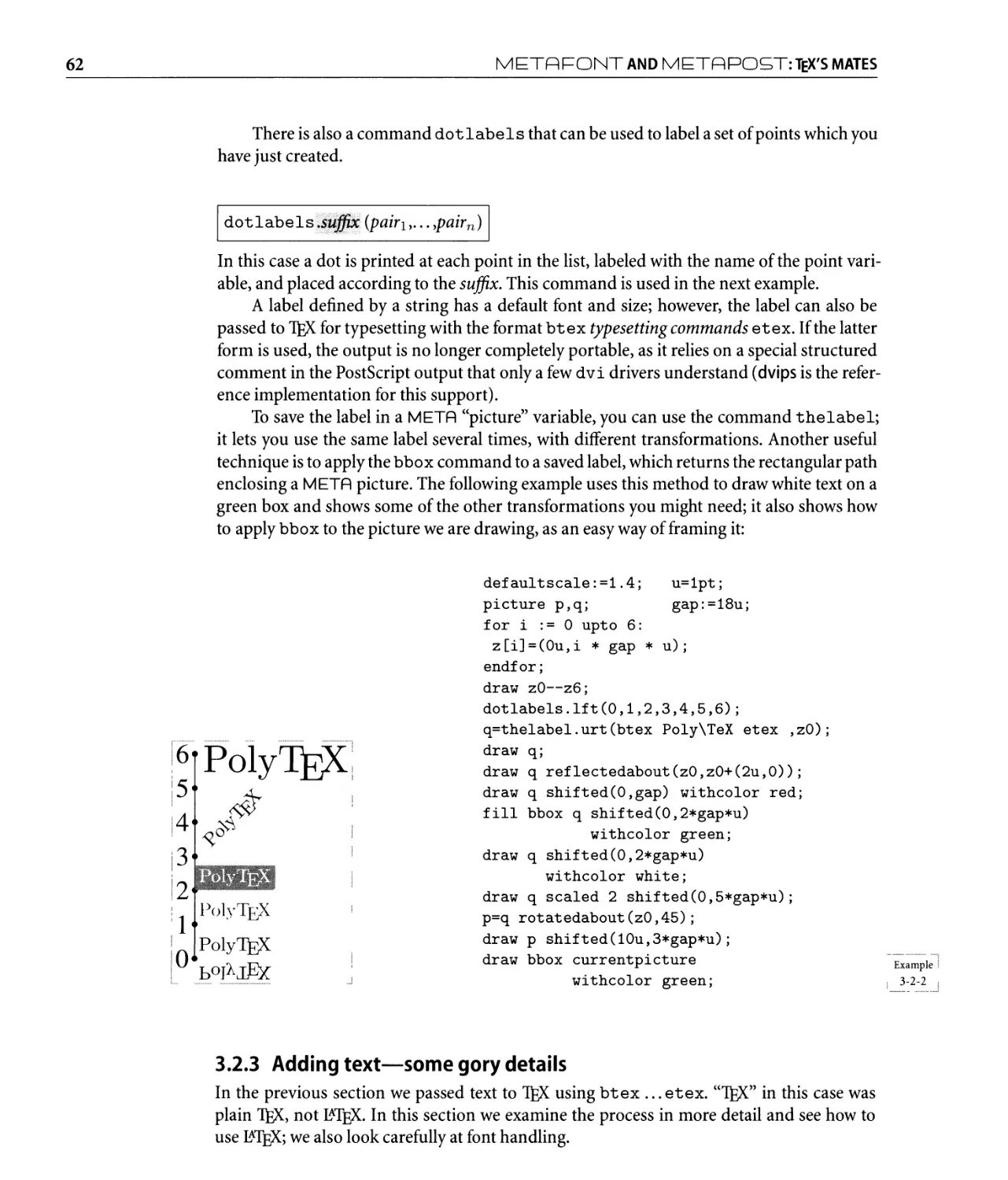
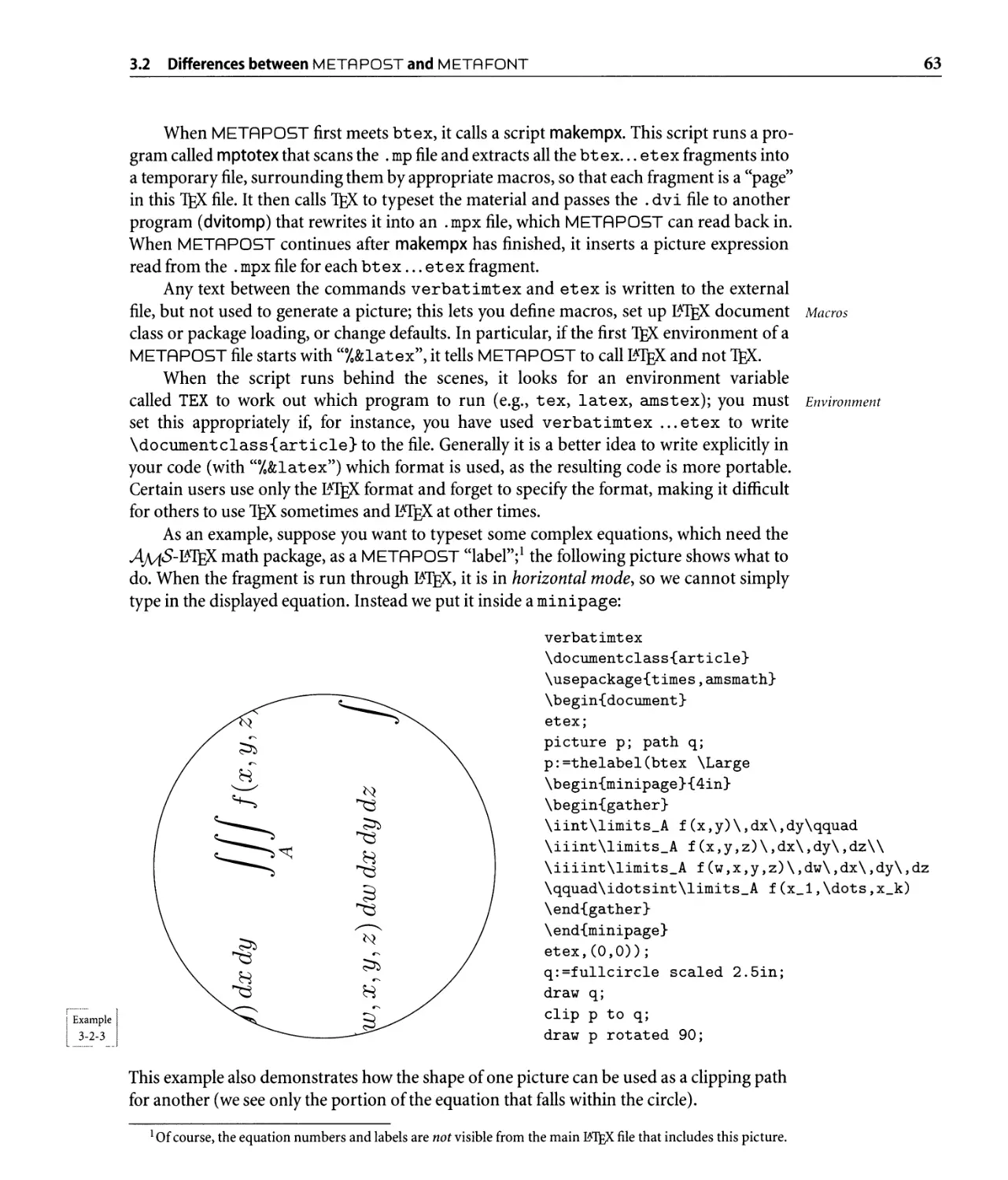
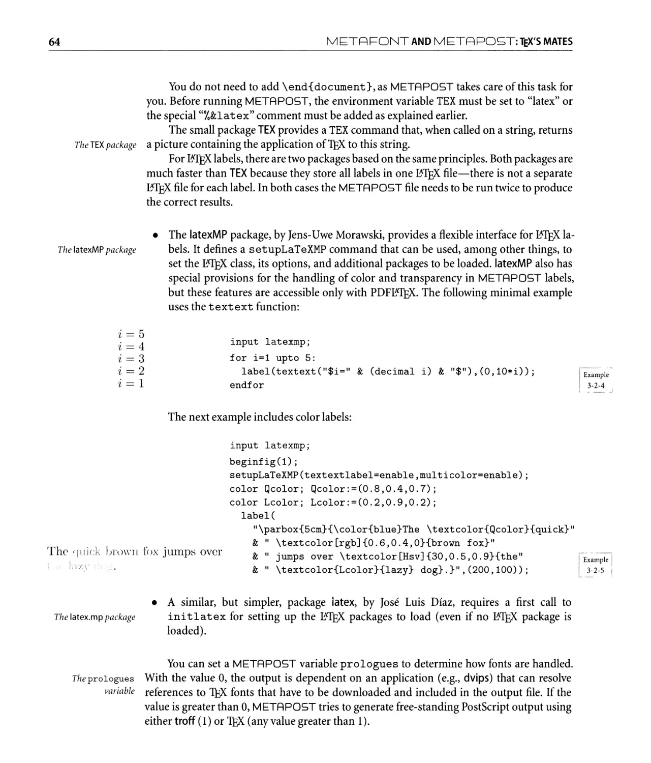
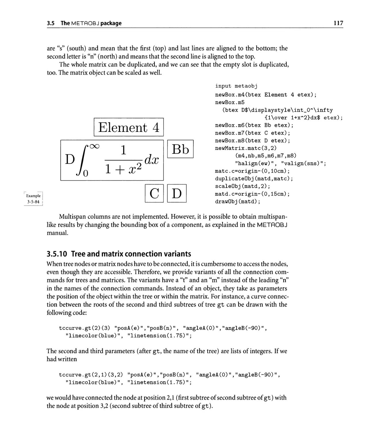
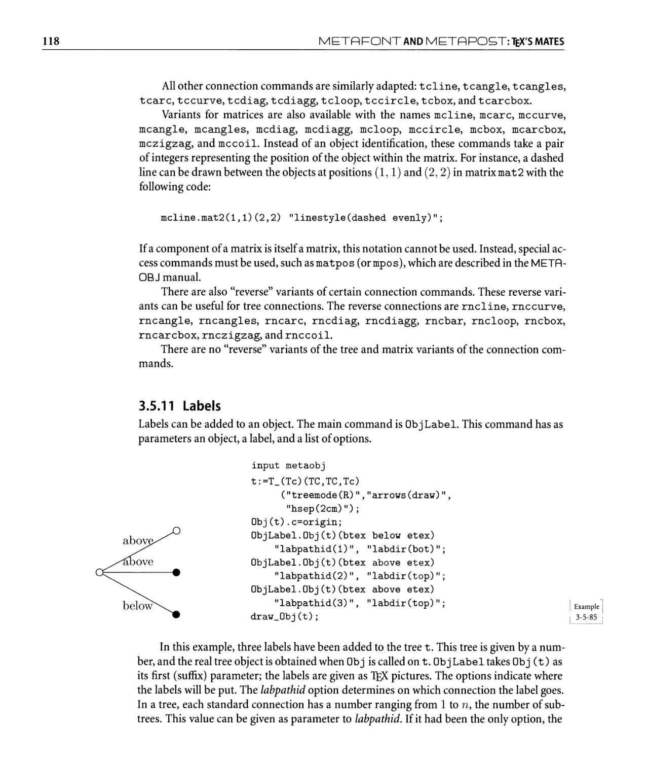
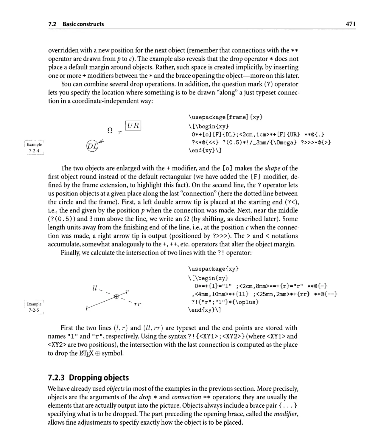
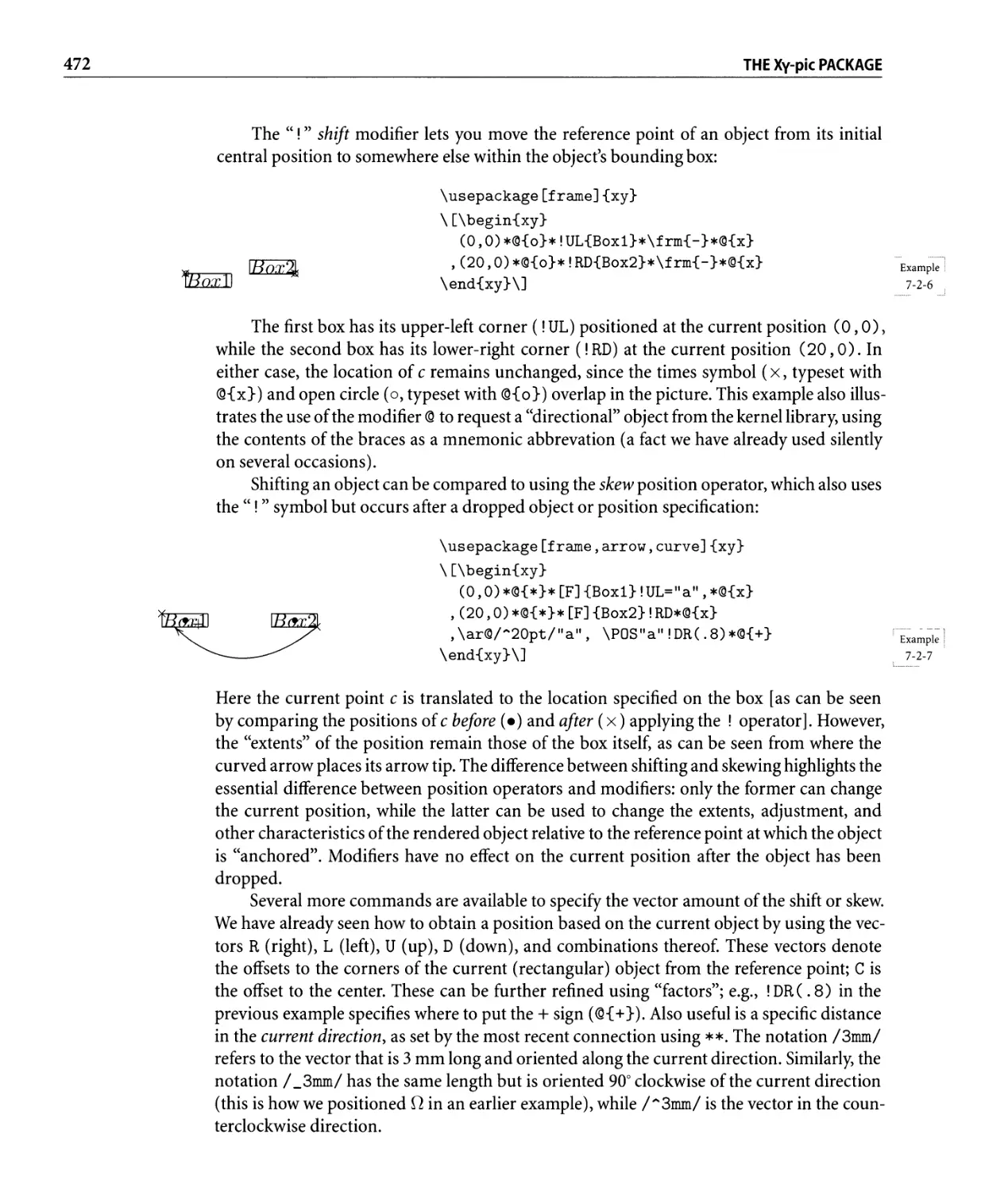
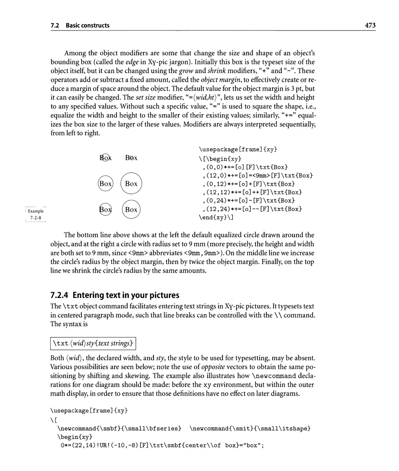
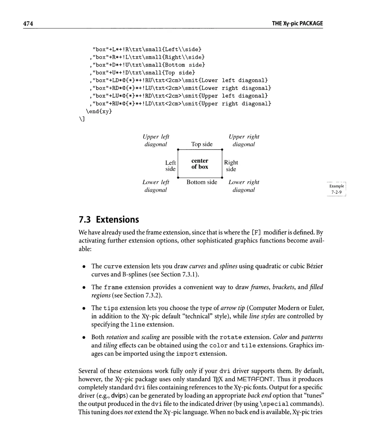
/


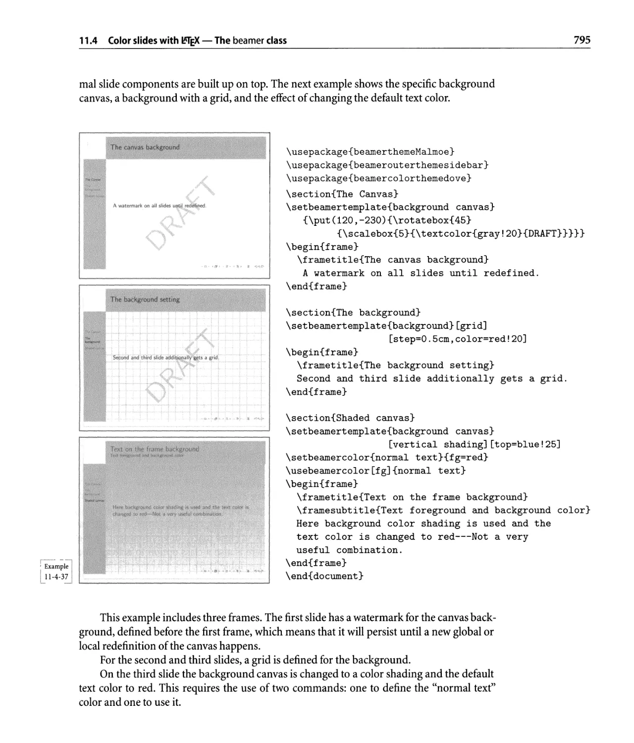


Author: Goossens M. Mittelbach F. Rahtz S.
Tags: programming computer science internet
ISBN: 978-0-321-50892-8
Year: 2008


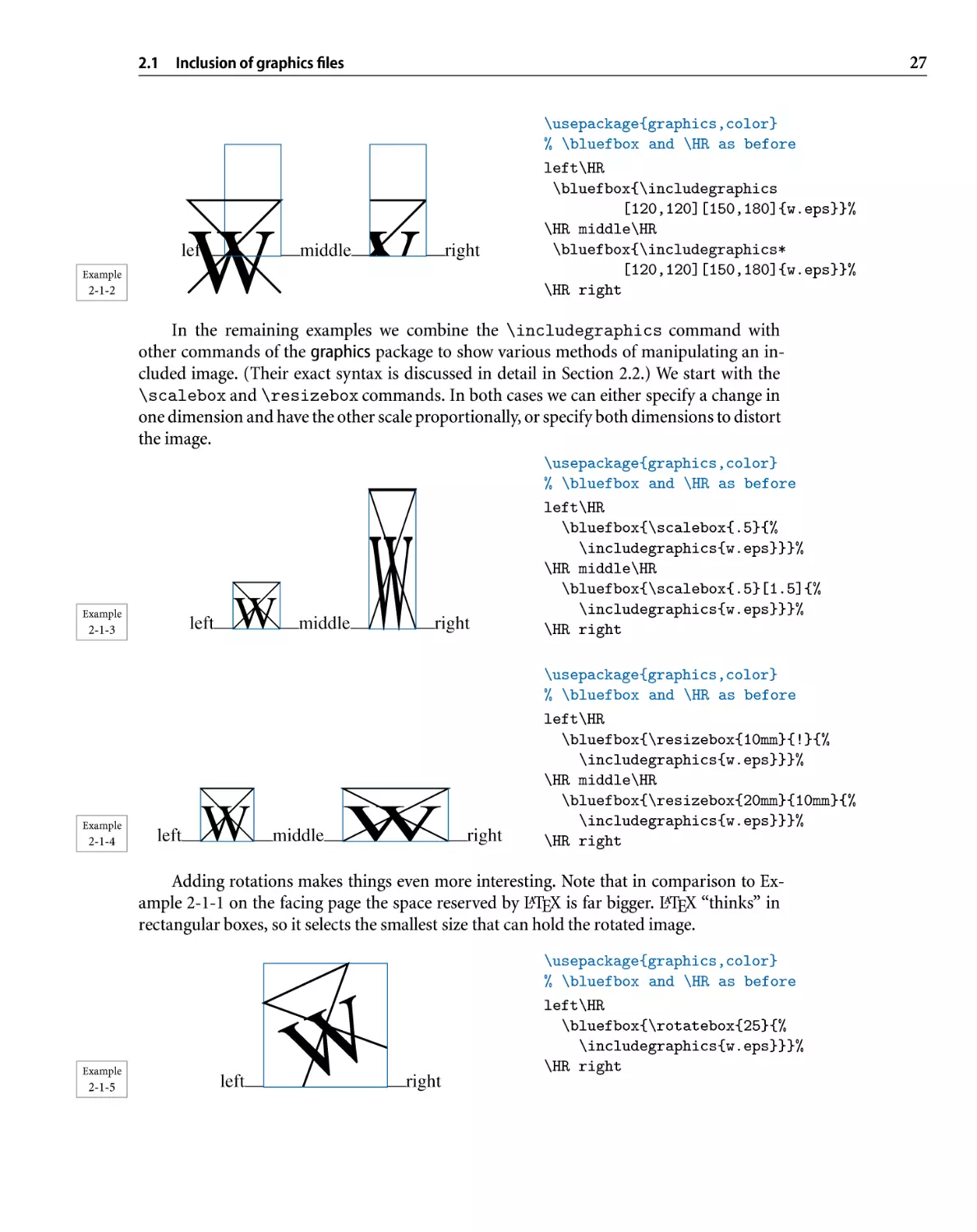
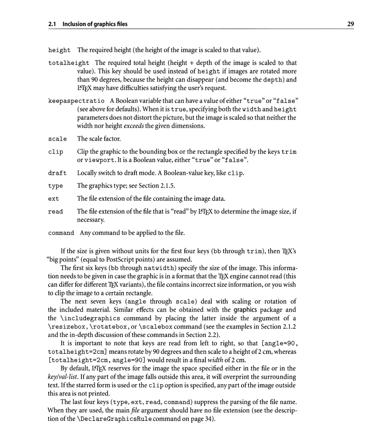
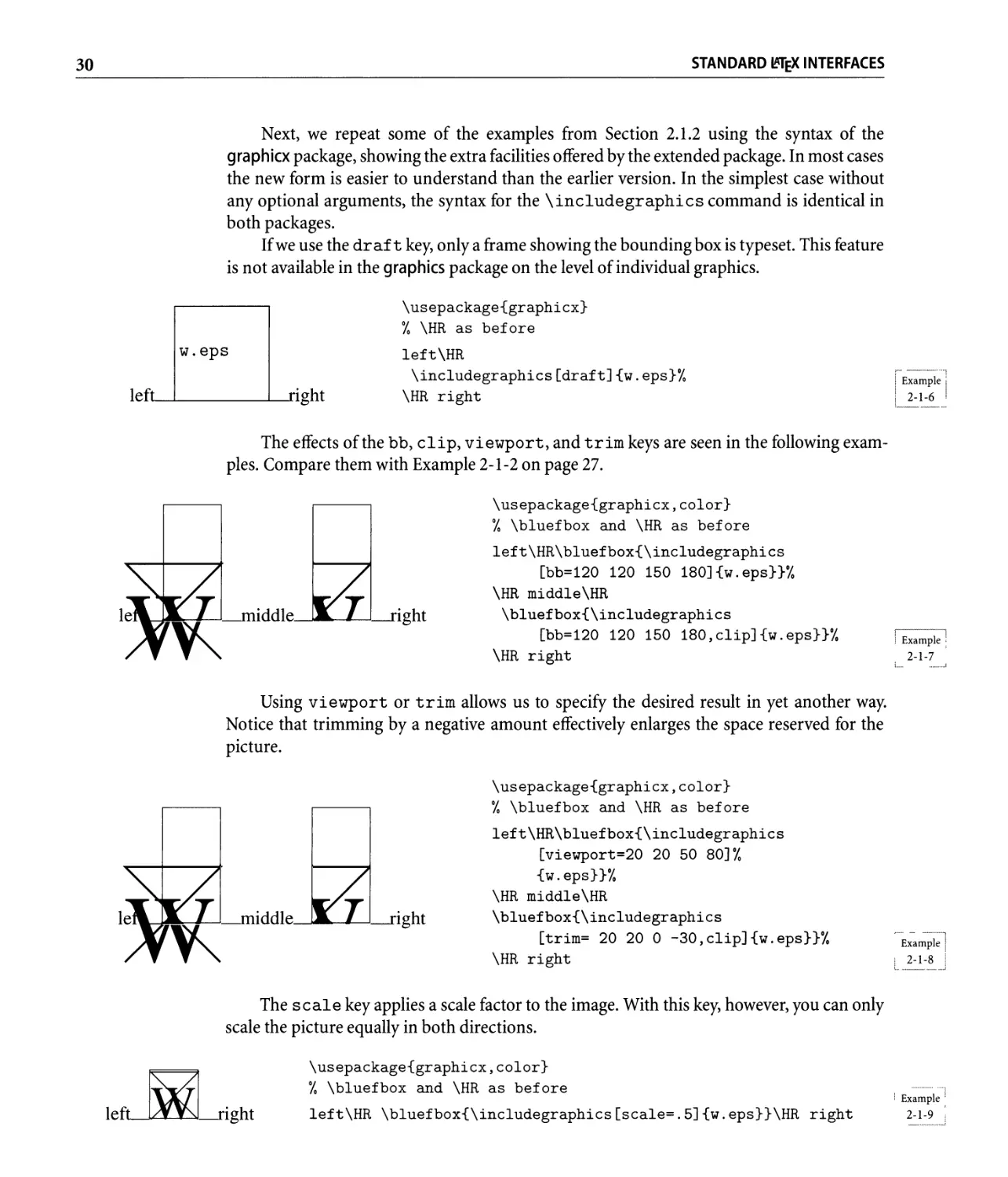
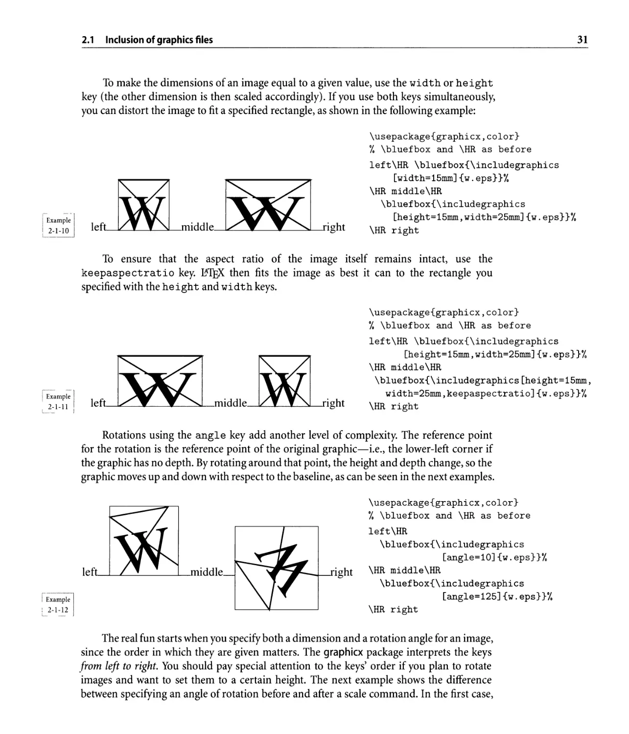
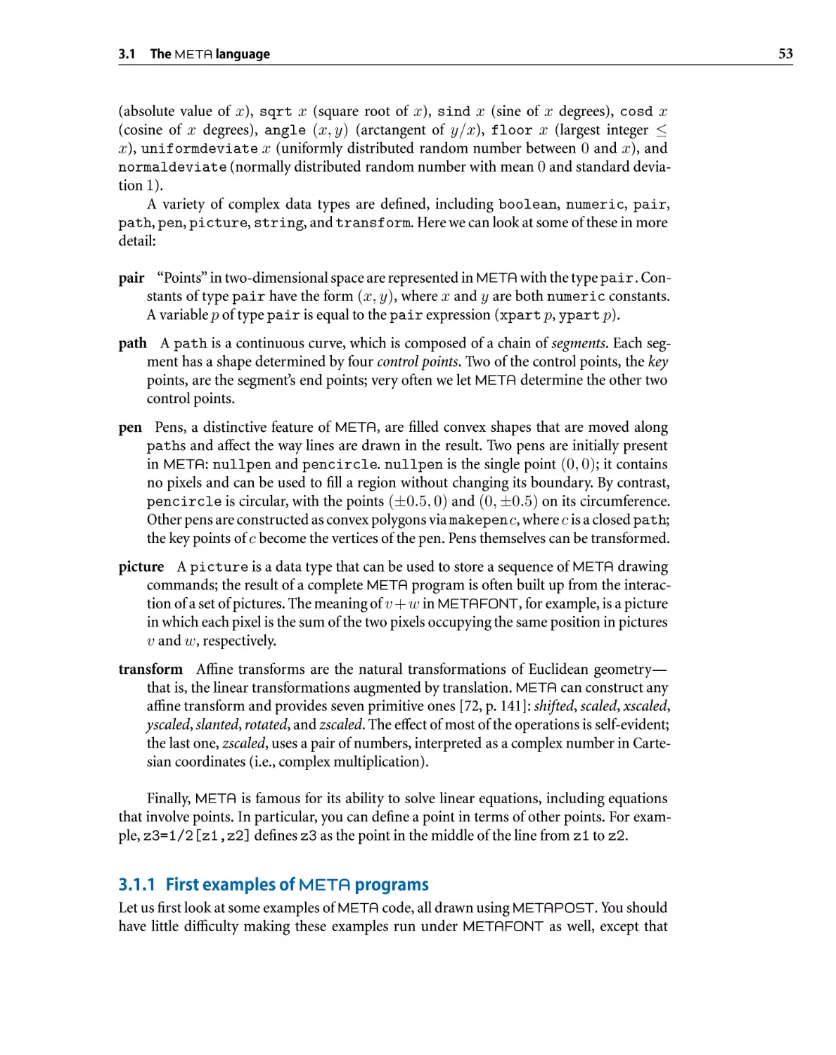
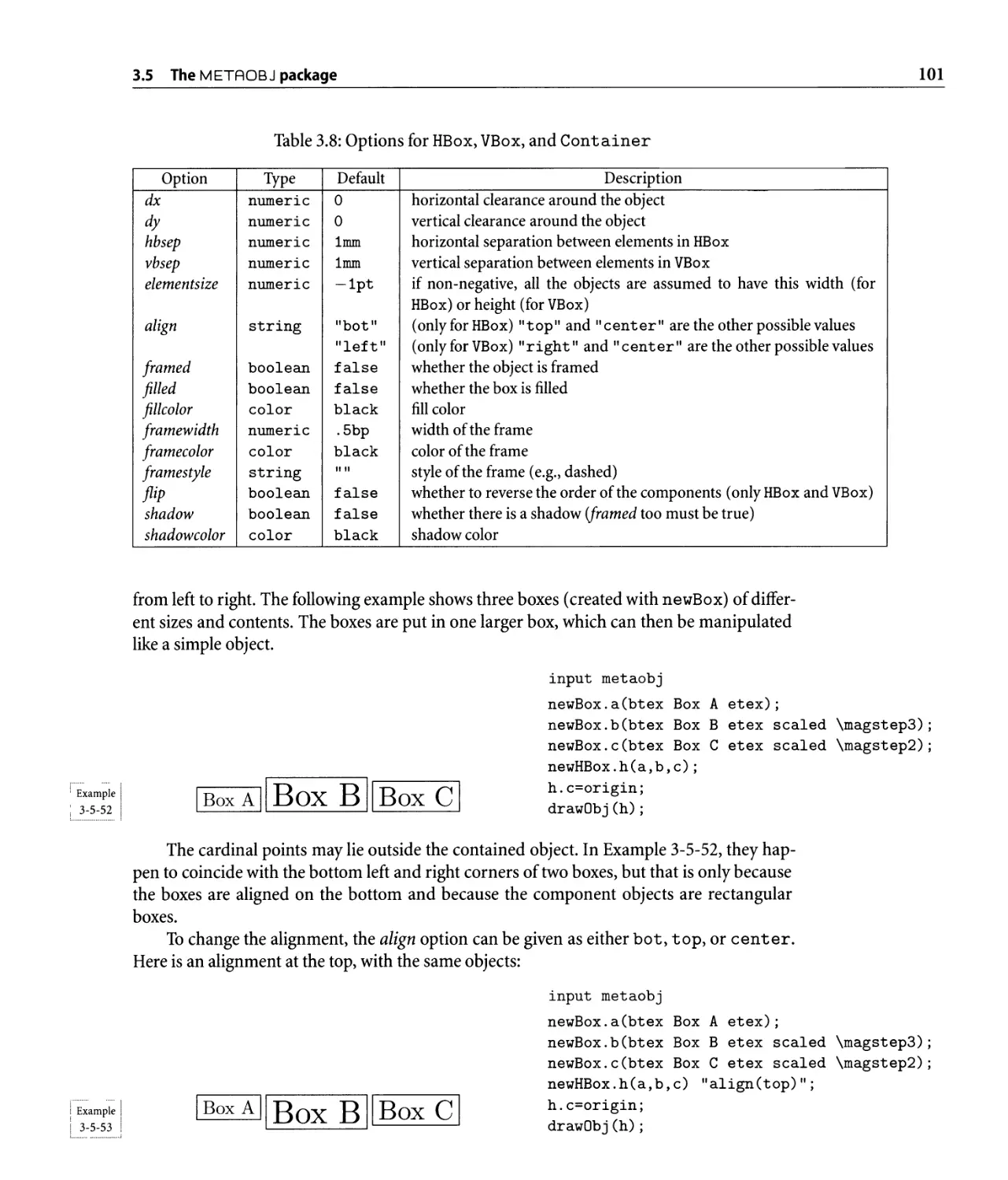
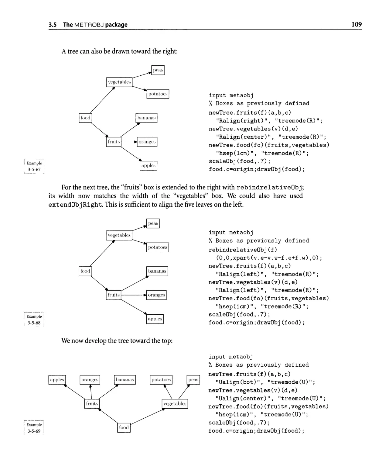
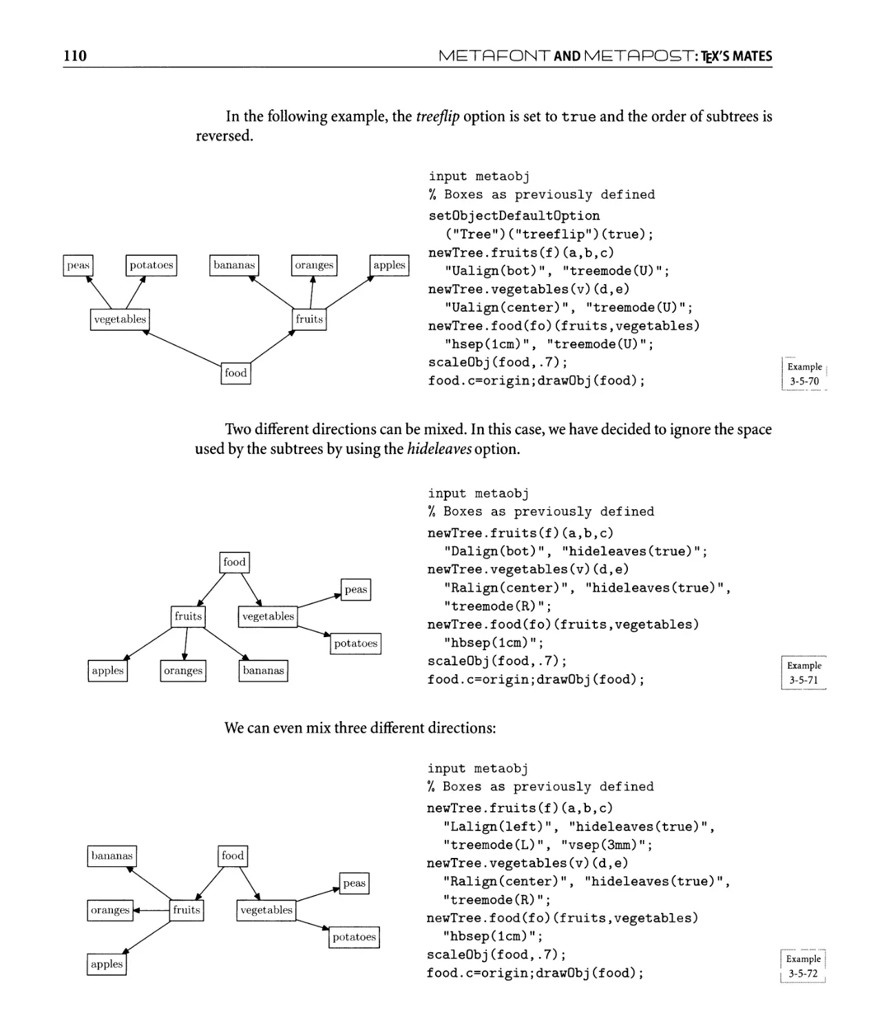
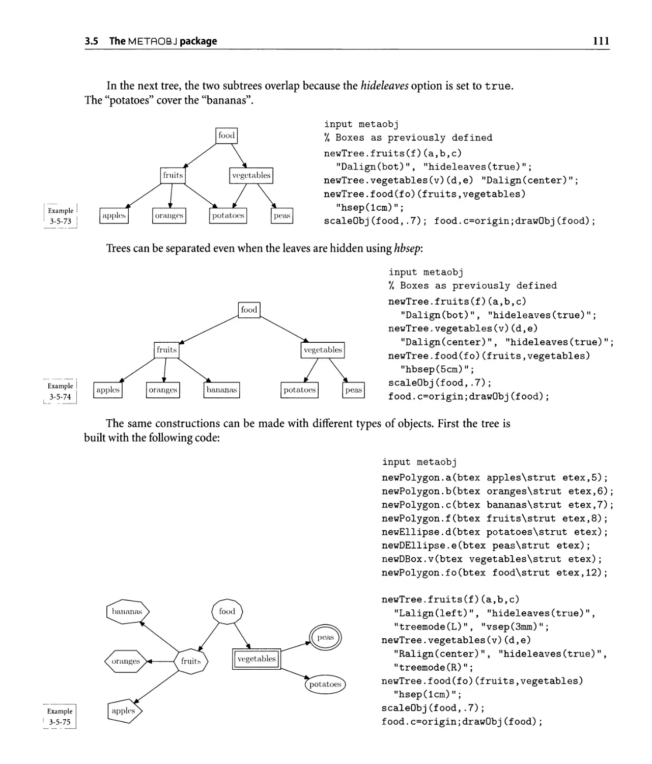
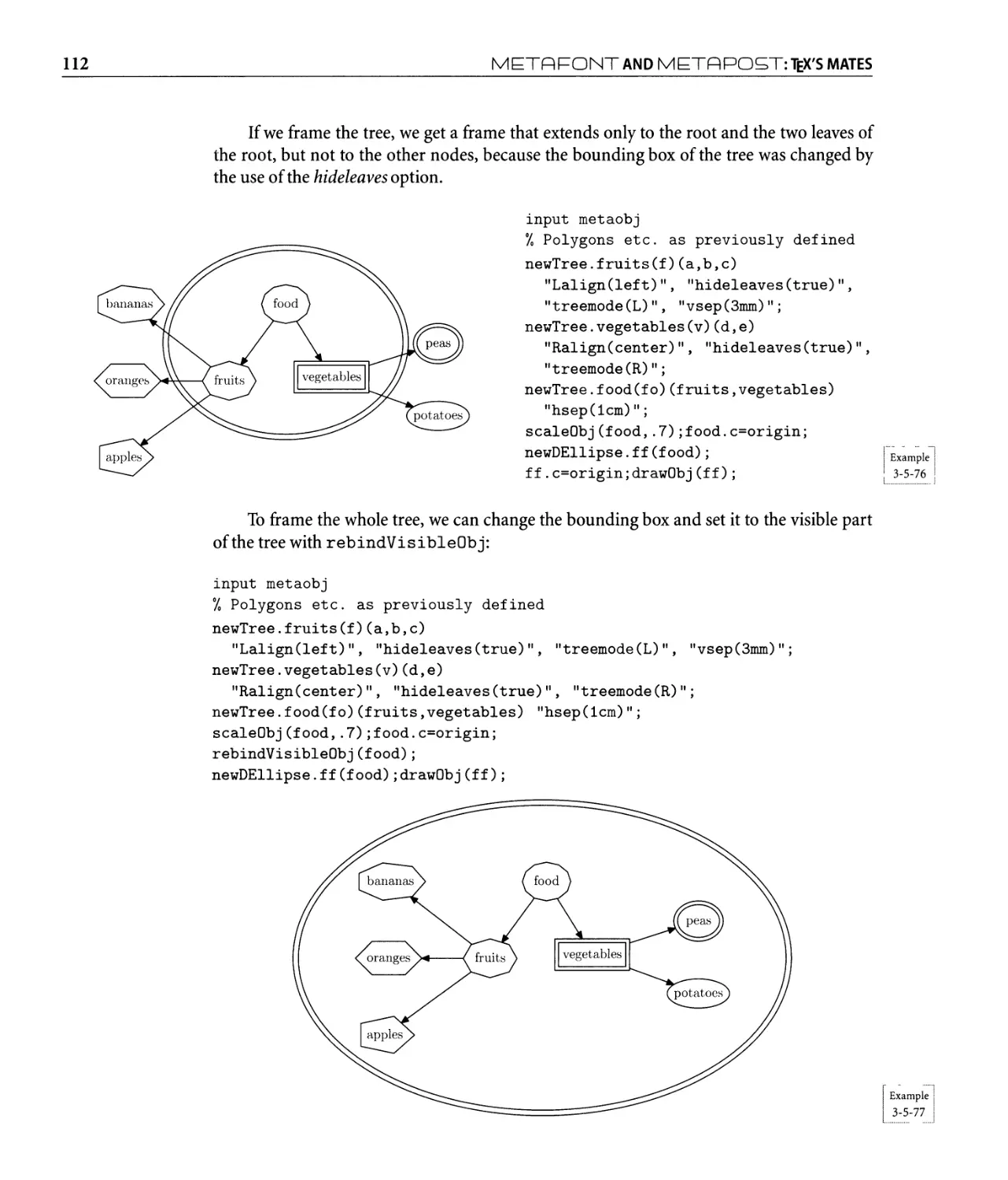
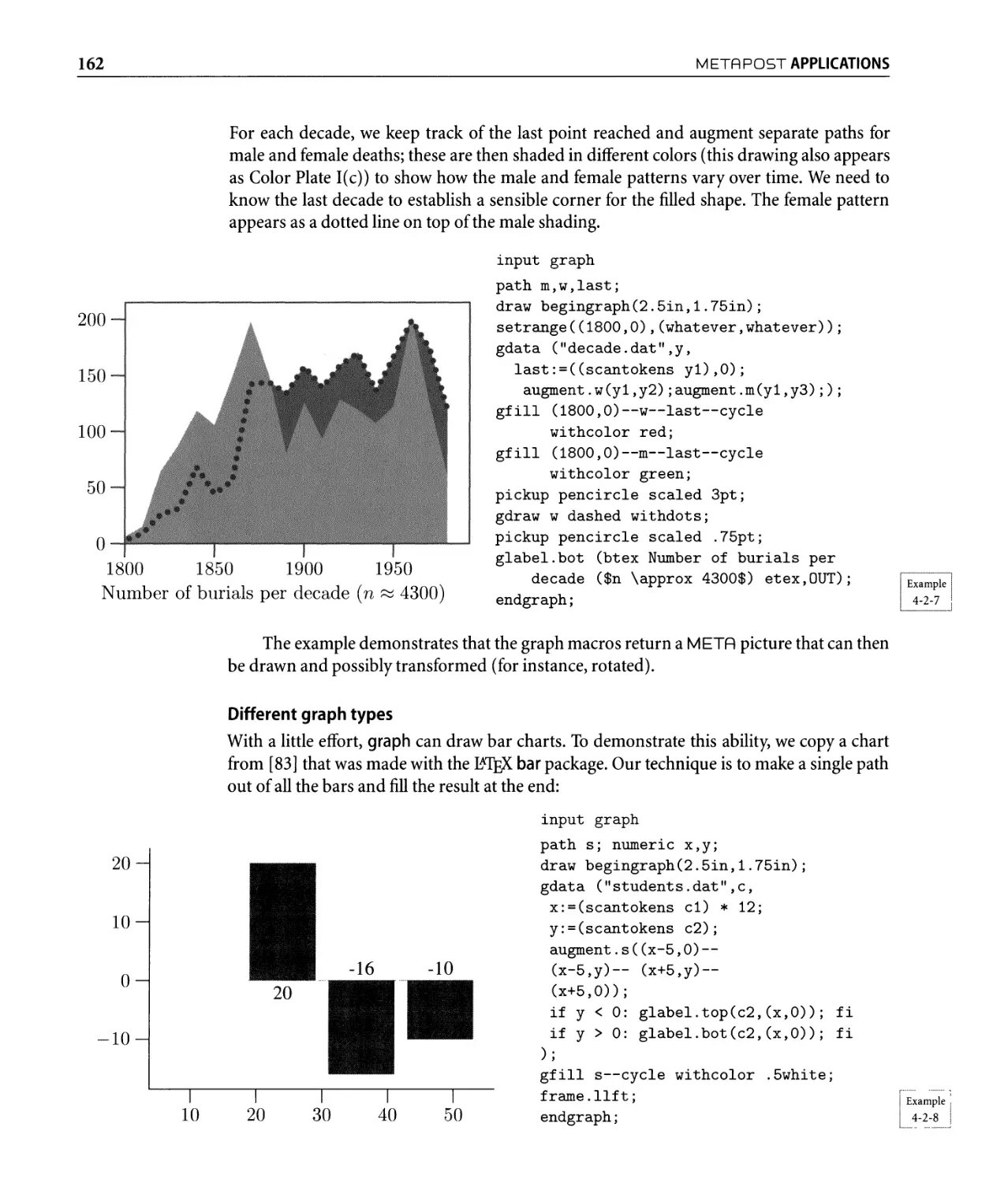
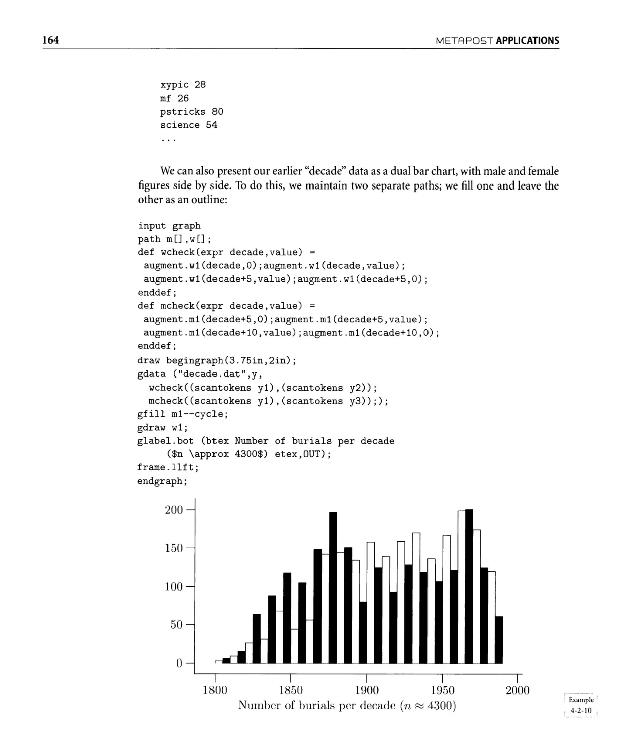
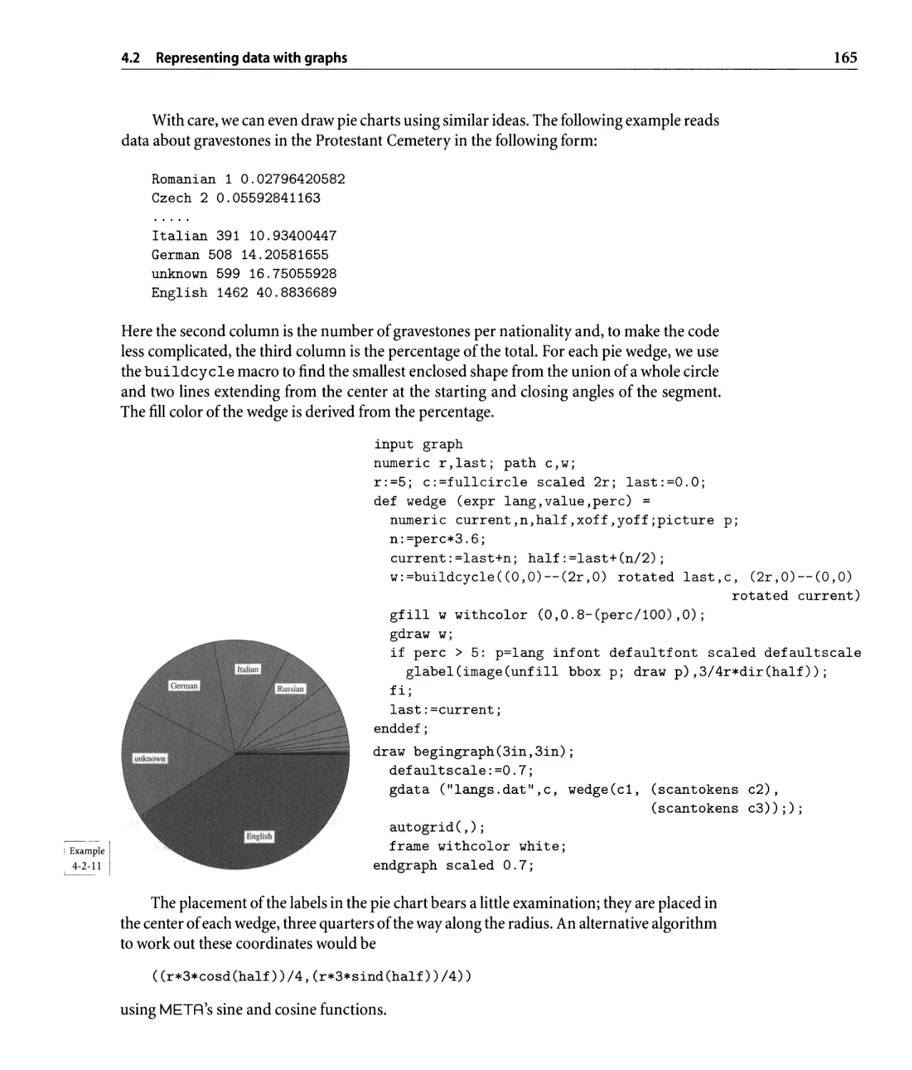
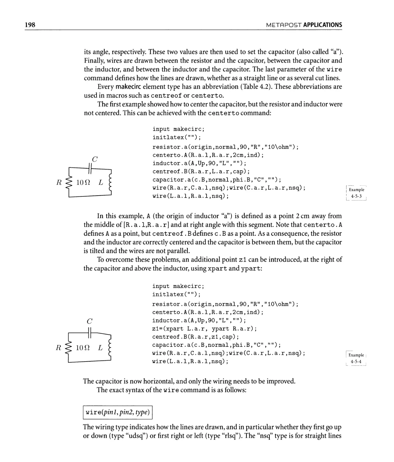
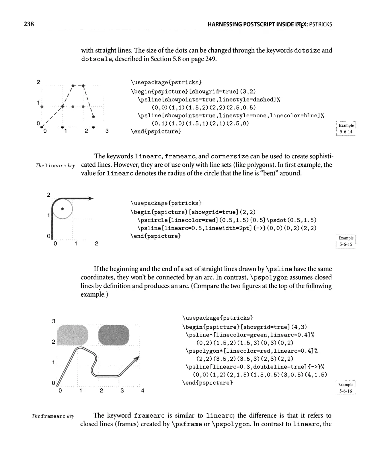
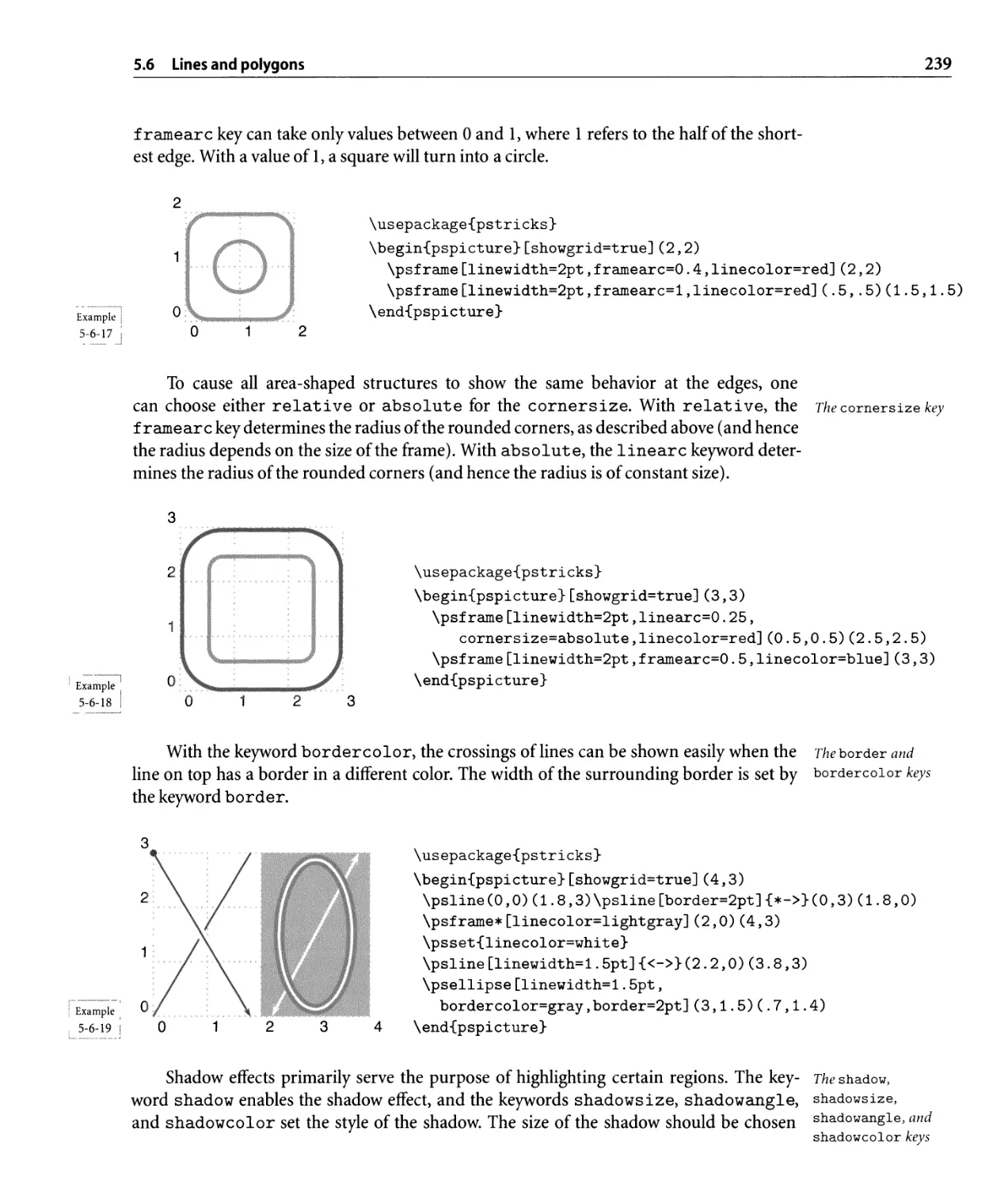
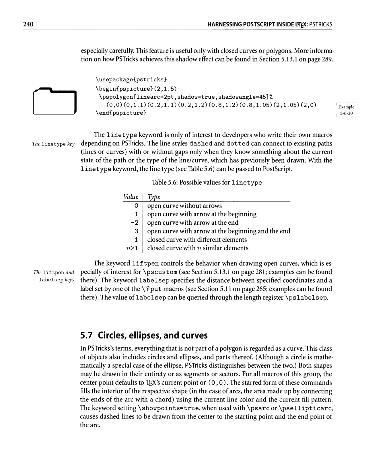
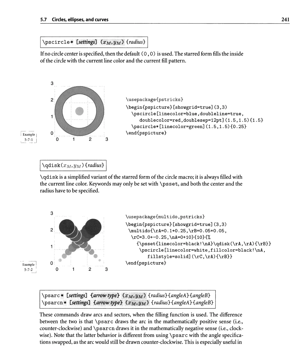
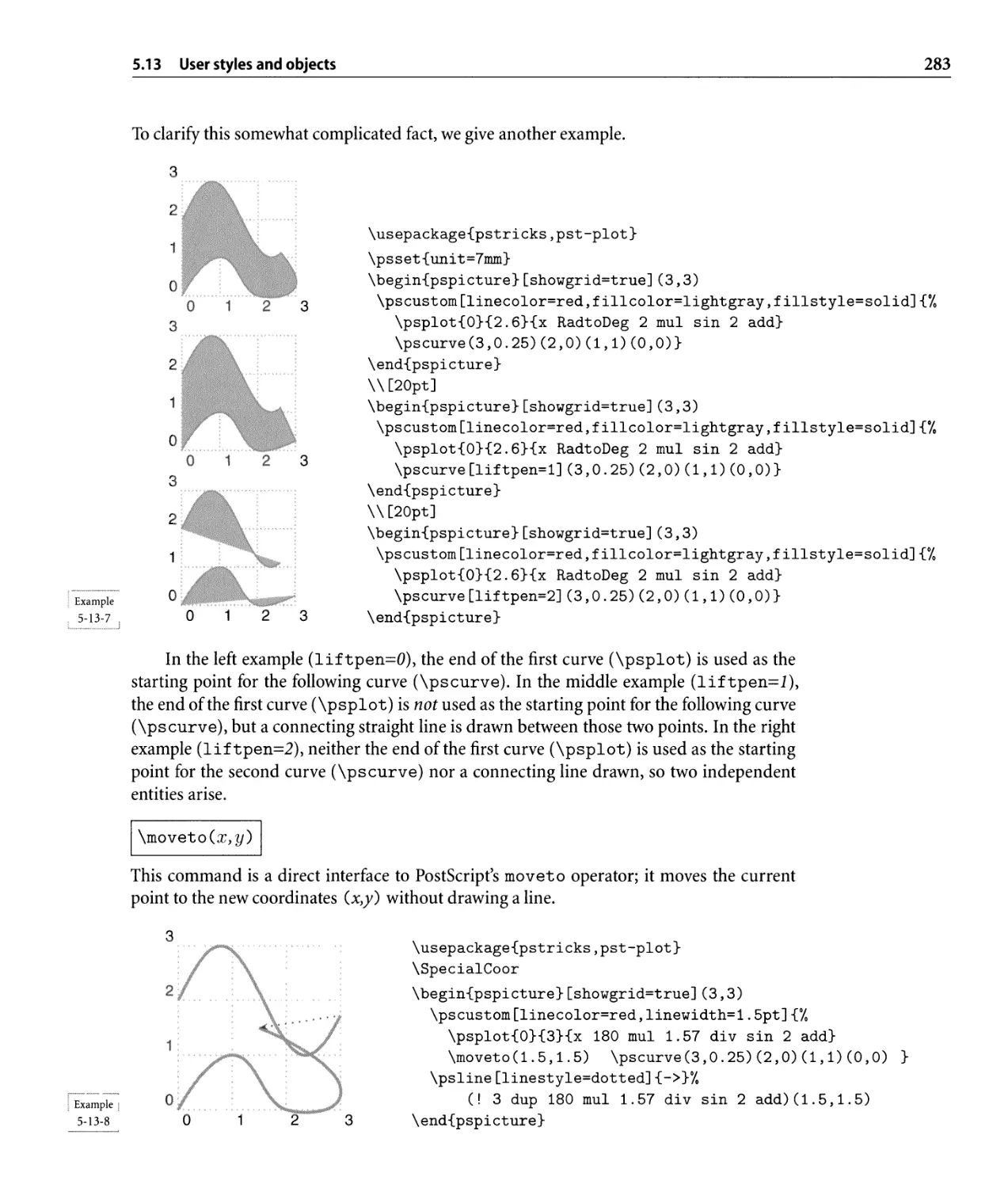
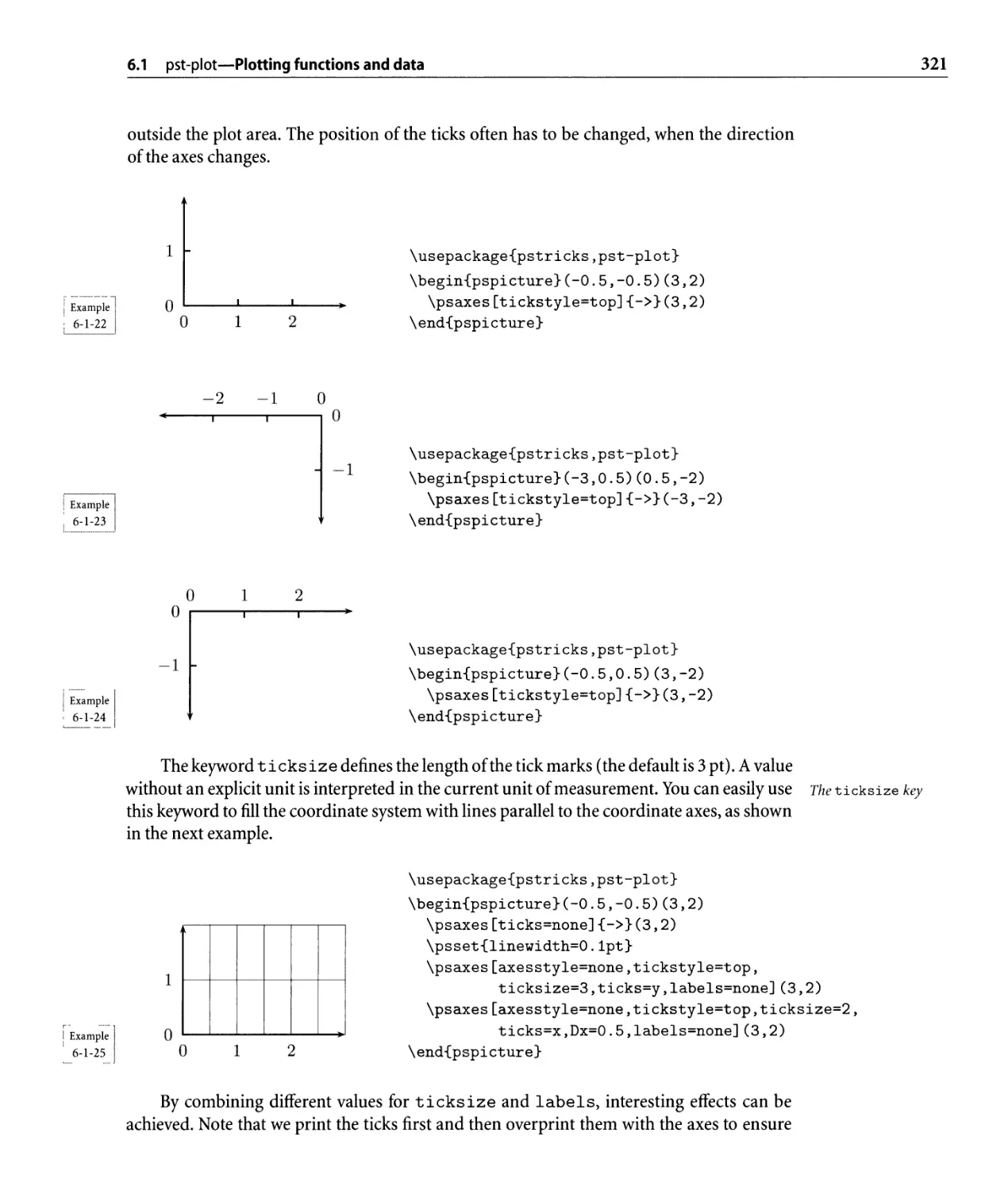
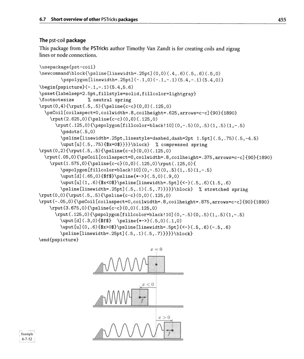
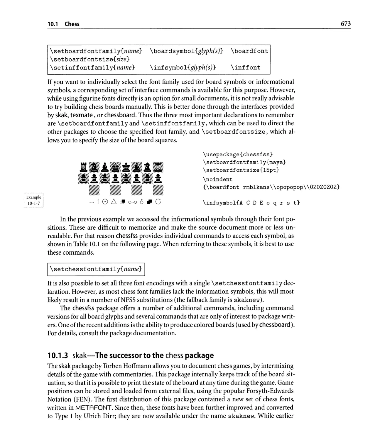
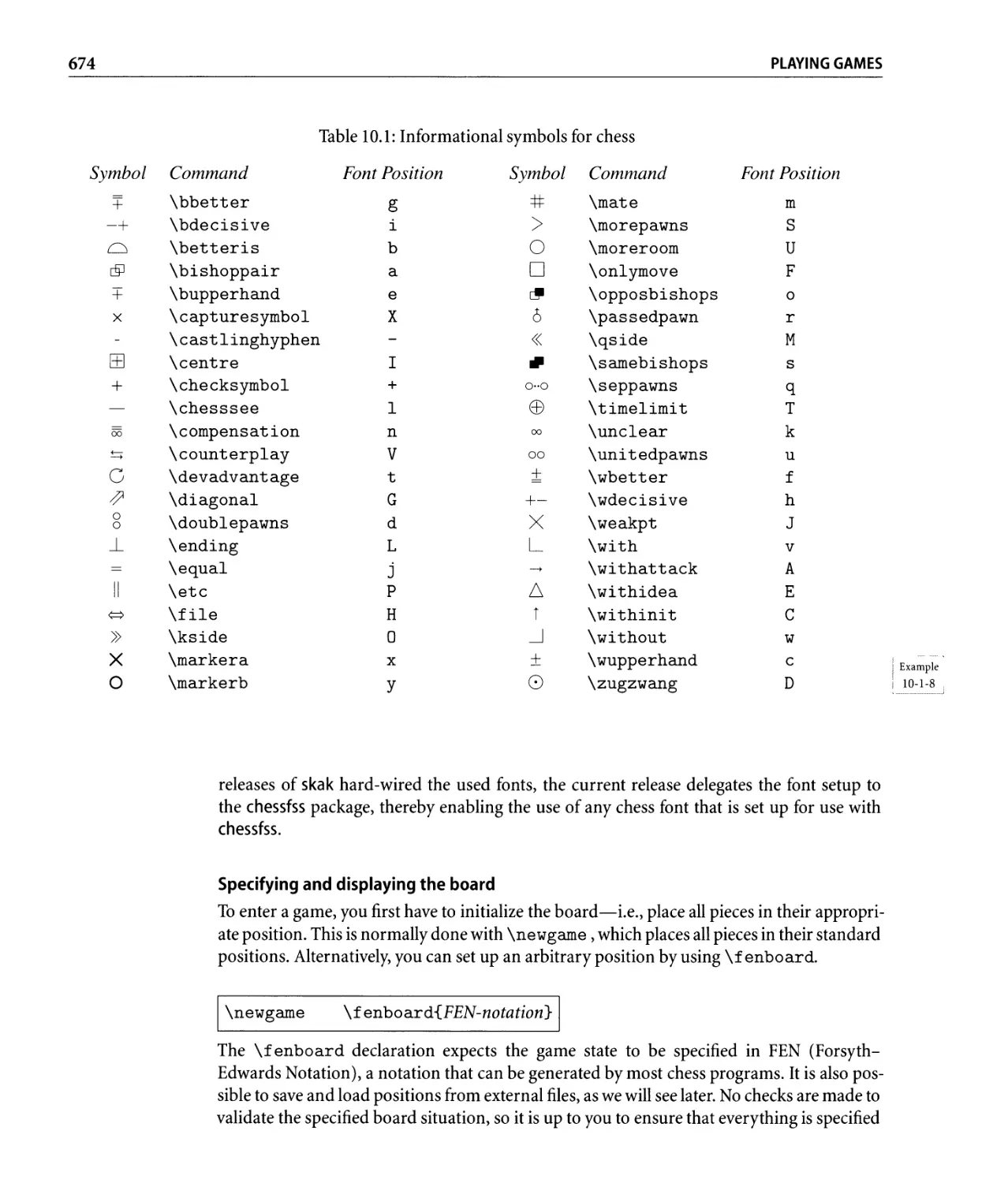
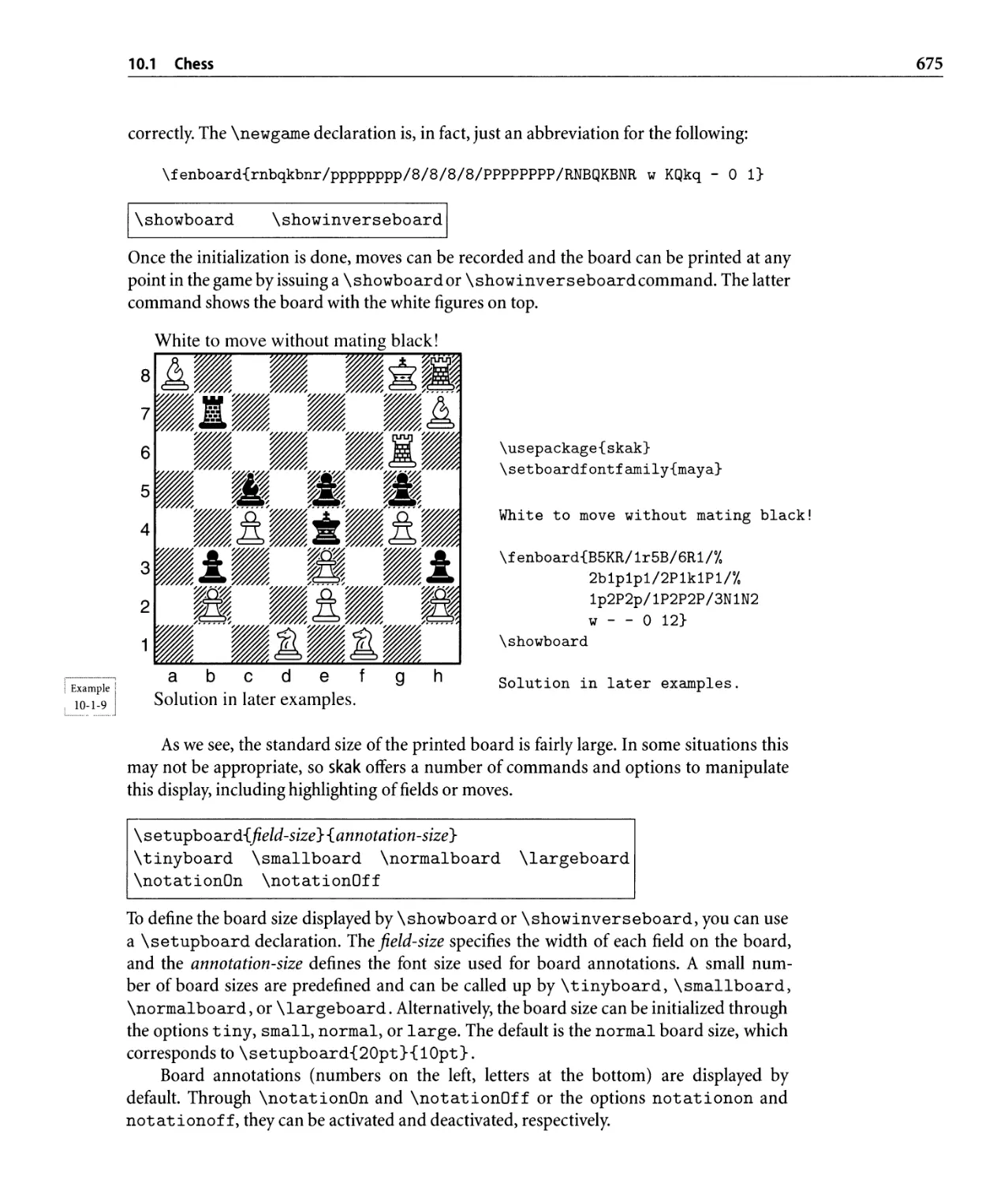
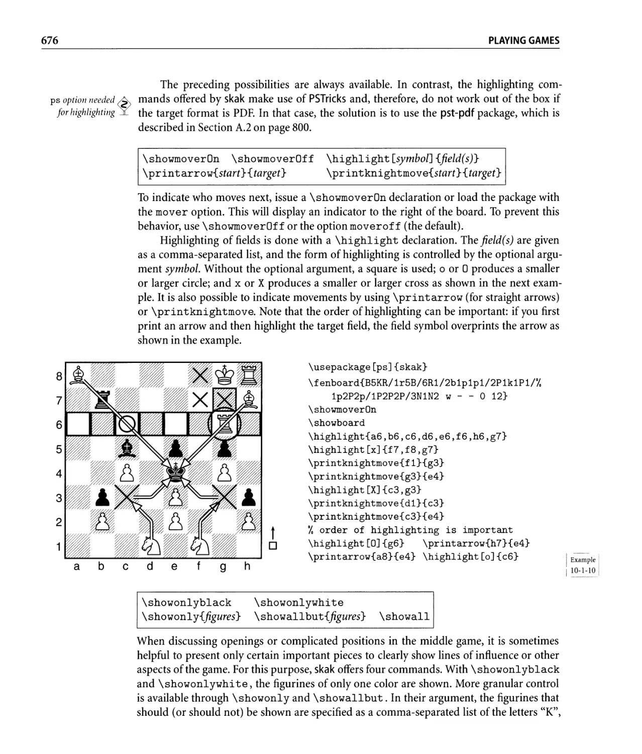
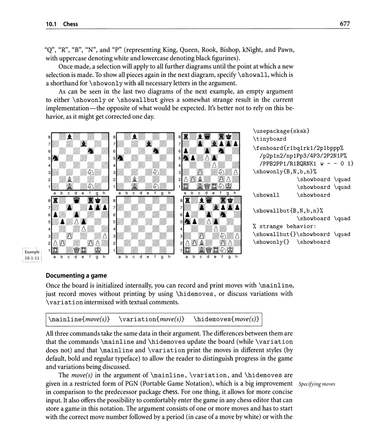
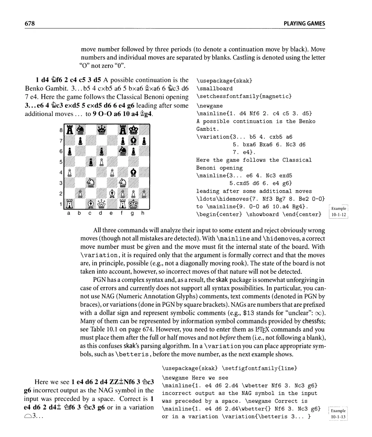
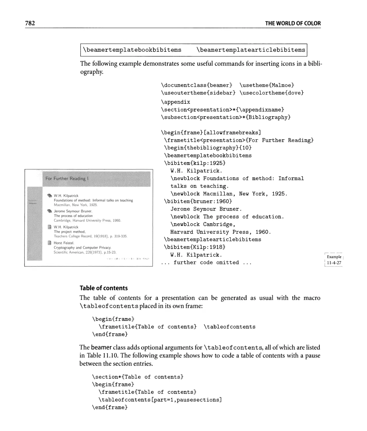
Text
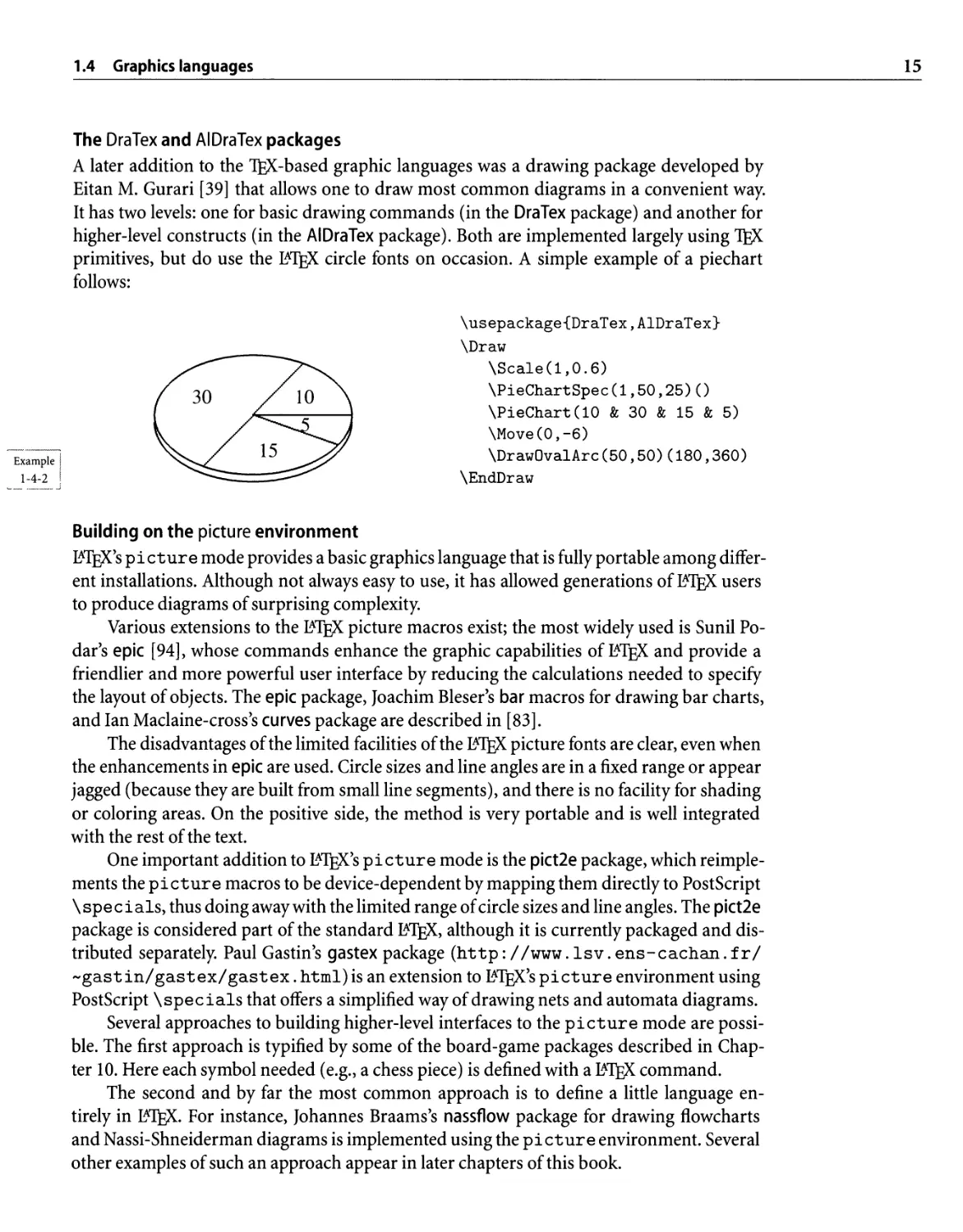
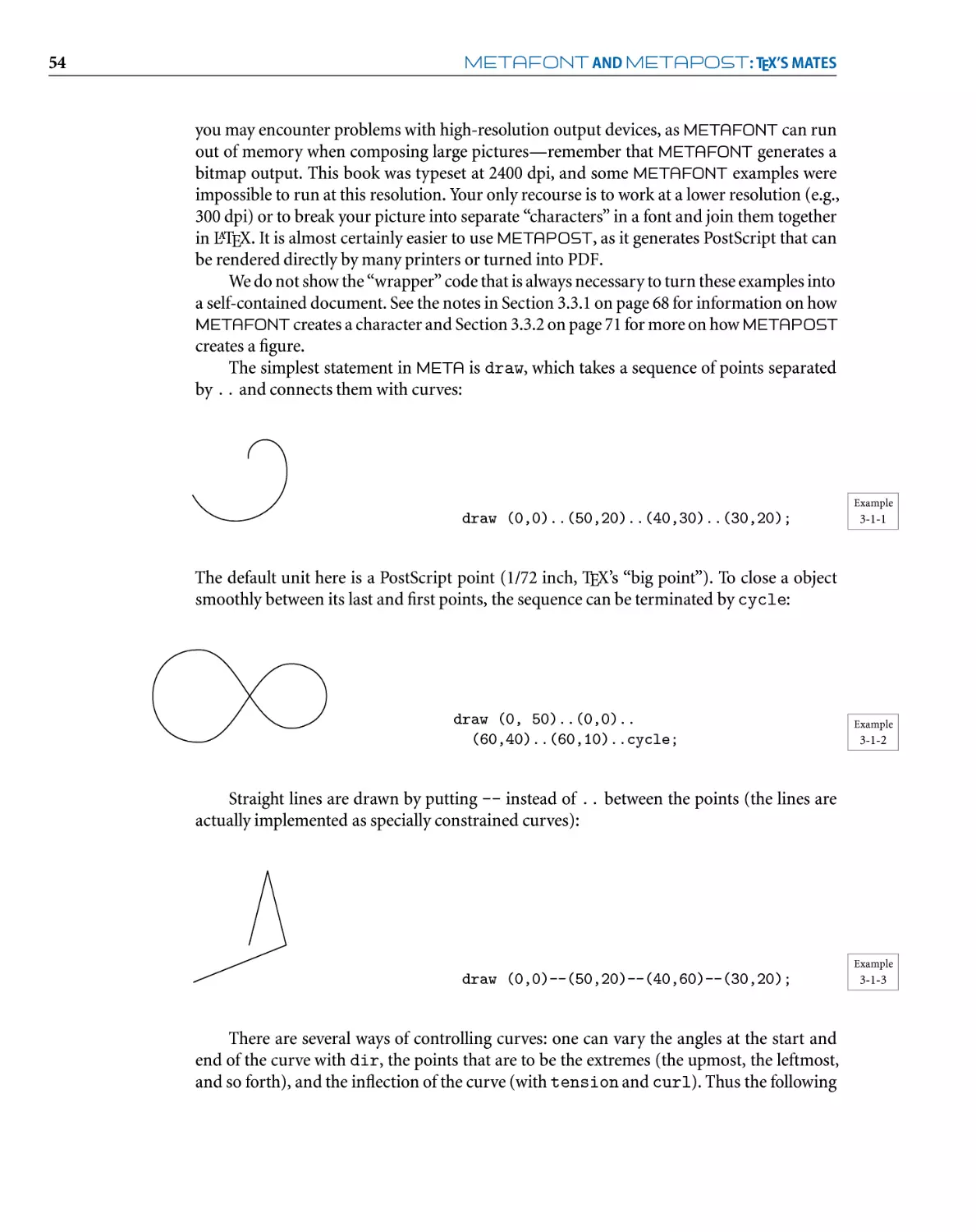
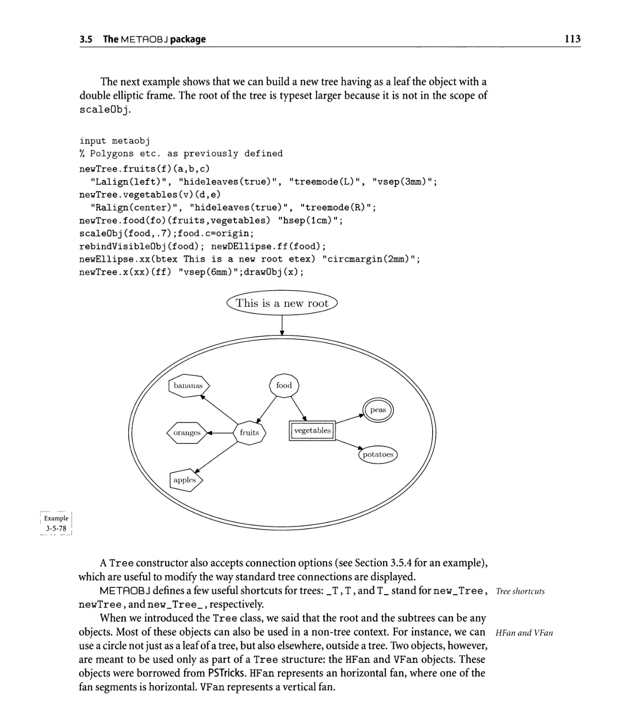
The LATEXGraphics
Companion
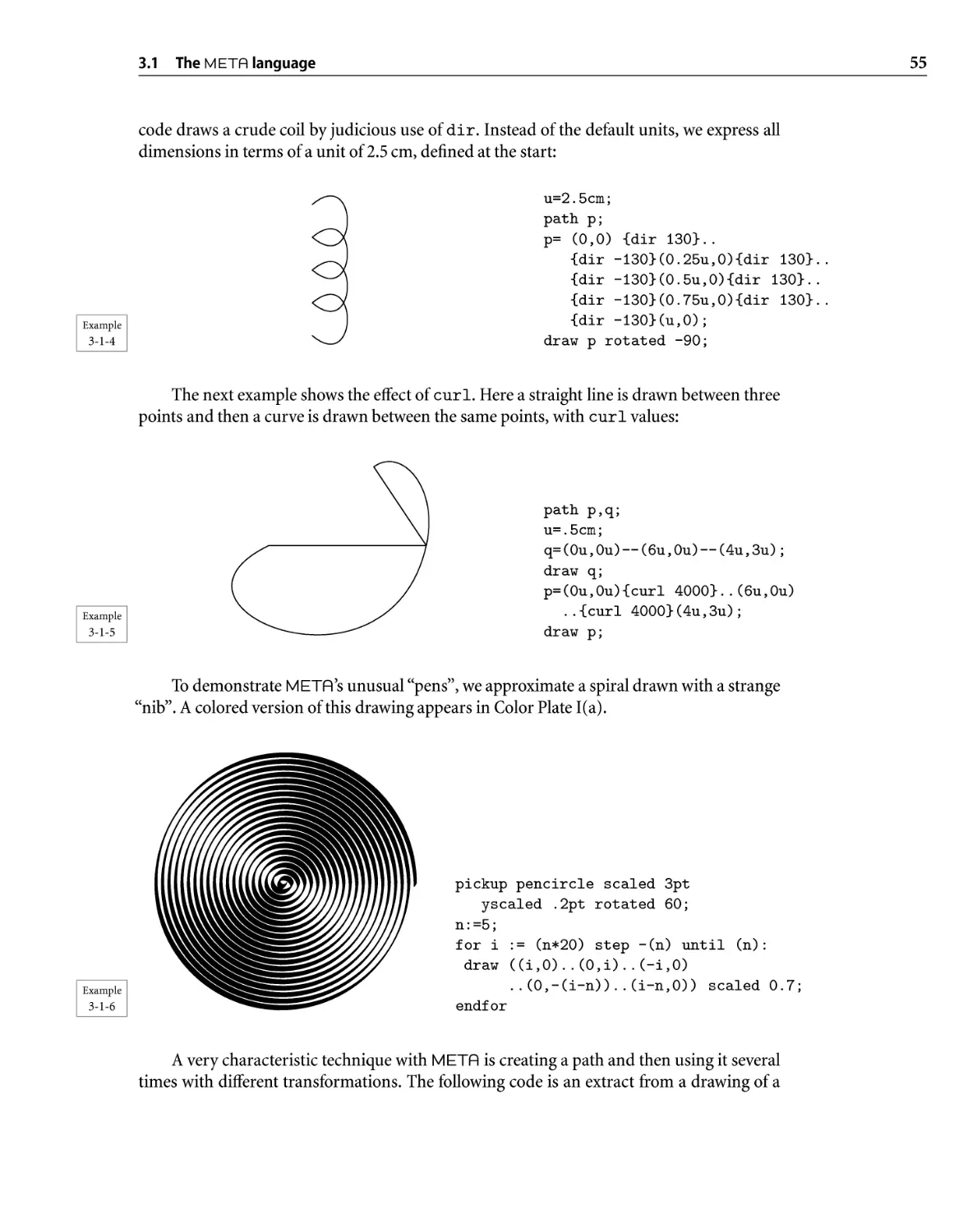
Second Edition
Michel Goossens
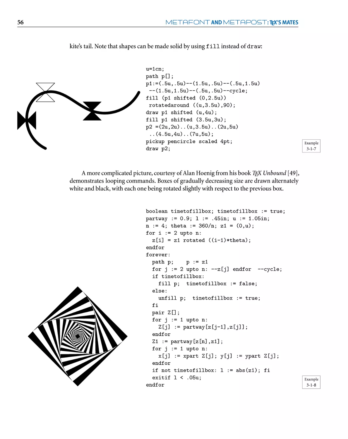
Frank Mittelbach
Sebastian Rahtz
Denis Roegel
Herbert Voß
Upper Saddle River, NJ Boston Indianapolis San Francisco
NewYork Toronto Montreal London Munich Paris Madrid
Capetown Sydney To k y o Singapore Mexico City
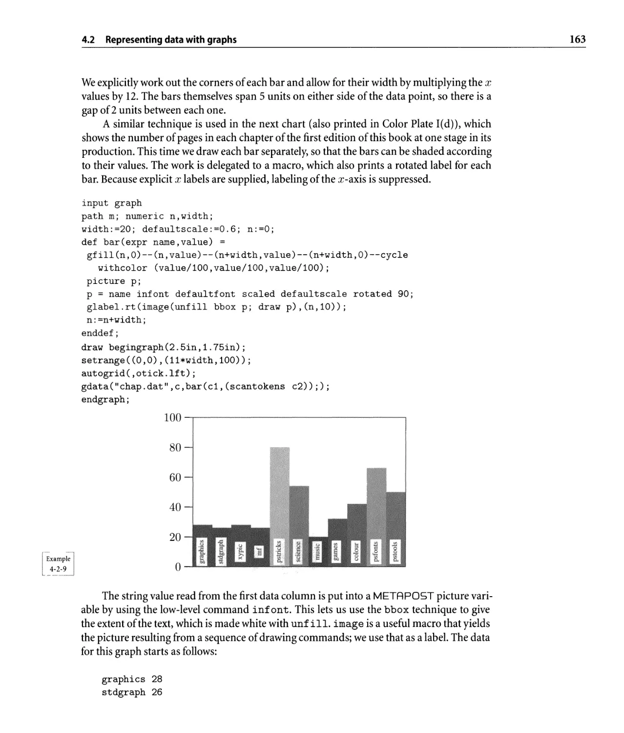
Many of the designations used by manufacturers and sellers to distinguish their products are claimed
as trademarks. Where those designations appear in this book, and Addison-Wesley was aware of a
trademark claim, the designations have been printed with initial capital letters or in all capitals.
The authors and publisher have taken care in the preparation of this book, but make no expressed or
implied warranty of any kind and assume no responsibility for errors or omissions. No liability is
assumed for incidental or consequential damages in connection with or arising out of the use of the
information or programs contained herein.
The publisher offers discounts on this book when ordered in quantity for bulk purchases and special
sales. For more information, please contact:
U.S. Corporate and Government Sales
(800) 382-3419
corpsales@pearsontechgroup.com
For sales outside of the United States, please contact:
International Sales
international@pearsoned.com
Visit Addison-Wesley on the Web: www.awprofessional.com
Library of Congress Cataloging-in-Publication Data
The LaTeX Graphics companion / Michel Goossens ... [et al.].
-- 2nd ed.
p. cm.
Includes bibliographical references and index.
ISBN 978-0-321-50892-8 (pbk. : alk. paper)
1. LaTeX (Computer file) 2. Computerized typesetting. 3. PostScript
(Computer program language) 4. Scientific illustration--Computer programs.
5. Mathematics printing--Computer programs. 6. Technical
publishing--Computer programs. I. Goossens, Michel.
Z253.4.L38G663 2008
686.2'2544536--dc22
2007010278
Copyright © 2008 by Pearson Education, Inc.
All rights reserved. No part of this publication may be reproduced, stored in a retrieval system, or
transmitted, in any form, or by any means, electronic, mechanical, photocopying, recording, or
otherwise, without the prior consent of the publisher.
The foregoing notwithstanding, the examples contained in this book and obtainable online on
CTAN are made available under the LATEX Project Public License (for information on the LPPL,
see www.latex-project.org/lppl).
For information on obtaining permission for use of material from this work, please submit a written
request to:
Pearson Education, Inc.
Rights and Contracts Department
75 Arlington Street, Suite 300
Boston, MA 02116
Fax: (617) 848-7047
ISBN 10:
0-321-50892-0
ISBN 13: 978-0-321-50892-8
Text printed in the United States on recycled paper at Courier in Westford, Massachusetts.
First printing, July 2007
We dedicate this book to the hundreds of LATEX developers
whose contributions are showcased in it,
and we salute their enthusiasm and hard work.
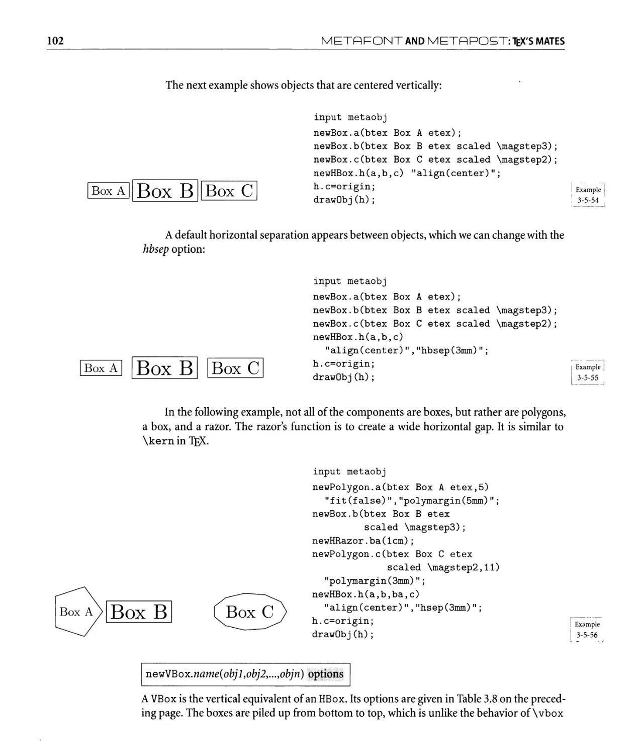
Wewouldalsoliketorememberwithaffection and thanks
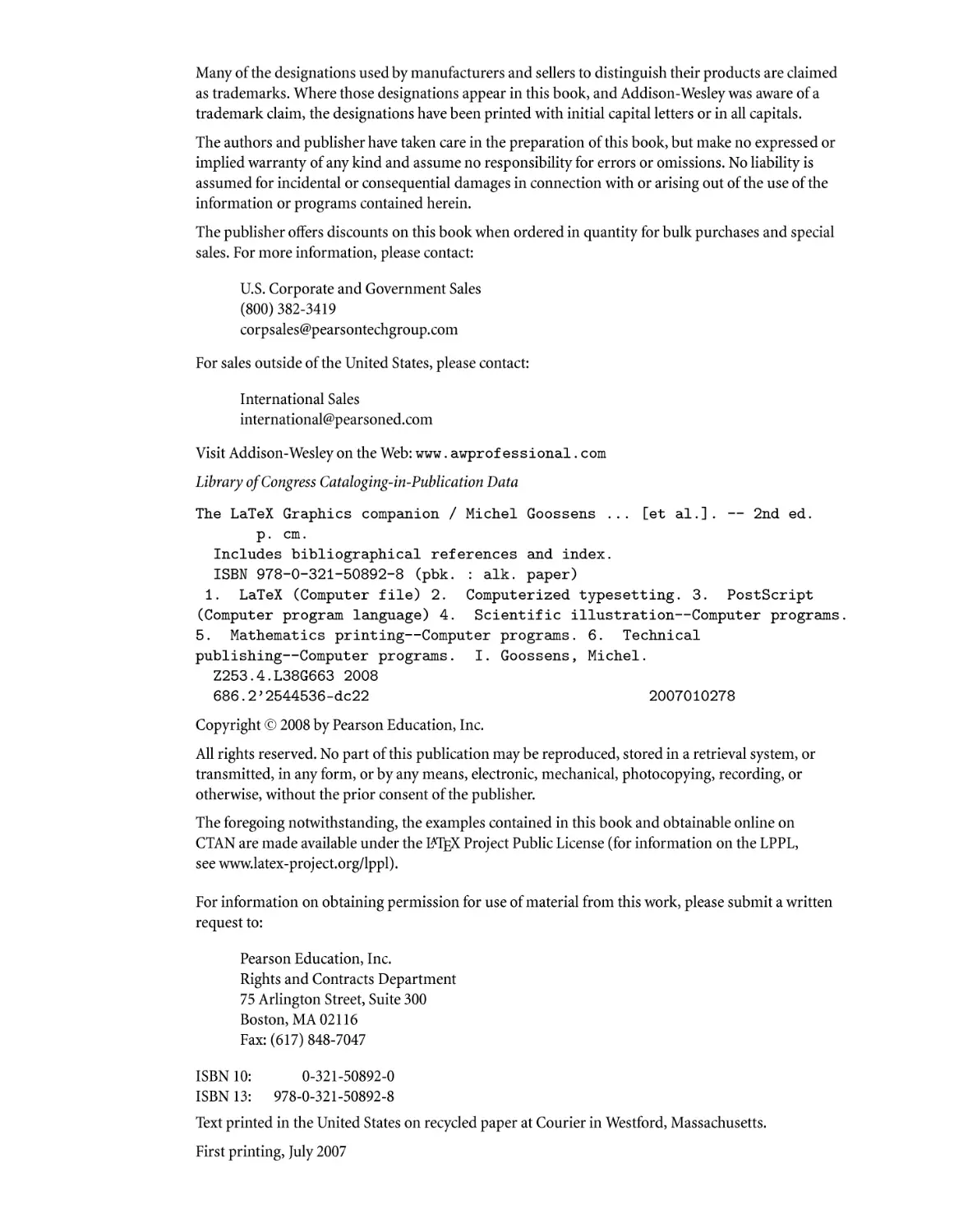
Daniel Taupin, whose MusiXTEX system is described in
Chapter 9, and who passed away in 2003, a great loss to our community.
Rhapsodie
pour piano
Compos´
e partiellement vers 1975, termin´
eenaoˆ
ut 2002
Daniel TAUPIN
ă1
Piano IG2
2
2
2
2
2ff
Allegro (˘ = 50)
#
˛
ˇ
˛
ˇ
!
tr EEEEEEE
ˉ
ˇˇ
ă
ă
ă
ă
ˇ
tr EEEEEEE
ˉ
ˇˇ
ă
ă
ă
ă
ˇ
#
!
tr EEEEEEE
ˉ
ˇˇ
ă
ă
ă
ă
ˇ
tr EEEEEEE
ˉ
ˇˇ
ă
ă
ă
ă
ˇ
#
!
tr EEEEEEE
ˉ
ˇˇ
ă
ă
ă
ă
ˇ
tr EEEEEEE
ˉ
ˇˇ
ă
ă
ă
ă
ˇ
#
!
tr EEEEEEE
ˉ
ˇˇ
ă
ă
ă
ă
ˇ
tr EEEEEEE
ˉ
ˇˇ
ă
ă
ă
ă
ˇ
#
!
tr EEEEEEE
ˉ
ˇˇ
ă
ă
ă
ă
ˇ
tr EEEEEEE
ˉ
ˇˇ
ă
ă
ă
ă
ˇ
ă6
IG2
2
#
!
tr EEEEEE
ˉ
ˇˇ
ę
ę
ę
ę
ˇ
tr EEEEEE
ˉ
ˇˇ
ę
ę
ę
ę
ˇ
#
!
tr EEEEEE
ˉ
ˇˇ
ę
ę
ę
ę
ˇ
tr EEEEEE
ˉ
ˇˇ
ę
ę
ę
ę
ˇ
#
!
tr EEEEEE
ˉ
ˇˇ
ę
ę
ę
ę
ˇ
tr EEEEEE
ˉ
ˇˇ
ę
ę
ę
ę
ˇ
#
ˉ
ˉ
˘
;ˇ`
ěě
ęę
ˇˇˇˇ
ğ
ğ
ğ
ğˇ
»»
˘`
˘`
˘`
!?ˇ-
ˇ
?(ˇ
#
ˉ
ˉ
˘
;ˇ`
ěě
ęę
ˇˇˇˇ
ğ
ğ
ğ
ğˇ
"
"
ă12
IG2
2
`
`˘`
˘`
˘`
!?ˇ(ˇ
?(ˇ
#
ˉ
ˉ
˘
<ˇ`
ăă
ˇˇˇˇ
ą
ą
ą
ą
ˇ
------
˘`
˘`
˘`
!
rit.
?ˇ(ˇ
?(ˇ
#
ˉ
ˉ
ˉ
ˉ
ˉ
|
'
'
˘`
˘`
''
˘`˘`
› 4˘`
!>
>ff
a tempo
#
˛
ˇ
˛
ˇ
!
ˉ
tr EEEEEEE
ˉ
ˇˇ
ę
ę
ę
ę
ˇ
tr EEEEEEE
ˉ
ˇˇ
ę
ę
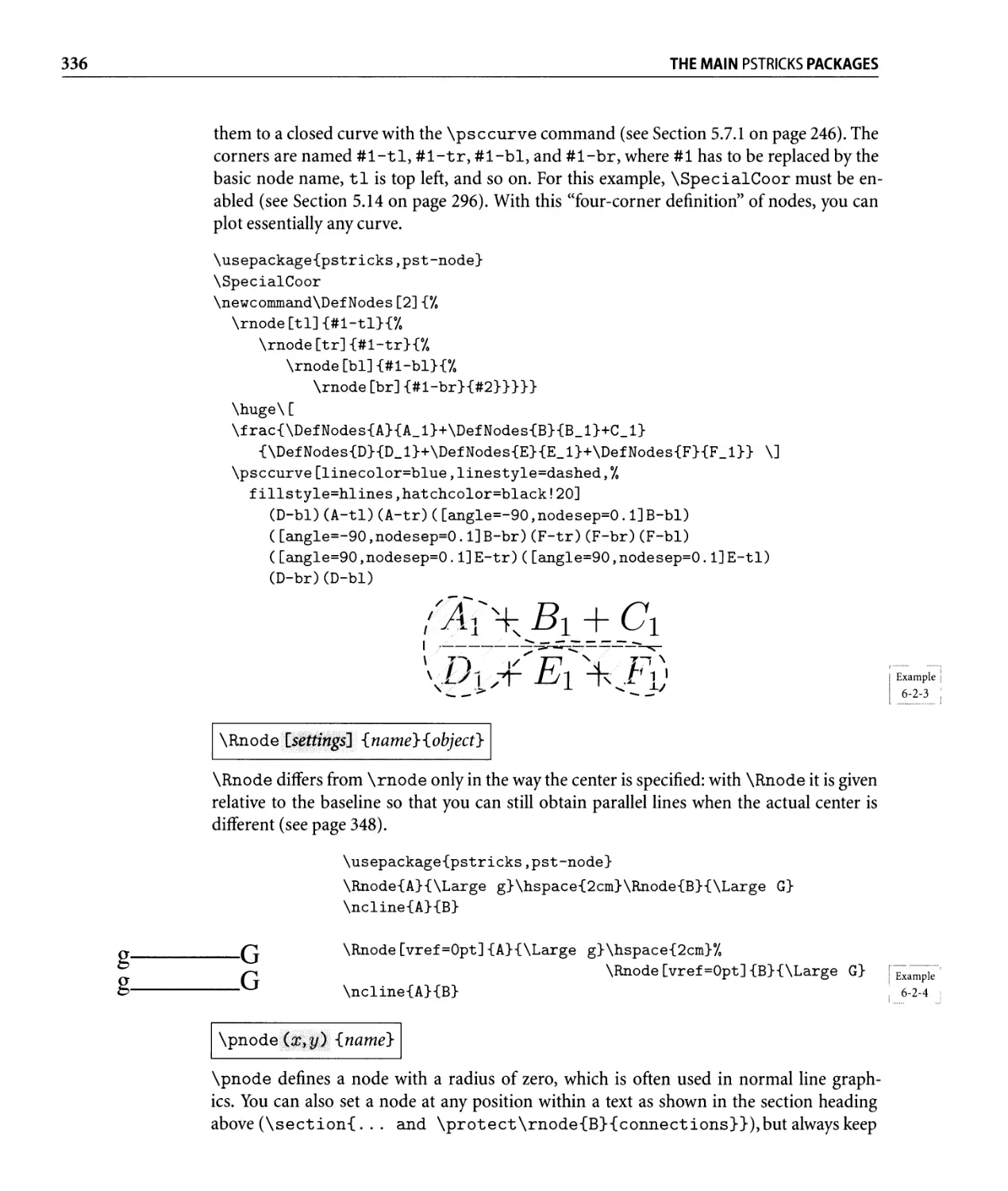
ę
ę
ˇ
ă18
IG2
2
#
!
ˉ
tr EEEEEE
ˉ
ˇˇ
ę
ę
ę
ę
ˇ
tr EEEEEE
ˉ
ˇˇ
ę
ę
ę
ę
ˇ
#
!
ˉ
tr EEEEEE
ˉ
ˇˇ
ę
ę
ę
ę
ˇ
tr EEEEEE
ˉ
ˇˇ
ę
ę
ę
ę
ˇ
#
!
ˉ
tr EEEEEE
ˉ
ˇˇ
ę
ę
ę
ę
ˇ
tr EEEEEE
ˉ
ˇˇ
ę
ę
ę
ę
ˇ
#
!
ˉ
tr EEEEEE
ˉ
ˇˇ
ę
ę
ę
ę
ˇ
tr EEEEEE
ˉ
ˇˇ
ę
ę
ę
ę
ˇ
#
!
ˉ
tr EEEEEE
ˉ
ˇˇ
ę
ę
ę
ę
ˇ
tr EEEEEE
ˉ
ˇˇ
ę
ę
ę
ę
ˇ
#
!
ˉ
tr EEEEEE
ˉ
ˇˇ
ę
ę
ę
ę
ˇ
tr EEEEEE
ˉ
ˇˇ
ę
ę
ę
ę
ˇ
ă24
IG2
2
#
!
ˉ
tr EEEEEEEE
ˉ
ˇˇ
ă
ă
ă
ă
ˇ
tr EEEEEEEE
ˉ
ˇˇ
ă
ă
ă
ă
ˇ
#
ˉ
ˉ
˘
=ˇ`
ą
ą
ˇˇˇˇ
ş
ş
şşˇ
ii
˘`
˘`
˘`
!
?ˇ-
ˇ
?(ˇ
#
ˉ
ˉ
˘˘
=ˇ`
śś
ş
şˇˇˇˇ
ş
ş
şşˇ
ii
˘`
˘`
˘`
!
?ˇ
-ˇ
?ˇ(ˇ
ă29
IG2
2
#
ˉ
ˉ
˘˘˘
˚ˇ`
ăă
ˇˇˇˇ
ą
ą
ą
ą
ˇ
------
˘`
˘`
˘`
!
?ˇ(ˇ
?ˇˇ(ˇ
#
ˉ
ˉ
˘4˘˘
˚ˇ`
ăă
ˇ \ˇˇˇ
ą
ą
ą
ą
\ˇ
------
˘`
˘`
˘`
!
rit.
?ˇ(ˇ
?ˇ\ˇ(ˇ
#ˉ
ˉ
ˉ
ˉ
ˉ
!
|
#˘`
˘`
p
C
˘`˘`› 4˘`
!>
>
Rhapsodie 26 mars 2003 (D. Taupin)
1
Music composed by Daniel Taupin and typeset with MusiXTEX
Contents
List of Figures
xvii
List of Tables
xxi
Preface xxv
Why
EX, and why PostScript? . . . . . . . . . . . . . . . . . . . . . . . . . . . .. XXVI
How this book is arranged . . . . . . . . . . . . . . . . . . . . . . . . . . . . . . . . XXVII
Typographic conventions. . . . . . . . . . . . . . . . . . . . . . . . . . . . . . . .. xxix
Using the examples . . . . . . . . . . . . . . . . . . . . . . . . . . . . . . . . . . .. xxxi
Finding all those packages and programs. . . . . . . . . . . . . . . . . . . . . . . xxxiii
1 Graphics with
EX 1
1.1 Graphics systems and typesetting . . . . . . . . . . . . . . . . . . . . . . . . . . . 2
1.2 Drawing types. . . . . . . . . . . . . . . . . . . . . . . . . . . . . . . . . . . . . . . . 3
1.3 TEX's interfaces . . . . . . . . . . . . . . . . . . . . . . . . . . . . . . . . . . . . . . . 6
1.3.1 Methods of integration . . . . . . . . . . . . . . . . . . . . . . . . . . . . 6
1.3.2 Methods of manipu lation . . . . . . . . . . . . . . . . . . . . . . . . . . . 8
1.3.3 TEX's graphics hooks . . . . . . . . . . . . . . . . . . . . . . . . . . . . . . 8
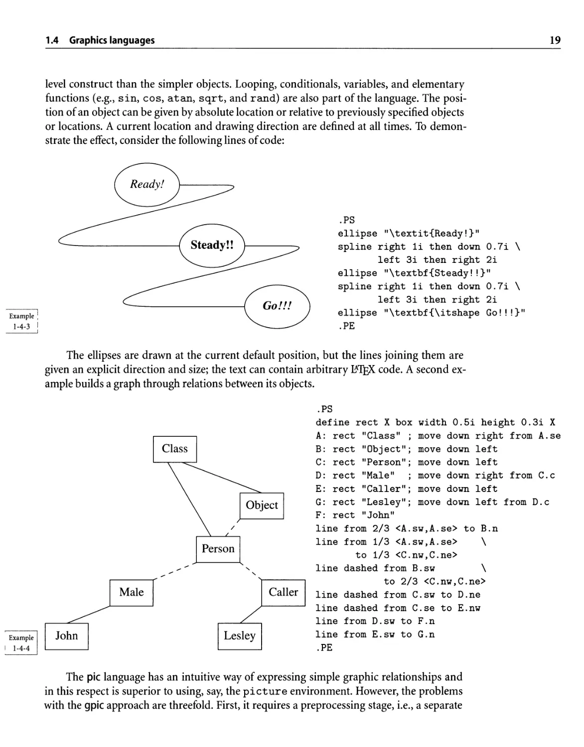
1.4 Graphics languages . . . . . . . . . . . . . . . . . . . . . . . . . . . . . . . . . . .. 10
1.4.1 Generic graphics languages. ......................... 10
1.4.2 TEX-based graphics languages . . . . . . . . . . . . . . . . . . . . . . .. 13
1.4.3 External graphics languages and drawing programs . . . . . . . . .. 17
1.5 Choosing a package . . . . . . . . . . . . . . . . . . . . . . . . . . . . . . . . . . .. 21
...
Vlll
CONTENTS
2 Standard EX Interfaces 23
2.1 Inclusion of graphics files. . . . . . . . . . . . . . . . . . . . . . . . . . . . . . . .. 23
2.1.1 Options for graphics and graphicx. . . . . . . . . . . . . . . . . . . . .. 24
2.1.2 The \includegraphics syntax in the graphics package. . . . . .. 25
2.1.3 The \includegraphics syntax in the graphicx package . . . . .. 28
2.1.4 Setting default key values for the graphicx package. . . . . . . . . .. 32
2.1.5 Declarations guiding the inclusion of images. . . . . . . . . . . . . .. 33
2.1.6 A caveat: encapsulation is important. . . . . . . . . . . . . . . . . . .. 35
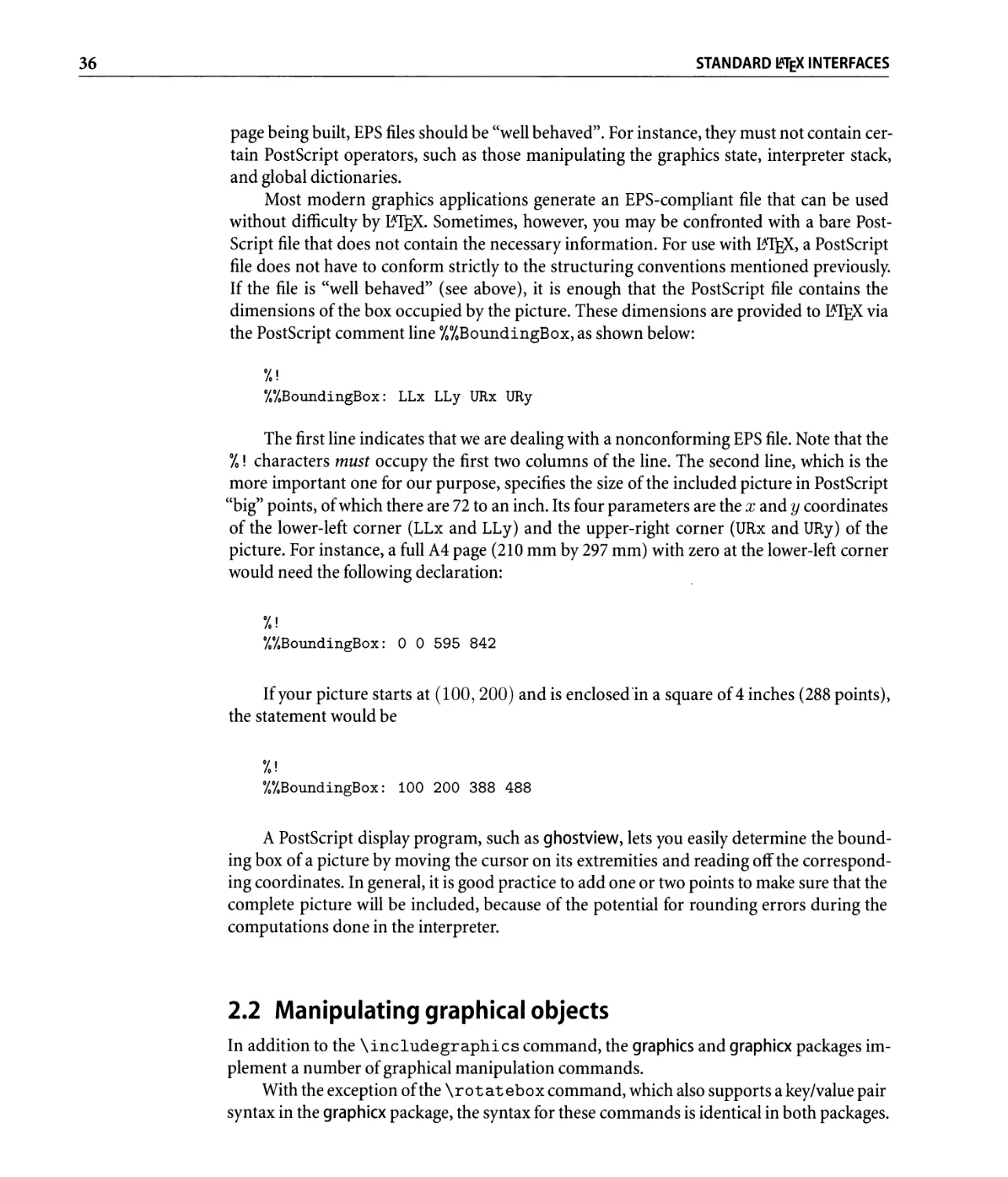
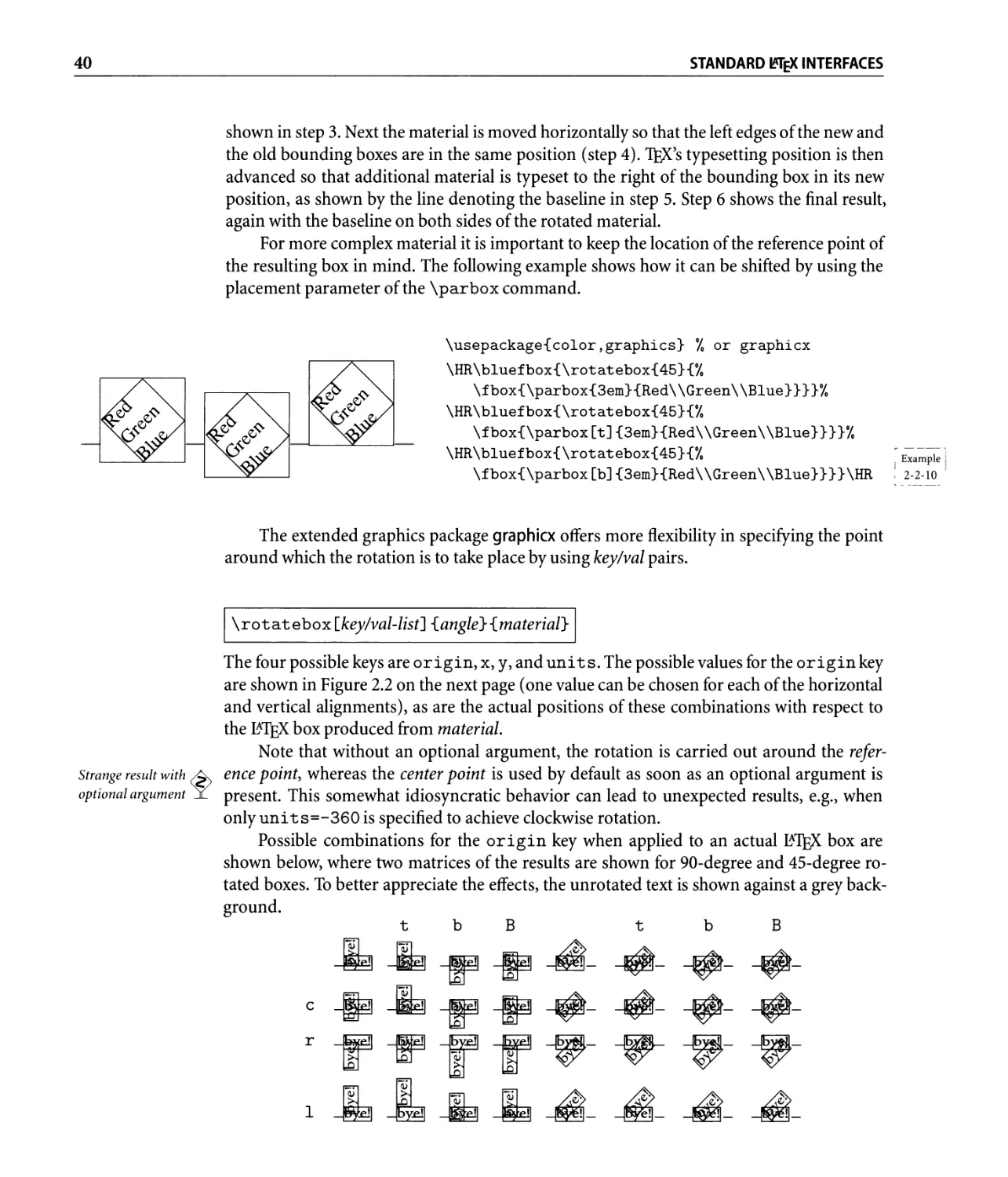
2.2 Manipulating graphical objects. . . . . . . . . . . . . . . . . . . . . . . . . . . .. 36
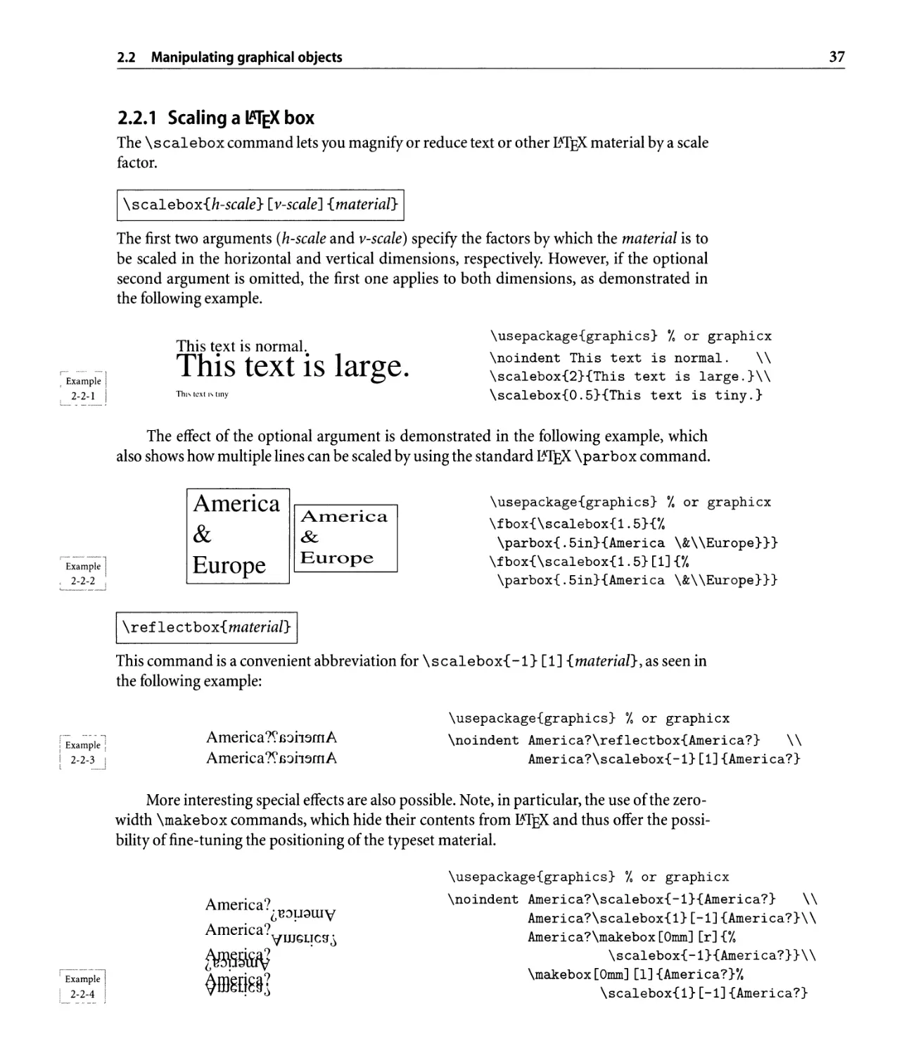
2.2.1 Scaling a EX box. . . . . . . . . . . . . . . . . . . . . . . . . . . . . . .. 37
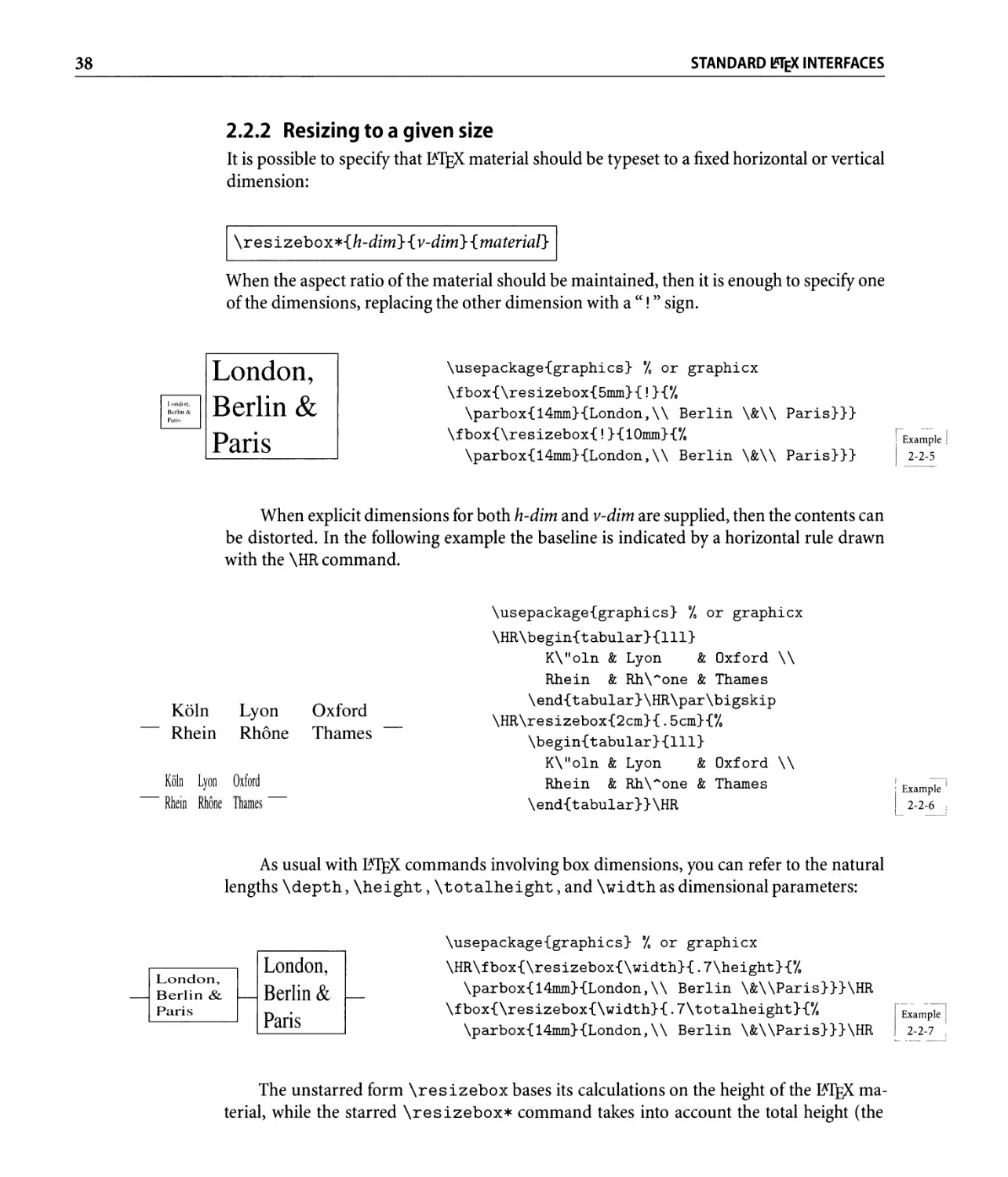
2.2.2 Resizing to a given size. . . . . . . . . . . . . . . . . . . . . . . . . . . .. 38
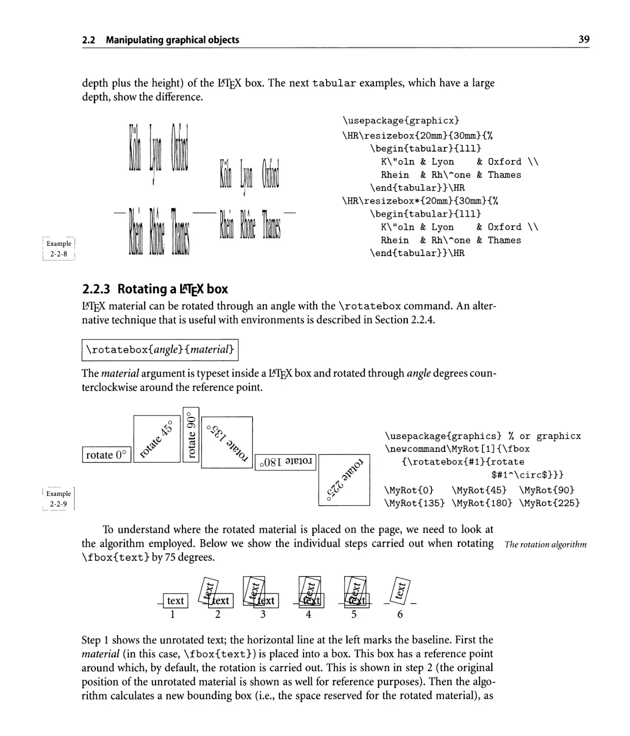
2.2.3 Rotating a EX box. . . . . . . . . . . . . . . . . . . . . . . . . . . . . .. 39
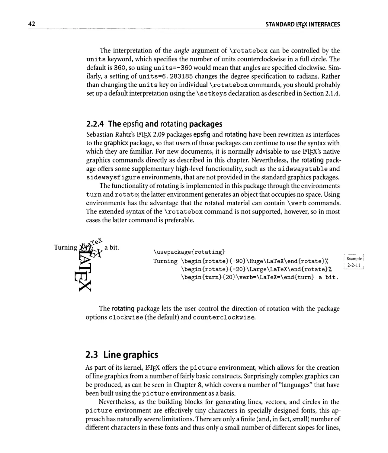
2.2.4 The epsfig and rotating packages . . . . . . . . . . . . . . . . . . . . .. 42
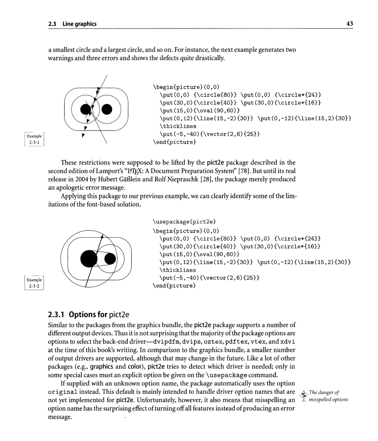
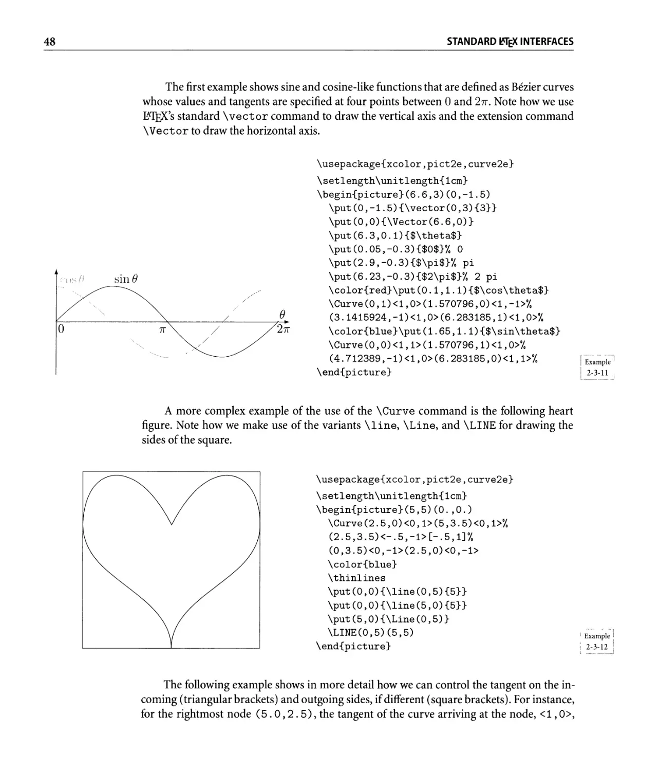
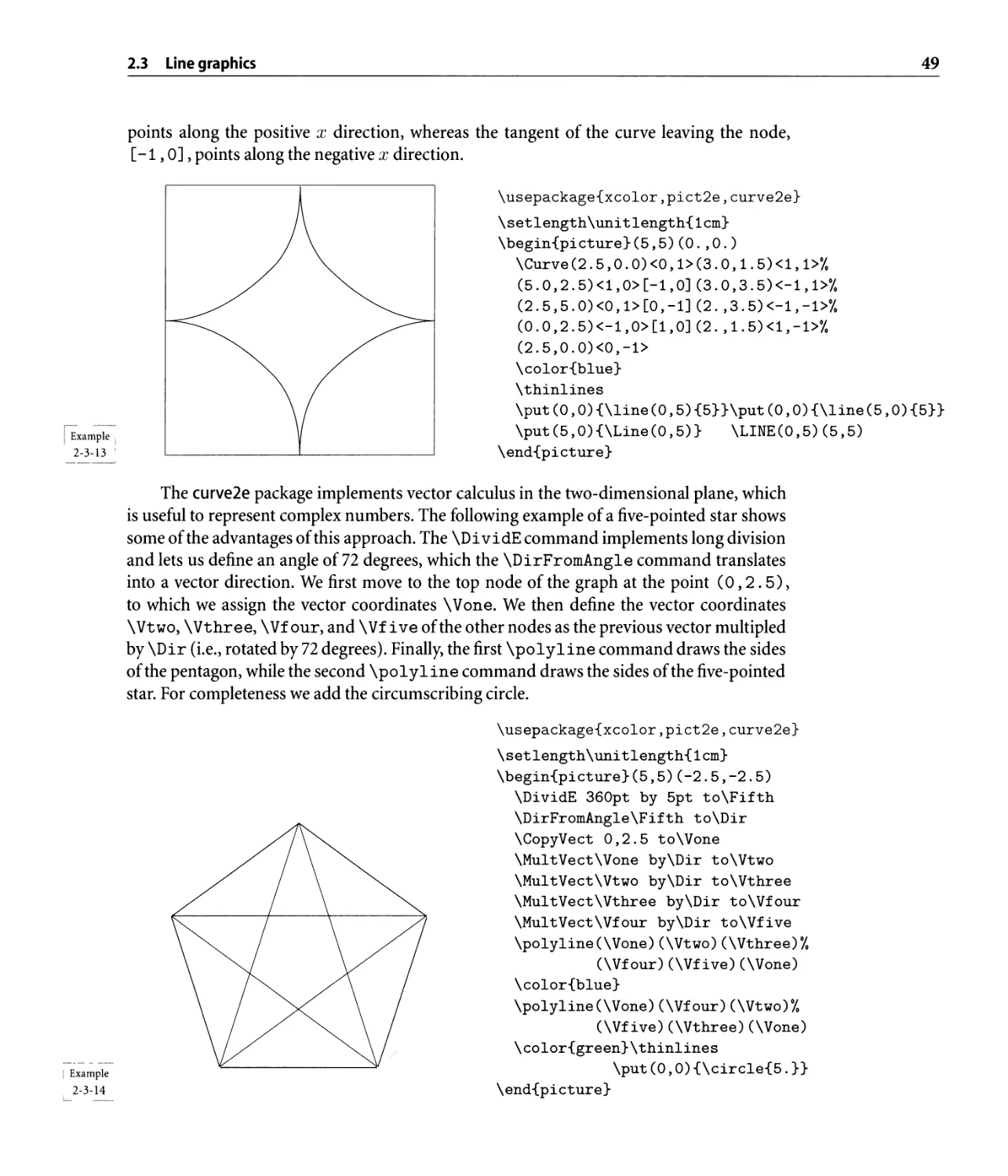
2.3 Line graphics . . . . . . . . . . . . . . . . . . . . . . . . . . . . . . . . . . . . . . .. 42
2.3.1 Options for pict2e. . . . . . . . . . . . . . . . . . . . . . . . . . . . . . .. 43
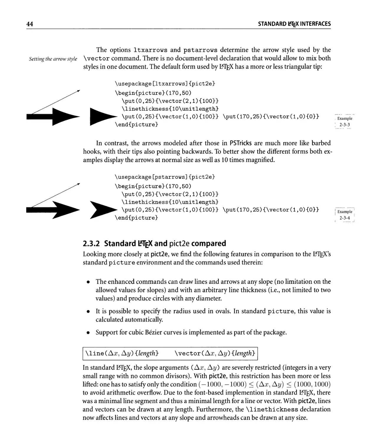
2.3.2 Standard EX and pict2e compared . . . . . . . . . . . . . . . . . . .. 44
2.3.3 Slightly beyond standard graphics: curve2e. . . . . . . . . . . . . . .. 47
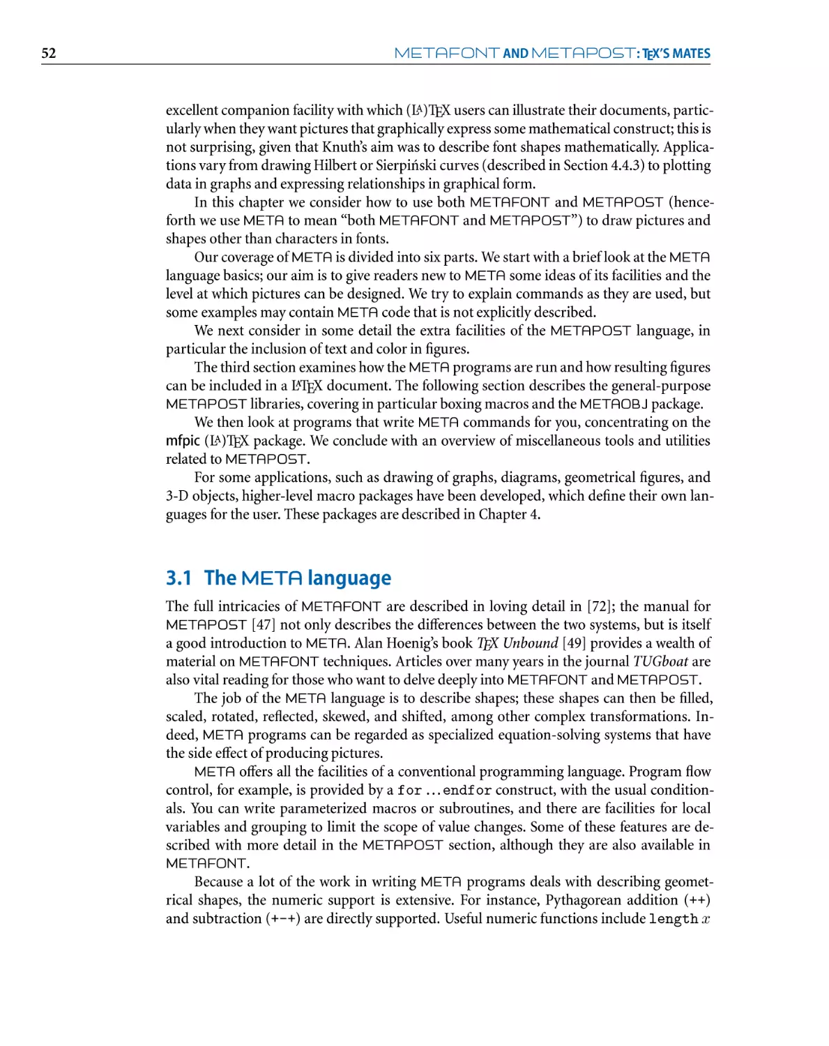
3 M(;TRFONT and M(;TRPO T: TEX's Mates S1
3.1 The META language . . . . . . . . . . . . . . . . . . . . . . . . . . . . . . . . . .. 52
3.1.1 First examples of META programs . . . . . . . . . . . . . . . . . . . .. 53
3.1.2 Defining macros. . . . . . . . . . . . . . . . . . . . . . . . . . . . . . . .. 57
3.2 Differences between METAPosT and METAFoNT . . . . . . . . . . . . . .. 60
3.2.1 Color. . . . . . . . . . . . . . . . . . . . . . . . . . . . . . . . . . . . . . .. 60
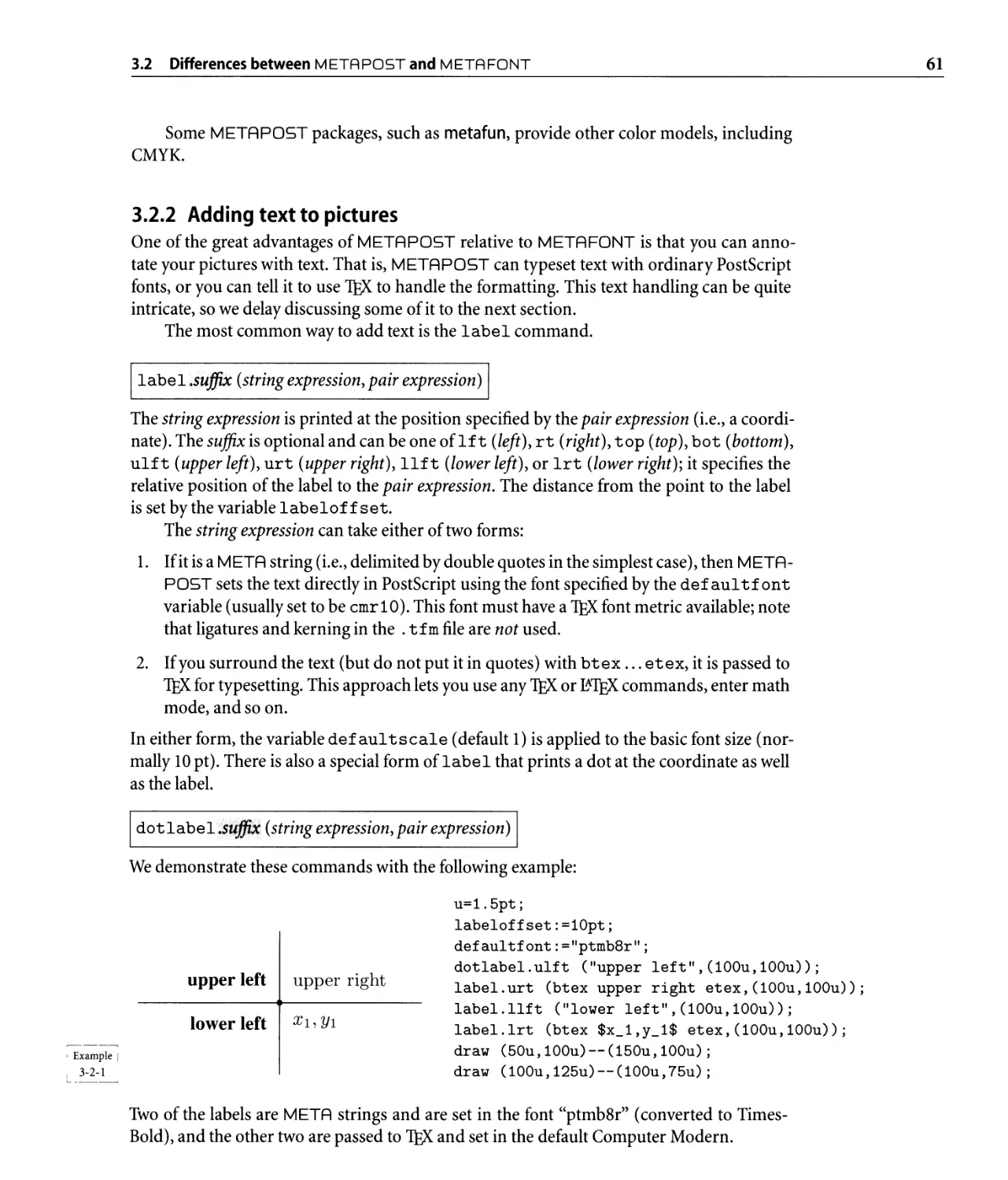
3.2.2 Adding text to pictures. . . . . . . . . . . . . . . . . . . . . . . . . . . .. 61
3.2.3 Adding text-some gory details. . . . . . . . . . . . . . . . . . . . . .. 62
3.2.4 I nte rna I stru ctu res . . . . . . . . . . . . . . . . . . . . . . . . . . . . . .. 65
3.2.5 File input and output. . . . . . . . . . . . . . . . . . . . . . . . . . . . .. 67
3.3 Running the META programs. . . . . . . . . . . . . . . . . . . . . . . . . . . . .. 68
3.3.1 Running META FONT . . . . . . . . . . . . . . . . . . . . . . . . . . . .. 68
3.3.2 Running META POST . . . . . . . . . . . . . . . . . . . . . . . . . . . .. 71
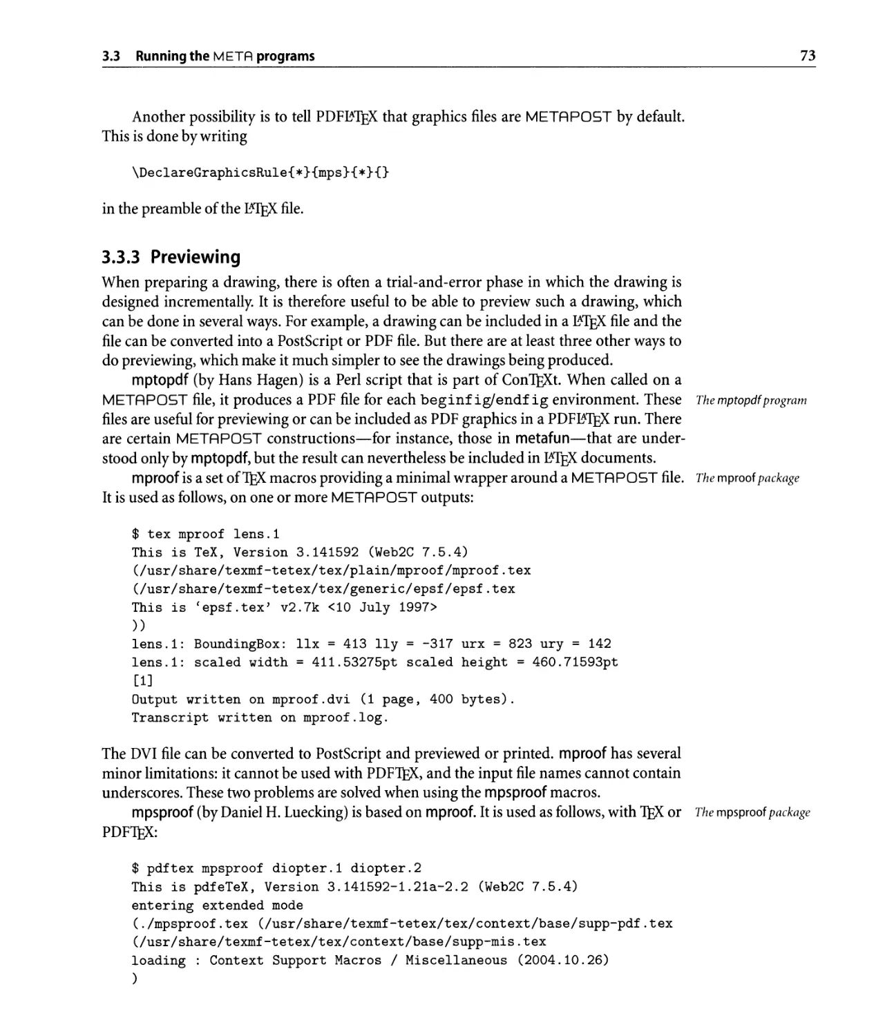
3.3.3 Previewing . . . . . . . . . . . . . . . . . . . . . . . . . . . . . . . . . . .. 73
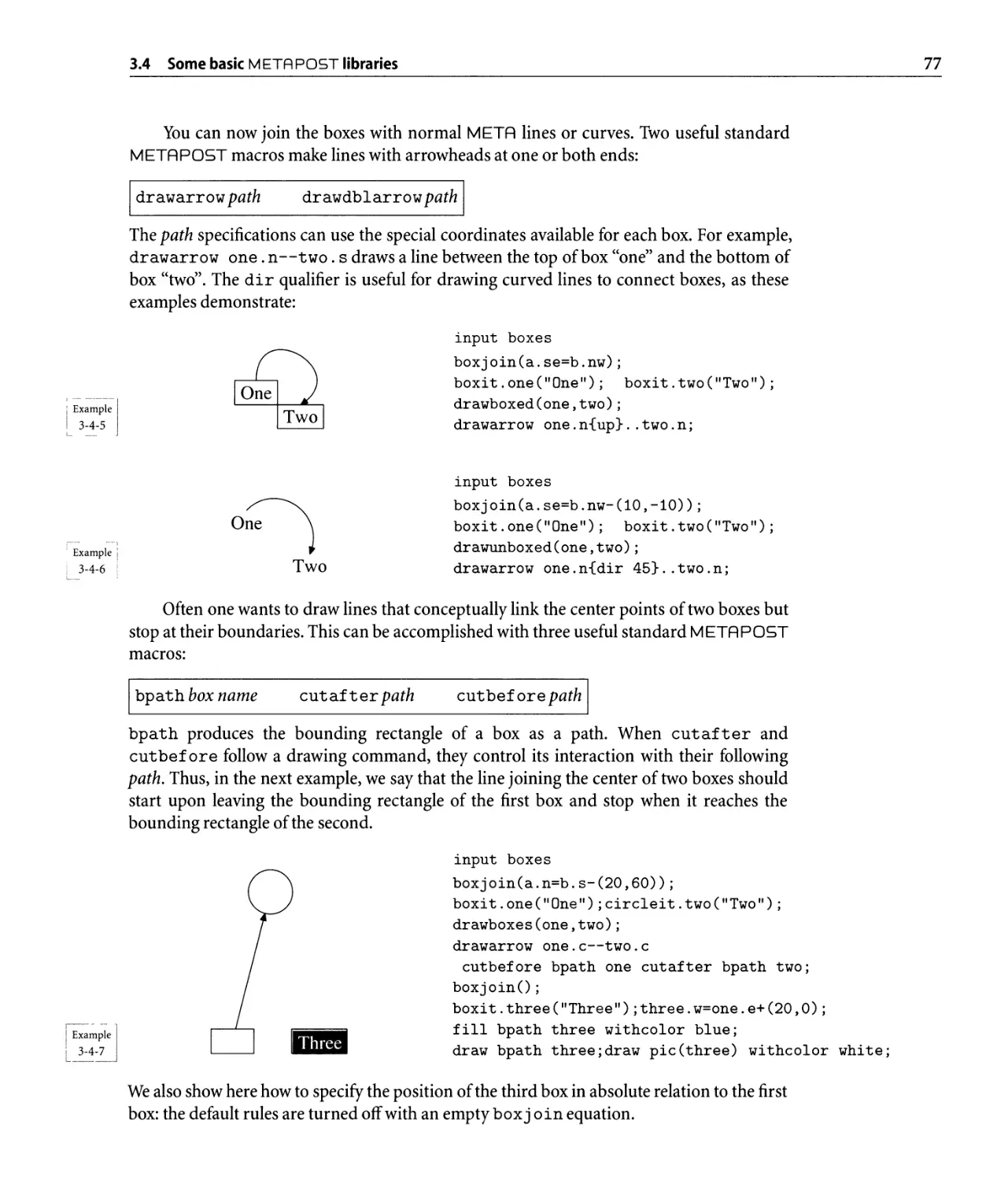
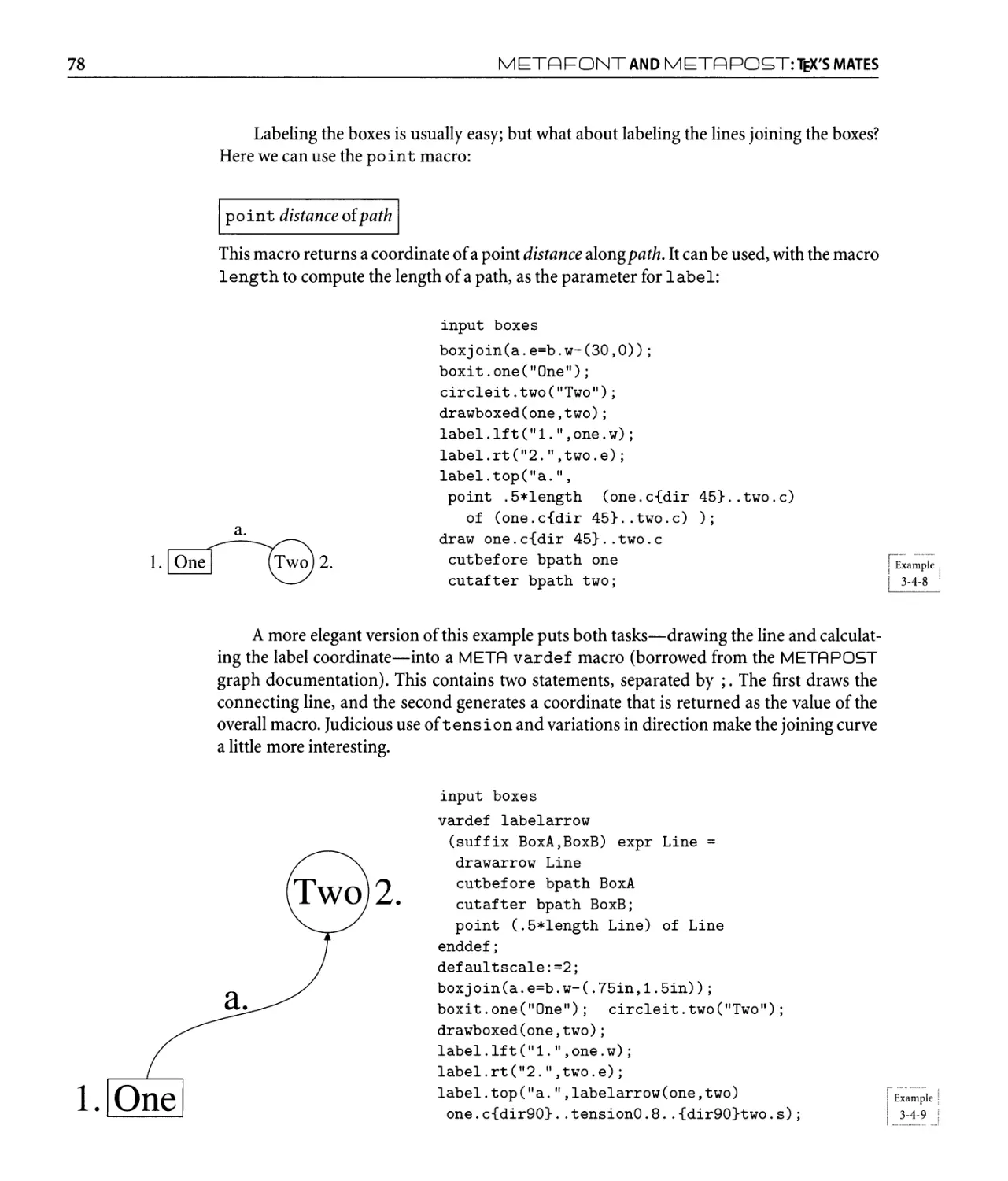
3.4 Some basic M ETA POST libraries . . . . . . . . . . . . . . . . . . . . . . . . . .. 74
3.4.1 The metafu n package . . . . . . . . . . . . . . . . . . . . . . . . . . . .. 74
3.4.2 The boxes package . . . . . . . . . . . . . . . . . . . . . . . . . . . . . .. 75
3.5 The M ETAoB J package . . . . . . . . . . . . . . . . . . . . . . . . . . . . . . . .. 80
3.5.1 Underlying principles. . . . . . . . . . . . . . . . . . . . . . . . . . . . .. 80
3.5.2 M ETAoB J concepts. . . . . . . . . . . . . . . . . . . . . . . . . . . . .. 81
3.5.3 Basic objects. . . . . . . . . . . . . . . . . . . . . . . . . . . . . . . . . .. 82
3.5.4 Con nections . . . . . . . . . . . . . . . . . . . . . . . . . . . . . . . . . .. 84
3.5.5 Containers.............................. . . . . .. 95
3.5.6 Box alignment constructors. . . . . . . . . . . . . . . . . . . . . . . . .. 100
3.5.7 Recursive objects and fractals . . . . . . . . . . . . . . . . . . . . . . .. 104
CONTENTS
.
IX
3.5 .8 Trees........................................
3.5.9 Matrices................................. . . . . .
3.5.10 Tree and matrix connection variants . . . . . . . . . . . . . . . . . . . .
3 .5. 11 Labels.......................................
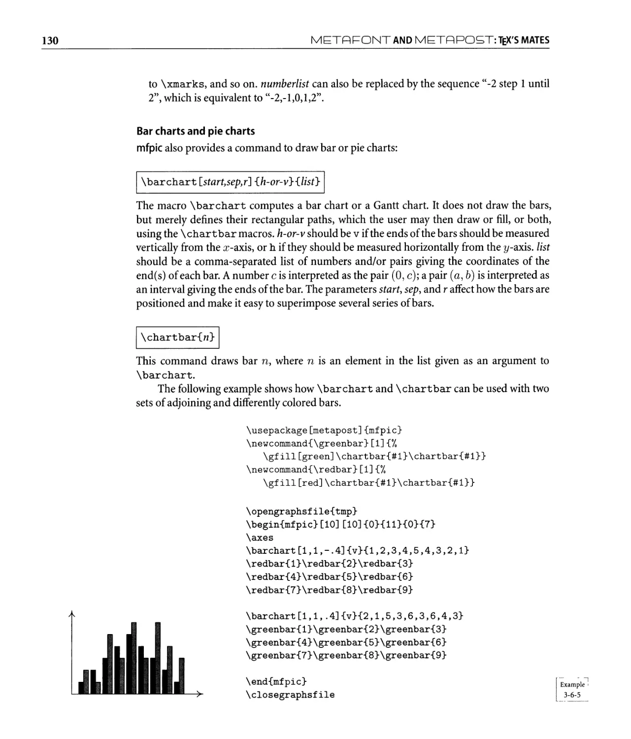
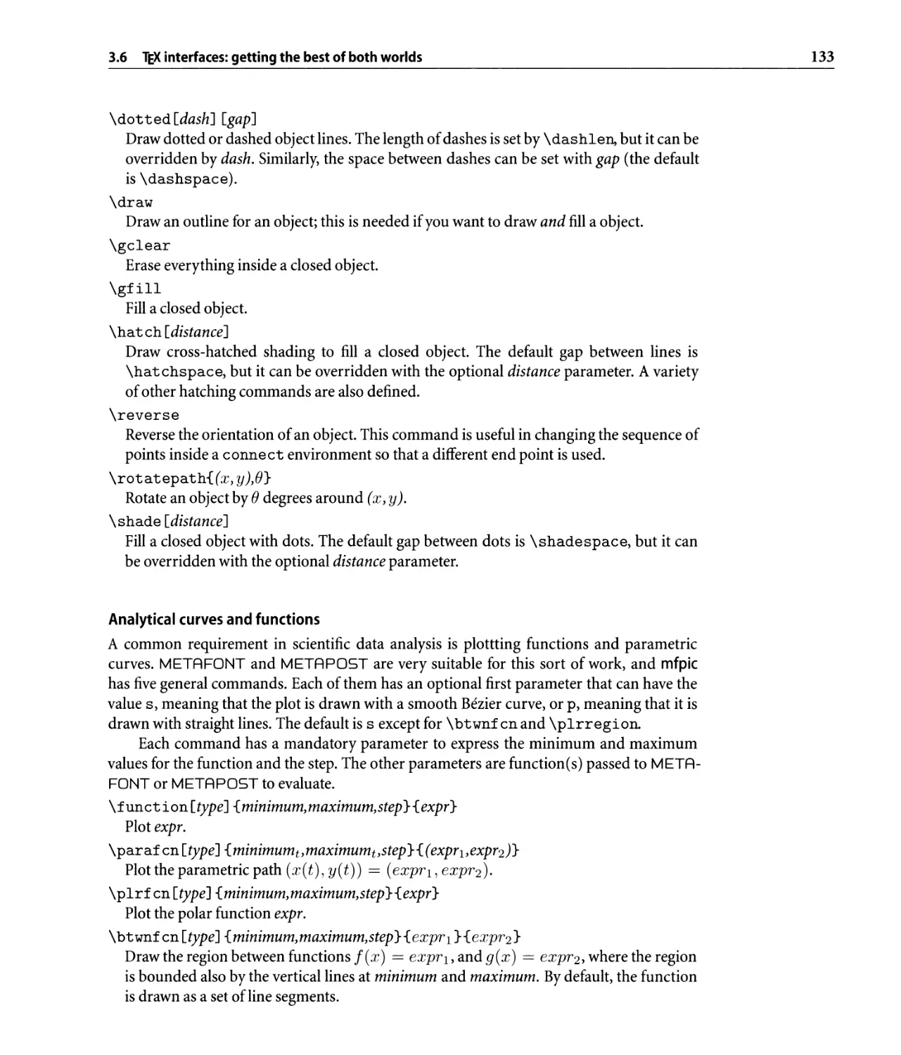
3.6 TEX interfaces: getting the best of both worlds. . . . . . . . . . . . . . . . . . . .
3.6.1 The emp package. . . . . . . . . . . . . . . . . . . . . . . . . . . . . . . .
3.6.2 The mfpic package . . . . . . . . . . . . . . . . . . . . . . . . . . . . . . .
3.6.3 The mft and mpt pretty-printers. . . . . . . . . . . . . . . . . . . . . . .
3.7 From META POST and to META POST . . . . . . . . . . . . . . . . . . . . . . .
3.8 The future of META POST . . . . . . . . . . . . . . . . . . . . . . . . . . . . . . . .
4 META POST Applications
4.1 A drawing toolkit. . . . . . . . . . . . . . . . . . . . . . . . . . . . . . . . . . . . . .
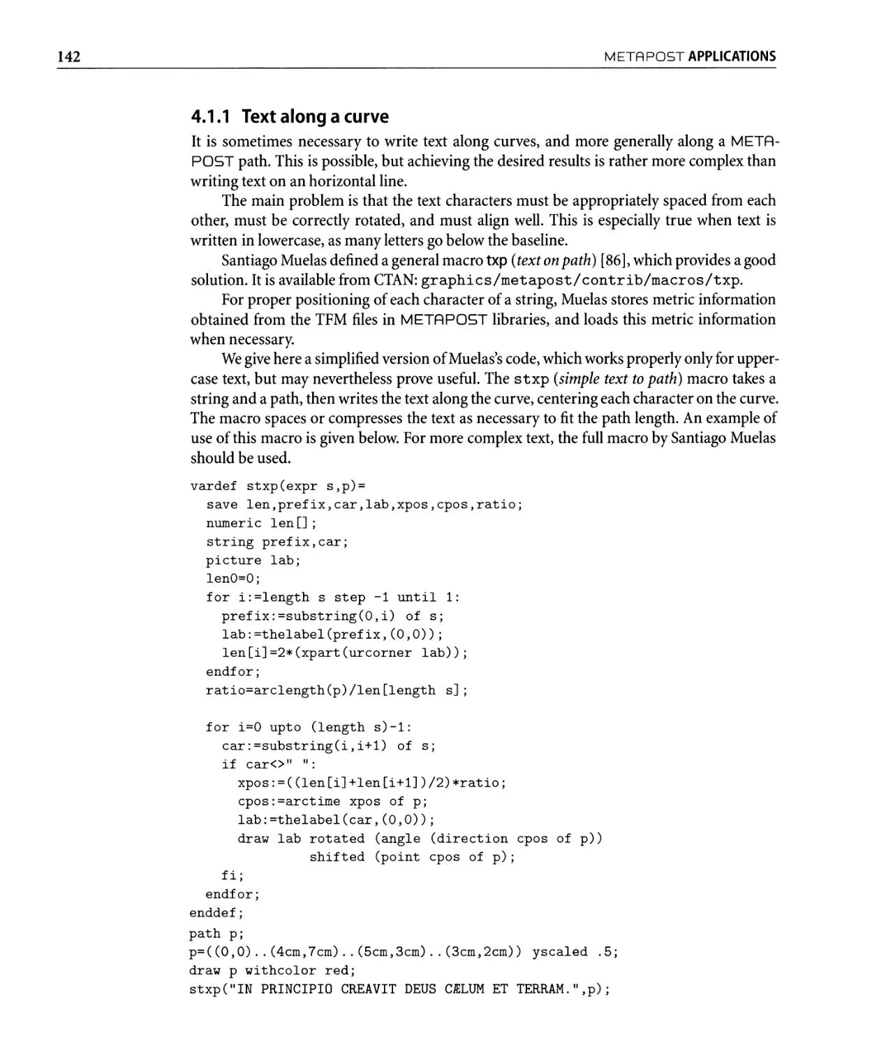
4.1.1 Text along a curve. . . . . . . . . . . . . . . . . . . . . . . . . . . . . . . .
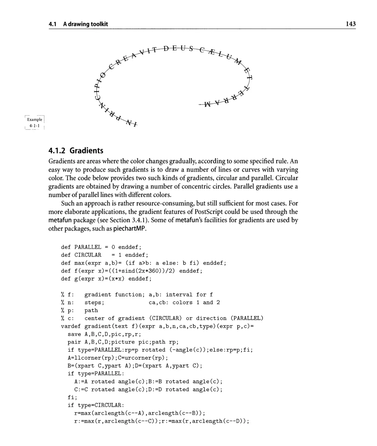
4.1.2 Gradients.....................................
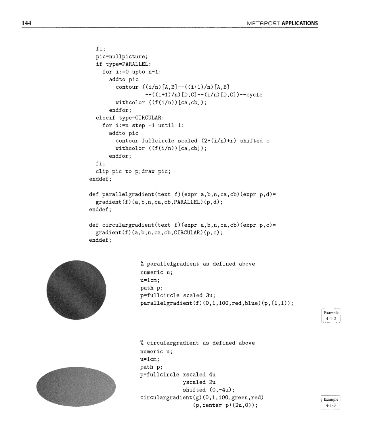
4.1.3 Hidden lines . . . . . . . . . . . . . . . . . . . . . . . . . . . . . . . . . . .
4.1.4 Multipaths and advanced clipping . . . . . . . . . . . . . . . . . . . . .
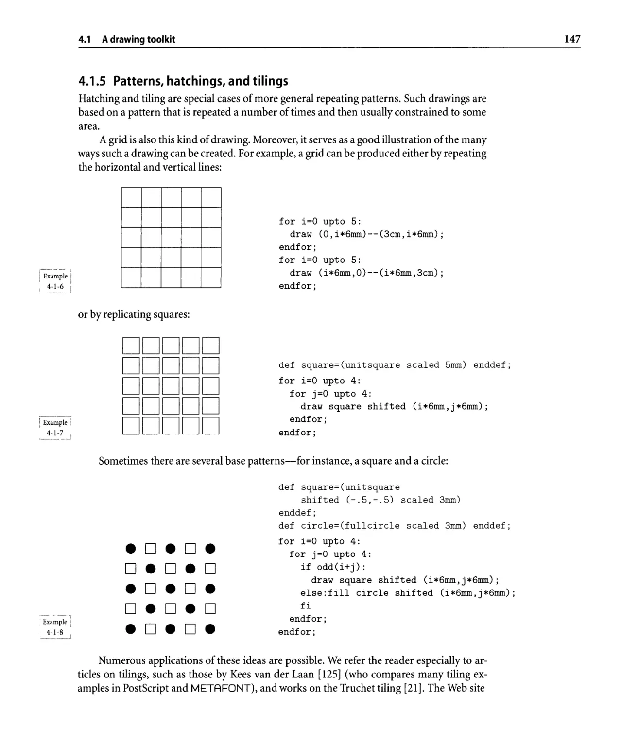
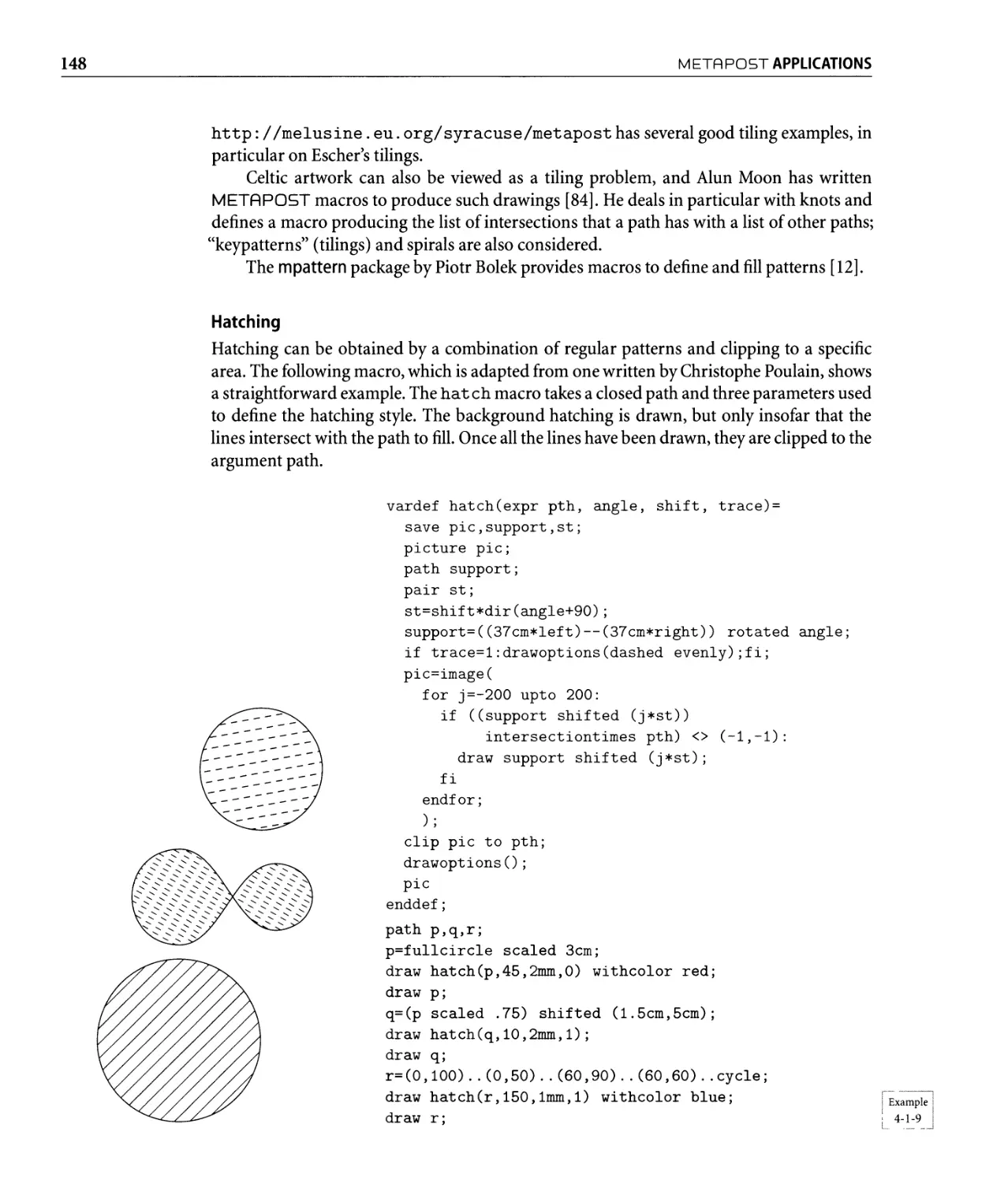
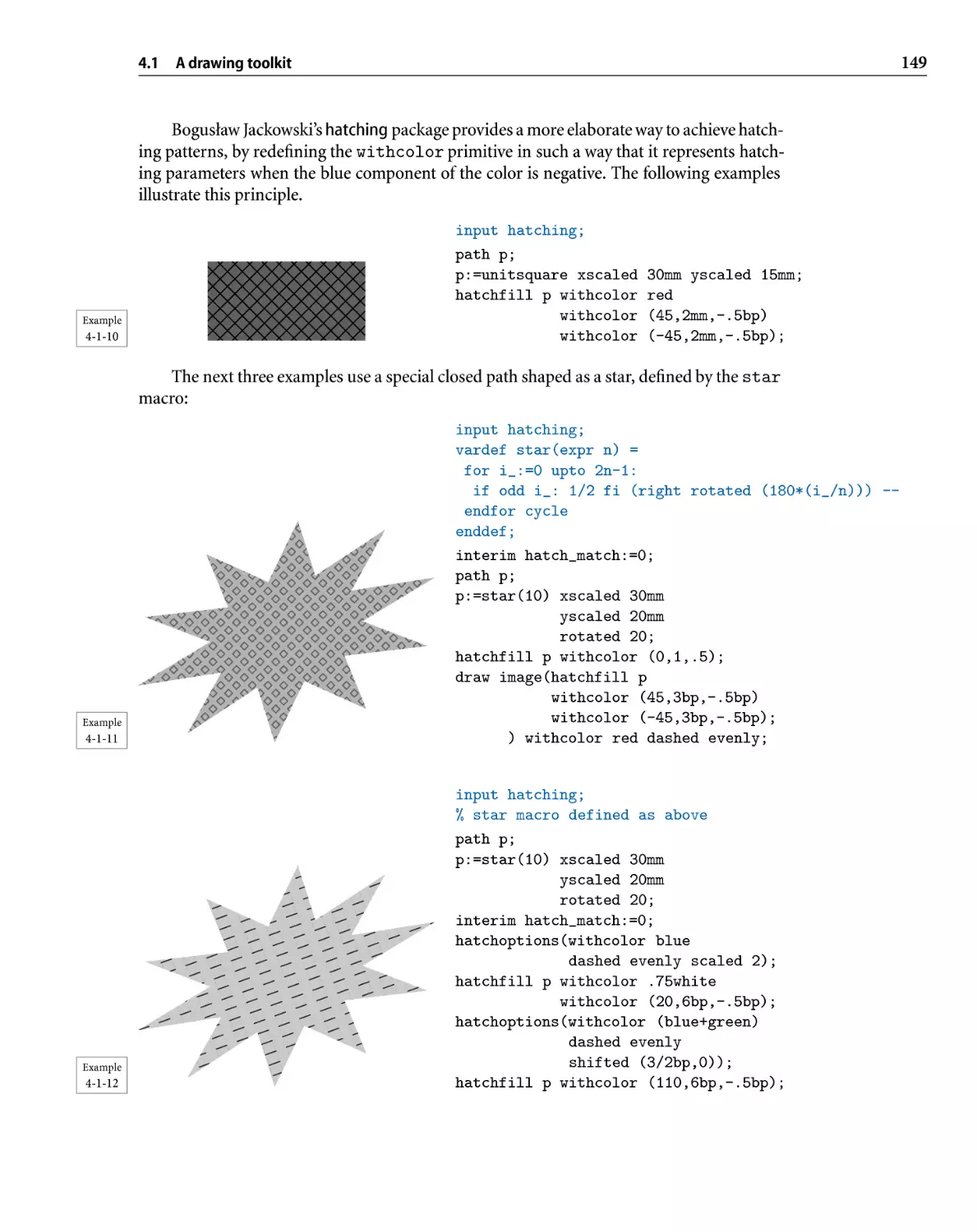
4.1.5 Patterns, hatchings, and tilings. . . . . . . . . . . . . . . . . . . . . . . .
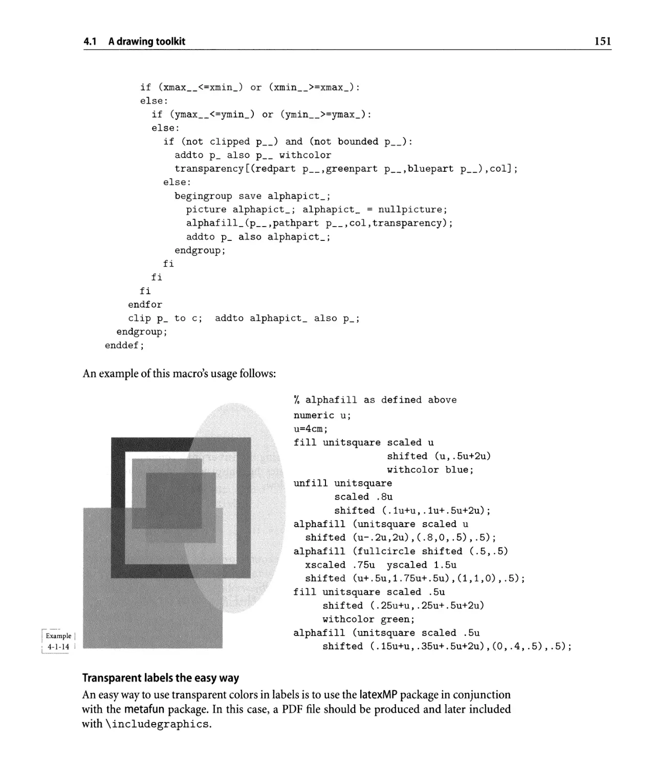
4.1.6 Transparency...................................
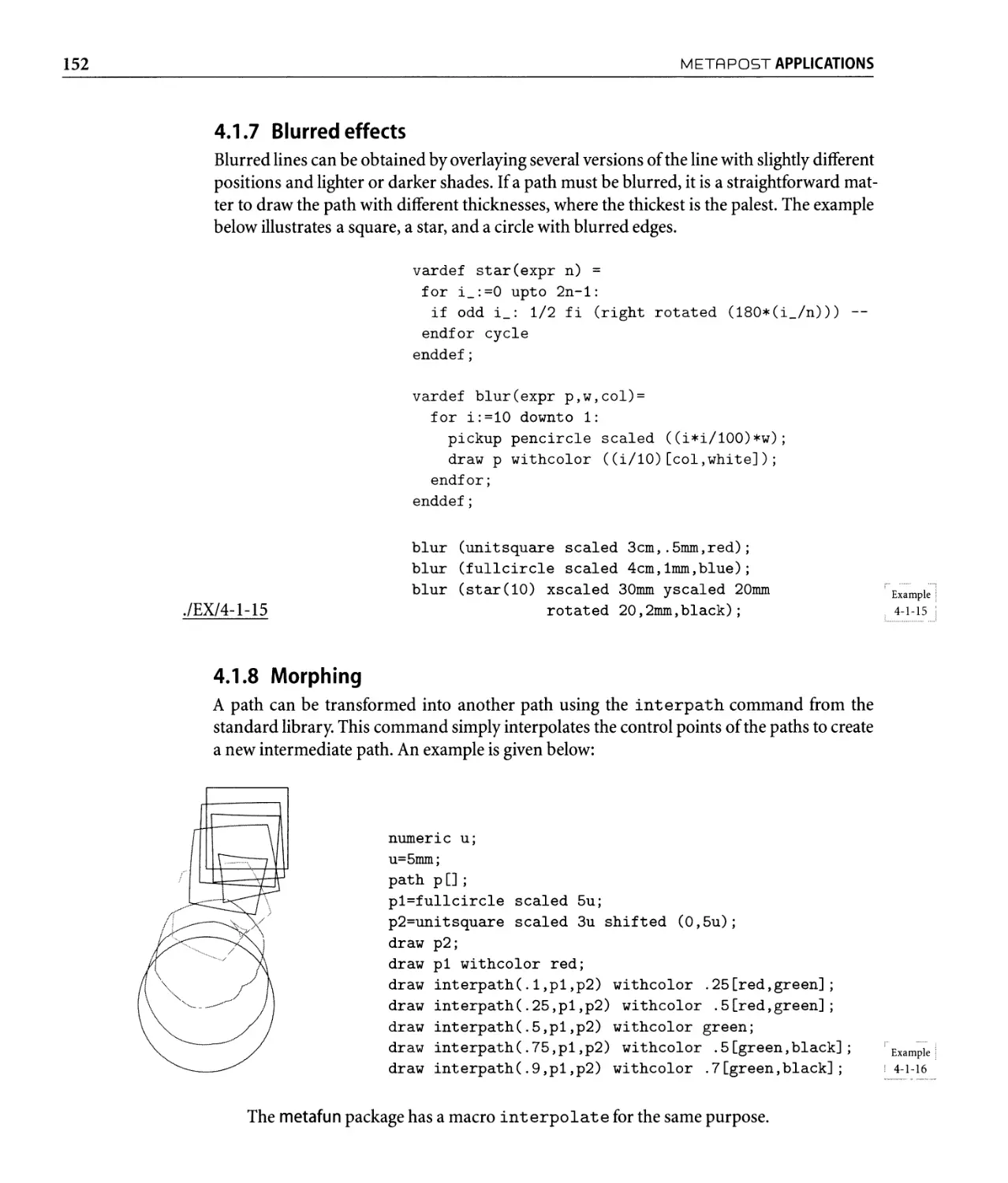
4.1.7 Blurredeffects..................................
4.1.8 Morphing.....................................
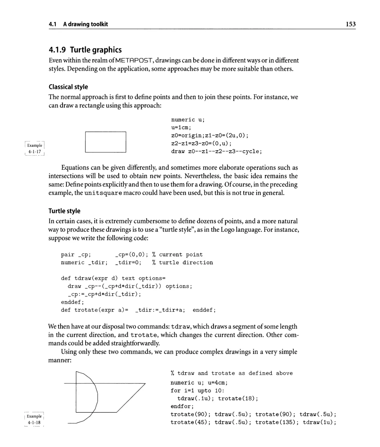
4.1 .9 T u rt leg rap h ics. . . . . . . . . . . . . . . . . . . . . . . . . . . . . . . . . .
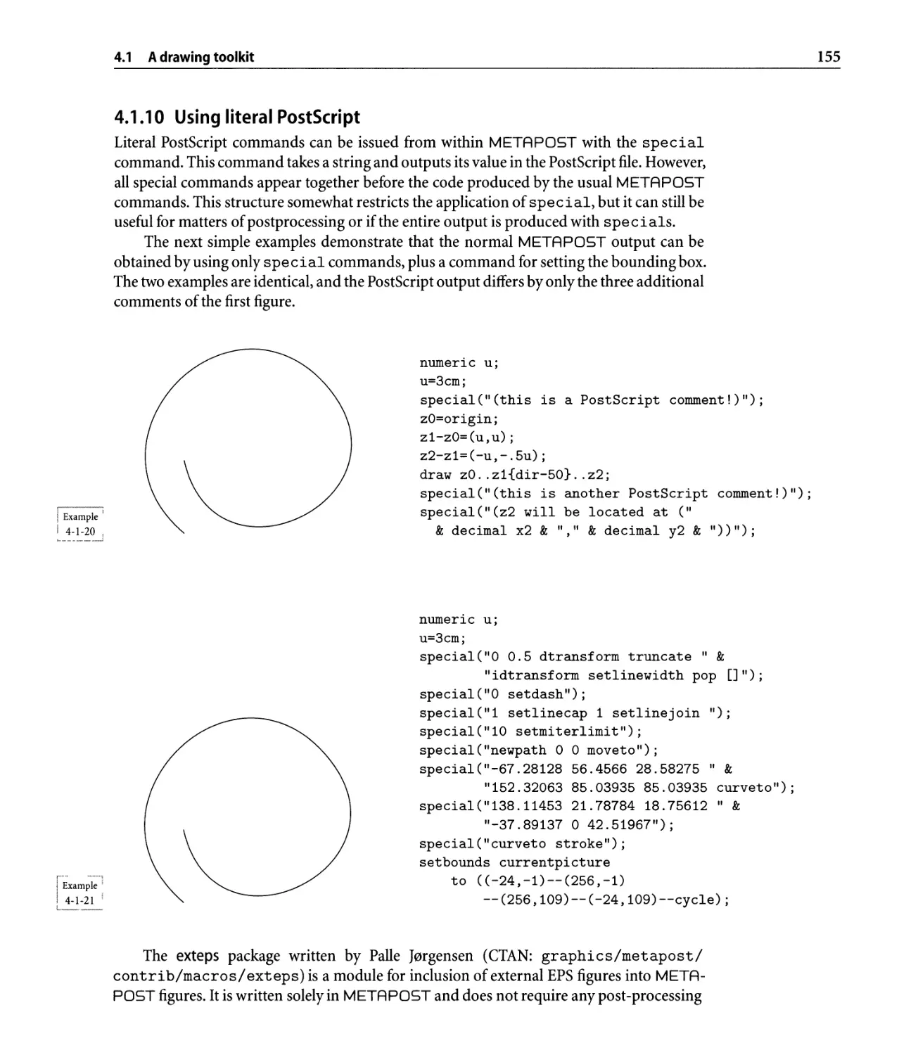
4.1.10 Using literal PostScript. . . . . . . . . . . . . . . . . . . . . . . . . . . . .
4.1.11 Animations....................................
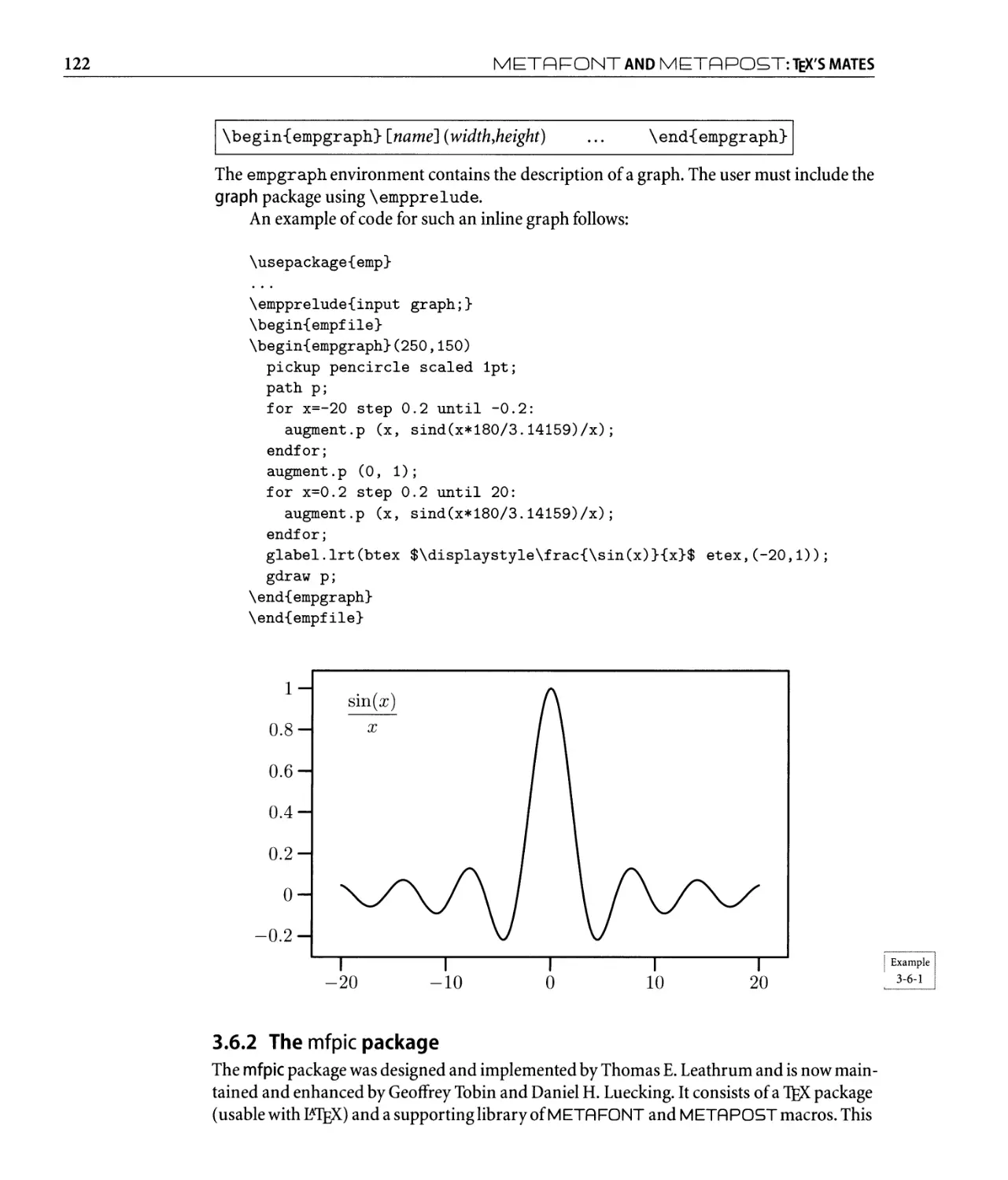
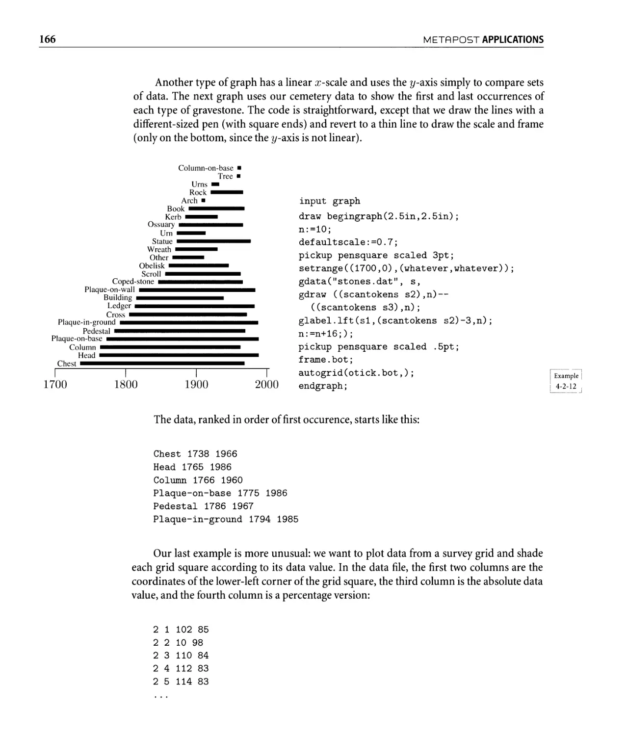
4.2 Representing data with graphs . . . . . . . . . . . . . . . . . . . . . . . . . . . . .
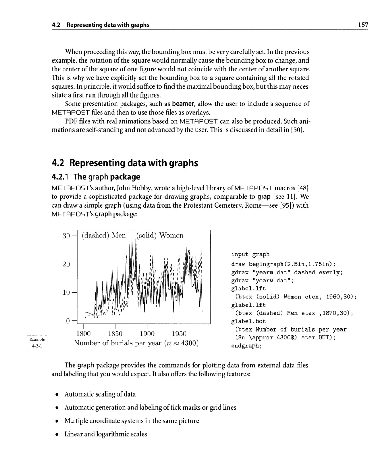
4.2.1 The graph package . . . . . . . . . . . . . . . . . . . . . . . . . . . . . . .
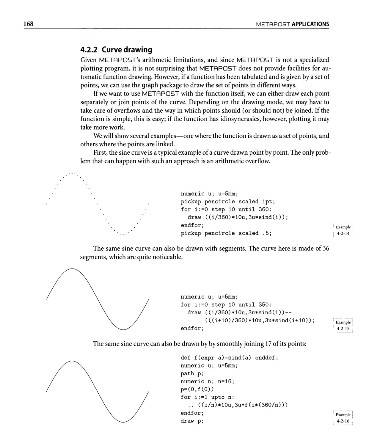
4.2.2 Curve drawing. .................................
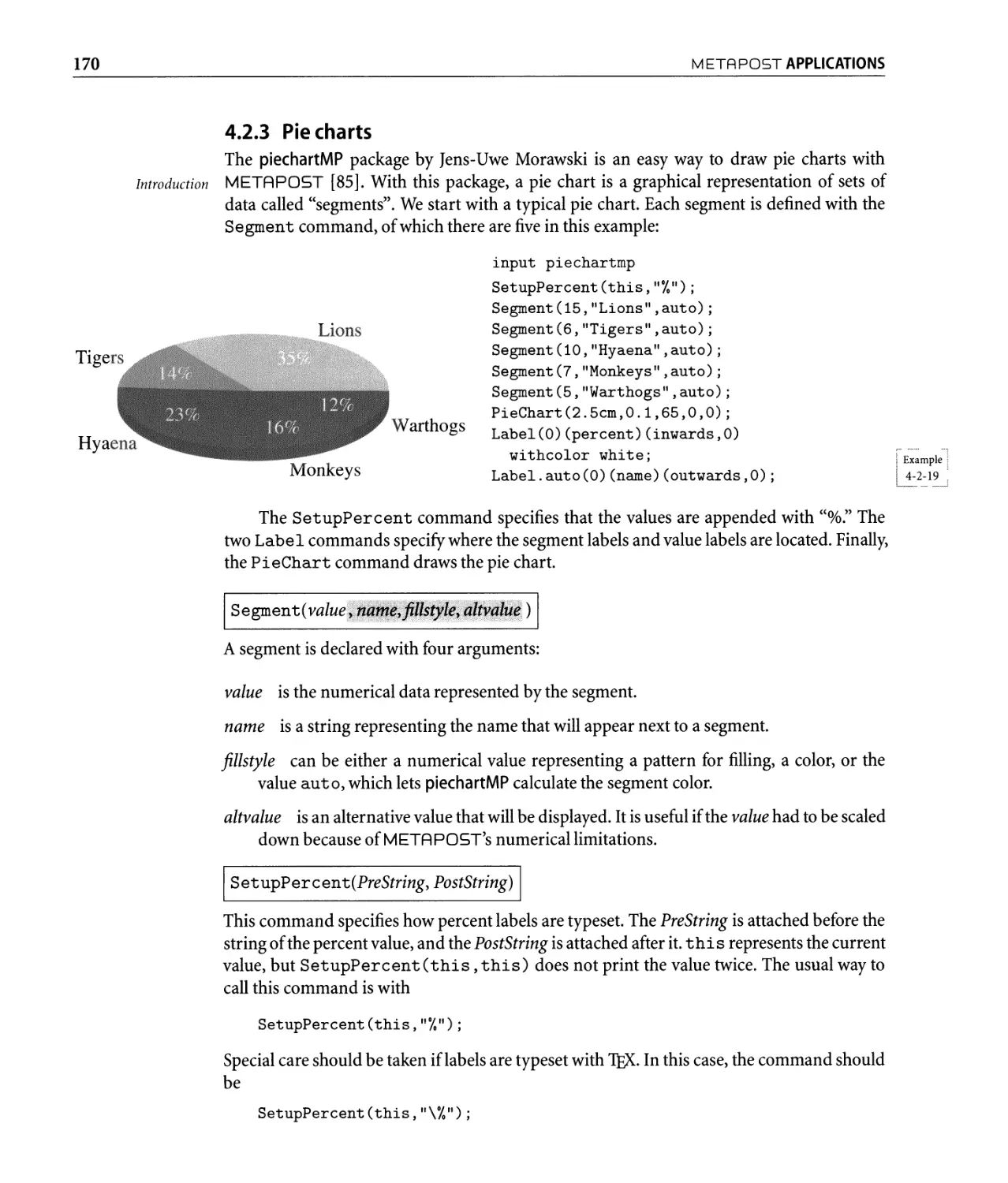
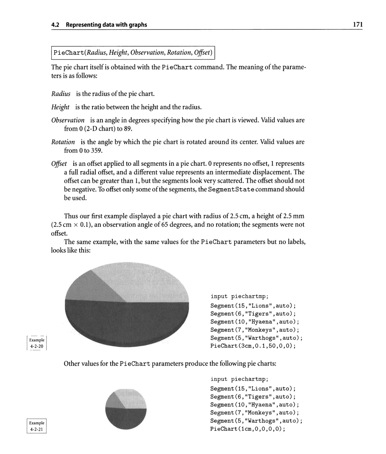
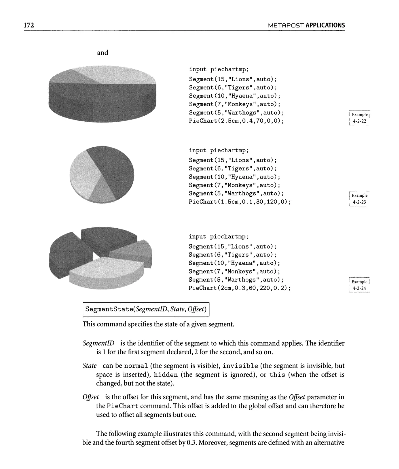
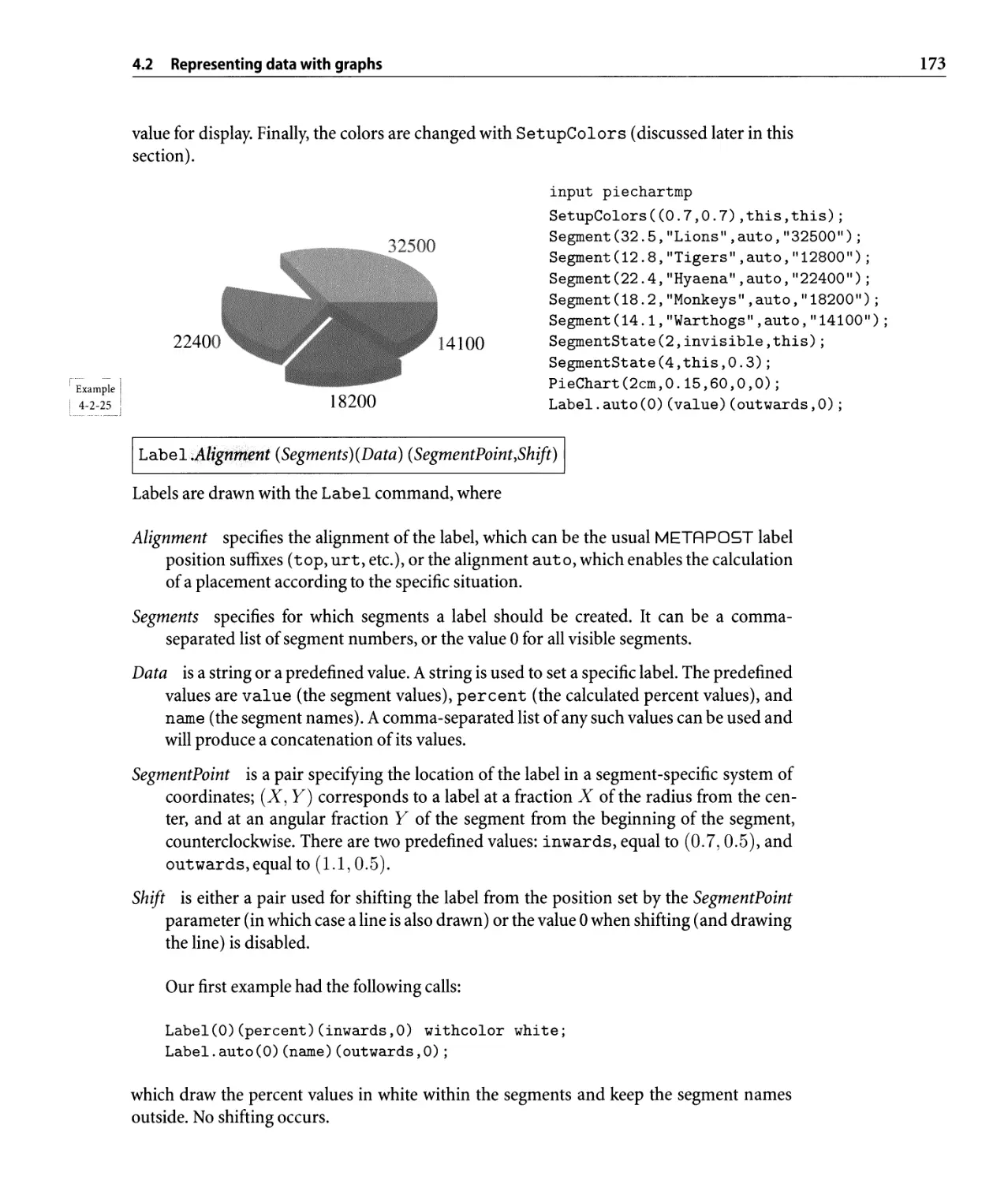
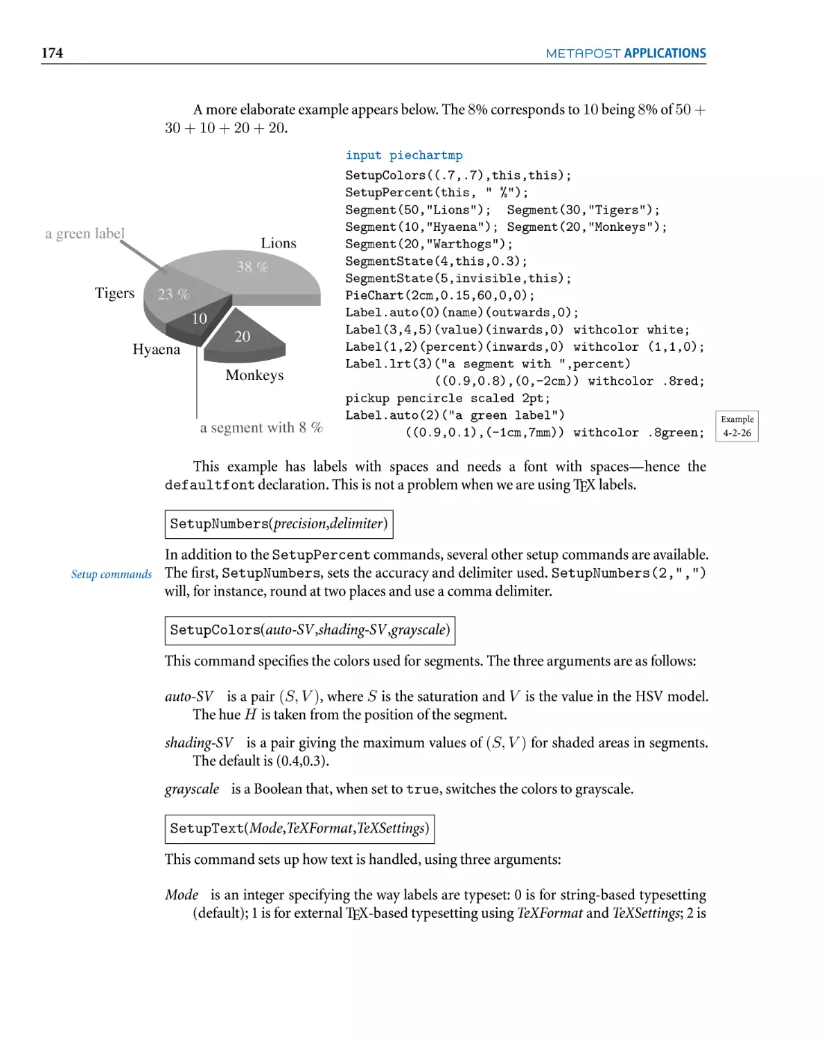
4.2.3 Pie charts. . . . . . . . . . . . . . . . . . . . . . . . . . . . . . . . . . . . .
4.3 Diagrams...........................................
4.3.1 Graphs. . . . . . . . . . . . . . . . . . . . . . . . . . . . . . . . . . . . . . .
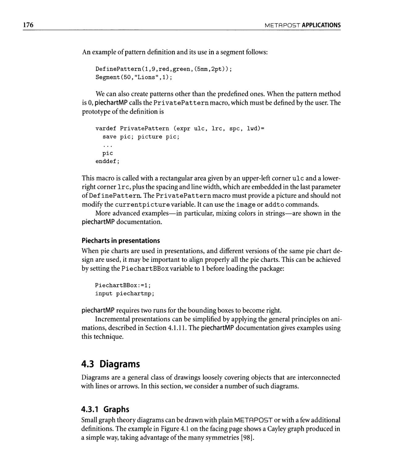
4.3.2 Flowcharts....................................
4.3.3 Block drawing and Bond graphs. . . . . . . . . . . . . . . . . . . . . . .
4.3.4 Box-line diagrams: the expressg package . . . . . . . . . . . . . . . . .
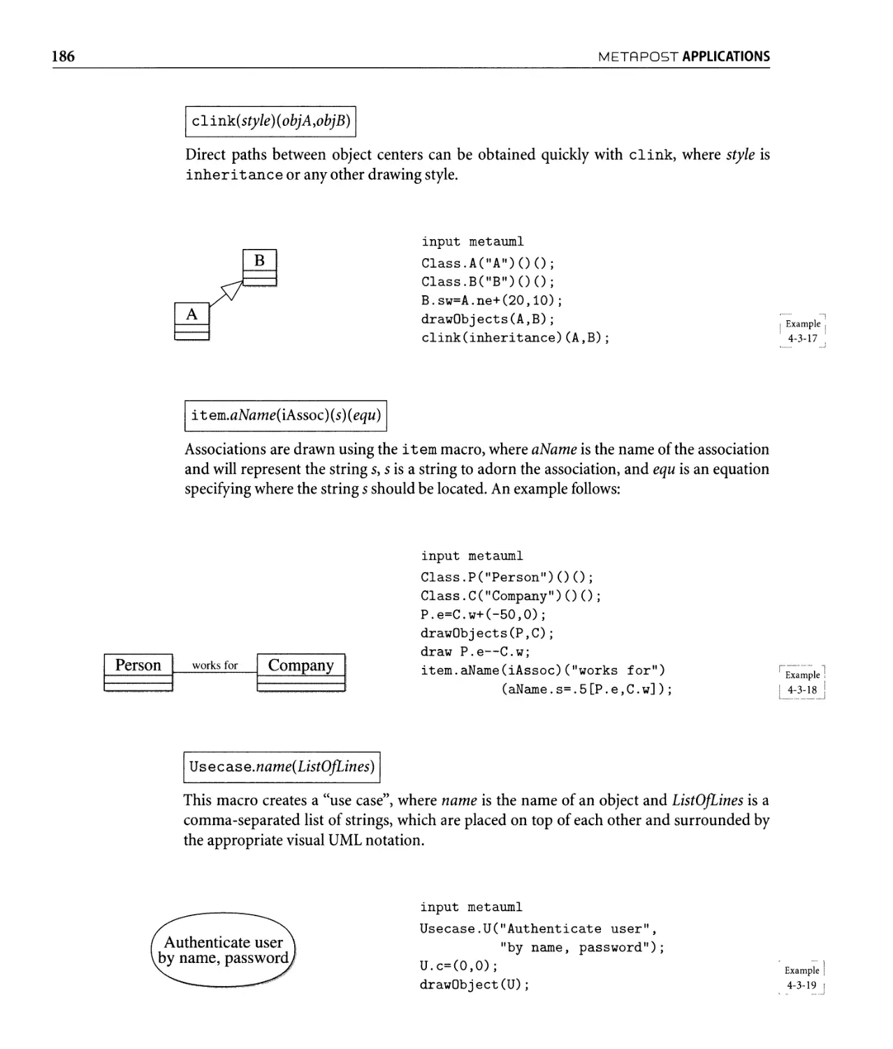
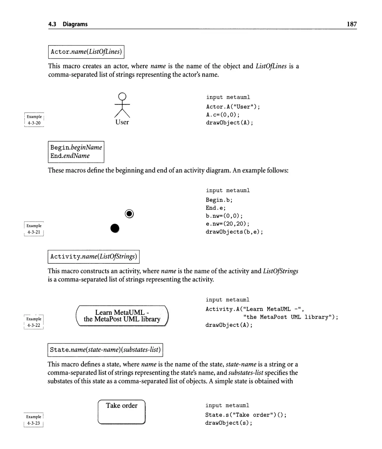
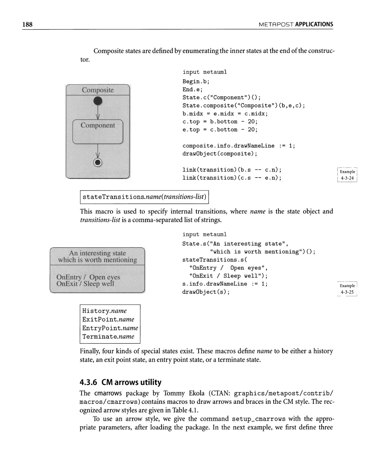
4.3.5 UML diagrams-MetaUML . . . . . . . . . . . . . . . . . . . . . . . . . .
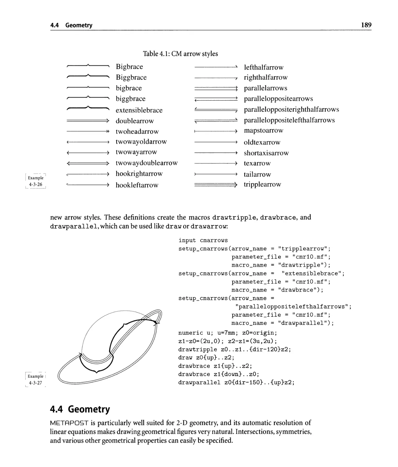
4.3.6 CM arrows utility . . . . . . . . . . . . . . . . . . . . . . . . . . . . . . . .
4.4 Geometry . . . . . . . . . . . . . . . . . . . . . . . . . . . . . . . . . . . . . . . . . .
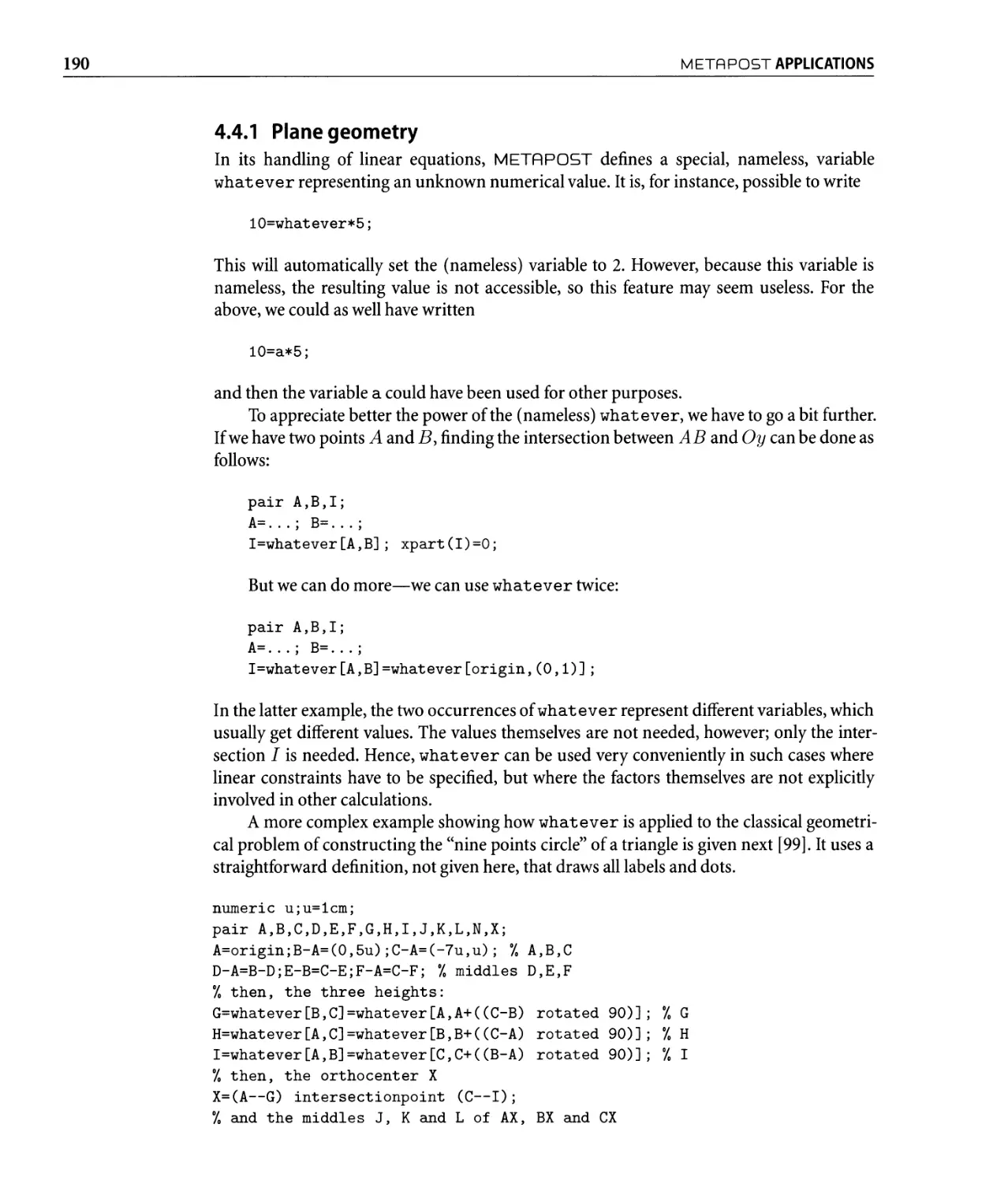
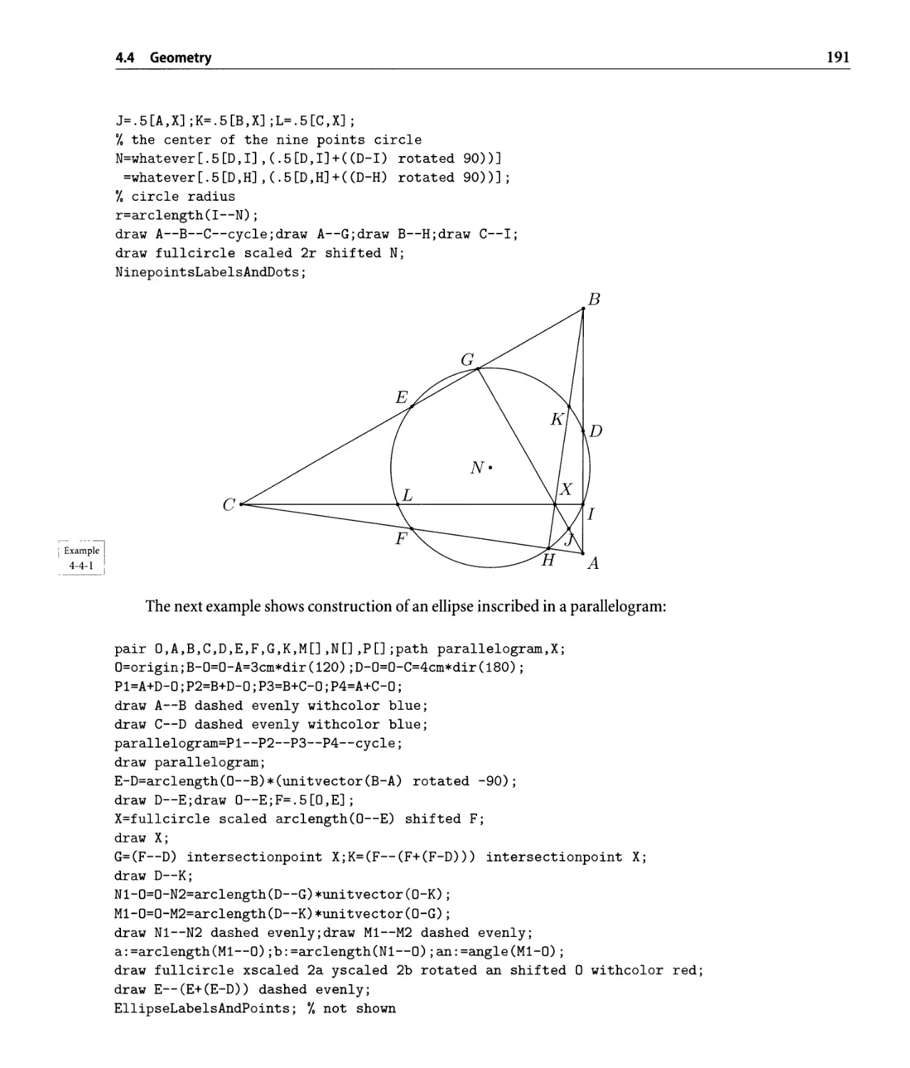
4.4.1 Plane geometry . . . . . . . . . . . . . . . . . . . . . . . . . . . . . . . . .
4.4.2 Space geometry. . . . . . . . . . . . . . . . . . . . . . . . . . . . . . . . .
4.4.3 Fractals and other complex objects. . . . . . . . . . . . . . . . . . . . .
4.4.4 Art.........................................
4.5 Science and engineering applications. . . . . . . . . . . . . . . . . . . . . . . . .
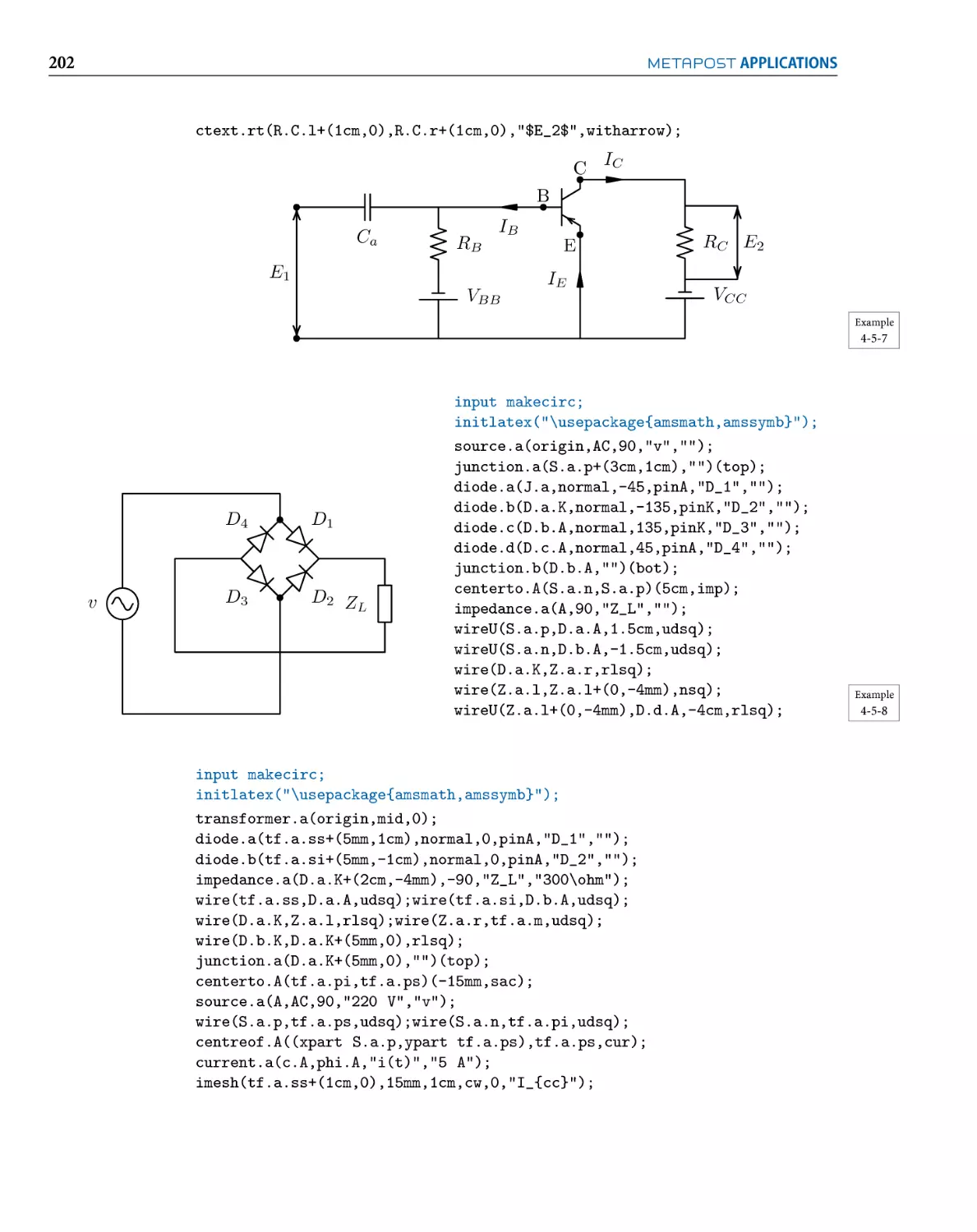
4.5.1 Electrical circuits. . . . . . . . . . . . . . . . . . . . . . . . . . . . . . . . .
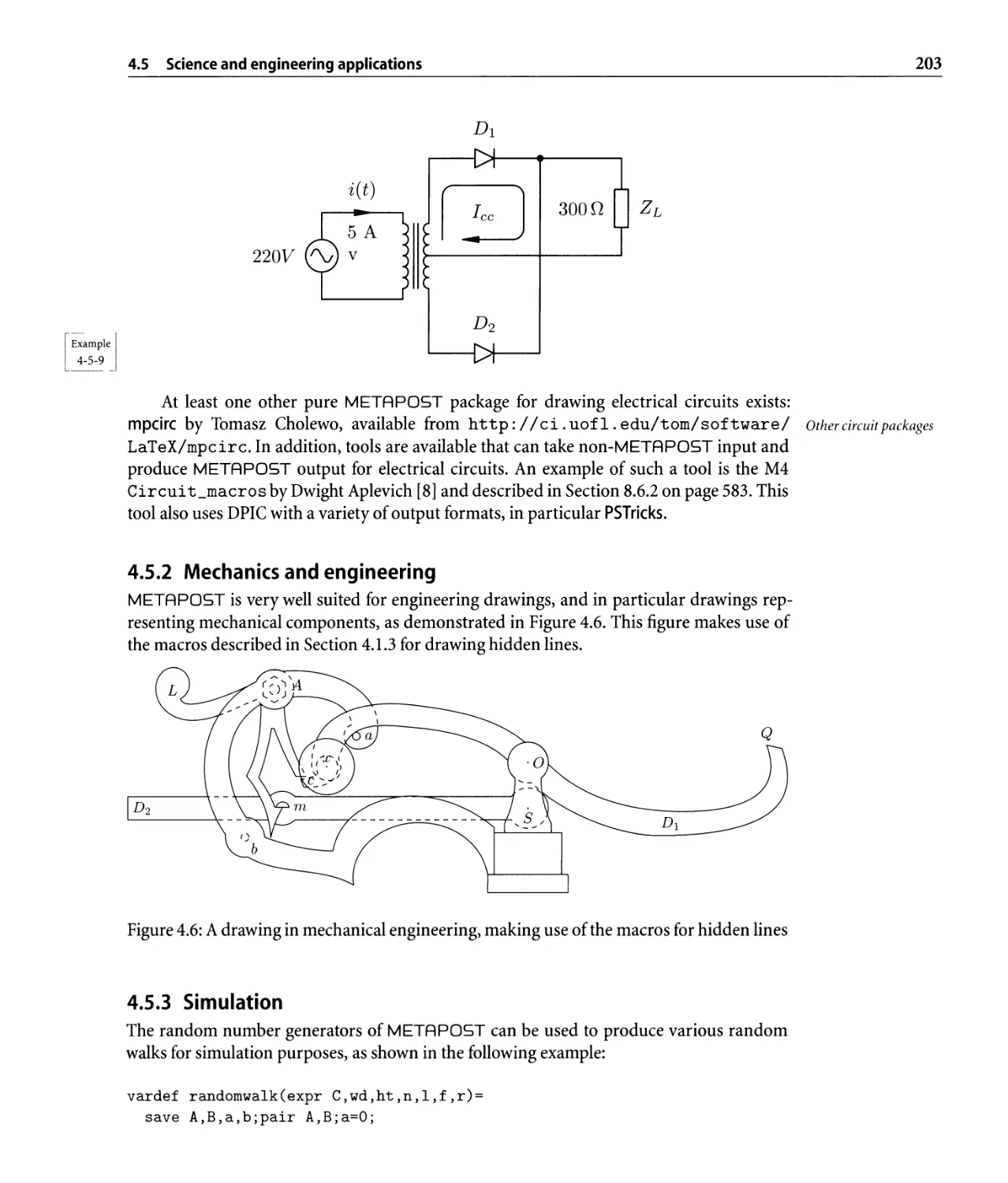
4.5.2 Mechanics and engineering. . . . . . . . . . . . . . . . . . . . . . . . . .
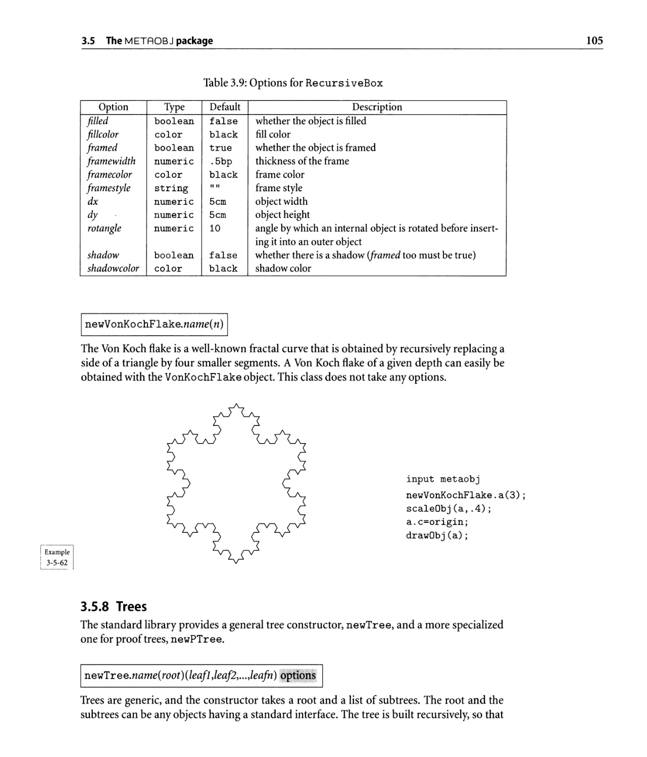
105
115
117
118
120
120
122
137
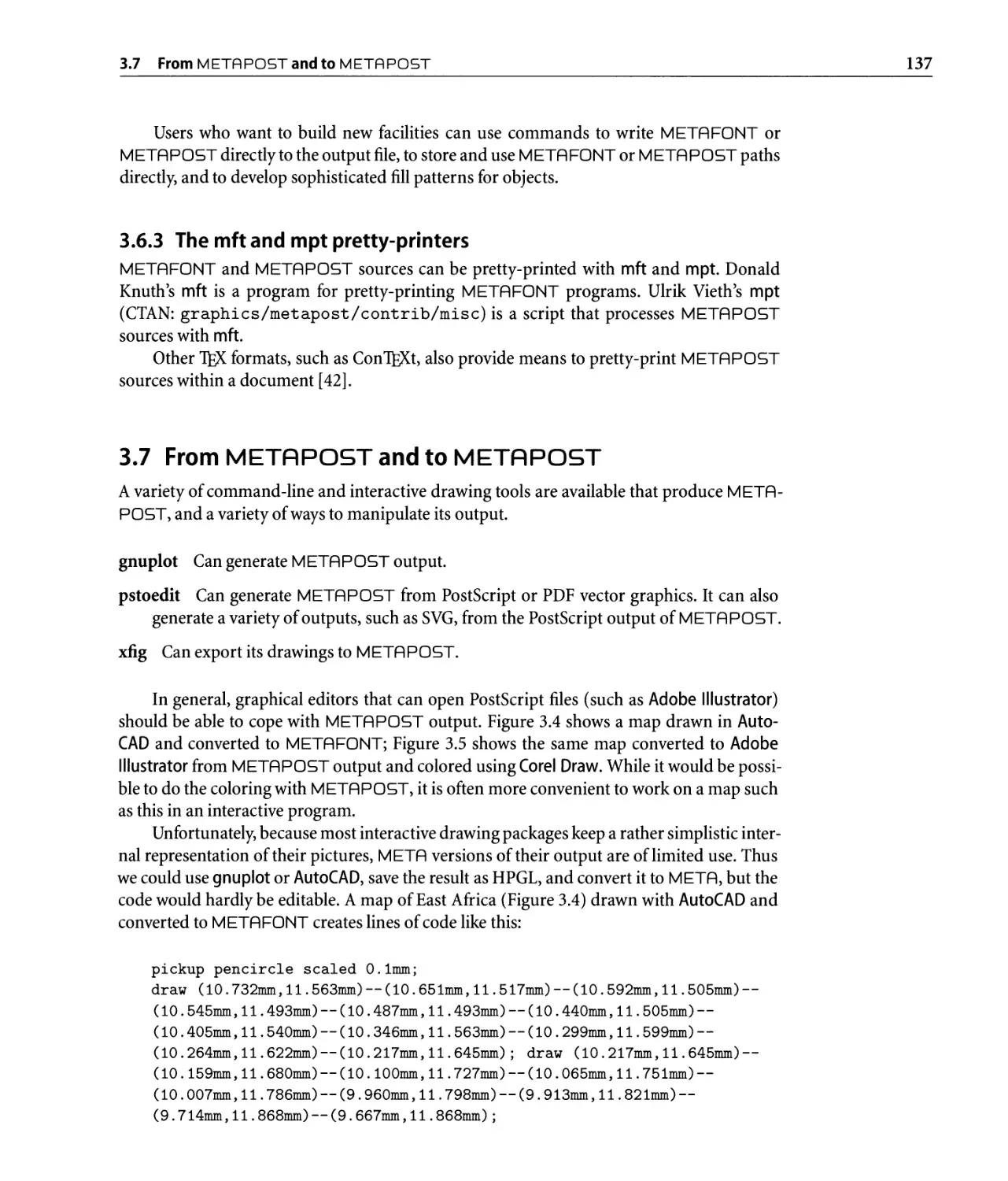
137
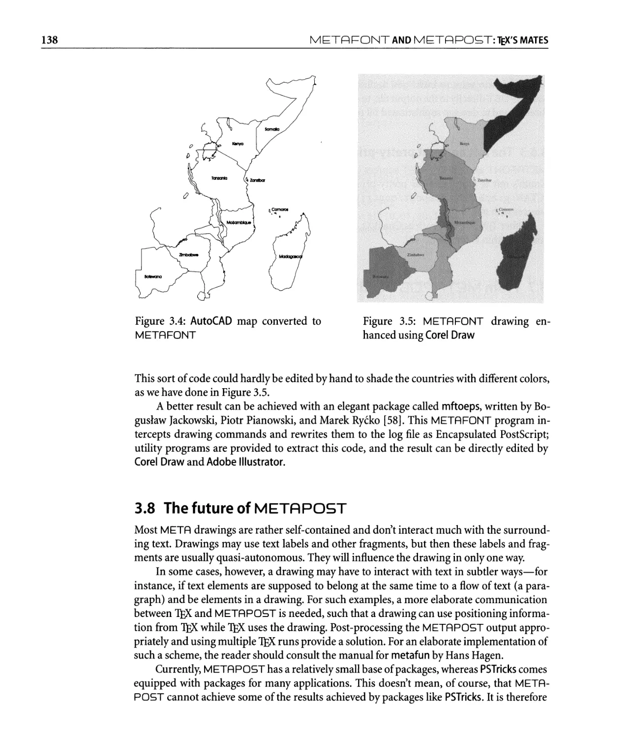
138
141
141
142
143
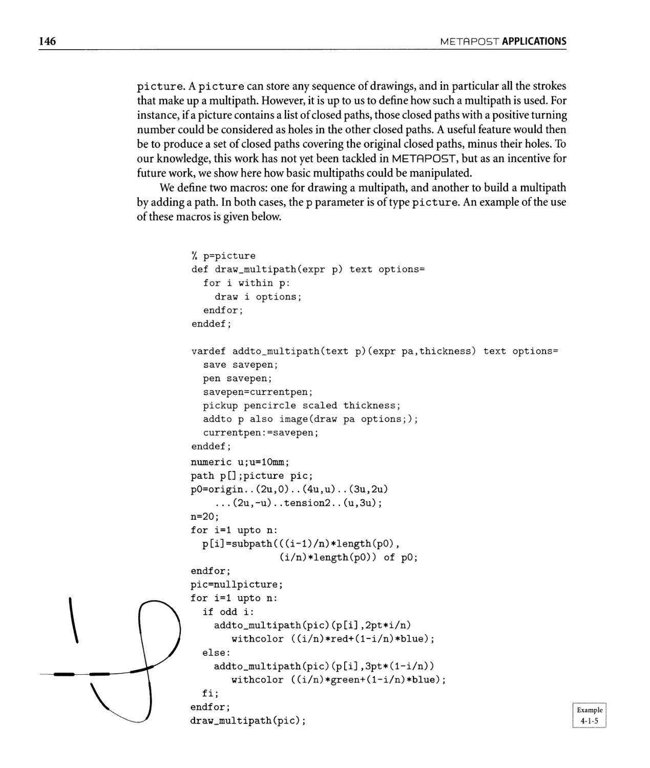
145
145
147
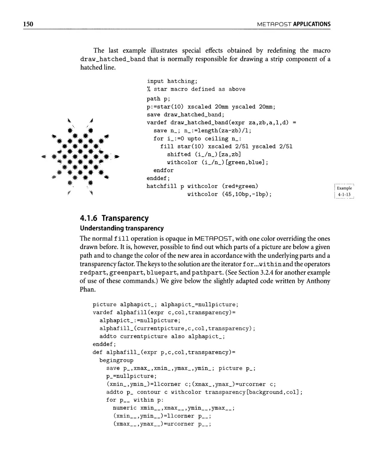
150
152
152
153
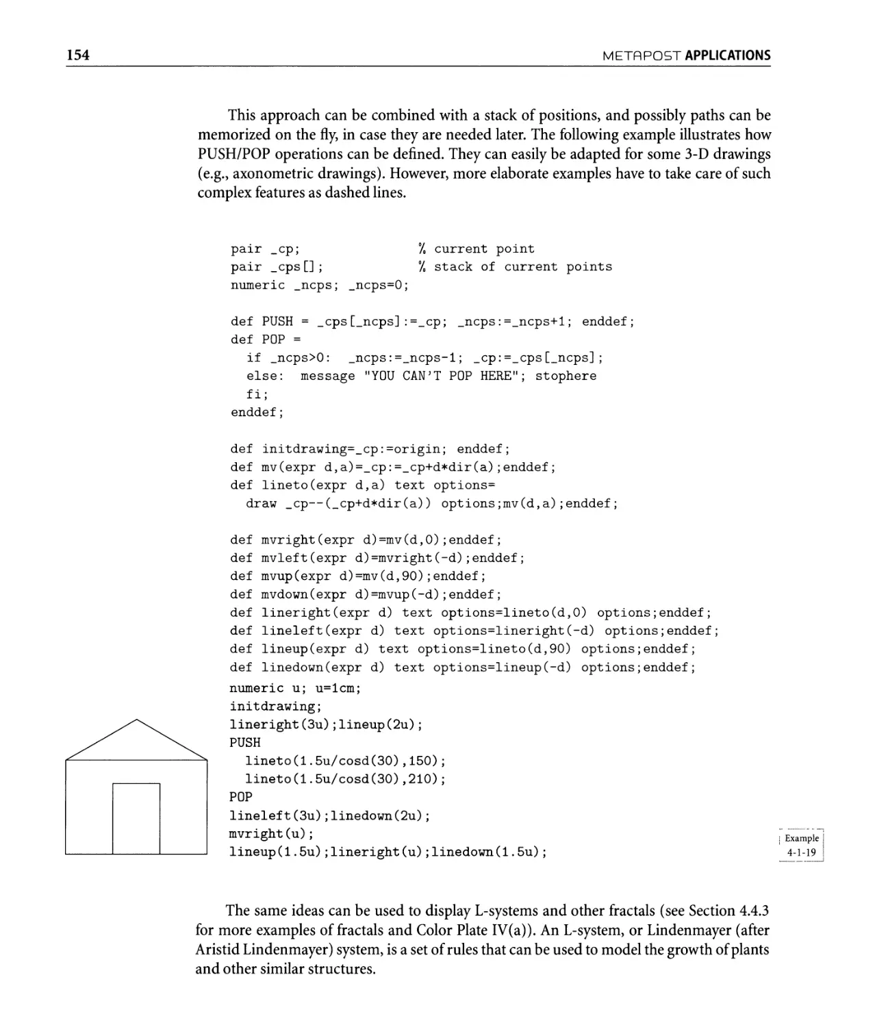
155
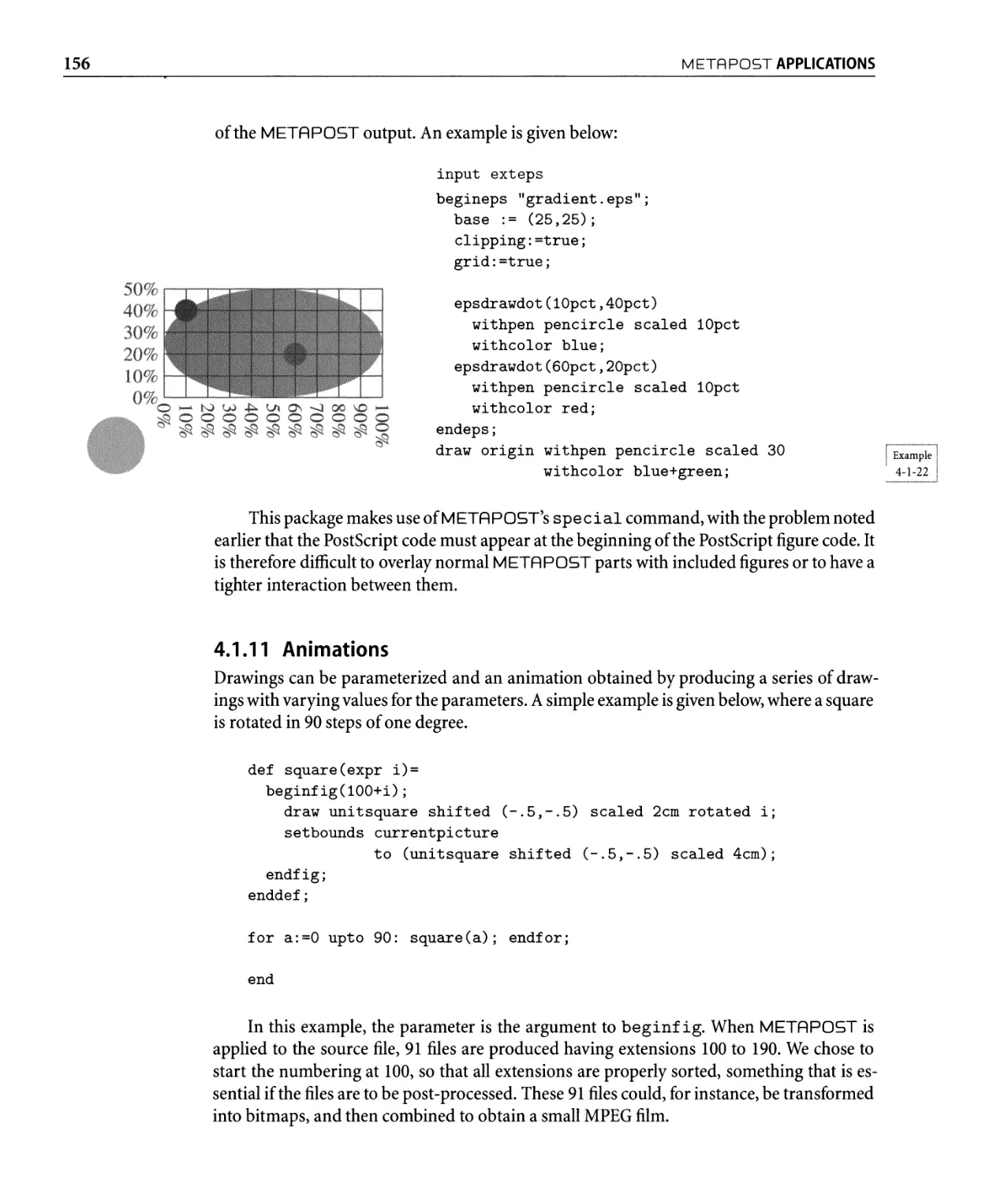
156
157
157
168
170
176
176
177
177
178
181
188
189
190
192
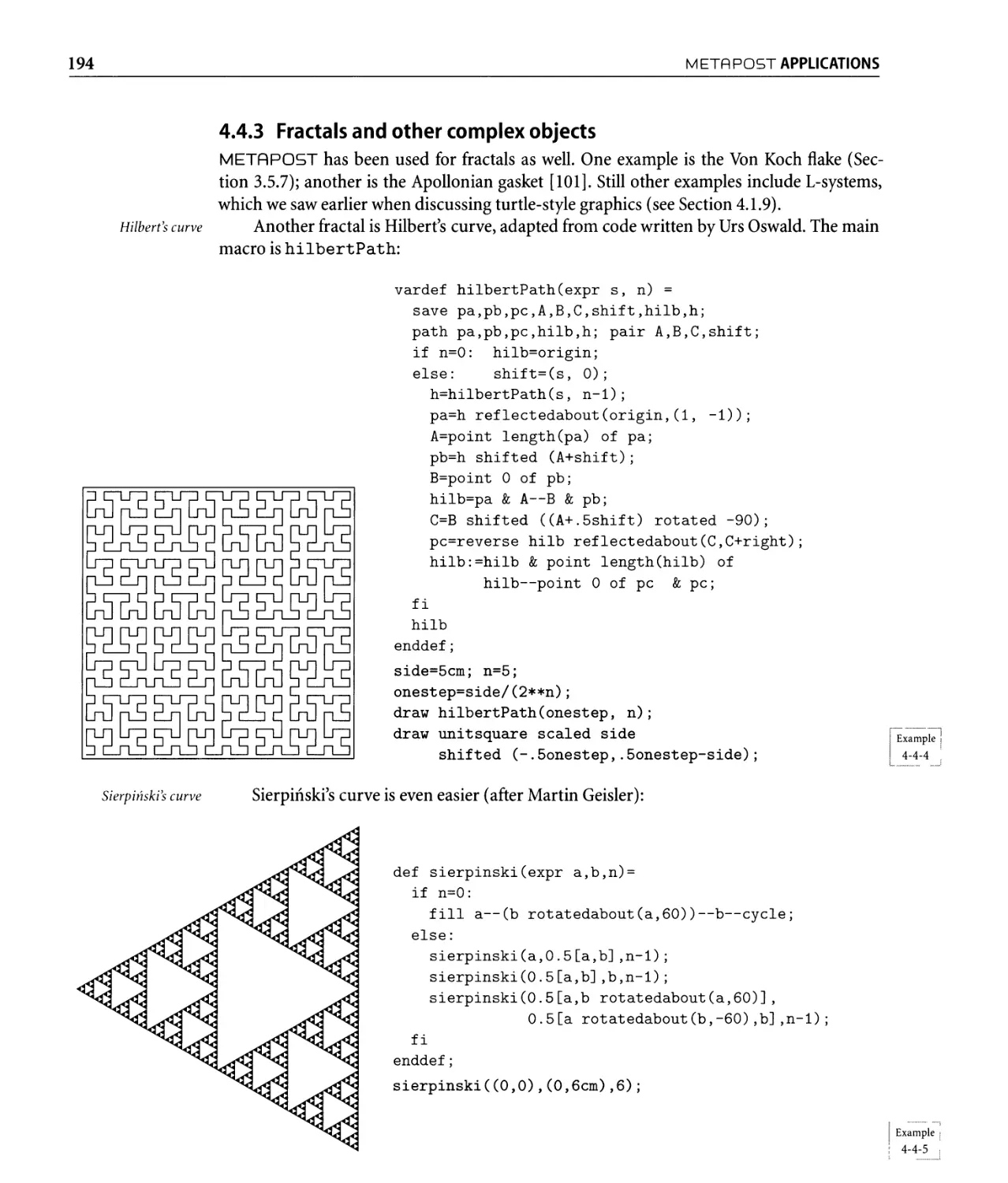
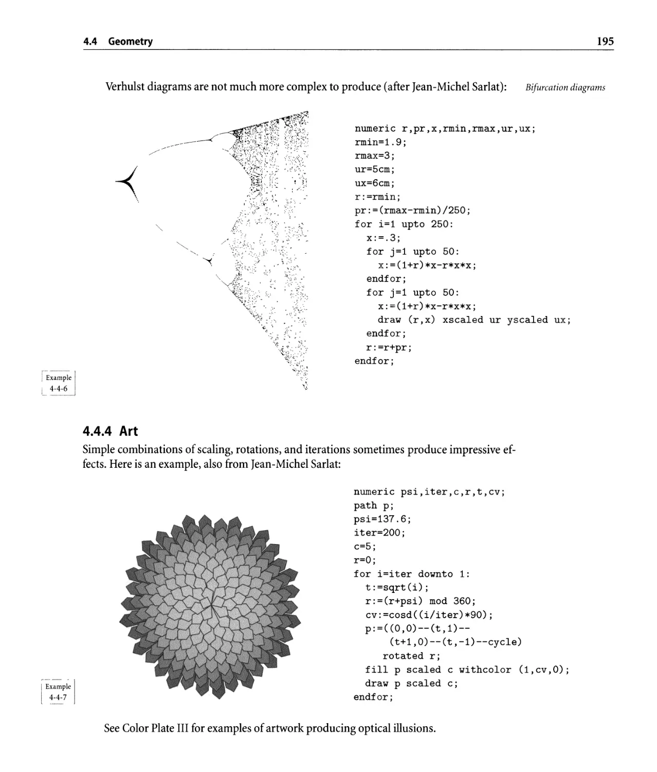
194
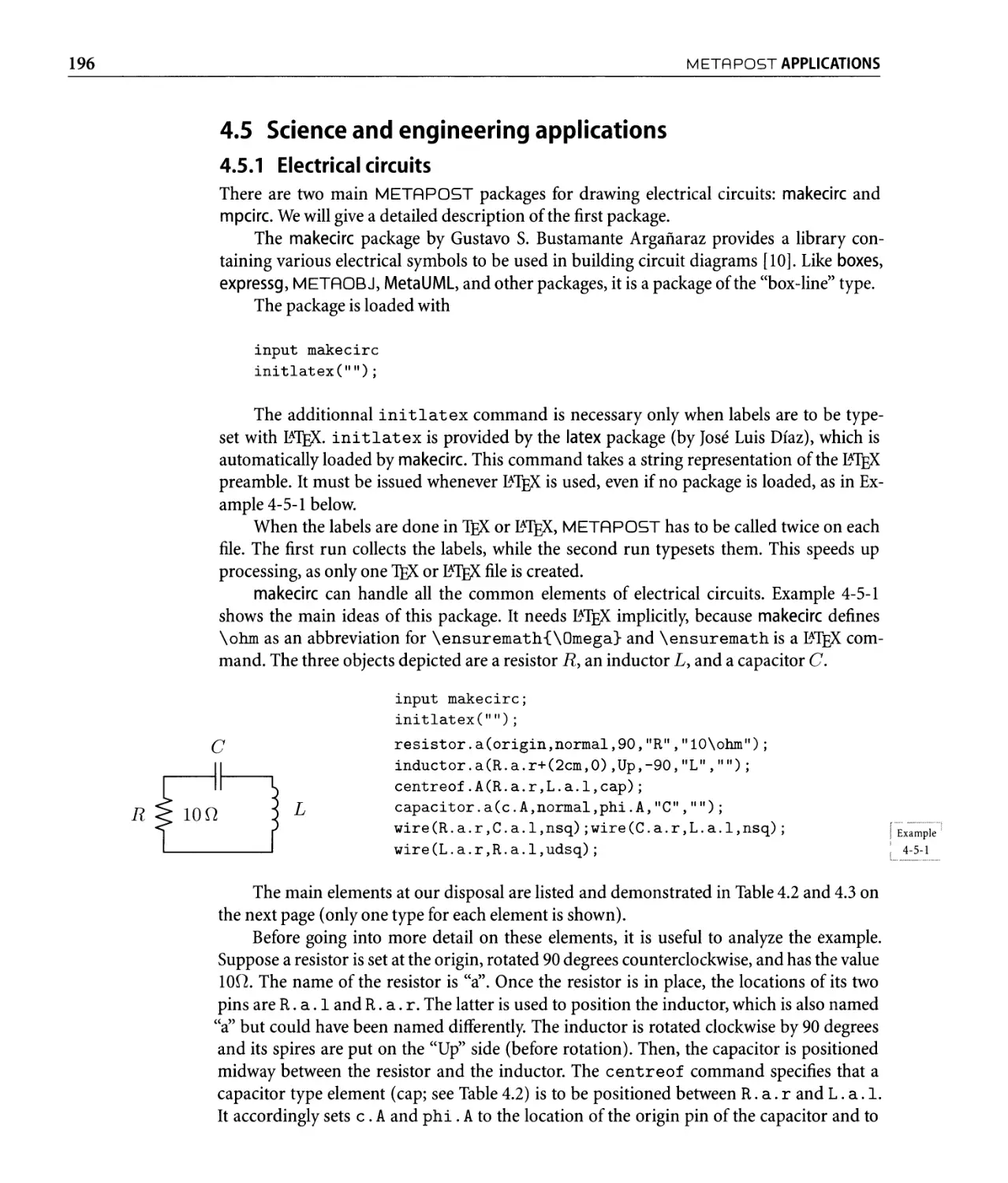
195
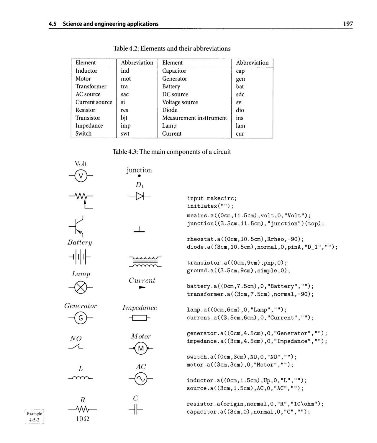
196
196
203
x
CONTENTS
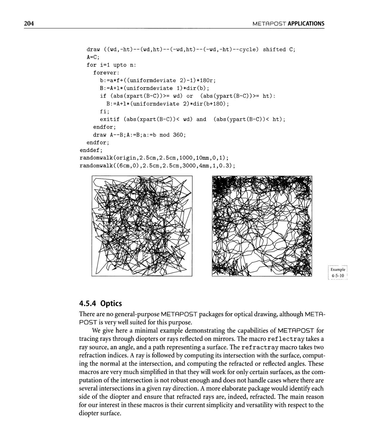
4.5.3 Simulation. . . . . . . . . . . . . . . . . . . . . . . . . . . . . . . . . . .. 203
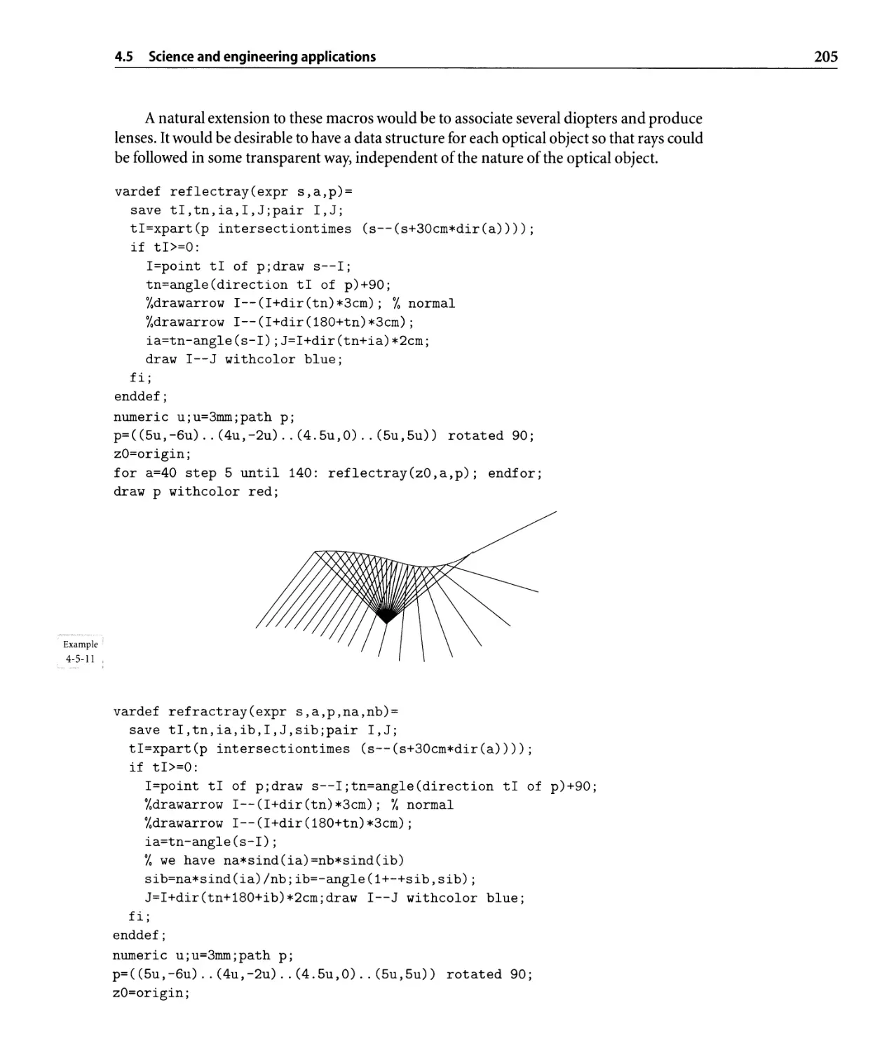
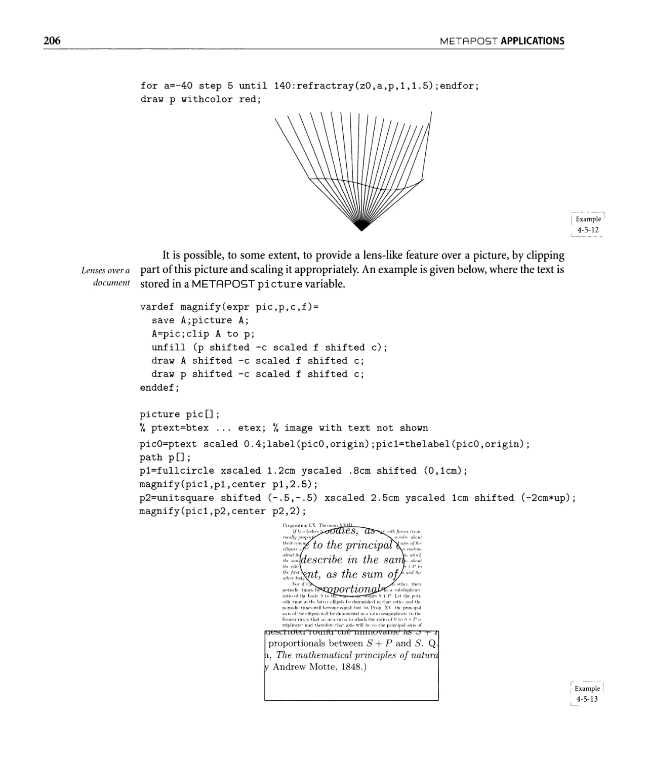
4.5.4 Optics . . . . . . . . . . . . . . . . . . . . . . . . . . . . . . . . . . . . . .. 204
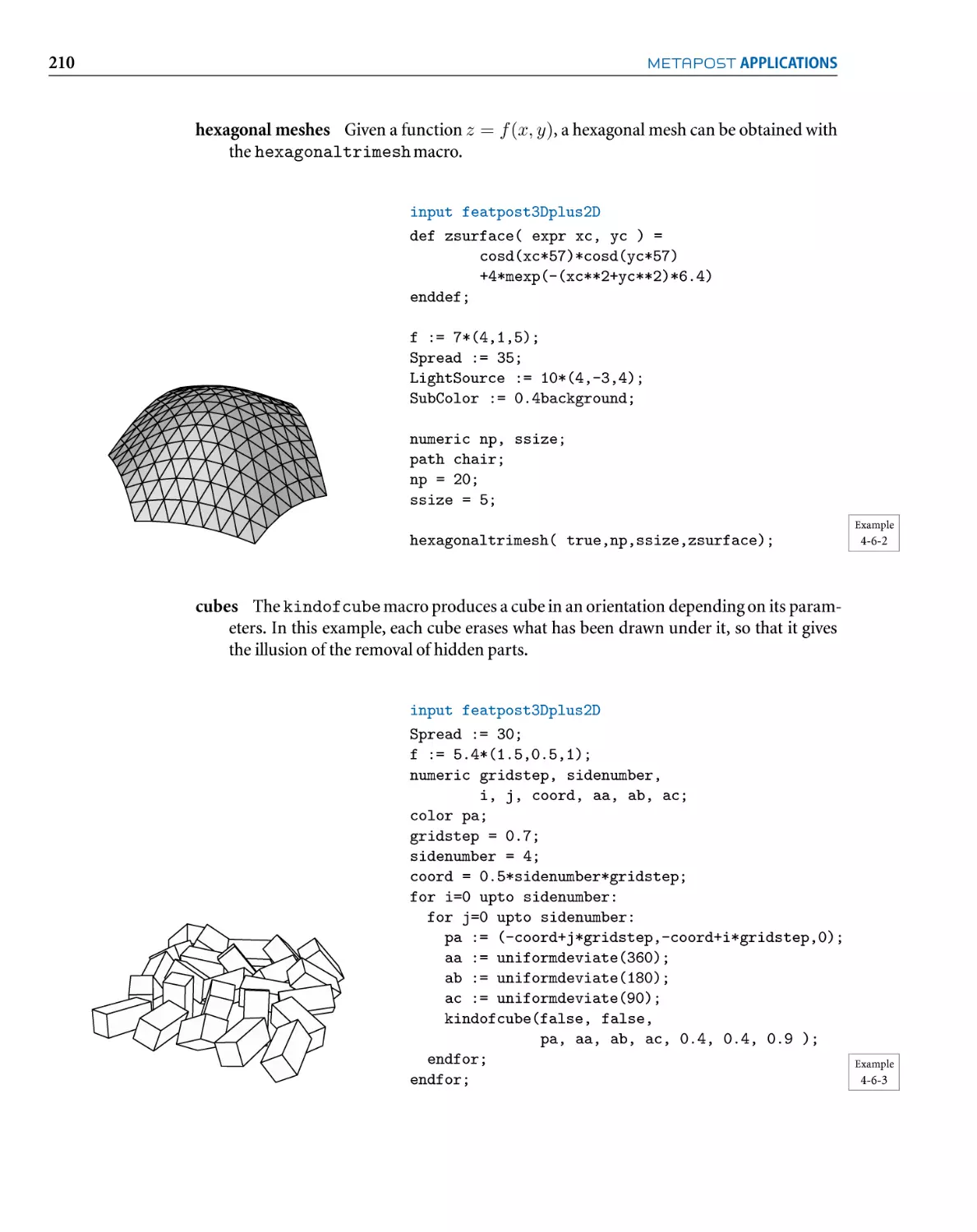
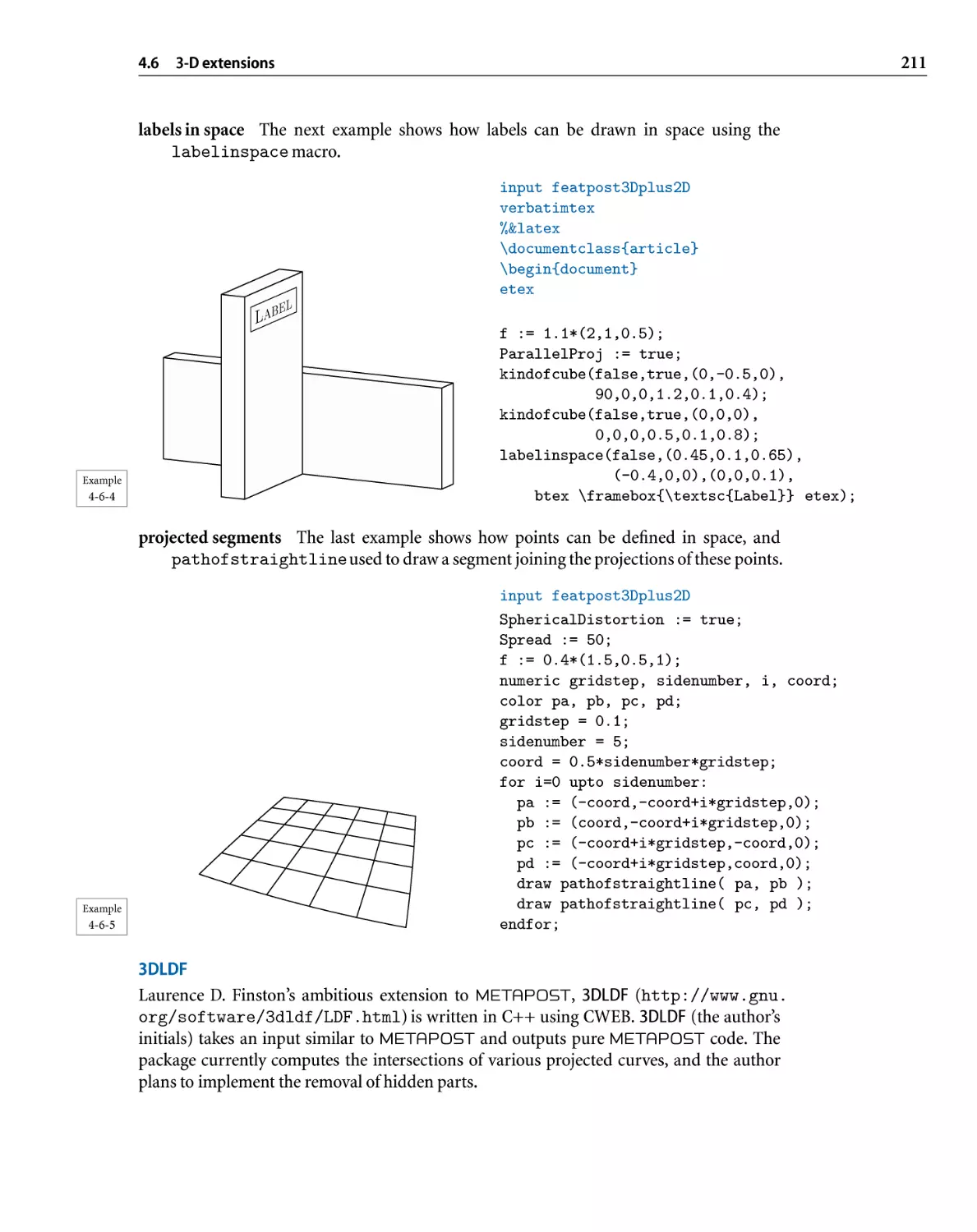
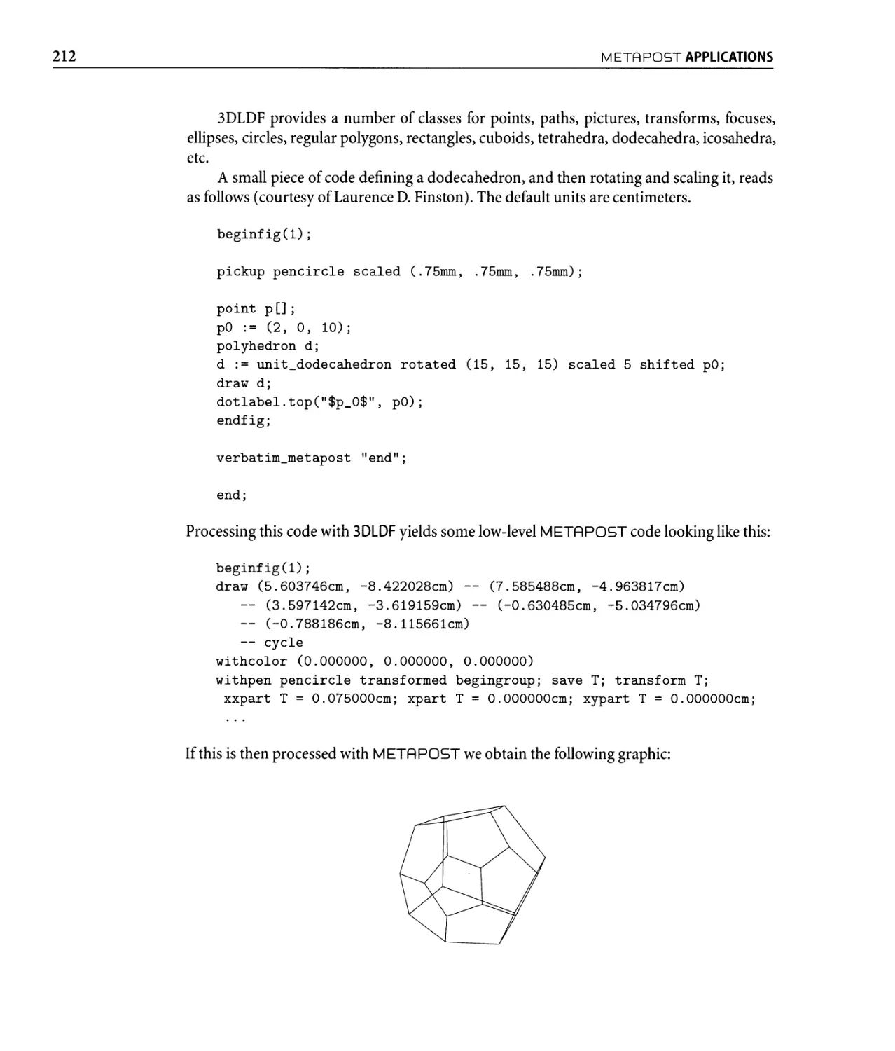
4.6 3-D extensions . . . . . . . . . . . . . . . . . . . . . . . . . . . . . . . . . . . . . .. 207
4.6.1 I ntrod uction . . . . . . . . . . . . . . . . . . . . . . . . . . . . . . . . . .. 207
4.6.2 Requirements for a 3-D extension. . . . . . . . . . . . . . . . . . . . .. 207
4.6.3 Overview of 3-D packages. . . . . . . . . . . . . . . . . . . . . . . . . .. 208
5 Harnessing PostScript Inside EX: PSTricks 213
5.1 The components of PSTricks . . . . . . . . . . . . . . . . . . . . . . . . . . . . . .. 214
5.1.1 The kernel .................................... 214
5.1.2 Loading the basic packages. . . . . . . . . . . . . . . . . . . . . . . . .. 215
5.1.3 Using colors . . . . . . . . . . . . . . . . . . . . . . . . . . . . . . . . . .. 216
5.2 Setting keywords, lengths, and coordinates . . . . . . . . . . . . . . . . . . . .. 217
5.2.1 Lengths and units. . . . . . . . . . . . . . . . . . . . . . . . . . . . . . .. 217
5.2.2 Angles............... . . . . . . . . . . . . . . . . . . . . . . .. 218
5.2.3 Coordinates...... . . . . . . . . . . . . . . . . . . . . . . . . . . . .. 219
5.2.4 Commands............................ . . . . . . .. 219
5.3 The pspi cture environment. . . . . . . . . . . . . . . . . . . . . . . . . . . . .. 220
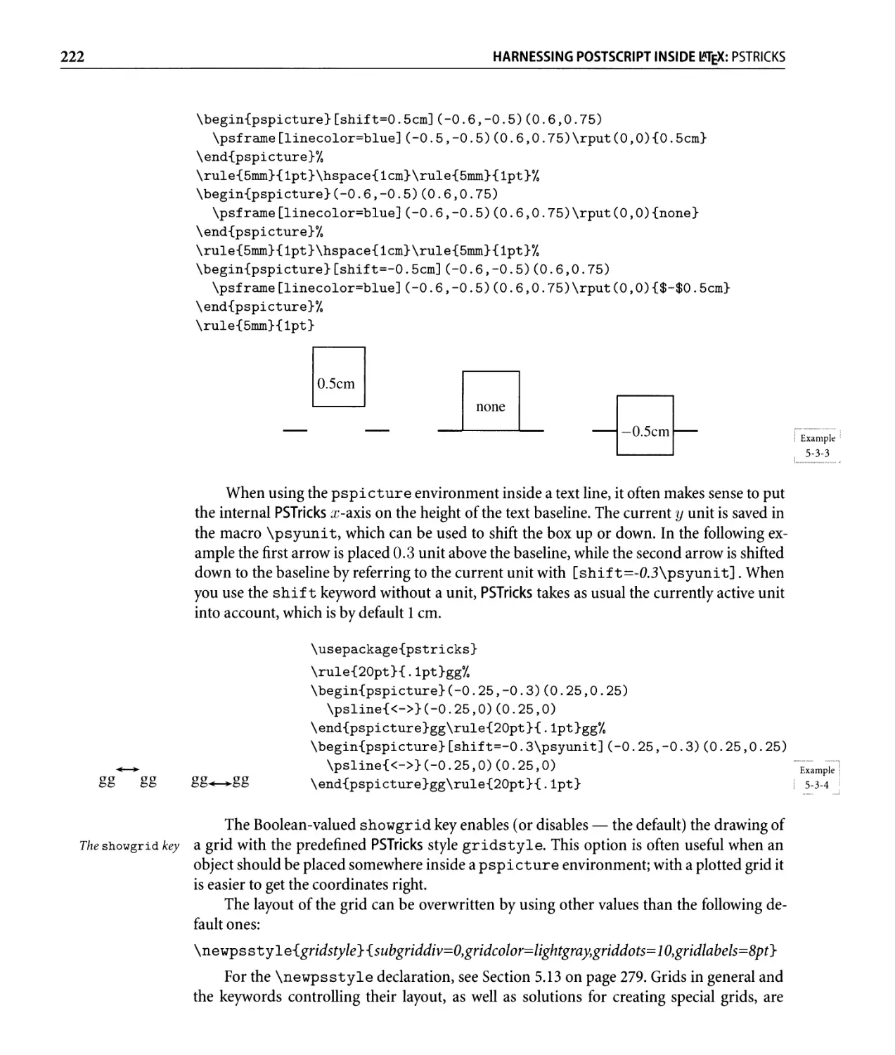
5.3.1 Keywords for the pspicture environment. . . . . . . . . . . . . . .. 221
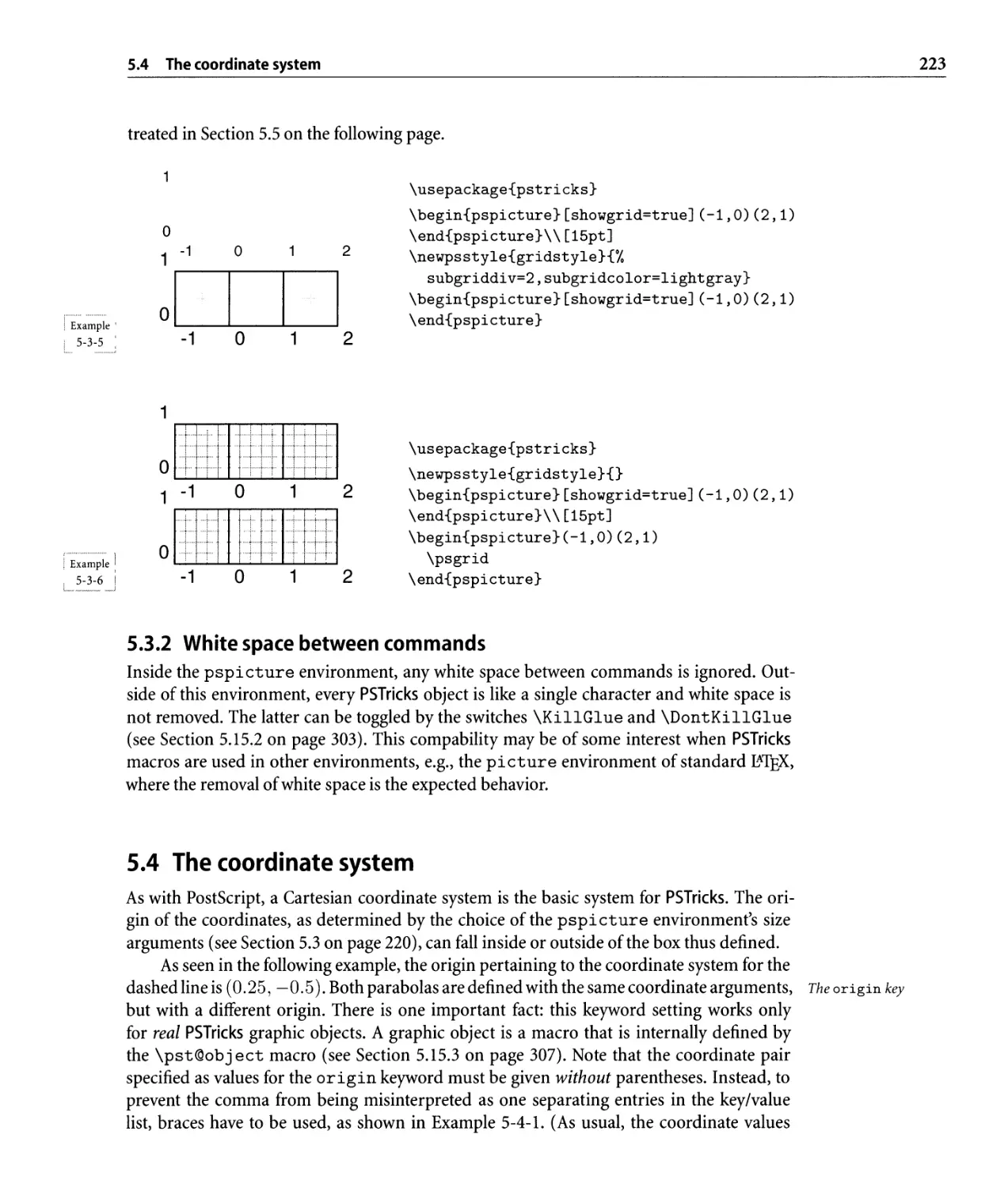
5.3.2 White space between commands. . . . . . . . . . . . . . . . . . . . .. 223
5.4 The coordinate system . . . . . . . . . . . . . . . . . . . . . . . . . . . . . . . . .. 223
5.5 Grids . . . . . . . . . . . . . . . . . . . . . . . . . . . . . . . . . . . . . . . . . . . .. 224
5.5.1 Keywords of the \psgrid command. . . . . . . . . . . . . . . . . . .. 226
5.5.2 Defining and using new grid commands. . . . . . . . . . . . . . . . .. 228
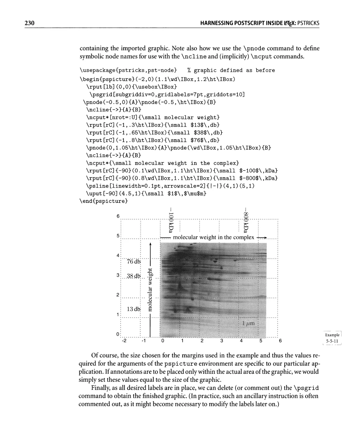
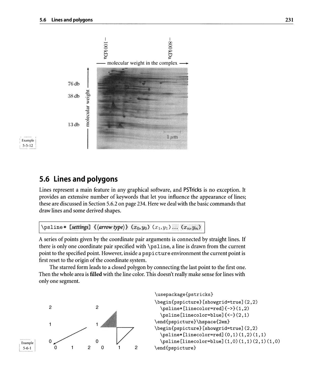
5.5.3 Embellishing pictures with the help of grids. . . . . . . . . . . . . . .. 229
5.6 Lines and polygons . . . . . . . . . . . . . . . . . . . . . . . . . . . . . . . . . . .. 231
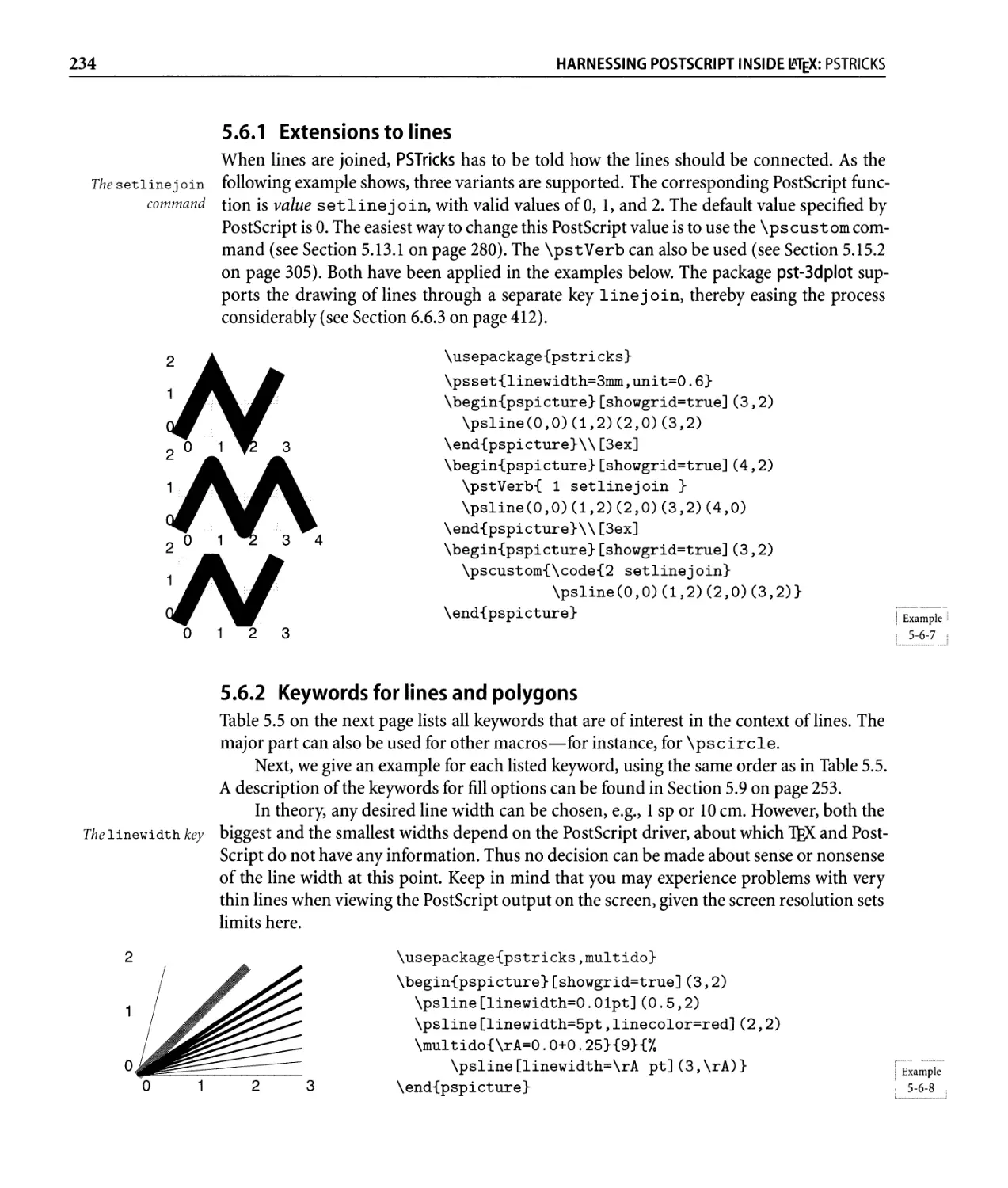
5.6.1 Extensions to lines . . . . . . . . . . . . . . . . . . . . . . . . . . . . . .. 234
5.6.2 Keywords for lines and polygons. . . . . . . . . . . . . . . . . . . . . .. 234
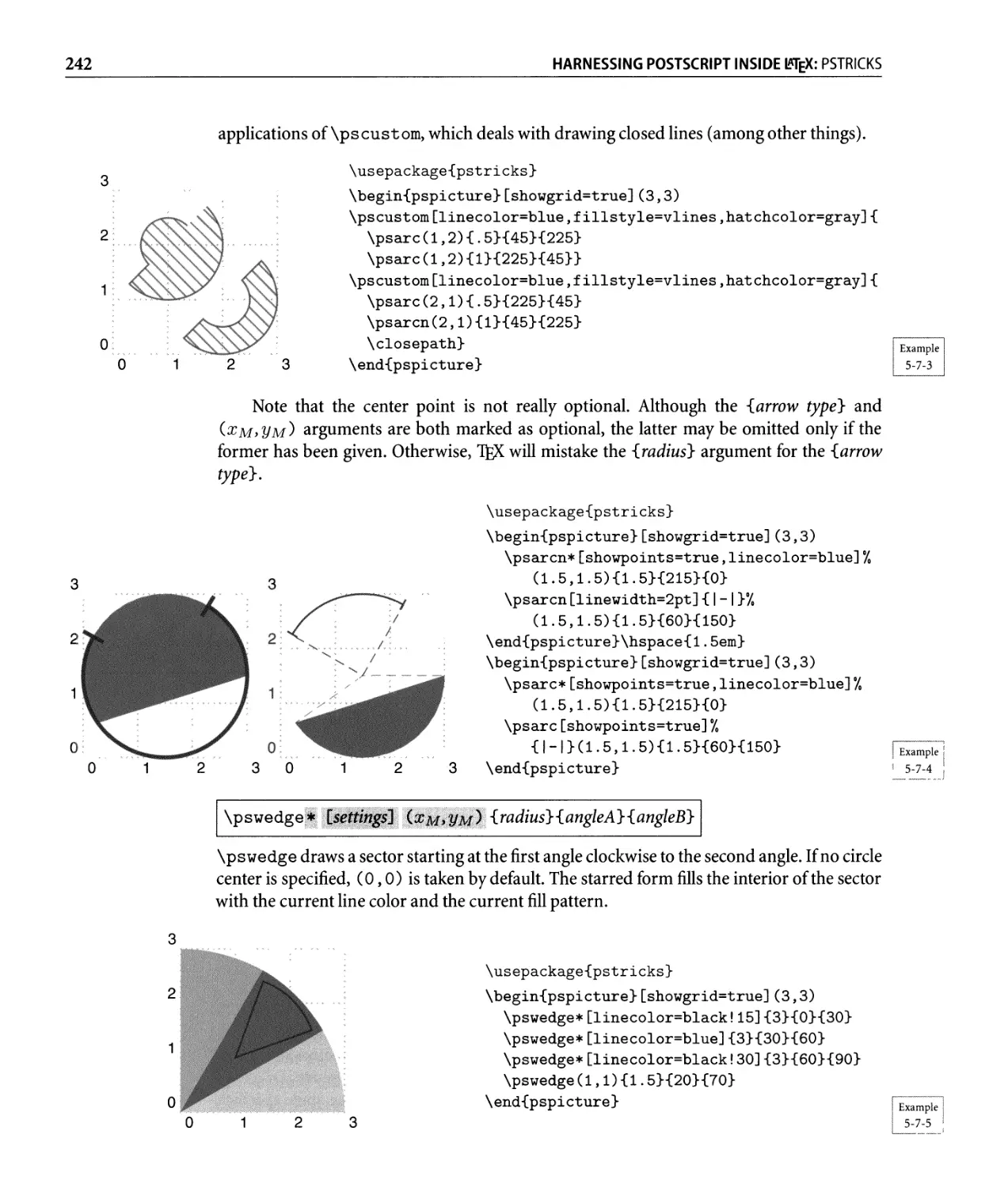
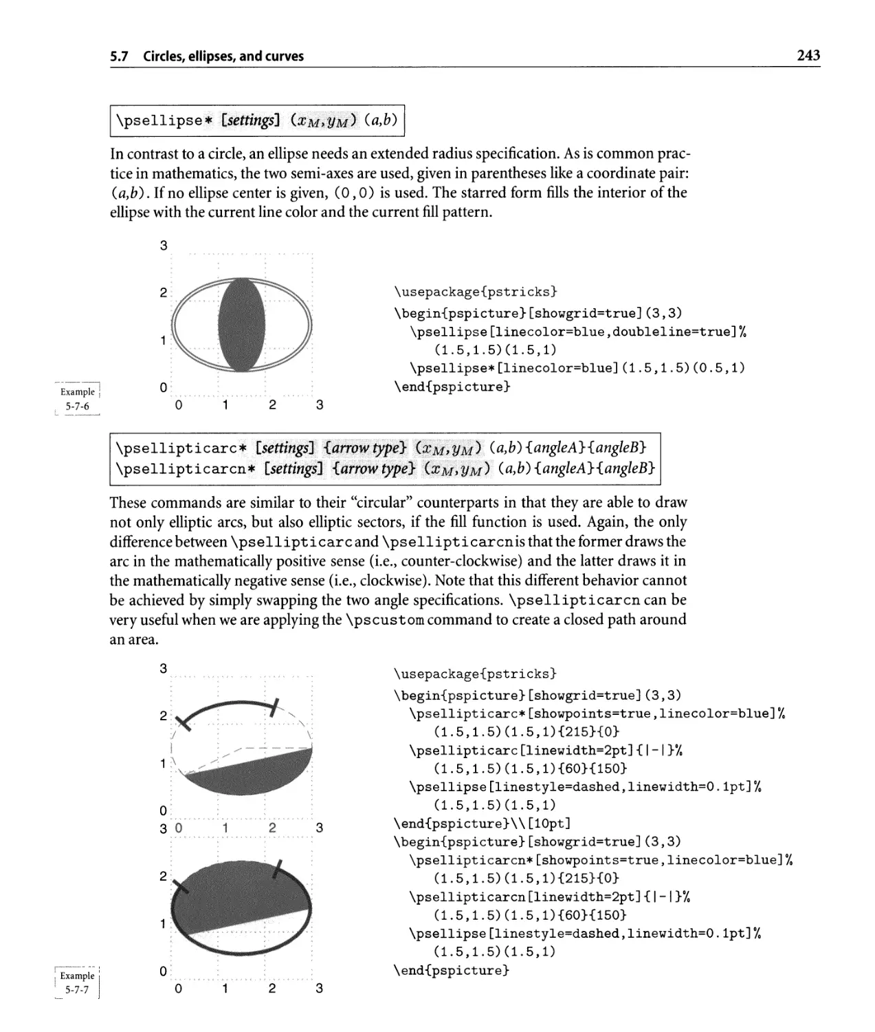
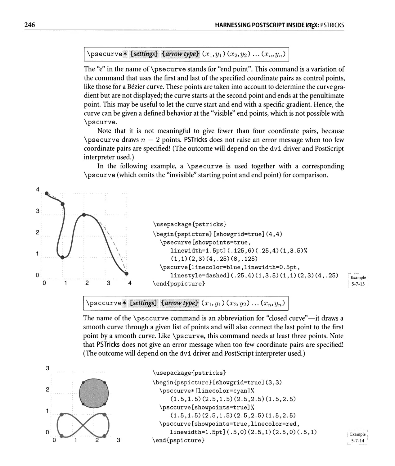
5.7 Circles, ellipses, and curves. . . . . . . . . . . . . . . . . . . . . . . . . . . . . . .. 240
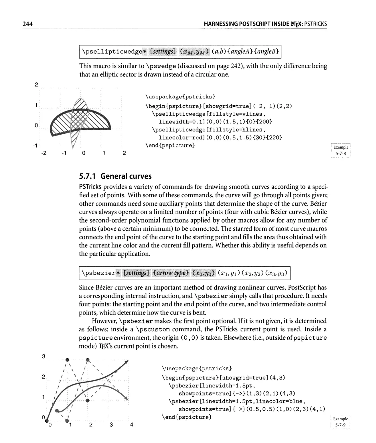
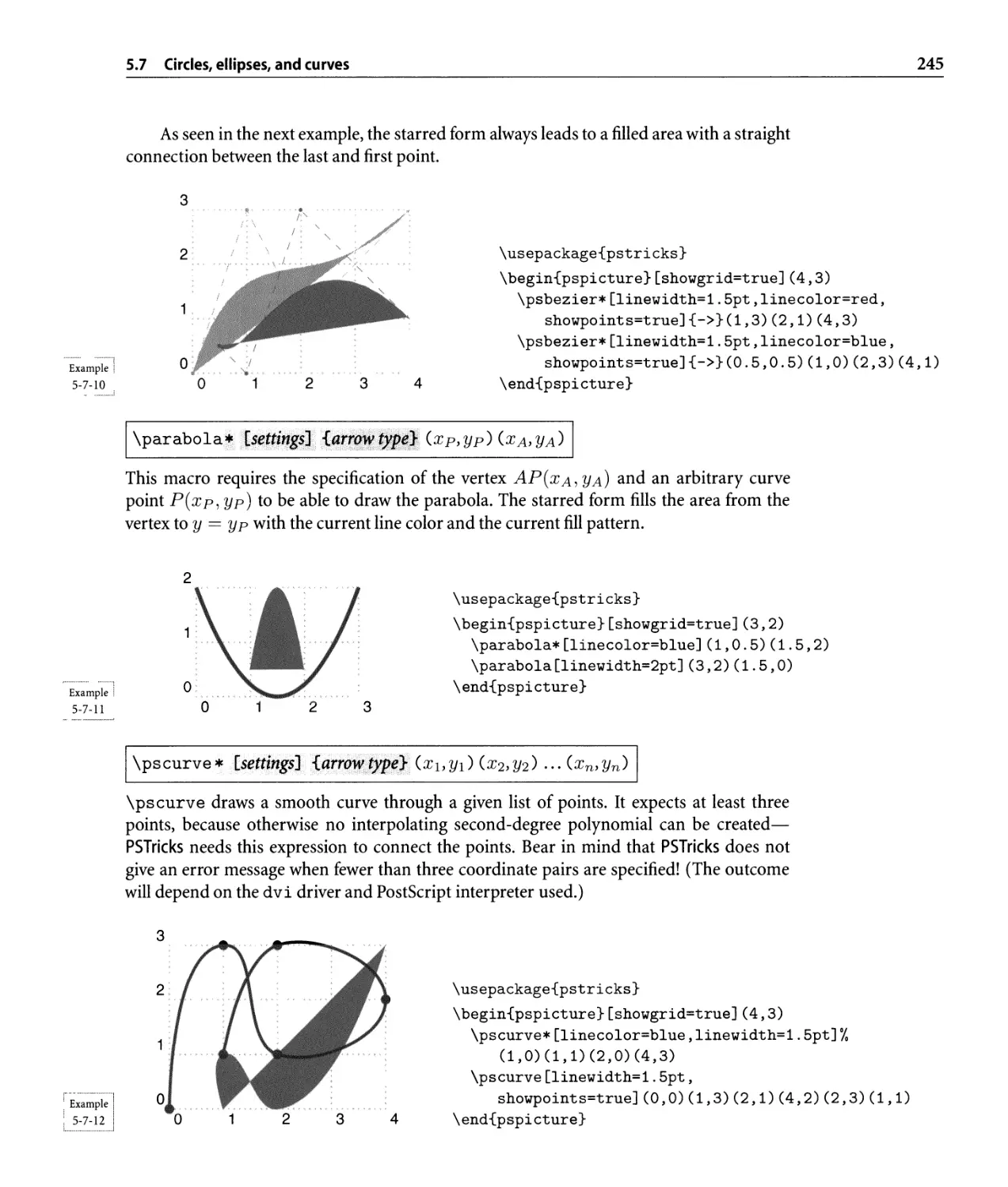
5.7.1 General curves. . . . . . . . . . . . . . . . . . . . . . . . . . . . . . . . .. 244
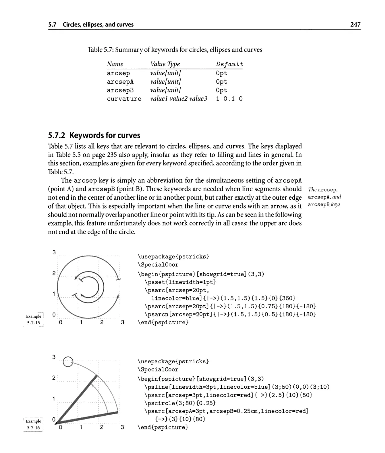
5.7.2 Keywords for cu rves . . . . . . . . . . . . . . . . . . . . . . . . . . . . .. 247
5.8 Dots and symbols . . . . . . . . . . . . . . . . . . . . . . . . . . . . . . . . . . . .. 249
5.8.1 Dot keywords . . . . . . . . . . . . . . . . . . . . . . . . . . . . . . . . .. 251
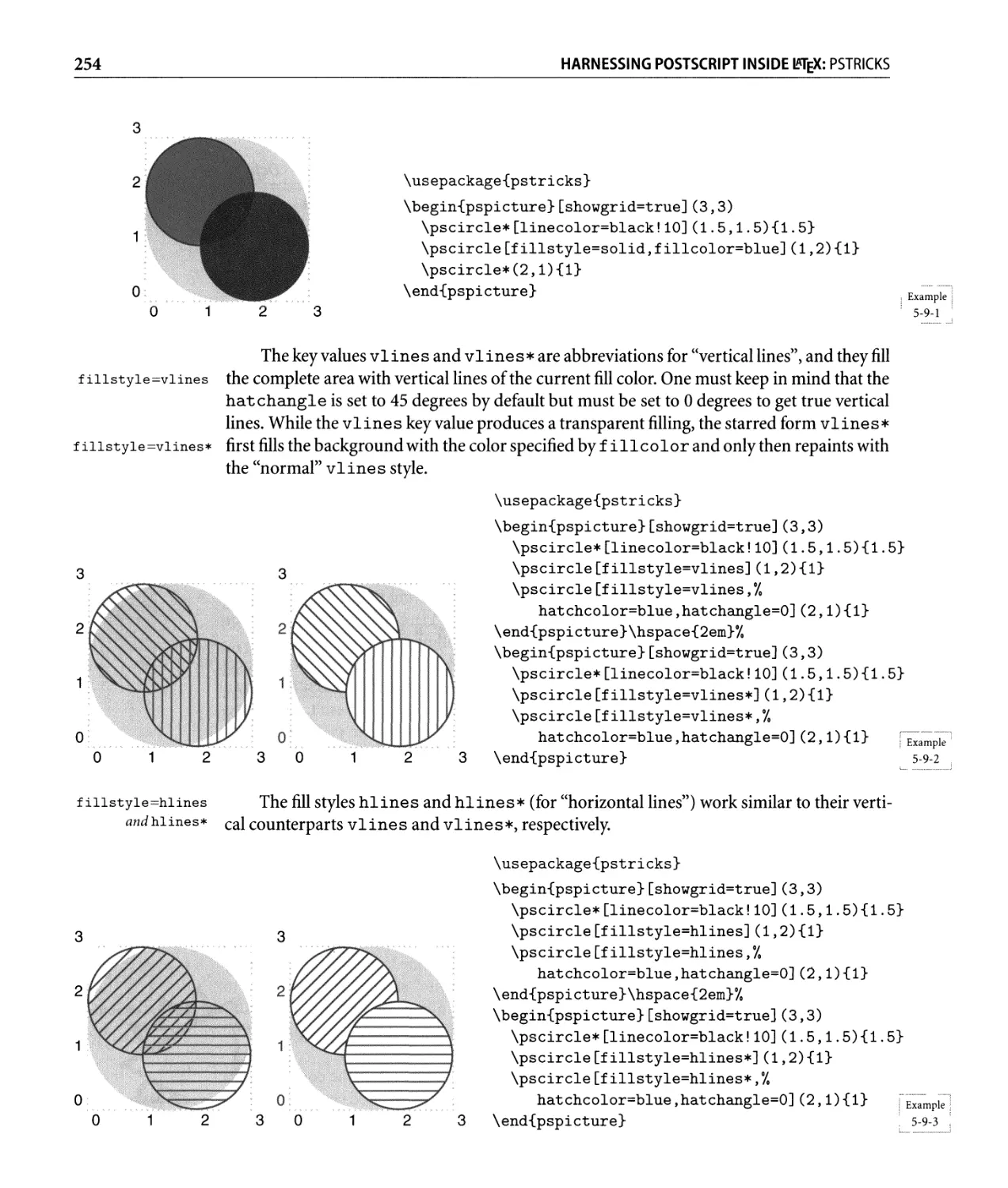
5.9 Filling areas . . . . . . . . . . . . . . . . . . . . . . . . . . . . . . . . . . . . . . . .. 253
5.9.1 Filling keywords. . . . . . . . . . . . . . . . . . . . . . . . . . . . . . . .. 253
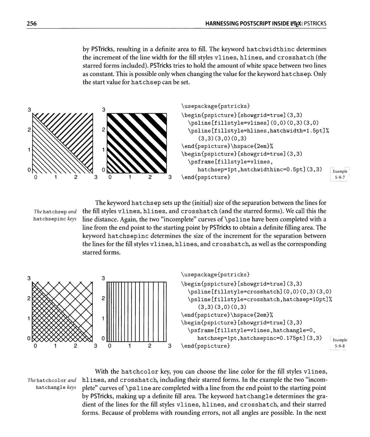
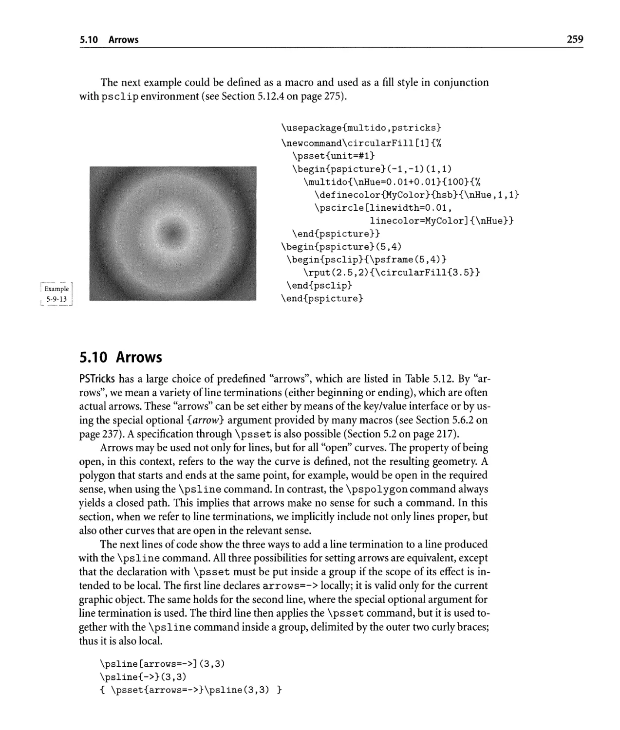
5.9.2 More fill styles. . . . . . . . . . . . . . . . . . . . . . . . . . . . . . . . .. 257
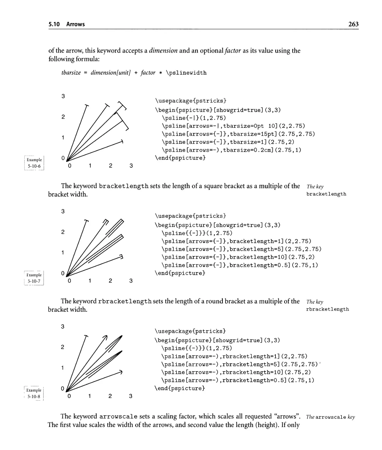
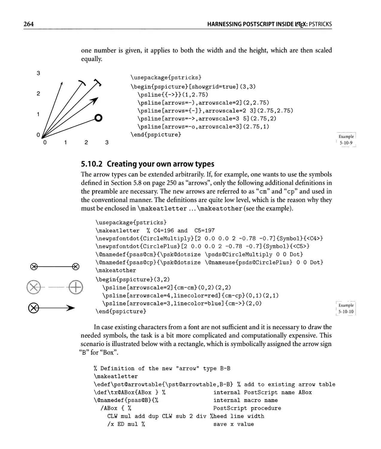
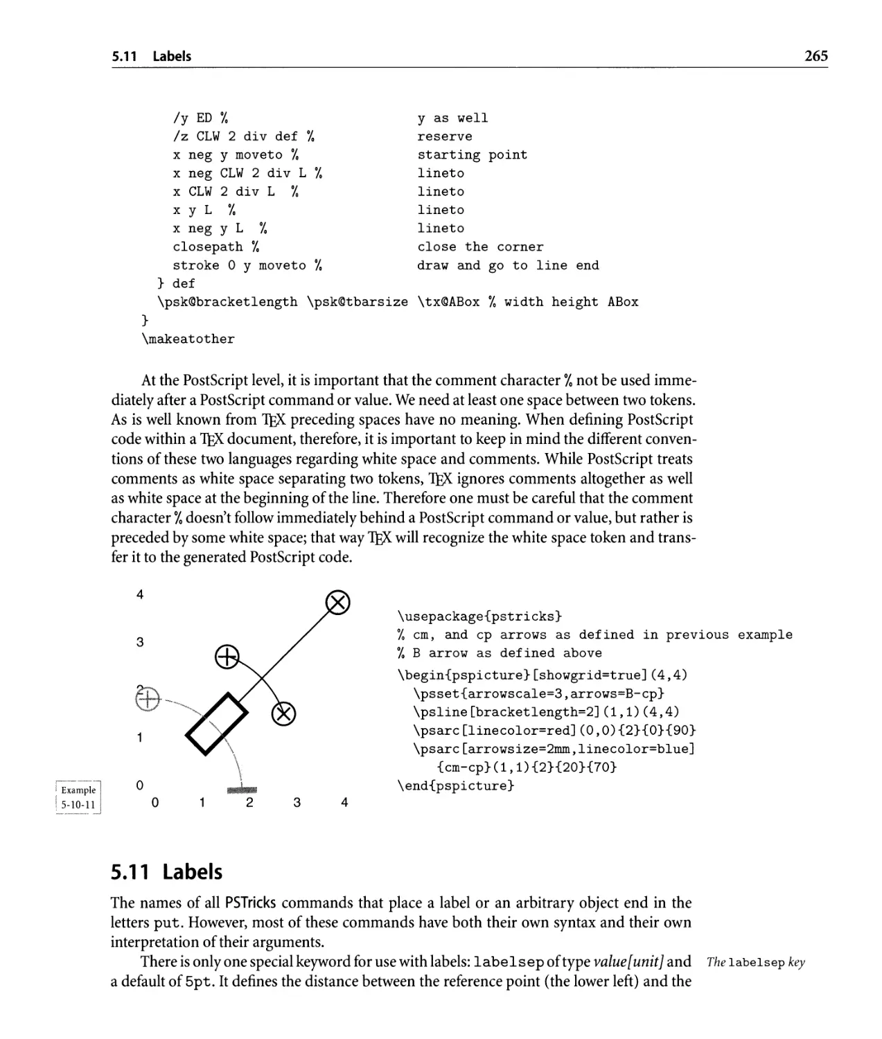
5.10 Arrows . . . . . . . . . . . . . . . . . . . . . . . . . . . . . . . . . . . . . . . . . . .. 259
5.10.1 Keywords for arrows . . . . . . . . . . . . . . . . . . . . . . . . . . . . .. 260
5.10.2 Creating your own arrow types. . . . . . . . . . . . . . . . . . . . . . .. 264
5 .11 Labels. . . . . . . . . . . . . . . . . . . . . . . . . . . . . . . . . . . . . . . . . . . .. 265
5.11.1 Reference points . . . . . . . . . . . . . . . . . . . . . . . . . . . . . . .. 266
5.11.2 Rotation angle. . . . . . . . . . . . . . . . . . . . . . . . . . . . . . . . .. 266
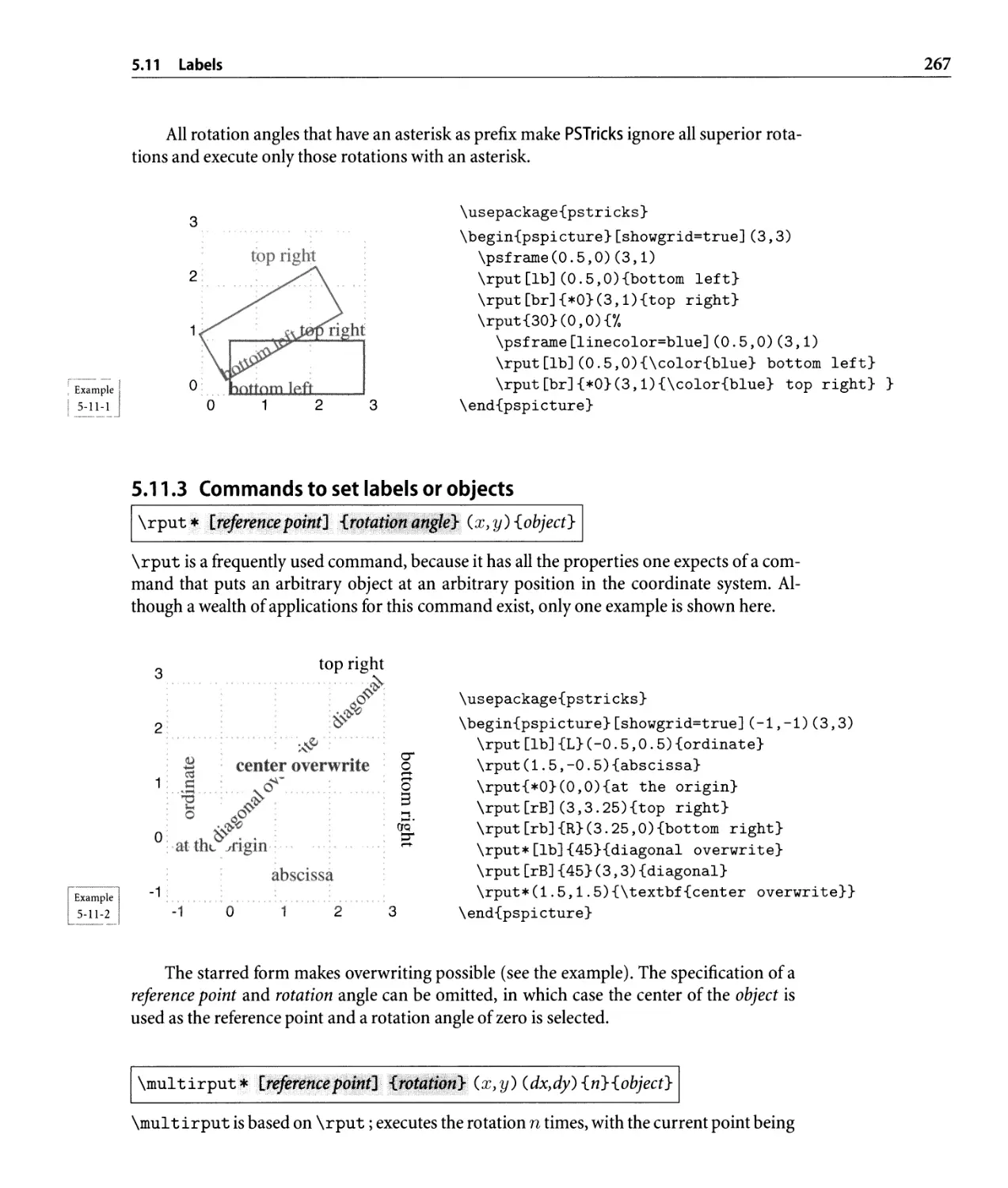
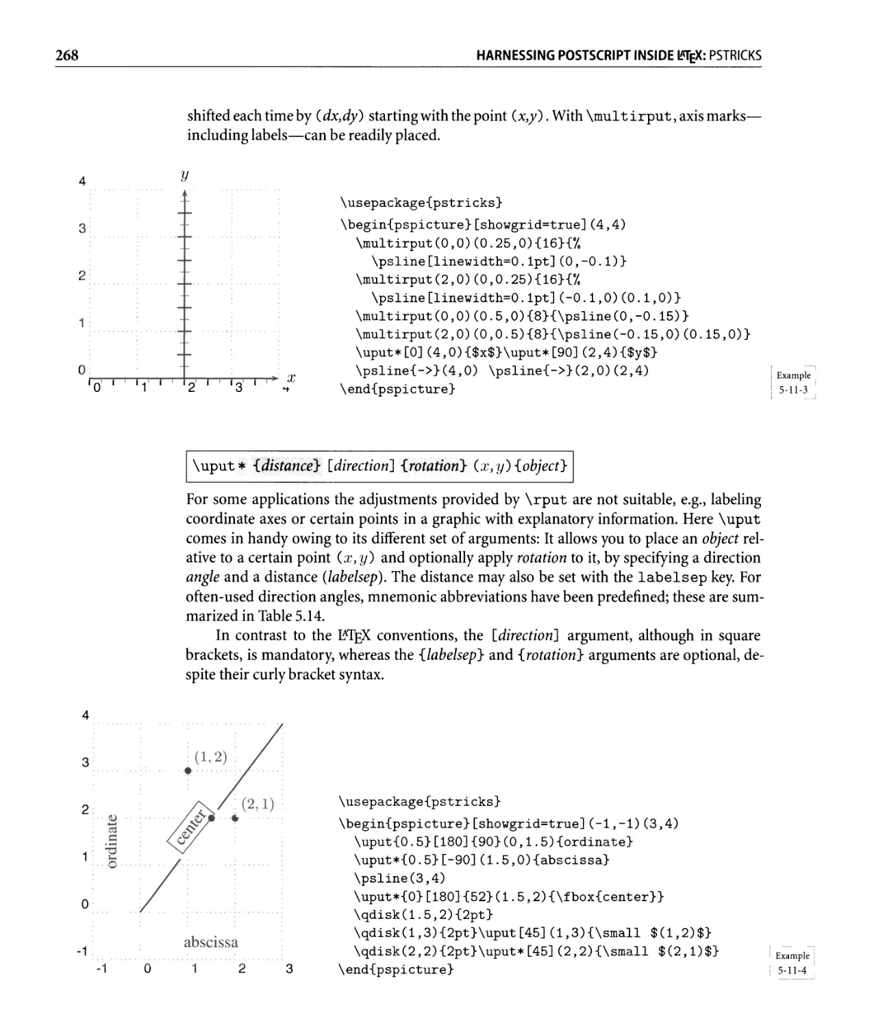
5.11.3 Commands to set labels or objects . . . . . . . . . . . . . . . . . . . .. 267
CONTENTS
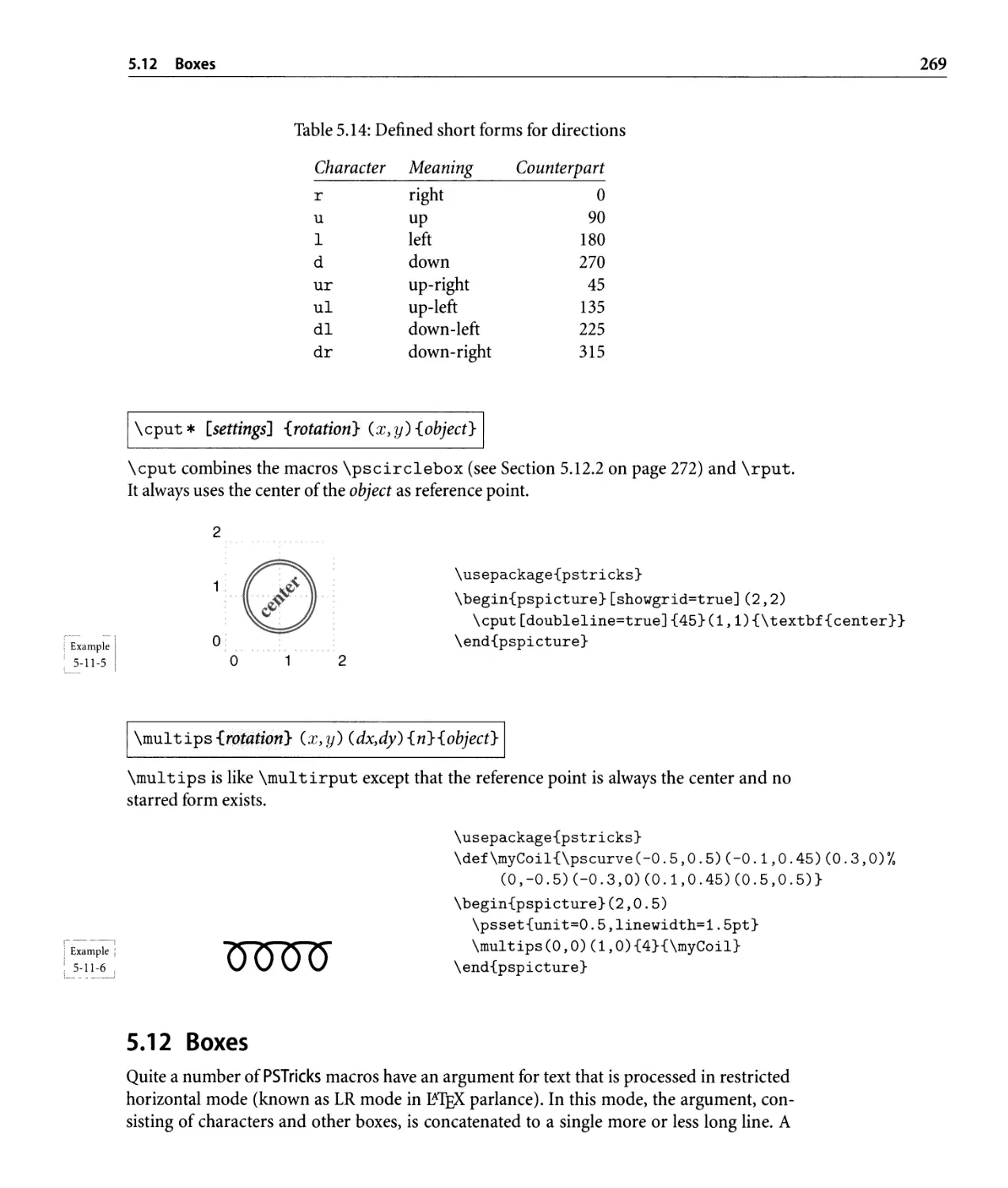
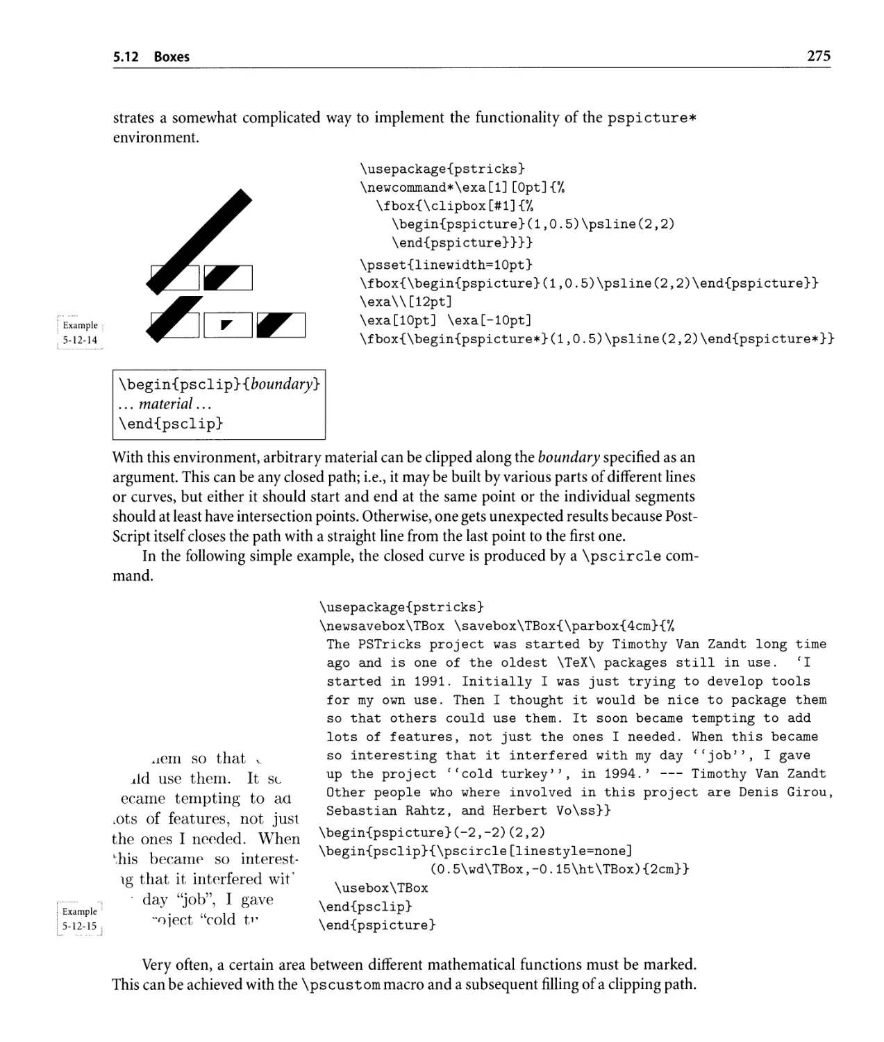
5.12 Boxes . . . . . . . . . . . . . . . . . . . . . . . . . . . . . . . . . . . . . . . . . . . .. 269
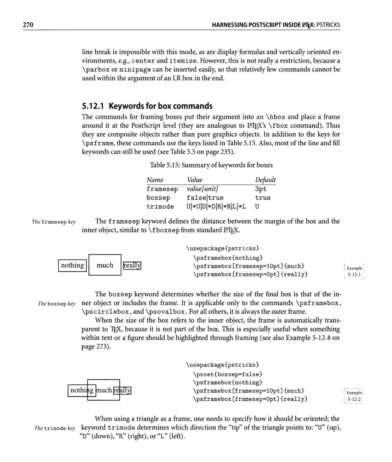
5.12.1 Keywords for box commands. . . . . . . . . . . . . . . . . . . . . . . .. 270
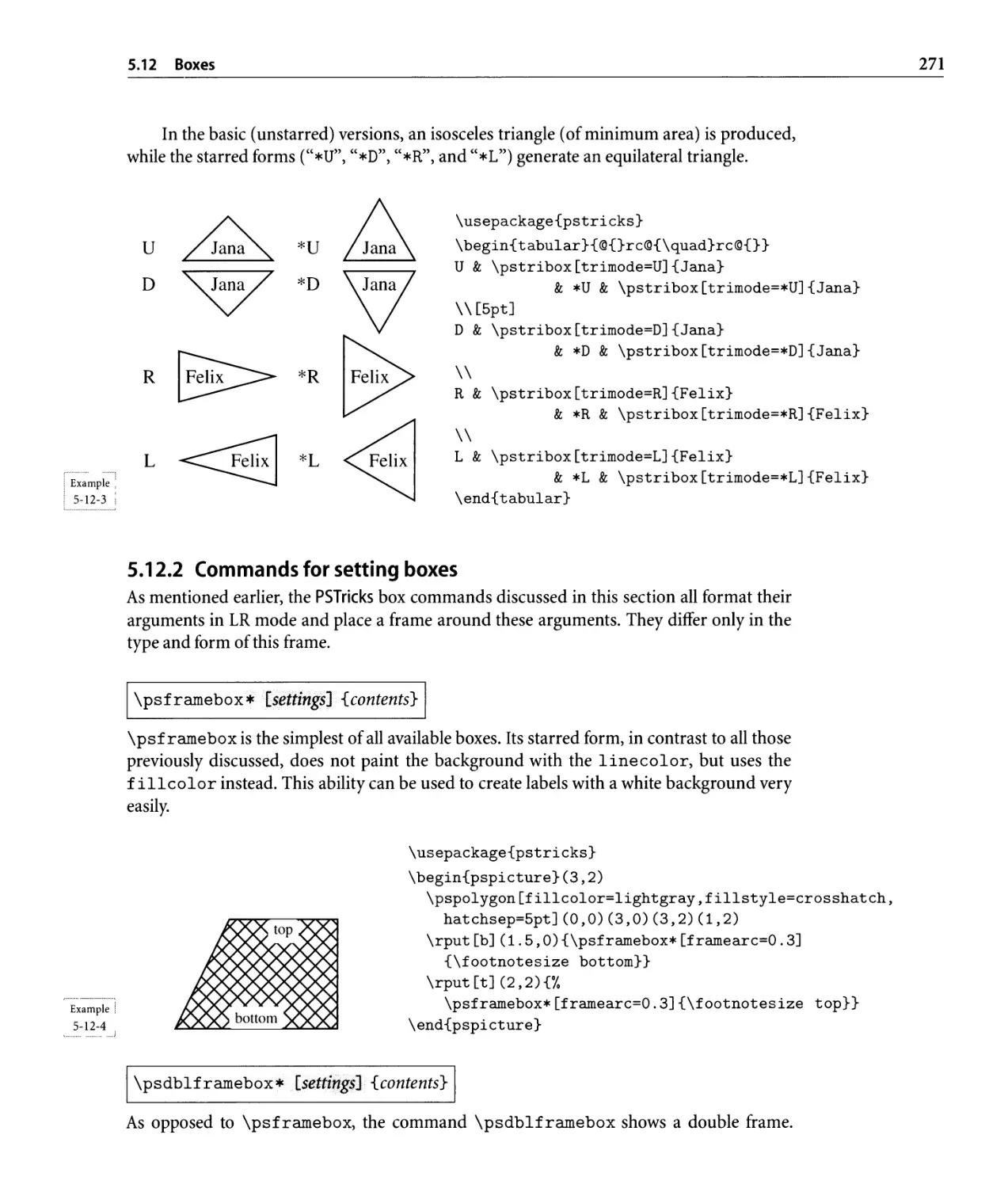
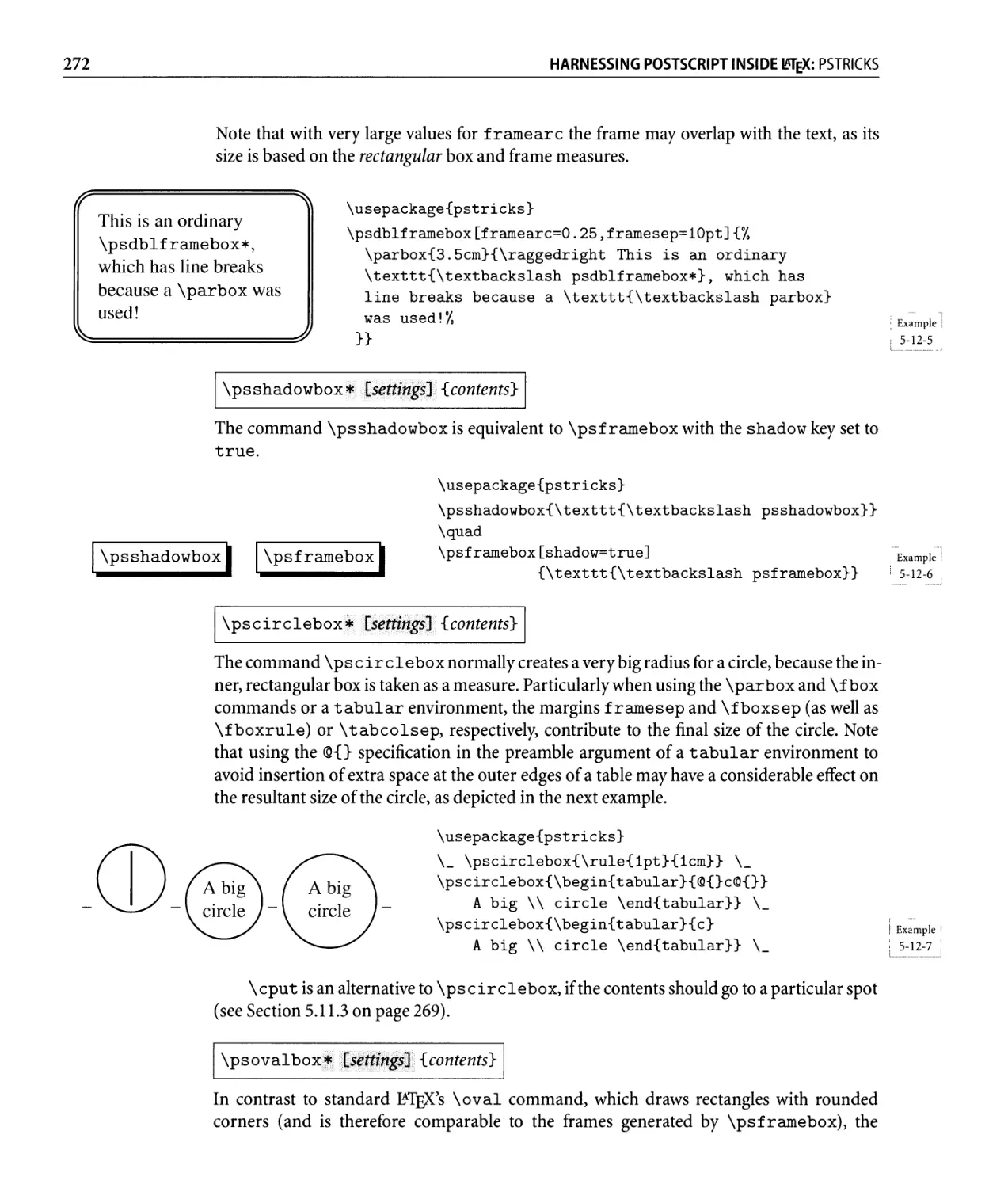
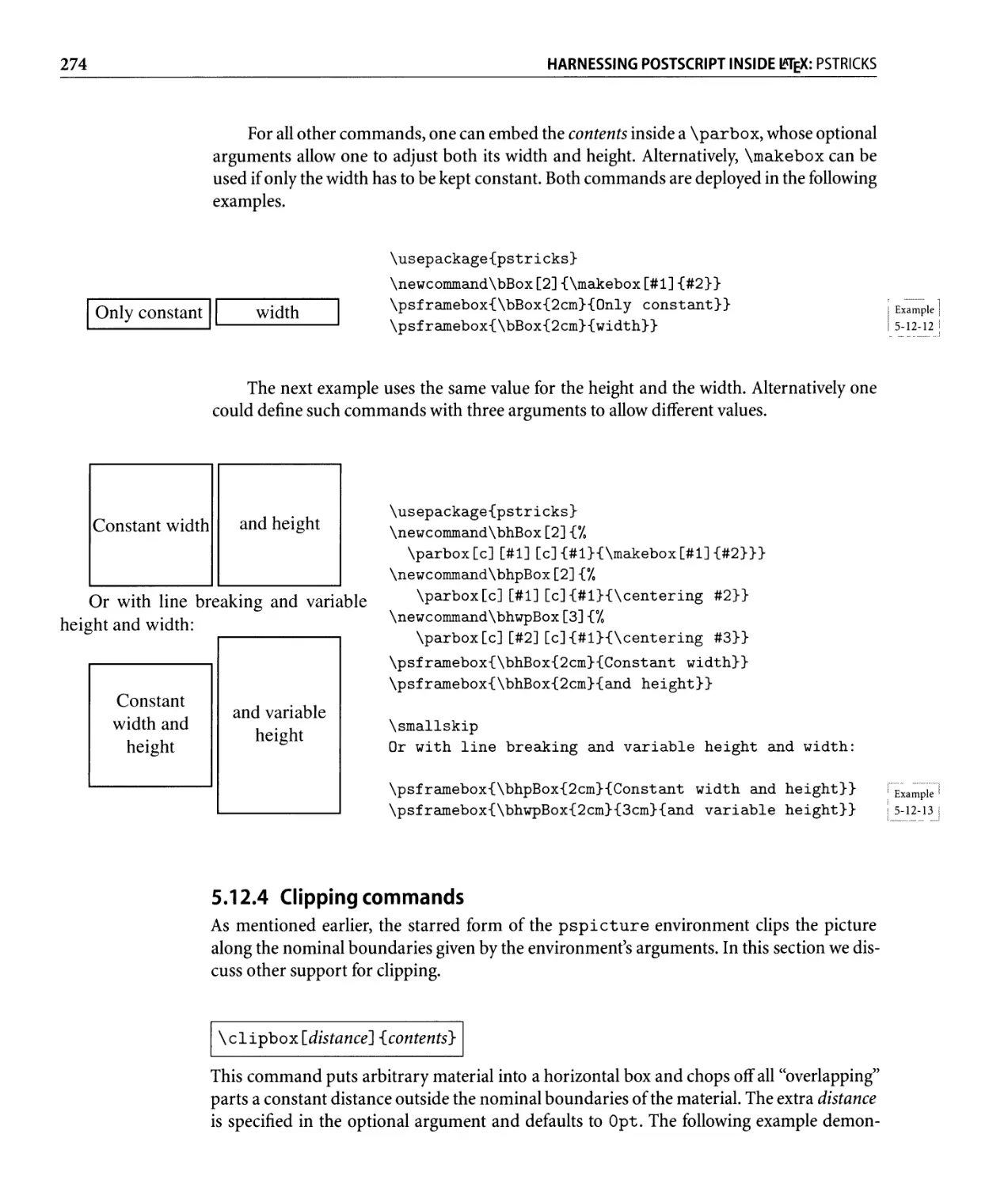
5.12.2 Commands for setting boxes. . . . . . . . . . . . . . . . . . . . . . . .. 271
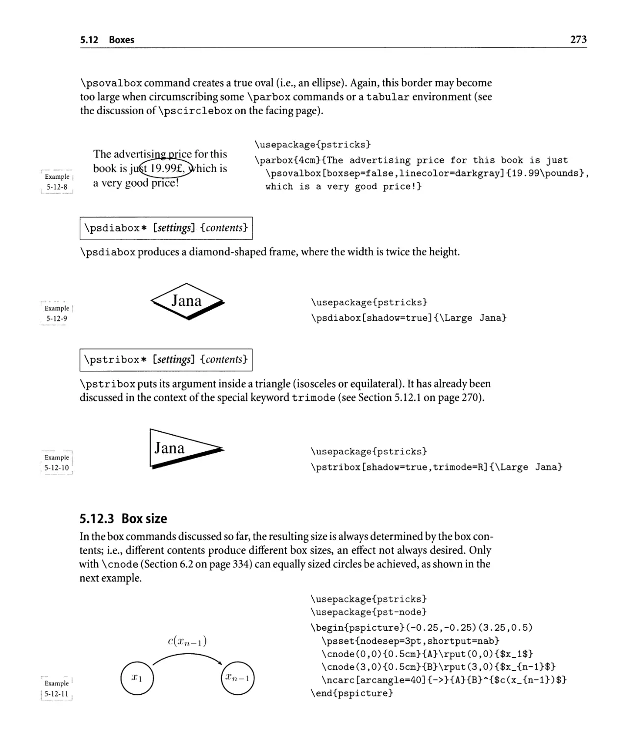
5.12.3 Box size . . . . . . . . . . . . . . . . . . . . . . . . . . . . . . . . . . . . .. 273
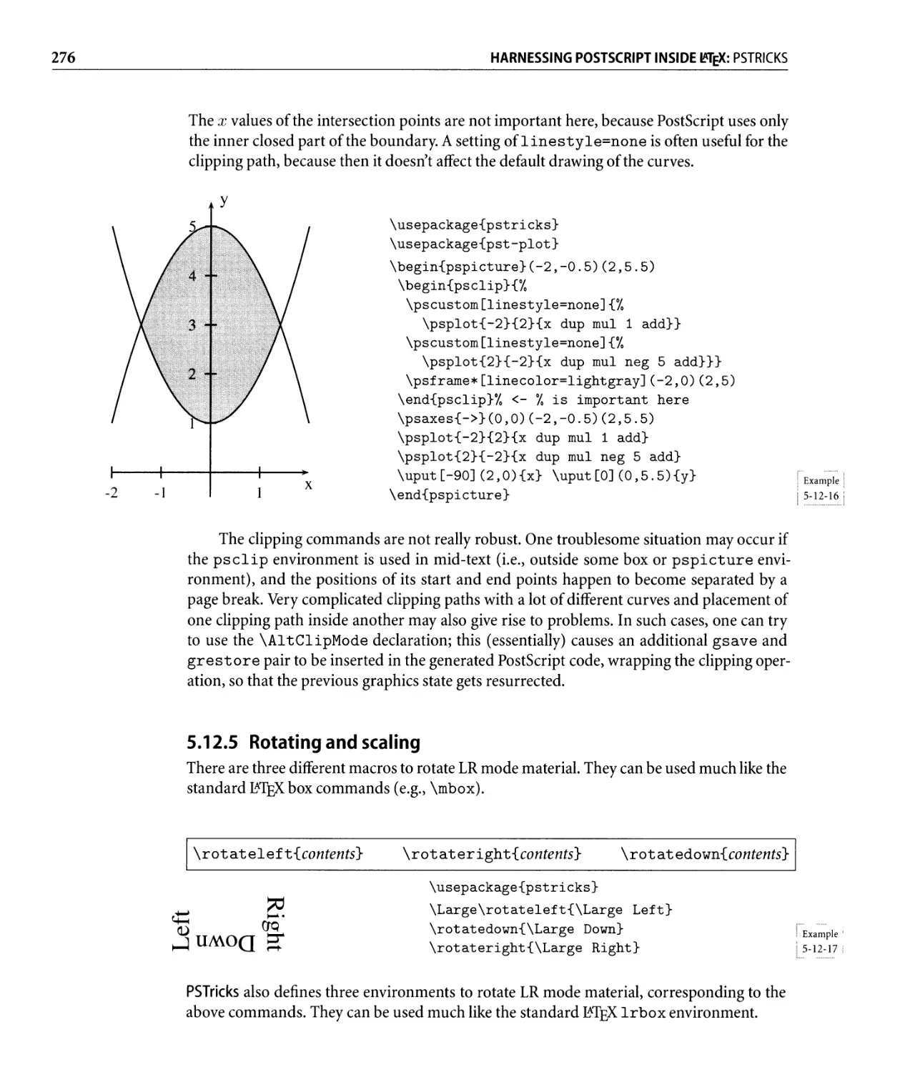
5.12.4 Clipping commands . . . . . . . . . . . . . . . . . . . . . . . . . . . . .. 274
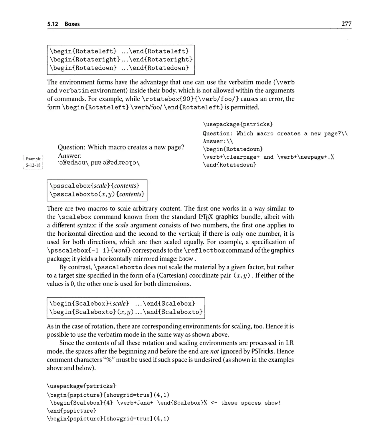
5.12.5 Rotating and scaling . . . . . . . . . . . . . . . . . . . . . . . . . . . . .. 276
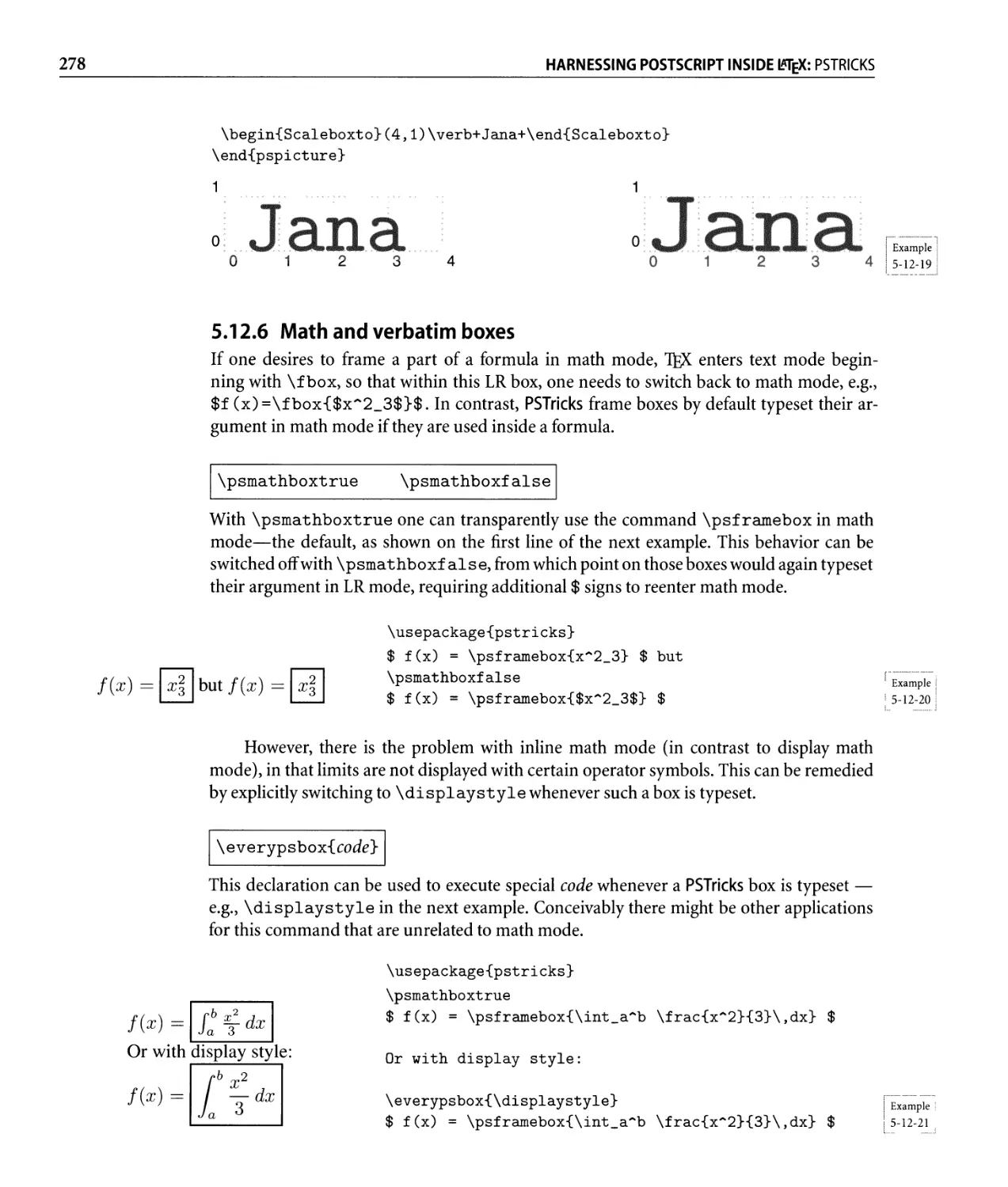
5.12.6 Math and verbatim boxes. . . . . . . . . . . . . . . . . . . . . . . . . .. 278
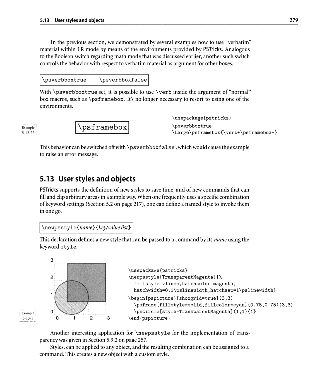
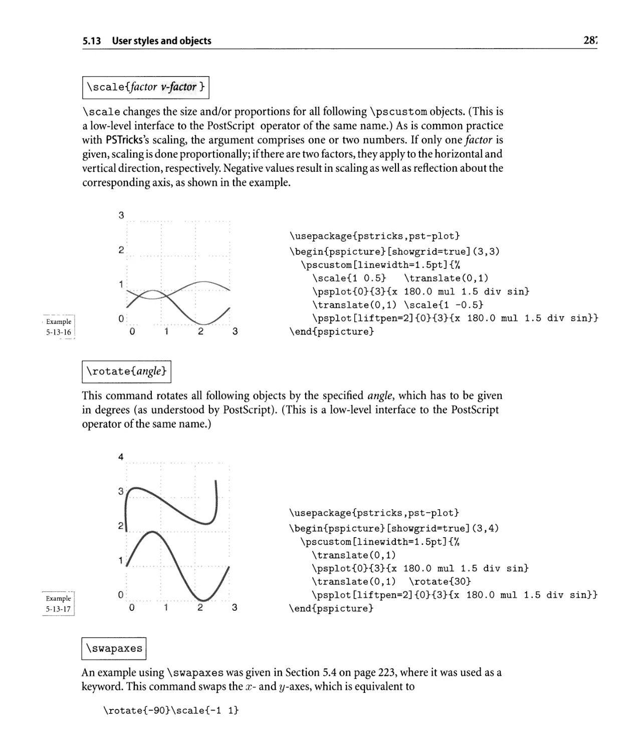
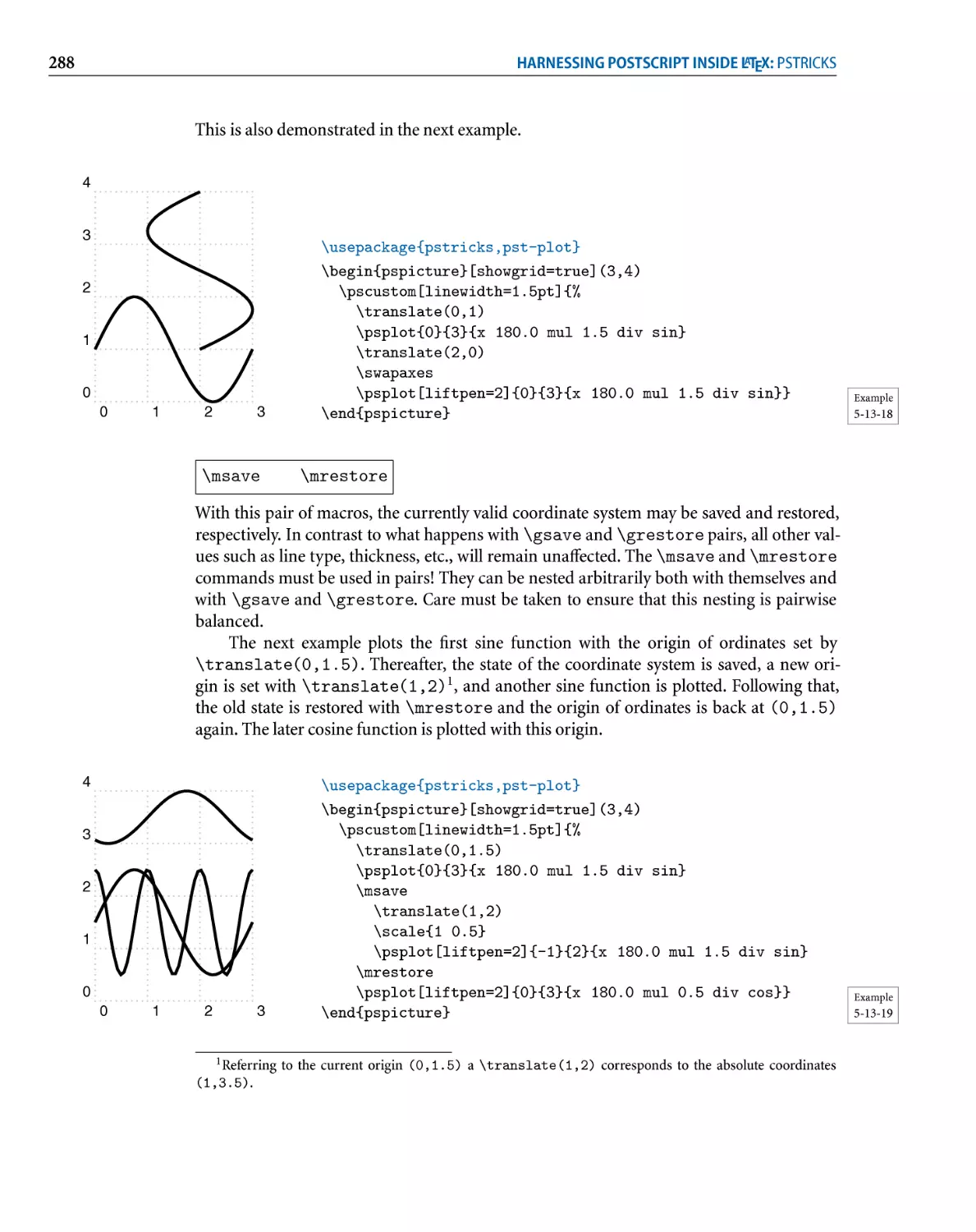
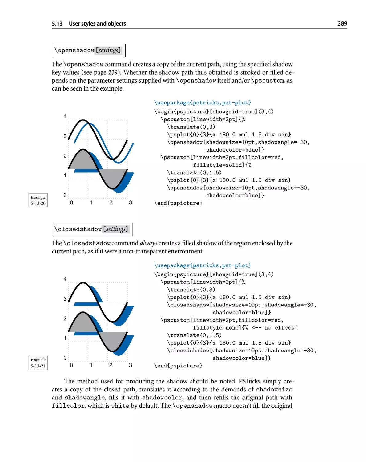
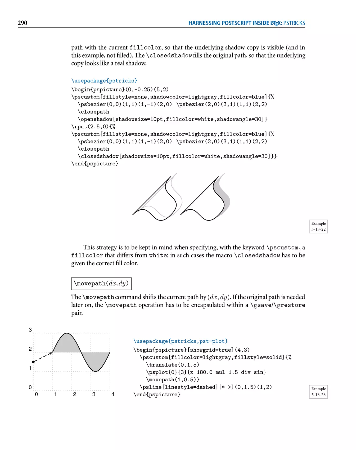
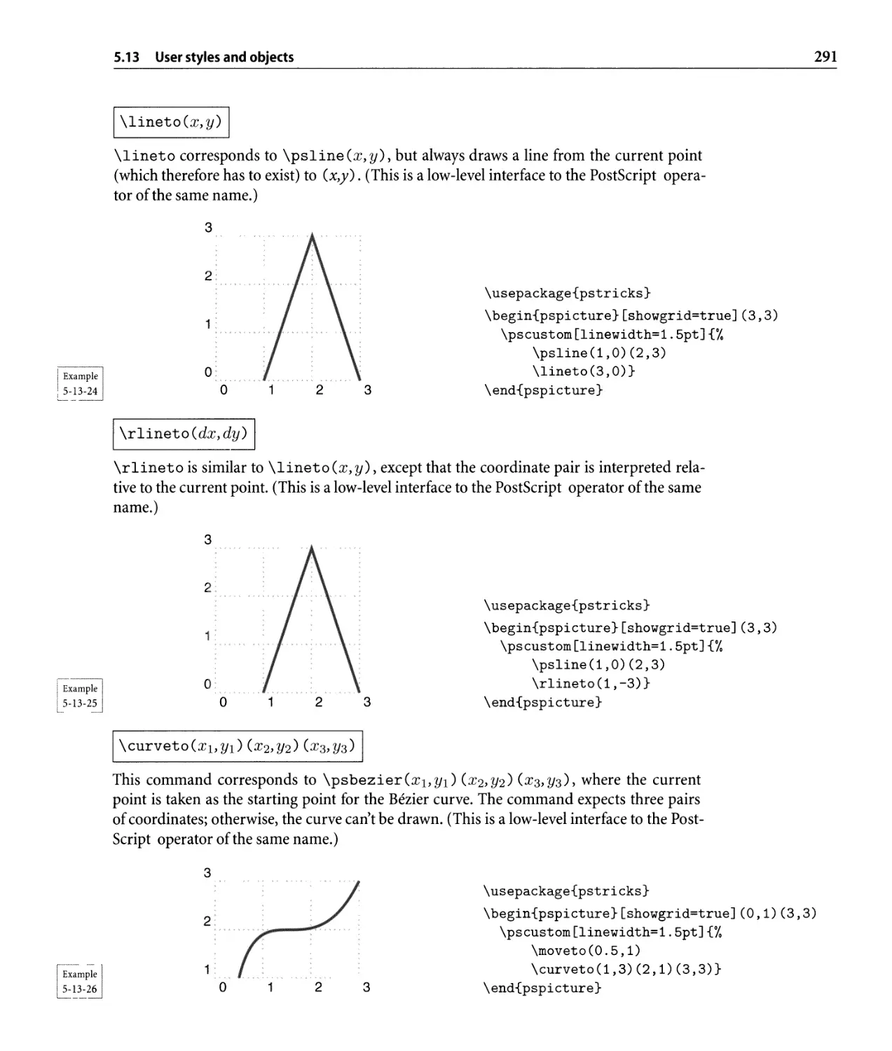
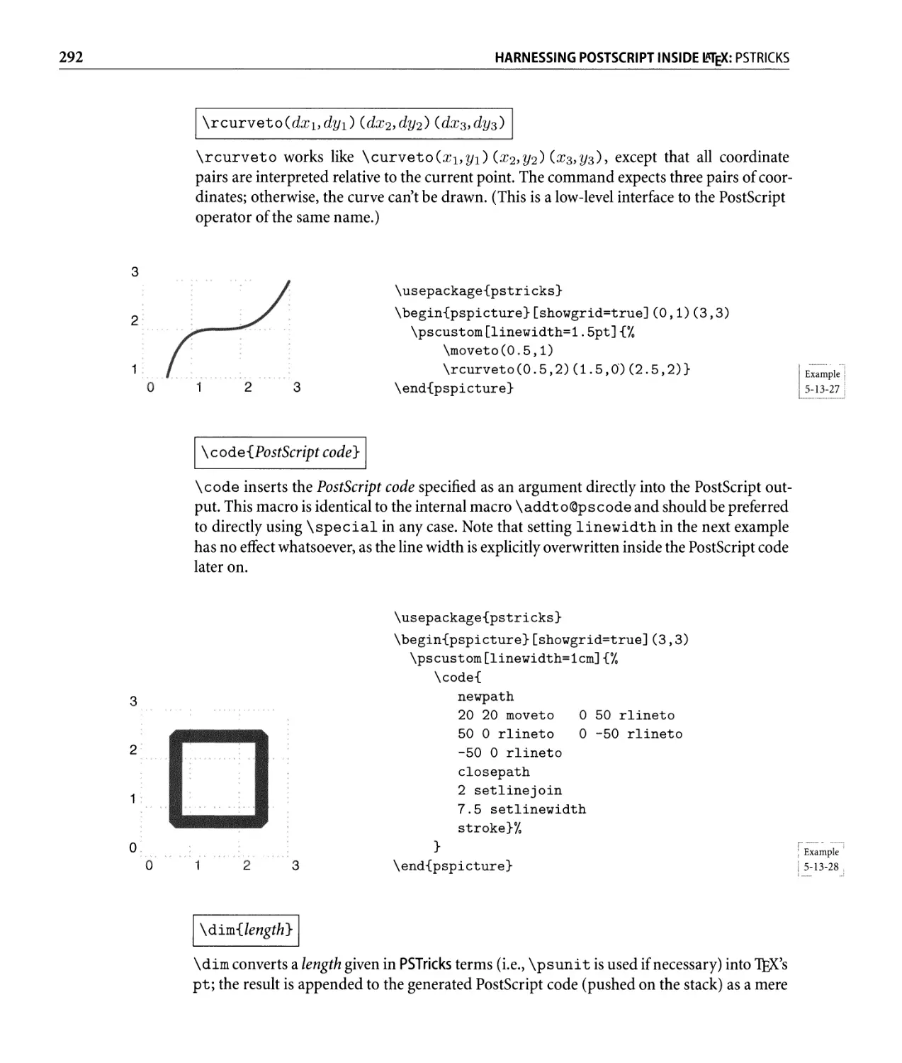
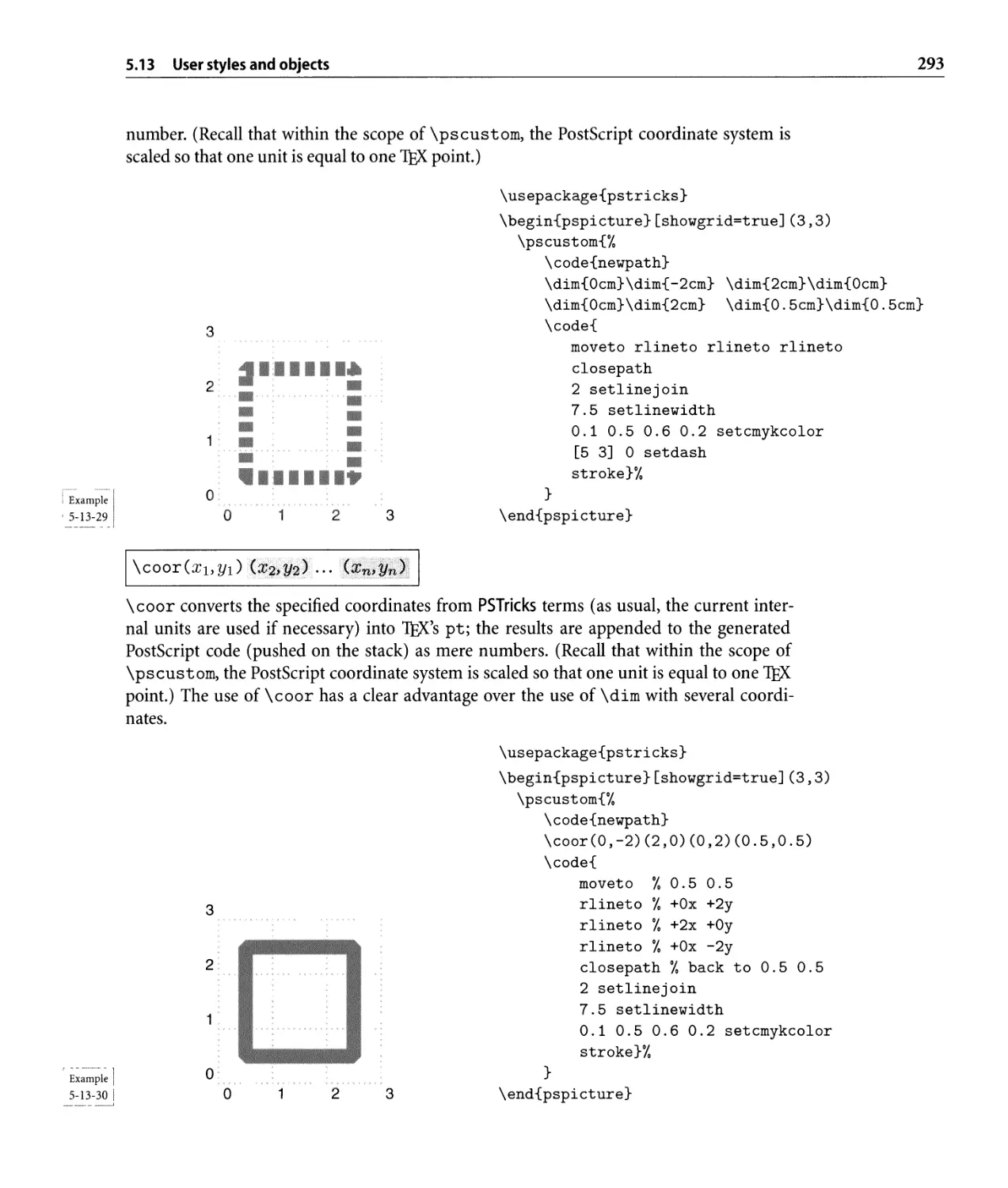
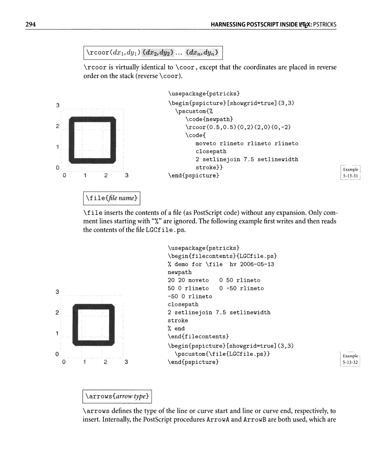
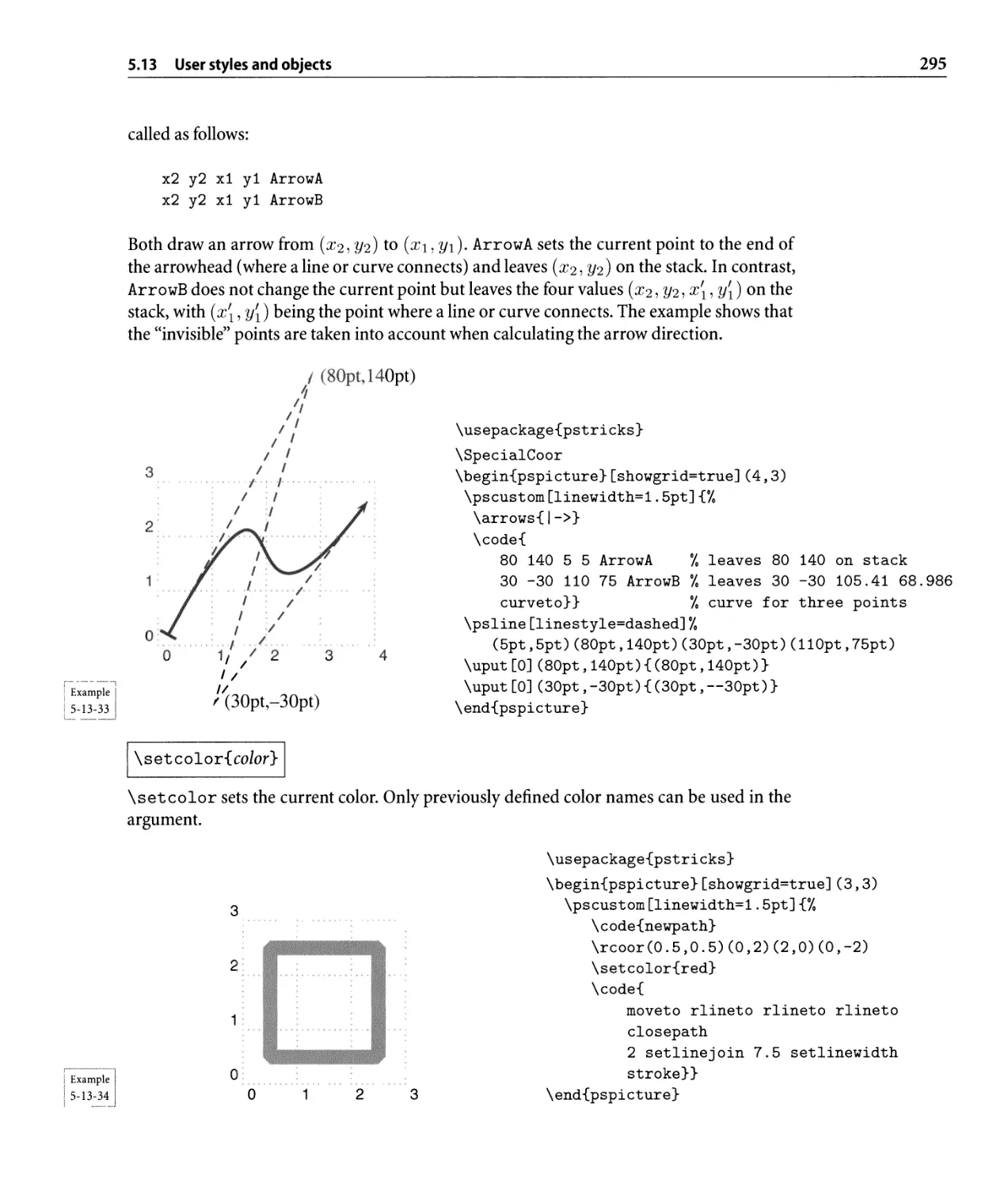
5.13 User styles and objects . . . . . . . . . . . . . . . . . . . . . . . . . . . . . . . . .. 279
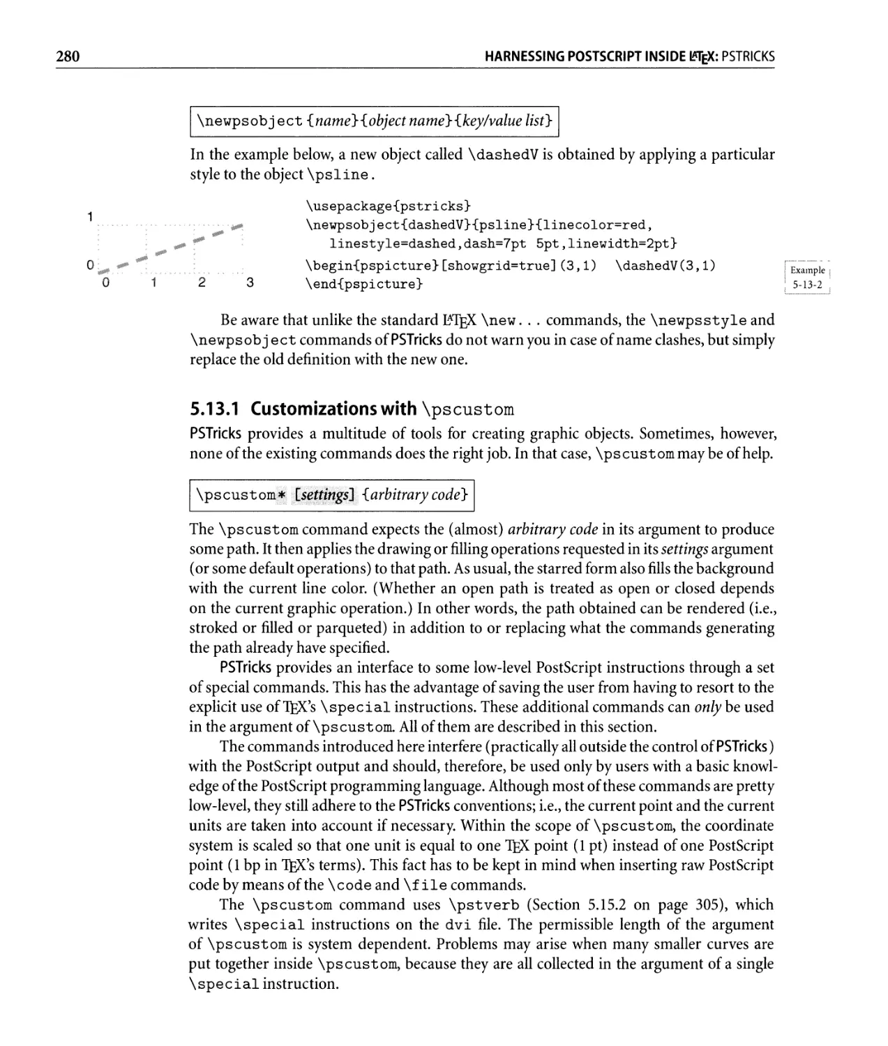
5.13.1 Customizations with \pscustom. . . . . . . . . . . . . . . . . . . . .. 280
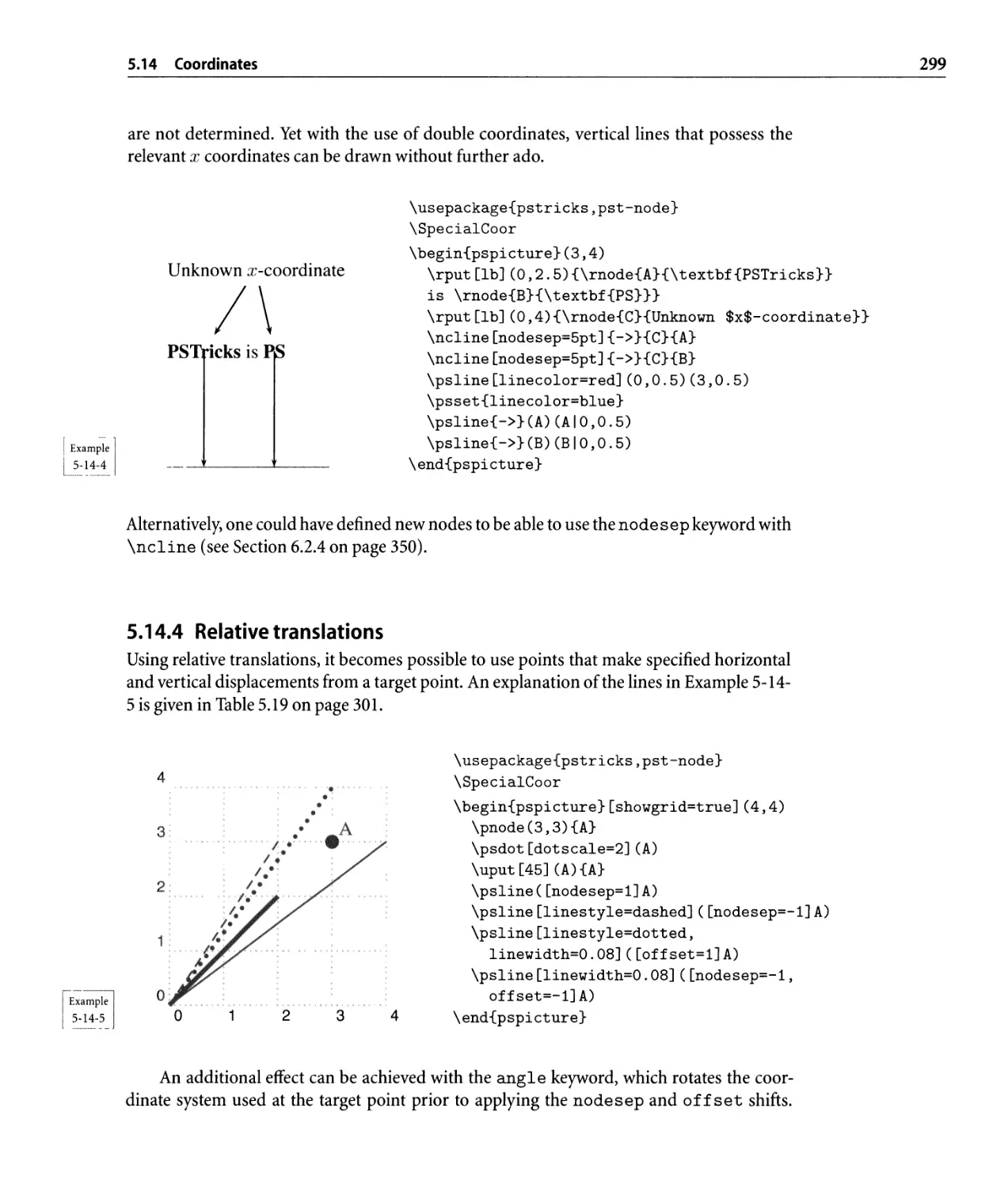
5.14 Coordinates . . . . . . . . . . . . . . . . . . . . . . . . . . . . . . . . . . . . . . . .. 296
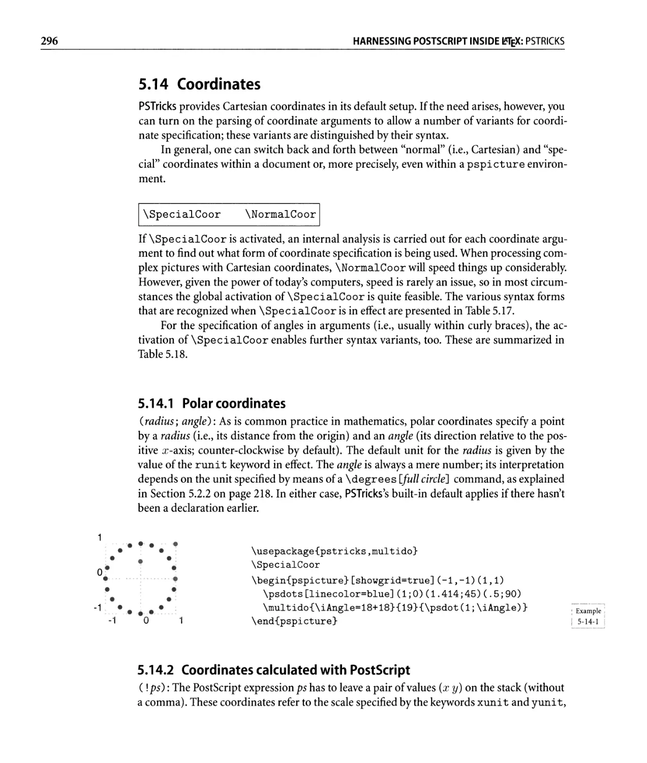
5.14.1 Polar coordinates . . . . . . . . . . . . . . . . . . . . . . . . . . . . . . .. 296
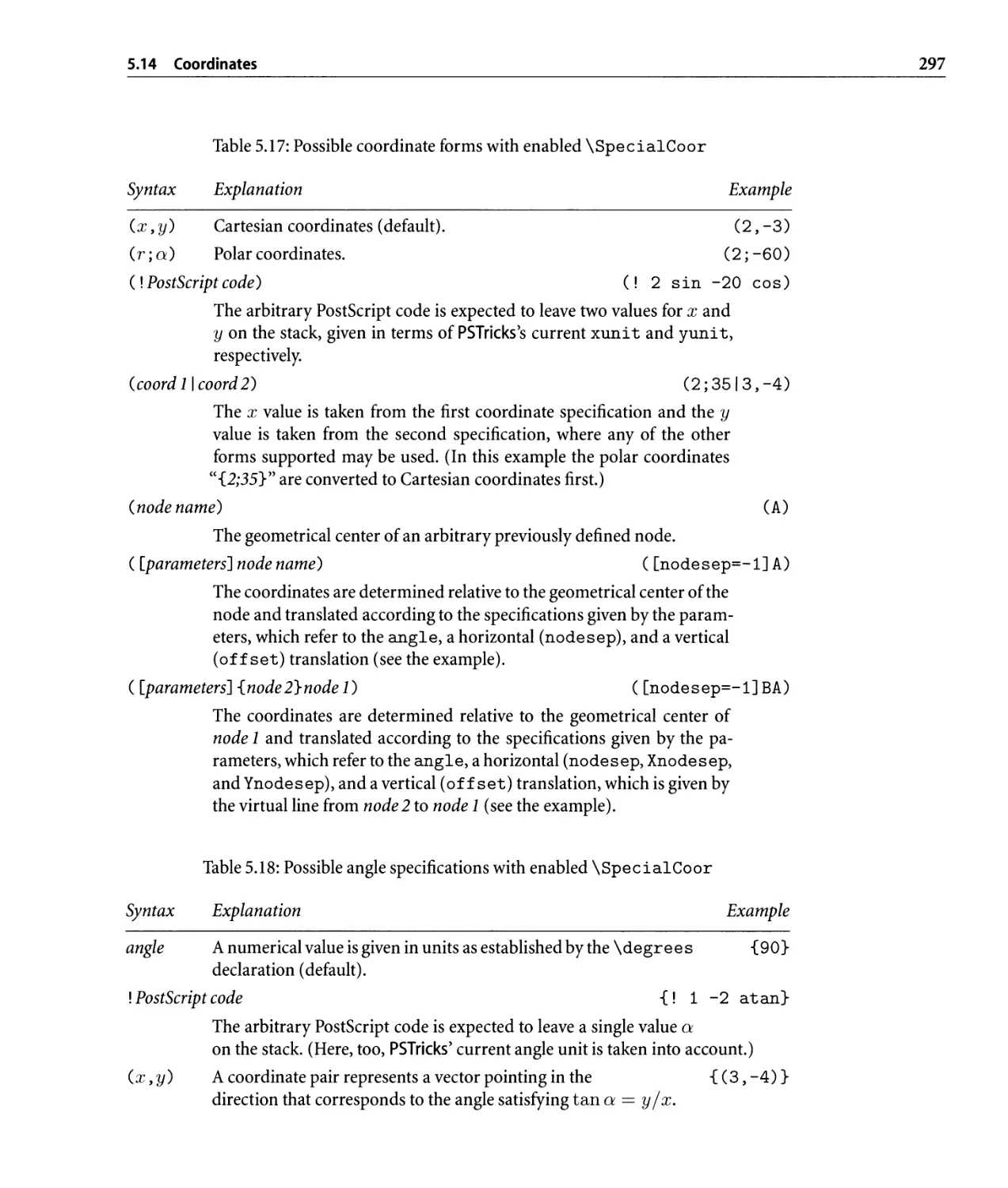
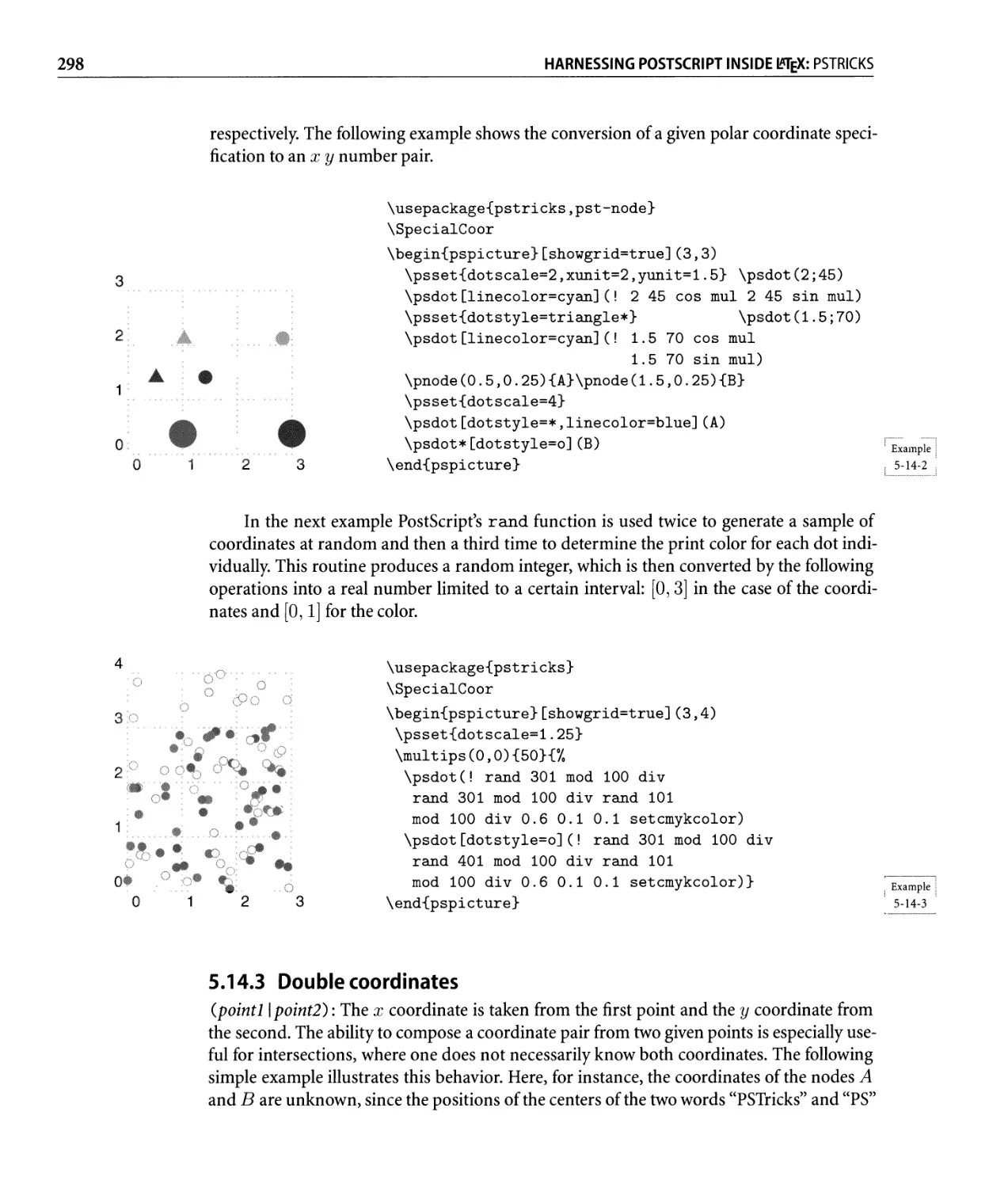
5.14.2 Coordinates calculated with PostScript. . . . . . . . . . . . . . . . . .. 296
5.14.3 Double coordinates. . . . . . . . . . . . . . . . . . . . . . . . . . . . . .. 298
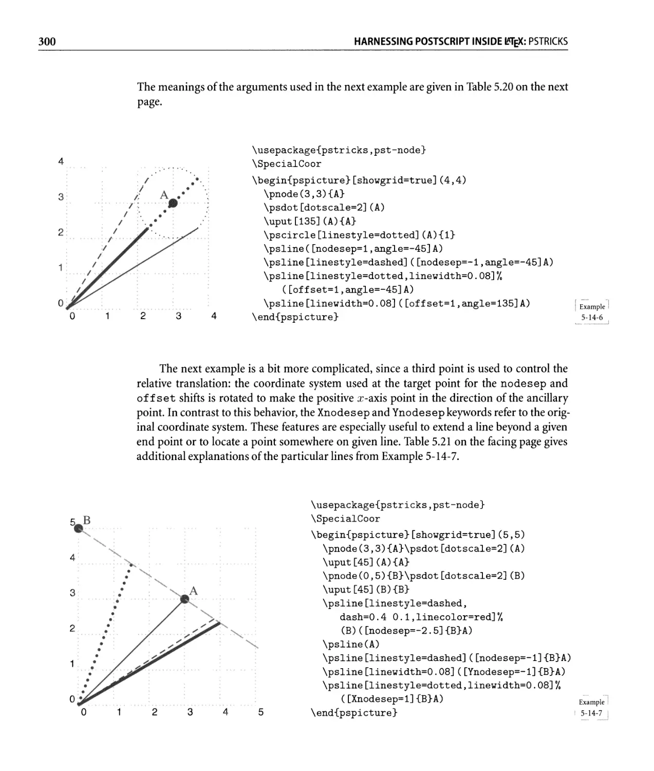
5.14.4 Relative translations . . . . . . . . . . . . . . . . . . . . . . . . . . . . .. 299
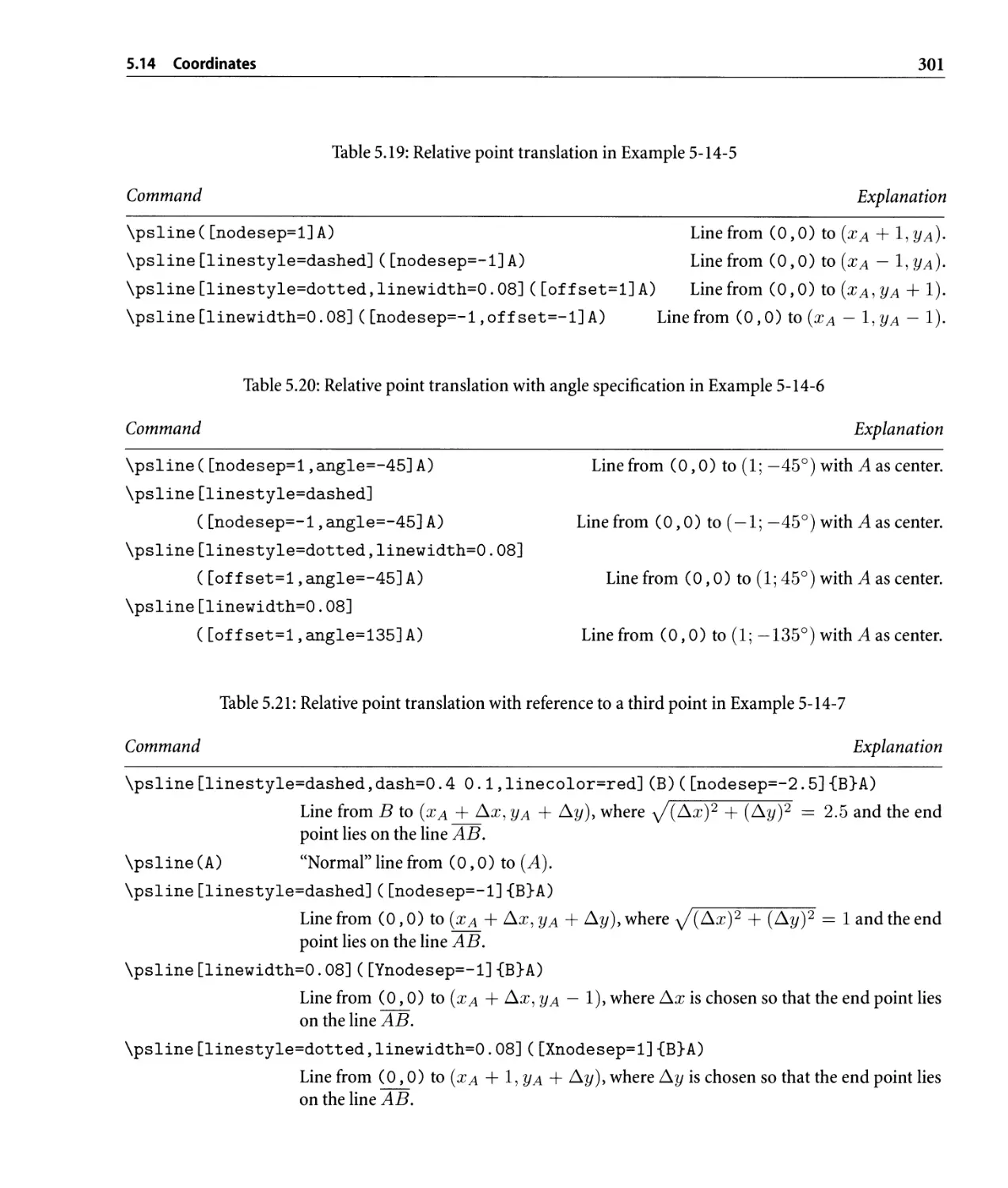
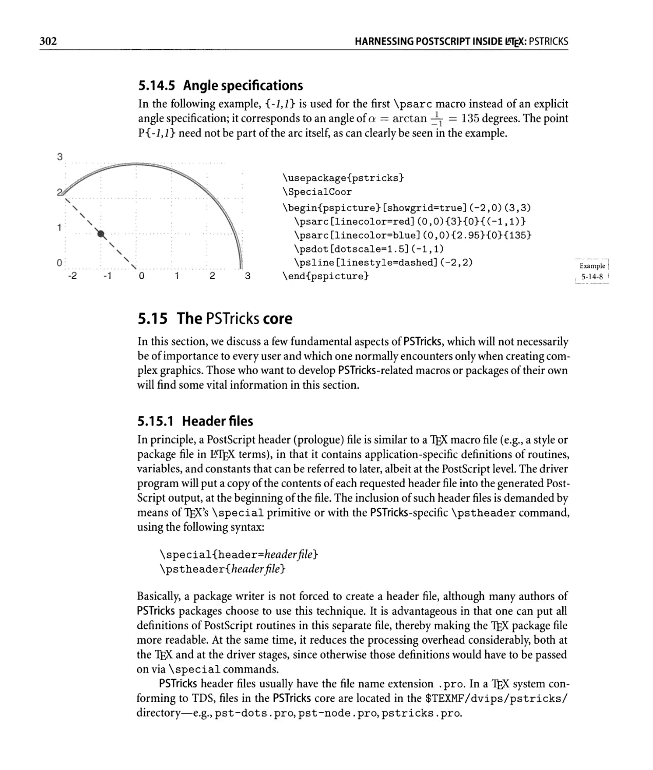
5.14.5 Angle specifications . . . . . . . . . . . . . . . . . . . . . . . . . . . . .. 302
5.15 The PSTricks core. . . . . . . . . . . . . . . . . . . . . . . . . . . . . . . . . . . . .. 302
5.15.1 Header files. . . . . . . . . . . . . . . . . . . . . . . . . . . . . . . . . . .. 302
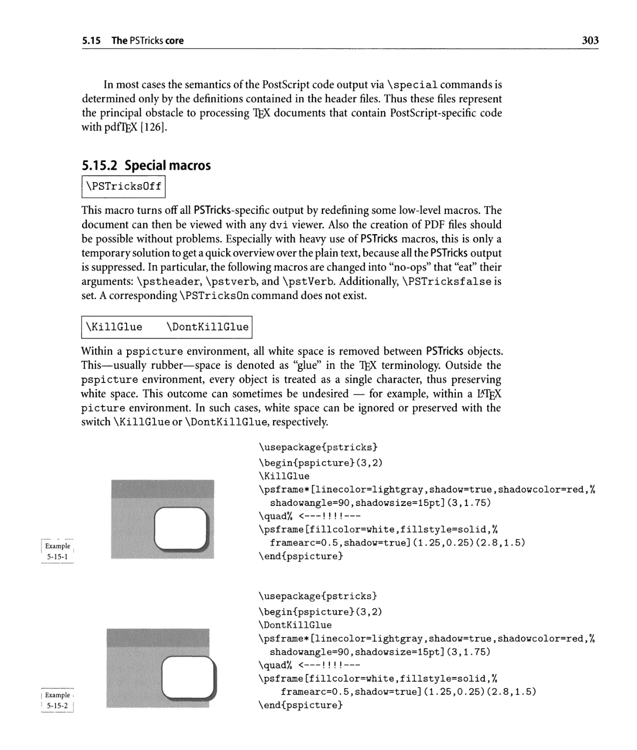
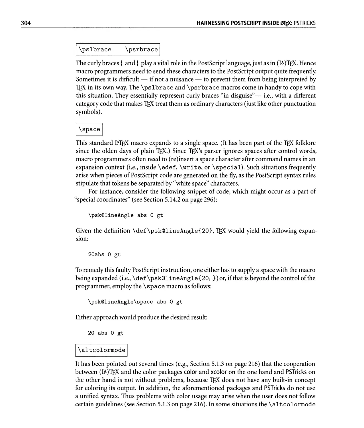
5.15.2 Special macros. . . . . . . . . . . . . . . . . . . . . . . . . . . . . . . . .. 303
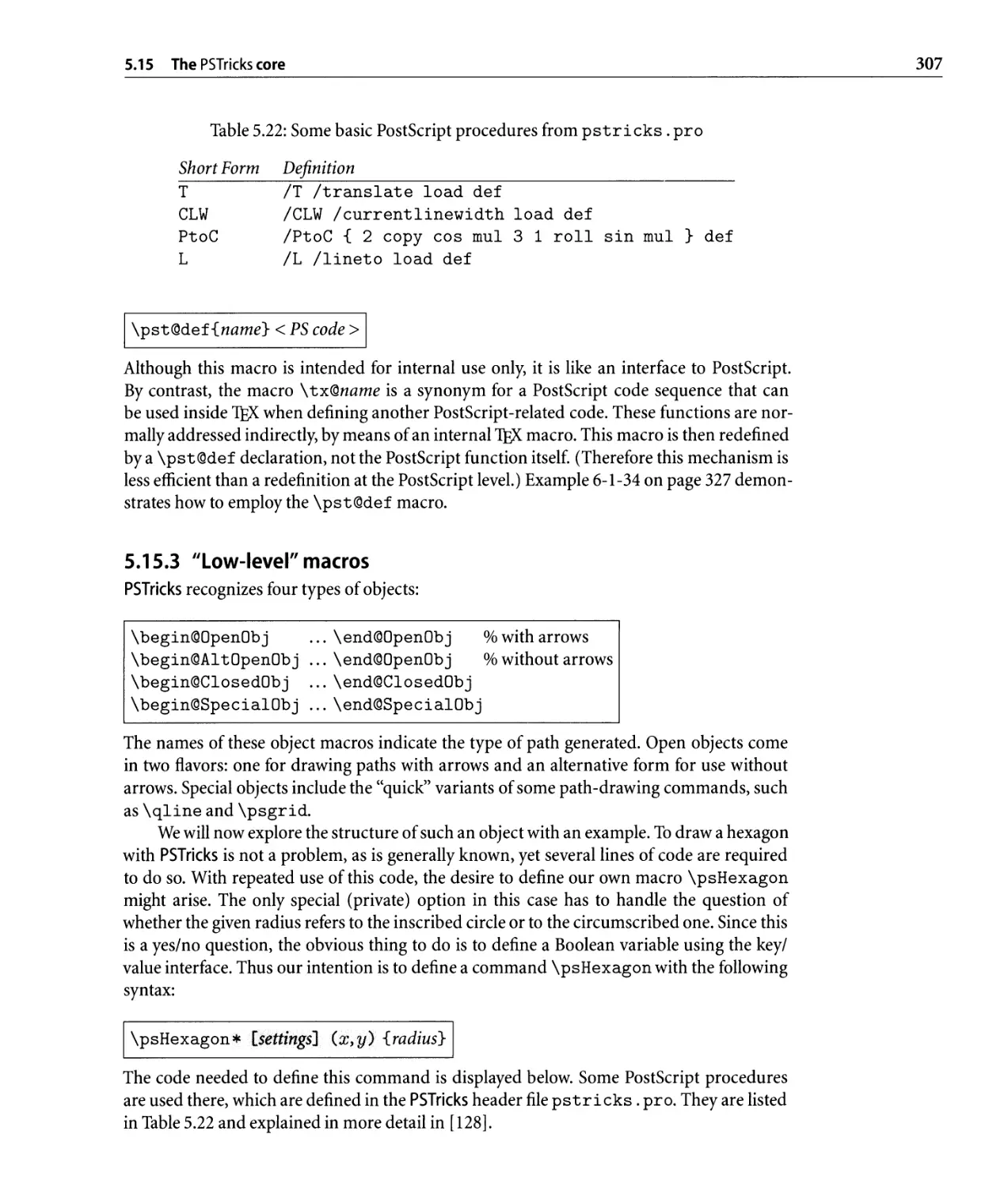
5.15.3 "low-level" macros. . . . . . . . . . . . . . . . . . . . . . . . . . . . . .. 307
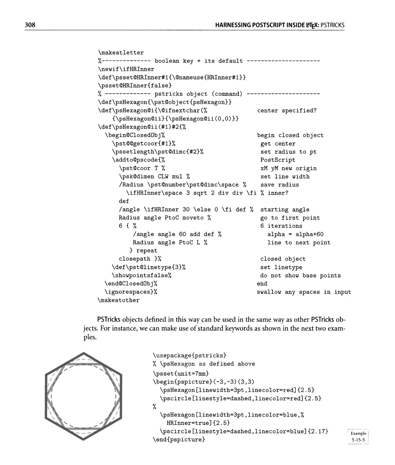
5.15.4 "High-level" macros. . . . . . . . . . . . . . . . . . . . . . . . . . . . . .. 309
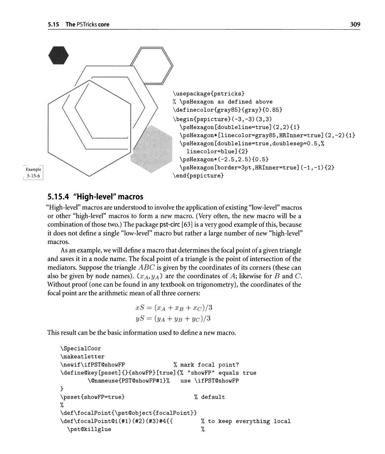
5.15.5 The "key/value" interface ........................... 310
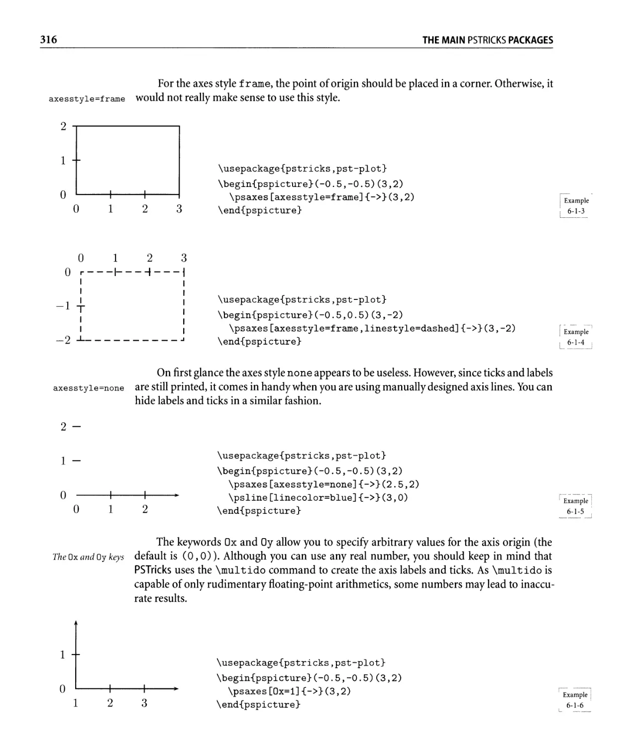
6 The Main PSTricks Packages 313
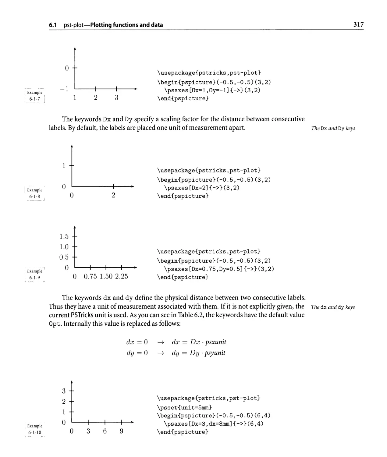
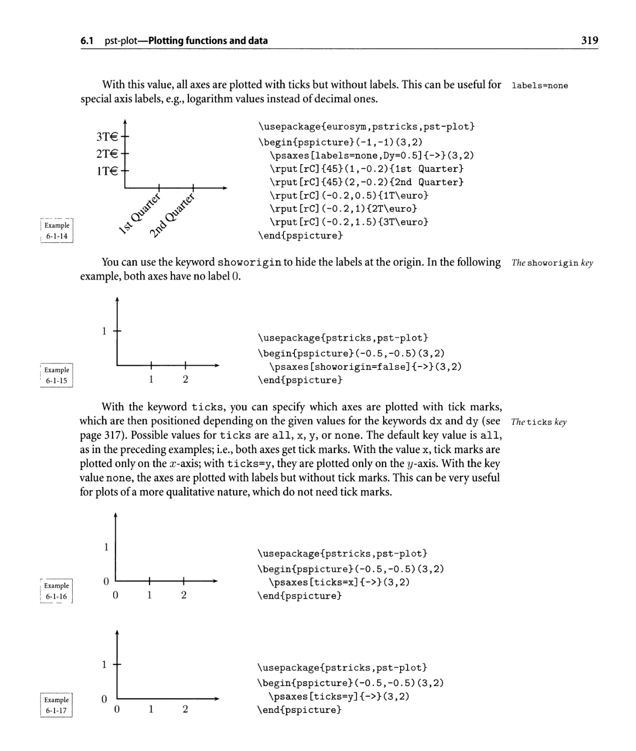
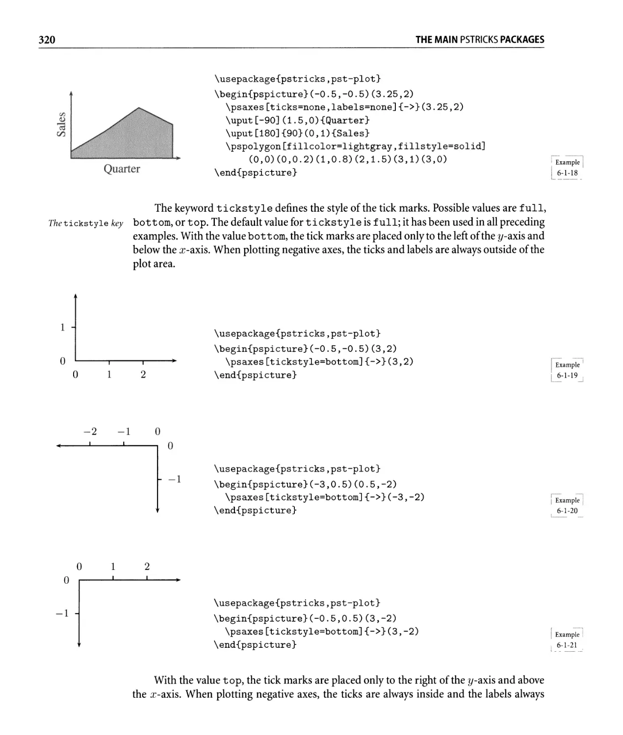
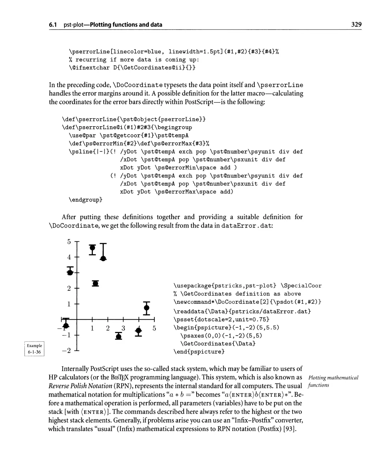
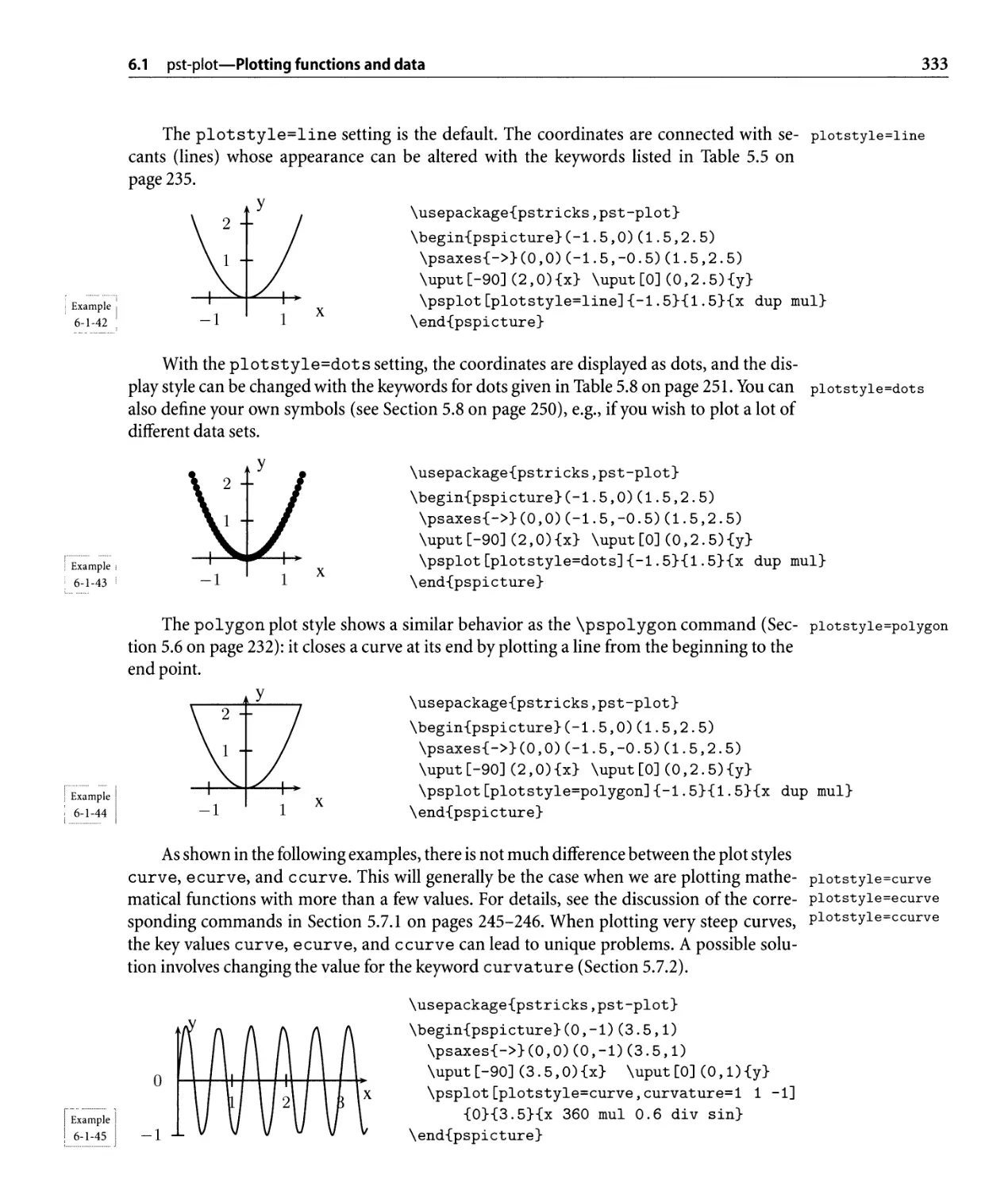
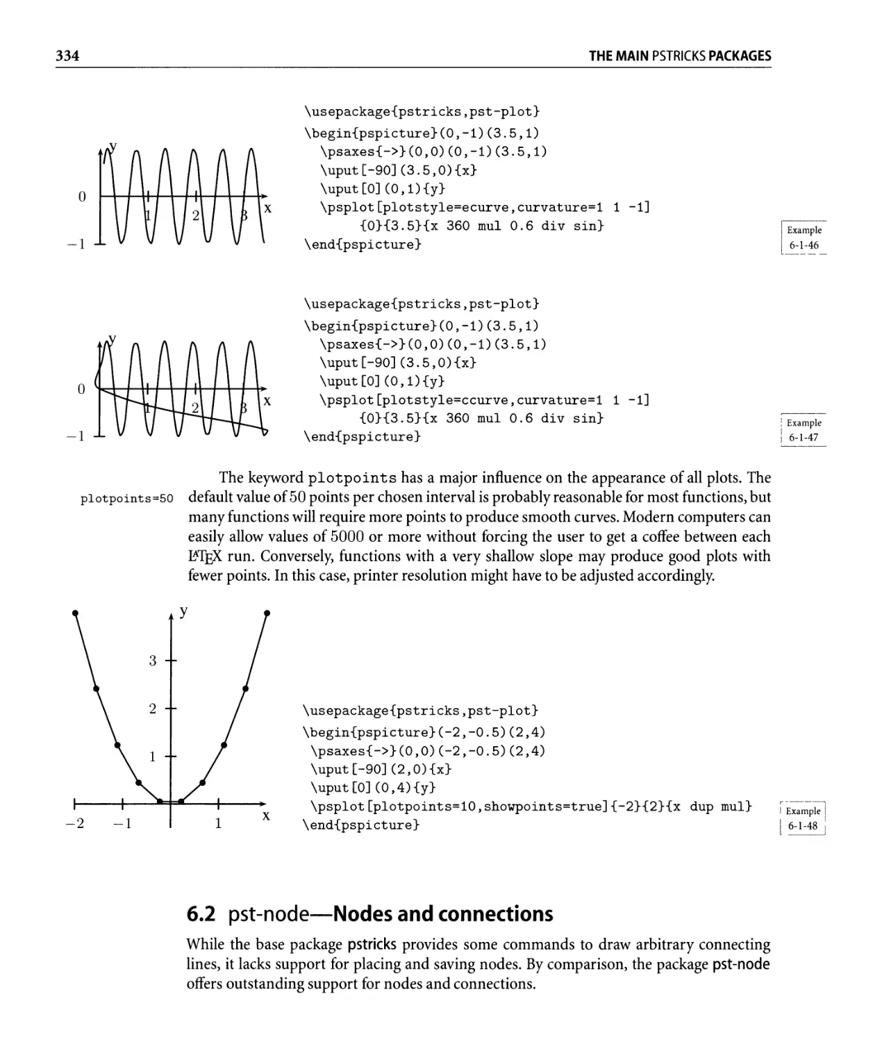
6.1 pst-plot-Plotting functions and data. . . . . . . . . . . . . . . . . . . . . . . .. 313
6.1.1 The coordinate system-ticks and labels . . . . . . . . . . . . . . . .. 314
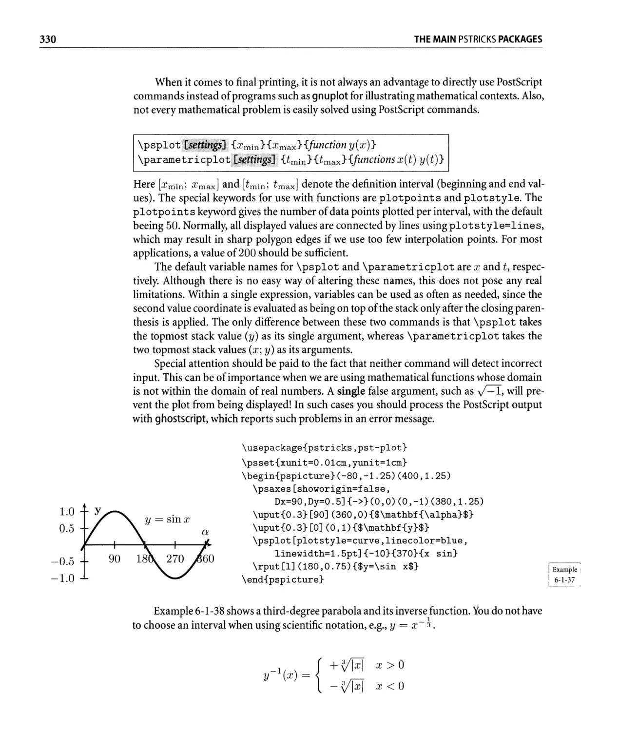
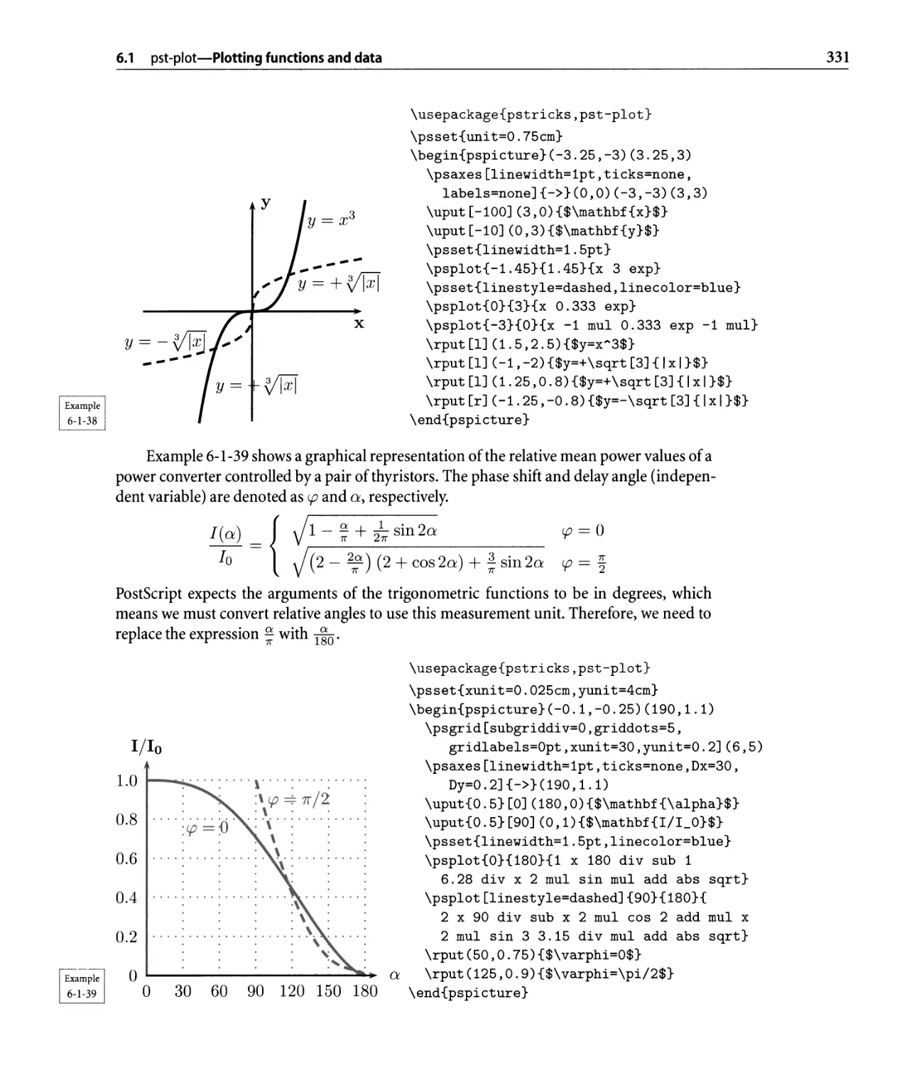
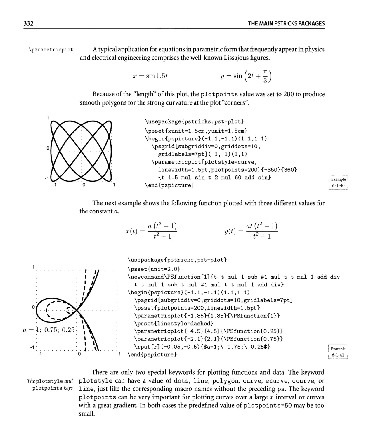
6.1.2 Plotting mathematical functions and data files. . . . . . . . . . . . .. 323
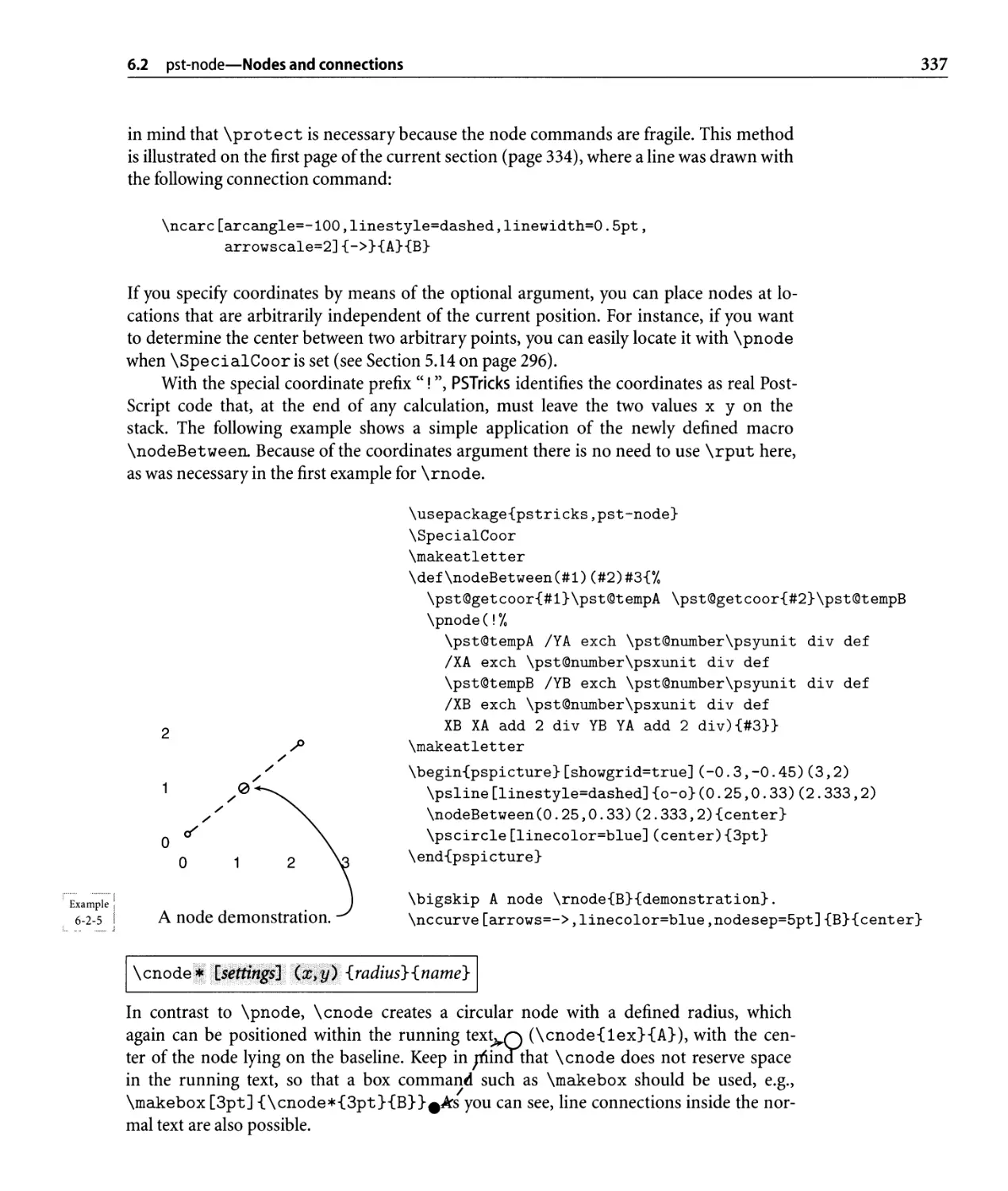
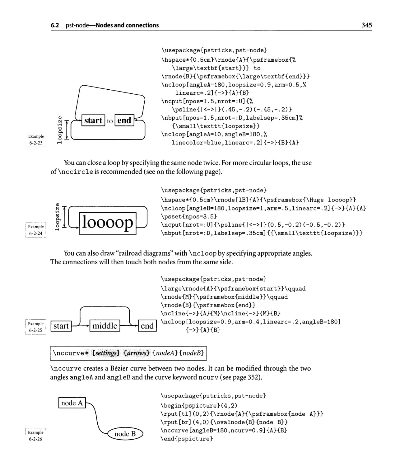
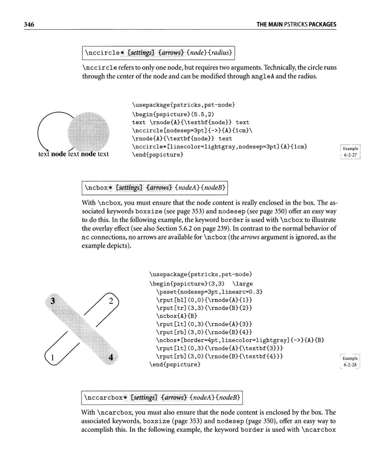
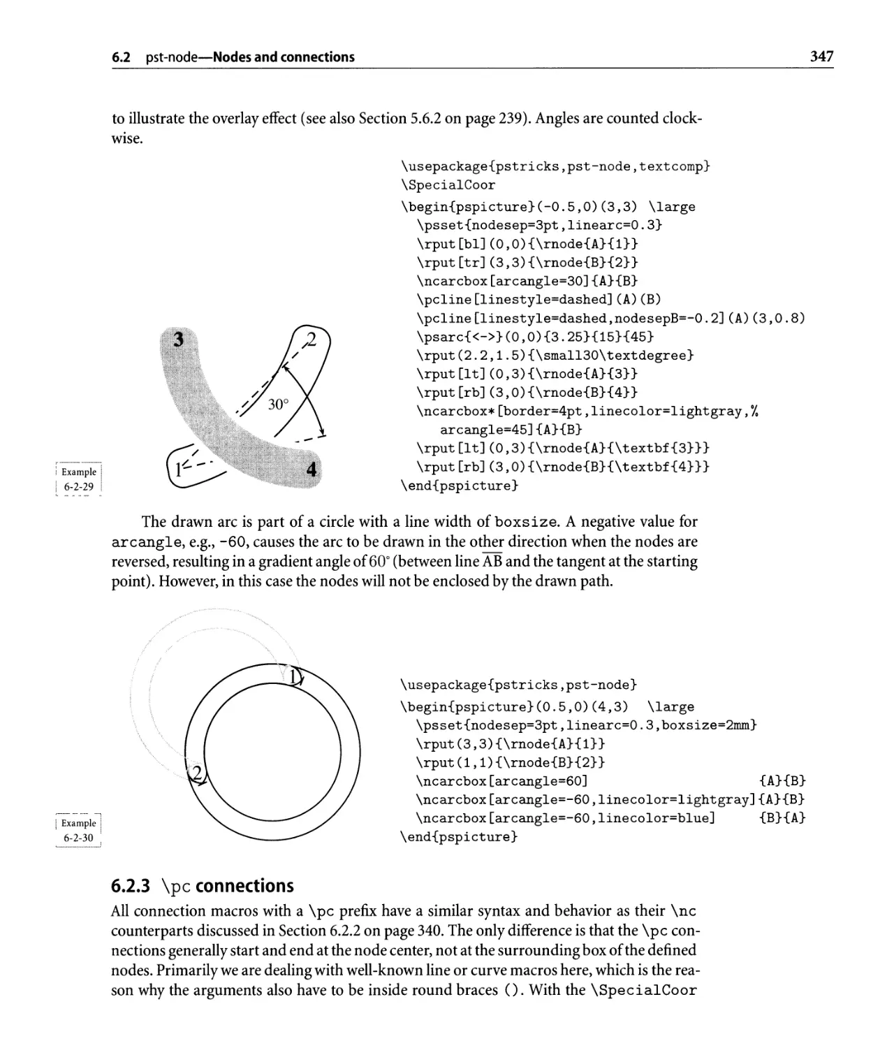
6.2 pst-node-Nodes and connections . . . . . . . . . . . . . . . . . . . . . . . . .. 334
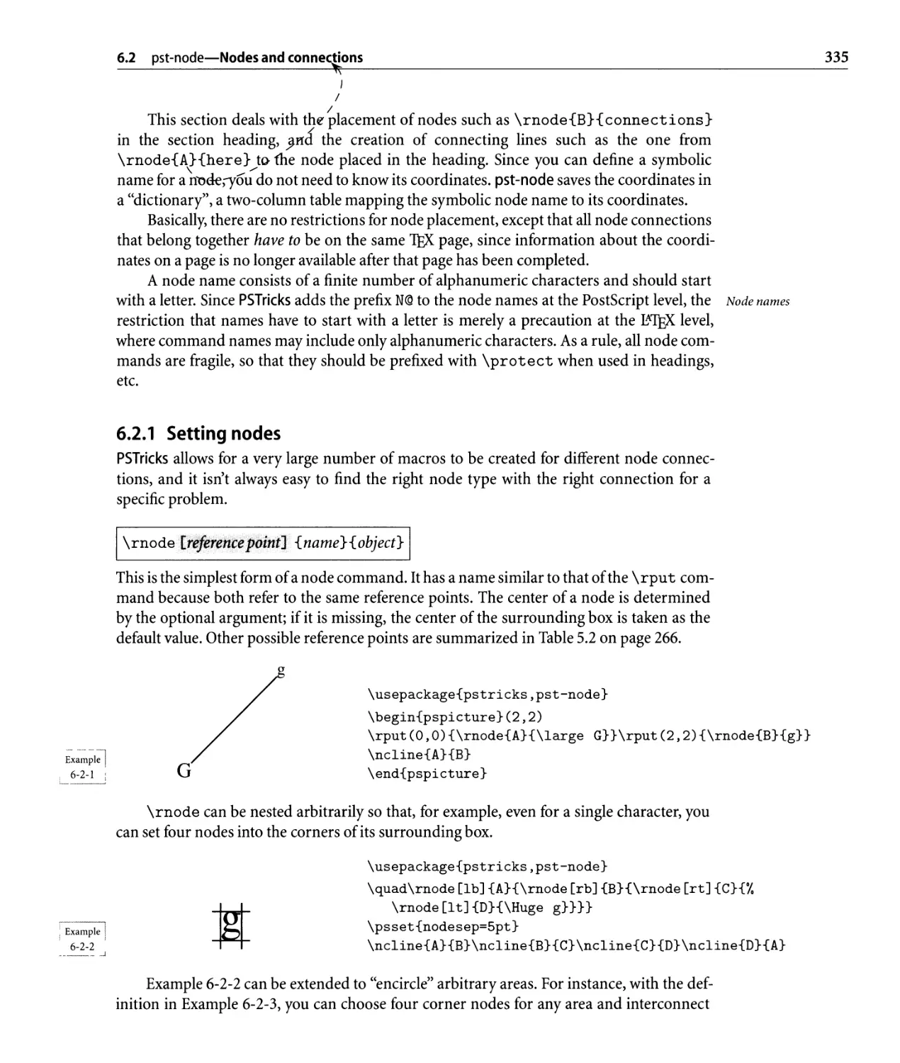
6.2.1 Setting nodes . . . . . . . . . . . . . . . . . . . . . . . . . . . . . . . . .. 335
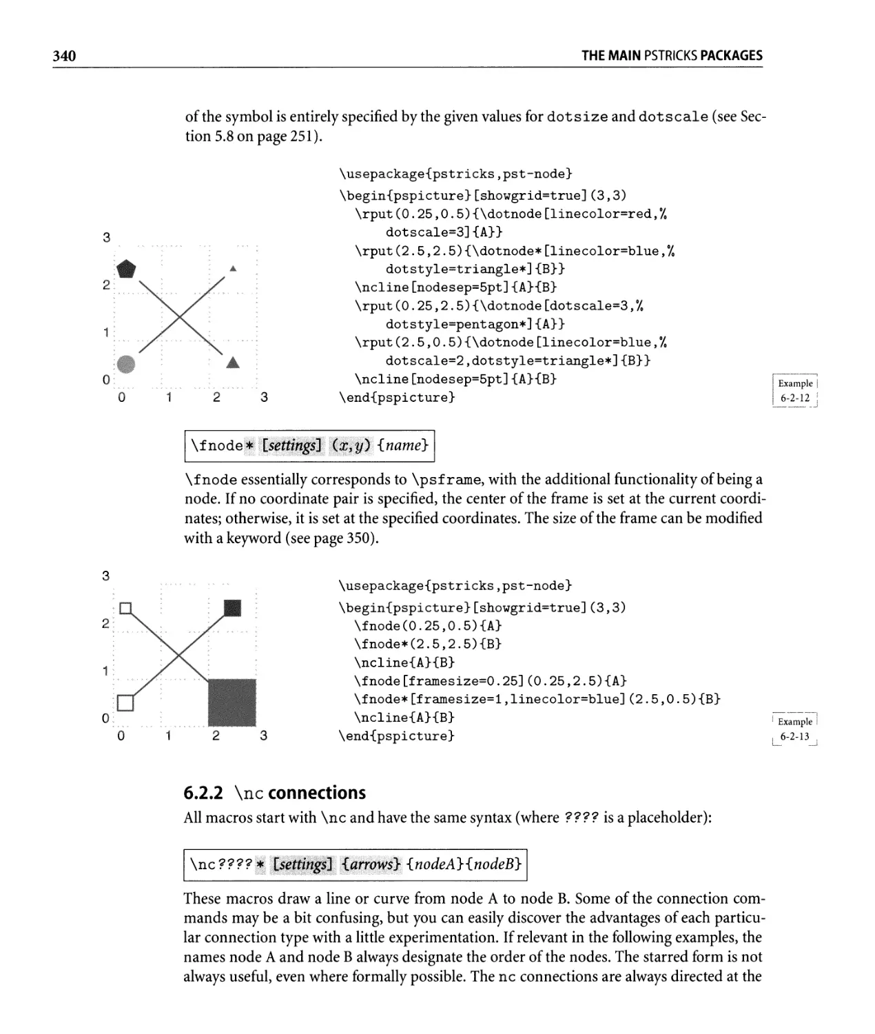
6.2.2 \nc connections . . . . . . . . . . . . . . . . . . . . . . . . . . . . . . .. 340
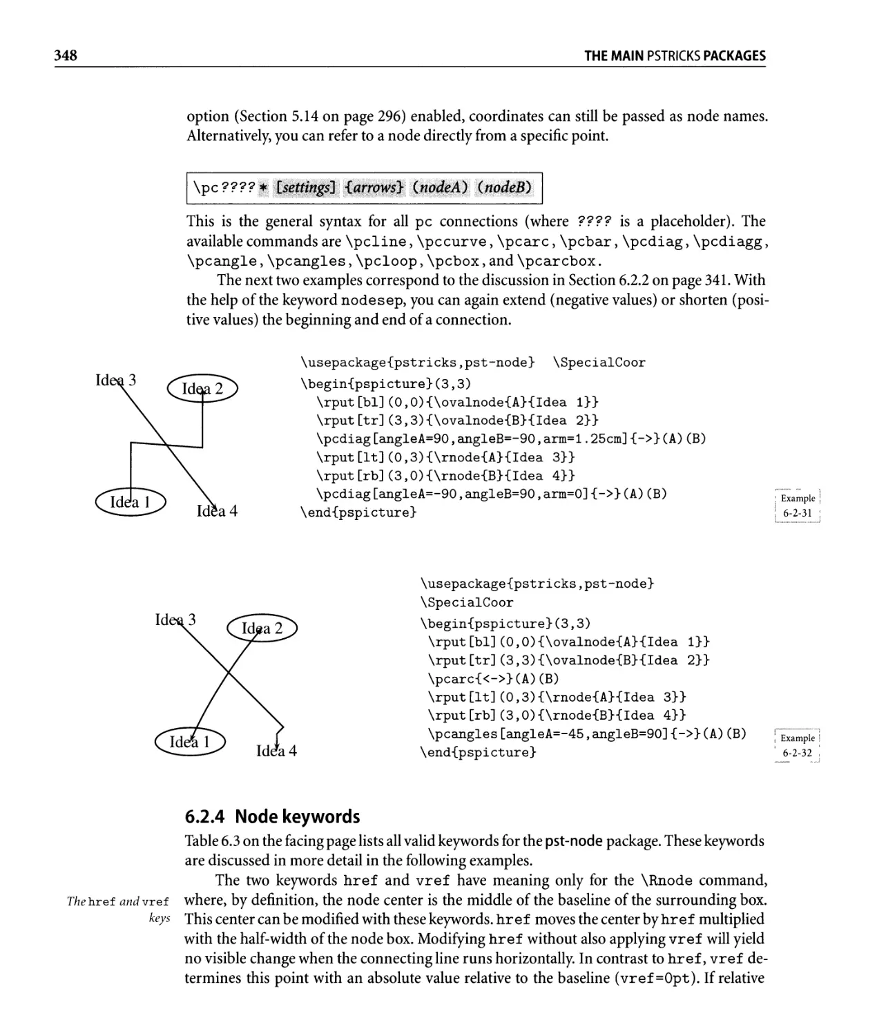
6.2.3 \pc connections . . . . . . . . . . . . . . . . . . . . . . . . . . . . . . .. 347
6.2.4 Node keywords . . . . . . . . . . . . . . . . . . . . . . . . . . . . . . . .. 348
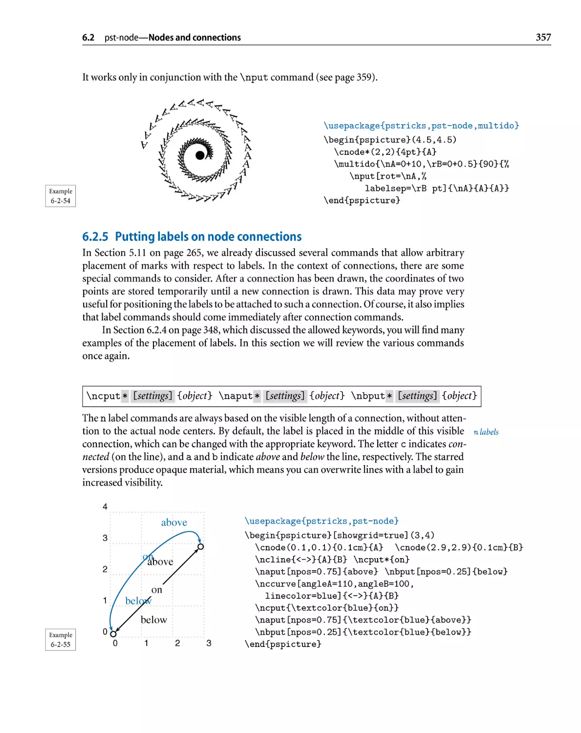
6.2.5 Putting labels on node connections. . . . . . . . . . . . . . . . . . . .. 357
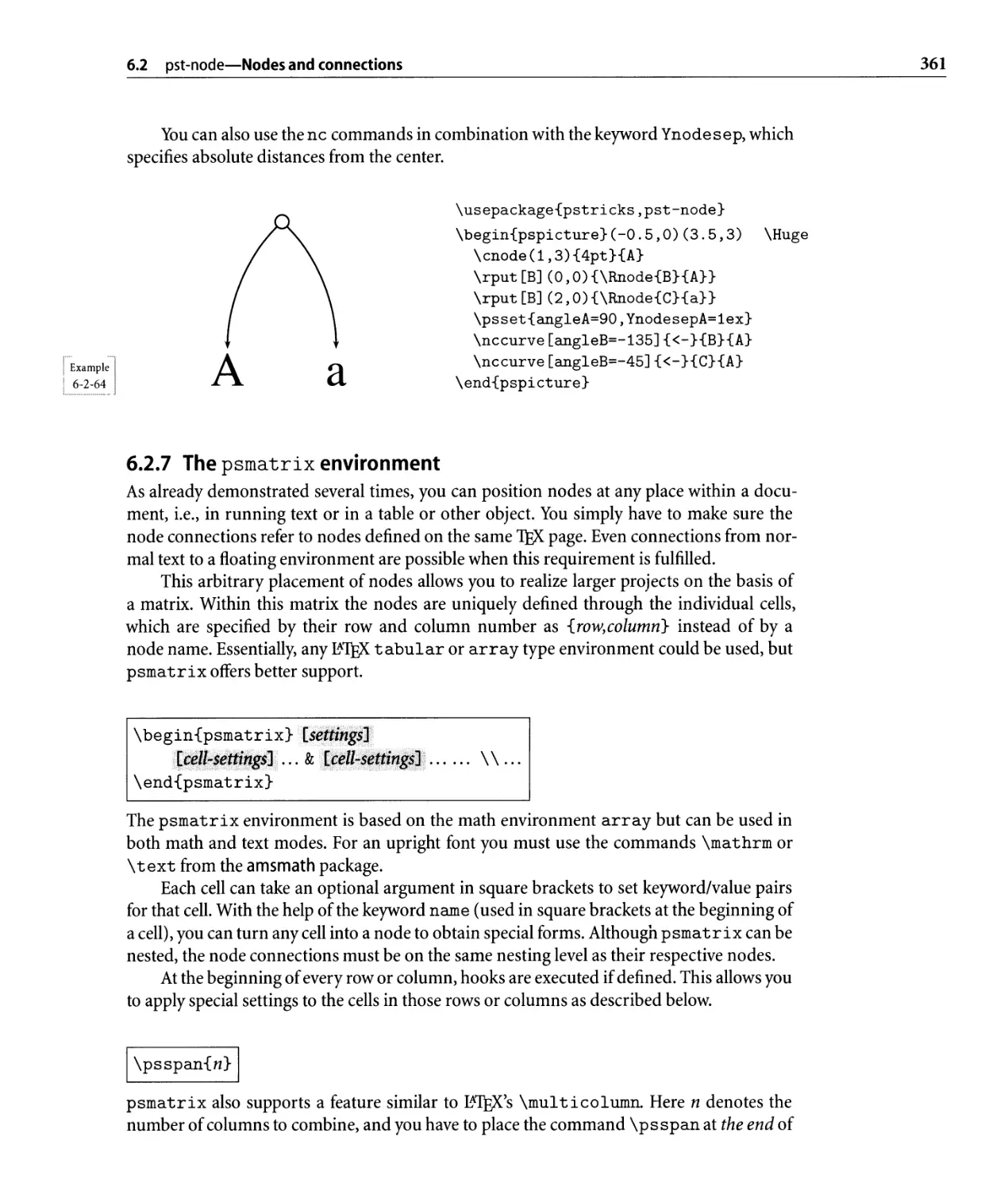
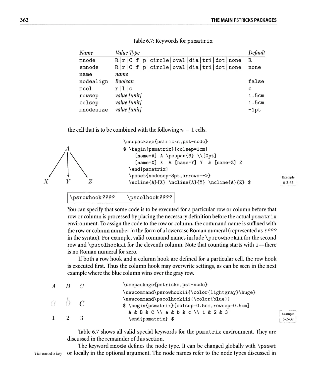
6.2.6 Multiple connections. . . . . . . . . . . . . . . . . . . . . . . . . . . . .. 360
6.2.7 The psmatrix environment. . . . . . . . . . . . . . . . . . . . . . . .. 361
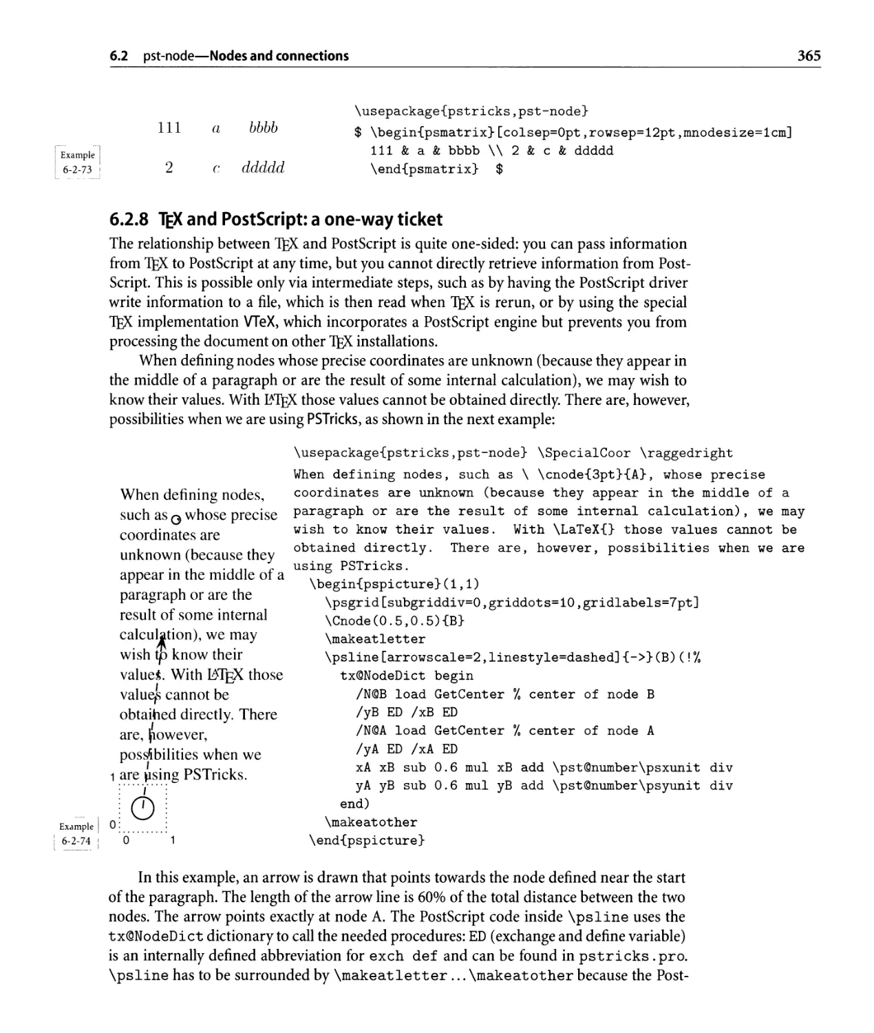
6.2.8 TEX and PostScript: a one-way ticket. . . . . . . . . . . . . . . . . . . .. 365
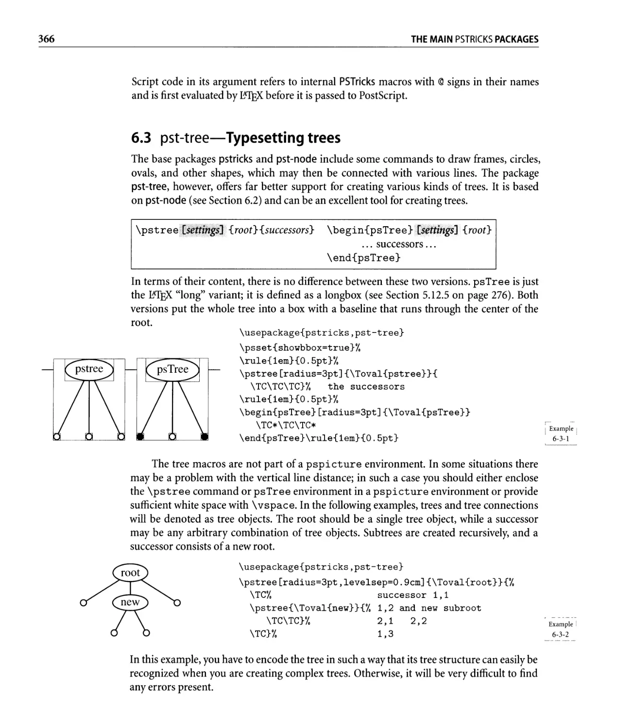
6.3 pst-tree- Typesetting trees . . . . . . . . . . . . . . . . . . . . . . . . . . . . . .. 366
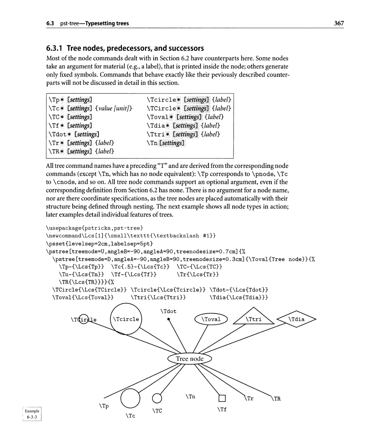
6.3.1 Tree nodes, predecessors, and successors . . . . . . . . . . . . . . . .. 367
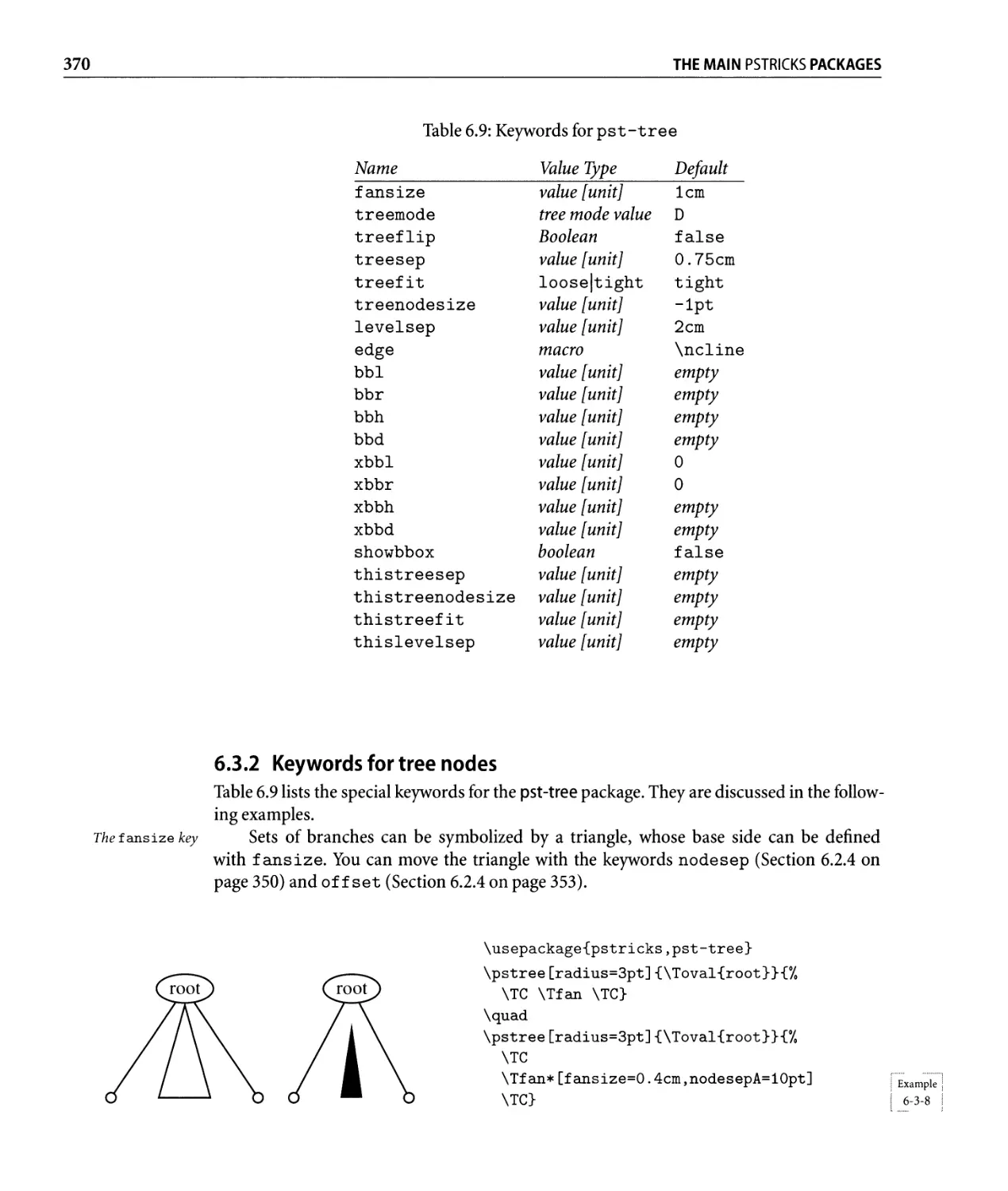
6.3.2 Keywords for tree nodes. . . . . . . . . . . . . . . . . . . . . . . . . . .. 370
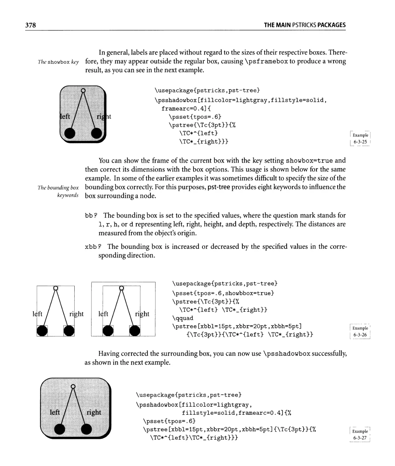
6.3.3 labels . . . . . . . . . . . . . . . . . . . . . . . . . . . . . . . . . . . . . .. 379
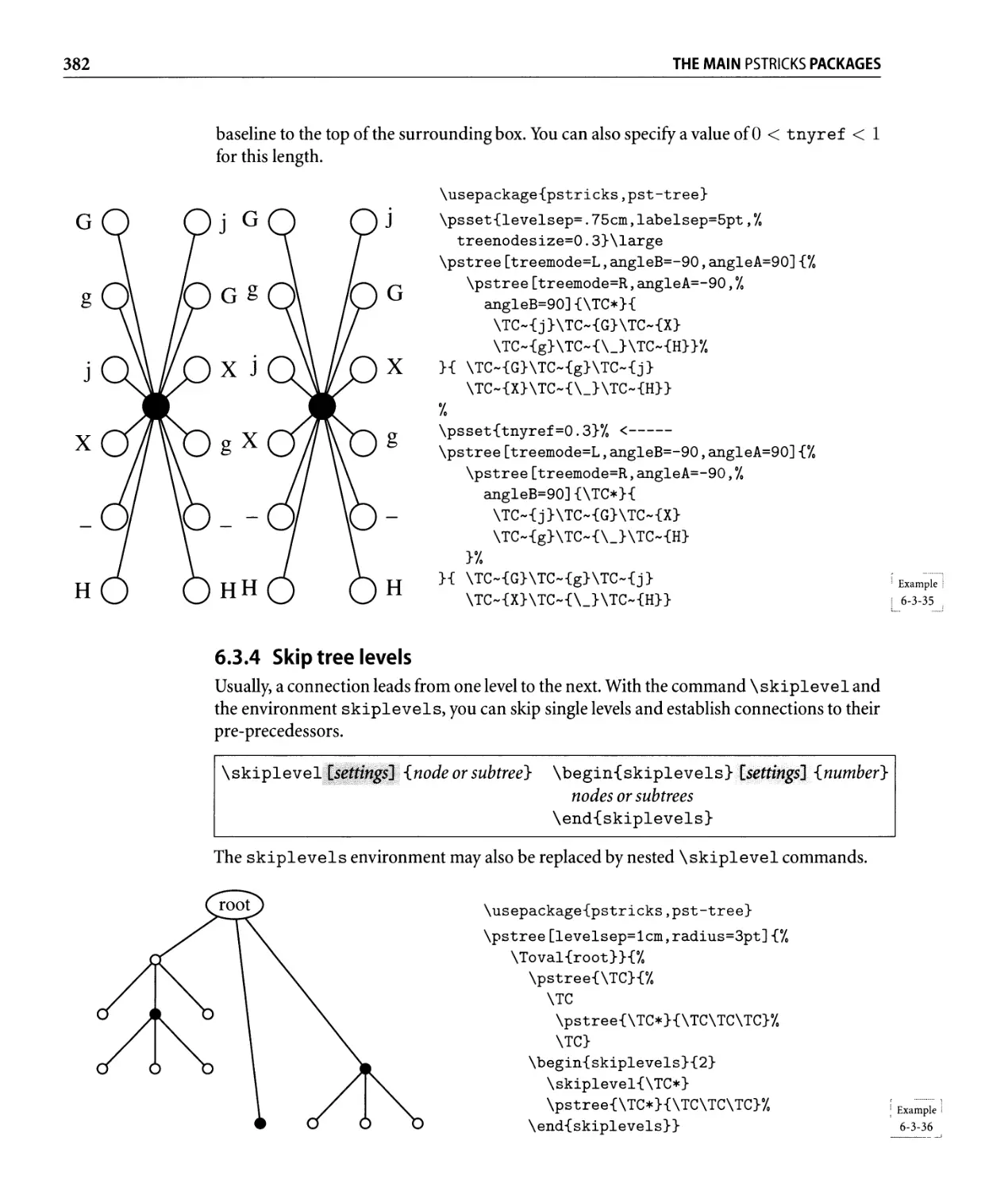
6.3.4 Skip tree levels. . . . . . . . . . . . . . . . . . . . . . . . . . . . . . . . .. 382
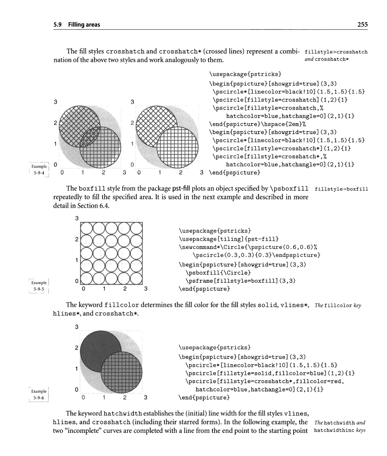
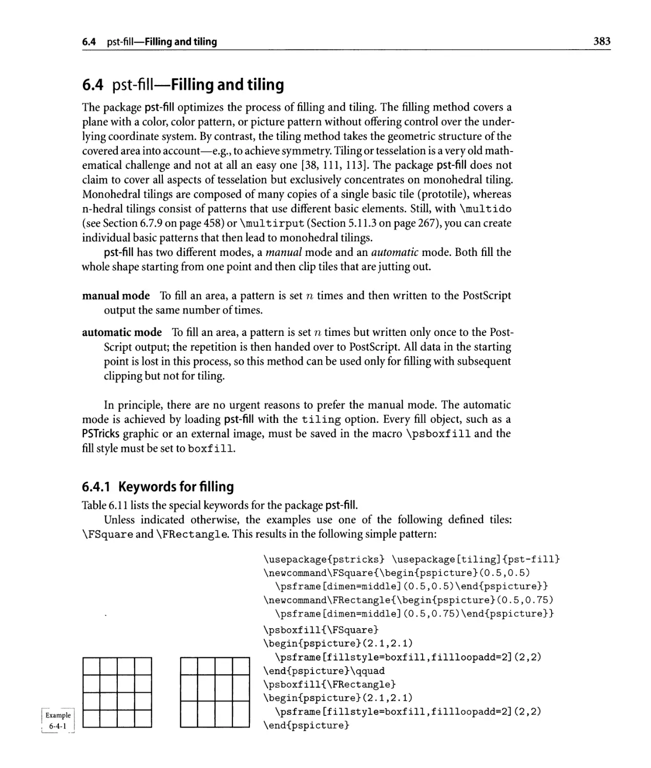
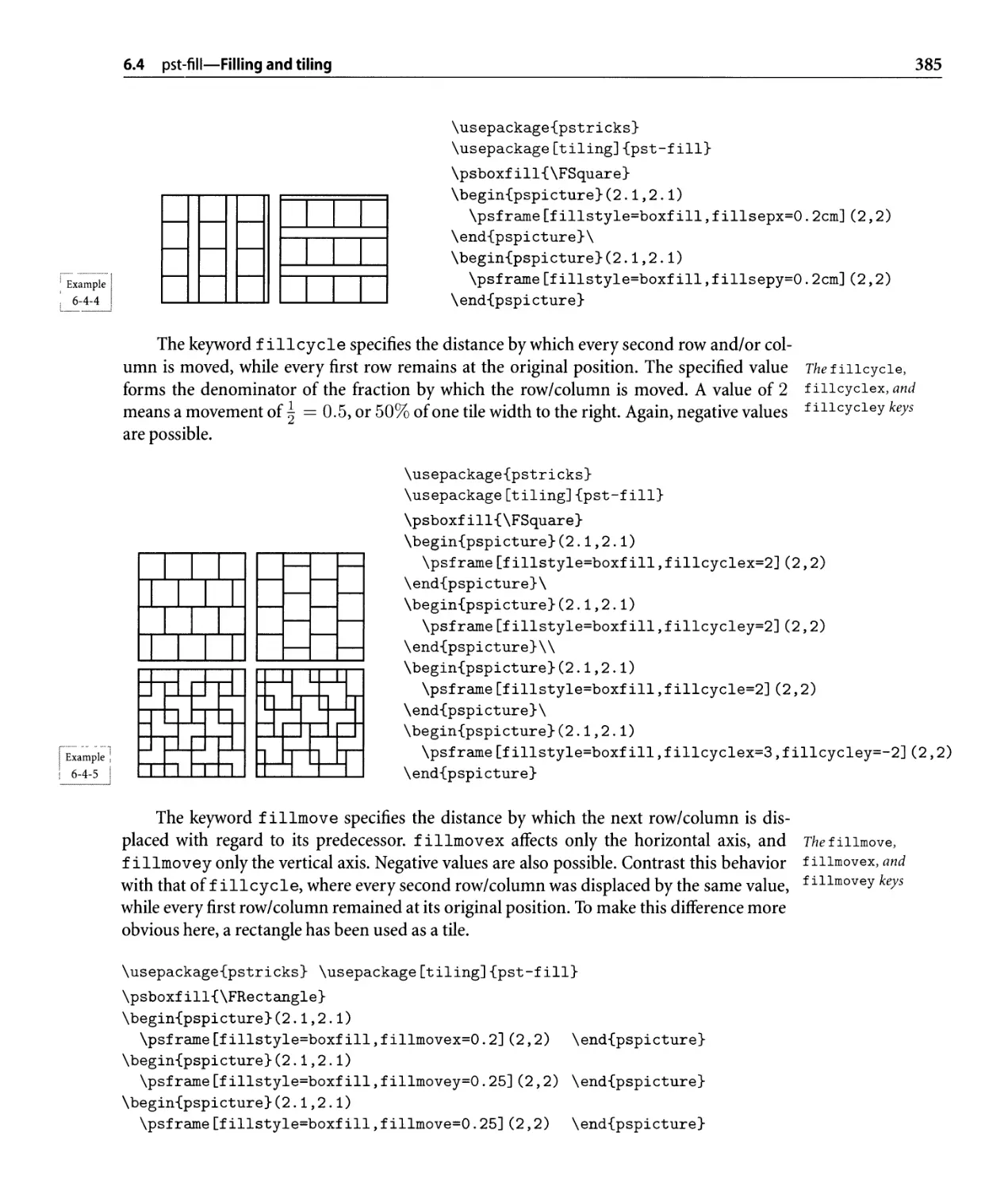
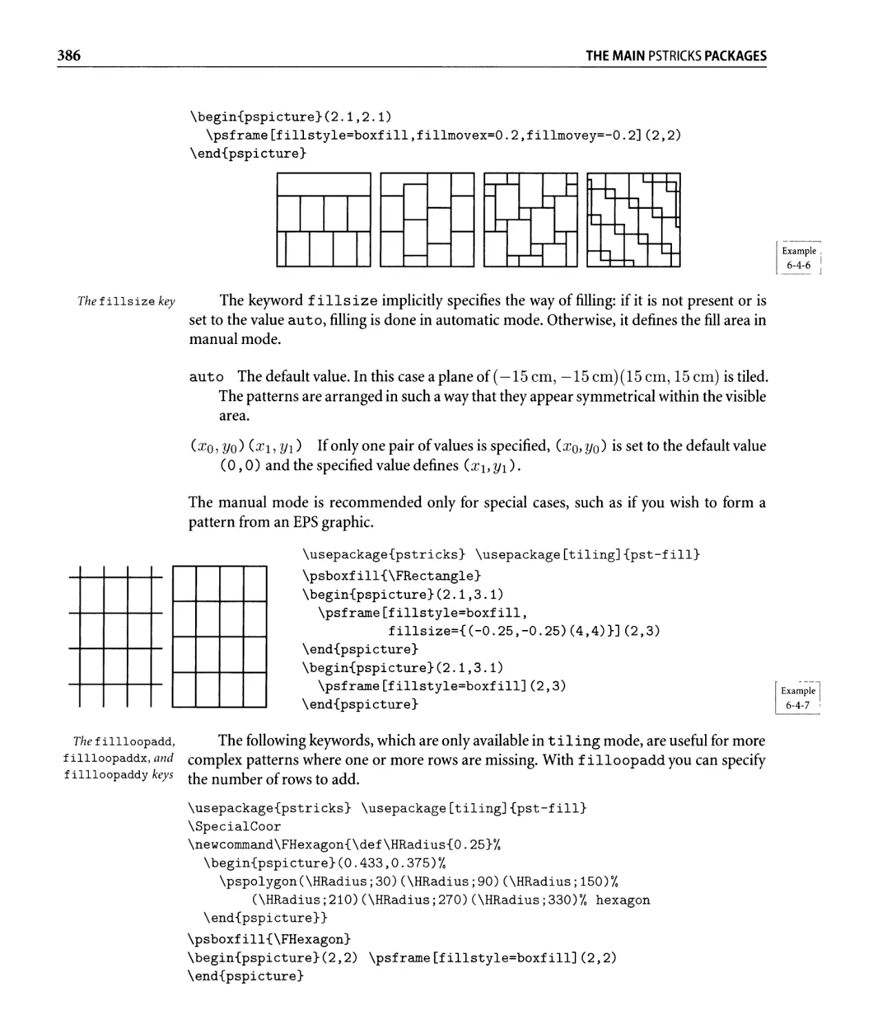
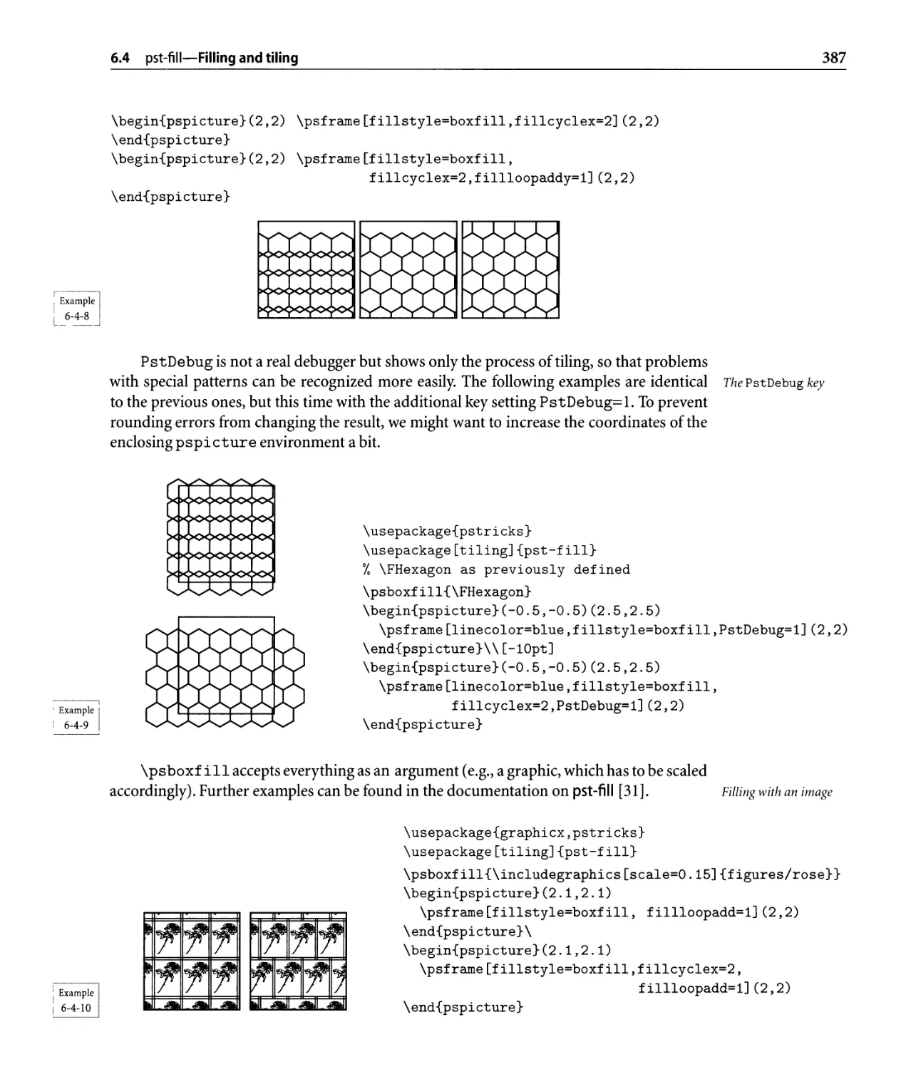
6.4 pst-fill-Filling and tiling. . . . . . . . . . . . . . . . . . . . . . . . . . . . . . . .. 383
6.4.1 Keywords for filling. . . . . . . . . . . . . . . . . . . . . . . . . . . . . .. 383
xii
CONTENTS
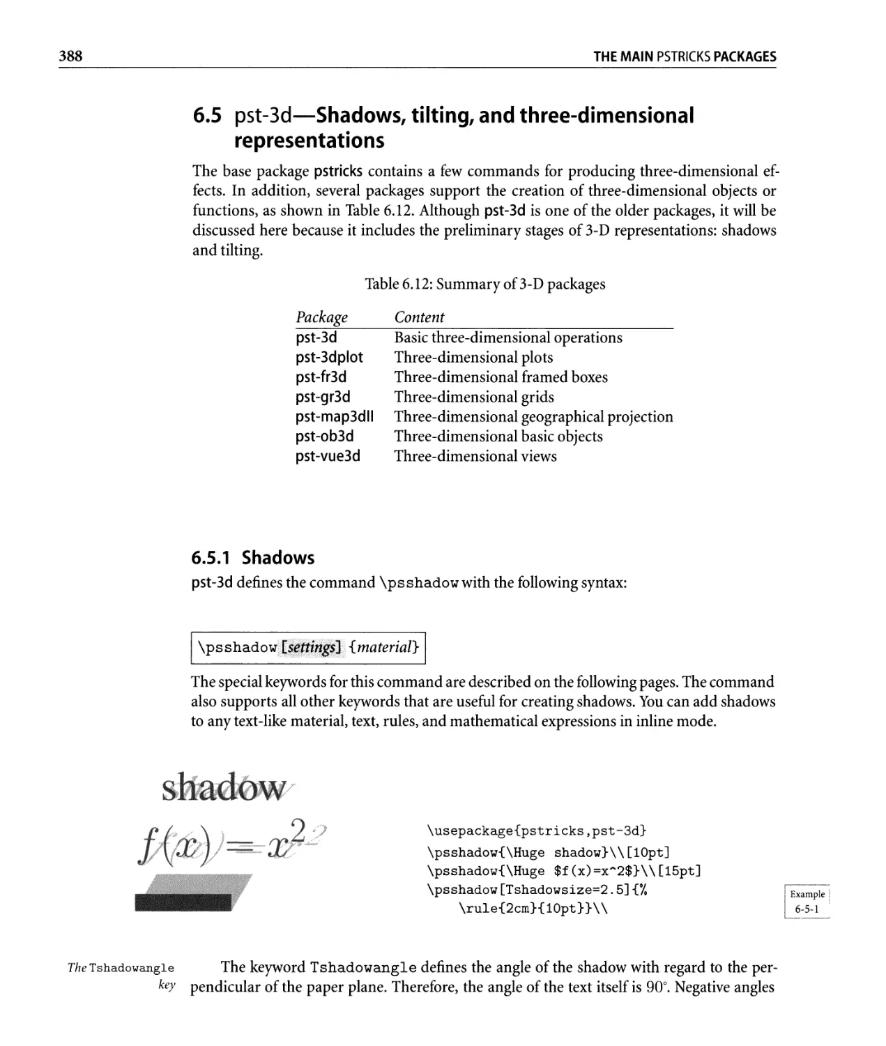
6.5 pst-3d-Shadows, tilting, and three-dimensional representations . . . . . .. 388
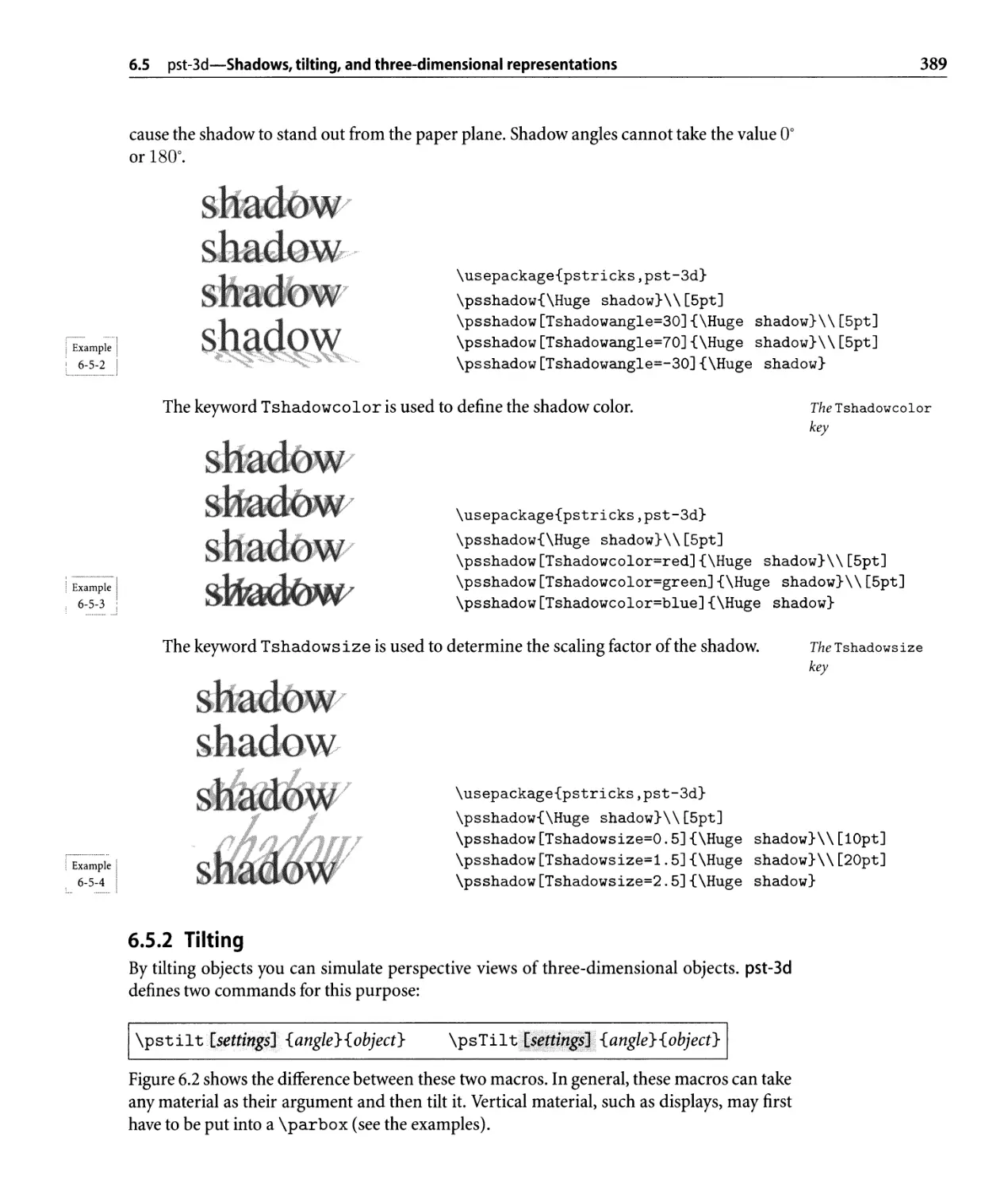
6.5.1 Shadows. . . . . . . . . . . . . . . . . . . . . . . . . . . . . . . . . . . .. 388
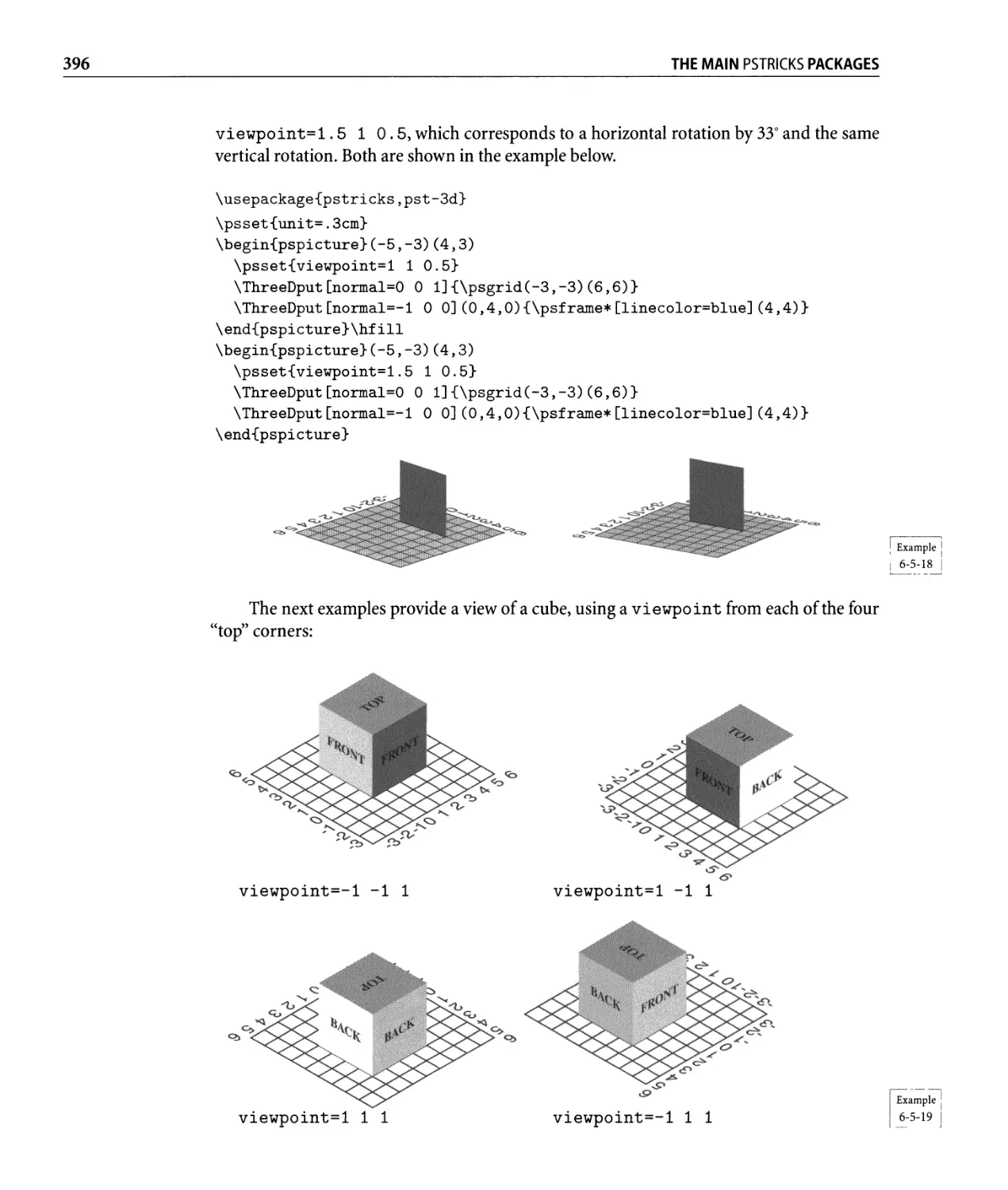
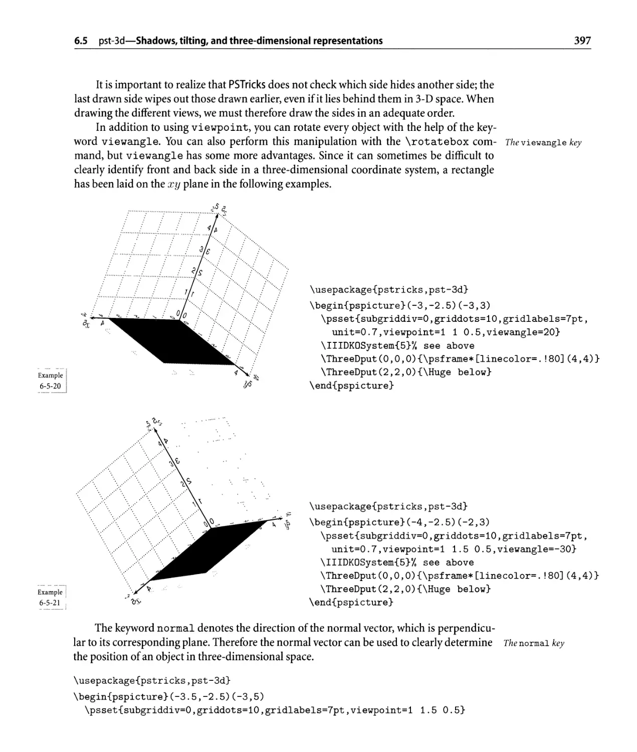
6.5.2 Tilting....................................... 389
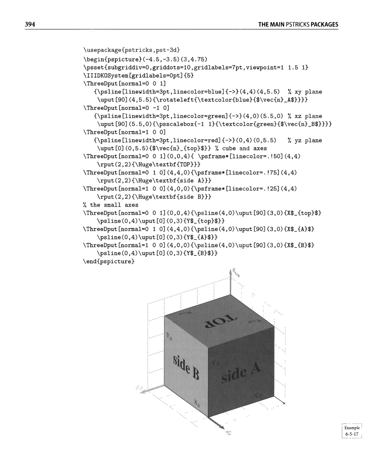
6.5.3 Three-dimensional representations. . . . . . . . . . . . . . . . . . . .. 392
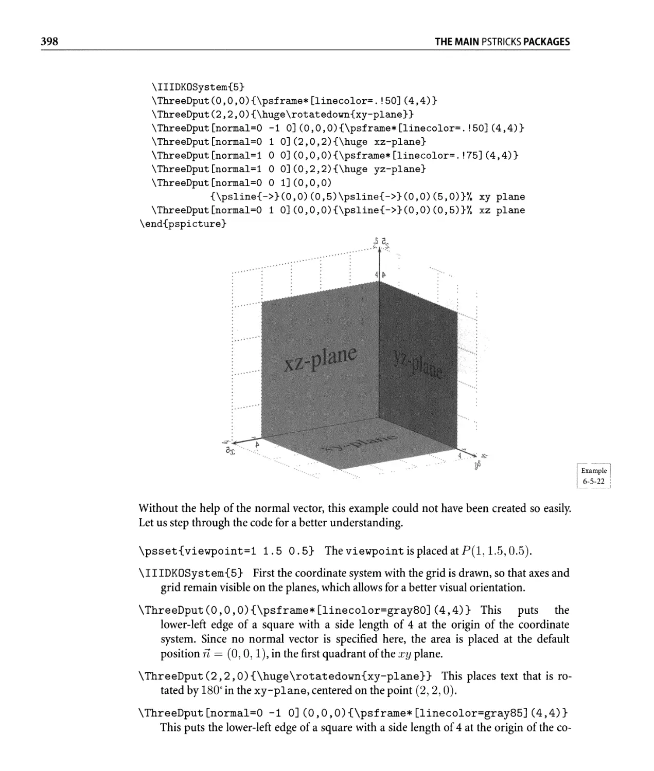
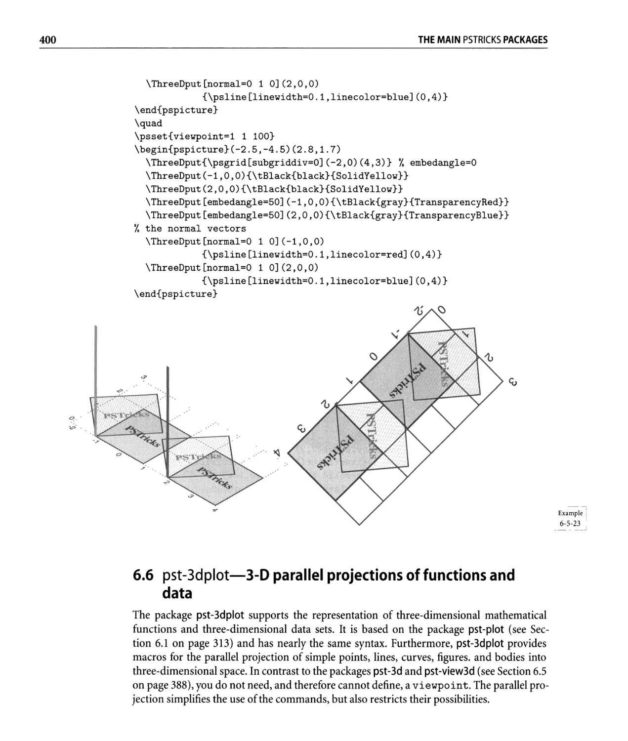
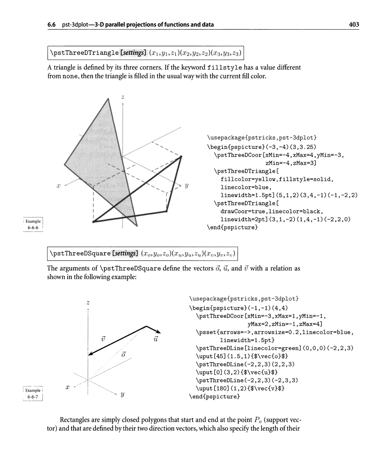
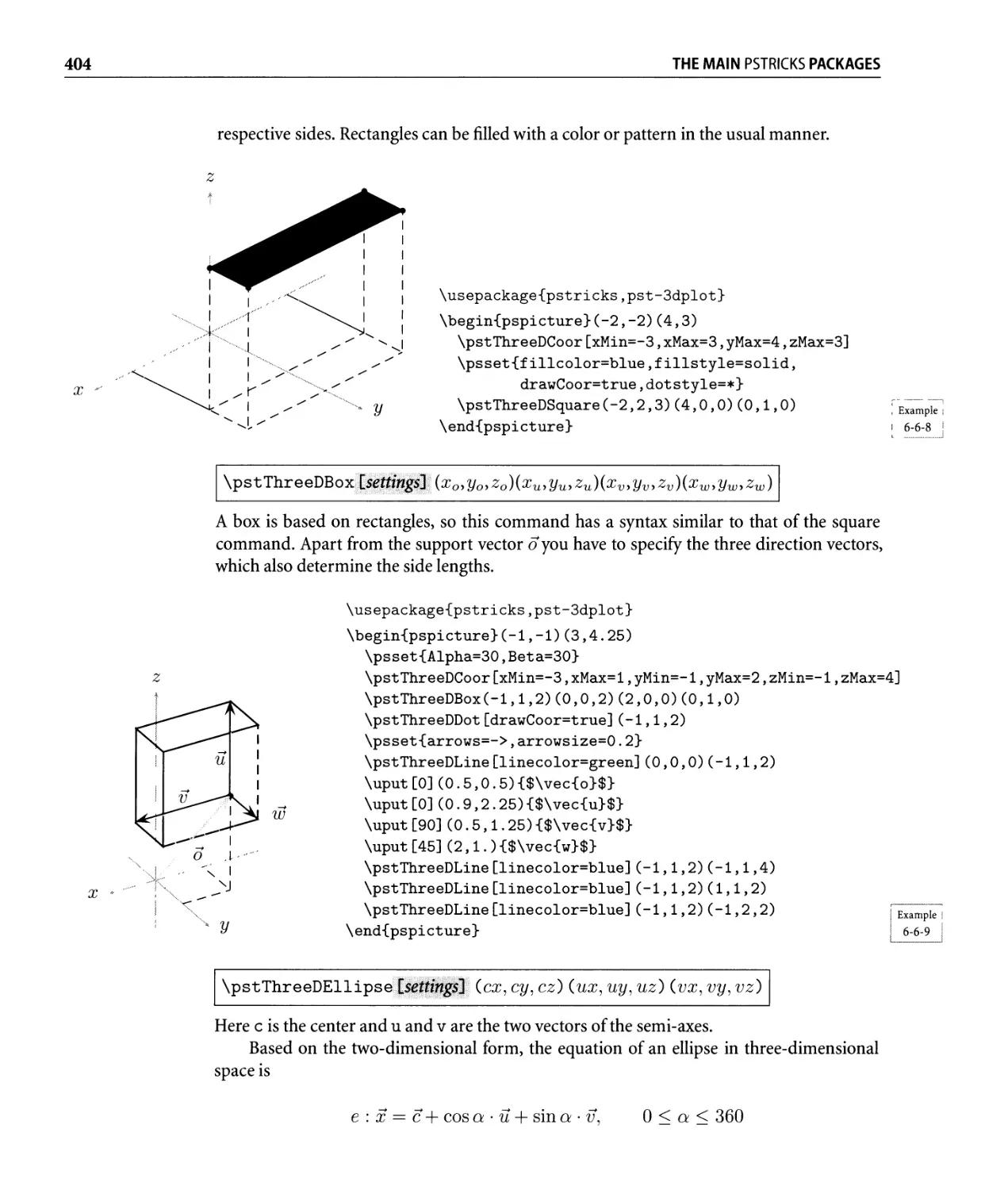
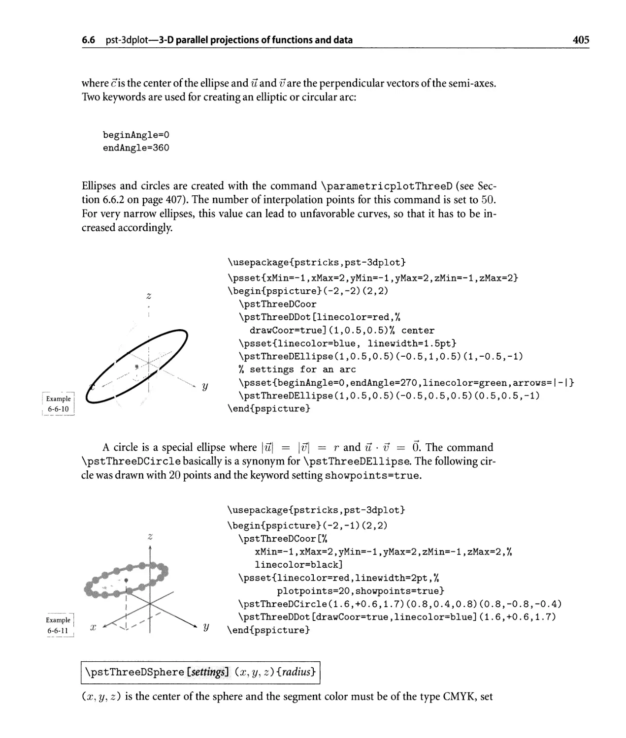
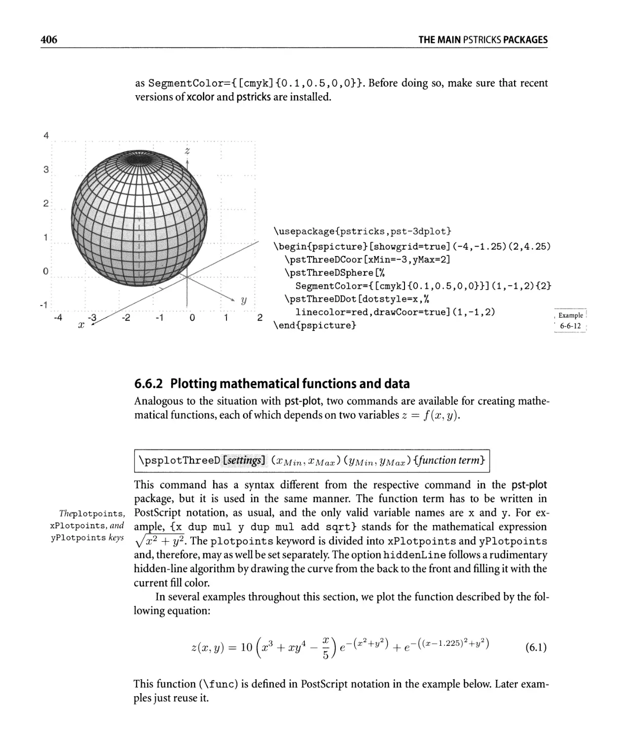
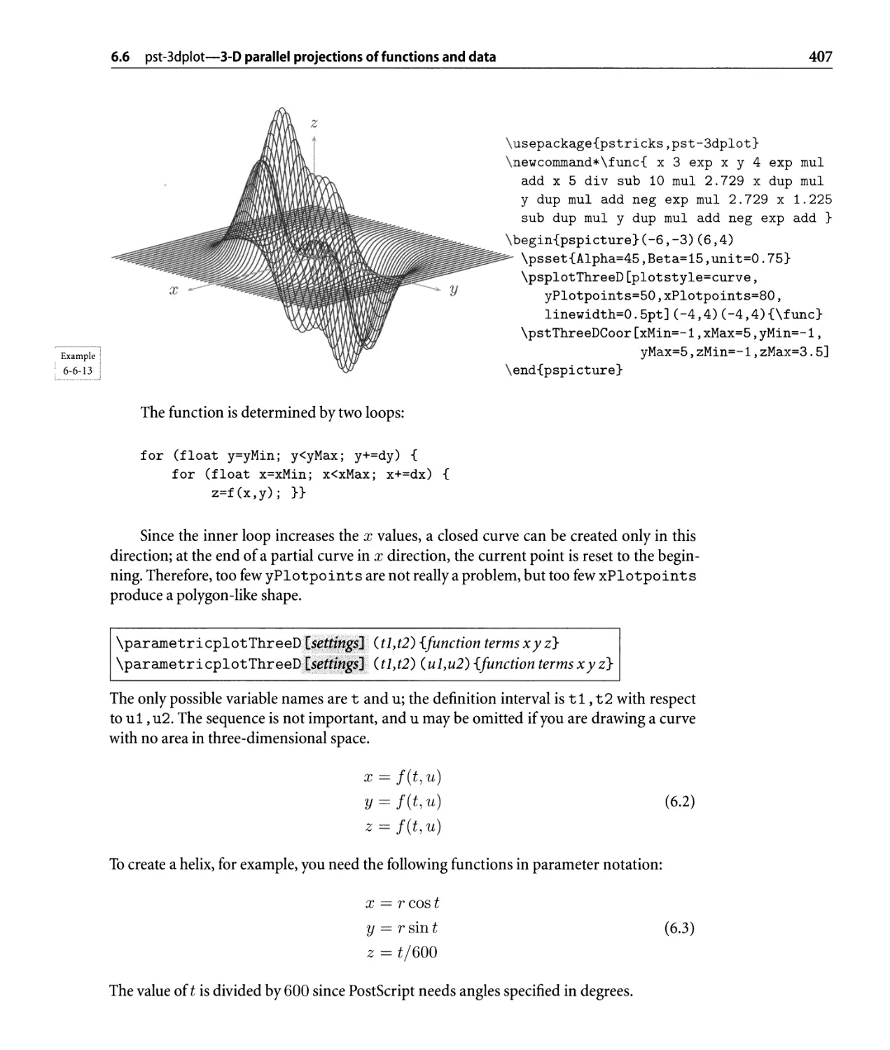
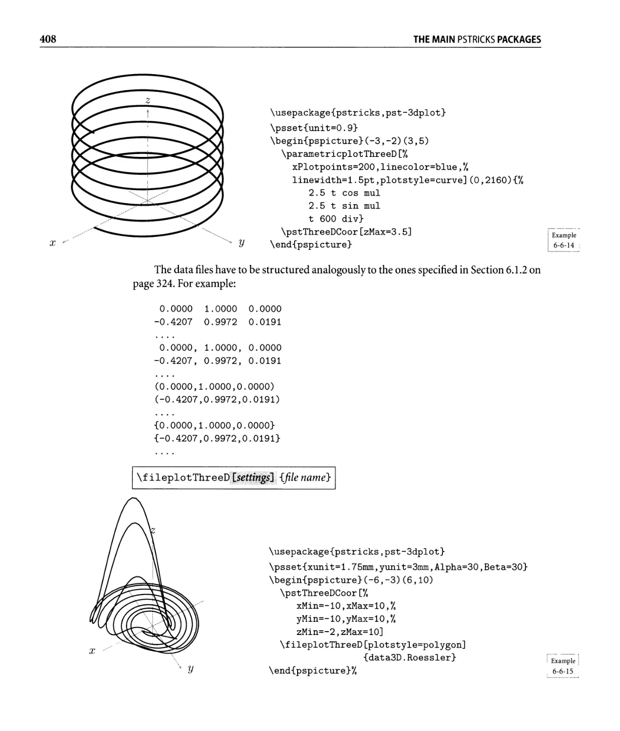
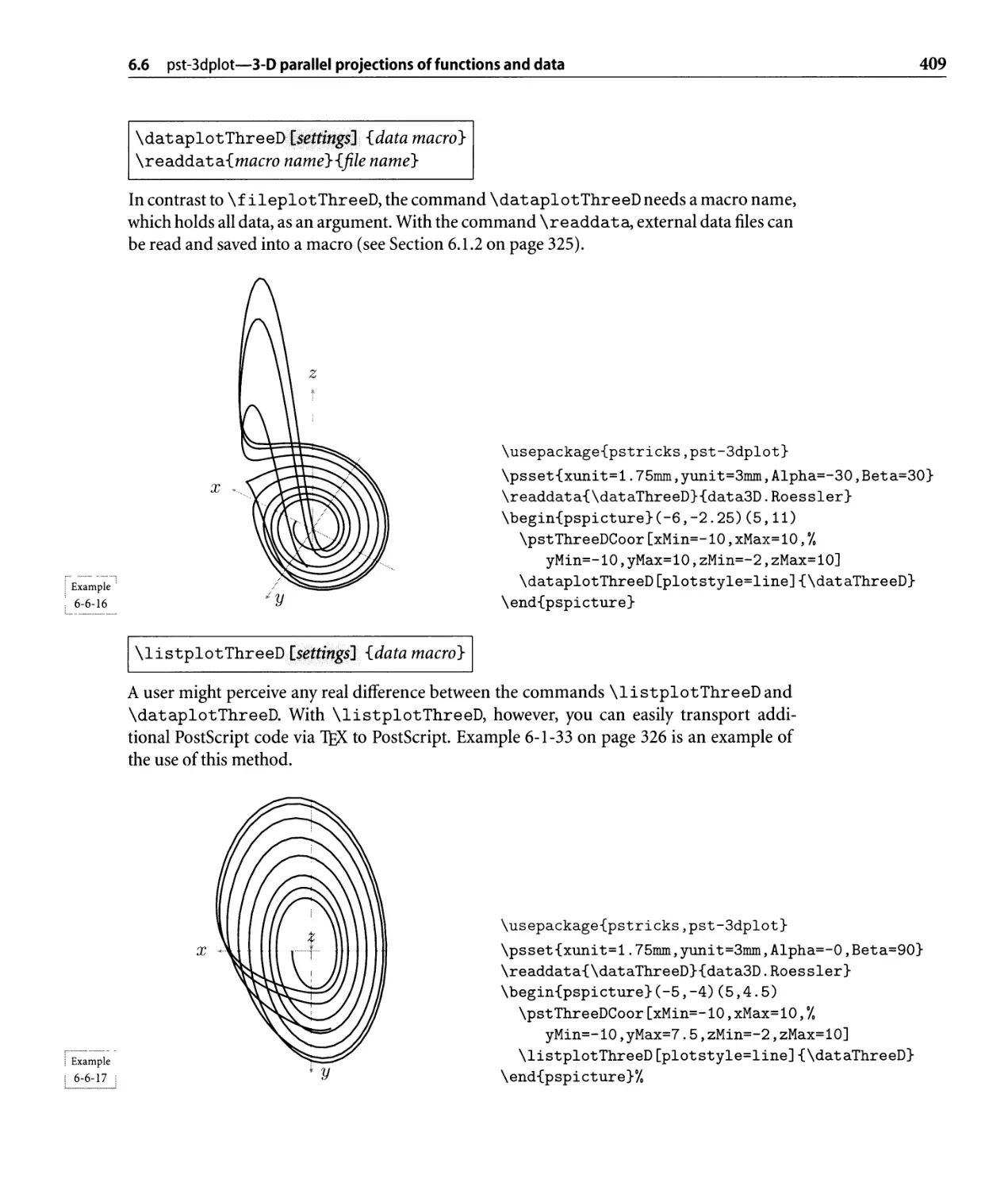
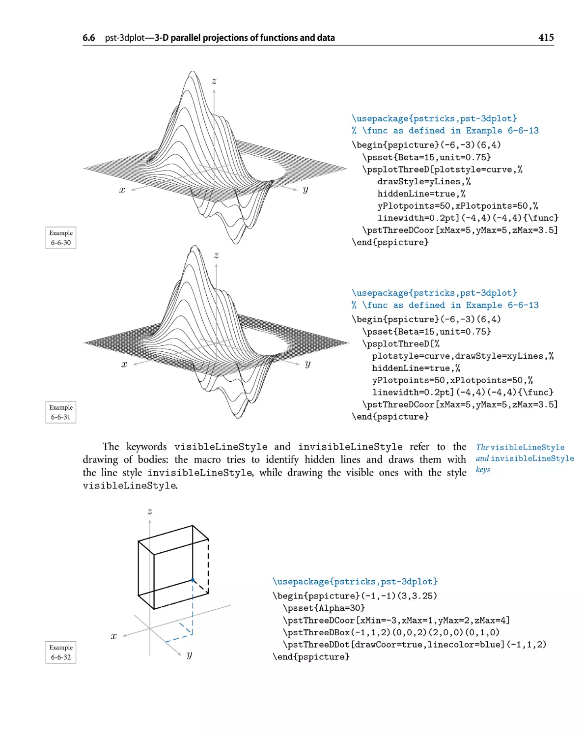
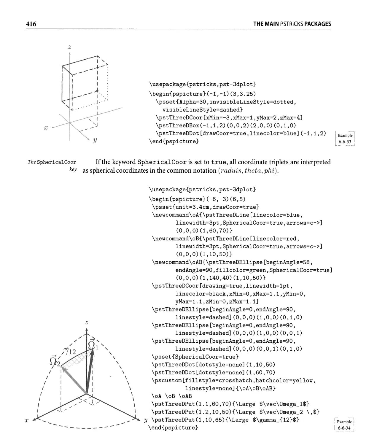
6.6 pst-3dplot-3-D parallel projections of functions and data. . . . . . . . . . .. 400
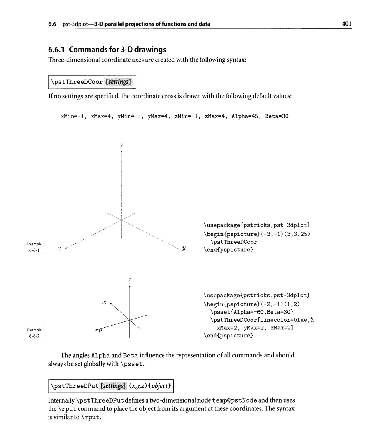
6.6.1 Commands for 3-D drawings. . . . . . . . . . . . . . . . . . . . . . . .. 401
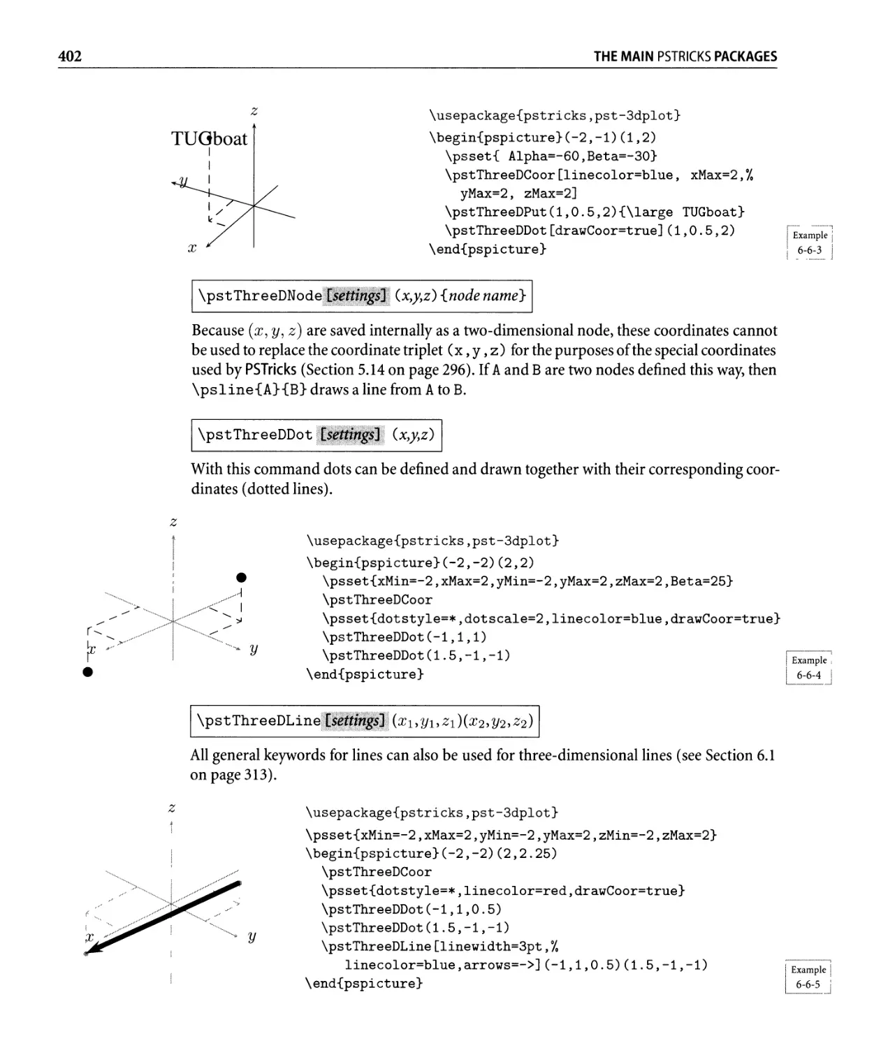
6.6.2 Plotting mathematical functions and data. . . . . . . . . . . . . . . .. 406
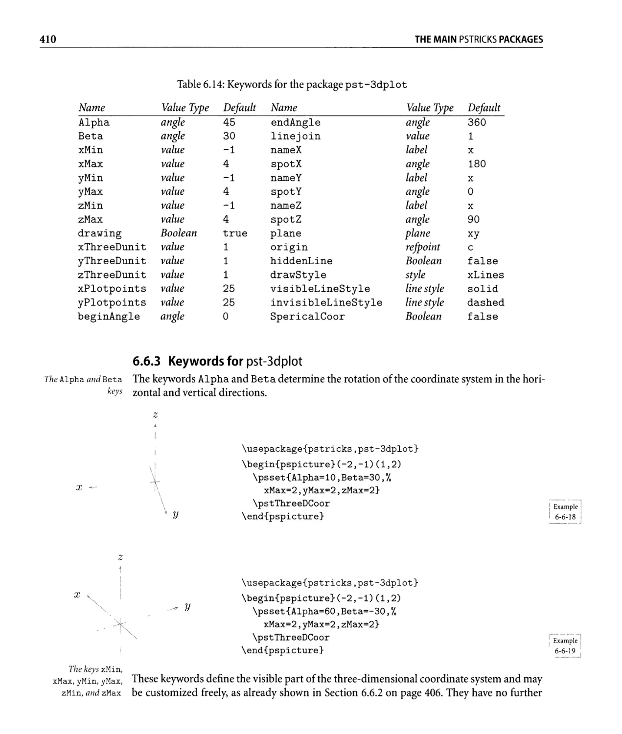
6.6.3 Keywords for pst-3dplot. . . . . . . . . . . . . . . . . . . . . . . . . . .. 410
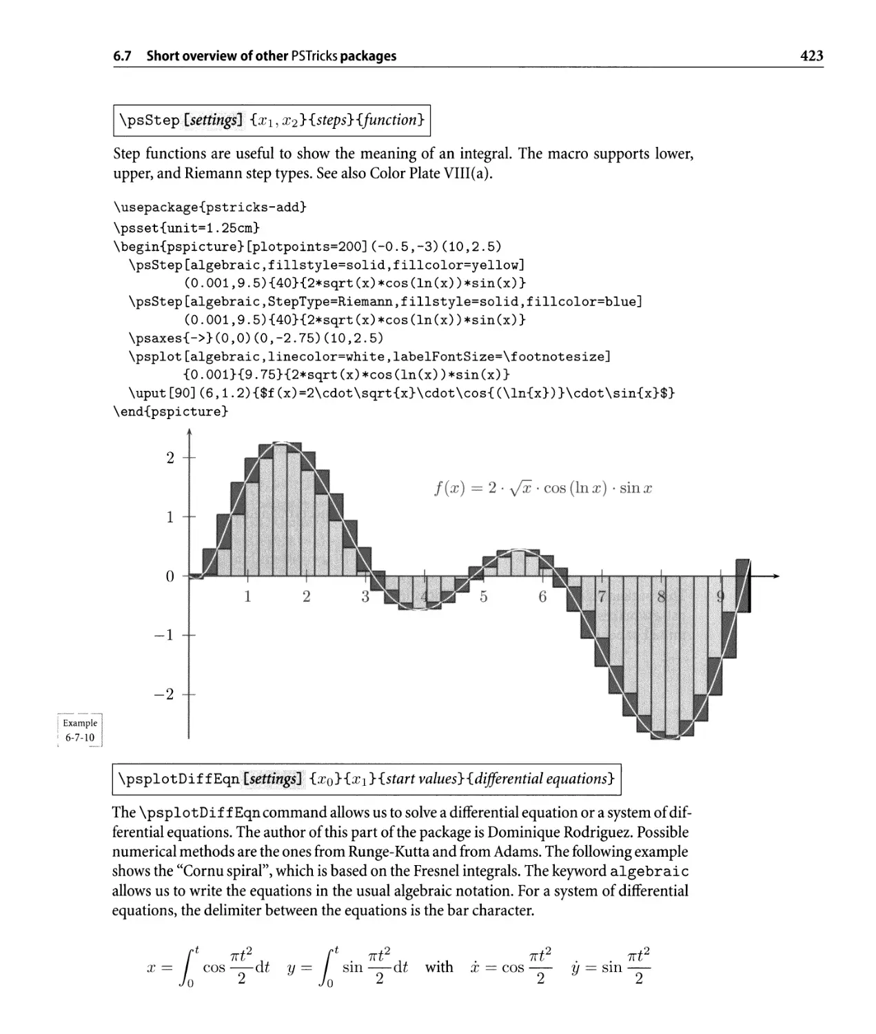
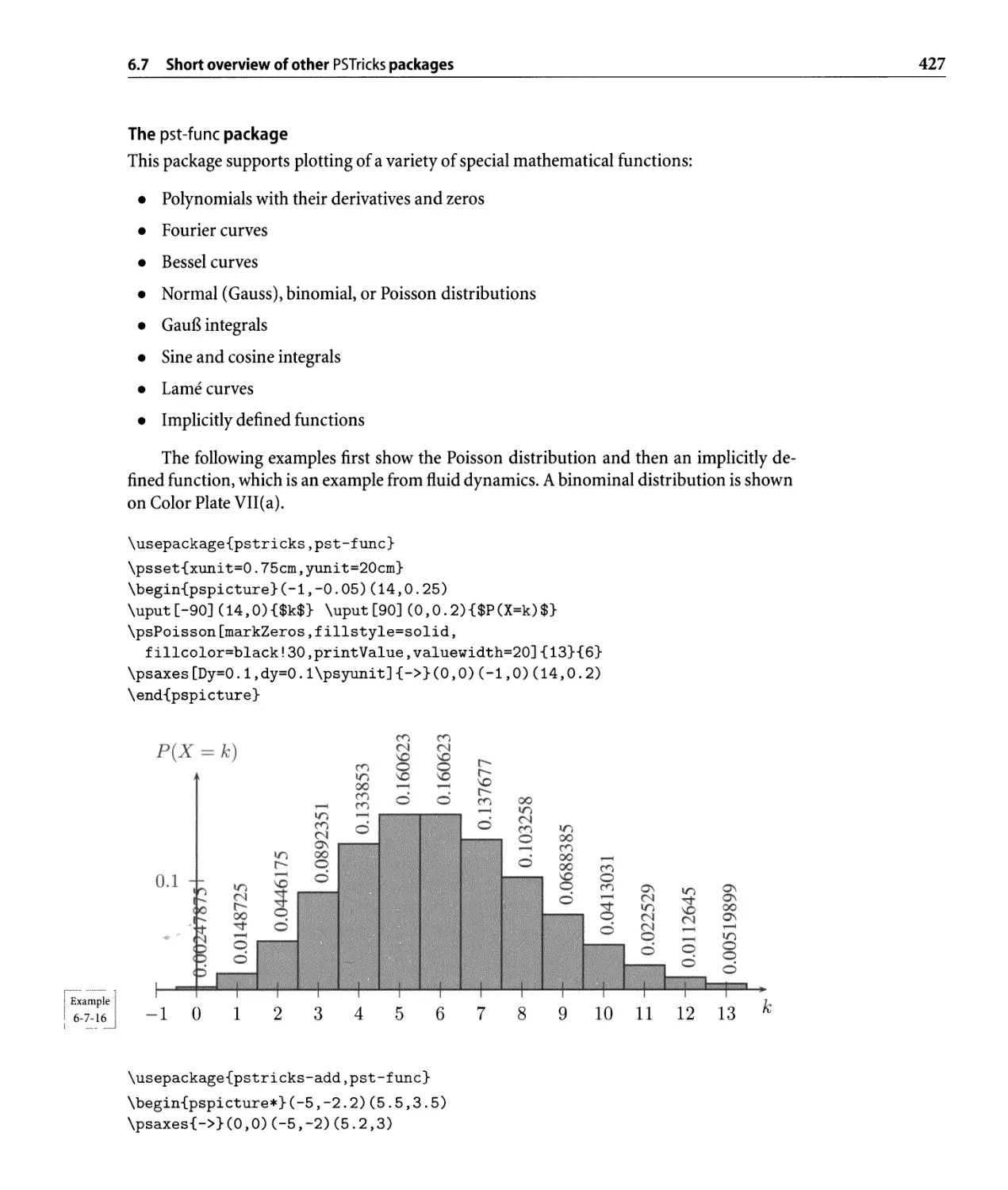
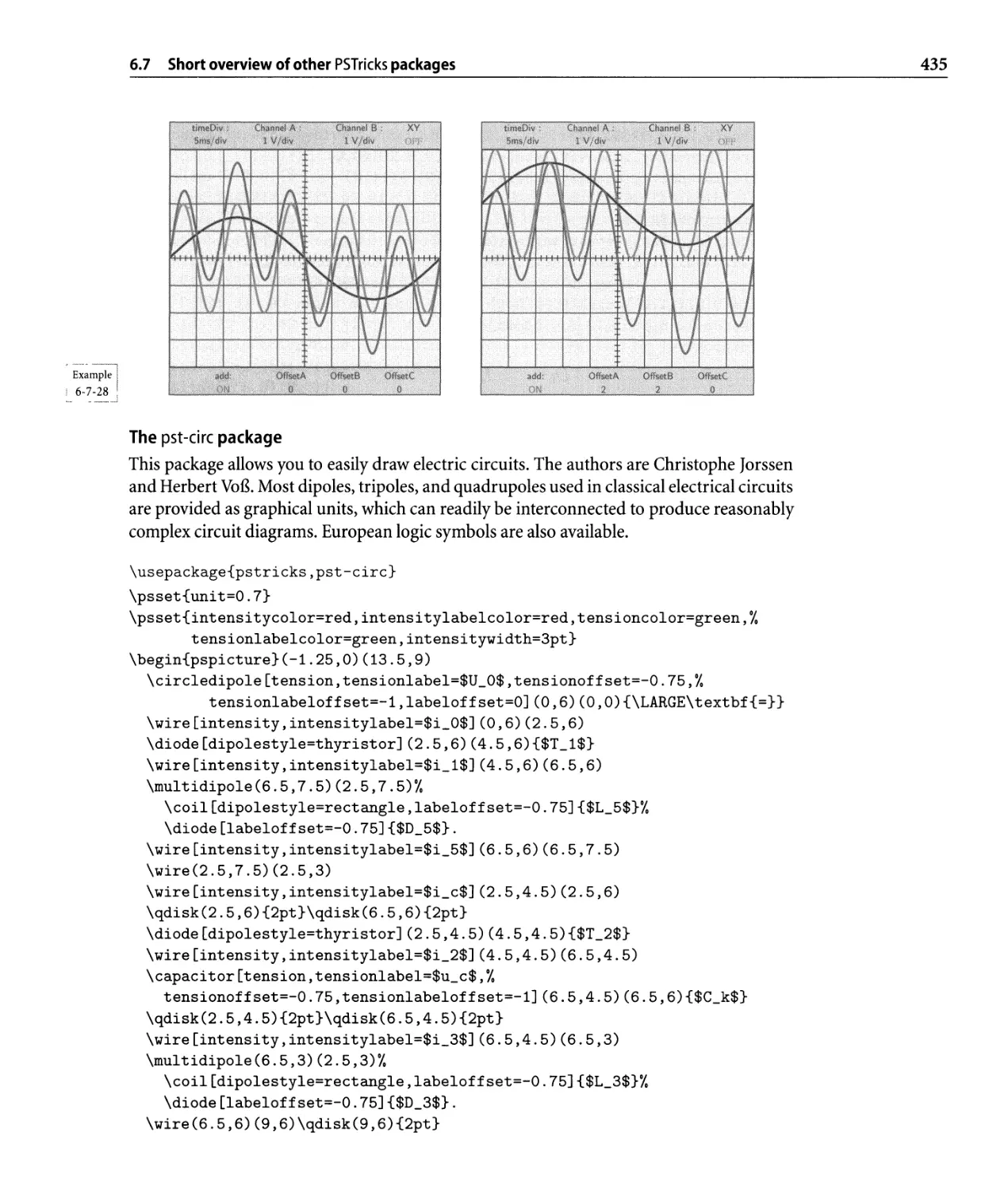
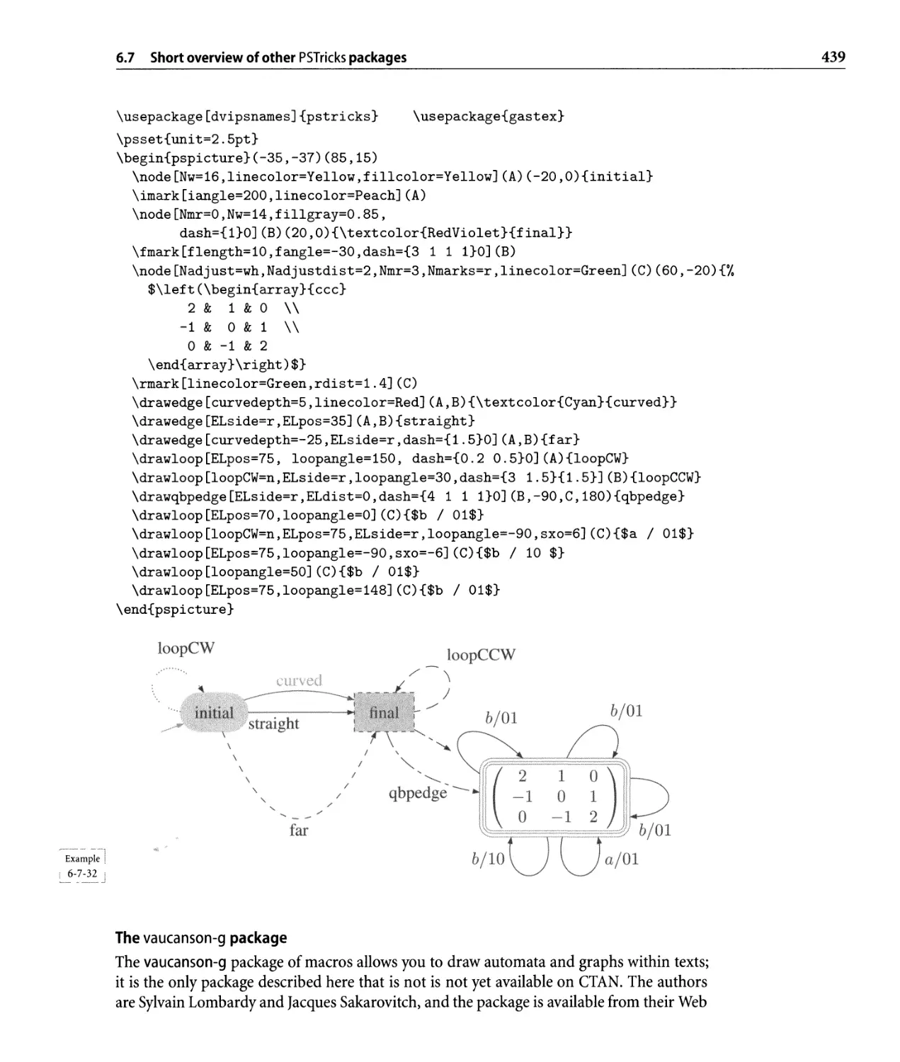
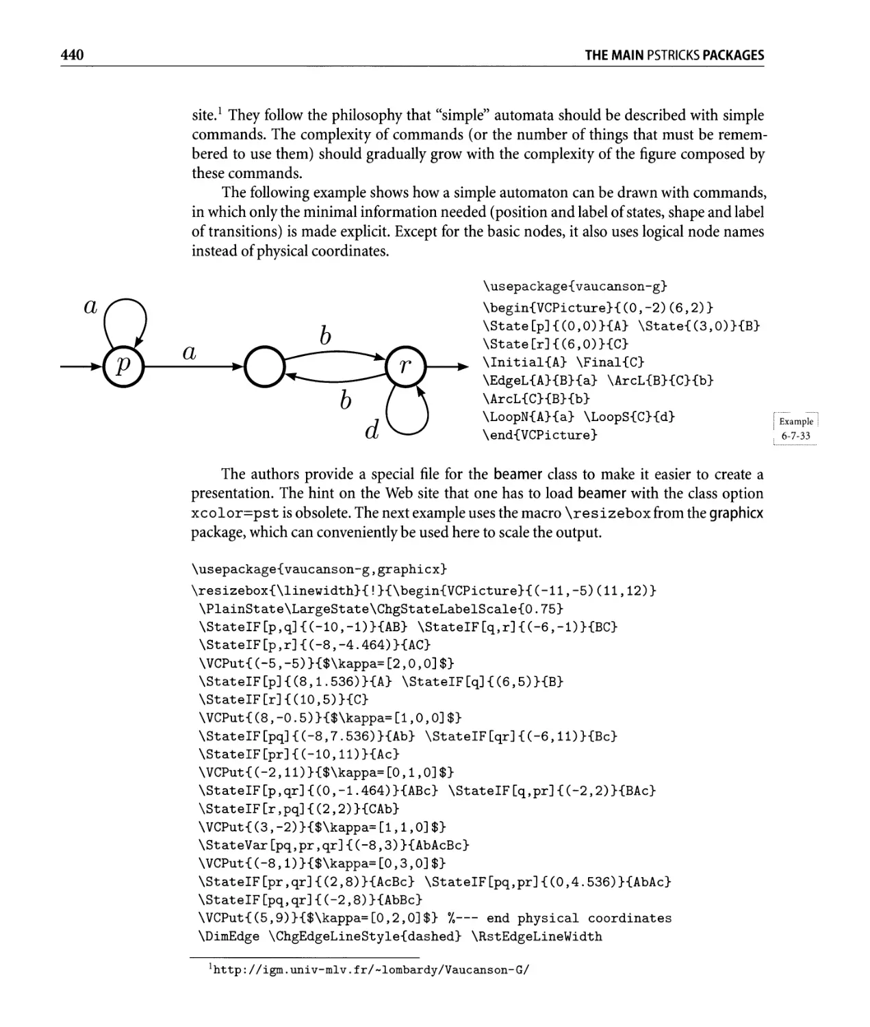
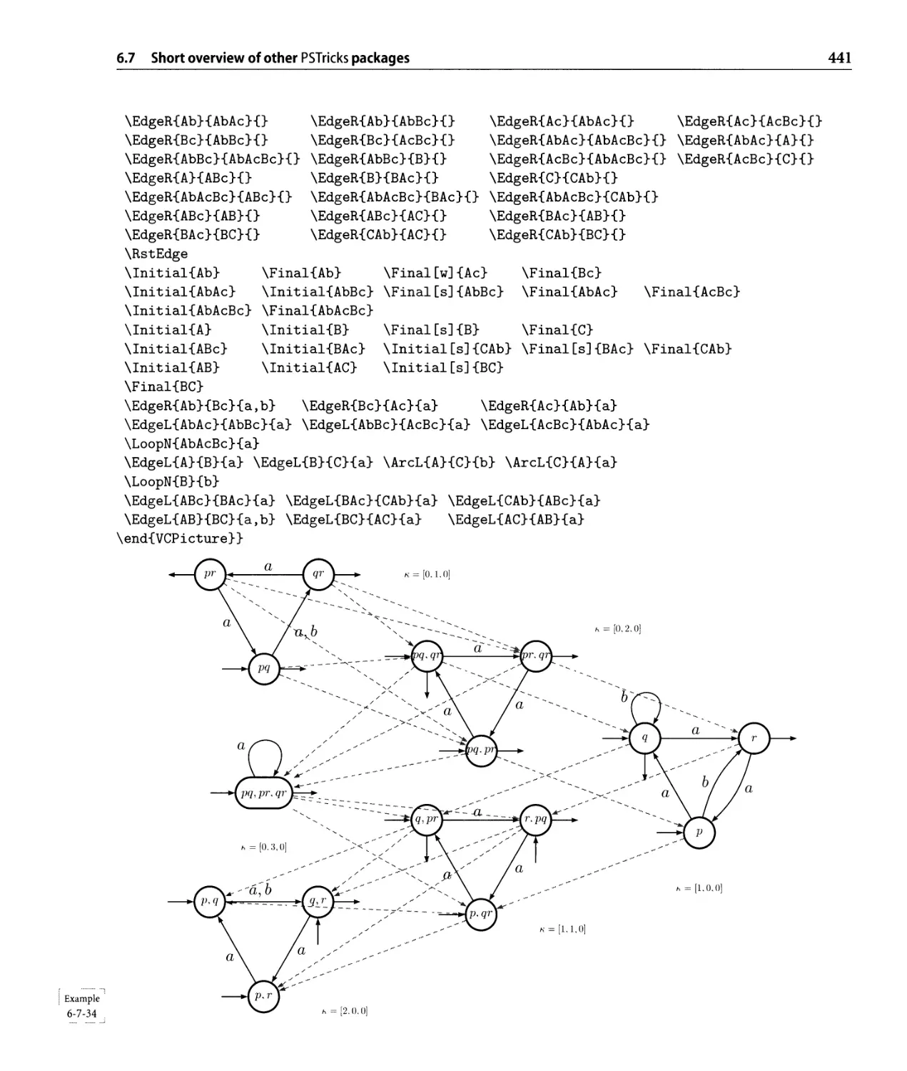
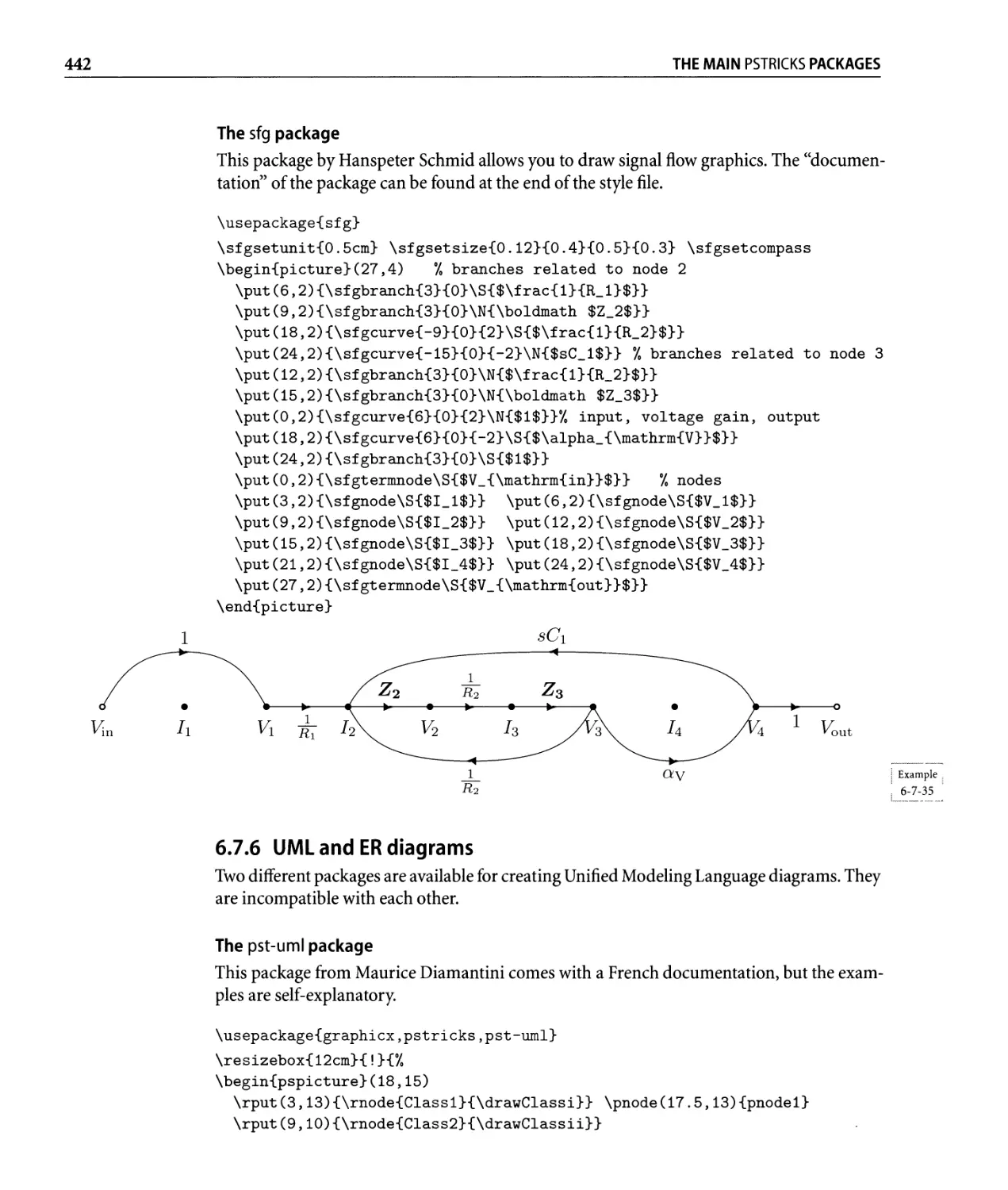
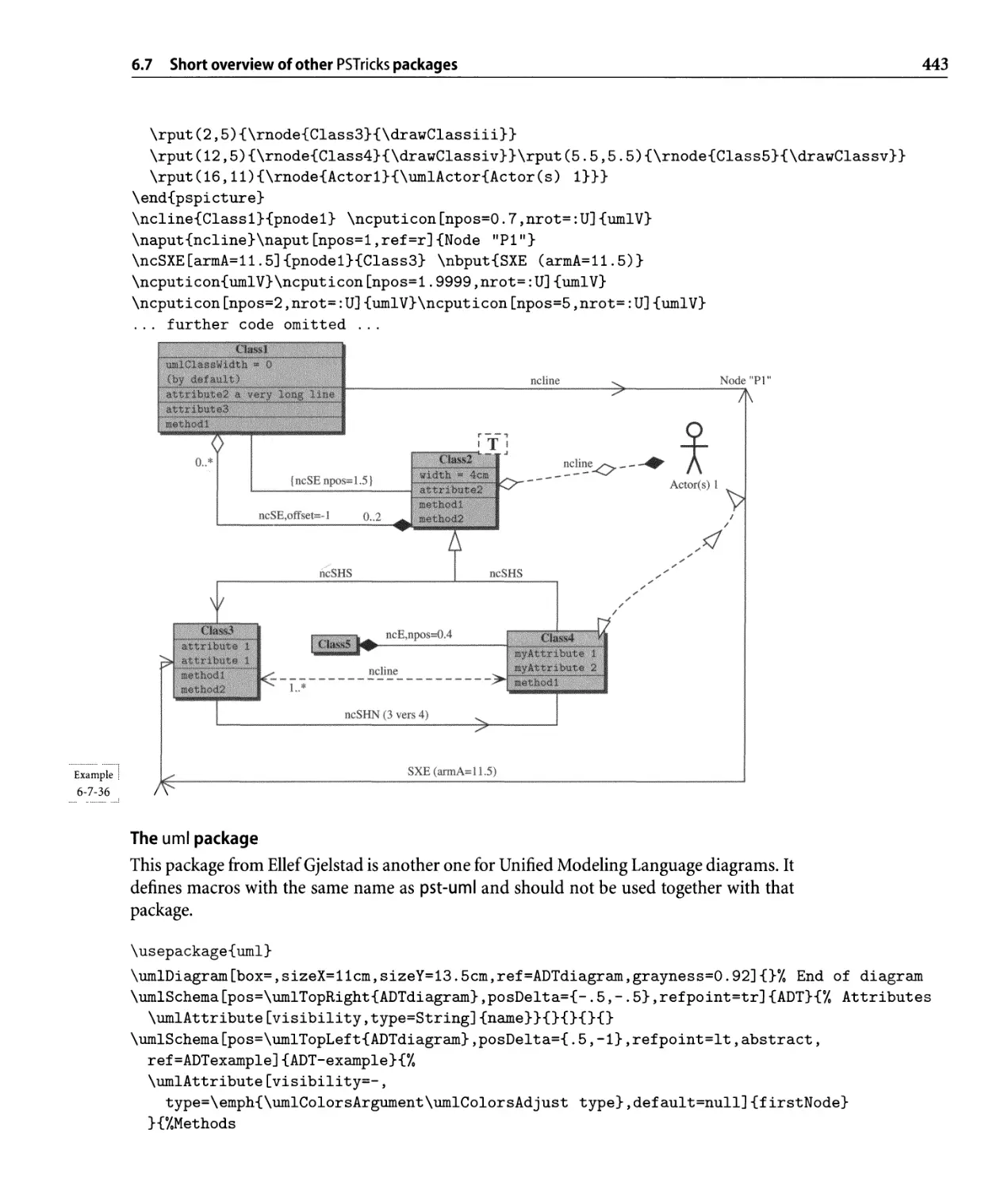
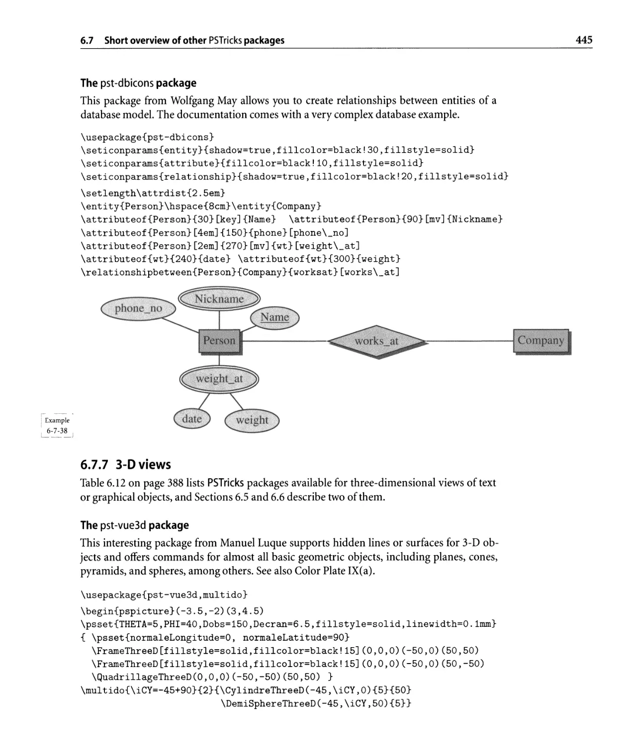
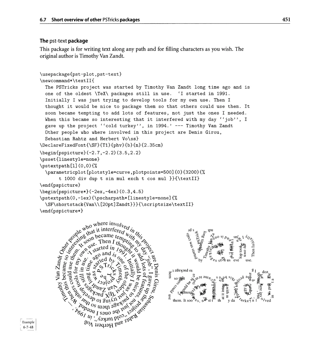
6.7 Short overview of other PSTricks packages. . . . . . . . . . . . . . . . . . . . .. 417
6.7.1 The pstricks-add package . . . . . . . . . . . . . . . . . . . . . . . . . .. 418
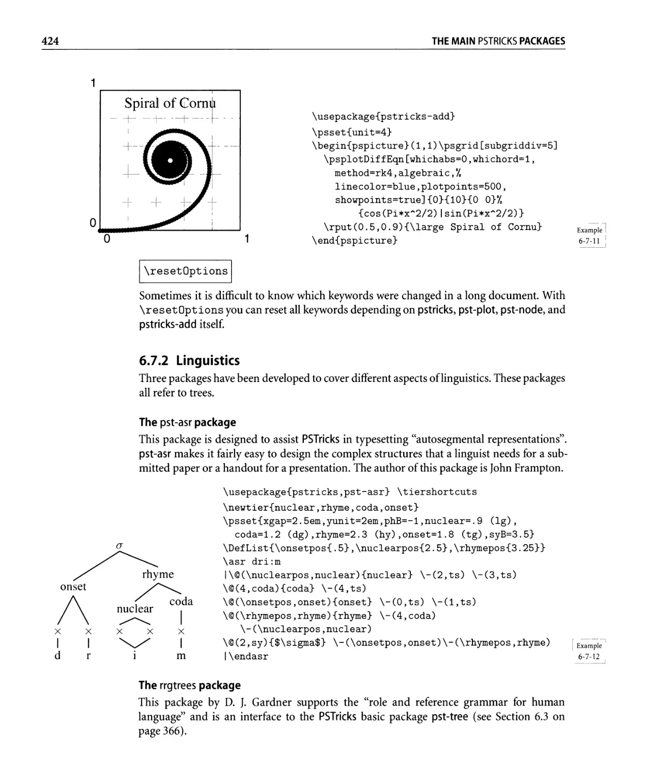
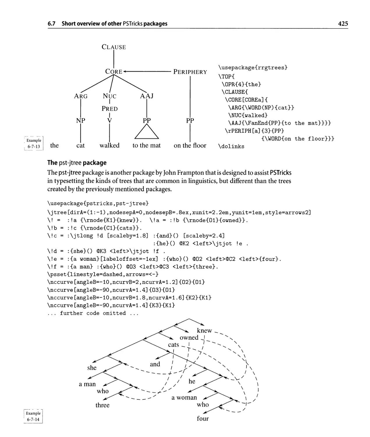
6.7.2 Linguistics....... . . . . . . . . . . . . . . . . . . . . . . . . . . . .. 424
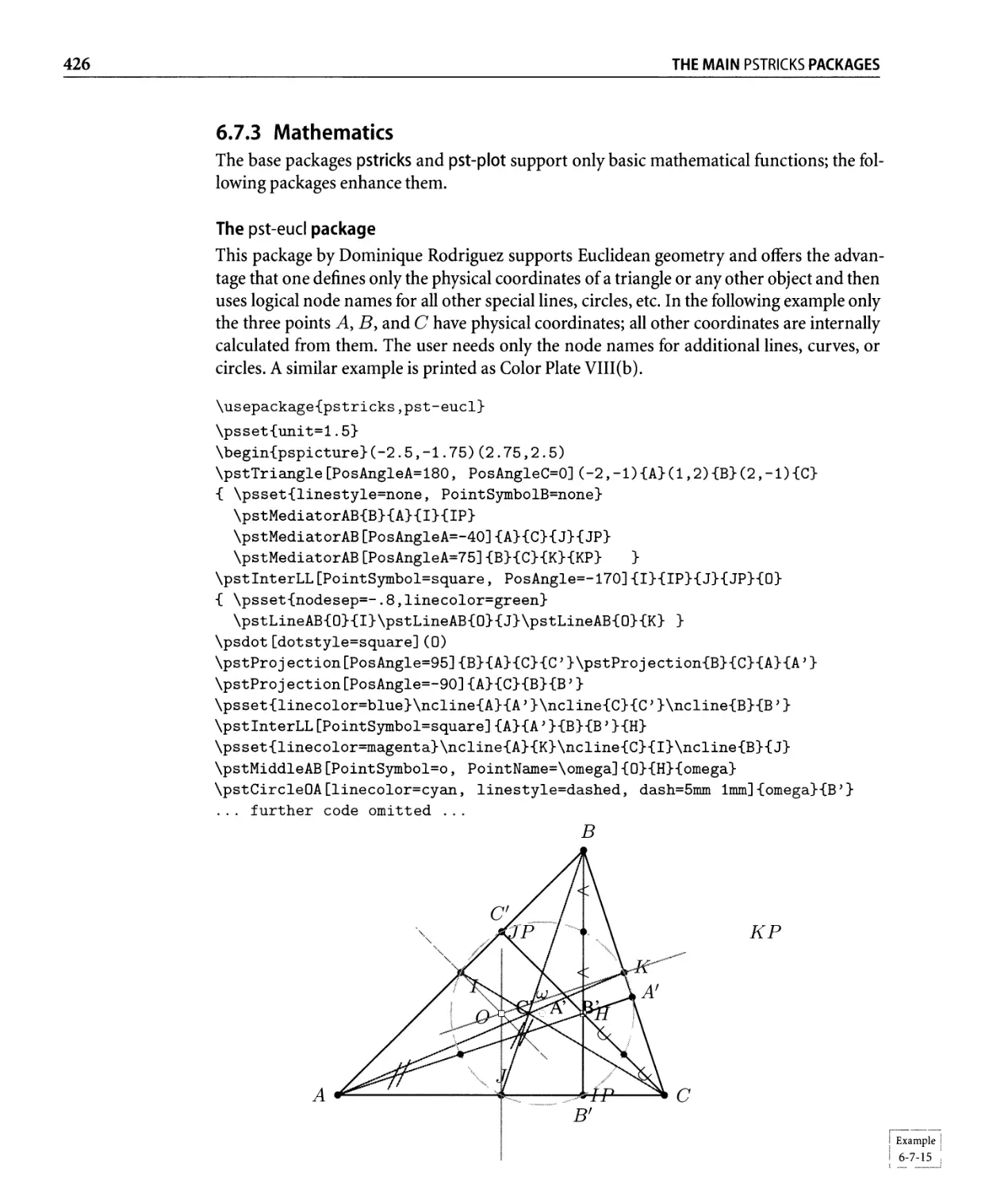
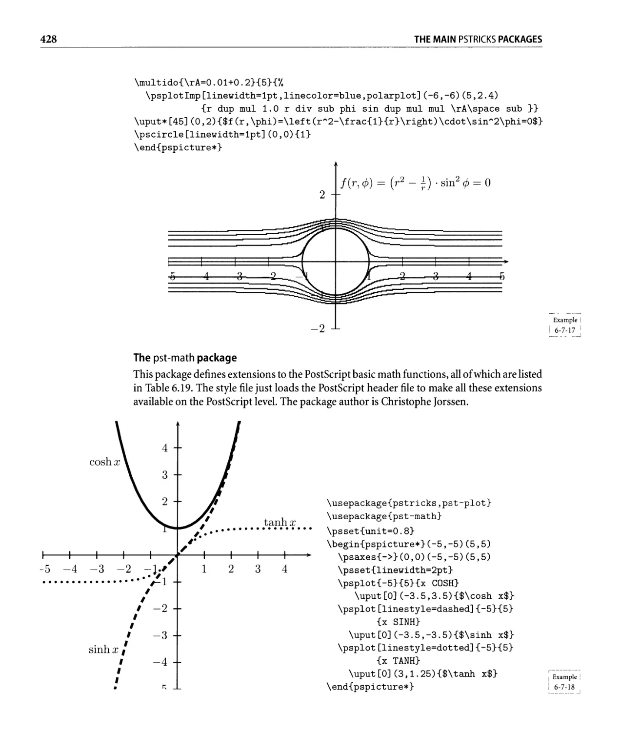
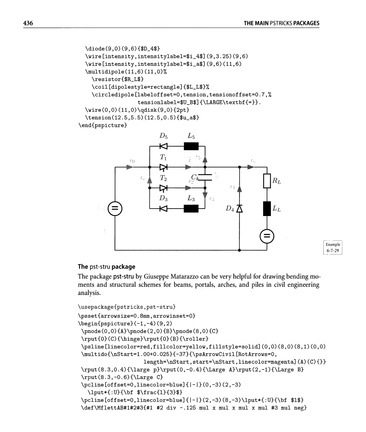
6.7.3 Mathematics. . . . . . . . . . . . . . . . . . . . . . . . . . . . . . . . . .. 426
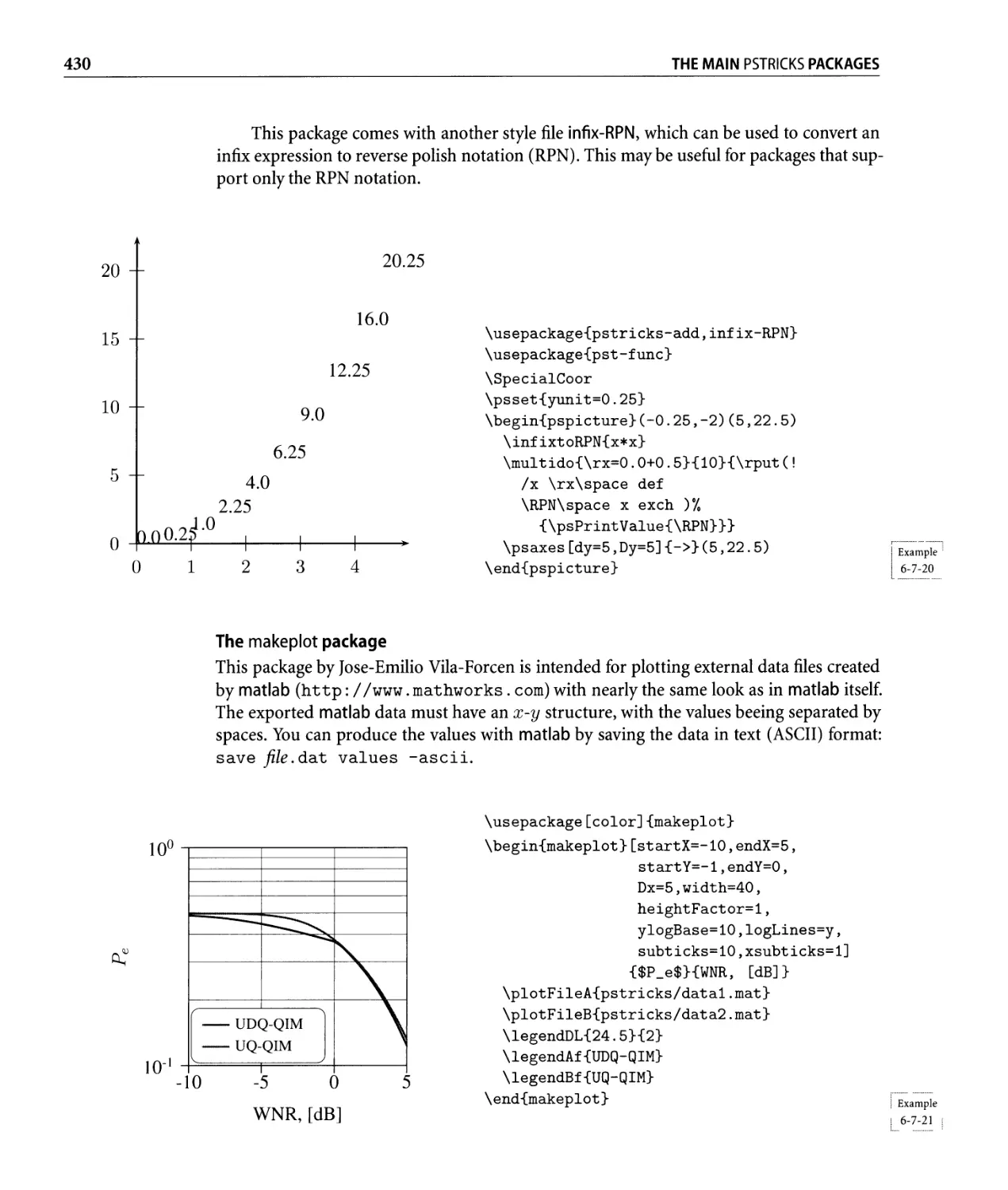
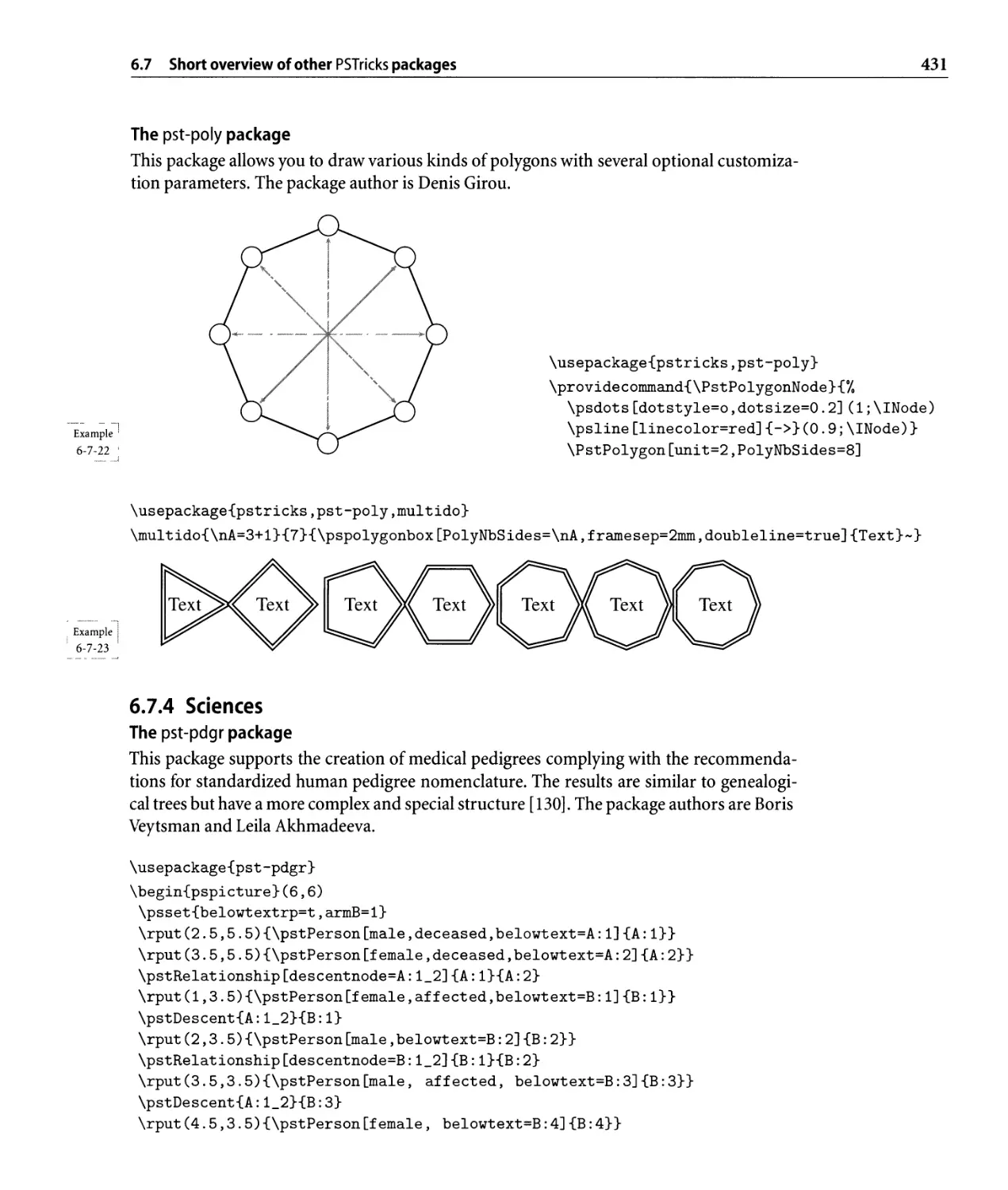
6.7.4 Sciences... . . . . . . . . . . . . . . . . . . . . . . . . . . . . . . . . . .. 431
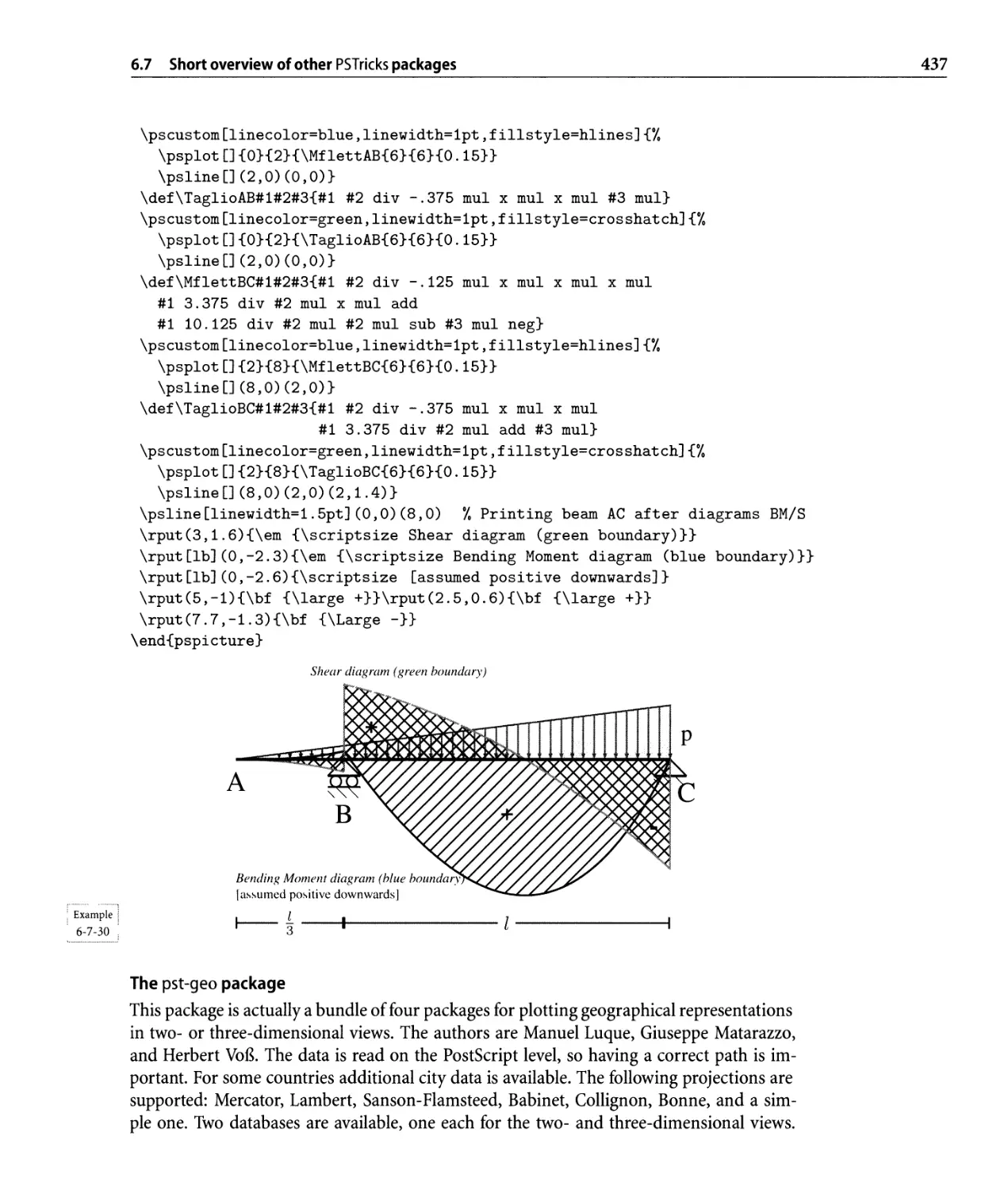
6.7.5 Information theory . . . . . . . . . . . . . . . . . . . . . . . . . . . . . .. 438
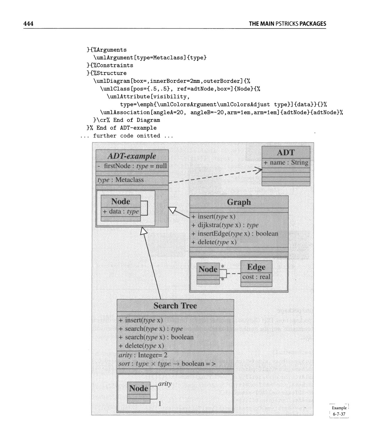
6.7.6 U M Lan d E R d i a g ram s . . . . . . . . . . . . . . . . . . . . . . . . . . . .. 442
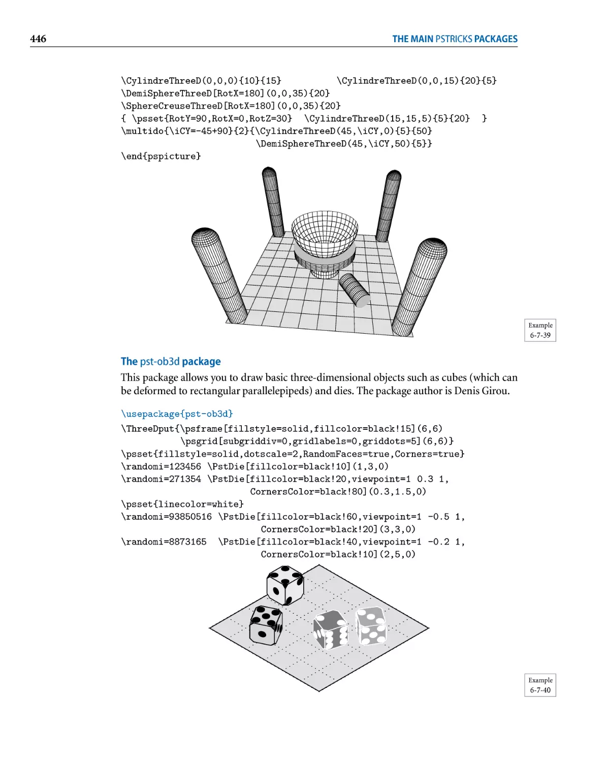
6.7 .7 3 - D vie w s . . . . . . . . . . . . . . . . . . . . . . . . . . . . . . . . . . . .. 445
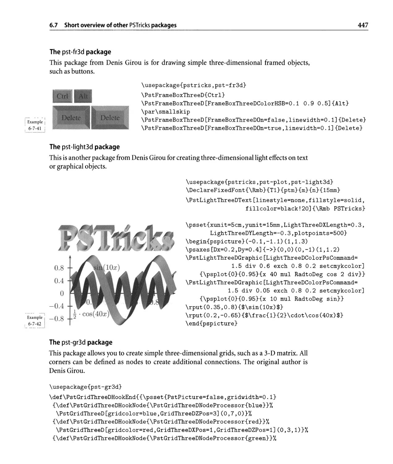
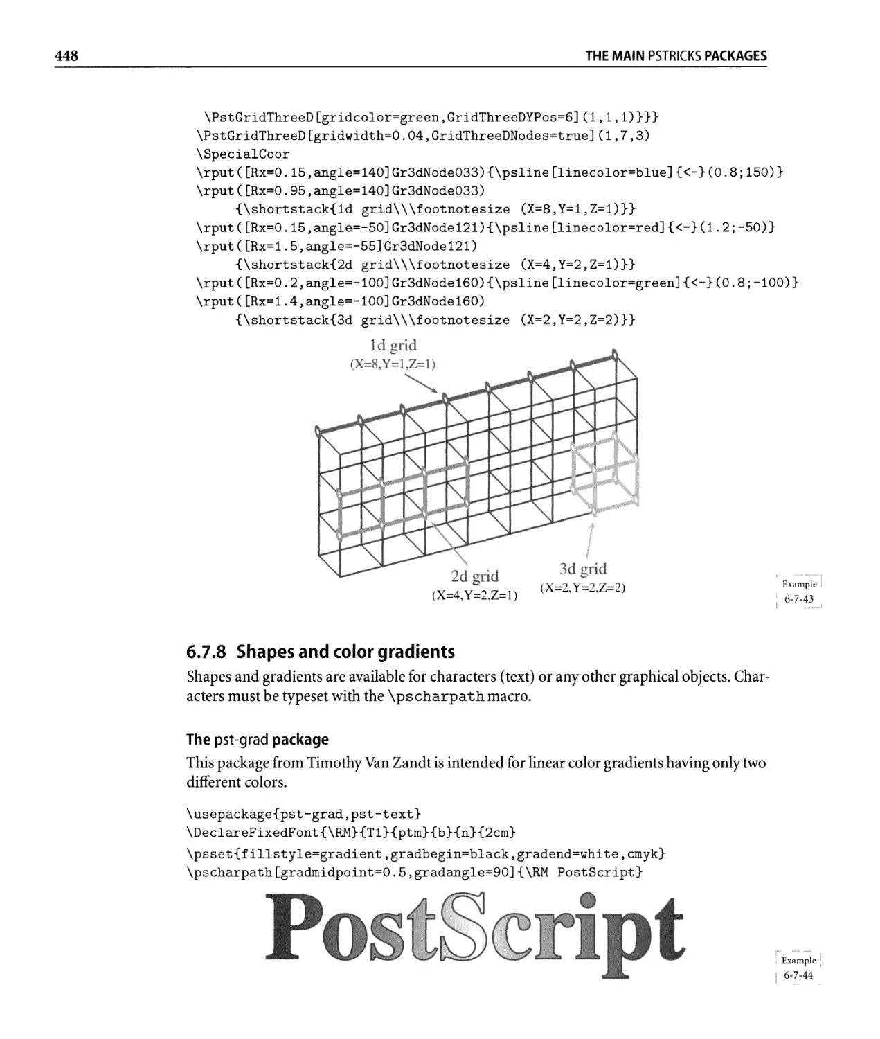
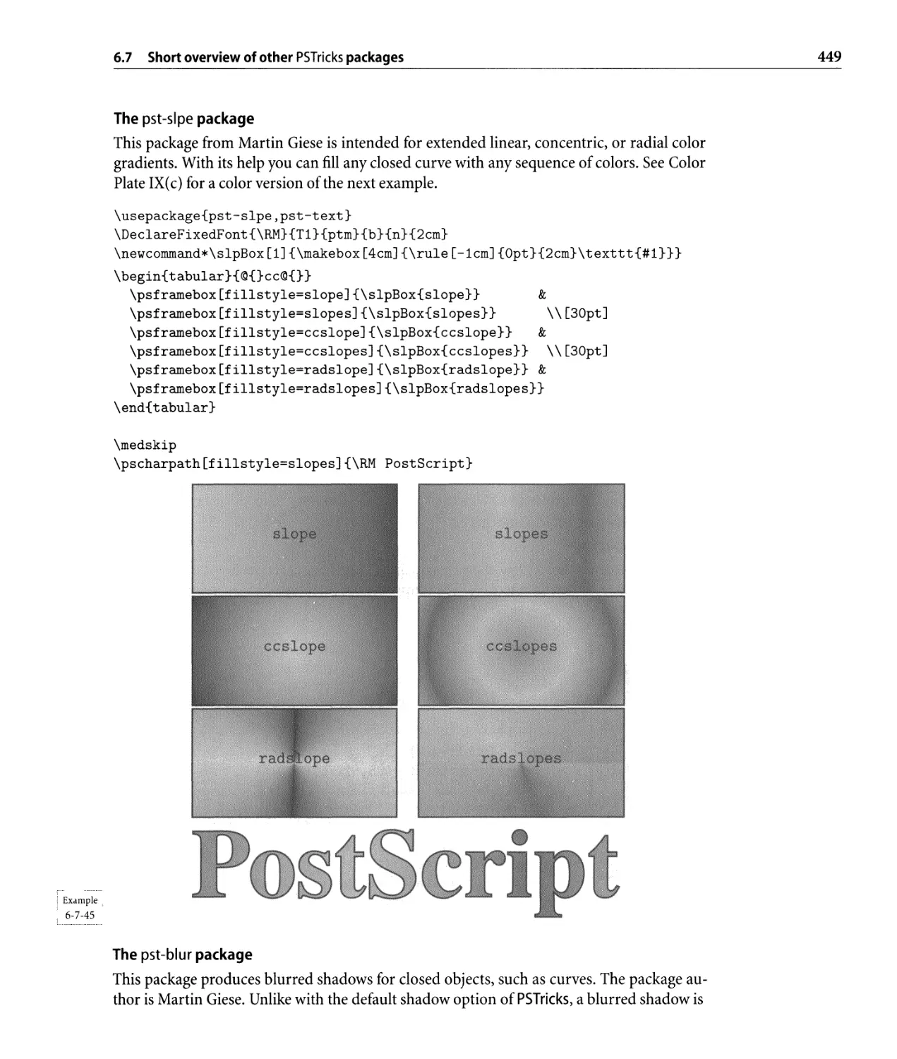
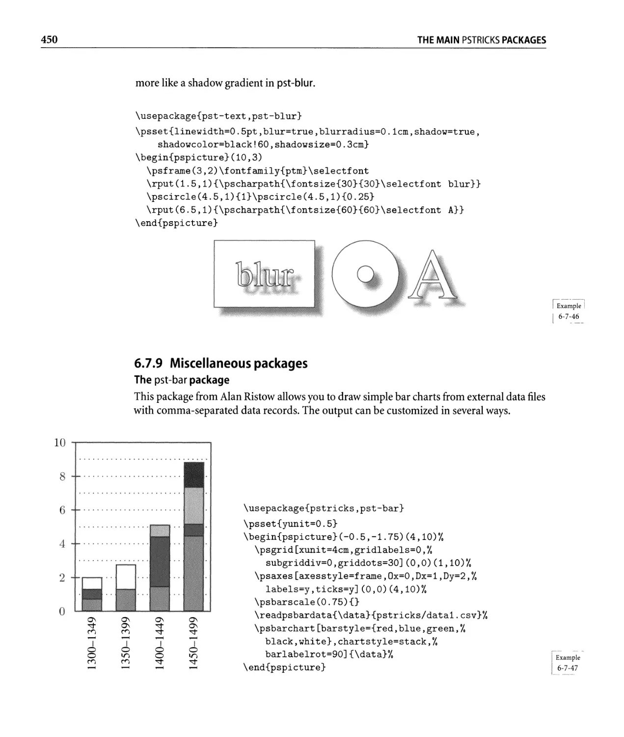
6.7.8 Shapes and color gradients. . . . . . . . . . . . . . . . . . . . . . . . .. 448
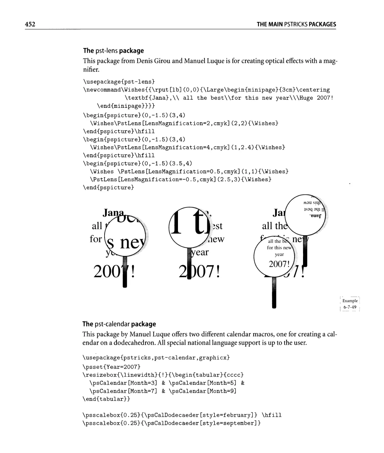
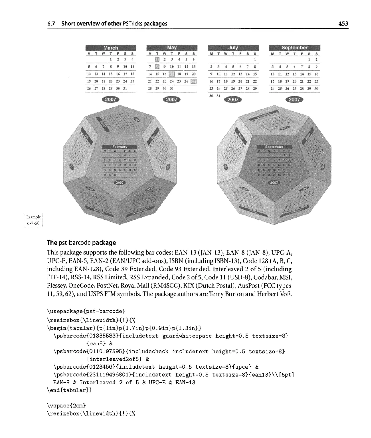
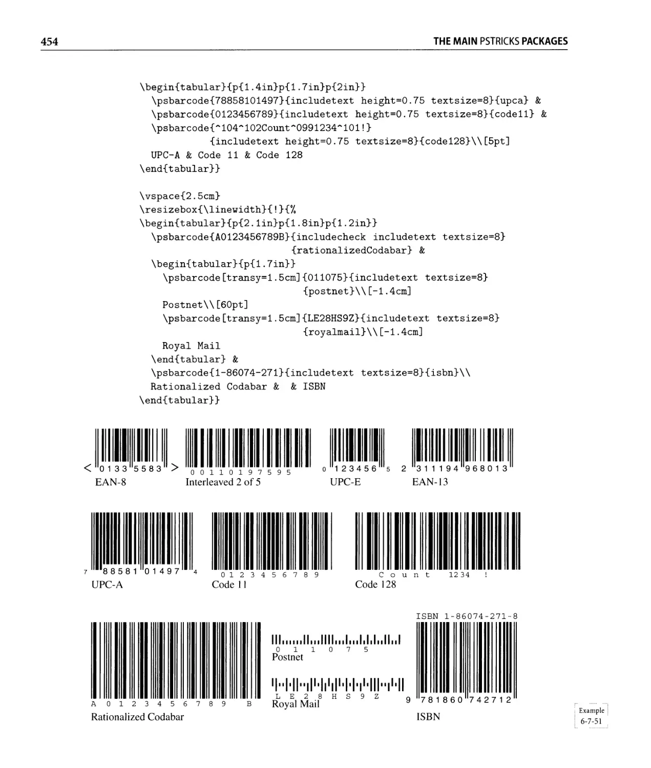
6.7.9 Miscellaneous packages. . . . . . . . . . . . . . . . . . . . . . . . . . .. 450
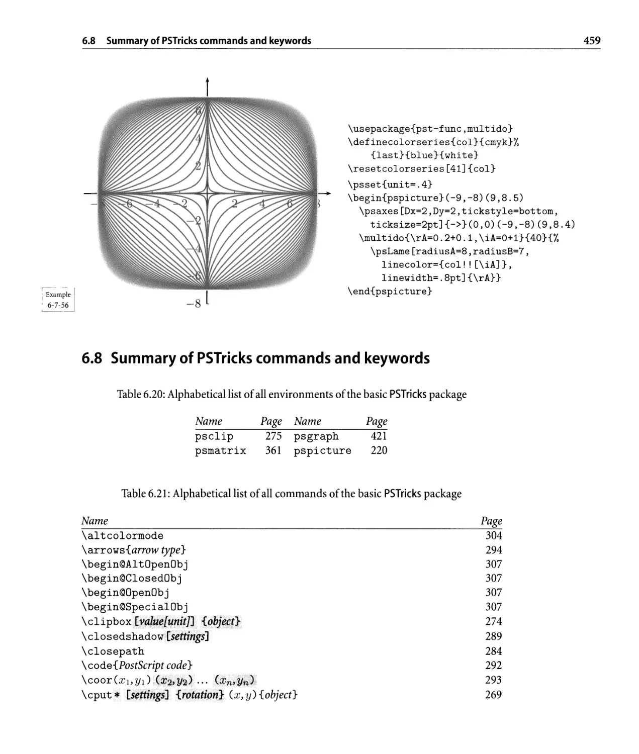
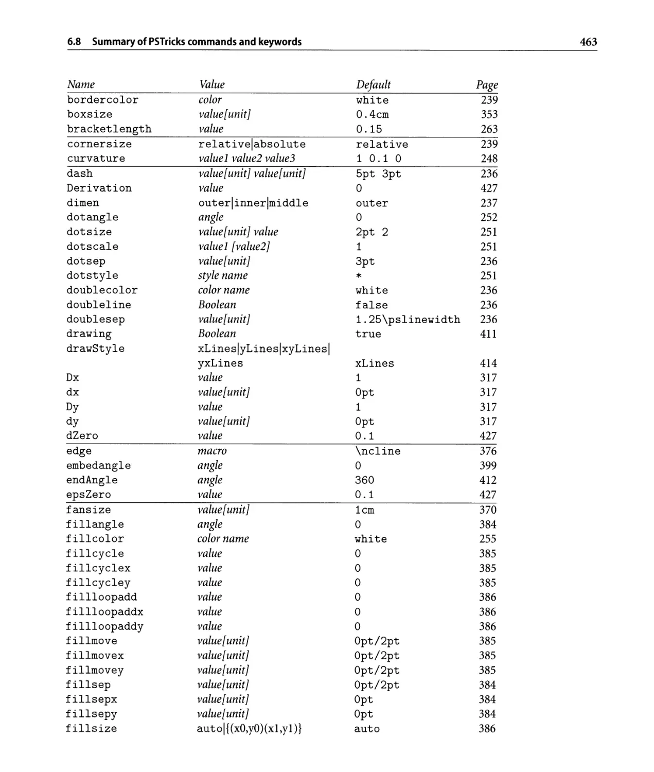
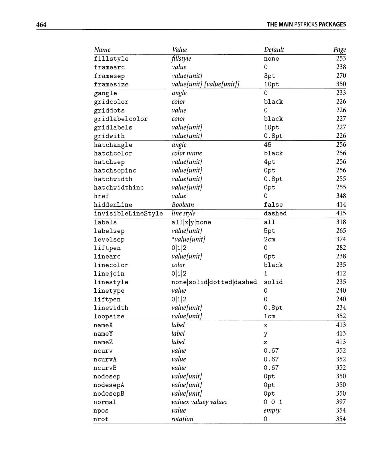
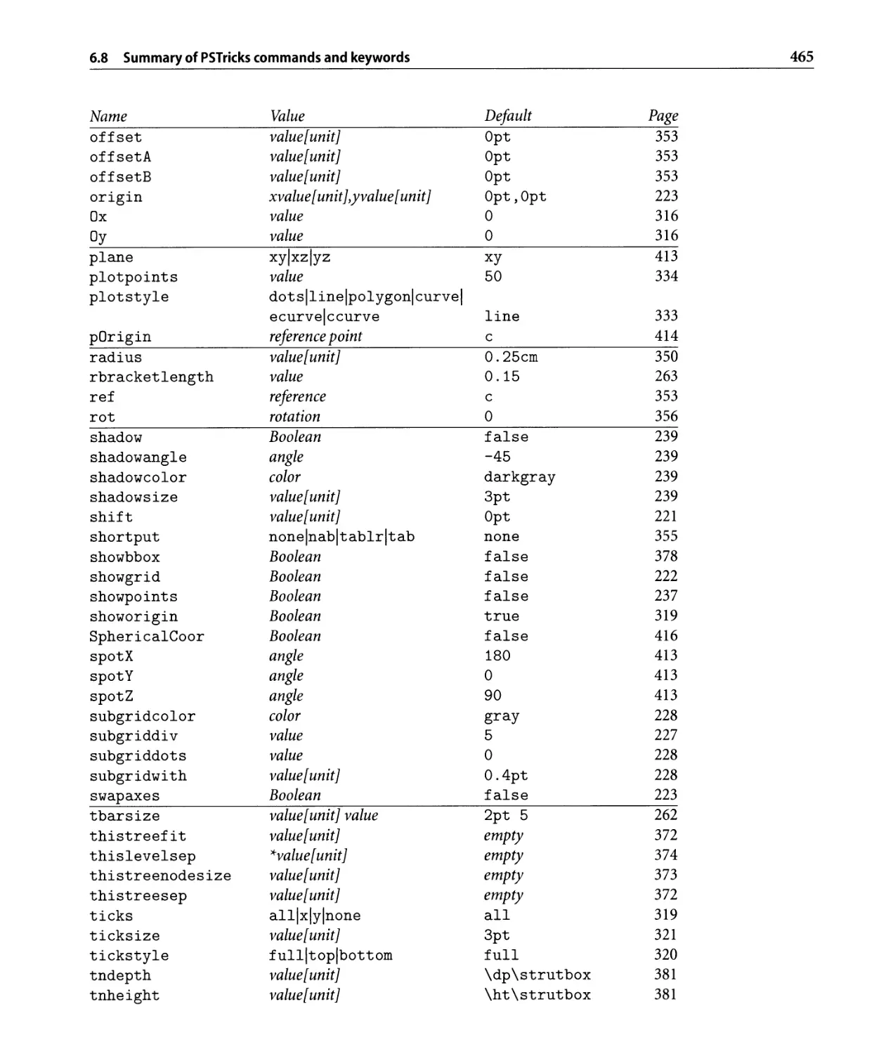
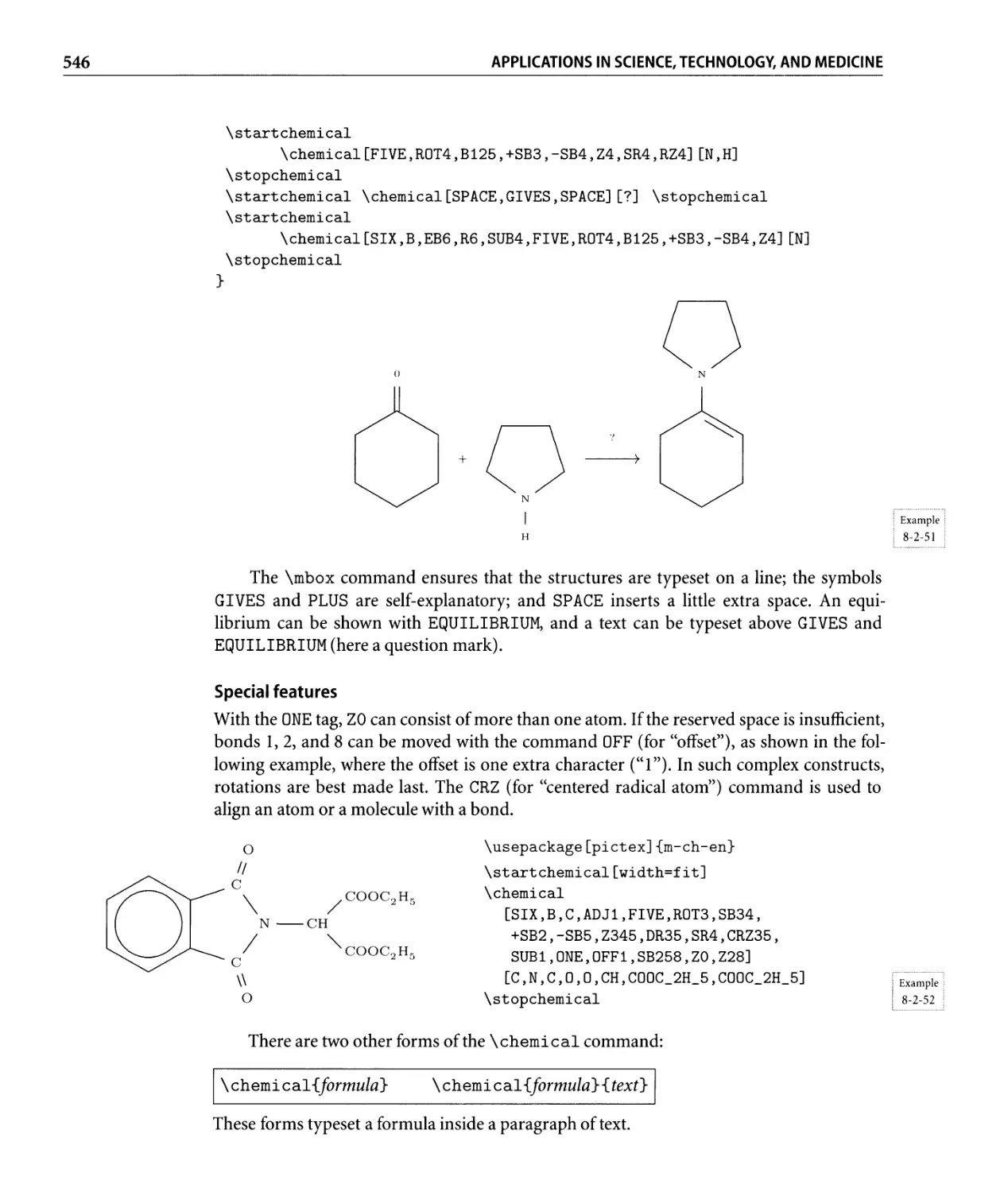
6.8 Summary of PSTricks commands and keywords. . . . . . . . . . . . . . . . . .. 459
7 The XV-pic Package 467
7. 1 I n t ro d u ci n g Xy - pic. . . . . . . . . . . . . . . . . . . . . . . . . . . . . . . . . . . .. 467
7.2 Basic constructs. . . . . . . . . . . . . . . . . . . . . . . . . . . . . . . . . . . . . .. 469
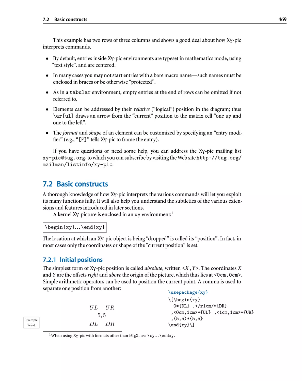
7.2.1 Initial positions . . . . . . . . . . . . . . . . . . . . . . . . . . . . . . . .. 469
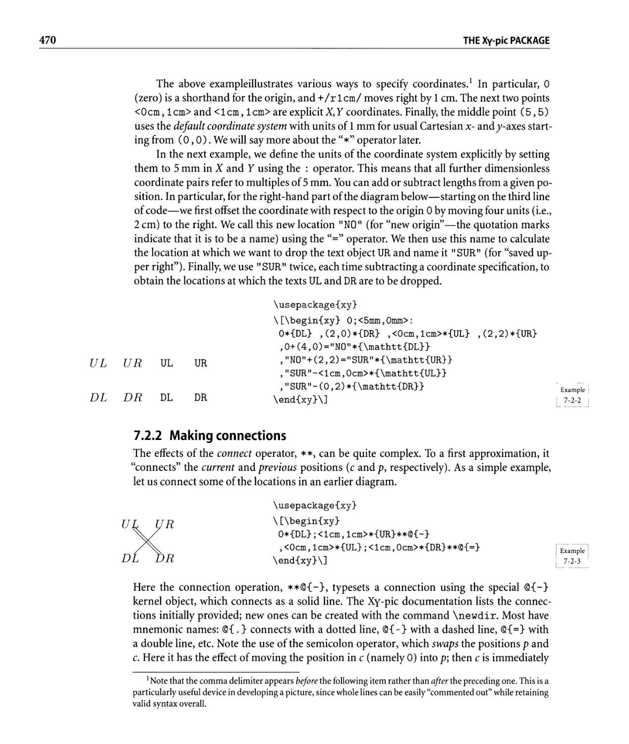
7.2.2 Making connections . . . . . . . . . . . . . . . . . . . . . . . . . . . . .. 470
7.2.3 Dropping objects. . . . . . . . . . . . . . . . . . . . . . . . . . . . . . .. 471
7.2.4 Entering text in your pictures. . . . . . . . . . . . . . . . . . . . . . . .. 473
7.3 Extensions.......................................... 474
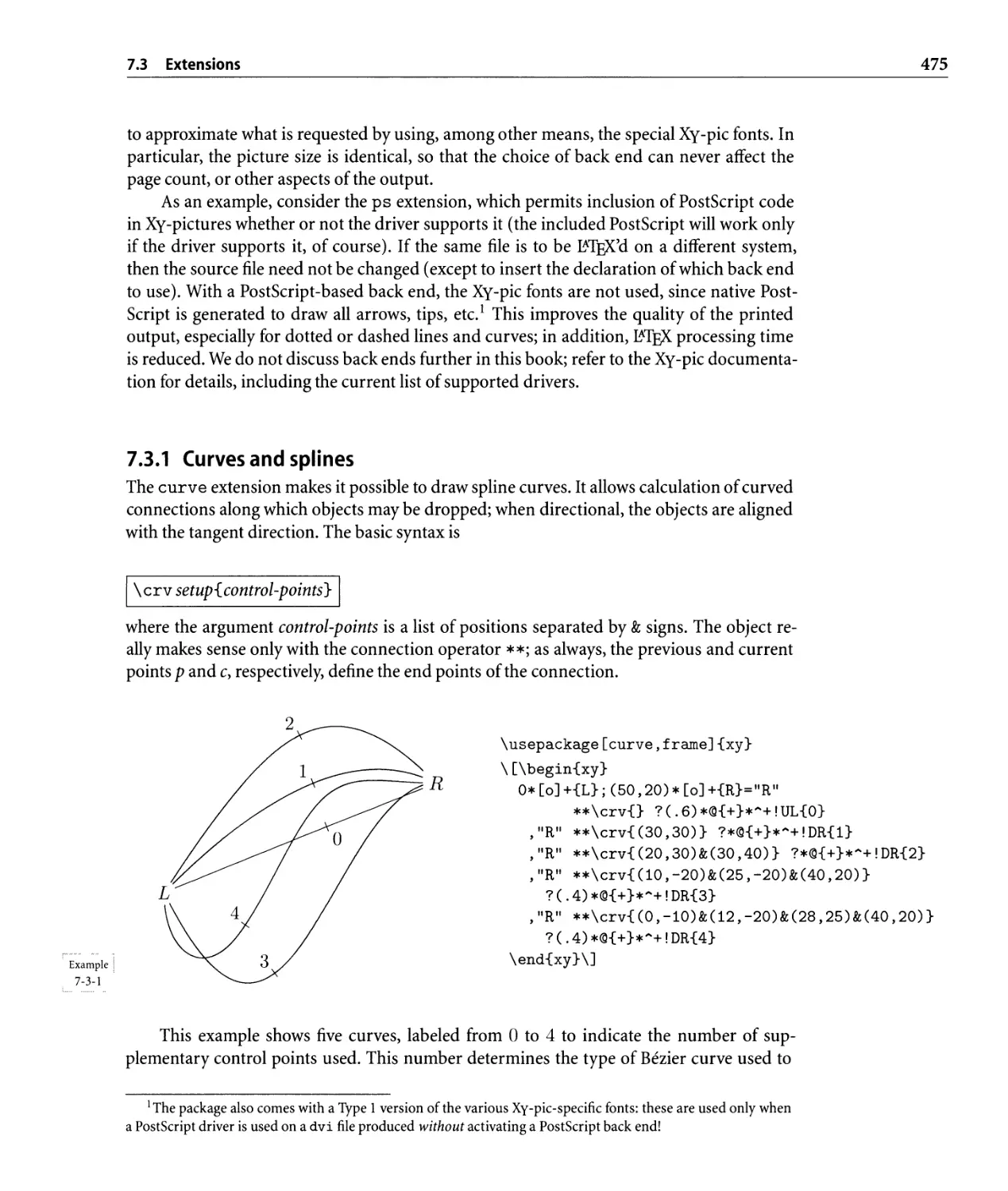
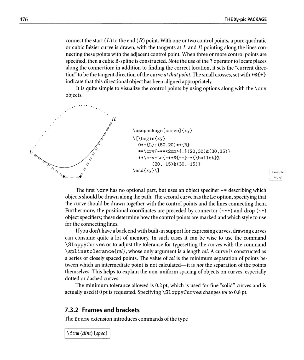
7.3.1 Curves and splines . . . . . . . . . . . . . . . . . . . . . . . . . . . . . .. 475
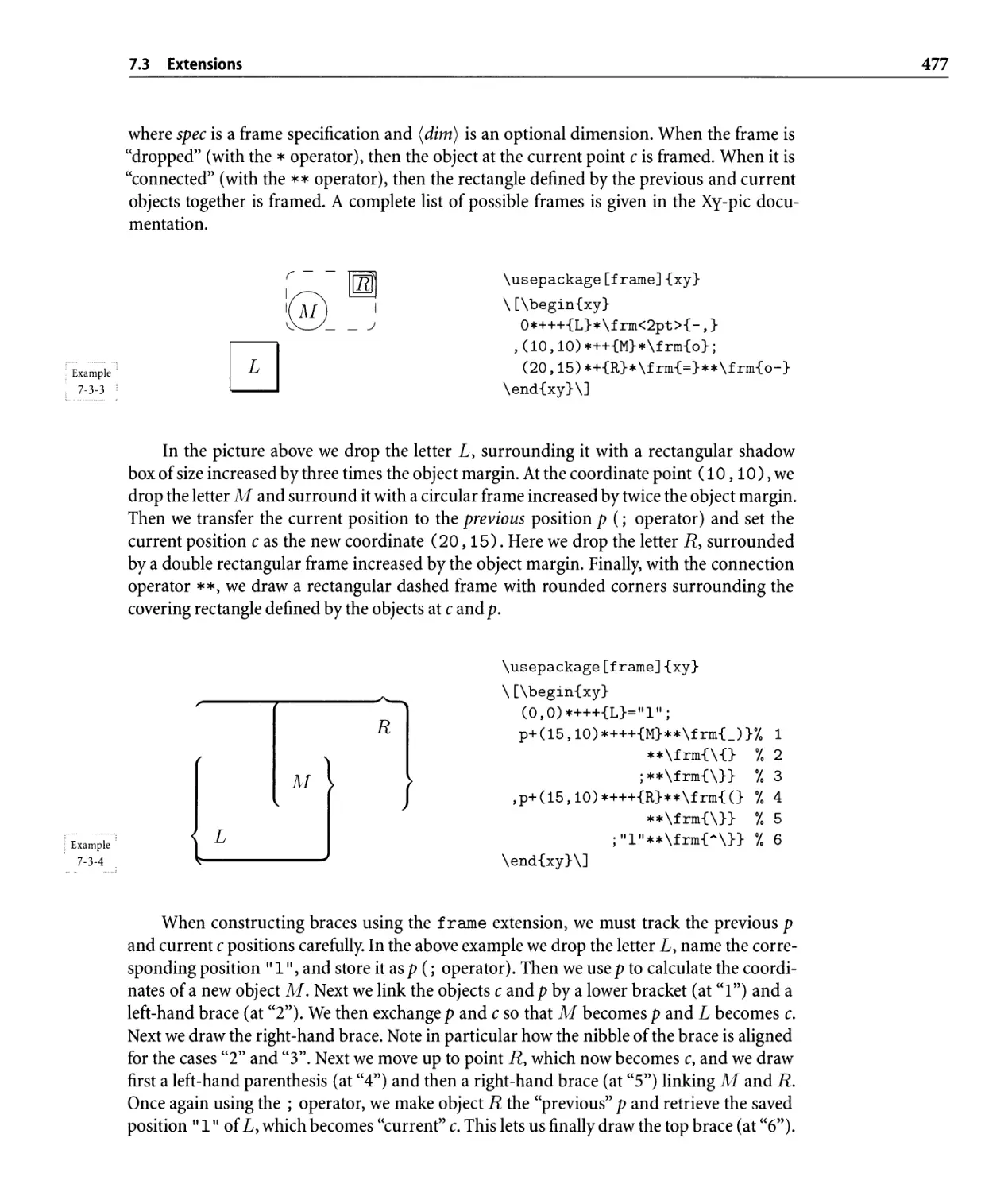
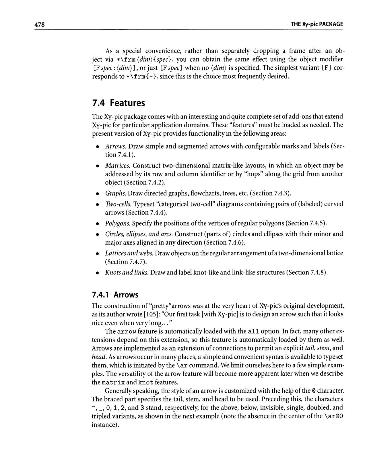
7.3.2 Frames and brackets . . . . . . . . . . . . . . . . . . . . . . . . . . . . .. 476
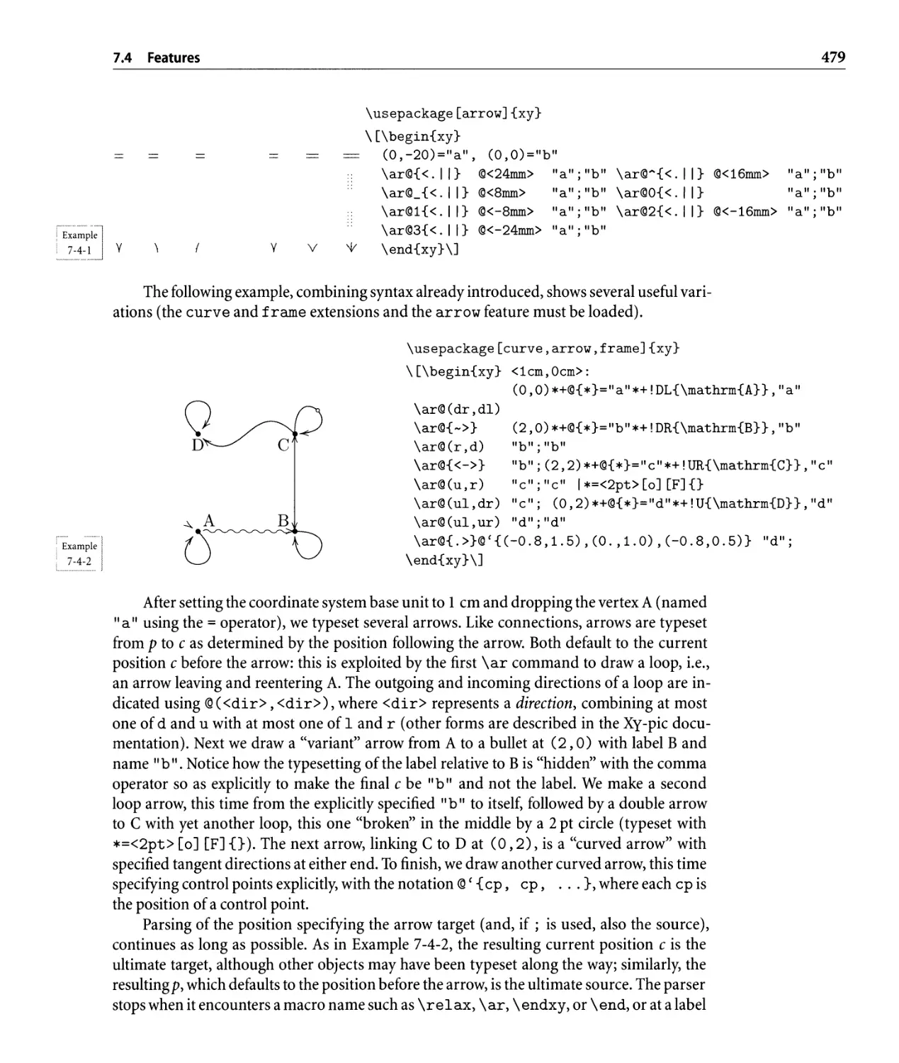
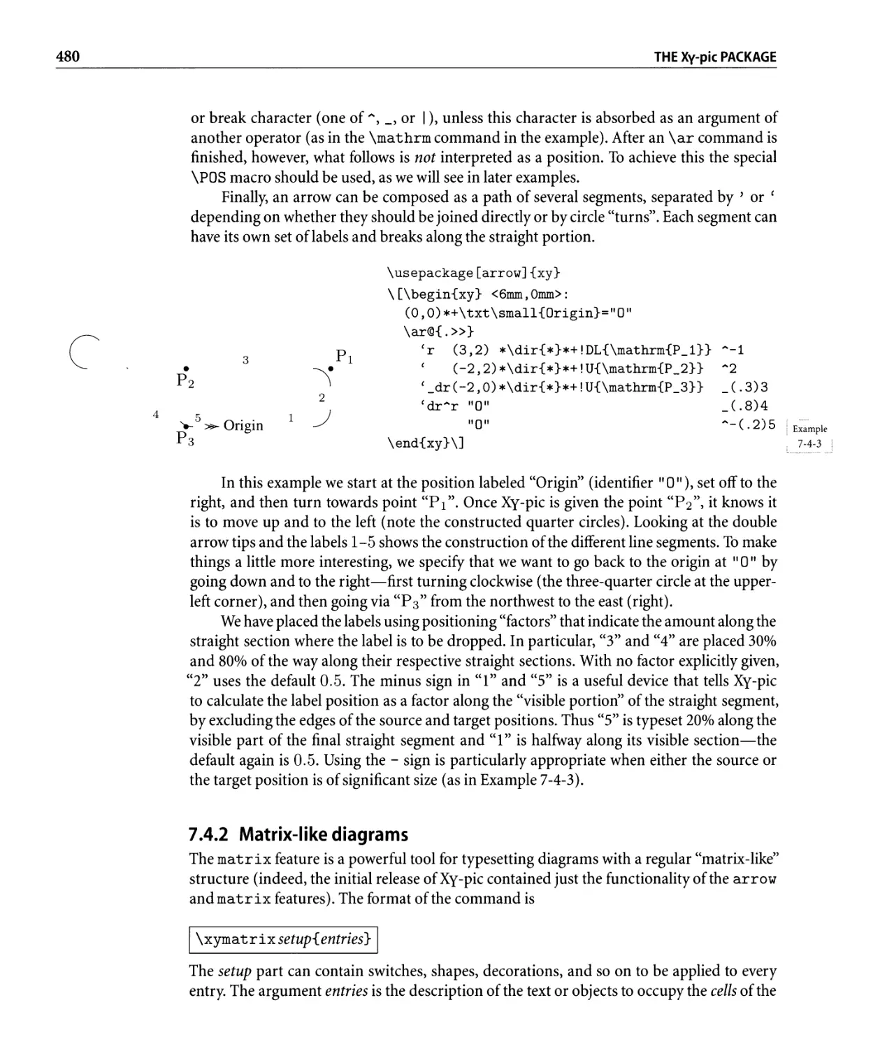
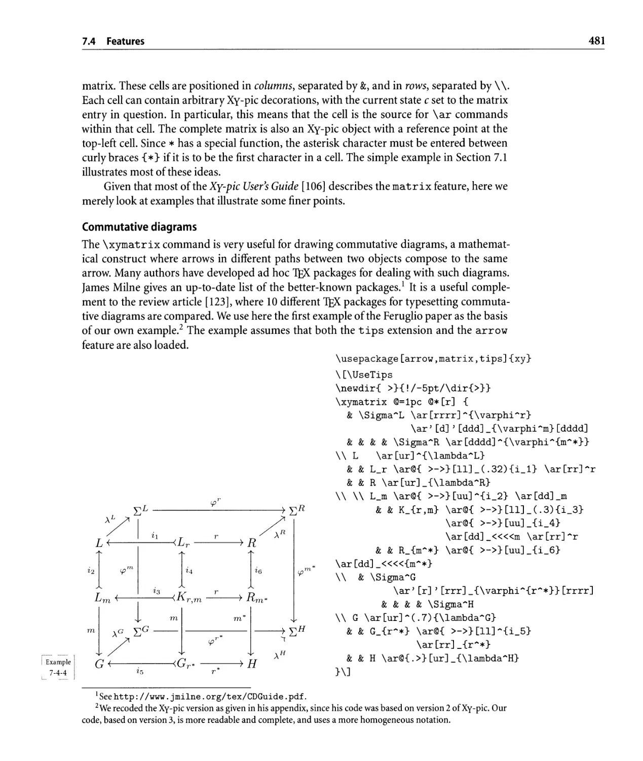
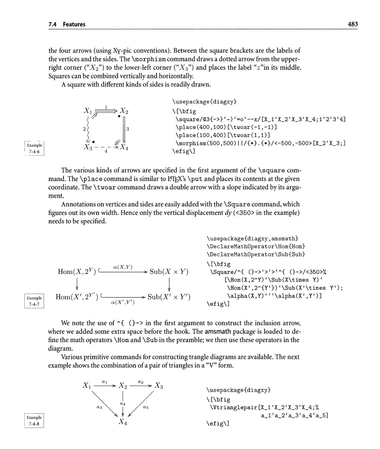
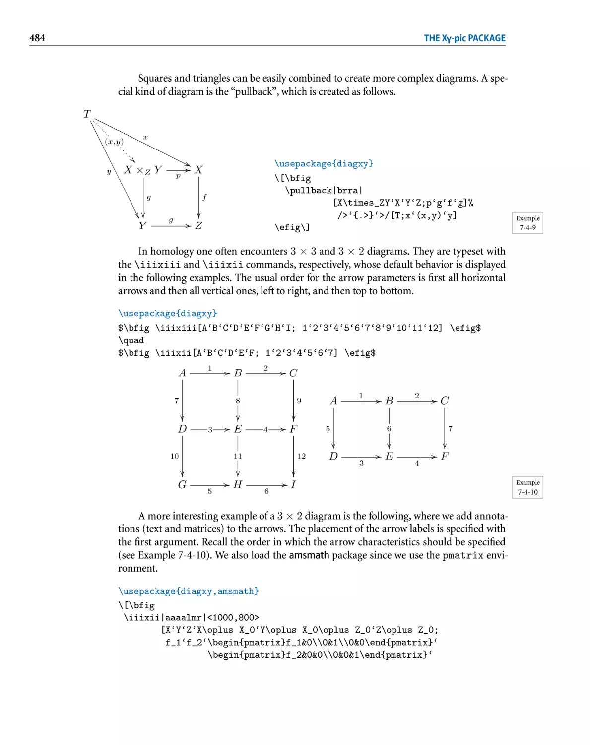
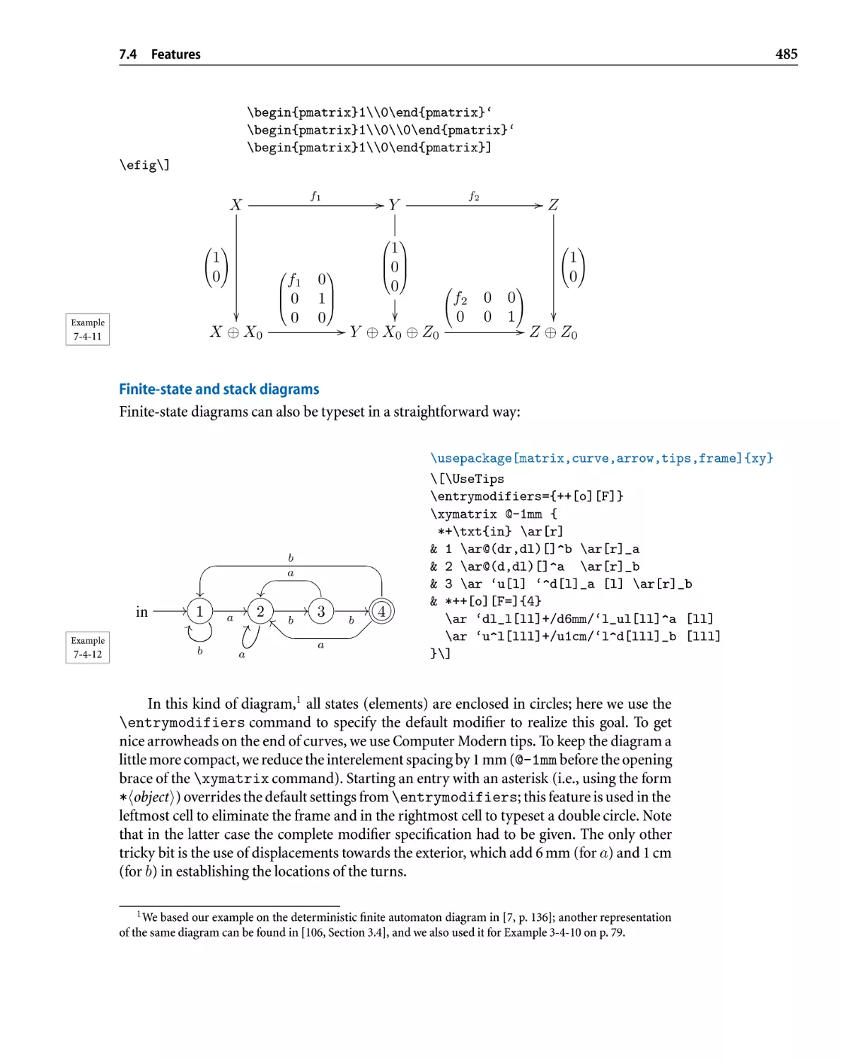
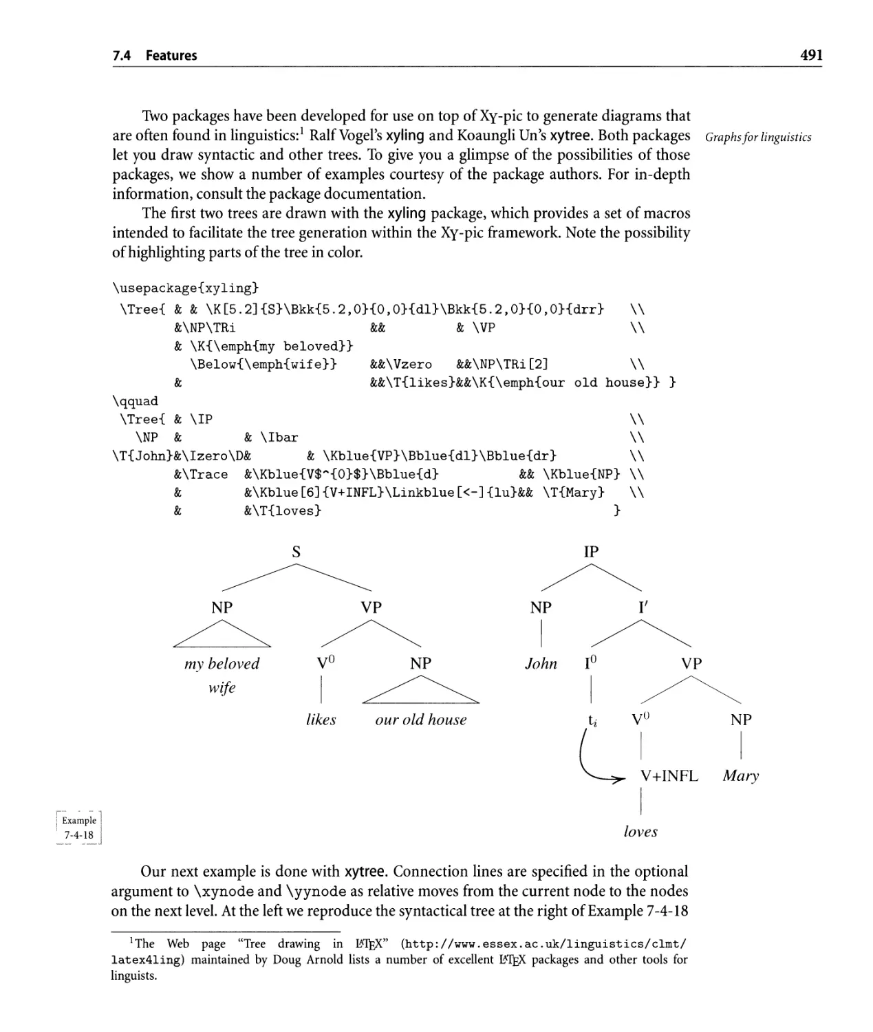
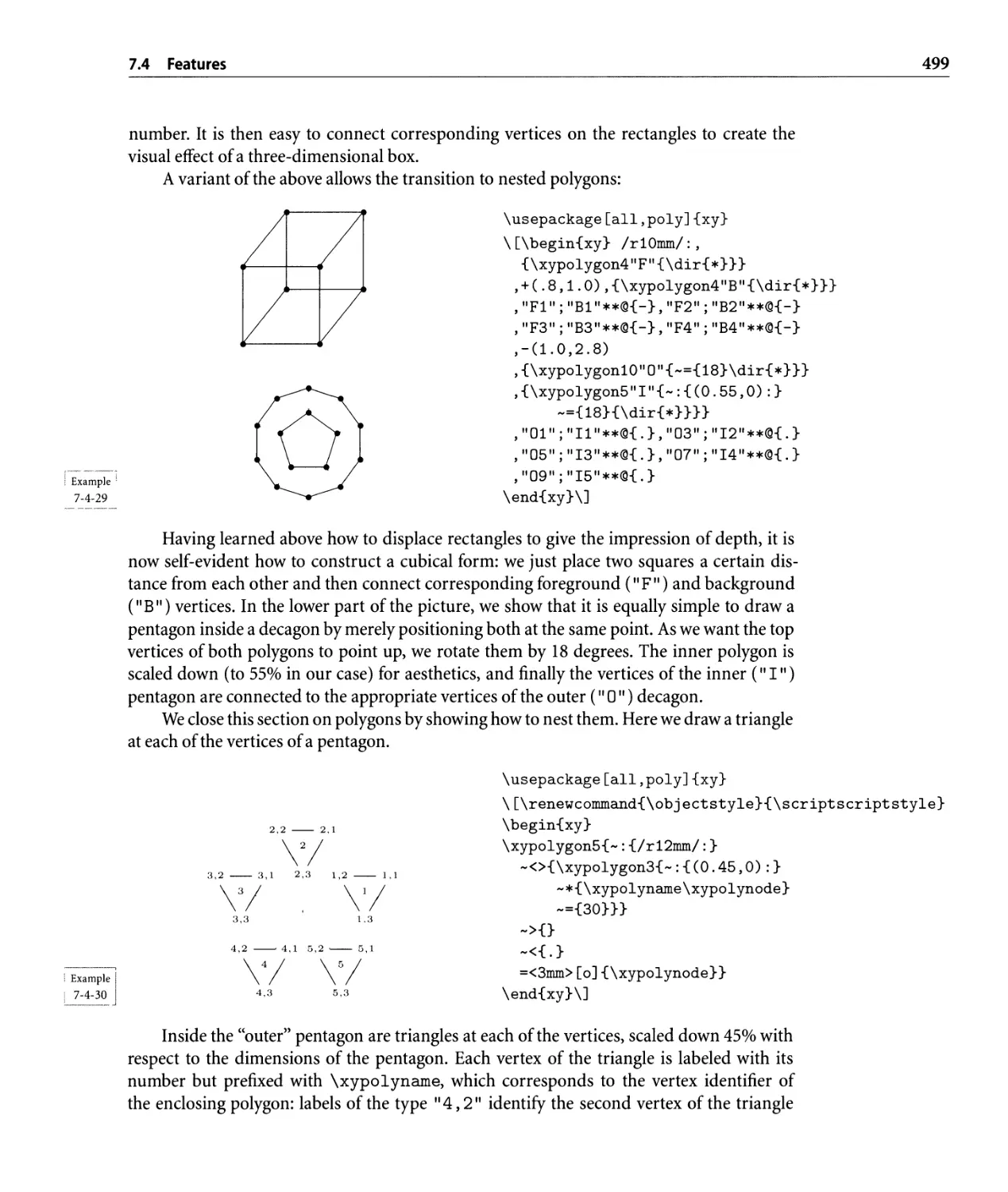
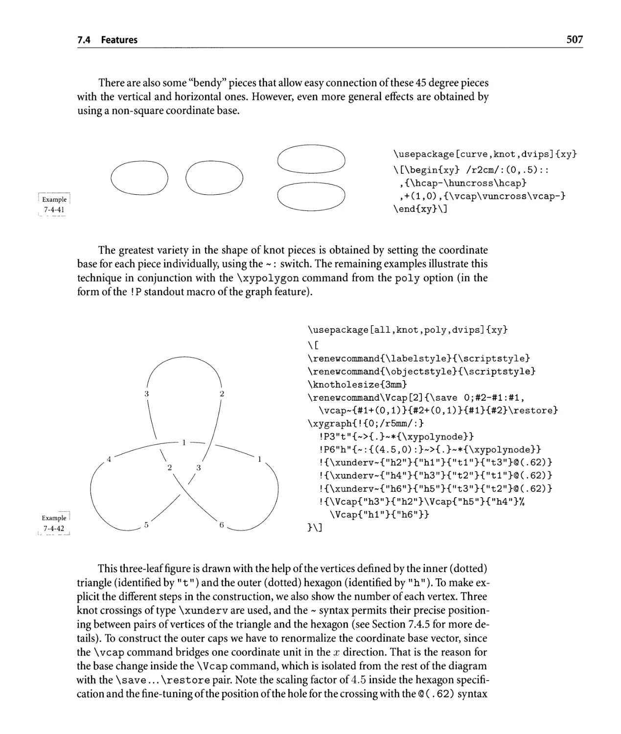
7.4 Featu res . . . . . . . . . . . . . . . . . . . . . . . . . . . . . . . . . . . . . . . . . .. 478
7.4.1 Arrows. . . . . . . . . . . . . . . . . . . . . . . . . . . . . . . . . . . . . .. 478
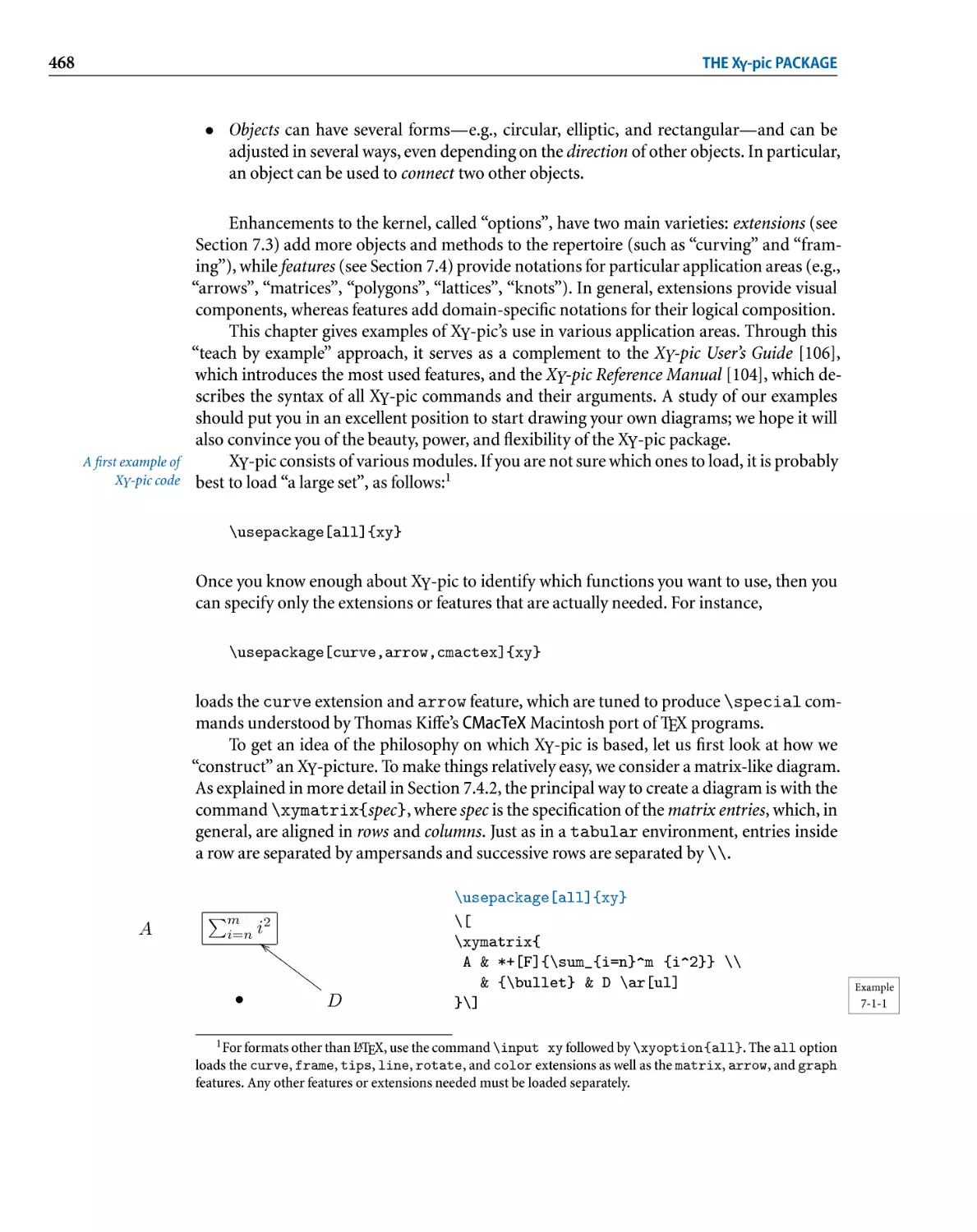
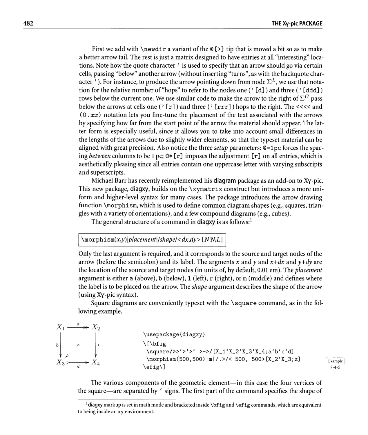
7.4.2 Matrix-like diagrams. . . . . . . . . . . . . . . . . . . . . . . . . . . . .. 480
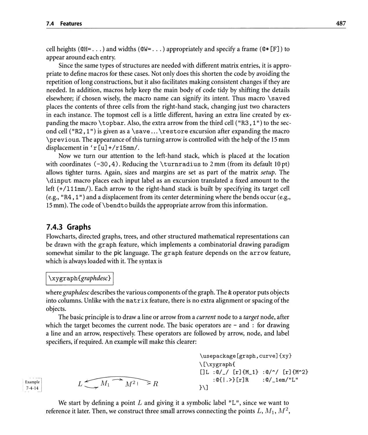
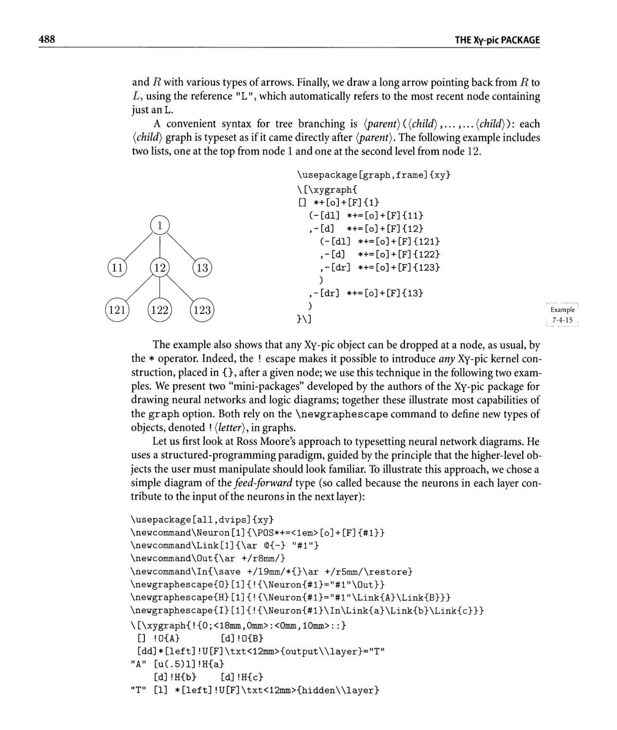
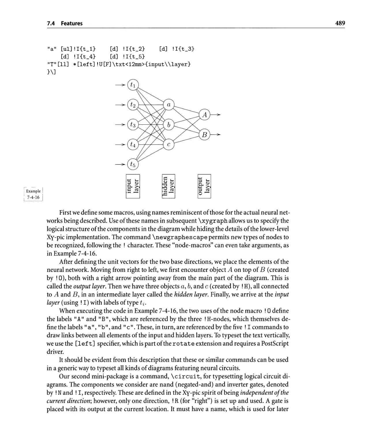
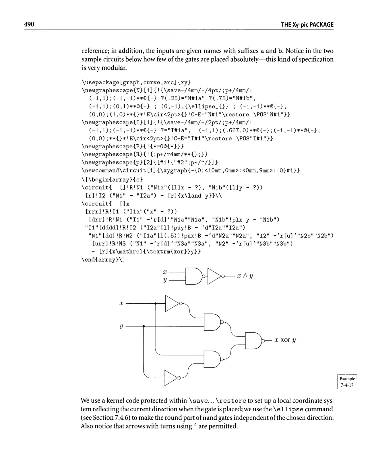
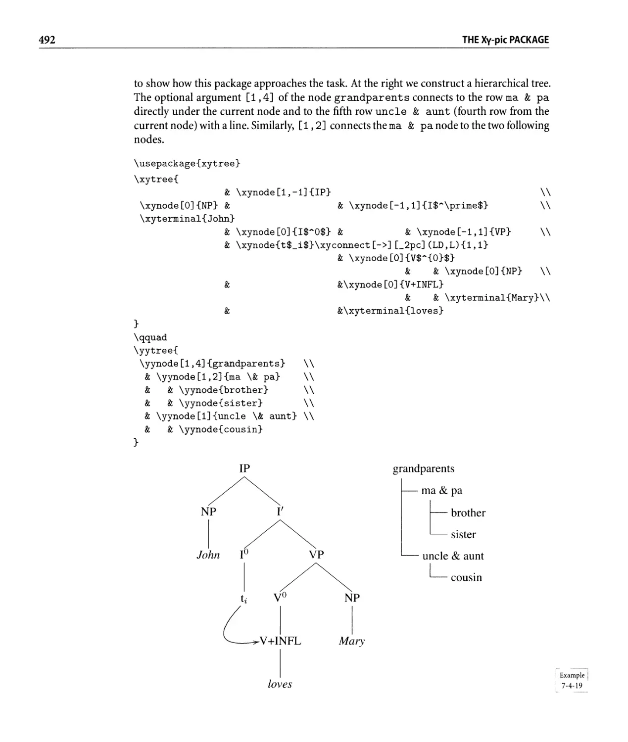
7.4.3 Graphs.................... . . . . . . . . . . . . . . . . . .. 487
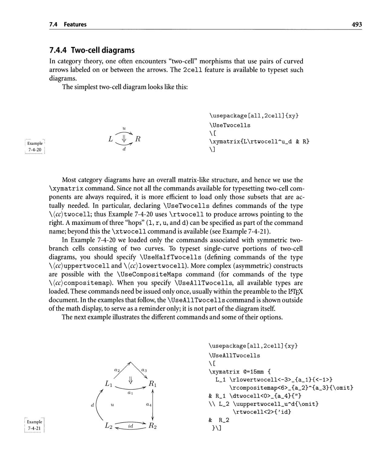
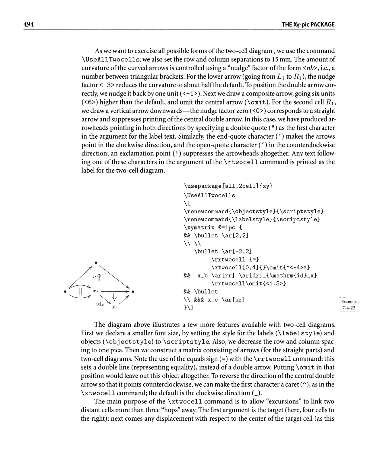
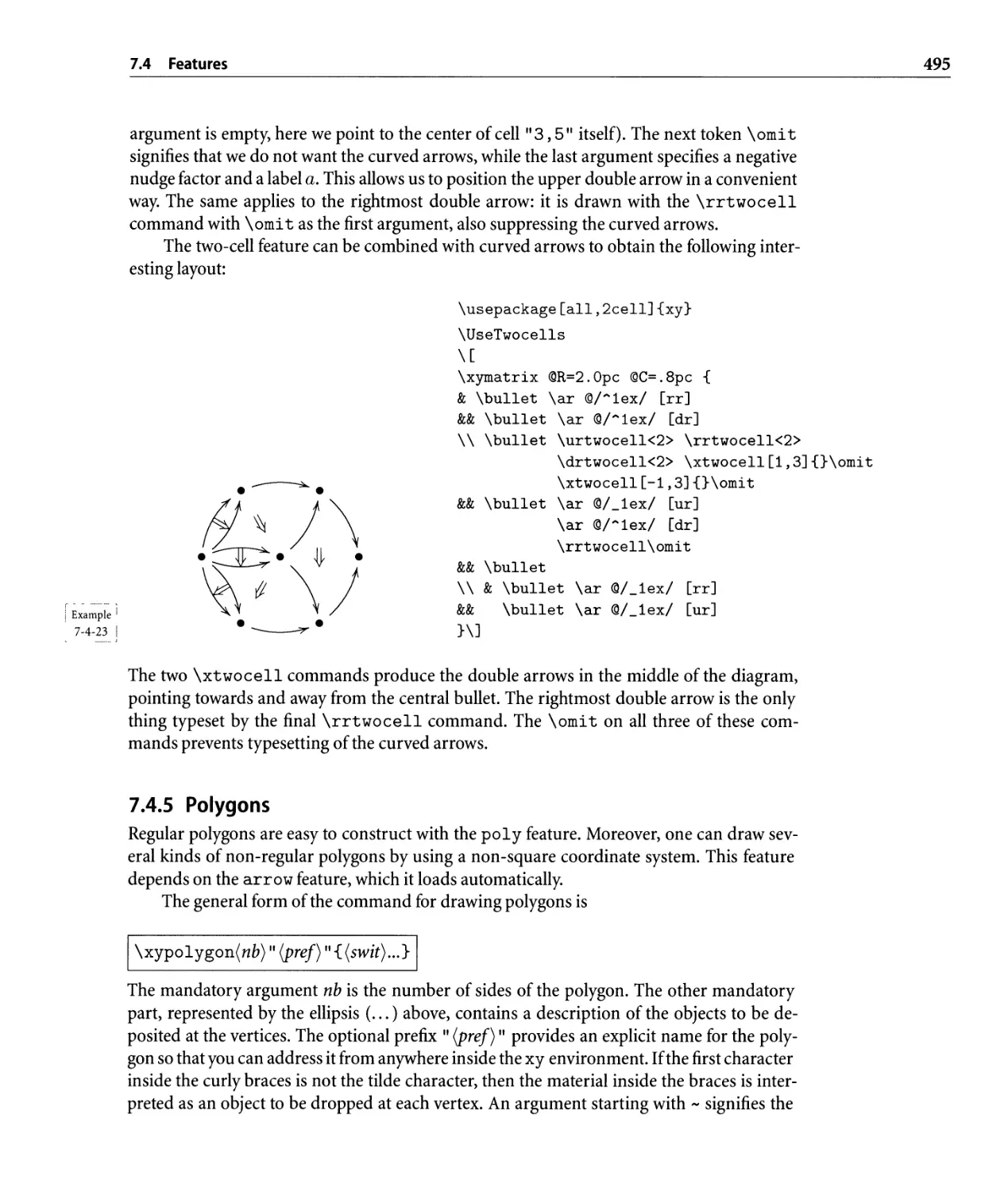
7.4.4 Two-cell diagrams. . . . . . . . . . . . . . . . . . . . . . . . . . . . . . .. 493
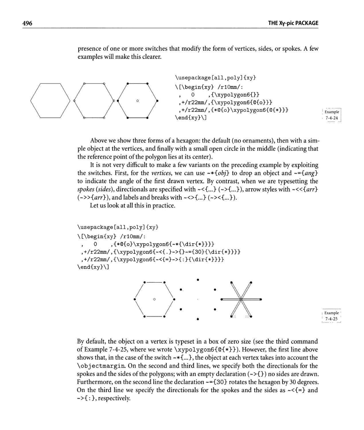
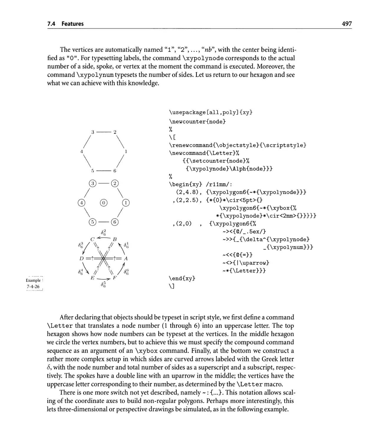
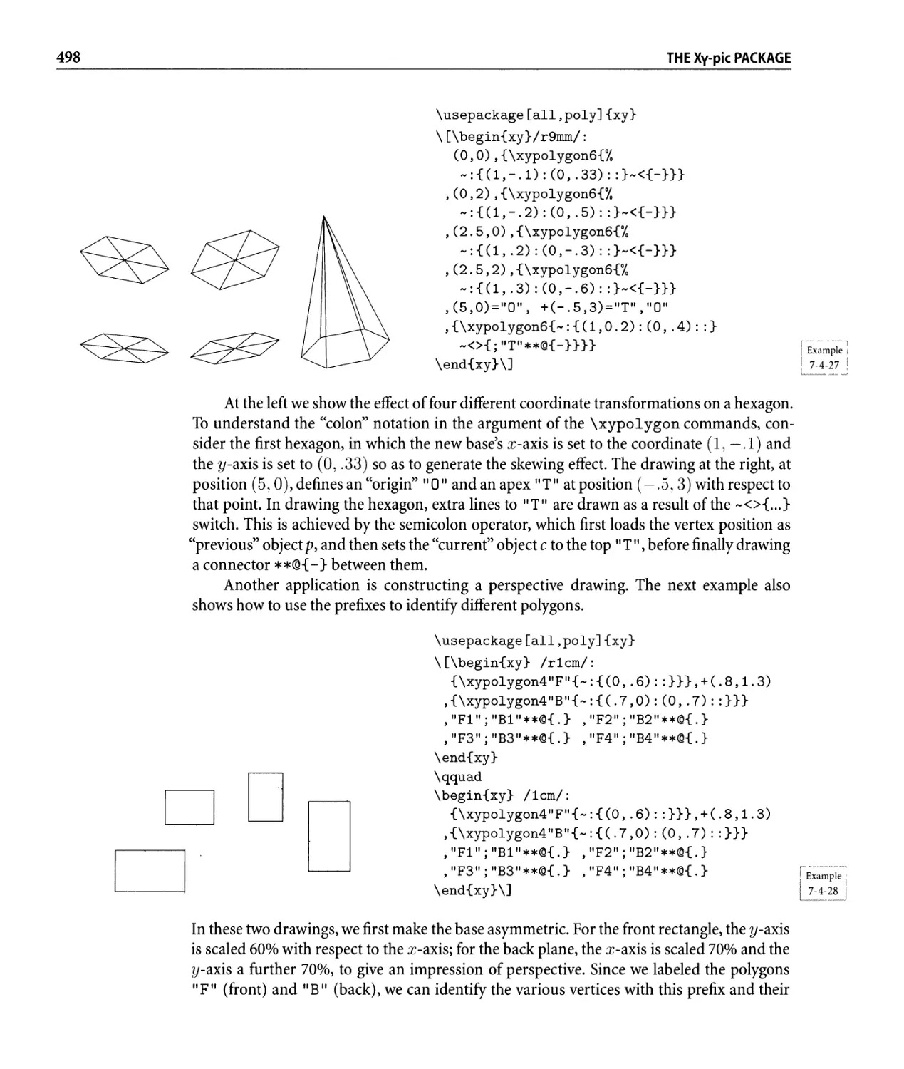
7.4.5 Polygons. . . . . . . . . . . . . . . . . . . . . . . . . . . . . . . . . . . .. 495
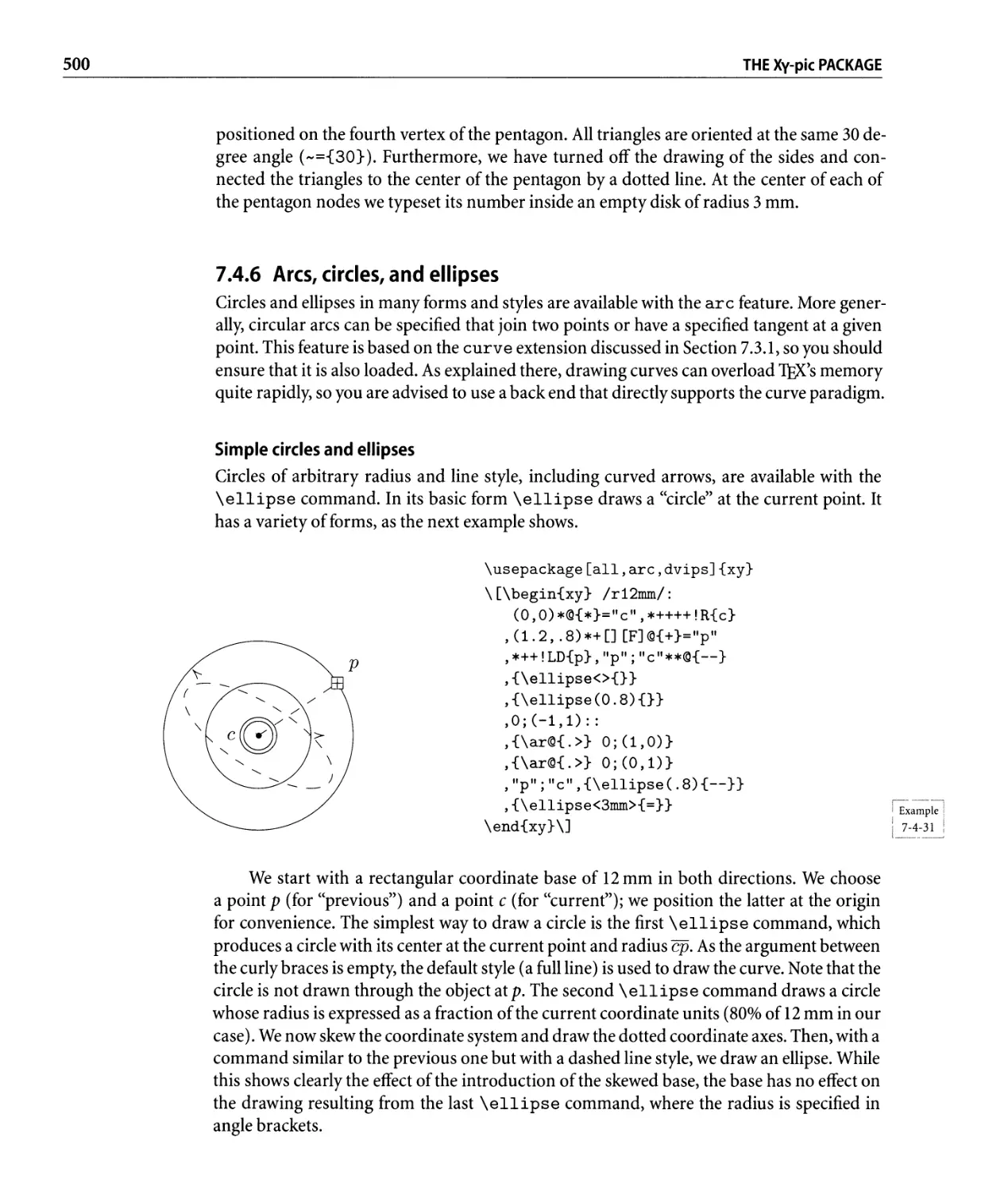
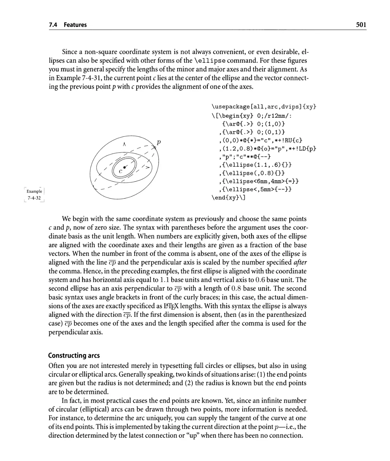
7.4.6 Arcs, circles, and ellipses. . . . . . . . . . . . . . . . . . . . . . . . . . .. 500
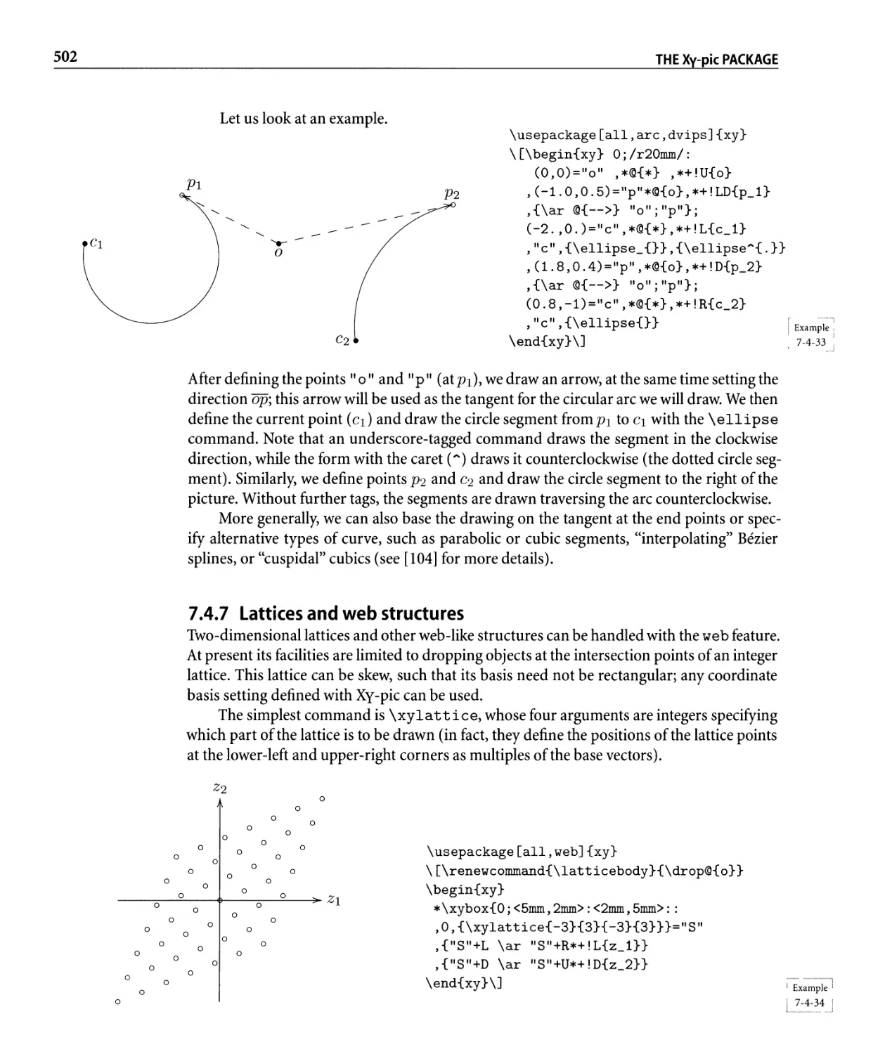
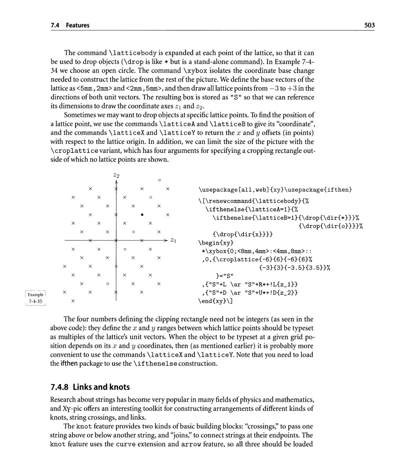
7.4.7 Lattices and web structures. . . . . . . . . . . . . . . . . . . . . . . . .. 502
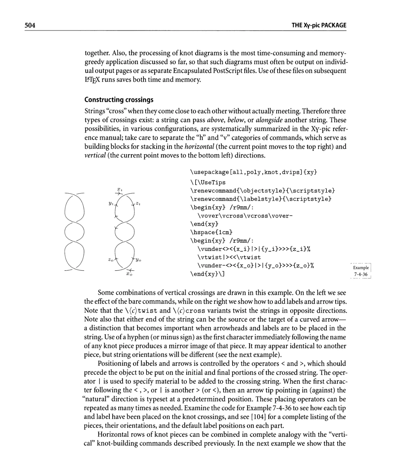
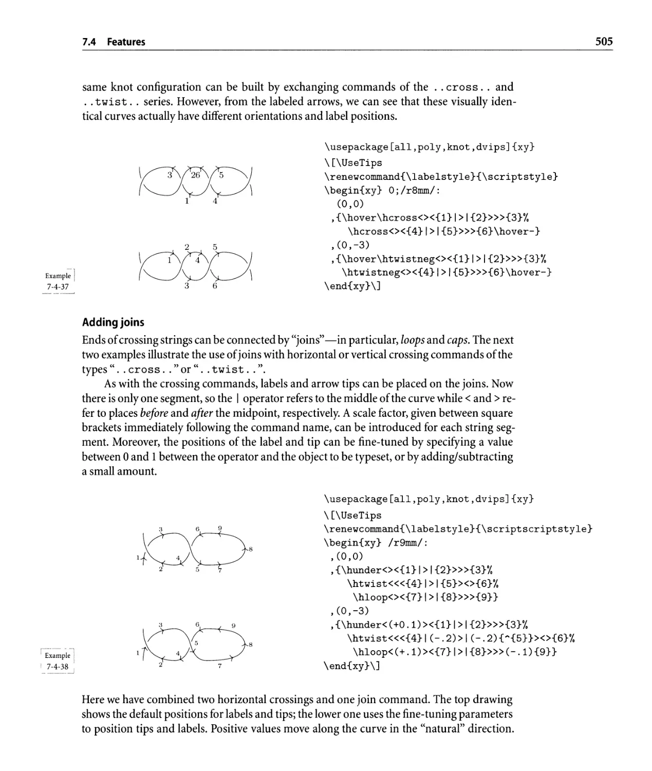
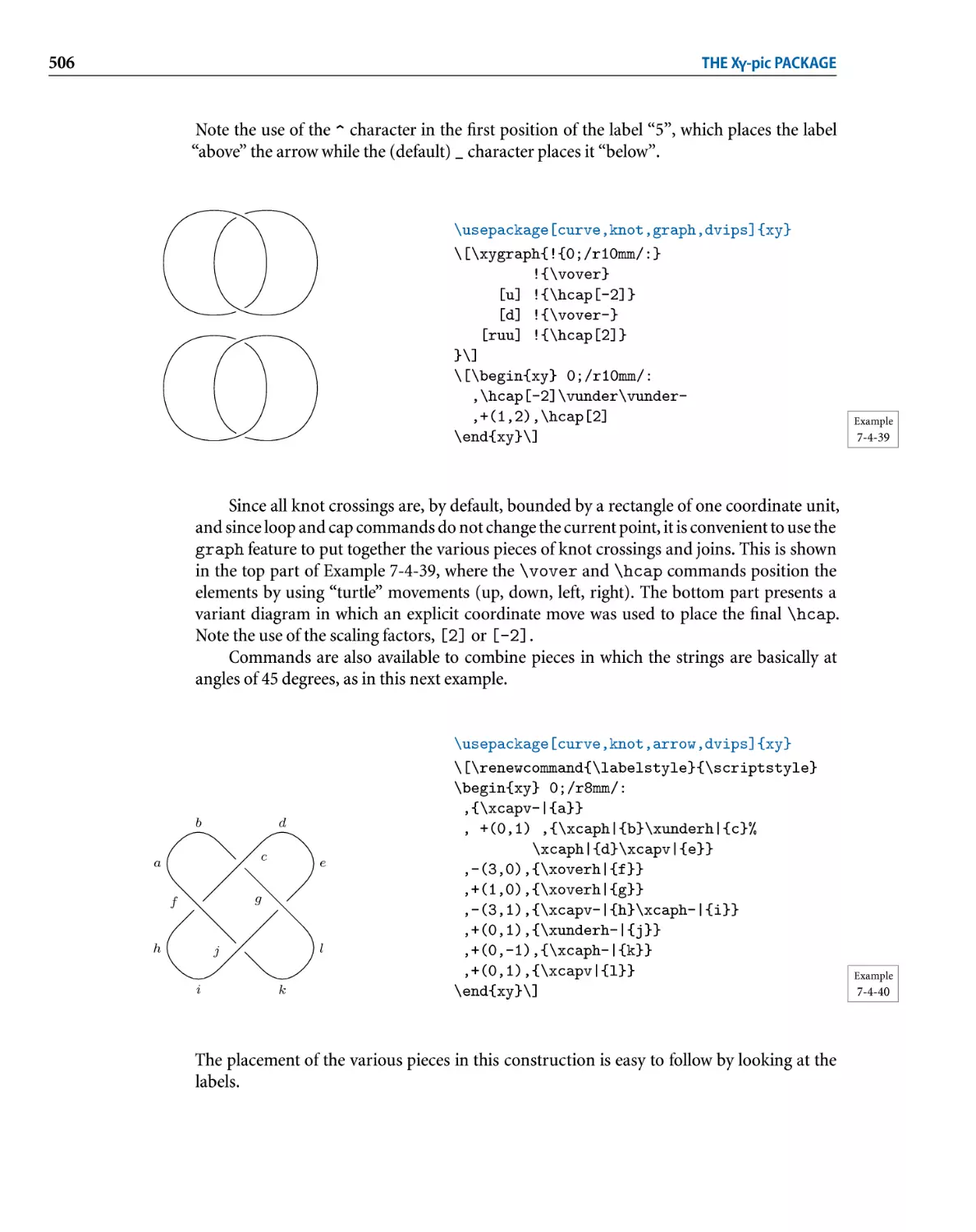
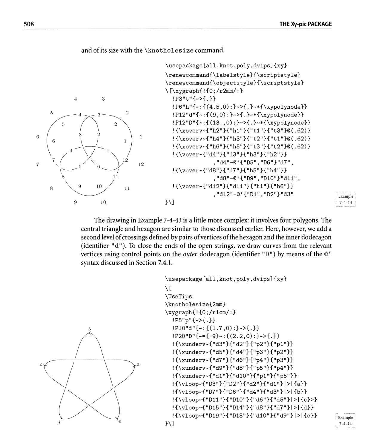
7.4.8 Links and knots. . . . . . . . . . . . . . . . . . . . . . . . . . . . . . . .. 503
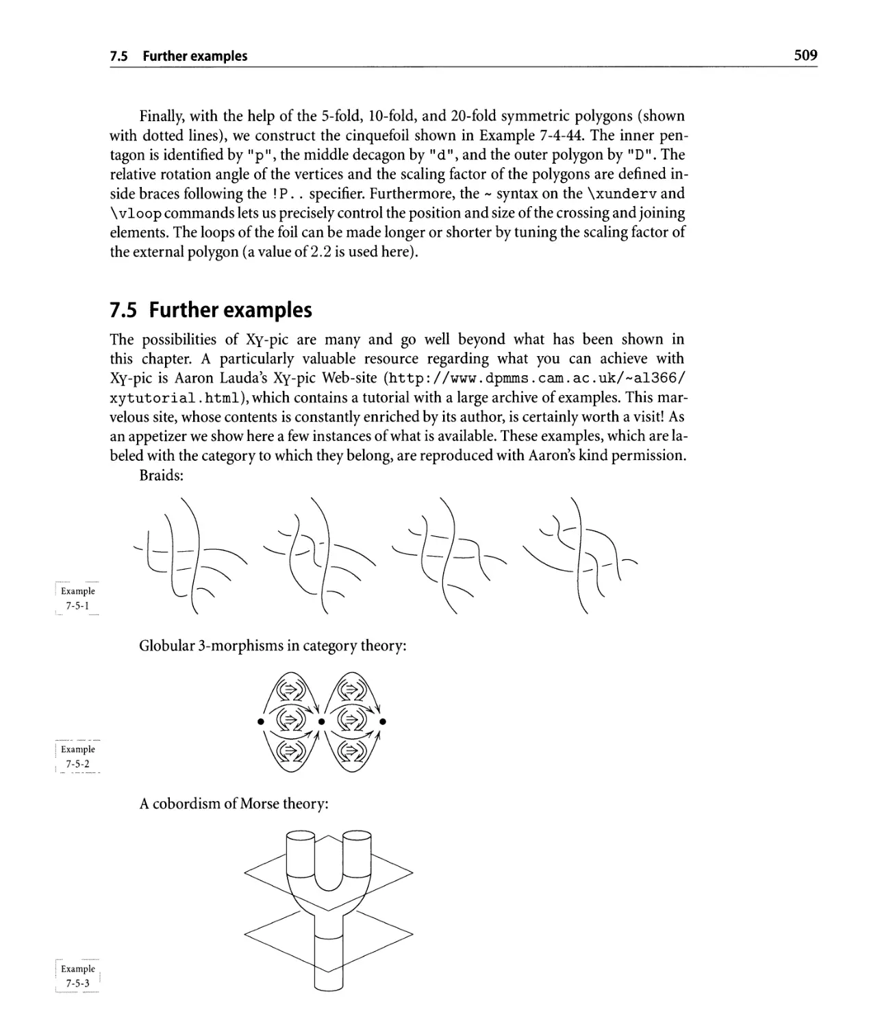
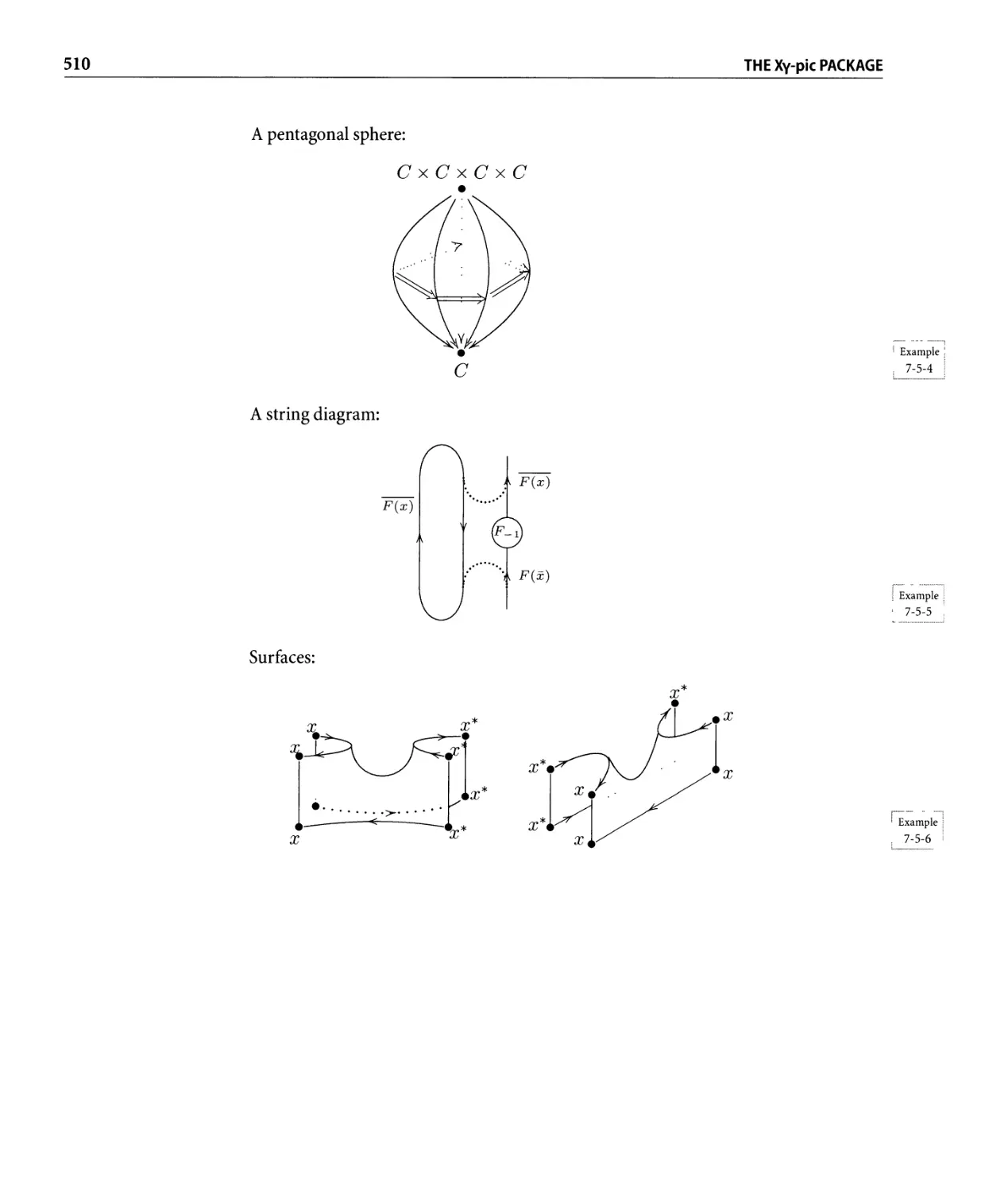
7.5 F u rt her e xa m pie s. . . . . . . . . . . . . . . . . . . . . . . . . . . . . . . . . . . . .. 509
8 Applications in Science, Technology, and Medicine 511
8.1 Typographical rules for scientific texts. . . . . . . . . . . . . . . . . . . . . . . .. 512
8. 1 . 1 G e tt i n g the u n its rig h t . . . . . . . . . . . . . . . . . . . . . . . . . . . .. 51 3
CONTENTS xiii
8.1.2 Typesetting chemical symbols . . . . . . . . . . . . . . . . . . . . . . .. 517
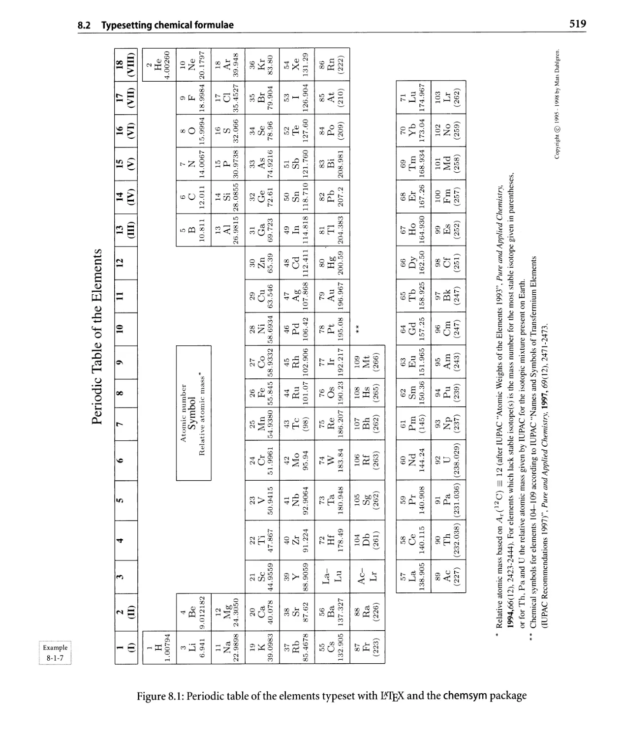
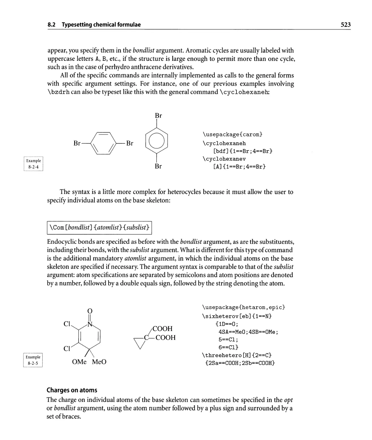
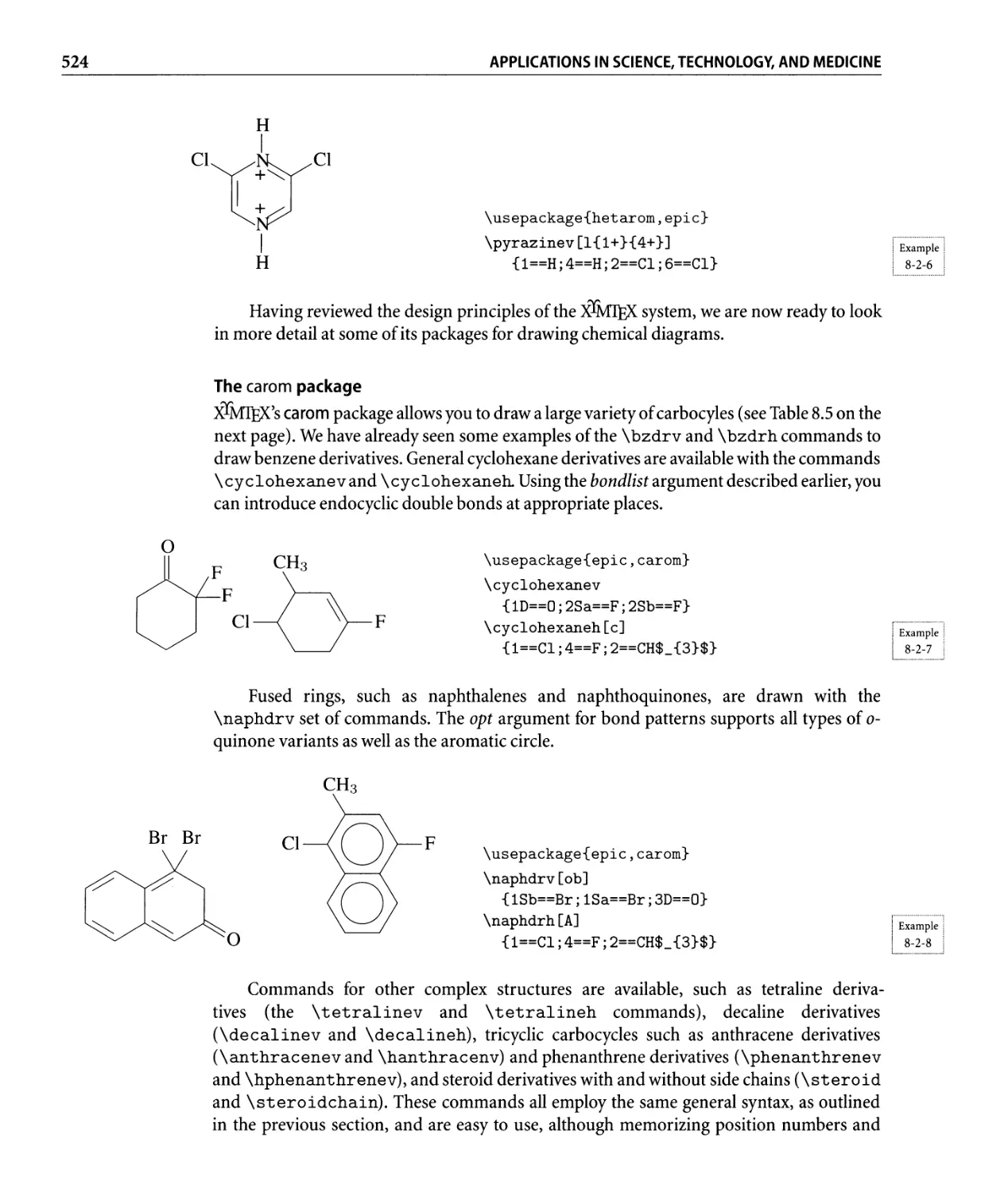
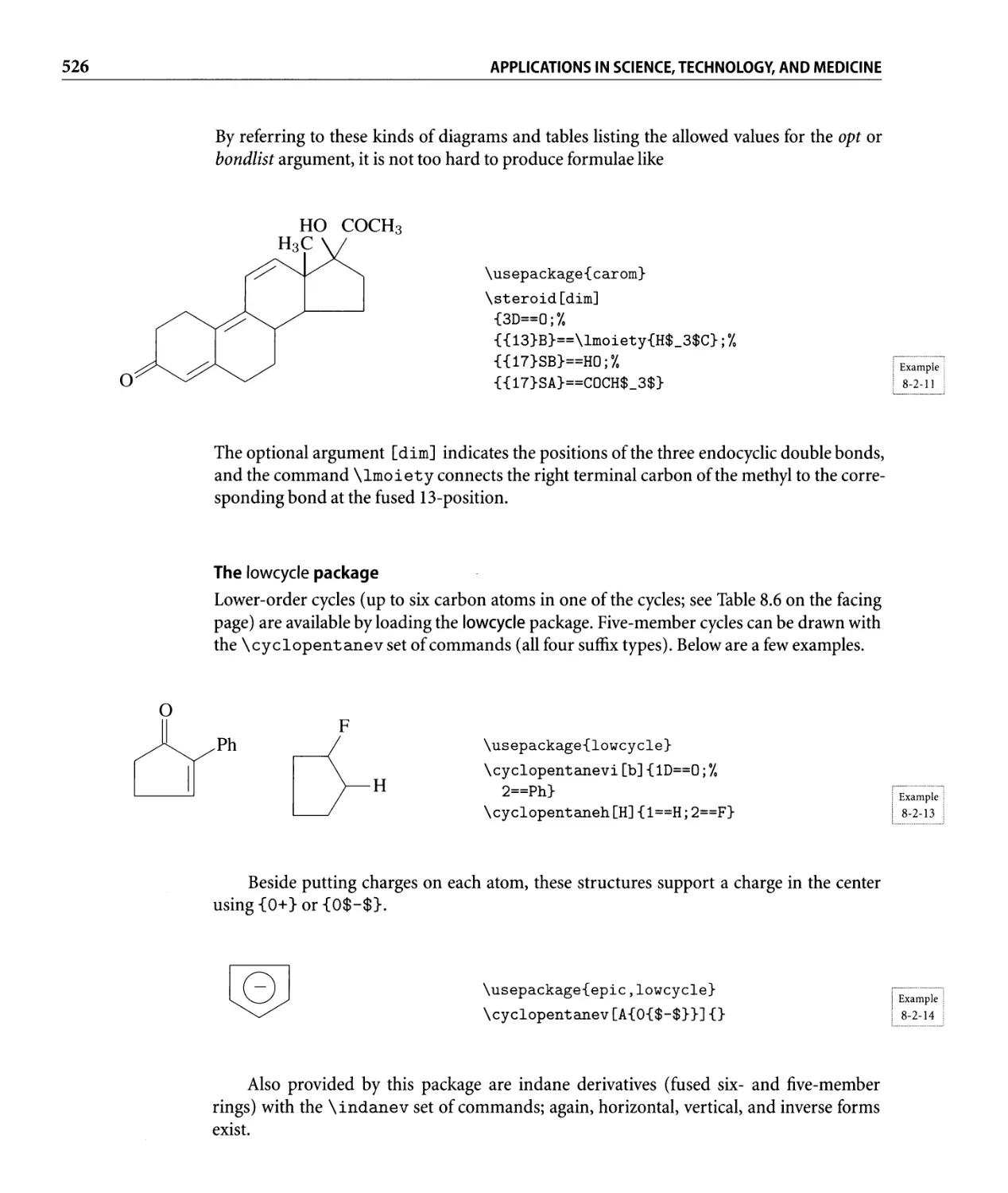
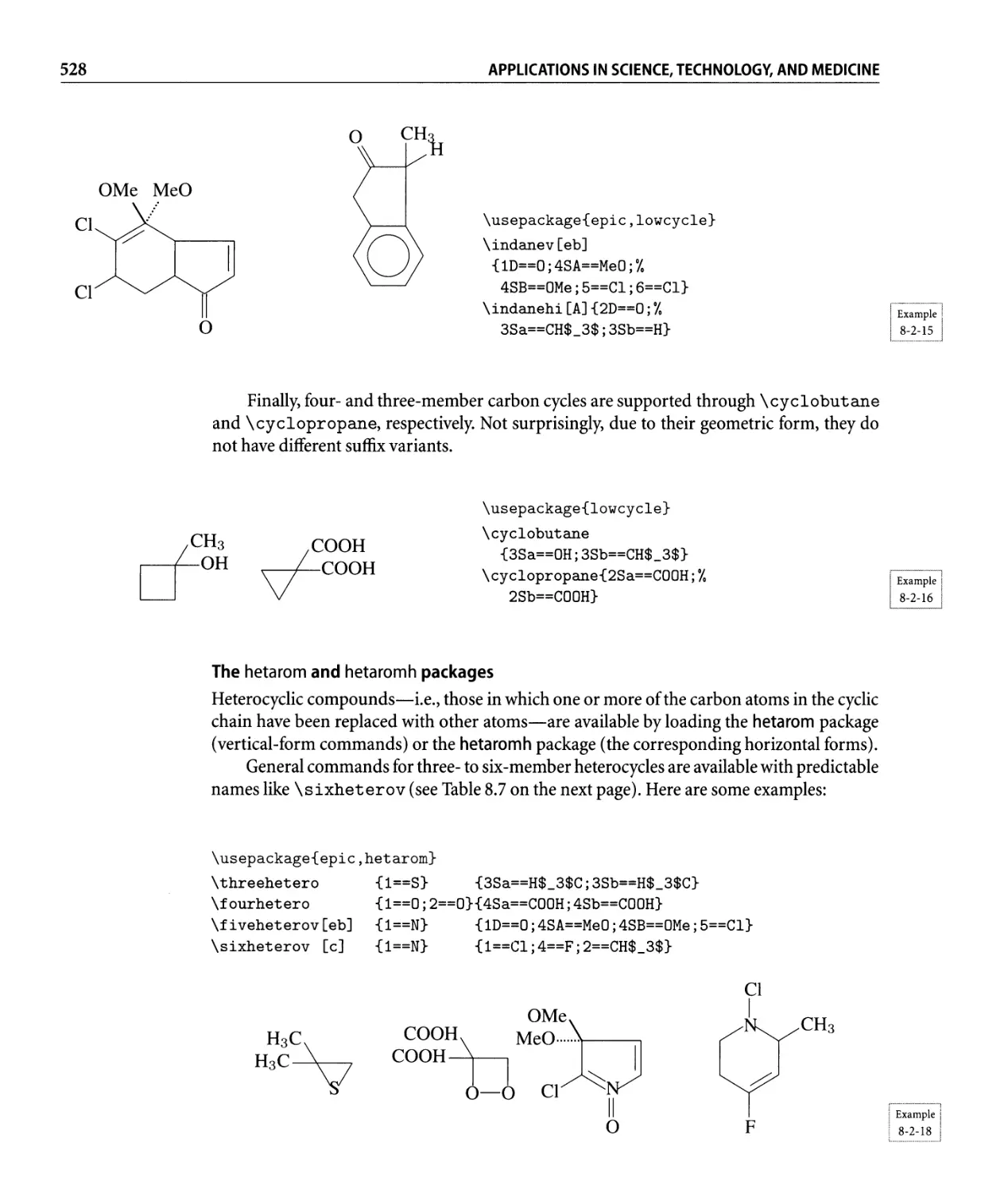
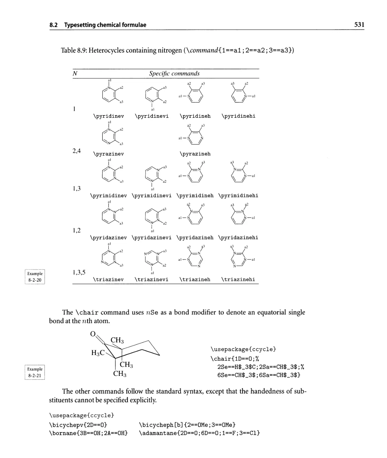
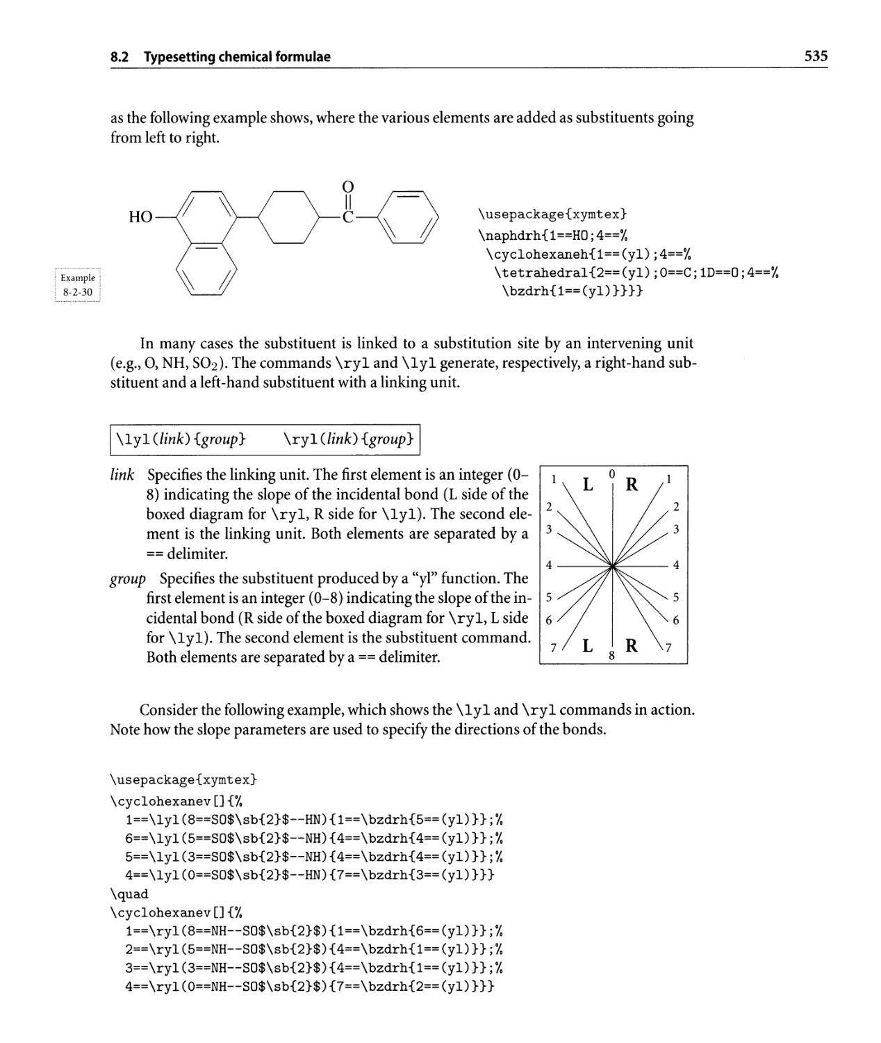
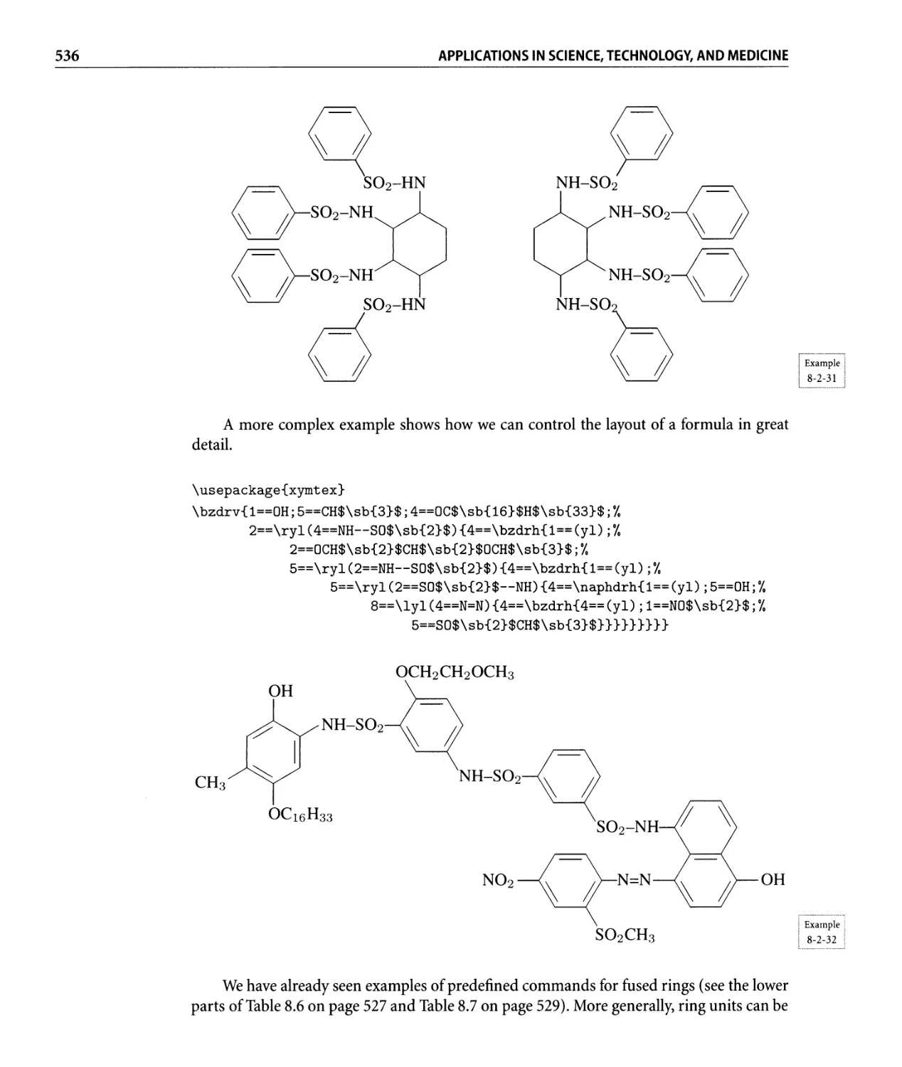
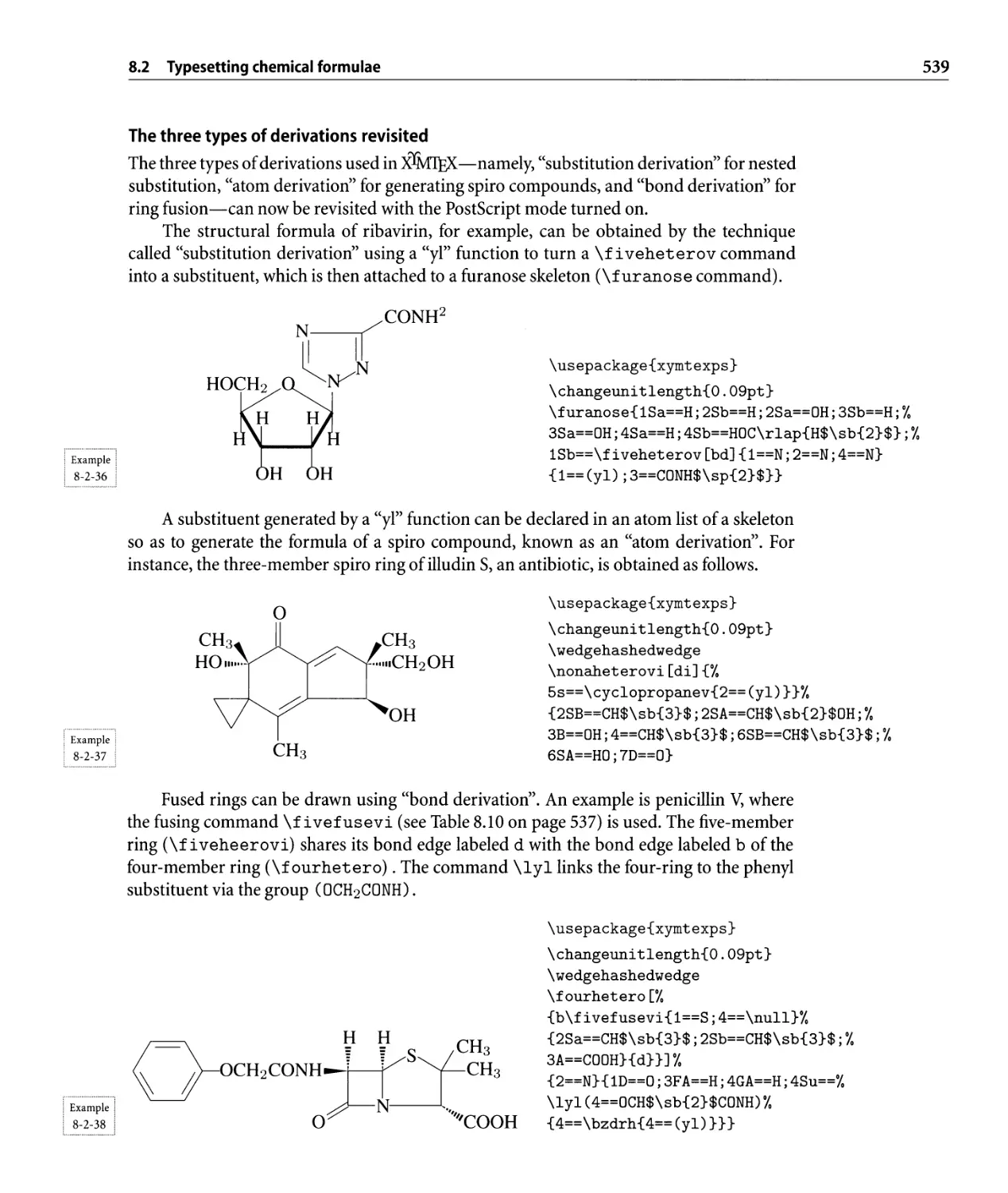
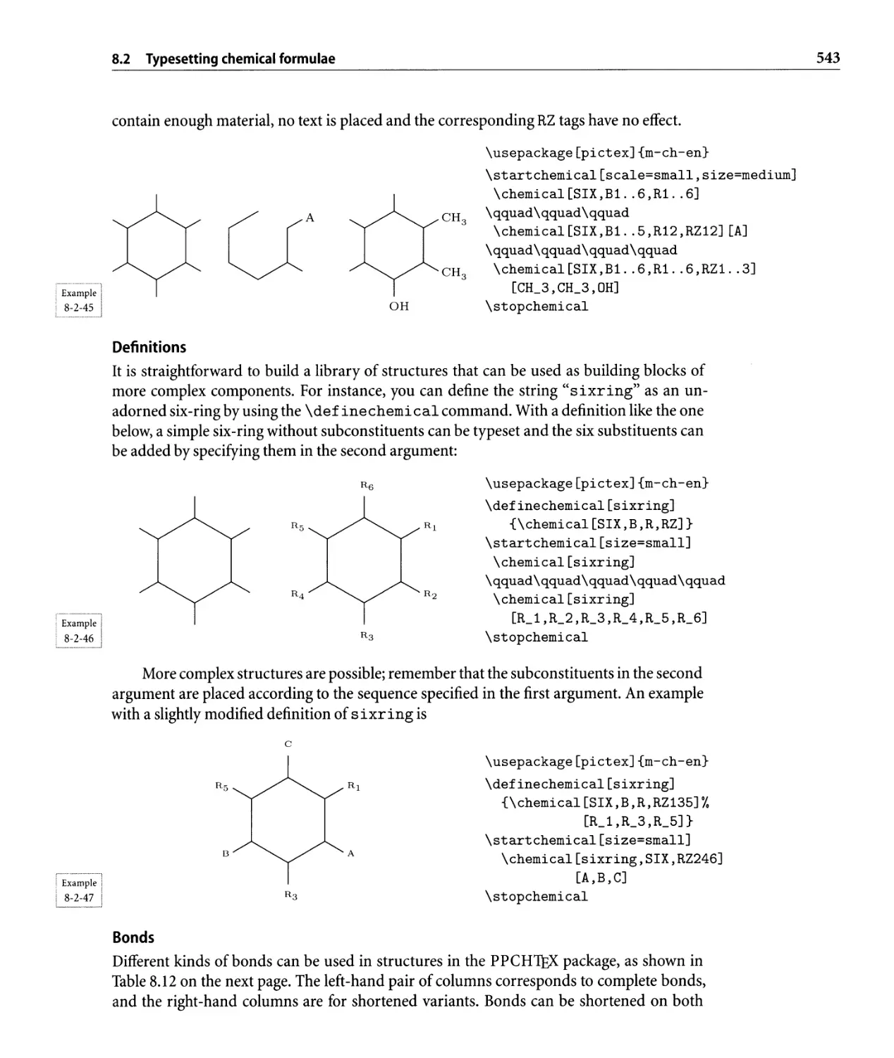
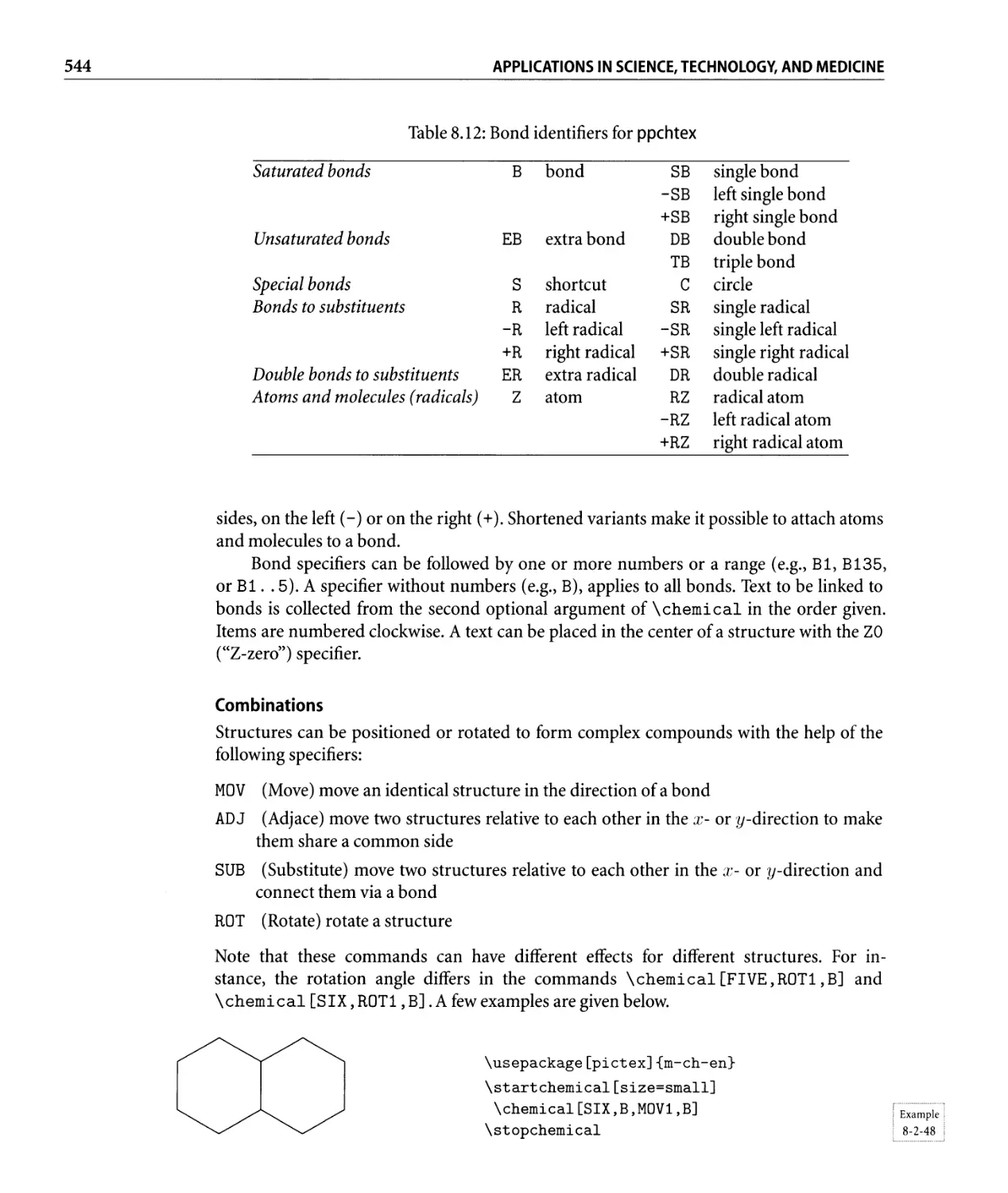
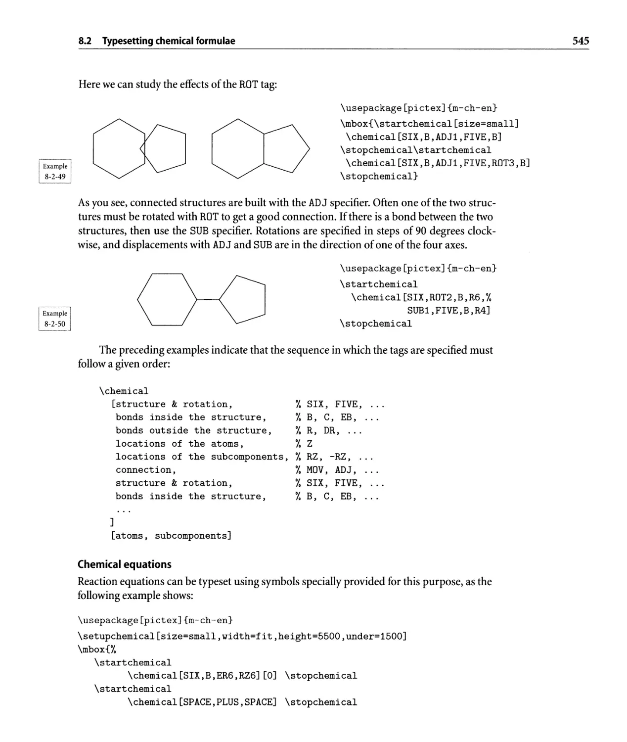
8.2 Typesetting chemical formulae . . . . . . . . . . . . . . . . . . . . . . . . . . . .. 518
8.2.1 The XlivrrEX system. . . . . . . . . . . . . . . . . . . . . . . . . . . . . . .. 520
8.2.2 The ppchtex package. . . . . . . . . . . . . . . . . . . . . . . . . . . . .. 541
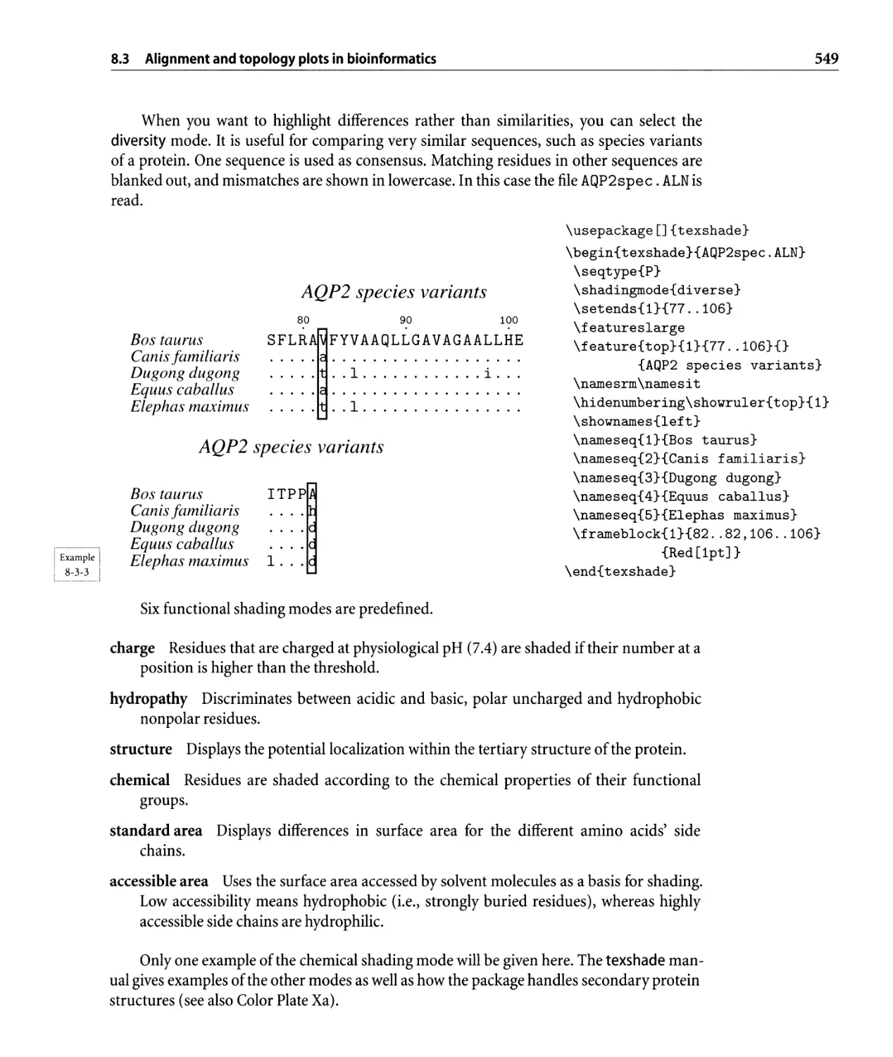
8.3 Alignment and topology plots in bioinformatics. . . . . . . . . . . . . . . . . .. 547
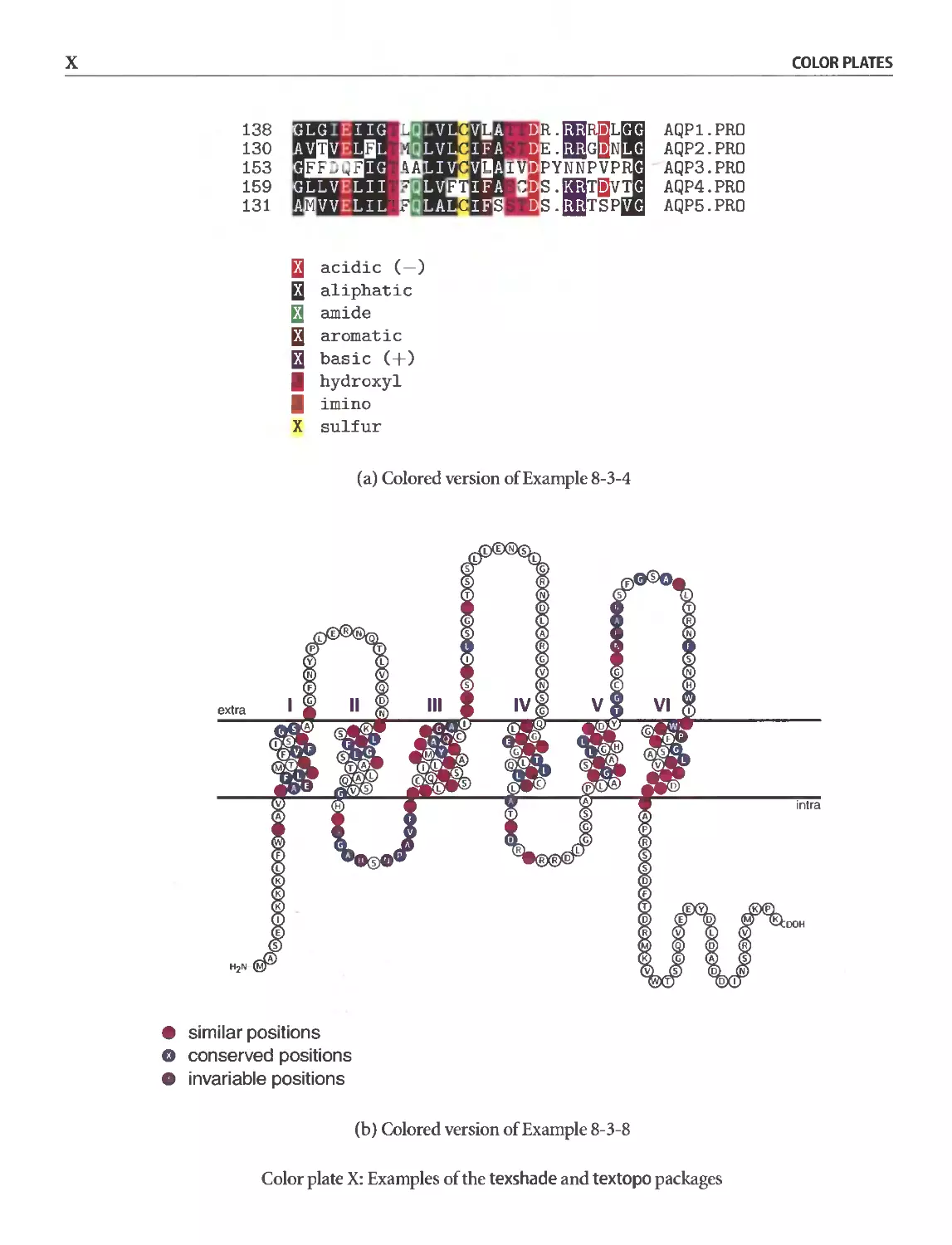
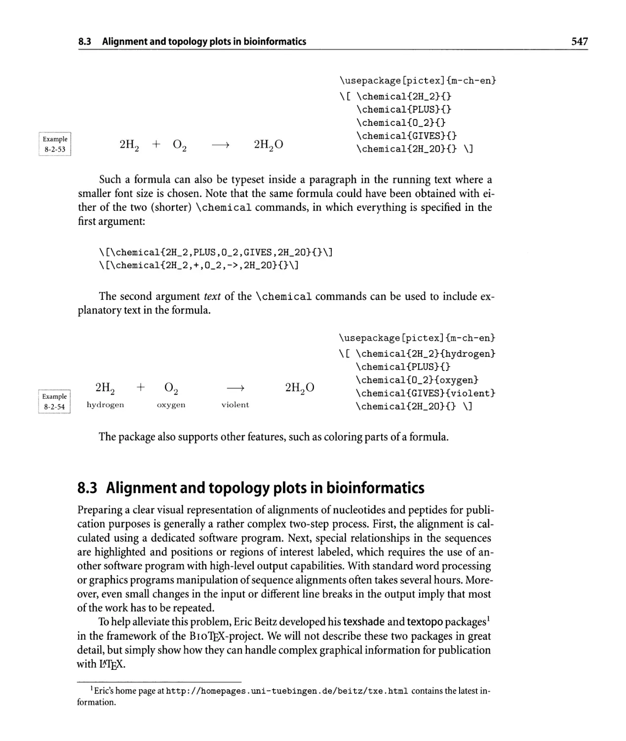
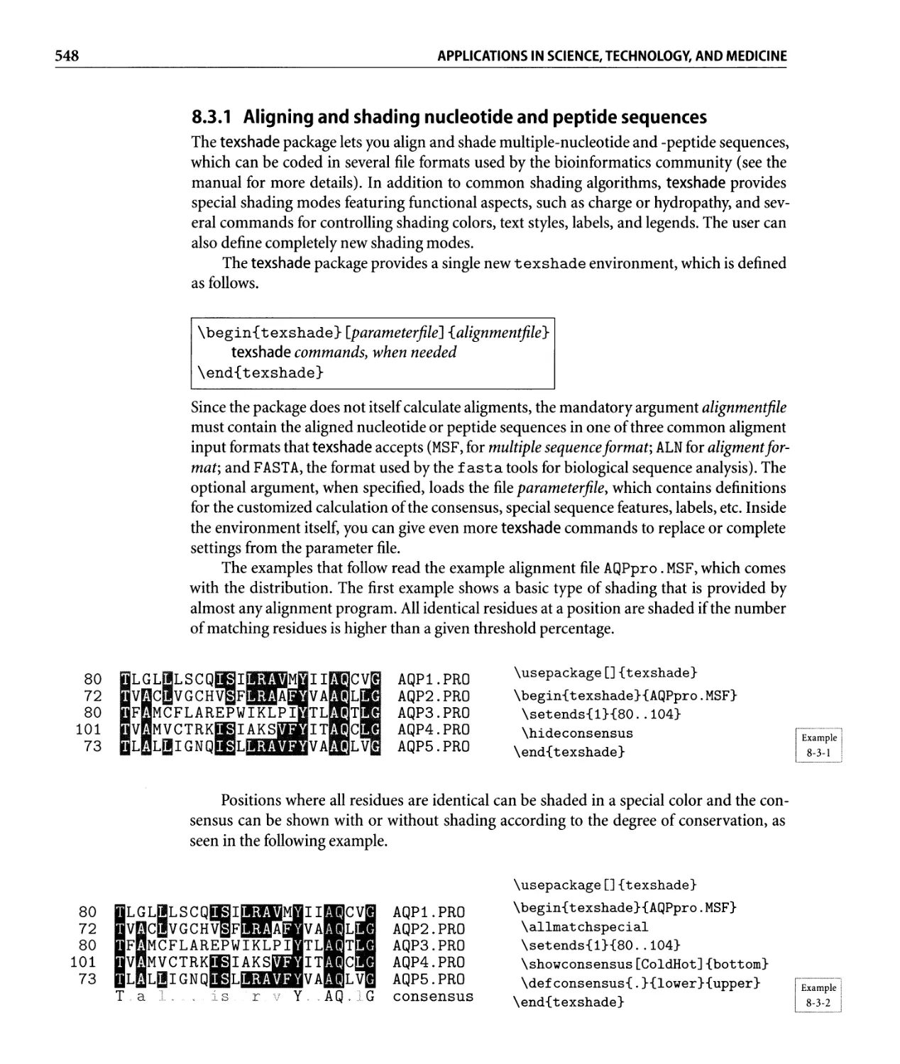
8.3.1 Aligning and shading nucleotide and peptide sequences . . . . . .. 548
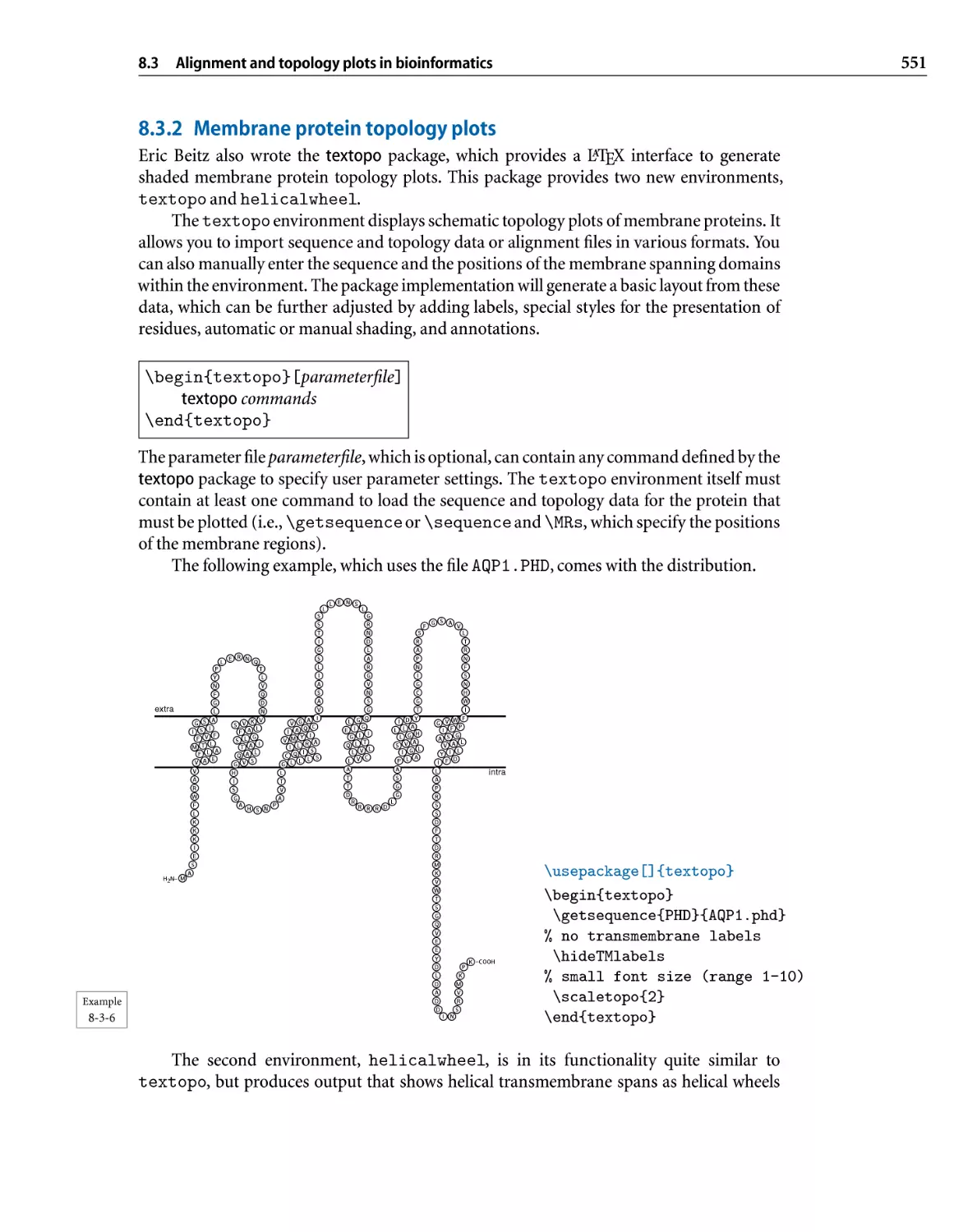
8.3.2 Membrane protein topology plots. . . . . . . . . . . . . . . . . . . . .. 551
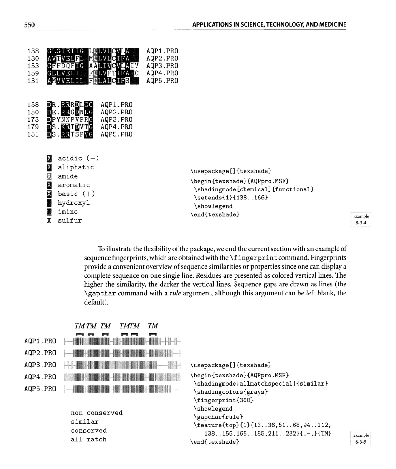
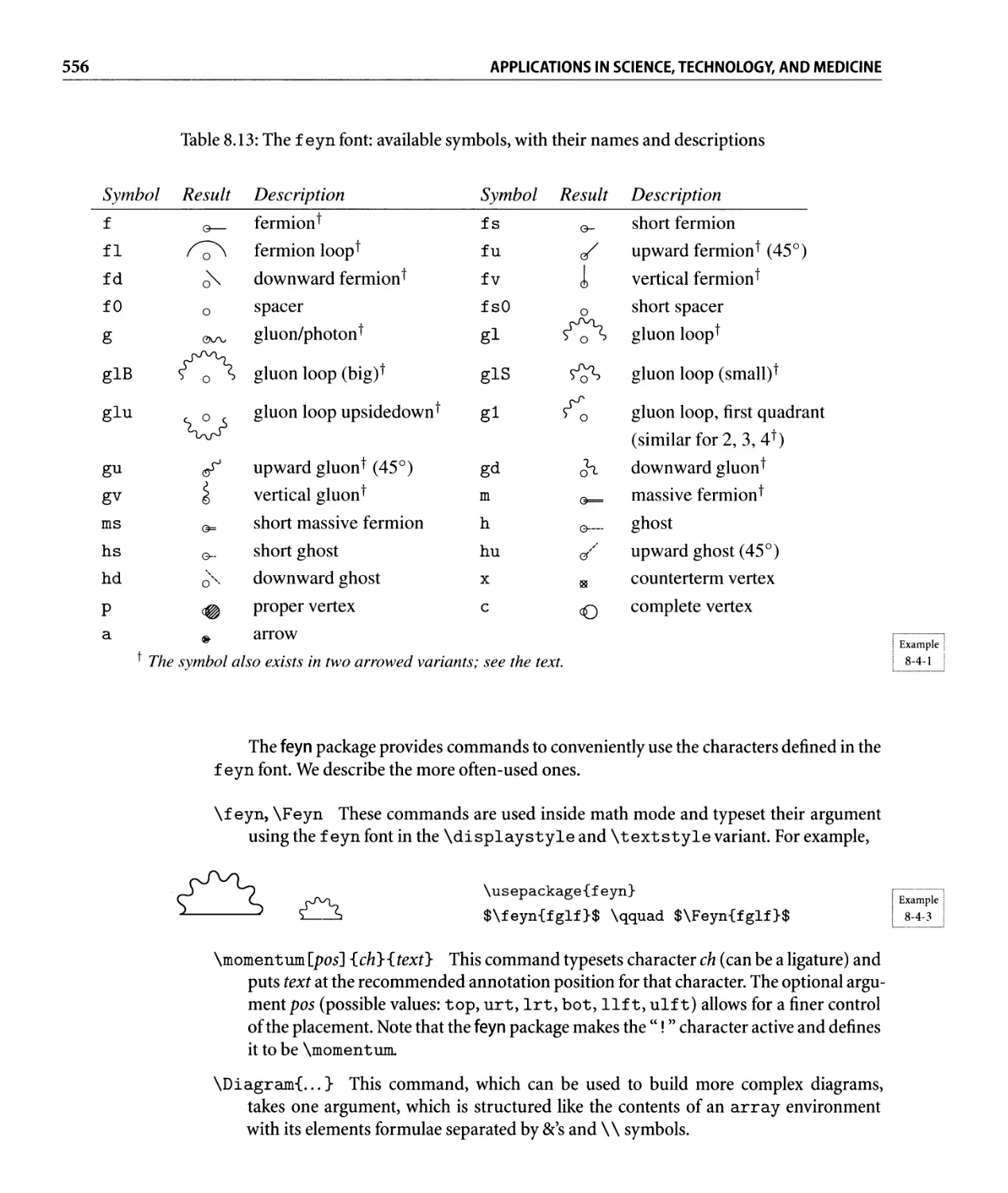
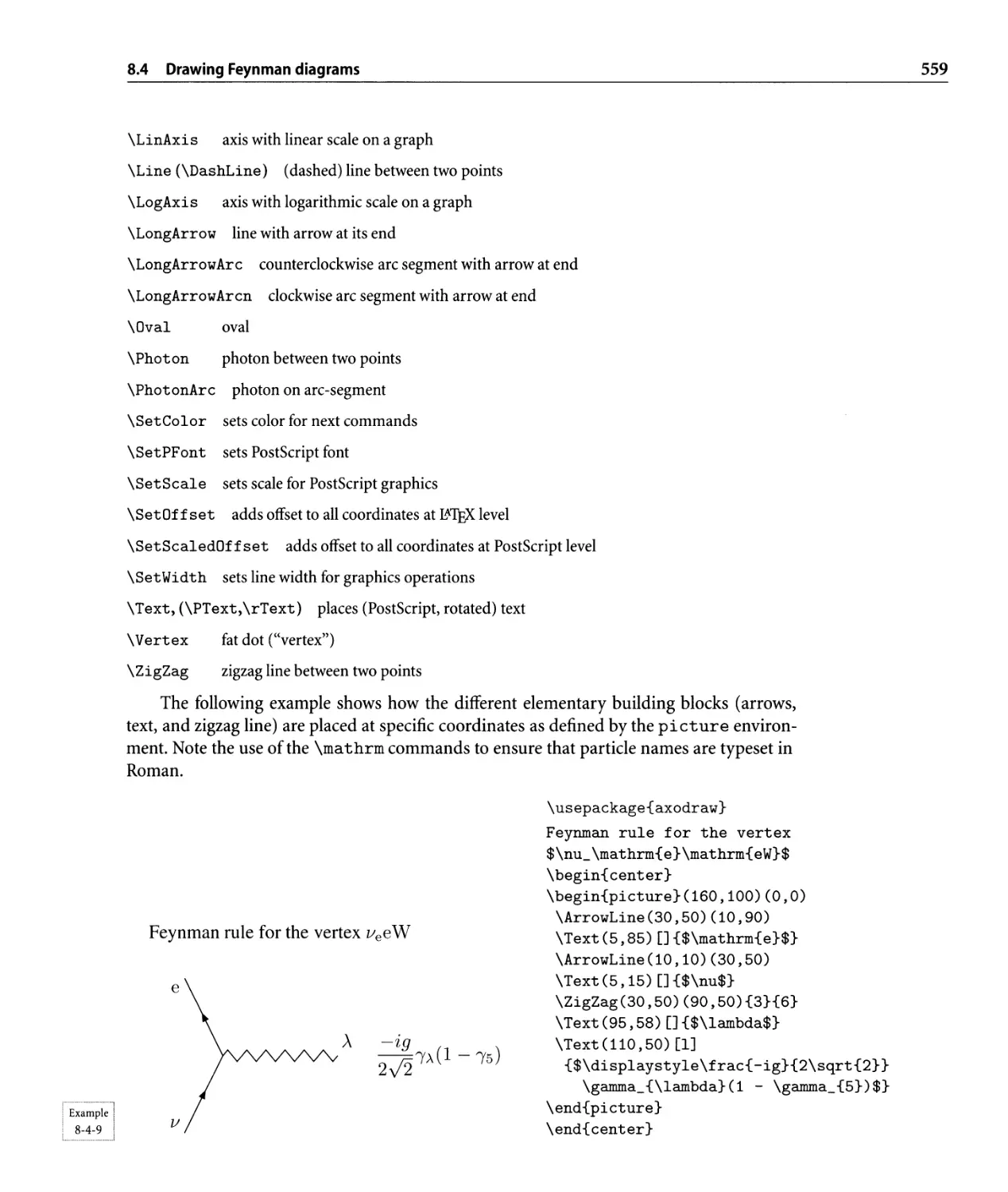
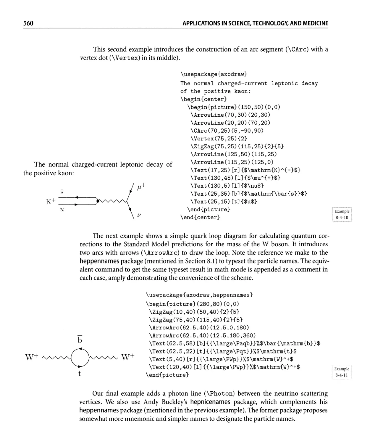
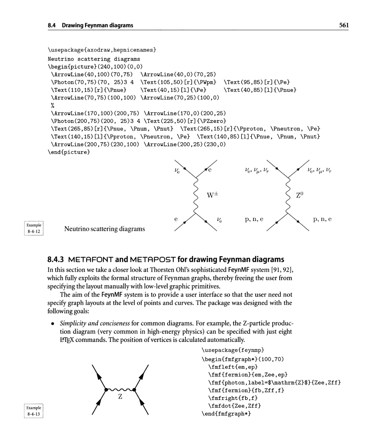
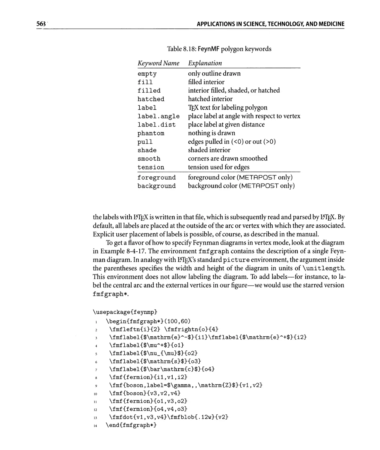
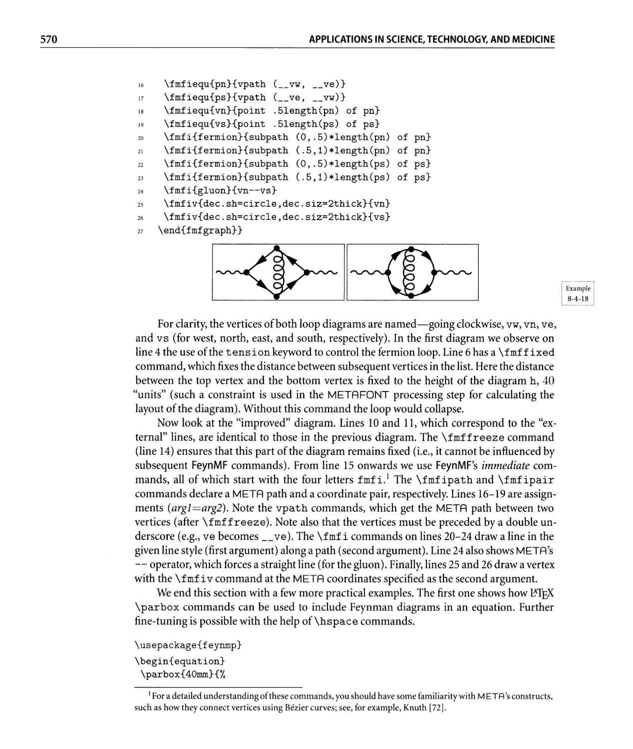
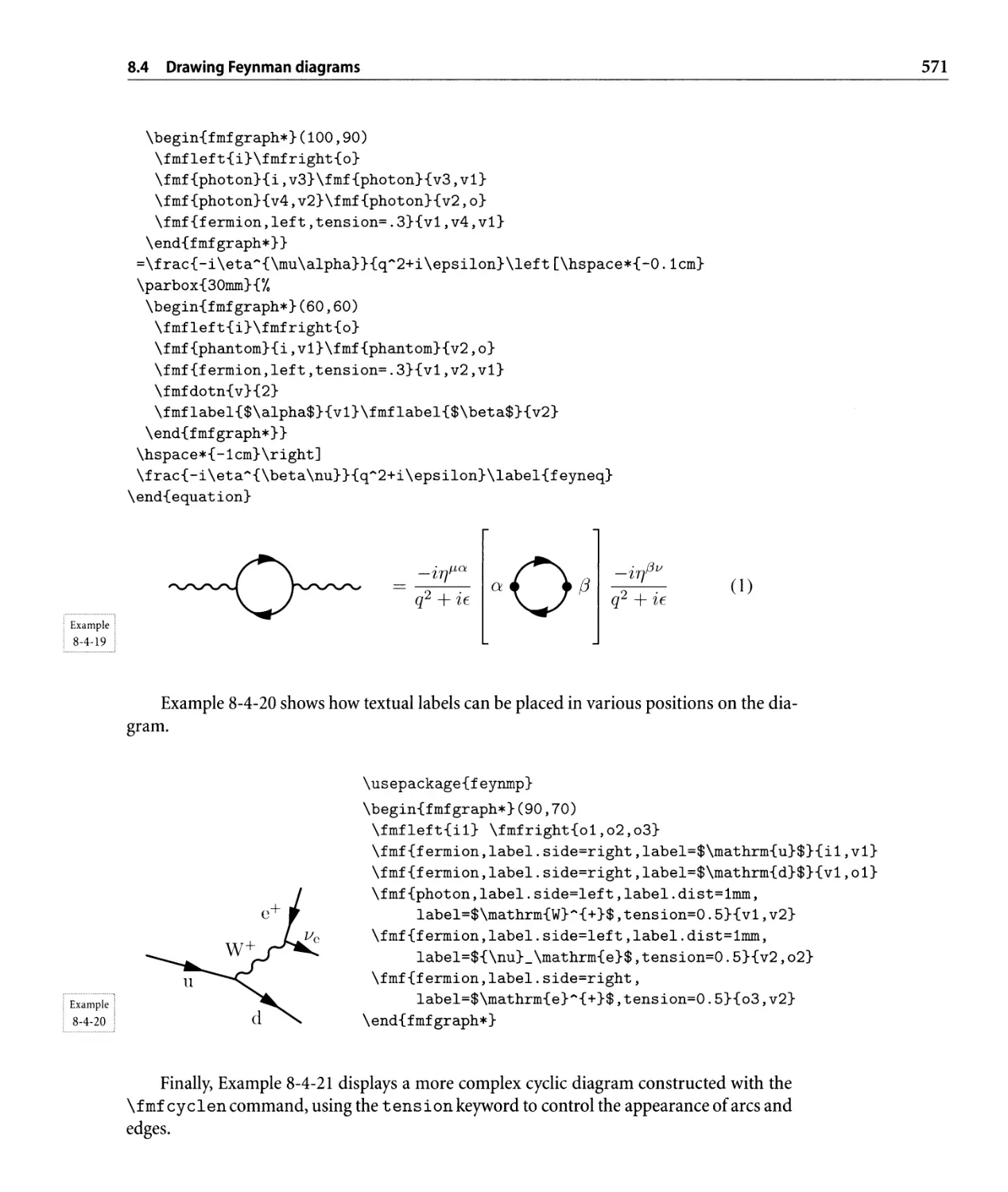
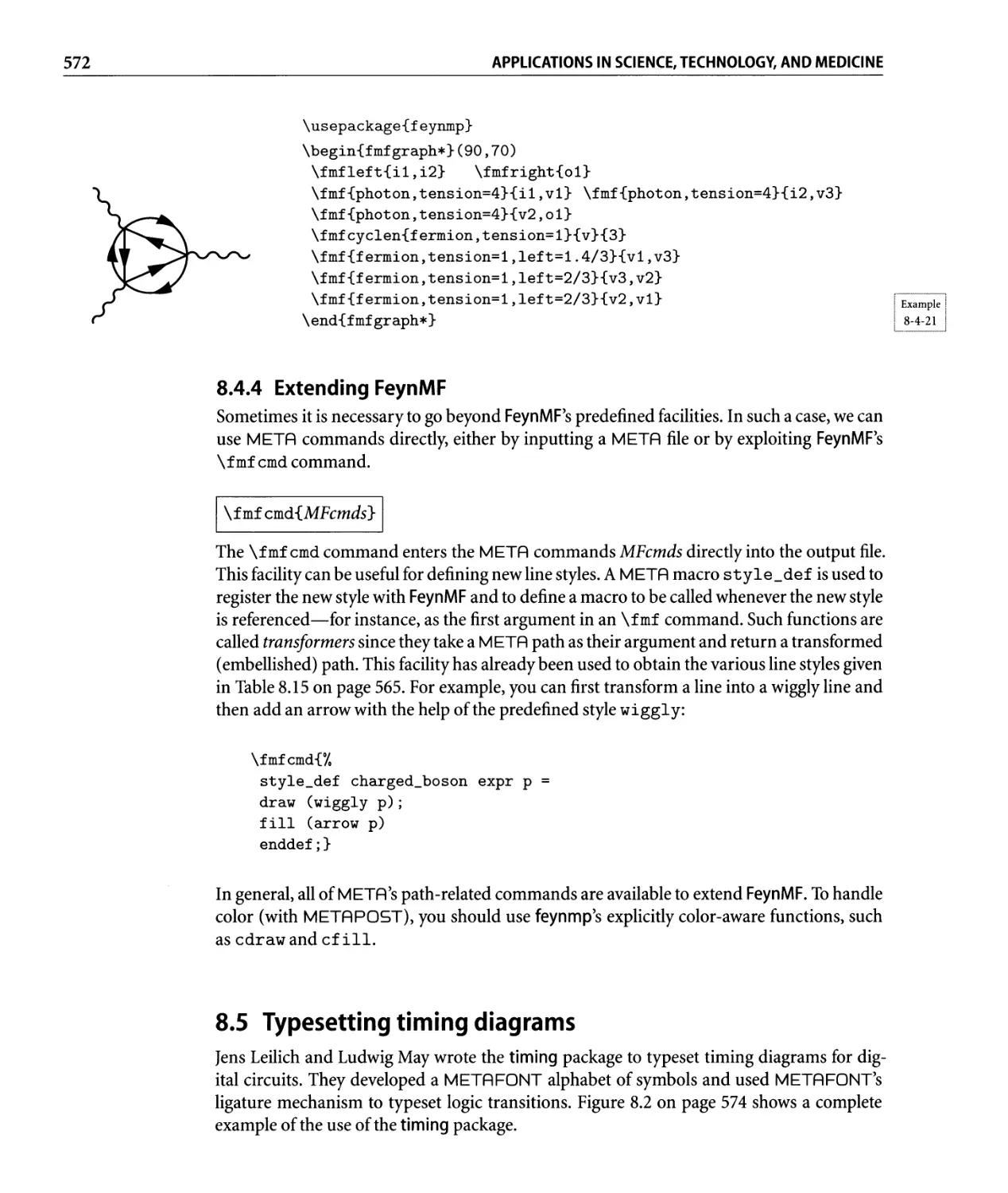
8.4 Drawing Feynman diagrams. . . . . . . . . . . . . . . . . . . . . . . . . . . . . .. 555
8.4.1 A special font for drawing Feynman diagrams . . . . . . . . . . . . .. 555
8.4.2 PostScript for drawing Feynman diagrams. . . . . . . . . . . . . . . .. 558
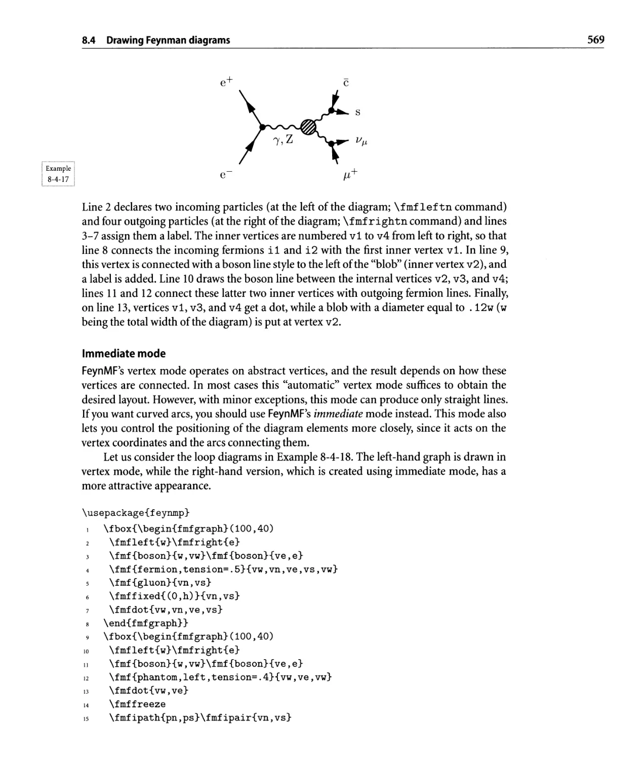
8.4.3 META FONT and META POST for drawing Feynman diagrams. .. 561
8.4.4 Extending FeynMF . . . . . . . . . . . . . . . . . . . . . . . . . . . . . .. 572
8.5 Typesetting timing diagrams . . . . . . . . . . . . . . . . . . . . . . . . . . . . .. 572
8.5.1 Commands in the timing environment. . . . . . . . . . . . . . . . .. 573
8.5.2 Customlzatlon . . . . . . . . . . . . . . . . . . . . . . . . . . . . . . . . .. 576
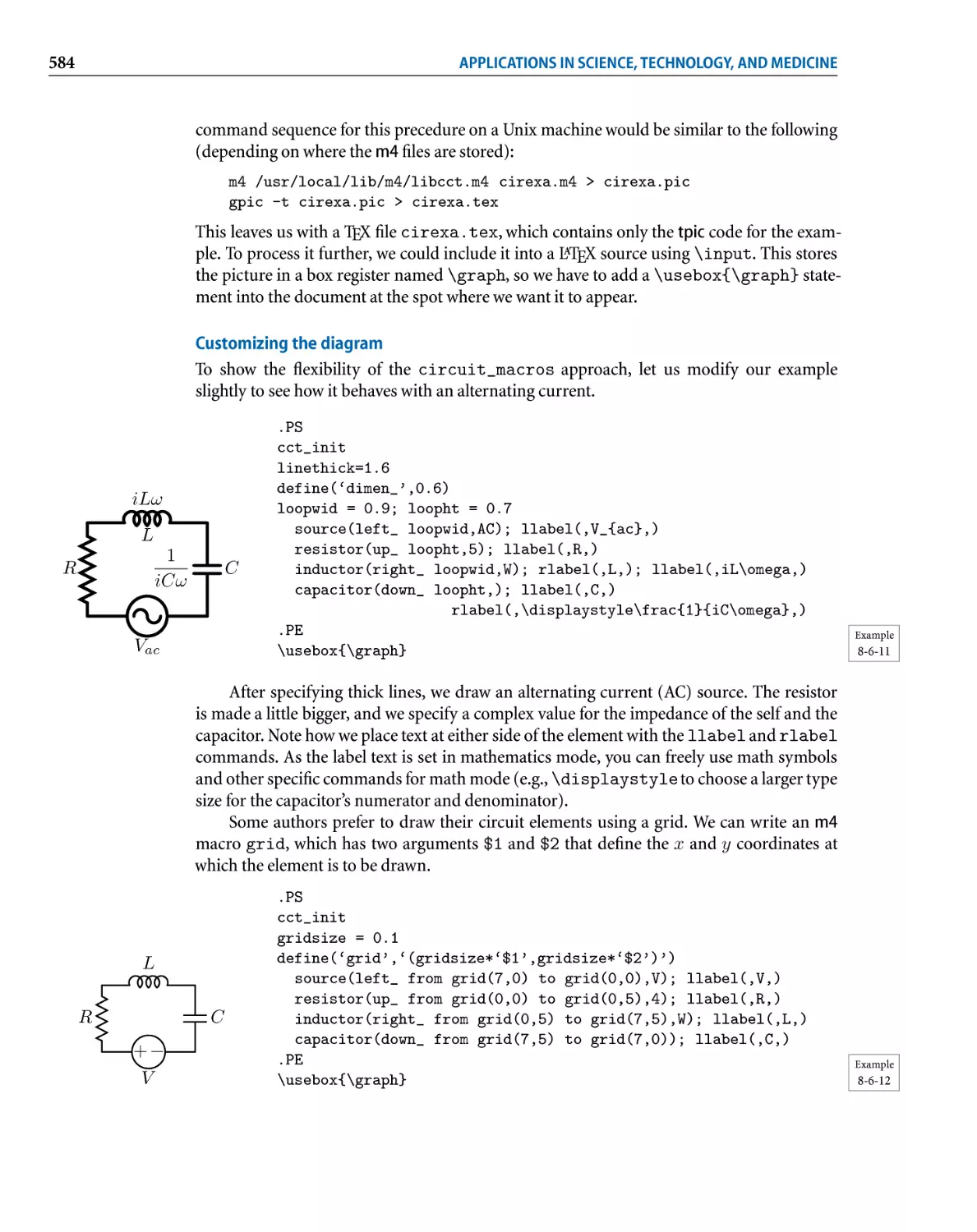
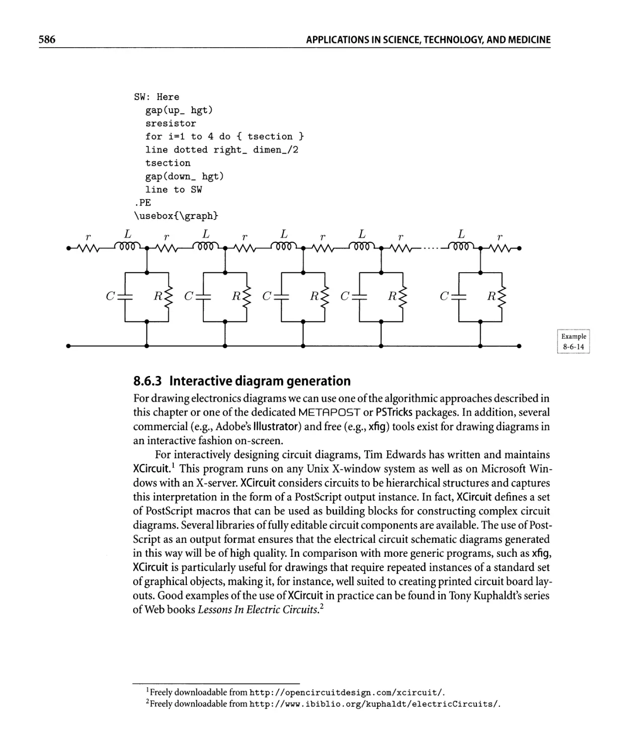
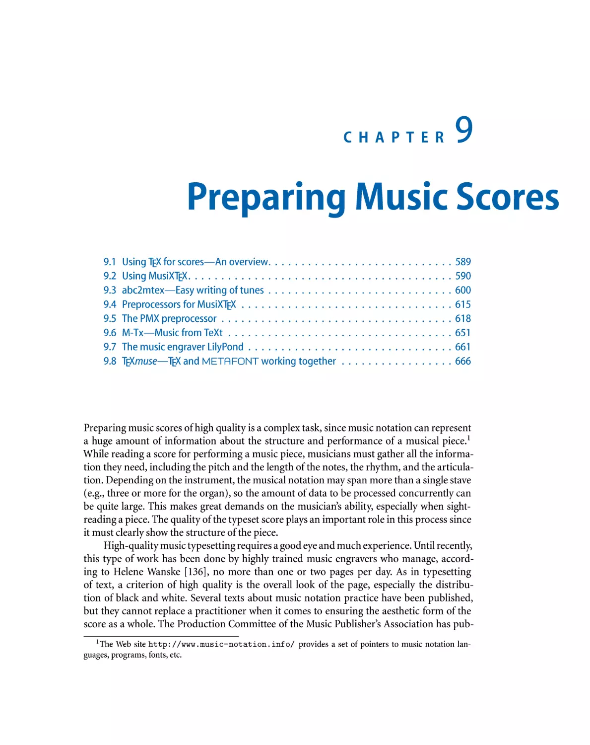
8.6 Electronics and optics circuits . . . . . . . . . . . . . . . . . . . . . . . . . . . . .. 576
8.6.1 A special font for drawing electronics and optics diagrams . . . . .. 576
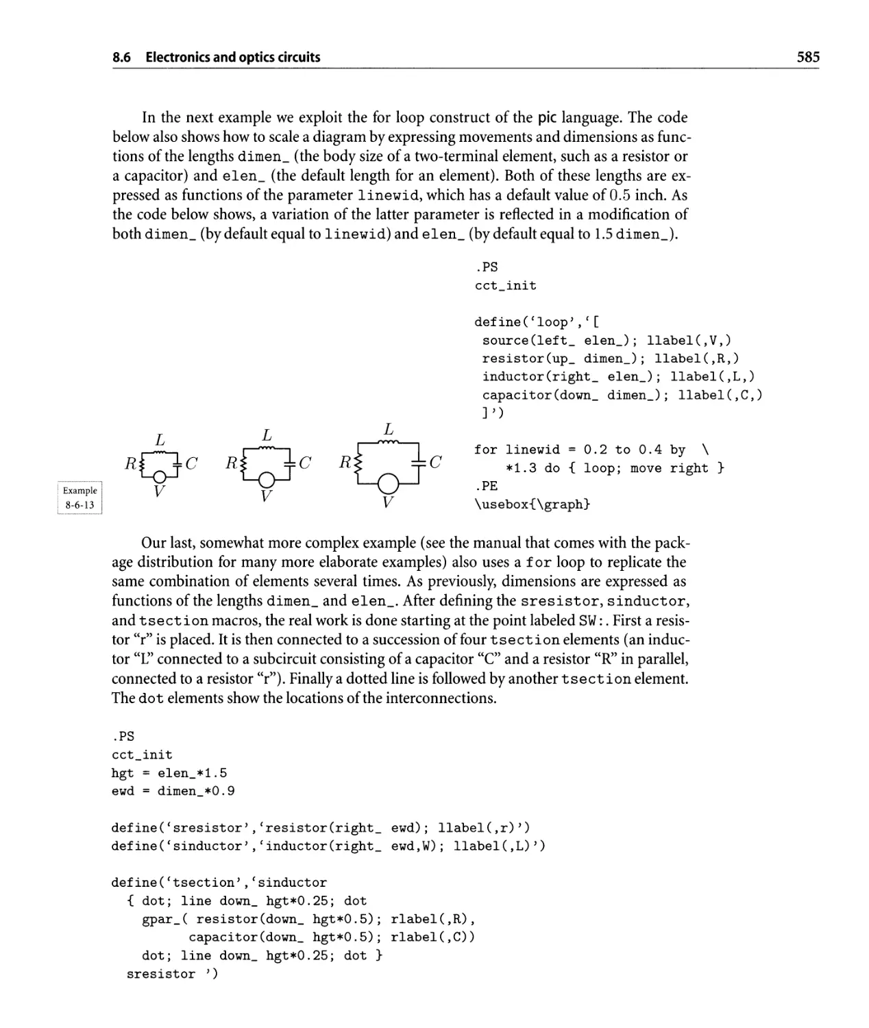
8.6.2 Using the m4 macro processor for electronics diagrams . . . . . . .. 583
8.6.3 Interactive diagram generation . . . . . . . . . . . . . . . . . . . . . .. 586
9 Preparing Music Scores 587
9.1 Using TEX for scores-An overview. . . . . . . . . . . . . . . . . . . . . . . . . .. 589
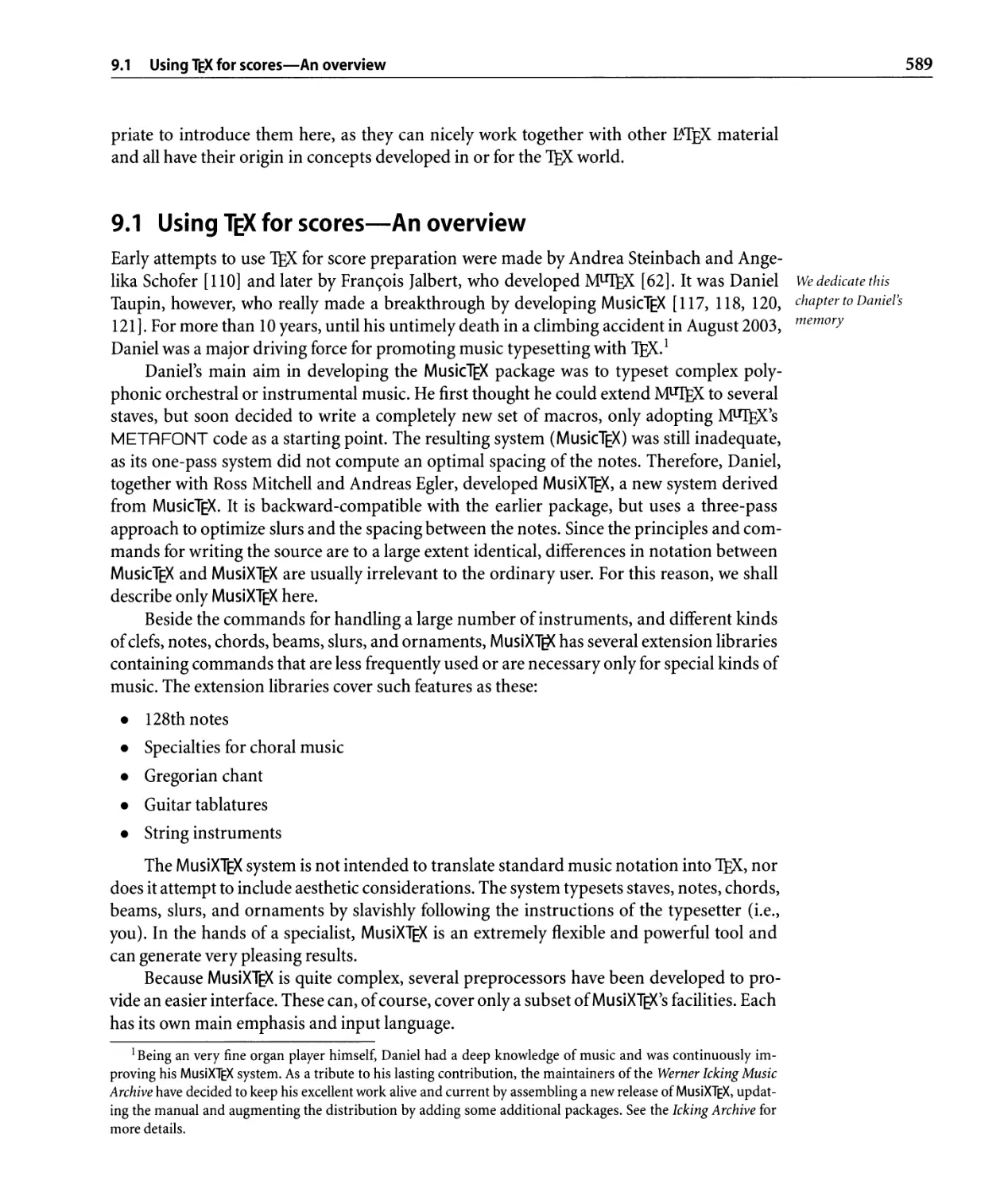
9.2 Using MusiXTEX . . . . . . . . . . . . . . . . . . . . . . . . . . . . . . . . . . . . . .. 590
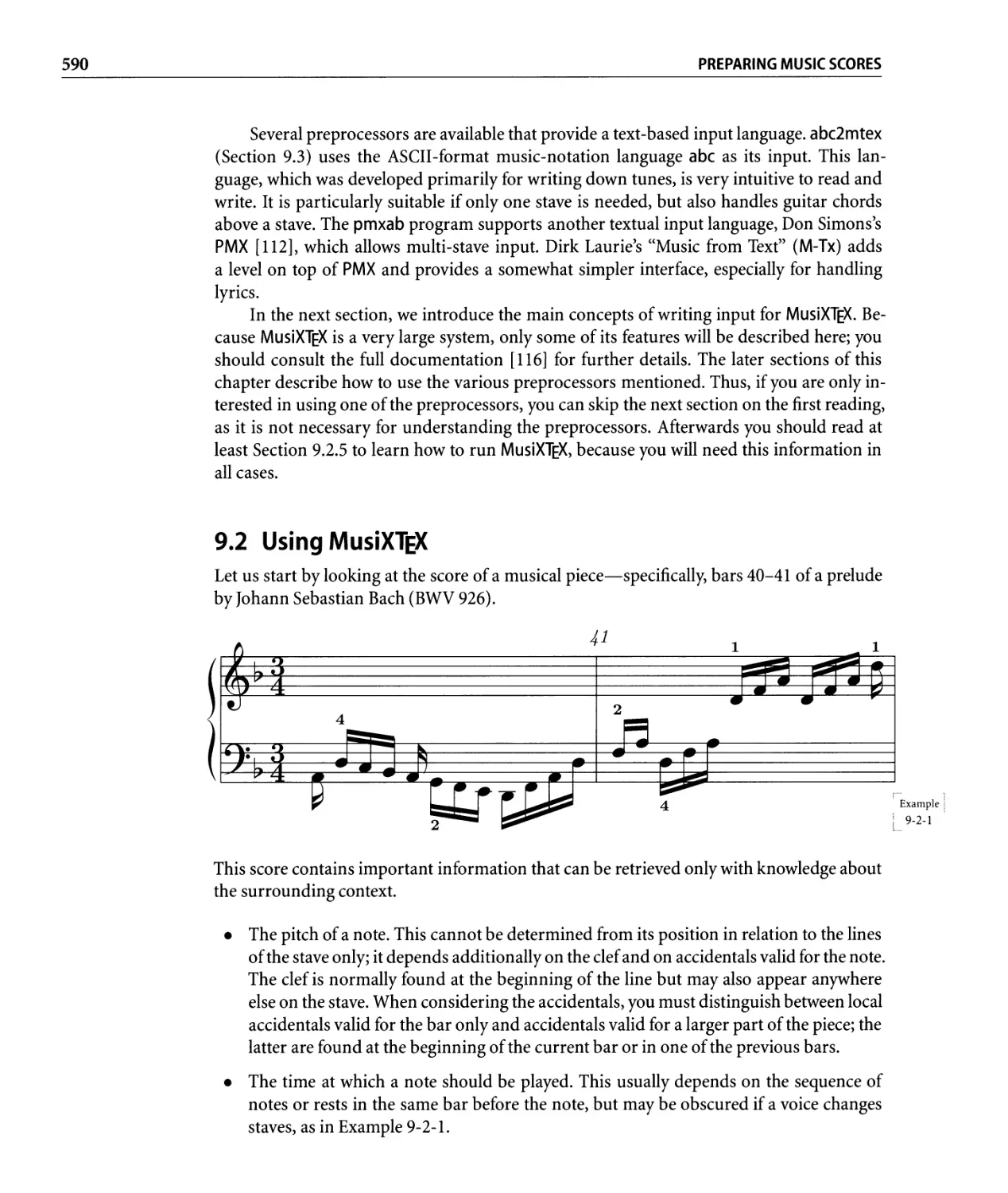
9.2.1 The structu re of a MusiXTEX sou rce . . . . . . . . . . . . . . . . . . . .. 591
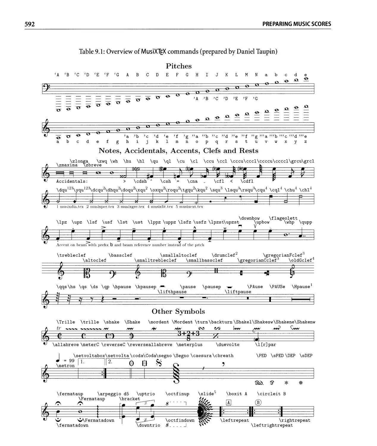
9.2.2 Writing notes. . . . . . . . . . . . . . . . . . . . . . . . . . . . . . . . . .. 591
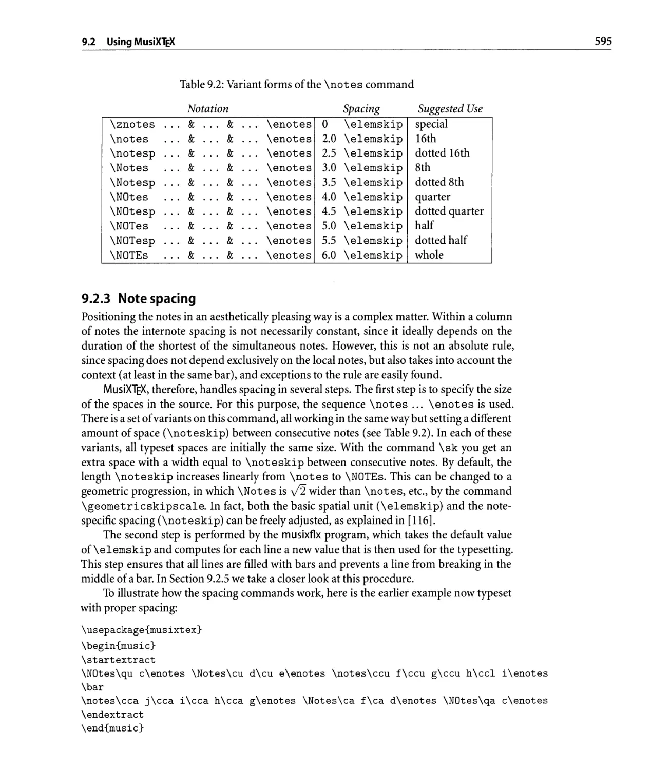
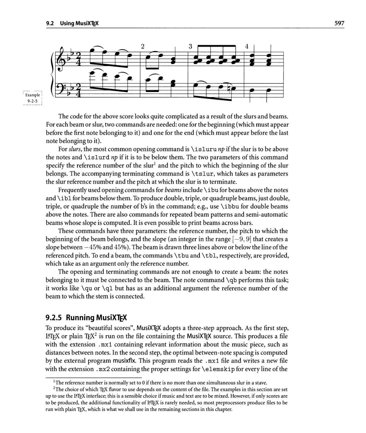
9.2.3 Note spacing. . . . . . . . . . . . . . . . . . . . . . . . . . . . . . . . . .. 595
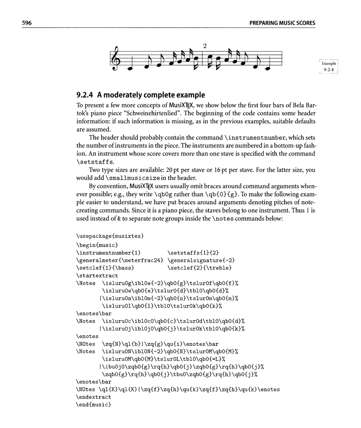
9.2.4 A moderately complete example . . . . . . . . . . . . . . . . . . . . .. 596
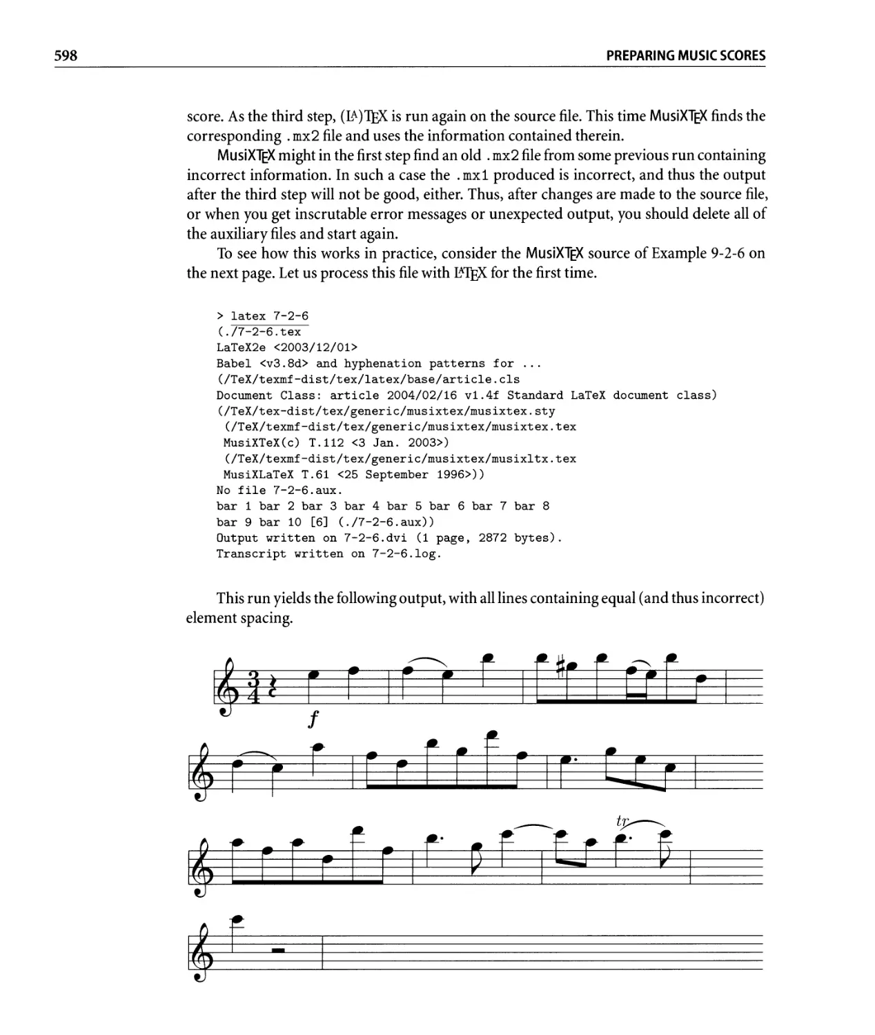
9.2.5 Running MusiXTEX. . . . . . . . . . . . . . . . . . . . . . . . . . . . . . .. 597
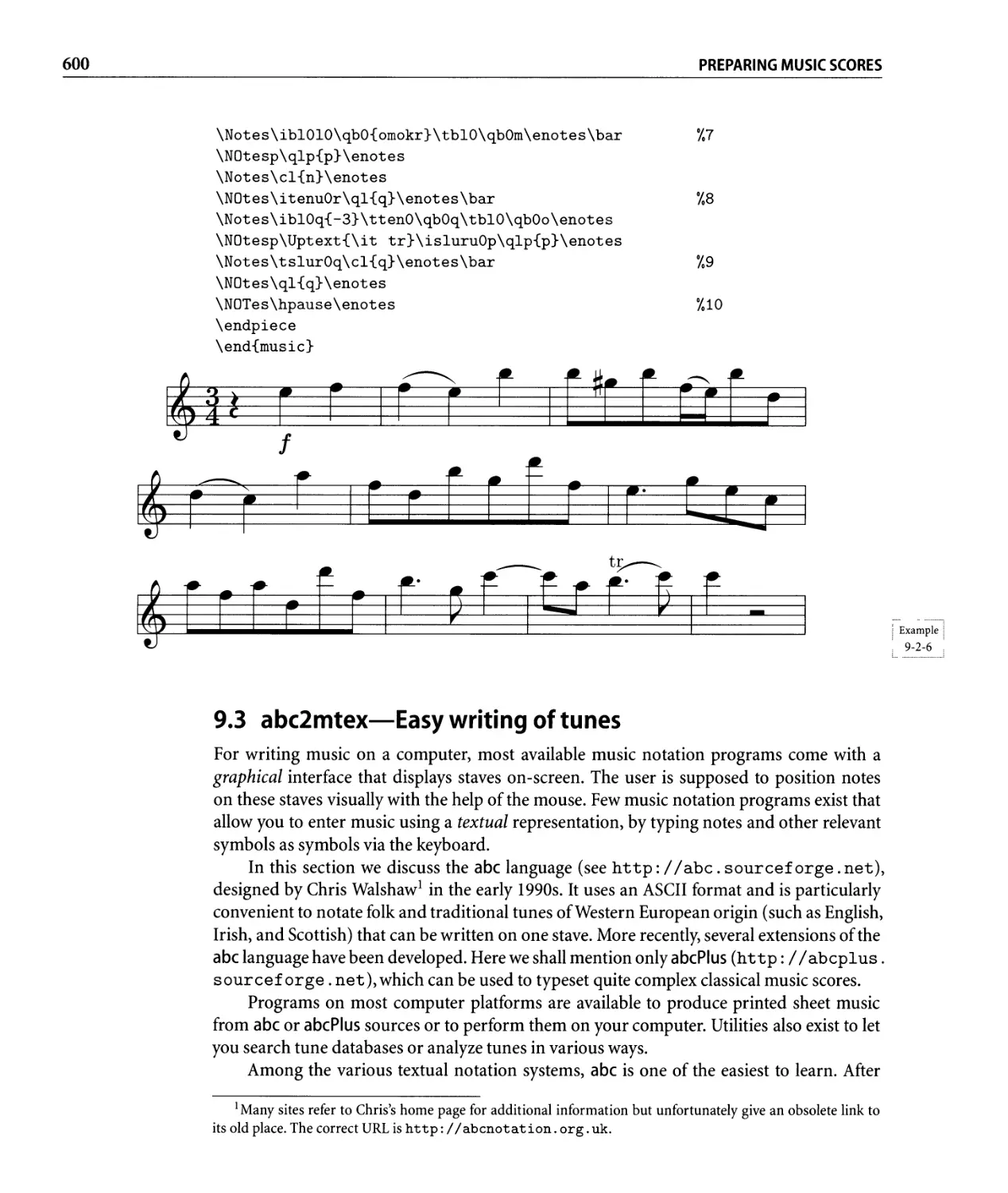
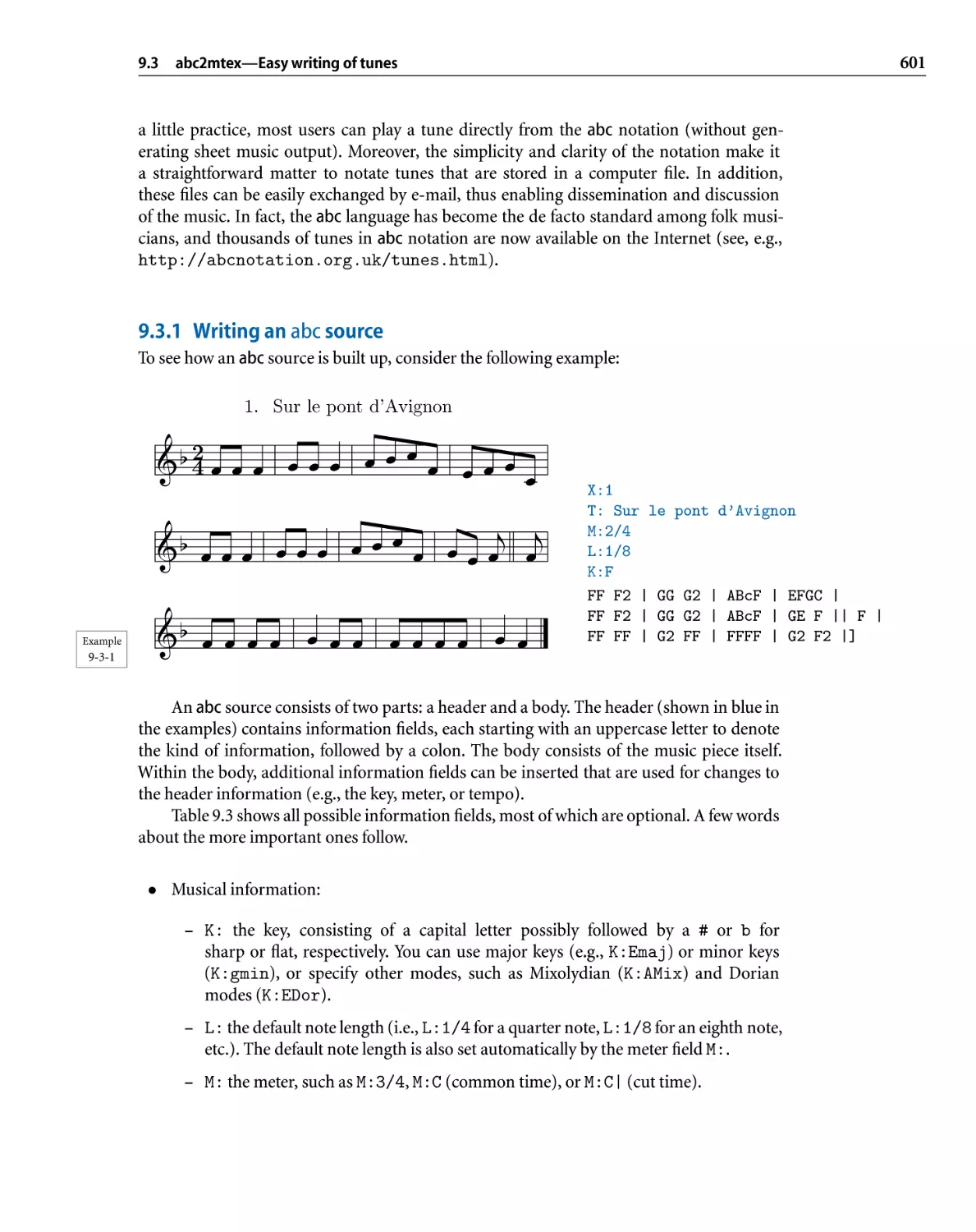
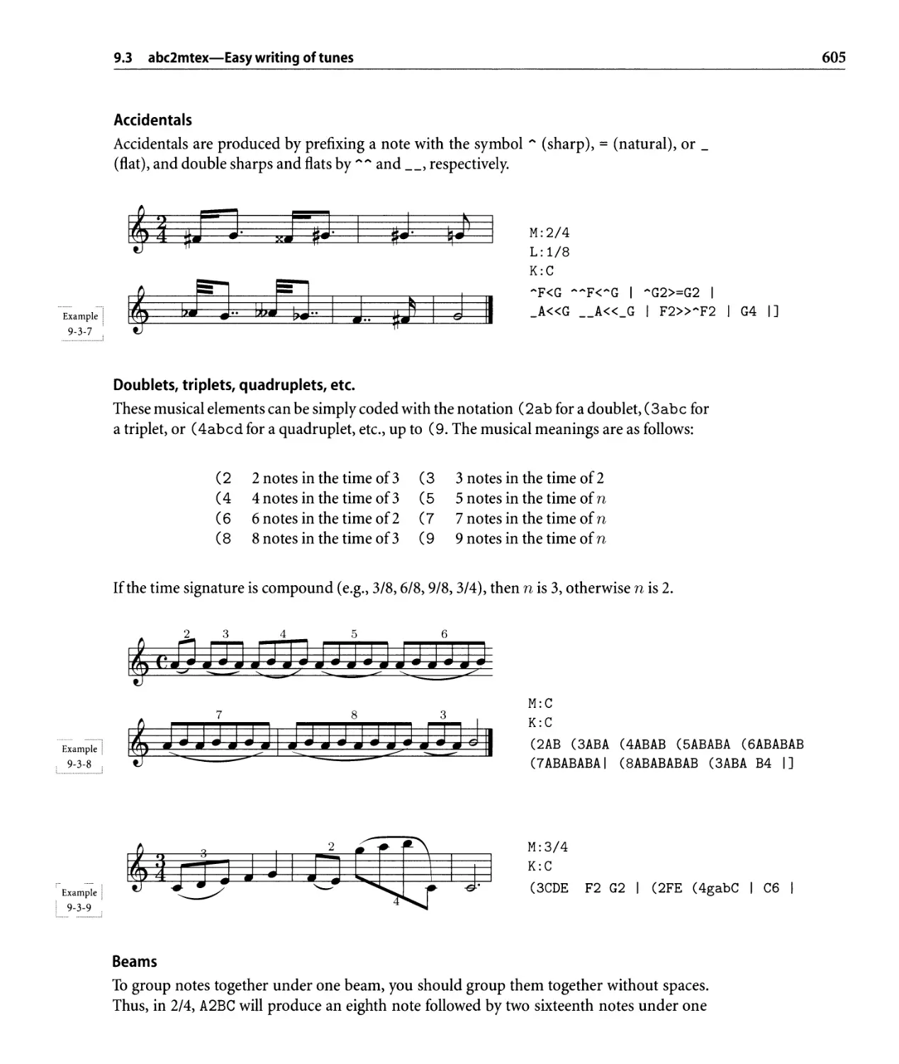
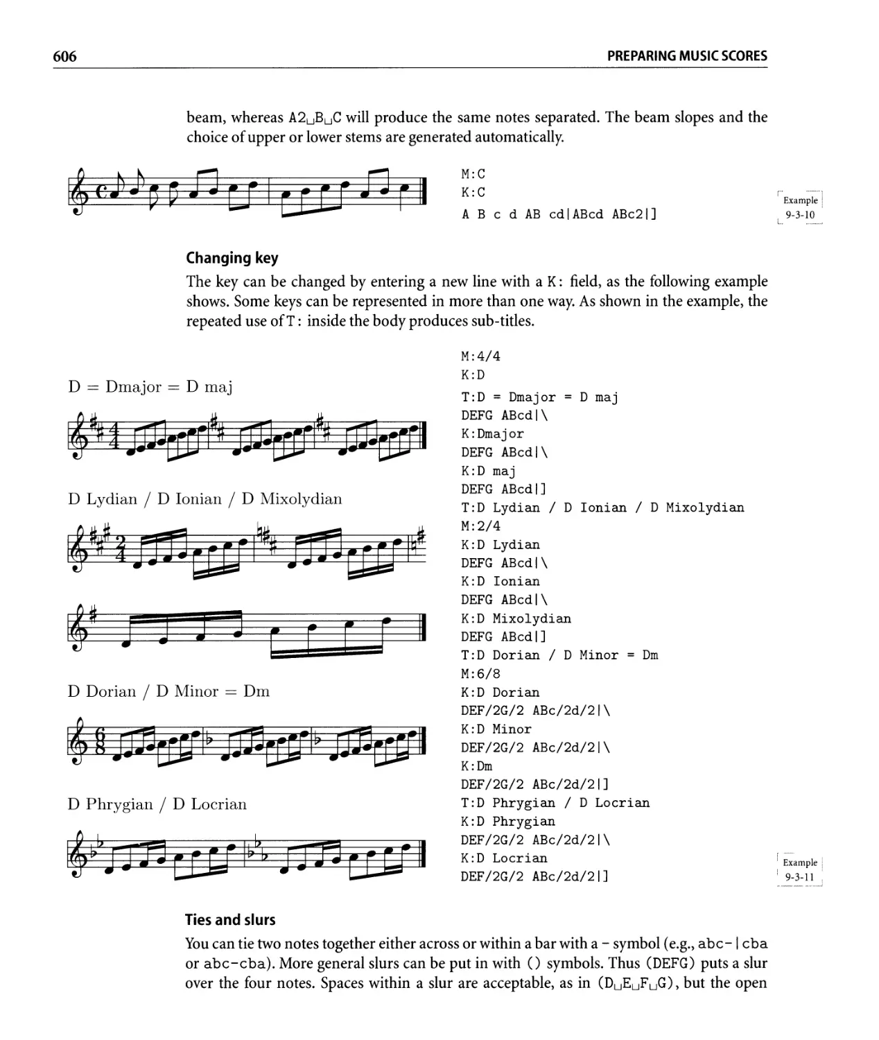
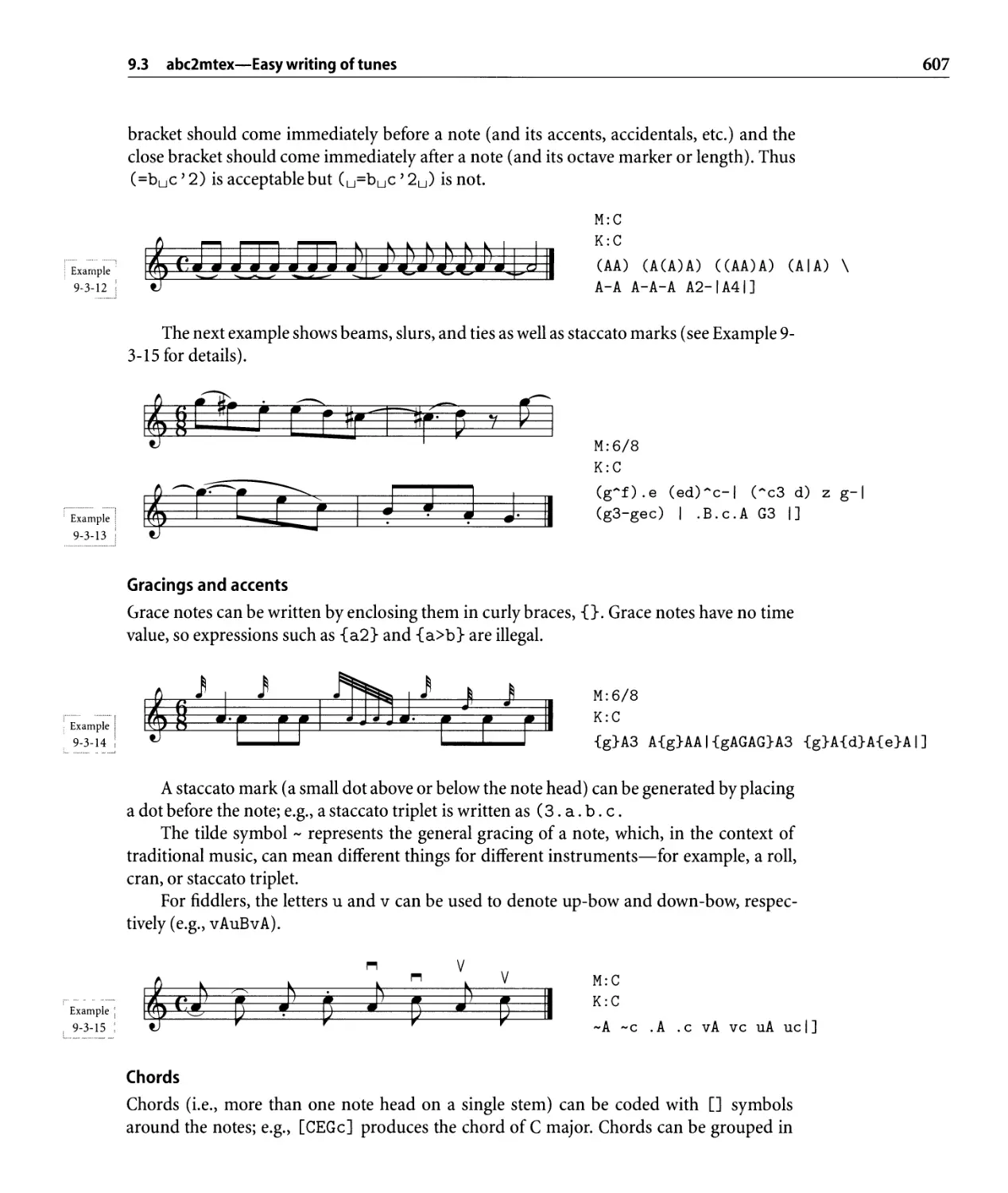
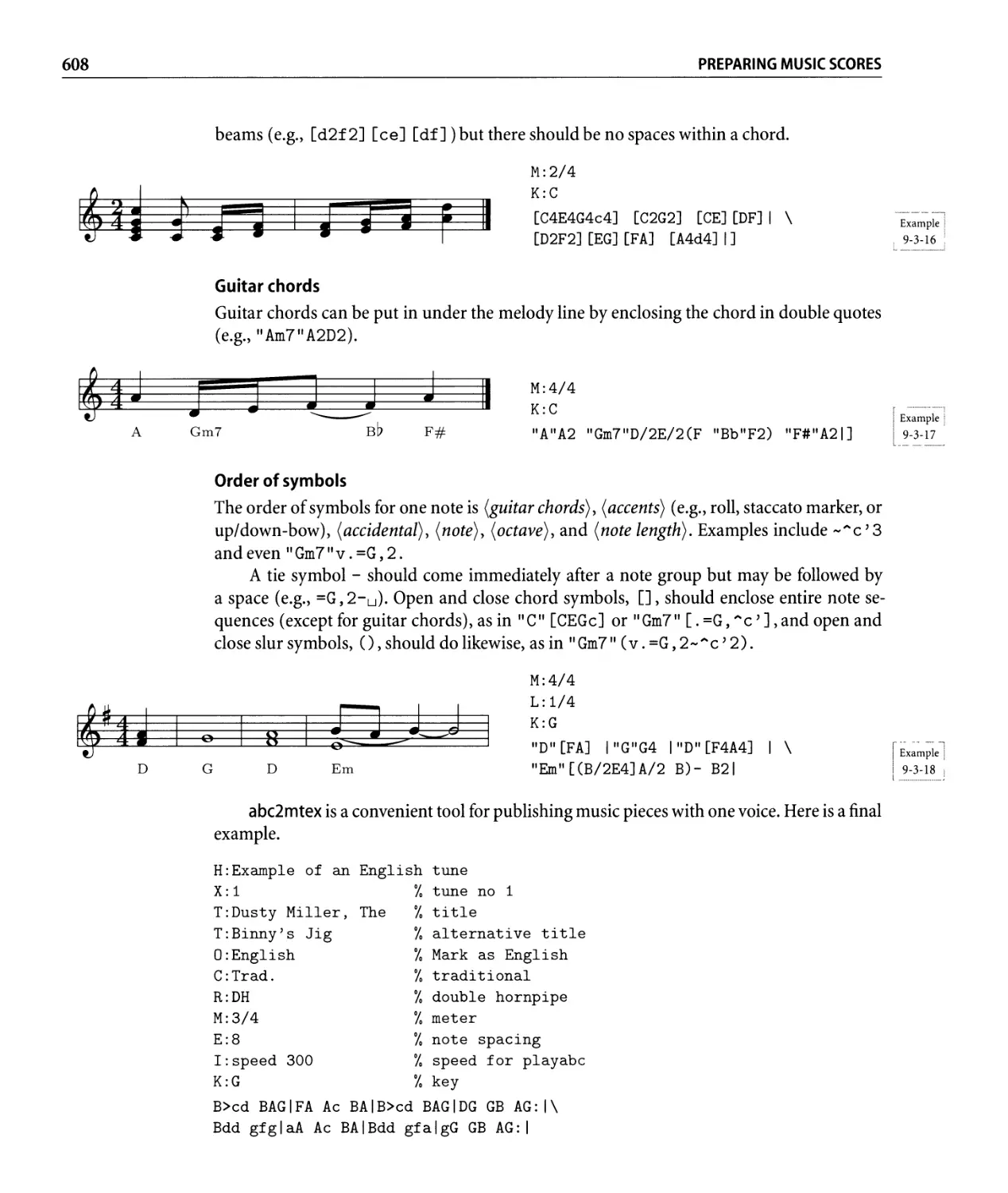
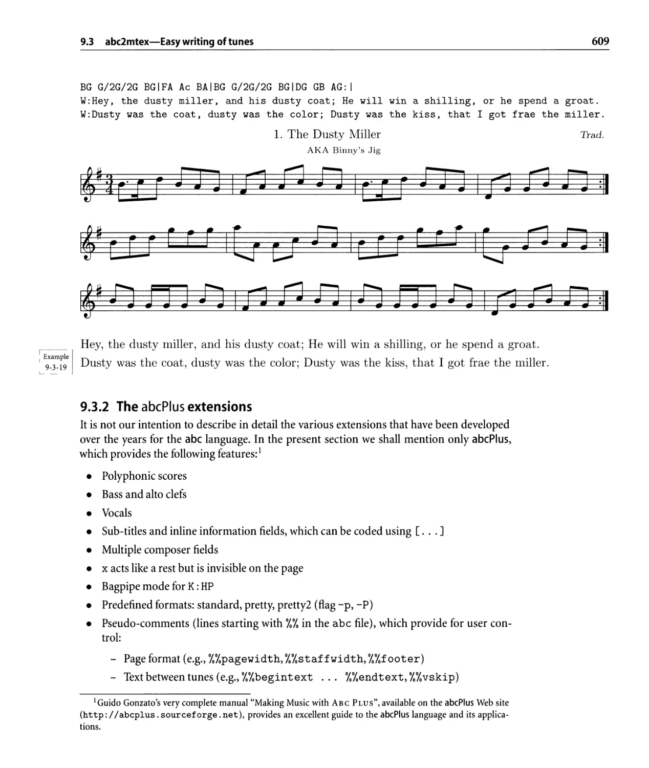
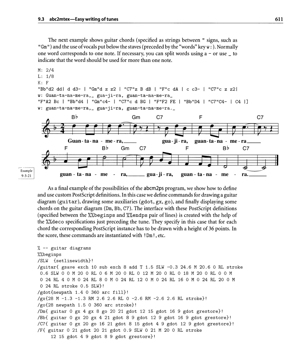
9.3 abc2mtex-Easy writing of tu nes. . . . . . . . . . . . . . . . . . . . . . . . . . .. 600
9.3.1 Writing an abc source . . . . . . . . . . . . . . . . . . . . . . . . . . . .. 601
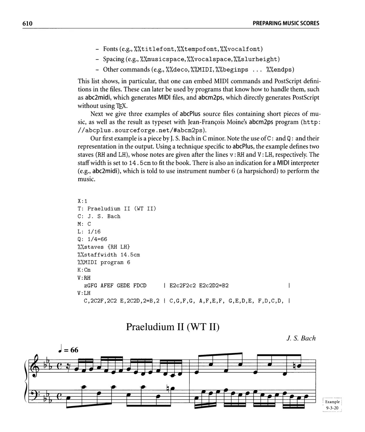
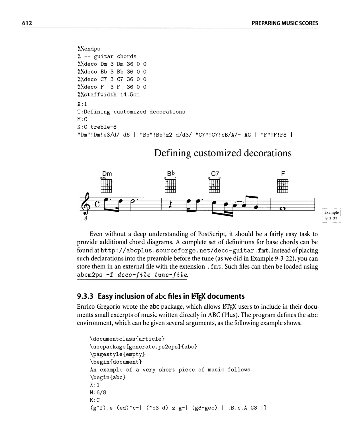
9.3.2 The abcPlus extensions . . . . . . . . . . . . . . . . . . . . . . . . . . .. 609
9.3.3 Easy inclusion of abc files in EX documents . . . . . . . . . . . . . .. 612
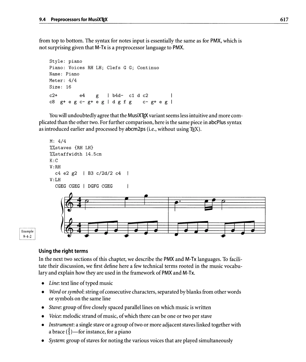
9.4 Preprocessors for MusiXTEX. . . . . . . . . . . . . . . . . . . . . . . . . . . . . . .. 615
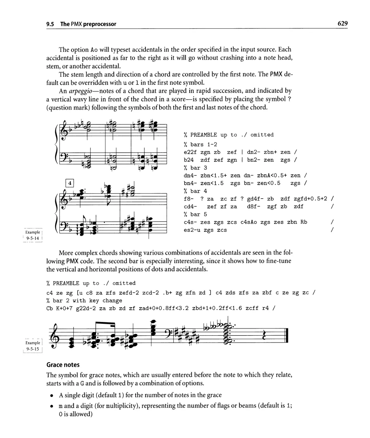
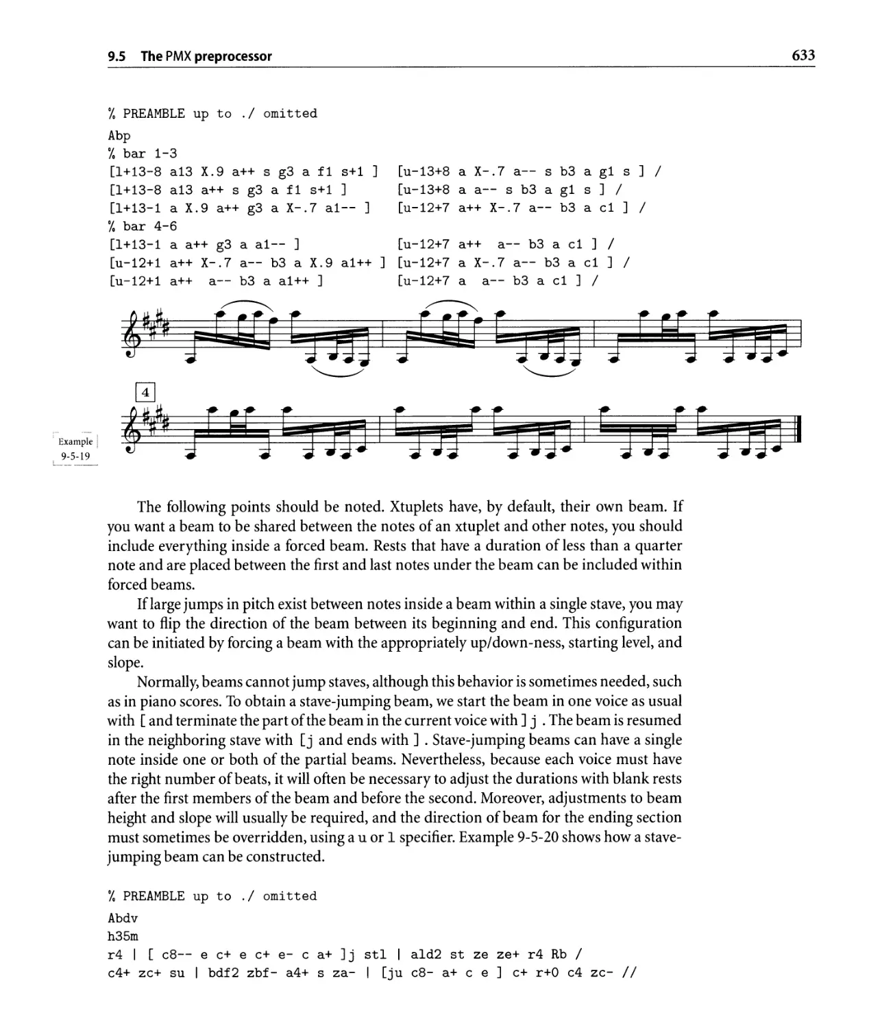
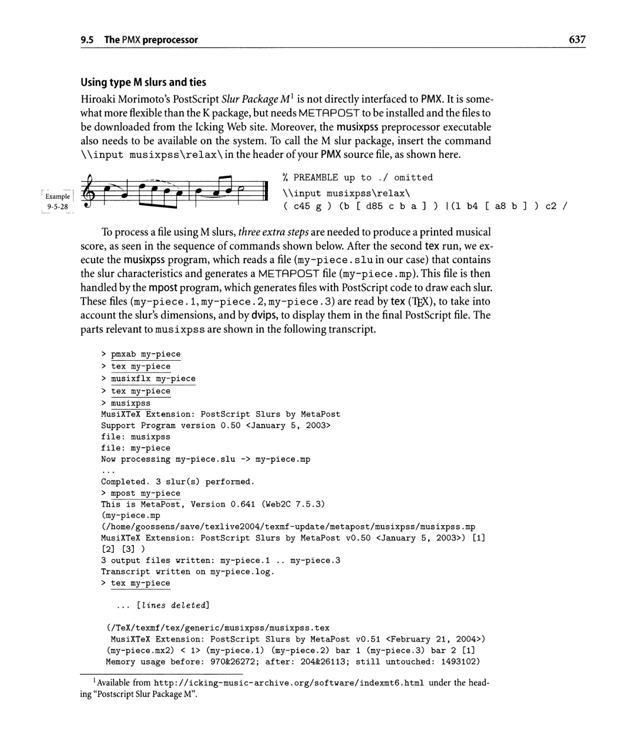
9.5 The PMX preprocessor. . . . . . . . . . . . . . . . . . . . . . . . . . . . . . . . . .. 618
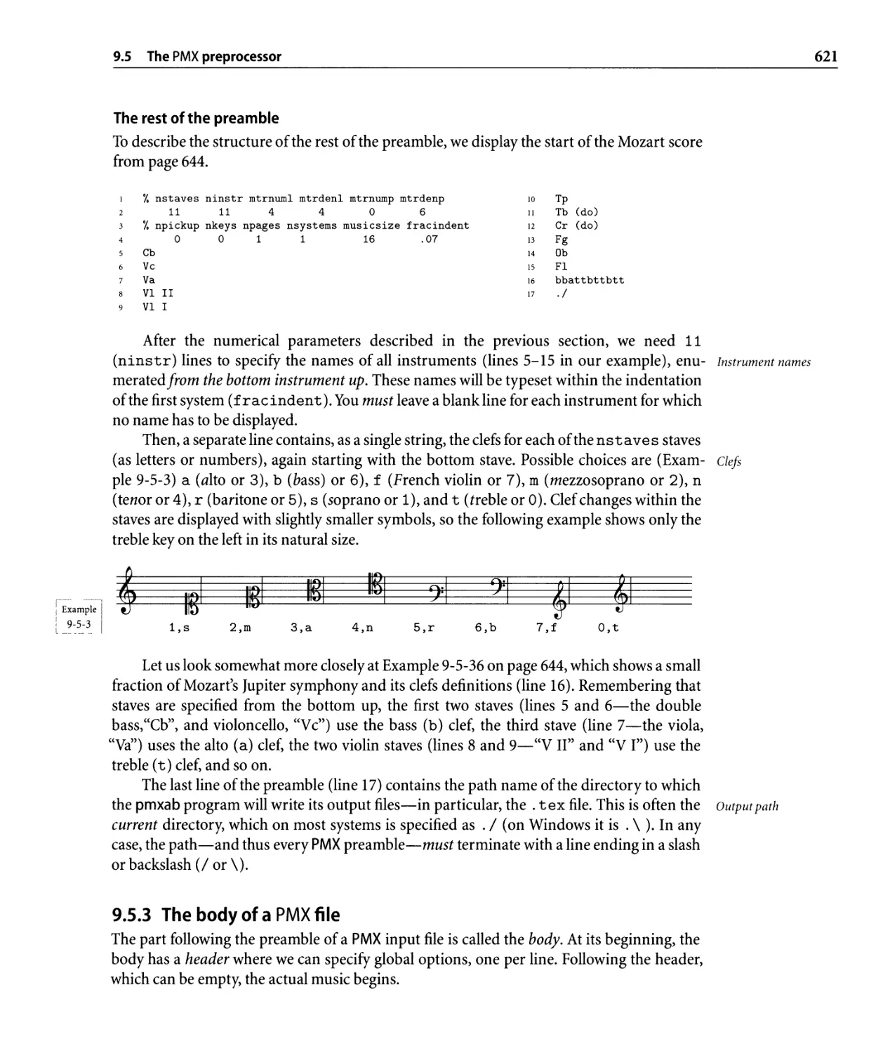
9.5.1 General structu re of a PMX score. . . . . . . . . . . . . . . . . . . . . .. 619
9.5.2 The preamble of a PMX file . . . . . . . . . . . . . . . . . . . . . . . . .. 619
9.5.3 The body of a PMX file . . . . . . . . . . . . . . . . . . . . . . . . . . . .. 621
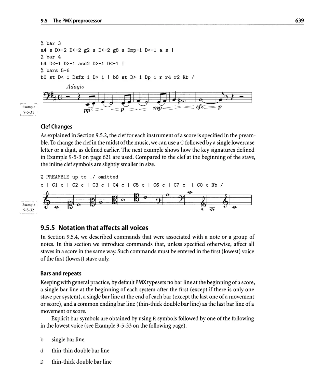
9.5.4 Notation to describe a stave . . . . . . . . . . . . . . . . . . . . . . . .. 622
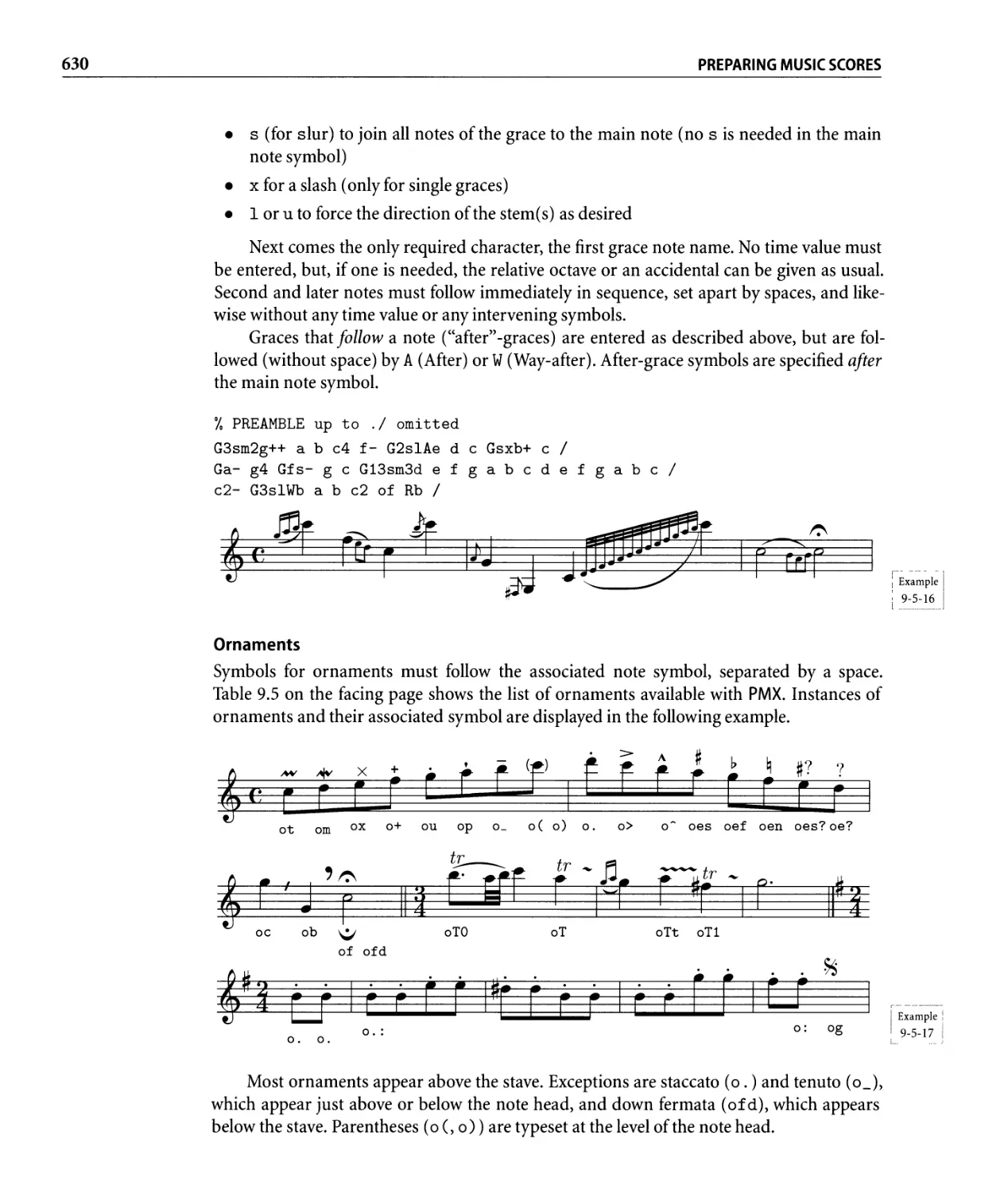
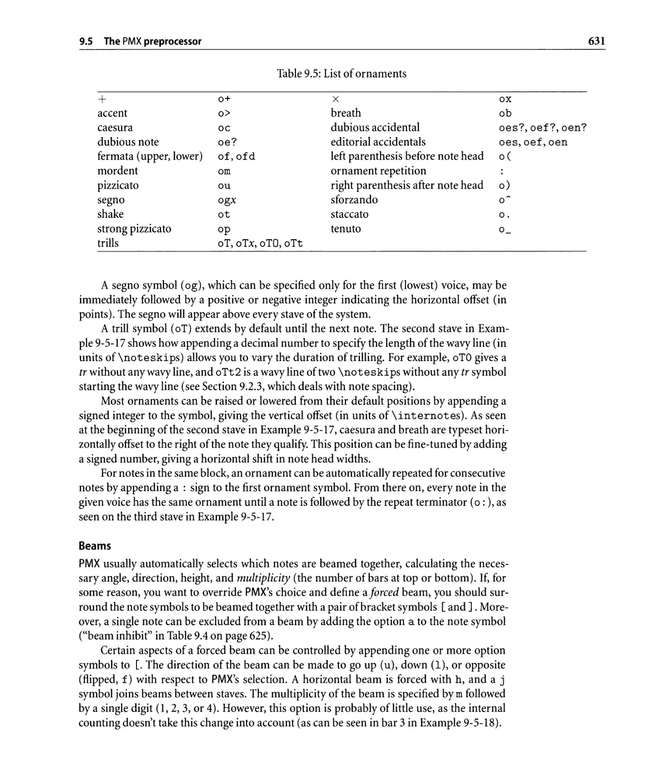
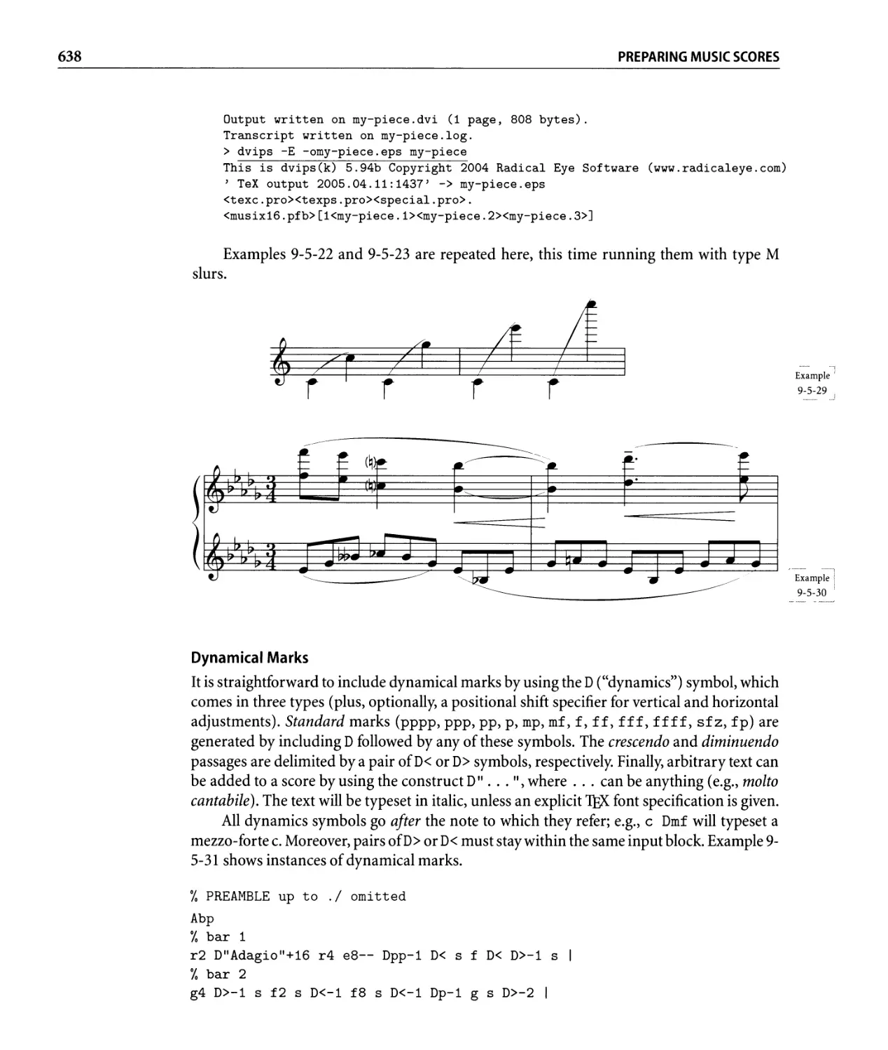
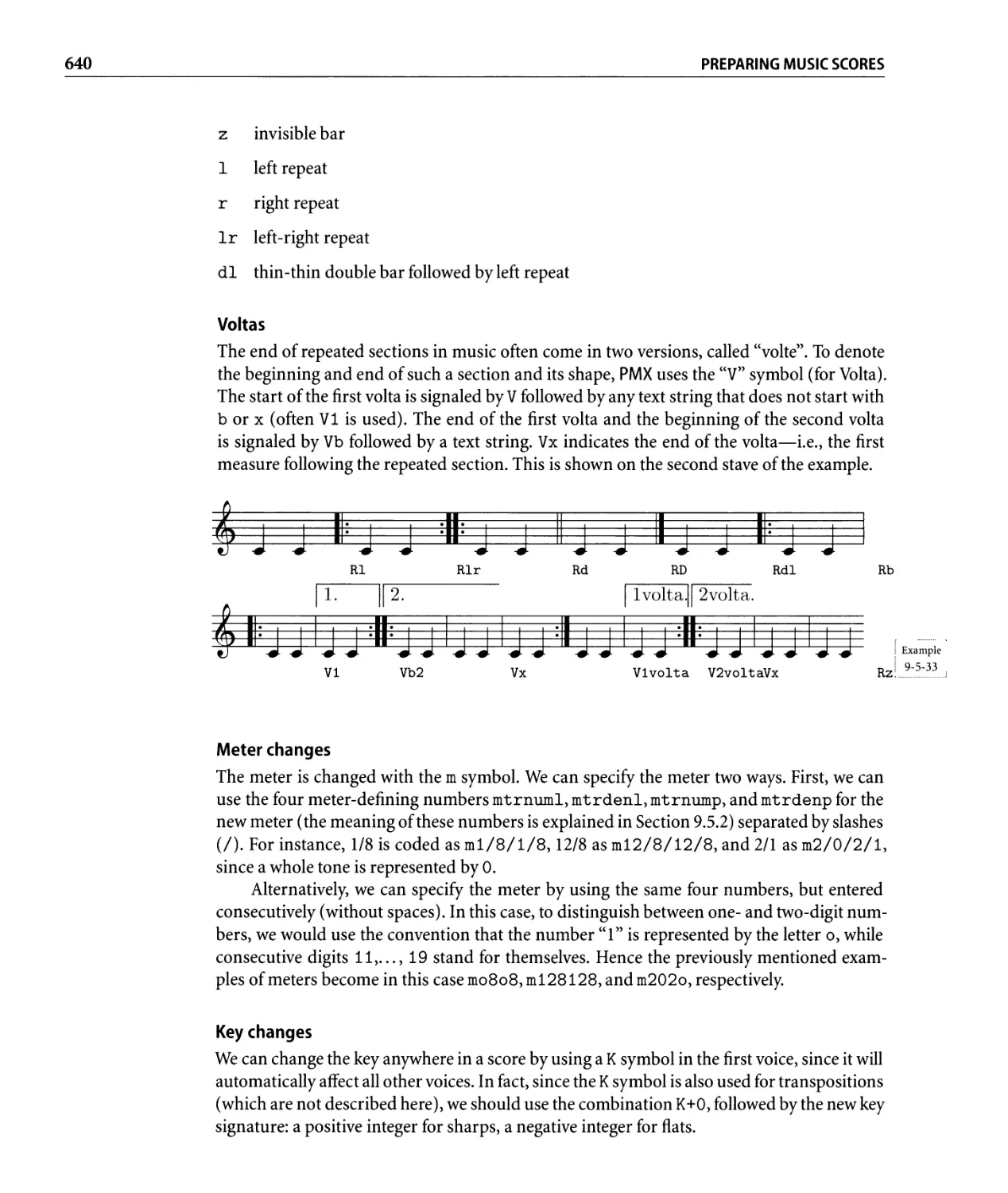
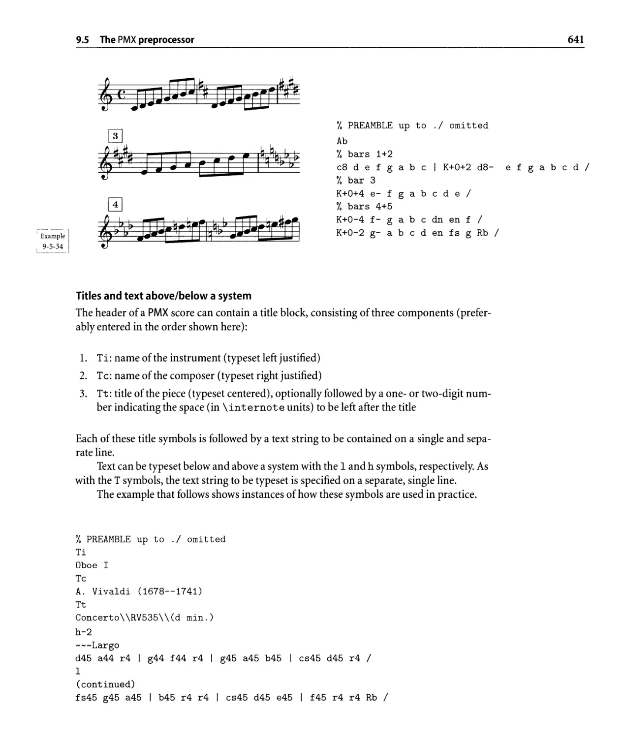
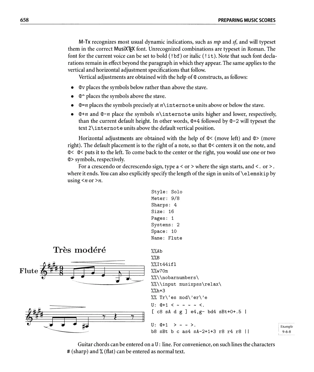
9.5.5 Notation that affects all voices . . . . . . . . . . . . . . . . . . . . . . .. 639
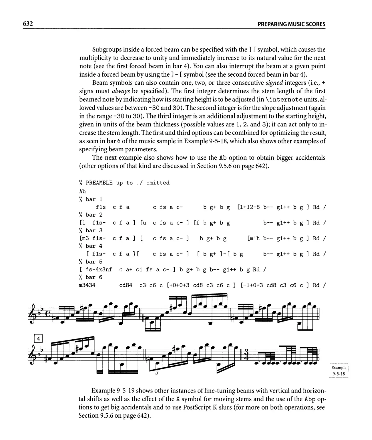
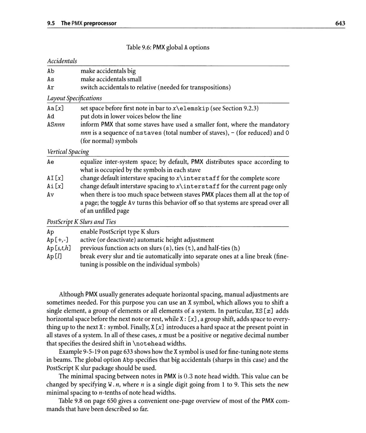
9.5.6 Some general options and technical adjustments . . . . . . . . . . .. 642
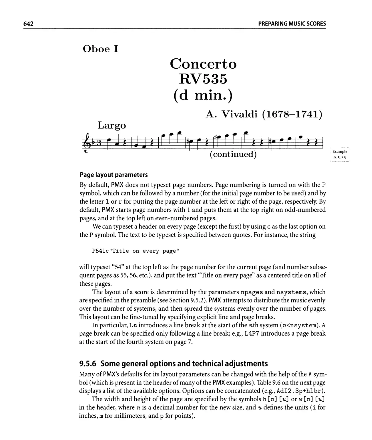
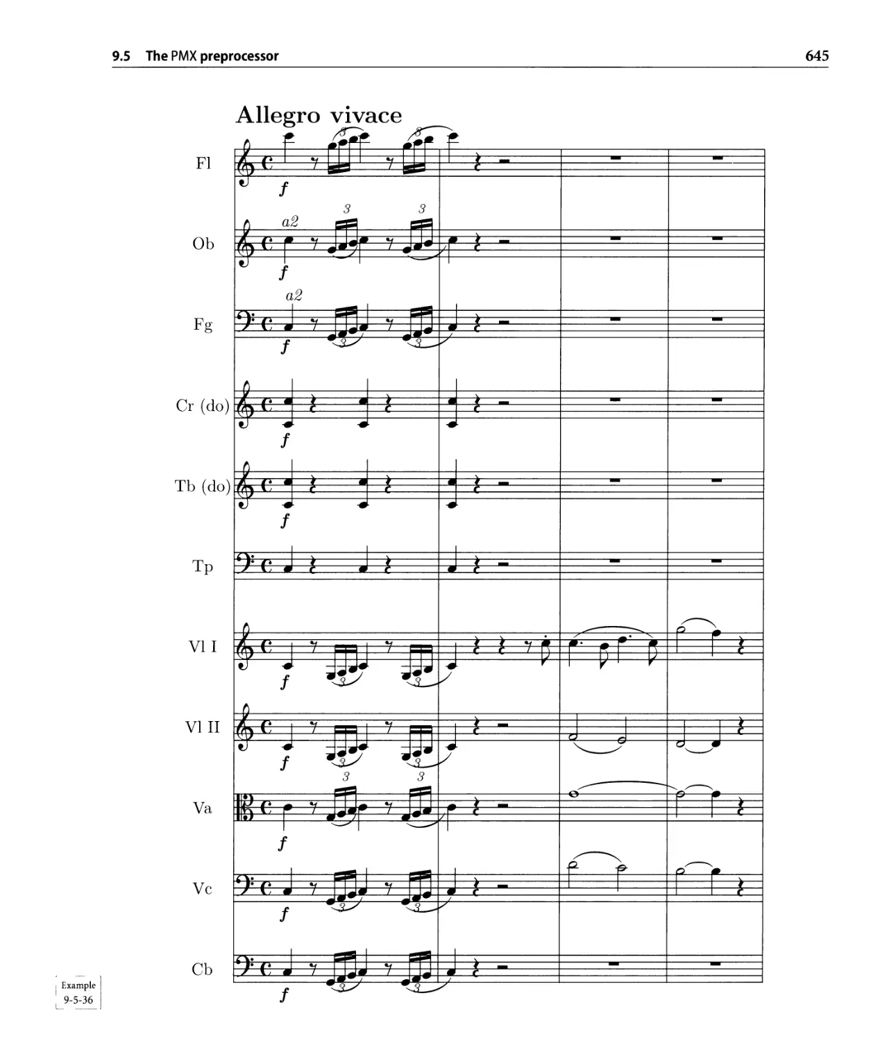
9.5.7 Two complete examples. . . . . . . . . . . . . . . . . . . . . . . . . . .. 644
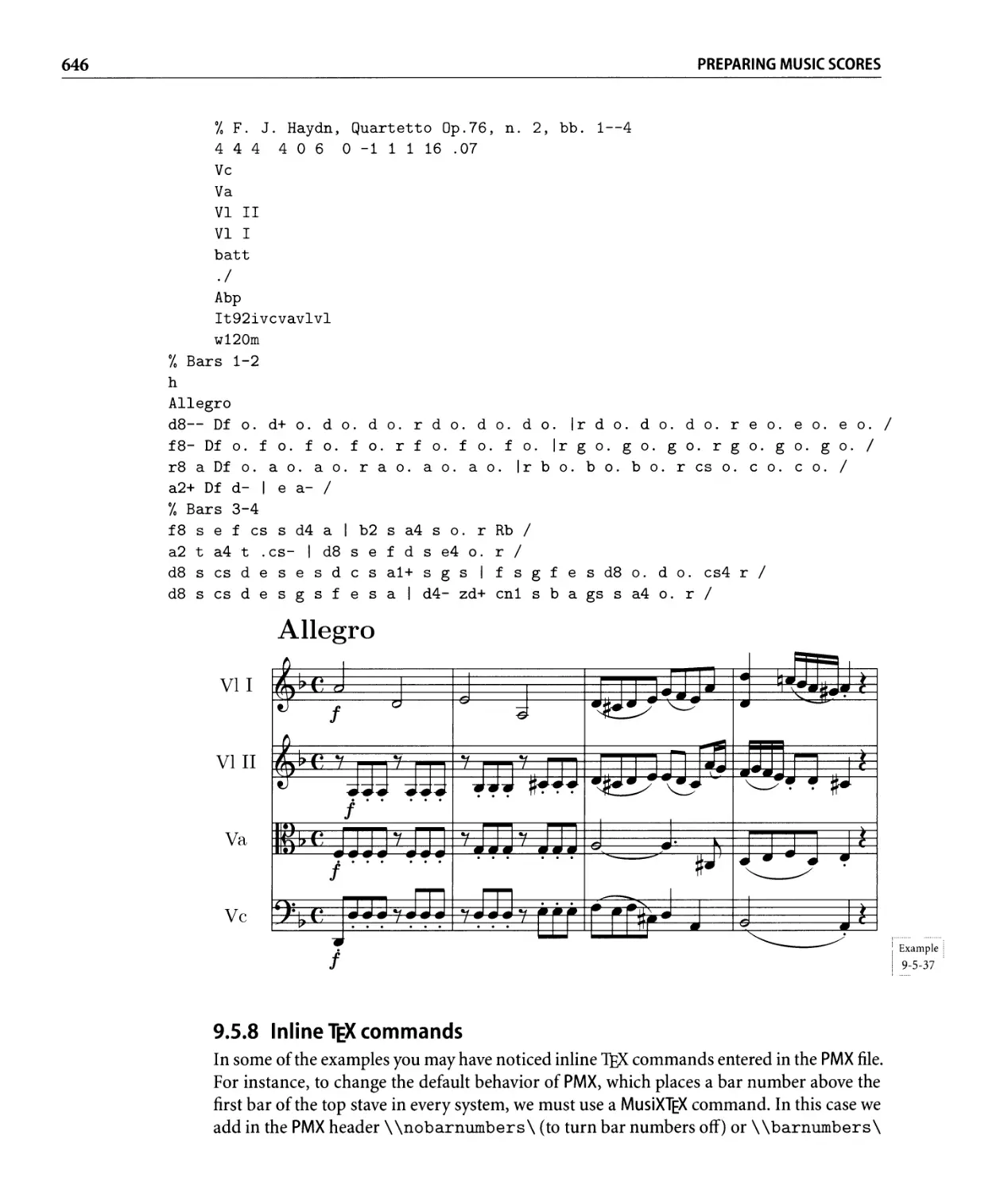
9.5.8 Inline TEX commands. . . . . . . . . . . . . . . . . . . . . . . . . . . . .. 646
9.5.9 Lyrics........ . . . . . . . . . . . . . . . . . . . . . . . . . . . . . . .. 647
.
ov
CONTENTS
9.5.10 Creating parts from a score . . . . . . . . . . . . . . . . . . . . . . . . .. 647
9.5.11 Making MIDI files . . . . . . . . . . . . . . . . . . . . . . . . . . . . . . .. 647
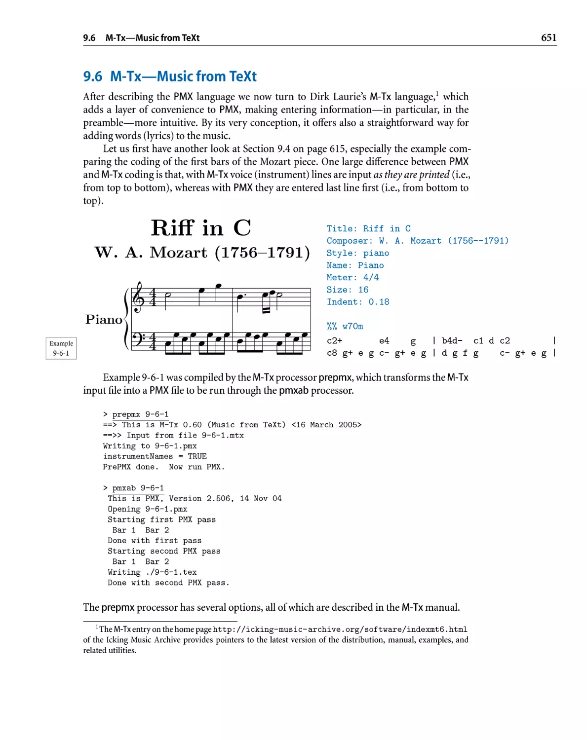
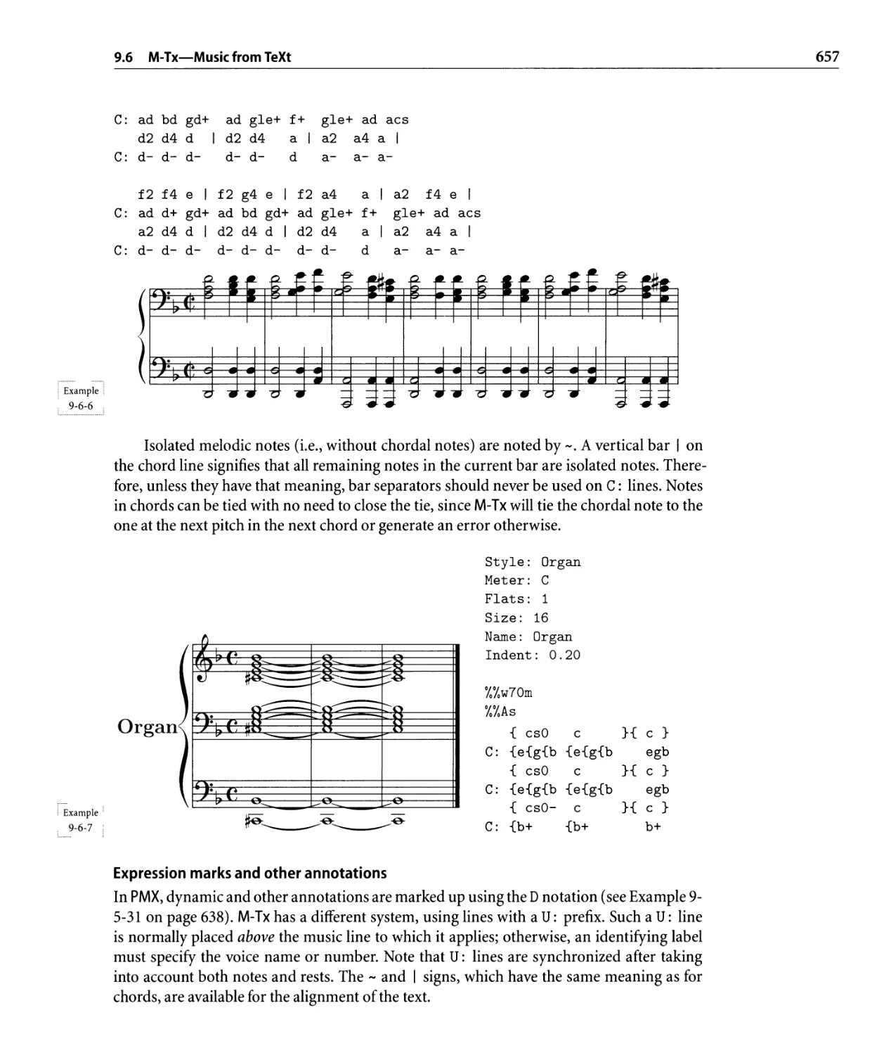
9.6 M - T x - Mus i c fro m TeXt. . . . . . . . . . . . . . . . . . . . . . . . . . . . . . . . .. 651
9.6.1 The M- Tx preamble. . . . . . . . . . . . . . . . . . . . . . . . . . . . . .. 652
9.6.2 The body of an M- Tx input file . . . . . . . . . . . . . . . . . . . . . . .. 654
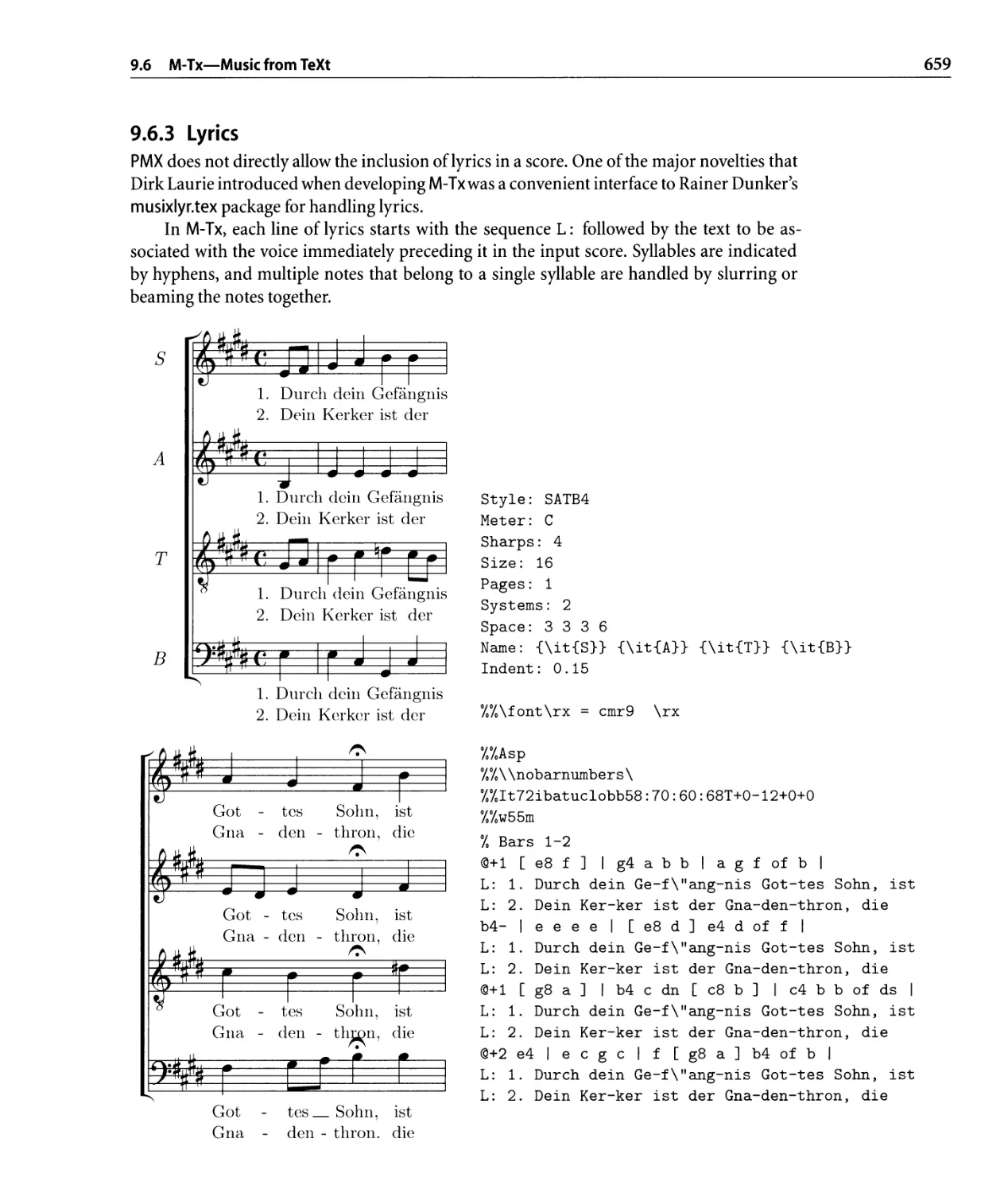
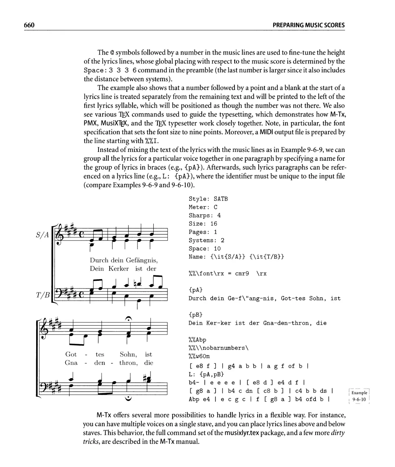
9.6.3 lyrics. . . . . . . . . . . . . . . . . . . . . . . . . . . . . . . . . . . . . . .. 659
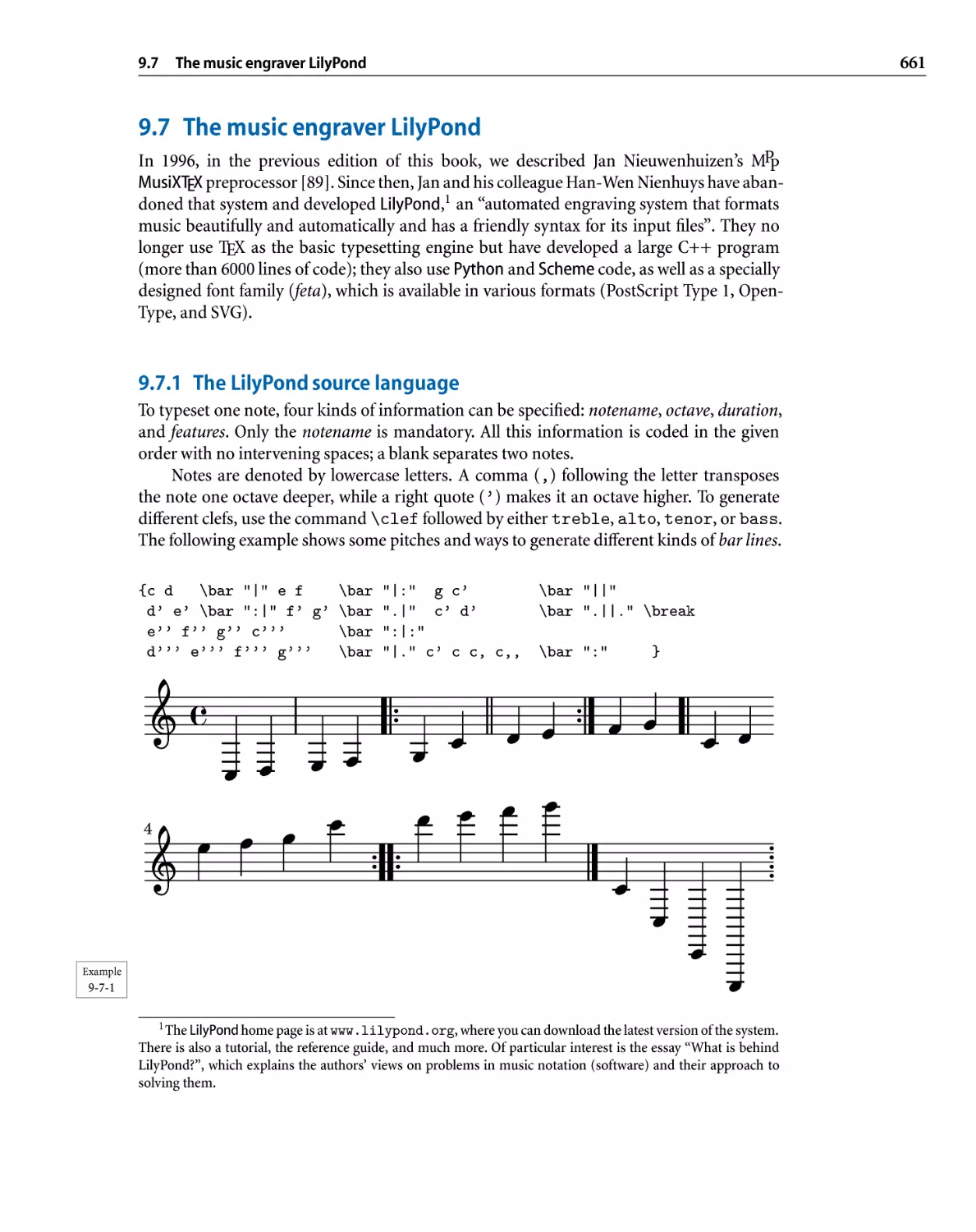
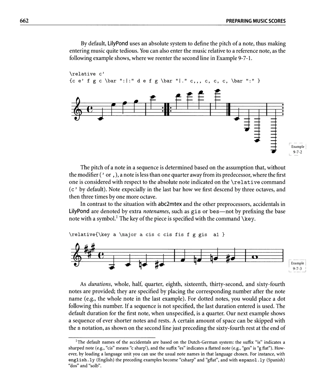
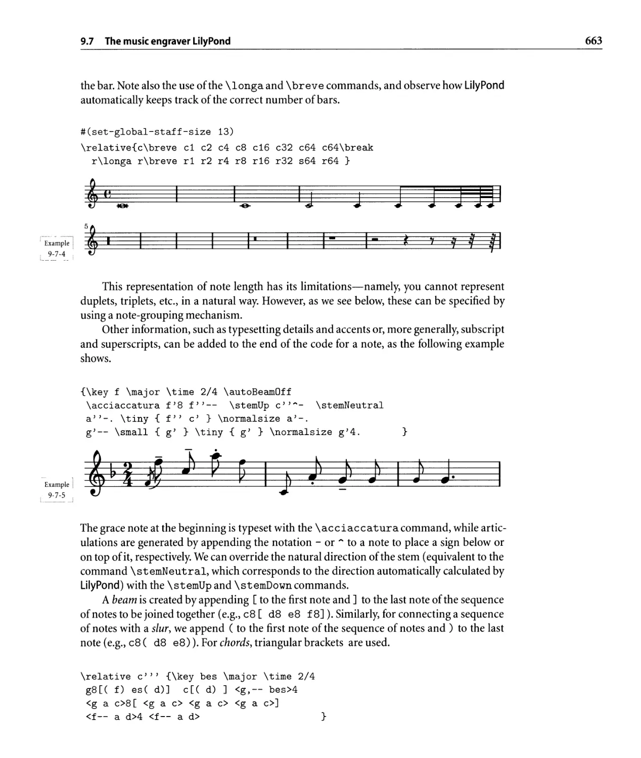
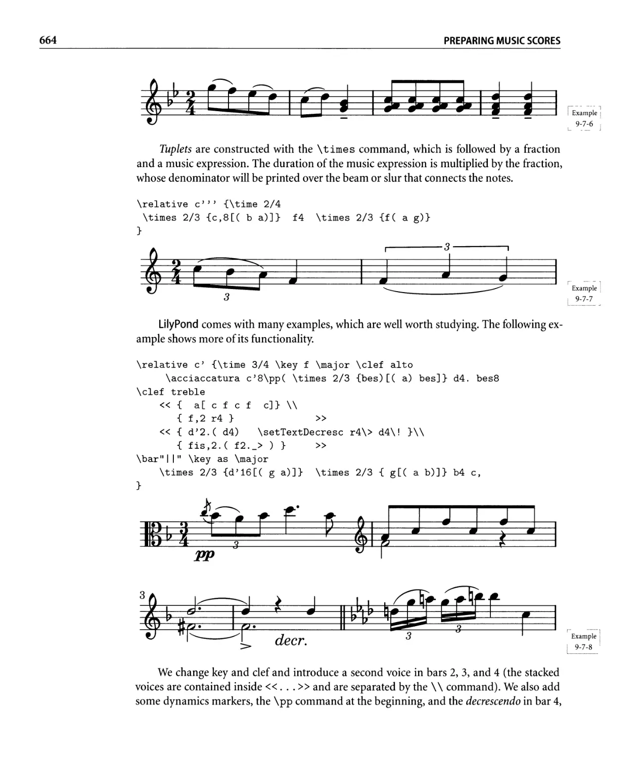
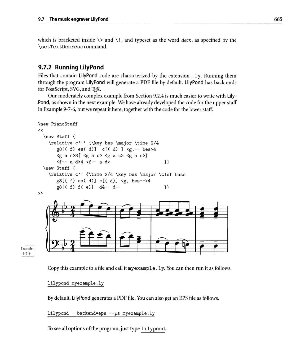
9.7 The music engraver lilyPond. . . . . . . . . . . . . . . . . . . . . . . . . . . . . .. 661
9.7.1 The LilyPond source language . . . . . . . . . . . . . . . . . . . . . . .. 661
9.7.2 Running LilyPond . . . . . . . . . . . . . . . . . . . . . . . . . . . . . . .. 665
9.8 TEXmuse- TEX and METAFoNT working together. . . . . . . . . . . . . . . .. 666
10 Playing Games 667
10.1 Chess . . . . . . . . . . . . . . . . . . . . . . . . . . . . . . . . . . . . . . . . . . . .. 668
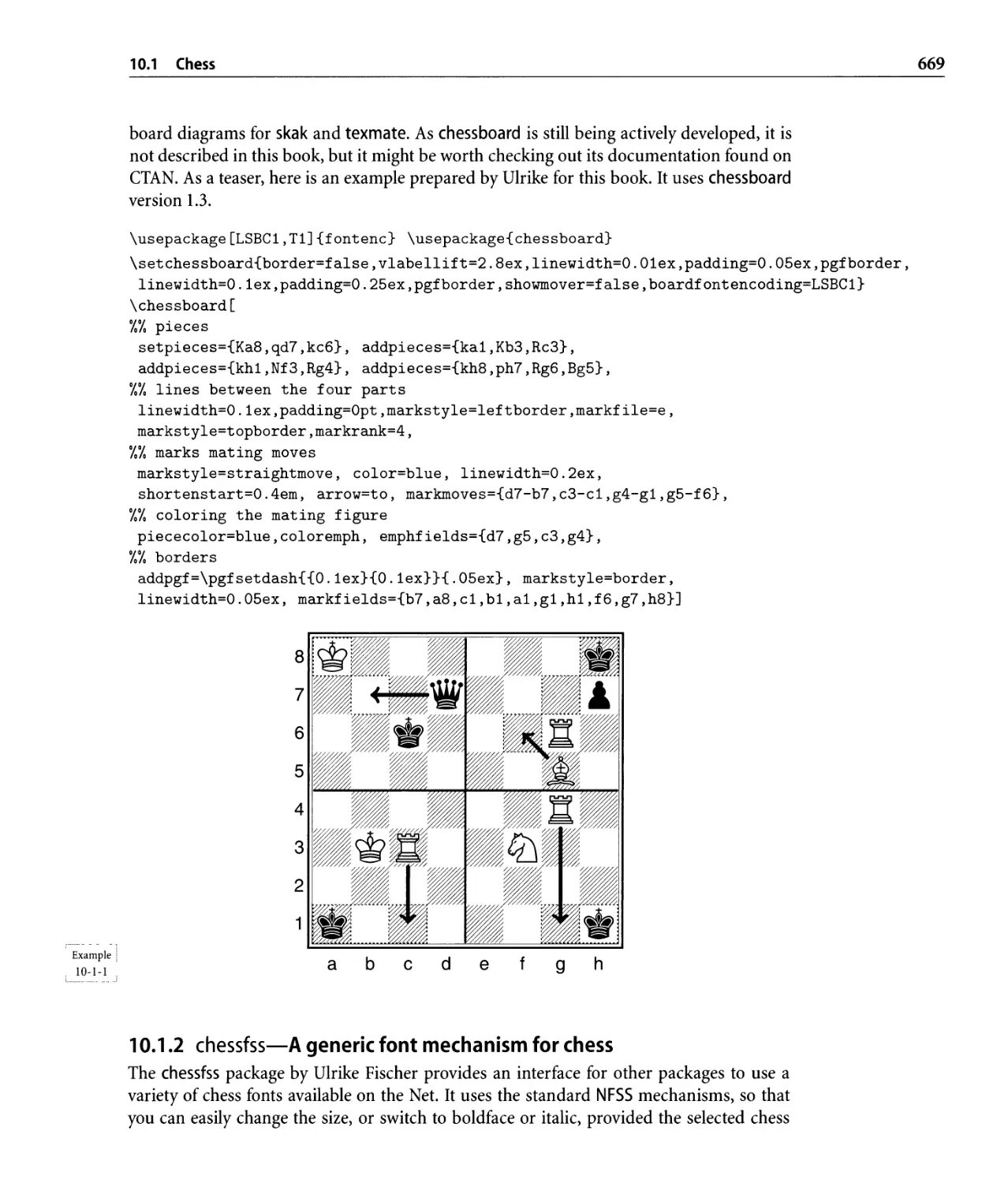
10.1.1 chessboard-Coloring your boards. . . . . . . . . . . . . . . . . . . .. 668
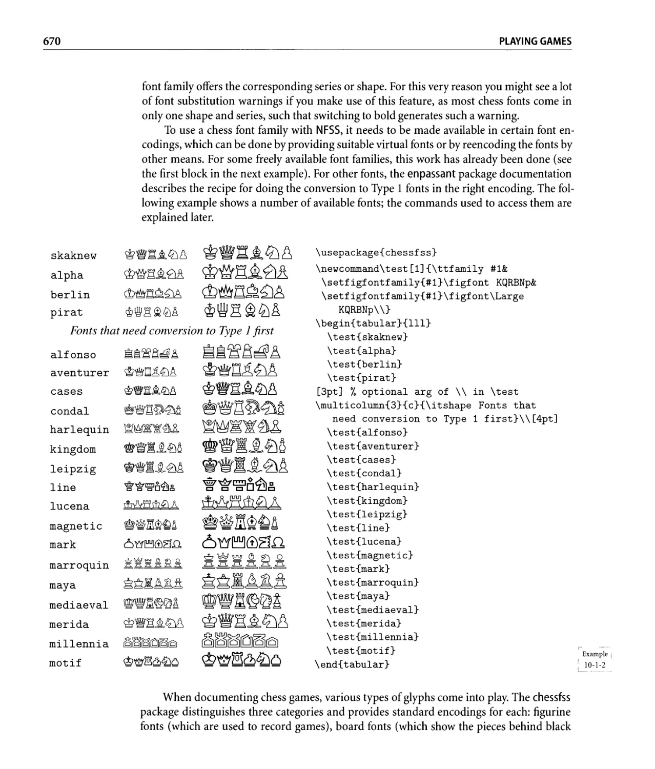
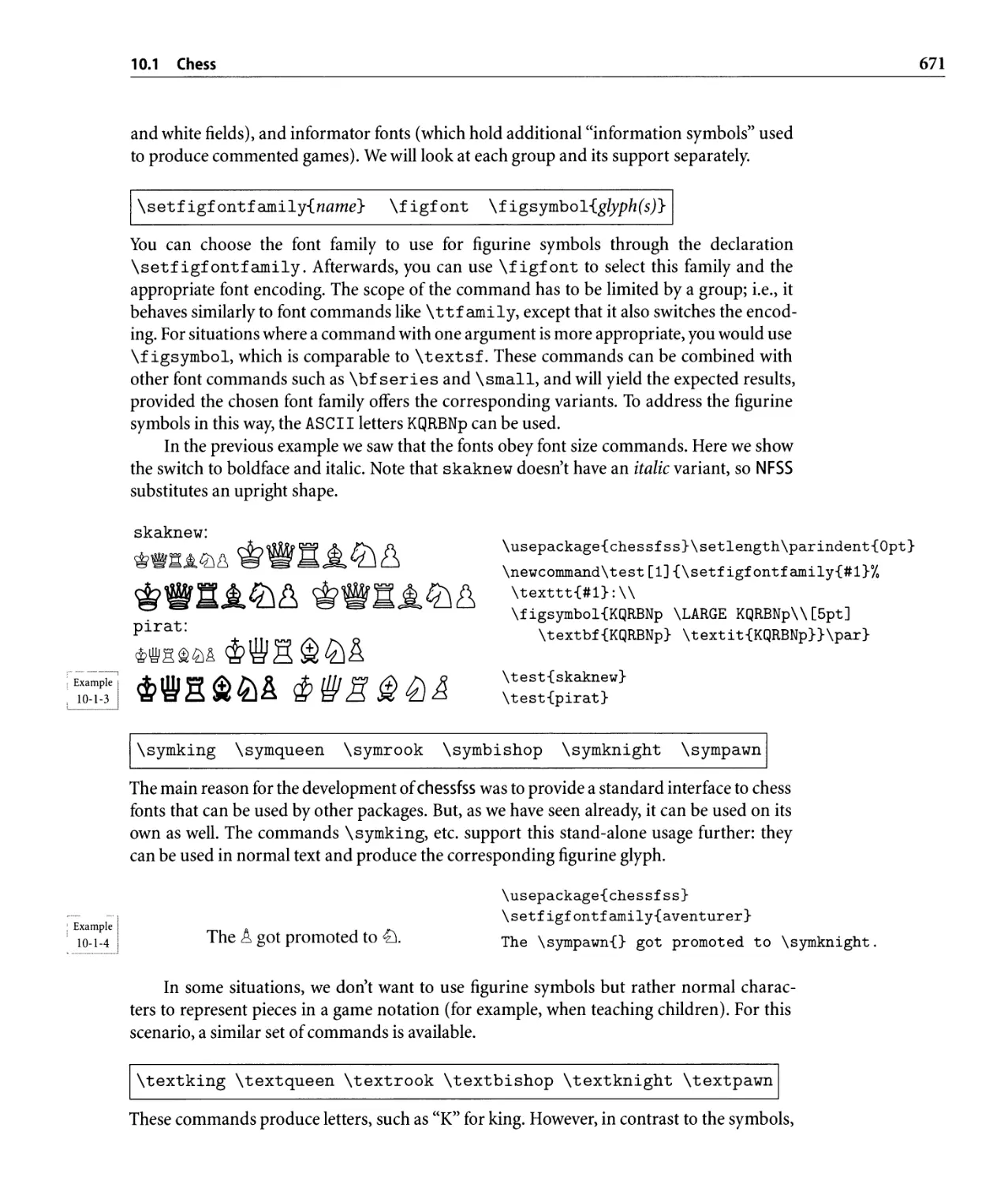
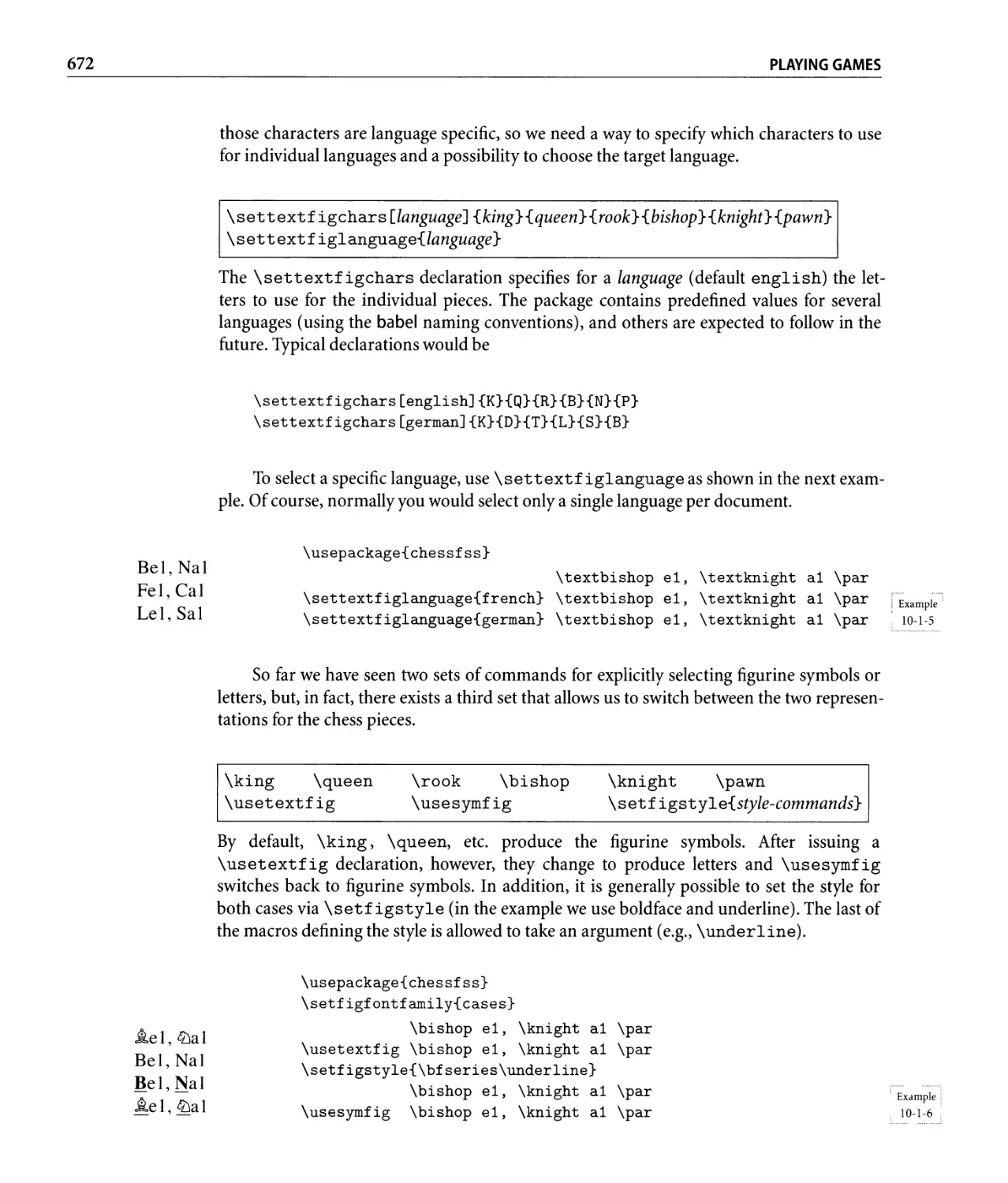
10.1.2 chessfss-A generic font mechanism for chess. . . . . . . . . . . . .. 669
10.1.3 skak- The successor to the chess package . . . . . . . . . . . . . . .. 673
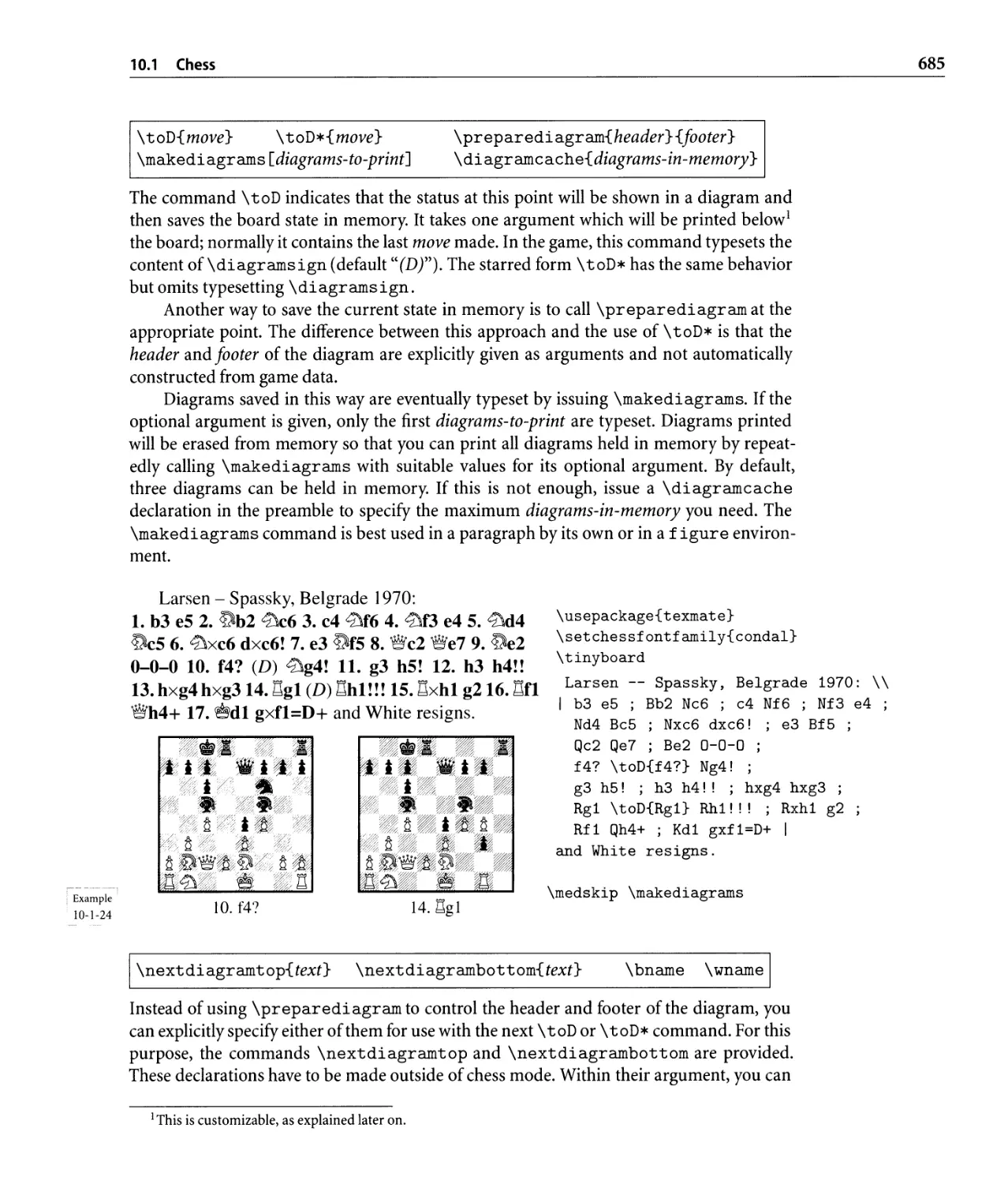
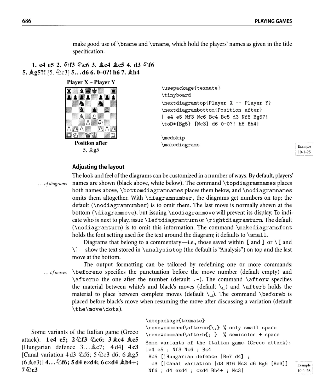
10.1.4 texmate- The power of three . . . . . . . . . . . . . . . . . . . . . . .. 680
10.1.5 Online resources for chess. .......................... 687
10.2 Xiangqi-Chinese chess . . . . . . . . . . . . . . . . . . . . . . . . . . . . . . . .. 687
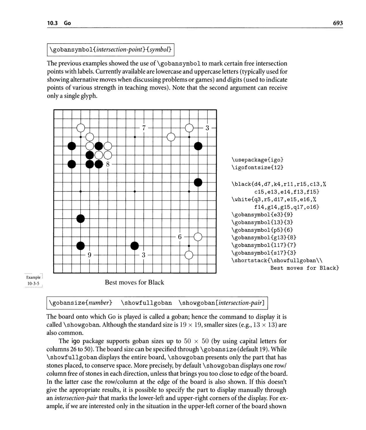
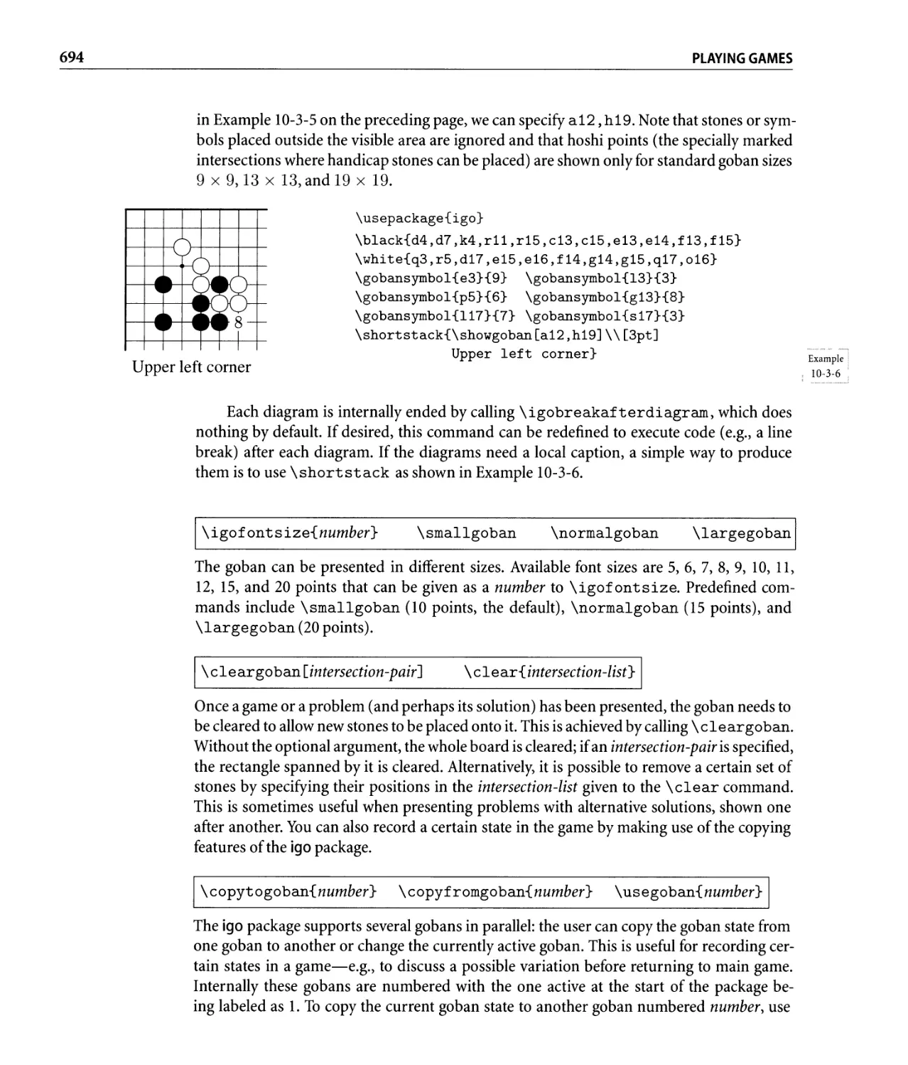
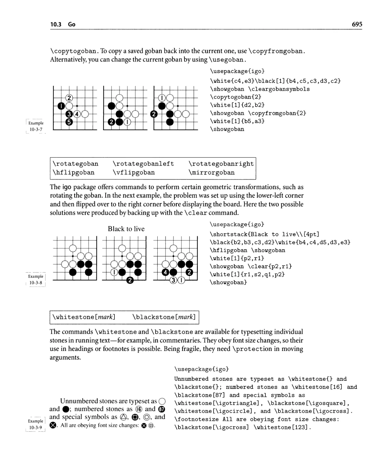
10.3 Go . . . . . . . . . . . . . . . . . . . . . . . . . . . . . . . . . . . . . . . . . . . . . .. 690
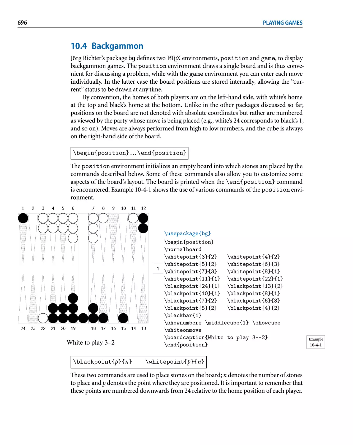
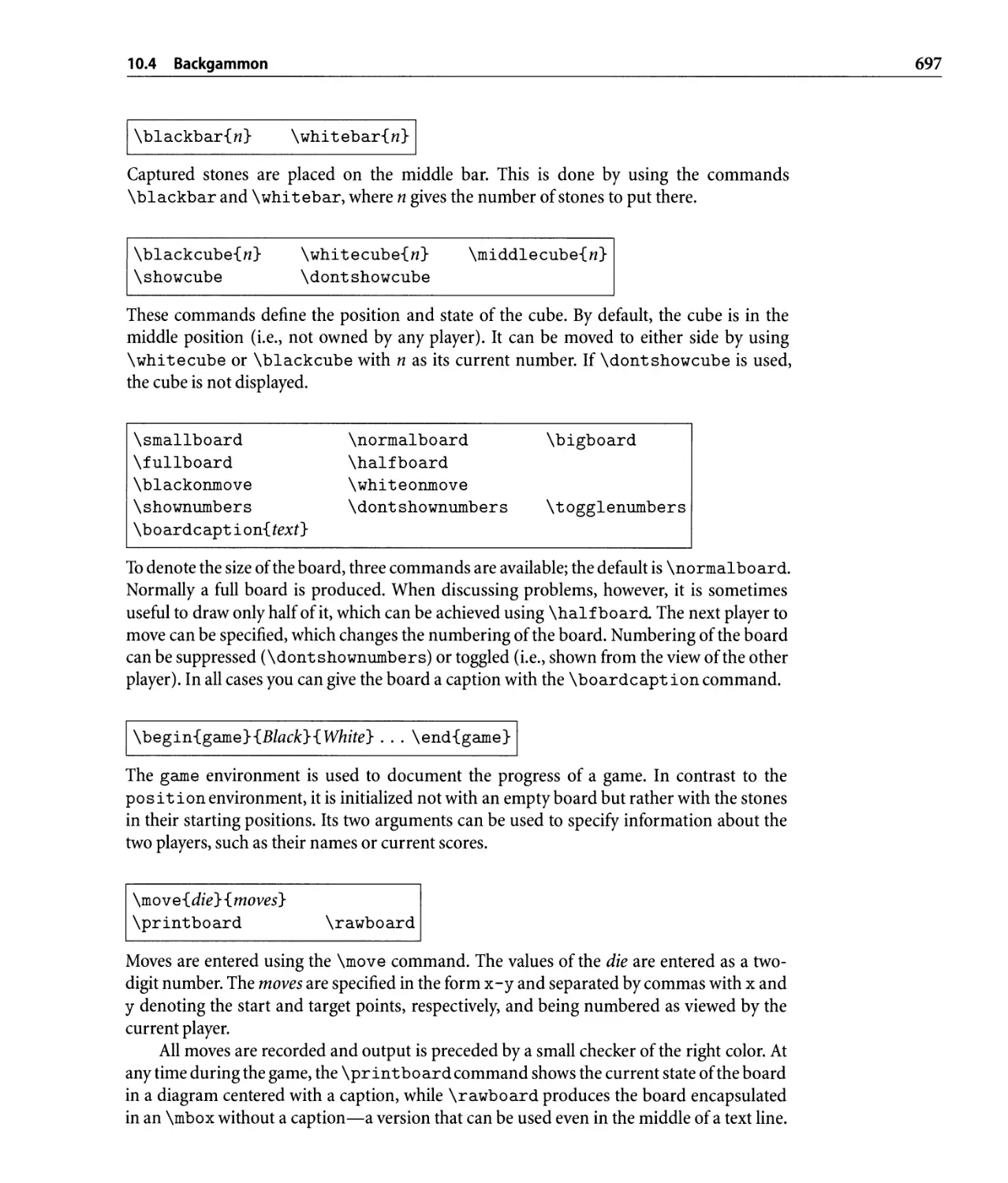
10.4 Backgammon. . . . . . . . . . . . . . . . . . . . . . . . . . . . . . . . . . . . . . .. 696
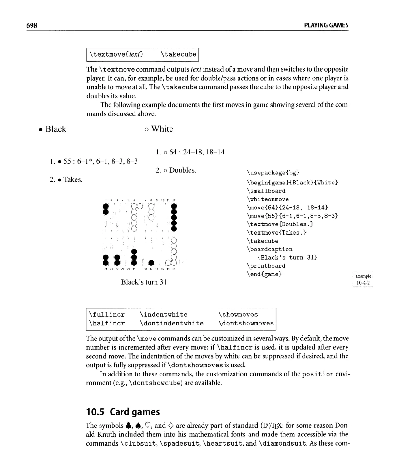
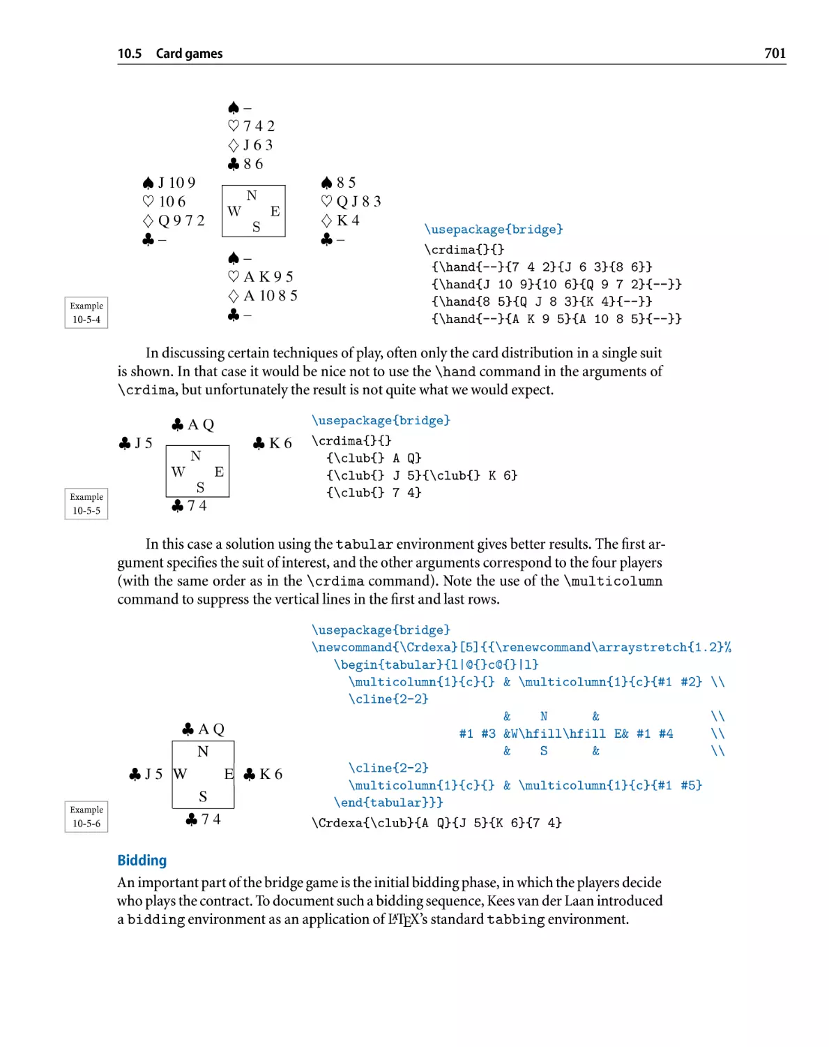
10.5 Card games . . . . . . . . . . . . . . . . . . . . . . . . . . . . . . . . . . . . . . . .. 698
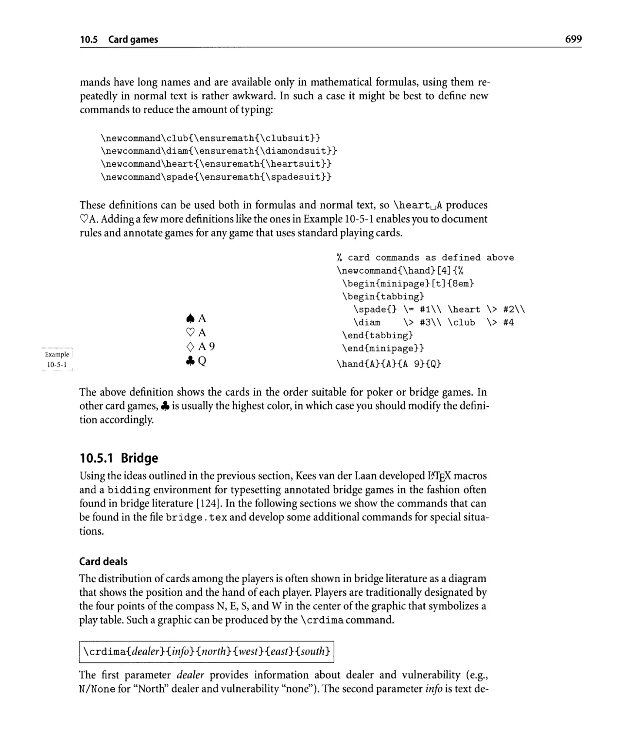
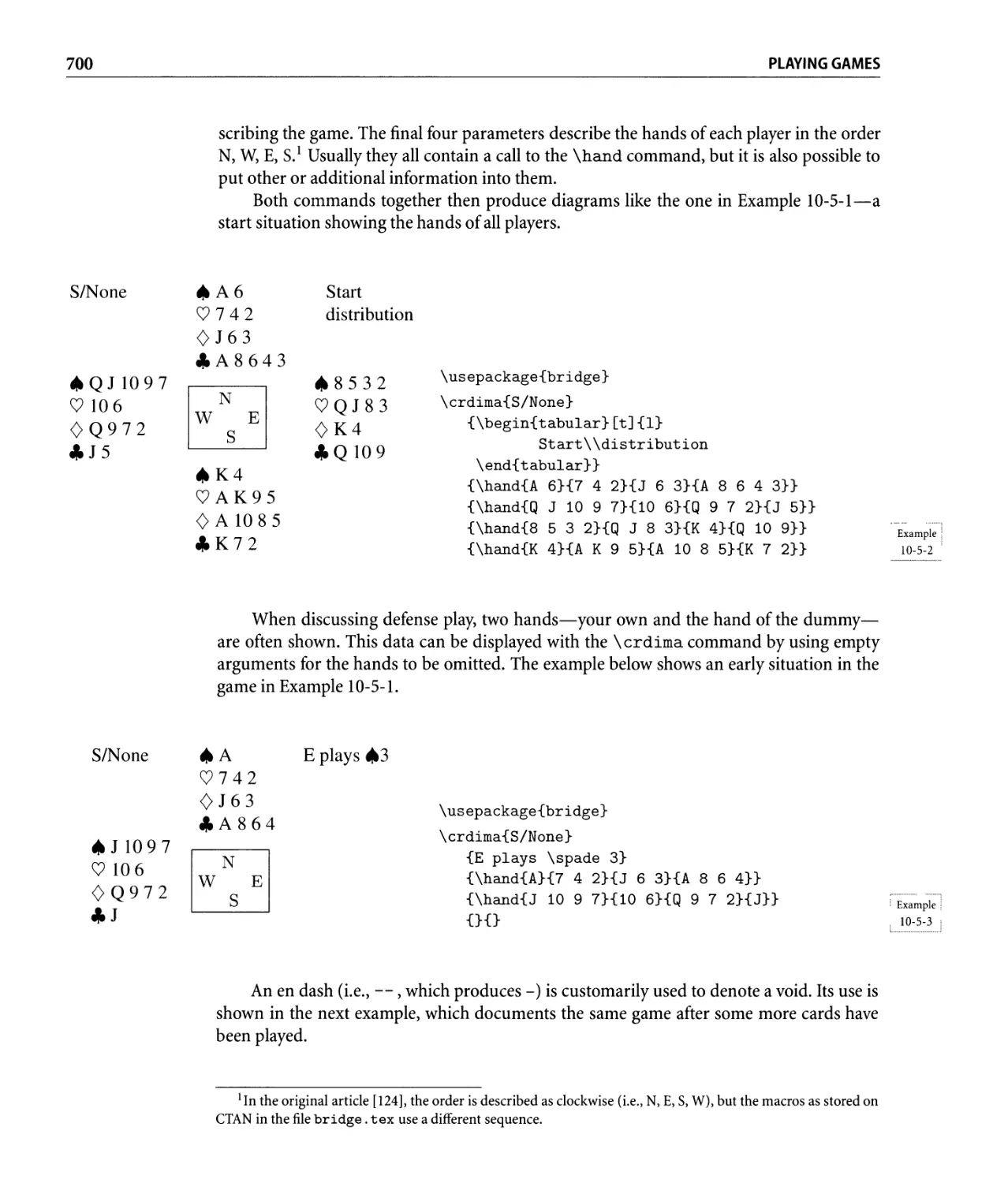
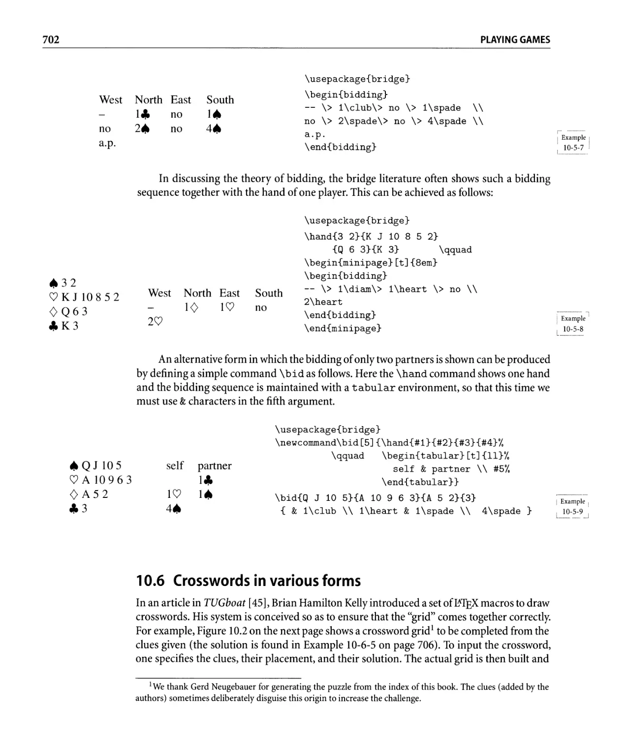
10.5.1 Bridge....................................... 699
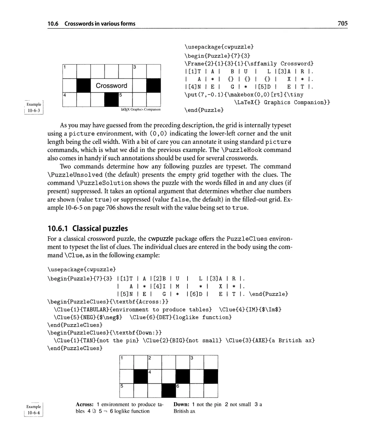
10.6 Crosswords in various forms. . . . . . . . . . . . . . . . . . . . . . . . . . . . . .. 702
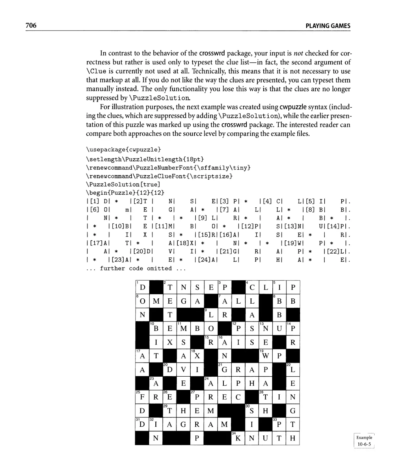
10.6.1 Classical puzzles. . . . . . . . . . . . . . . . . . . . . . . . . . . . . . . .. 705
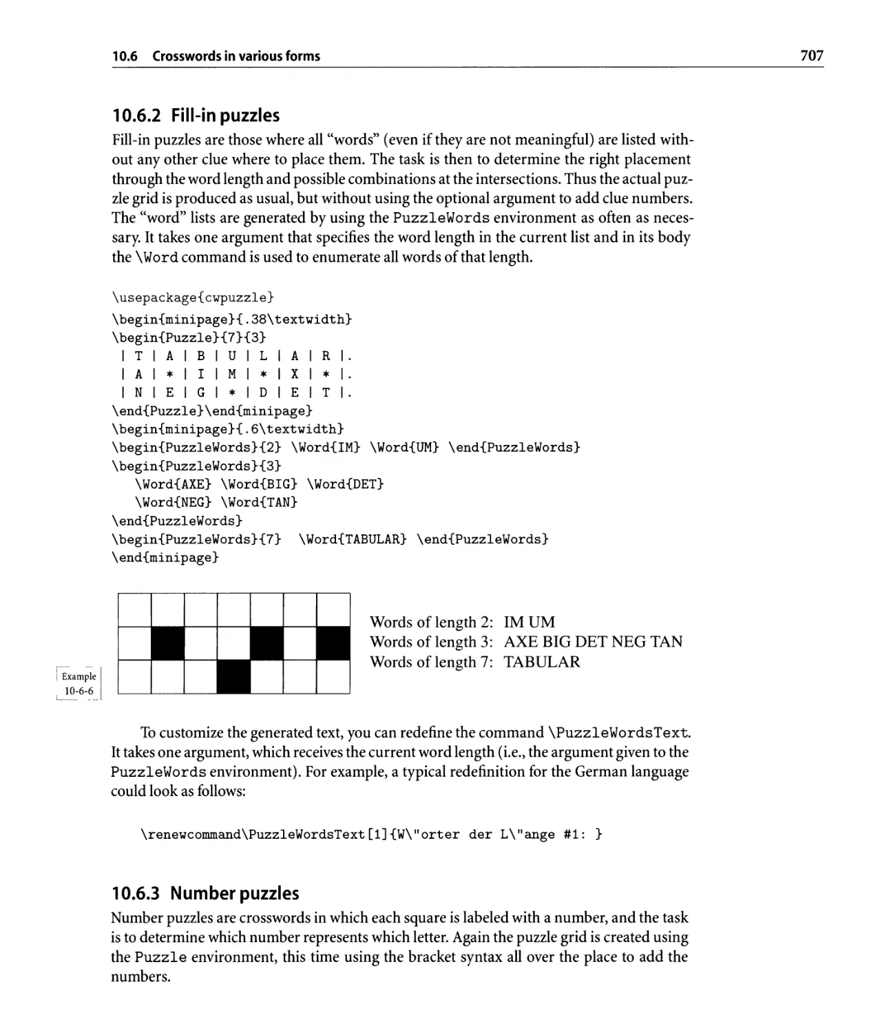
10.6.2 Fill-in puzzles. . . . . . . . . . . . . . . . . . . . . . . . . . . . . . . . . .. 707
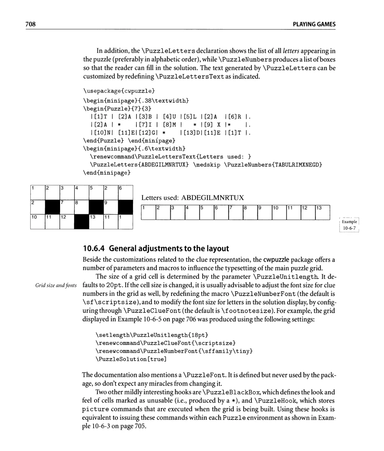
10.6.3 Number puzzles. . . . . . . . . . . . . . . . . . . . . . . . . . . . . . . .. 707
10.6.4 General adjustments to the layout. . . . . . . . . . . . . . . . . . . . .. 708
10.6.5 External puzzle generation . . . . . . . . . . . . . . . . . . . . . . . . .. 709
10.7 Sudokus . . . . . . . . . . . . . . . . . . . . . . . . . . . . . . . . . . . . . . . . . .. 709
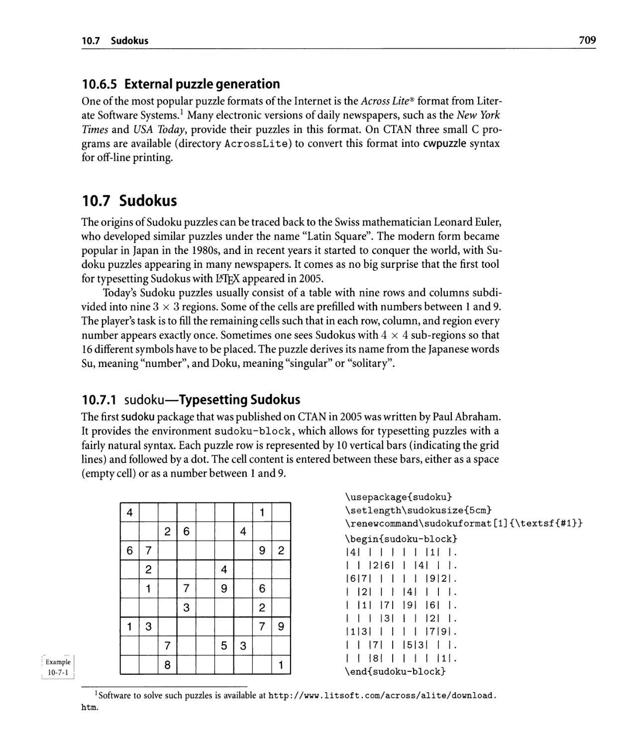
10.7.1 sudoku-Typesetting Sudokus. . . . . . . . . . . . . . . . . . . . . . .. 709
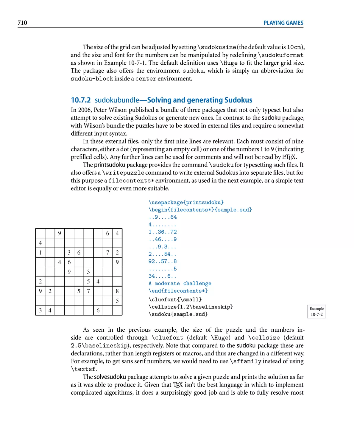
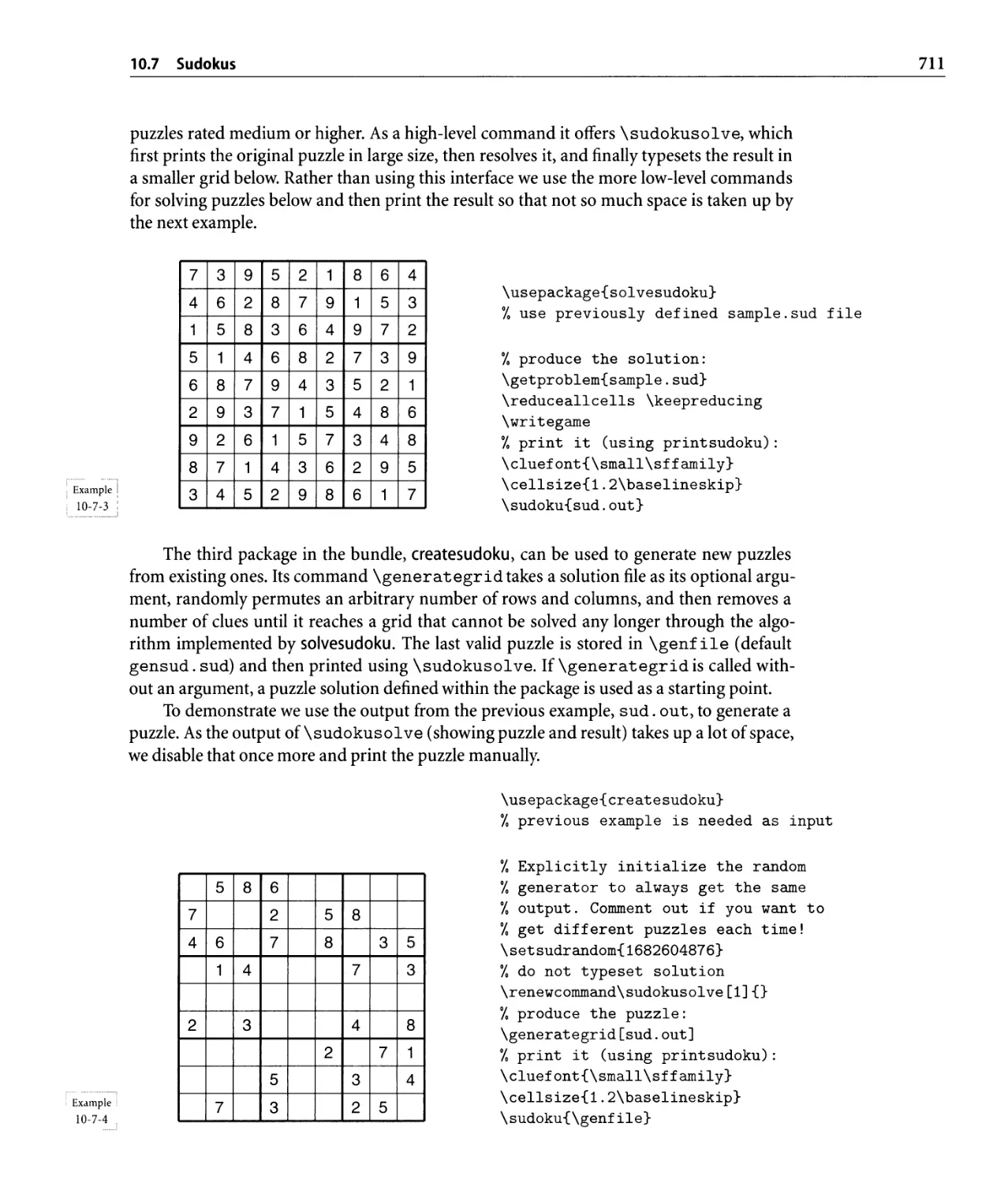
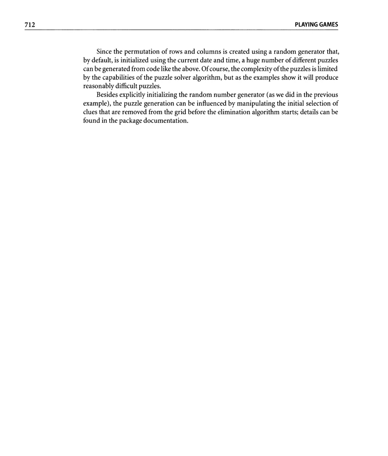
10.7.2 sudokubundle-Solving and generating Sudokus. . . . . . . . . . .. 710
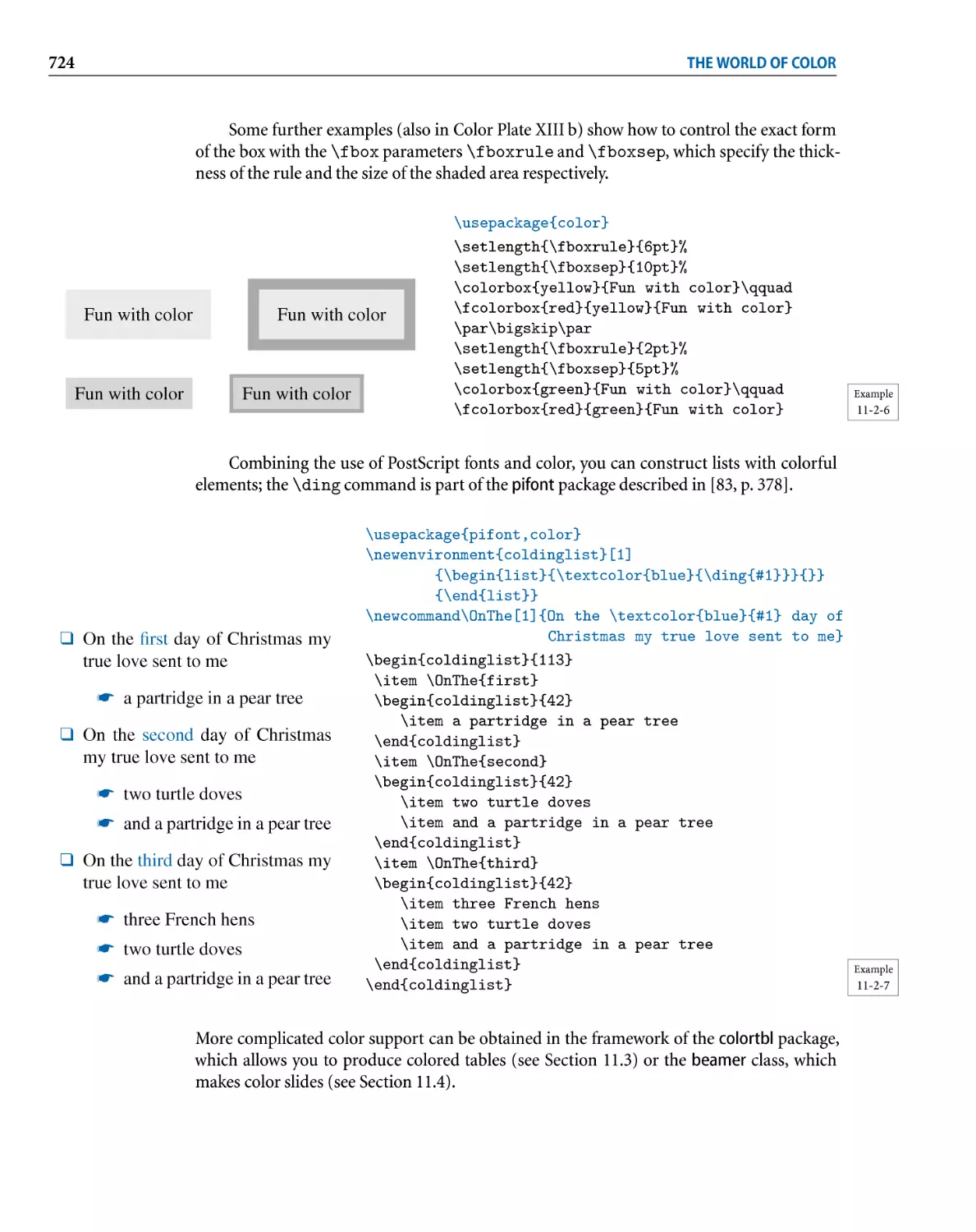
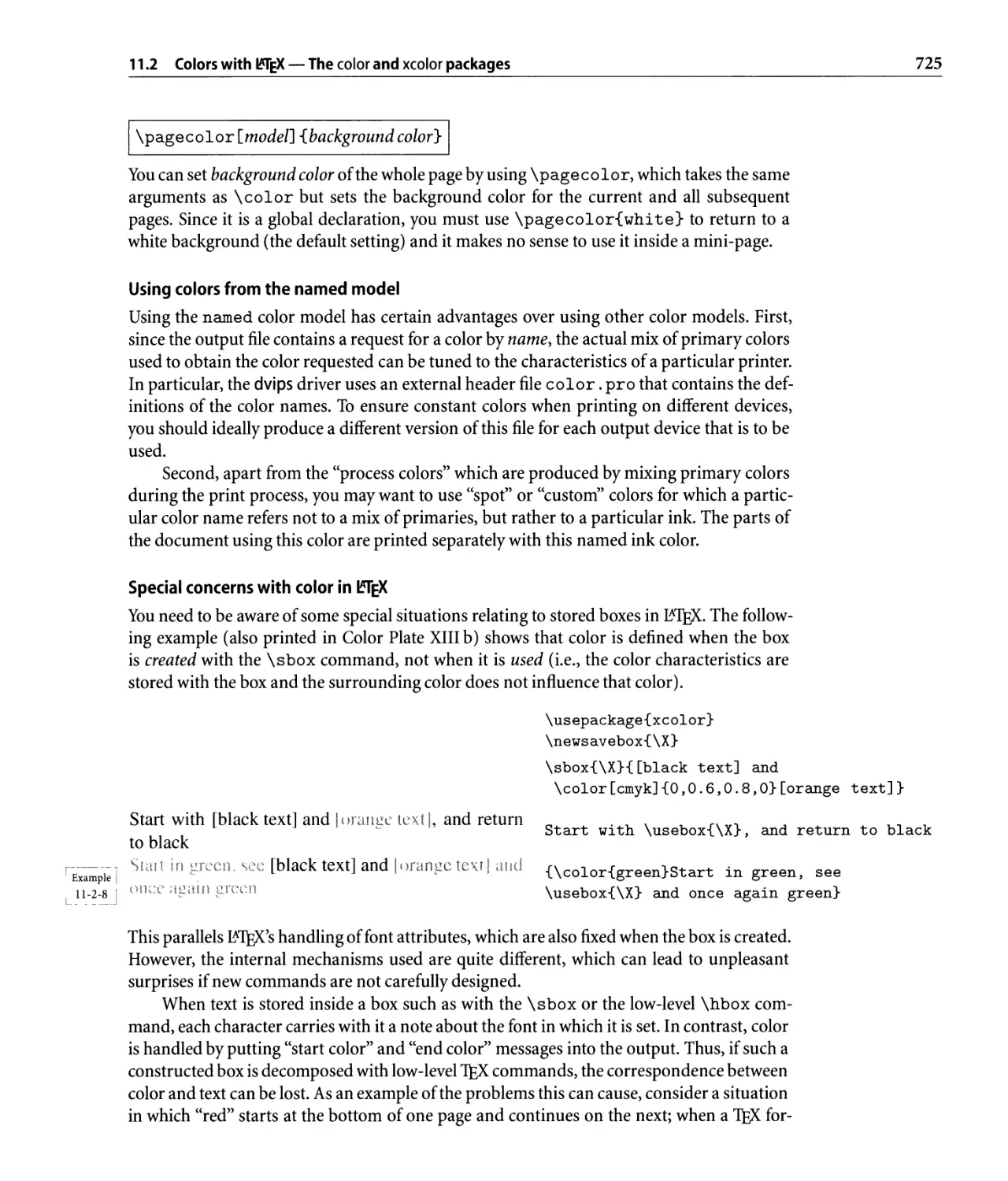
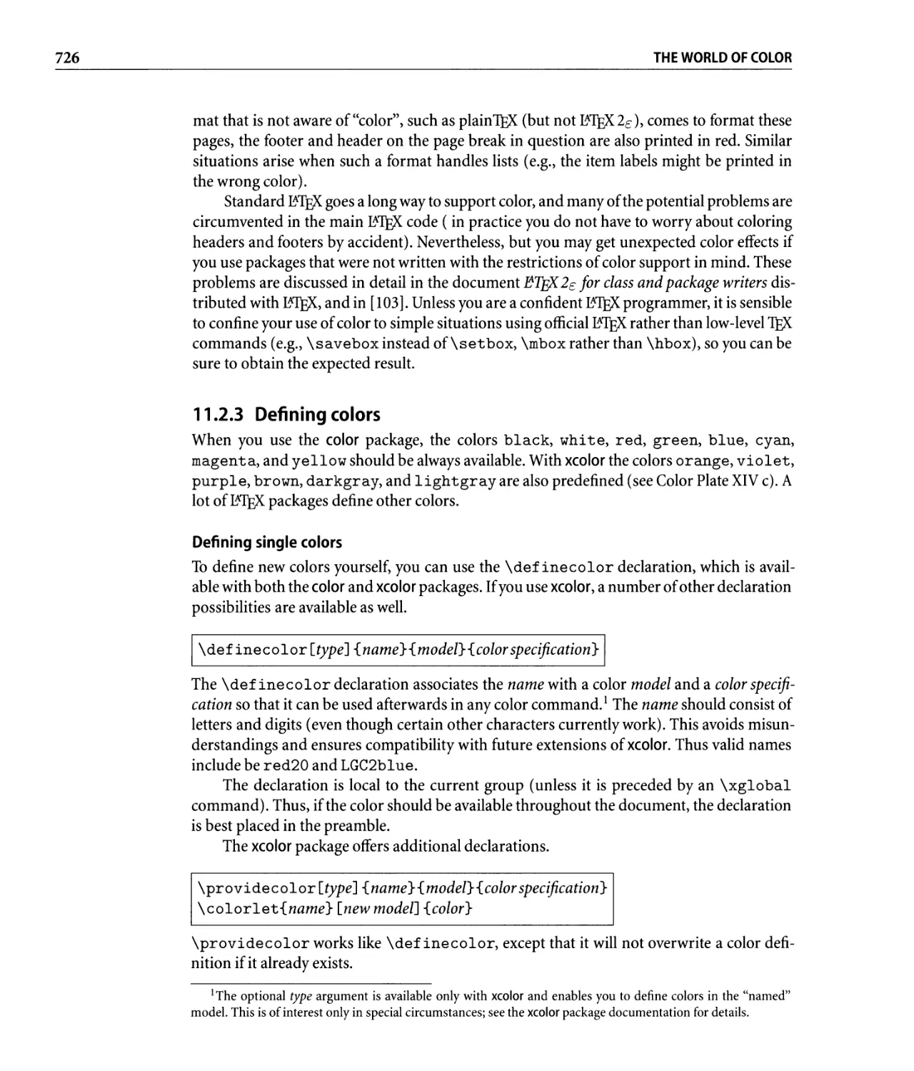
11 The World of Color 713
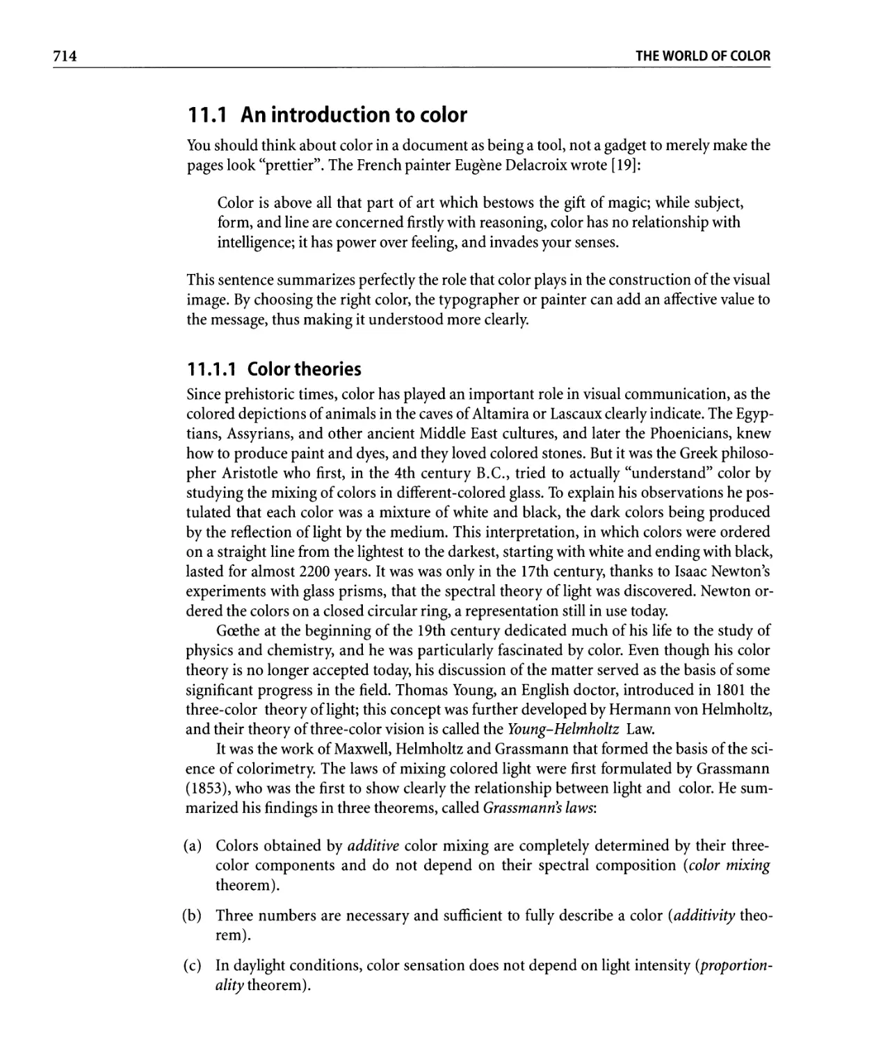
11.1 An introduction to color. . . . . . . . . . . . . . . . . . . . . . . . . . . . . . . . .. 714
11.1.1 Color theories . . . . . . . . . . . . . . . . . . . . . . . . . . . . . . . . .. 714
11.1.2 Color systems . . . . . . . . . . . . . . . . . . . . . . . . . . . . . . . . .. 715
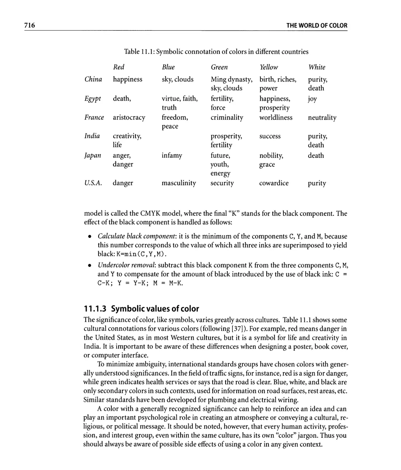
11.1.3 Symbolic values of color. . . . . . . . . . . . . . . . . . . . . . . . . . .. 716
11.1.4 Color harmonies. . . . . . . . . . . . . . . . . . . . . . . . . . . . . . . .. 717
11.1.5 Color and readability. . . . . . . . . . . . . . . . . . . . . . . . . . . . .. 718
11.2 Colors with EX - The color and xcolor packages . . . . . . . . . . . . . . . .. 719
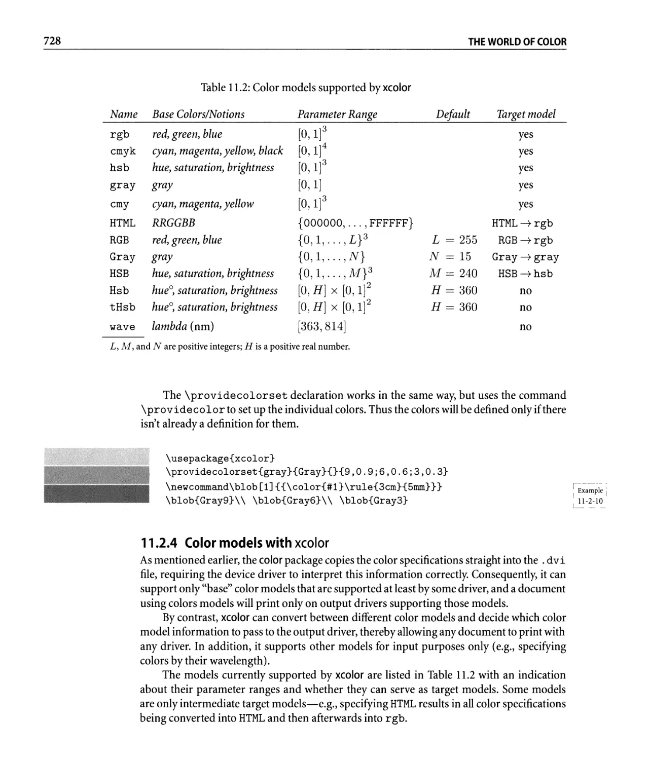
11.2.1 Options supported by color and xcolor. . . . . . . . . . . . . . . . . .. 720
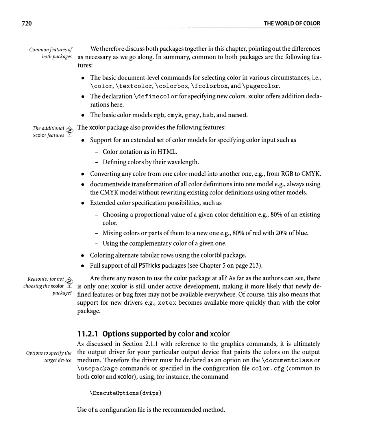
11.2.2 Using colors within the document. . . . . . . . . . . . . . . . . . . . .. 722
CONTENTS xv
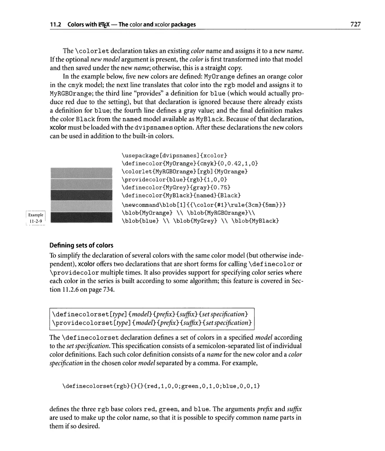
11.2.3 Defining colors. . . . . . . . . . . . . . . . . . . . . . . . . . . . . . . . .. 726
11.2.4 Color models with xcolor . . . . . . . . . . . . . . . . . . . . . . . . . .. 728
11.2.5 Extended color specification with xcolor. . . . . . . . . . . . . . . . .. 730
11.2.6 Support for color series . . . . . . . . . . . . . . . . . . . . . . . . . . .. 734
11.2.7 Color blending and masking . . . . . . . . . . . . . . . . . . . . . . . .. 737
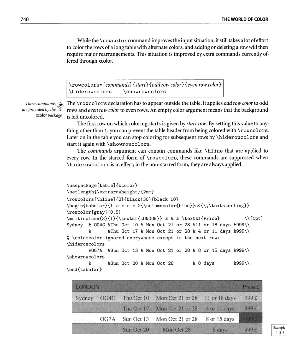
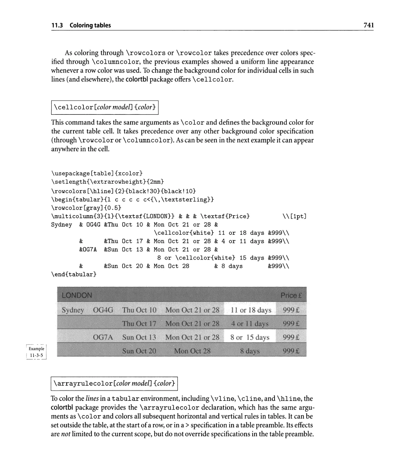
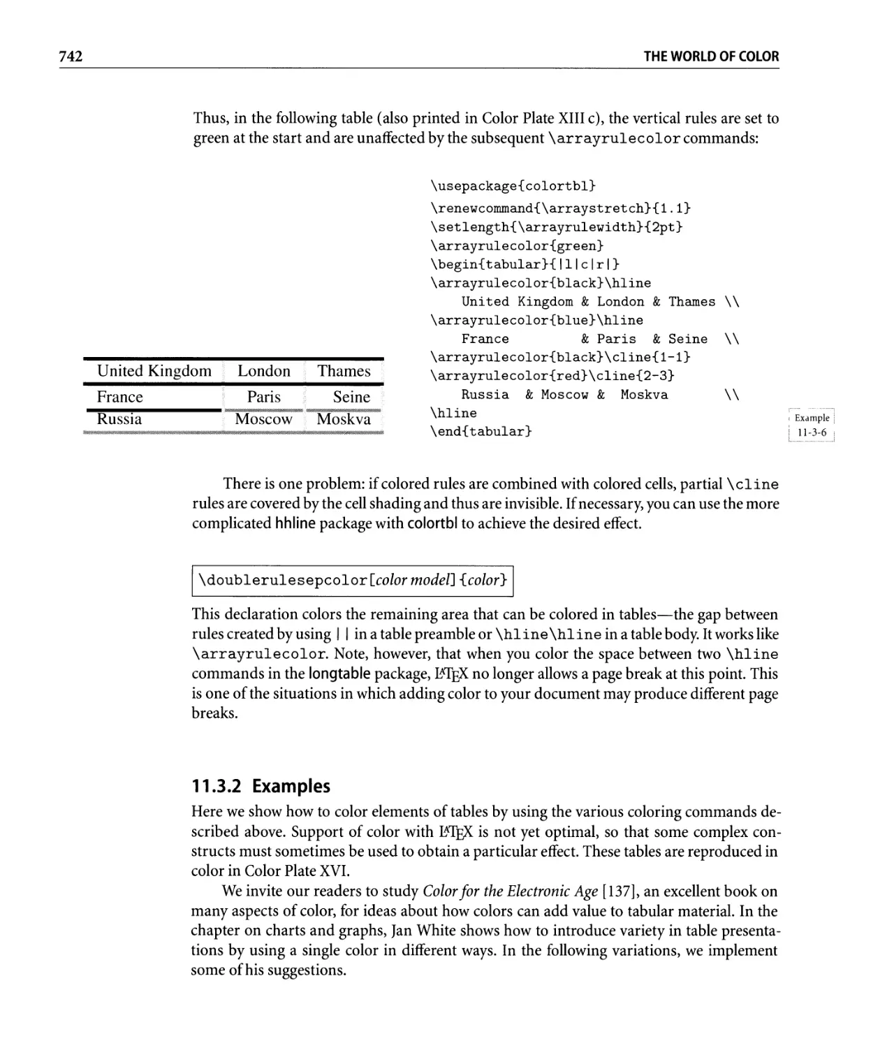
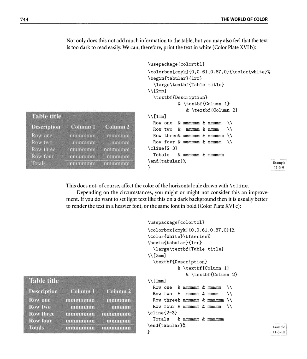
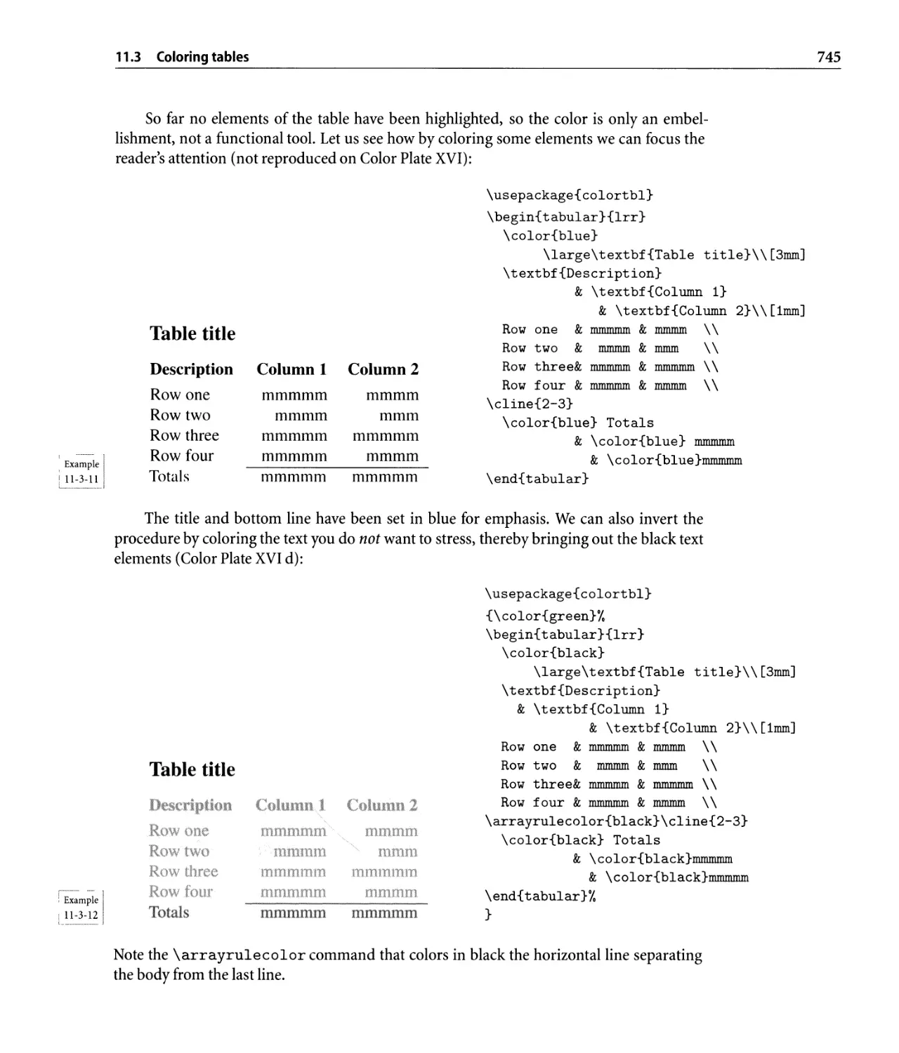
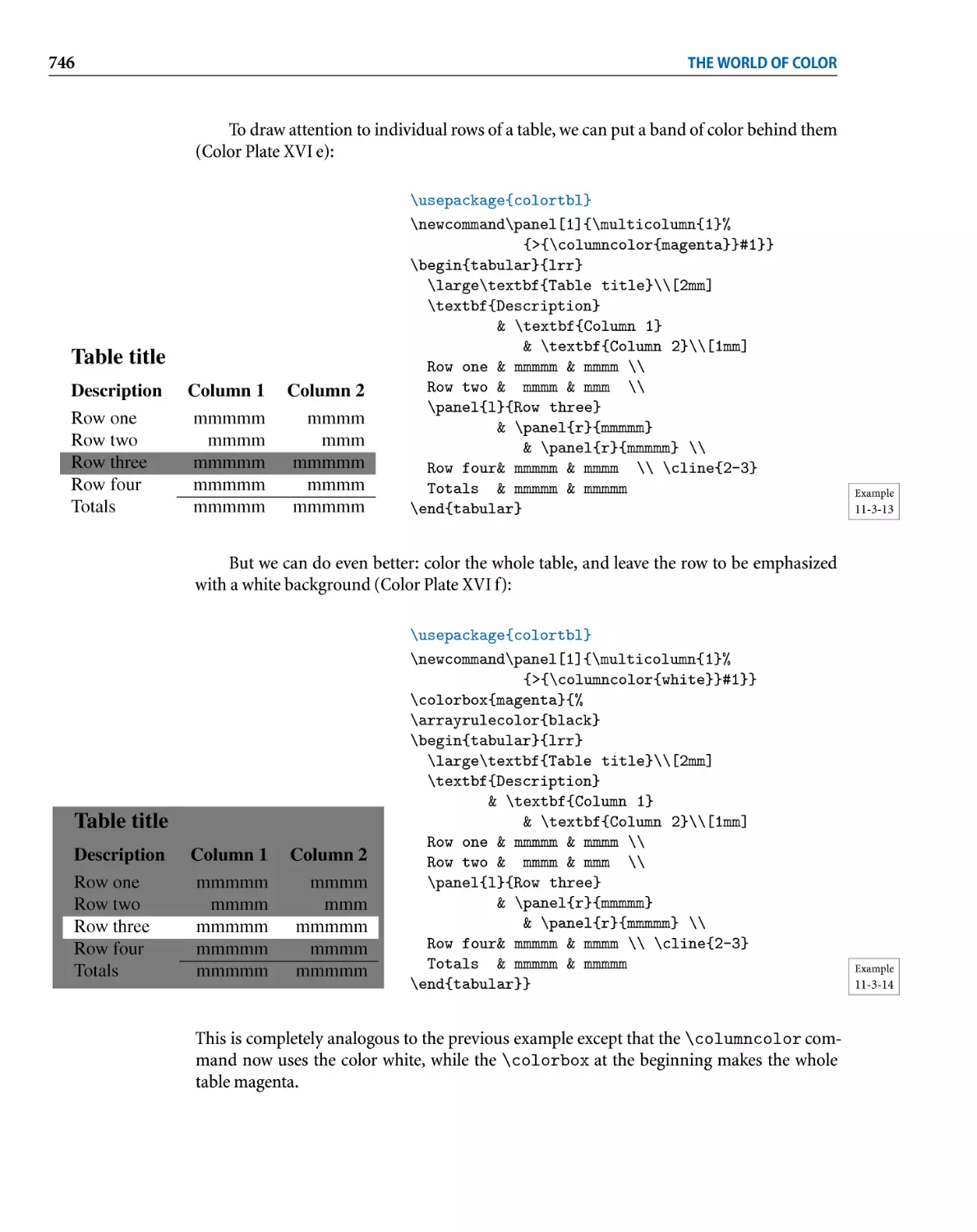
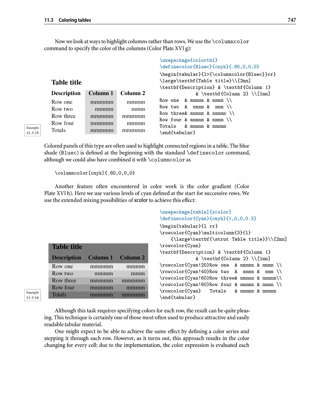
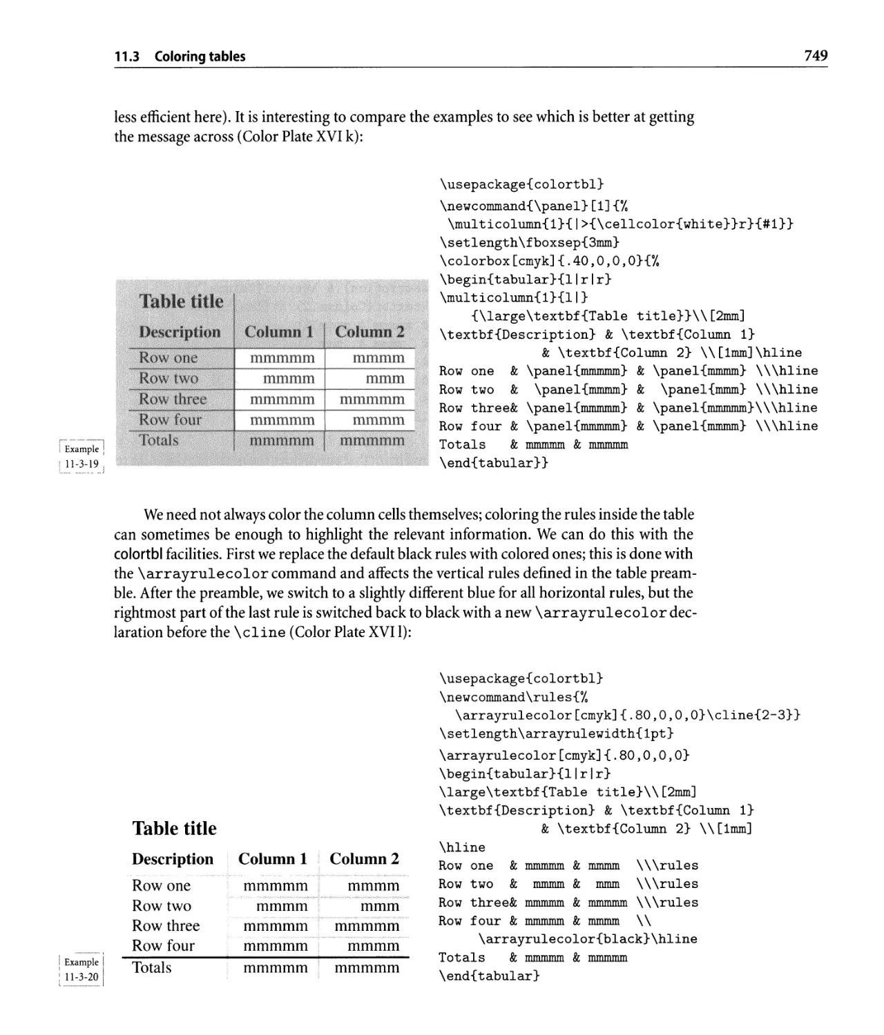
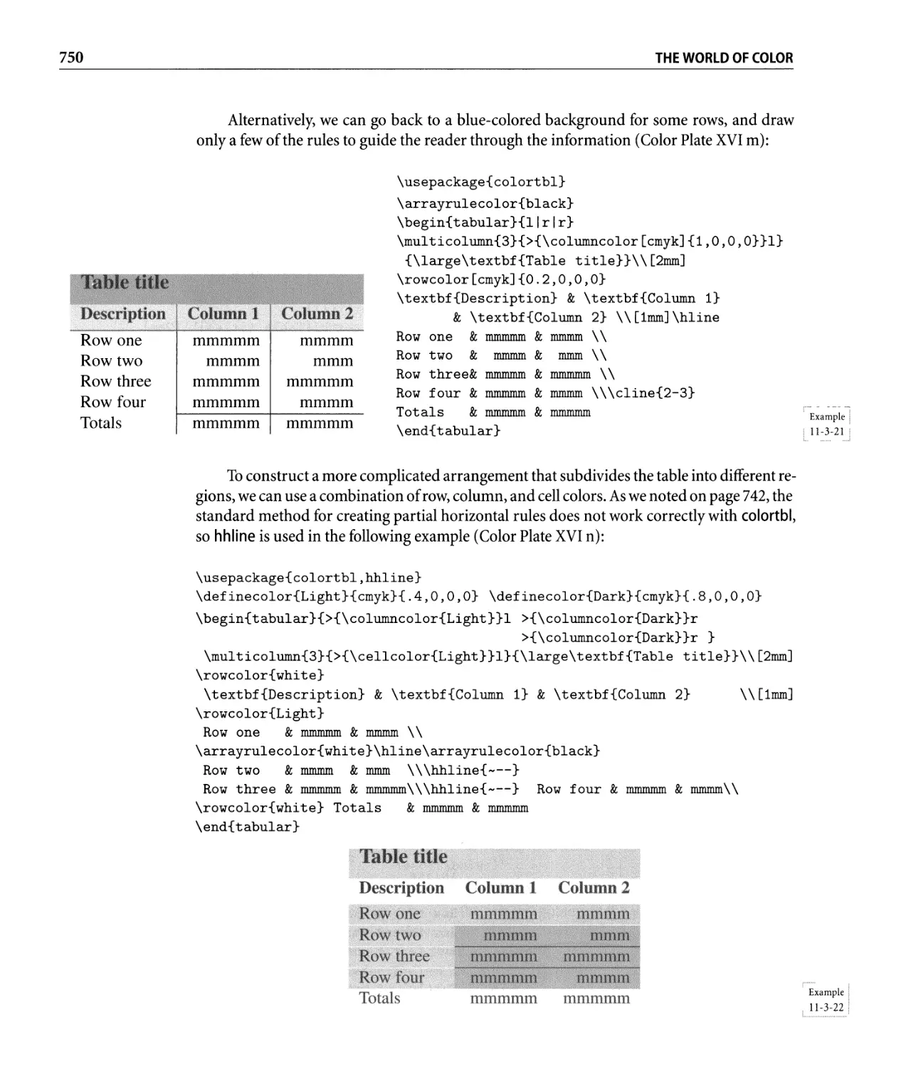
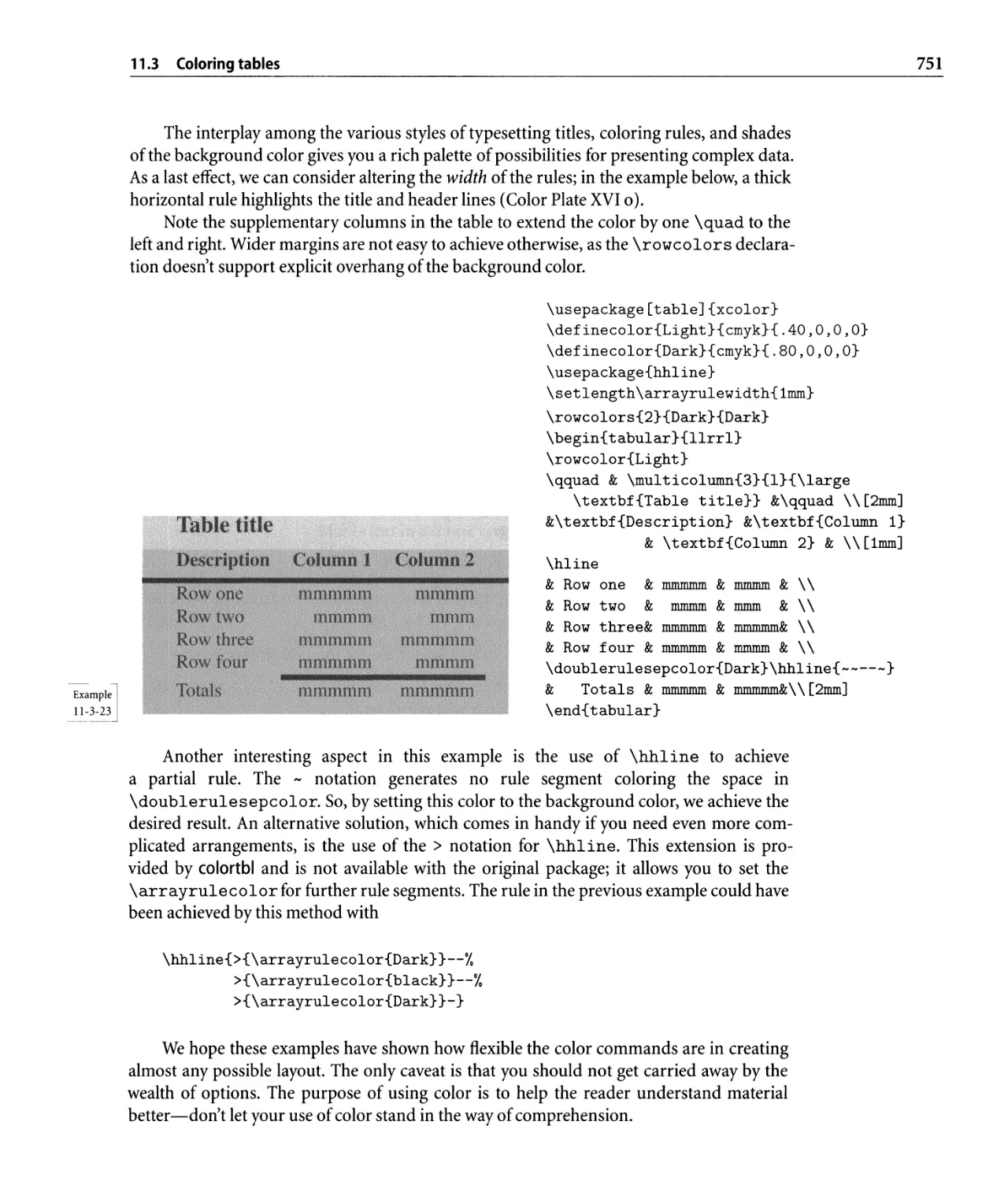
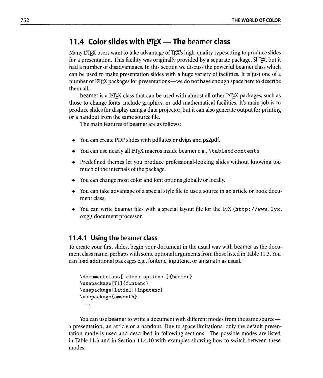
11.3 Coloring tables . . . . . . . . . . . . . . . . . . . . . . . . . . . . . . . . . . . . . .. 737
11.3.1 The colortbl package. . . . . . . . . . . . . . . . . . . . . . . . . . . . .. 737
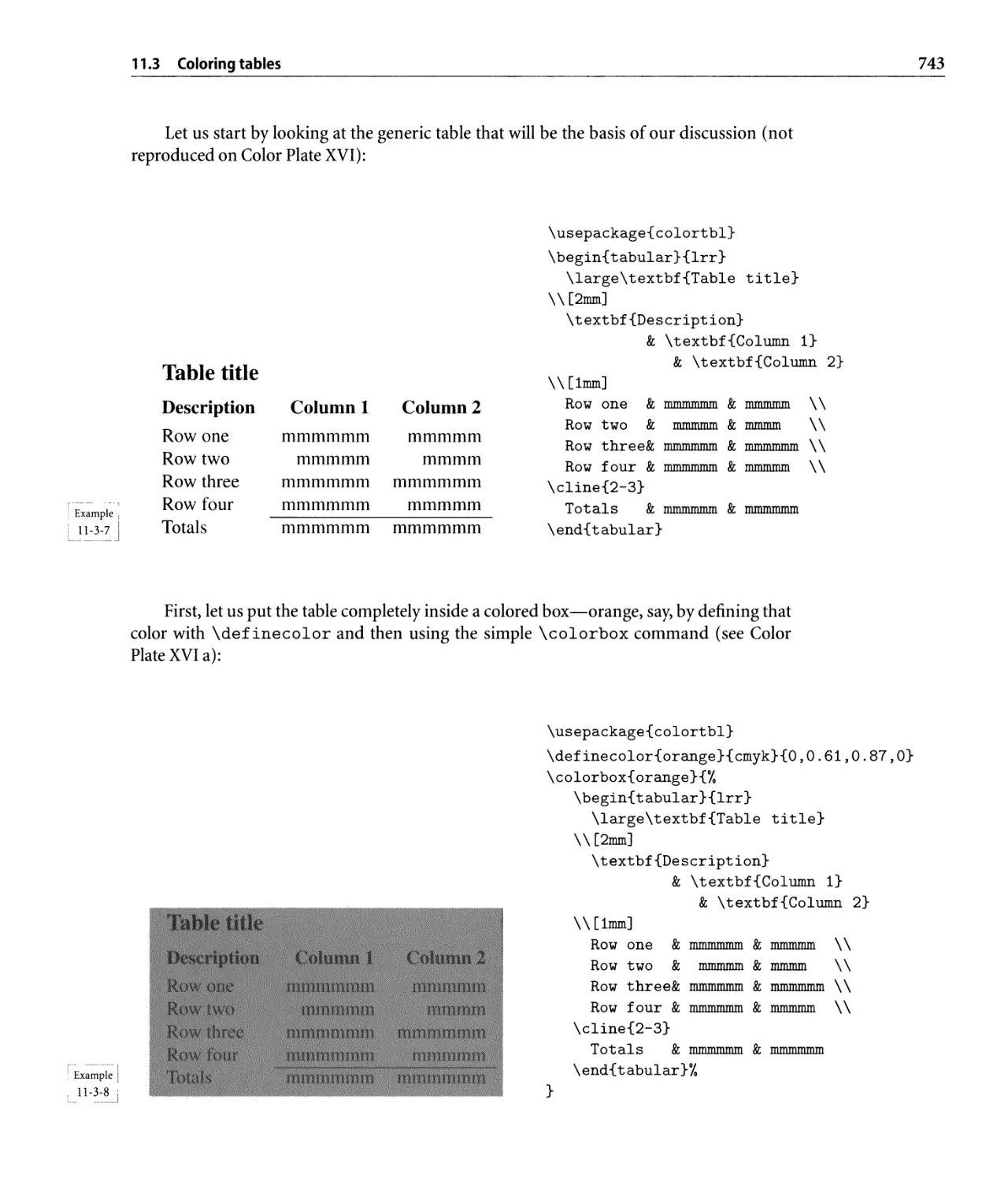
11.3.2 Examples..................................... 742
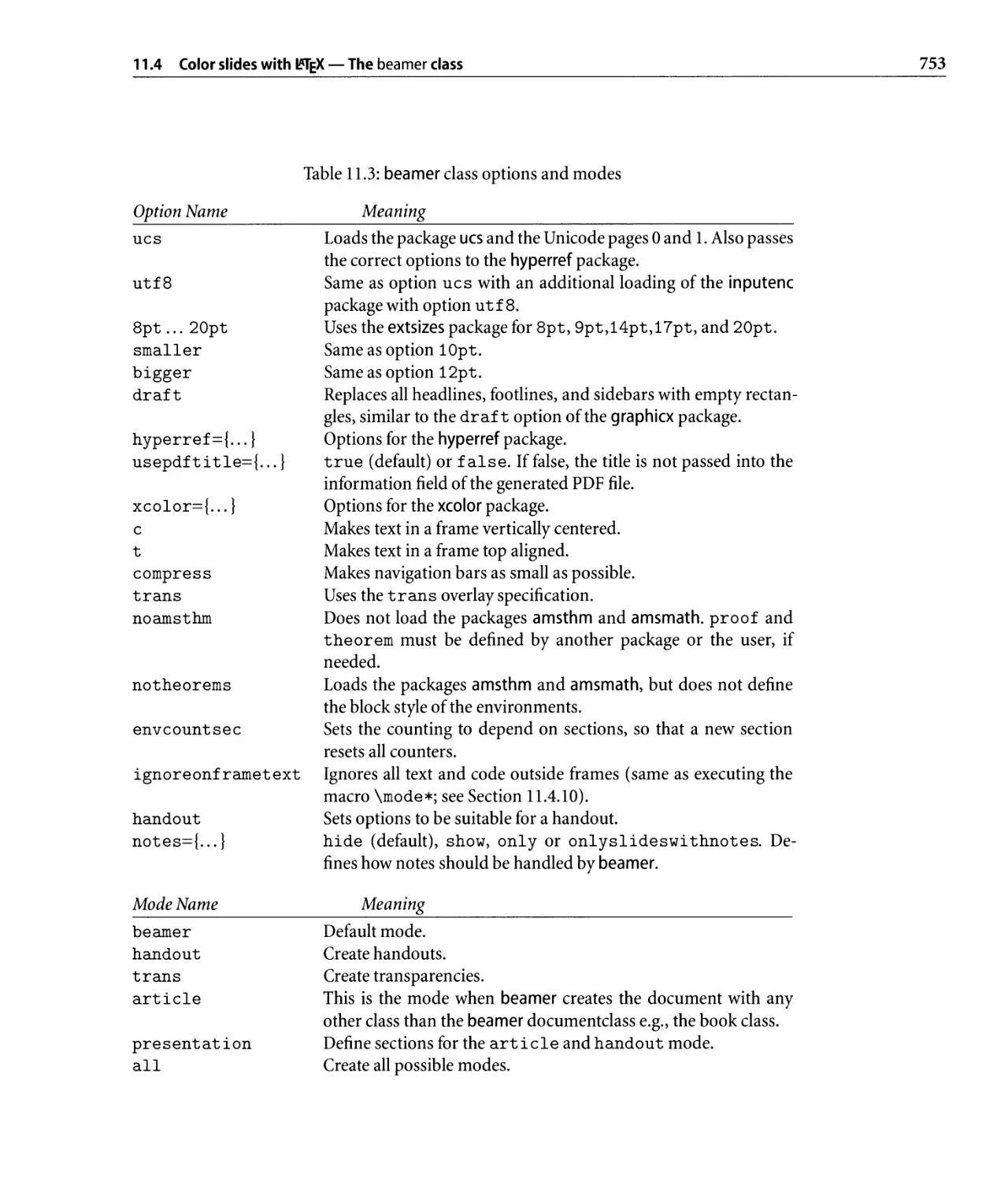
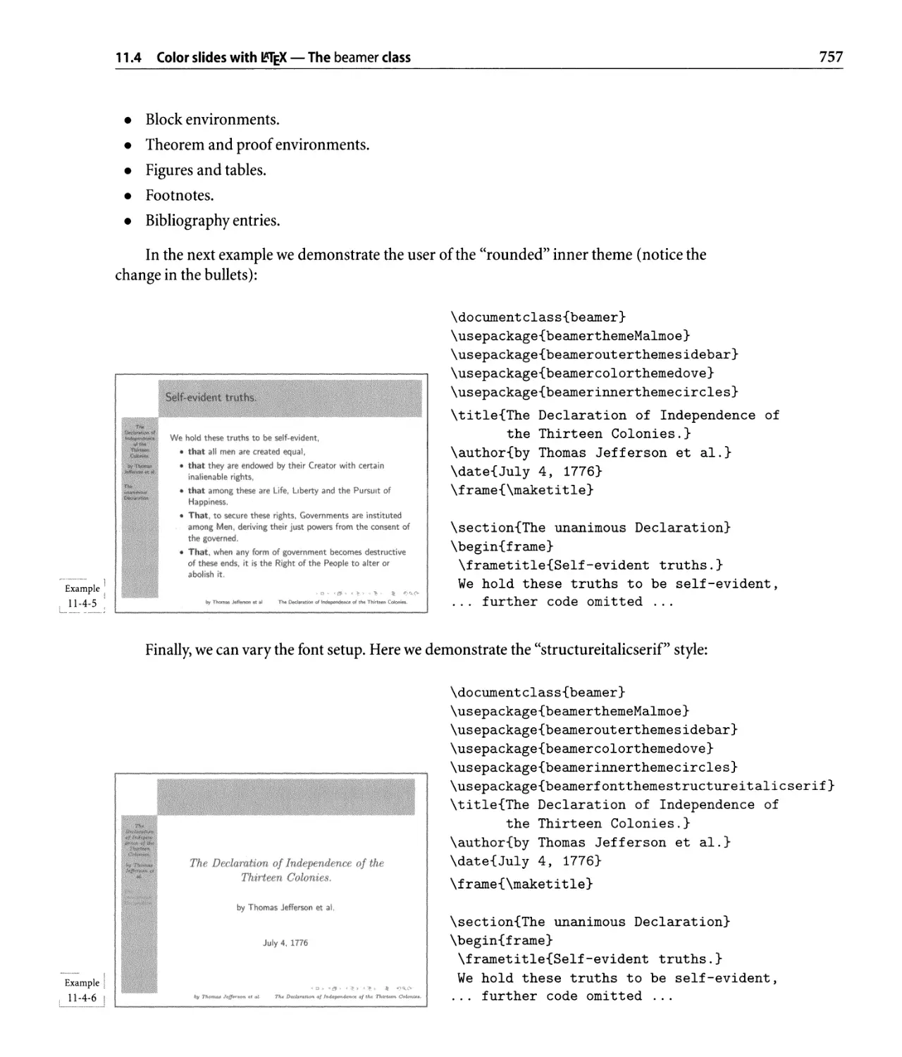
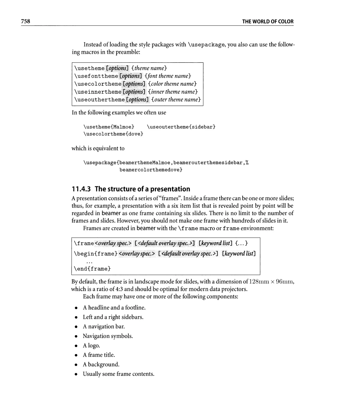
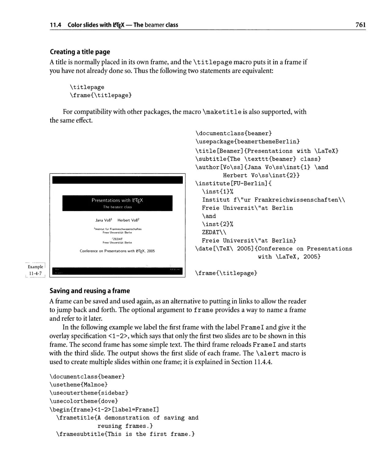
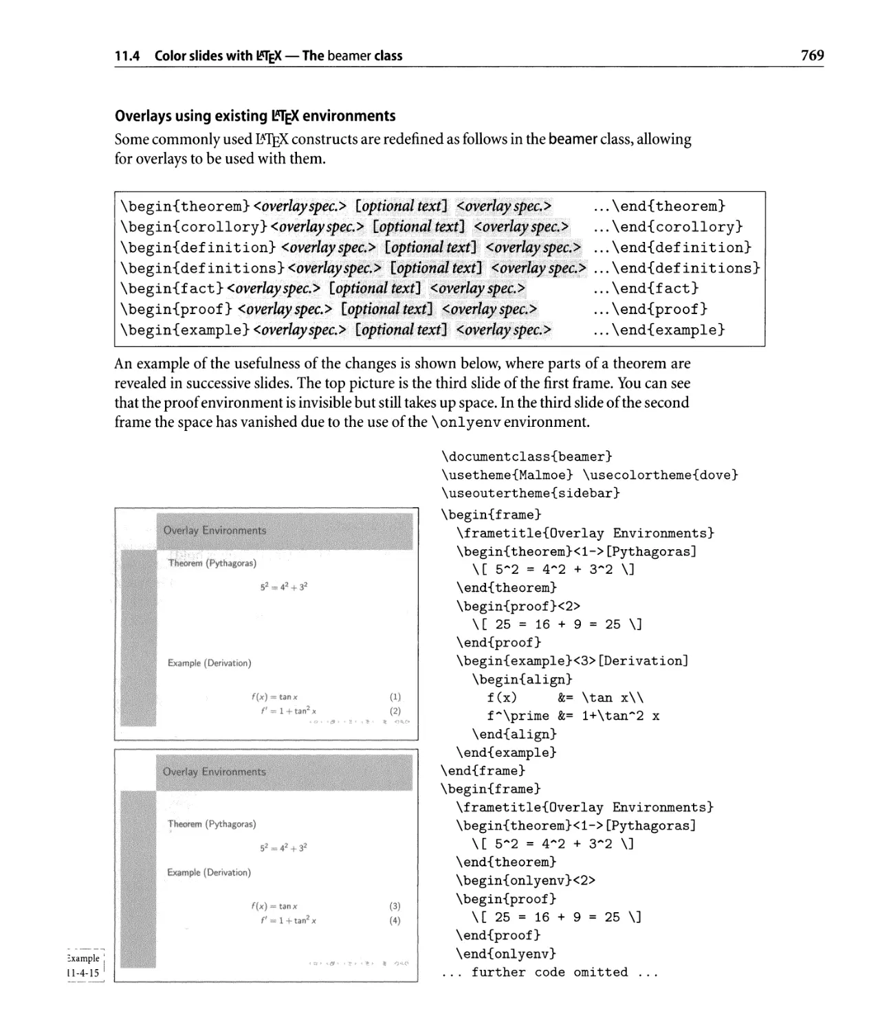
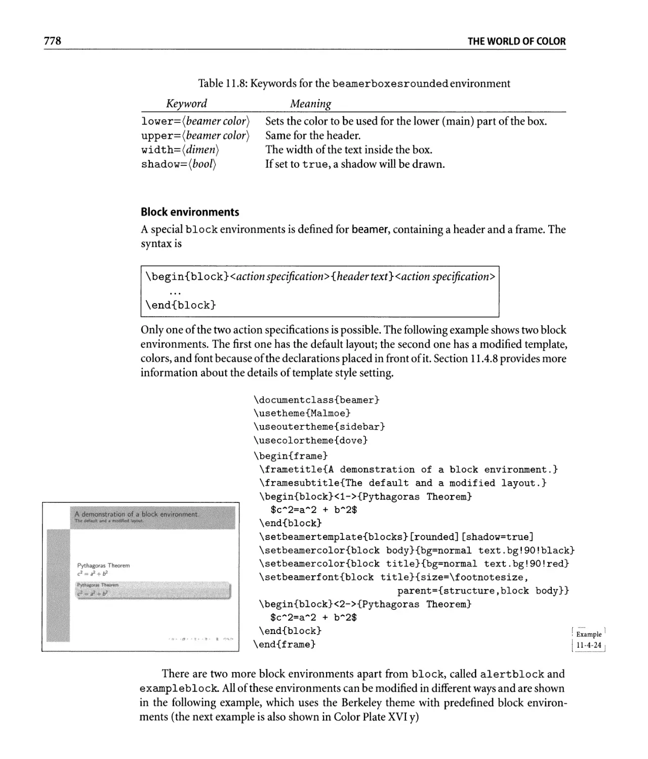
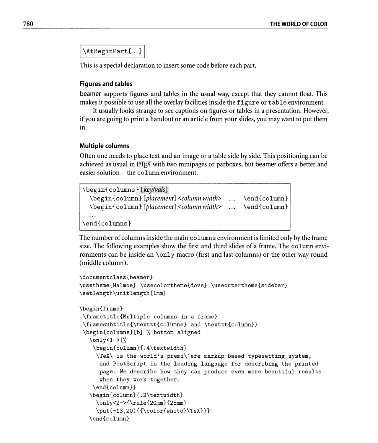
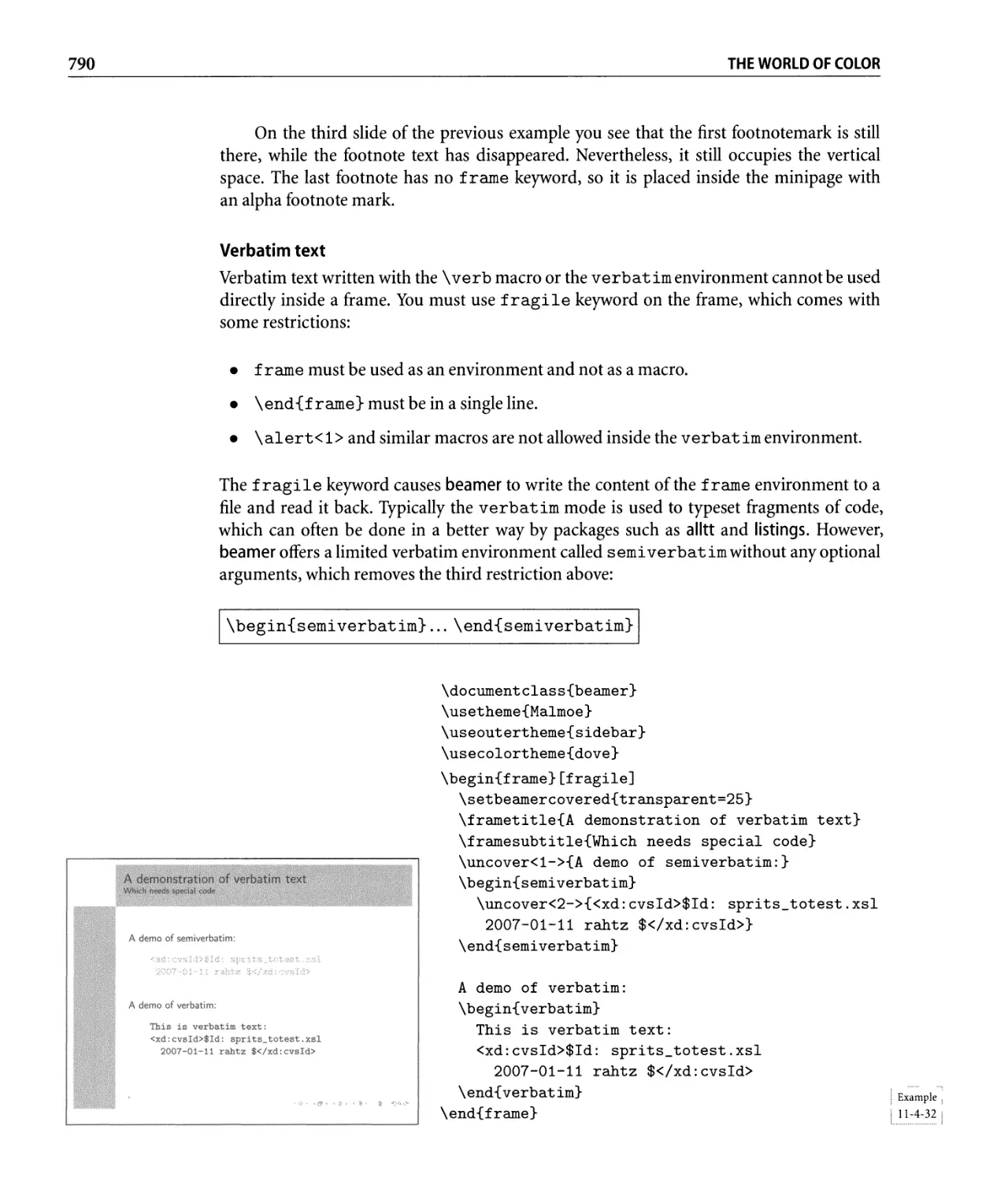
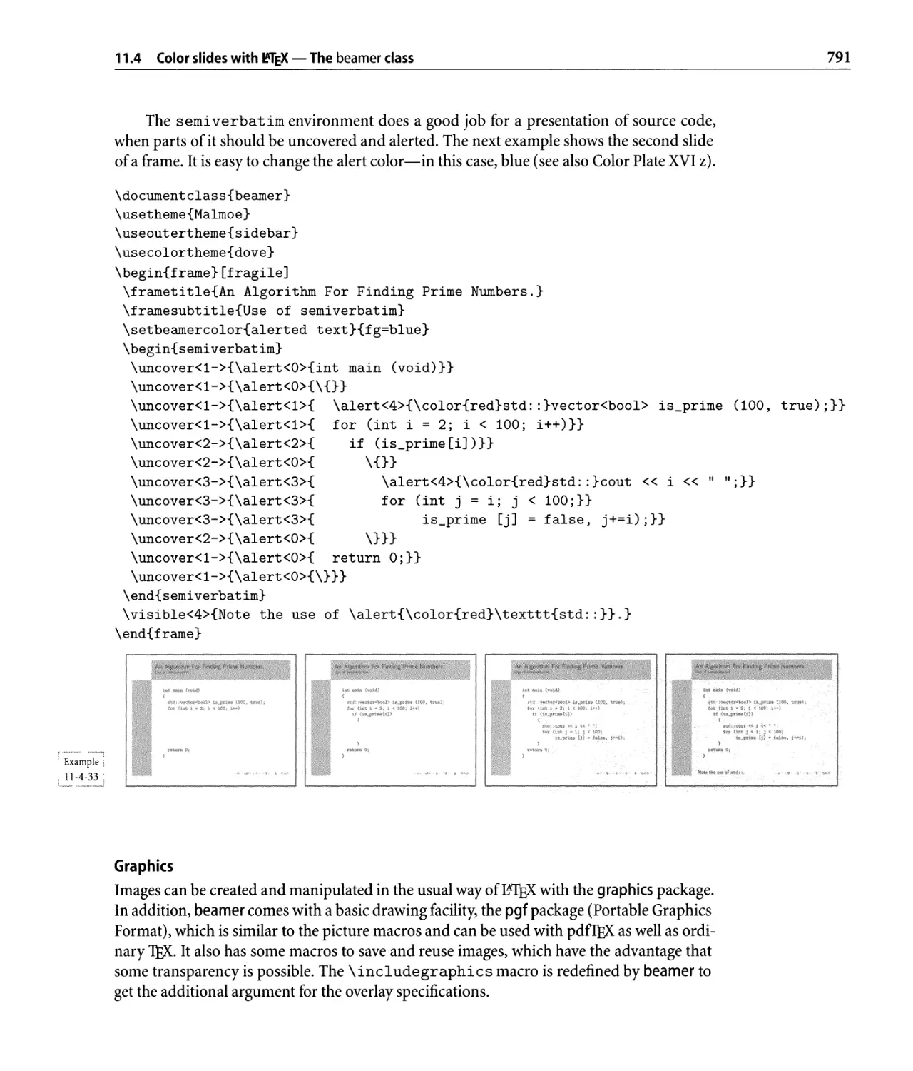
11.4 Color slides with EX - The beamer class . . . . . . . . . . . . . . . . . . . . .. 752
11.4.1 Using the beamer class. . . . . . . . . . . . . . . . . . . . . . . . . . . .. 752
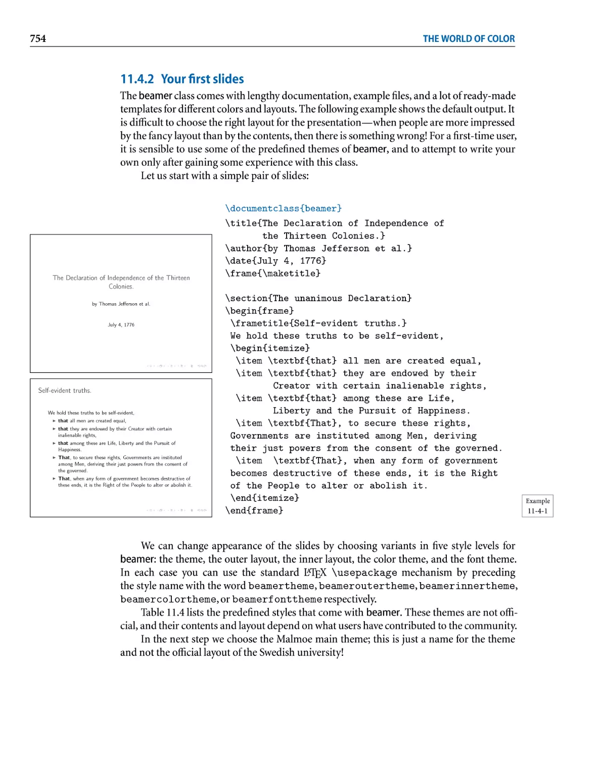
11.4.2 Your first slides. . . . . . . . . . . . . . . . . . . . . . . . . . . . . . . . .. 754
11.4.3 The structure of a presentation. . . . . . . . . . . . . . . . . . . . . . .. 758
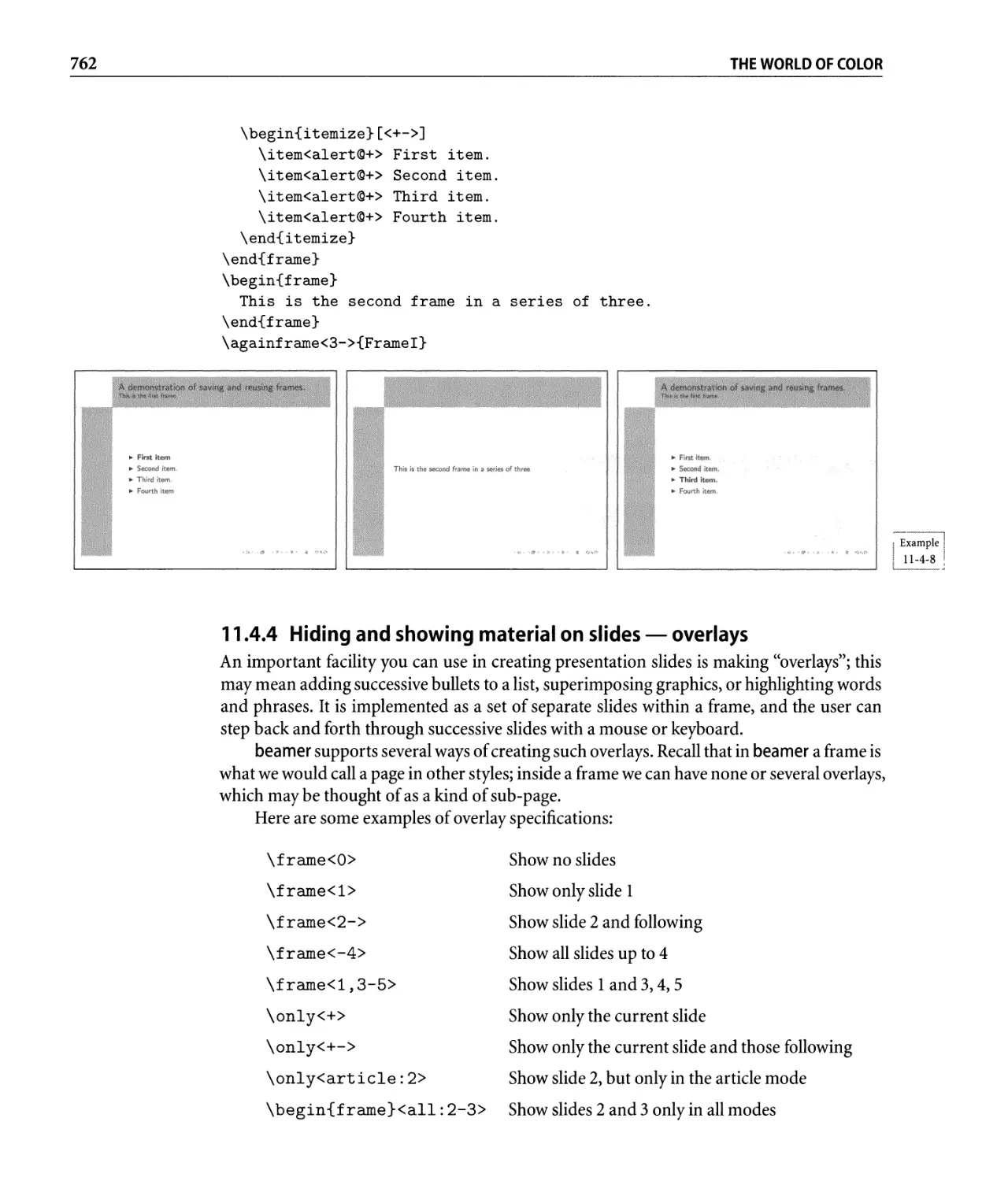
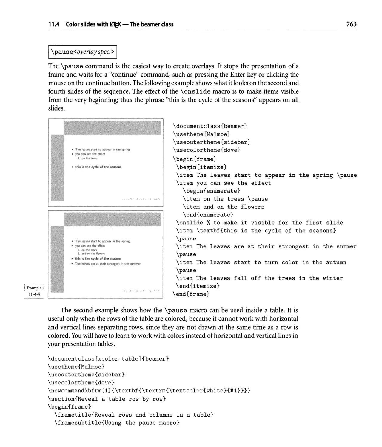
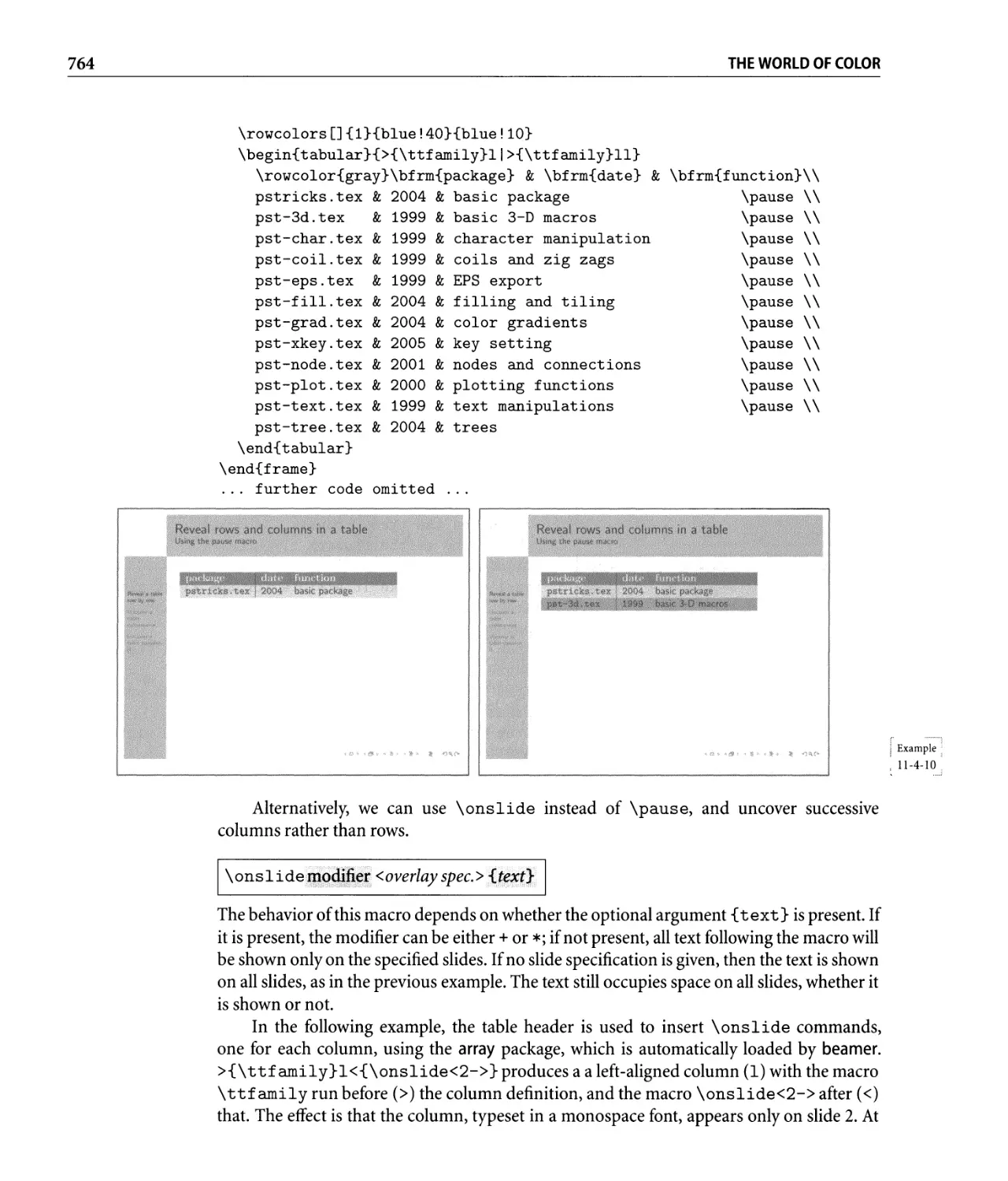
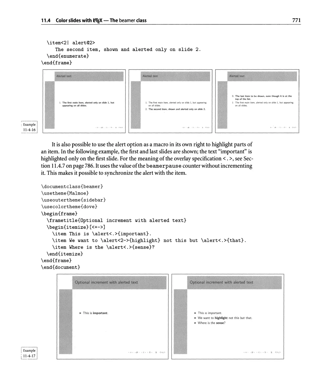
11.4.4 Hiding and showing material on slides - overlays . . . . . . . . . .. 762
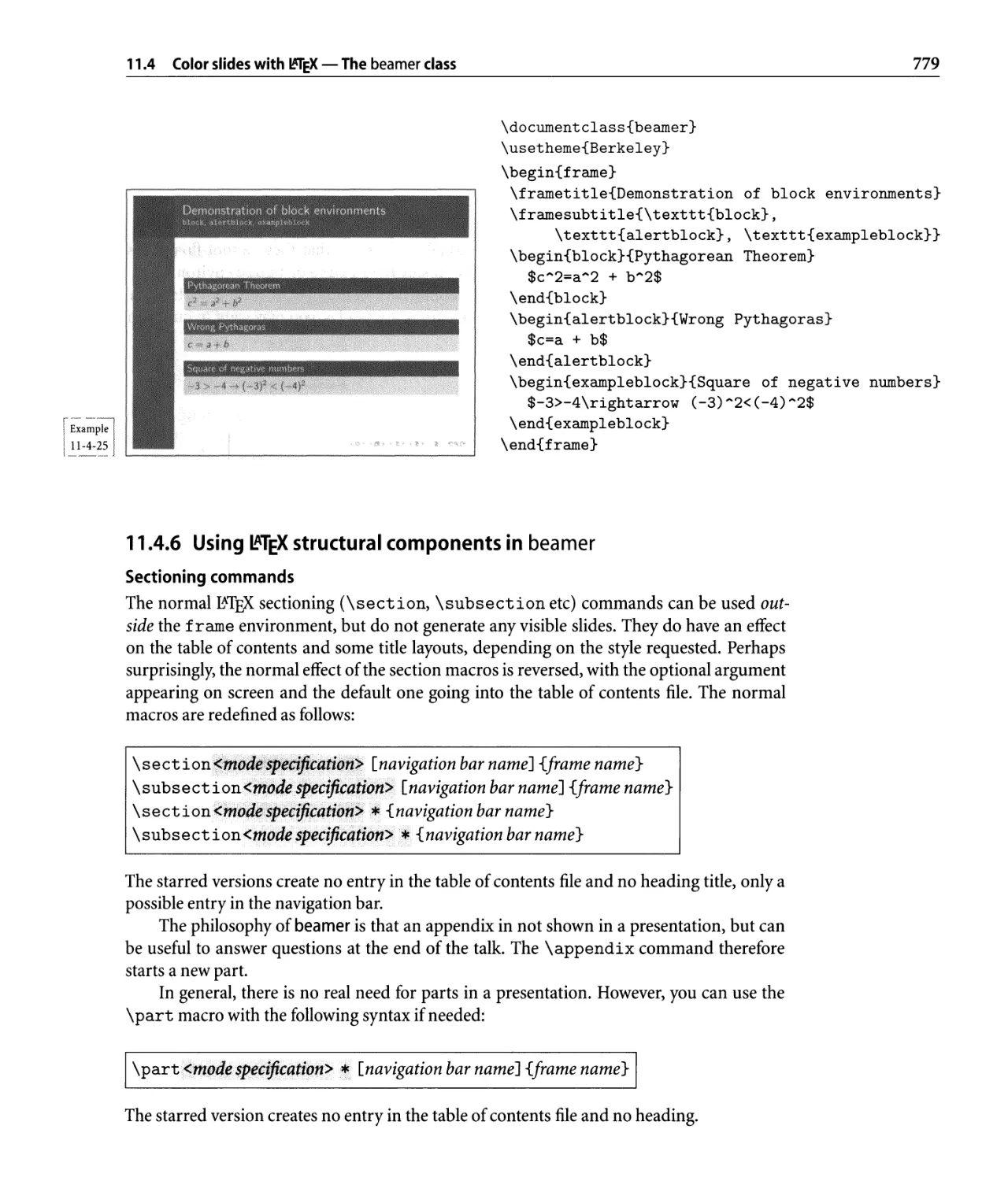
11.4.5 Additional facilities in beamer . . . . . . . . . . . . . . . . . . . . . . .. 772
11.4.6 Using EX structural components in beamer . . . . . . . . . . . . . .. 779
11.4.7 Using EX inline components in beamer. . . . . . . . . . . . . . . . .. 783
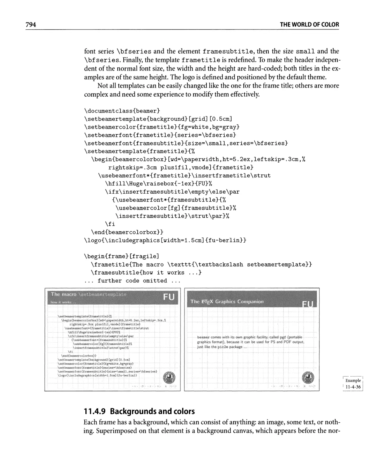
11.4.8 Managing your templates. . . . . . . . . . . . . . . . . . . . . . . . . .. 792
11.4.9 Backgrounds and colors. . . . . . . . . . . . . . . . . . . . . . . . . . .. 794
11.4.10 Document modes. . . . . . . . . . . . . . . . . . . . . . . . . . . . . . .. 796
11.4.11 The beamer project. . . . . . . . . . . . . . . . . . . . . . . . . . . . . .. 796
A Producing PDF from Various Sources 797
A.l dvi pdfm and dvi pdfmx . . . . . . . . . . . . . . . . . . . . . . . . . . . . . . . . .. 798
A.2 pst-pdf-From PostScript to PDF . . . . . . . . . . . . . . . . . . . . . . . . . . .. 800
A.2.1 Package options. . . . . . . . . . . . . . . . . . . . . . . . . . . . . . . .. 800
A.2.2 Usage....................................... 800
A.3 Generating PDF from EX . . . . . . . . . . . . . . . . . . . . . . . . . . . . . . .. 803
B EX Software and User Group Information 809
B.l Getting help. . . . . . . . . . . . . . . . . . . . . . . . . . . . . . . . . . . . . . . .. 809
B.2 How to get those TEX files? . . . . . . . . . . . . . . . . . . . . . . . . . . . . . . .. 810
B.3 Using CTAN . . . . . . . . . . . . . . . . . . . . . . . . . . . . . . . . . . . . . . . .. 810
B.3.1 Using the TEX file catalogue. . . . . . . . . . . . . . . . . . . . . . . . .. 811
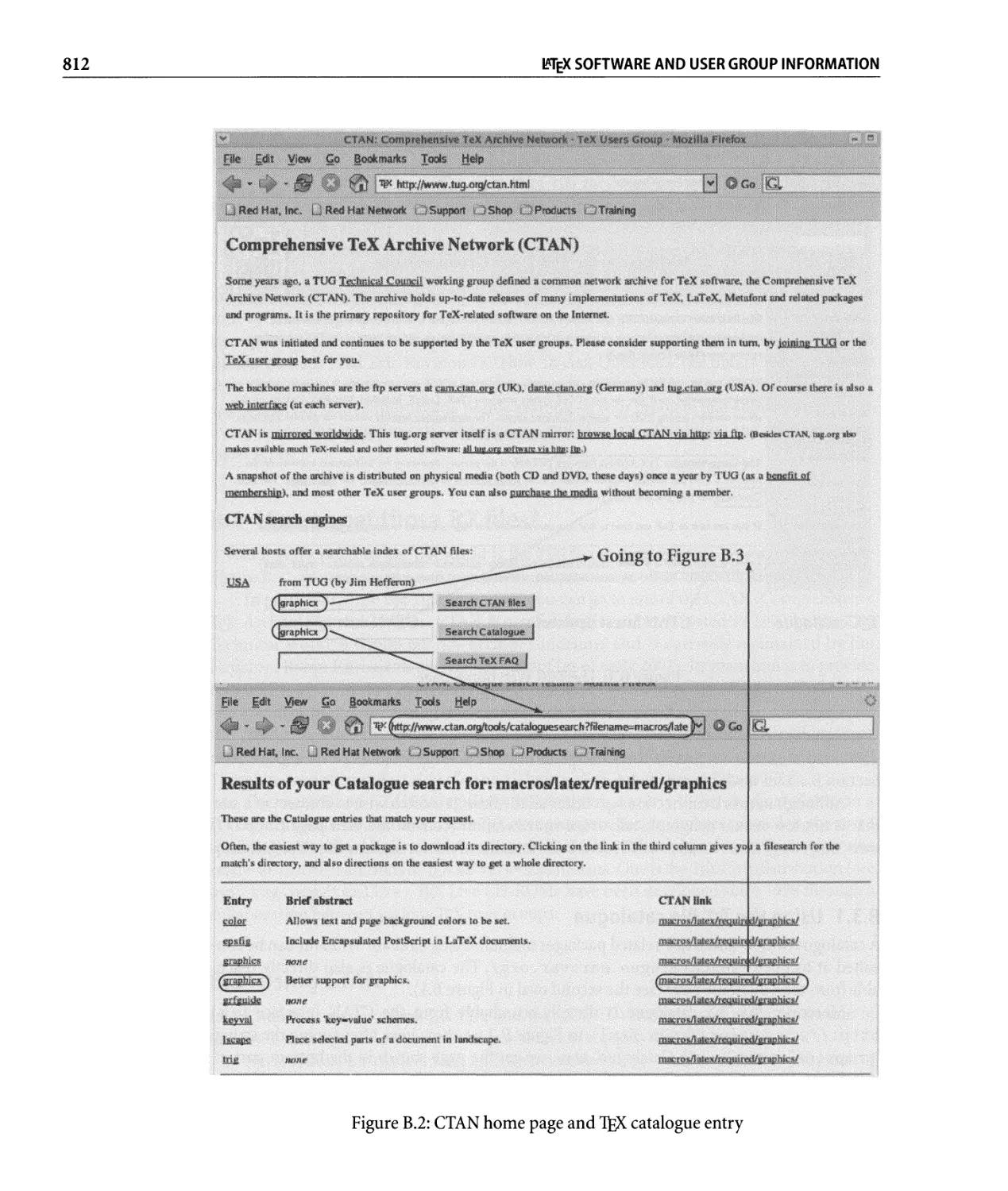
B.3.2 Finding files on the archive and transferring them. . . . . . . . . . .. 813
B.3.3 Getting files from the command line . . . . . . . . . . . . . . . . . . .. 814
B.4 Finding the documentation on your TEX system . . . . . . . . . . . . . . . . . .. 815
B.4.1 texdoc-Command-line interface for a search by name . . . . . . .. 815
B.4.2 texdoctk-Panel interface for a search by subject. . . . . . . . . . .. 816
B.5 TEX user groups. . . . . . . . . . . . . . . . . . . . . . . . . . . . . . . . . . . . . .. 817
Bibliography 819
Indexes 835
General Index . . . . . . . . . . . . . . . . . . . . . . . . . . . . . . . . . . . . . . .. 837
xvi
CONTENTS
METAFoNT and METAPosT . . . . . . . . . . . . . . . . . . . . . . . . . . .. 879
PST ricks. . . . . . . . . . . . . . . . . . . . . . . . . . . . . . . . . . . . . . . . . . .. 897
Xy- pic.. . . . . . . . . . . . . . . . . . . . . . . . . . . . . . . . . . . . . . . . . . . .. 919
Peo pie . . . . . . . . . . . . . . . . . . . . . . . . . . . . . . . . . . . . . . . . . . .. 924
List of Figures
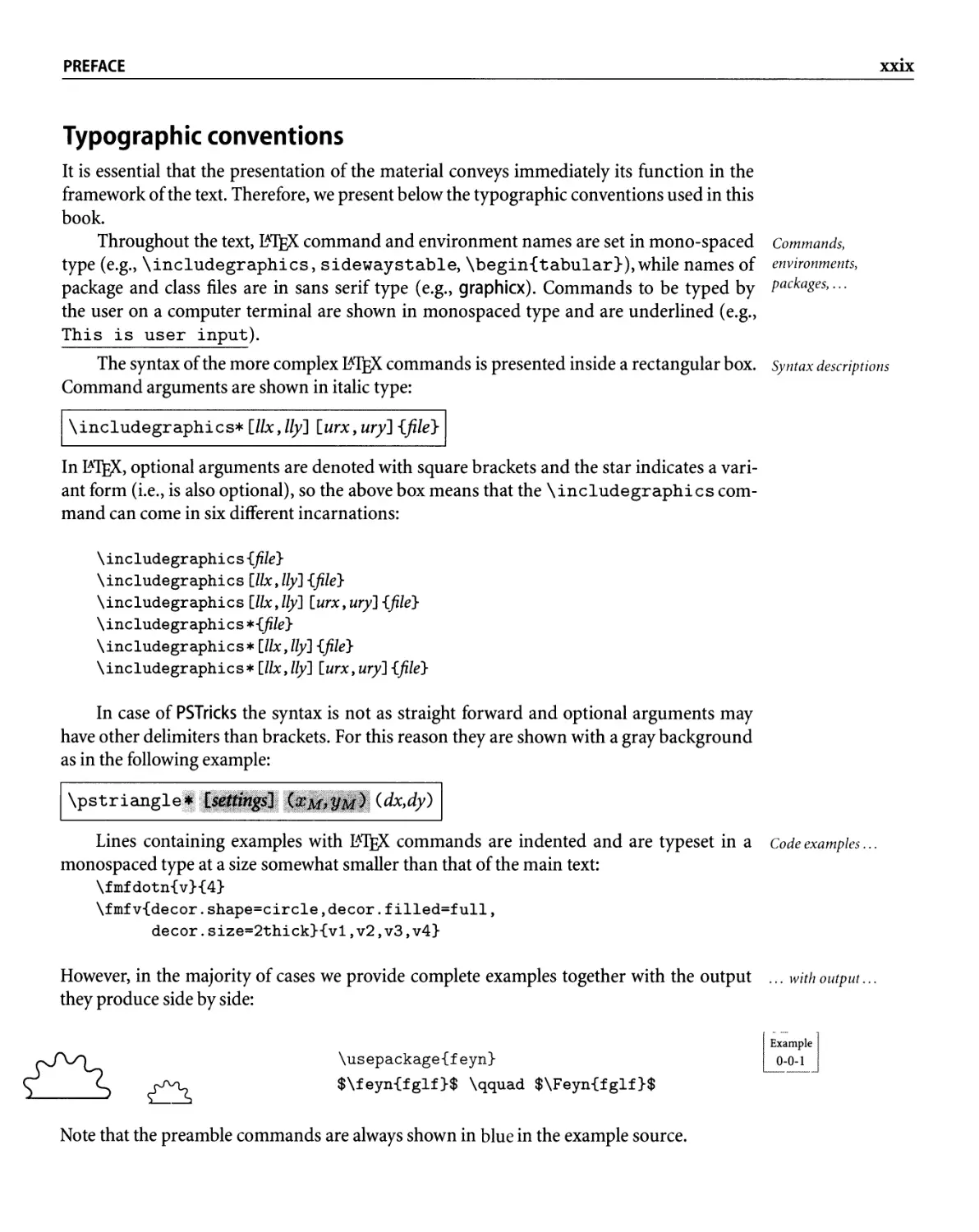
Music composed by Daniel Taupin and typeset with MusiX'lEX . . . . . . . . . . VI
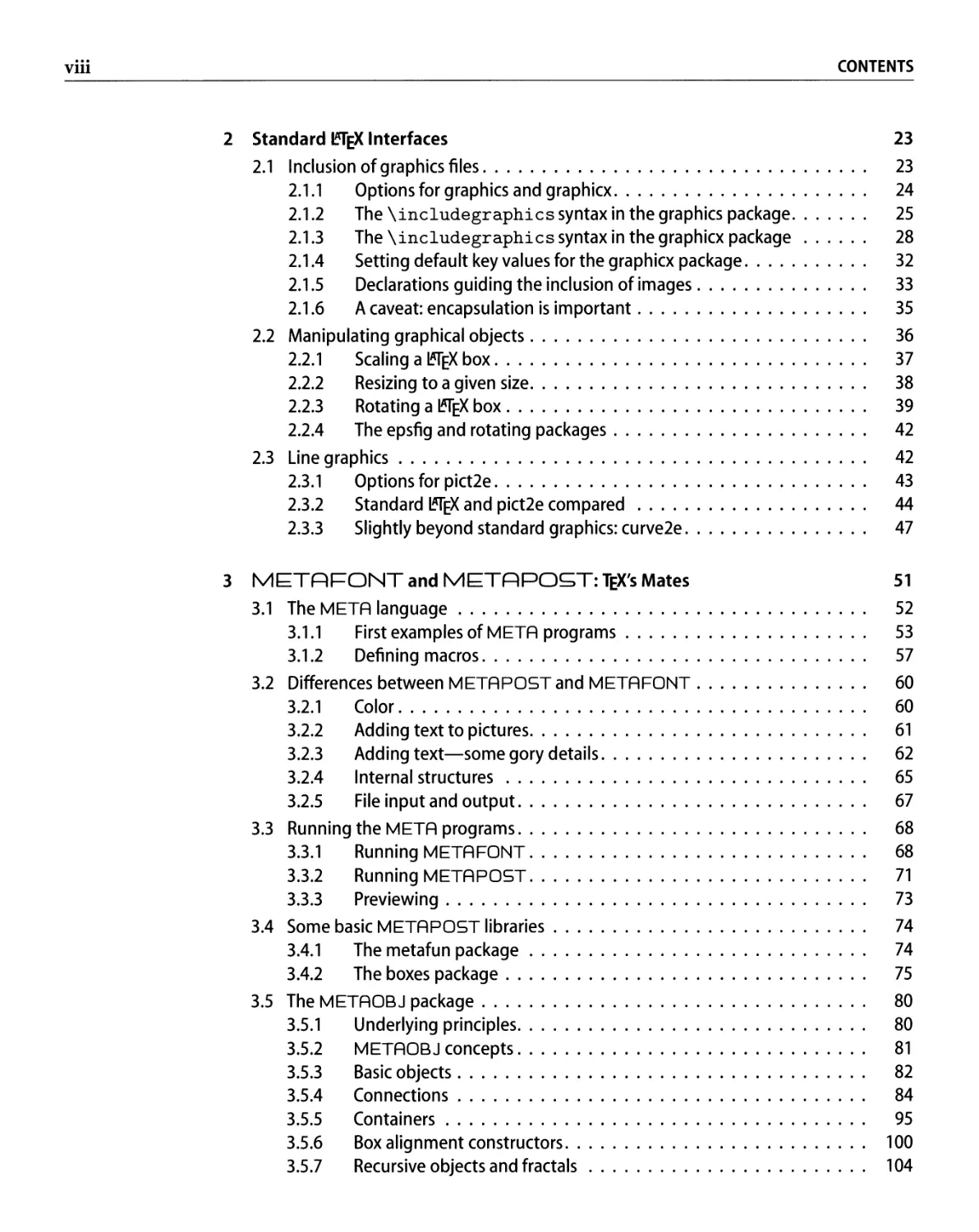
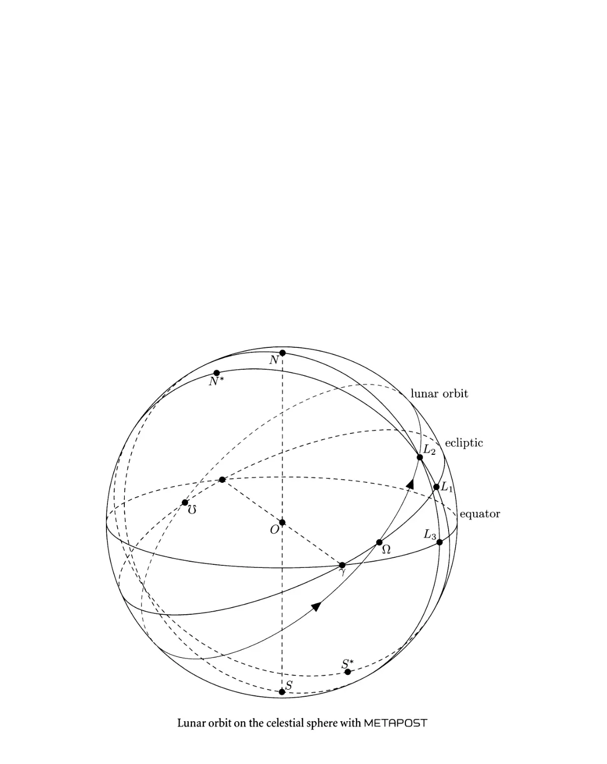
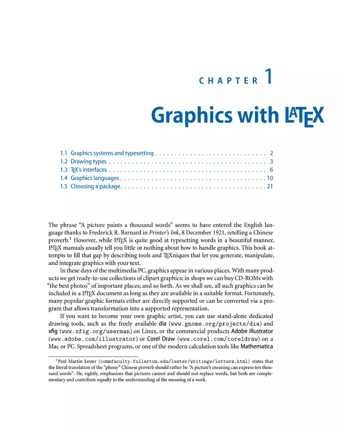
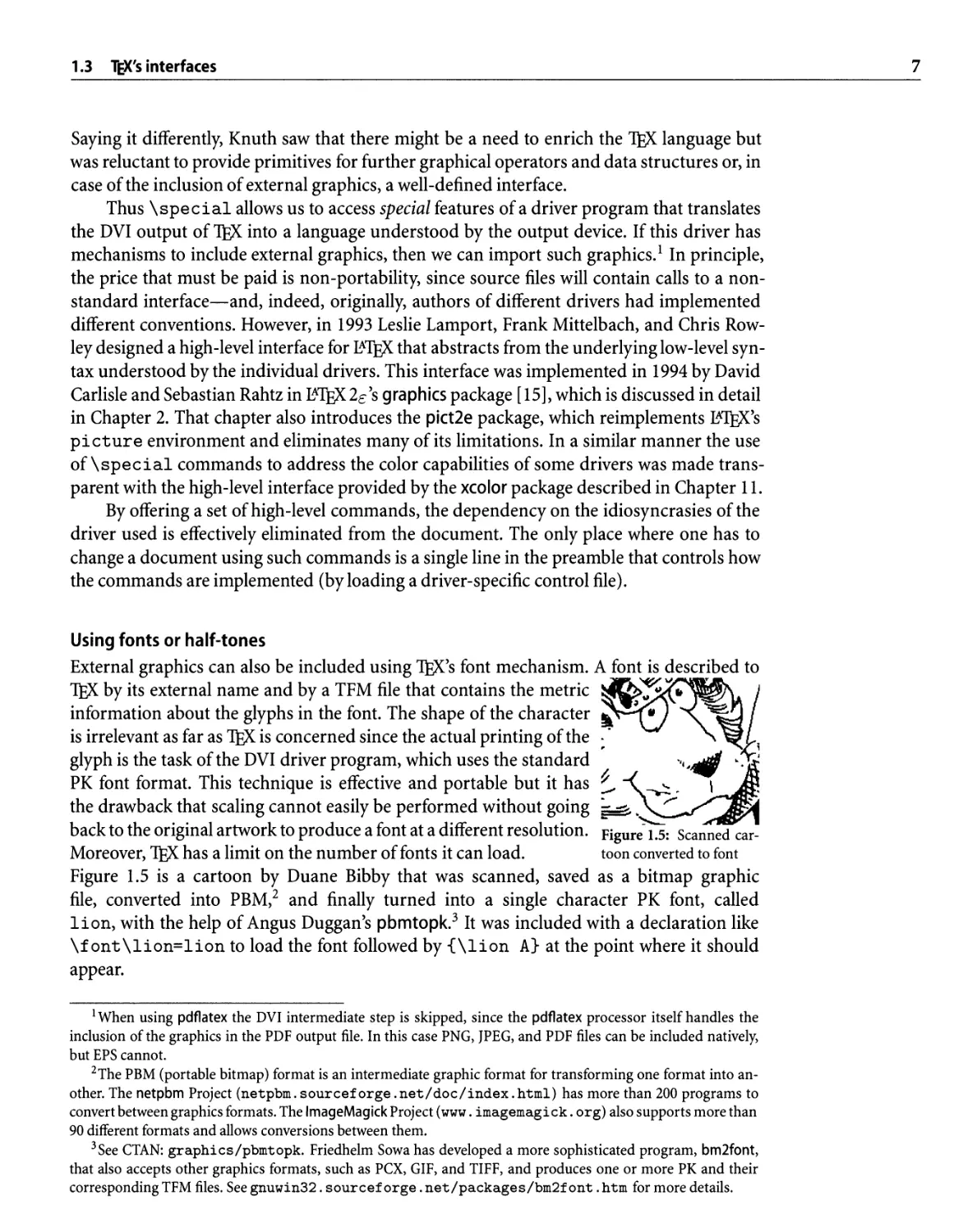
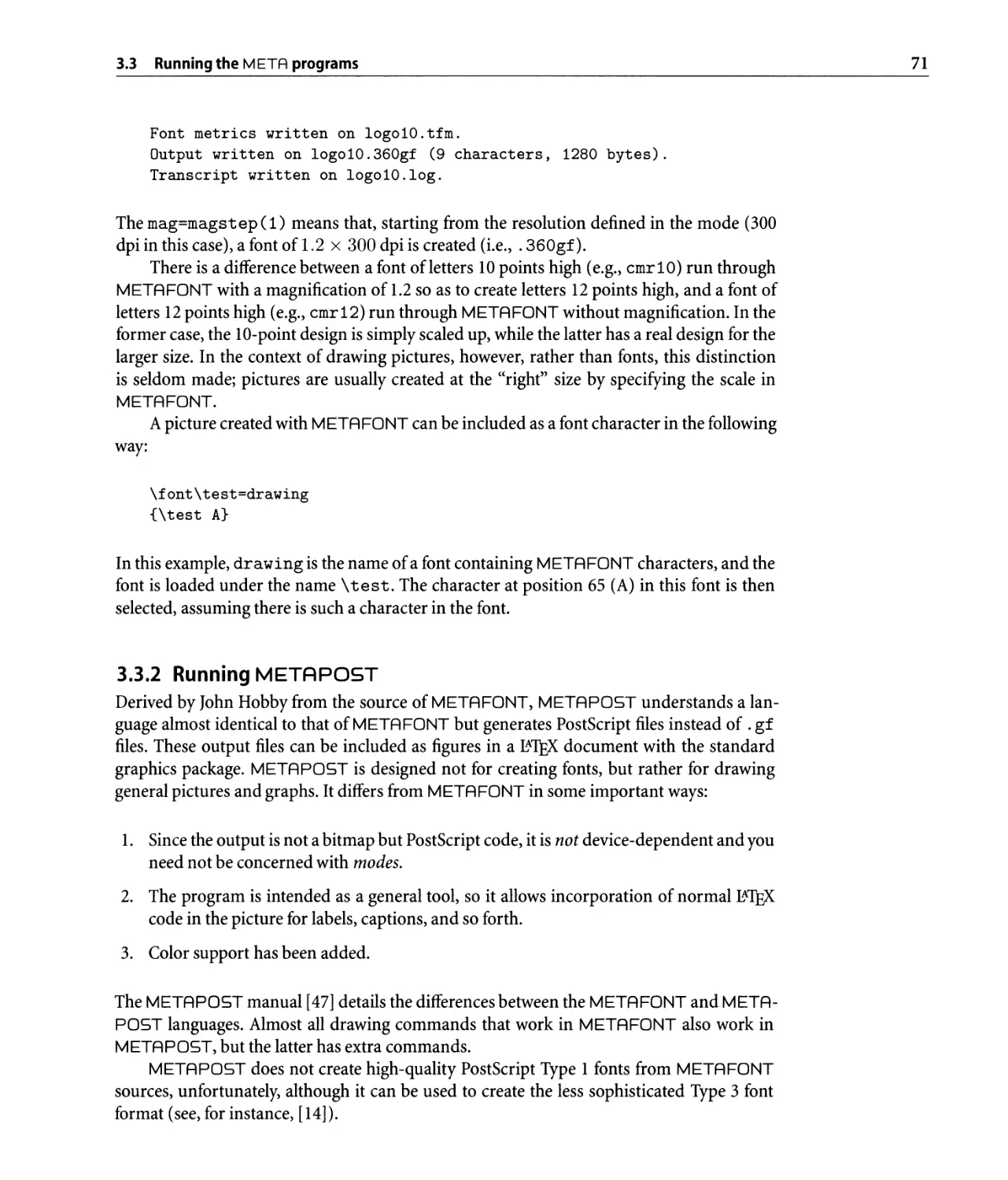
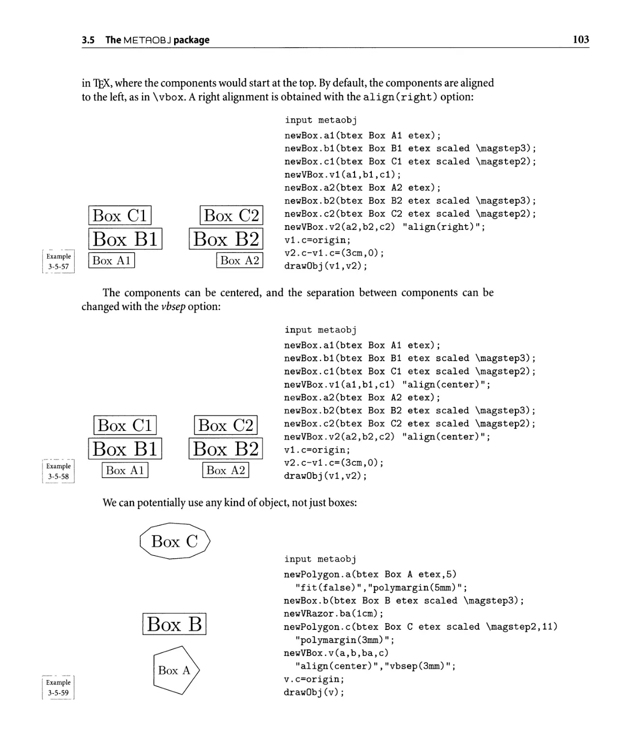
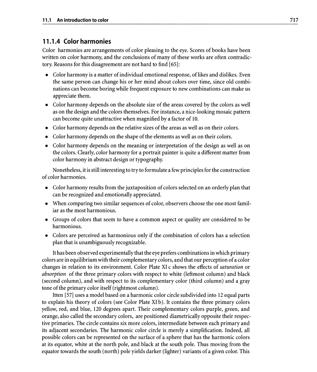
Lunar orbit on the celestial sphere with METAPoST . . . . . . . . . . . . . . .. xx
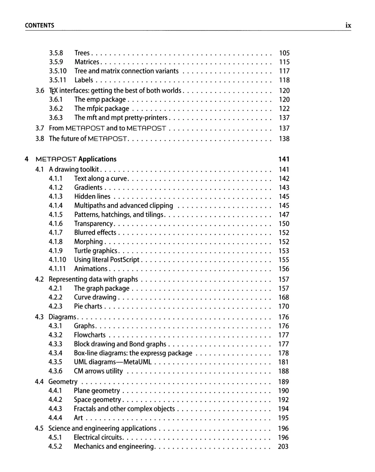
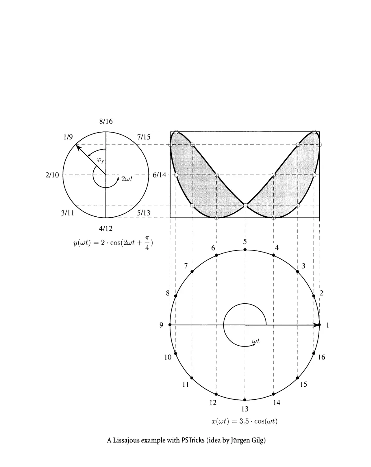
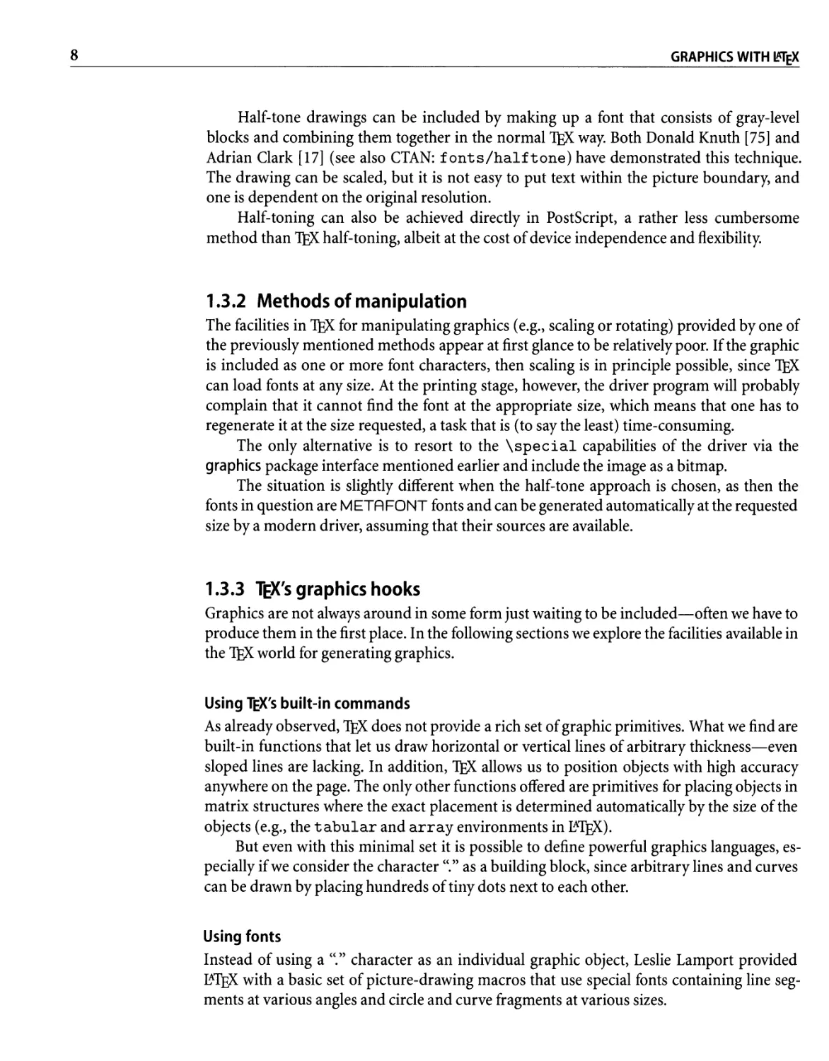
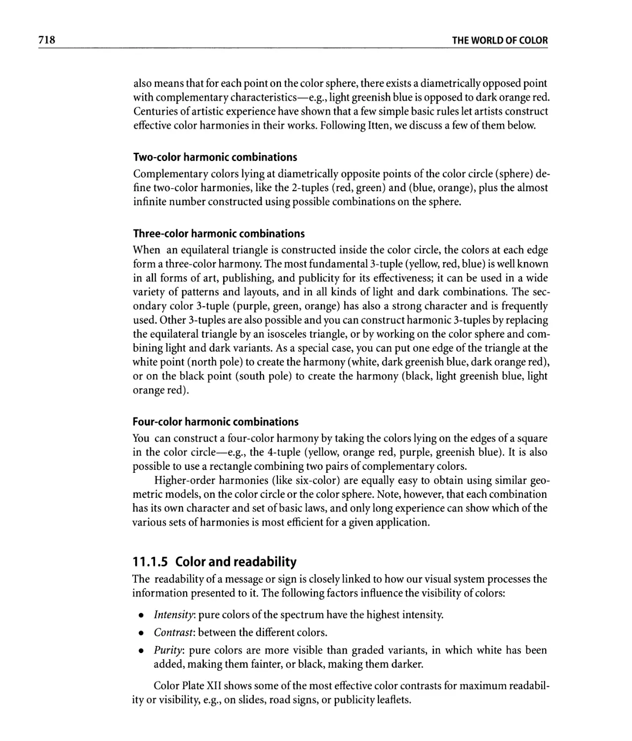
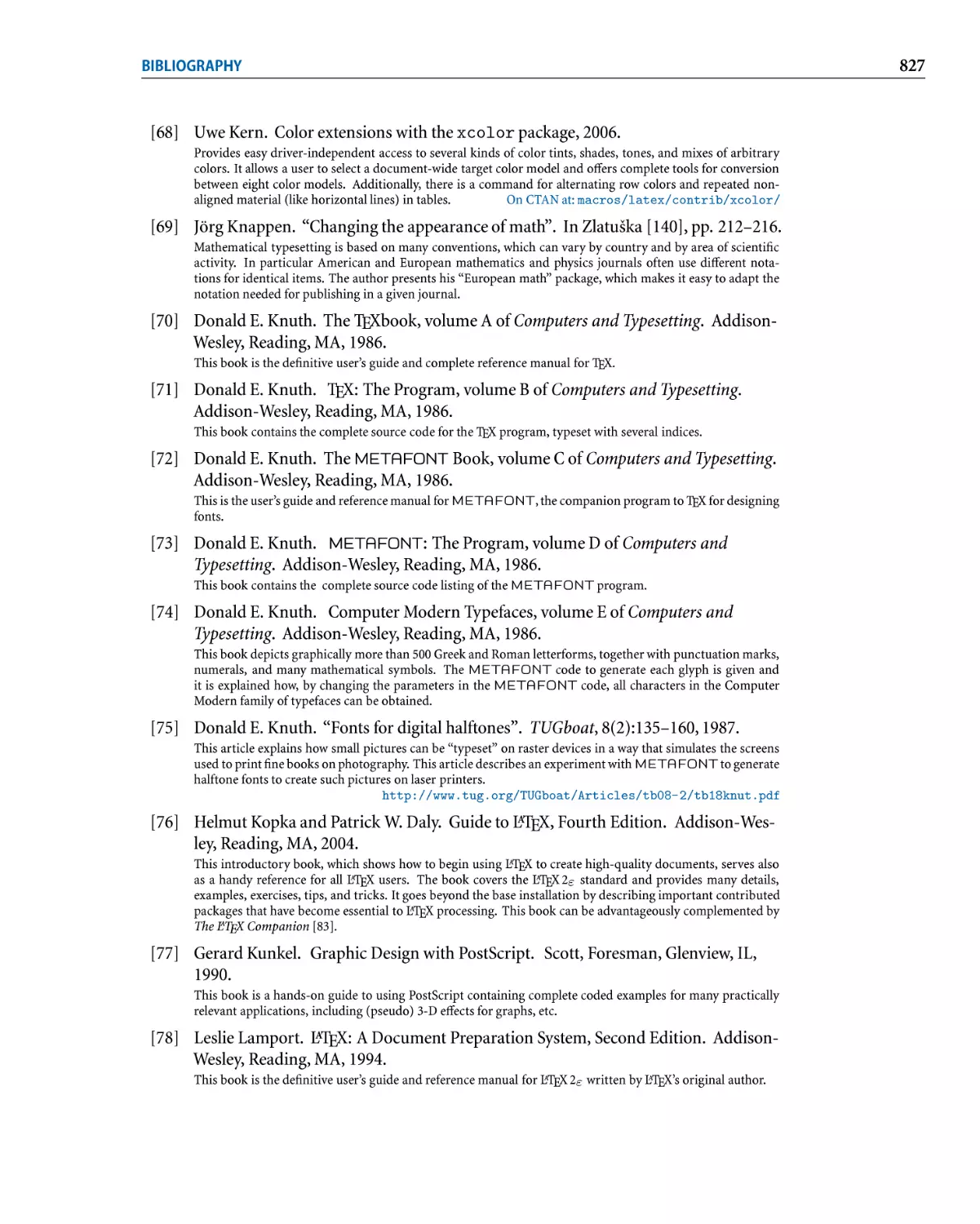
A Lissajous example with PSTricks. . . . . . . . . . . . . . . . . . . . . . . . . . . .. XXIV
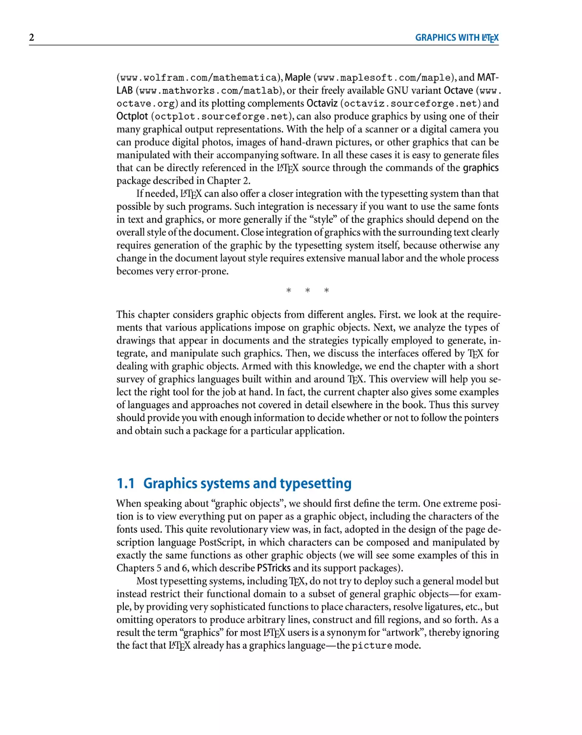
1.1 Pen and ink drawing of a bead . . . . . . . . . . . . . . . . . . . . . . . . . . . . . . . 4
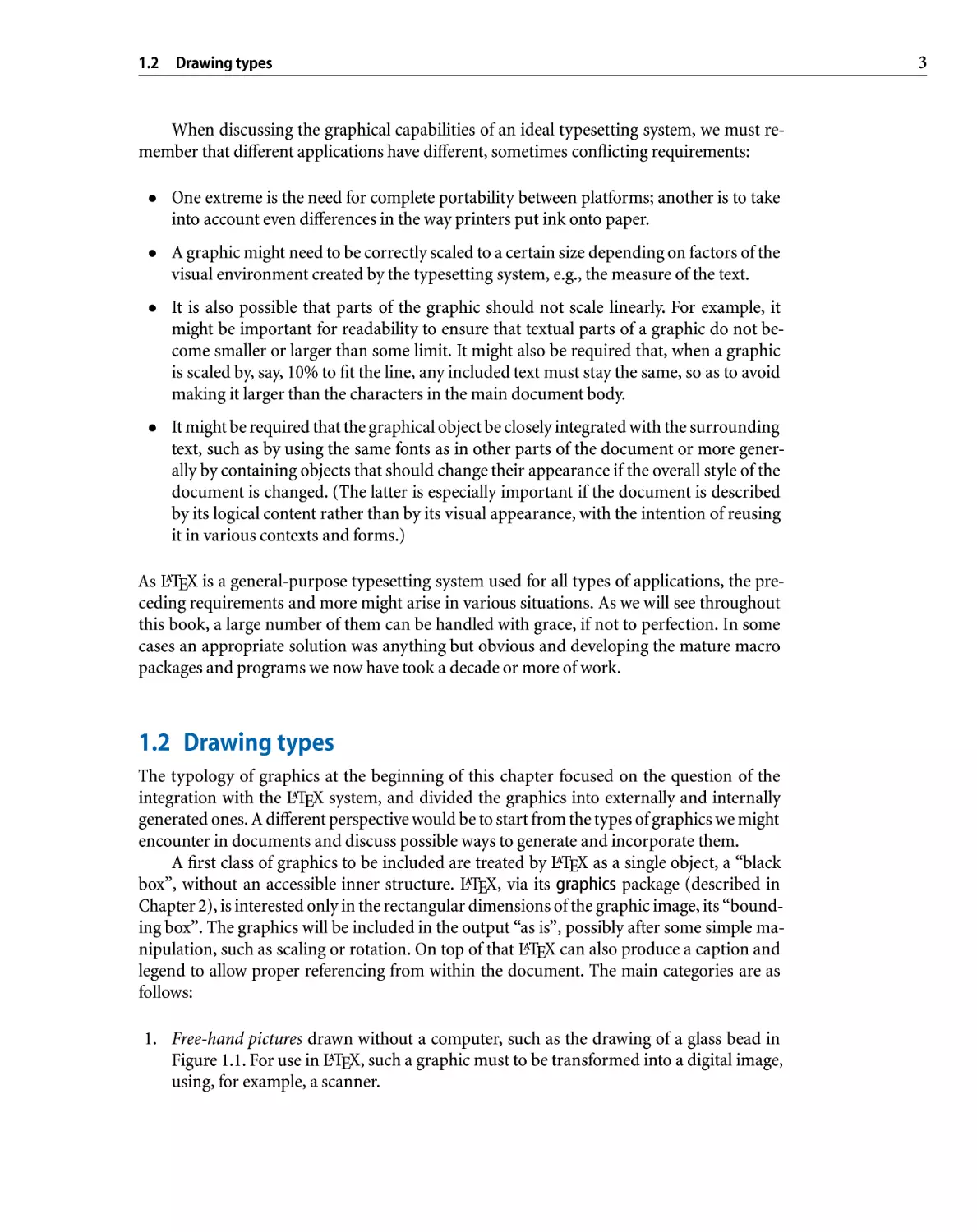
1.2 Bitmap drawing output created with GIMP . . . . . . . . . . . . . . . . . . . . . . . 4
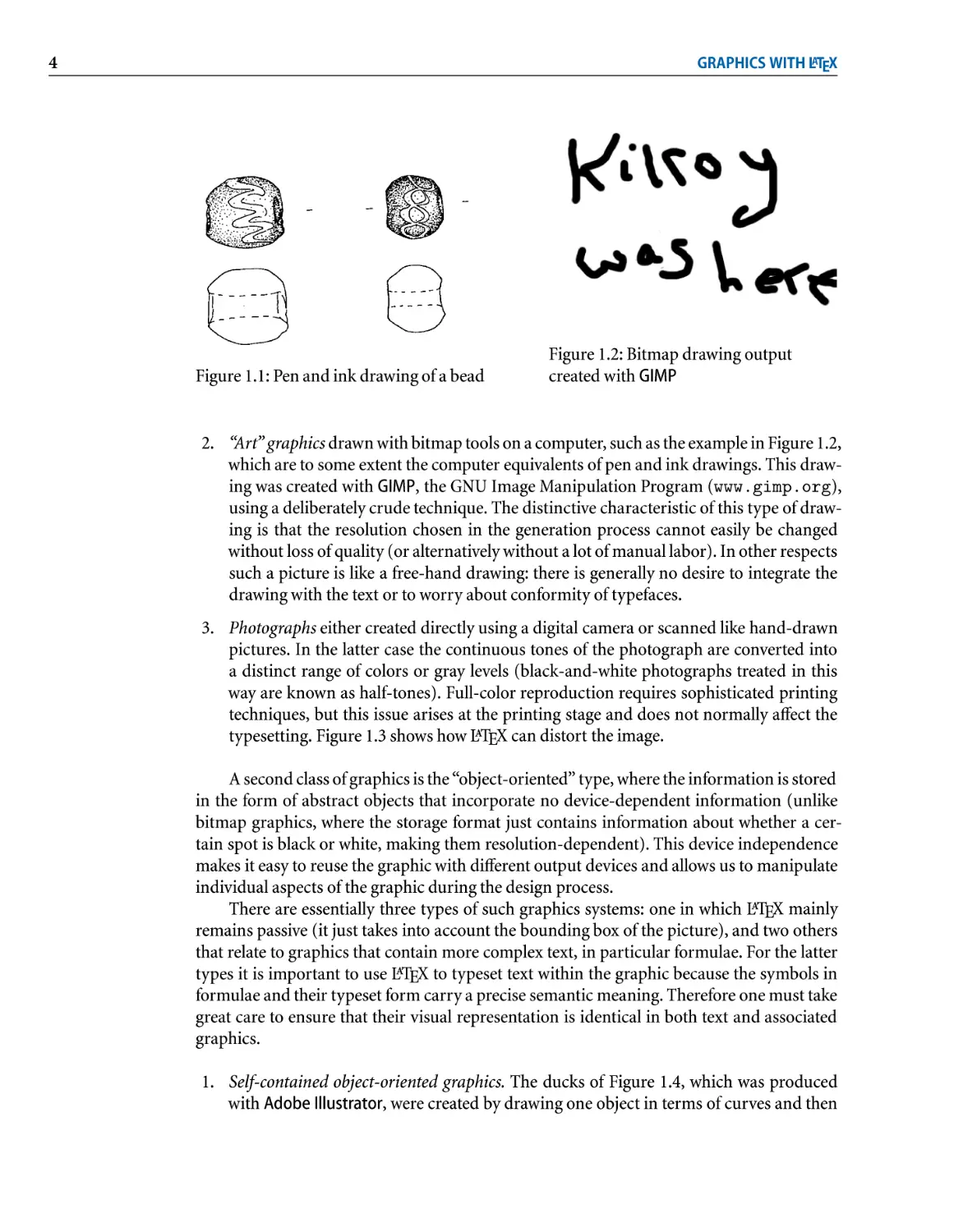
1.3 Digitally transformed image (vertically stretched). . . . . . . . . . . . . . . . . . . 5
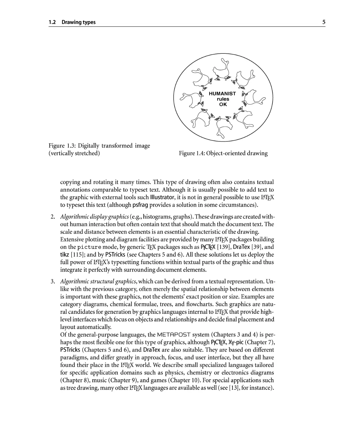
1.4 Object-oriented drawing. . . . . . . . . . . . . . . . . . . . . . . . . . . . . . . . . . . 5
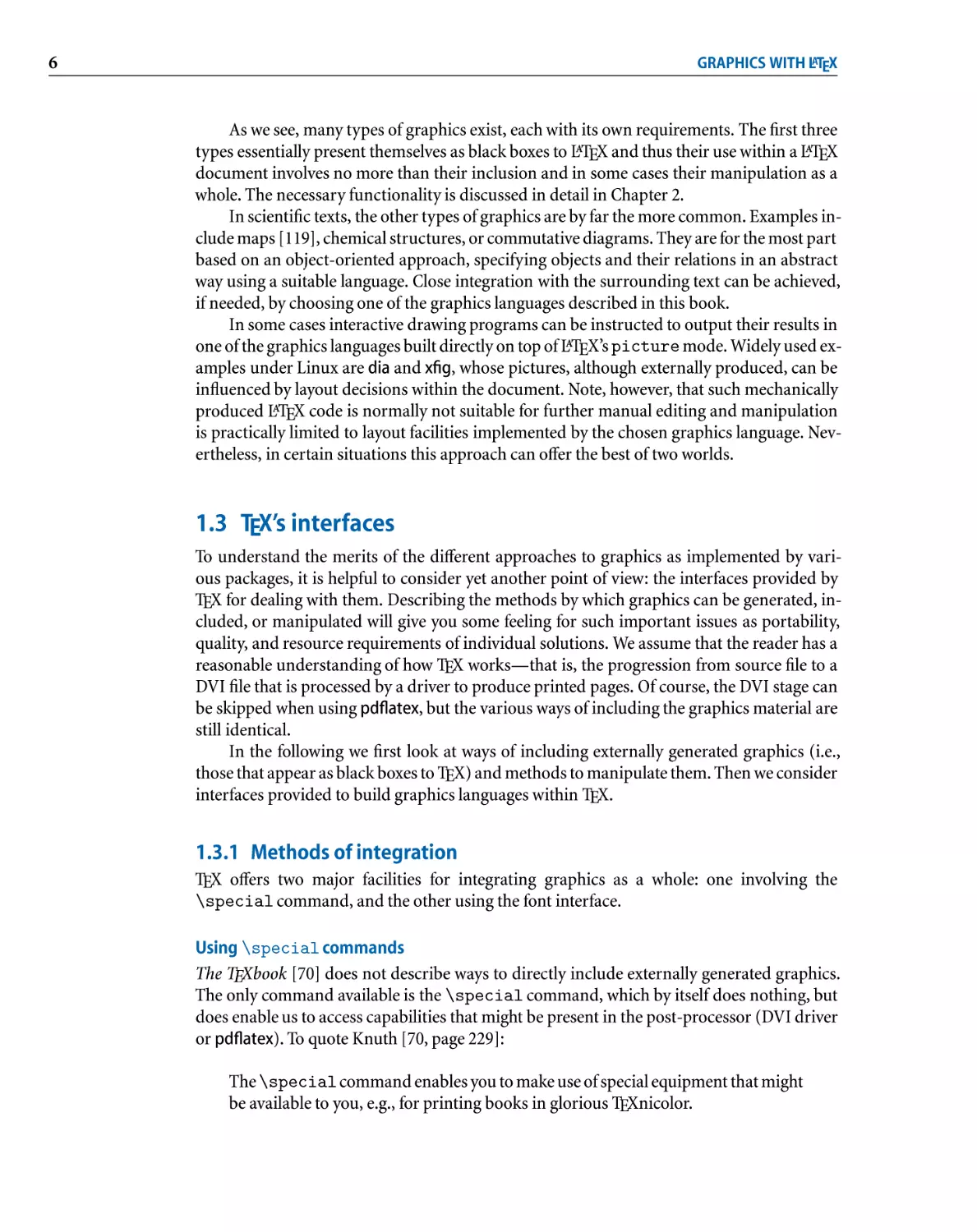
1.5 Scanned cartoon converted to font . . . . . . . . . . . . . . . . . . . . . . . . . . . . 7
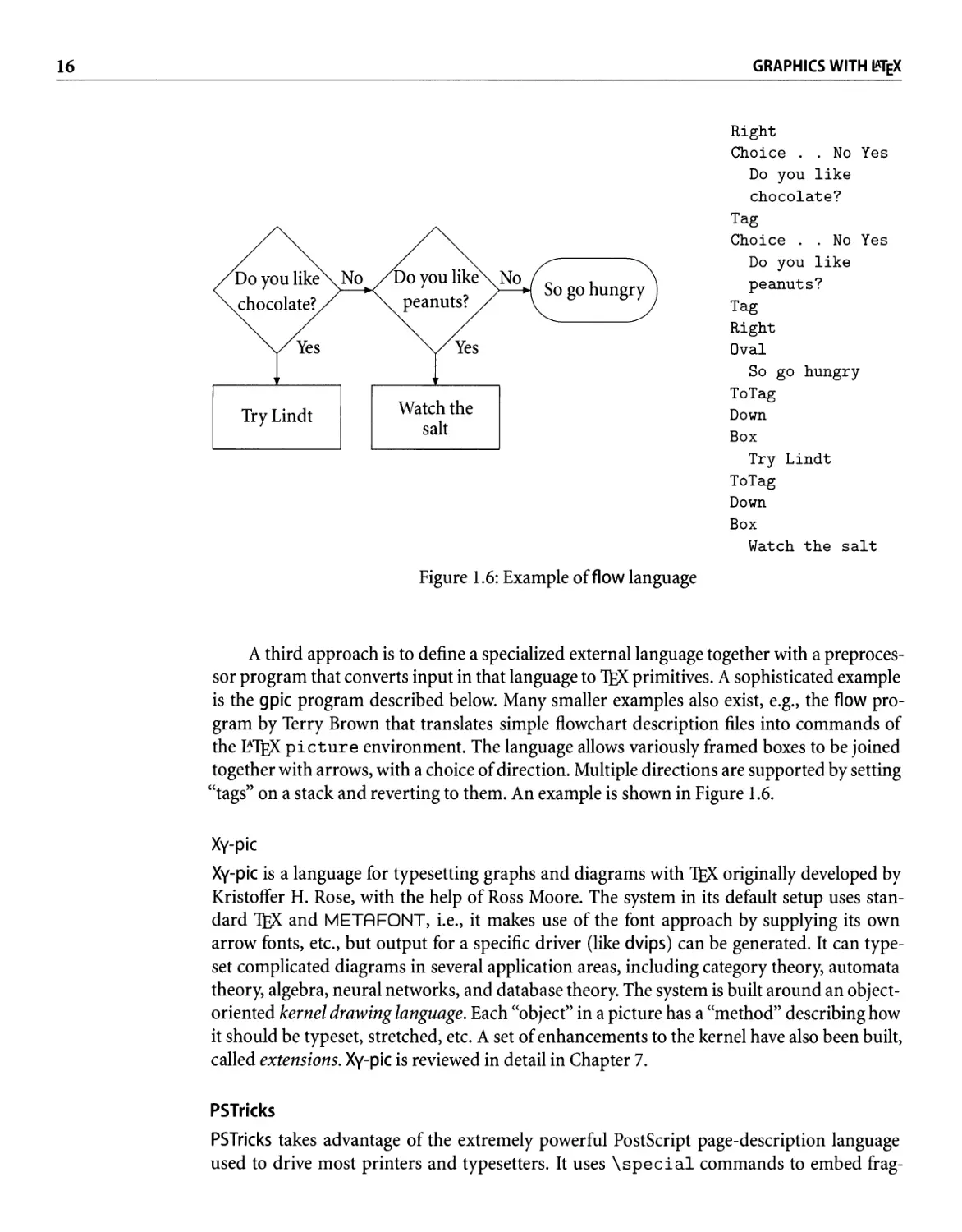
1.6 Example of flow language. . . . . . . . . . . . . . . . . . . . . . . . . . . . . . . . .. 16
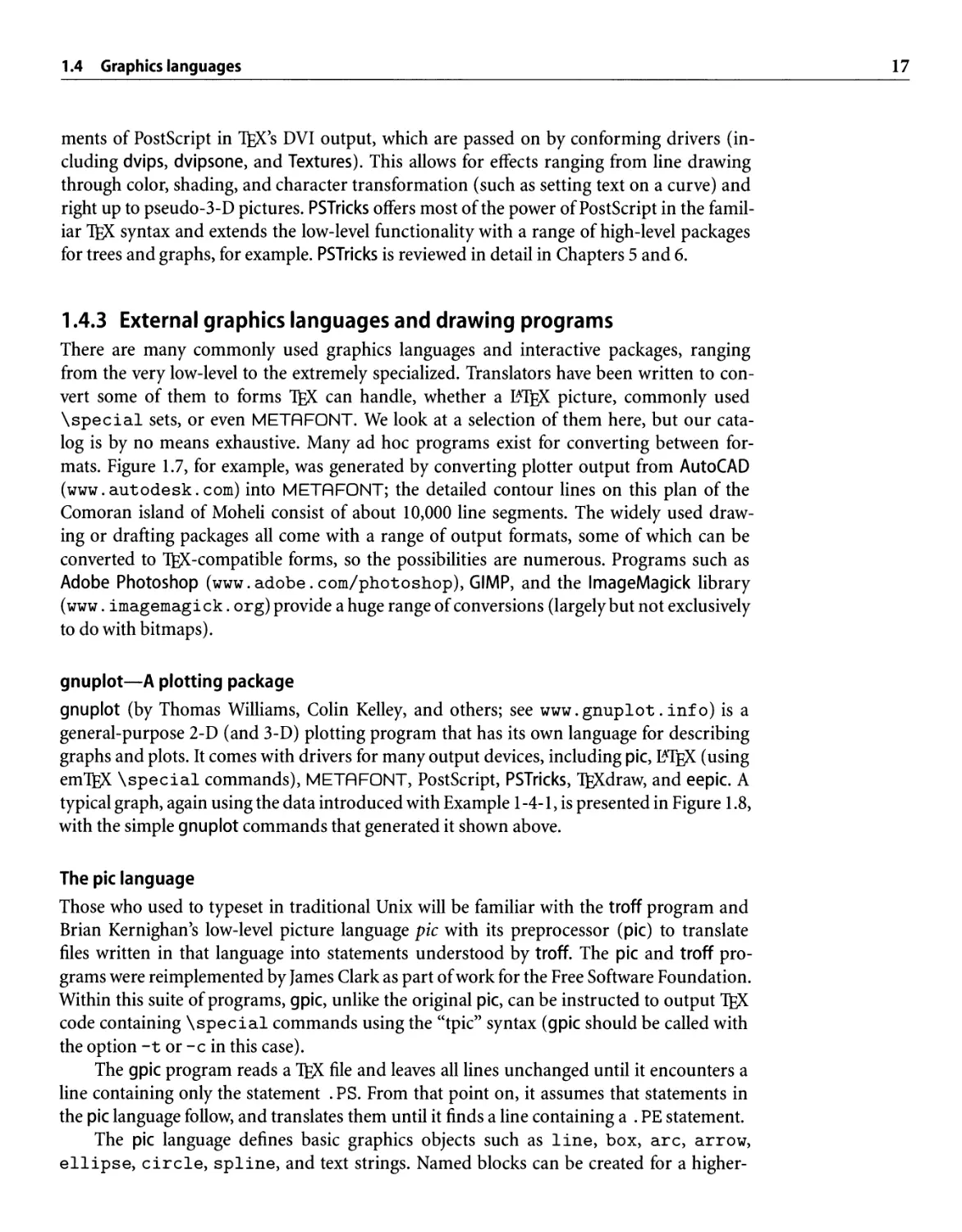
1.7 AutoCAD plotter output converted to META FONT. ................. 18
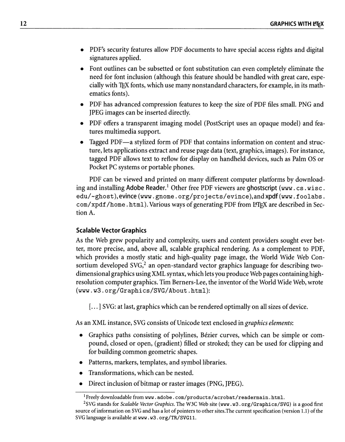
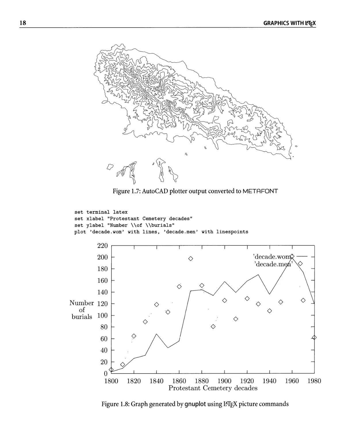
1.8 Graph generated by gnuplot using M-TFX picture commands . . . . . . . . . . .. 18
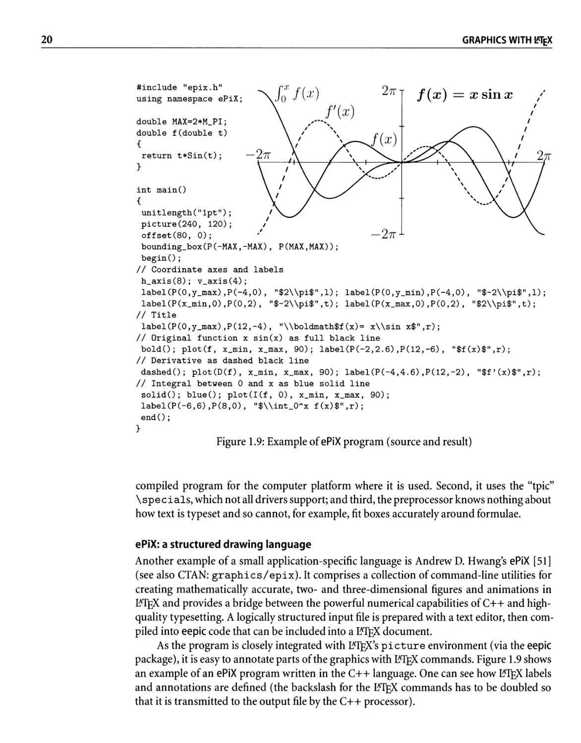
1.9 Example of ePiX program (source and result). . . . . . . . . . . . . . . . . . . . .. 20
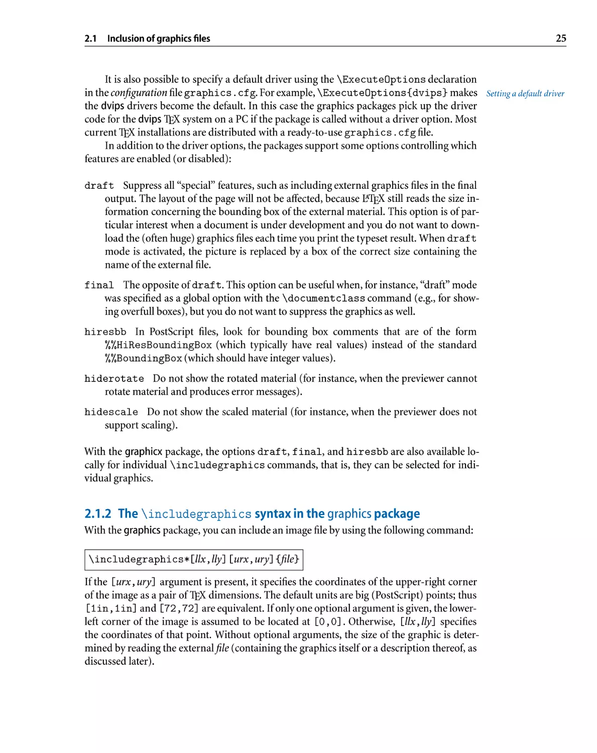
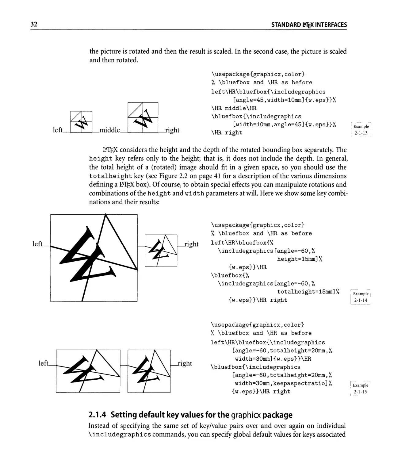
2.1 The contents of the file w . eps . . . . . . . . . . . . . . . . . . . . . . . . . . . . . .. 26
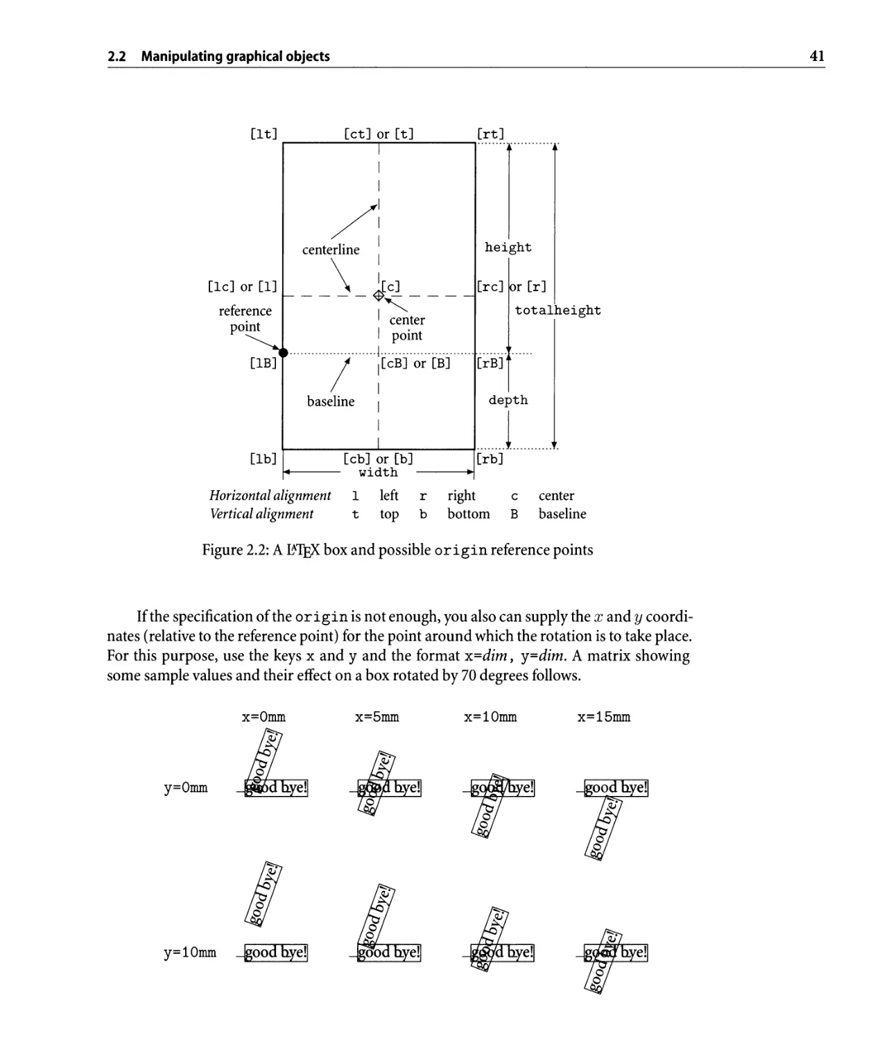
2.2 A M-TEX box and possible origin reference points . . . . . . . . . . . . . . . . .. 41
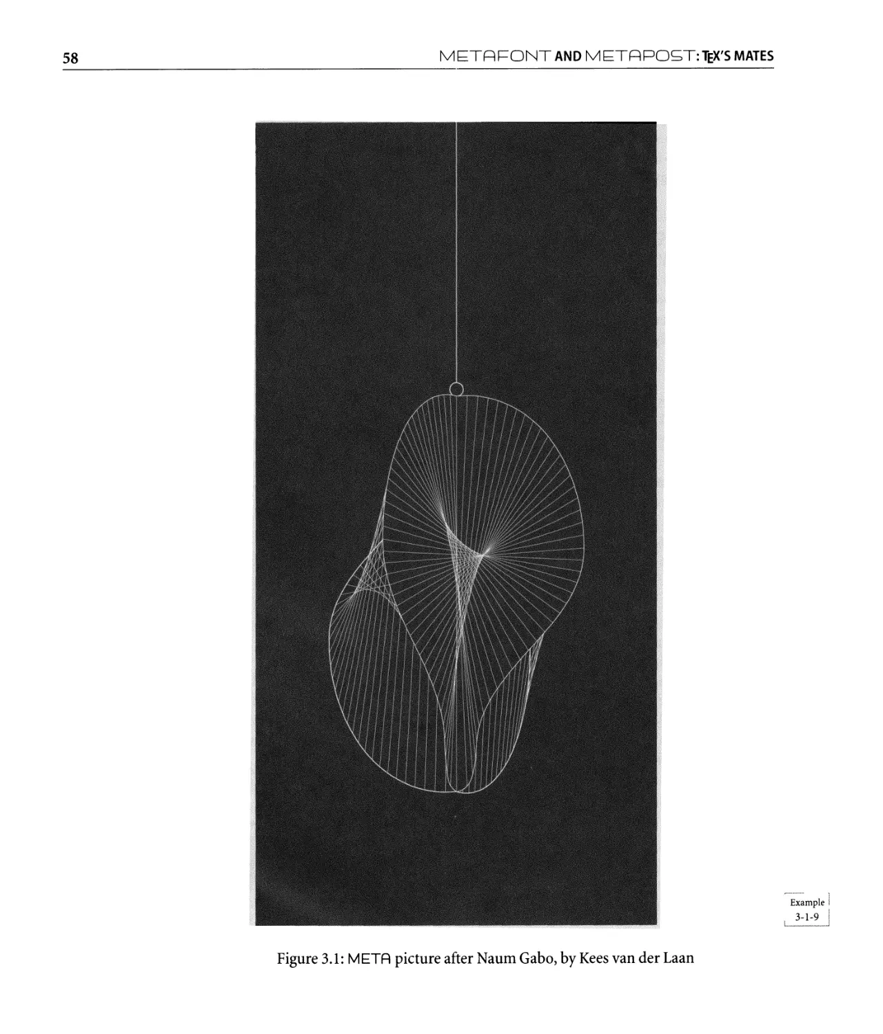
3.1 META picture after Naum Gabo. . . . . . . . . . . . . . . . . . . . . . . . . . . . .. 58
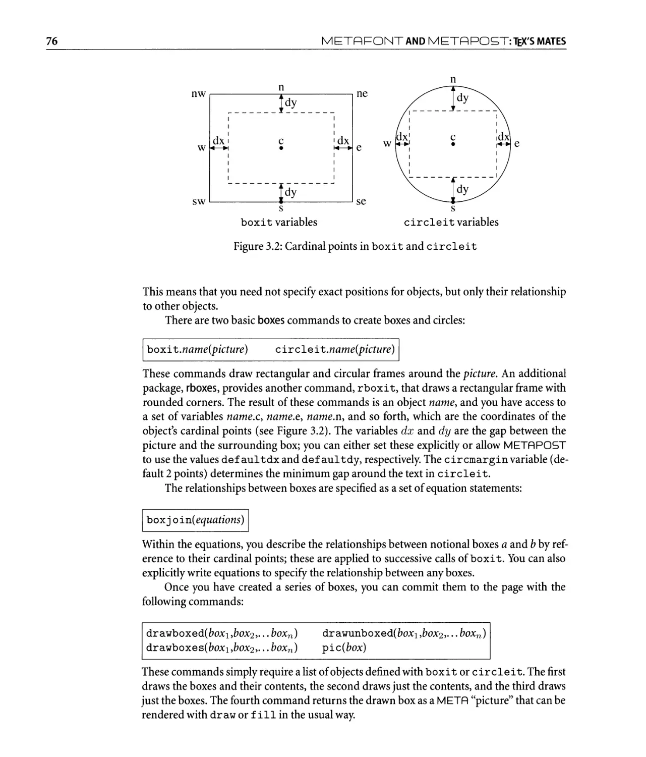
3.2 Cardinal points inboxit andcircleit . . . .. . . . . .. . . . .. . . . .. . .. 76
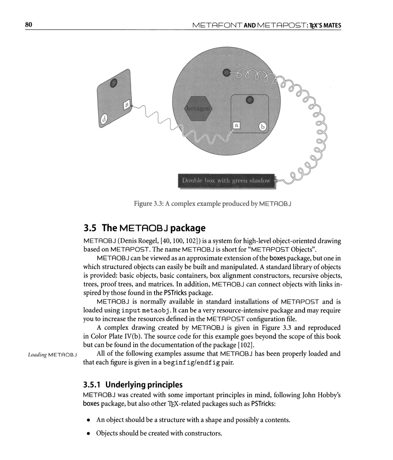
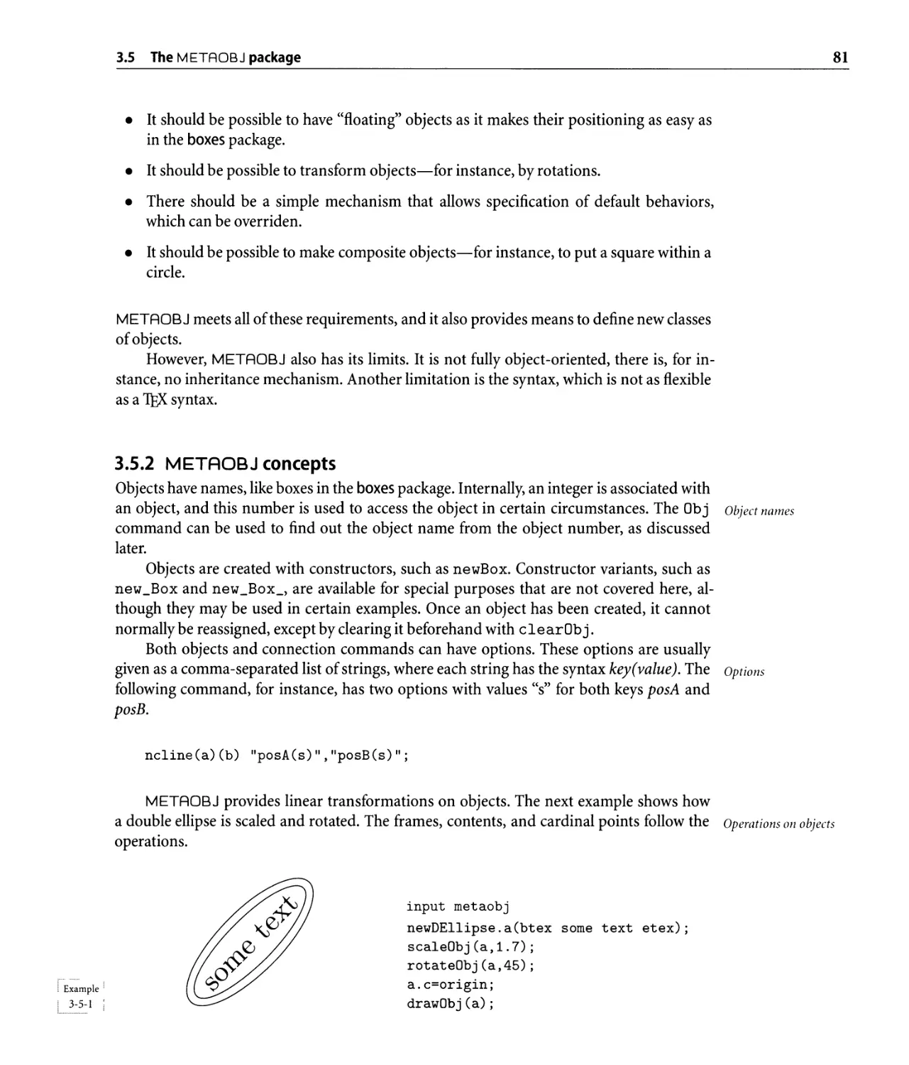
3.3 A complex example produced by METAoBJ . . . . . . . . . . . . . . . . . . . . .. 80
3.4 AutoCAD map converted to METAFoNT . . . . . . . . . . . . . . . . . . . . . . .. 138
3.5 METAFoNT drawing enhanced using Corel Draw . . . . . . . . . . . . . . . . .. 138
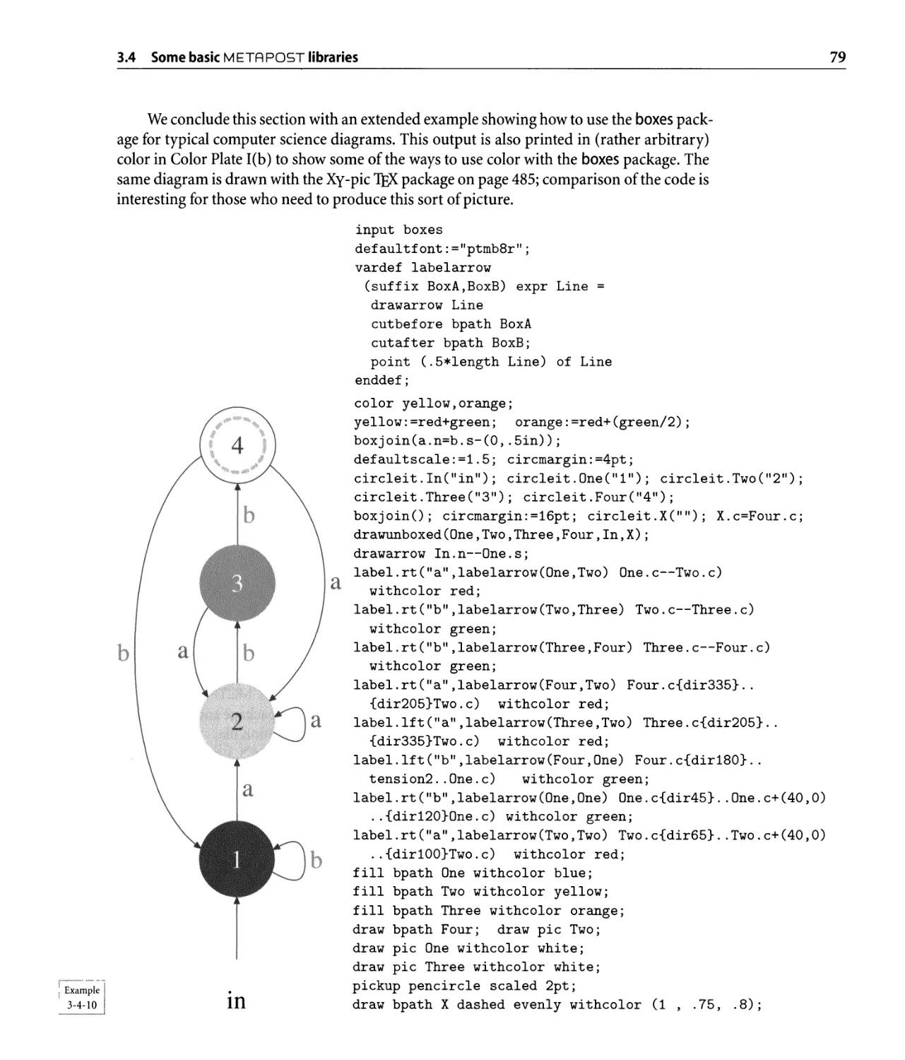
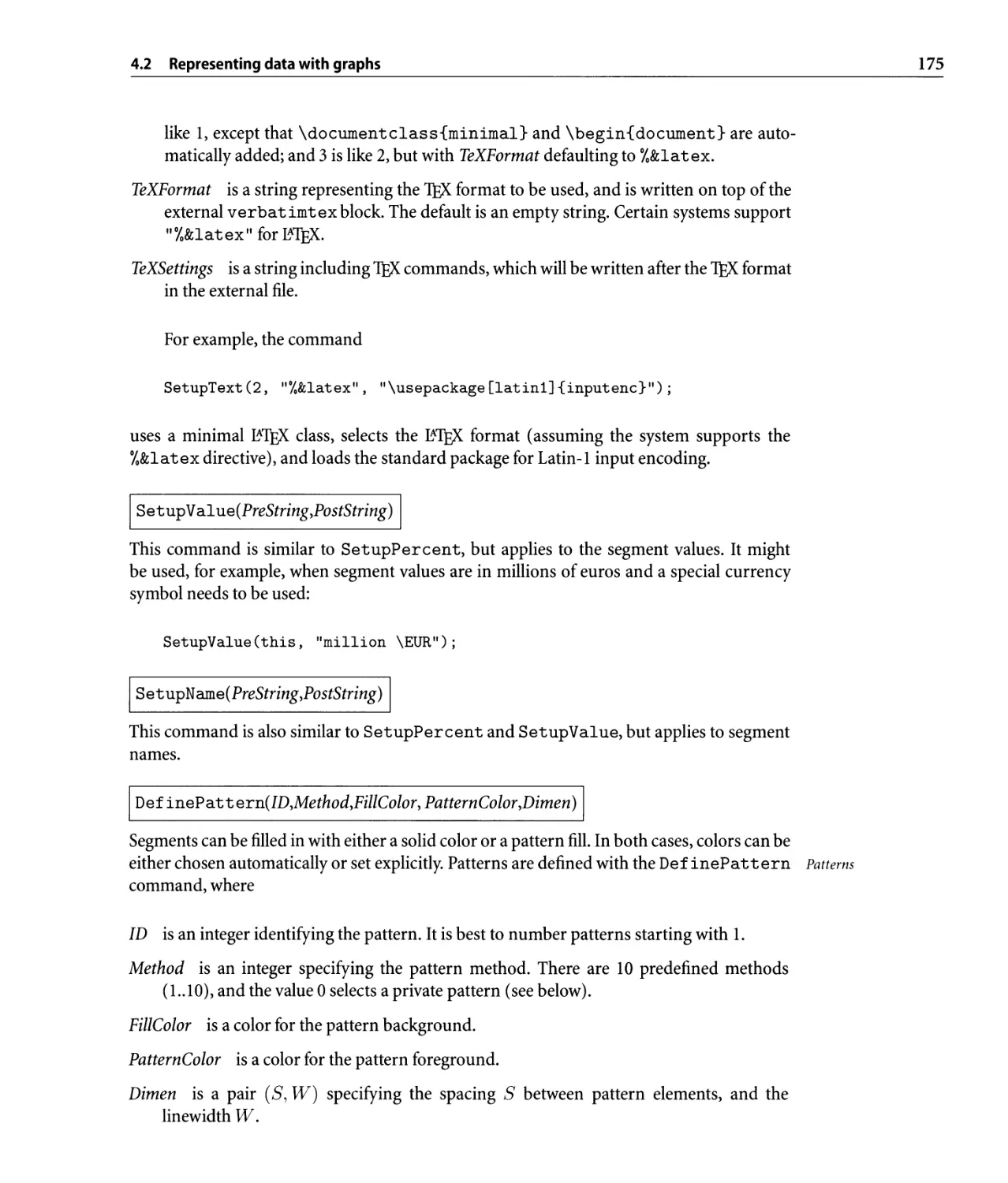
4.1 A Cayley graph drawn with M ETA POST . . . . . . . . . . . . . . . . . . . . . . .. 177
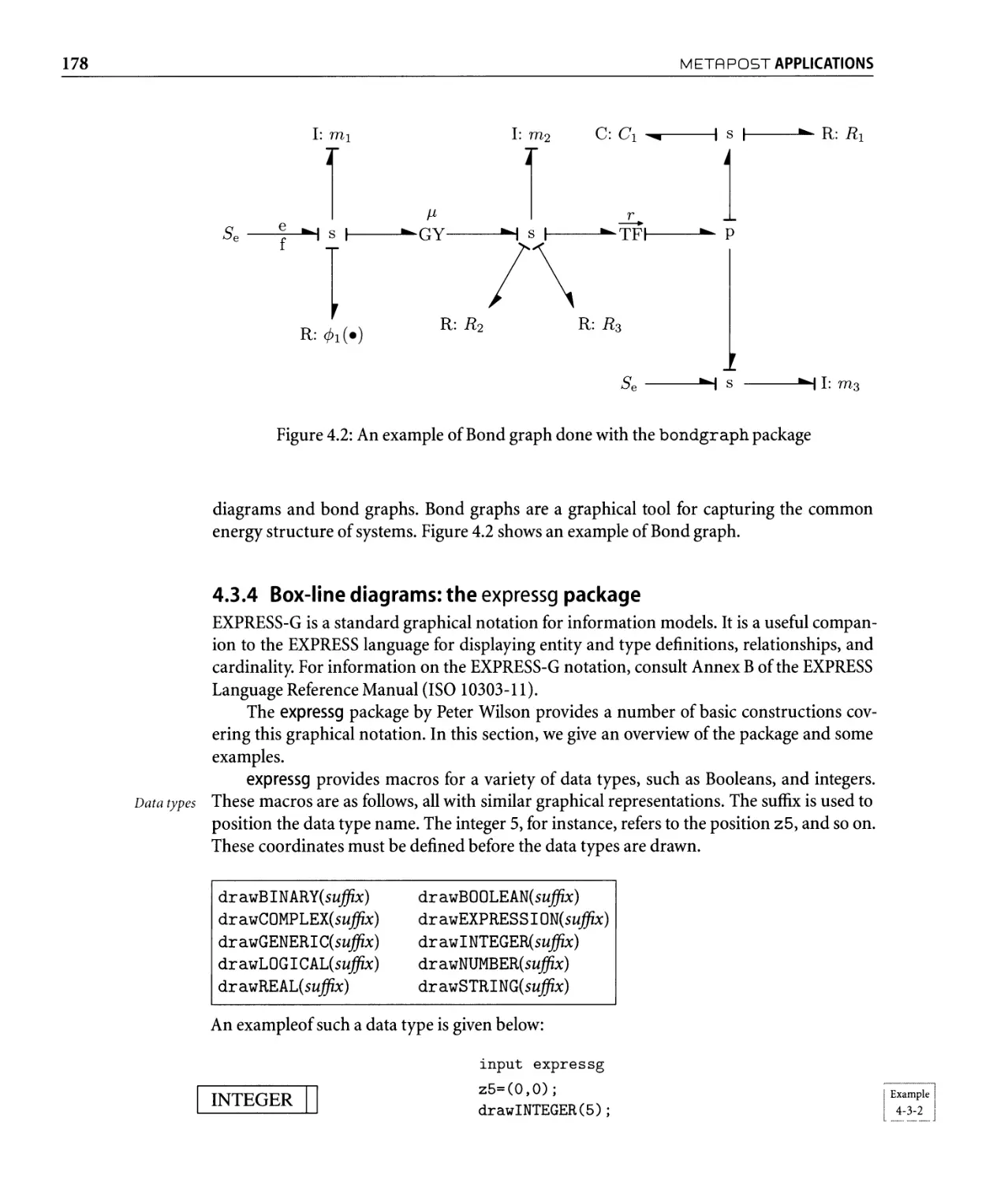
4.2 An example of Bond graph done with the bondgraph package . . . . . . . . .. 178
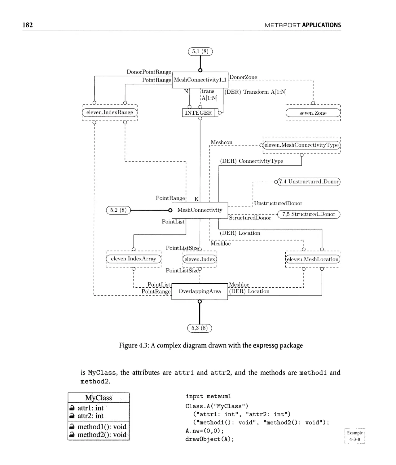
4.3 A complex diagram drawn with the expressg package . . . . . . . . . . . . . . .. 182
...
XVlll
LIST OF FIGURES
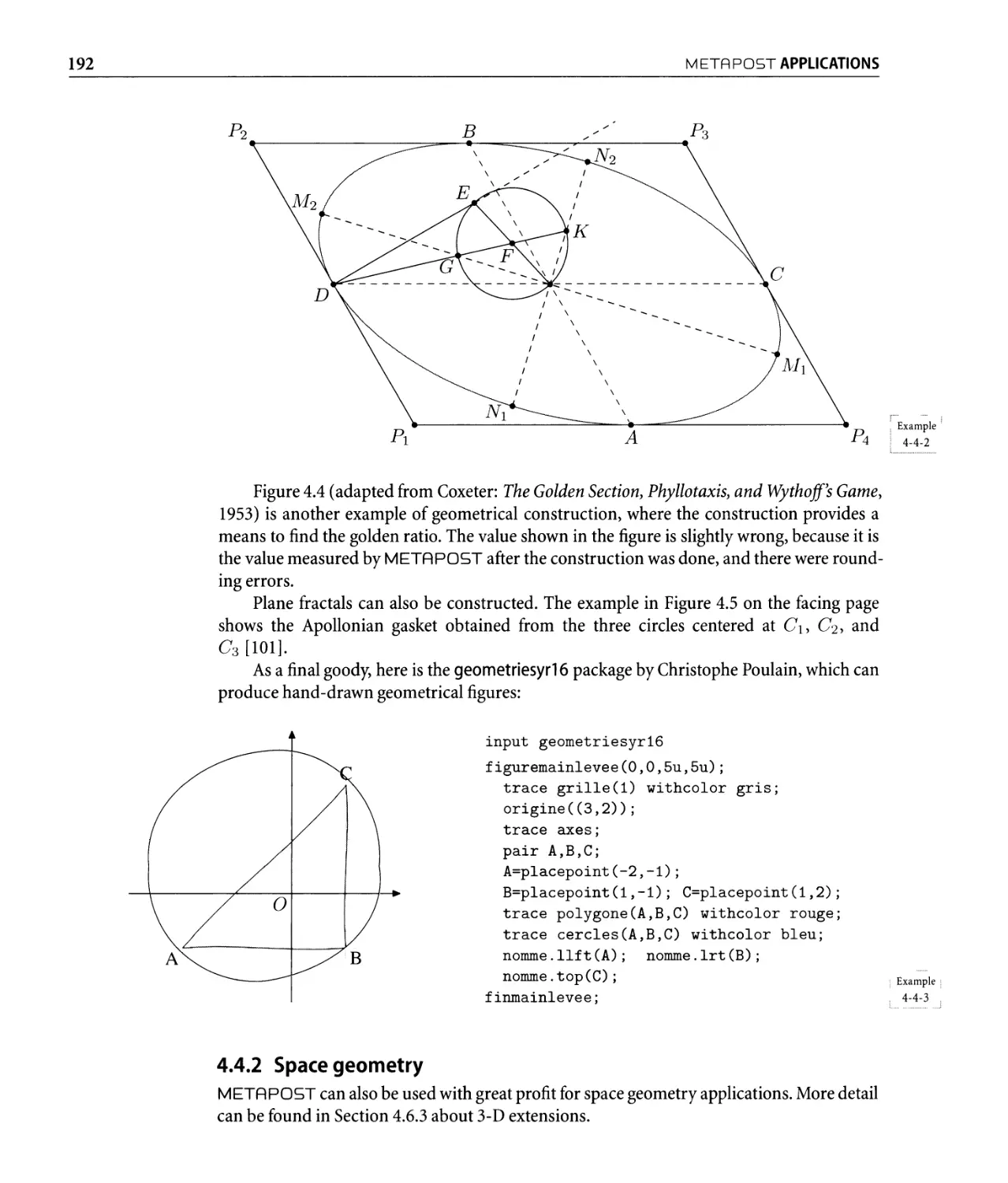
4.4 Pipping's construction for the golden number . . . . . . . . . . . . . . . . . . . .. 193
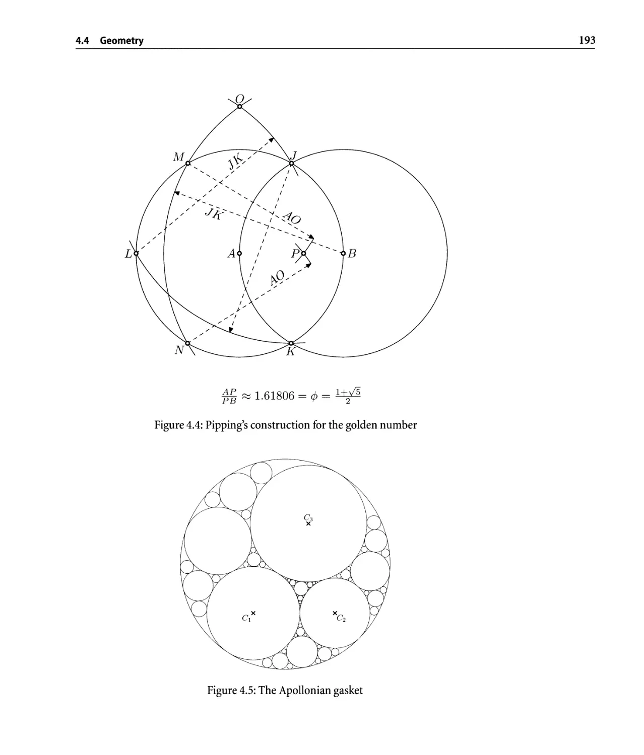
4.5 The Apollonian gasket . . . . . . . . . . . . . . . . . . . . . . . . . . . . . . . . . . .. 193
4.6 A drawing in mechanical engineering . . . . . . . . . . . . . . . . . . . . . . . . .. 203
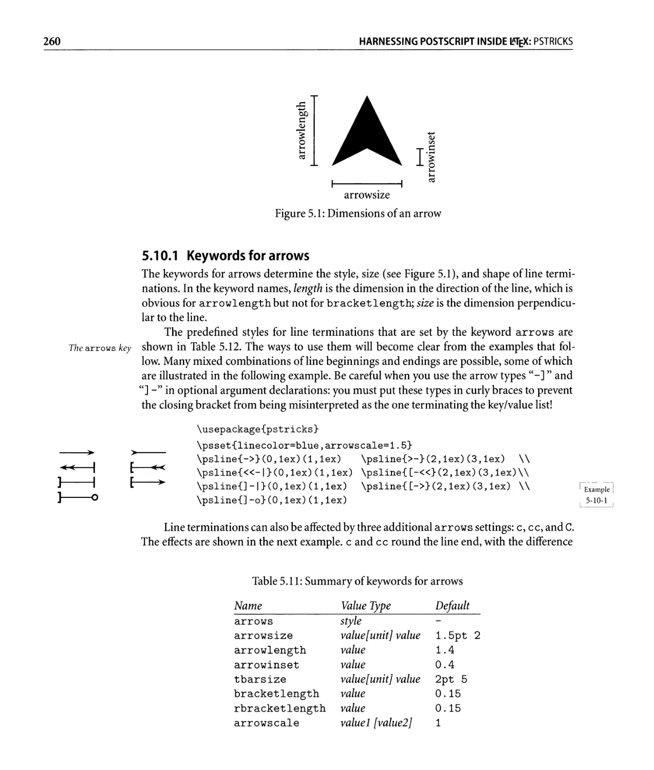
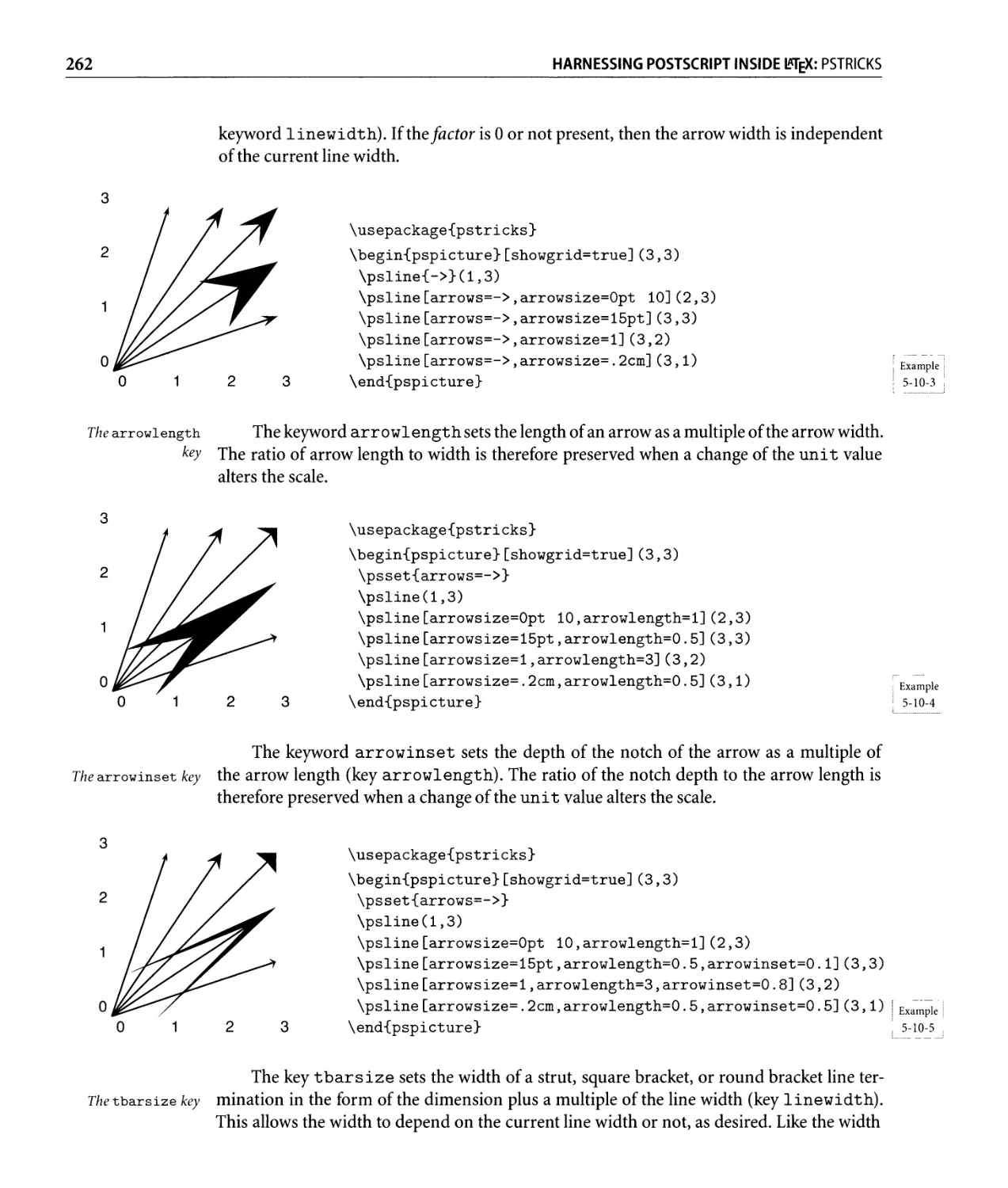
5.1 Dimensions of an arrow. . . . . . . . . . . . . . . . . . . . . . . . . . . . . . . . . .. 260
5.2 Reference point specification of a box. . . . . . . . . . . . . . . . . . . . . . . . . .. 266
6.1 Reference points for plotting coordinate axes. . . . . . . . . . . . . . . . . . . . .. 314
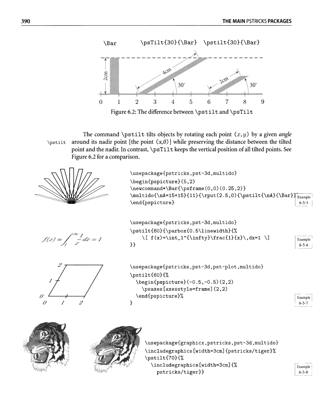
6.2 The difference between \pstilt and \psTilt. . . . . . . . . . . . . . . . . . .. 390
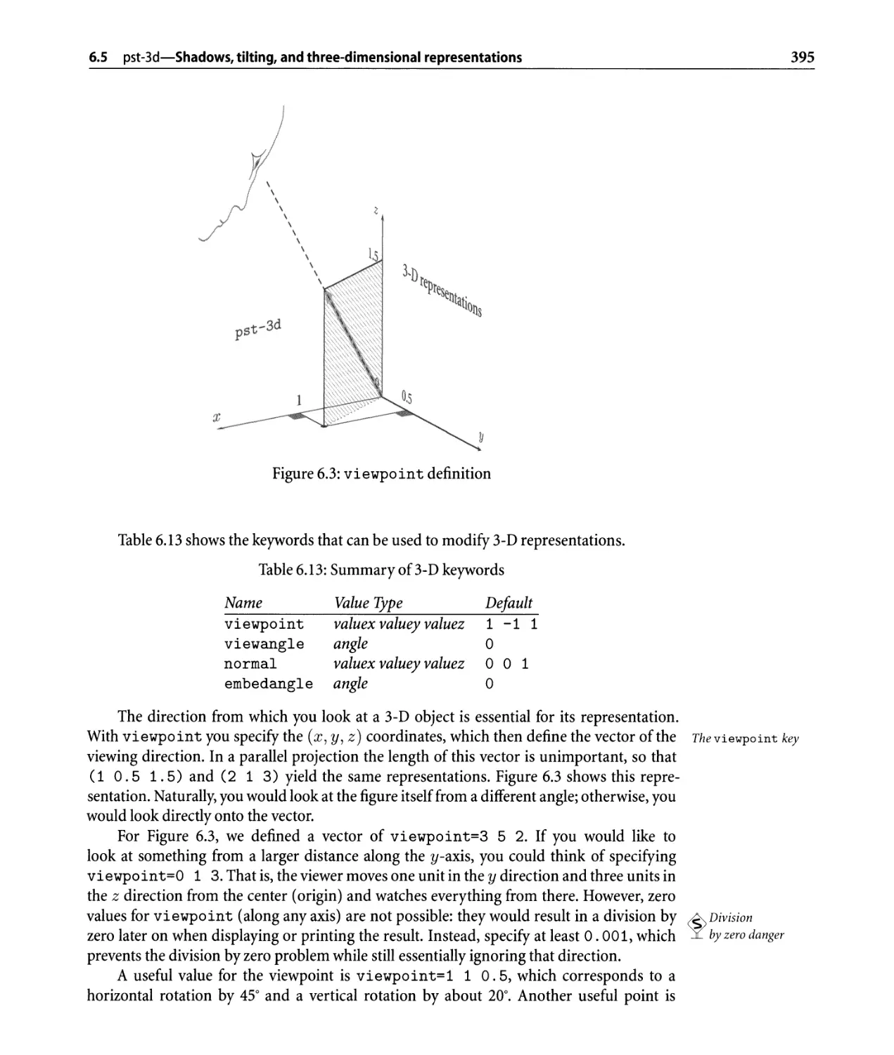
6.3 viewpoint definition. . . . . . . . . . . . . . . . . . . . . . . . . . . . . . . . . . .. 395
8.1 Periodic table typeset with M-JEX and chemsym . . . . . . . . . . . . . . . . . . .. 519
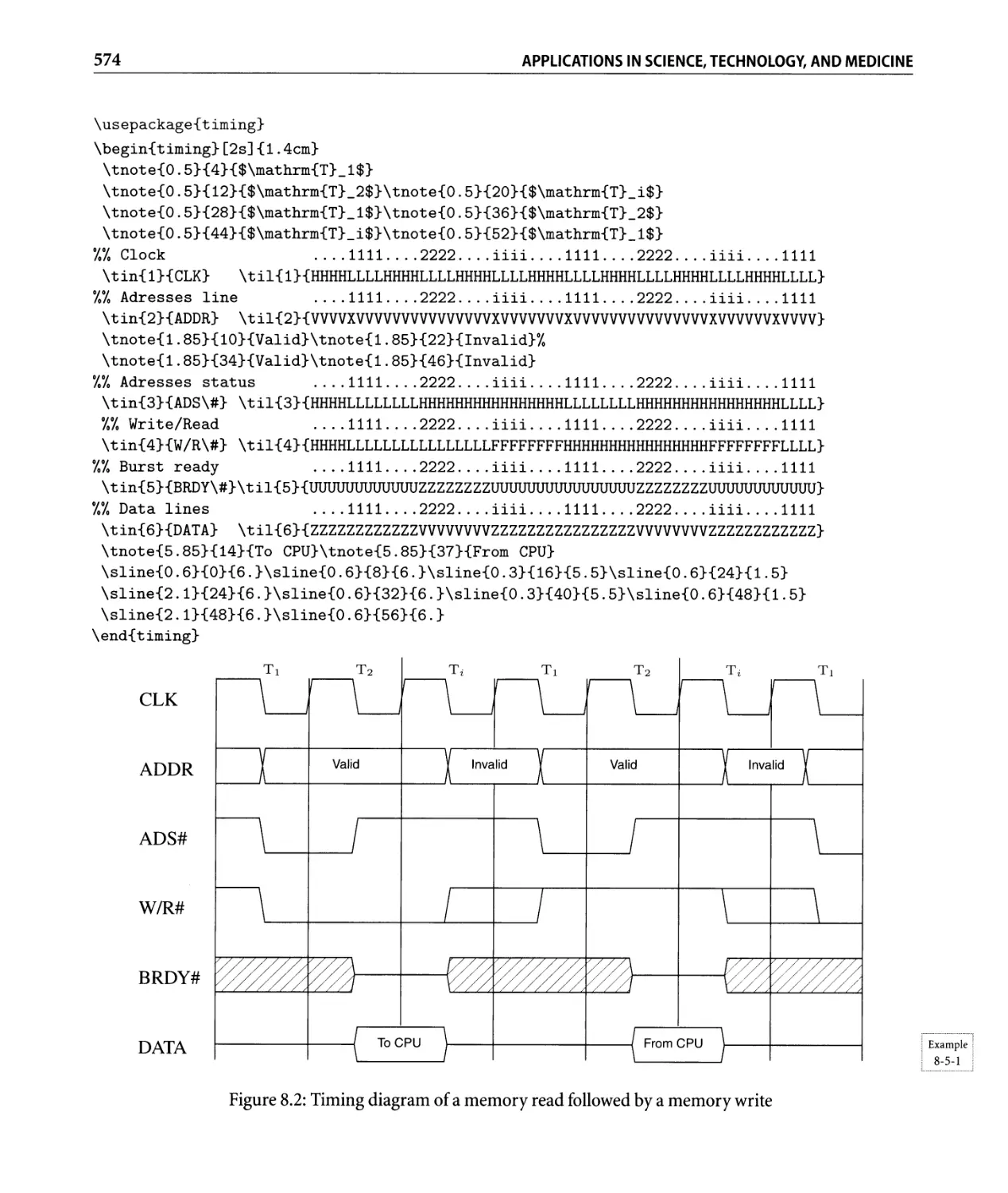
8.2 Timing diagram of a memory read followed by a memory write . . . . . . . . .. 574
9.1 Sequence of score pieces coded in MusiXTEX. . . . . . . . . . . . . . . . . . . . . .. 591
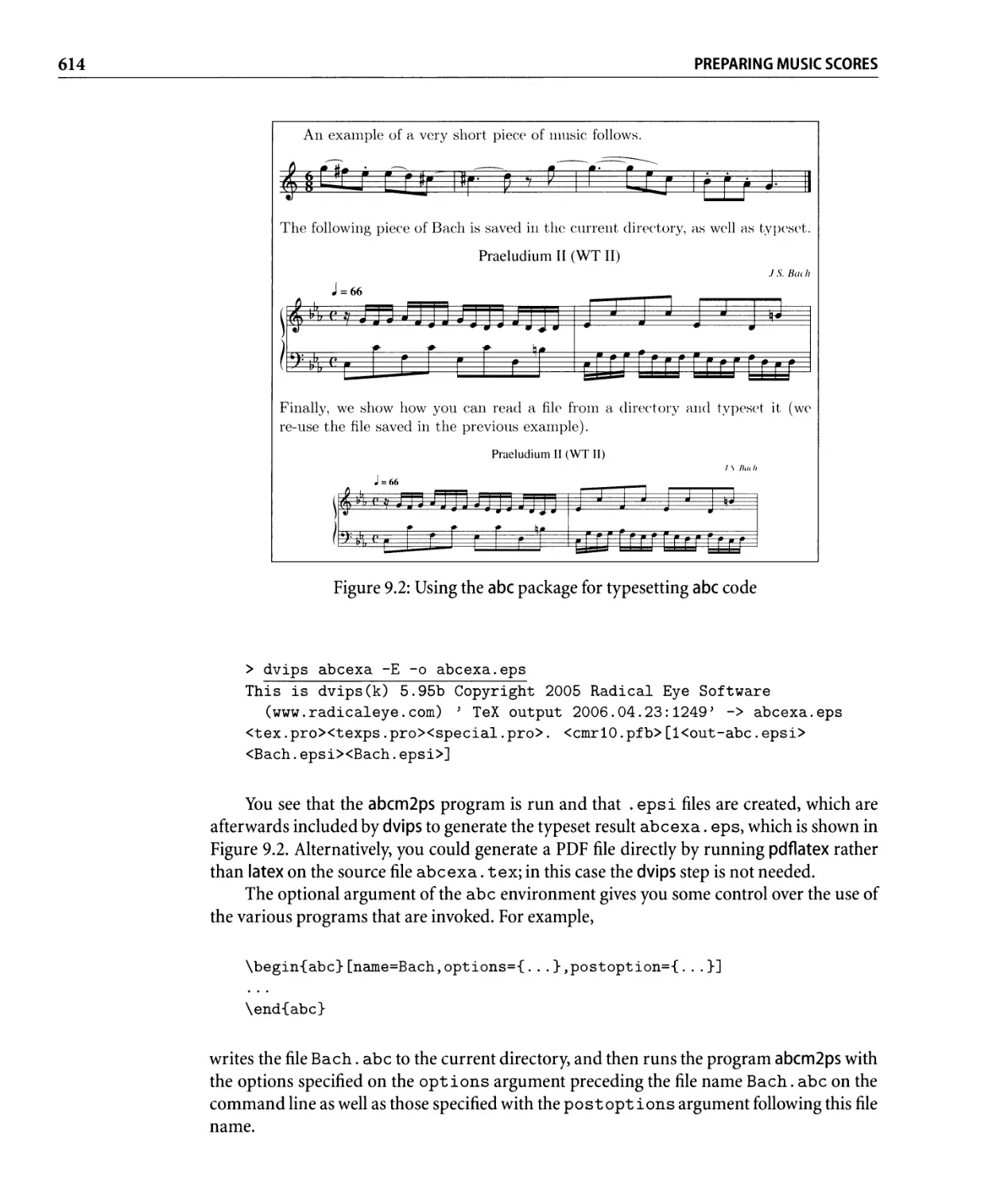
9.2 Using the abc package for typesetting abc code. . . . . . . . . . . . . . . . . . . .. 614
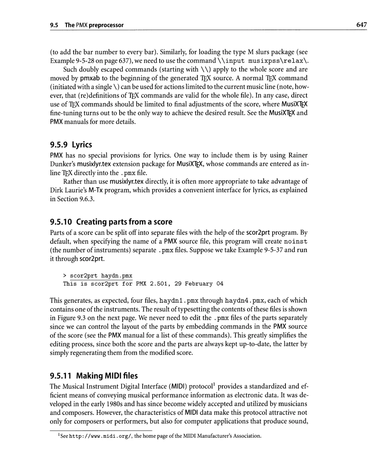
9.3 Individual voices created by scor2prt from a PMX score . . . . . . . . . . . . . .. 648
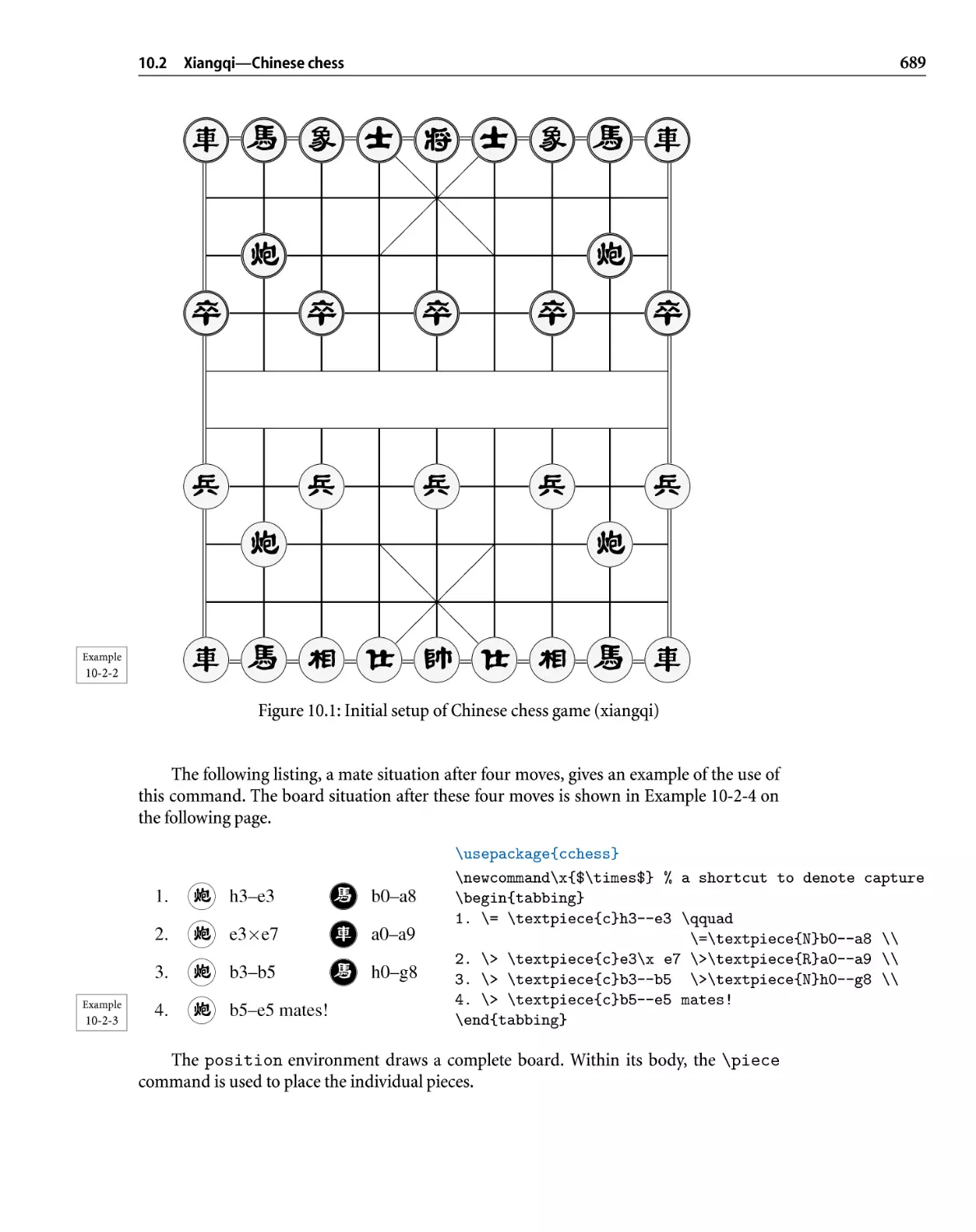
10.1 Initial setup of Chinese chess game (xiangqi). . . . . . . . . . . . . . . . . . . . .. 689
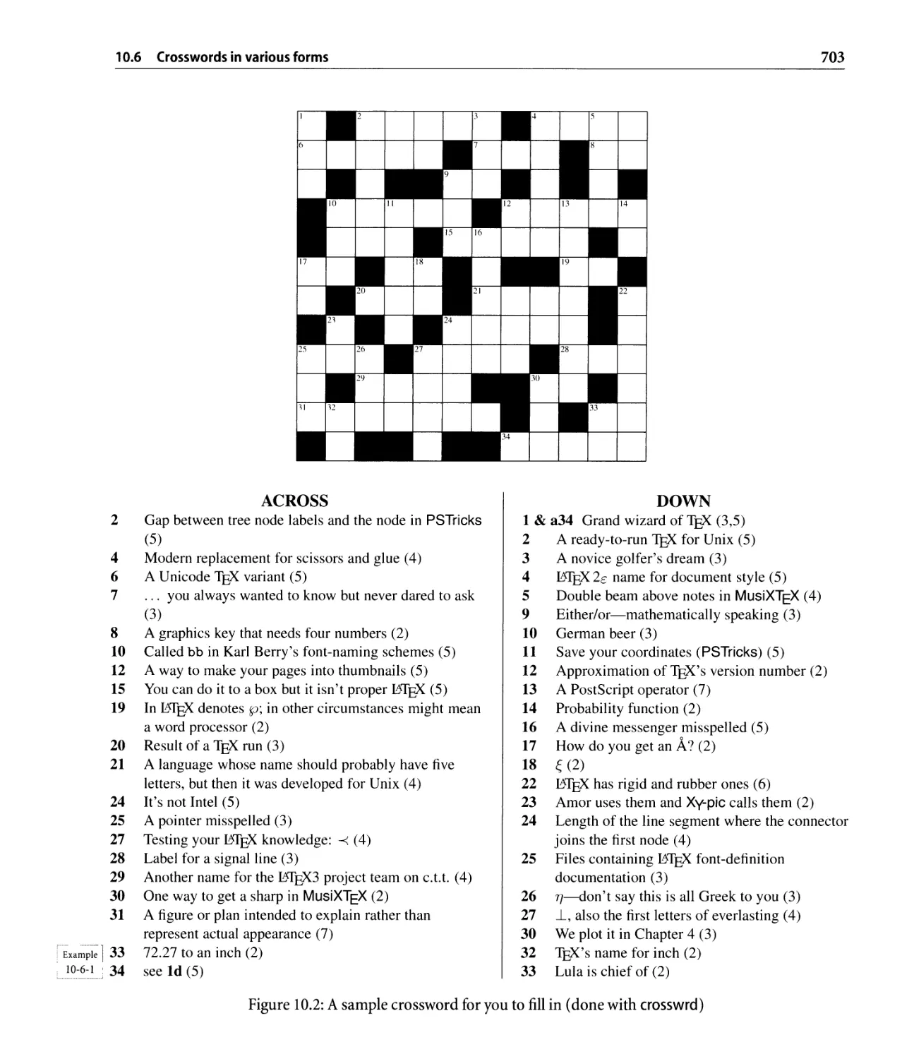
10.2 A sample crossword for you to fill in (done with crosswrd) .. . . . . . . . . . .. 703
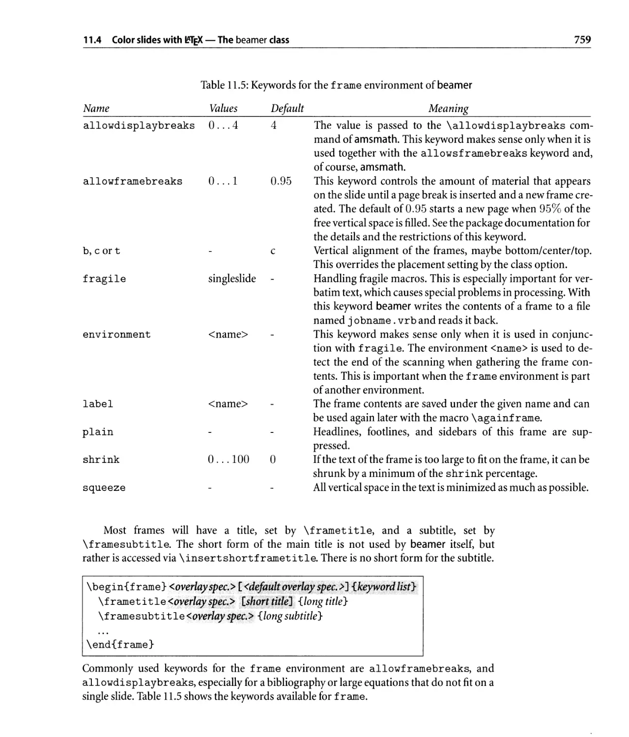
11.1 Table of contents in presentation and article display. . . . . . . . . . . . . . . . .. 760
11.2 The default navigation bar . . . . . . . . . . . . . . . . . . . . . . . . . . . . . . . .. 772
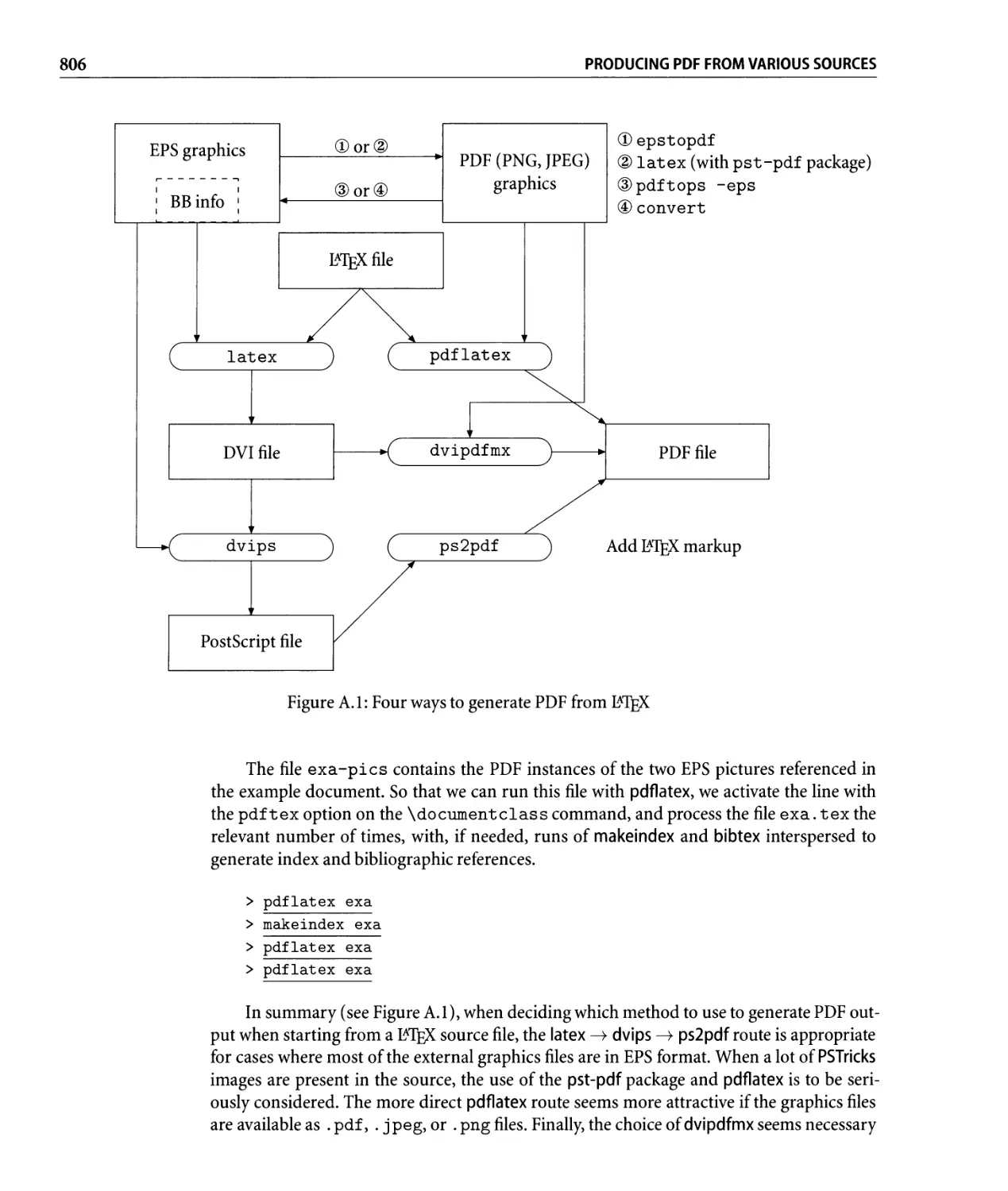
A.l Four ways to generate PDF from M-TFX . . . . . . . . . . . . . . . . . . . . . . . . .. 806
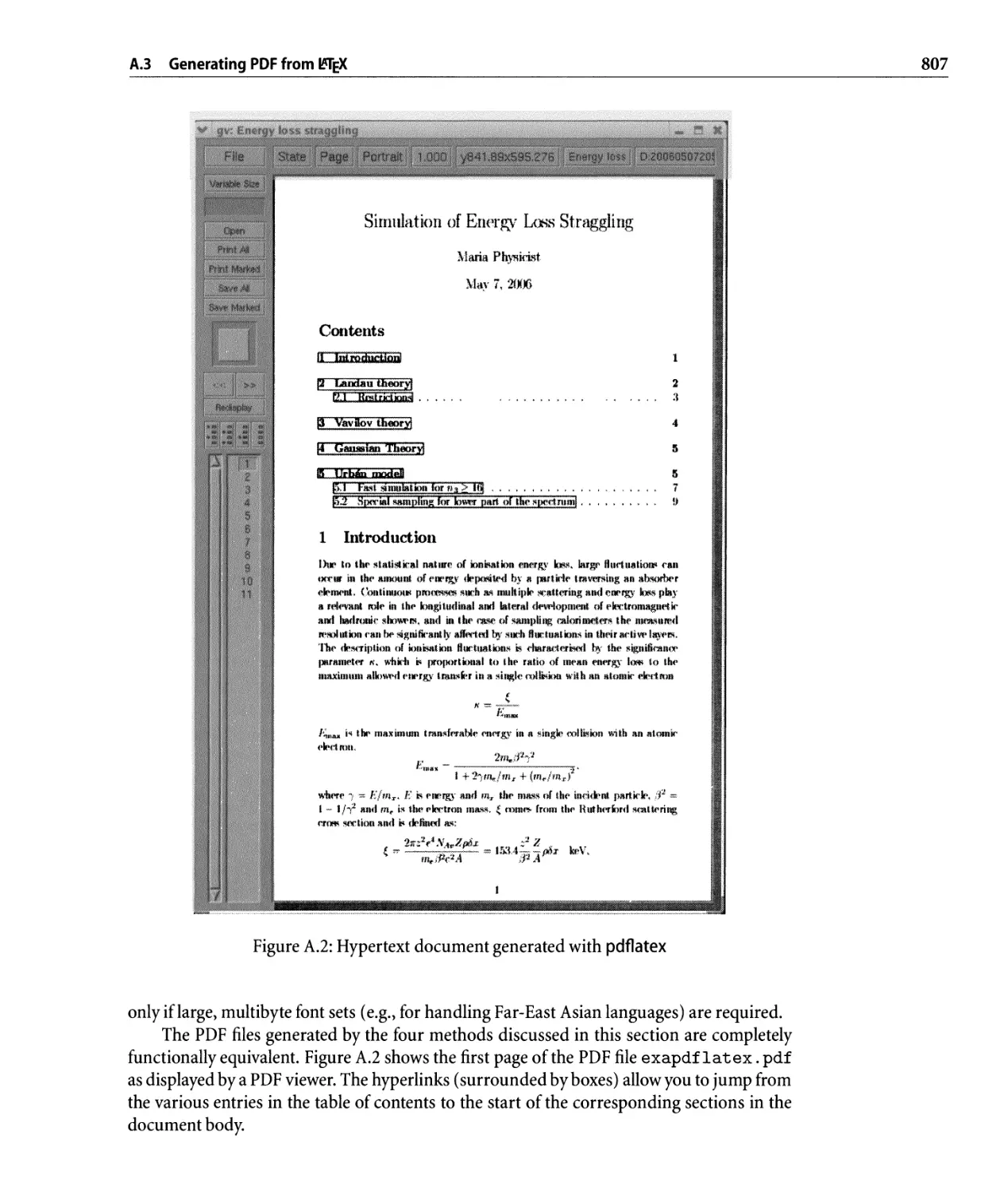
A.2 Hypertext document generated with pdflatex. . . . . . . . . . . . . . . . . . . . .. 807
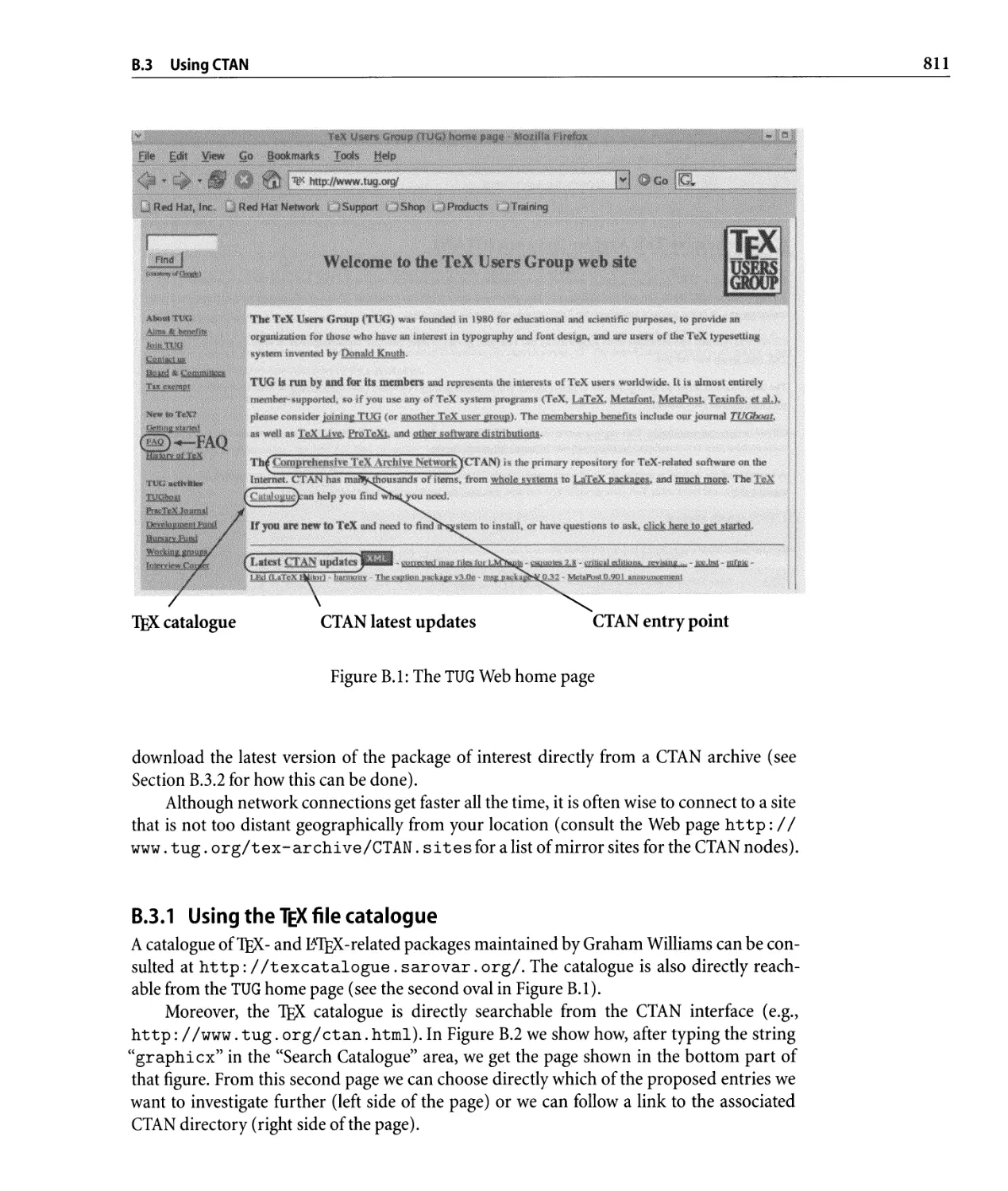
B .1 The TUG Web home page . . . . . . . . . . . . . . . . . . . . . . . . . . . . . . . . .. 811
B.2 CTAN home page and 'lEX catalogue entry . . . . . . . . . . . . . . . . . . . . . .. 812
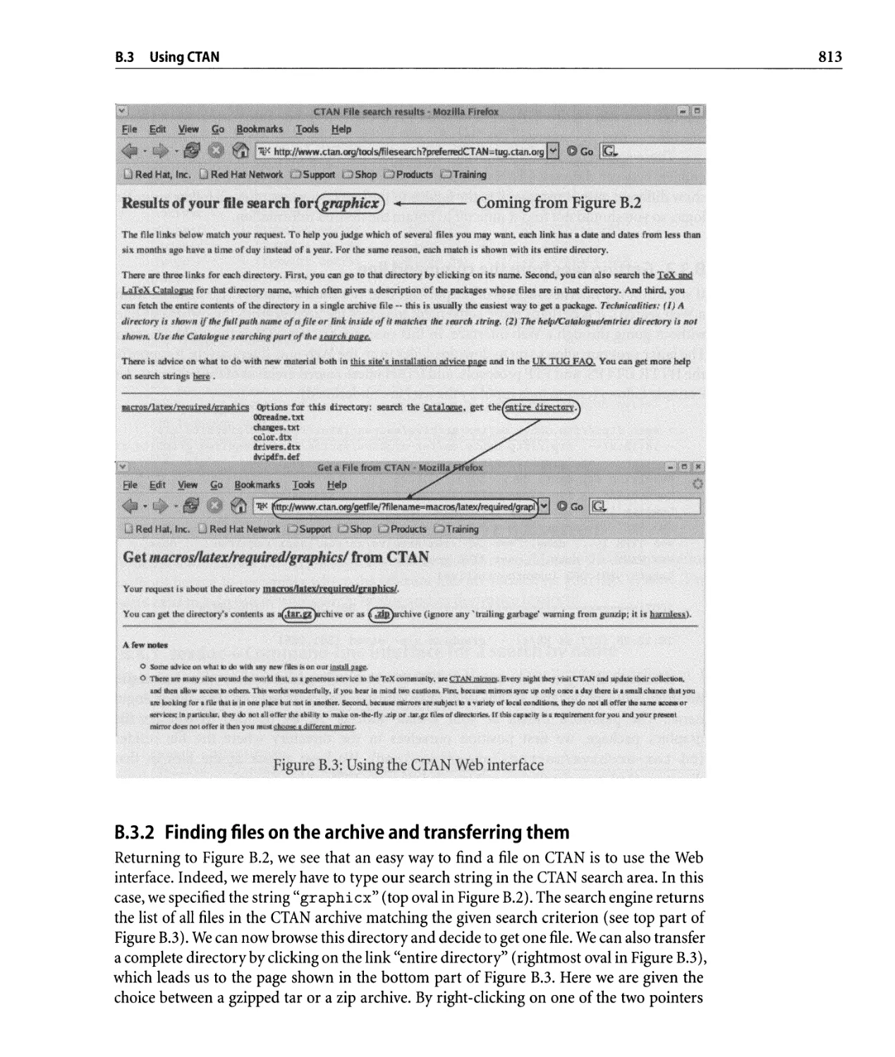
B.3 Using the CTAN Web interface. . . . . . . . . . . . . . . . . . . . . . . . . . . . . .. 813
B.4 Finding documentation with the texdoctk program. . . . . . . . . . . . . . . . .. 816
Color Plates
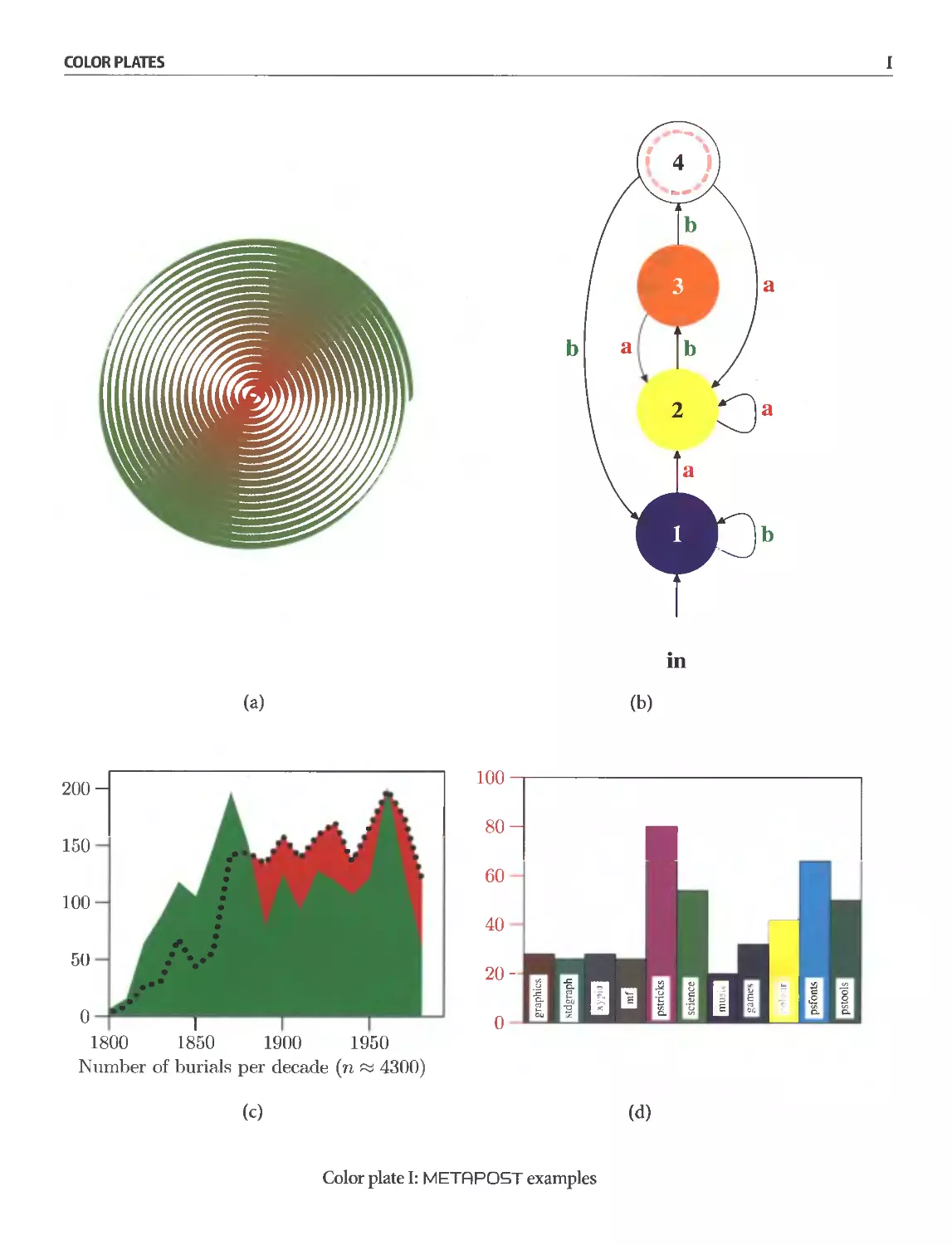
I META POST examples . . . . . . . . . . . . . . . . . . . . . . . . . . . . . . . . . . . I
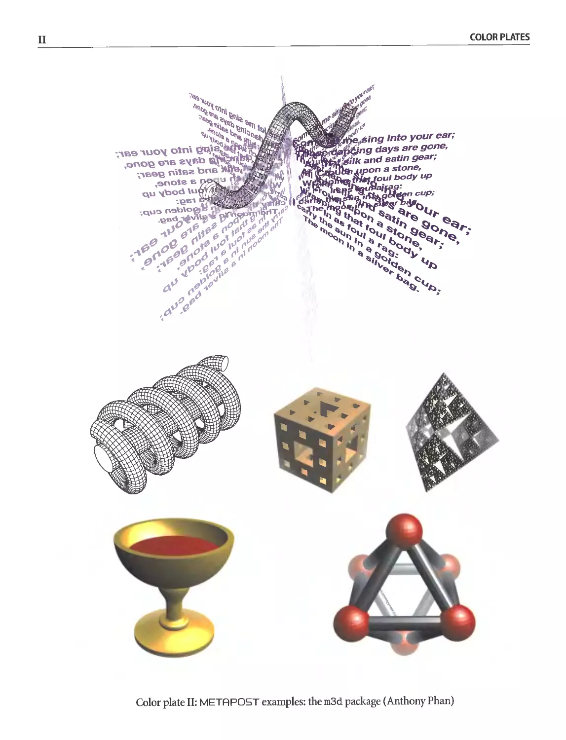
II META POST examples: the m3d package (Anthony Phan) . . . . . . . . . . . . . II
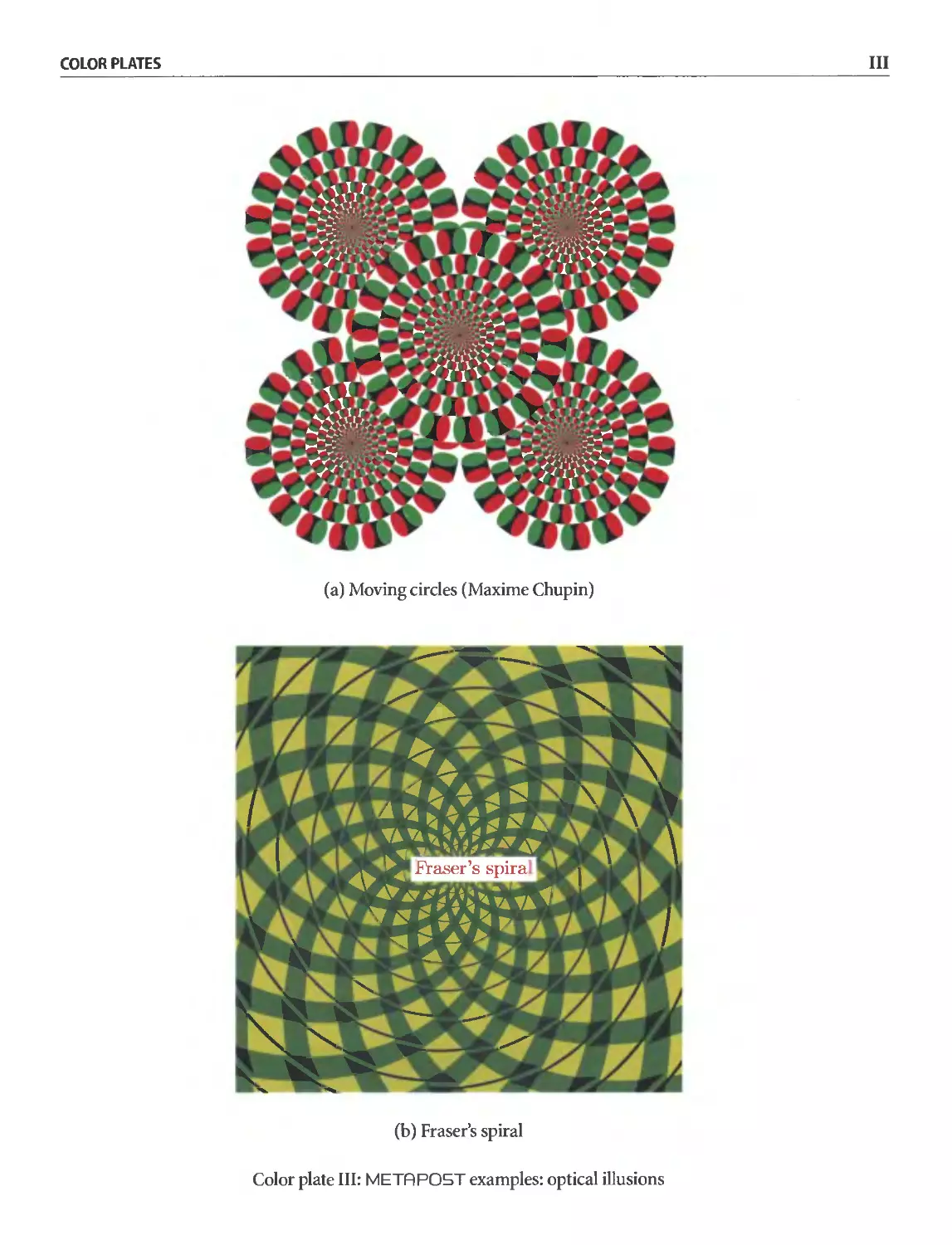
III META POST examples: optical illusions. . . . . . . . . . . . . . . . . . . . . . . .. III
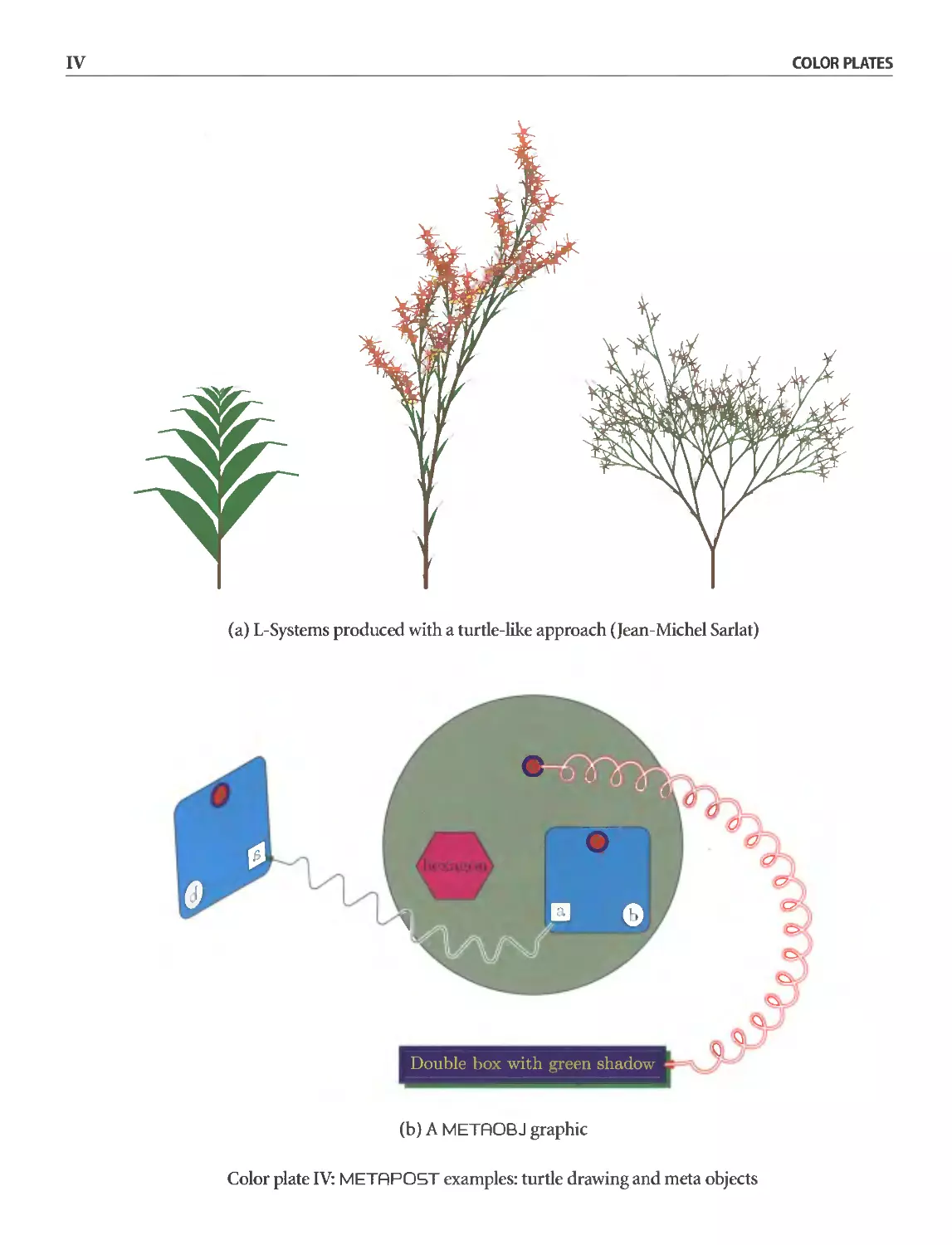
IV META POST examples: turtle drawing and meta objects . . . . . . . . . . . . .. IV
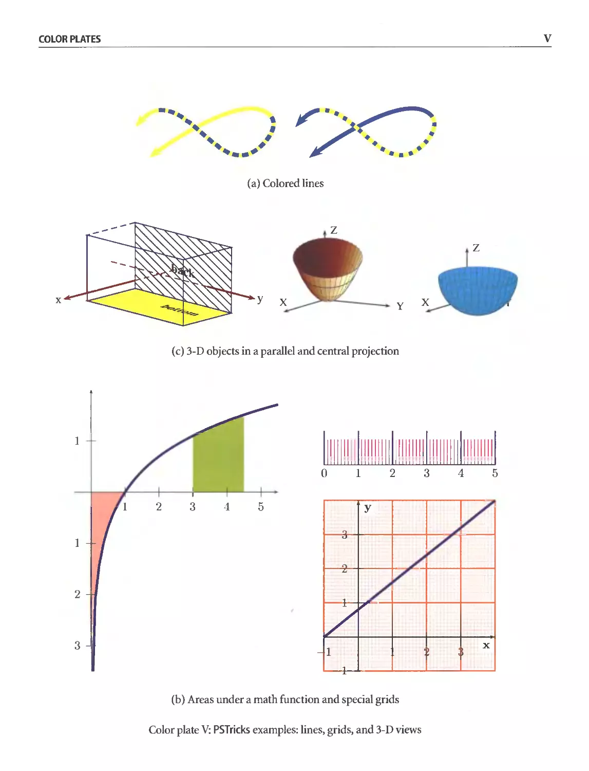
V PSTricks examples: lines, grids, and 3- D views . . . . . . . . . . . . . . . . . . . . . V
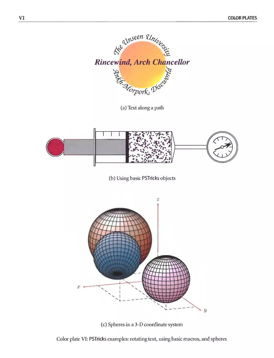
VI PSTricks examples: rotating text, using basic macros, and spheres . . . . . . . .. VI
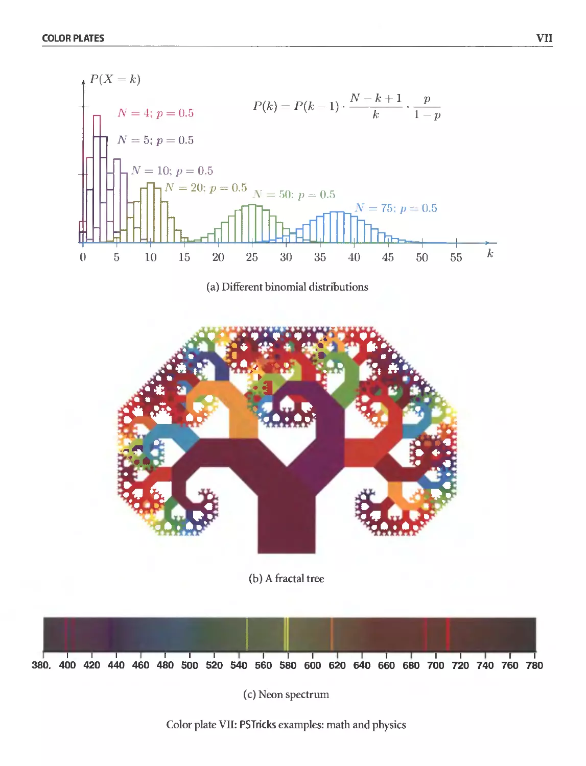
VII PSTricks examples: math and physics. . . . . . . . . . . . . . . . . . . . . . . . . .. VII
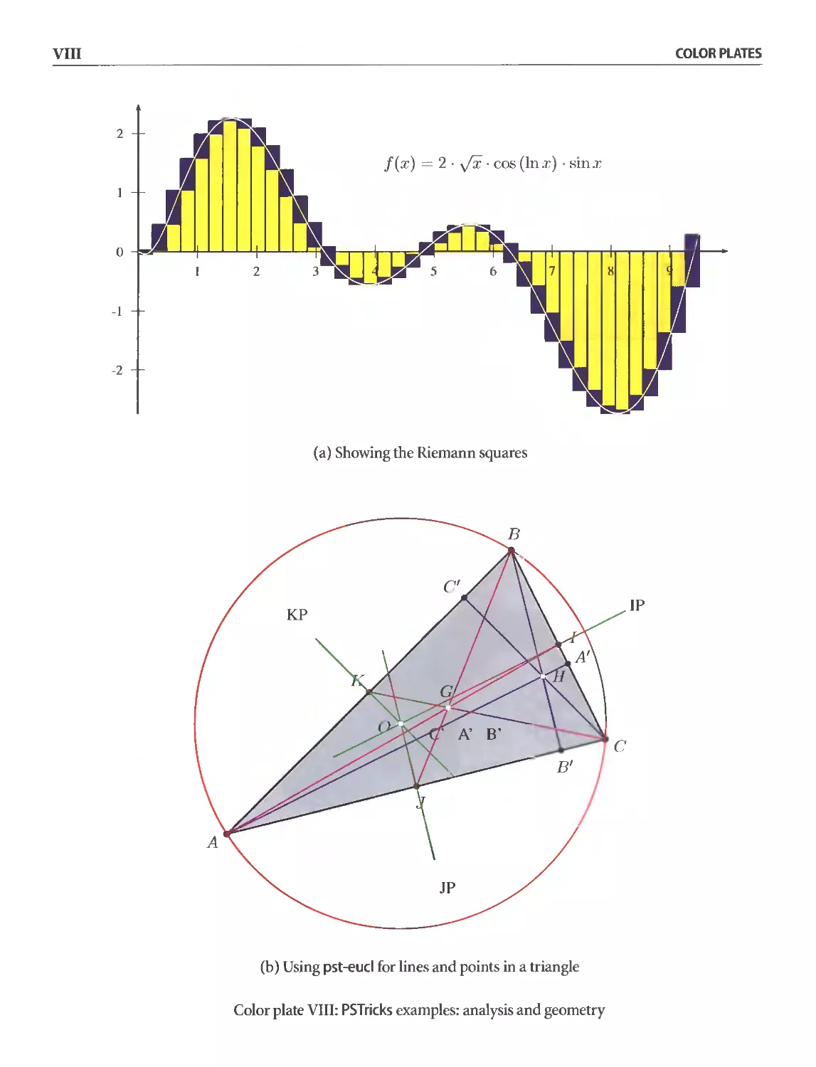
VIII PSTricks examples: analysis and geometry. . . . . . . . . . . . . . . . . . . . . . .. VIII
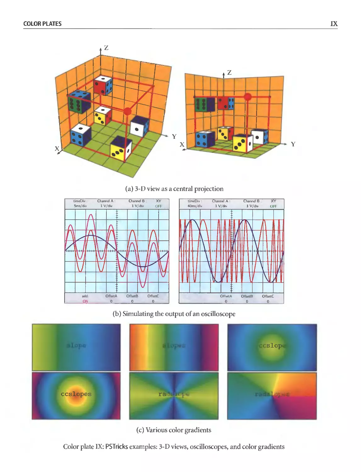
IX PSTricks examples: 3-D views, oscilloscopes, and color gradients. . . . . . . . .. IX
X Examples of the texshade and textopo packages. . . . . . . . . . . . . . . . . . . . X
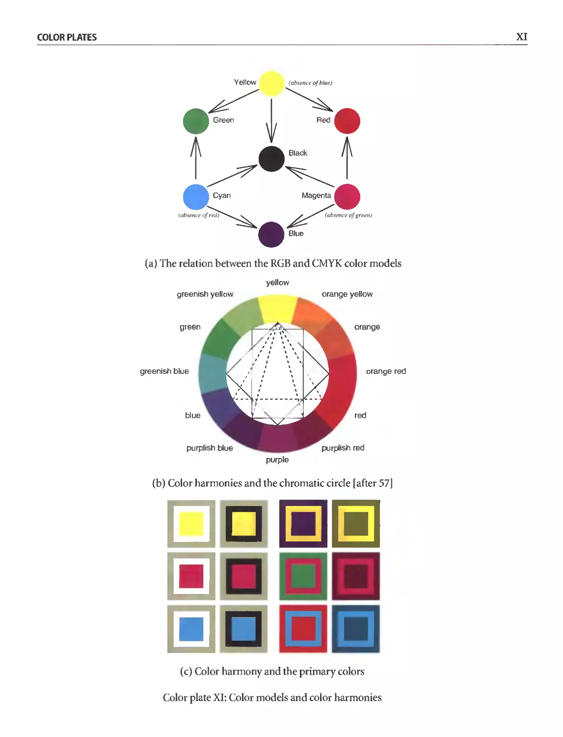
XI Color models and color harmonies . . . . . . . . . . . . . . . . . . . . . . . . . . .. XI
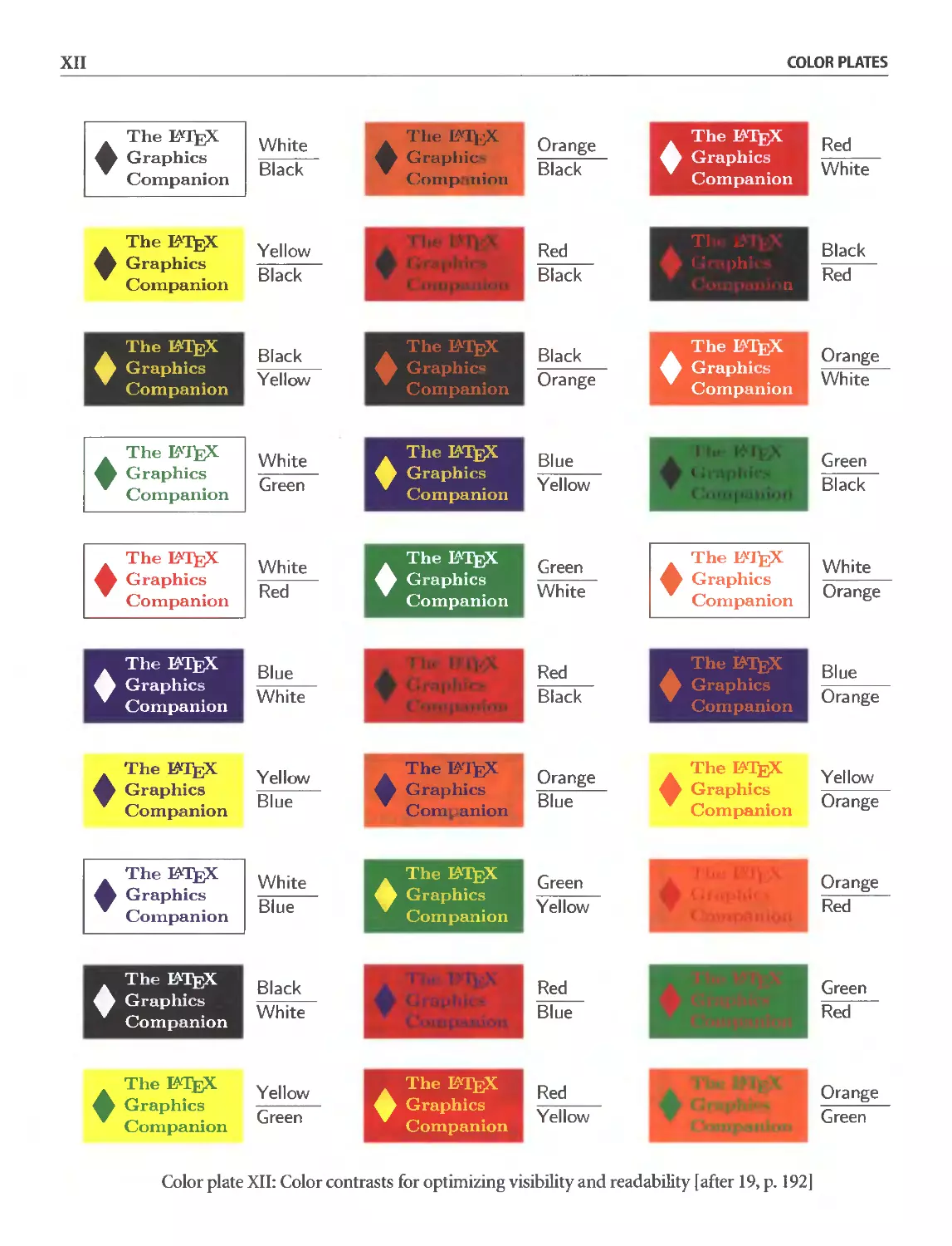
XII Color contrasts for optimizing visibility and readability . . . . . . . . . . . . . .. XII
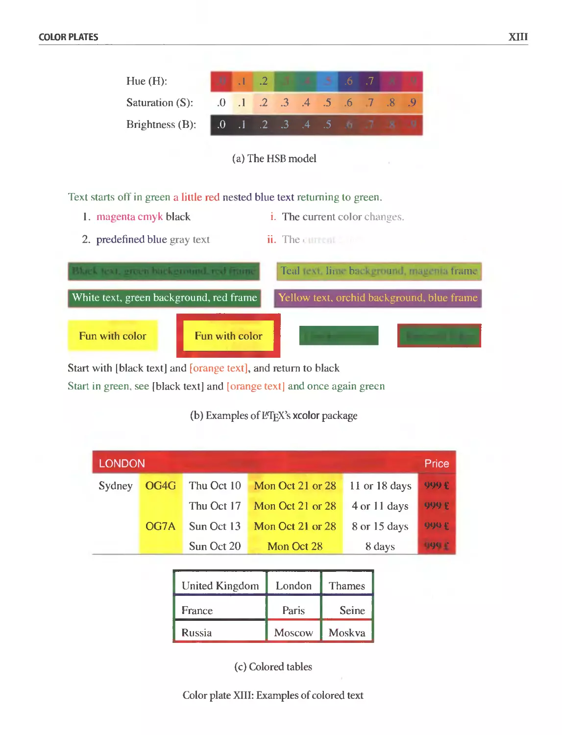
XIII Examples of colored text. . . . . . . . . . . . . . . . . . . . . . . . . . . . . . . . . .. XIII
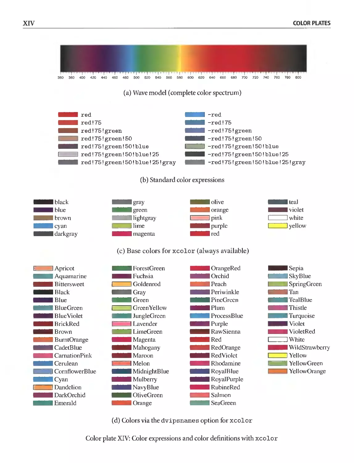
XIV Color expressions and color definitions with xcolor. . . . . . . . . . . . . . . .. XIV
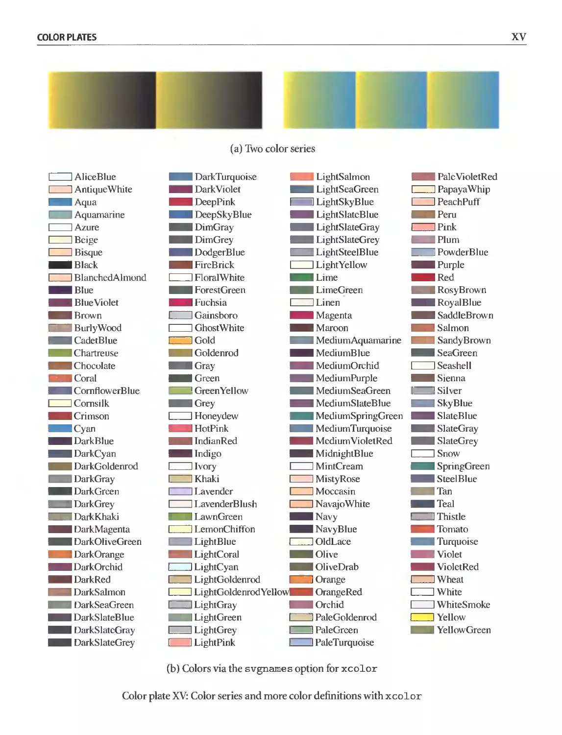
XV Color series and more color definitions with xcolor. . . . . . . . . . . . . . . .. XV
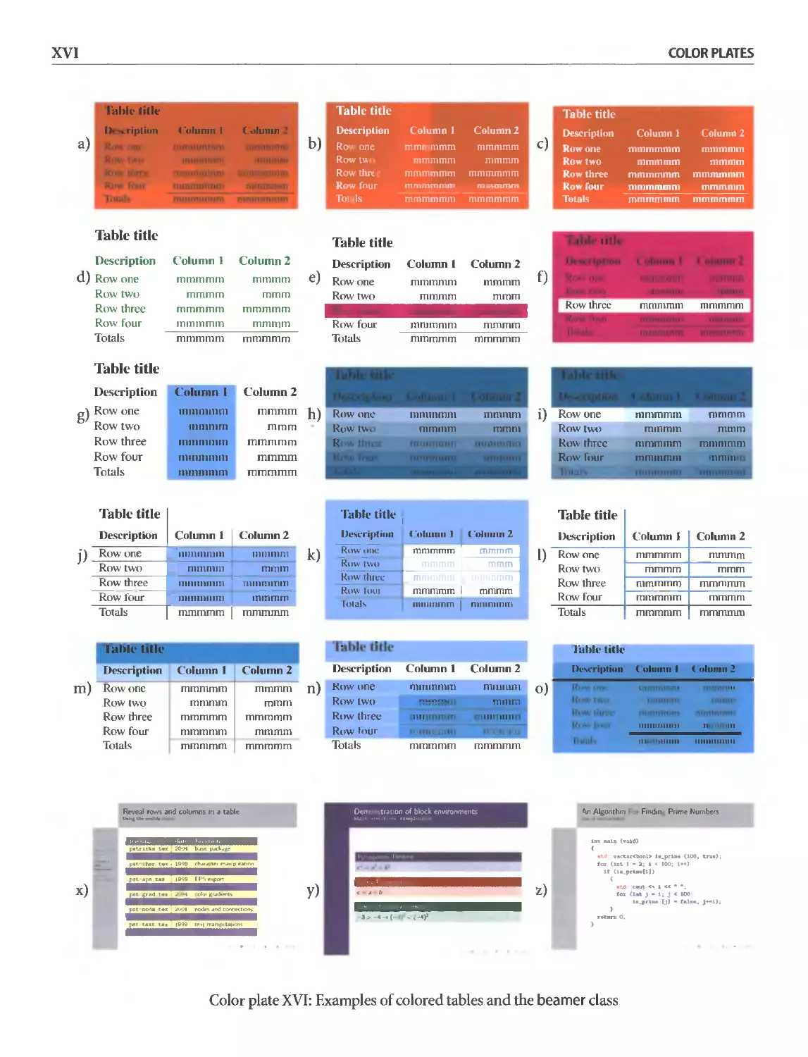
XVI Examples of colored tables and the beamer class. . . . . . . . . . . . . . . . . . .. XVI
1//
/'1
/ I
/
,/ I
,/,/ I
,/ I
,/,/ ...J --
,/ ............ I
,/,/ I
/.... I
/_ -------I----------
- - -/ -" " - - - -
/ /..... I
/// .......... I
.. ..... I
/1 U ..... ..... I
,/ /1 ""'-....1..
,/ 1 "\
/ / 0 .....
/ I I ..........
/ I I .....
I .....
\\1 / I.....
\1\ I ..........
1\ \ I
/ \ \
I \\ I
I
, \
I \ \
\ ,
'I
I
/
/
I
/
I
I
1 I
I I
I I
I I
I ,
I 1....-
1/1
/\ I
\ \
\ \
\ \
- -
equator
I
I
I
I S *....'
I _-
- - -1- - _ _ _ - - -.-
.........._ I s
- - _.....J _ ...
..----
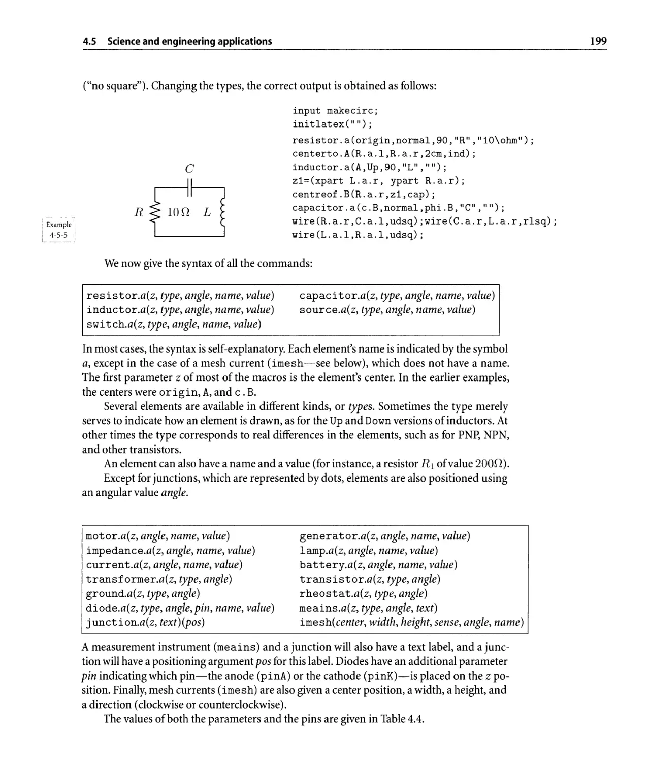
Lunar orbit on the celestial sphere with METAPo5T
List of Tables
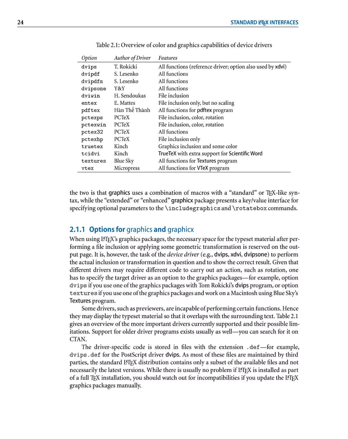
2.1 Overview of color and graphics capabilities of device drivers. . . . . . . . . . .. 24
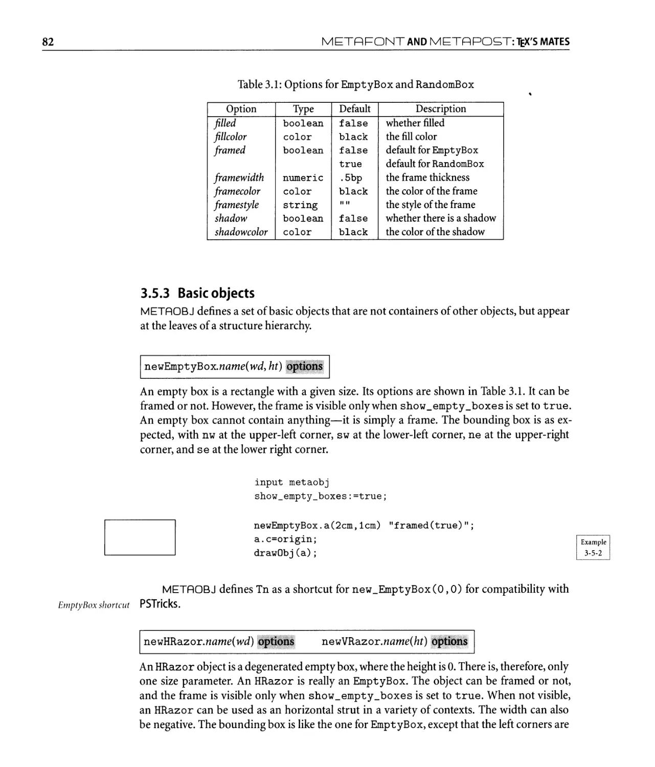
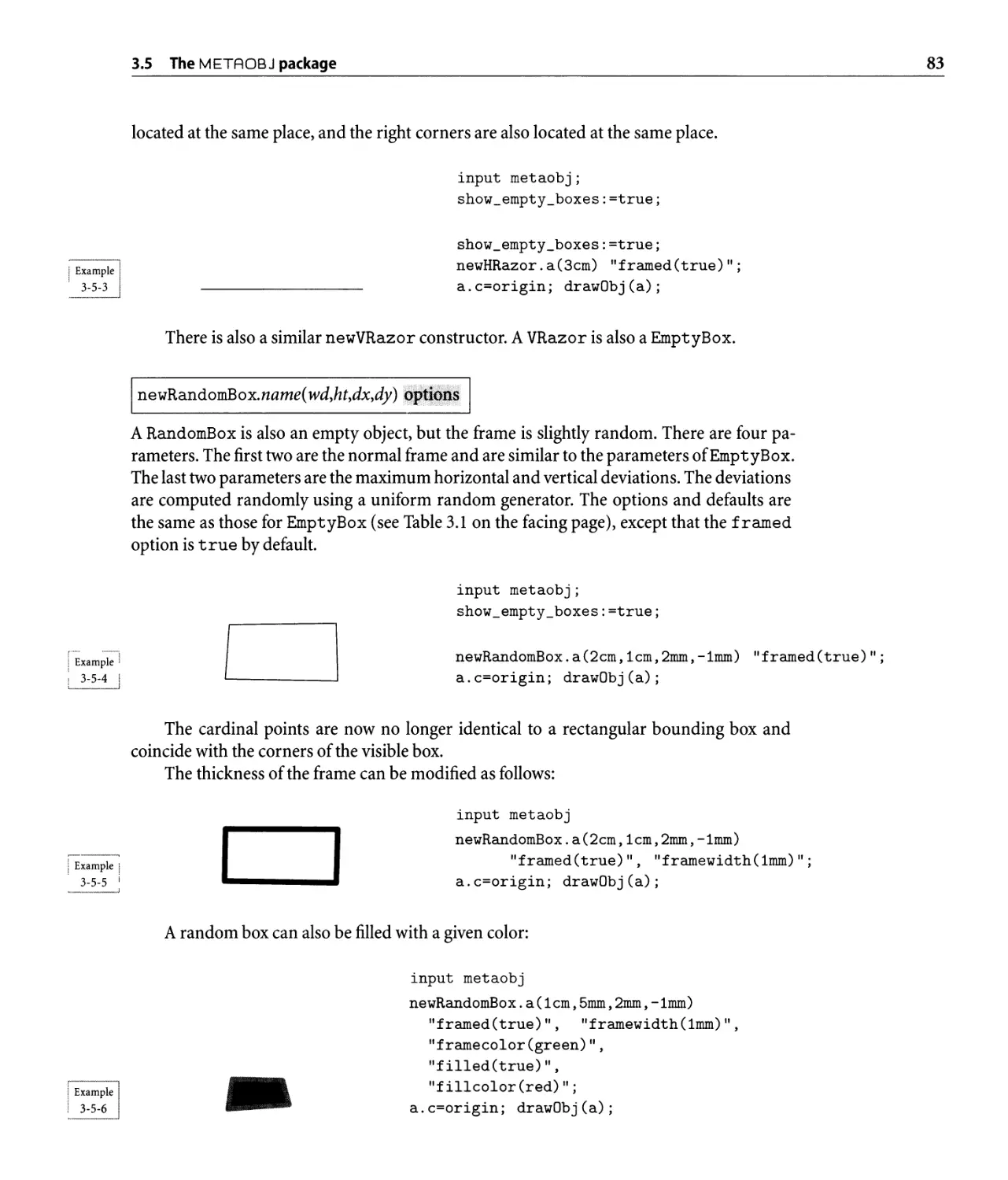
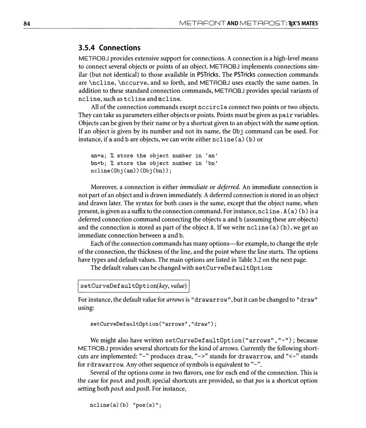
3.1 Options for EmptyBox and RandomBox. ........................ 82
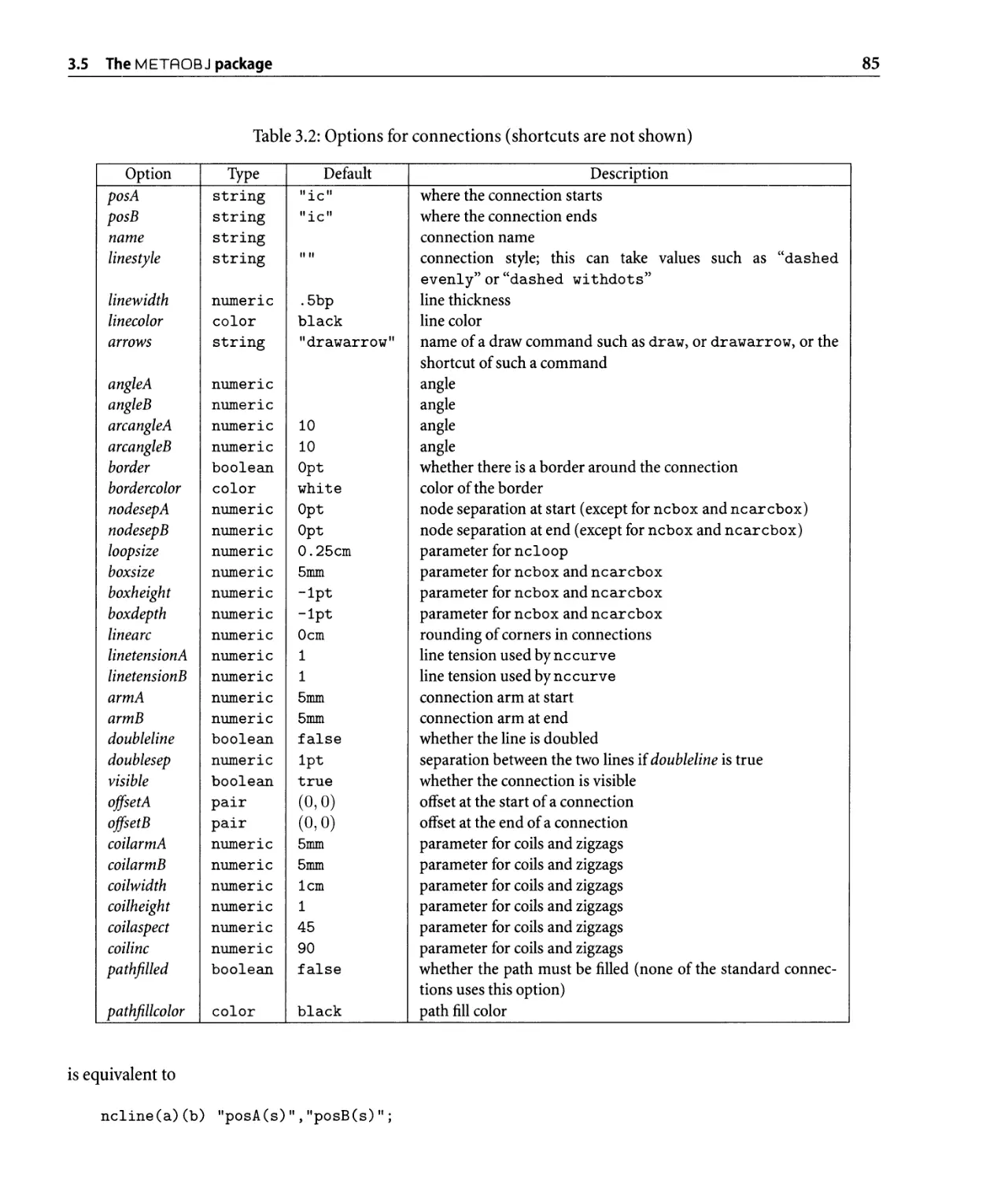
3.2 Options for connections. . . . . . . . . . . . . . . . . . . . . . . . . . . . . . . . . .. 85
3.3 Options for connection labels . . . . . . . . . . . . . . . . . . . . . . . . . . . . . .. 95
3.4 Options for Box. . . . . . . . . . . . . . . . . . . . . . . . . . . . . . . . . . . . . . .. 96
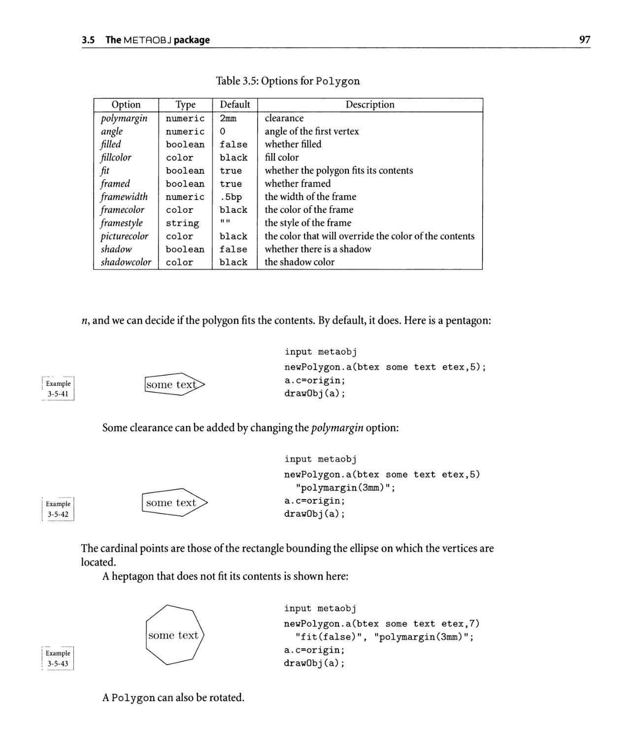
3.5 Options for Polygon . . . . . . . . . . . . . . . . . . . . . . . . . . . . . . . . . . .. 97
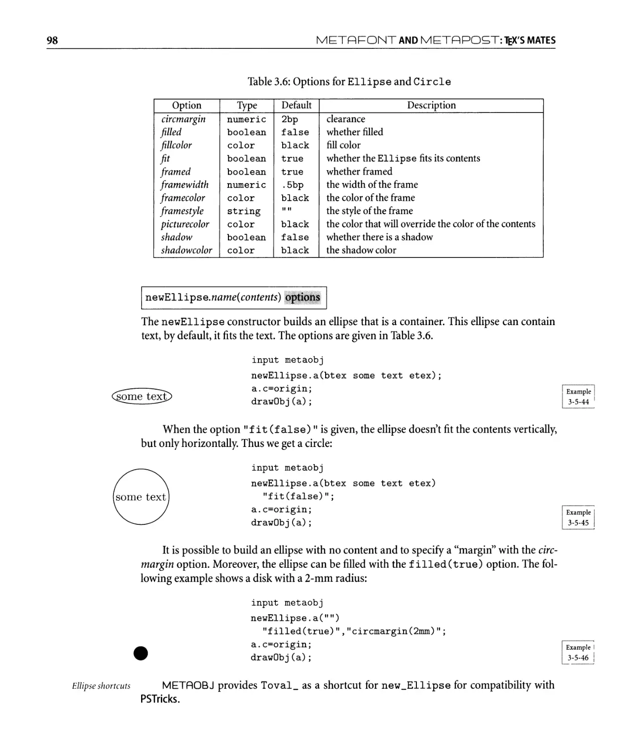
3.6 Options for Ellipse and Circle. . . . . . . . . . . . . . . . . . . . . . . . . . .. 98
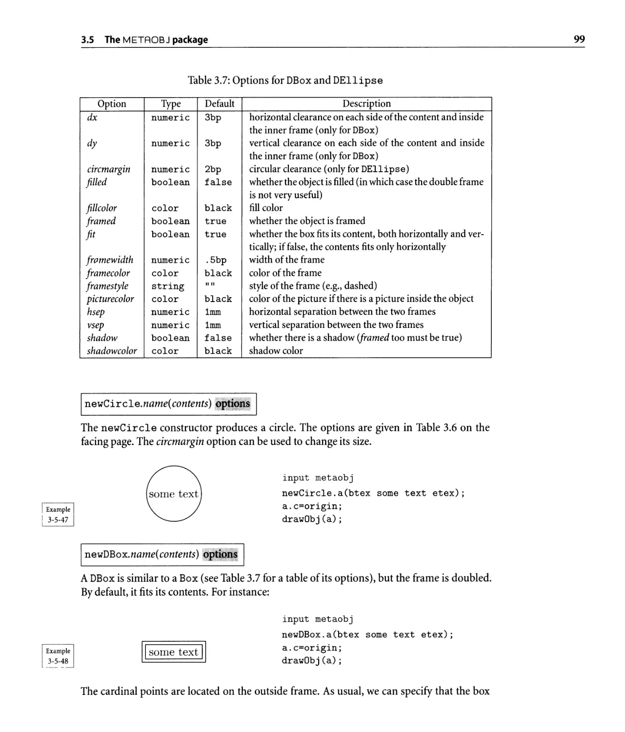
3.7 Options for DBox and DEll ips e . . . . . . . . . . . . . . . . . . . . . . . . . . . .. 99
3.8 Options for HBox, VBox, and Container. . . . . . . . . . . . . . . . . . . . . . .. 101
3.9 Options for Re curs i veBox . . . . . . . . . . . . . . . . . . . . . . . . . . . . . . .. 105
3.10 Options for Tree . . . . . . . . . . . . . . . . . . . . . . . . . . . . . . . . . . . . . .. 106
3.11 Options for HFan and VFan. . . . . . . . . . . . . . . . . . . . . . . . . . . . . . . .. 115
3.12 OptionsforMatrix . . . . . . . . . . . . . . . . . . . . . . . . . . . . . . . . . . . .. 116
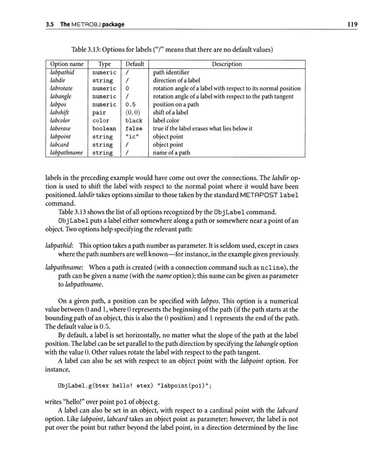
3.13 Options for labels . . . . . . . . . . . . . . . . . . . . . . . . . . . . . . . . . . . . . .. 119
4.1 CM arrow styles . . . . . . . . . . . . . . . . . . . . . . . . . . . . . . . . . . . . . . .. 189
4.2 Elements and their abbreviations . . . . . . . . . . . . . . . . . . . . . . . . . . . .. 197
4.3 The main components of a circuit. . . . . . . . . . . . . . . . . . . . . . . . . . . .. 197
4.4 Possible types, pins, and positioning pins for each element . . . . . . . . . . . .. 200
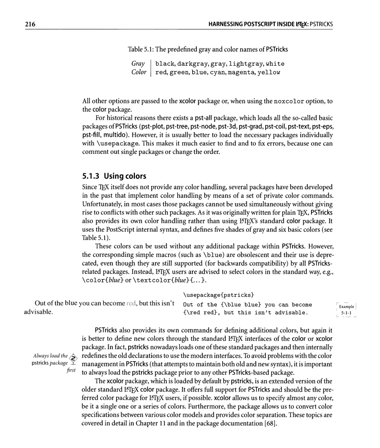
5.1 The predefined gray and color names of PSTricks. . . . . . . . . . . . . . . . . . .. 216
5.2 Lengths and their register names in PSTricks . . . . . . . . . . . . . . . . . . . . .. 218
5.3 Meaning of the starred form . . . . . . . . . . . . . . . . . . . . . . . . . . . . . . .. 220
5.4 Summary of keywords for setting grids . . . . . . . . . . . . . . . . . . . . . . . .. 227
5.5 Summary of keywords for lines and polygons. . . . . . . . . . . . . . . . . . . . .. 235
5.6 Possible values for 1 inet ype . . . . . . . . . . . . . . . . . . . . . . . . . . . . . .. 240
..
XXll
LIST OF TABLES
5.7 Summary of keywords for circles, ellipses and curves. . . . . . . . . . . . . . . .. 247
5.8 Summary of keywords for dot display . . . . . . . . . . . . . . . . . . . . . . . . .. 251
5.9 Summary of dot styles . . . . . . . . . . . . . . . . . . . . . . . . . . . . . . . . . . .. 252
5.10 Summary of the keywords used to fill areas. . . . . . . . . . . . . . . . . . . . . .. 253
5.11 Summary of keywords for arrows . . . . . . . . . . . . . . . . . . . . . . . . . . . .. 260
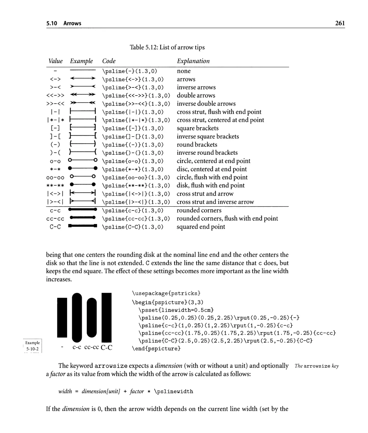
5.12 List of arrow tips . . . . . . . . . . . . . . . . . . . . . . . . . . . . . . . . . . . . . .. 261
5.13 Defined short forms for the rotation angles. . . . . . . . . . . . . . . . . . . . . .. 266
5.14 Defined short forms for directions . . . . . . . . . . . . . . . . . . . . . . . . . . .. 269
5.15 Summary of keywords for boxes. . . . . . . . . . . . . . . . . . . . . . . . . . . . .. 270
5.16 Meaningoftheliftpenkeyword ............................ 282
5.17 Possible coordinate forms with enabled \Spec ialCoor . . . . . . . . . . . . .. 297
5.18 Possible angle specifications with enabled \SpecialCoor. . . . . . . . . . . .. 297
5.19 Relative point translation . . . . . . . . . . . . . . . . . . . . . . . . . . . . . . . . .. 301
5.20 Relative point translation with angle specification. . . . . . . . . . . . . . . . . .. 301
5.21 Relative point translation with reference to a third point. . . . . . . . . . . . . .. 301
5.22 Some basic PostScript procedures from pstricks . pro . . . . . . . . . . . . .. 307
6.1 Plot macros included in the base package pstricks . . . . . . . . . . . . . . . . . .. 314
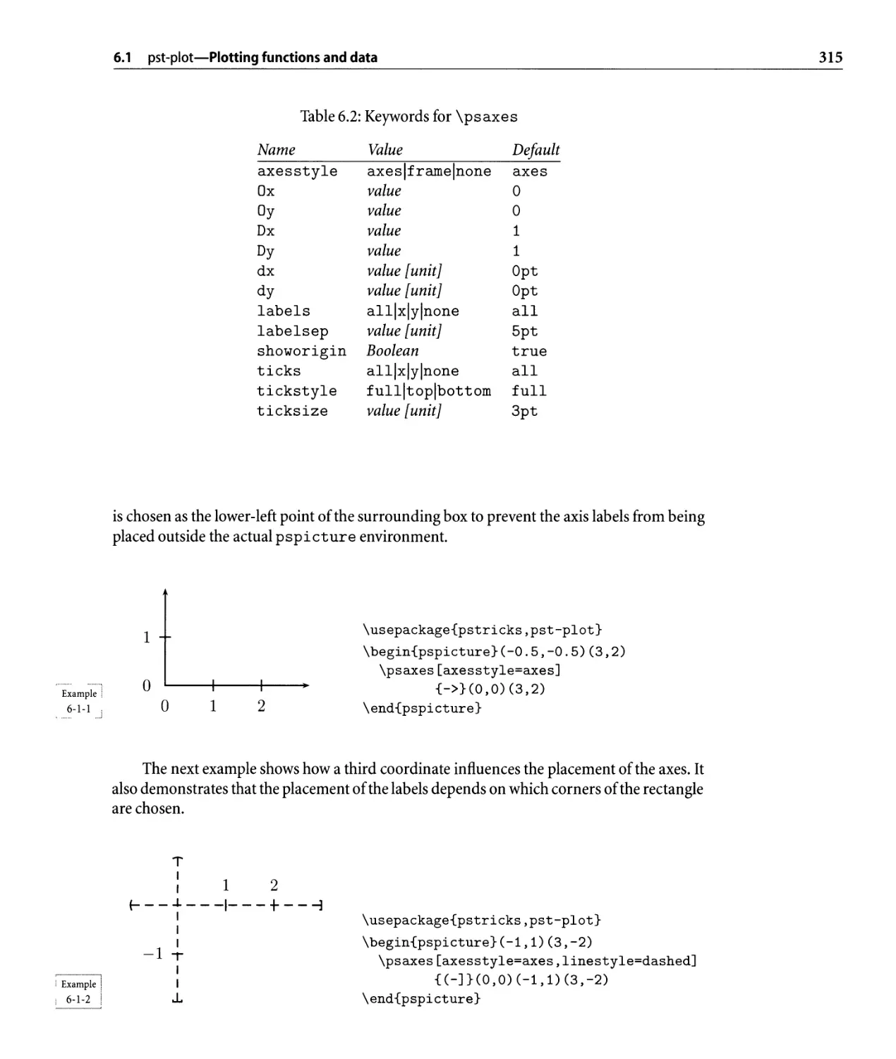
6.2 Keywordsfor\psaxes ................................... 315
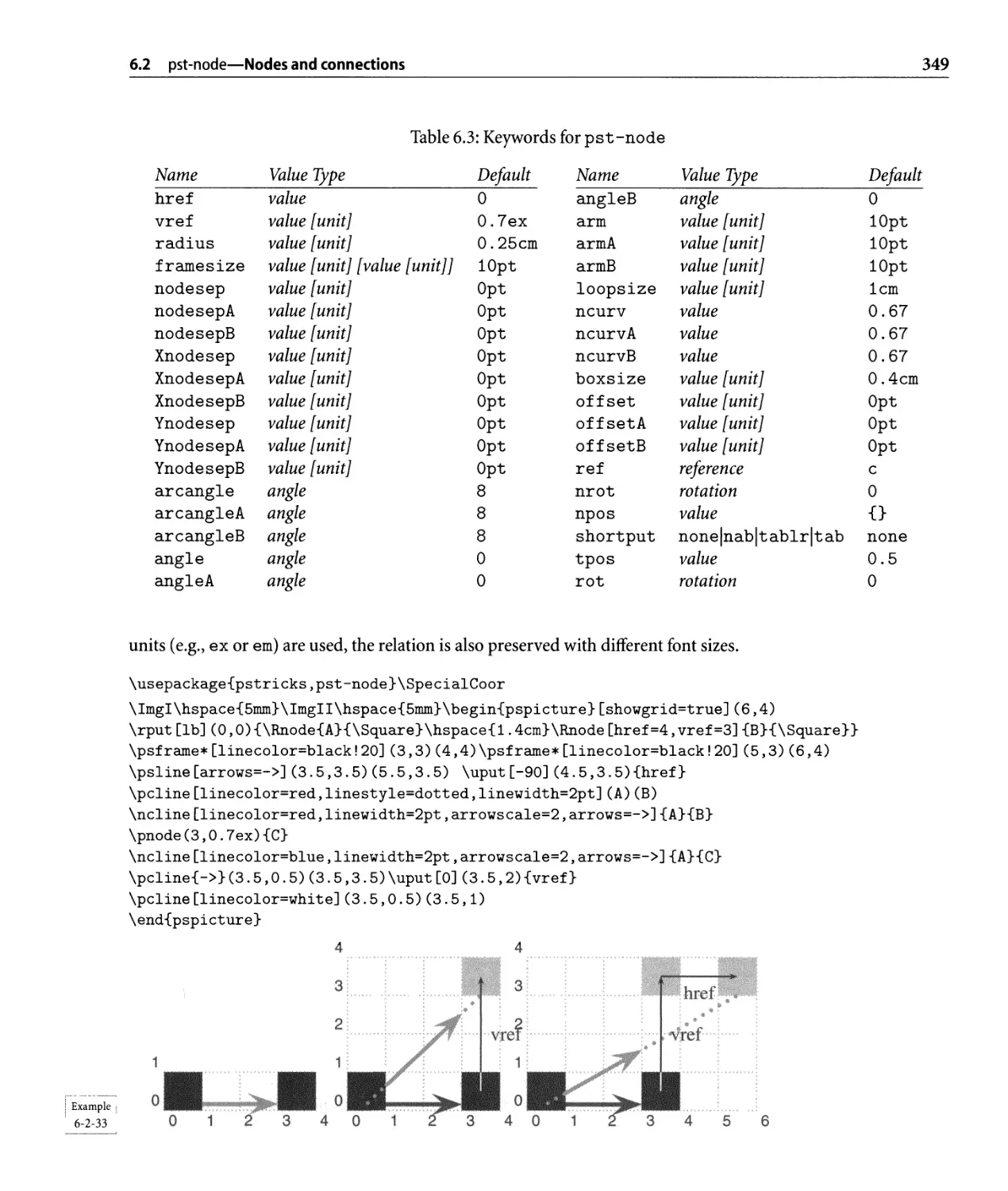
6.3 Keywords for ps t -node . . . . . . . . . . . . . . . . . . . . . . . . . . . . . . . . .. 349
6.4 Comparison of different node connections . . . . . . . . . . . . . . . . . . . . . .. 355
6.5 The short forms for nab. . . . . . . . . . . . . . . . . . . . . . . . . . . . . . . . . .. 356
6.6 The short forms for t ablr . . . . . . . . . . . . . . . . . . . . . . . . . . . . . . . .. 356
6.7 Keywords for psmatrix . . . . . . . . . . . . . . . . . . . . . . . . . . . . . . . . .. 362
6.8 The keyword values for mnode and the corresponding commands. . . . . . . .. 363
6.9 Keywords for pst-tree . . . . . . . . . . . . . . . . . . . . . . . . . . . . . . . . .. 370
6.10 Label keywords . . . . . . . . . . . . . . . . . . . . . . . . . . . . . . . . . . . . . . .. 380
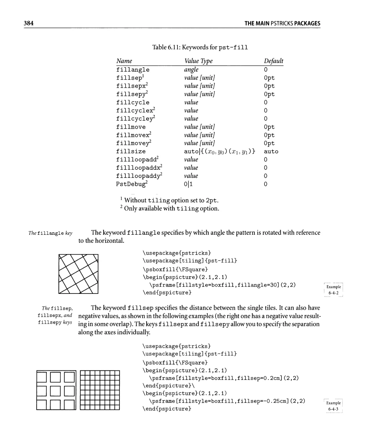
6 .11 Keywords for pst - fill . . . . . . . . . . . . . . . . . . . . . . . . . . . . . . . . .. 384
6.12 Summary of 3- D packages . . . . . . . . . . . . . . . . . . . . . . . . . . . . . . . .. 388
6.13 Summary of 3- D keywords . . . . . . . . . . . . . . . . . . . . . . . . . . . . . . . .. 395
6.14 Keywordsforthepackagepst-3dplot......................... 410
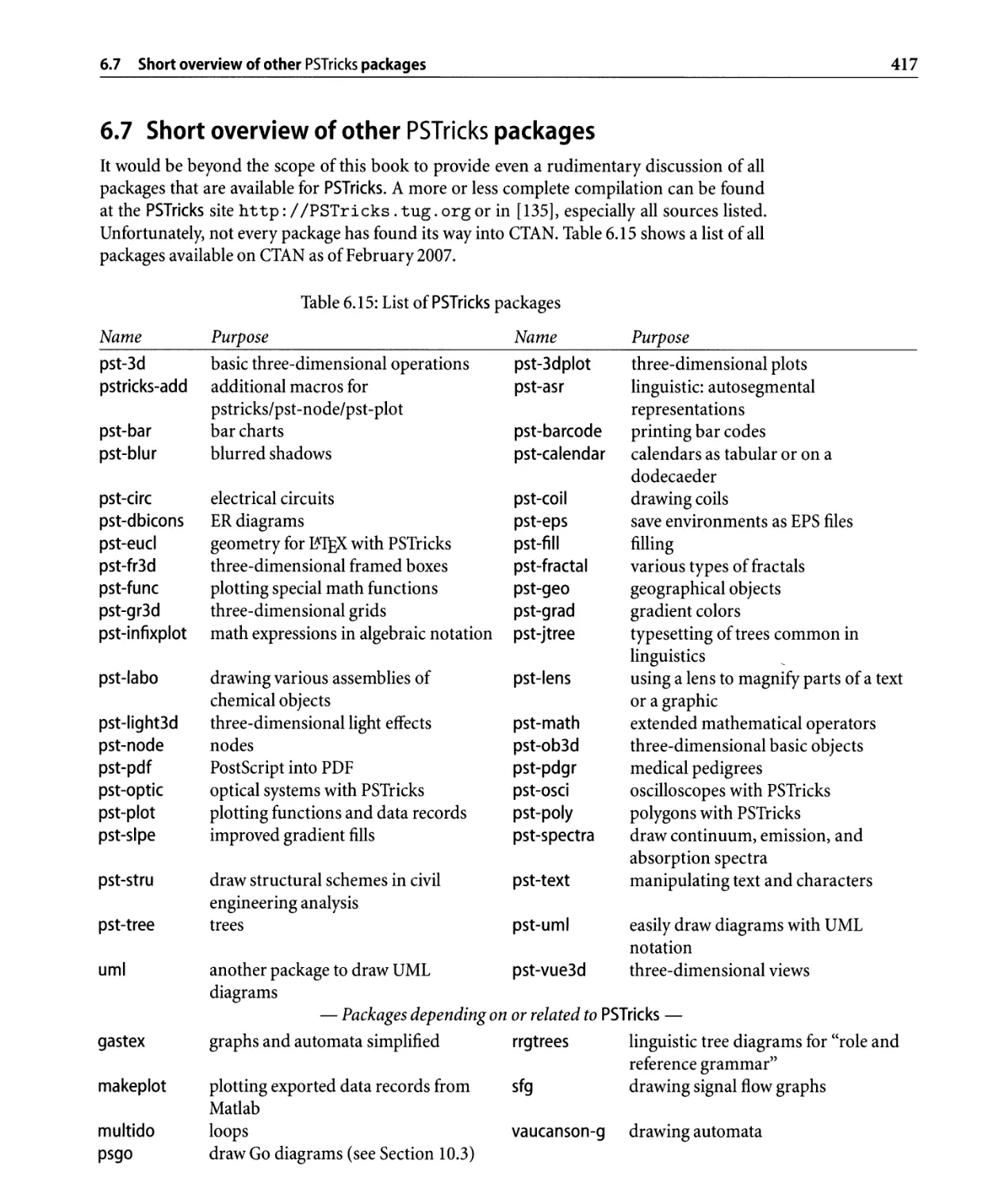
6.15 List of psTricks packages. . . . . . . . . . . . . . . . . . . . . . . . . . . . . . . . . .. 417
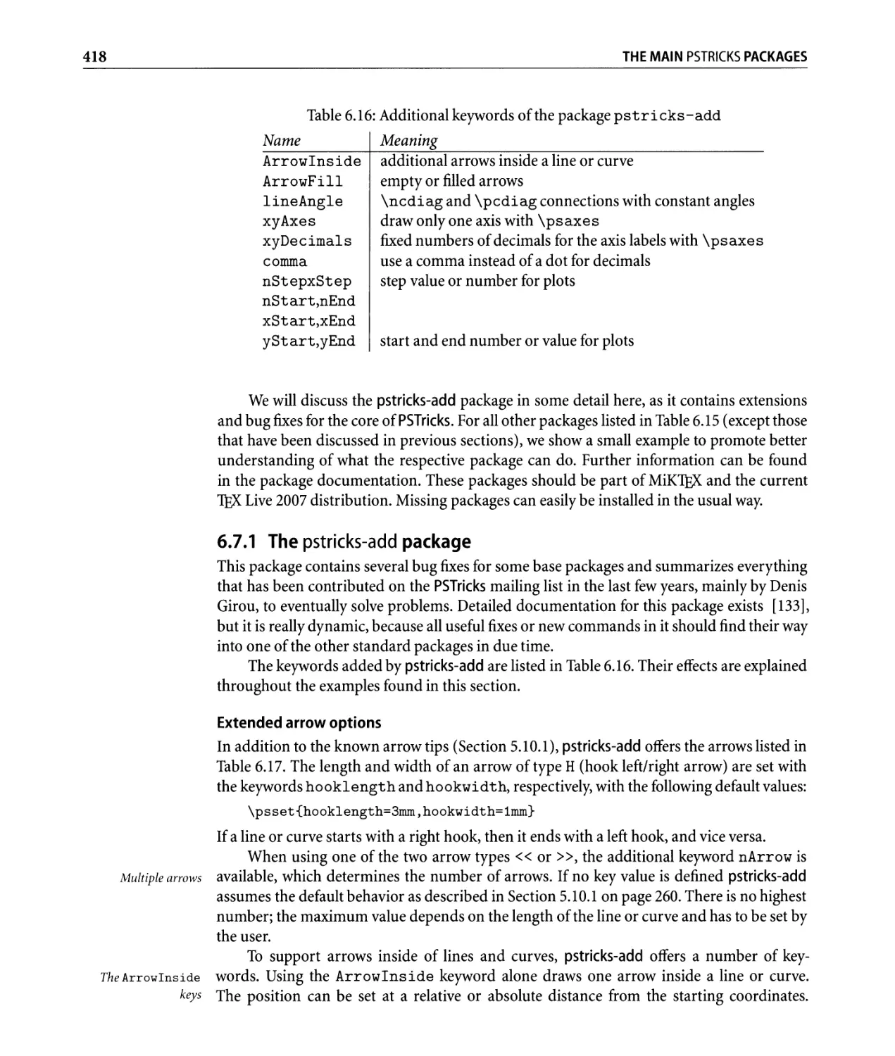
6.16 Additional keywords of the package pstricks-add. . . . . . . . . . . . . . . .. 418
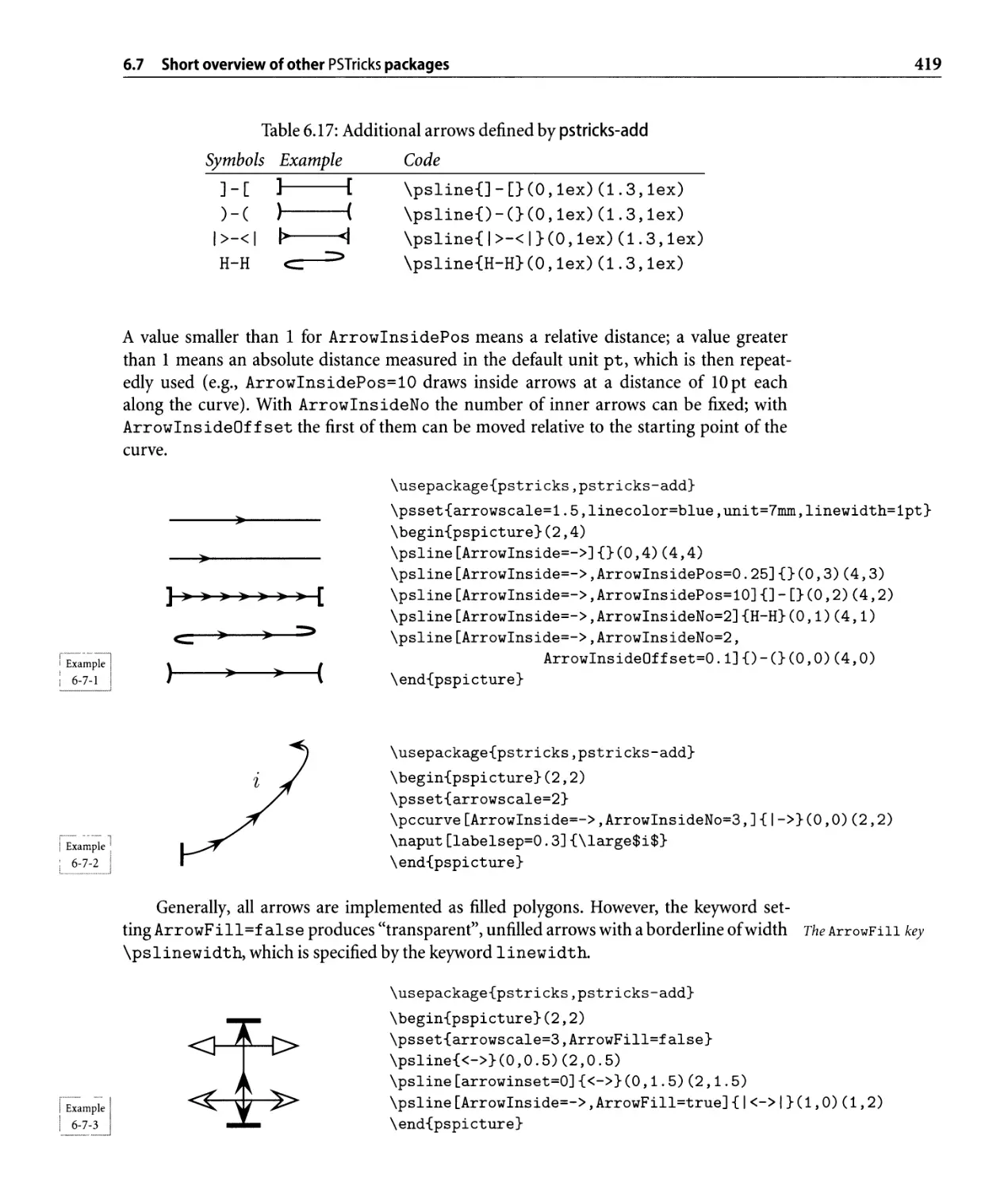
6.17 Additional arrows defined by pstricks-add. . . . . . . . . . . . . . . . . . . . . . .. 419
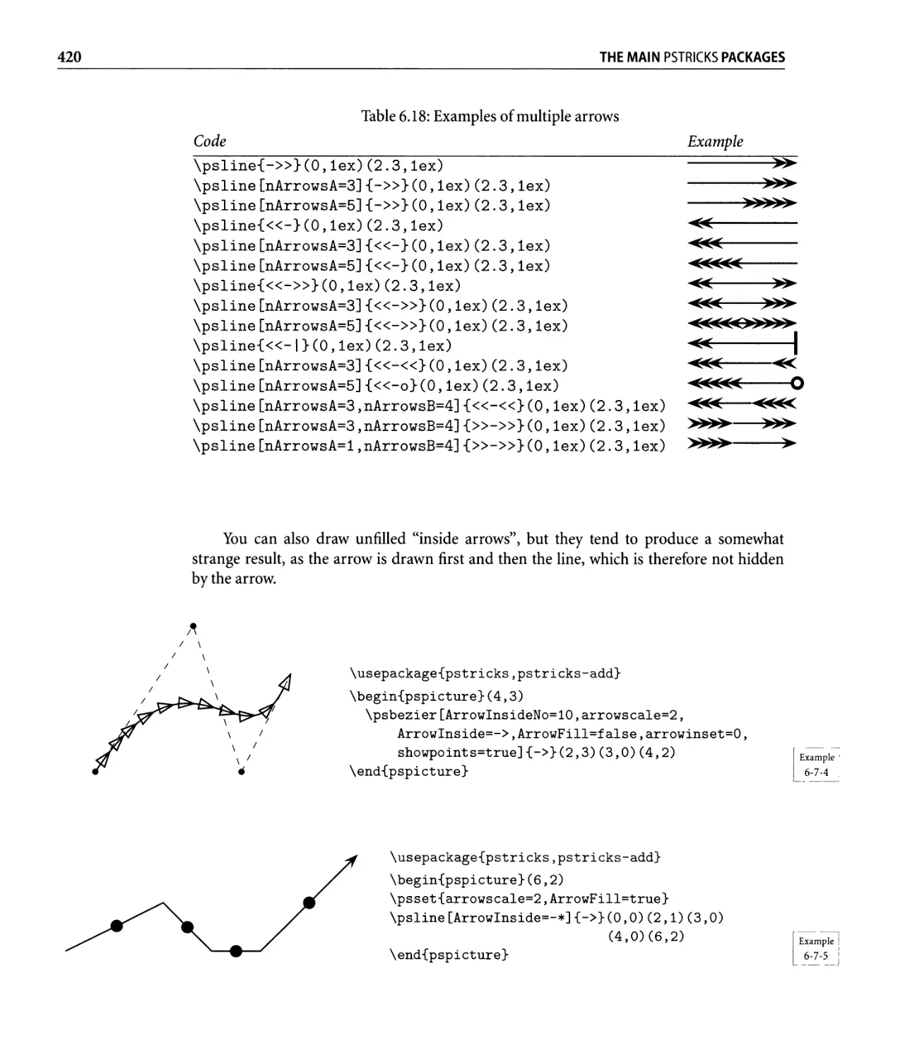
6.18 Examples of multiple arrows . . . . . . . . . . . . . . . . . . . . . . . . . . . . . . .. 420
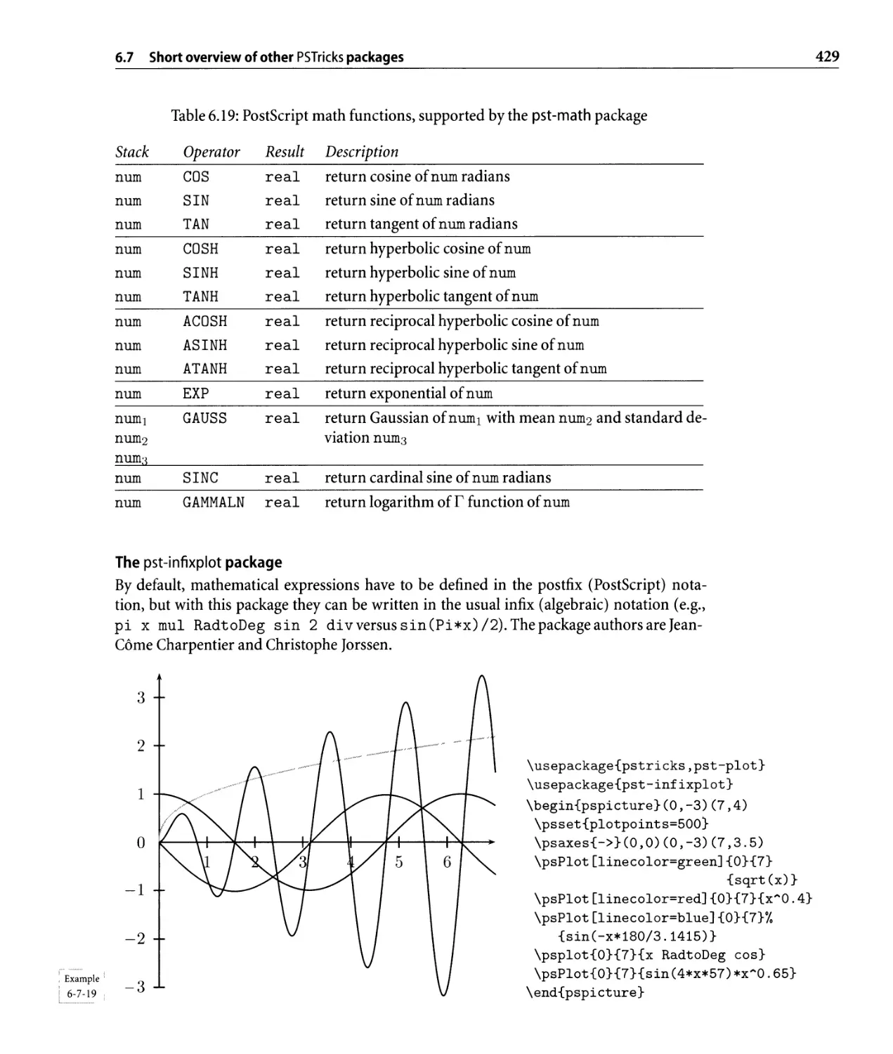
6.19 PostScript math functions, supported by the pst-math package . . . . . . . . .. 429
6.20 Alphabetical list of all environments of the basic PST ricks package. . . . . . . .. 459
6.21 Alphabetical list of all commands of the basic PST ricks package. . . . . . . . . .. 459
6.22 Alphabetical list of all keywords . . . . . . . . . . . . . . . . . . . . . . . . . . . . .. 462
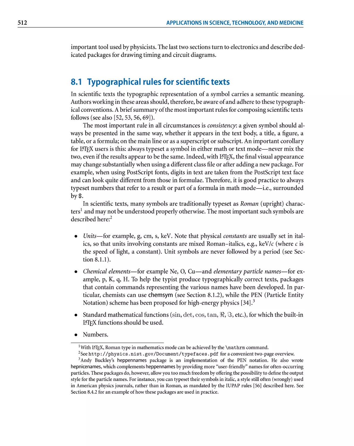
8.1 The importance of typographic rules in scientific texts. . . . . . . . . . . . . . .. 513
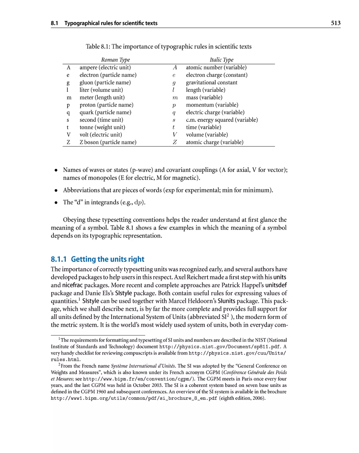
8.2 SI base units . . . . . . . . . . . . . . . . . . . . . . . . . . . . . . . . . . . . . . . . .. 514
8.3 Examples of SI -derived units . . . . . . . . . . . . . . . . . . . . . . . . . . . . . . .. 514
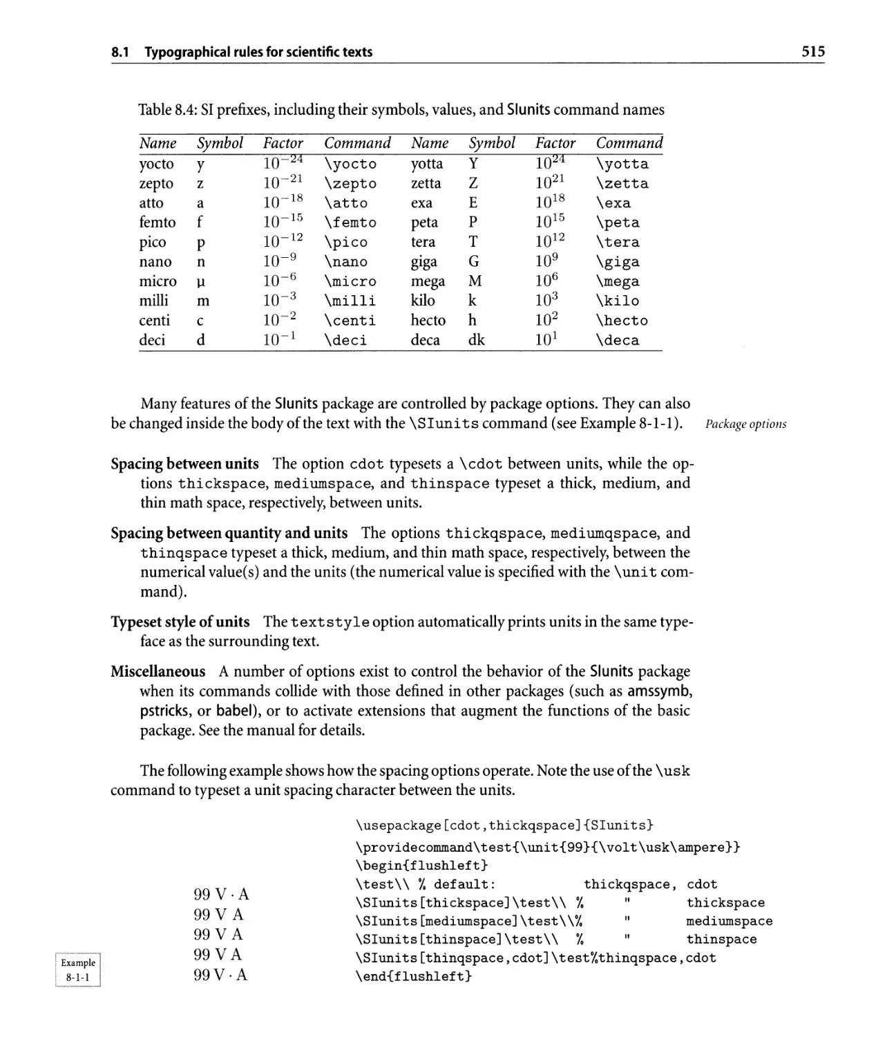
8.4 SI prefixes. . . . . . . . . . . . . . . . . . . . . . . . . . . . . . . . . . . . . . . . . . .. 515
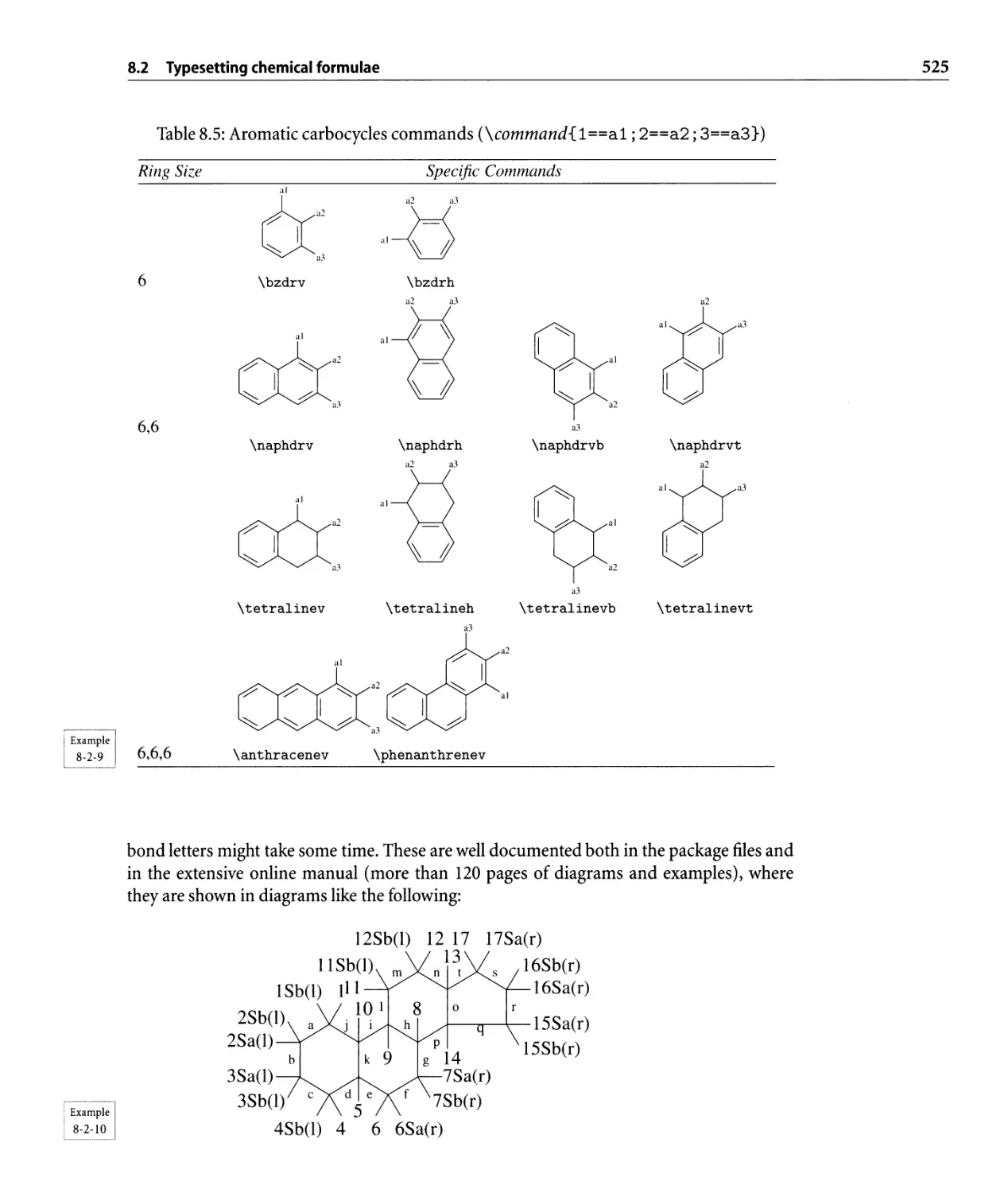
8.5 Aromatic carbocycles commands . . . . . . . . . . . . . . . . . . . . . . . . . . . .. 525
LIST OF TABLES
. ..
XXlll
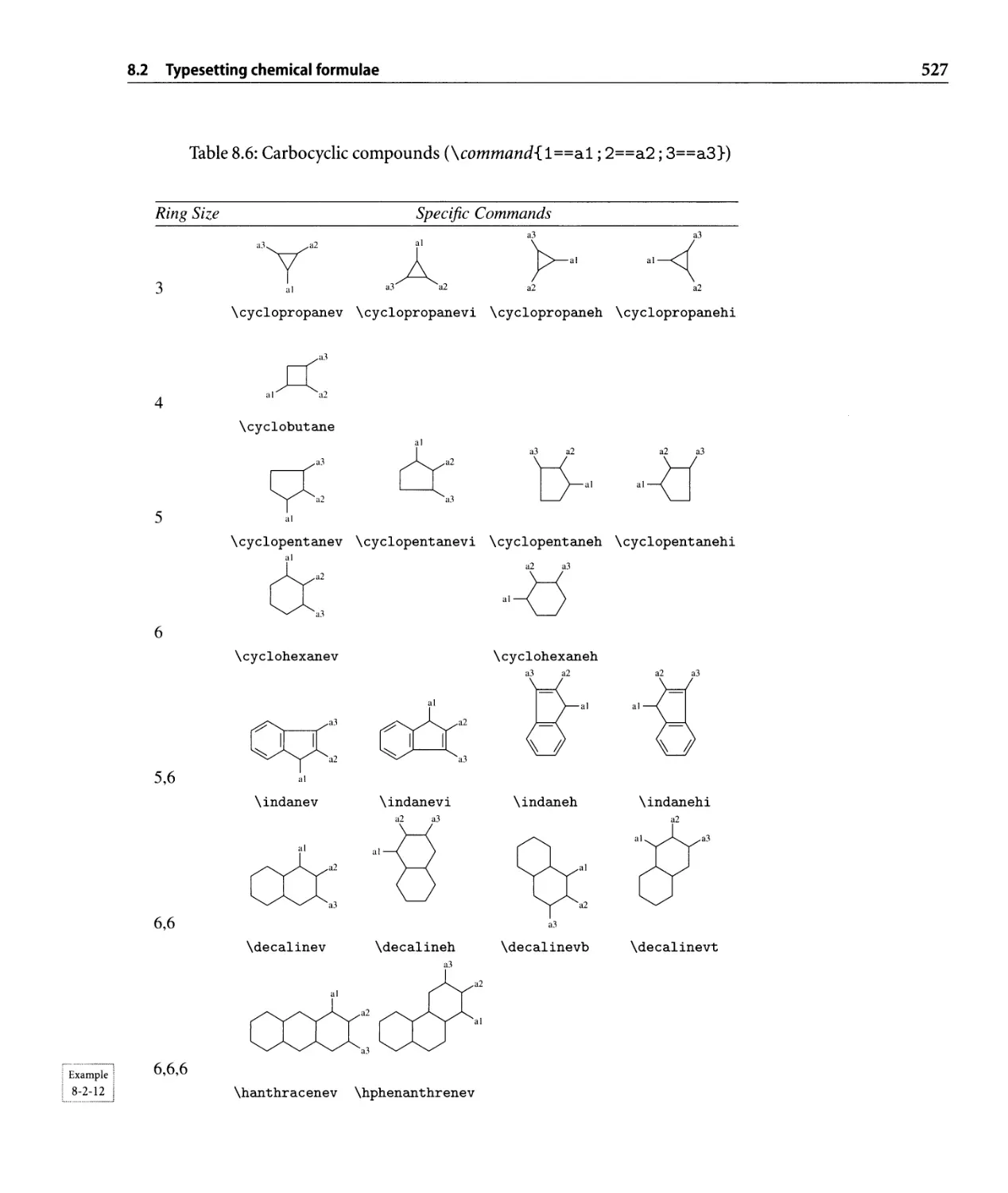
8.6 Carbocyclic compounds. . . . . . . . . . . . . . . . . . . . . . . . . . . . . . . . . .. 527
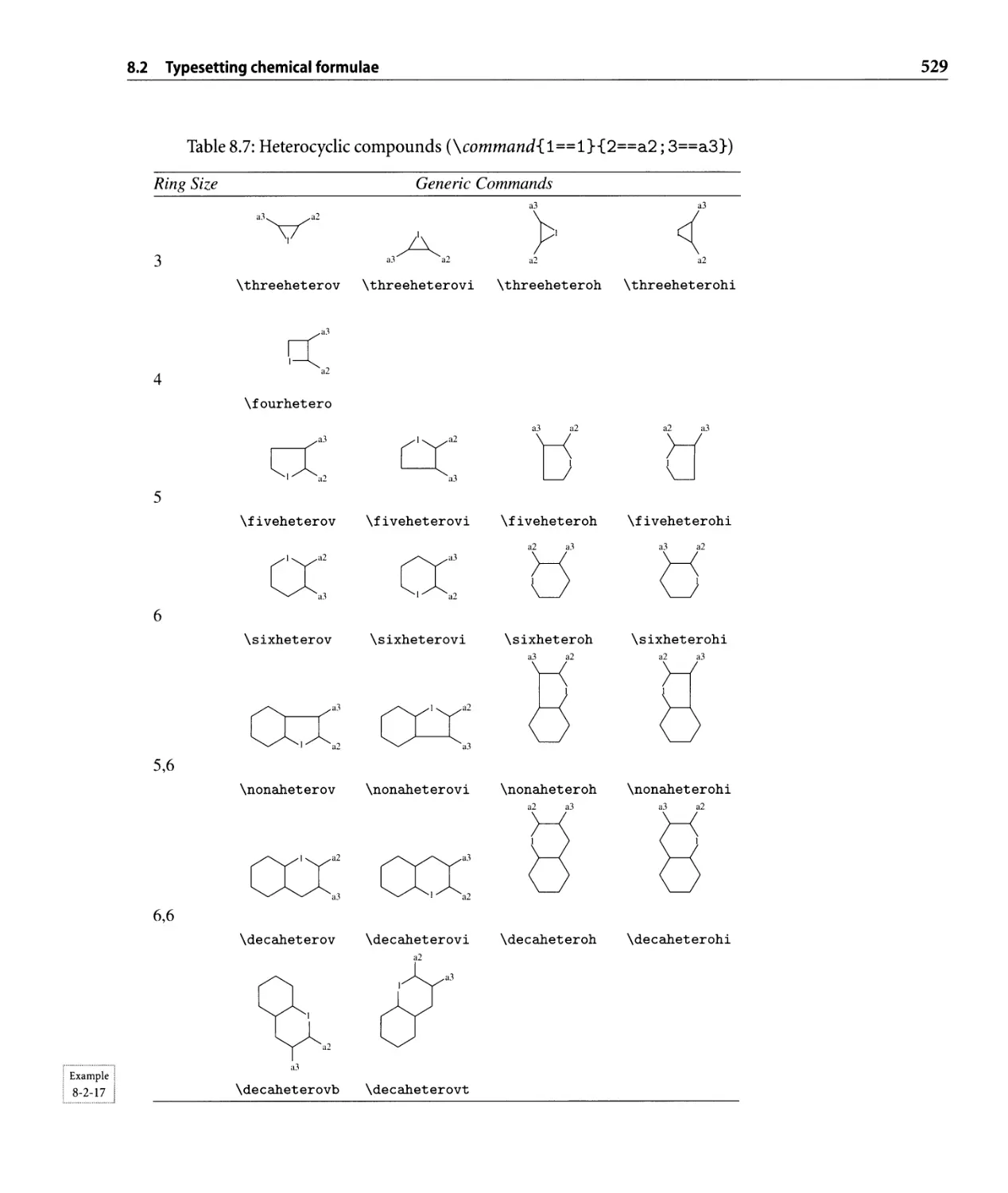
8.7 Heterocyclic compounds . . . . . . . . . . . . . . . . . . . . . . . . . . . . . . . . .. 529
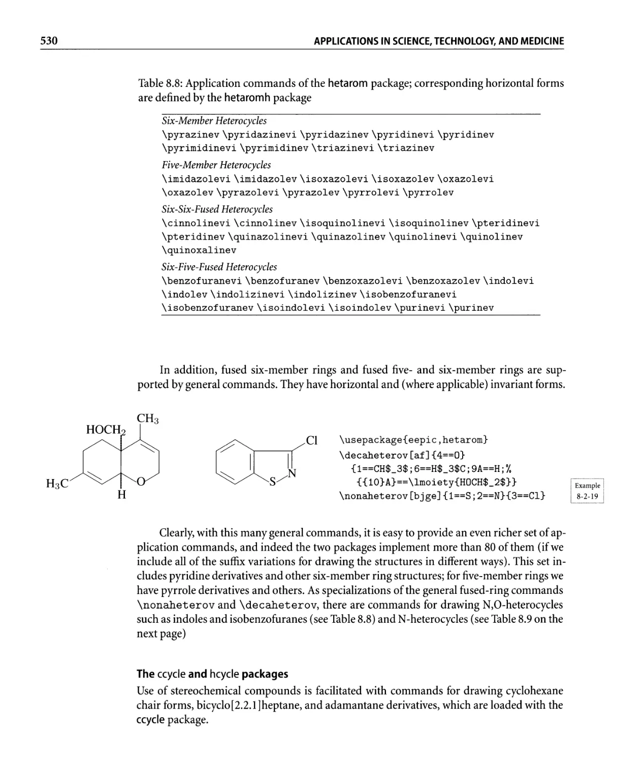
8.8 Application commands of the heta rom package . . . . . . . . . . . . . . . . . . .. 530
8.9 Heterocycles containing nitrogen . . . . . . . . . . . . . . . . . . . . . . . . . . . .. 531
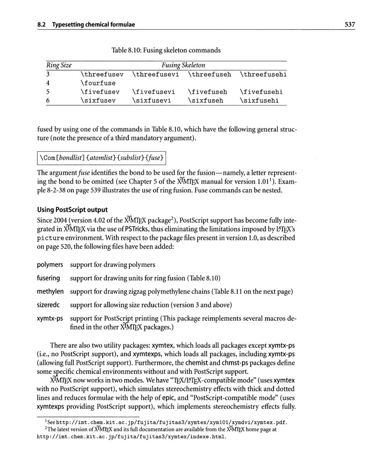
8.10 Fusing skeleton commands. . . . . . . . . . . . . . . . . . . . . . . . . . . . . . . .. 537
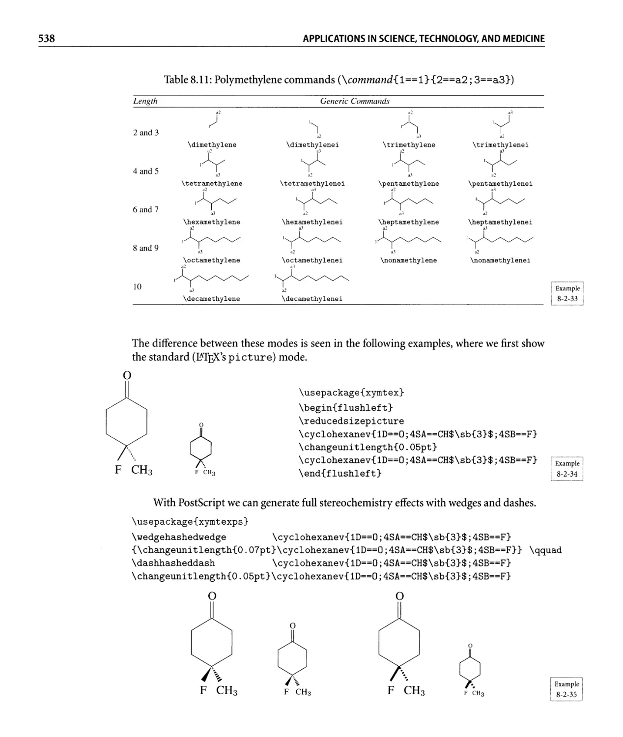
8.11 Polymethylene commands . . . . . . . . . . . . . . . . . . . . . . . . . . . . . . . .. 538
8.12 Bond identifiers for ppchtex . . . . . . . . . . . . . . . . . . . . . . . . . . . . . . .. 544
8.13 The f eyn font: available symbols, with their names and descriptions. . . . . .. 556
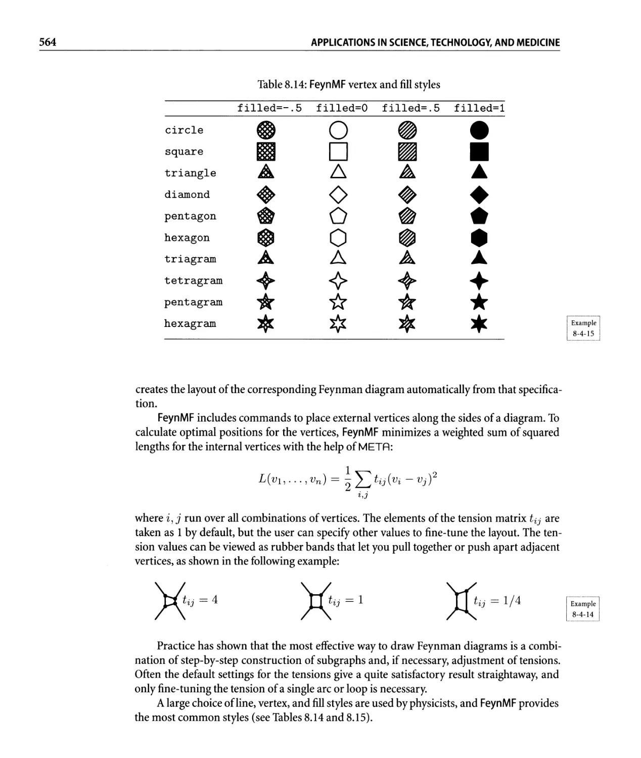
8.14 FeynMF vertex and fill styles . . . . . . . . . . . . . . . . . . . . . . . . . . . . . . .. 564
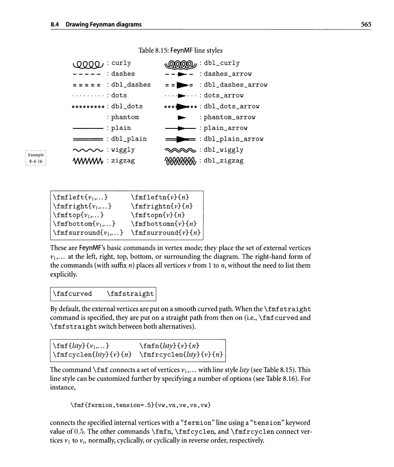
8.15 Feyn M F line styles. . . . . . . . . . . . . . . . . . . . . . . . . . . . . . . . . . . . . .. 565
8.16 FeynMF line-drawing keywords . . . . . . . . . . . . . . . . . . . . . . . . . . . . .. 566
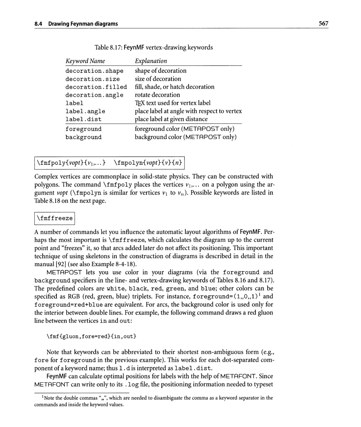
8.17 FeynMFvertex-drawingkeywords............................. 567
8.18 FeynMFpolygonkeywords ................................. 568
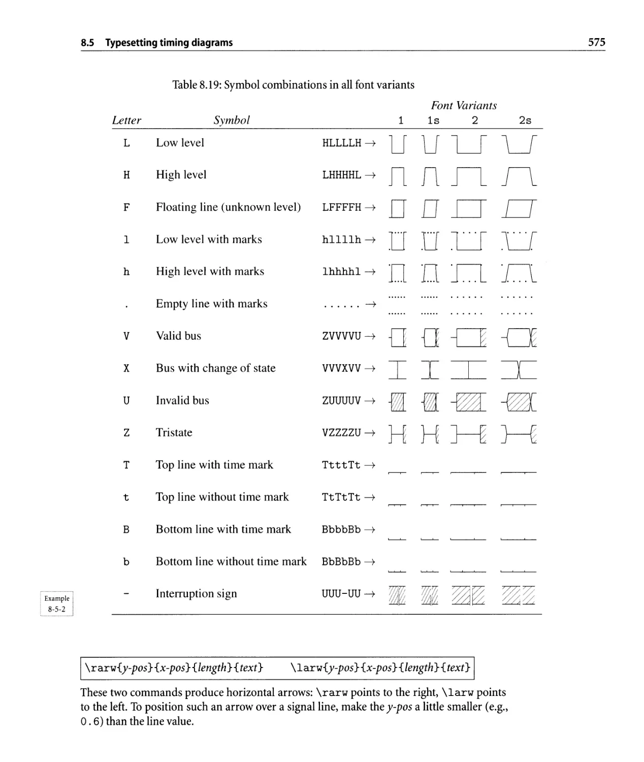
8.19 Symbol combinations in all font variants of the timing package . . . . . . . . .. 575
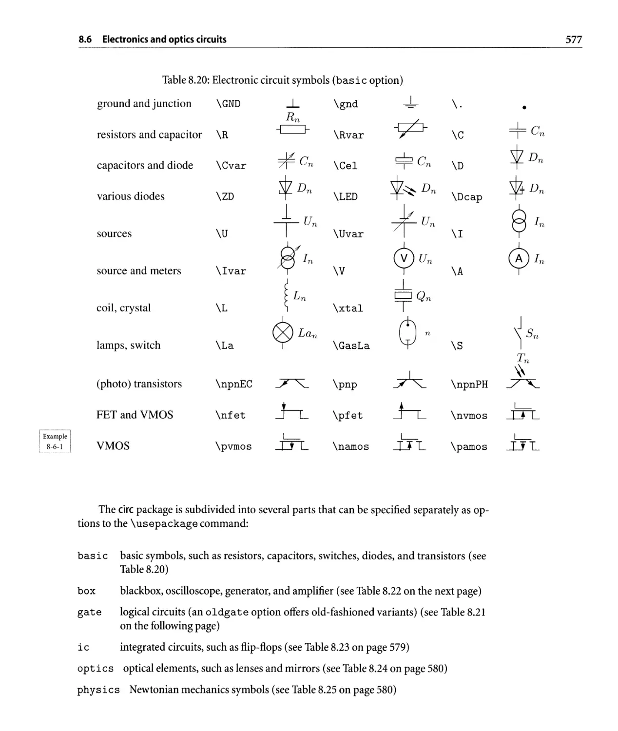
8.20 Electronic circuit symbols (basic option) . . . . . . . . . . . . . . . . . . . . . .. 577
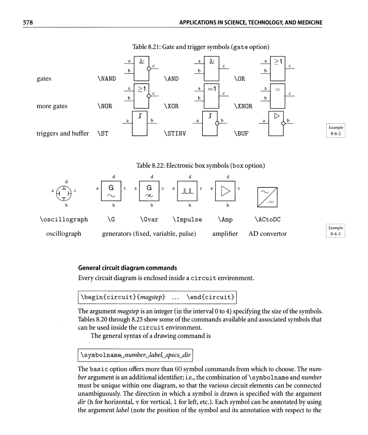
8.21 Gate and trigger symbols (gate option). . . . . . . . . . . . . . . . . . . . . . . .. 578
8.22 Electronic box symbols (box option). . . . . . . . . . . . . . . . . . . . . . . . . .. 578
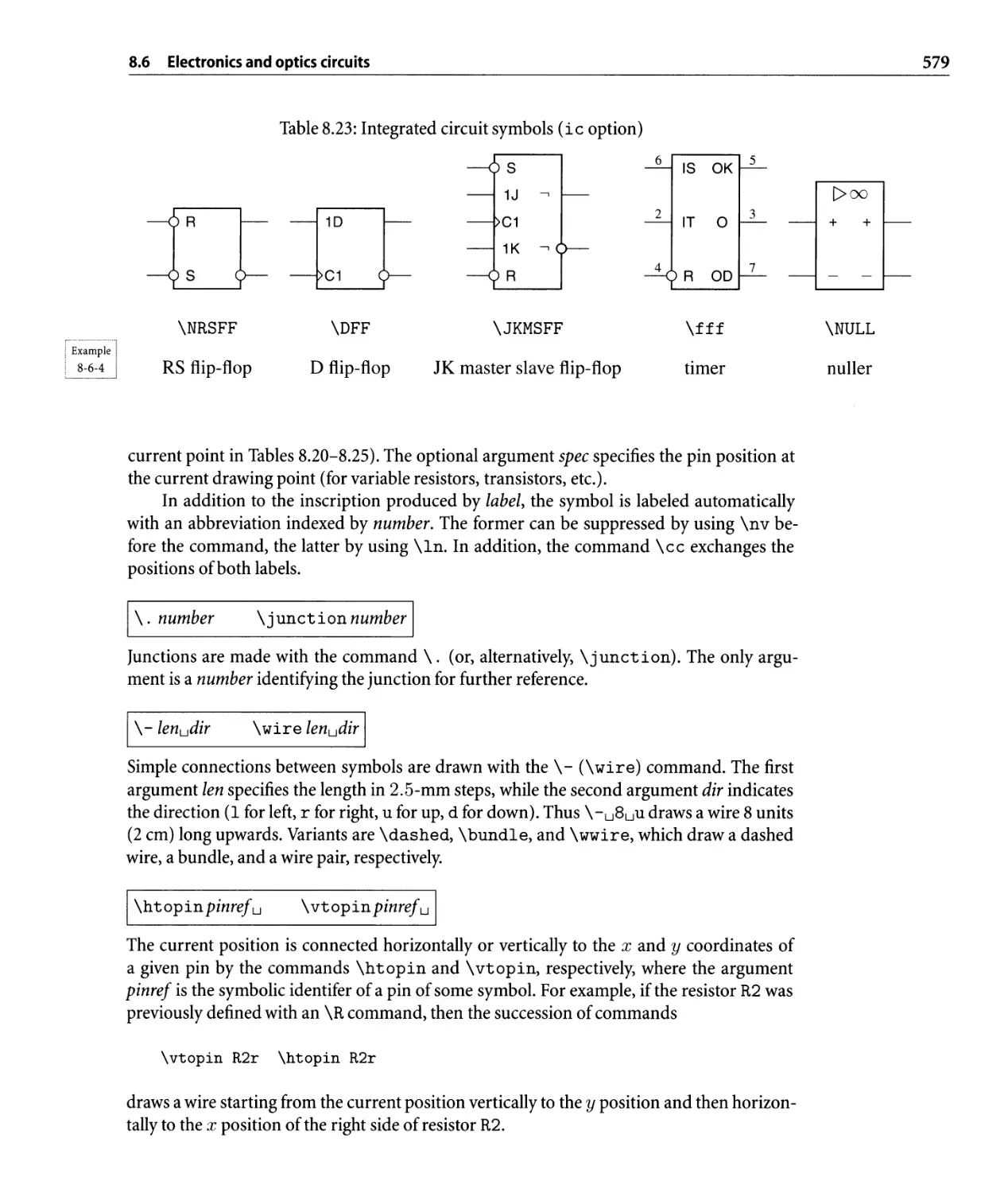
8.23 Integrated circuit symbols (ic option). . . . . . . . . . . . . . . . . . . . . . . . .. 579
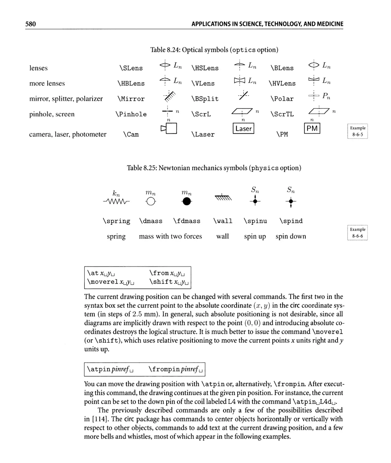
8.24 Optical symbols (optics option). ............................ 580
8.25 Newtonian mechanics symbols (physics option) . . . . . . . . . . . . . . . . .. 580
9.1 Overview of MusiXTEX commands. . . . . . . . . . . . . . . . . . . . . . . . . . . .. 592
9.2 Variantformsofthe\notescommand......................... 595
9.3 Overview of information fields in abc language tune files . . . . . . . . . . . . .. 602
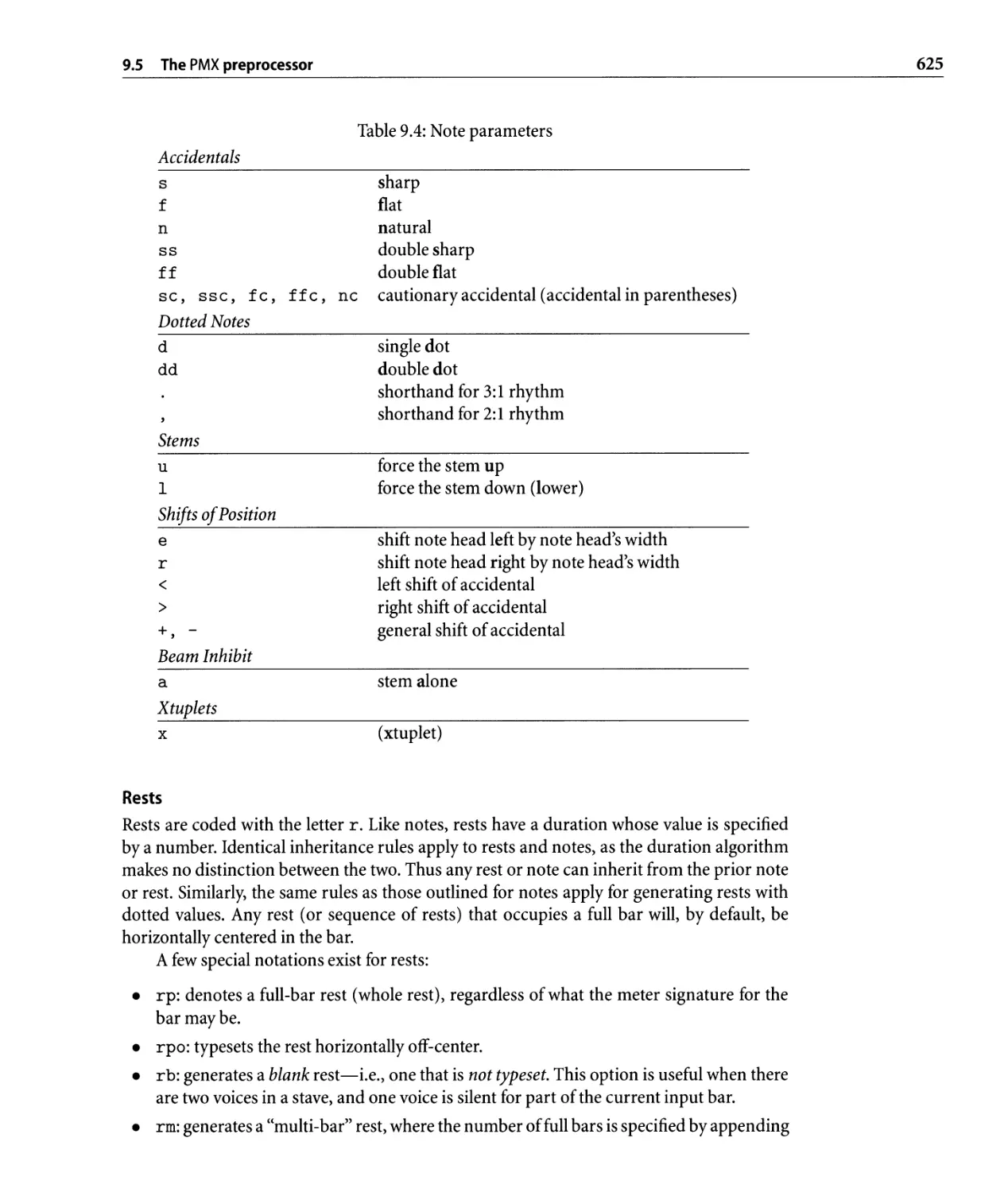
9.4 Note parameters. . . . . . . . . . . . . . . . . . . . . . . . . . . . . . . . . . . . . . .. 625
9.5 List of ornaments . . . . . . . . . . . . . . . . . . . . . . . . . . . . . . . . . . . . . .. 631
9.6 PMX global A options. . . . . . . . . . . . . . . . . . . . . . . . . . . . . . . . . . . .. 643
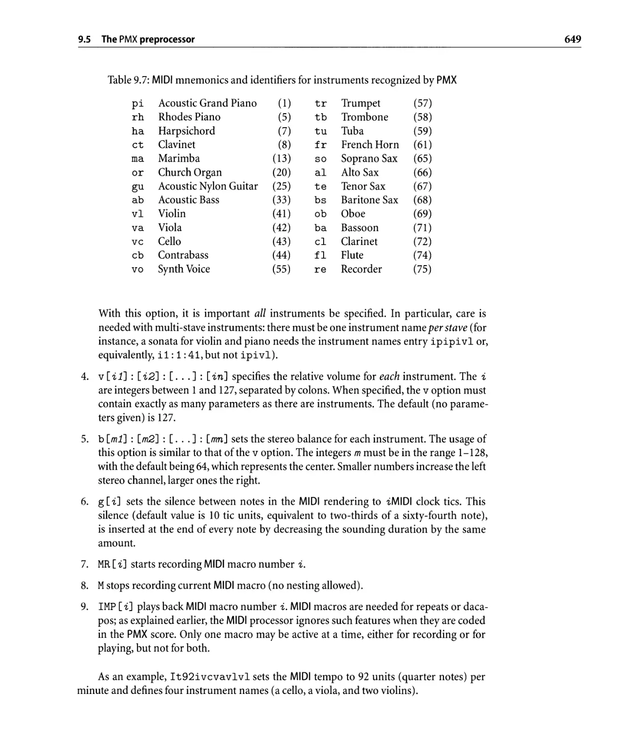
9.7 MIDI mnemonics and identifiers for instruments recognized by PMX . . . . . .. 649
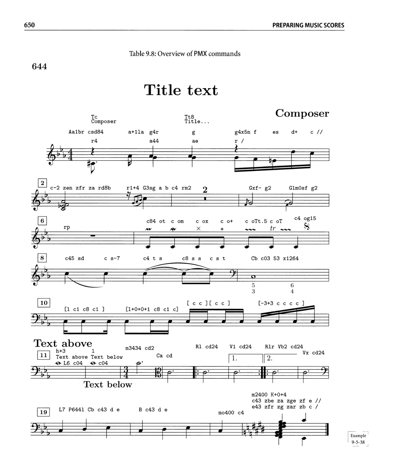
9.8 Overview of PMX commands. . . . . . . . . . . . . . . . . . . . . . . . . . . . . . .. 650
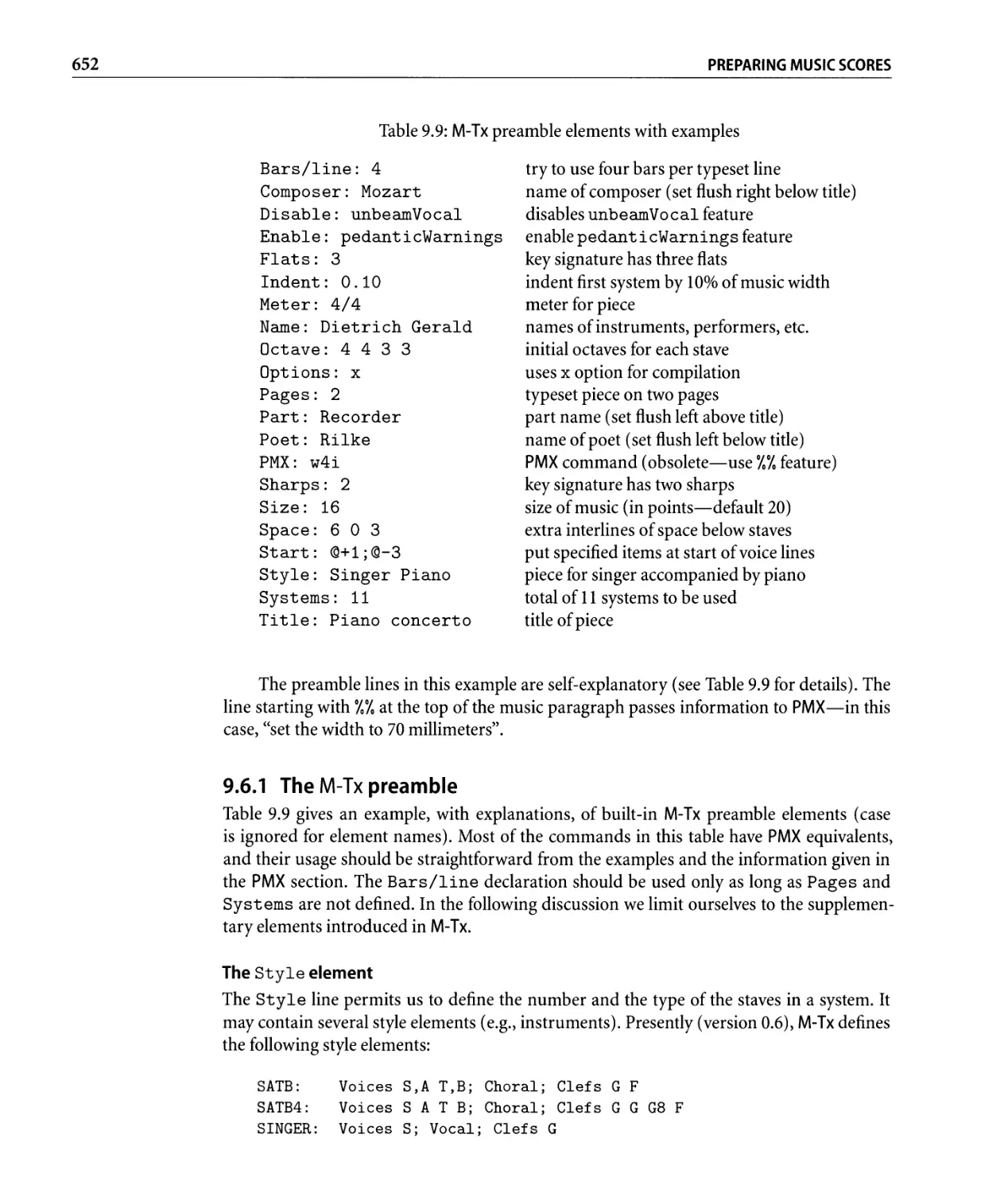
9.9 M-Txpreambleelementswithexamples......................... 652
10.1 Informational symbols for chess. . . . . . . . . . . . . . . . . . . . . . . . . . . . .. 674
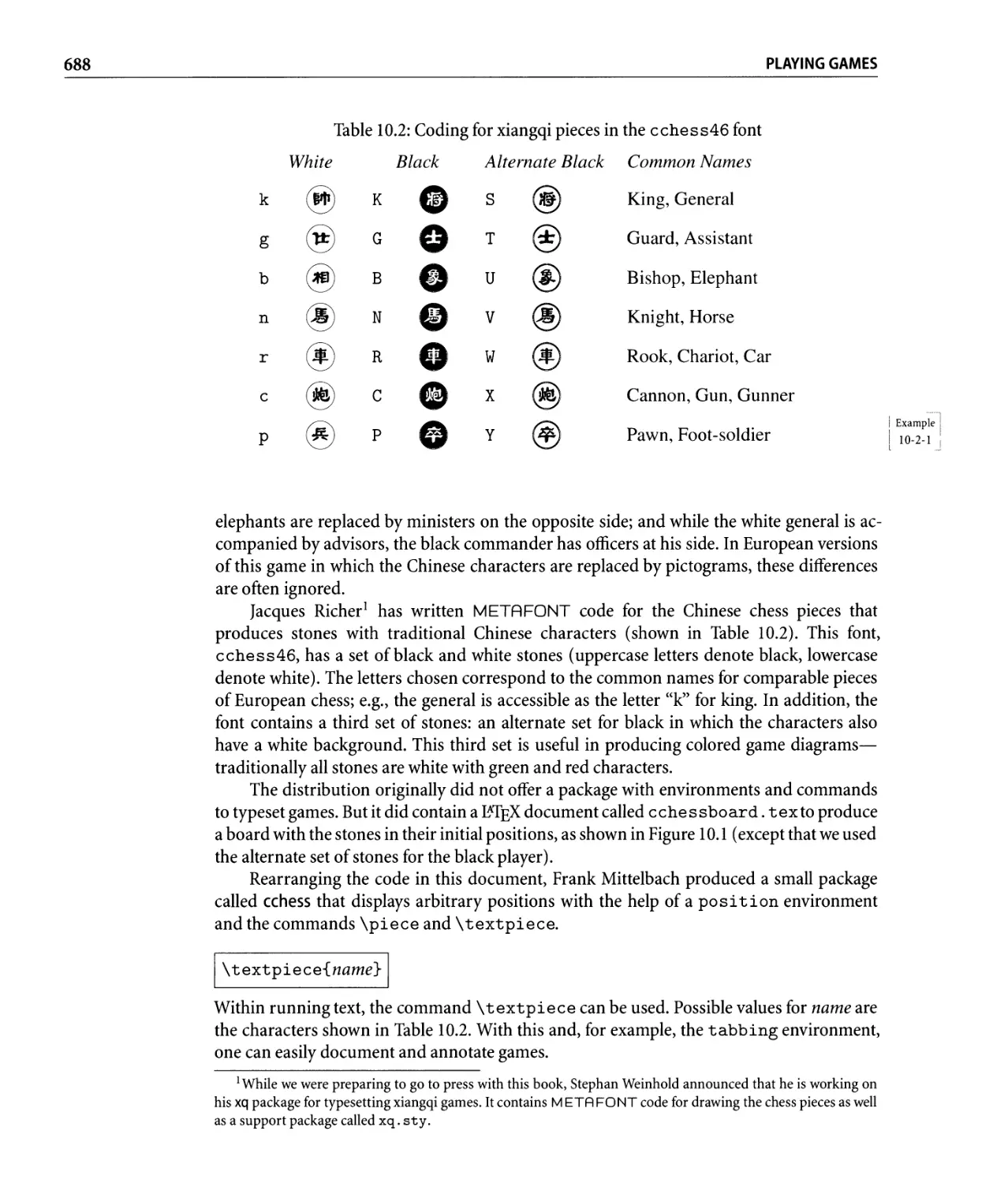
10.2 Coding for xiangqi pieces in the cchess46 font. . . . . . . . . . . . . . . . . . .. 688
11.1 Symbolic connotation of colors in different countries. . . . . . . . . . . . . . . .. 716
11.2 Color models supported by xcolor. . . . . . . . . . . . . . . . . . . . . . . . . . . .. 728
11.3 beamer class options and modes . . . . . . . . . . . . . . . . . . . . . . . . . . . .. 753
11.4 Predefined themes and layouts in beamer. . . . . . . . . . . . . . . . . . . . . . .. 755
11.5 Keywords for the frame environment of beamer . . . . . . . . . . . . . . . . . .. 759
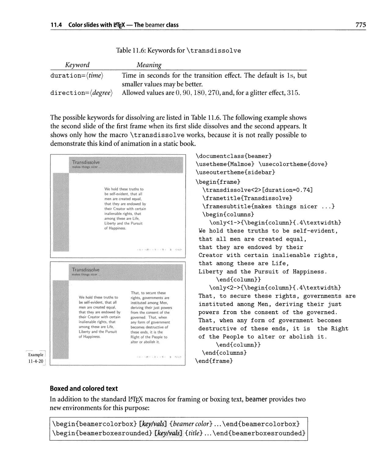
11.6 Keywords for \ transdissol ve . . . . . . . . . . . . . . . . . . . . . . . . . . . .. 775
11.7 Keywords for the beamercolorbox environment . . . . . . . . . . . . . . . . .. 777
11.8 Keywords for the beamerboxesrounded environment. . . . . . . . . . . . . .. 778
11.9 Keywordsforthecolumnsenvironment ........................ 781
11.10 Keywords for the \ tableof contents command . . . . . . . . . . . . . . . . .. 783
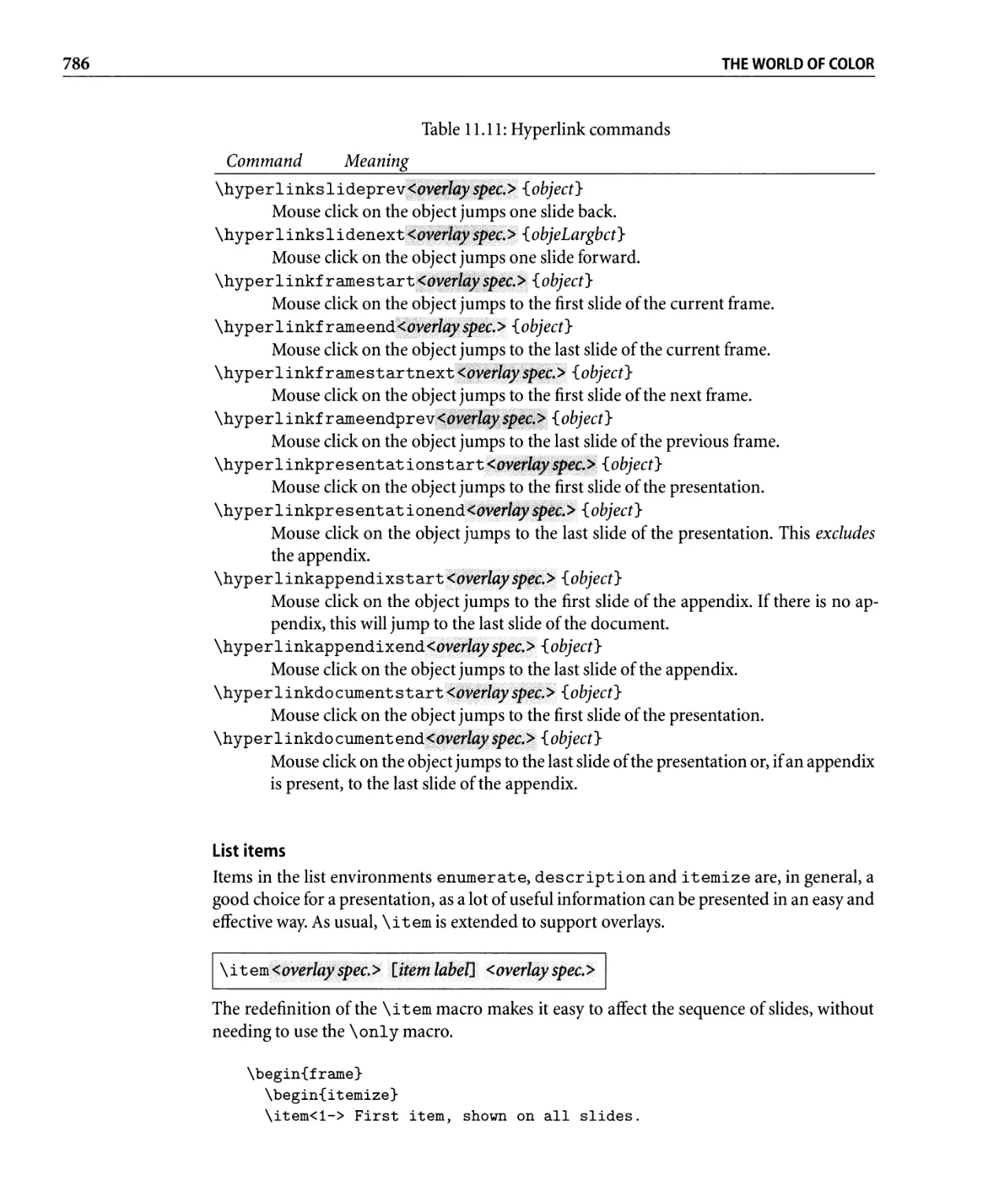
11.11 Hyperlink commands . . . . . . . . . . . . . . . . . . . . . . . . . . . . . . . . . . .. 786
11.12 Font attributes for beamer . . . . . . . . . . . . . . . . . . . . . . . . . . . . . . . .. 793
8/16
2/10
9
I
I
5 I
I
6 4 I
I
I
I
I
I
I
2
1
4/12
1f
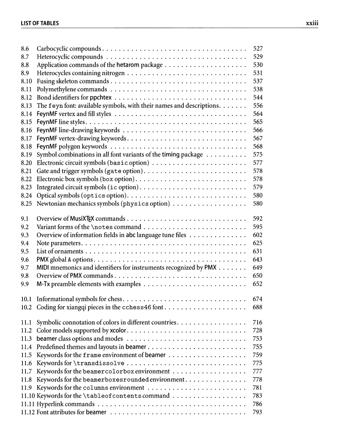
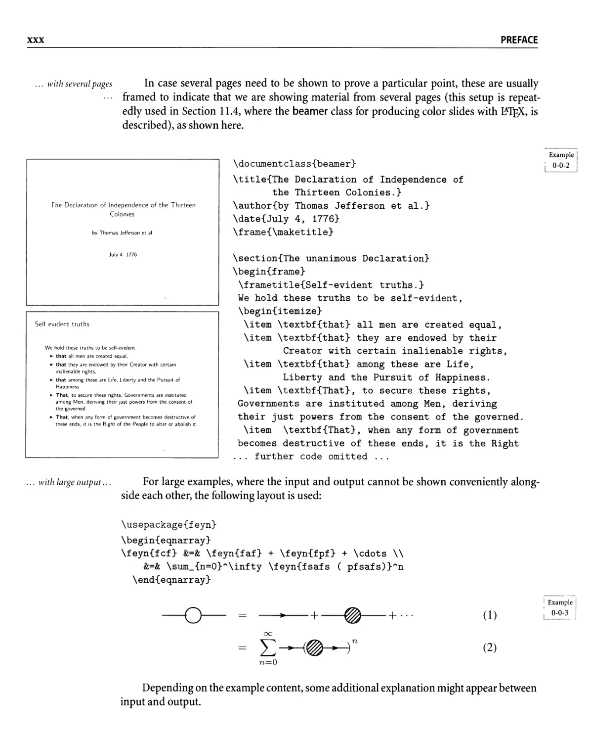
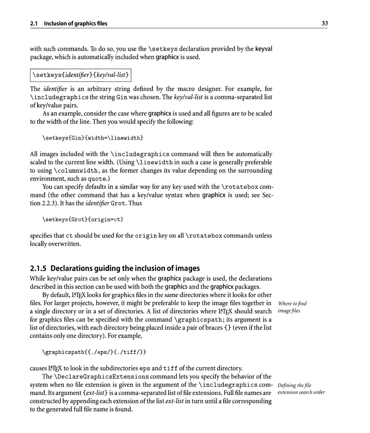
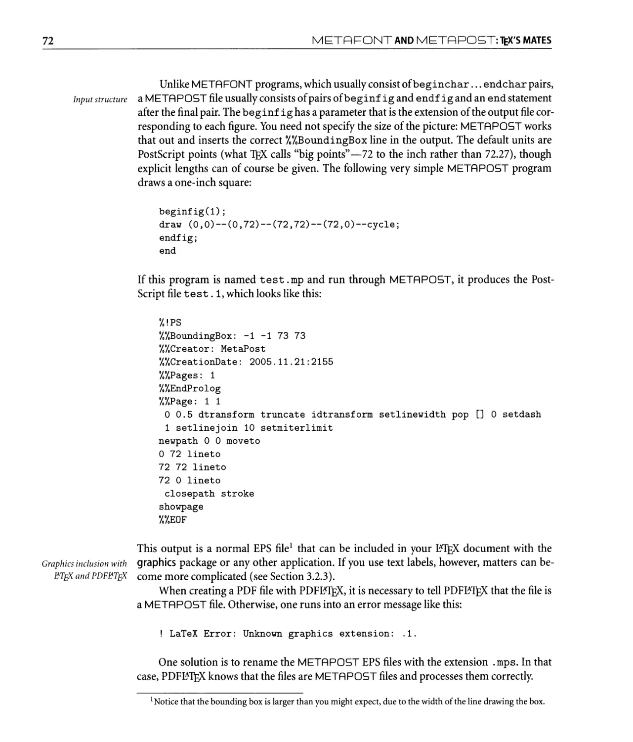
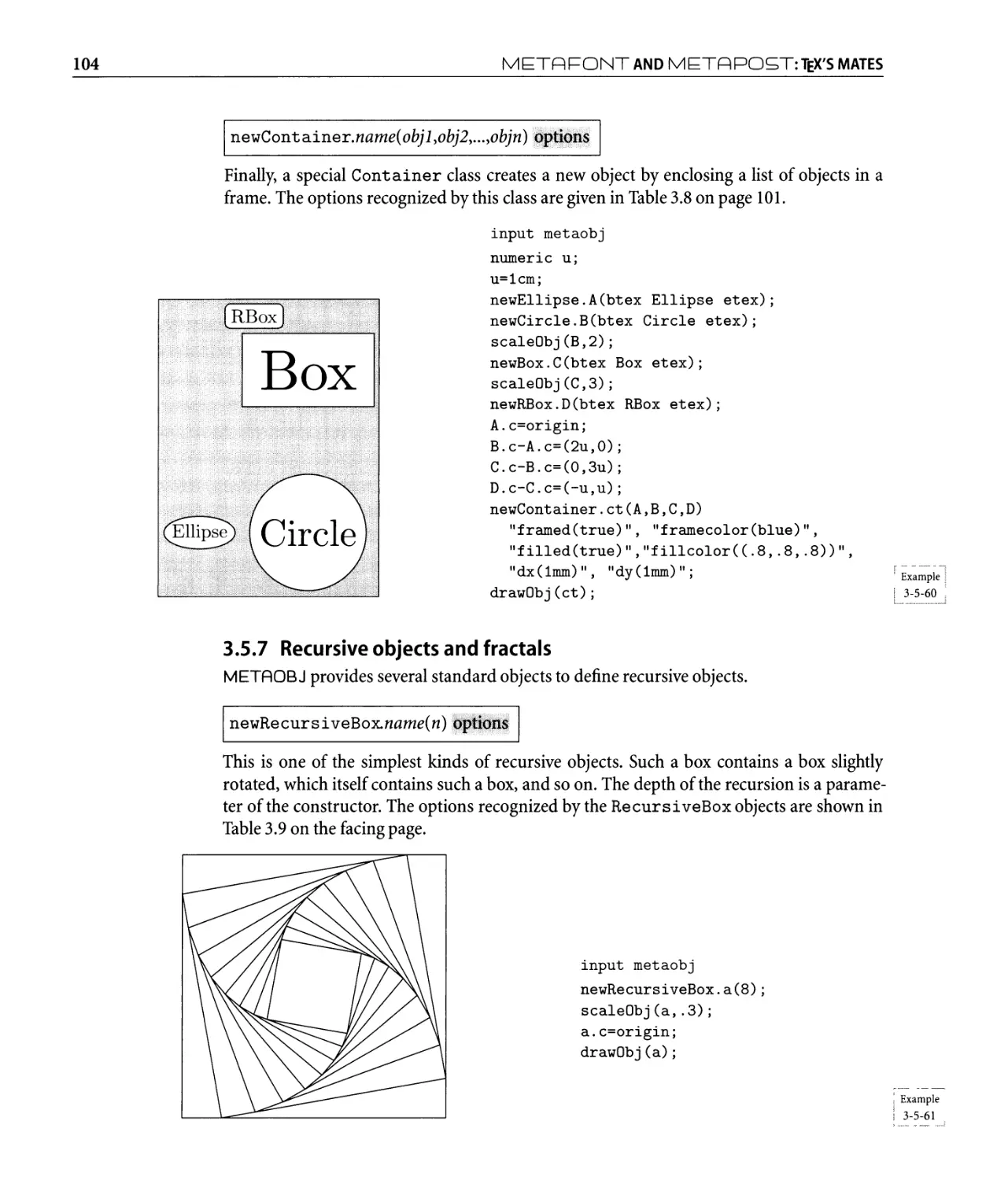
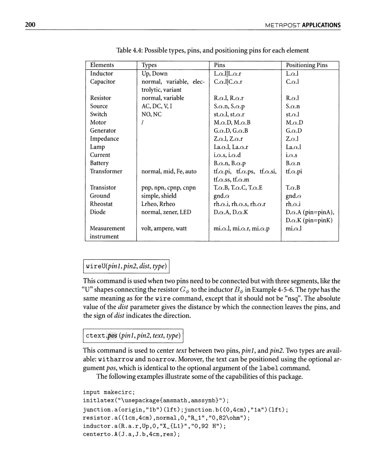
y(wt) == 2 . cos(2wt + 4 )
12
14
13
x(wt) == 3.5 . cos(wt)
A Lissajous example with PSTricks (idea by Jurgen Gilg)
Preface
More than a decade has passed since the publication of the first edition of The YTEX Graphics
Companion, and there have been many changes and new developments since 1996.
The second edition has seen a major change in the authorship: Frank, Michel and Se-
bastian have been joined by Denis and Herbert as authors, enriching the book with their
knowledge and experience in individual subject areas.
As in the first edition, this book describes techniques and tricks of extended M-TEX type-
setting in the area of graphics and fonts. We examine how to draw pictures with M-TFX and
how to incorporate graphics files into a TEX document. We explain how to program pic-
tures using METAFoNT and METAPo5T, as well as how to achieve special effects with
small fragments of embedded PostScript. We look in detail at a whole range of tools for build-
ing graphics in 'lEX itself.
'lEX is the world's premiere markup-based typesetting system, and PostScript (on
which PDF is based) is the leading language for describing the printed page. We describe
how they can produce even more beautiful results when they work together. 'lEX's mathemat-
ical capability, its paragraph building, its hyphenation, and its programmable extensibility
can cooperate with the graphical flexibility and font-handling capabilities of PostScript and
PDF to provide a rich partnership for both author and typesetter.
To be able to do justice to the graphics packages that have been further developed since
the first edition, we decided to omit a description of PostScript and PDF tools, and of font
technologies, from the printed version of this book. This material, which was covered in
Chapters 10 and 11 of the first edition, has been substantially expanded and is now freely
available (see http://xml. cern. ch/lgc2). It covers DVI-to-PostScript drivers, the free
program ghostscript to view PostScript and PDF files, tools for manipulating PostScript and
PDF files, and suggestions on how to combine the latest font technologies (PostScript Type 1
and OpenType) with M-TEX.
.
XXVI
PREFACE
This volume is not a complete consumer guide to packages. In trying to teach by ex-
ample, we present hundreds of self-contained code samples of the most useful types of solu-
tions, based on proven and well-known implementations. But, given the space available, we
cannot provide a full manual for every package. Our aim is simply to show how easy it is to
use a given package and to indicate whether it seems to do what is required-not to dwell
on the precise details of syntax or options. Nevertheless, we have described in more detail a
few selected tools that we consider especially important.
We assume you know some TEX; you cannot read this book by itself if you have never
used 'lEX before. We recommend that you start with YTEX: A Document Preparation Sys-
tem, Second Edition [78], or the Guide to YTEX, Fourth Edition [76], and continue with The
YTEX Companion, Second Edition [83], to explore some of the many (non-graphical) pack-
ages available.
Why I!\TEX, and why PostScript?
This book is about M-TEX, graphics, PostScript, and its child PDF. We believe that the struc-
tured approach of a system like M-TEX is the best way to use 'lEX, and M-TEX is by far the
most widely used 'lEX format. This means that it attracts contributors who develop new pack-
ages, and thus some of what we describe works only in M-TEX. We apologize in advance for
our M-TEX bias to those who appreciate the elegance of the original plain 'lEX format and its
derivatives, and we promise them that most of the packages will work well with any 'lEX di-
alect: the delights of systems such as META POST, PSTricks, XV-pic, and MusiXTEX are open
to all.
We also want to explain why we talk about PostScript so much. This language has been
well established for almost two decades as an extremely flexible page-description language,
and it remains the tool of choice for professional typesetters. Among the features that make
it so attractive are these:
. The quantity, quality, and flexibility of Type 1 fonts
. The device-independence and portability of files
. The quality of graphics and the quantity of drawing packages that generate it
. The facilities for manipulating text
. The mature color-printing technology
. The encapsulation conventions that make it easy to embed PostScript graphics
. The availability of screen-based implementations (e.g., ghostscript/ghostview)
PostScript has spawned an enterprising child, the PDF (Portable Document Format)
language, used by Adobe Acrobat and now well established as an exchange format for doc-
uments on the Web. Designed for screen display with hypertext features, PDF offers a new
degree of portability and efficiency. Although not the main subject of this book, we neverthe-
less mention that M-TEX can also produce "rich" PDF documents, and versions of 'lEX (e.g.,
pdflatex) that produce PDF directly are available.
PREFACE
..
XXVll
Again, we apologize to those of you who are disappointed not to read about TEX's
association with Mac's QuickDraw, or the Windows GDI, HPGL, PCL, etc., but with so many
packages available, we had to make a choice.
Please note that the absence of a given package or tool in this book in no way implies
that we consider it less useful or of inferior quality. We do think, though, that we have in-
cluded a representative set of tools and packages, and we sincerely hope that you will find
here one or more subjects to entertain you.
How this book is arranged
This book is subdivided in two basic ways: by application area and by technique. We suggest
that all readers look at Chapter 1 before going any further, because it introduces how we Basic information in
think about graphics and summarizes some techniques developed in later chapters. We also Chapters 1 and 2
suggest that you read Chapter 2, which covers the M-TFX standard graphics package, since the
tools for including graphics files will be needed often. Chapter 2 also covers pict2e, a package
that reimplements TEX'S pi cture environment using PostScript, and a further extension
curve2e. Together these packages not only do away with most of the limitations inherent
in the standard version of TFX's picture, but also offer new and powerful commands to
draw arcs and curves with mininal effort.
We have tried to make it possible to read each of the other chapters separately; you may
prefer to go straight to the chapters that cover your subject area or look at those that describe
a particular tool. Two chapters each are dedicated to the generic systems META POST and
PSTricks.
3 META FONT and META POST: 'lEX's Mates shows how to exploit the power of 'lEX's
META languages (Knuth's METAFoNT and its PostScript-based extension META-
POST). After introducing the basic functions, the basic METAPoST libraries are de-
scribed, as well as available 'lEX interfaces and miscellaneous tools and utilities.
4 META POST Applications introduces the METAPosT toolkit, and explains how to
use META POST's unparalleled expressive power for describing many types of graphs,
diagrams, and geometric constructs. Applications in the areas of science and engineer-
ing, 3-D representations, posters, etc. conclude the overview.
S Harnessing PostScript Inside 1FX: PSTricks walks the reader through the various com-
ponents of the PSTricks language, looking at such things as defining the coordinate sys-
tem, lines and polygons, circles, ellipses and curves, arrows, labels, fill areas, and much
more.
6 The Main PSTricks Packages takes you even deeper into the world of PSTricks. Armed
with the knowledge gained in Chapter 5, the reader will find here detailed descriptions
of the most common PSTricks packages-in particular, pst-plot for plotting functions
and data; pst-node for mastering nodes and their connections; pst-tree for creating tree
diagrams; pst-fill for filling and tiling areas; pst-3d for creating 3-D effects, such as shad-
ows and tilting; and pst-3dplot for handling 3-D functions and data sets. The chapter
ends with a summary of PSTricks commands and keywords.
...
XXVlll
PREFACE
The next four chapters discuss problems in special application areas and survey more
packages:
7 The XV-pic Package introduces a package that goes to great lengths to define a notation
for many kinds of mathematics diagrams and implements it in a generic and portable
way.
S Applications in Science, Technology, and Medicine looks at chemical formulae and
bonds, applications in bioinformatics, Feynman diagrams, timing diagrams, and elec-
tronic and optics circuits.
9 Preparing Music Scores first describes the principles of the powerful MusiXTEX package.
Then several preprocessors providing a more convenient interface are introduced: abc
for folk tunes, PMX for entering polyphonic music, and M- Tx (an offspring of PMX) for
dealing with multi-voice lyrics in scores. We also take a short look at LilyPond, a modern
music typesetter written in C++, and say a few words about 'lEXmuse.
10 Playing Games is for those who use M-TFX for playas well as for work. It shows you how
to describe chess games and typeset chess boards (the usual and oriental variants). This
chapter also describes how to handle Go, backgammon, and card games. We conclude
with crosswords in various forms and Sudokus, including how to typeset, solve, and
generate them.
Our last chapter addresses an area of general interest: color, and some of its common
uses in M-TEX.
11 The World of Color starts with a short general introduction to color. Next comes an
overview of the xcolor package and the colortbl package, that is based on xcolor. The
final part discusses the beamer class for producing color slides with TFX.
Appendix A describes ways to generate PDF from TEX. Appendix B introduces CTAN
and explains how to download the TEX packages described in this book.
As mentioned earlier, material about PostScript and PDF tools, as well as information
about how to use PostScript and Open Type fonts with TEX, is available as supplementary
material (see http://xml. cern. ch/lgc2), which covers the following subjects:
PostScript Fonts and Beyond describes the ins and outs of using PostScript fonts with
1EX. It also looks at the latest developments on how to integrate Open Type fonts by
creating 'lEX -specific auxiliary files ('lEX metrics, virtual fonts, etc.) or by reading the
font's characteristics directly in the Open Type source.
PostScript and PDF Tools starts with a short introduction to the PostScript, PDF, and
SVG languages. It then describes some freely available programs, in particular dvips
and pdflatex to generate PostScript and PDF, ghostscript and ghostview to manipulate
and view PostScript and PDF, plus a set of other tools that facilitate handling PostScript
and PDF files and conversions.
PREFACE
.
XXIX
Typographic conventions
It is essential that the presentation of the material conveys immediately its function in the
framework of the text. Therefore, we present below the typographic conventions used in this
book.
Throughout the text, M-JEX command and environment names are set in mono-spaced Commands,
type (e.g., \includegraphics, sidewaystable, \begin{ tabular}), while names of environments,
package and class files are in sans serif type (e.g., graphicx). Commands to be typed by packages,...
the user on a computer terminal are shown in monospaced type and are underlined (e.g.,
This is user input ).
The syntax of the more complex
JEX commands is presented inside a rectangular box. Syntax descriptions
Command arguments are shown in italic type:
\includegraphics* [llx, Zly] [urx, ury] {fiZe}
In
JEX, optional arguments are denoted with square brackets and the star indicates a vari-
ant form (i.e., is also optional), so the above box means that the \includegraphics com-
mand can come in six different incarnations:
\incl udegraphics {file}
\includegraphics [llx, lly] {file}
\includegraphics [llx, lly] [urx, ury] {.file}
\includegraphics * {.file}
\ incl udegraphics * [lIx, lly] {file}
\includegraphics* [lIx, lly] [urx, ury] {file}
In case of PST ricks the syntax is not as straight forward and optional arguments may
have other delimiters than brackets. For this reason they are shown with a gray background
as in the following example:
\ps t r i angl el! ill.'illll!
Lines containing examples with B\JEX commands are indented and are typeset in a Code examples. . .
monospaced type at a size somewhat smaller than that of the main text:
\fmfdotn{v}{4}
\fmfv{decor.shape=circle,decor.filled=full,
decor.size=2thick}{vl,v2,v3,v4}
However, in the majority of cases we provide complete examples together with the output . .. with output. . .
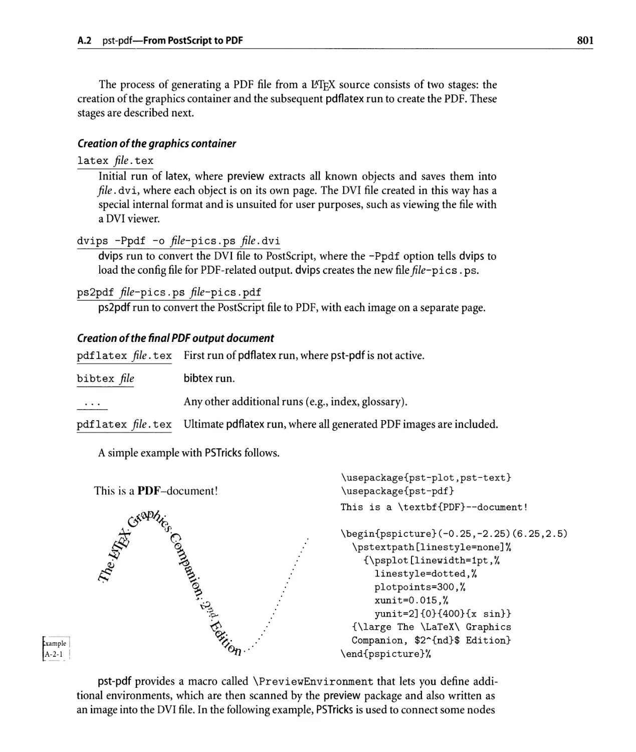
they produce side by side:
u
\usepackage{feyn}
$\feyn{fglf}$ \qquad $\Feyn{fglf}$
I E
mPle J
-0-1
Note that the preamble commands are always shown in blue in the example source.
xxx PREFACE
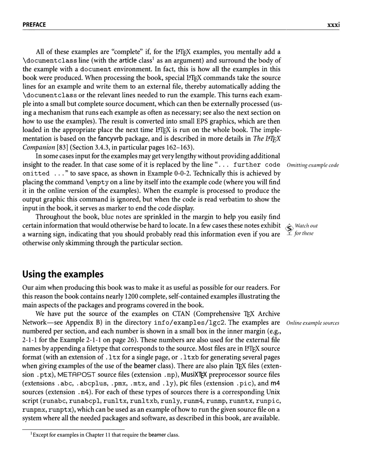
. .. with several pages In case several pages need to be shown to prove a particular point, these are usually
framed to indicate that we are showing material from several pages (this setup is repeat-
edly used in Section 11.4, where the beamer class for producing color slides with M-JEX, is
described), as shown here.
r he Declaration of Independence of the Thirteen
Colon les
by Thomas Jefferson et al
July 4 1776
Self E'vldpnt t rut hs
We hold these truths to be self-evident
.. that all men are created equal,
.. that they are endowed by their Creator with certain
Inalienable rights,
.. that among these are Life, Liberty and the Pursuit of
Happiness
.. That, to secure these rights, Governments are instituted
among Men, deriving their Just powers from the consent of
the governed
.. That, when any form of government becomes destructive of
these ends, It IS the Right of the People to alter or abolish It
\documentclass{beamer}
\title{The Declaration of Independence of
the Thirteen Colonies.}
\author{by Thomas Jefferson et al.}
\date{July 4, 1776}
\frame{\maketitle}
Example i
; 0-0-2 I
L...._-=--.J
\section{The unanimous Declaration}
\begin{frame}
\frametitle{Self-evident truths.}
We hold these truths to be self-evident,
\begin{itemize}
\item \textbf{that} all men are created equal,
\item \textbf{that} they are endowed by their
Creator with certain inalienable rights,
\item \textbf{that} among these are Life,
Liberty and the Pursuit of Happiness.
\item \textbf{That}, to secure these rights,
Governments are instituted among Men, deriving
their just powers from the consent of the governed.
\item \textbf{That}, when any form of government
becomes destructive of these ends, it is the Right
. .. further code omitted ...
. .. with large output. . . For large examples, where the input and output cannot be shown conveniently along-
side each other, the following layout is used:
\usepackage{feyn}
\begin{eqnarray}
\feyn{fcf} &=& \feyn{faf} + \feyn{fpf} + \cdots \\
&=& \sum_{n=O}A\infty \feyn{fsafs ( pfsafs)}A n
\end{eqnarray}
o
.
+
: I
; Example i
, I
: 0-0-3 I
1........................... J
+ .. .
(1)
(X)
L · ( · 1 n
n=O
(2)
Depending on the example content, some additional explanation might appear between
input and output.
PREFACE
.
XXX]
All of these examples are "complete" if, for the TEX examples, you mentally add a
\documentc1ass line (with the article class 1 as an argument) and surround the body of
the example with a document environment. In fact, this is how all the examples in this
book were produced. When processing the book, special MTEX commands take the source
lines for an example and write them to an external file, thereby automatically adding the
\documentc1ass or the relevant lines needed to run the example. This turns each exam-
ple into a small but complete source document, which can then be externally processed (us-
ing a mechanism that runs each example as often as necessary; see also the next section on
how to use the examples). The result is converted into small EPS graphics, which are then
loaded in the appropriate place the next time B\TFX is run on the whole book. The imple-
mentation is based on the fancyvrb package, and is described in more details in The YTEX
Companion [83] (Section 3.4.3, in particular pages 162-163).
In some cases input for the examples may get very lengthy without providing additional
insight to the reader. In that case some of it is replaced by the line" . .. further code
omi tted ..." to save space, as shown in Example 0-0-2. Technically this is achieved by
placing the command \ empt y on a line by itself into the example code (where you will find
it in the online version of the examples). When the example is processed to produce the
output graphic this command is ignored, but when the code is read verbatim to show the
input in the book, it serves as marker to end the code display.
Throughout the book, blue notes are sprinkled in the margin to help you easily find
certain information that would otherwise be hard to locate. In a few cases these notes exhibit
a warning sign, indicating that you should probably read this information even if you are
otherwise only skimming through the particular section.
Omitting example code
Watch out
Y for these
Using the examples
Our aim when producing this book was to make it as useful as possible for our readers. For
this reason the book contains nearly 1200 complete, self-contained examples illustrating the
main aspects of the packages and programs covered in the book.
We have put the source of the examples on CTAN (Comprehensive 'lEX Archive
Network-see Appendix B) in the directory inf 0/ examp1es/1gc2. The examples are Online example sources
numbered per section, and each number is shown in a small box in the inner margin (e.g.,
2-1-1 for the Example 2-1-1 on page 26). These numbers are also used for the external file
names by appending a filetype that corresponds to the source. Most files are in B\TEX source
format (with an extension of .1 tx for a single page, or .1 txb for generating several pages
when giving examples of the use of the beamer class). There are also plain 'lEX files (exten-
sion . ptx), METRPOST source files (extension. mp), MusiXTEX preprocessor source files
(extensions. abc, . abcp1us, . pmx, . mtx, and .1y), pic files (extension. pic), and m4
sources (extension. m4). For each of these types of sources there is a corresponding Unix
script (runabc, runabcp1, run1 tx, run1 txb, run1y, runm4, runmp, runmtx, runpic,
runpmx, runptx), which can be used as an example of how to run the given source file on a
system where all the needed packages and software, as described in this book, are available.
1 Except for examples in Chapter 11 that require the beamer class.
xxxii
PREFACE
To reuse any of the examples it is usually sufficient to copy the preamble code (typeset
in blue) into the preamble of your document and, if necessary, adjust the document text as
shown. In some cases it might be more convenient to place the preamble code into your own
package (or class file), thus allowing you to load this package in multiple documents using
\ usepackage . If you want to do the latter, there are two points to observe:
. Any use of the \usepackage command in the preamble code should be replaced by
\RequirePackage, which is the equivalent command for use in package and class
files (see e.g., Section A.4.5 of The YTEX Companion [83]).
. Any occurrence of \makeatletter and \makeatother must be removed from the
preamble code. This is very important because the \makeatother would stop correct
reading of such a file.
So let us assume you wish to reuse the code from the following (rather complex) example:
\usepackage{pstricks,pst-xkey}
\makeatletter
% '@, now normal "letter"
\newif\ifHRlnner
\def\psset@HRlnner#l{\@nameuse{HRInner#l}}
\psset@HRInner{false}
\def\psHexagon{\pst@object{psHexagon}}
\def\psHexagon@i{\@ifnextchar({\psHexagon@ii}%
{\psHexagon@ii(O,O)}}
\def\psHexagon@ii(#1)#2{%
\begin@ClosedObj% closed object
\pst@@getcoor{#l}% get center
\pssetlength\pst@dimc{#2}% set radius to pt
\addto@pscode{% PostScript
\pst@coor T % xM yM new origin
\psk@dimen CLW mul % set line width
jRadius \pst@number\pst@dimc\space % save radius
\ifHRInner\space 3 sqrt 2 div div \fi def % inner?
jangle \ifHRInner 30 \else 0 \fi def % starting angle
Radius angle PtoC moveto % go to first point
6 { % 6 iterations
jangle angle 60 add def % alpha = alpha+60
Radius angle PtoC L % line to next point
} repeat
closepath %
}%
\def\pst@linetype{3}%
\showpointsfalse%
\end@ClosedObj%
\ignorespaces}%
closed object
set linetype
do not show base points
end
swallow spaces
\makeatother
% '@, is restored as "non-letter"
PREFACE
xxxiii
\psset{unit=7mm}
\begin{pspicture}(-3,-3) (3,3)
\psHexagon[linewidth=3pt,linecolor=red] {2.5}
\pscircle [linestyle=dashed,linecolor=red] {2.5}
%
\psHexagon[linewidth=3pt,linecolor=blue,HRlnner=true]{2.5}
\pscircle[linestyle=dashed,linecolor=blue]{2.17}
\end{pspicture}
You have two alternatives: You can copy the preamble code (i.e., code colored blue) into your
own document preamble or you can place that code-but without the \makeatletter and
\makeatother and with \usepackage replaced by \RequirePackage-in a package
file (e.g., my hexagon. sty) and afterwards load this "package" in the preamble of your own
documents with \usepackage{myhexagon}.
Finding all those packages and programs
All of the packages and programs described in this book are freely available in public soft-
ware archives; a few are in the public domain, but most are protected by copyright and
available to you under an open-source license. Some programs are available only in source
form or work only on certain computer platforms, and you should be prepared for a certain
amount of "getting your hands dirty" in some cases. We also cannot guarantee that later ver-
sions of packages or programs will give results identical to those in our book. Many of these
packages and programs remain under active development, and new or changed versions ap-
pear several times a year; we completed this book in spring 2007, and tested the examples
with the versions current at that time.
In Appendix B we give full details on how to access CTAN sites and how to download
files using the Internet. You can also purchase the 1EX Collection DVD from one of the 'lEX
Users Groups. This DVD contains implementations of 'lEX for various systems, many pack-
ages and fonts, in particular it provides you with all the
TEX packages described in this
book and The Y1EX Companion, Second Edition. Some programs (such as the ones described
in the music chapter) are not available on CTAN (or the DVD) and must be downloaded
from the location indicated in the text.
I Examp i
-1
I 0-0-4 :
.
XXXIV
PREFACE
Acknowledg ments
We gratefully recognize all of our many colleagues in the 'lEX world who develop M-TFX
packages- not only those described here, but also the hundreds of others that help users
typeset their documents faster and better. Without the continuous effort of all these enthusi-
asts, 'lEX would not be the magnificent and flexible tool it is today.
We have many people to thank. Our primary debt, of course, is to the authors of the
programs and packages we describe. Every author whom we contacted to discuss problems
provided us with practical help in the spirit of the 'lEX community, and often gave us permis-
sion to reuse examples from their documentation.
We are greatly indebted to Eric Beitz, Ulrich Dirr, Ulrike Fischer, Federico Garcia, Uwe
Kern, Claudia Krysztofiak, Aaron Lauda, Susan Leech 0' Neale, Ross Moore, Janice Navarria,
Han- Wen Nienhuys, Ralf Vogel, and Damien Wyart, for their careful reading of sections of
the manuscript. Their numerous comments, suggestions, corrections, and hints have sub-
stantially improved the quality of the text. Special thanks go to Hubert GtiBlein, who greatly
helped us at all stages of preparation, verification, and typesetting.
As he did with The YTEX Companion, Second Edition, Richard Evans of Info de x Index-
ing Services in Raleigh, North Carolina, undertook the groundwork for the comprehensive
indexes in the back of the book-thank you, Dick.
On the publishing side, we wish to thank Peter Gordon, our editor at Addison-Wesley,
who gave us much-needed support and encouragement over the three years duration of this
project. When it came to production, Elizabeth Ryan was unfailingly patient with our id-
iosyncrasies and steered us safely to completion. Jill Hobbs edited our dubious prose into
real English; we greatly appreciate their work.
* * *
Our families and friends have lived through the preparation of this book over several
years, and we thank them for their patience and moral support.
Feedback
We would like to ask you, dear reader, for your collaboration. We kindly invite you to send
your comments, suggestions, or remarks to any of the authors. We shall be glad to correct
To Err is Human any mistakes or oversights in a future edition, and are open to suggestions for improve-
ments or the inclusion of important developments we may have overlooked. Any mistake
or oversight found in this book and reported represents a gain for all readers. The latest
version of the errata file (with contact details) can be found on the B\TEX project site at
http://www .latex-proj ect. org/guides/lgc2. err where you will also find an on-
line version of the index and other extracts from the book.
Michel Goossens
Frank Mittelbach
Sebastian Rahtz
Denis Roegel
Herbert VoB
June 2007
CHAPTER 1
Graphics with LATEX
1.1 Graphicssystemsandtypesetting............................. 2
1.2 Drawingtypes......................................... 3
1.3 TEX'
sinterfaces......................................... 6
1.4 Graphicslanguages......................................10
1.5 Choosingapackage......................................21
The phrase "A picture paints a thousand words" seems to have entered the English lan-
guage thanks to Frederick R. Barnard in Printer's Ink, 8 December 1921, retelling a Chinese
proverb.1 However, while LATEX is quite good at typesetting words in a beautiful manner,
LATEX manuals usually tell you little or nothing about how to handle graphics. This book at-
tempts to fill that gap by describing tools and TEXniques that let you generate, manipulate,
and integrate graphics with your text.
In these days of the multimedia PC, graphics appear in various places. With many prod-
ucts we get ready-to-use collections of clipart graphics; in shops we can buy CD-ROMs with
"the best photos" of important places; and so forth. As we shall see, all such graphics can be
included in a LATEX document as long as they are available in a suitable format. Fortunately,
many popular graphic formats either are directly supported or can be converted via a pro-
gram that allows transformation into a supported representation.
If you want to become your own graphic artist, you can use stand-alone dedicated
drawing tools, such as the freely available dia (www.gnome.org/projects/dia)and
xfig (www.xfig.org/userman) on Linux, or the commercial products Adobe Illustrator
(www.adobe.com/illustrator)orCorel Draw (www.corel.com/coreldraw)on a
Mac or PC. Spreadsheet programs, or one of the modern calculation tools like Mathematica
1 Paul Martin Lester (commfaculty.fullerton.edu/lester/writings/letters.html)state
sthat
the literal translation of the "phony" Chinese proverb should rather be "A picture's meaning can express ten thou-
sand words". He, rightly, emphasizes that pictures cannot and should not replace words, but both are comple-
mentary and contribute equally to the understanding of the meaning of a work.
2
GRAPHICS WITH LATEX
(www.wolfram.com/mathematica), Maple (www.maplesoft.com/maple), and MAT-
LAB (www.mathworks.com/matlab), or their freely available GNU variant Octave (www.
octave.org) and its plotting complements Octaviz (octaviz.sourceforge.net)and
Octplot (octplot.sourceforge.net), can also produce graphics by using one of their
many graphical output representations. With the help of a scanner or a digital camera you
can produce digital photos, images of hand-drawn pictures, or other graphics that can be
manipulated with their accompanying software. In all these cases it is easy to generate files
that can be directly referenced in the LATEX source through the commands of the graphics
package described in Chapter 2.
If needed, LATEX can also offer a closer integration with the typesetting system than that
possible by such programs. Such integration is necessary if you want to use the same fonts
in text and graphics, or more generally if the "style" of the graphics should depend on the
overall style of the document. Close integration of graphics with the surrounding text clearly
requires generation of the graphic by the typesetting system itself, because otherwise any
change in the document layout style requires extensive manual labor and the whole process
becomes very error-prone.
∗∗∗
This chapter considers graphic objects from different angles. First. we look at the require-
ments that various applications impose on graphic objects. Next, we analyze the types of
drawings that appear in documents and the strategies typically employed to generate, in-
tegrate, and manipulate such graphics. Then, we discuss the interfaces offered by TEXfor
dealing with graphic objects. Armed with this knowledge, we end the chapter with a short
survey of graphics languages built within and around TEX. This overview will help you se-
lect the right tool for the job at hand. In fact, the current chapter also gives some examples
of languages and approaches not covered in detail elsewhere in the book. Thus this survey
should provide you with enough information to decide whether or not to follow the pointers
and obtain such a package for a particular application.
1.1 Graphics systems and typesetting
When speaking about "graphic objects", we should first define the term. One extreme posi-
tion is to view everything put on paper as a graphic object, including the characters of the
fonts used. This quite revolutionary view was, in fact, adopted in the design of the page de-
scription language PostScript, in which characters can be composed and manipulated by
exactly the same functions as other graphic objects (we will see some examples of this in
Chapters 5 and 6, which describe PSTricks and its support packages).
Most typesetting systems, including TEX, do not try to deploy such a general model but
instead restrict their functional domain to a subset of general graphic objects---for exam-
ple, by providing very sophisticated functions to place characters, resolve ligatures, etc., but
omitting operators to produce arbitrary lines, construct and fill regions, and so forth. As a
result the term "graphics" for most LATEX users is a synonym for "artwork", thereby ignoring
the fact that LATEX already has a graphics language---the picture mode.
1.2 Drawing types
3
When discussing the graphical capabilities of an ideal typesetting system, we must re-
member that different applications have different, sometimes conflicting requirements:
One extreme is the need for complete portability between platforms; another is to take
into account even differences in the way printers put ink onto paper.
A graphic might need to be correctly scaled to a certain size depending on factors of the
visual environment created by the typesetting system, e.g., the measure of the text.
It is also possible that parts of the graphic should not scale linearly. For example, it
might be important for readability to ensure that textual parts of a graphic do not be-
come smaller or larger than some limit. It might also be required that, when a graphic
is scaled by, say, 10% to fit the line, any included text must stay the same, so as to avoid
making it larger than the characters in the main document body.
It might be required that the graphical object be closely integrated with the surrounding
text, such as by using the same fonts as in other parts of the document or more gener-
ally by containing objects that should change their appearance if the overall style of the
document is changed. (The latter is especially important if the document is described
by its logical content rather than by its visual appearance, with the intention of reusing
it in various contexts and forms.)
As LATEX is a general-purpose typesetting system used for all types of applications, the pre-
ceding requirements and more might arise in various situations. As we will see throughout
this book, a large number of them can be handled with grace, if not to perfection. In some
cases an appropriate solution was anything but obvious and developing the mature macro
packages and programs we now have took a decade or more of work.
1.2 Drawing types
The typology of graphics at the beginning of this chapter focused on the question of the
integration with the LATEX system, and divided the graphics into externally and internally
generated ones. A different perspective would be to start from the types of graphics we might
encounter in documents and discuss possible ways to generate and incorporate them.
A first class of graphics to be included are treated by LATEX as a single object, a "black
box", without an accessible inner structure. LATEX, via its graphics package (described in
Chapter 2), is interested only in the rectangular dimensions of the graphic image, its "bound-
ing box". The graphics will be included in the output "as is", possibly after some simple ma-
nipulation, such as scaling or rotation. On top of that LATEX can also produce a caption and
legend to allow proper referencing from within the document. The main categories are as
follows:
1. Free-hand pictures drawn without a computer, such as the drawing of a glass bead in
Figure 1.1. For use in LATEX, such a graphic must to be transformed into a digital image,
using, for example, a scanner.
4
GRAPHICS WITH LATEX
Figure 1.1: Pen and ink drawing of a bead
Figure 1.2: Bitmap drawing output
created with GIMP
2. "A r t " g r a p h i c s drawnwithbitmaptoolsonacomputer,suchastheexampleinFigure1.2,
which are to some extent the computer equivalents of pen and ink drawings. This draw-
ing was created with GIMP, the GNU Image Manipulation Program (www.gimp.org),
using a deliberately crude technique. The distinctive characteristic of this type of draw-
ing is that the resolution chosen in the generation process cannot easily be changed
without loss of quality (or alternatively without a lot of manual labor). In other respects
such a picture is like a free-hand drawing: there is generally no desire to integrate the
drawing with the text or to worry about conformity of typefaces.
3. Photographs either created directly using a digital camera or scanned like hand-drawn
pictures. In the latter case the continuous tones of the photograph are converted into
a distinct range of colors or gray levels (black-and-white photographs treated in this
way are known as half-tones). Full-color reproduction requires sophisticated printing
techniques, but this issue arises at the printing stage and does not normally affect the
typesetting. Figure 1.3 shows how LATEX can distort the image.
A second class of graphics is the "object-oriented" type, where the information is stored
in the form of abstract objects that incorporate no device-dependent information (unlike
bitmap graphics, where the storage format just contains information about whether a cer-
tain spot is black or white, making them resolution-dependent). This device independence
makes it easy to reuse the graphic with different output devices and allows us to manipulate
individual aspects of the graphic during the design process.
There are essentially three types of such graphics systems: one in which LATEXmainly
remains passive (it just takes into account the bounding box of the picture), and two others
that relate to graphics that contain more complex text, in particular formulae. For the latter
typesitisimportanttouseLATEX to typeset text within the graphic because the symbols in
formulae and their typeset form carry a precise semantic meaning. Therefore one must take
great care to ensure that their visual representation is identical in both text and associated
graphics.
1. Self-contained object-oriented graphics. The ducks of Figure 1.4, which was produced
with Adobe Illustrator, were created by drawing one object in terms of curves and then
1.2 Drawing types
5
Figure 1.3: Digitally transformed image
(vertically stretched)
HUMANIST
rules
OK
Figure 1.4: Object-oriented drawing
copying and rotating it many times. This type of drawing often also contains textual
annotations comparable to typeset text. Although it is usually possible to add text to
the graphic with external tools such Illustrator, it is not in general possible to use LATEX
totypesetthistext(althoughpsfrag providesasolutioninsomecircumstances).
2. Algorithmic display graphics (e.g., histograms, graphs). These drawings are created with-
out human interaction but often contain text that should match the document text. The
scale and distance between elements is an essential characteristic of the drawing.
Extensive plotting and diagram facilities are provided by many LATEXpackagesbuilding
on the picture mode, by generic TEXpackagessuchasPICTEX [139], DraTex [39], and
tikz [115]; and by PSTricks (see Chapters 5 and 6). All these solutions let us deploy the
full power of LATEX's typesetting functions within textual parts of the graphic and thus
integrate it perfectly with surrounding document elements.
3. Algorithmic structural graphics, which can be derived from a textual representation. Un-
like with the previous category, often merely the spatial relationship between elements
is important with these graphics, not the elements' exact position or size. Examples are
category diagrams, chemical formulae, trees, and flowcharts. Such graphics are natu-
ral candidates for generation by graphics languages internal to LATEX that provide high-
level interfaces which focus on objects and relationships and decide final placement and
layout automatically.
Of the general-purpose languages, the system (Chapters 3 and 4) is per-
haps the most flexible one for this type of graphics, although PICTEX, XY-pic (Chapter 7),
PSTricks (Chapters 5 and 6), and DraTex are also suitable. They are based on different
paradigms, and differ greatly in approach, focus, and user interface, but they all have
found their place in the LATEX world. We describe small specialized languages tailored
for specific application domains such as physics, chemistry or electronics diagrams
(Chapter 8), music (Chapter 9), and games (Chapter 10). For special applications such
as tree drawing, many other LATEX languages are available as well (see [13], for instance).
6
GRAPHICS WITH LATEX
As we see, many types of graphics exist, each with its own requirements. The first three
types essentially present themselves as black boxes to LATEX and thus their use within a LATEX
document involves no more than their inclusion and in some cases their manipulation as a
whole. The necessary functionality is discussed in detail in Chapter 2.
In scientific texts, the other types of graphics are by far the more common. Examples in-
clude maps [119], chemical structures, or commutative diagrams. They are for the most part
based on an object-oriented approach, specifying objects and their relations in an abstract
way using a suitable language. Close integration with the surrounding text can be achieved,
if needed, by choosing one of the graphics languages described in this book.
In some cases interactive drawing programs can be instructed to output their results in
one of the graphics languages built directly on top of LATEX's picture mode. Widely used ex-
amples under Linux are dia and xfig, whose pictures, although externally produced, can be
influenced by layout decisions within the document. Note, however, that such mechanically
produced LATEX code is normally not suitable for further manual editing and manipulation
is practically limited to layout facilities implemented by the chosen graphics language. Nev-
ertheless, in certain situations this approach can offer the best of two worlds.
1.3 TEX's interfaces
To understand the merits of the differentapproachestographicsasimplementedbyvari-
ous packages, it is helpful to consider yet another point of view: the interfaces provided by
TEX for dealing with them. Describing the methods by which graphics can be generated, in-
cluded, or manipulated will give you some feeling for such important issues as portability,
quality, and resource requirements of individual solutions. We assume that the reader has a
reasonable understanding of how TEX works---that is, the progression from source file to a
DVI file that is processed by a driver to produce printed pages. Of course, the DVI stage can
be skipped when using pdflatex, but the various ways of including the graphics material are
still identical.
In the following we first look at ways of including externally generated graphics (i.e.,
thosethatappearasblackboxestoTEX) and methods to manipulate them. Then we consider
interfaces provided to build graphics languages within TEX.
1.3.1 Methods of integration
TEXoffers two major facilities for integrating graphics as a whole: one involving the
\special command, and the other using the font interface.
Using \special commands
The TEXbook [70] does not describe ways to directly include externally generated graphics.
The only command available is the \special command, which by itself does nothing, but
does enable us to access capabilities that might be present in the post-processor (DVI driver
or pdflatex). To quote Knuth [70, page 229]:
The \special command enables you to make use of special equipment that might
be available to you, e.g., for printing books in glorious TEXnicolor.
, .3 TEXis interfaces
7
Saying it differently) Knuth saw that there might be a need to enrich the 1FX language but
was reluctant to provide primitives for further graphical operators and data structures or) in
case of the inclusion of external graphics) a well-defined interface.
Thus \special allows us to access special features of a driver program that translates
the DVI output of 1FX into a language understood by the output device. If this driver has
mechanisms to include external graphics, then we can import such graphics. 1 In principle,
the price that must be paid is non-portability) since source files will contain calls to a non-
standard interface-and) indeed, originally, authors of different drivers had implemented
different conventions. However, in 1993 Leslie Lamport, Frank Mittelbach, and Chris Row-
ley designed a high-level interface for E\TEX that abstracts from the underlying low-level syn-
tax understood by the individual drivers. This interface was implemented in 1994 by David
Carlisle and Sebastian Rahtz in E\TEX2 E )s graphics package [15], which is discussed in detail
in Chapter 2. That chapter also introduces the pict2e package, which reimplements E\1EX's
pi cture environment and eliminates many of its limitations. In a similar manner the use
of \special commands to address the color capabilities of some drivers was made trans-
parent with the high-level interface provided by the xcolor package described in Chapter 11.
By offering a set of high -level commands, the dependency on the idiosyncrasies of the
driver used is effectively eliminated from the document. The only place where one has to
change a document using such commands is a single line in the preamble that controls how
the commands are implemented (by loading a driver-specific control file).
Using fonts or half-tones
External graphics can also be included using 1FX's font mechanism. A font is described to
1EX by its external name and by a TFM file that contains the metric " It ·
information about the glyphs in the font. The shape of the character" ..
is irrelevant as far as 1FX is concerned since the actual printing of the :. ;
glyph is the task of the DVI driver program, which uses the standard ... ." ". I
PK font format. This technique is effective and portable but it has \
the drawback that scaling cannot easily be performed without going - ..... .
-
back to the original artwork to produce a font at a different resolution. Figure 1.5: Scanned car-
Moreover, 1FX has a limit on the number of fonts it can load. toon converted to font
Figure 1.5 is a cartoon by Duane Bibby that was scanned) saved as a bitmap graphic
file) converted into PBM, 2 and finally turned into a single character PK font) called
lion) with the help of Angus Duggan)s pbmtopk. 3 It was included with a declaration like
\font\lion=lion to load the font followed by {\lion A} at the point where it should
appear.
1 When using pdflatex the DVI intermediate step is skipped, since the pdflatex processor itself handles the
inclusion of the graphics in the PDF output file. In this case PNG, JPEG, and PDF files can be included natively,
but EPS cannot.
2The PBM (portable bitmap) format is an intermediate graphic format for transforming one format into an-
other. The netpbm Project (netpbm. sourceforge .net/doc/index .html) has more than 200 programs to
convert between graphics formats. The ImageMagick Project (www. imagemagick. org) also supports more than
90 different formats and allows conversions between them.
3 See CTAN: graphics/pbmtopk. Friedhelm Sowa has developed a more sophisticated program, bm2font,
that also accepts other graphics formats, such as PCX, GIF, and TIFF, and produces one or more PK and their
corresponding TFM files. See gnuwin32. sourceforge. net/packages/bm2font. htm for more details.
8
GRAPHICS WITH I!\TEX
Half-tone drawings can be included by making up a font that consists of gray-level
blocks and combining them together in the normal1FX way. Both Donald Knuth [75] and
Adrian Clark [17] (see also CTAN: fonts/halftone) have demonstrated this technique.
The drawing can be scaled, but it is not easy to put text within the picture boundary, and
one is dependent on the original resolution.
Half-toning can also be achieved directly in PostScript) a rather less cumbersome
method than 1FX half- toning) albeit at the cost of device independence and flexibility.
1.3.2 Methods of manipulation
The facilities in 1FX for manipulating graphics (e.g.) scaling or rotating) provided by one of
the previously mentioned methods appear at first glance to be relatively poor. If the graphic
is included as one or more font characters, then scaling is in principle possible) since 1EX
can load fonts at any size. At the printing stage, however) the driver program will probably
complain that it cannot find the font at the appropriate size, which means that one has to
regenerate it at the size requested) a task that is (to say the least) time-consuming.
The only alternative is to resort to the \special capabilities of the driver via the
graphics package interface mentioned earlier and include the image as a bitmap.
The situation is slightly different when the half-tone approach is chosen) as then the
fonts in question are M ETA FONT fonts and can be generated automatically at the requested
size by a modern driver, assuming that their sources are available.
1.3.3 TEX's graphics hooks
Graphics are not always around in some form just waiting to be included-often we have to
produce them in the first place. In the following sections we explore the facilities available in
the 1FX world for generating graphics.
Using TEX's built-in commands
As already observed) 1FX does not provide a rich set of graphic primitives. What we find are
built-in functions that let us draw horizontal or vertical lines of arbitrary thickness-even
sloped lines are lacking. In addition) 1EX allows us to position objects with high accuracy
anywhere on the page. The only other functions offered are primitives for placing objects in
matrix structures where the exact placement is determined automatically by the size of the
objects (e.g., the tabular and array environments in E\TEX).
But even with this minimal set it is possible to define powerful graphics languages, es-
pecially if we consider the character ".)) as a building block) since arbitrary lines and curves
can be drawn by placing hundreds of tiny dots next to each other.
Using fonts
Instead of using a ".» character as an individual graphic object, Leslie Lamport provided
E\TEX with a basic set of picture-drawing macros that use special fonts containing line seg-
ments at various angles and circle and curve fragments at various sizes.
, .3 TEXis interfaces
9
These macros have allowed programmers to produce surprisingly sophisticated output,
beyond the quite respectable uses to which the picture environment of basic E\TEX can be
put. The XV-pic package (see Chapter 7) follows a similar approach and has its own set of
fonts for arrowhead styles.
The approach of using fonts is not limited to working with technical drawing fragment
fonts created with METRFoNT. Music, chess, and Go fonts, which allow you to typeset mu-
sical scores, chessboards, and Go boards using 1FX as a layout engine) are available as well;
these are described in Chapters 9 and 10.
Using \special commands
We have already seen that the \ spe c i al command can be used to access graphics inclusion
capabilities provided by DVI drivers. Drivers' extended drawing capabilities can be accessed
in the same way.
To understand how the \ spe c i al command works, you can think of it as producing an
invisible space annotated in some way with the text of its argument. Depending on where in
the source the \special command was encountered, this "invisible space)) appears some-
where on the typeset page) just as a word in the source finally appears somewhere in a para-
graph. Thus, after typesetting a document with 1FX, each \special command is associated
with a position on a page.
When a driver encounters such an "invisible space)) produced by a \special, it knows
its position on the current page. It then reads the annotation (i.e., the argument of the
\special command) and (if it understands it) carries out the action requested. Therefore)
if the driver offers such capabilities, it is possible to denote points and regions for special
treatment) ranging from drawing a line between two points to rotating an area after type-
setting by 1EX. This is the mechanism by which some of the more complicated graphic
functions of some packages described in this book are implemented. Back in 1982 Knuth
wrote about using the \special command and conventions for the syntax within its argu-
ment [70, page 229]:
[. . . ] the author anticipates that certain standards for common graphic operations
will emerge in the 1EX user community, after careful experiments have been made
by different groups of people; then there will be a chance for some uniformity in
the use of the \special extensions.
Unfortunately) such a standard never emerged despite various efforts. Today, for graphics
inclusion, we have a high-level interface that abstracts from the underlying driver facili-
ties. The situation with respect to other drawing capabilities of driver programs via the
\special command is less satisfactory, as there exists neither a standard nor a high-level
interface that hides the capabilities of different drivers. However) as these capabilities de-
pend so strongly on the target language of the driver, it may be that useful standardization
cannot be achieved. Given the dominance of PostScript in the printer and typesetting mar-
ket) standardization of\special primitives for PostScript drivers is probably the most use-
ful thing to do. In effect, this is the route taken by psTricks (see Chapters 5 and 6).
10
GRAPHICS WITH TEX
1.4 Graphics languages
A number of distinct ways of producing graphics exist, each with its own advantages and
disadvantages in terms of ease of generation, flexibility, device independence, and ability
to include arbitrary 1EX text. With the help of TFX's graphics package it is possible to ma-
nipulate a graphic object as a whole using a variety of standard operations) such as scaling)
rotation, and so forth. However, to manipulate individual parts of a graphic these parts need
to be addressable in a suitable manner-i.e.) the source of the graphic must be in some ab-
stract graphic language.
After a short description of the general-purpose device- and resolution-independent
graphics languages PostScript) PDF, SVG, and CGM) the remainder of this section presents a
"roadshow)) of graphics languages, explaining how they make use of the interfaces provided
by 1FX or, in the case of external graphics languages, how they can interact with the 1EX
system to produce impressive documents. Several of these languages are discussed in detail
in later chapters; the others are included here to provide a first-level introduction.
1.4.1 Generic graphics languages
The current section describes important features of generic languages that are most often
used to store graphics information today. On medium- and high-volume printers most TEX
output is nowadays translated into PostScript or PDF for high-quality printing or view-
ing. On the Web, SVG has become an important player for all kinds of graphics) especially
graphic arts applications while WebCGM is available for more technical applications.
PostScript
PostScript [5] is a device- and resolution-independent, general-purpose, programming
language. PostScript programs describe a complete "output page)) and are written in the
form of ASCII source that can be viewed on a computer display with a previewer) such as
ghostview (www. cs . wisc . edu/ -ghost/ gv), and printed on a small laser printer or a
high- resolution phototypesetter.
In the PostScript language the following can be freely combined [1, 2, 16]:
. Arbitrary shapes, which can be constructed from lines) arcs, and cubic curves. The
shapes may self-intersect and contain disconnected sections and holes.
. Painting primitives) which permit shapes to be outlined with lines of any thickness,
filled with any color, or used as a clipping path to crop any other graphic.
. A general coordinate system, which supports all combinations of linear transforma-
tions, including scaling, rotation, reflection, and skewing. These transformations apply
uniformly to all page elements) including text) graphical images, and sampled images.
. Text characters) which are treated as graphical shapes that may be operated on by any
of the language's graphics operators. This is fully true for PostScript Type 3 fonts) where
character shapes are defined as ordinary PostScript language procedures. In contrast,
Adobe's PostScript Type 1 format defines a special smaller language where character
shapes are defined by using specially encoded procedures for efficiency of rendering.
'.4 Graphics languages
11
. Images (such as photographs or synthetically generated images), which can be sampled
at any resolution and with a variety of dynamic ranges, so that their rendering on the
output device can be closely controlled.
. Several color models (device-based: RGB, HSB, CMYK; standard-based: CIE) and con-
version functions from one model to another.
. Compression filters) such as JPEG and LZW.
All current implementations of1FX include a DVI - to- PostScript driver or generate Post-
Script or PDF directly. Commercial or shareware solutions include Textures (www. blue sky .
com/products/textures. html) on Macintosh and Personal1EX's PCTeX (www. pctex.
com) and Michael Vulis's VTeX (Visual1EX; see www.micropress-inc.com). In addition,
for more than a decade Tom Rokicki's dvips driver has been rightly regarded as the standard
by which other drivers are measured, and nowadays dvips is part of almost all1FX distribu-
tions. It is highly configurable and lets the user specify almost all settings to control output
devices in configuration files or on the command line. dvips will also automatically generate
missing fonts) if needed.
To view PostScript files, one can use Aladdin ghostscript (www. cs . wisc . edu/
,.., gho s t) a freely available PostScript interpreter written by L. Peter Deutsch. It can be used
to prepare output for various printing devices) to convert PostScript into raster formats, and
to manipulate PostScript (e.g., calculating the bounding box of an EPS file). The program
also handles PDF (see below).
The Portable Document Format
Adobe's Portable Document Format (PDF) [6] is a direct descendant of the PostScript
language. Whereas PostScript is a full-blown programming language, PDF is a second-
generation, more light-weight graphics language optimized for faster download and display.
Most of the advantages of PostScript remain: PDF guarantees page fidelity, down to the small-
est glyph or piece of white space, while being portable across different computer platforms.
For these reasons, PDF is being used ever more frequently in the professional printing world
as a replacement for PostScript. Moreover) all present -day browsers will embed or display
PDF material, alongside HTML, using plug-in technology. The latest versions of PDF (1.4
and later) have added many new features that are especially useful for multimedia applica-
tions. However, to ensure that files can be handled with minimal problems by different ap-
plications and printers, it is advisable to limit functions to those offered by PDF 1.4, or even
PDF 1.3.
The main characteristics ofPDF, as compared to PostScript) are:
. PDF offers full page independence by clearly separating resources from page objects.
. PDF) in contrast to PostScript) is not a programming language, i.e., PDF cannot calcu-
late values) although a small set of function objects allow for some simple arithmetic.
. PDF files are compact and fully searchable. Markup annotations and interactive hyper-
links make PDF files easy to navigate.
12
GRAPHICS WITH I!\TEX
. PDF's security features allow PDF documents to have special access rights and digital
signatures applied.
. Font outlines can be subsetted or font substitution can even completely eliminate the
need for font inclusion (although this feature should be handled with great care) espe-
cially with 1FX fonts) which use many nonstandard characters, for example) in its math-
ematics fonts).
. PDF has advanced compression features to keep the size of PDF files small. PNG and
JPEG images can be inserted directly.
. PDF offers a transparent imaging model (PostScript uses an opaque model) and fea-
tures multimedia support.
. Tagged PDF-a stylized form of PDF that contains information on content and struc-
ture, lets applications extract and reuse page data (text) graphics) images). For instance)
tagged PDF allows text to reflow for display on handheld devices) such as Palm OS or
Pocket PC systems or portable phones.
PDF can be viewed and printed on many different computer platforms by download-
ing and installing Adobe Reader. 1 Other free PDF viewers are ghostscript (www . cs . wisc .
edu/ -ghost),evince (www. gnome. org/projects/evince),andxpdf (www. foolabs.
com/xpdf /home. html). Various ways of generating PDF from E\TFX are described in Sec-
tion A.
Scalable Vector Graphics
As the Web grew popularity and complexity, users and content providers sought ever bet-
ter, more precise, and, above all, scalable graphical rendering. As a complement to PDF,
which provides a mostly static and high-quality page image, the World Wide Web Con-
sortium developed SVG)2 an open-standard vector graphics language for describing two-
dimensional graphics using XML syntax, which lets you produce Web pages containing high-
resolution computer graphics. Tim Berners- Lee, the inventor of the World Wide Web) wrote
(www. w3. org/Graphics/SVG/ About. html):
[. . . ] SVG: at last, graphics which can be rendered optimally on all sizes of device.
As an XML instance, SVG consists of Unicode text enclosed in graphics elements:
. Graphics paths consisting of polylines, Bezier curves, which can be simple or com-
pound, closed or open, (gradient) filled or stroked; they can be used for clipping and
for building common geometric shapes.
. Patterns, markers, templates) and symbol libraries.
. Transformations, which can be nested.
. Direct inclusion of bit map or raster images (PNG, JPEG).
1 Freely downloadable from www.adobe.com/products/ acrobat/readermain. html.
2SVG stands for Scalable Vector Graphics. The W3C Web site (www. w3. org/Graphics/SVG) is a good first
source of information on SVG and has a lot of pointers to other sites. The current specification (version 1.1) of the
SVG language is available at www. w3. org/TRISVG11.
'.4 Graphics languages
13
. Clipping, filter, and raster effects; alpha masks.
. Animations, scripts, groupings and styles.
. SVG fonts, which can be independent from the fonts installed on the system [36].
To fully exploit the possibilities of E\TEX on the Web) several DVI drivers can generate
SVG: Adrian Frischaufs dvi2svg (www. acti vemath. org/ -adrianf /dvi2svg), Rudolf
Sabo's dvisvg (dvisvg. sourcef orge . net), and Martin Gieseking's dvisvgm (dvisvgm.
sourceforge. net).
CGM and WebCGM
CGM (Computer Graphics Metafile) is an ISO standard [54] for defining vector and com-
posite vector and raster pictures. CGM is important in the fields of technical illustration, in-
teractive electronic documentation) geophysical data visualization, automotive engineering,
aeronautics, and the defense industry. It is specifically optimized for technical graphics with
long life cycles) very complex illustrations needing large file sizes, re-authoring capabilities,
interoperability (lots of data exchange), and compliance with industry standards.
As a complement to the more general-purpose SVG language the W3C, together with
the CGM-Open Consortium (www. cgmopen. org), developed WebCGM (www. cgmopen.
org/technical/webcgm_svg. htm). Technically speaking) WebCGM is a reasonably full
profile of CGM optimized for use on the Web. It features a rich set of graphics elements)
text strings defined as Unicode UTF-8 or UTF-16) complex paths, poly-symbols) smooth
curves defined as piecewise cubic Bezier elements, and a large set of color models. In addi-
tion WebCGM can integrate PNG and JPEG elements inside vector components.
Many commercial graphics tools provide CGM output; xfig (www . xf ig . org) is a free
tool where CGM can be obtained with the help of Brian Smith's transfig (CTAN: graphics/
transf ig).
1.4.2 TEX-based graphics languages
Several graphics languages that use the hooks provided by 1FX have been developed over
the years. They differ in their approach and focus and thus offer a wide range in portability)
resource usage, and flexibility.
Character-based diagrams and pictures
Pictures built from fonts with fixed-width characters can be produced on any machine with
nearly every editor and are easily incorporated into TFX using the verbatim environment.
However) they have the disadvantage of being crude) very limited, and rather cumbersome
to generate.
PICTEX
A hybrid approach to drawing pictures without any new fonts is available through Michael
Wichura's brilliant PlaEX [138, 139], which implements a complete plotting language mainly
by setting a myriad of dots taken from a standard 1FX font. Its main drawback is the large
computation and memory overhead (pictures can take several minutes to process on smaller
14
GRAPHICS WITH I!\TEX
machines) and it is not at all easy to use PIGEX with other packages without running out of
1EX "dimension)) variables 1 ). It has the advantage of scalability and ease of inserting plain
1EX text, and the complexity of the drawing language is more a design feature than a neces-
sary concomitant to the approach.
\usepackage{rawfonts,pictex}
\beginpicture \normalgraphs \longticklength=3pt
\setcoordinatesystem units <.02in,.01in>
\setplotarea x from 1780 to 1990, y from 0 to 220
\axis bottom label {decade} ticks numbered from 1780 to 1980 by 20 /
\axis left label {\stack {No.,of,burials}}
ticks withvalues 20 40 60 80 100 120 140 160 180 200 /
from 0 to 200 by 40 /
\setbars <-2pt,Opt> breadth <Opt> baseline at y = 0
\linethickness=4pt \plot "decade.wom"
\setbars < 2pt, Opt> breadth <4pt> baseline at y = 0
\linethickness=.25pt \plot "decade. men"
\endpicture
40
- -
-
- -
,... ,...
- ,...
,...
- -
-
-n .il I
I
120
100
No. 80
of
burials
60
20
1780 1800 1820 1840 1860 1880 1900 1920 1940 1960 1980
decade
Example
1-4-1
This example shows a histogram with the number of burials for men (white entries)
and women (black entries) per decade in the Protestant Cemetery in Rome [95]; the authors'
input is shown above the picture.
Advantages of a system like PIGEX are that annotations (e.g., the title) the labels on the
axes) are typeset by E\TEX, and can thus include maths formulae) and that parts of the graphic
can be shaded, rotated, and colored using standard
TEX packages. This flexibility gives the
user considerable power to improve the graphic's appearance while retaining compatibility
with 1FX fonts.
1 This should no longer be a problem when using etex or pdftex. You can also try Andreas Schnell's pictexwd
package, which reimplements PIGEX with fewer dimension registers.
'.4 Graphics languages
15
The DraTex and AIDraTex packages
A later addition to the 1FX-based graphic languages was a drawing package developed by
Eitan M. Gurari [39] that allows one to draw most common diagrams in a convenient way.
It has two levels: one for basic drawing commands (in the DraTex package) and another for
higher-level constructs (in the AIDraTex package). Both are implemented largely using 1FX
primitives, but do use the E\TFX circle fonts on occasion. A simple example of a piechart
follows:
Example I
1-4- 2 I
____________ J
\usepackage{DraTex,AIDraTex}
\Draw
\Scale(1,0.6)
\PieChartSpec(1,50,25)()
\PieChart(10 & 30 & 15 & 5)
\Move(O,-6)
\DrawOvalArc(50,50) (180,360)
\EndDraw
Building on the picture environment
TFX's pi cture mode provides a basic graphics language that is fully portable among differ-
ent installations. Although not always easy to use) it has allowed generations of
TEX users
to produce diagrams of surprising complexity.
Various extensions to the
TFX picture macros exist; the most widely used is Sunil Po-
dar's epic [94]) whose commands enhance the graphic capabilities of
TEX and provide a
friendlier and more powerful user interface by reducing the calculations needed to specify
the layout of objects. The epic package) Joachim Bleser's bar macros for drawing bar charts,
and Ian Maclaine-cross's curves package are described in [83].
The disadvantages of the limited facilities of the E\TEX picture fonts are clear) even when
the enhancements in epic are used. Circle sizes and line angles are in a fixed range or appear
jagged (because they are built from small line segments), and there is no facility for shading
or coloring areas. On the positive side) the method is very portable and is well integrated
with the rest of the text.
One important addition to E\TEX's picture mode is the pict2e package, which reimple-
ments the picture macros to be device-dependent by mapping them directly to PostScript
\specials, thus doing away with the limited range of circle sizes and line angles. The pict2e
package is considered part of the standard
TFX, although it is currently packaged and dis-
tributed separately. Paul Gastin's gastex package (http://www.lsv.ens-cachan.fr /
-gastin/ gastex/ gastex. html) is an extension to
TEX)s picture environment using
PostScript \specials that offers a simplified way of drawing nets and automata diagrams.
Several approaches to building higher-level interfaces to the picture mode are possi-
ble. The first approach is typified by some of the board-game packages described in Chap-
ter 10. Here each symbol needed (e.g.) a chess piece) is defined with a
TEX command.
The second and by far the most common approach is to define a little language en-
tirely in E\1EX. For instance, Johannes Braams's nassflow package for drawing flowcharts
and Nassi-Shneiderman diagrams is implemented using the picture environment. Several
other examples of such an approach appear in later chapters of this book.
16
GRAPHICS WITH I!\TEX
Try Lindt
Watch the
salt
Right
Choice . . No Yes
Do you like
chocolate?
Tag
Choice . . No Yes
Do you like
peanuts?
Tag
Right
Oval
So go hungry
ToTag
Down
Box
Try Lindt
ToTag
Down
Box
Watch the salt
Figure 1.6: Example of flow language
A third approach is to define a specialized external language together with a preproces-
sor program that converts input in that language to 1FX primitives. A sophisticated example
is the gpic program described below. Many smaller examples also exist) e.g.) the flow pro-
gram by Terry Brown that translates simple flowchart description files into commands of
the E\TEX picture environment. The language allows variously framed boxes to be joined
together with arrows, with a choice of direction. Multiple directions are supported by setting
"tags)) on a stack and reverting to them. An example is shown in Figure 1.6.
XV-pic
XV-pic is a language for typesetting graphs and diagrams with 1EX originally developed by
Kristoffer H. Rose, with the help of Ross Moore. The system in its default setup uses stan-
dard 1FX and METAFoNT, i.e., it makes use of the font approach by supplying its own
arrow fonts, etc., but output for a specific driver (like dvips) can be generated. It can type-
set complicated diagrams in several application areas) including category theory) automata
theory, algebra, neural networks, and database theory. The system is built around an object-
oriented kernel drawing language. Each «object)) in a picture has a «method)) describing how
it should be typeset, stretched, etc. A set of enhancements to the kernel have also been built)
called extensions. XV-pic is reviewed in detail in Chapter 7.
PSTricks
psTricks takes advantage of the extremely powerful PostScript page-description language
used to drive most printers and typesetters. It uses \special commands to embed frag-
'.4 Graphics languages
17
ments of PostScript in 1EX's DVI output) which are passed on by conforming drivers (in-
cluding dvips, dvipsone, and Textures). This allows for effects ranging from line drawing
through color, shading) and character transformation (such as setting text on a curve) and
right up to pseudo-3-D pictures. psTricks offers most of the power of PostScript in the famil-
iar 1EX syntax and extends the low-level functionality with a range of high-level packages
for trees and graphs, for example. psTricks is reviewed in detail in Chapters 5 and 6.
1.4.3 External graphics languages and drawing programs
There are many commonly used graphics languages and interactive packages) ranging
from the very low-level to the extremely specialized. Translators have been written to con-
vert some of them to forms 1EX can handle, whether a TFX picture, commonly used
\special sets, or even META FONT. We look at a selection of them here) but our cata-
log is by no means exhaustive. Many ad hoc programs exist for converting between for-
mats. Figure 1.7) for example) was generated by converting plotter output from AutoCAD
(www.autodesk.com) into METAFoNT; the detailed contour lines on this plan of the
Comoran island of Moheli consist of about 10)000 line segments. The widely used draw-
ing or drafting packages all come with a range of output formats, some of which can be
converted to 1EX -compatible forms) so the possibilities are numerous. Programs such as
Adobe Photoshop (www.adobe.com/photoshop). GIMP, and the ImageMagick library
(www. imagemagi ck . org) provide a huge range of conversions (largely but not exclusively
to do with bitmaps).
gnuplot-A plotting package
gnuplot (by Thomas Williams) Colin Kelley) and others; see www. gnuplot . inf 0) is a
general-purpose 2-D (and 3-D) plotting program that has its own language for describing
graphs and plots. It comes with drivers for many output devices) including pic, TFX (using
em1EX \special commands), METAFoNT, PostScript) psTricks, 1EXdraw, and eepic. A
typical graph, again using the data introduced with Example 1-4-1, is presented in Figure 1.8,
with the simple gnuplot commands that generated it shown above.
The pic language
Those who used to typeset in traditional Unix will be familiar with the troff program and
Brian Kernighan's low-level picture language pic with its preprocessor (pic) to translate
files written in that language into statements understood by troff. The pic and troff pro-
grams were reimplemented by James Clark as part of work for the Free Software Foundation.
Within this suite of programs, gpic) unlike the original pic, can be instructed to output 1EX
code containing \special commands using the "tpic)) syntax (gpic should be called with
the option -t or -c in this case).
The gpic program reads a 1EX file and leaves all lines unchanged until it encounters a
line containing only the statement . PS. From that point on) it assumes that statements in
the pic language follow) and translates them until it finds a line containing a . PE statement.
The pic language defines basic graphics objects such as line, box) arc, arrow)
ellipse, circle) spline, and text strings. Named blocks can be created for a higher-
18
GRAPHICS WITH TEX
\\
<::>
D4
tt\
Figure 1.7: AutoCAD plotter output converted to METAFoNT
set terminal latex
set xlabel "Protestant Cemetery decades"
set ylabel "Number \\of \\burials"
plot 'decade. worn' with lines, 'decade.men' with linespoints
Number
of
burials
220
200
180
160
140
120
100
80
60
40
20
o
1800
<>
o
<>
<>
<>
<>
<>
"<>
<>
<>
<>
<>
1820
1840
1860 1880 1900 1920
Protestant Cemetery decades
1940
1960
1980
Figure 1.8: Graph generated by gnuplot using TEX picture commands
'.4 Graphics languages
19
level construct than the simpler objects. Looping, conditionals, variables) and elementary
functions (e.g., sin, cos) at an, sqrt, and rand) are also part of the language. The posi-
tion of an object can be given by absolute location or relative to previously specified objects
or locations. A current location and drawing direction are defined at all times. To demon-
strate the effect) consider the following lines of code:
Example ,
1-4- 3
.PS
ellipse "\textit{Ready!}"
spline right 1i then down O.7i \
left 3i then right 2i
ellipse "\textbf{Steady! !}"
spline right 1i then down O.7i \
left 3i then right 2i
ellipse "\textbf{\itshape Go!! !}"
.PE
The ellipses are drawn at the current default position, but the lines joining them are
given an explicit direction and size; the text can contain arbitrary 1EX code. A second ex-
ample builds a graph through relations between its objects.
Class
Person
"
"
Male
Caller
Example
! 1-4-4
John
Lesley
.PS
define rect X box
A: rect "Class" ;
B: rect "Object";
C: rect "Person";
D: rect "Male"
E: rect "Caller";
G: rect "Lesley";
F: rect "John"
line from 2/3 <A.sw,A.se> to B.n
line from 1/3 <A.sw,A.se> \
to 1/3 <C.nw,C.ne>
line dashed from B.sw \
to 2/3 <C.nw,C.ne>
line dashed from C.sw to D.ne
line dashed from C.se to E.nw
line from D.sw to F.n
line from E.sw to G.n
.PE
width O.5i height O.3i X
move down right from A.se
move down left
move down left
move down right from C.c
move down left
move down left from D.c
The pic language has an intuitive way of expressing simple graphic relationships and
in this respect is superior to using, say, the picture environment. However, the problems
with the gpic approach are threefold. First, it requires a preprocessing stage, i.e., a separate
20
GRAPHICS WITH I!\TEX
#include "epix.h"
using namespace ePiX;
double MAX=2*M_PI;
double f(double t)
{
return t*Sin(t);
}
21f
f ( X) == X sin X
,
,
I
I
I
I
I
I
I
I
_.. f I ( X )
, ...
, ,
, ,
I ,
I '
,
I
int main()
{
unitlength(llpt");
picture(240, 120);
offset(80, 0);
bounding_box(P(-MAX,-MAX), P(MAX,MAX));
begin();
II Coordinate axes and labels
h_axis(8); v_axis(4);
label(P(0,y_max),P(-4,0), 1$2\\pi$",l); label(P(0,y_min),P(-4,0), 1$-2\\pi$",l);
label(P(x_min,0),P(0,2), 1$-2\\pi$",t); label(P(x_max,0),P(0,2), 1$2\\pi$",t);
II Title
label(P(0,y_max),P(12,-4), "\\boldmath$f(x)= x\\sin x$",r);
II Original function x sin(x) as full black line
bold(); plot(f, x_min, x_max, 90); label(P(-2,2.6),P(12,-6), "$f(x)$",r);
II Derivative as dashed black line
dashed(); plot(D(f), x_min, x_max, 90); label(P(-4,4.6),P(12,-2), "$f'(x)$",r);
II Integral between ° and x as blue solid line
solid(); blue(); plot(I(f, 0), x_min, x_max, 90);
label(P(-6,6) ,P(8,0), "$\\int_O....x f(x)$" ,r);
end();
}
,
,
,
,
,
,
,
,
'-_...'
-21f
Figure 1.9: Example of ePiX program (source and result)
compiled program for the computer platform where it is used. Second) it uses the "tpic))
\specials, which not all drivers support; and third, the preprocessor knows nothing about
how text is typeset and so cannot, for example) fit boxes accurately around formulae.
ePiX: a structured drawing language
Another example of a small application -specific language is Andrew D. Hwang's ePiX [51]
(see also CTAN: graphics/ epix). It comprises a collection of command-line utilities for
creating mathematically accurate) two- and three-dimensional figures and animations in
TEX and provides a bridge between the powerful numerical capabilities of c++ and high-
quality typesetting. A logically structured input file is prepared with a text editor, then com-
piled into eepic code that can be included into a E\TFX document.
As the program is closely integrated with E\TFX)s picture environment (via the eepic
package), it is easy to annotate parts of the graphics with E\TEX commands. Figure 1.9 shows
an example of an ePiX program written in the c++ language. One can see how 1EX labels
and annotations are defined (the backslash for the TEX commands has to be doubled so
that it is transmitted to the output file by the c++ processor).
, .S Choosing a package
21
METAFONTandMETAPOST
1EX has a companion font-creation program) METAFoNT. While METAFoNT was de-
signed for producing beautiful character shapes in fonts) it can also be used very successfully
to create drawings for 1EX. It offers very powerful techniques and data structures well suited
to many types of drawing) and has the advantages that it is available anywhere that 1EX is
and that its output (PK fonts after conversion) is understood by practically all DVI drivers.
It has two disadvantages) but both have solutions:
1. The syntax of METAFoNT is completely different from 1EX) and some users find it
hard to learn. An ingenious "wrapper)) solution is available in the mfpic TEX package)
which lets you describe your picture in familiar TEX syntax and have it written out in
METAFoNT form to generate the picture.
2. The bitmap font output of METAFoNT is awkward to handle in some drivers and re-
quires regeneration for each different output device; it renders very badly in the pop-
ular Adobe Acrobat program. METAFoNT also lacks support for some basic building
blocks like color. A nice solution is METAPoST) a reimplementation by John Hobby of
METAFoNT to produce device-independent PostScript output. Hobby)s version also
added support for color and provided some high-level graph-drawing support.
METAFoNT) mfpic) and META POST are explored in Chapters 3 and 4.
1.5 Choosing a package
Most people do not choose a graphics program or macro package on the basis of the method
1EX adopts to handle the output. Usually the type of picture to be produced is a more impor-
tant consideration than the way it is created. Excellent) often commercial, interactive tools
exist to address the particular needs of a user in a given subject area. Examples include Au-
toCAD for architects and engineers) ChemDraw (www.cambridgesoft.com/software/
ChemDraw) for chemists) Adobe Illustrator for graphic artists) sPss (www.spss.com) for
statisticians) Mathematica for mathematicians) GRASS (Geographic Resources Analysis Sup-
port System; see grass. i tc. it) for geographers) xfig for computer scientists) and Ex-
cel (www. micros oft . com/ excel) and calc (www. openoff ice. org/product/ calc.
html)) its free openoffice counterpart) for business people. However) sometimes creating
graphics by describing them in a special notation comes more naturally.
If you can make a completely free choice about which package to use) you might con-
sider the following points:
. The basic decision you make depends on the relationship between the picture and the
text. If the picture is a "black box))) then generate it separately and include it at the print-
ing stage. If its contents should have the same style as the text) then investigate drawing
packages integrated with 1EX.
. How important is total portability in the 1EX world to you? If it is vital) use the packages
that draw pictures using tiny dots or 1EX fonts. You could also choose the portability
22
GRAPHICS WITH I!\TEX
provided by common (but not standard) \special primitives) portability provided
by PostScript) or portability using black-box bitmap graphics. The future use intended
affects your choice of package.
. If you want to do "art)) graphics) which need interactive drawing or painting) then
choose a package that suits your subject area and that can drive the printer of your
choice. If you have a 1EX driver for a printer) then it will probably allow you to automati-
cally include files destined for the same printer. In practice) the most flexibility is offered
by the huge array of software written for the Macintosh and Microsoft Windows) but it
is sensible to choose a package that can write encapsulated PostScript or PDF) because
these are the most widely portable formats for publishing.
. If you want to include PostScript pictures) use the standard graphics package discussed
in Chapter 2) so that your documents are not dependent on the vagaries and syntax of
a particular driver.
. If you have non digital photographs to reproduce) you can easily scan them and include
them in 1EX. Scan them at the highest resolution you can afford (in terms of equip-
ment and disk storage)) but be sure that you understand the issues of scaling bitmaps-
scanning at 1200 dpi and then printing at 1270 dpi can produce unpleasant results due
to the tiny scaling that has to be performed.
. If you want to plot data in relatively simple ways) the choice of software will depend on
your normal working environment. If your data is in a spreadsheet) then you probably
have adequate facilities there. If you use a database) it might be easier to write retrieval
programs that generate pictures in a 1EX-world plotting language such as PSTricks or
META POST.
. If you are creating algorithmic pictures in which the layout is determined by your data
rather than the contents) and if the output includes a lot of textual material (particularly
mathematics or non-Roman scripts)) then you need to look at the macro packages that
implement drawing directly in 1EX) so that your text is processed by 1EX.
In this book we will show you the good points of many programs and E\TFX macro pack-
ages) but we cannot tell you which one is right for your needs. We hope that the variety and
quantity of pictures in the following chapters demonstrate that graphics in E\TFX is alive and
well and can meet almost any need.
CHAPTER 2
Standard LATEXInterfaces
2.1 Inclusionofgraphicsfiles ..................................23
2.2 Manipulatinggraphicalobjects...............................36
2.3 Linegraphics..........................................42
Since the introduction of LATEX2ε in 1994, LATEXhasoffered a uniform syntax for including
every kind of graphics file that can be handled by the different drivers. In addition, all kinds
of graphic operations (such as resizing and rotating) as well as color support are available.
These features are not part of the LATEX2ε kernel, but rather are loaded by the standard,
fully supported color, graphics,andgraphicx extension packages. Because the TEXprogram
does not have any direct methods for graphic manipulation, the packages must rely on fea-
tures supplied by the "driver" used to print the dvi file. Unfortunately, not all drivers sup-
port the same features, and even the internal method of accessing these extensions varies
among drivers. Consequently, all of these packages take options, such as dvips,tospecify
which external driver is being used. Through this method, unavoidable device-dependent
information is localized in a single place, the preamble of the document.
In this chapter we start by looking at graphics file inclusion. LATEXoffers both a simple in-
terface (graphics), which can be combined with the separate rotation and scaling commands,
and a more complex interface (graphicx), which features a powerful set of manipulation op-
tions. The chapter concludes with a discussion of the pict2e package, which implements the
driver encapsulation concept for line graphics and with a brief description of the curve2e
package, which is not part of the "standard LATEX interface" but nevertheless represents an
interesting extension to pict2e. Color support is covered in Chapter 11.
2.1 Inclusion of graphics files
The packages graphics and graphicx can both be used to scale, rotate, and reflect LATEXma-
terial or to include graphics files prepared with other programs. The difference between
24
STANDARD LATEXINTERFACES
Table 2.1: Overview of color and graphics capabilities of device drivers
Option
Author of Driver Features
dvips
T. Rokicki
All functions (reference driver; option also used by xdvi)
dvipdf S. Lesenko
All functions
dvipdfm S. Lesenko
All functions
dvipsone Y&Y
All functions
dviwin H. Sendoukas File inclusion
emtex
E. Mattes
File inclusion only, but no scaling
pdftex Hàn Thê´ Thành All functions for pdftex program
pctexps PCTeX
File inclusion, color, rotation
pctexwin PCTeX
File inclusion, color, rotation
pctex32 PCTeX
All functions
pctexhp PCTeX
File inclusion only
truetex Kinch
Graphics inclusion and some color
tcidvi Kinch
TrueTeX with extra support for Scientific Word
textures Blue Sky
All functions for Textures program
vtex
Micropress
All functions for VTeX program
the two is that graphics uses a combination of macros with a "standard" or TEX-like syn-
tax, while the "extended" or "enhanced" graphicx packagepresentsakey/valueinterfacefor
specifying optional parameters to the \includegraphics and \rotatebox commands.
2.1.1 Options for graphics and graphicx
When using LATEX's graphics packages, the necessary space for the typeset material after per-
forming a file inclusion or applying some geometric transformation is reserved on the out-
put page. It is, however, the task of the device driver (e.g., dvips, xdvi, dvipsone)toperform
the actual inclusion or transformation in question and to show the correct result. Given that
different drivers may require different code to carry out an action, such as rotation, one
has to specify the target driver as an option to the graphics packages---for example, option
dvips if you use one of the graphics packages with Tom Rokicki's dvips program, or option
textures if you use one of the graphics packages and work on a Macintosh using Blue Sky's
Textures program.
Some drivers, such as previewers, are incapable of performing certain functions. Hence
they may display the typeset material so that it overlaps with the surrounding text. Table 2.1
gives an overview of the more important drivers currently supported and their possible lim-
itations. Support for older driver programs exists usually as well---you can search for it on
CTAN.
The driver-specific code is stored in files with the extension .def---for example,
dvips.def for the PostScript driver dvips. As most of these files are maintained by third
parties, the standard LATEX distribution contains only a subset of the available files and not
necessarily the latest versions. While there is usually no problem if LATEXisinstalledaspart
of a full TEX installation, you should watch out for incompatibilities if you update the LATEX
graphics packages manually.
2.1 Inclusion of graphics files
25
It is also possible to specify a default driver using the \ExecuteOptions declaration
Setting a default driver
in the configuration file graphics.cfg. For example, \ExecuteOptions{dvips} makes
the dvips drivers become the default. In this case the graphics packages pick up the driver
code for the dvips TEX system on a PC if the package is called without a driver option. Most
current TEX installations are distributed with a ready-to-use graphics.cfg file.
In addition to the driver options, the packages support some options controlling which
features are enabled (or disabled):
draft Suppress all "special" features, such as including external graphics files in the final
output. The layout of the page will not be affected, because LATEXstillreadsthesizein-
formation concerning the bounding box of the external material. This option is of par-
ticular interest when a document is under development and you do not want to down-
load the (often huge) graphics files each time you print the typeset result. When draft
mode is activated, the picture is replaced by a box of the correct size containing the
name of the external file.
final The opposite of draft. This option can be useful when, for instance, "draft" mode
was specified as a global option with the \documentclass command (e.g., for show-
ing overfull boxes), but you do not want to suppress the graphics as well.
hiresbb In PostScript files, look for bounding box comments that are of the form
%%HiResBoundingBox (which typically have real values) instead of the standard
%%BoundingBox (which should have integer values).
hiderotate Do not show the rotated material (for instance, when the previewer cannot
rotate material and produces error messages).
hidescale Do not show the scaled material (for instance, when the previewer does not
support scaling).
With the graphicx package, the options draft, final,andhiresbb are also available lo-
cally for individual \includegraphics commands, that is, they can be selected for indi-
vidual graphics.
2.1.2 The \includegraphics syntax in the graphics package
With the graphics package, you can include an image file by using the following command:
\includegraphics*[llx,lly][urx,ury]{file}
If the [urx,ury] argument is present, it specifies the coordinates of the upper-right corner
of the image as a pair of TEX dimensions. The default units are big (PostScript) points; thus
[1in,1in] and [72,72] are equivalent. If only one optional argument is given, the lower-
left corner of the image is assumed to be located at [0,0].Otherwise,[llx,lly] specifies
the coordinates of that point. Without optional arguments, the size of the graphic is deter-
mined by reading the external file (containing the graphics itself or a description thereof, as
discussed later).
26
STANDARD LATEXINTERFACES
%!PS-Adobe-2.0
%%BoundingBox:100 100 150 150
100 100
translate % put origin at 100 100
00
moveto % define current point
50 50
rlineto % trace diagonal line
50 neg 0 rlineto % trace horizontal line
50 50 neg rlineto % trace other diagonal line
stroke
% draw (stroke) the lines
00
moveto % redefine current point
/Times-Roman findfont % get Times-Roman font
50
scalefont % scale it to 50 big points
setfont % make it the current font
(W) show
% draw an uppercase W
Figure 2.1: The contents of the file w.eps
The starred form of the \includegraphics command "clips" the graphics image
tothesizeofthespecifiedboundingbox.Inthenormalform(withoutthe*), any part of
the graphics image that falls outside the specified bounding box overprints the surrounding
text. The examples in the current and next sections use a small PostScript program (in a
file w.eps) that paints a large uppercase letter "W" and a few lines. Its source is shown in
Figure 2.1. Note the BoundingBox declaration, which stipulates that the image starts at the
point 100, 100 (in big points), and goes up to 150, 150; that is, its natural size is 50 big
points by 50 big points.
Intheexampleswealwaysembedthe\includegraphics command in an \fbox
(with a blue frame and zero \fboxsep) to show the space that LATEX reserves for the in-
cluded image. In addition, the baseline is indicated by the horizontal rules produced by the
\HR command, defined as an abbreviation for \rule{1em}{0.4pt}.
The first example shows the inclusion of the w.eps graphic at its natural size. Here the
picture and its bounding box coincide nicely.
left W right
\usepackage{graphics,color}
\newcommand\HR{\rule{1em}{0.4pt}}
\newcommand\bluefbox[1]{\textcolor{blue}{%
\setlength\fboxsep{0pt}\fbox{\textcolor{black}{#1}}}}
left\HR \bluefbox{\includegraphics{w.eps}}\HR right
Example
2-1-1
Next, we specify a box that corresponds to a part of the picture (and an area outside
it) so that some parts fall outside its boundaries, overlaying the material surrounding the
picture. If the starred form of the command is used, then the picture is clipped to the box
(specified as optional arguments), as shown on the right.
2.1 Inclusion of graphics files
27
Example
2-1-2
lefW middleW right
\usepackage{graphics,color}
% \bluefbox and \HR as before
left\HR
\bluefbox{\includegraphics
[120,120][150,180]{w.eps}}%
\HR middle\HR
\bluefbox{\includegraphics*
[120,120][150,180]{w.eps}}%
\HR right
In the remaining examples we combine the \includegraphics command with
other commands of the graphics package to show various methods of manipulating an in-
cluded image. (Their exact syntax is discussed in detail in Section 2.2.) We start with the
\scalebox and \resizebox commands. In both cases we can either specify a change in
one dimension and have the other scale proportionally, or specify both dimensions to distort
the image.
Example
2-1-3
left W middle W right
\usepackage{graphics,color}
% \bluefbox and \HR as before
left\HR
\bluefbox{\scalebox{.5}{%
\includegraphics{w.eps}}}%
\HR middle\HR
\bluefbox{\scalebox{.5}[1.5]{%
\includegraphics{w.eps}}}%
\HR right
Example
2-1-4 left W middle W right
\usepackage{graphics,color}
% \bluefbox and \HR as before
left\HR
\bluefbox{\resizebox{10mm}{!}{%
\includegraphics{w.eps}}}%
\HR middle\HR
\bluefbox{\resizebox{20mm}{10mm}{%
\includegraphics{w.eps}}}%
\HR right
Adding rotations makes things even more interesting. Note that in comparison to Ex-
ample 2-1-1 on the facing page the space reserved by LATEX is far bigger. LATEX"thinks"in
rectangular boxes, so it selects the smallest size that can hold the rotated image.
Example
2-1-5
left W right
\usepackage{graphics,color}
% \bluefbox and \HR as before
left\HR
\bluefbox{\rotatebox{25}{%
\includegraphics{w.eps}}}%
\HR right
28
STANDARD LATEXINTERFACES
2.1.3 The \includegraphics syntax in the graphicx package
The extended graphics package graphicx also implements \includegraphics but offers
a syntax for including external graphics files that is somewhat more transparent and user-
friendly. With today's TEX implementations, the resultant processing overhead is negligible,
so we suggest using this interface.
\includegraphics*[key/val-list]{file}
The starred form of this command exists only for compatibility with the standard version of
\includegraphics , as described in Section 2.1.2. It is equivalent to specifying the clip
key. The key/val-list is a comma-separated list of key=value pairs for keys that take a value.
For Boolean keys, specifying just the key is equivalent to key=true; not specifying the key
is equivalent to key=false. Possible keys are listed below:
bb
The bounding box of the graphics image. Its value field must contain four dimen-
sions, separated by spaces. This specification will overwrite the bounding box in-
formation that might be present in the external file.1
hiresbb Makes LATEXsearchfor%%HiResBoundingBox comments, which specify the
bounding box information with decimal precision, as used by some applications.
In contrast, the normal %%BoundingBox comment can take only integer values.
It is a Boolean value, either "true"or"false".
viewport Defines the area of the graphic for which LATEX reserves space. Material outside
this will still be print unless trim is used. The key takes four dimension argu-
ments (like bb), but the origin is with respect to the bounding box specified in
the file or with the bb keyword. For example, to describe a 20 bp square 10 bp to
the right and 15 bp above the lower-left corner of the picture you would specify
viewport=10 15 30 35.
trim Same functionality as the viewport key, but this time the four dimensions cor-
respond to the amount of space to be trimmed (cut off)attheleft-handside,bot-
tom, right-hand side, and top of the included graphics.
natheight, natwidth The natural height and width of the figure, respectively.2
angle The rotation angle (in degrees, counterclockwise).
origin Theoriginfortherotation,similartotheorigin parameter of the \rotatebox
command described on page 40.
width The required width (the width of the image is scaled to that value).
1There also exists an obsolete form kept for backward compatibility only: [bbllx=a, bblly=b,
bburx=c, bbury=d] is equivalent to [bb = a b c d], so the latter form should be used.
2These arguments can be used for setting the lower-left coordinate to (00) and the upper-right coordinate
to (natwidth natheight) and are thus equivalent to bb=0 0 w h,wherew and h are the values specified for
these two parameters.
2.1 Inclusion of graphics files
29
he igh t The required height (the height of the image is scaled to that value).
totalheight The required total height (height + depth of the image is scaled to that
value). This key should be used instead of height if images are rotated more
than 90 degrees, because the height can disappear (and become the depth) and
E\T£,X may have difficulties satisfying the user's request.
keepaspectratio A Boolean variable that can have a value of either «true" or «f alse"
(see above for defaults). When it is true, specifying both the width and height
parameters does not distort the picture, but the image is scaled so that neither the
width nor height exceeds the given dimensions.
scale The scale factor.
c 1 i P Clip the graphic to the bounding box or the rectangle specified by the keys trim
or viewport. It is a Boolean value, either «true" or «f alse".
draft Locally switch to draft mode. A Boolean-value key, like clip.
type The graphics type; see Section 2.1.5.
ext The file extension of the file containing the image data.
re ad The file extension of the file that is «read" by E\T£,X to determine the image size, if
necessary.
command Any command to be applied to the file.
If the size is given without units for the first four keys (bb through trim), then 1EX's
«big points" (equal to PostScript points) are assumed.
The first six keys (bb through natwidth) specify the size of the image. This informa-
tion needs to be given in case the graphic is in a format that the 1EX engine cannot read (this
can differ for different 1EX variants), the file contains incorrect size information, or you wish
to clip the image to a certain rectangle.
The next seven keys (angle through scale) deal with scaling or rotation of
the included material. Similar effects can be obtained with the graphics package and
the \includegraphics command by placing the latter inside the argument of a
\resizebox, \rotatebox, or \scalebox command (see the examples in Section 2.1.2
and the in-depth discussion of these commands in Section 2.2).
It is important to note that keys are read from left to right, so that [angle=90,
totalheight=2cm] means rotate by 90 degrees and then scale to a height of2 cm, whereas
[totalheight=2cm, angle=90] would result in a final width of2 cm.
By default, E\TEX reserves for the image the space specified either in the file or in the
key/val-list. If any part of the image falls outside this area, it will overprint the surrounding
text. If the starred form is used or the clip option is specified, any part of the image outside
this area is not printed.
The last four keys (type, ext, read, command) suppress the parsing of the file name.
When they are used, the main file argument should have no file extension (see the descrip-
tion of the \DeclareGraphicsRule command on page 34).
30
STANDARD I!\TEX INTERFACES
Next) we repeat some of the examples from Section 2.1.2 using the syntax of the
graphicx package) showing the extra facilities offered by the extended package. In most cases
the new form is easier to understand than the earlier version. In the simplest case without
any optional arguments) the syntax for the \includegraphics command is identical in
both packages.
If we use the dr af t key) only a frame showing the bounding box is typeset. This feature
is not available in the graphics package on the level of individual graphics.
w.eps
lef
ight
\usepackage{graphicx}
% \HR as before
left\HR
\includegraphics [draft] {w.eps}%
\HR right
The effects of the bb) clip) viewport) and trim keys are seen in the following exam-
ples. Compare them with Example 2-1-2 on page 27.
\usepackage{graphicx,co1or}
% \b1uefbox and \HR as before
left\HR\b1uefbox{\includegraphics
[bb=120 120 150 180]{w.eps}}%
\HR middle\HR
\bluefbox{\includegraphics
[bb=120 120 150 180,clip]{w.eps}}%
\HR right
Using viewport or trim allows us to specify the desired result in yet another way.
Notice that trimming by a negative amount effectively enlarges the space reserved for the
picture.
\usepackage{graphicx,color}
% \b1uefbox and \HR as before
left\HR\bluefbox{\includegraphics
[viewport=20 20 50 80]%
{w.eps}}%
\HR middle\HR
\bluefbox{\includegraphics
[trim= 20 20 0 -30,clip]{w.eps}}%
\HR right
-fight
The scale key applies a scale factor to the image. With this key) however) you can only
scale the picture equally in both directions.
lef
ight
\usepackage{graphicx,co1or}
% \b1uefbox and \HR as before
left\HR \bluefbox{\includegraphics[scale=.5]{w.eps}}\HR right
Example
2-1-6
I
Example :
2-1-7
""',....J
Example
2-1-8
! Example :
2-1-9
IE:-al
f
; I
L_'___
E;-al
[
e l
2.1 Inclusion of graphics files
31
To make the dimensions of an image equal to a given value) use the width or height
key (the other dimension is then scaled accordingly). If you use both keys simultaneously)
you can distort the image to fit a specified rectangle) as shown in the following example:
ight
\usepackage{graphicx,color}
% \bluefbox and \HR as before
1eft\HR \b1uefbox{\inc1udegraphics
[width=15mm] {w.eps}}%
\HR middle\HR
\bluefbox{\includegraphics
[height=15mm , width=25mm] {w.eps}}%
\HR right
To ensure that the aspect ratio of the image itself remains intact) use the
keepaspectratio key. M-TEX then fits the image as best it can to the rectangle you
specified with the height and width keys.
middle
ight
Exampl
' ]
2-1-11 lief
i......,....., j
\usepackage{graphicx, color}
% \b1uefbox and \HR as before
left\HR \bluefbox{\includegraphics
[height=15mm,width=25mm]{w.eps}}%
\HR midd1e\HR
\bluefbox{\includegraphics[height=15mm,
width=25mm,keepaspectratio] {w.eps}}%
\HR right
Rotations using the angle key add another level of complexity. The reference point
for the rotation is the reference point of the original graphic-i.e.) the lower-left corner if
the graphic has no depth. By rotating around that point) the height and depth change) so the
graphic moves up and down with respect to the baseline) as can be seen in the next examples.
lef
iddle
\usepackage{graphicx,color}
% \bluefbox and \HR as before
left\HR
\bluefbox{\includegraphics
[angle=10] {w.eps}}%
\HR middle\HR
\bluefbox{\includegraphics
[angle=125] {w.eps}}%
\HR right
The real fun starts when you specify both a dimension and a rotation angle for an image)
since the order in which they are given matters. The graphicx package interprets the keys
from left to right. You should pay special attention to the keys) order if you plan to rotate
images and want to set them to a certain height. The next example shows the difference
between specifying an angle of rotation before and after a scale command. In the first case)
32
STANDARD
EX INTERFACES
the picture is rotated and then the result is scaled. In the second case) the picture is scaled
and then rotated.
lefmmiddle
ight
\usepackage{graphicx,co1or}
% \bluefbox and \HR as before
1eft\HR\bluefbox{\includegraphics
[ang1e=45,width=10mm]{w.eps}}%
\HR midd1e\HR
\bluefbox{\includegraphics
[width=10mm,ang1e=45]{w.eps}}%
\HR right
Example
2-1-13
TFX considers the height and the depth of the rotated bounding box separately. The
he igh t key refers only to the height; that is) it does not include the depth. In general,
the total height of a (rotated) image should fit in a given space) so you should use the
totalheight key (see Figure 2.2 on page 41 for a description of the various dimensions
defining a
TFX box). Of course) to obtain special effects you can manipulate rotations and
combinations of the height and width parameters at will. Here we show some key combi-
nations and their results:
lef
\usepackage{graphicx,color}
% \bluefbox and \HR as before
ight left\HR\bluefbox{%
\includegraphics[ang1e=-60,%
height=15mm]%
{w.eps}}\HR
\b1uefbox{%
\includegraphics[angle=-60,%
tota1height=15mm]%
{w.eps}}\HR right
Example .
2-1-14
ight
\usepackage{graphicx,color}
% \bluefbox and \HR as before
left\HR\bluefbox{\includegraphics
[ang1e=-60,totalheight=20mm,%
width=30mm] {w.eps}}\HR
\b1uefbox{\inc1udegraphics
[angle=-60,totalheight=20mm,%
width=30mm,keepaspectratio]%
{w.eps}}\HR right
, Example.
2-1-15
I ..
2.1.4 Setting default key values for the graphicx package
Instead of specifying the same set of key/value pairs over and over again on individual
\includegraphics commands) you can specify global default values for keys associated
2.1 Inclusion of graphics files
33
with such commands. To do so) you use the \setkeys declaration provided by the keyval
package) which is automatically included when graphicx is used.
\ setkeys{ identifier } {key/val-list }
The identifier is an arbitrary string defined by the macro designer. For example) for
\includegraphics the string Gin was chosen. The key/val-list is a comma-separated list
of key/value pairs.
As an example) consider the case where graphicx is used and all figures are to be scaled
to the width of the line. Then you would specify the following:
\setkeys{Gin}{width=\linewidth}
All images included with the \includegraphics command will then be automatically
scaled to the current line width. (Using \linewidth in such a case is generally preferable
to using \columnwidth) as the former changes its value depending on the surrounding
environment) such as quot e.)
You can specify defaults in a similar way for any key used with the \rotatebox com-
mand (the other command that has a key/value syntax when graphicx is used; see Sec-
tion 2.2.3). It has the identifier Grot. Thus
\setkeys{Grot}{origin=ct}
specifies that ct should be used for the origin key on all \rotatebox commands unless
locally overwritten.
2.1.5 Declarations guiding the inclusion of images
While key/value pairs can be set only when the graphicx package is used) the declarations
described in this section can be used with both the graphics and the graphicx packages.
By default)
TFX looks for graphics files in the same directories where it looks for other
files. For larger projects) however) it might be preferable to keep the image files together in Where to find
a single directory or in a set of directories. A list of directories where
TFX should search image files
for graphics files can be specified with the command \graphicspath; its argument is a
list of directories) with each directory being placed inside a pair of braces {} (even if the list
contains only one directory). For example)
\graphicspath{{./eps/}{./tiff/}}
causes
1FX to look in the subdirectories eps and t if f of the current directory.
The \DeclareGraphicsExtensions command lets you specify the behavior of the
system when no file extension is given in the argument of the \includegraphics com- Defining thefile
mand. Its argument {ext-list} is a comma-separated list of file extensions. Full file names are extension search order
constructed by appending each extension of the list ext-list in turn until a file corresponding
to the generated full file name is found.
34
STANDARD I!\TEX INTERFACES
When the \includegraphics command is used with a file name without an exten-
sion) the algorithm tests for the existence of a graphics file to determine which extension to
use. Hence the graphics file must exist at the time
1FX is run. However) if a file extension
is specified) such as \includegraphics{gr. eps} instead of\includegraphics{gr})
then the graphics file need not exist at the time of the
TEX run. 1
TFX needs to know the size
of the image) however) so it must be specified in the arguments of the \includegraphics
command or in a file that is actually read by
TEX. (This file can be either the graphics file it-
self or another file specified with the read key or constructed from the list of file extensions.
In the latter case the file must exist at the time
TFX is run.)
With the declaration shown below) the \includegraphics command will first look
for the file file. ps and then) if no such file exists) for the file file. ps . gz:
\DeclareGraphicsExtensions{.ps,.ps.gz}
\inc1udegraphics{file}
If you want to make sure that a full file name must always be specified) then you should
use the following declaration. In the cases shown below) the size of the (bitmap) image is
specified explicitly on the \includegraphics command each time.
\DeclareGraphicsExtensions{{}}
\includegraphics[1in,1in]{file.pcx}
\includegraphics[75pt,545pt] [50pt,530pt] {file.pcx}
\includegraphics[bb=75 545 50 530]{file.pcx}
The action that has to take place when a file with a given extension is encountered is
controlled by the following command:
\De clare Gr aphi csRul e{ ext} {type} {read-file} {cmd}
Any number of these declarations is allowed. The meaning of the arguments is as follows:
ext The extension of the image file. It can be specified explicitly or) if the argument to
\includegraphics does not have an extension) it can be determined from the list of
extensions specified in the argument ext-list of the \DeclareGraphicsExtensions
command. A star (*) can be used to specify the default behavior for all extensions that
are not explicitly declared. For example)
\DeclareGraphicsRule{*}{eps}{*}{}
causes all undeclared extensions to be treated as EPS files) and the respective graphics
files are read to search for a %%BoundingBox comment.
type The «type» of the file involved. All files of the same type are input with the same in-
ternal command (which must be defined in the corresponding driver file). For example)
1 For instance) it can be created on the fly with a suitable \DeclareGraphicsRule declaration.
2.1 Inclusion of graphics files
35
all files with an extension of . ps) . eps) or . ps . gz should be classified as being of type
eps.
read-file The extension of the file that should be read to determine the size of the graph-
ics image. It can be identical to ext but) in the case of compressed or binary images)
which cannot be interpreted easily by
TFX) the size information (the bounding box)
is normally put in a separate file. For example) for compressed gzipped PostScript files
characterized by the extension . ps . gz) the corresponding readable files could have an
extension of . ps . bb. If the read-file argument is empty (Le.) {}) then the system does
not look for an external file to determine the size) and the size must be specified in the ar-
guments of the command \includegraphics. If the driver file specifies a procedure
for reading size files for type) then that procedure is used; otherwise) the procedure for
reading . eps files is used. Therefore) in the absence of any other specific format) you
can select the size of a bitmap picture by using the syntax for PostScript images (i.e.)
with a %%BoundingBoxline).
cmd The command to be inserted in the \special argument instead of the file name. In
general cmd is empty) but for compressed files you might want to un compress the image
file before including it in the file to be printed if the driver supports such an operation.
For instance) with the dvips driver) you could use
\Dec1areGraphicsRule{.ps.gz}{eps}{.ps.bb}{'gunzip #1}
where the argument #1 denotes the full file name. In this case the final argument causes
dvips to use the gunzip command to uncompress the file before inserting it into the
PostScript output.
The system described so far can present some problems if the extension ext does not cor-
respond to the type argument. One could) for instance) have a series of PostScript files called
file. 1) file. 2) .... Neither the graphics nor the graphicx package can automatically de-
tect that these are PostScript files. With the graphicx package) this situation can be handled
by using a type=eps key setting on each \includegraphics command. As explained
earlier) you can also define a default type by using a \DeclareGraphicsRule declaration
for a type *.
2.1.6 A caveat: encapsulation is important
It is important at this point to emphasize that PostScript is a page description language that
deals with the appearance of a complete printed page. This makes it difficult for authors to in-
clude smaller PostScript pictures created by external tools into their electronic (E\1FX) docu-
ments. To solve this problem Adobe has defined the Encapsulated PostScript file format (EPS
or EPSF) which complies with the PostScript Document Structuring Conventions Specifica-
tion [4] and the Encapsulated PostScript File Format Specification [3].
The EPS format defines standard rules for importing PostScript -language files into dif-
ferent environments. In particular) so as not to interfere destructively with the PostScript
36
STANDARD I!\TEX INTERFACES
page being built) EPS files should be «well behaved». For instance) they must not contain cer-
tain PostScript operators) such as those manipulating the graphics state) interpreter stack)
and global dictionaries.
Most modern graphics applications generate an EPS-compliant file that can be used
without difficulty by
TFX. Sometimes) however) you may be confronted with a bare Post-
Script file that does not contain the necessary information. For use with
1FX) a PostScript
file does not have to conform strictly to the structuring conventions mentioned previously.
If the file is «well behaved» (see above) it is enough that the PostScript file contains the
dimensions of the box occupied by the picture. These dimensions are provided to
TFX via
the PostScript comment line %%BoundingBox) as shown below:
0/ I
/0 .
%%BoundingBox: LLx LLy URx URy
The first line indicates that we are dealing with a nonconforming EPS file. Note that the
%! characters must occupy the first two columns of the line. The second line) which is the
more important one for our purpose) specifies the size of the included picture in PostScript
«big» points) of which there are 72 to an inch. Its four parameters are the x and y coordinates
of the lower-left corner (LLx and LLy) and the upper-right corner (URx and URy) of the
picture. For instance) a full A4 page (210 mm by 297 mm) with zero at the lower-left corner
would need the following declaration:
0/ I
/0 .
%%BoundingBox: 0 0 595 842
If your picture starts at (100, 200) and is enclosed'in a square of 4 inches (288 points)
the statement would be
0/ I
/0 .
%%BoundingBox: 100 200 388 488
A PostScript display program) such as ghostview) lets you easily determine the bound-
ing box of a picture by moving the cursor on its extremities and reading off the correspond-
ing coordinates. In general) it is good practice to add one or two points to make sure that the
complete picture will be included) because of the potential for rounding errors during the
computations done in the interpreter.
2.2 Manipulating graphical objects
In addition to the \includegraphics command) the graphics and graphicx packages im-
plement a number of graphical manipulation commands.
With the exception of the \rotatebox command) which also supports a key/value pair
syntax in the graphicx package) the syntax for these commands is identical in both packages.
mEx
p 1
'1
L,,,,.. 2..-
-_
j
i--
-
- --1
Example I
, 2-2-2 ;
t........
_
__-.J
Example :
2-2-3
Example
2-2-4
2.2 Manipulating graphical objects
37
2.2.1 Scaling a It\TEX box
The \scalebox command lets you magnify or reduce text or other
TEX material by a scale
factor.
\scalebox{h-scale} [v-scale] {material}
The first two arguments (h-scale and v-scale) specify the factors by which the material is to
be scaled in the horizontal and vertical dimensions) respectively. However) if the optional
second argument is omitted) the first one applies to both dimensions) as demonstrated in
the following example.
This text is normal.
This text is large.
\usepackage{graphics} % or graphicx
\noindent This text is normal. \\
\scalebox{2}{This text is large.}\\
\scalebox{0.5}{This text is tiny.}
Thl
tcxt " tmy
The effect of the optional argument is demonstrated in the following example) which
also shows how multiple lines can be scaled by using the standard
TFX \parbox command.
America
&
Europe
\usepackage{graphics} % or graphicx
\fbox{\sca1ebox{1.5}{%
\parbox{.5in}{America \&\\Europe}}}
\fbox{\scalebox{1.5}[1]{%
\parbox{.5in}{America \&\\Europe}}}
America
&
Europe
I \reflectbox{material} I
This command is a convenient abbreviation for \scalebox{ -1} [1] {material}) as seen in
the following example:
America?
£
il
mA
America
£
il
mA
\usepackage{graphics} % or graphicx
\noindent America?\ref1ectbox{America?} \\
America?\scalebox{-1} [1] {America?}
More interesting special effects are also possible. Note) in particular) the use of the zero-
width \makebox commands) which hide their contents from
TEX and thus offer the possi-
bility of fine- tuning the positioning of the typeset material.
A .?
menca. . UJUgUI V
.
A .?
merlca . V I1JGUCg .
.
tt81
S\W
mS[tE
\usepackage{graphics} % or graphicx
\noindent America?\scalebox{-1}{America?} \\
America?\scalebox{1} [-1] {America?}\\
America?\makebox[Omm] [r]{%
\scalebox{-1}{America?}}\\
\makebox[Omm] [1] {America?}%
\scalebox{1} [-1] {America?}
38
STANDARD It'TEX INTERFACES
2.2.2 Resizing to a given size
It is possible to specify that
TFX material should be typeset to a fixed horizontal or vertical
dimension:
\re size box*{h-dim} { v-dim} {material}
When the aspect ratio of the material should be maintained) then it is enough to specify one
of the dimensions) replacing the other dimension with a « ! » sign.
London,
Berlin &
Paris
\usepackage{graphics} % or graphicx
\fbox{\resizebox{5mm}{!}{%
\parbox{14mm}{London,\\ Berlin \&\\ Paris}}}
\fbox{\resizebox{!}{10mm}{%
\parbox{14mm}{London,\\ Berlin \&\\ Paris}}}
When explicit dimensions for both h-dim and v-dim are supplied) then the contents can
be distorted. In the following example the baseline is indicated by a horizontal rule drawn
with the \HR command.
Koln Lyon Oxford
Rhein Rhone Thames
Kaln Lyon Oxford
- Rhein Rhone Thames -
\usepackage{graphics} % or graphicx
\HR\begin{tabular}{lll}
K\"oln & Lyon & Oxford \\
Rhein & Rh\Aone & Thames
\end{tabular}\HR\par\bigskip
\HR\resizebox{2cm}{.5cm}{%
\begin{tabular}{lll}
K\"ol n & Lyon & Oxford \\
Rhein & Rh\Aone & Thames
\end{tabular}}\HR
As usual with
TFX commands involving box dimensions) you can refer to the natural
lengths \depth) \height) \ totalheight) and \width as dimensional parameters:
London
Berlin &
Paris
London,
Berlin &
Paris
\usepackage{graphics} % or graphicx
\HR\fbox{\resizebox{\width}{.7\height}{%
\parbox{14mm}{London,\\ Berlin \&\\Paris}}}\HR
\fbox{\resizebox{\width}{.7\totalheight}{%
\parbox{14mm}{London,\\ Berlin \&\\Paris}}}\HR
The unstarred form \resizebox bases its calculations on the height of the
TFX ma-
terial) while the starred \resizebox* command takes into account the total height (the
j'PP P'p.P ;
: Example !
I 2-2-5 '
, ...........:
I : Example i
i 2-2-6 :
1
-E;amPle
2-2-7
2.2 Manipulating graphical objects
39
depth plus the height) of the
TEX box. The next tabular examples) which have a large
depth) show the difference.
!
Il
1
!
\usepackage{graphicx}
\HR\resizebox{20mm}{30mm}{%
\begin{tabular}{lll}
K\"oln & Lyon & Oxford \\
Rhein & Rh\Aone & Thames
\end{tabular}}\HR
\HR\resizebox*{20mm}{30mm}{%
\begin{tabular}{lll}
K\"oln & Lyon & Oxford \\
Rhein & Rh\Aone & Thames
\end{tabular}}\HR
ij
lrij
ijr
-
fl
f
I
-
ij
f
If
-
2.2.3 Rotating a I!\TEX box
TEX material can be rotated through an angle with the \rotatebox command. An alter-
native technique that is useful with environments is described in Section 2.2.4.
I \rotatebox{angleHmaterial} I
The material argument is typeset inside a
TFX box and rotated through angle degrees coun-
terclockwise around the reference point.
I rotate 0 0 I
o
,0
o
a
o
2 (0/
.s t?I
e
b
0').
1.,1.,
\usepackage{graphics} % or graphicx
\newcommand\MyRot[1]{\fbox
{\rotatebox{#1}{rotate
$#1A\circ$}}}
\MyRot{O} \MyRot{45} \MyRot{90}
\MyRot{135} \MyRot{180} \MyRot{225}
I 0081 g1
101 I
,""...."m 1
i Example I
2-2-9
To understand where the rotated material is placed on the page) we need to look at
the algorithm employed. Below we show the individual steps carried out when rotating The rotation algorithm
\fbox{ text} by 75 degrees.
f&xtl
xtl
123
. ...
.. !ff7
-miD
-L!!J-
4 5 6
Step 1 shows the unrotated text; the horizontal line at the left marks the baseline. First the
material (in this case) \fbox{ text}) is placed into a box. This box has a reference point
around which) by default) the rotation is carried out. This is shown in step 2 (the original
position of the unrotated material is shown as well for reference purposes). Then the algo-
rithm calculates a new bounding box (i.e.) the space reserved for the rotated material) as
40
STANDARD t'TEX INTERFACES
shown in step 3. Next the material is moved horizontally so that the left edges of the new and
the old bounding boxes are in the same position (step 4). 1EX)s typesetting position is then
advanced so that additional material is typeset to the right of the bounding box in its new
position) as shown by the line denoting the baseline in step 5. Step 6 shows the final result)
again with the baseline on both sides of the rotated material.
For more complex material it is important to keep the location of the reference point of
the resulting box in mind. The following example shows how it can be shifted by using the
placement parameter of the \parbox command.
\usepackage{color,graphics} % or graphicx
\HR\bluefbox{\rotatebox{45}{%
\fbox{\parbox{3em}{Red\\Green\\Blue}}}}%
\HR\bluefbox{\rotatebox{45}{%
\fbox{\parbox[t] {3em}{Red\\Green\\Blue}}}}%
\HR\bluefbox{\rotatebox{45}{%
\fbox{\parbox[b] {3em}{Red\\Green\\Blue}}}}\HR
, Example !
I ;
, 2-2-10 .
The extended graphics package graphicx offers more flexibility in specifying the point
around which the rotation is to take place by using key/val pairs.
\rotatebox [key/val-list] {angle}{material}
Strange result with
optional argument Y
The four possible keys are origin) x) y) and uni ts. The possible values for the origin key
are shown in Figure 2.2 on the next page (one value can be chosen for each of the horizontal
and vertical alignments) as are the actual positions of these combinations with respect to
the
TEX box produced from material.
Note that without an optional argument) the rotation is carried out around the refer-
ence point) whereas the center point is used by default as soon as an optional argument is
present. This somewhat idiosyncratic behavior can lead to unexpected results) e.g.) when
only uni t s=-360 is specified to achieve clockwise rotation.
Possible combinations for the origin key when applied to an actual
1FX box are
shown below) where two matrices of the results are shown for 90-degree and 45-degree ro-
tated boxes. To better appreciate the effects) the unrotated text is shown against a grey back-
ground.
c
t b B t b B
JL
.
-.-
-
-
JL
. .- .-
-
-
-r
-r-r
-.
-
-
j1 . j1 v
.
v -. V "I:
. "" ""
I e-;_ e!_
_ e-,_
r
1
2.2 Manipulating graphical objects
41
I
I
/:
centerline : height
_ _ \ _ J
? _ _ _ ere] r [r]
I " totalheight
center
I point
........................j........-.............--.. ._._.... ......
j : [eB] or [B] [rB]
baseline I depth
I ........1........... .
[cb] or [b] [rb]
width
[It]
[ct] or [t]
[Ie] or [1]
reference
point
[lB]
[lb]
Horizontal alignment 1
Vertical alignment t
left r
top b
Crt]
right
bottom
c
B
center
baseline
Figure 2.2: A
TFX box and possible origin reference points
If the specification of the origin is not enough) you also can supply the x and y coordi-
nates (relative to the reference point) for the point around which the rotation is to take place.
For this purpose) use the keys x and y and the format x=dim, y=dim. A matrix showing
some sample values and their effect on a box rotated by 70 degrees follows.
x=Omm
x=5mm
y=Omm
I
y=10mm
x=10mm
x=15mm
42
STANDARD I!\TEX INTERFACES
The interpretation of the angle argument of \rotatebox can be controlled by the
uni t s keyword) which specifies the number of units counterclockwise in a full circle. The
default is 360) so using uni ts=-360 would mean that angles are specified clockwise. Sim-
ilarly) a setting of uni ts=6. 283185 changes the degree specification to radians. Rather
than changing the uni ts key on individual \rotatebox commands) you should probably
set up a default interpretation using the \setkeys declaration as described in Section 2.1.4.
2.2.4 The epsfig and rotating packages
Sebastian Rahtz)s
1FX 2.09 packages epsfig and rotating have been rewritten as interfaces
to the graphicx package) so that users of those packages can continue to use the syntax with
which they are familiar. For new documents) it is normally advisable to use
TEX)s native
graphics commands directly as described in this chapter. Nevertheless) the rotating pack-
age offers some supplementary high-level functionality) such as the sidewaystable and
s idewaysf igure environments) that are not provided in the standard graphics packages.
The functionality of rotating is implemented in this package through the environments
turn and rotate; the latter environment generates an object that occupies no space. Using
environments has the advantage that the rotated material can contain \ verb commands.
The extended syntax of the \rotatebox command is not supported) however) so in most
cases the latter command is preferable.
e
Turning
a bit.
\usepackage{rotating}
Turning \begin{rotate}{-90}\Huge\LaTeX\end{rotate}%
\begin{rotate}{-20}\Large\LaTeX\end{rotate}%
\begin{turn}{20}\verb=\LaTeX=\end{turn} a bit.
! Example i
L
,
_j
The rotating package lets the user control the direction of rotation with the package
options clockwise (the default) and counterclockwise.
2.3 Line graphics
As part of its kernel)
TEX offers the picture environment) which allows for the creation
of line graphics from a number of fairly basic constructs. Surprisingly complex graphics can
be produced) as can be seen in Chapter 8) which covers a number of «languages» that have
been built using the picture environment as a basis.
Nevertheless) as the building blocks for generating lines) vectors) and circles in the
picture environment are effectively tiny characters in specially designed fonts) this ap-
proach has naturally severe limitations. There are only a finite (and) in fact) small) number of
different characters in these fonts and thus only a small number of different slopes for lines)
2.3 Line graphics
43
a smallest circle and a largest circle) and so on. For instance) the next example generates two
warnings and three errors and shows the defects quite drastically.
[E
:
le I
\begin{picture}(O,O)
\put(O,O) {\circle{80}} \put(O,O) {\circle*{24}}
\put(30,0){\circle{40}} \put(30,0){\circle*{16}}
\put(15,0){\oval(90,60)}
\put(0,12){\line(15,-2){30}} \put(0,-12){\line(15,2){30}}
\thicklines
\put(-5,-40){\vector(2,6){25}}
\end{picture}
These restrictions were supposed to be lifted by the pict2e package described in the
second edition of Lamport)s «
1FX: A Document Preparation System» [78]. But until its real
release in 2004 by Hubert GaBlein and Rolf Niepraschk [28]) the package merely produced
an apologetic error message.
Applying this package to our previous example) we can clearly identify some of the lim-
itations of the font -based solution.
[ Ex
'
;
2-3-2
\usepackage{pict2e}
\begin{picture} (0,0)
\put(O,O) {\circle{80}} \put(O,O) {\circle*{24}}
\put(30,0){\circle{40}} \put(30,0){\circle*{16}}
\put(15,0){\oval(90,60)}
\put(0,12){\line(15,-2){30}} \put(0,-12){\line(15,2){30}}
\thicklines
\put(-5,-40){\vector(2,6){25}}
\end{picture}
2.3.1 Options for pict2e
Similar to the packages from the graphics bundle) the pict2e package supports a number of
different output devices. Thus it is not surprising that the majority of the package options are
options to select the back-end driver-dvipdfm) dvips) oztex) pdftex) vtex) and xdvi
at the time of this book)s writing. In comparison to the graphics bundle) a smaller number
of output drivers are supported) although that may change in the future. Like a lot of other
packages (e.g.) graphics and color) pict2e tries to detect which driver is needed; only in
some special cases must an explicit option be given on the \ usepackage command.
If supplied with an unknown option name) the package automatically uses the option
original instead. This default is mainly intended to handle driver option names that are
not yet implemented for pict2e. Unfortunately) however) it also means that misspelling an
option name has the surprising effect of turning off all features instead of producing an error
message.
The danger of
Jt misspelled options
44 STANDARD t'TEX INTERFACES
The options 1 txarrows and pstarrows determine the arrow style used by the
Setting the arrow style \ ve ct or command. There is no document-level declaration that would allow to mix both
styles in one document. The default form used by
1FX has a more or less triangular tip:
\usepackage [ltxarrows] {pict2e}
\begin{picture}(170, 50)
\put(0,25){\vector(2,1){100}}
\linethickness{10\unitlength}
\put(0,25){\vector(1,0){100}}
\end{picture}
\put(170,25){\vector(1,0){0}}
, Example
: 2-3-3
In contrast) the arrows modeled after those in PSTricks are much more like barbed
hooks) with their tips also pointing backwards. To better show the different forms both ex-
amples display the arrows at normal size as well as 10 times magnified.
\usepackage [pstarrows] {pict2e}
\begin{picture} (170 ,50)
\put(0,25){\vector(2,1){100}}
\linethickness{10\unitlength}
\put(0,25){\vector(1,0){100}}
\end{picture}
\put(170,25){\vector(1,0){0}}
Example :
2-3-4
2.3.2 Standard
TEX and pict2e compared
Looking more closely at pict2e) we find the following features in comparison to the
TFX)s
standard picture environment and the commands used therein:
. The enhanced commands can draw lines and arrows at any slope (no limitation on the
allowed values for slopes) and with an arbitrary line thickness (i.e.) not limited to two
values) and produce circles with any diameter.
. It is possible to specify the radius used in ovals. In standard picture) this value is
calculated automatically.
. Support for cubic Bezier curves is implemented as part of the package.
\line (
x,
y) {length}
\ vector(
x,
y) {length}
In standard
TEX) the slope arguments (
x,
y) are severely restricted (integers in a very
small range with no common divisors). With pict2e) this restriction has been more or less
lifted: one has to satisfy only the condition ( -1000, -1000) < (
x,
y) < (1000, 1000)
to avoid arithmetic overflow. Due to the font -based implemention in standard
TEX) there
was a minimal line segment and thus a minimal length for a line or vector. With pict2e) lines
and vectors can be drawn at any length. Furthermore) the \ 1 inethi ckne s s declaration
now affects lines and vectors at any slope and arrowheads can be drawn at any size.
2.3 Line graphics
45
\circle{diameter}
\circle*{diameter}
The standard
TFX \circle macro has restrictions on the values of the possible diameters:
only a fixed set of sizes are available) with the largest value being approximately 40 points
for circles and 15 points for filled disks. With pict2e) a circle or disk of any positive size
can be drawn. Obviously) specifying negative values is still impossible and will be flagged
as an error. Furthermore) the circle lines are now affected by \linethickness) while in
standard
TEX only two values (\ thinlines and \ thicklines) are supported.
1
, Example ,
2-3-5 '
1.:(!Ii
it l -
-
,
,
-
\usepackage{multido,pict2e}
\begin{picture}(118,60) (-45,-30)
\linethickness{1.6pt}
\multido{\iA=-30+10,\iB=15+5}{8}
{\put(\iA,O){\circle{\iB}}}
\put(50,0){\circle*{50}}
\end{picture}
The amount of improvement provided by pict2e can be clearly seen by comparing the
above example with the result produced by standard
TEX:
Example
2-3-6
\usepackage{multido}
\begin{picture}(118,60) (-45,-30)
\linethickness{1.6pt}
\multido{\iA=-30+10,\iB=15+5}{8}
{\put(\iA,O){\circle{\iB}}}
\put(50,0){\circle*{50}}
\end{picture}
\oval [radius] (
x,
y) [part]
\maxovalrad
Without using the package pict2e) the user can control only the size of an oval but not its
shape) since its corners would always consist of the «quarter circles of the largest possible
radius less than or equal to radius» [78) page 223]. The original definition therefore has only
one optional argument (for specifying which part of the oval to typeset).
With pict2e) an additional optional argument for specfying the radius is available. Its
default value is the command \maxovalrad) which defaults to 20 pt. The pict2e pack-
age will «auto-detect» whether its argument is a length value or a number (in which case
\uni tlength is used as the unit).
In the following example) the oval halves on the left are specified without the optional
radius argument) thus using the default of20 pt for the maximum. Consequentially) the inner
halves show half-circles that turn into ovals once the size exceeds 20 pt. This more or less
would be the result one gets without the pict2e package) except that the font -based solution
can render only a limited number of quarter-circles. Thus even the inner lines may not be
46
STANDARD t'TEX INTERFACES
perfect half-circles in that case. On the right side) an explicit value of 5 is used) so that real
ovals appear from the third \oval on (which has a vertical size of 15).
\usepackage{multido,pict2e}
\begin{picture}(100,80)
\thicklines
\multido{\iA=25+5,\iB=5+5}{10}
{\put(45,40){\oval(\iA,\iB) [I]}}
\multido{\iA=25+5,\iB=5+5}{10}
{\put(55,40){\oval[5] (\iA,\iB) [r]}}
\end{picture}
r........
! Example
i 2-3-7
The next example experiments with different values for \maxovalrad. On the left we
decrease it from 10 to 1 (inside to outside) so that the rounded corners get smaller and
smaller. Of course) we could have used those values directly in the optional radius argument;
in real life \maxovalrad will normally be used to set the default once. On the right we
increase the radius as we move outwards (this time using the optional argument): for the top
corners by 1 pt each time and on the bottom corners by 1 (\uni tlength). As our picture is
typeset with a \ uni tlength of 2 pt) the quarter-circles grow faster than the top ones. The
example also proves that \oval obeys changes to the \linethickness.
\usepackage{multido,pict2e}
\setlength\unitlength{2pt}
\linethickness{2pt}
\begin{picture}(100, 80)
\multido{\iA=25+5,\iB=5+5,\iM=10+-1}{10}
{\renewcommand\maxovalrad{\iM}
\put(45,40){\oval(\iA,\iB) [I]}}
\multido{\iA=25+5,\iB=5+5,\dM=2pt+1pt,\iM=2+1}{10}
{\put(55,40){\oval[\dM] (\iA,\iB) [rt]}
\put(55,40){\oval[\iM] (\iA,\iB) [rb]}}
\end{picture}
. .
; Example !
2-3-8 .
_..__.. ..j
\qbezier[nJ (ax,a y ) (bx,b y ) (Cx,C y )
\qbeziermax
\cbezier[nJ (ax,a y ) (bx,b y ) (Cx,C y ) (dx,d y )
The \qbezier command draws a quadratic Bezier curve using the three control points
given as mandatory picture arguments. In the standard
TEX implementation) the curve
is plotted using a number of small square dots (less or equal to \qbeziermax or specified
explicitly in the optional argument). As those dots are implemented in 1EX and not as font
2.3 Line graphics
47
characters) this is one of the few commands in the basic implementation that obeys changes
to \linethickness. The example shows the middle control point as a small circle.
\begin{picture}(100,40)
\put(50,42){\circle*{2}} \put(51,43){\tiny1}
\put(50,52){\circle*{2}} \put(51,53){\tiny2}
\qbezier(0,0)(50,42)(100,20) \qbezier[10](0,20)(50,52)(100,30)
\linethickness{3pt}
\put(50,62){\circle*{2}} \put(51,63){\tiny3}
\qbezier[30] (0,40)(50,62)(100,40)
\end{picture}
3
.
2
.................
.. .... I .... .
. . ..
Example :
_:-
-
J
With the pict2e package) the optional argument is ignored and the curve is always plot-
ted in a smooth manner using the graphics capability of the back-end output driver. In the
standard implementation) that would be possible only by plotting with a large number of
dots) which may exceed 1EX)s internal memory. The next example first repeats the curves in
the previous example but this time using pict2e. In addition) we added a cubic Bezier curve
with four control points) not available with standard
TFX.
.4
3
.
2
Example !
_
-_1
__J
\usepackage{pict2e}
\begin{picture} (100 ,80)
\put(50,42){\circle*{2}} \put(51,43){\tiny1}
\put(50,52){\circle*{2}} \put(51,53){\tiny2}
\qbezier(O,O) (50,42) (100,20)\qbezier[10] (0,20)(50,52)( 100,30)
\linethickness{3pt}
\put(50,62){\circle*{2}} \put(51,63){\tiny3}
\qbezier[30] (0,40)(50,62)(100,40)
% cubic bezier
\put(30,80){\circle*{2}} \put(31,81){\tiny4}
\put(70,0){\circle*{2}} \put(71,1){\tiny5}
\cbezier(O,O) (30,80) (70,0)(100,20)
\end{picture}
2.3.3 Slightly beyond standard graphics: curve2e
Claudio Beccari developed the package curve2e. This extension to pict2e includes ideas
from David Carlisle)s pspicture and Ian Maclaine-cross)s curves packages. Compared to
pict2e) curve2e enhances the syntax of the \line command and introduces two new com-
mands: \Line) which allows the user to specify the relative x and y displacements from
the current point) and \LINE) which has two absolute coordinates as its arguments. Simi-
larly) \ Vector and \ VECTOR are defined and extend the \ vector command. Claudio also
defines a \polyline command for drawing polylines between two (minimum) or more ver-
tices that are specified as arguments) as well as a \ Curve command for drawing third-order
Bezier curves. This macro needs a series of nodes on the curve together with the tangent at
each node. Finally) he introduces an \Arc command and some variants for drawing circular
arcs of any radius and any angular aperture.
48
STANDARD t'TEX INTERFACES
The first example shows sine and cosine-like functions that are defined as Bezier curves
whose values and tangents are specified at four points between 0 and 27r. Note how we use
TFX)s standard \ vector command to draw the vertical axis and the extension command
\ Vector to draw the horizontal axis.
sin e
\usepackage{xcolor,pict2e,curve2e}
\setlength\unitlength{1cm}
\begin{picture}(6.6,3) (0,-1.5)
\put(0,-1.5){\vector(0,3){3}}
\put(0,0){\Vector(6.6,0)}
\put(6.3,0.1){$\theta$}
\put(0.05,-0.3){$0$}% °
\put(2.9,-0.3){$\pi$}% pi
\put(6.23,-0.3){$2\pi$}% 2 pi
\color{red}\put(O.1,1.1){$\cos\theta$}
\Curve(0,1)<1,0>(1.570796,0)<1,-1>%
(3.1415924,-1)<1,0>(6.283185,1)<1,0>%
\color{blue}\put(1.65,1.1){$\sin\theta$}
\Curve(0,0)<1,1>(1.570796,1)<1,0>%
(4.712389,-1)<1,0>(6.283185,0)<1,1>%
\end{picture}
e
27r
A more complex example of the use of the \Curve command is the following heart
figure. Note how we make use of the variants \line) \Line) and \LINE for drawing the
sides of the square.
\usepackage{xcolor,pict2e,curve2e}
\setlength\unitlength{1cm}
\begin{picture}(5,5) (0. ,0.)
\Curve(2.5,0)<0,1>(5,3.5)<0,1>%
(2.5,3.5)<-.5,-1>[-.5,1]%
(0,3.5)<0,-1>(2.5,0)<0,-1>
\color{blue}
\thinlines
\put(0,0){\line(0,5){5}}
\put(0,0){\line(5,0){5}}
\put(5,0){\Line(0,5)}
\LINE(0,5) (5,5)
\end{picture}
The following example shows in more detail how we can control the tangent on the in-
coming (triangular brackets) and outgoing sides) if different (square brackets). For instance)
for the rightmost node (5. 0 , 2 . 5) ) the tangent of the curve arriving at the node) < 1 , 0»
Example
2-3-11
__,u,.. .. _;
I Example i
; 2-3-12
l
2.3 Line graphics
49
points along the positive x direction) whereas the tangent of the curve leaving the node)
[ -1 ,OJ ) points along the negative x direction.
Example :
2-3-13 '
\usepackage{xcolor,pict2e,curve2e}
\setlength\unitlength{1cm}
\begin{picture}(5,5) (0. ,0.)
\Curve(2.5,0.0)<0,1>(3.0,1.5)<1,1>%
(5.0,2.5)<1,0>[-1,0](3.0,3.5)<-1,1>%
(2.5,5.0)<0,1>[0,-1](2.,3.5)<-1,-1>%
(0.0,2.5)<-1,0>[1,0](2.,1.5)<1,-1>%
(2.5,0.0)<0,-1>
\color{blue}
\thinlines
\put(0,0){\line(0,5){5}}\put(0,0){\line(5,0){5}}
\put(5,0){\Line(0,5)} \LINE(0,5) (5,5)
\end{picture}
The curve2e package implements vector calculus in the two-dimensional plane) which
is useful to represent complex numbers. The following example of a five-pointed star shows
some of the advantages of this approach. The \Di vidE command implements long division
and lets us define an angle of72 degrees) which the \DirFromAngle command translates
into a vector direction. We first move to the top node of the graph at the point (0, 2 . 5) )
to which we assign the vector coordinates \ V one. We then define the vector coordinates
\ Vtwo) \ Vthree) \ Vfour) and \ Vfi ve of the other nodes as the previous vector multipled
by \Dir (i.e.) rotated by 72 degrees). Finally) the first \polyline command draws the sides
of the pentagon) while the second \polyline command draws the sides of the five-pointed
star. For completeness we add the circumscribing circle.
: Example
2-3-14
\usepackage{xcolor,pict2e,curve2e}
\setlength\unitlength{1cm}
\begin{picture}(5,5) (-2.5,-2.5)
\DividE 360pt by 5pt to\Fifth
\DirFromAngle\Fifth to\Dir
\CopyVect 0,2.5 to\Vone
\MultVect\Vone by\Dir to\Vtwo
\MultVect\Vtwo by\Dir to\Vthree
\MultVect\Vthree by\Dir to\Vfour
\MultVect\Vfour by\Dir to\Vfive
\polyline(\Vone) (\Vtwo) (\Vthree)%
(\Vfour) (\Vfive) (\Vone)
\color{blue}
\polyline(\Vone) (\Vfour) (\Vtwo)%
(\Vfive) (\Vthree) (\Vone)
\color{green}\thinlines
\put(0,0){\circle{5.}}
\end{picture}
50
STANDARD I!\TEX INTERFACES
We end our short overview of the curve2e package with instances of commands for
drawing circular arcs. If we want an arc with an opening angle of 30 degrees) we first de-
fine that angle (\ Twelfth) and turn it into a vector direction (\Dir). Using \Dir) the
\Mul tVect command lets us construct several circular arcs) that are 30 degrees apart: two
in the positive (counterclockwise) direction (\Vone and \Vtwo) and two in the negative
(clockwise) direction (\ Vmone and \ Vmtwo ).1 The arcs are drawn with the \Arc command)
where the first point specifies the center of the arc) the second the start point on the arc)
and the third the opening angle (in degrees) positive means counterclockwise). The variants
\ VectorArc and \ VectorARC draw an arrow at the end point) and at both start and end
points of the arc) respectively. The \ VECTOR command) in analogy with the \LINE com-
mand) draws a vector by specifying the absolute coordinates of its start and end points.
\usepackage{xcolor,pict2e,curve2e}
\setlength\unitlength{1cm}
\begin{picture}(2.5,5) (-2.5,-2.5)
\DividE 360pt by 12pt to\Twelfth
\DirFromAngle\Twelfth to\Dir
\CopyVect -2.5,0 to\Vzero
\MultVect\Vzero by\Dir to\Vone
\MultVect\Vone by\Dir to\Vtwo
\Arc(O.O,o.O) (\Vzero) {30}
\Arc(O.O,o.O) (\Vone) {30}
\VectorArc(O.O,o.O) (\Vtwo) {-30}
\color{blue}\MultVect\Vzero by*\Dir to\Vmone
\MultVect\Vmone by*\Dir to\Vmtwo
\Arc(O.O,o.O) (\Vzero) {-30}
\Arc(O.O,o.O) (\Vmone) {-30}
\VectorARC(O.O,O.O) (\Vmtwo) {30}
\color{green}\thinlines
\VECTOR(O,O) (\Vzero)
\VECTOR(O,O) (\Vone) \VECTOR(O ,0) (\Vmone)
\VECTOR(O,O) (\Vtwo) \VECTOR(O ,0) (\Vmtwo)
I Example I
L 2-3
\end{picture}
1 If the keyword "by» of the \Mul tVect command is followed by a star) the complex conjugate of the specified
direction is used to define the resulting vector.
CHAPTER 3
and
:TEX's Mates
3.1 The language.....................................52
3.2 Differences between and .................60
3.3 Running the pr
ograms ...............................68
3.4 Some basic libraries.............................74
3.5 The package...................................80
3.6 TEXinterfaces:gettingthebestofbothworlds ....................120
3.7 From and to ........................137
3.8 The future of ................................138
In designing the TEX typesetting system, Donald Knuth soon realized that he would also
have to write his own font design program. He devised ,alanguagefordescrib-
ing shapes, and a program to interpret that language and turn the shapes into a pattern of
dots for a printing or viewing device. The result of Knuth's work was TEX, ,and
the extensive Computer Modern font family written in . has also
been used to create special-purpose symbol fonts and some other font families.
The development of as a font description language paralleled to some
extent that of the PostScript language, which also describes character shapes very elegantly.
PostScript's strategy, however, is to leave the rendering of the shape until the final printing
stage, whereas seeks to precompute the bitmap output and print it on a fairly
dumb printing device.
Font design is a decidedly specialist art, and one that most of us are ill equipped to
tackle. , however, defines a very powerful language that can cope with most
graphical tasks. A sibling program, , was developed that uses essentially the
same language but generates PostScript instead of bitmaps. Together, the two provide an
52
AND :TEX'S MATES
excellent companion facility with which (LA)TEX users can illustrate their documents, partic-
ularly when they want pictures that graphically express some mathematical construct; this is
not surprising, given that Knuth's aim was to describe font shapes mathematically. Applica-
tions vary from drawing Hilbert or Sierpi´
nski curves (described in Section 4.4.3) to plotting
data in graphs and expressing relationships in graphical form.
Inthischapterweconsiderhowtouseboth and (hence-
forth we use to mean "both and ") to draw pictures and
shapes other than characters in fonts.
Our coverage of is divided into six parts. We start with a brief look at the
language basics; our aim is to give readers new to some ideas of its facilities and the
level at which pictures can be designed. We try to explain commands as they are used, but
some examples may contain code that is not explicitly described.
We next consider in some detail the extra facilities of the language, in
particular the inclusion of text and color in figures.
The third section examines how the programs are run and how resulting figures
canbeincludedinaLATEX document. The following section describes the general-purpose
libraries, covering in particular boxing macros and the package.
We then look at programs that write commands for you, concentrating on the
mfpic (LA)TEX package. We conclude with an overview of miscellaneous tools and utilities
related to .
For some applications, such as drawing of graphs, diagrams, geometrical figures, and
3-D objects, higher-level macro packages have been developed, which define their own lan-
guages for the user. These packages are described in Chapter 4.
3.1 The language
The full intricacies of are described in loving detail in [72]; the manual for
[47] not only describes the differences between the two systems, but is itself
a good introduction to .AlanHoenig'sbookTEX Unbound [49] provides a wealth of
material on techniques. Articles over many years in the journal TUGboat are
also vital reading for those who want to delve deeply into and .
The job of the language is to describe shapes; these shapes can then be filled,
scaled, rotated, reflected, skewed, and shifted, among other complex transformations. In-
deed, programs can be regarded as specialized equation-solving systems that have
thesideeffect of producing pictures.
offers all the facilities of a conventional programming language. Program flow
control, for example, is provided by a for ...endfor construct, with the usual condition-
als. You can write parameterized macros or subroutines, and there are facilities for local
variables and grouping to limit the scope of value changes. Some of these features are de-
scribed with more detail in the section, although they are also available in
.
Because a lot of the work in writing programs deals with describing geomet-
rical shapes, the numeric support is extensive. For instance, Pythagorean addition (++)
and subtraction (+-+) are directly supported. Useful numeric functions include length x
3.1 The language
53
(absolute value of x), sqrt x (square root of x), sind x (sine of x degrees), cosd x
(cosine of x degrees), angle (x, y) (arctangent of y/x), floor x (largest integer ≤
x), uniformdeviate x (uniformly distributed random number between 0 and x), and
normaldeviate (normally distributed random number with mean 0 and standard devia-
tion 1).
A variety of complex data types are defined, including boolean, numeric, pair,
path, pen, picture, string,andtransform. Here we can look at some of these in more
detail:
pair "Points" in two-dimensional space are represented in with the type pair .Con-
stants of type pair have the form (x, y),wherex and y are both numeric constants.
Avariablep of type pair is equal to the pair expression (xpart p, ypart p).
path A path is a continuous curve, which is composed of a chain of segments.Eachseg-
ment has a shape determined by four control points. Two of the control points, the key
points, are the segment's end points; very often we let determine the other two
control points.
pen Pens, a distinctive feature of , are filled convex shapes that are moved along
pathsandaffect the way lines are drawn in the result. Two pens are initially present
in : nullpen and pencircle. nullpen isthesinglepoint(0, 0);itcontains
no pixels and can be used to fill a region without changing its boundary. By contrast,
pencircle is circular, with the points ( 0.5, 0) and (0, 0.5) on its circumference.
Otherpensareconstructedasconvexpolygonsviamakepen c,wherec is a closed path;
the key points of c become the vertices of the pen. Pens themselves can be transformed.
picture A picture is a data type that can be used to store a sequence of drawing
commands; the result of a complete programisoftenbuiltupfromtheinterac-
tion of a set of pictures. The meaning of v + w in , for example, is a picture
in which each pixel is the sum of the two pixels occupying the same position in pictures
v and w, respectively.
transform Affine transforms are the natural transformations of Euclidean geometry---
that is, the linear transformations augmented by translation. can construct any
affine transform and provides seven primitive ones [72, p. 141]: shifted, scaled, xscaled,
yscaled, slanted, rotated,andzscaled.Theeffectofmostoftheoperationsisself-evident;
the last one, zscaled, uses a pair of numbers, interpreted as a complex number in Carte-
sian coordinates (i.e., complex multiplication).
Finally, is famous for its ability to solve linear equations, including equations
that involve points. In particular, you can define a point in terms of other points. For exam-
ple, z3=1/2[z1,z2] defines z3 as the point in the middle of the line from z1 to z2.
3.1.1 First examples of programs
Letusfirstlookatsomeexamplesof code, all drawn using . You should
have little difficulty making these examples run under as well, except that
54
AND :TEX'S MATES
you may encounter problems with high-resolution output devices, as can run
out of memory when composing large pictures---remember that generates a
bitmap output. This book was typeset at 2400 dpi, and some examples were
impossible to run at this resolution. Your only recourse is to work at a lower resolution (e.g.,
300 dpi) or to break your picture into separate "characters" in a font and join them together
in LATEX. It is almost certainly easier to use , as it generates PostScript that can
be rendered directly by many printers or turned into PDF.
We do not show the "wrapper" code that is always necessary to turn these examples into
aself-containeddocument.SeethenotesinSection3.3.1onpage68forinformationonhow
creates a character and Section 3.3.2 on page 71 for more on how
creates a figure.
The simplest statement in is draw, which takes a sequence of points separated
by .. andconnectsthemwithcurves:
draw (0,0)..(50,20)..(40,30)..(30,20);
Example
3-1-1
The default unit here is a PostScript point (1/72 inch, TEX's "big point"). To close a object
smoothly between its last and first points, the sequence can be terminated by cycle:
draw (0, 50)..(0,0)..
(60,40)..(60,10)..cycle;
Example
3-1-2
Straight lines are drawn by putting -- instead of .. between the points (the lines are
actually implemented as specially constrained curves):
draw (0,0)--(50,20)--(40,60)--(30,20);
Example
3-1-3
There are several ways of controlling curves: one can vary the angles at the start and
end of the curve with dir, the points that are to be the extremes (the upmost, the leftmost,
and so forth), and the inflection of the curve (with tension and curl). Thus the following
3.1 The language
55
code draws a crude coil by judicious use of dir. Instead of the default units, we express all
dimensions in terms of a unit of 2.5 cm, defined at the start:
Example
3-1-4
u=2.5cm;
path p;
p= (0,0) {dir 130}..
{dir -130}(0.25u,0){dir 130}..
{dir -130}(0.5u,0){dir 130}..
{dir -130}(0.75u,0){dir 130}..
{dir -130}(u,0);
draw p rotated -90;
The next example shows the effect of curl. Here a straight line is drawn between three
points and then a curve is drawn between the same points, with curl values:
Example
3-1-5
path p,q;
u=.5cm;
q=(0u,0u)--(6u,0u)--(4u,3u);
draw q;
p=(0u,0u){curl 4000}..(6u,0u)
..{curl 4000}(4u,3u);
draw p;
To d e m o n s t r a t e 's unusual "pens", we approximate a spiral drawn with a strange
"nib". A colored version of this drawing appears in Color Plate I(a).
Example
3-1-6
pickup pencircle scaled 3pt
yscaled .2pt rotated 60;
n:=5;
for i := (n*20) step -(n) until (n):
draw ((i,0)..(0,i)..(-i,0)
..(0,-(i-n))..(i-n,0)) scaled 0.7;
endfor
A very characteristic technique with is creating a path and then using it several
times with different transformations. The following code is an extract from a drawing of a
56
AND :TEX'S MATES
kite's tail. Note that shapes can be made solid by using fill instead of draw:
u=1cm;
path p[];
p1:=(.5u,.5u)--(1.5u,.5u)--(.5u,1.5u)
--(1.5u,1.5u)--(.5u,.5u)--cycle;
fill (p1 shifted (0,2.5u))
rotatedaround ((u,3.5u),90);
draw p1 shifted (u,4u);
fill p1 shifted (3.5u,3u);
p2 =(2u,2u)..(u,3.5u)..(2u,5u)
..(4.5u,4u)..(7u,5u);
pickup pencircle scaled 4pt;
draw p2;
Example
3-1-7
A more complicated picture, courtesy of Alan Hoenig from his book TEX Unbound [49],
demonstrates looping commands. Boxes of gradually decreasing size are drawn alternately
white and black, with each one being rotated slightly with respect to the previous box.
boolean timetofillbox; timetofillbox := true;
partway := 0.9; l := .45in; u := 1.05in;
n := 4; theta := 360/n; z1 = (0,u);
fori:=2upton:
z[i] = z1 rotated ((i-1)*theta);
endfor
forever:
pathp; p:=z1
for j := 2 upto n: --z[j] endfor --cycle;
if timetofillbox:
fill p; timetofillbox := false;
else:
unfill p; timetofillbox := true;
fi
pair Z[];
forj:=1upton:
Z[j] := partway[z[j-1],z[j]];
endfor
Z1 := partway[z[n],z1];
forj:=1upton:
x[j] := xpart Z[j]; y[j] := ypart Z[j];
endfor
if not timetofillbox: l := abs(z1); fi
exitif l < .05u;
endfor
Example
3-1-8
3.1 The M ETA language
57
Finally, a pleasing side effect of M ETA's curve-drawing abilities is it makes for a nice
artist's tool. Kees van der Laan demonstrates 1 in Figure 3.1 how METAPOST lends itself
to moving into 3-D description on the one hand, and art on the other hand, with a picture
modeled on Naum Gabo's constructivist art.
3.1.2 Defining macros
M ETA supports the definition of macros, the full intricacies of which are described in [72].
Here we give only a brief overview of their definition. Macros
Essentially two kinds of macros exist. The first kind is defined with def , the second with
vardef. The latter makes it possible to define macros with variable names. Here we will give
an insight into only the first kind. In its simplest form, a macro is merely an abbreviation. For
example,
def circle=
fullcircle scaled 1cm
enddef;
defines circle as a new META POST abreviation for a circle centered at the origin with a
diameter of 1 cm. A more useful definition would make use of parameters. For example,
def circle(expr c,r)=
fullcircle scaled 2r shifted c
enddef;
defines circle(c,r) as a circle with radius r and centered on c. It can be used with a call
such as draw circle ((3cm, 2cm) , 2cm) ;, which draws a circle with a diameter of 2 cm,
offset from the origin 3 cm in the x-axis and 2 cm in the y-axis.
Macros can have any of three kinds of parameters, each of which is identified by a spe-
cific keyword. The expr keyword denotes parameters that are evaluated, such as numerical
values, points, colors, and strings. The suff ix keyword denotes a type that represents a
name, rather than a value. Suffixes are used, for instance, in packages such as boxes. In the
next example, b 1 is a suffix representing a box around the letter A:
boxit.b1(btex $A$ etex);
The third and last keyword is text. It represents non-evaluated text, similar to macro pa-
rameters in lEX.
Another important feature of META POST is its ability to evaluate strings with
scantokens. Strings can be constructed, and these strings can represent macros or other
pieces of code. The METAPOST code can therefore be dynamically modified, depending
on the values of some parameters, for instance.
1 The code for this picture can be found on CTAN with the other examples from this book.
58
Mt;TRf=ONT AND Mt;TRPOST:TEX'S MATES
Figure 3.1: META picture after Naum Gabo, by Kees van der Laan
3.1 The M ETA language
59
It is sometimes desirable to have macros with default behaviors and optional argu-
ments. The easiest way to achieve this is to use a trailing t ext parameter, as in the following Options mechanisms
example:
def optarg text arg=
for i=arg:
message "arg=" & i;
endfor;
enddef;
optarg "a", "b", "c";
optarg
whose sole output is
arg=a
arg=b
arg=c
This is a very simple example, meant only to convey the basic idea. arg is a possibly empty
comma-separated list of arguments. In our example, all the parameters are strings, but, in
fact, the parameters could be of different types. The loop traverses the list and does some
action. The last call to optarg doesn't produce any output, because the for loop is never
entered.
A more elaborate scheme is the use of a "key/value" syntax. The METAOBJ package
was among the first META POST packages to provide such a syntax. It did so by enclosing
each key/value pair in a string, as in the following example:
ncline(a)(b) "linewidth(1mm)","linestyle(dashed evenly)";
Many
TEX packages follow the well-known «key=value" syntax; Jens-Uwe Morawski
showed how such a syntax can be used in METAPOST. His latexMP package defines a
macro for coping with lists of «key=value" pairs. As it seems to us a good idea for package
writers to use this syntax, we give here a complete example showing how short and simple
its usage is:
vardef executekeyval(text k)=
save _equals;
let _equals= =;
tertiarydef 11 _assign _rr =
hide(_ll_ _equals _rr_ ) 1
enddef;
save =;
let = _equals _assign
for _xx_ _equals k:endfor;
enddef;
60
Mt;TRf=ONT AND Mt;TRPOST:TEX'S MATES
vardef testkv text kv=
save a,b,c,s,t; %key names
pair c;string s,t;
executekeyval(kv);
A:=a;B:=b;
message "a=" & decimal a;
message "b=" & decimal b;
if known t:message "t=" & t;fi;
enddef;
testkv a=8*4,b=a+7,c=(1,2),s="hello",t=(s&" Bob!");
message "A=" & decimal A;
message "B=" & decimal B;
testkv b=a+7,a=8*4;
message "A=" & decimal A;
message "B=" & decimal B;
This code produces the following output:
a=32
b=39
t=hello Bob!
A=32
B=39
a=32
b=39
A=32
B=39
The user macro, called testkv, takes an optional list of comma-separated arguments.
The evaluation of this list is performed by the executekeyval macro, which is adapted
from Jens- Uwe Morawski's code. The user macro defines variables a, b, c, s, and t for the
keys. These variables are local, but in cases where the parameters need to be saved, they can
be assigned to global variables (A and B in the previous example). This example shows that
certain equations between arguments are possible.
3.2 Differences between METAPosT and METAFoNT
3.2.1 Color
Color in METAPOST is represented by a triple defining a color in terms of red, green, and
blue or, alternatively, in terms of one of the constants black, whi te, red, green, or blue.
The color triple is three real numbers between 0 and 1 for each of the red, green, and blue
values. It can be used in expressions just like pair, which makes possible color specifica-
tions like. 3blue and ( .4, .2, .5) - (.9, .7, .3). If the resulting color component ex-
ceeds 1 or becomes less than 0, it is automatically brought back to a legal value.
3.2 Differences between METAPOST and METAFONT
61
Some METAPOST packages, such as metafun, provide other color models, including
CMYK.
3.2.2 Adding text to pictures
One of the great advantages of META POST relative to METAFONT is that you can anno-
tate your pictures with text. That is, METAPOST can typeset text with ordinary PostScript
fonts, or you can tell it to use lEX to handle the formatting. This text handling can be quite
intricate, so we delay discussing some of it to the next section.
The most common way to add text is the label command.
label.sUjJix (string expression, pair expression)
The string expression is printed at the position specified by the pair expression (i.e., a coordi-
nate). The suffix is optional and can be one of 1ft {left),rt (right), top (top), bot (bottom),
ulft (upper left), urt (upper right), 11ft (lower left), or lrt (lower right); it specifies the
relative position of the label to the pair expression. The distance from the point to the label
is set by the variable labeloff set.
The string expression can take either of two forms:
1. Ifit is a META string (Le., delimited by double quotes in the simplest case), then META-
POST sets the text directly in PostScript using the font specified by the def aul tf ont
variable (usually set to be cmr 10). This font must have a lEX font metric available; note
that ligatures and kerning in the . tfm file are not used.
2. If you surround the text (but do not put it in quotes) with bt ex . . . et ex, it is passed to
lEX for typesetting. This approach lets you use any lEX or TEX commands, enter math
mode, and so on.
In either form, the variable defaul tscale (default 1) is applied to the basic font size (nor-
mally 10 pt). There is also a special form of label that prints a dot at the coordinate as well
as the label.
dotlabel. ujJix (string expression, pair expression)
We demonstrate these commands with the following example:
lower left Xl, Yl
u=1.5pt;
labeloffset:=10pt;
defaultfont:=" p tmb8r ll ;
dotlabel.ulft ("upper left ll ,(100u,100u));
label.urt (btex upper right etex,(100u,100u));
label.llft ("l ower left",(100u,100u));
label.lrt (btex $x_1,y_1$ etex,(100u,100u));
draw (50u,100u)--(150u,100u);
draw (100u,125u)--(100u,75u);
upper left upper right
, Example j
3-2-1
Two of the labels are M ETA strings and are set in the font "ptmb8r" (converted to Times-
Bold), and the other two are passed to lEX and set in the default Computer Modern.
62
Mt;TRf=ONT AND Mt;TRPOST:TEX'S MATES
There is also a command dotlabels that can be used to label a set of points which you
have just created.
I dotlabe 1 sill (pair!>.. · ,pair n) I
In this case a dot is printed at each point in the list, labeled with the name of the point vari-
able, and placed according to the suffix. This command is used in the next example.
A label defined by a string has a default font and size; however, the label can also be
passed to lEX for typesetting with the format btex typesetting commands etex. If the latter
form is used, the output is no longer completely portable, as it relies on a special structured
comment in the PostScript output that only a few dvi drivers understand (dvips is the refer-
ence implementation for this support).
To save the label in a META «picture" variable, you can use the command thelabel;
it lets you use the same label several times, with different transformations. Another useful
technique is to apply the bbox command to a saved label, which returns the rectangular path
enclosing a M ETA picture. The following example uses this method to draw white text on a
green box and shows some of the other transformations you might need; it also shows how
to apply b box to the picture we are drawing, as an easy way of framing it:
............
6 Poly'lEX:
i5
4
i3
I
defaultscale:=1.4;
picture p,q;
for i := 0 upto 6:
z[iJ=(Ou,i * gap * u);
endfor;
draw zO--z6;
dotlabels.lft(0,1,2,3,4,5,6);
q=thelabel.urt(btex Poly\TeX etex ,zO);
draw q;
draw q reflectedabout(zO,zO+(2u,0));
draw q shifted(O,gap) withcolor red;
fill bbox q shifted(0,2*gap*u)
withcolor green;
draw q shifted(0,2*gap*u)
withcolor white;
draw q scaled 2 shifted(0,5*gap*u);
p=q rotatedabout(zO,45);
draw p shifted(10u,3*gap*u);
draw bbox currentpicture
withcolor green;
u=1pt;
gap:=18u;
12
I
:1
J 0 Poly'lEX
bOJ1ffix
Example i
3-2-2
3.2.3 Adding text-some gory details
In the previous section we passed text to lEX using btex ... etex. "lEX" in this case was
plain lEX, not TEX. In this section we examine the process in more detail and see how to
use TEX; we also look carefully at font handling.
3.2 Differences between METAPOST and METAFONT 63
When METAPOST first meets btex, it calls a script makempx. This script runs a pro-
gram called mptotex that scans the. mp file and extracts all the btex... etex fragments into
a temporary file, surrounding them by appropriate macros, so that each fragment is a «page"
in this lEX file. It then calls lEX to typeset the material and passes the. dvi file to another
program (dvitomp) that rewrites it into an . mpx file, which METAPOST can read back in.
When METAPOST continues after makempx has finished, it inserts a picture expression
read from the. mpx file for each btex... etex fragment.
Any text between the commands verbatimtex and etex is written to the external
file, but not used to generate a picture; this lets you define macros, set up E\TEX document Macros
class or package loading, or change defaults. In particular, if the first lEX environment of a
METAPOST file starts with «%&latex", it tells METAPOST to call TEX and not lEX.
When the script runs behind the scenes, it looks for an environment variable
called TEX to work out which program to run (e.g., tex, latex, amstex); you must Environment
set this appropriately if, for instance, you have used verbatimtex ... etex to write
\documentclass{article} to the file. Generally it is a better idea to write explicitly in
your code (with «%&latex") which format is used, as the resulting code is more portable.
Certain users use only the TEX format and forget to specify the format, making it difficult
for others to use lEX sometimes and TEX at other times.
As an example, suppose you want to typeset some complex equations, which need the
AMS- TEX math package, as a METAPOST "label";1 the following picture shows what to
do. When the fragment is run through TEX, it is in horizontal mode, so we cannot simply
type in the displayed equation. Instead we put it inside a mini page:
l J
......
......
H
'-'"
N
H
;3
verbatimtex
\documentclass{article}
\usepackage{times,amsmath}
\begin{document}
etex;
picture p; path q;
p:=thelabel(btex \Large
\begin{minipage}{4in}
\begin{gather}
\iint\limits_A f(x,y)\,dx\,dy\qquad
\iiint\limits_A f(x,y,z)\,dx\,dy\,dz\\
\iiiint\limits_A f(w,x,y,z)\,dw\,dx\,dy\,dz
\qquad\idotsint\limits_A f(x_1,\dots,x_k)
\end{gather}
\end{minipage}
etex,(O,O));
q:=fullcircle scaled 2.5in;
draw q;
clip p to q;
draw p rotated 90;
This example also demonstrates how the shape of one picture can be used as a clipping path
for another (we see only the portion of the equation that falls within the circle).
1 Of course) the equation numbers and labels are not visible from the main 1EX file that includes this picture.
64 Mt;TRf=ONT AND Mt;TRPOST:TEX'S MATES
You do not need to add \end{document}, as METAPOST takes care of this task for
you. Before running METAPOST, the environment variable TEX must be set to "latex" or
the special "%&latex" comment must be added as explained earlier.
The small package TEX provides a TEX command that, when called on a string, returns
The TEX package a picture containing the application of lEX to this string.
For E\TFX labels, there are two packages based on the same principles. Both packages are
much faster than TEX because they store all labels in one E\TEX file-there is not a separate
TEX file for each label. In both cases the METAPOST file needs to be run twice to produce
the correct results.
. The latexMP package, by Jens- Uwe Morawski, provides a flexible interface for TEX la-
The latexMP package bels. It defines a setupLaTeXMP command that can be used, among other things, to
set the TEX class, its options, and additional packages to be loaded. latexMP also has
special provisions for the handling of color and transparency in METAPOST labels,
but these features are accessible only with PDFE\TFX. The following minimal example
uses the t ext ext function:
i 5
i 4
i 3
i 2
i 1
input latexmp;
for i=1 upto 5:
label(textext("$i=" & (decimal i) & "$"),(0,10*i));
endfor
Example
3-2-4
The next example includes color labels:
The (!
hr )\\'ll fox jumps over
input latexmp;
beginfig(1);
setupLaTeXMP(textextlabel=enable,multicolor=enable);
color Qcolor; Qcolor:=(0.8,0.4,0.7);
color Lcolor; Lcolor:=(0.2,0.9,0.2);
label (
"\parbox{5cm}{\color{blue}The \textcolor{Qcolor}{quick}"
& " \textcolor[rgb]{0.6,0.4,0}{brown fox}"
& " jumps over \textcolor[HsvJ{30,0.5,0.9}{the"
& " \textcolor{Lcolor}{lazy} dog}.}",(200,100));
Example
3-2-5
The latex.mp package
. A similar, but simpler, package latex, by Jose Luis Diaz, requires a first call to
ini tlatex for setting up the TFX packages to load (even if no lEX package is
loaded).
The prologues
variable
You can set a META POST variable prologues to determine how fonts are handled.
With the value 0, the output is dependent on an application (e.g., dvips) that can resolve
references to lEX fonts that have to be downloaded and included in the output file. If the
value is greater than 0, META POST tries to generate free-standing PostScript output using
either troff (1) or lEX (any value greater than 1).
3.2 Differences between METAPOST and METAFONT
65
When prologues is set to 0, METAPOST does not try to write self-contained Post-
Script, but inserts special comments for each font in the output that give the name and size
needed, like this:
%*Font: ptmr8r 9.96265 9.96265 28:c06
%*Font: cmsy10 9.96265 9.96265 01:8
%*Font: cmr7 6.97385 6.97385 31:8
When the picture is included in a TEX document, the. dvi-to-PostScript program needs
to read these commands and supply the fonts requested, either as bitmaps or in PostScript
Type 1 form. Currently, only Tom Rokicki's dvips understands this convention.
To ask META POST to write PostScript that can be included by any application or
edited by programs such as Adobe Illustrator, set prologues to 2 (avoid 1; this value is
for troff). Now each time you use a font (either as a META string or in a lEX fragment),
META POST looks it up in dvips's psfonts. map control file to find the real PostScript font
name and writes the PostScript file accordingly. It does not embed the font in the output,
so unless your fonts are built into your printer, you will have to supply them explicitly with
your job. If you use Type 1 Computer Modern fonts, you must ensure that they are listed in
psf onts . map and downloaded to the printer.
The drawback of this approach is that you cannot control the font encoding when using
PostScript fonts. For instance, the entry for «ptmb8r" in psfonts. map has instructions for
re-encoding it differently from the standard encoding. The METAPOST setup currently ig-
nores these instructions, however, so any characters outside the standard ASCII range are
likely to be wrong. If you want the META POST output to work with non-ASCII charac-
ters, we recommend that you use font names and lEX font metrics that are set up to use
Adobe Standard Encoding for text fonts. For mathematics, you have to make sure that no
re-encoding is required. Using Alan Jeffrey's TFX package mathptm helps, but it still uses
Computer Modern (e.g., for square root signs). As a last resort, you can create genuinely
free-standing PostScript files by including the picture in a TEX document that is otherwise
empty and running that document to PostScript.
3.2.4 Internal structures
Introductions to METAPOST often present it as a technical drawing tool. In reality its
power goes beyond the ability to define points and draw curves, fill surfaces, or label objects.
Of course, the ability to use equations as a geometrical aid is very convenient, but the
great strength of META POST is that it keeps its current drawing in memory until the figure
is closed with endf ig. As a consequence, it becomes possible to reflect on past drawing
instructions, either for introspection or as a basis for new drawings.
We give here a flavor of the latent power under the hood. When drawing commands
are issued, they are actually stored in the special picture variable currentpicture. This
variable, like any picture variable, has a tree-like structure, where nodes are operators that
apply to leaves.
The currentpicture can at any time be saved or even reset. The following example
first draws a circle, saves it in a picture variable, and then produces two reduced copies of
66
Mt;TRf=ONT AND Mt;TRPOST:TEX'S MATES
the same drawing, after having reset it (using nullpicture):
o
o
draw fullcircle scaled 2cm;
picture savepic;
savepic=currentpicture;
currentpicture:=nullpicture;
draw savepic scaled .5;
draw savepic scaled .5 shifted (3cm,0);
r le_ "
A picture is usually made of paths, and paths can be manipulated. New pictures can be
created by applying changes to a path's components. For instance, we can remove one end
point of a path:
path p,q;
p=(0,0)..(1cm,0)..(2cm,1cm)..(3cm,3cm);
q=subpath(1,3) of p;
It is also possible to traverse a picture using the for. . wi thin construction and iden-
tify its components. In the following example, two paths are drawn, but only the longest is
overdrawn in blue:
draw (0,0)..(1cm,0). .(2cm,1cm)..(3cm,3cm);
draw (0,0)--(3cm,3cm);
picture p;
p=currentpicture;
for i within p:
if stroked i:
if length(pathpart i»2:
draw pathpart i withcolor blue;
fi
fi
endfor;
mPl; 1 1
L_ 2-7
The fact that METAPOST keeps the drawing structure at hand, and doesn't output
it immediately, makes it possible to maintain firm control over the drawing. Intersections
can be computed within META POST and the results of those computations can be used to
influence other parts of the figure, without the need to run META POST several times.
A very interesting application of the introspection for..wi thin loop are Anthony
Phan's macros implementing transparency in META POST (see Section 4.1.6).
Another interesting application is a macro that determines when two pictures are clos-
est. It is, for instance, fairly easy to write a macro that puts two paths in tangent contact,
assuming one path is fixed and the other rotates around a point, no matter how the paths are
shaped, because META POST has access to the paths. By contrast, if the paths were output
immediately, extra calculations-either in METAPOST or in another language-would be
needed to achieve the same result. Only METAPOST's intersection capabilities are used in
the straightforward solution.
3.2 Differences between METAPOST and METAFONT
6j
The following macro summarizes all the introspection capabilities available using
wi thin. Each object is tested with the functions stroked, filled, textual, bounded,
and clipped to see what type it is. The macro can be used on any picture variable. It merely
traverses the variable and performs the draw, fill, or clip, and sets bounds as needed. This
should produce a copy of the picture given as an argument.
vardef reconstruct(expr p)=
for i within p:
if stroked i:
draw pathpart i withpen penpart i
withcolor (redpart i,greenpart i,bluepart i)
dashed dashpart i;
elseif filled i:
fill pathpart i withcolor (redpart i,greenpart i,bluepart i);
else if textual i:
save T;
transform T;
xpart T=xpart i;ypart
xxpart T=xxpart i;xypart
yxpart T=yxpart i;yypart
draw (textpart i infont
withcolor (redpart
elseif bounded i:
reconstruct(i);
setbounds currentpicture to pathpart i;
elseif clipped i:
reconstruct(i);
clip currentpicture to pathpart i;
fi;
endfor;
if length(p)=1: % special case
% (bounded and clipped are ignored above when
% the picture contains only one component)
if bounded p:setbounds currentpicture to pathpart p;fi;
if clipped p:clip currentpicture to pathpart p;fi;
T=ypart i ;
T=xypart i;
T=yypart i;
fontpart i) transformed T
i,greenpart i,bluepart i);
fi;
enddef;
3.2.5 File input and output
META POST files can be organized as modules and loaded with the familiar input com-
mand.
It is also possible to read individual lines from a file by using readfrom. However, a file
read with this command stays open unless the end of file has been reached. As this can some-
times be a problem, Ulrik Vieth wrote a short macro called closefrm (CTAN: graphics/
metapost/ contrib/macros/misc) that attempts to close a file by reading until its end.
68
Mt;TRf=ONT AND Mt;TRPOST:TEX'S MATES
The readfrom command reads a whole line and returns a string. This string can then
be analyzed by the user. Suppose a file data. txt contains two lines: one with the numerical
value 3, and the other with the pair (7,2). These two lines can be read into METAPOST
variables as follows:
numeric val;
pair p;
val=scantokens readfrom "data.txt";
p=scantokens readfrom "data.txt";
where scantokens is used to convert a string into the data it represents.
METAPOST can also be used to write output either to the terminal or to a file. Writing
to the terminal can be done with me s s age, which is useful for debugging. For instance, the
following example shows how the value of the time variable can be output on the terminal:
message "The current value of time is:" & decimal time;
In general, writing to a file is done with the wr it e command, as shown in the following
examples:
write "hello" to "tmp1";
write "How are you?" to "tmp1";
write EOF to "tmp1"; % close the tmp1 file
write "a=17;" to "tmp2";
write EOF to "tmp2"; % close the tmp2 file
input tmp2;
message "a=" & decimal a;
end
Several packages use this feature- for instance, the 3d package when it outputs a shell script.
3.3 Running the META programs
3.3.1 Running META FONT
To some extent METAFONT is like lEX; it has a low-level language on top of which you can
write user-level macros. Most users do not start from scratch but rather load a prebuilt li-
brary of useful commands ("base" files), such as the "plain" base written by Donald Knuth.
When a system implements "METAFONT", you can normally assume that the "plain" li-
brary is installed.
Each character, or object, in a METAFONT file is created by enclosing the code in a
beginchar. . . endchar group. The beginchar has four parameters: the name of the letter
being produced, the width, the height, and the depth. The following code, which consists of
a very simple line, creates a "letter" at position "X" in the font:
beginchar ("X", 50, 50, 0);
draw (0,0)..(50,50). .(50,0);
3.3 Running the M ETA programs
69
endchar;
end
You write a font source simply by creating a M ETA FONT file with a set of characters
defined. You must then run the program on it to create the bitmap . gf format output. An
interactive session with METAFONT to run a font file might look like this (on a Unix ma-
chine) :
> mf
This is METAFONT, Version 2.71828 (Web2C 7.5.3)
**\mode=qms;input 10g010
(/10cal/tex2004/texmf-dist/fonts/source/public/mflogo/10g010.mf
(/10cal/tex2004/texmf-dist/fonts/source/public/mflogo/logo.mf [77J [69J
[84J [65J [70J [80J [83J ["19] [78J) )
Font metrics written on 10g010.tfm.
Output written on 10g010.300gf (9 characters, 1124 bytes).
Transcript written on 10g010.10g.
The line with the "**" prompt tells us that METAFONT is waiting for input. At that
point we indicate the device for which we want to generate bitmapped fonts by using the
mode command, and we ask METAFONT to read a font source file and generate a bitmap
font. Now the resulting . gf file is transformed to . pk format for use with a previewer or
printer driver (although it is possible to use it directly):
> gftopk -verbose 10g010.300gf
This is GFtoPK, Version 2.3 (Web2C 7.5.3)
'METAFONT output 2006.05.01:1412'
1124 bytes packed to 512 bytes.
You can also ask META FONT to preview the character it is creating on the screen as it goes
along.
The mode is very important; it is here that you tell M ETA FONT about your printer or
screen. Because the software is creating bitmaps, it needs to know how many pixels there
are to an inch and how they are made. There is, for instance, a considerable difference be-
tween printers that (conceptually!) start with a white sheet of paper and put black dots on it
and printers that start with a black sheet and remove the areas that should be white. Mode
descriptions for a large number of devices are available in a special M ETA FONT file called
modes. mf that is maintained by Karl Berry (available with most METAFONT distributions
and on CTAN). Typical names are "cx" (the Canon 300 dpi laser printer engine used in many
machines), "ljfour" (HP LaserJet IV at 600 dpi), and "linoone" (Linotronic typesetter at 1270
dpi). The setup for each device provides values for a number of METAFONT internal vari-
ables, as this example for a LaserJet IV shows:
mode_def Ijfour =
mode_param (pixels_per_inch, 600);
mode_param (blacker, .25);
70
Mt;TRf=ONT AND Mt;TRPOST:TEX'S MATES
mode_param (fillin, 0);
mode_param (o_correction, 1);
mode_common_setup_;
enddef;
This is explained in [72, pages 90-93]. After setting the mode, you should normally execute
the command mode_setup, which initializes the internal setup appropriately for the mode.
The dpi (dots per inch) parameter in the mode description is used to name the output
file in conjunction with the magnification. METAFONT's bitmap output is a . gf (generic
font) file, which can be compressed into an equivalent . pk (packed) format by the auxiliary
program gftopk. If users specify an unknown mode or no mode at all, they will obtain file
names with the extension . 2602gf. This behavior invokes METAFONT's "proof" mode,
used by font designers to get a magnified view of their fonts at a resolution of2601.72 dpi-
36 pixels per point (hence the 2602 file extension).
If we run METAFONT again, this time with the mode for a Linotronic typesetter at
medium resolution, the output file has a different name and the . gf file is three times larger:
> mf
This is METAFONT, Version 2.71828 (Web2C 7.5.3)
**\mode=linoone;input 10g010
(/10cal/tex2004/texmf-dist/fonts/source/public/mflogo/log010.mf
(/10cal/tex2004/texmf-dist/fonts/source/public/mflogo/logo.mf [77] [69J
[84J [65J [70J [80J [83J [79J [78J) )
Font metrics written on 10g010.tfm.
Output written on 10g010.1270gf (9 characters, 3900 bytes).
Transcript written on 10g010.10g.
> gftopk -verbose 10g010.1270gf
This is GFtoPK, Version 2.3 (Web2C 7.5.3)
'METAFONT output 2006.05.01:1415'
3900 bytes packed to 1552 bytes.
Besides the. gf file, METAFONT usually creates a metric file (extension. tfm). The
metric file should always be the same, regardless of the mode or magnification selected. Al-
though lEX can scale the information in the. tfm files, the glyphs in the bitmap files cannot
be scaled. If you need a bigger character, you must run M ETA FONT again to generate the
bitmap images at the correct size and resolution.
Because lEX font sizes increase in geometric ratios ("magsteps", which go in steps of
1.2), you can specify values for those magsteps to METAFONT and create larger characters.
For example:
> mf
This is METAFONT, Version 2.71828 (Web2C 7.5.3)
**\mode=cx; mag=magstep(1); input 10g010;
(/10cal/tex2004/texmf-dist/fonts/source/public/mflogo/10g010.mf
(/10cal/tex2004/texmf-dist/fonts/source/public/mflogo/logo.mf [77J [69J
[84J [65J [70J [80J [83J [79J [78J) )
3.3 Running the M ETA programs
71
Font metrics written on 10g010.tfm.
Output written on 10g010.360gf (9 characters, 1280 bytes).
Transcript written on 10g010.10g.
The mag=mags t ep ( 1) means that, starting from the resolution defined in the mode (300
dpi in this case), a font of 1.2 x 300 dpi is created (i.e., .360gf).
There is a difference between a font of letters 10 points high (e.g., cmr 1 0) run through
M ETA FONT with a magnification of 1.2 so as to create letters 12 points high, and a font of
letters 12 points high (e.g., cmr 12) run through M ETA FONT without magnification. In the
former case, the 10-point design is simply scaled up, while the latter has a real design for the
larger size. In the context of drawing pictures, however, rather than fonts, this distinction
is seldom made; pictures are usually created at the "right" size by specifying the scale in
METAFONT.
A picture created with M ETA FONT can be included as a font character in the following
way:
\font\test=drawing
{\test A}
In this example, drawing is the name of a font containing METAFONT characters, and the
font is loaded under the name \ test. The character at position 65 (A) in this font is then
selected, assuming there is such a character in the font.
3.3.2 Running META POST
Derived by John Hobby from the source of METAFONT, METAPOST understands a lan-
guage almost identical to that of M ETA FONT but generates PostScript files instead of . gf
files. These output files can be included as figures in a TEX document with the standard
graphics package. METAPOST is designed not for creating fonts, but rather for drawing
general pictures and graphs. It differs from M ETA FONT in some important ways:
1. Since the output is not a bitmap but PostScript code, it is not device-dependent and you
need not be concerned with modes.
2. The program is intended as a general tool, so it allows incorporation of normal TEX
code in the picture for labels, captions, and so forth.
3. Color support has been added.
The META POST manual [47] details the differences between the META FONT and META-
POST languages. Almost all drawing commands that work in METAFONT also work in
METAPOST, but the latter has extra commands.
META POST does not create high-quality PostScript Type 1 fonts from META FONT
sources, unfortunately, although it can be used to create the less sophisticated Type 3 font
format (see, for instance, [14]).
72 Mt;TRf=ONT AND Mt;TRPOST:TEX'S MATES
Unlike M ETA FONT programs, which usually consist of begin char . . . end char pairs,
Input structure a META POST file usually consists of pairs ofbeginf ig and endf ig and an end statement
after the final pair. The beginf ig has a parameter that is the extension of the output file cor-
responding to each figure. You need not specify the size of the picture: METAPOST works
that out and inserts the correct %%BoundingBox line in the output. The default units are
PostScript points (what lEX calls "big points" -72 to the inch rather than 72.27), though
explicit lengths can of course be given. The following very simple META POST program
draws a one-inch square:
beginfig(1);
draw (0,0)--(0,72)--(72,72)--(72,0)--cycle;
endfig;
end
If this program is named test .mp and run through METAPOST, it produces the Post-
Script file test. 1, which looks like this:
%!PS
%%BoundingBox: -1 -1 73 73
%%Creator: MetaPost
%%CreationDate: 2005.11.21:2155
%%pages: 1
%%EndProlog
%%page: 1 1
o 0.5 dtransform truncate idtransform setlinewidth pop [] 0 setdash
1 setlinejoin 10 setmiterlimit
newpath 0 0 moveto
o 72 lineto
72 72 lineto
72 0 lineto
closepath stroke
showpage
%%EOF
This output is a normal EPS filel that can be included in your lEX document with the
Graphics inclusion with graphics package or any other application. If you use text labels, however, matters can be-
TEX and PDF TEX come more complicated (see Section 3.2.3).
When creating a PDF file with PDF TFX, it is necessary to tell PDF lEX that the file is
a METAPOST file. Otherwise, one runs into an error message like this:
! LaTeX Error: Unknown graphics extension: .1.
One solution is to rename the META POST EPS files with the extension. mps. In that
case, PDF TFX knows that the files are METAPOST files and processes them correctly.
1 Notice that the bounding box is larger than you might expect, due to the width of the line drawing the box.
3.3 Running the M ETA programs
73
Another possibility is to tell PDF TEX that graphics files are META POST by default.
This is done by writing
\DeclareGraphicsRule{*}{mps}{*}{}
in the preamble of the lEX file.
3.3.3 Previewing
When preparing a drawing, there is often a trial-and-error phase in which the drawing is
designed incrementally. It is therefore useful to be able to preview such a drawing, which
can be done in several ways. For example, a drawing can be included in a TEX file and the
file can be converted into a PostScript or PDF file. But there are at least three other ways to
do previewing, which make it much simpler to see the drawings being produced.
mptopdf (by Hans Hagen) is a Perl script that is part of ConlEXt. When called on a
METAPOST file, it produces a PDF file for each beginf ig/endf ig environment. These The mptopdf program
files are useful for previewing or can be included as PDF graphics in a PDF TFX run. There
are certain METAPOST constructions-for instance, those in metafun-that are under-
stood only by mptopdf, but the result can nevertheless be included in TEX documents.
mproof is a set of lEX macros providing a minimal wrapper around a METAPOST file. The mproof package
It is used as follows, on one or more METAPOST outputs:
$ tex mproof lens.1
This is TeX, Version 3.141592 (Web2C 7.5.4)
(/usr/share/texmf-tetex/tex/plain/mproof/mproof.tex
(/usr/share/texmf-tetex/tex/generic/epsf/epsf.tex
This is (epsf.tex' v2.7k <10 July 1997>
))
lens.1: BoundingBox: llx = 413 lly = -317 urx = 823 ury = 142
lens.1: scaled width = 411.53275pt scaled height = 460.71593pt
[1]
Output written on mproof.dvi (1 page, 400 bytes).
Transcript written on mproof.log.
The DVI file can be converted to PostScript and previewed or printed. mproof has several
minor limitations: it cannot be used with PDFlEX, and the input file names cannot contain
underscores. These two problems are solved when using the mpsproof macros.
mpsproof (by Daniel H. Luecking) is based on mproof. It is used as follows, with lEX or The mpsproof package
PDFlEX:
$ pdftex mpsproof diopter.1 diopter.2
This is pdfeTeX, Version 3.141592-1.21a-2.2 (Web2C 7.5.4)
entering extended mode
(./mpsproof.tex (/usr/share/texmf-tetex/tex/context/base/supp-pdf.tex
(/usr/share/texmf-tetex/tex/context/base/supp-mis.tex
loading: Context Support Macros / Miscellaneous (2004.10.26)
)
74
Mt;TRf=ONT AND Mt;TRPOST: TEX'S MATES
loading: Context Support Macros / PDF (2004.03.26)
)) [MP to PDFJ (./diopter.1) [MP to PDFJ (./diopter.2) [1{/var/lib/texm
f/fonts/map/pdftex/updmap/pdftex.map}J [2]</usr/share/texmf-tetex/fonts
/type1/bluesky/cm/cmr10.pfb></usr/share/texmf-tetex/fonts/type1/bluesky
/cm/cmr7.pfb></usr/share/texmf-tetex/fonts/type1/bluesky/cm/cmtex10.pfb>
Output written on mpsproof.pdf (2 pages, 13626 bytes).
Transcript written on mpsproof.log.
mpsproof also improves upon mproof by allowing file names to contain underscores and by
allowing the syntax: tex mpsproof \ \noheaders pic. 1, which omits all added text.
This is useful when creating an EPS or PDF file containing just the figure.
3.4 Some basic METAPosT libraries
3.4.1 The metafun package
Only a few general packages other than the plain macros are supplied with METAPOST.
The metafun package is a good supplement to plain that offers a variety of useful construc-
tions. It is primarily designed for use with ConlEXt, but a number of its features can also be
used in plain METAPOST and TEX. We give here a few examples of interesting features
that metafun adds to the plain macros. The metafun package is loaded with
input metafun
In addition to fullcircle and uni tsquare, metafun provides uni tcircle,
fullsquare,unitdiamond,andfulldiamon&
o
input metafun
draw fulldiamond scaled 1cm withcolor blue;
Example
3-4-1
There are also macros for quartercircles: llcircle, lrcircle, urcircle, and
ulcircle. Half-circles are obtained with tcircle, bcircle, lcircle, and rcircle.
Four triangle corners are also provided: 11 triangle, lrtriangle, ul triangle, and
urtriangle.
There are several operators in metafun for changing paths. randomized and
squeezed produce the following results:
......,
input metafun
draw unitsquare scaled 1.5cm
randomized (1mm,2mm);
draw unitsquare scaled 1.5cm
squeezed (1mm,5mm)
shifted (3cm,0);
.....
Example i
3-4-2
3.4 Some basic M ETA POST libraries
75
The smoothed operator introduces round corners:
Example
3-4-3
input metafun
draw unitsquare scaled 1.5cm smoothed 2mm;
Paths can also be simplified, with simplif ied:
input metafun
draw simplified
(((0,0)--(1,0)--(2,0)--
(2,1)--(0,1)--cycle)
scaled 1.5cm);
;tl
metafun extends the color capabilities of plain and allows the use ofCMYK colors, trans-
parency, and various operations such as greying. Most of these features will work properly
only when ConlEXt is used as the lEX engine. If you want to use them in a TEX document,
the META POST files can be converted to PDF files with mptopdf and then included in TFfC
using the standard graphics package.
For more details on metafun, consult its excellent manual [43].
3.4.2 The boxes package
When METAPOST was first made public, only two general-purpose macro libraries were
available: the boxes and graph packages, both written by John Hobby. Since then, many
other packages have been introduced -some of them very general, others more specialized.
In this section, we describe the boxes package; in the next section, we examine META-
OBJ, which extends boxes. The main application packages, some of them with boxing capa-
bilities, are described in Chapter 4.
One motivation for developing METAPOST was to provide tools comparable to those
available to troff users. One of the best troff tools is the pic language (see Section 1.4.3 on
page 17, and [67]), which is often used for drawing and linking boxes. John Hobby's boxes
library of METAPOST macros combined with standard METAPOST facilities can do a
similar job.
The boxes package is loaded with the following command:
input boxes
The idea behind the package is that drawings consist of four types of statements:
1. Creating named boxes (M ETA pictures)
2. Expressing relationships among boxes
3. Asking the system to place the boxes
4. Joining the boxes with lines and arrows
76
Mt;TRf=ONT AND Mt;TRPOST:TEX'S MATES
n
n
nw
ne
dy
I
I
I
dXI
c
.
I
I
I
Idx
w
e
dy
sw
se
s
boxi t variables
s
circlei t variables
Figure 3.2: Cardinal points in boxi t and circlei t
This means that you need not specify exact positions for objects, but only their relationship
to other objects.
There are two basic boxes commands to create boxes and circles:
boxi t.name(picture)
circlei t.name(picture)
These commands draw rectangular and circular frames around the picture. An additional
package, rboxes, provides another command, rboxi t, that draws a rectangular frame with
rounded corners. The result of these commands is an object name, and you have access to
a set of variables name.c, name.e, name.n, and so forth, which are the coordinates of the
object's cardinal points (see Figure 3.2). The variables dx and dy are the gap between the
picture and the surrounding box; you can either set these explicitly or allow METAPOST
to use the values defaul tdx and defaul tdy, respectively. The circmargin variable (de-
fault 2 points) determines the minimum gap around the text in circlei t.
The relationships between boxes are specified as a set of equation statements:
I boxj oin(equations) I
Within the equations, you describe the relationships between notional boxes a and b by ref-
erence to their cardinal points; these are applied to successive calls of boxi t. You can also
explicitly write equations to specify the relationship between any boxes.
Once you have created a series of boxes, you can commit them to the page with the
following commands:
drawboxed(boXl,boX2,... boxn)
drawboxes(boxl,boX2,... boxn)
drawunboxed(boXl ,bOX2,... boxn)
pic (box)
These commands simply require a list of objects defined with boxi tor circlei t. The first
draws the boxes and their contents, the second draws just the contents, and the third draws
just the boxes. The fourth command returns the drawn box as a M ETA "picture" that can be
rendered with draw or fill in the usual way.
!E ;; i I
Example
3-4-6
1E; le ,
i 3-4-7
L___ __
3.4 Some basic M ETA POST libraries
77
You can now join the boxes with normal META lines or curves. Two useful standard
META POST macros make lines with arrowhe ads at one or both ends:
Idrawarrowpa drawdblarrowpa 1
The path specifications can use the special coordinates available for each box. For example,
drawarrow one. n--two. s draws a line between the top of box «one" and the bottom of
box «two". The dir qualifier is useful for drawing curved lines to connect boxes, as these
examples demonstrate:
input boxes
boxjoin(a.se=b.nw);
boxit.one("One"); boxit.two("Two");
drawboxed(one,two);
drawarrow one.n{up}. .two.n;
o
input boxes
boxjoin(a.se=b.nw-(10,-10));
boxit.one("One"); boxit.two("Two");
drawunboxed(one,two);
drawarrow one.n{dir 45}. .two.n;
Two
Often one wants to draw lines that conceptually link the center points of two boxes but
stop at their boundaries. This can be accomplished with three useful standard METAPOST
macros:
bpath box name
cutafter path
cutbef ore path
bpath produces the bounding rectangle of a box as a path. When cutafter and
cutbef ore follow a drawing command, they control its interaction with their following
path. Thus, in the next example, we say that the line joining the center of two boxes should
start upon leaving the bounding rectangle of the first box and stop when it reaches the
bounding rectangle of the second.
input boxes
boxjoin(a.n=b.s-(20,60));
boxit.one("One");circleit.two("Two");
drawboxes(one,two);
drawarrow one.c--two.c
cutbefore bpath one cutafter bpath two;
boxjoin();
boxit.three("Three");three.w=one.e+(20,0);
fill bpath three withcolor blue;
draw bpath three;draw pic (three) withcolor white;
..
We also show here how to specify the position of the third box in absolute relation to the first
box: the default rules are turned off with an empty boxj oin equation.
78
Mt;TRf=ONT AND Mt;TRPOST:TEX'S MATES
Labeling the boxes is usually easy; but what about labeling the lines joining the boxes?
Here we can use the po in t macro:
I point distance of path I
This macro returns a coordinate of a point distance along path. It can be used, with the macro
length to compute the length of a path, as the parameter for label:
a.
input boxes
boxjoin(a.e=b.w-(30,0));
boxit.one("One");
circleit.two("Two");
drawboxed(one,two);
label.lft("1.",one.w);
label.rt("2.",two.e);
label.top("a.",
point .5*length (one.c{dir 45}..two.c)
of (one.c{dir 45}. .two.c) );
draw one.c{dir 45}..two.c
cutbefore bpath one
cutafter bpath two;
r-.... ..............
I Example i
i 3-4-8 .
I
A more elegant version of this example puts both tasks-drawing the line and calculat-
ing the label coordinate-into a META vardef macro (borrowed from the META POST
graph documentation). This contains two statements, separated by ;. The first draws the
connecting line, and the second generates a coordinate that is returned as the value of the
overall macro. Judicious use of tens i on and variations in direction make the joining curve
a little more interesting.
1. One
input boxes
vardef labelarrow
(suffix BoxA,BoxB) expr Line =
drawarrow Line
cutbefore bpath BoxA
cut after bpath BoxB;
point (.5*length Line) of Line
enddef;
defaultscale:=2;
boxjoin(a.e=b.w-(.75in,1.5in));
boxit.one("One"); circleit.two("Two");
drawboxed(one,two);
label.lft("1.",one.w);
label.rt("2.",two.e);
label.top("a.",labelarrow(one,two)
one.c{dir90}. .tensionO.8..{dir90}two.s);
r l: le,
3.4 Some basic M ETA POST libraries
79
We conclude this section with an extended example showing how to use the boxes pack-
age for typical computer science diagrams. This output is also printed in (rather arbitrary)
color in Color Plate I(b) to show some of the ways to use color with the boxes package. The
same diagram is drawn with the Xy-pic lEX package on page 485; comparison of the code is
interesting for those who need to produce this sort of picture.
..... ........... ..
; Example
3-4-10
.
In
input boxes
defaultfont:=" p tmb8r";
vardef labelarrow
(suffix BoxA,BoxB) expr Line =
drawarrow Line
cutbefore bpath BoxA
cutafter bpath BoxB;
point (.5*length Line) of Line
enddef;
color yellow, orange;
yellow:=red+green; orange:=red+(green/2);
boxjoin(a.n=b.s-(0,.5in));
defaultscale:=1.5; circmargin:=4pt;
circleit.In("in"); circleit.One("1"); circleit.Two("2");
circleit.Three("3"); circleit.Four("4");
boxjoin(); circmargin:=16pt; circleit.X(""); X.c=Four.c;
drawunboxed(One,Two,Three,Four,In,X);
drawarrow In.n--One.s;
label.rt("a",labelarrow(One,Two) One.c--Two.c)
withcolor red;
label.rt("b",labelarrow(Two,Three) Two. c--Three. c)
withcolor green;
label.rt("b",labelarrow(Three,Four) Three. c--Four. c)
withcolor green;
label.rt("a",labelarrow(Four,Two) Four.c{dir335}..
{dir205}Two.c) withcolor red;
label.lft("a",labelarrow(Three,Two) Three.c{dir205}..
{dir335}Two.c) withcolor red;
label.lft("b",labelarrow(Four,One) Four.c{dir180}..
tension2. .One.c) withcolor green;
label.rt("b",labelarrow(One,One) One.c{dir45}..One.c+(40,0)
..{dir120}One.c) withcolor green;
label.rt("a",labelarrow(Two,Two) Two.c{dir65}. .Two.c+(40,0)
..{dir100}Two.c) withcolor red;
fill bpath One withcolor blue;
fill bpath Two withcolor yellow;
fill bpath Three withcolor orange;
draw bpath Four; draw pic Two;
draw pic One withcolor white;
draw pic Three withcolor white;
pickup pencircle scaled 2pt;
draw bpath X dashed evenly withcolor (1 , .75, .8);
80
Mt;TRf=ONT AND Mt;TRPOST:TEX'S MATES
3.5 The METAoBJ package
METAOBJ (Denis Roegel, [40, 100, 102]) is a system for high-level object-oriented drawing
based on METAPOST. The name METROBJ is short for "METAPOST Objects".
METAOBJ can be viewed as an approximate extension of the boxes package, but one in
which structured objects can easily be built and manipulated. A standard library of objects
is provided: basic objects, basic containers, box alignment constructors, recursive objects,
trees, proof trees, and matrices. In addition, METROBJ can connect objects with links in-
spired by those found in the psTricks package.
METAOBJ is normally available in standard installations of METAPOST and is
loaded using input metaobj. It can be a very resource-intensive package and may require
you to increase the resources defined in the METAPOST configuration file.
A complex drawing created by METAOBJ is given in Figure 3.3 and reproduced
in Color Plate IV(b). The source code for this example goes beyond the scope of this book
but can be found in the documentation of the package [102].
Loading METROBJ All of the following examples assume that METROBJ has been properly loaded and
that each figure is given in a beginf ig/endf ig pair.
3.5.1 Underlying principles
METROBJ was created with some important principles in mind, following John Hobby's
boxes package, but also other lEX-related packages such as psTricks:
. An object should be a structure with a shape and possibly a contents.
. Objects should be created with constructors.
3.5 The METAOBJ package
81
. It should be possible to have «floating" objects as it makes their positioning as easy as
in the boxes package.
. It should be possible to transform objects-for instance, by rotations.
. There should be a simple mechanism that allows specification of default behaviors,
which can be overriden.
. It should be possible to make composite objects- for instance, to put a square within a
circle.
METROBJ meets all of these requirements, and it also provides means to define new classes
of objects.
However, METROBJ also has its limits. It is not fully object-oriented, there is, for in-
stance, no inheritance mechanism. Another limitation is the syntax, which is not as flexible
as a lEX syntax.
3.5.2 METAOBJ concepts
Objects have names, like boxes in the boxes package. Internally, an integer is associated with
an object, and this number is used to access the object in certain circumstances. The Db j Object names
command can be used to find out the object name from the object number, as discussed
later.
Objects are created with constructors, such as newBox. Constructor variants, such as
new _Box and new _Box_, are available for special purposes that are not covered here, al-
though they may be used in certain examples. Once an object has been created, it cannot
normally be reassigned, except by clearing it beforehand with c learDb j.
Both objects and connection commands can have options. These options are usually
given as a comma-separated list of strings, where each string has the syntax key(value). The Options
following command, for instance, has two options with values «s" for both keys posA and
posB.
ncline(a) (b) "posA(s)","posB(s)";
METROBJ provides linear transformations on objects. The next example shows how
a double ellipse is scaled and rotated. The frames, contents, and cardinal points follow the Operations on objects
operations.
: Example :
3-5-1
input metaobj
newDEllipse.a(btex some text etex);
scaleObj(a,1.7);
rotateObj(a,45);
a.c=origin;
drawObj(a);
82
Mt;TRf=ONT AND Mt;TRPOST:TEX'S MATES
Table 3.1: Options for EmptyBox and RandomBox
,
Option Type Default Description
filled boolean false whether filled
fillcolor color black the fill color
framed boolean false default for EmptyBox
true default for RandomBox
framewidth numeric .5bp the frame thickness
fram eco lor color black the color of the frame
framestyle string "" the style of the frame
shadow boolean false whether there is a shadow
shadowcolor color black the color of the shadow
3.5.3 Basic objects
METROBJ defines a set of basic objects that are not containers of other objects, but appear
at the leaves of a structure hierarchy.
I newEmptyBox.name(wd,ht) _I
An empty box is a rectangle with a given size. Its options are shown in Table 3.1. It can be
framed or not. However, the frame is visible only when show_empty _boxes is set to true.
An empty box cannot contain anything-it is simply a frame. The bounding box is as ex-
pected, with nw at the upper-left corner, swat the lower-left corner, ne at the upper-right
corner, and se at the lower right corner.
input metaobj
show_empty_boxes:=true;
D
newEmptyBox.a(2cm,1cm) "framed(true)";
a.c=origin;
drawObj(a);
Example
3-5-2
METAOBJ defines Tn as a shortcut for new _Empty Box (0 ,0) for compatibility with
EmptyBox shortcut PST ricks.
newHRazor.name( wd) i .ILIII,
new VRaz 0 r. name( h t )lllilll
An HRazor object is a degenerated empty box, where the height is o. There is, therefore, only
one size parameter. An HRazor is really an EmptyBox. The object can be framed or not,
and the frame is visible only when show_empty _boxes is set to true. When not visible,
an HRazor can be used as an horizontal strut in a variety of contexts. The width can also
be negative. The bounding box is like the one for Empt yBox, except that the left corners are
I
1 Example I
Example
! 3-5-4 i
L._
Example i
3-5-5 I
___.J
I Example
: 3-5-6
3.5 The METAOBJ package
83
located at the same place, and the right corners are also located at the same place.
input metaobj;
show_empty_boxes:=true;
show_empty_boxes:=true;
newHRazor.a(3cm) "framed(true)";
a.c=origin; drawObj(a);
There is also a similar newVRazor constructor. A VRazor is also a EmptyBox.
newRandomBox.name( wd,ht,dx,dy)
A RandomBox is also an empty object, but the frame is slightly random. There are four pa-
rameters. The first two are the normal frame and are similar to the parameters of Empty Box.
The last two parameters are the maximum horizontal and vertical deviations. The deviations
are computed randomly using a uniform random generator. The options and defaults are
the same as those for EmptyBox (see Table 3.1 on the facing page), except that the framed
option is t rue by default.
input metaobj;
show_empty_boxes:=true;
newRandomBox.a(2cm,1cm,2mm,-1mm) "framed(true)";
a.c=origin; drawObj(a);
The cardinal points are now no longer identical to a rectangular bounding box and
coincide with the corners of the visible box.
The thickness of the frame can be modified as follows:
input metaobj
newRandomBox.a(2cm,1cm,2mm,-1mm)
"framed(true)", "framewidth(1mm)";
a.c=origin; drawObj(a);
A random box can also be filled with a given color:
-
input metaobj
newRandomBox.a(1cm,5mm,2mm,-1mm)
"framed (true) " , "framewidth (1mm) " ,
"framecolor(green)",
"filled(true)",
"fillcolor(red)";
a.c=origin; drawObj(a);
84
Mt;TRf=ONT AND Mt;TRPOST:TEX'S MATES
3.5.4 Connections
METAOBJ provides extensive support for connections. A connection is a high-level means
to connect several objects or points of an object. METAOBJ implements connections sim-
ilar (but not identical) to those available in psTricks. The psTricks connection commands
are \ncline, \nccurve, and so forth, and METROBJ uses exactly the same names. In
addition to these standard connection commands, METROBJ provides special variants of
ncline, such as tcline andmcline.
All of the connection commands except nccircle connect two points or two objects.
They can take as parameters either objects or points. Points must be given as pair variables.
Objects can be given by their name or by a shortcut given to an object with the name option.
If an object is given by its number and not its name, the Db j command can be used. For
instance, if a and b are objects, we can write either ncline (a) (b) or
an=a; % store the object number in 'an'
bn=b; % store the object number in 'bn'
ncline(Obj(an))(Obj(bn));
Moreover, a connection is either immediate or deferred. An immediate connection is
not part of an object and is drawn immediately. A deferred connection is stored in an object
and drawn later. The syntax for both cases is the same, except that the object name, when
present, is given as a suffix to the connection command. For instance, nc 1 ine . A (a) (b) is a
deferred connection command connecting the objects a and b (assuming these are objects)
and the connection is stored as part of the object A. If we write ncl ine (a) (b), we get an
immediate connection between a and b.
Each of the connection commands has many options- for example, to change the style
of the connection, the thickness of the line, and the point where the line starts. The options
have types and default values. The main options are listed in Table 3.2 on the next page.
The default values can be changed with setCurveDefaul tDption:
I setCurveDefaul tOption(key, value} I
For instance, the default value for arrows is II drawarrow ", but it can be changed to II draw II
uSIng:
setCurveDefaultOption("arrows","draw");
We might also have written setCurveDefaultOption(larrows", "_") ; because
METROBJ provides several shortcuts for the kind of arrows. Currently the following short-
. I d «" d d «" d .c d d «" d
cuts are Imp emente : - pro uces raw, -> stan s lor rawarrow, an <- stan s
for rdrawarrow. Any other sequence of symbols is equivalent to «-".
Several of the options come in two flavors, one for each end of the connection. This is
the case for posA and posB; special shortcuts are provided, so that pos is a shortcut option
setting both posA and posB. For instance,
ncline(a)(b) "pos(s)";
3.5 The METAOBJ package
85
Option
posA
posB
name
linestyle
linewidth
linecolor
arrows
angleA
angleB
arcangleA
arcangleB
border
bordercolor
nodesepA
nodesep B
loopsize
boxsize
boxheight
boxdepth
linearc
linetensionA
linetensionB
armA
armB
doubleline
doublesep
visible
offsetA
offsetB
coilarmA
coilarmB
coilwidth
coilheight
coilaspect
coilinc
pathfilled
pa thfillco lor
is equivalent to
Table 3.2: Options for connections (shortcuts are not shown)
Type
string
string
string
string
numeric
color
string
numeric
numeric
numeric
numeric
boolean
color
numeric
numeric
numeric
numeric
numeric
numeric
numeric
numeric
numeric
numeric
numeric
boolean
numeric
boolean
pair
pair
numeric
numeric
numeric
numeric
numeric
numeric
boolean
color
Default
"ic"
"ic"
""
.5bp
black
"drawarrow"
10
10
Opt
white
Opt
Opt
0.25cm
5mm
-1pt
-1pt
Oem
1
1
5mm
5mm
false
1pt
true
(0,0)
(0,0)
5mm
5mm
1cm
1
45
90
false
black
ncline(a)(b) "posA(s)","posB(s)";
Description
where the connection starts
where the connection ends
connection name
connection style; this can take values such as "dashed
evenly" or "dashed withdots"
line thickness
line color
name of a draw command such as draw) or drawarrow) or the
shortcut of such a command
angle
angle
angle
angle
whether there is a border around the connection
color of the border
node separation at start (except for neb ox and ncarcbox)
node separation at end (except for ncbox and ncarcbox)
parameter for ncloop
parameter for ncbox and ncarcbox
parameter for ncbox and ncarcbox
parameter for ncbox and ncarcbox
rounding of corners in connections
line tension used by nc curve
line tension used by nc curve
connection arm at start
connection arm at end
whether the line is doubled
separation between the two lines if doubleline is true
whether the connection is visible
offset at the start of a connection
offset at the end of a connection
parameter for coils and zigzags
parameter for coils and zigzags
parameter for coils and zigzags
parameter for coils and zigzags
parameter for coils and zigzags
parameter for coils and zigzags
whether the path must be filled (none of the standard connec-
tions uses this option)
path fill color
86
Mt;TRf=ONT AND Mt;TRPOST:TEX'S MATES
These shortcuts can also be used with setCurveDefaul tOption and passed to a Tree
constructor. The shortcuts currently supported are pos, coilarm, linetension, offset, arm, an-
gle, arcangle, and nodesep.
I ncline(pol,po2) -I
ncline is the simplest of all connection commands. It connects either two points or two
objects by a straight line. If two objects are connected, the line is cut before the bounding
path of the first object and after the bounding path of the second object.
input metaobj
newCircle.a(btex start etex);
newCircle.b(btex end etex);
a.c=origin;
b.c-a.c=(3cm,1cm);
ncline(a) (b); drawObj(a,b);
In Example 3-5-7, the two circled objects are produced with the commands listed in
blue. The first commands create circle objects "a" and "b", each framing the labels "start"
and "end". The first object is centered at the origin, and the second is shifted from the first
by (3cm,lcm). This code is used in most of the following examples.
Ifncline is used to connect two object points (such as a. c and b. c), the bounding
paths of the objects are not taken into account:
input metaobj
% Circles produced as before
drawObj(a,b);
ncline(a.c)(b.c);
The thickness and the style of the line can easily be changed with the linewidth and
linestyle options:
input metaobj
% Circles produced as before
ncline(a) (b)
"linewidth(1mm)",
"linestyle(dashed evenly)";
drawObj(a,b);
The position where the line starts can be set with the posA option. Similarly, the po-
sition where the line ends can be set with the posB option. It must be one of the cardinal
points of the object. The default positions are the ic points-that is, the centers of the inter-
nal interface (see the METROBJ manual for more details). In the next example, posA (n)
; Example I
3-5-7 ,
---- - j
Example
3-5-9
Example
3-5-11
Example
3-5-12 :
Example
3-5-13
3.5 The METAOBJ package
87
causes the line to start at a . n. In addition, we have changed the direction of the arrow with
arrows «-).
input metaobj
% Circles produced as before
ncline(a)(b) "posA(n)","arrows«-)";
drawObj(a,b);
The starting point can also be offset by a vector with the offsetA option, and the end
point by a similar offsetB option. These options differ from those found in PST ricks, where
offsetA and offsetB are numerical values, not vectors.
8
ncline(a)(b) "offsetA((1cm,0))";
drawObj(a,b);
input metaobj
% Circles produced as before
A line can be doubled with doubleline, and the arrow style of the line can be changed
with the arrows option. This option takes a name of a draw function such as draw or
drawarrow as a parameter. A gap can be introduced at either end of the connection with
the nodesepA and nodesepB options.
8
input metaobj
% Circles produced as before
ncline(a)(b) "doubleline(true)",
"nodesepB(10mm)", "arrows(draw)";
drawObj(a,b);
I nccurve(pol,po2)lilii , I
nccurve draws a Bezier curve between the nodes. The default angles at which the curve
leaves or reaches the nodes are those obtained when a straight line connects the nodes.
Hence, without options, nccurve behaves like ncline. The two angles can be changed
with the angleA and angleB options.
input metaobj
% Circles produced as before
nccurve(a)(b) "angleA(O)";
drawObj(a,b);
88
Mt;TRf=ONT AND Mt;TRPOST:TEX'S MATES
In the next example, more parameters are modified-namely, the linecolor, the
linewidth, and linestyle-and the line is drawn double with doubleline.
input metaobj
% Circles produced as before
9
S tart /'
==-==
nccurve(a)(b) "angleA(-30)", "angleB(80)",
"linecolor(blue)", "linewidth(1mm) ",
"doubleline(true)", "linestyle(dashed withdots)";
drawObj(a,b);
The tension of the line (in META POST's sense) can be modified with the linetensionA
and linetensionB options (or with the linetension shortcut). This allows for control similar to
that provided by psTricks' ncurv A and ncurvB parameters. The default tensions are 1.
input metaobj
% Circles produced as before
8
8 ....
..
start....... ·
nccurve(a) (b) "angleA(-30)", "angleB(80)",
"linecolor(blue) ","linewidth(3pt) ",
"linestyle(dashed withdots)",
"linetension(2)";
drawObj(a,b);
ncarc(po1, po2)
ncarc connects the two nodes with an arc. The angle between the arc and the line between
the two nodes is arcangleA at the beginning and - arcangleB at the end. Default values draw
a curved connection, as shown below in red and green.
- - --...
input metaobj
% Circles produced as before
",
.....
.....
"
,
\
",
/
/
/
I
I
,
\
ncarc(a)(b) "linecolor(blue)";
ncarc(b)(a) "linecolor(blue)";
ncarc(a)(b) "arcangleA(50)";
ncarc(b) (a) "arcangleA(-90)","arcangleB(-110)",
"linestyle(dashed evenly)";
drawObj(a,b);
I ncbar(pol,po2) \111111
nc bar draws a line from the first node leaving at angle angleA. The line reaches the second
node with the same angle (angleB is ignored). These two lines are connected with a line at
Example :
3-5-15 ;
i Example,
3-5-16 '
3.5 The METAOBJ package
89
right angles, and each end line is at least as long as armA or armB (the length being measured
to the center of the objects). In this example, we also set the color with linecolor.
r -- --
Example i
: 3-5-17
input metaobj
% Circles produced as before
ncbar(a) (b) "angleA(-50)", "linecolor(blue)",
"linewidth(1pt)","armB(2cm)";
drawObj(a,b);
I ncangle(pol,po2) j I I
ncangle draws three segments, though in certain cases the third segment has no length.
The two extreme segments are at angles defined by the angleA and angleB options. The point
on the last segment at a distance armB from the node is connected to node A with a right
angle. armA is not taken into account.
8
8
input metaobj
% Circles produced as before
; Example ;
3-5-18 .
ncangle(a)(b) "angleA(-90)", "angleB(80)",
"linecolor(blue)","linewidth(1pt)","armB(2cm)";
drawObj(a,b);
I ncangles(pol,po2) i_l I
ncangles is similar to ncangle, but the length of arm A (measured from the node) is
fixed by the armA option. Arm A is connected to arm B by two line segments that meet arm
A and each other at right angles. The angle at which they join arm B, and the length of the
connecting segments, depend on the positions of the two arms. ncangles generally draws
a total of four line segments.
8
8
/
/ I
input metaobj
% Circles produced as before
I Example
I 3-5-19
ncangles(a) (b) "angleA(O)", "angleB(50)",
"linecolor(blue) ", "linewidth(1pt) ",
"armA(3cm)","armB(2cm)";
drawObj(a,b);
90
Mt;TRf=ONT AND Mt;TRPOST:TEX'S MATES
In the next example, the start of the line is offset by (0, 1 em), resulting in the line pass-
ing behind one of the objects because the objects are here drawn last.
8
input metaobj
% Circles produced as before
ncangles(a)(b) "angleA(O)", "angleB(50)",
"linecolor(blue)", "linewidth(1pt) ",
"armA(3cm)","armB(2cm)","offsetA((0,1cm))";
drawObj(a,b);
I ncdiag(pol,po2) 111II1
ncdiag draws an arm from each node at angle angleA or angleB, and with a length of armA
or armB (from the centers of the nodes). Then the two arms are connected by a straight line,
so that the whole line has three line segments.
input metaobj
% Circles produced as before
ncdiag(a) (b) "angleA(90)", "angleB(50)",
"linecolor(blue)","linewidth(1pt)",
"armA(3cm)","armB(2cm)";
drawObj(a,b);
I ncdiagg(pol,po2) i_Ii I
ncdiagg is similar to ncdiag, but only the arm for node A is drawn. The end of this arm is
then connected directly to node B. armB is not used.
input metaobj
% Circles produced as before
ncdiagg(a) (b) "angleA(90)", "angleB(50)",
"linecolor(blue) ", "linewidth(1pt) ",
"armA(3cm)";
drawObj(a,b);
I ncloop(pol,po2)1..I! I
ncloop is in the same family as ncangle and ncangles, but now typically five line seg-
ments are drawn. Hence ncloop can reach around to opposite sides of the nodes. The
1
I Example I
I 3-5-21
L J
I .
I Example !
I......
_
-
._..;
r..............
I Example
1 3-5-24 !
Example !
1 3-5-25
Example !
3-5-26 :
3.5 The METAOBJ package
91
lengths of the arms (from the centers of the nodes) are fixed by armA and armB. Starting
at arm A, ncloop makes a 90-degree turn to the left, drawing a segment of length loopsize.
This segment connects to arm B in the same way arm A connects to arm B with ncangles;
that is, two more segments are drawn, which join the first segment and each other at right
angles, and then join arm B.
input metaobj
% Circles produced as before
ncloop(a)(b) "angleA(O)", "armA(2cm)",
"angleB(180)", "armB(1cm)",
"linecolor(blue)","linewidth(1pt)";
drawObj(a,b);
ncloop(a)(b) "angleA(O)", "armA(2cm)",
"angleB(-100)","armB(1cm)",
"linecolor(blue)","linewidth(1pt)";
drawObj(a,b);
input metaobj
% Circles produced as before
The two last examples have only one node. Notice that the parameters for the b node
are set up but not used.
input metaobj
% Circles produced as before
9
ncloop(a)(a) "angleA(O)", "armA(1cm)",
"angleB(O)", "armB(1cm)",
"linecolor(blue)","linewidth(1pt)",
"100psize(1cm)";
drawObj(a,b);
input metaobj
% Circle produced as before
ncloop(a) (a)
"angleA (0) ", "armA (1cm) ", "off setA ( (0, 2mm) ) " ,
"angleB (0) ", "armB (1cm) ", "off setB ( (0, -3mm) ) " ,
"linecolor(blue)","linewidth(1pt)",
"100psize(1cm)";
drawObj(a);
92
Mt;TRf=ONT AND Mt;TRPOST:TEX'S MATES
I nccircle(po) -I
nccircle draws a circle, or part of a circle, that if complete, would pass through the center
of the node counterclockwise, at an angle of angleA. The angleB option is not used.
input metaobj
% Circle produced as before
nccircle(a) "angleA(O)",
"linecolor(blue)","linewidth(1pt)";
drawObj(a);
I ncbox(pol,po2) _I
ncbox and ncarcbox do not connect the nodes with an open curve, but rather enclose the
nodes in a box or curved box. The depth of the box is determined by the size of the objects
within it, or twice boxsize. The dimensions of the box can also be set explicitly with the box-
height and boxdepth options. The ends of the boxes extend beyond the nodes by nodesepA
and nodesepB.
Two of the sides of the ncbox box are parallel to the line connecting the two node cen-
ters. No angle is taken into account by ncbox.
input metaobj
% Circles produced as before
ncbox(a) (b)
"linecolor(blue)","linewidth(1pt)";
drawObj(a,b);
input metaobj
% Circles produced as before
ncbox(a) (b)
"linecolor(blue)","linewidth(1pt)",
"nodesepA(1cm)","nodesepB(1cm)";
drawObj(a,b);
..............1
Example I
. 3-5-27
L......
: Example '
3-5-28 :
Example .
! 3-5-29
3.5 The METAOBJ package
93
The corners can be rounded with the linearc option, as shown below:
Example
3-5-30
input metaobj
% Circles produced as before
ncbox(a) (b)
"linecolor(blue)","linewidth(1pt)",
"nodesepA(1cm)","nodesepB(1cm)",
"boxsize(1cm)";
ncbox(a) (b)
"linecolor(blue)","linewidth(1pt)",
"nodesepA(1.3cm)","nodesepB(1.1cm)",
"boxsize(1.5cm)","linearc(3mm)";
drawObj(a,b);
I ncarcbox(pol, p02) p 1tt$1
ncarcbox is similar to ncbox. It encloses the nodes in a curved box that is arcangleA
away from the line connecting the two nodes. PST ricks seems to count that angle clockwise,
whereas it is counted counterclockwise in ncarc. We decided for consistency to count the
angle counterclockwise in both cases. The arcangleB option is not used.
i Example !
3-5-31
input metaobj
% Circles produced as before
ncarcbox(a)(b) "arcangleA(O)",
"linecolor(blue)","linewidth(1pt)",
"nodesepA(5mm) ", "nodesepB(5mm)";
drawObj(a,b);
The second example shows the effect of changing the angle of the box. The value of
the arcangZeA option is used symmetrically for both objects. The box is made parallel to an
imaginary arc drawn here with dashes.
Example .
3-5-32
9
8//
input metaobj
% Circles produced as before
ncarcbox(a)(b) "arcangleA(-30)",
"linecolor(blue)","linewidth(1pt)",
"nodesepA(5mm)","nodesepB(5mm)",
"boxsize(1cm)";
ncarc(a) (b)
"arcangleA(-30)", "arcangleB(-30)",
"linestyle(dashed evenly)";
drawObj(a,b);
94
Mt;TRf=ONT AND Mt;TRPOST:TEX'S MATES
nczigzag(po1, po2)
nccoil(po1, po2)
These connections draw a coil or zigzag whose width (diameter) is coilwidth, with the dis-
tance along the axes for each period (360 degrees) being equal to coilheight x coilwidth.
nccoil draws a ((3-D" coil, which is projected onto the xz-axes. The center of the «3-D"
coil lies on the y z - plane at angle coilaspect to the z-axis. The coil is drawn by joining points
that lie at angle coilinc from each other along the coil. The coil is drawn as a Bezier curve
(not as a succession of segments, as with PST ricks), and it should always be smooth. How-
ever, decreasing coilinc may produce a better-looking coil, especially when coilaspect is near
o.
nczigzag does not use the coilaspect and coilinc parameters.
nczigzag and nccoil connect two points or two objects starting and ending with
straight-line segments of length coilarmA and coilarmB.
All the usual connection modifiers can be used on coils or zigzags. However, in certain
cases, strange effects can be produced-for instance, if coilwidth is too small with respect to
linearc.
The path_size parameter of META POST might potentially overflow if coilinc is
small and the coils have many turns. In that case, you should increase coilinc or enlarge
the dimensions of the coil.
input metaobj
% Circles produced as before
nczigzag(a) (b);
nczigzag(a) (b)
"angleA(-90)","angleB(120)",
"linetension(0.8)", "coilwidth(2mm)",
"linearc(.1mm)";
drawObj(a,b);
input metaobj
% Circles produced as before
nccoil(a)(b) "coilwidth(5mm)";
drawObj(a,b);
The next example shows various combinations of options, including the use of sym-
bolic shortcuts for the kind of arrow.
input metaobj
% Circles produced as before
nccoil(a) (b)
"doubleline(true) ", "coilwidth(2mm)",
"angleA(O)", "arrows(-)", "linewidth(1pt)";
drawObj(a,b);
Example :
I
: 3-5-33 :
. .
. .
....................................
i Example i
I
3-5-34
, Example
! 3-5-36
, Ex a
' 3-5-37
L...--
.............. ...........1
: Exa mple I
I 3-5-38
L__
3.5 The METAOBJ package
95
Table 3.3: Options for connection labels ("/" means that there are no default values)
Option name Type Default Description
labpic picture / a picture variable
labdir string / direction of a label
labpos numeric 0.5 position on a path
labangle numeric 0 rotation angle of a label with respect to the path tangent
labdist numeric 1 distance ratio for the label
Connections can also have labels, but those labels must be stored in a picture variable
and you may have to give the location of the labels on the connection. The main recognized Connection labels
options are listed in Table 3.3. The simplest case is the following:
input metaobj
% Circles produced as before
picture lab;
lab=btex $x$ etex;
ncline(a)(b) "labpic(lab)","labdir(top)";
drawObj(a,b);
3.5.5 Containers
All of the basic containers take a picture or an object and provide a frame for it. A picture can
be given in the lEX notation (btex...etex) or obtained in other ways-for instance, with
the image command of META POST.
newBox.name( contents)
Box is the simplest of the containers. It is similar to EmptyBox but is a container. By default,
the frame is visible. The size of the box is adapted to its contents. The options of this class
are given in Table 3.4 on the next page.
I some text I
input metaobj
newBox.a(btex some text etex);
a.c=origin;
drawObj(a);
By default, the frame fits the contents. With the fit (false) option, it is no longer
required to do so. The frame is then a square.
input metaobj
newBox.a(btex some text etex)
"fit(false)";
a.c=origin;
drawObj(a);
some text
96
Mt;TRf=ONT AND Mt;TRPOST:TEX'S MATES
Table 3.4: Options for Box
Option Type Default Description
dx numeric 3bp horizontal clearance left and right of the box
dy numeric 3bp vertical clearance above and below the box
filled boolean false whether filled
filleolor color black fill color
fit boolean true whether the box fits its contents
framed boolean true whether framed
framewidth numeric .5bp the width of the frame
frameeolor color black the color of the frame
framestyle string "" the style of the frame
pietureeolor color black the color that will override the color of the contents
shadow boolean false whether there is a shadow
shadoweolor color black the shadow color
rbox_radius numeric 0 radius of round corners
In addition, we can specify horizontal and vertical margins to the contents with the dx
and dy options. If the content is empty and we want a solid 4 mm x 4 mm square, we can
write the following code:
input metaobj
newBox.a("") "filled(true)",
" dx ( 2mm) ", " d Y ( 2mm) " ;
.
a.c=origin;
drawObj(a);
Example
: 3-5-39
!. .............................J
We can obtain round corners by specifying a radius. If the radius is too large, the clear-
ance (dx and dy) may have to be increased (it is also possible to call the newRBoxconstructor,
which creates a Box with a default value of 1 mm for rbox_radius).
input metaobj
newBox.a(btex This is an ovalbox etex)
"rbox_radius(2mm)";
a.c=origin;
drawObj(a);
j Example
3-5-40
(This is an ovalbox)
Box shortcuts
METAOBJ defines a few shortcuts for psTricks compatibility:
. Tr _(name) is equivalent to new_Box_ (name) ("framed(false) ");
. Tf is equivalent to new _Box_ ( " " ) ( "f i lIed ( true) " ) .
new Pol ygon. name( contents,n )
R
il!)
The newPolygon constructor builds polygons. The options of this class are given in
Table 3.5 on the facing page. Polygons are containers. The number of sides is specified with
E;am i' 'l
3-5-
I E: : I
l ................... ....u..;
i Example
: 3- 5-43
3.5 The METAOBJ package
97
Table 3.5: Options for Polygon
Option Type Default Description
polymargin numeric 2mm clearance
angle numeric 0 angle of the first vertex
filled boolean false whether filled
fillcolor color black fill color
fit boolean true whether the polygon fits its contents
framed boolean true whether framed
framewidth numeric .5bp the width of the frame
framecolor color black the color of the frame
framestyle string "" the style of the frame
picturecolor color black the color that will override the color of the contents
shadow boolean f al se whether there is a shadow
shadowcolor color black the shadow color
n, and we can decide if the polygon fits the contents. By default, it does. Here is a pentagon:
o me
input metaobj
newPolygon.a(btex some text etex,5);
a.c=origin;
drawObj(a);
Some clearance can be added by changing the polymargin option:
input metaobj
newPolygon.a(btex some text etex,5)
"polymargin(3mm)";
a.c=origin;
drawObj(a);
The cardinal points are those of the rectangle bounding the ellipse on which the vertices are
located.
A heptagon that does not fit its contents is shown here:
input metaobj
newPolygon.a(btex some text etex,7)
"fit(false)", "polymargin(3mm)";
a.c=origin;
drawObj(a);
A Polygon can also be rotated.
98
Mt;TRf=ONT AND Mt;TRPOST:TEX'S MATES
Table 3.6: Options for Ellipse and Circle
Option Type Default Description
. " numeric 2bp clearance
clrcmargln
filled boolean false whether filled
fillcolor color black fill color
fit boolean true whether the Ellipse fits its contents
framed boolean true whether framed
framewidth numeric .5bp the width of the frame
frame color color black the color of the frame
framestyle string "" the style of the frame
picturecolor color black the color that will override the color of the contents
shadow boolean false whether there is a shadow
shadowcolor color black the shadow color
I newEllipse.name(contents) -I
The newEllipse constructor builds an ellipse that is a container. This ellipse can contain
text, by default, it fits the text. The options are given in Table 3.6.
me te
input metaobj
newEllipse.a(btex some text etex);
a.c=origin;
drawObj(a);
I Example!
3-5-44 '
When the option "fit (false) " is given, the ellipse doesn't fit the contents vertically,
but only horizontally. Thus we get a circle:
input metaobj
newEllipse.a(btex some text etex)
"fit(false)";
a.c=origin;
drawObj(a);
Example 1 /
3-5-45
It is possible to build an ellipse with no content and to specify a "margin" with the circ-
margin option. Moreover, the ellipse can be filled with the filled (true) option. The fol-
lowing example shows a disk with a 2-mm radius:
.
input metaobj
newEllipse.a("")
"filled(true)","circmargin(2mm)";
a.c=origin;
drawObj(a);
Example i
3-5-46
Ellipse shortcuts METAOBJ provides Toval_ as a shortcut for new_Ellipse for compatibility with
PST ricks.
3.5 The METAOBJ package
99
Table 3.7: Options for DBox and DEllipse
Option Type Default Description
dx numeric 3bp horizontal clearance on each side of the content and inside
the inner frame (only for DBox)
dy numeric 3bp vertical clearance on each side of the content and inside
the inner frame (only for DBox)
. " numeric 2bp circular clearance (only for DEllipse)
elremargln
filled boolean false whether the object is filled (in which case the double frame
is not very useful)
filleolor color black fill color
framed boolean true whether the object is framed
fit boolean true whether the box fits its content, both horizontally and ver-
tically; if false, the contents fits only horizontally
fromewidth numeric .5bp width of the frame
frameeolor color black color of the frame
framestyle string "" style of the frame (e.g., dashed)
pietureeolor color black color of the picture if there is a picture inside the object
hsep numeric 1mm horizontal separation between the two frames
vsep numeric 1mm vertical separation between the two frames
shadow boolean false whether there is a shadow (framed too must be true)
shadoweolor color black shadow color
I newCircle.name(contents) -I
The newCircle constructor produces a circle. The options are given in Table 3.6 on the
facing page. The circmargin option can be used to change its size.
I Example I
I 3-5-47 I
input metaobj
newCircle.a(btex some text etex);
a.c=origin;
drawObj(a);
I newDBox.name(contents) -I
A DBox is similar to a Box (see Table 3.7 for a table of its options), but the frame is doubled.
By default, it fits its contents. For instance:
[ E; ; J
II some text II
input metaobj
newDBox.a(btex some text etex);
a.c=origin;
drawObj(a);
The cardinal points are located on the outside frame. As usual, we can specify that the box
100
Mt;TRf=ONT AND Mt;TRPOST:TEX'S MATES
should not fit its contents with the fit option:
input metaobj
newDBox.a(btex some text etex)
"fit(false)";
a.c=origin;
drawObj(a);
some text
Empty double boxes can also be defined, and the dimensions can be specified with the
dx and dy options. To have a box with internal dimensions of 2 cm x 2 cm, for example, we
can write the following code:
input metaobj
newDBox.a("") "dx(1cm)", "dy(1cm)";
a.c=origin;
drawObj(a);
newDElli pse.name(contents)
The newDEllipse constructor is to newEllipse as the newDBox constructor is to
newBox. See Table 3.7 on the preceding page for a list of its options. The following exam-
ple shows three objects built with newDEllipse. The first is an ellipse with a double frame,
the second is a circle, and the third is a filled circle.
et
input metaobj
newDEllipse.a(btex some text etex);
newDEllipse.b(btex other text etex) "fit(false)";
newDEllipse.c("")
"filled(true)", "circmargin(2mm) ";
a.c=origin;
a.c-b.c=(0,2cm);
c.c-a.c=(2cm,0);
drawObj(a,b,c);
.
3.5.6 Box alignment constructors
Two constructors to align other objects exist: HBox and VBox. Their names have been cho-
sen with analogy to the \hbox and \ vbox primitives of lEX, respectively.
newHBox.name( ohj 1 ,ohj2,...,ohjn)
The newHBox constructor provides horizontal alignment of objects. Its options are given in
Table 3.8 on the next page. By default, the objects are aligned on the bottom and they appear
t.......... -..
I Example ;
-5-49 I
Example
3-5-50
r''' '' ...............,
I Example
l 3 .? .?...l ,
3.5 The METAOBJ package
101
Table 3.8: Options for HBox, VBox, and Container
Option Type Default Description
dx numeric 0 horizontal clearance around the object
dy numeric 0 vertical clearance around the object
hbsep numeric 1mm horizontal separation between elements in HBox
vbsep numeric 1mm vertical separation between elements in VBox
elementsize numeric -1pt if non-negative, all the objects are assumed to have this width (for
HBox) or height (for VBox)
align string IIbot ll (only for HBox) II top II and II center" are the other possible values
III eft II (only for VBox) II right II and II center II are the other possible values
framed boolean false whether the object is framed
filled boolean false whether the box is filled
filleolor color black fill color
framewidth numeric .5bp width of the frame
frameeolor color black color of the frame
framestyle string 1111 style of the frame (e.g., dashed)
flip boolean false whether to reverse the order of the components (only HBox and VBox)
shadow boolean false whether there is a shadow (framed too must be true)
shadoweolor color black shadow color
from left to right. The following example shows three boxes (created with newBox) of differ-
ent sizes and contents. The boxes are put in one larger box, which can then be manipulated
like a simple object.
Exam' ie I
i.... . .? .?.. . I
I Box All Box BIIBox ci
input metaobj
newBox.a(btex Box A etex);
newBox.b(btex Box B etex scaled \magstep3);
newBox.c(btex Box C etex scaled \magstep2);
newHBox.h(a,b,c);
h.c=origin;
drawObj(h);
The cardinal points may lie outside the contained object. In Example 3-5-52, they hap-
pen to coincide with the bottom left and right corners of two boxes, but that is only because
the boxes are aligned on the bottom and because the component objects are rectangular
boxes.
To change the alignment, the align option can be given as either bot, top, or center.
Here is an alignment at the top, with the same objects:
IBoxAIIBox BIIBox cl
input metaobj
newBox.a(btex Box A etex);
newBox.b(btex Box B etex scaled \magstep3);
newBox.c(btex Box C etex scaled \magstep2);
newHBox.h(a,b,c) "align(top)lI;
h.c=origin;
drawObj(h);
102
Mt;TRf=ONT AND Mt;TRPOST:TEX'S MATES
The next example shows objects that are centered vertically:
I Box All Box BIIBox ci
input metaobj
newBox.a(btex Box A etex);
newBox.b(btex Box B etex scaled \magstep3);
newBox.c(btex Box C etex scaled \magstep2);
newHBox.h(a,b,c) "align(center)";
h.c=origin;
drawObj(h);
I ..... ....j
I Example :
I ;
: 3-5-54 .
! ................................
A default horizontal separation appears between objects, which we can change with the
hhsep option:
input metaobj
newBox.a(btex Box A etex);
newBox.b(btex Box B etex scaled \magstep3);
newBox.c(btex Box C etex scaled \magstep2);
newHBox.h(a,b,c)
"align(center)","hbsep(3mm)";
h.c=origin;
drawObj(h);
IBoxAI!Box BIIBox cl
Example
3-5-55
In the following example, not all of the components are boxes, but rather are polygons,
a box, and a razor. The razor's function is to create a wide horizontal gap. It is similar to
\kern in lEX.
IBox BI
input metaobj
newPolygon.a(btex Box A etex,5)
"fit(false)","polymargin(5mm)";
newBox.b(btex Box B etex
scaled \magstep3);
newHRazor.ba(1cm);
newPolygon.c(btex Box C etex
scaled \magstep2,11)
"polymargin(3mm)";
newHBox.h(a,b,ba,c)
"align(center)","hsep(3mm)";
h.c=origin;
drawObj(h);
Example
3-5-56
newVBox.name( ohj 1 ,ohj2,...,ohjn)
A VBox is the vertical equivalent of an HBox. Its options are given in Table 3.8 on the preced-
ing page. The boxes are piled up from bottom to top, which is unlike the behavior of \ vbox
r -
I Example
l_ 3
-5-57
i-E
l
- I
I 3-5-58
1 __........... __.........J
;]
3.5 The METAOBJ package
103
in lEX, where the components would start at the top. By default, the components are aligned
to the left, as in \vbox. A right alignment is obtained with the align(right) option:
I Box cli
IBox BII
I Box All
I Box c21
IBox B21
I Box A21
input metaobj
newBox.a1(btex Box A1 etex);
newBox.b1(btex Box B1 etex scaled \magstep3);
newBox.c1(btex Box C1 etex scaled \magstep2);
newVBox.v1(a1,b1,c1);
newBox.a2(btex Box A2 etex);
newBox.b2(btex Box B2 etex scaled \magstep3);
newBox.c2(btex Box C2 etex scaled \magstep2);
newVBox.v2(a2,b2,c2) "align(right)";
v1.c=origin;
v2.c-v1.c=(3cm,0);
drawObj(v1,v2);
The components can be centered, and the separation between components can be
changed with the vbsep option:
I Box cli
I Box BII
I Box A I I
I Box c21
IBox B21
I Box A21
input metaobj
newBox.a1(btex Box A1 etex);
newBox.b1(btex Box B1 etex scaled \magstep3);
newBox.c1(btex Box C1 etex scaled \magstep2);
newVBox.v1(a1,b1,c1) "align(center)";
newBox.a2(btex Box A2 etex);
newBox.b2(btex Box B2 etex scaled \magstep3);
newBox.c2(btex Box C2 etex scaled \magstep2);
newVBox.v2(a2,b2,c2) "align(center)";
v1.c=origin;
v2.c-v1.c=(3cm,0);
drawObj(v1,v2);
We can potentially use any kind of object, not just boxes:
IBoxBI
input metaobj
newPolygon.a(btex Box A etex,5)
"fit(false)","polymargin(5mm)";
newBox.b(btex Box B etex scaled \magstep3);
newVRazor.ba(1cm);
newPolygon.c(btex Box C etex scaled \magstep2,11)
"polymargin(3mm)";
newVBox.v(a,b,ba,c)
"align(center)","vbsep(3mm)";
v.c=origin;
drawObj(v);
104
Mt;TRf=ONT AND Mt;TRPOST:TEX'S MATES
newCon t ainer.name( ohj 1 ,ohj2,...,ohjn)
Finally, a special Container class creates a new object by enclosing a list of objects in a
frame. The options recognized by this class are given in Table 3.8 on page 101.
input metaobj
numeric u;
u=1cm;
newEllipse.A(btex Ellipse etex);
newCircle.B(btex Circle etex);
scaleObj(B,2);
newBox.C(btex Box etex);
scaleObj(C,3);
newRBox.D(btex RBox etex);
A.c=origin;
B.c-A.c=(2u,0);
C.c-B.c=(0,3u);
D.c-C.c=(-u,u);
newContainer.ct(A,B,C,D)
"framed(true)", "framecolor(blue)",
" fill e d ( true) " , "f ill c 0 1 or ( ( . 8, . 8, . 8) ) " ,
"dx (1mm) ", "dy (1mm) " ;
drawObj(ct);
3.5.7 Recursive objects and fractals
METAOBJ provides several standard ob jects to define recursive objects.
I newRecursiveBox.name(n) illlllli I
This is one of the simplest kinds of recursive objects. Such a box contains a box slightly
rotated, which itself contains such a box, and so on. The depth of the recursion is a parame-
ter of the constructor. The options recognized by the Recursi veBox objects are shown in
Table 3.9 on the facing page.
input metaobj
newRecursiveBox.a(8);
scaleObj (a, .3) ;
a.c=origin;
drawObj(a);
Example
3-5-61
3.5 The METAOBJ package
105
Table 3.9: Options for Recursi veBox
Option Type Default Description
filled boolean false whether the object is filled
filleolor color black fill color
framed boolean true whether the object is framed
framewidth numeric .5bp thickness of the frame
frameeolor color black frame color
framestyle string "" frame style
dx numeric 5cm object width
dy numeric 5cm object height
rotangle numeric 10 angle by which an internal object is rotated before insert-
ing it into an outer object
shadow boolean false whether there is a shadow (framed too must be true)
shadoweolor color black shadow color
I newVonKochFlake.name(n) I
The Von Koch flake is a well-known fractal curve that is obtained by recursively replacing a
side of a triangle by four smaller segments. A Von Koch flake of a given depth can easily be
obtained with the V onKochFlake object. This class does not take any options.
lF ; e I
input metaobj
newVonKochFlake.a(3);
scaleObj (a, .4);
a.c=origin;
drawObj(a);
3.5.8 Trees
The standard library provides a general tree constructor, newTree, and a more specialized
one for proof trees, newPTree.
newTree.name( root) (leaf1 ,leaf2,...,leafn)
Trees are generic, and the constructor takes a root and a list of sub trees. The root and the
sub trees can be any objects having a standard interface. The tree is built recursively, so that
106
Mt;TRf=ONT AND Mt;TRPOST:TEX'S MATES
Table 3.10: Options for Tree
Option Type Default Description
treemode string "D" direction in which the tree develops; there are four possible values: "D" (de-
fault), "U", "L") and "R"
treeflip boolean false whether to reverse the order of the subtrees
treenodehsize numeric -1pt if non-negative) all nodes are assumed to have this width
treenodevsize numeric -1pt if non-negative) all nodes are assumed to have this height
dx numeric 0 horizontal clearance around the tree
dy numeric 0 vertical clearance around the tree
hsep numeric 1cm for a horizontal tree, this is the separation between the root and the sub trees
vsep numeric 1cm for a vertical tree) this is the separation between the root and the subtrees
hbsep numeric 1cm for a vertical tree) this is the horizontal separation between subtrees; the sub-
trees are actually put in an HBox and the value of this option is passed to the
HBox constructor
vbsep numeric 1cm for an horizontal tree, this is the vertical separation between subtrees; the
sub trees are actually put in a VBox and the value of this option is passed to
the VBox constructor
hideleaves boolean false whether to take the subtrees into account in the bounding box
edge string "ncline" name of a connection command
framed boolean false whether the tree is framed
filled boolean false true if the tree is filled
filleolor color black fill color
framewidth numeric .5bp thickness of the frame
frameeolor color black color of the frame
framestyle string "" style of the frame
Dalign string "top" vertical alignment of subtrees for trees that go down (the root on the top);
the other possible values are" center" and "bot"
Ualign string "bot" vertical alignment of sub trees for trees that go up (the root on the bottom);
the other possible values are" center" and "top"
Lalign string "right" horizontal alignment of subtrees for trees that go left (the root on the right);
the other possible values are" center" and" left"
Ralign string "left" horizontal alignment of subtrees for trees that go right (the root on the left);
the other possible values are" center" and "right"
shadow boolean false whether there is a shadow (framed too must be true)
shadoweolor color black shadow color
the root and the subtrees given as arguments are not changed, but merely assembled by the
Tree constructor. This, of course, is not always adequate and can leave a lot of unnecessary
blank space, but it is the default behavior. Because the whole Tree object is memorized and
can be traversed, it is actually possible to reformat such an object completely and implement
any tree layout algorithm. The reader who is interested in pursuing such an endeavor is en-
couraged to consult the METAOBJ manual for further details. Trees support a large number
of options, which are summarized in Table 3.10.
3.5 The METAOBJ package
107
We start with a first tree. By default, a tree is constructed with the root at the top.
Example
3-5-63
input metaobj
newBox.a(btex apples etex);
newBox.b(btex oranges etex);
newBox.c(btex bananas etex);
newBox.d(btex potatoes etex);
newBox.e(btex peas etex);
newBox.f(btex fruits etex);
newBox.v(btex vegetables etex);
newBox.fo(btex food etex);
newTree.fruits(f) (a,b,c);
newTree.vegetables(v)(d,e);
newTree.food(fo)(fruits,vegetables);
scaleObj(food,.7);
food.c=origin;drawObj(food);
In this example, the leaves are aligned on the top, and the baselines of the labels are not
aligned, because the labels have different heights.
In the next example, the left subtree is aligned on the bottom with the Dalign option.
This was not sufficient to align all the baselines, because the word «bananas" has no descen-
ders. We therefore added a \strut in the lEX part of the labels; this command adds an
invisible vertical line that forces the box to have the size of ascenders and descenders. The
right sub tree is aligned on the center.
These new box definitions are also used in later examples.
[Ei; :
input metaobj
newBox.a(btex apples\strut etex);
newBox.b(btex oranges\strut etex);
newBox.c(btex bananas\strut etex);
newBox.f(btex fruits\strut etex);
newBox.d(btex potatoes\strut etex);
newBox.e(btex peas\strut etex);
newBox.v(btex vegetables\strut etex);
newBox.fo(btex food\strut etex);
newTree.fruits(f) (a,b,c) "Dalign(bot)";
newTree.vegetables(v) (d,e)
"Dalign(center)";
newTree.food(fo) (fruits,vegetables)
"hbsep(1cm)";
scaleObj(food,.7);
food.c=origin;drawObj(food);
108
Mt;TRf=ONT AND Mt;TRPOST:TeX'S MATES
The next example shows how the tree can be drawn toward the left with the treemode
option. The fruits are aligned on the left edge and the vegetables are centered.
input metaobj
% Boxes as previously defined
newTree.fruits(f) (a,b,c)
"Lalign(left)", "treemode(L)";
newTree.vegetables(v) (d,e)
"Lalign(center)", "treemode(L)";
newTree.food(fo) (fruits,vegetables)
"hsep(1cm)", "treemode(L)";
scaleObj(food,.7);
food.c=origin;drawObj(food);
This tree is not very pleasing, because the fruits and vegetables are not aligned. This
problem is solved in the next tree. Here, all five boxes on the left are extended to the right so
that their width is 3 cm. This is done with extendOb j Right, but it is not sufficient to align
the five boxes. We also need to make sure that the «fruits" are as large as the «vegetables".
Therefore, the «fruits" box is extended to the left with rebindrelati veObj so that its
width is exactly that of the "vegetables" box. We might also have called extendObj Left
with the appropriate value.
input metaobj
% Boxes as previously defined
extendObjRight.a(3cm);extendObjRight.b(3cm);
extendObjRight.c(3cm);extendObjRight.d(3cm);
extendObjRight.e(3cm);
rebindrelativeObj(f)
(O,O,O,-xpart(v.e-v.w-f.e+f.w));
newTree.fruits(f) (a,b,c)
"Lalign(left)", "treemode(L)";
newTree.vegetables(v) (d,e)
"Lalign(center)", Itreemode(L)";
newTree.food(fo) (fruits, vegetables)
"hsep(1cm)", "treemode(L)";
scaleObj(food,.7);
food.c=origin;drawObj(food);
Example 1
!
..::..5-6
mJ
3.5 The METAOBJ package
109
A tree can also be drawn toward the right:
Example I
I
3-5-67 i
J
input metaobj
% Boxes as previously defined
newTree.fruits(f) (a,b,c)
"Ralign(right)", "treemode(R)";
newTree.vegetables(v) (d,e)
"Ralign(center)", "treemode(R)";
newTree.food(fo) (fruits, vegetables)
"hsep(1cm)", "treemode(R)";
scaleObj(food,.7);
food.c=origin;drawObj(food);
For the next tree, the "fruits" box is extended to the right with rebindrelati veObj;
its width now matches the width of the "vegetables" box. We could also have used
extendOb j Right. This is sufficient to align the five leaves on the left.
Example-I
i 3-5-?.
J
oranges I
We now develop the tree toward the top:
, Example
I
! 3-5-69
L _
input metaobj
% Boxes as previously defined
rebindrelativeObj(f)
(O,O,xpart(v.e-v.w-f.e+f.w),O);
newTree.fruits(f) (a,b,c)
"Ralign(left)", "treemode(R)";
newTree.vegetables(v) (d,e)
"Ralign(left)", "treemode(R)";
newTree.food(fo) (fruits, vegetables)
"hsep(1cm)", "treemode(R)";
scaleObj(food,.7);
food.c=origin;drawObj(food);
input metaobj
% Boxes as previously defined
newTree.fruits(f) (a,b,c)
"Ualign(bot)", "treemode(U)";
newTree.vegetables(v) (d,e)
"Ualign(center)", "treemode(U)";
newTree.food(fo) (fruits, vegetables)
"hsep(1cm)", "treemode(U)";
scaleObj(food,.7);
food.c=origin;drawObj(food);
110
Mt;TRf=ONT AND Mt;TRPOST:TeX'S MATES
In the following example, the treeflip option is set to true and the order of subtrees is
reversed.
input metaobj
% Boxes as previously defined
setObjectDefaultOption
("Tree")("treeflip")(true);
newTree.fruits(f) (a,b,c)
"Ualign(bot)", "treemode(U)";
newTree.vegetables(v) (d,e)
"Ualign(center)", "treemode(U)";
newTree.food(fo) (fruits, vegetables)
"hsep(1cm)", "treemode(U)";
scaleObj(food,.7);
food.c=origin;drawObj(food);
Two different directions can be mixed. In this case, we have decided to ignore the space
used by the subtrees by using the hideleaves option.
input metaobj
% Boxes as previously defined
newTree.fruits(f) (a,b,c)
"Dalign(bot)", "hideleaves(true)";
newTree.vegetables(v) (d,e)
"Ralign(center)", "hideleaves(true)",
"treemode(R)";
newTree.food(fo) (fruits, vegetables)
"hbsep(1cm)";
scaleObj(food,.7);
food.c=origin;drawObj(food);
We can even mix three different directions:
input metaobj
% Boxes as previously defined
newTree.fruits(f) (a,b,c)
"Lalign(left)", "hideleaves(true)",
"treemode(L)", "vsep(3mm)";
newTree.vegetables(v) (d,e)
"Ralign(center)", "hideleaves(true)",
"treemode(R)";
newTree.food(fo) (fruits,vegetables)
"hbsep(1cm)";
scaleObj(food,.7);
food.c=origin;drawObj(food);
l : ; e _
xamPl
3-5-71
---
3.5 The METAOBJ package
111
In the next tree, the two sub trees overlap because the hideleaves option is set to true.
The "potatoes" cover the "bananas".
........... ]
Example I
3-5-73
input metaobj
% Boxes as previously defined
newTree.fruits(f) (a,b,c)
"Dalign(bot)", "hideleaves(true)";
newTree.vegetables(v) (d,e) "Dalign(center)";
newTree.food(fo) (fruits, vegetables)
"hsep(1cm)";
scaleObj(food,.7); food.c=origin;drawObj(food);
Trees can be separated even when the leaves are hidden using hhsep:
Example
3-5-74
input metaobj
% Boxes as previously defined
newTree.fruits(f) (a,b,c)
"Dalign(bot)", "hideleaves(true)";
newTree.vegetables(v) (d,e)
"Dalign(center)", "hideleaves(true)";
newTree.food(fo) (fruits, vegetables)
"hbsep(5cm)";
scaleObj(food,.7);
food.c=origin;drawObj(food);
The same constructions can be made with different types of objects. First the tree is
built with the following code:
-E a ple 1
' 3-5-75
u_ u_ u_......J
input metaobj
newPolygon.a(btex apples\strut etex,5);
newPolygon.b(btex oranges\strut etex,6);
newPolygon.c(btex bananas\strut etex,7);
newPolygon.f(btex fruits\strut etex,8);
newEllipse.d(btex potatoes\strut etex);
newDEllipse.e(btex peas\strut etex);
newDBox.v(btex vegetables\strut etex);
newPolygon.fo(btex food\strut etex,12);
newTree.fruits(f) (a,b,c)
"Lalign(left)", "hideleaves(true)",
"treemode(L)", "vsep(3mm)";
newTree.vegetables(v) (d,e)
"Ralign(center)", "hideleaves(true)",
"treemode(R)";
newTree.food(fo) (fruits, vegetables)
"hsep(1cm)";
scaleObj(food,.7);
food.c=origin;drawObj(food);
112
Mt;TRf=ONT AND Mt;TRPOST:TEX'S MATES
If we frame the tree, we get a frame that extends only to the root and the two leaves of
the root, but not to the other nodes, because the bounding box of the tree was changed by
the use of the hideleaves option.
input metaobj
% Polygons etc. as previously defined
newTree.fruits(f) (a,b,c)
"Lalign(left)", "hideleaves(true)",
"treemode(L)", "vsep(3mm)";
newTree.vegetables(v) (d,e)
"Ralign(center)", "hideleaves(true)",
"treemode(R)";
newTree.food(fo) (fruits, vegetables)
"hsep(1cm)";
scaleObj(food,.7);food.c=origin;
newDEllipse.ff(food);
ff.c=origin;drawObj(ff);
I-Ex m;le-1
I 3-5-76 :
,............................... J
To frame the whole tree, we can change the bounding box and set it to the visible part
of the tree with rebindVisibleObj:
input metaobj
% Polygons etc. as previously defined
newTree.fruits(f) (a,b,c)
"Lalign(left)", "hideleaves(true)", "treemode(L)", "vsep(3mm)";
newTree.vegetables(v) (d,e)
"Ralign(center)", "hideleaves(true)", "treemode(R)";
newTree.food(fo) (fruits, vegetables) "hsep(1cm)";
scaleObj(food,.7);food.c=origin;
rebindVisibleObj(food);
newDEllipse.ff(food);drawObj(ff);
[ ; e
3.5 The METAOBJ package
113
The next example shows that we can build a new tree having as a leaf the object with a
double elliptic frame. The root of the tree is typeset larger because it is not in the scope of
scaleObj.
input metaobj
% Polygons etc. as previously defined
newTree.fruits(f) (a,b,c)
"Lalign(left)", "hideleaves(true)", "treemode(L)", "vsep(3mm)";
newTree.vegetables(v) (d,e)
"Ralign(center)", "hideleaves(true)", "treemode(R)";
newTree.food(fo) (fruits, vegetables) "hsep(1cm)";
scaleObj(food,.7);food.c=origin;
rebindVisibleObj(food); newDEllipse.ff(food);
newEllipse.xx(btex This is a new root etex) "circmargin(2mm)";
newTree.x(xx)(ff) "vsep(6mm)";drawObj(x);
; Example
3-5-78
A Tree constructor also accepts connection options (see Section 3.5.4 for an example),
which are useful to modify the way standard tree connections are displayed.
METAOBJ defines a few useful shortcuts for trees: _ T , T , and T _ stand for new _ Tree, Tree shortcuts
newTree, and new _ Tree_, respectively.
When we introduced the Tree class, we said that the root and the subtrees can be any
objects. Most of these objects can also be used in a non-tree context. For instance, we can HFan and VFan
use a circle not just as a leaf of a tree, but also elsewhere, outside a tree. Two objects, however,
are meant to be used only as part of a Tree structure: the HFan and VFan objects. These
objects were borrowed from PSTricks. HFan represents an horizontal fan, where one of the
fan segments is horizontal. VFan represents a vertical fan.
114
Mt;TRf=ONT AND Mt;TRPOST:TEX'S MATES
newHFan.name( wd,ht) 1111111
newVFan.name( wd,ht)IIIIBI
Both HFan and VFan objects take a width and a height, as well as options. The height of an
HFan (and the width of a VFan) will usually be small, often o. These two classes are quite
similar to HRazor and VRazor, but they are classes in their own right. They differ from
ordinary boxes in the way they are connected to the root node. The connection takes the
appearance of a fan. The following example is inspired by a PSTricks example:
input metaobj
setObjectDefaultOption("Tree")
("hideleaves") (true);
t:=T_(new_Circle(btex foo etex))
(new_HFan_(1cm,0)("filled(true)"),
Tf,
_T(new_RBox(btex bar etex))
(new_HFan(1cm,0))
)
("Dalign(center)");
Obj(t).c=origin;
draw_Objet);
I
I Example
: 3-5-79
L-
Here we build a tree with a Circle root node and three subtrees. The first subtree is
an HFan of width 1 cm and height 0; this fan is filled. The second subtree is a black square
obtained with Tf, which is a shortcut for newBox with certain options. The third sub tree is
a tree with a rounded-corner box (newRBox) at its root and with one leaf, which is an HFan.
All of the leaves of the main tree are vertically centered, which creates the nice alignment; the
leaf of the third sub tree is actually hidden, because hideleaves is set to true. The two fans
are "pointed", which means that the top end reaches the bounding path. If the pointedfan
option is set to false, the top end of the fan is at the center of the root node.
The color of a fan can be changed with the fillcolor option, its style can be changed with
the fan lines tyle option, and the rounding of its corners can be modified with the fanlinearc
option.
A root node can also be a fan, as demonstrated in the following example:
input metaobj
t:=_T(new_Circle(btex foo etex))
(_T(new_HFan_(1cm,0)
("filled(true)",
"fillcolor(blue)",
II f anlinearc (1mm) II
)
)
(TC,new_HFan_(1cm,0)
("fanlinestyle(dashed evenly)II)));
Db j (t) . c=origin; Example
draw_Obj (t) ; 3-5-80
3.5 The M ETAOB J package
115
Table 3.11: Options for HFan and VFan
Option Type Default Description
filled boolean false whether filled
fillcolor color black fill color
edge string "yes" "yes" or "none" , depending on
whether edges should be drawn
pointedfan boolean true whether the fan is ((pointed"
fanlinestyle string "" style of the fan frame
fanlinearc numeric 0 radius of round corners
Here the red fan is the root of a sub tree. The top of the black disk is aligned with the
bottom of the fan, because descending trees are by default aligned on the top, and the fan is
considered an horizontal line and its top is the same as its bottom. This wouldn't have been
the case if the second parameter of new _HFan_ had not been set to o.
The two classes have exactly the same options (Table 3.11). Most of these options have
been explained earlier. The edge option is a string, which by default is II ye s ", meaning that
the fan edges must be drawn. In certain cases we may want fans to skip levels; one way of
achieving this effect is to set edge to II none II .
3.5.9 Matrices
A special Matrix class provides a combination of horizontal and vertical boxes. A matrix is
constructed with newMatrix by specifying a number n of rows and a number m of columns,
and then a list of n x m objects, given row by row. Table 3.12 on the next page shows all
options supported by the Matrix class.
newMa tr ix.name( nrows,ncolumns) (matrix elements)
Here is a first matrix with one row and one column. The matrix contains the object m 1, which
is a framed box.
: Example !
: i
! 3-5-81 :
rn
input metaobj
newBox.m1(btex A etex);
newMatrix.mat(1,1)(m1);
mat.c=origin;
drawObj(mat);
The second matrix contains two rows and one column:
B
c
input metaobj
newBox.m2(btex B etex) "dx(1cm)";
newBox.m3(btex C etex) "dy(1cm)";
newMatrix.mata(2,1)(m2,m3);
mata.c=origin;
drawObj(mata);
r"'Exa.
l
]
-82 I
116
Mt;TRf=ONT AND Mt;TRPOST:TEX'S MATES
Table 3.12: Options for Matrix
Option Type Default Description
dx numeric 0 horizontal clearance around the matrix
dy numeric 0 vertical clearance around the matrix
hsep numeric 1mm horizontal separation between columns
vsep numeric 1mm vertical separation between rows
matrixnodehsize numeric -1pt if non-negative, all the nodes are assumed to have this
width
matrixnodevsize numeric -1pt if non-negative, all the nodes are assumed to have this
height
halign string "c" a string where each character corresponds to one column
and specifies the horizontal alignment within that column
valign string "c" a string where each character corresponds to one row and
specifies the vertical alignment within that row
framed boolean false whether the matrix is framed
filled boolean false whether the matrix is filled
fillcolor color black fill color
framewidth numeric .5bp frame thickness
framecolor color black frame color
framestyle string "" frame style
shadow boolean false whether there is a shadow (framed too must be true)
shadowcolor color black shadow color
The next matrix has three rows and two columns, but only five elements. The last ele-
ment of the first line is empty. This is shown in the newMatrix call with an nb value-a
special value meaning "null box".
[Q][ill
input metaobj
newBox.m4(btex Element 4 etex);
newBox.m5
(btex D$\displaystyle\int_O \infty
{1\over 1+x 2}dx$ etex);
newBox.m6(btex Bb etex);
newBox.m7(btex C etex);
newBox.m8(btex D etex);
newMatrix.matc(3,2)
(m4,nb,m5,m6,m7,m8)
"halign(ew)", "valign(sns)";
matc.c=origin-(0,10cm);
drawObj(matc);
r E' amp]e I
I I
I 3-5-83 i
L___. _____!
I Element 41
1 00 1
D 2 dx
o l+x
By default, matrix elements are centered, both horizontally and vertically. It is possible
to specify different alignments for each column and each line with the halign and valign op-
tions. In the preceding example, halign has a string of two letters as arguments and specifies
that the left column is aligned to the right (e east) and the right column is aligned to the
left (w west). valign has a string of three letters as parameters. The first and third letters
3.5 The METAOBJ package
117
are «s" (south) and mean that the first (top) and last lines are aligned to the bottom; the
second letter is "n" (north) and means that the second line is aligned to the top.
The whole matrix can be duplicated, and we can see that the empty slot is duplicated,
too. The matrix object can be scaled as well.
D
I Element 41
1 IBbl
2 dx
l+x
ex>
. Example
3-5-84
[Q]@]
input metaobj
newBox.m4(btex Element 4 etex);
newBox.m5
(btex D$\displaystyle\int_O \infty
{1\over 1+x 2}dx$ etex);
newBox.m6(btex Bb etex);
newBox.m7(btex C etex);
newBox.m8(btex D etex);
newMatrix.matc(3,2)
(m4,nb,m5,m6,m7,m8)
"halign(ew)", "valign(sns)";
matc.c=origin-(0,10cm);
duplicateObj(matd,matc);
scaleObj(matd,2);
matd.c=origin-(0,15cm);
drawOb j (matd) ;
Multispan columns are not implemented. However, it is possible to obtain multispan-
like results by changing the bounding box of a component, as explained in the M ETAOB J
manual.
3.5.10 Tree and matrix connection variants
When tree nodes or matrix nodes have to be connected, it is cumbersome to access the nodes,
even though they are accessible. Therefore, we provide variants of all the connection com-
mands for trees and matrices. The variants have a "t" and an "m" instead of the leading «n"
in the names of the connection commands. Instead of an object, they take as parameters
the position of the object within the tree or within the matrix. For instance, a curve connec-
tion between the roots of the second and third subtrees of tree gt can be drawn with the
following code:
tccurve.gt(2)(3) "posA(e)","posB(n)", "angleA(0)","angleB(-90)",
"linecolor(blue)", "linetension(1.75)";
The second and third parameters (after gt, the name of the tree) are lists of integers. If we
had written
tccurve.gt(2,1)(3,2) "posA(e)I,lposB(n)", " ang l e A(0)","angleB(-90)",
"linecolor(blue)", "linetension(1.75)";
we would have connected the node at position 2,1 (first subtree of second subtree of gt) with
the node at position 3,2 (second subtree of third subtree of gt).
118
Mt;TRf=ONT AND Mt;TRPOST:TEX'S MATES
All other connection commands are similarly adapted: tcline, tcangle, tcangles,
teare, tccurve, tcdiag, tcdiagg, tcloop, tccircle, tcbox, and tcarcbox.
Variants for matrices are also available with the names meline, mcarc, mccurve,
mcangle, mcangles, mcdiag, mcdiagg, mcloop, mccircle, mcbox, mcarcbox,
mczigzag, and mccoil. Instead of an object identification, these commands take a pair
of integers representing the position of the object within the matrix. For instance, a dashed
line can be drawn between the objects at positions (1,1) and (2,2) in matrixmat2 with the
following code:
mcline.mat2(1,1) (2,2) "linestyle(dashed evenly)";
If a component of a matrix is itself a matrix, this notation cannot be used. Instead, special ac-
cess commands must be used, such as matpos (or mpos), which are described in the META-
OBJ manual.
There are also "reverse" variants of certain connection commands. These reverse vari-
ants can be useful for tree connections. The reverse connections are rncline, rnccurve,
rncangle, rncangles, rncarc, rncdiag, rncdiagg, rncbar, rncloop, rncbox,
rncarcbox, rnczigzag, and rnccoil.
There are no "reverse" variants of the tree and matrix variants of the connection com-
mands.
3.5.11 labels
Labels can be added to an object. The main command is ObjLabel. This command has as
parameters an object, a label, and a list of options.
input metaobj
t:=T_(Tc) (TC,TC,Tc)
("treemode(R)","arrows(draw)",
"hsep(2cm)");
Obj(t).c=origin;
ObjLabel.Obj(t) (btex below etex)
"labpathid(1)", "labdir(bot)";
ObjLabel.Obj(t) (btex above etex)
"labpathid(2)", "labdir(top)";
ObjLabel.Obj(t) (btex above etex)
"labpathid(3)", "labdir(top)";
draw_Objet);
In this example, three labels have been added to the tree t. This tree is given by a num-
ber, and the real tree object is obtained when Obj is called on t. Obj Label takes Obj (t) as
its first (suffix) parameter; the labels are given as lEX pictures. The options indicate where
the labels will be put. The labpathid option determines on which connection the label goes.
In a tree, each standard connection has a number ranging from 1 to n, the number of sub-
trees. This value can be given as parameter to labpathid. If it had been the only option, the
3.5 The METAOBJ package
119
Table 3.13: Options for labels ("I" means that there are no default values)
Option name Type Default Description
labpathid numeric / path identifier
labdir string / direction of a label
labrotate numeric 0 rotation angle of a label with respect to its normal position
labangle numeric / rotation angle of a label with respect to the path tangent
labpos numeric 0.5 position on a path
labshift pair (0,0) shift of a label
labcolor color black label color
laberase boolean false true if the label erases what lies below it
labpoint string "ic" object point
labcard string / object point
labpathname string / name of a path
labels in the preceding example would have come out over the connections. The labdir op-
tion is used to shift the label with respect to the normal point where it would have been
positioned.labdir takes options similar to those taken by the standard METAPOST label
command.
Table 3.13 shows the list of all options recognized by the Dbj Label command.
Db j Labe 1 puts a label either somewhere along a path or somewhere near a point of an
object. Two options help specifying the relevant path:
labpathid: This option takes a path number as parameter. It is seldom used, except in cases
where the path numbers are well known-for instance, in the example given previously.
labpathname: When a path is created (with a connection command such as ncline), the
path can be given a name (with the name option); this name can be given as parameter
to labpathname.
On a given path, a position can be specified with labpos. This option is a numerical
value between 0 and 1, where 0 represents the beginning of the path (if the path starts at the
bounding path of an object, this is also the 0 position) and 1 represents the end of the path.
The default value is 0.5.
By default, a label is set horizontally, no matter what the slope of the path at the label
position. The label can be set parallel to the path direction by specifying the labangle option
with the value o. Other values rotate the label with respect to the path tangent.
A label can also be set with respect to an object point with the labpoint option. For
instance,
ObjLabel.g(btex hello! etex) "labpoint(po1)";
writes "hello!" over point po 1 of object g.
A label can also be set in an object, with respect to a cardinal point with the labcard
option. Like labpoint, labcard takes an object point as parameter; however, the label is not
put over the point but rather beyond the label point, in a direction determined by the line
120
Mt;TRf=ONT AND Mt;TRPOST:TEX'S MATES
joining the center of the object and the point. For instance, to put the label ( -10, 10. - 10)
below (south) of the object at position (2, 1, 1) of the tree Obj (t), we can write
ObjLabel.ntreepos(Obj(t))(2,1,1)(btex $(-10,10.-10)$ etex)
"labcard(s)";
The ntreepos command used above takes an object and a tree position as parameters, and
returns the node at that position.
Four additional options apply in both cases (labels on a path or next to a point):
labrotate: With this option, a label can be rotated with respect to its normal position.
labshift: With this option, a label can be shifted in a way similar to the offsetA and offsetB
connection options.
labcolor: This option determines the color of the label.
laberase: This option determines whether the label erases what lies beneath it.
3.6 TEX interfaces: getting the best of both worlds
Although M ETA produces beautiful pictures, it is not an easy language for a casual user who
wants relatively simple diagrams. There are three ways to deal with this complexity:
1. Use of high-level libraries of META code, as described in Chapter 4
2. Use of an interactive drawing package that can generate M ETA output
3. Use of a TEX package that generates the necessary META code
One of the most sophisticated TEX packages that writes METAFONT is Thorsten Ohl's
feynmf, discussed in detail in Section 8.4 on page 555. feynmf was designed to create the
Feynman diagrams used by high-energy physicists and is a good example of a very spe-
cialized language that was carefully designed to solve one problem well. Its sibling package,
feynmp, uses METAPOST instead of META FONT.
The following sections describe other ways to use METAPOST within lEX. The most
straightforward method is to use the emp package, which provides one environment for ev-
ery picture but stays with the META POST syntax. Alternatively, mfpic is a package that
hides META POST and provides TFX macros for specific tasks. Finally, a seamless integra-
tion of lEX and METAPOST is achieved in ConlEXt, but a description of that package is
beyond the scope of this book.
3.6.1 The emp package
The emp package by Thorsten Ohl is a simple package for embedding METAPOST di-
agrams within a lEX source document. This approach offers several benefits. For in-
stance, the code for figures appear with the text, and there is no need to devise names
3.6 TEX interfaces: getting the best of both worlds
121
for META POST files. Moreover, an emp environment can be included in other graphical
environments, in particular within a picture environment. Here is an example mixing
\includegraphics and the emp and the picture environments:
\begin{empfile}
\begin{figure} [htbpJ
\begin{picture}(5,8.25)
\put(.. .){\includegraphics{.. .}}
\begin{emp}(10,10)
s = 1;
for d := 36 step -2 until 0:
draw origin withpen pencircle scaled d withcolor s*white;
s := 1 - s;
endfor
\end{emp}
\end{picture}
\end{figure}
\end{empfile}
The emp package provides the following environments:
\begin{empfile} [fileJ
\end{empfile}
The empfile environment is used to contain METAPOST code that will go into one
METAPOST file. It normally contains other environments such as emp, as in the preced-
ing example, and merely indicates the scope of the METAPOST file. If no file is given, the
default name for the METAPOST file is \j obname.mp.
\begin{emp} [nameJ (width,height)
\end{emp}
The emp environment contains the code of a figure that will be placed where the environment
appears. The width and height are mandatory. They are expressed in units of \ uni t length
and are available within METAPOST as wand h, respectively. The optional name argument
can be used to give a name to the drawing for future reuse with \ empus e.
\ begin {empdef} [nameJ (width,height)
\end{empdef}
The empdef environment is similar to emp, but the figure is not drawn immediately. It can
be drawn later using its name.
\begin{empcmds}
METAP05T commands
\end{empcmds}
The empcmds environment writes METAPOST commands to the current file (defined by
empf ile) outside of a figure.
122
Mt;TRf=ONT AND Mt;TRPOST:TEX'S MATES
\begin{empgraph} [nameJ (width,height)
\end{empgraph}
The empgraph environment contains the description of a graph. The user must include the
graph package using \empprelude.
An example of code for such an inline graph follows:
\usepackage{emp}
\empprelude{input graph;}
\begin{empfile}
\begin{empgraph} (250, 150)
pickup pencircle scaled 1pt;
path p;
for x=-20 step 0.2 until -0.2:
augment.p (x, sind(x*180/3.14159)/x);
endfor;
augment.p (0, 1);
for x=0.2 step 0.2 until 20:
augment.p (x, sind(x*180/3.14159)/x);
endfor;
glabel.lrt(btex $\displaystyle\frac{\sin(x)}{x}$ etex,(-20,1));
gdraw p;
\end{empgraph}
\end{empfile}
1
0.8
0.6
0.4
0.2
o
-0.2
sin ( x )
x
-20
Example
3-6-1
-10
o
10
20
3.6.2 The mfpic package
The mfpic package was designed and implemented by Thomas E. Leathrum and is now main-
tained and enhanced by Geoffrey Tobin and Daniel H. Luecking. It consists of a lEX package
(usable with TEX) and a supporting library of M ETA FONT and M ETA POST macros. This
3.6 TEX interfaces: getting the best of both worlds
123
section details the use of mfpic with
TEX and describes the version current in July 2006. As
mfpic provides equivalent methods to many METAPOST constructions, their complete de-
scription would amount to much repetition. For this reason, only a survey of the package is
given here.
How a drawing is processed
mfpic's
TEX macros write code to an external file and read in the resulting drawing either as
a character in a special font (this requires two passes of
TEX when the picture dimensions
change and a run of META FONT if the picture contents change at all) or as a META POST
drawing. When the output is processed with METAFONT, each picture is a single META-
FONT character. When it is processed with METAPOST, each picture is a stand-alone EPS
file.
The advantage of this system is that the
1FX user has access to all the power of META-
FONT or META POST as a drawing package without having to learn a new language. Type-
setting of labels and text is handled transparently by the
TFX macros, solving a major prob-
lem associated with using METAFONT (META POST is an easier system to use for this
reason).
META FONT mode
This mode is the default. A simple example of function plotting shows the clarity of mfpic
markup:
\usepackage{mfpic}
\opengraphsfile{tmpO}
\begin{mfpic} [15] {-3}{3}{-3}{3}
\axes
\function{-2,2,0.1}{((x**3)-x)/2}
\end{mfpic}
\closegraphsfile
I .
I Example !
G
One of the main drawbacks of mfpic in METAFONT mode is that you must be confi-
dent about running M ETA FONT on the "font" file that is generated and putting the results
where 1FX can find them. You also have to worry about METAFONT capacity, which can
easily be exceeded at high resolution. Likewise, you must keep track of whether the pictures
have changed and whether the font needs rerunning after each pass of
TEX; this is compara-
ble, however, to running BIBlEX or makeindex as part of the
TFX process and can be hidden
in intelligent batch files.
When using mfpic in M ETA FONT mode, you must remember that you are dealing with
a font. Thus you cannot have more than 255 pictures in a single font. In addition, you must
watch your lEX implementation, which usually has a limit on how many fonts it can load. If
you have several thousand pictures to create, you have to open a series of font files and keep
a sharp eye on the font memory.
124
Mt;TRf=ONT AND Mt;TRPOST:TEX'S MATES
METAPOST mode
This mode is selected by loading mfpic with the option "metapost" or by writing
\usemetapost in the TEX preamble.
\usepackage [metapostJ {mfpic}
\opengraphsfile{tmp}
\begin{mfpic} [15] {-5}{6}{-2}{2}
\axes
\function{-4,5,0.011}
{sin(x)*cos(1/(2x))+cos(x*x/2)}
\end{mfpic}
\closegraphsfile
: Example
3-6-3
The options of the package
The mfpic package can be loaded with several options:
metapost, \usemetapost: This option selects META POST as the figure processor. The
command must appear before the \ opengraphsf i Ie command; if the babel package
is used, mfpic should be loaded and \usemetapost (if used) declared before babel is
loaded. There is also a (default) metafont option.
mplabels, \usemplabels, \nomplabels: This option causes all label creation com-
mands to write their contents to the output file. In this case, labels are handled
by META POST and can be rotated. The user is responsible for adding the appro-
priate verbatimtex header to the output file if necessary. This can be done with
\mfpverbtex, but is usually necessary only when TEX macros are called. Care must
also be taken that TFX, and not lEX, is called in this case.
overlaylabels, \overlaylabels, \nooverlaylabels: With this option (or after the
command \overlaylabels), text labels are saved in a separate place from the rest
of a picture. When a picture is completed, the labels that were saved are added on top
of it.
truebbox, \usetruebbox, \notruebbox: This option causes mfpic to use the normal
META POST bounding box instead of the bounding box given in the mfpic environ-
ment.
clip, \clipmfpic, \noclipmfpic: This option removes all parts of the figure outside the
rectangle specified by the \mfpic command.
centeredcaptions, \usecenteredcaptions, \nocenteredcaptions: this
causes multiline captions created by \ tcaption to have all lines centered.
debug, \mfpicdebugtrue, \mfpicdebugfalse: This option causes mfpic to write de-
bug information to the .1og file.
option
clearsymbols, \clearsymbols, \noclearsymbols: mfpic has two commands, \point
and \plotsymbol, that place a small symbol at each of a list of points.
3.6 TEX interfaces: getting the best of both worlds
125
The first command can place either a small filled disk or an open disk, with the choice
being dictated by the setting of the Boolean \pointf ill true or \pointf illf alse.
The behavior of \point in the case of \pointfillfalse is to erase the interior of
the disk in addition to drawing its circumference.
The command \plotsymbol can place a variety of shapes-some open, some not. Its
behavior until now was simply to draw the shape without erasing the interior. Two other
commands that placed these symbols, \plotnodes and \plot, had the same behavior.
If you use the clearsymbols option, \plotsymbol and \plotnodes will erase the inte-
rior of the open symbols before drawing them. Thus \plotsymbol {SolidCircle}
still works just like \pointfill true\point, and now with this option
\plotsymbol{Circle} behaves the same as \pointfillfalse\point. The
\plot command is unaffected by this option.
draft, final, nowrite, \mfpicdraft, \mfpicfinal, \mfpicnowri te: These options are
useful when you are debugging figures that contain errors and you want to continue
with the processing of correct figures. Refer to the mfpic manual for more information
on these options.
The syntax of drawings
The section of a document that is to use mfpic must be surrounded by macros to open and
close a M ETA file containing the pictures to be included:
\opengraphsf ile{file}
\closegraphsfile
The name of the file will be (file) . mf or (file) . mp; the extension should not be specified. A
typical input file, with several drawings, would appear like this:
\opengraphsfile{tmp}
\begin{mfpic}. . .
\end{mfpic}
\begin{mfpic}. . .
\end{mfpic}
\begin{mfpic}. . .
\end{mfpic}
\closegraphsfile
You would normally have just one file per document. If you are using M ETA FONT and
there are more than 255 pictures, however, you must start a new file. You may prefer to have
a separate drawing file for each section.
Normally, \mfpic assigns the number 1 to the first mfpic environment, after which
the number is increased by one for each new mfpic environment. This number is used in-
126
Mt;TRf=ONT AND Mt;TRPOST:TEX'S MATES
ternally to include the picture. In METAFONT this number becomes the position of the
character in the font file; in METAPOST it is the extension of the graphics file that is output.
The command
I \mfpicnumber{num} I
tells mfpic to ignore this sequence and number the next mfpic picture with num (and the
one after that num+ 1, and so forth).
All picture drawing takes place inside an mfpic environment:
\begin{mfpic} [XscaleJ [YscaleJ {Xa}{Xb}{Ya}{Yb}
\end{mfpic}
The parameters give the picture's coordinate system and size:
Xscale x-scale of the coordinate system, in multiples of the length \mfpicuni t (the de-
fault value of which is 1 pt).
Yscale y-scale of coordinate system. If no Yscale is given, it is the same as the Xscale.
Xa Lower bound for x-axis coordinates.
Xb Upper bound for x-axis coordinates.
Ya Lower bound for y-axis coordinates.
Yb Upper bound for y-axis coordinates.
The four mandatory parameters set the size of the picture, and the two optional arguments
allow it to be scaled. Like TFX's pi cture environment, the mfpic package does not verify
whether elements of the drawing fall within the limits specified; they may well overlap the
surrounding text.
mfpic supports a number of primitive drawing commands, a set of object modifiers,
and some higher-level macros for drawing functions and performing special transforma-
tions. By default, each of the simple drawing commands draws a self-contained line or shape,
but these elements can be combined to make more complex shapes:
!\begin{connect} \end{connect}I
Inside a connect environment you can join objects together; extra line segments are drawn
from the end point of one object to the start of the next. Even if the objects are closed, like
circles, the joining lines are still (unfortunately) drawn.
The default is to render objects with lines. You can change this behavior with the
\setrender command:
I \setrender{commands} I
This is a switch; all objects within the ( TFX scope) of this command will be rendered using
commands. This allows a more succinct notation. For instance, to draw a series of shapes in
3.6 TEX interfaces: getting the best of both worlds
127
the same style, the single command \setrender{\gfill} causes all subsequent closed
objects to be filled.
All coordinates and distances are normally expressed in lEX point dimensions; angles
are expressed in degrees counterclockwise. The behavior of the drawing primitives depends
on a set of variables that you can set globally; these are mostly length commands, which are
changed with \setlength. mfpic also has a set of commands that can be used at any point
in a drawing to affect subsequent commands.
Many of mfpic's simple drawing commands and some of the modifiers are demon-
strated in the following example. The last line has multiple modifiers (\gf ill and
\ belosed).
r E
::
le I
, J
\usepackage[metapostJ{mfpic}
\opengraphsfile{tmp}
\begin{mfpic} [1] {-20}{80}{-20}{80}
\pen{.3pt}\axes
\lines{(1,1),(10,10),(30,10),(50,60),(70,80)}
\pen{3pt}
\arc[pJ{(0,0),10,80,80}
\pen{1pt}
\shade\circle{(40,40),10}
\arrow\dotted
\curve{(-10,-10),(5,10),(20,40),(-20,60)}
\gfill\bclosed\lines{(60,-10),(5,-5),(30,10)}
\end{mfpic}
\closegraphsfile
Color
When META POST is used, drawings can be colored. mfpic adds some support for color in
the form of two main commands:
\draweolor [model] {colorspec}
This command sets the default color for drawing elements.
\f illeolor [model] {colorspec}
This command sets the default color for filling.
The optional model may be one of rgb, RGB, cmyk, gray, and named:
rgb Three numbers in the range 0 to 1 separated by commas.
RGB Three numbers in the range 0 to 255 separated by commas.
cmyk Four numbers in the range 0 to 1 separated by commas.
gray One number in the range 0 to 1, with 1 for white and 0 for black.
named A META POST color variable name either predefined by mfpic or defined by the
user.
New color names may be defined as follows:
128
Mt;TRf=ONT AND Mt;TRPOST:TEX'S MATES
\mf pdef ine C 0 1 or{ name} {model} {colorspec}
This command defines a new color name.
M ETA FONT offers only limited support for color, and colored areas are approximated
by gray areas.
Basic drawing commands
\arc [cJ {(x, y),(XI, YI),()}
Draw an arc with center at (x, y), starting at point (Xl, YI), over () degrees.
\arc [aJ {(x,y),r,()a,()b}
Draw an arc with center at (x, y) and a radius r, between the angles ()a and ()b.
\arc [sJ {(xo, YO),(Xb YI),()}
Draw an arc from the point (xo, Yo) to the point (Xl, YI), at an angle of () degrees.
\arc [tJ {(xo, YO),(Xb YI),(X2, Y2)}
Draw an arc that passes through the three points.
\axis [hlenJ {one-axis}
Draw an axis. The parameter one-axis can be X or Y to produce an x- or y-axis; or it can
be l, b, r, or t to produce an axis on the border of the picture.
\doaxis [hlenJ {axis-list}
This command is like \axis, but takes a list of any or all of the six letters.
\axes
Draw axes to span the current picture. An arrowhead of length \ ax i she adl en is drawn
at the end of each axis. There are also \xaxis and \yaxis commands. These three com-
mands are retained only for compatibility.
\circle [formatJ {specification}
\circle [pJ {(x, y),r}
\circle [cJ {(x, y),(XI, YI)}
\circle [tJ {(Xl, YI),(X2, Y2),(X3, Y3)}
\circle [sJ {(Xl, YI),(X2, Y2),()}
Draw a circle. The circle can be specified in four different ways: by its center and radius
(case p), by its center and a point (case c), by three points (case t), or by two points and
an angle (case s).
\curve [tensionJ {(xo, Yo), (X2, Y2),... , (x n , Yn)}
Draw a Bezier path through the points. The optional parameter influences how smooth
the path is. It should be greater than 0.75; its default value is 1.
\cyclic{(xo, YO),(Xb YI),... , (x n , Yn)}
Draw a Bezier curve through the points, and join the last and first points to create a closed
object.
\ellipse [()J {(x, y),rx,r y }
Draw a centered ellipse (x, y) with a "width" of r x and a «height" of r y. If () is given, rotate
the ellipse by that amount.
\f cncurve [tensionJ {( Xo, Yo), (X2, Y2),. . ., (x n , Yn)}
Draw a curve through the specified points. If the points are listed with increasing (or de-
3.6 TEX interfaces: getting the best of both worlds
129
creasing) x coordinates, the curve will also have increasing ( or decreasing) x coordinates.
The tension should be greater or equal to 1.
\grid [ptsizeJ {xsep,ysep}
Draw a dot at every point for which the first coordinate is an integer multiple of xsep and
the second coordinate is an integer multiple of ysep.
\lines{(xo, Yo), (XI, YI),... , (x n , Yn)}
Draw line segments between points. \polylines is an alias for \lines.
\point [ptsizeJ {(xo, Yo), (Xl, YI),... , (x n , Yn)}
Draw small filled circles centered at the points. If the optional argument ptsize is present,
it determines the diameter of the disks, which otherwise equals the 1FX dimension
\pointsize.
\plot symbol [sizeJ {symbol}{ (xo, Yo), (XI, YI),. . ., (x n , Yn)}
Draw small symbols centered at the points (xo, Yo), (Xl, YI), and so on. The symbols must
be given by name, and the available symbols are Asterisk, Circle, Diamond, Square,
Triangle, Star, SolidCircle, SolidDiamond,SolidSquare, Solid Triangle,
SolidStar, Cross, and Plus.
\pointdef{name}(x, y)
Define a symbolic name \name for (x, y). \namex is defined to be x and \namey is de-
fined to be y.
\polygon{(xo, Yo), (XI, YI),... , (x n , Yn)}
Draw a closed polygon with vertices at the points.
\regpo 1 ygon{num} {name} {eqn I} {eqn2}
Draw a regular polygon with num sides. The second argument is a symbolic name that
can be used to refer to the vertices later. The last two arguments should be equations that
position two of the vertices or one vertex and the center. The center is refered to by nameO
and the vertices by name 1, name2, and so forth, going anticlockwise. name itself will be a
variable assigned the value of num.
\rect{(xo, Yo), (XI, YI)}
Draw a rectangle with corners at (xo,Yo) and (XI,YI).
\ turtle{(x, y),(Xb YI),(X2, Y2),... }
Draw a line segment starting at (x, y), and then draw line segments (x, y) to (x + Xl , Y +
YI), (x + Xl, Y + YI) to (x + Xl + X2, Y + YI + Y2), and so forth.
\sector{(x, y),r,()I,()2}
Draw a wedge of a circle from ()l to ()2 centered at (x, Y) with radius r.
\xmarks [lenJ {numberlist}
\ymarks [lenJ {numberlist}
\ tmarks [lenJ {numberlist}
\bmarks [lenJ {numberlist}
\lmarks [lenJ {numberlist}
\rmarks [lenJ {numberlist}
\axismarks{axis} [lenJ {numberlist}
Place marks on x, y, top, bottom, left, or right axes at the coordinates specified in the list.
The length of the marks is is len and defaults to \hashlen. \axismarks{x} is equivalent
130
Mt;TRf=ONT AND Mt;TRPOST:TEX'S MATES
to \xmarks, and so on. numberlist can also be replaced by the sequence "-2 step 1 until
2", which is equivalent to "-2,-1,0,1,2".
Bar charts and pie charts
mfpic also provides a command to draw bar or pie charts:
\ barchart [start,sep,r J {h-or-v}{list}
The macro \barchart computes a bar chart or a Gantt chart. It does not draw the bars,
but merely defines their rectangular paths, which the user may then draw or fill, or both,
using the \ chart bar macros. h-or-v should be v if the ends of the bars should be measured
vertically from the x-axis, or h if they should be measured horizontally from the y-axis. list
should be a comma-separated list of numbers and/or pairs giving the coordinates of the
end(s) of each bar. A number c is interpreted as the pair (0, c); a pair (a, b) is interpreted as
an interval giving the ends of the bar. The parameters start, sep, and r affect how the bars are
positioned and make it easy to superimpose several series of bars.
I \chartbadn} I
This command draws bar n, where n is an element in the list given as an argument to
\barchart.
The following example shows how \barchart and \chartbar can be used with two
sets of adjoining and differently colored bars.
\usepackage [metapostJ {mfpic}
\newcommand{\greenbar}[1J{%
\gfill [greenJ \chartbar{#1}\chartbar{#1}}
\newcommand{\redbar}[1J{%
\gfill[redJ\chartbar{#1}\chartbar{#1}}
\opengraphsfile{tmp}
\begin{mfpic} [10J [10J{0}{11}{0}{7}
\axes
\barchart[1,1,-.4]{v}{1,2,3,4,5,4,3,2,1}
\redbar{1}\redbar{2}\redbar{3}
\redbar{4}\redbar{5}\redbar{6}
\redbar{7}\redbar{8}\redbar{9}
\barchart[1,1,.4J{v}{2,1,5,3,6,3,6,4,3}
\greenbar{1}\greenbar{2}\greenbar{3}
\greenbar{4}\greenbar{5}\greenbar{6}
\greenbar{7}\greenbar{8}\greenbar{9}
\end{mfpic}
\closegraphsfile
[ 'Exam le-:
3-6-5
---- - _-....
3.6 leX interfaces: getting the best of both worlds
131
I \piechart [dir angle] {c, r Hlist} I
Like \barchart, this command doesn't draw anything, but computes the \piewedge re-
gions described next. The first part of the optional parameter, dir, is a single letter that may
be either c or a, which stand for clockwise and anticlockwise, respectively. angle is the start-
ing angle (90 degrees by default). The data is entered as a comma-separated list of positive
numbers. c is the center, and r is the radius of the pie chart.
I \pieTJedge [spec trans] {num} I
This command draws the wedge corresponding to data num. spec can be x (exploded), s
(shifted), or m (move to) and allows the wedge to be drawn at a different position. x is fol-
lowed by a distance in graph units, s by a pair of relative coordinates, and m by a pair of
absolute coordinates.
An example of the use of \piechart and \piewedge is given below.
I Example
: 3-6-6
._. - -
Drawing parameters
\dash1en (default 4pt)
Length of dashes.
\dashspace (default 4pt)
Gap between dashes.
\hash1en (default 4pt)
Length of hash marks on the axes.
\shadespace (default 1 pt)
Gap between dots drawn by \shade.
\hatchspace (default 3pt)
Gap between lines drawn by \hatch.
\usepackage [metapostJ {mfpic}
\opengraphsfile{tmp}
\begin{mfpic} [10J [10] {-7}{7}{-7}{7}
\axes
\piechart[c OJ{(0,0),5}{1,2,3,4,5,6,7,8,30}
\gfill[red]\piewedge{1}\piewedge{1}
\piewedge{2}
\piewedge{3}
\piewedge{4}
\gfill[blue]\piewedge[x 3J{5}\piewedge[x 3]{5}
\piewedge{6}
\gfill[green]\piewedge[x 2]{7}\piewedge[x 2]{7}
\piewedge{8}
\piewedge{9}
\end{mfpic}
\closegraphsfile
132
Mt;TRf=ONT AND Mt;TRPOST:TEX'S MATES
\mfpicuni t (default 1 pt)
Basic unit length for pictures.
\pointsize (default 2pt)
Diameter of circle for \point macro.
pointfi11ed (default true)
Boolean variable determining whether circles drawn by \po int are filled.
\head1en (default 3pt)
Length of arrowhead.
\axishead1en (default 5pt)
Length of arrowhead on \axes.
Global modifier commands
\headshape{ ratio} {tension} {filled}
Set the arrowheads shape. The arguments are: the ratio of the width of the arrowhead to
its length (default 1); the tension of the Bezier curves used to draw the arrowhead (default
1); and filled is a Boolean that determines whether arrowheads are filled (default true).
\pen{pensize}
Set the width of the drawing pen (the default is 5pt).
\dash1ineset
Set \dash1en and \dashspaee to 4pt.
\dot1ineset
Set \dash1en to Ipt and \dashspace to 2pt.
\darkershade
Make shading denser by multiplying \ shade spae e by a factor of 5/6.
\lightershade
Make shading lighter by multiplying \shadespace by a factor of6/5.
Figure modifier commands
Any object drawn with one of the simple commands, or a composite object created using
connect, can be modified with one or more prefix commands. These commands apply just
to the next object and are mostly used for closed objects such as circles, ellipses, and so on.
The filling commands do not draw an outline for the object and must come first if there is
more than one modifier.
\arrow [llengthJ [r()J [bdistanceJ
Draw an arrowhead at the last specified point of an object. The three optional param-
eters let you change the shape: the length of the arrowhead is set by length (default is
\head1en), the angle by (), and the distance from the end point by distance (this lets you
draw double arrowheads). The optional parameters can occur in any order but must be
preceded by the special key characters.
\bc1osed,\lc1osed,\se1osed,\cbc1osed
Close an open object by joining the end points; \lc1osed draws a straight line,
\bc1osed draws a Bezier curve, \sc1osed draws a smooth curve, and \cbc1osed
draws a cubic B-spline.
3.6 TEX interfaces: getting the best of both worlds
133
\dotted [dashJ [gapJ
Draw dotted or dashed object lines. The length of dashes is set by \dash1en, but it can be
overridden by dash. Similarly, the space between dashes can be set with gap (the default
is \dashspace).
\draw
Draw an outline for an object; this is needed if you want to draw and fill a object.
\gc1ear
Erase everything inside a closed object.
\gfi11
Fill a closed object.
\hat eh [distanceJ
Draw cross-hatched shading to fill a closed object. The default gap between lines is
\hat ehspace, but it can be overridden with the optional distance parameter. A variety
of other hatching commands are also defined.
\reverse
Reverse the orientation of an object. This command is useful in changing the sequence of
points inside a connect environment so that a different end point is used.
\rotatepath{(x, y),()}
Rotate an object by () degrees around (x, y).
\ shade [distanceJ
Fill a closed object with dots. The default gap between dots is \shadespaee, but it can
be overridden with the optional distance parameter.
Analytical curves and functions
A common requirement in scientific data analysis is plottting functions and parametric
curves. METAFONT and META POST are very suitable for this sort of work, and mfpic
has five general commands. Each of them has an optional first parameter that can have the
value s, meaning that the plot is drawn with a smooth Bezier curve, or p, meaning that it is
drawn with straight lines. The default is s except for \ btwnf en and \p1rregion.
Each command has a mandatory parameter to express the minimum and maximum
values for the function and the step. The other parameters are function( s) passed to M ETA-
FONT or META POST to evaluate.
\funct ion [typeJ {minimum, maximum, step } {expr }
Plot expr.
\paraf en [typeJ {minimumt,maximumt,step}{ (exprVexpr2)}
Plot the parametric path (x (t), y ( t)) (exprl, expr2).
\p1rf en [typeJ {minimum,maximum,step } {expr }
Plot the polar function expr.
\ bt wnf en [type J {min imum, maximum,step } {expr 1 } {expr2 }
Draw the region between functions f (x) exprl, and 9 (x) expr2, where the region
is bounded also by the vertical lines at minimum and maximum. By default, the function
is drawn as a set of line segments.
134
Mt;TRf=ONT AND Mt;TRPOST:TEX'S MATES
\p1rregion [typeJ {minimum, maximum, step } {expr }
Plot the polar region determined by r
expr(()). The () values are angles (measured in
degrees) between minimum and maximum. By default, the function is drawn as a set of
line segments.
Annotating drawings
Two commands for annotating drawings are processed entirely in
TEX and pass nothing to
the META FONT or META POST file.
I \tlabel[pos] (x,y){text} I
This command labels a graph with text at (x,y). By default, the text is positioned with its
lower-left corner at (x, y), but the optional position parameter pos can also be used. pas is
similar to the placing parameters for boxes in the picture environment. It specifies the
relative placement of the label with respect to the reference point: the first character is for
the vertical placement (t for top, c for center, and b for bottom), and the second character
is for the horizontal placement (1 for left, c for center, and r for right).
\ t capt ion [maxwidth,linewidthJ {text}
This command centers a caption underneath your drawing. You can specify how a long cap-
tion will be broken into lines with the optional parameters. If the caption is wider than
maxwidth x the width of the drawing, then the text is typeset in a paragraph with a line
length of linewidth x the width of the drawing. The default is [1.2,1. OJ .
Examples
We conclude our description of mfpic with some examples; these are designed not to show
all the features of the package but rather to demonstrate some typical applications.
A repetitive drawing can take advantage of
1FX)s programmability. Below we define
a macro to draw a flower petal and then call it several times with different modifiers. This
example uses an affine transformation (see Section 3.6.2) to allow cumulative rotation.
\usepackage [metapostJ {mfpic}
\opengraphsfile{tmp}
\begin{mfpic} [1.2J {-50}{50}{-50}{50}
\pen{.3pt}
\newcommand\petal{\bclosed\lines{(30,10),(0,0),(10,30)}}
\newcommand\halfflower
{\begin{coords}
\gfill\petal \turn{45}\petal\turn{45}
\shade\draw\petal\turn{45}\hatch\draw\petal
\end{coords}}
\halfflower\turn{180}\halfflower
\gclear\draw\circle{(0,0),10}
\end{mfpic}
\closegraphsfile
r Ex
mple
, 3-6-7
J...-
___
_ H__HH.n'
':
3.6 TEX interfaces: getting the best of both worlds
135
Our next picture, a simple data plot, demonstrates the use of labels; again, we use a
lEX macro to parameterize how these are drawn. Because the values in the x direction
have a much greater range than those in the y direction, the optional y scaling of the mfpie
environment is convenient. This also shows how a drawing as a whole can be manipulated
with the standard rotation macros.
rE :: le I
o Ir) 0 Ir)
N ......
o
S
o
S
u
o
o rJ'l
0'1
...... a
0...
..t::
.-
o 0..
Ir) rJ'l
00 ........
......
"-
o
o
00
...-
\usepackage[metapost]{mfpic}
\usepackage{graphicx}
\opengraphsfile{tmp}
\rotatebox{90}{\fbox{%
\begin{mfpic}[1.7] [4] {-10}{200}{-5}{35}
\newcommand\XmyLabel[2]{%
\tlabel[bc] (#1,-5){{\scriptsize#2}}
\lines{(#1,0),(#1,-2)}}
\newcommand\YmyLabel[1]{%
\tlabel[br] (-5,#1){{\scriptsize#1}}
\lines{(0,#1),(-2,#1)}}
\XmyLabel{0}{1800}\XmyLabel{50}{1850}
\XmyLabel{100}{1900}\XmyLabel{150}{1950}
\YmyLabel{5}\YmyLabel{10}
\YmyLabel{15}\YmyLabel{20}
\arrow\lines{(0,30),(0,0),(200,0)}
\lines{(03,3), (17,2), (19,10), (21,14),
(23,6), (26,6), (28,5), (30,14), (32,9),
(34 , 9), (36 , 10), (38 , 7), ( 40 , 7), ( 42 , 13) ,
(44,13), (46,14), (48,13), (50,11),
(52,13), (54,5), (56,13), (58,10),
(60,14), (62,17), (64,14), (66,10),
(68,23), (70,16), (72,27), (74,22),
(76,28), (78,22), (80,17), (82,29),
(84,13), (86,11), (88,12), (90,7),
(92,6), (94,6), (96,3), (98,8), (100,12),
(102,9), (104,14), (106,6), (108,19),
(110,6), (112,12), (114,11), (116,11),
(118,6), (120,5), (122,14), (124,13),
(126,17), (128,20), (130,9), (132,16),
(134,11), (136,11), (138,11), (140,12),
(142,11), (144,12), (146,13), (148,7),
(150,5), (152,11), (154,10), (156,18),
(158,13), (160,16), (162,26), (164,25),
(166,18), (168,18), (170,12), (172,13),
(174,16), (176,11), (178,14), (180,11),
(182,5), (184,15), (186,3)}
\tcaption[.8,.75]{Burials per year in the
Protestant Cemetery, Rome.}
\end{mfpic}}}
\closegraphsfile
136
Mt;TRf=ONT AND Mt;TRPOST:TEX'S MATES
A useful tool in these circumstances is the standard TEX if then package, which lets us
perform routine looping:
\usepackage [metapost] {mfpic}
\usepackage{ifthen}
\opengraphsfile{tmp}
\newcounter{mfcntA}
\begin{mfpic}[1.5]{-30}{40}{-25}{25}
\setcounter{mfcntA}{-30}
\whiledo{\themfcntA<31}{%
\ellipse[\themfcntA]{(O,O),40,12}
\addtocounter{mfcntA}{6}}%
\end{mfpic}
\closegraphsfile
: Example
3-6-9
Another use of looping is to draw a spiral, using the same technique as on page 55. This
is not necessarily the "correct" way to draw such a shape, which might be better expressed
using the \paraf en command:
\usepackage [metapost] {mfpic}
\usepackage{ifthen}
\opengraphsfile{tmp}
\begin{mfpic}[1.5]{-40}{50}{-48}{50}
\newcounter{mfcntA}
\newcounter{mfcntB}
\setcounter{mfcntA}{50}
\setcounter{mfcntB}{48}
\whiledo{\themfcntA>1}{%
\expandafter\curve{(\themfcntA,O),
(O,\themfcntA),
(-\themfcntA,O),
(O,-\themfcntB),
(\themfcntB,O)}
\addtocounter{mfcntA}{-2}%
\addtocounter{mfcntB}{-2}%
}
\end{mfpic}
\closegraphsfile
Going further
mfpic defines a set of affine transformations (rotation, reflection, translation, scaling, and
skewing) described in detail in the package documentation. We used one of these (\ turn)
in the "flower" example given earlier, to keep turning the current drawing state. All the trans-
formations are cumulative, but their effect can be conveniently limited with the coords en-
vironment (as demonstrated in the "flower" example).
3.7 From METAPOST and to METAPOST
137
Users who want to build new facilities can use commands to write METAFONT or
METAPOST directly to the output file, to store and use METAFONT or METAPOST paths
directly, and to develop sophisticated fill patterns for objects.
3.6.3 The mft and mpt pretty-printers
METAFONT and METAPOST sources can be pretty-printed with mft and mpt. Donald
Knuth's mft is a program for pretty-printing METAFONT programs. Ulrik Vieth's mpt
(CTAN: graphics/metapost/contrib/misc) is a script that processes METAPOST
sources with mft.
Other lEX formats, such as ConlEXt, also provide means to pretty-print METAPOST
sources within a document [42].
3.7 From META POST and to META POST
A variety of command-line and interactive drawing tools are available that produce META-
POST, and a variety of ways to manipulate its output.
gnuplot Can generate METAPOST output.
pstoedit Can generate METAPOST from PostScript or PDF vector graphics. It can also
generate a variety of outputs, such as SVG, from the PostScript output of METAPOST.
xfig Can export its drawings to METAPOST.
In general, graphical editors that can open PostScript files (such as Adobe Illustrator)
should be able to cope with META POST output. Figure 3.4 shows a map drawn in Auto-
CAD and converted to METAFONT; Figure 3.5 shows the same map converted to Adobe
Illustrator from METAPOST output and colored using Corel Draw. While it would be possi-
ble to do the coloring with METAPOST, it is often more convenient to work on a map such
as this in an interactive program.
Unfortunately, because most interactive drawing packages keep a rather simplistic inter-
nal representation of their pictures, M ETA versions of their output are of limited use. Thus
we could use gnuplot or AutoCAD, save the result as HPGL, and convert it to META, but the
code would hardly be editable. A map of East Africa (Figure 3.4) drawn with AutoCAD and
converted to METAFONT creates lines of code like this:
pickup pencircle scaled O.1mm;
draw (10.732mm,11.563mm)--(10.651mm,11.517mm)--(10.592mm,11.505mm)--
(10.545mm,11.493mm)--(10.487mm,11.493mm)--(10.440mm,11.505mm)--
(10.405mm,11.540mm)--(10.346mm,11.563mm)--(10.299mm,11.599mm)--
(10.264mm,11.622mm)--(10.217mm,11.645mm); draw (10.217mm,11.645mm)--
(10.159mm,11.680mm)--(10.100mm,11.727mm)--(10.065mm,11.751mm)--
(10.007mm,11.786mm)--(9.960mm,11.798mm)--(9.913mm,11.821mm)--
(9.714mm,11.868mm)--(9.667mm,11.868mm);
138
Mt;TRf=ONT AND Mt;TRPOST:TEX'S MATES
1\ ComoIoI
.
.
Figure 3.4: AutoCAD map converted to
METAFONT
Figure 3.5: METAFONT drawing en-
hanced using Corel Draw
This sort of code could hardly be edited by hand to shade the countries with different colors,
as we have done in Figure 3.5.
A better result can be achieved with an elegant package called mftoeps, written by Bo-
guslaw Jackowski, Piotr Pianowski, and Marek Rycko [58]. This METAFONT program in-
tercepts drawing commands and rewrites them to the log file as Encapsulated PostScript;
utility programs are provided to extract this code, and the result can be directly edited by
Corel Draw and Adobe Illustrator.
3.8 The future of METAPOST
Most M ETA drawings are rather self-contained and don't interact much with the surround-
ing text. Drawings may use text labels and other fragments, but then these labels and frag-
ments are usually quasi -autonomous. They will influence the drawing in only one way.
In some cases, however, a drawing may have to interact with text in subtler ways- for
instance, if text elements are supposed to belong at the same time to a flow of text (a para-
graph) and be elements in a drawing. For such examples, a more elaborate communication
between lEX and METAPOST is needed, such that a drawing can use positioning informa-
tion from lEX while lEX uses the drawing. Post-processing the METAPOST output appro-
priately and using multiple lEX runs provide a solution. For an elaborate implementation of
such a scheme, the reader should consult the manual for metafun by Hans Hagen.
Currently, META POST has a relatively small base of packages, whereas PSTricks comes
equipped with packages for many applications. This doesn't mean, of course, that M ETA-
POST cannot achieve some of the results achieved by packages like PSTricks. It is therefore
3.8 The future of M ETA POST
139
important to distinguish what is easy in METAPOST, what can be added to METAPOST
without much trouble, and what is more difficult to achieve.
The most important feature of METAPOST, in our view, is not the ability to solve lin-
ear equations, but rather the flexibility and the ability to manipulate complex objects and
to take them apart. For instance, one can compute the intersections of curves within META-
POST and use those intersections to build new curves. Curves can also be split into their
control points, which can then be used to build new objects. The fact that a picture can be
viewed as a tree of simple objects allows for a great variety of operations, most of which
have not yet been explored. However, this advantage is also a drawback: the whole drawing
remains in memory until the drawing is finished, which imposes some limits to the complex-
ity of a drawing.
The main disadvantages of META POST lie in the deferment of certain operations-
not only the memory problem just mentioned, but also the fact that operations such as
clipping are not done at the METAPOST level but rather at the PostScript level. It is some-
times useful to manipulate a clipped path within METAPOST, but this isn't easily achieved.
PSTricks has the same problem. This does not mean that there is no solution, but rather that
more elaborate schemes must involve either macros (or extensions to METAPOST) that
clip paths before outputting them to PostScript or an advanced communication between the
METAPOST source and the PostScript output, so that during a second run META POST
can use some of the information collected during the first run.
A lesser disadvantage of META POST is its syntax, which is not as flexible as lEX's
syntax. Many complex packages still have a cumbersome way of dealing with optional ar-
guments, but fortunately it is possible to rewrite or extend these packages to make use of a
natural and lEX-friendly key
value syntax. lEX interfaces (which can be written for META-
POST) alleviate such problems. Such a lEX interface does exist-namely, the mfpic package
described in this chapter-but it does not cover the full range of METAPOST's applica-
tions.
CHAPTER 4
Applications
4.1 Adrawingtoolkit ......................................141
4.2 Repr
esentingdatawithgraphs..............................157
4.3 Diagrams ...........................................176
4.4 Geometry...........................................189
4.5 Scienceandengineeringapplications..........................196
4.6 3-Dextensions........................................207
Chapter 3 gave a general overview of and , as well as an extensive
description of two multipurpose structuring packages, boxes and . However, as
is the case for LATEX, solutions to many problems can often be found by using existing high-
level packages. Sometimes several different packages are aimed at the same
tasks, and these packages come with both advantages and drawbacks.
Unfortunately, the perfect package is seldom at hand. It is therefore useful to have a
general idea of what can be achieved in , and to have some kind of toolbox
for problem solving. Understanding a number of basic tricks will enable the beginner to
supplement existing packages and achieve the desired results.
In this chapter, we start with a review of a number of basic problems and show how
these problems can be solved. Then we describe some standard applications of -
, ranging from geometry to physics.
4.1 A drawing toolkit
This section is devoted to a number of advanced features, which are located somewhere be-
tween low-level code and full application packages. We like to consider all
these features as a kind of toolkit, which can be used with benefit in wider applications.
142
META POST APPLICATIONS
4.1.1 Text along a curve
It is sometimes necessary to write text along curves, and more generally along a META-
POST path. This is possible, but achieving the desired results is rather more complex than
writing text on an horizontal line.
The main problem is that the text characters must be appropriately spaced from each
other, must be correctly rotated, and must align well. This is especially true when text is
written in lowercase, as many letters go below the baseline.
Santiago Muelas defined a general macro txp (text on path) [86], which provides a good
solution. It is available from CTAN: graphics/metapost/ contrib/macros/txp.
For proper positioning of each character of a string, Muelas stores metric information
obtained from the TFM files in M ETA POST libraries, and loads this metric information
when necessary.
We give here a simplified version ofMuelas's code, which works properly only for upper-
case text, but may nevertheless prove useful. The stxp (simple text to path) macro takes a
string and a path, then writes the text along the curve, centering each character on the curve.
The macro spaces or compresses the text as necessary to fit the path length. An example of
use of this macro is given below. For more complex text, the full macro by Santiago Muelas
should be used.
vardef stxp(expr s,p)=
save len,prefix,car,lab,xpos,cpos,ratio;
numeric len[];
string prefix, car;
picture lab;
lenO=O;
for i:=length s step -1 until 1:
prefix:=substring(O,i) of s;
lab:=thelabel(prefix,(O,O));
len[i]=2*(xpart(urcorner lab));
endfor;
ratio=arclength(p)/len[length s];
for i=O upto (length s)-l:
car:=substring(i,i+1) of s;
if car<>" ":
xpos:=«len[i]+len[i+1])/2)*ratio;
cpos:=arctime xpos of p;
lab: =thelabel (car, (0,0));
draw lab rotated (angle (direction cpos of p))
shifted (point cpos of p);
fi;
endfor;
enddef;
path p;
p=«O,O). .(4cm,7cm)..(5cm,3cm). . (3cm,2cm)) yscaled .5;
draw p withcolor red;
stxp("IN PRINCIPIO CREAVIT DEUS CJELUM ET TERRAM.",p);
4.1 A drawing toolkit
143
. Example
4-1-1
4.1.2 Gradients
Gradients are areas where the color changes gradually, according to some specified rule. An
easy way to produce such gradients is to draw a number of lines or curves with varying
color. The code below provides two such kinds of gradients, circular and parallel. Circular
gradients are obtained by drawing a number of concentric circles. Parallel gradients use a
number of parallel lines with different colors.
Such an approach is rather resource-consuming, but still sufficient for most cases. For
more elaborate applications, the gradient features of PostScript could be used through the
metafun package (see Section 3.4.1). Some of metafun's facilities for gradients are used by
other packages, such as piechartMP.
def PARALLEL = 0 enddef;
def CIRCULAR = 1 enddef;
def max(expr a,b)= (if a>b: a else: b fi) enddef;
def f(expr x)=«1+sind(2x*360))/2) enddef;
def g(expr x)=(x*x) enddef;
% f: gradient function; a,b: interval for f
% n: steps; ca,cb: colors 1 and 2
% p : path
% c: center of gradient (CIRCULAR) or direction (PARALLEL)
vardef gradient(text f) (expr a,b,n,ca,cb,type) (expr p,c)=
save A,B,C,D,pic,rp,r;
pair A,B,C,D;picture pic;path rp;
if type=PARALLEL:rp=p rotated (-angle(c));else:rp=p;fi;
A=llcorner(rp);C=urcorner(rp);
B=(xpart C,ypart A);D=(xpart A,ypart C);
if type=PARALLEL:
A:=A rotated angle(c);B:=B rotated angle(c);
C:=C rotated angle(c);D:=D rotated angle(c);
fi;
if type=CIRCULAR:
r=max(arclength(c--A),arclength(c--B));
r:=max(r,arclength(c--C));r:=max(r,arclength(c--D));
144
META POST APPLICATIONS
fi;
pic=nullpicture;
if type=PARALLEL:
for i:=O upto n-1:
addto pic
contour «i/n) [A,B]--«i+1)/n) [A,B]
--«i+1)/n) [D,C]--(i/n) [D,C])--cycle
withcolor «f(i/n)) [ca,cb]);
endfor;
elseif type=CIRCULAR:
for i:=n step -1 until 1:
addto pic
contour fullcircle scaled (2*(i/n)*r) shifted c
withcolor «f(i/n))[ca,cb]);
endfor;
fi;
clip pic to p;draw pic;
enddef;
def parallelgradient(text f) (expr a,b,n,ca,cb) (expr p,d)=
gradient(f)(a,b,n,ca,cb,PARALLEL)(p,d);
enddef;
def circulargradient(text f) (expr a,b,n,ca,cb) (expr p,c)=
gradient(f)(a,b,n,ca,cb,CIRCULAR)(p,c);
enddef;
% parallelgradient as defined above
numeric u;
u=lcm;
path p;
p=fullcircle scaled 3u;
parallelgradient(f)(O,1,100,red,blue)(p,(1,1));
I l r"'Exam I ".:
4-1-2
% circulargradient as defined above
numeric u;
u=lcm;
path p;
p=fullcircle xscaled 4u
yscaled 2u
shifted (O,-4u);
circulargradient(g) (O,1,100,green,red)
(p,center p+(2u,O));
i Example
4-1-3 I
........... ...........)
4.1 A drawing toolkit
145
4.1.3 Hidden lines
It is sometimes useful to hide parts of a path, but achieving proper results can be cumber-
some. The macro hiddenpath, while not absolutely general, provides a very simple means
to achieve this purpose in most cases. The macro works as follows: A path that should be
partly hidden is first drawn completely in the usual way. This will take care of all the non-
hidden parts. Next, for every part of a path hidden by another one, the hidden path macro
first erases the hidden part and then redraws it with dashed lines. This works even if some
paths are hidden by several other paths, as in the example below.
r'E:a ple 1
: 4-1
vardef hiddenpath(expr under,over)=
save p,q;
picture p,q;
p=image(draw under);clip p to over;
undraw p;
q=image(draw under dashed evenly);
clip q to over;
draw q;
enddef;
path pC];
pl=fullcircle scaled 3cm;
p2=fullcircle scaled 2cm shifted (2cm,O);
p3=fullcircle scaled 4cm shifted (1.5cm,2cm);
draw pl; % we draw the three circles totally
draw p2;
draw p3;
hiddenpath(pl,p2); % pl hidden by p2
hiddenpath(pl,p3); % pl p3
hiddenpath(p3,p2); % p3 p2
In certain cases, the order of operations will be meaningful. Nevertheless, the previous
macro should, with minor alterations, fit almost all hidden line problems. A more complex
example using this technique is given in Section 4.5.2.
The hiddenpath command in Example 4-1-4 illustrates METRPOST's clip com-
mand. With this command, a picture can be clipped with a path. However, contrary to
appearances, METRPOST does not go to the trouble of actually cutting the various com-
ponents of a picture; rather, it simply issues the appropriate PostScript orders. As a conse-
quence, it is not easy to obtain the contours of the clipped paths within METRPOST, if for
some reason these paths are needed.
METRPOST does not provide such advanced clipping features, but they could never-
theless be added on the macro level, using the following representation for multipaths.
4.1.4 Multipaths and advanced clipping
A multipath is an «interrupted path" - that is, a path that cannot be drawn with a single
stroke. Such paths can be represented as lists of paths. It is not necessary to introduce a
new data structure, as METRPOST already provides a most appropriate option-namely,
146
META POST APPLICATIONS
picture. A picture can store any sequence of drawings, and in particular all the strokes
that make up a multipath. However, it is up to us to define how such a multipath is used. For
instance, if a picture contains a list of closed paths, those closed paths with a positive turning
number could be considered as holes in the other closed paths. A useful feature would then
be to produce a set of closed paths covering the original closed paths, minus their holes. To
our knowledge, this work has not yet been tackled in METRPOST, but as an incentive for
future work, we show here how basic multipaths could be manipulated.
We define two macros: one for drawing a multipath, and another to build a multipath
by adding a path. In both cases, the p parameter is of type picture. An example of the use
of these macros is given below.
\
% p=picture
def draw_multipath(expr p) text options=
for i within p:
draw i options;
endfor;
enddef;
vardef addto_multipath(text p)(expr pa,thickness) text options=
save savepen;
pen savepen;
savepen=currentpen;
pickup pencircle scaled thickness;
addto p also image(draw pa options;);
currentpen:=savepen;
enddef;
numeric u;u=10mm;
path p[];picture pic;
pO=origin. .(2u,O)..(4u,u)..(3u,2u)
.. .(2u,-u). .tension2..(u,3u);
n=20;
for i=l upto n:
p[i]=subpath«(i-l)/n)*length(pO),
(i/n)*length(pO)) of pO;
endfor;
pic=nullpicture;
for i=l upto n:
if odd i:
addto_multipath(pic)(p[i],2pt*i/n)
withcolor «i/n)*red+(l-i/n)*blue);
else:
addto_multipath(pic)(p[i],3pt*(1-i/n))
withcolor «i/n)*green+(l-i/n)*blue);
fi;
endfor;
draw_multipathCpic);
Example
4-1-5
Example
4-1-6
:..
"1
: Example i
, 4-1-8
'_-=-...J
4.1 A drawing toolkit
147
4.1.5 Patterns, hatchings, and tilings
Hatching and tiling are special cases of more general repeating patterns. Such drawings are
based on a pattern that is repeated a number of times and then usually constrained to some
area.
A grid is also this kind of drawing. Moreover, it serves as a good illustration of the many
ways such a drawing can be created. For example, a grid can be produced either by repeating
the horizontal and vertical lines:
for i=O upto 5:
draw (O,i*6mm)--(3cm,i*6mm);
endfor;
for i=O upto 5:
draw (i*6mm,O)--(i*6mm,3cm);
endfor;
or by replicating squares:
DDDDD
DDDDD
DDDDD
DDDDD
DDDDD
def square=Cunitsquare scaled 5mm) enddef;
for i=O upto 4:
for j=O upto 4:
draw square shifted (i*6mm,j*6mm);
endfor;
endfor;
Sometimes there are several base patterns-for instance, a square and a circle:
eoeoe
oeoeo
eoeoe
oeoeo
eoeoe
def square=(unitsquare
shifted (-.5,-.5) scaled 3mm)
enddef;
def circle=(fullcircle scaled 3mm) enddef;
for i=O upto 4:
for j=O upto 4:
if odd(i+j):
draw square shifted (i*6mm,j*6mm);
else:fill circle shifted (i*6mm,j*6mm);
fi
endfor;
endfor;
Numerous applications of these ideas are possible. We refer the reader especially to ar-
ticles on tilings, such as those by Kees van der Laan [125] (who compares many tiling ex-
amples in PostScript and META FONT), and works on the Truchet tiling [21]. The Web site
148
METAPOsT APPLICATIONS
http://melusine.eu.org/syracuse/metaposthasseveralgoodtiling examples, in
particular on Escher's tilings.
Celtic artwork can also be viewed as a tiling problem, and Alun Moon has written
METAPosT macros to produce such drawings [84]. He deals in particular with knots and
defines a macro producing the list of intersections that a path has with a list of other paths;
"keypatterns" (tilings) and spirals are also considered.
The m pattern package by Piotr Bolek provides macros to define and fill patterns [12].
Hatching
Hatching can be obtained by a combination of regular patterns and clipping to a specific
area. The following macro, which is adapted from one written by Christophe Poulain, shows
a straightforward example. The hat ch macro takes a closed path and three parameters used
to define the hatching style. The background hatching is drawn, but only insofar that the
lines intersect with the path to fill. Once all the lines have been drawn, they are clipped to the
argument path.
vardef hatch(expr pth, angle, shift, trace)=
save pic,support,st;
picture pic;
path support;
pair st;
st=shift*dir(angle+90);
support=((37cm*left)--(37cm*right)) rotated
if trace=l:drawoptions(dashed evenly);fi;
pic=image(
for j=-200 upto 200:
if ((support shifted (j*st))
intersectiontimes pth) <> (-1,-1):
draw support shifted (j*st);
fi
endfor;
) ;
clip pic to pth;
drawoptions();
pic
enddef;
path p,q,r;
p=fullcircle scaled 3cm;
draw hatch(p,45,2mm,0) withcolor red;
draw p;
q=(p scaled .75) shifted (1.5cm,5cm);
draw hatch(q,10,2mm,1);
dr aw q;
r=(0,100)..(0,50). .(60,90). .(60,60)..cycle;
draw hatch(r,150,lmm,1) withcolor blue;
draw r;
angle;
Example
4-1-9
too
4.1 A drawing toolkit
149
Bogusław Jackowski's hatching package provides a more elaborate way to achieve hatch-
ing patterns, by redefining the withcolor primitiveinsuchawaythatitrepresentshatch-
ing parameters when the blue component of the color is negative. The following examples
illustrate this principle.
Example
4-1-10
input hatching;
path p;
p:=unitsquare xscaled 30mm yscaled 15mm;
hatchfill p withcolor red
withcolor (45,2mm,-.5bp)
withcolor (-45,2mm,-.5bp);
The next three examples use a special closed path shaped as a star, defined by the star
macro:
Example
4-1-11
input hatching;
vardef star(expr n) =
for i_:=0 upto 2n-1:
if odd i_: 1/2 fi (right rotated (180*(i_/n))) --
endfor cycle
enddef;
interim hatch_match:=0;
path p;
p:=star(10) xscaled 30mm
yscaled 20mm
rotated 20;
hatchfill p withcolor (0,1,.5);
draw image(hatchfill p
withcolor (45,3bp,-.5bp)
withcolor (-45,3bp,-.5bp);
) withcolor red dashed evenly;
Example
4-1-12
input hatching;
% star macro defined as above
path p;
p:=star(10) xscaled 30mm
yscaled 20mm
rotated 20;
interim hatch_match:=0;
hatchoptions(withcolor blue
dashed evenly scaled 2);
hatchfill p withcolor .75white
withcolor (20,6bp,-.5bp);
hatchoptions(withcolor (blue+green)
dashed evenly
shifted (3/2bp,0));
hatchfill p withcolor (110,6bp,-.5bp);
150
METAPOsT APPLICATIONS
The last example illustrates special effects obtained by redefining the macro
draw_hatched_band that is normally responsible for drawing a strip component of a
hatched line.
input hatching;
% star macro defined as above
.\ .-.
.. .......
111 .._...
. .
.. .
..1I1..__
...
........-
... .
. .
"
:f
path p;
p:=star(10) xscaled 20mm yscaled 20mm;
save draw_hatched_band;
vardef draw_hatched_band(expr za,zb,a,l,d) =
save n_; n_:=length(za-zb)/l;
for i_:=O upto ceiling n_:
fill star(10) xscaled 2/51 yscaled 2/5l
shifted (i_/n_) [za,zb]
withcolor (i_/n_)[green,blue];
endfor
enddef;
hatchfill p withcolor (red+green)
withcolor (45,10bp,-lbp);
Example
I 4-1-13
I _
_oo.
4.1.6 Transparency
Understanding transparency
The normal fill operation is opaque in METAPosT, with one color overriding the ones
drawn before. It is, however, possible to find out which parts of a picture are below a given
path and to change the color of the new area in accordance with the underlying parts and a
transparency factor. The keys to the solution are the iterator for...wi thin and the operators
redpart, greenpart, bluepart, and pathpart. (See Section 3.2.4 for another example
of use of these commands.) We give below the slightly adapted code written by Anthony
Phan.
picture alphapict_; alphapict_=nullpicture;
vardef alphafill(expr c,col,transparency)=
alphapict_:=nullpicture;
alphafill_(currentpicture,c,col,transparency);
addto currentpicture also alphapict_;
enddef;
def alphafill_(expr p,c,col,transparency)=
begingroup
save p_,xmax_,xmin_,ymax_,ymin_; picture p_;
p_=nullpicture;
(xmin_,ymin_)=llcorner c;(xmax_,ymax_)=urcorner c;
addto p_ contour c withcolor transparency [background, colJ ;
for p__ within p:
numeric xmin__,xmax__,ymin__,ymax__;
(xmin__,ymin__)=llcorner p__;
(xmax__,ymax__)=urcorner p__;
4.1 A drawing toolkit
151
if (xmax__<=xmin_) or (xmin__>=xmax_):
else:
if (ymax__<=ymin_) or (ymin__>=ymax_):
else:
if Cnot clipped p__) and (not bounded p__):
addto p_ also p__ withcolor
transparency[(redpart p__,greenpart p__,bluepart p__),col];
else:
begingroup save alphapict_;
picture alphapict_; alphapict_ = null picture;
alphafill_Cp__,pathpart p__,col,transparency);
addto p_ also alphapict_;
endgroup;
fi
fi
fi
endfor
clip p_ to c; addto alphapict_ also p_;
endgroup;
enddef;
An example of this macro's usage follows:
i Example i
4-1-14 !
% alphafill as defined above
numeric u;
u=4cm;
fill unitsquare scaled u
shifted (u,.5u+2u)
withcolor blue;
unfill unitsquare
scaled .8u
shifted (.lu+u,.lu+.5u+2u);
alphafill (unitsquare scaled u
shifted (u-.2u,2u),(.8,0,.5),.5);
alphafill (fullcircle shifted (.5,.5)
xscaled .75u yscaled 1.5u
shifted (u+.5u,1.75u+.5u),(1,1,0),.5);
fill unitsquare scaled .5u
shifted (.25u+u,.25u+.5u+2u)
withcolor green;
alphafill (unitsquare scaled .5u
shifted (.15u+u,.35u+.5u+2u),(O,.4,.5),.5);
Transparent labels the easy way
An easy way to use transparent colors in labels is to use the latexMP package in conjunction
with the metafun package. In this case, a PDF file should be produced and later included
with \includegraphics.
152
META POST APPLICATIONS
4.1.7 Blurred effects
Blurred lines can be obtained by overlaying several versions of the line with slightly different
positions and lighter or darker shades. If a path must be blurred, it is a straightforward mat-
ter to draw the path with different thicknesses, where the thickest is the palest. The example
below illustrates a square, a star, and a circle with blurred edges.
vardef star(expr n) =
for i_:=O upto 2n-l:
if odd i_: 1/2 fi (right rotated (180*(i_/n))) --
endfor cycle
enddef;
vardef blur(expr p,w,col)=
for i:=10 downto 1:
pickup pencircle scaled ((i*i/l00)*w);
draw p withcolor ((i/l0) [col,white]);
endfor;
enddef;
.IEX/4-1-15
blur (unitsquare scaled 3cm,.5mm,red);
blur (fullcircle scaled 4cm,lmm,blue);
blur (star(10) xscaled 30mm yscaled 20mm
rotated 20,2mm,black);
Example
. 4-1-15
4.1.8 Morphing
A path can be transformed into another path using the interpath command from the
standard library. This command simply interpolates the control points of the paths to create
a new intermediate path. An example is given below:
numeric u;
u=5mm;
path pC] ;
pl=fullcircle scaled 5u;
p2=unitsquare scaled 3u shifted (0,5u);
draw p2;
draw pl withcolor red;
draw interpath(.1,pl,p2) withcolor .25[red,green];
draw interpath(.25,pl,p2) withcolor .5[red,green];
draw interpath(.5,pl,p2) withcolor green;
draw interpath(.75,pl,p2) withcolor .5 [green, black] ;
draw interpath(.9,pl,p2) withcolor .7 [green, black] ;
... ........
. Example
: 4-1-16
The metafun package has a macro interpolate for the same purpose.
4.1 A drawing toolkit
153
4.1.9 Turtle graphics
Even within the realm of META POST, drawings can be done in different ways or in different
styles. Depending on the application, some approaches may be more suitable than others.
Classical style
The normal approach is first to define points and then to join these points. For instance, we
can draw a rectangle using this approach:
Example !
i
.
-1-17 i
D
numeric u;
u=lcm;
zO=origin;zl-z0=(2u,O);
z2-z1=z3-z0=(0,u);
draw zO--zl--z2--z3--cycle;
Equations can be given differently, and sometimes more elaborate operations such as
intersections will be used to obtain new points. Nevertheless, the basic idea remains the
same: Define points explicitly and then to use them for a drawing. Of course, in the preceding
example, the uni t square macro could have been used, but this is not true in general.
Turtle style
In certain cases, it is extremely cumbersome to define dozens of points, and a more natural
way to produce these drawings is to use a «turtle style", as in the Logo language. For instance,
suppose we write the following code:
pair _cp;
numeric _tdir;
_cp=(O,O); % current point
_tdir=O; % turtle direction
def tdrawCexpr d) text options=
draw _cp--C_cp+d*dir(_tdir)) options;
_cp:=_cp+d*dir(_tdir);
enddef;
def trotate(expr a)= _tdir:=_tdir+a; enddef;
We then have at our disposal two commands: tdraw, which draws a segment of some length
in the current direction, and trotate, which changes the current direction. Other com-
mands could be added straightforwardly.
Using only these two commands, we can produce complex drawings in a very simple
manner:
! Example ;
. .
4-1-18
% tdraw and trotate as defined above
numeric u; u=4cm;
for i=l upto 10:
tdraw(.lu); trotate(18);
endfor;
trotate(90); tdraw(.5u); trotate(90); tdraw(.5u);
trotate(45); tdraw(.5u); trotate(135); tdraw(lu);
154
METAPOsT APPLICATIONS
This approach can be combined with a stack of positions, and possibly paths can be
memorized on the ft.y, in case they are needed later. The following example illustrates how
PUSH/POP operations can be defined. They can easily be adapted for some 3-D drawings
(e.g., axonometric drawings). However, more elaborate examples have to take care of such
complex features as dashed lines.
pair _cp;
pair _cps[];
numeric _ncps; _ncps=O;
% current point
% stack of current points
def PUSH = _cps[_ncps] :=_cp; _ncps:=_ncps+l; enddef;
def POP =
if _ncps>O: _ncps:=_ncps-l; _cp:=_cps[_ncps];
else: message "YOU CAN'T POP HERE"; stophere
fi;
enddef;
def initdrawing=_cp:=origin; enddef;
def mv(expr d,a)=_cp:=_cp+d*dir(a);enddef;
def lineto(expr d,a) text options=
draw _cp--C_cp+d*dir(a)) options;mv(d,a);enddef;
def mvright(expr d)=mv(d,O);enddef;
def mvleft(expr d)=mvright(-d);enddef;
def mvup(expr d)=mv(d,90);enddef;
def mvdown(expr d)=mvup(-d);enddef;
def lineright(expr d) text options=linetoCd,O) options;enddef;
def lineleft(expr d) text options=lineright(-d) options;enddef;
def lineupCexpr d) text options=lineto(d,90) options;enddef;
def linedownCexpr d) text options=lineup(-d) options;enddef;
numeric u; u=lcm;
initdrawing;
lineright(3u);lineup(2u);
PUSH
lineto(1.5u/cosd(30),150);
lineto(1.5u/cosd(30),210);
POP
lineleft(3u);linedown(2u);
mvright(u);
lineup(1.5u);lineright(u);linedown(1.5u);
- .............. - -
i
i Exam p le i
i I
-..
The same ideas can be used to display L-systems and other fractals (see Section 4.4.3
for more examples of fractals and Color Plate IV (a)). An L-system, or Lindenmayer (after
Aristid Lindenmayer) system, is a set of rules that can be used to model the growth of plants
and other similar structures.
4.1 A drawing toolkit
155
4.1.10 Using literal PostScript
Literal PostScript commands can be issued from within METAPosT with the special
command. This command takes a string and outputs its value in the PostScript file. However,
all special commands appear together before the code produced by the usual METAPosT
commands. This structure somewhat restricts the application of special, but it can still be
useful for matters of postprocessing or if the entire output is produced with specials.
The next simple examples demonstrate that the normal METAPosT output can be
obtained by using only special commands, plus a command for setting the bounding box.
The two examples are identical, and the PostScript output differs by only the three additional
comments of the first figure.
Example I
4-1-20 I
-
-
.:
i Example i
I 4-1-21 i
L_oo_
numeric u;
u=3cm;
special("(this is a PostScript comment!)");
zO=origin;
zl-z0=(u,u);
z2-z1=(-u,-.5u);
draw zOo .zl{dir-50}..z2;
special("(this is another PostScript comment!)");
special("(z2 will be located at ("
& decimal x2 & "," & decimal y2 & "))11);
numeric u;
u=3cm;
special("O 0.5 dtransform truncate II &
"idtransform setlinewidth pop []");
special("O setdash");
special("l setlinecap 1 setlinejoin ");
special("l0 setmiterlimit");
special("newpath 0 0 moveto");
special("-67.28128 56.4566 28.58275 II &
"152.32063 85.03935 85.03935 curveto");
special("138.11453 21.78784 18.75612 II &
"-37.89137042.51967");
special("curveto stroke");
setbounds currentpicture
to ((-24,-1)--(256,-1)
--(256,109)--(-24,109)--cycle);
The exteps package written by Palle J0rgensen (CTAN: graphics/metapost/
contrib/macros/ exteps) is a module for inclusion of external EPS figures into META-
POST figures. It is written solely in METAPosT and does not require any post-processing
156
META POST APPLICATIONS
of the METAPosT output. An example is given below:
input exteps
begineps "gradient.eps";
base := (25,25);
clipping:=true;
grid:=true;
epsdrawdot(10pct,40pct)
withpen pencircle scaled 10pct
withcolor blue;
epsdrawdot(60pct,20pct)
withpen pencircle scaled 10pct
withcolor red;
endeps;
draw origin withpen pencircle scaled 30
withcolor blue+green;
"'--------:1
! Example I
, 4-1-22 I
I
This package makes use of META POST's special command, with the problem noted
earlier that the PostScript code must appear at the beginning of the PostScript figure code. It
is therefore difficult to overlay normal METAPosT parts with included figures or to have a
tighter interaction between them.
4.1.11 Animations
Drawings can be parameterized and an animation obtained by producing a series of draw-
ings with varying values for the parameters. A simple example is given below, where a square
is rotated in 90 steps of one degree.
def square(expr i)=
beginfig(100+i);
draw unitsquare shifted (-.5,-.5) scaled 2cm rotated i;
setbounds currentpicture
to (unitsquare shifted (-.5,-.5) scaled 4cm);
endfig;
enddef;
for a:=O upto 90: square(a); endfor;
end
In this example, the parameter is the argument to beginf ig. When META POST is
applied to the source file, 91 files are produced having extensions 100 to 190. We chose to
start the numbering at 100, so that all extensions are properly sorted, something that is es-
sential if the files are to be post-processed. These 91 files could, for instance, be transformed
into bitmaps, and then combined to obtain a small MPEG film.
4.2 Representing data with graphs
157
When proceeding this way, the bounding box must be very carefully set. In the previous
example, the rotation of the square would normally cause the bounding box to change, and
the center of the square of one figure would not coincide with the center of another square.
This is why we have explicitly set the bounding box to a square containing all the rotated
squares. In principle, it would suffice to find the maximal bounding box, but this may neces-
sitate a first run through all the figures.
Some presentation packages, such as beamer, allow the user to include a sequence of
META POST files and then to use those files as overlays.
PDF files with real animations based on META POST can also be produced. Such ani-
mations are self-standing and not advanced by the user. This is discussed in detail in [50].
4.2 Representing data with graphs
4.2.1 The graph package
META POST's author, John Hobby, wrote a high-level library of META POST macros [48]
to provide a sophisticated package for drawing graphs, comparable to grap [see 11]. We
can draw a simple graph (using data from the Protestant Cemetery, Rome-see [95]) with
META POST's graph package:
30 (dashed) l\1en (solid) Women
10
,
I 1\
I I I
I
I
,'I
/ I, ,
\J"
I
r /t I
J , , /
1/" \I' \
\ r J ,r I "
",,-' I ,
I
I I' t I
I ' I " II ,I
I I, I 'JI
I I I
I' I I PI 1'1
/I" 1,,',,\": I" ""IJI
, I II ',I II I " 1 II
I r I"
I\ I 'I I" V I n I I. " I
I' I_'ll II
' 'II II
I , I
I, II
I'
) J
input graph
draw begingraph(2.5in,1.75in);
gdraw "yearm.dat" dashed evenly;
gdraw "yearw. dat" ;
glabel.lft
(btex (solid) Women etex, 1960,30);
glabel.lft
(btex (dashed) Men etex ,1870,30);
glabel.bot
(btex Number of burials per year
($n \approx 4300$) etex,OUT);
endgraph;
20
o
. Example I
4-2-1
1800 1850 1900 1950
N urnber of burials per year (n
4300)
[nu,<, ",U."" " ....
. .
The graph package provides the commands for plotting data from external data files
and labeling that you would expect. It also offers the following features:
. Automatic scaling of data
. Automatic generation and labeling of tick marks or grid lines
. Multiple coordinate systems in the same picture
. Linear and logarithmic scales
158
METAPOsT APPLICATIONS
30
20
H
Q)
.D
S
i 10
. Plotting with arbitrary symbols
. Handling multiple columns in the same data file, with user-specified procedures
You start by inputting the graph macro package. Next you surround each plot with a
begingraph . . . endgraph pair; this returns a picture that you can render with draw (and
on which you can perform other transformations such as rotation). begingraph takes pa-
rameters (x and y dimensions separated by a comma) giving the size of the graph; the data
is scaled to fit automatically with special "g" -prefixed forms of draw and fill. gdraw has
the extra characteristic that, when followed by a file name, it draws the path created by read-
ing coordinate pairs from the file. It can be followed by normal M ETA qualifiers such as
wi thpen or META POST's wi thcolor and dashed. There are also "g" variants of other
commands: glabel, gdotlabel, gdrawarrow, and gdrawdblarrow.
gdraw can also be followed by a plot command with a parameter of a META POST
"picture" to be plotted at each coordinate. This can be typeset by TEX, as the following varia-
tion shows:
00
o .
o
.
.
8.£0 e.J .. ,
.
o
. .
! ... , · -:
o .
.. ., . (Jj
<60(Jj 0 ./A ...
.!
o 00
C£.& -mft. 'A& 0 .
00 ocrrtB 00 0
'jJ!
(!D ..
) &if,
CID 0.. 0 O. 0
0....' ceO) Otl)0 0
Ijf? A" . CIDO O)
0 0
i ,;,I.-V- 00 0 ·
input graph
draw begingraph(2.5in,1.75in);
gdraw "yearm.dat"
plot btex $\bullet$ etex;
gdraw "yearw.dat"
plot btex $\circ$ etex;
glabel.bot
(btex Burials etex,DUT);
glabel.lft
(btex Number etex rotated 90,DUT);
endgraph;
Example
4-2-2
o
1800
1850 1900
Burials
1950
Notice that the glabel command has a special form of the position parameter, OUT, mean-
ing that the text is to be placed outside the graph (it is normally used to place axis labels).
For this graph we also added a label to the y-axis, rotated by 90 degrees.
Frames, ticks, grids, and scales
By default, graphs have a frame on all sides, no grid, and tick marks on the bottom and
left. The frame can be altered with the frame command, which has the same set of optional
suffixes as label (see page 61). Grid lines and ticks are controlled with autogrid:
autogrid(x specification,y specification)
The specifications can have the value grid, i tick, or otick, which produce grid lines, in-
ner ticks, or outer ticks, respectively. They can be suffixed with . top or . bot for the x-axis
4.2 Representing data with graphs
159
and. 1ft and. rt for the y-axis, as the following example shows:
-..30
25
20
Example
4-2-3
..... 15
10
input graph
draw begingraph(2.5in,1.75in);
gfill "yearw.dat" withcolor red;
autogrid(grid.bot,itick.rt)
withcolor .5white;
frame.llft;
endgraph;
-5
1800
1850
1900
1950
To override graph's choice of where to put tick marks and how to write labels, you can
add explicit ticks with i tick or otick and grid lines with grid. These have the same suf-
fixes as auto grid and are followed by a META POST picture variable containing a label
or a format command, plus a coordinate. The format command is used to control how
numbers are printed:
f ormat(specification,number)
The specification consists of an optional initial string, a percent sign, an optional num-
ber indicating precision (default 3), a conversion letter (e, f, or g), and an optional final
string. The conversion letter determines whether scientific notation is used; %g will use dec-
imal format for most numbers. How the scientific notation used by format is typeset de-
pends on a METAPosT macro called ini t_numbers (see the manual); since this uses
the btex. . . etex system, you may need to look at it carefully if you are concerned about
precisely which fonts are used.
The following graph shows both types of explicit labeling. Remember to turn off the
normal marks at the end!
19th century
I
20th century
I
30
10
input graph
draw begingraph(2.5in,1.75in);
gfill "yearw.dat" withcolor red;
for y=10,20,30:
itick.lft(format("%g",y),y);
endfor
otick.top("19th century",1850);
otick.top("20th century",1950);
frame.llft;
autogrid ( , ) ;
endgraph;
20
,................................1
I Example I
4-2-4 I
..............1
160
META POST APPLICATIONS
15
10
I setcoords(x style,y style) I
The labeling can be changed by setcoords. The parameters for x and y can be set to log,
-log, linear, or-linear.
I setrange(min,max) I
While the program's scaling of data to fit the graph usually gives the right results, it can
be overridden with setrange. To do so, you need to supply the minimum and maximum
coordinates. The special constant origin is a useful shorthand for (0,0). To leave any value
to be figured out by METAPosT, specify whatever. If you specify no range at all, META-
POST works it out from the data values and adds a small border.
Reading data files
Although the gdraw and gf ill commands are often sufficient, we can get more control
over the data read from a file by using gda t a:
I gdata(filename, variable, commands) I
The commands are executed for every line of data in filename, with the values for each col-
umn available as, e.g., c1, c2, ..., cn for the variable name c. filename is a META string, so
simple names should be enclosed in quotes (file names can also be computed from META
variables). Using some more data from the Protestant Cemetery, in which each line consists
of a person's age at death, we can show the distribution of mortality by age by accumulating
data in an array and using it to create a path:
5
input graph
draw begingraph(2.5in,1.5in);
numeric p[];
path r;
for j := 0 upto 100:
p [j] : =0 ;
endfor
gdata ("ages.dat",y, age:=(scantokens yl);
p[age] :=p[age] + 1;);
r:=(O,O)
for j := 1 upto 100: --(j,p[j]) endfor;
gdraw r;
frame .llft ; Example
endgraph; 4-2-5
o
o
40
80
100
20
60
The only complications are the need to initialize the array and the conversion of the
string representation read from the data file into a numeric value with scantokens.
In the preceding example, the path created has straight edges. Sometimes it is desirable
to have a smooth path connecting the different values; in such a case the definition of the
path can readily be changed [109].
4.2 Representing data with graphs
161
For every line in the data file, gda t a actually separates the line into tokens using the
space as a delimiter. Different lines need not have the same number of tokens. If a data file
has different types of lines, however, the commands in gdata should take that fact into ac-
count, either by using a special token (for instance the first) as a selector for the others or by
checking whether a given token has been defined. gdata can therefore be used for reading
files in a ft.exible way, without outputting any graph.
When gdata reads data files, it stops when it reaches a blank line or end of file; if you
start gdata again with the same file name, it carries on reading another set of data. This al-
lows you to put all your data sets in one file-but use this command with care. One problem
is that data files remain open if there is a blank line at the end, since META POST thinks
some more data might follow. If you have many small data files, this situation can cause a
META POST error-check the end of your files.
The display in Example 4-2-5 is not very readable; it might be better to accumulate
data per decade of death from the file. As this gets a little more complicated, we abstract the
job into a META POST macro called by the gdata command, as demonstrated in the next
example:
100
80
60
40
20
f'''Exampi
' j 0
l 4- 2-.?...... J 0
40
20
60
80
input graph
draw begingraph(2.5in,1.75in);
setrange(origin,(100,100));
numeric p[]; path r;
for j := 0 step 10 until 100: p[j] :=0; endfor
def check(expr age) =
if age < 100: xage:=round(age/l0) * 10;
p[xage] :=p[xage] + 1; fi
enddef;
gdata ("ages.dat" ,y, check((scantokens yl)););
r:=(O,O) for j := 0 step 10 until 100:
--(j,p[j]) endfor --(100,0);
gfill r -- cycle withcolor blue;
frame. 11ft;
100 endgraph;
It is often useful to accumulate points on a path for each line read from the data file; the
macro augment is provided for this purpose. Given a suffix of a variable name of type ((path"
and a parameter of a coordinate, augment creates the path if it does not exist or adds the
point to an existing path. We use this command to show the gravestone data again, this time
processed to provide separate figures of deaths per decade for women (column 2) and men
( column 3):
1800 3 6
1810 9 15
1820 26 64
1830 31 88
162
META POST APPLICATIONS
For each decade, we keep track of the last point reached and augment separate paths for
male and female deaths; these are then shaded in different colors (this drawing also appears
as Color Plate I(c)) to show how the male and female patterns vary over time. We need to
know the last decade to establish a sensible corner for the filled shape. The female pattern
appears as a dotted line on top of the male shading.
200
150
100
50
o
1800 1850 1900 1950
Number of burials per decade (n
4300)
input graph
path m,w,last;
draw begingraph(2.5in,1.75in);
setrange((1800,0),(whatever,whatever));
gdata ("decade. dat" , y ,
last:=((scantokens yl),O);
augment.w(yl,y2);augment.m(yl,y3););
gfill (1800,0)--w--last--cycle
withcolor red;
gfill (1800,0)--m--last--cycle
withcolor green;
pickup pencircle scaled 3pt;
gdraw w dashed withdots;
pickup pencircle scaled .75pt;
glabel.bot (btex Number of burials per
decade ($n \approx 4300$) etex,OUT);
endgraph;
The example demonstrates that the graph macros return a M ETA picture that can then
be drawn and possibly transformed (for instance, rotated).
Different graph types
With a little effort, graph can draw bar charts. To demonstrate this ability, we copy a chart
from [83] that was made with the
TEX bar package. Our technique is to make a single path
out of all the bars and fill the result at the end:
20
10
-16 -10
mil
o
20
-10
10
20
30 40 50
input graph
path s; numeric x,y;
draw begingraph(2.5in,1.75in);
gdata (" students. dat" , c,
x:=(scantokens cl) * 12;
y:=(scantokens c2);
augment.s((x-5,0)--
(x-5,y)-- (x+5,y)--
(x+5,0));
if y < 0: glabel.top(c2,(x,0)); fi
if Y > 0: glabel.bot(c2,(x,0)); fi
) ;
gfill s--cycle withcolor .5white;
frame. 11ft;
endgraph;
Example
4-2-7
r.......... ...........,
l Example '
4-2-8
4.2 Representing data with graphs
163
We explicitly work out the corners of each bar and allow for their width by multiplying the x
values by 12. The bars themselves span 5 units on either side of the data point, so there is a
gap of 2 units between each one.
A similar technique is used in the next chart (also printed in Color Plate I(d)), which
shows the number of pages in each chapter of the first edition of this book at one stage in its
production. This time we draw each bar separately, so that the bars can be shaded according
to their values. The work is delegated to a macro, which also prints a rotated label for each
bar. Because explicit x labels are supplied, labeling of the x-axis is suppressed.
input graph
path m; numeric n,width;
width:=20; defaultscale:=0.6; n:=O;
def bar(expr name, value) =
gfill(n,O)--(n,value)--(n+width,value)--(n+width,O)--cycle
withcolor (value/l00,value/l00,value/l00);
picture p;
p = name infont defaultfont scaled defaultscale rotated 90;
glabel.rt(image(unfill bbox p; draw p),(n,10));
n:=n+width;
enddef;
draw begingraph(2.5in,1.75in);
setrange((0,0),(11*width,100));
autogrid(,otick.lft);
gdata("chap.dat" ,c,bar(cl, (scantokens c2)););
endgraph;
100
80
60
40
20
l
:
]
o
The string value read from the first data column is put into a META POST picture vari-
able by using the low-level command inf onto This lets us use the bbox technique to give
the extent of the text, which is made white with unf ill. image is a useful macro that yields
the picture resulting from a sequence of drawing commands; we use that as a label. The data
for this graph starts as follows:
graphics 28
stdgraph 26
164
METAPOsT APPLICATIONS
xypic 28
mf 26
pstricks 80
science 54
We can also present our earlier "decade" data as a dual bar chart, with male and female
figures side by side. To do this, we maintain two separate paths; we fill one and leave the
other as an outline:
input graph
path m [] , tv [] ;
def wcheck(expr decade, value) =
augment.wl(decade,O);augment.wl(decade,value);
augment.wl(decade+5,value);augment.wl(decade+5,0);
enddef;
def mcheck(expr decade, value) =
augment.ml(decade+5,0);augment.ml(decade+5,value);
augment.ml(decade+l0,value);augment.ml(decade+l0,0);
enddef;
draw begingraph(3.75in,2in);
gdata ("decade. dat" , y,
wcheck((scantokens yl),(scantokens y2));
mcheck((scantokens yl),(scantokens y3)););
gfill ml--cycle;
gdraw wl;
glabel.bot (btex Number of burials per decade
($n \approx 4300$) etex,OUT);
frame. lIft;
endgraph;
200
150
100
50
o
1800 1850 1900 1950
Nurnber of burials per decade (n
4300)
2000
Example i
I 4-2-10
L""
n
n" ___
4.2 Representing data with graphs
165
With care, we can even draw pie charts using similar ideas. The following example reads
data about gravestones in the Protestant Cemetery in the following form:
Romanian 1 0.02796420582
Czech 2 0.05592841163
Italian 391 10.93400447
German 508 14.20581655
unknown 599 16.75055928
English 1462 40.8836689
Here the second column is the number of gravestones per nationality and, to make the code
less complicated, the third column is the percentage of the total. For each pie wedge, we use
the buildcycle macro to find the smallest enclosed shape from the union of a whole circle
and two lines extending from the center at the starting and closing angles of the segment.
The fill color of the wedge is derived from the percentage.
: Exa
le ]
l.....
.
.
.
..
1 J
input graph
numeric r,last; path c,w;
r:=5; c:=fullcircle scaled 2r; last:=O.O;
def wedge (expr lang,value,perc) =
numeric current,n,half,xoff,yoff;picture p;
n:=perc*3.6;
current:=last+n; half:=last+(n/2);
w:=buildcycle((0,0)--(2r,0) rotated last,c, (2r,0)--(0,0)
rotated current)
gfill w withcolor (0,0.8-(perc/100),0);
gdraw w;
if perc > 5: p=lang infont defaultfont scaled default scale
glabel(image(unfill bbox p; draw p),3/4r*dir(half));
fi;
last:=current;
enddef;
draw begingraph(3in,3in);
defaultscale:=0.7;
gdata ("langs.dat",c, wedge(cl, (scantokens c2),
(scantokens c3)););
autogrid ( , ) ;
frame withcolor white;
endgraph scaled 0.7;
The placement of the labels in the pie chart bears a little examination; they are placed in
the center of each wedge, three quarters of the way along the radius. An alternative algorithm
to work out these coordinates would be
((r*3*cosd(half))/4,(r*3*sind(half))/4))
using META's sine and cosine functions.
166
META POST APPLICATIONS
Another type of graph has a linear x-scale and uses the y-axis simply to compare sets
of data. The next graph uses our cemetery data to show the first and last occurrences of
each type of gravestone. The code is straightforward, except that we draw the lines with a
different -sized pen (with square ends) and revert to a thin line to draw the scale and frame
(only on the bottom, since the y-axis is not linear).
Column-on-base -
Tree -
Urns -
Rock
Arch -
Book
Kerb
Ossuary
Urn
Statue
Wreath
Other
Obelisk
Scroll
Coped-stone
Plaque-on-wall
Building
Ledger
Cross
Plaque-in-ground
Pedestal
Plaque-on-base
Column
Head
Chest
I
1700
I
1800
I
1900
I
2000
input graph
draw begingraph(2.5in,2.5in);
n:=10;
defaultscale:=0.7;
pickup pensquare scaled 3pt;
setrange((1700,0),(whatever,whatever));
gdata(lIstones.dat", s,
gdraw ((scantokens s2),n)--
((scantokens s3),n);
glabel.lft(sl,(scantokens s2)-3,n);
n:=n+16;);
pickup pensquare scaled .5pt;
frame. bot;
autogrid(otick.bot,);
endgraph;
Example
4-2-12
The data, ranked in order of first occurence, starts like this:
Chest 1738 1966
Head 1765 1986
Column 1766 1960
Plaque-on-base 1775 1986
Pedestal 1786 1967
Plaque-in-ground 1794 1985
Our last example is more unusual: we want to plot data from a survey grid and shade
each grid square according to its data value. In the data file, the first two columns are the
coordinates of the lower-left corner of the grid square, the third column is the absolute data
value, and the fourth column is a percentage version:
2 1 102 85
2 2 10 98
2 3 110 84
2 4 112 83
2 5 114 83
4.2 Representing data with graphs
167
The text is printed in white or black depending on the percentage.
input graph
def sq(expr x,y,num,perc) =
gfill(x,y)--(x+l0,y)--(x+l0,y+l0)--(x,y+l0)--cycle
withcolor (perc/l00,perc/l00,perc/l00);
glabel(num,(x+5,y+5)) if perc < 50: withcolor white fi;
enddef;
defaultscale:=0.7;
draw begingraph(70mm,24mm);
setrange((20,10),(110,40));
autogrid(,);
gdata ("pot. dat" , c,
sq((scantokens cl)*10,(scantokens c2)*10, c3, (scantokens c4)););
endgraph;
Additional utilities
Two small packages by Ulrik Vieth provide useful additional functionality to the graph pack-
age:
. gpdata (CTAN: graphics/metapost/ contrib/macros/misc). This file modifies
the Grdln_ routine of the META POST graph package, so that it can parse and ignore
comment lines in data files starting with a «#" sign, similar to the conventions in Gnu-
plot.
. interpol (CTAN: graphics/metapost/ contrib/macros/misc). This file declares
a new internal quantity interpolating and modifies the augment and Mreadpath
routines of the METAPosT graph package to construct a path from data points using
Bezier curves instead of polygons (line segments) when interpolating is set posi-
tive.
Andreas Scherer has also shown how paths created with the augment macro can be
made smoother [109].
Finally, graphs can also be inserted inline in E\TFX., using the emp package (see Sec-
tion 3.6.1).
The matlab (CTAN: graphics/metapost/ contrib/macros/matlab) package by matZab package
Yang Yang is a METAPosT package for plotting 2-D data. It extends the graph package
(which it loads) by providing a Matlab-like syntax, making it easier to use for Matlab users.
168
METAPOsT APPLICATIONS
4.2.2 Curve drawing
Given METAPosT's arithmetic limitations, and since META POST is not a specialized
plotting program, it is not surprising that METAPosT does not provide facilities for au-
tomatic function drawing. However, if a function has been tabulated and is given by a set of
points, we can use the graph package to draw the set of points in different ways.
If we want to use METAPosT with the function itself, we can either draw each point
separately or join points of the curve. Depending on the drawing mode, we may have to
take care of overft.ows and the way in which points should (or should not) be joined. If the
function is simple, this is easy; if the function has idiosyncrasies, however, plotting it may
take more work.
We will show several examples-one where the function is drawn as a set of points, and
others where the points are linked.
First, the sine curve is a typical example of a curve drawn point by point. The only prob-
lem that can happen with such an approach is an arithmetic overft.ow.
numeric u; u=5mm;
pickup pencircle scaled lpt;
for i:=O step 10 until 360:
draw ((i/360)*10u,3u*sind(i));
endfor;
pickup pencircle scaled .5;
The same sine curve can also be drawn with segments. The curve here is made of 36
segments, which are quite noticeable.
numeric u; u=5mm;
for i:=O step 10 until 350:
draw ((i/360)*10u,3u*sind(i))--
(((i+l0)/360)*10u,3u*sind(i+l0));
endfor;
The same sine curve can also be drawn by by smoothly joining 17 of its points:
def f(expr a)=sind(a) enddef;
numeric U' u=5mm;
,
path p;
numeric n' n=16;
,
p=(O,f(O))
for i:=l upto n:
.. ((i/n)*10u,3u*f(i*(360/n)))
endfor;
draw p;
.... ........... ......
. .
j Example :
i 4-2-14 .
, Example
, 4-2-15
4.2 Representing data with graphs
169
Such curves can also easily be produced using the graph package, as shown below and
in Section 3.6.1.
20
10
x
2 + sin ( x )
o
-10
-20
]
-20
-10
o
10
20
verbatimtex
%&latex
\documentclass{article}
\begin{document}
etex
input graph
draw begingraph(2.5in,1.75in);
pickup pencircle scaled lpt;
path p;
for x=-20 step 0.1 until 20:
augment.p (x, x/(2+sind(x*180/3.14159)));
endfor;
glabel.lrt(btex $\displaystyle
\frac{x}{2+\sin(x)}$ etex,
(-20,20));
gdraw p;
endgraph;
Curves in polar coordinates can be drawn with the following custom definition of
polcurve. The polar equation of the curve is given by the r definition.
I Example
I
I 4- 2 - 18
def rCexpr theta)=
(theta/l0)
enddef;
vardef polcurve(text f) (expr c,a,b,n)=
save delta,_r,_a;
delta=(b-a)/n;
draw (c+f(a)*dir(a))
for i:=O upto n-l:
hideC
_a:=a+i*delta;
_r:=fC_a);)
. . (c+f(_a+delta)*dir(_a+delta))
endfor;
enddef;
polcurve(r)(origin,0,1150,1000);
Curves in space are also rather easy to achieve using these ideas, provided hidden lines
are not removed. 3-D surfaces based on curves can also be contemplated, and it is not too
difficult to extend curve drawings to surface drawings for functions such as z == f ( x, y).
170
METAPOsT APPLICATIONS
4.2.3 Pie charts
The piechartMP package by Jens- Uwe Morawski is an easy way to draw pie charts with
Introduction META POST [85]. With this package, a pie chart is a graphical representation of sets of
data called ((segments". We start with a typical pie chart. Each segment is defined with the
Segment command, of which there are five in this example:
Tigers
Warthogs
input piechartmp
SetupPercent(this,"%");
Segment(15,"Lions",auto);
Segment(6,"Tigers",auto);
Segment(10,"Hyaena",auto);
Segment(7,"Monkeys",auto);
Segment(5,"Warthogs",auto);
PieChart(2.5cm,0.1,65,0,0);
Label (0) (percent) (inwards,O)
withcolor white;
Label.auto(O)(name)(outwards,O);
I Example i
L 4- 2
1
._
Monkeys
The SetupPercent command specifies that the values are appended with ((0/0." The
two Label commands specify where the segment labels and value labels are located. Finally,
the PieChart command draws the pie chart.
S e gmen t ( value
lli_I
Ii"lr,li
11111111 )
A segment is declared with four arguments:
value is the numerical data represented by the segment.
name is a string representing the name that will appear next to a segment.
fillstyle can be either a numerical value representing a pattern for filling, a color, or the
value auto, which lets piechartMP calculate the segment color.
altvalue is an alternative value that will be displayed. It is useful if the value had to be scaled
down because of META POST's numerical limitations.
SetupPercent(PreString, PostString)
This command specifies how percent labels are typeset. The PreString is attached before the
string of the percent value, and the postString is attached after it. thi s represents the current
value, but SetupPercent(this, this) does not print the value twice. The usual way to
call this command is with
SetupPercent(this,"%");
Special care should be taken iflabels are typeset with TEX. In this case, the command should
be
SetupPercent(this,"\%");
4.2 Representing data with graphs
171
PieChart(Radius, Height, Observation, Rotation, Offset)
The pie chart itself is obtained with the PieChart command. The meaning of the parame-
ters is as follows:
Radius is the radius of the pie chart.
Height is the ratio between the height and the radius.
Observation is an angle in degrees specifying how the pie chart is viewed. Valid values are
from 0 (2-D chart) to 89.
Rotation is the angle by which the pie chart is rotated around its center. Valid values are
from 0 to 359.
Offset is an offset applied to all segments in a pie chart. 0 represents no offset, 1 represents
a full radial offset, and a different value represents an intermediate displacement. The
offset can be greater than 1, but the segments look very scattered. The offset should not
be negative. To offset only some of the segments, the SegmentState command should
be used.
Thus our first example displayed a pie chart with radius of 2.5 cm, a height of 2.5 mm
(2.5 cm x 0.1), an observation angle of 65 degrees, and no rotation; the segments were not
offset.
The same example, with the same values for the PieChart parameters but no labels,
looks like this:
I E:
I
input piechartmp;
Segment(15,"Lions",auto);
Segment(6,"Tigers",auto);
Segment(10,"Hyaena",auto);
Segment(7,"Monkeys",auto);
Segment(5,"Warthogs",auto);
PieChart(3cm,O.1,50,O,O);
Other values for the Pi eChart parameters produce the following pie charts:
Example
4-2-21
input piechartmp;
Segment(15,"Lions",auto);
Segment(6,"Tigers",auto);
Segment(10,"Hyaena",auto);
Segment(7,"Monkeys",auto);
Segment(5,"Warthogs",auto);
PieChart(lcm,O,O,O,O);
172
METAPOsT APPLICATIONS
and
input piechartmp;
Segment(15,"Lions",auto);
Segment(6,"Tigers",auto);
Segment(10,"Hyaena",auto);
Segment(7,"Monkeys",auto);
Segment(5,"Warthogs",auto);
PieChart(2.5cm,0.4,70,0,0);
i Example !
: 4-2-22
i....... .....
input piechartmp;
Segment(15,"Lions",auto);
Segment(6,"Tigers",auto);
Segment(10,"Hyaena",auto);
Segment(7,"Monkeys",auto);
Segment(5,"Warthogs",auto);
PieChart(1.5cm,0.1,30,120,0);
Example
4-2-23
........
input piechartmp;
Segment(15,"Lions",auto);
Segment(6,"Tigers",auto);
Segment (10, "Hyaena" , auto) ;
Segment (7 , "Monkeys" , auto) ;
Segment(5,"Warthogs",auto);
PieChart(2cm,0.3,60,220,0.2);
Example :
I
4-2-24
SegmentState(SegmentID, State, Offset)
This command specifies the state of a given segment.
SegmentID is the identifier of the segment to which this command applies. The identifier
is 1 for the first segment declared, 2 for the second, and so on.
State can be normal (the segment is visible), invisible (the segment is invisible, but
space is inserted), hidden (the segment is ignored), or this (when the offset is
changed, but not the state).
Offset is the offset for this segment, and has the same meaning as the Offset parameter in
the PieChart command. This offset is added to the global offset and can therefore be
used to offset all segments but one.
The following example illustrates this command, with the second segment being invisi-
ble and the fourth segment offset by 0.3. Moreover, segments are defined with an alternative
4.2 Representing data with graphs
173
value for display. Finally, the colors are changed with SetupColors (discussed later in this
section) .
22400
14100
input piechartmp
SetupColors((0.7,O.7),this,this);
Segment(32.5,"Lions l ,auto,"32500");
Segment(12.8,ITigers l ,auto,"12800");
Segment(22.4,"Hyaena",auto,"22400");
Segment(18.2,"Monkeys",auto,"18200");
Segment(14.1,"Warthogs l ,auto,"14100");
SegmentState(2,invisible,this);
SegmentState(4,this,O.3);
PieChart(2cm,O.15,60,O,O);
Label.auto(O) (value)(outwards,O);
Example
4-2-25
18200
Label
Alignment (Segments) (Data) (SegmentPoint,Shift)
Labels are drawn with the Label command, where
Alignment specifies the alignment of the label, which can be the usual META POST label
position suffixes (top, urt, etc.), or the alignment auto, which enables the calculation
of a placement according to the specific situation.
Segments specifies for which segments a label should be created. It can be a comma-
separated list of segment numbers, or the value 0 for all visible segments.
Data is a string or a predefined value. A string is used to set a specific label. The predefined
values are value (the segment values), percent (the calculated percent values), and
name (the segment names). A comma-separated list of any such values can be used and
will produce a concatenation of its values.
SegmentPoint is a pair specifying the location of the label in a segment -specific system of
coordinates; (X, Y) corresponds to a label at a fraction X of the radius from the cen-
ter, and at an angular fraction Y of the segment from the beginning of the segment,
counterclockwise. There are two predefined values: inwards, equal to (0.7,0.5), and
outwards, equal to (1.1,0.5).
Shift is either a pair used for shifting the label from the position set by the SegmentPoint
parameter (in which case a line is also drawn) or the value 0 when shifting (and drawing
the line) is disabled.
Our first example had the following calls:
Label(O)(percent)(inwards,O) withcolor white;
Label.auto(O)(name)(outwards,O);
which draw the percent values in white within the segments and keep the segment names
outside. No shifting occurs.
174
APPLICATIONS
Amoreelaborateexampleappearsbelow.The8% corresponds to 10 being 8%of50 +
30+10+20+20.
Lions
Tigers
Hyaena
Monkeys
38%
23%
a segment with 8 %
a green label
input piechartmp
SetupColors((.7,.7),this,this);
SetupPercent(this, " %");
Segment(50,"Lions"); Segment(30,"Tigers");
Segment(10,"Hyaena"); Segment(20,"Monkeys");
Segment(20,"Warthogs");
SegmentState(4,this,0.3);
SegmentState(5,invisible,this);
PieChart(2cm,0.15,60,0,0);
Label.auto(0)(name)(outwards,0);
Label(3,4,5)(value)(inwards,0) withcolor white;
Label(1,2)(percent)(inwards,0) withcolor (1,1,0);
Label.lrt(3)("a segment with ",percent)
((0.9,0.8),(0,-2cm)) withcolor .8red;
pickup pencircle scaled 2pt;
Label.auto(2)("a green label")
((0.9,0.1),(-1cm,7mm)) withcolor .8green; Example
4-2-26
This example has labels with spaces and needs a font with spaces---hence the
defaultfont declaration. This is not a problem when we are using TEXlabels.
SetupNumbers(precision,delimiter)
In addition to the SetupPercent commands, several other setup commands are available.
Setup commands The first, SetupNumbers, sets the accuracy and delimiter used. SetupNumbers(2,",")
will, for instance, round at two places and use a comma delimiter.
SetupColors(auto-SV ,shading-SV ,grayscale)
This command specifies the colors used for segments. The three arguments are as follows:
auto-SV is a pair (S, V ),whereS is the saturation and V is the value in the HSV model.
The hue H is taken from the position of the segment.
shading-SV is a pair giving the maximum values of (S, V ) for shaded areas in segments.
The default is (0.4,0.3).
grayscale is a Boolean that, when set to true, switches the colors to grayscale.
SetupText(Mode,Te X F o r m a t ,TeXSettings)
This command sets up how text is handled, using three arguments:
Mode is an integer specifying the way labels are typeset: 0 is for string-based typesetting
(default); 1 is for external TEX-based typesetting using Te X F o r m a t and TeXSettings;2is
4.2 Representing data with graphs
175
like 1, except that \documentclass{minimal} and \begin{document} are auto-
matically added; and 3 is like 2, but with TeXFormat defaulting to %&latex.
TeXFormat is a string representing the TEX format to be used, and is written on top of the
external verbatimtex block. The default is an empty string. Certain systems support
"%&latex" for E\TEX.
TeXSettings is a string including TEX commands, which will be written after the TEX format
in the external file.
For example, the command
SetupText(2, "%&latex", "\usepackage[latinl]{inputenc}");
uses a minimal E\TEX class, selects the E\TEX format (assuming the system supports the
%&latex directive), and loads the standard package for Latin-l input encoding.
Setup Val ue(PreString,PostString)
This command is similar to SetupPercent, but applies to the segment values. It might
be used, for example, when segment values are in millions of euros and a special currency
symbol needs to be used:
SetupValue(this, "million \EUR");
SetupN ame(PreString,PostString)
This command is also similar to SetupPercent and SetupValue, but applies to segment
names.
Def ineP at t ern(ID,Method,FillColor, PatternColor,Dimen)
Segments can be filled in with either a solid color or a pattern fill. In both cases, colors can be
either chosen automatically or set explicitly. Patterns are defined with the Def inePattern Patterns
command, where
ID is an integer identifying the pattern. It is best to number patterns starting with 1.
Method is an integer specifying the pattern method. There are 10 predefined methods
(1..10), and the value 0 selects a private pattern (see below).
FillColor is a color for the pattern background.
Pattern Color is a color for the pattern foreground.
Dimen is a pair (5, W) specifying the spacing 5 between pattern elements, and the
linewidth W.
176
METAPOsT APPLICATIONS
An example of pattern definition and its use in a segment follows:
DefinePattern(1,9,red,green,(5mm,2pt));
Segment(50,"Lions",1);
We can also create patterns other than the predefined ones. When the pattern method
is 0, piechartMP calls the Pri vatePattern macro, which must be defined by the user. The
prototype of the definition is
vardef PrivatePattern (expr ulc, Ire, spc, lwd)=
save pic; picture pic;
pic
enddef;
This macro is called with a rectangular area given by an upper-left corner ulc and a lower-
right corner lrc, plus the spacing and line width, which are embedded in the last parameter
ofDef inePattern. The Pri vatePattern macro must provide a picture and should not
modify the currentpicture variable. It can use the image or addto commands.
More advanced examples-in particular, mixing colors in strings-are shown in the
piechartMP documentation.
Piecharts in presentations
When pie charts are used in presentations, and different versions of the same pie chart de-
sign are used, it may be important to align properly all the pie charts. This can be achieved
by setting the PiechartBBox variable to 1 before loading the package:
PiechartBBox:=l;
input piechartmp;
piechartMP requires two runs for the bounding boxes to become right.
Incremental presentations can be simplified by applying the general principles on ani-
mations, described in Section 4.1.11. The piechartMP documentation gives examples using
this technique.
4.3 Diagrams
Diagrams are a general class of drawings loosely covering objects that are interconnected
with lines or arrows. In this section, we consider a number of such diagrams.
4.3.1 Graphs
Small graph theory diagrams can be drawn with plain METAPosT or with a few additional
definitions. The example in Figure 4.1 on the facing page shows a Cayley graph produced in
a simple way, taking advantage of the many symmetries [98].
4.3 Diagrams
177
Figure 4.1: A Cayley graph drawn with METAPosT
More complex graphs (or trees) should probably be produced with dedicated tools,
which can try to optimize the layout of these graphs. Computer algebra packages may also
have the ability to export METAPosT code.
4.3.2 Flowcharts
Flowchartsare another kind of diagram that is not too difficult to achieve with boxes,
METAoBJ, and other similar packages. The following example shows a simple METAoBJ
ft.owchart:
/--- -........
\ what ?/
.......-----
input metaobj
newBox.a(btex Input etex);
a.c=origin;
newEllipse.b(btex what? etex)
"framestyle(dashed evenly)";
a.s-b.n=(O,5mm);
newCircle.c(btex no! etex);
c.w-b.e=(lcm,O);
newPolygon.d(btex five etex,5)
"fit(false)", "polymargin(2mm)";
c.s-d.n=(O,lcm);
ncbar(a) (d) "angleA(180)", "armA(lcm)";
drawObj(a,b,c,d);ncline(a)(b);
ncline(b)(c);ncline(c)(d);
I Examplel
4-3-1 '
"."
..n'"'''''''''''''' -:
The expressg package can also be used for ft.owcharts; see Section 4.3.4 for an example.
4.3.3 Block drawing and Bond graphs
The blockdraw (CTAN: graphics/metapost/contrib/macros/blockdraw_mp)
package (Henrik Tidefelt) is a set of simple META POST macros for the creation of block
178
META POST APPLICATIONS
I: m1 I: m2 C: C 1 ........ 1 s 1 ....... R: R 1
I J-L I r 1
e
Be .......1 S 1 ....... G Y .......1 s 1 ....... T F 1 ....... P
f 1 1\
R: R 2 R: R3
R: 4>1 ( · )
Be .......1 S .......1 I: m3
Figure 4.2: An example of Bond graph done with the bondgraph package
diagrams and bond graphs. Bond graphs are a graphical tool for capturing the common
energy structure of systems. Figure 4.2 shows an example of Bond graph.
4.3.4 Box-line diagrams: the expressg package
EXPRESS-G is a standard graphical notation for information models. It is a useful compan-
ion to the EXPRESS language for displaying entity and type definitions, relationships, and
cardinality. For information on the EXPRESS-G notation, consult Annex B of the EXPRESS
Language Reference Manual (ISO 10303-11).
The expressg package by Peter Wilson provides a number of basic constructions cov-
ering this graphical notation. In this section, we give an overview of the package and some
examples.
expressg provides macros for a variety of data types, such as Booleans, and integers.
Data types These macros are as follows, all with similar graphical representations. The suffix is used to
position the data type name. The integer 5, for instance, refers to the position z5, and so on.
These coordinates must be defined before the data types are drawn.
drawBINARY(suffix)
drawCOMPLEX(suffix)
drawGENERIC(suffix)
dr a w LOG I CAL( suffix)
dr a w REAL( suffix)
drawBOOLEAN(suffix)
draw EXPRESS I ON(suffix)
drawINTEGER(suffix)
drawNUMBER(suffix)
drawSTRING(suffix)
An exampleof such a data type is given below:
I INTEGER 0
input expressg
z5=(0,0);
drawINTEGER(5);
I
I Example I
l
..-
_ J
4.3 Diagrams
179
drawc ircle box(suffix,diameter) (name)
drawoval box(suffix,length,height) (name)
drawroundedbox(suffix,length,height,radius) (name)
drawdashell i pse(suffix,length,height)
dr a wdash c i r c 1 e( suffix,diameter)
Circles, ovals, and rounded boxes are obtained with the above macros, whose parameters
are self-explanatory. Circle and oval boxes
input expressg
verbatimtex
\def\stack#l{\vbox{\halign{\hfil##\hfil\cr#l\crcr}}}
etex
zO=origin;zl-z0=z2-z1=(3cm,0);zO-z3=zl-z4=z2-z5=(0,1.5em);
drawovalbox(O, 2cm, lcm) (btex \stack{This is\cr a number} etex);
drawcirclebox(3, 1.5cm) (btex circular etex);
drawdashcircle(4, 2cm);label(btex phantom? etex,z4);
drawroundedbox(2, 1.5cm, lcm, 2mm)(" roun ded");
drawroundedbox(5, 1.5cm, lcm, Omm)(btex \stack{not\cr rounded} etex);
drawNUMBER(l);
I NUMBER 0
[ rounded J
Example I
4-3-3 !
/."",,---................
/ "-
/ '
I \
I \
, phantom? I
\ I
\ I
, /
"- /
...... ",.
not
rounded
.....i
dr a w LEVENT( suffix,length,height) (name)
drawGEVENT(suffix,length,height) (name)
Slanted rectangles can be used for events:
Slanted rectangles
L levent /
Example ;
I
4
.
.
... I
I gevent /
input expressg
zl=(O,O);
drawLEVENT(l, 2cm, lcm) (btex levent etex);
z2=(0,-2cm);
drawGEVENT(2, 2cm, lcm) (btex gevent etex);
180
METAPOsT APPLICATIONS
dr a w card bo x( suffix,length,height,fold) (name)
dr awdi amondbox(suffix,length,height) (name)
dr awindexbox( suffix,length,height,lengthl,heightl) (name)
There are also card boxes (with a folded corner of size fold), diamond boxes, and index boxes
Other boxes (with additional dimensions for the top rectangle).
Card text J
pack I
<B>
dr a wdashO( begin,end)
dr a wnormalD( begin,end)
dr a wnormal OA( begin,end)
dr awdashA( begin,end)
dr awno rmal OD( begin,end)
dr awn 0 rmalDCA( begin ,end)
input expressg
zO=origin;
drawcardbox(O, 3cm, lcm, 3mm)
(btex Card text etex);
zl=(1.5cm,-lcm);
drawdiamondbox(l, 2cm, lcm)
(btex jewel etex);
z2=(3.5cm,-1.5cm);
drawindexbox(2, 3cm, 2cm, lcm, 5mm)
(btex pack etex);
: Example
4-3-5
drawthi ckO( begin,end)
dr awnormal CA( begin,end)
dr awnormalF( begin,end)
drawdashOA( begin,end)
dr a wnormal CD( begin,end)
Finally, objects can be connected with relations. In this case, a relation takes two suffixes
Relations referring to coordinate variables.
--------------0
o
.
.
[>
<
--------------;:>
--------------[>
<>
.
..
input expressg
zl=(0,0);z101-zl=(3cm,0);
for i=2 upto 12:
zl-z[i]=z101-z[100+i]=(0,(i-l)*5mm);
endfor;
drawdashO(l, 101); % open circle
drawthickO(2,102); % open circle
drawnormalD(3, 103); % black dot
drawnormalCA(4, 104); % closed arrowhead
drawnormalOA(5, 105); % open arrowhead
drawnormalF(6, 106); % fanin
draw z7--z107 dashes;
drawdashA(8, 108); % arrow
drawdashOA(9, 109); % open arrowhead
drawnormalOD(10, 110); % open diamond
drawnormalCD(ll, 111); % closed diamond
% double closed arrowhead
drawnormalDCA(12, 112);
r Example
I ,
4-3-6 i
- )
4.3 Diagrams
181
A simple nonsensical ft.owchart, showing the use of individual points of an object, is
given in the next example. z 1 c is the middle of the LEVENT object set at point 1, z2bm
is the bottom middle of the diamond box object, etc. However, z3-and not z3c-is the
middle of the oval box object, and it would not work to set z3c= (0 , -4cm) . More details on
the handles available for each kind of object can be found in the expressg package manual.
. Example
4-3-7
An event
input expressg
z1c=(0,O);
drawLEVENT(1, 2cm, 1cm) (btex An event etex);
z2c=(O,-1.5cm);
drawdiamondbox(2, 3cm, 1cm)
(btex questions? etex);
z3=(0,-3cm);
drawovalbox(3, 2cm, 1cm) (btex Oval etex);
z4c=z3+(3cm,O);
drawcirclebox(4, 2cm) (btex The End etex);
drawarrow z1bm--z2tm;
drawarrow z2bm--z3tm;
drawarrow z3mr--z4ml;
label.llft(btex No etex,z2bm);
label.urt(btex Yes etex,z2mr);
More complex connections can be produced, as shown in Figure 4.3 on the next page
( courtesy of Peter Wilson).
4.3.5 UML diagrams-MetaUML
META POST is a natural candidate for UML diagrams. Plain META POST can be used
for making such diagrams, but there have also been several attempts at developing general
packages. Here we confine ourselves to the description of the basic features of MetaUML
(CTAN: graphics/metapost/contrib/macros/metauml). This package was devel-
oped by Ovidiu Gheorghie
[30].
MetaUML provides constructors for a variety of boxes and a variety of ways to connect
these boxes. There are many features common to this package and other packages of the
boxes family.
Clas s.name( ClassName) (ListOfAttributes, ListOfMethods)
The main command Class defines a class, and its arguments are as follows: name is the
name of a Class object representing a UML class; ClassName is a string representing the
class; ListOfAttributes is a comma-separated list of strings representing the attributes; and
ListOfMethods is a comma-separated list of strings representing the list of methods.
The following example defines an instance of Clas s, which is identified as A. This name
will be used only internally and will not be displayed. The visible name of the instance
182
META POST APPLICATIONS
Donor PointRange
DonorZone
Point Range MeshConnectivityl_l - - - - - - - - - - - - - - - - - - - - - - - -
N
I trans
: A[l :N]
I
(DER) Transforrn A[l:N]
I
I
I
I
I
I
_______.0._______
I I
r '1 1
. St"ven.Zone ).
L_______________I
1 I
eleven.IndexRange
L--c;:r-------c;r--'
1
I
I
1
I
I
1
I
1
I
r----------------------,
Meshcon .rl: . .
- - - - - - - - - - - - - - "-i...eleven.MeshCollllectIvltyType,A
I I
----------- -----------
I
I
I
I
I
1
I
I
I
I
Point Range I
(DER) ConnectivityType
- - - - - -c{,? ,4 U nstructuH"cLDonc n)
I
1
1
I
_ _ _ _ _ _
U nstructuredDonor
- - - - - - - - - - - - - { 7,5 Structur('cLDollor )
StructuredDonor . .
MeshConnectivity
PointList
(DER) Location
PointListSiz
LM
Woc---------------------:
- - - - -Q - - - - - - - - -
I I
elevell. I\leshLocat iOl
L---- O ---- ----I
I
I
I
¥
Q
---------------
OverlappingArea (DER) Location
I I
r eleven.IndexArray ),
I I
L - - - - - - -0 - - - - - - - I
I
I
I
_ _ _ )
q.i
J
i
t
Point Range
I 1
(e leven .Inde x),
I I
'-____ ____I
PointListSize9
I
I
Figure 4.3: A complex diagram drawn with the expressg package
is MyClass, the attributes are attr1 and attr2, and the methods are method1 and
method2.
NIyClass
. attri: .1nt
. attr2: int ..
. method 1 (): void
. method2():. void
input metauml
Class. A ("MyClass ")
(" attr1: int ", II attr2: int")
("method1(): void", " me thod2(): void ");
A.nw=(O,O);
drawObject(A);
Example
4-3-8 ,
t
: Example
4-3-9
Example ;
4-3-11
4.3 Diagrams
183
The location of the instance is set with a familiar command:
A.nw=(O,O);
It is drawn with
drawObject(A);
Each of the strings representing an attribute or a method may begin with a visibility
marker: «+" for public, «#" for protected (default), or «-" for private. MetaUML uses these
markers to render the appropriate locks.
Point
.. x: int
.. y: int
_ set(x:int, y:int)
_ getX():int
_ getY():int
.Q. debug():void
input metauml
Class.A("Point")
("#x: int ", "#y: int ")
("+set(x:int, y:int)II,
II +getX () : int II ,
"+getY():int",
"-debug():void");
A.nw=(O,O);
drawObject(A);
c las sSt ereot ype s.name(ListOfStereotypes)
This function is used to define stereotypes, where name is the object name of a previously
created class, and ListOfStereotypes is a comma-separated list of strings. An example of its
use follows:
«interface» ·
<<home»
User
input metauml
Class.A("User")()();
classStereotypes.A
("«interface»","«home»");
A.nw=(O,O);
drawObject(A);
Clas sT empla t e.name(ListOjTemplates) (class-object)
The macro ClassTemplate is the most convenient way of typesetting a class template.
This macro creates a visual object that is appropriately positioned near the class object it
adorns. It takes three arguments: name is the name of the template object, ListOfTemplates
is a comma-separated list of strings, and class-object is the name of a class object. An exam-
ple of its use follows:
i T ----.
I. . I
ilze: lnt I
______I
input metauml
Class.A("Vector")()();
ClassTemplate.T("T","size: int")(A);
A.nw=(O,O);
drawObjects(A,T);
184
META POST APPLICATIONS
I Template.name(ListOfTemplates) I
This macro is used to create template objects independently of class objects.
llink( how-to-draw-information) (path) ]
Several kinds of relations between classes are possible, which are represented using the 1 ink
macro. This macro takes two arguments: how-to-draw-information is either association
(bidirectional association), associationUni (unidirectional association), inheritance
(inheritance), aggregation (aggregation), aggregationUni (unidirectional aggrega-
tion), composition (composition), composi tionUni (unidirectional composition), or
transi tion (transition); and path is a METAPosT path.
A simple example with an inheritance link between two class instances follows:
input metauml
Class.A("A")()(); Class.B(IB")()();
B.e=A.w+(-20,O);
drawObjects(A,B);
link (inheritance) (B.e--A.w);
The 1 ink macro is powerful enough to draw relations following arbitrary paths.
pathManha t t anX(start,jinish)
rpathManha ttanX(start,jinish)
pa thManha t tan Y( start,jinish)
rpathManhattan Y(start,jinish)
«Manhattan" paths provide rectangular paths, like in a big city with parallel streets. The
four macros take the same arguments start and finish, which are the starting and fin-
ishing points of the paths, respectively. The pathManhattanX and rpathManhattanX
macros first draw a horizontal line, and then a vertical line, whereas pathManhattanY and
rpathManhattanY first draw a vertical line, and then an horizontal one. The "r" -prefixed
macros reverse the orientation of the paths. An example follows:
A
input metauml
Class.A("A")()(); Class.B("B")()();
B.sw=A.ne+(10,10);
drawObjects(A,B);
link (aggregationUni)
(rpathManhattanX(A.e,B.s));
link (inheritance)
(pathManhattanY(A.n,B.w));
. Example
4-3-13
pa thSt epX(start,jinish,delta)
pa thSt ep Y( start,jinish,delta)
Stair-like paths are obtained with pathStepX and pathStepY, where start is the beginning
of the path, finish is the end of the path, and delta is the amount by which the horizontal
line (when pathStepX is used) or vertical line (when pathStepY is used) extends in the
opposite direction before returning toward the end point.
4.3 Diagrams
185
B
input metauml
Class.A("A")()();
Class.B("B")()();
B.sw=A.ne+(10,10);
drawObjects(A,B);
stepX:=60;
link (aggregationUni)
(pathStepX(A.e,B.e,stepX));
stepY:=20;
link(inheritance)
(pathStepY(B.n,A.n,stepY));
: Example
4-3-14 .
A
pa thHor izon t al(pA,untilX)
rpa thHor izon t al(pA,untilX)
pa th Vert i cal(pA,untilY)
rpa th Vert i c al(pA,untilY)
Horizontal and vertical lines are also provided with these four macros, which draw a line
from pA until the coordinate untilX or untilY is reached. The "r" versions reverse the paths.
. Example I
. 4-3-15
i...
.."__,,.. ., _.....n......'
c
.. foo:int
B
A - .b
input metauml
Class.A(IA")()();
Class .B("B") (lib ") ();
Class.C(ICI)("foo:int")();
B.sw=A.e+(10,-10);
C.sw=A.nw+(0,20);
drawObjects(A,B,C);
untilX:=B.left;
link(association)
(pathHorizontal(A.e,untilX));
untilY:=C.bottom;
link(association)
(pathVertical(A.n,untilY));
pa thCu t( objA,objB) (path)
Paths can also be drawn between objects, using pathCut to get a correct contact at the bor-
ders. The path argument is the path to be defined between the two objects objA and objB. An
example of its use follows:
B
input metauml
Class.A("A")()();
Class.B("B")()();
B.sw=A.ne+(30,10);
drawObjects(A,B);
z=A.se + (30,-10);
link(transition)
(pathCut(A,B) (A.c--z--B.c));
A
Example
4-3-16
186
METAPOST APPLICATIONS
I Person I
cl ink(style) (objA,objB)
Direct paths between object centers can be obtained quickly with clink, where style is
inheri tance or any other drawing style.
B
input metauml
Class.A("A")()();
Class.B("B")()();
B.sw=A.ne+(20,10);
drawObjects(A,B);
clink(inheritance)(A,B);
A
I i tem.aName(iAssoc)(s)(equ) I
Associations are drawn using the item macro, where aName is the name of the association
and will represent the string s, s is a string to adorn the association, and equ is an equation
specifying where the string s should be located. An example follows:
works for
I Company I
input metauml
Class.P(IPerson")()();
Class.C("Company")()();
P.e=C.w+(-50,O);
drawObjects(P,C);
draw P.e--C.w;
item.aName(iAssoc)("works for")
(aName.s=.5[P.e,C.w]);
I Usecase.name(ListOjLines) I
This macro creates a «use case", where name is the name of an object and ListOfLines is a
comma-separated list of strings, which are placed on top of each other and surrounded by
the appropriate visual UML notation.
input metauml
Usecase. U("Authenticate user",
"by name, password");
U.c=(O,O);
drawObject(U);
j Example
. 4-3-17
....}
i---........ 1
: Example ;
..... 1
Example i
4-3-19
r----
; Example i
i 4-3-20
L....
Example
L.....
.=.
.=.
..
......J
. Example
: 4-3-22
....................................
4.3 Diagrams
187
I Actor.name(ListOjLines) I
This macro creates an actor, where name is the name of the object and ListOfLines is a
comma-separated list of strings representing the actor's name.
*
input metauml
Actor.A("User");
A.c=(O,O);
drawObject(A);
User
Begin.beginName
End.endName
These macros define the beginning and end of an activity diagram. An example follows:
@
input metauml
Begin.b;
End.e;
b.nw=(O,O);
e.nw=(20,20);
drawObjects(b,e);
.
Acti vi ty.name(ListOfStrings)
This macro constructs an activity, where name is the name of the activity and ListOfStrings
is a comma-separated list of strings representing the activity.
input metauml
Activity.A("Learn MetaUML _II,
lithe MetaPost UML library ");
drawObject(A);
Learn MetaUML -
the MetaPost UML library
St at e.name( state-name) (substates-list)
This macro defines a state, where name is the name of the state, state-name is a string or a
comma-separated list of strings representing the state's name, and substates-list specifies the
substates of this state as a comma-separated list of objects. A simple state is obtained with
Take order
input metauml
State.s("Take order")();
drawObject(s);
188
META POST APPLICATIONS
Composite states are defined by enumerating the inner states at the end of the construc-
tor.
input metauml
Begin.b;
End.e;
State.c("Component")();
State. composite (" Composite ") (b,e,c);
b.midx = e.midx = c.midx;
c.top = b.bottom - 20;
e.top = c.bottom - 20;
composite.info.drawNameLine 1;
drawObject(composite);
link(transition) (b.s
link(transition) (c.s
c.n);
e.n);
! Example :
i 4-3-24 i
L_._
s t at e Tr ans i t ions. name( transitions-list)
This macro is used to specify internal transitions, where name is the state object and
transitions-list is a comma -separated list of strings.
input metauml
State.s("An interesting state",
"which is worth mentioning")();
stateTransitions.s(
"OnEntry / Open eyes",
"OnExit / Sleep well");
s.info.drawNameLine 1;
drawObject(s);
Example
4-3-25
History.name
Exi tPoint.name
EntryPoint.name
Terminate.name
Finally, four kinds of special states exist. These macros define name to be either a history
state, an exit point state, an entry point state, or a terminate state.
4.3.6 CM arrows utility
The (marrows package by Tommy Ekola (CTAN: graphics/metapost/contrib/
macros/ cmarrows) contains macros to draw arrows and braces in the CM style. The rec-
ognized arrow styles are given in Table 4.1.
To use an arrow style, we give the command setup_cmarrows with the appro-
priate parameters, after loading the package. In the next example, we first define three
4.4 Geometry
189
Table 4.1: CM arrow styles
A
Bigbrace
"' Biggbrace
bigbrace
biggbrace
"'\ extensiblebrace
:
doublearrow
» twoheadarrow
) twowayoldarrow
twowayarrow
:» twowaydoublearrow
) hookrightarrow
hookleftarrow
,
.A.
,
.A.
,
.<
. .
I Example'
4-3-26
'-
,-
,
lefthalfarrow
, righthalfarrow
parallelarrows
) paralleloppositearrows
, paralleloppositerighthalfarrows
\. paralleloppositelefthalfarrows
mapstoarrow
oldtexarrow
shortaxisarrow
) texarrow
) tail arrow
> tripplearrow
new arrow styles. These definitions create the macros drawtripple, drawbrace, and
drawparallel, which can be used like draw or drawarrow:
Example :
4-3-27
input cmarrows
setup_cmarrows(arrow_name = "tripplearrow";
parameter_file = "cmr10.mf";
macro_name = "drawtripple");
setup_cmarrows(arrow_name = "extensible brace";
parameter_file = "cmr10.mf";
macro_name = "drawbrace");
setup_cmarrows(arrow_name =
"paralleloppositelefthalfarrows";
parameter_file = "cmr10.mf";
macro_name = "drawparallel");
numeric u; u=7mm; zO=origin;
z1-z0=(2u,0); z2-z1=(3u,2u);
drawtripple zOo .z1. . {dir-120}z2;
draw zO{up}.. z2;
drawbrace z1{up}. .z2;
drawbrace z1{down}..zO;
drawparallel zO{dir-150}. . {up}z2;
4.4 Geometry
METAPoST is particularly well suited for 2-D geometry, and its automatic resolution of
linear equations makes drawing geometrical figures very natural. Intersections, symmetries,
and various other geometrical properties can easily be specified.
190
METAPOsT APPLICATIONS
4.4.1 Plane geometry
In its handling of linear equations, METAPosT defines a special, nameless, variable
whatever representing an unknown numerical value. It is, for instance, possible to write
10=whatever*5;
This will automatically set the (nameless) variable to 2. However, because this variable is
nameless, the resulting value is not accessible, so this feature may seem useless. For the
above, we could as well have written
10=a*5;
and then the variable a could have been used for other purposes.
To appreciate better the power of the (nameless) whatever, we have to go a bit further.
If we have two points A and B, finding the intersection between A Band Oy can be done as
follows:
pair A,B,I;
A=. . .; B=...;
I=whatever[A,B]; xpart(I)=O;
But we can do more-we can use whatever twice:
pair A,B,I;
A =. . .; B=...;
I=whatever [A,B] =whatever [origin, (0,1)] ;
In the latter example, the two occurrences of whatever represent different variables, which
usually get different values. The values themselves are not needed, however; only the inter-
section I is needed. Hence, whatever can be used very conveniently in such cases where
linear constraints have to be specified, but where the factors themselves are not explicitly
involved in other calculations.
A more complex example showing how whatever is applied to the classical geometri-
cal problem of constructing the "nine points circle" of a triangle is given next [99]. It uses a
straightforward definition, not given here, that draws all labels and dots.
numeric u;u=1cm;
pair A,B,C,D,E,F,G,H,I,J,K,L,N,X;
A=origin;B-A=(0,5u);C-A=(-7u,u); % A,B,C
D-A=B-D;E-B=C-E;F-A=C-F; % middles D,E,F
% then, the three heights:
G=whatever[B,C]=whatever[A,A+((C-B) rotated 90)]; % G
H=whatever[A,C]=whatever[B,B+((C-A) rotated 90)]; % H
I=whatever[A,B]=whatever[C,C+((B-A) rotated 90)]; % I
% then, the orthocenter X
X=(A--G) intersectionpoint (C--I);
% and the middles J, K and L of AX, BX and CX
4.4 Geometry
191
J=.5[A,X] ;K=.5[B,X] ;L=.5[C,X] ;
% the center of the nine points circle
N=whatever[.5[D,I] ,(.5[D,I]+((D-I) rotated 90))]
=whatever[.5[D,H],(.5[D,H]+((D-H) rotated 90))];
% circle radius
r=arclength(I--N);
draw A--B--C--cycle;draw A--G;draw B--H;draw C--I;
draw fullcircle scaled 2r shifted N;
NinepointsLabelsAndDots;
B
c
i Exa
kl
4-4-1
______u J
The next example shows construction of an ellipse inscribed in a parallelogram:
pair O,A,B,C,D,E,F,G,K,M[],N[],P[];path parallelogram, X;
O=origin;B-O=O-A=3cm*dir(120);D-O=O-C=4cm*dir(180);
P1=A+D-O;P2=B+D-O;P3=B+C-O;P4=A+C-O;
draw A--B dashed evenly withcolor blue;
draw C--D dashed evenly withcolor blue;
parallelogram=P1--P2--P3--P4--cycle;
draw parallelogram;
E-D=arclength(O--B) * (unitvector(B-A) rotated -90);
draw D--E;draw O--E;F=.5[O,E];
X=fullcircle scaled arclength(O--E) shifted F;
draw X;
G=(F--D) intersectionpoint X;K=(F--(F+(F-D))) intersectionpoint X;
draw D--K;
N1-0=O-N2=arclength(D--G)*unitvector(O-K);
M1-0=O-M2=arclength(D--K)*unitvector(O-G);
draw N1--N2 dashed evenly;draw M1--M2 dashed evenly;
a:=arclength(M1--0);b:=arclength(N1--0);an:=angle(M1-0);
draw fullcircle xscaled 2a yscaled 2b rotated an shifted 0 withcolor red;
draw E--(E+(E-D)) dashed evenly;
EllipseLabelsAndPoints; % not shown
192
M ETA POST APPLICATIONS
P 2
B
.;
P 3
.;
.;
PI
A
P 4
I..... .....,
I Example I
4-4-2
Figure 4.4 (adapted from Coxeter: The Golden Section, Phyllotaxis, and Wythoff's Game,
1953) is another example of geometrical construction, where the construction provides a
means to find the golden ratio. The value shown in the figure is slightly wrong, because it is
the value measured by META POST after the construction was done, and there were round-
Ing errors.
Plane fractals can also be constructed. The example in Figure 4.5 on the facing page
shows the Apollonian gasket obtained from the three circles centered at 0 1 , O 2 , and
0 3 [101].
As a final goody, here is the geometriesyr16 package by Christophe Poulain, which can
produce hand-drawn geometrical figures:
input geometriesyr16
figuremainlevee(O,O,5u,5u);
trace grille(1) withcolor gris;
origine((3,2));
trace axes;
pair A,B,C;
A=placepoint(-2,-1);
B=placepoint(1,-1); C=placepoint(1,2);
trace polygone(A,B,C) withcolor rouge;
trace cercles(A,B,C) withcolor bleu;
nomme.llft(A); nomme.lrt(B);
nomme.top(C);
finmainlevee;
: Example .
4-4-3
4.4.2 Space geometry
META POST can also be used with great profit for space geometry applications. More detail
can be found in Section 4.6.3 about 3- D extensions.
4.4 Geometry
193
1.61806 == cp == I+ 2 v5
Figure 4.4: Pipping's construction for the golden number
Figure 4.5: The Apollonian gasket
194 METAPOsT APPLICATIONS
4.4.3 Fractals and other complex objects
METAPosT has been used for fractals as well. One example is the Yon Koch ft.ake (Sec-
tion 3.5.7); another is the Apollonian gasket [101]. Still other examples include L-systems,
which we saw earlier when discussing turtle-style graphics (see Section 4.1.9).
Hilbert's curve Another fractal is Hilbert's curve, adapted from code written by Urs Oswald. The main
macro is hilbertPath:
vardef hilbertPath(expr s, n) =
save pa,pb,pc,A,B,C,shift,hilb,h;
path pa,pb,pc,hilb,h; pair A,B,C,shift;
if n=O: hilb=origin;
else: shift=(s, 0);
h=hilbertPath(s, n-1);
pa=h reflectedabout(origin,(1, -1));
A=point length(pa) of pa;
pb=h shifted (A+shift);
B=point 0 of pb;
hilb=pa & A--B & pb;
C=B shifted ((A+.5shift) rotated -90);
pc=reverse hilb reflectedabout(C,C+right);
hilb:=hilb & point length(hilb) of
hilb--point 0 of pc & pc;
fi
hilb
enddef;
side=5cm; n=5;
onestep=side/(2**n);
draw hilbertPath(onestep, n);
draw unitsquare scaled side
shifted (-.50nestep,.50nestep-side);
[
: ;
Sierpinski's curve
Sierpinski's curve is even easier (after Martin Geisler):
def sierpinski(expr a,b,n)=
if n=O:
fill a--(b rotatedabout(a,60))--b--cycle;
else:
sierpinski(a,0.5[a,b] ,n-1);
sierpinski(0.5[a,b] ,b,n-1);
sierpinski(0.5[a,b rotatedabout(a,60)],
0.5[a rotatedabout(b,-60),b] ,n-1);
fi
enddef;
sierpinski((0,0),(O,6cm),6);
I Ex
'
l
"':
: 4-4-5
I .................
4.4 Geometry
195
Verhulst diagrams are not much more complex to produce (after Jean-Michel Sarlat):
Bifurcation diagrams
.. : ."',
numeric r,pr,x,rmin,rmax,ur,ux;
rmin=1.9;
rmax=3;
ur=5cm;
ux=6cm;
r:=rmin;
pr:=(rmax-rmin)/250;
for i=1 upto 250:
x:=.3;
for j=1 upto 50:
x:=(1+r)*x-r*x*x;
endfor;
for j=1 upto 50:
x:=(1+r)*x-r*x*x;
draw (r,x) xscaled ur yscaled ux;
endfor;
r:=r+pr;
endfor;
.......--
..............
......
-<.
.! .,'
:.!
',,:
I..o:.! -..... .. : .....
',' ":;', ....
r', ........ L I
" ..
::
.:>.=::(, ':,
,
',_ .... I.'
". . I:
': -
.,
.
r . . .. ::O : . . > . . ': . :' . /: '.,,:
:. :,:, ',:
'.: I .
... _ : .
.. :- .: .':).
".: '. .:. ..: ': .
.:: .', 0' ":' '...
.. :.'
:"" ,,':;-.... .. .-
. . -
. . 'J. ',:.' I'
. ..
'.' r
}" ',';..:. ..
"
. '.
:
.
'r:;: .:..= .:.
.
<
l.g:': .,.",
;:::
..
. ", .."...
..
I:::
'I
.:-: .. I
.
..:::..:.; ..:
..... .
.' .....:
t .. .. ..
1....< :-:-:
. '"...
. '<\'..--
'-tr;: "
rE
eJ
.\;
.i:;/i;
.
:
.:.::::
::-. .::;.
>
.
.
:
4.4.4 Art
Simple combinations of scaling, rotations, and iterations sometimes produce impressive ef-
fects. Here is an example, also from Jean-Michel Sarlat:
r---- _ I
I Example
l
.
.
.
?
numeric psi,iter,c,r,t,cv;
path p;
psi=137.6;
iter=200;
c=5;
r=O;
for i=iter downto 1:
t:=sqrt(i);
r:=(r+psi) mod 360;
cv:=cosd((i/iter)*90);
p:=((0,0)--(t,1)--
(t+1,0)--(t,-1)--cycle)
rotated r;
fill p scaled c withcolor (1,cv,0);
draw p scaled c;
endfor;
See Color Plate III for examples of artwork producing optical illusions.
196
METAPOsT APPLICATIONS
4.5 Science and engineering applications
4.5.1 Electrical circuits
There are two main METAPosT packages for drawing electrical circuits: makecire and
m pci re. We will give a detailed description of the first package.
The makecire package by Gustavo S. Bustamante Argaftaraz provides a library con-
taining various electrical symbols to be used in building circuit diagrams [10]. Like boxes,
expressg, METAoBJ, MetaUML, and other packages, it is a package of the ((box-line" type.
The package is loaded with
input makecirc
initlatex("");
The additionnal ini tlatex command is necessary only when labels are to be type-
set with
TFX. ini tlatex is provided by the latex package (by Jose Luis Diaz), which is
automatically loaded by makecire. This command takes a string representation of the
TEX
preamble. It must be issued whenever
TEX is used, even if no package is loaded, as in Ex-
ample 4-5-1 below.
When the labels are done in TEX or
TEX, METAPosT has to be called twice on each
file. The first run collects the labels, while the second run typesets them. This speeds up
processing, as only one TEX or
TFX file is created.
makecire can handle all the common elements of electrical circuits. Example 4-5-1
shows the main ideas of this package. It needs
TEX implicitly, because makecire defines
\ohm as an abbreviation for \ensuremath{\Omega} and \ensuremath is a
TEX com-
mand. The three objects depicted are a resistor R, an inductor L, and a capacitor C.
C
input makecirc;
initlatex("");
resistor.a(origin,normal,90,"R","10\ohm");
inductor.a(R.a.r+(2cm,O),Up,-90,"L","");
centreof.A(R.a.r,L.a.l,cap);
capacitor.a(c.A,normal,phi.A, "C", 1111);
wire(R.a.r,C.a.l,nsq);wire(C.a.r,L.a.l,nsq);
wire(L.a.r,R.a.l,udsq);
f "Ex
"
l
"':
I
4-5-1
R
L
The main elements at our disposal are listed and demonstrated in Table 4.2 and 4.3 on
the next page (only one type for each element is shown).
Before going into more detail on these elements, it is useful to analyze the example.
Suppose a resistor is set at the origin, rotated 90 degrees counterclockwise, and has the value
100. The name of the resistor is "a". Once the resistor is in place, the locations of its two
pins are R. a. 1 and R. a. r. The latter is used to position the inductor, which is also named
"a" but could have been named differently. The inductor is rotated clockwise by 90 degrees
and its spires are put on the "Up" side (before rotation). Then, the capacitor is positioned
midway between the resistor and the inductor. The centreof command specifies that a
capacitor type element (cap; see Table 4.2) is to be positioned between R. a. rand L . a. 1.
It accordingly sets c . A and phi. A to the location of the origin pin of the capacitor and to
4.5 Science and engineering applications
197
Table 4.2: Elements and their abbreviations
Element Abbreviation Element Abbreviation
Inductor ind Capacitor cap
Motor mot Generator gen
Transformer tra Battery bat
AC source sac DC source sdc
Current source SI Voltage source sv
Resistor res Diode dio
Transistor bjt Measurement insttrument Ins
Impedance Imp Lamp lam
Switch swt Current cur
Table 4.3: The main components of a circuit
Volt
-0-
junction
.
D I
---1:*-
-<
...L
input makecirc;
initlatex("");
meains. a ( (Oem, 11 . 5cm) , volt, 0, " Volt") ;
junction((3.5cm,11.5cm),"junction")(top);
Battery
-j 1+
rheostat.a((Ocm,10.5cm),Rrheo,-90);
diode.a((3cm,10.5cm),normal,0,pinA,ID_1","");
transistor.a((Ocm,9cm),pnp,0);
ground.a((3.5cm,9cm),simple,0);
Larnp
Current
battery.a((Ocm,7.5cm),0,"Battery","");
transformer.a((3cm,7.5cm),normal,-90);
--0-
Generator
-@-
Impedance
-c=J-
lamp.a((Ocm,6cm) ,0, II Lamp " , '"');
current. a ( (3. 5cm, 6cm) ,0, "Current" , '"') ;
NO
---./ L
Motor
generator.a((Ocm,4.5cm),0,"Generator","");
impedance.a((3cm,4.5cm),0,"Impedance","");
-@-
switch.a((Ocm,3cm),ND,0,"ND","");
motor. a( (3cm, 3cm) ,0, "Motor" , "") ;
L
AC
-&-
inductor.a((Ocm,1.5cm),Up,0,"L","II);
source.a((3cm,1.5cm),AC,0,"AC","");
. Example i
4-5-2 I
J
R
-AM--
IOn
C
-1
resistor.a(origin,normal,0,IR","10\ohm");
capacitor.a((3cm,0),normal,0,"C","");
198
META POST APPLICATIONS
R
R
its angle, respectively. These two values are then used to set the capacitor (also called "a").
Finally, wires are drawn between the resistor and the capacitor, between the capacitor and
the inductor, and between the inductor and the capacitor. The last parameter of the wire
command defines how the lines are drawn, whether as a straight line or as several cut lines.
Every makecirc element type has an abbreviation (Table 4.2). These abbreviations are
used in macros such as centreof or centerto.
The first example showed how to center the capacitor, but the resistor and inductor were
not centered. This can be achieved with the centerto command:
c
input makecirc;
initlatex("");
resistor.a(origin,normal,90,"R","10\ohm");
centerto.A(R.a.l,R.a.r,2cm,ind);
inductor.a(A,Up,90,"L","");
centreof.B(R.a.r,L.a.r,cap);
capacitor.a(c.B,normal,phi.B,"C","");
wire(R.a.r,C.a.l,nsq);wire(C.a.r,L.a.r,nsq);
wire(L.a.l,R.a.l,nsq);
r
I Example
: 4-5-3
L...
In this example, A (the origin of inductor "a") is defined as a point 2 cm away from
the middle of [R. a .1,R. a. r] and at right angle with this segment. Note that centerto. A
defines A as a point, but centreof . B defines c . B as a point. As a consequence, the resistor
and the inductor are correctly centered and the capacitor is between them, but the capacitor
is tilted and the wires are not parallel.
To overcome these problems, an additional point z 1 can be introduced, at the right of
the capacitor and above the inductor, using xpart and ypart:
c
input makecirc;
initlatex("II);
resistor.a(origin,normal,90,"R","10\ohm");
centerto.A(R.a.l,R.a.r,2cm,ind);
inductor. a (A, Up, 90 , ilL II , '"') ;
z1=(xpart L.a.r, ypart R.a.r);
centreof.B(R.a.r,z1,cap);
capacitor.a(c.B,normal,phi.B,"C","");
wire(R.a.r,C.a.l,nsq);wire(C.a.r,L.a.r,nsq);
wire(L.a.l,R.a.l,nsq);
Example .
4-5-4
Ion L
The capacitor is now horizontal, and only the wiring needs to be improved.
The exact syntax of the wire command is as follows:
I wire(pinl, pin2, type) I
The wiring type indicates how the lines are drawn, and in particular whether they first go up
or down (type "udsq") or first right or left (type "rlsq"). The "nsq" type is for straight lines
4.5 Science and engineering applications
199
("no square"). Changing the types, the correct output is obtained as follows:
c
R
100 L
I
E;:
e I
input makecirc;
ini tlatex ('''') ;
resistor.a(origin,normal,90,"R","10\ohm");
centerto.A(R.a.l,R.a.r,2cm,ind);
inductor a ( A U p 90 " L " ",, ) .
. , , , , ,
z1=(xpart L.a.r, ypart R.a.r);
centreof.B(R.a.r,z1,cap);
capacitor.a(c.B,normal,phi.B,"C","");
wire(R.a.r,C.a.l,udsq);wire(C.a.r,L.a.r,rlsq);
wire(L.a.l,R.a.l,udsq);
We now give the syntax of all the commands:
resistor.a(z, type, angle, name, value)
inductor.a(z, type, angle, name, value)
swi tch.a(z, type, angle, name, value)
capaci tor.a(z, type, angle, name, value)
source.a(z, type, angle, name, value)
In most cases, the syntax is self-explanatory. Each element's name is indicated by the symbol
a, except in the case of a mesh current (imesh-see below), which does not have a name.
The first parameter z of most of the macros is the element's center. In the earlier examples,
the centers were origin, A, and c . B.
Several elements are available in different kinds, or types. Sometimes the type merely
serves to indicate how an element is drawn, as for the Up and Down versions of inductors. At
other times the type corresponds to real differences in the elements, such as for PNP, NPN,
and other transistors.
An element can also have a name and a value (for instance, a resistor Rl of value 2000).
Except for junctions, which are represented by dots, elements are also positioned using
an angular value angle.
motor.a(z, angle, name, value)
impedance.a(z, angle, name, value)
current.a(z, angle, name, value)
transformer.a(z, type, angle)
ground.a(z, type, angle)
diode.a(z, type, angle, pin, name, value)
junction.a(z, text) (pos)
generator.a(z, angle, name, value)
lamp.a(z, angle, name, value)
battery.a(z, angle, name, value)
transistor.a(z, type, angle)
rheostat.a(z, type, angle)
meains.a(z, type, angle, text)
ime sh( center, width, height, sense, angle, name)
A measurement instrument (meains) and a junction will also have a text label, and a junc-
tion will have a positioning argument pos for this label. Diodes have an additional parameter
pin indicating which pin-the anode (pinA) or the cathode (pinK)-is placed on the z po-
sition. Finally, mesh currents (imesh) are also given a center position, a width, a height, and
a direction (clockwise or counterclockwise).
The values of both the parameters and the pins are given in Table 4.4.
200
META POST APPLICATIONS
Table 4.4: Possible types, pins, and positioning pins for each element
Elements
Inductor
Capacitor
Resistor
Source
Swi tch
Motor
Generator
Impedance
Lamp
Current
Battery
Transformer
Transistor
Ground
Rheostat
Diode
Measurement
instrument
Types
Up, Down
normal, variable, elec-
trolytic, variant
normal, variable
AC, DC, V, I
NO, NC
/
normal, mid, Fe, auto
pnp,npn,cpnp,cnpn
simple, shield
Lrheo,Rrheo
normal, zener, LED
volt, ampere, watt
wire U(pin l, pin2, dist, type)
Pins
L.a.1IL.a.r
C.a.1IC.a.r
R.a.1, R.a.r
S.a.n, S.a.p
st.a.1, st.a.r
M.a.D, M.a.B
G.a.D, G.a.B
Z.a.1, Z.a.r
La.a.1, La.a.r
La.s, La.d
B.a.n, B.a.p
tf.a.pi, tf.a.ps, tf.a.si,
tf.a.ss, tf.a.m
T.a.B, T.a.C, T.a.E
gnd.a
rh.a.i, rh.a.s, rh.a.r
D.a.A, D.a.K
mi.a.1, mLa.r, mi.a.p
Positioning Pins
L.a.1
C.a.1
R.a.1
S.a.n
st.a.1
M.a.D
G.a.D
Z.a.1
La.a.1
l.a.s
B.a.n
tf.a.pi
T.a.B
gnd.a
rh.a.i
D.a.A (pin=pinA),
D.a.K (pin=pinK)
mLn.1
This command is used when two pins need to be connected but with three segments, like the
«U" shapes connecting the resistor G cp to the inductor Bcp in Example 4-5-6. The type has the
same meaning as for the wire command, except that it should not be "nsq". The absolute
value of the dist parameter gives the distance by which the connection leaves the pins, and
the sign of dist indicates the direction.
ct ext._
(pin 1 , pin2, text, type)
This command is used to center text between two pins, pinl, and pin2. Two types are avail-
able: wi tharrow and no arrow. Morover, the text can be positioned using the optional ar-
gument pos, which is identical to the optional argument of the label command.
The following examples illustrate some of the capabilities of this package.
input makecirc;
initlatex("\usepackage{amsmath,amssymb}");
junction.a(origin,"1b")(lft);junction.b((0,4cm),"1a")(1ft);
resistor.a((1cm,4cm),normal,0,"R_1",10,82\ohm");
inductor.a(R.a.r,Up,0,"X_{L1}","0,92 H");
centerto.A(J.a,J.b,4cm,res);
4.5 Science and engineering applications
201
resistor.b(A,normal,90,"G_{\phi}","0,41\ohm");
centerto.B(J.a,J.b,7cm,ind);
inductor.b(B,Down,90,"B_{\phi}","2,24 H");
inductor.c(L.a.r+(3.6cm,0),Up,0,"X'_{L2}","O,9 H");
resistor.c(L.c.r,normal,0,"R'_2","0,8\ohm");
junction.c(R.c.r+(1cm,0),"2a")(rt);
junction.d(R.c.r+(1cm,-4cm),"2b") (rt);
wire(J.a,J.d,nsq);wire(J.b,R.a.l,nsq);
wireU(R.b.r,L.b.r,3mm,udsq);wireU(R.b.l,L.b.l,-3mm,udsq);
wire(L.a.r,(5.5cm,ypart R.b.r + 3mm),rlsq);
wire((5.5cm,ypart R.b.l - 3mm),(5.5cm,0),nsq);
wire(R.c.r,J.c,nsq);wire(L.c.l,(5cm,ypart L.c.l),nsq);
ctext(J.a,J.b,"$V_1$",noarrow);ctext(J.c,J.d,"$V'_2$",noarrow);
R I
XLI
X
2
R
1a
2a
0,820 0,92 H
0,9 H
0,80
VI
Gcp
0,41 0
2,24 H
Bcp
V'
2
i
:f
] 1 b
2b
input makecirc;
initlatex("\usepackage{amsmath,amssymb}");
transistor.a(origin,pnp,O);junction.B(T.a.B,"B")(top);
junction.E(T.a.E,"E")(llft);junction.C(T.a.C,"C")(top);
resistor.C(T.a.C+(2cm,-5mm),normal,-90,IR_C","");
source. CC (R. C. r , DC, -90, "V _ {CC}" , '"') ;
resistor. B (T . a. B+ ( -2cm, 0) , normal, -90 , "R_B" , '"') ;
source.EE(R.B.r,DC,-90,"V_{BB}","");
capacitor.a(T.a.B+(-3cm,0),normal,-180,"C_a","");
j unct ion. a (C. a. r+ ( -1 em, 0) , '"') (t op) ;
junction.b((xpart J.a,ypart S.EE.p-5mm),"")(bot);
wire(T.a.C,R.C.l,rlsq);wire(T.a.B,C.a.l,nsq);
wire(C.a.r,J.a,nsq);wireU(S.EE.p,S.CC.p,-5mm,udsq);
wire(J.b,S.EE.p+(0,-5mm),nsq);
wire(T.a.E,(xpart T.a.E,ypart S.EE.p-5mm),nsq);
current.E(T.a.E+(0,-1cm),90,"I_E","");current.C(T.a.C+(5mm,0),0,"I_C","");
current. B (J . B+ (-5mm, 0) , -180, "I_B" , '"') ;
ctext.lft(J.a,J.b,"$E_1$",witharrow);
wire(R.C.l,R.C.l+(1cm,0),nsq);wire(R.C.r,R.C.r+(1cm,0),nsq);
202
APPLICATIONS
ctext.rt(R.C.l+(1cm,0),R.C.r+(1cm,0),"$E_2$",witharrow);
B
E
C
RC
VCC
RB
VBB
Ca
IE
IC
IB
E1
E2
Example
4-5-7
v
D1
D2
D3
D4
ZL
input makecirc;
initlatex("\usepackage{amsmath,amssymb}");
source.a(origin,AC,90,"v","");
junction.a(S.a.p+(3cm,1cm),"")(top);
diode.a(J.a,normal,-45,pinA,"D_1","");
diode.b(D.a.K,normal,-135,pinK,"D_2","");
diode.c(D.b.A,normal,135,pinK,"D_3","");
diode.d(D.c.A,normal,45,pinA,"D_4","");
junction.b(D.b.A,"")(bot);
centerto.A(S.a.n,S.a.p)(5cm,imp);
impedance.a(A,90,"Z_L","");
wireU(S.a.p,D.a.A,1.5cm,udsq);
wireU(S.a.n,D.b.A,-1.5cm,udsq);
wire(D.a.K,Z.a.r,rlsq);
wire(Z.a.l,Z.a.l+(0,-4mm),nsq);
wireU(Z.a.l+(0,-4mm),D.d.A,-4cm,rlsq);
Example
4-5-8
input makecirc;
initlatex("\usepackage{amsmath,amssymb}");
transformer.a(origin,mid,0);
diode.a(tf.a.ss+(5mm,1cm),normal,0,pinA,"D_1","");
diode.b(tf.a.si+(5mm,-1cm),normal,0,pinA,"D_2","");
impedance.a(D.a.K+(2cm,-4mm),-90,"Z_L","300\ohm");
wire(tf.a.ss,D.a.A,udsq);wire(tf.a.si,D.b.A,udsq);
wire(D.a.K,Z.a.l,rlsq);wire(Z.a.r,tf.a.m,udsq);
wire(D.b.K,D.a.K+(5mm,0),rlsq);
junction.a(D.a.K+(5mm,0),"")(top);
centerto.A(tf.a.pi,tf.a.ps)(-15mm,sac);
source.a(A,AC,90,"220 V","v");
wire(S.a.p,tf.a.ps,udsq);wire(S.a.n,tf.a.pi,udsq);
centreof.A((xpart S.a.p,ypart tf.a.ps),tf.a.ps,cur);
current.a(c.A,phi.A,"i(t)","5 A");
imesh(tf.a.ss+(1cm,0),15mm,1cm,cw,0,"I_{cc}");
Example I
4-5-9
4.5 Science and engineering applications
203
D I
i(t)
ZL
GJ
3000
5A
D 2
At least one other pure METAPosT package for drawing electrical circuits exists:
mpcirc by Tomasz Cholewo, available from http: / / ci. uofl. edu/tom/ software/ Other circuit packages
LaTeX/mpcirc. In addition, tools are available that can take non-METAposT input and
produce METAPosT output for electrical circuits. An example of such a tool is the M4
Circui t_macros by Dwight Aplevich [8] and described in Section 8.6.2 on page 583. This
tool also uses DPIC with a variety of output formats, in particular PSTricks.
4.5.2 Mechanics and engineering
METAPosT is very well suited for engineering drawings, and in particular drawings rep-
resenting mechanical components, as demonstrated in Figure 4.6. This figure makes use of
the macros described in Section 4.1.3 for drawing hidden lines.
D 2
Dl
Q
Figure 4.6: A drawing in mechanical engineering, making use of the macros for hidden lines
4.5.3 Simulation
The random number generators of METAPosT can be used to produce various random
walks for simulation purposes, as shown in the following example:
vardef randomwalk(expr C,wd,ht,n,l,f,r)=
save A,B,a,b;pair A,B;a=O;
204
METAPOsT APPLICATIONS
draw ((wd,-ht)--(wd,ht)--(-wd,ht)--(-wd,-ht)--cycle) shifted C;
A=C;
for i=1 upto n:
forever:
b:=a*f+((uniformdeviate 2)-1)*180r;
B:=A+l*(uniformdeviate 1)*dir(b);
if (abs(xpart(B-C))>= wd) or (abs(ypart(B-C))>= ht):
B:=A+l*(uniformdeviate 2)*dir(b+180);
fi;
exitif (abs(xpart(B-C))< wd) and (abs(ypart(B-C))< ht);
endfor;
draw A--B;A:=B;a:=b mod 360;
endfor;
enddef;
randomwalk(origin,2.5cm,2.5cm,1000,10mm,0,1);
randomwalk((6cm,0),2.5cm,2.5cm,3000,4mm,1,0.3);
Example
4-5-10 !
4.5.4 Optics
There are no general-purpose METAPosT packages for optical drawing, although META-
POST is very well suited for this purpose.
We give here a minimal example demonstrating the capabilities of METAPosT for
tracing rays through diopters or rays reft.ected on mirrors. The macro ref lectray takes a
ray source, an angle, and a path representing a surface. The refractray macro takes two
refraction indices. A ray is followed by computing its intersection with the surface, comput-
ing the normal at the intersection, and computing the refracted or reft.ected angles. These
macros are very much simplified in that they will work for only certain surfaces, as the com-
putation of the intersection is not robust enough and does not handle cases where there are
several intersections in a given ray direction. A more elaborate package would identify each
side of the diopter and ensure that refracted rays are, indeed, refracted. The main reason
for our interest in these macros is their current simplicity and versatility with respect to the
diopter surface.
4.5 Science and engineering applications
205
A natural extension to these macros would be to associate several diopters and produce
lenses. It would be desirable to have a data structure for each optical object so that rays could
be followed in some transparent way, independent of the nature of the optical object.
vardef reflectray(expr s,a,p)=
save tI,tn,ia,I,J;pair I,J;
tI=xpart(p intersectiontimes (s--(s+30cm*dir(a))));
if tI>=O:
I=point tI of p;draw s--I;
tn=angle(direction tI of p)+90;
%drawarrow I--(I+dir(tn)*3cm); % normal
%drawarrow I--(I+dir(180+tn)*3cm);
ia=tn-angle(s-I);J=I+dir(tn+ia)*2cm;
draw I--J withcolor blue;
fi;
enddef;
numeric u;u=3mm;path p;
p=((5u,-6u)..(4u,-2u)..(4.5u,0). . (5u,5u)) rotated 90;
zO=origin;
for a=40 step 5 until 140: reflectray(zO,a,p); endfor;
draw p withcolor red;
Example
4-5-11
vardef refractray(expr s,a,p,na,nb)=
save tI,tn,ia,ib,I,J,sib;pair I,J;
tI=xpart(p intersectiontimes (s--(s+30cm*dir(a))));
if tI>=O:
I=point tI of p;draw s--I;tn=angle(direction tI of p)+90;
%drawarrow I--(I+dir(tn)*3cm); % normal
%drawarrow I--(I+dir(180+tn)*3cm);
ia=tn-angle(s-I);
% we have na*sind(ia)=nb*sind(ib)
sib=na*sind(ia)/nb;ib=-angle(1+-+sib,sib);
J=I+dir(tn+180+ib)*2cm;draw I--J withcolor blue;
fi;
enddef;
numeric u;u=3mm;path p;
p=((5u,-6u). . (4u,-2u). .(4.5u,0)..(5u,5u)) rotated 90;
zO=origin;
206
METAPOsT APPLICATIONS
Lenses over a
document
for a=-40 step 5 until 140:refractrayCzO,a,p,1,1.5);endfor;
draw p withcolor red;
It is possible, to some extent, to provide a lens-like feature over a picture, by clipping
part of this picture and scaling it appropriately. An example is given below, where the text is
stored in a METAPosT picture variable.
vardef magnifyCexpr pic,p,c,f)=
save A;picture A;
A=pic;clip A to p;
unfill Cp shifted -c scaled f shifted c);
draw A shifted -c scaled f shifted c;
draw p shifted -c scaled f shifted c;
enddef;
picture pic[];
% ptext=btex ... etex; % image with text not shown
picO=ptext scaled 0.4;labelCpicO,origin);pic1=thelabelCpicO,origin);
path p [] ;
p1=fullcircle xscaled 1.2cm yscaled .8cm shifted CO,1cm);
magnifyCpic1,p1,center p1,2.5);
p2=unitsquare shifted C-.5,-.5) xscaled 2.5cm yscaled 1cm shifted C-2cm*up);
magnifyCpic1,p2,center p2,2);
I'IOposition LX Tl" on'lIl .
If two bod;,'"" zes,
ro"aUy 1'1'01'01 wI'oh" about
th,';r(,()l1/1I to the P rinci p al a.l'i., ofttlt'
f'lhp..'il."i II- /0; FrIotlOIl
about th d . b ' h .', wll1"h
tilt""" escrz e zn t e sa It al"JI,1
tilt nth, + /' 10
tilt first nt as the sum Of I (llId tilt
othlT body , J/
For if Ih I otllll, tlll'lI
lwriodic t IIIIt'S h
II ,I 'lIhdllplicat<
rat.io of tIll' hody ., tn t 1 "I(" ., f I) L<'I th.. 1"'1'1-
odi( t.11llf'1ll till lall'l ..llipsis I", dlllllllish..dlll that ratio ,Illd tIlt
!" nodi" tlllH'S willl)(,(,()Ill" <,qllal: hilt h\ PlOp X\ tilt pi'll" Ipal
axis of tlH' ..lIipsis \\ Illlw dlllllllislll'd III " I "tlo s..S(lIl1plicllt( to t I",
f()nl1(
r ratio: that IS, in a ratio to whi{'h the' ratio of ,'-,' to ,e., -l- J> is
triplicat('. aile! tl"'I't'for.. that axis will b.. to till' princip"l"xi, of
proportionals between S + P and S. Q.
, The mathematical principles of natu'0
Andrew 1'v1otte, 1848.)
, .
; Example i
4-5-13
4.6 3-D extensions
207
4.6 3-D extensions
4.6.1 Introduction
METAPosT was written with an implicit 2-D structure: Curves are made of pairs, two-
dimensional closed paths can be filled, etc. These constraints are unsurprising, as the final
output was supposed to be a printed page or a screen.
M ETA POST can be extended in several directions, with the same 2-D output, using
"shallow" or "deep" techniques.
In the "shallow" model, 3-D capabilities are added as METAposTmacros. This type of
extension has been explored by several packages- in particular, Denis Roegel's 3d package
and Nobre's featpost package.
"Deep" extensions involve changes to the source of METAPosT itself. In this case, ex-
tensions may break compatibility with the standard METAPosT. Examples of such exten-
sions include 3DLDF (see Section 4.6.3) and, to a lesser extent, Asymptote [46].
Genuine 3-D extensions provide natural means to manipulate 3-D data and ease the
task of projecting points on a reference surface representing a screen. The removal of hid-
den parts, the computation of visual intersections, and the integration of text labels on 3-D
objects, while at the same time aiming at a vector output, are challenging tasks. It is therefore
no surprise that no 3-D METAPosT package or extension provides a full solution.
None of the 3-D extensions go beyond output on a 2-D surface (screen or page), al-
though it would be conceivable to have a 3-D extension to M ETA POST output data for a
3- D printer.
4.6.2 Requirements for a 3-D extension
Before comparing the various 3-D extensions written for META POST, it is useful to con-
sider the requirements for such an extension. In our mind, a reasonable 3-D extension to
M ETA POST should at least provide a solution to the following problems:
1. there should be a type for points in space, and this type should be subject to easy han-
dling;
2. for mere perspective drawing, an observer, a screen, and an orientation should be de-
fineable;
3. a projection routine should be available, so that a point can be projected on the screen,
and several kinds of projections could be provided;
4. lines or surfaces should be defineable, and projectable, with the removal of their hidden
parts;
5. complex objects-mainly bounded areas such as polyhedra-should be defineable;
6. there should be a good integration with TEX; and
7. vector graphics output should be available.
208
META POST APPLICATIONS
Some of these features are actually standard, whereas others exist in only some of the ex-
tensions developed so far. Some features, such as objects, are defined in METAoBJ, but not
in the context of a 3- D environment. And some of the 3- D extensions go beyond this point-
trying, for instance, to compute the intersections of the projections of various objects.
4.6.3 Overview of 3-D packages
This section gives a brief overview of the various 3-D extensions written for, or based on,
META POST.
3d/3dgeom
The 3d package by Denis Roegel was among the first packages to address 3-D issues in
META POST [97]. This package provides basic functionalities for setting up a perspective
projection and defining basic objects such as convex polyhedra. Its notion of an "object" (a
set of points and methods to draw them) is ft.at, and there can be no composed objects. This
package was specifically created for the animation of convex polyhedra; as such, it provides
a framework for the generation of GIF animations based on META POST drawings. How-
ever, there is no provision for hidden parts removal, other than in the simple case of convex
polyhedra.
Here are two figures produced with the 3d package:
The 3d package has been extended with the 3dgeom package aimed at basic space ge-
ometry [99]. With the 3dgeom package, it becomes possible to handle different kinds of
projections, to manipulate abstract objects such as lines and planes, and to compute their
intersections.
Here is a figure produced with the 3dgeom extension:
B
P4
P2
PI
4.6 3-D extensions
209
m3d
Anthony Phan's m3d (CTAN: graphics/meta post/ contrib/macros/m3D) is another
3-D extension to META POST. It can also produce animations, following the footsteps of
the 3d package. See Color Plate II for some nice drawings made with this package.
Metagraf
Metagraf (http://w3.mecanica.upm.es/metapost/metagraf . php) is a WYSI-
WYG interface for METAPosT created by Santiago Muelas. Metagraf outputs a META-
POST file, which can then be run through normal METAPosT. The program is written in
Java and is platform-independent.
Featpost
The featpost package, by Luis Nobre Gon<;alves, also provides basic 3-D functionalities and
is geared toward physics diagrams [32, 33]. The color type is used to represent points in
space. Like the 3d package, featpost does not handle the removal of hidden parts; it also
does not have any notion of complex objects.
Here, we illustrate some of featpost's features, without describing all the commands in
detail.
globes The tropicalglobe macro draws a globe in perspective, with its parallels. The
meridians are obtained with the spatialhalf circle macro. The position of the
camera is specified in the viewcentr variable.
input featpost3Dplus2D
color gammacnt;
numeric newradius,radius,aux,i,numc,foc,lc;
path conepath, latpath;
pen thickp;
f:= (2,3,4);
viewcentr:= 1.5*(1,1,1);
Spread:= 200;
Shifts:= 300;
radius= 0.5;
numc= 9;
thickp= pencircle scaled .5;
, !
: Example I
4-6-1 I
pickup thickp;
tropicalglobe(numc,black,radius,blue);
for i=1 upto numc: % longitudes
aux:= (i-1)*180/numc;
gammacnt:=(cosd(aux),sind(aux),O);
draw spatialhalfcircle
(black,gammacnt,radius,true);
endfor;
210
APPLICATIONS
hexagonal meshes Given a function z = f(x, y), a hexagonal mesh can be obtained with
the hexagonaltrimesh macro.
input featpost3Dplus2D
def zsurface( expr xc, yc ) =
cosd(xc*57)*cosd(yc*57)
+4*mexp(-(xc**2+yc**2)*6.4)
enddef;
f := 7*(4,1,5);
Spread := 35;
LightSource := 10*(4,-3,4);
SubColor := 0.4background;
numeric np, ssize;
path chair;
np=20;
ssize = 5;
hexagonaltrimesh( true,np,ssize,zsurface);
Example
4-6-2
cubes The kindofcube macro produces a cube in an orientation depending on its param-
eters. In this example, each cube erases what has been drawn under it, so that it gives
the illusion of the removal of hidden parts.
input featpost3Dplus2D
Spread := 30;
f := 5.4*(1.5,0.5,1);
numeric gridstep, sidenumber,
i, j, coord, aa, ab, ac;
color pa;
gridstep = 0.7;
sidenumber = 4;
coord = 0.5*sidenumber*gridstep;
for i=0 upto sidenumber:
for j=0 upto sidenumber:
pa := (-coord+j*gridstep,-coord+i*gridstep,0);
aa := uniformdeviate(360);
ab := uniformdeviate(180);
ac := uniformdeviate(90);
kindofcube(false, false,
pa, aa, ab, ac, 0.4, 0.4, 0.9 );
endfor;
endfor;
Example
4-6-3
4.6 3-D extensions
211
labels in space The next example shows how labels can be drawn in space using the
labelinspace macro.
Example
4-6-4
Label
input featpost3Dplus2D
verbatimtex
%&latex
\documentclass{article}
\begin{document}
etex
f := 1.1*(2,1,0.5);
ParallelProj := true;
kindofcube(false,true,(0,-0.5,0),
90,0,0,1.2,0.1,0.4);
kindofcube(false,true,(0,0,0),
0,0,0,0.5,0.1,0.8);
labelinspace(false,(0.45,0.1,0.65),
(-0.4,0,0),(0,0,0.1),
btex \framebox{\textsc{Label}} etex);
projected segments The last example shows how points can be defined in space, and
pathofstraightline used to draw a segment joining the projections of these points.
Example
4-6-5
input featpost3Dplus2D
SphericalDistortion := true;
Spread := 50;
f := 0.4*(1.5,0.5,1);
numeric gridstep, sidenumber, i, coord;
color pa, pb, pc, pd;
gridstep = 0.1;
sidenumber = 5;
coord = 0.5*sidenumber*gridstep;
for i=0 upto sidenumber:
pa := (-coord,-coord+i*gridstep,0);
pb := (coord,-coord+i*gridstep,0);
pc := (-coord+i*gridstep,-coord,0);
pd := (-coord+i*gridstep,coord,0);
draw pathofstraightline( pa, pb );
draw pathofstraightline( pc, pd );
endfor;
3DLDF
Laurence D. Finston's ambitious extension to , 3DLDF (http://www.gnu.
org/software/3dldf/LDF.html) is written in C++ using CWEB. 3DLDF (the author's
initials) takes an input similar to and outputs pure code. The
package currently computes the intersections of various projected curves, and the author
plans to implement the removal of hidden parts.
212
METAPOST APPLICATIONS
3DLDF provides a number of classes for points, paths, pictures, transforms, focuses,
ellipses, circles, regular polygons, rectangles, cuboids, tetrahedra, dodecahedra, icosahedra,
etc.
A small piece of code defining a dodecahedron, and then rotating and scaling it, reads
as follows (courtesy of Laurence D. Finston). The default units are centimeters.
beginfig(1);
pickup pencircle scaled (.75mm, . 75mm, .75mm);
point p[];
pO := (2, 0, 10);
polyhedron d;
d := unit_dodecahedron rotated (15, 15, 15) scaled 5 shifted pO;
draw d;
dotlabel.top("$p_O$", pO);
endfig;
verbatim_metapost "end";
end;
Processing this code with 3DLDF yields some low-level META POST code looking like this:
beginfig(1);
draw (5.603746cm, -8.422028cm) -- (7. 585488cm, -4. 963817cm)
(3.597142cm, -3.619159cm) -- (-0.630485cm, -5.034796cm)
-- (-0.788186cm, -8.115661cm)
-- cycle
withcolor (0.000000, 0.000000, 0.000000)
withpen pencircle transformed begingroup; save T; transform T;
xxpart T = 0.075000cm; xpart T = O.OOOOOOcm; xypart T = O.OOOOOOcm;
If this is then processed with META POST we obtain the following graphic:
CHAPTER 5
Harnessing PostScript
Inside LATEX: PSTricks
5.1 ThecomponentsofPSTricks................................214
5.2 Settingkeywords
,lengths
,andcoordinates......................217
5.3 The pspicture en
vir
on
ment ..............................220
5.4 Thecoordinatesystem...................................223
5.5 Grids..............................................224
5.6 Linesandpolygons.....................................231
5.7 Circles, ellipses, and curves ................................240
5.8 Dotsandsymbols......................................249
5.9 Filling areas ..........................................253
5.10 Ar
r
ows............................................259
5.11 Labels.............................................265
5.12 Bo
x
es.............................................269
5.13 Userstylesandobjects..................................279
5.14 Coordinates.........................................296
5.15 ThePSTrickscor
e......................................302
As we saw in Chapter 1, one way of drawing graphics with LATEX is to embed low-level picture
drawing primitives for the target device into LATEX macros, so that full typesetting informa-
tion is available and we can work in a familiar macro programming environment. When
the target device is something as rich as the full PostScript language, this can result in a
very powerful system. While many macro packages have implemented access to some parts
of PostScript for this purpose, the most complete is undoubtedly PSTricks.Inthenexttwo
chapters, we survey its capabilities and demonstrate some of the power that results from
combining LATEXandPostScript.
214
HARNESSING POSTSCRIPT INSIDE LATEX: PSTRICKS
We do not attempt to describe absolutely every PSTricks-related macro, nor do we give
examples of all the possible combinations and tricks, as this would require a large book of its
own, e.g., [135]. We have, however, tried to describe and give examples of all the important
features of the basic packages. You'll find a lot of useful information on the official PSTricks
We b s i t e a t http://PSTricks.tug.org/.
Because there are a great many commands and especially keywords in PSTricks,wepro-
vide a summary description at the end of the next chapter (Section 6.8 on page 459). PSTricks
and its related packages are extremely powerful, and their facilities may take some time to
understand. It is also documented in the individual packages and [127, 135], and its imple-
mentation is described in [126].
5.1 The components of PSTricks
The PSTricks project was started by Timothy Van Zandt a long time ago and is one of the
oldest TEXpackagesstillinuse.
I started in 1991. Initially I was just trying to develop tools for my own use. Then I thought
it would be nice to package them so that others could use them. It soon became tempting
to add lots of features, not just the ones I needed. When this became so interesting that it
interfered with my "day job", I gave up the project "cold turkey", in 1994.[Timothy Van Zandt]
After Timothy Van Zandt stopped working on the project, Denis Girou took over the
task to care for PSTricks, mainly fixing bugs and writing some more new packages; nowa-
days this job is done by Herbert Voß. Several developers are working on existing and new
packages, which is the reason why the number of these additional packages, which depend
on the basic PSTricks, is still increasing. A selection of them is discussed in Chapter 6, and
the full list is available at the official Web site at http://PSTricks.tug.org.
5.1.1 The kernel
The basic PSTricks package file is pstricks.tex, which provides the basic unit handling,
and basic graphic macros like dots, lines, frames, and so on. For some historical reason
the packages pstricks, pst-plot, pst-node,andpst-tree build the core of PSTricks and are
all available on CTAN in the directory CTAN:/graphics/pstricks/base/generic/.
Each PSTricks package has a corresponding LATEX style file, and the basic ones are stored in
CTAN:/graphics/pstricks/base/latex/. In general, the style files do nothing other
than load the TEXfileviathe\input macro.
The basic PSTricks packages consist of a core of picture-drawing primitives imple-
mented by \special commands that pass PostScript code to a driver, mainly dvips. The
packages also contain a set of higher-level macros for particular applications, like pst-plot
or pst-node.Withityoucan
Draw lines, polygons, circles, and curves.
Place and manipulate TEXtext.
5.1 The components of psTricks
215
. Plot data records and math functions with complicated labeled axes.
. Draw nodes and connectors (including trees).
. Color lines and fill objects.
. Define new graphical commands.
The packages rely on the ability of a dvi driver to pass through literal PostScript code
and know that it will interact with the lEX text in a controlled way. The dvips driver is the ref-
erence implementation, but the package works with many other drivers as well. The psTricks
installation guide explains what functionality the driver has to provide and how to set it up.
psTricks is not a tool for drawing just one type of diagram well, unlike many of the other
packages described in this book. It is a programming environment for as close a combina-
tion of lEX and PostScript as is possible with existing software; its strength is its modularity,
extensibility, and ability to access all the power of PostScript, and it is more or less easy to
write some extensions to the code.
Nearly all psTricks packages depend on other psTricks-related packages, which will be
loaded internally and are listed in the logfile. In the descriptions that follow, we do not nor-
mally indicate which file needs to be loaded for a particular function, since it is usually ob-
vious. However, each example of code shows the necessary \usepackage commands. Be
sure that you have the latest version of pstricks. sty installed when you are using M-TEX
with colors; it replaces the old and now-obsolete pstcol package. This is important to make
pstricks work with other packages that also use colors.
New modules for psTricks may be released, as the packages are still under development.
The material in this chapter was all tested with the files available in 2007.
5.1.2 Loading the basic packages
PST ricks packages are loaded into the document in the usual way:
\usepackage{pstricks}
Since psTricks was originally written for plain lEX, almost all psTricks packages are provided
as files with extension. tex. In most cases the appropriate M-TEX packages ( . sty files) ba-
sically do nothing other than load the corresponding . t ex file. An exception is the core
package pst ricks : pstricks. sty performs several tests for the color management, then
loads pstricks. tex, and modifies some of the lEX code afterwards. Thus the new version
of the pstricks package (version 0.32) supersedes the use of the now-obsolete package pstcol.
There are two options for pstricks. sty available, which make sense only in some
compatibility situations and are normally unimportant for M-TEX users.
noxcolor Instead of loading xcolor (default), use the old color package.
plain No color package is loaded and only psTricks's internal color handling is available.
216
HARNESSING POSTSCRIPT INSIDE It'TEX: PsTRICKs
Table 5.1: The predefined gray and color names of psTricks
Gray black,darkgray,gray,lightgray,white
Color red, green, blue, cyan, magenta, yellow
All other options are passed to the xcolor package or, when using the noxcolor option, to
the color package.
For historical reasons there exists a pst-all package, which loads all the so-called basic
packages of PST ricks (pst-plot, pst-tree, pst-node, pst-3d, pst-grad, pst-coil, pst-text, pst-eps,
pst-fill, multido). However, it is usually better to load the necessary packages individually
with \ usepackage. This makes it much easier to find and to fix errors, because one can
comment out single packages or change the order.
5.1.3 Using colors
Since lEX itself does not provide any color handling, several packages have been developed
in the past that implement color handling by means of a set of private color commands.
Unfortunately, in most cases those packages cannot be used simultaneously without giving
rise to conflicts with other such packages. As it was originally written for plain lEX, psTricks
also provides its own color handling rather than using MTEX's standard color package. It
uses the PostScript internal syntax, and defines five shades of gray and six basic colors (see
Table 5.1).
These colors can be used without any additional package within psTricks. However,
the corresponding simple macros (such as \blue) are obsolescent and their use is depre-
cated, even though they are still supported (for backwards compatibility) by all psTricks-
related packages. Instead, MTEX users are advised to select colors in the standard way, e.g.,
\color{blue} or \ textcolor{blue}{...}.
\usepackage{pstricks}
but this isn't Out of the {\blue blue} you can become
{\red red}, but this isn't advisable.
Out of the blue you can become
advisable.
Always load the
pstricks package Y
first
: Example
5-1-1
psTricks also provides its own commands for defining additional colors, but again it
is better to define new colors through the standard MTEX interfaces of the color or xcolor
package. In fact, pstricks nowadays loads one of these standard packages and then internally
redefines the old declarations to use the modern interfaces. To avoid problems with the color
management in psTricks (that attempts to maintain both old and new syntax), it is important
to always load the pstricks package prior to any other psTricks-based package.
The xcolor package, which is loaded by default by pstricks, is an extended version of the
older standard M-TEX color package. It offers full support for PST ricks and should be the pre-
ferred color package for M-TEX users, if possible. xcolor allows us to specify almost any color,
be it a single one or a series of colors. Furthermore, the package allows us to convert color
specifications between various color models and provides color separation. These topics are
covered in detail in Chapter 11 and in the package documentation [68].
5.2 Setting keywords, lengths, and coordinates
217
5.2 Setting keywords, lengths, and coordinates
PSTricks makes intensive use of the «key/value" interface provided by the package xkeyval
(see Section 5.15.5 on page 310), which is an extended version of the standard keyval pack-
age. A special adaption for PSTricks, called pst-x key, offers an interface between the old stand-
alone key setting mechanism of the basic psTricks packages and the corresponding mecha-
nism of newer packages, such as pst-3dplot and pst-asr (see Section 5.15.3). These new pack-
ages allow a specific key setting by a so-called family name (Section 5.15.5 on page 310).
\psset['f / {keYl =valuebkeY2=value2,...}
The optional argument is used only for newer packages that define the keyword inside a fam-
ily C(namespace") to prevent clashes with a keyword of the same name in another package.
Without an optional argument, all keywords of that name in all families are set. For details
on the family for a package, consult the package documentation.
psTricks knows two more ways of passing key/value specifications to the macros. This
may be confusing, because all such settings might also be achieved by means of \psset.
First, nearly all macros have an optional argument for passing key/value options to the
macro itself.
I (command): m I ' .. .1
All changes to parameters set by the optional argument are kept local to the current macro,
whereas those set by \psset are valid for all subsequent material and are subject to lEX's
grouping mechanism. Hence, the following first two declarations are equivalent and the
third one is valid for all following macros:
\psline[linewidth=5pt] (3,3)
{\psset{linewidth=5pt}\psline(3,3)}
\psset{linewidth=5pt}
\psline(3,3)
\pscircle(O,O){lcm}
% valid for the macro (local)
% local inside {...} group
% global for the following macros
Second, for some historical reason psTricks knows one more optional argument, enclosed in
braces, for the end arrows of the so-called open objects, like lines and curves.
(command) ID . gs
(...)(...)
This is indeed confusing for MTEX users, as it does not match the MTEX conventions (optional
arguments in [], mandatory arguments in {}).
5.2.1 Lengths and units
PSTricks provides two macros for setting and changing the values of length registers.
218
HARNESSING POSTSCRIPT INSIDE It'TEX: PsTRICKs
\pssetlength{length register} { value[unitJ}
\psaddtolength{length register} { value[unitJ}
The difference between these commands and the corresponding TEX commands is that the
length unit may be omitted. If no unit is specified, the one previously defined is used. If none
was given previously) the default unit of 1 ern is used. It can be changed for the x- and y-axes
separately or together with one keyword (see Table 5.2).
Table 5.2: Lengths and their register names in psTricks
Keyword Meaning Default Length Register
unit all together 1em \psunit
xunit x-aXIS 1em \psxunit
yunit y-axIs 1em \psyunit
runit radius (radians) 1em \psrunit
Specifying \psset{xunit=l cm,yunit=l cm,runit=l cm} is equivalent to setting
\psset{unit=lcm}. PST ricks-in contrast to lEX or TEX-allows us to use a length
with or without a unit. A missing unit is always replaced by the current one (if set by
\psset) or the predefined value of 1ern. Thus a consecutive use of two \psset{unit=0.5}
commands defines the current unit as 0.25em. Defining the units before a pspicture
environment also affects the coordinates of that environment. In the following examples the
first unit setting is done inside the pspicture environment and the second one outside this
environment. Hence) the \psline command has the same coordinate values in both cases,
but the dimensions for the two pspicture environments have to be specified differently.
/
\usepackage{pstricks}
\begin{pspicture} (2, 1)
\psset{xunit=0.5mm,yunit=lmm}
\psline{->}(20,10)
\end{pspicture}\\[O.75cm]
\psset{xunit=0.5mm,yunit=lmm}
\begin{pspicture} (20, 10)
\psline{->}(20,10)
\end{pspicture}
- -l
! Example I
5-2-1
/
5.2.2 Angles
The angles in polar coordinates (and other arguments) are specified in degrees (counter-
clockwise) by default. Since the predefined value of 360 degrees for a full circle is not the
best choice for all applications) you may change it with the following commands.
\degree
\radians
The \degrees command lets you specify the number of units in a full circle; the optional
argument defaults to 360) so \degrees is the same as \degrees [360] . If you prefer to
specify angles clockwise, use \degrees [-360] . If you want to draw a pie chart, a setting
5.2 Setting keywords, lengths, and coordinates
219
of 100 units in a full circle makes it easier to use percentage values: \degrees [100] . Fi-
nally) the argument need not be an integer value; e.g., \r adi ans is just a shortcut for
\degrees [6.28319].
5.2.3 Coordinates
For the packages supporting three-dimensional views, coordinates are triplets of values
(x, y, z). In all other situations they consist of pairs of values (x, y). In either case each
value may be given with or without a unit. If no unit is specified explicitly, then the current
default units are used, as explained in Section 5.2.1 on page 217. There is no restriction in
mixing values with different units and/or without a unit. For example, in
\psline(0.05,lin) (3mm,300pt)
the first value depends on the current unit (default 1 em); the other ones use explicit units.
PSTricks converts all of them into lEX)s internal unit (pt).
I\Specialcoor \Normalcoorl
By default, (\NormalCoor) PSTricks supports only Cartesian coordinates, which have to
be given as comma-separated values. After specifying \SpecialCoor you can use several
other powerful systems of coordinate specification. psTricks will analyze each coordinate
argument and determine from its structure the input coordinate system. For example, polar
coordinates are specified by separating the values with a semicolon; a full list of supported
coordinate systems is given in Section 5.14 on page 296.
When running MTEX it takes some extra time to test for the different special coordinates,
but with the power of to day's hardware one can normally use \SpecialCoor throughout
without any noticable effect. However, if one plots a function with more than 2000 points in
Cartesian notation on a slow machine, a \NormalCoor may be useful.
5.2.4 Commands
Almost all the commands have the same (complex) structure. They need some or all of
the following arguments, each of which has its consistent delimiters: obligatory arguments
are surrounded by braces, like {arg}; optional settings, controlled by the key/value inter-
face, are in square brackets, like [par 1 =va11, ... ] ; coordinates are in parentheses, like
(x, y) . Because psTricks macros can get very complex with lots of different arguments, the
summary macro descriptions here have a gray shading behind theillillili arguments. The
general syntactical form of most commands is
( command)
{arrowsl arguments} ( coordinates)
For all macros, except the ones beginning with the letter q (as an indication for «quick"),
there exists a star version, which basically is nothing else than an inverse representation
of the object, filled with the current linecolor (the other changed options are shown in
Table 5.3). The starred form of the command generally means that the object being drawn
220
HARNESSING POSTSCRIPT INSIDE I!\TEX: PsTRICKs
Table 5.3: Meaning of the starred form
linewidth
fillstyle
Opt
solid
fillcolor
linestyle
\pslinecolor
none
is to be solid rather than an outline. This is programmed in a rather algorithmic way; e.g.,
\psline* is not very useful at all. The optional settings in square brackets consist of a set of
key/value pairs that override, for the current object, psTricks's drawing defaults as discussed
below.
The existence of a starred form follows only some formal reasons in using PostScript
code. However, for some macros it is rather pointless to use this option, such as \psline
with only one line segment.
T
5.3 The pspicture environment I
I
In most cases a PST ricks graphic object is put into a box of its own and
bt drawn overlapping
the text, although this is possible: the following line appears here -+L psTricks takes lEX's
current point into account and draws the object, but doesn't insert any horizontal or vertical
space; hence lEX's current point is left unchanged. The pspicture environment is simply a
box command-it saves horizontal and vertical space for the drawing and has the following
syn tax:
\begin{pspicturel}
(xMax,yMax)
\end{pspicture }
The box that is produced by pspicture is placed by default with its lower-left corner at the
current baseline of the text, which can readily be seen in the next example.
\usepackage{pstricks,pst-plot}
Here we place a \texttt{pspicture} environment in the middle of a paragraph.
\psframebox[boxsep=Opt,framesep=Opt,linestyle=dashed]{%
\begin{pspicture}(-1,-0.5cm) (1.5,10mm)
\psaxes[labels=none]{->}(O,O) (-10mm,-5mm) (1.5cm,1)
\end{pspicture}} By placing objects outside the box boundaries one can
achieve overprinting of surrounding text.
Here we place a pspicture environment in the mid-
--- -----
I I
I I
I I
I
dIe of a paragraph.
_ _ _ _ _ _ _
By placing ob-
jects outside the box boundaries one can achieve over-
printing of surrounding text.
i Example
i 5-3-1
L.. _ ...uu..
__....J
5.3 The pspicture environment
221
Its internal origin depends on the given PSTricks coordinates and can also be placed out-
side of the box. In the example above the origin is at point (1, 0.5), measured from the lower
left of the box. The area taken up by the box is 2.5 em x 1.5 em (( X2 - Xl) X (Y2 - YI)).
Obviously, using a pspi cture environment within normal text is usually a bad idea, as its
size will affect the line spacing. It is therefore usually deployed within a display environment
such as center.
The pspi cture environment complies with the following rules to determine missing
values in the setup:
. In case all coordinates are missing, psTricks sometimes generates a low-level error. How-
ever, it may also silently produce incorrect output!
. In the case of only one given pair of coordinates, PSTricks always chooses (0,0) (x, y)
for the box. Negative values for (x, y) are no problem, but the lower left is always on
the baseline (see Example 5-3-2).
. PSTricks does not check if the values supplied make sense.
. Values without a unit are interpreted in psTricks's internal units (see Section 5.2.1 on
page 217).
. The coordinates define the space reserved for the picture. It is still possible to draw
outside of this box, in which case the drawing may potentially overprint other material
(also shown in the Example 5-3-2).
. The starred form of pspicture clips everything around the given box. It uses
\pstVerb and \pstverbscale for the clipping operation (see Section 5.15.2 on
page 305).
Example
5-3-2
1t ............. :
------
1
1 I
1 I
1 I
1 1
1 1
foo_l_ _ _ _ _ _ _1_ bar
\usepackage{pstricks}
foo\rule{5mm}{lpt}%
\begin{pspicture}(-2,-2)% => (0,0)(-2,-2)
\psdot*[dotscale=2] (0,0)
\psframe[linestyle=dashed] (-2,-2)
\psframe[linestyle=dotted] (2,0.5)
\end{pspicture}\rule{5mm}{lpt} bar
5.3.1 Keywords for the pspicture environment
There are only two special keywords for the pspi cture environment. All other parameters
are set but have no meaning for this environment itself; yet the values provided affect other
macros used within the environment. With the shift keyword the psTricks box can be The shift key
shifted relative to the text baseline in any vertical direction. A value of 0.5 em shifts the box
down. (This keyword's effect is similar to that of the E\TEX-macro \raisebox.)
\usepackage{pstricks}
\small\rule{5mm}{lpt}%
222
HARNESSING POSTSCRIPT INSIDE I!\TEX: PsTRICKs
\begin{pspicture} [shift=0.5cm] (-0.6,-0.5)(0.6,0.75)
\psframe[linecolor=blue] (-0.5,-0.5)(0.6,0.75)\rput(0,0) {0.5cm}
\end{pspicture}%
\rule{5mm}{lpt}\hspace{lcm}\rule{5mm}{lpt}%
\begin{pspicture}(-0.6,-0.5) (0.6,0.75)
\psframe[linecolor=blue] (-0.6,-0.5)(0.6,0.75)\rput(0,0) {none}
\end{pspicture}%
\rule{5mm}{lpt}\hspace{lcm}\rule{5mm}{lpt}%
\begin{pspicture} [shift=-O. 5cm] (-0.6,-0.5)(0.6,0.75)
\psframe[linecolor=blue] (-0.6,-0.5)(0.6,0.75)\rput(0,0) {$-$0.5cm}
\end{pspicture}%
\rule{5mm}{lpt}
[;]
none
-O.5cm
Example '
5-3-3
When using the pspicture environment inside a text line, it often makes sense to put
the internal psTricks x-axis on the height of the text baseline. The current y unit is saved in
the macro \psyuni t, which can be used to shift the box up or down. In the following ex-
ample the first arrow is placed 0.3 unit above the baseline, while the second arrow is shifted
down to the baseline by referring to the current unit with [shift=-O.3\psyuni t] . When
you use the shif t keyword without a unit, psTricks takes as usual the currently active unit
into account, which is by default 1 em.
gg gg
gg.....gg
\usepackage{pstricks}
\rule{20pt}{.lpt}gg%
\begin{pspicture}(-0.25,-0.3) (0.25,0.25)
\psline{<->}(-0.25,0) (0.25,0)
\end{pspicture}gg\rule{20pt}{.lpt}gg%
\begin{pspicture} [shift=-0.3\psyunit] (-0.25,-0.3)(0.25, 0.25)
\psline{<->}(-0.25,0) (0.25,0)
\end{pspicture}gg\rule{20pt}{.lpt}
Example
5-3-4
.....
The Boolean-valued showgrid key enables (or disables - the default) the drawing of
The showgrid key a grid with the predefined psTricks style gridstyle. This option is often useful when an
object should be placed somewhere inside a pspicture environment; with a plotted grid it
is easier to get the coordinates right.
The layout of the grid can be overwritten by using other values than the following de-
fault ones:
\newp s sty 1 e {grids tyle } {subgriddiv=O,gridcolor=lightgray,griddots= 1 O,gridlabels=8pt}
For the \newpsstyle declaration, see Section 5.13 on page 279. Grids in general and
the keywords controlling their layout, as well as solutions for creating special grids, are
5.4 The coordinate system
223
treated in Section 5.5 on the following page.
1
Example '
5-3-5 '
o
1 -1 0 1 2
o I I I I
-1 0 1 2
1
.... ..... ....... ... .....
........
....!...... .......... ..... ......f......!...
....,... .............
o
1 -1 0 1 2
o OOTI ITH Ill+
-1 0 1 2
]
Example :
5-3-6
\usepackage{pstricks}
\begin{pspicture} [showgrid=true] (-1,0)(2,1)
\end{pspicture}\\[15pt]
\newpsstyle{gridstyle}{%
subgriddiv=2,subgridcolor=lightgray}
\begin{pspicture} [showgrid=true] (-1,0)(2,1)
\end{pspicture}
\usepackage{pstricks}
\newpsstyle{gridstyle}{}
\begin{pspicture} [showgrid=true] (-1,0)(2,1)
\end{pspicture}\\[15pt]
\begin{pspicture}(-l,O) (2,1)
\psgrid
\end{pspicture}
5.3.2 White space between commands
Inside the pspicture environment, any white space between commands is ignored. Out-
side of this environment, every psTricks object is like a single character and white space is
not removed. The latter can be toggled by the switches \KillGlue and \DontKillGlue
(see Section 5.15.2 on page 303). This compability may be of some interest when psTricks
macros are used in other environments, e.g., the picture environment of standard MTEX,
where the removal of white space is the expected behavior.
5.4 The coordinate system
As with PostScript, a Cartesian coordinate system is the basic system for PSTricks. The ori-
gin of the coordinates, as determined by the choice of the pspicture environment's size
arguments (see Section 5.3 on page 220), can fall inside or outside of the box thus defined.
As seen in the following example, the origin pertaining to the coordinate system for the
dashed line is (0.25, - 0.5). Both parabolas are defined with the same coordinate arguments, The origin key
but with a different origin. There is one important fact: this keyword setting works only
for real psTricks graphic objects. A graphic object is a macro that is internally defined by
the \pst@obj ect macro (see Section 5.15.3 on page 307). Note that the coordinate pair
specified as values for the origin keyword must be given without parentheses. Instead, to
prevent the comma from being misinterpreted as one separating entries in the key/value
list, braces have to be used, as shown in Example 5-4-1. (As usual, the coordinate values
224
HARNESSING POSTSCRIPT INSIDE I!\TEX: PsTRICKs
may have an explicit measure; if it is missing, then the corresponding current default one is
used. )
\usepackage{pstricks,pst-plot}
\begin{pspicture}(-l,-l) (2,2)
\psaxes{->}(O,O) (-1,-1) (2,2)
\psset{linewidth=1.5pt}
\parabola(1,2) (-0.5,-0.5)
\parabola[origin={0.25,-0.5},
linestyle=dashed] (1,2)(-0.5,-0.5)
\qdisk(-0.5, 0){2pt}
\end{pspicture}
Example :
5-4-1
The keyword swapaxes comes in handy for plotting mathematical functions if the cal-
The swapaxes key culation of the inverse can be realized easier, such as when PostScript supports only the
inverse function. In the following example, the swapaxes=true setting is used to plot the
function y == arccos x in an easy way by simply plotting the cosine with swapped axes. Thus
there is no need to perform mathematical conversions; only the given interval is to be kept in
mind. The psTricks package pst-math offers support for mathematical functions for which
there is no direct support in PostScript [64].
Y
2 f(x) == arccos x
.
.
.
.
.
.
.
-1.0 -0.5
-1
x
\usepackage{pstricks,pst-plot}
\psset{xunit=1.5,plotpoints=200,plotstyle=dots}
\begin{pspicture}(-1.1,-3.25) (1.5,2.6)
\psaxes[Dx=0.5]{->}(0,0)(-1,-3.25)(1.5,2.5)
\uput[-90] (1.5,0){$x$}
\uput[O] (O,2.5){$y$}
\rput[l] (0. 2, 2) {$\mathbf{f (x)=\arccos x}$}
\psset{yunit=1.5,xunit=0.666667,swapaxes=true}
\pstVerb{/rad {180 3.141592654 div mul} def}
\psplot[linecolor=blue]{-3.141592654}{0}{x rad cos}
\psplot[plotstyle=dots,plotpoints=10]%
{0}{1.570796327}{x rad cos}
\end{pspicture}
Example!
5-4-2
1
-3
5.5 Grids
PST ricks offers a wide range of Cartesian coordinate grids; through a set of keywords many
characteristics can be adjusted according to your requirements. Further variants are pro-
vided by the pstricks-add package, especially concerning logarithmic axis graduations and
decimal labels.
5.5 Grids
225
\psgrid [settings] (x0, y0) (x1 , y1) (x2, y2)
The \psgrid macro is a very powerful tool for drawing coordinate grids. The syntax is easy
to use, but is valid only for Cartesian coordinate systems.
When no coordinates have been specified, \psgrid takes the ones defined by the en-
closing pspicture environment or, if not inside such an environment, a 10 × 10 rectangle
in the current units is assumed. If only one coordinate pair is given, it is taken to denote one
corner and (0,0) is established as the opposite corner. When using two coordinate pairs,
any two opposite corners of the grid should be specified. With three coordinate pairs given,
the first pair determines the intersection point of the lines to be labeled and the other two
pairs are interpreted as in the previous case.
In short: (x0, y0) defaults to (x1 , y1); the default for the latter is (0,0),and(outside
of a pspicture environment) the default for (x2, y2) is (10,10).
The labels are positioned along the two lines that intersect at (x0, y0),onthesideofthe
line pointing away from (x2 , y2), and shifted slightly horizontally or vertically towards the
latter coordinate so they won't interfere with other lines. In the next example, \psgrid has
no arguments, so it takes all coordinates from the surrounding pspicture environment.
The keywords used in this and the following examples are discussed in detail in Section 5.5.1
on the following page.
Example
5-5-1
-1
0
1
2
-1
0
1
2
\usepackage{pstricks}
\psset{griddots=0,gridlabels=7pt,subgriddiv=2}
\begin{pspicture}(-1,-1)(2,2)
\psgrid
\end{pspicture}
With only one pair of coordinates, \psgrid assumes that (0,0) is the opposite corner.
Exchanging the order of the coordinate pairs, as in the second figure, changes the position
of the labels from the left and bottom sides to the right and top sides of the rectangle, respec-
tively. (See also the last example below with three pairs of coordinates.)
Example
5-5-2
0
1
0
1
2
1
0
2
1
0
\usepackage{pstricks}
\begin{pspicture}(-1,-1)(2,2)
\psgrid[griddots=0,gridlabels=7pt,subgriddiv=2](1,2)
\end{pspicture}
\begin{pspicture}(-1,-1)(2,2)
\psgrid[griddots=0,gridlabels=7pt,
subgriddiv=2](1,2)(0,0)
\end{pspicture}
226
HARNESSING POSTSCRIPT INSIDE I!\TEX: PsTRICKs
By selecting any two opposite corners of the rectangle as (Xl, YI) and (X2, Y2), the
labels can be positioned on any desired pair of adjacent sides.
2 0 \usepackage{pstricks}
2 \begin{pspicture}(-l,-l) (2,2)
1 \psgrid[griddots=0,gridlabels=7pt,subgriddiv=2] (1,0)(0,2)
1 \end{pspicture}
------ \begin{pspicture}(-l,-l) (2,2)
\psgrid[griddots=0,gridlabels=7pt,subgriddiv=2] (0,2)(1,0) .......
..
......
0 Example
0 0 \end{pspicture} 5-5-3 I
In the next example three pairs of coordinates have been specified; hence the labels no
longer appear at the edges of the grid. In most applications (xo, Yo) will be (0,0), but as
the second figure depicts, other values may be chosen as well.
2
1
2
,
I 0 1 2
, 1
,
I
I
..... ..... .....
0
---...- .. I
I
I
-1
0
-1 0 1 2
.J
I
I -1
I
-1
\usepackage{pstricks}
\psset{griddots=0,gridlabels=7pt,subgriddiv=2}
\begin{pspicture} (-1 ,-1) (2,2)
\psgrid(0,0)(-1,-1)(2,2)
\end{pspicture}
\ quad
\begin{pspicture}(-l,-l) (2,2)
\psgrid(1,1)(2,2)(-1,-1)
\end{pspicture}
[---- -.
I Example .
I 5-5-4 ,
l .........................;
5.5.1 Keywords of the \psgrid command
Table 5.4 shows all keywords that are only valid for the \psgrid command. They are indi-
vidually discussed in the following examples.
The gridwidth key The gridwidth keyword determines the width of the main grid lines and should be
chosen rather too small than too big, at least wider than the sub-lines (subgridwidth).
2
2
1
1
-+---r-
o
o
o
o
2
1
1 2
\usepackage{pstricks}
\begin{pspicture}(2,2)
\psgrid% default is .8pt
\end{pspicture}\hspace{2em}
\begin{pspicture}(2,2)
\psgrid[gridwidth=O.lpt]
\end{pspicture}
l_j
tt:
The keyword gridcolor determines the color of the main grid lines and can be used
The gridcolor and for highlighting. The griddots keyword determines the number of dots if a dotted main
griddots keys grid line should be drawn instead of a continuous line. This is especially of interest when
the grid itself should stay in the background. Keep in mind that the dots can be seen only
5.5 Grids
227
Table 5.4: Summary of keywords for setting grids
Name
gridwidth
gridcolor
griddots
gridlabels
gridlabelcolor
subgriddiv
sub grid width
subgridcolor
subgriddots
Value Type
value[unit]
color
value
value [unit]
color
value
value[unit]
color
value
Default
O.8pt
black
o
10pt
black
5
O.4pt
gray
o
if subgriddi v is set to 0 or 1; otherwise, the dots would be overlaid by the lines of the
sub-grid.
2 2
:£xam p le I
I I
i 5-5-6 I
L... ........... J
1 . 1 ..
O. 0
. . . . . . . . . . .
o 1 2 0
1
\usepackage{pstricks}
\begin{pspicture}(2,2)
\psgrid[griddots=5,subgriddiv=0]
\end{pspicture}\hspace{2em}
\begin{pspicture}(2,2)
\psgrid[gridcolor=blue]
\end{pspicture}
2
The keyword gridlabels sets the font size of the labels, which can be set by a value
given with or without a unit. In the latter case, the current psTricks unit is taken into account. The gridlabels and
In many cases the default size of 10 pt is too large, as such labels are better set in a font size gridlabelcolor
smaller than the running text. The gridlabelcolor keyword determines the font color of keys
the labels, which may be useful for Web publishing.
2
2
1
1 .
mPI "' ]
5-5-7
o
o.
. . . . . . . . . . .
201 2
o
1
\usepackage{pstricks}
\begin{pspicture} (2,2)
\psgrid[gridlabelcolor=blue]
\end{pspicture}\hspace{2em}
\begin{pspicture}(2,2)
\psgrid[griddots=5,gridlabels=7pt, subgriddiv=O]
\end{pspicture}
The keyword subgriddi v determines the number of subdivisions between two main
divisions. To calculate the divisions, the values for xuni t and yuni t are taken into account. The subgriddi v and
This may cause massive problems when a small unit has been defined and \psgridis called sub grid width keys
with large absolute values, as the unit determines the distance between main divisions. For
instance, given a unit of 1 pt, a \psgrid (10cm, 10cm) command might give rise to trouble,
as there are about 280 main divisions and 1400 sub-divisions. Depending on the version of
PSTricks, the maximum number of divisions is limited (in the current version, to about 500).
228
HARNESSING POSTSCRIPT INSIDE I!\TEX: PsTRICKs
"",,,. ""''''1
""'" ,,,"'" '"''''''
....,
m..ml.."
r""'" " .m",m
0.1
Thesubgridcolor
and subgriddots
keys
Such problems can be avoided by locally switching to some unit of comparable magnitude:
\psgrid [unit=lcm] (lOcm,lOcm).
The keyword subgridwidth determines the width of the sub-grid lines and should be
chosen rather too small than too big and above all smaller than the superior main grid lines.
2
\usepackage{pstricks}
{\psset{unit=10}% local setting
\begin{pspicture} (0. 2,0. 2)
\psgrid[gridlabels=Opt,subgriddiv=40]
\uput[-90] (0.1,0){0.1}
\uput[-90] (0.2,0){0.2}
\end{pspicture}}\hspace{2em}
\begin{pspicture}(2,2)
\psgrid[subgridwidth=O.Olpt]
\end{pspicture}
f
I Example
5-5-8
1
o
0.2 0
1
2
The key subgridcolor determines the color of the sub-grid lines and can be used
for highlighting. The key subgriddots determines the number of dots if a dotted sub-grid
line should be drawn instead of a continuous line. This is especially of interest when the grid
itself should stay in the background.
2
\usepackage{pstricks}
\begin{pspicture} (2,2)
\psgrid[subgriddiv=10,gridlabels=0,
gridwidth=lpt,subgridwidth=O.lpt,
subgridcolor=blue]
\end{pspicture}\hspace{2em}
\begin{pspicture}(2,2)
\psgrid[griddots=10,subgriddots=5]
\end{pspicture}
I E;: ?l:d
1 ;
.....................
. . .
. . .
. . .
. . .
. . .
. .
0: : ;
.....................
012
5.5.2 Defining and using new grid commands
There is only one predefined command to draw grids: \psgrid. If you need to use some
settings of its numerous options consistently, you may want to define some abbreviations
for them. Of course, one way to achieve this is with standard TEX macros, such as
\newcommand\myGrid{\psgrid[subgriddiv=0,griddots=10,gridlabels=7pt]}
However, PSTricks offers two more elegant ways to accomplish this task:
\newpsstyle{dotGrid}{subgriddiv=0,griddots=5,gridlabels=7pt}
\psgrid[style=dotGrid]
\newpsobject{myGrid}{psgrid}{subgriddiv=0,griddots=5,gridlabels=7pt}
\myGrid
5.5 Grids
229
The first method is to define a new style (named dotGrid in the code above) that can be
used together with the style key to set all stored options in one go. (Styles are explained
in detail in Section 5.13 on page 279.) The second method is to create a new psTricks object
(named in the code above), which essentially is a command that is based on \psgrid with
a specific key setting.
5.5.3 Embellishing pictures with the help of grids
We often want to add a remark, measure, label, or some other description to a pre-existing
external graphic included in a document. Here we describe how psTricks's macros can be
applied to tackle this task.
As our first step, we want to determine the final overall size to be specified with the
pspicture environment. To this end, the graphic is saved in a private box called \IBox
with \sbox. This enables us to refer to the size of the imported graphic easily by using lEX's
low-level \wd (width) and \ht (height) operators. Since in our example we want to put
denotions and measures at the left and upper sides of the graphic, we allocate some extra
space there by specifying (-2, 0) as the lower-left corner and using a factor of 1.4 with the
graphic's height in the size arguments of the pspicture environment (also, a small margin
of 10 % of the graphic)s width is inserted to the right).
To keep coordinate specifications simple, we choose the alignment parameter value 1 b
for the \rput command, whereby we assign the lower-left corner of the graphic to the origin
of the pspicture environment.
To facilitate the positioning of the individual items, we lay a coordinate grid over the
graphic by means of \psgrid (see Section 5.5 on page 224) temporarily. (This will be re-
moved in the end.)
6
5:
. .... .
................................................................................ .
1 :
................... .
\usepackage{pstricks,pst-node}
4:
................... .
3:
................... .
\usepackage{graphicx}
\newsavebox\IBox
\sbox\IBox{\includegraphics
[scale=0.75] {pstricks/overlay50-2}}
\begin{pspicture}
(-2,0) (1.1\wd\IBox,1.2\ht\IBox)
\rput[lb] (O,O){\usebox\IBox}
\psgrid[subgriddiv=0,gridlabels=7pt,
griddots=10]
\end{pspicture}
2:
,-E:ample I
: I
: 5-5-10 i
_ .""J
0:
................... .
-2 -1 0
2
3
4
5 6
After these preliminaries it is relatively easy for us to position the labels as desired by
applying the appropriate PSTricks macros, again referring to the width and height of the box
230
HARNESSING POSTSCRIPT INSIDE I!\TEX: PsTRICKs
containing the imported graphic. Note also how we use the \pnode command to define
symbolic node names for use with the \ncline and (implicitly) \ncput commands.
\usepackage{pstricks,pst-node} % graphic defined as before
\begin{pspicture}(-2,0) (1.1\wd\IBox,1.2\ht\IBox)
\rput[lb] (O,O){\usebox\IBox}
\psgrid[subgriddiv=0,gridlabels=7pt,griddots=10]
\pnode(-O.5,O){A}\pnode(-O.5,\ht\IBox){B}
\ncline{->}{A}{B}
\ncput*[nrot=:U]{\small molecular weight}
\rput[rC] (-1,.3\ht\IBox){\small $13$\,db}
\rput[rC] (-1,.65\ht\IBox){\small $38$\,db}
\rput[rC] (-1,.8\ht\IBox){\small $76$\,db}
\pnode(0,1.05\ht\IBox){A}\pnode(\wd\IBox,1.05\ht\IBox){B}
\ncline{->}{A}{B}
\ncput*{\small molecular weight in the complex}
\rput[rC]{-90}(0.1\wd\IBox,1.1\ht\IBox){\small $-100$\,kDa}
\rput[rC]{-90}(O.8\wd\IBox,1.1\ht\IBox){\small $-800$\,kDa}
\psline[linewidth=O.lpt,arrowscale=2]{I-I}(4,1) (5,1)
\uput[-90] (4.5,1){\small $l$\,$\mu$m}
\end{pspicture}
I
6 00
o 0
:.........:.........:....0...:.........:.........:.........:..0.....:.........:
. . . . . . . . .
: : : u: : : : u: :
: : : p.j . . 'p.j: :
5' . . 1 1 . h . h 1 . .
: .. . .. .. .. : .. . .. .. .. ma ecu ar welg t In t e camp ex .....:
4: : ) :
. "76 d .... .... .. .. ..
. .
: :...c
3 .. .38 Q .. . ..
6
Example
5-5-11
;....
2: .:;
............. Co) ..
. . Q)
: :"0
: 13 db: a
1 . .
. .
0:
............... ....
-2 -1
Of course, the size chosen for the margins used in the example and thus the values re-
quired for the arguments of the pspicture environment are specific to our particular ap-
plication. If annotations are to be placed only within the actual area of the graphic, we would
simply set these values equal to the size of the graphic.
Finally, as all desired labels are in place, we can delete (or comment out) the \psgrid
command to obtain the finished graphic. (In practice, such an ancillary instruction is often
commented out, as it might become necessary to modify the labels later on.)
5.6 Lines and polygons
231
76 db
38db
13db
- 1
: Example I
5-5-12 :
I I
00
o 0
o 0
:r;-' :r;-'
u u
- molecular weight in the complex --.
1
.....
..c
OJ)
.
I-
ro
-;
u
Q)
"0
E
5.6 Lines and polygons
Lines represent a main feature in any graphical software, and psTricks is no exception. It
provides an extensive number of keywords that let you influence the appearance of lines;
these are discussed in Section 5.6.2 on page 234. Here we deal with the basic commands that
draw lines and some derived shapes.
\psline* (settings] {{arrow type)}
A series of points given by the coordinate pair arguments is connected by straight lines. If
there is only one coordinate pair specified with \psline, a line is drawn from the current
point to the specified point. However, inside a pspi cture environment the current point is
first reset to the origin of the coordinate system.
The starred form leads to a closed polygon by connecting the last point to the first one.
Then the whole area is filled with the line color. This doesn't really make sense for lines with
only one segment.
2
2
\usepackage{pstricks}
\begin{pspicture} [showgrid=true] (2,2)
\psline*[linecolor=red]{->}(1,2)
\psline [linecolor=blue] {<-}(2, 1)
\end{pspicture}\hspace{2em}
\begin{pspicture} [showgrid=true] (2,2)
\psline*[linecolor=red] (0,1)(1,2)(1,1)
\psline[linecolor=blue] (1,0)(1,1)(2,1)(1,0)
\end{pspicture}
1 1
....................... j 0/ 0
Example I
5-6-1 0 1 2 0 1 2
232
HARNESSING POSTSCRIPT INSIDE I!\TEX: PsTRICKs
I \qline(xbYl) (X2,Y2) I
This is the simplified version of \psline, because no local key setting via an optional argu-
ment is possible and exactly two points must be given (only one line segment). However, all
keys set with \psset are respected by \qline and can be local when grouping this setting
by putting it into parentheses, as seen in the example.
2
\usepackage{pstricks}
\begin{pspicture} [showgrid=true] (2,2)
{ \psset{linewidth=2pt} % key is valid and local!
\qline(0,2) (2,0)
\psset{linecolor=blue}
\qline(0,0)(1,2) }
\qline(0,0)(2,2)
\end{pspicture}
, Example i
, 5-6-2
1
o
o
1
2
\pspolygon8
(Xl, YI) (X2, Y2)
In contrast to \psline, the command \pspolygon represents by default a closed line, as
seen in the following examples) where the first and last points are not the same. When only
two points are given, (0, 0) is used as both starting point and end point. If the end point
is not identical to the starting point, a line is drawn from the end point to the starting point
to close the polygon. The asterisk version fills the inside of the polygon with the current line
color and the current fill pattern.
5
4
Example :
5-6-3
3
\usepackage{pstricks}
\begin{pspicture} [showgrid=true] (3,5)
\pspolygon[linewidth=1.5pt] (0,2)(1,0)
\pspolygon*[linearc=.2,linecolor=blue,
swapaxes=true] (0,1)(0,3)(3,1)(3,3)
\pspolygon[fillstyle=hlines,
linearc=0.3](0,2)(0,5)(3,5)(3,3.5)(1,3.5)(1,2)
\end{pspicture}
2
1
o
o
2
3
1
I \psframe, tIj.lt: I i1:. " (X2,Y2) I
\psframe draws a horizontal rectangle, which is given by two opposite points. If only one
point is given, (0, 0) is taken as the second one automatically. The starred form fills the
inside of the rectangle with the current line color and the current fill pattern, as seen in the
l:;: I:J
I _:;;l I
rEx l I
5-6-6
5.6 Lines and polygons
233
following example. For the rectangle the special keywords frame arc and cornersize are
recognized.
2
\usepackage{pstricks}
\begin{pspicture} [showgrid=true] (3,2)
\psframe*[linecolor=lightgray,shadow=true,shadowcolor=blue
shadowangle=90,shadowsize=15pt] (3,1.75)
\psframe[fillcolor=white,fillstyle=solid,
framearc=O. 5, shadow=true] (1.25,0.25)(2.8,1.5)
\end{pspicture}
1
o
o
1
3
2
\p sd i amond...)jc.. ..[setti'ngs]
(dx,dy)
\psdiamond draws a horizontal lozenge, which is given by its center and its perpendicular
diagonals. dx and dy specify only half of the lengths. If only one point is given, (0, 0) is
taken as the center automatically. The asterisk version fills the inside of the lozenge with the
current line color and the current fill pattern, as seen in the following example. With the
keyword setting gangle=angle, the lozenge can be rotated arbitrarily.
\usepackage{pstricks}
\begin{pspicture}(3,3)
\psdiamond*[linecolor=blue] (1.5,1.5)(1.5,1)
\psdiamond*[linecolor=red,gangle=45] (1.5,1.5)(0.5,0.75)
\psdiamond[fillstyle=solid,fillcolor=blue!60,
gangle=-45] (1.5,1.5)(0.25,0.5)
\end{pspicture}
\pstriangle
(dx,dy)
\pstriangle draws an isosceles triangle, which is given by the center of the baseline, the
length of this line, and the corresponding height. dx and dy specify the full length and base
height, respectively. If only one point is given, (0, 0) is taken as the center of the baseline
automatically. The starred form fills the inside of the triangle with the current line color
and the current fill pattern. With the keyword setting =angle, the triangle can be rotated
arbitrarily, as seen in the following example.
3
2
\usepackage{pstricks}
\begin{pspicture} [showgrid=true] (3,3)
\pstriangle[linecolor=blue] (1.5,0)(3,2.5)
\pstriangle*[linecolor=red] (1.5,0.5)(1,1)
\pstriangle[fillstyle=solid,fillcolor=cyan,
gangle=45] (1.5,1.5)(1,0.5)
\end{pspicture}
1
o
o
1
2
3
234 HARNESSING POSTSCRIPT INSIDE TEX: PsTRICKs
5.6.1 Extensions to lines
When lines are joined, PSTricks has to be told how the lines should be connected. As the
The setlinej oin following example shows, three variants are supported. The corresponding PostScript func-
command tion is value set line join, with valid values of 0, 1, and 2. The default value specified by
PostScript is o. The easiest way to change this PostScript value is to use the \ps cus t om com-
mand (see Section 5.13.1 on page 280). The \pstVerb can also be used (see Section 5.15.2
on page 305). Both have been applied in the examples below. The package pst-3dplot sup-
ports the drawing of lines through a separate key 1 ine join, thereby easing the process
considerably (see Section 6.6.3 on page 412).
\usepackage{pstricks}
\psset{linewidth=3mm,unit=0.6}
\begin{pspicture} [showgrid=true] (3,2)
\psline(0,0)(1,2)(2,0)(3,2)
\end{pspicture}\\[3ex]
\begin{pspicture} [showgrid=true] (4,2)
\pstVerb{ 1 setlinejoin }
\psline(0,0)(1,2)(2,0)(3,2)(4,0)
\end{pspicture}\\[3ex]
\begin{pspicture} [showgrid=true] (3,2)
\pscustom{\code{2 setlinejoin}
\psline(0,0)(1,2)(2,0)(3,2)}
\end{pspicture}
o 1 2 3
Example :
5-6-7
5.6.2 Keywords for lines and polygons
Table 5.5 on the next page lists all keywords that are of interest in the context of lines. The
major part can also be used for other macros-for instance, for \pscircle.
Next, we give an example for each listed keyword, using the same order as in Table 5.5.
A description of the keywords for fill options can be found in Section 5.9 on page 253.
In theory, any desired line width can be chosen, e.g., 1 sp or 10 em. However, both the
The linewidth key biggest and the smallest widths depend on the PostScript driver, about which lEX and Post-
Script do not have any information. Thus no decision can be made about sense or nonsense
of the line width at this point. Keep in mind that you may experience problems with very
thin lines when viewing the PostScript output on the screen, given the screen resolution sets
limits here.
o
1
2
3
\usepackage{pstricks,multido}
\begin{pspicture} [showgrid=true] (3,2)
\psline[linewidth=O.Olpt] (0.5,2)
\psline[linewidth=5pt,linecolor=red] (2,2)
\multido{\rA=O. 0+0. 25}{9}{%
\psline[linewidth=\rA pt](3,\rA)}
\end{pspicture}
2
1
o
5.6 Lines and polygons
235
Table 5.5: Summary of keywords for lines and polygons
Name
linewidth
linecolor
linestyle
dash
dotsep
doubleline
doublesep
doublecolor
dimen
arrows
showpoints
linearc
frame arc
cornersize
gangle
border
bordercolor
shadow
shadowsize
shadowangle
shadowcolor
linetype
liftpen
Value Type
value [ unit]
color
line style
value [unit] value [unit]
value[unit]
Boolean
value[unit]
color
dimen refpoint
arrow type
Boolean
value[unit]
value
relati vel absolute
angle
value [unit]
color
Boolean
value [ unit]
angle
color
value
01112
Default
0.8pt
black
solid
5pt 3pt
3pt
false
1.25\pslinewidth
white
outer
false
Opt
o
relative
o
Opt
white
false
3pt
-45
darkgray
o
o
As mentioned in Section 5.1.3, psTricks knows 11 predefined colors. Additional ones
can be defined by the user with the command \def inecolor from the color or xcolor pack- The linecolor key
age.
3
2 /
1 /
I Exa;;; i I oL
, 5-6-9 0 1 2 3
L____ ___
\usepackage{pstricks}
\begin{pspicture}[showgrid=true,linewidth=1.5pt] (3,3)
\psline[linecolor=black!50] (3,1)
\psline[linecolor=red] (3,2)
\psline[linecolor=magenta] (3,2.5)
\psline[linecolor=yellow] (3,3)
\definecolor{LColor}{rgb}{O.l,l,O.l}
\psline[linecolor=LColor] (1,3)
\end{pspicture}
The keyword linestyle can have one of the following values: solid, dashed,
dotted, or none. A line with the given line style none is not plotted, as can be gathered The linestyle key
from the example. Such a behavior is especially of interest when, for instance, we are filling
236
HARNESSING POSTSCRIPT INSIDE I!\TEX: PSTRICKS
areas without border lines or setting the end points (nodes) of a line without having them
drawn.
3
2
\usepackage{pstricks}
\begin{pspicture}[showgrid=true,linewidth=1.5pt] (3,3)
\psline[linestyle=none] (3,3)% <-- no line!
\psline[linestyle=solid] (3,2)
\psline[linestyle=dashed] (3,1)
\psline[linestyle=dotted] (3,0.5)
\end{pspicture}
1
----
----
----
'fI/IIIJ'fI/IIIJ ........
O -- --. · · · · ·
.,.. . .
o
1
3
2
The dash and dot sep
keys
The keyword dash defines the structure of a dashed line in an order of "black-white"
sequences, consisting of at least 1 sequence and a maximum of 11. The dotsep keyword
is similiar to dash and is enabled by the line style dot t ed. The size of the individual dots
depends on the specification of linewidth and is independent of the keywords dotsize
and dotscale, which refer to the \psdot macro (discussed later).
Example
. 5-6-10
\usepackage{pstricks,multido}
3 3 \begin{pspicture} [showgrid=true] (3,3)
\ , I , , . . . . . . \psset{linewidth=1.5pt,linestyle=dashed}
. .
\ , . . .
. . . . \multido{\rA=0.0+1.5,\rB=0.0+0.5}{7}{%
\ I , , . . . .
, .
2 \ 2 . . . . .
\ , I , , . . . \psline[dash=5pt \rA pt](1.5,0)(\rB,3)}
. . .
\ , I I , . . . .
. . . \end{pspicture}\hspace{1.5em}
\ , I .. . . . .
, ...... . \begin{pspicture} [showgrid=true] (3,3)
1 \'1 " 1 . .
.... . \psset{linewidth=2pt,linestyle=dotted}
\'1 ' " ..... .
\' ", ... .. \multido{\rA=0.0+1.5,\rB=0.0+0.5}{7}{%
. ...
..
0 0 \psline[dotsep=\rA pt](1.5,0)(\rB,3)} : Example
0 1 2 3 0 1 2 3 \end{pspicture} . 5-6-11
. .
. .
\..,. M_h_ '__ __ _ ---'
The doubleline,
doublesep,and
doublecolor keys
The keywords doublecolor and doublesep refer to the «inner part" of the double
line; the line color and line width itself can be changed with the keywords linecolor and
linewidth, respectively. The double line can be enabled by the keyword doubleline.
3
1
\usepackage{pstricks}
\begin{pspicture} [showgrid=true,
doubleline=true] (3,3)
\psline[doublesep=5pt] (1.5,3)
\psline[doublesep=5pt,doublecolor=blue] (3,1.5)
\psline(3,3)
\end{pspicture}
3
5.6 Lines and polygons 237
When a straight line is drawn, it is actually a filled rectangle. The question is how this
"rectangle" is positioned with respect to the given coordinates of the line. psTricks allows a The dimen key
special setting for macros with closed lines, like \psframe, \pscircle, and \psellipse.
For \pswedge, the dimen key applies to the radius only and doesn't affect the behavior at
the center point (which will always be located in the middle of the line). The key dimen
determines what the specified coordinates refer to: either the inner edge, the outer edge
(default), or the middle of the line. The following example demonstrates the effect of draw-
ing three rectangles and three circles with the same size specified, but with different settings
of dimen.
5
Example :
5-6-13
4
3
2
1
1
o
\usepackage{pstricks}
\begin{pspicture} [linewidth=10pt,
linecolor=blue] (5,5)
\psframe[dimen=outer] (1,0)(4,1)
\rput(2.5,0.5){outer}
\psframe[dimen=inner] (1,2)(4,3)
\rput(2.5,2.5){inner}
\psframe[dimen=middle] (1,4)(4,5)
\rput(2.5,4.5){middle}
\psgrid[subgriddiv=O,linecolor=black]
\end{pspicture}
\bigskip
\begin{pspicture} [linewidth=8pt,
linecolor=blue] (7,2)
\pscircle[dimen=outer] (1,1){1}
\pscircle[dimen=inner] (3.5,1){1}
\pscircle[dimen=middle] (6,1){1}
\psgrid[subgriddiv=O,linecolor=black]
\end{pspicture}
psTricks comes equipped with a large variety of predefined arrows and line end mark-
ings (summarized in Table 5.12 on page 261). These arrows can be requested via the key/- The arrows key
value interface or with the special option, e.g., for the \ps 1 ine macro:
\psline.*
\ psI ine* [settingsl{\arroWt)pe
If the line consists of several segments, the arrow specification refers to the beginning (first
segment) and the end (last segment) of the line set. By definition, \pspolygon creates
closed lines by connecting the last point to the first point, so that arrow specifications make
little sense here.
The keyword showpoints can be used with Bezier curves (and other curve-drawing The showpoints key
macros) to illustrate the position of the current control points. In some cases it is also useful
238
HARNESSING POSTSCRIPT INSIDE I!\TEX: PsTRICKs
with straight lines. The size of the dots can be changed through the keywords dotsize and
dotscale, described in Section 5.8 on page 249.
Oc(
o
.
1
.
2 3
\usepackage{pstricks}
\begin{pspicture} [showgrid=true] (3,2)
\psline[showpoints=true,linestyle=dashed]%
(0,0)(1,1)(1.5,2)(2,2)(2.5,0.5)
\psline[showpoints=true,linestyle=none,linecolor=blue]%
(0,1)(1,0)(1.5,1)(2,1)(2.5,0)
\end{pspicture}
; Example:
; 5-6-14
2
The keywords linearc, framearc, and cornersize can be used to create sophisti-
The linearc key cated lines. However, they are of use only with line sets (like polygons). In first example, the
value for 1 inearc denotes the radius of the circle that the line is «bent" around.
2
\usepackage{pstricks}
\begin{pspicture} [showgrid=true] (2,2)
\pscircle[linecolor=red] (0.5,1.5){0.5}\psdot(0.5,1.5)
\psline[linearc=0.5,linewidth=2pt] {->}(O,O) (0,2)(2,2)
\end{pspicture}
Example
5-6-15
1
o
o
1
2
If the beginning and the end of a set of straight lines drawn by \psline have the same
coordinates, they won't be connected by an arc. In contrast, \pspolygon assumes closed
lines by definition and produces an arc. (Compare the two figures at the top of the following
example.)
1
\usepackage{pstricks}
\begin{pspicture} [showgrid=true] (4,3)
\psline*[linecolor=green,linearc=0.4]%
(0,2)(1.5,2)(1.5,3)(0,3)(0,2)
\pspolygon*[linecolor=red,linearc=0.4]%
(2,2)(3.5,2)(3.5,3)(2,3)(2,2)
\psline[linearc=0.3,doubleline=true] {->}%
(0,0)(1,2)(2,1.5)(1.5,0.5)(3,0.5)(4,1.5)
\end{pspicture}
Example :
5-6-16
3
2
o
o
1
2
3
4
The framearc key The keyword framearc is similar to linearc; the difference is that it refers to
closed lines (frames) created by \psframe or \pspolygon. In contrast to linearc, the
Example
5-6-17 :
- ........... ....1
, ---
. Example
I
5-6-18 I
5.6 Lines and polygons
239
framearc key can take only values between 0 and I, where 1 refers to the half of the short-
est edge. With a value of 1, a square will turn into a circle.
2
1
\usepackage{pstricks}
\begin{pspicture} [showgrid=true] (2,2)
\psframe[linewidth=2pt,framearc=0.4,linecolor=red] (2,2)
\psframe[linewidth=2pt,framearc=1,linecolor=red] (.5,.5)( 1.5,1.5)
\end{pspicture}
o
o
1
2
To cause all area -shaped structures to show the same behavior at the edges, one
can choose either relative or absolute for the cornersize. With relati ve, the The cornersize key
framearc key determines the radius of the rounded corners, as described above (and hence
the radius depends on the size of the frame). With absolute, the linearc keyword deter-
mines the radius of the rounded corners (and hence the radius is of constant size).
3
\usepackage{pstricks}
\begin{pspicture} [showgrid=true] (3,3)
\psframe[linewidth=2pt,linearc=0.25,
cornersize=absolute,linecolor=red] (0.5,0.5)(2.5,2.5)
\psframe[linewidth=2pt,framearc=0.5,linecolor=blue] (3,3)
\end{pspicture}
1
2
3
With the keyword bordercolor, the crossings of lines can be shown easily when the The border and
line on top has a border in a different color. The width of the surrounding border is set by bordercolor keys
the keyword border.
3
\usepackage{pstricks}
\begin{pspicture} [showgrid=true] (4,3)
\psline(O,O) (1.8,3)\psline[border=2pt]{*->}(0,3) (1.8,0 )
\psframe*[linecolor=lightgray] (2,0)(4,3)
\psset{linecolor=white}
\psline[linewidth=1.5pt]{<->}(2.2,0) (3.8,3)
\psellipse[linewidth=1.5pt,
bordercolor=gray,border=2pt] (3,1.5)(.7,1.4)
\end{pspicture}
2
1
o
o
3
4
1
2
Shadow effects primarily serve the purpose of highlighting certain regions. The key- The shadow,
word shadow enables the shadow effect, and the keywords shadowsize, shadowangle, shadowsize,
and shadowcolor set the style of the shadow. The size of the shadow should be chosen shadowangle, and
shadowcolor keys
240
HARNESSING POSTSCRIPT INSIDE I!\TEX: PSTRICKS
especially carefully. This feature is useful only with closed curves or polygons. More informa-
tion on how psTricks achieves this shadow effect can be found in Section 5.13.1 on page 289.
\usepackage{pstricks}
\begin{pspicture} (2, 1.5)
\pspolygon[linearc=2pt, shadow=true, shadowangle=45] %
(0,0)(0,1.1)(0.2,1.1)(0.2,1.2)(0.8,1.2)(0.8,1.05)(2,1.05)(2,0)
\end{pspicture}
: Example
: 5-6-20
The 1 inet ype keyword is only of interest to developers who write their own macros
The linetype key depending on psTricks. The line styles dashed and dotted can connect to existing paths
(lines or curves) with or without gaps only when they know something about the current
state of the path or the type of the line/curve, which has previously been drawn. With the
linetype keyword, the line type (see Table 5.6) can be passed to PostScript.
Table 5.6: Possible values for linetype
Value Type
o open curve without arrows
-1 open curve with arrow at the beginning
-2 open curve with arrow at the end
-3 open curve with arrow at the beginning and the end
1 closed curve with different elements
n>1 closed curve with n similar elements
The keyword liftpen controls the behavior when drawing open curves, which is es-
The liftpen and pecially of interest for \pscustom (see Section 5.13.1 on page 281; examples can be found
labelsep keys there). The keyword labelsep specifies the distance between specified coordinates and a
label set by one of the \ ? put macros (see Section 5.11 on page 265; examples can be found
there). The value oflabelsep can be queried through the length register \pslabelsep.
5.7 Circles, ellipses, and curves
In PST ricks's terms, everything that is not part of a polygon is regarded as a curve. This class
of objects also includes circles and ellipses, and parts thereof. (Although a circle is mathe-
matically a special case of the ellipse, psTricks distinguishes between the two.) Both shapes
may be drawn in their entirety or as segments or sectors. For all macros of this group, the
center point defaults to lEX's current point or (0 , 0). The starred form of these commands
fills the interior of the respective shape (in the case of arcs, the area made up by connecting
the ends of the arc with a chord) using the current line color and the current fill pattern.
The keyword setting \showpoints=true, when used with \psarc or \psellipticarc,
causes dashed lines to be drawn from the center to the starting point and the end point of
the arc.
5.7 Circles, ellipses, and curves
241
\ps c ire 1 e*I ri1Jgil
{radius}
If no circle center is specified, then the default (0 ,0) is used. The starred form fills the inside
of the circle with the current line color and the current fill pattern.
3
1
\usepackage{pstricks}
\begin{pspicture} [showgrid=true] (3,3)
\pscircle[linecolor=blue,doubleline=true,
doublecolor=red,doublesep=12pt] (1.5,1.5){1.5}
\pscircle*[linecolor=green] (1.5,1.5){O.25}
\end{pspicture}
2
Example I
L _ -7 _ __I
o
o
1
2
3
I \qdisk(XM,YM Hradius} I
\qdisk is a simplified variant of the starred form of the circle macro; it is always filled with
the current line color. Keywords may only be set with \psset, and both the center and the
radius have to be specified.
3
1
\usepackage{multido,pstricks}
\begin{pspicture} [showgrid=true] (3,3)
\multido{\rA=O.1+0.25,\rB=0.05+0.05,
\rC=3.0+-0.25,\nA=O+10}{10}{%
{\psset{linecolor=black!\nA}\qdisk(\rA,\rA){\rB}}
\pscircle[linecolor=white,fillcolor=black!\nA,
fillstyle=solid] (\rC,\rA){\rB}}
\end{pspicture}
2
Example
5-7-2
o
o
1
2
3
{radius} {angleA} {angleB}
{radius} {angleA} {angleB}
These commands draw arcs and sectors, when the filling function is used. The difference
between the two is that \psarc draws the arc in the mathematically positive sense (i.e.,
counter-clockwise) and \psarcn draws it in the mathematically negative sense (i.e., clock-
wise). Note that the latter behavior is different from using \psarc with the angle specifica-
tions swapped, as the arc would still be drawn counter-clockwise. This is especially useful in
242
HARNESSING POSTSCRIPT INSIDE I!\TEX: PsTRICKS
applications of\pscustom, which deals with drawing closed lines (among other things).
3
2
1
o
o
1
2
\usepackage{pstricks}
\begin{pspicture} [showgrid=true] (3,3)
\pscustom[linecolor=blue,fillstyle=vlines,hatchcolor=gray] {
\psarc(1,2){.5}{45}{225}
\psarc(1,2){1}{225}{45}}
\pscustom[linecolor=blue,fillstyle=vlines,hatchcolor=gray] {
\psarc(2,1){.5}{225}{45}
\psarcn(2,1){1}{45}{225}
\ closepath} Example
\end{pspicture} 5-7-3
3
Note that the center point is not really optional. Although the {arrow type} and
(X M , Y M) arguments are both marked as optional, the latter may be omitted only if the
former has been given. Otherwise, lEX will mistake the {radius} argument for the {arrow
type} .
3
2
1
o
o
1
2
3
3 0
1
2
\pswedgel
3
\usepackage{pstricks}
\begin{pspicture} [showgrid=true] (3,3)
\psarcn*[showpoints=true,linecolor=blue]%
(1.5,1.5){1.5}{215}{O}
\psarcn[linewidth=2pt]{I-I}%
(1.5,1.5){1.5}{60}{150}
\end{pspicture}\hspace{1.5em}
\begin{pspicture} [showgrid=true] (3,3)
\psarc*[showpoints=true,linecolor=blue]%
(1.5,1.5){1.5}{215}{O}
\psarc[showpoints=true]%
{1-1}(1.5,1.5){1.5}{60}{150}
\end{pspicture}
I Example i
I 5-7-4
_ ____J
{radius} {angleA} {angleB}
\pswedge draws a sector starting at the first angle clockwise to the second angle. If no circle
center is specified, (0, 0) is taken by default. The starred form fills the interior of the sector
with the current line color and the current fill pattern.
3
2
1
o
o
1
2
3
\usepackage{pstricks}
\begin{pspicture} [showgrid=true] (3,3)
\pswedge*[linecolor=black!15]{3}{O}{30}
\pswedge*[linecolor=blue]{3}{30}{60}
\pswedge*[linecolor=black!30]{3}{60}{90}
\pswedge(1,1){1.5}{20}{70}
\end{pspicture}
Example I
5-7-5
I
5.7 Circles, ellipses, and curves
243
\ps e 11 ips e in$e fing$J
( a, b )
In contrast to a circle, an ellipse needs an extended radius specification. As is common prac-
tice in mathematics, the two semi -axes are used, given in parentheses like a coordinate pair:
(a, b). If no ellipse center is given, (0,0) is used. The starred form fills the interior of the
ellipse with the current line color and the current fill pattern.
3
1
\usepackage{pstricks}
\begin{pspicture} [showgrid=true] (3,3)
\psellipse[linecolor=blue,doubleline=true]%
(1.5,1.5)(1.5,1)
\psellipse*[linecolor=blue] (1.5,1.5)(0.5,1)
\end{pspicture}
2
Example
5-7-6
o
o
1
2
3
\psellipti
\pselliptic
(a, b) {angleA} {angleB}
(a, b) {angleA} {angleB}
These commands are similar to their «circular" counterparts in that they are able to draw
not only elliptic arcs, but also elliptic sectors, if the fill function is used. Again, the only
difference between \psellipticarc and \psellipticarcnis that the former draws the
arc in the mathematically positive sense (i.e., counter-clockwise) and the latter draws it in
the mathematically negative sense (i.e., clockwise). Note that this different behavior cannot
be achieved by simply swapping the two angle specifications. \psellipticarcn can be
very useful when we are applying the \pscustom command to create a closed path around
an area.
3
o
3
3
\usepackage{pstricks}
\begin{pspicture} [showgrid=true] (3,3)
\psellipticarc*[showpoints=true,linecolor=blue]%
(1.5,1.5)(1.5,1){215}{0}
\psellipticarc[linewidth=2pt] {I-I}%
(1.5,1.5)(1.5,1){60}{150}
\psellipse[linestyle=dashed,linewidth=O.lpt]%
(1.5,1.5)(1.5,1)
\end{pspicture}\\[10pt]
\begin{pspicture} [showgrid=true] (3,3)
\psellipticarcn*[showpoints=true,linecolor=blue]%
(1.5,1.5)(1.5,1){215}{0}
\psellipticarcn[linewidth=2pt]{I-I}%
(1.5,1.5)(1.5,1){60}{150}
\psellipse[linestyle=dashed,linewidth=O.lpt]%
(1.5,1.5)(1.5,1)
\end{pspicture}
1
2
1
2
:.................... f
: Exam p le :
! I
. 5-7-7 I
,..... J
o
o
1
2
3
244
HARNESSING POSTSCRIPT INSIDE I!\TEX: PSTRICKS
2
\psellipticwedgel
(a,b) {angleA} {angleB}
This macro is similar to \pswedge (discussed on page 242), with the only difference being
that an elliptic sector is drawn instead of a circular one.
\usepackage{pstricks}
\begin{pspicture} [showgrid=true] (-2,-1)(2,2)
\psellipticwedge[fillstyle=vlines,
linewidth=O.l] (0,0) (1.5,1){0}{200}
\psellipticwedge[fillstyle=hlines,
linecolor=red] (0,0)(0.5,1.5){30}{220}
\end{pspicture}
1
o
-1
-2
-1
o
1
2
5.7.1 General curves
psTricks provides a variety of commands for drawing smooth curves according to a speci-
fied set of points. With some of these commands, the curve will go through all points given;
other commands need some auxiliary points that determine the shape of the curve. Bezier
curves always operate on a limited number of points (four with cubic Bezier curves), while
the second-order polynomial functions applied by other macros allow for any number of
points (above a certain minimum) to be connected. The starred form of most curve macros
connects the end point of the curve to the starting point and fills the area thus obtained with
the current line color and the current fill pattern. Whether this ability is useful depends on
the particular application.
\psbezierll
(XI, Yl) (X2, Y2) (X3, Y3)
Since Bezier curves are an important method of drawing nonlinear curves, PostScript has
a corresponding internal instruction, and \ps bez i er simply calls that procedure. It needs
four points: the starting point and the end point of the curve, and two intermediate control
points, which determine how the curve is bent.
However, \psbezier makes the first point optional. If it is not given, it is determined
as follows: inside a \pscustom command, the psTricks current point is used. Inside a
pspicture environment, the origin (0,0) is taken. Elsewhere (i.e., outside ofpspicture
mode) lEX's current point is chosen.
2
1
o
\usepackage{pstricks}
\begin{pspicture} [showgrid=true] (4,3)
\psbezier[linewidth=1.5pt,
showpoints=true] {->}(1,3) (2,1) (4,3)
\psbezier[linewidth=1.5pt,linecolor=blue,
showpoints=true] {->}(0.5,0.5) (1,0)(2,3)(4,1)
\end{pspicture}
:....E . i.e I
! 5-7-9 I
, _ .. _ ....__..J
4
5.7 Circles, ellipses, and curves
245
As seen in the next example, the starred form always leads to a filled area with a straight
connection between the last and first point.
3
1
o
1
2
3
4
\usepackage{pstricks}
\begin{pspicture} [showgrid=true] (4,3)
\psbezier*[linewidth=1.5pt,linecolor=red,
showpoints=true] {->}(1,3) (2,1) (4,3)
\psbezier*[linewidth=1.5pt,linecolor=blue,
showpoints=true]{->}(0.5,0.5) (1,0)(2,3)(4,1)
\end{pspicture}
2
Example
5-7-10
o
\par abo 1 a < $ t .g
(Xp,yp) (XA,YA)
This macro requires the specification of the vertex AP(XA, YA) and an arbitrary curve
point P (x p, Y p) to be able to draw the parabola. The starred form fills the area from the
vertex to Y == Y p with the current line color and the current fill pattern.
2
1
\usepackage{pstricks}
\begin{pspicture} [showgrid=true] (3,2)
\parabola*[linecolor=blue] (1,0.5)(1.5,2)
\parabola[linewidth=2pt] (3,2)(1.5,0)
\end{pspicture}
Example
5-7 -11
o
o
1
2
3
\ps curve*IsettingsJ
(XbYl) (X2,Y2)... (xn,Yn)
\ps curve draws a smooth curve through a given list of points. It expects at least three
points, because otherwise no interpolating second -degree polynomial can be created-
psTricks needs this expression to connect the points. Bear in mind that psTricks does not
give an error message when fewer than three coordinate pairs are specified! (The outcome
will depend on the dvi driver and PostScript interpreter used.)
i Example
: 5-7-12
1
o
1
2
3
4
\usepackage{pstricks}
\begin{pspicture} [showgrid=true] (4,3)
\pscurve*[linecolor=blue,linewidth=1.5pt]%
(1,0)(1,1)(2,0)(4,3)
\pscurve[linewidth=1.5pt,
showpoints=true] (0,0)(1,3)(2,1)(4,2)(2,3)(1,1)
\end{pspicture}
246
HARNESSING POSTSCRIPT INSIDE TEX: PsTRICKs
\psecurve_
(Xl, YI) (X2, Y2) ... (X n , Yn)
The «e" in the name of \psecurve stands for «end point". This command is a variation of
the command that uses the first and last of the specified coordinate pairs as control points,
like those for a Bezier curve. These points are taken into account to determine the curve gra-
dient but are not displayed; the curve starts at the second point and ends at the penultimate
point. This may be useful to let the curve start and end with a specific gradient. Hence, the
curve can be given a defined behavior at the «visible" end points, which is not possible with
\pscurve.
Note that it is not meaningful to give fewer than four coordinate pairs, because
\psecurve draws n - 2 points. psTricks does not raise an error message when too few
coordinate pairs are specified! (The outcome will depend on the dvi driver and PostScript
interpreter used.)
In the following example, a \psecurve is used together with a corresponding
\ps curve (which omits the «invisible" starting point and end point) for comparison.
4
3
2
\usepackage{pstricks}
\begin{pspicture} [showgrid=true] (4,4)
\psecurve[showpoints=true,
linewidth=1.5pt] (.125,6)(.25,4)(1,3.5)%
( 1 , 1) (2, 3) (4, . 25) (8, . 125)
\pscurve[linecolor=blue,linewidth=0.5pt,
linestyle=dashed] (.25,4)(1,3.5)(1,1)(2,3)(4,.25)
\end{pspicture}
1
o
o
2
1
3
4
\psccurvei
(XbYI) (X2,Y2) ... (Xn,Yn)
The name of the \psccurve command is an abbreviation for «closed curve" -it draws a
smooth curve through a given list of points and will also connect the last point to the first
point by a smooth curve. Like \ps curve, this command needs at least three points. Note
that psTricks does not give an error message when too few coordinate pairs are specified!
(The outcome will depend on the dvi driver and PostScript interpreter used.)
3
\usepackage{pstricks}
\begin{pspicture} [showgrid=true] (3,3)
\psccurve*[linecolor=cyan]%
(1.5,1.5)(2.5,1.5)(2.5,2.5)(1.5,2.5)
\psccurve[showpoints=true]%
(1.5,1.5)(2.5,1.5)(2.5,2.5)(1.5,2.5)
\psccurve[showpoints=true,linecolor=red,
linewidth=1.5pt] (.5,0)(2.5,1)(2.5,0)(.5,1)
\end{pspicture}
- -- >
! Example:
, :
5-7-14
2
1
3
o
o
5.7 Circles, ellipses, and curves
247
Table 5.7: Summary of keywords for circles, ellipses and curves
Name Value Type Default
arcsep value [unit] Opt
arcsepA value [ unit] Opt
arcsepB value[unit] Opt
curvature value 1 value2 value3 1 0.1 0
5.7.2 Keywords for curves
Table 5.7 lists all keys that are relevant to circles, ellipses, and curves. The keys displayed
in Table 5.5 on page 235 also apply, insofar as they refer to filling and lines in general. In
this section, examples are given for every keyword specified, according to the order given in
Table 5.7.
The arcsep key is simply an abbreviation for the simultaneous setting of arcsepA
(point A) and arcsepB (point B). These keywords are needed when line segments should The arcsep,
not end in the center of another line or in another point, but rather exactly at the outer edge arcsepA, and
of that object. This is especially important when the line or curve ends with an arrow, as it arcsepB keys
should not normally overlap another line or point with its tip. As can be seen in the following
example, this feature unfortunately does not work correctly in all cases: the upper arc does
not end at the edge of the circle.
3
2
1
Example
5-7-15
o
o
2
1
, Example
5-7-16 :
1
1
2
3
\usepackage{pstricks}
\SpecialCoor
\begin{pspicture} [showgrid=true] (3,3)
\psset{linewidth=lpt}
\psarc[arcsep=20pt,
linecolor=blue]{I->}(1.5,1.5){1.5}{0}{360}
\psarc[arcsep=20pt]{I->}(1.5,1.5){0.75}{180}{-180}
\psarcn[arcsep=20pt]{I->}(1.5,1.5){0.5}{180}{-180}
\end{pspicture}
3
\usepackage{pstricks}
\SpecialCoor
\begin{pspicture} [showgrid=true] (3,3)
\psline[linewidth=3pt,linecolor=blue] (3;50)(0,0)(3;10)
\psarc[arcsep=3pt,linecolor=red] {->}{2.5}{10}{50}
\pscircle(3;80){0.25}
\psarc[arcsepA=3pt,arcsepB=0.25cm,linecolor=red]
{->}{3}{10}{80}
\end{pspicture}
248 HARNESSING POSTSCRIPT INSIDE I!\TEX: PsTRICKs
The curvature key controls the appearance of all curves except Bezier curves (where
The curvature key the control points are part of the curve specification). The other curves are determined by
an interpolating second-degree polynomial (y == ax 2 + bx + c), and the curvature can
be influenced by the curvature key. The default values satisfy most needs, but can lead to
insufficient results with curves that have to «steeply stub" the middle point (see Section 6.1.2
on page 333). A curve from A over C to B is drawn by «stubbing" point C in such a way that
the tangent in this point is perpendicular to the bisecting line of the angle AC B.
3
1
\usepackage{pstricks}
\begin{pspicture} [showgrid=true] (3,3)
\pscurve[showpoints=true,linecolor=red,
linewidth=1.5pt] (0,1)(2,2.5)(3,0)
\pspolygon[linewidth=0.3pt] (0,1)(2,2.5)(3,0)
\rput[IC]{-105.7}(2,2.5){
\psset{linewidth=0.2pt}
\psline[linestyle=dashed] (0,-1)(0,1)
\psline[linestyle=dashed] (0,0)(1.5,0)
\psarc(0,0){0.25}{0}{90}}
\uput[-75] (0, 1) {A}\uput [135] (3,0){B}\uput[45] (2,2.5){C }
\end{pspicture}
L _ _ _j
The bisecting line is displayed dashed in this example. This behavior is independent of
the scale as well as the choice of the values of the curvature parameters. The values for the
three parameters must be chosen from the range [-1; + 2]. The first parameter determines
the gradient of the curve in such a way that for values smaller than 0, the starting gradient
is smaller than the gradient of the line AC . For values larger than 0, the inverse is true and
the gradient is larger than that of the line AC . The following example demonstrates this for
the values [2; 1; 0; - 0.5; -1]. For the value 0, the curve corresponds to a straight line; for
negative values, a loop has to be inserted, because otherwise the aforementioned gradient
condition in point C cannot be fulfilled.
3
2
1
o
\usepackage{pstricks}
\begin{pspicture} [showgrid=true] (3,3)
\pscurve[showpoints=true,linecolor=red,
linestyle=dashed] (0,1)(2,2.5)(3,0)
\pscurve[linecolor=green,curvature=2 0.1 0](0,1)(2,2.5)(3,0)
\pscurve[linecolor=blue,curvature=O.O 0.10](0,1)(2,2.5)(3,0)
\pscurve[linecolor=gray,curvature=-0.5 0.10](0,1)(2,2.5)(3,0)
\pscurve[linecolor=black,curvature=-1.0 0.1 0](0,1)(2,2.5)(3,0)
\uput [-75] (0, 1) {A}\uput [180] (3,0){B}\uput [90] (2,2.5){C} Example
\end{pspicture} i 5-7-18
... ....... ...._,.._...._...
The second parameter influences the gradient right and left of the adjacent point, but
only when the gradient AC with respect to BC is larger than 45°. To show this effect, the
5.8 Dots and symbols
249
middle point C has been raised in the following example. As can be seen, the result is sym-
metrical around the middle point.
3
2
1
, Example
: 5-7-19
I
I
o
J3
\usepackage{pstricks}
\begin{pspicture} [showgrid=true] (3,3)
\pscurve[showpoints=true,linecolor=red,
linestyle=dashed] (0,0)(2,3)(2.5,0)
\pscurve[linecolor=green,curvature=l 2.0 0](0,0)(2,3)(2.5,0)
\pscurve[linecolor=blue,curvature=l 10](0,0)(2,3)(2.5,0)
\pscurve[linecolor=gray,curvature=l -0.5 0](0,0)(2,3)(2.5,0)
\pscurve[linecolor=black,curvature=l -1.0 0](0,0)(2,3)(2.5,0)
\uput[O] (O,O){A}\uput[O] (3,0){B}\uput[90] (2,2.5){C}
\end{pspicture}
The third parameter of the curvature keyword influences the gradient in every point.
For the value 0, the result is as described above. For the value -1, the tangent at point C
is parallel to the straight line AB . Contrary to the second parameter, changes to the third
parameter result in asymmetric effects in relation to the middle point: relocating the curve
upwards on the left side causes it to move downwards on the right, and vice versa. For more
information about the behavior of the curvature keyword, see [135].
3
I Example J
: 5-7-20 :
2
1
3
\usepackage{pstricks}
\begin{pspicture} [showgrid=true] (3,3)
\pscurve[showpoints=true,linecolor=red,
linestyle=dashed] (0,0)(2,2.5)(3,0)
\pscurve[linecolor=green,curvature=l 0.1 -1](0,0)(2,2.5)(3,0)
\pscurve[linecolor=blue,curvature=l 0.1 2](0,0)(2,2.5)(3,0)
\PlotLines % defined in preamble
\uput[O] (0, 0) {A}\uput [180] (3,0){B}\uput[90] (2,2.5){C}
\end{pspicture}
5.8 Dots and symbols
For psTricks a dot is everything that can be defined by the dotstyle key. This may be a dot
(i.e., filled circle) or a symbol such as ready-made character from a font or a little graphic
created with a PostScript subroutine. The symbols of the Zapf Dingbats font are espe-
cially easy to use because the font is already present inside PostScript. Such symbols can be
defined as new «dots". The definition of dot style and size has direct influence on the key
showpoints discussed in Section 5.6.2 on page 237.
\psdot
\psdot
The "singular" variant \psdot takes at most one point argument (which defaults to the
«current" point), whereas the «plural" form \psdot s must have at least one point but may
250
HARNESSING POSTSCRIPT INSIDE TEX: PsTRICKs
take as many points as desired. As depicted in Table 5.9 on page 252, the starred version of
\psdot produces filled symbols, if available.
2
\usepackage{pstricks}
\begin{pspicture} [showgrid=true] (3,2)
\psset{linecolor=blue}
\psdot*[dotstyle=pentagon,dotscale=5] (1.5,1.5)
\psdots[dotsize=.4cm,dotstyle=square]%
(0,0)(0.5,0)(1,1)(1.5,1)(2,2)(2.5,2)
\end{pspicture}
_..- .. .....1
3
\newpsf ontdot{name} [x W xS yS y W xO yO] {font name} {glyph number}
The \newpsf ontdot declaration allows you to define your own dot symbols. First you have
to choose a name that you later use with the dot style key (see example below). Next comes
a transformation specification that will be applied to the glyph. Although it is given in square
brackets, this argument is not optional! It conforms to the usual PostScript representation of
transformation matrices and comprises six numbers: x Wand y W - the values for the hor-
izontal and vertical scale factors; xS and yS-the values for the shearing factors in both di-
mensions; and xO and yO- the values for the offsets in the x and y directions. Then comes
the font name, which must be a valid psTricks internal or PostScript font designation, fol-
lowed by the glyph number, which is the slot position of the character (given as a hexadeci-
mal number enclosed in angle brackets). Which PostScript fonts will be available depend on
the driver used on the one hand and on the character sets built into the printing device on
the other hand. Alternatively, the psTricks internal «font" can be used, where the characters
are defined in the header file ps t -dot s . pro.
In the following example, we define three new symbols called CircPlus,
CircMul tiply, and Flower (plus a few variants of these). The first two symbols are
part of the Symbol font, and the third symbol comes from the Zapf Dingbats font of
PostScript with the numbers 196, 197, and 96.
\usepackage{pstricks}
\newpsfontdot{CircMultiply}[2 0 0 2 -.78 -.7]{Symbol}{<C4>}
\newpsfontdot{CircPlus}[2 0 0 2 -.78 -.7]{Symbol}{<C5>}
\newpsfontdot{CircPlus45}[2 2 -2 2 -.78 -.7]{Symbol}{<C5>}
% ... other definitions see example code ...
\begin{pspicture} [showgrid=true] (4,4)
\psset{dotscale=2.5} \psdot[dotstyle=Flower] (4,0)
\psdot[dotstyle=Flower45] (4,1) \psdot[dotstyle=Flower90](4,2)
\psdot[dotstyle=Flower135] (4,3)\psdot[dotstyle=Flowerl 80] (4,4)
\psdots[dotstyle=hFlower](O,O) \psdot[dotstyle=vFlower](l,l)
\psdot[dotstyle=hvFlower](O,l) \psdot[dotstyle=xsFlower](2,2)
\psdot[dotstyle=ysFlower] (3,3) \psdot[dotstyle=dxyFlower](2,3)
\psdot[dotstyle=ysFlower](2,4) \psdot[dotstyle=CircPlus](3,0)
\psdots[dotstyle=CircPlus45] (3,2)(1,2)(2,1)
\psdots[dotstyle=CircMultiply] (0,3)(0,4)(1,4)
\end{pspicture}
-- --::
! Example :
5-8-2
5.8 Dots and symbols
251
To find suitable values for the transformation specification often requires some hand-
work in the end, which is admittedly easier with axis-symmetrical glyphs.
5.8.1 Dot keywords
Table 5.8 shows the possible options for the dot macros.
Table 5.8: Summary of keywords for dot display
Name Value Type Default
dot style style name *
dotsize value[unit] [value] 2pt 2
dotscale value 1 [va lu e2] 1
dot angle angle 0
A large number of predefined styles to set dots exist, which are summarized in Table 5.9
on the following page, in which the right column shows examples with an additional
f ill color key setting. For better reading the symbols have been set with dotscale=1 .5
(see below). Additional symbols can be defined using \newpsfontdot as eXplained on the
facing page.
The size of a dot symbol is determined by two keywords. The dotsize key takes a
size specification and an optional number as values; the latter is treated as a multiple of the The dotsize and
linewidth value (see Section 5.6.2 on page 234). The default value is 2pt 2 , making the dot dotscale keys
size depend on the width used for drawing lines (a feature useful with showpo in t s ). If need
arises, you can use fixed dot sizes by using a factor of 0 (which is the default value, if omitted).
In the case of circles, the value specified with the dotsize key refers to the diameter.
Example i
5-8-3
D
\usepackage{pstricks,pst-node}
\psdot[dotsize=Opt 10,dotstyle=square](0,0)%
\psdot[dotsize=Opt 10,dotstyle=square] (2,0)%
\pcline[nodesep=5\pslinewidth,linewidth=10\pslinewidth](0,0)(2,0)
The other key affecting the size of dot symbols is dot scale, which takes one or two
numbers as values. If two numbers are given, they specify the scaling factor in the horizontal
and vertical directions, respectively; a single number applies to both directions. The default
value is 1 (hence no additional scaling takes effect).
3
1
\usepackage{multido,pstricks}
\begin{pspicture} [showgrid=true] (3,3)
\multido{\rA=0.25+0.25}{11}{%
\psdot[dotscale=\rA,dotstyle=triangle] (\rA,\rA)}
\multido{\rA=0.25+0.25,\rB=2.75+-0.25,\nB=0+9}{11}{%
\psdot*[dotscale=\rA\space 4,dotstyle=triangle,
linecolor=black!\nB] (\rA,\rB)}
\end{pspicture}
2
I
I Example
I
I 5-8-4
o
o
1
2
3
252
HARNESSING POSTSCRIPT INSIDE I!\TEX: PsTRICKs
Name
*
Bo
+
Add
Oplus
SolidOplus
BoldHexagon
asterisk
Asterisk
SolidAsterisk
otimes
BoldOtimes
Mul
1
Bar
Bullet
BoldCircle
Bsquare
Square
SolidSquare
Bdiamond
Diamond
SolidDiamond
Btriangle
Triangle
SolidTriangle
Bpentagon
Pentagon
SolidPentagon
BoldHexagon
Table 5.9: Summary of dot styles
\psdot
....
0000
++++
++++
EBEBEBEB
0000
0000
* * * *
* * * *
@@@@
@@@@
x x x x
I I I I
I I I I
....
0000
o 0 0 0
o 0 0 0
. . . .
o 0 0 0
o 0 0 0
+ + + +
LLLL
AAAA
0000
0000
....
0000
\psdot*
....
....
++++
++++
....
....
....
* * * *
* * * *
....
@@@@
....
x x x x
I I I I
I I I I
....
....
. . . .
....
. . . .
+ + + +
+ + + +
+ + + +
AAAA
AAAA
AA.A
....
....
....
....
Name
o
x
B+
BoldAdd
BoldOplus
Hexagon
SolidHexagon
Basterisk
BoldAsterisk
oplus
Otimes
SolidOtimes
BoldMul
BI
BoldBar
Circle
square
square*
BoldSquare
diamond
diamond*
BoldDiamond
triangle
triangle*
BoldTriangle
pentagon
pentagon*
BoldPentagon
Hexagon
SolidHexagon
\psdot
0000
x x x x
++++
++++
EBEBEBEB
0000
....
* * * *
****
ffiffiEBffi
@@@@
GGGG
x x x x
I I I I
I I I I
0000
0000
....
o 0 0 0
o 0 0 0
+ + + +
o 0 0 0
LLLL
AAAA
0000
....
0000
0000
....
\psdot*
....
x x x x
++++
++++
....
....
....
* * * *
****
ffiffiffiffi
....
....
x x x x
I I I I
I I I I
....
....
....
....
+ + + +
+ + + +
+ + + +
AAAA
AAAA
AAAA
....
....
....
....
....
Thedotangle key After the application of the other keywords, like dotsize and dotscale, the symbol
is rotated by the angle dotangle. The direction of the rotation is counter-clockwise.
\usepackage{multido,pstricks}
\begin{pspicture} [showgrid=true] (3,3)
\multido{\nA=O+30}{12}{%
\psdot[dotsize=2.25cm,dotstyle=triangle,
dotangle=\nA] (1.5,1.5)}
\end{pspicture}
3
2
1
o
o
3
1
2
-1
Example I
5-8-5
5.9 Filling areas
253
Name
fillstyle
fillcolor
hatchwidth
hatchwidthinc
hatchsep
hatchsepinc
hatchcolor
hatchangle
addfillstyle
Table 5.10: SummafY of the keywords used to fill areas
Value Type
none I solidi vlines Ivlines* Ihlines Ihlines*1
crosshatchlcrosshatch*
color
value[unit]
value[unit]
value[unit]
value [unit]
color
value
none I solidlvlineslvlines*lhlinesIhlines*I
crosshatchlcrosshatch*
Default
none
white
O.8pt
Opt
4pt
Opt
black
45
none
5.9 Filling areas
Each «real" psTricks graphic object command (that is, the commands internally defined
through the macro \pst@obj ect), except the commands starting with a «q", has also a
starfed variant that creates an object filled with the current linecolor. Other colors Of
patterns can be achieved by using the various keywords for filling areas.
Only areas with a closed path can be filled with a color or pattern. If a path is not defined
by a closed polygon or curve, PostScript will connect the last point with the first point by a
line to create a closed path. This may sometimes produce an unexpected result. In this sec-
tion we describe only the basic keys for the standard fill option of the main package pstricks.
Othef fill styles require the package pst-grad for gradients or pst-fill for filling with patterns
or tiles (see Section 6.4).
5.9.1 Filling keywords
The basic fill styles are solid with a defined color or with lines of different width, separation,
angle, and color.
Several standard filling styles exist: none, solid, vlines, vlines*, hlines,
hlines*, none, crosshatch, crosshatch*, and boxfill. The starred forms first fill Thefillstyle key
the background with the color specified by the f ill color keyword, and then work similar
to the un starred forms. The fill style none fills an area with «no" style, which may seem to
be useless, but actually suppfesses and deactivates selected fillings of partitions. This also fillstyle=none
provides an easy way to test and debug complex PST ricks figures. Simply changing the fill
style to none disables the filling but leaves the current line path unchanged.
The value solid must be used for the fillstyle key when filling the complete area
with the current fill color. This corresponds to the starred form of the used command, when fillstyle=solid
the line color is set to the fill color.
254
HARNESSING POSTSCRIPT INSIDE I!\TEX: PsTRICKs
3
2
1
o
o
1
\usepackage{pstricks}
\begin{pspicture} [showgrid=true] (3,3)
\pscircle*[linecolor=black!10] (1.5,1.5){1.5}
\pscircle[fillstyle=solid,fillcolor=blue] (1,2){1}
\pscircle*(2,1){1}
\end{pspicture}
2
3
: Example
5-9-1
The key values vI ine s and vI ine s * are abbreviations for «vertical lines" , and they fill
f illstyle =vlines the complete area with vertical lines of the current fill color. One must keep in mind that the
hat chang Ie is set to 45 degrees by default but must be set to 0 degrees to get true vertical
lines. While the vlines key value produces a transparent filling, the starred form vlines*
fillstyle=vlines* first fills the background with the color specified by f illcolor and only then repaints with
the «normal" vlines style.
3
2
1
o
o
1
2
3
3 0
1
2
\usepackage{pstricks}
\begin{pspicture} [showgrid=true] (3,3)
\pscircle*[linecolor=black!10] (1.5,1.5){1.5}
\pscircle[fillstyle=vlines] (1,2){1}
\pscircle[fillstyle=vlines,%
hatchcolor=blue,hatchangle=O] (2,1){1}
\end{pspicture}\hspace{2em}%
\begin{pspicture} [showgrid=true] (3,3)
\pscircle*[linecolor=black!10] (1.5,1.5){1.5}
\pscircle[fillstyle=vlines*] (1,2){1}
\pscircle[fillstyle=vlines*,%
hatchcolor=blue,hatchangle=O] (2,1){1}
3 \end{pspicture}
,......................n.
fillstyle=hlines The fill styles hlines and hlines* (for «horizontal lines") work similar to their verti-
andhlines* cal counterparts vlines and vlines*, respectively.
3
2
1
o
o
1
2
3
3 0
1
2
\usepackage{pstricks}
\begin{pspicture} [showgrid=true] (3,3)
\pscircle*[linecolor=black!10] (1.5,1.5){1.5}
\pscircle[fillstyle=hlines] (1,2){1}
\pscircle[fillstyle=hlines,%
hatchcolor=blue,hatchangle=O] (2,1){1}
\end{pspicture}\hspace{2em}%
\begin{pspicture} [showgrid=true] (3,3)
\pscircle*[linecolor=black!10J (1.5,1.5){1.5}
\pscircle[fillstyle=hlines*] (1,2){1}
\pscircle[fillstyle=hlines*,%
hatchcolor=blue ,hatchangle=O] (2,1) {1} Example
3 \end{pspicture} 5-9-3
.......n
: Example I 0
; 5-9-4
"HE ample ]
H"HH?' 9 .? J
'H' I
Example I
5-9-6 I
5.9 Filling areas
255
The fill styles crosshatch and crosshatch* (crossed lines) represent a combi- fillstyle=crosshatch
nation of the above two styles and work analogously to them. and crosshatch*
3
\usepackage{pstricks}
\begin{pspicture} [showgrid=true] (3,3)
\pscircle*[linecolor=black!10] (1.5,1.5){1.5}
\pscircle[fillstyle=crosshatch] (1,2){1}
\pscircle[fillstyle=crosshatch,%
hatchcolor=blue,hatchangle=O] (2,1){1}
\end{pspicture}\hspace{2em}%
\begin{pspicture} [showgrid=true] (3,3)
\pscircle*[linecolor=black!10] (1.5,1.5){1.5}
\pscircle[fillstyle=crosshatch*] (1,2){1}
\pscircle[fillstyle=crosshatch*,%
hatchcolor=blue,hatchangle=O] (2,1){1}
3 \end{pspicture}
3
2
1
1
3 0
1
2
2
The boxf ill style from the package pst-fill plots an object specified by \psboxf ill fillstyle=boxfill
repeatedly to fill the specified area. It is used in the next example and described in more
detail in Section 6.4.
3
2
\usepackage{pstricks}
\usepackage[tiling]{pst-fill}
\newcommand*\Circle{\pspicture(O.6,0.6)%
\pscircle(0.3,0.3){0.3}\endpspicture}
\begin{pspicture} [showgrid=true] (3,3)
\psboxfill{\Circle}
\psframe[fillstyle=boxfill] (3,3)
\end{pspicture}
1
o
o
1
2
3
The keyword f illcolor determines the fill color for the fill styles solid, vlines*, The fillcolor key
hlines*, and crosshatch*.
3
2
3
1
\usepackage{pstricks}
\begin{pspicture} [showgrid=true] (3,3)
\pscircle*[linecolor=black!10] (1.5,1.5){1.5}
\pscircle[fillstyle=solid,fillcolor=blue] (1,2){1}
\pscircle[fillstyle=crosshatch*,fillcolor=red,
hatchcolor=blue,hatchangle=O] (2,1){1}
\end{pspicture}
o
The keyword hatchwidth establishes the (initial) line width for the fill styles vlines,
hlines, and crosshatch (including their starred forms). In the following example, the Thehatchwidth and
two «incomplete" curves are completed with a line from the end point to the starting point hatchwidthinc keys
256
HARNESSING POSTSCRIPT INSIDE I!\TEX: PsTRICKs
by psTricks, resulting in a definite area to fill. The keyword hatchwidthinc determines
the increment of the line width for the fill styles vlines, hlines, and crosshatch (the
starred forms included). psTricks tries to hold the amount of white space between two lines
as constant. This is possible only when changing the value for the keyword hat chsep. Only
the start value for hat chs ep can be set.
3 3 \usepackage{pstricks}
\begin{pspicture} [showgrid=true] (3,3)
\psline[fillstyle=vlines] (0,0)(0,3)(3,0)
2 2 \psline[fillstyle=hlines,hatchwidth=1.5pt]%
(3,3)(3,0)(0,3)
1 1 \end{pspicture}\hspace{2em}%
\begin{pspicture} [showgrid=true] (3,3)
\psframe[fillstyle=vlines,
0 0 hatchsep=lpt,hatchwidthinc=0.5pt] (3,3) Example
0 1 2 3 0 1 2 3 \end{pspicture} 5-9-7
The keyword hatchsep sets up the (initial) size of the separation between the lines for
Thehatchsep and the fill styles vlines, hlines, and crosshatch (and the starred forms). We call this the
hatchsepinc keys line distance. Again, the two «incomplete" curves of \psline have been completed with a
line from the end point to the starting point by psTricks to obtain a definite filling area. The
keyword hatchsepinc determines the size of the increment for the separation between
the lines for the fill styles vlines, hlines, and crosshatch, as well as the corresponding
starred forms.
3 3 \usepackage{pstricks}
\begin{pspicture} [showgrid=true] (3,3)
\psline[fillstyle=crosshatch] (0,0)(0,3)(3,0)
2 2 \psline[fillstyle=crosshatch,hatchsep=10ptJ%
(3,3)(3,0)(0,3)
1 1 \end{pspicture}\hspace{2em}%
\begin{pspicture} [showgrid=true] (3,3)
\psframe[fillstyle=vlines,hatchangle=O,
0 0 hatchsep=lpt,hatchsepinc=0.175pt] (3,3) Example
0 1 2 3 0 1 2 3 \end{pspicture} 5-9-8
With the hatchcolor key, you can choose the line color for the fill styles vlines,
Thehatchcolor and hlines, and crosshatch, including their starred forms. In the example the two (incom-
hatchangle keys plete" curves of \psline are completed with a line from the end point to the starting point
by psTricks, making up a definite fill area. The keyword hatchangle determines the gra-
dient of the lines for the fill styles vlines, hlines, and crosshatch, and their starred
forms. Because of problems with rounding errors, not all angles are possible. In the next
5.9 Filling areas
257
example the two «incomplete" curves of \psline are completed with a line from the end
point to the starting point by psTricks to form a closed path for a definite fill area.
1
\usepackage{pstricks}
\begin{pspicture} [showgrid=true] (3,3)
\psline[fillstyle=crosshatch,
hatchcolor=blue] (0,0)(0,3)(3,0)
\psline[fillstyle=crosshatch,
hatchcolor=red] (3,3)(3,0)(0,3)
\end{pspicture}\hspace{2em}%
\begin{pspicture} [showgrid=true] (3,3)
\psline[fillstyle=hlines,hatchcolor=blue,
hatchangle=30] (0,0)(0,3)(3,0)
\psline[fillstyle=hlines,hatchcolor=red,
hatchangle=60] (3,3)(3,0)(0,3)
3 \end{pspicture}
3
3
1
2
1
2
Example: 0
5-9-9' 0
1
2
o
3 0
2
The package pst-fill allows you to define your own fill styles. Sometimes, however, it
may be easier to use two existing styles and print them one over the other. The keyword
addf illstyle determines such an additional fill style, so that especially in combination
with the fill type boxf ill there are manifold ways to fill areas. When you use this way of
filling, you must assign the boxf ill style to the addf illstyle key; the other way round
doesn't work.
The addfillstyle
key
3
o
1
2
3
\usepackage{pstricks}
\usepackage[tiling]{pst-fill}
\newcommand*\Circle{\pspicture(0.6,0.6)
\pscircle(0.3,0.3){0.3}\endpspicture}
\begin{pspicture} [showgrid=true] (3,3)
\psboxfill{\Circle}
\psframe[fillstyle=crosshatch,addfillstyle=boxfill,
hatchsep=10pt,hatchcolor=red] (3,3)
\end{pspicture}
1
2
Example
5-9-10
o
5.9.2 More fill styles
Transparencies are not possible in PostScript level 2, which is the standard for PostScript
printers these days; level 3 supports an alpha channel to create real transparencies. However,
we can define a fill style with lines, where the separation and the line width are very small; the
naked eye cannot perceive the difference between a solid filled area and such a hatch style.
This makes sense only for printing or on -screen output, when the viewer doesn't zoom into
h « I "
sue a co or .
In the next example we define a command \def ineTColor with two arguments; one
for the name of this new fill style and one for the basic color. (The pstricks-add package
258
HARNESSING POSTSCRIPT INSIDE I!\TEX: PsTRICKs
comes equipped with this command.) We print first the text and then the two rectangles,
each with the special fill style. The result looks like we are using real transparency colors.
\usepackage{pstricks}
\newcommand*\defineTColor[2]{% transparent "colors"
\newpsstyle{#l}{%
fillstyle=vlines,hatchcolor=#2,
hatchwidth=O.l\pslinewidth,hatchsep=l\pslinewidth}}
\defineTColor{tBlack40}{black!40}
\defineTColor{tBlack80}{black!80}
\begin{pspicture}(O,-l) (5,6)
\rput(2.5,2.5){\psframebox[doubleline=true,framearc=0.3]
{\Huge\textsf{PostScript}}}
\rput{-30}(1, l){\psframe [style=tBlack40] (2.5,4)}
\rput{30}(2.5,1){\psframe[style=tBlack80] (2.5,4)}
\end{pspicture}
I ...........- -....:
I Example :
5-9 . J......!
Remember that so-called Moire effects may occur, when lines of the two fill styles have
nearly the same gradient. In such a case one could select other angles for the lines, or choose
the fill style ero s sha t ch as an alternative.
Circular color gradients can be constructed easily, for example, by using the \mul t ido
Color gradients command. By default, the pstricks package loads the xcolor package, which is the reason why
no explicit loading of a color package is seen in the examples.
\usepackage{multido,pstricks}
\begin{pspicture}(-3,-3) (3,3)
\psset{unit=3}
\multido{\nHue=O.01+0.01}{100}{%
\definecolor{MyColor}{hsb}{\nHue,l,l}
\pscircle[linewidth=O.Ol,
linecolor=MyColor] {\nHue}}
\end{pspicture}
5.10 Arrows
259
The next example could be defined as a macro and used as a fill style in conjunction
with psclip environment (see Section 5.12.4 on page 275).
Example
5-9-13
5.10 Arrows
\usepackage{multido,pstricks}
\newcommand\circularFill[l]{%
\psset{unit=#l}
\begin{pspicture}(-l,-l) (1,1)
\multido{\nHue=O.01+0.01}{100}{%
\definecolor{MyColor}{hsb}{\nHue,l,l}
\pscircle[linewidth=O.Ol,
linecolor=MyColor] {\nHue}}
\end{pspicture}}
\begin{pspicture}(5,4)
\begin{psclip}{\psframe(5,4)}
\rput(2.5,2){\circularFill{3.5}}
\end{psclip}
\end{pspicture}
PSTricks has a large choice of predefined «arrows", which are listed in Table 5.12. By «ar-
rows", we mean a variety of line terminations (either beginning or ending), which are often
actual arrows. These «arrows" can be set either by means of the key/value interface or by us-
ing the special optional {arrow} argument provided by many macros (see Section 5.6.2 on
page 237). A specification through \psset is also possible (Section 5.2 on page 217).
Arrows may be used not only for lines, but for all «open" curves. The property of being
open, in this context, refers to the way the curve is defined, not the resulting geometry. A
polygon that starts and ends at the same point, for example, would be open in the required
sense, when using the \psline command. In contrast, the \pspolygon command always
yields a closed path. This implies that arrows make no sense for such a command. In this
section, when we refer to line terminations, we implicitly include not only lines proper, but
also other curves that are open in the relevant sense.
The next lines of code show the three ways to add a line termination to a line produced
with the \psline command. All three possibilities for setting arrows are equivalent, except
that the declaration with \psset must be put inside a group if the scope of its effect is in-
tended to be local. The first line declares arrows=- > locally; it is valid only for the current
graphic object. The same holds for the second line, where the special optional argument for
line termination is used. The third line then applies the \psset command, but it is used to-
gether with the \psline command inside a group, delimited by the outer two curly braces;
thus it is also local.
\psline[arrows=->] (3,3)
\psline{->}(3,3)
{ \psset{arrows=->}\psline(3,3) }
260
HARNESSING POSTSCRIPT INSIDE I!\TEX: PsTRICKs
....c::
0.0
c:=
o
V'J
c:=
r-
arrowslze
Figure 5.1: Dimensions of an arrow
5.10.1 Keywords for arrows
The keywords for arrows determine the style, size (see Figure 5.1), and shape of line termi-
nations. In the keyword names, length is the dimension in the direction of the line, which is
obvious for arrowlength but not for bracket length; size is the dimension perpendicu-
lar to the line.
The predefined styles for line terminations that are set by the keyword arrows are
The arrows key shown in Table 5.12. The ways to use them will become clear from the examples that fol-
low. Many mixed combinations of line beginnings and endings are possible, some of which
are illustrated in the following example. Be careful when you use the arrow types «- ] " and
«] -" in optional argument declarations: you must put these types in curly braces to prevent
the closing bracket from being misinterpreted as the one terminating the key/value list!
>
1(1( I [ 1(<:
] I [
] 0
\usepackage{pstricks}
\psset{linecolor=blue,arrowscale=1.5}
\psline{->}(O,lex) (l,lex) \psline{>-}(2,lex) (3,lex) \\
\psline{«-I}(O,lex)(l,lex) \psline{[-«}(2,lex)(3,lex)\\
\psline{]-I}(O,lex)(l,lex) \psline{[->}(2,lex)(3,lex) \\
\psline{]-o}(O,lex) (l,lex)
r.... .. ......
I Example
5-10-1
Line terminations can also be affected by three additional arrows settings: c, cc, and C.
The effects are shown in the next example. c and c c round the line end, with the difference
Table 5.11: Summary of keywords for arrows
Name Value Type Default
arrows style
arrowsize value[unit] value 1.5pt 2
arrowlength value 1.4
arrowinset value 0.4
tbarsize value[unit] value 2pt 5
bracketlength value 0.15
rbracketlength value 0.15
arrowscale value 1 [value2] 1
5.10 Arrows
261
Table 5.12: List of arrow tips
Value Example Code Explanation
\psline{-}(1.3,0) none
<-> < :» \psline{<->}(1.3,0) arrows
>-< :> <: \psline{>-<}(1.3,0) Inverse arrows
«-» « :»:» \psline{«-»}(1.3,0) double arrows
»-« « \psline{»-«}(1.3,0) inverse double arrows
I-I I I \psline{/-/}(1.3,0) cross strut, flush with end point
1*-1* I I \psline{I*-I*}(1.3,0) cross strut, centered at end point
[-] [ ] \psline{[-]}(1.3,0) square brackets
] - [ ] [ \psline{]-[}(1.3,0) inverse square brackets
(-) ( ) \psline{(-)}(1.3,0) round brackets
)-( ) ( \psline{)-(}(1.3,0) inverse round brackets
0-0 0 0 \psline{0-0}(1.3,0) circle, centered at end point
*-* . . \psline{*-*}(1.3,0) disc, centered at end point
00-00 0 0 \psline{00-00}(1.3,0) circle, flush with end point
**-** . . \psline{**-**}(1.3,0) disk, flush with end point
1<->1 1< :»1 \psline{I<->/}(1.3,0) cross strut and arrow
1>-<1 p <I \psline{I>-<I}(1.3,0) cross strut and inverse arrow
c-c I I \psline{c-c}(1.3,0) rounded corners
cc-cc I . \psline{cc-cc}(1.3,0) rounded corners, flush with end point
c-c . . \psline{C-C}(1.3,0) squared end point
being that one centers the rounding disk at the nominal line end and the other centers the
disk so that the line is not extended. C extends the line the same distance that c does, but
keeps the end square. The effect of these settings becomes more important as the line width
Increases.
: Example
. 5-10-2
c-c cc-cc c-c
\usepackage{pstricks}
\begin{pspicture}(3,3)
\psset{linewidth=0.5cm}
\psline(0.25,0.25)(0.25,2.25)\rput(0.25,-0.25){-}
\psline{c-c}(1,0.25) (1,2.25)\rput(1,-0.25){c-c}
\psline{cc-cc}(1.75,0.25)(1.75,2.25)\rput(1.75,-0.25){cc-cc}
\psline{C-C}(2.5,0.25) (2.5,2.25)\rput(2.5,-0.25){C-C}
\end{pspicture}
The keyword arrowsize expects a dimension (with or without a unit) and optionally The arrowsize key
a factor as its value from which the width of the arrow is calculated as follows:
width = dimension[unit] + factor * \pslinewidth
If the dimension is 0, then the arrow width depends on the current line width (set by the
262
HARNESSING POSTSCRIPT INSIDE I!\TEX: PsTRICKs
keyword linewidth). If the factor is 0 or not present, then the arrow width is independent
of the current line width.
3
2
\usepackage{pstricks}
\begin{pspicture} [showgrid=true] (3,3)
\psline{->}(1,3)
\psline[arrows=->,arrowsize=Opt 10](2,3)
\psline[arrows=->,arrowsize=15pt] (3,3)
\psline[arrows=->,arrowsize=l] (3,2)
\psline[arrows=->,arrowsize=.2cm] (3,1)
\end{pspicture}
1
o
o
1
2
3
The arrowlength The keyword arrowlength sets the length of an arrow as a multiple of the arrow width.
key The ratio of arrow length to width is therefore preserved when a change of the uni t value
alters the scale.
3
\usepackage{pstricks}
\begin{pspicture} [showgrid=true] (3,3)
\psset{arrows=->}
\psline(1,3)
\psline[arrowsize=Opt 10,arrowlength=1](2,3)
\psline[arrowsize=15pt,arrowlength=0.5] (3,3)
\psline[arrowsize=1,arrowlength=3] (3,2)
\psline[arrowsize=.2cm,arrowlength=0.5] (3,1)
\end{pspicture}
2
1
o
o
1
2
3
The keyword arrowinset sets the depth of the notch of the arrow as a multiple of
The arrowinset key the arrow length (key arrowlength). The ratio of the notch depth to the arrow length is
therefore preserved when a change of the uni t value alters the scale.
3
I Example
l 5-10-3
Example
5-10-4
2
\usepackage{pstricks}
\begin{pspicture} [showgrid=true] (3,3)
\psset{arrows=->}
\psline(1,3)
\psline[arrowsize=Opt 10,arrowlength=1](2,3)
\psline[arrowsize=15pt,arrowlength=0.5,arrowinset=0.1] (3,3)
\psline[arrowsize=1,arrowlength=3,arrowinset=0.8] (3,2)
\psline [arrowsize=. 2cm, arrowlength=O. 5, arrowinset=O. 5] (3, 1) ! Ex; le
\end{pspicture} . 5-10-5
1
o
o
2
3
1
The key tbarsize sets the width of a strut, square bracket, or round bracket line ter-
The tbarsize key mination in the form of the dimension plus a multiple of the line width (key linewidth).
This allows the width to depend on the current line width or not, as desired. Like the width
. Example
5-10-7
(.... I
: Example I I
I 5-10-8
........ ;
5.10 Arrows
263
of the arrow, this keyword accepts a dimension and an optional factor as its value using the
following formula:
tbarsize = dimension[unit] + factor * \pslinewidth
3
\usepackage{pstricks}
\begin{pspicture} [showgrid=true] (3,3)
\psline{-I}(1,2.75)
\psline[arrows=-I,tbarsize=Opt 10](2,2.75)
\psline[arrows={-]},tbarsize=15pt] (2.75,2.75)
\psline[arrows={-]},tbarsize=l] (2.75,2)
\psline[arrows=-),tbarsize=0.2cm] (2.75,1)
\end{pspicture}
2
1
o
o
1
3
2
The keyword bracket length sets the length of a square bracket as a multiple of the
bracket width.
The key
bracket length
3
\usepackage{pstricks}
\begin{pspicture} [showgrid=true] (3,3)
\psline{{-]}}(1,2.75)
\psline[arrows={-]},bracketlength=l] (2,2.75)
\psline[arrows={-]},bracketlength=5] (2.75,2.75)
\psline[arrows={-]},bracketlength=10] (2.75,2)
\psline[arrows={-]},bracketlength=0.5] (2.75,1)
\end{pspicture}
2
1
o
o
1
2
3
The keyword rbracketlength sets the length of a round bracket as a multiple of the
bracket width.
The key
rbracketlength
3
\usepackage{pstricks}
\begin{pspicture} [showgrid=true] (3,3)
\psline{{-)}}(1,2.75)
\psline[arrows=-),rbracketlength=l] (2,2.75)
\psline[arrows=-),rbracketlength=5](2.75,2.75)1
\psline[arrows=-),rbracketlength=10] (2.75,2)
\psline[arrows=-),rbracketlength=0.5] (2.75,1)
\end{pspicture}
2
1
o
o
1
2
3
The keyword arrowscale sets a scaling factor, which scales all requested «arrows". The arrowscale key
The first value scales the width of the arrows, and second value the length (height). If only
264
HARNESSING POSTSCRIPT INSIDE TEX: PsTRICKs
one number is given, it applies to both the width and the height, which are then scaled
equally.
3
1
\usepackage{pstricks}
\begin{pspicture} [showgrid=true] (3,3)
\psline{{->}}(1,2.75)
\psline[arrows=-),arrowscale=2] (2,2.75)
\psline[arrows={-]},arrowscale=23](2.75,2.75)
\psline[arrows=->,arrowscale=35](2.75,2)
\psline[arrows=-0,arrowscale=3] (2.75,1)
\end{pspicture}
Example
i 5-10-9
2
o
o
1
2
3
5.10.2 Creating your own arrow types
The arrow types can be extended arbitrarily. If, for example, one wants to use the symbols
defined in Section 5.8 on page 250 as «arrows", only the following additional definitions in
the preamble are necessary. The new arrows are referred to as « em" and « ep" and used in
the conventional manner. The definitions are quite low level, which is the reason why they
must be enclosed in \makeatletter ... \makeatother (see the example).
Q9
(8)
\usepackage{pstricks}
\makeatletter % C4=196 and C5=197
\newpsfontdot{CircleMultiply}[2 0.0 0.0 2 -0.78 -0.7]{Symbol}{<C4>}
\newpsfontdot{CirclePlus}[2 0.0 0.0 2 -0.78 -0.7]{Symbol}{<C5>}
\@namedef{psas@cm}{\psk@dotsize \psds@CircleMultiply 0 0 Dot}
\@namedef{psas@cp}{\psk@dotsize \@nameuse{psds@CirclePlus} 0 0 Dot}
\makeatother
\begin{pspicture}(3,2)
\psline[arrowscale=2]{cm-cm}(0,2) (2,2)
\psline [arrowscale=4,linecolor=red] {cm-cp}(O, 1) (2,1)
\psline[arrowscale=3,linecolor=blue] {cm->}(2,0)
\end{pspicture}
. Example
: 5-10-10
if
'<.,%"""" V
@
>
In case existing characters from a font are not sufficient and it is necessary to draw the
needed symbols, the task is a bit more complicated and computation ally expensive. This
scenario is illustrated below with a rectangle, which is symbolically assigned the arrow sign
« B " £ « B "
lor ox.
% Definition of the new "arrow" type B-B
\makeatletter
\edef\pst@arrowtable{\pst@arrowtable,B-B} % add to existing arrow table
\def\tx@ABox{ABox } % internal PostScript name ABox
\@namedef{psas@B}{% internal macro name
IABox { % PostScript procedure
CLW mul add dup CLW sub 2 div %heed line width
Ix ED mul % save x value
5.11 labels
265
Iy ED %
Iz CLW 2 div def %
x neg y moveto %
x neg CLW 2 div L %
x CLW 2 div L %
x Y L %
x neg y L %
closepath %
stroke 0 y moveto %
} def
\psk@bracketlength \psk@tbarsize \tx@ABox % width height ABox
}
\makeatother
y as well
reserve
starting point
lineto
lineto
lineto
lineto
close the corner
draw and go to line
end
At the PostScript level, it is important that the comment character % not be used imme-
diately after a PostScript command or value. We need at least one space between two tokens.
As is well known from lEX preceding spaces have no meaning. When defining PostScript
code within a lEX document, therefore, it is important to keep in mind the different conven-
tions of these two languages regarding white space and comments. While PostScript treats
comments as white space separating two tokens, lEX ignores comments altogether as well
as white space at the beginning of the line. Therefore one must be careful that the comment
character % doesn't follow immediately behind a PostScript command or value, but rather is
preceded by some white space; that way lEX will recognize the white space token and trans-
fer it to the generated PostScript code.
4
3
1
\
%
1 2
3
4
; . E ;I l
! 5-10-11
- -- -- -}
o
o
5.11 labels
\usepackage{pstricks}
% cm, and cp arrows as defined in previous example
% B arrow as defined above
\begin{pspicture} [showgrid=true] (4,4)
\psset{arrowscale=3,arrows=B-cp}
\psline[bracketlength=2] (1,1)(4,4)
\psarc[linecolor=red] (0,0){2}{0}{90}
\psarc[arrowsize=2mm,linecolor=blue]
{cm-cp}(1,1){2}{20}{70}
\end{pspicture}
The names of all psTricks commands that place a label or an arbitrary object end in the
letters put. However, most of these commands have both their own syntax and their own
interpretation of their arguments.
There is only one special keyword for use with labels: labelsep of type value[unit] and The labelsep key
a default of 5pt. It defines the distance between the reference point (the lower left) and the
266
HARNESSING POSTSCRIPT INSIDE I!\TEX: PsTRICKs
tl
t
tr
1
r
Bl - - - - - Baseline - - - - - - Br
bl
b
br
Figure 5.2: Reference point specification of a box
actual placement of the object for most label-placing commands (it doesn't affect \rput).
It is also available for \psaxes and related commands from the pst-plot package (see Sec-
tion 6.1 on page 313).
5.11.1 Reference points
Every object has a certain width, height and depth. To position it at a certain point you must
specify the coordinates for this point and the reference point of the object that should be
positioned there. By default, the reference point is the center of the object (box). This can be
changed by specifying a letter for the horizontal and vertical alignments. psTricks uses the
usual shortcuts for the reference point: I for left, r for right, t for top, b for bottom, and B
for baseline. Horizontal and vertical specifications can be used individually or combined as
shown in Figure 5.2.
5.11.2 Rotation angle
For the specification of the rotation angle, the wind directions may be given in the form of
abbreviations, summarized in Table 5.13. Those may be taken for certain angular values for
simplicity's sake.
Table 5.13: Defined short forms for the rotation angles
Letter Meaning
U up
L left
D down
R right
N north
W west
S south
E east
Counterpart
o
90
180
270
*0
*90
*180
*270
5.11 labels
267
All rotation angles that have an asterisk as prefix make psTricks ignore all superior rota-
tions and execute only those rotations with an asterisk.
o
1
2
3
\usepackage{pstricks}
\begin{pspicture} [showgrid=true] (3,3)
\psframe(0.5,0) (3,1)
\rput[lb] (0.5,0){bottom left}
\rput[br]{*0}(3,1){top right}
\rput{30}(0,0){%
\psframe[linecolor=blue] (0.5,0)(3,1)
\rput[lb] (0.5,O){\color{blue} bottom left}
\rput[br]{*0}(3,1){\color{blue} top right} }
\end{pspicture}
3
1
2
: Example
I 5-11-1
I
o
5.11.3 Commands to set labels or objects
(x, y) {object}
\rput is a frequently used command, because it has all the properties one expects of a com-
mand that puts an arbitrary object at an arbitrary position in the coordinate system. Al-
though a wealth of applications for this command exist, only one example is shown here.
3 top right
\usepackage{pstricks}
2 \begin{pspicture} [showgrid=true] (-1,-1)(3,3)
r:;j \rput[lb]{L}(-0.5,0.5){ordinate}
0 \rput(1.5,-0.5){abscissa}
"""'"
1 """'" \rput{*O}(O,O){at the origin}
0
a \rput[rB] (3,3.25){top right}
""'t
_. \rput[rb]{R}(3.25,0){bottom right}
(JQ
0 =:r'
"""'" \rput*[lb]{45}{diagonal overwrite}
\rput[rB]{45}(3,3){diagonal}
[Example ] -1 \rput*(1.5,1.5){\textbf{center overwrite}}
5-11-2 0 1 2 3 \end{pspicture}
-
The starred form makes overwriting possible (see the example). The specification of a
reference point and rotation angle can be omitted, in which case the center of the object is
used as the reference point and a rotation angle of zero is selected.
\multirput
(x, y) (dx,dy) {n}{object}
\mul t irput is based on \rput ; executes the rotation n times, with the current point being
268
HARNESSING POSTSCRIPT INSIDE I!\TEX: PsTRICKs
shifted each time by (dx,dy) starting with the point (x,y). With \mul tirput, axis marks-
including labels-can be readily placed.
4
y
X
"'t
\usepackage{pstricks}
\begin{pspicture} [showgrid=true] (4,4)
\multirput(O,O) (O.25,0){16}{%
\psline[linewidth=O.lpt] (0,-0.1)}
\multirput(2,0) (0,0.25){16}{%
\psline[linewidth=O.lpt] (-0.1,0)(0.1,0)}
\multirput(O,O) (0.5,0){8}{\psline(0,-0.15)}
\multirput(2,0)(0,0.5){8}{\psline(-0.15,0)(0.15,0)}
\uput*[O] (4, 0) {$x$}\uput* [90] (2,4){$y$}
\psline{->}(4,0) \psline{->}(2,0)(2,4)
\end{pspicture}
Example !
5-11-3 .
[direction] {rotation} (x, y) {object}
For some applications the adjustments provided by \rput are not suitable, e.g., labeling
coordinate axes or certain points in a graphic with explanatory information. Here \ uput
comes in handy owing to its different set of arguments: It allows you to place an object rel-
ative to a certain point (x, y) and optionally apply rotation to it, by specifying a direction
angle and a distance (labelsep). The distance may also be set with the labelsep key. For
often-used direction angles, mnemonic abbreviations have been predefined; these are sum-
marized in Table 5.14.
In contrast to the TEX conventions, the [direction] argument, although in square
brackets, is mandatory, whereas the {labelsep} and {rotation} arguments are optional, de-
spite their curly bracket syntax.
4
1
3
-1
o
1
2
\usepackage{pstricks}
\begin{pspicture} [showgrid=true] (-1,-1)(3,4)
\uput{0.5}[180]{90}(0,1.5){ordinate}
\uput*{0.5} [-90] (1.5,0){abscissa}
\psline(3,4)
\uput*{O} [180]{52}(1.5,2){\fbox{center}}
\qdisk(1.5,2){2pt}
\qdisk(1,3){2pt}\uput[45] (1,3){\small $(1,2)$}
\qdisk(2,2){2pt}\uput*[45] (2,2){\small $(2,1)$}
\end{pspicture}
Example
5-11-4 .
2
o
-1
3
5.12 Boxes
269
Table 5.14: Defined short forms for directions
Character Meaning
r right
u up
1 left
d down
ur up-right
ul up-left
dl down-left
dr down-right
Counterpart
o
90
180
270
45
135
225
315
\cput * [settingsl {rotation} (x, y) {object}
\cput combines the macros \pscirclebox (see Section 5.12.2 on page 272) and \rput.
It always uses the center of the object as reference point.
2
1
\usepackage{pstricks}
\begin{pspicture} [showgrid=true] (2,2)
\cput [doubleline=true] {45}(1, l){\textbf{center}}
\end{pspicture}
Exampl ]
I
5-11-5 j
o
o
1
2
\mul tips{rotation} (x, y) (dx,dy) {n}{object}
\mul tips is like \mul t irput except that the reference point is always the center and no
starred form exists.
Example :
5-11-6
0000
\usepackage{pstricks}
\def\myCoil{\pscurve(-0.5,0.5)(-0.1,0.45)(0.3,0)%
(0,-0.5)(-0.3,0)(0.1,0.45)(0.5,0.5)}
\begin{pspicture}(2,0.5)
\psset{unit=0.5,linewidth=1.5pt}
\multips(O,O) (1,0){4}{\myCoil}
\end{pspicture}
5.12 Boxes
Quite a number of PST ricks macros have an argument for text that is processed in restricted
horizontal mode (known as LR mode in E\T£,X parlance). In this mode, the argument, con-
sisting of characters and other boxes, is concatenated to a single more or less long line. A
270
HARNESSING POSTSCRIPT INSIDE I!\TEX: PsTRICKs
line break is impossible with this mode, as are display formulas and vertically oriented en-
vironments, e.g., center and itemize. However, this is not really a restriction, because a
\parbox or minipage can be inserted easily, so that relatively few commands cannot be
used within the argument of an LR box in the end.
5.12.1 Keywords for box commands
The commands for framing boxes put their argument into an \hbox and place a frame
around it at the PostScript level (they are analogous to TFX's \fbox command). Thus
they are composite objects rather than pure graphics objects. In addition to the keys for
\psframe, these commands use the keys listed in Table 5.15. Also, most of the line and fill
keywords can still be used (see Table 5.5 on page 235).
Table 5.15: Summary of keywords for boxes
Name
framesep
boxsep
trimode
Value
value[unit]
f alseltrue
ul*uIDI*DIRI*RILI*L
Default
3pt
true
U
The frarnesep key The framesep keyword defines the distance between the margin of the box and the
inner object, similar to \fboxs ep from standard TEX.
I nothing I B
\usepackage{pstricks}
\psframebox{nothing}
\psframebox[framesep=10pt] {much}
\psframebox[framesep=Opt] {really}
,
! Example
5-12-1 .
The boxsep keyword determines whether the size of the final box is that of the in-
Theboxsep key ner object or includes the frame. It is applicable only to the commands \psframebox,
\pscirclebox, and \psovalbox. For all others, it is always the outer frame.
When the size of the box refers to the inner object, the frame is automatically trans-
parent to lEX, because it is not part of the box. This is especially useful when something
within text or a figure should be highlighted through framing (see also Example 5-12-8 on
page 273).
I nothiill: UCh
\usepackage{pstricks}
\psset{boxsep=false}
\psframebox{nothing}
\psframebox[framesep=10pt] {much}
\psframebox[framesep=Opt] {really}
Example
5-12-2
When using a triangle as a frame, one needs to specify how it should be oriented; the
The trimode key keyword trimode determines which direction the (tip" of the triangle points to: (u" (up),
«D" (down), «R" (right), or «L" (left).
5.12 Boxes
271
In the basic (unstarred) versions, an isosceles triangle (of minimum area) is produced,
while the starred forms ("*U", «*D", «*R", and «*L") generate an equilateral triangle.
M
\usepackage{pstricks}
U *U \begin{tabular}{@{}rc@{\quad}rc@{}}
V U & \pstribox[trimode=U]{Jana}
D *D & *U & \pstribox[trimode=*U]{Jana}
\ \ [5pt]
D & \pstribox[trimode=D]{Jana}
& *D & \pstribox[trimode=*D]{Jana}
R *R \\
R & \pstribox[trimode=R] {Felix}
& *R & \pstribox[trimode=*R]{Felix}
\\
L *L L & \pstribox[trimode=L] {Felix}
Example : & *L & \pstribox[trimode=*L]{Felix}
5-12-3 ; \end{tabular}
5.12.2 Commands for setting boxes
As mentioned earlier, the psTricks box commands discussed in this section all format their
arguments in LR mode and place a frame around these arguments. They differ only in the
type and form of this frame.
\psframebox*[settingsl. {contents}
\psf rame box is the simplest of all available boxes. Its starred form, in contrast to all those
previously discussed, does not paint the background with the linecolor, but uses the
f illcolor instead. This ability can be used to create labels with a white background very
easily.
Example
5-12-4
\usepackage{pstricks}
\begin{pspicture}(3,2)
\pspolygon[fillcolor=lightgray,fillstyle=crosshatch,
hatchsep=5pt] (0,0)(3,0)(3,2)(1,2)
\rput[b] (1.5,0){\psframebox*[framearc=0.3]
{\footnotesize bottom}}
\rput[t] (2,2){%
\psframebox*[framearc=0.3]{\footnotesize top}}
\end{pspicture}
\psdblframebox*{settil1
sl {contents}
As opposed to \psframebox, the command \psdblframebox shows a double frame.
272
HARNESSING POSTSCRIPT INSIDE I!\TEX: PsTRICKs
Note that with very large values for frame arc the frame may overlap with the text, as its
size is based on the rectangular box and frame measures.
r
This is an ordinary
\psdblframebox*,
which has line breaks
because a \parbox was
used!
\usepackage{pstricks}
\psdblframebox[framearc=O. 25,framesep=10pt] {%
\parbox{3.5cm}{\raggedright This is an ordinary
\texttt{\textbackslash psdblframebox*}, which has
line breaks because a \texttt{\textbackslash parbox}
was used!%
}}
: Example i
5-12-5
\ p s shad 0 w b 0 x... ...msettit'lg$ i {contents}
The command \psshadowbox is equivalent to \psframebox with the shadow key set to
true.
\usepackage{pstricks}
\psshadowbox{\texttt{\textbackslash psshadowbox}}
\quad
\psframebox [shadow=true] Example
{\ texttt{\ textbackslash psframebox}} ! 5-12-6
l\pSShadoWboxl l\pSframeboxl
I \pscirclebox! I: g: ii {contents} I
The command \pscirclebox normally creates a very big radius for a circle, because the in-
ner, rectangular box is taken as a measure. Particularly when using the \parbox and \fbox
commands or a tabular environment, the margins framesep and \fboxsep (as well as
\fboxrule) or \ tabcolsep, respectively, contribute to the final size of the circle. Note
that using the @{} specification in the preamble argument of a tabular environment to
avoid insertion of extra space at the outer edges of a table may have a considerable effect on
the resultant size of the circle, as depicted in the next example.
-CD-
\usepackage{pstricks}
\_ \pscirclebox{\rule{lpt}{lcm}} \_
\pscirclebox{\begin{tabular}{@{}c@{}}
A big \\ circle \end{tabular}} \_
\pscirclebox{\begin{tabular}{c}
A big \\ circle \end{tabular}} \_
\cput is an alternative to \pscirclebox, if the contents should go to a particular spot
(see Section 5.11.3 on page 269).
\psovalbox
{contents}
In contrast to standard TFX's \oval command, which draws rectangles with rounded
corners (and is therefore comparable to the frames generated by \psframebox), the
Example .
: 5-12-9
: Example
. 5-12-10
. .
. _ __ . _u__ , _u..'
5.12 Boxes
273
\psovalbox command creates a true oval (i.e., an ellipse). Again, this border may become
too large when circumscribing some \parbox commands or a tabular environment (see
the discussion of \pscirclebox on the facing page).
\usepackage{pstricks}
\parbox{4cm}{The advertising price for this book is just
\psovalbox[boxsep=false,linecolor=darkgray] {19.99\poun dS},
which is a very good price!}
\psdiabox * [settings} {contents}
\psdiabox produces a diamond-shaped frame, where the width is twice the height.
\usepackage{pstricks}
\psdiabox[shadow=true]{\Large Jana}
I \pstribox* [settings] {contents} I
\pstri box puts its argument inside a triangle (isosceles or equilateral). It has already been
discussed in the context of the special keyword trimode (see Section 5.12.1 on page 270).
\usepackage{pstricks}
\pstribox[shadow=true,trimode=R]{\Large Jana}
5.12.3 Box size
In the box commands discussed so far, the resulting size is always determined by the box con-
tents; i.e., different contents produce different box sizes, an effect not always desired. Only
with \cnode (Section 6.2 on page 334) can equally sized circles be achieved, as shown in the
next example.
C(Xn-l)
8
\usepackage{pstricks}
\usepackage{pst-node}
\begin{pspicture}(-0.25,-0.25) (3.25,0.5)
\psset{nodesep=3pt,shortput=nab}
\cnode(0,0){0.5cm}{A}\rput(0,0){$x_l$}
\cnode(3,0){0.5cm}{B}\rput(3,0){$x_{n-l}$}
\ncarc [arcangle=40] {->}{A}{B}A{$c(x_{n-l})$}
\end{pspicture}
274
HARNESSING POSTSCRIPT INSIDE I!\TEX: PsTRICKs
For all other commands, one can embed the contents inside a \parbox, whose optional
arguments allow one to adjust both its width and height. Alternatively, \make box can be
used if only the width has to be kept constant. Both commands are deployed in the following
examples.
width
\usepackage{pstricks}
\newcommand\bBox[2] {\makebox[#l] {#2}}
\psframebox{\bBox{2cm}{Only constant}}
\psframebox{\bBox{2cm}{width}}
, .............. 1
I Example I
.. 5 .. ?u;
I Only constant II
The next example uses the same value for the height and the width. Alternatively one
could define such commands with three arguments to allow different values.
Constant width
and height
\usepackage{pstricks}
\newcommand\bhBox[2]{%
\parbox[c] [#1] [c]{#1}{\makebox[#lJ{#2}}}
\newcommand\bhpBox[2]{%
\parbox[c] [#1] [c]{#l}{\centering #2}}
\newcommand\bhwpBox[3]{%
\parbox[c] [#2J [c]{#l}{\centering #3}}
\psframebox{\bhBox{2cm}{Constant width}}
\psframebox{\bhBox{2cm}{and height}}
Or with line breaking and variable
height and width:
Constant
width and
height
and variable
height
\smallskip
Or with line breaking and variable height and width:
\psframebox{\bhpBox{2cm}{Constant width and height}}
\psframebox{\bhwpBox{2cm}{3cm}{and variable height}}
i Example
i
5-12-13 !
5.12.4 Clipping commands
As mentioned earlier, the starred form of the pspicture environment clips the picture
along the nominal boundaries given by the environment's arguments. In this section we dis-
cuss other support for clipping.
\clipbox [distance] {contents}
This command puts arbitrary material into a horizontal box and chops off all «overlapping"
parts a constant distance outside the nominal boundaries of the material. The extra distance
is specified in the optional argument and defaults to Opt. The following example demon-
5.12 Boxes
275
strates a somewhat complicated way to implement the functionality of the pspicture*
environment.
"'...
Example :
5-12-14
LIJ
\begin{psclip}{boundary}
. .. material . . .
\end{psclip}
\usepackage{pstricks}
\newcommand*\exa[l] [Opt]{%
\fbox{\clipbox[#l]{%
\begin{pspicture}(1,0.5)\psline(2,2)
\end{pspicture}}}}
\psset{linewidth=10pt}
\fbox{\begin{pspicture}(1,0.5)\psline(2,2)\end{pspicture}}
\exa\\[12pt]
\exa[10pt] \exa[-10pt]
\fbox{\begin{pspicture*}(1,0.5)\psline(2,2)\end{pspicture*}}
With this environment, arbitrary material can be clipped along the boundary specified as an
argument. This can be any closed path; i.e., it may be built by various parts of different lines
or curves, but either it should start and end at the same point or the individual segments
should at least have intersection points. Otherwise, one gets unexpected results because Post-
Script itself closes the path with a straight line from the last point to the first one.
In the following simple example, the closed curve is produced by a \pscircle com-
mand.
Example
5-12-15
i1em SO that '-
--ild use them. It SL
ecame tempting to ad
LOtS of features, not just
the ones I needed. When
his becaIlle so interest-
19 that it interfered wit'
day "job", I gave
() iect "cold tp
\usepackage{pstricks}
\newsavebox\TBox \savebox\TBox{\parbox{4cm}{%
The PSTricks project was started by Timothy Van Zandt long time
ago and is one of the oldest \TeX\ packages still in use. 'I
started in 1991. Initially I was just trying to develop tools
for my own use. Then I thought it would be nice to package them
so that others could use them. It soon became tempting to add
lots of features, not just the ones I needed. When this became
so interesting that it interfered with my day "job", I gave
up the project "cold turkey", in 1994.' --- Timothy Van Zandt
Other people who where involved in this project are Denis Girou,
Sebastian Rahtz, and Herbert Vo\ss}}
\begin{pspicture}(-2,-2) (2,2)
\begin{psclip}{\pscircle[linestyle=none]
CO.5\wd\TBox,-0.15\ht\TBox){2cm}}
\usebox\TBox
\end{psclip}
\end{pspicture}
Very often, a certain area between different mathematical functions must be marked.
This can be achieved with the \pscustom macro and a subsequent filling of a clipping path.
276
HARNESSING POSTSCRIPT INSIDE EX: PsTRICKS
The x values of the intersection points are not important here, because PostScript uses only
the inner closed part of the boundary. A setting oflinestyle=none is often useful for the
clipping path, because then it doesn't affect the default drawing of the curves.
-2
-1
1
x
\usepackage{pstricks}
\usepackage{pst-plot}
\begin{pspicture}(-2,-0.5) (2,5.5)
\begin{psclip}{%
\pscustom[linestyle=none]{%
\psplot{-2}{2}{x dup mull add}}
\pscustom[linestyle=none]{%
\psplot{2}{-2}{x dup mul neg 5 add}}}
\psframe*[linecolor=lightgray] (-2,0)(2,5)
\end{psclip}% <- % is important here
\psaxes{->}(0,0)(-2,-0.5)(2,5.5)
\psplot{-2}{2}{x dup mull add}
\psplot{2}{-2}{x dup mul neg 5 add}
\uput[-90] (2,0){x} \uput[O] (0,5.5){y}
\end{pspicture}
.".. ...........
! Example
I 5-12-16
The clipping commands are not really robust. One troublesome situation may occur if
the psclip environment is used in mid-text (i.e., outside some box or pspicture envi-
ronment), and the positions of its start and end points happen to become separated by a
page break. Very complicated clipping paths with a lot of different curves and placement of
one clipping path inside another may also give rise to problems. In such cases, one can try
to use the \Al tClipMode declaration; this (essentially) causes an additional gsave and
grestore pair to be inserted in the generated PostScript code, wrapping the clipping oper-
ation, so that the previous graphics state gets resurrected.
5.12.5 Rotating and scaling
There are three different macros to rotate LR mode material. They can be used much like the
standard M-TEX box commands (e.g., \mbox).
\rotateleft{conren }
\rotateright{conren }
\rotatedown{conren }
:::0
4:: .
j UMOa g.
\usepackage{pstricks}
\Large\rotateleft{\Large Left}
\rotatedown{\Large Down}
\rotateright{\Large Right}
i'" ......
i Example :
: 5-12-17 :
psTricks also defines three environments to rotate LR mode material, corresponding to the
above commands. They can be used much like the standard M-TEX lrbox environment.
5.12 Boxes
277
\begin{Rotateleft} ... \end{Rotateleft}
\begin{Rotateright}... \end{Rotateright}
\begin{Rotatedown} ... \end{Rotatedown}
The environment forms have the advantage that one can use the verbatim mode (\ verb
and verbatim environment) inside their body) which is not allowed within the arguments
of commands. For example) while \rotatebox{90}{\ verb/fool} causes an error, the
form \begin{Rotateleft} \ verb/fool \end{Rotateleft} is permitted.
Question: Which macro creates a new page?
Answer:
.a -edl1au\ pUB a -ed.I-ealJ\
\usepackage{pstricks}
Question: Which macro creates a new page?\\
Answer:\\
\begin{Rotatedown}
\verb+\clearpage+ and \verb+\newpage+.%
\end{Rotatedown}
\pss cale box{scale}{contents}
\psscaleboxto(x,y){conren }
There are two macros to scale arbitrary content. The first one works in a way similar to
the \scalebox command known from the standard M-TEX graphics bundle, albeit with
a different syntax: if the scale argument consists of two numbers, the first one applies to
the horizontal direction and the second to the vertical; if there is only one number, it is
used for both directions, which are then scaled equally. For example, a specification of
\psscalebox{ -1 1}{ word} corresponds to the \reflectboxcommand of the graphics
package; it yields a horizontally mirrored image: blOW.
By contrast) \psscaleboxto does not scale the material by a given factor, but rather
to a target size specified in the form of a (Cartesian) coordinate pair (x, y) . If either of the
values is 0, the other one is used for both dimensions.
\begin{Scalebox}{scale} ... \end{Scalebox}
\begin{Scaleboxto}(x,y)...\end{Scaleboxto}
As in the case of rotation, there are corresponding environments for scaling, too. Hence it is
possible to use the verbatim mode in the same way as shown above.
Since the contents of all these rotation and scaling environments are processed in LR
mode, the spaces after the beginning and before the end are not ignored by psTricks. Hence
comment characters «0/0" must be used if such space is undesired (as shown in the examples
above and below).
\usepackage{pstricks}
\begin{pspicture} [showgrid=true] (4,1)
\begin{Scalebox}{4} \verb+Jana+ \end{Scalebox}% <- these spaces show!
\end{pspicture}
\begin{pspicture} [showgrid=true] (4,1)
278
HARNESSING POSTSCRIPT INSIDE I!\TEX: PSTRICKS
\begin{Scaleboxto}(4,1)\verb+Jana+\end{Scaleboxto}
\end{pspicture}
1
1
o
o
o
1
2
3
4
5.12.6 Math and verbatim boxes
If one desires to frame a part of a formula in math mode, lEX enters text mode begin-
ning with \fbox, so that within this LR box, one needs to switch back to math mode, e.g.,
$f (x) =\fbox{$x....2_3$}$. In contrast, psTricks frame boxes by default typeset their ar-
gument in math mode if they are used inside a formula.
I\psmathboxtrue \psmathboxfalsel
With \psmathboxtrue one can transparently use the command \psframebox in math
mode- the default, as shown on the first line of the next example. This behavior can be
switched offwith \psmathboxfalse, from which point on those boxes would again typeset
their argument in LR mode, requiring additional $ signs to reenter math mode.
f(x) = Ix I butf(x) = Ix I
\usepackage{pstricks}
$ f(x) = \psframebox{x....2_3} $ but
\psmathboxfalse
$ f(x) = \psframebox{$x....2_3$} $
However, there is the problem with inline math mode (in contrast to display math
mode), in that limits are not displayed with certain operator symbols. This can be remedied
by explicitly switching to \displaystyle whenever such a box is typeset.
l\everYPsbox{Co }1
This declaration can be used to execute special code whenever a psTricks box is typeset -
e.g., \displaystyle in the next example. Conceivably there might be other applications
for this command that are unrelated to math mode.
f(x) = I J: x3 2 dx I
Or with display style:
bx2
f(x) =
\usepackage{pstricks}
\psmathboxtrue
$ f(x) = \psframebox{\int_a....b \frac{x....2}{3}\,dx} $
Or with display style:
\everypsbox{\displaystyle}
$ f(x) = \psframebox{\int_a....b \frac{x....2}{3}\,dx} $
Example
5-12-19
r - ----".,,- --
I Example
1 5-12-20
Example
5-12-21
5.13 User styles and objects
279
In the previous section, we demonstrated by several examples how to use «verbatim"
material within LR mode by means of the environments provided by PST ricks. Analogous
to the Boolean switch regarding math mode that was discussed earlier, another such switch
controls the behavior with respect to verbatim material as argument for other boxes.
I\psverbboxtrue \psverbboxfalsej
With \psverbboxtrue set, it is possible to use \ verb inside the argument of «normal"
box macros, such as \psframebox. It's no longer necessary to resort to using one of the
environments.
........... ......
Example j
i 5-12-22 i
I\psframeboxl
\usepackage{pstricks}
\psverbboxtrue
\Large\psframebox{\verb+\psframebox+}
This behavior can be switched off with \psverbboxf alse , which would cause the example
to raise an error message.
5.13 User styles and objects
psTricks supports the definition of new styles to save time, and of new commands that can
fill and clip arbitrary areas in a simple way. When one frequently uses a specific combination
of keyword settings (Section 5.2 on page 217), one can define a named style to invoke them
In one go.
I \newpsstyle{nameHkey/value list} I
This declaration defines a new style that can be passed to a command by its name using the
keyword style.
3
1
......... .....
j Example!
5-13-1
o
o
1
2
3
\usepackage{pstricks}
\newpsstyle{TransparentMagenta}{%
fillstyle=vlines,hatchcolor=magenta,
hatchwidth=O.l\pslinewidth,hatchsep=l\pslinewidth}
\begin{pspicture} [showgrid=true] (3,3)
\psframe[fillstyle=solid,fillcolor=cyan] (0.75,0.75)(3,3)
\pscircle[style=TransparentMagenta] (1,1){1}
\end{pspicture}
2
Another interesting application for \newpsstyle for the implementation of trans-
parency was given in Section 5.9.2 on page 257.
Styles, can be applied to any object, and the resulting combination can be assigned to a
command. This creates a new object with a custom style.
280
HARNESSING POSTSCRIPT INSIDE I!\TEX: PSTRICKS
1
o
o
\newpsobj ect {name}{object name} {keylvalue list}
In the example below, a new object called \dashedV is obtained by applying a particular
style to the object \psline.
\usepackage{pstricks}
\newpsobject{dashedV}{psline}{linecolor=red,
linestyle=dashed,dash=7pt 5pt,linewidth=2pt}
\begin{pspicture} [showgrid=true] (3,1) \dashedV(3,1)
\end{pspicture}
Example
5-13-2
1
2
3
Be aware that unlike the standard M-TEX \new. . . commands, the \newpsstyle and
\newps 0 b j e ct commands of psTricks do not warn you in case of name clashes, but simply
replace the old definition with the new one.
5.13.1 Customizations with \pscustom
psTricks provides a multitude of tools for creating graphic objects. Sometimes, however,
none of the existing commands does the right job. In that case, \pscustom may be of help.
\pscustom
{arbitrary code}
The \pscustom command expects the (almost) arbitrary code in its argument to produce
some path. It then applies the drawing or filling operations requested in its settings argument
(or some default operations) to that path. As usual, the starred form also fills the background
with the current line color. (Whether an open path is treated as open or closed depends
on the current graphic operation.) In other words, the path obtained can be rendered (i.e.,
stroked or filled or parqueted) in addition to or replacing what the commands generating
the path already have specified.
psTricks provides an interface to some low-level PostScript instructions through a set
of special commands. This has the advantage of saving the user from having to resort to the
explicit use of lEX's \special instructions. These additional commands can only be used
in the argument of\pscustom. All of them are described in this section.
The commands introduced here interfere (practically all outside the control of PST ricks )
with the PostScript output and should, therefore, be used only by users with a basic knowl-
edge of the PostScript programming language. Although most of these commands are pretty
low-level, they still adhere to the psTricks conventions; i.e., the current point and the current
units are taken into account if necessary. Within the scope of \pscustom, the coordinate
system is scaled so that one unit is equal to one lEX point (1 pt) instead of one PostScript
point (1 bp in lEX's terms). This fact has to be kept in mind when inserting raw PostScript
code by means of the \code and \file commands.
The \pscustom command uses \pstverb (Section 5.15.2 on page 305), which
writes \special instructions on the dvi file. The permissible length of the argument
of \pscustom is system dependent. Problems may arise when many smaller curves are
put together inside \pscustom, because they are all collected in the argument of a single
\special instruction.
5.13 User styles and objects
281
Since \pscustom creates only one closed path) any style keywords used must refer to
that path. In the following example, \psline is executed outside and inside \pscustom.
As seen from the coordinates, \psline inside \pscustom is intended to fill the lower tri-
angle, but this does not happen because the fill keywords linewidth, linecolor, and
fillstyle do not have an effect inside \pscustom. There are a few exceptions) such as
when setting arrows, which are pointed out separately in the following examples.
3
2
1
Example j
5-13-3
o
o
1
2
3
3 0
1
2
3
\usepackage{pstricks}
\begin{pspicture} [showgrid=true] (3,3)
\psline[linewidth=2pt,linecolor=blue,
fillstyle=vlines] (0,1)(2,3)(0,3)
\pscustom{%
\psline[linewidth=2pt,linecolor=blue,
fillstyle=hlines] (1,0)(3,2)(3,0)}
\end{pspicture}\qquad
\begin{pspicture} [showgrid=true] (3,3)
\psline[linewidth=2pt,linecolor=blue,
fillstyle=vlines] (0,1)(2,3)(0,3)
\pscustom[linewidth=2pt,linecolor=blue,
fillstyle=hlines] {\psline(l,O) (3,2) (3,0)}
\end{pspicture}
As a rule, it is not a good idea to use keywords on commands within \pscustom. This
is the reason why the left example is wrong.
The line styles dashed and dotted can cause problems) because they do not know
anything about an existing path in the first place. In those cases, one of the line types from
Table 5.6 on page 240 should be passed to \pscustom as a key value.
Some keywords are not available for use with \pscustom ,-namely, shadow,
border, doubleline, and showpoints. The keywords origin and swapaxes influ-
ence only \pscustom itself.
psTricks distinguishes between closed curves and open curves. Since \pscustomis sup-
posed to build a single curve, it does not make sense to use already-closed curves within Open and closed curves
\pscustom. The principal use of \pscustom is the concatenation of open curves. It helps
to remember that, in general, a straight line is drawn from the end point of the previous line
or curve to the start of the next one. However, a connecting line will not be drawn if the next
line or curve possesses a start arrow. This can clearly be seen from the following example,
where a straight connection is drawn from the end of the first arc to the start of the second
arc only in the first case, which has an end arrow, and not in the second case, which has a
start arrow.
2
1
, Example
, 5-13-4 '
o
o
1
, ,
, ,
, ,
. - -- -- -- .
\usepackage{pstricks}
\begin{pspicture} [showgrid=true] (2,2)
\psset{linewidth=1.5pt,arrowscale=2}
\pscustom[linecolor=red]{%
\psarc(0,0){1.5}{5}{85} \psarcn{->}(0,0){2}{85}{5}}
\pscustom[linecolor=blue]{%
\psarc(0,0){0.5}{5}{85} \psarcn{<-}(0,0){1}{85}{5}}
\end{pspicture}
2
282
HARNESSING POSTSCRIPT INSIDE I!\TEX: PSTRICKS
Table 5.16: Meaning of the liftpenkeyword
Value Meaning
o If a new line or curve does not start at the current point) a line from there to the
beginning of the line or curve starts the path (default behavior).
1 The current point is not called upon with incomplete coordinates) but instead the
origin of ordinates is taken. The paths are connected by a straight line.
2 Single lines or curves are treated as independent units; they do not use the current
point as a beginning (with incomplete coordinates) and no line from the current
point to the beginning of the next object is drawn.
The above example assumes that the arrow is specified locally) since it applies only to a
single curve here. Keep in mind that the commands \psline, \pscurve) and \psbezier
start with the current point when their list of arguments is «incomplete". The current point
is always set to the origin of coordinates outside \pscustom by PST ricks. In the following
example, a set of lines is created this way. Without \pscustom) three independent lines)
each starting at the origin of coordinates) would have been drawn.
2
1
o
1
2
3
\usepackage{pstricks}
\begin{pspicture} [showgrid=true] (3,2)
\pscustom[linecolor=red,linewidth=1.5pt]{%
\psline(1,2) \psline(2,0) \psline(3,2)}
\end{pspicture}
Example
5-13-5
o
Some graphic objects are not available inside\pscustom: the commands \psgrid,
\psdots) \qline, and \qdisk. Closed lines or curves should not be used inside the ar-
gument of \pscustom; otherwise) unexpected side effects may occur.
The liftpen key The keyword liftpen controls the behavior of\pscustom when several line or curve
parts are to be connected by \pscustom itself. The different values possible are shown in
Table 5.16.
The following example is identical to the previous one) except that now the \psline
macros use liftpen=l as a keyword value. Therefore all lines use the origin of the co-
ordinate system for the missing coordinate and not the current point, as they would with
liftpen=O.
o
1
2
3
\usepackage{pstricks}
\begin{pspicture} [showgrid=true] (3,2)
\pscustom[linecolor=red,linewidth=1.5pt]{%
\psline(1,2)
\psline[liftpen=l] (2,0)
\psline[liftpen=l] (3,2)}
\psline[linestyle=dashed] (1,2)(2,0)(3,2)
\end{pspicture}
: Example
; 5-13-6
2
1
o
5.13 User styles and objects
283
To clarify this somewhat complicated fact, we give another example.
3
3
3
3
2
1
Example
......?.=. .3 =.?....J
o
o
3
1
2
\usepackage{pstricks,pst-plot}
\psset{unit=7mm}
\begin{pspicture} [showgrid=true] (3,3)
\pscustom[linecolor=red,fillcolor=lightgray,fillstyle=solid]{%
\psplot{0}{2.6}{x RadtoDeg 2 mul sin 2 add}
\pscurve(3,0.25)(2,0)(1,1)(0,0)}
\end{pspicture}
\\[20pt]
\begin{pspicture} [showgrid=true] (3,3)
\pscustom[linecolor=red,fillcolor=lightgray,fillstyle=solid]{%
\pspIot{0}{2.6}{x RadtoDeg 2 mul sin 2 add}
\pscurve[liftpen=l] (3,0.25)(2,0)(1,1)(0,0)}
\end{pspicture}
\ \ [20pt]
\begin{pspicture} [showgrid=true] (3,3)
\pscustom[linecolor=red,fillcolor=lightgray,fillstyle=solid]{%
\psplot{0}{2.6}{x RadtoDeg 2 mul sin 2 add}
\pscurve[liftpen=2] (3,0.25)(2,0)(1,1)(0,0)}
\end{pspicture}
In the left example (liftpen=O), the end of the first curve (\psplot) is used as the
starting point for the following curve (\pscurve). In the middle example (liftpen=l),
the end of the first curve (\psplot) is not used as the starting point for the following curve
(\pscurve), but a connecting straight line is drawn between those two points. In the right
example (liftpen=2), neither the end of the first curve (\psplot) is used as the starting
point for the second curve (\pscurve) nor a connecting line drawn, so two independent
entities arise.
I\moveto(x,y) I
This command is a direct interface to PostScript's movet 0 operator; it moves the current
point to the new coordinates (x,y) without drawing a line.
3
Example !
5-13-8
3
\usepackage{pstricks,pst-plot}
\SpecialCoor
\begin{pspicture} [showgrid=true] (3,3)
\pscustom[linecolor=red,linewidth=1.5pt]{%
\psplot{0}{3}{x 180 mul 1.57 div sin 2 add}
\moveto(1.5,1.5) \pscurve(3,0.25)(2,0)(1,1)(0,0)}
\psline [linestyle=dotted] {->}%
(! 3 dup 180 mul 1.57 div sin 2 add)(1.5,1.5)
\end{pspicture}
284
HARNESSING POSTSCRIPT INSIDE I!'TEX: PSTRICKS
I\newpathl
The use and effect of this command are the same as for PostScript's corresponding newpa th
operator: the current path is deleted and a new one is started. All information about the old
path is lost. Hence the first curve is not drawn in the following example.
3
2
\usepackage{pstricks,pst-plot}
\begin{pspicture} [showgrid=true] (3,3)
\pscustom[linecolor=black!60,fillcolor=black!20,
fillstyle=solid,linewidth=1.5pt]{%
\psplot{0}{3}{x 180 mul 1.57 div sin 2 add}
\newpath
\pscurve(3,0.25)(2,0)(1,1)(0,0)}
\end{pspicture}
Example
5-13-9
1
o
o
1
3
2
I \closepath I
This is the counterpart of PostScript's closepath operator. The current path is closed by
connecting the end point to the starting point. (Several disconnected parts can be drawn
using \moveto, which will be treated independently.) The starting point is made the current
point. In the following example, the starting point (0 , 2) is made the new current point after
\closepath, and consequently the following curve gets a completely different shape.
3
2
3
1
\usepackage{pstricks,pst-pIot}
\begin{pspicture} [showgrid=true] (3,3)
\pscustom[linecolor=black!60,fillcolor=black!20,
fillstyle=solid,linewidth=1.5pt]{%
\psplot{0}{3}{x 180 mul 1.57 div sin 2 add}
\closepath
\pscurve(3,0.25)(2,0)(1,1)(0,0)}
\end{pspicture}
o
\ s t r 0 ke . [settings]
This command is not simply equivalent to PostScript's operator of the same name. Rather, it
performs that operation non-destructively, i.e., within a pair of gsave and grestore oper-
ators, and obeying the current line drawing parameters. This means that the path just drawn
is still available afterwards for further use. Hence it is possible to apply the \stroke com-
mand more than once to the same (partial) path within the body of a \pscustom macro
and pass it different parameter settings each time. This fact comes in handy in special appli-
cations like the following example, where we demonstrate how lines consisting of multiple
colors can be created in a simple manner: by overprinting with varying colors and decreas-
ing line widths. While the starred form of \pscustom initializes parameters with values
5.13 User styles and objects
285
suitable for filling, the linestyle key has to be specified locally to make \stroke effec-
tive.
\usepackage{pstricks,pst-plot}
\begin{pspicture} [showgrid=true] (3,3)
\pscustom[linecolor=white,linewidth=1.5pt]{%
\psplot{0}{3}{x 180 mul 1.57 div sin 1.5 mul 1.5 add}
\stroke[linecolor=red,linewidth=7pt]
\stroke[linecolor=blue,linewidth=4pt]
\stroke[linecolor=green,linewidth=2pt]
}
\end{pspicture}
\ fill [settings]
This command is not simply equivalent to PostScript's operator of the same name. Just as
\stroke does) it rather performs that operation non-destructively, i.e., within a pair of
gsave and grestore operators) and obeying the current filling parameters. This means
that the path just filled is still available afterwards for further use. Hence it is possible to
apply the \fill command more than once to the same (partial) path within the body of
a \pscustom macro and pass it different parameter settings each time. In the admittedly
somewhat contrived example below, we exploit this fact to apply various fillings in one go.
As the operations specified with \pscustom itself are always applied last, the white line
and light hatch pattern overprint the blue line generated by the \stroke command. While
the unstarred form of \pscustom initializes parameters with values suitable for stroking,
the f illstyle key has to be specified in order to make \f ill effective. However, as the
starred form of \pscustom will fill the area with the current line color and fill style at the
end anyway) overprinting any previous filling) the use of \f ill is pointless in this case.
3
\usepackage{pstricks,pst-plot}
\begin{pspicture} [showgrid=true] (3,3)
\pscustom[fillstyle=hlines,hatchcolor=lightgray,
hatchwidth=lpt,linecolor=white,linewidth=lpt]
{\psplot{0}{3}{x 180 mul 1.57 div sin 1.5 mul 1.5 add}
\closepath
\fill[fillstyle=solid,fillcolor=darkgray]
\fill[fillstyle=vlines,hatchcolor=gray,hatchwidth=3pt]
\stroke[linecolor=blue,linewidth=3pt]
}
\end{pspicture}
3
I\gsave \grestorel
With \gsave it is possible to save the current state of the PostScript stack that covers the
graphical output (e.g.) path details, color, line width, origin of ordinates). \grestore re-
turns the graphics state to what it was when \gsave was called. The commands \gsave
286
HARNESSING POSTSCRIPT INSIDE I!\TEX: PsTRICKs
and \grestore must always be used in pairs! (In addition to applying the corresponding
PostScript operators, they make up a group at the lEX level.) In the following examples, these
commands are used to fill an area without having a visible line drawn at the margin.
3
o
o
1
2
3
\usepackage{pstricks,pst-plot}
\begin{pspicture} [showgrid=true] (3,3)
\pscustom[linewidth=1.5pt]{%
\psplot{0}{3}{x 180.0 mul 1.5 div sin 1.5 mul 1.5 add}
\gsave
\psline(3,3) (0,3)% is _not_ drawn
\fill[fillcolor=lightgray,fillstyle=solid]
\grestore }
\end{pspicture}
.......... ...... .....
, ,
: Example !
5-13-13 :
1
2
Unlike in the earlier examples, now an area between two functions is filled. The path is built
by the sequence of function-line-function) where the last one is plotted from right to left.
o
1
2
3
\usepackage{pstricks,pst-plot}
\SpecialCoor
\begin{pspicture} [showgrid=true] (3,3)
\pstVerb{/rad {180.0 mul 2 div} def}
\pscustom[plotpoints=200]{%
\psplot{0}{3}{x rad sin 1.5 add}
\gsave
\psline(! 3 dup rad sin 1.5 add)%
(!3 dup rad sin neg 1.5 add)
\psplot{3}{0}{x rad sin neg 1.5 add}
\fill[fillcolor=lightgray,fillstyle=solid]
\grestore
\psplot[liftpen=2]{3}{0}{x rad sin neg 1.5 add} }
\end{pspicture}
: Example
: 5-13-14
3
1
2
o
l\translateCX,y) I
\ translate sets the origin of ordinates to (x,y) for all subsequent graphics operations.
(This is a low-level interface to the PostScript operator of the same name.)
3
1
o
o
1
2
3
\usepackage{pstricks,pst-plot}
\begin{pspicture} [showgrid=true] (3,3)
\pscustom[linewidth=1.5pt]{%
\translate(O,l)
\psplot{0}{3}{x 180.0 mul 1.5 div sin}
\translate(O,l)
\psplot[liftpen=2]{0}{3}{x 180.0 mul 1.5 div sin}}
\end{pspicture}
Example
5-13-15
2
5.13 User styles and objects
28:
I \scale{factor
"
} I
\scale changes the size and/or proportions for all following \pscustom objects. (This is
a low-level interface to the PostScript operator of the same name.) As is common practice
with psTricks's scaling, the argument comprises one or two numbers. If only one factor is
given, scaling is done proportionally; if there are two factors, they apply to the horizontal and
vertical direction, respectively. Negative values result in scaling as well as reflection about the
corresponding axis, as shown in the example.
3
o
o
1
2
3
\usepackage{pstricks,pst-plot}
\begin{pspicture} [showgrid=true] (3,3)
\pscustom[linewidth=1.5pt]{%
\scale{l 0.5} \translate(O,l)
\psplot{0}{3}{x 180.0 mul 1.5 div sin}
\translate(O,l) \scale{l -0.5}
\psplot[liftpen=2]{O}{3}{x 180.0 mul 1.5 div sin}}
\end{pspicture}
2
, Example
5-13-16
I \rotate{angle} I
This command rotates all following objects by the specified angle, which has to be given
in degrees (as understood by PostScript). (This is a low-level interface to the PostScript
operator of the same name.)
4
1
3
-;;l
-I
5-13-17
o
o
1
2
3
\usepackage{pstricks,pst-plot}
\begin{pspicture} [showgrid=true] (3,4)
\pscustom[linewidth=1.5pt]{%
\translate(O,l)
\psplot{0}{3}{x 180.0 mul 1.5 div sin}
\translate(O,l) \rotate{30}
\psplot[liftpen=2]{0}{3}{x 180.0 mul 1.5 div sin}}
\end{pspicture}
2
l\sW'apaxesl
An example using \swapaxes was given in Section 5.4 on page 223, where it was used as a
keyword. This command swaps the x- and y-axes, which is equivalent to
\rotate{-90}\scale{-1 1}
288
HARNESSING POSTSCRIPT INSIDE LATEX: PSTRICKS
This is also demonstrated in the next example.
0
1
2
3
0
1
2
3
4
\usepackage{pstricks,pst-plot}
\begin{pspicture}[showgrid=true](3,4)
\pscustom[linewidth=1.5pt]{%
\translate(0,1)
\psplot{0}{3}{x 180.0 mul 1.5 div sin}
\translate(2,0)
\swapaxes
\psplot[liftpen=2]{0}{3}{x 180.0 mul 1.5 div sin}}
\end{pspicture}
Example
5-13-18
\msave \mrestore
With this pair of macros, the currently valid coordinate system may be saved and restored,
respectively. In contrast to what happens with \gsave and \grestore pairs, all other val-
ues such as line type, thickness, etc., will remain unaffected. The \msave and \mrestore
commands must be used in pairs! They can be nested arbitrarily both with themselves and
with \gsave and \grestore. Care must be taken to ensure that this nesting is pairwise
balanced.
The next example plots the first sine function with the origin of ordinates set by
\translate(0,1.5). Thereafter, the state of the coordinate system is saved, a new ori-
gin is set with \translate(1,2)1, and another sine function is plotted. Following that,
theoldstateisrestoredwith\mrestore and the origin of ordinates is back at (0,1.5)
again. The later cosine function is plotted with this origin.
0
1
2
3
0
1
2
3
4
\usepackage{pstricks,pst-plot}
\begin{pspicture}[showgrid=true](3,4)
\pscustom[linewidth=1.5pt]{%
\translate(0,1.5)
\psplot{0}{3}{x 180.0 mul 1.5 div sin}
\msave
\translate(1,2)
\scale{1 0.5}
\psplot[liftpen=2]{-1}{2}{x 180.0 mul 1.5 div sin}
\mrestore
\psplot[liftpen=2]{0}{3}{x 180.0 mul 0.5 div cos}}
\end{pspicture}
Example
5-13-19
1Referring to the current origin (0,1.5) a \translate(1,2) corresponds to the absolute coordinates
(1,3.5).
5.13 User styles and objects
289
\openshadow[settings]
The \openshadow command creates a copy of the current path, using the specified shadow
key values (see page 239). Whether the shadow path thus obtained is stroked or filled de-
pends on the parameter settings supplied with \openshadow itself and/or \pscustom,as
canbeseenintheexample.
Example
5-13-20
0
1
2
3
0
1
2
3
4
\usepackage{pstricks,pst-plot}
\begin{pspicture}[showgrid=true](3,4)
\pscustom[linewidth=2pt]{%
\translate(0,3)
\psplot{0}{3}{x 180.0 mul 1.5 div sin}
\openshadow[shadowsize=10pt,shadowangle=-30,
shadowcolor=blue]}
\pscustom[linewidth=2pt,fillcolor=red,
fillstyle=solid]{%
\translate(0,1.5)
\psplot{0}{3}{x 180.0 mul 1.5 div sin}
\openshadow[shadowsize=10pt,shadowangle=-30,
shadowcolor=blue]}
\end{pspicture}
\closedshadow[settings]
The \closedshadow command always creates a filled shadow of the region enclosed by the
current path, as if it were a non-transparent environment.
Example
5-13-21
0
1
2
3
0
1
2
3
4
\usepackage{pstricks,pst-plot}
\begin{pspicture}[showgrid=true](3,4)
\pscustom[linewidth=2pt]{%
\translate(0,3)
\psplot{0}{3}{x 180.0 mul 1.5 div sin}
\closedshadow[shadowsize=10pt,shadowangle=-30,
shadowcolor=blue]}
\pscustom[linewidth=2pt,fillcolor=red,
fillstyle=none]{% <-- no effect!
\translate(0,1.5)
\psplot{0}{3}{x 180.0 mul 1.5 div sin}
\closedshadow[shadowsize=10pt,shadowangle=-30,
shadowcolor=blue]}
\end{pspicture}
The method used for producing the shadow should be noted. PSTricks simply cre-
ates a copy of the closed path, translates it according to the demands of shadowsize
and shadowangle, fills it with shadowcolor, and then refills the original path with
fillcolor,whichiswhite by default. The \openshadow macro doesn't fill the original
290
HARNESSING POSTSCRIPT INSIDE LATEX: PSTRICKS
path with the current fillcolor, so that the underlying shadow copy is visible (and in
this example, not filled). The \closedshadow fills the original path, so that the underlying
copy looks like a real shadow.
\usepackage{pstricks}
\begin{pspicture}(0,-0.25)(5,2)
\pscustom[fillstyle=none,shadowcolor=lightgray,fillcolor=blue]{%
\psbezier(0,0)(1,1)(1,-1)(2,0) \psbezier(2,0)(3,1)(1,1)(2,2)
\closepath
\openshadow[shadowsize=10pt,fillcolor=white,shadowangle=30]}
\rput(2.5,0){%
\pscustom[fillstyle=none,shadowcolor=lightgray,fillcolor=blue]{%
\psbezier(0,0)(1,1)(1,-1)(2,0) \psbezier(2,0)(3,1)(1,1)(2,2)
\closepath
\closedshadow[shadowsize=10pt,fillcolor=white,shadowangle=30]}}
\end{pspicture}
Example
5-13-22
This strategy is to be kept in mind when specifying, with the keyword \pscustom ,a
fillcolor that differs from white: in such cases the macro \closedshadow has to be
given the correct fill color.
\movepath(dx, dy)
The \movepath command shifts the current path by (dx, dy). If the original path is needed
later on, the \movepath operation has to be encapsulated within a \gsave/\grestore
pair.
0
1
2
3
4
0
1
2
3
\usepackage{pstricks,pst-plot}
\begin{pspicture}[showgrid=true](4,3)
\pscustom[fillcolor=lightgray,fillstyle=solid]{%
\translate(0,1.5)
\psplot{0}{3}{x 180.0 mul 1.5 div sin}
\movepath(1,0.5)}
\psline[linestyle=dashed]{*->}(0,1.5)(1,2)
\end{pspicture}
Example
5-13-23
5.13 User styles and objects
291
I \lineto(x,y) I
\lineto corresponds to \psline ex, y), but always draws a line from the current point
(which therefore has to exist) to (x,y). (This is a low-level interface to the PostScript opera-
tor of the same name.)
l:
;
3
2
\usepackage{pstricks}
\begin{pspicture} [showgrid=true] (3,3)
\pscustom[linewidth=1.5pt]{%
\psline(1,0)(2,3)
\lineto(3,0)}
\end{pspicture}
1
o
o
1
2
3
I\rlineto(dx,d
\rlineto is similar to \lineto (x, y), except that the coordinate pair is interpreted rela-
tive to the current point. (This is a low-level interface to the PostScript operator of the same
name.)
Example
5-13-25
3
\usepackage{pstricks}
\begin{pspicture} [showgrid=true] (3,3)
\pscustom[linewidth=1.5pt]{%
\psline(1,0)(2,3)
\rlineto(1,-3)}
\end{pspicture}
2
1
o
o
1
2
3
I \curveto(XbYl) (X2,Y2) (X3,Y3) I
This command corresponds to \psbezier(xl,Yl) (X2,Y2) (X3,Y3), where the current
point is taken as the starting point for the Bezier curve. The command expects three pairs
of coordinates; otherwise, the curve can't be drawn. (This is a low-level interface to the Post-
Script operator of the same name.)
I
i
3
2
\usepackage{pstricks}
\begin{pspicture} [showgrid=true] (0,1)(3,3)
\pscustom[linewidth=1.5pt]{%
\moveto(0.5,1)
\curveto(1,3)(2,1)(3,3)}
\end{pspicture}
1
o
2
3
1
292
HARNESSING POSTSCRIPT INSIDE I!\TEX: PsTRICKs
\rcurveto(dXI,dYI) ( dX 2,dY2) (dX3,dY3)
\rcurvet 0 works like \ curveto (Xl, YI) (X2, Y2) (X3, Y3), except that all coordinate
pairs are interpreted relative to the current point. The command expects three pairs of coor-
dinates; otherwise, the curve can't be drawn. (This is a low-level interface to the PostScript
operator of the same name.)
3
2
Example
5-13-27
\usepackage{pstricks}
\begin{pspicture} [showgrid=true] (0,1)(3,3)
\pscustom[linewidth=1.5pt]{%
\moveto(0.5,1)
\rcurveto(0.5,2)(1.5,O)(2.5,2)}
\end{pspicture}
1
o
1
2
3
I \code{PostScript code} I
\code inserts the PostScript code specified as an argument directly into the PostScript out-
put. This macro is identical to the internal macro \addto@pscode and should be preferred
to directly using \special in any case. Note that setting linewidth in the next example
has no effect whatsoever, as the line width is explicitly overwritten inside the PostScript code
later on.
3
\usepackage{pstricks}
\begin{pspicture} [showgrid=true] (3,3)
\pscustom[linewidth=lcm]{%
\code{
newpath
20 20 moveto 0 50 rlineto
50 0 rlineto 0 -50 rlineto
-50 0 rlineto
closepath
2 setlinejoin
7.5 setlinewidth
stroke}%
2
1
o
}
\end{pspicture}
r
-..---
..
: Example
I 5-13-28 .
, ...
.
o
2
1
3
I \dim{length} I
\dim converts a length given in psTricks terms (i.e., \psuni t is used if necessary) into lEX's
pt; the result is appended to the generated PostScript code (pushed on the stack) as a mere
5.13 User styles and objects
293
number. (Recall that within the scope of \pscustom, the PostScript coordinate system is
scaled so that one unit is equal to one lEX point.)
1
\usepackage{pstricks}
\begin{pspicture} [showgrid=true] (3,3)
\pscustom{%
\code{newpath}
\dim{Ocm}\dim{-2cm} \dim{2cm}\dim{Ocm}
\dim{Ocm}\dim{2cm} \dim{0.5cm}\dim{0.5cm}
\code{
moveto rlineto rlineto rlineto
closepath
2 setlinejoin
7.5 setlinewidth
0.1 0.5 0.6 0.2 setcmykcolor
[5 3] 0 setdash
stroke}%
3
2
o
1
2
3
}
\end{pspicture}
......'..1
Example 1 1
1_ _ --=2_9_
o
I \ c oo r (x 1, Y 1 ) ... . .. . ... . .. '. . i .
\coor converts the specified coordinates from psTricks terms (as usual, the current inter-
nal units are used if necessary) into lEX's pt; the results are appended to the generated
PostScript code (pushed on the stack) as mere numbers. (Recall that within the scope of
\pscustom, the PostScript coordinate system is scaled so that one unit is equal to one lEX
point.) The use of \coor has a clear advantage over the use of \dim with several coordi-
nates.
1
\usepackage{pstricks}
\begin{pspicture} [showgrid=true] (3,3)
\pscustom{%
\code{newpath}
\coor(0,-2)(2,0)(0,2)(0.5,0.5)
\code{
moveto % 0.5 0.5
rlineto % +Ox +2y
rlineto % +2x +Oy
rlineto % +Ox -2y
closepath % back to 0.5 0.5
2 setlinejoin
7.5 setlinewidth
0.1 0.5 0.6 0.2 setcmykcolor
stroke}%
3
2
o
1
2
3
}
\end{pspicture}
( _ _ ......m'._ _ ]
Example i
5-13-30
o
294
HARNESSING POSTSCRIPT INSIDE I!\TEX: PsTRICKs
\rcoor (dXl, dYl)
\rcoor is virtually identical to \coor, except that the coordinates are placed in reverse
order on the stack (reverse \coor).
o
o
1
2
3
\usepackage{pstricks}
\begin{pspicture} [showgrid=true] (3,3)
\pscustom{%
\code{newpath}
\rcoor(0.5,0.5)(0,2)(2,0)(0,-2)
\code{
moveto rlineto rlineto rlineto
closepath
2 setlinejoin 7.5 setlinewidth
stroke}}
\end{pspicture}
3
I \file{file name} I
\f ile inserts the contents of a file (as PostScript code) without any expansion. Only com-
ment lines starting with «%" are ignored. The following example first writes and then reads
the contents of the file LGCf ile . ps.
o
1
2
3
\usepackage{pstricks}
\begin{filecontents}{LGCfile.ps}
% demo for \file hv 2006-05-13
newpath
20 20 moveto 0 50 rlineto
50 0 rlineto 0 -50 rlineto
-50 0 rlineto
closepath
2 setlinejoin 7.5 setlinewidth
stroke
% end
\end{filecontents}
\begin{pspicture} [showgrid=true] (3,3)
\pscustom{\file{LGCfile.ps}}
\end{pspicture}
i
I I Example
5-13-32
3
1
2
o
I \arrows{arrow type} I
\arrows defines the type of the line or curve start and line or curve end, respectively, to
insert. Internally, the PostScript procedures Arrow A and ArrowB are both used, which are
5.13 User styles and objects
295
called as follows:
x2 y2 xl yl ArrowA
x2 y2 xl yl ArrowB
Both draw an arrow from (X2, Y2) to (Xl, YI). ArrowA sets the current point to the end of
the arrowhead (where a line or curve connects) and leaves (X2, Y2) on the stack. In contrast,
ArrowB does not change the current point but leaves the four values (X2, Y2, x , Y ) on the
stack, with (x , Y ) being the point where a line or curve connects. The example shows that
the «invisible" points are taken into account when calculating the arrow direction.
140pt)
Example
5-13-33
I /
1 /
1/
I (30pt,-30pt)
\usepackage{pstricks}
\SpecialCoor
\begin{pspicture} [showgrid=true] (4,3)
\pscustom[linewidth=1.5pt]{%
\arrows{I->}
\code{
80 140 5 5 ArrowA % leaves 80 140 on stack
30 -30 110 75 ArrowB % leaves 30 -30 105.41 68.986
curveto}} % curve for three points
\psline[linestyle=dashed]%
(5pt,5pt) (80pt,140pt) (30pt,-30pt) (110pt,75pt)
\uput[O] (80pt, 140pt){(80pt, 140pt)}
\uput[O] (30pt,-30pt){(30pt,--30pt)}
\end{pspicture}
l\setcolor{co r}1
\setcolor sets the current color. Only previously defined color names can be used in the
argument.
o
1
2
3
\usepackage{pstricks}
\begin{pspicture} [showgrid=true] (3,3)
\pscustom[linewidth=1.5pt]{%
\code{newpath}
\rcoor(0.5,0.5)(0,2)(2,0)(0,-2)
\setcolor{red}
\code{
moveto rlineto rlineto rlineto
closepath
2 setlinejoin 7.5 setlinewidth
stroke}}
\end{pspicture}
3
1
2
Example
5-13-34
o
296
HARNESSING POSTSCRIPT INSIDE I!\TEX: PsTRICKs
5.14 Coordinates
PSTricks provides Cartesian coordinates in its default setup. If the need arises, however, you
can turn on the parsing of coordinate arguments to allow a number of variants for coordi-
nate specification; these variants are distinguished by their syntax.
In general, one can switch back and forth between «normal" (i.e., Cartesian) and "spe-
cial" coordinates within a document or, more precisely, even within a pspi cture environ-
ment.
I\Specialcoor \Normalcoorl
If \SpecialCoor is activated, an internal analysis is carried out for each coordinate argu-
ment to find out what form of coordinate specification is being used. When processing com-
plex pictures with Cartesian coordinates, \NormalCoor will speed things up considerably.
However, given the power of today's computers, speed is rarely an issue, so in most circum-
stances the global activation of \SpecialCoor is quite feasible. The various syntax forms
that are recognized when \SpecialCoor is in effect are presented in Table 5.17.
For the specification of angles in arguments (i.e., usually within curly braces), the ac-
tivation of \SpecialCoor enables further syntax variants, too. These are summarized in
Table 5.18.
5.14.1 Polar coordinates
(radius; angle) : As is common practice in mathematics, polar coordinates specify a point
by a radius (i.e., its distance from the origin) and an angle (its direction relative to the pos-
itive x-axis; counter-clockwise by default). The default unit for the radius is given by the
value of the runi t keyword in effect. The angle is always a mere number; its interpretation
depends on the unit specified by means of a \degrees [full circle] command, as explained
in Section 5.2.2 on page 218. In either case, PSTricks's built-in default applies if there hasn't
been a declaration earlier.
1
o
.
\usepackage{pstricks,multido}
\SpecialCoor
\begin{pspicture} [showgrid=true] (-1,-1)(1,1)
\psdots[linecolor=blue] (1;0)(1.414;45)(.5;90)
\multido{\iAngle=18+18}{19}{\psdot(1;\iAngle)}
\end{pspicture}
-1
1
-1
5.14.2 Coordinates calculated with PostScript
( ! ps) : The PostScript expression ps has to leave a pair of values (x y) on the stack (without
a comma). These coordinates refer to the scale specified by the keywords xuni t and yuni t,
5.14 Coordinates
297
Table 5.17: Possible coordinate forms with enabled \SpecialCoor
Syntax
Explanation
Example
(x, y) Cartesian coordinates (default). (2, -3)
(r ; a) Polar coordinates. (2 ; -60)
( ! PostScript code) (! 2 sin -20 cos)
The arbitrary PostScript code is expected to leave two values for x and
y on the stack, given in terms of psTricks)s current xuni t and yuni t,
respectively.
(coord 11 coord 2) (2; 3513, -4)
The x value is taken from the first coordinate specification and the y
value is taken from the second specification, where any of the other
forms supported may be used. (In this example the polar coordinates
« {2;35}" are converted to Cartesian coordinates first.)
(node name) (A)
The geometrical center of an arbitrary previously defined node.
( [parameters] node name) ( [nodesep=-1] A)
The coordinates are determined relative to the geometrical center of the
node and translated according to the specifications given by the param-
eters) which refer to the angle, a horizontal (nodesep) and a vertical
(offset) translation (see the example).
( [parameters] {node2}node 1) ( [nodesep=-1] BA)
The coordinates are determined relative to the geometrical center of
node 1 and translated according to the specifications given by the pa-
rameters, which refer to the angle, a horizontal (nodesep, Xnodesep,
and Ynodesep), and a vertical (offset) translation, which is given by
the virtual line from node 2 to node 1 (see the example).
Table 5.18: Possible angle specifications with enabled \SpecialCoor
Syntax
Explanation
Example
angle A numerical value is given in units as established by the \degrees {gO}
declaration (default).
! PostScript code {! 1 -2 at an}
The arbitrary PostScript code is expected to leave a single value a
on the stack. (Here, too, psTricks' current angle unit is taken into account.)
(x, y) A coordinate pair represents a vector pointing in the {(3, -4) }
direction that corresponds to the angle satisfying tan a == y / x.
298
HARNESSING POSTSCRIPT INSIDE I!\TEX: PsTRICKs
respectively. The following example shows the conversion of a given polar coordinate speci-
fication to an x y number pair.
1
2
3
\usepackage{pstricks,pst-node}
\SpecialCoor
\begin{pspicture} [showgrid=true] (3,3)
\psset{dotscale=2,xunit=2,yunit=1.5} \psdot(2;45)
\psdot[linecolor=cyan](! 2 45 cos mul 2 45 sin mul)
\psset{dotstyle=triangle*} \psdot(1.5;70)
\psdot[linecolor=cyan](! 1.5 70 cos mul
1.5 70 sin mul)
\pnode(0.5,0.25){A}\pnode(1.5,0.25){B}
\psset{dotscale=4}
\psdot[dotstyle=*,linecolor=blue] (A)
\psdot*[dotstyle=o] (B)
\end{pspicture}
i Example
j 5-14-2 ;
3
2
1
o
o
In the next example PostScript's rand function is used twice to generate a sample of
coordinates at random and then a third time to determine the print color for each dot indi-
vidually. This routine produces a random integer, which is then converted by the following
operations into a real number limited to a certain interval: [0,3] in the case of the coordi-
nates and [0, 1] for the color.
4
o
1
2
3
\usepackage{pstricks}
\SpecialCoor
\begin{pspicture} [showgrid=true] (3,4)
\psset{dotscale=1.25}
\multips(0,0){50}{%
\psdot(! rand 301 mod 100 div
rand 301 mod 100 div rand 101
mod 100 div 0.6 0.1 0.1 setcmykcolor)
\psdot[dotstyle=o](! rand 301 mod 100 div
rand 401 mod 100 div rand 101
mod 100 div 0.6 0.1 0.1 setcmykcolor)}
\end{pspicture}
! Example
5-14-3
5.14.3 Double coordinates
(pointll point2): The x coordinate is taken from the first point and the y coordinate from
the second. The ability to compose a coordinate pair from two given points is especially use-
ful for intersections, where one does not necessarily know both coordinates. The following
simple example illustrates this behavior. Here, for instance, the coordinates of the nodes A
and B are unknown, since the positions of the centers of the two words "PSTricks" and "PS"
5.14 Coordinates
299
are not determined. Yet with the use of double coordinates, vertical lines that possess the
relevant x coordinates can be drawn without further ado.
/\
\usepackage{pstricks,pst-node}
\SpecialCoor
\begin{pspicture} (3,4)
\rput[lb] (0,2. 5) {\rnode{A}{\textbf{PSTricks}}
is \rnode{B}{\textbf{PS}}}
\rput[lb] (0,4) {\rnode{C}{Unknown $x$-coordinate}}
\ncline [nodesep=5pt] {->}{C}{A}
\ncline [nodesep=5pt] {->}{C}{B}
\psline[linecolor=red] (0,0.5)(3,0.5)
\psset{linecolor=blue}
\psline{->}(A) (AI0,0.5)
\psline{->}(B) (BI0,0.5)
\end{pspicture}
Unknown x-coordinate
PS icks is
! Exam i 1
L...?.= . ...I
Alternatively, one could have defined new nodes to be able to use the nodesep keyword with
\ncline (see Section 6.2.4 on page 350).
5.14.4 Relative translations
Using relative translations, it becomes possible to use points that make specified horizontal
and vertical displacements from a target point. An explanation of the lines in Example 5-14-
5 is given in Table 5.19 on page 301.
IE _ : ]
1
2
3
4
\usepackage{pstricks,pst-node}
\SpecialCoor
\begin{pspicture} [showgrid=true] (4,4)
\pnode(3,3){A}
\psdot[dotscale=2] (A)
\uput[45] (A){A}
\psline([nodesep=l]A)
\psline[linestyle=dashed] ([nodesep=-l]A)
\psline[linestyle=dotted,
linewidth=0.08] ([offset=l]A)
\psline[linewidth=0.08] ([nodesep=-l,
offset=-l]A)
\end{pspicture}
4
An additional effect can be achieved with the angle keyword, which rotates the coor-
dinate system used at the target point prior to applying the nodesep and offset shifts.
300
HARNESSING POSTSCRIPT INSIDE I!\TEX: PsTRICKs
The meanings of the arguments used in the next example are given in Table 5.20 on the next
page.
4
1
2
3
4
\usepackage{pstricks,pst-node}
\SpecialCoor
\begin{pspicture} [showgrid=true] (4,4)
\pnode(3,3){A}
\psdot[dotscale=2] (A)
\uput[135] (A) {A}
\pscircle[linestyle=dotted] (A){l}
\psline([nodesep=1,angle=-45]A)
\psline[linestyle=dashed] ([nodesep=-1,angle=-45]A)
\psline [linestyle=dotted,linewidth=O. 08]%
([offset=1,angle=-45]A)
\psline[linewidth=0.08] ([offset=1,angle=135]A)
\end{pspicture}
. .
i Example ;
5-14-6
The next example is a bit more complicated, since a third point is used to control the
relative translation: the coordinate system used at the target point for the nodesep and
off set shifts is rotated to make the positive x-axis point in the direction of the ancillary
point. In contrast to this behavior, the Xnodesep and Ynodesep keywords refer to the orig-
inal coordinate system. These features are especially useful to extend a line beyond a given
end point or to locate a point somewhere on given line. Table 5.21 on the facing page gives
additional explanations of the particular lines from Example 5-14-7.
4
3
2
1
o
o
1
3
4
2
5
\usepackage{pstricks,pst-node}
\SpecialCoor
\begin{pspicture} [showgrid=true] (5,5)
\pnode(3,3){A}\psdot[dotscale=2] (A)
\uput[45] (A){A}
\pnode(0,5){B}\psdot[dotscale=2] (B)
\uput[45] (B){B}
\psline[linestyle=dashed,
dash=0.40.1,linecolor=red]%
(B) ([nodesep=-2.5]{B}A)
\psline(A)
\psline[linestyle=dashed] ([nodesep=-l]{B}A)
\psline[linewidth=0.08] ([Ynodesep=-l]{B}A)
\psline[linestyle=dotted,linewidth=0.08]%
([Xnodesep=l]{B}A)
\end{pspicture}
Example :
; 5-14-7
5.14 Coordinates
301
Table 5.19: Relative point translation in Example 5-14-5
Command
Explanation
\psline ( [nodesep=1] A) Line from (0,0) to (XA + 1, YA).
\psline [linestyle=dashed] ( [nodesep=-1] A) Line from (0,0) to (XA - 1, YA).
\psline [linestyle=dotted, linewidth=O. 08] ([offset=1] A) Line from (0,0) to (X A, YA + 1).
\psline [linewidth=O. 08] ( [nodesep=-1, offset=-1] A) Line from (0,0) to (X A - 1, YA - 1).
Table 5.20: Relative point translation with angle specification in Example 5-14-6
Command
Explanation
Line from (0,0) to (1; -45 0) with A as center.
\psline([nodesep=1,angle=-45]A)
\psline[linestyle=dashed]
([nodesep=-1,angle=-45]A)
\psline[linestyle=dotted,linewidth=0.08]
([offset=1,angle=-45]A)
\psline[linewidth=0.08]
([offset=1,angle=135]A)
Line from (0,0) to (-1; -45°) with A as center.
Line from (0,0) to (1; 45°) with A as center.
Line from (0,0) to (1; -135°) with A as center.
Table 5.21: Relative point translation with reference to a third point in Example 5-14-7
Command
Explanation
\psline[linestyle=dashed,dash=0.4 0.1,linecolor=red] (B ) ([nodesep=-2 .5]{B}A)
Line from B to (XA + x, YA + Y), where V ( x)2 + ( y)2 == 2.5 and the end
point lies on the line AB .
\psline(A) «Normal" line from (0,0) to (A).
\psline[linestyle=dashed] ([nodesep=-1]{B}A)
Line from (0,0) to (XA + X,YA + y),where V ( x)2 + ( y)2 == 1 and the end
point lies on the line AB.
\psline[linewidth=0.08] ([Ynodesep=-1]{B}A)
Line from (0, 0 ) to (x A + x, Y A-I), where x is chosen so that the end point lies
on the line AB.
\psline[linestyle=dotted,linewidth=0.08] ([Xnodesep=1]{ B}A)
Line from (0, 0 ) to (x A + 1, Y A + y), where Y is chosen so that the end point lies
on the line AB.
302
HARNESSING POSTSCRIPT INSIDE I!\TEX: PsTRICKs
5.14.5 Angle specifications
In the following example, {-1, 1} is used for the first \psarc macro instead of an explicit
angle specification; it corresponds to an angle of a == arctan 1 == 135 degrees. The point
P{ -1,1} need not be part of the arc itself, as can clearly be seen in the example.
\usepackage{pstricks}
\SpecialCoor
\begin{pspicture} [showgrid=true] (-2,0)(3,3)
\psarc[linecolor=red] (0,0){3}{0}{(-1,1)}
\psarc[linecolor=blue] (0,0){2.95}{0}{135}
\psdot[dotscale=1.5] (-1,1)
\psline[linestyle=dashed] (-2,2)
\end{pspicture}
-2
-1
Example
. 5-14-8 i
o
1
2
3
5.15 The PSTricks core
In this section, we discuss a few fundamental aspects of psTricks, which will not necessarily
be of importance to every user and which one normally encounters only when creating com-
plex graphics. Those who want to develop psTricks-related macros or packages of their own
will find some vital information in this section.
5.15.1 Header files
In principle, a PostScript header (prologue) file is similar to a lEX macro file (e.g., a style or
package file in TEX terms), in that it contains application-specific definitions of routines,
variables, and constants that can be referred to later, albeit at the PostScript level. The driver
program will put a copy of the contents of each requested header file into the generated Post-
Script output, at the beginning of the file. The inclusion of such header files is demanded by
means of lEX's \special primitive or with the PST ricks-specific \pstheader command,
using the following syntax:
\special {header=headerfile}
\pstheader{header file}
Basically, a package writer is not forced to create a header file, although many authors of
PSTricks packages choose to use this technique. It is advantageous in that one can put all
definitions of PostScript routines in this separate file, thereby making the lEX package file
more readable. At the same time, it reduces the processing overhead considerably, both at
the lEX and at the driver stages, since otherwise those definitions would have to be passed
on via \special commands.
psTricks header files usually have the file name extension. pro. In a lEX system con-
forming to TDS, files in the psTricks core are located in the $TEXMF I dvips/pstricksl
directory-e.g., pst-dots. pro, pst-node. pro, pstricks. pro.
5.15 The psTricks core
303
In most cases the semantics of the PostScript code output via \special commands is
determined only by the definitions contained in the header files. Thus these files represent
the principal obstacle to processing lEX documents that contain PostScript -specific code
with pdfIEX [126].
5.15.2 Special macros
I\PSTricksOffl
This macro turns off all PSTricks-specific output by redefining some low-level macros. The
document can then be viewed with any dvi viewer. Also the creation of PDF files should
be possible without problems. Especially with heavy use of psTricks macros, this is only a
temporary solution to get a quick overview over the plain text, because all the psTricks output
is suppressed. In particular, the following macros are changed into «no-ops" that «eat" their
arguments: \pstheader, \pstverb, and \pstVerb. Additionally, \PSTricksfalse is
set. A corresponding \PSTricksOn command does not exist.
I\KillG1Ue \DontKillG1Uel
Within a pspicture environment, all white space is removed between PSTricks objects.
This- usually rubber-space is denoted as «glue" in the lEX terminology. Outside the
pspicture environment, every object is treated as a single character, thus preserving
white space. This outcome can sometimes be undesired - for example, within a :E\TEX
picture environment. In such cases, white space can be ignored or preserved with the
switch \KillGlue or \DontKillGlue, respectively.
Example ;
5-15-1
\usepackage{pstricks}
\begin{pspicture} (3,2)
\KillGlue
\psframe*[linecolor=lightgray,shadow=true,shadowcolor=red,%
shadowangle=90,shadowsize=15pt] (3,1.75)
\quad% <---!!! !---
\psframe[fillcolor=white,fillstyle=solid,%
framearc=O. 5, shadow=true] (1.25,0.25)(2.8,1.5)
\end{pspicture}
! Example ,
i 5-15-2
\usepackage{pstricks}
\begin{pspicture}(3,2)
\DontKillGlue
\psframe*[linecolor=lightgray,shadow=true,shadowcolor=red,%
shadowangle=90,shadowsize=15pt] (3,1.75)
\quad% <---!!! !---
\psframe[fillcolor=white,fillstyle=solid,%
framearc=O. 5, shadow=true] (1.25,0.25)(2.8,1.5)
\end{pspicture}
304
HARNESSING POSTSCRIPT INSIDE I!\TEX: PsTRICKs
I\pslbrace \psrbracel
The curly braces { and} playa vital role in the PostScript language, just as in (LA ) lEX. Hence
macro programmers need to send these characters to the PostScript output quite frequently.
Sometimes it is difficult - if not a nuisance - to prevent them from being interpreted by
lEX in its own way. The \pslbrace and \psrbrace macros come in handy to cope with
this situation. They essentially represent curly braces «in disguise" - i.e.) with a different
category code that makes lEX treat them as ordinary characters (just like other punctuation
symbols) .
I\spacel
This standard E\TE)C macro expands to a single space. (It has been part of the lEX folklore
since the olden days of plain lEX.) Since lEX)s parser ignores spaces after control words,
macro programmers often need to (re)insert a space character after command names in an
expansion context (i.e., inside \edef, \wri te, or \special). Such situations frequently
arise when pieces of PostScript code are generated on the fly) as the PostScript syntax rules
stipulate that tokens be separated by «white space" characters.
For instance, consider the following snippet of code, which might occur as a part of
«special coordinates" (see Section 5.14.2 on page 296):
\psk@lineAngle abs 0 gt
Given the definition \def\psk@lineAngle{20}, lEX would yield the following expan-
SIon:
20abs 0 gt
To remedy this faulty PostScript instruction, one either has to supply a space with the macro
being expanded (Le., \def\psk(QlineAngle{20 u }) or, if that is beyond the control of the
programmer, employ the \space macro as follows:
\psk@lineAngle\space abs 0 gt
Either approach would produce the desired result:
20 abs 0 gt
I\altcolormodej
It has been pointed out several times (e.g., Section 5.1.3 on page 216) that the cooperation
between (LA)lEX and the color packages color and xcolor on the one hand and psTricks on
the other hand is not without problems, because lEX does not have any built-in concept
for coloring its output. In addition) the aforementioned packages and psTricks do not use
a unified syntax. Thus problems with color usage may arise when the user does not follow
certain guidelines (see Section 5.1.3 on page 216). In some situations the \al tcolormode
5.1 5 The PST ricks core
305
declaration may resolve such conflicts. It redefines some internal macros so that they
(among other things) take care of saving the PostScript graphics state with gsave prior to
setting a color and restoring the state with gre store at the end of the lEX group. (However,
with this variant of color setting, the scope of color commands should not reach beyond
page boundaries.)
\addto@pscode{PostScript code}
\pstverb{PostScript code}
\pst@Verb{PostScript code}
\ cOde{PostScript code}
\pstVerb{PostScript code}
\pstverbscale
Several macros can be used to contribute to the generated PostScript code.
\addto@pscode This macro appends the PostScript code to the code accumulated for the
current psTricks object. It is used at various places by psTricks internally and may also
be useful to programmers for defining more involved macros.
\code This macro may be used only within the argument of \pscustom; it is explained
in Section 5.13.1 on page 292.
\pstverb This macro sends the PS code directly to the PostScript output, but has the
driver wrap it in a gsave/grestore pair and establish a standard PostScript coordi-
nate system) albeit with the origin at lEX's current point.
\pstVerb This macro, like the previous one, sends the PostScript code directly to the Post-
Script output, but does not change the current state of the graphical layer settings, such
as origin, scale, etc. (With the dvips driver, this corresponds to lEX's coordinate system;
i.e., the origin is located one inch down and right from the top-left corner of the paper)
and one unit is equal to one pixel.)
\pst@Verb This macro is like \pstVerb, but wraps the PostScript code so that the
psTricks dictionary (defined in pstricks. pro) is the current one.
\pstverbscale Whenused within the argument of \pstVerb, this macro restores a
standard PostScript coordinate system, albeit with the origin translated to lEX's origin.
(It uses a special dictionary defined in special. pro.)
The following example demonstrates the use of these commands.
\usepackage{pstricks}
Theoretically, both macros should draw the same filled square, as the
absolute coordinates are the same. But two different squares are drawn,
appearing in different places on the page, the small dark blue one
(pstverb)\pstverb{newpath 20 -20 moveto
40 0 rlineto 0 40 rlineto -40 0 rlineto 0 -40 rlineto
0.8 set gray fill}%
\pstVerb{newpath 20 -20 moveto
40 0 rlineto 0 40 rlineto -40 0 rlineto 0 -40 rlineto
1 0.56 0 0 setcmykcolor fill }%
306
HARNESSING POSTSCRIPT INSIDE I!\TEX: PsTRICKs
.
(pstVerb) outside of the text area and the big grey square amidst this
paragraph. The text "(pstverb)(pstVerb)"{} is placed correctly at the
current text position. However, the text afterwards is changed to blue
used in the book ($1\,0.56\, 0\, 0\,$ as CMYKa color). Only a
\black\verb+black+ command switches this back here. Additionally, two
different-sized squares are drawn, which is a problem with the
\verb+dvips+ program, because it does not reset all values properly.
With V\TeX{} both squares are of equal size, but on different positions.
Theoretically, both macros should draw the same filled square, as the absolute
coordinates are the same. But two different squares are d1'" IIp. IR aring in different
places on the page, the small dark blue one (pstverb )(pstV fD)()11t i.oe of the text area
and the big grey square amidst this paragraph. The text "(It1$ tf 1J , lfJstVerb)" is placed
correctly at the current text position. However, the text afferwarasis changed to blue
used in the book (1 0.5600 as CMYKa color). Only a black command switches this
back here. Additionally, two different-sized squares are drawn, which is a problem
with the dvi ps program, because it does not reset all values properly. With VTEX
both squares are of equal size, but on different positions.
\pstVerb provides the ability to write psTricks-compatible PostScript code to the Post-
Script output, while \pstverb exclusively writes local PostScript-compatible code, which
is embedded within the gsave - grestore pair. Both macros correspond to the \special
commands, e.g., for the dvips driver:
\pstverb ---+ \special {" ...}
\pstVerb ---+ \special {ps: ...}
In the following example, some of the trigonometrical constants are used. Instead of
inserting them as number values or defining them within the argument of \psplot, we
can write them with \pstVerb to the PostScript output prior to the \psplot command,
locally inside the pspicture environment. This has the advantage that the constants are
defined only once, and not for each and every calculated point. This would not work with
\pstverb, because the values then declared as local would not be known to psTricks after
that command finished.
\usepackage{pstricks,pst-plot}
\psset{yunit=3.5,plotpoints=200}
\begin{pspicture}(-0.5,-0.75) (5,0.75)
\pstVerb{%
leuler 2.718281828 def
Ipi 3.141592654 def
Irad {180 div pi mul } def
Ideg {pi div 180 mul } def }
\psplot{0}{5}{euler x neg exp x 6 mul deg sin mul}
\psaxes{->}(0,0)(0,-0.5)(5,0.75)
\end{pspicture}
I !
I Example
l_ 5-
5.15 The psTricks core
307
Table 5.22: Some basic PostScript procedures from pstricks. pro
Short Form
T
CLW
PtoC
L
Definition
IT Itranslate load def
ICLW Icurrentlinewidth load def
IptoC { 2 copy cos mul 3 1 roll sin mul } def
IL Ilineto load def
I \pst@def{name} < PS code> I
Although this macro is intended for internal use only, it is like an interface to PostScript.
By contrast, the macro \ tx@name is a synonym for a PostScript code sequence that can
be used inside lEX when defining another PostScript-related code. These functions are nor-
mally addressed indirectly, by means of an internal lEX macro. This macro is then redefined
by a \pst@def declaration, not the PostScript function itself. (Therefore this mechanism is
less efficient than a redefinition at the PostScript level.) Example 6-1-34 on page 327 demon-
strates how to employ the \pst@def macro.
5.15.3 "Low-level" macros
psTricks recognizes four types of objects:
\begin@OpenObj
\begin@AltOpenObj
\begin@ClosedObj
\begin@SpecialObj
. .. \ end@OpenObj
. .. \ end@OpenObj
... \end@ClosedObj
... \end@SpecialObj
0/0 with arrows
0/0 without arrows
The names of these object macros indicate the type of path generated. Open objects come
in two flavors: one for drawing paths with arrows and an alternative form for use without
arrows. Special objects include the «quick" variants of some path-drawing commands, such
as \qline and \psgrid.
We will now explore the structure of such an object with an example. To draw a hexagon
with psTricks is not a problem, as is generally known, yet several lines of code are required
to do so. With repeated use of this code, the desire to define our own macro \psHexagon
might arise. The only special (private) option in this case has to handle the question of
whether the given radius refers to the inscribed circle or to the circumscribed one. Since this
is a yes/no question, the obvious thing to do is to define a Boolean variable using the key/
value interface. Thus our intention is to define a command \psHexagon with the following
syn tax:
\psHexagon* [settingsl{x,y) {radius}
The code needed to define this command is displayed below. Some PostScript procedures
are used there, which are defined in the psTricks header file pstricks . pro. They are listed
in Table 5.22 and explained in more detail in [128].
308
HARNESSING POSTSCRIPT INSIDE I!\TEX: PsTRICKs
\makeatletter
%-------------- boolean key + its default ---------------------
\newif\ifHRlnner
\def\psset@HRlnner#l{\@nameuse{HRlnner#l}}
\psset@HRlnner{false}
% ------------- pstricks object (command) ---------------------
\def\psHexagon{\pst@object{psHexagon}}
\def\psHexagon@i{\@ifnextchar(%
{\psHexagon@ii}{\psHexagon@ii(O,O)}}
\def\psHexagon@ii(#1)#2{%
\begin@ClosedObj%
\pst@@getcoor{#l}%
\pssetlength\pst@dimc{#2}%
\addto@pscode{%
\pst@coor T %
\psk@dimen CLW mul %
IRadius \pst@number\pst@dimc\space %
\ifHRlnner\space 3 sqrt 2 div div \fi
def
langle \ifHRlnner 30 \else 0 \fi def % starting angle
Radius angle PtoC moveto % go to first point
6 { % 6 iterations
langle angle 60 add def %
Radius angle PtoC L %
} repeat
closepath }%
\def\pst@linetype{3}%
\showpointsfalse%
\end@ClosedObj%
\ignorespaces}%
\makeatother
center specified?
begin closed object
get center
set radius to pt
PostScript
xM yM new origin
set line width
save radius
% inner?
alpha = alpha+60
line to next point
closed object
set linetype
do not show base points
end
swallow any spaces in input
psTricks objects defined in this way can be used in the same way as other psTricks ob-
jects. For instance, we can make use of standard keywords as shown in the next two exam-
ples.
\usepackage{pstricks}
% \psHexagon as defined above
\psset{unit=7mm}
\begin{pspicture}(-3,-3) (3,3)
\psHexagon[linewidth=3pt,linecolor=red] {2.5}
\pscircle[linestyle=dashed,linecolor=red]{2.5}
%
\psHexagon[linewidth=3pt,linecolor=blue,%
HRlnner=true] {2.5}
\pscircle[linestyle=dashed,linecolor=blue]{2.17}
\end{pspicture}
: Example i
i
5-15-5 I
5.15 The psTricks core
309
Example
5-15-6
\usepackage{pstricks}
\psHexagon as defined above
\definecolor{gray85}{gray}{0.85}
\begin{pspicture} (-3,-3) (3,3)
\psHexagon[doubleline=true] (2,2){1}
\psHexagon*[linecolor=gray85,HRlnner=true] (2,-2){1}
\psHexagon[doubleline=true,doublesep=0.5,%
linecolor=blue]{2}
\psHexagon*(-2.5,2.5){0.5}
\psHexagon[border=3pt,HRlnner=true] (-1,-1){2}
\end{pspicture}
5.15.4 "High-level" macros
«High-level" macros are understood to involve the application of existing «low-level" macros
or other «high-level" macros to form a new macro. (Very often, the new macro will be a
combination of those two.) The package pst-circ [63] is a very good example of this, because
it does not define a single «low-level" macro but rather a large number of new «high-level"
macros.
As an example, we will define a macro that determines the focal point of a given triangle
and saves it in a node name. The focal point of a triangle is the point of intersection of the
mediators. Suppose the triangle ABC is given by the coordinates of its corners (these can
also be given by node names). (XA, YA) are the coordinates of A; likewise for Band C.
Without proof (one can be found in any textbook on trigonometry), the coordinates of the
focal point are the arithmetic mean of all three corners:
xS == (XA + XB + xc)/3
yS == (YA + YB + Yc)/3
This result can be the basic information used to define a new macro.
\SpecialCoor
\makeatletter
\newif\ifPST@showFP % mark focal point?
\define@key[psset]{}{showFP}[true]{% "showFP" equals true
\@nameuse{PST@showFP#l}% use \ifPST@showFP
}
\psset{showFP=true}
%
\def\focalPoint{\pst@object{focalPoint}}
\def\focalPoint@i(#1)(#2)(#3)#4{{
\pst@killglue
% default
% to keep everything local
%
310
HARNESSING POSTSCRIPT INSIDE I!\TEX: PsTRICKs
\begingroup
\use@par
\pst@getcoor{#l}\pst@tempa% point A % get coordinates as x y
\pst@getcoor{#2}\pst@tempb% point B %"
\pst@getcoor{#3}\pst@tempc% point C %"
\pnode(!% % set node
\pst@tempa IYA exch \pst@number\psyunit div def
IXA exch \pst@number\psxunit div def % x y in user coordinates
\pst@tempb IYB exch \pst@number\psyunit div def
IXB exch \pst@number\psxunit div def
\pst@tempc IYC exch \pst@number\psyunit div def
IXC exch \pst@number\psxunit div def
XA XB XC add add 3.0 div
YA YB YC add add 3.0 div
){#4}
\ifPST@showFP\qdisk(#4){2pt}\fi
\endgroup
}\ignorespaces}
\makeatother
% xFP
% yFP
% #5 = node name
The macro \pst@getcoorrenders important services here. Above all, it performs the
task of returning the coordinates in the normalized form used internally by psTricks, i.e., as a
pair of Cartesian coordinates, each terminated by a space. Recall that with \SpecialCoor
activated, coordinates may be present in the input in a variety of forms (see Section 5.14 on
page 296 and [128]).
The application of the macro is now easy, as demonstrated in the following example.
The next section provides more information on the way the key/value interface is handled
inside psTricks.
\usepackage{pstricks,pst-node,pst-xkey}
% \focalPoint as defined above
\begin{pspicture} (4,4)
\psset{linewidth=2pt}
\pspolygon[linecolor=red] (0,0)(2,4)(4,0)%
\focalPoint[showFP=true,linecolor=red] (0,0)(2,4)(4,0){FP1}%
\pnode(0,0){A}\pnode(0,4){B}\pnode(4,2){C}%
\pspolygon[linecolor=blue] (A)(B)(C)%
\focalPoint(A) (B) (C){FP2}%
{\psset{linecolor=blue}%
\qdisk(FP2) {2pt}}%
\ncline[linewidth=lpt]{<->}{FP1}{FP2}%
\end{pspicture}
5.15.5 The "key/value" interface
The package pst-xkey provides a specialization of the xkeyval package interface for psTricks.
It processes arguments in the key=value form-for instance, linecolor=red. The ac-
5.15 The PST ricks core 311
tual mechanism behind this is not of significance to psTricks users, but it will help PST ricks
package authors in defining and setting keys for their packages. The main reason is the possi-
bility of using multiple families in the \psset command, which allows each package to store
its keys in a well-chosen family, ensuring that no time needs to be spent checking whether
a particular key name has been used by another package. The pst-xkey package maintains a
list of the families used in a document that is using PST ricks packages and scans all of these
families when setting keys.
All psTricks packages use the package name as family name as well-e.g., a definition family name=package
from package pst-blur: name
\define@key[psset]{pst-blur}{blurradius}{\pst@getlength{#l}\psx@blurradius}
\psset[pst-blur]{radius=1.5pt}
Actually, a single type of keyword would suffice to cover all cases; but PST ricks already has
the ability to validate keywords on input and make appropriate corrections. Therefore, it is
advisable to distinguish keywords by their meaning and define them accordingly.
The general syntax for defining new keywords provided by the pst-xkey package is
\def ine@key [prefix] {family }{key} [default] {function}
For keys with Boolean values, a special interface will also declare the internal switch macro
on your behalf, using \newif.
\def ine@boolkey [prefix] {family} [macro-prefix] {key} [default] {function}
Below are some examples that might be used with psTricks. Note that psset must be used
as [prefix] (matching the name of the \psset command) and that the family is left empty
when the definition is not part or an extension of an existing package.
The macro-prefix (PST@ in our example) may be chosen quite arbitrarily, of course, but
serves to enforce a certain uniformity.
Boolean keys
The syntax of Boolean keys is as follows:
\define@boolkey[psset]{}[PST@]{name}[true]{}
Let's review the Boolean switch from the example in the previous section.
\define@boolkey[psset]{}[PST@]{showFP}[true]{}% use \ifPST@showFP
\psset{showFP=false} % set default value
Note that the specification of [true] does not establish a default value to be used when
the keyword is missing altogether, but rather the value to be taken when only the keyword
name is given in the input, without a value: for example, \focalPoint [showFP] will be
completed to \focalPoint [showFP=true] given the above definition. The macro-prefix
312
HARNESSING POSTSCRIPT INSIDE I!\TEX: PSTRICKS
(PST@ in our example) may be chosen quite arbitrarily, of course, but serves to enforce a
certain uniformity.
The pst-xkey package recognizes Boolean values regardless of their case (e.g., "True"
and "FALSE" are valid), but will otherwise reject erroneous input.
I nteger keys
The syntax for an integer keyword is as follows:
\define@key[psset]{}{name}{\pst@getint{#1}{\PST@name}}
Both the keyword value and the name of the macro, which is to save this value, are passed to
\pst@getint. Note that if the number given as a value is not an integer but a real number,
any fractional part is simply truncated. Otherwise, erroneous non-numeric input is treated
as 0, with a low-level lEX error message being produced. (In either case, the rejected input
will show up in lEX's output!)
Floating-point keys
The syntax for a floating-point keyword is as follows:
\define@key[psset]{}{name}{\pst@checknum{#1}{\PST@name} }
The \pst@checknum macro checks whether a valid value was input and saves it in the
macro \PST@name. Erroneous input l is treated as 0, with an error message issued by
PSTricks.
Dimension keys
The syntax for a length (dimension) keyword is as follows:
\define@key[psset]{}{name}{\pst@getlength{#1}{\PST@nam e}}
The \pst@getlength macro checks whether its first argument resembles a valid length
value in PSTricks's terms (i.e., the current default unit is used if none has been given explic-
itly) and stores it in the macro whose name is given as the second argument. Erroneous
non-numeric input is treated as 0, with a low-level lEX error message beeing produced. (As
an implementation-dependent side effect, empty input is treated as I, i.e., one PSTricks unit!)
String keys
The syntax for a string keyword is as follows:
\define@key[psset]{}{name}{\def\PST@name{#1}}
This is the simplest type. It simply saves the keyword value in the specified macro.
1 Funny: redundant "+" signs are rejected!
CHAPTER 6
The Main PSTricks Packages
6.1 pst-plot---Plottingfu
nctionsanddata .........................313
6.2 pst-node
---Nodesandcon
nections...........................334
6.3 pst-tr
ee---Typesettingtr
ees................................366
6.4 pst-fill---Filling and tiling .................................383
6.5 pst-3d---Shadows
,tilting,andthr
ee-dimensionalr
epr
esentations........388
6.6 pst-3dplot---3-Dparallelpr
ojectionsoffu
nctionsanddata ............400
6.7 Shorto
v
erviewofotherPSTrickspackages.......................417
6.8 Su
mmaryofPSTrickscommandsandkeywords....................459
The "main" packages of PSTricks nowadays have this name only for historical reasons.
PSTricks is used for those packages listed in the pst-all package. We do not follow this list
here. Instead, we describe the most common ones (e.g., pst-plot, pst-node)insomedetail.
Section 6.7 then gives an overview of other packages, showing at least one characteristic
example to help you understand the purpose of each package and approach that it takes.
6.1 pst-plot---Plotting functions and data
The base package pstricks provides some macros to plot function values and coordinates,
as listed in Table 6.1. All of these macros accept an arbitrary number of coordinate pairs as
arguments.
The pst-plot package provides improved commands for plotting external data and
functions as well as coordinate axes [59, 60, 131]. It supports only two-dimensional data
pairs. For plotting (x, y, z) data triplets or three-dimensional functions, you can use the
pst-3dplot package discussed in Section 6.6, which supports a parallel projection of 3-D ob-
jects [132, 134].
314
THE MAIN PSTRICKS PACKAGES
Table 6.1: Plot macros included in the base package pstricks
\psdots
\psline
\pspolygon
\pscurve
\psecurve
\psccurve
Section 5.8 on page 249
Section 5.6 on page 231
Section 5.6 on page 232
Section 5.7.1 on page 245
Section 5.7.1 on page 246
Section 5.7.1 on page 246
3
1
2
o
o 1 2 3 4
Figure 6.1: Reference points for plotting coordinate axes
6.1.1 The coordinate system-ticks and labels
Although you can use normal line commands to draw coordinate axes, this task is much
more easily accomplished using \psaxes provided with pst-plot.
\psaxe
(X2, Y2)
This command takes four optional arguments and one mandatory argument; Le., at least
one coordinate pair must be provided. The coordinates have to be given as Cartesian coor-
dinates; you cannot use special coordinates as described in Section 5.14 on page 296. Fig-
ure 6.1 shows the relationship between the specified coordinate pairs and the plotted axes.
The (XI, Yl) and (X2, Y2) arguments should specify any two opposite corners of the rect-
angle (see Figure 6.1). A missing (xo, Yo) defaults to (XI, Yl). If only one coordinate pair
is given, the origin (0, 0) is used for the first two. By default, no arrowheads are drawn.
With the arrow type argument, you can specify the kind of arrow tip desired, as described in
Section 5.10 on page 259.
Table 6.2 shows the keywords that are important for creating coordinate axes. They will
be explained in detail on the following pages. The keyword labelsep, which was discussed
in Section 5.11 on page 265, is important for labeling coordinate axes.
The keyword axesstyle can have the value axes, frame, or none. In the first case,
The axesstyle key two perpendicular lines are plotted, and the point of origin is placed at (Xo, Yo). The labels
are positioned in relation to the axes' alignment. In the following example, (-0. 5 , -0 . 5)
6.1 pst-plot-Plotting functions and data
315
Table 6.2: Keywords for \psaxes
Name
axesstyle
Ox
Oy
Dx
Dy
dx
dy
labels
labelsep
showorigin
ticks
tickstyle
ticksize
Value
axeslframelnone
value
value
value
value
value [unit]
value [unit]
allixlyinone
value [unit]
Boolean
allixlyinone
fullitopibottom
value [unit]
Default
axes
o
o
1
1
Opt
Opt
all
5pt
true
all
full
3pt
is chosen as the lower-left point of the surrounding box to prevent the axis labels from being
placed outside the actual pspicture environment.
1
Example
6-1-1 ....J
o
o
1
2
\usepackage{pstricks,pst-plot}
\begin{pspicture}(-0.5,-0.5) (3,2)
\psaxes[axesstyle=axes]
{->}(0,0)(3,2)
\end{pspicture}
The next example shows how a third coordinate influences the placement of the axes. It
also demonstrates that the placement of the labels depends on which corners of the rectangle
are chosen.
i Example
6-1- 2
T
: 1 2
f- - - J. - - -1- - - + - - .,
I
I
I
-1 T
I
I
..L
\usepackage{pstricks,pst-plot}
\begin{pspicture}(-l,l) (3,-2)
\psaxes[axesstyle=axes,linestyle=dashed]
{(-]}(0,0)(-1,1)(3,-2)
\end{pspicture}
316 THE MAIN PSTRICKS PACKAGES
For the axes style frame, the point of origin should be placed in a corner. Otherwise, it
axesstyle=frame would not really make sense to use this style.
2
1 --
\usepackage{pstricks,pst-plot}
\begin{pspicture}(-0.5,-0.5) (3,2)
\psaxes[axesstyle=frame]{->}(3,2)
\end{pspicture}
o
I
I
I
I
o
1
2
3
o 123
o r---I----f---i
I I
I I
I I
T I
I I
I I
...1.._ _ _ _ _ _ _ _ _ _ .J
\usepackage{pstricks,pst-plot}
\begin{pspicture}(-0.5,0.5) (3,-2)
\psaxes[axesstyle=frame,linestyle=dashed]{->}(3,-2)
\end{pspicture}
-1
-2
On first glance the axes style none appears to be useless. However, since ticks and labels
axesstyle=none are still printed, it comes in handy when you are using manually designed axis lines. You can
hide labels and ticks in a similar fashion.
2 -
1 -
\usepackage{pstricks,pst-plot}
\begin{pspicture}(-0.5,-0.5) (3,2)
\psaxes[axesstyle=none]{->}(2.5,2)
\psline [linecolor=blue] {->}(3,0)
\end{pspicture}
o
I
1
o
I
2
)
The keywords Ox and Oy allow you to specify arbitrary values for the axis origin (the
The Ox and Oy keys default is (0, 0) ). Although you can use any real number, you should keep in mind that
PST ricks uses the \mul tido command to create the axis labels and ticks. As \mul tido is
capable of only rudimentary floating-point arithmetics, some numbers may lead to inaccu-
rate results.
1
\usepackage{pstricks,pst-plot}
\begin{pspicture}(-0.5,-0.5) (3,2)
\psaxes[Ox=1]{->}(3,2)
\end{pspicture}
o
1
2
3
. .
I Example.
6-1-4
......
, Example
6-1-5
. Example
6-1-6
Example ,
6-1-7
..,
Example
6-1-8
Example:
6-1-9
: Example
6-1-10
6.1 pst-plot-Plotting functions and data
317
o
\usepackage{pstricks,pst-plot}
\begin{pspicture}(-0.5,-0.5) (3,2)
\psaxes[Ox=1,Oy=-1]{->}(3,2)
\end{pspicture}
-1
1
2
3
The keywords Dx and Dy specify a scaling factor for the distance between consecutive
labels. By default, the labels are placed one unit of measurement apart. The Dx and Dy keys
1
\usepackage{pstricks,pst-plot}
\begin{pspicture}(-0.5,-0.5) (3,2)
\psaxes [Dx=2] {->}(3,2)
\end{pspicture}
o
o 2
1.5
1.0
0.5
o
\usepackage{pstricks,pst-plot}
\begin{pspicture}(-0.5,-0.5) (3,2)
\psaxes[Dx=0.75,Dy=0.5]{->}(3,2)
\end{pspicture}
o 0.75 1.50 2.25
The keywords dx and dy define the physical distance between two consecutive labels.
Thus they have a unit of measurement associated with them. If it is not explicitly given, the The dx and dy keys
current PSTricks unit is used. As you can see in Table 6.2, the keywords have the default value
Opt. Internally this value is replaced as follows:
dx == 0
dy == 0
---+ dx == Dx . psxunit
---+ dy == Dy . psyunit
3
2
1
o
\usepackage{pstricks,pst-plot}
\psset{unit=5mm}
\begin{pspicture}(-0.5,-0.5) (6,4)
\psaxes[Dx=3,dx=8mm]{->}(6,4)
\end{pspicture}
o
3
6
9
318
THE MAIN PSTRICKS PACKAGES
2.4
2.0
1.6
1.2
0.8
0.4
o
\usepackage{pstricks,pst-plot}
\begin{pspicture}(-0.5,-0.5) (3,2)
\psaxes[Dx=1,dx=0.5cm,Dy=0.4,dy=0.3cm]{->}(3,2)
\end{pspicture}
o 1 2 3 4 5
If these keywords are changed from their default, it is best to use values with an explicit
unit of measurement. The two examples above also work without a unit. If you change the
unit values with \psset, however, the labels may come out wrong.
The labels key The labels keyword enables you to specify which axis is labeled. Possible values are
all, x, y, or none. You can influence the distance between the axis and the label with the key-
word labelsep (Table 6.2 on page 315). The label layout, however, can be changed only by
redefining the macros for typesetting the vertical and horizontal axis labels. Their original
definitions in the package are as follows:
\newcommand\pshlabel[l]{$#l$}
\newcommand\psvlabel[l]{$#l$}
labels=all
labels=x
labels=y
If you want to typeset all labels in a small text font, simply precede the argument # 1 with a
command like \small or \ tiny, as shown in the next examples. The package pstricks-add
(see Section 6.7.1 on page 418) offers additional options with which to influence the label
style.
The value all is the default value for the keyword labels and has been used in all of
the preceding examples; it ensures that both axes are labeled. If you set the keyword labels
to the value x, only the x-axis is labeled, which is useful when the y-axis needs special labels
that you cannot produce with the \psaxes command. The same is true for the y-axis with
the value y. The following examples show the behavior of the keyword labels with the
different values.
\usepackage{pstricks,pst-plot}
\renewcommand\pshlabel[l]{\small #1}
\begin{pspicture}(-0.5,-0.5) (3,2)
\psaxes[labels=x]{->}(3,2)
\end{pspicture}
o
2
o
\usepackage{pstricks,pst-plot}
\renewcommand\psvlabel[l]{\small #1}
\begin{pspicture}(-0.5,-0.5) (3,2)
\psaxes [labels=y] {->}(3,2)
\end{pspicture}
Example
i 6-1-12
. Example
6-1-13 :
.... "n'"
: E:a rj
; Example I
I 6-1-15 I
__....J
I ixa
...... . 1 =. 6 J
rE: ]
6.1 pst-plot-Plotting functions and data
319
With this value, all axes are plotted with ticks but without labels. This can be useful for labels=none
special axis labels, e.g., logarithm values instead of decimal ones.
3T€
2T€
1T€
\usepackage{eurosym,pstricks,pst-plot}
\begin{pspicture}(-l,-l) (3,2)
\psaxes[labels=none,Dy=0.5]{->}(3,2)
\rput[rC]{45}(1,-0.2){lst Quarter}
\rput[rC]{45}(2,-0.2){2nd Quarter}
\rput[rC] (-0.2,0.5){lT\euro}
\rput[rC] (-0.2,1){2T\euro}
\rput[rC] (-0.2,1.5){3T\euro}
\end{pspicture}
,,
c}et 'bet
rv
You can use the keyword showorigin to hide the labels at the origin. In the following The showorigin key
example, both axes have no label o.
1
\usepackage{pstricks,pst-plot}
\begin{pspicture}(-0.5,-0.5) (3,2)
\psaxes [showorigin=false] {->}(3,2)
\end{pspicture}
1
2
With the keyword ticks, you can specify which axes are plotted with tick marks,
which are then positioned depending on the given values for the keywords dx and dy (see The ticks key
page 317). Possible values for ticks are all, x, y, or none. The default key value is all,
as in the preceding examples; i.e., both axes get tick marks. With the value x, tick marks are
plotted only on the x-axis; with t i cks=y, they are plotted only on the y-axis. With the key
value none, the axes are plotted with labels but without tick marks. This can be very useful
for plots of a more qualitative nature, which do not need tick marks.
1
\usepackage{pstricks,pst-plot}
\begin{pspicture}(-0.5,-0.5) (3,2)
\psaxes[ticks=x]{->}(3,2)
\end{pspicture}
o
o
1
2
1
\usepackage{pstricks,pst-plot}
\begin{pspicture}(-0.5,-0.5) (3,2)
\psaxes [ticks=y] {->}(3,2)
\end{pspicture}
o
o
2
1
320
THE MAIN PSTRICKS PACKAGES
\usepackage{pstricks,pst-plot}
\begin{pspicture}(-0.5,-0.5) (3.25,2)
\psaxes[ticks=none,labels=none]{->}(3.25,2)
\uput[-90] (1.5,0){Quarter}
\uput[180]{90}(0,1){Sales}
\pspolygon [fillcolor=lightgray, fillstyle=solid]
(0,0)(0,0.2)(1,0.8)(2,1.5)(3,1)(3,0)
\end{pspicture}
The keyword tickstyle defines the style of the tick marks. Possible values are full,
Thetickstyle key bottom, or top. The default value for tickstyle is full; it has been used in all preceding
examples. With the value bottom, the tick marks are placed only to the left of the y-axis and
below the x-axis. When plotting negative axes, the ticks and labels are always outside of the
plot area.
1
\usepackage{pstricks,pst-plot}
\begin{pspicture}(-0.5,-0.5) (3,2)
\psaxes [tickstyle=bottom] {->}(3,2)
\end{pspicture}
o
o
1
2
-2
-1
o
o
-1
\usepackage{pstricks,pst-plot}
\begin{pspicture}(-3,0.5) (0.5,-2)
\psaxes [tickstyle=bottom] {->}(-3,-2)
\end{pspicture}
o
2
1
o
-1
\usepackage{pstricks,pst-plot}
\begin{pspicture}(-0.5,0.5) (3,-2)
\psaxes [tickstyle=bottom] {->}(3,-2)
\end{pspicture}
With the value top, the tick marks are placed only to the right of the y-axis and above
the x-axis. When plotting negative axes, the ticks are always inside and the labels always
Example ;
6-1-19 .
Example
. 6-1-20
I Example
6-1- 21
f -------l
i Example I
I 6-1-22
L.........._
kl
L.....?. .. .. . . .....J
I.E ' mple I
- _I
r_E:al I
6.1 pst-plot-Plotting functions and data
321
outside the plot area. The position of the ticks often has to be changed, when the direction
of the axes changes.
1
\usepackage{pstricks,pst-plot}
\begin{pspicture}(-0.5,-0.5) (3,2)
\psaxes [tickstyle=top] {->}(3,2)
\end{pspicture}
o
o
1
2
-2
-1
o
o
-1
\usepackage{pstricks,pst-plot}
\begin{pspicture}(-3,0.5) (0.5,-2)
\psaxes [tickstyle=top] {->}(-3,-2)
\end{pspicture}
o
o
1
2
-1
\usepackage{pstricks,pst-plot}
\begin{pspicture}(-0.5,0.5) (3,-2)
\psaxes[tickstyle=top] {->}(3,-2)
\end{pspicture}
The keyword ticksize defines the length of the tick marks (the default is 3 pt). A value
without an explicit unit is interpreted in the current unit of measurement. You can easily use The ticksize key
this keyword to fill the coordinate system with lines parallel to the coordinate axes, as shown
in the next example.
1
\usepackage{pstricks,pst-plot}
\begin{pspicture}(-0.5,-0.5) (3,2)
\psaxes[ticks=none]{->}(3,2)
\psset{linewidth=O.lpt}
\psaxes[axesstyle=none,tickstyle=top,
ticksize=3,ticks=y,labels=none] (3,2)
\psaxes[axesstyle=none,tickstyle=top,ticksize=2,
ticks=x,Dx=0.5,labels=none] (3,2)
\end{pspicture}
o
o
1
2
By combining different values for ticksize and labels, interesting effects can be
achieved. Note that we print the ticks first and then overprint them with the axes to ensure
322
THE MAIN PSTRICKS PACKAGES
1
o
that the blue ticks do not run into the axes.
\usepackage{pstricks,pst-plot}
\begin{pspicture}(-0.5,-0.5) (3,2)
\psset{linewidth=0.2pt,axesstyle=none,linecolor=blue,
tickstyle=bottom,ticksize=5pt,labels=none}
\psaxes[ticks=x,Dx=0.25] (2.5,1.75)
\psaxes[ticks=y,Dy=0.2] (2.5,1.75)
\psset{linewidth=0.4pt,ticksize=10pt,linecolor=black}
\psaxes[ticks=x] (2.5,1.75)
\psaxes[ticks=y] (2.5,1.75)
\psaxes[axesstyle=axes,ticks=none,
labels=all,labelsep=12pt] {->}(3,2)
\end{pspicture}
I Exa ; le !
l 6-1-26.......
o
2
1
On many occasions, you may need to label axes with symbols or text, e.g., months of
5peciallabels the year, instead of numbers. Example 6-1-14 on page 319 showed a way to achieve this ef-
fect. The package array job offers further support for labeling axes by enabling customized al-
phanumeric labels. The 1EX command \if case basically offers the same possibilities with-
out the need to load an external package. The trick is to use it within a redefinition of the
PSTricks macros \pshlabel and \psvlabel for labeling the axes, as shown in the next
example.
\usepackage{pstricks,pst-plot}
\newcommand\Month[l]{%
\ifcase#l\or January\or February\or March\or April\or May\or June\or%
July\or August\or September\or October\or November\or December\fi}%
\newcommand\Level[l]{%
\ifcase#l\or Low\or Medium\or High\fi}%
\renewcommand\psvlabel [1] {\footnotesize\Level{#l}}
\renewcommand\pshlabel[l] {\rput [rb] {30}{\footnotesize\Mo nth{#l}}}
\psset{unit=0.8}
\begin{pspicture}(-0.5,-1) (13,4)
\psaxes[showorigin=false]{->}(13,4)
\end{pspicture}
High
Medium
Low
'(>. c
\ '(>. i'O
\ (jv- s \ e;\ e;\ e;\ '\
v-'o O c\C
S c \> c;
'(>.
\V-
I Example
I.. .. ,= 7
6.1 pst-plot-Plotting functions and data
323
A similar approach can be used for angular degrees by applying suitable (local) changes
to the scaling factor. For example, plotting a sine function over the interval [0; 3w] can be
achieved by using 6 length units for 3w, resulting in a scaling factor of . The resulting x-
axis would then have a minimum length of 6 . 9.4248 em if a measuring unit of 1 cm
is used. The labels at each tick (one unit apart) should then show multiples of .
This type of labeling of the axes can be easily achieved with the help of the packages
if then and calc. Alternatively, the pstricks-add package provides a ready-made solution for
trigonometric labels (see Section 6.7.1 on page 418).
\usepackage{pstricks,pst-plot,ifthen,calc}
\newcounter{temp}
\renewcommand\pshlabel [1] {\small%
\ifthenelse{\isodd{#1}}{$\frac{#1}{2}\pi$}
{\setcounter{temp}{#1/2}$\thetemp\pi$}}
\begin{pspicture}(-0.5,-1.25) (10,1.25)
\psaxes[xunit=1.570796327,showorigin=false]{->}(0,0) (-0 .5,-1.25)(6.4,1.25)
\psplot [linecolor=blue,linewidth=1.5pt] {0}{9.424777961 }{x RadtoDeg sin}
\end{pspicture}
1
.!n
2
Qn
2
3n
: Example _ 1
6-1- 28
Here the command \psplot is invoked with the default scaling factor, allowing us to use
the interval [0; 3w] for this function.
6.1.2 Plotting mathematical functions and data files
The package pst-plot provides three plotting functions with two additional commands for
loading and saving data files or data records.
\f ileplotCsettingsJ {file name}
\dataplot[$eW1tg$ {macro name}
\listplotEs 1!lgsl {macro name}
All three commands can create the same output, and it is not easy to see the differences be-
tween them, apart from the different syntax. If possible, \dataplot uses the "quick plot";
this approach is not feasible, if it internally calls \listplot. Various criteria are applied
when making this decision. Here are two examples: the usage of the showpoints keyword
and of the curve plot style. Neither is supported by "quick plots". Using \dataplot with-
out these options, but with the default line key value for plot style, however, will result
in a "quick plot". This method is completely different from what \listplot would use, and
among other changes in its behavior it will not accept PostScript code inside the data. The
324
THE MAIN PSTRICKS PACKAGES
Data structures for
plotting data files
definition of a "quick plot" depends on the PostScript behavior of handling data records.
Normally, these details can be neglected when you are plotting external data files or data
records.
External data must be arranged in pairs of numerical values using one of the four de-
limiters: space, comma, parentheses, or curly brackets.
x y
x,y
(x,y)
{x,y}
The data pairs do not have to appear in separate lines and you can combine the delimiters.
A file with contents such as 1 2 3,4 (5,6) {7, 8} will still be accepted by the plotting
macros. You can considerably speed up processing by putting all numbers in square brack-
ets 1 because PostScript can then read the data as an array. On the downside, there are device-
specific limitations, regarding how many data records 1EX can read during one run.
Tab characters (\ t or \ 009) are not allowed as delimiters. PSTricks does not recognize
Tab characters them, so their inclusion leads to a data reading error. A possible workaround is to replace
the tab characters with spaces by means of an editor or other program, such as under U*X:
tr ' \ t' , , < in Pile > outPile
Moreover, data files must not include symbols other than numeric values and the 1EX com-
ment character "0/0".
You should use the command \f ileplot whenever you wish to plot two-dimensional
\fileplot data that is saved in an external file. There are a few drawbacks when using \f ileplot:
the plot style curve is not allowed and the key settings for arrows, linearc, and
showpoints are ignored.
Example 6-1-29 is a light absorption spectrum (A == 19 IJ) as a function of the wave-
length). Example 6-1-30 shows the evolution of a population as a function of the breeding
factor (known as a Feigenbaum or bifurcation diagram). The plotting style used here can be
derived from the source code.
1
3
2
\usepackage{pstricks,pst-plot}
\psset{xunit=0.025mm}
\begin{pspicture}(-200,-0.5) (1900,4.25)
\fileplot[plotstyle=line,linewidth=lpt,
linecolor=blue] {pstricks/fileplot.data}
\psaxes[dx=400,Dx=400]{->}(1900,4.1)
\psgrid[griddots=5,subgriddiv=1,
xunit=0.5cm,gridlabels=Opt] (8,4)
\end{pspicture}
I : al ; e_
o
o
400 800 1200 1600
1 (( [)) has to be the first symbol in each line.
6.1 pst-plot-Plotting functions and data
325
1.00
y
Feigenbaum diagram
0.75
.
,.
,-.
.
1
..-
.... ..! -
. \
r::. '-::r
. 't. ..
.
,.
. .
tt:.
"
1';
"(
.
.
.
.
0.50
.
.
.
0.25
i...... m ... .......... j
; Example i
. 6-1- 30
o
o
3
4 X
2
\usepackage{pstricks,pst-plot}
\psset{yunit=4cm}
\begin{pspicture}(-0.75,-0.5) (4.25,1.1)
\fileplot[plotstyle=dots,dotsize=1.5pt,
linecolor=blue] {pstricks/feigenbaum.data}
\psaxes[Dy=0.25]{->}(4.25,1.05)
\uput[-90] (4.25,0){$x$}
\uput[O] (0,1.05){$y$}
\rput[l] (0.3,0.95){Feigenbaum diagram}
\end{pspicture}
Just like \f ileplot, the command \dataplot expects external data. Instead of re-
siding in a file, however, the data has to be saved in a macro in a special way. To achieve this, \dataplot
we can use \readdata to read from an external data file and save the data in a macro as
follows:
\readdata{\bubble}{pstricks/bubble.data}
For details, see page 328. The size of the included data file( s) is limited only by the memory
constraints.
In addition, \dataplot supports plotting of simple overlays. The following example
shows two different data sets plotted on a single coordinate system:
Time
Bubble-Sort
.
.
.
..
.
.
... S.
lect-Sort
. .
. . .
Items
\usepackage{pstricks,pst-plot}
\psset{xunit=0.0005cm,yunit=0.004cm}
\begin{pspicture}(0,-50) (10000,1100)
\readdata{\bubble}{pstricks/bubble.data}
\readdata{\select}{pstricks/select.data}
\dataplot[plotstyle=line,linecolor=blue]{\bubble}
\dataplot[plotstyle=line,linestyle=dotted,
linewidth=2pt,linecolor=blue] {\select}
\psline{->}(O,O) (10000,0)\uput[-90] (9000,0){Items}
\psline{->}(0,0)(0,1000) \uput[0](0,1000){Time}
\rput[l] (4500, 800) {Bubble-Sort}
\rput[l] (7500,200){Select-Sort}
\end{pspicture}
From the user's point of view there are only small differences between \dataplot and
\f ileplot. When working with large amounts of data, \dataplot offers faster process-
ing, but uses more memory than \f ileplot. Moreover, when it is called with optional
keywords, \dataplot internally invokes \listplot, which is described in detail below.
Consequently, \dataplot is best used for plotting polygons, for which it produces much
faster results. Given the overall performance of today's hardware, however, this argument
seems to lose its importance.
326
THE MAIN PSTRICKS PACKAGES
In contrast to the preceding plot commands, the argument of \listplot is first ex-
\listplot panded if it contains TEX macros; otherwise, it is passed to PostScript without change. In
the process, TEX macros are replaced with their corresponding replacement text. It is pos-
sible to include entire PostScript programs in the argument to \listplot ,asshownin
Example 6-1-33.
The first example illustrates the Hénon attractor.
1
-1
-2
1
\usepackage{pstricks,pst-plot}
% definition of \henon with data points like this:
% \newcommand\henon{ 1.00000000 1.00000000
%
0.56000000 0.31000000
%
... many more ...}
\psset{xunit=1.5cm, yunit=2.5cm}
\begin{pspicture}(-2,-0.5)(1.5,1.25)
\psaxes{->}(0,0)(-2,-0.5)(1.5,1.25)
\listplot[showpoints=true,plotstyle=curve,
linecolor=blue]{\henon}
\end{pspicture}
Example
6-1-32
The second example includes the watermark "DRAFT", which was added to the original
data with additional PostScript code.
1
-1
-2
1
DRAFT
\usepackage{pstricks,pst-plot}
% \henon as in previous example
\newcommand{\dataA}{\henon
gsave
/Helvetica findfont 40 scalefont setfont
45 rotate
0.9 setgray
-60 10 moveto (DRAFT) show
grestore }
\psset{xunit=1.5cm, yunit=2.5cm}
\begin{pspicture}(-2,-0.5)(1.5,1.25)
\psaxes{->}(0,0)(-2,-0.5)(1.5,1.25)
\listplot[showpoints=true,linecolor=blue,
plotstyle=curve]{\dataA}
\end{pspicture}
Example
6-1-33
Instead of modifying the data set passed to \listplot, you can redefine the
\ScalePoints macro in pst-plot. For example, if you wanted to exchange the x and y val-
6.1 pst-plot-Plotting functions and data
327
ues and then rotate the whole plotted graphic, the redefinition would look like this:
- ..........1
: Example I
i......?.
1- 34 J
-2
\usepackage{pstricks,pst-plot}
\makeatletter
\pst@def{ScalePoints}<%
45 rotate % rotate all objects
Iy ED Ix ED
counttomark dup dup cvi eq not { exch pop } if
1m exch def In m 2 div cvi def
n { exch % exchanges the last two stack elements
y mul m 1 roll x mul m 1 roll
1m m 2 sub def } repeat>
\makeatother
\psset{yunit=1.5cm, xunit=2.5cm}
\begin{pspicture}(-0.5,-2) (1.25,2.0)
\psaxes{->}(O,O) (-0.5,-2) (1.25,2)
\listplot[showpoints=true,linecolor=blue,%
plotstyle=curve] {\henon}
\end{pspicture}
Together \pscustom and the low-level macro \code enable you to perform virtu-
ally any kind of manipulation at the PostScript level without having to interfere with the
\listplot macro. The following example illustrates how to include the coordinate values
next to their corresponding data points after the data has been plotted.
4
7
5
6
o
-1
6.8
-2
-3
-4
l:
:
:J
\usepackage{pstricks,pst-plot}
\makeatletter
\newcommand\plotValues[l]{\pscustom{\code{%
IxOffset 5 def lyOffset -2 def
IHelvetica findfont 10 scalefont setfont
IVarray [ #1 ] def lent 0 def
Varray length 2 div cvi {
Ix Varray cnt get def Iy Varray cnt 1 add get def
x \pst@number\psxunit mul xOffset add
y \pst@number\psyunit mul yOffset add
moveto x 10 string cvs show
lent cnt 2 add def } repeat}}}
\makeatother
\begin{pspicture}(3.5,0.5) (8,-5)
\psaxes [Ox=4] {->}(4,0) (8,-5)
\newcommand*\dataV{ 6.8 -1 5.9 -2 5.4 -3 5.7 -4 6.2 -5 }
\listplot[plotstyle=curve,showpoints=true,
linecolor=blue] {\dataV}
\plotValues{\dataV}
\end{pspicture}
328
THE MAIN PSTRICKS PACKAGES
\savedata{file} [data points]
\readdata'II_II lg n {macro}{file}
The implementation of the two commands for saving and loading data records is very
straightforward: \savedata takes the data points and saves them in the file; \readdata
expects a macro name and a file name as arguments. The latter command does not require
data to be in pairs since it reads the data step by step, ignoring any existing structure in the
file. This behavior can be useful for several types of user-defined additions. For instance,
some user applications store not only data but also error values. In such cases, it would be
nice to plot both the data and the corresponding errors. The macro \readdata reads any
list of data records and saves the data as a sequence in a given macro as follows:
u D u value! u D u value2 u D u value3 ...
The character D is inserted to get rid of trailing spaces when reading the data file and
is of no relevance for the standard use of the plot commands. At the PostScript level,
the D is replaced by an empty subroutine: /D {} def. Consequently, the data can easily
be manipulated in 1£X before the data macro is sent to PostScript. With the command
\(Qifnextchar D, you can define a macro that checks whether there is another data value
in the list. The following example shows how to do so using a data file (dataError. dat)
with the structure x y dmin dmax and the following content:
-0.7 -0.4
-0.43 3
1 4.6
1.2 2.3
1.7 3.9
2.7 -1.1
3.98 -0.7
4.5 0.7539
-0.1
o
-0.5
-0.2
-0.1
-0.2
-0.4
-0.5
0.5
0.4
0.2
0.2
1
0.3
o
0.4
The maximum upper and lower measurement deviations are denoted by dmax and
dmin, respectively, and use the same scale as the data values x and y. After reading the data
from a file with \readdata{dataError }{\Data}, the macro \Data contains the complete
data set in the following form:
D -0.7 D -0.4 D 0.1 D 0.5 D -0.43 D 3 D 0 D 0.4 D 1 D 4.6 D -0.5 D 0.2
D 1.2 D 2.3 D -0.2 D 0.2 D 1.7 D 3.9 D -0.1 D 1 D 2.7 D -1.1 D -0.2
D 0.3 D 3.98 D -0.7 D -0.4 D 0 D 4.5 D 0.7539 D -0.5 D 0.4
Instead of plotting only a single point, you now have to display a customized line such as
\psline{ I-I} ex ,y+dmax) ex ,y+dmin), which shows the error margins as a bar. We can
read four values (separated by Ds) from the data stored in the macro \Data and process
them, then check whether another D is present and repeat the process. This requires a low-
level1£X definition (using \def) as we pick up the arguments with special delimiters:
\def\GetCoordinates#l{\expandafter\GetCoordinates i#l}
% get rid of any preceding space if necessary:
\def\GetCoordinates@i#l{\GetCoordinates@ii#l}
% pick up four values separated by Ds:
\def\GetCoordinates@ii D #1 D #2 D #3 D #4 {\DoCoordinate{#1}{#2}%
6.1 pst-plot-Plotting functions and data
329
\pserrorLine[linecolor=blue, linewidth=1.5pt](#1,#2){#3}{#4}%
% recurring if more data is coming up:
\@ifnextchar D{\GetCoordinates@ii}{}}
In the preceding code, \DoCoordinate typesets the data point itself and \pserrorLine
handles the error margins around it. A possible definition for the latter macro-calculating
the coordinates for the error bars directly within PostScript-is the following:
\def\pserrorLine{\pst@object{pserrorLine}}
\def\pserrorLine@i(#1)#2#3{\begingroup
\use@par \pst@getcoor{#l}\pst@tempA
\def\ps@errorMin{#2}\def\ps@errorMax{#3}%
\psline{I-I}(! /yDot \pst@tempA exch pop \pst@number\psyunit div def
/xDot \pst@tempA pop \pst@number\psxunit div def
xDot yDot \ps@errorMin\space add )
(! /yDot \pst@tempA exch pop \pst@number\psyunit div def
/xDot \pst@tempA pop \pst@number\psxunit div def
xDot yDot \ps@errorMax\space add)
\endgroup}
After putting these definitions together and providing a suitable definition for
\DoCoordinate, we get the following result from the data in dataError. dat:
5
II
4
2
I
.
1
!
t
5
\usepackage{pstricks,pst-plot} \SpecialCoor
% \GetCoordinates definition as above
\newcommand*\DoCoordinate[2]{\psdot(#1,#2)}
\readdata{\Data}{pstricks/dataError.dat}
\psset{dotscale=2,unit=0.75}
\begin{pspicture}(-1,-2) (5,5.5)
\psaxes(O,O) (-1,-2)(5,5)
\GetCoordinates{\Data}
\end{pspicture}
-1
[ ;:17; eJ
-2
Internally PostScript uses the so-called stack system, which may be familiar to users of
HP calculators (or the Bm1EX programming language). This system, which is also known as Plotting mathematical
Reverse Polish Notation (RPN), represents the internal standard for all computers. The usual functions
mathematical notation for multiplications "a * b ==" becomes "a(ENTER)b(ENTER)*". Be-
fore a mathematical operation is performed, all parameters (variables) have to be put on the
stack [with (ENTER)]. The commands described here always refer to the highest or the two
highest stack elements. Generally, if problems arise you can use an "Infix-Postfix" converter,
which translates "usual" (Infix) mathematical expressions to RPN notation (Postfix) [93].
330
THE MAIN PSTRICKS PACKAGES
When it comes to final printing, it is not always an advantage to directly use PostScript
commands instead of programs such as gnuplot for illustrating mathematical contexts. Also,
not every mathematical problem is easily solved using PostScript commands.
\p s P 1 0 tlillilllt {x min} {x max} {junction y ( x) }
\parametri cplot;i.BllilltJi {tmin}{tmax}{junctions x( t) y( t)}
Here [Xmin; x max ] and [tmin; t max ] denote the definition interval (beginning and end val-
ues). The special keywords for use with functions are plot points and plot style. The
plotpoints keyword gives the number of data points plotted per interval, with the default
beeing 50. Normally, all displayed values are connected by lines using plotstyle=lines,
which may result in sharp polygon edges if we use too few interpolation points. For most
applications, a value of 200 should be sufficient.
The default variable names for \psplot and \parametricplot are x and t, respec-
tively. Although there is no easy way of altering these names, this does not pose any real
limitations. Within a single expression, variables can be used as often as needed, since the
second value coordinate is evaluated as being on top of the stack only after the closing paren-
thesis is applied. The only difference between these two commands is that \psplot takes
the topmost stack value (y) as its single argument, whereas \parametricplot takes the
two topmost stack values (x; y) as its arguments.
Special attention should be paid to the fact that neither command will detect incorrect
input. This can be of importance when we are using mathematical functions whose domain
is not within the domain of real numbers. A single false argument, such as A , will pre-
vent the plot from being displayed! In such cases you should process the PostScript output
with ghostscript, which reports such problems in an error message.
1.0
0.5
y == SIn x
\usepackage{pstricks,pst-plot}
\psset{xunit=O.Olcm,yunit=lcm}
\begin{pspicture}(-SO,-1.25) (400,1.25)
\psaxes[showorigin=false,
Dx=90,Dy=0.5]{->}(0,0)(0,-1)(3S0,1.25)
\uput{0.3} [90] (360,0) {$\mathbf{\alpha}$}
\uput{0.3} [0] (0, 1) {$\mathbf{y}$}
\psplot[plotstyle=curve,linecolor=blue,
linewidth=1.5pt]{-10}{370}{x sin}
\rput[l] (lS0,0.75){$y=\sin x$}
\end{pspicture}
Example j
L.....? .. . . .?. ,
-0.5
-1.0
Example 6-1-38 shows a third-degree parabola and its inverse function. You do not have
to choose an interval when using scientific notation, e.g., y == x- .
y-l(x) == { +VlXI
- VlXI
x>o
x<O
331
6.1 pst-plot-Plotting functions and data
\usepackage{pstricks,pst-plot}
\psset{unit=0.75cm}
\begin{pspicture} (-3. 25,-3) (3.25,3)
\psaxes[linewidth=lpt,ticks=none,
labels=none] {->}(O,O) (-3,-3) (3,3)
\uput[-100] (3,0){$\mathbf{x}$}
\uput[-10] (0, 3) {$\mathbf{y}$}
\psset{linewidth=1.5pt}
\psplot{-1.45}{1.45}{x 3 exp}
\psset{linestyle=dashed,linecolor=blue}
\psplot{0}{3}{x 0.333 exp}
\psplot{-3}{0}{x -1 mul 0.333 exp -1 mul}
\rput[l] (1.5,2.5){$y=x A 3$}
\rput[l] (-1,-2){$y=+\sqrt[3]{lxl}$}
\rput[l] (1.25,0.8){$y=+\sqrt[3]{lxl}$}
\rput[r] (-1.25,-0.8){$y=-\sqrt[3]{lxl}$}
\end{pspicture}
y
y == x 3
......
......
...
y==+
x
y==-
......
......
Example
6-1-38
Example 6-1-39 shows a graphical representation of the relative mean power values of a
power converter controlled by a pair of thyristors. The phase shift and delay angle (indepen-
dent variable) are denoted as <p and a, respectivel y.
I (a) _ { )1 - + sin 2a c.p = 0
T - ) (2 - 2; ) (2 + cos2a) + sin2a c.p =
PostScript expects the arguments of the trigonometric functions to be in degrees, which
means we must convert relative angles to use this measurement unit. Therefore, we need to
replace the expression with l O .
\usepackage{pstricks,pst-plot}
\psset{xunit=0.025cm,yunit=4cm}
\begin{pspicture} (-0. 1,-0.25) (190,1.1)
\psgrid[subgriddiv=0,griddots=5,
gridlabels=Opt,xunit=30,yunit=0.2] (6,5)
\psaxes[linewidth=lpt,ticks=none,Dx=30,
Dy=0.2]{->}(190,1.1)
\uput{0.5} [0] (180,0) {$\mathbf{\alpha}$}
\uput{0.5} [90] (O,l){$\mathbf{I/I_O}$}
\psset{linewidth=1.5pt,linecolor=blue}
\psplot{0}{180}{1 x 180 div sub 1
6.28 div x 2 mul sin mul add abs sqrt}
\psplot [linestyle=dashed] {90}{180}{
2 x 90 div sub x 2 mul cos 2 add mul x
2 mul sin 3 3.15 div mul add abs sqrt}
\rput(50,0.75){$\varphi=0$}
\rput(125,0.9){$\varphi=\pi/2$}
\end{pspicture}
1/10
1.0
0.8
0.6
0.4
0.2
-- --- -------- 0
Example a
6-1- 39 0 30 60 90 120 150 180
332 THE MAIN PSTRICKS PACKAGES
\parametricplot A typical application for equations in parametric form that frequently appear in physics
and electrical engineering comprises the well-known Lissajous figures.
x == sin 1.5t
y = sin ( 2t + ; )
Because of the "length" of this plot, the plotpoints value was set to 200 to produce
smooth polygons for the strong curvature at the plot "corners".
1
o
-1
-1
1
\usepackage{pstricks,pst-plot}
\psset{xunit=1.5cm,yunit=1.5cm}
\begin{pspicture}(-l.l,-l.l)(l.l,l.l)
\psgrid[subgriddiv=0,griddots=10,
gridlabels=7pt] (-1,-1)(1,1)
\parametricplot[plotstyle=curve,
linewidth=1.5pt,plotpoints=200] {-360}{360}
{t 1.5 mul sin t 2 mul 60 add sin}
\end{pspicture}
The next example shows the following function plotted with three different values for
the constant a.
\
. . ,
a == :1; o. 75 ; O. 25: ,
I 1
. . 1 \ .
1 . . .
- . . . . . . . . . . . . .1. . \. . . . . .
-1 0 1
x( t ) == a (t 2 - 1)
t 2 + 1
( t ) == at (t 2 - 1)
Y t 2 + 1
\usepackage{pstricks,pst-plot}
\psset{unit=2.0}
\newcommand\PSfunction[l]{t t mull sub #1 mul t t mull add div
t t mul 1 sub t mul #1 mul t t mul 1 add div}
\begin{pspicture}(-l.l,-l.l)(l.l,l.l)
\psgrid[subgriddiv=0,griddots=10,gridlabels=7pt]
\psset{plotpoints=200,linewidth=1.5pt}
\parametricplot{-1.85}{1.85}{\PSfunction{1}}
\psset{linestyle=dashed}
\parametricplot{-4.5}{4.5}{\PSfunction{0.25}}
\parametricplot{-2.1}{2.1}{\PSfunction{0.75}}
\rput [r] (-0.05, -0.5) {$a=l; \ 0.75; \ O. 25$} Example
\end{pspicture} 6-1-41
There are only two special keywords for plotting functions and data. The keyword
Theplotstyle and plot style can have a value of dots, line, polygon, curve, ecurve, ccurve, or
plotpoints keys line, just like the corresponding macro names without the preceding ps. The keyword
plotpoints can be very important for plotting curves over a large x interval or curves
with a great gradient. In both cases the predefined value of plotpoints=50 may be too
small.
6.1 pst-plot-Plotting functions and data
333
The plotstyle=line setting is the default. The coordinates are connected with se- plotstyle=line
cants (lines) whose appearance can be altered with the keywords listed in Table 5.5 on
page 235.
y
-1
1
x
\usepackage{pstricks,pst-plot}
\begin{pspicture}(-1.5,0) (1.5,2.5)
\psaxes{->}(0,0)(-1.5,-0.5)(1.5,2.5)
\uput[-90] (2,0){x} \uput[O] (0,2.5){y}
\psplot[plotstyle=line]{-1.5}{1.5}{x dup mul}
\end{pspicture}
Example I
6-1-42
With the plotstyle=dots setting, the coordinates are displayed as dots, and the dis-
play style can be changed with the keywords for dots given in Table 5.8 on page 251. You can plotstyle=dots
also define your own symbols (see Section 5.8 on page 250), e.g., if you wish to plot a lot of
different data sets.
Example i
. 6-1-43 !
-1
1
x
\usepackage{pstricks,pst-plot}
\begin{pspicture}(-1.5,0) (1.5,2.5)
\psaxes{->}(0,0)(-1.5,-0.5)(1.5,2.5)
\uput[-90] (2,O){x} \uput[O] (0,2.5){y}
\psplot[plotstyle=dots]{-1.5}{1.5}{x dup mul}
\end{pspicture}
The polygon plot style shows a similar behavior as the \pspolygon command (Sec- plotstyle=polygon
tion 5.6 on page 232): it closes a curve at its end by plotting a line from the beginning to the
end point.
y
-1
1
x
\usepackage{pstricks,pst-plot}
\begin{pspicture}(-1.5,0) (1.5,2.5)
\psaxes{->}(0,0)(-1.5,-0.5)(1.5,2.5)
\uput[-90] (2,0){x} \uput[O] (0,2.5){y}
\psplot[plotstyle=polygon]{-1.5}{1.5}{x dup mul}
\end{pspicture}
Exam i'e I
, !
i ....?. ..t.. . 4 I
As shown in the following examples, there is not much difference between the plot styles
curve, ecurve, and ccurve. This will generally be the case when we are plotting mathe- plotstyle=curve
matical functions with more than a few values. For details, see the discussion of the corre- plotstyle=ecurve
sponding commands in Section 5.7.1 on pages 245-246. When plotting very steep curves, plotstyle=ccurve
the key values curve, ecurve, and ccurve can lead to unique problems. A possible solu-
tion involves changing the value for the keyword curvature (Section 5.7.2).
o
x
\usepackage{pstricks,pst-plot}
\begin{pspicture} (0,-1) (3.5,1)
\psaxes{->}(0,0)(0,-1)(3.5,1)
\uput[-90] (3.5,0){x} \uput[O] (O,l){y}
\psplot[plotstyle=curve,curvature=l 1 -1]
{0}{3.5}{x 360 mul 0.6 div sin}
\end{pspicture}
Ex i 1
6-1-45 I -1
J
334
THE MAIN PSTRICKS PACKAGES
o
-1
o
-1
x
\usepackage{pstricks,pst-plot}
\begin{pspicture}(O,-l) (3.5,1)
\psaxes{->}(0,0)(0,-1)(3.5,1)
\uput[-90] (3.5,0){x}
\uput[O] (O,l){y}
\psplot[plotstyle=ecurve,curvature=l 1 -1]
{0}{3.5}{x 360 mul 0.6 div sin}
\end{pspicture}
\usepackage{pstricks,pst-plot}
\begin{pspicture} (0,-1) (3.5,1)
\psaxes{->}(0,0)(0,-1)(3.5,1)
\uput[-90] (3.5,0){x}
\uput[O] (O,l){y}
\psplot[plotstyle=ccurve,curvature=l 1 -1]
{0}{3.5}{x 360 mul 0.6 div sin}
\end{pspicture}
The keyword plotpoints has a major influence on the appearance of all plots. The
plotpoints=50 default value of 50 points per chosen interval is probably reasonable for most functions, but
many functions will require more points to produce smooth curves. Modern computers can
easily allow values of 5000 or more without forcing the user to get a coffee between each
MTEX run. Conversely, functions with a very shallow slope may produce good plots with
fewer points. In this case, printer resolution might have to be adjusted accordingly.
-2
-1
1
x
\usepackage{pstricks,pst-plot}
\begin{pspicture}(-2,-0.5) (2,4)
\psaxes{->}(0,0)(-2,-0.5)(2,4)
\uput[-90] (2,0){x}
\uput[O] (0,4){y}
\psplot[plotpoints=10,showpoints=true]{-2}{2}{x dup mul}
\end{pspicture}
6.2 pst-node-Nodes and connections
While the base package pstricks provides some commands to draw arbitrary connecting
lines, it lacks support for placing and saving nodes. By comparison, the package pst-node
offers outstanding support for nodes and connections.
r------
i Example
l.... . . - __
: Example
i
j 6-1-47
r
j Example
l 6-1-48
6.2 pst-node-Nodes and conne ons
J
/
/
This section deals with the- placement of nodes such as \rnode{B}{connections}
,(
in the section heading, ffd the creation of connecting lines such as the one from
\rnode{A}{here}/to- the node placed in the heading. Since you can define a symbolic
name for a irocle;y6u do not need to know its coordinates. pst-node saves the coordinates in
a "dictionary", a two-column table mapping the symbolic node name to its coordinates.
Basically, there are no restrictions for node placement, except that all node connections
that belong together have to be on the same lEX page, since information about the coordi-
nates on a page is no longer available after that page has been completed.
A node name consists of a finite number of alphanumeric characters and should start
with a letter. Since PSTricks adds the prefix N@ to the node names at the PostScript level, the Node names
restriction that names have to start with a letter is merely a precaution at the E\TEX level,
where command names may include only alphanumeric characters. As a rule, all node com-
mands are fragile, so that they should be prefixed with \protect when used in headings,
etc.
6.2.1 Setting nodes
PSTricks allows for a very large number of macros to be created for different node connec-
tions, and it isn't always easy to find the right node type with the right connection for a
specific problem.
\rnode[re!ete1t e'(:Jtntl {name} {object}
This is the simplest form of a node command. It has a name similar to that of the \rput com-
mand because both refer to the same reference points. The center of a node is determined
by the optional argument; if it is missing, the center of the surrounding box is taken as the
default value. Other possible reference points are summarized in Table 5.2 on page 266.
\usepackage{pstricks,pst-node}
\begin{pspicture}(2,2)
\rput(O,O){\rnode{A}{\large G}}\rput(2,2){\rnode{B}{g}}
\ncline{A}{B}
\end{pspicture}
G
\rnode can be nested arbitrarily so that, for example, even for a single character, you
can set four nodes into the corners of its surrounding box.
,--
: Example i
. .
6-2-2
______ _J
jgt
\usepackage{pstricks,pst-node}
\quad\rnode[lb] {A}{\rnode[rb] {B}{\rnode [rt] {C}{%
\rnode[lt]{D}{\Huge g}}}}
\psset{nodesep=5pt}
\ncline{A}{B}\ncline{B}{C}\ncline{C}{D}\ncline{D}{A}
Example 6-2-2 can be extended to "encircle" arbitrary areas. For instance, with the def-
inition in Example 6-2-3, you can choose four corner nodes for any area and interconnect
335
336
THE MAIN PSTRICKS PACKAGES
them to a closed curve with the \psccurve command (see Section 5.7.1 on page 246). The
corners are named #1-tl, #1-tr, #1-bl, and #1-br, where #1 has to be replaced by the
basic node name, tl is top left, and so on. For this example, \SpecialCoor must be en-
abled (see Section 5.14 on page 296). With this «four-corner definition" of nodes, you can
plot essentially any curve.
\usepackage{pstricks,pst-node}
\SpecialCoor
\newcommand\DefNodes [2] {%
\rnode[tl] {#l-tl}{%
\rnode[tr] {#l-tr}{%
\rnode[bl] {#l-bl}{%
\rnode[br] {#1-br}{#2}}}}}
\huge\[
\frac{\DefNodes{A}{A_1}+\DefNodes{B}{B_1}+C_1}
} {\DefNodes{D}{D_1}+\DefNodes{E}{E_1}+\DefNodes{F}{F_1} \]
\psccurve[linecolor=blue,linestyle=dashed,%
fillstyle=hlines,hatchcolor=black!20]
(D-bl) (A-tl) (A-tr) ([angle=-90,nodesep=0.1]B-bl)
([angle=-90,nodesep=0.1]B-br) (F-tr) (F-br) (F-bl)
([angle=90,nodesep=0.1]E-tr) ([angle=90,nodesep=0.1]E-tl)
(D-br) (D-bl)
/Al-- B 1 + C 1
I.'------ -- =--__ -=-
".. ......
' .. . / 7 . .. . .......'"' ... ) . .... . ..(/ E ,......... . ..... f T-; \
\ ..... ... . ..1 1 I
"7/ J;, ,...T 1 ,..:"- .1.1
-.... --- ....... .....
(......
l E le ;
\Rnode tlt g53 {name}{object}
\Rnode differs from \rnode only in the way the center is specified: with \Rnode it is given
relative to the baseline so that you can still obtain parallel lines when the actual center is
different (see page 348).
\usepackage{pstricks,pst-node}
\Rnode{A}{\Large g}\hspace{2cm}\Rnode{B}{\Large G}
\ncline{A}{B}
G
G
\Rnode[vref=Opt]{A}{\Large g}\hspace{2cm}%
\Rnode[vref=Opt]{B}{\Large G}
Example
6-2-4
g
g
\ncline{A}{B}
I \pnode l iiil {name} ]
\pnode defines a node with a radius of zero, which is often used in normal line graph-
ics. You can also set a node at any position within a text as shown in the section heading
above (\section{. .. and \protect \rnode{B}{connections}}), but always keep
6.2 pst-node-Nodes and connections
337
in mind that \protect is necessary because the node commands are fragile. This method
is illustrated on the first page of the current section (page 334), where a line was drawn with
the following connection command:
\ncarc[arcangle=-100,linestyle=dashed,linewidth=0.5pt,
arrowscale=2] {->}{A}{B}
If you specify coordinates by means of the optional argument, you can place nodes at lo-
cations that are arbitrarily independent of the current position. For instance, if you want
to determine the center between two arbitrary points, you can easily locate it with \pnode
when \SpecialCoor is set (see Section 5.14 on page 296).
With the special coordinate prefix"! ", PSTricks identifies the coordinates as real Post-
Script code that, at the end of any calculation, must leave the two values x y on the
stack. The following example shows a simple application of the newly defined macro
\nodeBetween. Because of the coordinates argument there is no need to use \rput here,
as was necessary in the first example for \rnode.
2
"P
/
/
/
1 0
/
/
/
0 if
0 1 2
\usepackage{pstricks,pst-node}
\SpecialCoor
\makeatletter
\def\nodeBetween(#l) (#2)#3{%
\pst@getcoor{#l}\pst@tempA \pst@getcoor{#2}\pst@tempB
\pnode ( ! %
\pst@tempA IYA exch \pst@number\psyunit div def
IXA exch \pst@number\psxunit div def
\pst@tempB IYB exch \pst@number\psyunit div def
IXB exch \pst@number\psxunit div def
XB XA add 2 div YB YA add 2 div){#3}}
\makeatletter
\begin{pspicture} [showgrid=true] (-0.3,-0.45)(3,2)
\psline[linestyle=dashed] {o-o}(0.25,0.33) (2.333,2)
\nodeBetween(0.25,0.33) (2.333,2){center}
\pscircle[linecolor=blue] (center) {3pt}
\end{pspicture}
. Example
6-2-5
A node demonstration.
\bigskip A node \rnode{B}{demonstration}.
\nccurve[arrows=->,linecolor=blue,nodesep=5pt]{B}{center}
\ cnodel
{radius}{name}
In contrast to \pnode, \ cnode creates a circular node with a defined radius, which
again can be positioned within the running tex (\cnode{lex}{A}), with the cen-
ter of the node lying on the baseline. Keep in ;Diner that \ cnode does not reserve space
in the running text, so that a box command such as \make box should be used, e.g.,
\makebox [3ptJ {\cnode*{3pt}{B} }ek{ you can see, line connections inside the nor-
mal text are also possible.
338
THE MAIN PSTRICKS PACKAGES
I \Cnodel__{name} I
The command \ Cnode essentially corresponds to \ cnode, except that the radius has to
be set with the keyword radius. In large documents, this saves you from the trouble of
specifying the radius for every single node, if all radii should have the same size anyway.
3
:.. .......: ..... <J ... .....:
: : /: :
2' . . .
:.........:. .t....... .....:
: I
: I
1 ::1 .
: . . . . . . . . ./: . . . . . . . . . : . . . . . . . . . :
./
0: : : :
.............................. .
o 1 2 3
\usepackage{pstricks,pst-node}
\begin{pspicture} (3,3)
\psgrid[subgriddiv=0,griddots=10,gridlabels=7pt]
\Cnode*[linecolor=red] (0.25,0.5){A}
\Cnode[linecolor=blue,radius=0.5] (2.25,2.5){B}
\nccurve [linestyle=dashed,angleB=180] {A}{B}
\end{pspicture}
\circlenodel
{name}{object}
\circlenode works like \pscirclebox, with the addition that the box serves as a node
as well. The size of the circle is entirely determined by its contents.
\usepackage{pstricks,pst-node}
\psframe[fillcolor=lightgray,%
fillstyle=solid] (-0.1,1)(3.75,-0.5)
\circlenode[linecolor=blue] {A}{A}\hspace{2cm}%
\circlenode*{B}{\huge B}
\ncline [linestyle=dashed] {A}{B}
\cnodeput 1
{name}{object}
\ cnodeput essentially corresponds to \ cput, which means a combination of \rput and
\circlenode, Le., \rput{angle}{\circlenode{name}{object}}. The starred form
fills the circle with the current value of the f illcolor keyword.
/-@
\usepackage{pstricks,pst-node}
\begin{pspicture}(3,3)
\cnodeput*[fillcolor=red]{45}(0.25,0.5){A}{\large A}
\cnodeput[linecolor=blue]{-45}(2.25,2.5){B}{\Large B}
\nccurve [linestyle=dashed,angleB=180] {A}{B}
\end{pspicture}
I
I
I
I
I
/
r E a 'I -1
l ..? . . .?.... ]
l"Exa ' i "1
L..... -! ?.....I
Example '"I
6-2-8 I
___---...1
Example ;
L.......? . . ?........i
Example i
6-2-10
: - t :l
6.2 pst-node-Nodes and connections
339
\ovalnode is like \psovalbox but the box serves as a node as well. The size of the oval is
entirely determined by its contents.
\usepackage{pstricks,pst-node}
\psframe[fillcolor=lightgray,%
fillstyle=solid] (-0.1,1)(4,-0.5)
\ovalnode{A}{AA}\hspace{1.25cm}%
\ovalnode*{B}{\huge BB}%
\ncline[linestyle=dashed]{A}{B}%
I \dianode * [setting-53 {nameHobject} I
\dianode essentially corresponds to \psdiabox but the box serves as a node as well. The
size of the rhombus is determined entirely by its contents.
\usepackage{pstricks,pst-node}
\psframe[fillcolor=lightgray,%
fillstyle=solid] (-0.1,1)(5,-0.5)
\dianode{A}{AA}\hspace{1.25cm}%
\dianode*{B}{\huge BB}%
\ncline [linestyle=dashed] {A}{B}%
i \ trinode * [setting$3 {nameHobject} I
\ trinode works like \pstribox (see Section 5.12.2 on page 273) but the box serves as a
node as well. The size of the triangle is entirely determined by its contents.
\usepackage{pstricks,pst-node}
\psframe[fillcolor=lightgray,%
fillstyle=solid] (-0.1,1.25)(5.2,-0.6)
\trinode{A}{AA}\hspace{1.25cm}%
\trinode*[trimode=L]{B}{\huge BB}%
\ncline [linestyle=dashed] {A}{B}%
340
THE MAIN PSTRICKS PACKAGES
of the symbol is entirely specified by the given values for dotsize and dotscale (see Sec-
tion 5.8 on page 251).
o
o
1
2
3
\usepackage{pstricks,pst-node}
\begin{pspicture} [showgrid=true] (3,3)
\rput(O.25,0.5){\dotnode[linecolor=red,%
dotscale=3] {A}}
\rput(2.5,2.5){\dotnode*[linecolor=blue,%
dotstyle=triangle*] {B}}
\ncline [nodesep=5pt] {A}{B}
\rput(0.25,2.5){\dotnode[dotscale=3,%
dotstyle=pentagon*] {A}}
\rput(2.5,0.5){\dotnode[linecolor=blue,%
dotscale=2,dotstyle=triangle*] {B}}
\ncline [nodesep=5pt] {A}{B}
\end{pspicture}
I Ex ple !
I 6-2-12 :
____ _J
3
I \fnodel_ Jlill{name} I
\fnode essentially corresponds to \psframe, with the additional functionality of being a
node. If no coordinate pair is specified, the center of the frame is set at the current coordi-
nates; otherwise, it is set at the specified coordinates. The size of the frame can be modified
with a keyword (see page 350).
3
1
2
3
\usepackage{pstricks,pst-node}
\begin{pspicture} [showgrid=true] (3,3)
\fnode(0.25,0.5){A}
\fnode*(2.5,2.5){B}
\ncline{A}{B}
\fnode[framesize=0.25] (0.25,2.5){A}
\fnode*[framesize=l,linecolor=blue] (2.5,0.5){B}
\ncline{A}{B}
\end{pspicture}
i Example
I 6-2-13 I
l...... ......i
6.2.2 \nc connections
All macros start with \nc and have the same syntax (where ???? is a placeholder):
\nc????
{nodeA}{nodeB}
These macros draw a line or curve from node A to node B. Some of the connection com-
mands may be a bit confusing, but you can easily discover the advantages of each particu-
lar connection type with a little experimentation. If relevant in the following examples, the
names node A and node B always designate the order of the nodes. The starred form is not
always useful, even where formally possible. The nc connections are always directed at the
6.2 pst-node-Nodes and connections
341
center of the node, while the values of the keyword node s ep and those for the angle specifi-
cations refer to the box frame.
\n c 1 ine E$It g$3
{nodeA}{nodeB}
The simplest of all connection types is \ncl ine, which just draws a straight line from one
node to another.
o
1
2
3
\usepackage{pstricks,pst-node}
\begin{pspicture} [showgrid=true] (3,3)
\rput[bl] (O,O){\rnode{A}{Idea 1}}
\rput[tr] (3,3){\rnode{B}{Idea 2}}
\ncline[nodesep=3pt,doubleline=true] {<->}{A}{B}
\rput[lt] (0, 3) {\rnode{A}{Idea 3}}
\rput[rb] (3,0){\rnode{B}{Idea 4}}
\ncline*[nodesep=3pt,doubleline=true]{<->}{A}{B}
\end{pspicture}
! Example
6-2-14
\n c ar C....fi$ r fi $
{nodeA}{nodeB}
\ncarc draws a curve whose gradient angle (in relation to the direct line) at the beginning
of the first node equals arc angle (see page 351).
Idea 3
Idea 2
\usepackage{pstricks,pst-node}
\begin{pspicture} (3,3)
\rput[bl] (O,O){\rnode{A}{Idea 1}}
\rput[tr] (3, 3) {\rnode{B}{Idea 2}}
\ncarc [nodesep=3pt,arcangle=20] {->}{A}{B}
\ncarc[nodesep=3pt,arcangle=20] {->}{B}{A}
\rput[lt] (0,3){\rnode{A}{Idea 3}}
\rput[rb] (3, 0) {\rnode{B}{Idea 4}}
\ncarc*[nodesep=3pt]{<->}{A}{B}
\ncarc*[nodesep=3pt] {<->}{B}{A}
\end{pspicture}
Example
6-2-15
Idea 1
Idea 4
\ncdi ag ttl8'$3
{nodeA}{nodeB}
\ncdiag also draws a line, albeit one that consists of three segments. Thus this connection
type is not useful for nodes that are positioned directly horizontally or vertically to each
other. You can modify the length of each segment with the arm keyword (see page 351).
342
THE MAIN PSTRICKS PACKAGES
Example 6-2-16 illustrates that, as mentioned previously, the starred version of
\ncdiag gives questionable results. Since the same is true for many of the examples, the
starred version will be used only if it produces a usable effect in a particular case.
Idea 4
\usepackage{pstricks,pst-node}
\begin{pspicture} (3,3)
\rput[bl] (0,0) {\ovalnode{A}{Idea 1}}
\rput[tr] (3,3) {\ovalnode{B}{Idea 2}}
\ncdiag[angleA=90,angleB=-90] {->}{A}{B}
\rput[lt] (0,3){\rnode{A}{Idea 3}}
\rput[rb] (3,0){\rnode{B}{Idea 4}}
\ncdiag*[angleA=-90,angleB=90]{->}{A}{B}
\end{pspicture}
I Ex . ple
6-2-16
In some cases, \ncdiag is more useful than \ncline, especially for connecting lines
that are not directed at the center of a node. You can force a straight line with arm=O and at
the same time use the angle option to direct the line at a different point on the node.
\usepackage{pstricks,pst-node}
\begin{pspicture}(2.75,3)
\rput(1.5,2.8){\ovalnode{A}{root}}
\rput[lb] (O,O){\ovalnode{B}{l}}
\rput[b] (1.5,0){\ovalnode{C}{2}}
\rput[rb] (3,0) {\ovalnode{D}{3}}
\ncline{->}{A}{B}\ncline{->}{A}{C}\ncline{->}{A}{D}
\psset{linecolor=blue}
\ncdiag[arm=0,angleA=80,angleB=-160] {<-}{B}{A}
\ncdiag[arm=0,angleA=100,angleB=-20] {<-}{D}{A}
\end{pspicture}
- ---)
Example i
6-2-17
\ncdiaggii
{nodeA}{nodeB}
\ncdiagg resembles \ncdiag, with the sole difference between the two being that an "arm"
(leg) is drawn only for the first node, so the connection consists of just two line segments.
You might think that \ncdi ag with armB=Opt would produce the same results, but this
is not the case, as the following example illustrates. With \ncdiag, there is a third "arm";
even through this segment is of zero length, it affects the the place where the connection is
made to the node (as this arm is directed to the center of the node with a default specifica-
tion of angleB=O). To achieve a similar behavior we would need to add angleB=30 in the
following example.
i Example
, 6-2-18
I Example :
: 6-2-19 !
- - --_.:
r
, Example
I
j 6-2-20 i
l......-_ __
6.2 pst-node-Nodes and connections
343
. ?;0000
0:)'
......... G
H
T
\usepackage{pstricks,pst-node}
\begin{pspicture}(-0.2,-1) (3,1)
\cnode{12pt}{a}
\rput[l] (3, 1) {\rnode{b}{H}} \rput[l] (3,-1){\rnode{c}{T}}
\ncdiagg[angleA=180,armA=1.5,nodesepA=3pt]{b}{a}
\nbput[nrot=:D,npos=1.3]{\texttt{\textbackslash ncdiagg}}
\ncdiag[angleA=180,armA=1.5,armB=0,nodesepA=3pt] {c}{a}
\naput[nrot=:D,npos=1.3]{\texttt{\textbackslash ncdiag}}
\end{pspicture}
\ncdi agg may also be used to draw a single line that starts at a specific angle from the
first node and is directed to the center of the second node.
\ncbar
{nodeA}{nodeB}
\ncbar is similar to \ncdiag but the angles between the segments are always 90°. With
differing arm lengths or a starting angle other than 90°, it produces a "slanting" connection.
The angle can only be changed for both nodes together, and angleA and angleB must have
the same value (see page 351).
connect words with \ncbar
t T
\ncangle
\usepackage{pstricks,pst-node}
\begin{pspicture}(O,-l) (3.5,2)
\rnode{A}{connect} words with %
\rnode{B}{\texttt{\textbackslash ncbar}}
\ncbar[nodesep=3pt,angle=-90] {<-**}{A}{B}
\ncbar[nodesep=3pt,angle=70] {A}{B}
\end{pspicture}
{nodeA}{nodeB}
\ncangle is similar to \ncdiag, but arm lengths and angles are calculated from the spec-
fied values to ensure correct values are used.
\usepackage{pstricks,pst-node}
\begin{pspicture} (4,3)
\rput[tl] (0,2) {\rnode{A}{\psframebox{node A}}}
\rput[br] (4,0){\ovalnode{B}{node B}}
\ncangle [angleB=90,armB=0,linearc=.5] {A}{B}
\end{pspicture}
344
THE MAIN PSTRICKS PACKAGES
armB
\ncangle
\usepackage{pstricks,pst-node}
% \showInfo defined in example code to display
% angle and arm info
\begin{pspicture} (4,3)
\rput[tl] (0, 3) {\rnode{A}{\psframebox{node A}}}
\rput[br] (4,0){\ovalnode{B}{node B}}
\ncangle[angleA=-70,angleB=90,armB=lcm,
linewidth=1.2pt] {A}{B}
\showInfo % see example code
\end{pspicture}
Example
. 6-2-21 :
{nodeA}{nodeB}
\ncangles is a kind of "plural form" of \ncangle because it can represent up to four line
segments. armA is connected to armB through two line segments, which are perpendicular
to each other. The angle between arm A and the middle segments is calculated as 90 + 2 x
angleA, and the angle between the middle segments and armB is then derived from the
values of the other angles.
\ncloop
\usepackage{pstricks,pst-node}
% \showInfo defined in example code to display
% angle and arm info
\begin{pspicture} (4,4)
\rput[tl] (0,4) {\rnode{A}{\psframebox{node A}}}
\rput[br] (4, 0) {\ovalnode{B}{node B}}
\ncangles [angleA=-90,angleB=135,armA=lcm,armB=. 5cm,
linearc=.15]{A}{B}
\showInfo % see example code
\end{pspicture}
: Example
: I
; 6-2-22 :
{nodeA}{nodeB}
\ncloop differs from the similar \ncangle and \ncangles commands in having a total
of five line segments. The first and the last of these segments are determined by the armA and
armB lengths and angleA and angleB angles as usual. The middle three segments connect
to one another at angles of 90°. The second line segment is always of length loops ize (see
page 352).
All changes of direction occur counterclockwise, which determines whether the whole
line is drawn above or below.
Example
. 6-2-23 .
. .
. .
. .
--, - -- -- --
I Example
. 6-2-25 :
( - - -........... ...
. .
: Example .
6-2-26
6.2 pst-node-Nodes and connections
345
Q)
' I
r-I
\usepackage{pstricks,pst-node}
\hspace*{0.5cm}\rnode{A}{\psframebox{%
\large\textbf{start}}} to
\rnode{B}{\psframebox{\large\textbf{end}}}
\ncloop[angleA=180,loopsize=0.9,arm=0.5,%
linearc=.2] {->}{A}{B}
\ncput[npos=1.5,nrot=:U]{%
\psline{I<->I}(.45,-.2)(-.45,-.2)}
\nbput[npos=1.5,nrot=:D,labelsep=.35cm]%
{\small\texttt{loopsize}}
\ncloop[angleA=10,angleB=180,%
linecolor=blue,linearc=.2] {->}{B}{A}
You can close a loop by specifying the same node twice. For more circular loops, the use
of\nccircle is recommended (see on the following page).
II WloooopW
\usepackage{pstricks,pst-node}
\hspace*{0.5cm}\rnode[lB]{A}{\psframebox{\Huge loooop}}
\ncloop[angleB=180,loopsize=1,arm=.5,linearc=.2] {->}{A} {A}
\psset{npos=3.5}
\ncput[nrot=:U]{\psline{I<->I}(0.5,-0.2) (-0.5,-0.2)}
\nbput [nrot=:D,labelsep=.35cm] {{\small\texttt{loopsize }}}
You can also draw "railroad diagrams" with \ncloop by specifying appropriate angles.
The connections will then touch both nodes from the same side.
I start I f -I middle I L ,I end I
\nc curve,[s m _11
\usepackage{pstricks,pst-node}
\large\rnode{A}{\psframebox{start}}\qquad
\rnode{M}{\psframebox{middle}}\qquad
\rnode{B}{\psframebox{end}}
\ncline{->}{A}{M}\ncline{->}{M}{B}
\ncloop[loopsize=0.9,arm=0.4,linearc=.2,angleB=180]
{->}{A}{B}
{nodeA}{nodeB}
\nccurve creates a Bezier curve between two nodes. It can be modified through the two
angles angleA and angleB and the curve keyword ncurv (see page 352).
\usepackage{pstricks,pst-node}
\begin{pspicture} (4,2)
\rput[tl] (0,2) {\rnode{A}{\psframebox{node A}}}
\rput[br] (4,0) {\ovalnode{B}{node B}}
\nccurve [angleB=180,ncurv=0.9] {A}{B}
\end{pspicture}
346
THE MAIN PSTRICKS PACKAGES
\nccircle
{node}{radius}
\nccircle refers to only one node, but requires two arguments. Technically, the circle runs
through the center of the node and can be modified through angleA and the radius.
\usepackage{pstricks,pst-node}
\begin{pspicture}(5.5,2)
text \rnode{A}{\textbf{node}} text
\nccircle [nodesep=3pt] {->}{A}{lcm}\
\rnode{A}{\textbf{node}} text
\nccircle*[linecolor=lightgray,nodesep=3pt]{A}{lcm}
\end{pspicture}
\ncboxi
{nodeA}{nodeB}
With \ncbox, you must ensure that the node content is really enclosed in the box. The as-
sociated keywords boxsize (see page 353) and nodesep (see page 350) offer an easy way
to do this. In the following example, the keyword border is used with \nc box to illustrate
the overlay effect (see also Section 5.6.2 on page 239). In contrast to the normal behavior of
nc connections, no arrows are available for \ncbox (the arrows argument is ignored, as the
example depicts).
\nccarcbox
\usepackage{pstricks,pst-node}
\begin{pspicture}(3,3) \large
\psset{nodesep=3pt,linearc=0.3}
\rput[bl] (O,O){\rnode{A}{l}}
\rput[tr] (3,3){\rnode{B}{2}}
\ncbox{A}{B}
\rput[lt] (0,3){\rnode{A}{3}}
\rput[rb] (3,0){\rnode{B}{4}}
\ncbox*[border=4pt,linecolor=lightgray]{->}{A}{B}
\rput[lt] (0,3) {\rnode{A}{\textbf{3}}}
\rput[rb] (3,0) {\rnode{B}{\textbf{4}}}
\end{pspicture}
, Example
. 6-2-28
{nodeA}{nodeB}
With \ncarcbox, you must also ensure that the node content is enclosed by the box. The
associated keywords, boxsize (page 353) and nodesep (page 350), offer an easy way to
accomplish this. In the following example, the keyword border is used with \ncarcbox
6.2 pst-node-Nodes and connections
347
to illustrate the overlay effect (see also Section 5.6.2 on page 239). Angles are counted clock-
WIse.
\usepackage{pstricks,pst-node,textcomp}
\SpecialCoor
\begin{pspicture}(-0.5,0)(3,3) \large
\psset{nodesep=3pt,linearc=0.3}
\rput[bl] (O,O){\rnode{A}{l}}
\rput[tr] (3,3) {\rnode{B}{2}}
\ncarcbox[arcangle=30] {A}{B}
\pcline[linestyle=dashed] (A) (B)
\pcline[linestyle=dashed,nodesepB=-0.2] (A)(3,0.8)
\psarc{<->}(0,0){3.25}{15}{45}
\rput(2.2,1.5){\smal130\textdegree}
\rput[lt] (0,3){\rnode{A}{3}}
\rput[rb] (3,0){\rnode{B}{4}}
\ncarcbox*[border=4pt,linecolor=lightgray,%
arcangle=45] {A}{B}
\rput[lt] (0,3) {\rnode{A}{\textbf{3}}}
\rput[rb] (3,0) {\rnode{B}{\textbf{4}}}
\end{pspicture}
The drawn arc is part of a circle with a line width of boxs ize. A negative value for
arcangle, e.g., -60, causes the arc to be drawn in the other direction when the nodes are
reversed, resulting in a gradient angle of 60° (between line AB and the tangent at the starting
point). However, in this case the nodes will not be enclosed by the drawn path.
! Exam p le i
I i
6-2-30 .
\usepackage{pstricks,pst-node}
\begin{pspicture}(0.5,0) (4,3) \large
\psset{nodesep=3pt,linearc=0.3,boxsize=2mm}
\rput(3,3){\rnode{A}{1}}
\rput(1,1){\rnode{B}{2}}
\ncarcbox[arcangle=60] {A}{B}
\ncarcbox[arcangle=-60,linecolor=lightgray] {A}{B}
\ncarcbox[arcangle=-60,linecolor=blue] {B}{A}
\end{pspicture}
6.2.3 \pc connections
All connection macros with a \pc prefix have a similar syntax and behavior as their \nc
counterparts discussed in Section 6.2.2 on page 340. The only difference is that the \pc con-
nections generally start and end at the node center, not at the surrounding box of the defined
nodes. Primarily we are dealing with well-known line or curve macros here, which is the rea-
son why the arguments also have to be inside round braces (). With the \SpecialCoor
348
THE MAIN PSTRICKS PACKAGES
option (Section 5.14 on page 296) enabled, coordinates can still be passed as node names.
Alternatively, you can refer to a node directly from a specific point.
\pc ????
This is the general syntax for all pc connections (where ???? is a placeholder). The
available commands are \pcline, \pccurve, \pcarc, \pcbar, \pcdiag, \pcdiagg,
\pcangle,\pcangles,\pcloop,\pcbox,and\pcarcbox.
The next two examples correspond to the discussion in Section 6.2.2 on page 341. With
the help of the keyword nodesep, you can again extend (negative values) or shorten (posi-
tive values) the beginning and end of a connection.
Id
\usepackage{pstricks,pst-node} \SpecialCoor
\begin{pspicture} (3,3)
\rput[bl] (O,O){\ovalnode{A}{Idea 1}}
\rput[tr] (3, 3) {\ovalnode{B}{Idea 2}}
\pcdiag[angleA=90,angleB=-90,arm=1.25cm]{->}(A) (B)
\rput[lt] (0,3){\rnode{A}{Idea 3}}
\rput[rb] (3,0){\rnode{B}{Idea 4}}
\pcdiag[angleA=-90,angleB=90,arm=0] {->}(A) (B)
\end{pspicture}
; Example ;
: 6-2-31 :
. .
. .
.................................
\usepackage{pstricks,pst-node}
\SpecialCoor
\begin{pspicture} (3,3)
\rput[bl] (0, 0) {\ovalnode{A}{Idea 1}}
\rput[tr] (3,3) {\ovalnode{B}{Idea 2}}
\pcarc{<->} (A) (B)
\rput[lt] (0,3){\rnode{A}{Idea 3}}
\rput[rb] (3,0){\rnode{B}{Idea 4}}
\pcangles [angleA=-45,angleB=90] {->}(A) (B)
\end{pspicture} 6-2-32
6.2.4 Node keywords
Table 6.3 on the facing page lists all valid keywords for the pst-node package. These keywords
are discussed in more detail in the following examples.
The two keywords href and vref have meaning only for the \Rnode command,
The href and vref where, by definition, the node center is the middle of the baseline of the surrounding box.
keys This center can be modified with these keywords. href moves the center by href multiplied
with the half-width of the node box. Modifying href without also applying vref will yield
no visible change when the connecting line runs horizontally. In contrast to href, vref de-
termines this point with an absolute value relative to the baseline (vref=Opt). If relative
6.2 pst-node-Nodes and connections
349
Table 6.3: Keywords for pst-node
Name Value Type Default Name Value Type Default
href value 0 angleB angle 0
vref value [unit] 0.7ex arm value [unit] 10pt
radius value [unit] 0.25cm armA value [unit] 10pt
framesize value [unit] [value [unit]] 10pt armB value [unit] 10pt
nodesep value [unit] Opt loopsize value [unit] 1cm
nodesepA value [unit] Opt ncurv value 0.67
nodesepB value [unit] Opt ncurvA value 0.67
Xnodesep value [unit] Opt ncurvB value 0.67
XnodesepA value [unit] Opt boxsize value [unit] 0.4cm
XnodesepB value [unit] Opt offset value [unit] Opt
Ynodesep value [unit] Opt offsetA value [unit] Opt
YnodesepA value [unit] Opt offsetB value [unit] Opt
YnodesepB value [unit] Opt ref reference c
arcangle angle 8 nrot rotation 0
arcangleA angle 8 npos value {}
arcangleB angle 8 short put nonelnabltablrltab none
angle angle 0 tpos value 0.5
angleA angle 0 rot rotation 0
units (e.g., ex or em) are used, the relation is also preserved with different font sizes.
\usepackage{pstricks,pst-node}\SpecialCoor
\ImgI\hspace{5mm}\ImgII\hspace{5mm}\begin{pspicture} [sho wgrid=true] (6,4)
\rput[lb] (0,0){\Rnode{A}{\Square}\hspace{1.4cm}\Rnode[h ref=4,vref=3] {B}{\Square}}
\psframe*[linecolor=black!20] (3,3) (4,4)\psframe*[linecolor=black!20] (5,3)(6,4)
\psline[arrows=->](3.5,3.5)(5.5,3.5) \uput[-90](4.5,3.5){href}
\pcline[linecolor=red,linestyle=dotted,linewidth=2pt]( A) (B)
\ncline[linecolor=red,linewidth=2pt,arrowscale=2,arrows=->] {A}{B}
\pnode(3,0.7ex){C}
\ncline[linecolor=blue,linewidth=2pt,arrowscale=2,arrows=->] {A}{C}
\pcline{->}(3.5,0.5)(3.5,3.5)\uput[0] (3.5,2){vref}
\pcline[linecolor=white] (3.5,0.5)(3.5,1)
\end{pspicture}
Example :
6-2-33
350
THE MAIN PSTRICKS PACKAGES
The radi us key
The r adi us keyword is useful when you wish to show nodes as circles of equal size.
\usepackage{pstricks,pst-node}
\Cnode(0.5,0){A}\rput(0.5,0){\Large a}
\Cnode(2.5,0){B}\rput(2.5,0){\Large B}
\ncline{A}{B} \\[5mm]
\Cnode[radius=0.5cm] (0.5,0){A}\rput(0.5,O){\Large a}
\Cnode[radius=0.5cm] (2.5,0){B}\rput(2.5,0){\Large B}
\ncline{A}{B}
The frarnesize key The framesize keyword only takes effect only when used in combination with
\fnode (see Section 6.2.1 on page 340). If only one value is passed to this keyword, it is
taken as the side length of a square.
D
.
\usepackage{pstricks,pst-node}
\fnode(0.5,0){A}\fnode*(2.5,0){B}
\ncline{A}{B} \\[5mm]
\fnode[framesize=20pt] (0.5,0){A}%
\fnode*[framesize=15pt](2.5,0){B}
\ncline{A}{B}
D
The nodesep,
nodesepA,and
nodesepB keys
o
0-
Normally a connection touches the outer box of a node. With nodesep, you can modify
this behavior at both ends of a connection. Thus the specifications for nodesep refer to both
ends, while nodesepA refers to the end at the first node and nodesepB to the end at the
second node.
D
.0
\usepackage{pstricks,pst-node}
\Cnode[radius=0.3cm] (0.25,0){A}%
\Cnode[radius=0.3cm] (2.5,0){B}
\ncarc{->}{A}{B}\ncarc{->}{B}{A} \\[5mm]
\Cnode[radius=0.3cm] (0.25,0){A}%
\Cnode[radius=0.3cm] (2.5,0){B}
\ncarc[nodesep=5pt]{->}{A}{B}%
\ncarc [nodesepA=-0.3cm,nodesepB=-0. 6cm] {->}{B}{A}
The Xnodesep and
Ynodesep keys and
their variants
XnodesepA .. .
The values for [XY] nodesep do not refer to the direct connecting line to the center of
the node. Instead, they determine the horizontal or vertical distance from the center of the
node. In contrast, the values for nodesep determine the distance to the surrounding box
(Section 5.14.4 on page 299). Example 6-2-37 shows connecting lines of different lengths.
I
Example !
: 6-2-34
r-- '.""""
: Example
i 6-2-35
: Example i
: 6-2-36 :
Example
, 6-2-38
- Ex ;; i 1
_ .J
6.2 pst-node-Nodes and connections
351
These keywords are especially useful when you need to work with special coordinates.
2
\usepackage{pstricks,pst-node}
\begin{pspicture} (2, 2) \psgrid [subgriddiv=2]
\cnode(0.25,1.75){0.25cm}{A} \cnode(1.75,0.25){0.25cm}{B}
\cnode(1.75,1.75){0.25cm}{C} \cnode(0.25,0.25){0.25cm}{D}
\ncline [nodesep=0.25] {<->}{A}{B}
\ncline [Ynodesep=0.25] {<->}{C}{D}
\end{pspicture}
1
o
o
1
2
The keyword arc angle defines the gradient angle of the connection at the two end
points relative to the straight line. In Example 6-2-36, the connections are relatively close to- The arc angle,
gether, a result that can be modified with the keyword arc angle. The values for arc angle arcangleA, and
always refer to both nodes, those for arcangleA to the first node, and those for arcangleB arcangleB keys
to the second node. Thus, with an appropriate choice of angles, you can form the connec-
tions into virtually any curve shape.
o
D
\usepackage{pstricks,pst-node}
\Cnode[radius=0.3cm] (0.25,0){A}%
\Cnode[radius=0.3cm] (2.5,0){B}
\ncarc{->}{A}{B}\ncarc{->}{B}{A} \\[5mm]
\Cnode[radius=0.3cm] (0.25,0){A}%
\Cnode[radius=0.3cm] (2.5,0){B}
\ncarc [arcangle=30] {->}{A}{B}%
\ncarc[arcangleA=30,arcangleB=-60] {->}{B}{A}
The keyword angle denotes the angle by which the connection reaches the nodes, rel-
ative to the horizontal line. The values for angle always refer to both nodes, while angleA The angle, angleA,
refers to the first node and angleB to the second node. Thus, with an appropriate choice of and angleB keys
angles, you can form the connections into virtually any curve shape.
\usepackage{pstricks,pst-node}
\Cnode[radius=0.3cm] (0.25,0){A}%
\Cnode[radius=0.3cm] (2.5,0){B}
\ncangle[angleA=45,angleB=135]{->}{A}{B}%
\nccurve[angleB=-45,angleA=-135]{->}{B}{A} \\[10mm]
\Cnode[radius=0.3cm] (0.25,0){A}%
\Cnode[radius=0.3cm] (2.5,0){B}
\nccurve [angle=30] {->}{A}{B}%
\nccurve[angleB=-45,angleA=-135] {->}{B}{A}
O:fl
The keyword arm defines the length of the straight line or arm, after which the connec- The arm, armA, and
tion is allowed to take another direction. Values for arm always refer to both nodes, while armB keys
352
THE MAIN PSTRICKS PACKAGES
armA refers to the first node and armB to the second node. If no explicit value is given, a
default of 10pt applies.
Q
6
\usepackage{pstricks,pst-node}
\Cnode[radius=0.3cm] (0.25,0){A}%
\Cnode[radius=0.3cm] (2.5,0){B}
\ncbar[angle=90] {->}{A}{B}%
\ncbar[angle=-90,arm=0.2cm]{->}{B}{A} \\[10mm]
\Cnode[radius=0.3cm] (0.25,0){A}%
\Cnode[radius=0.3cm] (2.5,0){B}
\psset{linearc=0.2cm}
\ncdiag[angle=90] {->}{A}{B}%
\ncdiag[angle=-90,armA=0.2cm,armB=0.75cm] {->}{B}{A}
Example .
; 6-2-40
I ..n.:
The loopsize key
The keyword loopsize defines the "height" of a connection that is formed into a loop.
Q)
l"t
r-I
(1)
N
.",
°1
o
"f
\usepackage{pstricks,pst-node}
\Cnode[radius=0.5cm] (1.5,0){A}%
\ncloop[angleA=O,angleB=180,
nodesepB=3pt,linearc=0.4cm] {<-<}{A}{A}
\psline[linewidth=0.lpt,tbarsize=5pt]{I<->I}(2.5,0) (2. 5,1)
\uput[0]{90}(2.5,0.5){\texttt{loopsize}}
\ncloop [angleB=-10,angleA=-170,linearc=0. 2cm,
loopsize=0.5cm] {->}{A}{A}
\psline[linewidth=0.lpt,tbarsize=5pt]{I<->I}(0.4,-0.6)(0.5,-0.2)
\uput[180]{70}(.5,-0.25){\texttt{loopsize}}
I Example
I 6-2-41
The keyword ncurv influences the behavior of a Bezier curve connection formed with
The ncurv, ncurvA, \nccurve. A small value for ncurv leads to a «tighter" curve that is closer to a line (Sec-
andncurvB keys tion 5.7.1 on page 244). As usual, ncurvA and ncurvB affect only the connection at the
corresponding side.
\usepackage{pstricks,pst-node}
\begin{pspicture}(4,3)
\rput[bl] (0, 0) {\rnode{A}{\psframebox{A}}}
\rput[tr] (3,3){\ovalnode{B}{B}}
\nccurve [angleB=180] {A}{B}
\rput[bl] (l,O){\rnode{C}{\psframebox{C}}}
\rput[tr] (4,3){\ovalnode{D}{D}}
\nccurve [angleB=180,ncurvA=0. 3,ncurvB=1] {C}{D}
\end{pspicture}
I Example
6-2-42
6.2 pst-node-Nodes and connections 353
The keyword boxsize refers exclusively to the two connection types, \ncbox and Theboxsize key
\ncarcbox, for which it specifies the half-width.
Example
6-2-43
.........
'D\
, ,
I I
I I
I I
/ I
/ /
/ /
/ /
",,/ /
" /
""
""
"
\usepackage{pstricks,pst-node}
\begin{pspicture}(4,3)
\rput[bl] (0, 0) {\rnode{A}{A}}
\rput[tr] (3,3){\rnode{B}{B}}
\ncbox{A}{B}
\rput[bl] (l,O){\rnode{C}{C}}
\rput[tr] (4, 3) {\rnode{D}{D}}
\ncarcbox[nodesep=5pt,linearc=0.3,linestyle=dashed,%
boxsize=0.25cm,arcangle=45] {C}{D}
\end{pspicture}
The keyword off set moves a connecting line to a position parallel to its original,
which simplifies the process of drawing double straight lines. The values for off set always The offset,
refer to both nodes, while off setA refers to the connection at first node and off setB offsetA, and
to the connection on the second node. These keys are not available for \ncarcbox and offsetB keys
\pcarcbox.
Example'
....?. 2-44 I
\usepackage{pstricks,pst-node}
\begin{pspicture} (3,3)
\rput[bl] (O,O){\rnode{A}{\psframebox{A}}}
\rput[tr] (3,3){\ovalnode{B}{B}}
\psset{offset=0.2,nodesep=2pt}
\ncline{->}{A}{B}
\ncline{->}{B}{A}
\end{pspicture}
The keyword ref refers to the reference points given in Table 5.2 on page 266 and is
useful only for labels that are set with \ncput. This keyword determines how the label is set The ref key
into the middle of a connecting line. For example, rb indicates that the lower-right corner is
set exactly into the middle of the connecting line.
..... I
Example I
6-2-45
/.
above
0 : on-.
below
"".
\usepackage{pstricks,pst-node}
\cnode(0.5,0){.5cm}{root}
\cnode*(3,1.5){4pt}{A}
\cnode*(3,0){4pt}{B}
\cnode*(3,-1.5){4pt}{C}
\psset{nodesep=3pt}
\ncline{root}{A} \ncput*{above}
\ncline{root}{B} \ncput*{on}
\ncline{root}{C} \ncput*{below}
354
THE MAIN PSTRICKS PACKAGES
/-
above
O on_-
below
"e
\usepackage{pstricks,pst-node}
\cnode(0.5,0){.5cm}{root}
\cnode*(3,1.5){4pt}{A}
\cnode*(3,0){4pt}{B}
\cnode*(3,-1.5){4pt}{C}
\psset{nodesep=3pt}
\ncline{root}{A} \ncput*[ref=rt]{above}
\ncline{root}{B} \ncput* [ref=lb] {on}
\ncline{root}{C} \ncput* [ref=lt] {below}
Example
6-2-46
With the keyword nrot, you can rotate labels before placing them. The possible val-
Thenrot key ues for reference angles are given in Table 5.13 on page 266 and have to be specified in the
form" : angle/short-form".
/e
()
/'?}
O on--
6t't
oty
'e
\usepackage{pstricks,pst-node}
\cnode(0.5,0){.5cm}{root}
\cnode*(3,1.5){4pt}{A}
\cnode*(3,0){4pt}{B}
\cnode*(3,-1.5){4pt}{C}
\psset{nodesep=3pt}
\ncline{root}{A} \ncput*[nrot=:U] {above}
\ncline{root}{B} \ncput*[nrot=:U]{on}
\ncline{root}{C} \ncput* [nrot=:U] {below}
Example
6-2-47 :
,;) /-
7 0
/ :9
O 2--
<11 0 }":
t}9
'e
\usepackage{pstricks,pst-node}
\cnode(0.5,0){.5cm}{root}
\cnode*(3,1.5){4pt}{A}
\cnode*(3,0){4pt}{B}
\cnode*(3,-1.5){4pt}{C}
\psset{nodesep=3pt}
\ncline{root}{A} \ncput* [nrot=:L] {above}
\ncline{root}{B} \ncput* [nrot=:R] {on}
\ncline{root}{C} \ncput* [nrot=:D] {below}
Example :
I 6-2-48 :
Every connection between two nodes consists of at least one segment (\ncline) and
Thenpos key may include up to a maximum of five segments (\ncloop). With npos, you can specify
the segments on which the label should appear. The real decimal value specifies both the
segment number and the relative position within the segment. For example, a value of 1.6
places the label into the second segment with a distance of 60% from the beginning of the
segment. Table 6.4 shows the number of segments possible with the different connection
types, including the permissible value range for npos and the corresponding default values.
6.2 pst-node-Nodes and connections
355
Table 6.4: Comparison of different node connections
Connection
\ncline
\nccurve
\ncarc
\ncbar
\ncdiag
\ncdiagg
\ncangle
\ncloop
\nccircle
d
:....E am i' ...1
6-2-49 I
moo mm.. ....1
Segments
1
1
1
3
3
2
3
5
1
$-;
0..
Range
o < npos < 1
o < npos < 1
o < npos < 1
o < npos < 3
o < npos < 3
o < npos < 2
o < npos < 3
o < npos < 5
o < npos < 1
Default
0.5
0.5
0.5
1.5
1.5
0.5
1.5
2.5
0.5
\usepackage{pstricks,pst-node}
\begin{pspicture}(3.5,3)
\rput[tl] (0,3){\rnode{A}{\psframebox{node A}}}
\rput[br] (3. 5, 0) {\ovalnode{B}{Kn. B}}
\ncangles [angleA=-90,arm=.4cm,linearc=. 15] {->}{A}{B}
\ncput*{d}
\nbput[nrot=:D,npos=2.5]{par}
\end{pspicture}
The segments of closed connections such as \ncbox and \ncarcbox are counted
clockwise starting from the lower side of the box.
Example
, 6-2-50
Oben - ......
1 2 \
I I
I I
II I
/ I
", I
" /
/ -- - - -
I 1 ", /
\ ,..
...... - - - - -" \)
\usepackage{pstricks,pst-node}
\begin{pspicture}(3.5,2)
\rput[bl] (.5,0){\rnode{A}{1}}
\rput[tr] (3.5,2){\rnode{B}{2}}
\ncarcbox[nodesep=.2cm,boxsize=.4,linearc=.4,%
arcangle=50,linestyle=dashed] {<->}{A}{B}
\nbput[nrot=:U]{Unten}
\nbput [npos=2] {Oben}
\end{pspicture}
The keyword shortput allows short forms for setting labels. You are not required
to use them, however, since all have corresponding "long forms". Possible key values are The shortput key
none, nab, tablr, and tab. They are discussed in turn below. The key value none disables short put =none
short put, which is the default setting; Le., no short form characters are recognized.
Table 6.5 on the following page lists the short forms for placing the labels when using
the key value nab. These short forms must follow immediately after a connection command, shortput =nab
resulting in a simplified notation.
356
THE MAIN PSTRICKS PACKAGES
Table 6.5: The short forms for nab
Table 6.6: The short forms for tablr
Short Form
....{text}
_ {text}
Short Form
....{text}
_ {text}
<{text}
>{text}
Long Form
\naput{text}
\nbput{text}
Long Form
\ taput{text}
\ tbput{text}
\ tlput{text}
\ trput{text}
o
!
\usepackage{pstricks,pst-node}
\cnode(0.5,0){.25cm}{root}
\cnode*(3,1){4pt}{A} \cnode*(3,-1){4pt}{C}
\psset{nodesep=3pt,shortput=nab}
\ncline{root}{A}A{$x$}
\ncline{root}{C}_{$y$}
\ncline{A}{C}\ncput*{$z$}
shortput=tabZr The short forms for the key value tablr are listed in Table 6.6. They must be placed
directly after a connection to be recognized as short forms.
.
o z
.
\usepackage{pstricks,pst-node}
\cnode(0.5,0){.25cm}{root}
\cnode*(3,1){4pt}{A}
\cnode*(3,-1){4pt}{C}
\psset{nodesep=3pt,shortput=tablr}
\ncline{root}{A}A{$x$}
\ncline{root}{C}_{$y$}
\ncline{A}{C}>{$z$}
The key value tab is a simplified form of tablr that implements only the first two
shortput =tab short forms in Table 6.6. It is only of historical interest, as there is no advantage to using tab
rather than tablr.
The tpos key The keyword tpos determines the relative position of a label within a line segment of a
connecting line from the series of the \ t ? pu t macros.
.z
o
.
\usepackage{pstricks,pst-node}
\cnode(0.5,0){.25cm}{root}
\cnode*(3,1){4pt}{A}
\cnode*(3,-1){4pt}{C}
\psset{nodesep=3pt,shortput=tablr}
\ncline{root}{A}A{$x$}
\ncline{root}{C}_{$y$}
\ncline{A}{C}> [tpos=0.2] {$z$}
The rot key
The keyword rot can take any value that is valid for \rput (Section 5.13 on page 266).
Example
6-2-51
Example
L....6.
.
-52....!
, .. E";a
le 1
I !
: 6-
..
6.2 pst-node---Nodes and connections
357
It works only in conjunction with the \nput command (see page 359).
Example
6-2-54
A
A
A
A
AAAA
A
A
A
AAAAAAA
A
A
A
A
A
A
A
A
AA
A
A AAAAAAA
A
A
A
A
A
A
A
AA
A
A A AAAAAA
A
A
A
A
A
A
A
AA
A
A A AAAAAA
A
A
A
A
A
A
A
AA
A
A AAAAAA
\usepackage{pstricks,pst-node,multido}
\begin{pspicture}(4.5,4.5)
\cnode*(2,2){4pt}{A}
\multido{\nA=0+10,\rB=0+0.5}{90}{%
\nput[rot=\nA,%
labelsep=\rB pt]{\nA}{A}{A}}
\end{pspicture}
6.2.5 Putting labels on node connections
In Section 5.11 on page 265, we already discussed several commands that allow arbitrary
placement of marks with respect to labels. In the context of connections, there are some
special commands to consider. After a connection has been drawn, the coordinates of two
points are stored temporarily until a new connection is drawn. This data may prove very
useful for positioning the labels to be attached to such a connection. Of course, it also implies
that label commands should come immediately after connection commands.
In Section 6.2.4 on page 348, which discussed the allowed keywords, you will find many
examples of the placement of labels. In this section we will review the various commands
once again.
\ncput * [settings]{object} \naput * [settings]{object} \nbput * [settings]{object}
The n label commands are always based on the visible length of a connection, without atten-
n labels
tion to the actual node centers. By default, the label is placed in the middle of this visible
connection, which can be changed with the appropriate keyword. The letter c indicates con-
nected (on the line), and a and b indicate above and below the line, respectively. The starred
versions produce opaque material, which means you can overwrite lines with a label to gain
increased visibility.
Example
6-2-55
0
1
2
3
0
1
2
3
4
on
above
below
on
above
below
\usepackage{pstricks,pst-node}
\begin{pspicture}[showgrid=true](3,4)
\cnode(0.1,0.1){0.1cm}{A} \cnode(2.9,2.9){0.1cm}{B}
\ncline{<->}{A}{B} \ncput*{on}
\naput[npos=0.75]{above} \nbput[npos=0.25]{below}
\nccurve[angleA=110,angleB=100,
linecolor=blue]{<->}{A}{B}
\ncput{\textcolor{blue}{on}}
\naput[npos=0.75]{\textcolor{blue}{above}}
\nbput[npos=0.25]{\textcolor{blue}{below}}
\end{pspicture}
358
THE MAIN PSTRICKS PACKAGES
o
1
2
3
\usepackage{pstricks,pst-node}
\begin{pspicture} [showgrid=true] (3,4)
\cnode(O.l,O.l){O.lcm}{A} \cnode(2.9,2.9){0.lcm}{B}
\ncline{<->}{A}{B} \ncput*[nrot=:U]{on}
\naput[nrot=:U,npos=0.75]{above}
\nbput[nrot=:U,npos=0.25]{below}
\nccurve [angle=90,linecolor=blue] {<->}{A}{B}
\ncput* [nrot=:U] {\textcolor{blue}{on}}
\naput[nrot=:U,npos=0.75]{\textcolor{blue}{above}}
\nbput[nrot=:U,npos=0.25]{\textcolor{blue}{below}}
\end{pspicture}
Note that "above" and "below" refer to the default directions "from left to right". If the
order of the nodes in the last example is reversed, the positions for "above" and "below" are
reversed as well. This can, of course, easily be corrected by exchanging the angle specifica-
tion :U (up) for :D (down).
4
o
1
2
3
\usepackage{pstricks,pst-node}
\begin{pspicture} [showgrid=true] (3,4)
\cnode(O.l,O.l){O.lcm}{A} \cnode(2.9,2.9){0.lcm}{B}
\ncline{<->}{B}{A} \ncput*[nrot=:U]{on}
\naput[nrot=:U,npos=0.75]{above}
\nbput[nrot=:U,npos=0.25]{below}
\nccurve[angle=90,linecolor=blue]{<->}{B}{A}
\ncput*[nrot=:U] {\textcolor{blue}{on}}
\naput[nrot=:U,npos=0.75]{\textcolor{blue}{above}}
\nbput[nrot=:U,npos=0.25]{\textcolor{blue}{below}}
\end{pspicture}
I Example
I 6-2-57
L_ __ _ __
\ tvput
\ taput
\tlput
{object}
{object}
{object}
\thput
\tbput
\ trput\
{object}
{object}
{object}
The differences between the \ t ?put commands are as follows: \ tvput places the label in
the vertical center; and \ thput in the horizontal center on the line. Placement above is done
with \ taput and below with \ tbput; \ tlput refers to left, and \ trput to the right of the
line.
The starred versions produce opaque material that overwrites lines to make labels more
visible. In calculating positions, these commands refer to the node centers regardless of
whether a connection is visible. The following example illustrates this difference: \ thput
puts the label lower than \ncpu t.
-I
Example
6-2-58
- 1
; : e I
r E ' Ple I
I......? . . .?.?.......I
6.2 pst-node-Nodes and connections
359
\usepackage{pstricks,pst-node}
\begin{pspicture} [showgrid=true] (3,3)
\cnode(0.5,0.5){0.5cm}{A}
\cnode(2.9,2.9){0.lcm}{B}
\ncline[linewidth=O.lpt]{<->}{A}{B}
\ncput{\textcolor{red}{n}}
\thput{\textcolor{blue}{t}}
\end{pspicture}
o
1
2
3
The \ t ?put commands are primarily intended for trees and commutative diagrams.
For this reason there are the additional versions for left and right positions and horizontal
and vertical centering. In the following example, the nodes are defined with \Rnode; other-
wise, we would not obtain horizontal lines (see Section 6.2.1 on page 336).
u
\usepackage{pstricks,pst-node}
\[
\setlength\arraycolsep{l.lcm}
\begin{array}{cc}
\Rnode{a}{(X-A)} & \Rnode{b}{A} \\[1.5cm]
\Rnode{c}{x} & \Rnode{d}{\tilde{X}}
\end{array}
\psset{nodesep=5pt,arrows=->}
\everypsbox{\scriptstyle}
\ncline{a}{c} \tlput{r}
\ncline{a}{b} \taput{u}
\ncline[linestyle=dashed]{c}{d} \tbput{b}
\ncline{b}{d} \trput{s}
\]
(X - A)
r j
) A
I s
x --------.... X
b
{node name}{object}
The command \nput is essentially identical to \uput (see Section 5.11.3 on page 268) but
refers to a node instead of a pair of coordinates.
A
O !
8 y I
e
c
\usepackage{pstricks,pst-node}
\cnode(0.5,0){.25cm}{root}
\nput[rot=90]{-90}{root}{root}
\cnode*(3,1){4pt}{A} \nput{130}{A}{A}
\cnode*(3,-1){4pt}{C} \nput{-130}{C}{C}
\psset{nodesep=3pt,shortput=nab}
\ncline{root}{A}A{$x$} \ncline{root}{C}_{$y$}
\ncline{A}{C}\ncput*{$z$}
360
THE MAIN PSTRICKS PACKAGES
6.2.6 Multiple connections
Sometimes you may need several connections to start and stop at a particular node. With
the off set key, you can very easily "separate" two connections of the same type.
word I to word2 to word3
l J l J
\usepackage{pstricks,pst-node}
\rnode{A}{word1} to \rnode{B}{word2} %
to \rnode{C}{word3}
\psset{angleA=-90,nodesep=3pt,%
arm=0.4,linearc=0.2}
\ncbar[offsetB=4pt] {->}{A}{B}
\ncbar[offsetA=4pt] {->}{B}{C}
Example '
6- 2-61
If connections point to two objects with boxes of different size, naturally the connec-
tions do not end at the same height.
a
\usepackage{pstricks,pst-node}
\begin{pspicture}(-0.5,0) (3,3) \Huge
\cnode(1,3){4pt}{A}
\rput[B] (0,0) {\Rnode{B}{A}}
\rput[B] (2,0){\Rnode{C}{a}}
\psset{angleA=90,armA=1,nodesepA=3pt}
\nccurve [angleB=-135] {<-}{B}{A}
\nccurve [angleB=-45] {<-}{C}{A}
\end{pspicture}
..- -- - ---- -
. .
I Example .
I
: 6-2-62
In this case, the nodesep key is not very helpful because you do not know the exact
size difference between the lowercase letter and the uppercase letter. Since the lower nodes
are defined with \Rnode, their centers are positioned at the same distance from the baseline
(see also Section 6.2.1 on page 336). Instead of the nc connection, you can now use the pc
version, which always refers to the node center. This way you obtain connections of equal
lengths since both end at the same distance from the node centers.
A
a
\usepackage{pstricks,pst-node}
\SpecialCoor
\begin{pspicture}(3,3)
\cnode(1,3){4pt}{A}
\rput[B] (O,O){\Rnode [vref=20pt] {B}{\Huge A}}
\rput[B] (2,0){\Rnode[vref=20pt] {C}{\Huge a}}
\psset{angleA=90,nodesepB=4pt}
\pccurve [angleB=-135] {<-}(B) (A)
\pccurve [angleB=-45] {<-}(C) (A)
\end{pspicture}
Example :
6-2-63 ,
6.2 pst-node-Nodes and connections
361
You can also use the nc commands in combination with the keyword Ynodesep, which
specifies absolute distances from the center.
Exampl "' 1
6-2-64
A
a
\usepackage{pstricks,pst-node}
\begin{pspicture}(-0.5,O) (3.5,3) \Huge
\cnode(1,3){4pt}{A}
\rput[B] (O,O){\Rnode{B}{A}}
\rput[B] (2,0){\Rnode{C}{a}}
\psset{angleA=90,YnodesepA=lex}
\nccurve[angleB=-135]{<-}{B}{A}
\nccurve[angleB=-45] {<-}{C}{A}
\end{pspicture}
6.2.7 The psmatrix environment
As already demonstrated several times, you can position nodes at any place within a docu-
ment, i.e., in running text or in a table or other object. You simply have to make sure the
node connections refer to nodes defined on the same 1EX page. Even connections from nor-
mal text to a floating environment are possible when this requirement is fulfilled.
This arbitrary placement of nodes allows you to realize larger projects on the basis of
a matrix. Within this matrix the nodes are uniquely defined through the individual cells,
which are specified by their row and column number as {row, column} instead of by a
node name. Essentially, any 1EX tabular or array type environment could be used, but
psmatrix offers better support.
\begin{psmatrix}
. .. &
\end{psmatrix}
... ... \\...
The psmatrix environment is based on the math environment array but can be used in
both math and text modes. For an upright font you must use the commands \mathrm or
\ text from the amsmath package.
Each cell can take an optional argument in square brackets to set keyword/value pairs
for that cell. With the help of the keyword name (used in square brackets at the beginning of
a cell), you can turn any cell into a node to obtain special forms. Although psmatrix can be
nested, the node connections must be on the same nesting level as their respective nodes.
At the beginning of every row or column, hooks are executed if defined. This allows you
to apply special settings to the cells in those rows or columns as described below.
!\psspan{n}1
psmatrix also supports a feature similar to TFX's \mul ticolumn. Here n denotes the
number of columns to combine, and you have to place the command \psspan at the end of
362
THE MAIN PSTRICKS PACKAGES
Name
mnode
emnode
name
nodealign
mcol
rowsep
colsep
mnodesize
Table 6.7: Keywords for psmatrix
Value Type
RlrlClflplcirclelovalldialtrildotlnone
RlrlClflplcirclelovalldialtrildotlnone
name
Boolean
rille
value [unit]
value [unit]
value [unit]
Default
R
none
false
c
1.5cm
1.5cm
-lpt
the cell that is to be combined with the following n - 1 cells.
A
x
y
z
\usepackage{pstricks,pst-node}
$ \begin{psmatrix}[colsep=lcm]
[name=A] A \psspan{3} \\[Opt]
[name=X] X & [name=Y] Y & [name=Z] Z
\end{psmatrix}
\psset{nodesep=3pt,arrows=->}
\ncline{A}{X} \ncline{A}{Y} \ncline{A}{Z} $
l\psroWhOOk???? \pSCOlhOOk????!
You can specify that some code is to be executed for a particular row or column before that
row or column is processed by placing the necessary definition before the actual psmatrix
environment. To assign the code to the row or column, the command name is suffixed with
the row or column number in the form of a lowercase Roman numeral (represented as ????
in the syntax). For example, valid command names include \psrowhookii for the second
row and \pscolhookxi for the eleventh column. Note that counting starts with i-there
is no Roman numeral for zero.
If both a row hook and a column hook are defined for a particular cell, the row hook
is executed first. Thus the column hook may overwrite settings, as can be seen in the next
example where the blue column wins over the gray row.
A
B
c
c
1
2
3
\usepackage{pstricks,pst-node}
\newcommand\psrowhookii{\color{lightgray}\huge}
\newcommand\pscolhookiii{\color{blue}}
$ \begin{psmatrix}[colsep=0.5cm,rowsep=0.5cm]
A & B & C \\ a & b & c \\ 1 & 2 & 3
\end{psmatrix} $
I Example .
L. 6. . . .??......;
Table 6.7 shows all valid special keywords for the psma tr ix environment. They are
discussed in the remainder of this section.
The keyword mnode defines the node type. It can be changed globally with \psset
The mnode key or locally in the optional argument. The node names refer to the node types discussed in
6.2 pst-node-Nodes and connections
363
Table 6.8: The keyword values for mnode and the corresponding commands
mnode Node Type Page mnode Node Type Page
R \Rnode 335 circle \circlenode 338
r \rnode 336 oval \ovalnode 339
C \Cnode 338 dia \dianode 339
f \fnode 340 tri \trinode 339
p \pnode 336 dot \dotnode 339
none no node
Section 6.2.1. They are listed in Table 6.8, along with a reference to the page where their
syntax is explained.
\usepackage{pstricks,pst-node}
$\begin{psmatrix} [mnode=dia,colsep=lcm]
& [mnode=circle] X \\ y & z
\end{psmatrix}
\psset{nodesep=3pt,arrows=->}
\ncline{1,2}{2,1} \ncline{1,2}{2,2}
\ncline[linestyle=dotted]{2,1}{2,2} $
The keyword emnode determines the node type for empty cells. It works only when it The emnode key
is specified globally. Even then, you should be aware that empty cells in the last column of
the matrix are not necessarily recognized.
rE mpl
I 6-2 J
o
" j
\
0.... 0
,
\
\
o
\usepackage{pstricks,pst-node}
\psset{linestyle=solid}
$\begin{psmatrix} [mnode=circle,emnode=tri,colsep=lcm]
& X & & \\ y & Z &
\end{psmatrix}
\psset{nodesep=3pt,arrows=->}
\ncline{1,2}{2,1} \ncline{1,2}{2,2} \ncline{2,2}{2,3}
\ncline[linestyle=dotted]{2,1}{2,2}
\ncline[linestyle=dashed,linecolor=blue]{->}{2,2}{1,1}$
)
The keyword name allows you to assign a name to any cell. The name must be specified
in the optional argument at the beginning of the cell, which causes problems with the first The name key
cell in a row when it is preceded by a line break. For example, the code
&
[name=K21] &
& ... \\
would appear to M-1EX as \ \ [name=K21] and, consequently, [name=K21] would be inter-
preted as an optional line feed. This would produce an error message indicating an invalid
value. A possible workaround is to write \ \ [Opt] or \ \ \space. The node names remain
364
THE MAIN PSTRICKS PACKAGES
valid with their assigned coordinates until they are reassigned, even if a new psmatrix has
been started.
\usepackage{pstricks,pst-node}
$ \begin{psmatrix}[mnode=dia,colsep=lcm]
& [mnode=circle,name=X] X \\[Opt]
[name=Y] Y & [name=Z] Z
\end{psmatrix}
\psset{nodesep=3pt,arrows=->}
\ncline{X}{Y} \ncline{X}{Z}
\ncline[linestyle=dotted]{Y}{Z} $
Normally, the bottom of a node lies on the baseline. With nodeal ign=true you can
Thenodealign key put the node center on the base line. As a rule, this choice has little effect on psmatrix since
the node content is generally represented by an entire cell.
a _bb_ X _cc
\usepackage{pstricks,pst-node}
aa\rule{lem}{0.5pt}\rnode{X}{\Huge X}\rule{lem}{0.5pt}bb%
\psset{nodealign=true}%
\rule{lem}{0.5pt}\rnode{X}{\Huge X}\rule{lem}{0.5pt}cc
Themcol key The keyword meal specifies the horizontal alignment within cells. It can be used both
globally and locally.
A XxXxX
\usepackage{pstricks,pst-node}
$ \begin{psmatrix}[colsep=lcm,mcol=c]
[name=A,mcol=r] A & [name=X] XxXxX \\[Opt]
[name=Y] YyYyY & [name=Z] Z
\end{psmatrix}
\psset{nodesep=3pt,arrows=->}
\ncline{X}{Y}\ncline{X}{Z}\ncline{A}{Y}
\ncline[linestyle=dotted]{Y}{Z} $
YyYyY ........ Z
The keywords rowsep and eolsep correspond to the dimension \arrayeolsep and
The rowsep and the \arraystreteh command. They specify additional vertical and horizontal space be-
colsep keys tween cells and can take any value, including a negative one.
ab
cd
\usepackage{pstricks,pst-node}
$ \begin{psmatrix}[colsep=Opt,rowsep=Opt]
a & b \\ c & d
\end{psmatrix} $
Usually, in array-like environments, the longest entry determines the width of a col-
Themnodesize key umn. With mnodesize you can assign the same width to all columns, if the given value is
sufficiently large for each column.
Example
6-2-69
Example
; 6-2-70
i....... .
: Example
6-2-71
. Example
. 6-2-72
6.2 pst-node-Nodes and connections
365
111
a bbbb
."1
Example I
6-2-73
2
c ddddd
\usepackage{pstricks,pst-node}
$ \begin{psmatrix}[colsep=Opt,rowsep=12pt,mnodesize=lcm]
111 & a & bbbb \\ 2 & c & ddddd
\end{psmatrix} $
6.2.8 TEX and PostScript: a one-way ticket
The relationship between 1EX and PostScript is quite one-sided: you can pass information
from 1EX to PostScript at any time, but you cannot directly retrieve information from Post-
Script. This is possible only via intermediate steps, such as by having the PostScript driver
write information to a file, which is then read when 1EX is rerun, or by using the special
1EX implementation VTeX, which incorporates a PostScript engine but prevents you from
processing the document on other 1EX installations.
When defining nodes whose precise coordinates are unknown (because they appear in
the middle of a paragraph or are the result of some internal calculation), we may wish to
know their values. With E'-TFX those values cannot be obtained directly. There are, however,
possibilities when we are using PSTricks, as shown in the next example:
Exa le I
6-2-74 ;
.................... i
When defining nodes,
such as 0 whose precise
coordinates are
unknown (because they
appear in the middle of a
paragraph or are the
result of some internal
calcu tion), we may
wish t:p know their
value . With TEX those
I
valutt cannot be
obtaihed directly. There
I
are, pow ever,
poss bilities when we
1 . . . g PSTricks.
: I :
: C0 :
. .
. .
O . .
. .
.......... .
o
\usepackage{pstricks,pst-node} \SpecialCoor \raggedright
When defining nodes, such as \ \cnode{3pt}{A}, whose precise
coordinates are unknown (because they appear in the middle of a
paragraph or are the result of some internal calculation), we may
wish to know their values. With \LaTeX{} those values cannot be
obtained directly. There are, however, possibilities when we are
using PSTricks.
\begin{pspicture}(l,l)
\psgrid[subgriddiv=0,griddots=10,gridlabels=7pt]
\Cnode(0.5,0.5){B}
\makeatletter
\psline[arrowscale=2,linestyle=dashed]{->}(B)(!%
tx@NodeDict begin
IN@B load GetCenter % center of node B
lyB ED IxB ED
IN@A load GetCenter % center of node A
lyA ED IxA ED
xA xB sub 0.6 mul xB add \pst@number\psxunit div
yA yB sub 0.6 mul yB add \pst@number\psyunit div
end)
\makeatother
\end{pspicture}
In this example, an arrow is drawn that points towards the node defined near the start
of the paragraph. The length of the arrow line is 600/0 of the total distance between the two
nodes. The arrow points exactly at node A. The PostScript code inside \ps 1 ine uses the
t x@N odeD i et dictionary to call the needed procedures: ED (exchange and define variable)
is an internally defined abbreviation for exeh def and can be found in pstrieks. pro.
\psline has to be surrounded by \makeatletter ... \makeatother because the Post-
366
THE MAIN PSTRICKS PACKAGES
Script code in its argument refers to internal PSTricks macros with @ signs in their names
and is first evaluated by M-1EX before it is passed to PostScript.
6.3 pst-tree- Typesetting trees
The base packages pstricks and pst-node include some commands to draw frames, circles,
ovals, and other shapes, which may then be connected with various lines. The package
pst-tree, however, offers far better support for creating various kinds of trees. It is based
on pst-node (see Section 6.2) and can be an excellent tool for creating trees.
\pst
{root} {successors} \begin{psTree}I][ .n_s {root}
. .. successors...
\end{psTree}
In terms of their content, there is no difference between these two versions. psTree is just
the M-TFX "long" variant; it is defined as a longbox (see Section 5.12.5 on page 276). Both
versions put the whole tree into a box with a baseline that runs through the center of the
root.
\usepackage{pstricks,pst-tree}
\psset{showbbox=true}%
\rule{lem}{0.5pt}%
\pstree[radius=3pt]{\Toval{pstree}}{
\TC\TC\TC}% the successors
\rule{lem}{0.5pt}%
\begin{psTree} [radius=3pt] {\Toval{psTree}}
\TC*\TC\TC*
\end{psTree}\rule{lem}{0.5pt}
Example i
6-3-1
The tree macros are not part of a pspieture environment. In some situations there
may be a problem with the vertical line distance; in such a case you should either enclose
the \pstree command or psTree environment in a pspieture environment or provide
sufficient white space with \ vspaee. In the following examples, trees and tree connections
will be denoted as tree objects. The root should be a single tree object, while a successor
may be any arbitrary combination of tree objects. Subtrees are created recursively, and a
successor consists of a new root.
\usepackage{pstricks,pst-tree}
\pstree[radius=3pt,levelsep=O.9cm]{\Toval{root}}{%
\TC% successor 1,1
\pstree{\Toval{new}}{% 1,2 and new subroot
\TC\TC}% 2,1 2,2
\TC}% 1,3
Example i
6-3-2
In this example, you have to encode the tree in such a way that its tree structure can easily be
recognized when you are creating complex trees. Otherwise, it will be very difficult to find
any errors present.
6.3 pst-tree- Typesetting trees
367
6.3.1 Tree nodes, predecessors, and successors
Most of the node commands dealt with in Section 6.2 have counterparts here. Some nodes
take an argument for material (e.g., a label), that is printed inside the node; others generate
only fixed symbols. Commands that behave exactly like their peviously described counter-
parts will not be discussed in detail in this section.
\ Tp*E tatf' ' J
\ TG m ift_sl {value [unit]}
\ TC*Esetllng s ]
\ Tf E$ ttitlgs]
\ T do t*Esetting$]
\ Tr* ([settings1 {label}
\ TR >E tting$l {label}
\Teirele*
\TCirele
\Toval
\Tdi
{label}
{label}
{label}
{label}
{ label}
All tree command names have a preceding "T" and are derived from the corresponding node
commands (except \ Tn, which has no node equivalent): \ Tp corresponds to \pnode, \ Te
to \ enode, and so on. All tree node commands support an optional argument, even if the
corresponding definition from Section 6.2 has none. There is no argument for a node name,
nor are there coordinate specifications, as the tree nodes are placed automatically with their
structure being defined through nesting. The next example shows all node types in action;
later examples detail individual features of trees.
\usepackage{pstricks,pst-tree}
\newcommand\Lcs[l]{\small\texttt{\textbackslash #1}}
\psset{levelsep=2em,labelsep=5pt}
\pstree[treemode=U,angleB=-90,angleA=90,treenodesize=0.7em]{%
\pstree[treemode=D,angleA=-90,angleB=90,treenodesize=0.3em] {\Toval{Tree node}}{%
\Tp-{\Les{Tp}} \Te{.5}-{\Les{Te}} \TC-{\Lcs{TC}}
\Tn-{\Les{Tn}} \Tf-{\Les{Tf}} \Tr{\Les{Tr}}
\TR{\Les{TR}}}}{%
\TCirele{\Les{TCirele}} \Tcirele{\Les{Teirele}} \Tdot-{\Les{Tdot}}
\Toval{\Lcs{Toval}} \Ttri{\Lcs{Ttri}} \Tdia{\Les{Tdia}}}
\T
\Tdot
\Tn
, -- 'l
; Example i
,_ 6-3 iJ
\Tp
\TC
\Tf
\Te
368
THE MAIN PSTRICKS PACKAGES
In this example, the difference between the two node variants may not be obvious, so
it will be reviewed here. Section 6.2.1 on page 336 explained the difference between \rnode
and \Rnode on a node level: \rnode regards the geometric center of the box as being the
node center, while \Rnode takes the baseline within the box as the center. Especially with
vertical tree structures, it is better that all text around the same horizontal axis appears on
the same baseline. In such cases only the application of \ TR makes sense.
{label} \ TRt
Reference points for \ Tr are set through the keyword ref.
A
X
A
X
b
\usepackage{pstricks,pst-tree}
\Large
\pstree [linewidth=0.2pt,nodesepB=3pt] {\TC*}{%
\Tr{a} \Tr{$\hat{X}$}
\Tr{b} \Tr{x}}
\quad
\pstree[linewidth=0.2pt,nodesepB=3pt] {\TC*}{%
\TR{a} \TR{$\hat{X}$}
\TR{b} \TR{x}}
a
b
x
a
x
I \Tnl_'j I
Whenever you wish to reserve space for a future node or simply make some room before
the next group of nodes starts, you should use a "nil" node (not in list), which does nothing
except occupy the space. Nevertheless, as the current point is moved to the nil node, you can
add any material there, e.g., using \rput.
nil a
c
\usepackage{pstricks,pst-tree}
\Large
\pstree [linewidth=0.2pt,nodesepB=3pt] {\TC*}
{\TR{l} \Tn\rput(O,O){nil} \TR{a} \Tn \TR{c}}
1
I \ Tf ani! iill.lli! I
Another special node is \ Tf an, which can, for instance, be used to symbolically continue
the tree when the tree structure would be fanned out too far. \ Tf an has no mandatory
6.3 pst-tree- Typesetting trees
369
argument, \uput follows it directly to prevent trailing spaces. The current point after set-
ting a tree node is (0, 0) , the center of the new root.
\"
\"
"
\ "
\ "
\ "
"
\ "
\usepackage{pstricks,pst-tree}
\pstree[treesep=0.2cm,linewidth=O.2pt,%
radius=3pt] {\TC}
Example i
6-3-6
ri gh t
/:1 1 / 1\ \\\\"
/1 1 //\\\\"
//1 1 1 / 1\ \\\\""
/ 1 / I \ \ \"
/ 1 1 \ \ "
. ........
{%
\Tfan*\uput[-90] (O,O){left}
\pstree [linestyle=dashed] {\Toval{centre}}
{%
\TC*\TC*\TC*\TC*\TC*\TC*\TC*\TC*\TC*\TC*
}
\Tfan[linestyle=dashed]%
\uput[-90] (O,O){right}
}
I\pssucc \pspredl
After a new succeeding node has been defined, the command \pssucc contains its internal
name. After a new node has been defined, the command \pspred contains the internal
name of its precedessor.
I \tspace{value[unitJ} I
For special cases, in which the methods described previously do not lead to the desired re-
sults, you can insert individual blank spaces with \ tspace. The extra 10pt in the next ex-
ample compensates for the fact that the left leaf node has only a short label.
121
12321
\usepackage{pstricks,pst-tree}
\begin{pspicture} (0,0. 25) (0.5,-2)
\pstree[nodesepB=4pt] {\Toval{root}}{%
\TR{l}
\tspace{10pt}
\TR{121}
\TR{12321}}
\end{pspicture}
Example
6-3-7
\psedge{nodeA}{nodeB}{connection macro}
The command \psedge was discussed in Section 6.3.2 on page 376, where you can also
find some examples for it. For the sake of completeness, its syntax is shown here again.
If you do not wish to have connecting lines, you can also define \psedge as empty:
\renewcommand \psedge [2] {}. Its two nodes are generally determined by the two nodes
\pssuccand\pspred
370
THE MAIN PSTRICKS PACKAGES
Table 6.9: Keywords for pst-tree
Name
fansize
treemode
treeflip
treesep
treefit
treenodesize
levelsep
edge
bbl
bbr
bbh
bbd
xbbl
xbbr
xbbh
xbbd
showbbox
thistreesep
thistreenodesize
thistreefit
thislevelsep
Value Type
value [unit]
tree mode value
Boolean
value [unit]
looseltight
value [unit]
value [unit]
macro
value [unit]
value [unit]
value [unit]
value [unit]
value [unit]
value [unit]
value [unit]
value [unit]
boolean
value [unit]
value [unit]
value [unit]
value [unit]
Default
1crn
D
false
O.75crn
tight
-1pt
2cm
\ncline
empty
empty
empty
empty
o
o
empty
empty
false
empty
empty
empty
empty
6.3.2 Keywords for tree nodes
Table 6.9 lists the special keywords for the pst-tree package. They are discussed in the follow-
ing examples.
The fansize key Sets of branches can be symbolized by a triangle, whose base side can be defined
with fansize. You can move the triangle with the keywords nodesep (Section 6.2.4 on
page 350) and offset (Section 6.2.4 on page 353).
\usepackage{pstricks,pst-tree}
\pstree[radius=3pt] {\Toval{root}}{%
\TC \Tfan \TC}
\quad
\pstree[radius=3pt]{\Toval{root}}{%
\TC
\Tfan*[fansize=0.4cm,nodesepA=10pt]
\TC}
I Example
l.... -3-8
6.3 pst-tree- Typesetting trees 371
The keyword treemode specifies the direction of the main tree and/or the following The treemode key
subtrees: (D )own, (L )eft, (R)ight, (U)p.
\usepackage{pstricks,pst-tree}
\begin{pspicture}(-0.75,0.25) (0.75,-4)
\pstree{\pstree[treemode=L] {\Toval{root}}{\TC*}}
{\pstree[treemode=L]{\Toval{left}}{\TC\TC}
\pstree{\Toval{new}}{\TC\TC}
\pstree[treemode=R] {\Toval{right}}
{\TC
\pstree[treemode=U]{\Toval{right}}{\TC*\TC*}
}
}
\end{pspicture}
; Example
6-3-9
Normally, all nodes are arranged from left to right and from top to bottom. This or-
der can be changed with the keyword treeflip locally as well as globally. In the examples Thetreeflip key
the use of this keyword becomes obvious wherever the sequence of the node ends is locally
reversed, because the order A-B is kept.
! Example
:_..?.-3- ? I
\usepackage{pstricks,pst-tree}
\pstree{\Toval{root}}
{\pstree{\Tcircle{A}}
{\Tcircle{l} \Tcircle{2}
\Tcircle{3} \Tcircle{4}
}
\pstree[treemode=R]{\Tcircle{B}}
{\Tcircle{l} \Tcircle{2}
\Tcircle{3} \Tcircle{4}
}
}
372
THE MAIN PSTRICKS PACKAGES
\usepackage{pstricks,pst-tree}
\pstree{\Toval{root}}{%
\pstree [treeflip=true] {\Tcircle{A}}{%
\Tcircle{l} \Tcircle{2}
\Tcircle{3} \Tcircle{4}}%
\pstree [treeflip=true,treemode=R] {%
\Tcircle{B}}{%
\Tcircle{l} \Tcircle{2}
\Tcircle{3} \Tcircle{4}}}
(........................... }
i Example
I I
6-3-11 i
The treesep and
thistreesep keys
You can define the distance between tree nodes with the keyword treesep. It automat-
ically causes the whole tree to become narrower or smaller, which may be very welcome with
larger tree structures.
\usepackage{pstricks,pst-tree}
\pstree[treesep=0.2cm]{\Toval{root}}{
\pstree{\Tcircle{A}}{%
\Tcircle{l} \Tcircle{2}
\Tcircle{3} \Tcircle{4}}%
\pstree [treemode=R] {\Tcircle{B}}{%
\Tcircle{l} \Tcircle{2}
\Tcircle{3} \Tcircle{4}}}
Example
6-3-12
With thistreesep, changes may be restricted to a single level.
\usepackage{pstricks,pst-tree}
\pstree [levelsep=lcm,radius=3pt] {\Toval{root}}{%
\pstree [thistreesep=0.2cm] {\TC}{%
\TC\TC*
\pstree{\TC*}{%
\TC\TC\TC\TC}%
\TC\TC}}
i
Example:
; 6-3-13
:
PSTricks determines the distance between end nodes with regard to their contents. This
The treef it and distance can be specified globally or locally with the keyword tree sep, but you can also in-
thistreef it keys struct PSTricks to generally make the distance a bit larger. With treef i t=t ight (default),
the minimal distance between two nodes on the same level equals treesep and is modified
6.3 pst-tree- Typesetting trees
373
only when node contents would overlap. With treefi t=loose, the distance of the perpen-
diculars of all nodes is at least treesep. This may cause nodes of higher levels to be farther
apart than nodes of lower levels. If all nodes are on the same level, there is no difference
between loose and tight.
Example
6-3-14
\usepackage{pstricks,pst-tree}
\pstree[treesep=O.5,levelsep=lcm,radius=3pt] {\Toval{ro ot}}{%
\pstree{\TC}{%
\TC*
\pstree{\TC}{\TC* \TC* \TC* \TC*}%
\TC* \TC*}}
Local changes, referring to a subtree, may be achieved with the keyword
thistreefi t.
\usepackage{pstricks,pst-tree}
\pstree [levelsep=lcm,radius=3pt] {%
\Toval{root}}{\pstree [thistreefit=loose] {\TC}{%
\TC\TC*
\pstree{\TC*}{\TC\TC\TC\TC}%
\TC\TC}
\pstree[thistreefit=tight]{\TC}{%
\TC\TC*
\pstree{\TC*}{\TC\TC\TC\TC}%
\TC\TC}}
I Example
6-3-15
If a tree level contains an odd number of nodes with contents of different width, the tree
connection in the center often is not a perpendicular line, which is not really visually appeal-
ing. You can use the keyword treenodesize to set the box to a fixed width or, for vertical
trees, to a fixed height and depth so that the structure becomes symmetrical with a perpen-
dicular line in the middle. If this method does not yield the desired result, you can insert or
Thetreenodesize
and
thistreenodesize
keys
374
THE MAIN PSTRICKS PACKAGES
remove (negative value) individual white space with \space (Section 6.3.1 on page 369).
1
121
12321
1
121
12321
\usepackage{pstricks,pst-tree}
\pstree [nodesepB=4pt] {%
\Toval{root}}{\TR{l} \TR{121} \TR{12321}}
\ quad
\pstree [nodesepB=4pt , treenodesize=O. 3cm] {% : Example
\Toval{root} }{\TR{l} \TR{121} \TR{12321}} 6-3-16
You can use thistreenodesize to specify local changes that are valid only for subse-
quent trees.
\usepackage{pstricks,pst-tree}
\pstree [levelsep=lcm,radius=3pt] {%
\Toval{root}}{%
\pstree [thistreenodesize=O.25cm] {\TC}{%
\TC\TC*
\pstree{\TC*}{%
\TC\TC\TC\TC}%
\TC\TC}}
.......... I
Example I
I
L..... 6 - 3-17 i
The keys 1eve1sep and this1eve1sep refer to the vertical and horizontal distances
The levelsep and between the centers of two levels, respectively. If the value of the keyword is prefixed with
thislevelsep keys an asterisk, it refers to the distance from the bottom of the current box to the top of the
successor's box; thus the distance can vary within levels.
\usepackage{pstricks,pst-tree}
\pstree[levelsep=lcm,radius=3pt]{\Toval{root}}{%
\pstree{\TC}{%
\TC
\pstree{\TC*}{%
\TC\TC\TC\TC
}%
\TC\TC
Example
6-3-18
}}
This method may enhance the appearance of trees-especially horizontal trees. The fol-
lowing example has been created with 1eve1sep=3cm. The different name lengths produce
unfavorable line lengths.
\usepackage{pstricks,pst-tree} \SpecialCoor
\psset{nodesep=5pt}
\pstree[treemode=R,levelsep=3cm]{%
\rnode{A}{}\Tr{\rnode{A}{}Friedrich Wilhelm}}{%
\pstree{\Tr{Friedrich I.}}{%
\Tr{\rnode{C}{}Friedrich Wilhelm I.} \Tr{Friedrich}}
6.3 pst-tree- Typesetting trees
375
Example ;
6-3-19
\pstree{\Tr{\rnode{B}{}Albrecht Friedrich}}{%
\Tr{Wilhelm Heinrich} \Tr{Friedrich}}}
\psset{arrowscale=2,linewidth=O.2pt}
\pcline[linestyle=dashed] (A)(AIO,-l) \pcline[linestyle=dashed] (B)(BIO,-l)
\pcline[linestyle=dashed] (C)(CIO,-l)
\pnode(AIO,-.8){Al}\pnode(BIO,-.8){A2} \ncline[arrows=<->]{Al}{A2}
\ncput*{\texttt{levelsep}}
\pnode(CIO,-.8){A3} \ncline[arrows=<->]{A2}{A3}\ncput*{\texttt{levelsep}}
Friedrich Wilhelm I.
-- 1
Friedrich I.
1 Friedrich
1
Friedrich Wilhelm 1
:
J Wilhelm Heinrich
I Albrecht Friedrich 1
: : t-- Friedrich
I I I
1 I I
1
1eve1sep
1
1eve1sep
I
A value of 1eve1sep=* 1 ern has a positive effect on this formation, so that the separa-
tion is between the end and beginning of two levels.
\usepackage{pstricks,pst-tree} \SpecialCoor
\pstree[treemode=R,levelsep=*lcm]{%
\Tr{Friedrich Wilhelm\rnode{A}{}}}{%
\pstree{\Tr{Friedrich I.}}{%
\Tr{Friedrich Wilhelm I.} \Tr{Friedrich}}
\pstree{\Tr{\rnode{Bl}{}Albrecht Friedrich\rnode{C}{}}}{%
\Tr{\rnode{B2}{}Wilhelm Heinrich} \Tr{Friedrich}}}
\psset{arrowscale=2,linewidth=O.2pt}
\pcline[linestyle=dashed] (A)(AIO,-l) \pcline[linestyle=dashed] (Bl)(BlI0,-1)
\pcline[linestyle=dashed](B2)(B210,-1) \pcline[linestyle=dashed](C)(CIO,-l)
\psline{<->}(AIO,-.8)(BlI0,-.8) \psline{<->}(B210,-.8)(CIO,-.8)
F ri
drich Wilhelm I.
Friedrich W
- Friedrich
Wi lhelm Heinrich
I
I
I
I - Friedrich
I
1
I
> 1
Example:
6-3-20 .
A Ibrecht Fried riC h
r
I
1 I
1 I
1 I
1 I
> 1 1 <
376
THE MAIN PSTRICKS PACKAGES
In contrast to the keyword 1eve1sep, this1eve1sep allows you to specify only the
distance for the subtree.
\usepackage{pstricks,pst-tree}
\pstree[levelsep=lcm,radius=3pt] {\Toval{root}}{%
\pstree [thislevelsep=2cm] {\TC}{%
\TC\TC*
\pstree{\TC*}{%
\TC\TC\TC\TC
}%
\TC\TC
i Example i
6-3-21 I
}}
PSTricks needs at least two (Jb.)TEX runs to calculate the correct distance. The values of the
intermediate runs are saved in the aux file (MTEX) or in \j 0 bname . tmp.
After a new tree node has been defined, \pssucc (successor) is set to the name of this
The edge key new node and \pspred (predecessor) to that of its preceding node. Thus you can create an
arbitrary line/curve between these two nodes as, for instance,
\ncline{\pspred}{\pssucc}
PSTricks offers a command for this case:
I \psedge{\pspred}{\pssucc} I
The command \psedge is identical to \nc1ine, unless it is redefined as in the fol-
lowing example, where curves are desired instead of simple lines. Such a redefinition takes
effect globally for the whole tree. With the option edge you can use this command locally by
passing a previously defined macro as its value, as also shown in the example.
.....
" .....
, .....
\ ........ - -0
,
,
,
, .... -0
\usepackage{pstricks,pst-tree}
\renewcommand\psedge[2]{%
\nccurve [angleA=0,angleB=180] {->}{#1}{#2}}
\newcommand\psedgeDash[2]{%
\nccurve[angleA=0,angleB=180,%
linestyle=dashed] {->}{#1}{#2}}
\pstree[treemode=R,levelsep=3cm]{\Tcircle{0}}{%
\Tcircle{l} \Tcircle{2}
\Tcircle [edge=\psedgeDash] {3}
\Tcircle[edge=\psedgeDash]{4}}%
Example
6-3-22
6.3 pst-tree- Typesetting trees
377
This strategy also enables you to improve the appearance of the last example from Sec-
tion 6.3.2 on page 374 by using \ncdiagg (Section 6.2.2 on page 342) for the connections.
\usepackage{pstricks,pst-tree}
\SpecialCoor
\def\edgeRed#1#2{\ncdiagg[angleA=180,arm=Opt,nodesep=2pt,linecolor=red] {#2}{#1}}
\def\edgeBlue#1#2{\ncdiagg[angleA=180,arm=Opt,nodesep=2pt,linecolor=blue] {#2}{#1}}
\pstree [treemode=R,levelsep=*lcm] {%
\Tr{Friedrich Wilhelm\rnode{A}{}}}{%
\pstree{\Tr[edge=\edgeRed]{Friedrich I.}}{%
\Tr[edge=\edgeRed]{Friedrich Wilhelm I.}
\Tr[edge=\edgeRed] {Friedrich}}
\pstree{\Tr[edge=\edgeBlue]{%
\rnode{Bl}{}Albrecht Friedrich\rnode{C}{}}}{%
\Tr[edge=\edgeBlue]{\rnode{B2}{}Wilhelm Heinrich}
\Tr[edge=\edgeBlue] {Friedrich}}}
\psset{arrowscale=2,linewidth=0.2pt}
\pcline[linestyle=dashed] (A)(AIO,-l) \pcline[linestyle=dashed] (Bl)(BlI0,-1)
\pcline[linestyle=dashed] (B2) (B210,-1)\pcline[linestyl e=dashed] (C)(CIO,-l)
\psline{<->}(AI0,-.8)(BlI0,-.8) \psline{<->}(B210,-.8)(CI0,-.8)
Friedrich Wilhelm I.
y// Friedrich I.
/////..:.d////.
,N//
,N'//
/,N///////,N/////
Friedrich
Example :
6-3-23 .
Friedrich Wilhel
____IWilhelm Heinrich
: t\Jbrecht Friedrich :
I I r------r-- Friedrich
I I 1 1
I I 1 I
I I 1 I
1<
I 1<
I
If you do not want to define the macros outside \pstree, you can assign them directly
to edge. If you wish to assign keywords to these macros as well, the entire definition has to
be enclosed in {}.
\usepackage{pstricks,pst-tree,amsmath}
\pstree[nodesepB=3pt,arrows=->,levelsep=2cm]{%
\Tdia{\begin{tabular}{c}olo\\\
\end{tabular}}}{%
\TR[edge={\ncbar[angle=180,armB=O.3cm]}] {x}
\TR{y}
\TR[edge={\ncbar[armB=O.3cm]}]{z}
: Example i
i 6-3-24
x
y
z
}
378 THE MAIN PSTRICKS PACKAGES
In general, labels are placed without regard to the sizes of their respective boxes. There-
The showbox key fore, they may appear outside the regular box, causing \psframebox to produce a wrong
result, as you can see in the next example.
t
\usepackage{pstricks,pst-tree}
\psshadowbox[fillcolor=lightgray,fillstyle=solid,
framearc=0.4]{
\psset{tpos=.6}
\pstree{\Tc{3pt}}{%
\TC*A{left}
\TC*_{right}}}
You can show the frame of the current box with the key setting showbox=true and
then correct its dimensions with the box options. This usage is shown below for the same
example. In some of the earlier examples it was sometimes difficult to specify the size of the
The bounding box bounding box correctly. For this purposes, pst-tree provides eight keywords to influence the
keywords box surrounding a node.
b b ? The bounding box is set to the specified values, where the question mark stands for
1, r, h, or d representing left, right, height, and depth, respectively. The distances are
measured from the object's origin.
x b b ? The bounding box is increased or decreased by the specified values in the corre-
sponding direction.
\usepackage{pstricks,pst-tree}
\psset{tpos=.6,showbbox=true}
\pstree{\Tc{3pt}}{%
\TC*A{left} \TC*_{right}}
\qquad
\pstree[xbbl=15pt,xbbr=20pt,xbbh=5pt]
{\Tc{3pt}}{\TC*A{left} \TC*_{right}}
ht
Having corrected the surrounding box, you can now use \psshadowbox successfully,
as shown in the next example.
\usepackage{pstricks,pst-tree}
\psshadowbox[fillcolor=lightgray,
fillstyle=solid,framearc=0.4]{%
\psset{tpos=.6}
\pstree[xbbl=15pt,xbbr=20pt,xbbh=5pt]{\Tc{3pt}}{%
\TC*A{left}\TC*_{right}}}
: Example
i 6-3-25 i
....>...)
: Example i
. I
6-3-27
6.3 pst-tree- Typesetting trees
379
6.3.3 labels
The connecting line from a predecessor to a new node (except for a root) is created imme-
diately after the new node has been defined. The pst-node macros are used internally, so
the coordinates of the two nodes \pssucc and \pspred are still available after the con-
nection has been created. Therefore you can use the label macros discussed in Section 6.2
on page 334 to create labels. In particular, vertically or horizontally aligned labels are easily
created with the \ t?put variants.
. Example
. 6-3-28
right
.
bottom
Example :
. 6-3-29 i
\usepackage{pstricks,pst-tree}
\psset{tpos=.6}% 60% from the beginning
\pstree[treemode=R, thistreesep=lcm,
thislevelsep=3cm,radius=2pt] {\Tc{3pt}}{%
\pstree[treemode=U, xbbr=20pt]{\Tc{3pt}A{top}}{%
\TC*A{left}
\TC*_{right}}
\TC*\ncput*{centre}
\TC*_{bottom}}
\usepackage{pstricks,pst-tree}
\psset{tpos=.6}% 60% from the beginning
\pstree[treemode=R, thistreesep=lcm,shortput=nab,nrot=:U,
thislevelsep=3cm,radius=2pt] {\Tc{3pt}}{%
\pstree[treemode=U, xbbr=20pt]{\Tc{3pt}A{top}}{%
\TC*A{left}
\TC*_{right}}
\TC*\ncput*{centre}
\TC*_{bottom}}
The macro \nput (Section 6.2.5 on page 359) is also available; it refers to a single node,
which would always be \pssucc here. Furthermore, pst-tree defines the following special
options:
11
f
g$il {object}
These options basically correspond to \nput, but are exclusively intended for tree connec-
tions here. You can use this short form in combination with other short or long forms to set
two labels in one step. Just keep in mind that if the rv variant is used in combination with
other label macros, it must come immediately after the node macro.
380
THE MAIN PSTRICKS PACKAGES
The following example shows practically every possible combination of labels. The in-
struction shortput=nab replaces short forms with their \n ?put long forms. The setting
nrot= : U requests that all labels appear in parallel to their line.
BI B2
\usepackage{pstricks,pst-tree}
\psset{tpos=.6}% 60% from the beginning
\pstree[treemode=R, thistreesep=lcm,%
shortput=nab,nrot=:U,thislevelsep=3cm,%
radius=2pt] {\Tc{3pt}-{A}}{%
\pstree[treemode=U, xbbr=20pt]{%
\Tc{3pt}-{B}A{top}}{%
\TC*-{Bl}A{left}
\TC*-{B2}_{right}}
\TC*-{C}\ncput*{centre} Example
\ TC*-{D} _ {bottom}} 6-3-30
Table 6.10: Label keywords
Name
tnpos
tnsep
tnheight
tndepth
tnyref
Value Type
llrlalb
value[unit]
value[unit]
value[unit]
number
Default
\empty
empty
\ht\strutbox
\dp\strutbox
empty
The tnpos key With the keyword tnpos you can arrange labels arbitrarily in the following ways: "(1)eft,
(r)ight, (a)bove, (b )elow". Only the abbreviations I, r, a, and b are valid.
bottom
\usepackage{pstricks,pst-tree}
\pstree [treesep=0.3cm] {\Tc{3pt}}{%
\TC*-[tnpos=a]{top}
\TC*-[tnpos=l]{left}
\TC*-[tnpos=r]{right}
\TC*-[tnpos=b] {bottom}}
I Example .
6-3-31
--
The tnsep key
In general, PSTricks sets a distance of labelsep between the label and the box. If you
Example
6-3-33
Example I
6-3-34
6.3 pst-tree- Typesetting trees
381
specify any value for tnsep, this value is taken. If it is negative, the distance is measured
starting from the node center- not from the node edge.
normal distance from node edge
\usepackage{pstricks,pst-tree}
\pstree [treesep=O.3cm] {\Tc{3pt}}{%
\TC-{normal distance}
\TC-[tnsep=3pt]{from node edge}
\TC-[tnsep=-3pt]{from node center}}
In regard to horizontal alignment, all labels refer to the same baseline. Sometimes, how-
ever, you may wish to align them to the nodes. For this case you can use tnheight=Opt to The tnheight and
eliminate the height of the label boxes, leaving them with only a depth, so that all labels are tndepth keys
aligned at the same distance from the nodes. The same applies for tndepth if the tree is
aligned vertically.
Xx
ag
xx-ag
\usepackage{pstricks,pst-tree}
\Huge\pstree [treesep=O.3cm,radius=3pt] {\Tc{3pt}}{%
\TC-{X}
\TC-{x}
\TC-{\_}
\TC-{\footnotesize a}
\TC-{g}}
\usepackage{pstricks,pst-tree}
\Huge\pstree[treesep=O.3cm,radius=3pt,%
tnheight=Opt] {\Tc{3pt}}{%
\TC-{X}
\TC-{x}
\TC-{\_}
\TC-{\footnotesize a}
\TC-{g}}
If this keyword is empty, which corresponds to {}, then vref is used for the vertical The tnyref key
positioning of the label (page 348). The keyword vref denotes the vertical distance from the
382
THE MAIN PSTRICKS PACKAGES
baseline to the top of the surrounding box. You can also specify a value of 0 < tnyref < 1
for this length.
\usepackage{pstricks,pst-tree}
G J G J \psset{levelsep=.75cm,labelsep=5pt,%
treenodesize=O.3}\large
\pstree[treemode=L,angleB=-90,angleA=90]{%
Gg G \pstree[treemode=R,angleA=-90,%
g angleB=90] {\TC*}{
\TC-{j}\TC-{G}\TC-{X}
\TC-{g}\TC-{\_}\TC-{H}}%
J X J X }{ \TC-{G}\TC-{g}\TC-{j}
\TC-{X}\TC-{\_}\TC-{H}}
%
X gX g \psset{tnyref=O.3}% <-----
\pstree[treemode=L,angleB=-90,angleA=90]{%
\pstree[treemode=R,angleA=-90,%
angleB=90] {\TC*}{
\TC-{j}\TC-{G}\TC-{X}
\TC-{g}\TC-{\_}\TC-{H}
}%
H HH H }{ \TC-{G}\TC-{g}\TC-{j} ; Example
\TC-{X}\TC-{\_}\TC-{H}} i 6-3-35
......d
6.3.4 Skip tree levels
Usually, a connection leads from one level to the next. With the command \skiplevel and
the environment skiplevels, you can skip single levels and establish connections to their
pre- precedessors.
\ skip 1 eve 1111111__«1' {node or subtree} \ be gin {sk i P 1 eve 1 s }
$f$fft
gs
{number}
nodes or subtrees
\end{skiplevels}
The skiplevels environment may also be replaced by nested \skiplevel commands.
\usepackage{pstricks,pst-tree}
\pstree[levelsep=lcm,radius=3pt]{%
\Toval{root}}{%
\pstree{\TC}{%
\TC
\pstree{\TC*}{\TC\TC\TC}%
\TC}
\begin{skiplevels}{2}
\skiplevel{\TC*}
\pstree{\TC*}{\TC\TC\TC}%
\end{skiplevels}}
( ............. "I
: Example :
6-3-36
6.4 pst-fill-Filling and tiling
383
6.4 pst-fill-Filling and tiling
The package pst-fill optimizes the process of filling and tiling. The filling method covers a
plane with a color, color pattern, or picture pattern without offering control over the under-
lying coordinate system. By contrast, the tiling method takes the geometric structure of the
covered area into account-e.g., to achieve symmetry. Tiling or tesselation is a very old math-
ematical challenge and not at all an easy one [38, 111, 113]. The package pst-fill does not
claim to cover all aspects of tesselation but exclusively concentrates on monohedral tiling.
Monohedral tilings are composed of many copies of a single basic tile (prototile), whereas
n-hedral tilings consist of patterns that use different basic elements. Still, with \mul tido
(see Section 6.7.9 on page 458) or \mul tirput (Section 5.11.3 on page 267), you can create
individual basic patterns that then lead to monohedral tilings.
pst-fill has two different modes, a manual mode and an automatic mode. Both fill the
whole shape starting from one point and then clip tiles that are jutting out.
manual mode To fill an area, a pattern is set n times and then written to the PostScript
output the same number of times.
automatic mode To fill an area, a pattern is set n times but written only once to the Post-
Script output; the repetition is then handed over to PostScript. All data in the starting
point is lost in this process, so this method can be used only for filling with subsequent
clipping but not for tiling.
In principle, there are no urgent reasons to prefer the manual mode. The automatic
mode is achieved by loading pst-fill with the tiling option. Every fill object, such as a
PSTricks graphic or an external image, must be saved in the macro \psboxfill and the
fill style must be set to boxf ill.
6.4.1 Keywords for filling
Table 6.11 lists the special keywords for the package pst-fill.
Unless indicated otherwise, the examples use one of the following defined tiles:
\FSquare and \FRectangle. This results in the following simple pattern:
!E
::
l
J
\usepackage{pstricks} \usepackage[tiling]{pst-fill}
\newcommand\FSquare{\begin{pspicture}(0.5,0.5)
\psframe[dimen=middle] (0.5,0.5)\end{pspicture}}
\newcommand\FRectangle{\begin{pspicture}(0.5,0.75)
\psframe[dimen=middle] (0. 5,0. 75) \end{pspicture}}
\psboxfill{\FSquare}
\begin{pspicture}(2.1,2.1)
\psframe[fillstyle=boxfill,fillloopadd=2] (2,2)
\end{pspicture}\qquad
\psboxfill{\FRectangle}
\begin{pspicture} (2. 1,2. 1)
\psframe[fillstyle=boxfill,fillloopadd=2] (2,2)
\end{pspicture}
384
THE MAIN PSTRICKS PACKAGES
Table 6.11: Keywords for pst-f ill
Name
fillangle
f ill sep l
f illsepx 2
f ill sepy 2
fillcycle
f illcyclex 2
fillcycler
fillmove
fillmovex 2
f illmover
fillsize
f illloopadd 2
f illloopaddx 2
fillloopaddr
PstDebui
Value Type
angle
value [unit)
value [unit)
value [unit)
value
value
value
value [unit)
value [unit)
value [unit)
autol{(xo, Yo) (Xl, YI)}
value
value
value
01 1
1 Without t i 1 ing option set to 2pt.
2 Only available with t i 1 ing option.
Default
o
Opt
Opt
Opt
o
o
o
Opt
Opt
Opt
auto
o
o
o
o
Thefillangle key The keyword fillangle specifies by which angle the pattern is rotated with reference
to the horizontal.
\usepackage{pstricks}
\usepackage [tiling] {pst-fill}
\psboxfill{\FSquare}
\begin{pspicture} (2. 1,2. 1)
\psframe[fillstyle=boxfill,fillangle=30] (2,2)
\end{pspicture}
The fillsep,
fillsepx,and
f illsepy keys
The keyword fill s ep specifies the distance between the single tiles. It can also have
negative values, as shown in the following examples (the right one has a negative value result-
ing in some overlap). The keys f illsepx and f illsepy allow you to specify the separation
along the axes individually.
\usepackage{pstricks}
\usepackage [tiling] {pst-fill}
\psboxfill{\FSquare}
\begin{pspicture} (2. 1,2. 1)
\psframe [fillstyle=boxfill,fillsep=O. 2cm] (2,2)
\end{pspicture}\
\begin{pspicture}(2.1,2.1)
\psframe[fillstyle=boxfill,fillsep=-0.25cm] (2,2)
\end{pspicture}
DD
DD
Example
6-4-3
6.4 pst-fill-Filling and tiling
385
Example
6-4-4
\usepackage{pstricks}
\usepackage [tiling] {pst-fill}
\psboxfill{\FSquare}
\begin{pspicture}(2.1,2.1)
\psframe [fillstyle=boxfill,fillsepx=O. 2cm] (2,2)
\end{pspicture}\
\begin{pspicture}(2.1,2.1)
\psframe[fillstyle=boxfill,fillsepy=0.2cm] (2,2)
\end{pspicture}
The keyword f illcycle specifies the distance by which every second rowand/or col-
umn is moved, while every first row remains at the original position. The specified value The f illcycle,
forms the denominator of the fraction by which the row/column is moved. A value of 2 fillcyclex, and
means a movement of == 0.5, or 50% of one tile width to the right. Again, negative values fillcycley keys
are possible.
r-u ."" - - - _u..,
I Example :
: 6-4-5 I
'--
\usepackage{pstricks}
\usepackage[tiling]{pst-fill}
\psboxfill{\FSquare}
\begin{pspicture}(2.1,2.1)
\psframe[fillstyle=boxfill,fillcyclex=2] (2,2)
\end{pspicture}\
\begin{pspicture}(2.1,2.1)
\psframe[fillstyle=boxfill,fillcycley=2] (2,2)
\end{pspicture}\\
\begin{pspicture}(2.1,2.1)
\psframe[fillstyle=boxfill,fillcycle=2] (2,2)
\end{pspicture}\
\begin{pspicture} (2. 1,2. 1)
\psframe[fillstyle=boxfill,fillcyclex=3,fillcycley=-2]( 2,2)
\end{pspicture}
The keyword fillmove specifies the distance by which the next row/column is dis-
placed with regard to its predecessor. f illmovex affects only the horizontal axis, and The fillmove,
fillmovey only the vertical axis. Negative values are also possible. Contrast this behavior fillmovex, and
with that of f illcycle, where every second row/column was displaced by the same value, fillmovey keys
while every first row/column remained at its original position. To make this difference more
obvious here, a rectangle has been used as a tile.
\usepackage{pstricks} \usepackage[tiling]{pst-fill}
\psboxfill{\FRectangle}
\begin{pspicture}(2.1,2.1)
\psframe[fillstyle=boxfill,fillmovex=0.2] (2,2) \end{pspicture}
\begin{pspicture}(2.1,2.1)
\psframe[fillstyle=boxfill,fillmovey=0.25](2,2) \end{pspicture}
\begin{pspicture} (2. 1,2. 1)
\psframe[fillstyle=boxfill,fillmove=0.25] (2,2) \end{pspicture}
386
THE MAIN PSTRICKS PACKAGES
\begin{pspicture}(2.1,2.1)
] \psframe[fillstyle=boxfill,fillmovex=0.2,fillmovey=-0.2 (2,2)
\end{pspicture}
[E; ; f
Thefillsize key The keyword fillsize implicitly specifies the way of filling: if it is not present or is
set to the value auto, filling is done in automatic mode. Otherwise, it defines the fill area in
manual mode.
auto The default value. In this case a plane of (-15 cm, -15 cm) (15 cm, 15 cm) is tiled.
The patterns are arranged in such a way that they appear symmetrical within the visible
area.
(Xo, Yo) (Xl, YI) If only one pair of values is specified, (xo, Yo) is set to the default value
(0 , 0) and the specified value defines (XI, YI).
The manual mode is recommended only for special cases, such as if you wish to form a
pattern from an EPS graphic.
\usepackage{pstricks} \usepackage[tiling]{pst-fill}
\psboxfill{\FRectangle}
\begin{pspicture} (2. 1,3. 1)
\psframe[fillstyle=boxfill,
fillsize={(-0.25,-0.25) (4,4)}] (2,3)
\end{pspicture}
\begin{pspicture} (2. 1,3. 1)
\psframe[fillstyle=boxfill] (2,3)
\end{pspicture}
r Exa l l
6-4-7 '
---
The f illloopadd,
fillloopaddx,and
f illloopaddy keys
The following keywords, which are only available in t i 1 ing mode, are useful for more
complex patterns where one or more rows are missing. With f illoopadd you can specify
the number of rows to add.
\usepackage{pstricks} \usepackage[tiling]{pst-fill}
\SpecialCoor
\newcommand\FHexagon{\def\HRadius{0.25}%
\begin{pspicture}(0.433,0.375)%
\pspolygon(\HRadius;30) (\HRadius;90) (\HRadius;150)%
(\HRadius;210) (\HRadius;270) (\HRadius;330)% hexagon
\end{pspicture}}
\psboxfill{\FHexagon}
\begin{pspicture}(2,2) \psframe[fillstyle=boxfill](2,2)
\end{pspicture}
i-E xa
6-4-8 I
----1
, Example
6-4-9
; Example
; 6-4-10
6.4 pst-fill-Filling and tiling
387
\begin{pspicture} (2,2) \psframe[fillstyle=boxfill,fillcyclex=2](2,2)
\end{pspicture}
\begin{pspicture} (2,2) \psframe[fillstyle=boxfill,
fillcyclex=2,fillloopaddy=1] (2,2)
\end{pspicture}
PstDebug is not a real debugger but shows only the process of tiling, so that problems
with special patterns can be recognized more easily. The following examples are identical The PstDebug key
to the previous ones, but this time with the additional key setting PstDebug=1. To prevent
rounding errors from changing the result, we might want to increase the coordinates of the
enclosing pspicture environment a bit.
\usepackage{pstricks}
\usepackage [tiling] {pst-fill}
% \FHexagon as previously defined
\psboxfill{\FHexagon}
\begin{pspicture}(-0.5,-0.5) (2.5,2.5)
\psframe[linecolor=blue,fillstyle=boxfill,PstDebug=l](2 ,2)
\end{pspicture}\\[-10pt]
\begin{pspicture}(-0.5,-0.5) (2.5,2.5)
\psframe[linecolor=blue,fillstyle=boxfill,
fillcyclex=2,PstDebug=l] (2,2)
\end{pspicture}
\psboxf ill accepts everything as an argument (e.g., a graphic, which has to be scaled
accordingly). Further examples can be found in the documentation on pst-fill [31]. Filling with an image
\usepackage{graphicx,pstricks}
\usepackage[tiling]{pst-fill}
\psboxfill{\includegraphics[scale=0.15]{figures/rose}}
\begin{pspicture} (2. 1,2. 1)
\psframe[fillstyle=boxfill, fillloopadd=1](2,2)
\end{pspicture}\
\begin{pspicture}(2.1,2.1)
\psframe[fillstyle=boxfill,fillcyclex=2,
fillloopadd=l] (2,2)
\end{pspicture}
388
THE MAIN PSTRICKS PACKAGES
6.5 pst-3d-Shadows, tilting, and three-dimensional
representations
The base package pstricks contains a few commands for producing three-dimensional ef-
fects. In addition, several packages support the creation of three-dimensional objects or
functions, as shown in Table 6.12. Although pst-3d is one of the older packages, it will be
discussed here because it includes the preliminary stages of 3- D representations: shadows
and tilting.
Package
pst-3d
pst-3d plot
pst-fr3d
pst-gr3d
pst-map3dll
pst-ob3d
pst-vue3d
Table 6.12: Summary of 3- D packages
Content
Basic three-dimensional operations
Three-dimensional plots
Three-dimensional framed boxes
Three-dimensional grids
Three-dimensional geographical projection
Three-dimensional basic objects
Three-dimensional views
6.5.1 Shadows
pst-3d defines the command \psshadowwith the following syntax:
I \psshadow!,II..; {material} I
The special keywords for this command are described on the following pages. The command
also supports all other keywords that are useful for creating shadows. You can add shadows
to any text-like material, text, rules, and mathematical expressions in inline mode.
\usepackage{pstricks,pst-3d}
\psshadow{\Huge shadow}\\[10pt]
\psshadow{\Huge $f(x)=x 2$}\\[15pt]
\psshadow[Tshadowsize=2.5]{%
\rule{2cm}{10pt}}\\
ample :
l__
The Tshadowangle The keyword Tshadowangle defines the angle of the shadow with regard to the per-
key pendicular of the paper plane. Therefore, the angle of the text itself is 90°. Negative angles
--- I
Example I
I
6-5-3 ;
Example I
6-5-4 I
. I
6.5 pst- 3d-Shadows, tilting, and three-dimensional representations
389
cause the shadow to stand out from the paper plane. Shadow angles cannot take the value 0°
or 180°.
\usepackage{pstricks,pst-3d}
\psshadow{\Huge shadow}\\[5pt]
\psshadow[Tshadowangle=30]{\Huge shadow}\\[5pt]
\psshadow[Tshadowangle=70]{\Huge shadow}\\[5pt]
\psshadow[Tshadowangle=-30]{\Huge shadow}
The keyword Tshadowcolor is used to define the shadow color.
The Tshadowcolor
key
\usepackage{pstricks,pst-3d}
\psshadow{\Huge shadow}\\[5pt]
\psshadow[Tshadowcolor=red]{\Huge shadow}\\[5pt]
\psshadow[Tshadowcolor=green]{\Huge shadow}\\[5pt]
\psshadow[Tshadowcolor=blue]{\Huge shadow}
The keyword Tshadows ize is used to determine the scaling factor of the shadow.
The Tshadowsize
key
\usepackage{pstricks,pst-3d}
\psshadow{\Huge shadow}\\[5pt]
\psshadow[Tshadowsize=0.5]{\Huge shadow}\\[10pt]
\psshadow[Tshadowsize=1.5]{\Huge shadow}\\[20pt]
\psshadow[Tshadowsize=2.5]{\Huge shadow}
6.5.2 Tilting
By tilting objects you can simulate perspective views of three-dimensional objects. pst-3d
defines two commands for this purpose:
\pstil tIsettings] {angle}{object}
{angle} {object}
\psTi
Figure 6.2 shows the difference between these two macros. In general, these macros can take
any material as their argument and then tilt it. Vertical material, such as displays, may first
have to be put into a \parbox (see the examples).
390
THE MAIN PSTRICKS PACKAGES
\Bar \psTilt{30}{\Bar} \pstilt{30}{\Bar}
o
2
4
6
7
8
9
3
5
1
Figure 6.2: The difference between \pst il t and \psTil t
The command \pstil t tilts objects by rotating each point (x, y) by a given angle
\pstil t around its nadir point [the point (x,D)] while preserving the distance between the tilted
point and the nadir. In contrast, \psTil t keeps the vertical position of all tilted points. See
Figure 6.2 for a comparison.
\usepackage{pstricks,pst-3d,multido}
\begin{pspicture} (5,2)
\newcommand*\Bar{\psframe(O,O) (0.25,2)}
\multido{\nA=15+15}{11}{\rput(2.5,0){\pstilt{\nA}{\Bar} xa 1
\end{pspicture} ! ____ -y ? J
\usepackage{pstricks,pst-3d,multido}
\pstilt{60}{\parbox{0.5\linewidth}{%
\[ f(x)=\int_l {\infty}\frac{l}{x}\,dx=l \]
: /(X) J
/(z) = -d:c=J
L J>
[E le
}}
o
o
J
\usepackage{pstricks,pst-3d,pst-plot,multido}
\pstilt{60}{%
\begin{pspicture}(-0.5,-0.5) (2,2)
\psaxes[axesstyle=frame] (2,2)
\end{pspicture}%
Example
6-5-7
2
}
\usepackage{graphicx,pstricks,pst-3d,multido}
\includegraphics [width=3cm] {pstricks/tiger}%
\pstilt{70}{%
\includegraphics [width=3cm] {%
pstricks/tiger}}
! E : : I
r
I Example
6-5-10
Example
6-5-11
Example
6-5-12
6.5 pst-3d-Shadows, tilting, and three-dimensional representations
391
\usepackage{pstricks,pst-3d,multido}
\newpsstyle{TransparencyBlack}{%
fillstyle=vlines,hatchwidth=O.l\pslinewidth,
hatchsep=1.5\pslinewidth}
\begin{pspicture}(2,3)
\rput[lb] (0,0){\pstilt{45}{\psframe[linestyle=dashed,%
fillstyle=solid,fillcolor=blue] (2,3)}}
\psframe[style=TransparencyBlack] (0,0)(2,3)
\end{pspicture}
The command \psTil t tilts objects in such a way that their vertical extension is pre-
served, while the horizontal extension grows as required so that, in theory, the object could \psTil t
become infinitely wide (see Figure 6.2 on the facing page).
\usepackage{pstricks,pst-3d,multido}
\begin{pspicture*} (\linewidth,2)
\newcommand*\Bar{\psframe(O,O) (0.25,2)}
\multido{\nA=10+10}{17}{\rput(0.5\linewidth,0){\psTilt{\nA}{\Bar}}}
\end{pspicture*}
/ a7 J
/(j) -dz J
:J .1'
\usepackage{pstricks,pst-3d}
\psTilt{60}{\parbox{0.5\linewidth}{%
\[ f(x)=\int_l {\infty}\frac{l}{x}\,dx=l \]
}}
o
o
\usepackage{pstricks,pst-3d,pst-plot}
\psTilt{60}{%
\begin{pspicture} (-0. 5,-0. 5) (2,2)
\psaxes[axesstyle=frame] (2,2)
\end{pspicture}%
J
:1
}
392
THE MAIN PSTRICKS PACKAGES
\usepackage{graphicx}
\usepackage{pstricks,pst-3d,pst-plot}
\includegraphics [width=3cm] {pstricks/tiger}%
\psTilt{70}{%
\includegraphics[width=3cm]{%
pstricks/tiger}}
; Example
, 6-5-13
\usepackage{pstricks,pst-3d}
\newpsstyle{TransparencyBlack}{%
fillstyle=vlines,hatchwidth=O.l\pslinewidth,
hatchsep=1.5\pslinewidth}
\begin{pspicture}(2,3)
\rput[lb] (0,0) {\psTilt{45}{\psframe [linestyle=dashed,%
fillstyle=solid,fillcolor=blue] (2,3)}}
\psframe [style=TransparencyBlack] (0,0) (2,3) Example
\end{pspicture} 6-5-14
The package rotating provides macros to rotate text, e.g., to produce slanted table head-
ings. The problem that arises when the text is surrounded by a frame is easily solved with
\pstil tor \psTil t.
1
4
2
5
3
6
\usepackage{pstricks,pst-3d}
\newcommand*\tabA{\begin{tabular}{*{3}{lp{lem}}I}\hline
\rotateleft{column 1\ }&\rotateleft{column 2\ }&
\rotateleft{column 3\ }
\end{tabular}}
\newcommand*\tabB{\begin{tabular}{*{3}{lp{lem}}I}\hline
1 & 2 & 3 \\\hline 4 & 5 & 6 \\\hline
\end{tabular}}
\begin{tabular}{l}
\pstilt{60}{\tabA}\\ \tabB
\end{tabular}\\[5pt]
\begin{tabular}{l}
\psTilt{60}{\tabA}\\ \tabB
\end{tabular}
Example
6-5-15
6.5.3 Three-dimensional representations
pst-3d supports only parallel projections, so geometrical objects like spheres or cylinders are
displayed with quite restricted options. Although pst-3d defines just a single macro for 3-D
projection, the package is very efficient and serves as a basis for other packages [80, 134].
6.5 pst- 3d-Shadows, tilting, and three-dimensional representations
393
\ ThreeDput[settings]
{object}
The package pst-3d defines only this one macro. Nevertheless with the help of this macro,
you can display virtually any linear or planar object within three-dimensional space. If no
coordinates are specified, the default value for the origin is (0 , 0 ,0) . The object is anything
that can be put into a box. If it is vertical material in the lEX sense, it first must be put into
a \parbox command or minipage environment. To simplify the source code, we use the
macro \IIIKOSystem in the following examples. This macro draws the coordinate axes
with their grid and will not be explicitly mentioned again.
: Example
I
L6-5-16
\usepackage{pstricks,pst-3d}
% \IIIDKoSystem and \xyPlain defined in
% example code
\begin{pspicture}(5,4.25)
\psset{subgriddiv=0,griddots=10,
gridlabels=7pt,viewpoint=1 -1 0.75}
\IIIDKoSystem{5}
\ThreeDput{\psframe*[linecolor=. !80](3,3)}
\ThreeDput(1.5,1.5,0){\Huge below}
\ThreeDput(0,0,1.5){%
\psframe*[linecolor=. !25] (3,3)}
\ThreeDput(1.5,1.5,1.5){\Huge middle}
\ThreeDput(0,0,3){%
\psframe*[linecolor=. !50](3,3)}
\ThreeDput(1.5,1.5,3){\Huge above}
\ThreeDput(4,4,0){%
\psframe*[linecolor=. !75](-1,-1)(1,1)}
\ThreeDput(4,4,0){\psdot[dotscale=3]}
% redraw front plain to appear on top
\xzPlain{5}
\end{pspicture}
The coordinates of \ ThreeDput refer to the origin of the object, which does not neces-
sarily have to be the visible geometrical center.
\psframe(2,2)%
\psframe(-l,-l(l,l)%
arbitrary text%
origin bottom left (0,0)
orlgln in the middle (0,0)
origin in the middle of the base line
In the preceding example, the smaller square with its center (0 , 0) has been positioned
exactly at the coordinates (4,4,0). The macro \ ThreeDput can be used in a variety of
ways, especially in conjunction with the package pst-vue3d [80]. By specifying the normal
vector n and a point P(x, y, z) on a straight line and/or a plane, you can determine its exact
position in space. Areas can be shaded in different levels of brightness to enhance the three-
dimensional appearance.
394
THE MAIN PSTRICKS PACKAGES
\usepackage{pstricks,pst-3d}
\begin{pspicture}(-4.5,-3.5) (3,4.75)
\psset{subgriddiv=0,griddots=10,gridlabels=7pt,viewpoint=l 1.5 1}
\IIIDKoSystem[gridlabels=Opt]{5}
\ThreeDput[normal=O 0 1]
{\psline[linewidth=3pt,linecolor=blue]{->}(4,4) (4,5.5) % xy plane
\uput[90] (4,5. 5) {\rotateleft{\textcolor{blue}{$\vec{n}_A$}}}}
\ThreeDput[normal=O -1 0]
{\psline[linewidth=3pt,linecolor=green]{->}(4,0) (5.5,0 ) % xz plane
\uput[90] (5.5,0){\psscalebox{-1 l}{\textcolor{green}{$\vec{n}_B$}}}}
\ThreeDput[normal=l 0 0]
{\psline[linewidth=3pt,linecolor=red] {->}(0,4) (0,5.5) % yz plane
\uput[O] (0,5.5){$\vec{n}_{top}$}} % cube and axes
\ThreeDput[normal=O 0 1](0,0,4){ \psframe*[linecolor=. !50] (4,4)
\rput(2,2){\Huge\textbf{ToP}}}
\ThreeDput[normal=O 1 0] (4,4,0){\psframe*[linecolor=. !75] (4,4)
\rput(2,2){\Huge\textbf{side A}}}
\ThreeDput[normal=l 0 0] (4,0,0){\psframe*[linecolor=. !25] (4,4)
\rput(2,2){\Huge\textbf{side B}}}
% the small axes
\ThreeDput[normal=O 0 1] (0,0,4){\psline(4,0)\uput[90] (3,0){X$_{top}$}
\psline(0,4)\uput[0] (0,3){Y$_{top}$}}
\ThreeDput[normal=O 1 0] (4,4,0){\psline(4,0)\uput[90] (3,0){X$_{A}$}
\psline(0,4)\uput[0] (0,3){Y$_{A}$}}
\ThreeDput[normal=l 00](4,0,0){\psline(4,0)\uput[90](3,0){X$_{B}$}
\psline(0,4)\uput[O] (0,3){Y$_{B}$}}
\end{pspicture}
1--
I Example
L - _=_ u?uw':
6.5 pst-3d-Shadows, tilting, and three-dimensional representations
395
Figure 6.3: viewpoint definition
Table 6.13 shows the keywords that can be used to modify 3-D representations.
Table 6.13: Summary of 3- D keywords
Name
viewpoint
viewangle
normal
embedangle
Value Type
valuex valuey valuez
angle
valuex valuey valuez
angle
Default
1 -1 1
o
001
o
The direction from which you look at a 3-D object is essential for its representation.
With viewpoint you specify the (x, y, z) coordinates, which then define the vector of the
viewing direction. In a parallel projection the length of this vector is unimportant, so that
(1 O. 5 1. 5) and (2 1 3) yield the same representations. Figure 6.3 shows this repre-
sentation. Naturally, you would look at the figure itself from a different angle; otherwise, you
would look directly onto the vector.
For Figure 6.3, we defined a vector of viewpoint=3 5 2. If you would like to
look at something from a larger distance along the y-axis, you could think of specifying
viewpoint=O 1 3. That is, the viewer moves one unit in the y direction and three units in
the z direction from the center (origin) and watches everything from there. However, zero
values for viewpoint (along any axis) are not possible: they would result in a division by
zero later on when displaying or printing the result. Instead, specify at least 0 . 001, which
prevents the division by zero problem while still essentially ignoring that direction.
A useful value for the viewpoint is viewpoint=1 1 0.5, which corresponds to a
horizontal rotation by 45° and a vertical rotation by about 20°. Another useful point is
The viewpoint key
Division
Jt by zero danger
396
THE MAIN PSTRICKS PACKAGES
viewpoint=1.5 1 0.5, which corresponds to a horizontal rotation by 33° and the same
vertical rotation. Both are shown in the example below.
\usepackage{pstricks,pst-3d}
\psset{unit=.3cm}
\begin{pspicture}(-5,-3) (4,3)
\psset{viewpoint=l 1 0.5}
\ThreeDput[normal=O 0 1]{\psgrid(-3,-3)(6,6)}
\ThreeDput[normal=-l 00](0,4,0){\psframe*[linecolor=blue](4,4)}
\end{pspicture}\hfill
\begin{pspicture} (-5,-3) (4,3)
\psset{viewpoint=1.5 1 0.5}
\ThreeDput[normal=O 0 1]{\psgrid(-3,-3)(6,6)}
\ThreeDput[normal=-l 00](0,4,0){\psframe*[linecolor=blue](4,4)}
\end{pspicture}
,-----------,
I Exam p le I
, I
6-5-18 i
The next examples provide a view of a cube, using a viewpoint from each of the four
«top" corners:
viewpoint=-1 -1 1
viewpoint=1 -1 1
viewpoint=1 1 1
viewpoint=-1 1 1
r ---- --
Example I
m _ 5-19 J
6.5 pst-3d-Shadows, tilting, and three-dimensional representations 397
It is important to realize that PSTricks does not check which side hides another side; the
last drawn side wipes out those drawn earlier, even if it lies behind them in 3- D space. When
drawing the different views, we must therefore draw the sides in an adequate order.
In addition to using viewpoint, you can rotate every object with the help of the key-
word viewangle. You can also perform this manipulation with the \rotatebox com- Theviewangle key
mand, but view angle has some more advantages. Since it can sometimes be difficult to
clearly identify front and back side in a three-dimensional coordinate system, a rectangle
has been laid on the xy plane in the following examples.
:' .... :
i........... .....:.........H:...... H?...; . . . .:....... ..
: .: '0,
..... ,::.........;.;.
0: /J
Example
6-5-20
:r '0
1;'0'
..... . .,
. .'
. .'
.' .
.' .
.' .
.0. ..0
. .'
.' .
.' .
. .0 t.
0.'
.0. '.'
.' .
.0.
.' .
.' .
. .'
.' .
. .'
.0. ..'
.' .
. .'
.' .
.' .
. .'
.' .
. to "
0. .0' '.
0" to.
.0' '0 ....
. ,t.
.' .
. .'
.' .
.' .
. .'
.' .
. .'
.' .
.' .
. .'
. .'
.' .
Example
6-5-21 .
-'? '0'S>
\usepackage{pstricks,pst-3d}
\begin{pspicture}(-3,-2.5) (-3,3)
\psset{subgriddiv=0,griddots=10,gridlabels=7pt,
unit=0.7,viewpoint=1 1 0.5,viewangle=20}
\IIIDKoSystem{5}% see above
\ThreeDput(O,O,O){\psframe*[linecolor=. !80] (4,4)}
\ThreeDput(2,2,0){\Huge below}
\end{pspicture}
\usepackage{pstricks,pst-3d}
\begin{pspicture}(-4,-2.5) (-2,3)
\psset{subgriddiv=0,griddots=10,gridlabels=7pt,
unit=0.7,viewpoint=1 1.5 0.5,viewangle=-30}
\IIIDKoSystem{5}% see above
\ThreeDput(O,O,O){\psframe*[linecolor=. !80] (4,4)}
\ThreeDput(2,2,0){\Huge below}
\end{pspicture}
The keyword normal denotes the direction of the normal vector, which is perpendicu-
1ar to its corresponding plane. Therefore the normal vector can be used to clearly determine The normal key
the position of an object in three-dimensional space.
\usepackage{pstricks,pst-3d}
\begin{pspicture} (-3. 5,-2. 5) (-3,5)
\psset{subgriddiv=0,griddots=10,gridlabels=7pt,viewpoint=l 1.5 0.5}
398
THE MAIN PSTRICKS PACKAGES
\IIIDKoSystem{5}
\ThreeDput(O,O,O){\psframe*[linecolor=. !50] (4,4)}
\ThreeDput (2, 2,0){\huge\rotatedown{xy-plane}}
\ThreeDput[normal=O -1 0] (O,O,O){\psframe*[linecolor=. !50] (4,4)}
\ThreeDput[normal=O 1 0] (2,0,2){\huge xz-plane}
\ThreeDput[normal=l 0 0] (O,O,O){\psframe*[linecolor=. !75] (4,4)}
\ThreeDput[normal=l 0 0] (0,2,2){\huge yz-plane}
\ThreeDput[normal=O 0 1](0,0,0)
{\psline{->}(0,0)(0,5)\psline{->}(0,0)(5,0)}% xy plane
\ThreeDput[normal=O 1 0] (O,O,O){\psline{->}(O,O)(0,5)}% xz plane
\end{pspicture}
[ &amPle
6-5-22
Without the help of the normal vector, this example could not have been created so easily.
Let us step through the code for a better understanding.
\psset{ viewpoint=1 1.5 o. 5} The viewpoint is placed at P(l, 1.5,0.5).
\IIIDKOSystem{5} First the coordinate system with the grid is drawn, so that axes and
grid remain visible on the planes, which allows for a better visual orientation.
\ ThreeDput (0,0,0) {\psframe* [linecolor=gray80J (4,4)} This puts the
lower-left edge of a square with a side length of 4 at the origin of the coordinate
system. Since no normal vector is specified here, the area is placed at the default
position ii == (0, 0, 1), in the first quadrant of the xy plane.
\ ThreeDput (2,2,0) {\huge \rotatedown{xy-plane}} This places text that is ro-
tated by 180 0 in the xy-plane, centered on the point (2,2,0).
\ThreeDput[normal=O -1 OJ (0,0,0){\psframe*[linecolor=gray85J (4,4)}
This puts the lower-left edge of a square with a side length of 4 at the origin of the co-
6.5 pst-3d-Shadows, tilting, and three-dimensional representations
399
ordinate system. Since the normal vector here is the «negative" y-axis, the square is
positioned in the first quadrant of the xz plane. With normal=O 1 0, it would have
been in the second quadrant.
\ ThreeDput [normal=O 1 OJ (2,0,2) {\huge xz-plane} This places the text in
the xy-plane centered on the point (2,0,2). Since with regard to the viewpoint you
look at the xz plane from the back, the normal vector for the area has to be reversed;
otherwise, the text would be visible from the «back".
\ThreeDput[normal=1 0 OJ (0,0,0){\psframe*[linecolor=gray90J (4,4)}
This puts the lower-left edge of a square with a side length of 4 at the origin of the coor-
dinate system. The normal vector is the «positive" x-axis, so the square is positioned in
the first quadrant of the y z plane.
\ ThreeDput [normal=1 0 OJ (0,2,2) {\huge yz-plane} This places the text in
the yz-plane centered on the point (0,2,2). Since the text is written on the «positive"
side of the area, the normal vector stays the same.
\ThreeDput [normal=O 0 1J (0,0,0) The coordinate axes have been covered by the
three areas and are now redrawn, first the x- and y-axes.
\ ThreeDput [normal=O 1 OJ (0,0,0) Now the z-axis is redrawn.
With viewangle, you can rotate an object perpendicular to the plane of the viewer.
With the keyword embedangle, you can rotate it perpendicular to the normal vector. The The embedangle key
angles are counted mathematically (Le., counterclockwise).
\usepackage{pstricks,pst-3d}
\newcommand\tBlack[2] {\psframe [style=#2] (2,2)
\rput(l,l){\textcolor{#l}{\textbf{PSTricks}}}}
\newpsstyle{SolidYellow}{fillstyle=solid,fillcolor=yellow}
\newpsstyle{TransparencyRed}{fillstyle=vlines,hatchcolor=red,
hatchwidth=O.l\pslinewidth,
hatchsep=l\pslinewidth}
\newpsstyle{TransparencyBlue}{fillstyle=vlines,hatchcolor=. !25,
hatchwidth=O.l\pslinewidth,
hatchsep=l\pslinewidth}
\begin{pspicture}(-1.2,-1.75) (4.8,3.7)
\psset{subgriddiv=0,griddots=10,gridlabels=7pt}
\ThreeDput{\psgrid[subgriddiv=O] (-2,0)(4,3)} % embedangle=O
\ThreeDput(-l,O,O){\tBlack{black}{SolidYellow}}
\ThreeDput(2,0,0){\tBlack{black}{SolidYellow}}
\ThreeDput[embedangle=50] (-l,O,O){\tBlack{gray}{Transpar encyRed}}
\ThreeDput[embedangle=50] (2,0,0){\tBlack{gray}{Transpare ncyBlue}}
% the normal vectors
\ThreeDput[normal=O 1 0] (-1,0,0)
{\psline[linewidth=O.l,linecolor=red] (0,4)}
400
THE MAIN PSTRICKS PACKAGES
\ThreeDput[normal=O 1 0](2,0,0)
{\psline[linewidth=O.l,linecolor=blue] (0,4)}
\end{pspicture}
\ quad
\psset{viewpoint=l 1 100}
\begin{pspicture}(-2.5,-4.5) (2.8,1.7)
\ThreeDput{\psgrid[subgriddiv=O] (-2,0)(4,3)} % embedangle=O
\ThreeDput(-l,O,O){\tBlack{black}{SolidYellow}}
\ThreeDput(2,0,0){\tBlack{black}{SolidYellow}}
\ThreeDput[embedangle=50] (-l,O,O){\tBlack{gray}{Transpa rencyRed}}
\ThreeDput[embedangle=50] (2, 0,0) {\tBlack{gray}{Transpare ncyBlue}}
% the normal vectors
\ThreeDput[normal=O 1 0](-1,0,0)
{\psline[linewidth=O.l,linecolor=red] (0,4)}
\ThreeDput[normal=O 10](2,0,0)
{\psline[linewidth=O.l,linecolor=blue] (0,4)}
\end{pspicture}
Example
6-5-23
6.6 pst-3dplot-3-D parallel projections of functions and
data
The package pst-3d plot supports the representation of three-dimensional mathematical
functions and three-dimensional data sets. It is based on the package pst-plot (see Sec-
tion 6.1 on page 313) and has nearly the same syntax. Furthermore, pst-3dplot provides
macros for the parallel projection of simple points, lines, curves, figures. and bodies into
three-dimensional space. In contrast to the packages pst-3d and pst-view3d (see Section 6.5
on page 388), you do not need, and therefore cannot define, a viewpoint. The parallel pro-
jection simplifies the use of the commands, but also restricts their possibilities.
6.6 pst- 3dplot-3-D parallel projections of functions and data
401
6.6.1 Commands for 3-D drawings
Three-dimensional coordinate axes are created with the following syntax:
I \pstThreeDCoorilllllBii I
If no settings are specified, the coordinate cross is drawn with the following default values:
xMin=-l, xMax=4, yMin=-l, yMax=4, zMin=-l, zMax=4, Alpha=45, Beta=30
z
I
i
I
!
j /
"'_.'-- ,;t<://
/' I .-'-..-.
/'/// '..-,...-.
.,..//"j''''
/"j"
Example :
6-6-1
x
-
._',,,- y
\usepackage{pstricks,pst-3dplot}
\begin{pspicture}(-3,-1) (3,3.25)
\pstThreeDCoor
\end{pspicture}
z
m
6-6-2 ,
, ''mm''''''.''''.m J
\usepackage{pstricks,pst-3dplot}
\begin{pspicture} (-2,-1) (1,2)
\psset{Alpha=-60,Beta=30}
\pstThreeDCoor[linecolor=blue,%
xMax=2, yMax=2, zMax=2]
\end{pspicture}
The angles Alpha and Bet a influence the representation of all commands and should
always be set globally with \psset.
\pstThreeDPut lijll II;! (x,y,z) {object}
Internally \pstThreeDPut defines a two-dimensional node temp@pstNode and then uses
the \rput command to place the object from its argument at these coordinates. The syntax
is similar to \rput.
402
THE MAIN PSTRICKS PACKAGES
Z
TUGboat
I
I
I
x
\usepackage{pstricks,pst-3dplot}
\begin{pspicture}(-2,-1) (1,2)
\psset{ Alpha=-60,Beta=-30}
\pstThreeDCoor[linecolor=blue, xMax=2,%
yMax=2, zMax=2]
\pstThreeDPut(1,0.5,2){\large TUGboat}
\pstThreeDDot[drawCoor=true] (1,0.5,2)
\end{pspicture}
\p s t Thr e eDN 0 de ,., : . ' . .. , ; . .. , rn ... . . . .. . . .. . .. . . . . 'i . . . .. . \ . .'. . I . ' . .. . .. . . . .. . ' . . . 1 . ' . .. . ' . . . '. . . . 1 . ' . .' . . . . . ' . ; . .' . . . . . . .I . ' . '. . ' . .. . . . .. . ' .. . I ' . P . ; . . . . . . . . ' . .. . . . .. . . . : .1 . . . . ' . .. . . .. .. . . . : . : . .. . ' . .. . .. . ( X Y Z ) { node name }
...,Ji....,......,.....,....,.,.,.,.....,...,. .'. ........ ..,',... "
.......'...,:.'...._........:...-.......-....,......... .............-.;..,.-.
...., .............................. ........
Because (x, y, z) are saved internally as a two-dimensional node, these coordinates cannot
be used to replace the coordinate triplet ex, y , z) for the purposes of the special coordinates
used by PSTricks (Section 5.14 on page 296). If A and B are two nodes defined this way, then
\psline{A}{B} draws a line from A to B.
I \pstThreeDDot'" (x,y,z) I
With this command dots can be defined and drawn together with their corresponding coor-
dinates (dotted lines).
z
4
;
!
!
,
,
,
!
.
/
" J:: <';
r,- '- /'// r-. -.-,,,._.<
r' ,?v" !,,-. -'''''' y
.
\usepackage{pstricks,pst-3dplot}
\begin{pspicture} (-2,-2) (2,2)
\psset{xMin=-2,xMax=2,yMin=-2,yMax=2,zMax=2,Beta=25}
\pstThreeDCoor
\psset{dotstyle=*,dotscale=2,linecolor=blue,drawCoor=true}
\pstThreeDDot(-l,l,l)
\pstThreeDDot(1.5,-1,-1)
\end{pspicture}
\pstThreeDLineii[llillllllli (Xl, Yl, Zl )(X2, Y2,Z2)
All general keywords for lines can also be used for three-dimensional lines (see Section 6.1
on page 313).
Z
Y
\usepackage{pstricks,pst-3dplot}
\psset{xMin=-2,xMax=2,yMin=-2,yMax=2,zMin=-2,zMax=2}
\begin{pspicture}(-2,-2) (2,2.25)
\pstThreeDCoor
\psset{dotstyle=*,linecolor=red,drawCoor=true}
\pstThreeDDot(-1,1,0.5)
\pstThreeDDot(1.5,-1,-1)
\pstThreeDLine[linewidth=3pt,%
linecolor=blue,arrows=->] (-1,1,0.5)(1.5,-1,-1)
\end{pspicture}
I Example :
L -6-4 J
6.6 pst- 3dplot-3-D parallel projections of functions and data
403
\pstThreeDTrianglel.s iflg"sIH (Xl, YI, Zl )(X2, Y2, Z2)(X3, Y3, Z3)
A triangle is defined by its three corners. If the keyword f illstyle has a value different
from none, then the triangle is filled in the usual way with the current fill color.
j Example
6-6-6
\usepackage{pstricks,pst-3dplot}
\begin{pspicture} (-3,-4) (3,3.25)
\pstThreeDCoor[xMin=-4,xMax=4,yMin=-3,
zMin=-4,zMax=3]
\pstThreeDTriangle[
fillcolor=yellow,fillstyle=solid,
linecolor=blue,
linewidth=1.5pt] (5,1,2)(3,4,-1)(-1,-2,2)
\pstThreeDTriangle[
drawCoor=true,linecolor=black,
linewidth=2pt] (3,1,-2)(1,4,-1)(-2,2,0)
\end{pspicture}
\pstThreeDSquare(]i t'l__$ > (x o , Yo, Zo)(Xu, Yu, Zu)(Xv, Yv, Zv)
The arguments of \pstThreeDSquare define the vectors 0, ii, and v with a relation as
shown in the following example:
Z
Example I
6-6-7
X h'
\usepackage{pstricks,pst-3dplot}
\begin{pspicture}(-l,-l) (4,4)
\pstThreeDCoor[xMin=-3,xMax=1,yMin=-1,
yMax=2,zMin=-1,zMax=4]
\psset{arrows=->,arrowsize=0.2,linecolor=blue,
linewidth=1.5pt}
\pstThreeDLine[linecolor=green] (0,0,0)(-2,2,3)
\uput[45] (1.5,1){$\vec{0}$}
\pstThreeDLine(-2,2,3) (2,2,3)
\uput[O] (3,2){$\vec{u}$}
\pstThreeDLine(-2,2,3) (-2,3,3)
\uput[180] (1,2){$\vec{v}$}
\end{pspicture}
Rectangles are simply closed polygons that start and end at the point Po (support vec-
tor) and that are defined by their two direction vectors, which also specify the length of their
404
THE MAIN PSTRICKS PACKAGES
respective sides. Rectangles can be filled with a color or pattern in the usual manner.
Z
X //"
I
I I
I I
I I
I / //// I I
I I ////<... I I
I //r//
: I
// I
,I
/' //1'---1_ /' /' /' , --.J
/
: "
,:,><
"
,,,,,,,--
,/' I ,.... /"----»- y
, I ,....
,,,,,"'"
1.
\usepackage{pstricks,pst-3dplot}
\begin{pspicture} (-2,-2) (4,3)
\pstThreeDCoor[xMin=-3,xMax=3,yMax=4,zMax=3]
\psset{fillcolor=blue,fillstyle=solid,
drawCoor=true,dotstyle=*}
\pstThreeDSquare(-2,2,3)(4,0,0)(0,1,0)
\end{pspicture}
r -
- -
--
: Example :
6-6-8
\p s t Thre eDBo x
I
I
j
1 (x 0 , Yo, zo) (xu, Yu, zu) (x v, Yv, Zv ) (x w , Yw, Zw )
A box is based on rectangles, so this command has a syntax similar to that of the square
command. Apart from the support vector oyou have to specify the three direction vectors,
which also determine the side lengths.
ill
\usepackage{pstricks,pst-3dplot}
\begin{pspicture}(-l,-l) (3,4.25)
\psset{Alpha=30,Beta=30}
\pstThreeDCoor[xMin=-3,xMax=1,yMin=-1,yMax=2,zMin=-1,zMax=4J
\pstThreeDBox(-1,1,2)(0,0,2)(2,0,0)(0,1,0)
\pstThreeDDot[drawCoor=true] (-1,1,2)
\psset{arrows=->,arrowsize=0.2}
\pstThreeDLine[linecolor=green] (0,0,0)(-1,1,2)
\uput[O] (0.5,0.5){$\vec{0}$}
\uput[O] (0.9,2.25){$\vec{u}$}
\uput[90] (0.5,1.25){$\vec{v}$}
\uput[45] (2,1.){$\vec{w}$}
\pstThreeDLine[linecolor=blue] (-1,1,2)(-1,1,4)
\pstThreeDLine[linecolor=blue] (-1,1,2)(1,1,2)
\pstThreeDLine[linecolor=blue] (-1,1,2)(-1,2,2)
\end{pspicture}
Z
X //
y
r-
' I ' Example :
6-6-9 i
I J
\pstThreeDEllipsell
lli,ill (ex, ey, cz) (ux, uy, uz) (vx, vy, vz)
Here c is the center and u and v are the two vectors of the semi-axes.
Based on the two-dimensional form, the equation of an ellipse in three-dimensional
space IS
e : X == c + cas a . 11 + sin a . if,
o < a < 360
6.6 pst-3dplot-3-D parallel projections of functions and data
405
where cis the center of the ellipse and il and vare the perpendicular vectors of the semi-axes.
Two keywords are used for creating an elliptic or circular arc:
beginAngle=O
endAngle=360
Ellipses and circles are created with the command \parametricplotThreeD (see Sec-
tion 6.6.2 on page 407). The number of interpolation points for this command is set to 50.
For very narrow ellipses, this value can lead to unfavorable curves, so that it has to be in-
creased accordingly.
z
Example
. 6-6-10
I
,
,
{. . ... . . . .... ....... . . . . ... .. . .' . . .. " . / . , . 1 1 ' . .: .. .. . //
:X / 'I . '.:.
,,/// ' '.,./ //
/,///, !
I
I
y
\usepackage{pstricks,pst-3dplot}
\psset{xMin=-1,xMax=2,yMin=-1,yMax=2,zMin=-1,zMax=2}
\begin{pspicture} (-2,-2) (2,2)
\pstThreeDCoor
\pstThreeDDot[linecolor=red,%
drawCoor=true] (1,0.5,0.5)% center
\psset{linecolor=blue, linewidth=1.5pt}
\pstThreeDEllipse(1,0.5,0.5) (-0.5,1,0.5) (1,-0.5,-1)
% settings for an arc
\psset{beginAngle=0,endAngle=270,linecolor=green,arrows=I-I}
\pstThreeDEllipse(1,0.5,0.5)(-0.5,0.5,0.5)(0.5,0.5,-1)
\end{pspicture}
A circle is a special ellipse where I ill == I vi == rand il . v == O. The command
\pstThreeDCircle basically is a synonym for \pstThreeDEllipse. The following cir-
cle was drawn with 20 points and the keyword setting showpoints=true.
-UUI
Example !
I
6-6-11
\usepackage{pstricks,pst-3dplot}
\begin{pspicture}(-2,-1) (2,2)
\pstThreeDCoor[%
xMin=-1,xMax=2,yMin=-1,yMax=2,zMin=-1,zMax=2,%
linecolor=black]
\psset{linecolor=red,linewidth=2pt,%
plotpoints=20,showpoints=true}
\pstThreeDCircle(1.6,+0.6,1.7)(0.8,0.4,0.8)(0.8,-0.8,-0.4)
\pstThreeDDot[drawCoor=true,linecolor=blue] (1.6,+0.6,1.7)
Y \end{pspicture}
\pstThreeDSphere{set il1g$ J (X, y, z) {radius}
(X, y, z) is the center of the sphere and the segment color must be of the type CMYK, set
406
THE MAIN PSTRICKS PACKAGES
as SegmentColor={ [cmyk] {O. 1,0.5,0, O}}. Before doing so, make sure that recent
versions of xcolor and pstricks are installed.
\usepackage{pstricks,pst-3dplot}
\begin{pspicture} [showgrid=true] (-4,-1.25)(2,4.25)
\pstThreeDCoor[xMin=-3,yMax=2]
\pstThreeDSphere[%
SegmentColor={[cmyk]{0.1,0.5,0,0}}] (1,-1,2){2}
\pstThreeDDot[dotstyle=x,%
linecolor=red,drawCoor=true] (1,-1,2)
\end{pspicture}
I Example
, 6-6-12 :
.......""""' - - -
6.6.2 Plotting mathematical functions and data
Analogous to the situation with pst-plot, two commands are available for creating mathe-
matical functions, each of which depends on two variables z == f (x, Y).
\psplotThreeDI HI__ 1 (XMin, XMax) (YMin, YMax) {function term}
This command has a syntax different from the respective command in the pst-plot
package, but it is used in the same manner. The function term has to be written in
Theplotpoints, PostScript notation, as usual, and the only valid variable names are x and y. For ex-
xPlotpoints, and am ple, {x dup mul y dup mul add sqrt} stands for the mathematical expression
yPlotpoints keys J x2 + y2. The plotpoints keyword is divided into xPlotpoints and yPlotpoints
and, therefore, may as well be set separately. The option hiddenLine follows a rudimentary
hidden -line algorithm by drawing the curve from the back to the front and filling it with the
current fill color.
In several examples throughout this section, we plot the function described by the fol-
lowing equation:
z(x, y) = 10 (x 3 + xy4 - ) e-( x 2 +y2) + e- ((x 1.225)2+y2) (6.1)
This function (\func) is defined in PostScript notation in the example below. Later exam-
ples just reuse it.
6.6 pst-3dplot-3-D parallel projections of functions and data 407
\usepackage{pstricks,pst-3dplot}
\newcommand*\func{ x 3 exp x y 4 exp mul
add x 5 div sub 10 mul 2.729 x dup mul
y dup mul add neg exp mul 2.729 x 1.225
sub dup mul y dup mul add neg exp add }
\begin{pspicture}(-6,-3) (6,4)
\psset{AIpha=45,Beta=15,unit=0.75}
\psplotThreeD[plotstyle=curve,
yPlotpoints=50,xPlotpoints=80,
linewidth=0.5pt] (-4,4) (-4,4){\func}
\pstThreeDCoor[xMin=-1,xMax=5,yMin=-1,
; Example yMax=5, zMin=-l, zMax=3. 5]
; 6-6-13 \end{pspicture}
The function is determined by two loops:
for (float y=yMin; y<yMax; y+=dy) {
for (float x=xMin; x<xMax; x+=dx) {
z=f(x,y); }}
Since the inner loop increases the x values, a closed curve can be created only in this
direction; at the end of a partial curve in x direction, the current point is reset to the begin-
ning. Therefore, too few yPlotpoints are not really a problem, but too few xPlotpoints
produce a polygon-like shape.
\parametricplotThreeD liBitl (tl,t2) {function terms x y z}
\parametricplotThreeDllil _I 1 (tl,t2) (ul,u2) {function terms x y z}
The only possible variable names are t and u; the definition interval is t 1 , t 2 with respect
to u1, u2. The sequence is not important, and u may be omitted if you are drawing a curve
with no area in three-dimensional space.
x == f(t,u)
y==f(t,u)
z == f(t, u)
( 6.2)
To create a helix, for example, you need the following functions in parameter notation:
x == r cas t
y == r sin t
z == t/600
(6.3 )
The value of t is divided by 600 since PostScript needs angles specified in degrees.
408
THE MAIN PSTRICKS PACKAGES
\usepackage{pstricks,pst-3dplot}
\psset{unit=0.9}
\begin{pspicture} (-3,-2) (3,5)
\parametricplotThreeD[%
xPlotpoints=200,linecolor=blue,%
linewidth=1.5pt,plotstyle=curve] (0,2160){%
2.5 t cos mul
2.5 t sin mul
t 600 div}
\pstThreeDCoor[zMax=3.5]
\end{pspicture}
Example
6-6-14 ·
X F
y
The data files have to be structured analogously to the ones specified in Section 6.1.2 on
page 324. For example:
0.0000
-0.4207
1.0000
0.9972
0.0000
0.0191
0.0000, 1.0000, 0.0000
-0.4207, 0.9972, 0.0191
(0.0000,1.0000,0.0000)
(-0.4207,0.9972,0.0191)
{0.0000,1.0000,0.0000}
{-0.4207,0.9972,0.0191}
\f ileplotThreeDIII llgjtli {file name}
\usepackage{pstricks,pst-3dplot}
\psset{xunit=1.75mm,yunit=3mm,Alpha=30,Beta=30}
\begin{pspicture} (-6,-3) (6,10)
\pstThreeDCoor[%
xMin=-10,xMax=10,%
yMin=-10,yMax=10,%
zMin=-2,zMax=10]
\fileplotThreeD[plotstyle=polygon]
{data3D.Roessler}
Example !
6-6-15
y
\end{pspicture}%
............... ........ . ..--._.,(
6.6 pst-3dplot-3-D parallel projections of functions and data
409
\dataplotThreeDE tti1J.I'S i {data macro}
\readdata{macro name} {file name}
In contrast to \fileplotThreeD, the command \dataplotThreeDneeds a macro name,
which holds all data, as an argument. With the command \readdata, external data files can
be read and saved into a macro (see Section 6.1.2 on page 325).
x
z
,, ,
. .
i Example ;
: 6-6-16
/
/
/y
\usepackage{pstricks,pst-3dplot}
\psset{xunit=1.75mm,yunit=3mm,Alpha=-30,Beta=30}
\readdata{\dataThreeD}{data3D.Roessler}
\begin{pspicture}(-6,-2.25) (5,11)
\pstThreeDCoor[xMin=-10,xMax=10,%
yMin=-10,yMax=10,zMin=-2,zMax=10]
\dataplotThreeD[plotstyle=line] {\dataThreeD}
\end{pspicture}
\listplotThreeD[$e tingsl {data macro}
A user might perceive any real difference between the commands \listplotThreeD and
\dataplotThreeD. With \listplotThreeD, however, you can easily transport addi-
tional PostScript code via lEX to PostScript. Example 6-1-33 on page 326 is an example of
the use of this method.
\usepackage{pstricks,pst-3dplot}
\psset{xunit=1.75mm,yunit=3mm,Alpha=-0,Beta=90}
\readdata{\dataThreeD}{data3D.Roessler}
\begin{pspicture} (-5,-4) (5,4.5)
\pstThreeDCoor[xMin=-10,xMax=10,%
yMin=-10,yMax=7.5,zMin=-2,zMax=10]
\listplotThreeD[plotstyle=line] {\dataThreeD}
\end{pspicture}%
410
THE MAIN PSTRICKS PACKAGES
Table 6.14: Keywords for the package pst-3dplot
Name Value Type Default Name Value Type Default
Alpha angle 45 endAngle angle 360
Beta angle 30 linejoin value 1
xMin value -1 nameX label x
xMax value 4 spotX angle 180
yMin value -1 nameY label x
yMax value 4 spotY angle 0
zMin value -1 nameZ label x
zMax value 4 spotZ angle 90
drawing Boolean true plane plane xy
xThreeDunit value 1 origin refpoint c
yThreeDunit value 1 hiddenLine Boolean false
zThreeDunit value 1 drawStyle style xLines
xPlotpoints value 25 visibleLineStyle line style solid
yPlotpoints value 25 invisibleLineStyle line style dashed
beginAngle angle 0 SpericalCoor Boolean false
The Alpha and Beta
keys
6.6.3 Keywords for pst-3dplot
The keywords Al pha and Bet a determine the rotation of the coordinate system in the hori-
zontal and vertical directions.
z
y
\usepackage{pstricks,pst-3dplot}
\begin{pspicture}(-2,-1) (1,2)
\psset{Alpha=10,Beta=30,%
xMax=2,yMax=2,zMax=2}
\pstThreeDCoor
\end{pspicture}
! Example
j 6-6-18
x -..,-
z
, ,>r Y
\usepackage{pstricks,pst-3dplot}
\begin{pspicture}(-2,-1) (1,2)
\psset{Alpha=60,Beta=-30,%
xMax=2,yMax=2,zMax=2}
\pstThreeDCoor
\end{pspicture}
: Example
6-6-19 .
x
The keys xMin,
xMax, yMin, yMax, These keywords define the visible part of the three-dimensional coordinate system and may
zMin, and zMax be customized freely, as already shown in Section 6.6.2 on page 406. They have no further
6.6 pst-3dplot-3-D parallel projections of functions and data 411
meaning. In particular, they do not depend on the given box size of the image, which is
already defined by the values of the pspicture environment.
The keyword drawing can be used to suppress the plotting of coordinate axes even as The dyawing key
important parameters are still calculated internally.
. Example i
, 6-6-20
in.............,..................;
.
I
I
............
/' .........
/ .........
\usepackage{pstricks,pst-3dplot}
\begin{pspicture}(-2,-1) (1,2)
\psset{xMax=2,yMax=2,zMax=2}
\pstThreeDCoor[drawing=false]
\pstThreeDDot[drawCoor=true,dotscale=2] (-1,-1,1)
\end{pspicture}
If you wish to change the scale of individual dimensions, you can do so by adjusting The xThreeDuni t,
these key values accordingly. Just keep in mind that they are not available for spherical coor- yThreeDuni t, and
dinates, so you cannot set SphericalCoor=true globally. zThreeDunit keys
· z
It..
I
'<..'. I
..
.
A.
i/ ,.......
,/
.......... ;//
/
\usepackage{pstricks,pst-3dplot}
\begin{pspicture}(-2,-1) (1,2)
\psset{xMin=-2,xMax=2, yMin=-2.2,yMax=2,zMax=2}
\pstThreeDCoor
\psset{drawCoor=true,dotscale=2}
\pstThreeDDot(-1.5,-1,1)
\pstThreeDDot[linecolor=red,yThreeDunit=2] (-1.5,-1,1)
\end{pspicture}
;////
1 Example
. 6-6-21
"
X /A" Y
The keywords xPlotpoints and yPlotpoints strongly influence the appearance of
a function. You have to find the correct values by trial and error.
ThexPlotpoints
and yPlotpoints
keys
\usepackage{graphicx,pstricks,pst-3dplot}
% \func as defined in Example 6-6-13
\psset{unit=0.7}
\makebox[\linewidth]{%
\begin{pspicture} (-4,-3) (4,4) \psset{Alpha=45,Beta=15}
\psplotThreeD[plotstyle=curve,yPlotpoints=10,xPlotpoints=10,
linewidth=0.5pt,hiddenLine=true] (-3,3) (-3,3){\func}
\pstThreeDCoor[xMax=5,yMax=5,zMax=3.5]
\end{pspicture}
\begin{pspicture} (-4,-3) (4,4) \psset{Alpha=45,Beta=15}
\psplotThreeD[plotstyle=curve,yPlotpoints=20,xPlotpoints=50,
linewidth=0.5pt,hiddenLine=true] (-3,3) (-3,3){\func}
\pstThreeDCoor[xMax=5,yMax=5,zMax=3.5]
\end{pspicture}}
412
THE MAIN PSTRICKS PACKAGES
z
yx
,f
H'J'
#.-,,-,
..-.---.".,,,. y
i Example
6-6-22 !
The beginAngle and
endAngle keys
The two keywords beginAngle and endAngle support the three-dimensional presen-
tation of elliptic and circular arcs.
z
4.
x $'/
y
\usepackage{pstricks,pst-3dplot}
\begin{pspicture} (-2,-2) (2,2)
\pstThreeDCoor[xMax=2,yMax=2,zMax=2]
\pstThreeDEllipse[beginAngle=30,
endAngle=270,arrows=I-I,linewidth=1.5pt]
(1,0.5,0.5)(-0.5,0.5,0.5)(0.5,0.5,-1)
\end{pspicture}
Example I
6-6-23 .
Sometimes you may wish to modify the look of edges, especially in triangles with sharp
The linej oin key edges. The key line join corresponds to the PostScript command setline join and can
take only the values 0 1112.
z
\usepackage{pstricks,pst-3dplot}
\begin{pspicture} (-3,-4) (3,3.25)
\pstThreeDCoor[xMin=-4,xMax=4,
yMin=-3,zMin=-4,zMax=3]
\psset{linewidth=4pt}
\pstThreeDTriangle[linejoin=O]
(3,1,-2)(1,4,-1)(-2,2,0)
\pstThreeDTriangle
[linejoin=l,linecolor=red]
(3,-1,-2)(1,-4,-1)(-2,-2,0)
\pstThreeDTriangle
[linejoin=2,linecolor=blue]
(-1,1,-2)(-4,-1,-1)(-2,-4,0.5)
\end{pspicture}
y
,
-
I
I Example :
6-6-24 !
Example
6-6-25
· Example
. 6-6-26
Example I
6-6-27
6.6 pst-3dplot-3-D parallel projections of functions and data
413
Normally, the axes are named x, y, and z as usual for Cartesian axes. With the name X,
name Y, and nameZ keywords you can change their names.
The nameX, name Y,
and nameZ keys
w
\usepackage{pstricks,pst-3dplot}
\begin{pspicture}(-2,-1) (1,2.5)
\psset{Alpha=-60,Beta=30,xMax=2,yMax=2,zMax=2}
\pstThreeDCoor[linecolor=blue,nameX=u,nameY=v,nameZ=w]
\end{pspicture}
In the example above, the labels were not optimally positioned. You can modify their The spotX, spotY,
positions with the spotX, spotY, and spotZ keywords, which define the angle by which a and spotZ keys
label is rotated, analogous to the uput command (Section 5.11.3 on page 268).
z
x
y
\usepackage{pstricks,pst-3dplot}
\begin{pspicture}(-2,-1) (1,2.5)
\psset{Alpha=-60,Beta=30,xMax=2,yMax=2,zMax=2}
\pstThreeDCoor[linecolor=blue,spotX=135,spotY=180]
\end{pspicture}
The keyword plane specifies the plane the command \pstPlanePut can write to. Pos- The plane key
sible values are xy I xz I yz.
z
\usepackage{pstricks,pst-3dplot}
\begin{pspicture}(-2,-1) (1,2.5)
\psset{xMax=2,yMax=2,zMax=2}
\pstThreeDCoor
\psset{porigin=lb}
\pstPlanePut(l,O,O){\fbox{\Huge\red xy}}
\pstPlanePut[plane=xz] (O,l,O){\fbox{\Huge\blue xz}}
\pstPlanePut[plane=yz] (0,0, 1) {\fbox{\Huge\green yz}}
\end{pspicture}
y
414
THE MAIN PSTRICKS PACKAGES
The keyword pOrigin is the positioning key, which is passed to the command \rput.
The pOrigin key Its effects concern only \pstThreeDPut, and the default value is based on the defaults for
\rput (see Section 5.11.1 on page 266).
x
y
z
xy
xz
yz \usepackage{pstricks,pst-3dplot}
\begin{pspicture}(-2,-1)(1,2.5)
\pstThreeDCoor[xMin=-1,xMax=2,yMin=-1,
yMax=2,zMin=-1,zMax=2]
\pstPlanePut[pOrigin=c](0,0,-1){\fbox{\Huge\red xy}}
\pstPlanePut[plane=xz,pOrigin=rb](0,0,0)
{\fbox{\Huge\blue xz}}
\pstPlanePut[plane=yz,pOrigin=lb](0,0,1.5)
{\fbox{\Huge\green yz}}
\end{pspicture}
Example
6-6-28
The keyword hiddenLine enables a very simple "hidden-line algorithm": the lines
The hiddenLine key are plotted with the command \pscustom and then filled with the predefined fill style
hiddenStyle.
\newpsstyle{hiddenStyle}{fillstyle=solid,fillcolor=white}
You can overwrite this style as required. Just keep in mind that the curves must be built
from the end to the beginning; otherwise, the hidden lines will be visible. For examples, see
Section 6.6.2 on page 406.
The keyword drawStyle defines the manner in which the function is plotted. Possible
The drawStyle key key values are xLines, yLines, xyLines,andyxLines. The values refer to the plotting
sequence; that is, xLines has the lines drawn in the x direction, whereas yxLines means
that they are first drawn in the y direction and then in the x direction.
x
y
z
\usepackage{pstricks,pst-3dplot}
% \func as defined in Example 6-6-13
\begin{pspicture}(-6,-3)(6,4)
\psset{Beta=15,unit=0.75}
\psplotThreeD[plotstyle=line,
drawStyle=xLines,
yPlotpoints=50,xPlotpoints=50,
linewidth=0.2pt](-4,4)(-4,4)
{\func}
\pstThreeDCoor[xMax=5,yMax=5,
zMax=3.5]
\end{pspicture}
Example
6-6-29
6.6 pst-3dplot---3-D parallel projections of functions and data
415
Example
6-6-30
x
y
z
\usepackage{pstricks,pst-3dplot}
% \func as defined in Example 6-6-13
\begin{pspicture}(-6,-3)(6,4)
\psset{Beta=15,unit=0.75}
\psplotThreeD[plotstyle=curve,%
drawStyle=yLines,%
hiddenLine=true,%
yPlotpoints=50,xPlotpoints=50,%
linewidth=0.2pt](-4,4)(-4,4){\func}
\pstThreeDCoor[xMax=5,yMax=5,zMax=3.5]
\end{pspicture}
Example
6-6-31
x
y
z
\usepackage{pstricks,pst-3dplot}
% \func as defined in Example 6-6-13
\begin{pspicture}(-6,-3)(6,4)
\psset{Beta=15,unit=0.75}
\psplotThreeD[%
plotstyle=curve,drawStyle=xyLines,%
hiddenLine=true,%
yPlotpoints=50,xPlotpoints=50,%
linewidth=0.2pt](-4,4)(-4,4){\func}
\pstThreeDCoor[xMax=5,yMax=5,zMax=3.5]
\end{pspicture}
The keywords visibleLineStyle and invisibleLineStyle refer to the The visibleLineStyle
and invisibleLineStyle
keys
drawing of bodies: the macro tries to identify hidden lines and draws them with
thelin
es
tyleinvisibleLineStyle, while drawing the visible ones with the style
visibleLineStyle.
Example
6-6-32
x
y
z
\usepackage{pstricks,pst-3dplot}
\begin{pspicture}(-1,-1)(3,3.25)
\psset{Alpha=30}
\pstThreeDCoor[xMin=-3,xMax=1,yMax=2,zMax=4]
\pstThreeDBox(-1,1,2)(0,0,2)(2,0,0)(0,1,0)
\pstThreeDDot[drawCoor=true,linecolor=blue](-1,1,2)
\end{pspicture}
416
THE MAIN PSTRICKS PACKAGES
\usepackage{pstricks,pst-3dplot}
\begin{pspicture}(-l,-l) (3,3.25)
\psset{Alpha=30,invisibleLineStyle=dotted,
visibleLineStyle=dashed}
\pstThreeDCoor[xMin=-3,xMax=1,yMax=2,zMax=4]
\pstThreeDBox(-1,1,2)(0,0,2)(2,0,0)(0,1,0)
\pstThreeDDot[drawCoor=true,linecolor=blue] (-1,1,2)
\end{pspicture}
The SphericalCoor If the keyword SphericalCoor is set to true, all coordinate triplets are interpreted
key as spherical coordinates in the common notation (raduis, theta, phi).
z
x
\usepackage{pstricks,pst-3dplot}
\begin{pspicture} (-6,-3) (6,5)
\psset{unit=3.4cm,drawCoor=true}
\newcommand\oA{\pstThreeDLine[linecolor=blue,
linewidth=3pt,SphericalCoor=true,arrows=c->]
(0,0,0)(1,60,70)}
\newcommand\oB{\pstThreeDLine[linecolor=red,
linewidth=3pt,SphericalCoor=true,arrows=c->]
(0,0,O)(1,10,50)}
\newcommand\oAB{\pstThreeDEllipse[beginAngle=58,
endAngle=90,fillcolor=green,SphericalCoor=true]
(0,0,0)(1,140,40)(1,10,50)}
\pstThreeDCoor[drawing=true,linewidth=lpt,
linecolor=black,xMin=O,xMax=l.l,yMin=O,
yMax=l.l,zMin=O,zMax=l.l]
\pstThreeDEllipse[beginAngle=0,endAngle=90,
linestyle=dashed] (0,0,0)(1,0,0)(0,1,0)
\pstThreeDEllipse[beginAngle=0,endAngle=90,
linestyle=dashed] (0,0,0)(1,0,0)(0,0,1)
\pstThreeDEllipse[beginAngle=0,endAngle=90,
linestyle=dashed] (0,0,0)(0,0,1)(0,1,0)
\psset{SphericalCoor=true}
\pstThreeDDot[dotstyle=none] (1,10,50)
\pstThreeDDot[dotstyle=none] (1,60,70)
\pscustom[fillstyle=crosshatch,hatchcolor=yellow,
linestyle=none] {\oA\oB\oAB}
\oA \oB \oAB
\pstThreeDPut(1.1,60,70){\Large $\vec\omega_l$}
\pstThreeDPut(1.2,10,50){\Large $\vec\omega_2 \,$}
y \pstThreeDPut(1,10,65){\Large $\gamma_{12}$}
\end{pspicture}
1'--
: Example
I 6-6-34
6.7 Short overview of other PST ricks packages
417
6.7 Short overview of other PST ricks packages
It would be beyond the scope of this book to provide even a rudimentary discussion of all
packages that are available for PST ricks. A more or less complete compilation can be found
at the PSTricks site http://PSTricks . tug. org or in [135], especially all sources listed.
Unfortunately, not every package has found its way into CTAN. Table 6.15 shows a list of all
packages available on CTAN as of February 2007.
Table 6.15: List of PSTricks packages
Name Purpose Name Purpose
pst- 3d basic three-dimensional operations pst-3dplot three-dimensional plots
pstricks-add additional macros for pst-asr linguistic: auto segmental
pstricks/pst - node/pst - plot representations
pst-bar bar charts pst -ba rcode printing bar codes
pst-blur blurred shadows pst-calendar calendars as tabular or on a
dodecaeder
pst-circ electrical circuits pst-coil drawing coils
pst-dbicons ER diagrams pst-eps save environments as EPS files
pst-eucl geometry for M-1EX with PSTricks pst-fill filling
pst-fr3d three-dimensional framed boxes pst-fractal various types of fractals
pst-func plotting special math functions pst-geo geographical objects
pst-gr3d three-dimensional grids pst-grad gradient colors
pst-infixplot math expressions in algebraic notation pst-jtree typesetting of trees common in
linguistics
pst-Iabo drawing various assemblies of pst -lens using a lens to magnify parts of a text
chemical objects or a graphic
pst-light3d three-dimensional light effects pst-math extended mathematical operators
pst-node nodes pst-ob3d three-dimensional basic objects
pst-pdf PostScript into PDF pst-pdgr medical pedigrees
pst-optic optical systems with PSTricks pst-osci oscilloscopes with PSTricks
pst -plot plotting functions and data records pst -poly polygons with PSTricks
pst-slpe improved gradient fills pst-spectra draw continuum, emission, and
absorption spectra
pst -stru draw structural schemes in civil pst-text manipulating text and characters
engineering analysis
pst-tree trees pst-uml easily draw diagrams with UML
notation
uml another package to draw UML pst-vue3d three-dimensional views
diagrams
makeplot
- Packages depending on or related to PSTricks -
graphs and automata simplified rrgtrees linguistic tree diagrams for «role and
reference grammar"
drawing signal flow graphs
sfg
gastex
multido
psgo
plotting exported data records from
Matlab
loops
draw Go diagrams (see Section 10.3)
vaucanson-g
drawing automata
418
THE MAIN PSTRICKS PACKAGES
Table 6.16: Additional keywords of the package pstricks-add
Name Meaning
ArrowInside additional arrows inside a line or curve
ArrowFill empty or filled arrows
lineAngle \ncdiag and \pcdiag connections with constant angles
xyAxes draw only one axis with \psaxes
xyDecimals fixed numbers of decimals for the axis labels with \psaxes
comma use a comma instead of a dot for decimals
nStepxStep step value or number for plots
nStart,nEnd
xStart,xEnd
yStart,yEnd start and end number or value for plots
We will discuss the pstricks-add package in some detail here, as it contains extensions
and bug fixes for the core of PST ricks. For all other packages listed in Table 6.15 (except those
that have been discussed in previous sections), we show a small example to promote better
understanding of what the respective package can do. Further information can be found
in the package documentation. These packages should be part of MiKlEX and the current
lEX Live 2007 distribution. Missing packages can easily be installed in the usual way.
6.7.1 The pstricks-add package
This package contains several bug fixes for some base packages and summarizes everything
that has been contributed on the PSTricks mailing list in the last few years, mainly by Denis
Girou, to eventually solve problems. Detailed documentation for this package exists [133],
but it is really dynamic, because all useful fixes or new commands in it should find their way
into one of the other standard packages in due time.
The keywords added by pstricks-add are listed in Table 6.16. Their effects are explained
throughout the examples found in this section.
Extended arrow options
In addition to the known arrow tips (Section 5.10.1), pstricks-add offers the arrows listed in
Table 6.17. The length and width of an arrow of type H (hook left/right arrow) are set with
the keywords hooklength and hookwidth, respectively, with the following default values:
\psset{hooklength=3mm,hookwidth=lmm}
If a line or curve starts with a right hook, then it ends with a left hook, and vice versa.
When using one of the two arrow types < < or > >, the additional keyword nArrow is
Multiple arrows available, which determines the number of arrows. If no key value is defined pstricks-add
assumes the default behavior as described in Section 5.10.1 on page 260. There is no highest
number; the maximum value depends on the length of the line or curve and has to be set by
the user.
To support arrows inside of lines and curves, pstricks-add offers a number of key-
The Arrowlnside words. Using the ArrowInside keyword alone draws one arrow inside a line or curve.
keys The position can be set at a relative or absolute distance from the starting coordinates.
r-E; ple l
I !
i 6- 7 -1 I
,
_ E ; j
6.7 Short overview of other PSTricks packages
419
Table 6.17: Additional arrows defined by pstricks-add
Symbols Example Code
]-[ ] [
)-( ) (
I >-< I I> <I
H-H Co.
\psline{]-[}(O,1ex)(1.3,1ex)
\psline{)-(}(O,1ex)(1.3,1ex)
\psline{I>-<I}(O,1ex)(1.3,1ex)
\psline{H-H}(O,1ex) (1.3,1ex)
A value smaller than 1 for Arrowlns idePos means a relative distance; a value greater
than 1 means an absolute distance measured in the default unit pt, which is then repeat-
edly used (e.g., ArrowlnsidePos=10 draws inside arrows at a distance of 10 pt each
along the curve). With ArrowlnsideNo the number of inner arrows can be fixed; with
ArrowlnsideOffset the first of them can be moved relative to the starting point of the
curve.
] [
c;;..
) (
\usepackage{pstricks,pstricks-add}
\psset{arrowscale=1.5,linecolor=blue,unit=7mm,linewidth=lpt}
\begin{pspicture} (2,4)
\psline[ArrowInside=->] {}(0,4) (4,4)
\psline [ArrowInside=->,ArrowInsidePos=O. 25] {}(0,3) (4,3 )
\psline[ArrowInside=->,ArrowInsidePos=10]{]-[}(0,2) (4, 2)
\psline [ArrowInside=->,ArrowInsideNo=2] {H-H}(O, 1) (4,1)
\psline[ArrowInside=->,ArrowInsideNo=2,
ArrowInsideoffset=O.l]{)-(}(O,O) (4,0)
\end{pspicture}
\usepackage{pstricks,pstricks-add}
\begin{pspicture} (2,2)
\psset{arrowscale=2}
\pccurve [ArrowInside=->,ArrowInsideNo=3,] {I->}(O,O) (2, 2)
\naput[labelsep=0.3]{\large$i$}
\end{pspicture}
Generally, all arrows are implemented as filled polygons. However, the keyword set-
ting ArrowFill=f alse produces «transparent", unfilled arrows with a borderline of width The ArrowFill key
\pslinewidth, which is specified by the keyword linewidth.
\usepackage{pstricks,pstricks-add}
\begin{pspicture}(2,2)
\psset{arrowscale=3,ArrowFill=false}
\psline{<->}(0,0.5) (2,0.5)
\psline[arrowinset=O] {<->}(0,1.5) (2,1.5)
\psline[ArrowInside=->,ArrowFill=true] {I <->1}(1,0) (1,2 )
\end{pspicture}
420
THE MAl N PSTRICKS PACKAGES
Table 6.18: Examples of multiple arrows
Code
\psline{-»}(O,1ex) (2.3,1ex)
\psline[nArrowsA=3]{-»}(O,1ex) (2.3,1ex)
\psline [nArrowsA=5] {-»}(O, 1ex) (2.3,1ex)
\psline{«-}(O,1ex) (2.3,1ex)
\psline[nArrowsA=3]{«-}(O,1ex) (2.3,1ex)
\psline [nArrowsA=5] {«-}(O, 1ex) (2.3,1ex)
\psline{«-»}(O,1ex) (2.3,1ex)
\psline[nArrowsA=3] {«-»}(O,1ex) (2.3,1ex)
\psline [nArrowsA=5] {«-»}(O, 1ex) (2.3,1ex)
\psline{«-I}(O,1ex)(2.3,1ex)
\psline [nArrowsA=3] {«-«}(O,1ex) (2.3,1ex)
\psline[nArrowsA=5]{«-o}(O,1ex) (2.3,1ex)
\psline[nArrowsA=3,nArrowsB=4]{«-«}(O,1ex) (2.3,1ex)
\psline[nArrowsA=3,nArrowsB=4]{»-»}(O,1ex) (2.3,1ex)
\psline[nArrowsA=1,nArrowsB=4]{»-»}(O,1ex) (2.3,1ex)
Example
»
»>
» >
«
«<
««<
« »
«-< »>
««
« I
«< «
««< 0
«< -««
»» »>
»» »
You can also draw unfilled «inside arrows", but they tend to produce a somewhat
strange result, as the arrow is drawn first and then the line, which is therefore not hidden
by the arrow.
/
/ \
/ \
/ \
/ \
/
/ \
I
I.
\usepackage{pstricks,pstricks-add}
\begin{pspicture}(4,3)
\psbezier[ArrowInsideNo=10,arrowscale=2,
ArrowInside=->,ArrowFill=false,arrowinset=O,
showpoints=true] {->}(2,3) (3,0) (4,2)
\end{pspicture}
lE ; :
\usepackage{pstricks,pstricks-add}
\begin{pspicture} (6,2)
\psset{arrowscale=2,ArrowFill=true}
\psline[ArrowInside=-*] {->}(O,O) (2,1) (3,0)
(4,0)(6,2)
\end{pspicture}
lE;; le
6.7 Short overview of other PSTricks packages
421
New commands and environments
\begin{psgraph}Is tiI18 (xMin,yMin) (xMax,yMax) {width} {height}
\end{psgraph}
In some cases it is not easy to get the right values for coordinate units. If possible, the en-
vironment psgraph calculates them internally and determines the values \psxuni t and
\psyuni t depending on the physical width and height of a box, respectively. lEX does not
support numerical calculations for floating-point numbers, so some problems may arise
when using psgraph, especially for very small or very large values. (xMin,yMin) and
(xMax,yMax) are the logical coordinates of the image, and width and height are the physical
dimensions of the image. If no unit is given, the current PSTricks unit is taken as default. Cal-
culating the right scaling values requires floating-point division, which is a bit tricky in lEX;
as a consequence, very small or large scalings are likely to cause problems. In such cases one
should use local xuni t and yuni t values and pass them in the optional settings argument
to the environment. For more information, see the package documentation [133].
\usepackage{pstricks,pstricks-add}
\readdata{\data}{pstricks/demo2.dat}%
\readdata{\dataII}{pstricks/demo3.dat}%
\pstScalePoints(1,1){1989 sub}{}
\psset{11x=-0.5cm,11y=-lcm, xAxisLabel=Year,yAxisLabel=Whatever,%
xAxisLabelPos={2in,-0.4in},yAxisLabelPos={-0.4in,lin}}
\begin{psgraph} [axesstyle=frame,Dx=2,ox=1989,subticks=2 ] (0,0) (12,6){4in}{2in}%
\listplot[linecolor=red,linewidth=2pt]{\data}
\listplot [linecolor=blue,linewidth=2pt] {\dataII}
\listplot[linewidth=lpt,yunit=0.5]{\dataII}
\end{psgraph}
6
5
4
I-.
(l)
;;>
(l) 3
..j.,.I
ro
..c
2
1
0
1989 1991
: Example
1 6-7-6
1993
1995
1997
1999
2001
Year
422
THE MAIN PSTRICKS PACKAGES
\psMatrixPlotliIIlIM_11 {rows}{columns}{data file}
The command \psMatrixPlot draws a visual representation of a given m x n matrix
(defined in PostScript) containing only the values 0 and 1.
\begin{filecontents}{LGCmatrix.dat}
/dotmatrix [ 0 1 1 0 0 0 0 1 1 1
o 1 101 1 1 0 1 0 101 1 000 1 1 0
o 0 1 000 0 0 1 1 1 1 1 1 1 0 1 001
o 0 1 1 0 1 0 1 1 1 1 0 0 0 1 1 0 0 0 1 ] def
\end{filecontents}
\usepackage{pstricks-add}
\begin{pspicture}(-0.5,-0.75) (6,6)
\psaxes[dx=0.5cm,dy=0.5cm]{->}(5.5,4)
\psMatrixPlot[unit=0.5,dotsize=0.55cm,
dotstyle=square*,linecolor=blue]
{7}{10}{LGCmatrix.dat}
\psMatrixPlot[unit=0.5,dotsize=.25cm,dotstyle=o,
Change Order] {7}{10}{LGCmatrix.dat}
\end{pspicture}
7 .0
6 0
5
4
3
2
1
o
o 1 2 3 4 5 6 7 8 9 10
\psf oreach{macro name}{ value list}{object}
This command implements a loop with an individual increment. It is a modified version of
lEX's \loop command. The loop variable must be a lEX valid name. The object, which is
executed n times, can be of any type (e.g., the \psdot command).
\usepackage{pstricks-add}
\begin{pspicture} [showgrid=true] (4,1)
\psforeach{\nA}{O, 0.25, 1.5, 3, 4}{%
\psdot[dotscale=3] (\nA,0.5)}
\end{pspicture}
\psforeach takes anything as a value for the list, so you can use the \SpecialCoor
feature to calculate the coordinates with all available PostScript commands. In the following
example the dots are set at a horizontal distance of sqrt (\nA) . The «!" character invokes
the PostScript mode. At the end of any calculation, a pair of coordinates must be on top of
the stack.
r .....
i Example
6-7-7
Example
i 6-7-8
\usepackage{pstricks-add}
\SpecialCoor
\begin{pspicture} [showgrid=true] (3,1)
\psforeach{\nA}{O 0.5, 2 sqrt 0.5, 3 sqrt 0.5,
4 sqrt 0.5, 5 sqrt 0.5, 6 sqrt 0.5}{%
\psdot [linecolor=blue, dotscale=2] ( ! \nA)} Example
\end{pspicture} 6-7-9
--
-,...
3
6.7 Short overview of other PSTricks packages
423
\psStep[settingsl {Xl, x2}{steps}{function}
Step functions are useful to show the meaning of an integral. The macro supports lower,
upper, and Riemann step types. See also Color Plate VIII(a).
\usepackage{pstricks-add}
\psset{unit=1.25cm}
\begin{pspicture} [plotpoints=200] (-0.5,-3)(10,2.5)
\psStep[algebraic,fillstyle=solid,fillcolor=yellow]
(0.001,9.5){40}{2*sqrt(x)*cos(ln(x))*sin(x)}
\psStep[algebraic,StepType=Riemann,fillstyle=solid,fillcolor=blue]
(0.001,9.5){40}{2*sqrt(x)*cos(ln(x))*sin(x)}
\psaxes{->}(0,0)(0,-2.75)(10,2.5)
\psplot[algebraic,linecolor=white,labelFontSize=\footnotesize]
{0.001}{9.75}{2*sqrt(x)*cos(ln(x))*sin(x)}
\uput[90] (6,1.2){$f(x)=2\cdot\sqrt{x}\cdot\cos{(\ln{x} )}\cdot\sin{x}$}
\end{pspicture}
1
2
o
-1
-2
Exa I J
6-7-10
l mm__
\psplotDiffEqn.Es t il1g {XO}{XI }{start values} {differential equations}
The \psplotDiffEqncommand allows us to solve a differential equation or a system of dif-
ferential equations. The author of this part of the package is Dominique Rodriguez. Possible
numerical methods are the ones from Runge- Kutta and from Adams. The following example
shows the «Cornu spiral", which is based on the Fresnel integrals. The keyword algebraic
allows us to write the equations in the usual algebraic notation. For a system of differential
equations, the delimiter between the equations is the bar character.
i t t2
X == cas dt
o 2
i t t2
Y == sin dt with
o 2
. 1ft 2
X == cas -
2
. . 1ft 2
Y == SIn -
2
424
THE MAIN PSTRICKS PACKAGES
1
Spiral of Lom*
m_m_ - - f-----
o
1
\usepackage{pstricks-add}
\psset{unit=4}
\begin{pspicture}(1,1)\psgrid[subgriddiv=5]
\psplotDiffEqn[whichabs=O,whichord=l,
method=rk4,algebraic,%
linecolor=blue,plotpoints=500,
showpoints=true]{O}{10}{O O}%
{cos(Pi*x
2/2)lsin(Pi*x
2/2)}
\rput(O.5,O.9){\large Spiral of Cornu}
\end{pspicture}
Example :
6-7 -11 ;
o
l\resetOptionsl
Sometimes it is difficult to know which keywords were changed in a long document. With
\resetOptions you can reset all keywords depending on pstricks, pst-plot, pst-node, and
pstricks-add itself.
6.7.2 Linguistics
Three packages have been developed to cover different aspects of linguistics. These packages
all refer to trees.
The pst-asr package
This package is designed to assist PST ricks in typesetting «auto segmental representations".
pst-asr makes it fairly easy to design the complex structures that a linguist needs for a sub-
mitted paper or a handout for a presentation. The author of this package is John Frampton.
(J"
rhyme
onset /':;:;da
/\
I
x x x x x
I I
I
d r 1 m
\usepackage{pstricks,pst-asr} \tiershortcuts
\newtier{nuclear,rhyme,coda,onset}
\psset{xgap=2.5em,yunit=2em,phB=-1,nuclear=.9 (lg),
coda=1.2 (dg),rhyme=2.3 (hy),onset=1.8 (tg),syB=3.5}
\DefList{\onsetpos{.5},\nuclearpos{2.5},\rhymepos{3.25 }}
\asr dri:m
I\@(\nuclearpos,nuclear){nuclear} \-(2,ts) \-(3,ts)
\@(4,coda){coda} \-(4,ts)
\@(\onsetpos,onset){onset} \-(O,ts) \-(l,ts)
\@(\rhymepos,rhyme){rhyme} \-(4,coda)
\-(\nuclearpos,nuclear)
\@ (2, sy) {$\sigma$} \ - (\onsetpos, onset) \ - (\rhymepos, rhyme) Example
I \endasr 6-7-12
The rrgtrees package
This package by D. J. Gardner supports the «role and reference grammar for human
language" and is an interface to the PST ricks basic package pst-tree (see Section 6.3 on
page 366).
6.7 Short overview of other psTricks packages
425
CLAUSE
, Ex m i l
l.. ,? .? - m I th e
PP
D
PP
\usepackage{rrgtrees}
\TOP{
\OPR{4}{the}
\CLAUSE{
\CORE[COREaJ{
\ARG{\WORD(NP) {cat}}
\NUC{walked}
\AAJ{\FanEnd{PP}{to the mat}}}}
\rPERIPH[aJ{3}{PP}
{\WORD{on the floor}}}
CORE (
PERIPHERY
ARG
NP
Nuc
I
PRED
I
V
AAJ
cat
walked
to the mat
on the floor
\dolinks
The pst-jtree package
The pst-jtree package is another package by John Frampton that is designed to assist PSTricks
in typesetting the kinds of trees that are common in linguistics, but different than the trees
created by the previously mentioned packages.
\usepackage{pstricks,pst-jtree}
\jtree[dirA=(1:-1),nodesepA=0,nodesepB=.8ex,xunit=2.2em,yunit=1em,style=arrows2]
\! = :!a {\rnode{K1}{knew}}. \!a = :!b {\rnode{01}{owned}}.
\'b = :!c {\rnode{C1}{cats}}.
\!c = :\jtlong !d [scaleby=1.8] :{and}() [scaleby=2.4]
:{he}() @K2 <left>\jtjot !e .
\!d = :{she}() @K3 <left>\jtjot !f .
\!e = :{a woman}[labeloffset=-1exJ :{who}() @02 <left>@C2 <left>{four}.
\!f = :{a man} :{who}() @03 <left>@C3 <left>{three}.
\psset{linestyle=dashed,arrows=<-}
\nccurve[angleB=-10,ncurvB=2,ncurvA=1.2]{02}{01}
\nccurve [angleB=-90,ncurvA=1.4] {03}{01}
\nccurve[angleB=-10,ncurvB=1.8,ncurvA=1.6] {K2}{K1}
\nccurve[angleB=-90,ncurvA=1.4J{K3}{K1}
. .. further code omitted ...
Exa ple ' I
6-7-14
-.........- - --
-
.........
,
,
......... \
" \
" \
'\.
1\
\
\
\
I
/
/
-1-
/
four
426
THE MAIN PsTRICKs PACKAGES
6.7.3 Mathematics
The base packages pstricks and pst-plot support only basic mathematical functions; the fol-
lowing packages enhance them.
The pst -eucl package
This package by Dominique Rodriguez supports Euclidean geometry and offers the advan-
tage that one defines only the physical coordinates of a triangle or any other object and then
uses logical node names for all other special lines, circles, etc. In the following example only
the three points A, B, and C have physical coordinates; all other coordinates are internally
calculated from them. The user needs only the node names for additional lines, curves, or
circles. A similar example is printed as Color Plate VIII(b).
\usepackage{pstricks,pst-eucl}
\psset{unit=1.5}
\begin{pspicture}(-2.5,-1.75) (2.75,2.5)
\pstTriangle[PosAngleA=180, PosAngleC=0](-2,-1){A}(1,2){B}(2,-1){C}
{ \psset{linestyle=none, PointSymbolB=none}
\pstMediatorAB{B}{A}{I}{IP}
\pstMediatorAB[PosAngleA=-40] {A}{C}{J}{JP}
\pstMediatorAB[PosAngleA=75] {B}{C}{K}{KP} }
\pstInterLL[PointSymbol=square, PosAngle=-170]{I}{IP}{J}{JP}{0}
{ \psset{nodesep=-.8,linecolor=green}
\pstLineAB{o}{I}\pstLineAB{o}{J}\pstLineAB{o}{K} }
\psdot[dotstyle=square] (0)
\pstProjection[PosAngle=95J{B}{A}{C}{C'}\pstProjection{B}{C}{A}{A'}
\pstProjection[PosAngle=-90] {A}{C}{B}{B'}
\psset{linecolor=blue}\ncline{A}{A'}\ncline{C}{C'}\ncline{B}{B'}
\pstInterLL[PointSymbol=square] {A}{A'}{B}{B'}{H}
\psset{linecolor=magenta}\ncline{A}{K}\ncline{C}{I}\ncline{B}{J}
\pstMiddleAB[PointSymbol=o, PointName=\omegaJ{o}{H}{omega}
\pstCircleoA[linecolor=cyan, linestyle=dashed, dash=5mm 1mm]{omega}{B'}
... further code omitted ...
B
KP
A
C
B'
r-----,
! Example i
I 6-7-15 :
\ _ _____J
6.7 Short overview of other psTricks packages
427
The pst-func package
This package supports plotting of a variety of special mathematical functions:
. Polynomials with their derivatives and zeros
. Fourier curves
. Bessel curves
. Normal (Gauss), binomial, or Poisson distributions
. GauB integrals
. Sine and cosine integrals
. Lame curves
. Implicitly defined functions
The following examples first show the Poisson distribution and then an implicitly de-
fined function, which is an example from fluid dynamics. A binominal distribution is shown
on Color Plate VII(a).
\usepackage{pstricks,pst-func}
\psset{xunit=0.75cm,yunit=20cm}
\begin{pspicture}(-1,-0.05) (14,0.25)
\uput[-90J(14,0){$k$} \uput[90J (0,0.2){$P(X=k)$}
\psPoisson[markZeros,fillstyle=solid,
fillcolor=black!30,printValue,valuewidth=20] {13}{6}
\psaxes[Dy=0.1,dy=0.1\psyunit]{->}(0,0)(-1,0)(14,0.2)
\end{pspicture}
I E6 ; eJ
-1 0
1
2
3
4
5
6
7
8
9
10 11 12 13
k
\usepackage{pstricks-add,pst-func}
\begin{pspicture*}(-5,-2.2) (5.5,3.5)
\psaxes{->}(0,0)(-5,-2)(5.2,3)
428
THE MAIN PsTRICKs PACKAGES
\multido{\rA=0.01+0.2}{5}{%
\psplotImp[linewidth=1pt,linecolor=blue,polarplot] (-6, -6)(5,2.4)
{r dup mul 1.0 r div sub phi sin dup mul mul \rA\space sub }}
\uput*[45](0,2){$f(r,\phi)=\left(r 2-\frac{1}{r}\right)\cdot\sin 2\phi=0$}
\pscircle[linewidth=1pt] (0,0){1}
\end{pspicture*}
2
f ( r, cp) == (r 2 - ) . sin 2 cp == 0
-2
Example i
: 6-7-17 :
The pst-math package
This package defines extensions to the PostScript basic math functions, all of which are listed
in Table 6.19. The style file just loads the PostScript header file to make all these extensions
available on the PostScript level. The package author is Christophe Jorssen.
,
'I
, tanh x
, .................
,.. .
I.
,
,
-5 -4 -3 -2 - ., 1 2 3 4
.. ,
................. r 1
,
,
I -2
I
I
, -3
. h '
SIn x I
I -4
I
I
.
\usepackage{pstricks,pst-plot}
\usepackage{pst-math}
\psset{unit=0.8}
\begin{pspicture*}(-5,-5) (5,5)
\psaxes{->}(O,O) (-5,-5)(5,5)
\psset{linewidth=2pt}
\psplot{-5}{5}{x COSH}
\uput[OJ(-3.5,3.5){$\cosh x$}
\psplot[linestyle=dashed]{-5}{5}
{x SINH}
\uput[O] (-3.5,-3.5){$\sinh x$}
\psplot[linestyle=dotted]{-5}{5}
{x TANH}
\uput[O] (3,1.25){$\tanh x$}
\end{pspicture*}
r-- - - ..............
Example:
6-7-18
6.7 Short overview of other psTricks packages
429
Table 6.19: PostScript math functions, supported by the pst -math package
Stack Operator Result Description
num CDS real return cosine of nurn radians
num SIN real return sine of nurn radians
num TAN real return tangent of nurn radians
num COSH real return hyperbolic cosine of n urn
num SINH real return hyperbolic sine of n urn
num TANH real return hyperbolic tangent of nurn
num ACOSH real return reciprocal hyperbolic cosine of num
num ASINH real return reciprocal hyperbolic sine ofnum
num ATANH real return reciprocal hyperbolic tangent of nurn
nurn EXP real return exponential of num
num} GAUSS real return Gaussian of nurn1 with mean nurn2 and standard de-
num2 viation nurn3
num :
num SINC real return cardinal sine of n urn radians
nurn GAMMALN real return logarithm of r function of n urn
The pst -j nfixplot package
By default, mathematical expressions have to be defined in the postfix (PostScript) nota-
tion, but with this package they can be written in the usual infix (algebraic) notation (e.g.,
pi x mul RadtoDeg sin 2 di v versus sin (Pi*x) /2). The package authors are Jean-
Come Charpentier and Christophe Jorssen.
3
2
1
o
-1
-2
< Example ;
6-7-19
-3
\usepackage{pstricks,pst-plot}
\usepackage{pst-infixplot}
\begin{pspicture} (0,-3) (7,4)
\psset{plotpoints=500}
\psaxes{->}(O,O) (0,-3) (7,3.5)
\psPlot[linecolor=green]{0}{7}
{sqrt(x)}
\psPlot[linecolor=redJ{0}{7}{x A O.4}
\psPlot[linecolor=blueJ{0}{7}%
{sin(-x*180/3.1415)}
\psplot{0}{7}{x RadtoDeg cos}
\psPlot{0}{7}{sin(4*x*57)*x A O.65}
\end{pspicture}
430
THE MAIN PsTRICKs PACKAGES
This package comes with another style file infix-RPN, which can be used to convert an
infix expression to reverse polish notation (RPN). This may be useful for packages that sup-
port only the RPN notation.
20 20.25
16.0
15 \usepackage{pstricks-add,infix-RPN}
12.25 \usepackage{pst-func}
\SpecialCoor
10 9.0 \psset{yunit=0.25}
\begin{pspicture}(-0.25,-2) (5,22.5)
6.25 \infixtoRPN{x*x}
\multido{\rx=0.0+0.5}{10}{\rput(!
5
4.0 /x \rx\space def
2.25 \RPN\space x exch )%
.0 {\psPrintValue{\RPN}}}
0 \psaxes[dy=5,Dy=5]{->}(5,22.5) Example
0 1 2 3 4 \end{pspicture} 6-7-20
____.u_
_ _.....
The makeplot package
This package by Jose-Emilio Vila- Forcen is intended for plotting external data files created
by matlab (http://www.mathworks.com) with nearly the same look as in matlab itself.
The exported matlab data must have an x-y structure, with the values beeing separated by
spaces. You can produce the values with matlab by saving the data in text (ASCII) format:
save file. dat values -ascii.
10- 1
-10
-5 0
WNR, [dB]
5
\usepackage [color] {makeplot}
\begin{makeplot} [startX=-10,endX=5,
startY=-1,endY=0,
Dx=5,width=40,
heightFactor=1,
ylogBase=10,logLines=y,
subticks=10,xsubticks=1]
{$P_e$}{WNR, [dB]}
\plotFileA{pstricks/data1.mat}
\plotFileB{pstricks/data2.mat}
\legendDL{24.5}{2}
\legendAf{UDQ-QIM}
\legendBf{UQ-QIM}
\end{makeplot}
Example
i..." 6- ?,
,
,.1. :
10°
- UDQ-QIM
- UQ-QIM
6.7 Short overview of other PST ricks packages
431
The pst-poly package
This package allows you to draw various kinds of polygons with several optional customiza-
tion parameters. The package author is Denis Girou.
--- ... - .....1
Example i
6-7-22 '
....... n,j
\usepackage{pstricks,pst-poly}
\providecommand{\PstPolygonNode}{%
\psdots[dotstyle=o,dotsize=0.2] (1;\INode)
\psline [linecolor=redJ {->}(0.9;\INode)}
\PstPolygon[unit=2,PolyNbSides=8]
\usepackage{pstricks,pst-poly,multido}
\multido{\nA=3+1}{7}{\pspolygonbox[PolyNbSides=\nA,framesep=2mm,doubleline=trueJ{Text}-}
, Example I
, 6-7-23 '
6.7.4 Sciences
The pst-pdgr package
This package supports the creation of medical pedigrees complying with the recommenda-
tions for standardized human pedigree nomenclature. The results are similar to genealogi-
cal trees but have a more complex and special structure [130]. The package authors are Boris
\Teytsman and Leila Akhmadeeva.
\usepackage{pst-pdgr}
\begin{pspicture}(6,6)
\psset{belowtextrp=t,armB=1}
\rput(2.5,5.5){\pstPerson[male,deceased,belowtext=A:1J{A:1}}
\rput(3.5,5.5){\pstPerson[female,deceased,belowtext=A:2]{A:2}}
\pstRelationship[descentnode=A:1_2]{A:1}{A:2}
\rput(1,3.5){\pstPerson[female,affected,belowtext=B:1]{B:1}}
\pstDescent{A:1_2}{B:1}
\rput(2,3.5){\pstPerson[male,belowtext=B:2J{B:2}}
\pstRelationship[descentnode=B:1_2J{B:1}{B:2}
\rput(3.5,3.5){\pstPerson[male, affected, belowtext=B:3]{B:3}}
\pstDescent{A:1_2}{B:3}
\rput(4.5,3.5){\pstPerson[female, belowtext=B:4]{B:4}}
432
THE MAIN PsTRICKs PACKAGES
\pstRelationship [descentnode=B: 3_4] {B:3}{B:4}
\rput(5.5,3.5){\pstPerson[female,affected, deceased, proband,
belowtext=B:5] {B:5}}
\pstDescent{A:1_2}{B:5}
\rput(0.5,1.5){\pstPerson[female,belowtext=C:1]{C:1}}
\pstDescent{B:1_2}{C:1}
\rput(1.5,1.5){\pstPerson[female,belowtext=C:2]{C:2}}
\pstDescent{B:1_2}{C:2}
\rput(2.5,1.5){\pstPerson[female, deceased,
belowtext=\parbox{2cm}{\centering C:3\\4/52}J{C:3}}
\pstDescent{B:1_2}{C:3}
\rput(3.5,1.5){\pstPerson[female, affected,belowtext=C:4J{C:4}}
\pstDescent{B:3_4}{C:4}
\rput(4.5,1.5){\pstPerson[male, insidetext=?,belowtext=C:5]{C:5}}
\pstDescent{B:3_4}{C:5}
\end{pspicture}
i Example
: 6-7-24 :
. .
4/52
The pst-spectra package
This package by Arnaud Schmittbuhl is based on the NASA lines database and allows you
to draw continuum, emission, and absorption spectra of a variety of predefined chemical
elements. A maximum of 16,880 visible lines from 99 chemical elements can be displayed.
See also Color Plate VII(c).
\usepackage{pst-spectra,pstricks-add}
\psspectrum[element=Si] (\linewidth,1)
\par
\renewcommand\pshlabel{\footnotesize\sffamily}
\begin{pspicture}(0,-0.5)(\linewidth,1.8) \psset{begin=650,end=450,gamma=1}
\psspectrum [absorption, element=Ne] (\linewidth,1.5)
\psaxes[Ox=650,Dx=-10,dx=0.8999,yAxis=false,ticksize=0 1mm,
ticks=x,subticks=O] (\linewidth,0.01)
\end{pspicture}
6.7 Short overview of other psTricks packages
433
\par
\begin{pspicture} (\linewidth, 1.2)
\psspectrum[absorption,lines={400,434.8,476.2,526.3,588.2,666.7},
lwidth=0.1] (\linewidth,1)
\end{pspicture}
--- --- --1
: Example ,
! 6-7-25 I
The pst-Iabo package
This package by Manuel Luque provides macros for a collection of simple and complex
devices used mainly for chemical applications. The package comes with a variety of ready-
made chemical glasses, bottles, etc.
Example
, .
i 6-7-26 i
\usepackage{pstricks,pst-labo}
\psscalebox{0.5}{\raisebox{1cm}
{\pstBallon[refrigerantBoulles,
glassType=ballon,
substance=\pstClouFerJ}}
\psscalebox{0.5}
{\pstDistillation
[AspectMelange=Diffusion,
CouleurDistillat=red]
(-3,-10)(7,6)}
434
THE MAIN PsTRICKs PACKAGES
The pst-optic package
This package by Manuel Luque and Herbert VoB is intended for optical systems with conver-
gent and divergent lenses and mirrors with linear rays; it also supports lenses and mirrors
for spherical optics. This package is mainly of interest for physics teachers in high schools.
\usepackage[cmyk]{pstricks} \usepackage{pst-optic}
\begin{pspicture*}(-7.5,-3) (7.5,3)
\rput(O,O){%
\lens[lensScale=0.6,XO=-4,nameF=F_1,nameA=A_1,nameB=B_1,
nameFi=F'_1,nameAi={ },nameBi={},nameO=O_1,
focus=1,OA=-2,lensGlass=true, lensWidth=0.5J}
\pspolygon[style=rayuresJaunes,linestyle=none] (B)(I)(B' )(I')(B)
\Transform
\rput(O,O){%
\lens[lensScale=1.2,XO=2,focus=2,nameA=A'_1,spotA=90,nameB=B'_1,
spotB=270,nameO=O_2,nameAi=A'_2,spotAi=270,nameBi=B'_2,spotBi=90,
nameF=F_2,nameFi=F'_2,lensTwo=true,lensGlass=true,lensWidth=0.5]}
\pspolygon[style=rayuresJaunes,linestyle=noneJ(B)(I)(B')(I')(B)
\end{pspicture*}
- ........
Example ;
I
6-7-27 :
__ _ _J
The pst -osci package
This package by Manuel Luque and Christophe Jorssen simulates the output of a one- or two-
channel oscilloscope. All switches on a real oscilloscope can be modified with special key
settings. A y-x view is also possible, such as for Lissajous figures. See also Color Plate IX(b).
\usepackage{pstricks,pst-osci}
\psscalebox{0.5}{\Oscillo[amplitude2=1.5,period2=50,period1=10,
combine=true,operation=add]}\qquad
\psscalebox{0.5}{\Oscillo[amplitude2=1.5,period2=50,period1=10,combine=true,
operation=add,offset1=2,offset2=2]}
6.7 Short overview of other psTricks packages
435
Example
: 6-7-28 !
The pst -ci rc package
This package allows you to easily draw electric circuits. The authors are Christophe Jorssen
and Herbert VoB. Most dipoles, tripoles, and quadrupoles used in classical electrical circuits
are provided as graphical units, which can readily be interconnected to produce reasonably
complex circuit diagrams. European logic symbols are also available.
\usepackage{pstricks,pst-circ}
\psset{unit=0.7}
\psset{intensitycolor=red,intensitylabelcolor=red,tensioncolor=green,%
tensionlabelcolor=green,intensitywidth=3pt}
\begin{pspicture}(-1.25,0) (13.5,9)
\circledipole[tension,tensionlabel=$U_O$,tensionoffset=-0.75,%
tensionlabeloffset=-1,labeloffset=OJ(0,6)(0,0){\LARGE\textbf{=}}
\wire[intensity,intensitylabel=$i_O$] (0,6)(2.5,6)
\diode[dipolestyle=thyristorJ (2.5,6)(4.5,6){$T_1$}
\wire[intensity,intensitylabel=$i_1$J(4.5,6)(6.5,6)
\multidipole(6.5,7.5)(2.5,7.5)%
\coil[dipolestyle=rectangle,labeloffset=-0.75] {$L_5$}%
\diode[labeloffset=-0.75] {$D_5$}.
\wire[intensity,intensitylabel=$i_5$J(6.5,6)(6.5,7.5)
\wire(2.5,7.5)(2.5,3)
\wire[intensity,intensitylabel=$i_c$] (2.5,4.5)(2.5,6)
\qdisk(2.5,6){2pt}\qdisk(6.5,6){2pt}
\diode[dipolestyle=thyristorJ (2.5,4.5)(4.5,4.5){$T_2$}
\wire [intensity, intensitylabel=$i_2$] (4.5,4.5)(6.5,4.5 )
\capacitor[tension,tensionlabel=$u_c$,%
tensionoffset=-0.75,tensionlabeloffset=-1J(6.5,4.5)(6.5,6){$C_k$}
\qdisk(2.5,4.5){2pt}\qdisk(6.5,4.5){2pt}
\wire[intensity,intensitylabel=$i_3$J (6.5,4.5)(6.5,3)
\multidipole(6.5,3) (2.5,3)%
\coil [dipolestyle=rectangle,labeloffset=-O. 75] {$L_3$}%
\diode[labeloffset=-0.75J{$D_3$}.
\wire(6.5,6) (9,6)\qdisk(9,6){2pt}
436
THE MAIN PsTRICKs PACKAGES
\diode(9,0) (9,6){$D_4$}
\wire[intensity,intensitylabel=$i_4$J(9,3.25)(9,6)
\wire[intensity,intensitylabel=$i_a$J(9,6)(11,6)
\multidipole(11,6) (11,0)%
\resistor{$R_L$}
\coil [dipolestyle=rectangleJ {$L_L$}%
\circledipole[labeloffset=0,tension,tensionoffset=0.7,%
tensionlabel=$U_B$J{\LARGE\textbf{=}}.
\wire(O,O) (11,0)\qdisk(9,0){2pt}
\tension(12.5,5.5)(12.5,0.5){$u_a$}
\end{pspicture}
D5
L5
'{. fJ
! 'I
,
f (';
T 2
C
/q
D3 L3
D4
The pst -stru package
The package pst-stru by Giuseppe Matarazzo can be very helpful for drawing bending mo-
ments and structural schemes for beams, portals, arches, and piles in civil engineering
analysis.
\usepackage{pstricks,pst-stru}
\psset{arrowsize=0.8mm,arrowinset=0}
\begin{pspicture}(-1,-4) (9,2)
\pnode(0,0){A}\pnode(2,0){B}\pnode(8,0){C}
\rput{O} (C) {\hinge}\rput{O} (B) {\roller}
\psline[linecolor=red,fillcolor=yellow,fillstyle=solidJ(0,0)(8,0)(8,1)(0,0)
\multido{\nStart=1.00+0.025}{-37}{\psArrowCivil[RotArrows=O,
length=\nStart,start=\nStart,linecolor=magentaJ(A)(C){}}
\rput(8.3,0.4){\large p}\rput(0,-0.4){\Large A}\rput(2,-1){\Large B}
\rput(8.3,-0.6){\Large C}
\pcline[offset=0,linecolor=blueJ{I-I}(0,-3) (2,-3)
\lput*{:U}{\bf $\frac{1}{3}$}
\pcline[offset=0,linecolor=blueJ{I-I}(2,-3) (8,-3)\lput *{:U}{\bf $l$}
\def\MflettAB#1#2#3{#1 #2 div -.125 mul x mul x mul x mul #3 mul neg}
6.7 Short overview of other psTricks packages
437
\pscustom[linecolor=blue,linewidth=1pt,fillstyle=hlines]{%
\psplot[]{0}{2}{\MflettAB{6}{6}{0.15}}
\psline[] (2,0)(0,0)}
\def\TaglioAB#1#2#3{#1 #2 div -.375 mul x mul x mul #3 mul}
\pscustom[linecolor=green,linewidth=1pt,fillstyle=crosshatch]{%
\psplot[] {0}{2}{\TaglioAB{6}{6}{0. 15}}
\psline[] (2,0)(0,0)}
\def\MflettBC#1#2#3{#1 #2 div -.125 mul x mul x mul x mul
#1 3.375 div #2 mul x mul add
#1 10.125 div #2 mul #2 mul sub #3 mul neg}
\pscustom[linecolor=blue,linewidth=1pt,fillstyle=hlines]{%
\psplot[]{2}{8}{\MflettBC{6}{6}{0.15}}
\psline[] (8,0)(2,0)}
\def\TaglioBC#1#2#3{#1 #2 div -.375 mul x mul x mul
#1 3.375 div #2 mul add #3 mul}
\pscustom[linecolor=green,linewidth=1pt,fillstyle=crosshatch]{%
\psplot[]{2}{8}{\TaglioBC{6}{6}{0.15}}
\psline[] (8,0)(2,0)(2,1.4)}
\psline[linewidth=1.5pt] (0,0)(8,0) % Printing beam AC after diagrams BM/S
\rput(3,1.6){\em {\scriptsize Shear diagram (green boundary)}}
\rput[lb] (0,-2.3){\em {\scriptsize Bending Moment diagram (blue boundary)}}
\rput[lb](0,-2.6){\scriptsize [assumed positive downwards]}
\rput(5,-1){\bf {\large +}}\rput(2.5,0.6){\bf {\large +}}
\rput(7.7,-1.3){\bf {\Large -}}
\end{pspicture}
Shear diagram (green boundary)
A
" N0' -
iX X X X x o ,1<oi',.
KXXXX X x")'" ----
1XXX)(XXXX o o, ----
KX"'XXXXX W' P
1 X X-X X x y An:-L.l
K v 'V IA) X .
,"
"'*'#¥*'N J '/. '. ')( X x X "
7'oXXXXXXX1C
NOX x x X x X X/'}G
1K
B x'VxX
X )(I'X X )
' ,'XfX Jilt x
\(o,
.J
Bending Moment diagram (blue boundary
" . . "
[d umed pO ltlve downwards]
: Example
6-7-30 :
l
3
l
The pst-geo package
This package is actually a bundle of four packages for plotting geographical representations
in two- or three-dimensional views. The authors are Manuel Luque, Giuseppe Matarazzo,
and Herbert VoB. The data is read on the PostScript level, so having a correct path is im-
portant. For some countries additional city data is available. The following projections are
supported: Mercator, Lambert, Sanson- Flamsteed, Babinet, Collignon, Bonne, and a sim-
ple one. Two databases are available, one each for the two- and three-dimensional views.
438
THE MAIN PsTRICKs PACKAGES
The packages are called pst-rnap2d, pst-rnap2dll, pst-rnap3d, and pst-rnap3dll. The data is
always read for the whole world, and the visible part is specified by the longitude and latitude
for the 3-D view and bypspicture coordinates for the 2-D view.
\usepackage{pstricks,pst-map2d}
% path to data files:
\psset{path=texmf/tex/latex/pstricks/data}
% select a larger unit value to make
% the map larger and more readable:
\psset{level=1,unit=9}
\begin{pspicture*}(-4.3,1.25) (-3.5,2.5)
\WorldMap[rivers=true,USA=true,
maillage=true]
\def\psNodeLabelStyle{\tiny}
\psset{mapCountry=USA,nodeWidth=0.2mm}
\input{cities.tex}
\end{pspicture*}
-
-
-l
Example I
: 6-7-31 i
6.7.5 Information theory
An automaton is a mathematical model for a finite state machine. Given an input it jumps
through a series of states according to a so-called transition function. This behavior can be
described by a symbolic scheme.
The gastex package
This package by Paul Gastin is intended for graphs and automata. It is not a PST ricks-related
package, but it uses the same way of passing graphical elements from E\TEX to PostScript.
However, it is possible to combine any psTricks command with gastex commands or to scale
graphics in an easy way. Although no documentation comes with the package, it includes
some quite self-explanatory examples.
6.7 Short overview of other PST ricks packages
439
\usepackage[dvipsnames] {pstricks} \usepackage{gastex}
\psset{unit=2.5pt}
\begin{pspicture}(-35,-37) (85,15)
\node[Nw=16,linecolor=Yellow,fillcolor=Yellow] (A) (-20, O){initial}
\imark [iangle=200, linecolor=Peach] (A)
\node[Nmr=0,Nw=14,fillgray=0.85,
dash={1}0] (B) (20,0){\textcolor{RedViolet}{final}}
\fmark[flength=10,fangle=-30,dash={3 11 1}0] (B)
\node[Nadjust=wh,Nadjustdist=2,Nmr=3,Nmarks=r,linecolor=Green] (C) (60,-20){%
$\left(\begin{array}{ccc}
2 & 1 & 0 \\
-1 & 0 & 1 \\
o & -1 & 2
\end{array}\right)$}
\rmark[linecolor=Green,rdist=1.4] (C)
\drawedge[curvedepth=5,linecolor=Red] (A,B){\textcolor{ Cyan}{curved}}
\drawedge[ELside=r,ELpos=35] (A,B){straight}
\drawedge[curvedepth=-25,ELside=r,dash={1.5}0] (A,B){far}
\drawloop[ELpos=75, loopangle=150, dash={0.2 O.5}0] (A) {loopCW}
\drawloop[loopCW=n,ELside=r,loopangle=30,dash={3 1.5}{1.5}](B){loopCCW}
\drawqbpedge[ELside=r,ELdist=0,dash={4 1 11}0](B,-90,C,180){qbpedge}
\drawloop[ELpos=70,loopangle=0] (C){$b /01$}
\drawloop[loopCW=n,ELpos=75,ELside=r,loopangle=-90,sxo=6] (C){$a /01$}
\drawloop[ELpos=75,loopangle=-90,sxo=-6] (C){$b / 10 $}
\drawloop[loopangle=50] (C){$b /01$}
\drawloop[ELpos=75,loopangle=148] (C){$b /01$}
\end{pspicture}
Example
: 6-7-32
........ -_...._- -"'
The vaucanson-g package
The vaucanson-g package of macros allows you to draw automata and graphs within texts;
it is the only package described here that is not is not yet available on CTAN. The authors
are Sylvain Lombardy and Jacques Sakarovitch, and the package is available from their Web
440
THE MAIN PSTRICKS PACKAGES
a
site. 1 They follow the philosophy that «simple" automata should be described with simple
commands. The complexity of commands (or the number of things that must be remem-
bered to use them) should gradually grow with the complexity of the figure composed by
these commands.
The following example shows how a simple automaton can be drawn with commands,
in which only the minimal information needed (position and label of states, shape and label
of transitions) is made explicit. Except for the basic nodes, it also uses logical node names
instead of physical coordinates.
b
\usepackage{vaucanson-g}
\begin{VCPicture}{(O,-2) (6,2)}
\State[p]{(O,O)}{A} \State{(3,O)}{B}
\State[r]{(6,O)}{C}
\Initial{A} \Final{C}
\EdgeL{A}{B}{a} \ArcL{B}{C}{b}
\ArcL{C}{B}{b}
\LoopN{A}{a} \LoopS{C}{d} Example
\end{VCPicture} 6-7-33
".......
a
The authors provide a special file for the bearner class to make it easier to create a
presentation. The hint on the Web site that one has to load bearner with the class option
xcolor=pst is obsolete. The next example uses the macro \resizebox from the graphicx
package, which can conveniently be used here to scale the output.
\usepackage{vaucanson-g,graphicx}
\resizebox{\linewidth}{!}{\begin{VCPicture}{(-11,-5)(1 1,12)}
\PlainState\LargeState\ChgStateLabelScale{O.75}
\StateIF[p,q]{(-10,-1)}{AB} \StateIF[q,r]{(-6,-1)}{BC}
\StateIF[p,r]{(-8,-4.464)}{AC}
\VCPut{(-5,-5)}{$\kappa=[2,O,O]$}
\StateIF[p]{(8,1.536)}{A} \StateIF[q]{(6,5)}{B}
\StateIF[r]{(10,5)}{C}
\VCPut{(8,-O.5)}{$\kappa=[1,O,O]$}
\StateIF[pq]{(-8,7.536)}{Ab} \StateIF[qr]{(-6,11)}{Bc}
\StateIF[pr]{(-10,11)}{Ac}
\VCPut{(-2,11)}{$\kappa=[O,1,O]$}
\StateIF[p,qr]{(O,-1.464)}{ABc} \StateIF[q,pr]{(-2,2)}{BAc}
\StateIF[r,pq] {(2,2)}{CAb}
\VCPut{(3,-2)}{$\kappa=[1,1,O]$}
\StateVar[pq,pr,qr] {(-8,3)}{AbAcBc}
\VCPut{(-8, 1)}{$\kappa=[O,3,O] $}
\StateIF[pr,qr]{(2,8)}{AcBc} \StateIF[pq,pr]{(O,4.536)}{AbAc}
\StateIF[pq,qr] {(-2,8)}{AbBc}
\VCPut{(5,9)}{$\kappa=[O,2,O]$} %--- end physical coordinates
\DimEdge \ChgEdgeLineStyle{dashed} \RstEdgeLineWidth
Ihttp://igm.univ-mlv.fr/-lombardy/Vaucanson-G/
6.7 Short overview of other PSTricks packages
441
\EdgeR{Ab}{AbAc}{}
\EdgeR{Bc}{AbBc}{}
\EdgeR{AbBc}{AbAcBc}{}
\EdgeR{A}{ABc}{}
\EdgeR{AbAcBc}{ABc}{}
\EdgeR{ABc}{AB}{}
\EdgeR{BAc}{BC}{}
\RstEdge
\Initial{Ab}
\Initial{AbAc}
\Initial{AbAcBc}
\Initial{A}
\Initial{ABc}
\Initial{AB}
\Final{BC}
\EdgeR{Ab}{Bc}{a,b} \EdgeR{Bc}{Ac}{a} \EdgeR{Ac}{Ab}{a}
\EdgeL{AbAc}{AbBc}{a} \EdgeL{AbBc}{AcBc}{a} \EdgeL{AcBc}{AbAc}{a}
\LoopN{AbAcBc}{a}
\EdgeL{A}{B}{a} \EdgeL{B}{C}{a} \ArcL{A}{C}{b} \ArcL{C}{A}{a}
\LoopN{B}{b}
\EdgeL{ABc}{BAc}{a} \EdgeL{BAc}{CAb}{a} \EdgeL{CAb}{ABc}{a}
\EdgeL{AB}{BC}{a,b} \EdgeL{BC}{AC}{a} \EdgeL{AC}{AB}{a}
\end{VCPicture}}
\EdgeR{Ab}{AbBc}{}
\EdgeR{Bc}{AcBc}{}
\EdgeR{AbBc}{B}{}
\EdgeR{B}{BAc}{}
\EdgeR{AbAcBc}{BAc}{}
\EdgeR{ABc}{AC}{}
\EdgeR{CAb}{AC}{}
\EdgeR{Ac}{AbAc}{}
\EdgeR{AbAc}{AbAcBc}{}
\EdgeR{AcBc}{AbAcBc}{}
\EdgeR{C}{CAb}{}
\EdgeR{AbAcBc}{CAb}{}
\EdgeR{BAc}{AB}{}
\EdgeR{CAb}{BC}{}
\EdgeR{Ac}{AcBc}{}
\EdgeR{AbAc}{A}{}
\EdgeR{AcBc}{C}{}
\Final{Ab}
\Initial{AbBc}
\Final{AbAcBc}
\Initial{B}
\Initial{BAc}
\Initial{AC}
\Final[w] {Ac}
\Final[s] {AbBc}
\Final{Bc}
\Final{AbAc}
\Final{AcBc}
\Final[s]{B} \Final{C}
\Initial[s]{CAb} \Final[s]{BAc} \Final{CAb}
\Initial[s] {BC}
K = [0. 1. 0]
"
"
- "
--............ :::
....
" --
"-
"-
- -- ......- ........ ........ .................... - >I
"-
h = [0.2.0]
............. "../
"';."'....
I Example :
6-7-34 ,
-
.P
......
<
"-
"-
"-
....
h = [0.3,0]
" ,><. : / / /
h = [1. o. OJ
/
"
,/
-. ...... ..-. "" -- --.
7
----
,/""/
,,/
K = [1.1,0]
,/
/'
"
,/
,/""/
/'
h = [2.0.0]
442
THE MAIN PSTRICKS PACKAGES
The sfg package
This package by Hanspeter Schmid allows you to draw signal flow graphics. The «documen-
tation" of the package can be found at the end of the style file.
\usepackage{sfg}
\sfgsetunit{O.5cm} \sfgsetsize{O.12}{O.4}{O.5}{O.3} \sfgsetcompass
\begin{picture} (27,4) % branches related to node 2
\put(6,2){\sfgbranch{3}{O}\S{$\frac{1}{R_1}$}}
\put(9,2){\sfgbranch{3}{O}\N{\boldmath $Z_2$}}
\put(18,2){\sfgcurve{-9}{O}{2}\S{$\frac{1}{R_2}$}}
\put(24,2){\sfgcurve{-15}{O}{-2}\N{$sC_1$}} % branches related to node 3
\put(12,2){\sfgbranch{3}{O}\N{$\frac{1}{R_2}$}}
\put(15,2){\sfgbranch{3}{O}\N{\boldmath $Z_3$}}
\put(O,2){\sfgcurve{6}{O}{2}\N{$1$}}% input, voltage gain, output
\put(18,2){\sfgcurve{6}{O}{-2}\S{$\alpha_{\mathrm{V}}$}}
\put(24,2){\sfgbranch{3}{O}\S{$1$}}
\put(O,2){\sfgtermnode\S{$V_{\mathrm{in}}$}} % nodes
\put(3,2){\sfgnode\S{$I_1$}} \put(6,2){\sfgnode\S{$V_1$}}
\put(9,2){\sfgnode\S{$I_2$}} \put(12,2){\sfgnode\S{$V_2$}}
\put(15,2){\sfgnode\S{$I_3$}} \put(18,2){\sfgnode\S{$V_3$}}
\put(21,2){\sfgnode\S{$I_4$}} \put(24,2){\sfgnode\S{$V_4$}}
\put(27,2){\sfgtermnode\S{$V_{\mathrm{out}}$}}
\end{picture}
1 sC 1
Vin
II
VI
1
Rl
1
R 2 Z3
1
V out
.
1
R2
av
I Example i
6-7 -35
6.7.6 UML and ER diagrams
Two different packages are available for creating Unified Modeling Language diagrams. They
are incompatible with each other.
The pst-urnl package
This package from Maurice Diamantini comes with a French documentation) but the exam-
ples are self-explanatory.
\usepackage{graphicx,pstricks,pst-uml}
\resizebox{12cm}{!}{%
\begin{pspicture} (18, 15)
\rput(3,13){\rnode{Class1}{\drawClassi}} \pnode(17.5,13){pnode1}
\rput(9,10){\rnode{Class2}{\drawClassii}}
6.7 Short overview of other PSTricks packages
443
\rput (2, 5) {\rnode{Class3}{\drawClassiii}}
\rput(12,5){\rnode{Class4}{\drawClassiv}}\rput(5.5,5.5) {\rnode{Class5}{\drawClassv}}
\rput(16,11){\rnode{Actor1}{\umlActor{Actor(s) 1}}}
\end{pspicture}
\ncline{Class1}{pnode1} \ncputicon[npos=O.7,nrot=:U]{umlV}
\naput{ncline}\naput[npos=1,ref=r]{Node "P1"}
\ncSXE[armA=11.5]{pnode1}{Class3} \nbput{SXE (armA=11.5)}
\ncputicon{umlV}\ncputicon[npos=1.9999,nrot=:U] {umlV}
\ncputicon[npos=2,nrot=:U] {umlV}\ncputicon[npos=5,nrot= :U]{umlV}
. .. further code omitted ...
"PI"
Example
6-7-36
The urnl package
This package from Ellef Gjelstad is another one for Unified Modeling Language diagrams. It
defines macros with the same name as pst-urnl and should not be used together with that
package.
\usepackage{uml}
\umlDiagram[box=,sizeX=11cm,sizeY=13.5cm,ref=ADTdiagram,grayness=O.92]{}% End of diagram
\umlSchema[pos=\umlTopRight{ADTdiagram},posDelta={-.5,-.5},refpoint=tr] {ADT}{% Attributes
\umlAttribute[visibility,type=String] {name}}{}{}{}{}
\umlSchema[pos=\umlTopLeft{ADTdiagram},posDelta={.5,-1},refpoint=lt,abstract,
ref=ADTexample] {ADT-example}{%
\umlAttribute[visibility=-,
type=\emph{\umlColorsArgument\umlColorsAdjust type},default=null]{firstNode}
}{%Methods
444
THE MAIN PSTRICKS PACKAGES
}{%Arguments
\umlArgument[type=Metaclass]{type}
}{%Constraints
}{%Structure
\umlDiagram[box=,innerBorder=2mm,outerBorder]{%
\umlClass[pos={.5,.5}, ref=adtNode,box=]{Node}{%
\umlAttribute[visibility,
type=\emph{\umlColorsArgument\umlColorsAdjust type}]{data}}{}%
\umlAssociation[angleA=20, angleB=-20,arm=1em,arm=1em]{adtNode}{adtNode}%
}\cr% End of Diagram
}% End of ADT-example
. .. further code omitted
,
i
<
/,i,
,
,
,
;"ij
\j?
,
'l'
,
; :,::\
i i,!, .':' .;
: :1<
-- 1
Example :
6-7-37
I
____-J
6.7 Short overview of other PSTricks packages
445
The pst-dbicons package
This package from Wolfgang May allows you to create relationships between entities of a
database model. The documentation comes with a very complex database example.
\usepackage{pst-dbicons}
\seticonparams{entity}{shadow=true,fillcolor=black!30,fillstyle=solid}
\seticonparams{attribute}{fillcolor=black!10,fillstyle=solid}
\seticonparams{relationship}{shadow=true,fillcolor=black!20,fillstyle=solid}
\setlength\attrdist{2.5em}
\entity{Person}\hspace{8cm}\entity{Company}
\attributeof{Person}{30} [key] {Name} \attributeof{Person}{90} [mv] {Nickname}
\attributeof{Person} [4em] {150}{phone} [phone\_no]
\attributeof{Person} [2em] {270} [mv] {wt} [weight\_at]
\attributeof{wt}{240}{date} \attributeof{wt}{300}{weight}
\relationshipbetween{Person}{Company}{worksat} [works\_a t]
6.7.7 3-D views
Table 6.12 on page 388 lists PSTricks packages available for three-dimensional views of text
or graphical objects, and Sections 6.5 and 6.6 describe two of them.
The pst-vue3d package
This interesting package from Manuel Luque supports hidden lines or surfaces for 3-D ob-
jects and offers commands for almost all basic geometric objects, including planes, cones,
pyramids, and spheres, among others. See also Color Plate IX(a).
\usepackage{pst-vue3d,multido}
\begin{pspicture}(-3.5,-2) (3,4.5)
\psset{THETA=5,PHI=40,Dobs=150,Decran=6.5,fillstyle=solid,linewidth=O.lmm}
{ \psset{normaleLongitude=O, normaleLatitude=90}
\FrameThreeD[fillstyle=solid,fillcolor=black!15] (0,0,0) (-50,0)(50,50)
\FrameThreeD[fillstyle=solid,fillcolor=black!15] (0,0,0)(-50,0)(50,-50)
\QuadrillageThreeD(0,0,0)(-50,-50)(50,50) }
\multido{\iCY=-45+90}{2}{\CylindreThreeD(-45,\iCY,0){5}{50}
\DemiSphereThreeD(-45,\iCY,50){5}}
446
THE MAIN PSTRICKS PACKAGES
\CylindreThreeD(0,0,0){10}{15}
\CylindreThreeD(0,0,15){20}{5}
\DemiSphereThreeD[RotX=180](0,0,35){20}
\SphereCreuseThreeD[RotX=180](0,0,35){20}
{ \psset{RotY=90,RotX=0,RotZ=30} \CylindreThreeD(15,15,5){5}{20} }
\multido{\iCY=-45+90}{2}{\CylindreThreeD(45,\iCY,0){5}{50}
\DemiSphereThreeD(45,\iCY,50){5}}
\end{pspicture}
Example
6-7-39
The pst-ob3d package
This package allows you to draw basic three-dimensional objects such as cubes (which can
be deformed to rectangular parallelepipeds) and dies. The package author is Denis Girou.
\usepackage{pst-ob3d}
\ThreeDput{\psframe[fillstyle=solid,fillcolor=black!15](6,6)
\psgrid[subgriddiv=0,gridlabels=0,griddots=5](6,6)}
\psset{fillstyle=solid,dotscale=2,RandomFaces=true,Corners=true}
\randomi=123456 \PstDie[fillcolor=black!10](1,3,0)
\randomi=271354 \PstDie[fillcolor=black!20,viewpoint=1 0.3 1,
CornersColor=black!80](0.3,1.5,0)
\psset{linecolor=white}
\randomi=93850516 \PstDie[fillcolor=black!60,viewpoint=1 -0.5 1,
CornersColor=black!20](3,3,0)
\randomi=8873165 \PstDie[fillcolor=black!40,viewpoint=1 -0.2 1,
CornersColor=black!10](2,5,0)
Example
6-7-40
6.7 Short overview of other PSTricks packages
447
The pst-fr3d package
This package from Denis Girou is for drawing simple three-dimensional framed objects,
such as buttons.
\usepackage{pstricks,pst-fr3d}
\PstFrameBoxThreeD{Ctrl}
\PstFrameBoxThreeD[FrameBoxThreeDColorHSB=O.l 0.9 0.5]{Alt}
\par\smallskip
\PstFrameBoxThreeD[FrameBoxThreeDOn=false,linewidth=O.l]{Delete}
\PstFrameBoxThreeD[FrameBoxThreeDOn=true,linewidth=O.l]{Delete}
The pst-light3d package
This is another package from Denis Girou for creating three-dimensional light effects on text
or graphical objects.
\usepackage{pstricks,pst-plot,pst-light3d}
\DeclareFixedFont{\Rmb}{Tl}{ptm}{m}{n}{15mm}
\PstLightThreeDText[linestyle=none,fillstyle=solid,
fillcolor=black!20]{\Rmb PSTricks}
\psset{xunit=5cm,yunit=15mm,LightThreeDXLength=0.3,
LightThreeDYLength=-0.3,plotpoints=500}
\begin{pspicture} (-0. 1,-1. 1) (1,1.3)
\psaxes[Dx=0.2,Dy=0.4]{->}(0,0) (0,-1) (1,1.2)
\PstLightThreeDGraphic[LightThreeDColorPsCommand=
1.5 div 0.6 exch 0.8 0.2 setcmykcolor]
{\psplot{0}{0.95}{x 40 mul RadtoDeg cos 2 div}}
\PstLightThreeDGraphic[LightThreeDColorPsCommand=
1.5 div 0.05 exch 0.8 0.2 setcmykcolor]
{\psplot{0}{0.95}{x 10 mul RadtoDeg sin}}
\rput(0.35,0.8){$\sin(10x)$}
\rput(0.2,-0.65){$\frac{1}{2}\cdot\cos(40x)$}
\end{pspicture}
The pst-gr3d package
This package allows you to create simple three-dimensional grids, such as a 3- D matrix. All
corners can be defined as nodes to create additional connections. The original author is
Denis Girou.
\usepackage{pst-gr3d}
\def\PstGridThreeDHookEnd{{\psset{PstPicture=false,gridwidth=O.l}
{\def\PstGridThreeDHookNode{\PstGridThreeDNodeProcessor{blue}}%
\PstGridThreeD[gridcolor=blue,GridThreeDZPos=3] (0,7,0)}%
{\def\PstGridThreeDHookNode{\PstGridThreeDNodeProcessor{red}}%
\PstGridThreeD[gridcolor=red,GridThreeDXPos=l,GridThreeDZPos=l] (0,3,1)}%
{\def\PstGridThreeDHookNode{\PstGridThreeDNodeProcessor{green}}%
448
THE MAIN PSTRICKS PACKAGES
\PstGridThreeD[gridcolor=green,GridThreeDYPos=6] (1,1,1 )}}}
\PstGridThreeD[gridwidth=0.04,GridThreeDNodes=true] (1,7,3)
\SpecialCoor
\rput([Rx=0.15,angle=140]Gr3dNode033){\psline[linecolor=blue]{<-}(0.8;150)}
\rput([Rx=0.95,angle=140]Gr3dNode033)
{\shortstack{ld grid\\\footnotesize (X=8,Y=1,Z=1)}}
\rput([Rx=0.15,angle=-50]Gr3dNode121){\psline[linecolor=red]{<-}(1.2;-50)}
\rput([Rx=1.5,angle=-55]Gr3dNode121)
{\shortstack{2d grid\\\footnotesize (X=4,Y=2,Z=1)}}
\rput([Rx=0.2,angle=-100]Gr3dNode160){\psline[linecolor=green]{<-}(0.8;-100)}
\rput([Rx=1.4,angle=-100]Gr3dNode160)
{\shortstack{3d grid\\\footnotesize (X=2,Y=2,Z=2)}}
(X=4, Y =2,Z= 1)
Example
6-7-43
i
6.7.8 Shapes and color gradients
Shapes and gradients are available for characters (text) or any other graphical objects. Char-
acters must be typeset with the \pscharpathmacro.
The pst -g rad package
This package from Timothy Van Zandt is intended for linear color gradients having only two
different colors.
\usepackage{pst-grad,pst-text}
\DeclareFixedFont{\RM}{Tl}{ptm}{b}{n}{2cm}
\psset{fillstyle=gradient,gradbegin=black,gradend=white,cmyk}
\pscharpath[gradmidpoint=0.5,gradangle=90]{\RM PostScript}
Example
I 6-?-44
6.7 Short overview of other PSTricks packages
449
The pst -sl pe package
This package from Martin Giese is intended for extended linear, concentric, or radial color
gradients. With its help you can fill any closed curve with any sequence of colors. See Color
Plate IX( c) for a color version of the next example.
\usepackage{pst-slpe,pst-text}
\DeclareFixedFont{\RM}{Tl}{ptm}{b}{n}{2cm}
\newcommand*\slpBox[l] {\makebox[4cm] {\rule [-lcm] {Opt}{2cm }\texttt{#l}}}
\begin{tabular}{@{}cc@{}}
\psframebox[fillstyle=slope] {\slpBox{slope}}
\psframebox[fillstyle=slopes] {\slpBox{slopes}}
\psframebox[fillstyle=ccslope] {\slpBox{ccslope}}
\psframebox[fillstyle=ccslopes] {\slpBox{ccslopes}}
\psframebox[fillstyle=radslope]{\slpBox{radslope}} &
\psframebox[fillstyle=radslopes] {\slpBox{radslopes}}
\end{tabular}
&
\\[30pt]
&
\\[30pt]
\medskip
\pscharpath[fillstyle=slopes]{\RM PostScript}
Example I
I 6-7-45
The pst-blur package
This package produces blurred shadows for closed objects, such as curves. The package au-
thor is Martin Giese. Unlike with the default shadow option of PSTricks, a blurred shadow is
450
THE MAIN PSTRICKS PACKAGES
more like a shadow gradient in pst-blur.
\usepackage{pst-text,pst-blur}
\psset{linewidth=0.5pt,blur=true,blurradius=0.lcm,shadow=true,
shadowcolor=black!60,shadowsize=0.3cm}
\begin{pspicture}(10,3)
\psframe(3,2)\fontfamily{ptm}\selectfont
\rput(1.5,1){\pscharpath{\fontsize{30}{30}\selectfont blur}}
\pscircle(4.5,1){1}\pscircle(4.5,1){0.25}
\rput(6.5,1){\pscharpath{\fontsize{60}{60}\selectfont A}}
\end{pspicture}
Example
I 6-7 4_ _
6.7.9 Miscellaneous packages
The pst -ba r package
This package from Alan Ristow allows you to draw simple bar charts from external data files
with comma-separated data records. The output can be customized in several ways.
10
0\ 0\ 0\ 0\
0\ 0\
('f") ('f")
....... .....-I .....-I .......
I I I I
0 0 0 0
0 lr) 0 lr)
('f") ('f")
.....-I ....... .....-I .......
\usepackage{pstricks,pst-bar}
\psset{yunit=0.5}
\begin{pspicture}(-0.5,-1.75) (4,10)%
\psgrid[xunit=4cm,gridlabels=0,%
subgriddiv=0,griddots=30] (0,0)(1,10)%
\psaxes[axesstyle=frame,Ox=0,Dx=1,Dy=2,%
labels=y,ticks=y] (0,0)(4,10)%
\psbarscale(0.75){}
\readpsbardata{\data}{pstricks/datal.csv}%
\psbarchart[barstyle={red,blue,green,%
black,white},chartstyle=stack,%
barlabelrot=90] {\data}%
\end{pspicture}
Example
6-7 -4 7
6.7 Short overview of other PSTricks packages
451
The pst-text package
This package is for writing text along any path and for filling characters as you wish. The
original author is Timothy Van Zandt.
\usepackage{pst-plot,pst-text}
\newcommand*\textII{
The PSTricks project was started by Timothy Van Zandt long time ago and is
one of the oldest \TeX\ packages still in use. 'I started in 1991.
Initially I was just trying to develop tools for my own use. Then I
thought it would be nice to package them so that others could use them. It
soon became tempting to add lots of features, not just the ones I needed.
When this became so interesting that it interfered with my day "job", I
gave up the project "cold turkey", in 1994.' --- Timothy Van Zandt
Other people who where involved in this project are Denis Girou,
Sebastian Rahtz and Herbert Vo\ss}
\DeclareFixedFont{\SF}{Tl}{phv}{b}{n}{2.35cm}
\begin{pspicture}(-2.7,-2.2) (3.5,2.2)
\psset{linestyle=none}
\pstextpath[l] (O,O){%
\parametricplot[plotstyle=curve,plotpoints=500]{0}{3200}{%
t 1000 div dup t sin mul exch t cos mul }}{\textII}
\end{pspicture}
\begin{pspicture*} (-2ex,-4ex) (0.3,4.5)
\pstextpath(O,-lex) {\pscharpath* [linestyle=none] {%
\SF\shortstack{Van\\[20pt]Zandt}}}{\scriptsize\textII}
\end{pspicture*}
[ ; e I
o here inVOl
.. t cd .
e 1\ t \t in erl ered II)
o<:(. \: \)ecame tel1} lyli'q 0/j,
",'\ ,,00 t> 1'hen I (l. 'Pl) 0
SV. d. /OlJ '< o.
O $ . s\ {te 1/1 19 q 1; V'
0 I." 0 and j :9 / -,.
0 (j. s ("f Q" ..??
"b "-' '-I . 'O \ed by o . J.
; , T . . 0 d
N S J...; r-<..... ;;j C, rlo . . '"
C\1 O.....j,.",I 1"\ ,..- \J).... '-If
C u"'d .- OJ) rJ1 'r' !'"'+ -- p.. 0
-; q ; S g- g .
. % (/) / l.)g O ;S i
U h lJf1 Z \\ c- r . 2' 0
o 0 C'}r '\'? -:1 \ 15
r;o 7 <1 t)7 .)f1d xa: '\s b. o Ioc., S
Y' "'" . ,ley} 'P OJ u l'\ ").q; "o cSf.
. /Jt)h Os UIgH) 'J c.. \ '0">
· 1>. t-'t) '1 '\ ':) r2 "" "-
06 t;1lJ I SguO 'J\\' ,\"). .
1ll. 1 '"Ad)(ln1 \'\O:
[J°il JJgqlgH \1\\
Jd S ;A ...... WU
8. g
? . (J'Q o S! Pq snf \ AI/t>
..... if; ::::-. $.. - VJ ,<'"
p,.s ntW. q ...;.
. ..::
if' $ 0 t:
0 0 (') £&f __ .... (l)
.$ . go =
p. ?' 0. . \,.J.. ..-
by Cs st\'I'l us eve use.
::r 1 g1JlDped 01 1J I dog
(l) (l)
3 so t1.. q t ;: ! glUe s g q S,rh ).0. gen &f
,.. C' v 0 'E Y/ ",0 . Q'" ro
,, 'l:J ..... Q... . <;:[? . ....
of) o "' t :4 ,r
J t: -. ..g t: 0-
! :on041 .:;. ::'0 ",", . .
t: ";:r;:J ..- ;.; .»'
'-:k: 3 >9" ..'. 0\ .5
them. It soo e s, n e'" st t th Y da I'lJrke"j n] °lved
452
THE MAIN PSTRICKS PACKAGES
The pst-lens package
This package from Denis Girou and Manuel Luque is for creating optical effects with a mag-
nifier.
\usepackage{pst-lens}
\newcommand\Wishes{{\rput[lb] (0,0) {\Large\begin{minipage}{3cm}\centering
\textbf{Jana},\\ all the best\\for this new year\\\Huge 2007!
\end{minipage}}}}
\begin{pspicture}(0,-1.5) (3,4)
\Wishes\PstLens[LensMagnification=2,cmyk] (2,2){\Wishes }
\end{pspicture}\hfill
\begin{pspicture}(0,-1.5) (3,4)
\Wishes\PstLens[LensMagnification=4,cmyk] (1,2.4){\Wish es}
\end{pspicture}\hfill
\begin{pspicture}(0,-1.5) (3.5,4)
\Wishes \PstLens[LensMagnification=0.5,cmyk] (1,1){\Wishes}
\PstLens[LensMagnification=-0.5,cmyk] (2.5,3){\Wishes}
\end{pspicture}
200
,
.
..... st
: Example
I 6-7-49 ,
l........... .... ,
The pst-calendar package
This package by Manuel Luque offers two different calendar macros, one for creating a cal-
endar on a dodecahedron. All special national language support is up to the user.
\usepackage{pstricks,pst-calendar,graphicx}
\psset{Year=2007}
\resizebox{\linewidth}{!}{\begin{tabular}{cccc}
\psCalendar[Month=3] & \psCalendar[Month=5] &
\psCalendar[Month=7] & \psCalendar[Month=9]
\end{tabular}}
\psscalebox{0.25}{\psCalDodecaeder[style=february]} \hfill
\psscalebox{0.25}{\psCalDodecaeder[style=september]}
6.7 Short overview of other PSTricks packages
453
Example -I
6-7-5 0_ j
The pst-barcode package
This package supports the following bar codes: EAN-I3 (IAN-I3), EAN-8 (IAN-8), UPC-A,
UPC-E, EAN-5, EAN-2 (EAN/UPC add-ons), ISBN (including ISBN-I3), Code 128 (A, B, C,
including EAN-I28), Code 39 Extended, Code 93 Extended, Interleaved 2 of 5 (including
ITF-I4), RSS-I4, RSS Limited, RSS Expanded, Code 2 of 5, Code 11 (USD-8), Codabar, MSI,
Plessey, OneCode, PostNet, Royal Mail (RM4SCC), KIX (Dutch Postal), AusPost (FCC types
11,59,62), and USPS FIM symbols. The package authors are Terry Burton and Herbert VoB.
\usepackage{pst-barcode}
\resizebox{\linewidth}{!}{%
\begin{tabular}{p{1in}p{1.7in}p{O.9in}p{1.3in}}
\psbarcode{01335583}{includetext guardwhitespace height=O.5 textsize=8}
{ean8} &
\psbarcode{0110197595}{includecheck includetext height=O.5 textsize=8}
{interleaved2of5} &
\psbarcode{0123456}{includetext height=O.5 textsize=8}{upce} &
\psbarcode{231119496801}{includetext height=O.5 textsize=8}{ean13}\\[5pt]
EAN-8 & Interleaved 2 of 5 & UPC-E & EAN-13
\end{tabular}}
\vspace{2cm}
\resizebox{\linewidth}{!}{%
454
THE MAIN PSTRICKS PACKAGES
\begin{tabular}{p{1.4in}p{1.7in}p{2in}}
\psbarcode{78858101497}{includetext height=O.75 textsize=8}{upca} &
\psbarcode{0123456789}{includetext height=O.75 textsize=8}{code11} &
\psbarcode{A104 A 102Count A 0991234 A 101!}
{includetext height=O.75 textsize=8}{code128}\\[5pt]
UPC-A & Code 11 & Code 128
\end{tabular}}
\vspace{2.5cm}
\resizebox{\linewidth}{!}{%
\begin{tabular}{p{2.1in}p{1.8in}p{1.2in}}
\psbarcode{A0123456789B}{includecheck includetext textsize=8}
{rationalizedCodabar} &
\begin{tabular}{p{1.7in}}
\psbarcode[transy=1.5cm]{011075}{includetext textsize=8}
{postnet}\\[-1.4cm]
Postnet\\[60pt]
\psbarcode[transy=1.5cm]{LE28HS9Z}{includetext textsize=8}
{royalmail}\\[-1.4cm]
Royal Mail
\end{tabular} &
\psbarcode{1-86074-271}{includetext textsize=8}{isbn}\\
Rationalized Codabar & & ISBN
\end{tabular}}
1111 II
< 01335583 >
EAN-8
1111111111111 1111111
0123456
UPC- E
111111111 III
o 0 1 1 0 1 975 9 5
Interleaved 2 of 5
5 2311194968013
EAN -13
7 8858101497 4
UPC-A
0123456789
Code 11
C 0 U n t
Code 128
1234
ISBN 1-86074-271-8
111....111111.1111...1...1.1.11111..1
o 1 1 0 7 5
Postnet
A 0123456789
Rati onalized Codabar
11111111111111111111111111111111111111
L E 2 8 H S 9 Z
Royal Mail
9 781860742712
ISBN
Example
6-7 - 51
B
6.7 Short overview of other PSTricks packages
455
The pst-coil package
This package from the PSTricks author Timothy Van Zandt is for creating coils and zigzag
lines or node connections.
\usepackage{pst-coil}
\newcommand\block{\psline[linewidth=.25pt] (0,0)(.4,.6)(.5,.6)(.5,0)
\pspolygon[linewidth=.25pt] (-.1,0)(-.1,-.1)(5.4,-.1)(5 .4,0)}
\begin{pspicture}(-.1,-.1)(5.4,5.6)
\psset{labelsep=2.5pt,fillstyle=solid,fillcolor=lightgray}
\footnotesize % neutral spring
\rput(0,4){\rput(.5,.5){\psline{c-c}(0,0) (.125,0)
\psCoil[coilaspect=0,coilwidth=.8,coilheight=.625,arrows=c-c] {90}{1890}
\rput(2.625,0){\psline{c-c}(0,0) (.125,0)
\rput(.125,0){\pspolygon[fillcolor=black!10] (0,-.5)(0, .5)(1, .5)(1,-.5)
\psdots ( .5,0)
\psline[linewidth=.25pt,linestyle=dashed,dash=2pt 1.5pt](.5,.75)(.5,-4.5)
\uput[u] (.5,.75){$x=0$}}}}\block} % compressed spring
\rput(0,2){\rput(.5,.5){\psline{c-c}(O,0)(.125,0)
\rput(.05,0){\psCoil[coilaspect=0,coilwidth=.8,coilheight=.375,arrows=c-c] {90}{1890}
\rput(1.575,0){\psline{c-c}(0,0) (.125,0)\rput(.125,0){
\pspolygon[fillcolor=black!10] (0,-.5)(0,.5)(1,.5)(1,-.5)
\uput[d] (.65,0){$f$}\psline{*->}(.5,0)(.9,0)
\uput[u] (1,.6){$x<0$}\psline[linewidth=.5pt]{<-}(.5, .6)(1.5, .6)
\psline[linewidth=.25pt] (.5,.1)(.5,.7)}}}}\block} % stretched spring
\rput(0,0){\rput(.5,.5){\psline{c-c}(0,0)(.125,0)
\rput(-.05,0){\psCoil[coilaspect=0,coilwidth=.8,coilheight=.875,arrows=c-c] {90}{1890}
\rput(3.675,0){\psline{c-c}(0,0) (.125,0)
\rput(.125,0){\pspolygon[fillcolor=black!10] (0,-.5)(0, .5)(1,.5)(1,-.5)
\uput[d] (.3,0){$f$} \psline{*->}(.5,0)(.1,0)
\uput[u] (0,.6){$x>0$}\psline[linewidth=.5pt]{<-}(.5,.6)(-.5, .6)
\psline[linewidth=.25pt] (.5,.1)(.5,.7)}}}}\block}
\end{pspicture}
x=o
I
i Example
6-7-52 '
456
THE MAIN PSTRICKS PACKAGES
The pst-fractal package
This package provides several macros for fractals: Julia and Mandelbrot sets, Sierpinski tri-
angle, Phyllotaxis, Fern, Koch flake, Apollonius circles, and Trees.
\psfract
\psSi (xo, Yo) (Xl, YI) (X2, Y2)
\ p sPh Y 11 0 tax i sE$e
ltijgs
\ p sF e rn.
tti
g$I
?l1oJ
\p sK 0 chf 1 akem
ett1n.l"
\p s A pp 0 1 on i us
Ug
4
(),
())
\ p s PTr e eCse
t
slf
a;O,y()
\psF Arrow
_tlg
{fraction}
\psfractal computes by default the Julia set; the Mandelbrot set is available by setting the
optional keyword type=Mandel. Depending on the algorithmn and the iteration depth,
the generation of the fractal will take some time. Every point is the result of an iteration with
several calculations of complex numbers.
\usepackage{pst-fractal}
\psfractal[type=Mandel, xWidth=9.6cm, yWidth=7.8cm,
dlter=15, baseColor=white](-2.5,-1.3)(O.7,1.3)
Example
6-7-53
The physical sizes of the fractal should be of the same ratio as the logical sizes. For the
above example we have 9.6 == 3 . (0.7+ 2.5) and 7.8 == 3 . (1.3 + 1.3), i.e., both are of a
factor 3 greater than the logical width and height.
6.7 Short overview of other PSTricks packages
457
The color for a point is produced by adding 400 to the number of iterations for this
point and then interpreting this sum as the wavelength of the color to be used. To reduce the
number of different colors in the output, you can set the keyword dlter to a value greater
than one. In that case the algorithm changes the color only after dI t er wavelength steps.
For the Phyllotaxis the size of the image depends to the iteration depth, which is set by
default to 6 steps.
E; ; e I
\usepackage{pst-fractal}
\begin{pspicture} (-3,-3) (3,3)
\psPhyllotaxis
\end{pspicture}
An example of \psPTree is shown on Color Plate VII(b).
The pst-eps package
This package, also from Denis Girou, allows you to write the pspicture environment or
a PSTricks object «on the fly" into an . eps file, which can then be read again into the MTEX
source in the same run. In the following example the macro \PSTtoEPS writes the PSTricks
object into the external file pstricks/frame. eps, which is then read immediately. Using
this package makes sense only for single images, because pst-pdf does a better job when you
are dealing with a larger number of exported images.
II
\usepackage{pst-eps,graphicx}
\PSTtoEPS[bbllx=-O.5,bblly=-O.5,bburx=5.3,bbury=3.4,
checkfile,headers=all,makeeps=all] {pstricks/frame.eps}{ %
\psgrid[subgriddiv=O] (5,3)
\psframe[linecolor=blue,linewidth=O.1] (1,1)(4,2)%
}
\includegraphics [scale=O.5] {pstricks/frame}
3
2
- - :-i
Example !
6-7-55 :
i...................... j
o
o
234 5
The pst-pdt package
As already mentioned, PSTricks is an abbreviation for PostScript tricks. It cannot be used
directly with the pdflatex program, however. The package pst-pdt from Rolf Niepraschk and
Hubert GaBlein supports the transformation from PostScript to PD F in such a way that you
458
THE MAIN PSTRICKS PACKAGES
can use pdflatex, at least in a last run. This is different from the way dvips-tps2pdf works,
as it allows you to make use of features that are available only with pdflatex.
Thepst-pdf package itself uses the preview package to intercept PSTricks-specific code
(macros and environments) at the MTEX level; anything else in the document is ignored. The
resulting dvi file thus collects all PSTricks-related parts as code snippets. This code is con-
verted to PostScript and then to PDF. This PDF file is an image container, which contains all
the PSTricks graphics as single PDF pages that can then be read by pdflatex.
Preparing this image container requires four steps:
1. latex file. tex creates a special dvi file (pst-pdf is active).
2. dvips -0 file-pies. ps file. dvi creates a PostScript file that collects all im-
ages as single pages.
3. ps2pdf file-pies. ps file-pies. pdf converts the image container to a PDF
file.
4. pdf latex file. tex creates the documents by replacing the PSTricks parts in the doc-
ument with the PDF images from the image container file (pst-pdf is inactive).
Unless the order or number of the images in the container changes, there is no need for
a new E\1FX run when only the text part was edited. In such a case a single pdfu\1FX run is
already sufficient. Scripts for different platforms are available on CTAN.
The only important consideration with this package is that preview takes the values of
the pspicture environment for building the bounding box and then everything outside of
this area is cut off.
The multido package
The multido package by Timothy Van Zandt is not actually a PSTricks-related package, but
it is listed together with the other PSTricks packages for historical reasons. The package can
be found at CTAN: /macros/ generic/mul tido. To prevent problems caused by the iden-
tical macro names found in the fp package, you should at least use multido version 1.41.
multido works best with integer values; it may cause problems when using real values due to
rounding problems when using 1FX arithmetics.
You should use the predefined prefixes from multido when declaring the counter vari-
able names. multido knows the following prefixes:
Prefix
d
n
1
r
Meaning
length (dimension)
counter
integer number
real number
Valid values are \dA,\nABC,\iAbCd, and \rAbCd. Additional information is available in
the package documentation [129]. The example shows 40 different curves of a so-called su-
perellipse (Lame curve) with \mul t ido{\r A=O.2+0.1, \iA=O+ 1}{ 40}{... }.
6.8 Summary of PSTricks commands and keywords
459
: _ i e J
1--___
-sl
\usepackage{pst-func,multido}
\definecolorseries{col}{cmyk}%
{last}{blue}{white}
\resetcolorseries [41] {col}
\psset{unit=.4}
\begin{pspicture} (-9,-S) (9,S.5)
\psaxes[Dx=2,Dy=2,tickstyle=bottom,
ticksize=2pt] {->}(O,O) (-9,-S) (9,S.4)
\multido{\rA=O.2+0.1,\iA=O+1}{40}{%
\psLame[radiusA=S,radiusB=7,
linecolor={col!! [\iA]},
linewidth=.Spt] {\rA}}
\end{pspicture}
6.8 Summary of PSTricks commands and keywords
Table 6.20: Alphabetical list of all environments of the basic PSTricks package
Name
psclip
psmatrix
Page Name
275 psgraph
361 pspicture
Page
421
220
Table 6.21: Alphabetical list of all commands of the basic PSTricks package
Name
\altcolormode
\arrows{arrow type}
\begin@AltOpenObj
\begin@ClosedObj
\begin@OpenObj
\begin@SpeciaIObj
\ c lip boxl I ij fl { 1
\ c 1 0 s edshadowE$etJ g$]
\closepath
\ cOde{PostScript code}
\coor eXl, Yl)
\cput . g ex, y) {object}
Page
304
294
307
307
307
307
274
289
284
292
293
269
460
THE MAIN PSTRICKS PACKAGES
Name
\curvetoeXl,Yl) e X 2,Y2) e X 3,Y3)
\ de gr e e sIvalue;fortnefullcircle]
\dim{number unit}
\DontKillGlue
\end@AltOpenObj
\end@ClosedObj
\end@OpenObj
\end@SpeciaIObj
\everypsbox{code}
\f ile{file name}
\f i II Isettings]
\grestore
\gsave
\KillGlue
\linetoex,y)
\movepathedx,dy)
\movetoex,y)
\mrestore
\msave
\multips{rotation} e:r,y) edx,dy) {n}{object}
\mul t irput* [rejerencepointl {rotation} e:D, y) edx,dy) {n}{object}
\newcmykcolor{name}{ valuel value2 value3 value4}
\newgray{name}{vafue}
\newrgbcolor{name}{vafuelvafue2vafue3}
\newhsbcolor{name}{ valuel value2 value3}
\newpath
\newpsf ontdot{name} [x W xS yS y W xO yO] {font name} {glyph number}
\newpsobj ect{name}{object name}{list of options}
\newp s sty I e{ name} {list of parameters}
\NormalCoor
\ openshadow(s<?ttings]
\parabola*Isettingsl.{arrow}. exp,yp) eXA,YA)
\psaddto1ength{length register} { value[unit]}
\ p s ar ciEsettingsl{arrow} . (WM,YM.). {radius} {an gleA} {an gleB}
\psarcn* .[settingsl {arrowl{x1vf,Y1vl) {radius}{angleA}{angleB}
\psbezier* [settings] {arrow} (xo,Yo) e X l, Yl) e r2, Y2) (:r ), Y:3)
\psccurve*[settingsl{arrow} eXl, Yl) e X 2, Y2) ... ex ru Yn)
\pscircle* [settingsl (XM,YNL) {radius}
\ p s c ire I e b 0 xilsettingsl{obJect}
\pscurve* [settingsl{arrow} e X l, Yl) e X 2, Y2) ... eX rn Yn)
\pscustom*[settings] [arbitrary code]
\psdblframebox¥ ...[settingsl {content}
\ p s di a bo x * .. [settingsJ {object}
Page
291
218
292
303
307
307
307
307
278
294
285
285
285
303
291
290
283
288
288
269
267
216
216
216
216
284
250
280
279
219,296
289
245
217
241
241
244
246
241
272
245
280
271
273
6.8 Summary of PSTricks commands and keywords
461
Name
\psdiamond* [settings] (XM,YM) edx,dy)
\psdot * [settings] (x,y)
\psdots* [settingsl eXl, Yl) .. . (xn,Yn)
\psecurve * [settings] {arrow} eXl, Yl) e X 2, Y2) ... ex n , Yn)
\psell ipse * [settings] (XM,YM) ea,b)
\ p sell i pt i car c * . [settingsJ{arrow
\psell i pt i carcn* [settingsl{arr w}
\ p sell i pt i ewe dge * [settingsl{ar1"oW}
\psframe * [settings] (Xl,Yl) e X 2, Y2)
\psframebox* [settingsl {content}
\pslbrace
\psline * [settings] {arrow} (Xl,Yl) (X2,Y2)
\psmathboxtrue
\psmathboxfalse
\psoval box * [settings] {object}
\pspolygon * [settings] eXl, Yl) e;J;2, Y2)
\psrbrace
\psscalebox{ valuel [value2]}{object}
\psscaleboxto(:r;, y) {object}
\psset{parl=valuel,par2=value2,... }
\pssetlength{length register} { valuer unit]}
\psshadowbox* [settingsl {object}
\pst@def{Code}
\pstriangle* [settings] eX1\J,Y1\l) edx,dy)
\pstri box * [settings] {object}
\PSTricksOff
\pstVerb
\pstverb
\psverbboxtrue
\psverbboxfalse
\pswedge * [settings] (XM,'llM) {radius}{angleA}{angleB}
\qdisk e;J; 1\1, Y Al ) {radius}
\qline (:I;b Yl ) (:];2, Y2)
\radian
\rcoor edxl,dy 1) (dx2,dy2) ... (aXtl,aJtl)
\rcurvetoedxl,dyl) edx2,dy2) edx3,dy3)
\r I inet 0 e dx,dy)
\rotate {angle}
\rot at edown{ object}
\rotateleft{object}
\rotateright{object}
\rput * [refpoint].{rotatinganglel ex, y) {object}
\scale{numl [num2]}
ea,b) {angleA} {angleB}
ea,b) {angleA}{angleB}
ea,b) {angleA}{angleB}
eX n , Yn)
Page
233
249
249
246
243
243
243
244
232
271
304
231
278
278
272
232
304
277
277
217
217
272
307
233
273
303
305
305
279
279
242
241
232
218
294
292
291
287
276
276
276
267
287
462
THE MAIN PSTRICKS PACKAGES
Name
\setcolor{color name}
\space
\SpecialCoor
\ s t r okeE5 lg 1
\swapaxes
\ translate ex, y)
\ upu t [angle]
ex, y) {object}
Page
295
304
219,296
284
287
286
268
Table 6.22: Alphabetical list of all keywords
Name Value Default Page
Alpha angle 45 410
ArrowFil1 Boolean true 418
Arrowlnside value empty 418
ArrowlnsideNo value 1 418
ArrowlnsideOffset value 0 418
ArrowlnsidePos value empty 418
addfillstyle fillstyle none 257
angle angle 0 351
angleA angle 0 351
angleB angle 0 351
arcangle angle 8 351
arc angle A angle 8 351
arcangleB angle 8 351
arcsep value [unit] Opt 247
arcsepA value[unit] Opt 247
arcsepB value[unit] Opt 247
arm value[unit] 10pt 351
armA value[unit] 10pt 351
armB value[unit] 10pt 351
arrowinset value 0.4 262
arrowlength value 1.4 262
arrows arrows 260
arrowscale value 1 [va lu e2] 1 263
arrowsize value [unit] value 1.5pt 2 261
axesstyle framestyle axes 314
bbd value[unit] empty 378
bbh value[unit] empty 378
bbl value[unit] empty 378
bbr value [unit] empty 378
beginAngle angle 0 412
Beta angle 30 410
border value[unit] Opt 239
6.8 Summary of PSTricks commands and keywords
463
Name Value Default Page
bordercolor color white 239
boxsize value[unit] 0.4cm 353
bracket length value 0.15 263
cornersize relati vel absolute relative 239
curvature value 1 value2 value3 1 0.1 0 248
dash value[unit] value[unit] 5pt 3pt 236
Derivation value 0 427
dimen outerlinnerlmiddle outer 237
dot angle angle 0 252
dotsize value [unit] value 2pt 2 251
dotscale value 1 [value2] 1 251
dotsep value[unit] 3pt 236
dot style style name * 251
doublecolor color name white 236
double line Boolean false 236
doublesep value [unit] 1.25\pslinewidth 236
drawing Boolean true 411
drawStyle xL ine s Iy Line s I xy Line s I
yxLines xLines 414
Dx value 1 317
dx value[unit] Opt 317
Dy value 1 317
dy value [unit] Opt 317
dZero value 0.1 427
edge macro \ncline 376
embedangle angle 0 399
endAngle angle 360 412
epsZero value 0.1 427
fansize value [unit] 1cm 370
fillangle angle 0 384
fillcolor color name white 255
fillcycle value 0 385
fillcyclex value 0 385
fillcycley value 0 385
fillloopadd value 0 386
fillloopaddx value 0 386
fillloopaddy value 0 386
fillmove value[unit] Opt/2pt 385
fillmovex value[unit] Opt/2pt 385
fillmovey value [unit] Opt/2pt 385
fillsep value [unit] Opt/2pt 384
fillsepx value[unit] Opt 384
fillsepy value [unit] Opt 384
fillsize autol{ (xO,yO)(x1,y1)} auto 386
464
THE MAIN PSTRICKS PACKAGES
Name Value Default Page
fillstyle fillstyle none 253
framearc value 0 238
framesep value[unit] 3pt 270
framesize value[unit] [value[unit]] 10pt 350
gangle angle 0 233
gridcolor color black 226
griddots value 0 226
gridlabelcolor color black 227
gridlabels value [unit] 10pt 227
grid with value[unit] 0.8pt 226
hatchangle angle 45 256
hatchcolor color name black 256
hatchsep value[unit] 4pt 256
hatchsepinc value[unit] Opt 256
hatchwidth value[unit] 0.8pt 255
hatchwidthinc value[unit] Opt 255
href value 0 348
hiddenLine Boolean false 414
invisibleLineStyle line style dashed 415
labels allixlyinone all 318
labelsep value[unit] 5pt 265
levelsep *value[unit] 2cm 374
liftpen 0111 2 0 282
linearc value[unit] Opt 238
linecolor color black 235
linejoin 0111 2 1 412
linestyle none 1 sol idldottedldashed solid 235
linetype value 0 240
liftpen 01112 0 240
linewidth value[unit] 0.8pt 234
loopsize value[unit] 1cm 352
nameX label x 413
nameY label y 413
nameZ label z 413
ncurv value 0.67 352
ncurvA value 0.67 352
ncurvB value 0.67 352
nodesep value[unit] Opt 350
nodesepA value [unit] Opt 350
nodesepB value [unit] Opt 350
normal valuex valuey valuez 001 397
npos value empty 354
nrot rotation 0 354
6.8 Summary of PSTricks commands and keywords
465
Name Value Default Page
offset value[unit] Opt 353
offsetA value[unit] Opt 353
offsetB value[unit] Opt 353
origin xvalue [unit ],yvalue [unit] Opt, Opt 223
Ox value 0 316
Oy value 0 316
plane xylxzlyz xy 413
plotpoints value 50 334
plot style dot s II ine Ipo I ygonl curve I
ecurvelccurve line 333
pOrigin reference point c 414
radius value[unit] 0.25cm 350
rbracketlength value 0.15 263
ref reference c 353
rot rotation 0 356
shadow Boolean false 239
shadowangle angle -45 239
shadowcolor color darkgray 239
shadowsize value[unit] 3pt 239
shift value[unit] Opt 221
short put nonelnabltablrltab none 355
showbbox Boolean false 378
showgrid Boolean false 222
showpoints Boolean false 237
showorigin Boolean true 319
SphericalCoor Boolean false 416
spotX angle 180 413
spotY angle 0 413
spotZ angle 90 413
subgridcolor color gray 228
subgriddiv value 5 227
subgriddots value 0 228
subgridwith value[unit] 0.4pt 228
swapaxes Boolean false 223
tbarsize value[unit] value 2pt 5 262
thistreefit value[unit] empty 372
thislevelsep *value[unit] empty 374
thistreenodesize value [unit] empty 373
thistreesep value [unit] empty 372
ticks allixlyinone all 319
ticksize value[unit] 3pt 321
tickstyle fullitopibottom full 320
tndepth value[unit] \dp\strutbox 381
tnheight value[unit] \ht\strutbox 381
466
THE MAIN PSTRICKS PACKAGES
Name Value Default Page
tnpos value [unit] empty 380
tnsep value[unit] empty 380
tnyref value empty 381
tpos value 0.5 356
treeflip Boolean false 371
treefit looseltight tight 372
treemode DIUIRIL D 371
treenodesize value[unit] -1pt 373
treesep value[unit] 0.75cm 372
trimode *UIDIRIL U 270
Tshadowangle angle 60 388
Tshadowcolor color lightgray 389
Tshadowsize value 1 389
viewpoint valuex valuey valuez 1 -1 1 395
viewangle angle 0 397
visibleLineStyle line style solid 415
vref value [unit] 0.7ex 348
xbbd value [unit] empty 378
xbbh value [unit] empty 378
xbbl value[unit] 0 378
xbbr value[unit] 0 378
xMin value -1 410
xMax value 4 410
Xnodesep value [unit] Opt 350
XnodesepA value[unit] Opt 350
XnodesepB value[unit] Opt 350
XPlotpoints value 25 411
xThreeDunit value 1 411
yMin value -1 410
yMax value 4 410
Ynodesep value[unit] Opt 350
YnodesepA value[unit] Opt 350
YnodesepB value[unit] Opt 350
yPlotpoints value 25 411
yThreeDunit value 1 411
zMin value -1 410
zMax value 4 410
zThreeDunit value 1 411
CHAPTER 7
The XY-pic Package
7.1 Introducing XY-pic......................................467
7.2 Basicconstr
ucts.......................................469
7.3 Extensions...........................................474
7.4 Featu
r
es............................................478
7.5 Fu
rtherexamples ......................................509
XY-pic is a general-purpose drawing package based on TEX. It works smoothly with most
formats, including LATEX, AMS-LATEX, AMS-TEX, and plain TEX. It has been used to type-
set complicated diagrams from numerous application areas, including category theory, au-
tomata, algebra, geometry, neural networks, and knot theory. XY-pic's generic syntax lets
you use a consistent mnemonic notation system that is based on the logical construction of
diagrams by the combination of various elementary visual components. You can also write
macros by combining these basic elements consistently to form higher-level structures spe-
cific to the intended application.
XY-pic was originally written by Kristoffer Høgsbro Rose [105]. Later Ross Moore
joined the development effort and the ensuing collaboration resulted in extensive revisions
and extensions [104, 106].
7.1 Introducing XY-pic
The XY-pic system is built around an object-oriented drawing language called the kernel:
this is a notation for composing "objects" with "methods" that correspond to the meaningful
drawing operations on the object.
The kernel supports the following basic graphic notions (see Section 7.2):
Positions can be specified in various formats. In particular, user-defined coordinates
can be absolute or relative to previous positions, objects, object edges, or points on
connections.
468
THE XY-pic PACKAGE
Objects can have several forms---e.g., circular, elliptic, and rectangular---and can be
adjusted in several ways, even depending on the direction of other objects. In particular,
an object can be used to connect two other objects.
Enhancements to the kernel, called "options", have two main varieties: extensions (see
Section 7.3) add more objects and methods to the repertoire (such as "curving" and "fram-
ing"), while features (see Section 7.4) provide notations for particular application areas (e.g.,
"arrows", "matrices", "polygons", "lattices", "knots"). In general, extensions provide visual
components, whereas features add domain-specific notations for their logical composition.
This chapter gives examples of XY-pic's use in various application areas. Through this
"teach by example" approach, it serves as a complement to the XY-pic User's Guide [106],
which introduces the most used features, and the XY-pic Reference Manual [104], which de-
scribes the syntax of all XY-pic commands and their arguments. A study of our examples
should put you in an excellent position to start drawing your own diagrams; we hope it will
alsoconvinceyouofthebeauty,power,andflexibilityoftheXY-pic package.
XY-pic consists of various modules. If you are not sure which ones to load, it is probably
Afirstexampleof
XY-pic code best to load "a large set", as follows:1
\usepackage[all]{xy}
Once you know enough about XY-pic to identify which functions you want to use, then you
can specify only the extensions or features that are actually needed. For instance,
\usepackage[curve,arrow,cmactex]{xy}
loads the curve extension and arrow feature, which are tuned to produce \special com-
mands understood by Thomas Kiffe's CMacTeX Macintosh port of TEXprograms.
To get an idea of the philosophy on which XY-pic is based, let us first look at how we
"c o n s t r u c t" a n XY-picture. To make things relatively easy, we consider a matrix-like diagram.
As explained in more detail in Section 7.4.2, the principal way to create a diagram is with the
command \xymatrix{spec},wherespec is the specification of the matrix entries,which,in
general, are aligned in rows and columns.Justasinatabular environment, entries inside
a row are separated by ampersands and successive rows are separated by \\.
A m
i=n i2
D
\usepackage[all]{xy}
\[
\xymatrix{
A & *+[F]{\sum_{i=n}^m {i^2}} \\
& {\bullet} & D \ar[ul]
}\]
Example
7-1-1
1ForformatsotherthanLATEX, use the command \input xy followed by \xyoption{all}.Theall option
loads the curve, frame, tips, line, rotate,andcolor extensions as well as the matrix, arrow,andgraph
features. Any other features or extensions needed must be loaded separately.
7.2 Basic constructs
469
This example has two rows of three columns and shows a good deal about how XY-pic
interprets commands.
By default, entries inside XY-pic environments are typeset in mathematics mode, using
"text style", and are centered.
In many cases you may not start entries with a bare macro name---such names must be
enclosed in braces or be otherwise "protected".
As in a tabular environment, empty entries at the end of rows can be omitted if not
referred to.
Elements can be addressed by their relative ("logical") position in the diagram; thus
\ar[ul] draws an arrow from the "current" position to the matrix cell "one up and
one to the left".
The format and shape of an element can be customized by specifying an "entry modi-
fier" (e.g., "[F]" tells XY-pic to frame the entry).
If you have questions or need some help, you can address the XY-pic mailing list
xy-pic@tug.org, to which you can subscribe by visiting the Web site http://tug.org/
mailman/listinfo/xy-pic.
7.2 Basic constructs
A thorough knowledge of how XY-pic interprets the various commands will let you exploit
its many functions fully. It will also help you understand the subtleties of the various exten-
sions and features introduced in later sections.
AkernelXY-picture is enclosed in an xy environment:1
\begin{xy}...\end{xy}
The location at which an XY-pic object is being "dropped" is called its "position". In fact, in
most cases only the coordinates or shape of the "current position" is set.
7.2.1 Initial positions
The simplest form of XY-pic position is called absolute,written<X,Y >.ThecoordinatesX
and Y are the offsets right and above the origin of the picture, which thus lies at <0cm,0cm>.
Simple arithmetic operators can be used to position the current point. A comma is used to
separate one position from another:
Example
7-2-1
DL DR
UL UR
5,5
\usepackage{xy}
\[\begin{xy}
0*{DL} ,+/r1cm/*{DR}
,<0cm,1cm>*{UL} ,<1cm,1cm>*{UR}
,(5,5)*{5,5}
\end{xy}\]
1 When using XY-pic with formats other than LATEX, use \xy...\endxy.
470
THE XV-pic PACKAGE
The above exampleillustrates various ways to specify coordinates. 1 In particular) 0
(zero) is a shorthand for the origin) and + / r 1 em/ moves right by 1 cm. The next two points
< 0 em, 1 em> and < 1 cm , 1 cm> are explicit X, Y coordinates. Finally) the middle point (5, 5)
uses the default coordinate system with units of 1 mm for usual Cartesian x- and y-axes start-
ing from (0, 0) . We will say more about the «*)) operator later.
In the next example) we define the units of the coordinate system explicitly by setting
them to 5 mm in X and Y using the : operator. This means that all further dimensionless
coordinate pairs refer to multiples of 5 mm. You can add or subtract lengths from a given po-
sition. In particular) for the right-hand part of the diagram below-starting on the third line
of code-we first offset the coordinate with respect to the origin 0 by moving four units (Le.)
2 cm) to the right. We call this new location "NO" (for «new origin)) -the quotation marks
indicate that it is to be a name) using the «=)) operator. We then use this name to calculate
the location at which we want to drop the text object UR and name it "SUR" (for «saved up-
per right))). Finally) we use" SUR" twice) each time subtracting a coordinate specification) to
obtain the locations at which the texts UL and DR are to be dropped.
UL UR
UL
UR
\usepackage{xy}
\[\begin{xy} O;<5mm,Omm>:
O*{DL} ,(2,0)*{DR} ,<Ocm,lcm>*{UL} ,(2,2)*{UR}
,0+(4,0)="NO"*{\mathtt{DL}}
, "NO"+(2,2)="SUR"*{\mathtt{UR}}
, "SUR"-<lcm,Ocm>*{\mathtt{UL}}
, "SUR"-(0,2)*{\mathtt{DR}}
\end{xy}\]
DL DR
DL
DR
7.2.2 Making connections
The effects of the connect operator) * *) can be quite complex. To a first approximation) it
«connects)) the current and previous positions (c and p) respectively). As a simple example)
let us connect some of the locations in an earlier diagram.
U X R
D R
\usepackage{xy}
\ [\begin{xy}
O*{DL};<lcm,lcm>*{UR}**@{-}
,<Ocm,lcm>*{UL};<lcm,Ocm>*{DR}**@{=}
\end{xy}\]
Here the connection operation) **@{ -}) typesets a connection using the special @{ - }
kernel object) which connects as a solid line. The Xy -pic documentation lists the connec-
tions initially provided; new ones can be created with the command \newdir. Most have
mnemonic names: @{ . } connects with a dotted line) @{ - } with a dashed line) @{ =} with
a double line) etc. Note the use of the semicolon operator) which swaps the positions p and
c. Here it has the effect of moving the position in c (namely 0) into p; then c is immediately
1 Note that the comma delimiter appears before the following item rather than after the preceding one. This is a
particularly useful device in developing a picture, since whole lines can be easily "commented out" while retaining
valid syntax overall.
7.2 Basic constructs
471
overridden with a new position for the next object (remember that connections with the **
operator are drawn from p to c). The example also reveals that the drop operator * does not
place a default margin around objects. Rather) such space is created implicitly) by inserting
one or more + modifiers between the * and the brace opening the object-more on this later.
You can combine several drop operations. In addition) the question mark (7) operator
lets you specify the location where something is to be drawn «along)) a just typeset connec-
tion in a coordinate- independent way:
o /'
IURI
\usepackage [frame] {xy}
\ [\begin{xy}
0*+[0] [F]{DL};<2cm, lcm>*+[F] {UR} **@{.}
?<*@{«} ?(0.5)*!/_3mm/{\Omega} ?»>*@{>}
\end{xy}\]
Example
7-2-4
(jjJj
The two objects are enlarged with the + modifier) and the [oJ makes the shape of the
first object round instead of the default rectangular (we have added the [FJ modifier) de-
fined by the frame extension) to highlight this fact). On the second line) the 7 operator lets
us position objects at a given place along the last «connection)) (here the dotted line between
the circle and the frame). First) a left double arrow tip is placed at the starting end (7<))
i.e.) the end given by the position p when the connection was made. Next) near the middle
(7 (0.5)) and 3 mm above the line) we write an 0 (by shifting) as described later). Some
length units away from the finishing end of the line) Le.) at the position c when the connec-
tion was made) a right arrow tip is output (positioned by 7»». The> and < notations
accumulate) somewhat analogously to the +) ++) etc. operators that alter the object margin.
Finally) we calculate the intersection of two lines with the 7! operator:
Example
7-2-5
ll
rr
\usepackage{xy}
\ [\begin{xy}
O*=+{l}="l" ; <2cm,8mm>*=+{r}="r" **@{-}
,<4mm,10mm>*+{11} ;<25mm,2mm>*+{rr} **@{--}
?!{"r";"l"}*{\oplus}
\end{xy}\]
First the two lines (l, r) and (ll, rr) are typeset and the end points are stored with
names" 1" and "r") respectively. Using the syntax 7! {<XYi>; <XY2>} (where <XVi> and
<XY2> are two positions)) the intersection with the last connection is computed as the place
to drop the E'-TFX EB symbol.
7.2.3 Dropping objects
We have already used objects in most of the examples in the previous section. More precisely)
objects are the arguments of the drop * and connection * * operators; they are usually the
elements that are actually output into the picture. Objects always include a brace pair {. . .}
specifying what is to be dropped. The part preceding the opening brace) called the modifier)
allows fine adjustments to specify exactly how the object is to be placed.
472
THE XV-pic PACKAGE
The « !)) shift modifier lets you move the reference point of an object from its initial
central position to somewhere else within the object's bounding box:
f I Hnx 4k
Hn.T1J
\usepackage[frame]{xy}
\ [\begin{xy}
(O,O)*@{o}*!UL{Boxl}*\frm{-}*@{x}
,(20,0)*@{0}*!RD{Box2}*\frm{-}*@{x}
\end{xy}\]
Example
7-2-6
The first box has its upper-left corner ( ! UL) positioned at the current position (0,0))
while the second box has its lower-right corner ( ! RD) at the current position (20, 0). In
either case) the location of c remains unchanged) since the times symbol (x) typeset with
@{x} ) and open circle ( 0) typeset with @{o} ) overlap in the picture. This example also illus-
trates the use of the modifier @ to request a «directional)) object from the kernel library) using
the contents of the braces as a mnemonic abbrevation (a fact we have already used silently
on several occasions).
Shifting an object can be compared to using the skew position operator) which also uses
the « ! )) symbol but occurs after a dropped object or position specification:
YH
\usepackage[frame,arrow,curve] {xy}
\ [\begin{xy}
(O,O)*@{*}*[F]{Boxl}!UL="a",*@{x}
,(20,0)*@{*}*[F]{Box2}!RD*@{x}
,\ar@/A20pt/ l a", \POS"a"!DR(.8)*@{+}
\end{xy}\]
Example
7-2-7
Here the current point c is translated to the location specified on the box [as can be seen
by comparing the positions of c before (.) and after (x) applying the! operator]. However)
the «extents)) of the position remain those of the box itself) as can be seen from where the
curved arrow places its arrow tip. The difference between shifting and skewing highlights the
essential difference between position operators and modifiers: only the former can change
the current position) while the latter can be used to change the extents) adjustment) and
other characteristics of the rendered object relative to the reference point at which the object
is «anchored)). Modifiers have no effect on the current position after the object has been
dropped.
Several more commands are available to specify the vector amount of the shift or skew.
We have already seen how to obtain a position based on the current object by using the vec-
tors R (right)) L (left)) U (up)) D (down)) and combinations thereof. These vectors denote
the offsets to the corners of the current (rectangular) object from the reference point; C is
the offset to the center. These can be further refined using «factors)); e.g.) ! DR ( .8) in the
previous example specifies where to put the + sign (@{ + }). Also useful is a specific distance
in the current direction) as set by the most recent connection using **. The notation 13mml
refers to the vector that is 3 mm long and oriented along the current direction. Similarly) the
notation I _3mml has the same length but is oriented 90° clockwise of the current direction
(this is how we positioned 0 in an earlier example)) while 1....3mml is the vector in the coun-
terclockwise direction.
7.2 Basic constructs
473
Among the object modifiers are some that change the size and shape of an object's
bounding box (called the edge in Xy-pic jargon). Initially this box is the typeset size of the
object itself) but it can be changed using the grow and shrink modifiers) «+)) and «-)). These
operators add or subtract a fixed amount) called the object margin) to effectively create or re-
duce a margin of space around the object. The default value for the object margin is 3 pt) but
it can easily be changed. The set size modifier) «=(wid,ht)))) lets us set the width and height
to any specified values. Without such a specific value) «=)) is used to square the shape) Le.)
equalize the width and height to the smaller of their existing values; similarly) «+=)) equal-
izes the box size to the larger of these values. Modifiers are always interpreted sequentially)
from left to right.
I@
B x
\usepackage[frame]{xy}
\ [\begin{xy}
,(0,0)*+=[0] [F]\txt{Box}
, (12,0)*+=[0]=<9mm> [F] \txt{Box}
, (0, 12)*+=[0]+[F]\txt{Box}
, (12,12)*+=[0]++[F]\txt{Box}
, (0,24)*+=[0]-[F]\txt{Box}
, (12,24)*+=[0]--[F]\txt{Box}
\end{xy}\]
Example
7-2-8
8
@
8
8
The bottom line above shows at the left the default equalized circle drawn around the
object) and at the right a circle with radius set to 9 mm (more precisely) the height and width
are both set to 9 mm) since <9mm> abbreviates <9mm, 9mm». On the middle line we increase
the circle)s radius by the object margin) then by twice the object margin. Finally) on the top
line we shrink the circle)s radius by the same amounts.
7.2.4 Entering text in your pictures
The \ txt object command facilitates entering text strings in Xy-pic pictures. It typesets text
in centered paragraph mode) such that line breaks can be controlled with the \ \ command.
The syntax is
I \txt (wid)sty{text strings} I
Both (wid)) the declared width) and sty) the style to be used for typesetting) may be absent.
Various possibilities are seen below; note the use of opposite vectors to obtain the same po-
sitioning by shifting and skewing. The example also illustrates how \neweommand decla-
rations for one diagram should be made: before the xy environment) but within the outer
math display) in order to ensure that those definitions have no effect on later diagrams.
\usepackage[frame]{xy}
\[
\newcommand{\smbf}{\small\bfseries} \newcommand{\smit}{\small\itshape}
\begin{xy}
0*=(22,14) !UR! (-10,-8) [F]\txt\smbf{center\\of box}="box";
474
THE XV-pic PACKAGE
"box"+L*+!R\txt\small{Left\\side}
, "box"+R*+!L\txt\small{Right\\side}
,"box"+D*+!U\txt\small{Bottom side}
,"box"+U*+!D\txt\small{Top side}
,"box"+LD*@{*}*+!RU\txt<2cm>\smit{Lower
,"box"+RD*@{*}*+!LU\txt<2cm>\smit{Lower
,"box"+LU*@{*}*+!RD\txt<2cm>\smit{Upper
,"box"+RU*@{*}*+!LD\txt<2cm>\smit{Upper
\end{xy}
\]
left diagonal}
right diagonal}
left diagonal}
right diagonal}
Upper left Upper right
diagonal Top side diagonal
Left center Right
side of box side
Lower left Bottom side Lower right
diagonal diagonal Example
7-2-9
'''_ ''U'_ _ ._.......i
7.3 Extensions
We have already used the frame extension) since that is where the [FJ modifier is defined. By
activating further extension options) other sophisticated graphics functions become avail-
able:
. The curve extension lets you draw curves and splines using quadratic or cubic Bezier
curves and B-splines (see Section 7.3.1).
. The f r arne extension provides a convenient way to draw frames) brackets) and filled
regions (see Section 7.3.2).
. The tips extension lets you choose the type of arrow tip (Computer Modern or Euler)
in addition to the Xy-pic default «technical)) style)) while line styles are controlled by
specifying the 1 ine extension.
. Both rotation and scaling are possible with the rotate extension. Color and patterns
and tiling effects can be obtained using the color and tile extensions. Graphics im-
ages can be imported using the import extension.
Several of these extensions work fully only if your dvi driver supports them. By default)
however) the Xy-pic package uses only standard 1EX and METAFONT. Thus it produces
completely standard dvi files containing references to the Xy-pic fonts. Output for a specific
driver (e.g.) dvips) can be generated by loading an appropriate back end option that «tunes))
the output produced in the dvi file to the indicated driver (by using \special commands).
This tuning does not extend the Xy-pic language. When no back end is available) Xy-pic tries
7.3 Extensions
475
to approximate what is requested by using) among other means) the special Xy-pic fonts. In
particular) the picture size is identical) so that the choice of back end can never affect the
page count) or other aspects of the output.
As an example) consider the ps extension) which permits inclusion of PostScript code
in Xy-pictures whether or not the driver supports it (the included PostScript will work only
if the driver supports it) of course). If the same file is to be E'-TEX)d on a different system)
then the source file need not be changed (except to insert the declaration of which back end
to use). With a PostScript-based back end) the Xy-pic fonts are not used) since native Post-
Script is generated to draw all arrows) tips) etc. 1 This improves the quality of the printed
output) especially for dotted or dashed lines and curves; in addition) E'-TEX processing time
is reduced. We do not discuss back ends further in this book; refer to the Xy-pic documenta-
tion for details) including the current list of supported drivers.
7.3.1 Curves and splines
The curve extension makes it possible to draw spline curves. It allows calculation of curved
connections along which objects may be dropped; when directional) the objects are aligned
with the tangent direction. The basic syntax is
I \crv setup{control-points} I
where the argument control-points is a list of positions separated by & signs. The object re-
ally makes sense only with the connection operator * *; as always) the previous and current
points p and c) respectively) define the end points of the connection.
Example i
7-3-1
R
\usepackage[curve,frame]{xy}
\ [\begin{xy}
0*[0]+{L};(50,20)*[0]+{R}="R"
**\crv{} ?(.6)*@{+}*A+!UL{0}
,"R" **\crv{(30,30)} ?*@{+}*A+!DR{l}
,"R" **\crv{(20,30)&(30,40)} ?*@{+}*A+!DR{2}
,"R" **\crv{(10,-20)&(25,-20)&(40,20)}
?(.4)*@{+}*A+!DR{3}
,"R" **\crv{(0,-10)&(12,-20)&(28,25)&(40,20)}
?(.4)*@{+}*A+!DR{4}
\end{xy}\]
This example shows five curves) labeled from 0 to 4 to indicate the number of sup-
plementary control points used. This number determines the type of Bezier curve used to
1 The package also comes with a Type 1 version of the various Xy-pic-specific fonts: these are used only when
a PostScript driver is used on a dvi file produced without activating a PostScript back end!
476
THE XV-pic PACKAGE
L
"
"
connect the start (L) to the end (R) point. With one or two control points) a pure quadratic
or cubic Bezier curve is drawn) with the tangents at Land R pointing along the lines con-
necting these points with the adjacent control point. When three or more control points are
specified) then a cubic B-spline is constructed. Note the use of the? operator to locate places
along the connection; in addition to finding the correct location) it sets the «current direc-
tion)) to be the tangent direction of the curve at that point. The small crosses) set with *@{ + })
indicate that this directional object has been aligned appropriately.
It is quite simple to visualize the control points by using options along with the \ erv
objects.
.......
R
II;
j!
'/
'II
II
II
II
II
II
II
".= = =.
\usepackage[curve]{xy}
\ [\begin{xy}
0*+{L};(SO,20)*+{R}
**\crv{-*=<2mm>{.}(20,30)&(30,3S)}
**\crv-Lc{-**@{==}-*{\bullet}%
(20,-lS)&(30,-lS)}
\end{xy}\]
Example:
7-3-2
The first \ crv has no optional part) but uses an object specifier - * describing which
objects should be drawn along the path. The second curve has the Le option) specifying that
the curve should be drawn together with the control points and the lines connecting them.
Furthermore) the positional coordinates are preceded by connector (- * *) and drop (- *)
object specifiers; these determine how the control points are marked and which style to use
for the connecting lines.
If you don)t have a back end with built-in support for expressing curves) drawing curves
can consume quite a lot of memory. In such cases it can be wise to use the command
\SloppyCurves or to adjust the tolerance for typesetting the curves with the command
\splinetolerance{tol}) whose only argument is a length to!. A curve is constructed as
a series of closely spaced points. The value of tol is the minimum separation of points be-
tween which an intermediate point is not calculated-it is not the separation of the points
themselves. This helps to explain the non-uniform spacing of objects on curves) especially
dotted or dashed curves.
The minimum tolerance allowed is 0.2 pt) which is used for fine «solid)) curves and is
actually used if 0 pt is requested. Specifying \SloppyCurves changes tol to 0.8 pt.
7.3.2 Frames and brackets
The frarne extension introduces commands of the type
I 'frill (dim) {spec} I
7.3 Extensions
477
where spec is a frame specification and (dim) is an optional dimension. When the frame is
«dropped)) (with the * operator)) then the object at the current point c is framed. When it is
«connected)) (with the ** operator)) then the rectangle defined by the previous and current
objects together is framed. A complete list of possible frames is given in the Xy-pic docu-
mentation.
r--mJ
- -
\usepackage[frame]{xy}
\ [\begin{xy}
0*+++{L}*\frm<2pt>{-,}
, (10,10)*++{M}*\frm{0};
(20, 15)*+{R}*\frm{=}**\frm{0-}
\end{xy}\]
Example
7-3-3
o
In the picture above we drop the letter L) surrounding it with a rectangular shadow
box of size increased by three times the object margin. At the coordinate point (10 , 10) ) we
drop the letter M and surround it with a circular frame increased by twice the object margin.
Then we transfer the current position to the previous position p (; operator) and set the
current position c as the new coordinate (20, 15) . Here we drop the letter R) surrounded
by a double rectangular frame increased by the object margin. Finally) with the connection
operator * *) we draw a rectangular dashed frame with rounded corners surrounding the
covering rectangle defined by the objects at c and p.
R
\usepackage[frame]{xy}
\ [\begin{xy}
(O,O)*+++{L}=ll";
p+(15,10)*+++{M}**\frm{_)}% 1
**\frm{\{} % 2
;**\frm{\}} % 3
,p+(15,10)*+++{R}**\frm{(} % 4
**\frm{\}} % 5
;ll"**\frm{A\}} % 6
AI
Example '
7-3-4
L
\end{xy}\]
When constructing braces using the frarne extension) we must track the previous p
and current c positions carefully. In the above example we drop the letter L) name the corre-
sponding position" 1") and store it as p (; operator). Then we use p to calculate the coordi-
nates of a new object M. Next we link the objects c and p by a lower bracket (at « 1))) and a
left-hand brace (at «2))). We then exchange p and c so that 1\11 becomes p and L becomes c.
Next we draw the right-hand brace. Note in particular how the nibble of the brace is aligned
for the cases «2)) and «3)). Next we move up to point R) which now becomes c) and we draw
first a left-hand parenthesis (at «4))) and then a right-hand brace (at «5))) linking M and R.
Once again using the ; operator) we make object R the «previous)) p and retrieve the saved
position" 1" of L) which becomes «current)) c. This lets us finally draw the top brace (at «6))).
478
THE XV-pic PACKAGE
As a special convenience) rather than separately dropping a frame after an ob-
ject via *\frm (dim) {spec}) you can obtain the same effect using the object modifier
[F spec: (dim) J ) or just [F specJ when no (dim) is specified. The simplest variant [FJ cor-
responds to * \frm{ - }) since this is the choice most frequently desired.
7 .4 Featu res
The Xy-pic package comes with an interesting and quite complete set of add-ons that extend
Xy-pic for particular application domains. These «features)) must be loaded as needed. The
present version ofXy-pic provides functionality in the following areas:
. Arrows. Draw simple and segmented arrows with configurable marks and labels (Sec-
tion 7.4.1).
. Matrices. Construct two-dimensional matrix-like layouts) in which an object may be
addressed by its row and column identifier or by «hops)) along the grid from another
object (Section 7.4.2).
. Graphs. Draw directed graphs) flowcharts) trees) etc. (Section 7.4.3).
. Two-cells. Typeset «categorical two-cell)) diagrams containing pairs of (labeled) curved
arrows (Section 7.4.4).
. Polygons. Specify the positions of the vertices of regular polygons (Section 7.4.5).
. Circles, ellipses, and arcs. Construct (parts of) circles and ellipses with their minor and
major axes aligned in any direction (Section 7.4.6).
. Lattices and webs. Draw objects on the regular arrangement of a two-dimensional lattice
(Section 7.4.7).
. Knots and links. Draw and label knot-like and link-like structures (Section 7.4.8).
7.4.1 Arrows
The construction of «pretty))arrows was at the very heart of Xy-pic)s original development)
as its author wrote [105]: «Our first task [with Xy-pic] is to design an arrow such that it looks
nice even when very long. . . ))
The arrow feature is automatically loaded with the all option. In fact) many other ex-
tensions depend on this extension) so this feature is automatically loaded by them as well.
Arrows are implemented as an extension of connections to permit an explicit tail) stem) and
head. As arrows occur in many places) a simple and convenient syntax is available to typeset
them) which is initiated by the \ar command. We limit ourselves here to a few simple exam-
ples. The versatility of the arrow feature will become more apparent later when we describe
the matrix and knot features.
Generally speaking) the style of an arrow is customized with the help of the @ character.
The braced part specifies the tail) stem) and head to be used. Preceding this) the characters
....) _) 0) 1) 2) and 3 stand) respectively) for the above) below) invisible) single) doubled) and
tripled variants) as shown in the next example (note the absence in the center of the \ar@O
instance) .
7.4 Featu res
479
\usepackage[arrow]{xy}
\ [\begin{xy}
(0,-20)="a", (O,O)="b"
. . \ar@{ <. II} @<24mm> "a"; "b" \ ar@A { <. ! I} @<16mm> "a";"b"
. .
. . \ ar@_ { <. I I} \ar@O{ <. I I}
. . @<8mm> "a";"b" "a";"b"
. . \ar@l{<. II} @<-8mm> "a";"b" \ar@2{<. II} @<-16mm> "a";"b"
. .
Exampi;l . . \ ar@3{ <. I I} @<-24mm> "a"; lib"
4 J Y \ ( Y V 'V \end{xy}\]
The following example) combining syntax already introduced) shows several useful vari-
ations (the curve and frarne extensions and the arrow feature must be loaded).
r........ ............;
L:?; le I
A
U
B
\usepackage[curve,arrow,frame]{xy}
\[\begin{xy} <lcm,Ocm>:
(O,O)*+@{*}="a"*+!DL{\mathrm{A}},"a"
\ar@(dr,dl)
\ar@{->} (2,0)*+@{*}="b"*+!DR{\mathrm{B}},"b"
\ar@ (r , d) "b" ; "b"
\ar@{<->} "b";(2,2)*+@{*}=" c "*+!UR{\mathrm{C}},"c"
\ar@(u,r) "c";"c" 1 *=<2pt> [0] [F]{}
\ar@(ul,dr) "c"; (0,2)*+@{*}="d"*+!U{\mathrm{D}},"d"
\ar@(ul,ur) "d";"d"
\ar@{.>}@'{(-0.8,1.5),(0.,1.0),(-0.8,0.5)} "d";
\end{xy}\]
After setting the coordinate system base unit to 1 cm and dropping the vertex A (named
II a" using the = operator)) we typeset several arrows. Like connections) arrows are typeset
from p to c as determined by the position following the arrow. Both default to the current
position c before the arrow: this is exploited by the first \ar command to draw a loop) i.e.)
an arrow leaving and reentering A. The outgoing and incoming directions of a loop are in-
dicated using @ ( <dir> , <dir> ) ) where <dir> represents a direction) combining at most
one of d and u with at most one of 1 and r (other forms are described in the Xy-pic docu-
mentation). Next we draw a «variant)) arrow from A to a bullet at (2,0) with label Band
name" b II . Notice how the typesetting of the label relative to B is «hidden)) with the comma
operator so as explicitly to make the final c be "b" and not the label. We make a second
loop arrow) this time from the explicitly specified "b" to itself) followed by a double arrow
to C with yet another loop) this one «broken)) in the middle by a 2 pt circle (typeset with
*=<2pt> [oJ [FJ {}). The next arrow) linking C to D at (0,2)) is a «curved arrow)) with
specified tangent directions at either end. To finish) we draw another curved arrow) this time
specifying control points explicitly) with the notation @ , {ep, cp, ...}) where each cp is
the position of a control point.
Parsing of the position specifying the arrow target (and) if ; is used) also the source))
continues as long as possible. As in Example 7-4-2) the resulting current position c is the
ultimate target) although other objects may have been typeset along the way; similarly) the
resultingp) which defaults to the position before the arrow) is the ultimate source. The parser
stops when it encounters a macro name such as \relax) \ar) \endxy) or \end) or at a label
480
THE XV-pic PACKAGE
or break character (one of ....) _) or I)) unless this character is absorbed as an argument of
another operator (as in the \mathrm command in the example). After an \ar command is
finished) however) what follows is not interpreted as a position. To achieve this the special
\POS macro should be used) as we will see in later examples.
Finally) an arrow can be composed as a path of several segments) separated by , or '
depending on whether they should be joined directly or by circle «turns)). Each segment can
have its own set of labels and breaks along the straight portion.
C 3 PI
.
P 2
2
4 __ 5
Origin 1
P 3
\usepackage[arrow]{xy}
\[\begin{xy} <6mm,Omm>:
(O,O)*+\txt\small{Origin}="O"
\ar@{.»}
'r (3,2) *\dir{*}*+!DL{\mathrm{P_l}}
(-2,2)*\dir{*}*+!U{\mathrm{P_2}}
'_dr(-2,0)*\dir{*}*+!U{\mathrm{P_3}}
'drAr "0"
"0"
A-l
A2
_ ( .3) 3
_ ( .8) 4
A-(.2)5
Example
7-4-3
\end{xy}\]
In this example we start at the position labeled «Origin)) (identifier "0")) set off to the
right) and then turn towards point «P 1)). Once Xy -pic is given the point «P 2))) it knows it
is to move up and to the left (note the constructed quarter circles). Looking at the double
arrow tips and the labels 1-5 shows the construction of the different line segments. To make
things a little more interesting) we specify that we want to go back to the origin at "0" by
going down and to the right-first turning clockwise (the three-quarter circle at the upper-
left corner)) and then going via «P 3 )) from the northwest to the east (right).
We have placed the labels using positioning «factors)) that indicate the amount along the
straight section where the label is to be dropped. In particular) «3)) and «4)) are placed 300/0
and 800/0 of the way along their respective straight sections. With no factor explicitly given)
«2)) uses the default 0.5. The minus sign in «1)) and «5)) is a useful device that tells Xy-pic
to calculate the label position as a factor along the «visible portion)) of the straight segment)
by excluding the edges of the source and target positions. Thus «5)) is typeset 200/0 along the
visible part of the final straight segment and «1)) is halfway along its visible section-the
default again is 0.5. Using the - sign is particularly appropriate when either the source or
the target position is of significant size (as in Example 7-4-3).
7.4.2 Matrix-like diagrams
The matrix feature is a powerful tool for typesetting diagrams with a regular «matrix-like))
structure (indeed) the initial release ofXy-pic contained just the functionality of the arrow
and matrix features). The format of the command is
I \xymatrixsetup{entries} I
The setup part can contain switches) shapes) decorations) and so on to be applied to every
entry. The argument entries is the description of the text or objects to occupy the cells of the
7.4 Featu res
481
matrix. These cells are positioned in columns) separated by &) and in rows) separated by \ \.
Each cell can contain arbitrary Xy-pic decorations) with the current state c set to the matrix
entry in question. In particular) this means that the cell is the source for \ar commands
within that cell. The complete matrix is also an Xy-pic object with a reference point at the
top-left cell. Since * has a special function) the asterisk character must be entered between
curly braces { * } if it is to be the first character in a cell. The simple example in Section 7.1
illustrates most of these ideas.
Given that most of the Xy-pic User's Guide [106] describes the matrix feature) here we
merely look at examples that illustrate some finer points.
Commutative diagrams
The \xymatrix command is very useful for drawing commutative diagrams) a mathemat-
ical construct where arrows in different paths between two objects compose to the same
arrow. Many authors have developed ad hoc 1EX packages for dealing with such diagrams.
James Milne gives an up-to-date list of the better-known packages. 1 It is a useful comple-
ment to the review article [123], where 10 different 1EX packages for typesetting commuta-
tive diagrams are compared. We use here the first example of the Feruglio paper as the basis
of our own example. 2 The example assumes that both the tips extension and the arrow
feature are also loaded.
Exa le I
7-4-4
L
/ I "1
L < < Lr
i2 I m }4
1,3
Lm ( 1 < Kr,m
ml p G-=l
G < < G r *
1,5
T'
cp
> R
> R
liB
> Rm*
m*l
r
cprn*
r
r*
cp
> H
I
A,H
*
r
> H
\usepackage[arrow,matrix,tips]{xy}
\ [\UseTips
\newdir{ >}{!/-Spt/\dir{>}}
\xymatrix @=lpc @*[r] {
& \SigmaAL \ar[rrrr]A{\varphiAr}
\ar' Cd]' [ddd]_{\varphiAm} [dddd]
& & & & \SigmaAR \ar[dddd]A{\varphiA{m A *}}
\\ L \ar[ur]A{\lambdaAL}
& & L_r \ar@{ >->}[11]_(.32){i_l} \ar[rr]Ar
& & R \ar[ur]_{\lambdaAR}
\\ \\ L_m \ar@{ >->}[uu]A{i_2} \ar[dd]_m
& & K_{r,m} \ar@{ >->}[11]_(.3){i_3}
\ar@{ >->}[uu]_{i_4}
\ar[dd]_««m \ar[rr]Ar
& & R_{m A *} \ar@{ >->}[uu]_{i_6}
\ar[dd]_««{m A *}
\\ & \SigmaAG
\ar'[r] , [rrr]_{\varphiA{r A *}}[rrrr]
& & & & \SigmaAH
\\ G \ar[ur]A(.7){\lambda A G}
& & G_{r A *} \ar@{ >->}[ll]A{i_S}
\ar[rr]_{r A *}
& & H \ar@{.>}[ur]_{\lambdaAH}
}\]
lSeehttp://www.jmilne.org/tex/CDGuide.pdf.
2We recoded the Xy-pic version as given in his appendix, since his code was based on version 2 ofXy-pic. Our
code, based on version 3, is more readable and complete, and uses a more homogeneous notation.
482
THE XV-pic PACKAGE
First we add with \newdir a variant of the @{> } tip that is moved a bit so as to make
a better arrow tail. The rest is just a matrix designed to have entries at all «interesting)) loca-
tions. Note how the quote character ' is used to specify that an arrow should go via certain
cells) passing «below)) another arrow (without inserting «turns))) as with the backquote char-
acter '). For instance) to produce the arrow pointing down from node L) we use that nota-
tion for the relative number of «hops)) to refer to the nodes one ( , [dJ ) and three ( , [dddJ)
rows below the current one. We use similar code to make the arrow to the right of G pass
below the arrows at cells one ( , [r J ) and three ( , [rrr J ) hops to the right. The < < < < and
(0. xx) notation lets you fine-tune the placement of the text associated with the arrows
by specifying how far from the start point of the arrow the material should appear. The lat-
ter form is especially useful, since it allows you to take into account small differences in
the lengths of the arrows due to slightly wider elements) so that the typeset material can be
aligned with great precision. Also notice the three setup parameters: @= 1 pc forces the spac-
ing between columns to be 1 pc; @* [r J imposes the adjustment [r J on all entries) which is
aesthetically pleasing since all entries contain one uppercase letter with varying subscripts
and superscripts.
Michael Barr has recently reimplemented his diagram package as an add-on to Xy-pic.
This new package) diagxy) builds on the \xymatrix construct but introduces a more uni-
form and higher-level syntax for many cases. The package introduces the arrow drawing
function \morphism) which is used to define common diagram shapes (e.g.) squares) trian-
gles with a variety of orientations)) and a few compound diagrams (e.g.) cubes).
The general structure of a command in diagxy is as follows: 1
\morphi sm(x)y) Iplacementl/ shape/ <dx)dy> [N'N;LJ
Only the last argument is required) and it corresponds to the source and target nodes of the
arrow (before the semicolon) and its label. The argments x and y and x+dx and y+dy are
the location of the source and target nodes (in units of) by default) 0.01 em). The placement
argument is either a (above)) b (below)) 1 (left)) r (right)) or m (middle) and defines where
the label is to be placed on the arrow. The shape argument describes the shape of the arrow
(using Xy-pic syntax).
Square diagrams are conveniently typeset with the \square command) as in the fol-
lowing example.
XI a X 2
'>'>
bj z je
X 3 > d '> X 4
\usepackage{diagxy}
\ [\bfig
\square/»'>'>' >->/[X_l'X_2'X_3'X_4;a'b'c'd]
\morphism(SOO,SOO) Iml/.>/<-SOO,-SOO>[X_2'X_3;z]
\efig\]
, Example
7-4-5
The various components of the geometric element-in this case the four vertices of
the square-are separated by C signs. The first part of the command specifies the shape of
1 diagxy markup is set in math mode and bracketed inside \ bf ig and \ ef ig commands, which are equivalent
to being inside an xy environment.
I E
;rJ
fa-;kl
I 7-
J
Example
7-4-8
7.4 Featu res
483
the four arrows (using Xy-pic conventions). Between the square brackets are the labels of
the vertices and the sides. The \morphi sm command draws a dotted arrow from the upper-
right corner ((X 2 ))) to the lower-left corner ((X 3 ))) and places the label «z))in its middle.
Squares can be combined vertically and horizontally.
A square with different kinds of sides is readily drawn.
1
XI > X 2
«1 ·
22 3
1. If
X 3 - - - -xX 4
4
\usepackage{diagxy}
\ [\bfig
\square/@3{->}'-)'=0'--x/[X_l'X_2'X_3'X_4;1'2'3'4]
\place(400,100) [\twoar(-l,-l)]
\place(100,400) [\twoar(l,l)]
\morphism(SOO,SOO)I 1/{*}.{*}/<-SOO,-SOO>[X_2'X_3;]
\efig\]
The various kinds of arrows are specified in the first argument of the \square com-
mand. The \plaee command is similar to E'-TEX)s \put and places its contents at the given
coordinate. The \ twoar command draws a double arrow with a slope indicated by its argu-
ment.
Annotations on vertices and sides are easily added with the \Square command) which
figures out its own width. Hence only the vertical displacement dy «350> in the example)
needs to be specified.
Hom(X, 2 Y ) (
Hom(X', 2 Y ') (
a(X,Y)
\usepackage{diagxy,amsmath}
\DeclareMathOperator\Hom{Hom}
\DeclareMathOperator\Sub{Sub}
\ [\bfig
\Square/ A { (}_>'>'>'A{ (}->/<3S0>%
[\Hom(X,2 A Y)'\Sub(X\times Y)'
\Hom(X',2 A {Y'})'\Sub(X'\times V');
\alpha(X,Y)"'\alpha(X' ,V')]
\efig\]
Sub(X x Y)
J
Sub(X' X Y')
a(X',Y')
We note the use of....{ (}-> in the first argument to construct the inclusion arrow)
where we added some extra space before the hook. The amsmath package is loaded to de-
fine the math operators \Hom and \Sub in the preamble; we then use these operators in the
diagram.
Various primitive commands for constructing trangle diagrams are available. The next
example shows the combination of a pair of triangles in a «V)) form.
al a2
Xl :> X 2 :> X 3
{4/
\usepackage{diagxy}
\ [\bfig
\Vtrianglepair[X_l'X_2'X_3'X_4;%
a_l'a_2'a_3'a_4'a_S]
X 4
\efig\]
484
THE XY-pic PACKAGE
Squares and triangles can be easily combined to create more complex diagrams. A spe-
cial kind of diagram is the "pullback", which is created as follows.
g
g
p
Z
f
X
x
X×ZY
(x,y)
T
Y
y
\usepackage{diagxy}
\[\bfig
\pullback|brra|
[X\times_ZY'X'Y'Z;p'g'f'g]%
/>'{.>}'>/[T;x'(x,y)'y]
\efig\]
Example
7-4-9
In homology one often encounters 3 × 3 and 3 × 2 diagrams. They are typeset with
the \iiixiii and \iiixii commands, respectively, whose default behavior is displayed
in the following examples. The usual order for the arrow parameters is first all horizontal
arrows and then all vertical ones, left to right, and then top to bottom.
\usepackage{diagxy}
$\bfig \iiixiii[A'B'C'D'E'F'G'H'I; 1'2'3'4'5'6'7'8'9'10'11'12] \efig$
\quad
$\bfig \iiixii[A'B'C'D'E'F; 1'2'3'4'5'6'7] \efig$
5
6
4
3
1
2 C
9
B
8
A
7
D
G
10
E
H
11
F
I
12
3
4
1
A
D
5
2
B
E
6
C
F
7
Example
7-4-10
A more interesting example of a 3 × 2 diagram is the following, where we add annota-
tions (text and matrices) to the arrows. The placement of the arrow labels is specified with
the first argument. Recall the order in which the arrow characteristics should be specified
(see Example 7-4-10). We also load the amsmath package since we use the pmatrix envi-
ronment.
\usepackage{diagxy,amsmath}
\[\bfig
\iiixii|aaaalmr|<1000,800>
[X'Y'Z'X\oplus X_0'Y\oplus X_0\oplus Z_0'Z\oplus Z_0;
f_1'f_2'\begin{pmatrix}f_1&0\\0&1\\0&0\end{pmatrix}'
\begin{pmatrix}f_2&0&0\\0&0&1\end{pmatrix}'
7.4 Features
485
\begin{pmatrix}1\\0\end{pmatrix}'
\begin{pmatrix}1\\0\\0\end{pmatrix}'
\begin{pmatrix}1\\0\end{pmatrix}]
\efig\]
Example
7-4-11
f1 0
01
00
f2 00
001
f1
X
X⊕X0
10
f2
Y
Y⊕X0⊕Z0
100
Z
Z⊕Z0
10
Finite-state and stack diagrams
Finite-state diagrams can also be typeset in a straightforward way:
Example
7-4-12
in
1
b
a
2
a
b
3
a
b
4
a
b
\usepackage[matrix,curve,arrow,tips,frame]{xy}
\[\UseTips
\entrymodifiers={++[o][F]}
\xymatrix @-1mm {
*+\txt{in} \ar[r]
& 1 \ar@(dr,dl)[]^b \ar[r]_a
& 2 \ar@(d,dl)[]^a \ar[r]_b
& 3 \ar 'u[l] '^d[l]_a [l] \ar[r]_b
& *++[o][F=]{4}
\ar 'dl_l[ll]+/d6mm/'l_ul[ll]^a [ll]
\ar 'u^l[lll]+/u1cm/'l^d[lll]_b [lll]
}\]
In this kind of diagram,1 all states (elements) are enclosed in circles; here we use the
\entrymodifiers command to specify the default modifier to realize this goal. To get
nice arrowheads on the end of curves, we use Computer Modern tips. To keep the diagram a
littlemorecompact,wereducetheinterelementspacingby1mm(@-1mm before the opening
brace of the \xymatrix command). Starting an entry with an asterisk (i.e., using the form
* object ) overrides the default settings from \entrymodifiers; this feature is used in the
leftmost cell to eliminate the frame and in the rightmost cell to typeset a double circle. Note
that in the latter case the complete modifier specification had to be given. The only other
tricky bit is the use of displacements towards the exterior, which add 6 mm (for a)and1cm
(for b) in establishing the locations of the turns.
1 We based our example on the deterministic finite automaton diagram in [7, p. 136]; another representation
of the same diagram can be found in [106, Section 3.4], and we also used it for Example 3-4-10 on p. 79.
486
THE XV-pic PACKAGE
As a final example) we draw stack diagrams with pointers.
\usepackage[matrix,arrow,frame]{xy}
\newcommand\topbar{\vrule height 0.4pt width 20mm}
\newcommand\previous{% turning-width of lSmm
\save\ar'r[u]+/rlSmm/' [u] [u]\restore }
\newcommand\saved[2]{\txt{#1\\\emph{saved} $d[#2]$\\}}
\newcommand\bendto[2]{% creates a bendy arrow, offset Smm
\save c!C+/rSmm/\ar C r #1!C+/l#2/ CA r #l!C #l!C\restore}
\newcommand\dinput[l]{% label-offset llmm
\save +/lllmm/*{d[#l]}\restore}
\ [\begin{xy}
\xymatrix"R" @M=Omm @H=12mm @W=20mm @R=Omm @*[F] {%
{\txt{\topbar\\s\\\\}} %1,1
\\ \saved{A}{2} %2,1
\\ \saved{B}{2}\previous %3,1
\\ \saved{C}{3} %4,1
}\turnradius{2mm}\POS(-30,+4)
\xymatrix @M=Omm @H=Smm @W=12mm @R=Omm @*[F] {%
\dinput{l}\bendto{"Rl,l"}{lSmm} %1,1
\\ \dinput{2}\bendto{"R3,1"}{17mm} %2,1
\\ \dinput{3}\bendto{"R4,1"}{19mm} %3,1
}
\end{xy}\]
d[l]
d[2]
d[3]
s
A
saved d[2]
B
saved d[2]
C
saved d[3]
I Example
I 7-4-13
l ___ _
We build up the picture using two \xymatrix commands) with text or labels on some
entries. Arrows between entries are specified as excursions that use previously defined posi-
tions and are enclosed within \save... \restore pairs so as not to affect the layout of the
subsequent matrix entries. Placing the right-hand stack first and assigning it the name "R"
lets us access its cells as positions while the left-hand stack is being built; indeed) some of
those cells are used as targets for arrows starting from the left-hand stack. For precise con-
trol on object positioning within each \xymatrix) we first kill the object margin (@M=Omm)
and row separation (@R=Omm) as part of the matrix setup. Furthermore) we choose exact
7.4 Featu res
487
cell heights (@H=. . .) and widths (@W=. . .) appropriately and specify a frame (@* [FJ) to
appear around each entry.
Since the same types of structures are needed with different matrix entries) it is appro-
priate to define macros for these cases. Not only does this shorten the code by avoiding the
repetition of long constructions) but it also facilitates making consistent changes if they are
needed. In addition) macros help keep the main body of code tidy by shifting the details
elsewhere; if chosen wisely) the macro name can signify its intent. Thus macro \saved
places the contents of three cells from the right-hand stack) changing just two characters
in each instance. The topmost cell is a little different) having an extra line created by ex-
panding the macro \ topbar. Also) the extra arrow from the third cell ("R3, 1") to the sec-
ond cell ("R2, 1 ") is given as a \save ... \restore excursion after expanding the macro
\previous. The appearance of this turning arrow is controlled with the help of the 15 mm
displacement in 'r [uJ + /r15mm/.
Now we turn our attention to the left-hand stack) which is placed at the location
with coordinates (-30,4). Reducing the \ turnradi us to 2 mm (from its default 10 pt)
allows tighter turns. Again) sizes and margins are set as part of the matrix setup. The
\dinput macro places each input label as an excursion translated a fixed amount to the
left (+/111mm/). Each arrow to the right-hand stack is built by specifying its target cell
(e.g.) "R4, 1 " ) and a displacement from its center determining where the bends occur (e.g.)
15 mm). The code of\bendto builds the appropriate arrow from this information.
7.4.3 Graphs
Flowcharts) directed graphs) trees) and other structured mathematical representations can
be drawn with the graph feature) which implements a combinatorial drawing paradigm
somewhat similar to the pic language. The graph feature depends on the arrow feature)
which is always loaded with it. The syntax is
l\xygraPh{graphd
c}1
where graphdesc describes the various components of the graph. The & operator puts objects
into columns. Unlike with the matrix feature) there is no extra alignment or spacing of the
objects.
The basic principle is to draw a line or arrow from a current node to a target node) after
which the target becomes the current node. The basic operators are - and : for drawing
a line and an arrow) respectively. These operators are followed by arrow) node) and label
specifiers) if required. An example will make this clearer:
Ex
;l
l
7
-4-1
_..I
>R
\usepaekage[graph,eurve] {xy}
\ [\xygraph{
[]L :@/_/ [r]{M_l} :@/A/ [r]{M A 2}
: @{ I . >} [r] R : @/_lem/"L"
}\]
We start by defining a point L and giving it a symbolic label "L") since we want to
reference it later. Then) we construct three small arrows connecting the points L) M 1) M 2 )
488
THE XV-pic PACKAGE
and R with various types of arrows. Finally) we draw a long arrow pointing back from R to
L) using the reference "L") which automatically refers to the most recent node containing
just an L.
A convenient syntax for tree branching is (parent) ((child) ,... ,... (child)): each
(child) graph is typeset as if it came directly after (parent). The following example includes
two lists) one at the top from node 1 and one at the second level from node 12.
\usepaekage[graph,frame] {xy}
\ [\xygraph{
[] *+ [0] + [F] {1}
(-[dl] *+=[o]+[F]{ll}
,-Cd] *+=[0]+[F]{12}
(-[dl] *+=[0]+[F]{121}
,-Cd] *+=[o]+[F] {122}
,-[dr] *+=[0]+[F]{123}
)
,-[dr] *+=[0]+[F]{13}
)
}\]
The example also shows that any Xy-pic object can be dropped at a node) as usual) by
the * operator. Indeed) the! escape makes it possible to introduce any Xy-pic kernel con-
struction) placed in {}) after a given node; we use this technique in the following two exam-
ples. We present two «mini-packages)) developed by the authors of the Xy-pic package for
drawing neural networks and logic diagrams; together these illustrate most capabilities of
the graph option. Both rely on the \newgrapheseape command to define new types of
objects) denoted! (letter)) in graphs.
Let us first look at Ross Moore)s approach to typesetting neural network diagrams. He
uses a structured-programming paradigm) guided by the principle that the higher-level ob-
jects the user must manipulate should look familiar. To illustrate this approach) we chose a
simple diagram of the feed-forward type (so called because the neurons in each layer con-
tribute to the input of the neurons in the next layer):
\usepaekage[all,dvips] {xy}
\neweommand\Neuron[l] {\POS*+=<lem> [o]+[F]{#l}}
\neweommand\Link[l]{\ar @{-} "#1"}
\neweommand\Out{\ar +/r8mm/}
\neweommand\In{\save +/19mm/*{}\ar +/rSmm/\restore}
\newgrapheseape{O} [1] {!{\Neuron{#l}="#l"\Out}}
\newgrapheseape{H} [1] {!{\Neuron{#l}="#l"\Link{A}\Link{ B}}}
\newgrapheseape{I}[l]{!{\Neuron{#l}\In\Link{a}\Link{b}\Link{e}}}
\[\xygraph{!{0;<18mm,Omm>:<Omm,10mm>: :}
[] ! O{A} Cd] ! O{B}
[dd] * [left] !U[F]\txt<12mm>{output\\layer}="T"
"A" [u(.S)l] !H{a}
Cd] !H{b} Cd] !H{e}
"T" [1] * [left] !U[F]\txt<12mm>{hidden\\layer}
7.4 Featu res
489
"a" [ul]! I{t_l} [d]! I{t_2} [d]! I{t_3}
Cd] ! I{t_4} [d]! I{t_5}
"T"[ll] * [left] !U[F]\txt<12mm>{input\\layer}
}\]
.j,..J $-;
(1)
0..
= C'd
-
$-;
(1)(1)
_ C'd
$-;
0..(1)
C'd
o
First we define some macros) using names reminiscent of those for the actual neural net-
works being described. Use of these names in subsequent \xygraph allows us to specify the
logical structure of the components in the diagram while hiding the details of the lower-level
Xy-pic implementation. The command \newgraphescape permits new types of nodes to
be recognized) following the ! character. These «node- macros)) can even take arguments) as
in Example 7-4-16.
After defining the unit vectors for the two base directions) we place the elements of the
neural network. Moving from right to left) we first encounter object A on top of B (created
by ! 0)) both with a right arrow pointing away from the main part of the diagram. This is
called the output layer. Then we have three objects a) b) and c (created by ! H)) all connected
to A and B) in an intermediate layer called the hidden layer. Finally) we arrive at the input
layer (using! I) with labels of type tie
When executing the code in Example 7-4-16) the two uses of the node macro ! 0 define
the labels "A" and "B") which are referenced by the three ! H - nodes) which themselves de-
fine the labels" a") "b") and" e " . These) in turn) are referenced by the five ! I commands to
draw links between all elements of the input and hidden layers. To typeset the text vertically)
we use the [leftJ specifier) which is part of the rotate extension and requires a PostScript
driver.
It should be evident from this description that these or similar commands can be used
in a generic way to typeset all kinds of diagrams featuring neural circuits.
Our second mini-package is a command) \cireui t) for typesetting logical circuit di-
agrams. The components we consider are nand (negated -and) and inverter gates) denoted
by ! Nand! I) respectively. These are defined in the Xy-pic spirit of being independent of the
current direction; however) only one direction) ! R (for «right))) is set up and used. A gate is
placed with its output at the current location. It must have a name) which is used for later
490
THE XV-pic PACKAGE
reference; in addition) the inputs are given names with suffixes a and b. Notice in the two
sample circuits below how few of the gates are placed absolutely-this kind of specification
is very modular.
\usepaekage[graph,eurve,are] {xy}
\newgrapheseape{N}[1]{!{\save-/4mm/-/4pt/;p+/4mm/:
(-1,1);(-1,-1)** {-} 7(.25)="N#la" 7(.75)="N#1b",
(-1,1);(0,1)** {-} ; (O,-l),{\ellipse_{}} ; (-1,-1)** {-},
(0,0);(1,0)**{}*!E\eir<2pt>{}!C-E="N#1"\restore \POS"N#1"}}
\newgrapheseape{I}[1]{!{\save-/4mm/-/2pt/;p+/4mm/:
(-1,1);(-1,-1)**@{-} 7="I#la", (-1,1);(.667,0)**@{-};(-1,-1)** {-},
(0,0);**{}*!E\eir<2pt>{}!C-E="I#1"\restore \POS"I#1"}}
\newgrapheseape{B}{!{*=o {*}}}
\newgrapheseape{R}{!{;p+/r4mm/**{};}}
\newgrapheseape{p}[2]{[#1!{"#2";p+/"/}]}
\neweommand\eireuit[1]{\xygraph{-{0;<10mm,Omm>:<Omm,9mm>: :0}#1}}
\ [\begin{array}{c}
\circui t{ []! R! Nl ("Nla" ( [1] x - 7), "Nlb" ( [1] y - 7))
[r] !I2 ("Nl" - "I2a") - [r]{x\land y}}\\
\circuit{ []x
[rrr] ! R ! 11 ( " I 1 a" ( " x " - 7))
[drr] !R!Nl ("11" -'r[d]' "Nla""Nla", "Nlb" !plx y - "Nlb")
"11" [dddd] !R!I2 ("I2a" [1] !puy!B - 'd"I2a""I2a")
"Nl" [dd] !R!N2 ("Ila" [l( .5)] !pux!B -'d"N2a""N2a", "12" -'r[u]' "N2b""N2b")
[urr] ! R! N3 ("Nl" -' r Cd] , "N3a" "N3a", "N2" -' r [u] , "N3b" "N3b")
- [r]{x\mathrel{\textrm{xor}}y}}
\end{array}\]
x
y
x/\y
y
x xor y
x
r ---
;; f e !
We use a kernel code protected within \save... \restore to set up a local coordinate sys-
tem reflecting the current direction when the gate is placed; we use the \ellipse command
(see Section 7.4.6) to make the round part of nand gates independent of the chosen direction.
Also notice that arrows with turns using , are permitted.
7.4 Featu res 491
Two packages have been developed for use on top ofXy-pic to generate diagrams that
are often found in linguistics: 1 Ralf Vogel's xyling and Koaungli Un)s xytree. Both packages Graphs for linguistics
let you draw syntactic and other trees. To give you a glimpse of the possibilities of those
packages) we show a number of examples courtesy of the package authors. For in-depth
information) consult the package documentation.
The first two trees are drawn with the xyling package) which provides a set of macros
intended to facilitate the tree generation within the Xy-pic framework. Note the possibility
of highlighting parts of the tree in color.
\usepaekage{xyling}
\Tree{ & & \K[5.2]{S}\Bkk{5.2,0}{0,0}{dl}\Bkk{5.2,0}{0,0}{drr}
&\NP\TRi && & \VP
& \K{\emph{my beloved}}
\Below{\emph{wife}}
\\
\\
&
&&\Vzero &&\NP\TRi[2] \\
&&\T{likes}&&\K{\emph{our old house}} }
\qquad
\Tree{ & \IP \\
\NP & & \ Ibar \ \
\T{John}&\Izero\D& & \Kblue{VP}\Bblue{dl}\Bblue{dr} \\
&\Traee &\Kblue{V$A{O}$}\Bblue{d} && \Kblue{NP} \\
& &\Kblue[6]{V+INFL}\Linkblue[<-]{lu}&& \T{Mary} \\
& &\ T{loves} }
s
IP
NP
YP
NP
I
I'
my beloved
wife
yO
I
NP
John
1 0
I
VP
likes
our old house
l V:+ INFL
I
NP
I
Mary
Exa ple _ I
7-4-18
__ ____J
loves
Our next example is done with xytree. Connection lines are specified in the optional
argument to \xynode and \yynode as relative moves from the current node to the nodes
on the next level. At the left we reproduce the syntactical tree at the right of Example 7-4-18
1 The Web page «Tree drawing in 1EX" (http://www.essex.ac . uk/linguistics/ clmt/
latex4ling) maintained by Doug Arnold lists a number of excellent TFX packages and other tools for
linguists.
492
THE XV-pic PACKAGE
to show how this package approaches the task. At the right we construct a hierarchical tree.
The optional argument [1, 4J of the node grandparents connects to the row ma & pa
directly under the current node and to the fifth row uncle & aunt (fourth row from the
current node) with a line. Similarly) [1, 2J connects the ma & pa node to the two following
nodes.
\usepaekage{xytree}
\xytree{
& \xynode[l,-l]{IP} \\
\xynode[O]{NP} & & \xynode[-l,l]{I$
\prime$} \\
\xyterminal{John}
& \xynode[O]{I$AO$} & & \xynode[-l,l]{VP} \\
& \xynode{t$_i$}\xyeonneet[->] [_2pe] (LD,L){l,l}
& \xynode[O]{V$A{O}$}
& & \xynode[O]{NP} \\
& &\xynode [0] {V+INFL}
& & \xyterminal{Mary}\\
& &\xyterminal{loves}
}
\qquad
\yytree{
\yynode [1,4] {grandparents} \\
& \yynode[1,2]{ma \& pa} \\
& & \yynode{brother} \\
& & \yynode{sister} \\
& \yynode[l]{unele \& aunt} \\
& & \yynode{eousin}
}
IP
NP I'
John 1° VP
ti VO NP
LV+INFL Mary
grandparents
ma & pa
L b.rother
sIster
uncle & aunt
L cousin
loves
Example
7-4-19
7.4 Featu res
493
7.4.4 Two-cell diagrams
In category theory) one often encounters «two-cell)) morphisms that use pairs of curved
arrows labeled on or between the arrows. The 2eell feature is available to typeset such
diagrams.
The simplest two-cell diagram looks like this:
"'j
Example i
7 -4-20 I
:............................ J
u
L
R
d
\usepaekage [all,2eell] {xy}
\UseTwoeells
\[
\xymatrix{L\rtwoeellAu_d & R}
\]
Most category diagrams have an overall matrix-like structure) and hence we use the
\xymatrix command. Since not all the commands available for typesetting two-cell com-
ponents are always required) it is more efficient to load only those subsets that are ac-
tually needed. In particular) declaring \UseTwoeells defines commands of the type
\ (cc)twoeell; thus Example 7-4-20 uses \rtwoeell to produce arrows pointing to the
right. A maximum of three «hops)) (1) r) u) and d) can be specified as part of the command
name; beyond this the \xtwoeell command is available (see Example 7-4-21).
In Example 7-4-20 we loaded only the commands associated with symmetric two-
branch cells consisting of two curves. To typeset single-curve portions of two-cell
diagrams) you should specify \UseHalfTwoeells (defining commands of the type
\(cc)uppertwoeell and \(cc)lowertwoeell). More complex (asymmetric) constructs
are possible with the \UseComposi teMaps command (for commands of the type
\ (cc)eomposi temap). When you specify \UseAll Twoeells) all available types are
loaded. These commands need be issued only once) usually within the preamble to the E'-TEX
document. In the examples that follow) the \UseAll Twoeells command is shown outside
of the math display) to serve as a reminder only; it is not part of the diagram itself.
The next example illustrates the different commands and some of their options.
d
u
a4
\usepaekage[all,2eell]{xy}
\UseAIITwoeells
\[
\xymatrix @=15mm {
L_1 \rlowertwoeell<-3>_{a_1}{<-1>}
\reompositemap<6>_{a_2}A{a_3}{\omit}
& R_1 \dtwoeell<0>_{a_4}{"}
\\ L_2 \uuppertwocell_uAd{\omit}
\rtwoeell<2>{'id}
A
L 1 -U- R 1
al
I ExamPI
''' j !
7 -4- 21
L2
R2
& R_2
}\]
494
THE XV-pic PACKAGE
As we want to exercise all possible forms of the two-cell diagram) we use the command
\UseAll Twoeells; we also set the row and column separations to 15 mm. The amount of
curvature of the curved arrows is controlled using a «nudge)) factor of the form <nb» i.e.) a
number between triangular brackets. For the lower arrow (going from £1 to R 1 )) the nudge
factor < -3> reduces the curvature to about half the default. To position the double arrow cor-
rectly) we nudge it back by one unit «-1». Next we draw a composite arrow) going six units
«6» higher than the default) and omit the central arrow (\omit). For the second cell R 1 )
we draw a vertical arrow downwards-the nudge factor zero «0» corresponds to a straight
arrow and suppresses printing of the central double arrow. In this case) we have produced ar-
rowheads pointing in both directions by specifying a double quote (") as the first character
in the argument for the label text. Similarly) the end-quote character ( , ) makes the arrows
point in the clockwise direction) and the open-quote character ( , ) in the counterclockwise
direction; an exclamation point ( ! ) suppresses the arrowheads altogether. Any text follow-
ing one of these characters in the argument of the \rtwoeell command is printed as the
label for the two-cell diagram.
.
La
. II Xb > ·
. /
Id x
Xc
\usepaekage[all,2eell]{xy}
\UseAIITwoeells
\[
\reneweommand{\objeetstyle}{\seriptstyle}
\reneweommand{\labelstyle}{\seriptstyle}
\xymatrix @=lpe {
&& \bullet \ar[2,2]
\\ \\
\bullet \ar[-2,2]
\rrtwocell {=}
\xtwoeell [0,4] {}\omit{A<-4>a}
&& x_b \ar[rr] \ar[dr]_{\mathrm{id}_x}
\rrtwoeell\omit{<1.5>}
&& \bullet
\\ &&& x_e \ar[ur]
}\]
. Example !
, 7-4-22
The diagram above illustrates a few more features available with two-cell diagrams.
First we declare a smaller font size) by setting the style for the labels (\labelstyle) and
objects (\obj eetstyle) to \seriptstyle. Also) we decrease the row and column spac-
ing to one pica. Then we construct a matrix consisting of arrows (for the straight parts) and
two-cell diagrams. Note the use of the equals sign (=) with the \rrtwoeell command: this
sets a double line (representing equality)) instead of a double arrow. Putting \omi t in that
position would leave out this object altogether. To reverse the direction of the central double
arrow so that it points counterclockwise) we can make the first character a caret (....)) as in the
\xtwoeell command; the default is the clockwise direction (_).
The main purpose of the \xtwoeell command is to allow «excursions)) to link two
distant cells more than three «hops)) away. The first argument is the target (here) four cells to
the right); next comes any displacement with respect to the center of the target cell (as this
7.4 Featu res
495
argument is empty) here we point to the center of cell" 3 , 5" itself). The next token \ ami t
signifies that we do not want the curved arrows) while the last argument specifies a negative
nudge factor and a label a. This allows us to position the upper double arrow in a convenient
way. The same applies to the rightmost double arrow: it is drawn with the \rrtwoeell
command with \ ami t as the first argument) also suppressing the curved arrows.
The two-cell feature can be combined with curved arrows to obtain the following inter-
esting layout:
r-- "'''-"
i Example i
7-4-23 I
........... J
. .
. .J \
\J
\usepaekage[all,2eell]{xy}
\UseTwoeells
\[
\xymatrix @R=2.0pe @C=.8pe {
& \bullet \ar @/A1ex/ err]
&& \bullet \ar @/A1ex/ [dr]
\\ \bullet \urtwocell<2> \rrtwocell<2>
\drtwoeell<2> \xtwocell[1,3]{}\omit
\xtwoeell[-1,3]{}\omit
&& \bullet \ar @/_lex/ Cur]
\ar @/A1ex/ [dr]
\rrtwoeell\omit
-------='?'"
&& \bullet
\\ & \bullet \ar @/_lex/ err]
&& \bullet \ar @/_lex/ Cur]
}\]
. .
The two \xtwoeell commands produce the double arrows in the middle of the diagram)
pointing towards and away from the central bullet. The rightmost double arrow is the only
thing typeset by the final \rrtwoeell command. The \omi t on all three of these com-
mands prevents typesetting of the curved arrows.
7.4.5 Polygons
Regular polygons are easy to construct with the po 1 y feature. Moreover) one can draw sev-
eral kinds of non-regular polygons by using a non-square coordinate system. This feature
depends on the arrow feature) which it loads automatically.
The general form of the command for drawing polygons is
I \xypolygon(nb) " (pref) " {(swit)...} I
The mandatory argument nb is the number of sides of the polygon. The other mandatory
part) represented by the ellipsis (...) above) contains a description of the objects to be de-
posited at the vertices. The optional prefix" \pref) " provides an explicit name for the poly-
gon so that you can address it from anywhere inside the xy environment. If the first character
inside the curly braces is not the tilde character) then the material inside the braces is inter-
preted as an object to be dropped at each vertex. An argument starting with - signifies the
496
THE XV-pic PACKAGE
presence of one or more switches that modify the form of vertices) sides) or spokes. A few
examples will make this clearer.
\usepaekage [all, poly] {xy}
\[\begin{xy} /r10mm/:
o , {\xypolygon6{}}
,+/r22mm/,{\xypolygon6{@{0}}}
,+/r22mm/,{*@{0}\xypolygon6{@{*}}}
\end{xy}\]
; Example
I 7-4-24
Above we show three forms of a hexagon: the default (no ornaments)) then with a sim-
ple object at the vertices) and finally with a small open circle in the middle (indicating that
the reference point of the polygon lies at its center).
It is not very difficult to make a few variants on the preceding example by exploiting
the switches. First) for the vertices) we can use -*{obj} to drop an object and -={ang}
to indicate the angle of the first drawn vertex. By contrast) when we are typesetting the
spokes (sides)) directionals are specified with -<{...} (->{...})) arrow styles with -«{arr}
(-»{arr})) and labels and breaks with -<>{...} (-><{...}).
Let us look at all this in practice.
\usepaekage[all,poly] {xy}
\[\begin{xy} /r10mm/:
o ,{*@{0}\xypolygon6{-*{\dir{*}}}}
,+/r22mm/,{\xypolygon6{-<{.}->{}-={30}{\dir{*}}}}
,+/r22mm/,{\xypolygon6{-<{=}->{:}{\dir{*}}}}
\end{xy}\]
.
.
I
. 0
\
.
.
\.
.
I.
.
.
! Example I
: 7-4-25 I
(............... ......)
.
.
By default) the object on a vertex is typeset in a box of zero size (see the third command
of Example 7-4-25) where we wrote \xypolygon6{@{*}}). However) the first line above
shows that) in the case of the switch -*{...}) the object at each vertex takes into account the
\ 0 b j e etmargin. On the second and third lines) we specify both the directionals for the
spokes and the sides of the polygons; with an empty declaration ( - >{} ) no sides are drawn.
Furthermore) on the second line the declaration -={30} rotates the hexagon by 30 degrees.
On the third line we specify the directionals for the spokes and the sides as -< { =} and
- > { : }) respectively.
7.4 Featu res
497
The vertices are automatically named « 1))) «2))) . . ') «nb))) with the center being identi-
fied as "0". For typesetting labels) the command \xypolynode corresponds to the actual
number of a side) spoke) or vertex at the moment the command is executed. Moreover) the
command \xypolynum typesets the number of sides. Let us return to our hexagon and see
what we can achieve with this knowledge.
2
\
1
/
\usepaekage[all,poly]{xy}
\neweounter{node}
%
\[
\reneweommand{\objeetstyle}{\seriptstyle}
\neweommand{\Letter}%
{{\seteounter{node}%
{\xypolynode}\Alph{node}}}
3
/
4
\
5
6
0-@
/ \
o @ CD
\ /
@-@
%
\begin{xy}
(2,4.8),
,(2,2.5),
,(2,0)
/r11mm/:
{\xypolygon6{-*{\xypolynode}}}
{*{0}*\eir<5pt>{}
\xypolygon6{-*{\xybox{%
*{\xypolynode}*\eir<2mm>{}}}}}
{\xypolygon6{%
-><{@/_.5ex/}
-»{_{\deltaA{\xypolynode}
_{\xypolynum}}}
<
Example !
7 -4- 26
6 2
6
C
B
"
I '\ f \J
D =t*t= A
4 \ t t ): 6
6 6 1 \\ 6 6
E --?"'" F
6 5
6
-«{@{=}}
-<>{I\uparrow}
-*{\Letter}}}
\end{xy}
\]
After declaring that objects should be typeset in script style) we first define a command
\Letter that translates a node number (1 through 6) into an uppercase letter. The top
hexagon shows how node numbers can be typeset at the vertices. In the middle hexagon
we circle the vertex numbers) but to achieve this we must specify the compound command
sequence as an argument of an \xybox command. Finally) at the bottom we construct a
rather more complex setup in which sides are curved arrows labeled with the Greek letter
6) with the node number and total number of sides as a superscript and a subscript) respec-
tively. The spokes have a double line with an uparrow in the middle; the vertices have the
uppercase letter corresponding to their number) as determined by the \Let t er macro.
There is one more switch not yet described) namely - : {...}. This notation allows scal-
ing of the coordinate axes to build non-regular polygons. Perhaps more interestingly) this
lets three-dimensional or perspective drawings be simulated) as in the following example.
498
THE XV-pic PACKAGE
<>o
D
D
\usepaekage[all,poly]{xy}
\ [\begin{xy}/r9mm/:
(0,0),{\xypolygon6{%
-:{(1,-.1):(0,.33)::}-<{-}}}
, (0,2),{\xypolygon6{%
-:{(1,-.2):(0,.5): :}-<{-}}}
,(2.5,0),{\xypolygon6{%
-:{(1,.2):(0,-.3)::}-<{-}}}
, (2.5,2),{\xypolygon6{%
-:{(1,.3):(0,-.6): :}-<{-}}}
, (5,0)="0", +(-.5,3)="T", 110"
,{\xypolygon6{-:{(1,0.2):(0,.4): :}
-<>{;"T"**@{-}}}}
\end{xy}\]
Example I
7-4-27 !
At the left we show the effect of four different coordinate transformations on a hexagon.
To understand the «colon)) notation in the argument of the \xypolygon commands) con-
sider the first hexagon) in which the new base)s x-axis is set to the coordinate (1, -.1) and
the y-axis is set to (0, .33) so as to generate the skewing effect. The drawing at the right) at
position (5, 0)) defines an «origin)) II 0 II and an apex" T" at position ( -.5, 3) with respect to
that point. In drawing the hexagon) extra lines to "T" are drawn as a result of the -<>{...}
switch. This is achieved by the semicolon operator) which first loads the vertex position as
«previous)) object p) and then sets the «current)) object c to the top II T" ) before finally drawing
a connector * *@{ - } between them.
Another application is constructing a perspective drawing. The next example also
shows how to use the prefixes to identify different polygons.
D
\usepaekage [all, poly] {xy}
\[\begin{xy} /r1em/:
{\xypolygon4 I F"{-:{(0,.6): :}}},+(.8,1.3)
,{\xypolygon4 I1 B II {-:{(.7,0): (0, .7): :}}}
,"F1";"B1"**@{.} ,"F2";"B2"**@{.}
,"F3";"B3"**@{.} ,"F4";"B4"**@{.}
\end{xy}
\qquad
\begin{xy} /lem/:
{\xypolygon4"F"{-:{(0,.6): :}}},+(.8,1.3)
,{\xypolygon4"B"{-:{(.7,0): (0, .7): :}}}
,"F1";"B1 11 **@{.} ,"F2";IB2"**@{.}
, "F3" ; "B3"**@{.} , "F4"; "B4"**@{.}
\end{xy}\]
Example I
7-4-28
In these two drawings) we first make the base asymmetric. For the front rectangle) the y-axis
is scaled 600/0 with respect to the x-axis; for the back plane) the x-axis is scaled 70% and the
y-axis a further 70%) to give an impression of perspective. Since we labeled the polygons
"F" (front) and "B" (back)) we can identify the various vertices with this prefix and their
7.4 Featu res
499
number. It is then easy to connect corresponding vertices on the rectangles to create the
visual effect of a three-dimensional box.
A variant of the above allows the transition to nested polygons:
\usepaekage [all, poly] {xy}
\[\begin{xy} /r10mm/:,
{\xypolygon4"F"{\dir{*}}}
,+(.8,1.0),{\xypolygon4"B"{\dir{*}}}
,"F1";"B1"**@{-},"F2";"B2"**@{-}
, "F3"; "B3"**@{-}, "F4"; "B4"**@{-}
,-(1.0,2.8)
, {\xypolygon10"O"{ -={18}\dir{*}}}
,{\xypolygon5"I"{-:{(0.55,0):}
-={18}{\dir{*}}}}
,"Ol";"I1"**@{.},"03";"I2"**@{.}
,"05";"I3"**@{.},"07";"I4"**@{.}
,"09 1i ;"I5"**@{.}
\end{xy}\]
Having learned above how to displace rectangles to give the impression of depth) it is
now self-evident how to construct a cubical form: we just place two squares a certain dis-
tance from each other and then connect corresponding foreground (" F" ) and background
( "B" ) vertices. In the lower part of the picture) we show that it is equally simple to draw a
pentagon inside a decagon by merely positioning both at the same point. As we want the top
vertices of both polygons to point up) we rotate them by 18 degrees. The inner polygon is
scaled down (to 550/0 in our case) for aesthetics) and finally the vertices of the inner (" I " )
pentagon are connected to the appropriate vertices of the outer ( " 0 " ) decagon.
We close this section on polygons by showing how to nest them. Here we draw a triangle
at each of the vertices of a pentagon.
\2/
\usepaekage [all,poly] {xy}
\ [\reneweommand{\objeetstyle}{\seriptseriptstyle}
\begin{xy}
\xypolygon5{-:{/r12mm/:}
-<>{\xypolygon3{-:{(0.45,0):}
-*{\xypolyname\xypolynode}
-={30}}}
->{}
-<{.}
=<3mm> [0] {\xypolynode}}
\end{xy}\]
2,2 - 2,1
3,2 - 3,1 2,3 1,2 - 1,1
\3/ \1/
3,3 1.3
4,2
4,1 5,2
5,1
\4/ \5/
: Example
7-4-30
4,3 5,3
Inside the «outer)) pentagon are triangles at each of the vertices) scaled down 450/0 with
respect to the dimensions of the pentagon. Each vertex of the triangle is labeled with its
number but prefixed with \xypolynarne) which corresponds to the vertex identifier of
the enclosing polygon: labels of the type "4, 2" identify the second vertex of the triangle
500
THE XV-pic PACKAGE
positioned on the fourth vertex of the pentagon. All triangles are oriented at the same 30 de-
gree angle (-={30}). Furthermore) we have turned off the drawing of the sides and con-
nected the triangles to the center of the pentagon by a dotted line. At the center of each of
the pentagon nodes we typeset its number inside an empty disk of radius 3 mm.
7.4.6 Arcs, circles, and ellipses
Circles and ellipses in many forms and styles are available with the arc feature. More gener-
ally) circular arcs can be specified that join two points or have a specified tangent at a given
point. This feature is based on the curve extension discussed in Section 7.3.1) so you should
ensure that it is also loaded. As explained there) drawing curves can overload 1EX)s memory
quite rapidly) so you are advised to use a back end that directly supports the curve paradigm.
Simple circles and ellipses
Circles of arbitrary radius and line style) including curved arrows) are available with the
\ellipse command. In its basic form \ellipse draws a «circle)) at the current point. It
has a variety of forms) as the next example shows.
\usepaekage[all,are,dvips]{xy}
\[\begin{xy} /r12mm/:
(O,O)*@{*}="e",*++++!R{e}
, (1.2, .8)*+[] [F]@{+}="p"
,*++!LD{p},"p";"e"**@{--}
,{\ellipse<>{}}
,{\ellipse(0.8){}}
,0;(-1,1)::
,{\ar@{.>} 0;(1,0)}
,{\ar@{.>} 0;(0,1)}
,"p";"e",{\ellipse(.8){--}}
, {\ellipse<3mm>{=}}
\end{xy}\]
We start with a rectangular coordinate base of 12 mm in both directions. We choose
a point p (for «previous))) and a point c (for «current))); we position the latter at the origin
for convenience. The simplest way to draw a circle is the first \ellipse command) which
produces a circle with its center at the current point and radius Cp o As the argument between
the curly braces is empty) the default style (a full line ) is used to draw the curve. Note that the
circle is not drawn through the object at p. The second \ellipse command draws a circle
whose radius is expressed as a fraction of the current coordinate units (80% of 12 mm in our
case). We now skew the coordinate system and draw the dotted coordinate axes. Then) with a
command similar to the previous one but with a dashed line style) we draw an ellipse. While
this shows clearly the effect of the introduction of the skewed base) the base has no effect on
the drawing resulting from the last \ellipse command) where the radius is specified in
angle brackets.
7.4 Featu res
501
Since a non-square coordinate system is not always convenient) or even desirable) el-
lipses can also be specified with other forms of the \ellipse command. For these figures
you must in general specify the lengths of the minor and major axes and their alignment. As
in Example 7-4-31, the current point c lies at the center of the ellipse and the vector connect-
ing the previous point p with c provides the alignment of one of the axes.
, Example :
. 7-4-32 ,
\usepaekage[all,are,dvips]{xy}
\[\begin{xy} 0;/r12mm/:
{\ar@{.>} 0;(1,0)}
,{\ar@{.>} 0;(0,1)}
,(O,O)*@{*}="e",*+!RU{e}
,(1.2,0.8)*@{0}="p",*+!LD{p}
,"p";"e"**@{--}
,{\ellipse(1.1,.6){}}
,{\ellipse(,0.8){}}
, {\ellipse<6mm,4mm>{=}}
,{\ellipse<,5mm>{--}}
\end{xy}\]
We begin with the same coordinate system as previously and choose the same points
c and p) now of zero size. The syntax with parentheses before the argument uses the coor-
dinate basis as the unit length. When numbers are explicitly given) both axes of the ellipse
are aligned with the coordinate axes and their lengths are given as a fraction of the base
vectors. When the number in front of the comma is absent) one of the axes of the ellipse is
aligned with the line cp and the perpendicular axis is scaled by the number specified after
the comma. Hence) in the preceding examples) the first ellipse is aligned with the coordinate
system and has horizontal axis equal to 1.1 base units and vertical axis to 0.6 base unit. The
second ellipse has an axis perpendicular to cp with a length of 0.8 base unit. The second
basic syntax uses angle brackets in front of the curly braces; in this case) the actual dimen-
sions of the axes are exactly specificed as E'-TFX lengths. With this syntax the ellipse is always
aligned with the direction cp o If the first dimension is absent) then (as in the parenthesized
case) cp becomes one of the axes and the length specified after the comma is used for the
perpendicular axis.
Constructing arcs
Often you are not interested merely in typesetting full circles or ellipses) but also in using
circular or elliptical arcs. Generally speaking) two kinds of situations arise: (1) the end points
are given but the radius is not determined; and (2) the radius is known but the end points
are to be determined.
In fact) in most practical cases the end points are known. Yet) since an infinite number
of circular (elliptical) arcs can be drawn through two points) more information is needed.
For instance) to determine the arc uniquely) you can supply the tangent of the curve at one
of its end points. This is implemented by taking the current direction at the point p-i.e.) the
direction determined by the latest connection or «up)) when there has been no connection.
502
Let us look at an example.
PI
P2
......--
o
.........
.........
.........
C2
THE XV-pic PACKAGE
\usepaekage [all,are,dvips] {xy}
\[\begin{xy} 0;/r20mm/:
(0,0)="0" ,*@{*} ,*+!U{o}
,(-1.0,0.5)="p"*@{0},*+!LD{p_1}
,{\ar @{-->} "o";"p"};
(-2.,0.)="e",*@{*},*+!L{e_1}
, "e",{\ellipse_{}},{\ellipse A {.}}
,(1.8,0.4)="p",*@{0},*+!D{p_2}
,{\ar @{-->} "o";"p"};
(0.8,-1)="e",*@{*},*+!R{e_2}
, "e" , {\ellipse{}} i Example:
\end{xy}\] 7-4-33 '
After defining the points" 0" and lip" (at PI)) we draw an arrow) at the same time setting the
direction op ; this arrow will be used as the tangent for the circular arc we will draw. We then
define the current point (Cl) and draw the circle segment from PI to Cl with the \ellipse
command. Note that an underscore-tagged command draws the segment in the clockwise
direction) while the form with the caret (....) draws it counterclockwise (the dotted circle seg-
ment). Similarly) we define points P2 and C2 and draw the circle segment to the right of the
picture. Without further tags) the segments are drawn traversing the arc counterclockwise.
More generally) we can also base the drawing on the tangent at the end points or spec-
ify alternative types of curve) such as parabolic or cubic segments) «interpolating)) Bezier
splines) or «cuspidal)) cubics (see [104] for more details).
7.4.7 lattices and web structures
Two-dimensional lattices and other web-like structures can be handled with the web feature.
At present its facilities are limited to dropping objects at the intersection points of an integer
lattice. This lattice can be skew) such that its basis need not be rectangular; any coordinate
basis setting defined with Xy-pic can be used.
The simplest command is \xylattice) whose four arguments are integers specifying
which part of the lattice is to be drawn (in fact) they define the positions of the lattice points
at the lower-left and upper-right corners as multiples of the base vectors).
\usepaekage [all, web] {xy}
\[\reneweommand{\lattieebody}{\drop@{o}}
\begin{xy}
*\xybox{0;<5mm,2mm>:<2mm,5mm>::
,0,{\xylattiee{-3}{3}{-3}{3}}}="S"
,{"S"+L \ar "S"+R*+!L{z_l}}
,{"S"+D \ar "S"+U*+!D{z_2}}
\end{xy}\]
Z2
0
0
0 0
0 0
0 0
0
0
0
0 0
0 0
0 0
0 0
0 0
0
o
o
ZI
0 0
0
0 0
0 0
0 0
0 0
0 0 0
0 0
0 0
0
0
0
o
o
o
7.4 Featu res
503
The command \latticebody is expanded at each point of the lattice) so that it can
be used to drop objects (\drop is like * but is a stand-alone command). In Example 7-4-
34 we choose an open circle. The command \xybox isolates the coordinate base change
needed to construct the lattice from the rest of the picture. We define the base vectors of the
lattice as <5mm, 2mm> and <2mm, 5mm» and then draw all lattice points from -3 to +3 in the
directions of both unit vectors. The resulting box is stored as "S" so that we can reference
its dimensions to draw the coordinate axes ZI and Z2.
Sometimes we may want to drop objects at specific lattice points. To find the position of
a lattice point) we use the commands \latticeA and \latticeB to give its «coordinate)))
and the commands \latticeX and \latticeY to return the x and y offsets (in points)
with respect to the lattice origin. In addition) we can limit the size of the picture with the
\croplattice variant) which has four arguments for specifying a cropping rectangle out-
side of which no lattice points are shown.
Z2
0
x x x \usepaekage[all,web] {xy}\usepaekage{ifthen}
x x x 0 \ [\reneweommand{\lattieebody}{%
x x x x \ifthenelse{\lattieeA=l}{%
x . x \ifthenelse{\lattieeB=l}{\drop{\dir{*}}}%
x x x x {\drop{\dir{o}}}}%
x x 0 x {\drop{\dir{x}}}}
Zl \begin{xy}
x x 0 x *\xybox{0;<Smm,4mm>:<4mm,Smm>::
x x x x ,0, {\eroplattiee{-6}{6}{-6}{6}%
x x x {-3}{3}{-3.5}{3.5}}%
x x x x }="S"
x 0 x x ,{"S"+L \ar "S"+R*+!L{z_l}}
Example ! X X x ,{"S"+D \ar "S"+U*+!D{z_2}}
7-4-35 x \end{xy}\]
.............. ...................
The four numbers defining the clipping rectangle need not be integers (as seen in the
above code): they define the x and y ranges between which lattice points should be typeset
as multiples of the lattice)s unit vectors. When the object to be typeset at a given grid po-
sition depends on its x and y coordinates) then (as mentioned earlier) it is probably more
convenient to use the commands \latticeX and \latticeY. Note that you need to load
the if then package to use the \ifthenelse construction.
7.4.8 links and knots
Research about strings has become very popular in many fields of physics and mathematics)
and Xy-pic offers an interesting toolkit for constructing arrangements of different kinds of
knots) string crossings) and links.
The knot feature provides two kinds of basic building blocks: «crossings:) to pass one
string above or below another string) and «joins:) to connect strings at their endpoints. The
knot feature uses the curve extension and arrow feature) so all three should be loaded
504
THE XV-pic PACKAGE
together. Also) the processing of knot diagrams is the most time-consuming and memory-
greedy application discussed so far) so that such diagrams must often be output on individ-
ual output pages or as separate Encapsulated PostScript files. Use of these files on subsequent
E'-TEX runs saves both time and memory.
Constructing crossings
Strings "cross)) when they come close to each other without actually meeting. Therefore three
types of crossings exist: a string can pass above) below) or alongside another string. These
possibilities) in various configurations) are systematically summarized in the Xy-pic refer-
ence manual; take care to separate the "h)) and "v)) categories of commands) which serve as
building blocks for stacking in the horizontal (the current point moves to the top right) and
vertical (the current point moves to the bottom left) directions.
\usepaekage[all,poly,knot,dvips]{xy}
\ [\UseTips
\reneweommand{\objeetstyle}{\seriptstyle}
\reneweommand{\labelstyle}{\seriptstyle}
\begin{xy} /r9mm/:
\vover\veross\veross\vover-
\end{xy}
\hspaee{lem}
\begin{xy} /r9mm/:
\vunder<><{x_i}I>I{y_i}»>{z_i}%
\vtwistl>«\vtwist
\vunder-<><{x_o} I > I {y_o}»>{z_o}%
\end{xy}\]
Example
7-4-36
Q
zoQyO
Xo
Some combinations of vertical crossings are drawn in this example. On the left we see
the effect of the bare commands) while on the right we show how to add labels and arrow tips.
Note that the \(c)twist and \(c)cross variants twist the strings in opposite directions.
Note also that either end of the string can be the source or the target of a curved arrow-
a distinction that becomes important when arrowheads and labels are to be placed in the
string. Use of a hyphen (or minus sign) as the first character immediately following the name
of any knot piece produces a mirror image of that piece. It may appear identical to another
piece) but string orientations will be different (see the next example).
Positioning of labels and arrows is controlled by the operators < and» which should
precede the object to be put on the initial and final portions of the crossed string. The oper-
ator I is used to specify material to be added to the crossing string. When the first charac-
ter following the < ) » or I is another> (or <)) then an arrow tip pointing in (against) the
"natural)) direction is typeset at a predetermined position. These placing operators can be
repeated as many times as needed. Examine the code for Example 7 -4-36 to see how each tip
and label have been placed on the knot crossings) and see [104] for a complete listing of the
pieces) their orientations) and the default label positions on each part.
Horizontal rows of knot pieces can be combined in complete analogy with the «verti-
cal)) knot-building commands described previously. In the next example we show that the
7.4 Featu res
505
same knot configuration can be built by exchanging commands of the . . cross. . and
. . twist. . series. However) from the labeled arrows) we can see that these visually iden-
tical curves actually have different orientations and label positions.
1 4
\usepaekage [all,poly,knot,dvips] {xy}
\ [\UseTips
\reneweommand{\labelstyle}{\seriptstyle}
\begin{xy} O;/rSmm/:
(0,0)
,{\hover\heross<><{1}1>1{2}»>{3}%
\heross<><{4} 1 > I {5}»>{6}\hover-}
,(0,-3)
,{\hover\htwistneg<><{1}1>1{2}»>{3}%
\htwistneg<><{4} I > 1 {5}»>{6}\hover-}
\end{xy}\]
Example !
7-4-37
&vb
3 6
Adding joins
Ends of crossing strings can be connected by "joins)) -in particular) loops and caps. The next
two examples illustrate the use of joins with horizontal or vertical crossing commands of the
« )) « . ))
types .. cross.. or .. tW1St .. .
As with the crossing commands) labels and arrow tips can be placed on the joins. Now
there is only one segment) so the I operator refers to the middle of the curve while < and> re-
fer to places before and after the midpoint) respectively. A scale factor) given between square
brackets immediately following the command name) can be introduced for each string seg-
ment. Moreover) the positions of the label and tip can be fine-tuned by specifying a value
between 0 and 1 between the operator and the object to be typeset) or by adding/subtracting
a small amount.
8
\usepaekage [all,poly,knot,dvips] {xy}
\ [\UseTips
\reneweommand{\labelstyle}{\seriptseriptstyle}
\begin{xy} /r9mm/:
, (0,0)
,{\hunder<><{1}1>1{2}»>{3}%
\htwist«<{4} 1 >1 {5}><>{6}%
\hloop<><{7}1>I{S}»>{9}}
,(0,-3)
,{\hunder«+0.1»<{1}1>1{2}»>{3}%
\htwist«<{4} I (-.2»1 (-.2){A{5}}><>{6}%
\hloop«+.1»<{7}1>I{S}»>(-.1){9}}
\end{xy}\]
9
. .
i Example !
! 7-4-38 .
8
7
Here we have combined two horizontal crossings and one join command. The top drawing
shows the default positions for labels and tips; the lower one uses the fine- tuning parameters
to position tips and labels. Positive values move along the curve in the "natural)) direction.
506
THE XY-pic PACKAGE
Note the use of the ^ character in the first position of the label "5", which places the label
"above" the arrow while the (default) _ character places it "below".
\usepackage[curve,knot,graph,dvips]{xy}
\[\xygraph{!{0;/r10mm/:}
!{\vover}
[u] !{\hcap[-2]}
[d] !{\vover-}
[ruu] !{\hcap[2]}
}\]
\[\begin{xy} 0;/r10mm/:
,\hcap[-2]\vunder\vunder-
,+(1,2),\hcap[2]
\end{xy}\]
Example
7-4-39
Since all knot crossings are, by default, bounded by a rectangle of one coordinate unit,
and since loop and cap commands do not change the current point, it is convenient to use the
graph feature to put together the various pieces of knot crossings and joins. This is shown
in the top part of Example 7-4-39, where the \vover and \hcap commands position the
elements by using "turtle" movements (up, down, left, right). The bottom part presents a
variant diagram in which an explicit coordinate move was used to place the final \hcap.
Note the use of the scaling factors, [2] or [-2].
Commands are also available to combine pieces in which the strings are basically at
angles of 45 degrees, as in this next example.
a
b
c
d
e
f
g
h
i
j
k
l
\usepackage[curve,knot,arrow,dvips]{xy}
\[\renewcommand{\labelstyle}{\scriptstyle}
\begin{xy} 0;/r8mm/:
,{\xcapv-|{a}}
, +(0,1) ,{\xcaph|{b}\xunderh|{c}%
\xcaph|{d}\xcapv|{e}}
,-(3,0),{\xoverh|{f}}
,+(1,0),{\xoverh|{g}}
,-(3,1),{\xcapv-|{h}\xcaph-|{i}}
,+(0,1),{\xunderh-|{j}}
,+(0,-1),{\xcaph-|{k}}
,+(0,1),{\xcapv|{l}}
\end{xy}\]
Example
7-4-40
The placement of the various pieces in this construction is easy to follow by looking at the
labels.
7.4 Featu res
507
There are also some "bendy)) pieces that allow easy connection of these 45 degree pieces
with the vertical and horizontal ones. However) even more general effects are obtained by
using a non-square coordinate base.
00
C)
\usepackage [curve,knot,dvips] {xy}
\[\begin{xy} /r2cm/:(0,.5)::
, {\hcap-\huncross\hcap}
,+(l,O),{\vcap\vuncross\vcap-}
\end{xy}\]
The greatest variety in the shape of knot pieces is obtained by setting the coordinate
base for each piece individually) using the -: switch. The remaining examples illustrate this
technique in conjunction with the \xypolygon command from the poly option (in the
form of the! P standout macro of the graph feature).
\usepackage [all,knot,poly,dvips] {xy}
\[
\renewcommand{\labelstyle}{\scriptstyle}
\renewcommand{\objectstyle}{\scriptstyle}
\knotholesize{3mm}
\renewcommand\Vcap[2]{\save 0;#2-#1:#1,
\vcap-{#1+(0,1)}{#2+(0,1)}{#1}{#2}\restore}
\xygraph{!{0;/r5mm/:}
!P3"t"{->{.}-*{\xypolynode}}
! P6"h"{ -: {(4. 5,0) : }->{. }-*{\xypolynode}}
!{\xunderv-{"h2"}{"h1"}{"t1"}{"t3"}@(.62)}
!{\xunderv-{"h4"}{"h3"}{"t2"}{"t1"}@(.62)}
!{\xunderv-{"h6"}{"h5"}{"t3"}{"t2"}@(.62)}
!{\Vcap{"h3"}{"h2"}\Vcap{"h5"}{"h4"}%
\Vcap{"h1"}{"h6"}}
Example
7 -4-42
f\
3 2
\
4
1-
1
2 3
/
5 6
}\]
This three-leaf figure is drawn with the help of the vertices defined by the inner ( dotted)
triangle (identified by "t ") and the outer (dotted) hexagon (identified by "h"). To make ex-
plicit the different steps in the construction) we also show the number of each vertex. Three
knot crossings of type \xunderv are used) and the - syntax permits their precise position-
ing between pairs of vertices of the triangle and the hexagon (see Section 7.4.5 for more de-
tails). To construct the outer caps we have to renormalize the coordinate base vector) since
the \ veap command bridges one coordinate unit in the x direction. That is the reason for
the base change inside the \ V cap command) which is isolated from the rest of the diagram
with the \save... \restore pair. Note the scaling factor of 4.5 inside the hexagon specifi-
cation and the fine- tuning of the position of the hole for the crossing with the (Q ( . 62) syntax
508
THE XV-pic PACKAGE
and of its size with the \knotholesize command.
4 3
\usepackage[all,knot,poly,dvips]{xy}
\renewcommand{\labelstyle}{\scriptstyle}
\renewcommand{\objectstyle}{\scriptstyle}
\ [\xygraph{!{O;/r2mm/:}
!P3"t"{->{.}}
!P6"h"{-:{(4.5,O):}->{.}-*{\xypolynode}}
!P12"d"{-:{(9,O):}->{.}-*{\xypolynode}}
!P12"D"{-:{(13.,O):}->{.}-*{\xypolynode}}
!{\xoverv-{"h2"}{"hl"}{"tl"}{"t3"}@(.62)}
!{\xoverv-{"h4"}{"h3"}{"t2"}{"tl"}@(.62)}
!{\xoverv-{"h6"}{"h5"}{"t3"}{"t2"}@(.62)}
!{\vover-{"d4"}{"d3"}{"h3"}{"h2"}}
,"d4"-@'{"D5","D6"}"d7",
!{\vover-{"dS"}{"d7"}{"h5"}{"h4"}}
,"dS"-@'{"D9","Dl0"}"dll",
!{\vover-{"d12"}{"dll"}{"hl"}{"h6"}}
,"d12"-@'{"Dl","D2"}"d3"
5
2
(\'
6
1
3 2
6 4 71 1
\ 5 "6-->12
8 11
8 11
9 10
7
12
}\]
The drawing in Example 7-4-43 is a little more complex: it involves four polygons. The
central triangle and hexagon are similar to those discussed earlier. Here) however) we add a
second level of crossings defined by pairs of vertices of the hexagon and the inner dodecagon
(identifier" d"). To close the ends of the open strings) we draw curves from the relevant
vertices using control points on the outer dodecagon (identifier "D") by means of the @ ,
syntax discussed in Section 7.4.1.
b
\usepackage[all,knot,poly,dvips]{xy}
\[
\UseTips
\knotholesize{2mm}
\xygraph{!{O;/rlcm/:}
!P5" p "{->{.}}
!Pl0"d"{-:{(1.7,O):}->{.}}
!P20"D"{-={-9}-:{(2.2,O):}->{.}}
!{\xunderv-{"d3"}{"d2"}{"p2"}{"pl"}}
!{\xunderv-{"d5"}{"d4"}{"p3"}{"p2"}}
!{\xunderv-{"d7"}{"d6"}{"p4"}{"p3"}}
!{\xunderv-{"d9"}{"dS"}{"p5"}{"p4"}}
!{\xunderv-{"dl"}{"dl0"}{"pl"}{"p5"}}
!{\vloop-{IID3"}{IID2"}{IId2"}{IIdl"}I>I{a}}
!{\vloop-{"D7"}{"D6"}{"d4"}{"d3"}I>I{b}}
!{\vloop-{"Dll"}{"Dl0"}{"d6"}{"d5"}I>I{c}>}
!{\vloop-{"D15"}{"D14"}{"dS"}{"d7"}I>I{d}}
!{\vloop-{"D19"}{"D1S"}{"dl0"}{"d9"}I>I{e}}
}\]
! Example
7-4-44 .
c
a
d
e
7.5 Further examples
509
Finally) with the help of the 5- fold) 10- fold) and 20- fold symmetric polygons (shown
with dotted lines)) we construct the cinquefoil shown in Example 7-4-44. The inner pen-
tagon is identified by "p") the middle decagon by "d" ) and the outer polygon by "D". The
relative rotation angle of the vertices and the scaling factor of the polygons are defined in-
side braces following the ! P. . specifier. Furthermore) the - syntax on the \xunderv and
\ vloop commands lets us precisely control the position and size of the crossing and joining
elements. The loops of the foil can be made longer or shorter by tuning the scaling factor of
the external polygon (a value of 2.2 is used here).
7.5 Further examples
The possibilities of Xy - pic are many and go well beyond what has been shown in
this chapter. A particularly valuable resource regarding what you can achieve with
Xy-pic is Aaron Lauda)s Xy-pic Web-site (http://www.dpmms.earn.ae . ukl -a13661
xytutorial. html)) which contains a tutorial with a large archive of examples. This mar-
velous site) whose contents is constantly enriched by its author) is certainly worth a visit! As
an appetizer we show here a few instances of what is available. These examples) which are la-
beled with the category to which they belong) are reproduced with Aaron)s kind permission.
Braids:
" J _
'--
C-
,-)- '-C
'-- 0
t
Example
7-5-1
Globular 3-morphisms in category theory:
i Example
7-5-2
££
.
.
.
A cobordism of Morse theory:
...... ..............
! Example ,
7-5-3
510
THE XV-pic PACKAGE
A pentagonal sphere:
CxCxCxC
.
C
A string diagram:
F(x)
:.......... F(x)
Surfaces:
x*
.
x*
.
I *
j t x.
. x* x.
.......
.>...... * j
- - * x
x x x
r:
Example
, 7-5-5
1E
pl
-']
7-5-6
COLOR PLATES
I
(a)
2°° 1
150
.
.
.
.
.
.
.
.
.
.
'. .
.- ....
.
...
.
.
100
50
..
o I
1800 1850 1900 1950
Number of burials per decade (n
4300)
(c)
3
a
b a jb
2 ::Ja
b
in
(b)
100 l -
80
60
40 II
20 - .c II
I
E'
u
"0
:2 .
.
9
g- "" is.
Ob
"- ""
0
(d)
Color plate I: METAP05T examples
II
COLOR PLATES
r-
..
.. . ....... .
.... .
... . of
.. .. .. of
..
III!
III
.
.'"
/
..,.
./....,:.L>'..
It II', 'Y;":i;"
"V;:'."
'''''''''
'(-7
k
f::::t .
" Jo
.
, ;
f10
::\:..r:;: .'
",." ii6:f" ,'. .
':
;A
"\
:'
\
Color plate II: METAP05T examples: the m3d package (Anthony Phan)
COLOR PLATES
III
, \Ir'
............,'\1 1 ,
............ ,
...:
;; .\";,e.
"' /J
1
. f...
........ :
.... J'I'':'''-''''1.,.
.r Jll{\.".......
IJl\
1
...
\.....
'1\1
'\1
'{IT
...... \{ Ir,/ .r
..... ...
......,....; .........
""''-'' r '
I
""
......
,.:--. .......
,.,.. !11\\...... ......
I J\ '"
./ II '......
,J 1 .\ \
---:
,-
..... ......J.I '" ,"1..., .......
..5J;I \
., 1
(a) Moving circles (Maxime Chupin)
I
-- - ...."
/.. "
""" \
....
4 "" "',
_ "A- It. '\ \ .,
A t1 .... \
". Y.A , . ,. ...... ... \
'" '" . , . , Ii' ..."
. .. Fraser's spira
.... ... . .. ... 'f. i
,,- "."
..... _ .A .., .
.....y
,
"
,,
,
..... ....
I
-
-
".,.,
.....
(b) Fraser's spiral
Color plate III: METAP05T examples: optical illusions
IV
COLOR PLATES
(a) L-Systems produced with a turtle-like approach (Jean-Michel Sarlat)
"
()
o . . .
, , 0
o
o
o 0
o
o
,
D
C>
4)
C>
C>
C:>
c::.
<:j
C) C:\
Double box with green shadow
(b) A METAOBJ graphic
Color plate IV: METAP05T examples: turtle drawing and meta objects
COLOR PLATES
v
-.
4t4t .
.. .
. #
..... .#
....-
,--.. .
/ + .
+ .
+ .
....
(a) Colored lines
x
y X
z
z
y
X
(c) 3-D objects in a parallel and central projection
1
2
4
5
3
2
3
o
2
3
4
5
1
y I
n
u
n
..
1
/
- 1 x
1
(b) Areas under a math function and special grids
Color plate V: PST ricks examples: lines, grids, and 3- D views
VI
COLOR PLATES
cV-'f.S een fJ7zZb.
e.....
J.. .
\.'1
Rincewind, Arch Chancellor
'v
07pork.t 'JP
(a) Text along a path
(b) Using basic PSTricks objects
z
x -
,
Color plate VI: PSTricks examples: rotating text, using basic macros, and spheres
"
"
"
I
I
I
" I
'J..._----
"
"" I __
....---- y
(c) Spheres in a 3-D coordinate system
COLOR PLATES
VII
P(X = k)
N = 4; p = 0.5
N = 5; p = 0.5
P(k) = P(k -1) . N - k + 1 .
k I-p
.711 = 10; p = 0.5
1\T - ') 0 ' P - 0 " )
H - -. - ., \ " _ " () . _ O r:
. -,). p - .v
o
5
10
15
20
25
30
35
k
40
45
50
55
(a) Different binomial distributions
6
..
.6._ .
6 '1'1 .
..
.....« .
. .
6 _
.
.
..
. .'
.,..
....
-
-
.
...
..
.
.
-
.
...
......
6.. ·
· . · . · .. .6
... ' .. '.
· 6 '.
-.. . .
. .
-i
..
......"
(b) A fractal tree
. .-.
*' -.
. -
. · if:-
. .
-.
-
. . .
.
. ,
.
. -.
. +-
. ...
-
.
. ...
. .
... .
.......
I I I I I I I I I I I I I I
380. 400 420 440 460 480 500 520 540 560 580 600 620 640 660 680 700 720 740 760 780
(c) Neon spectrum
Color plate VII: PSTricks examples: math and physics
VIII
COLOR PLATES
2 iii
I
I
I
0 .
2
-I
-2
f(x) = 2 . .jX. cos (lnx) . sinx
7
(a) Showing the Riemann squares
(b) Using pst -eucl for lines and points in a triangle
Color plate VIII: PSTricks examples: analysis and geometry
II
t-
I
I
[J
IP
COLOR PLATES
IX
J
I I
j--=
lii-
>t
" "
""
-
.
.. I
.
t Z
,
I "
I · ", I I
y J.} J'.: I "I ':
x .. ...'
. ---..
(a) 3-D view as a central projection
timeD..... Ol nnel A : Channel B XY
Smsfdiv 1 V/div 1 Vjdl''i Off
f\
f\ f\
q /" A ....... If'
f\
V "-
j ....... H ,/ \\1
I
V V
V
add OfhetA OfhetB Ofhet(
ON 0 0 0
ccslopes
tlmeDiv. Channel A . Channel B
4Omsjdi.... 1 V/d..... 1 V/dIY Off
\\ \
\ I
\
\
\ \
1\
I
OIF.etA OfhetB OfhetC
0 0 0
(b) Simulating the output of an oscilloscope
slop
ra. ...
(c) Various color gradients
Color plate IX: PSTricks examples: 3-D views, oscilloscopes, and color gradients
y
. . .
x
COLOR PLATES
138
130
153
159
131
GLG IIG 1 VLCVLA DR. I .R L I
AvDv L L LVLCIFA DE...G N
G IG ALIVCV AIVDPYNNPVPR
GLLV LII LVFTIFA. DS.mmT VT
AMVV LIL'r LALCIFS DS.mmTSP
AQP1. PRO
AQP2.PRO
AQP3.PRO
AQP4.PRO
AQP5.PRO
fa acidic (-)
fa aliphatic
fa amide
fa aromatic
fa basic (+)
. hydroxyl
. imino
X sulfur
(a) Colored version of Example 8-3-4
F
L
K
K
K
I
E
s
H2 N -r#>
L
T
R
N
extra
intra
. similar positions
o conserved positions
. invariable positions
(b) Colored version of Example 8- 3-8
Color plate X: Examples of the texshade and textopo packages
COLOR PLATES
XI
Yellow (absenceofbJue)
.
t .,t
. Cyan Magenta.
(ab"nCeOf r"nceofgreenl
. Blue
(a) The relation between the RGB and CMYK color models
yellow
greenish yellow
orange yellow
green
' '
II ",
:':' \\ I
I I '\
I I ,\
, ,
, .
(---1'
.....................
red
orange
greenish blue
orange red
blue
purplish blue
pu rplish red
purple
(b) Color harmonies and the chromatic circle [after 57]
DD
DDD
(c) Color harmony and the primary colors
Color plate XI: Color models and color harmonies
XII
COLOR PLATES
The T£X White The 'IEX Orange The R<T£X Red
+ Graphics + Graphic + Graphics
Black Black White
Companion Comp nion Companion
The T£X Yellow Red '1'1 1. Black
+ Graphics j' >h"
Black Black Red
Companion n
The R<TEX Black The R<TEX Black The TEX Orange
+ Graphics + Graphic" + Graphics
Companion Yellow Companion Orange Companion White
The T£X White The R<TEX Blue Green
+ Graphics + Graphics
Green Yellow Black
Companion Companion
The T£X White The TEX Green The T£X White
+ Graphics + Graphics + Graphics
Companion Red Companion White Companion Orange
The R<TEX Blue Red The R<TEX Blue
+ Graphics + Graphics
White Black Orange
Companion Companion
The R<T£X Yellow The T£X Orange The TEX Yellow
+ Graphics + Graphics + Graphics
Companion Blue Com. anion Blue Companion Orange
The TEX White The R<TEX Green Orange
+ Graphics + Graphics
Companion Blue Companion Yellow Red
The R<TEX Black Red Green
+ Graphics White Blue Red
Companion
The TEX Yellow The WIEX Red Orange
+ Graphics + Graphics
Green Yellow Green
Companion Companion
Color plate XII: Color contrasts for optimizing visibility and readability [after 19, p. 192]
COLOR PLATES
XIII
Hue (H): .\ .2 .6 .7
Saturation (S): .0 .1 .2 .3 .4 .5 .6 7 .8 .9
Brightness (B): .0 .] .2 .3 .4 .5
(a) The HSB model
Text starts off in green a little red nested blue text returning to green.
I. magenta cmyk black I. The current color changes.
2. predefined blue gray text
11. The,
Te.tl
]it b'
tr um
White text, green background, red frame
Yellow text, orchid back.ground, blue frame
Fun with color
Fun with color
Start with [black text] and [orange text], and return to black
Start in green, see [black text] and [orange text] and once again green
(b) Examp]es of TEX's xcolor package
LONDON Price
Sydney OG4G Thu Oct 10 Mon Oct 21 or 28 11 or 18 days t)t)t) £
Thu Oct ]7 Mon Oct 21 or 28 4 or ] ] days t)t)1) I:
OG7A Sun Oct 13 Mon Oct 21 or 28 8 or 15 days t)t)o £
Sun Oct 20 Mon Oct 28 8 days t){ .
United Kingdom London Thames
France Paris Seine
Russia Moscow Moskva
(c) Colored tables
Color plate XIII: Examples of colored text
XIV
COLOR PLATES
I'I JII'JIII'III'1i1 III 11111) I I I I I 'I ' I ' I ' 1
(a) Wave model (complete color spectrum)
_red
_ red!75
_ red!75!green
red!75!green!50
_ red!75!green!50!blue
c====J red!75!green!50!blue!25
_ red!75!green!50!blue!25!gray
_black
_blue
_ brown
_cyan
_ darkgray
c:==::J Apricot
_ Aquamarine
_ Bittersweet
_ Black
_Blue
_ BlueGreen
_BlueViolet
_ BrickRed
_Brown
_ BurntOrange
_ CadetBlue
_ CamationPink
_ Cerulean
CornftowerBlue
_Cyan
[==:J Dandelion
_ DarkOrchid
_ Emerald
_ -red
_ -red!75
_ -red!75!green
_ -red!75!green!50
c====J -red! 75 !green! 50 !blue
_ -red!75!green!50!blue!25
_ -red!75!green!50!blue!25!gray
(b) Standard color expressions
_gray
_green
_Iightgray
_Jlime
_ magenta
_olive
_orange
c::==J pink
_purple
_red
(c) Base colors for xcolor (always available)
_ ForestGreen
_ Fuchsia
[==:J Goldenrod
_Gray
_ Green
[==:JGreenYellow
_ JungleGreen
===:J Lavender
_ LimeGreen
_ Magenta
_ Mahogany
_Maroon
===:J Melon
_ MidnightBlue
_ Mulberry
_NavyBlue
_ OliveGreen
_ Orange
_ OrangeRed
_Orchid
_Peach
_ Periwinkle
_ PineGreen
_Plum
_ ProcessBlue
_ Purple
_ RawSienna
_Red
_ RedOrange
_ RedViolet
_ Rhodamine
_ RoyalBlue
_ RoyalPurple
_ RubineRed
_ Salmon
_ SeaGreen
(d) Colors via the dvipsnames option for xcolor
_teal
_ violet
[==:J white
[==:J yellow
_Sepia
_SkyBlue
_ SpringGreen
_Tan
_TeaIBlue
_Thistle
_ Turquoise
_ Violet
_ VioletRed
c::==J White
_ WildStrawberry
[==:J Yellow
I YellowGreen
YellowOrange
Color plate XIV: Color expressions and color definitions with xcolor
COLOR PLATES
xv
[:=:J AliceBlue
[:=:J AntiqueWhite
_ Aqua
Aquamarine
[:=:J Azure
[:=:J Beige
[:=:J Bisque
_ Black
[:=:J B1anchedAlmond
_Blue
_ BlueViolet
_ Brown
BurlyWood
_ CadetBlue
_ Chartreuse
_ Chocolate
.. Coral
_ CornftowerBlue
[:=:J Cornsilk
_ Crimson
_Cyan
_ DarkBlue
_ DarkCyan
_ DarkGoldenrod
DarkGray
_ DarkGreen
_ DarkGrey
_ DarkKhaki
_ DarkMagenta
_ DarkOliveGreen
_ DarkOrange
_ DarkOrchid
_ DarkRed
_ DarkSaimon
_ DarkSeaGreen
_ DarkSlateBlue
_ DarkSlateGray
_ DarkSlateGrey
(a) Two color series
_ DarkTurquoise _ LightSalmon
_ DarkViolet _ LightSeaGreen
_ DeepPink [:=:J LightSkyBlue
_ DeepSkyBlue _ LightSlateBlue
_ DimGray _ LightSlateGray
_ DimGrey _ LightSlateGrey
_ DodgerBlue _ LightSteelBlue
_ FireBrick [:=:J LightYellow
[:=:J FloralWhite _ Lime
_ ForestGreen _ LimeGreen
_ Fuchsia [:=:J Linen
[:=:J Gainsboro _ Magenta
[:=:J GhostWhite _ Maroon
r:::=:::J Gold _ MediumAquamarine
_ Goldenrod _ MediumBlue
_ Gray _ MediumOrchid
_ Green _ MediumPurple
----, GreenYellow _ MediumSeaGreen
_ Grey _ MediumSlateBlue
[:=:J Honeydew _ MediumSpringGreen
_ HotPink _ MediumTurquoise
_ IndianRed _ Medium VioletRed
_ Indigo _ MidnightBlue
[:=:J Ivory [:=:J MintCream
r:::=:::J Khaki [:=:J MistyRose
[:=:J Lavender [:=:J Moccasin
[:=:J LavenderBlush [:=:J NavajoWhite
_ LawnGreen _ Navy
[:=:J LemonChitfon _ NavyBlue
LightBlue [:=:J OldLace
_ LightCoral _ Olive
[:=:J LightCyan _ OliveDrab
[:=:J LightGoldenrod Orange
[:=:J LightGoldenrodYello OrangeRed
[=:J LightGray _ Orchid
_ LightGreen [:=:J PaleGoldenrod
[:=:J LightGrey c=J PaleGreen
[:=:J LightPink c=J PaleTurquoise
(b) Colors via the svgnames option for xcolor
_ PaleVioletRed
[:=:J PapayaWhip
[:=:J PeachPutf
_ Peru
[:=:J Pink
_Plum
.-:J PowderBlue
_ Purple
_Red
_ RosyBrown
_ RoyalBlue
_ SaddleBrown
_ Salmon
_ Sandy Brown
_ SeaGreen
[:=:J Seashell
_ Sienna
----, Silver
_ Sky Blue
_ SlateBlue
_ SlateGray
_ SlateGrey
[:=:J Snow
_ SpringGreen
_ SteelBlue
_Tan
_Teal
c=:J Thistle
_ Tomato
_ Turquoise
_ Violet
_ VioletRed
[:=:J Wheat
[:=:J White
[:=:J WhiteSmoke
[:=:J Yellow
_ YellowGreen
Color plate XV: Color series and more color definitions with xcolor
XVI COLOR PLATES
l'>thll' Ii tie Table title Table title
U ...ril)tion .'olunllli (...,lul1m Description Column I Column 2 Description Column 1 Column 2
a) b) Ro one mmr mmm mmmmm c) Row one mmmmmm mmmmm
RowtVl mmmmm mmmm Row two mmmmm mmmm
Row thrt mmmmmm mmmmmm Row three mmmmmm mmmmmm
Row four Row Cour mmmmmm mmmmm
TOl Is mmmmmm mmmmmm Totals mmmmmm mmmmmm
Table title Table title II
Description Column 1 Column 2 Description Column I Column 2
d) Row one mmmmm mmmm e) Row one mmmmm mmmm f)
Row two mmmm mmm Row two mmmm mmm
Row three mmmmm mmmmm Row three mmmmm mmmmm
Row four mmrnmm mmrnm Row four mmmmm mmmm
Totals mmmmm mmmmm Totals mmmmm mmmmm
Table title
Description Column I Column 2
g) Row one mllllnlUm mmmm h) Rnwnne
Row two tlllnlUm mmm Row ty,,,-
Row three mmmmm mmmmm R
Row four nnlllnmlll mmmm
Totals mmmmm mmmmm
Table title Table Ii tie
Description Column I Column 2 Ue"il"riptinn
j) Row one 111111111111111 mmmm k) Ruw onc
Row two mmmm mmm Row two
How thi.t:'t.'
Row three Illmllllllm mmnunm
If.)w l'Our Row loUi
111111ml11111 mmmm Inial,
Totals mmmmm mmmmm
1l111111lmJU mmmm i) Row one mmmmm mmmm
mmmm mmm Row two mmmm mmm
Ro", three mml11l1lm mmmmm
Row rnllr mffimffim nml1l
('01111111I1 ('olulI1I12
I)
mmmm
IlIl11l11mm I mmml1llTl
Table tith-
Description Column J Column 2
Row one mmmmm mmmm
Row two mmmm mmm
Row three mmmmm mmmmm
Row four mnimmm mmmm
TOIais mmmmm mmmmm
I ahl htle rahle lille
Description Column 1 Column 2 Description Column J Column 2 I)l"l'ril)tion (olllllln I ( ulullln2
m) Row one mmmmm mmmm n) I{ow one rnmmmm mlllmrn 0)
Row two mmmm mmm Rowtwu ml11m
Row three mmmmm mmmmm Row three Hli 11I111111
Row four mmmmm mmmm Row tnur
Totals mmmmm mmmmm Totals mmmmm mmmmm
Reveal rows and columns In a table
---
[)e" tratlon or block enwonments
loll> . ,] ,1I1 , ....,:lb.
n Algorlfhm Fmdlh Prime Numbef"!i
- -
pnr ct. t... 2004 b SI( p ck g
10'ro_ll1bold)
.
ok.. 8,..d, n's
y)
nd .,ec'roorC'bool:. 1._prl..lle (leo, 'rorue);
for (lot I - 2; 1 100; I..)
if (l._pru.UJ)
.
pet bar t.... 1999 <h..r.. I 'm.."p...."on
x)
p''ro-ep!I'ro... EPS 'Por1:
p!lt grad I...
z)
.'rod caut < 1 « - -;
p!lt"o".t...
lat UD'r. J - 1; J I: 100
1._prl_lJJ -1e.l..,J-U;
3.>-......(- ....,-4f
)
retul'1l0,
pftt-ten te..
t ., m..n'pul.."on,
Color plate XVI: Examples of colored tables and the beamer class
CHAPTER 8
Applications in Science,
Technology, and Medicine
8.1 Typographicalr
ulesforscientifictexts .........................512
8.2 Typesettingchemicalfor
mulae..............................518
8.3 Align
mentandtopologyplotsinbioinfor
matics...................547
8.4 DrawingFeyn
mandiagrams ...............................555
8.5 Typesettingtimingdiagrams...............................572
8.6 Electr
onicsandopticscir
cuits...............................576
Because of its unsurpassed mathematical typesetting, TEX is widely used in the area of sci-
ence, technology, and medicine (STM). It is not surprising, therefore, that the STM commu-
nity has developed a number of packages to typeset the diagrams and schematics needed
in their various disciplines. Chapter 8 of The LATEX Companion, Second Edition [83], de-
scribes in detail the AMS-LATEX package, which makes marking up (higher) mathematics
rather more convenient than with TEX's basic commands. Chapter 10 of that book mentions
a few simple packages, such as epic, eepic,andpspicture (or the recently released pict2e),
which complement LATEX's picture environment for drawing "simple" generic graphics. Of
course, the general packages, such as (Chapters 3 and 4) and PSTricks (Chap-
ters 5 and 6), or even the slightly more directed XY-pic package (Chapter 7) may provide all
the functionality you need to typeset even the most complex graphics. Nevertheless, the spe-
cific needs of a given user community are often better served by a more targeted approach;
the packages covered in this chapter address such problem areas.
In scientific texts, precision and consistency are of the utmost importance. Therefore
we start with a brief discussion of typographic conventions in scientific texts. The next two
sections describe packages for typesetting chemical structures and complex biological pro-
tein topologies. Section 8.4 explores various ways of constructing Feynman diagrams, an
512
APPLICATIONS IN SCIENCE, TECHNOLOGY, AND MEDICINE
important tool used by physicists. The last two sections turn to electronics and describe ded-
icated packages for drawing timing and circuit diagrams.
8.1 Typographical rules for scientific texts
In scientific texts the typographic representation of a symbol carries a semantic meaning.
Authors working in these areas should, therefore, be aware of and adhere to these typograph-
ical conventions. A brief summary of the most important rules for composing scientific texts
follows (see also [52, 53, 56, 69]).
The most important rule in all circumstances is consistency:agivensymbolshouldal-
ways be presented in the same way, whether it appears in the text body, a title, a figure, a
table, or a formula; on the main line or as a superscript or subscript. An important corollary
for LATEX users is this: always typeset a symbol in either math or text mode---never mix the
two, even if the results appear to be the same. Indeed, with LATEX, the final visual appearance
may change substantially when using a different class file or after adding a new package. For
example, when using PostScript fonts, digits in text are taken from the PostScript text face
and can look quite different from those in formulae. Therefore, it is good practice to always
typeset numbers that refer to a result or part of a formula in math mode---i.e., surrounded
by $.In scientific texts, many symbols are traditionally typeset as Roman (upright) charac-
ters1 and may not be understood properly otherwise. The most important such symbols are
described here:2
Units---for example, g, cm, s, keV. Note that physical constants are usually set in ital-
ics, so that units involving constants are mixed Roman--italics, e.g., keV/c (where c is
the speed of light, a constant). Unit symbols are never followed by a period (see Sec-
tion 8.1.1).
Chemical elements---for example Ne, O, Cu---and elementary particle names---for ex-
ample, p, K, q, H. To help the typist produce typographically correct texts, packages
that contain commands representing the various names have been developed. In par-
ticular, chemists can use chemsym (see Section 8.1.2), while the PEN (Particle Entity
Notation) scheme has been proposed for high-energy physics [34].3
Standard mathematical functions (sin, det, cos, tan, , , etc.), for which the built-in
LATEX functions should be used.
Numbers.
1With LATEX, Roman type in mathematics mode can be achieved by the \mathrm command.
2See http://physics.nist.gov/Document/typefaces.pdf for a convenient two-page overview.
3Andy Buckley's heppennames package is an implementation of the PEN notation. He also wrote
hepnicenames, which complements heppennames by providing more "user-friendly" names for often-occurring
particles. These packages do, however, allow you too much freedom by offering the possibility to define the output
style for the particle names. For instance, you can typeset their symbols in italic, a style still often (wrongly) used
in American physics journals, rather than in Roman, as mandated by the IUPAP rules [56] described here. See
Section8.4.2foranexampleofhowthesepackagesareusedinpractice.
8.1 Typographical rules for scientific texts
513
Table 8.1: The importance of typographic rules in scientific texts
Roman Type
Italic Type
A ampere (electric unit)
A atomic number (variable)
e electron (particle name)
e electron charge (constant)
g gluon (particle name)
g gravitational constant
ll
i
t
e
r
(
v
o
l
u
m
e
u
n
i
t
)
l length (variable)
m meter (length unit)
m mass (variable)
p proton (particle name)
p momentum (variable)
q quark (particle name)
q electric charge (variable)
ss
e
c
o
n
d
(
t
i
m
e
u
n
i
t
)
s c.m. energy squared (variable)
t tonne (weight unit)
t time (variable)
V volt (electric unit)
V volume (variable)
Z Z boson (particle name)
Z atomic charge (variable)
Names of waves or states (p-wave) and covariant couplings (A for axial, V for vector);
names of monopoles (E for electric, M for magnetic).
Abbreviations that are pieces of words (exp for experimental; min for minimum).
The "d" in integrands (e.g., dp).
Obeying these typesetting conventions helps the reader understand at first glance the
meaning of a symbol. Table 8.1 shows a few examples in which the meaning of a symbol
depends on its typographic representation.
8.1.1 Getting the units right
The importance of correctly typesetting units was recognized early, and several authors have
developed packages to help users in this respect. Axel Reichert made a first step with his units
and nicefrac packages. More recent and complete approaches are Patrick Happel's unitsdef
package and Danie Els's SIstyle package. Both contain useful rules for expressing values of
quantities.1 SIstyle can be used together with Marcel Heldoorn's SIunits package. This pack-
age, which we shall describe next, is by far the more complete and provides full support for
all units defined by the International System of Units (abbreviated SI2 ), the modern form of
the metric system. It is the world's most widely used system of units, both in everyday com-
1 The requirements for formatting and typesetting of SI units and numbers are described in the NIST (National
Institute of Standards and Technology) document http://physics.nist.gov/Document/sp811.pdf.A
very handy checklist for reviewing compuscripts is available from http://physics.nist.gov/cuu/Units/
rules.html.
2 From the French name Système International d'Unités. The SI was adopted by the "General Conference on
Weights and Measures", which is also known under its French acronym CGPM (Conférence Générale des Poids
et Mesures;seehttp://www.bipm.fr/en/convention/cgpm/). The CGPM meets in Paris once every four
years, and the last CGPM was held in October 2003. The SI is a coherent system based on seven base units as
defined in the CGPM 1960 and subsequent conferences. An overview of the SI system is available in the brochure
http://www1.bipm.org/utils/common/pdf/si_brochure_8_en.pdf (eighth edition, 2006).
514
APPLICATIONS IN SCIENCE, TECHNOLOGY, AND MEDICINE
Table 8.2: SI base units, including their names, symbols, and their Siunits command names
Physical Quantity Name Symbol Command
length meter m \metre
mass kilogram kg \kilogram
time second s \second
electric current ampere A \ampere
thermodynamic temperature kelvin K \kelvin
amount of substance mole mol \mole
luminous intensity candela cd \candela
Table 8.3: Examples of SI-derived units, including their special names, symbols, and Siunits
command names
Physical Quantity
frequency
force
pressure
energy
power
electric charge
potential difference
capacitance
electric resistance
magnetic flux
magnetic flux density
inductance
eelsius temperature
activity (of radionuclide)
absorbed dose
dose equivalent
catalytic activity
Name
hertz
newton
pascal
joule
watt
coulomb
volt
farad
ohm
weber
tesla
henry
celsius
becquerel
gray
sievert
katal
Symbol
Hz (S-l)
N (mkgs- 2 )
Pa (N m- 2 )
J (N m)
W(JS-1)
e (A s)
V(WA- 1 )
F (e V-I)
Q(VA- 1 )
Wb (m 2 kgs- 2 A-I)
T (Wb m- 2 )
H (WbA-- 1 )
O( (K)
Bq (S-I)
Gy (J kg-I)
SV (J kg-I)
kat (S-l mol)
Command
\hertz
\newton
\pascal
\joule
\watt
\coulomb
\volt
\farad
\ohm
\weber
\tesla
\henry
\celsius
\becquerel
\gray
\sievert
\kat
merce and in science. The Siunits package implements the basic standardization principles
of the SI system:
1. It is based on seven well-defined ((base units" that, by convention, are considered as
dimensionally independent (Table 8.2).
2. It defines a set of ((derived units", units that can be constructed by combining base units
according to given algebraic relations. The names and symbols of such derived units
can have their own special names and symbols (see Table 8.3 for examples).
3. Multiples and subdivisions of units are decimal only (see Table 8.4 on the facing page).
8.1 Typographical rules for scientific texts 515
Table 8.4: SI prefixes, including their symbols, values, and Siunits command names
Name Symbol Factor Command Name Symbol Factor Command
yocto y 10- 24 \yocto yotta Y 10 24 \yotta
zepto z 10- 21 \zepto zetta Z 10 21 \zetta
atto a 10- 18 \atto exa E 10 18 \exa
femto f 10- 15 \femto peta P 10 15 \peta
piCO p 10- 12 \pico tera T 10 12 \tera
nano n 10- 9 \nano giga G 10 9 \giga
mIcro II 10- 6 \micro mega M 10 6 \mega
milli m 10- 3 \milli kilo k 10 3 \kilo
centi c 10- 2 \centi hecto h 10 2 \hecto
deci d 10- 1 \deci deca dk 10 1 \deca
Many features of the Siunits package are controlled by package options. They can also
be changed inside the body of the text with the \ S I uni t s command (see Example 8-1-1). Package options
Spacing between units The option cdot typesets a \cdot between units, while the op-
tions thickspace, mediumspace, and thinspace typeset a thick, medium, and
thin math space, respectively, between units.
Spacing between quantity and units The options thickqspace, mediumqspace, and
thinqspace typeset a thick, medium, and thin math space, respectively, between the
numerical value(s) and the units (the numerical value is specified with the \uni t com-
mand).
Typeset style of units The textstyle option automatically prints units in the same type-
face as the surrounding text.
Miscellaneous A number of options exist to control the behavior of the Siunits package
when its commands collide with those defined in other packages (such as amssymb,
pst ricks, or babel), or to activate extensions that augment the functions of the basic
package. See the manual for details.
The following example shows how the spacing options operate. Note the use of the \ usk
command to typeset a unit spacing character between the units.
[ ;: l
99 V . A
99V A
99V A
99V A
99 V . A
\usepackage [cdot,thickqspaceJ {SIunits}
\providecommand\test{\unit{99}{\volt\usk\ampere}}
\begin{flushleft}
\test\\ % default: thickqspace, cdot
\SIunits[thickspaceJ\test\\ % " thickspace
\SIunits[mediumspaceJ\test\\% " mediumspace
\SIunits[thinspaceJ\test\\ % " thinspace
\SIunits[thinqspace,cdotJ\test%thinqspace,cdot
\end{flushleft}
516
APPLICATIONS IN SCIENCE, TECHNOLOGY, AND MEDICINE
We can combine several units, their multiples or subdivisions, their reciprocals, etc., as
the following example shows.
2.2 A/s
3 Wm- 3
3.2 J Imol K
10 rn 2
5 g/cm 2
6.022 10 23 nlol- 1
\usepackage [mediumspace,mediumqspaceJ {SIunits}
\begin{flushleft}
\unit{2.2}{\ampere\per\second}\\ \unit{3}{\watt\metre\rpcubed}
\unit{3.2}{\micro\joule\per\mole\usk\kelvin}\\
\unit{10}{\square\metre}\\ \unit{5}{\gram\per\centi\metre\squared}\\
\unit{6.022\,\power{10}{23}}{\reciprocal\mole}\\
\end{flushleft}
Example
8-1- 2
More than 100 ready-to-use combinations of units (see the package documentation for
a full list) are predefined. A few examples follow.
Ams
C -3
,m
J kg- 1 K- 1
kg S-1 m- 3
m 2 S-2
W m- 2 sr- 1
\usepackage{SIunits}
\begin{flushleft}
\amperemetresecond\\
\jouleperkilogramkelvinnp\\
\squaremetrepersquaresecondnp\\
\end{flushleft}
\coulombpercubicmetrenp\\
\kilogrampersecondcubicmetrenp\\
\wattpersquaremetresteradiannp
Example
8-1- 3
eomplementary user commands can be added in the SIuni ts . cf g configuration file,
which is loaded at the end of the package.
Alternatively, such additional definitions can be grouped in a new package, dedicated
to a given application area. For instance, Andy Buckley developed the hepunits package,
which extends the original Siunits package with a set of units commonly used in high-energy
physics. The following example shows the commands of the hepunits (and Siunits) packages
in action. We also see that these commands can be used invariably inside text or mathemat-
ics mode, with the typeset result being correct in both cases. This feature makes these pack-
ages very convenient for authors since typographic rules are automatically taken care of.
5 MHz, 5 GHz, 5 THz
1.0 mrad, 1.0 G
Luminosity: 10 32 cm- 2 S-l ,
10 25 cm- 2 S-l
Cross-sections and event rates:
1 fb, 1 pb
3 fb-I 3 b-l
, P
Energy and momenta:
3 meV, 3 GeY,
20 key-I, 20 Tey-l
9 meY/c, 9 MeY/c
10 MeY/c 2 , 10 TeY/c 2
\usepackage{hepunits}
\begin{flushleft}
\unit{5}{\MHz}, $\unit{5}{\GHz}$, \unit{5}{\THz} \\
\unit{1.0}{\mrad}, $\unit{1.0}{\gauss}$ \\
Luminosity: \unit{\power{10}{32}}{\lumiunits},
$\unit{\power{10}{25}}{\lumiunits}$\\
Cross-sections and event rates: \\
\unit{1}{\femtobarn}, $\unit{1}{\picobarn}$ \\
\unit{3}{\invfemtobarn}, $\unit{3}{\invpicobarn}$ \\
Energy and momenta:\\
\unit{3}{\meV}, $\unit{3}{\GeV}$, \\
\unit{20}{\kinveV}, $\unit{20}{\TinveV}$\\
\unit{9}{\meVoverc}, $\unit{9}{\MeVoverc}$\\
\unit{10}{\MeVovercsq}, $\unit{10}{\TeVovercsq}$\\
\end{flushleft}
Example
8-1-4
8.1 Typographical rules for scientific texts
517
8.1.2 Typesetting chemical symbols
Chemistry texts often contain the names of the elements. From the discussion in Section 8.1,
we know that element names should be set in Roman type. Mats Dahlgren developed the
chemsym package to ensure the typographic correctness of the element names. It provides
commands for the 109 chemical elements, using the same names as those in the periodic
table of the elements. Some supplementary commands handle chemical groups such as \ OH,
\COOH, and \CH, and the command \kemtkn lets you define further customized chemical
symbols. As there are already M-TEX commands that use some of the element names, the
chemsym package renames these commands as follows: 1
\H -t \h
\0 -t \00
\P -t \PP
\S -t \SS
\Re -t \re
\Pr -t \pr
Hungarian umlaut u
Danish and Norwegian 0
Paragraph sign
Section sign
Real part (math mode)
Probability function Pr (math mode)
In addition, the Sb environment of the amstex package is renamed SB.
To simplify entering chemical formulae, M-TEX's superscript and subscript symbols ....
and _, respectively, are redefined to be available outside mathematics mode. For example,
2\H_2 plus \0_2 gives 2\H_2\0 in an explosive reaction.
produces
2H 2 plus O 2 gives 2H 2 0 in an explosive reaction.
Some packages, however, rely on the original meaning of the.... character-most notably
those packages, like longtable, that use the........ syntax to handle control characters. In this
case the redefinition results in chaos and should be turned off by specifying the collision
option when loading chemsym with the \ usepackage command.
A complex and interesting example of chemsym is Mats Dahlgren's file pertab. tex
(Figure 8.1 corresponds to a slightly simplified version), which typesets the complete peri-
odic table of the elements and is part of the chemsym distribution. For instance, the line
starting with potassium (K) was entered as follows inside the tabular environment:
_{19} & _{20} & _{21} & _{22} & _{23} &
_{24} & _{25} & _{26} & _{27} & _{28} &
_{29} & _{30} & _{31} & _{32} & _{33} &
_{34} & _{35} & _{36} \\
\K & \Ca & \Sc & \Ti & \V &
\Cr & \Mn & \Fe & \Co & \Ni &
1 It should be noted that renaming of commands that depend on 1EX)s encoding, Le., commands that might
change internal meaning if the font encoding changes, such as \H or \0, can never be fully successful. To a certain
extent these commands remember their old name; for example, they write that name into external files. This can
produce surprises in the table of contents, for example.
518 APPLICATIONS IN SCIENCE, TECHNOLOGY, AND MEDICINE
\Cu & \Zn & \Ga & \Ge & \As &
\Se & \Br & \Kr \\
....{39.0983} & ....{40.078} & ....{44.9559} & ....{47.867} &....{50.9415}&
....{51.9961} & ....{54.9380} & ....{55.845} & ....{58. 9332}&....{58. 6934}&
....{63.546} & ....{65.39} & ....{69.723} & ....{72.61} &....{74.9216}&
....{78.96} & ....{79.904} & ....{83.80} \\\hline
It is not straightforward to typeset isotopes correctly with M-TEX, since their notation
Typesetting isotope uses superscripted and subscripted material in front of the symbol for positioning the
names atomic and nuclear numbers. One could use an ad hoc mathematical notation but in this
case one can have problems with the alignment, as shown in the following example.
207Bi and 60Co
83 29
207Bi and 60Co
83 29
\usepackage{chemsym}
\begin{flushleft}
% pure math
$....{207}_{83}\mathrm{Bi}$ and $....{60}_{29}\mathrm{Co}$\\[1exJ
% math and chemsym package commands
$....{207}_{83}\Bi$ and $....{60}_{29}\Co$
\end{flushleft}
Example
8-1-5
Heiko Bauke's isotope package introduces the \isotope command, which is defined
as follows:
\isotope [nuclear number] [atomic number] {element name}
One no longer has to use mathematics mode to get the correct typeset result. A command
\isotopestyle lets you specify the style in which the isotope name and numbers are type-
set, as the following example shows.
207Bi and 60Co
83 29
207Bi and 60Co
83 29
\usepackage{isotope}
\begin{flushleft}
\isotope[207J [83] {Bi} and \isotope[60J [29] {Co} \\[1exJ
\renewcommand{\isotopestyle}{\sf}% sans-serif
\isotope[207J [83] {Bi} and \isotope[60J [29] {Co}
\end{flushleft}
Example
8-1-6
8.2 Typesetting chemical formulae
ehemical diagrams are quite complex, and (LA)TEX has few utilities for typesetting them. 1
This is due in part to the fact that, although M-TEX's picture environment is quite adequate
for drawing simple figures, a more structured set of macros is needed for chemical formulae.
The first attempts at special chemistry packages were ehemTEX by Roswitha T. Haas
and Kevin e. Kane [41] and a plain TEX macro \structure by Michael Ramek [96].
These approaches represented a step forward, but it remained difficult to accommodate
more than a few constituent groups in a systematic and transparent way. More recently,
1 See [90] for an interesting overview of electronic publishing and chemical text processing.
8.2 Typesetting chemical formulae
519
Example
8-1-7
C/'J
-.j....I
C
QJ
8
QJ
QJ
...c:
-.j....I
o
QJ
..D
u
.
'"d
o
.
QJ
,-.
00
>
---
,-.
t---
>
---
,-.
>
---
IF) ,-.
>
---
,-.
>
---
,-.
---
N
Q
0\
00
t---
IF)
,-.
N
---
,-.
---
0 t- X)
Q) 0 \D N'
c <J.) t- "f \D X) "f <J.)
N::r:g r-IZ r-I e: C"J M lO><r-I oo
0 X) C"J '---/
"f N C"J r-I
"f t- "f "f
00 N 1O a; 0
t-..........1O e: 1O 0
r-IO C"J o) X)
\D
00 1O t- N '---/
r-I C"J r-I
"f \D 0
co co co
ooo U) "f <J.) "f 0
C"JU)00 oo
L') N t- N '---/
r-I C"J r-I
t- oo \D 0 r-I
\D C"J r-I co 00
t-Z 0 1O t- C"J [f.) N r-I,.Qt- C"J ......
0 r-I e: C"J e: 1OU)"":" 00 00
"f 0 "f N C
r-I C"J t- r-I N
r-I 1O 0
r-I 1O r-I r-I N
coO 0 "f ...... 00 N <J.) \D o t- N,.Q
r-IU) C"JUN 1OU)00 oo o
N 00 t- r-I N
r-I N r-I
r-I 1O C"J 00 C"J
r-I r-I r-I cd r-I 00
1O X) C"J..........OO r-I
0 r-I C: C"JUo) "f "f 00
r-I \D co r-I C
N r-I N
r-I
0') r-I
o C"J 00'"O"f b.O L')
o '
N L0 "fON oo::r:g
\D r-I N
r-I
\D 00 t-
;:j t- b.O 0);:j25S
NOM "f t- ",
\D 0 0)
r-I r-I
"f N X)
00 ...... 0) co'"O oo *
NZ,,: "f t- *
00
L') r-I r-I
N co t-
t- 0 1O,..c::a; r-I O) co
t- N
NOe: "f N t- N O \D
r-I N
* 00 0 '---/
[fJ 1O r-I r-I
u; 1O t-
I-<
C) a "f "f ;:j [f.)N 00 [f.)1O
..D & "f 8 Oo S::r:
a- u 1O 0)
;j 0 ..... 1O r-I r-I '---/
...o 0 t-
v a .3 00 0 t-,..c::N'
'::: >-. (\j 1O C"JUoo L') <J.) N
sC/.) a.J N e: "fE-i t- ", S
.:: "f 00 '---/
+" +" L') r-I
-<
Q) r-I "f
c::::: co "f
"f N 0 00 co 4-< C"J
"f ' S
NOe: "f L0 t- C"J
00
r-I r-I '---/
1O
1O "f X)
r-I r-I,.Q C"J cd
C"J>"f b.O
N e: "fZC: t-E-ic r-IU)N
0 N ,x) '---/
1O 0) r-I
t- "f "f,.Q
...... \D o N 4-<"f
E-i "fN ::r:oo SQ
t- r-I t-
"f 0') r-I '---/
1O 1O ;:j I
r-I UlO 0')>-0 U
NU)e: C"J e:
"f 00
"f 00
N 0 t-
X) N b.02 00 N co cd 00 cd co
<J.) r-I o cd b 00 co
N
"f r-I r-I NO O C"JU) LI') oo
C "f "f 00 C"J '---/
N r-I
"f X) C"J 00 1O
0) r-I cd 00 t-,.Q 0
r-I::r:b ...... "f r-I O) 1O[f.)0) t- C"J
C"J r-Ize: r-I C"J lOON oo
0 co N 1O '---/
r-I N C"J 00 r-I
t-
co
r-I ;:j0') C"J N
t- S
t- '---/
r-I
"f 00;'
0,.Q N
t->- SZ
r-I '---/
"f
S r-I'"Ooo
0)
coE-ioo C lO
r-I N
\D '---/
r-I
\D ost:'
00
\D t- S
\D
r-I '---/
0
o
t- 0) 0') [f.) N
co::r: LI')
N
co '---/
r-I
0
co :>-, 004-<r-I
coQ O
r-I '---/
1O
L') ,.Q t- t:'
\DE-ioo
1O '---/
r-I
1O coSt:'
"f'"O
COU O
r-I
L')
\D lOSM
C"J ;:j
\D ""';
1O
r-I
co "f;:jo;'
N S
coU)
r-I '---/
r-ISG' C"J P-t t:'
co ; Z
'---/
"f C')
N
0'"O N C
\DZ 0) 00
C"J
r-I N
'---/
00 co
0 cd8
0) C') r-I
lO o ,....;
"f C"J
r-I N
'---/
1O 00
r-I ,..c::C"J
00 <J.) r-I o 0
lOOo O)E-iN
"f C"J
r-I N
'---/
1O
t-cda;
U t-
1O 00 oo
C"J '---/
r-I
r./;
(1)
v:.
c.
.... ......
"': c:
'
ro
0..
U ,5
""\:$ c:
, ;:: (1)
- >
'51
(1)
'"\j 0..
:;::.8
.::;:s 0 t::
,;!.: (1) s
::::: (1)
0.... =c (1)
.:3 ..d i:i3
M v:. t::
0\ t1 ro E
0\ 0 ::I
S c: 's
v:. 0 l-
t:: t::
(1) ...... (1) v:.
E I- v:. c:
(1) ..2 ('fj
UJ I- 0.. E--
(1) (1) '- N ,
(1) ..c ::: 0
-5 E -'
"';< r--
'- ::I ,_ 0
;; S..c E N
...... v:. U
6 '0. 61
(1) .8 "'0 0\'
;;> -5 . @ \0
u . (1) v:. r-:
's -5 E
o I- ro ....
g...2 C.
.8 u ....
u ....... U "':
;1. . _ i3::; .......
.... (1) i3::; '
2=C- D
I- ro >->-
(1) ..c .8 1=!
..::: ..::.:: c: Of)'
5 u c:
'"" ..:2 ,- :.a
Of)1-
III -8 8 ""\:$
:E ro u :;::
,...-.., ::: E ro ::;:s
uv:.ug;
C'I E 's - :::::
,..., (1) 0 I 0....
"-;::'E
OJ 0..>
C) ,::: 0\
5 t5 0\
"'Ou..C)
(1) l-
v:. (1)
ro ..c::
..c ......
N::>
6 "'0
u @
's N (1j
oN'P-.
:=,
(1) \0
, ::: \0
.;
-v 0\
t::z::
v:.
t::
(1)
E v:.
(1) c:
C) ,9
I-
..2-g
v:. (1)
"0 E
E g
>-> u
v:. (1)
t::z::
U
e
...c
u
I- 's
..2 (1)
I- ..c::
o U
* *
*
Figure 8.1: Periodic table of the elements typeset with M-TFX and the chemsym package
C
2
C1J
:c
8
v;
(;j
;;.,
X)
:J\
:J\
1£'.
0'.
0'
G
E
°t J
;.,
0..
o
U
520
APPLICATIONS IN SCIENCE, TECHNOLOGY, AND MEDICINE
Shinsaku Fujita has developed the XYMIEX system, a set ofMTEX packages for drawing a wide
variety of chemical structural formulae; this system is described in Section 8.2.1.
Another approach to drawing chemical formulae is the ppeHTEX package written by
Hans Hagen and A. F. Otten, which is the subject of Section 8.2.2.
8.2.1 The XYMrEX system
The commands ofShinsaku Fujita's XYMIEX package [23-26] offer a systematic approach for
specifying arguments for substituent groups and their positions, endocyclic double bonds,
and bond patterns, while an additional argument lets you specify heteroatoms on vertices of
heterocycles. XYMIEX uses only M-1EX's picture environment and in some cases the exten-
sion package epic, so it is highly portable. It consists of a set of package files, each specialized
to treat a particular kind of chemical structure:
aliphat
carom
ccycle
chemstr
lowcycle
hcycle
hetarom
hetaromh
locant
aliphatic compounds
vertical and horizontal carbocyclic compounds
bicyclic compounds, etc.
basic typesetting commands for atoms and bonds
carbocyles with five members or fewer
pyranose and furanose derivatives
vertical heterocyclic compounds
horizontal heterocyclic compounds
helper package producing locant numbers and bond letters
The packages can be loaded individually using M-1EX's \usepackage command, but the
chemstr package is loaded automatically by any of the other packages. The xymtex package
loads all packages in the XYMIEX bundle.
General conventions
The XYMIEX command names are based on the standard nomenclature used for organic
compounds [55]. The invariant part of a structure-i.e., the base skeleton containing fixed
bonds and atoms-is automatically printed with no designation, while the varying part-
Le., substituent groups, additional bonds and atoms-is specified by a set of arguments.
The commands can be subdivided into those for general and specific use. The specific
commands offer convenient shortcuts for drawing a narrow range of structures in a partic-
ular category, while the general commands support a wider range at the cost of additional
specification. This distinction is also reflected in the command names; e.g., specific com-
mands for drawing certain N-heterocyles would be \isoindolev or \purinev (with the
N atoms automatically typeset), while the name for the underlying general command would
be \nonaheterov (i.e., describing the geometric structure of the base skeleton without any
atoms in predefined positions).
Syntax for specific commands
For carbocycles and heterocycles we have the abstract syntax \Com [opt] {subslist} where
\ Com is a command name corresponding to the compound to be typeset. It is usually
8.2 Typesetting chemical formulae
521
suffixed by either v or h, denoting a vertical or horizontal representation of the structure,
respectively. If alternative orientations are possible, the name might be further suffixed with
the letter i.
The preselected bond pattern can be modified by the argument opt, consisting of one
or two letter combinations denoting a certain bond pattern. The values allowed and their
exact meaning depend on the command; a detailed discussion appears in the manual [26].
The subslist argument lists substituents, with their bonds separated by semicolons if
there is more than one bond-substituent pair. A bond is specified by a number giving the
atom's position in the structure to which it is attached, optionally followed by a bond mod-
ifier (one or more letters) that classifies the type of bond to be used. The substituent is sep-
arated from this by two equals signs; e.g., 1D==O; 3==OCH$_3$; . . . means that the bond
at the atom in position 1 takes an oxygen atom (0) through a double bond, the bond in
position 3 takes a methoxy group through a single bond, and so on. Atom positions are
numbered sequentially, usually in a clockwise fashion starting at the top for vertically ori-
ented structures and on the left for horizontally oriented ones. Possible bond modifiers for
the bond at an atom at position n are as follows:
nS exocyclic single bond at n-atom (equivalent to specifying just n)
nD exocyclic double bond
nA alpha single bond represented as a dotted line
nB beta single bond represented as a bold line
The nA modifier relies on the availability of the \dottedline command as defined by the
epic or eepic package. If neither package is loaded, the bond appears as a single line of nor-
mal width; i.e., it looks the same as if n were specified.
If n is greater than 9, it must be surrounded by two braces; otherwise the commands
fail to parse their subslist argument correctly. For example, while you can write lD==O to
attach an 0 atom with a double bond to the first atom of a structure, you would specify
{{13} }D==O to attach it to the thirteenth atom. Unfortunately, there is no error message-
the only indication of a problem is an incorrectly drawn structure.
As a first example, let us look at the 1,4-dibromobenzene compound (also known as
para -dibromobenzene or p-dibromobenzene). We can get several different representations
by using the h and v suffixes on the command name and by specifying a bond pattern in the
optional argument.
\usepackage{carom}
\bzdrh{1==Br;4==Br} \bzdrv{1==Br;4==Br}
\bzdrv[lJ{1==Br;4==Br} \bzdrv[cJ{1==Br;4==Br}
Br Br
Br
Br
Br
I Example I
t.. ...J
Br
Br
Br
522
APPLICATIONS IN SCIENCE, TECHNOLOGY, AND MEDICINE
The optional argument [lJ designates a left-oriented set of double bonds (the default
is [r J ) and [c J specifies an aromatic circle. Other legal values for the optional argument
for \bzdrv and \bzdrv are [paJ to [pcJ for the three p-quinone variants (two examples
are shown below) and [oaJ to [ofJ for the six o-quinone variants.
Instead of letting the command decide on the handedness of a substituent, you can
specify it explicitly using \rmoiety and \lmoiety commands, as shown in the following
example with left-handed and right-handed methanesulfonimido groups:
CH 3
o
(ly CH 3
U
II
N-S0 2 CH 3
\usepackage{carom}
\bzdrv[paJ{1D==O;4D==%
\lmoiety{CH$_{3}$SO$_{2}$--N};%
2==CH$_{3}$}
\bzdrv[paJ{1D==O;4D==%
\rmoiety{N--SO$_{2}$CH$_{3}$};%
2==CH$_{3}$}
"
CH 3 S0 2 -N
Example
8-2-2
Depending on the base structure, two bonds might also be possible at a locant. In that
case the modifiers for a bond in position n are as follows:
nSA alpha single bond represented as a dotted line
nSB beta single bond represented as a bold line
nSa unspecified alpha single bond
nSb unspecified beta single bond
Again, the dotted line for the alpha bond requires the use of the epic or eepic package. As an
abstract example we show below all bond modifiers in a single structure; real-life examples
follow later on.
1
5Sa
5Sb
2D
\usepackage{carom,epic}
\cyclohexanev{1==1;%
2D==2D;%
3A==3A;%
4B==4B;%
5Sa==5Sa;5Sb==5Sb;%
6SA==6SA;6SB==6SB}
6SB
6SA .......
..
.....3A
4B
Example
8-2-3
Syntax for general commands
The general commands, such as \cyclohexanev in Example 8-2-3, are similar to the spe-
cific commands, but can have a variable set of skeletal heteroatoms so as to cover a wider
range of compound structures. For carbocycles the general syntax is
\Com [bondlistJ {subslist}
where, instead of an optional argument specifying a predefined bond pattern, we now have
an optional bondlist argument that lets us specify double bonds individually. The possible
double bonds of the structure are internally labeled as a, b, c, etc.; to make the desired bonds
8.2 Typesetting chemical formulae
523
appear, you specify them in the bondlist argument. Aromatic cycles are usually labeled with
uppercase letters A, B, etc., if the structure is large enough to permit more than one cycle,
such as in the case of perhydro anthracene derivatives.
All of the specific commands are internally implemented as calls to the general forms
with specific argument settings. For instance, one of our previous examples involving
\ bzdrh can also be typeset like this with the general command \ cyclohexaneh:
Br
Br
Br
Example
8-2-4
Br
\usepackage{carom}
\cyclohexaneh
[bdfJ{1==Br;4==Br}
\cyclohexanev
[A] {1==Br;4==Br}
The syntax is a little more complex for heterocycles because it must allow the user to
specify individual atoms on the base skeleton:
\ Com [bondlistJ {atomlist} {subslist}
Endocyclic bonds are specified as before with the bondlist argument, as are the substituents,
including their bonds, with the subslist argument. What is different for this type of command
is the additional mandatory atomlist argument, in which the individual atoms on the base
skeleton are specified if necessary. The argument syntax is comparable to that of the subslist
argument: atom specifications are separated by semicolons and atom positions are denoted
by a number, followed by a double equals sign, followed by the string denoting the atom.
;mrJ
I 8-2-5
L_____
/COOH
VC-C()OH
\usepackage{hetarom,epic}
\sixheterov[ebJ{1==N}
{1D==O;
4SA==MeO;4SB==OMe;
5==Cl;
6==Cl}
\threehetero [HJ {2==C}
{2Sa==COOH;2Sb==COOH}
CI
o
II
CI
OMe MeO
Charges on atoms
The charge on individual atoms of the base skeleton can sometimes be specified in the opt
or bondlist argument, using the atom number followed by a plus sign and surrounded by a
set of braces.
524
APPLICATIONS IN SCIENCE, TECHNOLOGY, AND MEDICINE
H
I
cIl
cl
I
H
\usepackage{hetarom,epic}
\pyrazinev[1{1+}{4+}J
{1==H;4==H;2==Cl;6==Cl}
Having reviewed the design principles of the XTMIEX system, we are now ready to look
in more detail at some of its packages for drawing chemical diagrams.
The carom package
XTMIEX's carom package allows you to draw a large variety of carbocyles (see Table 8.5 on the
next page). We have already seen some examples of the \bzdrv and \bzdrh commands to
draw benzene derivatives. General cyclohexane derivatives are available with the commands
\ cyclohexanev and \ cyclohexaneh. Using the bondlist argument described earlier, you
can introduce endocyclic double bonds at appropriate places.
CH 3
\usepackage{epic,carom}
\cyclohexanev
{1D==O;2Sa==F;2Sb==F}
\cyclohexaneh[cJ
{1==Cl;4==F;2==CH$_{3}$}
F
F
CI
F
Fused rings, such as naphthalenes and naphthoquinones, are drawn with the
\naphdrv set of commands. The opt argument for bond patterns supports all types of 0-
quinone variants as well as the aromatic circle.
CH 3
Br Br
\usepackage{epic,carom}
\naphdrv[obJ
{1Sb==Br;1Sa==Br;3D==O}
\naphdrh[AJ
{1==Cl;4==F;2==CH$_{3}$}
Cl
F
o
eommands for other complex structures are available, such as tetraline deriva-
tives (the \ tetralinev and \ tetralineh commands), decaline derivatives
(\decalinev and \decalineh), tricyclic carbocycles such as anthracene derivatives
(\anthracenev and \hanthracenv) and phenanthrene derivatives (\phenanthrenev
and \hphenanthrenev), and steroid derivatives with and without side chains (\steroid
and \steroidchain). These commands all employ the same general syntax, as outlined
in the previous section, and are easy to use, although memorizing position numbers and
Example
8-2-6
r
---------
-;
I Example !
L
_
_,,_
Example
8-2-8
8.2 Typesetting chemical formulae
525
Table 8.5: Aromatic carbocycles commands (\command{l==al; 2==a2; 3==a3})
Ring Size
Specific Commands
al
(x ,,2
a3
a2 a3
"' -< 5
6
\bzdrv
\bzdrh
a2
a3
al
"2
a3
al
6,6
\naphdrv
\naphdrh
a2
a3
al
0):"2
a3
al
\tetralinev
\tetralineh
a3
;---l
I Example I
L..... =. .= .._..;
al
6,6,6
\anthracenev
\phenanthrenev
a3
\naphdrvb
a3
\tetralinevb
a2
a1
a2
al
a3
a2
\naphdrvt
a2
al
a3
a2
\tetralinevt
bond letters might take some time. These are well documented both in the package files and
in the extensive online manual (more than 120 pages of diagrams and examples), where
they are shown in diagrams like the following:
17Sa(r)
16Sb(r)
16Sa(r)
15Sa(r)
15Sb(r)
Example
8-2-10
12Sb(1)
11Sb(1) m
1 Sb(1) III
2Sb(1) . 10 1
J
2Sa(1)
3Sa(l)
3Sb(1)
4Sb(l)
p
g 14
7Sa(r)
7Sb(r)
6 6Sa(r)
526
APPLICATIONS IN SCIENCE, TECHNOLOGY, AND MEDICINE
By referring to these kinds of diagrams and tables listing the allowed values for the opt or
bondlist argument, it is not too hard to produce formulae like
HO COCH 3
H 3 C
o
\usepackage{carom}
\steroid[dimJ
{3D==O;%
{{13}B}==\lmoiety{H$_3$C};%
{{17}SB}==HO;%
{{17}SA}==COCH$_3$}
The optional argument [dim] indicates the positions of the three endocyclic double bonds,
and the command \ lmo i et y connects the right terminal carbon of the methyl to the corre-
sponding bond at the fused 13- position.
The lowcycle package
Lower-order cycles (up to six carbon atoms in one of the cycles; see Table 8.6 on the facing
page) are available by loading the lowcycle package. Five-member cycles can be drawn with
the \cyclopentanev set of commands (all four suffix types). Below are a few examples.
o
a Ph
F
H
\usepackage{lowcycle}
\cyclopentanevi[bJ{1D==O;%
2==Ph}
\cyclopentaneh[HJ{1==H;2==F}
Beside putting charges on each atom, these structures support a charge in the center
using {O+} or {O$-$}.
C@J
\usepackage{epic,lowcycle}
\cyclopentanev[A{O{$-$}}J{}
Also provided by this package are indane derivatives (fused six-and five-member
rings) with the \ indanev set of commands; again, horizontal, vertical, and inverse forms
exist.
Example
8-2-11
Example
8-2-13
Example
8-2-14
8.2 Typesetting chemical formulae
527
Table 8.6: earbocyclic compounds (\command{1==al; 2==a2; 3==a3})
Ring Size
3
4
5
6
5,6
6,6
Example
8-2-12
6,6,6
Specific Commands
"'y"'
al
A
a3 a2
a3
}>-"
a2
a3
,1-«
a2
\cyclopropanev \cyclopropanevi \cyclopropaneh \cyclopropanehi
A'"
al a2
\cyclobutane
r--(J
Ta2
al
&"2
a3
'6- al al-d3
\cyclopentanev \cyclopentanevi \cyclopentaneh \cyclopentanehi
al
/v-a2 .1 ")-<,3
a3 -\J
\cyclohexanev
(Ir--("3
a2
al
al
cPt::
\indanev
\indanevi
a2 a3
"I "I ---<--S
aX a2 0
a3
\decalinev
\decalineh
a3
al
oXx
a3
\hanthracenev \hphenanthrenev
\cyclohexaneh
a3 a2
tf al
\indaneh
al
a2
a3
\decalinevb
a2
al
a2 a3
,1 -8
\indanehi
a2
a3
\decalinevt
528
APPLICATIONS IN SCIENCE, TECHNOLOGY, AND MEDICINE
o
CH lI
OMe MeO
\usepackage{epic,lowcycle}
\indanev[ebJ
{1D==O;4SA==MeO;%
4SB==OMe;5==Cl;6==Cl}
\indanehi [A] {2D==O;%
3Sa==CH$_3$;3Sb==H}
CI
Cl
Finally, four- and three-member carbon cycles are supported through \cyclobutane
and \cyclopropane, respectively. Not surprisingly, due to their geometric form, they do
not have different suffix variants.
H3
U ()H
\usepackage{lowcycle}
\cyclobutane
{3Sa==OH;3Sb==CH$_3$}
\cyclopropane{2Sa==COOH;%
2Sb==COOH}
1()()H
V COOH
The hetarom and hetaromh packages
Heterocyclic compounds-i.e., those in which one or more of the carbon atoms in the cyclic
chain have been replaced with other atoms-are available by loading the hetarom package
(vertical-form commands) or the hetaromh package (the corresponding horizontal forms).
General commands for three- to six-member heterocycles are available with predictable
names like \sixheterov (see Table 8.7 on the next page). Here are some examples:
\usepackage{epic,hetarom}
\threehetero {1==S} {3Sa==H$_3$C;3Sb==H$_3$C}
\fourhetero {1==O;2==O}{4Sa==COOH;4Sb==COOH}
\fiveheterov[ebJ {1==N} {1D==O;4SA==MeO;4SB==OMe;5==Cl}
\sixheterov [cJ {1==N} {1==Cl;4==F;2==CH$_3$}
H3
H 3 C Y
OMe
cg Me(). .
0-0 cIA
II
o
CI
I
CH 3
F
Example
8-2-15
l I
Example
8-2-16
Example
8-2-18
8.2 Typesetting chemical formulae
529
Table 8.7: Heterocyclic compounds (\command{1==1}{2==a2; 3==a3})
Ring Size Generic Commands
a3 a3
a3""ifa2 A J>
I
3 a3 a2 a2 a2
\threeheterov \threeheterovi \threeheteroh \threeheterohi
Q"
4 a2
\fourhetero
a3 a2 a2 a3
Ce' C:(' b tf
I a2 a3
5
\fiveheterov \fiveheterovi \fiveheteroh \fiveheterohi
a2 a3 a3 a2
((' ex"' U d
a3 I a2
6
\sixheterov \sixheterovi \sixheteroh \sixheterohi
a3 a2 a2 a3
r1-----(a3
IAa2
5,6
\nonaheterov
cxx a2
a3
6,6
\decaheterov
a2
a3
Example
8-2-17
\decaheterovb
\decaheterovt
(ylya2
a3
\nonaheterovi
\nonaheterohi
\nonaheteroh
a2
a3
a2
a3
CCX"
] a2
\decaheterovi
\decaheterohi
\decaheteroh
a2
a3
530
APPLICATIONS IN SCIENCE, TECHNOLOGY, AND MEDICINE
Table 8.8: Application commands of the hetarom package; corresponding horizontal forms
are defined by the hetaromh package
Six-Member Heterocycles
\pyrazinev \pyridazinevi \pyridazinev \pyridinevi \pyridinev
\pyrimidinevi \pyrimidinev \ triazinevi \ triazinev
Five-Member Heterocycles
\imidazolevi \imidazolev \isoxazolevi \isoxazolev \oxazolevi
\oxazolev \pyrazolevi \pyrazolev \pyrrolevi \pyrrolev
Six-Six-Fused Heterocycles
\cinnolinevi \cinnolinev \isoquinolinevi \isoquinolinev \pteridinevi
\pteridinev \quinazolinevi \quinazolinev \quinolinevi \quinolinev
\quinoxalinev
Six-Five-Fused Heterocycles
\benzofuranevi \benzofuranev \benzoxazolevi \benzoxazolev \indolevi
\indolev \indolizinevi \indolizinev \isobenzofuranevi
\isobenzofuranev \isoindolevi \isoindolev \purinevi \purinev
In addition, fused six-member rings and fused five- and six-member rings are sup-
ported by general commands. They have horizontal and (where applicable) invariant forms.
CH 3
H 3 C
Cl
\usepackage{eepic,hetarom}
\decaheterov[afJ{4==O}
{1==CH$_3$;6==H$_3$C;9A==H;%
{{10}A}==\lmoiety{HOCH$_2$}}
\nonaheterov[bjgeJ{1==S;2==N}{3==Cl}
r "'m""mnwm"nnl
l ExamPle !
_ -2 n J
H
elearly, with this many general commands, it is easy to provide an even richer set of ap-
plication commands, and indeed the two packages implement more than 80 of them (if we
include all of the suffix variations for drawing the structures in different ways). This set in-
eludes pyridine derivatives and other six-member ring structures; for five-member rings we
have pyrrole derivatives and others. As specializations of the general fused-ring commands
\nonaheterov and \decaheterov, there are commands for drawing N,O-heterocycles
such as indoles and isobenzofuranes (see Table 8.8) and N-heterocycles (see Table 8.9 on the
next page)
The ccycle and hcycle packages
Use of stereochemical compounds is facilitated with commands for drawing cyclohexane
chair forms, bicyclo [2.2.1] heptane, and adamantane derivatives, which are loaded with the
ccycle package.
8.2 Typesetting chemical formulae
531
Table 8.9: Heterocycles containing nitrogen (\command{1==a1; 2==a2; 3==a3})
N Specific commands
al
I a2 a3 a3 a2
(("' (X"3 "1- ( 5 V -"I
a3 a2
I
al
\pyridinev \pyridinevi \pyridineh \pyridinehi
al
I a2 a3
(x:: >=<
al-V
2,4 \pyrazinev \pyrazineh
al
I a') a3 a3 a2
- / \ =<
(;Y"' (JW"3 >= N
"I-U U-"I
N, a2
a3
1,3 I
al
\pyrimidinev \pyrimidinevi \pyrimidineh \pyrimidinehi
al
I '\ a3 a3 ;;2
(("2 (:(' b d
N/IN-...... a2 al-N /; ,;-al
a3
1,2 I
al
\pyridazinev \pyridazinevi \pyridazineh \pyridazinehi
al
I a2 /3 a2
rya2 N Wa3 >= N N =<
N)la2 al-LJ ,;-al
N N-...... N--1/
a3 N
I
Example 1,3,5 al
8-2-20 \triazinev \triazinevi \triazineh \triazinehi
The \ chair command uses nSe as a bond modifier to denote an equatorial single
bond at the nth atom.
Example
8-2-21
\usepackage{ccycle}
\chair{1D==O;%
2Se==H$_3$C;2Sa==CH$_3$;%
6Se==CH$_3$;6Sa==CH$_3$}
The other commands follow the standard syntax, except that the handedness of sub-
stituents cannot be specified explicitly.
\usepackage{ccycle}
\bicychepv{2D==O}
\bornane{3B==OH;2A==OH}
\bicycheph[bJ{2==OMe;3==OMe}
\adamantane{2D==O;6D==O;1==F;3==Cl}
532
APPLICATIONS IN SCIENCE, TECHNOLOGY, AND MEDICINE
o
F
CI
OMe OMe
ar()
OH
The commands for drawing furanoses and pyranoses derivatives are defined in the
hcycle package. Below are examples of both.
HOH 2 C(HO)HC
CH 2 0Ts
o
\usepackage{xymtex}
\furanose [bJ {1D==O; 2Sa==OH; %
3Sa==\lmoiety{HO};%
4Sb==HOH$_2$C(HO)HC}
\qquad
\pyranose [a] {3Sb==OAc;%
4Sa==AcO;5Sb==CH$_{2}$OTs}
Ac
The aliphat package
To draw tetrahedral and other aliphatic compounds you need the aliphat package. Given that
the skeleton of tetrahedral or trigonal units consists only of a single atom, the commands for
drawing them have no bondlist argument. They do, however, take an optional argument in
which a charge for this atom can be specified, as seen below. Another advantage offered by
this type of command is the possibility of assigning an atom symbol to the central position
by specifying, e.g., Q==C.
+ Cl", p
CI-C-CI CH 3 -N-H C
I Cl
H
\usepackage{aliphat}
\tetrahedral{0==C;1D==O;2==Cl;%
4==Cl}
\qquad
\tetrahedral [{O+}J {O==N;%
1==H.2==CH $ 3 $ .3==H.4==H }
, -, ,
\square{0==C;1D==O;2==Cl;4==Cl}
Example
8-2-22
Example
8-2-23
Example
8-2-24
Example
8-2-25
Example
8-2-26
8.2 Typesetting chemical formulae
533
There are six commands for drawing trigonal units. Those starting with an uppercase
letter have an angle of 120 0 between the diagonal bonds, while the others are 90 0 apart.
/F
O===C
""Cl
C 1 ""
C===O
p/
P"" /Cl
C
II
o
o
II
C
p/
Cl
p
/Cl
C
"
o
o
II
C
p/ ""Cl
\usepackage{aliphat}
\begin{flushleft}
\rtrigonal{O==C;1D==O;2==Cl;3==F}\quad
\ltrigonal{0==C;1D==O;2==Cl;3==F}\quad
\utrigonal{0==C;1D==O;2==Cl;3==F}\\
\Utrigonal{0==C;1D==O;2==Cl;3==F}\quad
\dtrigonal{0==C;1D==O;2==Cl;3==F}\quad
\Dtrigonal{0==C;1D==O;2==Cl;3==F}
\end{flushleft}
Drawing ethylene derivatives is supported with the \ethylene command (notice the
missing suffix) and its vertical forms \ethylenev and \Ethylenev, the latter having the
diagonal bonds 120 0 apart. Inner double and triple bonds are specified with d (default) and
t in the optional argument.
P Br
\C=C/
C/ \
/H
N+
III
C
H3C/ "CH 3
\usepackage{aliphat}
\ethylene{1==C;2==C}
{1==F;2==Cl;3==H;4==Br}
\qquad
\ethylenev[t{2+}J{1==C;2==N}
{1==H$_3$C;2==CH$_3$;3==H}
Finally, the package supports the drawing of configurations of the tetrahedra carbon in
different projections through the commands \ tetrastereo and \dtetrastereo, and
the configuration of ethane with the command \ethanestereo. Here the central atoms
can be specified explicitly.
Ph
H Br
p p
CI'\YBf
Cl Br P H
Example
8-2-27 H
\usepackage{aliphat}
\setlength\unitlength{0.1pt}
\tetrastereo{1==F;%
2==Cl;3==H;4==Br}
\dtetrastereo{1==F;%
2==Cl;3==H;4==Br}
\ethanestereo{1==C;2==C}
{1==F;2==Cl;3==H;4==Br;%
5==Ph;6==H}
534
APPLICATIONS IN SCIENCE, TECHNOLOGY, AND MEDICINE
H
I
(Y F
Combining structures
The hetarom and hetaromh packages also support six- and five-member building blocks,
which can be fused with other ring structures to produce new ring systems. Their syntax is
comparable to that for general heterocycles but with one additional mandatory argument:
\Com [bondlistJ {atomlist}{subslist}{omit}
The omit argument specifies which bonds are to be deleted from the structure.
Ycl
o
o
CI
\usepackage{hetarom}
\sixunitv[bJ{1==N}{1==H;2==F}{d}
\fiveunitv[bJ{}{1D==O;2==Cl}{d}
\fiveunitvi[bJ{}{1D==O;2==Cl}{d}
Example
8-2-28
The corresponding horizontal commands are defined in the hetaromh package.
Drawing complex structures
More complicated structural formulae can be constructed from the commands described
in previous sections by combining two or more structures inside a picture environment.
This technique is explained in detail in ehapter 14 (Combining structures) of the XYMIEX
manual for version 1.01. Moreover, ehapter 15 (Large substituents) explains how XYMIEX
commands can be used inside the argument of another. 1
Since version 2 of XYMIEX 2 the combination method mentioned in the previous para-
graph has been conveniently extended by the introduction of the ((yl" function. Almost all
XYMIEX commands can be converted into the corresponding substituent by adding the code
(y 1) together with a locant number; i.e., in the subslist argument we can write something
like {n== (yl) ; . . .}, n to specify the locant at which the structure will be attached.
a3
al
Example
8-2-29
\usepackage{carom}
\bzdrh{1==a1;4==\bzdrh{1==(yl);3==a3}}
Here the benzene ring at the right in converted into a substituent by specifying (y 1)
and is connected by its locant 1 to locant 4 of the benzene ring at the left. Nesting is possible,
lS ee http://imt.chem.kit.ac.jp/fujita/fujitas3/xymtex/xym101/xymdvi/xymtex.pdf.
2 All versions of XTMJEX-in particular the more recent ones-can be downloaded from the XYMIEX home
page at http://imt.chem.kit.ac.jp/fujita/fujitas3/xymtex/indexe.html. There you can also
find the manuals for all versions as well as some recent journal articles describing XYMIEX.
8.2 Typesetting chemical formulae
535
as the following example shows, where the various elements are added as substituents going
from left to right.
\usepackage{xymtex}
\naphdrh{1==HO;4==%
\cyclohexaneh{1==(yl);4==%
\tetrahedral{2==(yl);0==C;1D==O;4==%
\bzdrh{1==(yl)}}}}
HO
o
" -0
c \ /;
Example
8-2-30
In many cases the substituent is linked to a substitution site by an intervening unit
(e.g., 0, NH, S02). The commands \ryl and \lyl generate, respectively, a right-hand sub-
stituent and a left-hand substituent with a linking unit.
I \lyl{linkHgroup} \ryl{linkHgroup} I
link Specifies the linking unit. The first element is an integer (0- 1
8) indicating the slope of the incidental bond (L side of the
boxed diagram for \ryl, R side for \lyl). The second ele- 2
ment is the linking unit. Both elements are separated by a 3
== delimiter.
group Specifies the substituent produced by a ((yl" function. The
first element is an integer (0-8) indicating the slope of the in - 5
cidental bond (R side of the boxed diagram for \ryl, L side 6
for \ 1 Y 1). The second element is the substituent command.
7
Both elements are separated by a == delimiter.
4
5
6
LOR
2
3
4
eon sider the following example, which shows the \lyl and \ryl commands in action.
Note how the slope parameters are used to specify the directions of the bonds.
\usepackage{xymtex}
\cyclohexanev[J{%
1==\lyl(8==SO$\sb{2}$--HN){1==\bzdrh{5==(yl)}};%
6==\lyl(5==SO$\sb{2}$--NH){4==\bzdrh{4==(yl)}};%
5==\lyl(3==SO$\sb{2}$--NH){4==\bzdrh{4==(yl)}};%
4==\lyl (0==SO$\sb{2}$--HN) {7==\bzdrh{3==(yl)}}}
\quad
\cyclohexanev[J{%
1==\ryl(8==NH--SO$\sb{2}$){1==\bzdrh{6==(yl)}};%
2==\ryl(5==NH--SO$\sb{2}$){4==\bzdrh{1==(yl)}};%
3==\ryl(3==NH--SO$\sb{2}$){4==\bzdrh{1==(yl)}};%
4==\ryl(0==NH--SO$\sb{2}$){7==\bzdrh{2==(yl)}}}
536
APPLICATIONS IN SCIENCE, TECHNOLOGY, AND MEDICINE
Q
S02- HN
< }- S()2- NH
< }- S()2- NH
S02- HN
o
P
NH-S0 2
NH-S()2 -{ >
NH-S02 -{ >
NH-SO
Example
8-2-31
A more complex example shows how we can control the layout of a formula in great
detail.
\usepackage{xymtex}
\bzdrv{1==OH;5==CH$\sb{3}$;4==OC$\sb{16}$H$\sb{33}$;%
2==\ryl(4==NH--SO$\sb{2}$){4==\bzdrh{1==(yl);%
2==OCH$\sb{2}$CH$\sb{2}$OCH$\sb{3}$;%
5==\ryl(2==NH--SO$\sb{2}$){4==\bzdrh{1==(yl);%
5==\ryl(2==SO$\sb{2}$--NH){4==\naphdrh{1==(yl);5==OH;%
8==\lyl(4==N=N){4==\bzdrh{4==(yl);1==NO$\sb{2}$;%
5==SO$\sb{2}$CH$\sb{3}$}}}}}}}}}
OCH 2 CH 2 0CH 3
CH 3
NH-S0 2
NH-S0 2
OH
N0 2
N=N
OH
OC 16 H 33
S02 CH 3
Example
8-2-32
We have already seen examples of predefined commands for fused rings (see the lower
parts of Table 8.6 on page 527 and Table 8.7 on page 529). More generally, ring units can be
8.2 Typesetting chemical formulae
537
Ring Size
3
4
5
6
\threefusev
\fourfuse
\fivefusev
\sixfusev
Table 8.10: Fusing skeleton commands
Fusing Skeleton
\threefusevi \threefuseh
\threefusehi
\fivefusevi
\sixfusevi
\fivefuseh
\sixfuseh
\fivefusehi
\sixfusehi
fused by using one of the commands in Table 8.10, which have the following general struc-
ture (note the presence of a third mandatory argument).
\Com [bondlistJ {atomlist}{subslist}f..fuse}
The argument fuse identifies the bond to be used for the fusion-namely, a letter represent-
ing the bond to be omitted (see ehapter 5 of the XYMIEX manual for version 1.011). Exam-
ple 8-2-38 on page 539 illustrates the use of ring fusion. Fuse commands can be nested.
Using PostScript output
Since 2004 (version 4.02 of the XYMIEX package 2 ), PostScript support has become fully inte-
grated in XYMIEX via the use of PSTricks, thus eliminating the limitations imposed by E\TFX's
picture environment. With respect to the package files present in version 1.0, as described
on page 520, the following files have been added:
polymers support for drawing polymers
fusering support for drawing units for ring fusion (Table 8.10)
methylen support for drawing zigzag polymethylene chains (Table 8.11 on the next page)
sizeredc support for allowing size reduction (version 3 and above)
xymtx-ps support for PostScript printing (This package reimplements several macros de-
fined in the other XYMIEX packages.)
There are also two utility packages: xymtex, which loads all packages except xymtx-ps
(i.e., no PostScript support), and xymtexps, which loads all packages, including xymtx-ps
(allowing full PostScript support). Furthermore, the chemist and chmst-ps packages define
some specific chemical environments without and with PostScript support.
XYMIEX now works in two modes. We have ((TEX/E\TEX -compatible mode" (uses xymtex
with no PostScript support), which simulates stereochemistry effects with thick and dotted
lines and reduces formulae with the help of epic, and ((PostScript -compatible mode" (uses
xymtexps providing PostScript support), which implements stereochemistry effects fully.
lSeehttp://imt.chem.kit.ac.jp/fujita/fujitas3/xymtex/xym101/xymdvi/xymtex.pdf.
2The latest version ofXYMIEX and its full documentation are available from the XYMIEX home page at
http://imt.chem.kit.ac.jp/fujita/fujitas3/xymtex/indexe.htmI.
538
APPLICATIONS IN SCIENCE, TECHNOLOGY, AND MEDICINE
Table 8.11: Polymethylene commands (\command{ 1==1}{2==a2; 3==a3})
Length
10
Generic Commands
a2 a2 a3
I) I] I Iy
a2 a3 a2
\dimethylene \dimethylenei \trimethylene \trimethylenei
a2 a3 a2 a3
lAy IrA IY I
a3 a2 a3 a2
\tetramethylene \tetramethylenei \pentamethylene \pentamethylenei
a2 a3 a2 a.1
I I I I
a3 a2 a3 a2
\hexamethylene \hexamethylenei \heptamethylene \heptamethylenei
a2 a3 a2 a.1
I l l I
a3 a2 a3 a2
\octamethylene \octamethylenei \nonamethylene \nonamethylenei
a2 a3
I I Example
a3 a2
\decamethylene \decamethylenei 8-2-33
2 and 3
4 and 5
6 and 7
8 and 9
The difference between these modes is seen in the following examples, where we first show
the standard (M-TEX's picture) mode.
o
II
F CH3
\usepackage{xyrntex}
\begin{flushleft}
\reducedsizepicture
\cyclohexanev{1D==O;4SA==CH$\sb{3}$;4SB==F}
\changeunitlength{0.05pt}
\cyclohexanev{1D==O;4SA==CH$\sb{3}$;4SB==F}
\end{flushleft}
F CH 3
Q
Example
8-2-34
With PostScript we can generate full stereochemistry effects with wedges and dashes.
\usepackage{xymtexps}
\wedgehashedwedge \cyclohexanev{1D==O;4SA==CH$\sb{3}$;4SB==F}
{\changeunitlength{0.07pt}\cyclohexanev{1D==O;4SA==CH$\sb{3}$;4SB==F}} \qquad
\dashhasheddash \cyclohexanev{1D==O;4SA==CH$\sb{3}$;4SB==F}
\changeunitlength{0.05pt}\cyclohexanev{1D==O;4SA==CH$\sb{3}$;4SB==F}
0
0
F CH 3 F CH 3 Q Example
F CH3 F CH3 8-2-35
8.2 Typesetting chemical formulae
539
The three types of derivations revisited
The three types of derivations used in xlM1:Fx - namely, ((substitution derivation" for nested
substitution, ((atom derivation" for generating spiro compounds, and ((bond derivation" for
ring fusion-can now be revisited with the PostScript mode turned on.
The structural formula of ribavirin, for example, can be obtained by the technique
called ((substitution derivation" using a ((yl" function to turn a \f i veheterov command
into a substituent, which is then attached to a furanose skeleton (\furanose command).
Example
8-2-36
Ii---(C()NH 2
WN
\usepackage{xymtexps}
\changeunitlength{O.09pt}
\furanose{1Sa==H;2Sb==H;2Sa==OH;3Sb==H;%
3Sa==OH;4Sa==H;4Sb==HOC\rlap{H$\sb{2}$};%
1Sb==\fiveheterov[bdJ{1==N;2==N;4==N}
{1==(yl);3==CONH$\sp{2}$}}
A substituent generated by a ((yl" function can be declared in an atom list of a skeleton
so as to generate the formula of a spiro compound, known as an ((atom derivation". For
instance, the three- member spiro ring of illudin S, an antibiotic, is obtained as follows.
OH
\usepackage{xymtexps}
\changeunitlength{O.09pt}
\wedgehashedwedge
\nonaheterovi[diJ{%
5s==\cyclopropanev{2==(yl)}}%
{2SB==CH$\sb{3}$;2SA==CH$\sb{2}$OH;%
3B==OH;4==CH$\sb{3}$;6SB==CH$\sb{3}$;%
6SA==HO;7D==O}
Example
8-2-37
CH 3
......CH 2 0H
CH 3
Fused rings can be drawn using ((bond derivation". An example is penicillin V, where
the fusing command \fivefusevi (see Table 8.10 on page 537) is used. The five-member
ring (\f i veheerovi) shares its bond edge labeled d with the bond edge labeled b of the
four-member ring (\fourhetero) . The command \lyllinks the four-ring to the phenyl
substituent via the group (OCH2CONH).
Example
8-2-38
H H
< )- ()CH2C()NH J rSjC
3
O
N .#I"ICOOH
\usepackage{xymtexps}
\changeunitlength{O.09pt}
\wedgehashedwedge
\fourhetero[%
{b\fivefusevi{1==S;4==\null}%
{2Sa==CH$\sb{3}$;2Sb==CH$\sb{3}$;%
3A==COOH}{d}}J%
{2==N}{1D==O;3FA==H;4GA==H;4Su==%
\lyl(4==OCH$\sb{2}$CONH)%
{4==\bzdrh{4==(yl)}}}
540
APPLICATIONS IN SCIENCE, TECHNOLOGY, AND MEDICINE
Configurations, conformations, and reaction schemes
Numerous configurations of tetrahedral molecules with wedged bonds can be drawn us-
ing variants of the command \tetrahedral.Fo
rin
sta
n
c
e
,thefollo
wingFis
che
rdia
-
gram, which shows the absolute configuration of the sugar D-glucose, uses four nested
\tetrahedral commands.
C
CHO
H
OH
C
HO
H
C
H
OH
C
H
OH
CH2OH
\usepackage{xymtexps}
\changeunitlength{0.09pt}
\tetrahedral{0==C;1A==CHO;%
2B==H;4B==OH;3A==%
\tetrahedral{0==C;1==(yl);%
2B==HO;4B==H;3A==%
\tetrahedral{0==C;1==(yl);%
2B==H;4B==OH;3A==%
\tetrahedral{0==C;1==(yl);%
2B==H;4B==OH;3A==CH$\sb{2}$OH}}}}
Example
8-2-39
Finally, reaction schemes containing tetrahedral molecules with wedged bonds can also
be handled. For instance, consider the Walden inversion reaction, which is drawn with the
help of the chemeqn environment and the \reactrarrow command, both of which are
defined in the chemist package (part of the XΥMTEX distribution).
\usepackage{xymtexps,chmst-ps}
\begin{chemeqn}
HO\sp{-}~+~
\raisebox{-28pt}{\ltetrahedralS{0==C;1==Cl;%
2==C$\sb{3}$H$\sb{7}$;%
3A==CH$\sb{3}$;4B==C$\sb{2}$H$\sb{5}$}}
\reactrarrow{0pt}{1cm}{}{}\qquad
\raisebox{-28pt}{\dtrigpyramid[{0{~~$\delta+$}}]%
{0==C;4A==HO$\sp{\delta-}$;%
5A==Cl$\sp{\delta-}$;%
1==C$\sb{3}$H$\sb{7}$;%
2A==CH$\sb{3}$;%
3B==C$\sb{2}$H$\sb{5}$}}
\quad\reactrarrow{0pt}{1cm}{}{}\quad
\raisebox{-28pt}{\rtetrahedralS{0==C;1==HO;%
2==C$\sb{3}$H$\sb{7}$;%
3A==CH$\sb{3}$;4B==C$\sb{2}$H$\sb{5}$}}
~+~Cl\sp{-} \label{myeqn}
\end{chemeqn}
- +
CCl
C3H7
CH3
C2H5
δ+
C
HOδ-
Clδ-
C3H7
CH3
C2H5
C
HO
C3H7
CH3
C2H5
+ -
(1)
Example
8-2-40
8.2 Typesetting chemical formulae
541
8.2.2 The ppchtex package
Hans Hagen and A. F. Otten are the developers ofppeHTEX [44], a package for typesetting
chemical formulae originally based on PlaEX [138]. Presently, a PSTricks interface is avail-
able. You can use the PlaEX interface by specifying the pi ct ex option; you can choose the
PSTricks interface by specifying the pstricks option (the latter is chosen for the examples).
This ppeHTEX package describes the chemical structures more by their graphical represen-
tation than their chemical significance. Unlike XYM!EX, which relies on the M-TEX picture
environment, this package can be used with both plain TEX and M-TFX.
Rather than trying to explain the syntax in detail 1 we merely present some examples
here, with the hope of giving you a feeling for the approach taken.
Structures
ehemical structure formulae are typeset with the help of four basic commands, all of which
are used in the following example.
Example
8-2-41
\usepackage[pictexJ{m-ch-en}
\setupchemical
[axis=on,border=on,scale=small,
size=mediumJ
\startchemical
\chemical[FIVE,B,R,RZJ [1,2,3,4,5]
\stopchemical
\setupchemical [typesetting-data]
\startchemical [typesetting-data]
The \setupchemical command establishes various characteristics for setting the follow-
ing chemical formulae. Its scope is limited to the current group. Typesetting instructions can
also be specified on the \ start chemi c al command itself, in which case the instructions
remain valid only up to the corresponding \stopchemical command (i.e., for the current
formula).
c
D
A
F
\usepackage[pictexJ{m-ch-en}
\setupchemical[axis=onJ
\startchemical
[width=6000,scale=small,size=mediumJ
\chemical[CARBON,CB1J [A,B,C,D,E,FJ
\stopchemical
Example
8-2-42
lS ee http://www.pragma-ade.com/general/manuals/mp-ch-en.pdf. the PPCH1FX manual, for a
full description.
542
APPLICATIONS IN SCIENCE, TECHNOLOGY, AND MEDICINE
o
\ chemi cal [structure] [atoms/molecule-list]
\chemical, the main command, can occur several times between the \startchemical
and \stopchemical commands that delimit a chemical formula. Its first argument defines
the structure that is filled with the data presented in the second (optional) argument. Any
text in the atoms/molecule-list is typeset in math mode (but with letters set properly in Ro-
man). If the argument is missing, the command produces a skeleton with no atoms. There
are eight prede.fined base structures that can be used in the first argument structure:
5
3 4
,1/ »-J )=(
- - 4
/1'
2
2 3 2
ONE THREE FOUR FIVE
6
4 6
5 1 3 ' 3*'
2
4 2 5 4
2 2
3 Example
SIX CARBON NEWMAN EQUILIBRIUM 8-2-43
ehemical bonds between e atoms inside these structures are indicated, for example, by
the letter B and are referenced by numbers. Various representations are possible, as shown
below for a six-ring structure:
/
\usepackage [pictexJ {m-ch-en}
\startchemical[scale=small,size=mediumJ
\chemical[SIX,B1,B2,B3,B4,B5,B6J
\qquad\qquad\qquad
\chemical[SIX,B135J
\qquad\qquad\qquad
\chemical[SIX,B1. .5]
\stopchemical
Example
8-2-44
(J
Substructures can be added by the R tag, where the position on the ring again is indi-
cated by a number. This tag merely draws bonds for subcomponents; the actual subcompo-
nent must be declared explicitly with a RZ tag, and its ((value" (e.g., an atom), is then speci-
fied inside the second optional argument. When the second argument is omitted or doesn't
8.2 Typesetting chemical formulae
543
contain enough material, no text is placed and the corresponding RZ tags have no effect.
CH 3
A
CH 3
Example
8-2-45
OH
\usepackage [pictexJ {m-ch-en}
\startchemical[scale=small,size=mediumJ
\chemical[SIX,B1..6,R1. .6]
\qquad\qquad\qquad
\chemical[SIX,B1..5,R12,RZ12J [A]
\qquad\qquad\qquad\qquad
\chemical[SIX,B1. .6,R1. .6,RZ1. .3]
[CH_3,CH_3,OHJ
\stopchemical
Definitions
It is straightforward to build a library of structures that can be used as building blocks of
more complex components. For instance, you can define the string ((sixring" as an un-
adorned six-ring by using the \def inechemi cal command. With a definition like the one
below, a simple six-ring without subconstituents can be typeset and the six substituents can
be added by specifying them in the second argument:
R6
R2
R5
Rl
R4
Example
8-2-46
R3
\usepackage [pictexJ {m-ch-en}
\definechemical[sixringJ
{\chemical[SIX,B,R,RZJ}
\startchemical[size=smallJ
\chemical[sixringJ
\qquad\qquad\qquad\qquad\qquad
\chemical[sixringJ
[R_1,R_2,R_3,R_4,R_5,R_6J
\stopchemical
More complex structures are possible; remember that the subconstituents in the second
argument are placed according to the sequence specified in the first argument. An example
with a slightly modified definition of s ixr ing is
c
R5
A
Rl
I3
Example
8-2-47
R3
\usepackage[pictexJ{m-ch-en}
\definechemical[sixringJ
{\chemical[SIX,B,R,RZ135J%
[R_1,R_3,R_5J}
\startchemical[size=smallJ
\chemical[sixring,SIX,RZ246J
[A , B , CJ
\stopchemical
Bonds
Different kinds of bonds can be used in structures in the ppeHTEX package, as shown in
Table 8.12 on the next page. The left-hand pair of columns corresponds to complete bonds,
and the right-hand columns are for shortened variants. Bonds can be shortened on both
544
APPLICATIONS IN SCIENCE, TECHNOLOGY, AND MEDICINE
Table 8.12: Bond identifiers for ppchtex
Saturated bonds B bond SB single bond
-SB left single bond
+SB right single bond
Unsaturated bonds EB extra bond DB double bond
TB triple bond
Special bonds S shortcut C circle
Bonds to substituents R radical SR single radical
-R left radical -SR single left radical
+R right radical +SR single right radical
Double bonds to substituents ER extra radical DR double radical
Atoms and molecules (radicals) Z atom RZ radical atom
-RZ left radical atom
+RZ right radical atom
sides, on the left ( - ) or on the right ( + ). Shortened variants make it possible to attach atoms
and molecules to a bond.
Bond specifiers can be followed by one or more numbers or a range (e.g., Bl, B135,
or Bl. .5). A specifier without numbers (e.g., B), applies to all bonds. Text to be linked to
bonds is collected from the second optional argument of \chemical in the order given.
Items are numbered clockwise. A text can be placed in the center of a structure with the ZO
( (( Z " ) . fi
-zero speCl ere
Combinations
Structures can be positioned or rotated to form complex compounds with the help of the
following specifiers:
MOV (Move) move an identical structure in the direction of a bond
ADJ (Adjace) move two structures relative to each other in the x- or v-direction to make
them share a common side
SUB (Substitute) move two structures relative to each other in the r- or v-direction and
connect them via a bond
ROT (Rotate) rotate a structure
Note that these commands can have different effects for different structures. For in-
stance, the rotation angle differs in the commands \ chemi cal [FIVE, ROTl , B] and
\chemical [SIX, ROT1, B]. A few examples are given below.
\usepackage [pictexJ {m-ch-en}
\startchemical[size=smallJ
\chemical[SIX,B,MOV1,BJ
\stopchemical
Example
8-2-48
8.2 Typesetting chemical formulae
545
Here we can study the effects of the ROT tag:
I j
\usepackage[pictexJ{m-ch-en}
\mbox{\startchemical[size=smallJ
\chemical[SIX,B,ADJ1,FIVE,BJ
\stopchemical\startchemical
\chemical[SIX,B,ADJ1,FIVE,ROT3,BJ
\stopchemical}
As you see, connected structures are built with the ADJ specifier. Often one of the two struc-
tures must be rotated with ROT to get a good connection. If there is a bond between the two
structures, then use the SUB specifier. Rotations are specified in steps of 90 degrees clock-
wise, and displacements with ADJ and SUB are in the direction of one of the four axes.
I ; J
\usepackage [pictexJ {m-ch-en}
\startchemical
\chemical[SIX,ROT2,B,R6,%
SUB 1 , FIVE, B, R4J
\stopchemical
The preceding examples indicate that the sequence in which the tags are specified must
follow a given order:
\chemical
[structure & rotation, % SIX, FIVE, ...
bonds inside the structure, % B, C, EB, ...
bonds outside the structure, % R, DR, ...
locations of the atoms, % Z
locations of the subcomponents, % RZ, -RZ, ...
connection, % MOV, ADJ, ...
structure & rotation, % SIX, FIVE, ...
bonds inside the structure, % B, C, EB, ...
]
[atoms, subcomponents]
Chemical equations
Reaction equations can be typeset using symbols specially provided for this purpose, as the
following example shows:
\usepackage [pictexJ {m-ch-en}
\setupchemical[size=small,width=fit,height=5500,under=1500]
\mbox{%
\startchemical
\chemical[SIX,B,ER6,RZ6J [OJ \stopchemical
\startchemical
\chemical[SPACE,PLUS,SPACEJ \stopchemical
546
APPLICATIONS IN SCIENCE, TECHNOLOGY, AND MEDICINE
\startchemical
\chemical[FIVE,ROT4,B125,+SB3,-SB4,Z4,SR4,RZ4] [N,H]
\stopchemical
\startchemical \chemical[SPACE,GIVES,SPACE] [?] \stopchemical
\startchemical
\chemical[SIX,B,EB6,R6,SUB4,FIVE,ROT4,B125,+SB3,-SB4,Z4] [N]
\stopchemical
}
o
o
N
0 ?
+
N
Example
H 8-2-51
The \mbox command ensures that the structures are typeset on a line; the symbols
GIVES and PLUS are self-explanatory; and SPACE inserts a little extra space. An equi-
librium can be shown with EQUILIBRIUM, and a text can be typeset above GIVES and
EQUILIBRIUM (here a question mark).
Special features
With the ONE tag, ZO can consist of more than one atom. If the reserved space is insufficient,
bonds 1, 2, and 8 can be moved with the command OFF (for ((offset"), as shown in the fol-
lowing example, where the offset is one extra character (((1"). In such complex constructs,
rotations are best made last. The CRZ (for ((centered radical atom") command is used to
align an atom or a molecule with a bond.
o
II
C
\ /COOC 2 H 5
N-CH
/ "'-COOC 2 Hr:
C v
\\
o
\usepackage [pictex] {rn-ch-en}
\startchemical[width=fit]
\chemical
[SIX,B,C,ADJ1,FIVE,ROT3,SB34,
+SB2,-SB5,Z345,DR35,SR4,CRZ35,
SUB1,ONE,OFF1,SB258,ZO,Z28]
[C,N,C,O,O,CH,COOC_2H_5,COOC_2H_5]
\stopchemical
Example
8-2-52
There are two other forms of the \chemical command:
\chemical {formula}
\chemical {jormula} {text}
These forms typeset a formula inside a paragraph of text.
8.3 Alignment and topology plots in bioinformatics
547
Example
8-2-53
2H 2 + 02
----+
2H 2 0
\usepackage [pictex] {m-ch-en}
\[ \chemical{2H_2}{}
\chemical{PLUS}{}
\chemical{O_2}{}
\chemical{GIVES}{}
\chemical{2H_20}{} \]
Such a formula can also be typeset inside a paragraph in the running text where a
smaller font size is chosen. Note that the same formula could have been obtained with ei-
ther of the two (shorter) \ chemi cal commands, in which everything is specified in the
first argument:
\ [\chemical{2H_2,PLUS,O_2,GIVES,2H_20}{}\]
\ [\chemical{2H_2,+,O_2,->,2H_20}{}\]
The second argument text of the \chemical commands can be used to include ex-
planatory text in the formula.
:"" -' ""'S
! Example I
L _ =
2H 2 + 02
----+
2H 2 0
\usepackage [pictex] {m-ch-en}
\[ \chemical{2H_2}{hydrogen}
\chemical{PLUS}{}
\chemical{O_2}{oxygen}
\chemical{GIVES}{violent}
\chemical{2H_20}{} \]
hydrogen oxygen
violent
The package also supports other features, such as coloring parts of a formula.
8.3 Alignment and topology plots in bioinformatics
Preparing a clear visual representation of alignments of nucleotides and peptides for publi-
cation purposes is generally a rather complex two-step process. First, the alignment is cal-
culated using a dedicated software program. Next, special relationships in the sequences
are highlighted and positions or regions of interest labeled, which requires the use of an-
other software program with high-level output capabilities. With standard word processing
or graphics programs manipulation of sequence alignments often takes several hours. More-
over, even small changes in the input or different line breaks in the output imply that most
of the work has to be repeated.
To help alleviate this problem, Eric Beitz developed his texshade and textopo packages 1
in the framework of the BIoTEX-project. We will not describe these two packages in great
detail, but simply show how they can handle complex graphical information for publication
with M-TFX.
1 Eric's home page at http://homepages.uni -tuebingen. de/bei tz/txe. htmI contains the latest in-
formation.
548
APPLICATIONS IN SCIENCE, TECHNOLOGY, AND MEDICINE
80
72
80
101
73
80
72
80
101
73
8.3.1 Aligning and shading nucleotide and peptide sequences
The texshade package lets you align and shade multiple-nucleotide and -peptide sequences,
which can be coded in several file formats used by the bioinfofmatics community (see the
manual for more details). In addition to common shading algorithms, texshade provides
special shading modes featuring functional aspects, such as charge or hydropathy, and sev-
eral commands for controlling shading colors, text styles, labels, and legends. The user can
also define completely new shading modes.
The texshade package provides a single new texshade environment, which is defined
as follows.
\begin{ texshade} [parameterfile] {alignmentfile}
texshade commands, when needed
\end{texshade}
Since the package does not itself calculate aligments, the mandatory argument alignmentfile
must contain the aligned nucleotide or peptide sequences in one of three common aligment
input formats that texshade accepts (MSF, for multiple sequence format; ALN for aligment for-
mat; and FASTA, the format used by the fasta tools for biological sequence analysis). The
optional argument, when specified, loads the file parameterfile, which contains definitions
for the customized calculation of the consensus, special sequence features, labels, etc. Inside
the environment itself, you can give even more texshade commands to feplace Of complete
settings from the parameter file.
The examples that follow read the example alignment file AQPpro . MSF, which comes
with the distribution. The first example shows a basic type of shading that is provided by
almost any alignment program. All identical residues at a position are shaded if the numbef
of matching residues is higher than a given threshold percentage.
\usepackage[]{texshade}
\begin{texshade}{AQPpro.MSF}
\setends{1}{80. .104}
\hideconsensus
\end{texshade}
Example
8-3-1
AQP1. PRO
AQP2.PRO
AQP3.PRO
AQP4.PRO
AQP5.PRO
Positions where all residues are identical can be shaded in a special color and the con-
sensus can be shown with or without shading according to the degree of conservation, as
seen in the following example.
LGLI!LSCQ(ljlI!ilJjM II. ' . CV
V l emVGeHV F A VAIIL
FiM . eFLAREPWIKLPI TL . t . ..' . .T
v MveTRK IL IAKS ITlle
L'L IGNQ L &a VAtlLV
T a 18 r Y. .AQ. G
\usepackage [] {texshade}
\begin{texshade}{AQPpro.MSF}
\allmatchspecial
\setends{1}{80. .104}
\showconsensus [ColdHot] {bottom}
\defconsensus{.}{lower}{upper}
\end{texshade}
r
AQP1. PRO
AQP2.PRO
AQP3.PRO
AQP4.PRO
AQP5.PRO
consensus
8.3 Alignment and topology plots in bioinformatics
549
When you want to highlight differences rather than similarities, you can select the
diversity mode. It is useful for comparing very similar sequences, such as species variants
of a protein. One sequence is used as consensus. Matching residues in other sequences are
blanked out, and mismatches are shown in lowercase. In this case the file AQP2spec . ALN is
read.
AQP2 species variants
80
Bos taurus SFLR
Canis familiaris
Dugong dugong
Equus caballus
Elephas maximus
90
100
FYVAAQLLGAVAGAALLHE
. .1........... .i...
. .1................
AQP2 species variants
Example
8-3-3
Bos taurus
Canis familiaris
Dugong dugong
Equus caballus
Elephas maximus 1...
Six functional shading modes are predefined.
\usepackage [] {texshade}
\begin{texshade}{AQP2spec.ALN}
\seqtype{P}
\shadingmode{diverse}
\setends{1}{77. .106}
\featureslarge
\feature{top}{1}{77. .106}{}
{AQP2 species variants}
\namesrm\namesit
\hidenumbering\showruler{top}{1}
\shownames{left}
\nameseq{1}{Bos taurus}
\nameseq{2}{Canis familiaris}
\nameseq{3}{Dugong dugong}
\nameseq{4}{Equus caballus}
\nameseq{5}{Elephas maximus}
\frameblock{1}{82. .82,106. .106}
{Red[1pt]}
\end{texshade}
charge Residues that are charged at physiological pH (7.4) are shaded if their number at a
position is higher than the threshold.
hydropathy Discriminates between acidic and basic, polar uncharged and hydrophobic
nonpolar residues.
structure Displays the potential localization within the tertiary structure of the protein.
chemical Residues are shaded according to the chemical properties of their functional
groups.
standard area Displays differences in surface area for the different amino acids' side
chains.
accessible area Uses the surface area accessed by solvent molecules as a basis for shading.
Low accessibility means hydrophobic (i.e., strongly buried residues), whereas highly
accessible side chains are hydrophilic.
Only one example of the chemical shading mode will be given here. The texshade man-
ual gives examples of the other modes as well as how the package handles secondary protein
structures (see also eolor Plate Xa).
550
APPLICATIONS IN SCIENCE, TECHNOLOGY, AND MEDICINE
138
130
153
159
131
158
150
173
179
151
AQP1. PRO
AQP2.PRO
AQP3.PRO
AQP4.PRO
AQP5.PRO
AQP1.PRO
AQP2.PRO
AQP3.PRO
AQP4.PRO
AQP5.PRO
t3 acidic (-)
tat aliphatic
Kfl aml . de
fa aromatic
fa basic (+)
I hydroxyl
I imino
X sulfur
\usepackage [] {texshade}
\begin{texshade}{AQPpro.MSF}
\shadingmode [chemical] {functional}
\setends{1}{138. .166}
\showlegend
\end{texshade}
Example
8-3-4
To illustrate the flexibility of the package, we end the current section with an example of
sequence fingerprints, which are obtained with the \f ingerprint command. Fingerprints
provide a convenient overview of sequence similarities or properties since one can display a
complete sequence on one single line. Residues are presented as colored vertical lines. The
higher the similarity, the darker the vertical lines. Sequence gaps are drawn as lines (the
\gapchar command with a rule argument, although this argument can be left blank, the
default).
TMTM TM TMrM TM
pili PI" .. .. pili
non conserved
similar
conserved
all match
\usepackage[]{texshade}
\begin{texshade}{AQPpro.MSF}
\shadingmode [allmatchspecial] {similar}
\shadingcolors{grays}
\fingerprint{360}
\showlegend
\gapchar{rule}
\feature{top}{1}{13. .36,51. .68,94. .112,
138. .156,165. .185,211. .232}{,-,}{TM}
\end{texshade}
Example
8-3-5
AQP1. PRO
AQP2.PRO
AQP3.PRO
AQP4.PRO
AQP5.PRO
8.3 Alignment and topology plots in bioinformatics
551
8.3.2 Membrane protein topology plots
Eric Beitz also wrote the textopo package, which provides a LATEX interface to generate
shaded membrane protein topology plots. This package provides two new environments,
textopo and helicalwheel.
The textopo environment displays schematic topology plots of membrane proteins. It
allows you to import sequence and topology data or alignment files in various formats. You
can also manually enter the sequence and the positions of the membrane spanning domains
within the environment. The package implementation will generate a basic layout from these
data, which can be further adjusted by adding labels, special styles for the presentation of
residues, automatic or manual shading, and annotations.
\begin{textopo}[parameterfile]
textopo commands
\end{textopo}
The parameter file parameterfile, which is optional, can contain any command defined by the
textopo package to specify user parameter settings. The textopo environment itself must
contain at least one command to load the sequence and topology data for the protein that
must be plotted (i.e., \getsequence or \sequence and \MRs, which specify the positions
of the membrane regions).
The following example, which uses the file AQP1.PHD, comes with the distribution.
Example
8-3-6
extra
intra
H2N ◦
M◦
A◦
S◦
E
◦I◦
K
◦
K
◦
K
◦
L
◦
F
◦
W
◦
R
◦
A
◦
V◦
V◦
A◦
E
◦
F◦
L◦
A
◦
M◦
T◦
L
◦
F◦
V◦
F
◦I◦
S◦I
◦
G◦
S◦
A◦
L
◦
G
◦
F
◦
N
◦
Y◦
P◦
L◦
E◦
R◦
N◦
Q◦
T◦
L
◦
V
◦
Q
◦
D
◦
N
◦
V
◦
K
◦
V
◦
S◦
L
◦
A
◦
F◦
G
◦
L
◦
S◦I
◦
A
◦
T◦
L
◦
A
◦
Q◦
S
◦
V
◦
G
◦
H
◦I◦
S◦
G◦
A◦
H◦
S◦
N◦
P◦
A◦
V
◦
T
◦
L◦
G◦
L◦
L◦
L◦
S
◦
C◦
Q◦I ◦
S
◦I◦
L◦
R◦
A
◦
V◦
M◦
Y◦I
◦I◦
A◦
Q◦
C
◦
V◦
G◦
A◦I◦
V
◦
A
◦
S
◦
A
◦I◦
L
◦
S
◦
G
◦I◦
T
◦
S
◦
S◦
L◦
L◦
E◦
N◦
S◦
L◦
G
◦
R
◦
N
◦
D
◦
L
◦
A
◦
R
◦
G
◦
V
◦
N
◦
S
◦
G
◦
Q
◦
G
◦
L◦
G
◦I
◦
E◦I
◦I
◦
G◦
T
◦
L
◦
Q◦
L
◦
V
◦
L◦
C
◦
V
◦
L
◦
A
◦
T
◦
T
◦
D◦
R◦
R◦
R◦
R◦
D◦
L◦
G
◦
G
◦
S
◦
A◦
P◦
L◦
A
◦I◦
G◦
L
◦
S◦
V◦
A
◦
L◦
G◦
H
◦
L◦
L◦
A
◦I◦
D◦
Y◦
T
◦
G
◦
C
◦
G
◦I◦
N
◦
P
◦
A
◦
R◦
S◦
F◦
G◦
S◦
A◦
V◦
L◦
T
◦
R
◦
N
◦
F
◦
S
◦
N
◦
H
◦
W
◦I
◦
F
◦
W
◦
V
◦
G◦
P
◦
F
◦I◦
G
◦
S
◦
A◦
L
◦
A
◦
V◦
L
◦I
◦
Y◦
D
◦
F
◦I
◦
L
◦
A
◦
P
◦
R
◦
S
◦
S
◦
D
◦
F
◦
T
◦
D
◦
R
◦
M
◦
K
◦
V
◦
W
◦
T
◦
S
◦
G
◦
Q
◦
V
◦
E
◦
E
◦
Y
◦
D
◦
L
◦
D
◦
A
◦
D◦
D◦I ◦
N◦
S◦
R
◦
V
◦
M◦
K◦
P◦
K COOH
\usepackage[]{textopo}
\begin{textopo}
\getsequence{PHD}{AQP1.phd}
% no transmembrane labels
\hideTMlabels
% small font size (range 1-10)
\scaletopo{2}
\end{textopo}
The second environment, helicalwheel,isinitsfu
n
ctio
n
alityquitesimila
rto
textopo, but produces output that shows helical transmembrane spans as helical wheels
552
APPLICATIONS IN SCIENCE, TECHNOLOGY, AND MEDICINE
or nets. All or a subset of the transmembrane domains as well as their order can be chosen.
Different views of the cell membrane are possible.
\begin{helicalwheel} [parameterfile] {helixlist}
!urtherhelicalwheel commands
\end{helicalwheel}
The parameter file, which is optional, is as described for textopo. The mandatory argu-
ment helixlist contains the list of the helices to be displayed.
The example shows helices 1 and 4 of an aquaporin and rotates helix 4 by 50 degrees.
\usepackage[]{textopo}
\begin{helicalwheel}{1,4[50]}
\getsequence{PHD}{AQP1.phd}
\end{helicalwheel}
140
Example
8-3-7
The full functionality of texshade is available with textopo. For example, protein topol-
ogy plots can be shaded automatically according to the functional properties of their amino
acid residues or according to sequence conservation based on protein alignments. Thus
most texshade commands can be used in addition to the commands provided by textopo.
A simple example of a topology plot with shading calculated according to protein align-
ffient data follows. The sequence and topology data are read in one file, and shading is ap-
plied as calculated from alignment data read in a second file (see also eolor Plate Xb).
\usepackage[]{texshade,textopo}
\begin{textopo}
\getsequence{PHD}{AQP1.phd}
\applyshading{similar}{AQPpro.MSF}
\allmatchspecial
\loopextent{15}
\end{textopo}
8.3 Alignment and topology plots in bioinformatics
553
extra
intra
Example
8-3-8
. similar positions
o conserved positions
. invariable positions
A final annotated example shows how sequence data can be specified inline with the
\sequence command. The \loopextent commands set the number of residues allowed
in the straight sections (including the bends) for the loops in the structure. However, the
fifth loop in the example is very long; hence the \loopf oot command was used to con-
trol its layout. We let the loop go down in a straight line by 10 residues, then let it turn
left. From that point onwards, the parameters defined in the \loopextent argument ap-
ply (12 residues for each loop turn). The \labelstyle sets the style to be used for subse-
quent labels, which are associated to residue regions with the \labelregion commands.
These latter commands show the ((neck" where the fifth loop descends and the role of the
\loopextent settings.
\usepackage [] {textopo}
\begin{textopo}
\sequence{%
MNTSAPPAVS PNITVLAPGK GPWQVAFIGI TTGLLSLATV
TGNLLVLISF KVNTELKTVN NYFLLSLACA DLIIGTFSMN
LYTTYLLMGH WALGTLACDL WLALDYVASN ASVMNLLLIS
FDRYFSVTRP LSYRAKRTPR RAALMIGLAW LVSFVLWAPA
ILFWQYLVGE RTVLAGQCYI QFLSQPIITF GTAMAAFYLP
VTVMCTLYWR IYRETENRAR ELAALQGSET PGKGGGSSSS
554
APPLICATIONS IN SCIENCE, TECHNOLOGY, AND MEDICINE
SERSQPGAEG SPETPPGRCC RCCRAPRLLQ AYSWKEEEEE
DEGSMESLTS SEGEEPGSEV VIKMPMVDPE AQAPTKQPPR
SSPNTVKRPT KKGRDRAGKG QKPRGKEQLA KRKTFSLVKE
KKAARTLSAI LLAFILTWTP YNIMVLVSTF CKDCVPETLW
ELGYWLCYVN STINPMCYAL CNKAFRDTFR LLLLCRWDKR
RWRKIPKRPG SVHRTPSRQC}
% position of the membrane regions
\MRs{25..47,62..82,100..121,142..164,187. .209,367..387,402..421}
\Nterm{extra}% sets N-terminus
\loopfoot{5}{left[10]}% foot at 5th loop turns left after 10 residues
\loopextent{12}% maximum number of residues in straight sections of loop
\loopextent[C]{26}% for C-termini loop set to 26
\scaletopo{+1}
\labelstyle{black}{circ}{Black}{Black}{White}{}
\labelregion[E,7]{210..219}{black}{'neck'}
\labelregion[W,7]{237[NW]. .248[SW]}{black}{'loopextent'}
\hidelegend
\end{textopo}
extra
intra
Example
8-3-9
8.4 Drawing Feynman diagrams
555
8.4 Drawing Feynman diagrams
The graphical technique of Feynman diagrams was introduced by American physicist
Richard Feynman in 1948 as a practical method for performing calculations in quantum
field theory. In recognition for his work in quantum field theory. Feynman shared the 1965
Nobel Prize in physics with Julian Schwinger and Shin-Ichiro Tomonaga.
Originally the technique of Peynman diagrams was used to calculate scattering cross
sections in particle physics. This implies summing the amplitudes of all possible interme-
diate (and possibly virtual) states. Each such state is represented by its Feynman diagram.
The Feynman technique offers a convenient way to keep track of tortuous calculations by
introducing a symbolic notation for the factors appearing in each term of the perturbation
series. Feynman diagrams do not necessarily represent real processes. They nevertheless
provide a deeper physical insight into the nature of particle interactions. For this reason
they have found their way into other fields of physics, such as statistical mechanics (see
http:// en. wiki pedia. org/wiki/Feynman_diagram for more).
Given their importance in physics, several authors have developed ways of creating
Feynman diagrams. Michael Levine's feynman package [79] is an implementation on top of
standard E\TEX's picture environment. This makes it completely portable, but the graph-
ics output is less than perfect and complex graphs are often impossible to draw. FeynArts
is a Mathematica package that includes procedures to calculate and draw Feynman dia-
grams [20]. We will not describe these packages any further.
Instead, we shall look in greater detail at the work of Norman Gray, who has devel-
oped a dedicated feyn font; Jos Vermaseren, whose axodraw package uses \special com-
mands to directly access PostScript primitives; and Thorsten Ohl, whose FeynMF system
uses METAFoNT or META POST for drawing.
8.4.1 A special font for drawing Feynman diagrams
Norman Gray designed the font feyn, which allows users to typeset relatively simple Feyn-
man diagrams inside equations or within text, in a size matching the surrounding text size.
The characters in the feyn font are accessed by the \feyn command, which must be
used inside math mode. Given that in math mode spaces are ignored white space can be
added to increase legibility.
All characters available in the feyn font are displayed in Table 8.13 on the following
page in their \ textstyle variant, together with their name and a short description. As
seen in Table 8.13, almost all characters are obtained by typing a single letter or a couple of
letters that form a ligature. The reference point of each character is indicated by the 0 sign.
eharacters that are marked with a t sign exist in two arrowed variants: an ((X' variant for
arrows pointing rightwards or upwards, and a ((V" variant for arrows pointing leftwards or
downwards. Unassigned positions in the f eyn font are filled with a dummy character.
Example
8-4-2
Arrows: ----.- + rvrv
Fermion: -. Unknown:::
\usepackage{feyn}
Arrows: $\feyn{fA + gV}$ \newline
Fermion: $\feyn{fs}$. Unknown: $\feyn{A}$.
556
APPLICATIONS IN SCIENCE, TECHNOLOGY, AND MEDICINE
Table 8.13: The f eyn font: available symbols, with their names and descriptions
Symbol Result Description Symbol Result Description
f fermion t fs G- short fermion
fl t;;\ fermion loop t fu c/ upward fermion t (45°)
fd downward fermion t fv vertical fermion t
fO 0 spacer fsO 0 short spacer
g (!)VV gluon/photon t gl gluon loop t
glB f:\ gluon loop (big) t glS gluon loop (small)t
glu 'V gluon loop upsidedown t g1 gluon loop, first quadrant
(similar for 2, 3, 4 t)
gu d upward gluon t (45°) gd J-t downward gluon t
gv vertical gluon t m massive fermion t
ms @= short massive fermion h 0---- ghost
hs short ghost hu Q{ ,/ upward ghost (45°)
0--
hd , downward ghost x counterterm vertex
0',- !81
P proper vertex c cO complete vertex
a arrow
Example
t The symbol also exists in two arrowed variants,. see the text. 8-4-1
The feyn package provides commands to conveniently use the characters defined in the
feyn font. We describe the more often-used ones.
\feyn, \Feyn These commands are used inside math mode and typeset their argument
using the feyn font in the \displaystyle and \ textstyle variant. For example,
u
6
\usepackage{feyn}
$\feyn{fglf}$ \qquad $\Feyn{fglf}$
Example
8-4-3
\momentum Cpos] {ch}{text} This command typesets character ch (can be a ligature) and
puts text at the recommended annotation position for that character. The optional argu-
ment pos (possible values: top, urt, lrt, bot, 11ft, ulft) allows for a finer control
of the placement. Note that the feyn package makes the " ! " character active and defines
it to be \momentum.
\Diagram{...} This command, which can be used to build more complex diagrams,
takes one argument, which is structured like the contents of an array environment
with its elements formulae separated by &'s and \ \ symbols.
Example
8-4-4
Example
8-4-6
Example
8-4-7
8.4 Drawing Feynman diagrams
557
\vertexlabel{p}{text} This command adds a label to a vertex. p can have only two
values: _, which places text below the vertex, and...., which places text above the vertex.
For example,
rv\j
b
\usepackage{feyn}
$\feyn{\vertexlabel_{b}g\vertexlabel....{a}}$
The next example shows a simple fermion propagator. We load David earlisle's slashed
package to conveniently produce slashed symbols, which occur frequently in Feynman dia-
gram calculations. The! character serves as a shorthand for the \momentum command to
place the ((p" above the arrowed fermion line.
a P b
---....- ==
ib ab
\usepackage{feyn,slashed}
$ \feyn{\vertexlabel....a
!{fA}p \vertexlabel....b}
= \displaystyle
\frac{i\delta....{ab}}{\slashed{p}-m_O} $
p - rno
The \Diagram command handles its argument as an array, as shown in the following
example, where two fermion lines join to form a gluon line, with three vertices labeled with
indices which are referenced in the formula on the right -hand side.
a
" = ig'l!"(TC)ab
/ v ';:c
b
\usepackage{feyn}
$
\Diagram{\vertexlabel....a \\
fd \\
& g\vertexlabel_{\mu,c} \\
\vertexlabel_b fu}
= \displaystyle ig\gamma_\mu (T....c)_{ab}
$
A fermion line with two gluon loops is shown next. The size effect of the \f eyn as
compared to the \Feyn command is clearly seen.
and -G-
\usepackage{feyn}
$\feyn{fs f glu f gl f fs}$ and
$\Feyn{fs f glu f gl f fs}$
Our final example shows how the f eyn characters can be used as structural elements
of an equation.
\usepackage{feyn}
\begin{eqnarray}
\feyn{fcf} &=& \feyn{faf} + \feyn{fpf} + \cdots \\
&=& \sum_{n=O}....\infty \feyn{fsafs ( pfsafs)}....n
\end{eqnarray}
558
APPLICATIONS IN SCIENCE, TECHNOLOGY, AND MEDICINE
0 . + + . . . (1)
ex)
L . ( n (2) Example
n=O 8-4-8
8.4.2 PostScript for drawing Feynman diagrams
Jos Vermaseren's axodraw package defines a set of drawing primitives that can be used for
simple graphics. This package is particularly well suited for Feynman diagrams but can
also be used for flowcharts. It uses PostScript to implement its drawing commands and is
presently interfaced only to dvi ps.
The commands ofaxodraw should be executed inside a picture or figure environ-
ment. Inside such an environment, objects can be placed at arbitrary positions with text be-
tween them. We next give a one-line summary of each of these commands, without detailing
their arguments. See the manual for details. 1
\ArrowArc (\DashArrowArc) counterclockwise (dashed) arrowed arc segment
\ArrowArcn (\DashArrowArcn) clockwise (dashed) arrowed arc segment
\ArrowLine (\DashArrowLine) (dashed) line with arrow in its middle
\BBox, \BBoxc blanked-out box
\BCirc
\Boxc
. blanked -out circle
box
\BText, (\B2Text) blanked-out box with one (two) lines of text
\CArc (\DashCArc) (dashed) counterclockwise arc segment
\CBox, \CBoxc blanked-out colored box
\CCirc (\COval) blanked-out colored circle (oval)
\CText (\C2Text) blanked-out colored box with one (two) lines of text
\ CTr i blanked -out colored triangle
\Curve (\DashCurve) (dashed) curve through given points
\EBox box
\ETri (\BTri) (blanked-out) triangle
\GBox, \GBoxc blanked-out grayscale box
\GCirc (\GOval) blanked-out grayscale circle (oval)
\GlueArc gluon on arc-segment
\Gluon gluon between two points
\GText (\G2Text) blanked-out grayscale box with one (two) lines of text
\GTri blanked-out grayscale triangle
1 The page http://www.nikhef.nI/-f orm/maindir / others/ others. htmI gives access to the man-
ual as well as the latest version of the package.
8.4 Drawing Feynman diagrams
559
\LinAxis axis with linear scale on a graph
\Line (\DashLine) (dashed) line between two points
\LogAxis axis with logarithmic scale on a graph
\LongArrow line with arrow at its end
\LongArrowArc counterclockwise arc segment with arrow at end
\LongArrowArcn clockwise arc segment with arrow at end
\Oval
\Photon
oval
photon between two points
\PhotonArc photon on arc-segment
\SetColor sets color for next commands
\SetPFont sets PostScript font
\SetScale sets scale for PostScript graphics
\SetOff set adds offset to all coordinates at E\TFX level
\SetScaledOff set adds offset to all coordinates at PostScript level
\SetWidth sets line width for graphics operations
\ Text, (\PText, \rText) places (PostScript, rotated) text
\Vertex
fat dot ("vertex")
zigzag line between two points
\ZigZag
The following example shows how the different elementary building blocks (arrows,
text, and zigzag line) are placed at specific coordinates as defined by the picture environ-
ment. Note the use of the \ma thrm commands to ensure that particle names are typeset in
Roman.
e
A
-2g
-1-\(1 - 15)
2)2
\usepackage{axodraw}
Feynman rule for the vertex
$\nu_\mathrm{e}\mathrm{eW}$
\begin{center}
\begin{picture}(160,100) (0,0)
\ArrowLine(30,50) (10,90)
\Text(5,85) []{$\mathrm{e}$}
\ArrowLine(10,10) (30,50)
\Text(5,15) []{$\nu$}
\ZigZag(30,50) (90,50){3}{6}
\Text(95,58) []{$\lambda$}
\Text(110,50) [1]
{$\displaystyle\frac{-ig}{2\sqrt{2}}
\gamma_{\lambda}(1 - \gamma_{5})$}
\end{picture}
\end{center}
Feynman rule for the vertex vee W
Example
8-4-9
v
560
APPLICATIONS IN SCIENCE, TECHNOLOGY, AND MEDICINE
This second example introduces the construction of an arc segment (\CArc) with a
vertex dot (\ Vertex) in its middle).
11+
S
K+
U
v
\usepackage{axodraw}
The normal charged-current leptonic decay
of the positive kaon:
\begin{center}
\begin{picture} (150, 50) (0,0)
\ArrowLine(70,30) (20,30)
\ArrowLine(20,20) (70,20)
\CArc(70,25) (5,-90,90)
\Vertex(75,25){2}
\ZigZag(75,25) (115,25){2}{5}
\ArrowLine(125,50) (115,25)
\ArrowLine(115,25) (125,0)
\Text(17,25) [r]{$\mathrm{K}A{+}$}
\Text(130,45) [1] {$\mu A {+}$}
\Text(130,5) [1] {$\nu$}
\Text(25,35) [b]{$\mathrm{\bar{s}}$}
\Text(25,15) [t]{$u$}
\end{picture}
\end{center}
The normal charged-current leptonic decay of
the positive kaon:
Example
8-4-10
The next example shows a simple quark loop diagram for calculating quantum cor-
rections to the Standard Model predictions for the mass of the W boson. It introduces
two arcs with arrows (\ArrowArc) to draw the loop. Note the reference we make to the
heppennames package (mentioned in Section 8.1) to typeset the particle names. The equiv-
alent command to get the same typeset result in math mode is appended as a comment in
each case, amply demonstrating the convenience of the scheme.
w+
w+
\usepackage{axodraw,heppennames}
\begin{picture}(280,80) (0,0)
\ZigZag(10,40) (50,40){2}{5}
\ZigZag(75,40) (115,40){2}{5}
\ArrowArc(62.5,40) (12.5,0,180)
\ArrowArc(62.5,40) (12.5,180,360)
\Text(62.5,58) [b]{{\large\Paqb}}%$\bar{\mathrm{b}}$
\Text(62.5,22) [t]{{\large\Pqt}}%$\mathrm{t}$
\Text(5,40) [r]{{\large\PWp}}%$\mathrm{W}A+$
\Text(120,40) [1] {{\large\PWp}}%$\mathrm{W}A+$
\end{picture}
b
t
Example
8-4-11
Our final example adds a photon line (\Photon) between the neutrino scattering
vertices. We also use Andy Buckley's hepnicenames package, which complements his
heppennames package (mentioned in the previous example). The former package proposes
somewhat more mnemonic and simpler names to designate the particle names.
8.4 Drawing Feynman diagrams
561
\usepackage{axodraw,hepnicenames}
Neutrino scattering diagrams
\begin{picture}(240,100) (0,0)
\ArrowLine(40,100) (70,75) \ArrowLine(40,0) (70,25)
\Photon(70,75) (70, 25)3 4 \Text(105,50)[r]{\PWpm}
\Text(110,15) [r]{\Pnue} \Text(40,15) [1] {\Pe}
\ArrowLine(70,75)(100,100) \ArrowLine(70,25)(100,0)
%
\ArrowLine(170,100)(200,75) \ArrowLine(170,0)(200,25)
\Photon(200,75) (200, 25)3 4 \Text(225,50) [r]{\PZzero}
\Text(265,85) [r]{\Pnue, \Pnum, \Pnut} \Text(265,15) [r]{\Pproton, \Pneutron, \Pe}
\Text(140,15) [1] {\Pproton, \Pneutron, \Pe} \Text(140,85) [1] {\Pnue, \Pnum, \Pnut}
\ArrowLine(200,75)(230,100) \ArrowLine(200,25)(230,0)
\end{picture}
\Text(95,85) [r]{\Pe}
\Text(40,85) [1] {\Pnue}
e
V e , vJ-L' v T
V e ' vJ-L' v T
w:!:
Zo
V e
p,n,e
p,n,e
Example
8-4-12
Neutrino scattering diagrams
8.4.3 METAFONT and METAPOST for drawing Feynman diagrams
In this section we take a closer look at Thorsten Ohl's sophisticated FeynMF system [91, 92],
which fully exploits the formal structure of Feynman graphs, thereby freeing the user from
specifying the layout manually with low-level graphic primitives.
The aim of the FeynMF system is to provide a user interface so that the user need not
specify graph layouts at the level of points and curves. The package was designed with the
following goals:
. Simplicity and conciseness for common diagrams. For example, the Z-particle produc-
tion diagram (very common in high-energy physics) can be specified with just eight
E\TEX commands. The position of vertices is calculated automatically.
\usepackage{feynmp}
\begin{fmfgraph*}(100,70)
\fmfleft{em,ep}
\fmf{fermion}{em,Zee,ep}
\fmf{photon,label=$\mathrm{Z}$}{Zee,Zff}
\fmf{fermion}{fb,Zff,f}
\fmfright{fb,f}
\fmfdot{Zee,Zff}
\end{fmfgraph*}
Example
8-4-13
562
APPLICATIONS IN SCIENCE, TECHNOLOGY, AND MEDICINE
. Expressiveness and extensibility for complex diagrams.
. Portability. Only M-TEX and METAFoNT (or METAPoST) are needed.
. Integration with M-TEX. All labels, including complex math expressions, are typeset by
E\TEX.
Two versions of the FeynMF package are available: feynmf uses METAFoNT for draw-
ing, whereas feynmp uses META POST and can add color to diagrams. Apart from this
distinction, the programs differ little at the M-TEX level. Just as in ehapter 3, we use the term
M ETA here if the explanation is valid for both programs.
The FeynMF system works by writing META FONT or META POST code into an exter-
nal file. The sequence of use is as follows:
1. Run M-TEX; this writes METAFoNT or METAPoST code for all the pictures into a file.
2. Run META FONT or META POST; this generates either a set of PostScript files (META-
POST) or a font with a set of characters, one for each picture; in addition, an auxiliary
file with labeling information is created.
3. Run M-TEX again; this time the pictures or the font and the labeling information are used.
If the FeynMF code in the E\TEX file does not change, there is no need to run METAFoNT or
META POST again every time you process the M-TEX file.
The choice to use METAFoNT or META POST is taken in the preamble of a document
by loading either the feynmf or feynmp package. The commands defining your diagrams
are then placed within the scope of an fmffile environment, which has an argument spec-
ifying the name of the file for intermediate METAFoNT or METAPoST code. Thus the
skeleton of a complete M-TEX file might look like this:
\documentclass{article}
\usepackage{feynmf}
\begin{document}
\begin{fmffile}{fmpict}
. . .. diagram commands
\end{fmffile}
\end{document}
Here we chose feynmf, so a METAFoNT file called fmpict. mf is created in which each
character represents one diagram.
To avoid a naming clash between the transcript files ofTEX and METAFoNT or META-
POST, all of which usually have the extension .log, the E\TEX source file cannot have the
same name as the FeynMF file specified as the argument on the fmff ile environment
(fmpict in the above example).
When a file like the one containing the diagram of Example 8-4-13 is run through E\TEX
for the first time, you see messages like the following:
This is pdfeTeXk, Version 3.141592-1.30.4-2.2 (Web2C 7.5.5)
%&-line parsing enabled.
8.4 Drawing Feynman diagrams
563
entering extended mode
(./feynmfex.tex
LaTeX2e <2003/12/01>
(/texlive/2005/texmf-dist/tex/latex/base/article.cls
Document Class: article 2004/02/16 v1.4f Standard LaTeX document class
(/texlive/2005/texmf-dist/tex/latex/base/size10.clo))
(/texlive/2005/texmf-dist/tex/latex/feynmf/feynmf.sty
Package: (feynmf' v1.0 (rev. 1.12) <1995/05/06> (ohl))
No file feynmfex.aux.
feynmf: Files fmpict.mf and fmpict.tfm not found:
feynmf: This job will create fmpict.mf, process it later with METAFONT
feynmf: and then reprocess this file. Don't worry about a harmless premature
feynmf: MakeTeXTFM that might have failed just a moment ago!
feynmf: Label file fmpict.t1 not found:
feynmf: Process fmpict.mf with METAFONT and then reprocess this file.
[1J (./feynmfex.aux) )
Output written on feynmfex.dvi (1 page, 232 bytes).
Transcript written on feynmfex.log.
The resulting file fmpict . mf must be processed by the METAFONT program to gen-
erate the TEX font metric file fmpict . tfm as well as a generic font. gf file. This file is then
transformed with gftopk into a packed bitmap image of type . pk so that it can be used with
a d v i driver:
> mf "\mode=localfont; \input fmpict"
This is METAFONT, Version 2.71828 (Web2C 7.5.5)
(fmpict.mf
(/texlive/2005/texmf-dist/metafont/feynmf/feynmf.mf)
:1:\fmfL(49.98672,41.08102,b){$\mathrm {Z}$}% [1J )
Font metrics written on fmpict.tfm.
Output written on fmpict.600gf (1 character, 4168 bytes).
Transcript written on fmpict.log.
> gftopk fmpict.600gf
When METRPoST rather than METAFoNT is used to generate the images, the
FeynMF system writes a METRPoST file called fmpict .mp. When the METAPo5T pro-
gram runs with this file as input, PostScript drawings in files named fmpict . n are created
for each diagram in the input file (where n is the sequence number of the graph). These
drawing files are automatically included in following E\TEX runs using the standard graphics
package.
You can run FeynMF in two different modes, depending on how you want to tackle a
particular problem:
. Vertex mode, in which the layout is determined automatically from the mathematical
description of the graph (including its vertices and arcs); physical coordinates are not
normally specified.
. Immediate mode, in which you can completely control all physical coordinates by cod-
ing in META.
Vertex mode and algorithmic layout
In vertex mode, everything can be specified at the M-TFX level and no knowledge of M ETA is
needed. For maximal flexibility, FeynMF accepts a mathematical description of a graph and
564
APPLICATIONS IN SCIENCE, TECHNOLOGY, AND MEDICINE
Table 8.14: FeynMF vertex and fill styles
filled=-.5 filled=O filled=.5 filled=1
circle . 0 .
square II D .
triangle A A .
diamond . <> .
pentagon . 0 .
hexagon . 0 .
triagram A A A
tetragram + <} + +
pentagram * * * *
hexagram * * * * '- -------l
I Example I
I...... . . .. .. .....J
creates the layout of the corresponding Feynman diagram automatically from that specifica-
tion.
FeynMF includes commands to place external vertices along the sides of a diagram. To
calculate optimal positions for the vertices, FeynMF minimizes a weighted sum of squared
lengths for the internal vertices with the help of META:
1 2
L ( VI, . . . , 'On) == 2 t ij (Vi - 'OJ)
,J
where i, j run over all combinations of vertices. The elements of the tension matrix tij are
taken as 1 by default, but the user can specify other values to fine-tune the layout. The ten-
sion values can be viewed as rubber bands that let you pull together or push apart adjacent
vertices, as shown in the following example:
Xi j = 4
ij = 1
ij = 1/4
Example
8-4-14
Practice has shown that the most effective way to draw Feynman diagrams is a combi-
nation of step-by-step construction of subgraphs and, if necessary, adjustment of tensions.
Often the default settings for the tensions give a quite satisfactory result straightaway, and
only fine- tuning the tension of a single arc or loop is necessary.
A large choice of line, vertex, and fill styles are used by physicists, and FeynMF provides
the most common styles (see Tables 8.14 and 8.15).
8.4 Drawing Feynman diagrams
565
\..Q.Q.Q.SU : cur 1 y
- - - - - : dashes
Table 8.15: FeynMF line styles
: dbl_curly
- - .... - : dashes_arrow
-----
-----
: dbl_dashes
: dot s
= = = : dbl_dashes_arrow
. . . . . . . : dots_arrow
ooo oo : dbl_dots_arrow
: phantom_arrow
. : plain_arrow
: dbl_plain_arrow
: dbl_wiggly
: dbl_zigzag
000000000 : dbl_dots
Example
8-4-16
: phantom
: plain
: dbl_plain
: wiggly
WNWV'v : zigzag
\fmfleft{ VI,... }
\fmfright{ Vl,... }
\fmftop{ VI,... }
\fmfbottom{ VI,... }
\fmf surround{ VI,. . . }
\fmfleftn{v}{n}
\fmfrightn{v}{n}
\fmftopn{v}{n}
\fmfbottomn{v}{n}
\fmfsurround{v}{n}
These are FeynMF's basic commands in vertex mode; they place the set of external vertices
VI,... at the left, right, top, bottom, or surrounding the diagram. The right-hand form of
the commands (with suffix n) places all vertices v from 1 to n, without the need to list them
explicitly.
I\fmfcurved \fmfstraightl
By default, the external vertices are put on a smooth curved path. When the \fmf straight
command is specified, they are put on a straight path from then on (i.e., \fmf curved and
\fmfstraight switch between both alternatives).
\fmf {lsty} { Vb... }
\fmfcyclen{ ry}{v}{n}
\fmfn{lsty}{ v}{n}
\fmfrcyclen{ ry}{v}{n}
The command \fmf connects a set of vertices Vb... with line style lsty (see Table 8.15). This
line style can be customized further by specifying a number of options (see Table 8.16). For
instance,
\fmf{fermion,tension=.5}{vw,vn,ve,vs,vw}
connects the specified internal vertices with a ((fermion" line using a ((tension" keyword
value of 0.5. The other commands \fmfn, \fmfcyclen, and \fmfrcyclen connect ver-
tices VI to V n normally, cyclically, or cyclically in reverse order, respectively.
566
APPLICATIONS IN SCIENCE, TECHNOLOGY, AND MEDICINE
Table 8.16: FeynMF line-drawing keywords
Keyword Name
label
label. side
label.dist
left
right
straight
tag
tension
width
foreground
background
Explanation
TEX text used for arc label
place label at ((left" or ((right"
place label at given distance
draw half-circle on left
draw half-circle on right
draw straight line (default)
tag for disambiguating arc (if needed)
draw tighter (> 1) or looser « 1) arc
line width
foreground color (METAPoST only)
background color (METAPoST only)
I \fmfpen{ wgt} I
This command sets the thickness (weight) of the lines to wgt. Predefined sizes are thin and
thick. To change the width of individual arcs, use the width keyword (see Table 8.16).
\fmfv{ vopt} { Vb... } \fmfvn{ vopt} { v}{n}
The command \fmfv declares the set of internal vertices VI,... with options vopt (\fmfvn
does the same for vertices VI to v n ). Table 8.14 on page 564 shows some of the available
vertex forms and fill styles, and Table 8.17 on the facing page shows possible values for the
options associated with vertices.
I \fmfdot{vb...} \fmfdotn{vHn} I
This is a special case of the \fmfv command, in which a set of vertices is drawn as dots. For
instance, the two following commands are equivalent:
\fmfdotn{v}{4}
\fmfv{decor.shape=circle,decor.filled=full,
decor.size=2thick}{v1,v2,v3,v4}
\fmfblo b{dia}{ VI,. . . } \fmfblo bn{dia}{ v}{n}
Similarly, Thorsten Ohl has created a shorthand for drawing a ((blob"; both commands below
have the same result:
\fmfv{decor.shape=circle,decor.filled=shaded,
decor.size=5mm}{vblob}
\fmfblob{5mm}{vblob}
8.4 Drawing Feynman diagrams
567
Table 8.17: FeynMF vertex-drawing keywords
Keyword Name
decoration. shape
decoration. size
decoration. filled
decoration. angle
label
label. angle
label.dist
foreground
background
Explanation
shape of decoration
size of decoration
fill, shade, or hatch decoration
rotate decoration
TEX text used for vertex label
place label at angle with respect to vertex
place label at given distance
foreground color (META POST only)
background color (METAPoST only)
\fmfpoly{ vopt} { VI,... } \fmpolyn{ vopt} { v}{n}
eomplex vertices are commonplace in solid -state physics. They can be constructed with
polygons. The command \fmfpoly places the vertices VI,... on a polygon using the ar-
gument vopt (\fmpolyn is similar for vertices VI to v n ). Possible keywords are listed in
Table 8.18 on the next page.
I\fmffreezej
A number of commands let you influence the automatic layout algorithms of FeynMF. Per-
haps the most important is \fmffreeze, which calculates the diagram up to the current
point and ((freezes" it, so that arcs added later do not affect its positioning. This important
technique of using skeletons in the construction of diagrams is described in detail in the
manual [92] (see also Example 8-4-18).
METAPo5T lets you use color in your diagrams (via the foreground and
background specifiers in the line- and vertex-drawing keywords of Tables 8.16 and 8.17).
The predefined colors are white, black, red, green, and blue; other colors can be
specified as RGB (red, green, blue) triplets. For instance, foreground=(1"O,,1) 1 and
foreground=red+blue are equivalent. For arcs, the background color is used only for
the interior between double lines. For example, the following command draws a red gluon
line between the vertices in and out:
\fmf{gluon,fore=red}{in,out}
Note that keywords can be abbreviated to their shortest non -ambiguous form (e.g.,
fore for foreground in the previous example). This works for each dot-separated com-
ponent of a keyword name; thus 1. d is interpreted as label. dist.
FeynMF can calculate optimal positions for labels with the help of METAFoNT. Since
METAFoNT can write only to its .log file, the positioning information needed to typeset
1 Note the double commas ",,", which are needed to disambiguate the comma as a keyword separator in the
commands and inside the keyword values.
56J'
APPLICATIONS IN SCIENCE, TECHNOLOGY, AND MEDICINE
Table 8.18: FeynMF polygon keywords
Keyword Name
empty
fill
filled
hatched
label
label. angle
label.dist
phantom
pull
shade
smooth
tension
foreground
background
Explanation
only outline drawn
filled interior
interior filled, shaded, or hatched
hatched interior
TEX text for labeling polygon
place label at angle with respect to vertex
place label at given distance
nothing is drawn
edges pulled in «0) or out (>0)
shaded interior
corners are drawn smoothed
tension used for edges
foreground color (METAPo5T only)
background color (METAPo5T only)
the labels with E\TEX is written in that file, which is subsequently read and parsed by M-TEX. By
default, all labels are placed at the outside of the arc or vertex with which they are associated.
Explicit user placement of labels is possible, of course, as described in the manual.
To get a flavor of how to specify Feynman diagrams in vertex mode, look at the diagram
in Example 8-4-17. The environment fmf gr aph contains the description of a single Feyn-
man diagram. In analogy with M-TEX's standard picture environment, the argument inside
the parentheses specifies the width and height of the diagram in units of \uni tlength.
This environment does not allow labeling the diagram. To add labels-for instance, to la-
bel the central arc and the external vertices in our figure-we would use the starred version
fmfgraph*.
\usepackage{feynmp}
\begin{fmfgraph*} (100,60)
2 \fmfleftn{i}{2} \fmfrightn{o}{4}
\fmflabel{$\mathrm{e}
-$}{i1}\fmflabel{$\mathrm{e}
+$}{i2}
4 \fmflabel{$\mu
+$}{o1}
5 \fmflabel{$\nu_{\mu}$}{o2}
6 \fmflabel{$\mathrm{s}$}{o3}
7 \fmflabel{$\bar\mathrm{c}$}{o4}
8 \fmf{fermion}{i1,v1,i2}
9 \fmf{boson,label=$\gamma,,\mathrm{Z}$}{v1,v2}
10 \fmf{boson}{v3,v2,v4}
II \fmf{fermion}{o1,v3,o2}
12 \fmf{fermion}{o4,v4,o3}
13 \fmfdot{v1,v3,v4}\fmfblob{.12w}{v2}
14 \end{fmfgraph*}
8.4 Drawing Feynman diagrams
569
e+
c
s
VJ-L
Example
8-4-17
e
JL+
Line 2 declares two incoming particles (at the left of the diagram; \fmfleftn command)
and four outgoing particles (at the right of the diagram; \fmfrightn command) and lines
3-7 assign them a label. The inner vertices are numbered v 1 to v4 from left to right, so that
line 8 connects the incoming fermions i 1 and i2 with the first inner vertex v1. In line 9,
this vertex is connected with a boson line style to the left of the ((blob" (inner vertex v2), and
a label is added. Line 10 draws the boson line between the internal vertices v2, v3, and v4;
lines 11 and 12 connect these latter two inner vertices with outgoing fermion lines. Finally,
on line 13, vertices v 1, v3, and v4 get a dot, while a blob with a diameter equal to . 121,.1 (w
being the total width of the diagram) is put at vertex v2.
Immediate mode
FeynMF's vertex mode operates on abstract vertices, and the result depends on how these
vertices are connected. In most cases this ((automatic" vertex mode suffices to obtain the
desired layout. However, with minor exceptions, this mode can produce only straight lines.
If you want curved arcs, you should use FeynMF's immediate mode instead. This mode also
lets you control the positioning of the diagram elements more closely, since it acts on the
vertex coordinates and the arcs connecting them.
Let us consider the loop diagrams in Example 8-4-18. The left-hand graph is drawn in
vertex mode, while the right -hand version, which is created using immediate mode, has a
more attractive appearance.
\usepackage{feynmp}
\fbox{\begin{fmfgraph}(100,40)
2 \fmfleft{w}\fmfright{e}
\fmf{boson}{w,vw}\fmf{boson}{ve,e}
4 \fmf{fermion,tension=.5}{vw,vn,ve,vs,vw}
\fmf{gluon}{vn,vs}
6 \fmffixed{(O,h)}{vn,vs}
7 \fmfdot{vw,vn,ve,vs}
8 \end{fmfgraph}}
9 \fbox{\begin{fmfgraph} (100,40)
10 \fmfleft{w}\fmfright{e}
11 \fmf{boson}{w,vw}\fmf{boson}{ve,e}
12 \fmf{phantom,left,tension=.4}{vw,ve,vw}
13 \fmfdot{ vw, ve}
14 \fmffreeze
15 \fmfipath{pn,ps}\fmfipair{vn,vs}
570
APPLICATIONS IN SCIENCE, TECHNOLOGY, AND MEDICINE
16 \fmfiequ{pn}{vpath (__vw, __ve)}
17 \fmfiequ{ps}{vpath (__ve, __vw)}
18 \fmfiequ{vn}{point .5length(pn) of pn}
19 \fmfiequ{vs}{point .5length(ps) of ps}
20 \fmfi{fermion}{subpath (0,.5)*length(pn) of pn}
21 \fmfi{fermion}{subpath (.5,1)*length(pn) of pn}
22 \fmfi{fermion}{subpath (0,.5)*length(ps) of ps}
23 \fmfi{fermion}{subpath (.5,1)*length(ps) of ps}
24 \fmfi{gluon}{vn--vs}
25 \fmfiv{dec.sh=circle,dec.siz=2thick}{vn}
26 \fmfiv{dec.sh=circle,dec.siz=2thick}{vs}
27 \end{fmfgraph}}
Example
8-4-18
For clarity, the vertices of both loop diagrams are named-going clockwise, vw, vn, ve,
and vs (for west, north, east, and south, respectively). In the first diagram we observe on
line 4 the use of the tension keyword to control the fermion loop. Line 6 has a \fmffixed
command, which fixes the distance between subsequent vertices in the list. Here the distance
between the top vertex and the bottom vertex is fixed to the height of the diagram h, 40
((units" (such a constraint is used in the M ETA FONT processing step for calculating the
layout of the diagram). Without this command the loop would collapse.
Now look at the ((improved" diagram. Lines 10 and 11, which correspond to the ((ex-
ternal" lines, are identical to those in the previous diagram. The \fmffreeze command
(line 14) ensures that this part of the diagram remains fixed (i.e., it cannot be influenced by
subsequent FeynMF commands). From line 15 onwards we use FeynMF's immediate com-
mands, all of which start with the four letters fmf i. 1 The \fmf i path and \fmf i pair
commands declare a M ETA path and a coordinate pair, respectively. Lines 16-19 are assign-
ments (argl==arg2). Note the vpath commands, which get the META path between two
vertices (after \fmffreeze). Note also that the vertices must be preceded by a double un-
derscore (e.g., ve becomes __ ve). The \fmfi commands on lines 20-24 draw a line in the
given line style (first argument) along a path (second argument). Line 24 also shows META's
-- operator, which forces a straight line (for the gluon). Finally, lines 25 and 26 draw a vertex
with the \fmfi v command at the META coordinates specified as the second argument.
We end this section with a few more practical examples. The first one shows how E\TEX
\parbox commands can be used to include Peynman diagrams in an equation. Further
fine-tuning is possible with the help of \hspace commands.
\usepackage{feynmp}
\begin{equation}
\parbox{40mm}{%
1 For a detailed understanding of these commands, you should have some familiarity with META's constructs,
such as how they connect vertices using Bezier curves; see, for example, Knuth [72].
8.4 Drawing Feynman diagrams
571
\begin{fmfgraph*}(100,90)
\fmfleft{i}\fmfright{o}
\fmf{photon}{i,v3}\fmf{photon}{v3,v1}
\fmf{photon}{v4,v2}\fmf{photon}{v2,o}
\fmf{fermion,left,tension=.3}{v1,v4,v1}
\end{fmfgraph*}}
=\frac{-i\eta A {\mu\alpha}}{q A 2+i\epsilon}\left[\hspace*{-0.1cm}
\parbox{30mm}{%
\begin{fmfgraph*}(60,60)
\fmfleft{i}\fmfright{o}
\fmf{phantom}{i,v1}\fmf{phantom}{v2,o}
\fmf{fermion,left,tension=.3}{v1,v2,v1}
\fmfdotn{v}{2}
\fmflabel{$\alpha$}{v1}\fmflabel{$\beta$}{v2}
\end{fmfgraph*}}
\hspace*{-1cm}\right]
\frac{-i\eta A {\beta\nu}}{q A 2+i\epsilon}\label{feyneq}
\end{equation}
-iTJfLQ
q2 + iE
aO
-iTJ{3l/
q2 + iE
(1)
Example
8-4-19
Example 8-4-20 shows how textual labels can be placed in various positions on the dia-
gram.
\usepackage{feynmp}
\begin{fmfgraph*} (90,70)
\fmfleft{i1} \fmfright{o1,o2,o3}
\fmf{fermion,label.side=right,label=$\mathrm{u}$}{i1,v1}
\fmf{fermion,label.side=right,label=$\mathrm{d}$}{v1,o1}
\fmf{photon,label.side=left,label.dist=1mm,
label=$\mathrm{W}A{+}$,tension=0.5}{v1,v2}
\fmf{fermion,label.side=left,label.dist=1mm,
label=${\nu}_\mathrm{e}$,tension=0.5}{v2,o2}
\fmf{fermion,label.side=right,
label=$\mathrm{e}A{+}$,tension=0.5}{o3,v2}
\end{fmfgraph*}
Example
8-4-20
Finally, Example 8-4-21 displays a more complex cyclic diagram constructed with the
\fmf cyclen command, using the tension keyword to control the appearance of arcs and
edges.
572
APPLICATIONS IN SCIENCE, TECHNOLOGY, AND MEDICINE
\usepackage{feynmp}
\begin{fmfgraph*} (90,70)
\fmfleft{i1,i2} \fmfright{o1}
\fmf{photon,tension=4}{i1,v1} \fmf{photon,tension=4}{i2,v3}
\fmf{photon,tension=4}{v2,o1}
\fmfcyclen{fermion,tension=1}{v}{3}
\fmf{fermion,tension=1,left=1.4/3}{v1,v3}
\fmf{fermion,tension=1,left=2/3}{v3,v2}
\fmf{fermion,tension=1,left=2/3}{v2,v1}
\end{fmfgraph*}
I Example
i 8-4-21
L.
8.4.4 Extending FeynMF
Sometimes it is necessary to go beyond FeynMF's predefined facilities. In such a case, we can
use META commands directly, either by inputting a META file or by exploiting FeynMF's
\fmf cmd command.
I \fmfcmd{MFcmds} I
The \fmf cmd command enters the META commands MPcmds directly into the output file.
This facility can be useful for defining new line styles. A META macro style_def is used to
register the new style with FeynMF and to define a macro to be called whenever the new style
is referenced-for instance, as the first argument in an \fmf command. Such functions are
called transformers since they take a M ETA path as their argument and return a transformed
(embellished) path. This facility has already been used to obtain the various line styles given
in Table 8.15 on page 565. For example, you can first transform a line into a wiggly line and
then add an arrow with the help of the predefined style wiggly:
\fmfcmd{%
style_def charged_boson expr p =
draw (wiggly p);
fill (arrow p)
enddef;}
In general, all of META's path-related commands are available to extend FeynMF. To handle
color (with META POST), you should use feynmp's explicitly color-aware functions, such
as cdraw and cf ill.
8.5 Typesetting timing diagrams
Jens Leilich and Ludwig May wrote the timing package to typeset timing diagrams for dig-
ital circuits. They developed a META FONT alphabet of symbols and used META FONT's
ligature mechanism to typeset logic transitions. Figure 8.2 on page 574 shows a complete
example of the use of the timing package.
8.5 Typesetting timing diagrams
573
8.5.1 Commands in the timing environment
The commands described in this section can be used only inside the timing environment;
it is an extension ofE\TEX's picture environment, so that all picture-specific commands
are available as well. The chosen \uni tlength unit is 1sp.
\begin{ timing} [symbol-type] {label-width}... \end{ timing}
The optional argument symbol-type specifies which of the four timing-symbol font variants
is to be used. Its value can be 1, 1s, 2, or 2s, where the digit represents the width (about 1 or
2 mm) and the letter s selects oblique (rather than vertical) lines to connect the signal levels.
By default, symbols of type 2 are used. Table 8.19 on page 575 shows all of the signal sym-
bols with their representative letters and examples in all four font variants. The mandatory
argument label-width gives the width of the widest label describing the signals. These labels
are typeset to the left of the signal lines.
I \til{y-posHsymbols} I
A signal line in a timing diagram is typeset using the \ t il command; y-pos denotes the line
position in the diagram. In most cases you should use consecutive integer values. The second
argument symbols contains a combination of letters (see Table 8.19 on page 575) represent-
ing various signal states. Because of the way in which the symbol fonts are implemented, it
is best to have at least two identical letters representing each state. Otherwise, the ligature
mechanism that draws the state transitions may not work correctly.
The symbols argument can also contain one of following commands:
\ t imingcount er{separation} {Start-value} {End-value} {Interval}
\ cant t imingcoun t er{separation} {Start-value} {End-value} {Interval}
These commands typeset a scale of numbers representing timing values. The second form
\conttimingcounter, for use after an interruption, also leaves the necessary space.
I \tin{y-posHtext} I
The \ t in command describes the label of the signal line. By using the same y-pos value as
in the corresponding \ t i 1 command, the argument text is centered properly to the left of
the line.
I \ tnot e{y-posHx-posH text} I
The \ tnote command lets you place annotations anywhere on a signal line. Again, the y-
pos should correspond to the value in the \ til command (you may want to add or subtract
a bit to move the text vertically). The x-pos denotes the horizontal start position-that is, the
width of the symbols produced by letters in the symbols argument of the \ t i 1 command is
used as a unit (e.g., a value of 5 denotes the position after LHHHL).
574
APPLICATIONS IN SCIENCE, TECHNOLOGY, AND MEDICINE
\usepackage{timing}
\begin{timing}[2s]{1.4cm}
\tnote{0.5}{4}{$\mathrm{T}_1$}
\tnote{0.5}{12}{$\mathrm{T}_2$}\tnote{O.5}{20}{$\mathrm{T}_i$}
\tnote{0.5}{28}{$\mathrm{T}_1$}\tnote{0.5}{36}{$\mathrm{T}_2$}
\tnote{0.5}{44}{$\mathrm{T}_i$}\tnote{0.5}{52}{$\mathrm{T}_1$}
%% Clock ... .1111... .2222... .iiii... .1111... .2222... .iiii... .1111
\tin{1}{CLK} \til{1}{HHHHLLLLHHHHLLLLHHHHLLLLHHHHLLLLHHHHLLLLHHHHLLLLHHHHLLLL}
%% Adresses line ....1111....2222....iiii....1111....2222....iiii. ...1111
\tin{2}{ADDR} \til{2}{VVVVXVVVVVVVVVVVVVVVXVVVVVVVXVVVVVVVVVVVVVVVXVVVVVVXVVVV}
\tnote{1.85}{10}{Valid}\tnote{1.85}{22}{Invalid}%
\tnote{1.85}{34}{Valid}\tnote{1.85}{46}{Invalid}
%% Adresses status .. ..1111... .2222... .iiii... .1111.. ..2222... .iiii... .1111
\tin{3}{ADS\#} \til{3}{HHHHLLLLLLLLHHHHHHHHHHHHHHHHLLLLLLLLHHHHHHHHHHHHHHHHLLLL}
%% Write/Read ....1111....2222....iiii....1111....2222....iiii....1111
\tin{4}{W/R\#} \til{4}{HHHHLLLLLLLLLLLLLLLLFFFFFFFFHHHHHHHHHHHHHHHHFFFFFFFFLLLL}
%% Burst ready... .1111... .2222. ...iiii.. ..1111....2222.. ..iiii.. ..1111
\tin{5}{BRDY\#}\til{5}{UUUUUUUUUUUUZZZZZZZZUUUUUUUUUUUUUUUZZZZZZZZUUUUUUUUUUUU}
%% Data lines .. ..1111....2222... .iiii... .1111... .2222... .iiii... .1111
\tin{6}{DATA} \til{6}{ZZZZZZZZZZZZVVVVVVVVZZZZZZZZZZZZZZZZVVVVVVVVZZZZZZZZZZZZ}
\tnote{5.85}{14}{To CPU}\tnote{5.85}{37}{From CPU}
\sline{O.6}{0}{6.}\sline{0.6}{8}{6.}\sline{0.3}{16}{5.5}\sline{0.6}{24}{1.5}
\sline{2.1}{24}{6.}\sline{O.6}{32}{6.}\sline{0.3}{40}{5.5}\sline{0.6}{48}{1.5}
\sline{2.1}{48}{6.}\sline{0.6}{56}{6.}
\end{timing}
Tl
T 2
T i
Tl
T2
T'i
Tl
CLK
ADDR
Valid
Invalid
Valid
Invalid
ADS#
W/R#
BRDY#
DATA
To CPU
From CPU
Example
8-5-1
Figure 8.2: Timing diagram of a memory read followed by a memory write
8.5 Typesetting timing diagrams
575
Table 8.19: Symbol combinations in all font variants
Font Variants
Le tte r Symbol 1 1s 2 2s
L Low level HLLLLH --+ U U LJ V
H High level LHHHHL --+ n n JL n
F Floating line (unknown level) LFFFFH --+ D 0 IT 0-
U U U U
1 Low level with marks hllllh --+
. .
TI f1 TI D
h High level with marks Ihhhhl --+
. . . .
. . . . . . . . . . . .
Empty line with marks ...... --+
. . . . . . . . . . . .
V Valid bus ZVVVVU --+ -D a -D -D
x Bus with change of state VVVXVV --+ I I I I
u Invalid bus ZUUUUV --+ i1
-f@{
Z Tristate VZZZZU --+ H H H H
T Top line with time mark TtttTt --+
t Top line without time mark Tt Tt Tt --+
B Bottom line with time mark BbbbBb --+
b Bottom line without time mark BbBbBb --+
Interruption sign uuu - UU --+
71:
Example 1/ /( ZJ
8-5-2
\r arw{y-pOS} {x-pos} {length} {text}
\ 1 arw{y-pos} {x-pos} {length} {text}
These two commands produce horizontal arrows: \rarw points to the right, \larw points
to the left. To position such an arrow over a signal line, make the y-pos a little smaller (e.g.,
o . 6) than the line value.
576
APPLICATIONS IN SCIENCE, TECHNOLOGY, AND MEDICINE
I \sline{y-posHx-posHy2-pos} I
A vertical line is drawn with the \sline command, starting at y-pos/x-pos and going down
to y2-pos/x-pos. The width of such lines can be influenced with
TEX's \linethickness
declaration.
8.5.2 Customization
A diagram can be further fine- tuned with the following commands:
I\timescalefactorl
This command controls the separation between lines (the default value is 2, which means
there is one empty line between two signal lines that are one vertical y-pos apart).
l\timadjUstl
This command adjusts the vertical lines (the default value is Opt). It can be of help if the
printer driver does not position the vertical lines properly in the middle of the state transi-
tions.
Both these values are set using \renewcommand
8.6 Electronics and optics circuits
As with Feynman diagrams (see Section 8.4), a variety of techniques can be used to type-
set circuit diagrams. In this section we first look at the ci rc package, which uses dedicated
fonts. Next we study the circuit_macros package, a series of macros written for the m4
macro processor. Finally we briefly mention the interactive XCircuit package, which gener-
ates PostScript output. 1
8.6.1 A special font for drawing electronics and optics diagrams
The circ package (eTAN: macros/ generic/ diagrams/ circ) by Sebastian Tannert and
Andreas Tille can be used to typeset circuit and optics diagrams. This package provides a
convenient way to draw diagrams containing not only resistors, capacitors, and transistors,
but also lenses, mirrors, and the like. Symbols are coded in M ETA FONT, so that the output
can be printed or viewed on any device.
The principles underlying the circ package are similar to those in a turtle system: all
symbols and wires are drawn with respect to a ((current" point that is advanced automatically,
though if necessary the drawing position and direction can be set by hand. The package
has commands to draw, justify, link, and position symbols and wires either absolutely or
relatively.
1 There is also the makecirc package by Gustavo S. Bustamante Argaiiaraz, a M ETA POST library for drawing
electric circuit diagrams, see the section on electrical circuits in Chapter 4.
8.6 Electronics and optics circuits
577
Table 8.20: Electronic circuit symbols (basic option)
ground and junction \GND ...L \gnd ---L \. .
Rn -p --L
resistors and capacitor \R -1 I- \Rvar \C Cn
capacitors and diode \Cvar #C n \Cel $C n \D *Dn
various diodes \ZD *Dn \LED * Dn \Dcap $Dn
1 U JfUn e In
sources \U T n \Uvar \1
source and meters \1var In \V Un \A In
Ln
c=J Qn
coil, crystal \L \xtal T
lamps, switch \La Lan \GasLa Qn \S Sn
Tn
A \\
(photo) transistors \npnEC "- \pnp \npnPH J''-.
3-L J-----L L-
FET and VMOS \nfet \pfet \nvmos --ITL-
Example L- L- L-
8-6-1 VMOS \pvmos ---ITL \namos .lJL \pamos -LJL
The ci rc package is subdivided into several parts that can be specified separately as op-
tions to the \usepackage command:
bas i c basic symbols, such as resistors, capacitors, switches, diodes, and transistors (see
Table 8.20)
box blackbox, oscilloscope, generator, and amplifier (see Table 8.22 on the next page)
gate logical circuits (an oldgate option offers old-fashioned variants) (see Table 8.21
on the following page)
ic integrated circuits, such as flip-flops (see Table 8.23 on page 579)
opt i c s optical elements, such as lenses and mirrors (see Table 8.24 on page 580)
physics Newtonian mechanics symbols (see Table 8.25 on page 580)
578
APPLICATIONS IN SCIENCE, TECHNOLOGY, AND MEDICINE
Table 8.21: Gate and trigger symbols (gate option)
a & a & a >1
c c
b b b
gates \NAND \AND \OR
a >1 a ==1 a
c c
b b b
more gates \NOR \XOR \XNOR
J J [>
a b a a
Example
triggers and buffer \ST \STINV \BUF 8-6-2
Table 8.22: Electronic box symbols (box option)
d d d d
d am e a I : I e aGe a[Ge
aWe
b b b b b
\oscillograph \G \Gvar \Impulse \Amp \ACtoDC
Example
oscillograph generators (fixed, variable, pulse) amplifier AD convertor 8-6-3
General circuit diagram commands
Every circuit diagram is enclosed inside a circui t environment.
\begin{circui t}{magstep} ... \end{circui t}
The argument magstep is an integer (in the interval 0 to 4) specifying the size of the symbols.
Tables 8.20 through 8.25 show some of the commands available and associated symbols that
can be used inside the circuit environment.
The general syntax of a drawing command is
\ s ym bo lnameu number u labeluspecsudir
The basic option offers more than 60 symbol commands from which to choose. The num-
ber argument is an additional identifier; i.e., the combination of\symbolname and number
must be unique within one diagram, so that the various circuit elements can be connected
unambiguously. The direction in which a symbol is drawn is specified with the argument
dir (h for horizontal, v for vertical, 1 for left, etc.). Each symbol can be annotated by using
the argument label (note the position of the symbol and its annotation with respect to the
8.6 Electronics and optics circuits
579
Table 8.23: Integrated circuit symbols (ic option)
S 6 IS OK 5
1J --, [>00
10 C1 2 IT 0 3
+ +
1K --,
R 4 R 00 7
\NRSFF \DFF \JKMSFF \fff \NULL
Example
8-6-4 RS flip-flop D flip-flop JK master slave flip-flop timer nuller
current point in Tables 8.20-8.25). The optional argument spec specifies the pin position at
the current drawing point (for variable resistors, transistors, etc.).
In addition to the inscription produced by label, the symbol is labeled automatically
with an abbreviation indexed by number. The former can be suppressed by using \nv be-
fore the command, the latter by using \ In. In addition, the command \ c c exchanges the
positions of both labels.
I ,. number 'junction number I
Junctions are made with the command \. (or, alternatively, \junction). The only argu-
ment is a number identifying the junction for further reference.
I '-lenudir 'wire lenudir I
Simple connections between symbols are drawn with the \- (\wire) command. The first
argument len specifies the length in 2.5-mm steps, while the second argument dir indicates
the direction (1 for left, r for right, u for up, d for down). Thus \ -u8uu draws a wire 8 units
(2 em) long upwards. Variants are \dashed, \bundle, and \wwire, which draw a dashed
wire, a bundle, and a wire pair, respectively.
I 'htopinpinrefu 'vtopinpinrefu I
The current position is connected horizontally or vertically to the x and y coordinates of
a given pin by the commands \htopin and \vtopin, respectively, where the argument
pinref is the symbolic identifer of a pin of some symbol. For example, if the resistor R2 was
previously defined with an \R command, then the succession of commands
\vtopin R2r \htopin R2r
draws a wire starting from the current position vertically to the y position and then horizon-
tally to the x position of the right side of resistor R2.
580
APPLICATIONS IN SCIENCE, TECHNOLOGY, AND MEDICINE
Table 8.24: Optical symbols (optics option)
lenses \SLens d:::>L \HSLens +Ln \BLens ct> Ln
1 n
I
more lenses \HBLens
Ln \VLens t:+:J L n \HVLens
L
I n
mirror, splitter, polarizer \Mirror -
\BSplit -;Y- \Polar +P n
; I
pinhole, screen \Pinhole -1- n \ScrL / I / n \ScrTL / ; / n
I I
n n n
cO I Laser I IPMI Example
camera, laser, photometer \Carn \Laser \PM 8-6-5
Table 8.25: Newtonian mechanics symbols (physics option)
k n m n m n Sn Sn
-wvvv- 0 .
+ +
\spring \dmass \fdmass \wall \spinu \spind
Example
sprIng mass with two forces wall spIn up spin down 8-6-6
\at xuyu
\moverel XuYu
\fromxuyu
\shift XuYu
The current drawing position can be changed with several commands. The first two in the
syntax box set the current point to the absolute coordinate (X, y) in the circ coordinate sys-
tem (in steps of 2.5 mm). In general, such absolute positioning is not desirable, since all
diagrams are implicitly drawn with respect to the point (0, 0) and introducing absolute co-
ordinates destroys the logical structure. It is much better to issue the command \moverel
(or \shift), which uses relative positioning to move the current points x units right and y
units up.
I \atpinpinrefu \frompinpinrefu I
You can move the drawing position with \atpin or, alternatively, \frompin. After execut-
ing this command, the drawing continues at the given pin position. For instance, the current
point can be set to the down pin of the coil labeled L4 with the command \atpinuL4du.
The previously described commands are only a few of the possibilities described
in [114]. The circ package has commands to center objects horizontally or vertically with
respect to other objects, commands to add text at the current drawing position, and a few
more bells and whistles, most of which appear in the following examples.
8.6 Electronics and optics circuits
581
Examples
Our first example is taken from the circ reference manual, which discusses in detail how the
drawing is produced; it shows a circuit for measuring the current -amplifying characteristics
of an npn transistor.
I B
Ie
R 1
5 10 kO
Example
8-6-7
\usepackage [basic] {circ}
\begin{circuit}{O}
\npn1 {?} B 1 % draw npn transistor
\frompin npn1C % draw from collector
\- 1 u % a little wire up
\nl\A1 {$I_C$} u % A-meter for collector current
\atpin npn1B % next draw from base
\- 1 1 % a little wire left
\R1 {510 k$\Omega$} 1 % place resistor on base
\- 1 1 % add little wire left
\centerto A1 % align centered on first A-meter
\nl\A2 {$I_B$} u % draw second A-meter
\frompin A2b % connect second A-meter to
\vtopin R1l % resistor
\frompin A1t
\- 1 u \.1 % connection point
\frompin A2t
\vtopin .1
\htopin .1 % connect second A-meter to 1.
\- 1 u \cc\connection1
{$U_b$} c u % connect to voltage
\frompin npn1E % connect emitter to
\- 1 d \GND1 % ground
\end{circuit}
Another example from the reference manual is an experimental setup in optics, with a
laser, a modulator, lenses, mirrors, a camera, and a screen:
\usepackage[basic,optics]{circ}
\begin{circuit}{O}
\nl\Laser1 {} r
\oa 2 r
\Polar1 {} r
\oa 2 r
\nl\OM1 P1 {} {} {} {} h
\atpin OM1P3
\oa 4 r
\cc\BLens1 {} r
\oa 2 r
\nl\Pinhole1 {} r
\oa 7 r
\cc\SLens2 {} r
% laser
% optical axis
% polarizer
% optical modulator
% first lens
% pinhole
% second lens
582
APPLICATIONS IN SCIENCE, TECHNOLOGY, AND MEDICINE
\oa 1 r
\Polar2 {} r
\oa 3 r
\oa 3 r
\nl\BSplit1 {} + d
\atpin BSplit1+
\oa 2 r
\nl\Cam1 {camera} . r
\atpin BLens1: \shift 0 2 \P3
\atpin Pinhole1: \shift 0 2 \P4
\atpin SLens2: \shift 0 2 \P5
\Dtext{\small $f_1$} from P3 to P4
\Dtext{\small $f_2$} from P4 to P5
\atpin BSpli t 1 .
\oa 5 d
\Mirror1 {} * R
\oa 2 r
\nl\ScrL1 {screen} h
\end{circuit}
% analyzer
% beam splitter
% continue drawing right
% camera
% mark middle of first lens
% mark middle of pinhole
% mark middle of second lens
% f_1
% f_2
% second part of beam down
% mirror
% white screen
PI I .. 11 . I .. 12 · I P 2
I Laser f -----
----- j()
f --------
------t----------------11-----
----------
----
L 1 L 2
I
I
I
I
I
I
I
m--a
camera
Example
8-6-8
screen
A more complex example (courtesy of the package authors) follows, given without code.
It represents an operational amplifier.
R
R
2R
2R
2R
U o
R 2
R 1 = 2R
I
2R
R3
Example
8-6-9
8.6 Electronics and optics circuits
583
8.6.2 Using the m4 macro processor for electronics diagrams
A procedure completely independent of TEX and METRFONT forms the basis of the cir-
cuit_macros package written by Dwight Aplevich. His approach uses a series of macros writ-
ten for the m4 macro processor available on Unix systems. These macros generate code in
the pic language, which can be handled by a pic (gpic) interpreter generating TEX input in
the form oftpic \specials. Aplevich has developed a special tpic interpreter dpic that can
generate output for mfpic and PSTricks, as well as several other formats. 1
Basic principles
The circuit_macros package has a number of m4 libraries, each containing a set of basic
macros, that let you construct complex electronic and flow diagrams. The IEEE Standard
315 of 1975 is followed for drawing the electronics and electrical elements.
Quite complex diagrams can be composed fairly easily (the distribution contains the
worked -out code of the complex example at the end of [81]). Here we merely show how to
obtain a simple circuit. The m4 code for our first example looks like this:
R
+
c Vc
.PS
cct init
define('dimen_' ,0.6)
loopwid = 0.9; loopht = 0.7
source(left_ loopwid); llabel(-,v_s,+)
resistor(up_ loopht); llabel(,R,); b_current(i)
inductor(right_ loopwid,L); rlabel(,L,)
capacitor(doWIl_ loopht,C); llabel(+,v_C,-); rlabel(,C,)
.PE
\usebox{\graph}
Example
8-6-10
v
s
The macros . PS and . PE enclose each picture (these are the usual delimiters for the
pic program). The first macro command cct_ini t initializes some local variables for the
circuit package (global parameters, such as line widths, page size, and scaling factors). The
default value for the width of the picture is 0.5 inch. On the following two lines we set the
width of the body element (dimen_) and, since we want to draw a loop circuit, we specify its
width (loopwid) and height (loopht). Then we put a current source moving left and label
it with plus and minus signs and v s, draw a resistor (going up ), label it R, and add a current
arrow at i. This is followed by a self (inductor) at L. The loop is closed by a capacitor at C,
with an indication of the voltage Vc and the polarity of the charges on the plates. Note the
use of the llabel and rlabel commands to place texts to the left and right of the circuit
element, respectively.
Before we can use this input with E\TEX, we must perform several translation steps. First
we have to translate the m4 instructions into pic code by executing m4 using the library
libcct. m4, which contains definitions for commonly used elements. This file is then run
through a pic-language interpreter like gpic to generate tpic \specials. The result can then
be processed by TEX and finally interpreted by a . dvi-reading program such as dvips. The
1 The program dpic does not come with the distribution, but it can be downloaded from the author's Web site
athttp://ece.uwaterloo.ca/-aplevich/dpic/.
584
APPLICATIONS IN SCIENCE, TECHNOLOGY, AND MEDICINE
command sequence for this precedure on a Unix machine would be similar to the following
(depending on where the m4 files are stored):
m4 /usr/local/lib/m4/libcct.m4 cirexa.m4 > cirexa.pic
gpic -t cirexa.pic > cirexa.tex
This leaves us with a TEXfilecirexa.tex,whichcontainsonlythetpic code for the exam-
ple. To process it further, we could include it into a LATEXsourceusing\input.Thisstores
the picture in a box register named \graph,sowehavetoadda\usebox{\graph} state-
ment into the document at the spot where we want it to appear.
Customizing the diagram
To show the flexibility of the circuit_macros approach, let us modify our example
slightly to see how it behaves with an alternating current.
Vac
R
L
iLω
C
1
iCω
.PS
cct_init
linethick=1.6
define('dimen_',0.6)
loopwid = 0.9; loopht = 0.7
source(left_ loopwid,AC); llabel(,V_{ac},)
resistor(up_ loopht,5); llabel(,R,)
inductor(right_ loopwid,W); rlabel(,L,); llabel(,iL\omega,)
capacitor(down_ loopht,); llabel(,C,)
rlabel(,\displaystyle\frac{1}{iC\omega},)
.PE
\usebox{\graph}
Example
8-6-11
After specifying thick lines, we draw an alternating current (AC) source. The resistor
is made a little bigger, and we specify a complex value for the impedance of the self and the
capacitor. Note how we place text at either side of the element with the llabel and rlabel
commands. As the label text is set in mathematics mode, you can freely use math symbols
and other specific commands for math mode (e.g., \displaystyle to choose a larger type
size for the capacitor's numerator and denominator).
Some authors prefer to draw their circuit elements using a grid. We can write an m4
macro grid, which has two arguments $1 and $2 that define the x and y coordinates at
which the element is to be drawn.
-
+
V
R
L
C
.PS
cct_init
gridsize = 0.1
define('grid','(gridsize*'$1',gridsize*'$2')')
source(left_ from grid(7,0) to grid(0,0),V); llabel(,V,)
resistor(up_ from grid(0,0) to grid(0,5),4); llabel(,R,)
inductor(right_ from grid(0,5) to grid(7,5),W); llabel(,L,)
capacitor(down_ from grid(7,5) to grid(7,0)); llabel(,C,)
.PE
\usebox{\graph}
Example
8-6-12
8.6 Electronics and optics circuits
585
In the next example we exploit the for loop construct of the pic language. The code
below also shows how to scale a diagram by expressing movements and dimensions as func-
tions of the lengths dimen_ (the body size of a two-terminal element, such as a resistor or
a capacitor) and elen_ (the default length for an element). Both of these lengths are ex-
pressed as functions of the parameter linewid, which has a default value of 0.5 inch. As
the code below shows, a variation of the latter parameter is reflected in a modification of
both dimen_ (by default equal to linewid) and elen_ (by default equal to 1.5 dimen_).
.PS
cct init
def ine ( , loop' , , [
source(left_ elen_); llabel(,V,)
resistor Cup_ dimen_); llabelC,R,)
inductorCright_ elen_); llabelC,L,)
capacitor(down_ dimen_); llabelC,C,)
] ' )
L L L
RQC RQC RQC for linewid = 0.2 to 0.4 by \
*1.3 do { loop; move right }
Example V V .PE
8-6-13 V \usebox{\graph}
Our last, somewhat more complex example (see the manual that comes with the pack-
age distribution for many more elaborate examples) also uses a f or loop to replicate the
same combination of elements several times. As previously, dimensions are expressed as
functions of the lengths dimen_ and elen_. After defining the sresistor, sinductor,
and tsection macros, the real work is done starting at the point labeled SW:. First a resis-
tor ((r" is placed. It is then connected to a succession of four tsection elements (an induc-
tor "r' connected to a sub circuit consisting of a capacitor ((e" and a resistor ((R" in parallel,
connected to a resistor ((r"). Finally a dotted line is followed by another tsection element.
The dot elements show the locations of the interconnections.
.PS
cct init
hgt = elen_*1.5
ewd = dimen_*O.9
defineC'sresistor','resistorCright_ ewd); llabelC,r)')
defineC'sinductor','inductorCright_ ewd,W); llabelC,L)')
define('tsection','sinductor
{ dot; line doWIl_ hgt*O.25; dot
gpar_C resistorCdown_ hgt*O.5); rlabelC,R),
capacitorCdown_ hgt*O.5); rlabelC,C))
dot; line down_ hgt*O.25; dot}
sresistor ')
586
APPLICATIONS IN SCIENCE, TECHNOLOGY, AND MEDICINE
r
SW: Here
gap (up_ hgt)
sresistor
for i=1 to 4 do { tsection }
line dotted right_ dimen_/2
tsection
gap(doWIl_ hgt)
line to SW
.PE
\usebox{\graph}
L
L
L
L
L
r
r
r
r
r
c
R
c
c
c
c
Example
8-6-14
8.6.3 Interactive diagram generation
For drawing electronics diagrams we can use one of the algorithmic approaches described in
this chapter or one of the dedicated METRPOST or PSTricks packages. In addition, several
commercial (e.g., Adobe's Illustrator) and free (e.g., xfig) tools exist for drawing diagrams in
an interactive fashion on -screen.
For interactively designing circuit diagrams, Tim Edwards has written and maintains
XCircuit. 1 This program runs on any Unix X-window system as well as on Microsoft Win-
dows with an X-server. XCircuit considers circuits to be hierarchical structures and captures
this interpretation in the form of a PostScript output instance. In fact, XCircuit defines a set
of PostScript macros that can be used as building blocks for constructing complex circuit
diagrams. Several libraries of fully editable circuit components are available. The use of Post-
Script as an output format ensures that the electrical circuit schematic diagrams generated
in this way will be of high quality. In comparison with more generic programs, such as xfig,
XCircuit is particularly useful for drawings that require repeated instances of a standard set
of graphical objects, making it, for instance, well suited to creating printed circuit board lay-
outs. Good examples of the use ofXCircuit in practice can be found in Tony Kuphaldt's series
of Web books Lessons In Electric Circuits. 2
1 Freely downloadable from http://opencircuitdesign.com/xcircui t/.
2 Freely downloadable from http://www.ibiblio . org/kuphaldt/ electricCircui ts/.
CHAPTER 9
Preparing Music Scores
9.1 Using TEXforscor
es---Ano
v
erview............................589
9.2 Using MusiXTEX........................................590
9.3 abc2mtex
---Easywritingoftu
nes............................600
9.4 Preprocessors for MusiXTEX ................................615
9.5 ThePMXpr
epr
ocessor ...................................618
9.6 M-Tx
---Musicfr
omTeXt ..................................651
9.7 Themusicengra
v
erLilyPond...............................661
9.8 TEXmuse---TEXand workingtogether .................666
Preparing music scores of high quality is a complex task, since music notation can represent
a huge amount of information about the structure and performance of a musical piece.1
While reading a score for performing a music piece, musicians must gather all the informa-
tion they need, including the pitch and the length of the notes, the rhythm, and the articula-
tion. Depending on the instrument, the musical notation may span more than a single stave
(e.g.
,threeormorefortheorgan),sotheamountofdatatobeprocessedconcurrentlycan
be quite large. This makes great demands on the musician's ability, especially when sight-
reading a piece. The quality of the typeset score plays an important role in this process since
it must clearly show the structure of the piece.
High-quality music typesetting requires a good eye and much experience. Until recently,
this type of work has been done by highly trained music engravers who manage, accord-
ing to Helene Wanske [136], no more than one or two pages per day. As in typesetting
of text, a criterion of high quality is the overall look of the page, especially the distribu-
tion of black and white. Several texts about music notation practice have been published,
but they cannot replace a practitioner when it comes to ensuring the aesthetic form of the
scoreasawhole.TheProductionCommitteeoftheMusicPublisher'sAssociationhaspub-
1 The Web site http://www.music- notation.info/ provides a set of pointers to music notation lan-
guages, programs, fonts, etc.
588
PREPARING MUSIC SCORES
lished a text that outlines a series of standards for music notation (http://www.mpa.org/
notation/notation.pdf). The Big Site of Music Notation and Engraving (http://www.
coloradocollege.edu/dept/MU/Musicpress/) intends to provide a helpful source
for musicians, typesetters, students, publishers, and anyone else who is interested in music
notation and engraving. See also Jean-Pierre Coulon's Essay on the true art of music engrav-
ing (http://icking- music-archive.org/lists/sottisier/sottieng.pdf).
In recent years several computer systems for writing scores have been devel-
oped. Encore (www.encoremusic.com), Finale (www.finalemusic.com), and Sibelius
(www.sibelius.com) are examples of commercial products, while Rosegarden (http:
//www.rosegardenmusic.com/)andnoteedit (http://developer.berlios.de/
projects/noteedit) are freely available developments. All of these programs are of the
WYSIWYG (What You See Is What You Get) type, and most of them have reached a gen-
uine state of perfection. However, they cannot yet replace an experienced music engraver.
All they can do to ensure high-quality typesetting is to create a "nice" draft: they contribute
to a high-quality score only if they leave the aesthetic decisions to the experienced user.
This role is even more evident when one considers nonstandard situations, which are
encountered in modern music, for which notational requirements are hard to standardize at
all. Indeed, music, as a live art form, evolves continuously, and its current practice is often
quite distinct from that of the 18th and 19th centuries, when the "standard" music notation
was consolidated. Whereas standard notational practices are quite sufficient for popular and
commercial music (and thus the favored target for commercial software), "modern" music
goes well beyond this traditional form, in particular in its graphic representation. Moreover,
musicology has notational needs (e.g., symbols for highlighting certain notes, unusual ties,
superposition of staves) for the analysis of all kinds of music---classical and contemporary,
western and oriental, ethnic from various peoples of the world---that go well beyond the pos-
sibilities of current professional typesetting applications. What is needed is a programmable
system, and here TEX can be an important player.
In this chapter, after a short historical introduction (Section 9.1), we first consider
MusiXTEX,asetofTEX macros that build a very powerful and flexible tool for typesetting
scores. As MusiXTEX makes no aesthetic decisions---these choices must all be made by the
typesetter---it is quite complex to use. Therefore several preprocessors have been developed
to provide an easier interface. In Section 9.3, we introduce the abc language, which is in
widespread use for folk tunes. In Section 9.5, we describe the PMX language, which makes
entering polyphonic music more convenient. In Section 9.6, we have a look at the M-Tx lan-
guage, an offspring of PMX, which adds, among other features, support for dealing with
multi-voice lyrics in scores. In Section 9.7, we introduce LilyPond, a music typesetter writ-
ten in C++, while Section 9.8 says a few words about TEXmuse.
The Wer ner Icking Music Archive (http://icking-music-archive.org)contains
a lot of material related to music software. In particular, it is the definitive archive of soft-
ware related to MusiXTEX, including pointers to the latest developments of abc, PMX, M-Tx,
and their brethren. It also contains hundreds of freely available music scores typeset with
MusiXTEX, often with accompanying input files, so that it is an ideal source of examples.
This chapter is somewhat unusual as it contains little LATEX: MusiXTEX is essentially low-
level TEX, albeit with a LATEX interface; some of the programs discussed to translate musical
languages, such as abc,evenbypassTEX altogether. We nevertheless believe that it is appro-
9.1 Using TEX for scores-An overview
589
priate to introduce them here, as they can nicely work together with other E\TEX material
and all have their origin in concepts developed in or for the lEX world.
9.1 Using TEX for scores-An overview
Early attempts to use lEX for score preparation were made by Andrea Steinbach and Ange-
lika Schofer [110] and later by Fran<;ois Jalbert, who developed MUJEX [62]. It was Daniel We dedicate this
Taupin, however, who really made a breakthrough by developing MusicTEX [117, 118, 120, chapter to Daniel's
121]. For more than 10 years, until his untimely death in a climbing accident in August 2003, memory
Daniel was a major driving force for promoting music typesetting with lEX. 1
Daniel's main aim in developing the MusicTEX package was to typeset complex poly-
phonic orchestral or instrumental music. He first thought he could extend MUJEX to several
staves, but soon decided to write a cOITlpletely new set of macros, only adopting MUJEX's
METAFONT code as a starting point. The resulting system (MusicTEX) was still inadequate,
as its one-pass system did not compute an optimal spacing of the notes. Therefore, Daniel,
together with Ross Mitchell and Andreas Egler, developed MusiXTEX, a new system derived
from MusicTEX. It is backward-compatible with the earlier package, but uses a three-pass
approach to optimize slurs and the spacing between the notes. Since the principles and com-
mands for writing the source are to a large extent identical, differences in notation between
MusicTEX and MusiXTEX are usually irrelevant to the ordinary user. For this reason, we shall
describe only MusiXTEX here.
Beside the commands for handling a large number of instruments, and different kinds
of clefs, notes, chords, beams, slurs, and ornaments, MusiXTE,X has several extension libraries
containing commands that are less frequently used or are necessary only for special kinds of
music. The extension libraries cover such features as these:
. 128th notes
. Specialties for choral music
. Gregorian chant
. Guitar tablatures
. String instruments
The MusiXTEX system is not intended to translate standard music notation into lEX, nor
does it attempt to include aesthetic considerations. The system typesets staves, notes, chords,
beams, slurs, and ornaments by slavishly following the instructions of the typesetter (i.e.,
you). In the hands of a specialist, MusiXTEX is an extremely flexible and powerful tool and
can generate very pleasing results.
Because MusiXTEX is quite complex, several preprocessors have been developed to pro-
vide an easier interface. These can, of course, cover only a subset of MusiXTEX's facilities. Each
has its own main emphasis and input language.
1 Being an very fine organ player himself, Daniel had a deep knowledge of music and was continuously im-
proving his MusiXTEX system. As a tribute to his lasting contribution, the maintainers of the Werner Icking Music
Archive have decided to keep his excellent work alive and current by assembling a new release of MusiXTEX, updat-
ing the manual and augmenting the distribution by adding some additional packages. See the Icking Archive for
more details.
590
PREPARING MUSIC SCORES
Several preprocessors are available that provide a text-based input language. abc2mtex
(Section 9.3) uses the ASCII-format music-notation language abc as its input. This lan-
guage, which was developed primarily for writing down tunes, is very intuitive to read and
write. It is particularly suitable if only one stave is needed, but also handles guitar chords
above a stave. The pmxab program supports another textual input language, Don Simons's
PMX [112], which allows multi-stave input. Dirk Laurie's ((Music from Text" (M-Tx) adds
a level on top of PMX and provides a somewhat simpler interface, especially for handling
lyrics.
In the next section, we introduce the main concepts of writing input for MusiXTEX. Be-
cause MusiXTEX is a very large system, only some of its features will be described here; you
should consult the full documentation [116] for further details. The later sections of this
chapter describe how to use the various preprocessors mentioned. Thus, if you are only in-
terested in using one of the preprocessors, you can skip the next section on the first reading,
as it is not necessary for understanding the preprocessors. Afterwards you should read at
least Section 9.2.5 to learn how to run MusiXTEX, because you will need this information in
all cases.
9.2 Using MusiXTEX
Let us start by looking at the score of a musical piece-specifically, bars 40-41 of a prelude
by Johann Sebastian Bach (BWV 926).
41
1
1
2
4
, Example I
I 9-2-1
l....,
This score contains important information that can be retrieved only with knowledge about
the surrounding context.
. The pitch of a note. This cannot be determined from its position in relation to the lines
of the stave only; it depends additionally on the clef and on accidentals valid for the note.
The clef is normally found at the beginning of the line but may also appear anywhere
else on the stave. When considering the accidentals, you must distinguish between local
accidentals valid for the bar only and accidentals valid for a larger part of the piece; the
latter are found at the beginning of the current bar or in one of the previous bars.
. The time at which a note should be played. This usually depends on the sequence of
notes or rests in the same bar before the note, but may be obscured if a voice changes
staves, as in Example 9- 2-1.
9.2 Using MusiXTEX
591
1 note sequence 31
1 note sequence 21
I note sequence 11
1 note seq. 61
1 note seq. 51
[ note seq. 41
I note seq. 91
I note seq. 81
I note seq. 71
I note seq. 12 1
I note seq. III
I note seq. 10 I
Figure 9.1: Sequence of score pieces coded in MusiXTEX
9.2.1 The structure of a MusiXTEX source
The MusiXTEX input specifies the structure and kind of information in scores. But the score
of a piece of music with several staves has two dimensions: the x-axis represents the time
and is divided by the bars, and the y-axis is used for the staves. To quote Daniel Taupin:
The musician reads or thinks several consecutive notes (typically a long beat or a
group of logically connected notes), then he goes [...] to the next instrument or
voice and finally assembles the whole to build a sequence of music lasting roughly
a few seconds. He then proceeds to the next bar or beat of this score.
Using this theory, Taupin implemented an input syntax that describes the score in small
chunks starting with some notes in the bottom stave and then moving upwards (see Fig-
ure 9.1). The question of whether this bottom-up order is more natural than a top-down
approach is a matter of debate in the music literature. Indeed, some of the preprocessors for
MusiXTEX enter information into the staves from top to down.
The fundamental command of MusiXTEX is
I \notes... & ... & ... \enotes I
which describes one vertical row of note sequences. The character & separates note se-
quences that are to be typeset on one stave of the various voices or instruments, starting
from the bottom. Multiple staves are separated by the I character: for instance, the score
of a song for violin and piano would be coded using \not e s. .. I ... & ... \ enot e s
for each column of groups of notes considered a logical unit-not merely chords contain-
ing notes to be played simultaneously, but also small sequences of consecutive notes that
build a musical phrase. Therefore the main part of a MusiXTEX source is determined by the
\notes. . . \enotes commands. One or more of these commands is followed by the \bar
command denoting the end of a bar. MusiXTEX provides a number of variant forms, such as
\Notes and \NOtes (see Table 9.2 on page 595), that differ only in how they set the space
between individual notes.
9.2.2 Writing notes
MusiXTEX provides many commands for typesetting score elements (Table 9.1 shows the
most frequently used) that are the basis for work with this system. We concentrate here on
some of the basic commands for writing notes to show the underlying principles.
592
PREPARING MUSIC SCORES
Table 9.1: Overview of MusiXTEX commands (prepared by Daniel Taupin)
Pitches
'A 'B 'c 'D 'E 'F 'G A B C D E F G H I J K L M N a b c d e
..0.. -e-
0 -e-
: (,') 0
(,') 0
(,') 0
(,') 0
u 0
-e- u -e- 'A 'B 'c 'D 'E 'F 'G
u -e- u
-e- u -e- ..0..
u -e-
u -e- ..0.. -e- ..0..
..0.. -e-
..0.. -e-
..0.. -e-
-e-
-e-u-e-
a b c d
'a 'b 'c 'd 'e 'f 'g "a "b "c "d "e "f "g "'a "'b "'c "'d "'e
e f g h i j k 1 m n 0 p q r s t u v w x y z
Notes, Accidentals, Accents, Clefs and Rests
\zm=
on:bre:Wq
Wh x
c1 I>
ee
)
e eeel
Aecidentals: > \edsh
\esh = \ena _ \efl < \edfl .
\dqu 12:3\yqu12:3\dcqu2\dhqu2\doqu2\xqu2 \oxqu 2 \roqu 2 \ tgqu 2 \kqu 2 \squ 3 \lsqu\rsqu:\cqu 4 \ cq1 4 \chu 4 \ch1 4
1 Illll<,ixdia..tex 2 rnu
ixper.tex :3 mu
ixgre.tex 4 mllsixlit.tex 5 Illusixext.tex
\downbow \flageolett
u Pz
fU Sf ;gu st ;F PPZ J:r SfZ ;tFUPzst
rPbOWr
W.hP J;;
Acc('nt on beam with prefIx b and beam reference number instead of t he pItch
\ trebleclef \bassclef \smallal to clef \drumclef 2 \greg9rianFclef:3
\al toclef \small treblec1ef \smallbassclef \:regorianCclef. J \oldGc1ef 4
'}
18 '} II - .,C
\qs \ds \qp \hpause \hpausep --- \pause \pausep ___ \PAuse \PAUSe \Hpause 1
\lifthpause \liftpause
\qqs\hs
'7
I
-
- .
-
- .
.
I
I I
Other Symbols
\Trille \trille \shake \Shake \mordent \Mordent \turn\backturn\Shakel\Shakesw\Shakene\Shakenw
-;:.
., ll'g':J';; l- 5'
'-
\a ll abreve \meterC \rever seC \reverseall abreve \meterpl us \duevol te \ l[r] par
= 99\ r
voltabOX I \ 1
etvolta
cod
oda
egno \Segno \caesura \cbreath
\metron' . '17 l:jT
'
I : 1
/
\PED \sPED \DEP \sDEP
.
*
*
\fermataup \arpeggio d5 \uptrio
\Fermataup \bracke
1:\ 1:\ 13_
\octfinup
\slide;)
\boxit A \circleit B
8- - - - l
[!] @
Fermatadown
\fermatadown
\octfindown
\downtrio 8 _ _ _ _ J
\leftrepeat \rightrepeat
\leftrightrepeat
.2 Using MusiXTEX
593
Specifying note pitches
The pitch of notes is denoted by letters (see Table 9.1 on the preceding page). It is important
to note that this specification does not depend on the current clef. This is one deviation
from the MusiXTEX principle that the representation of information about a musical piece
is normally very similar to the way it is represented in the score itself. This feature exists
so that you can change the clef for a few bars only, for example, without having to correct
all the notes affected by it. The positions of the notes in the staves of the typeset score are
automatically adjusted to the new clef.
Accidentals must be specified separately, for instance, to put a flat or sharp before a
certain note; for example, with pitch e, you would write \fla e or \sh e, or simply _e or
"" e, respectively. To define the key signature of the whole piece or a part of it, you use the
command \generalsignature, which has a number as argument (positive for sharps
and negative for flats).
Note symbols
To build a note, the pitch specification must be combined with a command specifying the
duration of the no te and the direction of the stem. The most frequently used note commands,
which also set a single space after the note, are as follows:
\ wh p : whole note at pitch p
\hu p : half note at pitch p with stem up
\hl p : half note at pitch p with stem down
\ha p : half note at pitch p, whose stem direction is chosen automatically according to the
convention used for melodies; the stem points upwards if it is below the third line of the
stave, but otherwise is presented stem down
\ qu p : quarter note at pitch p with stem up
\ q 1 P : quarter note at pitch p with stem down
\qa p : quarter note at pitch p with automatic stem
\ eu p : eighth note at pitch p with stem up (The letter e in this and the following com-
mands comes from the French word "croche", meaning eighth note; e e and e e e stand
for «double croche" and «triple croche"; etc.)
\ e 1 p : eighth note at pitch p with stem down
\ ea p : eighth note at pitch p with automatic stem
\ e eu p : sixteenth note at pitch p with stem up
\eel p: sixteenth note at pitch p with stem down
\ e e a p : sixteenth note at pitch p with automatic stem
\eeeup: thirty-second note at pitch p with stem up
594
PREPARING MUSIC SCORES
\cccl p: thirty-second note at pitch p with stem down
\ c c c cu p : sixty-fourth note at pitch p with stem up
\ccccl p: sixty-fourth note at pitchp with stem down
We can use these commands to typeset a first simple example:
\usepackage{musixtex}
\begin{music}
\startextract
\Notes\qu c\cu d\cu e\ccu f\ccu g \ccu h\ccl i\enotes\bar
\Notes\cca j\cca i\cca h\cca g\ca f\ca d\qa c\enotes
\endextract
\end{music}
I
i Example
9-2-2
As we are using E\TFX, everything must be placed into a music environment (if plain
lEX is used, the wrapper is slightly different). The coding of the notes starts with the com-
mand \startextract and is ended by \endextract. If you are writing a whole piece,
use \startpiece and \endpiece instead.
To get a dotted quarter with pitch c, you can write \qu{. c} or use the command \pt
and write \ptuc\quuc. For rests, the following commands are provided among others:
\pause for a full bar rest, \hpause for a half-note rest, \qp for a quarter-note rest and
\ds for an eighth-note rest.
The note symbol commands introduced earlier are not enough, however. To handle
chords, you need commands that do not add a space after them, and to typeset chords with
very small intervals, you need to be able to put the head of the note to the right or left side
of the stem. For these purposes there is a set of non -spacing commands like the commands
shown earlier but starting with \z. . ., and a set of commands for shifting note heads to the
right or left starting with with \r. . . or \1. . ., respectively.
In typesetting chords, use non -spacing commands for all notes in the chord except the
last. If the last note is stemmed, one stem for the chord is produced that links all of the
simultaneous notes:
3
i i I
\usepackage{musixtex}
\begin{music}
\startextract
\Notes\zw c\zw e\zw g\wh j\enotes\bar
\Notes\zh c\zh f\zh h\hu j\zh d\rh f%
\zh g\hu i\enotes\bar
\Notes\zw c\zw e\zw g\wh j\enotes
\endextract
\end{music}
Example
9-2-3
9.2 Using MusiXTEX
595
Table 9.2: Variant forms of the \notes command
Notation
Spaeing
Suggested Use
\znotes . . . & . . . & . . . \enotes 0 \elemskip special
\notes . . . & . . . & . . . \enotes 2.0 \elemskip 16th
\notesp . . . & . . . & . . . \enotes 2.5 \elemskip dotted 16th
\Notes . . . & . . . & . . . \enotes 3.0 \elemskip 8th
\Notesp . . . & . . . & . . . \enotes 3.5 \elemskip dotted 8th
\NOtes . . . & . . . & . . . \enotes 4.0 \elemskip quarter
\NOtesp . . . & . . . & . . . \enotes 4.5 \elemskip dotted quarter
\NOTes . . . & . . . & . . . \enotes 5.0 \elemskip half
\NOTesp . . . & . . . & . . . \enotes 5.5 \elemskip dotted half
\NOTEs . . . & . . . & . . . \enotes 6.0 \elemskip whole
9.2.3 Note spacing
Positioning the notes in an aesthetically pleasing way is a complex matter. Within a column
of notes the internote spacing is not necessarily constant, since it ideally depends on the
duration of the shortest of the simultaneous notes. However, this is not an absolute rule,
since spacing does not depend exclusively on the local notes, but also takes into account the
context (at least in the same bar), and exceptions to the rule are easily found.
MusiXTEX, therefore, handles spacing in several steps. The first step is to specify the size
of the spaces in the source. For this purpose, the sequence \notes ... \enotes is used.
There is a set of variants on this command, all working in the same way but setting a different
amount of space (\noteskip) between consecutive notes (see Table 9.2). In each of these
variants, all typeset spaces are initially the same size. With the command \ sk you get an
extra space with a width equal to \not e ski p between consecutive notes. By default, the
length \noteskip increases linearly from \notes to \NOTEs. This can be changed to a
geometric progression, in which \Notes is j2 wider than \notes, etc., by the command
\geometricskipscale. In fact, both the basic spatial unit (\elemskip) and the note-
specific spacing (\noteski p) can be freely adjusted, as explained in [116].
The second step is performed by the musixflx program, which takes the default value
of\elemskip and computes for each line a new value that is then used for the typesetting.
This step ensures that all lines are filled with bars and prevents a line from breaking in the
middle of a bar. In Section 9.2.5 we take a closer look at this procedure.
To illustrate how the spacing commands work, here is the earlier example now typeset
with proper spacing:
\usepackage{musixtex}
\begin{music}
\startextract
\NOtes\qu c\enotes \Notes\cu d\cu e\enotes \notes\ccu f\ccu g\ccu h\ccl i\enotes
\bar
\notes\cca j\cca i\cca h\cca g\enotes \Notes\ca f\ca d\enotes \NOtes\qa c\enotes
\endextract
\end{music}
596
PREPARING MUSIC SCORES
, Example
9-2-4
9.2.4 A moderately complete example
To present a few more concepts of MusiXTEX, we show below the first four bars of Bela Bar-
tok's piano piece «Schweinehirtenlied". The beginning of the code contains some header
information: if such information is missing, as in the previous examples, suitable defaults
are assumed.
The header should probably contain the command \instrumentnumber, which sets
the number of instruments in the piece. The instruments are numbered in a bottom-up fash-
ion. An instrument whose score covers more than one stave is specified with the command
\ set s t af f s.
Two type sizes are available: 20 pt per stave or 16 pt per stave. For the latter size, you
would add \smallmusicsize in the header.
By convention, MusiXTEX users usually omit braces around command arguments when-
ever possible; e.g., they write \qbOg rather than \qb{O}{g}. To make the following exam-
ple easier to understand, we have put braces around arguments denoting pitches of note-
creating commands. Since it is a piano piece, the staves belong to one instrument. Thus I is
used instead of & to separate note groups inside the \notes commands below:
\zq{N}\ql{b}l\zq{g}\qu{i}\enotes\bar
\isluruON\iblON{-2}\qbO{N}\tslurOM\qbO{M}%
\isluruOM\qbO{M}\tslurOL\tblO\qbO{=L}%
l\ibuOjO\zqbO{g}\rq{h}\qbO{j}\zqbO{g}\rq{h}\qbO{j}%
\zqbO{g}\rq{h}\qbO{j}\tbuO\zqbO{g}\rq{h}\qbO{j}%
\enotes\bar
\NOtes \ql{K}\ql{K}I \zq{f}\zq{h}\qu{k}\zq{f}\zq{h}\qu{k}\enotes
\endextract
\end{music}
\usepackage{musixtex}
\begin{music}
\instrumentnumber{l} \setstaffs{1}{2}
\generalmeter{\meterfrac24} \generalsignature{-2}
\setclef{l}{\bass} \setclef{2}{\treble}
\startextract
\Notes \isluruOg\iblOe{-2}\qbO{g}\tslurOf\qbO{f}%
\isluruOe\qbO{e}\tslurO{d}\tblO\qbO{d}%
l\isluruOn\iblOm{-2}\qbO{n}\tslurOm\qbO{m}%
\isluruOl\qbO{l}\tblO\tslurOk\qbO{k}%
\enotes\bar
\Notes \isluruOc\iblOcO\qbO{c}\tslurOd\tblO\qbO{d}%
l\isluruOj\iblOjO\qbO{j}\tslurOk\tblO\qbO{k}%
\enotes
\NOtes
\Notes
9.2 Using MusiXTEX
597
, Example
9-2-5
The code for the above score looks quite complicated as a result of the slurs and beams.
For each beam or slur, two commands are needed: one for the beginning (which must appear
before the first note belonging to it) and one for the end (which must appear before the last
note belonging to it).
For slurs, the most common opening command is \ i s 1 uru np if the slur is to be above
the notes and \ i s 1 urd np if it is to be below them. The two parameters of this command
specify the reference number of the slur 1 and the pitch to which the beginning of the slur
belongs. The accompanying terminating command is \ t slur, which takes as parameters
the slur reference number and the pitch at which the slur is to terminate.
Frequently used opening commands for beams include \ i bu for beams above the notes
and \ i bl for beams below them. To produce double, triple, or quadruple beams, just double,
triple, or quadruple the number of b's in the command; e.g., use \i bbu for double beams
above the notes. There are also commands for repeated beam patterns and semi-automatic
beams whose slope is computed. It is even possible to print beams across bars.
These commands have three parameters: the reference number, the pitch to which the
beginning of the beam belongs, and the slope (an integer in the range [-9,9] that creates a
slope between -450/0 and 450/0). The beam is drawn three lines above or below the line of the
referenced pitch. To end a beam, the commands \ tbu and \ tbl, respectively, are provided,
which take as an argument only the reference number.
The opening and terminating commands are not enough to create a beam: the notes
belonging to it must be connected to the beam. The note command \ q b performs this task;
it works like \ qu or \ q 1 but has as an additional argument the reference number of the
beam to which the stem is connected.
9.2.5 Running MusiXTEX
To produce its "beautiful scores", MusiXTEX adopts a three-step approach. As the first step,
E\TEX or plain lEX 2 is run on the file containing the MusiXTEX source. This produces a file
with the extension . mx 1 containing relevant information about the music piece, such as
distances between notes. In the second step, the optimal between-note spacing is computed
by the external program musixflx. This program reads the . mx 1 file and writes a new file
with the extension. mx2 containing the proper settings for \elemski p for every line of the
1 The reference number is normally set to 0 if there is no more than one simultaneous slur in a stave.
2The choice of which lEX flavor to use depends on the content of the file. The examples in this section are set
up to use the IJIEX interface; this is a sensible choice if music and text are to be mixed. However, if only scores are
to be produced, the additional functionality of 1EX is rarely needed, so most preprocessors produce files to be
run with plain lEX, which is what we shall use in the remaining sections in this chapter.
598
PREPARING MUSIC SCORES
score. As the third step, (Jb.)lEX is run again on the source file. This time MusiXTEX finds the
corresponding . mx2 file and uses the information contained therein.
MusiXTEX might in the first step find an old . mx2 file from some previous run containing
incorrect information. In such a case the . mx 1 produced is incorrect, and thus the output
after the third step will not be good, either. Thus, after changes are made to the source file,
or when you get inscrutable error messages or unexpected output, you should delete all of
the auxiliary files and start again.
To see how this works in practice, consider the MusiXTEX source of Example 9-2-6 on
the next page. Let us process this file with E\TEX for the first time.
> latex 7-2-6
(./7-2-6.tex
LaTeX2e <2003/12/01>
Babel <v3.8d> and hyphenation patterns for ...
(/TeX/texmf-dist/tex/latex/base/article.cls
Document Class: article 2004/02/16 v1.4f Standard LaTeX document class)
(/TeX/tex-dist/tex/generic/musixtex/musixtex.sty
(/TeX/texmf-dist/tex/generic/musixtex/musixtex.tex
MusiXTeX(c) T.112 <3 Jan. 2003»
(/TeX/texmf-dist/tex/generic/musixtex/musixltx.tex
MusiXLaTeX T.61 <25 September 1996»)
No file 7-2-6.aux.
bar 1 bar 2 bar 3 bar 4 bar 5 bar 6 bar 7 bar 8
bar 9 bar 10 [6] (./7-2-6.aux))
Output written on 7-2-6.dvi (1 page, 2872 bytes).
Transcript written on 7-2-6.log.
This run yields the following output, with all lines containing equal (and thus incorrect)
element spacing.
r r rr L
f
....-.....
tL-
9.2 Using MusiXTEX
599
Next we process the generated. mx1 file with musixflx.
> musixflx 7-2-6
«< musixflex 0.83/T.63dt+jh.2 »>
decoding command line
open <7-2-6.mx1> for input
testing versionnumber
open <7-2-6.mx2> for output
reading
compute
thats all, bye
Finally, as the third pass, we reprocess the source with E\TEX.
> latex 7-2-6
(./7-2-6.tex
LaTeX2e <2003/12/01>
Babel <v3.8d> and hyphenation patterns for ...
(/TeX/texmf-dist/tex/latex/base/article.cls
Document Class: article 2004/02/16 v1.4f Standard LaTeX document class)
(/TeX/tex-dist/tex/generic/musixtex/musixtex.sty
(/TeX/texmf-dist/tex/generic/musixtex/musixtex.tex
MusiXTeX(c) T.112 <3 Jan. 2003»
(/TeX/texmf-dist/tex/generic/musixtex/musixltx.tex
MusiXLaTeX T.61 <25 September 1996»)
(./7-2-6.aux) (7-2-6.mx2)
< 1> bar 1 bar 2 bar 3 < 2> bar 4 bar 5 bar 6
< 3> bar 7 bar 8 bar 9 bar 10 [6] (./7-2-6.aux))
Output written on 7-2-6.dvi (1 page, 2772 bytes).
Transcript written on 7-2-6.10g.
Note how the fiie 7-2-6 . mx2 (the result of the musixflx run) is read by E\TEX so that its
contents can be handled by the MusiXTEX macros to correct the spacing. As a final result,
we obtain the following nice-looking typeset score (the first bars of Sonata Sesta for treble
recorder and basso continuo by Francesco Maria Veracini):
\usepackage{musixtex}
\begin{music}
\instrumentnumber{l}
\generalmeter{\meterfrac34}
\nobarnumbers
\startpiece
\NOtes\qp\zcharnote N\f\ql{lm}\enotes\bar %1
\NOtes\isluruOm\ql{m}\tslurOl\ql{l}\ql{p}\enotes\bar %2
\Notes\iblOlO\qbO{pAnp}\enotes
\notes\nbblO\isluruOm\qbO{m}\tblO\tslurOl\qbO{l}\enotes
\Notes\qbOp\tblO\qbOk\enotes\bar%3
\NOtes\isluruOk\ql{k}\tslurOj\ql{j}\ql{o}\enotes\bar %4
\Notes\iblOlO\qbO{mkpnr}\tblO\qbOm\enotes\bar %5
\NOtesp\qlp{l}\enotes
\Notes\iblOn{-4}\qbO{nl}\tblO\qbOj\enotes\bar %6
600
PREPARING MUSIC SCORES
\Notes\iblOlO\qbO{omokr}\tblO\qbOm\enotes\bar
\NOtesp\qlp{p}\enotes
\Notes\cl{n}\enotes
\NOtes\itenuOr\ql{q}\enotes\bar
\Notes\iblOq{-3}\ttenO\qbOq\tblO\qbOo\enotes
\NOtesp\Uptext{\it tr}\isluruOp\qlp{p}\enotes
\Notes\tslurOq\cl{q}\enotes\bar
\NOtes\ql{q}\enotes
\NOTes\hpause\enotes
\endpiece
\end{music}
%7
%8
%9
%10
r
f
r
r
....-.....
i Example
9-2-6
.... ............................1
9.3 abc2mtex-Easy writing of tunes
For writing music on a computer, most available music notation programs come with a
graphieal interface that displays staves on -screen. The user is supposed to position notes
on these staves visually with the help of the mouse. Few music notation programs exist that
allow you to enter music using a textual representation, by typing notes and other relevant
symbols as symbols via the keyboard.
In this section we discuss the abc language (see http : / / abc . sourcef orge . net),
designed by Chris Walshaw 1 in the early 1990s. It uses an ASCII format and is particularly
convenient to notate folk and traditional tunes of Western European origin (such as English,
Irish, and Scottish) that can be written on one stave. More recently, several extensions of the
abc language have been developed. Here we shall mention only abcPlus (http: / / abcplus.
sourcef orge . net), which can be used to typeset quite complex classical music scores.
Programs on most computer platforms are available to produce printed sheet music
from abc or abcPlus sources or to perform them on your computer. Utilities also exist to let
you search tune databases or analyze tunes in various ways.
Among the various textual notation systems, abc is one of the easiest to learn. After
1 Many sites refer to Chris's home page for additional information but unfortunately give an obsolete link to
its old place. The correct URL is http: / / abcnotation. org. uk.
9.3 abc2mtex---Easy writing of tunes
601
a little practice, most users can play a tune directly from the abc notation (without gen-
erating sheet music output). Moreover, the simplicity and clarity of the notation make it
a straightforward matter to notate tunes that are stored in a computer file. In addition,
these files can be easily exchanged by e-mail, thus enabling dissemination and discussion
of the music. In fact, the abc language has become the de facto standard among folk musi-
cians, and thousands of tunes in abc notation are now available on the Internet (see, e.g.,
http://abcnotation.org.uk/tunes.html).
9.3.1 Writing an abc source
To s e e h o w a n abc source is built up, consider the following example:
Example
9-3-1
1. Sur le pont d Avignon
G22
4 ˇˇˇ
ˇˇˇ
ˇˇˇ
Ð
Ð
ˇ
ˇˇˇ
Ð
Ð
ˇ
G2 ˇˇˇ
ˇˇˇ
ˇˇˇ
Ð
Ð
ˇ
ˇ
æ
æ
ˇ(ˇ(ˇ
G2 ˇˇˇˇ
ˇˇˇ
ˇˇˇˇ
ˇˇ
X:1
T: Sur le pont d'Avignon
M:2/4
L:1/8
K:F
FFF2|GGG2|ABcF|EFGC|
FFF2|GGG2|ABcF|GEF||F|
F
FF
F|G
2F
F|F
F
F
F|G
2F
2|]
An abc source consists of two parts: a header and a body. The header (shown in blue in
the examples) contains information fields, each starting with an uppercase letter to denote
the kind of information, followed by a colon. The body consists of the music piece itself.
Within the body, additional information fields can be inserted that are used for changes to
the header information (e.g., the key, meter, or tempo).
Table 9.3 shows all possible information fields, most of which are optional. A few words
about the more important ones follow.
Musical information:
-- K: the key, consisting of a capital letter possibly followed by a # or b for
sharp or flat, respectively. You can use major keys (e.g., K:Emaj)orminorkeys
(K:gmin), or specify other modes, such as Mixolydian (K:AMix)andDorian
modes (K:EDor).
-- L: the default note length (i.e., L:1/4 foraquarternote,L:1/8 for an eighth note,
etc.). The default note length is also set automatically by the meter field M:.
-- M: the meter, such as M:3/4, M:C (common time), or M:C| (cut time).
602
PREPARING MUSIC SCORES
Table 9.3: Overview of information fields in abc language tune files
Field and Usage
A header
B header
C header
D header
E header, body
F header
G header
H header
I header
K last in header
L header, body
M header, body
N header
o header
P header, body
Q header, body
R header
S header
T second in header
U header
V header, body
W body
w body
X start of header
Z header
Example and Notes
Area. A : London
Book.B:Groovy Songs
Composer. C : Beethoven
Discography. D: The piano sonatas
see comments below
File name. F: sonatas. abc
Group. G: gui tar
History. H: This sonata was written...
Information. I : lowered by a semi tone
Key. K : C
Note length. L: 1/4, L: l/S
Meter. M: 3/4, M: l/S, C
Notes. N: See also...
Origin. 0: German
Part. P : ABAC, P : A, P : B
Tempo. Q: 1/4=66
Rhythm. R: Reel
Source. S : Collected in Bonn
Title.T:First movement
User defined. U: T=! trill! (abcm2ps extension)
Voice. V: 1 (abcm2ps extension)
Lyrics at end. W: some text. . .
Inline lyrics. w: some text. . . (abcm2ps extension)
Reference number. X : 1
Transcription notes. Z: Copied from original
- Q: tempo; can be used to specify the notes per minute (e.g., Q: C3=40 would
be 40 dotted quarter notes per minute). An absolute tempo can also be set (e.g.,
Q: 1/S=120 is 120 eighth notes per minute), irrespective of the default note length.
. Song information:
- T: the title; second field in the header. It denotes the main title of the piece. It can
be used several times in the header to indicate variant names (see Example 9-3-19
on page 608). It can also be used in the body to indicate sub-titles for parts of the
piece (see Example 9-3-11 on page 606).
- X: sequence number of the piece in the file; first field of the header.
. Technical information:
- E: the value of\elemskip in MusiXTEX; used to manipulate the internote spacing
in the output (see Section 9.2.3).
Example
9-3-2
: Example !
9-3-3
9.3 abc2mtex-Easy writing of tunes
603
The order of the fields is not important except that X: must come first, T: must come
second, and K: must come last since it denotes the start of the body. All three are mandatory
(at least when used in conjunction with the abc2mtex program). However, to save space, we
will normally omit X: and T: lines in the examples given in this book.
Note on
7 the examples
Repeat/bar symbols
As Example 9-3-1 shows, bars are separated by I. More generally, double bars are denoted
by II or I J (thin, thick). Repeats are generated by : I (left), : : (left-right), or I : (right).
Finally, first and second repeats are obtained by additionally using [1 and [2.
M:2/4
K:C
CS I DS I I ES I FS I] GS I: AS
DS I ES 1[1 DS I CS : I [2 CS I]
\
Note pitch and length
For each of the notes you write the letter used in music. Uppercase letters are used for low
notes; lowercase letters are used for higher notes. A right quote ( ') is suffixed to a lowercase
letter to represent the next higher octave, while suffixing the uppercase letters with a comma
denotes the next lower octave. To obtain a rest, you use the letter z.
M:C
L: 1/4
K:C
C, D, E, F,IG, A, B, CID E F GIA B c dl
e f g a Ib c' d' e'lf' g' a' zl]
The default note length depends on the meter specified. The sixteenth note is used if
the meter represented as a decimal number is less than 0.75 and the eighth note otherwise;
thus, for a 4/4 meter, the default note length is an eighth note. This default note length can
be changed with the information field L : .
Notes of differing lengths are obtained by putting a multiplier after the letter. Thus, in
2/4, A or A1 is a sixteenth note, A2 an eighth note, A3 a dotted eighth note, A4 a quarter note,
A6 a dotted quarter note, A 7 a double dotted quarter note, AS a half note, A 12 a dotted half
note, A 14 a double dotted half note, A 15 a triple dotted half note, and so on. In 3/4, A is an
eighth note, A2 a quarter note, A3 a dotted quarter note, A4 a half note, and so on.
604
PREPARING MUSIC SCORES
To get shorter notes or rests, either divide them-e.g., in 3/4, A/2 is a sixteenth note
and A/4 is a thirty-second note-or change the default note length with the L: field.
....... 1 "J I
.. ...
...
. ...
...
7 I
. ...
...
. ...
..
7 t I
M:C
K:C
L: 1/16
A A2 A3 A4 A6 A7 AS A12 A15 A16 z z21]
L: l/S
A/2 A A2 A3 A4 A6 A7 AS A12 A15 z/2 zl]
L: 1/4
A/4 A/2 A A2 A3 A4 A6 A7 z/4 z/2 z I] i Example
9-3-4
As seen previously, the default note length changes with the meter. This is shown in the
following example, which also displays how the use of \ lets you continue the music on the
same line (by default, every source line produces one line in the output score).
A
1 1. 1 2 .
M:7/S
K:C
CDEF GFE I \
M:2/4
CDEF GFED 1[1 CEGE GEGE : I [2 CEGE C4 I]
i Example :
L....,,?,
,
,
,
...,",j
Broken rhythms
A common occurrence in traditional music is the use of a dotted or broken rhythm. For ex-
ample, hornpipes music features dotted eighth notes followed by sixteenth notes. To support
this, abc notation uses a > to mean «the previous note is dotted, the next note halved" and <
to mean «the previous note is halved, the next note dotted". As a logical extension, > > means
that the first note is double dotted and the second quartered, and> > > means that the first
note is triple dotted and the length of the second divided by eight (and similarly for < < and
«<).
. .h- r . !
r " ! r". B
M:6/4
K:C
A2>B2 c>d e»f f2»>g2 I
A2<G2 F<E D«C B,2«<C2 I]
Example :
9-3-6
.......... ......
Example I
9-3-7
Example
9-3-8
, ,
, Example I
9-3-9
9.3 abc2mtex-Easy writing of tunes
605
Accidentals
Accidentals are produced by prefixing a note with the symbol"" (sharp), = (natural), or _
(flat), and double sharps and flats by "" "" and __, respectively.
J J .
M:2/4
L: l/S
K:C
AF<G AAF<AG I AG2>=G2 I
A«G __A«_G I F2»AF2 I G4 I]
Doublets, triplets, quadruplets, etc.
These musical elements can be simply coded with the notation (2ab for a doublet, (3abc for
a triplet, or (4abcd for a quadruplet, etc., up to (9. The musical meanings are as follows:
(2 2 notes in the time of3 (3
(4 4 notes in the time of3 (5
(6 6 notes in the time of2 (7
(S 8 notes in the time of3 (9
3 notes in the time of 2
5 notes in the time of n
7 notes in the time of n
9 notes in the time of n
If the time signature is compound (e.g., 3/8, 6/8, 9/8, 3/4), then n is 3, otherwise n is 2.
M:C
K:C
(2AB (3ABA (4ABAB (5ABABA (6ABABAB
(7ABABABAI (SABABABAB (3ABA B4 I]
M:3/4
K:C
(3CDE F2 G2 I (2FE (4gabC I C6 I
Beams
To group notes together under one beam, you should group them together without spaces.
Thus, in 2/4, A2BC will produce an eighth note followed by two sixteenth notes under one
606
PREPARING MUSIC SCORES
beam, whereas A2uBuC will produce the same notes separated. The beam slopes and the
choice of upper or lower stems are generated automatically.
M:C
K:C
ABc d AB cdlABcd ABc21]
, Example
9-3-10
Changing key
The key can be changed by entering a new line with a K: field, as the following example
shows. Some keys can be represented in more than one way. As shown in the example, the
repeated use ofT: inside the body produces sub-titles.
D == Dmajor == D maj
D Lydian / D Ionian / D Mixolydian
J f j C [ r I
D Dorian / D Minor == Dm
D Phrygian / D Locrian
M:4/4
K:D
T:D = Dmajor = D maj
DEFG ABcdl\
K:Dmajor
DEFG ABcdl\
K : D maj
DEFG ABcd I]
T:D Lydian / D Ionian / D Mixolydian
M:2/4
K:D Lydian
DEFG ABcdl\
K:D Ionian
DEFG ABcdl\
K:D Mixolydian
DEFG ABcd I ]
T:D Dorian / D Minor = Dm
M:6/8
K:D Dorian
DEF/2G/2 ABc/2d/21\
K:D Minor
DEF/2G/2 ABc/2d/21\
K:Dm
DEF/2G/2 ABc/2d/21]
T:D Phrygian / D Locrian
K:D Phrygian
DEF/2G/2 ABc/2d/21\
K:D Locrian
DEF/2G/2 ABc/2d/21]
: Example
; 9-3-11
Ties and slurs
You can tie two notes together either across or within a bar with a - symbol (e.g., abc - leba
or abc-cba). More general slurs can be put in with () symbols. Thus (DEFG) puts a slur
over the four notes. Spaces within a slur are acceptable, as in (DuEuF uG), but the open
Example '
9-3-12 I
j........ ............!
; Example I
, I
, 9-3-14 ;
Example;
9-3-15 :
9.3 abc2mtex-Easy writing of tunes
607
bracket should come immediately before a note (and its accents, accidentals, etc.) and the
close bracket should come immediately after a note (and its octave marker or length). Thus
(=buc' 2) is acceptable but (u=buc' 2u) is not.
M:C
K:C
(AA) (A (A) A) ((AA) A) (A I A) \
A-A A-A-A A2-IA41]
The next example shows beams, slurs, and ties as well as staccato marks (see Example 9-
3-15 for details).
1 @
M:6/8
K:C
(gAf).e (ed)Ac-1 (A c 3 d) z g-I
(g3-gec) I .B.c.A G3 I]
-
Gracings and accents
Grace notes can be written by enclosing them in curly braces, {}. Grace notes have no time
value, so expressions such as {a2} and {a>b} are illegal.
) J. C ) I ') r )
M:6/8
K:C
{g}A3 A{g}AAI{gAGAG}A3 {g}A{d}A{e}AI]
A staccato mark (a small dot above or below the note head) can be generated by placing
a dot before the note; e.g., a staccato triplet is written as (3. a. b . c .
The tilde symbol,.., represents the general gracing of a note, which, in the context of
traditional music, can mean different things for different instruments-for example, a roll,
cran, or staccato triplet.
For fiddlers, the letters u and v can be used to denote up-bow and down-bow, respec-
tively (e.g., vAuBvA).
)-D i- p
M:C
K:C
-A -c .A .c vA vc uA ucl]
Chords
Chords (Le., more than one note head on a single stem) can be coded with [J symbols
around the notes; e.g., [CEGcJ produces the chord of C major. Chords can be grouped in
608
PREPARING MUSIC SCORES
f
beams (e.g., [d2f2J [ceJ [dfJ ) but there should be no spaces within a chord.
M:2/4
K:C
[C4E4G4c4] [C2G2] [CE] [DF] I \
[D2F2] [EG] [FA] [A4d4] I]
I
Example
9-3-16 '
Guitar chords
Guitar chords can be put in under the melody line by enclosing the chord in double quotes
(e.g., "Am 7" A2D2).
J J j J J I M:4/4
--- K:C [ Example
A Gm? Bb F# "A"A2 IGm7"D/2E/2(F "Bb"F2) IF#"A21] 9-3-17
- --
..;
Order of symbols
The order of symbols for one note is (guitar ehords), (aeeents) (e.g., roll, staccato marker, or
up/down-bow), (aeeidental), (note), (oetave), and (note length). Examples include ",,""c' 3
and even "Gm7"v. =G, 2.
A tie symbol - should come immediately after a note group but may be followed by
a space (e.g., =G, 2- u ). Open and close chord symbols, [J, should enclose entire note se-
quences (except for guitar chords), as in "C" [CEGcJ or "Gm7" [. =G, ""c' J, and open and
close slur symbols, (), should do likewise, as in "Gm 7" (v . =G , 2"" "" c ' 2) .
D
G
D Em
M:4/4
L: 1/4
K:G
liD II [FA] I "G"G4 I "D" [F4A4] I \
"Em"[(B/2E4]A/2 B)- B21
r- Ex
le 1
I 9-3-18
l
o
abc2mtex is a convenient tool for publishing music pieces with one voice. Here is a final
example.
H:Example of an English tune
X:l % tune no 1
T:Dusty Miller, The % title
T:Binny's Jig % alternative title
O:English % Mark as English
C:Trad. % traditional
R:DH % double hornpipe
M:3/4 % meter
E:8 % note spacing
I:speed 300 % speed for playabc
K:G % key
B>cd BAGIFA Ac BAIB>cd BAGIDG GB AG: 1\
Bdd gfglaA Ac BAIBdd gfalgG GB AG: I
9.3 abc2mtex-Easy writing of tunes
609
BG G/2G/2G BGIFA Ac BAIBG G/2G/2G BGIDG GB AG: I
W:Hey, the dusty miller, and his dusty coat; He will win a shilling, or he spend a groat.
W:Dusty was the coat, dusty was the color; Dusty was the kiss, that I got frae the miller.
1. The Dusty Miller
Trad.
AKA Binny's Jig
: , .. , ' , ' , ' , E 9 .. _ ' , , ' ,3 ' , ' , m , .. ,_ ' , .. 1 9 .i I Hey, the dusty miller, and his dusty coat; He will win a shilling, or he spend a groat.
. . Dusty was the coat, dusty was the color; Dusty was the kiss, that I got frae the miller.
9.3.2 The abcPlus extensions
It is not our intention to describe in detail the various extensions that have been developed
over the years for the abc language. In the present section we shall mention only abcPlus,
which provides the following features: 1
. Polyphonic scores
. Bass and alto clefs
. Vocals
. Sub-titles and inline information fields, which can be coded using [. . . J
. Multiple composer fields
. x acts like a rest but is invisible on the page
. Bagpipe mode for K : HP
. Predefined formats: standard, pretty, pretty2 (flag -p, -P)
. Pseudo-comments (lines starting with %% in the abc file), which provide for user con-
trol:
- Page format (e.g., %%pagewidth, %%staffwidth, %%footer)
- Text between tunes (e.g., %%begintext ... %%endtext, %%vskip)
1 Guido Gonzato's very complete manual «Making Music with ABC PLUS", available on the abcPlus Web site
(http://abcplus.sourcef orge . net), provides an excellent guide to the abcPlus language and its applica-
tions.
610
PREPARING MUSIC SCORES
- Fonts (e.g., %%ti tlefont, %%tempofont, %%vocalfont)
- Spacing (e.g., %%musicspace, %%vocalspace, %%slurheight)
- Other commands (e.g., %%deco, %%MIDI, %%beginps ... %%endps)
This list shows, in particular, that one can embed MIDI commands and PostScript defini-
tions in the files. These can later be used by programs that know how to handle them, such
as abc2midi, which generates MIDI files, and abcm2ps, which directly generates PostScript
without using lEX.
Next we give three examples of abcPlus source files containing short pieces of mu-
sic, as well as the result as typeset with Jean-Fran<;ois Moine's abcm2ps program (http:
/ / abcplus. sourceforge. net/#abcm2ps).
Our first example is a piece by J. S. Bach in C minor. Note the use of c: and Q: and their
representation in the output. Using a technique specific to abcPlus, the example defines two
staves (RH and LH), whose notes are given after the lines v : RH and V : LH, respectively. The
staff width is set to 14. 5cm to fit the book. There is also an indication for a MIDI interpreter
(e.g., abc2midi), which is told to use instrument number 6 (a harpsichord) to perform the
mUSIC.
X: 1
T: Praeludium II (WT II)
C: J. S. Bach
M: C
L: 1/16
Q: 1/4=66
%%staves {RH LH}
%%staffwidth 14.5cm
%%MIDI program 6
K:Cm
V:RH
zGFG AFEF GEDE FDCD
V:LH
C,2C2F,2C2 E,2C2D,2=B,2
E2c2F2c2 E2c2D2=B2
C,G,F,G, A,F,E,F, G,E,D,E, F,D,C,D,
Praeludium II (WT II)
J. S. Bach
J = 66
\
?
I I I I I
JI" . rl I I I
11 h I ri e..t I I I I I I I I - . - 1-1...-
r, r"'- v I 1 ,,/ eA ..-I ..-I _ I I I ..-I I ...--
"- V I -- . - -...---- - - - . -
.., -- - . -- . .. . -- - .
. . . -
'" " . I - I - - - - - . -
- .. , 11 Ii r- - .- - - - - - .- . - - .-
I h I ,/ - I I r- - r- r-_r-
- v 11 I I I I I I I I I
I I
- -
9.3 abc2mtex-Easy writing of tunes
611
The next example shows guitar chords (specified as strings between " signs, such as
"Gm" ) and the use of vocals put below the staves (preceded by the "words" key w : ). Normally
one word corresponds to one note. If necessary, you can split words using a - or use _ to
indicate that the word should be used for more than one note.
M: 2/4
L: 1/8
K: F
IBb"d2 ddl d d3- I "Gm"d z z2 I "C7"z B dB I "F"C dA I c c3-
w: Guan-ta-na-me-ra,_ gua-ji-ra, guan-ta-na-me-ra_
"F"A2 Bc I "Bb"d4 I IGm"c4- I "C7"c d BG I "F"F2 FE I "Bb"D4
w: guan-ta-na-me-ra,_ gua-ji-ra, guan-ta-na-me-ra._
"C7"c z z21
"C7"C4- I C4 I]
E ;;; el
- -
r G m C7 F C7
-rt -rt
Guan- ta- na - me - ra, gua- ji - ra, guan-ta- na - me - ra
F B Gm C7 F B C7
------
guan - ta- na - me
ra,
gua- ji - ra, guan - ta- na - me
ra.
As a final example of the possibilities of the abcm2ps program, we show how to define
and use custom PostScript definitions. In this case we define commands for drawing a guitar
diagram (guitar), drawing some auxiliaries (gdot, gx, go), and finally displaying some
chords on the guitar diagram (Dm, Bb, C7). The interface with these PostScript definitions
(specified between the %%beginps and %%endps pair of lines) is created with the help of
the %%deco specifications just preceding the tune. They specify in this case that for each
chord the corresponding PostScript instance has to be drawn with a height of 36 points. In
the score, these commands are instantiated with ! Dm ! , etc.
% -- guitar diagrams
%%beginps
/SLW {setlinewidth}!
/guitar{ gsave exch 10 sub exch 8 add T 1.5 SLW -0.3 24.6 M 20.6 0 RL stroke
0.6 SLW 0 0 M 20 0 RL 0 6 M 20 0 RL 0 12 M 20 0 RL 0 18 M 20 0 RL 0 0 M
o 24 RL 4 0 M 0 24 RL 80M 0 24 RL 120M 0 24 RL 160M 0 24 RL 200M
o 24 RL stroke 0.5 SLW}!
/gdot{newpath 1.4 0 360 arc fill}!
/gx{28 M -1.3 -1.3 RM 2.6 2.6 RL 0 -2.6 RM -2.6 2.6 RL stroke}!
/go{28 newpath 1.5 0 360 arc stroke}!
/Dm{ guitar 0 gx 4 gx 8 go 20 21 gdot 12 15 gdot 16 9 gdot grestore}!
/Bb{ guitar 0 gx 20 gx 4 21 gdot 8 9 gdot 12 9 gdot 16 9 gdot grestore}!
/C7{ guitar 0 gx 20 go 16 21 gdot 8 15 gdot 4 9 gdot 12 9 gdot grestore}!
/F{ guitar 0 21 gdot 20 21 gdot 0.9 SLW 0 21 M 20 0 RL stroke
12 15 gdot 4 9 gdot 8 9 gdot grestore}!
612
PREPARING MUSIC SCORES
%%endps
% -- guitar chords
%%deco Dm 3 Dm 36 0 0
%%deco Bb 3 Bb 36 0 0
%%deco C7 3 C7 36 0 0
%%deco F 3 F 36 0 0
%%staffwidth 14.5cm
X: 1
T:Defining customized decorations
M:C
K:C treble-S
"Dm" ! Dm! e3/d/ d6 I "Bb"! Bb! z2 d/d3/ "C7"! C7! cB/ A/- AG I "F"! F! FS I
Defining customized decorations
Dm
1m
.
8
Sb
x x
Ii
I t
C7
If
.
F
II
..
f........' ..,..,
I Example i
I '
, 9-3-22
l....,.. ..........,
Even without a deep understanding of PostScript, it should be a fairly easy task to
provide additional chord diagrams. A complete set of definitions for base chords can be
found at http://abcplus.sourceforge . net/deco-guitar. fmt. Instead of placing
such declarations into the preamble before the tune (as we did in Example 9-3-22), you can
store them in an external file with the extension . fmt. Such files can then be loaded using
abcm2ps -f deco-file tune-fil
9.3.3 Easy inclusion of abc files in I!\TEX documents
Enrico Gregorio wrote the abc package, which allows E\TEX users to include in their docu-
ments small excerpts of music written directly in ABC (Plus). The program defines the abc
environment, which can be given several arguments, as the following example shows.
\documentclass{article}
\usepackage [generate,ps2eps] {abc}
\pagestyle{empty}
\begin{document}
An example of a very short piece of music follows.
\begin{abc}
X: 1
M:6/S
K:C
(gAf).e (ed)Ac-1 (A c 3 d) z g-I (g3-gec) I .B.c.A G3 I]
9.3 abc2mtex-Easy writing of tunes
613
\end{abc}
The following piece of Bach is saved in the current
directory, as well as typeset.
\begin{abc} [name=Bach]
X:2
T: Praeludium II (WT II)
C: J.S. Bach
M: C
L: 1/16
Q:l/4=66
%%staves {RH LH}
%%MIDI program 6
K:Cm
V:RH
zGFG AFEF GEDE FDCD E2c2F2c2 E2c2D2=B2
V:LH
C,2C2F,2C2 E,2C2D,2=B,2 C,G,F,G, A,F,E,F, G,E,D,E, F,D,C,D,
\end{abc}
Finally, we show how you can read a file from a directory and
typeset it (we reuse the file saved in the previous example).
\renewcommand{\abcwidth}{.8\linewidth}
\abcinput{Bach}
\end{document}
This E\TFX source file can be typeset with the following command (note the
-shell-escape command line option):
> latex -shell-escape abcexa
This is pdfeTeXk, Version 3.141592-1.30.4-2.2 (Web2C 7.5.5)
\write18 enabled.
%&-line parsing enabled.
entering extended mode
(./abcexa.tex
LaTeX2e <2003/12/01>
... lines deleted...
(./abcexa.aux)abcm2ps-4.11.8 (October 12, 2005)
File out-abc.abc
Output written on out-abc.ps (1 page, 1 title, 17562 bytes)
<out-abc.epsi>abcm2ps-4.11.8 (October 12, 2005)
File Bach.abc
Output written on Bach.ps (1 page, 1 title, 18396 bytes)
<Bach.epsi>abcm2ps-4.11.8 (October 12, 2005)
File Bach.abc
Output written on Bach.ps (1 page, 1 title, 18396 bytes)
<Bach.epsi> [1] (./abcexa.aux) )
Output written on abcexa.dvi (1 page, 788 bytes).
Transcript written on abcexa.log.
614
PREPARING MUSIC SCORES
An exalnple of a very short piece of nlusic follows.
-
- B_
The following piece of Bach is saved in the current directorY1 as well as typeset.
Praeludium II (WT II)
.I S. 8m II
J = 66
II I
\
l :
r
I
I
-
- . -
...
...
...
....
h.
-
-
.
FinallY1 we show how you can read a file' froln a directory and typeset it (we'
re- use the file saved in the previous exam pIe).
Praeludium II (WT II)
I \ 8m II
:
Figure 9.2: Using the abc package for typesetting abc code
> dvips abcexa -E -0 abcexa.eps
This is dvips(k) 5.95b Copyright 2005 Radical Eye Software
(www.radicaleye.com) , reX output 2006.04.23:1249' -> abcexa.eps
<tex.pro><texps.pro><special.pro>. <cmrl0.pfb>[1<out-abc.epsi>
<Bach. epsi><Bach. epsi>]
You see that the abcm2ps program is run and that . eps i files are created, which are
afterwards included by dvips to generate the typeset result abcexa . eps, which is shown in
Figure 9.2. Alternatively, you could generate a PDF file directly by running pdflatex rather
than latex on the source file abcexa. tex; in this case the dvips step is not needed.
The optional argument of the abc environment gives you some control over the use of
the various programs that are invoked. For example,
\begin{abc} [name=Bach,options={. . .},postoption={.. .}]
\end{abc}
writes the file Bach. abc to the current directory, and then runs the program abcm2ps with
the options specified on the options argument preceding the file name Bach. abc on the
command line as well as those specified with the postopt ions argument following this file
name.
9.4 Preprocessors for MusiXTEX
615
You can even run a different program than abcm2ps by specifying its name as argument
of the program option. For instance,
\begin{abc} [name=Bach,program={myabcprog}]
\end{abc}
will run the program myabcprog (if it exists!) on the file Bach. abc. Finally, as seen in the
source code of the example in Figure 9.2 on the preceding page, the code of an abc file
that resides on an external file can be input and typeset with the help of the command
\abcinput. Our example also shows how you can control the width of the typeset music
piece by redefining the \abcwidth length. This is best done with respect to a known length,
such as \linewidth (\abcwidth is set equal to \linewidth by default). A change to
\abcwidth affects all subsequent music inclusions, subject to the usual scoping rules.
Package options
shellescape/noshellescape
The option shellescape (default) means that E\TEX calls external programs to type-
set the music environments. If you do not want E\TEX to run programs automatically,
specify noshellescape. In this case, since E\TFX by default uses the same file name
for the. abc files that it writes, you should provide a different name for each abc envi-
ronment to prevent overwriting. A shell command script out-abc. sh is produced to
help you manage this situation.
generate/nogenerate
The option generate (default) will process the. abc files by means of the external pro-
grams. In case you do not want this behavior (e.g., because the sources did not change),
specify the nogenerate option. Similar to the previous case, you must then specify a
different name with each of the abc environments.
ps2eps/ps2epsi
The option ps2eps (default) specifies that the ps2eps Perl script must be used to gener-
ate the EPS files to be included. With the ps2epsi option, the ps2epsi program is used
instead.
9.4 Preprocessors for MusiXTEX
MusiXTEX, which we described in Section 9.2, is undoubtedly one of the best programs for
typesetting musical scores: it produces ready-to-print, high-quality output in PostScript and
PDF format; it is stable; and it is freely available.
Nevertheless its use seems to be limited, with few exceptions, to musicians who have
a scientific background. MusiXTEX is far from having an intuitive «look and feel". Indeed, it
often uses terms that belong more to the everyday language of computer programmers than
to the vocabulary of musicians. Moreover, coding a musical score in the MusiXTEX language
remains a somewhat tedious process.
616
PREPARING MUSIC SCORES
MusiXTEX input
Piano
Fortunately, there exist two higher-level preprocessing languages, Don Simons's PMX
and Dirk Laurie's M- Tx, which can significantly simplify the input process. As an illustration,
let us consider the input that has to be coded for the first two bars of Mozart's piano sonata
KV 545 with MusiXTEX, PMX and M- Tx.
\usepackage{musixtex}
\setnamel{Piano}
\setstaffs12
\generalmeter{\meterfrac44}
\nobarnumbers
\startextract
\Notes\ibuOfO\qbO{cge}\tbuO\qbOgl\hl j\en
\Notes\ibuOfO\qbO{cge}\tbuO\qbOgl\ql l\sk\ql n\en
\bar
\Notes\ibuOfO\qbO{dgf}l\qlp i\en
\notes\tbuO\qbOgl\ibbllj3\qblj\tbll\qblk\en
\Notes\ibuOfO\qbO{cge}\tbuO\qbOgl\hl j\en
\endextract
! Example
9-4-1
Now let's look at the same example in the PMX input language. If we ignore the preamble
PMX input part (in blue), we end up with very few lines representing the notes, and it is almost possible
to guess their meaning even without further explanation. But just like with MusiXTEX, the
staves have to be entered in a bottom-up order, which is fairly unnatural for musicians.
M- Tx input
% PREAMBLE:
% nstaves ninstr mtrnuml mtrdenl mtrnump mtrdenp
2 144 4 4
% npickup nkeys npages nsystems music size fracindent
o 0 1 1 16 0.12
Piano
tt
./
% Bars 1-2
c8 g+ e g c- g+ e g
c2+ e4 g
d g f g c- g+ e g Rb /
bd4- cl d c2 /
The M- Tx language uses a somewhat more readable preamble and specifies the staves
9.4 Preprocessors for MusiXTEX
617
from top to bottom. The syntax for notes input is essentially the same as for PMX, which is
not surprising given that M- Tx is a preprocessor language to PMX.
Style: piano
Piano: Voices RH LH; Clefs G G; Continuo
Name: Piano
Meter: 4/4
Size: 16
c2+ e4 g
c8 g+ e g c- g+ e g
b4d- cl d c2
d g f g c- g+ e g
You will undoubtedly agree that the MusiXTEX variant seems less intuitive and more com-
plicated than the other two. For further comparison, here is the same piece in abcPlus syntax
as introduced earlier and processed by abcm2ps (i.e., without using lEX).
M: 4/4
%%staves {RH LH}
%%staffwidth 14.5cm
K:C
V:RH
c4 e2 g2 B3 c/2d/2 c4
V:LH
CGEG CGEG DGFG CGEG
iEX;';;Pl;l
9-4- 2 J
\
I
Using the right terms
In the next two sections of this chapter, we describe the PMX and M-Tx languages. To facili-
tate their discussion, we first define here a few technical terms rooted in the music vocabu-
1ary and explain how they are used in the framework of PMX and M- Tx.
. Line: text line of typed music
. Word or symbol: string of consecutive characters, separated by blanks from other words
or symbols on the same line
. Stave: group of five closely spaced parallel lines on which music is written
. Voiee: melodic strand of music, of which there can be one or two per stave
. Instrument: a single stave or a group of two or more adjacent staves linked together with
a brace ({)-for instance, for a piano
. System: group of staves for noting the various voices that are played simultaneously
618
PREPARING MUSIC SCORES
9.5 The PMX preprocessor
Before going into the details of Don Simons's PMX language, we describe the sequence of
steps needed to go from the PMX source file to the typeset output «page".
1. The music piece is coded in the PMX language with the help of a text editor and is saved
into a normal text file, which should have the suffix. pmx (e.g., my-piece. pmx).
2. This text file, my-piece. pmx, is run through the PMX processor, pmxab. 1 This pro-
duces (among others) the output file my-piece. tex. Whenever pmxab terminates
due to a syntax error, the exit code is set to 1 (0 when there are no errors). Moreover,
pmxab always writes a file pmxaerr. dat containing the line number in the. pmx file
where the syntax error occurred (0 when the run was successful).
3. The file my-piece. tex is then processed with lEX to produce a . dvi output file. In
fact, as already mentioned, this step is a three-pass procedure, consisting of (i) running
lEX, (ii) running musixflx, and (iii) running lEX again (see Section 9.2.5).
4. The file my-piece. dvi can be viewed with a DVI viewer or can be translated into
PostScript, such as with dvips. Of course, if in the previous step you had used pdftex
rather than tex, you would have obtained PDF output directly.
As an example, we put the PMX file shown on page 616 through the various stages of
this run procedure.
> pmxab my-piece.pmx
This is PMX, Version 2.506, 14 Nov 04
Opening my-piece.pmx
Starting first PMX pass
Bar 1 Bar 2
Done with first pass
Starting second PMX pass
Bar 1 Bar 2
Writing ./my-piece.tex
Done with second PMX pass. Now run TeX
> tex my-piece.tex
... [log output not shown]
> musixflx my-piece.tex
. .. [log output not shown]
> tex my-piece.tex
[log output not shown]
> dvips -E -omy-piece.eps my-piece.dvi
This is dvips(k) 5.94b Copyright 2004 Radical Eye Software (www.radicaleye.com)
, TeX output 2005.03.29:1424' -> my-piece.eps
<tex.pro><texps.pro>. <cmbx12.pfb><musix20.pfb><cmrl0.pfb><musixspx.pfb> [1]
1 pmxab is a program written in Fortran. Its source and precompiled binaries for several computer platforms
are available from the Icking Archive (http://icking-music-archi ve. org/software/indexmt6.
html) under the heading «PMX".
9.5 The PMX preprocessor
619
9.5.1 General structure of a PMX score
A PMX music score always has two parts: a preamble followed by a body. The preamble con-
tains musical as well as typographical specifications about the score. The body codes the
music itself. It normally starts with a header followed by the bars for each of the instruments
and voices from the bottom up. Comments can be introduced in the score by putting a ((%"
in the first column of a line. Such lines are ignored by the pmxab processor.
9.5.2 The preamble of a PMX file
To describe the structure of the preamble in detail, let us consider the first line of Mozart's
Jupiter Symphony from page 644.
The numerical parameters
The first four lines of the score input are reproduced here.
% nstaves ninstr mtrnuml mtrdenl mtrnump mtrdenp
11 11 4 4 0 6
% npickup nkeys npages nsystems musicsize fracindent
o 0 1 1 16 .07
The first line(s) of the preamble (ignoring comment lines) must contain exactly 12 nu-
merical parameters, separated by one or more spaces or newlines. In fact, the preceding is
equivalent to this (much less readable) one-liner:
11 11 4 4 0 6 0 0 1 1 16 .07
A short explanation of each of these numbers follows (the names of these parameters
are purely mnemonic and have no formal significance for PMX). The first eight numbers
specify musical parameters. The ninth to twelfth numbers define the typographic layout.
nstaves (an integer < 12) is the total number of staves per system (this limit of 12 staves
can be increased). A system is a coherent set of staves to be played simultaneously. Moreover, Number ofstaves
the number of voices in a stave may change as the piece progresses, but the total number of
voices at anyone time cannot exceed 12. Thus, when there are 12 staves, there can be only
one voice per stave.
ninstr (an integer < nstaves) is the number of instruments. Each instrument has a
unique name (see below). If some instruments have more than one stave, they will have Number of instruments
their staves joined with a curly bracket. In such a case the number of staves per instrument
is assigned by preceding ninstr with a minus sign, and following it with the number of
staves in each instrument in succession, in sequence from the bottom one up. Indeed, in a
PMX input file, the first stave to be specified is the bottom one of the system as it appears
in the final score, and the last stave specified is the top one. These numbers must add up to
nstaves. For instance, 9 -7 1 1 1 1 2 2 1 means that there are nine staves, for a total
of seven instruments, of which the second and third (from the bottom up) have two staves
each, and the other five instruments have only one stave.
620 PREPARING MUSIC SCORES
mtrnuml and mtrdenl are a pair of numbers determining the logieal meter of the piece.
Meter specification PMX uses these values to calculate the length of a bar, where mtrnuml is the numerator of
the meter (the number of beats per measure), and mtrdenl is its denominator.
mtrnump and mtrdenp are a pair of integers that are not used by PMX in its analysis of
Meter representation the timing. These numbers determine the appearance of the meter in the printed output.
When mtrnump is positive, its value and that of mtrdenp are printed literally as the numer-
ator and denominator of the time signature. If mtrnump is negative, the absolute values of
mtrnump and mtrdenp will be used for the signature, which will be printed with a vertical
slash through it. When mtrnump is zero, the value of mtrdenp determines the signature, as
follows:
1 2
am
;-
0 1 2 3 4 5 6 7 I 9-5-1
I
L _
...._
..,
Pickup bar length npickup is the number of beats in a pickup bar, if one is present. npickup need not be an
integer, as the following example shows (the values of npickup are given under the stave).
:5
-
-
2
j
j j j II [i;amPle
0.0625 9-5-2
-
-- -"
Key signature nkeys is the key signature. If nkeys is a positive integer, it specifies the integer for sharps; if
negative, it specifies the number of flats. For instance, the previous example had nkeys set
to -1.
Pages in the output npages is the total number of pages. If it is zero, the next parameter specifies the average
number of bars per system.
Total number of nsystems is the total number of systems. When npages is zero, nsystems is interpreted
systems as the average number of bars per system. In this case the PMX processor will calculate an
optimal number of pages.
Stave height musicsize is the height of a stave, in points (only the values 16 and 20 are allowed).
First system fracindent is the indentation of the first system from the left margin, expressed as a deci-
indentation mal fraction of the total line width (useful for specifying the instrument names).
9.5 The PMX preprocessor
621
The rest of the preamble
To describe the structure of the rest of the preamble, we display the start of the Mozart score
from page 644.
% nstaves ninstr mtrnuml mtrdenl mtrnump mtrdenp 10 Tp
11 11 4 4 0 6 11 Tb (do)
% npickup nkeys npages nsystems musicsize fracindent 12 Cr (do)
4 0 0 1 1 16 .07 13 Fg
Cb 14 Db
6 VC IS FI
7 Va 16 bbattbttbtt
VI II 17 ./
9 VI I
After the numerical parameters described in the previous section, we need 11
(ninstr) lines to specify the names of all instruments (lines 5-15 in our example), enu- Instrument names
merated from the bottom instrument up. These names will be typeset within the indentation
of the first system (f r ac indent). You must leave a blank line for each instrument for which
no name has to be displayed.
Then, a separate line contains, as a single string, the clefs for each of the ns t a ve s staves
(as letters or numbers), again starting with the bottom stave. Possible choices are (Exam- Clefs
pie 9-5-3) a (alto or 3), b (bass) or 6), f (French violin or 7), m (mezzosoprano or 2), n
(tenor or 4), r (baritone or 5), s (soprano or 1), and t (treble or 0). Clef changes within the
staves are displayed with slightly smaller symbols, so the following example shows only the
treble key on the left in its natural size.
f....... ..............j 18 1 S - I ')11 ')11 ,
l : : le I 1,s 2,m 3,a 4,n 5,r 6,b 7,f O,t
Let us look somewhat more closely at Example 9-5-36 on page 644, which shows a small
fraction of Mozart's Jupiter symphony and its clefs definitions (line 16). Remembering that
staves are specified from the bottom up, the first two staves (lines 5 and 6- the double
bass, "Cb", and violoncello, "V c") use the bass (b) clef, the third stave (line 7- the viola,
"Va") uses the alto (a) clef, the two violin staves (lines 8 and 9- «V II" and «V I") use the
treble (t) clef, and so on.
The last line of the preamble (line 17) contains the path name of the directory to which
the pmxab program will write its output files-in particular, the. tex file. This is often the Output path
eurrent directory, which on most systems is specified as . / (on Windows it is . \ ). In any
case, the path-and thus every PMX preamble-must terminate with a line ending in a slash
or backslash (/ or \).
9.5.3 The body of a PMX file
The part following the preamble of a PMX input file is called the body. At its beginning, the
body has a header where we can specify global options, one per line. Following the header,
which can be empty, the actual music begins.
622
PREPARING MUSIC SCORES
The music is specified using a bloek as the base unit. Each block consists of up to 15
complete bars. The input data for these bars are specified for each stave in turn, working
from the bottom upwards, since the sequence of staves (and thus the instruments) is defined
in the preamble. The data for each stave must start on a new line, can extend over as many
lines as needed, and may include blank lines or comment lines, but it must end with a /
(slash). If a stave contains more than one voiee, these are separated by / /. A block ends with
the slash of the last stave of the last instrument (the top stave in the score).
For convenience, many users of PMX put only one bar per block. If you prefer to put
more than one bar in a block, however, it is advisable (although not required) to separate
bars with a I (((vertical stroke"). This provides visual separation in the input file and helps
pmxab better diagnose input errors. It is also good practice to separate the blocks with com-
ment lines that indicate which bar is being coded. A piekup bar, when present (pickup> 0),
must be in a block with the first full bar.
Generally speaking, PMX input code comprises sequences of symbols, each one contain-
ing one or more adjacent characters, separated by one or more spaces or newlines. Thus
several characters strung together without spaces are considered one single symbo1.
9.5.4 Notation to describe a stave
In this section we describe the notation that is used to produce the material for individual
staves, such as to obtain notes, rests, and chords. Section 9.5.5 on page 639 then discusses the
notation that affects all voices of a system. To shorten the examples we will omit the header
part of the examples if it doesn't contribute anything new.
Notes
A single note, characterized by its piteh and duration, is the basic input item of a music score.
The pitch is specified using the traditional one-letter lowerease note name: c (do), d (re),
e (mi), f (fa), g (sol), a (la), b (si). Possible aeeidentals are attached to the note name: s
(sharp), f (flat), n (natural), ss (double sharp), ff (double flat).
The basie duration (i.e., exclusive of a possible dot) is specified by appending an un-
signed digit following to the note name: 9 (double whole or breve), 0 (whole or semi-breve),
2 (half), 4 (quarter), 8 (eighth or quaver), 1 (sixteenth or semi-quaver), 3 (thirty-second),
and 6 (sixty-fourth). For a sequence of notes with an equal duration, this number needs to
be given explicitly only for the first note of the sequence, since subsequent, consecutive notes
without explicit duration "inherit" their basic durations from the most recent note with an
explicit duration.
Dotted or doubly dotted notes are specified by including a d or dd somewhere inside
the note symbol following the note name. Dots are never inherited and, therefore, must be
specified for every note in question.
The oetave that is needed to fully qualify the pitch of a note can be specified by the sec-
ond digit following the note name. 1 This digit indicates the octave to which the note belongs.
1 Unlike the letters for accidentals and dots (and other letters to be explained later), the two digits for duration
and pitch, if present, must always be given in this order. Specifically, if the duration digit is omitted (inherited
duration), the octave can no longer be specified explicitly by an unsigned digit.
9.5 The PMX preprocessor
623
For reference, octave 4 runs from middle C to the B above, as seen in the following schema.
Example
9-5-4
c41
If we omit an explicit octave specifier, PMX will make the note «inherit" the pitch and
assign it to the octave that makes it nearest to the most recent note in the same voiee. Thus,
for jumps of less than a fourth up or down, you need to enter only the note name to fully
specify the pitch.
By contrast, for jumps of a fifth or more, you need to specify the octave either explicitly,
as described above, or relatively, by adding a + or - to a note symbol, which moves it an
octave higher or lower than it would otherwise be. Two consecutive plus signs will raise the
pitch two octaves, and so forth, as seen in Example 9-5-5, where we also use the equivalent
absolute notation for duration and pitch.
Example
9-5-5
r p
F
% PREAMBLE up to ./ omitted
c8 d e c+ b4 g- I
c2++ g2-- I cO Rb /
% Or in absolute values
c84 d84 e84 c85 b44 g43
c26 g23 I c04 Rb /
, ,
, ,
, '
..,".." .... .,,, "I
It is always good practice, though not strictly necessary, to specify for the first note of
each line of music in a block not only the note name and a basic duration value but also the
explicit octave. In later blocks, PMX will use the obvious inheritance rules from the end of the
prior block. Nevertheless, it is safest to reset the octave at the start of a new block, especially
if the number of voices in a stave has changed from the prior block. Note that duration is
never inherited across block ends, so it must be reset at the start of each input block.
Stems and other note parameters
Although pmxab does a decent job when translating the PMX source into MusiXTEX, it is
sometimes necessary to help pmxab generate lEX code that guarantees a better placement
of some visual components defining a note. Therefore, PMX has several parameters that let
you specify the display characteristics of a note in a printed score. Table 9.4 on page 625 gives
an overview of the more important of these parameters. Practical instances of how one can
characterize the form of a note according to these parameters are seen in Examples 9-5-6
to 9-5-9 on the next page.
624
PREPARING MUSIC SCORES
de2 d2
¥:-r j r ' .. 1
cu cd c8 cdd4 cl c2 c2 cr2
a14
[I]
c8 c
c
ca cs cf en css
cff c
csc cfc cnc csi cfi cni
I Example
: 9-5-6
The positions of the dots for dotted notes can be adjusted by using + and - signs im-
mediately following the letter d. The first value indicates a vertieal displacement (in units of
\internote, which is the vertical spacing of contiguous notes for the current instrument);
the second value, when present, indicates a horizontal displacement (in multiples of note
head widths). The following example shows how this works in practice.
. r r
. l:;
c4d+0+l c8 c4d+2 c8 c4d-2+1 c8 c4dd+2 cl
It is possible to modify the position of an accidental, but in this case we must introduce
the values of both the vertical and horizontal displacements (e.g., +1 +0). As in many other
cases, only the horizontal position needs to be tuned. A special notation for left «) and
right (» shifts is possible, where in each case these symbols are followed by a floating-point
number. Examples of specifying the position of accidentals using both notations are given
next.
r r :x: r r T
1"....., -
I Example
c4+s+1 +0 cf-l-l cn-2+0 css+0-2 c4s<.85 cs>.2 cf<.3 cf>.2 9-5-8
l ........, J
Pointed rhythms (having the value 3: 1) can be easily entered using a ((dot" symbol ( . )
without duration indicator, rather than with a d. For example, the first bar (((a" in Example 9-
5-9) was coded eS . g c. a g. f; this is evidently much simpler than edS g1 cdS a1 gdS
f 1.
Similarly, ternary 2: 1 rhythms can be coded using a comma ( , ). For instance, part ((b"
of the following example was coded e4+ , die, e I d , b I cd; the full form; would be
e4+ dS I c4 eS I d4 bS I cd4.
a
r '
b
,. .....un..... ....
I Example i
,
,
l ,?, ,?,=,?,...1
9.5 The PMX preprocessor
625
Table 9.4: Note parameters
Aeeidentals
s sharp
f fl
n natural
s s double sharp
f f double flat
s c, sse, fe, f fe, nc cautionary accidental (accidental in parentheses)
Dotted Notes
d
dd
single dot
double dot
shorthand for 3: 1 rhythm
shorthand for 2: 1 rhythm
Stems
u
1
Shifts of Position
e
r
<
>
+, -
force the stem up
force the stem down (lower)
shift note head left by note head's width
shift note head right by note head's width
left shift of accidental
right shift of accidental
general shift of accidental
Beam Inhibit
a
Xtuplets
x
stem alone
(xtuplet)
Rests
Rests are coded with the letter r. Like notes, rests have a duration whose value is specified
by a number. Identical inheritance rules apply to rests and notes, as the duration algorithm
makes no distinction between the two. Thus any rest or note can inherit from the prior note
or rest. Similarly, the same rules as those outlined for notes apply for generating rests with
dotted values. Any rest (or sequence of rests) that occupies a full bar will, by default, be
horizontally centered in the bar.
A few special notations exist for rests:
. rp: denotes a full-bar rest (whole rest), regardless of what the meter signature for the
bar may be.
. rpo: typesets the rest horizontally off-center.
. r b: generates a blank rest-i.e., one that is not typeset. This option is useful when there
are two voices in a stave, and one voice is silent for part of the current input bar.
. rm: generates a «multi-bar" rest, where the number of full bars is specified by appending
626
PREPARING MUSIC SCORES
an integer n. This will generate the multi-bar rest symbol with the number n typeset
above it.
- -
;
I
[I] % PREAMBLE up to ./ omitted
15 rO I r2 r4 r8 rl r3 r6 rb /
I r4+3 r8-6 r r .r rdd r3 /
; ; -
; ..
I - - II I I
rp I rpo I rm15 Rb / Example
7 9-5-10
Xtuplets
PMX checks that the sum of durations of all notes or rests in a bar add up to the total re-
quired by the bar's meter. For polyrhythmic music, PMX supports the traditional xtuplets-
doublets, triplets, etc.-together with their usual notation.
Xtuplets can have from 2 to 24 notes (or rests) and, by default, all notes in an xtuplet
have the same duration. Nevertheless, some can be dotted or have twice the basic duration.
The following notation applies.
1. The symbol for the first note of an xtuplet begins exactly like a note symbol, with the
name of the first note in the xtuplet (or r if it starts with a rest), and an optional duration
digit. However, this duration, whether given explicitly or inherited from a previous note
or augmented by a dot, is not the duration of the first note, but rather represents the
total duration of the whole xtuplet.
2. Next, without space, comes x (for «xtuplet"), followed by a one- or two-digit integer,
indicating the number of notes in the xtuplet. If the first note is to be dotted, add the
usual d; if it is to have twice the basic duration, add a D or F (see below). The only
options allowed after this begin with the letter n and control the printed appearance of
the xtuplet:
. If n is omitted, the xtuplet is printed in the standard way (e.g., for a triplet, a 3 is
typeset above or below). By default, PMX prints a bracket only if the xtuplet notes
are unbeamed; otherwise, just the xtuplet number is printed.
. If n is followed by an unsigned integer, this integer is taken as the number to be
printed instead of the natural (default) one.
. If n is followed by the letter f (flip), the xtuplet number is flippped vertically from
its default position.
. The position of the xtuplet number can be adjusted in the usual way with
one or two signed numbers following n: the first is a vertical shift (in units of
\internote), and the second (optional) a horizontal shift (in note head widths),
as explained with Example 9-5-7.
. If n is given but followed by a space (thus ending the first-note symbol), no number
will be printed.
9.5 The PMX preprocessor
627
3. The second through the last notes of the xtuplet are then each given by a separate note
symbol, containing the meaningful subset of the parameters permitted for notes or
rests:
(a) The note name, which is required, as the first character. It can be an r (for a rest),
except that PMX does not allow that the last note of an xtuplet be a rest.
(b) An accidental.
(c) An octave change (+ or -). The octave may also be given explicitly. This is the
only digit allowed, since no explicit duration is allowed in symbols for the second
through last members of the xtuplet, as their duration is determined by the first
note.
(d) A d (dot). The next note after the dotted one is automatically shortened to half the
normal value.
(e) The character D in the note symbol for any note in an xtuplet doubles the duration
of this note. As this accounts for two notes of the xtuplet, it will decrease the ex-
pected number of notes in the xtuplet by one. If used for the first note of an xtuplet,
D goes before an optional n parameter.
(f) The character F is a variant ofD in which the doubled note will typeset as dotted, a
notation sometimes used by Bach.
Beaming of xtuplets is done automatically. If it is to be inhibited, add the a ((alone"
option; see Table 9.4) to the first-note symbol. Grace notes are not allowed in xtuplets.
Example 9-5-11 shows how xtuplets are built in practice (note the change of measure
after the second bar-this notation is eXplained on page 640). By merely changing the spec-
ifier of the first note of the xtuplet (compare bars 1 and 2, or 3 and 5), the variant forms are
obtained. Note that the first flip in bar 5 has been lowered even further due to the specifier
cd4x2n -4f.
% PREAMBLE up to ./ omitted
% Bar 1
[3] 5 e4x5 f g a b c4x3 g e c2x14
d e f gab c d e f gab /
Example;
9-5-11
. .
% Bar 2
e44x5n+l+l f gab c4x3n g e
c2x14n7-1 d e f gab c d e f gab /
% Bars 3-6
m6868
cd4x2 c- fd4x4 gab I cd2 /
cd4x2n-4f c- fd4x4nf gab I cd2 Rb /
628
PREPARING MUSIC SCORES
To introduce a note with twice the duration of the other notes in the xtuplet (which
reduces the total number of notes by one unit), you would use a D specifier (or F if you want
the note dotted). Dotted notes inside an xtuplet are entered with the d specifier.
3 3
% PREAMBLE up to ./ omitted
J . 3 - c4x3D d e4x3F f gx3d a b cx3 gd e Rb /
L 3
Chords
A ehord consists of notes that share a common stem and have the same duration. In PMX
a chord is characterized by its ((main" or ((first" note, which is coded specially, as well as by
one or more supplementary notes, which are all separated by a space. The symbols of the
supplementary notes of a chord all start with z, followed by the note name, an octave indi-
cator (+ or -, if needed). Although PMX will try to avoid collisions between notes you might
sometimes select to move the note head to the right or left, which is achieved by adding r
or e, respectively. The example also shows how lEX code can be passed to MusiXTEX at the
beginning of the body. More details on this behavior are found in Section 9.5.8 on page 646.
2 1 2 4 0 0 0 -1 1 2 16 0.0
bt
./
\\nobarnumbers\
w54m
% bars 1-3
f22 za zc zf gf- zb zdf zgf
c2 zef zf za df- zgf zb zdf
% bars 4-5
dn2- zbn+ zen I cs zes zgs zcs
bn2- zen zgs I es zgs zcs /
Rb /
ef- zgn zb zef /
b- zdf zef zgn /
The main note is written as usual and can have all kinds of modifiers, as described
previously. In particular, you can specify its duration, which is inherited by all other notes
of the chord. A dot on the main note is inherited, so that adding a d to the supplementary
notes is redundant unless you want to shift the dot of the note in question. In this case the d
must be specified, followed by the relevant shift parameters.
The position of accidentals is calculated automatically, but you can shift accidentals of
chord notes manually with the techniques available for single notes. Note, however, that a
manual shift of any accidental in a chord will disable automatic positioning of all accidentals
in a chord, unless you preface the shift parameter with A (e.g., zcsA<. 5), which will add the
manual shift to that applied automatically by PMX.
[
I Example
I
! 9-5-12
Example
9-5-13 ,
,...,. ......... J
9.5 The PMX preprocessor
629
The option Ao will typeset accidentals in the order specified in the input source. Each
accidental is positioned as far to the right as it will go without crashing into a note head,
stem, or another accidental.
The stem length and direction of a chord are controlled by the first note. The PMX de-
fault can be overridden with u or 1 in the first note symbol.
An arpeggio-notes of a chord that are played in rapid succession, and indicated by
a vertical wavy line in front of the chord in a score-is specified by placing the symbol ?
(question mark) following the symbols of both the first and last notes of the chord.
Example
! 9-5-14 I
% PREAMBLE up to ./ omitted
% bars 1-2
e22f zgn zb zef dn2- zbn+ zen /
b24 zdf zef zgn bn2- zen zgs /
% bar 3
dn4- zbn<1.5+ zen dn- zbnA<O.5+ zen /
bn4- zen<1.5 zgs bn- zen<O.5 zgs /
% bar 4
f8- ? za zc zf ? gd4f- zb zdf zgfd+O.5+2 /
cd4- zef zf za d8f- zgf zb zdf /
% bar 5
c4s- zes zgs zcs c4sAo zgs zes zbn Rb /
es2-u zgs zcs /
More complex chords showing various combinations of accidentals are seen in the fol-
lowing PMX code. The second bar is especially interesting, since it shows how to fine-tune
the vertical and horizontal positions of dots and accidentals.
% PREAMBLE up to ./ omitted
c4 ze zg [u c8 za zfs zefd-2 zcd-2 .b+ zg zfn zd ] c4 zds zfs za zbf c ze zg zc /
% bar 2 with key change
Cb K+O+7 g22d-2 za zb zd zf zad+O+O.8ff<3.2 zbd+l+0.2ff<1.6 zcff r4 /
.
.
Grace notes
The symbol for grace notes, which are usually entered before the note to which they relate,
starts with a G and is followed by a combination of options.
. A single digit (default 1) for the number of notes in the grace
. m and a digit ( for multiplicity), representing the number of flags or beams (default is 1;
o is allowed)
630
PREPARING MUSIC SCORES
. s (for slur) to join all notes of the grace to the main note (no s is needed in the main
note symbol)
. x for a slash (only for single graces)
. 1 or u to force the direction of the stem( s) as desired
Next comes the only required character, the first grace note name. No time value must
be entered, but, if one is needed, the relative octave or an accidental can be given as usual.
Second and later notes must follow immediately in sequence, set apart by spaces, and like-
wise without any time value or any intervening symbols.
Graces that follow a note ((after" -graces) are entered as described above, but are fol-
lowed (without space) by A (After) or W (Way-after). After-grace symbols are specified after
the main note symbol.
% PREAMBLE up to ./ omitted
G3sm2g++ a b c4 f- G2s1Ae d c Gsxb+ C /
Ga- g4 Gfs- g c G13sm3d e f gab c d e f gab c /
c2- G3s1Wb a b c2 of Rb /
I:'
-- ---- -
: Example
: 9-5-16
l
Ornaments
Symbols for ornaments must follow the associated note symbol, separated by a space.
Table 9.5 on the facing page shows the list of ornaments available with PMX. Instances of
ornaments and their associated symbol are displayed in the following example.
. :> A #
ot om ox 0+ OU op 0_ 0 (0) o. 0> 0- oes oef oen oes? oe?
r/
oc ob \;,I oTO
of ofd
tr - Fi -- t
r
pf-
C
oT
oTt oTl
0:
o. :
og
i Example
I
I 9-5-17
o. o.
Most ornaments appear above the stave. Exceptions are staccato (0. ) and tenuto (0_),
which appear just above or below the note head, and down fermata (of d), which appears
below the stave. Parentheses (0 (, 0) ) are typeset at the level of the note head.
9.5 The PMX preprocessor
631
Table 9.5: List of ornaments
+ 0+ X ox
accent 0> breath ob
caesura oc dubious accidental oes?,oef?,oen?
dubious note oe? editorial accidentals oes,oef,oen
fermata (upper, lower) of,ofd left parenthesis before note head o(
mordent om ornament repetition
pizzica to ou right parenthesis after note head 0)
segno ogx sforzando 0
shake ot staccato o.
strong pizzicato op ten uto 0
trills oT,oTx,oTO,oTt
A segno symbol (og), which can be specified only for the first (lowest) voice, may be
immediately followed by a positive or negative integer indicating the horizontal offset (in
points). The segno will appear above every stave of the system.
A trill symbol (oT) extends by default until the next note. The second stave in Exam-
ple 9-5-17 shows how appending a decimal number to specify the length of the wavy line (in
units of\noteskips) allows you to vary the duration of trilling. For example, oTO gives a
tr without any wavy line, and oTt2 is a wavy line of two \noteski ps without any tr symbol
starting the wavy line (see Section 9.2.3, which deals with note spacing).
Most ornaments can be raised or lowered from their default positions by appending a
signed integer to the symbol, giving the vertical offset (in units of \ in t ernot es). As seen
at the beginning of the second stave in Example 9-5-17, caesura and breath are typeset hori-
zontally offset to the right of the note they qualify. This position can be fine-tuned by adding
a signed number, giving a horizontal shift in note head widths.
For notes in the same block, an ornament can be automatically repeated for consecutive
notes by appending a : sign to the first ornament symbol. From there on, every note in the
given voice has the same ornament until a note is followed by the repeat terminator (0: ), as
seen on the third stave in Example 9-5-17.
Beams
PMX usually automatically selects which notes are beamed together, calculating the neces-
sary angle, direction, height, and multiplieity (the number of bars at top or bottom). If, for
some reason, you want to override PMX's choice and define a foreed beam, you should sur-
round the note symbols to be beamed together with a pair of bracket symbols [and J . More-
over, a single note can be excluded from a beam by adding the option a to the note symbol
("beam inhibit" in Table 9.4 on page 625).
Certain aspects of a forced beam can be controlled by appending one or more option
symbols to [. The direction of the beam can be made to go up (u), down (1), or opposite
(flipped, f) with respect to PMX's selection. A horizontal beam is forced with h, and a j
symbol joins beams between staves. The multiplicity of the beam is specified by m followed
by a single digit (1, 2, 3, or 4). However, this option is probably of little use, as the internal
counting doesn't take this change into account (as can be seen in bar 3 in Example 9- 5-18).
632
PREPARING MUSIC SCORES
Subgroups inside a forced beam can be specified with the J [symbol, which causes the
multiplicity to decrease to unity and immediately increase to its natural value for the next
note (see the first forced beam in bar 4). You can also interrupt the beam at a given point
inside a forced beam by using the J - [ symbol (see the second forced beam in bar 4).
Beam symbols can also contain one, two, or three consecutive signed integers (i.e., +
signs must always be specified). The first integer determines the stem length of the first
beamed note by indicating how its starting height is to be adjusted (in \internote units, al-
lowed values are between -30 and 30). The second integer is for the slope adjustment (again
in the range -30 to 30). The third integer is an additional adjustment to the starting height,
given in units of the beam thickness (possible values are 1, 2, and 3); it can act only to in-
crease the stem length. The first and third options can be combined for optimizing the result,
as seen in bar 6 of the music sample in Example 9-5-18, which also shows other examples of
specifying beam parameters.
The next example also shows how to use the Ab option to obtain bigger accidentals
(other options of that kind are discussed in Section 9.5.6 on page 642).
% PREAMBLE up to ./ omitted
Ab
% bar 1
fls c f a c fs a c- b g+ b g [1 +12-8 b-- gl++ b g ] Rd /
% bar 2
[1 fls- c f a ] [u c fs a c- ] [f b g+ b g b-- gl++ b g ] Rd /
% bar 3
[m3 f ls- c f a ] [ c fs a c- ] b g+ b g [mlh b-- gl++ b g ] Rd /
% bar 4
[ f ls- c f a ] [ c fs a c- ] [ b g+ ]-[ b g b-- gl++ b g ] Rd /
% bar 5
[ fs-4x3nf c a+ cl fs a c- ] b g+ b g b-- gl++ b g Rd /
% bar 6
m3434 cd84 c3 c6 c [+0+0+3 cd8 c3 c6 c ] [-1+0+3 cd8 c3 c6 c ] Rd /
Example :
9-5-18 '
Example 9-5-19 shows other instances of fine-tuning beams with vertical and horizon-
tal shifts as well as the effect of the X symbol for moving stems and the use of the A bp op-
tions to get big accidentals and to use PostScript K slurs (for more on both operations, see
Section 9.5.6 on page 642).
9.5 The PMX preprocessor
633
% PREAMBLE up to ./ omitted
Abp
% bar 1-3
[1+13-8 a13 X.9 a++ s g3 a fl s+l] [u-13+8 a X-.7 a-- s b3 a gl s ] /
[1+13-8 a13 a++ s g3 a fl s+l ] [u-13+8 a a-- s b3 a gl s ] /
[1+13-1 a X.9 a++ g3 a X-.7 al--] [u-12+7 a++ X-.7 a-- b3 a cl] /
% bar 4-6
[1+13-1 a a++ g3 a al-- ] [u-12+7 a++ a-- b3 a cl ] /
[u-12+1 a++ X-.7 a-- b3 a X.9 al++] [u-12+7 a X-.7 a-- b3 a cl ] /
[u-12+1 a++ a-- b3 a al++ ] [u-12+7 a a-- b3 a cl ] /
Example :
9-5-19
[!]
The following points should be noted. Xtuplets have, by default, their own beam. If
you want a beam to be shared between the notes of an xtuplet and other notes, you should
include everything inside a forced beam. Rests that have a duration of less than a quarter
note and are placed between the first and last notes under the beam can be included within
forced beams.
If large jumps in pitch exist between notes inside a beam within a single stave, you may
want to flip the direction of the beam between its beginning and end. This configuration
can be initiated by forcing a beam with the appropriately up/down-ness, starting level, and
slope.
Normally, beams cannot jump staves, although this behavior is sometimes needed, such
as in piano scores. To obtain a stave-jumping beam, we start the beam in one voice as usual
with [and terminate the part of the beam in the current voice with J j . The beam is resumed
in the neighboring stave with [j and ends with J . Stave-jumping beams can have a single
note inside one or both of the partial beams. Nevertheless, because each voice must have
the right number of beats, it will often be necessary to adjust the durations with blank rests
after the first members of the beam and before the second. Moreover, adjustments to beam
height and slope will usually be required, and the direction of beam for the ending section
must sometimes be overridden, using a u or 1 specifier. Example 9-5-20 shows how a stave-
jumping beam can be constructed.
% PREAMBLE up to ./ omitted
Abdv
h35m
r4 I [ c8-- e c+ e c+ e- c a+ ]j stl I ald2 st ze ze+ r4 Rb /
c4+ zc+ su I bdf2 zbf- a4+ s za- I [ju c8- a+ c e ] c+ r+O c4 zc- //
634
PREPARING MUSIC SCORES
% second voice in top stave
rb4 I erO+ I rbO /
-- --------
() .
, ... . I )
1\ 6U - '-- - .. &.t -
""' "I I' -. - - I
,-v ,
U - -
-
J
pr-.
I--
- .
-- -
,j.
\.
,
r
,,""".. \.
.. 6U ,
, "I, r
I
- -
- -
..
Slurs and Ties
In PMX a slur can be created by putting a ( before the first note and a ) following the last
note of the slur from which they are separated by spaces (slurs to or from grace notes are
created differently; see Example 9-5-16).
-rE-r
I
% PREAMBLE up to ./ omitted
( c45 g ) ( [ d85 c b a] ) I (1 b4 [ a8 b ] ) c2 /
Slurs can also be defined by using the «slur toggle": put an s after the first and last
notes defining the slur. This s symbol turns a slur on or off, depending on its current state.
Similarly, there exists a t toggle for creating ties. For all practical purposes, however, ties are
indistinguishable from slurs, except with the K-package, which typesets true ties.
Because of the limitations of the fonts used by MusiXTEX for typesetting PMX scores,
the slurs generated are not always of the required quality, as can be seen in the following
example.
n
% PREAMBLE up to ./ omitted
(u c14 c+ ) (u cl- g++ ) I
(u cl-- e++ ) (u cl-- e+++ ) Rb /
Example .
, 9-5-22 ,
, ,
r
Later in this section we will address this shortcoming with the help of supplementary pack-
ages. See Example 9-5-25 on page 636.
In complicated scores, where you have slurs inside slurs, PMX lets you identify each slur
by appending a single digit or letter (0 to 9, A to Z) to the opening character ( (, s, t) for the
slur. Then the correct slur can be closed by specifying the identifying character following the
closing symbol (), s, t) for the slur. Example 9-5-23, which includes part of a music piece
by Ernest Bloch, shows how the six slurs were identified with letters from A to F.
% PREAMBLE up to ./ omitted
% bar 1
(A e4x3n g bff cf4x3n b g )A (B e4x3n bf e /
9.5 The PMX preprocessor
635
f8+ (C zf+ e- ze+ c4nc- zcnc+ (Dtl b- D< (Et zb+ /
% bar 2
g4x3n an g e4x3n b e g4x3n a g )B+O+O-8 Rb /
b4- )Dt D< zb+ )Et )C+O+O+4:24 dd4- D< (F+l zd+ 0_ e8- D< ze+ )F /
---
-------------
Example ,
9-5-23 '
Usually, PMX generates slurs that are quite acceptable, although sometimes we might
want to optimize their visual appearance. Therefore, just after the closing symbol that de-
fines the slur (including the identifier, if present), we can add u to instruct PMX to put the
slur above the notes, or 1 or d to force it below. The start or end points of a slur can be
shifted from their default positions by appending one or two explicitly signed numbers. The
first one, which must be an integer, gives the vertical shift (\internote units); the second,
which may be decimal, specifies the horizontal offset, in note head widths. These two num-
bers can be followed by a signed, nonzero integer to specify a vertical adjustment to the
mid-height of the slur (again in \internote units). Finally, you can tune the slope by ap-
pending a : (colon) followed by two integers that specify the slope at the beginning and end
of the slur, respectively (see the section on slurs and ties in the MusiXTEX manual for details).
Instances of fine- tuning slur positions are seen at the end of the Band C slurs in Example 9-
5-23.
Dotted (broken) slurs are obtained by adding the option b in the start symbol of the
slur.
: Example i
9-5-24 '
[I]
-...-
% PREAMBLE up to ./ omitted
( c45 g ) ( [d85 c b a ] )
(b c45 g ) (b [ d85 c b a ] )
(1 b4 [ a8 b ] ) c2 /
(lb b4 [ a8 b ] ) c2 /
Additional packages for generating slurs
For typesetting slurs, PMX uses MusiXTEX's built-in, font-based slur mechanism. Generally,
this approach works quite well, although for some ties for complicated layouts it lacks flexi-
bility. For such cases users can turn to two packages that are based on PostScript slurs.
636
PREPARING MUSIC SCORES
Invoking and using type K slurs
Stanislav Kneifl's PostScript Slur Paekage K 1 is directly supported by PMX. After installing
the files of this package, you can activate it by adding the Ap symbol in the preamble of the
PMX source file. To see the result of this package's action, we repeat here Example 9-5-22
from page 634, this time adding the A p option in the header.
% PREAMBLE up to ./ omitted
Ap
(u c14 c+ ) (u cl- g++ ) I
(u cl-- e++ ) (u cl-- e+++ ) Rb /
For type K slurs, some optional parameters can be used in the slur symbol to change
the shape of the slur. Example 9-5-26 shows how an f option flattens the slur, while h, H, and
HH increase the slur's curvature more and more, thereby raising (or lowering) its middle.
Ig -
% PREAMBLE up to ./ omitted
Ap
( e44 g ) I (f e g ) I (h e g ) /
(H e g ) I (HH e g ) /
S=
"--/
The behavior of slurs and ties-in particular, their appearance if they span lines-is
controlled by the A specifier, which can appear either in the preamble (for global settings)
or in the score (for local settings). The PMX manual has more details. Example 9-5-27 is the
same as Example 9-5-23 from page 634 after adding Ap to the preamble to call the K slurs.
(
1 Available from http://icking-music-archive . org/software/indexmt6 .html under the head-
ing «Postscript Slur Package K".
Example
i 9-5-25 '
v u -
-
""S
1 Example !
: 9-5-26 ,
_N
r.... mm ..' ....., !
, Example !
9-5-27 '
9.5 The PMX preprocessor
637
Using type M slurs and ties
Hiroaki Morimoto's PostScript Slur Paekage M 1 is not directly interfaced to PMX. It is some-
what more flexible than the K package, but needs META POST to be installed and the files to
be downloaded from the Icking Web site. Moreover, the musixpss preprocessor executable
also needs to be available on the system. To call the M slur package, insert the command
\ \input musixpss\relax\ in the header of your PMX source file, as shown here.
r" ,, -- -, -
; Example! _ __
9-5-28
I
% PREAMBLE up to ./ omitted
\\input musixpss\relax\
( c45 g ) (b [ d85 c b a] ) 1(1 b4 [ a8 b ] ) c2 /
To process a file using M slurs, three extra steps are needed to produce a printed musical
score, as seen in the sequence of commands shown below. After the second tex run, we ex-
ecute the musixpss program, which reads a file (my-piece. slu in our case) that contains
the slur characteristics and generates a META POST file (my-piece. mp). This file is then
handled by the mpost program, which generates files with PostScript code to draw each slur.
These files (my-piece. 1, my-piece. 2, my-piece. 3) are read by tex (lEX), to take into
account the slur's dimensions, and by dvips, to display them in the final PostScript file. The
parts relevant to musixpss are shown in the following transcript.
> pmxab my-piece
> tex my-piece
> musixflx my-piece
> tex my-piece
> musixpss
MusiXTeX Extension: PostScript Slurs by MetaPost
Support Program version 0.50 <January 5, 2003>
file: musixpss
file: my-piece
Now processing my-piece.slu -> my-piece.mp
Completed. 3 slur(s) performed.
> mpost my-piece
This is MetaPost, Version 0.641 (Web2C 7.5.3)
(my-piece.mp
(/home/goossens/save/texlive2004/texmf-update/metapost/musixpss/musixpss.mp
MusiXTeX Extension: PostScript Slurs by MetaPost vO.50 <January 5, 2003» [1J
[2J [3J )
3 output files written: my-piece.1 .. my-piece.3
Transcript written on my-piece. log.
> tex my-piece
... [Lines deLetedJ
(/TeX/texmf/tex/generic/musixpss/musixpss.tex
MusiXTeX Extension: PostScript Slurs by MetaPost vO.51 <February 21, 2004»
(my-piece.mx2) < 1> (my-piece.1) (my-piece.2) bar 1 (my-piece.3) bar 2 [1J
Memory usage before: 970&26272; after: 204&26113; still untouched: 1493102)
1 Available from http://icking-music-archi ve. org/ software/ indexmt6. html under the head-
ing «Postscript Slur Package M".
638
PREPARING MUSIC SCORES
Output written on my-piece.dvi (1 page, 808 bytes).
Transcript written on my-piece.log.
> dvips -E -omy-piece.eps my-piece
This is dvips(k) 5.94b Copyright 2004 Radical Eye Software (www.radicaleye.com)
, TeX output 2005.04.11:1437' -> my-piece.eps
<texc.pro><texps.pro><special.pro>.
<musix16.pfb>[1<my-piece.1><my-piece.2><my-piece.3>]
Examples 9-5-22 and 9-5-23 are repeated here, this time running them with type M
slurs.
....I
Example '
9-5-29
-- ------
-----------
....
/__./ Example
9-5-30
Dynamical Marks
It is straightforward to include dynamical marks by using the D ("dynamics") symbol, which
comes in three types (plus, optionally, a positional shift specifier for vertical and horizontal
adjustments). Standard marks (pppp, ppp, pp, p, mp, mf, f, ff, fff, ffff, sfz, fp) are
generated by including D followed by any of these symbols. The ereseendo and diminuendo
passages are delimited by a pair ofD< or D> symbols, respectively. Finally, arbitrary text can
be added to a score by using the construct D" . . . ", where . . . can be anything (e.g., molto
eantabile). The text will be typeset in italic, unless an explicit lEX font specification is given.
All dynamics symbols go after the note to which they refer; e.g., c Dmf will typeset a
mezzo-forte c. Moreover, pairs ofD> or D< must stay within the same input block. Example 9-
5- 31 shows instances of dynamical marks.
% PREAMBLE up to ./ omitted
Abp
% bar 1
r2 D"Adagio"+16 r4 e8-- Dpp-l D< s f D< D>-l s
% bar 2
g4 D>-l s f2 s D<-l f8 s D<-l Dp-l g s D>-2 I
9.5 The PMX preprocessor
639
....I
Example I I
9-5-31
...-_....-.._ .._.u... .. J
% bar 3
a4 s D>-2 D<-2 g2 s D<-2 g8 s Dmp-l D<-l a s I
% bar 4
b4 D<-l D>-l asd2 D>-l D<-l
% bars 5-6
bO st D<-l Dsfz-l D>-l I b8 st D>-l Dp-l r r4 r2 Rb /
Adagio
:- i= "1E-
. -
'PP :=:::::=- -c::::::::::::: p :=:::::=- -<::::::: mp -=::::::::= ::::>- -=::::::::::: S J z======- p
Clef Changes
As explained in Section 9.5.2, the clef for each instrument of a score is specified in the pream-
ble. To change the clef in the midst of the music, we can use a C followed by a single lowercase
letter or a digit, as defined earlier. The next example shows how the key signatures defined
in Example 9-5-3 on page 621 are used. Compared to the clef at the beginning of the stave,
the inline clef symbols are slightly smaller in size.
% PREAMBLE up to ./ omitted
c I Cl c I C2 c I C3 c I C4 c
o
C5 c I C6 c I C7 c CO c Rb /
o -e-
') : 1 0 ') : 1
...... ...._.. .. 1
Example I
9-5-32 I
, J
o
eo
9.5.5 Notation that affects all voices
In Section 9.5.4, we described commands that were associated with a note or a group of
notes. In this section we introduce commands that, unless specified otherwise, affect all
staves in a score in the same way. Such commands must be entered in the first (lowest) voice
of the first (lowest) stave only.
Bars and repeats
Keeping with general practice, by default PMX typesets no bar line at the beginning of a score,
a single bar line at the beginning of each system after the first (except if there is only one
stave per system), a single bar line at the end of each bar (except the last one of a movement
or score), and a common ending bar line (thin-thick double bar line) as the last bar line of a
movement or score.
Explicit bar symbols are obtained by using R symbols followed by one of the following
in the lowest voice (see Example 9-5-33 on the following page).
b single bar line
d thin-thin double bar line
D thin-thick double bar line
640 PREPARING MUSIC SCORES
z invisible bar
1 left repeat
r right repeat
lr left-right repeat
dl thin-thin double bar followed by left repeat
Voltas
The end of repeated sections in music often come in two versions, called «volte". To denote
the beginning and end of such a section and its shape, PMX uses the «V" symbol (for Volta).
The start of the first volta is signaled by V followed by any text string that does not start with
b or x (often V1 is used). The end of the first volta and the beginning of the second volta
is signaled by Vb followed by a text string. Vx indicates the end of the volta-i.e., the first
measure following the repeated section. This is shown on the second stave of the example.
. . . .
Rl
Rlr
Rd
RD
Rdl
Rb
1 1. II 2. 1 1 volta. 1I 2volta.
. . . . . .
Vi
Vb2
Vx
Vivolta V2voltaVx
r
! Example
Rz ! .....?,
,?,
,..;
Meter changes
The meter is changed with the m symbol. We can specify the meter two ways. First, we can
use the four meter-defining numbers mtrnuml, mtrdenl, mtrnump, and mtrdenp for the
new meter (the meaning of these numbers is explained in Section 9.5.2) separated by slashes
(/). For instance, 1/8 is coded as ml/S/l/S, 12/8 as m12/S/12/S, and 2/1 as m2/0/2/1,
since a whole tone is represented by o.
Alternatively, we can specify the meter by using the same four numbers, but entered
consecutively (without spaces). In this case, to distinguish between one- and two-digit num-
bers, we would use the convention that the number « 1" is represented by the letter 0, while
consecutive digits 11,..., 19 stand for themselves. Hence the previously mentioned exam-
ples of meters become in this case moSoS, m12S12S, and m2020, respectively.
Key changes
We can change the key anywhere in a score by using a K symbol in the first voice, since it will
automatically affect all other voices. In fact, since the K symbol is also used for transpositions
(which are not described here), we should use the combination K+O, followed by the new key
signature: a positive integer for sharps, a negative integer for flats.
9.5 The PMX preprocessor
641
[I]
r"'E a' i ]
9-5-34 i
..........................., j
[I]
% PREAMBLE up to ./ omitted
Ab
% bars 1+2
c8 d e f gab c K+O+2 d8- e f gab c d /
% bar 3
K+O+4 e- f gab c d e /
% bars 4+5
K+O-4 f- gab c dn en f /
K+O-2 g- a b c d en fs g Rb /
Titles and text above/below a system
The header of a PMX score can contain a title block, consisting of three components (prefer-
ably entered in the order shown here):
1. T i: name of the instrument (typeset left justified)
2. Tc: name of the composer (typeset right justified)
3. Tt: title of the piece (typeset centered), optionally followed by a one- or two-digit num-
ber indicating the space (in \internote units) to be left after the title
Each of these title symbols is followed by a text string to be contained on a single and sepa-
rate line.
Text can be typeset below and above a system with the 1 and h symbols, respectively. As
with the T symbols, the text string to be typeset is specified on a separate, single line.
The example that follows shows instances of how these symbols are used in practice.
% PREAMBLE up to ./ omitted
Ti
Oboe I
Tc
A. Vivaldi (1678--1741)
Tt
Concerto\\RV535\\(d min.)
h-2
---Largo
d45 a44 r4 g44 f44 r4 I g45 a45 b45 I cs45 d45 r4 /
1
(continued)
fs45 g45 a45 I b45 r4 r4 I cs45 d45 e45 I f45 r4 r4 Rb /
642
PREPARING MUSIC SCORES
Oboe I
Concerto
RV535
(d min.)
A. Vivaldi (1678-1 741)
Largo
r I 1
( continued)
Page layout parameters
By default, PMX does not typeset page numbers. Page numbering is turned on with the P
symbol, which can be followed by a number (for the initial page number to be used) and by
the letter 1 or r for putting the page number at the left or right of the page, respectively. By
default, PMX starts page numbers with 1 and puts them at the top right on odd-numbered
pages, and at the top left on even-numbered pages.
We can typeset a header on every page (except the first) by using c as the last option on
the P symbol. The text to be typeset is specified between quotes. For instance, the string
P541c"Title on every page"
will typeset "54" at the top left as the page number for the current page (and number subse-
quent pages as 55, 56, etc.), and put the text «Title on every page" as a centered title on all of
these pages.
The layout of a score is determined by the parameters npages and nsystems, which
are specified in the preamble (see Section 9.5.2). PMX attempts to distribute the music evenly
over the number of systems, and then spread the systems evenly over the number of pages.
This layout can be fine-tuned by specifying explicit line and page breaks.
In particular, Ln introduces a line break at the start of the nth system (n<nsystem). A
page break can be specified only following a line break; e.g., L4P7 introduces a page break
at the start of the fourth system on page 7.
9.5.6 Some general options and technical adjustments
Many of PMX's defaults for its layout parameters can be changed with the help of the A sym-
bol (which is present in the header of many of the PMX examples). Table 9.6 on the next page
displays a list of the available options. Options can be concatenated (e.g., AdI2 . 3p+ hl br).
The width and height of the page are specified by the symbols h [nJ [uJ or w [nJ [uJ
in the header, where n is a decimal number for the new size, and u defines the units (i for
inches, m for millimeters, and p for points).
9.5 The PMX preprocessor
643
Table 9.6: PMX global A options
Aeeidentals
A b make accidentals big
As make accidentals small
Ar switch accidentals to relative (needed for transpositions)
Layout Speeifieations
Aa [xJ set space before first note in bar to x\elemskip (see Section 9.2.3)
Ad put dots in lower voices below the line
ASnnn inform PMX that some staves have used a smaller font, where the mandatory
nnn is a sequence of nstaves (total number of staves), - (for reduced) and 0
(for normal) symbols
Vertieal Spaeing
Ae equalize inter-system space; by default, PMX distributes space according to
what is occupied by the symbols in each stave
change default interstave spacing to x\interstaff for the complete score
change default interstave spacing to x\interstaff for the current page only
when there is too much space between staves PMX places them all at the top of
a page; the toggle A v turns this behavior off so that systems are spread over all
of an unfilled page
PostSeript K Slurs and Ties
Ap enable PostScript type K slurs
Ap [ +,- J active (or deactivate) automatic height adjustment
A p [s, t, hJ previous function acts on slurs (s), ties (t), and half- ties (h)
Ap [1] break every slur and tie automatically into separate ones at a line break (fine-
tuning is possible on the individual symbols)
A I [xJ
Ai [xJ
Av
Although PMX usually generates adequate horizontal spacing, manual adjustments are
sometimes needed. For this purpose you can use an X symbol, which allows you to shift a
single element, a group of elements or all elements of a system. In particular, XS [xJ adds
horizontal space before the next note or rest, while X: [xJ, a group shift, adds space to every-
thing up to the next X: symbol. Finally, X [xJ introduces a hard space at the present point in
all staves of a system. In all of these cases, x must be a positive or negative decimal number
that specifies the desired shift in \notehead widths.
Example 9-5-19 on page 633 shows how the X symbol is used for fine-tuning note stems
in beams. The global option A bp specifies that big accidentals (sharps in this case) and the
PostScript K slur package should be used.
The minimal spacing between notes in PMX is 0.3 note head width. This value can be
changed by specifying W . n, where n is a single digit going from 1 to 9. This sets the new
minimal spacing to n- tenths of note head widths.
Table 9.8 on page 650 gives a convenient one-page overview of most of the PMX com-
mands that have been described so far.
644
PREPARING MUSIC SCORES
9.5.7 Two complete examples
% Mozart, Symphony No 41, in C K 551 "Jupiter"
% nstaves ninstr mtrnuml mtrdenl mtrnump mtrdenp
11 11 4 4 0 6
% npickup nkeys npages nsystems musicsize fracindent
o 0 1 1 16 .07
Cb
Vc
Va
VI II
VI I
Tp
Tb (do)
Cr (do)
Fg
Db
Fl
bbattbttbtt
./
\\interstaff{12.}\
w120m
Abp
B
h
Allegro vivace
% Bars 1-2
c4- Df r8 g8x3 s a b c4 s r8 g8x3 s a b I c4 s r r2 /
c4- Df r8 g8x3 s a b c4 s r8 g8x3 s a b I c4 s r r2 /
c4 Df r8 g8x3 s a b c4 s r8 g8x3 s a b I c4 s r r2 /
c4 Df r8 g8x3 s a b c4 s r8 g8x3 s a b I c4 s r r2 /
c4 Df r8 g8x3 s a b c4 s r8 g8x3 s a b I c4 s r r r8 c+ o. /
c4- r c r I c r r2 /
c4 Df zc+ r c- zc+ r I c- zc+ r r2 /
c4 Df zc+ r c- zc+ r I c- zc+ r r2 /
c4- Df D"a2"+16 r8 g8x3 s a b c4 s r8 g8x3 s a b I c4 s r r2 /
c4+ Df D"a2"+16 r8 g8x3 s a b c4 s r8 g8x3 s a b I c4 s r r2 /
c4++ Df r8 g8x3 s a b c4 s r8 g8x3 s a b I c4 s r r2 /
% Bars 3-4
rp I rp Rb /
d2+ s c sib t b4 t r /
gO+ t I g2 t t g4 t r /
f2 s e sid t d4 t r /
c4 s .b d.c s I g2+ s f4 s r /
rp rp /
rp rp /
rp rp /
rp rp /
rp rp /
rp rp /
9.5
The PMX preprocessor
645
Allegro vivace
---
1
I
1
f)
FI
y
1\ I. 1
, ,
,: LJf
t..
Ob
f'J
.Ii
1\ I.
r,:"tI. ..
\.'
t...
Fg
"lI,.
.. "
" ..,
f)
Cr (do)
1\ re .
r", .. J
, .
u ..
f
f)
Tb (do)
1\ I. .
, 'J
'-' "
u ..
f
Tp
I
C ,. I
.. I. I
'J _
_r-I
I
I I
.....-!
-
I I
1 1 1
.....-!
-
-
\.
#
r
...,
I
-
-
...,
I
f
a2
3
==
1 1
I _
.-I -
-- /1
1
"t
I
3
==
1 1 1
1.-1
.-I -
--
-
-
"t
I
\.
,
r
J I
1
1
-
-
1
}
a2
1
1
I "t
I
_I
.. ..... 1
I I
I ...-I
..-1.- /
-
- I
........ 1
\.
,
r
-
f
\.
#
r
\.
#
r
\.
,
r
"t
-
-
...-I
..-1..- /
- ---- "
.
'I.
#
r
-
'I.
#
r
.
-
-
..
..
.
\.
#
r
-
'I.
#
r
.
-
-
..
..
1
1
-
\.
,
r
-
\.
,
r
-
-
-
tJ .....- --... c;
.Ii \. \. . /' -. 1 r- \.
VI I 1\ " "t "t , , "t . - r- - ,
r,:"tI. .. J I r r I \ I \ r
'- I I I I j I I j I
U .. I I 1..-1 --!t:lf ,. I ". I ,
J.......-
f
f'J
Ii \.
VI II 1\ I. ..., I ..., I # - I 1 1 1 #
, , 1 I I I 1 r 1 I 1 r
'- l 1 1 1 1 1 I 1 D ,.j 1 1
U .. 1 1 1..-1 -14i- .. 0,---,,_
j...... . -
f . /
3 3
-'- -
II. ,. r-, r- I \. -... r- r- \.
Va Ilki' " .- "t I .- "t I I .- , - I I ,
.I , r- I 1 ..-I. r- I I ..-I _ r- r I 1 r
II.' I - - / , I
I ---.-' I I
f
I - 1 - I p .
C"lI,. 1 ....... I .. ..... I \. 1 1 I 1 \.
Vc .. " "t I "t I I , - I I ,
, - I I ..-I _ I I ..-I - r 1 1 r
...-1_-/ ...-I _ - /
f - - /
1 - 1 - 1
C"", . 1 ....... 1 IiiiII ..... 1 \.
Cb .. " "t I I "t I , - - -
, - I 1 ..-I _ I I ..-I - r
, ........ 1 ...-1_-/ ...-I _ - /
Example I f - -
I
9-5-36 !
646 PREPARING MUSIC SCORES
% F. J. Haydn, Quartetto Op.76, n. 2, bb. 1--4
4 4 4 4 0 6 0 -1 1 1 16 .07
Vc
Va
VI II
VI I
batt
./
Abp
It92ivcvavlvl
w120m
% Bars 1-2
h
Allegro
d8-- Df o. d+ o. d o. d o. r d o. d o. d o. Ir d o. d o. d o. reo. e o. e o. /
f8- Df o. f o. f o. f o. r f o. f o. f o. Ir g o. g o. g o. r g o. g o. g o. /
r8 a Df o. a o. a o. r a o. a o. a o. Ir b o. b o. b o. r cs o. c o. c o. /
a2+ Df d- I e a- /
% Bars 3-4
f8 s e f cs s d4 a I b2 s a4 s o. r Rb /
a2 t a4 t .cs- I d8 s e f d s e4 o. r /
d8 s cs des e s d c s a1+ s g s I f s g f e s d8 o. d o. cs4 r /
d8 s cs des g s f e s a I d4- zd+ cnl s bags s a4 o. r /
Allegro
Va
j
i Example
1,9-5-37
VI I
VI II
Vc
9.5.8 Inline TEX commands
In some of the examples you may have noticed inline lEX commands entered in the PMX file.
For instance, to change the default behavior of PMX, which places a bar number above the
first bar of the top stave in every system, we must use a MusiXTEX command. In this case we
add in the PMX header \ \no barnumbers \ (to turn bar numbers off) or \ \ barnumbers \
9.5 The PMX preprocessor
647
(to add the bar number to every bar). Similarly, for loading the type M slurs package (see
Example 9-5-28 on page 637), we need to use the command \ \ input musixpss\relax\.
Such doubly escaped commands (starting with \ \) apply to the whole score and are
moved by pmxab to the beginning of the generated lEX source. A normal lEX command
(initiated with a single \) can be used for actions limited to the current music line (note, how-
ever, that (re)definitions of lEX commands are valid for the whole file). In any case, direct
use of lEX commands should be limited to final adjustments of the score, where MusiXTEX
fine-tuning turns out to be the only way to achieve the desired result. See the MusiXTEX and
PMX manuals for more details.
9.5.9 lyrics
PMX has no special provisions for lyrics. One way to include them is by using Rainer
Dunker's musixlyr.tex extension package for MusiXTEX, whose commands are entered as in-
line lEX directly into the . pmx file.
Rather than use musixlyr.tex directly, it is often more appropriate to take advantage of
Dirk Laurie's M- Tx program, which provides a convenient interface for lyrics, as explained
in Section 9.6.3.
9.5.10 Creating parts from a score
Parts of a score can be split off into separate files with the help of the scor2prt program. By
default, when specifying the name of a PMX source file, this program will create no ins t
(the number of instruments) separate. pmx files. Suppose we take Example 9-5-37 and run
it through scor2prt.
> scor2prt haydn.pmx
This is scor2prt for PMX 2.501, 29 February 04
This generates, as expected, four files, haydnl . pmx through haydn4 . pmx, each of which
contains one of the instruments. The result of typesetting the contents of these files is shown
in Figure 9.3 on the next page. We never need to edit the . pmx files of the parts separately
since we can control the layout of the parts by embedding commands in the PMX source
of the score (see the PMX manual for a list of these commands). This greatly simplifies the
editing process, since both the score and the parts are always kept up-to-date, the latter by
simply regenerating them from the modified score.
9.5.11 Making MIDI files
The Musical Instrument Digital Interface (MI DI) protocol 1 provides a standardized and ef-
ficient means of conveying musical performance information as electronic data. It was de-
veloped in the early 1980s and has since become widely accepted and utilized by musicians
and composers. However, the characteristics of MI DI data make this protocol attractive not
only for composers or performers, but also for computer applications that produce sound,
1 See http://www . midi. org/, the home page of the MIDI Manufacturer's Association.
648
PREPARING MUSIC SCORES
Vc
Va
Alle gro
').
° e
. .. ... ... .
j
Allegro
haydnl . pmx
E e
haydn2.pmx
VI II
Alleg ro
(:'1
... ... ..
jOO 00.
VI I
Alle gro
( ;
haydn3.pmx
haydn4.pmx
Figure 9.3: Individual voices created by scor2prt from a PMX score
such as multimedia presentations or computer games. The «standard MIDI file" is used to
distribute music playable on MIDI players. Today practically all computer platforms can play
such files, with hundreds of Web sites offering (free) downloads.
It is not surprising, then, that music editing systems, such as abcPlus and the abc2midi
program (see Section 9.3.2), can handle MIDI files. Similarly, PMX offers a convenient way to
generate MIDI output from the score.
Due to its lack of expressivity (rhythmic accents, dynamics, intonation, etc.), you
should not expect the generated MIDI files to be of a quality that comes close to the per-
formance by a human player. Moreover, the PMX MIDI processor ignores graces, ornaments,
repeats, voltas, octaviation, etc. Only simple ties, coded as s or (, are recognized. Neverthe-
less, the generated MIDI files can be extremely useful as an acoustic check for detecting errors
in the notes entered.
To produce a MIDI file concurrently with the MusiXTEX output, it is sufficient to enter the
symbol I, plus a series of options in the header of the PMX file. This will generate a MIDI
file with the extension . mid (an I symbol can also appear at the beginning of subsequent
blocks). In most cases the order of the options matters-so it is advisable to adhere to the
order in which they are given here.
1. t [xJ sets the tempo to x quarter notes per minute (default 96). The tempo can be
changed as often as needed at the start of an input block.
2. p [xJ inserts a pause of x quarter notes for all instruments at the beginning of the input
block.
3. i [i1 i2. . . inJ assigns the MIDI instrument names i1, i2, . . . , in to the staves of
the respective PMX instruments. Table 9.7 on the facing page displays a list of recognized
two-letter mnemonics, along with their corresponding identifiers in the range 1-128,
as specified in the General Midi standard (see the PMX manual). In fact, numbers and
mnemonics may be mixed, but consecutive pairs of numbers must be separated by :
( colon).
9.5 The PMX preprocessor
649
Table 9.7: MIDI mnemonics and identifiers for instruments recognized by PMX
pi Acoustic Grand Piano (1) tr Trumpet (57)
rh Rhodes Piano (5) tb Trombone (58)
ha Harpsichord (7) tu Tuba (59)
ct Clavinet (8) fr French Horn (61)
ma Marimba (13) so Soprano Sax (65)
or Church Organ (20) al Alto Sax (66)
gu Acoustic Nylon Guitar (25) te Tenor Sax (67)
ab Acoustic Bass (33) bs Baritone Sax (68)
vl Violin (41) ob Oboe (69)
va Viola (42) ba Bassoon (71)
vc Cello (43) cl Clarinet (72)
cb Contrabass (44) fl Flute (74)
vo Synth Voice (55) re Recorder (75)
With this option, it is important all instruments be specified. In particular, care is
needed with multi-stave instruments: there must be one instrument name per stave (for
instance, a sonata for violin and piano needs the instrument names entry ipipi vl or,
equivalently, i 1 : 1 : 41, but not ipi vl).
4. v [ i 1J : [i2] : [. . . J : [inJ specifies the relative volume for eaeh instrument. The i
are integers between 1 and 127, separated by colons. When specified, the v option must
contain exactly as many parameters as there are instruments. The default (no parame-
ters given) is 127.
5. b [m1J : [m2] : [. . . J : [mnJ sets the stereo balance for each instrument. The usage of
this option is similar to that of the v option. The integers m must be in the range 1-128,
with the default being 64, which represents the center. Smaller numbers increase the left
stereo channel, larger ones the right.
6. g [i] sets the silence between notes in the MIDI rendering to iMIDI clock tics. This
silence (default value is 10 tic units, equivalent to two-thirds of a sixty-fourth note),
is inserted at the end of every note by decreasing the sounding duration by the same
amount.
7. MR [iJ starts recording MIDI macro number i.
8. M stops recording current MIDI macro (no nesting allowed).
9. IMP [iJ plays back MIDI macro number i. MIDI macros are needed for repeats or daca-
pos; as explained earlier, the MIDI processor ignores such features when they are coded
in the PMX score. Only one macro may be active at a time, either for recording or for
playing, but not for both.
As an example, It92ivcvavlvl sets the MIDI tempo to 92 units (quarter notes) per
minute and defines four instrument names (a cello, a viola, and two violins).
650
PREPARING MUSIC SCORES
Table 9.8: Overview of PMX commands
644
Title text
Tt8 Composer
Ti tIe. . .
g4r g g4x5n f es d+ c II
a44 ae r I
t [ r--1r I r
Tc
Composer
Aa1br csd84
r4
.
a+11a
n zfr
za rd8b
r1+4 G3sg a b c4 rm2
1
2 Gxf- g2 GlmOsf g2
.
fJ
-
J J J
C 0+ c oTt.5 c oT c4 og15
+ -- tr --
J J J J 1
cst Cb c03 53 x1264
rp
c84 ot c om c ox
MI
X
c45 sd
c s-7
c4 t s
c8 s s
-------
r
')II
f,
r
r
"'"
5
3
6
4
[ill
[ c c ] [ c c ]
[1 c1 c8 c1 ] [1 +0+0+ 1 c8 c1 c]
J j
F .r r [ r
j
[-3+3 c c c c ]
;-- Y: F
k
Text above
h+3 1
Text above Text below
-e- L6 c04 -e- c04
I
Text
m3434 cd2
Ca cd
Rl cd24
V1 cd24
Rlr Vb2 cd24
Vx cd24
1 1.
kr '
11 2 .
:
r '
'):1
. lIf '
below
.
r '
[ill
L7 P6441 Cb c43 d e
B c43 d e
m2400 K+0+4
c43 zbe za zge zf e II
e43 zfr zg zar zb c I
m0400 c4
J
r
Example '
9-5-38 .
9.6 M-Tx---Music from TeXt
651
9.6 M-Tx---Music from TeXt
After describing the PMX language we now turn to Dirk Laurie's M-Tx language,1 which
adds a layer of convenience to PMX,makingenteringinformation---inparticular
,inthe
preamble---more intuitive. By its very conception, it offers also a straightforward way for
adding words (lyrics) to the music.
Let us first have another look at Section 9.4 on page 615, especially the example com-
paring the coding of the first bars of the Mozart piece. One large difference between PMX
and M-Tx coding is that, with M-Tx voice (instrument) lines are input as they are printed (i.e.,
from top to bottom), whereas with PMX they are entered last line first (i.e., from bottom to
top).
Example
9-6-1 IJPiano IG 4
4
4
4
RiffinC
W. A. Mozart (1756 1791)
ˇ
ˇˇˇ
ˇ
ˇˇˇ
˘
ˇˇ
ˇˇˇ
ˇ`
ˇ
ˇ
ĞĞ
ĞĞ
ˇ
ˇ
ˇˇˇ
˘
Title: Riff in C
Composer: W. A. Mozart (1756--1791)
Style: piano
Name: Piano
Meter: 4/4
Size: 16
Indent: 0.18
%% w70m
c2+
e4 g |b4d- c1dc2
|
c8g+egc-g+eg|dgfg c-g+eg|
Example 9-6-1 was compiled by the M-Tx processor prepmx, which transforms the M-Tx
input file into a PMX file to be run through the pmxab processor.
> prepmx 9-6-1
==> This is M-Tx 0.60 (Music from TeXt) <16 March 2005>
==>> Input from file 9-6-1.mtx
Writing to 9-6-1.pmx
instrumentNames = TRUE
PrePMX done. Now run PMX.
> pmxab 9-6-1
This is PMX, Version 2.506, 14 Nov 04
Opening 9-6-1.pmx
Starting first PMX pass
Bar1Bar2
Done with first pass
Starting second PMX pass
Bar1Bar2
Writing ./9-6-1.tex
Done with second PMX pass.
The prepmx processor has several options, all of which are described in the M-Tx manual.
1 The M-Tx entry on the home page http://icking- music- archive.org/software/indexmt6.html
of the Icking Music Archive provides pointers to the latest version of the distribution, manual, examples, and
related utilities.
652
PREPARING MUSIC SCORES
Table 9.9: M- Tx preamble elements with examples
Bars/line: 4
Composer: Mozart
Disable: unbeamVocal
Enable: pedanticWarnings
Flats: 3
Indent: 0.10
Meter: 4/4
Name: Dietrich Gerald
Octave: 4 4 3 3
Options: x
Pages: 2
Part: Recorder
Poet: Rilke
PMX: w4i
Sharps: 2
Size: 16
Space: 6 a 3
Start: @+1;@-3
Style: Singer Piano
Systems: 11
Title: Piano concerto
try to use four bars per typeset line
name of composer (set flush right below title)
disables unbeamVocal feature
enable pedanticWarnings feature
key signature has three flats
indent first system by 100/0 of music width
meter for piece
names of instruments, performers, etc.
initial octaves for each stave
uses x option for compilation
typeset piece on two pages
part name (set flush left above title)
name of poet (set flush left below title)
PMX command (obsolete-use %% feature)
key signature has two sharps
size of music (in points-default 20)
extra interlines of space below staves
put specified items at start of voice lines
piece for singer accompanied by piano
total of 11 systems to be used
title of piece
The preamble lines in this example are self-explanatory (see Table 9.9 for details). The
line starting with %% at the top of the music paragraph passes information to PMX-in this
case, "set the width to 70 millimeters".
9.6.1 The M- Tx preamble
Table 9.9 gives an example, with explanations, of built-in M-Tx preamble elements (case
is ignored for element names). Most of the commands in this table have PMX equivalents,
and their usage should be straightforward from the examples and the information given in
the PMX section. The Bars/line declaration should be used only as long as Pages and
Systems are not defined. In the following discussion we limit ourselves to the supplemen-
tary elements introduced in M- T x.
The Style element
The Style line permits us to define the number and the type of the staves in a system. It
may contain several style elements (e.g., instruments). Presently (version 0.6), M-Tx defines
the following style elements:
SATB:
SATB4:
SINGER:
Voices S,A T,B; Choral; Clefs G F
Voices SAT B; Choral; Clefs G G G8 F
Voices S; Vocal; Clefs G
9.6 M- Tx-Music from TeXt
653
PIANO:
ORGAN:
SOLO:
DUET:
TRIO:
QUARTET:
QUINTET:
SEXTET:
SEPTET:
Voices RH LH; Continuo; Clefs G F
Voices RH LH Ped; Continuo; Clefs G F F
Voices V; Clefs G
Voices Vl Vc; Clefs G F
Voices Vl Va Vc; Clefs G C F
Voices Vl V2 Va Vc; Clefs G G C F
Voices Vl V2 Va Vcl Vc2; Clefs G G C F F
Voices Vl V2 Val Va2 Vcl Vc2; Clefs G G C C F F
Voices Vl V2 Val Va2 Vcl Vc2 Cb; Clefs G G C C F F F
In these definitions, Voices gives the labels of the voices, which are later used to iden-
tify lyrics lines and out -of-sequence music lines (do not use labels such as L, U, C, 1 or L 1
since they conflict with M-Tx labels for chords, lyrics, etc.). Labels separated by blanks be-
long to voices on different staves; labels separated by a comma, to voices on the same stave
(SATB has four voices on two staves, SATB4 has them on four staves). The maximum num-
ber of voices is 15, written in up to 15 staves.
The Clefs part defines the clefs for each of the staves. You can use C (alto), F (bass), or
G (treble), as well as any PMX key notation (see Example 9-5-3 on page 621). The symbolS
or G8 indicates music written in the treble clef but sounding an octave lower (useful for the
tenor voice in choral music; see the definition of the SA TB4 style).
The Vocal specifier treats the voices as vocal for the purpose of beams and lyrics.
Cont inuo staves belong to a single instrument, and are grouped together by braces.
Choral means that all voices are vocal and belong to a choir; their staves will be grouped
together by brackets. (Similarly, instrumental voices can be grouped together with brackets
by using Group instead of Choral as a specifier.)
New styles can be readily defined. For instance, a piano score with four voices on two
staves could be defined and then referenced as follows:
Piano4v: Voices RH1,RH2 LH1,LH2; Continuo; Clefs G F
Style: Piano4v
Given that the whole preamble is read, and new style elements saved, before any of the com-
mands is interpreted, the order in which the commands occur in the input file is irrelevant.
Note, however, that when an element is defined multiple times, the last instance will be used.
The Space and Start elements
In the final fine-tuning stage of a score, the Start element can be useful since it allows you
to insert additional space after each voice. For instance, you can add space after each system
of a quartet (after the fourth of the four voices) with Space: 0 0 0 1. By contrast, in a
score for one vocal accompanied by piano, Space: 2 0 0 (or simpler, Space: 2) will
leave two lines (for the lyrics) after the first stave.
Global adjustments to the lyrics lines are introduced with the Start element, which
uses @ symbols with a syntax like the one explained with Example 9-6-8.
The Options element
The string following an Options: element is transmitted to the M-Tx prepmx preprocessor,
thus simplifying considerably the command-line sequence needed to run that program (see
the M-Tx manual for more details).
654
PREPARING MUSIC SCORES
9.6.2 The body of an M-Tx input file
Most PMX commands and symbols are also accepted by M-Tx or can be passed through to
the PMX processor using the %% notation. For instance, global A options (see Table 9.6 on
page 643) can be introduced, such as %%Abp.
Bars and meter changes
The notation for bars is mostly taken from Chris Walshaw's abc (see Example 9-3-2)-
namely, I for a normal bar line, II for a simple double bar (section separation), and I]
for a thin-thick double bar (end of a movement). Repeats are generated by : I (left repeat),
: : (left-right repeat), and I : (right repeat).
Normal bar lines, which are usually optional, correspond to actual bar separations, and
their presence makes life easier. The double line and repeat signs may appear in mid-bar;
they must appear in the bottom voice and are optional elsewhere, but for readability it is
advisable to add them in all voices.
M-Tx handles a pickup as an incomplete «bar 0", which must be coded by a bar line
in the first voice. When an incomplete bar appears at the end of a final paragraph, M- Tx
automatically redefines the meter without printing a new time signature.
Your ability to vary the number of voices per stave and to change the meter is more
restricted in M- Tx than in PMX; see the M- Tx documentation for details.
Beams and slurs
Like PMX, M- Tx constructs beams in instrumental voices automatically. In vocal music, it is
customary to use beams only when the notes in question are sung to the same single syllable.
Hence, when selecting a style like SA TB or Singer that involves voices, M- Tx will ensure that
notes will normally appear unbeamed, except those that appear under slurs. This feature can
be overridden with PMX's «forced beam" construct (using [. . .]).
The slur notation is similar to forced beams, but uses parentheses.
Style: SATB
Sharps: 2
Meter: 3/4
Space: 9
Size: 16
o
o
o
van
van
van
God,
God,
God,
r.
ek kom.
ek kom.
ek kom.
%% w70m
%% As
f4 I e2 a4 I ( d4 c ) b I a2d
d4 I b2 e4 I ( f4 e ) d I c2d
L: 0 Lam van God, ek kom.
L: 0 Lam van God, ek kom.
L: 0 Lam van God, ek kom.
a4 I g2s a4 I a2 g4s I a2d
d4 I d2 c4 I ( b4 e ) e I a2d
: Example
9-6-2
9.6 M- Tx-Music from TeXt
655
Slurs can be nested, as in ( c8 d e ( f g ) f db) c2. Occasionally a slur ends
at a note and the next one starts immediately. In this case you can use the slur continuation
code) ( as a single word after the note. For a tie, use braces {. . .} instead of parentheses,
with a continuation tie being coded as }{.
With multi-verse lyrics, sometimes a slur should appear in one verse but not in another.
In this case you can start the slur with (" or { " , which will produce a slur symbol that is no
longer solid, but broken like a dotted line. The following example shows how to synchronize
lyrics by using void syllables and extension rules.
Style: Singer
Meter: 3/4
Size: 16
i Example :
9-6-3
She is a dan
You'll get a bro
gerous woman
ken heart
%% w70m
%% As
e f g ( a2d a ) (" g8 f ) (" e4 e )
L: She is a dan-ge-rous wo-man
L: You'll get a bro--ken heart
I
...............
The trailing underscore on "heart" takes the place of a syllable of lyrics, and on a longer
note would produce a lyrics rule that extends to the end of the melisma. Very long melismas
can be coded with multiple underscores, e.g., Oh______ or, more conveniently, Oh_ 6.
Conversely, when you want to make a melisma but without typesetting a visible slur,
you can code a "blind" slur, which starts with (- or {- and ends with) - or }-. Its effect on
the lyrics is identical to that of a normal slur.
Style: ST
ST: Voices S T; Choral; Clefs G G
Meter: C/
Size: 16
Pages: 1
Systems: 1
Space: 2 2
Name: {\it{Superius}} {\it{Tenor}}
%%Ab
%%w120m
% Superius
@+1 rp I rp I cO+ I d2 {- ( e I e4 ) c }- ( c2 I c ) f I
L: A-ve ve-rum cor-
% Tenor
@-2 fO I g2 {- ( a I a4 ) f }- ( f2 If) {- ( c+ I c4 ) [bf8 a ] a4.f }- I fO I
L: A-ve ve-rum, ve-rum
656
PREPARING MUSIC SCORES
Superius
A ve ve rum_ cor -
Tenor
-----
r......
A i Example
ve ve rum, _ ve rum I 9-6-4 i
L............................J
Chords
As a complement to PMX's z notation for representing chords (see Example 9-5-13 on
page 628), M-Tx offers the possibility to have a basic melodic line immediately followed by a
separate line (prefixed with C : ) for the chordal notes.
The chordal notes are a concatenated sequence of note names in PMX notation, with
the exception of t for «flat" and 1 for «note head left". The melodic (base) note cannot be
shifted (i.e., have a displaced note head), and such notes can be present only on the chord
line (e.g., the f in bar 1 and the e in bar 3 of the top stave are typeset to the right of the staff).
Style: Piano
Meter: m2400
Flats: 1
%%Ab
%%w70m
c2 df I b bn es
C: etfra gtbdt dtertgn engs gscs
f2- gf I ef I dn cs+ I
C: acf bdtgt gnbet bn+en esgscs
: Example
9-6-5
With M- Tx, the pitch of the melodic line is determined by the base note only, which
serves as frame of reference for the whole chord. This is different from the situation with
PMX, where the pitch of each chordal note (using the z. . . notation) is determined by the
previous note. The melodic structure of the piece (base line and chordal notes) are thus
clearly identified, as can be seen in the coding of the introduction to Schubert's song Der
Tod und das Miidehen, which also has two bass (F) clefs for the piano score.
Style: PianoBass
PianoBass: Voices RH LH; Clefs F F; Continuo
Meter: C/
Flats: 1
Pages: 1
Systems: 1
Size: 16
%%wll0m
f2 g4 e I f2 a4 a I a2 f4 e I
9.6 M- Tx-Music from TeXt
657
c: ad bd gd+ ad gle+ f+ gle+ ad acs
d2 d4 d d2 d4 a I a2 a4 a I
c: d- d- d- d- d- d a- a- a-
f2 f4 e I f2 g4 e I f2 a4 a I a2 f4 e I
c: ad d+ gd+ ad bd gd+ ad gle+ f+ gle+ ad acs
a2 d4 d I d2 d4 d I d2 d4 a I a2 a4 a I
c: d- d- d- d- d- d- d- d- d a- a- a-
I .. .... ,.. e- .. e !-
=-= = =
£ ,. -. - - -. -- - - :::II. - -. - - -. - - -. -- I c: r- :10. -
.., II. - - - - - - - - - - r- - -
, h. '-I
I'
£ ,.
.. I IIi - - - - - - - - - - - - - -
, h. '-I -- - - -- - - - - """ - - -- - -
I' . C . . c . . .
"'ill "'ill "'ill - - - "'ill "'ill "'ill'" "'ill - - -
.. ..
Example
9-6-6
Isolated melodic notes (i.e., without chordal notes) are noted by "". A vertical bar I on
the chord line signifies that all remaining notes in the current bar are isolated notes. There-
fore, unless they have that meaning, bar separators should never be used on C: lines. Notes
in chords can be tied with no need to close the tie, since M- Tx will tie the chordal note to the
one at the next pitch in the next chord or generate an error otherwise.
Organ { cso c }{ c }
c: {e{g{b {e{g{b egb
{ csO c }{ c }
c: {e{g{b {e{g{b egb
Example i { cso- C }{ C }
9-6-7 ' #&-----..---&,..---......:& c: {b+ {b+ b+
Style: Organ
Meter: C
Flats: 1
Size: 16
Name: Organ
Indent: 0.20
%%w70m
%%As
Expression marks and other annotations
In PMX, dynamic and other annotations are marked up using the D notation (see Example 9-
5-31 on page 638). M-Tx has a different system, using lines with aU: prefix. Such aU: line
is normally placed above the music line to which it applies; otherwise, an identifying label
must specify the voice name or number. Note that U: lines are synchronized after taking
into account both notes and rests. The,." and I signs, which have the same meaning as for
chords, are available for the alignment of the text.
658
PREPARING MUSIC SCORES
M- Tx recognizes most usual dynamic indications, such as mp and sf, and will typeset
them in the correct MusiXTEX font. Unrecognized combinations are typeset in Roman. The
font for the current voice can be set to bold (! bf) or italic (! it). Note that such font decla-
rations remain in effect beyond the paragraph in which they appear. The same applies to the
vertical and horizontal adjustment specifications that follow.
Vertical adjustments are obtained with the help of @ constructs, as follows:
. @v places the symbols below rather than above the stave.
. @,.. places the symbols above the stave.
. @=n places the symbols precisely at n\internote units above or below the stave.
. @+n and @-n place the symbols n\internote units higher and lower, respectively,
than the current default height. In other words, @+4 followed by @-2 will typeset the
text 2\internote units above the default vertical position.
Horizontal adjustments are obtained with the help of @< (move left) and @> (move
right). The default placement is to the right of a note, so that @< centers it on the note, and
@< @< puts it to the left. To come back to the center or the right, you would use one or two
@> symbols, respectively.
For a crescendo or decrescendo sign, type a < or > where the sign starts, and <. or > .
where it ends. You can also explicitly specify the length of the sign in units of\elemskip by
using <n or >n.
Style: Solo
Meter: 9/8
Sharps: 4
Size: 16
Pages: 1
Systems: 2
Space: 10
Name: Flute
Tres lllodere
%%Ab
%%B
%%It44ifl
%%w70m
%%\\nobarnumbers\
%%\\input musixpss\relax\
%%h+3
%% Tr\'es mod\'er\'e
U: @+1 < - - - - <.
[ c8 sA d g ] e4,g- bd4 sBt+0+.5 I
Flute
.
7
7
U: @+1 > - - >.
b8 sBt b c as4 sA-2+1+3 r8 r4 r8 I I
Example
9-6-8
Guitar chords can be entered on aU: line. For convenience, on such lines the characters
# (sharp) and % (flat) can be entered as normal text.
9.6 M- Tx-Music from TeXt
659
9.6.3 lyrics
PMX does not directly allow the inclusion of lyrics in a score. One of the major novelties that
Dirk Laurie introduced when developing M-Txwas a convenient interface to Rainer Dunker's
musixlyr.tex package for handling lyrics.
In M- Tx, each line of lyrics starts with the sequence L: followed by the text to be as-
sociated with the voice immediately preceding it in the input score. Syllables are indicated
by hyphens, and multiple notes that belong to a single syllable are handled by slurring or
beaming the notes together.
s
A
T
B
1. Dureh dein Gefangnis
2. Dein Kerker ist der
ist
Gna - die
Got
Gna -
tes _ Sohn, ist
den - thran. die
Style: SATB4
Meter: C
Sharps: 4
Size: 16
Pages: 1
Systems: 2
Space: 3 3 3 6
Name: {\it{S}} {\it{A}} {\it{T}} {\it{B}}
Indent: 0.15
%%\font\rx = cmr9 \rx
%%Asp
%%\\nobarnumbers\
%%It72ibatuclobb58:70:60:68T+0-12+0+0
%%w55m
% Bars 1-2
@+1 [ e8 f ] I g4 a b b I a g f of b I
L: 1. Durch dein Ge-f\"ang-nis Got-tes Sohn, ist
L: 2. Dein Ker-ker ist der Gna-den-thron, die
b4- lee eel [e8 d ] e4 d of f I
L: 1. Durch dein Ge-f\"ang-nis Got-tes Sohn, ist
L: 2. Dein Ker-ker ist der Gna-den-thron, die
@+1 [ g8 a] I b4 c dn [ c8 b] I c4 b b of ds I
L: 1. Durch dein Ge-f\"ang-nis Got-tes Sohn, ist
L: 2. Dein Ker-ker ist der Gna-den-thron, die
@+2 e4 I e c g c I f [ g8 a ] b4 of b I
L: 1. Durch dein Ge-f\"ang-nis Got-tes Sohn, ist
L: 2. Dein Ker-ker ist der Gna-den-thron, die
660
PREPARING MUSIC SCORES
The @ symbols followed by a number in the music lines are used to fine-tune the height
of the lyrics lines, whose global placing with respect to the music score is determined by the
Space: 3 3 3 6 command in the preamble (the last number is larger since it also includes
the distance between systems).
The example also shows that a number followed by a point and a blank at the start of a
lyrics line is treated separately from the remaining text and will be printed to the left of the
first lyrics syllable, which will be positioned as though the number was not there. We also
see various lEX commands used to guide the typesetting, which demonstrates how M- Tx,
PM X, MusiXTEX, and the lEX typesetter work closely together. Note, in particular, the font
specification that sets the font size to nine points. Moreover, a MIDI output file is prepared by
the line starting with %%1.
Instead of mixing the text of the lyrics with the music lines as in Example 9-6-9, we can
group all the lyrics for a particular voice together in one paragraph by specifying a name for
the group of lyrics in braces (e.g., {pA}). Afterwards, such lyrics paragraphs can be refer-
enced on a lyrics line (e.g., L: {pA}), where the identifier must be unique to the input file
(compare Examples 9-6-9 and 9-6-10).
Style: SATB
Meter: C
Sharps: 4
Size: 16
Pages: 1
Systems: 2
Space: 10
Name: {\it{S/A}} {\it{T/B}}
B/A
Durch dein GeHingnis,
Dein Kerker ist der
T/B
Got
Gna -
Sahn,
thran,
ist
die
tes
den -
\:I
%%\font\rx = crnr9 \rx
{pA}
Durch de in Ge-f\"ang-nis, Got-tes Sohn, ist
{pB}
Dein Ker-ker ist der Gna-den-thron, die
%%Abp
%%\\nobarnumbers\
%%w60m
[ e8 f ] I g4 a b b I a g f of b I
L: {pA,pB}
b4- lee eel [e8 d ] e4 d f I
[ g8 a] I b4 c dn [ c8 b] I c4 b b ds I
Abp e4 I e c g c I f [ g8 a ] b4 ofd b I
Example
I 9-6-10
l
M- Tx offers several more possibilities to handle lyrics in a flexible way. For instance,
you can have multiple voices on a single stave, and you can place lyrics lines above and below
staves. This behavior, the full command set of the musixlyr.tex package, and a few more dirty
trieks, are described in the M- Tx manual.
9.7 The music engraver LilyPond
661
9.7 The music engraver LilyPond
In 1996, in the previous edition of this book, we described Jan Nieuwenhuizen's MPP
MusiXTEX preprocessor [89]. Since then, Jan and his colleague Han-Wen Nienhuys have aban-
doned that system and developed LilyPond,1 an "automated engraving system that formats
music beautifully and automatically and has a friendly syntax for its input files". They no
longer use TEX as the basic typesetting engine but have developed a large C++ program
(more than 6000 lines of code); they also use Python and Scheme code,aswellasaspecially
designed font family (feta), which is available in various formats (PostScript Type 1, Open-
Type, and SVG).
9.7.1 The LilyPond source language
To typeset one note, four kinds of information can be specified: notename, octave, duration,
and features.Onlythenotename is mandatory. All this information is coded in the given
order with no intervening spaces; a blank separates two notes.
Notes are denoted by lowercase letters. A comma (,) following the letter transposes
the note one octave deeper, while a right quote (') makes it an octave higher. To generate
different clefs, use the command \clef followed by either treble, alto, tenor,orbass.
The following example shows some pitches and ways to generate different kinds of bar lines.
{cd \bar"|"ef \bar"|:"gc'
\bar "||"
d' e' \bar ":|" f' g' \bar ".|" c' d'
\bar ".||." \break
e'' f'' g'' c'''
\bar ":|:"
d''' e''' f''' g''' \bar "|." c' c c, c,, \bar ":" }
Example
9-7-1
4
1 The LilyPond home page is at www.lilypond.org, where you can download the latest version of the system.
There is also a tutorial, the reference guide, and much more. Of particular interest is the essay "What is behind
LilyPond?", which explains the authors' views on problems in music notation (software) and their approach to
solving them.
662
PREPARING MUSIC SCORES
By default, LilyPond uses an absolute system to define the pitch of a note, thus making
entering music quite tedious. You can also enter the music relative to a reference note, as the
following example shows, where we reenter the second line in Example 9-7-1.
\relative c'
{c e' f g c \bar ": I:" d e f g \bar "I." c", c, c, c, \bar "." }
.
. .
. .
.
, Example
9-7-2
The pitch of a note in a sequence is determined based on the assumption that, without
the modifier ( , or ,), a note is less than one quarter away from its predecessor, where the first
one is considered with respect to the absolute note indicated on the \relati ve command
(c' by default). Note expecially in the last bar how we first descend by three octaves, and
then three times by one more octave.
In contrast to the situation with abc2mtex and the other preprocessors, accidentals in
LilyPond are denoted by extra notenames, such as gis or bes-not by prefixing the base
note with a symbol. 1 The key of the piece is specified with the command \key.
\relative{\key a \major a cis c cis fis f g gis a1}
As durations, whole, half, quarter, eighth, sixteenth, thirty-second, and sixty-fourth
notes are provided; they are specified by placing the corresponding number after the note
name (e.g., the whole note in the last example). For dotted notes, you would place a dot
following this number. If a sequence is not specified, the last duration entered is used. The
default duration for the first note, when unspecified, is a quarter. Our next example shows
a sequence of ever shorter notes and rests. A certain amount of space can be skipped with
the s notation, as shown on the second line just preceding the sixty- fourth rest at the end of
1 The default names of the accidentals are based on the Dutch-German system: the suffix "is" indicates a
sharped note (e.g., «cis" means «c sharp'), and the suffix "es" indicates a flatted note (e.g., ('ges" is "g flat"). How-
ever, by loading a language unit you can use the usual note names in that language chosen. For instance, with
english .ly (English) the preceding examples become "csharp" and "gflat", and with espanol.ly (Spanish)
«dos" and «solb".
9.7 The music engraver LilyPond
663
the bar. Note also the use of the \longa and \breve commands, and observe how LilyPond
automatically keeps track of the correct number of bars.
#(set-global-staff-size 13)
\relative{c\breve c1 c2 c4 c8 c16 c32 c64 c64\break
r\longa r\breve r1 r2 r4 r8 r16 r32 s64 r64 }
( I J J J m
i8t-
Example I I · I- I- , f II
9-7-4
.,,- -
This representation of note length has its limitations-namely, you cannot represent
duplets, triplets, etc., in a natural way. However, as we see below, these can be specified by
using a note-grouping mechanism.
Other information, such as typesetting details and accents or, more generally, subscript
and superscripts, can be added to the end of the code for a note, as the following example
shows.
{\key f \major \time 2/4 \autoBeamOff
\acciaccatura f'8 f"-- \stemUp C"A- \stemNeutral
a"-. \tiny { f" c' } \normalsize a'-.
g'-- \small { g' } \tiny { g' } \normalsize g'4. }
i ) m .
The grace note at the beginning is typeset with the \acciaccatura command, while artic-
ulations are generated by appending the notation - or ,.. to a note to place a sign below or
on top of it, respectively. We can override the natural direction of the stem (equivalent to the
command \stemNeutral, which corresponds to the direction automatically calculated by
LilyPond) with the \stemUp and \stemDown commands.
A beam is created by appending [ to the first note and J to the last note of the sequence
of notes to be joined together (e.g., c8 [ d8 e8 f 8J ). Similarly, for connecting a sequence
of notes with a slur, we append ( to the first note of the sequence of notes and) to the last
note (e.g., c8 ( d8 e8)). For ehords, triangular brackets are used.
\relative c'" {\key bes \major \time 2/4
g8[( f) es( d)] c[( d) ] <g,-- bes>4
<g a c>8[ <g a c> <g a c> <g a c>]
<f-- a d>4 <f-- a d> }
664
PREPARING MUSIC SCORES
. -- -- "I
Example >
9-7-6
Tuplets are constructed with the \ time s command, which is followed by a fraction
and a music expression. The duration of the music expression is multiplied by the fraction,
whose denominator will be printed over the beam or slur that connects the notes.
\relative c'" {\time 2/4
\times 2/3 {c,8[( b a)]} f4 \times 2/3 {f( a g)}
}
3
j
J
------
. Example
9-7-7
LilyPond comes with many examples, which are well worth studying. The following ex-
ample shows more of its functionality.
\relative c' {\time 3/4 \key f \major \clef alto
\acciaccatura c'8\pp( \times 2/3 {bes)[( a) bes]} d4. bes8
\clef treble
«{ a[ c f c f c]} \\
{ f,2 r4 } »
« { d'2.( d4) \setTextDecresc r4\> d4\! }\\
{ fis,2.( f2._> ) } »
\bar" II" \key as \maj or
\times 2/3 {d'16[( g a)]} \times 2/3 { g[( a b)]} b4 c,
}
deer.
Example
9-7-8
We change key and clef and introduce a second voice in bars 2, 3, and 4 (the stacked
voices are contained inside < < . . . > > and are separated by the \ \ command). We also add
some dynamics markers, the \pp command at the beginning, and the deereseendo in bar 4,
9.7 The music engraver LilyPond
665
which is bracketed inside \ > and \!, and typeset as the word deer., as specified by the
\setTextDecresc command.
9.7.2 Running lilyPond
Files that contain LilyPond code are characterized by the extension .1y. Running them
through the program LilyPond will generate a PDF file by default. Lilypond has back ends
for PostScript, SVG, and lEX.
Our moderately complex example from Section 9.2.4 is much easier to write with Lily-
,Pond, as shown in the next example. We have already developed the code for the upper staff
in Example 9-7-6, but we repeat it here, together with the code for the lower staff.
\new Piano Staff
«
\new Staff {
\relative c'" {\key bes \major \time 2/4
g8 [( f) es ( d)] c [( d) ] <g, -- bes>4
<g a c>8[ <g a c> <g a c> <g a c>]
<f-- a d>4 <f-- a d> }}
\new Staff {
\relative c" {\time 2/4 \key bes \major \clef bass
g8[( f) es( d)] c[( d)] <g, bes-->4
g8[( f) f( e)] d4-- d-- }}
»
Example
9-7-9
Copy this example to a file and call it myexample .1y. You can then run it as follows.
lilypond myexample.ly
By default, LilyPond generates a PDF file. You can also get an EPS file as follows.
lilypond --backend=eps --ps myexample.ly
To see all options of the program, just type 1 i 1 ypond.
666
PREPARING MUSIC SCORES
9.8 TEXmuse- TEX and META FONT working together
A promising new approach is Federico Garcia's lEXmuse [27], where lEX and METAFONT
work together to produce a score. First, lEX collects the information about the notes (their
starting points, number of note heads, direction of the stems, possible accidentals or accents,
stave in a poly tonic piece on which the note occurs, etc.). With this information lEX builds
a METAFONT program that does not consist only of single notes but rather combines all
the notes of a vertical axis into one large character. Based on the characteristics of the next
note, lEX figures out the shortest rhythmic value of the current character and determines
the spacing, taking into account possible glue. A score is thus typeset as a single line of text
with its words (vertical columns) automatically designed.
In summary, a E\TEX run with lEXmuse on a music piece typesets musical material by
creating one new font for each page (consisting of "large" characters), on which META-
FONT is run automatically to generate the. tfm and. pk instances. After a change to the
score, these instances must be deleted so that lEX always uses the correct latest version gen-
erated on the fly.
At the time of writing (early 2007) "stage 1" of the program has been implemented. 1
This version can typeset the basic musical components of Bach's Inventions, pieces for piano
featuring two staves with one voice per staff and needing only limited additional interpreta-
tive notation. These pieces are ideal material for testing this stage and for preparing further
developments of lEXmuse, where improvements for ties, line breaking, time signatures, rest
typesetting, beam heights, etc., need to be addressed.
IThe 1EXmuse home page http://www.fedegarcia.net/TeX/TeXmuse . html contains information
about the current status of the system.
CHAPTER 10
Playing Games
10.1 Chess.............................................668
10.2 Xiangqi---Chinesechess.................................687
10.3 Go...............................................690
10.4 Backgammon........................................696
10.5 Cardgames.........................................698
10.6 Cr
osswordsinv
ariousfor
ms...............................702
10.7 Sudokus...........................................709
Board and card games have a long history, and thousands of books in many languages have
been dedicated to chess, Go, cards, and the like. These books almost always use diagrams to
explain the rules or show the evolution of a game. In the present chapter we look at a number
of examples showing how to prepare such graphical presentations with LATEX.
Most game packages are concerned with making available either a special font for type-
setting the right symbols or macros for producing nice examples of the state of play. The
highly developed field of chess notation, however, lends itself well to an algorithmic typeset-
ting system like LATEX. The chess packages, with which we begin, keep track of the state of
moves and allow various forms of output.
We move next to the rather similar games of Chinese chess and Go, followed by
backgammon. We then look at cards, where the classic game of bridge has a special pack-
age, before concluding the chapter with the esoteric subject of crossword and Sudoku puz-
zles. Although crossword design is not a game, it has some similar typesetting problems,
and LATEX-using crossword makers will enjoy using the sophisticated package to help them.
In the case of Sudoku, there is even a package that generates new puzzles or solves existing
ones.
668
PLAYING GAMES
10.1 Chess
Typesetting chess using lEX started in 1988, when Wolfgang Appelt developed a number of
Two decades ofhistory macros for this purpose [9]. This early attempt was done without a font containing chess fig-
ures, so Appelt denoted them with symbols like O. A little later, Zalman Rubinstein [107])
produced a first simple chess font with METRFONT. Nearly four years later, Piet Tutelaers,
a Dutch chess enthusiast, designed a rather classical-looking chess font and developed an
accompanying MTEX package [122] that turned MTEX for the first time into a mature typeset-
ting system for chess journals.
Piet's chess package internally kept track of the positions of all pieces on the board so
that it was easy to display the current board once in a while. For doing so, it used a some-
what uncommon and verbose notation: moves were denoted by always providing the start
and end positions on the board (e.g., \move g1f3 g8f6) instead of allowing the use of
Portable Game Notation (PGN; e.g., 1. Nf3 Nf6). As an alternative, the chess package in-
troduced a «tournament style" notation in which a I sign would signal notation in «chess
mode", similar to the use of $ to indicate inline «math mode".
Following these early attempts, several people worked on improving the situation fur-
In the second decade there The first package to surface was skak by Torben Hoffmann. Just like the chess package,
it internally keeps track of the board positions and supports displaying the board or parts
of it at any point. In contrast to chess, it uses a subset of PGN as its input syntax. It comes
with a new set of fonts that offers additional symbols needed for game analysis and provides
a number of bells and whistles to customize layout and style. In addition, it offers import
and export possibilities in the popular Forsyth-Edwards Notation (FEN) used by many pro-
grams, so that it becomes easy to professionally typeset boards and games.
In contrast, the texmate package by Federico Garcia concentrated on providing a com-
pact and easy-to-use input syntax (based on the tournament style of the chess package).
Unfortunately, its first implementation lacked the possibility to keep track of the board situ-
ation automatically, so that diagrams had to be set up manually.
Both packages were still confined to use the fonts provided with skak, making it very
Today's situation difficult to use any other chess fonts available via the Net. This situation prompted Ulrike
Fischer to develop the chessfss package. This package provides a number of generic font
switching and support commands that allows the user to switch between different chess
fonts with ease, based on NFSS (New Font Selection Scheme) methods. Of course, as long
as packages use hard-wired direct font calls, this isn't going to help. Thus the next step in
the evolution was to modify existing packages to rely on chessfss rather than doing their
own font setup. This became reality with skak version 1.4 (described in Section 10.1.3 on
page 673) and texmate version 2. In fact, texmate did undergo an even larger set of modifi-
cations: it now uses skak to keep track of board positions and thus provides the features of
all three packages together. The new texmate is described in Section 10.1.4 on page 680.
10.1.1 chessboard-Coloring your boards
Ulrike also developed the chessboard package, which allows you to produce sophisticated
chessboard diagrams with ease, including colored boards. At the moment it works as a stand-
alone package but perhaps we'll see a future version of this package forming the basis for
10.1 Chess
669
board diagrams for skak and texmate. As chessboard is still being actively developed, it is
not described in this book, but it might be worth checking out its documentation found on
CTAN. As a teaser, here is an example prepared by Ulrike for this book. It uses chessboard
version 1.3.
\usepackage[LSBC1,T1]{fontenc} \usepackage{chessboard}
\setchessboard{border=false,vlabellift=2.8ex,linewidth=0. 01ex,padding=0. 05ex,pgfborder,
linewidth=0.1ex,padding=0.25ex,pgfborder,showmover=false,boardfontencoding=LSBC1}
\chessboard[
%% pieces
setpieces={KaS,qd7,kc6}, addpieces={ka1,Kb3,Rc3},
addpieces={kh1,Nf3,Rg4}, addpieces={khS,ph7,Rg6,Bg5},
%% lines between the four parts
linewidth=0.1ex,padding=Opt,markstyle=leftborder,markfile=e,
markstyle=topborder,markrank=4,
%% marks mating moves
markstyle=straightmove, color=blue, linewidth=0.2ex,
shortenstart=0.4em, arrow=to, markmoves={d7-b7,c3-c1,g4-g1,g5-f6},
%% coloring the mating figure
piececolor=blue,coloremph, emphfields={d7,g5,c3,g4},
%% borders
addpgf=\pgfsetdash{{0.1ex}{0.1ex}}{.05ex}, markstyle=border,
linewidth=0.05ex, markfields={b7,aS,c1,b1,a1,g1,h1,f6,g7,hS}]
6
1
Example i
10-1-1
a bed e
f
9 h
10.1.2 chessfss-A generic font mechanism for chess
The chessfss package by Ulrike Fischer provides an interface for other packages to use a
variety of chess fonts available on the Net. It uses the standard N FSS mechanisms, so that
you can easily change the size, or switch to boldface or italic, provided the selected chess
670
PLAYING GAMES
font family offers the corresponding series or shape. For this very reason you might see a lot
of font substitution warnings if you make use of this feature, as most chess fonts come in
only one shape and series, such that switching to bold generates such a warning.
To use a chess font family with NFSS, it needs to be made available in certain font en-
co dings, which can be done by providing suitable virtual fonts or by reencoding the fonts by
other means. For some freely available font families, this work has already been done (see
the first block in the next example). For other fonts, the enpassant package documentation
describes the recipe for doing the conversion to Type 1 fonts in the right encoding. The fol-
lowing example shows a number of available fonts; the commands used to access them are
explained later.
skaknew W J:LtQJ J: lLJ \usepackage{chessfss}
alpha ill '2)R wYf1 R \newcommand\test[1]{\ttfamily #1&
\setfigfontfamily{#1}\figfont KQRBNp&
dJ B f)8 dJ E1 fJ8
berlin \setfigfontfamily{#1}\figfont\Large
pirat W LW KQRBNp\\}
Fonts that need conversion to Type 1 first \begin{tabular}{lll}
\test{skaknew}
alfonso g B B \test{alpha}
C fJ \t Id fJ \test{berlin}
aventurer \test{pirat}
cases :g.ifiJLS :aJkqj [3pt] % optional arg of \\ in \test
condal eoeo e \multicolumn{3}{c}{\itshape Fonts that
r!;l YJl4) );J1 1l1\ need conversion to Type 1 first}\\[4pt]
harlequin \test{alfonso}
kingdom <w I LfJ6 m 6 \test{aventurer}
1.f. 11 ljL Q \test{cases}
leipzig \test{condal}
line -E7 EJD c [!!!]D IJ \test{harlequin}
c c c c C C C c
lucena m DillflA m Dmf)A \test{kingdom}
o 0 0 cb4d 11 \test{leipzig}
0 0 0 ill4d ill _ t _' [1
magnetic ill:.. :.... \test{line}
mark 6 (!) .o. 6Y1 C!J \test{lucena}
2'ii 2:Jg W l2. Q \test{magnetic}
marroquin gggggg \test{mark}
maya g:i,gMft :i Ji \test{marroquin}
mediaeval £ iZ1! 0! \test{maya}
\test{mediaeval}
merida st> l8 W E: l2J8 \test{merida}
millennia 8tQ1 8 [O] [Q] \test{millennia}
rn&6iJ6 \test{motif} Example!
motif rn &{£j O \end{tabular} 10-1-2
--..-- -
When documenting chess games, various types of glyphs come into play. The chessfss
package distinguishes three categories and provides standard encodings for each: figurine
fonts (which are used to record games), board fonts (which show the pieces behind black
10.1 Chess
671
and white fields), and informator fonts (which hold additional «information symbols" used
to produce commented games). We will look at each group and its support separately.
\setfigfontfamily{name} \figfont \figsymbol{g ph )}
You can choose the font family to use for figurine symbols through the declaration
\setfigfontfamily. Afterwards, you can use \figfont to select this family and the
appropriate font encoding. The scope of the command has to be limited by a group; i.e., it
behaves similarly to font commands like \ ttf amily, except that it also switches the encod-
ing. For situations where a command with one argument is more appropriate, you would use
\figsymbol, which is comparable to \textsf. These commands can be combined with
other font commands such as \bfseries and \small, and will yield the expected results,
provided the chosen font family offers the corresponding variants. To address the figurine
symbols in this way, the ASCI I letters KQRBNp can be used.
In the previous example we saw that the fonts obey font size commands. Here we show
the switch to boldface and italic. Note that skaknew doesn't have an italic variant, so NFSS
substitutes an upright shape.
skaknew:
=LtQJ tZJ
'iVJ:ti.tZJ tZJ
pirat:
W liJ W
- -- --,
: E;; : <1> W A cJ; l/!I B tfJ !l
\usepackage{chessfss}\setlength\parindent{Opt}
\newcommand\test[1]{\setfigfontfamily{#1}%
\texttt{#1}:\\
\figsymbol{KQRBNp \LARGE KQRBNp\\[5pt]
\textbf{KQRBNp} \textit{KQRBNp}}\par}
\test{skaknew}
\test{pirat}
\symking \symqueen \symrook \symbishop \symknight \sympawn
The main reason for the development of chessfss was to provide a standard interface to chess
fonts that can be used by other packages. But, as we have seen already, it can be used on its
own as well. The commands \symking, etc. support this stand-alone usage further: they
can be used in normal text and produce the corresponding figurine glyph.
i Example
10-1-4
The got promoted to fJ.
\usepackage{chessfss}
\setfigfontfamily{aventurer}
The \sympawn{} got promoted to \symknight.
In some situations, we don't want to use figurine symbols but rather normal charac-
ters to represent pieces in a game notation (for example, when teaching children). For this
scenario, a similar set of commands is available.
\textking \textqueen \textrook \textbishop \textknight \textpawn
These commands produce letters, such as «K" for king. However, in contrast to the symbols,
672
PLAYING GAMES
those characters are language specific, so we need a way to specify which characters to use
for individual languages and a possibility to choose the target language.
\ set text f igchars [language] {king} {queen} {rook} {bishop} {knight} {pawn}
\set text f iglanguage{language}
The \settextfigchars declaration specifies for a language (default english) the let-
ters to use for the individual pieces. The package contains predefined values for several
languages (using the babel naming conventions), and others are expected to follow in the
future. Typical declarations would be
\settextfigchars [english] {K}{Q}{R}{B}{N}{P}
\settextfigchars[german]{K}{D}{T}{L}{S}{B}
To select a specific language, use \settextfiglanguage as shown in the next exam-
ple. Of course, normally you would select only a single language per document.
Bel, Nal \usepackage{chessfss}
\textbishop e1, \textknight a1 \par
Fel, Cal \settextfiglanguage{french} \textbishop e1, \textknight a1 \par Example
Le l, Sa 1 \settextfiglanguage{german} \textbishop e1, \textknight a1 \par 10-1-5
So far we have seen two sets of commands for explicitly selecting figurine symbols or
letters, but, in fact, there exists a third set that allows us to switch between the two represen-
tations for the chess pieces.
\king \queen
\usetextfig
\rook \bishop
\usesymfig
\knight \pawn
\setf igst yle{style-commands}
By default, \king, \queen, etc. produce the figurine symbols. After issuing a
\usetextfig declaration, however, they change to produce letters and \usesymfig
switches back to figurine symbols. In addition, it is generally possible to set the style for
both cases via \setfigstyle (in the example we use boldface and underline). The last of
the macros defining the style is allowed to take an argument (e.g., \underline).
cie 1, f{)a 1
Bel, Nal
B el, N al
ci e 1 , f{) a 1
\usepackage{chessfss}
\setfigfontfamily{cases}
\bishop e1, \knight a1 \par
\usetextfig \bishop e1, \knight a1 \par
\setfigstyle{\bfseries\underline}
\bishop e1, \knight a1 \par
\usesymfig \bishop e1, \knight a1 \par
Example
10-1-6
10.1 Chess
673
\setboardfontfamily{name} \boardsymbol{g ph )} \boardfont
\setboardfontsize{sae}
\setinffontfamily{name} \infsymbol{g ph )} \inffont
If you want to individually select the font family used for board symbols or informational
symbols, a corresponding set of interface commands is available for this purpose. However,
while using figurine fonts directly is an option for small documents, it is not really advisable
to try building chess boards manually. This is better done through the interfaces provided
by skak, texmate , or chessboard. Thus the three most important declarations to remember
are \setboardfontfamily and \setinffontfamily, which can be used to direct the
other packages to choose the specified font family, and \setboardfontsize, which al-
lows you to specify the size of the board squares.
- --.....- ......... --1
Exa . mPle I
10-1-7
1M . A _ . V "
a a. I a ...
/ ....., ;......, ;.,....., ;.....",
A ¥ A A ¥ A
£ £ £ £
;" " "" ", ;. " " " " ", ;"""" ", ;" " " """,
. . . .
-+ i 8 D cJI 0 00 0 0 C
\usepackage{chessfss}
\setboardfontfamily{maya}
\setboardfontsize{15pt}
\noindent
{\boardfont rmblkans\\opopopop\\OZOZOZOZ}
\infsymbol{A C D E 0 q r s t}
In the previous example we accessed the informational symbols through their font po-
sitions. These are difficult to memorize and make the source document more or less un-
readable. For that reason chessfss provides individual commands to access each symbol, as
shown in Table 10.1 on the following page. When referring to these symbols, it is best to use
these commands.
I \setchessfontfamily{name} I
It is also possible to set all three font encodings with a single \setchessfontfamilydec-
laration. However, as most chess font families lack the information symbols, this will most
likely result in a number ofNFSS substitutions (the fallback family is skaknew).
The chessfss package offers a number of additional commands, including command
versions for all board glyphs and several commands that are only of interest to package writ-
ers. One of the recent additions is the ability to produce colored boards (used by chessboa rd ).
For details, consult the package documentation.
10.1.3 skak- The successor to the chess package
The skak package by Torben Hoffmann allows you to document chess games, by intermixing
details of the game with commentaries. This package internally keeps track of the board sit-
uation, so that it is possible to print the state of the board at any time during the game. Game
positions can be stored and loaded from external files, using the popular Forsyth-Edwards
Notation (FEN). The first distribution of this package contained a new set of chess fonts,
written in M ETA FONT. Since then, these fonts have been further improved and converted
to Type 1 by Ulrich Dirr; they are now available under the name skaknew. While earlier
674
PLAYING GAMES
Table 10.1: Informational symbols for chess
Symbol Command Font Position Symbol Com/nand Font Position
=+= \bbetter g #: \mate m
-+ \bdecisive i > \morepawns S
0 \betteris b 0 \moreroom U
@ \bishoppair a D \onlymove F
=+= \bupperhand e \opposbishops 0
x \capturesymbol X 0 \passedpawn r
\castlinghyphen « \qside M
rn \centre I \samebishops s
+ \checksymbol + 0"0 \seppawns q
\chesssee 1 EB \timelimit T
00 \compensation n 00 \unclear k
\counterplay V 00 \unitedpawns u
C \devadvantage t :i:: \wbetter f
\diagonal G +- \wdecisive h
0 \doublepawns d X \weakpt J
0
\ending L L \with v
- \equal J \withattack A
II \etc p D \withidea E
<=> \file H i \withinit C
» \kside 0 \without w
X \markera x :i:: \wupperhand c Example
0 \markerb y 8 \zugzwang D 10-1-8 .
..............................;
releases of skak hard-wired the used fonts, the current release delegates the font setup to
the chessfss package, thereby enabling the use of any chess font that is set up for use with
chessfss.
Specifying and displaying the board
To enter a game, you first have to initialize the board-i.e., place all pieces in their appropri-
ate position. This is normally done with \newgame , which places all pieces in their standard
positions. Alternatively, you can set up an arbitrary position by using \f enboard.
I \newgame \fenboard{FEN-notation} I
The \f enboard declaration expects the game state to be specified in FEN (Forsyth-
Edwards Notation), a notation that can be generated by most chess programs. It is also pos-
sible to save and load positions from external files, as we will see later. No checks are made to
validate the specified board situation, so it is up to you to ensure that everything is specified
10.1 Chess
675
correctly. The \newgame declaration is, in fact, just an abbreviation for the following:
\fenboard{rnbqkbnr/pppppppp/8/8/8/8/PPPPPPPP/RNBQKBNR w KQkq - 0 1}
l\shoWboard \showinverseboardl
Once the initialization is done, moves can be recorded and the board can be printed at any
point in the game by issuing a \showboard or \showinverseboardcommand. The latter
command shows the board with the white figures on top.
White to move without mating black!
8
7 I. . .
. . .:i
. n n
5 R
-ii-*-ii
- .. -
3 :1_ / _:1
H RiiR
/...... . . /......
a bed e f 9 h
Solution in later examples.
6
4
2
1
\usepackage{skak}
\setboardfontfamily{maya}
White to move without mating black!
\fenboard{B5KR/1r5B/6R1/%
2b1p1p1/2P1k1P1/%
1p2P2p/1P2P2P/3N1N2
w - - 0 12}
\showboard
Solution in later examples.
As we see, the standard size of the printed board is fairly large. In some situations this
may not be appropriate, so skak offers a number of commands and options to manipulate
this display, including highlighting of fields or moves.
\ s et up bo ard {field - size} {annotation- size}
\tinyboard \smallboard \normalboard \largeboard
\notationOn \notationOff
To define the board size displayed by \showboard or \showinverseboard, you can use
a \setupboard declaration. The field-size specifies the width of each field on the board,
and the annotation-size defines the font size used for board annotations. A small num-
ber of board sizes are predefined and can be called up by \ tinyboard, \smallboard,
\normalboard, or \largeboard. Alternatively, the board size can be initialized through
the options tiny, small, normal, or large. The default is the normal board size, which
corresponds to \setupboard{20pt}{10pt}.
Board annotations (numbers on the left, letters at the bottom) are displayed by
default. Through \notationOn and \notationOff or the options notationon and
notationoff, they can be activated and deactivated, respectively.
676
PLAYING GAMES
ps option needed
for highlighting Y
The preceding possibilities are always available. In contrast, the highlighting com-
mands offered by skak make use of PSTricks and, therefore, do not work out of the box if
the target format is PDF. In that case, the solution is to use the pst-pdt package, which is
described in Section A.2 on page 800.
\showmoverOn \showmoverOff
\ pr in t arr 0 w{start} {target}
\highlight [symbol] {field(s)}
\ pr in t kn i gh t mo v e{start} {target}
To indicate who moves next, issue a \showmoverOn declaration or load the package with
the mover option. This will display an indicator to the right of the board. To prevent this
behavior, use \showmoverOff or the option moveroff (the default).
Highlighting of fields is done with a \highlight declaration. The field(s) are given
as a comma-separated list, and the form of highlighting is controlled by the optional argu-
ment symbol. Without the optional argument, a square is used; 0 or 0 produces a smaller
or larger circle; and x or X produces a smaller or larger cross as shown in the next exam-
ple. It is also possible to indicate movements by using \printarrow (for straight arrows)
or \printknightmove. Note that the order of highlighting can be important: if you first
print an arrow and then highlight the target field, the field symbol overprints the arrow as
shown in the example.
8
t
o
7
\usepackage [ps] {skak}
\fenboard{B5KR/1r5B/6R1/2b1p1p1/2P1k1P1/%
1p2P2p/1P2P2P/3N1N2 w - - 0 12}
\showmoverOn
\showboard
\highlight{a6,b6,c6,d6,e6,f6,h6,g7}
\highlight[x]{f7,fS,g7}
\printknightmove{f1}{g3}
\printknightmove{g3}{e4}
\highlight[X]{c3,g3}
\printknightmove{d1}{c3}
\printknightmove{c3}{e4}
% order of highlighting is important
\highlight[O]{g6} \printarrow{h7}{e4}
\printarrow{aS}{e4} \highlight[o]{c6}
6
5
4
3
2
1
a bed e
f
9 h
\showonlyblack
\showonly{figures}
\showonlywhite
\showallbut{figu
s}
\showall
When discussing openings or complicated positions in the middle game, it is sometimes
helpful to present only certain important pieces to clearly show lines of influence or other
aspects of the game. For this purpose, skak offers four commands. With \showonlyblack
and \showonlywhi te, the figurines of only one color are shown. More granular control
is available through \showonly and \showallbut. In their argument, the figurines that
should (or should not) be shown are specified as a comma-separated list of the letters «K",
I E;
';;
le
i 10-1-10
10.1 Chess
677
« Q " « R " « B " « N " d « P " ( . K . Q R k B . h kN . h d P
, , , , an representIng lng, ueen, 00, IS op, 19 t, an awn,
with uppercase denoting white and lowercase denoting black figurines).
Once made, a selection will apply to all further diagrams until the point at which a new
selection is made. To show all pieces again in the next diagram, specify \showall, which is
a shorthand for \showonly with all necessary letters in the argument.
As can be seen in the last two diagrams of the next example, an empty argument
to either \showonly or \showallbut gives a somewhat strange result in the current
implementation - the opposite of what would be expected. It's better not to rely on this be-
havior, as it might get corrected one day.
Example :
:..,1., .. .. .. .. .. I
5
\usepackage{skak}
\tinyboard
\fenboard{r1bq1rk1/2p1bppp%
/p2p1n2/np1Pp3/4P3/2P2N1P%
/PPB2PP1/R1BQRNK1 w - - 0 1}
\showonly{B,N,b,n}%
\showboard \quad
\showboard \quad
\showall \showboard
\showallbut{B,N,b,n}%
\showboard \quad
% strange behavior:
\showallbut{}\showboard \quad
\showonly{} \showboard
Documenting a game
Once the board is initialized internally, you can record and print moves with \mainl ine,
just record moves without printing by using \hidemoves, or discuss variations with
\ variat ion intermixed with textual comments.
\mainline{move(s)} \variation{move(s)} \hidemoves{move(s)}
All three commands take the same data in their argument. The differences between them are
that the commands \mainline and \hidemoves update the board (while \variation
does not) and that \mainline and \variation print the moves in different styles (by
default, bold and regular typeface) to allow the reader to distinguish progress in the game
and variations being discussed.
The move(s) in the argument of \mainline, \variation, and \hidemoves are
given in a restricted form of PGN (Portable Game Notation), which is a big improvement Specifying moves
in comparison to the predecessor package chess. For one thing, it allows for more concise
input. It also offers the possibility to comfortably enter the game in any chess editor that can
store a game in this notation. The argument consists of one or more moves and has to start
with the correct move number followed by a period (in case of a move by white) or with the
678
PLAYING GAMES
move number followed by three periods (to denote a continuation move by black). Move
numbers and individual moves are separated by blanks. Castling is denoted using the letter
«0" not zero «0".
1 d4 f6 2 c4 cS 3 dS A possible continuation is the
Benko Gambit. 3... b5 4 cxb5 a6 5 bxa6 xa6 6 c3 d6
7 e4. Here the game follows the Classical Benoni opening
3. . . e6 4 c3 exdS 5 cxdS d6 6 e4 g6 leading after some
additional moves. .. to 9 0-0 a6 10 a4 g4.
a b c
h
\usepackage{skak}
\smallboard
\setchessfontfamily{magnetic}
\newgame
\mainline{1. d4 Nf6 2. c4 c5 3. d5}
A possible continuation is the Benko
Gambit.
\variation{3. .. b5 4. cxb5 a6
5. bxa6 Bxa6 6. Nc3 d6
7. e4}.
Here the game follows the Classical
Benoni opening
\mainline{3. .. e6 4. Nc3 exd5
5.cxd5 d6 6. e4 g6}
leading after some additional moves
\ldots\hidemoves{7. Nf3 Bg7 8. Be2 O-O}
to \mainline{9. 0-0 a6 10.a4 Bg4}.
\begin{center} \showboard \end{center}
Example :
10- 1-12
All three commands will analyze their input to some extent and reject obviously wrong
moves (though not all mistakes are detected). With \mainline and \hidemoves, a correct
move number must be given and the move must fit the internal state of the board. With
\ variat ion, it is required only that the argument is formally correct and that the moves
are, in principle, possible (e.g., not a diagonally moving rook). The state of the board is not
taken into account, however, so incorrect moves of that nature will not be detected.
PGN has a complex syntax and, as a result, the skak package is somewhat unforgiving in
case of errors and currently does not support all syntax possibilities. In particular, you can-
not use NAG (Numeric Annotation Glyphs) comments, text comments (denoted in PGN by
braces), or variations (done in PGN by square brackets). NAGs are numbers that are prefixed
with a dollar sign and represent symbolic comments (e.g., $13 stands for «unclear": 00).
Many of them can be represented by information symbol commands provided by chessfss;
see Table 10.1 on page 674. However, you need to enter them as M-TFX commands and you
must place them after the full or half moves and not before them (i.e., not following a blank),
as this confuses skak's parsing algorithm. In a \ variat ion you can place appropriate sym-
bols, such as \betteris, before the move number, as the next example shows.
\usepackage{skak} \setfigfontfamily{line}
\newgame Here we see
\mainline{1. e4 d6 2.d4 \wbetter Nf6 3. Nc3 g6}
incorrect output as the NAG symbol in the input
was preceded by a space. \newgame Correct is
\mainline{1. e4 d6 2.d4\wbetter{} Nf6 3. Nc3 g6}
or in a variation \variation{\betteris 3... }
Here we see 1 e4 d6 2 d4 ZZ + Nf6 3 c3
g6 incorrect output as the NAG symbol in the
input was preceded by a space. Correct is 1
e4 d6 2 d4 + f6 3 c3 g6 or in a variation
Q3. . .
,
I Example
10-1-13
10.1 Chess
679
The skak package only distinguishes between the main game (specified by \mainline
and \hidemoves commands) and one level of variations. If a more detailed analysis is nec-
essary, try the texmate package, which offers up to three levels of nested variations.
\wmove{move} \bmove{move} \lastmove
For commentaries, skak offers a few additional commands to typeset individual moves. The
command \lastmove typesets the last move in the main game including its move numbers,
while \ wmove and \ bmove typeset a single move notation (for white or black) without the
number.
\storegame{label} \restoregame{label} \savegame{name} \loadgame{name}
Another way to document variations is to save the board position at a certain point and
return to it later. This can be done in memory (using \storegame) or externally in a file
(using \savegame). With \storegame, the current board situation is saved in memory
and can be referenced through its label. Thus, to return to this position, you would use
\restoregame with the same label.
The commands \savegame and \loadgame work in a similar manner but use the
external file name. f en for storing or retrieving the game state. The current state of the game
is stored in FEN notation, so this is the way to generate this notation from within skak.
Changing the style
The skak package offers three predefined styles for presenting the moves of a game. They
can be selected with \styleA, \styleB (the default), and \styleC, respectively. Alterna-
tively, or in addition, a default style for the whole document can be defined by giving one of
the options styleA, styleB, or styleC.
As the package analyzes each move and splits it into its components, it is possible to
provide highly granular control with respect to spacing, fonts, and punctuation characters.
The next example shows the standard styles in action.
Style A: 1. e4, d6 2. d4,
f6 3.
c3 3.
f3, e5 4. d5, c6 5. c4, 'S'b6
Style B: 1 e4 d6 2 d4
f6 3
c3 3 f3 e5
4 d5 c6 5 c4 'Sob6
Style C:
1
2
3
e4
d4
c3
d6
f6
\usepackage{skak} \setchessfontfamily{condal}
Style A: \styleA\newgame
\mainline{1. e4 d6 2.d4 Nf6 3. Nc3}
\variation{3.f3 e5 4. d5 c6 5. c4 Qb6} \par
Style B: \styleB\newgame
\rnainline{1. e4 d6 2.d4 Nf6 3. Nc3}
\variation{3.f3 e5 4. d5 c6 5. c4 Qb6} \par
Style C: \styleC\newgame
\mainline{1. e4 d6 2.d4 Nf6 3. Nc3}
\variation{3.f3 e5 4. d5 c6 5. c4 Qb6}
Example ,
10-1-14
3 f3 e5 4 d5 c6 5 c4 'Sob6
Unfortunately, the package offers no user interface to define new styles or adjust exist-
ing ones-to do so you have to copy the definitions for, say, \styleA into the preamble or
a separate package and adjust them there.
680
PLAYING GAMES
10.1.4 texmate- The power of three
The texmate package was developed by Federico Garcia because he was not satisfied with
the syntax and typesetting flexibility offered by early versions of skak. For a while, both pack-
ages were developed independently, focusing on different aspects of chess typesetting. When
chessfss became available and with it the ability to readily use different chess fonts, Federico
reimplemented texmate to make use of it. At this point he decided to delegate the task of
board management to the skak package so that all such commands, such as \ showboard,
are available the moment texmate is loaded. In this respect the new texmate combines the
power of all three packages.
Move notations
The texmate package supports the PGN input notation (similar to the «tournament nota-
tion" developed for the chess package) to denote moves in a chess game. However, in con-
trast to the former package, it is more flexible in the supported syntax: Essentially it requires
only that moves are separated by spaces; the user is free to add punctuation marks and/or
move numbers at will. The input is given in «chess mode", which is entered and exited us-
ing a I sign, similar to the use of $ to indicate inline «math mode". In situations where
I should not indicate chess mode (e.g., in tabular environments), you can disable it via
\makebarother and then later reenable it with \makebarchess. As an alternative to this
short notation, you can use the environment texmate to denote chess mode.
If move numbers are given, they are normally verified when texmate passes the input to
skak. In the next example, we have to explicitly disable that behavior with \SkakOff. After
all, the moves are nonsensical if they are considered to belong to a single game.
Input as 1. e4 c5 2. lZJf3 d6 3. d4 cxd4 or as
1. e4 c5 2. lZJf3 d6 3. d4 cxd4 or as 1. e4 c5 2. lZJf3
d6 3. d4 cxd4
\usepackage{texmate} \SkakOff
Input as le4 c5 Nf3 d6 d4 cxd41
or as 11 e4 c5 2 Nf3 d6 3 d4 cxd41
or as 11. e4 c5 ; 2. Nf3 d6 ; 3. d4 cxd41
I [movers)] \ [ comments-in-chess-mode \] I
Within chess mode, the notation [... ] denotes a variation. The texmate package then ex-
pects it to contain an alternative move or sequence of moves. If no move numbers are given,
it will automatically label them accordingly, as can be seen in the next example. Such com-
ments can be nested up to three levels. The formatting differs from level to level and can be
adjusted.
Some variants of the Italian game (Greco attack):
1. e4 e5 2. f3 c6 3. .f.c4 .f.c5 [Hungarian de-
fence 3... .f.e7 4. d4] 4. c3 [Canal variation 4. d3
f6 5. c3 d6 6. .f.g5 (6. .f.e3)] 4... f6 5. d4
exd4 6. cxd4 .f.b4+ 7. c3
\usepackage{texmate}
\setchessfontfamily{leipzig}
Some variants of the Italian game
(Greco attack):
11. e4 e5 ; 2. Nf3 Nc6 ; 3. Bc4
Bc5 [I Hungarian defence IBe7 d4J
4. c3 [I Canal variation Id3 Nf6 Nc3 d6
Bg5 [ Be3]] Nf6 ;
5. d4 exd4; 6. cxd4 Bb4+ ; 7. Nc3
Example .
. 10-1-16
10.1 Chess
681
1\[ comments-in-chess-mode \J I
For free commentaries that include text, the automatically produced punctuation symbols
at either side are usually not necessary or wanted. For this case \ [... \J is provided. The
difference is that, by default, no parentheses or other punctuation is added on either side and
it is left to the reader to provide whatever is necessary. The comment is still interpreted as a
variation; i.e., moves within it will not be considered part of the game. In contrast, simply
ending chess mode with I, typesetting the comment, and then restarting it would not work
if moves are present within the comment.
The commentary is still parsed in chess mode, so if it should start out with normal text,
you must cancel this mode inside via \ [I and resun1e it at the end via I \J .
Example
10-1-17
Accelerated Benoni Defense analysis:
1. d4 lbf6 2. lbf3 c5 3. d5 g6 4. lbc3
g7
5. e4 d6 6.
b5+ this is not very ambitious:
the main goal is to set the trap 6... lbbd7?!
7. a4a6
e2 and white is quite strong. The
right answer is 6...
d7! 7. a4! The bishop
exchange would ease black's development and
going back with 7.
e2 is weak because of
7. . . bS! +
\usepackage{texmate}
\setchessfontfamily{cases}
Accelerated Benoni Defense analysis: \\
I d4 Nf6 ; Nf3 c5 ; d5 g6 ; Nc3 Bg7 ; e4 d6 ;
Bb5+ \[1 this is not very ambitious: the main
goal is to set the trap I \ahead Nbd7?! ; a4
a6 ; Be2 I and white is quite strong. The right
answer is '\J Bd7! ; a4! \[1 The bishop exchange
would ease black's development and going back
with I Be2 I is weak because of I b5!\bbetter \J I
When a commentary is opened with either [ or \ [ , it is assumed that a variation is
discussed (i.e., an alternative move for the last move made). Therefore texmate temporarily
undoes the last move on the board so that the first move inside the commentary will show the
same move number as used outside the commentary. However, sometimes you might want
to talk about developments that may come. For this texmate offers different possibilities.
\ threat<threat>
\ Threat<numbered-move(s»
With \ threat, simple threats can be denoted. The texmate package inserts a triangle (pro-
duced by \ wi thidea) and typesets threat without a move number. Note the special way of
denoting the argument to this command. In contrast, \ Threat typesets a threatening vari-
ation including move numbers. In this case, neither the symbol \ wi thidea nor any spaces
are added automatically. If necessary, you can force a space with \u and typeset the symbol
in front of the numbered-move(s).
; Example
10-1-18
Steinitz - Walsh, London 1870:
1. e4 c5 2. lbc3 lbc6 3. lbf3 h6 4. d4 cxd4
5. lbxd4
b6 6.
e3!
xb2 7. lbdb5 DB:b I !
b4 8. c7+
d8 9.
d2 DlbdS+ B:b8 10. B:bl
d411.
d3lbb4? 12.lb3b5lbxd3+ 13. cxd3
xd3 14. lbe6+!!D IS.
aS+ ... 16.
xd3
e8 15. lbbc7#
\usepackage{texmate}
\setchessfontfamily{cases}
Steinitz -- Walsh, London 1S70: \\
I e4 c5 ; Nc3 Nc6 ; Nf3 h6 ; d4 cxd4 ; Nxd4 Qb6
Be3! Qxb2 ; Ndb5 \threat<Rb1!> Qb4 ; c7+ KdS ;
Bd2 \threat<Nd5+> RbS; Rb1 Qd4 ; Bd3 Nb4? ;
N3b5 Nxd3+ ; cxd3 Qxd3 ; Ne6+!! \Threat<\withidea
Ba5+ \dummy\,\dots Qxd3> KeS; Nbc7 \# I
682
PLAYING GAMES
\ahead \dummy \ddummy
It is, of course, also possible to talk about the next move in a commentary started with \[ or
[:simplyprefixthefirstmoveinsidewith\ahead .
If certain moves are irrelevant for the analysis you can use \dummy or \ddummy to ad-
vance the game state by one or two half-moves, respectively. This means that skak can't fol-
low the position on the board any longer, so texmate immediately disables this functionality
with \SkakOff upon encountering these commands for the remainder of the variation.
French Defense analysis:
1.e4e62.d4d53.¤c3¥d44.e×d5e×d55.¥d3
¤c6 6. a3 ¥e7 7. ¥f4! [7...¤×d4?! 8. ¥b5+!
¤c6 9. ¤×d5 ¥d6 10. £e2+ ¤ge7 11. ¦d1 ¥d7
12. ¥×c6 ¥×c6 13. ¤×c7+!h] 7. . . a6! [7...¥e6
8. ¤f3 ¤f6 (8. . . ¥g4 9. h3! ¥h5 10. ¤b5!¦c8
¥f5!h)9.¤b5! ¦c8 10. ¤e5! ¤×e5 11. d×e5...
12. ¤×a7] 8. ¤f3!
\usepackage{texmate}
\setchessfontfamily{leipzig}
French Defense analysis:\\
|e4e6;d4d5;Nc3Bd4;exd5exd5;
Bd3 Nc6 ; a3 Be7 ; Bf4! [ \ahead Nxd4?! ;
Bb5+! Nc6 ; Nxd5 Bd6 ; Qe2+ Nge7 ;
Rd1 Bd7 ; Bxc6 Bxc6 ; Nxc7+!\wdecisive ]
a6![Be6;Nf3Nf6[Bg4;h3!Bh5;Nb5!
Rc8 ; Bf5!\wdecisive] ; Nb5! Rc8 ;
Ne5! Nxe5 ; dxe5 \dummy\,\dots Nxa7 ] Nf3! | Example
10-1-19
If there are multiple variations to discuss as alternatives at a certain point in the game,
you can use the variations environment or its starred form.
\begin{variations} \var variation1 \var variation2 ... \end{variations}
Inside the variations environment, each variation is introduced with a \var command.
This will typeset the first move of a variation in boldface and separate variations by a semi-
colon. Alternatively, you can use \var*, in which case no special formatting is applied. The
starred form variations* of the environment is equivalent to using \var* for all varia-
tions.
*+*+q+*+
+*+*N*+*
*+*+mO*K
+*+*+*+*
*+*+lNo+
+pO*+*+*
*+*Pp+v+
+*+*+*+*
Mate in 3 moves by Bayersdorfer, 1888
1. ¤d3!E2. £a8+ ¢d4 3. £a4# [1...¤d4
2. ¤c5+ ¢e5 (2...¢f4 3. £b8#) 3. £b8# ;
1...c×d2 2. ¤f5! E£×e6# ¢d5 (2...¢×f5
3. £g6#) 3. £a8#]
\usepackage{texmate}
\setchessfontfamily{leipzig}
\position{4Q3/4N3/4np1K/8/4kNp1/1Pp5/3PP1b1/8}
\shortstack{\showboard\\
Mate in 3 moves by Bayersdorfer, 1888}
| Nd3! \Threat<\withidea Qa8+ Kd4 Qa4 \#>
[\ahead\begin{variations}
\var Nd4 Nc5+ Ke5 [Kf4 Qb8 \#] Qb8 \#
\var cxd2 Nf5! \threat<Qxe6 \#>
Kd5 [Kxf5 Qg6 \#] Qa8 \#
\end{variations}] |
Example
10-1-20
10.1 Chess
683
How the variations are formatted within the paragraph depends on whether the envi-
ronment is used within [or \ [ . In short commentaries the variations are typeset inline, but
within \ [ they are formatted as itemize environments. The environment can be nested
and its formatting can be changed by using a \ VariationsEnvironment as shown in the
next example. Here we make use of the extended capabilities of the para list package by spec-
ifying the format of items for the list.
Main variations in the Orang-Utang opening:
1. b4
a) 1... c6 2.
b2 'S'b6
b) 1... d5 2.
b2 'Sod6
c) 1... d5 2.
b2
f6 3. g3
d) 1... d5 2.
b2
f6 3. e3
e) 1... e5 2. a3
f) 1... d5 2.
b2 f6
.......1
Example ;
A
10-1-21 i g) 1... d5 2.
b2
xb4 3.
xe5
f6
.......J
\usepackage{texmate,paralist}
\setchessfontfamily{condal}
\VariationsEnvironment
{\begin{enumerate} [a)]}{\end{enumerate}}
Main variations in the Orang-Utang opening:\\
I b4 \[ \ahead \begin{variations}
\var c6 Bb2 Qb6
\var d5 Bb2 Qd6
\var d5 Bb2 Nf6 g3
\var d5 Bb2 Nf6 e3
\var e5 a3
\var d5 Bb2 f6
\var d5 Bb2 Bxb4 ; Bxe5 Nf6
\end{variations} \J I
Starting and ending a game
To start a new game in your document, you can use \newgame , as known from skak. As an
alternative, texmate offers \makegameti tIe, which both initializes the board and typesets
a title from previously specified information. This data is entered using the following com-
mands (each taking one argument): \whi tename, \blackname, \chessevent, \ECO,
\chessopening, \welo, and \belo. If you document more than one game, you need to
update this information (if necessary using an empty argument); otherwise, it will be car-
ried forward from game to game.
To record the outcome of the game, you can place \resigns after the last move. This
will show «0: 1" or «1 : 0" depending on which player resigns (i.e., does not move).
D Paul Morphy
. Duke Karl & Count Isouard
Paris 1858
\usepackage{texmate}
\setchessfontfamily{condal}
\whitename{Paul Morphy}
\blackname{Duke Karl \& Count Isouard}
\chessevent{Paris 1S5S}
\makegametitle
1. e4 e5 2.
f3 d6
:ood4
g
o
. dxe5
xf3-S°xf3 I e4 e5 Nf3 d6 d4 Bg4 dxe5 Bxf3
5. dxe5
c4 6.
f6 "@b3 7. @e7
c3c6 8.
g5 Qxf3 dxe5 Bc4 Nf6 Qb3 Qe7 Nc3
b5 9.
xb5 cxb5 10.
xb5+
bd70-0-0 11.
d8 c6 Bg5 b5 Nxb5 cxb5 Bxb5+ Nbd7
gxd712.
xd7
dl13. °Soe6
xd7+
xd714. -S°b8+ 0-0-0 RdS Rxd7 Rxd7 Rd1 Q e6
Example
10-1-22 J
xb8 15.
d8# 1 : 0 Bxd7+ Nxd7 QbS+ NxbS RdS\# \resigns I
684
PLAYING GAMES
Setting up position
As texmate loads skak, it should, in principle, be possible to directly use skak's \f enboard
command to set up the board position. However, in that case texmate's mechanism for type-
setting moves wouldn't know the current move number or who is next to play. For this reason
texmate has its own implementation of \f enboard. It also offers a second command to set
up the board in situations where detailed status information is not needed.
\f enboard{FEN-notation}
\posi tion [next] {board-setup}
The \f enboard command expects a complete FEN-notation, analyzes that input to enable
texmate's mechanisms, and then passes the data to skak to update the board position.
Ifit doesn't matter who can castle, where, etc. you can use the simpler \posi tioncom-
mand instead. This command also expects the board-setup in FEN notation, but to simplify
the input you can leave out information on empty squares on the right of each line. The posi-
tion can then be visualized with \showboard as usual. If moves following the position setup
should be typeset, you need to inform texmate who is next by also specifying in the optional
argument something like «b 9" (Le., the color of the next player and the move number).
\usepackage{texmate}
\setchessfontfamily{condal}
\position[w 1]{B5KR/1r5B/6R/%
2b1p1p/2P1k1P/%
1p2P2p/1P2P2P/3N1N}
Solution to Example 10-1-9
\begin{center}
\shortstack{\showboard \\[5pt]
Solution to Example 10-1-9}
\end{center}
1. 6c [ any other move results in immediate
checkmate] 1... x7h
R6c [I any other move results
in immediate checkmate I] Rx7h
I Example
. 10-1-23
There also exists a command called \diagram, which is a shorthand for \posi tion
followed by \showboard. It accepts the same arguments as \posi tion.
Typesetting diagrams
As mentioned earlier, texmate uses the skak package to keep track of the position on the
board. Thus, to typeset a diagram of the current situation on the board, \ showboard or
any other of the skak commands can be used. In addition, texmate offers commands to save
the status for typesetting at a later stage (e.g., several diagrams in a float).
10.1 Chess
685
\ toD{move} \ toD*{move}
\makediagrams [diagrams-to-printJ
\preparedi agram{header } {footer }
\diagramcache{diagrams-in-memory}
The command \ t oD indicates that the status at this point will be shown in a diagram and
then saves the board state in memory. It takes one argument which will be printed below 1
the board; normally it contains the last move made. In the game, this command typesets the
content of\diagramsign (default «(D)"). The starred form \toD* has the same behavior
but omits typesetting \diagramsign.
Another way to save the current state in memory is to call \preparediagram at the
appropriate point. The difference between this approach and the use of \ toD* is that the
header and footer of the diagram are explicitly given as arguments and not automatically
constructed from game data.
Diagrams saved in this way are eventually typeset by issuing \makediagrams. If the
optional argument is given, only the first diagrams-to-print are typeset. Diagrams printed
will be erased from memory so that you can print all diagrams held in memory by repeat-
edly calling \makediagrams with suitable values for its optional argument. By default,
three diagrams can be held in memory. If this is not enough, issue a \diagramcache
declaration in the preamble to specify the maximum diagrams-in-memory you need. The
\makediagrams command is best used in a paragraph by its own or in a figure environ-
ment.
Larsen - Spassky, Belgrade 1970:
1. b3 e5 2. b2 c6 3. c4 f6 4. f3 e4 5. d4
c5 6. xc6 dxc6! 7. e3 f5 8. o@oc2 o@oe7 9. e2
0-0-0 10. f4? (D) g4! 11. g3 h5! 12. h3 h4!!
13. hxg4 hxg314. ggl (D) gh1!!! 15. gxh1 g216. gfl
o@oh4+ 17. ed1 gxf1=D+ and White resigns.
10. f4?
14. gl
\usepackage{texmate}
\setchessfontfarnily{condal}
\tinyboard
Larsen -- Spas sky, Belgrade 1970: \\
I b3 e5 ; Bb2 Nc6 ; c4 Nf6 ; Nf3 e4
Nd4 Bc5 ; Nxc6 dxc6! ; e3 Bf5 ;
Qc2 Qe7 ; Be2 0-0-0 ;
f4? \toD{f4?} Ng4! ;
g3 h5! ; h3 h4!! ; hxg4 hxg3
Rg1 \toD{Rg1} Rh1!!! ; Rxh1 g2
Rf1 Qh4+ ; Kd1 gxf1=D+ I
and White resigns.
\medskip \makediagrams
\next di agr amt op{ text} \next di agr ambo t t om{ text}
\ bname \ wname
Instead of using \preparediagram to control the header and footer of the diagram, you
can explicitly specify either of them for use with the next \ t oD or \ t oD* command. For this
purpose, the commands \nextdiagramtop and \nextdiagrambottom are provided.
These declarations have to be made outside of chess mode. Within their argument, you can
1 This is customizable, as explained later on.
686
PLAYING GAMES
make good use of \ bllame and \ wname, which hold the players' names as given in the title
specification.
1. e4 e5 2. tDf3 tDc6 3. ..tc4 ..tc5 4. d3 tDf6
5. ..tg5?! [5. tLJc3] 5... d6 6. O-O?! h6 7. ..th4
\usepackage{texmate}
\tinyboard
\nextdiagramtop{Player X -- Player Y}
\nextdiagrambottom{Position after}
I e4 e5 Nf3 Nc6 Bc4 Bc5 d3 Nf6 Bg5?!
\toD*{Bg5} [Nc3] d6 O-O?! h6 Bh41
\rnedskip
\makediagrams
Example
; 10-1-25
t._.. ........ _ _
Adjusting the layout
The look and feel of the diagrams can be customized in a number of ways. By default, players'
... of diagrams names are shown (black above, white below). The command \ topdiagramllames places
both names above, \bottomdiagramllames places them below, and \nodiagramnames
omits them altogether. With \diagramnumber, the diagrams get numbers on top; the
default (\nodiagramnumber) is to omit them. The last move is normally shown at the
bottom (\diagrammove), but issuing \nodiagrammove will prevent its display. To indi-
cate who is next to play, issue \leftdiagramturn or \rightdiagramturn. The default
(\llodiagramturn) is to omit this information. The command \makediagramsfont
holds the font setting used for the text around the diagram; it defaults to \small.
Diagrams that belong to a commentary-i.e., those saved within [and J or \ [ and
\J -show the text stored in \analysistop (the default is ( nalysis") on top and the last
move at the bottom.
The output formatting can be tailored by redefining one or more commands:
... of moves \ bef oreno specifies the punctuation before the move number (default empty) and
\afterno the one after the number (default .""). The command \afterw specifies
the material between white's and black's moves (default \u) and \afterb holds the
material to place between complete moves (default \u). The command \beforeb is
placed before black's move when resuming the move after discussing a variation (default
\ the \move \dots).
Some variants of the Italian game (Greco
attack): 1 e4 e5; 2 tDf3 tDc6; 3..tc4 .tc5
[Hungarian defence 3... *e7; 4 d4] 4 c3
[Canal variation 4 d3 tLJf6; 5 tLJc3 d6; 6 g5
(6 *e3)] 4... tDf6; 5 d4 exd4; 6 cxd4 .tb4+;
7 tDc3
\usepackage{texmate}
\renewcommand\afterno{\,} % only small space
\renewcommand\afterb{; } % semicolon + space
Some variants of the Italian game (Greco attack):
le4 e5 ; Nf3 Nc6 ; Bc4
Bc5 [I Hungarian defence IBe7 d4J
c3 [I Canal variation Id3 Nf6 Nc3 d6 Bg5 [Be3JJ
Nf6 ; d4 exd4 ; cxd4 Bb4+ ; Nc31
Example !
10-1-26 :
10.2 Xiangqi-Chinese chess
687
The fonts used for the main game (level 1 ) and the three levels of commentaries can be
adjusted by redefining the commands \ifont to \i vfont corresponding to the four levels.
Similarly, there are a number of commands to produce the punctuation around the variant
levels. For example, the default definitions for level 2 ( first-order variants) are
\newcommand\iiopen{[} \newcommand\iiclose{\leavevmode\unskip]}
Note the use of \leavevmode \unskip to remove any preceding space on the line before
typesetting the closing bracket. By redefining these commands other conventions can be
implemented.
. .. of fonts and of
opening and closing
punctuations
Some variants of the Italian game (Greco
attack): 1. e4 e5 2. liJf3 liJc6 3. .i.c4 .i.c5
(Hungarian defence 3... e7 4. d4) 4. c3
(Canal variation 4. d3 QJf6 5. QJc3 d6 6. g5
6. e3) 4.. .liJf6 5. d4 exd4 6. cxd4 .i.b4+
7. liJc3
\usepackage{texmate}
\renewcommand\iiopen{(}
\renewcommand\iiclose{\leavevrnode\unskip)}
\renewcommand\iiiopen{} \renewcommand\iiiclose{}
\renewcommand\iiifont{\itshape}
Some variants of the Italian game (Greco attack):
le4 e5 ; Nf3 Nc6 ; Bc4
Bc5 [I Hungarian defence IBe7 d4]
c3 [I Canal variation Id3 Nf6 Nc3 d6 Bg5 [Be3]]
Nf6 ; d4 exd4 ; cxd4 Bb4+ ; Nc31
Example i
1 0-1- ?n';
10.1.5 Online resources for chess
There are several chess-related databases containing complete games, such as ChessBase
and NicBase. Information about these formats can be found on CTAN in support/
chesstools. That directory also contains some Pascal programs by Jiirgen Lamers that can
convert these formats to J1.TEX. As the programs are quite old, they are intended to work with
the chess package notation. They can, however, generate «short" notation that should be pro-
cessable by texmate with little or no correction. These programs, together with some exam-
pIe databases, are available as binaries and source files on CTAN in support/ chesstools.
Besides the material available on CTAN, there are a number of online resources
for chess that contain free material (e.g., news items, theory discussions, fonts, games).
An important source for news and games is http://www.chesscenter.com/twic/
twic . html. The site http://www.enpassant.dk/chess/homeeng . htm covers mate-
rial for chess publishing, including the fonts used in this chapter. At http://pgn21 tx.
sourceforge. net/ you will find the pgn21tx program by Dirk Bachle to convert PGN into
J1.TEX. A free chess database with export to J1.TEX is scid, see http://scid . sourceforge.
net/. Its potential successor can be found at http://sourceforge .net/projects/
chessx/.
10.2 Xiangqi-Chinese chess
The Chinese chess game, xiangqi, has the same roots as the European chess game but shows
extensive differences. For example, the two armies are separated by a river that some pieces
cannot cross. Also interesting is the fact that the two armies have different pieces: the white
688
PLAYING GAMES
Table 10.2: Coding for xiangqi pieces in the cchess46 font
White Black Alternate Black Common Names
k @ K . S @ King, General
g @ G 0 T @ Guard, Assistant
b @ B e U @ Bishop, Elephant
n @ N e V @ Knight, Horse
r @ R 0 W @ Rook, Chariot, Car
c @ c e X @ Cannon, Gun, Gunner
@ e @ Pawn, Foot-soldier i Example
p p y I
I 10-2-1 I
l ...;
elephants are replaced by ministers on the opposite side; and while the white general is ac-
companied by advisors, the black commander has officers at his side. In European versions
of this game in which the Chinese characters are replaced by pictograms, these differences
are often ignored.
Jacques Richer 1 has written METAFONT code for the Chinese chess pieces that
produces stones with traditional Chinese characters (shown in Table 10.2). This font,
cchess46, has a set of black and white stones (uppercase letters denote black, lowercase
denote white). The letters chosen correspond to the common names for comparable pieces
of European chess; e.g., the general is accessible as the letter «k" for king. In addition, the
font contains a third set of stones: an alternate set for black in which the characters also
have a white background. This third set is useful in producing colored game diagrams-
traditionally all stones are white with green and red characters.
The distribution originally did not offer a package with environments and commands
to typeset games. But it did contain a E\TEX document called cchessboard. texto produce
a board with the stones in their initial positions, as shown in Figure 10.1 (except that we used
the alternate set of stones for the black player).
Rearranging the code in this document, Frank Mittelbach produced a small package
called cchess that displays arbitrary positions with the help of a po sit i on environment
and the commands \pi ece and \ textpiece.
I \textpiece{name} I
Within running text, the command \ textpiece can be used. Possible values for name are
the characters shown in Table 10.2. With this and, for example, the tabbing environment,
one can easily document and annotate games.
1 While we were preparing to go to press with this book, Stephan Weinhold announced that he is working on
his xq package for typesetting xiangqi games. It contains M ETA FONT code for drawing the chess pieces as well
as a support package called xq. sty.
10.2 Xiangqi---Chinese chess
689
Example
10-2-2
Figure 10.1: Initial setup of Chinese chess game (xiangqi)
The following listing, a mate situation after four moves, gives an example of the use of
this command. The board situation after these four moves is shown in Example 10-2-4 on
the following page.
Example
10-2-3
1. h3--e3 b0--a8
2. e3×e7 a0--a9
3. b3--b5 h0--g8
4. b5--e5 mates!
\usepackage{cchess}
\newcommand\x{$\times$} % a shortcut to denote capture
\begin{tabbing}
1. \= \textpiece{c}h3--e3 \qquad
\=\textpiece{N}b0--a8 \\
2. \> \textpiece{c}e3\x e7 \>\textpiece{R}a0--a9 \\
3. \> \textpiece{c}b3--b5 \>\textpiece{N}h0--g8 \\
4. \> \textpiece{c}b5--e5 mates!
\end{tabbing}
The position environment draws a complete board. Within its body, the \piece
command is used to place the individual pieces.
690
PLAYING GAMES
I \piece{fileHrankHname} I
The \piece command places a piece name at a certain file and rank (the horizontal and
vertical position). The file argument can take a letter in the range from a to i (left to right),
while the rank is specified by a number between 1 and 10 (bottom to top).
\usepackage{cchess}
\smallboard
\begin{position}
\piece{a}{1}{r}\piece{i}{1}{r}
\piece{b}{1}{n}\piece{h}{1}{n}
\piece{c}{1}{b}\piece{g}{1}{b}
\piece{d}{1}{g}\piece{f}{1}{g}
\piece{e}{5}{c}\piece{e}{7}{c}
\piece{a}{4}{p}\piece{c}{4}{p}
\piece{e}{4}{p}\piece{g}{4}{p}
\piece{i}{4}{p}\piece{e}{1}{k}
\piece{a}{9}{R}\piece{i}{10}{R}
\piece{a}{8}{N}\piece{g}{8}{N}
\piece{c}{10}{B}\piece{g}{10}{B}
\piece{d}{10}{G}\piece{f}{10}{G}
\piece{b}{8}{C}\piece{h}{S}{C}
\piece{a}{7}{P}\piece{c}{7}{P}
\piece{g}{7}{P}
\piece{i}{7}{P}\piece{e}{10}{K}
\end{position}
In addition, the package offers the commands \largeboard, \normalboard, and
\smallboard that specify the size of the board and pieces. Figure 10.1 on the previous
page shows a normal-size board, whereas Example 10-2-4 uses \smallboard.
In the current implementation the cchess package uses \special commands for Post-
Script drivers to place the pieces on the board without reconstructing the picture. But this is
not the only way to program this behavior, as we will see in Section 10.3. Perhaps the future
will bring us a new and extended implementation of this package that includes concepts used
in the chess package to allow documenting of tournaments, annotated games, and analysis
of this interesting Eastern game.
1 0.3 Go
Go, which is perhaps the most popular Asian game, is played by two players using black and
white stones on the intersections of a 19 x 19 grid. Stones, after being placed, are never
moved unless they are captured, so in documenting the course of a game you usually show a
board with numbered stones. If more than one diagram is used to document a game, stones
from earlier diagrams (i.e., stones placed in earlier parts of the game) are typically shown
without numbers. An algebraic notation such as we saw for chess is normally not used.
10.3 Go 691
In 1991, Hanna Kolodziejska developed a number of fonts and an accompanying pack-
age go to typeset Go diagrams and document full or partial games. The fonts available in Early attempts
the three sizes 10pt, 15pt, and 20pt contain numbered stones in the range 1-252, as well
as unnumbered stones, various symbols, and intersection and border lines to produce a dis-
play of the board. In addition, a font with a single character shows the traditional symbol for
the Go game.
. Example
10-3-1
\newfont\gosign{gosign50}
\begin{center}
\fbox{\gosign\symbol{O}}
\end{center}
In principle, more than 250 stones might potentially be used in a game, in which case
it could not be represented in a single diagram with the currently available fonts. How-
ever, since for readability it is usually best to put no more than 100 moves on a single dia-
gram (and then restart the numbering), this theoretical limitation is not that important in
practice.
In 2001, Victor Bos developed the package psgo, which works on top of PST ricks instead
of deploying its own fonts. Compared to go, it uses a different, but similarly verbose input
syntax and offers a few additional possibilities for marking stones.
These early Go packages used a very verbose input syntax, which-while fairly
consistent-is somewhat painful to enter manually. In addition, at least the go package had A newer package
a number of technical problems and limitations, as it redefined commands already existing
in M-TEX, thus conflicting with other packages. To improve that situation, in 2003 :Etienne
Dupuis developed the package igo, which built upon the existing fonts (with slight updates)
but provided a radically changed user interface with additional features. The remainder of
this section describes the igo package.
Like the chess package, igo has commands for board initialization, placement of stones
(which in this case are equivalent to moves), and display of the board or parts of the board.
The actual syntax, however, is quite different.
To place stones on the board, each line intersection is identified by a column label (a
lowercase letter in the set a, b, c, d, e, f, g, h, j, k, 1, m, n, 0, p, q, r, s, t, note the absence of
i!) and a row number (in the range 1-19), with the lower-left corner of the board being the
starting point. Stones are then added using the \black and \whi te commands.
\black [mark] {intersection-list} \ whi te [mark] {intersection-list}
The commands \ black and \ whi te add stones at each intersection point specified in
the comma-separated intersection-list. This list should contain no spaces and no trailing
conlma; a single intersection point can also be used.
If the optional mark argument is a positive number or the command \ igonone, then
all stones in the intersection-list will receive alternate colors and the command name simply
692
PLAYING GAMES
indicates the color of the first stone being placed. This method is most suitable to record
games or longer sequences where the order of play needs to be indicated.
\usepackage{igo}
\white[\igonone]{q3,q5,p5,p6,p4,q7}
\showgoban[m1,t8]
\white[6]{r5,r6,s5,n6,m4}
\showgoban
Example
10-3-2
If \white or \black is used without an optional argument or if the optional argument
is \igotriangle , \igosquare , \igocircle ,or\igocross , then all stones typeset
are of the same color and decorated with the respective glyph as specified by the optional
argument. This input method is most suitable for documenting Go problems, where the
order of stones placed previously is unimportant.
Æ
\usepackage{igo}
\white{o3,q2,q3,q4,r2,r5,r6,r7}
\black{p5,q5,r3,r4,s4,s5,t3}
\showgoban
\black[\igotriangle]{s2}
\white[\igosquare]{s1}
\gobansymbol{s3}{a}\gobansymbol{t4}{b}
\white[1]{t2,t1}
\showgoban
Example
10-3-3
\cleargobansymbols
Once the progress in a game has been shown in a diagram, it is customary to show
the already placed stones in later diagrams without numbers, achieved by issuing a
\cleargobansymbols command. This helps in identifying newly placed stones and
makes the diagrams more readable. Whether numbering is continued is a matter of taste.
Although igo supports sequentially numbered stones for a full game, for readability it is usu-
ally better to restart numbering when three-digit numbers are reached and you can afford
to typeset more than a single diagram.
\usepackage{igo}
\white{q3}
\showgoban[p1,t8]
\black[1]{q5,p5,p6,p4,q7}
\gobansymbol{r5}{a}\gobansymbol{o6}{b}
\showgoban[n1,t8]\cleargobansymbols
\white[6]{r5,r6,s5,n6,m4}
\showgoban
Example
10-3-4
10.3 Go
693
\go bans ymbol {intersection-point }{symbol}
The previous examples showed the use of\gobansymbol to mark certain free intersection
points with labels. Currently available are lowercase and uppercase letters (typically used for
showing alternative moves when discussing problems or games) and digits (used to indicate
points of various strength in teaching moves) . Note that the second argument can receive
only a single glyph.
............... .....
Example :
10-3-5 ,
7 )- -3-
t-
. 8
6- -{
9 3
Best moves for Black
\usepackage{igo}
\igofontsize{12}
\black{d4,d7,k4,r11,r15,c13,%
c15,e13,e14,f13,f15}
\white{q3,r5,d17,e15,e16,%
f14,g14,g15,q17,o16}
\gobansymbol{e3}{9}
\gobansymbol{13}{3}
\gobansymbol{p5}{6}
\gobansymbol{g13}{8}
\gobansymbol{117}{7}
\gobansymbol{s17}{3}
\shortstack{\showfullgoban\\
Best moves for Black}
\go bans ize{number} \showfullgo ban \ showgo ban [intersection-pair]
The board onto which Go is played is called a goban; hence the command to display it is
called \showgoban. Although the standard size is 19 x 19, smaller sizes (e.g., 13 x 13) are
also common.
The igo package supports goban sizes up to 50 x 50 (by using capital letters for
columns 26 to 50). The board size can be specified through \gobansize (default 19). While
\showfullgoban displays the entire board, \showgoban presents only the part that has
stones placed, to conserve space. More precisely, by default \showgoban displays one row/
column free of stones in each direction, unless that brings you too close to edge of the board.
In the latter case the row/column at the edge of the board is also shown. If this doesn't
give the appropriate results, it is possible to specify the part to display manually through
an intersection-pair that marks the lower-left and upper-right corners of the display. For ex-
ample, if we are interested only in the situation in the upper-left corner of the board shown
694
PLAYING GAMES
in Example 10-3-5 on the preceding page, we can specify a12, h19. Note that stones or sym-
bols placed outside the visible area are ignored and that hoshi points (the specially marked
intersections where handicap stones can be placed) are shown only for standard goban sizes
9 x 9, 13 x 13, and 19 x 19.
\usepackage{igo}
\black{d4,d7,k4,r11,r15,c13,c15,e13,e14,f13,f15}
\white{q3,r5,d17,e15,e16,f14,g14,g15,q17,o16}
\gobansymbol{e3}{9} \gobansymbol{13}{3}
\gobansymbol{p5}{6} \gobansymbol{g13}{S}
\gobansymbol{117}{7} \gobansymbol{s17}{3}
\shortstack{\showgoban[a12,h19]\\[3pt]
Upper left corner}
Example
10-3-6
Upper left corner
Each diagram is internally ended by calling \igobreakafterdiagram, which does
nothing by default. If desired, this command can be redefined to execute code (e.g., a line
break) after each diagram. If the diagrams need a local caption, a simple way to produce
them is to use \shortstack as shown in Example 10-3-6.
\igof onts ize{number}
\smallgoban
\normalgoban
\largegoban
The goban can be presented in different sizes. Available font sizes are 5, 6, 7, 8, 9, 10, 11,
12, 15, and 20 points that can be given as a number to \igofontsize. Predefined com-
mands include \smallgoban (10 points, the default), \normalgoban (15 points), and
\largegoban (20 points).
\ cleargo ban [intersection-pair]
\ c 1 e ar{ intersection-list}
Once a game or a problem (and perhaps its solution) has been presented, the goban needs to
be cleared to allow new stones to be placed onto it. This is achieved by calling \cleargoban.
Without the optional argument, the whole board is cleared; if an intersection-pair is specified,
the rectangle spanned by it is cleared. Alternatively, it is possible to remove a certain set of
stones by specifying their positions in the intersection-list given to the \clear command.
This is sometimes useful when presenting problems with alternative solutions, shown one
after another. You can also record a certain state in the game by making use of the copying
features of the igo package.
\copytogoban{number} \copyfromgoban{number} \usegoban{number}
The igo package supports several gobans in parallel: the user can copy the goban state from
one goban to another or change the currently active goban. This is useful for recording cer-
tain states in a game-e.g., to discuss a possible variation before returning to main game.
Internally these gobans are numbered with the one active at the start of the package be-
ing labeled as 1. To copy the current goban state to another goban numbered number, use
10.3 Go
695
\copytogoban. To copy a saved goban back into the current one, use \copyfromgoban.
Alternatively, you can change the current goban by using \usegoban.
\usepackage{igo}
\white{c4,e3}\black[1]{b4,c5,c3,d3,c2}
\showgoban \cleargobansymbols
\copytogoban{2}
\white[1]{d2,b2}
\showgoban \copyfromgoban{2}
\white[1] {b5,a3}
\showgoban
Example
10-3-7
\rotategoban
\hflipgoban
\rotategobanleft
\vflipgoban
\rotategobanright
\mirrorgoban
The igo package offers commands to perform certain geometric transformations, such as
rotating the goban. In the next example, the problem was set up using the lower-left corner
and then flipped over to the right corner before displaying the board. Here the two possible
solutions were produced by backing up with the \clear command.
\usepackage{igo}
\shortstack{Black to live\\[4pt]
\black{b2,b3,c3,d2}\white{b4,c4,d5,d3,e3}
\hflipgoban \showgoban
\white[1]{p2,r1}
\showgoban \clear{p2,r1}
\white[1]{r1,s2,q1,p2}
\showgoban}
Example I
10-3-8 .
Black to live
\whitestone[mark]
\blackstone [mark]
The commands \whi testone and \blackstone are available for typesetting individual
stones in running text-for example, in commentaries. They obey font size changes, so their
use in headings or footnotes is possible. Being fragile, they need \protection in moving
arguments.
\usepackage{igo}
Unnumbered stones are typeset as \whitestone{} and
\blackstone{}; numbered stones as \whitestone[16] and
\blackstone[87] and special symbols as
\whitestone[\igotriangle], \blackstone[\igosquare],
\whitestone[\igocircle], and \blackstone[\igocross].
\footnotesize All are obeying font size changes:
\blackstone[\igocross] \whitestone[123].
Unnumbered stones are typeset as 0
and e; numbered stones as @ and q,
and special symbols as @, @, @, and
O. All are obeying font size changes: 0 @.
Example!
10-3-9 .
696
PLAYING GAMES
10.4 Backgammon
Jörg Richter's package bg defines two LATEX environments, position and game,todisplay
backgammon games. The position environment draws a single board and is thus conve-
nient for discussing a problem, while with the game environment you can enter each move
individually. In the latter case the board positions are stored internally, allowing the "cur-
rent" status to be drawn at any time.
By convention, the homes of both players are on the left-hand side, with white's home
at the top and black's home at the bottom. Unlike in the other packages discussed so far,
positions on the board are not denoted with absolute coordinates but rather are numbered
as viewed by the party whose move is being placed (e.g., white's 24 corresponds to black's 1,
and so on). Moves are always performed from high to low numbers, and the cube is always
on the right-hand side of the board.
\begin{position} ...\end{position}
The position environment initializes an empty board into which stones are placed by the
commands described below. Some of these commands also allow you to customize some
aspects of the board's layout. The board is printed when the \end{position} command
is encountered. Example 10-4-1 shows the use of various commands of the position envi-
ronment.
White to play 3--2
\usepackage{bg}
\begin{position}
\normalboard
\whitepoint{3}{2} \whitepoint{4}{2}
\whitepoint{5}{2} \whitepoint{6}{3}
\whitepoint{7}{3} \whitepoint{8}{1}
\whitepoint{11}{1} \whitepoint{22}{1}
\blackpoint{24}{1} \blackpoint{13}{2}
\blackpoint{10}{1} \blackpoint{8}{1}
\blackpoint{7}{2} \blackpoint{6}{3}
\blackpoint{5}{2} \blackpoint{4}{2}
\blackbar{1}
\shownumbers \middlecube{1} \showcube
\whiteonmove
\boardcaption{White to play 3--2}
\end{position}
Example
10-4-1
\blackpoint{p}{n} \whitepoint{p}{n}
These two commands are used to place stones on the board; n denotes the number of stones
to place and p denotes the point where they are positioned. It is important to remember that
these points are numbered downwards from 24 relative to the home position of each player.
10.4 Backgammon
697
I\blackbar{n} \whitebar{n}I
Captured stones are placed on the middle bar. This is done by using the commands
\blackbar and \whi tebar, where n gives the number of stones to put there.
\blackcube{n}
\showcube
\whitecube{n}
\dontshowcube
\middlecube{n}
These commands define the position and state of the cube. By default, the cube is in the
middle position (i.e., not owned by any player). It can be moved to either side by using
\whi tecube or \blackcube with n as its current number. If \dontshowcube is used,
the cube is not displayed.
\smallboard
\fullboard
\blackonmove
\shownumbers
\boardcaption{text}
\normalboard
\halfboard
\whiteonmove
\dontshownumbers
\bigboard
\togglenumbers
To denote the size of the board, three commands are available; the default is \normal board.
Normally a full board is produced. When discussing problems, however, it is sometimes
useful to draw only half of it, which can be achieved using \halfboard The next player to
move can be specified, which changes the numbering of the board. Numbering of the board
can be suppressed (\dontshownumbers) or toggled (i.e., shown from the view of the other
player). In all cases you can give the board a caption with the \ boardcapt ion command.
\begin{game}{Black}{White} . . . \end{game}
The game environment is used to document the progress of a game. In contrast to the
posi tion environment, it is initialized not with an empty board but rather with the stones
in their starting positions. Its two arguments can be used to specify information about the
two players, such as their names or current scores.
\move{die}{moves}
\printboard
\rawboard
Moves are entered using the \move command. The values of the die are entered as a two-
digit number. The moves are specified in the form x-y and separated by commas with x and
y denoting the start and target points, respectively, and being numbered as viewed by the
current player.
All moves are recorded and output is preceded by a small checker of the right color. At
anytime during the game, the \printboardcommand shows the current state of the board
in a diagram centered with a caption, while \rawboard produces the board encapsulated
in an \mbox without a caption -a version that can be used even in the middle of a text line.
698
PLAYING GAMES
I\textmove{rext} \takecubel
The \ t extmove command outputs text instead of a move and then switches to the opposite
player. It can, for example, be used for double/pass actions or in cases where one player is
unable to move at all. The \ takecube command passes the cube to the opposite player and
doubles its value.
The following example documents the first moves in game showing several of the com-
mands discussed above.
. Black
o White
1. 0 64 : 24-18, 18-14
1. . 55 : 6-1 *, 6-1, 8-3, 8-3
2. 0 Doubles.
\usepackage{bg}
\begin{game}{Black}{White}
\smallboard
\whiteonmove
\move{64}{24-1S, 1S-14}
\move{55}{6-1,6-1,S-3,S-3}
\textmove{Doubles.}
\textmove{Takes.}
\takecube
\boardcaption
{Black's turn 31}
\printboard
\end{game}
Example
10-4-2
2. . Takes.
1 ? j 4
) 6 / 8 9 10 11 1?
." 'W8" I
I""
"",
\\\1, ] ,
, ,
i', I, I
Iii,' I. I, ,1,1
/4 ? j ?? /1 ?O 19 111 1/ 16 1
14 1 j
I 1 \ I
" '
Black's turn 31
\fullincr
\halfincr
\indentwhite
\dontindentwhite
\showmoves
\dontshowmoves
The output of the \move commands can be customized in several ways. By default, the move
number is incremented after every move; if \half incr is used, it is updated after every
second move. The indentation of the moves by white can be suppressed if desired, and the
output is fully suppressed if \dont showmoves is used.
In addition to these commands, the customization commands of the posi tion envi-
ronment (e.g., \dont showcube) are available.
10.5 Card games
The symbols -" ., v, and <) are already part of standard (LA ) lEX: for some reason Don-
ald Knuth included them into his mathematical fonts and made them accessible via the
commands \clubsui t, \spadesui t, \heartsui t, and \diamondsui t. As these com-
10.5 Card games
699
mands have long names and are available only in mathematical formulas, using them re-
peatedly in normal text is rather awkward. In such a case it might be best to define new
commands to reduce the amount of typing:
\newcommand\club{\ensuremath{\clubsuit}}
\newcommand\diam{\ensuremath{\diamondsuit}}
\newcommand\heart{\ensuremath{\heartsuit}}
\newcommand\spade{\ensuremath{\spadesuit}}
These definitions can be used both in formulas and normal text, so \heartuA produces
v A. Adding a few more definitions like the ones in Example 10-5-1 enables you to document
rules and annotate games for any game that uses standard playing cards.
Example
10-5-1
.A
vA
0A9
,.Q
% card commands as defined above
\newcommand{\hand}[4]{%
\begin{minipage}[t] {Sem}
\begin{tabbing}
\spade{} \= #1\\ \heart \> #2\\
\diam \> #3\\ \club \> #4
\end{tabbing}
\end{minipage}}
\hand{A}{A}{A 9}{Q}
The above definition shows the cards in the order suitable for poker or bridge games. In
other card games,,. is usually the highest color, in which case you should modify the defini-
tion accordingly.
1 0.5.1 Bridge
Using the ideas outlined in the previous section, Kees van der Laan developed TEX macros
and a bidding environment for typesetting annotated bridge games in the fashion often
found in bridge literature [124]. In the following sections we show the commands that can
be found in the file bridge. tex and develop some additional commands for special situa-
tions.
Card deals
The distribution of cards among the players is often shown in bridge literature as a diagram
that shows the position and the hand of each player. Players are traditionally designated by
the four points of the compass N, E, S, and W in the center of the graphic that symbolizes a
play table. Such a graphic can be produced by the \ crdima command.
\crdima{dealer }{info}{north}{ west}{east}{south}
The first parameter dealer provides information about dealer and vulnerability (e.g.,
N IN one for «North" dealer and vulnerability «none"). The second parameter info is text de-
700
PLAYING GAMES
S/None
, Q J 109 7
vl06
()Q972
-' J 5
S/None
, J 109 7
V 106
()Q972
-'J
scribing the game. The final four parameters describe the hands of each player in the order
N, W, E, S. 1 Usually they all contain a call to the \hand command, but it is also possible to
put other or additional information into them.
Both commands together then produce diagrams like the one in Example 10-5-1-a
start situation showing the hands of all players.
'A6
v 742
()J63
-'A8643
Iw: EI
'K4
vAK95
() A 10 8 5
-'K72
Start
distribution
'8532
vQJ83
() K4
-' Q 109
\usepackage{bridge}
\crdima{S/None}
{\begin{tabular}[t]{l}
Start\\distribution
\end{tabular}}
{\hand{A 6}{7 4 2}{J 6 3}{A 8 6 4 3}}
{\hand{Q J 10 9 7}{10 6}{Q 9 7 2}{J 5}}
{\hand{8 5 3 2}{Q J 8 3}{K 4}{Q 10 9}}
{\hand{K 4}{A K 9 5}{A 10 8 5}{K 7 2}}
Example
10-5-2
When discussing defense play, two hands-your own and the hand of the dummy-
are often shown. This data can be displayed with the \crdima command by using empty
arguments for the hands to be omitted. The example below shows an early situation in the
game in Example 10-5-1.
'A
v 7 42
()J63
'-A864
Iw: EI
E plays ,3
\usepackage{bridge}
\crdima{S/None}
{E plays \spade 3}
{\hand{A}{7 4 2}{J 6 3}{A 8 6 4}}
{\hand{J 10 9 7}{10 6}{Q 9 7 2}{J}}
{}{}
An en dash (i.e., -- , which produces -) is customarily used to denote a void. Its use is
shown in the next example, which documents the same game after some more cards have
been played.
1 In the original article [124], the order is described as clockwise (Le., N, E, S, W), but the macros as stored on
CTAN in the file bridge. tex use a different sequence.
10.5 Card games
701
Example
10-5-4
♠--
♥ 742
♦ J63
♣86
♠ J109
♥106
♦ Q972
♣--
♠85
♥ QJ83
♦K4
♣--
♠--
♥ AK95
♦ A1085
♣--
\usepackage{bridge}
\crdima{}{}
{\hand{--}{7 4 2}{J 6 3}{8 6}}
{\hand{J 10 9}{10 6}{Q 9 7 2}{--}}
{\hand{8 5}{Q J 8 3}{K 4}{--}}
{\hand{--}{A K 9 5}{A 10 8 5}{--}}
In discussing certain techniques of play, often only the card distribution in a single suit
is shown. In that case it would be nice not to use the \hand command in the arguments of
\crdima, but unfortunately the result is not quite what we would expect.
Example
10-5-5
♣AQ
♣J5
♣K6
♣74
\usepackage{bridge}
\crdima{}{}
{\club{} A Q}
{\club{} J 5}{\club{} K 6}
{\club{} 7 4}
In this case a solution using the tabular environment gives better results. The first ar-
gument specifies the suit of interest, and the other arguments correspond to the four players
(with the same order as in the \crdima command). Note the use of the \multicolumn
command to suppress the vertical lines in the first and last rows.
Example
10-5-6
♣AQ
N
♣J5WE
♣K6
S
♣74
\usepackage{bridge}
\newcommand{\Crdexa}[5]{{\renewcommand\arraystretch{1.2}%
\begin{tabular}{l|@{}c@{}|l}
\multicolumn{1}{c}{} & \multicolumn{1}{c}{#1 #2} \\
\cline{2-2}
&N&
\
\
#1 #3 &W\hfill\hfill E& #1 #4 \\
&S&
\
\
\cline{2-2}
\multicolumn{1}{c}{} & \multicolumn{1}{c}{#1 #5}
\end{tabular}}}
\Crdexa{\club}{A Q}{J 5}{K 6}{7 4}
Bidding
An important part of the bridge game is the initial bidding phase, in which the players decide
who plays the contract. To document such a bidding sequence, Kees van der Laan introduced
a bidding environment as an application of LATEX's standard tabbing environment.
702
PLAYING GAMES
West North East
1-' no
no 2. no
a.p.
South
1.
4.
\usepackage{bridge}
\begin{bidding}
-- \> 1\club\> no \> 1\spade \\
no \> 2\spade\> no \> 4\spade \\
a.p.
\end{bidding}
i Example
10- 5-7
.32
V K J 10 8 5 2
o Q63
-' K 3
. Q J 105
vAI0963
0A52
-'3
In discussing the theory of bidding, the bridge literature often shows such a bidding
sequence together with the hand of one player. This can be achieved as follows:
West North East South
10 1 V no
\usepackage{bridge}
\hand{3 2}{K J 10 8 5 2}
{Q 6 3}{K 3} \qquad
\begin{minipage} [t]{8em}
\begin{bidding}
-- \> 1\diam\> 1\heart \> no \\
2\heart
\end{bidding}
\end{minipage}
: Example
10-5-8
2v
An alternative form in which the bidding of only two partners is shown can be produced
by defining a simple command \bid as follows. Here the \hand command shows one hand
and the bidding sequence is maintained with a tabular environment, so that this time we
must use & characters in the fifth argument.
self partner
1-'
Iv 1.
4.
\usepackage{bridge}
\newcommand\bid[5] {\hand{#1}{#2}{#3}{#4}%
\qquad \begin{tabular} [t] {ll}%
self & partner \\ #5%
\end{tabular}}
\bid{Q J 10 5}{A 10 9 6 3}{A 5 2}{3}
{ & 1\club \\ 1\heart & 1\spade \\ 4\spade}
. .
. .
. .
.....
___u..
_
: Example :
10-5-9
10.6 Crosswords in various forms
In an article in TUGboat [45], Brian Hamilton Kelly introduced a set ofMTEX macros to draw
crosswords. His system is conceived so as to ensure that the «grid" comes together correctly.
For example, Figure 10.2 on the next page shows a crossword grid 1 to be completed from the
clues given (the solution is found in Example 10-6-5 on page 706). To input the crossword,
one specifies the clues, their placement, and their solution. The actual grid is then built and
1 We thank Gerd Neugebauer for generating the puzzle from the index of this book. The clues (added by the
authors) sometimes deliberately disguise this origin to increase the challenge.
10.6 Crosswords in various forms
703
Exa l; 1 33
,...... . .? . .......; 34
2
ACROSS
Gap between tree node labels and the node in PSTricks
(5)
Modern replacement for scissors and glue (4)
A Unicode TEX variant (5)
. .. you always wanted to know but never dared to ask
(3)
A graphics key that needs four numbers (2)
Called bb in Karl Berry's font-naming schemes (5)
A way to make your pages into thumbnails (5)
You can do it to a box but it isn't proper IbTEX (5)
In IbTEX denotes p; in other circumstances might mean
a word processor (2)
Result of a TEX run (3)
A language whose name should probably have five
letters, but then it was developed for Unix (4)
It's not Intel (5)
A pointer misspelled (3)
Testing your IbTEX knowledge: -< (4)
Label for a signal line (3)
Another name for the IbTEX3 project team on c. t. t. (4)
One way to get a sharp in MusiXTEX (2)
A figure or plan intended to explain rather than
represent actual appearance (7)
72.27 to an inch (2)
see Id (5)
4
6
7
8
10
12
15
19
20
21
24
25
27
28
29
30
31
DOWN
1 & a34 Grand wizard of TEX (3,5)
2 A ready-to-run TfY( for Unix (5)
3 A novice golfer's dream (3)
4 IbTEX 2€ name for document style (5)
5 Double beam above notes in MusiXTEX (4)
9 Either/or-mathematically speaking (3)
10 German beer (3)
11 Save your coordinates (PSTricks) (5)
12 Approximation of TfY('s version number (2)
13 A PostScript operator (7)
14 Probability function (2)
16 A divine messenger misspelled (5)
17 How do you get an A? (2)
18 (2)
22 IbTEX has rigid and rubber ones (6)
23 Amor uses them and XV-pic calls them (2)
24 Length of the line segment where the connector
joins the first node (4)
25 Files containing IbTEX font-definition
documentation (3)
26 77-don't say this is all Greek to you (3)
27 -.1, also the first letters of everlasting (4)
30 We plot it in Chapter 4 (3)
32 TEX's name for inch (2)
33 Lula is chief of (2)
Figure 10.2: A sample crossword for you to fill in (done with crosswrd)
704
PLAYING GAMES
verified automatically. For example, the input for the first two clues from Figure 10.2 would
be
\clue{2}{A}{3}{1}{TNSEP}{Gap between tree node labels and
the node in \textsf{PSTricks}}{5}
\clue{1 \& a34}{D}{1}{1}{DON}{Grand wizard of \TeX{}}{3,5}
The downside of this approach is that the input source does not show the actual layout of
the crossword. To produce one, you have to translate back from a finished puzzle (on paper)
into \ clue statements like the above.
A different approach has been taken in the cwpuzzle package by Gerd Neugebauer,
where the crossword puzzle is graphically represented in the source and the specification
of clues is done in a separate step. This package supports classical crossword puzzles, num-
ber puzzles, and fill-in puzzles. (In number puzzles, all letters are replaced by numbers and
the task is to figure out which number represents which letter; in fill-in puzzles, the list of
clues is replaced by a list of all words in the puzzle and the task is to find the correct places
for the words). In all cases the puzzle is constructed using the Puzzle environment.
I \begin{PuzzleHcolumnsHrows} I
The arguments columns and rows specify the horizontal and vertical numbers of cells, re-
spectively. Each line in the body of the environment describes the contents of the cells in one
row. Cells are surrounded by vertical bars and the end of the line is marked with a dot. The
contents of a cell can be a *, denoting a black box or a single character, possibly prefixed by
a number in brackets, to denote the start of a clue. For number puzzles you would put such
a number in each cell; for fill-in puzzles no such numbers are needed. For instance,
\usepackage{cwpuzzle}
\begin{Puzzle}{7}{3}
I [1J T I A I [2] B I U I L I [3J A R I .
I A I * I [4] I I M I * I X * I.
5 I [5]N I E I G I * I [6]D I E T I .
i Example
\end{Puzzle} I 10-6-2
( .....
As a final possibility, you can put {} in a cell, in which case this cell is left completely
empty and not even a frame is produced. This lets you produce non-rectangular puzzles or
leave space for an ad or a picture in the middle of the puzzle. The latter output is produced us-
ing the \Frame command. As the name indicates it produces a frame and typesets material
inside.
\Frame{horizontal} { vertical} { width} {height} {content}
The arguments horizontal and vertical specify the lower-left corner of the frame and width
and height the extension towards the right and the top-all in units of crossword cells. The
content can contain any material and is typeset as centered. If it is too large it will overlap
with other elements of the puzzle.
10.6 Crosswords in various forms
705
4
Crossword
5
\usepackage{cwpuzzle}
\begin{Puzzle}{7}{3}
\Frame{2}{1}{3}{1}{\sffamily Crossword}
I [1]T I A I B I U I L I [3]A I R I.
I A I * I {} I {} I {} I X I * I.
I [4]N I E I G I * I [5]D I E I T I.
\put(7,-O.1){\makebox(O,O) [rt] {\tiny
\LaTeX{} Graphics Companion}}
3
1
, Examp e I
i 1O-6-
lATEX Graphic, CompanIOn
\end{Puzzle}
As you may have guessed from the preceding description, the grid is internally typeset
using a pi ct ure environment, with (0, 0) indicating the lower-left corner and the unit
length being the cell width. With a bit of care you can annotate it using standard picture
commands, which is what we did in the previous example. The \PuzzleHook command
also comes in handy if such annotations should be used for several crosswords.
Two commands determine how any following puzzles are typeset. The command
\PuzzleUnsol ved (the default) presents the empty grid together with the clues. The
command \PuzzleSolution shows the puzzle with the words filled in and any clues (if
present) suppressed. It takes an optional argument that determines whether clue numbers
are shown (value true) or suppressed (value false, the default) in the filled-out grid. Ex-
ample 10-6-5 on page 706 shows the result with the value being set to true.
10.6.1 Classical puzzles
For a classical crossword puzzle, the cwpuzzle package offers the PuzzleClues environ-
ment to typeset the list of clues. The individual clues are entered in the body using the com-
mand \ Cl ue, as in the following example:
\usepackage{cwpuzzle}
\begin{Puzzle}{7}{3} I [1]T A I [2]B U I L I [3]A R I.
I A * 1[4]1 M I * I X * I.
I [5]N I E I G I * I [6]D lET I. \end{Puzzle}
\begin{PuzzleClues}{\textbf{Across:}}
\Clue{1}{TABULAR}{environment to produce tables} \Clue{4}{IM}{$\Im$}
\Clue{5}{NEG}{$\neg$} \Clue{6}{DET}{loglike function}
\end{PuzzleClues}
\begin{PuzzleClues}{\textbf{Down:}}
\Clue{1}{TAN}{not the pin} \Clue{2}{BIG}{not small} \Clue{3}{AXE}{a British ax}
\end{PuzzleClues}
2
3
5
Example
10-6-4
Across: 1 environment to produce ta- Down: 1 not the pin 2 not small 3 a
bies 4 5 -. 6 Ioglike function British ax
706
PLAYING GAMES
In contrast to the behavior of the crosswrd package, your input is not checked for cor-
rectness but rather is used only to typeset the clue list-in fact, the second argument of
\ Cl ue is currently not used at all. Technically, this means that it is not necessary to use
that markup at all. If you do not like the way the clues are presented, you can typeset them
manually instead. The only functionality you lose this way is that the clues are no longer
suppressed by \PuzzleSolution.
For illustration purposes, the next example was created using cwpuzzle syntax (includ-
ing the clues, which are suppressed by adding \PuzzleSolution), while the earlier presen-
tation of this puzzle was marked up using the crosswrd package. The interested reader can
compare both approaches on the source level by comparing the example files.
\usepackage{cwpuzzle}
\setlength\PuzzleUnitlength{18pt}
\renewcommand\PuzzleNumberFont{\sffamily\tiny}
\renewcommand\PuzzleClueFont{\scriptsize}
\Puzzle8olution[true]
\begin{Puzzle}{12}{12}
I [1] D I * I [2]T I NI 81 EI [3] PI * I [4] CI LI [5] II PI.
I [6] 0 I ml E I GI AI * I [7] AI LI LI * I [8] BI B I .
I NI * I T I * I * I [9J LI RI * I AI * I BI * I .
I * I [10]BI E 1 [11]MI BI 01 * I [12] P I 8 I [13] N I U I [14J PI.
I * I II X I 81 * I [15]RI [16]AI II 81 EI * I R I .
I [1 7] A I TI * I AI [18]XI * NI * I * I [19JWI PI * I .
I AI * I [20]DI VI II * I [21JGI RI AI PI * I [22] L I .
I * I [23] A I * I EI * I [24]AI LI PI HI AI * I E I .
further code omitted
10.6 Crosswords in various forms
707
10.6.2 Fill-in puzzles
Fill-in puzzles are those where all «words" (even if they are not meaningful) are listed with-
out any other clue where to place them. The task is then to determine the right placement
through the word length and possible combinations at the intersections. Thus the actual puz-
zle grid is produced as usual, but without using the optional argument to add clue numbers.
The «word" lists are generated by using the PuzzleWords environment as often as neces-
sary. It takes one argument that specifies the word length in the current list and in its body
the \Word command is used to enumerate all words of that length.
\usepackage{cwpuzzle}
\begin{minipage}{.38\textwidth}
\begin{Puzzle}{7}{3}
I T I A I B I U I L A I R I.
I A I * I I I M I * X I * I.
I N I E I G I * I DIE I T I.
\end{Puzzle}\end{minipage}
\begin{minipage}{.6\textwidth}
\begin{PuzzleWords}{2} \Word{IM} \Word{UM} \end{PuzzleWords}
\begin{PuzzleWords}{3}
\Word{AXE} \Word{BIG} \Word{DET}
\Word{NEG} \Word{TAN}
\end{PuzzleWords}
\begin{PuzzleWords}{7} \Word{TABULAR} \end{PuzzleWords}
\end{minipage}
Exam ie I
L._... . 6- __1
Words of length 2: 1M UM
Words of length 3: AXE BIG DET NEG TAN
Words of length 7: TABULAR
To customize the generated text, you can redefine the command \PuzzleWordsText.
It takes one argument, which receives the current word length (i.e., the argument given to the
PuzzleWords environment). For example, a typical redefinition for the German language
could look as follows:
\renewcommand\PuzzleWordsText[1]{W\"orter der L\"ange #1: }
10.6.3 Number puzzles
Number puzzles are crosswords in which each square is labeled with a number, and the task
is to determine which number represents which letter. Again the puzzle grid is created using
the Puzzle environment, this time using the bracket syntax all over the place to add the
numbers.
708
PLAYING GAMES
In addition, the \PuzzleLetters declaration shows the list of all letters appearing in
the puzzle (preferably in alphabetic order), while \PuzzleNumbers produces a list of boxes
so that the reader can fill in the solution. The text generated by \PuzzleLetters can be
customized by redefining \PuzzleLettersText as indicated.
\usepackage{cwpuzzle}
\begin{minipage}{.38\textwidth}
\begin{Puzzle}{7}{3}
I [1]T I [2]A I [3]B I [4]U I [5]L I [2]A I [6]R I.
I [2] A I * I [7] I I [8] M I * I [9] X I * I .
I [10]NI [11]EI [12]GI * I [13]DI [11]E I [1]T I.
\end{Puzzle} \end{minlpage}
\begin{minipage}{.6\textwidth}
\renewcommand\PuzzleLettersText{Letters used: }
\PuzzleLetters{ABDEGILMNRTUX} \medskip \PuzzleNumbers{TABULRIMXNEGD}
\end{minipage}
2
3
4
5
2
6
Letters used: ABDEGILMNRTUX
1 2 3 4 5 6 7 8 9 10 11 12 13
10.6.4 General adjustments to the layout
Beside the customizations related to the clue representation, the cwpuzzle package offers a
number of parameters and macros to influence the typesetting of the main puzzle grid.
The size of a grid cell is determined by the parameter \PuzzleUni tlength. It de-
Grid size and fonts faults to 20pt. If the cell size is changed, it is usually advisable to adjust the font size for clue
numbers in the grid as well, by redefining the macro \PuzzleNumberFont (the default is
\sf\scriptsize), and to modify the font size for letters in the solution display, by con fig-
uringthrough \PuzzleClueFont (the default is \footnotesize). For example, the grid
displayed in Example 10-6-5 on page 706 was produced using the following settings:
\setlength\PuzzleUnitlength{18pt}
\renewcommand\PuzzleClueFont{\scriptsize}
\renewcommand\PuzzleNumberFont{\sffamily\tiny}
\PuzzleSolution[true]
The documentation also mentions a \PuzzleFont. It is defined but never used by the pack-
age, so don't expect any miracles from changing it.
Two other mildly interesting hooks are \PuzzleBlackBox, which defines the look and
feel of cells marked as unusable (i.e., produced by a *), and \PuzzleHook, which stores
picture commands that are executed when the grid is being built. Using these hooks is
equivalent to issuing these commands within each Puzzle environment as shown in Exam-
ple 10-6-3 on page 705.
10.7 Sudokus
709
10.6.5 External puzzle generation
One of the most popular puzzle formats of the Internet is the Across Lite@ format from Liter-
ate Software Systems.! Many electronic versions of daily newspapers, such as the New York
Times and USA Today, provide their puzzles in this format. On CTAN three small C pro-
grams are available (directory AcrossLi te) to convert this format into cwpuzzle syntax
for off-line printing.
10.7 Sudokus
The origins of Sudoku puzzles can be traced back to the Swiss mathematician Leonard Euler,
who developed similar puzzles under the name «Latin Square". The modern form became
popular in Japan in the 1980s, and in recent years it started to conquer the world, with Su-
doku puzzles appearing in many newspapers. It comes as no big surprise that the first tool
for typesetting Sudokus with M-lEX appeared in 2005.
Today's Sudoku puzzles usually consist of a table with nine rows and columns subdi-
vided into nine 3 x 3 regions. Some of the cells are prefilled with numbers between 1 and 9.
The player's task is to fill the remaining cells such that in each row, column, and region every
number appears exactly once. Sometimes one sees Sudokus with 4 x 4 sub-regions so that
16 different symbols have to be placed. The puzzle derives its name from the Japanese words
Su, meaning «number", and Doku, meaning «singular" or «solitary".
1 0.7.1 sudoku- Typesetting Sudokus
The first sudoku package that was published on CTAN in 2005 was written by Paul Abraham.
It provides the environment sudoku-block, which allows for typesetting puzzles with a
fairly natural syntax. Each puzzle row is represented by 10 vertical bars (indicating the grid
lines) and followed by a dot. The cell content is entered between these bars, either as a space
(empty cell) or as a number between 1 and 9.
: Example
10-7-1
4 1
2 6 4
6 7 9 2
2 4
1 7 9 6
3 2
1 3 7 9
7 5 3
8 1
\usepackage{sudoku}
\setlength\sudokusize{5cm}
\renewcommand\sudokuformat[1]{\textsf{#1}}
\begin{sudoku-block}
141 I I I I I 111 I.
I I 12161 I 141 I /.
16171 I I I I 1912/.
I 121 I / 141 I I I.
I 111 171 /9/ 161 I.
/ I / /3/ / / 121 I.
/1/3/ / I I 1 /7191.
1 1 171 1 15131 I I.
1 I 181 1 1 I I 111.
\end{sudoku-block}
1 Software to solve such puzzles is available at http://www.litsoft.com/across/ ali tel download.
htm.
710
PLAYING GAMES
Thesizeofthegridcanbeadjustedbysetting\sudokusize(the default value is 10cm),
and the size and font for the numbers can be manipulated by redefining \sudokuformat
as shown in Example 10-7-1. The default definition uses \Huge to fit the larger grid size.
The package also offers the environment sudoku, which is simply an abbreviation for
sudoku-block inside a center environment.
10.7.2 sudokubundle---Solving and generating Sudokus
In 2006, Peter Wilson published a bundle of three packages that not only typeset but also
attempt to solve existing Sudokus or generate new ones. In contrast to the sudoku package,
with Wilson's bundle the puzzles have to be stored in external files and require a somewhat
different input syntax.
In these external files, only the first nine lines are relevant. Each must consist of nine
characters, either a dot (representing an empty cell) or one of the numbers 1 to 9 (indicating
prefilled cells). Any further lines can be used for comments and will not be read by LATEX.
The printsudoku package provides the command \sudoku for typesetting such files. It
also offers a \writepuzzle command to write external Sudokus into separate files, but for
this purpose a filecontents* environment, as used in the next example, or a simple text
editor is equally or even more suitable.
9
64
4
13
672
469
93
25
4
92
57
8
5
34
6
\usepackage{printsudoku}
\begin{filecontents*}{sample.sud}
..9....64
4........
1..36..72
..46....9
...9.3...
2....54..
92..57..8
........5
34....6..
A moderate challenge
\end{filecontents*}
\cluefont{\small}
\cellsize{1.2\baselineskip}
\sudoku{sample.sud}
Example
10-7-2
As seen in the previous example, the size of the puzzle and the numbers in-
side are controlled through \cluefont (default \Huge)a
n
d\cellsize (default
2.5\baselineskip), respectively. Note that compared to the sudoku package these are
declarations, rather than length registers or macros, and thus are changed in a different way.
For example, to get sans serif numbers, we would need to use \sffamily instead of using
\textsf.
The solvesudoku package attempts to solve a given puzzle and prints the solution as far
as it was able to produce it. Given that TEX isn't the best language in which to implement
complicated algorithms, it does a surprisingly good job and is able to fully resolve most
10.7 Sudokus
711
puzzles rated medium or higher. As a high-level command it offers \sudokusol ve, which
first prints the original puzzle in large size, then resolves it, and finally typesets the result in
a smaller grid below. Rather than using this interface we use the more low-level commands
for solving puzzles below and then print the result so that not so much space is taken up by
the next example.
7 3 9 5 2 1 8 6 4
4 6 2 8 7 9 1 5 3
1 5 8 3 6 4 9 7 2
5 1 4 6 8 2 7 3 9
6 8 7 9 4 3 5 2 1
2 9 3 7 1 5 4 8 6
9 2 6 1 5 7 3 4 8
8 7 1 4 3 6 2 9 5
3 4 5 2 9 8 6 1 7
\usepackage{solvesudoku}
% use previously defined sample.sud file
% produce the solution:
\getproblem{sample.sud}
\reduceallcells \keepreducing
\writegame
% print it (using printsudoku):
\cluefont{\small\sffamily}
\cellsize{1.2\baselineskip}
\sudoku{sud.out}
The third package in the bundle, createsudoku, can be used to generate new puzzles
from existing ones. Its command \generategrid takes a solution file as its optional argu-
ment, randomly permutes an arbitrary number of rows and columns, and then removes a
number of clues until it reaches a grid that cannot be solved any longer through the algo-
rithm implemented by solvesudoku. The last valid puzzle is stored in \genfile (default
gensud. sud) and then printed using \sudokusol ve. If \generategrid is called with-
out an argument, a puzzle solution defined within the package is used as a starting point.
To demonstrate we use the output from the previous example, sud. out, to generate a
puzzle. As the output of \sudokusol ve (showing puzzle and result) takes up a lot of space,
we disable that once more and print the puzzle manually.
\usepackage{createsudoku}
% previous example is needed as input
Example
10-7-4
5 8 6
7 2 5 8
4 6 7 8 3 5
1 4 7 3
2 3 4 8
2 7 1
5 3 4
7 3 2 5
% Explicitly initialize the random
% generator to always get the same
% output. Comment out if you want to
% get different puzzles each time!
\setsudrandom{1682604876}
% do not typeset solution
\renewcommand\sudokusolve[1]{}
% produce the puzzle:
\generategrid[sud.out]
% print it (using printsudoku):
\cluefont{\small\sffamily}
\cellsize{1.2\baselineskip}
\sudoku{\genfile}
712
PLAYING GAMES
Since the permutation of rows and columns is created using a random generator that,
by default, is initialized using the current date and time, a huge number of different puzzles
can be generated from code like the above. Of course, the complexity of the puzzles is limited
by the capabilities of the puzzle solver algorithm, but as the examples show it will produce
reasonably difficult puzzles.
Besides explicitly initializing the random number generator (as we did in the previous
example), the puzzle generation can be influenced by manipulating the initial selection of
clues that are removed from the grid before the elimination algorithm starts; details can be
found in the package documentation.
CHAPTER 11
The World of Color
11.1 Anintr
oductiontocolor .................................714
11.2 Colors with LATEX---Thecolorandx
colorpackages.................719
11.3 Coloringtables.......................................737
11.4 Color slides with LATEX---Thebeamerclass......................752
For many people, color is indispensable for effective graphics. All of the modern interactive
drawing packages support coloring of lines, filling objects with color, etc., and all of the stan-
dard bitmap file formats such as GIF (Graphics Interchange Format), PNG (Portable Net-
work Graphic), JPEG (Joint Photographic Experts Group), PBM (Portable Bitmap), TIFF
(Tagged Image File Format), BMP (Windows Bitmap), SVG (Scalable Vector Graphic), and
Encapsulated PostScript support color. Thus, if you generate a picture with a drawing pack-
age, and then import it into your LATEX document using the packages described in Chapter 2,
youshouldhavenoproblemsifyourprintingorviewingdevicesupportscolor.However,
you do have to know something about how color is represented and which color model you
are using. We discuss these issues in the first part of this chapter.
If you prepare your graphics using LATEX itself or simply want colored text, you need
some special support from both LATEX and your driver. The main body of this chapter de-
scribes the extended LATEX xcolor package, which we believe is powerful enough to meet
almost all needs and is capable of working with most other packages. xcolor extends the old
color package with features such as color mixing, color sequences, and tabular shading.
LATEX users often request color for use in presentations. The xcolor package can, of
course, be used with old LATEX slides classes, but we devote some space to explaining a more
sophisticated class, beamer, and give lots of examples of its facilities.
Asthebookisprintedintwocolors,itispossibletoshowsomecoloreffects in examples.
All other colors will appear in grayscale throughout the text. However, we repeat selected ex-
amples in the color plates. We indicate when the reader should refer to the full-color version.
You can also take the example source code, run it through LATEXorpdfLATEX, and view the
PostScript or PDF output.
CHAPTER
11
The World of Color
11.1 An introduction to color . . . . . . . . . . . . . . . . . . . . . . . . . . . . . . . . . 714
11.2 Colors with EX - The color and xcolor packages. . . . . . . . . . . . . . . . . 719
11.3 Coloring tables . . . . . . . . . . . . . . . . . . . . . . . . . . . . . . . . . . . . . . . 737
11.4 Color slides with EX - The beamer class. . . . . . . . . . . . . . . . . . . . . . 752
For many people, color is indispensable for effective graphics. All of the modern interactive
drawing packages support coloring of lines, filling objects with color, etc., and all of the stan-
dard bit map file formats such as GIF (Graphics Interchange Format), PNG (Portable Net-
work Graphic), JPEG (Joint Photographic Experts Group), PBM (Portable Bitmap), TIFF
(Tagged Image File Format), BMP (Windows Bitmap), SVG (Scalable Vector Graphic), and
Encapsulated PostScript support color. Thus, if you generate a picture with a drawing pack-
age, and then import it into your E\TEX document using the packages described in Chapter 2,
you should have no problems if your printing or viewing device supports color. However,
you do have to know something about how color is represented and which color model you
are using. We discuss these issues in the first part of this chapter.
If you prepare your graphics using E\'lEX itself or simply want colored text, you need
some special support from both E\TEX and your driver. The main body of this chapter de-
scribes the extended E\TEX xcolor package, which we believe is powerful enough to meet
almost all needs and is capable of working with most other packages. xcolor extends the old
color package with features such as color mixing, color sequences, and tabular shading.
E\TEX users often request color for use in presentations. The xcolor package can, of
course, be used with old E\TEX slides classes, but we devote some space to explaining a more
sophisticated class, beamer, and give lots of examples of its facilities.
As the book is printed in two colors, it is possible to show some color effects in examples.
All other colors will appear in grayscale throughout the text. However, we repeat selected ex-
amples in the color plates. We indicate when the reader should refer to the full-color version.
You can also take the example source code, run it through E\TEX or pdiliTEX, and view the
PostScript or PDF output.
714
THE WORLD OF COLOR
11.1 An introduction to color
You should think about color in a document as being a tool, not a gadget to merely make the
pages look "prettier". The French painter Eugene Delacroix wrote [19]:
Color is above all that part of art which bestows the gift of magic; while subject,
form, and line are concerned firstly with reasoning, color has no relationship with
intelligence; it has power over feeling, and invades your senses.
This sentence summarizes perfectly the role that color plays in the construction of the visual
image. By choosing the right color, the typographer or painter can add an affective value to
the message, thus making it understood more clearly.
11.1.1 Color theories
Since prehistoric times, color has played an important role in visual communication, as the
colored depictions of animals in the caves of Altamira or Lascaux clearly indicate. The Egyp-
tians, Assyrians, and other ancient Middle East cultures, and later the Phoenicians, knew
how to produce paint and dyes, and they loved colored stones. But it was the Greek philoso-
pher Aristotle who first, in the 4th century B. C., tried to actually "understand" color by
studying the mixing of colors in different -colored glass. To explain his observations he pos-
tulated that each color was a mixture of white and black, the dark colors being produced
by the reflection of light by the medium. This interpretation, in which colors were ordered
on a straight line from the lightest to the darkest, starting with white and ending with black,
lasted for almost 2200 years. It was was only in the 17th century, thanks to Isaac Newton's
experiments with glass prisms, that the spectral theory of light was discovered. Newton or-
dered the colors on a closed circular ring, a representation still in use today.
Grethe at the beginning of the 19th century dedicated much of his life to the study of
physics and chemistry, and he was particularly fascinated by color. Even though his color
theory is no longer accepted today, his discussion of the matter served as the basis of some
significant progress in the field. Thomas Young, an English doctor, introduced in 1801 the
three-color theory of light; this concept was further developed by Hermann von Helmholtz,
and their theory of three-color vision is called the Young-Helmholtz Law.
It was the work of Maxwell, Helmholtz and Grassmann that formed the basis of the sci-
ence of colorimetry. The laws of mixing colored light were first formulated by Grassmann
(1853), who was the first to show clearly the relationship between light and color. He sum-
marized his findings in three theorems, called Grassmann's laws:
(a) Colors obtained by additive color mixing are completely determined by their three-
color components and do not depend on their spectral composition (color mixing
theorem) .
(b) Three numbers are necessary and sufficient to fully describe a color (additivity theo-
rem).
(c) In daylight conditions, color sensation does not depend on light intensity (proportion-
ality theorem).
11.1 An introduction to color
715
Recent studies and experiments have consolidated our knowledge in the field of color;
see, e.g., [29, 87] for more details.
11.1.2 Color systems
Today we know that several representations may be used to describe colors, any of which
can be chosen depending on the targeted application domain-for instance, additive or sub-
stractive color mixing, color perception theory, television, artwork, dyes, or gray levels. In
particular, PostScript subdivides color spaces into three categories:
. Device color spaces: colors or gray levels are directly expressed in units that the output
device understands. Examples of such models are RGB (Red, Green, Blue) and a variant
for television YIQ, CMYK (Cyan, Magenta, Yellow, Black), and HSB, also called HSV
(Hue, Saturation, Brightness or Value). See Color Plate XI a) and Color Plate XIII a) for
demonstrations of the RGB and HSB models.
. CIE color spaces: colors are specified in a device-independent way. In 1931 the Com-
mission lnternationale de l'Eclairage (CIE) established a colormetric system defining
all colors in an unambiguous and objective way. In 1964 (CIEUCS) and 1976 (CIELAB/-
CIELUV), extensions were introduced in the CIE model to correct certain shortcomings
of the original version.
. Special color spaces: these are used for special applications, such as patterns, color maps,
and separations.
An introduction to the use of color with PostScript can be found in [77] and [82]. A detailed
description of all the models and algorithms to transform colors from one space to another
is beyond the scope of this book. More details can be found in [5, 22, 61, 108]; [29] classi-
fies all the color models that have been proposed into groups; see also [87]. We deal simply
with the RGB and CMYK models, since these are widely used in the printing and computer
industries.
The additive RGB color space
In RGB space, all colors are obtained by the superposition (addition) of three primary com-
ponents, defined by the CIE as red (700 nm), green (546.1 nm), and blue (435.8 nm). In this
model the electrons of the cathode ray tube hit phosphorus elements that emit light of the
right wavelength, and combine (add) to give the desired color (see Color Plate XI a).
The subtractive CMYK color space
The printing industry does not use the RGB primary colors, but rather their complements:
cyan, magenta, and yellow. This is because inks "subtract" their complementary colors from
the white light that falls on the surface; e.g., cyan ink absorbs the red component of white
light and thus, in terms of the additive primaries, cyan is white minus red i.e., blue plus green.
Similarly, magenta absorbs the green component and corresponds to red plus blue, while yel-
low, which absorbs blue, is red plus green (see Color Plate XI a). In practice, the printing in-
dustry uses a process called "undercolor removal" in which a fourth "color", black, is added
so as to create a darker black than is available by mixing the three colored inks. This color
716
THE WORLD OF COLOR
Table 11.1: Symbolic connotation of colors in different countries
Red Blue Green Yellow White
China happiness sky, clouds Ming dynasty, birth, riches, purity,
sky, clouds power death
Egypt death, virtue, faith, fertili ty, happiness, JOY
truth force prosperity
France aristocracy freedom, criminali ty worldliness neutrality
peace
India creativity, prosperity, success purity,
life fertili ty death
Japan anger, infamy future, nobility, death
danger youth, grace
energy
US.A. danger masculinity security cowardice purity
model is called the CMYK model, where the final "K" stands for the black component. The
effect of the black component is handled as follows:
. Calculate black component: it is the minimum of the components C, Y, and M, because
this number corresponds to the value of which all three inks are superimposed to yield
black: K=min (C , Y , M) .
. Undercolor removal: subtract this black component K from the three components C, M,
and Y to compensate for the amount of black introduced by the use of black ink: C =
C-K; Y = Y-K; M = M-K.
11.1.3 Symbolic values of color
The significance of color, like symbols, varies greatly across cultures. Table 11.1 shows some
cultural connotations for various colors (following [37]). For example, red means danger in
the United States, as in most Western cultures, but it is a symbol for life and creativity in
India. It is important to be aware of these differences when designing a poster, book cover,
or computer interface.
To minimize ambiguity, international standards groups have chosen colors with gener-
ally understood significances. In the field of traffic signs, for instance, red is a sign for danger,
while green indicates health services or says that the road is clear. Blue, white, and black are
only secondary colors in such contexts, used for information on road surfaces, rest areas, etc.
Similar standards have been developed for plumbing and electrical wiring.
A color with a generally recognized significance can help to reinforce an idea and can
play an important psychological role in creating an atmosphere or conveying a cultural, re-
ligious, or political message. It should be noted, however, that every human activity, profes-
sion, and interest group, even within the same culture, has its own "color" jargon. Thus you
should always be aware of possible side effects of using a color in any given context.
11.1 An introduction to color
717
11.1.4 Color harmonies
Color harmonies are arrangements of color pleasing to the eye. Scores of books have been
written on color harmony, and the conclusions of many of these works are often contradic-
tory. Reasons for this disagreement are not hard to find [65]:
. Color harmony is a matter of individual emotional response, of likes and dislikes. Even
the same person can change his or her mind about colors over time, since old combi-
nations can become boring while frequent exposure to new combinations can make us
appreciate them.
. Color harmony depends on the absolute size of the areas covered by the colors as well
as on the design and the colors themselves. For instance, a nice-looking mosaic pattern
can become quite unattractive when magnified by a factor of 10.
. Color harmony depends on the relative sizes of the areas as well as on their colors.
. Color harmony depends on the shape of the elements as well as on their colors.
. Color harmony depends on the meaning or interpretation of the design as well as on
the colors. Clearly, color harmony for a portrait painter is quite a different matter from
color harmony in abstract design or typography.
Nonetheless, it is still interesting to try to formulate a few principles for the construction
of color harmonies.
. Color harmony results from the juxtaposition of colors selected on an orderly plan that
can be recognized and emotionally appreciated.
. When comparing two similar sequences of color, observers choose the one most famil-
iar as the most harmonious.
. Groups of colors that seem to have a common aspect or quality are considered to be
harmonious.
. Colors are perceived as harmonious only if the combination of colors has a selection
plan that is unambiguously recognizable.
It has been observed experimentally that the eye prefers combinations in which primary
colors are in equilibrium with their complementary colors, and that our perception of a color
changes in relation to its environment. Color Plate XI c shows the effects of saturation or
absorption of the three primary colors with respect to white (leftmost column) and black
(second column), and with respect to its complementary color (third column) and a gray
tone of the primary color itself (rightmost column).
Itten [57] uses a model based on a harmonic color circle subdivided into 12 equal parts
to explain his theory of colors (see Color Plate XI b). It contains the three primary colors
yellow, red, and blue, 120 degrees apart. Their complementary colors purple, green, and
orange, also called the secondary colors, are positioned diametrically opposite their respec-
tive primaries. The circle contains six more colors, intermediate between each primary and
its adjacent secondaries. The harmonic color circle is merely a simplification. Indeed, all
possible colors can be represented on the surface of a sphere that has the harmonic colors
at its equator, white at the north pole, and black at the south pole. Thus moving from the
equator towards the south (north) pole yields darker (lighter) variants of a given color. This
718
THE WORLD OF COLOR
also means that for each point on the color sphere, there exists a diametrically opposed point
with complementary characteristics-e.g., light greenish blue is opposed to dark orange red.
Centuries of artistic experience have shown that a few simple basic rules let artists construct
effective color harmonies in their works. Following Itten, we discuss a few of them below.
Two-color harmonic combinations
Complementary colors lying at diametrically opposite points of the color circle (sphere) de-
fine two-color harmonies, like the 2-tuples (red, green) and (blue, orange), plus the almost
infinite number constructed using possible combinations on the sphere.
Three-color harmonic combinations
When an equilateral triangle is constructed inside the color circle, the colors at each edge
form a three-color harmony. The most fundamental3-tuple (yellow, red, blue) is well known
in all forms of art, publishing, and publicity for its effectiveness; it can be used in a wide
variety of patterns and layouts, and in all kinds of light and dark combinations. The sec-
ondary color 3- tuple (purple, green, orange) has also a strong character and is frequently
used. Other 3-tuples are also possible and you can construct harmonic 3-tuples by replacing
the equilateral triangle by an isosceles triangle, or by working on the color sphere and com-
bining light and dark variants. As a special case, you can put one edge of the triangle at the
white point (north pole) to create the harmony (white, dark greenish blue, dark orange red),
or on the black point (south pole) to create the harmony (black, light greenish blue, light
orange red).
Four-color harmonic combinations
You can construct a four-color harmony by taking the colors lying on the edges of a square
in the color circle-e.g., the 4- tuple (yellow, orange red, purple, greenish blue). It is also
possible to use a rectangle combining two pairs of complementary colors.
Higher-order harmonies (like six-color) are equally easy to obtain using similar geo-
metric models, on the color circle or the color sphere. Note, however, that each combination
has its own character and set of basic laws, and only long experience can show which of the
various sets of harmonies is most efficient for a given application.
11.1.5 Color and readability
The readability of a message or sign is closely linked to how our visual system processes the
information presented to it. The following factors influence the visibility of colors:
. Intensity: pure colors of the spectrum have the highest intensity.
. Contrast: between the different colors.
. Purity: pure colors are more visible than graded variants, in which white has been
added, making them fainter, or black, making them darker.
Color Plate XII shows some of the most effective color contrasts for maximum readabil-
ity or visibility, e.g., on slides, road signs, or publicity leaflets.
11.2 Colors with It'TEX - The color and xcolor packages
719
11.2 Colors with EX - The color and xcolor packages
When M-'lEX 2 E was released in 1994, it provided for the first time some abstraction layers for
graphics (see Chapter 2) and color (in shape of the color package by David Carlisle).
E\TEX's color support is built around the idea of a system of color models. The color
models supported by a driver may vary, but typically include the following:
rgb red green blue. A comma-separated list of three real numbers between 0 and 1 (the
color components in function of the additive RGB model).
cmyk cyan magenta yellow black. A comma-separated list of four real numbers between
o and 1 gives the components of the color according to the subtractive CMYK model
used in most printers.
gray grayscale. A single real number between 0 (black) and 1 (white).
hsb hue saturation brightness. A comma-separated list of three real numbers between 0
and 1. This model is understood only by some drivers.
named A name selected from a list of predefined colors is used. Here the actual color is
defined in the driver, e.g., through special profiles; this method is supported by only
some drivers.
When the named color model is available then the driver may predefine the color for
each name according to one of the other color models, or refer to color names supported
by the printer or page-description language like PostScript. The dvips driver, for example,
offers 64 "Crayola" colors, as originally proposed by Jim Hafner in his colordvi and foiltex
packages (see the file colordvi . tex coming with your 'lEX distribution for a list). It is im-
portant to realize that these colors are defined not according to fixed CMYK or RGB values
in the document, but rather at the PostScript level in a replaceable header file that can be cus-
tomized for different printers. The idea was to allow some independence from fixed CMYK
or RGB values that may not look right on your device.
The abstraction layer provided by the color package hides the \special syntax that
differs between device drivers, but otherwise passes color model information to the driver
for execution. Therefore a document containing, for example, colors specified as CMYK val-
ues would only work with drivers supporting that color model, thereby reducing the device
independence- in case of "named" colors, sometimes even to a single driver.
This "partial device" dependency asked for some future development-which hap-
pened in 2003 in the form of the package xcolor by Uwe Kern. Uwe's xcolor implements an Enter the xcolor
upward-compatible version of the color user interface while adding a number of useful func- package
tions such as extended color model support. Thus documents written for use with the color
package can be processed unmodified with the xcolor package (with additional functional-
ity in the back end, such as outputting all colors in a certain color model regardless of the
model specified on input).
In the opposite direction (though it is not normally necessary), documents written with
xcolor can usually be processed with color with only some small declaration adjustments, un-
less heavy use of extended specification possibilities has been made in document commands
rather than in declarations. The latter, while allowed, is discouraged, as it makes documents
difficult to maintain.
720
THE WORLD OF COLOR
Common features of
both packages
We therefore discuss both packages together in this chapter, pointing out the differences
as necessary as we go along. In summary, common to both packages are the following fea-
tures:
. The basic document-level commands for selecting color in various circumstances, i.e.,
\color, \textcolor, \colorbox, \fcolorbox, and \pagecolor.
. The declaration \def inecolor for specifying new colors. xcolor offers addition decla-
rations here.
. The basic color models rgb, cmyk, gray, hsb, and named.
The additional The xcolor package also provides the following features:
xcolor features Y
Reason(s) for not
choosing the xcolor Y
package?
Options to specify the
target device
. Support for an extended set of color models for specifying color input such as
- Color notation as in HTML.
- Defining colors by their wavelength.
. Converting any color from one color model into another one, e.g., from RGB to CMYK.
. documentwide transformation of all color definitions into one model e.g., always using
the CMYK model without rewriting existing color definitions using other models.
. Extended color specification possibilities, such as
- Choosing a proportional value of a given color definition e.g., 800/0 of an existing
color.
- Mixing colors or parts of them to a new one e.g., 800/0 of red with 200/0 of blue.
- Using the complementary color of a given one.
. Coloring alternate tabular rows using the colortbl package.
. Full support of all PSTricks packages (see Chapter 5 on page 213).
Are there any reason to use the color package at all? As far as the authors can see, there
is only one: xcolor is still under active development, making it more likely that newly de-
fined features or bug fixes may not be available everywhere. Of course, this also means that
support for new drivers e.g., xetex becomes available more quickly than with the color
package.
11.2.1 Options supported by color and xcolor
As discussed in Section 2.1.1 with reference to the graphics commands, it is ultimately
the output driver for your particular output device that paints the colors on the output
medium. Therefore the driver must be declared as an option on the \documentclass or
\usepackage commands or specified in the configuration file color. cfg (common to
both color and xcolor), using, for instance, the command
\Executeoptions{dvips}
Use of a configuration file is the recommended method.
11.2 Colors with It'TEX - The color and xcolor packages
721
The following driver options are supported: dvipdfmx,l dvipdfm, dvipdf,
dvipsone,dvips,dviwin,emtex,pctex32,pctexhp,pctexps,pctexwin,pdftex,
tcidvi, textures, truetex, vtex, and xetex. 1
A few options control the behavior of the named model. By default, the named color
model has no predeclared names; the dvipsnames option defines a set of 68 CMYK colors
(Color Plate XIV d) that are defined in the color prologue of dvips.2 The xcolor package ad-
ditionally offers a set of 147 RGB color names according to the SVG 1.1 specification and a
set of 317 RGB color names according to Unix/XII standards. These sets are made available
by specifying the svgnames (Color Plate XV b) or x11names option respectively. Note that
there is a certain overlap in the names of these sets, which makes it important to specify the
right order if the sets should be used together. With xcolor the colors in the named model
become immediately available when one of the previously mentioned options is given. 3
There is an important difference between the color and xcolor packages regarding how
the dvipsnames option is handled. The color package implicitly invokes the dvipsnames
option with certain device drivers (dvips and others). This makes documents less portable,
since the use of the corresponding color names without an explicit dvipsnames option will
result in "unknown color" errors if the document is processed with a different driver such
as pdftex. Therefore, xcolor always requires an explicit dvipsnames option to use these
names- which then works in all cases.
With the color package the colors are passed unmodified to the output device (i.e., the
target model corresponds to the input model). In this situation it is up to the driver to inter-
pret the color model specification; if that operation fails, the document cannot be printed
on that particular device. With the xcolor package it is also possible to specify an explicit
target color model through an option. If this is done, all color specifications are internally
converted to the target model prior to passing them to the driver-specific code. 4 This way
the document can effectively use any color model, yet still remains printable on any output
device that supports at least one basic color model, such as rgb or cmyk. Target color mod-
els are rgb, cmy, cmyk, hsb, gray, RGB, HTML, HSB, and Gray (these color models are ex-
plained in Section 11.2.4 on page 728). The default pass-through can be explicitly requested
using the option na t ur ale
With both packages it is possible to turn off the effect of all color commands by speci-
fying the monochrome option. This ability can be useful when you are previewing the docu-
ment prior to printing it.
The remaining options are specific to the xcolor package. To provide support for
other packages or extend them in a suitable way, there are currently two options available:
hyperref enables support for the hyperref package and table loads the colortbl package.
By default (option showerrors), an undefined color results in an error. When using
the option hide errors, the color is replaced by black and only a warning is displayed.
When the prologue option is used, xcolor writes all color definitions into a PostScript
prologue file with the extension . xcp. This feature can be useful in conjunction with the
1 Not available with the color package.
2To use these with color commands from the color package) you have to specify the usenames option. Other-
wise they are available only for definitions with \definecolor.
3If the option name is suffixed by a star) (e.g.) svgnames*) the set is loaded without defining the names for
use. In that case they have to be explicitly defined using \def inecolors or a similar declaration.
4 Section 11.2.4 on page 728 explains how this setting can be overridden at any point in a document.
Options for the named
model
Options for the target
color model
Black and white
requested
Miscellaneous options
722
THE WORLD OF COLOR
named color model, where the actual color definitions are under the control of a device
driver such as dvips. Details can be found in the package documentation.
11.2.2 Using colors within the document
The syntax for color changes is similar to that of font changes. It has two forms, one declar-
ative and the other with arguments for local changes. The commands in this section are
available with both color and xcolor.
The simplest and most portable way of using color is specifying it by name. With this
Using predefined colors approach, the user does not need to know the color model used. All drivers define the colors
by name black and whi te; if they support the RGB model, they define red, green, and blue, and
if they support the CMYK model, they also define cyan, magenta, and yellow.
Additional colors can be defined either through options (Section 11.2.1 on page 720) or
through color declarations (Section 11.2.3 on page 726).
\ color{color}
\ textcolor{color }{text}
The first form, \color, is a state-changing command that sets colors to remain "active" un-
til the end of the current (implicit or explicit) group. The second form, \ text color, is a
command suitable for short colored text fragments: \textcolor{color}{text} is equiva-
lent to {\color{color } text}. This example is also printed in Color Plate XIII b.
jn
:: J. j
a little red
\usepackage{color}
{\color{green} Text starts off in green
\textcolor{red}{a little red}
{\color{blue}nested blue text}
returning to green.}
r ...... .............. ;
I Example
I
I 11-2-1
I ..............
nested blue text
tej
Using explicit color If the predefined colors are not sufficient, you can specify a color explicitly with respect
model values to a given color model.
\color [model] {specification}
\ textcolor [model] {specification}{text}
Note that the meaning of the first mandatory argument (specification) to the \color and
\ textcolor commands changes when the option model is given; instead of a predefined
color name, you supply the appropriate values for the model.
With xcolor the specification possibilities are further extended as explained in Sec-
tion 11.2.5 on page 730.
The example in the previous section (with predefined colors) can be rewritten in terms
of the RGB model as follows (see also Color Plate XIII b):
nested blue text
J ff'l .
\usepackage{color}
{\color[rgb]{O,l,O} Text starts off in green
\textcolor[rgb]{l,O,O}{a little red}
{\color[rgb]{O,O,l}nested blue text}
returning to green.}
I Exa; l l
1 11-2-2 !
l ............M.......J
. \. f :", r'f: > :
In f (:;n a little red
:"''E
le I
_
1-2-3 J
Exampl
"'1
11-2-4 1
_..m_.... __....I
,- E;
:
e-I
!................................I
11.2 Colors with It'TEX - The color and xcolor packages
723
Another example (also in Color Plate XIII b) that mixes predefined and local color spec-
ifications is the following list:
1. Inao-cnta clnvk black
t:" 0/
\usepackage{color}
\begin{enumerate}
\item \textcolor[cmyk]{O,l,O,O}{magenta cmyk} black
\item \color[gray]{0.5}
\textcolor{blue}{predefined blue}
gray text
\end{enumerate}
2. predefined blue gray text
As the use of local color specifications throughout a document reduces its portability
and makes updating it cumbersome, it is usually best to avoid using this feature. A better
approach is to define your own colors in the preamble and then refer to them by name, as
discussed in Section 11.2.3 on page 726.
Two commands similar to \fbox produce boxes with backgrounds shaded in a given Colored boxes
color.
\colorbox [model] {background color } {text}
The \ colorbox command puts the text into a box and colors the background. This back-
ground extends \fboxsep in all four directions. If the optional model argument is given,
the background color has to be specified in the syntax for this model, exemplified with the
two levels of gray below.
\usepackage{color}
\colorbox{blue}{Black text on blue background}
\par\colorbox[gray] {.80}{%
\textcolor{blue}{Light background}}
\par\colorbox[gray] {.20}{%
\textcolor{white}{Dark background}}
\f colorbox [model] {frame color} [background model] {background color } {text}
The \f colorbox command puts a frame (in the color specified) around the colored box
(this example is also in Color Plate XIII b). If the model argument is used it applies to both
the frame color and the background color; i.e., both need to be specified in the syntax for the
given model. With xcolor it is possible to specify a separate background model.
\usepackage{color}
\fcolorbox{red}{green}{Black text,
green background, red frame}
\par\smallskip
\fcolorbox{red}{green}{\color{white}%
White text, green background, red frame}
724
THE WORLD OF COLOR
Some further examples (also in Color Plate XIII b) show how to control the exact form
of the box with the \fbox parameters \fboxrule and \fboxsep, which specify the thick-
ness of the rule and the size of the shaded area respectively.
Fun with color
Fun with color
Fun with color
Fun with color
\usepackage{color}
\setlength{\fboxrule}{6pt}%
\setlength{\fboxsep}{10pt}%
\colorbox{yellow}{Fun with color}\qquad
\fcolorbox{red}{yellow}{Fun with color}
\par\bigskip\par
\setlength{\fboxrule}{2pt}%
\setlength{\fboxsep}{5pt}%
\colorbox{green}{Fun with color}\qquad
\fcolorbox{red}{green}{Fun with color}
Example
11-2-6
Combining the use of PostScript fonts and color, you can construct lists with colorful
elements; the \ding command is part of the pifont package described in [83, p. 378].
On the first day of Christmas my
true love sent to me
a partridge in a pear tree
On the second day of Christmas
my true love sent to me
two turtle doves
and a partridge in a pear tree
On the third day of Christmas my
true love sent to me
three French hens
two turtle doves
and a partridge in a pear tree
\usepackage{pifont,color}
\newenvironment{coldinglist}[1]
{\begin{list}{\textcolor{blue}{\ding{#1}}}{}}
{\end{list}}
\newcommand\OnThe[1]{On the \textcolor{blue}{#1} day of
Christmas my true love sent to me}
\begin{coldinglist}{113}
\item \OnThe{first}
\begin{coldinglist}{42}
\item a partridge in a pear tree
\end{coldinglist}
\item \OnThe{second}
\begin{coldinglist}{42}
\item two turtle doves
\item and a partridge in a pear tree
\end{coldinglist}
\item \OnThe{third}
\begin{coldinglist}{42}
\item three French hens
\item two turtle doves
\item and a partridge in a pear tree
\end{coldinglist}
\end{coldinglist}
Example
11-2-7
More complicated color support can be obtained in the framework of the colortbl package,
which allows you to produce colored tables (see Section 11.3) or the beamer class, which
makes color slides (see Section 11.4).
11.2 Colors with It'TEX - The color and xcolor packages
725
\pagecolor [model] {background color}
You can set background color of the whole page by using \pagecolor, which takes the same
arguments as \color but sets the background color for the current and all subsequent
pages. Since it is a global declaration, you must use \pagecolor{ whi te} to return to a
white background (the default setting) and it makes no sense to use it inside a mini-page.
Using colors from the named model
Using the named color model has certain advantages over using other color models. First,
since the output file contains a request for a color by name, the actual mix of primary colors
used to obtain the color requested can be tuned to the characteristics of a particular printer.
In particular, the dvips driver uses an external header file color. pro that contains the def-
initions of the color names. To ensure constant colors when printing on different devices,
you should ideally produce a different version of this file for each output device that is to be
used.
Second, apart from the "process colors" which are produced by mixing primary colors
during the print process, you may want to use "spot" or "custom" colors for which a partic-
ular color name refers not to a mix of primaries, but rather to a particular ink. The parts of
the document using this color are printed separately with this named ink color.
Special concerns with color in I!fTEX
You need to be aware of some special situations relating to stored boxes in E\TEX. The follow-
ing example (also printed in Color Plate XIII b) shows that color is defined when the box
is created with the \sbox command, not when it is used (i.e., the color characteristics are
stored with the box and the surrounding color does not influence that color).
\usepackage{xcolor}
\newsavebox{\X}
\sbox{\X}{[black text] and
\color[cmyk]{0,0.6,0.8,0}[orange text]}
Start with [black text] and I { }rangc
to black
I, and return
Start with \usebox{\X}, and return to black
;.'_n__
-
'1
. .
(,;rnIi in
, S(,'C [black text] and lorange
t! ;q >(!
! ! ..L
".)
{\color{green}Start in green, see
\usebox{\X} and once again green}
; Example !
11-2-8
"'--- - -
tHI \
C'
n
n
This parallels E\'lEX's handling of font attributes, which are also fixed when the box is created.
However, the internal mechanisms used are quite different, which can lead to unpleasant
surprises if new commands are not carefully designed.
When text is stored inside a box such as with the \sbox or the low-level \hbox com-
mand, each character carries with it a note about the font in which it is set. In contrast, color
is handled by putting "start color" and "end color" messages into the output. Thus, if such a
constructed box is decomposed with 10w-level1£X commands, the correspondence between
color and text can be lost. As an example of the problems this can cause, consider a situation
in which "red" starts at the bottom of one page and continues on the next; when a 'lEX for-
726
THE WORLD OF COLOR
mat that is not aware of "color", such as plain'lEX (but not E\TEX2 E ), comes to format these
pages, the footer and header on the page break in question are also printed in red. Similar
situations arise when such a format handles lists (e.g., the item labels might be printed in
the wrong color).
Standard E\TEX goes a long way to support color, and many of the potential problems are
circumvented in the main E\TEX code ( in practice you do not have to worry about coloring
headers and footers by accident). Nevertheless, but you may get unexpected color effects if
you use packages that were not written with the restrictions of color support in mind. These
problems are discussed in detail in the document TEX 2 E for class and package writers dis-
tributed with E\TEX, and in [103]. Unless you are a confident E\TEX programmer, it is sensible
to confine your use of color to simple situations using official E\TEX rather than low-level 'lEX
commands (e.g., \savebox instead of\setbox, \mbox rather than \hbox), so you can be
sure to obtain the expected result.
11.2.3 Defining colors
When you use the color package, the colors black, white, red, green, blue, cyan,
magenta, and yellow should be always available. With xcolor the colors orange, violet,
purple, brown, darkgray, and lightgray are also predefined (see Color Plate XIV c). A
lot of E\TEX packages define other colors.
Defining single colors
To define new colors yourself, you can use the \definecolor declaration, which is avail-
able with both the color and xcolor packages. If you use xcolor, a number of other declaration
possibilities are available as well.
\def inecolor [type] {name}{model}{color specification}
The \def inecolor declaration associates the name with a color model and a color specifi-
cation so that it can be used afterwards in any color command. 1 The name should consist of
letters and digits (even though certain other characters currently work). This avoids misun-
derstandings and ensures compatibility with future extensions of xcolor. Thus valid names
include be red20 and LGC2blue.
The declaration is local to the current group (unless it is preceded by an \xglo bal
command). Thus, if the color should be available throughout the document, the declaration
is best placed in the preamble.
The xcolor package offers additional declarations.
\providecolor [type] {name}{model}{color specification}
\ colorlet{name} [new model] {color}
\providecolor works like \def inecolor, except that it will not overwrite a color defi-
nition if it already exists.
1 The optional type argument is available only with xcolor and enables you to define colors in the "named»
model. This is of interest only in special circumstances; see the xcolor package documentation for details.
11.2 Colors with It'TEX - The color and xcolor packages
727
The \colorlet declaration takes an existing color name and assigns it to a new name.
If the optional new model argument is present, the color is first transformed into that model
and then saved under the new name; otherwise, this is a straight copy.
In the example below, five new colors are defined: MyOrange defines an orange color
in the cmyk model; the next line translates that color into the rgb model and assigns it to
MyRGBOrange; the third line "provides" a definition for blue (which would actually pro-
duce red due to the setting), but that declaration is ignored because there already exists
a definition for blue; the fourth line defines a gray value; and the final definition makes
the color Black from the named model available as MyBlack. Because of that declaration,
xcolor must be loaded with the dvipsnames option. After these declarations the new colors
can be used in addition to the built-in colors.
\usepackage[dvipsnames] {xcolor}
\definecolor{Myorange}{cmyk}{0,0.42,1,0}
\colorlet{MyRGBorange} [rgb] {Myorange}
\providecolor{blue}{rgb}{l,O,O}
\definecolor{MyGrey}{gray}{0.75}
\definecolor{MyBlack}{named}{Black}
\newcommand\blob[l] {{\color{#1}\rule{3cm}{5mm}}}
\blob{Myorange} \\ \blob{MyRGBorange}\\
\blob{blue} \\ \blob{MyGrey} \\ \blob{MyBlack}
Defining sets of colors
To simplify the declaration of several colors with the same color model (but otherwise inde-
pendent), xcolor offers two declarations that are short forms for calling \def inecolor or
\providecolor multiple times. It also provides support for specifying color series where
each color in the series is built according to some algorithm; this feature is covered in Sec-
tion 11.2.6 on page 734.
\def inecolorset [type] {model} {prefix} {suffix} {set specification}
\providecolorset [type] {model} {prefix} {suffix} {set specification}
The \def inecolorset declaration defines a set of colors in a specified model according
to the set specification. This specification consists of a semicolon-separated list of individual
color definitions. Each such color definition consists of a name for the new color and a color
specification in the chosen color model separated by a comma. For example,
\definecolorset{rgb}{}{}{red,l,O,O;green,O,l,O;blue,O,0,1}
defines the three rgb base colors red, green, and blue. The arguments prefix and suffix
are used to make up the color name, so that it is possible to specify common name parts in
them if so desired.
728
THE WORLD OF COLOR
Table 11.2: Color models supported by xcolor
Name Base Colors/Notions Parameter Range Default Target model
rgb red, green, blue [0, 1]3 yes
cmyk cyan, magenta, yellow, black [0, 1]4 yes
hsb hue, saturation, brightness [0, 1]3 yes
gray gray [0, 1] yes
cmy cyan, magenta, yellow [0, 1]3 yes
HTML RRGGBB {OOOOOO,...,FFFFFF} HTML -t rgb
RGB red, green, blue {O, 1, . . . , L}3 L == 255 RGB -t rgb
Gray gray {O, 1, . . . , N} N == 15 Gray -t gray
HSB hue, saturation, brightness {O, 1, . . . , M}3 M == 240 HSB -t hsb
Hsb hueo, saturation, brightness [0, H] x [0, 1] 2 H == 360 no
tHsb hueo, saturation, brightness [ 0, H] x [0, 1] 2 H == 360 no
wave lambda (nm) [363,814] no
L) M) and N are positive integers; H is a positive real number.
The \providecolorset declaration works in the same way, but uses the command
\providecolorto set up the individual colors. Thus the colors will be defined only if there
isn't already a definition for them.
\usepackage{xcolor}
\providecolorset{gray}{Gray}{}{9,0.9;6,0.6;3,0.3}
\newcommand\blob[l] {{\color{#1}\rule{3cm}{5mm}}}
\blob{Gray9}\\ \blob{Gray6}\\ \blob{Gray3}
: Example ;
. 11-2-10
11.2.4 Color models with xcolor
As mentioned earlier, the color package copies the color specifications straight into the. dvi
file, requiring the device driver to interpret this information correctly. Consequently, it can
support only "base" color models that are supported at least by some driver, and a document
using colors models will print only on output drivers supporting those models.
By contrast, xcolor can convert between different color models and decide which color
model information to pass to the output driver, thereby allowing any document to print with
any driver. In addition, it supports other models for input purposes only (e.g., specifying
colors by their wavelength).
The models currently supported by xcolor are listed in Table 11.2 with an indication
about their parameter ranges and whether they can serve as target models. Some models
are only intermediate target models-e.g., specifying HTML results in all color specifications
being converted into HTML and then afterwards into rgb.
11.2 Colors with It'TEX - The color and xcolor packages
729
The first four models-rgb, cmyk, hsb, and gray-are the ones directly supported
by PostScript. The cmy model is a simple complement of rgb, mainly used internally for
transformation purposes. HTML is a model derived from rgb to enable color specifications
as used in CSS or Web pages.
. Example
: 11-2-11
dante
\usepackage{xcolor}
\newcommand*\DANTE{%
{\usefont{oTl}{dante}{m}{n}\selectfont DANTE}}
\colorbox[HTML] {E5E5E5}{%
\color[HTML] {2BOOFO}\Huge\DANTE}
RGB, Gray, and HSB correspond to the base models with the same names in lowercase,
except that the input ranges are not in the range 0 to 1 but instead are discrete integer values
in adjustable intervals (default values are shown in Table 11.2). Hs band tHs b are variations
ofhsb where the hue value is represented by a range different from [0,1]. With the default
of H = 360, one can think of this model as representing the 360 degrees of a color wheel.
The tHsb corresponds to Hsb after applying a set of piecewise linear transformations, a
useful feature when you are working with different types of color wheels (for details, see
the package documentation [68]). Finally, the wave model is an attempt to enter a color
specification by its wavelength in the visible light spectrum. It is an input model only, with
no conversions set up to transform any of the other models to this one.
The next example shows an application of the wave model displaying the entire spec-
trum by placing small vertical lines side by side, each of which is colored in the color corre-
sponding to the wavelength of the position (also shown in Color Plate XIV a).
\usepackage{xcolor}
\newcounter{WL} \setlength\unitlength{.75pt}
\begin{picture} (460,60) (355,-10)
\sffamily \tiny \linethickness{1.25\unitlength}
\setcounter{WL}{360}
\multiput(360,0) (1,0){456}%
{{\color[wave] {\theWL}\line(O, 1) {50}}\stepcounter{WL}}
\linethickness{0.25\unitlength}%
\setcounter{WL}{360}
\multiput(360,0) (20,0){23}%
{\picture(O,O)
\line(0,-1){5} \multiput(5,0)(5,0){3}{\line(0,-1){2.5}}
\put(0,-10){\makebox(0,0){\theWL}}\addtocounter{WL}{20}
\endpicture}
\end{picture}
Example i
11- 2 -12 360 380 400 420 440 460 480 500 520 540 560 580 600 620 640 660 680 700 720 740 760 780 800
730
THE WORLD OF COLOR
So how do we specify the target color model? One possibility is to set it as a pack-
age option as described in Section 11.2.1 on page 720. Alternatively, it can be set using
\selectcolormodelor\substitutecolormodel.
I \selectcolormodel{model} I
The \selectcolormodel declaration takes one of the model names suitable as a target
model from Table 11.2 as its argument. From that point on, all color specifications will be
converted into that model (or the corresponding base model as described earlier). The dec-
laration is local to the current group.
A useful technique is to set cmy k as the target model, which is often required by printing
houses. Another interesting technique is to use gray, as it allows you to simulate how your
document looks on a black-and-white printer.
Transformation from one color model into another is not always 1000/0 accurate, as
some of the color models represent different color spaces. In addition, all the calculations
performed by xcolor are done within the somewhat limited accuracy of the 'lEX engine. Thus,
if you have a certain color specification in some model, it might be best to pass it on un-
changed to the driver if that driver supports this model.
In the situation where your driver has a broken or nonexistent implementation of
a certain model while other models are properly supported, you can use the command
\substi tutecolormodel to transform that one color model, leaving the handling of oth-
ers unchanged.
\subst i tutecolormodel {source model}{target model}
The \subst i tutecolormodel declaration directs xcolor to transform any color specifica-
tion given in the source model into the corresponding form in the target model. The declara-
tion is local to the current group.
11.2.5 Extended color specification with xcolor
The advantages of xcolor over the old color package become obvious when you look at the
color specification possibilities. With color you can only specify colors by giving their values
in a some color model, but what happens if you don't have the right values available? In that
case, a calculator, patience, and a good knowledge of the formulas behind the color models
are required-the latter being something the average user will lack!
The xcolor package offers an extended specification syntax that allows you to perform
many tasks without knowing these internal details. We will introduce this syntax first with
a number of practical examples and only afterwards give the precise syntax and algorithm
used. The examples use \ color as the command for demonstration even though this syntax
is available for all color commands-including the \colorlet declaration, where it is most
useful.
If a document is printed in two colors (like the book you are currently reading), it may
Printing in two colors be possible to mix the second color with white or black at no extra cost (just as you are
normally able to produce gray by mixing the black color with white). To mix white into a
specific color (a process called tinting), you append an exclamation mark to the color name
11.2 Colors with LATEX---Thecolor and xcolor packages
731
followed by a number. This number describes the percentage of this color to use in the mix,
with the remainder being white.
Example
11-2-13
\usepackage{xcolor}
\newcommand\blob[1]{{\color{#1}\rule{1.5cm}{5mm}}}
\blob{blue} \blob{blue!75} \\ \blob{blue!50} \blob{blue!25}
What we see in this example is actually an abbreviation of the more general syntax for
Tone and shade
mixing colors: if the second color in the mix is not white, you have to specify it as well by
adding it to the right, again separated by an exclamation mark. The next example shows the
mixing of blue with black (called adding tone) and gray (called shading).
Example
11-2-14
\usepackage{xcolor}
\newcommand\blob[1]{{\color{#1}\rule{1.5cm}{5mm}}}
\blob{blue}
\blob{blue}\\
\blob{blue!75!black} \blob{blue!75!gray}\\
\blob{blue!50!black} \blob{blue!50!gray}\\
\blob{blue!25!black} \blob{blue!25!gray}
It is also possible to mix more than two colors in this way, but you have to understand Colorful mix
how the algorithm works to do it successfully. Assume you have the three colors in individual
buckets and some empty buckets for mixing. You mix the first two colors according to the
specified percentage into a free bucket. That gives you a new color in that bucket. Then you
use this color and mix it with the third color again into a free bucket, etc.
If you want to mix several colors with a specific percentage in the final mix, that can still
be quite tricky. The next example reimplements the mix of blue and gray (which is a 50%
mix of black and white) from the previous example. Here it is clearly simpler to first mix
black and white and then blue to obtain the same results as before.
Example
11-2-15
\usepackage{xcolor}
\newcommand\blob[1]{{\color{#1}\rule{1.5cm}{5mm}}}
\blob{blue}
\blob{blue}
\\
\blob{white!50!black!25!blue} \blob{blue!75!gray}\\
\blob{white!50!black!50!blue} \blob{blue!50!gray}\\
\blob{white!50!black!75!blue} \blob{blue!25!gray}
It is also possible to specify the complement of a color or color mix with this syntax,
by putting a minus sign before the specification. The complement is the color that, if com-
bined with the original color, yields white. However, in the example below, mixing the colors
test and anti yields gray due to the fact that each of the colors in the mix consists of 50%
white. Only the extended specification in the third row (explained afterwards) allows us to
use 100% of each color, i.e., combine them.
Example
11-2-16
\usepackage{xcolor}
\colorlet{test}{yellow!90} \colorlet{anti}{-test}
\newcommand\blob[1]{\fbox{\color{#1}\rule{1.5cm}{5mm}}}
\blob{test}
\blob{anti}
\\
\blob{test!50!anti}
\blob{gray}
\\
\blob{rgb,1:test,1;anti,1}
732
THE WORLD OF COLOR
As an alternative (or rather an extension as we will see), xcolor allows us to mix colors
by adding defined portions of different colors in the mix. For instance, 2 parts blue plus
3 parts black and white should result in the color in the last line of the example. All colors
participating in the mix are first converted into a specified core model (the next example uses
rgb) and are then mixed according to the factor specified after each color and an optional
divisor specified after the core model (as in the previous example).
\usepackage{xcolor}
\newcommand\blob[1]{{\color{#1}\rule{1.3cm}{5mm}}}
\blob{blue} \blob{blue} \\
\blob{rgb:blue,6;white,1;black,1} \blob{blue!75!gray}\\
\blob{rgb:blue,2;white,1;black,1} \blob{blue!50!gray}\\
\blob{rgb:blue,2;white,3;black,3} \blob{blue!25!gray}
This example uses named colors in the mix. However, each color can be replaced by a
color mix (as introduced in the earlier examples), allowing very flexible specifications.
Standard color expressions
The examples so far (see also Color Plate XIV b) have probably introduced the syntax of
color expressions well enough for most practical situations. Here we formally define it and
explain the algorithm that is used to produce the result color.
! Example
,.... ..1 . . .. .?...J
Mixing in the painters
way
TiP> (colora)! (valuel) ! (colorl) ! . .. ! (value n ) ! (color n )fP()stfixl
.._>.r....+.>
The algorithm starts by extracting the color model and parameters from (colora) to define
a temporary color (temp). If the (postfix) has the form ! ! [num], then the (temp) color will
be the corresponding color (num) from the color series named (colora); see Section 11.2.6
on page 734 for details.
It then takes (temp), (valuel)' and (colorl) to mix a new color by taking (valuel) %
of (temp) and (100 - (valuel)) % of (colorl)' saving the result as the new (temp) color. If
(colorl) is defined in a different model than temp, it is first transformed into the latter model
and then mixed. This step is then repeated for all remaining color pairs.
Finally, (temp) is changed to its complementary color if the (prefix) consists of an odd
number of minus signs (-). At this point temp contains the result color, which is then either
used or serves as input to other operations depending on the calling command.
The (postfix) can also take the form ! ! followed by zero or more + signs. This syntax
is used in conjunction with color series (explained in Section 11.2.6 on page 734). It has no
influence on the color produced.
Extended color expressions
Example 11-2-17 introduced the extended color expressions of xcolor. In this section we
formally define them.
(core model)
: (exprl) , lfacl) ; (exp r 2) , lf ac 2) ; .. . ; (expr n) , lfac n )
Each (expri) in the extended expression is a color expression as discussed earlier. These
expressions are all evaluated according to the algorithm above and then converted into the
11.2 Colors with It'TEX - The color and xcolor packages
733
specified (core model), resulting in a vector C i in that model. Each color (expri) has an
associated weight factor lfaci). The result color is then calculated as
lfaci)
(result color) = (div) C i
1,=1
That is, each color vector from the first step is multiplied with a weight based on its lfaci)
value and then all the results are summed.
If (div) is not present, it is calculated automatically as (div) == L =l lfaci) i= 0 and
required to be non-zero. In most cases (div) will probably be implicit; if explicitly given
it is not required to equal the sum of all factors. Example 11-2-16 on page 731 used 1 ==
(div) == lfaci) (adding each color at full strength to the mix) to superimpose a color and its
complement.
The current color in color expressions
There also exists a reserved color name" . " (a dot) for use in color expressions. It is declared
implicitly and denotes what PostScript calls the current color. This notation can be useful
when calculating colors based on each other; e.g., in the next example the background color
moves from dark towards white, while the text color changes in the opposite direction.
This effect is achieved by using an expression based on the current color inside the
definition of \ CBox: with every call to this command, the new current color is set to 800/0
of the old one (\color{. ! 80}). The following \colorbox then uses this color for the
background and its complement for the text.
\usepackage{xcolor,multido}
\newcommand\CBox[l]{%
\color{. !80}\colorbox{.}{{\color{-.}#1}}}
\multido{\iCol=1+1}{10}{%
\CBox{\Huge\strut\iCol}}
Color expressions within PSTricks
Many commands in PSTricks support keywords to set the color of some part of the current
object or to fill the background, for example. PSTricks loads xcolor by default and allows all
the color- related keywords to take an xcolor expression instead of a previously declared color
if so desired.
! Example
. 11-2-19
\usepackage{pstricks}
\psframebox[linecolor={[rgb]{O,O,l}},
fillcolor=yellow!90!cyan,
doublecolor=-yellow!90!cyan,
fillstyle=solid,doubleline=true,
doublesep=10pt,framesep=10pt]
{\Huge Test\textcolor{red!75}{Test}}
The only potential problems you have to watch out for are that the square brackets
around the color model might be mistaken for the end of the optional argument holding
734
THE WORLD OF COLOR
the key value list. Similarly, commas used in the extended color expressions might be mis-
taken for a comma separating the key/value pairs in the argument. In that case you have
to surround the color expression with an extra set of braces, as we did for the linecolor
value in the example above.
11.2.6 Support for color series
With the declarations given in Section 11.2.3 on page 726, it is possible to assign specific
colors to names. Sometimes, however, a large number of different colors are needed, each
built according to some algorithm. In this case it may be impractical to predeclare all color
names individually. For this situation xcolor offers a color series declaration.
A color series declaration defines a base color and an algorithm for generating in-
dividual colors from this base. Once such an algorithm is defined with the command
\def inecolorseries, it has to be initialized with \resetcolorseries. From that
point on it is possible to access the colors within the series using the standard color expres-
sion (page 732). By using a special postfix form in such an expression we can step through
the series as well as explicitly access a specific component.
There is an important difference between a color series and a single color defined by the
commands in Section 11.2.3: a color series is global for the document, whereas a color, when
declared by \def inecolor and friends, is local in its group.
\ def ine color s er i e s{ name} {core-model} {method}
[base-model] {base-spec} [step-model] {step-spec}
\resetcolorseries [divisor] {name}
The algorithm and the base color for a color series are declared with the command
\def inecolorseries and associated with name. This has to happen exactly once per
series and usually occurs in the document preamble. The initialization is done with
\resetcolorseries. This command can appear as often as necessary to restart the se-
ries, such as with a different divisor.
\resetcolorseries initializes the series with the declared base color specified
through the base-model and base-spec converted to the core-model. Furthermore, it cal-
culates a step vector that defines, given one color within the series, how to obtain the
next color. This step vector depends on the chosen method as well as on the arguments
step-model, step-spec, and divisor. If the optional divisor argument is missing, it defaults
to \colorseriescycle (which, in turn, has a default definition of 16). The available
methods last, grad, and step are discussed below.
The last method When last is specified in \def inecolorseries, the arguments step-model and step-
spec denote the last color in the series and the step vector s is calculated as
s = 1 (1 - b)
divisor
(11.1)
where band f are the color vectors of the base and last colors, respectively, expressed in
the core-model. Thus when stepping through the series, the color gradually transforms from
the base color to the last color, with the amount of change depending on the size of divisor.
11.2 Colors with It'TEX - The color and xcolor packages
735
In the next example we transform black into white in 200 steps. Each of the color expres-
sions explicitly requests a color in the sequence using the syntax ! ! [num]. Later examples
show different methods to access the colors in a color sequence.
Example '
11-2-20
\usepackage{xcolor,multido}
\definecolorseries{testA}
{rgb}{last}{black}{white}
\resetcolorseries[200]{testA}% series of 200 col
\linethickness{0.005\linewidth}
\noindent
\multido{\nC=1+1}{200}{\color{testA! ! [\nC]}%
\line(0,1){50}\hspace{0.005\linewidth}}
With the grad method the step vector s is given by
The grad method
1
s == d " step- spec
IVlsor
(11.2 )
In this case the optional argument step-model is ignored and the mandatory argument step-
spec denotes a transformation vector in the core-model. Combining Equations (11.1) and
(11.2), it follows that
f == b + step-spec
In other words the last color in the color series is given by adding step-spec to its base color.
In the example below, two color series are defined: testB runs gradually from yellow
([rgb] (1,1,0)) to black ([rgb] (0,0,0)) defined by using the vector (-1, -1,0) and
the method grad, and testC transforms yellow into cyan ([rgb] (0,1,1)), again using
gr ad and an appropriate transformation vector.
This time we use the ! ! +. .. syntax to step through the color series. With the postfix
! ! the current color in the series is chosen. Afterwards, for each +, one step in the color
series is calculated. Thus testB! ! + selects each color in the series testB one by one, while
testC! ! +++ prints every third step. Whenever we reach the end of the series, the series
restarts at the beginning. Thus testB is traversed twice (as the \mul tido has 200 steps but
the series only 100) and testC three times (200 steps in the series but jumping ahead three
steps each time). This is also printed on Color Plate XV (a).
\usepackage{xcolor,multido}
\definecolorseries{testB}{rgb}{grad}[rgb]{l,l,O}{-l,-l,a}
\definecolorseries{testC}{rgb}{grad}[rgb]{l,l,O}{-l,O,1}
\resetcolorseries[90]{testB}\resetcolorseries[180]{testC}
\linethickness{0.005\linewidth}
\noindent
\multido{\nC=1+1}{180}{\color{testB! !+}%
\line(O, 1){50}\hspace{0.005\linewidth}}\\ [2pt]
\multido{\nC=1+1}{180}{\color{testC! !+++}%
\line(0,1){50}\hspace{0.005\linewidth}}
736 THE WORLD OF COLOR
The step method In contrast to grad, the step method interprets step-spec directly as the step vector
and applies it each time.
\usepackage{xcolor,multido}
\definecolorseries{testC}{rgb}{step}
[rgb]{0.85,0.15,0.55}{0.37,0.47,0.17}
\resetcolorseries [100] {testC}
\linethickness{O.Ol\linewidth}
\noindent
\multido{\nC=1+1}{100}{\color{testC! !+}%
\line(0,1){50}\hspace{0.01\linewidth}}
\\[2pt]
\linethickness{0.02\linewidth}
\multido{\nC=1+1}{50}{\color{testC! !++}%
\line(0,1){50}\hspace{0.02\linewidth}}
Example
, 11-2-22
Obviously, when applying a step vector (Xl, . . . , X n ) such as (0.37,0.47,0. 17)
multiple times, the resulting vector components will quickly go outside the [0, 1] interval.
To prevent this and ensure that each step results in a defined color vector in the core-model,
the resulting vector is always remapped into the unit cube using the mapping
U(X)={ _[X]
if X == 1
if;r -=I 1
U(Xl"" ,X n ) == (U(Xl),'" ,U(Xn)),
The general algorithm is described in the xcolor package documentation.
In the last example of this section, we visualize the HSB (Hue, Saturation, Brightness)
model, which is well suited for graphics artists. In this model colors are given by one num-
ber (the hue), and saturation and brightness can easily be varied, independently of the color.
This model is also well suited to color calculations. In the example (also printed in Color
Plate XIII a), we vary each of the three HSB parameters in turn, in 10 steps of 0 to 1 by defin-
ing a suitable color series. The numbers are printed with the complementary color, which is
available by the minus sign: \color{ -testH! ! [\nColr]}.
\usepackage{xcolor,multido}
\definecolorseries{testH}{hsb}{last} [hsb] {a, 1, 1} [hsb] { 1,1,1}
\definecolorseries{testS}{cmyk}{last}[hsb]{.l,O,l}[hsb]{.1,1,1}
\definecolorseries{testB}{cmyk}{last}[hsb]{l,l,O} [hsb] {1,1,1}
\resetcolorseries[10]{testH} \resetcolorseries[10]{testS}
\resetcolorseries [10] {testB}
\newcommand\dotest[2]{\makebox[25mm] [1]{#1:}
\multido{\nColr=0+1}{10}{\colorbox{#2! ! [\nColr]}
{\color{-#2!! [\nColr]}\strut .\nColr}}}
\dotest{Hue (H)}{testH} \\
\dotest{Saturation (S)}{testS} \\
\dotest{Brightness (B)}{testB}
11.3 Coloring tables
737
Hue (H):
Saturation (S):
Brightness (B):
11.2.7 Color blending and masking
The xcolor package offers an number of auxiliary features such as color blending and color
masking. The process of color blending involves adding a certain color expression to all
subsequent color commands. With color masking, a specified color is masked out from all
following color specifications. A special application of this technique is color separation, in
which all colors in the document are separated into the base colors of a specific color model
(e.g., cmyk). Details can be found in the package documentation.
11.3 Coloring tables
Adding color to tables is not as straightforward as one might like. The basic problem is that
color support for lines and cells cannot be provided at the 'lEX level but must be added in the
code of the various packages. Table packages are complex and varied, and the standard ones
do not directly provide color. E\TEX's color or (even better) the xcolor package can provide a
standard interface to the color facilities of drivers, but a good deal of work must still be done
on the internal commands of the table-building environment (tabular or array).
11.3.1 The colortbl package
The colortbl package was written by David Carlisle to provide basic facilities for coloring
table cells and lines. It can be used with other E\TEX table add-on packages such as longtable,
dcolumn, and hhline, l and loads the standard color and array packages to provide basic fa-
cilities.
To combine colortbl with xcolor (which offers some extended functionalities for tables),
load xcolor with the option table, which then automatically loads colortbl and adds some
additional commands for use in tables.
\columncolor [color model] {color} [left overhang] [right overhang]
This is the basic command of the colortbl package. It can be used only in the argument
of a > column specifier, either in a table preamble or in the column specification of a
\mul ticolumn. It provides a background color for that column or cell. The color model
and color specifications are just as in normal use of the color /xcolor package. The "overhang"
arguments determine how far the color spreads beyond the column contents; they default to
the values of\ tabcolsep (in tabular) or \arraycolsep (in array); i.e., the color fills
the entire column.
1 You can also use colortbl with tabular*, but see the documentation for examples of border conditions
where this does not yield the expected results.
738
THE WORLD OF COLOR
As our first example we show a multicolor table with interesting proposals for a few days'
trip to Australia, also printed as Color Plate XIII c:
\usepackage{colortbl}
\setlength{\extrarowheight}{2mm} \setlength{\tabcolsep}{2mm}
\begin{tabular}{l *{2}{>{\columncolor{yellow}}c c}
>{\columncolor{red}\bfseries}c<{\,\textsterling}}
\hline
\multicolumn{3}{>{\columncolor{red}}1}{\color{white}\textsf{LoNDoN}}
&\multicolumn{3}{>{\columncolor{red}}r}{\color{white}\textsf {Price}}
\ \ [lpt]
\hline
Sydney & oG4G &Thu Oct 10 &Mon Oct 21 or 28 &11 or 18 days &999\\
& &Thu Oct 17 &Mon Oct 21 or 28 & 4 or 11 days &999\\
& oG7A &Sun Oct 13 &Mon Oct 21 or 28 & 8 or 15 days &999\\
& &Sun Oct 20 &Mon Oct 28 & 8 days &999\\
\hline
\end{tabular}
I...... ...........
I Example
11-3-1
Contrast this with the following simpler version, in which the \newcolumntype com-
mand defines a column with gray background and the colors cover only the text in the cells,
not the white space on either side:
\usepackage{colortbl}
\setlength{\extrarowheight}{2mm} \setlength{\tabcolsep}{2mm}
\newcolumntype{G}{>{\columncolor[gray] {0.8}[Opt] [Opt]}c}
\begin{tabular}{l c G c G >{\bfseries}c<{\,\textsterling}}
\hline
\multicolumn{3}{>{\columncolor[gray] {0.5}}1}{\textsf{LoNDo N}}
&\multicolumn{3}{>{\columncolor[gray] {0.5}}r}{\textsf{Pric e}}
\ \ [lpt]
\hline
Sydney & oG4G &Thu Oct 10 &Mon Oct 21 or 28 &11 or 18 days &999\\
& &Thu Oct 17 &Mon Oct 21 or 28 & 4 or 11 days &999\\
& oG7A &Sun Oct 13 &Mon Oct 21 or 28 & 8 or 15 days &999\\
& &Sun Oct 20 &Mon Oct 28 & 8 days &999\\
\hline
\end{tabular}
11.3 Coloring tables
739
;amPlel
-3-2
This system is fine for vertically colored tables, but how do we handle tables where rows
have alternate colors? Using \mul t i col umn would be very clumsy, so colortbl has an extra
command.
\rowcolor [color model] {color} [left overhang] [right overhang]
This command can be used only at the start of a row; it overrides any current
\ col umncolor specifications (in the preamble or \mul t i col umn specification), but its
scope is limited to the current row as shown in the next example. Since all rows except the
fourth use \rowcolor the blue color specified for the last column appears only on that line.
\usepackage{colortbl}
\setlength{\extrarowheight}{2mm}
\begin{tabular}{l c c c c >{\columncolor{blue}}c<{\,\textsterling}}
\hline \rowcolor[gray]{0.5}
\multicolumn{3}{1}{\textsf{LoNDoN}} & & & \textsf{Price} \\[lpt]
\hline \rowcolor[gray]{0.9}
Sydney & oG4G &Thu Oct 10 &Mon Oct 21 or 28 &11 or 18 days &999\\
\hline \rowcolor[gray]{0.7}
& &Thu Oct 17 &Mon Oct 21 or 28 & 4 or 11 days &999\\
\hline
&oG7A &Sun Oct 13 &Mon Oct 21 or 28 & 8 or 15 days &999\\
\hline \rowcolor[gray]{0.7}
& &Sun Oct 20 &Mon Oct 28 & 8 days &999\\
\hline
\end{tabular}
Example
11-3-3
740
THE WORLD OF COLOR
These commands
are provided by the Y
xcolor package
While the \rowcolor command improves the input situation, it still takes a lot of effort
to color the rows of a long table with alternate colors, and adding or deleting a row will then
require major rearrangements. This situation is improved by extra commands currently of-
fered through xcolor.
\rowcolors* [commands] {start} {odd row color }{even row color}
\hiderowcolors \showrowcolors
The \rowcolors declaration has to appear outside the table. It applies odd row color to odd
rows and even row color to even rows. An empty color argument means that the background
is left uncolored.
The first row on which coloring starts is given by start row. By setting this value to any-
thing other than 1, you can prevent the table header from being colored with \rowcolors.
Later on in the table you can stop coloring for subsequent rows by \hiderowcolors and
start it again with \showrowcolors.
The commands argument can contain commands like \hline that are applied to
every row. In the starred form of \rowcolors, these commands are suppressed when
\hiderowcolors is in effect; in the non-starred form, they are always applied.
\usepackage [table] {xcolor}
\setlength{\extrarowheight}{2mm}
\rowcolors[\hline]{2}{black!30}{black!10}
\begin{tabular}{l c c c c >{\columncolor{blue}}c<{\,\textsterling}}
\rowcolor[gray] {0.5}
\multicolumn{3}{1}{\textsf{LoNDoN}} & & & \textsf{Price} \\[lpt]
Sydney & oG4G &Thu Oct 10 & Mon Oct 21 or 28 &11 or 18 days &999\\
& &Thu Oct 17 & Mon Oct 21 or 28 & 4 or 11 days &999\\
% \colomcolor ignored everywhere except in the next row:
\hiderowcolors
&oG7A &Sun Oct 13 & Mon Oct 21 or 28 & 8 or 15 days &999\\
\showrowcolors
& &Sun Oct 20 & Mon Oct 28 & 8 days &999\\
\end{tabular}
I&;;pk
I 11-3-4
L_____
11.3 Coloring tables
741
As coloring through \rowcolors or \rowcolor takes precedence over colors spec-
ified through \columncolor, the previous examples showed a uniform line appearance
whenever a row color was used. To change the background color for individual cells in such
lines (and elsewhere), the colortbl package offers \cellcolor.
I \cellcolor[colormodel]{color} I
This command takes the same arguments as \color and defines the background color for
the current table cell. It takes precedence over any other background color specification
(through \rowcolor or \columncolor). As can be seen in the next example it can appear
anywhere in the cell.
\usepackage[table] {xcolor}
\setlength{\extrarowheight}{2mm}
\rowcolors[\hline]{2}{black!30}{black!10}
\begin{tabular}{l c c c c c<{\,\textsterling}}
\rowcolor[gray] {0.5}
\multicolumn{3}{1}{\textsf{LoNDoN}} & & & \textsf{Price}
Sydney & oG4G &Thu Oct 10 & Mon Oct 21 or 28 &
\cellcolor{white} 11 or 18 days &999\\
& &Thu Oct 17 & Mon Oct 21 or 28 & 4 or 11 days &999\\
&oG7A &Sun Oct 13 & Mon Oct 21 or 28 &
8 or \cellcolor{white} 15 days &999\\
&Sun Oct 20 & Mon Oct 28 & 8 days &999\\
\ \ [lpt]
&
\end{tabular}
i---..... - ".... I
' Example i
: 11-3-5 i
:.............. _ __ -..-J
\arrayrulecolor [color model] {color}
To color the lines in a tabular environment, including \ vline, \cline, and \hline, the
colortbl package provides the \arrayrulecolor declaration, which has the same argu-
ments as \color and colors all subsequent horizontal and vertical rules in tables. It can be
set outside the table, at the start of a row, or in a > specification in a table preamble. Its effects
are not limited to the current scope, but do not override specifications in the table preamble.
742
THE WORLD OF COLOR
Thus, in the following table (also printed in Color Plate XIII c), the vertical rules are set to
green at the start and are unaffected by the subsequent \arrayrulecolor commands:
London
\usepackage{colortbl}
\renewcommand{\arraystretch}{l.l}
\setlength{\arrayrulewidth}{2pt}
\arrayrulecolor{green}
\begin{tabular}{lllclrl}
\arrayrulecolor{black}\hline
United Kingdom & London & Thames \\
\arrayrulecolor{blue}\hline
France & Paris & Seine \\
\arrayrulecolor{black}\cline{l-l}
\arrayrulecolor{red}\cline{2-3}
Russia & Moscow & Moskva \\
\hline
\end{tabular}
United Kingdom
France
Russia
Thames
Paris Seine
W*'MW'#'#'#'AW'#'MW' &' #'-=.. WP.7#'_#'&'MW' MW' /'w'w;
Moscow Moskva
i%.w. g",}M.'W =..@fff _=&,,@",@"_&,&,&, AW'#'_a@y &,_#,AW'#'_#'#'
There is one problem: if colored rules are combined with colored cells, partial \cline
rules are covered by the cell shading and thus are invisible. If necessary, you can use the more
complicated hhline package with colortbl to achieve the desired effect.
\doublerulesepcolor [color model] {color}
This declaration colors the remaining area that can be colored in tables-the gap between
rules created by using I I in a table preamble or \hl ine \hl ine in a table body. It works like
\arrayrulecolor. Note, however, that when you color the space between two \hline
commands in the longtable package, E\TEX no longer allows a page break at this point. This
is one of the situations in which adding color to your document may produce different page
breaks.
11.3.2 Examples
Here we show how to color elements of tables by using the various coloring commands de-
scribed above. Support of color with E\TEX is not yet optimal, so that some complex con-
structs must sometimes be used to obtain a particular effect. These tables are reproduced in
color in Color Plate XVI.
We invite our readers to study Color for the Electronic Age [137], an excellent book on
many aspects of color, for ideas about how colors can add value to tabular material. In the
chapter on charts and graphs, Ian White shows how to introduce variety in table presenta-
tions by using a single color in different ways. In the following variations, we implement
some of his suggestions.
11.3 Coloring tables
743
Let us start by looking at the generic table that will be the basis of our discussion (not
reproduced on Color Plate XVI):
Table title
Description Column 1 Column 2
Row one mmmmmm mmmmm
Row two mmmmm mmmm
Row three mmmmmm mmmmmm
Row four mmmmmm mmmmm
Totals mmmmmm mmmmmm
\usepackage{colortbl}
\begin{tabular}{lrr}
\large\textbf{Table title}
\ \ [2mm]
\textbf{Description}
& \textbf{Column 1}
& \textbf{Column 2}
\ \ [lmm]
Row one & mmmmmm & mmmmm \\
Row two & mmmmm & mmmm \\
Row three& mmmmmm & mmmmmm \\
Row four & mmmmmm & mmmmm \\
\cline{2-3}
Totals & mmmmmm & mmmmmm
\end{tabular}
First, let us put the table completely inside a colored box-orange, say, by defining that
color with \definecolor and then using the simple \colorbox command (see Color
Plate XVI a):
Ex ' 'l ' !
11-3-8
\usepackage{colortbl}
\definecolor{orange}{cmyk}{0,0.61,0.87,0}
\colorbox{orange}{%
\begin{tabular}{lrr}
\large\textbf{Table title}
\ \ [2mm]
\textbf{Description}
& \textbf{Column 1}
& \textbf{Column 2}
\ \ [lmm]
Row one & mmmmmm & mmmmm \\
Row two & mmmmm & mmmm \\
Row three& mmmmmm & mmmmmm \\
Row four & mmmmmm & mmmmm \\
\cline{2-3}
Totals & mmmmmm & mmmmmm
\end{tabular}%
}
744
THE WORLD OF COLOR
Not only does this not add much information to the table, but you may also feel that the text
is too dark to read easily. We can, therefore, print the text in white (Color Plate XVI b):
\usepackage{colortbl}
\colorbox[cmyk] {0,0.61,0.87,0}{\color{white}%
\begin{tabular}{lrr}
\large\textbf{Table title}
\ \ [2mm]
\textbf{Description}
& \textbf{Column 1}
& \textbf{Column 2}
\ \ [lmm]
Row one & mmmmmm & mmmmm \\
Row two & mmmmm & mmmm \\
Row three& mmmmmm & mmmmmm \\
Row four & mmmmmm & mmmmm \\
\cline{2-3}
Totals & mmmmmm & mmmmmm
\end{tabular}%
}
Example '
11-3-9
This does not, of course, affect the color of the horizontal rule drawn with \ cline.
Depending on the circumstances, you might or might not consider this an improve-
ment. If you do want to set light text like this on a dark background then it is usually better
to render the text in a heavier font, or the same font in bold (Color Plate XVI c):
\usepackage{colortbl}
\colorbox[cmyk]{0,0.61,0.87,0}{%
\color{white}\bfseries%
\begin{tabular}{lrr}
\large\textbf{Table title}
\ \ [2mm]
\textbf{Description}
& \textbf{Column 1}
& \textbf{Column 2}
\ \ [lmm]
Row one & mmmmmm & mmmmm \\
Row two & mmmmm & mmmm \\
Row three& mmmmmm & mmmmmm \\
Row four & mmmmmm & mmmmm \\
\cline{2-3}
Totals & mmmmmm & mmmmmm
\end{tabular}%
}
, Example
1 11-3-10
I.......
11.3 Coloring tables
745
So far no elements of the table have been highlighted, so the color is only an embel-
lishment, not a functional tool. Let us see how by coloring some elements we can focus the
reader's attention (not reproduced on Color Plate XVI):
Table title
Description Column 1 Column 2
Row one mmmmm mmmm
Row two mmmm mmm
Row three mmmmm mmmmm
Example Row four mmmmm mmmm
11-3-11 Total s mmmmm mmmmm
\usepackage{colortbl}
\begin{tabular}{lrr}
\color{blue}
\large\textbf{Table title}\\[3mm]
\textbf{Description}
& \textbf{Column 1}
& \textbf{Column 2}\\[lmm]
Row one & mmmmm & mmmm \\
Row two & mmmm & mmm \\
Row three& mmmmm & mmmmm \\
Row four & mmmmm & mmmm \\
\cline{2-3}
\color{blue} Totals
& \color{blue} mmmmm
& \color{blue}mmmmm
\end{tabular}
The title and bottom line have been set in blue for emphasis. We can also invert the
procedure by coloring the text you do not want to stress, thereby bringing out the black text
elements (Color Plate XVI d):
\usepackage{colortbl}
{\color{green}%
\begin{tabular}{lrr}
\color{black}
\large\textbf{Table title}\\[3mm]
\textbf{Description}
& \textbf{Column 1}
& \textbf{Column 2}\\[lmm]
Row one & mmmmm & mmmm \\
Row two & mmmm & mmm \\
Row three& mmmmm & mmmmm \\
Row four & mmmmm & mmmm \\
\arrayrulecolor{black}\cline{2-3}
\color{black} Totals
& \color{black}mmmmm
& \color{black}mmmmm
\end{tabular}%
}
Table title
...... j
Example I
11-3-12 j
Note the \arrayrulecolor command that colors in black the horizontal line separating
the body from the last line.
746
THE WORLD OF COLOR
To draw attention to individual rows of a table, we can put a band of color behind them
(Color Plate XVI e):
Table title
Description Column 1 Column 2
Row one
mmmmm
mmmm
Row two
mmmm
mmm
Row three
mmmmm mmmmm
Row four
mmmmm
mmmm
Totals
mmmmm mmmmm
\usepackage{colortbl}
\newcommand\panel[1]{\multicolumn{1}%
{>{\columncolor{magenta}}#1}}
\begin{tabular}{lrr}
\large\textbf{Table title}\\[2mm]
\textbf{Description}
& \textbf{Column 1}
& \textbf{Column 2}\\[1mm]
Row one & mmmmm & mmmm \\
Rowtwo& mmmm&mmm\\
\panel{l}{Row three}
& \panel{r}{mmmmm}
& \panel{r}{mmmmm} \\
Row four& mmmmm & mmmm \\ \cline{2-3}
Totals & mmmmm & mmmmm
\end{tabular}
Example
11-3-13
But we can do even better: color the whole table, and leave the row to be emphasized
with a white background (Color Plate XVI f):
Table title
Description Column 1 Column 2
Row one
mmmmm
mmmm
Row two
mmmm
mmm
Row three
mmmmm mmmmm
Row four
mmmmm
mmmm
Totals
mmmmm mmmmm
\usepackage{colortbl}
\newcommand\panel[1]{\multicolumn{1}%
{>{\columncolor{white}}#1}}
\colorbox{magenta}{%
\arrayrulecolor{black}
\begin{tabular}{lrr}
\large\textbf{Table title}\\[2mm]
\textbf{Description}
& \textbf{Column 1}
& \textbf{Column 2}\\[1mm]
Row one & mmmmm & mmmm \\
Rowtwo& mmmm&mmm\\
\panel{l}{Row three}
& \panel{r}{mmmmm}
& \panel{r}{mmmmm} \\
Row four& mmmmm & mmmm \\ \cline{2-3}
Totals & mmmmm & mmmmm
\end{tabular}}
Example
11-3-14
This is completely analogous to the previous example except that the \columncolor com-
mand now uses the color white, while the \colorbox at the beginning makes the whole
table magenta.
11.3 Coloring tables
747
Now we look at ways to highlight columns rather than rows. We use the \columncolor
command to specify the color of the columns (Color Plate XVI g):
Example
11-3-15
Table title
Description Column 1 Column 2
Row one
mmmmm
mmmm
Row two
mmmm
mmm
Row three
mmmmm mmmmm
Row four
mmmmm
mmmm
Totals
mmmmm mmmmm
\usepackage{colortbl}
\definecolor{Bluec}{cmyk}{.60,0,0,0}
\begin{tabular}{l>{\columncolor{Bluec}}rr}
\large\textbf{Table title}\\[2mm]
\textbf{Description} & \textbf{Column 1}
& \textbf{Column 2} \\[1mm]
Row one & mmmmm & mmmm \\
Rowtwo & mmmm& mmm\\
Row three& mmmmm & mmmmm \\
Row four & mmmmm & mmmm \\
Totals & mmmmm & mmmmm
\end{tabular}
Colored panels of this type are often used to highlight connected regions in a table. The blue
shade (Bluec) is defined at the beginning with the standard \definecolor command,
although we could also have combined it with \columncolor as
\columncolor[cmyk]{.60,0,0,0}
Another feature often encountered in color work is the color gradient (Color
Plate XVI h). Here we use various levels of cyan defined at the start for successive rows. We
use the extended mixing possibilities of xcolor to achieve this effect:
Example
11-3-16
Table title
Description Column 1 Column 2
Row one
mmmmm
mmmm
Row two
mmmm
mmm
Row three
mmmmm mmmmm
Row four
mmmmm
mmmm
Totals
mmmmm mmmmm
\usepackage[table]{xcolor}
\definecolor{Cyan}{cmyk}{1,0,0,0.3}
\begin{tabular}{l rr}
\rowcolor{Cyan}\multicolumn{3}{l}
{\large\textbf{\strut Table title}}\\[2mm]
\rowcolor{Cyan}
\textbf{Description} & \textbf{Column 1}
& \textbf{Column 2} \\[1mm]
\rowcolor{Cyan!20}Row one & mmmmm & mmmm \\
\rowcolor{Cyan!40}Row two & mmmm & mmm \\
\rowcolor{Cyan!60}Row three& mmmmm & mmmmm\\
\rowcolor{Cyan!80}Row four & mmmmm & mmmm \\
\rowcolor{Cyan} Totals & mmmmm & mmmmm
\end{tabular}
Although this task requires specifying colors for each row, the result can be quite pleas-
ing. This technique is certainly one of those most often used to produce attractive and easily
readable tabular material.
One might expect to be able to achieve the same effect by defining a color series and
stepping it through each row. However, as it turns out, this approach results in the color
changing for every cell: due to the implementation, the color expression is evaluated each
748
THE WORLD OF COLOR
time (rather than once per row). Nevertheless, this also results in an interesting application
(Color Plate XVI i).
\usepackage[table]{xcolor}
\definecolor{Cyan}{cmyk}{1,O,0,0.3}
\definecolorseries{XXX}{cmyk}{last}{white}{Cyan}
\resetcolorseries[20]{XXX}
\rowcolors{2}{XXX! !+}{XXX! !+}
\begin{tabular}{lrr}
\rowcolor{Cyan}\multicolumn{3}{1}
{\large\textbf{\strut Table title}}\\[2mm]
\rowcolor{Cyan}
\textbf{Description} & \textbf{Column 1}
& \textbf{Column 2} \\[lmm]
Row one & mmmmm & mmmm \\
Row two & mmmm & mmm \\
Row three& mmmmm & mmmmm\\
Row four & mmmmm & mmmm \\
Totals & mmmmm & mmmmm
\end{tabular}
Example :
11-3-17
To emphasize the titles and headings, we can color fields we consider less important. To
further guide the eye, we can add some vertical and horizontal lines (Color Plate XVI j):
Table title
Column 1
\usepackage{colortbl}
\begin{tabular}{l
*2{1>{\columncolor[cmyk]{.40,0,0,0}}r}}
\rowcolor{white}
\large\textbf{Table title} \\[2mm]
\rowcolor{white}
\textbf{Description} & \textbf{Column 1}
& \textbf{Column 2} \\[lmm]\hline
Row one & mmmmm & mmmm \\\hline
Row two & mmmm & mmm \\\hline
Row three& mmmmm & mmmmm\\\hline
Row four & mmmmm & mmmm \\\hline
\rowcolor{white}
Totals & mmmmm & mmmmm
\end{tabular}
Example
: 11-3-18
As already remarked, we can color the region containing the important text and leave
the less important text region white. As we want the surrounding region to extend a bit be-
yond the table limits, we reset the \fboxsep width to 3 mm, and we choose a lightish blue
tint as the background color. The rest is similar to the previous example, although here we
used the approach in which we recolor individual cells with \cellcolor rather than using
\rowcolor and \columncolor (to show a different coding approach, even though it is
11.3 Coloring tables
749
less efficient here). It is interesting to compare the examples to see which is better at getting
the message across (Color Plate XVI k):
,
i Example
11-3-19
_J
\usepackage{colortbl}
\newcommand{\panel}[l]{%
\multicolumn{l}{I>{\cellcolor{white}}r}{#l}}
\setlength\fboxsep{3mm}
\colorbox[cmyk]{.40,0,0,0}{%
\begin{tabular}{llrlr}
\multicolumn{l}{ll}
{\large\textbf{Table title}}\\[2mm]
\textbf{Description} & \textbf{Column 1}
& \textbf{Column 2} \\[lmm]\hline
Row one & \panel{mmmmm} & \panel{mmmm} \\\hline
Row two & \panel{mmmm} & \panel{mmm} \\\hline
Row three& \panel{mmmmm} & \panel{mmmmm}\\\hline
Row four & \panel{mmmmm} & \panel{mmmm} \\\hline
Totals & mmmmm & mmmmm
\end{tabular}}
We need not always color the column cells themselves; coloring the rules inside the table
can sometimes be enough to highlight the relevant information. We can do this with the
colortbl facilities. First we replace the default black rules with colored ones; this is done with
the \arrayrulecolor command and affects the vertical rules defined in the table pream-
ble. After the preamble, we switch to a slightly different blue for all horizontal rules, but the
rightmost part of the last rule is switched back to black with a new \arrayrulecolor dec-
laration before the \cline (Color Plate XVI 1):
Table title
Description Column 1 Column 2
Row one ffiffimmm mmmm
Row two mmmm mmm
Row three mffimmm mmmmm
Row four mmffimm mmmm
I Ex ' ' i ' i Totals ffimffimm mmmmm
l.. .. .. . . . .?..1
\usepackage{colortbl}
\newcommand\rules{%
\arrayrulecolor[cmyk] {.80,0,0,0}\cline{2-3}}
\setlength\arrayrulewidth{lpt}
\arrayrulecolor[cmyk] {.80,0,0,0}
\begin{tabular}{llrlr}
\large\textbf{Table title}\\[2mm]
\textbf{Description} & \textbf{Column 1}
& \textbf{Column 2} \\[lmm]
\hline
Row one & mmmmm & mmmm \\\rules
Row two & mmmm & mmm \\\rules
Row three& mmmmm & mmmmm \\\rules
Row four & mmmmm & mmmm \\
\arrayrulecolor{black}\hline
Totals & mmmmm & mmmmm
\end{tabular}
750
THE WORLD OF COLOR
Alternatively, we can go back to a blue-colored background for some rows, and draw
only a few of the rules to guide the reader through the information (Color Plate XVI m):
Row one mmmmm mmmm
Row two mmmm mmm
Row three mmmmm mmmmm
Row four mmmmm mmmm
Totals mmmmm mmmmm
\usepackage{colortbl}
\arrayrulecolor{black}
\begin{tabular}{llrlr}
\multicolumn{3}{>{\columncolor[cmyk] {1,0,0,0}}1}
{\large\textbf{Table title}}\\[2mm]
\rowcolor[cmyk]{0.2,0,0,0}
\textbf{Description} & \textbf{Column 1}
& \textbf{Column 2} \\[lmm]\hline
Row one & mmmmm & mmmm \\
Row two & mmmm & mmm \\
Row three& mmmmm & mmmmm \\
Row four & mmmmm & mmmm \\\cline{2-3}
Totals & mmmmm & mmmmm
\end{tabular}
, Example I
11-3-21 :
To construct a more complicated arrangement that subdivides the table into different re-
gions, we can use a combination of row, column, and cell colors. As we noted on page 742, the
standard method for creating partial horizontal rules does not work correctly with colortbl,
so hhline is used in the following example (Color Plate XVI n):
\usepackage{colortbl,hhline}
\definecolor{Light}{cmyk}{.4,0,0,0} \definecolor{Dark}{cmyk}{.8,0,0,0}
\begin{tabular}{>{\columncolor{Light}}l >{\columncolor{Dark}}r
>{\columncolor{Dark}}r }
\multicolumn{3}{>{\cellcolor{Light}}1}{\large\textbf{TabIe title}}\\[2mm]
\rowcolor{white}
\textbf{Description} & \textbf{Column 1} & \textbf{Column 2} \\[lmm]
\rowcolor{Light}
Row one & mmmmm & mmmm \\
\arrayrulecolor{white}\hline\arrayrulecolor{black}
Row two & mmmm & mmm \\\hhline{---}
Row three & mmmmm & mmmmm\\\hhline{---} Row four & mmmmm & mmmm\\
\rowcolor{white} Totals & mmmmm & mmmmm
\end{tabular}
. Example
11-3-22
11.3 Coloring tables
751
The interplay among the various styles of typesetting titles, coloring rules, and shades
of the background color gives you a rich palette of possibilities for presenting complex data.
As a last effect, we can consider altering the width of the rules; in the example below, a thick
horizontal rule highlights the title and header lines (Color Plate XVI 0).
Note the supplementary columns in the table to extend the color by one \ quad to the
left and right. Wider margins are not easy to achieve otherwise, as the \rowcolors declara-
tion doesn't support explicit overhang of the background color.
Example
11-3-23
\usepackage[table]{xcolor}
\definecolor{Light}{cmyk}{.40,0,0,0}
\definecolor{Dark}{cmyk}{.80,0,0,0}
\usepackage{hhline}
\setlength\arrayrulewidth{lmm}
\rowcolors{2}{Dark}{Dark}
\begin{tabular}{llrrl}
\rowcolor{Light}
\qquad & \multicolumn{3}{1}{\large
\textbf{Table title}} &\qquad \\[2mm]
&\textbf{Description} &\textbf{Column 1}
& \textbf{Column 2} & \\[lmm]
\hline
& Row one & mmmmm & mmmm & \\
& Row two & mmmm & mmm & \\
& Row three& mmmmm & mmmmm& \\
& Row four & mmmmm & mmmm & \\
\doublerulesepcolor{Dark}\hhline{-----}
& Totals & mmmmm & mmmmm&\\[2mm]
\end{tabular}
Another interesting aspect in this example is the use of \hhl ine to achieve
a partial rule. The - notation generates no rule segment coloring the space in
\doublerulesepcolor. So, by setting this color to the background color, we achieve the
desired result. An alternative solution, which comes in handy if you need even more com-
plicated arrangements, is the use of the > notation for \hhl ine. This extension is pro-
vided by colortbl and is not available with the original package; it allows you to set the
\arrayrulecolor for further rule segments. The rule in the previous example could have
been achieved by this method with
\hhline{>{\arrayrulecolor{Dark}}--%
>{\arrayrulecolor{black}}--%
>{\arrayrulecolor{Dark}}-}
We hope these examples have shown how flexible the color commands are in creating
almost any possible layout. The only caveat is that you should not get carried away by the
wealth of options. The purpose of using color is to help the reader understand material
better-don't let your use of color stand in the way of comprehension.
752
THE WORLD OF COLOR
11.4 Color slides with It\TeX - The beamer class
Many E\TEX users want to take advantage of 'lEX's high-quality typesetting to produce slides
for a presentation. This facility was originally provided by a separate package, SliTEX, but it
had a number of disadvantages. In this section we discuss the powerful beamer class which
can be used to make presentation slides with a huge variety of facilities. It is just one of a
number of M-'lEX packages for presentations-we do not have enough space here to describe
them all.
beamer is a M-TEX class that can be used with almost all other E\TEX packages, such as
those to change fonts, include graphics, or add mathematical facilities. It's main job is to
produce slides for display using a data projector, but it can also generate output for printing
or a handout from the same source file.
The main features of beamer are as follows:
. You can create PDF slides with pdflatex or dvips and ps2pdf.
. You can use nearly all M-TEX macros inside beamer e.g., \ tableof contents.
. Predefined themes let you produce professional-looking slides without knowing too
much of the internals of the package.
. You can change most color and font options globally or locally.
. You can take advantage of a special style file to use a source in an article or book docu-
ment class.
. You can write beamer files with a special layout file for the LyX (http://www . lyx.
org) document processor.
11.4.1 Using the beamer class
To create your first slides, begin your document in the usual way with beamer as the docu-
ment class name, perhaps with some optional arguments from those listed in Table 11.3. You
can load additional packages e.g., fontenc, inputenc, or amsmath as usual.
\documentclass[ class options ]{beamer}
\usepackage [Tl] {fontenc}
\usepackage[latinl]{inputenc}
\usepackage{amsmath}
You can use beamer to write a document with different modes from the same source-
a presentation, an article or a handout. Due to space limitations, only the default presen-
tation mode is used and described in following sections. The possible modes are listed
in Table 11.3 and in Section 11.4.10 with examples showing how to switch between these
modes.
11.4 Color slides with It'TEX - The beamer class
753
Option Name
ucs
utf8
8pt . .. 20pt
smaller
bigger
draft
hyperref={... }
usepdft i tle={...}
xcolor={... }
c
t
compress
trans
noamsthm
notheorems
envcountsec
ignoreonframetext
handout
notes={... }
Mode Name
beamer
handout
trans
article
presentation
all
Table 11.3: beamer class options and modes
Meaning
Loads the package ucs and the Unicode pages 0 and 1. Also passes
the correct options to the hyperref package.
Same as option ucs with an additional loading of the inputenc
package with option utf8.
Uses the extsizes package for 8pt, 9pt,14pt,17pt, and 20pt.
Same as option 10pt.
Same as option 12pt.
Replaces all headlines, footlines, and sidebars with empty rectan-
gles, similar to the draft option of the graphicx package.
Options for the hyperref package.
true (default) or false. If false, the title is not passed into the
information field of the generated PDF file.
Options for the xcolor package.
Makes text in a frame vertically centered.
Makes text in a frame top aligned.
Makes navigation bars as small as possible.
Uses the trans overlay specification.
Does not load the packages amsthm and amsmath. proof and
theorem must be defined by another package or the user, if
needed.
Loads the packages amsthm and amsmath, but does not define
the block style of the environments.
Sets the counting to depend on sections, so that a new section
resets all counters.
Ignores all text and code outside frames (same as executing the
macro \mode*; see Section 11.4.10).
Sets options to be suitable for a handout.
hide (default), show, only or onlyslideswi thnotes. De-
fines how notes should be handled by beamer.
Meaning
Default mode.
Create handouts.
Create transparencies.
This is the mode when beamer creates the document with any
other class than the beamer documentclass e.g., the book class.
Define sections for the article and handout mode.
Create all possible modes.
754
THE WORLD OF COLOR
11.4.2 Your first slides
The beamer class comes with lengthy documentation, example files, and a lot of ready-made
templates for different colors and layouts. The following example shows the default output. It
is difficult to choose the right layout for the presentation---when people are more impressed
by the fancy layout than by the contents, then there is something wrong! For a first-time user,
it is sensible to use some of the predefined themes of beamer, and to attempt to write your
own only after gaining some experience with this class.
Let us start with a simple pair of slides:
The Declaration of Independence of the Thirteen
Colonies.
by Thomas Jefferson et al.
July 4, 1776
Self-evident truths.
We hold these truths to be self-evident,
that all men are created equal,
that they are endowed by their Creator with certain
inalienable rights,
that among these are Life, Liberty and the Pursuit of
Happiness.
That, to secure these rights, Governments are instituted
among Men, deriving their just powers from the consent of
the governed.
That, when any form of government becomes destructive of
these ends, it is the Right of the People to alter or abolish it.
\documentclass{beamer}
\title{The Declaration of Independence of
the Thirteen Colonies.}
\author{by Thomas Jefferson et al.}
\date{July 4, 1776}
\frame{\maketitle}
\section{The unanimous Declaration}
\begin{frame}
\frametitle{Self-evident truths.}
We hold these truths to be self-evident,
\begin{itemize}
\item \textbf{that} all men are created equal,
\item \textbf{that} they are endowed by their
Creator with certain inalienable rights,
\item \textbf{that} among these are Life,
Liberty and the Pursuit of Happiness.
\item \textbf{That}, to secure these rights,
Governments are instituted among Men, deriving
their just powers from the consent of the governed.
\item \textbf{That}, when any form of government
becomes destructive of these ends, it is the Right
of the People to alter or abolish it.
\end{itemize}
\end{frame}
Example
11-4-1
We can change appearance of the slides by choosing variants in five style levels for
beamer: the theme, the outer layout, the inner layout, the color theme, and the font theme.
In each case you can use the standard LATEX \usepackage mechanism by preceding
the style name with the word beamertheme, beameroutertheme, beamerinnertheme,
beamercolortheme,or beamerfonttheme respectively.
Table 11.4 lists the predefined styles that come with beamer. These themes are not offi-
cial, and their contents and layout depend on what users have contributed to the community.
In the next step we choose the Malmoe main theme; this is just a name for the theme
and not the official layout of the Swedish university!
11.4 Color slides with It'TEX - The beamer class
755
Type
themes
outer themes
inner layouts
color themes
font themes
Table 11.4: Predefined themes and layouts in beamer
Name
Antibes, Bergen, Berkeley, Berlin, Boadilla, boxes, Copenhagen,
Darmstadt, default, Dresden, Frankfurt, Goettingen, Hannover,
Ilmenau, JuanLesPins, Luebeck, Madrid, Malmoe, Marburg,
Montpellier, Palo Alto, Pittsburgh, Rochester, Singapore, Szeged,
Warsaw
default, infolines, miniframes, shadow, sidebar, smoothbars,
smoothtree, split, tree
circles, default, inmargin, rectangles, rounded
albatross, beetle, crane, default, dolphin, dove, fly, lily, orchid, rose,
seagull, seahorse, sidebartab, structure, whale
default, professionalfonts, serif, structurebold, structureitalicserif,
structuresmallcapsserif
The example shows the second slide of our simple presentation. The contents are the
same, the view different:
__ _11'IJ .___
\documentclass{beamer}
\usepackage{beamerthemeMalmoe}
\title{The Declaration of Independence of
the Thirteen Colonies.}
\author{by Thomas Jefferson et al.}
\date{July 4, 1776}
\frame{\maketitle}
\section{The unanimous Declaration}
\begin{frame}
\frametitle{Self-evident truths.}
We hold these truths to be self-evident,
\begin{itemize}
\item \textbf{that} all men are created equal,
. .. further code omitted ...
Self-evident truths
We hold these truths to be self-evident,
. that all men are created equal,
. that they are endowed by their Creator with certain
Inalienable nghts,
. that among these are Life, Liberty and the Pursuit of
Happiness
. That, to secure these nghts, Governments are instituted
among Men, denvlng their Just powers from the consent of
the governed
. That, when any form of government becomes destructive of
these ends, It IS the Right of the People to alter or abolish It
! Example
11-4-2
The outer theme, or layout, styles control everything to do with the frame layout:
. The head- and footline.
. The sidebars.
. The logo.
. The frame title.
756
THE WORLD OF COLOR
Since we often use a rectangular display with a width greater than the height (in general,
a proportion of 4:3), it is often a good idea to have a menu on the side. The theme "sidebar"
in the next example demonstrates this:
\documentclass{beamer}
\usepackage{beamerthemeMalmoe}
\usepackage{beamerouterthemesidebar}
\title{The Declaration of Independence of
the Thirteen Colonies.}
\author{by Thomas Jefferson et al.}
\date{July 4, 1776}
\frame{\maketitle}
\section{The unanimous Declaration}
\begin{frame}
\frametitle{Self-evident truths.}
We hold these truths to be self-evident,
. .. further code omitted ...
Example i
I I
l_ I..!-3
Choosing the right colors for a presentation is not easy and often comes down to per-
sonal preference. Try to avoid choosing a color for its own sake, and focus on the information
in the slide. We show the «dove" color theme in the next example:
\documentclass{beamer}
\usepackage{beamerthemeMalmoe}
\usepackage{beamerouterthemesidebar}
\usepackage{beamercolorthemedove}
\title{The Declaration of Independence of
the Thirteen Colonies.}
\author{by Thomas Jefferson et al.}
\date{July 4, 1776}
\frame{\maketitle}
\section{The unanimous Declaration}
\begin{frame}
\frametitle{Self-evident truths.}
We hold these truths to be self-evident,
. .. further code omitted ...
I E l "'!
, I
: 11-4-4 !
_........ ............. .....I
The inner theme controls the layout of the frame contents. It implements the following
features:
. Title and part pages.
. Itemize environments.
. Enumerate environments.
. Description environments.
11.4 Color slides with It'TEX - The beamer class
757
. Block environments.
. Theorem and proof environments.
. Figures and tables.
. Footnotes.
. Bibliography entries.
In the next example we demonstrate the user of the "rounded" inner theme (notice the
change in the bullets):
1
Example ;
. 11-4- 5 :
_, ......... . n...... J
\documentclass{beamer}
\usepackage{beamerthemeMalmoe}
\usepackage{beamerouterthemesidebar}
\usepackage{beamercolorthemedove}
\usepackage{beamerinnerthemecircles}
\title{The Declaration of Independence of
the Thirteen Colonies.}
\author{by Thomas Jefferson et al.}
\date{July 4, 1776}
\frame{\maketitle}
\section{The unanimous Declaration}
\begin{frame}
\frametitle{Self-evident truths.}
We hold these truths to be self-evident,
... further code omitted ...
Finally, we can vary the font setup. Here we demonstrate the "structureitalicserif" style:
\documentclass{beamer}
\usepackage{beamerthemeMalmoe}
\usepackage{beamerouterthemesidebar}
\usepackage{beamercolorthemedove}
\usepackage{beamerinnerthemecircles}
\usepackage{beamerfontthemestructureitalicserif}
\title{The Declaration of Independence of
the Thirteen Colonies.}
\author{by Thomas Jefferson et al.}
\date{July 4, 1776}
\frame{\maketitle}
\section{The unanimous Declaration}
\begin{frame}
\frametitle{Self-evident truths.}
We hold these truths to be self-evident,
. .. further code omitted ...
758
THE WORLD OF COLOR
Instead of loading the style packages with \ usepackage, you also can use the follow-
ing macros in the preamble:
\usethemel ' igDI {theme name}
\usefontthemel '-I MII< {font theme name}
\usecolorthemel ill _11 {color theme name}
\useinnerthemel _li_RII {inner theme name}
\useoutherthemel _li li {outer theme name}
In the following examples we often use
\usetheme{Malmoe} \useoutertheme{sidebar}
\usecolortheme{dove}
which is equivalent to
\usepackage{beamerthemeMalmoe,beamerouterthemesidebar,%
beamercolorthemedove}
11.4.3 The structure of a presentation
A presentation consists of a series of "frames" . Inside a frame there can be one or more slides;
thus, for example, a presentation with a six item list that is revealed point by point will be
regarded in bea mer as one frame containing six slides. There is no limit to the number of
frames and slides. However, you should not make one frame with hundreds of slides in it.
Frames are created in beamer with the \frame macro or frame environment:
\f
\begin{f
[keyword list ] {...}
[keyword list]
\end{frame}
By default, the frame is in landscape mode for slides, with a dimension of 128rnm x 96rnm,
which is a ratio of 4:3 and should be optimal for modern data projectors.
Each frame may have one or more of the following components:
. A headline and a footline.
. Left and a right sidebars.
. A navigation bar.
. Navigation symbols.
. A logo.
. A frame title.
. A background.
. Usually some frame contents.
11.4 Color slides with It'TEX - The beamer class
759
Table 11.5: Keywords for the frame environment ofbeamer
Name Values Default Meaning
allowdisplaybreaks o . . .4 4 The value is passed to the \allowdisplaybreaks com-
mand of amsmath. This keyword makes sense only when it is
used together with the allowsframebreaks keyword and,
of course, amsmath.
allowframebreaks 0...1 0.95 This keyword controls the amount of material that appears
on the slide until a page break is inserted and a new frame cre-
ated. The default of 0.95 starts a new page when 95% of the
free vertical space is filled. See the package documentation for
the details and the restrictions of this keyword.
b, c or t c Vertical alignment of the frames, maybe bottom/center/top.
This overrides the placement setting by the class option.
fragile singleslide Handling fragile macros. This is especially important for ver-
batim text, which causes special problems in processing. With
this keyword beamer writes the contents of a frame to a file
named j 0 bname . vrb and reads it back.
environment <name> This keyword makes sense only when it is used in conjunc-
tion with fragile. The environment <name> is used to de-
tect the end of the scanning when gathering the frame con-
tents. This is important when the frame environment is part
of another environment.
label <name> The frame contents are saved under the given name and can
be used again later with the macro \againframe.
plain Headlines, footlines, and sidebars of this frame are sup-
pressed.
shrink o . . . 100 0 If the text of the frame is too large to fit on the frame, it can be
shrunk by a minimum of the shr ink percentage.
squeeze All vertical space in the text is minimized as much as possible.
Most frames will have a title, set by \framet i tle, and a subtitle, set by
\framesubti tle. The short form of the main title is not used by beamer itself, but
rather is accessed via \insertshortframeti tIe. There is no short form for the subtitle.
\begin{f
\frametit
\framesubtit
{long title}
{long subtitle}
\end{frame}
Commonly used keywords for the frame environment are allowframebreaks, and
allowdisplaybreaks, especially for a bibliography or large equations that do not fit on a
single slide. Table 11.5 shows the keywords available for frame.
760
THE WORLD OF COLOR
Outline
Contents
1 Introduction
I I Why m.Jrkup text)
I 2 Choosing wh.Jt to enl.Ode
I 1 Enwding l.Jngu.Jge,
I 4 Representing non-Lltm lharacter,
2 XML
2 I The orIgm, of XML
2 2 Rules of XML elements .Jnd .Jttribute,
2 1 Rule, ot XML lOmmenh, entities and PI,
2 4 M.Jk1l1g rule, tor XML DTD, .Jnd ,chern.J,
3 TEl
1 I The histor) of the TEl project
1 2 TEl core m.Jrkup
11 TEl extrd module,
1 4 M.Jkmg your own ,chern.J
A Appendix
A I Web re,OUlle,
A 2 Too).,
A 1 Pr.Jctil.JI exercise,
3
1
1
1
Figure 11.1: Table of contents in presentation and article display
Let us look at some practical examples of how to change beamer's behavior with com-
mands in the preamble.
\documentclass [xcolor=tables] {beamer}
\mode<article>{
\usepackage{fullpage}
\usepackage{hyperref}}
\mode<presentation>{
\setbeamertemplate{background canvas}[vertical shading]
[bottom=red! 10,top=blue! 10]
\usetheme{Warsaw}
\usefonttheme[onlysmall] {structure bold}}
\setbeamercolor{math text}{fg=green!50!black}
\setbeamercolor{normal text in math text}{parent=math text}
\setbeamercovered{dynamic}
The option xcolor=table is an example of beamer's way of passing options to other
packages. beamer itself loads the extended color package by default, but without any options
set.
One powerful feature of beamer is the ability to set different options depending on the
output mode. If you have set the class options to make a printable version of the slides, the
"article" \mode macro is activated, which can load additional packages. The "presentation"
mode is the default.
Figure 11.1 shows how the table of contents is typeset differently in the presentation and
article versions.
Overlay specifications Another very important tool is the overlay specification, which determines which slide
components of a frame to typeset. In the simplest case, it consists simply of a slide number
(e.g., 3). This causes beamerto show only the third slide of that frame. There are many other
ways to use overlays, as described in more detail in Section 11.4.4 on page 762.
11.4 Color slides with I!'TEX - The beamer class
761
Creating a title page
A title is normally placed in its own frame, and the \ tit lepage macro puts it in a frame if
you have not already done so. Thus the following two statements are equivalent:
\titlepage
\frame{\titlepage}
For compatibility with other packages, the macro \maket it le is also supported, with
the same effect.
Presentations with I0TEX
fhe beamer class
Jana VoB l Herbert VoB 2
l'nst,tut fur Frankreichwissenschaften
Frele Un,versitat Berlin
2ZEDAT
Frele Un,versitat Berlin
Conference on Presentations with It\TEX, 2005
\documentclass{beamer}
\usepackage{beamerthemeBerlin}
\title[Beamer]{Presentations with \LaTeX}
\subtitle{The \texttt{beamer} class}
\author[Vo\ss]{Jana Vo\ss\inst{l} \and
Herbert Vo\ss\inst{2}}
\institute[FU-Berlin] {
\inst{l}%
Institut f\"ur Frankreichwissenschaften\\
Freie Universit\"at Berlin
\ and
\inst{2}%
ZEDAT\\
Freie Universit\"at Berlin}
\date[\TeX\ 2005]{Conference on Presentations
with \LaTeX, 2005}
\frame{\titlepage}
Saving and reusing a frame
A frame can be saved and used again, as an alternative to putting in links to allow the reader
to jump back and forth. The optional argument to frame provides a way to name a frame
and refer to it later.
In the following example we label the first frame with the label Fr ame I and give it the
overlay specification <1-2>, which says that only the first two slides are to be shown in this
frame. The second frame has some simple text. The third frame reloads Fr ame I and starts
with the third slide. The output shows the first slide of each frame. The \alert macro is
used to create multiple slides within one frame; it is explained in Section 11.4.4.
\documentclass{beamer}
\usetheme{Malmoe}
\useoutertheme{sidebar}
\usecolortheme{dove}
\begin{frame}<1-2> [label=FrameI]
\frametitle{A demonstration of saving and
reusing frames.}
\framesubtitle{This is the first frame.}
762
THE WORLD OF COLOR
\begin{itemize} [<+->]
\item<alert@+> First item.
\item<alert@+> Second item.
\item<alert@+> Third item.
\item<alert@+> Fourth item.
\end{itemize}
\end{frame}
\begin{frame}
This is the second frame in a series of three.
\end{frame}
\againframe<3->{FrameI}
, l E xamPlel
11-4-8 I
I ,
L _....:
11.4.4 Hiding and showing material on slides - overlays
An important facility you can use in creating presentation slides is making "overlays"; this
may mean adding successive bullets to a list, superimposing graphics, or highlighting words
and phrases. It is implemented as a set of separate slides within a frame, and the user can
step back and forth through successive slides with a mouse or keyboard.
beamer supports several ways of creating such overlays. Recall that in beamer a frame is
what we would call a page in other styles; inside a frame we can have none or several overlays,
which may be thought of as a kind of sub-page.
Here are some examples of overlay specifications:
\frame<O>
\frame<l>
\frame<2->
\frame<-4>
\frame<1,3-5>
\only<+>
\only<+->
\only<article:2>
\begin{frame}<all:2-3>
Show no slides
Show only slide 1
Show slide 2 and following
Show all slides up to 4
Show slides 1 and 3, 4, 5
Show only the current slide
Show only the current slide and those following
Show slide 2, but only in the article mode
Show slides 2 and 3 only in all modes
11.4 Color slides with It'TEX - The beamer class
763
I \pause<overlay spec.> I
The \pause command is the easiest way to create overlays. It stops the presentation of a
frame and waits for a "continue" command, such as pressing the Enter key or clicking the
mouse on the continue button. The following example shows what it looks on the second and
fourth slides of the sequence. The effect of the \onslide macro is to make items visible
from the very beginning; thus the phrase «this is the cycle of the seasons" appears on all
slides.
! Example i
11-4-9
\documentclass{beamer}
\usetheme{Malmoe}
\useoutertheme{sidebar}
\usecolortheme{dove}
\begin{frame}
\begin{itemize}
\item The leaves start to appear in the spring \pause
\item you can see the effect
\begin{enumerate}
\item on the trees \pause
\item and on the flowers
\end{enumerate}
\onslide % to make it visible for the first slide
\item \textbf{this is the cycle of the seasons}
\pause
\item The leaves are at their strongest in the summer
\pause
\item The leaves start to turn color in the autumn
\pause
\item The leaves falloff the trees in the winter
\end{itemize}
\end{frame}
The second example shows how the \pause macro can be used inside a table. It is
useful only when the rows of the table are colored, because it cannot work with horizontal
and vertical lines separating rows, since they are not drawn at the same time as a row is
colored. You will have to learn to work with colors instead of horizontal and vertical lines in
your presentation tables.
\documentclass [xcolor=table] {beamer}
\usetheme{Malmoe}
\useoutertheme{sidebar}
\usecolortheme{dove}
\newcommand\bfrm[l] {\textbf{\textrm{\textcolor{white}{#l }}}}
\section{Reveal a table row by row}
\begin{frame}
\frametitle{Reveal rows and columns in a table}
\framesubtitle{Using the pause macro}
764
THE WORLD OF COLOR
\rowcolors[]{1}{blue!40}{blue!10}
\begin{tabular}{>{\ttfamily}lI >{\ttfamily}ll}
\rowcolor{gray}\bfrm{package} & \bfrm{date} &
pstricks.tex & 2004 & basic package
pst-3d.tex & 1999 & basic 3-D macros
pst-char.tex & 1999 & character manipulation
pst-coil.tex & 1999 & coils and zig zags
pst-eps.tex & 1999 & EPS export
pst-fill.tex & 2004 & filling and tiling
pst-grad.tex & 2004 & color gradients
pst-xkey.tex & 2005 & key setting
pst-node.tex & 2001 & nodes and connections
pst-plot.tex & 2000 & plotting functions
pst-text.tex & 1999 & text manipulations
pst-tree.tex & 2004 & trees
\end{tabular}
\end{frame}
. .. further code omitted ...
\bfrm{function}\\
\pause \\
\pause \\
\pause \\
\pause \\
\pause \\
\pause \\
\pause \\
\pause \\
\pause \\
\pause \\
\pause \\
! Example 1
, 11-4-10
Alternatively, we can use \onslide instead of \pause, and uncover successive
columns rather than rows.
\onslidel
iii.lt <overlay spec.>
The behavior of this macro depends on whether the optional argument { text} is present. If
it is present, the modifier can be either + or *; if not present, all text following the macro will
be shown only on the specified slides. If no slide specification is given, then the text is shown
on all slides, as in the previous example. The text still occupies space on all slides, whether it
is shown or not.
In the following example, the table header is used to insert \onslide commands,
one for each column, using the array package, which is automatically loaded by beamer.
>{\ ttfamily} 1<{\onslide<2->} produces a a left-aligned column (1) with the macro
\ ttf amily run before (» the column definition, and the macro \onslide<2-> after «)
that. The effect is that the column, typeset in a monospace font, appears only on slide 2. At
11.4 Color slides with LATEX---Thebeamer class
765
the end of the last column, the use of \onslide without a specification ensures that the first
column on the next row is once more shown normally, so that the whole first column is seen
(the last slide is also shown in Color Plate XVI x).
Example
11-4-11
Reveal a table
row by row
Unc over a
table
columnwise
Unc over a
table rowwise
II
Reveal rows and columns in a table
Using the onslide macro
package
pstricks.tex
pst-3d.tex
pst-char.tex
pst-coil.tex
pst-eps.tex
pst-fill.tex
pst-grad.tex
pst-xkey.tex
pst-node.tex
pst-plot.tex
pst-text.tex
pst-tree.tex
Reveal a table
row by row
Unc over a
table
columnwise
Unc over a
table rowwise
II
Reveal rows and columns in a table
Using the onslide macro
package
date
pstricks.tex 2004
pst-3d.tex 1999
pst-char.tex 1999
pst-coil.tex 1999
pst-eps.tex 1999
pst-fill.tex 2004
pst-grad.tex 2004
pst-xkey.tex 2005
pst-node.tex 2001
pst-plot.tex 2000
pst-text.tex 1999
pst-tree.tex 2004
Reveal a table
row by row
Unc over a
table
columnwise
Unc over a
table rowwise
II
Reveal rows and columns in a table
Using the onslide macro
package
date function
pstricks.tex 2004 basic package
pst-3d.tex 1999 basic 3-D macros
pst-char.tex 1999 character manipulation
pst-coil.tex 1999 coils and zig zags
pst-eps.tex 1999 EPS export
pst-fill.tex 2004 lling and tiling
pst-grad.tex 2004 color gradients
pst-xkey.tex 2005 key setting
pst-node.tex 2001 nodes and connections
pst-plot.tex 2000 plotting functions
pst-text.tex 1999 text manipulations
pst-tree.tex 2004 trees
\documentclass[xcolor=table]{beamer}
\usetheme{Malmoe}
\useoutertheme{sidebar}
\usecolortheme{dove}
\newcommand\bfrm[1]
{\textbf{\textrm{\textcolor{white}{#1}}}}
\section{Reveal a table row by row}
\begin{frame}
\frametitle{Reveal rows and columns in a table}
\framesubtitle{Using the pause macro}
...
\end{frame}
\section{Uncover a table columnwise}
\begin{frame}
\frametitle{Reveal rows and columns in a table}
\framesubtitle{Using the onslide macro}
\rowcolors[]{1}{blue!40}{yellow!20}
\begin{tabular}{>{\ttfamily}l<{\onslide<2->}|%
>{\ttfamily}l<{\onslide<3->}l<{\onslide}@{}}
\rowcolor{gray}
\bfrm{package}&\bfrm{date}&\bfrm{function} \\
pstricks.tex & 2004 & basic package
\\
pst-3d.tex & 1999 & basic 3-D macros
\\
pst-char.tex & 1999 & character manipulation\\
pst-coil.tex & 1999 & coils and zig zags \\
pst-eps.tex & 1999 & EPS export
\\
pst-fill.tex & 2004 & filling and tiling \\
... further code omitted ...
\onslide canalsobeusedtoshowspecificrowsofatable,aswesawearlierwith
\pause. The following example shows the third and fifth slides of the frame. Note that in
the example the \onslide commands are added at the end of the rows (affecting the next)
and not at the beginning, as that would trigger the coloring of the row.
\documentclass[xcolor=table]{beamer}
\usetheme{Malmoe} \useoutertheme{sidebar} \usecolortheme{dove}
\newcommand\bfrm[1]{\textbf{\textrm{\textcolor{white}{#1}}}}
\section{Reveal a table row by row} \begin{frame} ... \end{frame}
\section{Uncover a table columnwise} \begin{frame} ... \end{frame}
\section{Uncover a table rowwise II}
\begin{frame}
\frametitle{Reveal rows and columns in a table}
766
THE WORLD OF COLOR
\framesubtitle{Using the onslide macro}
\rowcolors[]{1}{blue!40}{blue!10}
\begin{tabular}{>{\ttfamily}ll>{\ttfamily}ll}
\rowcolor{gray}\bfrm{package} & \bfrm{date} &
pstricks.tex & 2004 & basic package
pst-3d.tex & 1999 & basic 3-D macros
pst-char.tex & 1999 & character manipulation
pst-coil.tex & 1999 & coils and zig zags
pst-eps.tex & 1999 & EPS export
pst-fill.tex & 2004 & filling and tiling
pst-grad.tex & 2004 & color gradients
pst-xkey.tex & 2005 & key setting
pst-node.tex & 2001 & nodes and connections
pst-plot.tex & 2000 & plotting functions
pst-text.tex & 1999 & text manipulations
pst-tree.tex & 2004 & trees
\end{tabular}
\end{frame}
\bfrm{function} \\
\onslide<2-> \\
\onslide<3-> \\
\onslide<4> \\
\onslide<5-> \\
\onslide<6,4> \\
\onslide<7-> \\
\onslide<2-8> \\
\onslide<9-> \\
\onslide<1,5,10->\\
\onslide<ll-> \\
\onslide<12-> \\
Example I
11-4-12 :
The \ onl y macro provides a way to hide and reveal material within the body of the
slide.
I \ anI y< overlay spec. > {text} I
The first argument determines the slide numbers on which the contents of the second argu-
ment appear. Almost any combination is possible:
. An absolute number for a single slide.
. Absolute numbers for different slides, separated by commas.
. A range for an interval of slides.
. An open range for a defined start/end of the slides.
11.4 Color slides with It'TEX - The beamer class
767
The output shows the third and sixth slides. Note that the words have not yet been re-
vealed.
\documentclass{beamer}
\usetheme{Malmoe}
\useoutertheme{sidebar}
\usecolortheme{dove}
\begin{frame}
\frametitle{The Pythagorean Theorem}
\only<1,8>{OK, let's start \ldots}
\[ \only<2->{a A 2} \only<3->{ + }
\only<4->{b A 2} \only<5->{ = }
\only<6->{c A 2} \]
\only<7>{Or in words:}\par
\only<8>{The Pythagorean Theorem asserts that
for a \textbf{right} triangle, the square
of the hypotenuse is equal to the sum of
the squares of the other two sides!}
\end{frame}
Opaqueness
In addition to simply hiding or showing slides, you can show them partially, with a degree
of transparency.
\uncover<overlay spec.>{text}
\ s et be amer c overed{argument}
\opaqueness<overlay spec. > {percentage of opaqueness}
Like \only and \onslide, \uncover shows some text under the conditions of the
overlay specification. In this case text that is not being shown on the current slide is
rendered opaquely. The background is rendered in a transparent way, determined by
\setbeamercovered This command can take the following values:
invisible The default; the text is visible or not.
transparent=(value) Typesets the inactive material in a "transparent" way with a
opaqueness of 0..100%, where 0 is totally transparent.
dynami c Defines the value for the opaqueness depending on the slide number.
highly dynami c Same with stronger differences in the slides.
768
THE WORLD OF COLOR
still covered=(opaqueness list) Lets the user define the opaqueness.
again covered= (opaqueness list) Lets the user define the opaqueness of slides, which
are again covered.
The degree of opaqueness is set by \opaqueness. The following example shows the
fourth slide. The [-15pt ] spacing is used here to force text to overlap and demonstrate
how the transparency works.
\ visible<overlay spec. > {text}
\invisible<overlay spec. > {text}
\documentclass{beamer}
\usetheme{Malmoe}
\useoutertheme{sidebar}
\usecolortheme{dove}
\newcommand\HText{\Huge Getting started}
\begin{frame}
\frametitle{The transparent
\texttt{uncover} macro}
\setbeamercovered{transparent}
\uncover<l>{\HText} \\[-15pt]
\uncover<2>{\color{red}\HText} \\[-15pt]
\uncover<3>{\color{green}\HText}\\[-15pt]
\uncover<4>{\color{blue}\HText} \\[-15ptJ
\uncover<5>{\color{cyan}\HText}
\end{frame}
f ..................._,
I Example!
111-4-14 i
l_.........._ __
\visible is similar to \uncover, except that the opaqueness setting has no effect.
\invisi ble is the other way round.
Sometimes you want to change some text in a frame depending on which slide is being
shown.
\al t<overlay spec. > {default text} {alternative text} <overlay spec.>
On the slide determined by the overlay specification, the default text is shown; otherwise, the
alternative is shown. The overlay specification can appear only once, before or after the text
arguments.
You can also display different text before and after a particular slide.
\ temporal <overlay spec. > {before text} {default text} {after text}
The arguments do not have to be just text, but can contain anything that is legal E\TEX, such
as color definitions:
\temporal<3>{\color{red}}{\color{green}}{\color{blue}}
11.4 Color slides with It'TEX - The beamer class
769
Overlays using existing I!tTEX environments
Some commonly used E\TEX constructs are redefined as follows in the beamer class, allowing
for overlays to be used with them.
\ begin {theorem} <overlaysp) c.>
\begin{corollory}
\begin{definition}
\begin{definitions
\begin{fact
\begin{proof}
\ be g in { examp 1 e }<()verla)'$ ec.
... \end{ theorem}
...\end{corollory}
...\end{definition}
...\end{definitions}
... \end{fact}
...\end{proof}
... \end{example}
An example of the usefulness of the changes is shown below, where parts of a theorem are
revealed in successive slides. The top picture is the third slide of the first frame. You can see
that the proof environment is invisible but still takes up space. In the third slide of the second
frame the space has vanished due to the use of the \onlyenv environment.
:xample ;
ll-4-15 i
\documentclass{beamer}
\usetheme{Malmoe} \usecolortheme{dove}
\useoutertheme{sidebar}
\begin{frame}
\frametitle{Overlay Environments}
\begin{theorem}<l-> [Pythagoras]
\[ 5 A 2 = 4 A 2 + 3 A 2 \]
\end{theorem}
\begin{proof}<2>
\[ 25 = 16 + 9 = 25 \]
\end{proof}
\begin{example}<3> [Derivation]
\begin{align}
f(x) &= \tan x\\
fA\prime &= 1+\tan A 2 x
\end{align}
\end{example}
\end{frame}
\begin{frame}
\frametitle{Overlay Environments}
\begin{theorem}<l-> [Pythagoras]
\[ 5 A 2 = 4 A 2 + 3 A 2 \]
\end{theorem}
\begin{onlyenv}<2>
\begin{proof}
\[ 25 = 16 + 9 = 25 \]
\end{proof}
\end{onlyenv}
. .. further code omitted ...
770
THE WORLD OF COLOR
The beamer class also includes the following new environments onlyenv, al tenv,
visibleenv, uncover en v, and in vis ibleenv which have the same effect as the macros
defined earlier. An example of onlyenv appears in the second frame of the previous exam-
ple (bottom picture).
Overlay areas
When the text changes dynamically, it can be annoying when text that appears on every
slide moves to a different position on different slides within the same frame. beamer has two
environments to hold such texts in a static way.
\begin{overlayarea}{area width} {area height}
\ be gin {overpr int} {area width}
\end{overlayarea}
\end{overprint}
Actions on overlays
Every overlay specification can have an additional action specification with the following
syntax:
<overlay specification I (action)@overlay specification>
The space after the I character is important. The action can have one of five values:
uncover Uncovers the text item or text block (default).
alert Changes the appearance of the text item or text block (the default is bold).
only The text item or text block is inserted only in the specified slide(s).
visible Makes the item or text block visible for the specified slide(s).
invisi ble The other way round.
In the following example, the first item must appear at the start of the list to ensure that
the enumerate starts with the number O. We see here all three slides in the frame, showing
the sequence in which items appear.
\documentclass{beamer}
\usetheme{Malmoe}
\useoutertheme{sidebar}
\usecolortheme{dove}
\begin{frame}
\frametitle{Alerted text}
\begin{enumerate}
\item<3-1 alert@3>[O.]
The last item to be shown, even though it is
at the top of the list.
\item<l-1 alert@l>
The first main item, alerted only on slide 1,
but appearing on all slides.
11.4 Color slides with It'TEX - The beamer class
771
\item<21 alert@2>
The second item, shown and alerted only on slide 2.
\end{enumerate}
\end{frame}
,.....---
! Example
_Ll-= . _
It is also possible to use the alert option as a macro in its own right to highlight parts of
an item. In the following example, the first and last slides are shown; the text "important" is
highlighted only on the first slide. For the meaning of the overlay specification < . >, see Sec-
tion 11.4.7 on page 786. It uses the value of the beamerpaus e counter without incrementing
it. This makes it possible to synchronize the alert with the item.
\documentclass{beamer}
\usetheme{Malmoe}
\useoutertheme{sidebar}
\usecolortheme{dove}
\begin{frame}
\frametitle{Optional increment with alerted text}
\begin{itemize} [<+->]
\item This is \alert<.>{important}.
\item We want to \alert<2->{highlight} not this but \alert<.>{that}.
\item Where is the \alert<.>{sense}?
\end{itemize}
\end{frame}
\end{document}
am
: 11-4-17
L _
772
THE WORLD OF COLOR
Often an itemized list should have every active item highlighted, which is possible with
the optional argument of the itemize environment. This example shows the third slide of
the frame:
\documentclass{beamer}
\usetheme{Malmoe}
\useoutertheme{sidebar}
\usecolortheme{dove}
\begin{frame}
\begin{itemize}[<+-I alert@+>]
\item \TeX
\item \LaTeX
\item \BibTeX
\item and so on
\end{itemize}
\end{frame}
\end{document}
Example
; 11-4-18 I
11.4.5 Additional facilities in beamer
Navigation bar
In most of the examples we have seen in this chapter, an area of navigation symbols has
appeared in the lower-right corner of the slides, which is seen enlarged in Figure 11.2. The
symbols are as follows:
. A slide icon as a single rectangle with left and right arrows
. A frame icon as three slide icons stacked on top of one another, with left and right ar-
rows
. A subsection icon as a highlighted subsection entry in a table of contents with left and
right arrows
. A section icon as a highlighted section entry (together with all subsections) in a table of
contents with left and right arrows
. A presentation icon as a completely highlighted table of contents
. An appendix icon as a highlighted table of contents consisting of only one section (this
icon is shown only if there is an appendix)
. Back and forward icons as circular arrows
. A search/find icon as a magnifier
Figure 11.2: The default navigation bar with the symbols for (from left to right) slide, frame,
subsection, section, document, and back/search/forward navigation
11.4 Color slides with It'TEX - The bea mer class
773
The navigation bar can be modified. For instance, you can suppress all the symbols with
the following command:
\setbeamertemplate{navigation symbols}{}
The predefined symbols are available through these macros:
. \insertslidenavigationsymbol (slide navigation symbol with hyperlinked left
and right arrows)
. \insertframenavigationsymbol (frame navigation symbol with hyper linked left
and right arrows)
. \insertsubsectionnavigationsymbol (subsection navigation symbol with hy-
perlinked left and right arrows)
. \insertsectionnavigationsymbol (section navigation symbol with hyper linked
left and right arrows)
. \insertdocnavigationsymbol (presentation navigation symbol and, if needed,
the appendix navigation symbol)
. \insertbackfindforwardnavigationsymbol (back, find, and forward naviga-
tion symbol)
It is also possible to define your own symbols or to resize the existing ones. The follow-
ing example first deletes the default navigation bar and then puts the first two navigation
symbols for the slides and the frames at the bottom of the left sidebar. These two navigation
symbols should meet most of your needs for a presentation. The example shows the last slide
in the first frame.
\documentclass[xcolor=table]{beamer}
\usetheme{Malmoe}
\useoutertheme[width=42pt,left] {sidebar}
\usecolortheme{dove}
\setbeamertemplate{footline}{}
\setbeamertemplate{navigation symbols}{}
\setbeamertemplate{sidebar left}{%
\vspace*{\fill}
\scalebox{l} [2] {\insertslidenavigationsymbol}
\scalebox{l} [2] {\insertframenavigationsymbol}
}
\newcommand\bfrm[l]
{\textbf{\textrm{\textcolor{white}{#l}}}}
\section{Uncover a table rowwise}
\begin{frame}
\frametitle{Uncover rows and columns in tables}
... further code omitted ...
774
THE WORLD OF COLOR
Here, the optional argument of the style package beamerouterthemesidebar deter-
mines the position and size of the sidebar. One \setbeamertemplate suppresses the
default navigation bar, and another creates a new navigation bar inside the left sidebar.
\scale box is used to stretch existing symbols in the vertical direction.
Animation, sound, and movies
The beamer class comes with multimedia, a style file for using sound or video in a presen-
tation. These kinds of effects obviously depend on which PDF viewer you use when playing
sounds or viewing movies. If your viewer supports sound and video, you would load the
package as usual with
\usepackage{multimedia}
The multimedia package provides the following macros:
\animat
\animatevalue<start slide>-<end slide>{name}{start value}{end value}
\moviet r)lli iS {poster text} {file name}
\hyperlinkmovi {movie label} {text}
\sound e)' j.' ( J {poster text} {file name}
\hyper 1 inksoundL eJlr ll {sound label} {text}
\hyperlinkmute{text}
Transitions
Presentations can look nicer if a slide seems to dissolve slightly while a new one appears,
instead of making an abrupt change from one slide to the next. You can set this preference
with the following macros:
\ transblindshorizontal e,.ltlys ec.> {key/vals}
\ transblindsvertical rlajts . c.>- {key/vals}
\ transboxin I m ii. {key/vals}
\ transboxout l ys"il {key/vals}
\ transdissol ve r tl ), 21 >- {key/vals}
\ t r an s d ur at i 0 n rl l Yf_II. {key /vals}
\ transgli tter<: lflalsp . {key/vals}
\ transspli tverticalin rl ), B(!c.:> {key/vals}
\ transspli tverticalout }Ierlt1)'.s2 c.>- {key/vals}
\ transspli thorizontalin<::()verlnysfJec.> {key/vals}
\ transspli thorizontalout<oll ,.ltlJsfJec > {key/vals}
\ transwipe<::averlays.1' c. {key/vals}
11.4 Color slides with It'TEX - The beamer class
775
Keyword
duration=(time)
Table 11.6: Keywords for \ transdissol ve
Meaning
Time in seconds for the transition effect. The default is 1 s, but
smaller values may be better.
Allowed values are 0,90, 180,270, and, for a glitter effect, 315.
direction=(degree)
The possible keywords for dissolving are listed in Table 11.6. The following example shows
the second slide of the first frame when its first slide dissolves and the second appears. It
shows only how the macro \ transdissol ve works, because it is not really possible to
demonstrate this kind of animation in a static book.
\documentclass{beamer}
\usetheme{Malmoe} \usecolortheme{dove}
\useoutertheme{sidebar}
\begin{frame}
\transdissolve<2> [duration=0.74]
\frametitle{Transdissolve}
\framesubtitle{makes things nicer...}
\begin{columns}
\only<1->{\begin{column}{.4\textwidth}
We hold these truths to be self-evident,
that all men are created equal,
that they are endowed by their
Creator with certain inalienable rights,
that among these are Life,
Liberty and the Pursuit of Happiness.
\end{column}}
\only<2->{\begin{column}{.4\textwidth}
That, to secure these rights, governments are
instituted among Men, deriving their just
powers from the consent of the governed.
That, when any form of government becomes
destructive of these ends, it is the Right
of the People to alter or abolish it.
\end{column}}
\end{columns}
\end{frame}
Boxed and colored text
In addition to the standard E\TEX macros for framing or boxing text, beamer provides two
new environments for this purpose:
\begin{beamercolorbox} [ke)'Avalsl {beamer color} ... \end{beamercolorbox}
\begin{beamerboxesrounded}E e1l11t.l 3i{title} ... \end{beamerboxesrounded}
776
THE WORLD OF COLOR
There are a lot of keywords for beamercolorbox, which are shown in Table 11.7. The key-
words for beamerboxesroundedare shown in Table 11.8 on page 778.
\documentclass{beamer}
\usetheme{Malmoe} \usecolortheme{dove}
\useoutertheme{sidebar}
\begin{frame}
\frametitle{A demonstration of beamer boxes}
\setbeamercolor{postit}{fg=black,bg=yellow}
\begin{beamercolorbox} [sep=lem,wd=5cm] {postit}
this is a \texttt{beamercolorbox}
\end{beamercolorbox}
\setbeamercolor{headerCol}{fg=black,bg=lightgray}
\setbeamercolor{bodyCol}{fg=white,bg=gray}
\begin{beamerboxesrounded} [upper=headerCol,%
lower=bodyCol,shadow=true] {Example}
\texttt{beamerboxesrounded}\\
with a shadow\\ and some nonsense text \ldots\\
\end{beamerboxesrounded}
\end{frame}
i Example
I 11-4-21
t...... ......... ............
Logos
Often the corporate layout design for a company, university, or institute includes a logo,
which can be easily defined:
I \logo{object} ]
The object can be anything-maybe some text or more often a graphic. It is placed by the
theme packages using the \insertlogo macro; there are no optional arguments to posi-
tion the logo, as it is always set at 'lEX's current point. Unlike all other frame objects, the logo
must be defined before the frame environment, usually in the preamble. In the following
example, the logo is placed by the theme package in the upper-left corner; in other themes,
such as the Malmoe theme we use elsewhere, it goes to the lower-left corner.
\documentclass{beamer}
\usetheme{Malmoe} \useoutertheme{sidebar}
\usecolortheme{dove}
\pgfdeclareimage[width=1.5cm]{uni-logo}{fu-berlin}
\logo{\pgfuseimage{uni-logo}}
\title{Quantum mechanics for beginners}
\author{Herbert Vo\ss}
\institute{ZEDAT} \date{\today}
\begin{frame}{A demonstration of a logo}
The logo is placed by the chosen theme. It can
also be used with the \texttt{\textbackslash
insertlogo} macro at the current point.
\end{frame}
Example .
11-4- 22
. .
. .
. .
'....... ..........................d
11.4 Color slides with It'TEX - The beamer class
777
Keyword
wd=(dimen)
dp=(dimen)
ht=(dimen)
left
right
center
leftskip=(dimen)
rightskip=(dimen)
sep=(dimen)
colsep=(dimen)
colsep*=(dimen)
shadow= ( bool)
rounded= (bool)
ignorebg
vmode
Table 11.7: Keywords for the beamercolorbox environment
Meaning
The width of the box. Using a minipage inside this environment may be a good idea, if
you have problems with the box width. If the dimension is greater than \ text width,
then beamer does wd=\ textwidth.
The depth of the box.
The height of the box.
Typesets the box text left -aligned and with a ragged right border. This is the default. To
get a better ragged right border, use the r igh t ski p keyword.
Typesets the box text right-aligned with a (very) ragged left border.
Centers the text inside the box.
'lEX's left skip is a glue that is inserted at the left end of every line.
Same for the right skip. A good value may be rightskip=Opt plus 4em.
Separation between text and border.
Separation between text and border for a colored background.
Adds some space if the box text is greater than the defined width.
Draws a shadow behind the box.
Causes the borders of the box to be rounded off if there is a background installed.
Ignores the background color.
Causes 'lEX to be in vertical mode when the box starts.
Inserting a second logo is not possible with the \insertlogo macro. You can in-
stead tweak the theme, as we do in the following example, where we override the template's
sidebar left, use footline to position the second logo, and make sidebar right
empty.
r
; Example
I
I 11-4-23
\documentclass{beamer}
\usetheme{Malmoe} \usecolortheme{dove}
\useoutertheme{sidebar}
\pgfdeclareimage[height=2.25ex,
width=2.5\baselineskip] {institute-logo}{zedat}
\pgfdeclareimage[height=1.3cm] {uni}{fu-berlin}
\logo{\pgfuseimage{uni}}
\setbeamertemplate{footline}{%
\raisebox{-2ex}{\pgfuseimage{institute-logo}}
\usebeamerfont{date in head/foot}
\insertshortdate{}\hfill
\usebeamertemplate{navigation symbols}\hfill
\insertframenumber{}/\inserttotalframenumber}
\setbeamertemplate{sidebar right}{}
\title{Introduction to Quantum Computers}
. .. further code omitted ...
The two logos-one for the university and one for the institute-are declared with
the \pgfdeclareimage macro. The main logo is passed to the internal template with the
macro \logo. Then the footline is defined as a horizontal line with the objects "institute
logo - date - navigation symbols - framenumber/totalnumber".
778
THE WORLD OF COLOR
Table 11.8: Keywords for the beamerboxesroundedenvironment
Keyword Meaning
lower=(beamercolor) Sets the color to be used for the lower (main) part of the box.
upper=(beamer color) Same for the header.
width=(dimen) The width of the text inside the box.
shadow=(bool) If set to true, a shadow will be drawn.
Block environments
A special block environments is defined for beamer, containing a header and a frame. The
syntax is
\ begin {block}<action specification>{header text} <action specification>
\end{block}
Only one of the two action specifications is possible. The following example shows two block
environments. The first one has the default layout; the second one has a modified template,
colors, and font because of the declarations placed in front of it. Section 11.4.8 provides more
information about the details of template style setting.
\documentclass{beamer}
\usetheme{Malmoe}
\useoutertheme{sidebar}
\usecolortheme{dove}
\begin{frame}
\frametitle{A demonstration of a block environment.}
\framesubtitle{The default and a modified layout.}
\begin{block}<l->{Pythagoras Theorem}
$c....2=a....2 + b....2$
\end{block}
\setbeamertemplate{blocks} [rounded] [shadow=true]
\setbeamercolor{block body}{bg=normal text.bg!90!black}
\setbeamercolor{block title}{bg=normal text.bg!90!red}
\setbeamerfont{block title}{size=\footnotesize,
parent={structure,block body}}
\begin{block}<2->{Pythagoras Theorem}
$c....2=a....2 + b....2$
\end{block} Example:
\end{frame} 11-4-24
There are two more block environments apart from block, called alertblock and
exampleblock. All of these environments can be modified in different ways and are shown
in the following example, which uses the Berkeley theme with predefined block environ-
ments (the next example is also shown in Color Plate XVI y)
11.4 Color slides with I!\TEX - The beamer class
779
r E a
l_ _ 1-4- j
\documentclass{beamer}
\usetheme{Berkeley}
\begin{frame}
\frametitle{Demonstration of block environments}
\framesubtitle{\texttt{block},
\texttt{alertblock}, \texttt{exampleblock}}
\begin{block}{Pythagorean Theorem}
$c 2=a 2 + b 2$
\end{block}
\begin{alertblock}{Wrong Pythagoras}
$c=a + b$
\end{alertblock}
\begin{exampleblock}{Square of negative numbers}
$-3>-4\rightarrow (-3) 2«-4) 2$
\end{exampleblock}
\end{frame}
11.4.6 Using TEX structural components in beamer
Sectioning commands
The normal E\TEX sectioning (\section, \subsection etc) commands can be used out-
side the frame environment, but do not generate any visible slides. They do have an effect
on the table of contents and some title layouts, depending on the style requested. Perhaps
surprisingly, the normal effect of the section macros is reversed, with the optional argument
appearing on screen and the default one going into the table of contents file. The normal
macros are redefined as follows:
\section_tl I ' rI i M_ [navigation bar name] {frame name}
\subsection 1Itft_e$, gi tl [navigation bar name] {frame name}
\ sect i on<m II'tti! pj 'I tfJ ... ... {navigation bar name}
\subsection<:mQt:lesJ1ecifictition {navigation bar name}
The starred versions create no entry in the table of contents file and no heading title, only a
possible entry in the navigation bar.
The philosophy of beamer is that an appendix in not shown in a presentation, but can
be useful to answer questions at the end of the talk. The \appendix command therefore
starts a new part.
In general, there is no real need for parts in a presentation. However, you can use the
\part macro with the following syntax if needed:
\part lt1. iie$ e rp ati(J1J? [navigation bar name] {frame name}
The starred version creates no entry in the table of contents file and no heading.
780
THE WORLD OF COLOR
I \AtBeginPart{... } I
This is a special declaration to insert some code before each part.
Figures and tables
beamer supports figures and tables in the usual way, except that they cannot float. This
makes it possible to use all the overlay facilities inside the figure or table environment.
It usually looks strange to see captions on figures or tables in a presentation. However,
if you are going to print a handout or an article from your slides, you may want to put them
In.
Multiple columns
Often one needs to place text and an image or a table side by side. This positioning can be
achieved as usual in E\TEX with two minipages or parboxes, but beamer offers a better and
easier solution-the column environment.
\begin{columns
\begin{column} [placement] <column width>
\ begin { column} [placement] <column width>
\end{column}
\end{column}
\end{columns}
The number of columns inside the main columns environment is limited only by the frame
size. The following examples show the first and third slides of a frame. The column envi-
ronments can be inside an \only macro (first and last columns) or the other way round
(middle column).
\documentclass{beamer}
\usetheme{Malmoe} \usecolortheme{dove} \useoutertheme{sidebar}
\setlength\unitlength{lmm}
\begin{frame}
\frametitle{Multiple columns in a frame}
\framesubtitle{\texttt{columns} and \texttt{column}}
\begin{columns}[b] % bottom aligned
\only<l->{%
\begin{column}{.4\textwidth}
\TeX\ is the world's premi\'ere markup-based typesetting system,
and PostScript is the leading language for describing the printed
page. We describe how they can produce even more beautiful results
when they work together.
\end{column}}
\begin{column}{.2\textwidth}
\only<2->{\rule{20mm}{25mm}
\put(-13,20){{\color{white}\TeX}}}
\end{column}
11.4 Color slides with It\TEX - The beamer class
781
\only<3>{%
\begin{column}{.2\textwidth}
{\color{red}\rule{20mm}{40mm}}
\put(-13,20){\LaTeX}
\end{column}}
\end{columns}
\end{frame}
{--......- -- ')
I
i Example I
i 11-4-26
In addition to the column environment, there is a \ C 0 1 umn macro, which starts a new
column that remains active until another column macro or environment appears, or until
the end of the main column. The keywords for the columns and column environments are
listed in Table 11.9.
Bibliography
A bibliography in a presentation looks a little odd. However, sometimes it may be useful to
refer to additional literature or if the presentation will be printed as an article or handout.
Table 11.9: Keywords for the columns environment
Keyword
b
Meaning
Aligned at the bottom line of the columns.
Vertically centered relative to each column. The default, unless
the global option t is used.
Same as totalwidth=\textwidth.
Aligned at the baseline of the first line. The default if the global
option t is used.
Similar to the t keyword, except that it is really aligned at the top
of the first line and not only the baseline.
Total width of all columns.
c
onlytextwidth
t
T
totalwidth=(dimen)
782
THE WORLD OF COLOR
\beamertemplatebookbibitems
\beamertemplatearticlebibitems
The following example demonstrates some useful commands for inserting icons in a bibli-
ography.
\documentclass{beamer} \usetheme{Malmoe}
\useoutertheme{sidebar} \usecolortheme{dove}
\appendix
\section<presentation>*{\appendixname}
\subsection<presentation>*{Bibliography}
\begin{frame} [allowframebreaks]
\frametitle<presentation>{For Further Reading}
\begin{thebibliography}{10}
\beamertemplatebookbibitems
\bibitem{kilp:1925}
W.H. Kilpatrick.
\newblock Foundations of method: Informal
talks on teaching.
\newblock Macmillan, New York, 1925.
\bibitem{bruner:1960}
Jerome Seymour Bruner.
\newblock The process of education.
\newblock Cambridge,
Harvard University Press, 1960.
\beamertemplatearticlebibitems
\bibitem{Kilp:1918}
W.H. Kilpatrick.
. .. further code omitted
, Example i
: 11-4-27
L.....
Table of contents
The table of contents for a presentation can be generated as usual with the macro
\ tableof contents placed in its own frame:
\begin{frame}
\frametitle{Table of contents} \tableofcontents
\end{frame}
The beamer class adds optional arguments for \ tableof contents, all of which are listed
in Table 11.10. The following example shows how to code a table of contents with a pause
between the section entries.
\section*{Table of contents}
\begin{frame}
\frametitle{Table of contents}
\tableofcontents[part=l,pausesections]
\end{frame}
11.4 Color slides with It'TEX - The beamer class
783
Table 11.10: Keywords for the \ tableof contents command
Keyword
hideallsubsections
hide other subsections
part=(part number)
Meaning
Causes all sections except the current one to be shown in a semi-transparent way.
Also, all subsections except those in the current section are shown in the
semi-transparent way. This command is a shorthand for specifying the following
keywords:
sectionstyle=show/shaded,subsectionstyle=show/show/shaded.
currentsubsection Similar to current sect ion.
firstsection=(section number)
Specifies which section should be numbered as section « 1". This is useful if you
have a first section (like an overview section) that should not be numbered.
Section numbers are not shown by default. To show them, you must use a
different table of contents template.
Causes all subsections to be hidden.
Causes the subsections of sections other than the current one to be hidden.
Causes the table of contents of part <part number> to be shown, instead of the
table of contents of the current part (which is the default).
Causes a \pause command to be issued before each section. This is useful if you
wish to show the table of contents in an incremental way.
pause subsections Same for subsections.
sections= (overlay specification)
Causes only the sections mentioned in the overlay specification to be shown.
sect ionstyle= (current/other)
Specifies how sections should be displayed. Possible styles are show, shaded,
and hide.
subse ct i onsty le= (current/other/subsections in other sections)
Specifies how subsections should be displayed.
current sect ion
pausesections
11.4.7 Using EX inline components in beamer
All of the usual E\TEX macros can be used inside beamer frames, but many of them are rede-
fined to add extra power.
Hyperlinks
beamer loads the hyperref package by default, except when the presentation mode is set
to «article". In the latter case the package must be loaded manually in the preamble via
\usepackage{hyperref}.
A target for a hyperlink can be created in the normal way by a \hypertarget or
\label command. This is no problem when writing an article, where all targets are perma-
nently visible. In a presentation, however, a target may be invisible or in a transparent mode,
so a jump to it may be possible but meaningless. This makes it tricky to create hyperlinks in
a presentation which uses the overlay technique.
784
THE WORLD OF COLOR
In the following example the frame starts with the first item and buttons for jumping
to the second and third items. The first button becomes invisible when slide 2 is visible, as
seen in the second screenshot, where a new link appears as the second item. In the third
sCfeenshot the third item appears, and the link reappears at the bottom of the second item.
\documentclass{beamer}
\usetheme{Malmoe} \useoutertheme{sidebar} \usecolortheme{dove}
\begin{frame}
\frametitle{Hyperlinks and -targets}
\begin{itemize}
\item<l-> First item.
\item<2> \hyperlink{jumptofourth}
{\beamergotobutton{Jump to fourth item}}
\hypertarget<4>{jumptofourth}{}
\item<3-> Third item. \item<4-> Fourth item.
\end{itemize}
\invisible<2>{\hyperlink{jumptosecond}
{\beamergotobutton{Jump to second item}}}
\invisible<3>{\hyperlink{jumptothird}
{\beamergotobutton{Jump to third item}}}
\hypertarget<2>{jumptosecond}{}
\hypertarget<3>{jumptothird}{}
\hyperlink{frameII<2>}{\beamergotobutton{Jump to next frame}}
\end{frame}
To make it simplier for you to do hyperlinking, the frame environment has an op-
tional argument for labels (see Table 11.5 on page 759). The beamer class constructs tar-
gets for each slide in labelled frames. Thus, for a frame with the label frame II, a target
frame II <2> is created automatically for the second slide of the frame, which we can link to
as follows:
\hyperlink{frameII<2>}{\beamergotobutton{Jump to second frame}}
beamer knows about a lot of predefined targets (shown in Table 11.11 on page 786),
which makes hyperlinking very easy. The links are created for sections and subsections
as well as for frames, with the frame in the macro name simply being replaced with the
11.4 Color slides with It'TEX - The beamer class
785
section or subsection. All of these macros also accept an overlay specification at the
end, rather than at the beginning.
Example :
, 11-4-29 I
\documentclass{beamer} \usetheme{Malmoe}
\useoutertheme{sidebar} \usecolortheme{dove}
\title{The Declaration of Independence of
the Thirteen Colonies.}
\author{by Thomas Jefferson et al.}
\date{July 4, 1776}
\begin{frame}
\frametitle{Hyperlinks and -targets}
\begin{itemize}
\item<l-> all men are created equal,
\item<2-> they are endowed by their
Creator with certain inalienable rights,
\item<3-> among these are Life,
Liberty and the Pursuit of Happiness.
\item<4-> to secure these rights,
Governments are instituted among Men, deriving
their just powers from the consent of the governed.
\end{itemize}
\hyperlink{jumptoI}
{\beamergotobutton{Jump back to first frame}}
\hypertarget<2>{jumptoI}{}
\end{frame}
Targets are defined for a frame with the name j umpt 0 followed by the number of the
frame.
La bels
I 'label <overl(j,)t$peq.,;> {label name} I
Without an overlay specification, only the active slide gets the label. This behavior is impor-
tant when you are jumping from a reference point to a slide. In this case it makes sense only
when the text referring to the label is visible.
\begin{frame}
\begin{align}
c A 2 &= a A 2 + b A 2 \label{Pythagoras}\\
c A 2 &= a A 2 + bA2-2ab\cos\gamma \label{cosin-theorem}
\end{align}
Start \uncover<2>{end}
\only<3>{The specification is needed now.\label<3>{mylabel}}
\end{frame}
786
THE WORLD OF COLOR
Table 11.11: Hyperlink commands
Command Meaning
\hyperlinksl {object}
Mouse click on the object jumps one slide back.
\hyperlinksl {objeLargbct}
Mouse click on the object jumps one slide forward.
\hyperlinkframest {object}
Mouse click on the object jumps to the first slide of the current frame.
\h yper 1 inkf r ameend_ " jl! I {object}
Mouse click on the object jumps to the last slide of the current frame.
\h yper 1 inkf r ame s t artnextg_R I('__fl_I. {object}
Mouse click on the object jumps to the first slide of the next frame.
\hyper 1 inkf r ameendprevmlllll'lili;ii {object}
Mouse click on the object jumps to the last slide of the previous frame.
\hyperlinkpresentationst {object}
Mouse click on the object jumps to the first slide of the presentation.
\hyperlinkpresentati {object}
Mouse click on the object jumps to the last slide of the presentation. This excludes
the appendix.
\h yper 1 inkappendixs t art __ 'JI'.I , _ {object}
Mouse click on the object jumps to the first slide of the appendix. If there is no ap-
pendix, this will jump to the last slide of the document.
\h yper 1 inkappendix end r rlt.l)l$' I r {object}
Mouse click on the object jumps to the last slide of the appendix.
\hyperlinkdocument {object}
Mouse click on the object jumps to the first slide of the presentation.
\hyperlinkdocument {object}
Mouse click on the object jumps to the last slide of the presentation or, if an appendix
is present, to the last slide of the appendix.
List items
Items in the list environments enumerate, description and itemize are, in general, a
good choice for a presentation, as a lot of useful information can be presented in an easy and
effective way. As usual, \i tern is extended to support overlays.
The redefinition of the \ item macro makes it easy to affect the sequence of slides, without
needing to use the \ onl y macro.
\begin{frame}
\begin{itemize}
\item<l-> First item, shown on all slides.
11.4 Color slides with It'TEX - The beamer class
787
\item<2-> Second item, shown on slide 2 and following.
\item<2-> Third item, also shown on slide 2 and following.
\item<3-> Fourth item, shown on slide 3.
\end{itemize}
\end{frame}
The problem with this macro is that the overlap specifications force us to effectively per-
form a manual enumeration. Luckily, beamer supports a more practical way to increment
the overlay numbers.
\item<+->[item label]
Here beamer accesses the counter beamerpauses, increments it, and then uses its
value. The itemized list can now be edited in an easy way, so that adding or deleting an item
is no longer a problem.
\begin{frame}
\begin{itemize}
\item<+-> First item, shown on all slides.
\item<+-> Second item, shown on slide 2 and following.
\item<+-> Third item, shown on slide 3 and following.
\item<+-> Fourth item, shown on slide 4.
\end{itemize}
\end{frame}
In the following example all items have the same overlay specification. In this case the
short form can be used.
\begin{frame}
\begin{itemize} [<+->]
\item First item, shown on all slides.
\item Second item, shown on slide 2 and following.
\item Third item, shown on slide 3 and following.
\item Fourth item, shown on slide 4.
\end{itemize}
\end{frame}
Coming back to the original definition of the first itemized example, where the third
item should appear on the second slide, the automatic increment can be avoided with a dot:
\item<.->[item label]
In this case the counter beamerpauses will not be incremented for the third item, but is
also active for the second slide.
\begin{frame}
\begin{itemize}
788
THE WORLD OF COLOR
\item<+-> First item, shown on all slides.
\item<+-> Second item, shown on slide 2 and following.
\item<.-> Third item, also shown on slide 2 and following.
\item<+-> Fourth item, shown on slide 3.
\end{itemize}
\end{frame}
The dot symbol merely stops the counter from being incremented; it cannot be used for
the case "fourth item shown together with the first one". The counter has to be decreased or
the increment must be a negative number in such cases. beamer supports this behavior with
an optional increment:
\item<+«increment»->[item label]
\begin{frame}
\begin{itemize}
\item<+-> First item, shown on all slides.
\item<+> Second item, shown only on slide 2.
\item<+> Third item, shown only on slide 3.
\item<+(-\value{beamerpauses})-> Fourth item,
shown on slide 1 and following.
\end{itemize}
\end{frame}
This demonstrates elegantly how to make the last item visible at the same time as the
first one without knowing how many items are in the list. The second and third items are
shown only on one specific slide; on all other slides they are invisible (but do occupy space).
Text styles
As expected, the standard macros for changing the text style are redefined to support over-
lays:
{text}
{text}
{text}
{text}
{text}
{ value(s)} {text}
{text}
The effect is the same on all of these macros. If there is an overlay specification, the text
style is changed for only the specified slide( s), but has no effect on the other slides. Thus
\ texti t<3>{This is in italic} causes the text to appear in italic on the third slide.
The \structure macro provides a generic facility, which sets the style for the specified
slides to whatever is defined by \setbeamerfont. The display of the following example
shows the last slide of the frame.
11.4 Color slides with It'TEX - The beamer class
789
\documentclass{beamer}
\usetheme{Malmoe} \usecolortheme{dove}
\useoutertheme{sidebar}
\setbeamerfont{structure}{shape=\scshape}
\begin{frame}
\frametitle{Text macros}
\framesubtitle{Other text macros}
Start. \textbf<l->{This is in bold font.}
Start. \textit<2->{This is in italic font.}
Start. \textsl<3->{This is slanted.}
Start. \textrm<4->{This is in Roman font.}
Start. \textsf<5->{This is sans serif.}
Start. {\color<6->[rgb]{0,0,1}Colorized}
Start. \structure<7>{This is structured.}
Start. This is only text. Finish
\end{frame}
Footnotes
Having footnotes in a presentation is usually unwise, and they should be used with caution.
As usual, the macro is redefined to support overlays.
\ f 0 otnot e e l $per;.?
Footnotes appear at the bottom of the current frame and cannot be moved to another frame.
There is only one keyword possible, frame, which causes beamer to typeset the footnote
right at the bottom of the frame. This is important for minipages, where the footnote is nor-
mally placed at the bottom of the minipage itself.
\documentclass{beamer}
\usetheme{Malmoe} \useoutertheme{sidebar} \usecolortheme{dove}
\begin{frame} \frametitle{A demonstration of footnotes}
\framesubtitle{A bad idea in presentations}
\only<l->{Cats, dogs and lions\footnote<l>{all carnivores} are scary}\\[4ex]
\only<2->{\fbox{\begin{minipage} [t]{O.4\linewidth}shee p
and goats\footnote[frame]{herbivores} are dull \end{minipage}}}
\only<3->{\fbox{\begin{minipage} [t]{O.45\linewidth}
pigs and men\footnote{omnivores} are interesting \end{minipage}}}
\end{frame}
Finish\\
Finish\\
Finish\\
Finish\\
Finish\\
Finish\\
Finish\\
Exampi I
. 11-4-31 '
790
THE WORLD OF COLOR
On the third slide of the previous example you see that the first footnotemark is still
there, while the footnote text has disappeared. Nevertheless, it still occupies the vertical
space. The last footnote has no frame keyword, so it is placed inside the minipage with
an alpha footnote mark.
Verbatim text
Verbatim text written with the \ verb macro or the verbatim environment cannot be used
directly inside a frame. You must use fragile keyword on the frame, which comes with
some restrictions:
. frame must be used as an environment and not as a macro.
. \end {frame} must be in a single line.
. \alert<l> and similar macros are not allowed inside the verbatim environment.
The fragile keyword causes beamer to write the content of the frame environment to a
file and read it back. Typically the verbatim mode is used to typeset fragments of code,
which can often be done in a better way by packages such as alltt and listings. However,
beamer offers a limited verbatim environment called semi verbatim without any optional
arguments, which removes the third restriction above:
\begin{semiverbatim}... \end{semiverbatim}
\documentclass{beamer}
\usetheme{Malmoe}
\useoutertheme{sidebar}
\usecolortheme{dove}
\begin{frame} [fragile]
\setbeamercovered{transparent=25}
\frametitle{A demonstration of verbatim text}
\framesubtitle{Which needs special code}
\uncover<l->{A demo of semi verbatim:}
\begin{semiverbatim}
\uncover<2->{<xd:cvsld>$Id: sprits_totest.xsl
2007-01-11 rahtz $</xd:cvsld>}
\end{semiverbatim}
A demo of verbatim:
\begin{verbatim}
This is verbatim text:
<xd:cvsld>$Id: sprits_totest.xsl
2007-01-11 rahtz $</xd:cvsld>
\end{verbatim}
\end{frame}
. .
! Example I
11-4-32 i
J
11.4 Color slides with It'TEX - The beamer class
791
The semi verbatim environment does a good job for a presentation of source code,
when parts of it should be uncovered and alerted. The next example shows the second slide
of a frame. It is easy to change the alert color-in this case, blue (see also Color Plate XVI z).
\documentclass{beamer}
\usetheme{Malmoe}
\useoutertheme{sidebar}
\usecolortheme{dove}
\begin{frame} [fragile]
\frametitle{An Algorithm For Finding Prime Numbers.}
\framesubtitle{Use of semiverbatim}
\setbeamercolor{alerted text}{fg=blue}
\begin{semiverbatim}
\uncover<l->{\alert<O>{int main (void)}}
\uncover<l->{\alert<O>{\{}}
\uncover<l->{\alert<l>{ \alert<4>{\color{red}std: :}vector<bool> is_prime (100, true);}}
\uncover<l->{\alert<l>{ for (int i = 2; i < 100; i++)}}
\uncover<2->{\alert<2>{ if (is_prime[i])}}
\uncover<2->{\alert<0>{ \{}}
\uncover<3->{\alert<3>{ \alert<4>{\color{red}std::}cout « i « " ";}}
\uncover<3->{\alert<3>{ for (int j = i; j < lOa;}}
\uncover<3->{\alert<3>{ is_prime [j] = false, j+=i);}}
\uncover<2->{\alert<O>{ \}}}
\uncover<l->{\alert<O>{ return a;}}
\uncover<l->{\alert<O>{\}}}
\end{semiverbatim}
\visible<4>{Note the use of \alert{\color{red}\texttt{std: :}}.}
\end{frame}
Graphics
Images can be created and manipulated in the usual way ofMTEX with the graphics package.
In addition, beamer comes with a basic drawing facility, the pgf package (Portable Graphics
Format), which is similar to the picture macros and can be used with pdfIEX as well as ordi-
nary 'lEX. It also has some macros to save and reuse images, which have the advantage that
some transparency is possible. The \includegraphics macro is redefined by beamer to
get the additional argument for the overlay specifications.
792
THE WORLD OF COLOR
\includegraphic {file name}
\pgfdeclareimage{key/vals}{beamer name } {file name}
\pgfuseimage{key/va
}{beamername}
The following example shows both ways of using a graphic. The screenshot is the thirteenth
slide, which is easy to control because each line has five pictures. The automatic slide control
is done by the option <+-> together with the \only and \includegraphics macros.
\documentclass{beamer} \usetheme{Malmoe}
\useoutertheme{sidebar} \usecolortheme{dove}
\pgfdeclareimage[width=2cm] {fu}{fu-berlin}
\newcommand\FU{\only<+->{\pgfuseimage{fu}}}
\newcommand\fu
{\includegraphics<+-> [width=2cm] {fu-berlin}}
\logo{\includegraphics[width=1.5cm]{fu-berlin}}
\begin{frame}
\frametitle{A demonstration of using a graphic}
\framesubtitle{includegraphics and pgfuseimage}
\FU \fu \FU \fu \FU\par \fu \FU \fu \FU \fu\par
\FU \fu \FU \fu \FU
\end{frame}
...... I
Example
, 11-4-34
Often a full-screen graphic is needed, which is possible with an empty frame (keyword
plain) and filling the background canvas with the graphic.
\documentclass{beamer} \usetheme{Malmoe}
\useoutertheme{sidebar} \usecolortheme{dove}
\setbeamertemplate{background canvas}{%
\includegraphics[width=\paperwidth]%
{fu-berlin-air}}
\begin{frame} [plain]
\end{frame}
.........1
Example :
: 11-4-35
This image shows the main campus of the Free University of Berlin and is courtesy of
Foster & Partners.
11.4.8 Managing your templates
The beamer class is totally driven by templates, and nearly everything can be overwritten or
simply defined by the user. In general there are three kinds of templates:
11.4 Color slides with It'TEX - The beamer class
793
Table 11.12: Font attributes for beamer
Keyword Meaning
size=( TFXfont size)
Sets the size of the beamer font. The font size must be a standard E\TEX command (\tiny,
\scriptsize, \footnotesize, \small, \normalsize, \large, \Large, \huge, and \Huge.)
used for setting the font size; otherwise it should be empty. beamer itself defines two more font sizes,
\ Tiny and \ TINY, for very small text. Note that an empty definition is different than \normalsize.
An empty definition doesn't change anything, the current font setting is valid.
size*={ (size in pt)}{ (baselineskip)}
Sets the size attribute of the font to the given size in points and the baseline skip to the given value.
Note that not all font sizes are available.
shape= (font shape)
Sets the shape attribute of the font. The command must be a default E\TEX shape: \ i t shape,
\slshape,\scshape,or\upshape.
shape *= ( TFX abbreviation)
Sets the shape attribute of the font using the E\TEX's abbreviations for attributes (n, it, sl , sc , u),
which is the same as shape=\fontshape {. . .}.
series=( TFX series name)
Sets the series attribute of the font; it must be \bfseries or \mdseries.
series*=( TFX abbreviation)
Same effect as series=\fontseries {. . .}.
f amily= ( TFX font family)
Sets the font family attribute, which must be either \rmf amily, \ ttf amily, or \sff amily.
family*=( TEX abbreviation)
Same effect as family=\fontfamily {. . .}.
parent=(parent list)
Specifies a list of parent fonts.
\ set be amert empla t e{ beamer element}
\setbeamercolor* {beamer element} {definition}
\setbeamerf ont* {beamer element} {attributes}
[. . . ] { (definition) }
The starred versions reset all attributes to the default values to make only the new definitions
active. The default is, in general, the empty definition.
With the optional argument for the \setbeamertemplate macro, you can use prede-
fined values e.g., a circle or a square for itemized lists. The package documentation describes
all of the beamer elements (there are a lot of them!). Here we show only a few examples to
see how it works.
Table 11.12 shows all attributes that are possible when setting the fonts.
The next example defines its own title header for the main-title and sub-title of the
frame. The first beamer element, which is redefined with default values, is the background.
With \setbeamercolor, the element frameti tle gets the foreground color whi te and
the background color gray. With \setbeamerfont, the element frametitle gets the
794
THE WORLD OF COLOR
font series \bfseries and the element framesubti tle, then the size small and the
\bf series. Finally, the template frameti tle is redefined. To make the header indepen-
dent of the normal font size, the width and the height are hard-coded; both titles in the ex-
amples are of the same height. The logo is defined and positioned by the default theme.
Not all templates can be easily changed like the one for the frame title; others are more
complex and need some experience to modify them effectively.
\documentclass{beamer}
\setbeamertemplate{background} [grid] [0.5cm]
\setbeamercolor{frametitle}{fg=white,bg=gray}
\setbeamerfont{frametitle}{series=\bfseries}
\setbeamerfont{framesubtitle}{size=\small,series=\bfseries}
\setbeamertemplate{frametitle}{%
\begin{beamercolorbox} [wd=\paperwidth,ht=5.2ex,leftskip =.3cm,%
rightskip=.3cm pluslfil,vmode]{frametitle}
\usebeamerfont*{frametitle}\insertframetitle\strut
\hfill\Huge\raisebox{-lex}{FU}%
\ifx\insertframesubtitle\empty\else\par
{\usebeamerfont*{framesubtitle}{%
\usebeamercolor[fg] {framesubtitle}%
\insertframesubtitle}\strut\par}%
\fi
\end{beamercolorbox}}
\logo{\includegraphics [width=1.5cm] {fu-berlin}}
\begin{frame} [fragile]
\frametitle{The macro \texttt{\textbackslash setbeamertemplate}}
\framesubtitle{how it works ...}
. .. further code omitted ...
I......... ....................1
, Example '
! 11-4-36
11.4.9 Backgrounds and colors
Each frame has a background, which can consist of anything: an image, some text, or noth-
ing. Superimposed on that element is a background canvas, which appears before the nor-
11.4 Color slides with It'TEX - The beamer class
795
mal slide components are built up on top. The next example shows the specific background
canvas, a background with a grid, and the effect of changing the default text color.
\usepackage{beamerthemeMalmoe}
\usepackage{beamerouterthemesidebar}
\usepackage{beamercolorthemedove}
\section{The Canvas}
\setbeamertemplate{background canvas}
{\put(120,-230){\rotatebox{45}
{\scalebox{5}{\textcolor{gray!20}{DRAFT}}}}}
\begin{frame}
\frametitle{The canvas background}
A watermark on all slides until redefined.
\end{frame}
\section{The background}
\setbeamertemplate{background} [grid]
[step=O. 5cm,color=red! 20]
\begin{frame}
\frametitle{The background setting}
Second and third slide additionally gets a grid.
\end{frame}
\section{Shaded canvas}
\setbeamertemplate{background canvas}
[vertical shading] [top=blue!25]
\setbeamercolor{normal text}{fg=red}
\usebeamercolor[fg]{normal text}
\begin{frame}
\frametitle{Text on the frame background}
\framesubtitle{Text foreground and background color}
Here background color shading is used and the
text color is changed to red---Not a very
useful combination.
\end{frame}
\end{document}
This example includes three frames. The first slide has a watermark for the canvas back-
ground, defined before the first frame, which means that it will persist until a new global or
local redefinition of the canvas happens.
For the second and third slides, a grid is defined for the background.
On the third slide the background canvas is changed to a color shading and the default
text color to red. This requires the use of two commands: one to define the "normal text"
color and one to use it.
796
THE WORLD OF COLOR
11.4.10 Document modes
Table 11.3 listed the possible modes of a document. Switching between these different modes
is possible with the \mode macro:
\mode<mode specification> {object}
\mode<mode specification>
\mode*
In the first case the object, which can be simple text or anything else, is set in the specified
mode. For example,
\mode<article>{This text is printed only in the article mode}
The other cases are more sophisticated, working more like switches. The second macro form
allows you to switch between the different modes.
\mode<article>
This text is typeset only in \verb+article+ mode.
\verb!verbatim text is ok {!
\mode
<presentation>
{ % this text is inserted only in presentation mode
\frame{\tableofcontents[currentsection]}}
Here we are back to article mode. This text is not inserted in
presentation mode.
\mode
<presentation>
This text is inserted only in presentation mode.
[ ... ]
The final usage pattern for the \mode macro, with a star, causes beamer, if in presen-
tation mode, to ignore all text and code outside of a \frame macro or environment. In the
article mode, the starred version has no effect. There is also a class option to activate this
behavior right from the beginning of a document (see Table 11.3).
11.4.11 The beamer project
In this book we have merely been able to give an overview of beamer, which is a hugely
complex package. If we have whetted your appetite for learning more, the main Web page at
https : / / sourcef orge . net/pro j ects/latex- beamer has many more details; you
can also subscribe to the beamer mailing list there to keep up-to-date with changes.
Appendix
A
Producing PDF
from Various Sources
A.l dvipdfm and dvipdfmx. . . . . . . . . . . . . . . . . . . . . . . . . . . . . . . . . . . 798
A.2 pst-pdf-From PostScript to PDF . . . . . . . . . . . . . . . . . . . . . . . . . . . . 800
A.3 Generati ng PDF from
EX. . . . . . . . . . . . . . . . . . . . . . . . . . . . . . . . . 803
The only graphical object that M-'lEX can handle internally is the picture environment,
which is very easy to use but rather restrictive. All other graphical material must be encap-
sulated in \special commands and later extracted by the DVI processor (e.g., dvips), and
transformed into PostScript code. Alternatively, we can use an extended 'lEX, such as pdf-
tex, in which we can directly embed PD F code. Packages such as pstricks can produce the
\special commands for DVI, but this method does not work with pdflatex. Depending
on whether you need to include EPS graphics files in your M-'lEX document, one or more
strategies can be used to obtain PDF output:
. latex creates a DVI file, which is read by dvips, which creates a PostScript file, which is
finally translated into PDF by ps2pdf or Acrobat Distiller (this is the traditional way).
. The package pst -pdf is used.
. dvipdfm creates the DVI file and generates PDF directly.
. pdflatex, or another 'lEX variant such as Michael Vulis's VT eX, 1 reads the M-TEX source
and creates PD F directly.
In this appendix we first describe the dvipdfm and dvipdfmx programs, which generate
PDF from a DVI file. Then we turn our attention to the pst-pdf package, which automates
the translation of EPS images and PSTricks PostScript code into PDF. The final part of the
appendix looks at an example of a M-'lEX file that is translated into PDF using each of the first
four alternatives mentioned above.
1 Visual Tp)(: see http://www.micropress-inc.com/
798
PRODUCING PDF FROM VARIOUS SOURCES
A.l dvipdfm and dvipdfmx
Mark A. Wicks's program dvipdfm (http://gaspra.kettering.edu/dvipdfm/) sup-
ports the following features:
. Bookmarks, named destinations, and annotations (many of Acrobat Distiller's
pdf mark features)
. dvi ps specials
. Inclusion of METAP05T output and of arbitrary PostScript files with help from an
external program
. Thumbnails (generated by g hostscri pt)
. Arbitrary, nested linear transformations (including scaling and rotation) of typeset ma-
terial
. Inclusion ofPDF images, including cropping by supplying a bounding box
. Inclusion ofJPEG and PNG images
. A color stack for keeping track of the current color
. Partial font embedding and Flate compression to reduce file size
. Balancing of page and destination trees to speed up reader access for very large docu-
ments
A detailed description of how these functions are supported can be found in the program
documentation (CTAN: dviware/dvipdfm/dvipdfm-O.13.2c.pdf). To take advan-
tage of these functions when running dvipdfm on a DVI file, you must specify the dvi pdfm
option with M-TFX (and hyperref).
Shunsaku Hirata and Jin-Hwan Cho extended dvipdfm to enhance its Unicode capa-
bilities, adding support for multibyte character encodings and large character sets for East
Asian languages by CID-keyed fonts. Their dvipdfmx program (http://pro j ect . ktug.
or. kr / dvipdfmx/) also has support for many features of Han Th Thanh's pdfIEX pro-
gram.
dvipdfmx is a must if you want to deal with large character sets, since all traditional
methods-especially pdftex-cannot handle those natively. For instance, dvipdfmx lets you
extract and search 16-bit characters. Full support for PostScript Type 1, TrueType, and Open-
Type is provided, and if the font resides on the system you can instruct dvipdfmx not to
embed it. dvipdfmx is used by the 'lEX variant xetex. PDF encryption and multiple page
sizes in a single document are possible.
The following command-line options are available for dvipdfm:
- c Disable color specials.
This option forces all color commands to be ignored. Useful for printing a color
document on a black-and-white printer.
-e Disable partial font embedding.
Useful for forms that need complete fonts, or for PFB files that dvipdfm cannot
parse.
A.1 dvipdfm and dvipdfmx
799
-f Set font map file name (default t 1fonts. map).
-1 Select landscape. Only meaningful for paper sizes specified on the command line.
-m number Specify additional magnification for document.
-0 filename Output PDF file name (default dvifile. pdf).
-p papersize Output paper size (default "letter").
Possible other values are "legal", "ledger", "tabloid", "a4", and "a3";
papersize can also be specified as w<uni t> , h<uni t> (e.g., "20cm, 30cm").
-s page_ranges Select a subset of pages from the DVI file.
Similar to dvips's -pp option, but with the colon range indicator replaced by a hy-
phen; e.g., dvipdfm -s 10,21, 73-92 prints pages 10,21, and 73 through 92.
If the first page in a range is empty, PDF generation starts at the beginning of the
document ( dvipdfm -s -20 ). If the last page in a range is empty, the end of the
document is taken ( dvi pdfm -s 97- ).
-t Embed thumbnail images. Thumbnails must be generated by a separate program.
-d Delete thumbnail images after embedding.
-x number Horizontal offset for document (default 1 in).
-y number Vertical offset for document (default 1 in).
-z number zlib compression level.
The value of number must be in the range 0 (no compression) to 9 (maximal com-
pression, the default).
-v Verbose. Display complete file.
-vv Superverbose. Display maximal log messages.
To the preceding options, dvipdfmx adds the following options:
-d number PDF decimal digits. The value of number must be in the range 0-5 (default 2).
-r number Resolution for raster fonts. In DPI (default 600).
-c number Option flags (default 0).
OxOOO 1 Reserved.
Ox0002 Use semi-transparent filling for tpic shading command, instead of opaque
gray color (requires PDF 1.4).
Ox0004 Treat all CID Fonts as fixed-pitch fonts.
Ox0008 Do not replace duplicate font map entries.
Positive values are always ORed with previously given flags, while negative values re-
place old values.
-0 number Maximum depth of open bookmark items (default 0).
800
PRODUCING PDF FROM VARIOUS SOURCES
- P number Permission flags for PDF encryption (default Ox003C).
-s Enable PDF encryption.
- T Embed thumbnail images. Like -t, but image files are removed when finished.
-v number PDF minor version (default 3).
A.2 pst-pdf-From PostScript to PDF
The pst-pdf package uses the M-TEX package preview, which is part of the preview [66, 88]
bundle. The preview package extracts all "marked" parts in a M-TFX document into a DVI file,
in which each such part is saved on a separate page. This makes it easy to convert the DVI
file into PDF format and then include these parts in a subsequent pdflatex run.
A.2.1 Package options
act i ve Enables the extraction modus of the preview package; the DVI output col-
lects only the images (default).
inact i ve Only the packages pstricks and graphicx are loaded; all macros are disabled.
pstricks The package pstricks is loaded (default).
nopstricks The package pstricks is not loaded; however, if the macro detects any
PSTricks macro, then pst ricks will be loaded automatically nevertheless.
draft Same meaning as for package graphicx, but only valid for the last pdflatex
run.
final In the last pdflatex mode the container file is used (default).
t ightpage White space around images is cut (default).
notightpage White space around images is not cut.
displaymath Treats displaymath, eqnarray, equation, and $$ or \ c... \) as im-
ages.
other All other options are passed to the package pstricks.
When you specify the inactive option, all the pst-pdf macros will be disabled, apart
from the trimming function, so that latex can be run in the usual way and PostScript output
can be generated (with dvips), if desired.
A.2.2 Usage
pst-pdf was originally designed for PSTricks. This fact explains why it supports by default
the pspicture and psmatrix environments, as well as all commands that are internally
defined through \pst@object. The pst-pdf package works with the help of the package
preview completely in the background; you simply have to load the package in the preamble
of a document.
A.2 pst-pdf-From PostScript to PDF
801
The process of generating a PDF file from a M-TEX source consists of two stages: the
creation of the graphics container and the subsequent pdflatex run to create the PDF. These
stages are described next.
Creation of the graphics container
latex file. tex
Initial run of latex, where preview extracts all known objects and saves them into
file. dvi, where each object is on its own page. The DVI file created in this way has a
special internal format and is unsuited for user purposes, such as viewing the file with
a DVI viewer.
dvips -Ppdf -0 file-pics. ps file. dvi
dvips run to convert the DVI file to PostScript, where the -Ppdf option tells dvips to
load the con fig file for PDF-related output. dvips creates the new file file-pics . ps.
ps2pdf file-pics. ps file-pics. pdf
ps2pdf run to convert the PostScript file to PDF, with each image on a separate page.
Creation of the final PDF output document
pdflatex file. tex First run ofpdflatex run, where pst-pdf is not active.
bibtex file
bibtex run.
Any other additional runs (e.g., index, glossary).
pdflatex file. tex Ultimate pdflatex run, where all generated PDF images are included.
A simple example with PSTricks follows.
[: ! ;e !
(:; : b
fY
&1;(;
. .
. '0
..,.
.?
.?-'
.
. .
Fl.-.. .
;"11 . .
\usepackage{pst-plot,pst-text}
\usepackage{pst-pdf}
This is a \textbf{PDF}--document!
This is a PDF-document!
\begin{pspicture}(-O.25,-2.25) (6.25,2.5)
\pstextpath[linestyle=none]%
{\psplot[linewidth=lpt,%
linestyle=dotted,%
plotpoints=300,%
xunit=O.015,%
yunit=2]{O}{400}{x sin}}
{\large The \LaTeX\ Graphics
Companion, $2 A {nd}$ Edition}
\end{pspicture}%
pst-pdf provides a macro called \PreviewEnvironment that lets you define addi-
tional environments, which are then scanned by the preview package and also written as
an image into the DVI file. In the following example, PSTricks is used to connect some nodes
802
PRODUCING PDF FROM VARIOUS SOURCES
in a tabular format. With the command \PreviewEnvironment{ tabular}, this environ-
ment is also written into the DVI file. There are no restrictions in declaring environments
for preview.
\usepackage{bigdelim,multirow,array}
\usepackage [table] {pstricks} \usepackage{pst-node,pst-pdf}
\PreviewEnvironment{tabular}
\definecolor{Gray}{gray}{O.1}
\renewcommand\arraystretch{l.l}
\begin{tabular}{clcll} \multicolumn{1}{c}{\textbf{Segments}}
& \multicolumn{1}{c}{\textbf{Usage}} & \\\cline{2-2}
OxO & \cellcolor{gray}Kernel text and data & \\\cline{2-2}
Ox1 & \cellcolor{gray}User text & \\\cline{2-2}
Ox2 & \cellcolor{red}User stack, data & \\\cline{2-2}
Ox3 & \pnode{A}
& \rdelim\}{5}{5.5cm}[\parbox{7.5cm}{Available for the user process\\
\hspace*{O.25cm}\pnode{A2}-if \texttt{shmat()}or
\texttt{mmap()} is called}]\\\cline{2-2}
Ox4 & & \\\cline{2-2} Ox5--0xA & & \\\cline{2-2}
OxB & & \\\cline{2-2} OxC & \pnode{B} & \\\cline{2-2}
OxD & \cellcolor{gray}Shared library text & \\\cline{2-2}
OxE & & \pnode{B2} \\\cline{2-2}
\ncline[arrows=->,linewidth=2pt,linecolor=blue,doubleline=true] {A}{B}%
\ncdiag[arrows=->,linewidth=1.25pt,linearc=O.2,%
angleA=180,angleB=O,armA=O.2cm,nodesepB=-O.25cm,armB=O.625cm] {A2}{B2}%
OxF & \cellcolor{gray}\footnotesize Per-process shared library data
& \\\cline{2-2}
\end{tabular}
Segments
OxO
Ox!
Ox2
Ox3
Ox4
Ox5-0xA
OxB
OxC
OxD
OxE
OxF
Usage
Available for the user process
if shmat () or mmap () is called
Example
A-2-2
The package pst-pdf also supports EPS images with the help of a postscript environ-
ment, whose contents are scanned by preview, written into the DVI file, and then converted
to PDF. This approach is sometimes easier to use than ps2pdf, because the conversion of the
EPS image occurs in the background.
A.3 Generating PDF from I!tTEX
803
It is important to realize that pst -pdf numbers all images consecutively. If anything
changes in the order of the images, when an image is added, deleted, or just edited, the first
three runs for building the graphics image container must be repeated. By contrast, if only
the text was edited, then rerunning pdflatex once is sufficient, as long as the PDF image con-
tainer exists, since all images are taken from there.
A.3 Generating PDF from TEX
As explained at the beginning of this appendix, a PDF file may be generated from a M-TFX
source in several different ways. The route that you should follow depends mostly on the
graphics material that you want to include. If most of it is in EPS format, the easiest way is to
use latex, followed by dvips and finally ps2pdf. If all of your graphics files are already in PDF
format, with some JPEG and PNG images, the more direct route is to run pdflatex. You can
also combine both approaches by running latex and the dvipdfmx program. The xetex 'lEX
variant, which is designed to work with Unicode text internally, depends on dvipdfmx.
If you make a lot of use of PSTricks, you should look at the technique introduced in
Section A.2 based on the pst -pdf package.
As an example of these four possibilities, we will use a medium-size file exa. tex,
where we also are interested in taking advantage of PDF's hypertext capabilities by loading
the hyperref package in the M-TFX source. Given that the way the M-TFX structural informa-
tion is translated into PDF hypertext commands differs for each program (dvips, dvipdfm,
and pdflatex), we have to indicate which program will generate the final PostScript or PDF
output (see the three first lines of the M-TFX source of the file exa. tex).l
\documentclass[a4paper,dvipdfm] {article} % using dvipdfm
%\documentclass[a4paper,dvips] {article} % using dvips & ps2pdf
%\documentclass [a4paper,pdftex] {article} % using pdflatex with pdf graphics
\usepackage{graphicx}
\usepackage{url}
\usepackage{makeidx}
\usepackage [backref] {hyperref}
\makeindex
\title{Simulation of Energy Loss Straggling}
\author{Maria Physicist}
\begin{document}
\maketitle
\tableofcontents
\section{Introduction}
Running the example with latex and dvipdfmx
For the first run we use dvipdfmx to generate the PDF. Therefore we must ensure that we
have the images also available as . pdf files and that each image is accompanied by a small
1 This example is more or less identical-a few hyperref and PDF-related lines have been added-to the TEX
code described in Appendix A of the LaTeX Web Companion[35] and is available as inf 0/ examples/l wc/ apa/
latexexa. tex on CTAN.
804
PRODUCING PDF FROM VARIOUS SOURCES
text file that specifies its bounding box (dvipdfmx assumes that for each image fig . pdf there
exists a file fig . bb). For transforming EPS files into PDF, we can use the script epstopdf (part
of the 'lEX Live distribution). Information about the resulting PDF file can be obtained with
the pdfinfo utility (part of the xpdf distribution).
> Is *.eps
phys332-1.eps phys332-2.eps
> more phys332-1.bb
%%BoundingBox: 0 0 567 567
> epstopdf phys332-1.eps
> pdfinfo phys332-1.pdf
Producer: GNU Ghostscript 7.05
Tagged: no
Pages: 1
Encrypted: no
Page size: 567 x 567 pts
File size: 11549 bytes
Optimized: no
PDF version: 1.3
We observe that the bounding box of the PDF corresponds to the bounding box of the
EPS source. If this were not the case, the PDF image could be cropped to the correct size with
the pdfcrop utility, which is part of the 'lEX Live distribution (see Appendix B).
Next we run the M-TEX source exa. tex the correct number of times through latex, be-
fore generating the PDF file with dvipdfmx.
> latex exa
> latex exa
> makeindex exa
> latex exa
> dvipdfmx -0 exadvipdfmx.pdf exa
exa.dvi -> exadvipdfrnx.pdf
[1] [2] [3] [4] [5] [6] [7] [8] [9] [10] [11]
130030 bytes written
The resulting file is written to exadvipdfmx. pdf and can be viewed with ghostview,
Adobe Reader, etc. Since we activated the hyperref package in the M-TEX source, the viewer
can navigate conveniently through the document.
Running the example with latex, dvips, and ps2pdf
Ifwe activate the dvips option on the \documentclass command in the M-TFX source and
run latex the correct number of times, we can use dvips and ps2pdf (or its explicit variant
ps2pdf13) to obtain the PDF output file exadvips. pdf. This file has the same (hypertext)
characteristics as exadvipdfmx. pdf in the previous example.
A.3 Generating PDF from I!tTEX
805
> rm *.aux
> latex exa
> latex exa
> makeindex exa
> latex exa
> dvips -jO exa -oexadvips.ps
> ps2pdf13 -sPAPERSIZE=a4 exadvips.ps
# get rid of program-specific entries in aux file
Running the example with pdflatex
Since we already have all images in PDF format, we can run pdflatex directly and obtain the
file exapdflatex. pdf, which is functionally equivalent to the PDF output files generated
in the two previous cases.
> rm *.aux
> pdflatex exa
> pdflatex exa
> makeindex exa
> pdflatex exa
> mv exa.pdf exapdflatex.pdf
# get rid of program-specific entries in aux file
Running the example with pdflatex, using the pst-pdf package
As the fourth alternative for generating PDF, we load the pst-pdf package in the preamble of
our example M-TEX file exa. tex (see page 803).
\documentclass [a4paper,dvips] {article}
%\documentclass[a4paper,pdftex] {article} %.. once graphics are in pdf
\usepackage{graphicx}
\usepackage{url}
\usepackage{makeidx}
\usepackage{pst-pdf}%««« line added
\usepackage[backref] {hyperref}
First we produce the PDF version of the EPS images by running the example with the
dvips option for the hyperlinks (see Section A.2 for the details of the procedure).
> latex exa
Output written on exa.dvi (2 pages, 3344 bytes).
Transcript written on exa.log.
> dvips -Ppdf -0 exa-pics.ps exa.dvi
This is dvips(k) 5.95b Copyright 2005 Radical Eye Software
, TeX output 2006.05.30:1632' -> exa-pics.ps
<tex.pro><alt-rule.pro><pstricks.pro><pst-dots.pro><special.pro>.
[1 <phys332-1 . eps>] [2<phys332-2. eps> ]
> ps2pdf exa-pics.ps exa-pics.pdf
806
PRODUCING PDF FROM VARIOUS SOURCES
EPS graphics
CD or
PDF (PNG, JPEG)
graphics
CD epstopdf
latex (with pst-pdf package)
CID pdftops -eps
@ convert
BB info
CID or @
M-TEX file
latex
pdflatex
DVI file
dvipdfmx
PD F file
dvips
ps2pdf
Add M-TEX markup
PostScript file
Figure A.l: Four ways to generate PDF from E\TEX
The file exa-pics contains the PDF instances of the two EPS pictures referenced in
the example document. So that we can run this file with pdtlatex, we activate the line with
the pdftex option on the \documentclass command, and process the file exa. tex the
relevant number of times, with, if needed, runs of makeindex and bibtex interspersed to
generate index and bibliographic references.
> pdflatex exa
> make index exa
> pdflatex exa
> pdflatex exa
In summary (see Figure A.l), when deciding which method to use to generate PDF out-
put when starting from a M-TFX source file, the latex -+ dvips -+ ps2pdf route is appropriate
for cases where most of the external graphics files are in EPS format. When a lot of PSTricks
images are present in the source, the use of the pst-pdf package and pdtlatex is to be seri-
ously considered. The more direct pdtlatex route seems more attractive if the graphics files
are available as . pdf, . j peg, or . png files. Finally, the choice of dvipdfmx seems necessary
A.3 Generating PDF from I!tTEX
807
Sirnlliation of Enert:{V U)iS Straggling
Maria PhYRi!it:Jt
May 7, 20fX3
Contents
1 11 N PUJ
12 Landa u theory!
121 Hffitridions + , + , , ,
13 Va v ilov theory! 4
14 G tw.8S j an 'I'h oor y) "
15 JIrWiP fill S
) , J tB. '"i t :Si mu lati on f or n 3? 161 ' + , + , . , , , . . , , . , + , + + ,+ 7
.2 Stmrial 83m pli n fo r 10 \\'" p art o r t he ()(' ctrnm f . . . . , . , . " !)
1 Introductiou
f), to thf' statistir31 rndilrc of ioni+3tion fJoorID' 0,$, largr OurtuatiolF ('an
fX1:"1B' in tbc t amount of NIrt'g,V drp(wk'd by a putidc- tmver#ing an at.rn"brr
et.-nwnt. O)nthMJm pnu uch & multipt.- ath ing and cnrrg,Y k pf3y
a rel('"\I3m rolr tn tht' k)ugltudinal anti lateral tWwlopmcut of t'kj(;tronmgtlrtw+
anrt Iwtronit Slk)Wf'fS. and in tht' m of ampting eatorifnf.1tm the mm."Hu,'!.d
n !'\(>llItion {'an f:w si nj&+antty aJfft1NI by milCh 8uctuatK)nS in tbMr adiw t l3)-'('fS.
The drf«Tiption of toni!o;ation fluctuations is dv rt«1erMI by tb. $lgnifirnu(X'
Iwamehy . y,i1ida proportional to tht' ratio of mran ffit'rg.\' I( to t .
ma.dmum aUowNI f'11f'rgy t1'3D$' r in a ingl. o)lft.lkm witb an atomic c dron
t
...
;; : "/.'_/.w__"/.«'
14.: tR o.
l mLX 1"1 tlw- maximum tran rf'fable ('Uf'f,gy In 3 inglc mH ion with an atomir
' d ron,
. 211leIP1'J
Emu - , 'J .
I + 2;'ft /mr + (m'flm,r.J
wh",f' f -;::; B/t1h. E is f'1J1rgJ amI t1l:,- thr m& s of th(' ind(k-nt partidc", ({1 Z'Z;
1- Ij..?- and m'f is the f'n trou m3. . rom..,. rrom dw Hutlu'fi.,rd '3twring
f",fffl'l soctioo and to { nued 3.'i:
211;2 r 4 N 4vZp6" ,::? z /.
««' ;;;;Tti >2'A' >- z:;; 1[ l/.ljjj A pi5x }reV,
Figure A.2: Hypertext document generated with pdtlatex
1
2
:
only if large, multibyte font sets (e.g., for handling Far- East Asian languages) are required.
The PDF files generated by the four methods discussed in this section are completely
functionally equivalent. Figure A.2 shows the first page of the PDF file exapdflatex. pdf
as displayed by a PDF viewer. The hyperlinks (surrounded by boxes) allow you to jump from
the various entries in the table of contents to the start of the corresponding sections in the
document body.
Appendix
B
It\TEX Software and User
Group Information
B.l Getting help . . . . . . . . . . . . . . . . . . . . . . . . . . . . . . . . . . . . . . . . . 809
B.2 How to get those TEX fi les? . . . . . . . . . . . . . . . . . . . . . . . . . . . . . . . . 810
B.3 U si n g (TAN . . . . . . . . . . . . . . . . . . . . . . . . . . . . . . . . . . . . . . . . . . 81 0
B.4 Finding the documentation on your TEX system. . . . . . . . . . . . . . . . . . . . 815
B.5 TEX user groups. . . . . . . . . . . . . . . . . . . . . . . . . . . . . . . . . . . . . . . . 817
We hope that, when reading this book, you will actually be tempted to get one or more of the
packages and programs we describe onto your computer and try them out yourself, see how
useful they are to your work-or perhaps just have some fun.
The files and packages that are described in this book are available in most 'lEX distri-
butions, such as the 'lEX Live DVD or on the 'lEX Collection DVD of DANTE. The newest
versions can also be downloaded directly from the Internet. The aim of this appendix is to
provide you with the information necessary to obtain current releases of these DVDs (CD-
ROMs are available on demand) and to give hints on how to locate and get the files you need
directly from the Internet.
B.l Getting help
While we certainly hope that your questions have been answered in this book, we know that
this cannot be the case for all of them. For additional information related to specific packages
discussed in the book, it can be helpful to read the original documentation provided with the
package. Appendix B.4 suggests ways to find that documentation on your system.
The existing ((Frequently Asked Questions" (FAQ) documents are particularly valuable
resources. The most important one is the UK-TUG FAQ by Robin Fairbairns, which is avail-
able at http://www.tex.ac . uk/faq (or http://faq . tug. org).
810
TEX SOFTWARE AND USER GROUP INFORMATION
If precomposed answers are not enough to answer your questions, several news groups
are devoted to general 'lEX and M-TFX questions: news: / / comp. text. tex is perhaps the
most important one, with usually more than 100 messages posted each day. Many of the
authors mentioned in this book are regular contributors on the news groups and help with
answering questions and requests. Thus there is a vast amount of helpful material on the In-
ternet that can be conveniently searched using any search engine that indexes news entries.
If you post to any of these news groups, please adhere to basic netiquette. The com-
munity is friendly but sometimes direct and expects you to have done some research of
your own first (e.g., read the FAQ first and searched the archived news, such as via google.
groups) and not ask questions that have been answered several hundred times before. You
should perhaps read Eric Raymond's "How To Ask Questions The Smart Way", available
at http://www . catb. org/ -esr /faqs/smart-questions. html, as a starter. Also, if
applicable, provide a minimal and usable example of your problem that allows others to eas-
ily reproduce the symptoms you experience- this will save others time and might get you a
faster reply.
B.2 How to get those TEX files?
A useful entry point to the 'lEX world is the TUG home page (http://www . tug. org; see
Figure B.l). From there you can reach most information sources about 'lEX worldwide.
In particular, from the TUG home page you can go to one of the CTAN (Comprehensive
'lEX Archive Network) nodes. CTAN is a collaborative effort initiated in 1992 by the TUG
Technical Working Group on 'lEX Archive Guidelines and is currently maintained by Jim
Hefferon, Robin Fairbairns, and Rainer Schopf (as of early 2007). Its main aim is to provide
easy access to up-to-date copies of all nonproprietary versions of 'lEX, M-TEX, METAFONT,
and ancillary programs, as well as their associated files.
Presently, three backbone machines act as FTP servers: in the United Kingdom (cam.
ctan. org), in Germany (dante. ctan. org), and in the United States (tug. ctan. org).
These sites are mirrored worldwide and all have a Web interface (see Figure B.2).
The material on CTAN is regularly (currently on a yearly basis) made available on a
DVD and and distributed by various 'lEX user groups to their members (if needed, the corre-
sponding material is also available on several CD-ROMs). These days this DVD also contains
ready-to-run distributions of'lEX for various platforms. One is the 'lEX Live distribution (see
www. tug. org/texli ve).'lEX Live CD-ROMs have been developed since 1996 through a
collaboration between various 'lEX user groups.
B.3 Using CTAN
In Section B.2, we described 'lEX Live and the CTAN DVD. Obtaining the latest version of
this DVD is an optimal way to gain access to recent versions of M-TFX software.
Nevertheless, for readers with an Internet connection, it makes sense to query one of
the CTAN nodes every now and then to see whether one of the M-TFX components you need
has been updated. In particular, the TUG home page includes an area that gives a list of the
latest updates available on CTAN (see Figure B.l, bottom oval). If you find updates, you can
B.3 Using (TAN
811
1FX catalogue
CTAN latest updates
CTAN entry point
Figure B.l: The TUG Web home page
download the latest version of the package of interest directly from a CTAN archive (see
Section B.3.2 for how this can be done).
Although network connections get faster all the time, it is often wise to connect to a site
that is not too distant geographically from your location (consult the Web page http : / /
www. tug. org/tex-archi ve/CTAN . si tes for a list of mirror sites for the CTAN nodes).
B.3.1 Using the TEX file catalogue
A catalogue of 'lEX - and M-TEX - related packages maintained by Graham Williams can be con-
sulted at http://texcatalogue . sarovar. org/. The catalogue is also directly reach-
able from the TUG home page (see the second oval in Figure B.1).
Moreover, the 'lEX catalogue is directly searchable from the CTAN interface (e.g.,
http://www . tug. org/ ctan. html). In Figure B.2 we show how, after typing the string
"graphicx" in the "Search Catalogue" area, we get the page shown in the bottom part of
that figure. From this second page we can choose directly which of the proposed entries we
want to investigate further (left side of the page) or we can follow a link to the associated
CTAN directory (right side of the page).
812
EX SOFTWARE AND USER GROUP INFORMATION
Figure B.2: CTAN home page and 'lEX catalogue entry
B.3 Using (TAN
813
8.3.2 Finding files on the archive and transferring them
Returning to Figure B.2, we see that an easy way to find a file on CTAN is to use the Web
interface. Indeed, we merely have to type our search string in the CTAN search area. In this
case, we specified the string "graphicx" (top oval in Figure B.2). The search engine returns
the list of all files in the CTAN archive matching the given search criterion (see top part of
Figure B.3). We can now browse this directory and decide to get one file. We can also transfer
a complete directory by clicking on the link "entire directory" (rightmost oval in Figure B.3),
which leads us to the page shown in the bottom part of Figure B.3. Here we are given the
choice between a gzipped tar or a zip archive. By right -clicking on one of the two pointers
814
I!tTEX SOFTWARE AND USER GROUP INFORMATION
(bottom ovals in Figure B.3), we download the archive in the desired format to our local
machine so that we can install the files.
These search facilities are actively maintained and updated and, in fact, differ in look
and feel between different CTAN nodes or mirrors. By the time you read this book, they may
show different output compared to the figures in the book. However, they all follow a similar
logic, so you should not find it difficult to obtain the desired information.
8.3.3 Getting files from the command line
If you know the Internet address of the package that you want to transfer (for instance from
a Web search), it is perhaps more convenient to access the archive from the command line,
without going through a Web interface. In this case you can use FTP or the wget program.
The latter program allows you to download files from the Web non-interactively. It supports
the HTTP, HTTPS, and FTP protocols, and CTAN offers zipped archives of the packages. An
example follows (commands input by the user are underlined).
> wget ftp://ftp.dante.de/tex-archive/macros/latex/required/graphics.zip
--18:13:27-- ftp://ftp.dante.de/tex-archive/macros/latex/required/graphics.zip
=> 'graphics. zip'
Resolving ftp.dante.de... 80.237.210.73
Connecting to ftp.dante.de[80.237.210.73] :21... connected.
Logging in as anonymous ... Logged in!
==> SYST ... done. ==> PWD ... done.
==> TYPE I... done. ==> CWD /tex-archive/macros/latex/required ... done.
==> PASV ... done. ==> RETR graphics. zip ... done.
Length: 361,065 (unauthoritative)
100%[====================================>] 361,065
378.48K/s
18:13:28 (377.84 KB/s) - 'graphics. zip' saved [361,065]
Alternatively, you can use the FTP protocol. To demonstrate this technique,
we first connect to the CTAN site ( ftp. dante . de ) and specify ftp as a login
name. The password should be your e-mail address. As we decidedtQ transfer the
graphics package, we first position ourselves in the directory where the file resides
( cd tex-archi ve/macros/latex/required ). We have a look at the files in that
directory (ls), transfer the zip archive, and close the FTP session ( qui t ).
> ftp ftp.dante.de
Connected to ftp.dante.de (80.237.210.73).
220 ProFTPD 1.2.10 Server (CTAN) [80.237.210.73]
Name (ftp.dante.de:goossens): ftp
331 Guest login ok, send your complete e-mail address as password.
Password: uuu.vvv@xxx.zz (use your emaiL address here!)
230 Anonymous access granted, restrictions apply.
Remote system type is UNIX.
Using binary mode to transfer files.
ftp> cd tex-archive/macros/latex/required
250 CWD command successful
ftp> Is
B.4 Finding the documentation on your TEX system
815
227 Entering Passive Mode (80,237,210,73,145,185).
150 Opening ASCII mode data connection for file list
drwxrwxr-x 6 ftpmaint server 94 Oct 22 2004 amslatex
-rw-rw-r-- 1 ftpmaint server 2121853 May 1 17:26 amslatex.zip
drwxrwxr-x 2 ftpmaint server 4096 Apr 1 22:03 babel
-rw-rw-r-- 1 ftpmaint server 3098120 May 1 17:25 babel.zip
drwxrwsr-x 2 ftpmaint server 4096 Mar 1 2004 cyrillic
-rw-rw-r-- 1 ftpmaint server 37586 May 1 17:25 cyrillic. zip
drwxrwsr-x 2 ftpmaint server 4096 Dee 20 14:43 graphics
-rw-rw-r-- 1 ftpmaint server 361065 May 1 17:25 graphics. zip
drwxrwxr-x 2 ftpmaint server 4096 Apr 12 15:26 psnfss
-rw-rw-r-- 1 ftpmaint server 1068096 May 1 17:25 psnfss.zip
drwxrwsr-x 2 ftpmaint server 4096 Mar 1 2004 tools
-rw-rw-r-- 1 ftpmaint server 280673 May 1 17:25 tools. zip
226 Transfer complete.
ftp> get graphics. zip
local: graphics. zip remote: graphics. zip
227 Entering Passive Mode (80,237,210,73,145,193).
150 Opening BINARY mode data connection for graphics. zip (361065 bytes)
226 Transfer complete.
361065 bytes received in 0.832 sees (4.2e+02 Kbytes/sec)
ftp> quit
221 Goodbye.
8.4 Finding the documentation on your TEX system
When you want to use a M-TFX package, it would be nice if you could study the documentation
without having to remember where the relevant files are located on your 'lEX system. Two
ways exist to help you in your search: texdoc and its derivative texdoctk.
8.4.1 texdoc-Command-line interface for a search by name
Thomas Esser developed the program texdoc, which is part of the 'lEX Live distribution. If
you know the name of the file describing a package, you can find the relevant documentation
files as follows:
texdoc -1 pspicture
/TeXlive/t17/texmf/doc/latex/carlisle/pspicture.dvi
/TeXlive/t17/texmf/doc/html/catalogue/entries/pspicture.html
The -1 option tells texdoc to list only the paths to the files that fulfill the selection crite-
rion (in this case, files called pspicture regardless of their extension). If you do not specify
the -1 option, texdoc will show you the entire contents of the documentation file (in this
case, pspicture . dvi) with the help of the relevant display program (for instance, xdvi or
Windvi).
If you do not know the precise name of the file, you can specify the - s option and pro-
vide a wildcard -like specification as a search pattern.
texdoc -s *picture*
/TeXlive/t17/texmf/doc/generic/mfpic/examples/lapictures.tex
816
I!tTEX SOFTWARE AND USER GROUP INFORMATION
Figure B.4: Finding documentation with the texdoctk program
/TeXlive/t17/texmf/doc/generic/mfpic/examples/pictures.tex
/TeXlive/t17/texmf/doc/latex/carlisle/pspicture.dvi
/TeXlive/t17/texmf/doc/html/catalogue/entries/pspicture.html
/TeXlive/t17/texmf/doc/html/catalogue/entries/pspicture.xml
Here we have picked up files that have the string picture in their name-among them the
"pspicture" files we found previously.
The texdoc utility is quite useful, but it has a drawback: you must know the name of
the file describing the package that you want to use. This is not always just the name of the
package itself (as with pspicture in the previous examples).
8.4.2 texdoctk-Panel interface for a search by subject
Thomas Ruedas took a somewhat different approach to provide easy access to the documen-
tation for files present on your 'lEX system. His texdoctk program uses a graphical user inter-
face based on perl and Tk. It relies on a database that groups documentation files included
in Thomas Esser's t et ex distribution ('lEX Live uses some components of t et ex) into a
number of categories. As with texdoc, the display or print programs present on the system
will be used for viewing (e.g., xdvi, dvips).
B.S TEX user groups
817
Figure B.4 on the facing page shows how we used the texdoctk system to display the doc-
umentation for the graphics package. We navigated from the main panel, where we chose
the "Graphics" category (I), which opened the "Graphics" menu (lower left), where
we selected "PS and other graphics (graphics/ graphicx) ". We then clicked the
"View" button (2), which called the PostScript viewer Adobe Reader (3), which displayed
the text of the documentation.
Figure B.4 on the preceding page also shows all available documentation categories
(note the button labeled "Miscellaneous" in the lower-right corner for special cases) as
well as the "Search", "Settings", and "Help/About" buttons for more advanced use.
8.5 TEX user groups
'lEX users in several countries have set up 'lEX user groups, mostly based on language affini-
ties. If you need help, you should contact your local user group first, since its members might
be able to come up with an answer that is most suited to your language-dependent work-
ing environment. Here we give some information about groups that have a formal existence
(see http://www . tug. org/usergroups. html for up-to-date and more complete lists).
They can help you obtain 'lEX-related material on DVDs or other publications.
cn: China PR esc: Spain (Catalan)
name: Chinese TeX Users Group name: Catalan TeX Users Group
language: Chinese language: Catalan
Web site: www.rons.net.cn e-mail: valiente@lsi.upc.es
e-mail: info@mail.rons.net.cn Web site: www-lsi.upc.es/-valiente/
cz: Czech Republic tug-catalan.html
language: Czech fr: France
name: CsTUG name: GUTenberg
e-mail: cstug@cstug.cz language: French
Web site: www.cstug.cz e-mail: gut@irisa.fr
de: Germany Web site: www.gutenberg.eu.org
name: DANTE e.Y. fra: France (Astex)
language: German short name: AsTEX
e-mail: dante@dante.de language: French
Web site: www.dante.de e-mail: astex-admin@univ-orleans.fr
dk: Denmark Web site: www.univ-orleans.fr/EXT/
name: DK- TUG ASTEX/astex/doc/en/web/html/
language: Danish astexOOO.htm
e-mail: board@tug.dk gr: Greece
Web site: www.tug.dk name: Greek TeX Friends Group
ee: Estonia language: Greek
name: Estonian User Group e-mail: eft@ocean1.ee.duth.gr
e-mail: saar@aai.ee Web site: obelix.ee.duth.gr/eft/
es: Spain (CervanreX) hu: Hungary
name: Cervan TeX name: MaTeX
language: Spanish language: Hungarian
e-mail: secretario@cervantex.org e-mail: matex@math.klte.hu
Web site: www.cervantex.org Web site: www.math.klte.hu/-matex/
818
eX SOFTWARE AND USER GROUP INFORMATION
in: India pt: Portugal
name: TUG India name: GUTpt
e-mail: tugindia@river-valley.com language: Portuguese
Web site: www.river-valley.com/tug/ e-mail: GUTpt@hilbert.mat.uc.pt
kr: Korea Web site: http:
name: KTUG //hilbert.mat.uc.pt/-GUTpt/
language: Korean Russia
e-mail: info@mail.ktug.or.kr ru:
CyrTUG
Web site: www.ktug.or.kr name:
e-mail: cyrtug@mir.msk.su
It: Lithuania Web site: www.cemi.rssi.ru/cyrtug/
name: Lietuvos TeX'o Vartotojv Grupe discussion: CyrTeX-en@vsu.ru
e-mail: vytass@ktl.mii.lt subscription: CyrTeX-en-on@vsu.ru
mx: Mexico
name: TeX Mexico si: Slovenia
e-mail: tex@ciencia.dcc.umich.mx name: TeXCeH
Web site: ciencia.dcc.umich.mx./tex/ e-mail: Tex.Ceh@fmf.uni-lj.si
nl: Netherlands) Belgium (Flemish part) Web site: vlado.fmf.uni-lj.si/texceh/
texceh.htm
name: NTG
language: Dutch uk: United Kingdom
e-mail: info@ntg.nl name: UKTUG
Web site: www.ntg.nl language: British English
no: Nordic countries e-mail: uktug-enquiries@tex.ac.uk
name: NTUG Web site: uk.tug.org
language: Scandinavian languages e-mail: enxtw1@nottingham.ac.uk
e-mail: dag@ifi.uio.no
Web site: www.ifi.uio.no/-dag/ntug/ us: reX User Group
discussion: nordictex@ifi.uio.no (international)
ph: Philippines name: TUG
e-mail: office@tug.org
name: TUG-Philippines
e-mail: fpmuga@admu.edu.ph Web site: www.tug.org
pI: Poland vn: Vietnam
name: GUST name: VietTU G
language: Polish e-mail: kyanh@02.pl
e-mail: sekretariat@gust.org.pl Web site: www.viettug.org
Web site: www.GUST.org.pl
Bibliography
[1] Adobe Systems Inc. (Glenn C. Reid). PostScript Language Program Design. Addi-
son-Wesley, Reading, MA, 1988.
This so-called "Green Book" introduces programming techniques for designing efficient PostScript programs
with the help of examples in the areas of typesetting text, constructing graphics, writing calculators, debug-
ging programs, etc. These directly usable examples accomplish specific practical tasks and have been carefully
designed and debugged to show in detail how the language works. Each of the fifteen chapters addresses a spe-
cific aspect of top-to-bottom program design or problem solving and contains some useful advice. Available
electronically from
http://partners.adobe.com/public/developer/ps/sdk/sample/index_psbooks.html
[2] Adobe Systems Inc. PostScript Language Tutorial and Cookbook. Addison-Wesley,
Reading, MA, 1985.
This so-called "Blue Book" has a Tu t o r i a l section with numerous annotated examples and short programs,
and a Cookbook section which is a collection of useful techniques and procedures for the PostScript language.
Available electronically from
http://partners.adobe.com/public/developer/ps/sdk/sample/index_psbooks.html
[3] Adobe Systems Inc. "Encapsulated PostScript File Format Specification (Version
3.0)". Technical Note 5002, 1992.
This technical note details the Encapsulated PostScript file (EPSF) format, a standard format for importing
and exporting PostScript language files among applications in a variety of heterogeneous environments. The
EPSF format is based on and conforms to the document structuring conventions (DSC) [4].
http://partners.adobe.com/public/developer/en/ps/5002.EPSF_Spec.pdf
[4] Adobe Systems Inc. "PostScript Document Structuring Conventions Specification
(Version 3.0)". Technical Note 5001, 1992.
This technical note defines a standard set of document structuring conventions (DSC), which will help ensure
that a PostScript document is device independent. DSC allows PostScript language programs to communicate
their document structure and printing requirements to document managers in a way that does not affect the
PostScript language page description.
http://partners.adobe.com/public/developer/en/ps/5001.DSC_Spec.pdf
820
BIBLIOGRAPHY
[5] Adobe Systems Inc. PostScript Language Reference Manual, Third Edition. Addi-
son-Wesley, Reading, MA, 1999.
This so-called "Red Book" describes the syntax and semantics of the complete PostScript language. The book
documents the imaging model and the graphics, fonts, device, and rendering operators. Available electroni-
cally from
http://www.adobe.com/products/postscript/pdfs/PLRM.pdf
[6] Adobe Systems Inc. PDF Reference (Version 1.6), Fifth Edition. Addison-Wesley,
Reading, MA, 2005.
This is the specification of Adobe's Portable Document Format (PDF). The book introduces and explains all
aspects of the PDF format, including its architecture and imaging model (allowing transparency and opacity
for text, images, and graphics), the command syntax, the graphics operators, fonts, and rendering, and the
relation between PostScript and PDF.
http://partners.adobe.com/public/developer/en/pdf/PDFReference16.pdf
[7] AlfredV.Aho,MonicaS.Lam,RaviSethi,andJeffrey D. Ullman. Compilers:
Principles, Techniques and Tools, Second Edition. Addison-Wesley, Reading, MA,
2007.
This book is the standard reference about compiler construction and is widely regarded as the classic definitive
compiler technology text. It not only provides a thorough introduction to compiler design but it also shows
how to apply compiler technology to a broad range of problems in software design and development. This
second edition includes the most recent developments in compiling. See also
http://en.wikipedia.org/wiki/Compilers:_Principles, _Techniques_and_Tools
[8] Dwight Aplevich. "Circuit_macros". MAPS, 31:19--24, 2005.
This article describes macros for drawing electrical circuits. On CTAN at: graphics/circuit_macros
[9] Wolfgang Appelt. "Typesetting chess". TUGboat, 9(3):284--287, 1988.
This article describes how TEX can be used to typeset chess games and chess diagrams.
http://www.tug.org/TUGboat/Articles/tb09-3/tb22appelt.pdf
[10] Gustavo S. Bustamante Argañaraz. makecirc: A library for electrical
circuit diagrams drawing.
This manual is the documentation of makecirk,a library containing diverse symbols for use in
(electric) circuit diagrams. The system can be easily integrated in LATEX documents and combined with other
drawings and graphics.
On CTAN at: graphics/metapost/contrib/macros/makecirc/MakeCirc- en.pdf
[11] Jon Bentley and Brian Kernighan. "Grap --- a language for typesetting graphs".
Computing Science Technical Report 114, AT&T Bell Laboratories, Murray Hill, NJ,
1984.
Grap is a language for describing graphical displays of data. It provides automatic scaling, labeling of axes,
some programming constructs, and a macro facility. It is intended primarily for including graphs in docu-
ments prepared for the Unix operating system. Document available electronically as:
http://cm.bell-labs.com/cm/cs/cstr/114.ps.gz
[12] Piotr Bolek. " and patterns". TUGboat, 19(3):276--283, 1998.
This article presents macros for defining and using patterns.
http://www.tug.org/TUGboat/Articles/tb19-3/tb60bolek.pdf
On CTAN at: graphics/metapost/contrib/macros/mpattern
[13] Anne Brüggemann-Klein and Derrick Wood. "Drawing trees nicely with TEX".
Electronic publishing --- origin, dissemination and design, 2(2), 1989.
This article describes a solution to the tree-drawing problem that integrates an excellent tree-drawing algo-
rithm implemented as a TEX package (TreeTEX). Also available on pages 185--206 of [18].
[14] Włodzimierz Bzyl. "The Tao of fonts". TUGboat, 23(1):27--40, 2002.
This article presents a new technique for creating fonts. It is based on ,andisable toproduce
Type 1 and Type 3 fonts.
http://www.tug.org/TUGboat/Articles/tb23-1/bzyl.pdf
BIBLIOGRAPHY
821
[15] David Carlisle. "Packages in the "graphics" bundle (The LATEX3 Project)", 2006.
Part of the LATEX distribution, the documentation describes a collection of LaTeX packages for: producing
color, including graphics (e.g., PostScript) files and how to rotate and scale objects.
On CTAN at: latex/required/graphics/grfguide.pdf
[16] Bill Casselman. Mathematical Illustrations. A manual of geometry and PostScript.
Cambridge University Press, Cambridge, United Kingdom, 2005.
This book shows how to use PostScript for producing mathematical graphics at several levels of sophistica-
tion. It discusses some of the mathematics involved in computer graphics and gives some hints about good
style in mathematical illustration. After providing a short introduction to the basic features of the PostScript
language, the author describes several 2-D and 3-D graphics techniques and algorithms. The appendices deal
with more technical matters (see http://www.ams.org/notices/200701/rev- roegel.pdf for a de-
tailed review).
http://www.math.ubc.ca/~cass/graphics/manual/
[17] Adrian F. Clark. "Halftone Output from TEX". TUGboat, 8(3):270--274, 1987.
This article presents results that the author obtained while doing experiments with halftone production on an
early laser printer device.
http://www.tug.org/TUGboat/Articles/tb08-3/tb19clark.pdf
[18] Malcolm Clark, editor. TEX Applications, Uses, Methods. Ellis Horwood, Chich-
ester, 1990.
Papers from the 1988 TEXeter Conference.
[19] Pierre Duplan, Roger Jauneau, and Jean-Pierre Jauneau. Maquette et mise en page,
Fifth Edition. Electre - Éditions du Cercle de la Librarie, Paris, 2004.
This book (in French) presents the results of an analysis by the authors of the layout of over 400 documents---
on paper as well as on screen. From this study they derive a set of fundamental rules for making a graphical
composition look well balanced geometrically and color-wise. The importance of fully integrating image and
text is emphasized. When designing for the Internet its space- and timeless communication aspects should be
fully integrated from the start.
[20] Hagen Eck and Sepp Küblbeck. "Generating Feynman graphs and amplitudes with
FeynArts 3". Computer Physics Communications, 140:418--431, 2001.
This article describes FeynArts (http://www.feynarts.de/), a Mathematica package that can be used for
the generation and visualization of Feynman diagrams and amplitudes. The main features of version 3 are:
generation of diagrams at three levels, user-definable model files, support for supersymmetric models, and
publication-quality Feynman diagrams in PostScript or LaTeX.http://arxiv.org/abs/hep-ph/0012260
[21] Philippe Esperet and Denis Girou. "Coloriage du pavage dit « de Truchet »".
Cahiers GUTenberg, 31:5--18, 1998.
This article presents the results of a contest to solve an algorithmic problem on tiling of a plane. A presenta-
tion of the main answers received is followed by an implementation of the algorithms in and
PSTricks.
http://www.gutenberg.eu.org/pub/GUTenberg/publicationsPDF/31-girou.pdf
[22] JamesD.Foley,AndriesvanDam,StevenK.Feiner,andJohnF.Hughes. Computer
Graphics, Principles and Practice, Second Edition. Addison-Wesley, Reading, MA,
1990.
This standard reference work is one of the most comprehensive and authoritative in the field of computer
graphics. Current concepts as well as practical applications are dealt with. The text also provides a thorough
presentation of the mathematical principles of geometric transformations and viewing. Lecture notes on com-
puter graphics are available from van Dam's web site
http://www.cs.brown.edu/courses/cs123/lectures.shtml
[23] Shinsaku Fujita and Nobuya Tanaka. "XΥMTEX (Version 2.00) as Implementation of
the XΥMNotationandtheXΥM Markup Language". TUGboat, 21(1):7--14, 2000.
Thisarticlepresentssomeofthenewfeaturesaddedinversions1.01and2ofXΥMTEX. Version 2 implements
the XΥM notation, a linear notation for representing organic structures. The XΥM notation removes layout data
by virtue of the newly introduced concepts of yl-function, substitution derivation, atom derivation, and bond
derivation. The article also describes the XΥMML markup language. It shows how XΥMML markup can be used
for representing organic structures and how it translates into the XΥM notation, which, in turn, can be typeset
with XΥMTEX.
http://www.tug.org/TUGboat/Articles/tb21-1/tb66fuji.pdf
822
BIBLIOGRAPHY
[24] Shinsaku Fujita and Nobuya Tanaka. "Size reduction of chemical structural
formulas in XΥMTEX (Version 3.00)". TUGboat, 22(4):285--289, 2001.
This article shows how XΥMTEX system (Version 3.00) provides a method for permitting the size reduction of
structural formulas within the scope of the LATEX picture environment and the epic package.
http://www.tug.org/TUGboat/Articles/tb22-4/tb72fuji.pdf
[25] Shinsaku Fujita. "XΥMTEX for drawing chemical structural formulas". TUGboat,
16(1):80--88, 1995.
This article introduces XΥMTEX, a package consisting of a set of LATEX style files. The package has been devel-
oped for drawing a wide variety of chemical structural formulas. Its commands offer an ensemble of system-
atic arguments for specifying substituents and their positions, endocyclic double bonds, and bond patterns.
In some cases, they have an additional argument for specifying hetero-atoms on the vertices of heterocy-
cles. As a result of this systematic feature, XΥMTEX fits perfectly well in the device-independent concept of
TEX.
http://www.tug.org/TUGboat/Articles/tb16-1/tb46fuji.pdf
[26] Shinsaku Fujita. "XΥMTEX: a macro package for typesetting chemical structural
formulas", 2006.
The manual of successive XΥMTEXversionsaswellasinformationaboutthelatestdevelopmentsareavailable
from the URL
http://imt.chem.kit.ac.jp/fujita/fujitas3/xymtex/indexe.html
[27] Federico Garcia. "On musical typesetting: Sonata for TEXand ,Op.2".
TUGboat, 24(2):169--182, 2003.
In this article the author explains why he thinks that existing typesetting systems for music cannot cope with
several aspects of music compostion, such as new music and its non-standard representation, musicology,
which needs some parts of a score to be circled, highlighted, tied together, etc. He first details the nature of
musical typesetting with the problem of horizontal spacing, line breaking, and the use of glue. He then shows
how his program TEXmuse deals with the challenges mentioned and ends with a description of its implemen-
tation.
http://www.tug.org/TUGboat/Articles/tb24-2/tb77garcia.pdf
[28] Hubert Gäßlein and Rolf Niepraschk. The pict2e - package, 2004.
This new package extends the existing LATEX picture environment, using the familiar technique of driver
files.
On CTAN at: macros/latex/contrib/pict2e/
[29] Frans Gerritsen. Evolution in Color. Schiffer Publishing Ltd, West Chester, PA,
1988.
This book is an overview of the theory of color from antiquity to the present. Thanks to its many illustrations
the book clearly explains how the concept of color perception evolved over the ages. More information on
color is on Bruce MacEvoy's Web page (http://www.handprint.com/HP/WCL/wcolor.html)or Charles
Poynton's color Web page (http://www.poynton.com/ColorFAQ.html).
[30] Ovidiu Gheorghie¸
s. "AnIntroductiontoMetaUML:ExquisiteUMLDiagramsin
". MAPS, 32:2--15, 2005.
This article provides an introduction to the MetaUML package, a for drawing UML diagrams.
On CTAN at: graphics/metapost/contrib/macros/metauml
[31] Denis Girou. pst-fill---A PSTricks package for filling and tiling, 2006.
This is the documentation of a PSTricks-based package for filling and tiling areas or characters.
On CTAN at: graphics/pstricks/contrib/pst-fill/
[32] Luís Nobre Gonçalves. "FEATPOST and a Review of 3D Packages" .
volume 3130 of Lecture Notes in computer Science, pp. 112--124. Springer-Verlag,
Berlin, Germany / Heidelberg, Germany / London, UK / etc., 2004.
This article is a description of FEATPOST,a package for 3-D graphics.
On CTAN at: graphics/metapost/contrib/macros/featpost/doc
[33] Luís Nobre Gonçalves. "FEATPOST macros", 2004.
Manual of the FEATPOST macros for 3-D graphics.
On CTAN at: graphics/metapost/contrib/macros/featpost/latex/macroMan.tex
BIBLIOGRAPHY
823
[34] Michel Goossens and Eric van Herwijnen. "The elementary Particle Entity Nota-
tion (PEN) scheme". TUGboat, 13(2):201--207, 1992.
This article introduces a scheme for marking up elementary particle names in LATEX and SGML. The scheme
assures the typographic correctness of the printed symbols. It also allows automatic extraction of information
about the entities used in the text.
http://www.tug.org/TUGboat/Articles/tb13-2/tb35goossens.pdf
[35] Michel Goossens, Sebastian Rahtz, Eitan M. Gurai, Ross Moore, and Robert S.
Sutor. The LATEX Web Companion: Integrating TEX, HTML, and XML. Addison-
Wesley, Reading, MA, 1999.
This book teaches (scientific) authors how to publish on the Web or other hypertext presentation systems,
building on their experience with LATEX and taking into account their specific needs in fields such as mathe-
matics, non-European languages, and algorithmic graphics. The book explains how to make full use of the
Adobe Acrobat format from LATEX, convert legacy documents to HTML or XML, make use of math in Web
applications, use LATEX as a tool in preparing Web pages, read and write simple XML/SGML, and produce
high-quality printed pages from Web-hosted XML or HTML pages using TEXorPDF.
[36] Michel Goossens and Vesa Sivunen. "LATEX, SVG, Fonts". TUGboat, 22(4):269--280,
2001.
This article gives a short overview of SVG and points out its advantages for describing in a portable way the
graphics content of electronic documents. The conversion of Type 1 font instances into SVG outlines is de-
scribed, and it is shown how these SVG font glyphs can be used in SVG instances of documents typeset with
TEX.
http://www.tug.org/TUGboat/Articles/tb22-4/tb72goos.pdf
[37] Timothy G. Greenwood. "International cultural differences in software". Digital
Technical Journal, 5(16):8--20, 1993.
Throughout the world, computer users approach a computer system with a specific set of cultural require-
ments. In all cultures, they expect computer systems to accommodate their needs, including when interacting
with computers through written language where culture influences the way computer systems must operate.
The article gives examples of various national conventions for the presentation of date, time, and numbers.
It then explains how the design of an adequate user interface must take into account these conventions in the
way it uses images, color, sound, and in the overall layout of the screen. The author concludes that successful
computer systems must respond to the multicultural needs of users.
http://www.hpl.hp.com/hpjournal/dtj/vol5num3/vol5num3art1.pdf
[38] Branko Grünbaum and Geoffrey Sheppard. Tilings and Patterns. W.H. Freeman,
New York, 1987.
This is the definitive book on ways to tile the two-dimensional plane. The authors treat well-known periodic
tilings such as those in a bathroom, the patterns of bricks on walls, or the wonderful geometries created by
Islamic artists. They also describe aperiodic tilings, such as Penrose tiles, which use a five-way symmetry to
cover the plane without ever repeating; Amman constructs using a four-way plan to define tiles that forever
create new patterns; and spiral tiles, which are perfectly regular, but different at every scale. For more on
tilings see:
http://en.wikipedia.org/wiki/Category:Tiling
[39] Eitan M Gurari. TEXandLATEX: Drawing and Literate Programming. McGraw-Hill,
New York, 1994.
This book describes device-independent tools for drawing figures with (LA)TEX. Supported are drawing basic
shapes, such as lines, rectangles and Bézier curves, as well as utilities for producing more complex graphs,
such as charts and diagrams. Also described are packages that allow (LA)TEX to support literate programming.
[40] Eckhart Guthörlein. "Object-Oriented Graphics with MetaObj". MAPS, 31:77--86,
2005.
This article is an introduction to the package, and provides some interesting examples.
[41] Roswitha T. Haas and Kevin C. O'Kane. "Typesetting chemical structure formulas
with the text formatter TEX/LATEX". Computers and Chemistry, 11(4):251--271, 1987.
This article describes how to incorporate chemical structure diagrams into compuscripts prepared with LATEX.
With the help of some 30 LATEX macros it is easy to typeset common structural fragments such as branching
patterns and alicyclic and heterocyclic rings. These macros permit optional substituents and multiple bonds.
Fragments from different macros can be combined.
824
BIBLIOGRAPHY
[42] Hans Hagen. "Pretty printing TEX, MetaPost, Perl and JavaScript". MAPS, 20:286--
289, 1998.
This article explains that, although one has to use CWEB-like environments for real pretty printing of sources,
TEX can also do a rather good job. CONTEXT's verbatim environment has pretty printing built in, and either
specific colors or fonts can be used.
http://www.ntg.nl/maps/pdf/20_43.pdf
[43] Hans Hagen. metafun, 2002.
This is the metafun manual. The metafun system provides an interface between and TEX.
The required TEX macros are included in CONTEXT, and the code comes with metafun.
Thanks to metafun, definitions can be easily integrated in TEX code, thus adding large graph-
ics capabilities to TEX. Available electronically from
http://www.pragma- ade.com/general/manuals/metafun-p.pdf
[44] J. Hagen and A. F. Otten. "PPCHTEX: typesetting chemical formulas in TEX".
TUGboat, 17(1):54--66, 1996.
This article describes PPCHTEX, a package for typesetting chemical formulas with a multi-lingual inter-
face. The manual is at the URL http://www.pragma- ade.com/general/manuals/mp- ch- en.pdf.The
package can use PICTEXorPSTricks, is compatible with other macro packages, and falls back on a few generic
context modules. It supports typesetting chemical structure formulas like six-rings at different sizes, parts of
which can be reused. It also can deal with reaction mechanisms.
http://www.tug.org/TUGboat/Articles/tb17-1/tb50hage.pdf
[45] Brian Hamilton Kelly. "Some macros to draw crosswords". TUGboat, 11(1):103--
119, 1990.
This is a description of a package to typeset crossword diagrams.
http://www.tug.org/TUGboat/Articles/tb11-1/tb27kelly.pdf
[46] Andy Hammerlindl, John Bowman, and Tom Prince. Asymptote, 2005. Version
0.76.
The manual of the Asymptote system, a system similar to , is available electronically from
http://asymptote.sourceforge.net
[47] John D. Hobby. "A user's manual for ". Computing Science Technical
Report 162, AT&T Bell Laboratories, 1992.
The system implements a picture-drawing language very much like Knuth's
except that it outputs PostScript commands instead of bitmaps. is a powerful language for
producing figures for documents targetted to PostScript output devices. It provides easy access to all features
of PostScript and it includes facilities for integrating text and graphics. The appendix of this user's manual
explains the differences between and . The document is available electronically
as:
http://cm.bell-labs.com/cm/cs/cstr/162.ps.gz
[48] John D. Hobby. "Drawing graphs with ". Computing Science
Technical Report 164, AT&T Bell Laboratories, 1993.
This report describes a graph-drawing package that has been implemented as an extension to the -
graphics language, which has a powerful macro facility for implementing such extensions. A few
new language features to support the graph macros are introduced. The proposed features for generating and
manipulating pictures allow the user to perform actions that would be difficult to achieve in a stand-alone
package. The document is available electronically as:
http://cm.bell-labs.com/cm/cs/cstr/164.ps.gz
[49] Alan Hoenig. TEX Unbound: Strategies for Fonts, Graphics, and More. Oxford
University Press, New York, 1998.
This book describes how to produce good typography with LATEX, in particular how to set up and make proper
use of PostScript fonts, and create high-quality graphics illustrations with TEX-friendly methods. It contains
many examples and summaries of procedures to follow. The book starts with a good overview of TEX, LATEX,
,and , explaining how they all fit together. The second part of the book de-
scribes TEX's font mechanisms. The author does not limit himself to a description of how to set up a standard
font family, but includes a lot of more advanced material. Examples included are using special effect fonts,
specifying font families that contain alternate character sets or symbols, integrating high-quality commercial
fonts, and typesetting mathematics with fonts other than the original TEXfonts (there is a 30-page overview
on how to combine available mathematics font families with various often-used typefaces). The final part of
BIBLIOGRAPHY
825
the book discusses graphics applications, in particular , , PSTricks,PICTEX, and
mfpic.
[50] Jan Holeˇ
cek and Petr Sojka. "Animations in pdfTEX-generated PDF: A new method
for directly embedding animation into PDF". volume 3130 of Lecture Notes in
computer Science, pp. 179--191. Springer-Verlag, Berlin, Germany / Heidelberg,
Germany / London, UK / etc., 2004.
This article describes a method for producing real animations within a PDF file.
[51] Andrew D. Hwang. "ePiX: A utility for creating mathematically accurate figures".
TUGboat, 25(2):172--176, 2004.
This article describes ePiX, a collection of command line utilities for creating mathematically accurate, logi-
cally structured, camera-quality 2- and 3-dimensional figures and animations in LATEX. ePiX provides a bridge
between the powerful numerical capabilities of C++ and the high-quality typesetting of LATEX.
http://www.tug.org/TUGboat/Articles/tb25-2/tb81hwang.pdf
[52] International Organization for Standardization, Geneva, Switzerland. Quantities
and Units (Parts 0 to 13), 1992. International Standard ISO 31-0:1992.
Part 0: General principles (1992, Amd 1:1998, Amd 2:2005); Part 1: Space and time (1992, Amd 1:1998); Part
2: Periodic and related phenomena (1992, Amd 1:1998); Part 3: Mechanics (1992, Amd 1:1998); Part 4: Heat
(1992, Amd 1:1998); Part 5: Electricity and magnetism (1992, Amd 1:1998); Part 6: Light and related electro-
magnetic (1992, Amd 1:1998); Part 7: Acoustics (1992, Amd 1:1998); Part 8: Physical chemistry and molecular
(1992, Amd 1:1998); Part 9: Atomic and nuclear physics (1992, Amd 1:1998); Part 10: Nuclear reactions and
ionizing (1992, Amd 1:1998); Part 11: Mathematical signs and symbols for for use in the physical sciences
and technology (1992, Amd 1:1998); Part 12: Characteristic numbers (1992, Amd 1:1998); Part 13: Solid state
physics (1992, Amd 1:1998).
[53] International Organization for Standardization, Geneva, Switzerland. SI Units and
Recommendations for the Use of their Multiples and of Certain Other Units, 1992.
International Standard ISO 1000:1992.
[54] International Organization for Standardization, Geneva, Switzerland. Information
Technology---Computer graphics -- Metafile for the Storage and Transfer of Picture
Description Information, 1999. International Standard ISO 8632:1999.
Part 1: Functional specification (1999, Cor 1:2006); Part 2: Character Encoding (1999); Part 3: Binary encoding
(1999); Part 4: Clear text encoding (1999). In part freely downloadable from http://isotc.iso.org/
livelink/livelink/fetch/2000/2489/Ittf_Home/PubliclyAvailableStandards.htm
[55] International Union of Pure and Applied Chemistry. Nomenclature of Organic
Chemistry. Pergamon, Oxford, 1979.
Many recommendations on organic and biochemical nomenclature, symbols and terminology, etc. are avail-
able at the IUPAP Web site:
http://www.chem.qmul.ac.uk/iupac/
[56] International Union of Pure and Applied Physics. "Symbols, units, nomenclature
and fundamental constants in physics". Physica, 146A:1--67, 1987.
Information is available on the IUPAP Web site (www.iupap.org). The IUPAP Report number is 25. For the
latest on the values of fundamental constants consult the NIST website:
http://physics.nist.gov/cuu/Constants
[57] Johannes Itten. The Art of Color: The Subjective Experience and Objective Ratio-
nale of Color. Wiley, New York, 1974.
The author introduces two approaches to understanding the art of color. Subjective feelings and objective
color principles are described in detail and clarified by color reproductions.
826
BIBLIOGRAPHY
[58] Bogusław Jackowski. "A -eps interface". TUGboat, 16(4):388--395,
1995.
This article explains that one of the best features of the TEX/ system is its openness, i.e., its ca-
pability of collaboration with other systems. This is illustrated by presenting a -to-PostScript
interface, mftoeps,basedona kernel with the necessary definitions for translating the de-
scription of graphic objects from to PostScript. The PostScript output code is written to a file
from which it can be extracted. Two utilities that address the task of further manipulation of
graphics objects in PostScript are described.
http://www.tug.org/TUGboat/Articles/tb16-4/tb49jack.pdf
[59] Laura E. Jackson and Herbert Voß. "Die mathematischen Funktionen von Post-
Script". Die TEXnische Komödie, 1/02:40--47, 2002.
This article summerizes all PostScript functions that can be used to calculate mathematical expressions and
can be used with the \psplot macro from the PSTricks package bundle.
[60] Laura E. Jackson and Herbert Voß. "Die plot-funktionen von pst-plot". Die
TEXnische Komödie, 2/02:27--34, 2002.
This article describes the use of the plotting macros of pst-plot from the PSTricks package bundle. It gives
examples for plotting mathematical functions and external data files that can be read by a special macro.
[61] Richard Jackson, Lindsay MacDonald, and Ken Freeman. Computer Generated
Color: A Practical Guide to Presentation and Display. Wiley, New York, 1994.
This book offers practical advice on how to use color effectively for presentation on computer screens and for
printing on paper.
[62] François Jalbert. "MuTEX user's guide", 1989.
MuTEX, based on work for their Master's Thesis by Andrea Steinbach and Angelika Schofer, is a set of macros
allowing TEX to typeset beautiful music. http://icking- music- archive.org/software/mutex/
[63] Christophe Jorssen and Herbert Voß. The pst-circ - package, 2004.
pst-circ is a package built above PSTricks and, in particular, pst-node. It can easily draw current dipoles, some
tripoles, and quadrupoles used in elecronic or electric theory.
On CTAN at: graphics/pstricks/contrib/pst- circ/
[64] Christophe Jorssen. pst-math - a PSTricks package for mathematical function,
2004.
PostScript lacks a lot of basic operators. pst-math provides all the operators in a PostScript-header file. In
addition, sinc, gauss, gammaln, and bessel are implemented (only partially for the latter). pst-math is designed
essentially to work with pst-plot but can be used in whatever PostScript code.
On CTAN at: graphics/pstricks/contrib/pst- math/
[65] Deane B. Judd and Günter Wyszecki. Color in Business, Science, and Industry,
Second Edition. Wiley, New York, 1963.
The perception of color permeates our daily lives. The color of soil, vegetables, fruit, meat, textiles, minerals,
the sky, or a human face, informs us about their value or state. Color management is an essential tool to
effectively control all aspects of color in the commercial process.
[66] David Kastrup. preview-latex, 2003.
preview-latex allows appropriately selected parts of a LATEX document to be formatted and displayed within
your Emacs editor, allowing you to view what it looks like while still allowing you to edit it.
On CTAN at: support/preview-latex/
[67] Brian Kernighan. "PIC --- a graphics language for typesetting". Computing Science
Technical Report 116, AT&T Bell Laboratories, Murray Hill, NJ, 1984.
Pic is a language for drawing simple figures on a typesetter. The basic objects in pic are boxes, ellipses, lines,
arrows, arcs, spline curves, and text. These may be placed anywhere, at positions specified absolutely or in
terms of previous objects. Pic is a troff preprocessor.
Document available electronically as:
http://cm.bell-labs.com/cm/cs/cstr/116.ps.gz
BIBLIOGRAPHY
827
[68] Uwe Kern. Color extensions with the xcolor package, 2006.
Provides easy driver-independent access to several kinds of color tints, shades, tones, and mixes of arbitrary
colors. It allows a user to select a document-wide target color model and offers complete tools for conversion
between eight color models. Additionally, there is a command for alternating row colors and repeated non-
aligned material (like horizontal lines) in tables.
On CTAN at: macros/latex/contrib/xcolor/
[69] Jörg Knappen. "Changing the appearance of math". In Zlatuška [140], pp. 212--216.
Mathematical typesetting is based on many conventions, which can vary by country and by area of scientific
activity. In particular American and European mathematics and physics journals often use different nota-
tions for identical items. The author presents his "European math" package, which makes it easy to adapt the
notation needed for publishing in a given journal.
[70] Donald E. Knuth. The TEXbook, volume A of Computers and Typesetting. Addison-
Wesley, Reading, MA, 1986.
This book is the definitive user's guide and complete reference manual for TEX.
[71] Donald E. Knuth. TEX: The Program, volume B of Computers and Typesetting.
Addison-Wesley, Reading, MA, 1986.
This book contains the complete source code for the TEX program, typeset with several indices.
[72] Donald E. Knuth. The Book, volume C of Computers and Typesetting.
Addison-Wesley, Reading, MA, 1986.
This is the user's guide and reference manual for , the companion program to TEXfordesigning
fonts.
[73] Donald E. Knuth. : The Program, volume D of Computers and
Typesetting. Addison-Wesley, Reading, MA, 1986.
This book contains the complete source code listing of the program.
[74] Donald E. Knuth. Computer Modern Typefaces, volume E of Computers and
Typesetting. Addison-Wesley, Reading, MA, 1986.
This book depicts graphically more than 500 Greek and Roman letterforms, together with punctuation marks,
numerals, and many mathematical symbols. The code to generate each glyph is given and
it is explained how, by changing the parameters in the code, all characters in the Computer
Modern family of typefaces can be obtained.
[75] Donald E. Knuth. "Fonts for digital halftones". TUGboat, 8(2):135--160, 1987.
This article explains how small pictures can be "typeset" on raster devices in a way that simulates the screens
used to print fine books on photography. This article describes an experiment with to generate
halftone fonts to create such pictures on laser printers.
http://www.tug.org/TUGboat/Articles/tb08-2/tb18knut.pdf
[76] Helmut Kopka and Patrick W. Daly. Guide to LATEX, Fourth Edition. Addison-Wes-
ley, Reading, MA, 2004.
This introductory book, which shows how to begin using LATEX to create high-quality documents, serves also
as a handy reference for all LATEX users. The book covers the LATEX2ε standard and provides many details,
examples, exercises, tips, and tricks. It goes beyond the base installation by describing important contributed
packages that have become essential to LATEX processing. This book can be advantageously complemented by
The LATEXCompanion[83].
[77] Gerard Kunkel. Graphic Design with PostScript. Scott, Foresman, Glenview, IL,
1990.
This book is a hands-on guide to using PostScript containing complete coded examples for many practically
relevant applications, including (pseudo) 3-D effects for graphs, etc.
[78] Leslie Lamport. LATEX: A Document Preparation System, Second Edition. Addison-
Wesley, Reading, MA, 1994.
This book is the definitive user's guide and reference manual for LATEX2ε written by LATEX's original author.
828
BIBLIOGRAPHY
[79] Michael J. S. Levine. "A LATEX graphics routine for drawing feynman diagrams".
Computer Physics Communications, 58:181--198, 1990.
This article describes a package that uses LATEX's picture environment for drawing Feynman diagrams. The
package and its manual are available
On CTAN at: macros/latex209/contrib/feynman
[80] Manuel Luque. The pst-vue3d - package, 2004.
Three-dimensional objects like cubes, spheres, and others can be viewed from different points. The distribu-
tion includes a comprehensive set of examples of usage.
On CTAN at: graphics/pstricks/contrib/pst- vue3d/
[81] M. P. Maclenan and G. M. Burns. "An approach to drawing circuit diagrams for text
books". TUGboat, 12(1):66--69, 1991.
This article describes a library of pictograms, which are defined using macros embodied in PICTEX. These
pictograms are used to create applications that enable high-definition circuit diagrams to be easily included
in TEXdocuments.
http://www.tug.org/TUGboat/Articles/tb12-1/tb31maclenan.pdf
[82] Henry McGilton and Mary Campione. PostScript by Example. Addison-Wesley,
Reading, MA, 1992.
This book first introduces the basic concepts of PostScript language (paths, graphic states, text, clipping, trans-
formations, arcs, curves, and images). It then presents a set of tools to construct fonts, patterns, forms, and
manage your printing environment. PostScript Level 2 issues such as patterns, forms, images, composite fonts,
halftones, and color models are covered. With its many hands-on exercises and step-by-step instructions, this
book becomes a genuine toolkit, for building effective PostScript programs.
[83] Frank Mittelbach, Michel Goossens, Johannes Braams, David Carlisle, and Chris
Rowley. The LATEX Companion, Second Edition. Addison-Wesley, Reading, MA,
2004.
This book describes over 200 LATEX packages and presents a whole series of tips and tricks for using LATEXin
both traditional and modern typesetting, in particular how to customize layout features to your own needs---
from phrases and paragraphs to headings, lists, and pages. It provides expert advice on using LaTeX's basic
formatting tools to create all types of publication, from memos to encyclopedias. It covers in depth important
extension packages for tabular and technical typesetting, floats and captions, multi-column layouts, including
reference guides and discussion of the underlying typographic concepts. It details techniques for generating
and typesetting indexes, glossaries, and bibliographies, with their associated citations.
[84] Alun Moon. "Digital Illumination". TUGboat, 24(1):18--22, 2003.
This article explains how Donald Knuth's programs TEXand ( )havemadedig-
ital typography and calligraphy a reality. The author, an amateur calligrapher in Celtic artwork, explores how
these tools can be used for digital illumination. He shows some nice examples of knotwork and keypatterns
that he was able to draw.
http://www.tug.org/TUGboat/Articles/tb24-1/moon- celtic.pdf
[85] Jens-Uwe Morawski. piechartMP: Drawing pie-charts with MetaPost, 2002.
This is the manual for the piechartMP package.
On CTAN at: graphics/metapost/contrib/macros/piechartmp
[86] Santiago Muelas. "A macro routine for writing text along a path in MetaPost".
MAPS, pp. 103--113, 2000.
This article describes a general macro written in pure for putting any text using any font over
any path. The routine is explained in detail and some graphics examples are given.
http://www.ntg.nl/maps/pdf/25_14.pdf
On CTAN at: graphics/metapost/contrib/macros/txp
[87] Antal Nemcsics. Colour Dynamics: Environmental Colour Design. Prentice Hall,
New York, 1993.
The book defines color dynamics and their effects on the environment. After explaining the fundamentals of
chromatics (color spaces, color vision, color harmony) the psychosomatic effects of color, such as the relation
between color and space, color and function, and color and illumnination, are discussed.
[88] Rolf Niepraschk. "Anwendungen des LATEX-pakets preview". Die TEXnische
Komödie, 1/2003:60--65, 2003.
This article describes how PostScript-related code can be integrated into sources, which will be compiled with
pdfLATEX.
BIBLIOGRAPHY
829
[89] Jan Nieuwenhuizen and Han-Wen Nienhuys. "MusiXTEX pre-processor---using
TEXandtheMusiXTEX macro package to write parts and scores of music", 1996.
Deprecated package, replaced by LilyPond. http://icking- music- archive.org/software/mpp/
[90] A. C. Norris and A. L. Oakley. "Electronic publishing and chemical text processing".
In Clark [18], pp. 207--225.
This article describes strategies to combine high-quality computer-based scientific typesetting of chemical
structures with low cost. Results are reported of how to interface an interactive chemical editor with PostScript
and TEX.
[91] Thorsten Ohl. "Drawing feynman diagrams with LATEXand ". Com-
puter Physics Communications, 90:340--354, 1995.
This article describes FeynMF, a package for easy drawing of professional-quality Feynman diagrams with
(or ). Most diagrams are drawn satisfactorily from the structure of the graph
without need for manual intervention. Nevertheless all the power of (or )is
available for the more complicated cases or for fine tuning the layout.
http://www.cpc.cs.qub.ac.uk/summaries/ADCD_v1_0.html
[92] Thorsten Ohl. "feynMF, Drawing Feynman Diagrams with LATEXand -
", 1996.
Some information is available at the URL http://xml.cern.ch/textproc/feynmf.html.
On CTAN at: macros/latex/contrib/feynmf
[93] Premshree Pillai. infix-postfix.py, 2003.
This package provides a solution with Python for an Infix--Postfix converter.
http://aspn.activestate.com/ASPN/Cookbook/Python/Recipe/228915
[94] Sunil Podar. "Enhancements to the picture environment of LATEX". Technical
Report 86-17, Dept. of Computer Science, State University of New York, Stony
Brook, NY, 1986.
This report describes the epic macros, which extend the capabilities of LATEX picture without requiring new
facilities.
On CTAN at: macros/latex/contrib/epic/picman.tex
[95] Sebastian Rahtz. "The Protestant Cemetery, Rome". Opuscula Romana, 16:149--
167, 1987.
This article discusses a study undertaken under the auspices of the Unione Internazionale degli Istituti di
Archeologia, Storia e Storia dell'Arte in Roma.
[96] Michael Ramek. "Chemical structure formulae and x/y diagrams with TEX". In
Clark [18], pp. 227--258.
Macros are presented to easily generate chemical structure formulae and x/y diagrams. Plain TEXandaDVI
driver that can handle rules are sufficient to generate the graphics output.
[97] Denis Roegel. "Creating 3D animations with ". TUGboat, 18(4):274--
283, 1997.
This article describes the 3d package for representing and animating objects in space.
http://www.tug.org/TUGboat/Articles/tb18-4/tb57roeg.pdf
On CTAN at: graphics/metapost/contrib/macros/3d
[98] Denis Roegel. " , l'intelligence graphique". Cahiers GUTenberg,
41:5--16, 2001.
This article, in French, explains the advantages of a text-oriented approach to graphics, as provided by the
language.
http://www.gutenberg.eu.org/pub/GUTenberg/publicationsPDF/41- roegel.pdf
[99] Denis Roegel. "Space geometry with ". TUGboat, 22(4):298--314,
2001.
This article describes the author's package for drawing space geometry figures in .
http://www.tug.org/TUGboat/Articles/tb22-4/tb72roeg.pdf
830
BIBLIOGRAPHY
[100] Denis Roegel. " : Very high-level objects in ". TUGboat,
23(1):93--100, 2002.
This article summarizes the main features of ,a package for manipulating graph-
ics in a structured way.
http://www.tug.org/TUGboat/Articles/tb23-1/roegel.pdf
On CTAN at: graphics/metapost/contrib/macros/metaobj
[101] Denis Roegel. "Kissing Circles: A French Romance in ". TUGboat,
26(1):10--17, 2005.
This article describes macros for drawing the Apollonian gasket, a well known fractal.
http://www.tug.org/TUGboat/Articles/tb26-1/tb82roegel.pdf
[102] Denis Roegel. The tutorial and reference manual, 2007.
This is the manual, describing a packageforthemanipulationofstructured
objects, boxes, trees, matrices, connections, etc.
On CTAN at: graphics/metapost/contrib/macros/metaobj
[103] Tom Rokicki. "Driver Support for Color in TEX: Proposal and Implementation".
TUGboat, 15(3):205--212, 1994.
This article presents a new implementation of color support, with a proposal for an initial standard for color
and color-like specials. Examples show the difficulties to be addressed when supporting color. An implemen-
tation of a driver providing a solution to these problems is described.
http://www.tug.org/TUGboat/Articles/tb15-3/tb44rokicki.pdf
[104] Kristoffer H. Rose and Ross Moore. "XY-pic reference manual. version 3.7", 1999.
This document describes in detail the capabilities of the XY-pic package for typesetting graphs and diagrams in
TEX. The package works with most TEX formats, including plain TEX, LATEX, and AMS-LATEX. Several styles
of input for various diagram types are supported; they all share a mnemonic notation based on the logical
composition of visual components. The electronic version of the manual is distributed with the package.
On CTAN at: macros/generic/diagrams/xypic/xy-3.7/doc/xyrefer.pdf
[105] Kristoffer H. Rose. "How to typeset pretty diagram arrows with TEX---design
decisions used in XY-pic". In Zlatuška [140], pp. 183--190.
This article gives a non-technical overview of how to draw arrows with TEX, and in particular with the author's
XY-pic system. The article shows how a large variety of arrows can be obtained by combining a few special
fonts.
[106] Kristoffer H. Rose. "XY-pic user's guide. version 3.7", 1999.
XY-pic is a package for typesetting graphs and diagrams with TEX. This user guide concentrates on how to
typeset matrix-like diagrams. The electronic version of the manual is distributed with the package.
On CTAN at: macros/generic/diagrams/xypic/xy-3.7/doc/xyguide.pdf
[107] Zalman Rubinstein. "Chess printing via and TEX". TUGboat,
10(2):170--172, 1989.
This article presents a -TEX system to enable printing chess positions with ease by incorporat-
ing them in arbitrary TEX output. The chess board is integrated with the chess pieces.
http://www.tug.org/TUGboat/Articles/tb10-2/tb24rubinstein.pdf
[108] Rod Salmon and Mel Slater. Computer Graphics --- Systems & Concepts. Addison-
Wesley Europe, Amsterdam, 1987.
A practical guide to the construction and implementation of computer graphics systems. The basic princi-
ples for building such systems for a range of 2-D and 3-D applications are explained. The Graphical Kernel
System (GKS) is treated in detail and its characteristics are compared with those of other systems, including
PostScript. Aspects of human--computer interaction, equipment, and systems design are discussed.
[109] Andreas Scherer. "Smoothing augmented paths in ". TUGboat,
20(2):142, 1999.
This article shows a slight change to the graph package in order to produce smooth curves in
graphs drawn from data.
http://www.tug.org/TUGboat/Articles/tb20-2/tb63gibb.pdf
BIBLIOGRAPHY
831
[110] Angelika Schofer and Andreas Steinbach. "Automatisierter Notensatz mit TEX".
Technical report, Rheinische Friedrich-Wilhelms-Universität, Bonn, 1987.
This report, which combined and updated the content of the masters theses of both authors, demonstrated that
music typesetting was possible. Their mutex package was rather limited, and is hardly ever used nowadays.
However, it inspired Daniel Taupin, who took up the baton, and developed MusixTEX (see Ref. [116]).
On CTAN at: macros/mtex
[111] Claus Schönleber and Frank Klinkenberg-Haaß. "Goldene Schnittmuster". mc-
Extra, 2:21--25, 1995.
This article covers metalic alloys, non-periodic tilings and Penrose-tilings.
[112] Don Simons. "PMX, a preprocessor for MusiXTEX. Version 0.92", 1995.
PMX facilitates typesetting music scores and parts that have an almost professional appearance. It is easier
tolearnthanMusiXTEX, of which it is a preprocessor. PMX automatically takes care of grouping notes, se-
lecting groups of notes to be beamed, defining beam heights and slopes, spreading the entire piece evenly
over specified numbers of systems and pages, and inserting extra spaces where needed to make room for
accidentals, flags, dots, and new clefs. Note values, rests, ornaments, slurs, and limited text strings can
be specified. Every voice in every bar must have exactly the correct number of beats in the current meter,
but you may change the meter at the beginning of any measure, with or without printing the new time sig-
nature. PMX checks the timings and other aspects of the input for consistency before generating its out-
put.
http://icking- music- archive.org/software/pmx/pmx250.pdf
[113] Ian Stewart. "Ungewöhnliche Kachelungen". Spektrum der Wissenschaft, p. 114,
2001.
This article explains how, starting with a very simple construction, one can get very complicated tilings and
patterns.
http://www.wissenschaft- online.de/spektrum/index.php?action=rubrik_
detail&artikel_id=5811
[114] Sebastian Tannert and Andreas Tille. "The CIRC package", 2005.
This is a description of CIRC, a tool for typesetting circuit diagrams and block schematics. The package defines
a large set of electrical symbols including resistors, capacitors, and transistors, which can be connected with
wires in a very easy way. All symbols are drawn with and the symbol set can be easily extended
by the user.
On CTAN at: macros/generic/diagrams/circ/circ.pdf
[115] Till Tantau. The TikZandPGFPackages.
PGF is a TEX macro package for generating graphics. It is platform- and format-independent. It comes with a
user-friendly syntax layer called TikZ. It is somewhat less powerful than PSTricks, which can use the full power
of the PostScript language (e.g., for inline function plotting) and has a nice library of extra packages for specific
application areas. However, it works together with most important TEX backend drivers, including pdftex
(which is not directly possible with PSTricks)anddvips. Moreover, since it is a recent development, its syntax
is somewhat more consistent that PSTricks'
. Thehomepageisathttp://sourceforge.net/projects/
pgf/. On CTAN at: graphics/pgf/doc/generic/pgf/version-for-pdftex/en/pgfmanual.pdf
[116] Daniel Taupin, Ross Mitchell, and Andreas Egler. "MusiXTEX, using TEXtowrite
polyphonic or instrumental music, Version T.113", 2005.
MusiXTEXisasetofTEX macros to typeset orchestral or polyphonic music. This guide contains a technical and
detailed description of all features of the system. The main author of MusiXTEX, Daniel Taupin, passed away
in 2003. Two years later the MusiXTEX community decided to help keep his excellent work alive and current
by assembling a new release (T.113), correcting various minor bugs, updating some references and providing
dynamic links to archived versions where possible. No new functionality was introduced but a few additional
packages were added to the basic distribution.
http://icking- music- archive.org/software/musixtex/musixdoc.pdf
[117] Daniel Taupin. "MusicTEX: using TEX to write polyphonic or instrumental music".
In Zlatuška [140], pp. 257--272.
This article gives a short overview of MusicTEX, a set of (LA)TEX macros to nicely typeset polyphonic, in-
strumental, or orchestral music. Many voices or instrument lines, as well as up to four staffspervoiceare
supported. Several note sizes, most usual ornaments, and such features as grace notes and cadenzas are also
available. It is explained that the major typesetting difficulty resides in the handling of glue and of breaking
lines when meeting irregular music and slurs.
832
BIBLIOGRAPHY
[118] Daniel Taupin. "MusicTEX: using TEX to write polyphonic or instrumental music".
TUGboat, 14(3):203--211, 1993.
This article is a short introduction to MusicTEX, a set of TEXandL
ATEX macros to typeset polyphonic, in-
strumental or orchestral music. It handles an important number of instruments or voices (up to nine) and
staffs (up to four for each instrument). Most usual ornaments are available, including several note sizes, grace
notes, and cadenzas. Several staff sizes can coexist in the same score to combine full-size staffs with smaller
"reminder" staffs. The LATEX version is not suited for producing full scores but it can be used to typeset mu-
sic excerpts in musicographic texts. Special attention has to be given to glue and line breaking in the case of
irregular music and slurs. http://www.tug.org/TUGboat/Articles/tb14-3/tb40musictex.pdf
[119] Daniel Taupin. "Using TEXand to build complicated maps". TUG-
boat, 14(3):196--202, 1993.
The article descibes the procedure to publish a catalog of 1500 crags and climbable rocks in France. All relevant
information, such as name, location, and importance, are stored in a large TEX master file. The marks and their
associated text, as well as their optimal position are calculated from these data and are superimposed on a map
generated in .
http://www.tug.org/TUGboat/Articles/tb14-3/tb40taupin- maps.pdf
[120] Daniel Taupin. "MusiXTEX, even more beautiful than MusicTEXformusictype-
setting". In Wietse Dol, editor, "Proceedings of the 9th European TEXConference,
September 4--8 1995, Arnhem, The Netherlands", pp. 351--358. Nederlandstalige
TEX Gebruikersgroep, 1995.
This article is a description of MusiXTEX as a new music typesetting package derived from MusicTEX.
MusiXTEX is a three-pass system and produces more beautiful scores than MusicTEX, which was a one-pass
system. The first pass performs a rough TEXing which reports the spacings of each music section, the sec-
ond pass uses an external program to compute optimal note spacings, and the third pass lets TEXinclude
this information to typeset the final score. This results in more visually attractive slurs and regularly spaced
notes.
http://www.ntg.nl/maps/pdf/E_23.pdf
[121] Daniel Taupin. "MusicTEX, using TEX to write polyphonic and instrumental music,
Version 5.17", 1996.
This is a deprecated package. Use MusiXTEX instead. Old files are still available at the URL
http://icking- music- archive.org/software/musictex/
[122] Piet Tutelaers. "A font and a style for typesetting chess using LATEXorTEX". TUG-
boat, 13(1):85--90, 1992.
The author decribes how he built a 26-character chess font with . The font consists of a chess
board and separate sets of black and white chess pieces and empty squares. The TEXmacrosfortypesetting
chess using the font are described.
http://www.tug.org/TUGboat/Articles/tb13-1/tb34tutelaers.pdf
[123] Gabriel Valiente Feruglio. "Typesetting commutative diagrams". TUGboat,
15(4):466--484, 1994.
This article presents a review of macro packages for typesetting commutative diagrams, which are compared
according to several criteria, such as capability to produce complex diagrams, ease of use, quality of the output
diagrams, readability of the documentation, installation procedures, resource requirements, availability, and
portability. The compatibility of the different macro packages is also analyzed.
http://www.tug.org/TUGboat/Articles/tb15-4/tb45vali.pdf
[124] Kees van der Laan. "Typesetting bridge via LATEX". TUGboat, 10(1):113--116, 1989.
Macros and a bidding environment for typesetting bridge card distributions and bidding sequences are de-
scribed complemeted by examples borrowed from the bridge literature.
http://www.tug.org/TUGboat/Articles/tb10-1/tb23laan.pdf
[125] Kees van der Laan. "Tiling in PostScript and ---Escher'swink".
MAPS, 19:39--67, 1997.
This article describes programs for various tilings, both in and in PostScript.
http://www.ntg.nl/maps/pdf/19_12.pdf
BIBLIOGRAPHY
833
[126] Timothy Van Zandt and Denis Girou. "Inside PSTricks". TUGboat, 15(3):239--246,
1994.
The macro-commands of the PSTricks package offer impressive additional capabilities to (LA)TEXusers,by
giving them direct access to much of the power of PostScript, including full support for color. The article
describes the implementation of a few of the features of PSTricks (version 0.94).
http://www.tug.org/TUGboat/Articles/tb15-3/tb44tvz.pdf
[127] Timothy Van Zandt. "PSTricks user's guide", 1993.
This is the official PSTricks documentation.
http://tug.org/PSTricks/doc/pst- usrfull.pdf
[128] Timothy Van Zandt. PSTricks - PostScript macros for Generic TEX, Documented
Code, 1997.
PSTricks is a collection of PostScript macros that is compatible with most TEX macro packages, including Plain
TEXandLATEX. Included are macros for color, graphics, rotation, and overlays. This is the documented code.
There is also a User's Guide and a read-me file.
On CTAN at: graphics/pstricks/doc/code/pst- code.pdf
[129] Timothy Van Zandt. The multido package, 2004.
Fixed-point arithmetic is used when working on the loop variable, so that the package is equally applicable in
graphics applications like PSTricks as it is with the more common integer loops.
On CTAN at: graphics/pstricks/base/generic/
[130] Boris Veytsman and Leila Akhmadeeva. "Drawing Medical Pedigree Trees with TEX
and PSTricks". The PracTEXJournal, 2006(4).
The package provides a set of macros based on PSTricks to draw medical pedigrees according to the recom-
mendations for standardized human pedigree nomenclature. The drawing commands place the symbols on a
pspicture canvas. An interface for making trees is also provided.
http://tug.org/pracjourn/2006-4/veytsman
[131] Herbert Voß and Jana Voß. "The plot functions of pst-plot". TUGboat, 22-
4:314--318, 2001.
Plotting of external data records is one of the standard problems of technical--industrial publications. Very
often the data files are imported into gnuplot, provided with axes of coordinates and further references and
finally exported to LATEX. This article explains ways to get proper data plotting without using external applica-
tions.
http://www.tug.org/TUGboat/Articles/tb22-4/tb72vossplot.pdf
[132] Herbert Voß. "Three-dimensional plots with pst-3dplot". TUGboat, 22-4:319--
329, 2001.
There exist several packages for plotting three-dimensional graphical objects. This article describes
pst-3dplot, which is similiar to the pst-plot package for two dimensional objects, mathematical functions and
datafiles.
http://www.tug.org/TUGboat/Articles/tb22-4/tb72voss3d.pdf
[133] Herbert Voß. The pstricks-add - package, 2006.
This package collects together examples that have been posted to the PSTricks mailing list, together with some
additional features for PSTricks . The package also includes additions and bugfixes for PSTricks, pst-plot,
pst-node and pst-tree.
On CTAN at: graphics/pstricks/contrib/pstricks- add/
[134] Herbert Voß. The pst-3dplot - package, 2006.
ApackageusingPSTricks to draw a large variety of graphs and plots, including 3-D math functions. Data can
be read from external data files, making this package a generic tool for graphing within TEX/LATEXwithoutthe
need for external tools.
On CTAN at: graphics/pstricks/contrib/pst-3dplot/
[135] Herbert Voß. PSTricks: Grafik für TEXundLATEX, Fourth Edition. DANTE --
Lehmanns, Heidelberg/Hamburg, 2007.
This book explains all keywords and macros of the basic packages of the PSTricks bundle uing examples. A lot
of the additional packages including pst-vue3d, pst-3dplot or pst-eucl,arealsomentioned.
834
BIBLIOGRAPHY
[136] Helene Wanske. "Notenproduktion im Umbruch. Gedanken zur gegenwärtigen
und zukünftigen Musikalienherstellung". In Hans-Joachim Koppitz, editor,
"Gutenberg-Jahrbuch 1990", pp. 237--243. Gutenberg-Gesellschaft, Internationale
Vereinigung für Geschichte und Gegenwart der Druckkunst e.V., Mainz, Germany,
1990.
[137] Jan V. White. Color for the Electronic Age. Watson-Guptil Publications, New York,
1990.
This book is about the functional use of color in charts, graphs, typography, and pictures. It shows how color
can be used as a practical and efficient tool to focus attention, explain relationships, and analyze data; how
color helps the reader comprehend information faster; and how it can establish identity by associating a cer-
tain color with a given element thus easing recognition and turning information into knowledge. Colors can
have psychological and emotional effects, carry cultural connotations, and must thus be used with great care.
With the help of hundreds of "right" and "wrong" examples the author shows practically and clearly what
works and what does not in many of the important areas of written communication.
Useful rules about color patterns can also be found on the Web in Susan Fowler's "Color and patterns"
(http://www.fast- consulting.com/color/cp_toc.htm), Jan White's "Full color" (http://www.
insideoutdesign.com/full_color.pdf), Ann L. Wiley's "Effective color" (http://www.tec.ufl.
edu/~kdtn/effcol.pdf), or Aries Arditi's "Effective color contrast" (http://www.lighthouse.org/
color_contrast.htm).
[138] Michael J. Wichura. The PICTEXManual. Number6inTEXniques: publications for
the TEXcommunity.TEX Users Group, Providence, RI, 1987.
This book describes the PICTEX language. The syntax of each command is fully detailed. With the help of
many examples it is explained how to setup a graph, draw rules, lines, curves, dots and dashes, and generate
shadings. Inclusion of PICTEX pictures in a page, the rotation of images, and how to use LATEXandPICTEX
together are described. The level of reader understanding can be tested with the help of several dozen exercises,
whose answers are included in an appendix.
[139] Michael J. Wichura. "Macros for drawing PiCtures". TUGboat, 9(2):193--197, 1988.
This article is a short overview of PICTEX, a collection of TEXmacrosthatletTEX users easily instruct TEXto
typeset beautiful pictures, and in particular mathematical figures, as a part of their books.
http://www.tug.org/TUGboat/Articles/tb09-2/tb21wichura-pictex.pdf
[140] Jiˇ
ríc Zlatuška, editor. EuroTEX '92: Proceedings of the 7th European TEXConfer-
ence, Prague, Czechoslovakia, September 14--18, 1992. Masarykova Universita,
Brno, 1992.
Indexes
GeneralIndex ..........................................837
and ...............................879
PSTricks..............................................897
XY-pic ...............................................919
People...............................................924
The index has been split into five parts. We start with a general index that covers all
entries apart from those of the three large graphics languages, , PSTricks,and
XY-pic, that are described in chapters 3, 5, and 7 respectively. These three languages each
have their own separate index, in order to do justice to the specific terms they use to denote
their native constructs. This also helps the reader to avoid mistakenly finding a solution
offered by one language when creating a graphic in one of the other languages. Important
general concepts are additionally cross-referenced from the general index. We end with an
index of authors.
To make the indexes easier to use, the entries are distinguished by their "type", and this
is often indicated by one of the following "type words" at the beginning of the main entry or
asub-entry:
boolean, counter, document class, env., file, file extension, font, key, key value,
option, package, program, rigid length, or syntax.
The absence of an explicit "type word" means that the "type" is either a LATEX "command"
or simply a "concept".
Use by, or in connection with, a particular package is indicated by adding the package
name (in parentheses) to an entry or sub-entry. There is one "virtual" package name, tlgc,
that indicates commands introduced only for illustrative purposes in this book.
A blue italic page number indicates that the command or concept is demonstrated in
an example on that page.
836
INDEXES
When there are several page numbers listed, bold face indicates a page containing im-
portant information about an entry, such as a definition or basic usage.
When looking for the position of an entry in the index, you need to realize that, when
they come at the start of a command or file extension, both the characters \ and . are ig-
nored. All symbols come before all letters and everything that starts with the @ character
will appear immediately before A.
CH3
CH2OH
OH
CH3
CH3
HO
O
K+
μ
ν
ˉ
s
u
Vac
R
L
iLω
C
1
iCω
8BZ Z ZKS
7ZrZ Z ZB
6ZZZRZ
5Zaoo
4 ZPZkZPZ
3ZpZ O Zp
2OZPZO
1 Z ZNZNZ
abcde f gh
Æ
Æ
Æ
1
2
3
4
5
6
IJGG22222
22222
3
4
3
4
ˇ
ˇ
ˇ
ˇ
ˇ
Ã
Ã
ˇ
3
ŔŔ
ˇ2ˇ ˇ
ÉÉ
ˇˇ2ˇˇ
˝^ˇ
˝^ˇ
ˇ
ˇ
ˇ6ˇˇˇˇˇˇ
ˇ
ˇ
j
ˇ
`
ˇ
`
ˇ
ˇ
-ˇ
ˇ
General Index
Symbols
! syntax (xcolor), 731, 732
\! (LilyPond), 665
!! syntax (xcolor), 735
!!+ syntax (xcolor), 735
!![num] syntax (xcolor), 732, 735
"..." syntax
(abc), 608
(pic), 19
' syntax
(LilyPond), 661, 662
(MusiXTEX), 592
(abc), 603
'' syntax
(LilyPond), 661, 665
(MusiXTEX), 592
''' syntax
(LilyPond), 661, 663, 665
(MusiXTEX), 592
\( (pst-pdf), 800
(" syntax (M-Tx), 655
(...) syntax
(LilyPond), 663, 664, 665
(M-Tx), 654, 655
(PMX), 634, 635--638, 648
(abc), 607, 608
(2 syntax (abc), 605
(3 syntax (abc), 605
(4 syntax (abc), 605
(5 syntax (abc), 605
(6 syntax (abc), 605
(7 syntax (abc), 605
(8 syntax (abc), 605
(~...)~ syntax (M-Tx), 655
\) (pst-pdf), 800
)( syntax (M-Tx), 655
* syntax (cwpuzzle), 704, 705
+ syntax
(PMX), 623, 624, 625
(m-ch-en), 544
(texmate), 683
, syntax
(LilyPond), 661, 662
(PMX), 624, 625
(abc), 603
- syntax
(LilyPond), 663
(M-Tx), 655
(PMX), 623, 624, 625, 628
(abc), 607, 608, 611
(m-ch-en), 544
(xcolor), 731, 732
\- (circ), 579
-- syntax
(LilyPond), 665
(M-Tx), 655
. syntax
(MusiXTEX), 594
(PMX), 624, 625
(abc), 607
(cwpuzzle), 704, 705
838 (Symbols)
GENERAL INDEX
. syntax (cont.)
(printsudoku), 710
(sudoku), 709
(xcolor), 733
\. (circ), 579
.PE syntax (pic), 17, 583
.PS syntax (pic), 17, 583
.c syntax (pic), 19
.n syntax (pic), 19
.ne syntax (pic), 19
.nw syntax (pic), 19
.se syntax (pic), 19
.sw syntax (pic), 19
.| syntax (LilyPond), 661, 662
.||. syntax (LilyPond), 661, 662
/ syntax (abc), 608
: syntax
(LilyPond), 661, 662
(PMX), 631
(xcolor), 732
:: syntax
(M-Tx), 654
(abc), 603
:| syntax
(LilyPond), 661, 662
(M-Tx), 654
(abc), 603, 604
:|: syntax (LilyPond), 661, 662
; syntax (xcolor), 732
< syntax
(M-Tx), 658
(MusiXTEX), 592
(PMX), 624, 625
(abc), 604, 605
<. syntax (M-Tx), 658
<...> syntax (LilyPond), 663, 665
<< syntax (abc), 604, 605
<<...>> syntax (LilyPond), 664, 665
<<< syntax (abc), 604
= syntax
(MusiXTEX), 592
(abc), 605
> syntax
(M-Tx), 658
(MusiXTEX), 592
(PMX), 624, 625
(abc), 604, 605
(colortbl), 751
\> (LilyPond), 665
>. syntax (M-Tx), 658
>> syntax (abc), 604, 605
>>> syntax (abc), 604
? syntax (PMX), 629
\[ (texmate), 680, 681, 682, 683, 686
[...] syntax
(LilyPond), 663, 664, 665
(M-Tx), 654
(PMX), 631, 632, 634
(abc), 608
(cwpuzzle), 704, 705
(texmate), 680, 681--683, 686, 687
[...]/ syntax (LilyPond), 664
[1 syntax (abc), 603, 604
[2 syntax (abc), 603, 604
[j syntax (PMX), 633
\# (texmate), 681--683
& syntax (MusiXTEX), 591, 596
^ syntax
(LilyPond), 663
(MusiXTEX), 592, 593
(abc), 605, 607
(chemsym), 517
^^ syntax (abc), 605
~ syntax
(M-Tx), 657
(abc), 607
(colortbl), 751
\ syntax (abc), 604, 608
{" syntax (M-Tx), 655
{...} syntax
(M-Tx), 655, 657
(abc), 607
{~...}~ syntax (M-Tx), 655
{} syntax (cwpuzzle), 704, 705
}{ syntax (M-Tx), 655, 657
_ syntax
(LilyPond), 663, 664
(M-Tx), 655
(MusiXTEX), 592, 593
(abc), 605, 611
(chemsym), 517
__ syntax (abc), 605
\] (texmate), 680, 681
]-[ syntax (PMX), 632
][ syntax (PMX), 632
]j syntax (PMX), 633
' syntax
(MusiXTEX), 592
(dvips), 35
| syntax, 668
(LilyPond), 661, 662
(M-Tx), 654, 657
(MusiXTEX), 591, 596
(abc), 601, 603, 604, 605, 607, 608
(cwpuzzle), 704, 705
(sudoku), 709
(texmate), 680, 681, 683, 686
|. syntax (LilyPond), 661, 662
GENERAL INDEX
(Symbols--A) 839
|: syntax
(LilyPond), 661, 662
(M-Tx), 654
(abc), 603
|] syntax
(M-Tx), 654
(abc), 601, 603, 604, 605, 607, 608
|| syntax
(LilyPond), 661, 662
(M-Tx), 654
(abc), 603
0-0 syntax (texmate), 686
0-0-0 syntax (texmate), 683
1,4-dibromobenzene, 521, 523
10pt option (beamer), 753
12pt option (beamer), 753
14pt option (beamer), 753
17pt option (beamer), 753
20pt option (beamer), 753
3-D, see and PSTricks index
8pt option (beamer), 753
9pt option (beamer), 753
@
@+ syntax (M-Tx), 658, 659
@- syntax (M-Tx), 658
@< syntax (M-Tx), 658
@= syntax (M-Tx), 658
@> syntax (M-Tx), 658
@^ syntax (M-Tx), 658
@v syntax (M-Tx), 658
A
A syntax (PMX), 630
\A (circ), 577, 581
a syntax (PMX), 625, 631
Aa syntax (PMX), 643
Ab syntax (PMX), 632, 643
abbreviations, scientific texts, 513
.abc file extension, xxxi
abc env. (abc), 612, 614, 615
abc language, xxviii, 600--615, 654
abc package, 612--615
abc notation system, see music scores (abc2mtex)
abc2midi program, 610, 648
abc2mtex program, 590, 600--612, 662
\abcinput (abc), 612, 615
abcm2ps program, 602, 610, 611, 614, 615, 617
abcPlus language, 600, 609, 610, 617, 648
.abcplus file extension, xxxi
Abp syntax (PMX), 633
absorption, color, 717
accents (musical), 592, 607
LilyPond, 663
\acciaccatura (LilyPond), 663, 664
accidentals (musical)
attaching to note names, 622
examples, 592
positioning, 624, 628
symbols, 605
Acrobat Distiller program, 797, 798
actions, slides, 770
active option (pst-pdf), 800
\ACtoDC (circ), 578
Ad syntax (PMX), 643
\adamantane (ccycle), 531
additive color space, 715
addpgf key (chessboard), 669
addpieces key (chessboard), 669
ADJ syntax (m-ch-en), 544, 545
Adobe Acrobat program, 21
Adobe Reader program, 12, 804, 817
Adobe Illustrator program, 1, 4, 21
Adobe Photoshop program, 17
Ae syntax (PMX), 643
\afterb (texmate), 686
\afterno (texmate), 686
\afterw (texmate), 686
againcovered key (beamer), 768
\againframe (beamer), 759, 761
\ahead (texmate), 681, 682, 683
AI syntax (PMX), 643
Ai syntax (PMX), 643
AlDraTex package, 15
\alert (beamer), 761, 771, 790, 791
alertblock env. (beamer), 778, 779
algorithmic display drawings, 5
algorithmic structural drawings, 5
alignment
nucleotide sequences, 548--550
peptide sequences, 548--550
aliphat package, 520, 532
aliphatic compounds, 532, 533
all option (beamer), 753
\allabreve (MusiXTEX), 592
allegro (musical), 646
allegro vivace (musical), 644
\allmatchspecial
(texshade), 548
(textopo), 552
\allowdisplaybreaks (beamer), 759
allowdisplaybreaks key (beamer), 759
allowframebreaks key (beamer), 759, 782
allowsframebreaks key (beamer), 759
alltt package, 790
\alt (beamer), 768
altenv env. (beamer), 770
alto syntax (LilyPond), 661, 664
\altoclef (MusiXTEX), 592
840 (A--B)
GENERAL INDEX
\Amp (circ), 578
\ampere (SIunits), 514, 515, 516
\amperemetresecond (SIunits), 516
amsmath package, 752, 753, 759
amssymb package, 515
amstex package, 517
amsthm package, 753
\analysistop (texmate), 686
\AND (circ), 578
angle key (graphicx), 28, 31, 32
\animate (beamer), 774
\animatevalue (beamer), 774
animation, see index
animation, slides, 774
annotations, see also commentaries
chemical formulas, 547
chess, 675
music scores, 657, 658
timing diagrams, 573
anthracene derivatives, 525
\anthracenev (carom), 524, 525
Ap syntax (PMX), 636, 643
\appendix (beamer), 779
\applyshading (textopo), 552
Ar syntax (PMX), 643
\Arc (curve2e), 47, 50
arc (pic), 17
arcs (Feynman diagrams)
edges, 572
segments with arrows, 560
aromatic carbocycles, 525
\arpeggio (MusiXTEX), 592
arpeggio (musical), 629
array env.,8,737
array package, 737, 764
\arrayrulecolor (colortbl), 741, 742, 745, 746, 749--751
\arrayrulewidth rigid length, 742
arrow (pic), 17
\ArrowArc (axodraw), 558, 560
\ArrowArcn (axodraw), 558
\ArrowLine (axodraw), 558, 559--561
arrowsFeynman diagrams, 559--561
styles, 44
timing diagrams, 575
art graphics, 4,22
article option (beamer), 753
article document class, xxxi
AS syntax (PMX), 643
As syntax (PMX), 643
aspect ratio, keeping, 29, 31, 38
\at (circ), 580
atan (pic), 19
\AtBeginPart (beamer), 780
atom derivation, 539
atoms, aligning with bonds, 546
\atpin (circ), 580, 581
\atto (SIunits), 515
\author (beamer), 754, 757, 761
\autoBeamOff (LilyPond), 663
AutoCAD program, 17, 21
automata, see and PSTricks index
automata drawings, 15
Av syntax (PMX), 643
axodraw package, 555, 558--561
B
B syntax (m-ch-en), 542, 544
b key (beamer), 759, 781
b syntax (PMX), 635, 637
\B2Text (axodraw), 558
babel package, 515
Bach musical example, 590, 610
backgammon, 696, 697, 698
background syntax (beamer), 794, 795
background color, documents, 723, 724, 725
background canvas syntax (beamer), 792, 795
\backturn (MusiXTEX), 592
\bar (LilyPond), 661, 662
(MusiXTEX), 591, 594--596, 599
bar package, 15
bar charts, see and PSTricks index
bar codes, see PSTricks index
bars (musical)
changes, 654
double, 603
repeats, 603, 639
symbols, 603, 639
thick, 603
thin, 603
Bars/line: syntax (M-Tx), 652
Bartok musical example, 596
base units, 514
basic option (circ), 577, 578
basic duration (musical), 622
\bass (MusiXTEX), 596
bass syntax (LilyPond), 661, 665
\bassclef (MusiXTEX), 592
bb key (graphicx), 28, 29, 30
\bbetter (texmate), 680, 681
\BBox (axodraw), 558
\BBoxc (axodraw), 558
\BCirc (axodraw), 558
beamer option (beamer), 753
beamer document class, xxxi, 752, 753, 754--758, 759, 760--796
beamerboxesrounded env. (beamer), 775, 776, 778
beamercolorbox env. (beamer), 775, 776, 777, 794
\beamergotobutton (beamer), 784, 785
beamerouterthemesidebar package, 774
GENERAL INDEX
(B) 841
beamerpauses counter (beamer), 788
\beamertemplatearticlebibitems (beamer), 782
\beamertemplatebookbibitems (beamer), 782
beams (musical)
grouping notes, 606
jumping staves, 633
LilyPond, 663
M-Tx, 654, 655
MusiXTEX, 597
PMX, 631, 632, 633
xtuplets, 627, 628
\becquerel (SIunits), 514
\beforeb (texmate), 686
\beforeno (texmate), 686
\belo (texmate), 683
\benzofuranev (hetarom), 530
\benzofuranevi (hetarom), 530
\benzoxazolev (hetarom), 530
\benzoxazolevi (hetarom), 530
bes syntax (LilyPond), 662, 663
\betteris (skak), 678
Bézier curves
cubic, 47
quadratic, 46, 47
\bfseries (chessfss), 671
bg key (beamer), 776, 778, 794
bg package, 696--698
\Bi (chemsym), 518
\bibitem (beamer), 782
bibliographies, slides, 782
bibtex program, 801, 806
\bicycheph (ccycle), 531
\bicychepv (ccycle), 531
\bid (tlgc), 702
bidding env. (bridge), 699, 701, 702
\bigboard (bg), 697
bigger option (beamer), 753
bioinformatics, see also scientific texts
membrane protein topology plots, 551--553
nucleotide sequences
aligning, 548--550
highlighting, 548--550
sequence fingerprints, 550
shading, 548--550
peptide sequences
aligning, 548--550
highlighting, 548--550
sequence fingerprints, 550
shading, 548--550
\bishop (chessfss), 672
\black (igo), 691, 692--695
black syntax (xcolor), 722, 726
"black box" drawings, 3, 4
black-and-white, 721
\blackbar (bg), 696, 697
\blackcube (bg), 697
\blackname (texmate), 683
\blackonmove (bg), 697
\blackpoint (bg), 696
\blackstone (igo), 695
blending color, 737
\BLens (circ), 580, 581
blobs (Feynman diagrams), 566
block env. (beamer), 777, 778, 779
block environments, slides, 778, 779
block body syntax (beamer), 778
block title syntax (beamer), 778
blocks (musical), 622
blue syntax (xcolor), 722, 723, 726, 727
\bluefbox (tlgc), 26
bm2font program, 7
\bmove (skak), 679
\bname (texmate), 685, 686
board games, see backgammon, see chess, see Go
\boardcaption (bg), 696, 697, 698
\boardfont (chessfss), 673
boardfontencoding key (chessboard), 669
\boardsymbol (chessfss), 673
bodyCol syntax (beamer), 776
bonds (chemical)
aligning atoms or molecules, 546
between C atoms, 542
derivation, 539
description, 543
directions, 535, 536
identifiers, 544
modifiers, 522
border key (chessboard), 669
\bornane (ccycle), 531
\bottomdiagramnames (texmate), 686
bounding box
aspect ratio, keeping, 29
clipping graphics to, 29, 30
comments, 25, 28
draft mode, 25, 29, 30
final mode, 25
fitting to graphics, 26, 27
height, 28, 29, 32
\includegraphics syntax, 28--32
resizing, 27
rotated material, hiding, 25
rotating, 27, 31, 32
scaled material, hiding, 25
scaling, 27,29
specifying, 28, 30
trimming space, 28, 30
viewports, 28, 30
width, 28, 29
BoundingBox (PostScript), 25, 26, 28, 34, 35
box (pic), 17, 19
842 (B--C)
GENERAL INDEX
box option (circ), 577
\Boxc (axodraw), 558
boxes, see also frames
colored, in documents, 723, 724
slides, text in, 775, 776
\boxit (MusiXTEX), 592
\bracket (MusiXTEX), 592
\break (LilyPond), 661
\breve (LilyPond), 663
bridge package, 699--702
bridge (card game)
bidding, 702
dealing, 699, 700, 701
bridge.tex file (bridge), 699, 700
broken musical rhythms, 604
brown syntax (xcolor), 726
\BSplit (circ), 580, 581
\BText (axodraw), 558
\BTri (axodraw), 558
\BUF (circ), 578
\bundle (circ), 579
\bupperhand (texmate), 680
\bzdrh (carom), 521, 523, 524, 525, 534, 535, 536
\bzdrv (carom), 521, 522, 524, 525, 536
C
C syntax
(PMX), 639
(m-ch-en), 544
\C (circ), 577
c key (beamer), 759, 781
c option (beamer), 753
\C2Text (axodraw), 558
C: syntax
(M-Tx), 656
(abc), 608, 610
\ca (MusiXTEX), 593, 594, 595
\caesura (MusiXTEX), 592
calc program, 21
calculations, drawing tools for, 1
calendars, see PSTricks index
\Cam (circ), 580, 581
\candela (SIunits), 514
captions
chess, 684--686
Go board, 694
carbocycles, 524
carbocyclic compounds, 527
CARBON syntax (m-ch-en), 541, 542
\CArc (axodraw), 558, 560
card games
bridge
bidding, 702
dealing, 699, 700, 701
suits, representing, 698, 699
caret (^), sharp symbol, 605
carets (^^), double flat symbol, 605
carom package, 520, 524
CB syntax (m-ch-en), 541
\cbezier (pict2e), 46, 47
\CBox (axodraw), 558
(tlgc), 733
\CBoxc (axodraw), 558
\cbreath (MusiXTEX), 592
\cc (circ), 579, 581
\cca (MusiXTEX), 593, 594, 595
\ccccl (MusiXTEX), 592, 594
\ccccu (MusiXTEX), 592, 594
\cccl (MusiXTEX), 592, 594
\cccu (MusiXTEX), 592, 593
cchess package, 687--690
cchessboard.tex file (cchess), 688
\CCirc (axodraw), 558
\ccl (MusiXTEX), 592, 593, 594, 595
\ccu (MusiXTEX), 592, 593, 594, 595
ccycle package, 520, 530
\cdfl (MusiXTEX), 592
cdot option (SIunits), 515
\cdsh (MusiXTEX), 592
\Cel (circ), 577
\cellcolor (colortbl), 741, 748, 749
cells (table), color, 741
\cellsize
(createsudoku), 711
(printsudoku), 710
(solvesudoku), 711
\celsius (SIunits), 514
center key (beamer), 777
\centerto (circ), 581
\centi (SIunits), 515, 516
.cfg file extension (graphics), 25
\cfl (MusiXTEX), 592
CGM language, 13
CGM (Computer Graphics Metafile), 13
CGM-Open Consortium, 13
\CH (chemsym), 517
\chair (ccycle), 531
\changeunitlength
(xymtexps), 538, 539, 540
(xymtex), 538
character-based diagrams and pictures, 13
charges on atoms, 524, 526
charts, see also and PSTricks index, see graphs
ChemDraw program, 21
chemeqn env. (chemist), 540
\chemical (m-ch-en), 541, 542, 543--545, 546, 547
chemical bonds, see bonds (chemical)
GENERAL INDEX
(C) 843
chemical formulas, see also scientific texts
1,4-dibromobenzene, 521, 523
aliphatic compounds, 532, 533
annotation, 547
anthracene derivatives, 525
aromatic carbocycles, 525
atom derivation, 539
bonds
aligning atoms or molecules, 546
derivation, 539
description, 543
directions, 535, 536
identifiers, 544
modifiers, 522
carbocycles, 524
carbocyclic compounds, 527
charges on atoms, 524, 526
combinations, 543
command syntax, 520--522
configuration, 540
conformations, 540
conventions, 520
cyclohexane chair forms, 531
decaline derivatives, 525
definitions, 543
derivation, 539
elements, symbols for, 512
endocyclic bonds, 523
ethylene derivatives, 533
four-member carbon cycles, 528
furanoses, 532
fused five- and six-member rings, 530
fused rings, 524
fusing ring units, 536
handidness of substituents, 522, 531, 535
heterocyclic compounds, 528--530
indane derivatives, 528
inside paragraphs, 547
lower-order cycles, 527, 528
Periodic Table of the Elements, 519
phenanthrene derivatives, 525
polymethylene commands, 538
PostScript output, 537, 538
pyranoses derivatives, 532
reaction schemes, 540
stereochemical compounds, 530--532
stereochemistry effects, 538
steroid derivatives, 525, 526
structures
atoms, aligning with bonds, 546
basic commands for, 541, 542
bond identifiers, 544
bonds, 543
bonds, aligning atoms or molecules, 546
chemical bonds, 542
chemical formulas (cont.)
combinations, 544, 545
combining, 534
complex, 534, 535
libraries of, 543
molecules, aligning with bonds, 546
moving, 544, 545
positioning, 544, 545
reaction equations, 545
rotating, 544, 545
substructures, 543
substitution derivation, 539
tetrahedral compounds, 532, 533
tetrahedron carbon configurations, 533
tetraline derivatives, 525
three-member carbon cycles, 528
tricyclic carbocycles, 525
trigonal units, 532, 533
chemical symbols, 517, 518
chemist package, 537, 540
chemstr package, 520
chemsym package, 512, 517, 518, 519
chess $ (dollar sign), comment indicator, 678
boardannotations, 675
displaying, 674, 675, 676, 677
hiding pieces, 676
highlighting, 676
next move indicator, 676
printing, 675
size, 675
specifying, 674--677
captions, 684--686
Chinese, 687, 688--690
pieces, 688
coloring the board, 668, 669
diagrams
adjusting layout, 686, 687
typesetting, 684, 685, 686
documenting a game, 679
ending games, 683
FEN (Forsyth-Edwards-Notation), 674
fontsFigurine symbols, 671
generic mechanism, 669--673
list of, 670
normal characters, 671
selecting, 672, 673
switching, 672
informational symbols, 674
moves
error detection, 678
printing, 677
recording, 675
844 (C)
GENERAL INDEX
chess (cont.)specifying, 677, 678
style, changing, 679
nested variations, 679
notation
commentaries, 681, 682
overview, 680--683
threats, 681
variations, 680, 682, 683
online resources, 687
overview, 668
setting up position, 684
starting games, 683
titles, 683
chess package, 668, 677, 680, 687, 690, 691
\chessboard (chessboard), 669
chessboard package, 668, 669, 673
\chessevent (texmate), 683
chessfss package, 668, 669--673, 674, 678, 680
\chessopening (texmate), 683
\chl (MusiXTEX), 592
chmst-ps package, 537
chords (musical)
abc2mtex, 608
LilyPond, 663
M-Tx, 656, 657
MusiXTEX, 594
PMX, 628, 629
\chu (MusiXTEX), 592
CIE (Commission Internationale de l'Eclairage), color spaces,
715
\cinnolinev (hetarom), 530
\cinnolinevi (hetarom), 530
\circ, 39
circ package, 576--582
\circle, 43
(curve2e), 49
(pict2e), 43, 45, 47
circle (pic), 17
\circle*, 43
(pict2e), 43,45
\circleit (MusiXTEX), 592
circlesdrawing, 45
circuit env. (circ), 578, 581
\cl (MusiXTEX), 592, 593, 599
\clear (igo), 694, 695
\cleargoban (igo), 694
\cleargobansymbols (igo), 692, 695
clearing, Go board, 694
\clef (LilyPond), 661, 664, 665
clef changes (musical), 639
clefs (musical), 592, 653
\cline (colortbl), 741
clip key (graphicx), 28, 29, 30
clipping graphics to bounding box, 29, 30
clockwise option (rotating), 42
\club (bridge), 701, 702
(tlgc), 699
\clubsuit, 698, 699
\Clue (cwpuzzle), 705, 706
\clue (crosswrd), 703, 704
\cluefont
(createsudoku), 711
(printsudoku), 710
(solvesudoku), 711
cmy option (xcolor), 721
cmy syntax (xcolor), 728, 729
cmyk option (xcolor), 721
cmyk syntax
(color), 720
(xcolor), 720, 723, 725, 727--730
CMYK (Cyan, Magenta, Yellow, Black) color, 715, 719
\cna (MusiXTEX), 592
\Co (chemsym), 518
collision option (chemsym), 517
color
absorption, 717
adding tone, 731
additive color space, 715
and light, 714
and readability, 718
black-and-white, 721
blending, 737
categories of (PostScript), 715
color package
defining colors, 726--728
options, 720--722
overview, 719, 720
Commission Internationale de l'Eclairage, 715
complement, specifying, 731
contrast, 718
core model, 732
Crayola colors, 719
cultural connotations, 716
defining
assigning to names, 734, 735, 736
sets of colors, 727
single colors, 726, 727
device color spaces, 715
error warnings, 721
expressions
current color, 733
extended, 732
PSTricks, 733
standard, 732
Feynman diagrams, 567
four-color harmonics, 718
Grassman's Law, 714
GENERAL INDEX
(C) 845
color (cont.)
harmonic color circle, 717
harmonies, 717, 718
intensity, 718
masking, 737
mixing, 731
models supported, 719
monochrome, 721
overview, 719, 720
primary colors, 717
purity, 718
saturation, 717
secondary colors, 717
series, 734, 735, 736
shading, 731
slides, see slides (color)
special color spaces, 715
spectrum, displaying, 729
subtractive color space, 715
symbolic values, 716
tables, see tables, color
text documents, 725
slides, 775, 776
tables, 745, 748
theories, 714, 715
three-color harmonics, 718
three-color theory, 714
tinting, 731
two-color harmonics, 718
undefined colors, 721
within documents
background, 723, 724, 725
colored boxes, 723, 724
lists, 724
mixing colors, 723, 725
named colors, 725
portability, 723
special concerns, 725
specifying by color model, 722
specifying by name, 722
stored boxes, 725
tables, 724
text inside a box, 725
xcolor package
color models, 728--730
extended specification, 734
options, 720--722
overview, 719, 720
Young-Helmholtz Law, 714
\color(beamer), 788, 789
(colortbl), 741
(color), 741, 744, 745
(curve2e), 48--50
\color (cont.)
(xcolor), 720, 722, 723, 725
color key
(beamer), 795
(chessboard), 669
color package, 719--722, 726, 728, 730, 737
color models
CIE color spaces, 715
CMYK (Cyan, Magenta, Yellow, Black), 715, 719
gray, 719
HSB (Hue, Saturation, Brightness) color, 715, 719
HSV (Hue, Saturation, Value) color, 715
named
behavior options, 721
in LATEX documents, 725
support for, 719
overview, 715
RGB (Red, Green, Blue) color, 715, 719
target, specifying, 730
xcolor package, 728--730
color.cfg file (xcolor), 720
color.pro file (dvips), 725
\colorbox
(color), 743, 744, 746, 749
(xcolor), 720, 723, 724, 729, 733
colordvi package, 719
coloremph key (chessboard), 669
\colorlet (xcolor), 726, 727, 730
\colorseriescycle (xcolor), 734
colortbl package, 720, 721, 737--751
colsep key (beamer), 777
colsep* key (beamer), 777
\column (beamer), 781
column env. (beamer), 780, 781
\columncolor (colortbl), 737, 738, 739, 741, 746--748, 750, 751
columns env. (beamer), 780, 781
columns (table), color, 738, 747
\columnwidth rigid length, 33
comma (,), octave indicator, 603
command key (graphicx), 29
commentaries, chess, 681, 682, see also annotations
Commission Internationale de l'Eclairage (CIE), color spaces,
715
complementary color, specifying, 731
complex numbers, representing, 49,50
complex vertices (Feynman diagrams), 567
Composer: syntax (M-Tx), 651, 652
compound time signatures (musical), 605
Comprehensive TEXArchiveNetwork,see CTAN
compress option (beamer), 753
computer generated drawings, 5
Computer Graphics Metafile (CGM), 13
\connection (circ), 581
contrast, 718
\conttimingcounter (timing), 573
846 (C--D)
GENERAL INDEX
convert program, 806
\COOH (chemsym), 517
\copyfromgoban (igo), 694, 695
copying, Go board, 694, 695
\copytogoban (igo), 694, 695
\CopyVect (curve2e), 49, 50
Corel Draw program, 1
corollory env. (beamer), 769
cos (pic), 19
\coulomb (SIunits), 514
\coulombpercubicmetrenp (SIunits), 516
counterclockwise option (rotating), 42
\COval (axodraw), 558
\cql (MusiXTEX), 592
\cqu (MusiXTEX), 592
Crayola colors, 719
\Crdexa (tlgc), 701
\crdima (bridge), 699, 700, 701
createsudoku package, 710--712
crossword env. (crosswrd), 703
crosswords
{} (curly braces), empty cell indicator, 704, 705
classical puzzles, 705, 706
creating, 702, 703, 704, 705
external puzzle generation, 709
fill-in puzzles, 707
layout adjustment, 708
number puzzles, 707, 708
crosswrd package, 702--704
CRZ syntax (m-ch-en), 546
\csh (MusiXTEX), 592
CTAN (Comprehensive TEXArchiveNetwork)
archived files, finding and transferring, 813
description, 810
files, from the command line, 814
TEX file catalogue, 811
web access, 810, 811, 812, 813, 814
\CText (axodraw), 558
\CTri (axodraw), 558
\cu (MusiXTEX), 592, 593, 594, 595
cubic Bézier curves, 47
cultural connotations of color, 716
curly braces ({})
around arguments (musical), 596
empty crossword cell indicator, 704, 705
grace notes (musical), 607
currentsection key (beamer), 783
currentsubsection key (beamer), 783
\Curve(axodraw), 558
(curve2e), 47, 48, 49
curve2e package, 47--50
curvesBézier
cubic, 47
curves (cont.)
quadratic, 46, 47
drawing, 47, 48--50
curves package, 15, 47
\Cvar (circ), 577
cwpuzzle package, 704--708, 709
cyan syntax (xcolor), 722, 726
Cyan, Magenta, Yellow, Black (CMYK) color, 715, 719
\cyclobutane (lowcycle), 527, 528
cyclohexane chair forms, 531
\cyclohexaneh (carom), 523, 524, 527, 535
\cyclohexanev (carom), 522, 523, 524, 527, 535, 538
\cyclopentaneh (lowcycle), 526, 527
\cyclopentanehi (lowcycle), 527
\cyclopentanev (lowcycle), 526, 527
\cyclopentanevi (lowcycle), 526, 527
\cyclopropane (lowcycle), 528
\cyclopropaneh (lowcycle), 527
\cyclopropanehi (lowcycle), 527
\cyclopropanev (lowcycle), 527, 539
\cyclopropanevi (lowcycle), 527
D
D syntax (PMX), 638
\D (circ), 577
d syntax
(M-Tx), 654
(PMX), 624, 625
"d" in integrands, 513
D"..." syntax (PMX), 638
D<...D> syntax (PMX), 638
\DANTE (tlgc), 729
darkgray syntax (xcolor), 726
\DashArrowArc (axodraw), 558
\DashArrowArcn (axodraw), 558
\DashArrowLine (axodraw), 558
\DashCArc (axodraw), 558
\DashCurve (axodraw), 558
\dashed (circ), 579
dashed (pic), 19
\dashhasheddash (xymtexps), 538
\DashLine (axodraw), 559
\date (beamer), 754, 757, 761
date in head/foot syntax (beamer), 777
DB syntax (m-ch-en), 544
\Dcap (circ), 577
dcolumn package, 737
\dcqu (MusiXTEX), 592
dd syntax (PMX), 624, 625
\ddummy (texmate), 682
\deca (SIunits), 515
\decaheteroh (hetarom), 529
\decaheterohi (hetarom), 529
\decaheterov (hetarom), 529, 530
\decaheterovb (hetarom), 529
GENERAL INDEX
(D) 847
\decaheterovi (hetarom), 529
\decaheterovt (hetarom), 529
decaline derivatives, 525
\decalineh (carom), 524, 527
\decalinev (carom), 524, 527
\decalinevb (carom), 527
\decalinevt (carom), 527
\decamethylene (methylen), 538
\decamethylenei (methylen), 538
\deci (SIunits), 515
\DeclareGraphicsExtensions (graphics/graphicx), 33, 34
\DeclareGraphicsRule (graphics/graphicx), 29, 34, 35
dedicated drawing tools, see drawing tools (dedicated)
.def file extension (graphics/graphicx), 24
\defconsensus (texshade), 548
define (pic), 19
\definechemical (m-ch-en), 543
\definecolor
(color), 743, 747, 748, 751
(xcolor), 720, 721, 726, 727, 734
\definecolorseries (xcolor), 734, 735, 736
\definecolorset (xcolor), 727, 728
definition env. (beamer), 769
definitions env. (beamer), 769
\DEP (MusiXTEX), 592
\depth (graphics/graphicx), 38
depth key (graphicx), 29
derivation, 539
derived units, 514
description env. (beamer), 786
device color spaces, 715
\DFF (circ), 579
\dhqu (MusiXTEX), 592
dia program, 1, 6
\Diagram (feyn), 556, 557
\diagram (texmate), 684
\diagramcache (texmate), 685
\diagrammove (texmate), 686
\diagramnumber (texmate), 686
diagrams, see also graphs
character-based, 13
typesetting, 16
\diagramsign (texmate), 685
\diam (bridge), 702
(tlgc), 699
\diamondsuit, 698, 699
\dimethylene (methylen), 538
\dimethylenei (methylen), 538
\ding (pifont), 724
direction key (beamer), 775
\DirFromAngle (curve2e), 49, 50
Disable: syntax (M-Tx), 652
displaymath env. (pst-pdf), 800
displaymath option (pst-pdf), 800
dissolves, slides, 774, 775
diversity package, 549
\DividE (curve2e), 49
\DividECurve (curve2e), 49, 50
\dmass (circ), 580
document env., xxxi
documentation, see also online resources
command-line interface, 815
panel interface, 816
search by name, 815
search by product, 816
texdoc, 815
texdock, 816
\documentclass, xxxi
dollar sign ($), comment indicator (chess), 678
\dontindentwhite (bg), 698
\dontshowcube (bg), 697, 698
\dontshowmoves (bg), 698
\dontshownumbers (bg), 697
\doqu (MusiXTEX), 592
dotted notes (musical), 622
dotted rhythms (musical), 604
\dottedline (epic), 521
double bars (musical), 603
double flat symbol (musical), 605
double quotes ("..."), guitar chords, 608
\doublerulesepcolor (colortbl), 742, 751
doublets (musical), 605
doubly dotted notes (musical), 622
down (pic), 19
down fermata ornaments (musical), 630
\downbow (MusiXTEX), 592
\downtrio (MusiXTEX), 592
dp key (beamer), 777
dpic program, 583
\dqu (MusiXTEX), 592
DR syntax (m-ch-en), 544
draft key (graphicx), 29, 30
draft option
(beamer), 753
(graphics/graphicx), 25
(pst-pdf), 800
DraTex package, 5, 15
drawing graphic objects, see graphics languages, see
manipulating graphic objects
drawing tools (dedicated), see also graphics languages
calculations, 1
Corel Draw,1
dia,1
for plotting, 2, 17
gnuplot,17
Maple,2
Mathematica,2
MATLAB,2
Octave,2
848 (D--E)
GENERAL INDEX
drawing tools (dedicated) (cont.)
Octaviz,2
Octplot,2
overview, 1, 2
xfig,1
drawing types
algorithmic display, 5
algorithmic structural, 5
art graphics
choosing a language for, 22
description, 4
"blackbox",3,4
computer generated, 5
derived from textual representation, 5
free-hand pictures, 3, 4
object-oriented, 4, 5
overview, 3--6
photographs, 4
self-contained object-oriented, 4
singleobject,3,4
\drumclef (MusiXTEX), 592
\ds (MusiXTEX), 592, 594
\dtetrastereo (aliphat), 533
\Dtext (circ), 581
\Dtrigonal (aliphat), 533
\dtrigonal (aliphat), 533
\dtrigpyramid (xymtexps), 540
\duevolte (MusiXTEX), 592
\dummy (texmate), 681, 682
duration key (beamer), 775
duration of musical notes, 622, 662
Dusty Miller musical example, 608
dvi2svg program, 13
dvipdf option
(graphics/graphicx), 24
(xcolor), 721
dvipdf program, 24
dvipdfm option
(graphics/graphicx), 24
(pict2e), 43
(xcolor), 721
dvipdfm program, 24, 797, 798, 803
dvipdfmx option (xcolor), 721
dvipdfmx program, 797--799, 803, 804, 806
dvips option
(graphics/graphicx), 24
(pict2e), 43
(xcolor), 721
dvips program, xxviii, 11, 16, 17, 24, 25, 558, 614, 618, 637, 719,
721, 722, 725, 797--801, 803--806
dvips.def file (graphics/graphicx), 24
dvipsnames option (xcolor), 721, 727
dvipsone option
(graphics/graphicx), 24
(xcolor), 721
dvipsone program, 17, 24
dvisvg program, 13
dvisvgm program, 13
dviwin option
(graphics/graphicx), 24
(xcolor), 721
dviwin program, 24
dynamic key (beamer), 767
dynamical marks (musical), 638
E
e syntax (PMX), 625, 628
E: syntax (abc), 602, 608
EB syntax (m-ch-en), 544
\EBox (axodraw), 558
\ECO (texmate), 683
edges (Feynman diagrams), 572
eepic package, 17, 20, 511, 521, 522
electrical circuits, see and PSTricks index
electronic box symbols, 578
electronics diagrams
drawing position, moving, 580
electronic box symbols, 578
font for, 576--582
gate symbols, 578
integrated circuit symbols, 579
interactive generation, 586
junctions, 579
m4 macro processor, 583--585
npn transistor, 581
optics, 581
pin connections, 579
symbol connections, 579
symbols, 577
trigger symbols, 578
\elemskip rigid length (MusiXTEX), 595, 597, 602
ellipse (pic), 17, 19
emphfields key (chessboard), 669
\empty, xxxi
emTeX program, 24
emtex option
(graphics/graphicx), 24
(xcolor), 721
Enable: syntax (M-Tx), 652
encapsulation, 35, 36
Encore program, 588
\endextract (MusiXTEX), 594, 596
endocyclic bonds, 523
\endpiece (MusiXTEX), 594, 599
engineering drawings, see bioinformatics, see chemical formulas,
see Feynman diagrams, see scientific texts
\enotes (MusiXTEX), 591, 594--596, 599
enpassant package, 670
\ensuremath, 699
enumerate env. (beamer), 770, 786
GENERAL INDEX
(E--F) 849
envcountsec option (beamer), 753
environment key (beamer), 759
Environment Variables
TEX ( ), 63,64
epic package, 15, 511, 520--522, 537
ePiX language, 20
ePiX program, 20
.eps file extension, 35
(graphics/graphicx), 35
EPS (Encapsulated PostScript), 35, 36
epsfig package, 42
epstopdf program, 804, 806
eqnarray env. (pst-pdf), 800
equal sign (=), natural symbol (musical), 605
equation env. (pst-pdf), 800
EQUILIBRIUM syntax (m-ch-en), 542, 546
ER syntax (m-ch-en), 544
etex program, 14
\ethanestereo (aliphat), 533
\ethylene (aliphat), 533
ethylene derivatives, 533
\Ethylenev (aliphat), 533
\ethylenev (aliphat), 533
\ETri (axodraw), 558
evince program, 12
\exa (SIunits), 515
example env. (beamer), 769
exampleblock env. (beamer), 778, 779
examples, this book, xxxi, xxxiii
Excel program, 21
exclamation points (!!), color expression, 732
\ExecuteOptions,25
expression marks (musical), 657, 658
ext key (graphicx), 29
external vertices (Feynman diagrams), 564
\extrarowheight rigid length (array), 738--741
extsizes package, 753
F
\f (MusiXTEX), 599
f syntax (PMX), 624, 625, 631, 636
fact env. (beamer), 769
family key (beamer), 793
family* key (beamer), 793
FAQs (Frequently Asked Questions), 809, see also online
resources
\farad (SIunits), 514
\fboxrule rigid length (xcolor), 723, 724
\fboxsep rigid length (xcolor), 724, 748
fc syntax (PMX), 625
\fcolorbox (xcolor), 720, 723, 724
\fdmass (circ), 580
\feature (texshade), 549
\featureslarge (texshade), 549
\femto (SIunits), 515
\femtobarn (hepunits), 516
FEN (Forsyth-Edwards-Notation), 674
\fenboard
(skak), 674, 675--677
(texmate), 684
\fermatadown (MusiXTEX), 592
\Fermataup (MusiXTEX), 592
\fermataup (MusiXTEX), 592
\Feyn (feyn), 557
\feyn (feyn), 555--557
feyn package, 555--558
FeynArts package, 555
feynman package, 555
Feynman diagrams, see also scientific texts
arc segments with arrows, 560
arrows, 559--561
direct use of commands, 572
font for, 555--557
history of, 555
immediate mode
arcs, 572
definition, 563
diagrams in equations, 570
edges, 572
freezing diagrams, 570
labels, 571
loop diagrams, 569
overview, 569--572
overview, 561--563
photons, 561
PostScript, 558--561
transformers, 572
vertex dots, 560
vertex mode
algorithmic layout, 563--569
blobs, 566
coloring diagrams, 567
complex vertices, 567
definition, 563
external vertices, placing, 564
fill styles, 564
freezing a diagram, 567
internal vertices, 566
labels, 567, 568, 569
line styles, 565
line thickness, 566
line-drawing keywords, 566
polygon keywords, 567, 568
vertex styles, 564
vertex-drawing keywords, 567
vertices, as dots, 566
vertices, connecting, 565
zigzag lines, 559, 560
feynmf package, 561--572
feynmp package, 562, 572
850 (F)
GENERAL INDEX
ff syntax (PMX), 625
ffc syntax (PMX), 625
\fff (circ), 579
fg key (beamer), 776, 794, 795
\figfont (chessfss), 670, 671
\figsymbol (chessfss), 671
figure env. (beamer), 780
figures, slides, 780
Figurine chess symbols, 671
file extensions
search order, 33, 34
specifying, 29, 34, 35
file name parsing, suppressing, 29
file type, specifying, 34
filecontents* env., 710
fill styles (Feynman diagrams), 564
fill-in puzzles, 707, see also crosswords
final option
(graphics/graphicx), 25
(pst-pdf), 800
Finale program, 588
\fingerprint (texshade), 550
finite state diagrams, see and PSTricks index
firstsection key (beamer), 783
FIVE syntax (m-ch-en), 542
\fivefuseh (fusering), 537
\fivefusehi (fusering), 537
\fivefusev (fusering), 537
\fivefusevi (fusering), 537
\fiveheteroh (hetarom), 529
\fiveheterohi (hetarom), 529
\fiveheterov (hetarom), 528, 529, 539
\fiveheterovi (hetarom), 529
\fiveunitv (hetarom), 534
\fiveunitvi (hetarom), 534
\fla (MusiXTEX), 593
\flageolett (MusiXTEX), 592
flat symbol (musical), 605
Flats: syntax (M-Tx), 652, 656
flow program, 16
flow charts, 16, see also index
flow language, 16
\fmf (feynmf), 561, 565, 567--572
\fmfblob (feynmf), 566
\fmfblobn (feynmf), 566
\fmfbottom (feynmf), 565
\fmfbottomn (feynmf), 565
\fmfcmd (feynmf), 572
\fmfcurved (feynmf), 565
\fmfcyclen (feynmf), 565, 572
\fmfdot (feynmf), 561, 566, 568, 569
\fmfdotn (feynmf), 566, 570
fmffile env. (feynmf), 562
\fmffixed (feynmf), 569, 570
\fmffreeze (feynmf), 567, 569, 570
fmfgraph env. (feynmf), 568, 569
fmfgraph* env. (feynmf), 561, 568, 570--572
\fmfi (feynmf), 569, 570
\fmfiequ (feynmf), 569
\fmfipair (feynmf), 570
\fmfipath (feynmf), 569, 570
\fmfiv (feynmf), 569, 570
\fmflabel (feynmf), 568, 570
\fmfleft (feynmf), 561, 565, 569--572
\fmfleftn (feynmf), 565, 568, 569
\fmfn (feynmf), 565
\fmfpen (feynmf), 566
\fmfpoly (feynmf), 567
\fmfrcyclen (feynmf), 565
\fmfright (feynmf), 561, 565, 569--572
\fmfrightn (feynmf), 565, 568, 569
\fmfstraight (feynmf), 565
\fmfsurround (feynmf), 565
\fmftop (feynmf), 565
\fmftopn (feynmf), 565
\fmfv (feynmf), 566
\fmfvn (feynmf), 566
\fmpolyn (feynmf), 567
.fmt file extension (abc), 612
foiltex package, 719
fontenc package, 752
fonts
cchess46 (cchess), 688
chessFigurine symbols, 671
generic mechanism, 669--673
list of, 670
normal characters, 671
selecting, 672, 673
switching, 672
electronics diagrams, 576--582
feyn (feyn), 555--557
Feynman diagrams, 555--557
gosign50 (go), 691
optics diagrams, 576--582
skaknew (skak), 673
slides, 758
Symbol (pstricks), 250
timing diagrams, 573
ZapfDingbats (pstricks), 249, 250
footline syntax (beamer), 773, 777
\footnote (beamer), 789
footnotes, slides, 789
Forsyth-Edwards-Notation (FEN), 674
FOUR syntax (m-ch-en), 542
four-color harmonics, 718
four-member carbon cycles, 528
\fourhetero (hetarom), 528, 529
fractals, see and PSTricks index
fragile key (beamer), 759, 790, 791
GENERAL INDEX
(F--G) 851
\Frame (cwpuzzle), 704, 705
\frame (beamer), 754, 758, 761
frame env. (beamer), 754, 758, 759, 761, 776, 784, 790
frame key (beamer), 789, 790
\frameblock (texshade), 549
frames, see also boxes
slides, creating, 758
text in slides, 775, 776
\framesubtitle (beamer), 759
framesubtitle syntax (beamer), 794
\frametitle (beamer), 754, 755, 759
frametitle syntax (beamer), 794
free-hand pictures, 3, 4
freezing a Feynman diagram, 567, 570
Frequently Asked Questions (FAQs), see online resources
\from (circ), 580
from (pic), 19
\frompin (circ), 580, 581
\fullboard (bg), 697
\fullincr (bg), 698
\furanose (hcycle), 532, 539
furanoses, 532
fused five- and six-member rings, 530
fused rings, 524
fusering package, 537
fusing ring units, 536
G
\G (circ), 578
\G2Text (axodraw), 558
game env. (bg), 696, 697, 698
games, see backgammon, see bridge, see chess, see crosswords,
see Go, see Sudoku
\gapchar (texshade), 550
gastex package, 15
gate option (circ), 577
gate symbols, 578
\gauss (hepunits), 516
\GBox (axodraw), 558
\GBoxc (axodraw), 558
\GCirc (axodraw), 558
\generalmeter (MusiXTEX), 596, 599
\generalsignature (MusiXTEX), 593, 596
\generategrid (createsudoku), 711
\genfile (createsudoku), 711
gensud.sud file (createsudoku), 711
\geometricskipscale (MusiXTEX), 595
geometry, see and PSTricks index
\getproblem (solvesudoku), 711
\getsequence (textopo), 551, 552
\GeV (hepunits), 516
.gf file extension (feynmf), 563
gftopk program, 563
ghostscript program, xxv, xxvi, xxviii, 11, 12, 798
ghostview program, xxvi, xxviii, 10, 36, 804
\GHz (hepunits), 516
\giga (SIunits), 515
GIMP program, 4, 17
gis syntax (LilyPond), 662
GIVES syntax (m-ch-en), 546
global A options (musical), 643
\GlueArc (axodraw), 558
\Gluon (axodraw), 558
\GND (circ), 581
gnuplot program, 17,18
Go goban (board)
captions, 694
clearing, 694
copying, 694, 695
displaying, 693, 694
rotating, 695
size, 694
history of, 690, 691
stones
identifying, 692
placing, 691, 692, 693
typesetting, 695
go package, 690, 691
\gobansize (igo), 693
\gobansymbol (igo), 692, 693, 694
\gosign (tlgc), 691
\GOval (axodraw), 558
gpic program, 16, 17, 19, 583, 584
grace notes (musical)
{} (curly braces), 607
~(tilde),607
in xtuplets, 627
LilyPond, 663
PMX, 627, 629, 630
gracings (musical), 607
grad syntax (xcolor), 734--736
gradients (table), color, 747, 748
\gram (SIunits), 516
graphic objects
conflicting requirements, 3
definition, 2
drawing, see graphics languages, see manipulating graphic
objects
manipulating, see manipulating graphic objects
typesetting, 2, 3
graphics
elements, SVG, 12
files, including, see including graphics files
rotating
bounding box, 27, 31, 32
graphic objects, 39--42
\includegraphics keys, 29
reference points, 40--42
852 (G--H)
GENERAL INDEX
graphics (cont.)
scaling
bounding box, 27,29
graphic objects, 37
\includegraphics keys, 29, 30
text, 37
slides, 792
systems, typesetting, 2, 3
graphics package, 2, 3, 7, 8, 10, 23--27, 30, 33--40, 791
graphics languages, see also drawing tools
AlDraTex package, 15
DraTex package, 15
CGM (Computer Graphics Metafile), 13
character-based diagrams and pictures, 13
choosing, 21, 22
diagrams, typesetting, 16
ePix, 20
flow language, 16
for basic objects, 17, 18, 19,20
for plotting, 17, 18
gnuplot,17
pic, 17, 19
graphs
drawing, 17, 18
typesetting, 16
kernel drawing language, 16
LATEX picture mode extensions, 15, 16
, see index
PDF (Portable Document Format), 11, 12
pic, 17--20
PICTEX, 13, 14
pictures, 17--20
pictures from fonts, 13
PostScript, 10, 11
PSTricks, see PSTricks index
structured drawing, 20
SVG (Scalable Vector Graphics), 12, 13
TEX-based, 13--17
WebCGM, 13
XY-pic, 16
graphics.cfg file (graphics/graphicx), 25
\graphicspath (graphics/graphicx), 33
graphicx package, 23--25, 28--42, 800
graphs, see also , PSTricks,andXY-pic index, see also
diagrams, see also plotting
drawing, 17, 18
graphics languages
drawing, 17, 18
typesetting, 16
histogram, 14
pie chart, 15
typesetting, 16
GRASS program, 21
Grassman's Law, 714
Gray option (xcolor), 721
Gray syntax (xcolor), 728, 729
\gray (SIunits), 514
gray option (xcolor), 721
gray syntax
(color), 720
(xcolor), 720, 723, 728--730
gray color model, 719
\grcl (MusiXTEX), 592
\grcu (MusiXTEX), 592
green syntax (xcolor), 722, 726, 727
\gregorianCclef (MusiXTEX), 592
\gregorianFclef (MusiXTEX), 592
grid key (beamer), 794
grids, see and PSTricks index
\GText (axodraw), 558
\GTri (axodraw), 558
guitar chords, 608, 611, 612
guitar diagrams, drawing, 612
gunzip program, 35
\Gvar (circ), 578
H
H syntax (PMX), 636
\H (chemsym), 517
\h (chemsym), 517
h syntax (PMX), 631, 632, 636
\ha (MusiXTEX), 593
\halfboard (bg), 697
\halfincr (bg), 698
\hand (bridge), 700--702
(tlgc), 699
handidness of substituents, 522, 531, 535
handout option (beamer), 753
\hanthracenev (lowcycle), 527
\hanthracenv (carom), 524
harmonic color circle, 717
harmonies, color, 717, 718
\HBLens (circ), 580
\hbox, 725
hcycle package, 520, 532
headerCol syntax (beamer), 776
headings (table), color, 748
\heart(bridge), 702
(tlgc), 699
\heartsuit, 698, 699
\hecto (SIunits), 515
\height (graphics/graphicx), 38
height (pic), 19
height key (graphicx), 29, 31, 32
helicalwheel env. (textopo), 551, 552
helixwheel env. (textopo), 552
help, see online resources
\henry (SIunits), 514
GENERAL INDEX
(H--I) 853
hepnicenames package, 512, 560
heppennames package, 512, 560
\heptamethylene (methylen), 538
\heptamethylenei (methylen), 538
hepunits package, 516, 517
\hertz (SIunits), 514
hetarom package, 520, 528, 530, 534
hetaromh package, 520, 528, 534
heterocyclic compounds, 528--530
\hexamethylene (methylen), 538
\hexamethylenei (methylen), 538
\hflipgoban (igo), 695
HH syntax (PMX), 636
\hhline(colortbl), 751
(hhline), 750
hhline package, 737, 742, 750
hide key value (beamer), 753
hideallsubsections key (beamer), 783
\hideconsensus (texshade), 548
hideerrors option (xcolor), 721
\hidelegend (textopo), 553
\hidemoves (skak), 677, 678, 679
\hidenumbering (texshade), 549
hideothersubsections key (beamer), 783
hiderotate option (graphics/graphicx), 25
\hiderowcolors (xcolor), 740
hidescale option (graphics/graphicx), 25
\hideTMlabels (textopo), 551
hiding/showing
chess pieces, 676
slides
alternative text, 769
opaqueness, 768
slide elements, 767
specific rows, 765
successive columns, 763
successive rows, 763
transparency, 768
high-energy physics, units, 516
\highlight (skak), 676
highlighting
chess, 676
nucleotide sequences, 548--550
peptide sequences, 548--550
slides, parts of elements, 771
table elements, with color, 745, 749, 750
text in tables, 744
highlydynamic key (beamer), 767
hiresbb key (graphicx), 28
hiresbb option (graphics/graphicx), 25
HiResBoundingBox (PostScript), 25, 28
\hl (MusiXTEX), 592, 593
\hline (colortbl), 741
How To Ask Questions The Smart Way, 810
\Hpause (MusiXTEX), 592
\hpause (MusiXTEX), 592, 594, 599
\hpausep (MusiXTEX), 592
\hphenanthrenev
(carom), 524
(lowcycle), 527
\HR (tlgc), 26
\hs (MusiXTEX), 592
HSB option (xcolor), 721
HSB syntax (xcolor), 728, 729
Hsb syntax (xcolor), 728, 729
hsb option (xcolor), 721
hsb syntax
(color), 720
(xcolor), 720, 728, 729
HSB (Hue, Saturation, Brightness) color, 715, 719
\HSLens (circ), 580
HSV (Hue, Saturation, Value) color, 715
ht key (beamer), 777, 794
HTML option (xcolor), 721
HTML syntax (xcolor), 728, 729
\htopin (circ), 579, 581
\hu (MusiXTEX), 592, 593, 594
\HVLens (circ), 580
\hyperlink (beamer), 784, 785
\hyperlinkappendixend (beamer), 786
\hyperlinkappendixstart (beamer), 786
\hyperlinkdocumentend (beamer), 786
\hyperlinkdocumentstart (beamer), 786
\hyperlinkframeend (beamer), 786
\hyperlinkframeendprev (beamer), 786
\hyperlinkframestart (beamer), 786
\hyperlinkframestartnext (beamer), 786
\hyperlinkmovie (beamer), 774
\hyperlinkmute (beamer), 774
\hyperlinkpresentationend (beamer), 786
\hyperlinkpresentationstart (beamer), 786
hyperlinks, slides, 784--818
\hyperlinkslidenext (beamer), 786
\hyperlinkslideprev (beamer), 786
\hyperlinksound (beamer), 774
hyperref option
(beamer), 753
(xcolor), 721
hyperref package, 721, 753, 783, 798, 803--805
\hypertarget (beamer), 783, 784, 785
hyphen (-), tie symbol, 607, 608
II syntax (PMX), 648
\I (circ), 577
i syntax (pic), 19
I: syntax (abc), 608
\ib (MusiXTEX), 599
\ibbu (MusiXTEX), 597
854 (I)
GENERAL INDEX
\ibl (MusiXTEX), 596, 597
\ibu (MusiXTEX), 596, 597
ic option (circ), 577
\ifont (texmate), 687
ignorebg key (beamer), 777
ignoreonframetext option (beamer), 753
igo package, 691--695
\igobreakafterdiagram (igo), 694
\igocircle (igo), 692
\igocross (igo), 692, 695
\igofontsize (igo), 693, 694
\igonone (igo), 691, 692
\igosquare (igo), 692, 695
\igotriangle (igo), 692, 695
\iiclose (texmate), 687
\iiiclose (texmate), 687
\iiifont (texmate), 687
\iiiopen (texmate), 687
\iiopen (texmate), 687
illustrations, see drawing
Illustrator program, 586
image file location, specifying, 33
ImageMagick program, 7, 17
images, see drawing
\imidazolev (hetarom), 530
\imidazolevi (hetarom), 530
immediate mode (Feynman diagrams)
arcs, 572
definition, 563
diagrams in equations, 570
edges, 572
freezing diagrams, 570
labels, 571
loop diagrams, 569
overview, 569--572
\Impulse (circ), 578
inactive option (pst-pdf), 800
\includegraphics
(beamer), 791, 792, 794
(graphics), 26, 27, 33--35
(graphicx), 24, 25, 28, 30--32, 33--35
\includegraphics*
(graphics), 25, 27
(graphicx), 28
including graphics files
aspect ratio, keeping, 29, 31
bounding box
aspect ratio, keeping, 29
clipping graphics to, 29, 30
comments, 25, 28
draft mode, 25, 29, 30
final mode, 25
fitting to graphics, 26, 27
height, 28, 29, 32
\includegraphics syntax, 28--32
including graphics files (cont.)
resizing, 27
rotated material, hiding, 25
rotating, 27, 31, 32
scaled material, hiding, 25
scaling, 27,29
specifying, 28, 30
trimming space, 28, 30
viewports, 28, 30
width, 28, 29
commands, inserting, 35
declarations, 33--35
default key values, setting, 32, 33
draft mode, 25, 30
encapsulation, 35, 36
file extensions
search order, 33, 34
specifying, 29, 34, 35
file name parsing, suppressing, 29
file type, specifying, 34
final mode, 25
height, 28, 29, 31, 32
image size, 29
\includegraphics syntax, 25--32
location of image files, 33
options, 24, 25
rotated material, hiding, 25
rotation, 29, 31, 32
scaled material, hiding, 25
scaling, 29, 30
scaling factor, 29, 30
trimming space, 28, 30
viewports, 28, 30
width, 28, 29, 31
indane derivatives, 528
\indaneh (lowcycle), 527
\indanehi (lowcycle), 527, 528
\indanev (lowcycle), 526, 527, 528
\indanevi (lowcycle), 527
Indent: syntax (M-Tx), 651, 652
\indentwhite (bg), 698
\indolev (hetarom), 530
\indolevi (hetarom), 530
\indolizinev (hetarom), 530
\indolizinevi (hetarom), 530
\inffont (chessfss), 673
\infsymbol (chessfss), 673
inputenc package, 752, 753
\insertbackfindforwardnavigationsymbol (beamer),
773
\insertdocnavigationsymbol (beamer), 773
\insertframenavigationsymbol (beamer), 773
\insertframenumber (beamer), 777
\insertframesubtitle (beamer), 794
\insertlogo (beamer), 776, 777
GENERAL INDEX
(I--L) 855
\insertsectionnavigationsymbol (beamer), 773
\insertshortdate (beamer), 777
\insertshortframetitle (beamer), 759
\insertslidenavigationsymbol (beamer), 773
\insertsubsectionnavigationsymbol (beamer), 773
\inserttotalframenumber (beamer), 777
\inst (beamer), 761
\institute (beamer), 761
\instrumentnumber (MusiXTEX), 596
instruments (musical)
clefs, 621
definition, 617
names, 621
number of, 596, 619
integrated circuit symbols, 579
intensity, color, 718
internal vertices (Feynman diagrams), 566
International System of Units (SI), 512--516
internote spacing (musical), 602
\invfemtobarn (hepunits), 516
\invisible (beamer), 768, 784
invisible key (beamer), 767
invisibleenv env. (beamer), 770
\invpicobarn (hepunits), 516
\islurd (MusiXTEX), 597
\isluru (MusiXTEX), 596, 597, 599
\isobenzofuranev (hetarom), 530
\isobenzofuranevi (hetarom), 530
\isoindolev (hetarom), 520, 530
\isoindolevi (hetarom), 530
\isoquinolinev (hetarom), 530
\isoquinolinevi (hetarom), 530
\isotope (isotope), 518
isotope package, 518
\isotopestyle (isotope), 518
\isoxazolev (hetarom), 530
\isoxazolevi (hetarom), 530
\item (beamer), 770, 786, 787, 788
itemize env. (beamer), 771, 772, 786, 787
\itenu (MusiXTEX), 599
\IvaR (circ), 577
\ivfont (texmate), 687
Jj syntax (PMX), 631
\JKMSFF (circ), 579
\joule (SIunits), 514, 516
\jouleperkilogramkelvinnp (SIunits), 516
.jpeg file extension (pst-pdf), 806
\junction (circ), 579
junctions, 579
K
K syntax (PMX), 640, 641
K type slurs (musical), 636
K: syntax (abc), 601, 603, 604--606
\kat (SIunits), 514
keepaspectratio key (graphicx), 29, 31, 32
\keepreducing (solvesudoku), 711
\kelvin (SIunits), 514, 516
\kemtkn (chemsym), 517
kernel drawing language, 16
\key (LilyPond), 662, 663--665
key (musical)
changes, 641
LilyPond, 662
notation, 601
signature, 620
keyval package, 33
\kilo (SIunits), 515
\kilogram (SIunits), 514
\kilogrampersecondcubicmetrenp (SIunits), 516
\king (chessfss), 672
\kinveV (hepunits), 516
\knight (chessfss), 672
\kqu (MusiXTEX), 592
L
L syntax (PMX), 642
\L (circ), 577
\l (MusiXTEX), 592
l syntax (PMX), 625, 631, 633, 637, 641
\l... (MusiXTEX), 594
L: syntax
(M-Tx), 655, 659, 660
(abc), 601, 603, 604
\La (circ), 577
lab apparatus, see PSTricks index
\label (beamer), 783, 785
label key (beamer), 759, 761
\labelregion (textopo), 553
labels Feynman diagrams, 567, 568, 569, 571
slides, 785
timing diagrams, 573
\labelstyle (textopo), 553
large option (skak), 675
\largeboard
(cchess), 690
(skak), 675
\largegoban (igo), 694
\larw (timing), 575
\Laser (circ), 580, 581
last syntax (xcolor), 734
\lastmove (skak), 679
latex program, 797, 800, 801, 803, 804, 806
LATEX files, obtaining
web access, 810, 811, 812, 813, 814
\LED (circ), 577
856 (L--M)
GENERAL INDEX
left (pic), 19
left key (beamer), 777
\leftdiagramturn (texmate), 686
\leftrepeat (MusiXTEX), 592
\leftrightrepeat (MusiXTEX), 592
leftskip key (beamer), 777, 794
libcct.m4 file (pic), 583
\lifthpause (MusiXTEX), 592
\liftpause (MusiXTEX), 592
light, and color, 714
lightgray syntax (xcolor), 726
LilyPond language, 661--665
LilyPond program, xxviii, 661--665
LilyPond notation system, see music scores (LilyPond)
\LinAxis (axodraw), 559
\LINE (curve2e), 47, 48--50
\Line (axodraw), 559
(curve2e), 47, 48--50
\line, 43
(curve2e), 47, 48--50
(pict2e), 43,44
line (pic), 17
line graphics
arrow styles, 44
Bézier curves
cubic, 47
quadratic, 46, 47
circles, 45
curves, 47, 48--50
limitations, 42, 43
ovals, 45, 46
overview, 42, 43
radii, specifying, 45, 46
representing complex numbers, 49,50
slope arguments, 44
line styles (Feynman diagrams), 565
line-drawing keywords (Feynman diagrams), 566
lines (musical)
breaks, 642
definition, 617
lines (rules), see also connections
stylesFeynman diagrams, 564, 565, 566
thickness, 566
tables, color
adding, 748
inside the table, 749
partial, 751
selected, 750
whole table, 741
width, 751
\linethickness,47
(pict2e), 44, 45,46
(timing), 576
\linewidth rigid length, 33
linewidth key (chessboard), 669
linguistics, see PSTricks and XY-pic index
list env., 724
list items, slides, 786--788
listings package, 790
lists, colored, 724
\lmoiety (chemstr), 522, 526
\ln (circ), 579
\loadgame (skak), 679
locant package, 520
.log file extension (feynmf), 562, 567
\LogAxis (axodraw), 559
logical circuit diagrams, see XY-pic index
logical meter (musical), 620
\logo (beamer), 776, 777, 792, 794
logos, slides, 776, 777
\longa (LilyPond), 663
\LongArrow (axodraw), 559
\LongArrowArc (axodraw), 559
\LongArrowArcn (axodraw), 559
longtable package, 517, 737, 742
loop diagrams (Feynman diagrams), 569
\loopextent (textopo), 552, 553
\loopfoot (textopo), 553
lowcycle package, 520, 526
lower key (beamer), 778
lower-order cycles, 527, 528
\lppz (MusiXTEX), 592
\lpz (MusiXTEX), 592
\lpzst (MusiXTEX), 592
\lsf (MusiXTEX), 592
\lsfz (MusiXTEX), 592
\lsqu (MusiXTEX), 592
\lst (MusiXTEX), 592
\ltetrahedralS (aliphat), 540
\ltrigona (aliphat), 533
.ltx file extension, xxxi
ltxarrows option (pict2e), 44
.ltxb file extension, xxxi
\lumiunits (hepunits), 516
.ly file extension, xxxi
(LilyPond), 665
\lyl (chemstr), 535, 536
lyrics (musical)
global adjustment, 653
M-Tx, 659, 660
PMX, 647
M
m syntax (PMX), 629, 630, 631, 640
M type slurs (musical), 637, 638
m-ch-en package, 541--547
M-Tx notation system, see music scores (M-Tx)
M-Tx language, xxviii, 616, 617, 651--660
GENERAL INDEX
(M) 857
M-Tx program, 647
.m4 file extension, xxxi
m4 program, 576, 583, 584
M: syntax (abc), 601, 604, 605, 606
magenta syntax (xcolor), 722, 726
magnifying glass effect, see PSTricks index
\mainline (skak), 677, 678, 679
\major (LilyPond), 663--665
\makeatletter, xxxii, xxxiii
\makeatother, xxxii, xxxiii
\makebarchess (texmate), 680
\makebarother (texmate), 680
\makebox
zero-width, 37
(cwpuzzle), 705
makecirc package, 576
\makediagrams (texmate), 685, 686
\makediagramsfont (texmate), 686
\makegametitle (texmate), 683
makeindex program, 806
\maketitle (beamer), 754, 757, 761
manipulating graphic objects
aspect ratio, keeping, 38
height, changing, 38, 39, see also bounding box
line graphics
arrow styles, 44
circles, 45, see also circles, see also ovals
cubic Bézier curves, 47
curves, 47, 48--50
limitations, 42, 43
ovals, 45, 46
overview, 42, 43
quadratic Bézier curves, 46, 47
radii, specifying, 45, 46
representing complex numbers, 49,50
slope arguments, 44
resizing, 38, 39
rotating
LATEXbox,39--42
reference point, 40--42
scaling, 37
width, changing, 38, 39
Maple program, 2
markfields key (chessboard), 669
markfile key (chessboard), 669
markstyle key (chessboard), 669
masking color, 737
Mathematica program, 1, 21
mathematical functions, symbols for, 512
mathematical plots, see PSTricks index
\mathrm, 512
MATLAB program, 2
matrices, see PSTricks and XY-pic index
\maxovalrad (pict2e), 45,46
mechanical drawings, see index
mediumqspace option (SIunits), 515
mediumspace option (SIunits), 515
\mega (SIunits), 515
membrane protein topology plots, 551--553
language, 21, see also index
, see index
package, see index
, see index
meter (musical)
abc notation system, 601
changes, 640, 654
logical, 620
M-Tx, 654
PMX, 640
representation, 620
Meter: syntax (M-Tx), 651, 652
\meterC (MusiXTEX), 592
\meterfrac (MusiXTEX), 596, 599
\meterplus (MusiXTEX), 592
methylen package, 537
\metre (SIunits), 514, 516
\metron (MusiXTEX), 592
\Mev (hepunits), 516
\MeVoverc (hepunits), 516
\meVoverc (hepunits), 516
\MeVovercsq (hepunits), 516
mfpic package, 21, 583
\MHz (hepunits), 516
\micro (SIunits), 515, 516
.mid file extension (PMX), 648
\middlecube (bg), 696, 697
MIDI language, 610, 647--649, 660
MIDI mnemonics, 649
\milli (SIunits), 515
minus sign (-), color expression, 732
\Mirror (circ), 580, 581
\mirrorgoban (igo), 695
mixing color, 731
\mode (beamer), 760, 796
\mode* (beamer), 753, 796
\mole (SIunits), 514, 516
molecules, aligning with bonds, 546
\momentum (feyn), 556, 557
monochrome, 721
monochrome option (xcolor), 721
\Mordent (MusiXTEX), 592
\mordent (MusiXTEX), 592
MOV syntax (m-ch-en), 544
\move (bg), 697, 698
move (pic), 19
mover option (skak), 676
\moverel (circ), 580
moveroff option (skak), 676
\movie (beamer), 774
movies, slides, 774
858 (M)
GENERAL INDEX
Mozart example, 651
.mp file extension, xxxi
mpost program, 637
\mrad (hepunits), 516
\MRs (textopo), 551, 553
.mtx file extension, xxxi
\multicolumn, 701
(colortbl), 737, 739
\multido (multido), 45
multimedia package, 774
\MultVect (curve2e), 49, 50
music env. (MusiXTEX), 594, 595, 596, 599
music scores, overview, 587--589
music scores (abc2mtex)
abc notation system, 600
' (right quote), octave indicator, 603
(...),slursymbol,607, 608
, (comma), octave indicator, 603
-(hyphen),tiesymbol,607, 608
= (equal sign), natural symbol, 605
[] (square brackets), chord symbols, 608
"..." (double quotes), guitar chords, 608
{} (curly braces), grace notes, 607
~(tilde),gracenotes,607
^(caret), sharp symbol, 605
^^(carets), double flat symbol, 605
_ (underscore), flat symbol, 605
__ (underscores), double flat symbol, 605
accents, 607
accidentals, 605
bar symbols, 603
bars, 603
beams, 606
broken rhythms, 604
changing key, 606
chords, 608
compound time signatures, 605
dotted rhythms, 604
double bars, 603
doublets, 605
Dusty Miller example, 608
fiddler instructions, 607
gracings, 607
guitar chords, 608
information fields, description of, 601, 602
information fields, table of, 602
internote spacing, 602
key, 601
lowercase letters, 603
meter, 601
musical information, 601
note length, 601, 603, 604
note pitch, 603
order of symbols, 608
pitch, 603, 604
music scores (abc2mtex) (cont.)
quadruplets, 605
repeat symbols, 603
sequence number, 602
slurs, 607
song title, 602
staccato marks, 607
tempo, 602
ties, 607
triplets, 605
uppercase letters, 603
writing source, 601
abcPlus extensions, 609--612
Bach example, 610
external programs, calling, 615
guitar chords, 611, 612
guitar diagrams, drawing, 612
including in LATEXdocuments,612--614, 615
overview, 600
PostScript definitions, 612
writing to PDF, 614
music scores (LilyPond)
accents, 663
chords, 663
notes
accents, 663
beams, 663
chords, 663
duration, 662, 663
grace notes, 663
key, 662
notation, 661
ornaments, 664
pitch, 662
slurs, 663, 664
triplets, 664
ornaments, 664
rests, 663
running LilyPond, 665
slurs, 663, 664
source language, 661--665
triplets, 664
music scores (M-Tx)
annotations, 657, 658
bar changes, 654
beams, 654, 655
body of file, 654--658
chords, 656, 657
clefs, 653
expression marks, 657, 658
horizontal adjustment, 658
instruments, definition, 617
lines, definition, 617
lyrics, 659, 660
global adjustment, 653
GENERAL INDEX
(M) 859
music scores (M-Tx) (cont.)
meter changes, 654
Mozart example, 651
overview, 651, 652
pickups, 654
preamble of file, 652, 653
slursblind, 655
broken, 655
description, 654, 655
dotted, 655
notation, 654
staves, 617, 652
symbols, definition, 617
systems, definition, 617
vertical adjustment, 658
voicedefinition, 617
labels, 653
spacing after, 653
words, definition, 617
music scores (MusiXTEX)
{} (curly braces), around arguments, 596
Bach example, 590
Bartok example, 596
beams, 597
chords, 594
commands, 592
instruments, number of, 596
notes
commands, 595
pitch, 590, 593
spacing, 595
symbols, 592, 593, 594
timing, 590
preprocessors, 615, 616, 617
running MusiXTEX, 597, 598, 599
slurs, 597
source structure, 591
type sizes, 596
music scores (PMX)
% (percent sign), comment indicator, 619
allegro, 646
allegro vivace, 644
blocks, 622
body of file, 621
horizontal spacing, manual adjustment, 643
inline TEX commands, 646
instruments
clefs, 621
definition, 617
names, 621
number of, 619
key signature, 620
lines, definition, 617
music scores (PMX) (cont.)
logical meter, 620
lyrics, 647
meter representation, 620
MIDI, 647
MIDI mnemonics, 649
notation, all voices
bar symbols, 639
bars, 639
global A options, 643
key changes, 641
line breaks, 642
meter changes, 640
page breaks, 642
page layout, 642
page numbering, 642
repeats, 639
text blocks, 641
title blocks, 641
voltas, 640
notation, staves
accidentals, 622, 624, 628
arpeggio, 629
basic duration, 622
beams, 631, 632, 633
beams for xtuplets, 627, 628
chords, 628, 629
clef changes, 639
definition, 617
dotted notes, 622
doubly dotted notes, 622
down fermata ornaments, 630
duration of notes, 622
dynamical marks, 638
grace notes, 629, 630
grace notes, in xtuplets, 627
height, 620
horizontal displacement, 624
note parameters, 624, 625
notes, 622, 623, 624
number of, 619
octaves, 623
on staves, 622--624
ornaments, 630, 631
parameters, 623, 624, 625
pitch, 622
pointed rhythms, 624
rests, 625, 626
slurs, 634--638
staccato ornaments, 630
stems, 623, 624
tenuto ornaments, 630
ties, 634, 635, 637
xtuplets, 626, 627, 628
860 (M--N)
GENERAL INDEX
music scores (PMX) (cont.)
notes
accidentals, 622, 624, 628
basic duration, 622
dotted, 622
doubly dotted, 622
duration, 622
grace notes, 629, 630
horizontal displacement, 624
octaves, 623
on staves, 622--624
parameters, 623, 624, 625
pitch, 622
pointed rhythms, 624
stems, 623, 624
numerical parameters, 619, 620
output path, 621
overview, 618
page height and width, 642
pages, number of, 620
parts of, 619
pickup bar length, 620
pickups, 620
PMX commands, 650
preamble of file, 619, 620, 621
signature, 620
splitting apart, 647, 648
structure of a score, 619
symbols, definition, 617
systems
definition, 617
indentation, 620
number of, 620
voice, definition, 617
words, definition, 617
music scores (TEX)
inline commands, 646
overview, 589, 590
with , 666
music scores (TEXmuse), 666
MusicTEX package, 589
musixflx program, 595, 597, 599, 618
musixlyr.tex package, 647, 659, 660
musixpss program, 637
MusiXTEX package, xxvi, xxviii, xxxi, 588, 589--599, 602, 615--617,
623, 628, 634, 635, 646--648, 658, 660, 661
MusiXTEXnotationsystem,see music scores (MusiXTEX)
.mx1 file extension (MusiXTEX), 597, 598, 599
.mx2 file extension (MusiXTEX), 597, 598
myhexagon.sty file (tlgc), xxxiii
\MyRot (tlgc), 39
N
n syntax (PMX), 624, 625
Name: syntax (M-Tx), 651, 652
named syntax
(color), 720
(xcolor), 720, 722, 727
named colors
behavior options, 721
support for, 719
within documents, 725
\nameseq (texshade), 549
\namesit (texshade), 549
\namesrm (texshade), 549
\NAND (circ), 578
\nano (SIunits), 515
\naphdrh (carom), 524, 525, 535, 536
\naphdrv (carom), 524, 525
\naphdrvb (carom), 525
\naphdrvt (carom), 525
nassflow package, 15
natheight key (graphicx), 28
natural option (xcolor), 721
natural symbol (musical), 605
natwidth key (graphicx), 28
navigation bar, slides, 772, 773, 774
navigation symbols syntax (beamer), 773, 777
\nbb (MusiXTEX), 599
nc syntax (PMX), 625
nesting chess variations, 679
netpbm program, 7
nets, drawing, 15
\newcolumntype (array), 738
\newgame
(skak), 674, 675, 678, 679
(texmate), 683
NEWMAN syntax (m-ch-en), 542
news groups, 810, see also online resources
\newton (SIunits), 514
Newtonian mechanics symbols, 580
\nextdiagrambottom (texmate), 685, 686
\nextdiagramtop (texmate), 685, 686
\nfet (circ), 577
nicefrac package, 513
\nl (circ), 581
noamsthm option (beamer), 753
\nobarnumbers (MusiXTEX), 599
\nodiagrammove (texmate), 686
\nodiagramnames (texmate), 686
\nodiagramnumber (texmate), 686
\nodiagramturn (texmate), 686
\nonaheteroh (hetarom), 529
\nonaheterohi (hetarom), 529
\nonaheterov (hetarom), 520, 529, 530
\nonaheterovi (hetarom), 529, 539
\nonamethylene (methylen), 538
\nonamethylenei (methylen), 538
nopstricks option (pst-pdf), 800
\NOR (circ), 578
GENERAL INDEX
(N) 861
normal option (skak), 675
normal text syntax (beamer), 795
\normalboard
(bg), 697, 698
(cchess), 690
(skak), 675
\normalgoban (igo), 694
\normalsize (LilyPond), 663
notation (chess)
commentaries, 681, 682
overview, 680--683
threats, 681
variations, 680, 682, 683
notation (musical), see also music scores (abc2mtex)
all voices
bar symbols, 639
bars, 639
global A options, 643
key changes, 641
line breaks, 642
meter changes, 640
page breaks, 642
page layout, 642
page numbering, 642
repeats, 639
text blocks, 641
title blocks, 641
voltas, 640
staves
accidentals, 622, 624, 628
arpeggio, 629
basic duration, 622
beams, 631, 632, 633
beams for xtuplets, 627, 628
chords, 628, 629
clef changes, 639
definition, 617
dotted notes, 622
doubly dotted notes, 622
down fermata ornaments, 630
duration of notes, 622
dynamical marks, 638
grace notes, 629, 630
grace notes, in xtuplets, 627
height, 620
horizontal displacement, 624
note parameters, 624, 625
notes, 622, 623, 624
number of, 619
octaves, 623
on staves, 622--624
ornaments, 630, 631
parameters, 623, 624, 625
pitch, 622
pointed rhythms, 624
notation (musical) (cont.)
rests, 625, 626
slurs, 634--638
staccato ornaments, 630
stems, 623, 624
tenuto ornaments, 630
ties, 634, 635, 637
xtuplets, 626, 627, 628
\notationOff (skak), 675
notationoff option (skak), 675
\notationOn (skak), 675
notationon option (skak), 675
noteedit program, 588
\NOTEs (MusiXTEX), 595
\NOTes (MusiXTEX), 595, 599
\NOtes (MusiXTEX), 591, 595, 596, 599
\Notes (MusiXTEX), 591, 594, 595, 596, 599
\notes (MusiXTEX), 591, 595, 596, 599
notes option (beamer), 753
notes (annotations), see annotations, see commentaries
notes (musical)
accents (LilyPond), 663
accidentals, 622, 624, 628
basic duration, 622
beams, 663
chords (LilyPond), 663
commands, 595
describing staves, 622, 623, 624
dotted, 622, 624
doubly dotted, 622
duration, 622
LilyPond, 662, 663
examples, 592
grace notes
{} (curly braces), 607
~(tilde),607
in xtuplets, 627
LilyPond, 663
PMX, 627, 629, 630
horizontal displacement, 624
internote spacing, 602
key (LilyPond), 662
length, 601, 603, 604
notation, 661
octaves, 623
on staves, 622--624
ornaments (LilyPond), 664
parameters, 623, 624, 625
accidentals, 624, 625
beam inhibit, 624, 625
dotted notes, 624, 625
shift of position, 624, 625
stems, 624, 625
xtuplets, 625
862 (N--O)
GENERAL INDEX
notes (musical) (cont.)
pitchabc2mtex, 603, 604
LilyPond, 662
MusiXTEX, 590
specifying, 593, 622
pointed rhythms, 624
slurs (LilyPond), 663, 664
spacing, 595
stems, 623, 624
symbols, 592, 593, 594
timing, 590
triplets (LilyPond), 664
\noteskip rigid length (MusiXTEX), 595
\NOTesp (MusiXTEX), 595
\NOtesp (MusiXTEX), 595, 599
\Notesp (MusiXTEX), 595
\notesp (MusiXTEX), 595
notheorems option (beamer), 753
notightpage option (pst-pdf), 800
\npn (circ), 577, 581
\NRSFF (circ), 579
\Nterm (textopo), 553
nucleotide sequences
aligning, 548--550
highlighting, 548--550
sequence fingerprints, 550
shading, 548--550
\NULL (circ), 579
number puzzles, 707, 708, see also crosswords
numbers, symbols for, 512
\nv (circ), 579
\nvmos (circ), 577
O
\O (chemsym), 517
o( syntax (PMX), 630, 631
o) syntax (PMX), 630, 631
o+ syntax (PMX), 630, 631
o. syntax (PMX), 630, 631
o.: syntax (PMX), 630
O: syntax (abc), 608
o: syntax (PMX), 630
o> syntax (PMX), 630, 631
oˆ syntax (PMX), 631
o_ syntax (PMX), 630, 631
o˜ syntax (PMX), 630
\oa (circ), 581
ob syntax (PMX), 630, 631
object-oriented drawings, 4, 5
oc syntax (PMX), 630, 631
\octamethylene (methylen), 538
\octamethylenei (methylen), 538
Octave program, 2
Octave: syntax (M-Tx), 652
octaves (musical), 623
Octaviz program, 2
\octfindown (MusiXTEX), 592
\octfinup (MusiXTEX), 592
Octplot program, 2
oe? syntax (PMX), 630, 631
oef syntax (PMX), 630, 631
oef? syntax (PMX), 631
oen syntax (PMX), 630, 631
oen? syntax (PMX), 631
oes syntax (PMX), 630, 631
oes? syntax (PMX), 630, 631
of syntax (PMX), 630, 631
ofd syntax (PMX), 630, 631
OFF syntax (m-ch-en), 546
og syntax (PMX), 630, 631
\OH (chemsym), 517
\ohm (SIunits), 514
oldgate option (circ), 577
\oldGclef (MusiXTEX), 592
\OM (circ), 581
om syntax (PMX), 630, 631
ONE syntax (m-ch-en), 542, 546
online access to CTAN, 810, 811, 812, 813, 814
online resources
Adobe Illustrator,1
Adobe Photoshop,17
archived files, finding and transferring, 813
automata diagrams, 15
CGM-Open Consortium, 13
CTAN (Comprehensive TEX Archive Network), 810
web access, 810, 811, 812, 813, 814
dedicated drawing tools, 1, 2
documentation
command-line interface, 815
panel interface, 816
search by name, 815
search by product, 816
texdoc, 815
texdock, 816
DVI to SVG conversion, 13
FAQs (Frequently Asked Questions), 809
files, getting from the command line, 814
How To Ask Questions The Smart Way, 810
nets, drawing, 15
news groups, 810
PDF viewers, 12
plotting programs, 17
program files, obtaining
web access, 810, 811, 812, 813, 814
TEX file catalogue, 811
TEX files, 810
TEX user groups, 817, 818
TUG home page, 810, 811
\only (beamer), 766, 767, 775, 780, 785, 786, 792
GENERAL INDEX
(O--P) 863
only key value (beamer), 753
\onlyenv (beamer), 769
onlyenv env. (beamer), 769, 770
onlyslideswithnotes key value (beamer), 753
onlytextwidth key (beamer), 781
\onslide (beamer), 763, 764, 765, 767
\OO (chemsym), 517
op syntax (PMX), 630, 631
\opaqueness (beamer), 767, 768
opaqueness, slides, 768
openoffice program, 21
optics option (circ), 577
optics diagrams, see also and PSTricks index
example, 581
font for, 576--582
symbols, 580
Options: syntax (M-Tx), 652
\OR (circ), 578
orange syntax (xcolor), 726
origin key (graphicx), 28, 33, 40,41
original option (pict2e), 43
ornaments (musical)
description, 630, 631
example, 630
LilyPond, 664
table of, 631
\oscillograph (circ), 578
oscilloscope channels, see PSTricks index
oT syntax (PMX), 630, 631
ot syntax (PMX), 630, 631
oT0 syntax (PMX), 630
oT1 syntax (PMX), 630
oTO syntax (PMX), 631
oTt syntax (PMX), 630, 631
ou syntax (PMX), 630, 631
\Oval (axodraw), 559
\oval, 43
(pict2e), 43, 45, 46
ovals, drawing, 45, 46
overlayarea env. (beamer), 770
overlays, slide, see slides (color), overlay specification
overprint env. (beamer), 770
ox syntax (PMX), 630, 631
\oxazolev (hetarom), 530
\oxazolevi (hetarom), 530
\oxqu (MusiXTEX), 592
oztex option (pict2e), 43
P
P syntax (PMX), 642
\P (chemsym), 517
packages
PICTEX,5,13, 14, 541
XY-pic, xxvi, xxviii, 5, 9, 16, see also XY-pic index
XΥMTEX, 520--540
packages (cont.)
abc, 612--615
AlDraTex,15
aliphat, 520, 532
alltt, 790
amsmath, 361, 483, 484, 752, 753, 759
amssymb, 515
amstex, 517
amsthm, 753
array, 737, 764
arrayjob, 322
axodraw, 555, 558--561
babel, 124, 515
bar, 15, 162
beamerouterthemesidebar, 774
bg, 696--698
bridge, 699--702
calc, 323
carom, 520, 524
cchess, 687--690
ccycle, 520, 530
chemist, 537, 540
chemstr, 520
chemsym, 512, 517, 518, 519
chess, 668, 677, 680, 687, 690, 691
chessboard, 668, 669, 673
chessfss, 668, 669--673, 674, 678, 680
chmst-ps, 537
circ, 576--582
color, 215, 216, 235, 304, 719--722, 726, 728, 730, 737
colordvi, 719
colortbl, 720, 721, 737--751
createsudoku, 710--712
crosswrd, 702--704
curve2e, 47--50
curves, 15, 47
cwpuzzle, 704--708, 709
dcolumn, 737
diagram, 482
diagxy, 482
diversity, 549
DraTex,5,15
eepic, 17, 20, 511, 521, 522
emp, 120, 121, 167
enpassant, 670
epic, 15, 511, 520--522, 537
epsfig,42
extsizes, 753
feyn, 555--558
FeynArts, 555
feynman, 555
feynmf, 120, 561--572
feynmp, 120, 562, 572
foiltex, 719
fontenc, 752
864 (P)
GENERAL INDEX
packages (cont.)
fp, 458
fusering, 537
gastex, 15, 438, 439
go, 690, 691
graphics,2,3,7,8,10,23--27, 30, 33--40, 72, 277, 791
graphicx, 23--25, 28--42, 800
hcycle, 520, 532
hepnicenames, 512, 560
heppennames, 512, 560
hepunits, 516, 517
hetarom, 520, 528, 530, 534
hetaromh, 520, 528, 534
hhline, 737, 742, 750
hyperref, 721, 753, 783, 798, 803--805
ifthen, 136, 323, 503
igo, 691--695
infix-RPN, 430
inputenc, 752, 753
isotope, 518
keyval, 33, 217
listings, 790
locant, 520
longtable, 517, 737, 742
lowcycle, 520, 526
m-ch-en, 541--547
makecirc, 576
makeplot, 430
mathptm,65
methylen, 537
mfpic, 21, 52, 120, 122--136, 139, 583
mproof, 73, 74
mpsproof, 73, 74
multido, 216, 458, 459
multimedia, 774
MusicTEX, 589
MusiXTEX, xxvi, xxviii, xxxi, 588, 589--599, 602, 615--617,
623, 628, 634, 635, 646--648, 658, 660, 661
musixlyr.tex, 647, 659, 660
nassflow,15
nicefrac, 513
paralist, 683
pict2e, 7, 15, 42--47, 511
pictexwd,14
pifont, 724
polymers, 537
ppchtex, 541--547
preview, 458, 800--802
printsudoku, 710--712
psfrag,5
psgo, 691
pspicture, 47, 511
pst-3d, 216, 388--400
pst-3dplot, 217, 234, 313, 388, 400--416
pst-all, 216, 313
packages (cont.)
pst-asr, 217, 424
pst-bar, 450
pst-barcode, 453
pst-blur, 449, 450
pst-calendar, 452
pst-circ, 309, 435
pst-coil, 216, 455, 456
pst-dbicons, 445
pst-eps, 216, 457
pst-eucl, VIII, 426
pst-fill, 216, 255, 257, 383--387
pst-fr3d, 388, 447
pst-fractal, 456, 457
pst-func, 427
pst-geo, 437, 438
pst-gr3d, 388, 447
pst-grad, 216, 448
pst-infixplot, 429, 430
pst-jtree, 425
pst-labo, 433
pst-lens, 452
pst-light3d, 447
pst-map2d, 438
pst-map2dII, 438
pst-map3d, 438
pst-map3dII, 388, 438
pst-math, 224, 428, 429
pst-node, 214, 216, 313, 334--366, 379, 424
pst-ob3d, 388, 446
pst-optic, 434
pst-osci, 434
pst-pdf, 457, 458, 797, 800--803, 805, 806
pst-pdgr, 431
pst-plot, 214, 216, 266, 313--334, 400, 406, 424, 426
pst-poly, 431
pst-slpe, 449
pst-spectra, 432
pst-stru, 436
pst-text, 216, 451
pst-tree, 214, 216, 366--382, 424
pst-uml, 442, 443
pst-view3d, 400
pst-vue3d, 388, 393, 445
pst-xkey, 217, 310--312
pstcol, 215
pstricks, 213--466, 515, 797, 800
pstricks-add, 224, 257, 318, 323, 418--424
rotating, 42, 392
rrgtrees, 424, 425
sfg, 442
SIstyle, 513
SIunits, 513--516
sizeredc, 537
skak, 668, 669, 673--679, 680, 682
GENERAL INDEX
(P) 865
packages (cont.)
slashed, 557
SliTEX, 752
solvesudoku, 710--712
sudoku, 709, 710
texmate, 668, 669, 673, 679, 680--687
texshade, 547--550, 552
textopo, 547, 551--555
tikz,5
timing, 572--576
tlgc, 835
ucs, 753
uml, 443
units, 513
unitsdef, 513
vaucanson-g, 439, 440
xcolor, 7, 215, 216, 235, 258, 304, 406, 713, 719--737, 740,
747, 753
xkeyval, 217, 310
xq, 688
xyling, 491
xymtex, 520, 537
xymtexps, 537
xymtx-ps, 537
xytree, 491
padding key (chessboard), 669
\pagecolor (xcolor), 720, 725
Pages syntax (M-Tx), 655
pages (musical)
breaks, 642
layout, 642
numbering, 642
Pages: syntax (M-Tx), 652
paralist package, 683
\parbox, 37, 40
parens ((...)), slur symbol, 607, 608
parent key (beamer), 778, 793
\part (beamer), 779
part key (beamer), 782, 783
Part: syntax (M-Tx), 652
\pascal (SIunits), 514
\PAUSe (MusiXTEX), 592
\PAuse (MusiXTEX), 592
\pause(MusiXTEX), 592, 594
(beamer), 763, 764, 765, 783
\pausep (MusiXTEX), 592
pausesections key (beamer), 782, 783
pausesubsections key (beamer), 783
\pawn (chessfss), 672
PBM (portable bitmap) format, 7
pbmtopk program, 7
PCTeX program, 11
pctex32 option
(graphics/graphicx), 24
(xcolor), 721
pctex32 program, 24
pctexhp option
(graphics/graphicx), 24
(xcolor), 721
pctexhp program, 24
pctexps option
(graphics/graphicx), 24
(xcolor), 721
pctexps program, 24
pctexwin option
(graphics/graphicx), 24
(xcolor), 721
pctexwin program, 24
PDF language, 11, 12
.pdf file extension (pst-pdf), 806
pdfcrop program, 804
pdfinfo program, 804
pdflatex program, xxvi, xxviii, 6, 7, 797, 800, 801, 803, 805, 806
PDFs
creating
dvipdfm program, 798--800
dvipdfmx program, 798--800
from LATEX, 803--807
from PostScript, 800, 801, 802, 803
music scores, 614
overview, 797
pst-pdf package, 800, 801, 802, 803
description, 11, 12
viewers, 12
vs. PostScript, 11, 12
pdftex option
(graphics/graphicx), 24
(pict2e), 43
(xcolor), 721
pdftex program, 14, 24, 618, 721, 797, 798
pdftops program, 806
\PED (MusiXTEX), 592
\pentamethylene (methylen), 538
\pentamethylenei (methylen), 538
peptide sequences
aligning, 548--550
highlighting, 548--550
sequence fingerprints, 550
shading, 548--550
\per (SIunits), 516
percent sign (%), comment indicator, 619
Periodic Table of the Elements, 519
pertab.tex file (chemsym), 517
\peta (SIunits), 515
\pfet (circ), 577
pgfborder key (chessboard), 669
\pgfdeclareimage (beamer), 776, 777, 792
866 (P)
GENERAL INDEX
\pgfuseimage (beamer), 777, 792
pgn2ltx program, 687
phenanthrene derivatives, 525
\phenanthrenev (carom), 524, 525
photographs, 4
\Photon (axodraw), 559, 561
\PhotonArc (axodraw), 559
photons (Feynman diagrams), 561
physics option (circ), 577
physics diagrams, see index
\PianoStaff (LilyPond), 665
.pic file extension, xxxi
pic language, 17--20
pic program, 17, 583, 585
pickups (musical), 620, 654
bar length, 620
\pico (SIunits), 515
\picobarn (hepunits), 516
pict2e package, 7, 15, 42--47, 511
PICTEX package, 5, 13, 14, 541
pictexwd package, 14
picture env., xxvii, 5--7, 9, 15, 16, 19, 20, 44, 520, 534, 541, 555,
568, 573, 797
(axodraw), 559
(cwpuzzle), 705, 708
(pict2e), 42
pictures, see also drawing
character-based, 13
from fonts, 13
photographs, 4
pic language, 17--20
pie charts, see index
\piece (cchess), 688, 689, 690
piececolor key (chessboard), 669
pifont package, 724
pin connections, 579
\Pinhole (circ), 580, 581
pitch (musical)
abc notation system, 603
abc2mtex, 603
LilyPond, 662
MusiXTEX, 590, 593
PMX, 622
.pk file extension (feynmf), 563
placement, see positioning
plain key (beamer), 759, 792
plotting, see also graphs
drawing tools for, 2, 17
gnuplot, 17, 18
programs for, 17
PLUS syntax (m-ch-en), 546
plus sign (+), color expression, 732
\PM (circ), 580
PMX language, xxviii, 616, 617, 618--649, 651--654, 656, 657, 659,
660
.pmx file extension, xxxi
(PMX), 618, 647
PMX notation system, see music scores (PMX)
PMX: syntax (M-Tx), 652
pmxab program, 590, 618--649, 651
pmxaerr.dat file (PMX), 618
.png file extension (pst-pdf), 806
\pnp (circ), 577
Poet: syntax (M-Tx), 652
pointed rhythms (musical), 624
\Polar (circ), 580, 581
polygon keywords (Feynman diagrams), 567, 568
\polyline (curve2e), 47, 49
polymers package, 537
polymethylene commands, 538
portable bitmap (PBM) format, 7
\position (texmate), 682, 684
position env.
(bg), 696, 697, 698
(cchess), 688, 689, 690
postit syntax (beamer), 776
PostScript
description, 10, 11
drivers, 11
Feynman diagrams, 558--561
from TEXDVI,11
PDFs from, 800, 801, 802, 803
viewing, 10, 11
vs. PDF, 11, 12
PostScript language, 10, 11
postscript env. (pst-pdf), 802
\power (SIunits), 516
\PP (chemsym), 517
\pp (LilyPond), 664
ppchtex package, 541--547
\Pr (chemsym), 517
\pr (chemsym), 517
\preparediagram (texmate), 685
prepmx program, 651--660
presentation option (beamer), 753
presentations, see slides
preview package, 800--802
\PreviewEnvironment (pst-pdf), 801
primary colors, 717
\printarrow (skak), 676
\printboard (bg), 697, 698
printing
chess board, 675
chess moves, 675, 677
\printknightmove (skak), 676
printsudoku package, 710--712
program files, obtaining
web access, 810, 811, 812, 813, 814
prologue option (xcolor), 721
proof env. (beamer), 753, 769
GENERAL INDEX
(P--R) 867
\protect (igo), 695
\providecolor (xcolor), 726, 727, 728
\providecolorset (xcolor), 727, 728
.ps file extension (graphics/graphicx), 35
ps option (skak), 676
.ps.bb file extension (graphics/graphicx), 35
.ps.gz file extension (graphics/graphicx), 35
ps2eps program, 615
ps2epsi program, 615
ps2pdf program, 797, 801--806
ps2pdf13 program, 804, 805
psfrag package, 5
\psframebox (xcolor), 733
psgo package, 691
psmatrix env. (pst-pdf), 800
pspicture env. (pst-pdf), 800
pspicture package, 47, 511
pst-eucl package, VIII
pst-pdf package, 797, 800--803, 805, 806
\pst@object (pst-pdf), 800
pstarrows option (pict2e), 44
PSTricks, see PSTricks index
pstricks option (pst-pdf), 800
pstricks package, 515, 797, 800
\pt (MusiXTEX), 594
\pteridinev (hetarom), 530
\pteridinevi (hetarom), 530
\PText (axodraw), 559
.ptx file extension, xxxi
\purinev (hetarom), 520, 530
\purinevi (hetarom), 530
purity of color, 718
purple syntax (xcolor), 726
\put (curve2e), 48, 49
(cwpuzzle), 705
Puzzle env. (cwpuzzle), 704, 705, 707, 708
\PuzzleBlackBox (cwpuzzle), 708
\PuzzleClueFont (cwpuzzle), 708
PuzzleClues env. (cwpuzzle), 705
\PuzzleFont (cwpuzzle), 708
\PuzzleHook (cwpuzzle), 705, 708
\PuzzleLetters (cwpuzzle), 708
\PuzzleLettersText (cwpuzzle), 708
\PuzzleNumberFont (cwpuzzle), 708
\PuzzleNumbers (cwpuzzle), 708
puzzles, see crosswords, see Sudoku
\PuzzleSolution (cwpuzzle), 705, 706, 708
\PuzzleUnitlength rigid length (cwpuzzle), 708
\PuzzleUnsolved (cwpuzzle), 705
PuzzleWords env. (cwpuzzle), 707
\PuzzleWordsText (cwpuzzle), 707
\pvmos (circ), 577
\pyranose (hcycle), 532
pyranoses derivatives, 532
\pyrazinev (hetarom), 524, 530
\pyrazolev (hetarom), 530
\pyrazolevi (hetarom), 530
\pyridazinev (hetarom), 530
\pyridazinevi (hetarom), 530
\pyridinev (hetarom), 530
\pyridinevi (hetarom), 530
\pyrimidinev (hetarom), 530
\pyrimidinevi (hetarom), 530
\pyrrolev (hetarom), 530
\pyrrolevi (hetarom), 530
Python program, 661
Q
\Q (circ), 577
Q: syntax (abc), 602, 610
\qa (MusiXTEX), 593, 594, 595
\qb (MusiXTEX), 596, 597, 599
\qbezier, 46, 47
(pict2e), 46, 47
\qbeziermax,46
\ql (MusiXTEX), 592, 593, 596, 597, 599
\qlp (MusiXTEX), 599
\qp (MusiXTEX), 592, 594, 599
\qqs (MusiXTEX), 592
\qs (MusiXTEX), 592
\qu (MusiXTEX), 592, 593, 594--596, 597
quadratic Bézier curves, 46, 47
quadruplets (musical), 605
\queen (chessfss), 672
\quinazolinev (hetarom), 530
\quinazolinevi (hetarom), 530
\quinolinev (hetarom), 530
\quinolinevi (hetarom), 530
\quinoxalinev (hetarom), 530
\qupp (MusiXTEX), 592
R
R syntax
(PMX), 639
(m-ch-en), 542, 544
\R (circ), 577, 581
r syntax (PMX), 625, 626, 628
\r... (MusiXTEX), 594
R: syntax (abc), 608
radii, specifying, 45, 46
rand (pic), 19
\rarw (timing), 575
\rawboard (bg), 697
Rb syntax (PMX), 639, 640
rb syntax (PMX), 625, 626
RD syntax (PMX), 639, 640
Rd syntax (PMX), 639, 640
Rdl syntax (PMX), 640
868 (R--S)
GENERAL INDEX
\Re (chemsym), 517
\re (chemsym), 517
reaction equations, 545
reaction schemes, 540
\reactrarrow (chemist), 540
read key (graphicx), 29,34
readability, and color, 718
\reciprocal (SIunits), 516
rect (pic), 19
red syntax (xcolor), 722, 726, 727
\reduceallcells (solvesudoku), 711
\reducedsizepicture (xymtex), 538
\reflectbox (graphics/graphicx), 37
\relative (LilyPond), 662--665
repeat symbols (musical), 603
repeats (musical), 639
\RequirePackage, xxxii
\resetcolorseries (xcolor), 734, 735, 736
\resigns (texmate), 683
\resizebox
(graphics/graphicx), 38, 39
(graphics), 27
\resizebox* (graphics/graphicx), 38, 39
resizingbounding box, 27
graphic objects, 38, 39
text, 38, 39
\restoregame (skak), 679
rests (musical), 592, 625, 626
LilyPond, 663
\reverseallabreve (MusiXTEX), 592
\reverseC (MusiXTEX), 592
RGB option (xcolor), 721
RGB syntax (xcolor), 728, 729
rgb option (xcolor), 721
rgb syntax
(color), 720
(xcolor), 720, 722, 727--729, 732
RGB (Red, Green, Blue) color, 715, 719
\rh (MusiXTEX), 594
right (pic), 19
right key (beamer), 777
\rightdiagramturn (texmate), 686
\rightrepeat (MusiXTEX), 592
rightskip key (beamer), 777, 794
Rl syntax (PMX), 640
Rlr syntax (PMX), 640
rm syntax (PMX), 625, 626
\rmoiety (chemstr), 522
\rook (chessfss), 672
\roqu (MusiXTEX), 592
Rosegarden program, 588
ROT syntax (m-ch-en), 544, 545
rotate env. (rotating), 42
\rotatebox
(graphics/graphicx), 36, 39, 40
(graphics), 27
(graphicx), 24, 33, 39, 40,42
rotated material, hiding, 25
\rotategoban (igo), 695
\rotategobanleft (igo), 695
\rotategobanright (igo), 695
rotating
bounding box, 27, 31, 32
chemical structures, 544, 545
Go board, 695
graphic objects, 39--42
\includegraphics keys, 29
reference points, 40--42
rotating package, 42
rounded key (beamer), 777, 778
\rowcolor
(colortbl), 739, 740, 741, 747, 748, 750, 751
(xcolor), 763, 765
\rowcolors (xcolor), 740, 741, 751, 763, 765
rows (table), color
alternate, 739, 740
selected, 746
rp syntax (PMX), 625, 626
\rpcubed (SIunits), 516
rpo syntax (PMX), 625, 626
\rq (MusiXTEX), 596
Rr syntax (PMX), 640
\rsqu (MusiXTEX), 592
\rtetrahedralS (aliphat), 540
\rText (axodraw), 559
\rtrigonal (aliphat), 533
\Rvar (circ), 577
\ryl (chemstr), 535, 536
RZ syntax (m-ch-en), 542, 543, 544
Rz syntax (PMX), 640
SS syntax (m-ch-en), 544
\S (chemsym), 517
(circ), 577
s syntax
(LilyPond), 662
(PMX), 624, 625, 630, 634, 648
sample.sud file (tglc), 710, 711
saturation, 717
\savegame (skak), 679
SB env. (chemsym), 517
SB syntax (m-ch-en), 544
Sb env. (amstex), 517
\sbox, 725
sc syntax (PMX), 625
Scalable Vector Graphics (SVG), 12, 13
GENERAL INDEX
(S) 869
scale key (graphicx), 29, 30
\scalebox
(beamer), 774
(graphics/graphicx), 37
(graphics), 27
scaled material, hiding, 25
\scaletopo (textopo), 551, 553
scalingbounding box, 27,29
graphic objects, 37
\includegraphics keys, 29, 30
text, 37
scaling factor, 29, 30
Scheme program, 661
scid program, 687
science diagrams, see PSTricks index
scientific texts, see also bioinformatics, see also chemical
formulas, see also Feynman diagrams
abbreviations, 513
chemical elements, symbols for, 512
chemical symbols, 517, 518
consistency, 512
"d" in integrands, 513
electronics diagrams
drawing position, moving, 580
electronic box symbols, 578
examples, 581, 582
font for, 576--582
gate symbols, 578
integrated circuit symbols, 579
interactive generation, 586
junctions, 579
m4 macro processor, 583--585
pin connections, 579
symbol connections, 579
symbols, 577
trigger symbols, 578
mathematical functions, symbols for, 512
Newtonian mechanics symbols, 580
numbers, symbols for, 512
optics diagrams
experimental setup, 581
font for, 576--582
symbols, 580
state names, symbols for, 513
symbols, 512
table of, 512
timing diagrams
annotation, 573
arrows, 575
customizing, 576
fonts, specifying, 573
labels, 573
overview, 572--576
separation between lines, 576
scientific texts (cont.)
signal lines, 573
symbols argument, 573, 575
timing values, 573
vertical line adjustment, 576
vertical lines, 576
unitsbase, 514
combining, 516
derived, 514
high-energy physics, 516
prefixes, 514
SI (International System of Units), 512--516
spacing between, 515
symbols for, 512
typeset style, 515
wave names, symbols for, 513
Scientific Word program, 24
scor2prt program, 647
\ScrL (circ), 580, 581
\ScrTL (circ), 580
\sDEP (MusiXTEX), 592
\second (SIunits), 514, 516
secondary colors, 717
\section (beamer), 779
sectioning commands, slides, 779
sections key (beamer), 783
sectionstyle key (beamer), 783
\segno (MusiXTEX), 592
\selectcolormodel (xcolor), 730
self-contained object-oriented drawings, 4
semiverbatim env. (beamer), 790, 791
sep key (beamer), 776, 777
\seqtype (texshade), 549
\sequence (textopo), 551, 553
sequence fingerprints, 550
series key (beamer), 793, 794
series* key (beamer), 793
\setbeamercolor (beamer), 760, 776, 778, 793, 794
\setbeamercovered (beamer), 760, 767
\setbeamerfont (beamer), 778, 788, 789, 793, 794
\setbeamertemplate (beamer), 773, 774, 777, 778, 793, 794,
795
\setboardfontfamily
(chessfss), 673
(skak), 675
\setboardfontsize (chessfss), 673
\setchessboard (chessboard), 669
\setchessfontfamily
(chessfss), 673
(skak), 678, 679
(texmate), 683, 686
\setclef (MusiXTEX), 596
\SetColor (axodraw), 559
\setends (texshade), 548--550
870 (S)
GENERAL INDEX
\setfigfontfamily
(chessfss), 670, 671
(skak), 678
\setfigstyle (chessfss), 672
\setinffontfamily (chessfss), 673
\setkeys
(graphicx), 33
(keyval), 33
\SetOffset (axodraw), 559
\SetPFont (axodraw), 559
setpieces key (chessboard), 669
\SetScale (axodraw), 559
\SetScaledOffset (axodraw), 559
\setstaffs (MusiXTEX), 596
\setsudrandom (createsudoku), 711
\setTextDecresc (LilyPond), 664, 665
\settextfigchars (chessfss), 672
\settextfigfontfamily (chessfss), 672
\settextfiglanguage (chessfss), 672
\setupboard (skak), 675
\setupchemical (m-ch-en), 541, 545
\setvolta (MusiXTEX), 592
\setvoltabox (MusiXTEX), 592
\SetWidth (axodraw), 559
\sh (MusiXTEX), 593
\shadincolors (texshade), 550
shading
color, 731
nucleotide sequences, 548--550
peptide sequences, 548--550
\shadingmode (texshade), 549, 550
shadow key (beamer), 776, 777, 778
\Shake (MusiXTEX), 592
\shake (MusiXTEX), 592
\Shakel (MusiXTEX), 592
\Shakene (MusiXTEX), 592
\Shakenw (MusiXTEX), 592
\Shakesw (MusiXTEX), 592
shape key (beamer), 789, 793
shape* key (beamer), 793
sharp symbol (musical), 605
Sharps: syntax (M-Tx), 652, 658, 660
\shift (circ), 580, 581
shortenstart key (chessboard), 669
\shortstack (igo), 693--695
show key value (beamer), 753
\showall (skak), 676, 677
\showallbut (skak), 676, 677
\showboard
(skak), 675, 676--678
(texmate), 680, 684
\showconsensus (texshade), 548
\showcube (bg), 696, 697
showerrors option (xcolor), 721
\showfullgoban (igo), 693
\showgoban (igo), 692, 693, 694, 695
showing, see hiding/showing
\showinverseboard (skak), 675
\showlegend (texshade), 550
showmover key (chessboard), 669
\showmoverOff (skak), 676
\showmoverOn (skak), 676
\showmoves (bg), 698
\shownames (texshade), 549
\shownumbers (bg), 696, 697
\showonly (skak), 676, 677
\showonlyblack (skak), 676
\showonlywhite (skak), 676
\showrowcolors (xcolor), 740
\showruler (texshade), 549
shrink key (beamer), 759
SI (International System of Units), 512--516
Sibelius program, 588
sidebar left syntax (beamer), 773
sidebar right syntax (beamer), 777
sidewaysfigure env. (rotating), 42
sidewaystable env. (rotating), 42
\sievert (SIunits), 514
signal lines, 573
sin (pic), 19
single-object drawings, 3, 4
SIstyle package, 513
\SIunits (SIunits), 515
SIunits package, 513--516
SIunits.cfg file (SIunits), 516
SIX syntax (m-ch-en), 542
\sixfuseh (fusering), 537
\sixfusehi (fusering), 537
\sixfusev (fusering), 537
\sixfusevi (fusering), 537
\sixheteroh (hetarom), 529
\sixheterohi (hetarom), 529
\sixheterov (hetarom), 523, 528, 529
\sixheterovi (hetarom), 529
\sixunitv (hetarom), 534
Size syntax (M-Tx), 655
size key (beamer), 778, 793, 794
size* key (beamer), 793
Size: syntax (M-Tx), 652
sizeredc package, 537
\sk (MusiXTEX), 595
skak package, 668, 669, 673--679, 680, 682
\SkakOff (texmate), 680, 682
\slashed (slashed), 557
slashed package, 557
\SLens (circ), 580, 581
\slide (MusiXTEX), 592
slides document class, 713
GENERAL INDEX
(S) 871
slides (color)
choosing colors, 756
creating, 754--758
fonts, 758
frames, creating, 758
hiding/showing, see slides (color), overlay specification
macros, 758
main features, 752
modes, 752
options
beamer class, 752
conditional, 760
frame environment, 759
presentation structure, 758, 759, 760, 761
styles, 754
tables, 780
templates, 754
themes, 754--757
title pages, 761
titles, 759
slides (color), overlay specification
actions, 770
animation, 774
bibliographies, 782
block environments, 778, 779
boxed text, 775, 776
colored text, 775, 776
creating, 763
definition, 760, 762
dissolves, 774, 775
dynamic text, holding static, 770
figures, 780
footnotes, 789
for existing LATEXenvironments,769
framing text, 775, 776
graphics, 792
hiding/showing
alternative text, 769
opaqueness, 768
slide elements, 767
specific rows, 765
successive columns, 763
successive rows, 763
transparency, 768
highlighting parts of elements, 771
hyperlinks, 784--818
labels, 785
list items, 786--788
logos, 776, 777
movies, 774
multiple columns, 780
navigation bar, 772, 773, 774
overlay areas, 770
preformatted text, 790, 791
sectioning commands, 779
slides (color), overlay specification (cont.)
sound, 774
source code representation, 791
specifying, 765
table of contents, 782
tables, 780
text styles, 789
transitions, 774, 775
verbatim text, 790, 791
video, 774
\sline (timing), 574, 576
SliTEX package, 752
slope arguments, 44
slurs (musical)
abc2mtex, 607
blind, 655
broken, 655
description, 654, 655
dotted, 655
Ktype,636
LilyPond, 663, 664
Mtype,637, 638
MusiXTEX commands, 597
notation, 654
PMX, 634, 635, 636--638
\small(LilyPond), 663
(chessfss), 671
small option (skak), 675
\smallaltoclef (MusiXTEX), 592
\smallbassclef (MusiXTEX), 592
\smallboard
(bg), 696, 697
(cchess), 690
(skak), 675, 678
smaller option (beamer), 753
\smallgoban (igo), 694
\smallmusicsize (MusiXTEX), 596
\smalltrebleclef (MusiXTEX), 592
solvesudoku package, 710--712
song title, 602
\sound (beamer), 774
sound, slides, 774
source code representation, slides, 791
SPACE syntax (m-ch-en), 546
Space syntax (M-Tx), 655
space, trimming, 28, 30
Space: syntax (M-Tx), 652, 659, 660
\spade(bridge), 700, 702
(tlgc), 699
\spadesuit, 698, 699
\special,6--8,9, 15--17, 20, 22, 35, 583, 690, 797
(tpic), 583
(xcolor), 719
872 (S)
GENERAL INDEX
special color spaces, 715
spectrum, displaying, 729
\sPED (MusiXTEX), 592
\spind (circ), 580
\spinu (circ), 580
spline (pic), 17, 19
\spring (circ), 580
SPSS program, 21
sqrt (pic), 19
\squ (MusiXTEX), 592
\square(SIunits), 516
(aliphat), 532
square brackets ([])
chord symbols (musical), 608
\squared (SIunits), 516
\squaremetrepersquaresecondnp (SIunits), 516
squeeze key (beamer), 759
SR syntax (m-ch-en), 544
\SS (chemsym), 517
ss syntax (PMX), 624, 625
ssc syntax (PMX), 625
\ST (circ), 578
staccato marks (musical), 607
staccato ornaments (musical), 630
\Staff (LilyPond), 665
Start: syntax (M-Tx), 652
\startchemical (m-ch-en), 541, 542, 543--546
\startextract (MusiXTEX), 594, 596
\startpiece (MusiXTEX), 594, 599
state names, symbols for, 513
staves (musical)
accidentals, 622, 624, 628
arpeggio, 629
basic duration, 622
beams, 631, 632, 633
beams for xtuplets, 627, 628
chords, 628, 629
clef changes, 639
defining, 652
definition, 617
dotted notes, 622
doubly dotted notes, 622
down fermata ornaments, 630
duration of notes, 622
dynamical marks, 638
grace notes, 629, 630
grace notes, in xtuplets, 627
height, 620
horizontal displacement, 624
note parameters, 624, 625
notes, 622, 623, 624
number of, 619
octaves, 623
on staves, 622--624
staves (musical) (cont.)
ornaments, 630, 631
parameters, 623, 624, 625
pitch, 622
pointed rhythms, 624
rests, 625, 626
slurs, 634--638
staccato ornaments, 630
stems, 623, 624
tenuto ornaments, 630
ties, 634, 635, 637
xtuplets, 626, 627, 628
\stemDown (LilyPond), 663
\stemNeutral (LilyPond), 663
\stemNeutraltiny (LilyPond), 663
stems (musical), 623, 624
\stemUp (LilyPond), 663
step key (beamer), 795
step syntax (xcolor), 734, 736
stereochemical compounds, 530--532
stereochemistry effects, 538
\steroid (carom), 524, 526
steroid derivatives, 525, 526
\steroidchain (carom), 524
stillcovered key (beamer), 768
\STINV (circ), 578
\stopchemical (m-ch-en), 541, 542, 543--546
\storegame (skak), 679
\structure (beamer), 788, 789
structure syntax (beamer), 789
structured drawing, 20
structures, chemical
atoms, aligning with bonds, 546
basic commands for, 541, 542
bonds
aligning atoms or molecules, 546
chemical, 542
description, 543
identifiers, 544
combinations, 544, 545
combining, 534
complex, 534, 535
libraries of, 543
molecules, aligning with bonds, 546
moving, 544, 545
positioning, 544, 545
reaction equations, 545
rotating, 544, 545
substructures, 543
Style: syntax (M-Tx), 651, 652
\styleA (skak), 679
styleA option (skak), 679
\styleB (skak), 679
styleB option (skak), 679
\styleC (skak), 679
GENERAL INDEX
(S--T) 873
styleC option (skak), 679
styles
arrows (pict2e), 44
chess moves, 679
fills, 564, 565
linesFeynman diagrams, 564, 565, 566
thickness, 566
slide text, 789
slides, 754
units typeset, 515
vertices, 564, 565
SUB syntax (m-ch-en), 544, 545
\subsection (beamer), 779
subsectionstyle key (beamer), 783
\substfont (xymtexps), 540
\substfontsize (xymtexps), 540
\substitutecolormodel (xcolor), 730
substitution derivation, 539
\subtitle (beamer), 761
subtractive color space, 715
sud.out file (solvesudoku), 711
Sudoku, 709--711, 712
\sudoku(createsudoku), 711
(printsudoku), 710
(solvesudoku), 711
sudoku env. (sudoku), 710
sudoku package, 709, 710
sudoku-block env. (sudoku), 709, 710
\sudokuformat (sudoku), 709, 710
\sudokusize rigid length (sudoku), 709, 710
\sudokusolve
(createsudoku), 711
(solvesudoku), 711
SVG language, 12, 13
SVG (Scalable Vector Graphics), 12, 13
svgnames option (xcolor), 721
svgnames* option (xcolor), 721
\symbishop (chessfss), 671
\symbol, 691
symbols
chemical diagrams, 512, 517, 518
electronics diagrams
connections, 579
electronic box, 578
gate, 578
integrated circuits, 579
state names, 513
table of, 577
trigger, 578
wave names, 513
mathematical functions, 512
musical
(...),slursymbol,607, 608
symbols (cont.)
-(hyphen),tiesymbol,607, 608
= (equal sign), natural symbol, 605
[] (square brackets), chord symbols, 608
^(caret), sharp symbol, 605
^^(carets), double flat symbol, 605
_ (underscore), flat symbol, 605
__ (underscores), double flat symbol, 605
accidentals, 605
bar symbols, 603, 639
definition, 617
notes, 592, 593, 594
order of, 608
repeat, 603
Newtonian mechanics, 580
numbers, 512
optics diagrams, 580
scientific texts, 512
units, 512
wave names, 513
symbols argument, 573, 575
\symking (chessfss), 671
\symknight (chessfss), 671
\sympawn (chessfss), 671
\symqueen (chessfss), 671
\symrook (chessfss), 671
Systems syntax (M-Tx), 655
systems (musical)
definition, 617
indentation, 620
number of, 620
Systems: syntax (M-Tx), 652
T
T key (beamer), 781
t key (beamer), 759, 781
t option (beamer), 753
T: syntax (abc), 601, 602, 603, 606, 608
tabbing env., 688, 701
table env. (beamer), 780
table option (xcolor), 721, 737
table of contents, slides, 782
\tableofcontents (beamer), 752, 782, 783
tables, color
cells, 741
columns, 738, 747
entire table, 743
gaps between lines, 742
gradients, 747, 748
headings, 748
highlighting elements, 745, 749, 750
light text on dark background, 744
lines (rules)
adding, 748
inside the table, 749
874 (T)
GENERAL INDEX
tables, color (cont.)
partial, 751
selected, 750
whole table, 741
width, 751
rows
alternate, 739, 740
selected, 746
slides, 780
text, 745, 748
titles, 748
tabular env., 8, 39, 702, 737, 741
(texmate), 680
tabular* env. (colortbl), 737
\takecube (bg), 698
TB syntax (m-ch-en), 544
\tb (MusiXTEX), 599
\tbl (MusiXTEX), 596, 597
\tbu (MusiXTEX), 596, 597
Tc syntax (PMX), 641
tcidvi option
(graphics/graphicx), 24
(xcolor), 721
templates, slides, 754
tempo (musical), 602
\temporal (beamer), 768
tenor syntax (LilyPond), 661
tenuto ornaments (musical), 630
\tera (SIunits), 515
\tesla (SIunits), 514
\tetrahedral (aliphat), 532, 535, 540
tetrahedral compounds, 532, 533
tetrahedron carbon configurations, 533
tetraline derivatives, 525
\tetralineh (carom), 524, 525
\tetralinev (carom), 524, 525
\tetralinevb (carom), 525
\tetralinevt (carom), 525
\tetramethylene (methylen), 538
\tetramethylenei (methylen), 538
\tetrastereo (aliphat), 533
\TeVovercsq (hepunits), 516
.tex file extension (PMX), 621
tex program, 618, 637
TEX file archives, 810, see also CTAN
TEX files, obtaining
web access, 810, 811, 812, 813, 814
TEX, interfaces
generating graphics, 8, 9
graphic hooks
\special commands, 9
built-in commands, 8
fonts, 8
graphics integration
\special commands, 6, 7
TEX, interfaces (cont.)
fonts, 7, 8
half-tones, 7, 8
manipulating graphics, 8
overview, 6
TEX-based drawing languages, 13--17
texdoc program, 815, 816
texdoctk program, 815--817
texmate env. (texmate), 680
texmate package, 668, 669, 673, 679, 680--687
texshade env. (texshade), 548, 549, 550
texshade package, 547--550, 552
\Text (axodraw), 559--561
text blocks, 641
colored, inside a box, 725
in documents, 725
resizing, 38, 39
scaling, 37
slides
alternative, 769
boxed, 775, 776
colored, 775, 776
framing, 775, 776
holding static, 770
preformatted, 790, 791
styles, 789
verbatim, 790, 791
tables
color, 745, 748
light on dark background, 744
\textbf (beamer), 788, 789
\textbishop (chessfss), 671, 672
\textcolor (xcolor), 720, 722, 723, 724
\textit (beamer), 788, 789
\textking (chessfss), 671
\textknight (chessfss), 671, 672
\textmove (bg), 698
textopo env. (textopo), 551, 552, 553
textopo package, 547, 551--555
\textpawn (chessfss), 671
\textpiece (cchess), 688, 689
\textqueen (chessfss), 671
\textrm (beamer), 788, 789
\textrook (chessfss), 671
\textsf (beamer), 788, 789
\textsl (beamer), 788, 789
textstyle option (SIunits), 515
texttopo env. (textopo), 551
Textures program, 11, 17, 24
textures option
(graphics/graphicx), 24
(xcolor), 721
\textwidth rigid length (beamer), 777
.tfm file extension, 666
GENERAL INDEX
(T) 875
\tgqu (MusiXTEX), 592
thebibliography env. (beamer), 782
themes, slides, 754--757
then (pic), 19
theorem env. (beamer), 753, 769
\thicklines
(curve2e), 49
(pict2e), 45
thickqspace option (SIunits), 515
thickspace option (SIunits), 515
\thinlines
(curve2e), 48--50
(pict2e), 45
thinqspace option (SIunits), 515
thinspace option (SIunits), 515
\Threat (texmate), 681, 682
\threat (texmate), 681, 682
THREE syntax (m-ch-en), 542
three-color harmonics, 718
three-color theory, 714
three-member carbon cycles, 528
\threefuseh (fusering), 537
\threefusehi (fusering), 537
\threefusev (fusering), 537
\threefusevi (fusering), 537
\threehetero (hetarom), 523, 528
\threeheteroh (hetarom), 529
\threeheterohi (hetarom), 529
\threeheterov (hetarom), 529
\threeheterovi (hetarom), 529
tHsb syntax (xcolor), 728, 729
\THz (hepunits), 516
Ti syntax (PMX), 641
ties (musical), 607, 637
PMX, 634, 635
tightpage option (pst-pdf), 800
tikz package, 5
\til (timing), 573
tilde (~), grace notes, 607
\timadjust (timing), 576
\time (LilyPond), 663, 664, 665
\times (LilyPond), 664
\timescalefactor (timing), 576
timing env. (timing), 573, 574
timing package, 572--576
timing diagrams
annotation, 573
arrows, 575
customizing, 576
fonts, specifying, 573
labels, 573
overview, 572--576
separation between lines, 576
signal lines, 573
symbols argument, 573, 575
timing diagrams (cont.)
timing values, 573
vertical line adjustment, 576
vertical lines, 576
timing values, 573
\timingcounter (timing), 573
\tin (timing), 573, 574
tinting, 731
\TinveV (hepunits), 516
\tiny (LilyPond), 663
tiny option (skak), 675
\tinyboard
(skak), 675, 677
(texmate), 686
\title (beamer), 754, 757, 761
title blocks (musical), 641
title pages, slides, 761
Title: syntax (M-Tx), 652
\titlepage (beamer), 761
titles
chess, 683
slides, 759
tables, 748
\tnote (timing), 573, 574
to (pic), 19
\toD (texmate), 685
\toD* (texmate), 685, 686
\togglenumbers (bg), 697
top key (beamer), 795
\topdiagramnames (texmate), 686
\totalheight (graphics/graphicx), 38
totalheight key (graphicx), 29, 32
totalwidth key (beamer), 781
tpic program, 583, 584
trans option (beamer), 753
\transblindshorizontal (beamer), 774
\transblindsvertical (beamer), 774
\transboxin (beamer), 774
\transboxout (beamer), 774
\transdissolve (beamer), 774, 775
\transduration (beamer), 774
transfig program, 13
\transglitter (beamer), 774
transitions, slides, 774, 775
transparency, slides, 768
transparent key (beamer), 767
\transsplithorizontalin (beamer), 774
\transsplithorizontalout (beamer), 774
\transsplitverticalin (beamer), 774
\transsplitverticalout (beamer), 774
\transwipe (beamer), 774
\treble (MusiXTEX), 596
treble syntax (LilyPond), 661, 664
\trebleclef (MusiXTEX), 592
trees, see and PSTricks index
876 (T--V)
GENERAL INDEX
\triazinev (hetarom), 530
\triazinevi (hetarom), 530
tricyclic carbocycles, 525
trigger symbols, 578
trigonal units, 532, 533
\Trille (MusiXTEX), 592
\trille (MusiXTEX), 592
trim key (graphicx), 28, 29, 30
\trimethylene (methylen), 538
\trimethylenei (methylen), 538
trimming space, 28, 30
triplets (musical), 605
LilyPond, 664
troff program, 17
TrueTeX program, 24
truetex option
(graphics/graphicx), 24
(xcolor), 721
\tslur (MusiXTEX), 596, 597, 599
Tt syntax (PMX), 641
\ttfamily (beamer), 764
TUG home page, 810, 811
\turn (MusiXTEX), 592
turn env. (rotating), 42
turtle graphics, see index
two-color harmonics, 718
type key (graphicx), 29,35
typesetting, overview, 2, 3
typographic conventions, this book, xxix, xxxi
U
\U (circ), 577
u syntax
(PMX), 625, 631, 633, 634, 636
(abc), 607
U: syntax (M-Tx), 657, 658
ucs option (beamer), 753
ucs package, 753
UML diagrams, see and PSTricks index
\uncover (beamer), 767, 768, 785
uncoverenv env. (beamer), 770
\underline, 672
underscore (_), flat symbol (musical), 605
underscores (__), double flat symbol (musical), 605
\unit (SIunits), 515, 516
(hepunits), 516
\unitlength rigid length
(curve2e), 48
(pict2e), 45, 46
(timing), 573
units base, 514
combining, 516
derived, 514
units (cont.)
high-energy physics, 516
prefixes, 514
SI (International System of Units), 512--516
spacing between, 515
symbols for, 512
typeset style, 515
units key (graphicx), 40,42
units package, 513
unitsdef package, 513
\upbow (MusiXTEX), 592
upper key (beamer), 776, 778
\uppz (MusiXTEX), 592
\Uptext (MusiXTEX), 599
\uptrio (MusiXTEX), 592
\upz (MusiXTEX), 592
\upzst (MusiXTEX), 592
\usebeamercolor (beamer), 794
\usebeamerfont (beamer), 777, 794
\usebeamertemplate (beamer), 777
\usecolortheme (beamer), 758
\usefonttheme (beamer), 758, 760
\usegoban (igo), 694, 695
\useinnertheme (beamer), 758
usenames option (xcolor), 721
\useoutertheme (beamer), 758, 773
\useouthertheme (beamer), 758
\usepackage, xxxii
(beamer), 754, 758
usepdftitle option (beamer), 753
\usesymfig (chessfss), 672
\usetextfig (chessfss), 672
\usetheme (beamer), 758, 760
\usf (MusiXTEX), 592
\usfz (MusiXTEX), 592
\usk (SIunits), 515, 516
\ust (MusiXTEX), 592
utf8 option
(beamer), 753
(inputenc), 753
\Utrigonal (aliphat), 533
\utrigonal (aliphat), 533
\Uvar (circ), 577
V
V syntax (PMX), 640
\V (circ), 577
v syntax (abc), 607
V: syntax (abc), 610
\var (texmate), 682, 683
\var* (texmate), 682
\variation (skak), 677, 678, 679
variations env. (texmate), 682, 683
variations* env. (texmate), 682
\VariationsEnvironment (texmate), 683
GENERAL INDEX
(V--X) 877
\VECTOR (curve2e), 47, 50
\Vector (curve2e), 47, 48
\vector, 43
(curve2e), 47, 48
(pict2e), 43, 44, 46
\VectorARC (curve2e), 50
\VectorArc (curve2e), 50
\verb rotating output, 42
(beamer), 790
verbatim env., 13
(beamer), 790
\Vertex (axodraw), 559, 560
vertex dots (Feynman diagrams), 560
vertex mode (Feynman diagrams)
algorithmic layout, 563--569
blobs, 566
coloring diagrams, 567
complex vertices, 567
definition, 563
external vertices, placing, 564
fill styles, 564, 565
freezing a diagram, 567
internal vertices, 566
labels, 567, 568, 569
line styles, 564, 565
line thickness, 566
line-drawing keywords, 566
polygon keywords, 567, 568
vertex styles, 564, 565
vertex-drawing keywords, 567
vertices, as dots, 566
vertices, connecting, 565
vertex styles (Feynman diagrams), 564, 565
vertex-drawing keywords (Feynman diagrams), 567
\vertexlabel (feyn), 557
vertical shading syntax (beamer), 795
vertices (Feynman diagrams), 565, 566
\vflipgoban (igo), 695
video, slides, 774
viewport key (graphicx), 28, 29, 30
viewports, 28, 30
violet syntax (xcolor), 726
\visible (beamer), 768, 791
visibleenv env. (beamer), 770
vlabellift key (chessboard), 669
\VLens (circ), 580
\vline (colortbl), 741
vmode key (beamer), 777, 794
voice (musical)
definition, 617
labels, 653
spacing after, 653
\volt (SIunits), 514, 515
voltas (musical), 640
VTeX program, 11, 24, 797
vtex option
(graphics/graphicx), 24
(pict2e), 43
(xcolor), 721
\vtopin (circ), 579, 581
Vx syntax (PMX), 640
W
W syntax (PMX), 630
W. syntax (PMX), 643
w.eps file (tlgc), 26
W: syntax (abc), 608
w: syntax (abc), 611
\wall (circ), 580
watermarks, see PSTricks index
\watt (SIunits), 514, 516
\wattpersquaremetresteradiannp (SIunits), 516
wave syntax (xcolor), 728, 729
wave names, symbols for, 513
\wbetter (skak), 678
wd key (beamer), 776, 777, 794
\wdecisive (texmate), 682
WebCGM, 13
\weber (SIunits), 514
\wedgehashedwedge (xymtexps), 538, 539
\welo (texmate), 683
wget program, 814
\wh (MusiXTEX), 592, 593, 594
\white (igo), 691, 692--695
white syntax (xcolor), 722, 723, 726
\whitebar (bg), 697
\whitecube (bg), 697
\whitename (texmate), 683
\whiteonmove (bg), 696, 697, 698
\whitepoint (bg), 696
\whitestone (igo), 695
\whp (MusiXTEX), 592
\width (graphics/graphicx), 38
width (pic), 19
width key
(beamer), 778, 792
(graphicx), 28, 29, 31--33
\wire (circ), 579
\withidea (texmate), 681
\wmove (skak), 679
\wname (texmate), 685, 686
\Word (cwpuzzle), 707
words (musical), 617
\writegame (solvesudoku), 711
\writepuzzle (printsudoku), 710
\wwire (circ), 579
X
X syntax (PMX), 632, 633, 643
878 (X--Z)
GENERAL INDEX
x key (graphicx), 40,41
x syntax (PMX), 625, 627, 628, 630
x11names option (xcolor), 721
X: syntax
(PMX), 643
(abc), 601, 602, 603, 608
XCircuit program, 576, 586
xcolor option (beamer), 753
xcolor package, 7, 713, 719--737, 740, 747, 753
.xcp file extension (xcolor), 721
xdvi option (pict2e), 43
xdvi program, 24
xetex option (xcolor), 720, 721
xetex program, 798, 803
xfig program, 1, 6, 13, 21, 586
\xglobal (xcolor), 726
xiangqi chess, 687, 688--690
\XNOR (circ), 578
\XOR (circ), 578
xpdf program, 12, 804
xq package, 688
\xqu (MusiXTEX), 592
xtuplets (musical), 626, 627, 628
XΥMTEX package, 520--540
xymtex package, 520, 537
xymtexps package, 537
xymtx-ps package, 537
XY-pic package, xxvi, xxviii, 5, 9, 16, see also XY-pic index
Y
y key (graphicx), 40,41
yellow syntax (xcolor), 722, 724, 726
\yocto (SIunits), 515
\yotta (SIunits), 515
Young-Helmholtz Law, 714
\yqu (MusiXTEX), 592
Z
Z syntax (m-ch-en), 544
z syntax
(PMX), 628
(abc), 603, 604, 607
\z... (MusiXTEX), 594
Z0 syntax (m-ch-en), 544, 546
\zbreve (MusiXTEX), 592
\zcharnote (MusiXTEX), 599
\ZD (circ), 577
\zepto (SIunits), 515
\zetta (SIunits), 515
\zh (MusiXTEX), 594
\ZigZag (axodraw), 559, 560
zigzag lines (Feynman diagrams), 559, 560
zlib program, 799
\zlonga (MusiXTEX), 592
\zmaxima (MusiXTEX), 592
\znotes (MusiXTEX), 595
\zq (MusiXTEX), 596
\zqb (MusiXTEX), 596
\zw (MusiXTEX), 594
\zwq (MusiXTEX), 592
35%
14%
23%
16% 12%
Lions
Tigers
Hyaena
Monkeys
Warthogs
start
end
D
C
A
B
M1
M2
N1
N2
F
E
K
G
P1
P2
P3
P4
D1
D2
ZL
300 Ω
220V
v
i(t)
5A
Icc
foo
Learn MetaUML -
the MetaPost UML library
User
and
Symbols
\( (pst-pdf), 800
\) (pst-pdf), 800
++ syntax ( ), 52
+-+ syntax ( ), 52
-- syntax ( ), 54
.. syntax ( ), 54
_T ( ), 114
3-D extensions
animations, 209
cubes, 210
curve intersections, computing, 211
globes, 209
hexagonal meshes, 210
labels in space, 211
files, creating, 209
overview, 207
packages for, 208--212
perspective projection, 208
physics diagrams, 209
projected segments, 211
requirements, 207
3DLDF program, 211, 212
3d package, 68, 207--209
3dgeom package, 208
A
abs ( ), 56
Acrobat Distiller program, 797, 798
active option (pst-pdf), 800
activities, UML
beginning, 187
constructing, 187
ending, 187
Activity (metaUML), 187
Actor (metaUML), 187
actors, 187
addto ( ), 143, 146, 150, 176
\addtocounter (mfpic), 136
Adobe Reader program, 804, 817
Adobe Illustrator program, 65, 137, 138
affine transforms
mfpic, 136
language, 53
align key ( ), 101--103
alignment ( )
boxeshorizontal, 101
horizontal separation, 102
mixed objects, 102, 103
vertical, 101, 103
within frames, 104
880 (A--B)
AND
alignment ( ) (cont.)
trees, 107, 108
analytical curves (mfpic), 133
angle ( ), 53, 142, 191, 205
angle key ( ), 86
angle dimensions (mfpic), 127
angleA key ( ), 85, 87--92, 94, 177
angleB key ( ), 85, 87, 88--91, 92, 94
animation
3d package, 208
m3d package, 209
techniques, 156, 157
annotations
mfpic, 134
drawings, 134
pictures, 61--64,65
\arc (mfpic), 127, 128
arcangle key ( ), 86
arcangleA key ( ), 85, 88, 93
arcangleB key ( ), 85, 88, 93
arclength ( ), 142, 191
arcs
mfpic, 128
, 88
arctime ( ), 142
arm key ( ), 86
armA key ( ), 85, 89--91, 177
armB key ( ), 85, 89--91
\arrow (mfpic), 127, 132, 135
arrows
mfpicdrawing, 132
length, 132
shape, 132
cmarrows, 188
connections ( ), 87
arrows key ( ), 84, 85, 87, 94, 118
geometry, 195
associations, UML, 186
augment (graph), 161, 162, 164, 167, 169
AutoCAD program, 137
autogrid (graph), 158, 159, 163, 165--167
\axes (mfpic), 123, 124, 127, 128, 130, 131, 132
axes, drawing (mfpic), 128
\axis (mfpic), 128
\axisheadlen rigid length (mfpic), 128, 132
\axismarks (mfpic), 129
B
babel package, 124
bar package, 162
bar charts
mfpic, 130
graph, 162, 163, 164, 166
\barchart (mfpic), 130, 131
base (exteps), 156
basic objects, 82, 83
battery (makecirc), 197, 199
bbox ( ), 62, 163, 165
bcircle (metafun), 74
\bclosed (mfpic), 127, 132
Begin (metaUML), 187, 188
beginchar ( ), 68,72
begineps (exteps), 156
beginfig ( ), 72, 73, 80, 156
begingraph (graph), 157, 158, 169
Bézier curves ( ), 87, 88
Bézier paths (mfpic), 128
bibtex program, 801, 806
Bigbrace (cmarrows), 189
bigbrace (cmarrows), 189
Biggbrace (cmarrows), 189
biggbrace (cmarrows), 189
bitmap (.gf) output files, 69, 70
black ( ), 60
block drawing, 177
blockdraw package, 177
blue ( ), 60
bluepart ( ), 150
blurred effects, 152
\bmarks (mfpic), 129
Bond graphs, 177
boolean ( ), 53, 56
border key ( ), 85
bordercolor key ( ), 85
bot syntax ( ), 61
bounded ( ), 67, 150
bounding box (mfpic), 124
BoundingBox (PostScript), 72
Box ( class), 95, 96, 99
box-line diagrams, 178--180, 181
boxdepth key ( ), 85, 92
boxes
alignment ( )
centering, 103
horizontal, 101
horizontal separation, 102
mixed objects, 102, 103
vertical, 101, 103
within frames, 104
empty, 82, 83
boxes package, 57, 75, 76, 79--81, 177
boxheight key ( ), 85, 92
boxit (boxes), 76, 77, 78
boxjoin (boxes), 76, 77, 78, 79
boxsize key ( ), 85, 92, 93
bpath ( ), 77, 78, 79
btex ( ), 61--63, 95, 157, 158, 159, 162, 164
\btwnfcn (mfpic), 133
AND
(B--C) 881
buildcycle ( ), 165
C
capacitor (makecirc), 196, 197, 198, 199, 201
capacitors, 196
captions, centering, 124, 134
card boxes, 180
\cbclosed (mfpic), 132
Celtic artwork, 148
centering (mfpic)
captions, 124, 134
ellipses, 128
symbols, 129
centerto (makecirc), 198, 199, 200, 202
centreof (makecirc), 196, 198, 199, 202
\chartbar (mfpic), 130
Circle ( class), 114
\circle (mfpic), 127, 128
circleit (boxes), 76, 77, 78, 79
circles
connections ( ), 92
diagrams, 179
diameter (mfpic), 132
drawing (mfpic), 128
filled and centered, 129
filling (mfpic), 132
nine points circle of a triangle, 190
wedge of (mfpic), 129
circmargin (boxes), 76, 79
circmargin key ( ), 98, 100
circular
containers ( ), 98--100
gradients, 143, 144
Class (metaUML), 181, 182, 183--186
class
relations (UML diagrams), 184
templates (UML diagrams), 183
classStereotypes (metaUML), 183
ClassTemplate (metaUML), 183
clearing (mfpic)
closed objects, 133
symbols, 124
clearObj ( ), 81
\clearsymbols (mfpic), 124
clink (metaUML), 186
clip ( ), 63, 143, 145, 148, 150, 206
\clipmfpic (mfpic), 124
clipped ( ), 67, 150
clipping
figures (mfpic), 124
tools, 148
clipping (exteps), 156
closedobjects
clearing, 133
filling, 133
polygons (mfpic), 129
closefrm ( ), 67
\closegraphsfile (mfpic), 125
closing objects
mfpic, 132
language, 54
cmarrows package, 188
CMYK color, 75
coilarm key ( ), 86
coilarmA key ( ), 85, 94
coilarmB key ( ), 85, 94
coilaspect key ( ), 85, 94
coilheight key ( ), 85, 94
coilinc key ( ), 85, 94
coils, connections ( ), 94
coilwidth key ( ), 85, 94
color
mfpic, 127
CMYK, 75
drawings, 127
graying, 75
labels, 120
vs. ,60
transparency, 75
color ( ), 60, 64, 79, 209
commands (mfpic), 127
comments (mfpic), 134
Comprehensive TEXArchiveNetwork,see CTAN
connect env. (mfpic), 126, 132, 133
connections ( )
arcs, 88
arrow style, 87
behind objects, 90
Bézier curves, 87, 88
circles, 92
coils, 94
curved boxes, 93
double straight line, 87
inside boxes, 92, 93
labels for, 95
line starting point, 87
line style, 86
line thickness, 86
looping lines, 91, 92
multi-segment lines, 89--91
overview, 84--86
rounded corners, 93
straight lines, 86, 87
zigzags, 94
connectors, diagrams, 180
Container ( class), 104
882 (C--D)
AND
containers ( )
circular, 98--100
description, 95
double-walled
box, 99, 100
circle, 100
ellipsis, 100
elliptical, 98--100
margins, 96, 97
oval boxes, 96
polygons, 97
rounded corners, 96
simple box, 95
square box, 95
contour ( ), 143, 150
control points, 53
convert program, 806
coordinate dimensions (mfpic), 127
coordinate system, specifying (mfpic), 126
coords env. (mfpic), 136
Corel Draw program, 137, 138
cosd ( ), 53, 195
CTAN (Comprehensive TEXArchiveNetwork)
archived files, finding and transferring, 813
description, 810
files, from the command line, 814
TEX file catalogue, 811
web access, 810, 811, 812, 813, 814
ctext (makecirc), 200, 201
cubes, 210
curl ( ), 54, 55
current (makecirc), 197, 199, 201, 202
currentpen ( ), 146
currentpicture ( ), 62, 65, 66, 155, 156, 176
\curve (mfpic), 127, 128, 136
curved box connections ( ), 93
curvesfunction drawing, 168, 169
intersections, computing, 211
language
3-D, 57, 58
controlling, 55
drawing, 54
path data, 53
polar coordinates, 169
through points (mfpic), 128
cutafter ( ), 77, 78, 79
cutbefore ( ), 77, 78, 79
cycle ( ), 54, 56, 161, 162, 164
\cyclic (mfpic), 128
D
Dalign key ( ), 107, 110, 111, 114
\darkershade (mfpic), 132
dashed ( ), 79, 86, 88, 157, 158, 162
dashed lines (mfpic), 133
dashes (expressg), 180
dashes (mfpic)
gap between, 131, 133
length, 132
length of, 131
lines, 133
spacing, 132
\dashlen rigid length (mfpic), 131--133
\dashlineset (mfpic), 132
\dashspace rigid length (mfpic), 131--133
data types, language, 53
DBox ( class), 99
debugging figures (mfpic), 125
def ( ), 57
defaultdx (boxes), 76
defaultdy (boxes), 76
defaultfont ( ), 61, 79, 163, 165, 174
defaultscale ( ), 61, 62, 78, 79, 163, 165--167
DefinePattern (piechartMP), 175, 176
diagrams
block drawing, 177
Bond graphs, 177
box-line, 178--180, 181
card boxes, 180
circles, 179
connectors, 180
diamond boxes, 180
embedding in LATEX, 120, 121, 122
flow charts, 177, 181
graphs, 176
index boxes, 180
ovals, 179
relations, 180
rounded boxes, 179
slanted rectangles, 179
diamond-shaped boxes, 180
diode (makecirc), 197, 199, 202
dir ( ), 54, 55, 77--79
direction ( ), 142, 205
disadvantages, 139
displaymath env. (pst-pdf), 800
displaymath option (pst-pdf), 800
distance dimensions (mfpic), 127
\doaxis (mfpic), 128
documentation, see also online resources
command-line interface, 815
panel interface, 816
search by name, 815
search by product, 816
texdoc, 815
texdock, 816
dotlabel ( ), 61
dotlabels ( ), 62
\dotlineset (mfpic), 132
AND
(D) 883
dots (shading), gap between (mfpic), 131, 133, 134
\dotted (mfpic), 127, 133
dotted lines (mfpic), 133
double-walled containers ( )
box, 99, 100
circle, 100
ellipsis, 100
doublearrow (cmarrows), 189
doubleline key ( ), 85, 87, 88, 94
doublesep key ( ), 85
dpi (dots per inch), 70
draft option (pst-pdf), 800
\draw (mfpic), 133, 134
draw ( ), 54, 55, 56, 76, 84, 87, 158, 189
draw_hatched_band (hatching), 150
draw_Obj ( ), 114, 118
drawarrow ( ), 77, 78, 79, 84, 87, 189
drawBINARY (expressg), 178
drawBOOLEAN (expressg), 178
drawboxed (boxes), 76, 77, 78
drawboxes (boxes), 76, 77
drawcardbox (expressg), 180
drawcirclebox (expressg), 179, 181
\drawcolor (mfpic), 127
drawCOMPLEX (expressg), 178
drawdashA (expressg), 180
drawdashcircle (expressg), 179
drawdashellipse (expressg), 179
drawdashO (expressg), 180
drawdashOA (expressg), 180
drawdblarrow ( ), 77
drawdiamondbox (expressg), 180, 181
drawEXPRESSION (expressg), 178
drawGENERIC (expressg), 178
drawGEVENT (expressg), 179
drawindexbox (expressg), 180
drawing
animation, 156, 157
blurred effects, 152
boxes
commands for, 76
committing to the page, 76
joining, 77
labeling connections, 78,79
relationships between, 76
Celtic artwork, 148
circles, 74
circular gradients, 143, 144
clipping, 148
diamonds, 74
gradients, 143, 144
grids, 147, 148--150
hatching, 148--150
lines
creating grids, 147
drawing (cont.)
hiding, 145
repeating, 147
morphing, 152
multipaths, 145
parallel gradients, 143, 144
pathsinterrupting, 145, 146
multipaths, 145, 146
patterns, 147--150
PostScript commands, 155, 156
rounded corners, 75
simplified paths, 75
squares
creating grids, 147
repeating, 147
squeezing shapes, 74
text along a curve, 142
tilings, 147--150
transparency, 150, 151
turtle graphics
classic style, 153
turtle style, 153, 154
drawing (mfpic)
affine transforms, 136
analytical curves, 133
angle dimensions, 127
annotations, 134
arcs, 128
arrowheads
drawing, 132
length, 132
shape, 132
axes, 128
bar charts, 130
basic commands, 128--130
Bézier paths, 128
bounding box, 124
centering
captions, 124, 134
ellipses, 128
symbols, 129
circlesdiameter, 132
filling, 132
simple, 128
clearing
closed objects, 133
symbols, 124
clipping figures, 124
closed polygons, 129
closing open objects, 132
color, 127
commands, 127
comments, 134
884 (D--E)
AND
drawing (mfpic) (cont.)
coordinate dimensions, 127
coordinate system, specifying, 126
curves through points, 128
dashed lines, 133
dashes
gap between, 131, 133
length, 132
length of, 131
spacing, 132
debugging figures, 125
distance dimensions, 127
dots (shading), gap between, 131, 133, 134
dotted lines, 133
figure modifiers, 132, 133
filled centered circles, 129
filling closed objects, 133
functions, 133
global modifiers, 132
grids, 129
hash marks, length of, 131
hatching, line spacing, 131, 133, 134
joining objects, 126
labels, 124, 134
line segments, 129
looping, 136
mode, 123
mode, 124
modifiers, 127
numbering pictures, 126
object outlines, 133
options, 124, 125
pen, setting width, 132
pie charts, 131
plotting functions and parametric curves, 133, 135
pretty printing, 137
primitives, 126
processing, 123
rectangles, 129
regular polygons, 129
repetitive, 134
reversing objects, 133
rotating objects, 133, 135
shading, dot spacing, 131, 132, 134
size, specifying, 126
spirals, 136
symbolic names, 129
syntax, 125--127
unit length, basic, 132
wedge of a circle, 129
drawINTEGER (expressg), 178
drawLEVENT (expressg), 179, 181
drawLOGICAL (expressg), 178
drawnormalCA (expressg), 180
drawnormalCD (expressg), 180
drawnormalD (expressg), 180
drawnormalDCA (expressg), 180
drawnormalF (expressg), 180
drawnormalOA (expressg), 180
drawnormalOD (expressg), 180
drawNUMBER (expressg), 178
drawObj ( ), 81, 82, 83, 95, 177
drawObject (metaUML), 182, 183, 186--188
drawObjects (metaUML), 183, 184, 185--187
drawoptions ( ), 148
drawovalbox (expressg), 179, 181
drawREAL (expressg), 178
drawroundedbox (expressg), 179
drawSTRING (expressg), 178
drawthickO (expressg), 180
drawunboxed (boxes), 76, 77, 79
dual bar charts, 164
duplicateObj ( ), 117
.dvi file extension ( ), 63
dvipdfm program, 797, 798, 803
dvipdfmx program, 797--799, 803, 804, 806
dvips program, 62, 65, 797--801, 803--806
dvitomp program, 63
dx key ( ), 96, 100, 104
dy key ( ), 96, 100, 104
E
electrical circuits
capacitors, 196
centering elements, 198
centering text, 200--202
command syntax, 199
element abbreviations, 198
element types, 199
elements of, 196--199
inductors, 196
pin connections, 200
resistors, 196
symbols, 196, 197, 198
wiring type, 198
\ellipse (mfpic), 128, 136
ellipses
centered, 128
in a parallelogram, 191
elliptical containers ( ), 98--100
emp env. (emp), 121
emp package, 120, 121, 167
empcmds env. (emp), 121
empdef env. (emp), 121
empfile env. (emp), 121
empgraph env. (emp), 122
\empprelude (emp), 122
empty boxes ( ), 82, 83
EmptyBox ( class), 82, 83, 95
\empuse (emp), 121
AND
(E--G) 885
End (metaUML), 187, 188
end ( ), 72
endchar ( ), 68,72
endeps (exteps), 156
endfig ( ), 65, 72, 73, 80
endfor ( ), 52, 55
endgraph (graph), 157, 158, 169
EntryPoint (metaUML), 188
EPS output files, 72,73
epsdrawdot (exteps), 156
epstopdf program, 804, 806
eqnarray env. (pst-pdf), 800
equation env. (pst-pdf), 800
etex ( ), 61--63, 95, 157, 158, 159, 162, 164
exitif ( ), 56, 204
ExitPoint (metaUML), 188
, 137, 138
expr ( ), 57
expressg package, 177, 178, 181, 182
extendObjLeft ( ), 108
extendObjRight ( ), 108, 109
extensiblebrace (cmarrows), 189
exteps package, 155
Ffanlinearc key ( ), 114
fanlinestyle key ( ), 114
FAQs (Frequently Asked Questions), 809, see also online
resources
\fcncurve (mfpic), 128
featpost package, 207, 209
feynmf package, 120
feynmp package, 120
figure modifiers (mfpic), 132, 133
file input/output, 67, 68
fill ( ), 56, 76, 150, 151, 158
\fillcolor (mfpic), 127
fillcolor key ( ), 83, 104, 114
filled ( ), 67
filled key ( ), 83, 96, 98, 100, 104, 114
fills (mfpic)
centered circles, 129
closed objects, 133
fills, closed objects, 133
final option (pst-pdf), 800
finite state diagram, 79
fit key ( ), 97, 98, 100, 102, 103, 177
flipping trees ( ), 110
floor ( ), 53
flow charts, 177, 181
font files, 69
fonts
encoding, 65
magsteps, 70, 71
PostScript, 71
fonts (cont.)
size, 70,71
for ( ), 52, 55, 59, 66, 150
forever ( ), 56, 204
format (graph), 159
fractalsHilbert's cur ve, 194
Koch flake, 105
, 104, 105
, 194, 195
Sierpi´
nski's curve, 194
Verhulst diagrams, 195
frame (graph), 158, 159, 160--162, 164--166
framecolor key ( ), 83, 104
framed key ( ), 82, 83, 104
frames
aligning boxes ( ), 104
graphs, 158, 159
trees ( ), 112, 113
framestyle key ( ), 177
framewidth key ( ), 83
Frequently Asked Questions (FAQs), see online resources
fullcircle ( ), 63, 66, 74, 165
fulldiamond (metafun), 74
fullsquare (metafun), 74
\function (mfpic), 123, 124, 133
functions
drawing, 168, 169
plotting (mfpic), 133, 135
G
\gclear (mfpic), 133, 134
gdata (graph), 160, 161, 162, 163, 165, 166, 167
gdotlabel (graph), 158
gdraw (graph), 157, 158, 160, 162, 164--166, 169
gdrawarrow (graph), 158
gdrawdblarrow (graph), 158
generator (makecirc), 197, 199
geometriesyr16 package, 192
geometry
art, 195
ellipse in a parallelogram, 191
fractals, 194, 195
golden ratio, 192
hand-drawn figures, 192
Hilbert's cur ve, 194
nine points circle of a triangle, 190
plane, 190, 191, 192
space, 192
Verhulst diagrams, 195
.gf file extension ( ), 69--71
\gfill (mfpic), 127, 131, 133, 134
gfill (graph), 159, 160, 161--165, 167
gftopk program, 70
ghostscript program, 798
886 (G--I)
AND
ghostview program, 804
glabel (graph), 157, 158, 162--167, 169
global modifiers (mfpic), 132
globes, 209
gnuplot program, 137
golden ratio, 192
gpdata package, 167
gradients, tools, 143, 144
grap program, 157
graph package, 75, 122, 157, 158, 159, 162,
167--169
graphics package, 72
graphicx package, 800
graphsbar charts, 162, 163, 164, 166
Bond, 177
data files
comment lines, 167
reading, 160--162
dual bar charts, 164
frames, 158, 159
grids, 158, 159
inserting in LATEX, 167
labels
aligning, 173
annotations, 134
creating, 159, 160
pie charts, 173, 174
positioning, 173
shifting, 173, 174
overview, 157, 158
pie charts
drawing, 165, 171--173
height, 171
labels, 173, 174
observation angle, 171
offsets, 171
radius, 171
segments, 170, 171, 172, 175, 176
setup for, 174, 175
text handling, 174
scales, 158, 159
text, printing, 167
ticks, 158, 159
types of, 162--167
graying, 75
green ( ), 60
greenpart ( ), 150
\grid (mfpic), 129
grid (exteps), 156
(graph), 158, 159
grids
mfpic, 129
from lines, 147
grids (cont.)
from multiple base patterns, 147
from squares, 147
graphs, 158, 159
ground (makecirc), 197, 199
H
halign key ( ), 116
hand-drawn figures, 192
hash marks, length of (mfpic), 131
\hashlen rigid length (mfpic), 129, 131
\hatch (mfpic), 131, 133
hatch_match (hatching), 149
hatchfill (hatching), 149, 150
hatching
hatch macro, 148
hatching package, 149, 150
line spacing (mfpic), 131, 133, 134
hatching package, 149
hatchoptions (hatching), 149
\hatchspace rigid length (mfpic), 131, 133
HBox ( class), 100, 102, 106
hbsep key ( ), 102, 107, 110, 111
\headlen rigid length (mfpic), 132
\headshape (mfpic), 132
help, see online resources
hexagonal meshes, 210
hexagonaltrimesh (featpost), 210
HFan ( class), 113, 114
hideleaves key ( ), 110--114
hiding/showing lines, 145
Hilbert's cur ve, 194
History (metaUML), 188
hookleftarrow (cmarrows), 189
hookrightarrow (cmarrows), 189
horizontal
box alignment ( ), 101
box separation ( ), 102
fans, trees ( ), 113, 114, 115
How To Ask Questions The Smart Way, 810
HRazor ( class), 82, 114
hsep key ( ), 102, 108--113, 118
hyperlinks, slides, 797--818
hyperref package, 798, 803--805
Iifthen package, 136
image ( ), 95, 146, 148, 149, 163, 165, 176
imesh (makecirc), 199, 202
impedance (makecirc), 197, 199, 202
, 137, 138
inactive option (pst-pdf), 800
index boxes, 180
inductor (makecirc), 196, 197, 198, 199, 200
AND
(I--L) 887
inductors, 196
infont ( ), 163, 165
init_numbers (graph), 159
initlatex
(latex), 64
(makecirc), 196
input ( ), 67,75
internal structures, 65, 66,67
interpath ( ), 152
interpol package, 167
interpolate (metafun), 152
interpolating ( ), 167
intersectionpoint ( ), 191
intersectiontimes ( ), 148, 205
introspection, 66, 67
item (metaUML), 186
itick (graph), 158, 159
Jjoining objects (mfpic), 126
.jpeg file extension (pst-pdf), 806
junction (makecirc), 197, 199, 200--202
K
kindofcube (featpost), 210, 211
Koch flake, 105
L
labangle key ( ), 95, 119
labcard key ( ), 119
labcolor key ( ), 119, 120
labdir key ( ), 95, 118, 119
labdist key ( ), 95
Label (piechartMP), 170, 173, 174
label ( ), 61, 64, 78, 119, 158, 200
labelinspace (featpost), 211
labeloffset ( ), 61
labels
mfpic, 124, 134
color, 120
connections ( ), 95
erasing beneath, 120
graphs
aligning, 173
creating, 159, 160
positioning, 173
shifting, 173, 174
in pictures, 61, 62, 63, 64,65
in space, 211
, 118, 119, 120
, 124
on graphs (mfpic), 134
pie charts, 173, 174
positioning, 119
labels (cont.)
rotating, 120
shifting, 120
laberase key ( ), 119, 120
labpathid key ( ), 118, 119
labpathname key ( ), 119
labpic key ( ), 95
labpoint key ( ), 119
labpos key ( ), 95, 119
labrotate key ( ), 119, 120
labshift key ( ), 119, 120
Lalign key ( ), 108, 110--113
lamp (makecirc), 197, 199
latex package, 64, 196
latex program, 797, 800, 801, 803, 804, 806
LATEX files, obtaining
web access, 810, 811, 812, 813, 814
latex.mp package, 64
latexMP package, 59, 64, 151
lcircle (metafun), 74
\lclosed (mfpic), 132
lefthalfarrow (cmarrows), 189
length ( ), 52, 66, 78, 79, 142
lft syntax ( ), 61
libraries
boxes package, 75--79
metafun package, 74, 75
\lightershade (mfpic), 132
linear equations, solving, 53
linear transformation ( ), 81
linearc key ( ), 85, 93, 94
linecolor key ( ), 85, 88--93
lines
creating grids, 147
hiding, 145
repeating, 147
segments (mfpic), 129
starting point ( ), 87
styles ( ), 86
thickness ( ), 86
UML diagrams, 185
\lines (mfpic), 127, 129, 135
linestyle key ( ), 85, 86, 88, 93
linetension key ( ), 86, 88, 94
linetensionA key ( ), 85, 88
linetensionB key ( ), 85, 88
linewidth key ( ), 85, 86, 88--94
link (metaUML), 184, 185, 188
llcircle (metafun), 74
llcorner ( ), 150
llft syntax ( ), 61
lltriangle (metafun), 74
\lmarks (mfpic), 129
.log file extension (mfpic), 124
888 (L--M)
AND
loopingmfpic, 136
commands, 56
connection lines, 91, 92
lines ( ), 91, 92
loopsize key ( ), 85, 91
lrcircle (metafun), 74
lrt syntax ( ), 61
lrtriangle (metafun), 74
M
m3d package, 209
macros, language
arguments, 59
default behavior, 59
defining, 57--60
key=value pairs, 59,60
parameters, 57
string evaluation, 57
types of, 57
variable names, 57
magsteps, 70, 71
makecirc package, 196, 198
makeindex program, 123, 806
makempx program, 63
makepen ( ), 53
Manhattan paths, 184
mapstoarrow (cmarrows), 189
margins, containers ( ), 96, 97
mathptm package, 65
matlab package, 167
matpos ( ), 118
Matrix ( class), 115
mcangle ( ), 118
mcangles ( ), 118
mcarc ( ), 118
mcarcbox ( ), 118
mcbox ( ), 118
mccircle ( ), 118
mccoil ( ), 118
mccurve ( ), 118
mcdiag ( ), 118
mcdiagg ( ), 118
mcline ( ), 84, 118
mcloop ( ), 118
mczigzag ( ), 118
meains (makecirc), 197, 199
mechanical drawings, 203
message ( ), 68
language, 51--167
affine transforms, 53
closing objects, 54
control points, 53
curves
3-D, 57, 58
language (cont.)
controlling, 55
drawing, 54
path data, 53
data types, 53
description, 52, 53
drawing commands, storing, 53
linear equations, solving, 53
looping commands, 56
macros
arguments, 59
default behavior, 59
defining, 57--60
key=value pairs, 59,60
parameters, 57
string evaluation, 57
types of, 57
variable names, 57
pair data, 53
path data, 53
paths, transforming, 56
pen data, 53
pens, 53, 55
picture data, 53
point representation, 53
segments, 53
straight lines, drawing, 54
transform data, 53, 56
mode (mfpic), 123
metafun package, 61, 73--75, 138, 143, 151, 152
Metagraf program, 209
package, 80--120
basic objects, 82, 83
box alignment
centering, 103
horizontal, 101
horizontal separation, 102
mixed objects, 102, 103
vertical, 101, 103
within frames, 104
concepts, 81
connections
arcs, 88
arrow style, 87
behind objects, 90
Bézier curves, 87, 88
circles, 92
coils, 94
curved boxes, 93
double straight line, 87
inside boxes, 92, 93
labels for, 95
line starting point, 87
line style, 86
line thickness, 86
AND
(M--N) 889
package (cont.)
looping lines, 91, 92
multi-segment lines, 89--91
overview, 84--86
rounded corners, 93
straight lines, 86, 87
zigzags, 94
containers
circular, 98--100
description, 95
double-walled box, 99, 100
double-walled circle, 100
double-walled ellipsis, 100
elliptical, 98--100
margins, 96, 97
oval boxes, 96
polygons, 97
rounded corners, 96
simple box, 95
square box, 95
description, 80
empty boxes, 82, 83
fractals, 104, 105
labels, 118, 119, 120
linear transformation, 81
principles, 80
recursive objects, 104, 105
trees
aligning, 107, 108
flipping, 110
framing, 112, 113
horizontal fans, 113, 114, 115
left to right, 109
mixed directions, 110
mixed objects, 111
overlapping subtrees, 111
overview, 105
right to left, 108
root at the bottom, 109
separating, 111
vertical fans, 113, 114, 115
mode (mfpic), 124
MetaUML package, 181
metric (.tfm)outputfiles,69
\mfpdefinecolor (mfpic), 128
\mfpic (mfpic), 124, 125
mfpic env. (mfpic), 124, 125, 126, 135
mfpic package, 52, 120, 122--136, 139
\mfpicdebugfalse (mfpic), 124
\mfpicdebugtrue (mfpic), 124
\mfpicdraft (mfpic), 125
\mfpicfinal (mfpic), 125
\mfpicnowrite (mfpic), 125
\mfpicnumber (mfpic), 126
\mfpicunit rigid length (mfpic), 126, 132
\mfpverbtex (mfpic), 124
mft program, 137
mftoeps package, 138
mode, 69, 70
mode ( ), 69
mode_setup ( ), 70
modifiers (mfpic), 127
morphing, 152
motor (makecirc), 197, 199
.mp file extension ( ), 63
mpattern package, 148
mpcirc package, 196, 203
mpos ( ), 118
mproof package, 73, 74
.mps file extension ( ), 72
mpsproof package, 73, 74
mpt program, 137
mptopdf program, 73, 75
mptotex program, 63
.mpx file extension ( ), 63
Mreadpath (graph), 167
multi-segment lines ( ), 89--91
multipaths, 145
N
\name (mfpic), 129
name key ( ), 85, 119
naming output files, 70
nb ( ), 116, 117
ncangle ( ), 89,90
ncangles ( ), 89, 90,91
ncarc ( ), 88,93
ncarcbox ( ), 85, 92, 93
ncbar ( ), 88, 89, 177
ncbox ( ), 85, 92, 93
nccircle ( ), 84, 92
nccoil ( ), 94
nccurve ( ), 85, 87, 88
ncdiag ( ), 90
ncdiagg ( ), 90
ncline ( ), 84, 86, 87, 95, 119, 177
ncloop ( ), 85, 90, 91
nczigzag ( ), 94
new_Box ( ), 81
new_Box_ ( ), 81
new_Circle ( ), 114
new_HFan ( ), 114
new_HFan_ ( ), 114
new_RBox ( ), 114
newBox ( ), 81, 95, 96, 100, 101, 102--104, 114, 177
newCircle ( ), 86, 99, 104, 177
newContainer ( ), 104
\newcounter (mfpic), 136
newDBox ( ), 99, 100
newDEllipse ( ), 81, 100, 112, 113
890 (N--P)
AND
newEllipse ( ), 98, 100, 104, 113, 177
newEmptyBox ( ), 82
newHBox ( ), 100, 101, 102
newHFan ( ), 114
newHRazor ( ), 82, 83, 102
newMatrix ( ), 115, 116, 117
newPolygon ( ), 96, 97, 102, 103, 177
newPTree ( ), 105
newRandomBox ( ), 83
newRBox ( ), 96, 104, 114
newRecursiveBox ( ), 104
news groups, 810, see also online resources
newTree ( ), 105, 107, 108--113
newVBox ( ), 102, 103
newVFan ( ), 114
newVonKochFlake ( ), 105
newVRazor ( ), 82, 83, 103
nine points circle of a triangle, 190
\nocenteredcaptions (mfpic), 124
\noclearsymbols (mfpic), 124
\noclipmfpic (mfpic), 124
nodesep key ( ), 86
nodesepA key ( ), 85, 87, 92, 93
nodesepB key ( ), 85, 87, 92, 93
\nomplabels (mfpic), 124
\nooverlaylabels (mfpic), 124
nopstricks option (pst-pdf), 800
normaldeviate ( ), 53
notightpage option (pst-pdf), 800
\notruebbox (mfpic), 124
ntreepos ( ), 120
nullpen ( ), 53
nullpicture ( ), 66, 150
numbering pictures (mfpic), 126
numeric ( ), 53
O
Obj ( ), 81, 84, 114, 118, 120
object outlines (mfpic), 133
ObjLabel ( ), 118, 119
observation angle, pie charts, 171
offset key ( ), 86
offsetA key ( ), 85, 87, 90, 91, 120
offsetB key ( ), 85, 87, 91, 120
offsets, pie charts, 171
oldtexarrow (cmarrows), 189
online access to CTAN, 810, 811, 812, 813, 814
online resources
archived files, finding and transferring, 813
CTAN (Comprehensive TEX Archive Network), 810
web access, 810, 811, 812, 813, 814
documentation
command-line interface, 815
panel interface, 816
search by name, 815
online resources (cont.)
search by product, 816
texdoc, 815
texdock, 816
FAQs (Frequently Asked Questions), 809
files, getting from the command line, 814
How To Ask Questions The Smart Way, 810
news groups, 810
program files, obtaining
web access, 810, 811, 812, 813, 814
TEX file catalogue, 811
TEX files, 810
TEX user groups, 817, 818
TUG home page, 810, 811
open objects, closing, 132
\opengraphsfile (mfpic), 124, 125
optical drawings, 204, 205, 206
origin ( ), 160, 161
otick (graph), 158, 159, 166
OUT syntax ( ), 158
output files
bitmap (.gf), 69, 70
EPS (Encapsulated PostScript), 72,73
metric (.tfm), 69
naming, 70
PDF (Portable Document Format), 72, 73
oval box containers ( ), 96
ovals, 179
overlapping subtrees ( ), 111
\overlaylabels (mfpic), 124
P
pair ( ), 53, 56, 60, 84
\parafcn (mfpic), 133, 136
parallel gradients, 143, 144
parallelarrows (cmarrows), 189
paralleloppositearrows (cmarrows), 189
paralleloppositelefthalfarrows (cmarrows), 189
paralleloppositerighthalfarrows (cmarrows), 189
parametric curves, plotting, 133, 135
path ( ), 53, 55, 56
pathCut (metaUML), 185
pathfillcolor key ( ), 85
pathfilled key ( ), 85
pathHorizontal (metaUML), 185
pathManhattanX (metaUML), 184
pathManhattanY (metaUML), 184
pathofstraightline (featpost), 211
pathpart ( ), 66, 150
paths between object centers, 186
between objects, 185
Bézier, 128
interrupting, 145, 146
multipaths, 145, 146
AND
(P) 891
paths (cont.)
transforming, 56
UML diagrams
arbitrary, relations between, 184
between object centers, 186
between objects, 185
lines, 185
Manhattan, 184
rectangular, 184
stair-like, 184, 185
pathStepX (metaUML), 184
pathStepY (metaUML), 184
pathVertical (metaUML), 185
patterns, 147--150
.pdf file extension (pst-pdf), 806
PDF output files, 72, 73
pdfcrop program, 804
pdfinfo program, 804
pdflatex program, 797, 800, 801, 803, 805, 806
PDFs
creating
dvipdfm program, 798--800
dvipdfmx program, 798--800
from LATEX, 803--807
from PostScript, 800, 801, 802, 803
overview, 797
pst-pdf package, 800, 801, 802, 803
pdftex program, 797, 798
pdftops program, 806
\pen (mfpic), 127, 132, 134
pen ( ), 53
pencircle ( ), 53, 55, 56, 79, 162
pens language, 53, 55
setting width (mfpic), 132
pensquare ( ), 166
perspective projection, 208
physics diagrams, 209
pic (boxes), 76, 77, 79
pic language, 75
pickup ( ), 55, 56, 79, 162, 166
picture ( ), 53, 62, 63, 65, 66, 95, 146, 206
picture env., 797
(emp), 121
pictures
annotating, 61, 62, 63, 64,65
numbering, 126
size, specifying, 126
text in, 61--64,65
pie charts
mfpic, 131
drawing, 131, 165, 171--173
height, 171
labels, 173, 174
observation angle, 171
pie charts (cont.)
offsets, 171
radius, 171
segments, 170, 171, 172, 175, 176
setup for, 174, 175
text handling, 174
PieChart (piechartMP), 170, 171, 172--174
\piechart (mfpic), 131
PiechartBBox (piechartMP), 176
piechartMP package, 143, 170, 176
\piewedge (mfpic), 131
pin connections, 200
.pk file extension ( ), 69, 70
plain package, 74, 75
plane geometry, 190, 191, 192
\plot (mfpic), 125
plot (graph), 158
\plotnodes (mfpic), 125
\plotsymbol (mfpic), 124, 125, 129
plotting functions and parametric curves (mfpic), 133, 135
\plrfcn (mfpic), 133
\plrregion (mfpic), 133, 134
.png file extension (pst-pdf), 806
\point (mfpic), 124, 125, 129, 132
point ( ), 78, 79, 142
point representation, 53
\pointdef (mfpic), 129
pointfilled boolean (mfpic), 132
\pointfillfalse (mfpic), 125
\pointfilltrue (mfpic), 125
\pointsize rigid length (mfpic), 129, 132
polar coordinates, 169
Polygon ( class), 97
\polygon (mfpic), 129
polygons
closed, 129
containers ( ), 97
regular, 129
\polylines (mfpic), 129
polymargin key ( ), 97, 102, 103, 177
pos key ( ), 84, 86
posA key ( ), 81, 84--86, 87
posB key ( ), 81, 84--86
positioning labels
connections, 95
overview, 119
PostScript
commands, 155, 156
fonts, 65
PDFs from, 800, 801, 802, 803
postscript env. (pst-pdf), 802
pretty printing (mfpic), 137
preview package, 800--802
\PreviewEnvironment (pst-pdf), 801
892 (P--S)
AND
previewing
characters, 69
drawings, 73,74
primitives (mfpic), 126
printing text, 167
PrivatePattern (piechartMP), 176
program files, obtaining
web access, 810, 811, 812, 813, 814
projected segments, 211
prologues ( ), 64, 65
ps2pdf program, 797, 801--806
ps2pdf13 program, 804, 805
psfonts.map file (dvips), 65
psmatrix env. (pst-pdf), 800
pspicture env. (pst-pdf), 800
pst-pdf package, 797, 800--803, 805, 806
\pst@object (pst-pdf), 800
pstricks option (pst-pdf), 800
pstricks package, 797, 800
R
radius, pie charts, 171
Ralign key ( ), 109--113
random number generators, 203
RandomBox ( class), 83
randomized (metafun), 74
rbox_radius key ( ), 96
rboxes package, 76
rboxit (rboxes), 76
rcircle (metafun), 74
rdrawarrow ( ), 84
readfrom ( ), 67, 68
rebindrelativeObj ( ), 108, 109
rebindVisibleObj ( ), 112, 113
\rect (mfpic), 129
rectangles
slanted, 179
with corners (mfpic), 129
rectangular paths, 184
recursive objects ( ), 104, 105
RecursiveBox ( class), 104
red ( ), 60
redpart ( ), 150
reflectedabout ( ), 62
\regpolygon (mfpic), 129
regular polygons (mfpic), 129
relations, diagrams, 180
repeating lines, 147
repetitive drawings (mfpic), 134
resistor (makecirc), 196, 197, 198, 199, 200, 201
resistors, 196
\reverse (mfpic), 133
reversing objects (mfpic), 133
rheostat (makecirc), 197, 199
righthalfarrow (cmarrows), 189
\rmarks (mfpic), 129
rncangle ( ), 118
rncangles ( ), 118
rncarc ( ), 118
rncarcbox ( ), 118
rncbar ( ), 118
rncbox ( ), 118
rnccoil ( ), 118
rnccurve ( ), 118
rncdiag ( ), 118
rncdiagg ( ), 118
rncline ( ), 118
rncloop ( ), 118
rnczigzag ( ), 118
rotated ( ), 55, 56, 63, 162--165
rotatedabout ( ), 62, 194
rotatedaround ( ), 56
rotateObj ( ), 81
\rotatepath (mfpic), 133
rotating
labels, 120
objects (mfpic), 133, 135
round ( ), 161
rounded boxes, 179
rounded corners ( )
connections, 93
containers, 96
rpathHorizontal (metaUML), 185
rpathManhattanX (metaUML), 184
rpathManhattanY (metaUML), 184
rpathVertical (metaUML), 185
rt syntax ( ), 61
running, 68--73
Sscaled ( ), 55, 56, 62, 63, 66, 74, 79, 162, 163, 165, 166
scaleObj ( ), 81, 104, 105, 107--112, 113, 117
scales, 158, 159
scantokens ( ), 57, 68, 160, 161--165, 166, 167
science and engineering drawings
electrical circuits
capacitors, 196
centering elements, 198
centering text, 200--202
command syntax, 199
element abbreviations, 198
element types, 199
elements of, 196--199
inductors, 196
pin connections, 200
resistors, 196
symbols, 196, 197, 198
wiring type, 198
mechanical drawings, 203
optics, 204, 205, 206
AND
(S--T) 893
science and engineering drawings (cont.)
random number generators, 203
simulation, 203
\sclosed (mfpic), 132
\sector (mfpic), 129
Segment (piechartMP), 170, 171--174, 176
segments
language, 53
pie charts, 170--172, 175, 176
projected, 211
SegmentState (piechartMP), 171, 172, 173, 174
setbounds ( ), 155, 156
setcoords (graph), 160
\setcounter (mfpic), 136
setCurveDefaultOption ( ), 84, 86
setObjectDefaultOption ( ), 110, 114
setrange (graph), 160, 161, 162, 163, 166, 167
\setrender (mfpic), 126
SetupColors (piechartMP), 173, 174
setupLaTeXMP (latexMP), 64
SetupName (piechartMP), 175
SetupNumbers (piechartMP), 174
SetupPercent (piechartMP), 170, 174, 175
SetupText (piechartMP), 174, 175
SetupValue (piechartMP), 175
\shade (mfpic), 127, 131, 133
\shadespace rigid length (mfpic), 131--133
shading, dot spacing (mfpic), 131--133, 134
shifted ( ), 56, 62, 66, 142
shifting labels, 120
shortaxisarrow (cmarrows), 189
show_empty_boxes ( ), 82, 83
Sierpi´
nski's curve, 194
simplified (metafun), 75
simulation, 203
sind ( ), 53
slanted rectangles, 179
slides (color), overlay specification
hyperlinks, 797--818
smoothed (metafun), 75
source (makecirc), 197, 199, 201, 202
space geometry, 192
spatialhalfcircle (featpost), 209
\special, 797
special ( ), 155, 156
spirals (mfpic), 136
sqrt ( ), 53, 195
square box containers ( ), 95
squares
creating grids, 147
repeating, 147
squeezed (metafun), 74
stair-like paths, 184, 185
State (metaUML), 187, 188
states, UML
composite, 188
defining, 187
internal transitions, 188
special, 188
stateTransitions (metaUML), 188
step ( ), 55, 205
stereotypes, UML, 183
straight lines
connections ( ), 86, 87
drawing, 54
string ( ), 53, 142
stroked ( ), 66,67
styles
arrows, 188
lines
connections, 86
thickness, 86
turtle graphics
classic, 153
turtle, 153, 154
subpath ( ), 146
substring ( ), 142
suffix ( ), 57
switch (makecirc), 197, 199
symbolic names (mfpic), 129
symbols
centered, 129
clearing, 124
electrical circuit diagrams, 196, 197, 198
syntax (mfpic), 125--127
T
T_ ( ), 118
tailarrow (cmarrows), 189
TC ( ), 114, 118
Tc ( ), 118
tcangle ( ), 118
tcangles ( ), 118
\tcaption (mfpic), 124, 134, 135
tcarc ( ), 118
tcarcbox ( ), 118
tcbox ( ), 118
tccircle ( ), 118
tccurve ( ), 118
tcdiag ( ), 118
tcdiagg ( ), 118
tcircle (metafun), 74
tcline ( ), 84, 118
tcloop ( ), 118
Template (metaUML), 184
template objects, UML, 184
tension ( ), 54, 78, 79
Terminate (metaUML), 188
TEX (TEX), 64
894 (T--U)
AND
TEX package, 64
TEX file archives, 810, see also CTAN
TEX files, obtaining
web access, 810, 811, 812, 813, 814
texarrow (cmarrows), 189
texdoc program, 815, 816
texdoctk program, 815--817
text
along a curve, 142
centering, 200--202
in pictures, 61, 62, 63, 64,65
pie charts, 174
printing, 167
text ( ), 57, 59
textext (latexMP), 64
textual ( ), 67
Tf ( ), 96, 114
.tfm file extension ( ), 61, 70
thelabel ( ), 62, 63, 142, 206
ticks, 158, 159
tightpage option (pst-pdf), 800
tiling, 147--150
time ( ), 68
\tlabel (mfpic), 134, 135
\tmarks (mfpic), 129
Tn ( ), 82
top syntax ( ), 61
Toval_ ( ), 98
Tr_ ( ), 96
transform ( ), 53
transformer (makecirc), 197, 199, 202
transistor (makecirc), 197, 199, 201
transparency, 75, 150, 151
Tree ( class), 86, 106, 113
treemode key ( ), 108--113, 118
trees ( )
aligning, 107, 108
flipping, 110
framing, 112, 113
horizontal fans, 113, 114, 115
left to right, 109
mixed directions, 110
mixed objects, 111
overlapping subtrees, 111
overview, 105
right to left, 108
root at the bottom, 109
separating, 111
vertical fans, 113, 114, 115
tripplearrow (cmarrows), 189
troff program, 64, 65, 75
tropicalglobe (featpost), 209
true ( ), 56
TUG home page, 810, 811
\turn (mfpic), 134, 136
\turtle (mfpic), 129
turtle graphics
classic style, 153
turtle style, 153, 154
twoheadarrow (cmarrows), 189
twowayarrow (cmarrows), 189
twowaydoublearrow (cmarrows), 189
twowayoldarrow (cmarrows), 189
txp package, 142
U
Ualign key ( ), 109, 110
ulcircle (metafun), 74
ulft syntax ( ), 61
ultriangle (metafun), 74
UML diagrams
activities
beginning, 187
constructing, 187
ending, 187
actors, 187
arrows, 188
associations, 186
between object centers, 186
between objects, 185
braces, 188
class relations, 184
class templates, typesetting, 183
overview, 181
paths
arbitrary, relations between, 184
between object centers, 186
between objects, 185
lines, 185
Manhattan, 184
rectangular, 184
stair-like, 184, 185
rectangular, 184
sample, 181
stair-like, 184
states
composite, 188
defining, 187
internal transitions, 188
special, 188
stereotypes, defining, 183
template objects, creating, 184
use cases, 186
unfill ( ), 56, 151, 163, 165, 206
uniformdeviate ( ), 53, 204, 210
unit length, basic (mfpic), 132
unitcircle (metafun), 74
unitdiamond (metafun), 74
\unitlength (emp), 121
unitsquare ( ), 74, 75, 151, 153
AND
(U--Z) 895
unitvector ( ), 191
until ( ), 55
upto ( ), 56
urcircle (metafun), 74
urcorner ( ), 142, 150
urt syntax ( ), 61
urtriangle (metafun), 74
use cases, UML, 186
Usecase (metaUML), 186
\usecenteredcaptions (mfpic), 124
\usemetapost (mfpic), 124
\usemplabels (mfpic), 124
\usetruebbox (mfpic), 124
V
valign key ( ), 116
vardef ( ), 57, 78
VBox ( class), 100, 102, 106
vbsep key ( ), 103
verbatimtex ( ), 63, 124, 175
Verhulst diagrams, 195
vertical fans, trees ( ), 113, 114, 115
VFan ( class), 113, 114
viewcentr (featpost), 209
visible key ( ), 85
VonKochFlake ( class), 105
VRazor ( class), 83, 114
vsep key ( ), 110--113
VTeX program, 797
W
wedge of a circle (mfpic), 129
wget program, 814
whatever ( ), 160, 162, 166, 190
\whiledo (mfpic), 136
white ( ), 60
wire (makecirc), 196, 198, 199--202
wireU (makecirc), 200, 202
wiring type, 198
withcolor ( ), 62, 66, 74, 79, 149, 158, 159,
161--163, 165, 167
withdots ( ), 88, 162
within ( ), 66, 67, 146, 150
withpen ( ), 158
write ( ), 68
X
\xaxis (mfpic), 128
xetex program, 798, 803
\xmarks (mfpic), 129, 130
xpart ( ), 53, 56, 198
xpdf program, 804
xscaled ( ), 149
.gf (bitmap) output files, 69, 70
.tfm (metric) output files, 69
Y
\yaxis (mfpic), 128
\ymarks (mfpic), 129
ypart ( ), 53, 56, 198
yscaled ( ), 55, 149
Z
zigzag lines ( ), 94
zlib program, 799
A
nion T
phi
C mpa
eL
E X Graphic
panion The L
ATEX
G
phics Co
on
nT
G aphi
sCo
heLAT
n The
T
EXGp
Comp
cs Compani The LATE XGr
T X Graphics Companion Th
LA TE X Graph
C
p
nTheLATEX
X Graph
mpanio
nTheL
A
hi
sC
he
EXGrap
mp
ics Co
The LA TE XGra
ATEX aph
Companion Th
heLATEX
hic
ompanion The
E
EXGr
ics Compani
on The
Graphi
cC
L
ion
LATEX
hics Companion The LA
LAT
Companion T
mpani
Graphics
Graphics C
ATE X
he LATEXGraph
i
Co
ionTheLATEX
ap
EXG
Companion The L
The L
hics Com
hics
EXG
eLATEXG
nT
mp
ATE X
Gr
ompanion Th
TheA E X Graphics Comp
mpanion The LA T
Grap
aphics Com
he
nion The
T
om
hics Compan
he LATE XG
L
A TXGraphi
panion
omp
eLA
s
Graphics
pan
TheLATEXGra
panion The LA
Companion The
Graphics Co
ATEX
on
x
y
z
20
-3.0
-4.0
-5.0
3.0 4.0
3.0
4.0
A
B
C
I
IC
I
IA
AOB
BOB
I1
I3
I1C
I1B
I1A
I2B
I2C
I2A
I3A
I3C
I3B
0
A triangle with all important
lines and circles and some 3-D magic
The LATEX Graphics Compani
on
The LATEX Graphics Companio
n
The LATEX Graphics Companion
The LATEX Graphics Compan
ion
T
he LATE X Graphics Comp
anion
The LA
TEX Graphics Co
mpanion
PSTricks
Symbols
\( (pst-pdf), 800
(-) key value (pstricks), 261
\) (pst-pdf), 800
)-( key value (pstricks), 261
* key value (pstricks), 252
**-** key value (pstricks), 261
*-* key value (pstricks), 261
*0 key value (pstricks), 267
*D key value (pstricks), 270, 271
*L key value (pstricks), 270, 271
*R key value (pstricks), 270, 271
*U key value (pstricks), 270, 271
+ key value (pstricks), 252
- key value (pstricks), 261
-) key value (pstricks), 263, 264
-<< key value (pstricks), 260
-> key value (pstricks), 259, 260, 262, 264
-] key value (pstricks), 260, 264
-o key value (pstricks), 264
<-> key value (pstricks), 261
<<- key value (pstricks), 260
<<->> key value (pstricks), 261
> syntax (pst-node), 356
>- key value (pstricks), 260
>-< key value (pstricks), 261
>>-<< key value (pstricks), 261
[-] key value (pstricks), 261
\jobname.tmp file (pst-tree), 376
{ } (curly braces), 304
^ syntax (pst-node), 356
_ syntax (pst-node), 356
]- key value (pstricks), 260
]-[ key value (pstricks), 261
]-o key value (pstricks), 260
]-| key value (pstricks), 260
| key value (pstricks), 252
|*-|* key value (pstricks), 261
|-| key value (pstricks), 261
|<->| key value (pstricks), 261
|>-<| key value (pstricks), 261
3-D coordinates, 219
3-D parallel projections
3-D lines, 402
boxes, 404
circles, 405
coordinate axes, specifying, 401, 402
dotted lines, 402
ellipses, 405
keywords for
axes labels, moving, renaming, 413
circular arcs, 412
coordinate system rotation, 410
dimension scale, changing, 411
drawing style, 414, 415
edge appearance, 412
elliptical arcs, 412
hidden lines, drawing, 415, 416
list of, 410
plane, specifying, 413
plot points, 411
898 (Symbols--A)
PSTricks
3-D parallel projections (cont.)
positioning the origin, 414
spherical coordinates, 416
suppressing coordinate axes, 411
plotting mathematical functions and data, 407--409
rectangles, 404
spheres, 406
square, 403
triangle, 403
3-D representation
buttons, 447
framed objects, 447
geometric objects, 445, 446
grids, 447
hidden lines or surfaces, 445
keywords, 395
light effects, 447
normal vector direction, 397--399
rotating, 397, 399
shading, 394
sides hiding sides, 397
types of objects, 393
view angle, 397
viewpoint, 395, 396, 397
views, 219, 397
3-D views, 219
@
\@ifnextchar, 328
A
a key value (pst-tree), 380
\AAJ (rrgtrees), 425
absolute key value (pstricks), 235, 239
absorption key (pst-spectra), 432
absorption spectra, 432
Acrobat Distiller program, 797, 798
active option (pst-pdf), 800
Add key value (pstricks), 252
addfillstyle key (pstricks), 253, 257
\addto@pscode (pstricks), 292, 305
Adobe Reader program, 804, 817
affected key (pst-pdgr), 431
algebraic key (pstricks-add), 423
alignment, tree node labels, 379, 381, 382
all key value (pst-plot), 315, 318, 319
Alpha key (pst-3dplot), 401, 408, 409, 410, 411
\AltClipMode (pstricks), 276
\altcolormode (pstricks), 304
amplitude1 key (pst-osci), 434
amsmath package, 361
angle key (pst-node), 297, 299, 300, 343, 349, 351, 352
angleA key (pst-node), 342--345, 346, 348, 349, 351, 352, 360,
361
angleB key (pst-node), 338, 342--345, 348, 349, 351, 352, 353,
360, 361
angles
connections, 351
in arguments, 218
specifications, 218, 302
Apollonius circles, 456
arcangle key (pst-node), 341, 347, 349, 351, 355
arcangleA key (pst-node), 349, 351
arcangleB key (pst-node), 349, 351
arced box connections, 347
\ArcL (vaucanson-g), 440
arcs 3-D parallel projections
circular, 412
elliptical, 412
bent lines, 238
commands for, 241, 242
ellipses, 243
separation, 247
arcsep key (pstricks), 247, 248
arcsepA key (pstricks), 247
arcsepB key (pstricks), 247
\ARG (rrgtrees), 425
arm key (pst-node), 341, 349, 351, 352, 360
armA key (pst-node), 343, 344, 349, 351, 352, 360
armB key (pst-node), 344, 345, 349, 351, 352
armB key value (pst-node), 342
array env., 361
\arraycolsep rigid length, 364
arrayjob package, 322
\arraystretch, 364
ArrowA (PostScript), 294, 295
ArrowB (PostScript), 294, 295
ArrowFill key (pstricks-add), 418, 419, 420
arrowinset key
(pstricks-add), 419
(pstricks), 260, 262
ArrowInside key (pstricks-add), 418, 419, 420
ArrowInsideNo key (pstricks-add), 419
ArrowInsideOffset key (pstricks-add), 419
ArrowInsidePos key (pstricks-add), 419
arrowlength key (pstricks), 260, 262
arrows
creating your own, 264, 265
custom style, 295, 418, 419, 420
inside lines and curves, 419
keywords for, 260--264, 418
length, 262
line termination, 259, 260, 261, 263
notch depth, 262
pre-defined, 259--261
round bracket termination, 263
rounded ends, 261
scaling factor, 264
PSTricks
(A--B) 899
arrows (cont.)
size, 261
square bracket termination, 263
strut width, 263
transparent, unfilled, 419
unfilled, inside, 420
\arrows (pstricks), 294, 295
arrows key (pstricks), 235, 237, 259, 260, 262--264
arrowscale key (pstricks), 260, 263, 264, 365, 419
arrowsize key (pstricks), 260, 261, 262
art, geometry, 456, 457
Asterisk key value (pstricks), 252
asterisk key value (pstricks), 252
\attributeof (pst-dbicons), 445
auto key value (pst-fill), 386
automata, 438, 439--442
aux file (pst-tree), 376
axes 3-D parallel projections
labels, moving, 413
renaming, 413
specifying, 401, 402
suppressing, 411
plots
origin, 316
specifying, 319
axes key value (pst-plot), 314, 315
axesstyle key (pst-plot), 314, 315, 316, 321, 322, 391, 392
B
b key value (pst-tree), 380
B+ key value (pstricks), 252
B-cp key value (tlgc), 265
BALLON key (pst-labo), 433
Bar key value (pstricks), 252
\Bar (pst-3d), 390
bar charts, 450
bar codes, 453
barstyle key (pst-bar), 450
baseColor key (pst-fractal), 456
Basterisk key value (pstricks), 252
bbd key (pst-tree), 370, 378
bbh key (pst-tree), 370, 378
bbl key (pst-tree), 370, 378
bbllx key (pst-eps), 457
bblly key (pst-eps), 457
bbr key (pst-tree), 370, 378
bburx key (pst-eps), 457
bbury key (pst-eps), 457
Bdiamond key value (pstricks), 252
beamer document class, 440
\begin@AltOpenObj (pstricks), 307
\begin@ClosedObj (pstricks), 307
\begin@OpenObj (pstricks), 307
\begin@SpecialObj (pstricks), 307
beginAngle key (pst-3dplot), 405, 410, 412, 416
belowtext key (pst-pdgr), 431
bending lines, 238
Beta key (pst-3dplot), 401, 408, 409, 410, 411
Bézier curves
connections, 345, 352
drawing, 244, 245, 291
\bhpBox (tlgc), 274
bibtex program, 801, 806
black key value (pstricks), 216, 235
blank spaces, tree nodes, 369
\blue (pstricks), 216
blue key value (pstricks), 216, 221, 232
blur key (pst-blur), 450
blurradius key (pst-blur), 450
blurred shadows, 450
Bo key value (pstricks), 252
BoldAdd key value (pstricks), 252
BoldAsterisk key value (pstricks), 252
BoldBar key value (pstricks), 252
BoldCircle key value (pstricks), 252
BoldDiamond key value (pstricks), 252
BoldHexagon key value (pstricks), 252
BoldMul key value (pstricks), 252
BoldOplus key value (pstricks), 252
BoldOtimes key value (pstricks), 252
BoldPentagon key value (pstricks), 252
BoldSquare key value (pstricks), 252
BoldTriangle key value (pstricks), 252
Boolean keys, 311, 312
border key (pstricks), 235, 239, 281, 346, 347
bordercolor key (pstricks), 235, 239
borders, 239
bottom key value (pst-plot), 315, 320
bounding boxes
creating, 220, 221
shifting, 221--223
tree nodes, 378
boxes, see also frames
% (percent sign), comment character, 277
3-D parallel projections, 404
clipping, 274, 275, 276
commands for, 271--273
connection lines
drawing, 346, 347
size, 353
diamond-shaped, 273
double frame, 272
equilateral triangle, 273
framing, 270
ignoring spaces, 277
internal margins, 270
isosceles triangle, 273
keywords for, 270, 271
math, 278, 279
900 (B--C)
PSTricks
boxes (cont.)
oval-shaped, 273
rotating, 276, 277
scaling, 276, 277
separation, 270
shadows, 272
simple, 271
size, 270, 273, 274
triangular frames, 271, 273
verbatim, 278, 279
boxfill key value (pstricks), 253, 255, 257
boxfill option (pst-fill), 383
boxsep key (pstricks), 270, 273
boxsize key (pst-node), 346, 347, 349, 353, 355
Bpentagon key value (pstricks), 252
br key value (pstricks), 267
bracketlength key (pstricks), 260, 263, 265
Bsquare key value (pstricks), 252
Btriangle key value (pstricks), 252
Bullet key value (pstricks), 252
buttons, 3-D, 447
B| key value (pstricks), 252
C
C key value (pst-node), 362, 363
C syntax (pstricks), 260, 261
c key value (pst-node), 362
c syntax (pstricks), 260, 261
C-C key value (pstricks), 261
c-c key value (pstricks), 261
calc package, 323
calendars, 452
Cartesian coordinates, 224--226, 296
cc syntax (pstricks), 260
cc-cc key value (pstricks), 261
ccurve key value (pst-plot), 332, 333, 334
cells, matrices
empty cells, nodes for, 363
names, 364
spacing, 364
changeOrder key (pstricks-add), 422
charts, see graphs
Circle key value (pstricks), 252
\Circle (tlgc), 255, 257
circle key value (pst-node), 362, 363
\circledipole (pst-circ), 435
\circlenode (pst-node), 338, 363
circles3-D parallel projections, 405
center, specifying, 241, 242
degrees in, specifying, 218
fills, 241
keywords for, 247--249
overview, 240
sectors, 242
CircMultiply key value (tlgc), 250
CircPlus key value (tlgc), 250
circular
connection lines, 346
nodes, 337, 338, 350
civil engineering analysis, 436
\CLAUSE (rrgtrees), 425
\clipbox (pstricks), 274, 275
clipping boxes, 274, 275, 276
\closedshadow (pstricks), 289, 290
\closepath (pstricks), 284
closepath (PostScript), 284, 294
closing paths, 284
cm-> key value (tlgc), 264
cm-cm key value (tlgc), 264
cm-cp key value (tlgc), 264
cmyk key (pst-lens), 452
\Cnode (pst-node), 338, 350--352, 363, 365
\cnode (pst-node), 273, 337, 338, 351, 353--361
\cnodeput (pst-node), 338
\code (pstricks), 234, 280, 292, 293--295, 305, 327
coilaspect key (pst-coil), 455
coilheight key (pst-coil), 455
coils, 455
coilwidth key (pst-coil), 455
color
conflicts, resolving, 304
fills, 255
gradients, 448--450
lines, 235
overview, 216
setting, 295
\color, 216
color package, 215, 216, 235, 304
colsep key (pst-node), 362, 363--365
columns, matrices
combining, 362
hooks, 362
width, 365
comma key (pstricks-add), 418
command summary, 459--466
commands, 219, 220
comment indicator, percent sign (%), 277
commenting out grids, 230, 231
components
basic packages, loading, 215, 216
color, 216
kernel, 214, 215
Comprehensive TEXArchiveNetwork,see CTAN
connections, see also lines, see also nodes
labels
above the line, 357--359
below the line, 357--359
horizontal center, 359
middle of line, 353, 354
PSTricks
(C--D) 901
connections (cont.)
on specified segments, 355
on the line, 357--359
positioning, 357--359
relative position, 356
rotating, 354, 357
short forms, 356
vertical center, 359
package description (pst-node), 334, 335
pst-coil, 455
to node center, 347, 348
to node edge
angle, 351
arced box, 347
Bézier curves, 345, 352
box lines, 346, 347
box size, 353
circular lines, 346
curved, 341, 351
diagonal lines, 342, 343
gradient angle, 351
looped lines, 345, 352
multiple per node, 360, 361
parallel lines, 353
railroad diagrams, 345
segment arms, 352
segmented line, 342, 344
segments, counting, 355
segments, maximum number of, 354
separation from nodes, 350, 351
straight line, 341
continuum spectra, 432
convert program, 806
\coor (pstricks), 293, 294
coordinates
3-D, 219
3-D parallel projections, rotating, 410
angle specifications, 302
axes, specifying, 401, 402
calculating with PostScript, 296, 297, 298
Cartesian, 296
default, 219, 296
determining, 296
double, 298, 299
overview, 223, 224
plotting functions and data, 314
polar, 296
relative translations, 299, 300
saving and restoring, 288, 305
units, calculating, 421, 422
\CORE (rrgtrees), 425
Corners key (pst-ob3d), 446
CornersColor key (pst-ob3d), 446
cornersize key (pstricks), 233, 235, 238, 239
\cput (pst-node), 338
(pstricks), 269, 272
crosshatch key value (pstricks), 253, 255--257, 258
crosshatch fills, 255
crosshatch* key value (pstricks), 253, 255
crossing lines, 239
CTAN (Comprehensive TEXArchiveNetwork)
archived files, finding and transferring, 813
description, 810
files, from the command line, 814
TEX file catalogue, 811
web access, 810, 811, 812, 813, 814
curly braces ({ }), 304
curvature key
(pst-plot), 333
(pstricks), 247, 248, 249
curve key value (pst-plot), 323, 332, 333
curved line connections, 341, 351, 369, 376
curves
arc separation, 247
Bézier, 244, 245, 291
coordinates relative to current point, 292
curvature control, 247
gradients, 248, 249
keywords for, 247--249
mathematical plots, closing, 333
overview, 240
parabolas, 245
pen behavior, 240
points, displaying, 237
smooth
Bézier curves, 244, 245
overview, 244
through a list of points, 245, 246
\curveto (pstricks), 291, 292
curveto (PostScript), 291, 295
cyan key value (pstricks), 216
\CylindreThreeD (pst-vue3d), 445
D
D key value (pstricks), 270, 271
d key value (pstricks), 269
darkgray key value (pstricks), 216, 235
dash key (pstricks), 235, 236, 300
dashed key value (pstricks), 220, 221, 235, 236, 240, 281, 300, 302
dashed lines, 235, 240
\dashedV (tlgc), 280
dashes, 236
\Data (tlgc), 328
dataError.dat file (tlgc), 328, 329
\dataplot (pst-plot), 323, 325
\dataplotThreeD (pst-3dplot), 409
deceased key (pst-pdgr), 431
Decran key (pst-vue3d), 445
902 (D--E)
PSTricks
\def, 328
\define@boolkey (pst-xkey), 311
\define@key (pst-xkey), 311, 312
\definecolor (color), 235, 258, 259
\definecolorseries (xcolor), 459
\defineTColor (pstricks-add), 257
\DefList (pst-asr), 424
\degrees (pstricks), 218, 219, 296, 297
degrees, specifying for circles, 218
dia key value (pst-node), 362, 363
diagonal connections, 342, 343, 377
diagrams
ER, 442--445
graphs
rotating, 327
within text, 439--442
UML, 442--445
Diamond key value (pstricks), 252
diamond key value (pstricks), 252
diamond* key value (pstricks), 252
diamond-shaped boxes, 273, 339
diamonds, 233
\dianode (pst-node), 339, 363
differential equations, plotting, 424
\dim (pstricks), 292, 293
dimen key
(pst-node), 344
(pstricks), 235, 237
dimension keys, 312
dimension scale, changing, 411
\diode (pst-circ), 435
dirA key (pst-jtree), 425
displaymath env. (pst-pdf), 800
displaymath option (pst-pdf), 800
\displaystyle (tex), 278
\Distillation (pst-labo), 433
dIter key (pst-fractal), 456, 457
dl key value (pstricks), 269
\DoCoordinate (tlgc), 329
documentation, see also online resources
command-line interface, 815
panel interface, 816
search by name, 815
search by product, 816
texdoc, 815
texdock, 816
\dolinks (rrgtrees), 425
\DontKillGlue (pstricks), 223, 303
dot key value (pst-node), 362, 363
dotangle key (pstricks), 251, 252
dotGrid key value (tlgc), 228, 229
\dotnode (pst-node), 339, 340, 363
dots
as nodes, 340
defining, 250, 251
dots (cont.)
definition, 249, 250
keywords for, 251
pre-defined styles, 251
rotating coordinates, 252
size, 251
dots key value (pst-plot), 332, 333
dotscale key (pstricks), 236, 238, 251, 252, 298, 300, 302, 340
dotsep key (pstricks), 235, 236
dotsize key (pstricks), 236, 238, 250--252, 340
dotstyle key (pstricks), 249, 250--252, 298, 340
dotted key value (pstricks), 221, 235, 236, 240, 281, 300
dotted lines, 235, 236, 240, 402
double coordinates, 298, 299
double frame boxes, 272
double lines, 236
doublecolor key (pstricks), 235, 236, 241
doubleline key (pstricks), 235, 236, 238, 269, 281
doublesep key (pstricks), 235, 236, 241
dr key value (pstricks), 269
draft option (pst-pdf), 800
drawCoor key (pst-3dplot), 402--404, 411
\drawedge (gastex), 439
drawing key (pst-3dplot), 410, 411
\drawloop (gastex), 439
drawStyle key (pst-3dplot), 410, 414, 415, 416
duplicate macro names, 458
dvipdfm program, 797, 798, 803
dvipdfmx program, 797--799, 803, 804, 806
dvips program, 305, 306, 797--801, 803--806
Dx key (pst-plot), 224, 315, 317, 318, 324, 325
dx key (pst-plot), 315, 317, 318, 319, 324, 325
Dy key (pst-plot), 315, 317, 318
dy key (pst-plot), 315, 317, 318, 319
E
ecurve key value (pst-plot), 332, 333, 334
ED (PostScript), 365
\edef (tex), 304
edge key (pst-tree), 370, 376, 377
\EdgeL (vaucanson-g), 440
edges, 3-D parallel projections, 412
electrical circuits, pst-circ package, 435
element key (pst-spectra), 432
ellipses3-D parallel projections, 405
arcs, 243
drawing, 243
keywords for, 247--249
overview, 240
sectors, 243, 244
embedangle key (pst-3d), 395, 399
emission spectra, 432
emnode key (pst-node), 362, 363
\empty, 380
PSTricks
(E--F) 903
\end@ClosedObj (pstricks), 307
\end@OpenObj (pstricks), 307
\end@SpecialObj (pstricks), 307
endAngle key (pst-3dplot), 405, 410, 412, 416
endX key (makeplot), 430
endY key (makeplot), 430
\entity (pst-dbicons), 445
.eps file extension (pst-eps), 457
epstopdf program, 804, 806
eqnarray env. (pst-pdf), 800
equation env. (pst-pdf), 800
equilateral triangle boxes, 273
ER diagrams, 442--445
error margins, mathematical plots, 329
error messages, mathematical plots, 330
Euclidean geometry, 426
\everypsbox (pstricks), 278, 359
extensions, lines, 234
Ff key value (pst-node), 362, 363
\FanEnd (rrgtrees), 425
fanned tree nodes, 369
fansize key (pst-tree), 370
FAQs (Frequently Asked Questions), 809, see also online
resources
\fbox, 270, 272
\fboxrule rigid length, 272
\fboxsep rigid length, 270, 272
female key (pst-pdgr), 431
\file (pstricks), 280, 294
\fileplot (pst-plot), 323, 324, 325
\fileplotThreeD (pst-3dplot), 408, 409
files, inserting, 294
\fill (pstricks), 285, 286
fill (PostScript), 285
fillangle key (pst-fill), 384
fillcolor key (pstricks), 220, 233, 253, 254--256, 285, 289, 338,
392
fillcycle key (pst-fill), 384, 385
fillcyclex key (pst-fill), 384, 385, 387
fillcycley key (pst-fill), 384, 385
fillloopadd key (pst-fill), 383, 384, 386, 387
fillloopaddx key (pst-fill), 384, 386
fillloopaddy key (pst-fill), 384, 386
fillmove key (pst-fill), 384, 385
fillmovex key (pst-fill), 384, 385, 386
fillmovey key (pst-fill), 384, 385, 386
filloopadd key (pst-fill), 386
fills, see also tiling
automatic vs. manual, 383, 386
circles, 241
color, 255
complex patterns, 386
creating your own, 257
fills (cont.)
crosshatch, 255
debugging, 387
horizontal lines, 254
keywords for, 253, 383--387
line color, 257
line distance, 256
line gradient, 257
line width, 256
overview, 253
package description (pst-fill), 383
paths, 285
rotating patterns, 384
row/column shifting, 385
simple patterns, 383
solid, 254
standard styles for, 253
tile separation, 384
vertical lines, 254
whitespace, 256
with graphics, 387
with objects, 255
without marginal lines, 286
fillsep key (pst-fill), 384
fillsepx key (pst-fill), 384, 385
fillsepy key (pst-fill), 384, 385
fillsize key (pst-fill), 384, 386
fillstyle key
(pst-fill), 383--387
(pstricks), 220, 233, 253, 254--257, 279, 281, 284, 285, 289,
392, 448, 449, 451
final option (pst-pdf), 800
finite state diagrams, 438--442
floating point number keys, 312
Flower key value (tlgc), 250
\fmark (gastex), 439
\fnode (pst-node), 340, 350, 363
\focalPoint (tlgc), 310, 311
four corner node definition, 336
fp package, 458
fractals, 456, 457
frame key value (pst-plot), 314--316
framearc key (pstricks), 233, 235, 238, 239, 258, 271, 272
FrameBoxThreeDColorHSB key (pst-fr3d), 447
FrameBoxThreeDOn key (pst-fr3d), 447
frames, see also boxes
3-D objects, 447
boxes, 270
nodes, 340, 350
rounded corners, 238, 239
framesep key (pstricks), 270, 271, 272
framesize key (pst-node), 340, 349, 350
\FrameThreeD (pst-vue3d), 445
\FRectangle (tlgc), 383
Frequently Asked Questions (FAQs), see online resources
904 (F--I)
PSTricks
\FSquare (tlgc), 383
full key value (pst-plot), 315, 320
\func (tlgc), 406
G
gangle key (pstricks), 233, 235
gastex package, 438, 439
geographical representations, 438
geometric objects, 3-D, 445, 446
geometry
Apollonius circles, 456
fractals, 456, 457
Koch flake, 456
Mandelbrot set, 456
Phyllotaxis, 457
Sierpinski triangle, 456
ghostscript program, 330, 798
ghostview program, 804
glue, 303
gnuplot program, 330
gradient angle connections, 351
gradients
color, 448--450
curves, 248, 249
graphics package, 277
graphicx package, 800
graphs, see also diagrams, see also plotting
rotating, 327
within text, 439--442
gray key value (pstricks), 216
green key value (pstricks), 216, 241
\grestore (pstricks), 285, 286, 288, 290
grestore (PostScript), 276, 284, 285, 286, 305, 306
gridcolor key
(pst-gr3d), 447
(pstricks), 226, 227, 228
griddots key
(pst-plot), 332
(pstricks), 226, 227, 228
gridlabelcolor key (pstricks), 227
gridlabels key (pstricks), 227, 228, 394
grids 3-D, 447
Cartesian coordinate system, 224--226
commands, defining new, 228
commenting out, 230, 231
creating, 225
embellishing pictures, 229, 230
highlighting, 226
labelsfont size, 227
positioning, 225, 226
lines
color, specifying, 226, 227
dotted, 226, 227
grids (cont.)width, specifying, 226
overview, 224--226
subdivisions
creating, 227, 228
line color, 228
line width, 228
gridstyle key value (pstricks), 222
GridThreeDNodes key (pst-gr3d), 447
GridThreeDXPos key (pst-gr3d), 447
GridThreeDYPos key (pst-gr3d), 447
gridwidth key (pstricks), 226, 227, 228
\gsave (pstricks), 285, 286, 288, 290
gsave (PostScript), 276, 284, 285, 286, 305, 306
H
Hénon attractor, 326, 327
hatchangle key (pstricks), 253, 254, 255--257
hatchcolor key (pstricks), 253, 255, 256, 257, 279, 285
hatchsep key (pstricks), 253, 256, 279
hatchsepinc key (pstricks), 253, 256
hatchwidth key (pstricks), 253, 255, 256, 279, 285
hatchwidthinc key (pstricks), 253, 255, 256
\hbox (tex), 270
header files, 302, 303
help, see online resources
Hexagon key value (pstricks), 252
hexagons, 308, 309
hidden lines
3-D, 445
algorithms, 414
drawing, 415, 416
hidden surfaces, 3-D, 445
hiddenLine key (pst-3dplot), 406, 410, 411, 414
hiding/showing tick marks, 316
high level macros, 309, 310
highlighting grids, 226
hlines key value (pstricks), 253, 254, 255, 256, 257, 281
hlines* key value (pstricks), 253, 254, 255
hooklength key (pstricks-add), 418
hookwidth key (pstricks-add), 418
horizontal lines, fills, 254
How To Ask Questions The Smart Way, 810
href key (pst-node), 348, 349
HRInner key (tlgc), 308, 309
\ht (tex), 229--231
hyperlinks, slides, 797--818
hyperref package, 798, 803--805
Iiangle key (gastex), 439
\IBox (tlgc), 229--231
\ifcase, 322
ifthen package, 323
PSTricks
(I--L) 905
illustrations, see pictures
images, see pictures
\imark (gastex), 439
inactive option (pst-pdf), 800
infix (algebraic) notation, 429, 430
infix-RPN package, 430
\infixtoRPN (pst-infixplot), 430
information theory, 439--442
\Initial (vaucanson-g), 440
inner key value (pstricks), 237
\input (tex), 214
integer keys, 312
intensitycolor key (pst-circ), 435
intensitylabelcolor key (pst-circ), 435
intensitywidth key (pst-circ), 435
invisibleLineStyle key (pst-3dplot), 410, 415
isosceles triangle boxes, 273
isosceles triangles, 233
J
\jobname (pst-tree), 376
.jpeg file extension (pst-pdf), 806
\jtlong (pst-jtree), 425
\jtree (pst-jtree), 425
K
key key (pst-dbicons), 445
key/value interface
Boolean keys, 311, 312
defining commands with, 310--312
defining new keywords, 311
dimension keys, 312
floating point number keys, 312
integer keys, 312
low-level declaration, 310--312
real number keys, 312
string keys, 312
key/value specification, 217
keyval package, 217
keywords
3-D parallel projections
axes labels, moving, renaming, 413
circular arcs, 412
coordinate system rotation, 410
dimension scale, changing, 411
drawing style, 414, 415
edge appearance, 412
elliptical arcs, 412
hidden lines, drawing, 415, 416
list of, 410
plane, specifying, 413
plot points, 411
positioning the origin, 414
spherical coordinates, 416
keywords (cont.)
suppressing coordinate axes, 411
3-D representation, 395
arrows, 260--264, 418
boxes, 270, 271
circles, 247--249
curves, 247--249
dots, 251
ellipses, 247--249
fills, 253, 383--387
lines, 234
nodes, 370--378
polygons, 234
pspicture environment, 221--223
PSTricks, summary, 459--466
symbols, 251
trees, 370--378
\KillGlue (pstricks), 223, 303
Koch flake, 456
L
L key value (pstricks), 270, 271
l key value
(pst-node), 362
(pst-tree), 380
(pstricks), 269
lab apparatus, 433
labels 3-D parallel projection axes, moving, 413
centering on objects, 269
commands for, 267
connections
above the line, 357--359
below the line, 357--359
horizontal center, 359
middle of line, 353, 354
on specified segments, 355
on the line, 357--359
positioning, 357--359
relative position, 356
rotating, 354, 357
short forms, 356
vertical center, 359
coordinate axes, 268
directions, short forms, 238
gridsfont size (labels), 227
positioning, 225, 226
overwriting, 267
plots
axis origin, 316
axis, specifying, 318
fonts (labels), 318
hiding, 316
omitting, 319
906 (L)
PSTricks
labels (cont.)origin, hiding, 319
placing, 315
point of origin, 316
spacing, 317
symbols as, 322, 323
text as, 322, 323
points in a graphic, 268
reference points, 266
rotation angle, 266
tree nodes
aligning, 379, 381, 382
creating, 379
examples of, 380
positioning, 378
separation, 381
labels key (pst-plot), 315, 318, 319--322
labelsep key (pstricks), 240, 265, 268, 314, 315, 318, 345, 357
latex program, 797, 800, 801, 803, 804, 806
LATEX files, obtaining
web access, 810, 811, 812, 813, 814
lB key value (pstricks), 267
lb key value (pstricks), 229, 231, 267
lengtharrows, 262
ticks, 321
units
converting to TEX, 293
setting and changing, 217
\lens (pst-optic), 434
lenses, 434
lensGlass key (pst-optic), 434
LensMagnification key (pst-lens), 452
lensScale key (pst-optic), 434
levelsep key (pst-tree), 370, 372, 373, 374, 375--377, 382
liftpen key (pstricks), 235, 240, 282, 283, 286--288
light effects, 3-D, 447
lightgray key value (pstricks), 216, 223
LightThreeDColorPsCommand key (pst-light3d), 447
line key value (pst-plot), 323, 332, 333
lineAngle key (pstricks-add), 418
linear rays, 434
linearc key (pstricks), 232, 235, 238--240, 343, 345, 352, 355,
360
lineColor key (pst-3dplot), 402
linecolor key
(pst-node), 346, 347
(pstricks), 219, 231--234, 235, 236, 239, 241, 281, 283, 285,
296, 298
linejoin key (pst-3dplot), 234, 410, 412
lines, see also connections, see also paths
3-D parallel projections, 402
bending, 238
borders, 239
lines (cont.)
colorfills, 257
grid subdivisions, 228
user defined, 235
crossing, 239
custom styles, 282, 283, 285--291
double, 236
drawing, 231, 232
end markings, 237, 238
extensions, 234
fills, distance, 256
from current point, 285--291
gradient fills, 257
grids
color, specifying, 226, 227
dotted, 226, 227
width, specifying, 226
hidden line algorithm, 414
hidden, drawing, 415, 416
keywords for, 234
mathematical plots, customized, 328
positioning, 237
styles
custom, 282, 283, 285--291
dashed, 235, 236, 240
dotted, 235, 236, 240, 402
fills, 256
grid subdivisions, 228
solid, 235
width, 228, 256
width, 228, 234, 256
zigzag, 455
lines key value (pst-plot), 330
linestyle key (pstricks), 220, 235, 236, 276, 285, 315, 316, 332
\lineto (pstricks), 291
lineto (PostScript), 291, 294
linetype key (pstricks), 235, 240
linewidth key (pstricks), 220, 230, 232, 234, 235, 236, 239, 241,
248, 249, 251, 259, 261, 262, 268, 269, 281, 285
linguistics, 424, 425
Lissajou figures, 332
\listplot
(pst-plot), 323, 325, 326, 327
(pstricks-add), 421
\listplotThreeD (pst-3dplot), 409
\loop (pstricks-add), 422
looped connection lines, 345, 352
looping, 422
\LoopL (vaucanson-g), 440
\LoopN (vaucanson-g), 440
\LoopS (vaucanson-g), 440
loopsize key (pst-node), 344, 345, 349, 352
loose key (pst-tree), 373
low level macros, 307--309
PSTricks
(L--N) 907
lozenges, horizontal, 233
LR (restricted horizontal Left-Right) mode, 269
lrbox env., 276
M
macros
assigned to tree node edges, 377
duplicate names, 458
high level, 309, 310
low level, 307--309
special, 303--307
magenta key value (pstricks), 216, 235, 279
magnifying glass effect, 452
\makeatletter, 264, 365
\makeatother, 264, 365
\makebox, 337
makeindex program, 806
makeplot env. (makeplot), 430
makeplot package, 430
male key (pst-pdgr), 431
Mandel key value (pst-fractal), 456
Mandelbrot set, 456
mapCountry key (pst-geo), 438
maps, 438
markZeros key (pst-func), 427
math boxes, 278, 279
mathematical plots
adding values to data points, 327
curves, closing, 333
customized lines, 328
data delimiters, 324
data file, size limits, 325
error margins, 329
error messages, 330
external data, 324
functions, 332
Hénon attractor, 326, 327
Lissajou figures, 332
loading data records, 328
maximum upper/lower deviations, 328
package description (pst-plot), 323, 324, 325, 326
plot points, 334
plot style, 332, 333, 334
printing, 330
relative mean power values, 331
rotating a graph, 327
RPN (Reverse Polish Notation), 329
saving data records, 328
stack system, 329
symbols in data files, 324
tab characters, 324
third degree parabola with inverse function, 331
watermarks, 326
mathematics
drawing polygons, 431
Euclidean geometry, 426
infix (algebraic) notation, 429, 430
plotting matlab files, 430
plotting special functions, 427
Poisson distribution, 427
PostScript extensions, 428
RPN (Reverse Polish Notation), 430
\mathrm, 361
matlab files, plotting, 430
matrices
nodes
cell names, 364
cell spacing, 364
column width, 365
combining columns, 362
empty cells, nodes for, 363
node type, defining, 363
overview, 361
positioning, 364
row spacing, 364
row/column hooks, 362
plotting, 422
mcol key (pst-node), 362, 364
medical pedigrees, 431
middle key value (pstricks), 237
minipage env., 393
mirrors, 434
mnode key (pst-node), 362, 363, 364
mnodesize key (pst-node), 362, 364, 365
Moiré effect, 258
monohedral tiling, 383
Month key (pst-calendar), 452
\movepath (pstricks), 290
\moveto (pstricks), 283, 284, 291, 292
moveto (PostScript), 283, 294
\mrestore (pstricks), 288
\msave (pstricks), 288
Mul key value (pstricks), 252
\multidipole (pst-circ), 435
\multido (multido), 236, 258, 296, 458, 459
multido package, 216, 458, 459
\multips (pstricks), 269, 298
\multirput
(pst-fill), 383
(pstricks), 267, 268, 269
mv key (pst-dbicons), 445
\myCoil (tlgc), 269
\myGrid (tlgc), 229
N
\n? put (pst-tree), 380
nab key value (pst-node), 349, 355
nAdjust key (gastex), 439
908 (N)
PSTricks
nAdjustdist key (gastex), 439
name key (pst-node), 361, 362, 363, 364
nameX key (pst-3dplot), 410, 413
nameY key (pst-3dplot), 410, 413
nameZ key (pst-3dplot), 410, 413
naming nodes, 335
\naput (pst-node), 343, 356, 357, 358
nArrow key (pstricks-add), 418
\nbput (pst-node), 345, 355, 356, 357, 358
\nc???? (pst-node), 340
\ncangle (pst-node), 343, 344, 351, 355
\ncangles (pst-node), 344
\ncarc (pst-node), 273, 337, 341, 350, 351, 355
\ncarcbox (pst-node), 346, 347, 353, 355
\ncbar (pst-node), 343, 352, 355, 360, 377, 378
\ncbox (pst-node), 346, 353, 355
\nccarcbox (pst-node), 346
\nccircle (pst-node), 345, 346, 355
\nccurve (pst-node), 338, 345, 351, 352, 355, 360, 361
nccurve key (pst-node), 338
\ncdiag(pst-node), 341, 342, 343, 355
(pstricks-add), 418
\ncdiagg (pst-node), 342, 343, 355, 377
\ncline (pst-node), 230, 231, 335, 336, 338--340, 341, 342, 345,
349--351, 353--359, 362--365, 370, 374
\ncloop (pst-node), 344, 345, 352, 354, 355
\ncput (pst-node), 230, 231, 344, 345, 353--356, 357, 358, 359, 374
\ncputicon (pst-uml), 442
\ncSE (pst-uml), 442
\ncSXE (pst-uml), 442
ncurv key (pst-node), 345, 349, 352
ncurvA key (pst-node), 349, 352
ncurvB key (pst-node), 349, 352
nEnd key (pstricks-add), 418
nesting nodes, 335
\newcommand, 228
\newif, 311
\newpath (pstricks), 284
newpath (PostScript), 284
\newpsfontdot (pstricks), 250, 251
\newpsobject (pstricks), 228, 280
\newpsstyle (pstricks), 222, 228, 279, 280
\newpssytle (pst-3dplot), 414
news groups, 810, see also online resources
\newtier (pst-asr), 424
nil tree nodes, 368
Nmarks key (gastex), 439
Nmr key (gastex), 439
\node (gastex), 439
nodealign key (pst-node), 362, 364
\nodeBetween (tlgc), 337
nodes
center, determining, 335, 336
center, moving, 348, 349
nodes (cont.)
circular, 337, 338, 350
connections, 455
connector separation, 350, 351
defined radius, 337
diamond shaped, 339
dots, 340
four corner definition, 336
frames, 340, 350
in a matrix
cell names, 364
cell spacing, 364
column width, 365
combining columns, 362
empty cells, nodes for, 363
node type, defining, 363
overview, 361
positioning, 364
row spacing, 364
row/column hooks, 362
in running text, 337
multiple connections, 360, 361
naming, 335
nesting nodes, 335
oval shaped, 339
placing, 335
plotting curves, 336
positioning, 336, 337, 361
radius, setting, 338
simple, 335
symbol size, 340
treesblank spaces, inserting, 369
bounding boxes, 378
command names, 367
curved connectors, 369, 376
diagonal connectors, 377
distance between, 372--376
fanned, 369
keywords for, 370--378
level separation, 375, 376
macros, assigned to edges, 377
nil, 368
order, changing, 371
predecessors, 367--369
reference points, setting, 368
reserving space for, 368
sets of branches, combining, 370
successors, 367--369
tree direction, specifying, 371
types, 367
trees, labels
alignment, 379, 381, 382
creating, 379
examples of, 380
PSTricks
(N--P) 909
nodes (cont.)positioning, 378
separation, 381
triangular, 339
nodesep key (pst-node), 251, 297, 299, 300, 335, 336, 340, 341,
343, 346, 348, 349, 350, 351, 353--356, 359, 360,
362--364, 368, 374
nodesepA key (pst-node), 349, 350, 360
nodesepB key (pst-node), 349, 350, 360, 368, 374, 377
nodeWidth key (pst-geo), 438
none key value
(pst-node), 349, 355, 362, 363
(pst-plot), 314, 315, 316, 318, 319
(pstricks), 220, 235, 236, 253, 276, 289, 290
nopstricks option (pst-pdf), 800
normal key (pst-3d), 395, 397
normal vector direction, 3-D, 397--399
\NormalCoor (pstricks), 219, 296
normaleLatitude key (pst-vue3d), 445
normaleLongitude key (pst-vue3d), 445
notightpage option (pst-pdf), 800
noxcolor option (pstricks), 215, 216
npos key (pst-node), 344, 345, 349, 354, 357, 358, 442
\nput (pst-node), 344, 357, 359
nrot key (pst-node), 344, 345, 349, 354, 358, 442
nStart key (pstricks-add), 418
nStep key (pstricks-add), 418
\NUC (rrgtrees), 425
Nw key (gastex), 439
O
o key value (pstricks), 251, 252
o-o key value (pstricks), 261
object types, 307
objects, as fills, 255
offset key (pst-node), 297, 299, 300, 349, 353, 354, 355, 360
offsetA key (pst-node), 349, 353, 360
offsetB key (pst-node), 349, 353, 360
online access to CTAN, 810, 811, 812, 813, 814
online resources
archived files, finding and transferring, 813
CTAN (Comprehensive TEX Archive Network), 810
web access, 810, 811, 812, 813, 814
documentation
command-line interface, 815
panel interface, 816
search by name, 815
search by product, 816
texdoc, 815
texdock, 816
FAQs (Frequently Asked Questions), 809
files, getting from the command line, 814
How To Ask Questions The Smart Way, 810
news groups, 810
online resources (cont.)
program files, obtaining
web access, 810, 811, 812, 813, 814
TEX file catalogue, 811
TEX files, 810
TEX user groups, 817, 818
TUG home page, 810, 811
onset key (pst-asr), 424
oo-oo key value (pstricks), 261
\openshadow (pstricks), 289, 290
operation key (pst-osci), 434
Oplus key value (pstricks), 252
oplus key value (pstricks), 252
\OPR (rrgtrees), 425
optical systems, 434
origin key
(pst-3dplot), 410
(pstricks), 223, 224, 281
origin (3-D), positioning, 414
origin of ordinates, translating, 286
oscilloscope channels, 434
Otimes key value (pstricks), 252
otimes key value (pstricks), 252
outer key value (pstricks), 235, 237
oval key value (pst-node), 362, 363
oval-shaped boxes, 273, 339
\ovalnode (pst-node), 339, 342, 345, 348, 352, 353, 363
Ox key (pst-plot), 315, 316
Oy key (pst-plot), 315, 316, 317
P
p key value (pst-node), 362, 363
\parabola (pstricks), 224, 245
parabolas, 245
parallel connection lines, 353
\parametricplot (pst-plot), 330, 332
\parametricplotThreeD (pst-3dplot), 405, 407, 408
\parbox, 272, 389, 393
paths, see also lines
closing, 284
creating, 284
deleting, 284
filling, 285
moving, 290
stroke, 284, 285
\pc???? (pst-node), 348
\pcangle (pst-node), 348
\pcangles (pst-node), 348
\pcarc (pst-node), 348
\pcarcbox (pst-node), 348, 353
\pcbar (pst-node), 348
\pcbox (pst-node), 348
\pccurve (pst-node), 348, 360
910 (P)
PSTricks
\pcdiag(pst-node), 348
(pstricks-add), 418
\pcdiagg (pst-node), 348
\pcline (pst-node), 251, 348
\pcloop (pst-node), 348
.pdf file extension (pst-pdf), 806
PDF files, 458
pdfcrop program, 804
pdfinfo program, 804
pdflatex program, 457, 458, 797, 800, 801, 803, 805, 806
PDFs
creating
dvipdfm program, 798--800
dvipdfmx program, 798--800
from LATEX, 803--807
from PostScript, 800, 801, 802, 803
overview, 797
pst-pdf package, 800, 801, 802, 803
pdftex program, 797, 798
pdftops program, 806
pen behavior, 240
Pentagon key value (pstricks), 252
pentagon key value (pstricks), 252
pentagon* key value (pstricks), 252
percent sign (%), comment indicator, 277
period1 key (pst-osci), 434
perspective projection, see tilting
phB key (pst-asr), 424
PHI key (pst-vue3d), 445
Phyllotaxis, 457
picture env., 223, 303, 797
pictures, embellishing with grids, 229, 230
placement, see positioning
plain option (pstricks), 215
plane key (pst-3dplot), 410, 413, 414
plot points, 3-D parallel projections, 411
plotpoints key (pst-plot), 224, 330, 332, 334, 405, 406
plotstyle key (pst-plot), 224, 323, 324--327, 330--334, 411
plotting, see also graphs
coordinate system, 314
coordinate units, calculating, 421, 422
differential equations, 424
labels
axis origin, 316
axis, specifying, 318
fonts, 318
hiding, 316
omitting, 319
origin, hiding, 319
placing, 315
point of origin, 316
spacing, 317
symbols as, 322, 323
text as, 322, 323
plotting (cont.)
looping, 422
mathematical plots
3-D parallel projections, 407--409
adding values to data points, 327
curves, closing, 333
customized lines, 328
data delimiters, 324
data file, size limits, 325
error margins, 329
error messages, 330
external data, 324
functions, 332
Hénon attractor, 326, 327
Lissajou figures, 332
loading data records, 328
maximum upper/lower deviations, 328
package description (pst-plot), 323, 324, 325, 326
plot points, 334
plot style, 332, 333, 334
printing, 330
relative mean power values, 331
rotating a graph, 327
RPN (Reverse Polish Notation), 329
saving data records, 328
stack system, 329
symbols in data files, 324
tab characters, 324
third degree parabola with inverse function, 331
watermarks, 326
matlab files, 430
matrices, 422
package description, 313
special functions, 427
step functions, 423
ticks
axes, specifying, 319
axis origin, 316
hiding, 316
length, 321
point of origin, 316
position, 321
size, 322
style, 320, 321
.png file extension (pst-pdf), 806
\pnode (pst-node), 230, 231, 299, 300, 310, 336, 337, 363, 436
points
current, moving, 283
curves, displaying, 237
displaying, 237, 238
Poisson distribution, 427
polar coordinates, 296
polarplot key (pst-func), 427
polygon key value (pst-plot), 332, 333
PSTricks
(P) 911
polygons, see also pecific polygons
drawing, 232, 431
keywords for, 234
PolyNbSides key (pst-poly), 431
pOrigin key (pst-3dplot), 414
PosAngle key (pst-eucl), 426
positioning
labels
connections, 357--359
tree nodes, 378
lines, 237
nodes, 336, 337, 361
PostScript
% (percent sign), comment character, 265
code, in PostScript output, 292, 305, 306, 307
coordinates, converting to TEX, 293, 294
mathematical extensions, 428
PDFs from, 800, 801, 802, 803
sending information to TEX, 365, 366
stack state, saving, 286
postscript env. (pst-pdf), 802
predecessor tree nodes, 367--369
preview package, 458, 800--802
\PreviewEnvironment (pst-pdf), 801
printing plots, 330
printValue key (pst-func), 427
.pro file extension (pstricks), 302
program files, obtaining
web access, 810, 811, 812, 813, 814
\protect (pst-node), 335, 337
ps2pdf program, 797, 801--806
ps2pdf13 program, 804, 805
\psaddtolength (pstricks), 218
\psAppolonius (pst-fractal), 456
\psarc (pstricks), 241, 242, 247, 248, 281, 302, 344
\psarcn (pstricks), 241, 242, 247, 281, 344
\psArrowCivil (pst-stru), 436
\psaxes(pst-plot), 224, 266, 276, 314, 315--327, 329--334, 391, 392,
459
(pstricks-add), 418
\psbarchart (pst-bar), 450
\psbarcode (pst-calendar), 453
\psbarscale (pst-bar), 450
\psbezier (pstricks), 244, 245, 282, 290, 291
\psBinomialN (pst-func), 427
\psboxfill (pst-fill), 255, 257, 383, 384--387
\psCalDodecaeder (pst-calendar), 452
\psCalendar (pst-calendar), 452
\psccurve (pstricks), 246, 336
\pscharpath (pst-text), 450
\pscircle (pstricks), 234, 238, 241, 247, 255, 257, 259, 275, 308,
309
\pscirclebox
(pst-node), 338
\pscirclebox (cont.)
(pstricks), 269, 270, 272
\psclip (pstricks), 276
psclip env. (pstricks), 259, 275, 276
\psCoil (pst-coil), 455
\pscolhook (pst-node), 362
\pscolhook???? (pst-node), 362
\pscurve (pstricks), 245, 246, 248, 249, 282, 283, 284
\pscustom (pstricks), 234, 240, 276, 280, 281--290, 293, 294, 295,
305, 327, 436
\psdblframebox (pstricks), 271, 272
\psdiabox
(pst-node), 339
(pstricks), 273
\psdiamond (pstricks), 233
\psdot (pstricks), 236, 249, 250--252, 296, 298, 300, 302, 339
\psdot* (pstricks), 252
\psdots (pstricks), 249, 250, 282, 296
\psecurve (pstricks), 246
\psedge (pst-tree), 369, 376
\psellipse (pstricks), 239, 243
\psellipticarc (pstricks), 243
\psellipticarcn (pstricks), 243
\psellipticwedge (pstricks), 244
\pserrorLine (tlgc), 329
\psFArrow (pst-fractal), 456
\psFern (pst-fractal), 456
\psforeach (pstricks-add), 422
\psFractal (pst-fractal), 456
\psfractal (pst-fractal), 456
\psframe (pstricks), 232, 233, 237, 238, 239, 267, 270, 303, 306,
340, 383, 393
\psframebox (pstricks), 258, 270, 271, 272, 274, 278, 279, 352,
448, 449
\psgraph (pstricks-add), 421
psgraph env. (pstricks-add), 421
\psgrid (pstricks), 225, 226, 227--230, 282, 324, 325, 331
\psHexagon (tlgc), 307, 308, 309
\pshlabel (pst-plot), 318, 322
\psKochflake (pst-fractal), 456
\pslabelsep rigid length (pstricks), 240
\psLame (pst-func), 459
\pslbrace (pstricks), 304
\psline (pstricks), 218, 219, 231, 232, 234--236, 237, 238, 239,
247, 259--263, 268, 281--283, 291, 299, 300, 302, 365
\psline* (pstricks), 220
\pslinecolor (pstricks), 220
\pslinewidth (pstricks), 235, 261, 263
\psmathboxfalse (pstricks), 278
\psmathboxtrue (pstricks), 278
psmatrix env.
(pst-node), 361, 362--365
(pst-pdf), 800
\psMatrixPlot (pstricks-add), 422
\psovalbox (pstricks), 270, 272, 273, 339
912 (P)
PSTricks
\psPhyllotaxis (pst-fractal), 456, 457
pspicture env.
(pst-pdf), 800
(pstricks), 218, 220--223, 225, 229, 303, 457
pspicture environment
bounding boxes
creating, 220, 221
shifting, 221--223
keywords for, 221--223
missing values, determining, 221
whitespace between commands, 223
pspicture* env. (pstricks), 220, 275
\psPlot (pst-infixplot), 429
\psplot (pst-plot), 224, 276, 283, 285--289, 306, 323, 330, 331,
333, 334, 428
\psplotDiffEqn (pstricks-add), 423, 424
\psplotImp (pst-func), 427
\psplotThreeD (pst-3dplot), 406, 407, 411
\pspolygon
(pst-plot), 320, 333
(pstricks), 232, 237, 238, 248, 271, 310
\pspolygonbox (pst-poly), 431
\pspred (pst-tree), 369, 376, 379
\psPTree (pst-fractal), 456, 457
\psrbrace (pstricks), 304
\psrowhook (pst-node), 362
\psrowhook???? (pst-node), 362
\psrunit (pstricks), 218
\psscalebox (pstricks), 277
\psscaleboxto (pstricks), 277
\psset (pstricks), 217, 218, 232, 259, 311, 418
\pssetlength (pstricks), 218
\psshadow (pst-3d), 388, 389
\psshadowbox
(pst-tree), 378
(pstricks), 272, 378
\psSier (pst-fractal), 456
\psspan (pst-node), 361, 362
\psspectrum (pst-spectra), 432
\psStep (pstricks-add), 423
\pssucc (pst-tree), 369, 376, 379
pst-3d package, 216, 388--400
pst-3dplot package, 217, 234, 313, 388, 400--416
pst-all package, 216, 313
pst-asr package, 217, 424
pst-bar package, 450
pst-barcode package, 453
pst-blur package, 449, 450
pst-calendar package, 452
pst-circ package, 309, 435
pst-coil package, 216, 455, 456
pst-dbicons package, 445
pst-dots.pro file (pstricks), 250, 302
pst-eps package, 216, 457
pst-eucl package, 426
pst-fill package, 216, 255, 257, 383--387
pst-fr3d package, 388, 447
pst-fractal package, 456, 457
pst-func package, 427
pst-geo package, 437, 438
pst-gr3d package, 388, 447
pst-grad package, 216, 448
pst-infixplot package, 429, 430
pst-jtree package, 425
pst-labo package, 433
pst-lens package, 452
pst-light3d package, 447
pst-map2d package, 438
pst-map2dII package, 438
pst-map3d package, 438
pst-map3dII package, 388, 438
pst-math package, 224, 428, 429
pst-node package, 214, 216, 313, 334--366, 379, 424
pst-node.pro file (pstricks), 302
pst-ob3d package, 388, 446
pst-optic package, 434
pst-osci package, 434
pst-pdf package, 457, 458, 797, 800--803, 805, 806
pst-pdgr package, 431
pst-plot package, 214, 216, 266, 313--334, 400, 406, 424, 426
pst-poly package, 431
pst-slpe package, 449
pst-spectra package, 432
pst-stru package, 436
pst-text package, 216, 451
pst-tree package, 214, 216, 366--382, 424
pst-uml package, 442, 443
pst-view3d package, 400
pst-vue3d package, 388, 393, 445
pst-xkey package, 217, 310--312
\pst@arrowtable (pstricks), 264
\pst@checknum
(pst-xkey), 312
(pstricks), 312
\pst@def (pstricks), 307
\pst@getcoor (pstricks), 310
\pst@getint
(pst-xkey), 312
(pstricks), 312
\pst@getlength
(pst-xkey), 312
(pstricks), 312
\pst@object (pstricks), 253
\pst@Verb (pstricks), 305
\pst@object (pst-pdf), 800
pstcol package, 215
PstDebug key (pst-fill), 384, 387
\PstDie (pst-ob3d), 446
\pstextpath (pst-text), 451
\PstFrameBoxThreeD (pst-fr3d), 447
PSTricks
(P--R) 913
\PstGridThreeD (pst-gr3d), 447
\pstheader (pstricks), 302, 303
\psTilt (pst-3d), 389, 390, 391, 392
\pstilt (pst-3d), 389, 390, 391, 392
\psTilt{30}{\Bar} (pst-3d), 390
\pstilt{30}{\Bar} (pst-3d), 390
\pstInterLL (pst-eucl), 426
\PstLens (pst-lens), 452
\PstLightThreeDGraphic (pst-light3d), 447
\PstLightThreeDText (pst-light3d), 447
\pstPlanePut (pst-3dplot), 413--415
\PstPolygonNode (pst-poly), 431
\pstProjection (pst-eucl), 426
psTree env. (pst-tree), 366
\pstree (pst-tree), 366, 367--382
\pstree,TC,Toval (pst-tree), 372
\pstRelationship (pst-pdgr), 431
\pstriangle (pstricks), 233
\pstribox
(pst-node), 339
(pstricks), 271, 273
pstricks option (pst-pdf), 800
pstricks package, 213--466, 797, 800
PSTricks packages, see 3-D parallel projections, see 3-D
representation, see specific packages, see arrows, see
connections, see fills, see nodes, see plotting, see
sciences, see trees
pstricks-add package, 224, 257, 318, 323, 418--424
pstricks.pro file (pstricks), 302, 305, 307, 365
pstricks.sty file (pstricks), 215
pstricks.tex file (pstricks), 214, 215
\PSTricksfalse (pstricks), 303
\PSTricksOff (pstricks), 303
\PSTricksOn (pstricks), 303
\pstScalePoints (pstricks-add), 421
\pstThreeDBox (pst-3dplot), 404, 415, 416
\pstThreeDCircle (pst-3dplot), 405
\pstThreeDCoor (pst-3dplot), 401, 402--416
\pstThreeDDot (pst-3dplot), 402, 403--405, 411, 416
\pstThreeDEllipse (pst-3dplot), 404, 405, 412, 416
\pstThreeDLine (pst-3dplot), 402, 403
\pstThreeDNode (pst-3dplot), 402
\pstThreeDPut (pst-3dplot), 401, 402, 414
\pstThreeDSphere (pst-3dplot), 405, 406
\pstThreeDSquare (pst-3dplot), 403, 404
\pstThreeDTriangle (pst-3dplot), 403, 412
\PSTtoEPS (pst-eps), 457
\pstTriangle (pst-eucl), 426
\pstVerb (pstricks), 221, 224, 234, 303, 305, 306
\pstverb (pstricks), 280, 303, 305, 306
\pstverbscale (pstricks), 221, 305
\psunit (pstricks), 218, 292
\psverbboxfalse (pstricks), 279
\psverbboxtrue (pstricks), 279
\psvlabel (pst-plot), 318, 322
\pswedge (pstricks), 237, 242, 244
\psxunit (pstricks), 218
\psyunit (pstricks), 218, 222
Q
\qdisk (pstricks), 224, 241, 268, 282
\qline (pstricks), 232, 282
R
R key value
(pst-node), 362, 363
(pstricks), 270, 271
r key value
(pst-node), 362, 363
(pst-tree), 380
(pstricks), 269
\radians (pstricks), 218, 219
radius key
(pst-node), 338, 349, 350, 351, 352
(pst-tree), 366, 369--374, 376, 379--382
railroad diagrams, 345
\raisebox, 221
rand (PostScript), 298
RandomFaces key (pst-ob3d), 446
rB key value (pstricks), 267
rb key value
(pst-node), 353
(pstricks), 267
rbracketlength key (pstricks), 260, 263
rC key value (pstricks), 231
\rcoor (pstricks), 294, 295
\rcurveto (pstricks), 292
rcurveto (PostScript), 292
\readdata
(pst-3dplot), 409
(pst-plot), 325, 328, 329
\readpsbardata (pst-bar), 450
real number keys, 312
rectangles
3-D parallel projections, 404
horizontal, 232, 233
\red (pstricks), 216
red key value (pstricks), 216
ref key(pst-node), 349, 353
(pst-tree), 368
\reflectbox (graphics), 277
refrigerantBoulles key (pst-labo), 433
\relationshipbetween (pst-dbicons), 445
relative key value (pstricks), 235, 239
relative mean power values, 331
\resetOptions (pstricks-add), 424
restricted horizontal Left-Right (LR) mode, 269
\rlineto (pstricks), 291
914 (R--S)
PSTricks
rlineto (PostScript), 291, 294
\Rnode (pst-node), 336, 348, 349, 359--361, 363
\rnode(pst-node), 299, 335, 336, 337, 341--348, 352, 353, 355, 360,
363, 364
(pst-tree), 374--377
rot key (pst-node), 349, 356, 357
\rotate (pstricks), 287
rotate (PostScript), 287
\rotatebox (graphicx), 277, 397
Rotatedown env. (pstricks), 277
\rotatedown (pstricks), 276
Rotateleft env. (pstricks), 277
\rotateleft (pstricks), 276
Rotateright env. (pstricks), 277
\rotateright (pstricks), 276
rotating
3-D objects, 397, 399
boxes, 276, 277
connection labels, 354, 357
coordinate system, 410
dot coordinates, 252
fill patterns, 384
graphs, 327
objects, 287
symbols, 252
text, 392
rotating package, 392
rows, matrices, 362, 364
rowsep key (pst-node), 362, 364, 365
\rPERIPH (rrgtrees), 425
RPN (Reverse Polish Notation), 329, 430
\rput (pstricks), 229--231, 261, 266, 267, 268, 269, 271, 299, 331,
341, 342, 355, 368
rrgtrees package, 424, 425
\Rrnode (pst-node), 360
runit key (pstricks), 218, 296
S
\savedata (pst-plot), 328
savingcoordinates, 288, 305
data records, 328
PostScript stack state, 286
\sbox, 229
\scale (pstricks), 287, 288
scale (PostScript), 287
Scalebox env. (pstricks), 277
\scalebox (graphics), 277
Scaleboxto env. (pstricks), 277
\ScalePoints (pst-plot), 326
scalingboxes, 276, 277
objects, 287
sciences
absorption spectra, 432
civil engineering analysis, 436
continuum spectra, 432
electrical circuits, 435
emission spectra, 432
geographical representations, 438
lab apparatus, 433
lenses, 434
linear rays, 434
maps, 438
medical pedigrees, 431
mirrors, 434
optical systems, 434
oscilloscope channels, 434
sectors
circles, 242
ellipses, 243, 244
SegmentColor key (pst-3dplot), 406
segmented connections
arms, 352
counting, 355
drawing, 342, 344
maximum number of, 354
SegmentSymbol key (pst-eucl), 426
setcmykcolor (PostScript), 298
\setcolor (pstricks), 295
setlinejoin (PostScript), 234, 294, 412
setlinewidth (PostScript), 294
sfg package, 442
\sfgbranch (sfg), 442
\sfgcurve (sfg), 442
\sfgnode (sfg), 442
\sfgtermnod (sfg), 442
shading
2-D as highlighting, 239, 240
boxes, 272
custom styles, 289
packages, 388, 389
3-D, 394
shadow key (pstricks), 233, 235, 239, 240, 272--274, 281, 303
shadowangle key (pstricks), 233, 235, 239, 240, 289, 303
shadowcolor key (pstricks), 233, 235, 239, 289, 303
shadows
as highlighting, 239, 240
boxes, 272
custom styles, 289
packages, 388, 389
shadowsize key (pstricks), 235, 239, 289, 290, 303
shift key (pstricks), 221, 222
shortput key (pst-node), 273, 349, 355, 356, 359
showbbox key (pst-tree), 370
showbox key (pst-tree), 378
showFP key (tlgc), 311
PSTricks
(S) 915
showgrid key (pstricks), 222, 223
showing, see hiding/showing
showorigin key (pst-plot), 315, 319, 323
showpoints key (pstricks), 235, 237, 238, 243, 281, 323, 326,
327, 330, 331, 334, 405
Sierpinski triangle, 456
\skiplevel (pst-tree), 382
\skiplevels (pst-tree), 382
skiplevels env. (pst-tree), 382
slanting, see tilting
slides (color), overlay specification
hyperlinks, 797--818
smooth curves
Bézier curves, 244, 245
overview, 244
through a list of points, 245, 246
solid key value (pstricks), 220, 235, 236, 253, 255, 279, 283, 285
solid fills, 254
SolidAsterisk key value (pstricks), 252
SolidDiamond key value (pstricks), 252
SolidHexagon key value (pstricks), 252
SolidOplus key value (pstricks), 252
SolidOtimes key value (pstricks), 252
SolidPentagon key value (pstricks), 252
SolidSquare key value (pstricks), 252
SolidTriangle key value (pstricks), 252
space
as fill, 256
between commands, 223
ignoring/preserving, 277, 303
inserting, 304
\space(pst-tree), 374
(tex), 304
\special, 797
(tex), 214, 280, 292, 302, 303, 304, 306
special.pro file, 305
\SpecialCoor (pstricks), 219, 296, 298--300, 302, 310, 336, 337,
347, 348, 365
SpericalCoor key (pst-3dplot), 410
spheres, 3-D, 406
spherical coordinates, 416
SphericalCoor key (pst-3dplot), 411, 416
spotX key (pst-3dplot), 410, 413
spotY key (pst-3dplot), 410, 413
spotZ key (pst-3dplot), 410, 413
Square key value (pstricks), 252
square key value (pstricks), 251, 252
square* key value (pstricks), 252
squares, 3-D parallel projections, 403
stack system, 329
startX key (makeplot), 430
startY key (makeplot), 430
\State (vaucanson-g), 440
step functions, 423
StepType key (pstricks-add), 423
straight connection line, 341
string keys, 312
\stroke (pstricks), 284, 285
stroke (PostScript), 284, 294
stroke, paths, 284, 285
style key
(pst-calendar), 452
(pst-jtree), 425
(pstricks), 229, 258, 279
styles 3-D parallel projections, 414, 415
arrows, 295, 418, 419, 420
dots, 251
fills, 253
lines
custom, 282, 283, 285--291
dashed, 235, 236, 240
dotted, 235, 236, 240, 402
fills, 256
grid subdivisions, 228
solid, 235
width, 228, 256
mathematical plots, 332, 333, 334
shadows, 289
symbols, 251
symbols, pre-defined, 251
ticks, 320, 321
user-defined
closed curves, concatenating, 281
defining, 279, 280
fills, 281
lines, 281
PostScript output, 280
subgridcolor key (pstricks), 227, 228
subgriddiv key
(pst-plot), 332
(pstricks), 227, 228
subgriddots key (pstricks), 227, 228
subgridwidth key (pstricks), 226, 227, 228
successor tree nodes, 367--369
\swapaxes (pstricks), 287, 288
swapaxes key (pstricks), 224, 232, 281
swapping axes, 288
syB key (pst-asr), 424
symbols
defining, 250, 251
definition, 249, 250
in data files, 324
keywords for, 251
pre-defined styles, 251
rotating, 252
size, 251
916 (T)
PSTricks
T
tab key value (pst-node), 349, 355, 356
tab characters, 324
\tabcolsep rigid length, 272
tablr key value (pst-node), 349, 355, 356
tabular env., 272
\taput (pst-node), 356, 358
tbarsize key (pstricks), 260, 262, 263, 352
\tbput (pst-node), 356, 358
\TC (pst-tree), 366, 367, 369--371, 373, 374, 376, 378--382
\Tc (pst-tree), 367, 378--382
\TCircle (pst-tree), 367
\Tcircle (pst-tree), 367, 371--373
\Tdia (pst-tree), 367
\Tdot (pst-tree), 367
tensioncolor key (pst-circ), 435
tensionlabelcolor key (pst-circ), 435
tessellation, see tiling
TEX % (percent sign), comment character, 265
getting information from PostScript, 365, 366
TEX file archives, 810, see also CTAN
TEX files, obtaining
web access, 810, 811, 812, 813, 814
texdoc program, 815, 816
texdoctk program, 815--817
text
along a path, 451
rotating, 392
shapes, 448--450
slanting, 392
\text (amsmath), 361
\textcolor, 216
\Tf (pst-tree), 367
\Tfan (pst-tree), 368, 369, 370
THETA key (pst-vue3d), 445
third degree parabola with inverse function, 331
thislevelsep key (pst-tree), 370, 374, 376, 379, 380
thistreefit key (pst-tree), 370, 372, 373
thistreenodesize key (pst-tree), 370, 373, 374
thistreesep key (pst-tree), 370, 372, 379, 380
\thput (pst-node), 358, 359
three dimensional, see 3-D
\ThreeDput (pst-3d), 393, 394, 397, 399, 446
ticks
axes, specifying, 319
axis origin, 316
hiding, 316
length, 321
point of origin, 316
position, 321
size, 322
style, 320, 321
ticks key (pst-plot), 315, 319, 320
ticksize key (pst-plot), 315, 321, 322
tickstyle key (pst-plot), 315, 320, 321, 322
tight key (pst-tree), 373
tightpage option (pst-pdf), 800
tiling, 383, see also fills
tiling option (pst-fill), 383, 386
tilting, 390--392
\tlput (pst-node), 356, 358
\Tn (pst-tree), 367, 368
tndepth key (pst-tree), 380, 381
tnheight key (pst-tree), 380, 381
tnpos key (pst-tree), 380, 381
tnsep key (pst-tree), 380, 381
tnyref key (pst-tree), 380, 381, 382
\TOP (rrgtrees), 425
top key value (pst-plot), 315, 320
\Toval (pst-tree), 366, 367, 369--380
\Tp (pst-tree), 367
tpos key
(pst-node), 349, 356
(pst-tree), 378
\TR (pst-tree), 367, 368, 369, 374, 377
\Tr (pst-tree), 367, 368, 374--377
transforms, see specific transforms
\translate (pstricks), 286, 287--290
translate (PostScript), 286
transparency, 257, 258
TransparentMagenta key value (tlgc), 279
\transy (pst-calendar), 453
treefit key (pst-tree), 370, 372
treeflip key (pst-tree), 370, 371, 372
treemode key (pst-tree), 367, 370, 371, 372, 374--377, 379, 380,
382
treenodesize key (pst-tree), 367, 370, 373, 374
trees general syntax, 366
nodesblank spaces, inserting, 369
bounding boxes, 378
command names, 367
curved connectors, 369, 376
diagonal connectors, 377
distance between, 372--376
fanned, 369
keywords for, 370--378
level separation, 375, 376
macros, assigned to edges, 377
nil, 368
order, changing, 371
predecessors, 367, 369
reference points, setting, 368
reserving space for, 368
sets of branches, combining, 370
successors, 367--369
tree direction, specifying, 371
types, 367
PSTricks
(T--X) 917
trees (cont.)
nodes, labels
aligning, 379
alignment, 381, 382
creating, 379
examples of, 380
positioning, 378
separation, 381
skipping levels, 382
treesep key (pst-tree), 369, 370, 372, 373, 380--382
\Tri (pst-tree), 367
tri key value (pst-node), 362, 363
Triangle key value (pstricks), 252
triangle key value (pstricks), 251, 252
triangle* key value (pstricks), 252, 298
triangles, 3-D parallel projections, 403
triangular frames, 271, 273
triangular nodes, 339
trimode key
(pst-node), 339
(pstricks), 270, 271, 273
\trinode (pst-node), 339, 363
\trput (pst-node), 356, 358
Tshadowangle key (pst-3d), 388, 389
Tshadowcolor key (pst-3d), 388, 389, 390, 391
Tshadowsize key (pst-3d), 388, 389
\tspace (pst-tree), 369
\Ttri (pst-tree), 367
TUG home page, 810, 811
\tvput (pst-node), 358
tx@NodeDict (PostScript), 365
type key (pst-fractal), 456
U
U key value (pstricks), 270, 271
u key value (pstricks), 269
ul key value (pstricks), 269
uml package, 443
UML diagrams, 442--445
\umlArgument (uml), 443
\umlAttribute (uml), 443
\umlClass (pst-uml), 442
\umlSchema (uml), 443
\umlSubClass (uml), 443
unit key (pstricks), 218, 262, 269
\uput (pstricks), 224, 230, 231, 268, 300, 320, 331, 333
ur key value (pstricks), 269
\usebox, 229--231
\usepackage, 215
V
vaucanson-g package, 439, 440
VCPicture env. (vaucanson-g), 440
\verb, 277, 279
verbatim env., 277
verbatim boxes, 278, 279
vertical lines as fills, 254
view angle, 3-D objects, 397
viewangle key (pst-3d), 395, 397, 399
viewpoint key (pst-3d), 393, 394, 395, 396, 397, 398, 399
viewpoint, 3-D objects, 395, 396, 397
views (3-D), order of, 397
visibleLineStyle key (pst-3dplot), 410, 415
vlines key (pstricks), 392
vlines key value (pstricks), 253, 254, 255, 256, 279, 281, 285
vlines* key value (pstricks), 253, 254, 255
vref key
(pst-node), 348, 349, 360
(pst-tree), 381
\vspace (pst-tree), 366
VTeX program, 365, 797
W
watermarks, 326
\wd (tex), 229--231
wget program, 814
white key value (pstricks), 216, 235
whitespace, see space
\wire (pst-circ), 435
\WORD (rrgtrees), 425
\WorldMap (pst-geo), 438
\write (tex), 304
writing objects into files, on the fly, 457
X
x key value
(pst-plot), 315, 318, 319
(pstricks), 252
xAxisLabel key (pstricks-add), 421
xAxisLabelPos key (pstricks-add), 421
xbbd key (pst-tree), 370, 378
xbbh key (pst-tree), 370, 378
xbbl key (pst-tree), 370, 378
xbbr key (pst-tree), 370, 378--380
xcolor package, 215, 216, 235, 258, 304, 406
xEnd key (pstricks-add), 418
xetex program, 798, 803
xgap key (pst-asr), 424
xkeyval package, 217, 310
xLines key value (pst-3dplot), 414
xMax key (pst-3dplot), 401, 410, 411
xMin key (pst-3dplot), 401, 410, 411
Xnodesep key (pst-node), 297, 300, 349, 350, 351
XnodesepA key (pst-node), 349, 350
XnodesepB key (pst-node), 349
xpdf program, 804
xPlotPoints key (pst-3dplot), 407, 408
xPlotpoints key (pst-3dplot), 406, 410, 411, 415
918 (X--Z)
PSTricks
xStart key (pstricks-add), 418
xStep key (pstricks-add), 418
xThreeDunit key (pst-3dplot), 410, 411
xunit key (pstricks), 218, 224, 227, 296, 298, 323
xWidth key (pst-fractal), 456
xyAxes key (pstricks-add), 418
xyDecimals key (pstricks-add), 418
xyLines key value (pst-3dplot), 414
Y
y key (pst-plot), 319
y key value (pst-plot), 315, 318, 319
yAxisLabel key (pstricks-add), 421
yAxisLabelPos key (pstricks-add), 421
Year key (pst-calendar), 452
yellow key value (pstricks), 216
yEnd key (pstricks-add), 418
yLines key value (pst-3dplot), 414
yMax key (pst-3dplot), 401, 410, 411
yMin key (pst-3dplot), 401, 410, 411
Ynodesep key (pst-node), 297, 300, 349, 350, 351, 361
YnodesepA key (pst-node), 349, 361
YnodesepB key (pst-node), 349
yPlotpoints key (pst-3dplot), 406, 407, 410, 411, 415
yStart key (pstricks-add), 418
yThreeDunit key (pst-3dplot), 410, 411
yunit key (pstricks), 218, 224, 227, 296, 298, 306
ywidth key (pst-fractal), 456
yxLines key value (pst-3dplot), 414
Z
zigzag lines, 455
zlib program, 799
zMax key (pst-3dplot), 401, 410, 411
zMin key (pst-3dplot), 401, 410, 411
zThreeDunit key (pst-3dplot), 410, 411
1
3
2
5
4
6
7
8
9
•
••
•
•
•
•
•
•
•
A
B
output
layer
a
b
c
hidden
layer
t1
t2
t3
t4
t5
input
layer
s
A
saved d[2]
B
saved d[2]
C
saved d[3]
d[1]
d[2]
d[3]
in
1
b
a
2
a
b
3
a
b
4
a
b
ΣL
φr
φm
ΣR
φm∗
L
λL
Lr
i1
r
R λR
Lm
i2
m
Kr, m
i3
i4
m
r
Rm∗
i6
m∗
ΣG
φr∗
ΣH
G
λG
Gr∗
i5
r∗
H λH
XY-pic
Symbols
! syntax, 472, 473, 488, 489, 494
" syntax, 494
"..." syntax, 470
' syntax, 480, 482, 494
(..,..) syntax, 470
(0.x x) syntax, 482
* syntax, 468--470, 471, 472, 473, 475, 476--478, 481, 488, 503
** syntax, 470, 471, 472, 475, 476, 477, 498
+ syntax, 468, 471, 473, 475
++ syntax, 471, 473, 485
+= syntax, 473
, syntax, 469
- syntax, 473, 480, 487
-- syntax, 473
/.../ syntax, 472
/^.../ syntax, 472
/_.../ syntax, 472
/d.../ syntax, 485
/l.../ syntax, 486, 487
/r.../ syntax, 470, 486
/u.../ syntax, 485
: syntax, 470, 487
; syntax, 470, 477, 479
< syntax, 471, 504, 505
<..,..> syntax, 469
<<<< syntax, 482
= syntax, 470, 473, 479, 494
> syntax, 471, 504, 505
? syntax, 471, 475, 476
?! syntax, 471
?< syntax, 471
?>>> syntax, 471
[F] syntax, 468, 469, 471--473, 474, 478, 479, 485, 486, 488, 500
[o] syntax, 471, 473, 475, 479, 485, 488, 499
& syntax, 468, 475, 481, 487
\ c cross, 504
\ c twist, 504
\ cc compositemap, 493
\ cc lowertwocell, 493
\ cc twocell, 493
\ cc uppertwocell, 493
^ syntax, 478, 480, 494, 502, 506
~ syntax, 495, 507, 509
~* syntax, 476, 496, 497, 499, 507, 508
~** syntax, 476
~: syntax, 497, 498, 499, 507, 508
~< syntax, 496, 498, 499
~<> syntax, 496, 497--499
~<< syntax, 496, 497
~= syntax, 496, 499, 500, 508
~> syntax, 496, 497, 499, 507, 508
~>< syntax, 496, 497
~>> syntax, 496, 497
\\, 468, 473, 481
_ syntax, 478, 480, 494, 506
' syntax, 480, 482, 490, 494
| syntax, 480, 504, 505
0 syntax, 470, 478
1 syntax, 478
920 (Symbols--D)
XY-pic
2 syntax, 478
2cell option, 493
3 syntax, 478
@
@ syntax, 472, 478
@*[F] syntax, 486, 487
@*[r] syntax, 481, 482
@{*} syntax, 472, 473
@{+} syntax, 472, 475, 476
@{--} syntax, 470, 471, 500, 501
@{-} syntax, 470, 471, 488, 490, 498, 499
@{.} syntax, 470, 471, 498, 499
@{<<} syntax, 471
@{==} syntax, 476
@{=} syntax, 470, 497
@{>} syntax, 471
@{o} syntax, 472
@{x} syntax, 472
@'{...} syntax, 479, 508
@H syntax, 486, 487
@M syntax, 486
@R syntax, 486
@W syntax, 486, 487
A
Adobe Reader program, 817
all option, 468, 478
amsmath package, 483, 484
\ar, 468, 472, 478, 479--481, 485, 486, 488, 494, 495, 500--503
arc option, 500
arcs, 501, 502
arrow option, 468, 478, 479, 480, 481, 487, 495, 503
arrows
custom, 478, 479, 480
in commutative diagrams, 481--484
B
braids, 509
C
C syntax, 472
category theory, 509
circles, 500, 501
\circuit (private), 489, 490
CMacTeX program, 468
cobordism of Morse theory, 510
color option, 468, 474
commutative diagrams
3x2diagrams,484
3x3diagrams,484
annotations, 483
cubical, 481
description, 481
commutative diagrams (cont.)
pullbacks, 484
square, 482, 483
triangular, 483
Comprehensive TEXArchiveNetwork,see CTAN
connections, 470, 471
\croplattice, 503
crossings
knots, 504, 505
links, 504, 505
\crv, 475, 476
CTAN (Comprehensive TEXArchiveNetwork)
archived files, finding and transferring, 813
description, 810
files, from the command line, 814
TEX file catalogue, 811
web access, 810, 811, 812, 813, 814
curly braces ({ }), 477
curve option, 468, 474, 475, 479, 500, 503
curves, 475, 476
D
D syntax, 472
diagram package, 482
diagxy package, 482
documentation, see also online resources
command-line interface, 815
panel interface, 816
search by name, 815
search by product, 816
texdoc, 815
texdock, 816
drawing
arcs, 501, 502
arrows
custom, 478, 479, 480
in commutative diagrams, 481--484
braces, 477
brackets, 476, 477, 478
braids, 509
category theory, 509
circles, 500, 501
cobordism of Morse theory, 510
connections, 470, 471
constructing pictures, 468
curves, 475, 476
ellipses, 500, 501
extensions, 468
features, 468
frames, 476, 477, 478
globular 3-morphisms, 509
graphic notions, 467
graphs
basic principle, 487
hidden layers, 489
XY-pic
(D--K) 921
drawing (cont.)
input layers, 489
linguistics trees, 491, 492
logical circuit diagrams, 489, 490
neural network diagrams, 488, 489
output layers, 489
tree branching, 488
kernel, 467
knots
crossings, 504, 505
joins, 505--508, 509
lattices, 502, 503
links
crossings, 504, 505
joins, 505--508, 509
matrix-like diagrams
3x2,484
3x3,484
annotations, 483
command syntax, 480
commutative diagrams, 481--484
finite state diagrams, 485, 486, 487
homology, 484
pullback effect, 484
square, 482, 483
stack diagrams, 485, 486, 487
modules, 468
object margins, 473
objects
bounding box, 473
definition, 468
dropping, 471, 472, 473
edge, 473
shifting, 472
sizing, 473
options, 468
pentagonal sphere, 510
polygons
3-D, 498
cubes, 499
general form, 495
hexagons, 496, 497
nesting, 499
perspective drawings, 498
positions
absolute, 469
definition, 467
initial, 469
specifying, 469, 470
spline curves, 475, 476
string diagram, 510
text, in pictures, 473
two-cell diagrams, 493--495
web structures, 502, 503
\drop, 502, 503
E
\ellipse, 490, 500, 501, 502
ellipses, 500, 501
\endxy, 469, 479
\entrymodifiers, 485
FFAQs (Frequently Asked Questions), 809, see also online
resources
frame option, 468, 474, 476, 477, 479
frames, 476, 477, 478
Frequently Asked Questions (FAQs), see online resources
\frm, 472, 476, 477, 478, 507
G
globular 3-morphisms, 509
graph option, 468, 487, 488, 506
graphsbasic principle, 487
hidden layers, 489
input layers, 489
linguistics trees, 491, 492
logical circuit diagrams, 489, 490
neural network diagrams, 488, 489
output layers, 489
tree branching, 488
H
\hcap, 506
help, see online resources
hidden graph layers, 489
How To Ask Questions The Smart Way, 810
hyperlinks, slides, 809--818
Iifthen package, 503
\ifthenelse (ifthen), 503
\iiixii (diagxy), 484
\iiixiii (diagxy), 484
import option, 474
input graph layers, 489
Jjoins knots, 505--508, 509
links, 505--508, 509
K
kernel, 467
knot option, 478, 503
\knotholesize, 507, 508
922 (K--R)
XY-pic
knots
crossings, 504, 505
joins, 505--508, 509
L
L syntax, 472
\labelstyle, 494, 504--508
LATEX files, obtaining
web access, 810, 811, 812, 813, 814
\latticeA, 503
\latticeB, 503
\latticebody, 502, 503
lattices, 502, 503
\latticeX, 503
\latticeY, 503
Lc syntax, 476
line option, 468, 474
linguistics trees, 491, 492
links
crossings, 504, 505
joins, 505--508, 509
logical circuit diagrams, 489, 490
M
matrix option, 468, 478, 480, 481, 487
matrix-like diagrams
3x2,484
3x3,484
annotations, 483
command syntax, 480
commutative diagrams, 481--484
finite state diagrams, 485, 486, 487
homology, 484
pullback effect, 484
square, 482, 483
stack diagrams, 485, 486, 487
\morphism (diagxy), 482, 483
N
nesting, polygons, 499
neural network diagrams, 488, 489
\newdir, 470, 481, 482
\newgraphescape, 488, 489, 490
news groups, 810, see also online resources
O
object margins, 473
\objectmargin rigid length, 496
objectsbounding box, 473
definition, 468
dropping, 471, 472, 473
edge, 473
shifting, 472
sizing, 473
\objectstyle, 494, 497, 499, 504, 507, 508
\omit, 493, 494, 495
online access to CTAN, 810, 811, 812, 813, 814
online resources
archived files, finding and transferring, 813
CTAN (Comprehensive TEX Archive Network), 810
web access, 810, 811, 812, 813, 814
documentation
command-line interface, 815
panel interface, 816
search by name, 815
search by product, 816
texdoc, 815
texdock, 816
FAQs (Frequently Asked Questions), 809
files, getting from the command line, 814
How To Ask Questions The Smart Way, 810
news groups, 810
program files, obtaining
web access, 810, 811, 812, 813, 814
TEX file catalogue, 811
TEX files, 810
TEX user groups, 817, 818
TUG home page, 810, 811
output graph layers, 489
P
pentagonal sphere, 510
pic program, 487
\place (diagxy), 483
poly option, 495, 507
polygons
3-D, 498
cubes, 499
general form, 495
hexagons, 496, 497
nesting, 499
perspective drawings, 498
\POS, 480, 486, 488, 490
positioning
absolute, 469
definition, 467
initial, 469
specifying, 469, 470
program files, obtaining
web access, 810, 811, 812, 813, 814
ps option, 475
\pullback (diagxy), 484
R
R syntax, 472
\restore, 486, 487, 488, 490, 507
rotate option, 468, 474, 489
\rrtwocell, 494, 495
XY-pic
(R--Y) 923
\rtwocell, 493, 494
S
\save, 486, 487, 488, 490, 507
slides (color), overlay specification
hyperlinks, 809--818
\SloppyCurves, 476
spline curves, 475, 476
\splinetolerance, 476
\Square (diagxy), 483
\square (diagxy), 482, 483
square brackets ([]), 476, 477, 478
string diagram, 510
T
TEX file archives, 810, see also CTAN
TEX files, obtaining
web access, 810, 811, 812, 813, 814
texdoc program, 815, 816
texdoctk program, 815--817
text, in pictures, 473
tile option, 474
tips option, 468, 474, 481
\Tree (xyling), 491
tree branching, 488
TUG home page, 810, 811
\turnradius, 487
two-cell diagrams, 493--495
\twoar (diagxy), 483
\txt, 473
U
U syntax, 472
\UseAllTwocells, 493, 494
\UseCompositeMaps, 493
\UseHalfTwocells, 493
\UseTwocells, 493, 495
V
\vcap, 507
\vcross, 504
\vloop, 508, 509
\vover, 504, 506, 508
\Vtrianglepair (diagxy), 483
\vtwist, 504
\vunder, 504
W
web option, 502
web structures, 502, 503
wget program, 814
X
\xoverv, 508
\xtwocell, 493, 494, 495
\xunderv, 507, 508, 509
\xy, 469
xy env., 469, 495
\xybox, 497, 502, 503
\xyconnect (xytree), 492
\xygraph, 487, 488, 489, 490, 506--508
\xylattice, 502
xyling package, 491
\xymatrix, 468, 480, 481, 482, 485, 486, 493--495
\xynode (xytree), 491, 492
\xyoption, 468
\xypolygon, 495, 496--499, 507
\xypolyname, 499
\xypolynode, 497, 499, 507, 508
\xypolynum, 497
\xytree (xytree), 492
xytree package, 491
Y
\yynode (xytree), 491, 492
\yytree (xytree), 492
People
Abraham, Paul, 709
Akhmadeeva, Leila, 431
Aplevich, Dwight, 203, 583
Apollonius, 192, 194
Appelt, Wolfgang, 668
Arnold, Doug, 491
Bächle, Dirk, 687
Barnard, Frederick R., 1
Barr, Michael, 482
Bauke, Heiko, 518
Beccari, Claudio, 47
Beitz, Eric, xxxiv, 547, 551
Berners-Lee, Tim, 12
Berry, Karl, 69
Bibby, Duane, 7
Bleser, Joachim, 15
Bolek, Piotr, 148
Bos, Victor, 691
Braams, Johannes, 15
Brown, Terry, 16
Buckley, Andy, 512, 516, 560
Burton,Terry,453
Bustamante Argañaraz, Gustavo S.,
196, 576
Carlisle, David, 7, 47, 557, 719, 737
Charpentier, Jean-Côme, 429
Cho, Jin-Hwan, 798
Cholewo, Tomasz, 203
Chupin, Maxime, III
Clark, Adrian, 8
Clark, James, 17
Coulon, Jean-Pierre, 588
Coxeter, Harold Scott MacDonald,
192
Díaz, José Luis, 64, 196
Dahlgren, Mats, 517
Deutsch, L. Peter, 11
Diamantini, Maurice, 442
Dirr, Ulrich, xxxiv, 673
Duggan, Angus, 7
Dunker, Rainer, 647, 659
Dupuis, Étienne, 691
Edwards, Tim, 586
Egler, Andreas, 589
Ekola, Tommy, 188
Els, Danie, 513
Esser, Thomas, 815, 816
Fairbairns, Robin, 809, 810
Finston, Laurence D., 211, 212
Fischer, Ulrike, xxxiv, 668, 669
Frampton, John, 424, 425
Fraser, James, III
Frischauf, Adrian, 13
Fujita, Shinsaku, 520
Gäßlein, Hubert, xxxiv, 43, 457
Gabo, Naum, 57, 58
Garcia, Federico, xxxiv, 666, 668, 680
Gardner, D. J., 424
Gastin, Paul, 15, 438
Geisler, Martin, 194
Gheorghie¸
s, Ovidiu, 181
Giese, Martin, 449
Gieseking, Martin, 13
Gilg, Jürgen, xxiv
Girou, Denis, 214, 431, 446, 447, 452,
457
Gjelstad, Ellef, 443
Gonzato, Guido, 609
Gray, Norman, 555
Gregorio, Enrico, 612
Gurari,EitanM.,15
PEOPLE
925
Hàn, Thê´ Thành, 24, 798
Haas, Roswitha T., 518
Hafner, Jim, 719
Hagen, Hans, 73, 138, 520, 541
Hamilton Kelly, Brian, 702
Happel, Patrick, 513
Hefferon, Jim, 810
Heldoorn, Marcel, 513
Hilbert, David, 52, 194
Hirata, Shunsaku, 798
Hobby, John, 21, 71, 75, 80, 157
Hoenig, Alan, 52, 56
Hoffmann, Torben, 668, 673
Hwang, Andrew D., 20
Jackowski, Bogusław, 138, 149
Jalbert, François, 589
Jeffrey, Alan, 65
Jorssen, Christophe, 428, 429, 434,
435
Jørgensen, Palle, 155
Kane,KevinC.,518
Kelley, Colin, 17
Kern, Uwe, xxxiv, 719
Kernighan, Brian, 17
Kiffe, Thomas, 468
Kinch, Richard, 24
Kneifl, Stanislav, 636
Knuth, Donald, 6--9, 51, 137, 698
Koch, Helge von, 105, 194
Kołodziejska, Hanna, 691
Krysztofiak, Claudia, xxxiv
Lamers, Jürgen, 687
Lamport, Leslie, 7, 8
Lauda, Aaron, xxxiv, 509
Laurie, Dirk, 590, 616, 647, 651, 659
Leathrum, Thomas E., 122
Leech O'Neale, Susan, xxxiv
Leilich, Jens, 572
Lesenko, Sergey, 24
Lester, Paul Martin, 1
Levine, Michael, 555
Lindenmayer, Aristid, 154
Lombardy, Sylvain, 439
Luecking, Daniel H., 73, 122
Luque, Manuel, 433, 434, 437, 445,
452
Maclaine-cross, Ian, 15, 47
Matarazzo, Giuseppe, 436, 437
Mattes, Eberhard, 24
May, Ludwig, 572
May, Wolfgang, 445
Milne, James, 481
Mitchell, Ross, 589
Mittelbach,Frank,7,688
Moon, Alun, 148
Moore, Ross, xxxiv, 16, 467, 488
Morawski, Jens-Uwe, 59, 60, 64, 170
Morimoto, Hiroaki, 637
Muelas, Santiago, 142, 209
Navarria, Janice, xxxiv
Neugebauer, Gerd, 702, 704
Newton, Isaac, 714
Nienhuys, Han-Wen, xxxiv, 661
Niepraschk, Rolf, 43, 457
Nieuwenhuizen, Jan, 661
Nobre Gonçalves, Luís, 209
Ohl, Thorsten, 120, 555, 561, 566
Oswald,Urs,194
Otten, A. F., 520, 541
Phan, Anthony, II, 66, 150, 209
Pianowski, Piotr, 138
Pipping, Nils Johan, 193
Podar, Sunil, 15
Poulain, Christophe, 148, 192
Rahtz, Sebastian, 7, 42
Ramek, Michael, 518
Raymond, Eric, 810
Reichert, Axel, 513
Richer, Jacques, 688
Richter, Jörg, 696
Ristow, Alan, 450
Rodriguez, Dominique, 423, 426
Roegel, Denis, 80, 207, 208
Rokicki, Tom, 11, 24, 65
Rose, Kristoffer H., 16, 467
Rowley, Chris, 7
Rubinstein, Zalman, 668
Ruedas, Thomas, 816
Ry´
cko, Marek, 138
Sabo, Rudolf, 13
Sakarovitch, Jacques, 439
Sarlat, Jean-Michel, IV, 195
Schöpf, Rainer, 810
Scherer, Andreas, 167
Schmid, Hanspeter, 442
Schmittbuhl, Arnaud, 432
Schnell, Andreas, 14
Schofer, Angelika, 589
Sendoukas, Hippocrates, 24
Sierpi´
nski, Wacław, 52, 194
Simons, Don, 590, 616, 618
Smith, Brian, 13
Sowa, Friedhelm, 7
Steinbach, Andrea, 589
Tannert, Sebastian, 576
Taupin, Daniel, v, vi, 589, 591, 592
Tidefelt, Henrik, 177
Tille, Andreas, 576
Tobin, Geoffrey,122
Tutelaers, Piet, 668
Un, Koaungli, 491
van der Laan, Kees, 57, 58, 147, 699,
701
Van Zandt, Timothy, 214, 448, 451,
455, 458
Verhulst, Ferdinand, 195
Vermaseren, Jos, 555, 558
Veytsman, Boris, 431
Vieth, Ulrik, 67, 137, 167
Vila-Forcen, Jose-Emilio, 430
Voß, Herbert, 214, 434, 435, 437, 453
Vogel, Ralf, xxxiv, 491
Vulis, Michael, 11, 797
Walshaw, Chris, 600, 654
Wanske, Helene, 587
Weinhold, Stephan, 688
White, Jan, 742
Wichura, Michael, 13
Wicks, Mark A., 24, 798
Williams, Graham, 811
Williams, Thomas, 17
Wilson, Peter, 178, 181, 710
Wyart, Damien, xxxiv
Wy thoff, Willem Abraham, 192
Yang, Yang, 167
Young, Thomas, 714