Springer
New York Berlin Heidelberg Barcelona Hong Kong London Milan Paris Singapore Tokyo
Paul R. Halmos
Finite-Dimensional
Vector Spaces
Editorial Board
S. Axler
Mathematics Department
San Francisco State
University
San Francisco, CA 94132
USA
F.W. Gehring
Mathematics Department
East Hall
University of Michigan
Ann Arbor, MI 48109
USA
K.A. Ribet
Department of Mathematics
University of California
at Berkeley
Berkeley, CA 94720-3840
USA
Mathematics Subject Classifications (2000): 15-01, 15A03
Library of Congress Cataloging in Publication Data
Halmos, Paul Richard, 1916-
Finite-dimensional vector spaces.
(Undeigraduate texts in mathematics)
Reprint of the 2d ed. published by Van Nostrand,
Princeton, N.J., in series: The University series
in undergraduate mathematics.
Bibliography: p.
1. Vector spaces. 2. Transformations (Mathematics).
I. Title.
[QA186.H34 1974]	512'.523	74-10688
Printed on acid-free paper.
All rights reserved.
© 1958 by Litton Educational Publishing, Inc.
and 1974, 1987 by Springer-Verlag New York Inc.
Printed and bound by Edwards Brothers, Ann Arbor, Michigan.
Printed in the United States of America.
9 8 7
ISBNfe387-90093-4 Jspringer-Verlag New York Berlin Heidelberg
ISBN 3-540 90093^4 Springer-Verlag Berlin Heidelberg New York SPIN 10772463
PREFACE
My purpose in this book is to treat linear transformations on finitedimensional vector spaces by the methods of more general theories. The idea is to emphasize the simple geometric notions common to many parts of mathematics and its applications, and to do so in a language that gives away the trade secrets and tells the student what is in the back of the minds of people proving theorems about integral equations and Hilbert spaces. The reader does not, however, have to share my prejudiced motivation. Except for an occasional reference to undergraduate mathematics the book is self-contained and may be read by anyone who is trying to get a feeling for the linear problems usually discussed in courses on matrix theory or “higher” algebra. The algebraic, coordinate-free methods do not lose power and elegance by specialization to a finite number of dimensions, and they are, in my belief, as elementary as the classical coordinatized treatment.
I originally intended this book to contain a theorem if and only if an infinite-dimensional generalization of it already exists. The tempting easiness of some essentially finite-dimensional notions and results was, however, irresistible, and in the final result my initial intentions are just barely visible. They are most clearly seen in the emphasis, throughout, on generalizable methods instead of sharpest possible results. The reader may sometimes see some obvious way of shortening the proofs I give. In such cases the chances are that the infinite-dimensional analogue of the shorter proof is either much longer or else non-existent.
A preliminary edition of the book (Annals of Mathematics Studies, Number 7, first published by the Princeton University Press in 1942) has been circulating for several years. In addition to some minor changes in style and in order, the difference between the preceding version and this one is that the latter contains the following new material: (1) A brief discussion of fields, and, in the treatment of vector spaces with inner products, special attention to the real case. (2) A definition of determinants in invariant terms, via the theory of multilinear forms. (3) Exercises.
The exercises (well over three hundred of them) constitute the most significant addition; I hope that they will be found useful by both student
vi PREFACE
and teacher. There are two things about them the reader should know. First, if an exercise is neither imperative (“prove that . . nor interrogative (“is it true that . . . ?”) but merely declarative, then it is intended as a challenge. For such exercises the reader is asked to discover if the assertion is true or false, prove it if true and construct a counterexample if false, and, most important of all, discuss such alterations of hypothesis and conclusion as will make the true ones false and the false ones true. Second, the exercises, whatever their grammatical form, are not always placed so as to make their very position a hint to their solution. Frequently exercises are stated as soon as the statement makes sense, quite a bit before machinery for a quick solution has been developed. A reader who tries (even unsuccessfully) to solve such a “misplaced” exercise is likely to appreciate and to understand the subsequent developments much better for his attempt. Having in mind possible future editions of the book, I ask the reader to let me know about errors in the exercises, and to suggest improvements and additions. (Needless to say, the same goes for the text.)
None of the theorems and only very few of the exercises are my discovery; most of them are known to most working mathematicians, and have been known for a long time. Although I do not give a detailed list of my sources, I am nevertheless deeply aware of my indebtedness to the books and papers from which I learned and to the friends and strangers who, before and after the publication of the first version, gave me much valuable encouragement and criticism. I am particularly grateful to three men: J. L. Doob and Arlen Brown, who read the entire manuscript of the first and the second version, respectively, and made many useful suggestions, and John von Neumann, who was one of the originators of the modem spirit and methods that I have tried to present and whose teaching was the inspiration for this book.
P. R. H.
CONTENTS
CHAPTER	PAGE
I. SPACES.............................................. 1
1. Fields, 1; 2. Vector spaces, 3; 3. Examples, 4; 4. Comments, 5;
5. Linear dependence, 7; 6. Linear combinations, 9; 7. Bases, 10;
8.	Dimension, 13; 9. Isomorphism, 14; 10. Subspaces, 16; 11. Calculus of subspaces, 17; 12. Dimension of a subspace, 18; 13. Dual spaces, 20; 14. Brackets, 21; 15. Dual bases, 23; 16.Reflexivity, 24;
17.	Annihilators, 26; 18. Direct sums, 28; 19. Dimension of a direct sum, 30; 20. Dual of a direct sum, 31; 21. Quotient spaces, 33;
22.	Dimension of a quotient space, 34; 23. Bilinear forms, 35;
24.	Tensor products, 38; 25. Product bases, 40; 26. Permutations, 41; 27. Cycles, 44; 28. Parity, 46; 29. Multilinear forms, 48;
30.	Alternating forms, 50; 31. Alternating forms of maximal degree, 52
IL TRANSFORMATIONS............................................. 55
32.	Linear transformations, 55; 33. Transformations as vectors, 56;
34.	Products, 58; 35. Polynomials, 59; 36. Inverses, 61; 37. Matrices, 64; 38. Matrices of transformations, 67; 39. Invariance, 71;
40.	Reducibility, 72; 41. Projections, 73; 42. Combinations of projections, 74; 43. Projections and invariance, 76; 44. Adjoints, 78;
45.	Adjoints of projections, 80; 46. Change of basis, 82; 47. Similarity, 84; 48. Quotient transformations, 87; 49. Range and nullspace, 88; 50. Rank and nullity, 90; 51. Transformations of rank one, 92; 52. Tensor products of transformations, 95; 53. Determinants, 98; 54. Proper values, 102; 55. Multiplicity, 104; 56. Triangular form, 106; 57. Nilpotence, 109; 58. Jordan form, 112
HI. ORTHOGONALITY...............................................П8
59.	Inner products, 118; 60. Complex inner products, 120; 61. Inner product spaces, 121; 62. Orthogonality, 122; 63. Completeness, 124;
64.	Schwarz's inequality, 125; 65. Complete orthonormal sets, 127;
УШ	CONTENTS
-------------------------------------.--
CHAPTER	PAGE
66. Projection theorem, 129; 67. Linear functionals, 130; 68. Parentheses versus brackets, 131; 69. Natural isomorphisms, 133;
70. Self-adjoint transformations, 135; 71. Polarization, 138;
72. Positive transformations, 139; 73. Isometries, 142; 74. Change of orthonormal basis, 144; 75. Perpendicular projections, 146;
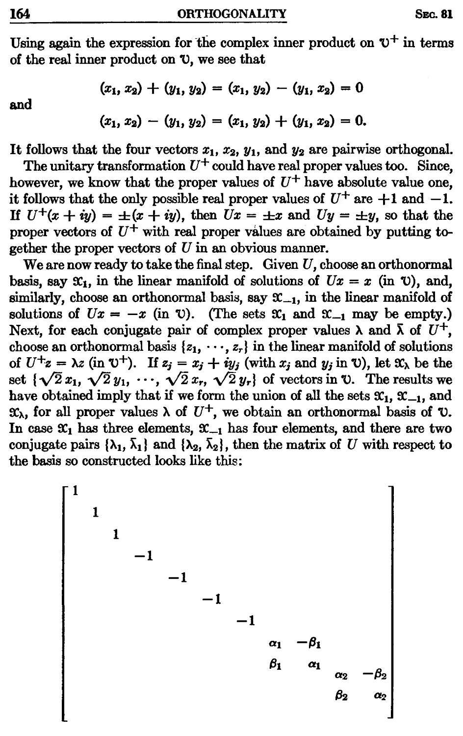
76. Combinations of perpendicular projections, 148; 77. Com-plexification, 150; 78. Characterization of spectra, 153; 79. Spectral theorem, 155; 80. Normal transformations, 159; 81. Orthogonal transformations, 162; 82. Functions of transformations, 165;
83. Polar decomposition, 169; 84. Commutativity, 171; 85. Self-adjoint transformations of rank one, 172
IV. ANALYSIS...............................175
86. Convergence of vectors, 175; 87. Norm, 176; 88. Expressions for the norm, 178; 89. Bounds of a self-adjoint transformation, 179;
90. Minimax principle, 181; 91. Convergence of linear transformations, 182; 92. Ergodic theorem, 184; 93. Power series, 186
Appendix. HILBERT SPACE....................................189
Recommended Reading, 195
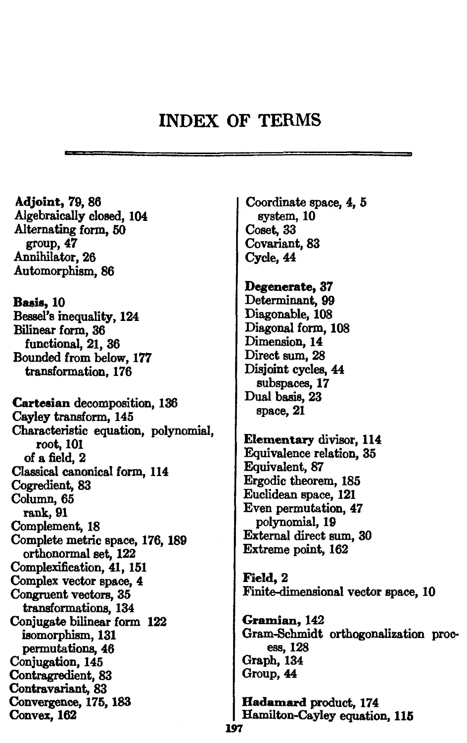
Index of Terms, 197
Index of Symbols, 200
CHAPTER I
SPACES
§ 1.	Fields
In what follows we shall have occasion to use various classes of numbers (such as the class of all real numbers or the class of all complex numbers). Because we should not, at this early stage, commit ourselves to any specific class, we shall adopt the dodge of referring to numbers as scalars. The reader will not lose anything essential if he consistently interprets scalars as real numbers or as complex numbers; in the examples that we shall study both classes will occur. To be specific (and also in order to operate at the proper level of generality) we proceed to list all the general facts about scalars that we shall need to assume.
(A)	To every pair, a and fi, of scalars there corresponds a scalar a + P, called the sum of a and p, in such a way that
(1)	addition is commutative, a + p = p + a,
(2)	addition is associative, a + (3 + y) = (a + /3) + y,
(3)	there exists a unique scalar 0 (called zero) such that a + 0 = a for every scalar a, and
(4)	to every scalar a there corresponds a unique scalar —a such that a + (—a) = 0.
(B)	To every pair, a and p, of scalars there corresponds a scalar ap, called the product of a and p, in such a way that
(1)	multiplication is commutative, ap = pa,
(2)	multiplication is associative, a(fiy) — (ap)y,
(3)	there exists a unique non-zero scalar 1 (called one) such that al = a for every scalar a, and
(4)	to every non-zero scalar a there corresponds a unique scalar a-1
I or — I such that aa~1 — 1.
(C) Multiplication is distributive with respect to addition, «(/3 + y) = aft + ay.
Tf addition and multiplication are defined within some set of objects (scalars) so that the conditions (A), (B), and (C) are satisfied, then that set (together with the given operations) is called a field. Thus, for example, the set Q of all rational numbers (with the ordinary definitions of sum and product) is a field, and the same is true of the set 61 of all real numbers and the set C of all complex numbers.
KXERCISlSS
1.	Almost all the laws of elementary arithmetic are consequences of the axioms defining a field. Prove, in particular, that if is a field, and if a, and у belong to ff, then the following relations hold.
(a)	0 + a = a.
(b)	If a + /3 = a + y, then /3 = y.
(c)	a + (p — a) = 0. (Here P — a = P + (—a).)
(d)	a-0 = 0-a = 0. (For clarity or emphasis we sometimes use the dot to indicate multiplication.)
(e)	(-l)a = —a.
(f)	(-a)(-0) = aP.
(g)	If aP = 0, then either a = 0 or P = 0 (or both).
2.	(a) Is the set of all positive integers a field? (In familiar systems, such as the integers, we shall almost always use the ordinary operations of addition and multiplication. On the rare occasions when we depart from this convention, we shall give ample warning. As for “positive,” by that word we mean, here and elsewhere in this book, “greater than or equal to zero.” If 0 is to be excluded, we shall say “strictly positive.”)
(b)	What about the set of all integers?
(c)	Can the answers to these questions be changed by re-defining addition or multiplication (or both)?
3.	Let m be an integer, m 2, and let Zm be the set of all positive integers less than m, Z„ = {0, 1, • • •, m — 1}. If a and p are in Z™ let a + p be the least positive remainder obtained by dividing the (ordinary) sum of a and p by m, and, similarly, let ap be the least positive remainder obtained by dividing the (ordinaiy) product of a and p by m. (Example: if m = 12, then 3 + 11 = 2 and 3-11 = 9.)
(a)	Prove that Zm is a field if and only if m is a prime.
(b)	What is -1 in Z6?
(c)	What is J in Z??
4.	The example of Z₽ (where p is a prime) shows that not quite all the laws of elementary arithmetic hold in fields; in Zs, for instance, 1 + 1 = 0. Prove that if is a field, then either the result of repeatedly adding 1 to itself is always different from 0, or else the first time that it is equal to 0 occurs when the number of summands is a prime. (The characteristic of the field S is defined to be 0 in the first case and the crucial prime in the second.)
5.	Let Q(\/2) be the set of all real numbers of the form a + p\/2, where a and 0 are rational.
(a)	Is Q(\/2) a field?
(b)	What if a and are required to be integers?
6.	(a) Does the set of all polynomials with integer coefficients form a field?
(b) What if the coefficients are allowed to be real numbers?
7.	Let S be the set of all (ordered) pairs (a, 0) of real numbers.
(a)	If addition and multiplication are defined by
(«, 0) + (v> 8) = (a +7, 0 + 8) and
(a, 0)(7, 6) = (ay, 08), does £F become a field?
(b)	If addition and multiplication are defined by
(a, 0) + (T, 8) = (a + 7,0 + 8) and
(a, 0)(7, 8) = (ay — 08, aS + 07), is 5 a field then?
(c)	What happens (in both the preceding cases) if we consider ordered pairs of complex numbers instead?
§ 2.	Vector spaces
We come now to the basic concept of this book. For the definition that follows we assume that we are given a particular field fF; the scalars to be used are to be elements of 5.
Definition. A vector space is a set D of elements called vectors satisfying the following axioms.
(A)	To every pair, x and y, of vectors in *0 there corresponds a vector X + y, called the sum of x and y, in such a way that
(1)	addition is commutative, x + у = у + x,
(2)	addition is associative, x + (y + z) = (x + y) + z,
(3)	there exists in X) a unique vector 0 (called the origin) such that x + 0 = x for every vector x, and
(4)	to every vector x in X) there corresponds a unique vector — x such that x 4- (—x) = 0.
(B)	To every pair, a and x, where a is a scalar and a: is a vector in X), there corresponds a vector ax in X), called the product of a and x, in such a way that
(1)	multiplication by scalars is associative, a(fix) = (aff)x, and
(2)	lx — x for every vector x.
(C)	(1) Multiplication by scalars is distributive with respect to vector addition, a(x + y) = ax + ay, and
(2)	multiplication by vectors is distributive with respect to scalar addition, (a + fi)x = ax + fix.
These axioms are not claimed to be logically independent; they are merely a convenient characterization of the objects we wish to study. The relation between a vector space *0 and the underlying field fF is usually described by saying that V is a vector space over SF. If JF is the field (R of real numbers, V) is called a real vector space; similarly if <F is Q or if 5 is C, we speak of rational vector spaces or complex vector spaces.
§ 3.	Examples
Before discussing the implications of the axioms, we give some examples. We shall refer to these examples over and over again, and we shall use the notation established here throughout the rest of our work.
(1)	Let C1(= C) be the set of all complex numbers; if we interpret x + у and ax as ordinary complex numerical addition and multiplication, C1 becomes a complex vector space.
(2)	Let (P be the set of all polynomials, with complex coefficients, in a variable t. To make O’ into a complex vector space, we interpret vector addition and scalar multiplication as the ordinary addition of two polynomials and the multiplication of a polynomial by a complex number; the origin in O’ is the polynomial identically zero.
Example (1) is too simple and example (2) is too complicated to be typical of the main contents of this book. We give now another example of complex vector spaces which (as we shall see later) is general enough for all our purposes.
(3)	Let 6я, n = 1, 2, • • •, be the set of all n-tuples of complex numbers. If x = (fb • • •, fn) and у = (i)lf • • •, 4n) are elements of Cn, we write, by definition,
X + у = (fl + 41, •••,£» + 4n)>
ax = (afi, • • •, af„),
0= (0, ••♦,()),
—X = (—fl, •••, —fn).
It is easy to verify that all parts of our axioms (A), (B), and (C), § 2, are satisfied, so that e” is a complex vector space; it will be called n-dimensional complex coordinate space.
(4)	For each positive integer n, let 6*» be the set of all polynomials (with complex coefficients, as in example (2)) of degree gn — 1, together with the polynomial identically zero. (In the usual discussion of degree, the degree of this polynomial is not defined, so that we cannot say that it has degree — 1.) With the same interpretation of the linear operations (addition and scalar multiplication) as in (2), (Pn is a complex vector space.
(5)	A close relative of C” is the set 61” of all n-tuples of real numbers. With the same formal definitions of addition and scalar multiplication as for 6”, except that now we consider only real scalars a, the space (R" is a real vector space; it will be called n-dimensional real coordinate space.
(6)	All the preceding examples can be generalized. Thus, for instance, an obvious generalization of (1) can be described by saying that every field may be regarded as a vector space over itself. A common generalization of (3) and (5) starts with an arbitrary field and forms the set of n-tuples of elements of ff; the formal definitions of the linear operations are the same as for the case = C.
(7)	A field, by definition, has at least two elements; a vector space, however, may have only one. Since every vector space contains an origin, there is essentially (i.e., except for notation) only one vector space having only one vector. This most trivial vector space will be denoted by 6.
(8)	If, in the set (R of all real numbers, addition is defined as usual and multiplication of a real number by a rational number is defined as usual, then 61 becomes a rational vector space.
(9)	If, in the set e of all complex numbers, addition is defined as usual and multiplication of a complex number by a real number is defined as usual, then <3 becomes a real vector space. (Compare this example with (1); they are quite different.)
§4.	Comments
A few comments are in order on our axioms and notation. There are striking similarities (and equally striking differences) between the axioms for a field and the axioms for a vector space over a field. In both cases, the axioms (A) describe the additive structure of the system, the axioms (B) describe its multiplicative structure, and the axioms (C) describe the connection between the two structures. Those familiar with algebraic terminology will have recognized the axioms (A) (in both § 1 and § 2) as the defining conditions of an abelian (commutative) group; the axioms (B) and (C) (in § 2) express the fact that the group admits scalars as operators. We mention in passing that if the scalars are elements of a ring (instead of a field), the generalized concept corresponding to a vector space is called a module.
Special real vector spaces (such as (R2 and (R3) are familiar in geometry. There seems at this stage to be no excuse for our apparently uninteresting insistence on fields other than (R, and, in particular, on the field C of complex numbers. We hope that the reader is willing to take it on faith that we shall have to make use of deep properties of complex numbers later (conjugation, algebraic closure), and that in both the applications of vector spaces to modem (quantum mechanical) physics and the mathematical generalization of our results to Hilbert space, complex numbers play an important role. Their one great disadvantage is the difficulty of drawing pictures; the ordinaiy picture (Argand diagram) of в1 is indistinguishable from that of (R2, and a graphic representation of C2 seems to be out of human reach. On the occasions when we have to use pictorial language we shall therefore use the terminology of (Rn in Cn, and speak of в2, for example, as a plane.
Finally we comment on notation. We observe that the symbol 0 has been used in two meanings: once as a scalar and once as a vector. To make the situation worse, we shall later, when we introduce linear functionals and linear transformations, give it still other meanings. Fortunately the relations among the various interpretations of 0 are such that, after this word of warning, no confusion should arise from this practice.
EXERCISES
1.	Prove that if x and у are vectors and if a is a scalar, then the following relations hold.
(a)	0 + x = x.
(b)	-0 - 0.
(c)	a-0 = 0.
(d)	0-a; = 0. (Observe that the same symbol is used on both sides of this equation; on the left it denotes a scalar, on the right it denotes a vector.)
(e)	If ax = 0, then either a = 0 or x = 0 (or both).
(f)	-x- (-1)2.
(g)	У + (я ~ 2/) = я. (Here х - у = х + (-у).)
2.	If р is a prime, then Z₽" к a vector space over Zp (cf. § 1, Ex. 3); how many vectors are there in this vector space?
3.	Let *0 be the set of all (ordered) pairs of real numbers. If x = (fi, $») and У — (4i> Ч») are elements of *0, write
® + У = (fi +	+ 4»)
ox - (af i, 0)
0 = (0, 0)
-2 = (-fc, -fc).
Is V a vector space with respect to these definitions of the linear operations? Why?
4.	Sometimes a subset of a vector space is itself a vector space (with respect to the linear operations already given). Consider, for example, the vector space C* and the subsets 4) of C’ consisting of those vectors (£i, f i, (•») for which
(a)	& is real,
(b)	b = 0,
(c)	either & = 0 or £» = 0,
(d)fc + fc = 0, (e) ft + & - 1.
In which of these cases is V a vector space?
5.	Consider the vector space & and the subsets D of <P consisting of those vectors (polynomials) x for which
(a)	x has degree 3,
(b)	2x(0) - z(l),
(c)	x(f) St 0 whenever 0 t Sa 1,
(d)	x(t) = x(l — f) for all t.
In which of these cases is D a vector space?
§ 5.	Linear dependence
Now that we have described the spaces we shall work with, we must specify the relations among the elements of those spaces that will be of interest to us.
We begin with a few words about the summation notation. If corresponding to each of a set of indices i there is given a vector if, and if it is not necessary or not convenient to specify the set of indices exactly, we shall simply speak of a set of vectors. (We admit the possibility that the same vector corresponds to two distinct indices. In all honesty, therefore, it should be stated that what is important is not which vectors appear in {x,}, but how they appear.) If the index-set under consideration is finite, we shall denote the sum of the corresponding vectors by x< (or, when desirable, by a more explicit symbol such as ®<). In order to avoid frequent and fussy case distinctions, it is a good idea to admit into the general theory sums such as У?; x, even when there are no indices i to be summed over, or, more precisely, even when the index-set under consideration is empty. (In that case, of course, there are no vectors to sum, or, more precisely, the set {ж,-} is also empty.) The value of such an “empty sum” is defined, naturally enough, to be the vector 0.
Definition. A finite set {ж<} of vectors is linearly dependent if there exists a corresponding set {a,} of scalars, not all zero, such that
" 0.
If, on the other hand, 52»	= 0 implies that a,- = 0 for each i, the
set {а:^} is linearly independent.
The wording of this definition is intended to cover the case of the empty set; the result in that case, though possibly paradoxical, dovetails very satisfactorily with the rest of the theoiy. The result is that the empty set of vectors is linearly independent. Indeed, if there are no indices i, then it is not possible to pick out some of them and to assign to the selected ones a non-zero scalar so as to make a certain sum vanish. The trouble is not in avoiding the assignment of zero; it is in finding an index to which something can be assigned. Note that this argument shows that the empty set is not linearly dependent; for the reader not acquainted with arguing by “vacuous implication,” the equivalence of the definition of linear independence with the straightforward negation of the definition of linear dependence needs a little additional intuitive justification. The easiest way to feel comfortable about the assertion “22,- atXi = 0 implies that а,- = 0 for each i,” in case there are no indices i, is to rephrase it this way: “if a,x,- = 0, then there is no index i for which a,-	0.” This
version is obviously true if there is no index i at all.
Linear dependence and independence are properties of sets of vectors; it is customary, however, to apply the adjectives to vectors themselves, and thus we shall sometimes say “a set of linearly independent vectors” instead of “a linearly independent set of vectors.” It will be convenient also to speak of the linear dependence and independence of a not necessarily finite set, SC, of vectors. We shall say that 90 is linearly independent if every finite subset of 90 is such; otherwise 90 is linearly dependent.
To gain insight into the meaning of linear dependence, let us study the examples of vector spaces that we already have.
(1)	If x and у are any two vectors in C1, then x and у form a linearly dependent set. If x = у — 0, this is trivial; if not, then we have, for example, the relation yx + (— x)y — 0. Since it is clear that every set containing a linearly dependent subset is itself linearly dependent, this shows that in e1 every set containing more than one element is a linearly dependent set.
(2)	More interesting is the situation in the space (P. The vectors x, y, and z, defined by
x(t) = 1 — t,
y(t) = <(1 - t),
z(f) = 1 - t2,
are, for example, linearly dependent, since x + у — z = 0. However, the infinite set of vectors xq, xi, x2, • • •, defined by
z0(i) - 1,	=	®2(t) = t2, •••»
is a linearly independent set, for if we had any relation of the form
ao-Co + aizi 4— • + «n®n = 0,
then we should have a polynomial identity
«о 4* «1^ 4---h = 0,
whence	a0 = “i =•••=«» = 0.
(3)	As we mentioned before, the spaces C” are the prototype of what we want to study; let us examine, for example, the case n = 3. To those familiar with higher-dimensional geometry, the notion of linear dependence in this space (or, more properly speaking, in its real analogue (R3) has a concrete geometric meaning, which we shall only mention. In geometrical language, two vectors are linearly dependent if and only if they are collinear with the origin, and three vectors are linearly dependent if and only if they are coplanar with the origin. (If one thinks of a vector not as a point in a space but as an arrow pointing from the origin to some given point, the preceding sentence should be modified by crossing out the phrase “with the origin” both times that it occurs.) We shall presently introduce the notion of linear manifolds (or vector subspaces) in a vector space, and, in that connection, we shall occasionally use the language suggested by such geometrical considerations.
§ 6.	Linear combinations
We shall say, whenever x =	a,x,-, that x is a linear combination of
{Xi); we shall use without any further explanation all the simple grammatical implications of this terminology. Thus we shall say, in case x is a linear combination of {x,|, that x is linearly dependent on {xj}; we shall leave to the reader the proof that if {x»| is linearly independent, then a necessary and sufficient condition that x be a linear combination of {x,| is that the enlarged set, obtained by adjoining x to {x,j, be linearly dependent. Note that, in accordance with the definition of an empty sum, the origin is a linear combination of the empty set of vectors; it is, moreover, the only vector with this property.
The following theorem is the fundamental result concerning linear dependence.
Theorem. The set of non-zero vectors xi, • • •, x„ is linearly dependent if and only if some xj, 2 к n, is a linear combination of the preceding ones.
proof. Let us suppose that the vectors xi, • • •, xn are linearly dependent, and let к be the first integer between 2 and n for which xi, • • •, x* are linearly
dependent. (If worse comes to worst, our assumption assures us that к = n will do.) Then
“1^1 4---* + «Jt^k = 0
for a suitable set of as (not all zero); moreover, whatever the a’s, we cannot have аь = 0, for then we should have a linear dependence relation among Xi, • • •, xt-i, contrary to the definition of k. Hence
— «i ,	, -ak-i
ж* =-----Xi 4------1--------a*_i•
ak	ak
as was to be proved. This proves the necessity of our condition; sufficiency is clear since, as we remarked before, every set containing a linearly dependent set is itself such.
§ 7.	Bases
Definition. A (linear) basis (or a coordinate system) in a vector space T) is a set SC of linearly independent vectors such that every vector in D is a linear combination of elements of SC. A vector space D is finitedimensional if it has a finite basis.
Except for the occasional consideration of examples we shall restrict our attention, throughout this book, to finite-dimensional vector spaces.
For examples of bases we turn again to the spaces (? and 6". In (?, the set {xn}, where xn(t) = tn, n = 0, 1, 2, • • •, is a basis; every polynomial is, by definition, a linear combination of a finite number of xn. Moreover (? has no finite basis, for, given any finite set of polynomials, we can find a polynomial of higher degree than any of them; this latter polynomial is obviously not a linear combination of the former ones.
An example of a basis in en is the set of vectors x,-, i = 1, • • - , n, defined by the condition that the j-th coordinate of x,- is 3,-y. (Here we use for the first time the popular Kronecker 3; it is defined by 3tJ- = 1 if i = j and $ij = 0 if i 5^ j.) Thus we assert that in e3 the vectors xj = (1, 0, 0), x2 = (0, 1, 0), and x3 = (0, 0, 1) form a basis. It is easy to see that they are linearly independent; the formula
x = (fi, $2, fa) = fr^i + f2z2 + fs^s
proves that every x in C3 is a linear combination of them.
In a general finite-dimensional vector space *0, with basis |xi, • • •, xn}, we know that every x can be written in the form
x = fiA-;
we assert that the f’s are uniquely determined by x. The proof of this
assertion is an argument often used in the theory of linear dependence. If we had x = ^3, %x,-, then we should have, by subtraction,
£2» (?» Vi)xi = 0.
Since the are linearly independent, this implies that f» — 4» = 0 for i = 1, • • •, n; in other words, the £’s are the same as the ij’s. (Observe that writing {xi, • • , xn | for a basis with n elements is not the proper thing to do in case n = 0. We shall, nevertheless, frequently use this notation. Whenever that is done, it is, in principle, necessary to adjoin a separate discussion designed to cover the vector space G. In fact, however, everything about that space is so trivial that the details are not worth writing down, and we shall omit them.)
Theorem. If 4) is a finite-dimensional vector space and if {yi, ym} is any set of linearly independent vectors in X>, then, unless the y’s already form a basis, we can find vectors ym+i, • • •, Ут+р so that the totality of the y’s, that is, {ylf • • •, ym, ym+i, • • •, Ут+p}, is a basis. In other words, every linearly independent set can be extended to a basis.
proof. Since *0 is finite-dimensional, it has a finite basis, say {xif •••, xn}. We consider the set 8 of vectors
Vlt " * ', Утг ‘ > xn>
in this order, and we apply to this set the theorem of § 6 several times in succession. In the first place, the set 8 is linearly dependent, since the y’s are (as are all vectors) linear combinations of the x’s. Hence some vector of 8 is a linear combination of the preceding ones; let z be the first such vector. Then z is different from any y{, i = 1, •••, m (since the y’s are linearly independent), so that z is equal to some x, say z = x;. We consider the new set S' of vectors
У1> * * ", Ут> " " ", xi—1,	xn<
We observe that every vector in *0 is a linear combination of vectors in S', since by means of ylf •••, ym, xit •••, x,_i we may express x,-, and then by means of Xi, • • •, x,_i, x,-, x,+i, • • •, xn we may express any vector. (The x’s form a basis.) If 8' is linearly independent, we are done. If it is not, we apply the theorem of § 6 again and again the same way till we reach a linearly independent set containing ylt • • •, ym, in terms of which we may express every vector in D. This last set is a basis containing the y’s.
EXERCISES
1.	(a) Prove that the four vectors
x = (1,0,0),
у = (0,1, 0),
z = (0, 0,1),
и = (1, 1, 1),
in C* form a linearly dependent set, but any three of them are linearly independent. (To test the linear dependence of vectors x = (&, &, £г), у = (sji, уг, %), and z = (fi, fz, fa) in &, proceed as follows. Assume that a, {3, and у can be found so that ax + ity + yz — 0. This means that
o£i + frn + 7f i = 0,
afe + fr]z + 7fr = 0,
«Ь + (3i)S + 7f» = 0.
The vectors x, y, and г are linearly dependent if and only if these equations have a solution other than a = ft = у = 0.)
(b) If the vectors x, у, z, and и in (P are defined by x(f) = 1, y(f) — t, z(f) = t2, and u(t) = 1 + t + I2, prove that x, y, z, and w are linearly dependent, but any three of them are linearly independent.
2.	Prove that if Gt is considered as a rational vector space (see § 3, (8)), then a necessaiy and sufficient condition that the vectors 1 and £ in (R be linearly independent is that the real number g be irrational.
3.	Is it true that if x, y, and г are linearly independent vectors, then so also are x + у, у + z, and z + x?
4.	(a) Under what conditions on the scalar f are the vectors (1 + f, 1 — Q and (1 — £, 1 + £) in 62 linearly dependent?
(b) Under what conditions on the scalar £ are the vectors (£, 1, 0), (1, %, 1), and (0, 1, £) in (R* linearly dependent?
(o) What is the answer to (b) for Qs (in place of (R2)?
5. (a) The vectors (£t, £2) and (41, 92) in & are linearly dependent if and only if
(b) Find a similar necessary and sufficient condition for the linear dependence of two vectors in C‘. Do the same for three vectors in Cs.
(c) Is there a set of three linearly independent vectors in в2?
6.	(a) Under what conditions on the scalars £ and tj are the vectors (1, £) and (1, 97) in e2 linearly dependent?
(b)	Under what conditions on the scalars £, 4, and f are the vectors (1, £, £2), (1,4, чг), and (1, f, f2) in в* linearly dependent?
(c)	Guess and prove a generalization of (a) and (b) to в".
7.	(a) Find two bases in e4 such that the only vectors common to both are (0, 0,1,1) and (1,1, 0, 0).
(b) Find two bases in C4 that have no vectors in common so that one of them contains the vectors (1, 0, 0, 0) and (1, 1, 0, 0) and the other one contains the vectors (1, 1,1, 0) and (1, 1, 1, 1).
8.	(a) Under what conditions on the scalar £ do the vectors (1,1,1) and (1, f, f2) form a basis of 6*?
(b) Under what conditions on the scalar f do the vectors (0, 1, %), (f, 0,1), and (£, 1,1 -Ь $) form a basis of
9.	Consider the set of all those vectors in 6’ each of whose coordinates is either 0 or 1; how many different bases does this set contain?
10.	If SC is the set consisting of the six vectors (1,1,0,0), (1,0,1,0), (1,0,0,1), (0, 1, 1, 0), (0, 1, 0, 1), (0, 0, 1, 1) in &, find two different maximal linearly independent subsets of 9C. (A maximal linearly independent subset of 9C is a linearly independent subset ‘У of SC that becomes linearly dependent every time that a vector of 9C that is not already in 'y is adjoined to *y.)
11.	Prove that every vector space has a basis. (The proof of this fact is out of reach for those not acquainted with some transfinite trickery, such as well-ordering or Zorn’s lemma.)
§8. Dimension
Theorem 1. The number of elements in any basis of a finite-dimensional vector space U is the same as in any other basis.
proof. The proof of this theorem is a slight refinement of the method used in § 6, and, incidentally, it proves something more than the theorem states. Let 9C = {xx, • • xn} and у = |yi,   •, ym} be two finite sets of vectors, each with one of the two defining properties of a basis; i.e., we assume that every vector in U is a linear combination of the x’s (but not that the x’s are linearly independent), and we assume that the y’s are linearly independent (but not that every vector is a linear combination of them). We may apply the theorem of § 6, just as above, to the set 8 of vectors
Ут, xi, • • •, xn.
Again we know that every vector is a linear combination of vectors of S and that S is linearly dependent. Reasoning just as before, we obtain a set S’ of vectors
Ут,	Xf—j,	Xn,
again with the property that every vector is a linear combination of vectors of S'. Now we write ym_i in front of the vectors of S' and apply the same argument. Continuing in this way, we see that the x’s will not be exhausted before the y’s, since otherwise the remaining y’s would have to be linear combinations of the ones already incorporated into 8, whereas we know
that the y’s are linearly independent. In other words, after the argument has been applied m times, we obtain a set with the1 same property the x’s had, and this set differs from the set of x’s in that m of them are replaced by y’s. This seemingly innocent statement is what we are after; it implies that n m. Consequently if both 9C and are bases (so that they each have both properties), then n m and m n.
Definition. The dimension of a finite-dimensional vector space 1) is the number of elements in a basis of *0.
Observe that since the empty set of vectors is a basis of the trivial space 6, the definition implies that that space has dimension 0. At the same time the definition (together with the fact that we have already exhibited, in § 7, one particular basis of 6”) at last justifies our terminology and enables us to announce the pleasant result: n-dimensional coordinate space is n-dimensional. (Since the argument is the same for (Rn and for e", the assertion is true in both the real case and the complex case.)
Our next result is a corollary of Theorem 1 (via the theorem of § 7).
Theobem 2. Every set of n + 1 vectors in an n-dimensional vector space U is linearly dependent. A set of n vectors in U is a basis if and only if it is linearly independent, or, alternatively, if and only if every vector in *0 is a linear combination of elements of the set.
§9. Isomorphism
As an application of the notion of linear basis, or coordinate system, we shall now fulfill an implicit earlier promise by showing that every finite-dimensional vector space over a field is essentially the same as (in technical language, is isomorphic to) some 5".
Definition. Two vector spaces 41 and *0 (over the same field) are isomorphic if there is a one-to-one correspondence between the vectors x of 41 and the vectors у of U, say у = T(x), such that
^(«l®! + «2®г) = «l^l) + «2T(®2)-
In other words, 41 and V are isomorphic if there is an isomorphism (such as T) between them, where an isomorphism is a one-to-one correspondence that preserves all linear relations.
It is easy to see that isomorphic finite-dimensional vector spaces have the same dimension; to each basis in one space there corresponds a basis in the other space. Thus dimension is an isomorphism invariant; we shall now show that it is the only isomorphism invariant, in the sense that every
two vector spaces with the same finite dimension (over the same field, of course) are isomorphic. Since the isomorphism of 41 and “0 on the one hand, and of *0 and on the other hand, implies that 41 and V? are isomorphic, it will be sufficient to prove the following theorem.
Theorem. Every n-dimensional vector space *0 over afield 5 is isomorphic totf*.
proof. Let {хъ •••, x„} be any basis in "U. Each x in U can be written in the form -|----------f- fnxn, and we know that the scalars	in
are uniquely determined by x. We consider the one-to-one correspondence
® (fl> "  fn)
between U and ff". If у —	4-----b Wn, then
ax + fry =* (ofi + /3iji)xi 4---F (of„ 4- fr]n)Xn,
this establishes the desired isomorphism.
One might be tempted to say that from now on it would be silly to try to preserve an appearance of generality by talking of the general n-dimensional vector space, since we know that, from the point of view of studying linear problems, isomorphic vector spaces are indistinguishable, and, consequently, we might as well always study ffn. There is one catch. The most important properties of vectors and vector spaces are the ones that are independent of coordinate systems, or, in other words, the ones that are invariant under isomorphisms. The correspondence between 4? and was, however, established by choosing a coordinate system; were we always to study SF”, we would always be tied down to that particular coordinate system, or else we would always be faced with the chore of showing that our definitions and theorems are independent of the coordinate system in which they happen to be stated. (This horrible dilemma will become clear later, on the few occasions when we shall be forced to use a particular coordinate system to give a definition.) Accordingly, in the greater part of this book, we shall ignore the theorem just proved, and we shall treat n-dimensional vector spaces as self-respecting entities, independently of any basis. Besides the reasons just mentioned, there is another reason for doing this: many special examples of vector spaces, such for instance as (Pn, would lose a lot of their intuitive content if we were to transform them into e" and speak of coordinates only. In studying vector spaces, such as (Pn, and their relation to other vector spaces, we must be able to handle them with equal ease in different coordinate systems, or, and this is essentially the same thing, we must be able to handle them without using any coordinate systems at all.
EXERCISES
1.	(a) What is the dimension of the set в of all complex numbers considered as a real vector space? (See § 3, (9).)
(b) Every complex vector space *U is intimately associated with a real vector space V-; the space U- is obtained from *0 by refusing to multiply vectora of "0 by anything other than real scalars. If the dimension of the complex vector space *0 is n, what is the dimension of the real vector space D~?
2.	Is the set 01 of all real numbers a finite-dimensional vector space over the field Q of all rational numbers? (See § 3, (8). The question is not trivial; it helps to know something about cardinal numbers.)
3.	How many vectora are there in an n-dimensional vector space over the field Zp (where p is a prime)?
4.	Discuss the following assertion: if two rational vector spaces have the same cardinal number (i.e., if there is some one-to-one correspondence between them), then they are isomorphic (i.e., there is a linearity-preserving one-to-one correspondence between them). A knowledge of the basic facts of cardinal arithmetic is needed for an intelligent discussion.
§ 10.	Subspaces
The objects of interest in geometry are not only the points of the space under consideration, but also its lines, planes, etc. We proceed to study the analogues, in general vector spaces, of these higher-dimensional elements.
Definition. A non-empty subset 911 of a vector space U is a subspace or a linear manifold if along with every pair, x and y, of vectors contained in 9TC, every linear combination ax + fiy is also contained in 911.
A word of warning: along with each vector x, a subspace also contains x — x. Hence if we interpret subspaces as generalized lines and planes, we must be careful to consider only lines and planes that pass through the origin.
A subspace 911 in a vector space D is itself a vector space; the reader can easily verify that, with the same definitions of addition and scalar multiplication as we had in D, the set satisfies the axioms (A), (B), and (C) of §2.
Two special examples of subspaces are: (i) the set О consisting of the origin only, and (ii) the whole space X). The following examples are less trivial.
(1)	Let n and m be any two strictly positive integers, m n. Let 9K be the set of all vectors x = (fi, • • •, £„) in в" for which fi = • • • =	= 0.
(2)	With m and n as in (1), we consider the space (?n, and any m real numbers itm. Let 9П be the set of all vectors (polynomials) x in (Pn for which ж(<1) =•• = s(4n) = 0.
(3)	Let 911 be the set of all vectors x in (P for which x(t) *= x(—f) holds identically in t.
We need some notation and some terminology. For any collection {9E,} of subsets of a given set (say, for example, for a collection of subspaces in a vector space U), we write Q, 9TC, for the intersection of all 9IL, i.e., for the set of points common to them all. Also, if 911 and 91 are subsets of a set, we write 911 CZ 91 if 911 is a subset of 91, that is, if every element of 911 lies in 91 also. (Observe that we do not exclude the possibility 9E = 91; thus we write U CD as well as 0 C U.) For a finite collection {9Ui, • • •, 9TCn}, we shall write 91li П • • • Л 9TCn in place of 911/, in case two subspaces 9П. and 91 are such that 9TC. Г1 91 = 0, we shall say that 911 and 91 are disjoint.
§ 11.	Calculus of subspaces
Theorem 1.	The intersection of any collection of subspaces is a subspace.
proof. If we use an index v to tell apart the members of the collection, so that the given subspaces are 9TC„ let us write
arc = f|, ж,.
Since every 9Tt, contains 0, so does 911, and therefore 9E is not empty. If x and у belong to 911 (that is, to all 9E„), then ax + py belongs to all 911», and therefore 911 is a subspace.
To see an application of this theorem, suppose that 8 is an arbitrary set of vectors (not necessarily a subspace) in a vector space U. There certainly exist subspaces ЭЕ containing every element of 8 (that is, such that 8 CZ 911); the whole space *0 is, for example, such a subspace. Let 9Tt be the intersection of all the subspaces containing 8; it is clear that 911 itself is a subspace containing 8. It is clear, moreover, that 9TC is the smallest such subspace; if 8 is also contained in the subspace 91, 8 CZ 91, then 911 CZ 91. The subspace 9K so defined is called the subspace spanned by 8 or the span of S. The following result establishes the connection between the notion of spanning and the concepts studied in §§ 5-9.
Theorem 2.	If 8 is any set of vectors in a vector space U and if W. is the subspace spanned by 8, then 3R is the same as the set of all linear combinations of elements of 8.
proof. It is clear that a linear combination of linear combinations of elements of S may again be written as a linear combination of elements of S. Hence the set of all linear combinations of elements of S is a subspace containing S; it follows that this subspace must also contain 5E. Now turn the argument around: 311 contains S and is a subspace; hence 311 contains all linear combinations of elements of s.
We see therefore that in our new terminology we may define a linear basis as a set of linearly independent vectors that spans the whole space.
Our next result is an easy consequence of Theorem 2; its proof may be safely left to the reader.
Theorem 3.	If 5C and 3C are any two subspaces and if 3E is the subspace spanned by 3C and 3C together, then 311 is the same as the set of cdl vectors of the form x + y, with xinSC and у in 3C.
Prompted by this theorem, we shall use the notation 3C + 3C for the subspace 511 spanned by 3C and 3C. We shall say that a subspace 3C of a vector space D is a complement of a subspace 3C if ЗС П 3C = e and 3C + 3C = D.
§ 12. Dimension of a subspace
Theorem 1. A subspace 3E in an n-dimensional vector space *0 is a vector space of dimension g n.
proof. It is possible to give a deceptively short proof of this theorem that runs as follows. Every set of n + 1 vectors in U is linearly dependent, hence the same is true of Sit; hence, in particular, the number of elements in each basis of 511 is n, Q.E.D.
The trouble with this argument is that we defined dimension n by requiring in the first place that there exist a finite basis, and then demanding that this basis contain exactly n elements. The proof above shows only that no basis can contain more than n elements; it does not show that any basis exists. Once the difficulty is observed, however, it is easy to fill the gap. If 511 = ©, then Sit is O-dimensional, and we are done. If 3E contains a non-zero vector xlf let Sltj (С Sit) be the subspace spanned by xj. If 511 = SEj, then Sit is 1-dimensional, and we are done. If 3115^ SEi, let ^2 be an element of 3E not contained in SEi, and let SE2 be the subspace spanned by Xj and xa; and so on. Now we may legitimately employ the argument given above; after no more than n steps of this sort, the process reaches an end, since (by § 8, Theorem 2) we cannot find n + 1 linearly independent vectors.
The following result is an important consequence of this second and correct proof of Theorem 1.
Theobem 2. Given any m-dimensional subspace SHI in an n-dimensional vector space X), we can find a basis {xlt xm, xm+i, • • •, xn} in 43 so that xi, • • •, are in SHI and form, therefore, a basis of SHI.
We shall denote the dimension of a vector space 43 by the symbol dim 43. In this notation Theorem 1 asserts that if SHI is a subspace of a finite-dimensional vector space 43, then dim SHI S dim 43.
EXERCISES
1.	If SHI and SH are finite-dimensional subspaces with the same dimension, and if SHI C SH, then SHI = 91.
2.	If SHI and SH are subspaces of a vector space 43, and if every vector in 43 belongs either to SHI or to SH (or both), then either Ж = 43 or SH = 43 (or both).
3.	If x, y, and a are vectors such that x + у + z = 0, then x and у span the same subspace as у and z.
4.	Suppose that x and у are vectors and SHI is a subspace in a vector space 43; let 3C be the subspace spanned by SHI and x, and let 3C be the subspace spanned by SHI and y. Prove that if у is in 3C but not in SHI, then x is in 3C.
5.	Suppose that £, SHI, and 91 are subspaces of a vector space.
(a)	Show that the equation
£ Л (9H + SH.) = (£ П SHI) + (£ 0 91)
is not necessarily true.
(b)	Prove that
£ П (SHI + (£ П 91)) = (£ П SHI) 4- (£ 0 91).
6.	(a) Can it happen that a non-trivial subspace of a vector space 43 (i.e., a subspace different from both 6 and 43) has a unique complement?
(b) If SHI is an m-dimensional subspace in an n-dimensional vector space, then every complement of SHI has dimension n — m.
7.	(a) Show that if both SHI and SH are three-dimensional subspaces of a fivedimensional vector space, then SHI and SH. are not disjoint.
(b) If SHI and SH are finite-dimensional subspaces of a vector space, then
dim SHI 4-dim 91 = dim (SHI + SH.) + dim (SHI Г1 91).
8.	A polynomial x is called even if x(—4) = x{f) identically in t (see § 10, (3)), and it is called odd if x(—t) = —x(0.
(a)	Both the class SHI of even polynomials and the class SH of odd polynomials are subspaces of the space (P of all (complex) polynomials.
(b)	Prove that SHI and SH are each other’s complements.
§ 13.	Dual spaces
Definition. A linear functional on a vector space "0 is a scalar-valued function у defined for every vector x, with the property that (identically in the vectors and x2 and the scalars ai and a2)
y(aiXi,+ a2x2) =	+ a$j(x2).
Let us look at some examples of linear functionals.
(1)	For x = (fc, • • •, £n) in e", write y(x) = More generally, let «1, • • «я be any n scalars and write
y(x) = ai£i -|-----1- a„£n.
We observe that for any linear functional у on any vector space
3/(0) = j/(0-0) = 0-j/(0) = 0;
for this reason a linear functional, as we defined it, is sometimes called homogeneous. In particular in e", if у is defined by
y(x) = «!$! -|-----f- Onln + ft
then у is not a linear functional unless /3 = 0.
(2)	For any polynomial x in (P, write y(x) = x(0). More generally, let ai, • • -, an be any n scalars, let ti,   tn be any n real numbers, and write
3/(1) = aix(fi) -I---l-anx(fn).
Another example, in a sense a limiting case of the one just given, is obtained as follows. Let (а, b) be any finite interval on the real «-axis, and let a be any complex-valued integrable function defined on (a, b); define у by
Гь
y(x) = I a(f)x(f) di.
J a
(3)	On an arbitraiy vector space *0, define у by writing
y(x) = 0 for every x in *0.
The last example is the first hint of a general situation. Let *0 be any vector space and let D' be the collection of all linear functionals on *0. Let us denote by 0 the linear functional defined in (3) (compare the comment at the end of § 4). If yi and y2 are linear functionals on U and if aj and a2 are scalars, let us write у for the function defined by
y(x) - aiy^x) + asya(x).
It is easy to see that у is a linear functional; we denote it by aiyi + a2y2. With these definitions of the linear concepts (zero, addition, scalar multiplication), the set 43' forms a vector space, the dual space of 43.
§ 14.	Brackets
Before studying linear functionals and dual spaces in more detail, we wish to introduce a notation that may appear weird at first sight but that will clarify many situations later on. Usually we denote a linear functional by a single letter such as y. Sometimes, however, it is necessary to use the function notation fully and to indicate somehow that if у is a linear functional on 43 and if x is a vector in V, then y(x) is a particular scalar. According to the notation we propose to adopt here, we shall not write у followed by a; in parentheses, but, instead, we shall write x and у enclosed between square brackets and separated by a comma. Because of the unusual nature of this notation, we shall expend on it some further verbiage.
As we have just pointed out [x, y] is a substitute for the ordinary function symbol y(x); both these symbols denote the scalar we obtain if we take the value of the linear function у at the vector x. Let us take an analogous situation (concerned with functions that are, however,* not linear). Let у be the real function of a real variable defined for each real number x by y(x) = x2. The notation [x, y] is a symbolic way of writing down the recipe for actual operations performed; it corresponds to the sentence [take a number, and square it].
Using this notation, we may sum up: to every vector space 43 we make correspond the dual space 43' consisting of all linear functionals on 43; to every pair, x and y, where x is a vector in *0 and у is a linear functional in 43', we make correspond the scalar [x, y] defined to be the value of у at x. In terms of the symbol [x, y] the defining property of a linear functional is
(!)	[«iXi + a2x2, y] = ttl[xi, у] + a2[x2, у],
and the definition of the linear operations for linear functionals is
(2)	[x,	+ a2y2] = «i[x, yj 4- a2[x, y2].
The two relations together are expressed by saying that [x, y] is a bilinear functional of the vectors x in 43 and у in 43'.
EXERCISES
1.	Consider the set в of complex numbers as a real vector space (as in § 3, (9)). Suppose that for each x = fi + »f2in C (where fi and f2 are real numbers and * = V—1) the function у is defined by
(a)	y(x) = fi,
(b)	y{x) = f2,
(c)	y(x) = ii*
(d)	y(x) = fi - if2,
(e)	y(x) = Vf j2 + £22. (The square root sign attached to a positive number always denotes the positive square root of that number.)
In which of these cases is у a linear functional?
2.	Suppose that for each x = (fi, f2, fa) in в’ the function у is defined by
(») У&) = fi + f2,
(b)	y{x) = fi - f82,
(c)	y{x~) = fl + 1,
(d)	?/(z) = fi — 2f2 + 3f8.
In which of these cases is у a linear functional?
3.	Suppose that for each x in (P the function у is defined by r+2
(a)	y(x) = J x(i) di,
J'2
(ж(«))2Л,
0
(c)	y(x) = f t2x(t) dtf
Jo
(d)	y(x) = f «(Z2) di,
Jo
(e)	y(x) =
at
/Ру ।
In which of these cases is у a linear functional?
4.	If (во, ai, аг, • • •) is an arbitrary sequence of complex numbers, and if a: is an element of (P, z(Z) = 22<-o fA write y(x) = S“-o f»«<- Prove that у is an element of (P' and that every element of <P' can be obtained in this manner by a suitable choice of the a/s.
5.	If у is a non-zero linear functional on a vector space T), and if a is an arbitrary scalar, does there necessarily exist a vector x in *0 such that [x, y] = «?
6.	Prove that if у and z are linear functionals (on the same vector space) such that [x, у] = 0 whenever [x, z] = 0, then there exists a scalar a such that у = az. (Hint: if [®o, z] 5^ 0, write a = [®o, vl/jasa, z].)
§ 15.	Dual bases
One more word before embarking on the proofs of the important theorems. The concept of dual space was defined without any reference to coordinate systems; a glance at the following proofs will show a superabundance of coordinate systems. We wish to point out that this phenomenon is inevitable; we shall be establishing results concerning dimension, and dimension is the one concept (so far) whose very definition is given in terms of a basis.
Theorem 1.	If *0 is an n-dimensional vector space, if {xj, • • - , xn} is a basis in *0, and if {«i, • • •, «»} is any set of n scalars, then there is one and only one linear functional у on *0 such that [xj, у] = сц for i = 1, - • -, n.
proof. Every x in U may be written in the form x = fixj -|--------£nx„
in one and only one way; if у is any linear functional, then
[s, У] = fifci, 2/14---F tnfcn, 2/1.
From this relation the uniqueness of у is clear; if [x,-, y] = a,-, then the value of [x,y] is determined, for every x, by [x,y] =	£»«»' The argument
can also be turned around; if we define у by
[x, 2/1 = £i«i -I---F fn«n,
then у is indeed a linear functional, and [xif j/} = a,-.
Theorem 2.	If X) is an n-dimensional vector space and if 9C = {xj, - • x„} is a basis in U, then there is a uniquely determined basis SC' in X', SC' = {?/!, • • •, j/n}, with the property that [x,-, y,} = Consequently the dual space of an n-dimensional space is n-dimensional.
The basis SC' is called the dual basis of SC.
proof. It follows from Theorem 1 that, for each j = 1, • • •, n, a unique Уз in x' can be found so that [x4-, ?/,•] = 5#; we have only to prove that the set SC' = {j/j, • • •, pn} is a basis in X'.
In the first place, SC' is a linearly independent set, for if we had + • • • + otnyn = 0, in other words, if
«12/1 4----F «п2/»1 = «1к» 2/1] 4----F an[x, yj = 0
for all x, then we should have, for x « x4,
0 ™	«/[*£>> yji —	“ «»•
In the second place, every у in D' is a linear combination of ylt •••, yn. To prove this, write fo, y] = сц; then, for x = 22» &x»» we have
Iх, y\ = $i«i 4----b in«n-
On the other hand
[ж, yA = 22» уА = 6’>
so that, substituting in the preceding equation, we get
Iх, y] = аг[х, 7/J 4---F a„lx, yn]
= Iх, «1Z/1 4----F any»].
Consequently у = а\у\ Ч--------F «n?/n, and the proof of the theorem is
complete.
We shall need also the following easy consequence of Theorem 2.
Theorem 3.	If и and v are any two different vectors of the n-dimensional vector space D, then there exists a linear functional у on D such that [u, y} H k, ?/]; or> equivalently, to any non-zero vector x in 4) there corresponds ay in V such that [x, y] 0.
proof. That the two statements in the theorem are indeed equivalent is seen by considering x = и — v. We shall, accordingly, prove the latter statement only.
Let 90 — {xlt • • •, xn} be any basis in "0, and let ЯУ = {^, • • •, yn\ be the dual basis in ‘O'. И x = 22» then (as above) [x, yA — tj. Hence if Iх, yl — 0 for ah У, and, in particular, if [x, у A = 0 for j — 1, • • •, n, then x = 0.
§ 16.	Reflexivity
It is natural to think that if the dual space D' of a vector space D, and the relations between a space and its dual, are of any interest at all for D, then they are of just as much interest for ‘O'. In other words, we propose now to form the dual space (‘0')' of D'; for simplicity of notation we shall denote it by D". The verbal description of an element of D" is clumsy: such an element is a linear functional of linear functionals. It is, however, at this point that the greatest advantage of the notation [x, y] appears; by means of it, it is easy to discuss D and its relation to ’0".
If we consider the symbol [x, y] for some fixed у = y0, we obtain nothing new: [x, 7/0] is merely another way of writing the value yo(x) of the function yo at the vector x. If, however, we consider the symbol [x, y] for some fixed x = xo, then we observe that the function of the vectors in U', whose value at у is [z0, !/], is a scalar-valued function that happens to be linear
(see § 14, (2)); in other words, [xq, y\ defines a linear functional on V, and, consequently, an element of V*.
By this method we have exhibited some linear functionals on "O'; have we exhibited them all? For the finite-dimensional case the following theorem furnishes the affirmative answer.
Theorem. If X) is a finitedimensional vector space, then corresponding to every linear functional z0 on X' there is a vector Xq in D such that z0(y) — fco, y] — У&о) for every у in X'; the correspondence z0 x0 between X" and X is an isomorphism.
The correspondence described in this statement is called the natural correspondence between X" and X-
proof. Let us view the correspondence from the standpoint of going from D to X"; in other words, to every x0 in 1) we make correspond a vector z0 in X" defined by z0(i/) *= y(x0) for every у in X'. Since [x, y] depends linearly on x, the transformation x0 —» Zq is linear.
We shall show that this transformation is one-to-one, as far as it goes. We assert, in other words, that if x\ and x2 are in D, and if Zi and z2 are the corresponding vectors in X" (so that z^y) = [хъ j/J and z2(y) = [x2, y] for all у in D'), and if гг = Z2, then Xi = x2. To say that zi = z2 means that [Xi, y] = [x2, г/] for every у in X'; the desired conclusion follows from § 15, Theorem 3.
The last two paragraphs together show that the set of those linear functionals z on X’ (that is, elements of X") that do have the desired form (that is, z(y) is identically equal to [x, y] for a suitable x in X) is a subspace of X" which is isomorphic to X and which is, therefore, n-dimensional. But the n-dimensionality of X implies that of X', which in turn implies that X" is n-dimensional. It follows that X" must coincide with the n-dimensional subspace just described, and the proof of the theorem is complete.
It is important to observe that the theorem shows not only that D and X" are isomorphic—this much is trivial from the fact that they have the same dimension—but that the natural correspondence is an isomorphism. This property of vector spaces is called reflexivity; every finite-dimensional vector space is reflexive.
It is frequently convenient to be mildly sloppy about X": for finitedimensional vector spaces we shall identify X" with X (by the natural isomorphism), and we shall say that the element z0 of X" is the same as the element x0 of X whenever z0(y) = [x0, y] for all у in X'. In this language it is very easy to express the relation between a basis SC, in D, and the dual basis of its dual basis, in "0"; the symmetry of the relation [x,-, yf\ = 6ц shows that SC" < SC-
§ 17.	Annihilators
Definition. The annihilator 8° of any subset S of a vector space D (8 need not be a subspace) is the set of all vectors у in D' such that [x, y] is identically zero for all x in 8.
Thus 0° = D' and *0° = 6 (C *0'). If D is finite-dimensional and 8 contains a non-zero vector, so that 8^6, then § 15, Theorem 3 shows that 8° V.
Theorem 1. If Ж is an m-dimensional subspace of an n-dimensional vector space D, then Ж0 is an (n — m)-dimensional subspace of 1)'.
proof. We leave it to the reader to verify that Ж0 (in fact S°, for an arbitrary 8) is always a subspace; we shall prove only the statement concerning the dimension of 9K°.
Let SC = {xi, • • - , x„} be a basis in “0 whose first m elements are in Ж (and form therefore a basis for Ж); let sc' = {?/i,	уn} be the dual
basis in “O'. We denote by 91 the subspace (in ЧУ) spanned by ym+l, clearly 91 has dimension n — m. We shall prove that Ж0 = 91.
If x is any vector in Ж, then x is a linear combination of xi, • • •, xm,
x = ХГ-i
and, for any j = m + 1, • • •, n, we have
[x, У,] = Zifa, yjl = 0.
In other words, y, is in Ж0 for j = m + 1, - • •, n; it follows that 91 is contained in Ж0,
91 С Ж0.
Suppose, on the other hand, that у is any element of 9TC°. Since y, being in "O', is a linear combination of the basis vectors yu • • •, yn, we may write
У = L”-i W-
Since, by assumption, у is in Ж0, we have, for every i = 1, • • •, m,
0 = [xi} y] = S”-i y}{Xi, yf\ = %•;
in other words, у is a linear combination of • • •, yn- This proves that у is in 91, and consequently that
Ж0 C 91,
and the theorem follows.
Theorem 2. If 9R is a subspace in a finite-dimensional vector space X), then 9R00 ( = (9R°)°) = SR.
proof. Observe that we use here the convention, established at the end of § 16, that identifies V and 43". By definition, SR00 is the set of all vectors x such that [x, y\ = 0 for all у in SR°. Since, by the definition of 9R°, [x> = 0 for all x in SR and all у in SR°, it follows that SR C SR00. The desired conclusion now follows from a dimension argument. Let fjR be тп-dimensional; then the dimension of SR° is n — m, and that of SR00 is n — (n — m) = m. Hence SR = 5R00, as was to be proved.
exercises
1.	Define a non-zero linear functional у on 6* such that if xj = (1, 1, 1) and хг = (1, 1, -1), then [xi, y] = [xit 2/] = 0.
2.	The vectors xi = (1, 1, 1), x2 = (1, 1, —1), and x3 = (1, —1, —1) form a basis of &. If {?/i, у2, уз | is the dual basis, and if x = (0,1, 0), find [x, j/j, [x, j/2], and [x, j/з].
3.	Prove that if у is a linear functional on an n-dimensional vector space 43, then the set of all those vectors x for which [x, у] = 0 is a subspace of 43; what is the dimension of that subspace?
4.	If t/(x) = £i + & + Ь whenever x = (&,	£») is a vector in 6*, then у
is a linear functional on 6s; find a basis of the subspace consisting of all those vectors x for which [x, y] = 0.
5.	Prove that if m < n, and if yi,  • •, yn are linear functionals on an n-dimensional vector space 43, then there exists a non-zero vector x in 43 such that [x, У A = 0 for j = 1, m. What does this result say about the solutions of linear equations?
6.	Suppose that m < n and that yi, •••, ym are linear functionals on an n-dimensional vector space 43. Under what conditions on the scalars «j, •••, a„ is it true that there exists a vector x in 43 such that [x, 2/,] = a, for j = 1, • • •, mt What does this result say about the solutions of linear equations?
7.	If 43 is an n-dimensional vector space over a finite field, and if 0 g m g n then the number of m-dimensional subspaces of 43 is the same as the number of (n — nz)-dimensional subspaces.
8.	(a) Prove that if S is any subset of a finite-dimensional vector space, then S00 coincides with the subspace spanned by S.
(b)	If S and 3 are subsets of a vector space, and if S C 3, then 3° G S°.
(c)	If 9R and 91 are subspaces of a finite-dimensional vector space, then (9R П 9l)° = 3R° -|- 91® and (9R + 91)® = 9R° П 91°. (Hint: make repeated use of (b) and of § 17, Theorem 2.)
(d)	Is the conclusion of (c) valid for not necessarily finite-dimensional vector spaces?
9.	This exercise is concerned with vector spaces that need not be finite-dimensional; most of its parts (but not all) depend on the sort of transfinite reasoning that is needed to prove that every vector space has a basis (cf. § 7, Ex. 11).
(a)	Suppose that f and g are scalar-valued functions defined on a set JK; if a and /3 are scalars write h = aj + Pg for the function defined by Л(ж) = cifix) + pg(x) for all x in 9C. The set of all such functions is a vector space with respect to this definition of the linear operations, and the same is true of the set of all finitely non-zero functions. (A function/on 90 \s finitely non-zero if the set of those elements x of 90 for which fix) 0 is finite.)
(b)	Every vector space is isomorphic to the set of all finitely non-zero functions on some set.
(c)	If U is a vector space with basis 90, and if / is a scalar-valued function defined on the set 90, then there exists a unique linear functional у on U such that [x, y] = fix) for all ж in SC.
(d)	Use (a), (b), and (c) to conclude that every vector space U is isomorphic to a subspace of “O'.
(e)	Which vector spaces are isomorphic to their own duals?
(f)	If ‘У is a linearly independent subset of a vector space U, then there exists a basis of U containing y. (Compare this result with the theorem of § 7.)
(g)	If 90 is a set and if у is an element of 90, write fv for the scalar-valued function defined on 90 by writing fv(x) = 1 or 0 according as x = у or x y. Let 4) be the set of all functions /„ together with the function g defined by g(x) = 1 for all x in 90. Prove that if 90 is infinite, then *y fa a linearly independent subset of the vector space of all scalar-valued functions on 90.
(h)	The natural correspondence from U to U" fa defined for all vector spaces (not only for the finite-dimensional ones); if x0 fa in U, define the corresponding element zo of V" by writing Zo(y) = [ж0, у] for all у in “O'. Prove that if U fa reflexive (i.e., if every z0 in U" can be obtained in this manner by a suitable choice of x0), then U is finite-dimensional. (Hint: represent U' as the set of all scalar-valued functions on some set, and then use (g), (f), and (c) to construct an element of V" that fa not induced by an element of U.)
Warning: the assertion that a vector space fa reflexive if and only if it fa finitedimensional would shock most of the experts in the subject. The reason fa that the customary and fruitful generalization of the concept of reflexivity to infinitedimensional spaces fa not the simple-minded one given in (h).
§ 18.	Direct sums
We shall study several important general methods of making new vector spaces out of old ones; in this section we begin by studying the easiest one.
Definition. If 41 and U are vector spaces (over the same field), their direct sum is the vector space "W (denoted by 41 ф U) whose elements are all the ordered pairs (x, y) with x in 41 and у in U, with the linear operations defined by
“1(^1» 2/1) + «2(^2, У 2) — (0ЦХ1 + «2X2, ait/i 4- агУг)-
We observe that the formation of the direct sum is analogous to the way in which the plane is constructed from its two coordinate axes.
We proceed to investigate the relation of this notion to some of our earlier ones.
The set of all vectors (in *W) of the form {x, 0) is a subspace of *W; the correspondence (x, 0) x shows that this subspace is isomorphic to 41. It is convenient, once more, to indulge in a logical inaccuracy and, identifying x and (x, 0), to speak of 41 as a subspace of *W. Similarly, of course, the vectors у of "0 may be identified with the vectors of the form (0, y) in *W, and we may consider U as a subspace of *W. This terminology is, to be sure, not quite exact, but the logical difficulty is much easier to get around here than it was in the case of the second dual space. We could have defined the direct sum of 41 and 1) (at least in the case in which 41 and U have no non-zero vectors in common) as the set consisting of all x’s in 41, all y’s in U, and all those pairs (x, y) for which г И 0 and у 0. This definition yields a theory analogous in every detail to the one we shall develop, but it makes it a nuisance to prove theorems because of the case distinctions it necessitates. It is clear, however, that from the point of view of this definition 41 is actually a subset of 41 фи. In this sense then, or in the isomorphism sense of the definition we did adopt, we raise the question: what is the relation between 41 and U when we consider these spaces as subspaces of the big space W?
Theorem. If 41 and U are subspaces of a vector space W, then the following three conditions are equivalent.
(1)	*W = 41 ф D.
(2)	41 П U = 6 and 41 + U = *W (i.e., 41 and U are complements of each other).
(3)	Every vector z in *W may be written in the form z = x + y, with x in 41 and у in *0, in one and only one way.
proof. We shall prove the implications (1) =Ф (2) => (3) => (1).
(1)	=> (2). We assume that W = 4i Ф11. If z = (x, y) lies in both 41 and U, then x = у = 0, so that z = 0; this proves that 41 П U = 6. Since the representation z = (x, 0) + (0, y) is valid for every z, it follows also that 41 + D = *W.
(2)	=> (3). If we assume (2), so that, in particular, 41 + U = *W, then it is clear that every z in *W has the desired representation, z = x + y. To prove uniqueness, we assume that z =	+ yi and z = x2 + У2, with
xi and x2 in 41 and yi and y2 in D. Since Xi + yi — x2 + y2, it follows that xt — x2 = y2 — yi. Since the left member of this last equation is in 41 and the right member is in D, the disjointness of 41 and U implies that xt = x2 and yi = y2.
(3)	=* (1). This implication is practically indistinguishable from the definition of direct sum. If we form the direct sum 41 ф X), and then
identify (x, 0) and (0, y) with x and у respectively, we are committed to identifying the sum (x, y) = (x, 0) + (0, y) with what we are assuming to be the general element z = x + у of W; from the hypothesis that the representation of z in the form x + у is unique we conclude that the correspondence between (x, 0) and x (and also between (0, y) and y) is one-to-one.
If two subspaces 41 and D in a vector space *W are disjoint and span “W (that is, if they satisfy (2)), it is usual to say that is the internal direct sum of 41 and “0; symbolically, as before, *W = 41 ф V. If we want to emphasize the distinction between this concept and the one defined before, we describe the earlier one by saying that W is the external direct sum of 41 and X>. In view of the natural isomorphisms discussed above, and, especially, in view of the preceding theorem, the distinction is more pedantic than conceptual. In accordance with our identification convention, we shall usually ignore it.
§ 19.	Dimension of a direct sum
What can be said about the dimension of a direct sum? If 41 is n-dimensional, X is m-dimensional, and = 41 Ф X), what is the dimension of W? This question is easy to answer.
Theorem 1.	The dimension of a direct sum is the sum of the dimensions of its summands.
proof. We assert that if {a;!, ••,xn} is a basis in 41, and if {yv, --^Ут} is a basis in D, then the set {xlt • • •, xn, ylf • • -, ym\ (or, more precisely, the set {(xx, 0), • • •, (xn, 0), (0, yv), (0, ym)}) is a basis in *W. The easiest proof of this assertion is to use the implication (1) => (3) from the theorem of the preceding section. Since every z in W may be written in the form z = x + y, where я is a linear combination of xi, • • •, xn and у is a linear combination of yit • • •, ym, it follows that our set does indeed span W. To show that the set is also linearly independent, suppose that
OtiXt -J--F CCnXn + Р1У1 4   + fimym = 0.
The uniqueness of the representation of 0 in the form x + у implies that
«1X1 -I---F anxH = /31У1 -1---F Pmym = 0,
and hence the linear independence of the x’s and of the y’s implies that
ai	= 31 =•••=	“ 0-
Theorem 2.	If *W is any (n + ?n)-dmensional vector space, and if 'll is any n-dimensional subspace of W, then there exists an m-dimensional subspace X) in’V? such that *W — 01 ф U.
proof. Let fai!, • • •, xn] be any basis in 01; by the theorem of § 7 we may find a set {g/i, • • -, ym} of vectors in *W with the property that {.r1( • • •» xn, Vi, ‘",Ут} is a basis in W. Let "0 be the subspace spanned by 2/i, • • •» Ут', we omit the verification that W = 'll ф "0.
Theorem 2	says that every subspace of a finite-dimensional vector space has a complement.
§ 20.	Dual of a direct sum
In most of what follows we shall view the notion of direct sum as defined for subspaces of a vector space U; this avoids the fuss with the identification convention of § 18, and it turns out, incidentally, to be the more useful concept for our later work. We conclude, for the present, our study of direct sums, by observing the simple relation connecting dual spaces, annihilators, and direct sums. To emphasize our present view of direct summation, we return to the letters of our earlier notation.
Theorem. If 9TC and 91 are subspaces of a vector space U, and ifX) = yfl Ф 91, then 9П' is isomorphic to 91° and 3l' to 9U°, and *0' = 9TC° ф 91°.
proof. To simplify the notation we shall use, throughout this proof, x, x', and x° for elements of 9П, 911', and 9TC°, respectively, and we reserve, similarly, the letters у for 91 and z for U. (This notation is not meant to suggest that there is any particular relation between, say, the vectors x in 911 and the vectors x' in 911'.)
If z' belongs to both 9TC° and 91°, i.e., if z'(z) — z'fy) — 0 for all x and У, then z'(z) = z'(x + y) = 0 for all z; this implies that 9TC° and 91° are disjoint. If, moreover, z' is any vector in U', and if z = x + y, we write x°(z) = z'(y) and p°(z) = z'(x). It is easy to see that the functions x° and thus defined are linear functionals on U (i.e., elements of U') belonging to 9K° and 91° respectively; since z' = x° + y°, it follows that "O' is indeed the direct sum of 9TC° and 91°.
To establish the asserted isomorphisms, we make correspond to every x° a y' in 91' defined by y'fy) = x°(y). We leave to the reader the routine verification that the correspondence x° —> y' is linear and one-to-one, and therefore an isomorphism between 9TC° and 91'; the corresponding result for 91° and 911' follows from symmetry by interchanging x and y. (Observe that for finite-dimensional vector spaces the mere existence of an isomorphism between, say, 911° and 91' is trivial from a dimension argu
ment; indeed, the dimensions of both 911° and 91' are equal to the dimension of 91.)
We remark, concerning our entire presentation of the theory of direct sums, that there is nothing magic about the number two; we could have defined the direct sum of any finite number of vector spaces, and we could have proved the obvious analogues of all the theorems of the last three sections, with only the notation becoming more complicated. We serve warning that we shall use this remark later and treat the theorems it implies as if we had proved them.
EXERCISES
1.	Suppose that x, y, u, and v are vectors in в4; let 9ГС and 91 be the subspaces of 64 spanned by {x, у | and {u, v} respectively. In which of the following cases is it true that 64 = 9Еф ЭТ?
(a)	x = (1,1, 0, 0), у = (1, 0,1, 0)
и	= (0, 1,	0, 1),	v	=	(0,	0, 1,	1).
(b)	х	= (-1,	1, 1, 0), у	=	(0,	1, -1, 1)
и	= (1, 0,	0, 0),	v	=	(0,	0, 0,	1).
(с)	х	= (1, 0,	0, 1),	у	=	(0,	1, 1,	0)
и	= (1, 0,	1, 0),	v	=	(0,	1, 0,	1).
2.	If9TC is the subspace consisting of all those vectors (£i,	fn+i, • ••,
£2„) in C2n for which = • • • = fn = 0, and if 91 is the subspace of all those vectors for which fy = f„+y, j — 1, • • •, n, then в2п = 911 @91.
3.	Construct three subspaces 9TC, 9tb and 9l2 of a vector space 43 so that 9Tl@ 9li = 9K@ = 1) but 9li 9li. (Note that this means that there is no cancellation law for direct sums.) What is the geometric picture corresponding to this situation?
4.	(a) If 'll, 43, and W are vector spaces, what is the relation between *U@(V @"W) and (<U.@‘U)@'W (i.e., in what sense is the formation of direct sums an associative operation)?
(b) In what sense is the formation of direct sums commutative?
5.	(a) Three subspaces £, 9E, and 91 of a vector space “0 are called independent if each one к disjoint from the sum of the other two. Prove that a necessary and sufficient condition for D — £@ (911 @ 91) (and also for 13 = (£@ 9TC)@ 91) is that £, 9U, and 91 be independent and that 43 = £ + 9TC + 91. (The subspace JS + 9ГС + 91 is the set of all vectors of the form x + у + г, with x in <£, у in 911, and г in 91.)
(b)	Give an example of three subspaces of a vector space 43, such that the sum of all three is V, such that every two of the three are disjoint, but such that the three are not independent.
(c)	Suppose that x, y, and г are elements of a vector space and Chat £, 911. and 91 are the subspaces spanned by x, y, and г, respectively. Prove that the vectors x, y, and z are linearly independent if and only if the subspaces <£, 911, and 91 are independent.
(d)	Prove that three finite-dimensional subspaces are independent if and only if the sum of their dimensions is equal to the dimension of their sum.
(e)	Generalize the results (a)-(d) from three subspaces to any finite number.
§ 21. Quotient spaces
We know already that if Ж is a subspace of a vector space 1), then there are, usually, many other subspaces 91 in U such that Ж Ф 9c = U. There is no natural way of choosing one from among the wealth of complements of Ж. There is, however, a natural construction that associates with Ж and U a new vector space that, for all practical purposes, plays the role of a complement of Ж. The theoretical advantage that the construction has over the formation of an arbitrary complement is precisely its “natural” character, i.e., the fact that it does not depend on choosing a basis, or, for that matter, on choosing anything at all.
In order to understand the construction it is a good idea to keep a picture in mind. Suppose, for instance, that *U = ffi2 (the real coordinate plane) and that Ж consists of all those vectors (fx, |2) for which f2 = 0 (the horizontal axis). Each complement of Ж is a line (other than the horizontal axis) through the origin. Observe that each such complement has the property that it intersects every horizontal line in exactly one point. The idea of the construction we shall describe is to make a vector space out of the set of all horizontal lines.
We begin by using Ж to single out certain subsets of U. (We are back in the general case now.) If x is an arbitrary vector in U, we write x 4- Ж for the set of all sums x 4- у with у in Ж; each set of the form x + Ж is called a coset of Ж. (In the case of the plane-line example above, the cosets are the horizontal lines.) Note that one and the same coset can arise from two different vectors, i.e., that even if x y, it is possible that x + ж = у -J- Ж. It makes good sense, just the same, to speak of a coset, say 3C, of Ж, without specifying which element (or elements) 3C comes from; to say that 3C is a coset (of Ж) means simply that there is at least one % such that 3C = x + Ж.
If 5C and 3C are cosets (of 911), we write 3C 4- К for the set of all sums U + v with и in 5C and v in 5C; we assert that 5C + 3C is also a coset of 911. Indeed, if 3C = x + Ж and 3C = у 4- Ж, then every element of 3C + ЭС belongs to the coset (x 4- у) 4- ж (note that Ж 4- Ж = 911), and, conversely, every element of (x 4- y) 4- Ж is in 5C 4- 3C. (If, for instance, z is in Ж, then (x 4- y) 4- z = (x 4- z) 4* (y + 0)-) In other words, 3C 4- 3C — (% 4- y) 4- Ж, so that 3C 4- 3C is a coset, as asserted. We leave to the reader the verification that coset addition is commutative and associative. The coset Ж (i.e., 0 4* 9K) is such that 3C 4* 911 = 3C for every coset 3C, and, moreover, Ж is the only coset with this property. (If (x 4- Ж) + (y 4- Ж) = x 4- 9ГС, then x 4- ж contains x 4- У, so that x + у = x + и for some u in ОТ; this implies that у is in Ж, and hence that у 4- ж = Ж.) If 3C is a coset, then the set consisting of all the vectors — u, with и in 3C,
is itself a coset, which we shall denote by —3C. The coset —3C is such that 3C + (—3C) = 311, and, moreover, —3C is the only coset with this property. To sum up: the addition of cosets satisfies the axioms (A) of §2.
If 3C is a coset and if a is a scalar, we write a3C for the set consisting of all the vectors au with и in 3C in case а ^0; the coset 0-3C is defined to be 311. A simple verification shows that this concept of multiplication satisfies the axioms (B) and (C) of § 2.
The set of all cosets has thus been proved to be a vector space with respect to the linear operations defined above. This vector space is called the quotient space of *0 modulo 311; it is denoted by *0/311.
§ 22. Dimension of a quotient space
Theorem 1. If ЗП and 91 are complementary subspaces of a vector space *0, then the correspondence that assigns to each vector у in 91 the coset у 4- 311 is an isomorphism between 91 and *0/311.
proof. If yi and y2 are elements of 9Z such that yi 4- ЗГС = y2 + 3TC, then, in particular, yY belongs to ?/2 4- ЗГС, so that yi = y2 + x for some x in ЭИ. Since this means that yi — y2 = x, and since 911 and 91 are disjoint, it follows that x = 0, and hence that yi = y2. (Recall that yi — y2 belongs to 91 along with yi and y2.) This argument proves that the correspondence we are studying is one-to-one, as far as it goes. To prove that it goes far enough, consider an arbitrary coset of 311, say z 4- 311. Since V = 91 + ЭЕ, we may write z in the form у 4- x, with x in 3R and у in 91; it follows (since x 4- 9E = ЗЕ) that z 4- 9TC = 2/ 4- 3TC. This proves that every coset of 3R can be obtained by using an element of Sfl (and not just any old element of X>); consequently у —* у 4- 3R is indeed a one-to-one correspondence between 91 and *0/311. The linear property of the correspondence is immediate from the definition of the linear operations in *0/311; indeed, we have
(«12/1 4- a2y2) 4- 31Z — ajfyi 4- 3TC) 4- «2(2/2 4- зге).
Theorem 2. If SR is an m-dimensional subspace of an n-dimensional vector space *0, then *0/311 has dimension n — m.
proof. Use § 19, Theorem 2 to find a subspace 91 so that 3TC © 91 = *0. The space 91 has dimension n — m (by § 19, Theorem 1), and it is isomorphic to *0/911 (by Theorem 1 above).
There are more topics in the theory of quotient spaces that we could discuss (such as their relation to dual spaces and annihilators). Since, however, most such topics are hardly more than exercises, involving the
use of techniques already at our disposal, we turn instead to some new and non-obvious ways of manufacturing useful vector spaces.
EXERCISES
1.	Consider the quotient spaces obtained by reducing the space (P of polynomials modulo various subspaces. If 3E = (Pn, is CP/9TC finite-dimensional? What if 9E is the subspace consisting of all even polynomials? What if 9E is the subspace consisting of all polynomials divisible by x„ (where x„(t) = t")?
2.	If S and 3 are arbitrary subsets of a vector space (not necessarily cosets of a subspace), there is nothing to stop us from defining S + 3 just as addition was defined for cosets, and, similarly, we may define aS (where a is a scalar). If the class of all subsets of a vector space is endowed with these “linear operations,” which of the axioms of a vector space are satisfied?
3.	(a) Suppose that 9E is a subspace of a vector space D. Two vectors x and у of T) are congruent modulo 9E, in symbols x =s у (ЗЕ), if x — у is in 9E. Prove that congruence modulo BE is an equivalence relation, i.e., that it is reflexive (x = x), symmetric (if x = y, then у = x), and transitive (if x s= у and у - 2, then x = 2).
(b)	If ai and a2 are scalars, and if хъ xt, yi, and уг are vectors such that xi e yx (9E)andx2 = 2/2 (3E), thenaixi + a2x2 s ajt/i -J- a2y2 (3E).
(c)	Congruence modulo 3E splits X into equivalence classes, i.e., into sets such that two vectors belong to the same set if and only if they are congruent. Prove that a subset of D is an equivalence class modulo 3E if and only if it is a coset of 3E.
4.	(a) Suppose that 3E is a subspace of a vector space D. Corresponding to every linear functional у on D/3E (i.e., to every element у of (U/ЗЕ)'), there is a linear functional 2 on X (i.e., an element of ЧУ); the linear functional 2 is defined by z(x) = y(x + 3E). Prove that the correspondence у —» 2 is an isomorphism between (D/ЗЕ)' and 3E°.	,
(b) Suppose that 3E is a subspace of a vector space X. Corresponding to every coset у + 3E° of 9E° in U' (i.e., to every element 3C of ЧУ/9Е0), there is a linear functional 2 on 3E (i.e., an element 2 of 3E'); the linear functional 2 is defined by z(x) = y(x). Prove that г is unambiguously determined by the coset 3C (that is, it does not depend on the particular choice of у), and that the correspondence 3C —> z is an isomorphism between D'/3E° and 3E'.
5.	Given a finite-dimensional vector space X, form the direct sum W = and prove that the correspondence (x, у} —» (г/, x) is an isomorphism between W and W.
§ 23. Bilinear forms
If El and D are vector spaces (over the same field), then their direct sum "W = qi ф X is another vector space; we propose to study certain functions on W. (For present purposes the original definition of 'll ф *U, via ordered pairs, is the convenient one.) The value of such a function, say w, at an element (x, y) of *W will be denoted by w(x, y). The study of linear func
tions on *W is no longer of much interest to us; the principal facts concerning them were discussed in § 20. The functions we want to consider now are the bilinear ones; they are, by definition, the scalar-valued functions on W with the property that for each fixed value of either argument they depend linearly on the other argument. More precisely, a scalarvalued function w on W is a bilinear form (or bilinear functional) if
w(aiXi + a2x2, У) = aiw(xi, y) + a2w(x2, y) and
w(x, a^y! + a2y2) = aiw(x, yi) + a2w(x, y2), identically in the vectors and scalars involved.
In one special situation we have already encountered bilinear functionals. If, namely, is the dual space of 41, "0 = 41', and if we write w(x, y) = [x, y] (see § 14), then w is a bilinear functional on 41 ® 41'. For an example in a more general situation, let 41 and D be arbitrary vector spaces (over the same field, as always), let и and v be elements of 41' and X' respectively, and write w(x, y) = u(x)v(y) for all x in 41 and у in *0. An even more general example is obtained by selecting a finite number of elements in 4l', say щ, •••, ut, selecting the same finite number of elements in X', say vi, vk) and writing w(x, y) = ui(x)vi(y) 4--------1- Uk(x)vk(y). Which
of the words, “functional” or “form,” is used depends somewhat on the context and, somewhat more, on the user’s whim. In this book we shall generally use “functional” with “linear” and “form” with “bilinear” (and its higher-dimensional generalizations).
If wi and w2 are bilinear forms on W, and if cq and a2 are scalars, we write w for the function on *W defined by
w(x, y) = «i«>i(®, у) + а2«^(х, у).
It is easy to see that w is a bilinear form; we denote it by aiwi + a2w2. With this definition of the linear operations, the set of all bilinear forms on "W is a vector space. The chief purpose of the remainder of this section is to determine (in the finite-dimensional case) how the dimension of this space depends on the dimensions of 41 and X.
Theorem 1. If 41 is an n-dimensional vector space with basis {xi, —, xn}, if X is an m-dimensional vector space with basis {yi, •••, ym\, and if [aij] is any set of nm scalars (i — 1, —, n; j = 1, —, m), then there is one and only one bilinear form w on 41 © X such that w(xf, yf) = ац for all i and j.
proof. If x = 52,- i{Xi, у = 22? щУ}, and w is a bilinear form on 41 Ф *0 such that w(xi, yf) = ац, then
w(x, y) = 22. 'E, &nw(xit yf) = 22. 22/
From this equation the uniqueness of w is dear; the existence of a suitable w is proved by reading the same equation from right to left, that is, defining w by it. (Compare this result with § 15, Theorem 1.)
Theorem2. If 4L is an n-dimensional vector space with basis {zi, •••,zn}, and if D is an m-dimensional vector space with basis {г/i, —, ym}> then there is a uniquely determined basis {tOpe| (p = 1, • • •, n; q = 1, • • •, m) in the vector space of all bilinear forms on 41 ф T) with the property that wpg(xi, Xj) = Siptijg. Consequently the dimension of the space of bilinear forms on 41 ф D is the product of the dimensions of 41 and "0.
proof. Using Theorem 1, we determine wpq (for each fixed p and q) by the given condition wpg(a:,-, yj) = The bilinear forms so determined are linearly independent, since
Xp Xe = 0 implies that
0 =	'.p } Otpgbipbjg — Ctij.
If, moreover, w is an arbitrary element of W, and if w(xit yf) = ац, then w = Xp	Indeed, if x = 52» f»1»' and у = 52/W, ^еп
VJpqtx, y) ~ X. X//	B ip4qi
and, consequently,
U)(x, Vi = X» X/ fi1?/2 * 4 **»/ = jXp X2d apq№pq(x, y).
It follows that the wpq form a basis in the space of bilinear forms; this completes the proof of the theorem. (Compare this result with § 15, Theorem 2.)
EXERCISES
1. (a) If w is a bilinear form on <Й"ф (Rn, then there exist scalars ay, i, j = !,•••, n, such that if x = ($ i, • • •, $„) and у = (iji, • • •, i?n), then w(x, y) = X« X/ ау&ч/. The scalars ац are uniquely determined by w.
(b) If z is a linear functional on the space of all bilinear forms on (й"ф CR", then there exist scalars j8y such that (in the notation of (a)) z(iz>) = Xi for every w. The scalars /?y are uniquely determined by z.
2. A bilinear form w on 41 is degenerate if, as a function of one of its two arguments, it vanishes identically for some non-zero value of its other argument; otherwise it is non-degenerate.
(a) Give an example of a degenerate bilinear form (not identically zero) on
е*ф e*.
(b) Give an example of a non-degenerate biUnear form on 6* ф 6*.
3.	If w is a bilinear form on 'll® D, if у о is in 4J, and if a function у is defined on 41 by y(x) = w(x, j/o), then у is a linear functional on 41. Is it true that if w is nondegenerate, then every linear functional on 41 can be obtained this way (by a suitable choice of ?/o)?
4.	Suppose that for each x and у in (P„ the function w is defined by
(a)	w{x, y) = f x(t)y(t) dt,
(b)	w(x, y) = x(l) + 2/(1),
(c)	w(x, y) = x(l)-?/(l),
(d)	w(x, y) = x(l)
\di/ t-i
In which of these cases is w a bilinear form on (?„ © (Pn? In which cases is it nondegenerate?
5.	Does there exist a vector space "0 and a bilinear form w on V© 4J such that w is not identically zero but w(x, x) = 0 for every x in 4J?
6.	(a) A bilinear form w on D © 4J is symmetric if w(x, y) = w(y, x) for all x and y. A quadratic form on X is a function q on X obtained from a bilinear form w by writing g(x) = w(x, x). Prove that if the characteristic of the underlying scalar field is different from 2, then every symmetric bilinear form is uniquely determined by the corresponding quadratic form. What happens if the characteristic is 2?
(b) Can a non-symmetric bilinear form define the same quadratic form as a symmetric one?
§ 24. Tensor products
In this section we shall describe a new method of putting two vector spaces together to make a third, namely, the formation of their tensor product. Although we shall have relatively little occasion to make use of tensor products in this book, their theory is closely allied to some of the subjects we shall treat, and it is useful in other related parts of mathematics, such as the theory of group representations and the tensor calculus. The notion is essentially more complicated than that of direct sum; we shall therefore begin by giving some examples of what a tensor product should be, and the study of these examples will guide us in laying down the definition.
Let 41 be the set of all polynomials in one variable s, with, say, complex coefficients; let X be the set of all polynomials in another variable f; and, finally, let *W be the set of all polynomials in the two variables s and t. With respect to the obvious definitions of the linear operations, 41, X, and W are all complex vector spaces; in this case we should like to call W, or something like it, the tensor product of 41 and X. One reason for this terminology is that if we take any x in 41 and any у in X, we may form their product, that is, the element z of *W defined by z(s, t) = x(s)j/(t).
(This is the ordinary product of two polynomials. Here, as before, we are doggedly ignoring the irrelevant fact that we may even multiply together two elements of 41, that is, that the product of two polynomials in the same variable is another polynomial in that variable. Vector spaces in which a decent concept of multiplication is defined are called algebras, and their study, as such, lies outside the scope of this book.)
In the preceding example we considered vector spaces whose elements are functions. We may, if we wish, consider the simple vector space en as a collection of functions also; the domain of definition of the functions is, in this case, a set consisting of exactly n points, say the first n (strictly) positive integers. In other words, a vector ($1л •••,$„) may be considered as a function (j whose value f(t) is defined for i = 1, • • - , n; the definition of the vector operations in e” is such that they correspond, in the new notation, to the ordinary operations performed on the functions (j. If, simultaneously, we consider em as the collection of functions ij whose value i?(j) is defined for j = 1, • • •, m, then we should like the tensor product of en and em to be the set of all functions f whose value f (i, j) is defined for i = 1, n and j = 1, • • -, m. The tensor product, in other words, is the collection of all functions defined on a set consisting of exactly nm objects, and therefore naturally isomorphic to enm. This example brings out a property of tensor products—namely, the multiplicativity of dimension —that we should like to retain in the general case.
Let us now try to abstract the most important properties of these examples. The definition of direct sum was one possible rigorization of the crude intuitive idea of writing down, formally, the sum of two vectors belonging to different vector spaces. Similarly, our examples suggest that the tensor product 11 ® U of two vector spaces 11 and U should be such that to every x in 11 and у in U there corresponds a “product” z = x®2/in11®‘0, in such a way that the correspondence between x and z, for each fixed y, as well as the correspondence between у and z, for each fixed x, is linear. (This means, of course, that (ajxi + a2x2) ® у should be equal to «i(®i ® y) + «2(^2 ® y), and that a similar equation should hold for x ® («12/1 + a2y2).) To put it more simply, x ® у should define a bilinear (vector-valued) function of x and y.
The notion of formal multiplication suggests also that if и and v are linear functionals on 11 and T) respectively, then it is their product w, defined by w(x, y) = u{x)v{y), that should be in some sense the general element of the dual space (11 ® *0)'. Observe that this product is a bilinear (scalar-valued) function of x and y.
§ 25. Product bases
After one more word of preliminary explanation we shall be ready to discuss the formal definition of tensor products. It turns out to be technically preferable to get at 'll ® *U indirectly, by defining it as the dual of another space; we shall make tacit use of reflexivity to obtain 'll ® "0 itself. Since we have proved reflexivity for finite-dimensional spaces only, we shall restrict the definition to such spaces.
Definition. The tensor product 41 ® D of two finite-dimensional vector spaces 41 and "0 (over the same field) is the dual of the vector space of all bilinear forms on 41 ф "0. For each pair of vectors x and y, with x in 41 and у in D, the tensor product z — x ® у of x and у is the element of 41 ® D defined by z(w) = w(x, y) for every bilinear form w.
This definition is one of the quickest rigorous approaches to the theory, but it does lead to some unpleasant technical complications later. Whatever its disadvantages, however, we observe that it obviously has the two desired properties: it is clear, namely, that dimension is multiplicative (see § 23, Theorem 2, and § 15, Theorem 2), and it is clear that x ® у depends linearly on each of its factors.
Another possible (and deservedly popular) definition of tensor product is by formal products. According to that definition 41 ® D is obtained by considering all symbols of the form а,{х, ® y,), and, within the set of such symbols, making the identifications demanded by the linearity of the vector operations and the bilinearity of tensor multiplication. (For the purist: in this definition x ® у stands merely for the ordered pair of x and y; the multiplication sign is just a reminder of what to expect.) Neither definition is simple; we adopted the one we gave because it seemed more in keeping with the spirit of the rest of the book. The main disadvantage of our definition is that it does not readily extend to the most useful generalizations of finite-dimensional vector spaces, that is, to modules and to infinite-dimensional spaces.
For the present we prove only one theorem about tensor products. The theorem is a further justification of the product terminology, and, incidentally, it is a sharpening of the assertion that dimension is multiplicative.
Theorem. If X — {xi, • • •, xn} and 4| = {уь • • - , yn\ are bases in 41 and *U respectively, then the set Z of vectors гц = a:,- ® y; (i = 1, • • •, n; j = 1, • • •, m) is a basis in 41 ® *0.
proof. Let toPa be the bilinear form on 41 ф D such that u>pe(a:,-,yy) = SipSjq (i, p = 1, • • •, n; j, q = 1, • • •, m); the existence of such bilinear forms, and the fact that they constitute a basis for all bilinear forms, follow
from § 23, Theorem 2. Let {w'pq] be the dual basis in 41 ® *U, so that
W pg] — SipSjg. If W —— LEg OpgWpg is an arbitrary bilinear form on 41 ф U, then
w'o(w) = [10, w'n] = 22p Xe «pekpe, = ац = w(xit yj) = zy(w).
The conclusion follows from the fact that the vectors w'n do constitute a basis of 41 ® U.
EXERCISES
1.	If x = (1, 1) and у = (1, 1, 1) are vectors in (R2 and respectively, find the coordinates of x ® у in 61* ® 61* with respect to the product basis {ач ® yj}, where x,- = (Sa, Sa) and у; = (6ц, 6ц, 6з>).
2.	Let (Pn.m be the space of all polynomials 2 with complex coefficients, in two variables s and t, such that either 2 = 0 or else the degree of z(s, Z) is m — 1 for each fixed s and 3s n — 1 for each fixed t. Prove that there exists an isomorphism between 6>n ® (Pm and such that the element 2 of that corresponds to x ® у (x in (Ря, у in (Pm) is given by a(s, Z) = x(s)y(Z).
3.	To what extent is the formation of tensor products commutative and associative? What about the distributive law 41 ® (D ф W) = (41 ® V) ф (41 ® *W)?
4.	If U is a finite-dimensional vector space, and if x and у are in U, is it true that x ® у = у ® x?
5.	(a) Suppose that U is a finite-dimensional real vector space, and let 41 be the set G of all complex numbers regarded as a (two-dimensional) real vector space. Form the tensor product *O+ = 41 ® U. Prove that there is a way of defining products of complex numbers with elements of U+ so that a(x ® y) = ax ® у whenever a and x are in C and у is in X).
(b)	Prove that with respect to vector addition, and with respect to complex scalar multiplication as defined in (a), the space U+ is a complex vector space.
(c)	Find the dimension of the complex vector space "0+ in terms of the dimension of the real vector space T).
(d)	Prove that the vector space T) is isomorphic to a subspace in T)+ (when the latter is regarded as a real vector space).
The moral of this exercise is that not only can every complex vector space be regarded as a real vector space, but, in a certain sense, the converse is true. The vector space ‘0+ is called the complexification of *U. 6
6. If 41 and T) are finite-dimensional vector spaces, what is the dual space of 41' ® X)'?
§ 26. Permutations
The main subject of this book is usually known as linear algebra. In the last three sections, however, the emphasis was on something called multilinear algebra. It is hard to say exactly where the dividing line is between
the two subjects. Since, in any case, both are quite extensive, it would not be practical to try to stuff a detailed treatment of both into the same volume. Nor is it desirable to discuss linear algebra in its absolutely pure state; the addition of even a small part of the multilinear theory (such as is involved in the modem view of tensor products and determinants) extends the domain of applicability of the linear theory pleasantly out of proportion with the effort involved. We propose, accordingly, to continue the study of multilinear algebra; our intention is to draw a more or less straight line between what we already know and the basic facts about determinants. With that in mind, we shall devote three sections to the discussion of some simple facts about combinatorics; the connection between those facts and multilinear algebra will appear immediately after that discussion.
By a permutation of the integers between 1 and к (inclusive) we shall mean a one-to-one transformation that assigns to each such integer another one (or possibly the same one). To say that the transformation тг is one-to-one means, of course, that if jr(l), •••, тг(к) are the integers that тг assigns to 1, •  - ,k, respectively, then ir(i) = ir(j) can happen only in case i = j. Since this implies that both the sets {1, • • •, к | and {тг(1), • • , тг(/с)} consist of exactly к elements, it follows that they consist of exactly the same elements. From this, in turn, we infer that a permutation тг of the set {1, • • •, k] maps that set onto itself, that is, that if 1 g j g k, then there exists at least one i (and, in fact, exactly one) such that тг(г) = j. The total number of the integers under consideration, namely, k, will be held fixed throughout the following discussion.
The theory of permutations, like everything else, is best understood by staring hard at some non-trivial examples. Before presenting any examples, however, we shall first mention some of the general things that can be done with permutations; by this means the examples will illustrate not only the basic concept but also its basic properties.
If a and r are arbitrary permutations, a permutation (to be denoted by ar) can be defined by writing
(<гт)(г) = o(ri)
for each i. To prove that or is indeed a permutation, observe that if (сгт)(г) = (ст) O’), then т(г) = r(j) (since a is one-to-one), and therefore i — j (since r is one-to-one). The permutation ar is called the product of the permutations a and r. Warning: the order is important. In general ffT j£. Tff) or, in other words, permutation multiplication is not commutative.
Multiplication of permutations is associative; that is, if тг, a, and r are permutations, then
(1)	(*'<r)r •= тг(<гт*).
To prove this, we must show that
((»г<г)т)(*) = (тг(<гт))(г)
for every i. The proof consists of several applications of the definition of product, as follows:
((ячг»(г) = (iro-)(ri) = r(<r(r(t))), and
(я-(<гт))(г) = 1г((ат)(г)) = тг(а(т(г))).
In view of this result we may and shall omit parentheses in writing the product of three or more permutations. The result also enables us to prove the obvious laws of exponents. The powers of a permutation it are defined inductively by writing jrl = ir and тгр+1 = it-it* for all p = 1, 2, 3, • • •; the associative law implies that тртг® = ir₽+e and (тг₽)9 = тгр® for all p and q. Observe that any two powers of a permutation commute with each other, that is, that irpjre = ttV.
The simplest permutation is the identity (to be denoted by e); it is defined by e(i) = i for each i. If it is an arbitrary permutation, then
(2)	tit = ite = it,
or, in other words, multiplication by e leaves every permutation unaffected. The proof is straightforward; for every i we have
(ея-)(г) = е(я-(г)) = ir(i) and
(”•«)(«) = ir(e(i)) - it(i\
The permutation e behaves, from the point of view of multiplication, like the number 1. In analogy with the usual numerical convention, the zero-th power of every permutation it is defined by writing jt° = e.
If it is an arbitrary permutation, then there exists a permutation (to be denoted by ir~T) such that
(3)	it~ 1ir = ятг-1 = e.
To define ir~1 (j), where, of course, 1 j S fc, find the unique i such that ’dO — 3, and write ?r_1(j) = f; the validity of (3) is an immediate consequence of the definitions. The permutation a--1 is called the inverse of sr.
Let S* be the set of all permutations of the integers between 1 and k. What we have proved so far is that an operation of multiplication can be defined for the elements of S* so that (1) multiplication is associative, (2) there exists an identity element, that is, an element such that multiplication by it leaves every element of Si fixed, and (3) every element has an inverse, that is, an element whose product with the given one is the iden
tity. A set satisfying (l)-(3) is called a group with respect to the concept of product that those conditions refer to; the set St, in particular, is called the symmetric group of degree k. Observe that the integers 1, • • •, к could be replaced by any к distinct objects without affecting any of the concepts defined above; the change would be merely a notational matter.
§27. Cycles
A simple example of a permutation is obtained as follows: choose any two distinct integers between 1 and k, say, p and q, and write
r(p) = q,
r(q) = P, r(i) = i whenever i p and i q.
The permutation т so defined is denoted by (p, 5); every permutation of this form is called a transposition. If r is a transposition, then t2 = «.
Another useful way of constructing examples is to choose p distinct integers between 1 and k, say, ii, • • - , ip, and to write
<r(iy) = ij+i whenever 1 j < p,
<r(ip) = ii,
a(i) = i whenever i iit • • , i ip.
The permutation a so defined is denoted by (я, • - - , ip). If p = 1, then <r = e; if p = 2, then a is a transposition. For any p with 1 < p k, every permutation of the form (i’i, • • •, ip) is called a p-cycle, or simply a cycle-, the 2-cycles are exactly the transpositions. Warning: it is not assumed that »!<•••< ip. If, for instance, к = 5 and p = 3, then there are twenty distinct cycles. Observe also that the notation for cycles is not unique; the symbols (1, 2, 3), (2, 3, 1), and (3, 1, 2) all denote the same permutation. Two cycles (г\, • • •, гр) and (я, • • •, jg) are disjoint if none of the i’s is equal to any of the j’s. If <r and r are disjoint cycles, then ar = та, or, in other words a and r commute.
Theorem 1.	Every permutation is the product of pairwise disjoint cycles.
proof. If rr is a permutation and if i is such that тг(г) i (assume, for the moment, that ir e), form the sequence (i, ir(i), ir2(i), • • •). Since there are only a finite number of distinct integers between 1 and k, there must exist exponents p and q (0 p < q) such that ттр(г) = гг’(г). The one-to-one character of тг implies that тг’-₽(г) = i, or, with an obvious change of notation, what we have proved is that there must exist a strictly
positive exponent p such that хр(г) = i. If p is selected to be the smallest exponent with this property, then the integers i, • ••, are distinct from each other. (Indeed, ifOSg<r<p and ir®(i) = я-г(г), then irr~’(t) = i, contradicting the minimality of p.) It follows that (г, • • •,
is a p-cycle. If there is a j between 1 and к different from each of i, • • •, xp-1(t) and different from we repeat the procedure that led us to this cycle, with j in place of i. We continue forming cycles in this manner as long as after each step we can still find a new integer that -it does not send on itself; the product of the disjoint cycles so constructed is тг. The case тг = t is covered by the rather natural agreement that a product with no factors, an “empty product,’’ is to be interpreted as the identity permutation.
Theorem 2.	Every cycle is a product of transpositions.
proof. Suppose that <r is a p-cycle; for the sake of notational simplicity, we shall give the proof, which is perfectly general, in the special case p = 5. The proof itself consists of one line:
(г\, i2, i3, i4, i5) = (ilt is)(ii, i4)(ii, is)(ii, iz)-
A few added words of explanation might be helpful. In view of the definition of the product of permutations, the right side of the last equation operates on each integer between 1 and к from the inside out, or, perhaps more suggestively, from right to left. Thus, for example, the result of applying (ti, is)(ii, i^fii, h)(ii, *2) to i3 is calculated as follows: (ii, intis') ~ г'з> (ii, *з)(»з) = ii, (»i, ii)(ii) = it, (1'1, г’бХй) = it, so that (*1, is)&i, i4){ii, »з)(я, 4Х*з) = Ч-
For the sake of reference we put on record the following immediate corollary of the two preceding theorems.
Theorem 3.	Every permutation is a product of transpositions.
Observe that the transpositions in Theorems 2 and 3 were not asserted to be disjoint; in general they are not.
EXERCISES
1.	(a) How many permutations are there in 8*?
(b) How many distinct p-cycles are there in S± (1 p £ Jfe)?
2.	If <r and r are permutations (in S±), then (от)-1 =
3.	(a) If о and т are permutations (in 8*), then there exists a unique permutation тг such that ат = t.
(b) If it, <r, and т are permutations such that тг<т = xr, then о = r.
4.	Give an example of a permutation that is not the product of disjoint transpositions.
5.	Prove that every permutation in St is the product of transpositions of the form (j, j + 1), where 1 j < k. Is this factorization unique?
6.	Is the inverse of a cycle also a cycle?
7.	Prove that the representation of a permutation as the product of disjoint cycles is unique except possibly for the order of the factors.
8.	The order of a permutation тг is the least integer p (> 0) such that irp = e.
(a)	Every permutation has an order.
(b)	What is the order of a p-cycle?
(c)	If <7 is a p-cycle, r is a g-cycle, and a and r are disjoint, what is the order of CT?
(d)	Give an example to show that the assumption of disjointness is essential in (c).
(e)	If тг is a permutation of order p and if тг4 — e, then q is divisible by p.
9.	Every permutation in S* (k > 1) can be written as a product, each factor of which is one of the transpositions (1, 2), (1, 3), (1, 4), • • •, (1, k).
10.	Two permutations a and т are called conjugate if there exists a permutation тг such that стг = irr. Prove that a and т are conjugate if and only if they have the same cycle structure. (This means that in the representation of a as a product of disjoint cycles, the number of p-cycles is, for each p, the same as the corresponding number for t.)
§28. Parity
Since (1, 3)(1, 2) = (1, 2)(2, 3)(= (1, 2, 3)), we see that the representation of a permutation (even a cycle) as a product of transpositions is not necessarily unique. Since (1, 3)(1, 4)(1, 2)(3, 4)(3, 2) = (1, 4)(1, 3)(1, 2) (= (1, 2, 3, 4)), we see that even the number of transpositions needed to factor a cycle is not necessarily unique. There is, nevertheless, something unique about the factorization, namely, whether the number of transpositions needed is even or odd. We proceed to state this result precisely, and to prove it.
Assume, for simplicity of notation, that к = 4. Let / be the polynomial (in four variables tt, t2, t3, t4) defined by
f(h, h> h) = (h ~	~ h)(fi — <4)^2 ~ h)(h ~ h)(h ~ h)-
(In the general case f is the product of all the differences ti — t3- with 1 i < j = k.) Each permutation v in S4 converts f into a new polynomial, denoted by vf; by definition
W)(*i, h, h, hl = /(<«•(!)» k<2), G<3), G<4))-
In words: to obtain irf, replace each variable in /by the one whose subscript is obtained by allowing тг to act on the subscript of the given one. If, for instance, т = (2, 4), then
(т/)(Ь> ti, h, t4) = Ui — t4)(h — h)(fi ~ fe)(4 — ts)(h ~	~ fe)-
If a — (1, 3, 2, 4), so that ar = (1, 3, 2), then both (<т(т/))(Ь, <2, <з, <4) and ((<rr)/)(h, t2, f3, t4) are equal to
(<з ~ h)(h — fe)fe — h) (fi ~ fe)($i — i4)(fe — t4).
These computations illustrate, and indicate the proofs of, three important facts. (1) For every permutation it, the factors of тг/ are the same as the factors of f, except possibly for sign and order- consequently тг/ = / or else тг/ = —f. The permutation тг is called even if тг/ = / and odd if тг/ = —/. The signum (or sign) of a pennutation тг, denoted by sgn тг, is +1 or — 1 according as тг is even or odd, so that we always have тг/ = (sgn тг)/. The fact that тг is even, or odd, is sometimes expressed by saying that the parity of тг is even, or odd, respectively. (2) If т is a transposition, then sgn r = — 1, or, equivalently, every transposition is odd. The proof is the obvious generalization of the following reasoning about the special example (2, 4). Exactly one factor of / contains both t2 and <4, and that one changes sign in the passage from / to тг/. If a factor contains neither t2 nor t4, it stays fixed. The factors containing only one of <2 and t4 come in pairs (such as the pair (t2 — t3) and (t3 — t4), or the pair (tj — t2) and (tj — t4)). Each factor in such a pair goes into the other factor, except possibly that its sign may change; if it changes for one factor, it will change for its mate. (3) If <t and т are permutations, then (ar)f = a(rf); consequently ar is even if and only if a and r have the same parity. Observe that sgn (ar) = (sgn o) (sgn r).
It follows from (2) and (3) that a product of a bunch of transpositions is even if and only if there are an even number of them, and it is odd otherwise. (Note, in particular, by looking at the proof of § 27, Theorem 2, that a p-cycle is even if and only if p is odd; in other words, if a is a p-cycle, then sgn<r = (—l)p+1.) Conclusion: no matter how a permutation тг is factored into transpositions, the number of factors is always even (this is the case if тг is even), or else it is always odd (this is the case if тг is odd).
The product of two even permutations is even; the inverse of an even permutation is even; the identity permutation is even. These facts are summed up by saying that the set of all even permutations is a subgroup of St; this subgroup (to be denoted by Gt) is called the alternating group of degree k.
EXERCISES
1.	How many permutations are there in Ct*?
2.	Give examples of even permutations with even order and even permutations with odd order; do the same for odd permutations.
3.	Every permutation in Ct* (fc > 2) can be written as a product, each factor of which is one of the 3-cycles (1, 2, 3), (1, 2, 4), • • •, (1, 2, k).
§ 29.	Multilinear forms
We are now ready to proceed with multilinear algebra. The basic concept is that of multilinear form (or functional), an easy generalization of the concept of bilinear form. Suppose that 1>i, • • - , X)k are vector spaces (over the same field); a к-linear form (fc = 1, 2, 3, • • •) is a scalar-valued function on the direct sum D* ф -  • ф D* with the property that for each fixed value of any к — 1 arguments it depends linearly on the remaining argument. The 1-linear forms are simply the linear functionals (on U j), and the 2-linear forms are the bilinear forms (on Ui @ 4)2). The 3-linear (or trilinear) forms are the scalar-valued functions w (on “th ф U2 Ф Ds) such that
w(a1x1 + a2X2, у, z) = а1го(хъ y, z) + a2w(x2, y, z),
and such that similar identities hold for w(x, а\ух + a2y2, г) and w(x, y, «1 2i + «а 2г)- A function that is A:-linear for some к is called a multilinear form.
Much of the theory of bilinear forms extends easily to the multilinear case. Thus, for instance, if Wi and w2 are Minear forms, if аг and a2 are scalars, and if w is defined by
wfa,  • •, xk) = aiWifri,  • -, xk) + a2w2(xlt • • -,xk)
whenever X{ is in U,, i = 1, • • •, k, then w is a Minear form, denoted by «itoi + a2w2. The set of all Minear forms is a vector space with respect to this definition of the linear operations; the dimension of that vector space is the product nj - • - nk, where, of course, n,- is the dimension of Ч),-. The proofs of all these statements are just like the proofs (in § 23) of the corresponding statements for the bilinear case. We could go on imitating the bilinear theory and, in particular, studying multiple tensor products. In order to hold our multilinear digression to a minimum, we shall proceed instead in a different, more special, and, for our purposes, more useful direction.
In what follows we shall restrict our attention to the case in which the к spaces D,- are all equal to one and the same vector space, say, *0; we shall assume that D is finite-dimensional. In this case we shall call a “Minear
form on Ui ф • • • ф 4)t” simply a “Л-linear form on 4),” or, even more simply, a “Л-linear form”; the language is slightly inaccurate but, in context, completely unambiguous. If the dimension of 4) is n, then the dimension of the vector space of all Л-linear forms is nk. The space 4) and, of course, the dimension n will be held fixed throughout the following discussion.
The special character of the case we are studying enables us to apply a technique that is not universally available; the technique is to operate on Л-linear forms by permutations in St. If w is a Л-linear form, and if ir is in St, we write
«w(®i,	= w(xT(i), • • •, xT(t))
whenever xlf •-•, are in 4). The function irto so defined is again a Л-linear form. (The value of mo at (я?х,  • •, xt) is more honestly denoted by (ttw)(xi, • • •, xt); since, however, the simpler notation does not appear to lead to any confusion, we shall continue to use it.)
Using the way permutations act on Л-linear forms, we can define some interesting sets of such forms. Thus, for instance, a Л-linear form w is called symmetric if mo = w for every permutation т in S*. (Note that if Л = 1, then this condition is trivially satisfied.) The set of all symmetric Л-linear forms is a subspace of the space of all Л-linear forms. Hence, in particular, the origin of that space, the Л-linear form 0, is symmetric. For a non-trivial example, suppose that Л = 2, let yi and y2 be linear functionals on 4), and write
w(xi, x2) = yi(xi)y2(x2) + Viix^y^Xi).
This procedure for constructing Л-linear forms has useful generalizations. Thus, for instance, if 1 h < к n, and if и is an Л-linear form and v is а (Л — A)-linear form, then the equation
w(xu ••гХк) = u(xlt • • - , xh)-v(xh+1, ••,X1c)
defines a Л-linear form w, which, in general, is not symmetric. A symmetric Л-linear form can be obtained from w (or, for that matter, from any given Л-linear form) by forming 52 ’rw. where the summation is extended over all permutations я- in St.
We shall not study symmetric Л-linear forms any more. We introduced them here because they constitute a very natural class of functions definable in terms of permutations. We abandon them now in favor of another class of functions, which play a much greater role in the theory.
§ 30.	Alternating forms
A fc-linear form w is skew-symmetric if me = — w for every odd permutation я- in St. Equivalently, w is skew-symmetric if mo = (sgn r)w for every permutation я in St- (If mo = (sgn ir)w for all я, then, in particular, mo = — w whenever я is odd. If, conversely, mo = — w for all odd ir, then, given an arbitrary я, factor it into transpositions, say, я = ti - • • rg, observe that sgn я = (—1)®, and, since mo = (—l)®w, conclude that mo — (sgn ir)w, as asserted. This proof makes tacit use of the unproved but easily available fact that if <r and r are permutations in St, then a(rw) = (<tt)w.) The set of all skew-symmetric fc-linear forms is a subspace of the space of all fc-linear forms. To get a non-trivial example of a skew-symmetric bilinear form w, let yi and y2 be linear functionals and write
u>(zi, z2) = Ух(хх)у2(х2) - yi(x2)y2(xx).
More generally, if w is an arbitrary А-linear form, a skew-symmetric fc-linear form can be obtained from w by forming 52 (sgn ’r)’rw, where the summation is extended over all permutations я in S*.
A fc-linear form w is called alternating if w(xlt • • xk) — 0 whenever two of the x’s are equal. (Note that if fc = 1, then this condition is vacuously satisfied.) The set of all alternating fc-linear forms is a subspace of the space of all fc-linear forms. There is an important relation between alternating and skew-symmetric forms.
Theorem 1.	Every alternating multilinear form is skew-symmetric.
proof. Suppose that w is an alternating fc-linear form, and that i and j are integers, 1 i < j iS fc. If x1} • • •, x* are vectors, we write
Wafa, xf) = w(xx,  • xt);
if the x’s other than x,- and Xj are held fixed (temporarily), then w0 is an alternating bilinear form of its two arguments. Since, by bilinearity,
Wofe + Xj, Xj + Xj) = W0(Xi, Xi) + W0(Xi, Xj) + W0(Xj, Xi) + W0(Xj, Xj), and since, by the alternating character of w0, the left side and the two extreme terms of the right side of this equation all vanish, we see that wo(xj, Xi) = — Wafa, Xj). This, however, says that
(i, j)w(xi, • •', xk) = —w(xx, xk),
or, since the x’s are arbitrary, that (i, j)w = — w. Since every odd permutation я is the product of an odd number of transpositions, such as (t, j),
it follows that nc = —w for every odd ir, and the proof of the theorem is complete.
The connection between alternating forms and skew-symmetric ones involves one subtle point. Consider the following “proof” of the converse of Theorem 1: if w is a skew-symmetric Л-linear form, if 1 i < j k, and if xi, •  Xk are vectors such that Xi = Xj, then (i, j)w(xi, • • •, xt) = w(xi, • • •, xt) since Xi = xj, and at the same time, (i, j)w(xi, • • •, xt) = —w(xi, • • •, xt) since w is skew-symmetric; consequently w(xlf • • - , xt) = — w(xi, • - •, Xk), so that w is alternating. This argument is wrong; the trouble is in the inference “if w = — w, then w = 0.” If we examine that inference in more detail, we find that it is based on the following reasoning: if w = — w, then w + w = 0, so that (1 + l)w = 0. This is correct. The trouble is that in certain fields 1 + 1 = 0, and therefore the inference from (1 + l)w = 0 to w = 0 is not justified; the converse of Theorem 1 is, in fact, false for vector spaces over such fields.
Theorem 2.	If Xi, •••, Xk are linearly dependent vectors and if w is an alternating к-linear form, then w(xi, • • -,Xk) =0.
proof. If Xi = 0 for some i, the conclusion is trivial. If all the Xi are different from 0, we apply the theorem of § 6 to find an хл, 2 h fc, that is a linear combination of the preceding ones. If, say, хд = а,-ж,-, replace xj, in w(xi, xt) by this expansion, use the linearity of w(xi, • • •, Xk) in its й-th argument, and draw the desired conclusion by an (h — l)-fold application of the assumption that w is alternating.
In one extreme case (namely, when к = n) a sort of converse of Theorem 2 is true.
Theorem 3.	If w is a non-zero alternating n-linear form, and if xit • • •, xn are linearly independent vectors, then ю(х1г • xn) 0.
proof. Since (§ 8, Theorem 2) the vectors xx, xn form a basis, we may, given an arbitrary set of n vectors yi, -,yn, write each у as a linear combination of the x’s. If we replace each у in w(yx, —, г/я) by the corresponding linear combination of x’s and expand the result by multilinearity, we obtain a long linear combination of terms such as w(zi, • • •, zn), where each z is one of the x’s. If, in such a term, two of the z’s coincide, then, since w is alternating, that term must vanish. If, on the other hand, all the z’s are distinct, then w(zu zn) = mofe, - • •, xn) for some permutation тг. Since (Theorem 1) w is skew-symmetric, it follows that «’(z1, • • •» zn) = (sgn tt)u)(xi, • • •, xn). If w(xi, • • -, xn) were 0, it would follow that w(zi, —, z„) «= 0, and hence that w(yi, —, yn) = 0 for all
, Ут contradicting the assumption that w # 0.
The proof (not the statement) of this result yields a valuable corollaiy.
Theorem 4.	Any two alternating n-linear forms are linearly dependent.
proof. Suppose that wi and w2 are alternating n-linear forms and that [xj, • • •, xn} is a basis. Given any n vectors ylf   -,yn, write each of them as a linear combination of the x’s, and, just as above, replace each of them, in both Wi(yi, • • •, yn) and u)2(j/i, • • •, yn), by the corresponding linear combination. It follows that each of • • •, yn) and w2(j/i,	is a
linear combination (the same linear combination) of terms such as w^Zi, • - •, z„) and w2(zj, • • •, z„), where each z is one of the x’s. Since Wi(xi, • • •, xn) and w2(xi, • • •, xn) are scalars, they are linearly dependent, so that there exist scalars eq and a2 not both zero, such that a1w1(x1, • • - , xn) + a2w2(xi, • • •, xn) = 0; from these facts we may infer that aiWi + a2w2 = 0, as asserted.
§ 31. Alternating forms of maximal degree
Glancing back at the last section, the reader will observe that we did not give any non-trivial examples of alternating Minear forms, and we did not even indirectly hint at any existence theorem concerning them. In fact they do not always exist; § 30, Theorem 2 implies, for instance, that if к > n, then 0 is the only alternating Minear form. (See § 8, Theorem 2.) For the applications we have in mind, we need only one existence theorem; we proceed to prove a rather sharp form of it.
Theorem. If n > 0, the vector space of alternating n-linear forms on an n-dimensional vector space is one-dimensional.
proof. We show first that if 1 к n, then there exists at least one non-zero alternating Minear form; the proof goes by induction on k. If к = 1, the desired result follows from the existence of non-trivial linear functionals (see § 15, Theorem 3). If 1 к < n, we assume that v is a nonzero alternating Minear form; using v we shall construct a non-zero alternating (k + l)-linear form w. Since v H 0, we can find vectors x?, • • •, x* such that v(xi, - • •, x°)	0 (the superscripts are just indices here). Since
к < n, we can find a vector x*+1 that does not belong to the subspace spanned by x°, • • •, xk, and (see § 17, Theorem 1) then we can find a linear functional и such that w(x?) = • • • = w(x°) = 0 and u(x°+1)	0.
The promised (fc + l)-linear form w is obtained from the linear functional и and the Minear form v by writing
(1) w(xu • • •, xt, *4+i) = 22i-i (»> * + 1)Ф1, • • •> хк)и(хк+1')
— »(®1, • • ®i)w(zi+1).
Thus, for instance, if fc — 3, then
w(xlf x2, x8, x4) — v(x4, x2, x3)w(xi) + v(xi, x4, x3)u(x2)
+ v(xi, X2, Z4)u(z3) — v(xb x2, x3)u(x4).
It follows from the elementary discussion in § 29 that w is indeed a (fc + 1)-linear form; we are to prove that it is non-zero and alternating.
The fact that w is not identically zero is easy to prove. Indeed, since u(z?) = 0 for i = 1, • • •, fc, it follows that if we replace each x4 by x° in (1), i = 1, • • •, fc + 1, then the first fc terms of the sum on the right all vanish, and, consequently,
(2)	w(x?, • • •, x2, a£+i) = -v(x^,	a£)u(4+1) # 0.
Suppose now that xlf  , ik, are vectors and i and j are integers such that l^t<jgfc + l and X{ = Xj. We are to prove that, under these circumstances, w(xu xk, Xk+i) — 0. We note that both Xi and Xj occur in the argument of v in all but two of the fc + 1 terms on the right side of (1). Since v is alternating, the terms in which both x,- and Xj do so occur all vanish.
The remainder of the proof splits naturally into two cases. If j = к + 1, then all that is left is
(г, к + 1)фх, • • •, Xk)u(xt+l) — v(xi,  • Xk)u(xk+i),
and, since x,- = x*+i, this is clearly equal to 0. If j £ k, then each of the two possibly non-vanishing terms that are still left can be obtained from the other by an application of the transposition (», j). It follows that those terms differ in sign only, and hence that their sum is zero. This proves that w is alternating and proves, therefore, that the dimension of the space of alternating n-linear forms is not less than 1.
The fact that the dimension of the space of alternating n-linear forms is not more than 1 is an immediate consequence of § 30, Theorem 4.
This concludes our discussion of multilinear algebra. The reader might well charge that the discussion was not very strongly motivated. The complete motivation cannot be contained in this book; the justification for studying multilinear algebra is the wide applicability of the subject. The only application that we shall make is to the theory of determinants (which, to be sure, could be treated by more direct but less elegant methods, involving much greater dependence on arbitrary choices of bases); that application belongs to the next chapter.
EXERCISES
1.	Interpret the following matrices as linear transformations on & or C:l and, in each case find a basis such that the matrix of the transformation with respect to that basis is triangular.
2.	Give an example of a skew-symmetric multilinear form that is not alternating. (Recall that in view of the discussion in § 30 the field of scalars must have characteristic 2.)
3.	Give an example of a non-zero alternating Minear form w on an n-dimensional space (fc < n), such that w(zi, • • •, z*) = 0 for some set of linearly independent vectors zi, • • •, z*.
4.	What is the dimension of the space of all symmetric Л-linear forms? What about the skew-symmetric ones? What about the alternating ones?
CHAPTER II
TRANSFORMATIONS
§32	. Linear transformations
We come now to the objects that really make vector spaces interesting.
Definition. A linear transformation (or operator) A on a vector space *0 is a correspondence that assigns to every vector x in *0 a vector Ax in *0, in such a way that
A (ax + j8y) = aAx + $Ay
identically in the vectors x and у and the scalars a and /3.
We make again the remark that we made in connection with the definition of linear functionals, namely, that for a linear transformation A, as we defined it, AO = 0. For this reason such transformations are sometimes called homogeneous linear transformations.
Before discussing any properties of linear transformations we give several examples. We shall not bother to prove that the transformations we mention are indeed linear; in all cases the verification of the equation that defines linearity is a simple exercise.
(1)	Two special transformations of considerable importance for the study that follows, and for which we shall consistently reserve the symbols 0 and 1 respectively, are defined (for all x) by Ox = 0 and lx = x.
(2)	Let Xq be any fixed vector in *0, and let yo be any linear functional on 4J; write Ax = y0(x)-x0. More generally: let {xj, • • •, xn] be an arbitrary finite set of vectors in 1) and let [y^, • • •, у„} be a corresponding set of linear functionals on *0; write Ax = yi(x)xl H---1- yn(x)xn. It is not
difficult to prove that if, in particular, t) is n-dimensional, and the vectors
• • •> xn form a basis for *0, then every linear transformation A has the form just described.
(3)	Let тг be a permutation of the integers {1, • • •, n}; if x = (f ъ •••,£„) is a vector in Cn, write Ax = (fr(i), • • •, £„(„)). Similarly, let тг be a polynomial with complex coefficients; if x is a vector (polynomial) in (P, write Ax = у for the polynomial defined by y(t) = х(тг(4)).
(4)	For any x in 6>n, x(t) = fA write (Dx)(t) =	jV’-1-
(We use the letter D here as a reminder that Dx is the derivative of the polynomial x. We remark that we might have defined D on (P as well as on (P„; we shall make use of this fact later. Observe that for polynomials the definition of differentiation can be given purely algebraically, and does not need the usual theory of limiting processes.)
(5)	For every x in G>, x(t) =	write Sx = Xi-o1 ti+1-
(Once more we are disguising by algebraic notation a well-known analytic dx
concept. Just as in (4) (Dx)(f) stood for —, so here (Sx)(t) is the same as pl	ut
| x(s) ds.)
Jo
(6)	Let m be a polynomial with complex coefficients in a variable t. (We may, although it is not particularly profitable to do so, consider m as an element of G>.) For every x in G>, we write Mx for the polynomial defined by (Mx)(t) = m(t)x(t). For later purposes we introduce a special symbol; in case m(t) = t, we shall write T for the transformation M, so that (Tx)(f) = tx(t).
§	33. Transformations as vectors
We proceed now to derive certain elementary properties of, and relations among, linear transformations on a vector space. More particularly, we shall indicate several ways of making new transformations out of old ones; we shall generally be satisfied with giving the definition of the new transformations and we shall omit the proof of linearity.
If A and В are linear transformations, we define their sum, S = A + B, by the equation Sx = Ax + Bx (for every x). We observe that the commutativity and associativity of addition in *0 imply immediately that the addition of linear transformations is commutative and associative. Much more than this is true. If we consider the sum of any linear transformation A and the linear transformation 0 (defined in the preceding section), we see that A 4- 0 = A. If, for each A, we denote by —A the transformation defined by (—A)x = —(Ax), we see that A + (— A) = 0, and that the transformation —A, so defined, is the only linear transformation В with the property that A + В = 0. To sum up: the properties of a vector space, described in the axioms (A) of § 2, appear again in the set of
all linear transformations on the space; the set of all linear transformations is an abelian group with respect to the operation of addition.
We continue in the same spirit. By now it will not surprise anybody if the axioms (B) and (C) of vector spaces are also satisfied by the set of all linear transformations. They are. For any A, and any scalar «, we define the product aA by the equation (aA)x = a(Ax). Axioms (B) and (C) are immediately verified; we sum up as follows.
Theorem. The set of all linear transformations on a vector space is itself a vector space.
We shall usually ignore this theorem; the reason is that we can say much more about linear transformations, and the mere fact that they form a vector space is used only very rarely. The “much more” that we can say is that there exists for linear transformations a more or less decent definition of multiplication, which we discuss in the next section.
EXERCISES
1.	Prove that each of the correspondences described below is a linear transformation.
(а)	4) is the set 6 of complex numbers regarded as a real vector space; Ax is the complex conjugate of x.
(b)	*0 is (P; if x is a polynomial, then (Ax)(t) = x(t + 1) — x(t).
(c)	t) is the Л-fold tensor product of a vector space with itself; A is such that A(zi 0 • • • 0 xfc) = xr(n 0 • • • 0 xr(t), where тг is a permutation of {1, • • •, k}.
(d)	4) is the set of all Л-linear forms on a vector space; (Aw)(xi, •••,Xk) = w(xr(i), • • •, xF(*)), where тг is a permutation of {1, • • Л}.
(e)	V is the set of all Л-linear forms on a vector space; if w is in 4), then Aw = Утгги, where the summation is extended over all permutations тг in S*.
(f)	Same as (e) except that Aw = У. (sgn тг) ttw.
2.	Prove that if T) is a finite-dimensional vector space, then the space of all linear transformations on *0 is finite-dimensional, and find its dimension.
3.	The concept of a “linear transformation,” as defined in the text, is too special for some purposes. According to a more general definition, a linear transformation from a vector space 'll to a vector space t) over the same field is a correspondence A that assigns to every vectofc x in 41 a vector Ax in *0 so that
A(ca 4- fly) = aAx + 0Ay.
Prove that each of the correspondences described below is a linear transformation in this generalized sense.
(a)	T) is the field of scalars of 'll; A is a linear functional on 41.
(b)	41 is the direct sum of V with some other space; A maps each pair in 41 onto its first coordinate.
(с)	*0 is the quotient of 41 modulo a subspace; A maps each vector in 41 onto the coset it determines.
(d)	Let w be a bilinear functional on a direct sum 'll® Do- Let 1) be the dual of Do, and define A to be the correspondence that assigns to each xo in 41 the linear functional on Do obtained from w by setting its first argument equal to x0.
4.	(a) Suppose that 41 and D are vector spaces over the same field. If A and В are linear transformations from 41 to D, if a and /? are scalars, and if
Cx = aAx + @Bx
for each x in 41, then C is a linear transformation from 41 to D.
(b)	If we write, by definition, С = aA + 0B, then the set of all linear transformations from 41 to D becomes a vector space with respect to this definition of the linear operations.
(c)	Prove that if 41 and D are finite-dimensional, then so is the space of all linear transformations from 41 to D, and find its dimension.
5.	Suppose that 911 is an m-dimensional subspace of an n-dimensional vector space D. Prove that the set of those linear transformations A on D for which Ax = 0 whenever x is in 911 is a subspace of the set of all linear transformations on D, and find the dimension of that subspace.
§34	. Products
The product P of two linear transformations A and В, P = AB, is defined by the equation Px = A(Bx).
The notion of multiplication is fundamental for all that follows. Before giving any examples to illustrate the meaning of transformation products, let us observe the implications of the symbolism, P = AB. To say that P is a transformation means, of course, that given a vector x, P does something to it. What it does is found out by operating on x with B, that is, finding Bx, and then operating on the result with A. In other words, if we look on the symbol for a transformation as a recipe for performing a certain act, then the symbol for the product of two transformations is to be read from right to left. The order to transform by AB means to transform first by В and then by A. This may seem like an undue amount of fuss to raise about a small point; however, as we shall soon see, transformation multiplication is, in general, not commutative, and the order in which we transform makes a lot of difference.
The most notorious example of non-commutativity is found on the space (P. We consider the differentiation and multiplication transforma-
tions D and T, defined by (Dx){t) = and (Tx)(t) = tx(t); we have at
d	dx
(DTx)® = -(&(«) =x(t) + t-U/t	Qih
and
(TDx)(f) = t——
In other words, not only is it false that DT = TD (so that DT — TD = 0), but, in fact, {DT — TD)x = x for every x, so that DT — TD = 1.
On the basis of the examples in § 32, the reader should be able to construct many examples of pairs of non-commutative transformations. Those who are used to thinking of linear transformations geometrically can, for example, readily convince themselves that the product of two rotations of (ft3 (about the origin) depends in general on the order in which they are performed.
Most of the formal algebraic properties of numerical multiplication (with the already mentioned notable exception of commutativity) are valid in the algebra of transformations. Thus we have
(1)	AO = 0A = 0,
(2)	Al = IA = A,
(3)	A{B + O = AB + AC,
(4)	(A + B)C = AC + BC,
(5)	A{BC) = {AB)C.
The proofs of all these identities are immediate consequences of the definitions of addition and multiplication; to illustrate the principle we prove (3), one of the distributive laws. The proof consists of the following computation:
{A{B + C))x = A{{B + C)x) = A{Bx + Cx)
= A{Bx) + A{Cx) = {AB)x + (AC)x
= {AB + AC)x.
§	35. Polynomials
The associative law of multiplication enables us to write the product of three (or more) factors without any parentheses; in particular we may consider the product of any finite number, say, m, of factors all equal to A. This product depends only on A and on m (and not, as we just remarked, on any bracketing of the factors); we shall denote it by Am. The justification for this notation is that, although in general transformation multiplication is not commutative, for the powers of one transformation we do have the usual laws of exponents, AnAm = An+m and {An)m = Anm. We observe that A1 = A; it is customary also to write, by definition, A0 = 1. With these definitions the calculus of powers of a single trans-
formation is almost exactly the same as in ordinary arithmetic. We may, in particular, define polynomials in a linear transformation. Thus if p is any polynomial with scalar coefficients in a variable t, say p(t) = a0 + a^t 4-----l-otnf1, we may form the linear transformation
p(A) = aol + aiA 4-------b anAn.
The rules for the algebraic manipulation of such polynomials are easy. Thus p(t)g(t) = r(l) implies p(A)q(A) = r(A) (so that, in particular, any p(A) and g(A) are commutative); if p(t) = a (identically), we shall usually write p(A) = a (instead of p(A) = a-1); this is in harmony with the use of the symbols 0 and 1 for linear transformations.
If p is a polynomial in two variables and if A and В are linear transformations, it is not usually possible to give any sensible interpretation to p(A, B). The trouble, of course, is that A and В may not commute, and even a simple monomial, such as s2!, will cause confusion. If p(s, t) = s2!, what should we mean by p(A, B)4 Should it be A2B, or ABA, or BA24 It is important to recognize that there is a difficulty here; fortunately for us it is not necessary to try to get around it. We shall work with polynomials in several variables only in connection with commutative transformations, and then everything is simple. We observe that if AB = BA, then AnBm = BmAn, and therefore p(A, B) has an unambiguous meaning for every polynomial p. The formal properties of the correspondence between (commutative) transformations and polynomials are just as valid for several variables as for one; we omit the details.
For an example of the possible behavior of the powers of a transformation we look at the differentiation transformation D on (P (or, just as well, on G>n, for some n). It is easy to see that for every positive integer k, and for every polynomial x in &, we have (Z/a:)(t) =	. We observe that what-
ever else D does, it lowers the degree of the polynomial on which it acts by exactly one unit (assuming, of course, that the degree is 1). Let a: be a polynomial of degree n — 1, say; what is Dnx4 Or put it another way: what is the product of the two (commutative) transformations D* and P"—k (where к is any integer between 0 and n), considered on the space (P„? We mention this example to bring out the disconcerting fact implied by the answer to the last question; the product of two transformations may vanish even though neither one of them is zero. A non-zero transformation whose product with some non-zero transformation is zero is called a divisor of zero.
EXERCISES
1.	Calculate the linear transformations DnSn and SnDn, n = 1, 2, 3, • • •; in other words, compute the effect of each such transformation on an arbitrary element of (P. (Here D and S denote the differentiation and integration transformations defined in § 32.)
2.	If A and В are linear transformations such that AB — BA commutes with A, then AkB — BAk = kAk~1(AB — BA) for every positive integer k.
3.	Suppose that Ax(t) = x(t + 1) for every x in (P„; prove that if D is the differentiation operator, then
D D2 1+1!+ 2!
 Dn~l -A V(n- 1)!	’
4.	(a) If A is a linear transformation on an n-dimensional vector space, then there exists a non-zero polynomial p of degree n2 such that p(A) = 0.
(b) If Ax = yrfx)xB (see § 32, (2)), find a non-zero polynomial p such that p(A) = 0. What is the smallest possible degree p can have?
5.	The product of linear transformations between different vector spaces is defined only if they “match” in the following sense. Suppose that *11, D, and are vector spaces over the same field, and suppose that A and В are linear transformations from 41 to *0 and from U to *№, respectively. The product C = BA (the order is important) is defined to be the linear transformation from 41 to given by Cx = B(Ax). Interpret and prove as many as possible among the equations § 34, (l)-(5) for this concept of multiplication.
6.	Let A be a linear transformation on an n-dimensional vector space 4).
(a)	Prove that the set of all those linear transformations В on D for which AB = 0 is a subspace of the space of all linear transformations on T).
(b)	Show that by a suitable choice for A the dimension of the subspace described in (a) can be made to equal 0, or n, or n2. What values can this dimension attain?
(c)	Can every subspace of the space of all linear transformations be obtained in the manner described in (a) (by the choice of a suitable А)?
7.	Let A be a linear transformation on a vector space 4), and consider the correspondence that assigns to each linear transformation X on 4) the linear transformation AX. Prove that this correspondence is a linear transformation (on the space of all linear transformations). Can every linear transformation on that space be obtained in this manner (by the choice of a suitable А)?
§36. Inverses
In each of the two preceding sections we gave an example; these two examples bring out the two nasty properties that the multiplication of linear transformations has, namely, non-commutativity and the existence of divisors of zero. We turn now to the more pleasant properties that linear transformations sometimes have.
It may happen that the linear transformation A has one or both of the following two very special properties.
(i) If xi x2, then Axi # Ая2.
(ii) To every vector у there corresponds (at least) one vector x such that Ax = y.
If ever A has both these properties we shall say that A is invertible. If A is invertible, we define a linear transformation, called the inverse of A and denoted by A-1, as follows. If y0 is any vector, we may (by (ii)) find an a:0 for which Aa:0 = yo- This a:0 is, moreover, uniquely determined, since x0 # xi implies (by (i)) that yQ = Ax0 Axj. We define A~ 1y0 to be xq. To prove that A-1 is linear, we evaluate A-1 («i?/i + «22/2)- If Axi = ух&пААх^ = «/2, then the linearity of A tells us that A («iXi + a2x2) = aiyi + a2y2, so that A-1(aiyi + a2y2) =	+ a2x2 = сцА-1^ +
«2А ly2.
As a trivial example of an invertible transformation we mention the identity transformation 1; clearly 1—1 = 1. The transformation 0 is not invertible; it violates both the conditions (i) and (ii) about as strongly as they can be violated.
It is immediate from the definition that for any invertible A we have
AA-1 = A-1 A = 1;
we shall now show that these equations serve to characterize A-1.
Theorem 1.	If A, В, and C are linear transformations such that
AB = CA = 1,
then A is invertible and A-1 = В = C.
proof. If AxI = Ax2, then CAxi = CAx2, so that (since CA = 1) = x2; in other words, the first condition of the definition of invertibility is satisfied. The second condition is also satisfied, for if у is any vector and x = By, then у = ABy = Ax. Multiplying AB = 1 on the left, and CA = 1 on the right, by A-1, we see that A-1 = В = C.
To show that neither AB = 1 nor CA = 1 is, by itself, sufficient to ensure the invertibility of A, we call attention to the differentiation and integration transformations D and S, defined in § 32, (4) and (5). Although DS = 1, neither D nor 8 is invertible; D violates (i), and 8 violates (ii).
In finite-dimensional spaces the situation is much simpler.
Theorem 2.	A linear transformation A on a finite-dimensional vector space T) is invertible if and only if Ax = 0 implies that x = 0, or, alternatively, if and only if every у in V can be written in the form у = Ax.
proof. If A is invertible, both conditions are satisfied; this much is trivial. Suppose now that Ax = 0 implies that x = 0. Then и # v, that is, и — v # 0, implies that A(u — v) 0, that is, that Au Av, this proves (i). To prove (ii), let {xi, • • -, xn} be a basis in "0; we assert that {Aaq, •••, Axn} is also a basis. According to §8, Theorem 2, we need only prove linear independence. But 22 > а,Ах,- = 0 means A (22,- a^,) = 0, and, by hypothesis, this implies that 22» а*х* — 0; the linear independence of the Xi now tells us that = • • • = an = 0. It follows, of course, that every vector у may be written in the form у = 22» “,Ах< “ A (22»' aixi)'
Let us assume next that every у is an Ax, and let {yi,  • yn] be any basis in Я). Corresponding to each у,- we may find a (not necessarily unique) x, for which yi = Axi; we assert that [xi, • • •, xn} is also a basis. For 22» «»х» = 0 implies 22» a,Az; = 22» аРВ = 0, so that a\ = ••• = «„ = (). Consequently every x may be written in the form x = 22» °чхп an(l &x = 0 implies, as in the argument just given, that x = 0.
Theorem 3.	If A and В are invertible, then AB is invertible and (AB)~l — B~1A~1. If A is invertible and a # 0, then aA is invertible and («A)"1
= —A-1. If A is invertible, then A-1 is invertible and (A-1)— 1 = A. a
proof. According to Theorem 1, it is sufficient to prove (for the first statement) that the product of AB with B~ 1A-1, in both orders, is the identity; this verification we leave to the reader. The proofs of both the remaining statements are identical in principle with this proof of the first statement; the last statement, for example, follows from the fact that the equations AA"1 = A-1 A = 1 are completely symmetric in A and A-1.
We conclude our discussion of inverses with the following comment. In the spirit of the preceding section we may, if we like, define rational functions of A, whenever possible, by using A-1. We shall not find it useful to do this, except in one case: if A is invertible, then we know that An is also invertible, n = 1, 2, • • •; we shall write A-” for (A")—1, so that A~n = (A-1)”.
EXERCISES
1.	Which of the linear transformations described in § 33, Ex. 1 are invertible?
2.	A linear transformation A is defined on Q2 by
A(&, 6) = (aji + Ph, + 5£2),
where a, p, 7, and 5 are fixed scalars. Prove that A is invertible if and only if aS —
Py 0.
3.	If A and В are linear transformations (on the same vector space), then a necessary and sufficient condition that both A and В be invertible is that both AB and BA be invertible.
4.	If A and В are linear transformations on a finite-dimensional vector space, and if AB = 1, then both A and В are invertible.
5.	(a) If А, В, C, and D are linear transformations (all on the same vector space), and if both A + В and A — В are invertible, then there exist linear transformations X and Y such that
AX + BY = C and
BX + AY = D.
(b) To what extent are the invertibility assumptions in (a) necessary?
6.	(a) A linear transformation on a finite-dimensional vector space is invertible if and only if it preserves linear independence. To say that A preserves linear independence means that whenever 90 is a linearly independent set in the space *0 on which A acts, then AX is also a linearly independent set in X). (The symbol АЭС denotes, of course, the set of all vectors of the form Ax, with x in 90.)
(b) Is the assumption of finite-dimensionality needed for the validity of (a)?
7.	Show that if A is a linear transformation such that A* — A + 1 = 0, then A is invertible.
8.	If A and В are linear transformations (on the same vector space) and if AB = 1, then A is called a left inverse of В and В is called a right inverse of A. Prove that if A has exactly one right inverse, say B, then A is invertible. (Hint: consider BA + В - 1.)
9.	If A is an invertible linear transformation on a finite-dimensional vector space *0, then there exists a polynomial p such that A-1 = p(A). (Hint: find a non-zero polynomial q of least degree such that q(A) = 0 and prove that its constant term cannot be 0.)
10.	Devise a sensible definition of invertibility for linear transformations from one vector space to another. Using that definition, decide which (if any) of the linear transformations described in § 33, Ex. 3 are invertible.
§37. Matrices
Let us now pick up the loose threads; having introduced the new concept of linear transformation, we must now find out what it has to do with the old concepts of bases, linear functionals, etc.
One of the most important tools in the study of linear transformations on finite-dimensional vector spaces is the concept of a matrix. Since this concept usually has no decent analogue in infinite-dimensional spaces, and since it is possible in most considerations to do without it, we shall try not to use it in proving theorems. It is, however, important to know what a matrix is; we enter now into the detailed discussion.
Definition. Let *0 be an n-dimensional vector space, let 9C — {xi, • • •, xn} be any basis of *0, and let A be a linear transformation on Since every vector is a linear combination of the x,-, we have in particular
A®/ = 22» aijxi
for j = 1, • • •, n. The set («о) of n2 scalars, indexed with the double subscript i, j, is the matrix of A in the coordinate system SC; we shall generally denote it by [A], or, if it becomes necessary to indicate the particular basis SC under consideration, by [A; SC]. A matrix (a,y) is usually written in the form of a square array:
	«11 «12
	«21 «22
ГА] =	• • • •
«In
«2n
-«nl «rt2   ' «nn-
the scalars (««, • • •, a,n) form a row, and (aiy, • • •, anj) a column, of [А].
This definition does not define “matrix"; it defines “the matrix associated under certain conditions with a linear transformation.” It is often useful to consider a matrix as something existing in its own right as a square array of scalars; in general, however, a matrix in this book will be tied up with a linear transformation and a basis.
We comment on notation. It is customary to use the same symbol, say, A, for the matrix as for the transformation. The justification for this is to be found in the discussion below (of properties of matrices). We do not follow this custom here, because one of our principal aims, in connection with matrices, is to emphasize that they depend on a coordinate system (whereas the notion of linear transformation does not), and to study how the relation between matrices and linear transformations changes as we pass from one coordinate system to another.
We call attention also to a peculiarity of the indexing of the elements «u of a matrix [А]. A basis is a basis, and so far, although we usually indexed its elements with the first n positive integers, the order of the elements in it was entirely immaterial. It is customary, however, when speaking of matrices, to refer to, say, the first row or the first column. This language is justified only if we think of the elements of the basis 9C as arranged in a definite order. Since in the majority of our considerations the order of the rows and the columns of a matrix is as irrelevant as the order of the elements of a basis, we did not include this aspect of matrices in our definition. It is important, however, to realize that the appearance of the square array associated with [A] varies with the ordering of SC.
Everything we shall say about matrices can, accordingly, be interpreted from two different points of view; either in strict accordance with the letter of our definition, or else following a modified definition which makes correspond a matrix (with ordered rows and columns) not merely to a linear transformation and a basis, but also to an ordering of the basis.
One more word to those in the know. It is a perversity not of the author, but of nature, that makes us write
AXy = 23»*
instead of the more usual equation
^.Xy — 23/
The reason is that we want the formulas for matrix multiplication and for the application of matrices to numerical vectors (that is, vectors (fi, • • •, fn) in 6") to appear normal, and somewhere in the process of passing from vectors to their coordinates the indices turn around. To state our rule explicitly: write Ax3- as a linear combination of xlf • • - , xn, and write the coefficients so obtained as the j-th column of the matrix [А]. (The first index on а,у is always the row index; the second one, the column index.)
For an example we consider the differentiation transformation D on the space (Pn, and the basis {xi, • • •, xn] defined by х,(£) = tl~*, i = 1, • • •, n. What is the matrix of D in this basis? We have
Dxi = Ozj	+ 0x2 4 Ь	0xn_!	+	0xn
Dxz = 1X1	+ 0x2 + • " +	Oxn_i	+	0xn
Dxs = Oxi	+ 2x2 + • • • +	0xn—i	+	0xn
Dxn = 0X1 + 0x2 4-------1- (n — l)Zn-l + 0xn,
so that
0	1	0	•••	0	O'
0	0	2	•••	0	0
(2)

0 0 0	0 n-1
.0 0 0 ••• 0	0 .
The unpleasant phenomenon of indices turning around is seen by comparing (1) and (2).
§ 38. Matrices of transformations
There is now a certain amount of routine work to be done, most of which we shall leave to the imagination. The problem is this: in a fixed coordinate system 9C = {a^, • • -, xn], knowing the matrices of A and B, how can we find the matrices of aA + @B, of AB, of 0, 1, etc.?
Write [A] = (a,j), [В] = (Зо), C = aA + /ЗВ, [C] = (7^); we assert that
7,7 = aa,y + pfiif,
also if [0] = (0,7) and [1] = (e#), then
0,7 = 0 and
e>7 = 3,7 (= the Kronecker delta).
A more complicated rule is the following: if С = AB, [C] = (7,7), then
7.7 = 22* aikfikj-
To prove this we use the definition of the matrix associated with a transformation, and juggle, thus:
Cxj = A (Bxj) = A (22* @kj%k) = 221: PkjAxjc
= 22* G-ik&i) = 22» (22* aH^kj}^i-
The relation between transformations and matrices is exactly the same as the relation between vectors and their coordinates, and the analogue of the isomorphism theorem of § 9 is true in the best possible sense. We shall make these statements precise.
With the aid of a fixed basis 9C, we have made correspond a matrix [A] to every linear transformation A; the correspondence is described by the relations Ax, = 22,- We assert now that this correspondence is one-to-one (that is, that the matrices of two different transformations are different), and that every array (atJ) of n2 scalars is the matrix of some transformation. To prove this, we observe in the first place that knowledge of the matrix of A completely determines A (that is, that Ax is thereby uniquely defined for every x), as follows: if x = 22a then Ax = 22j ZjAxj = 22у &(22»’ <*а*д = 22* (22;	other words, if
у = Ax = 22» then
Vi = 22>
Compare this with the comments in §37 on the perversity of indices.) In the second place, there is no law against reading the relation Ax3- = Xta^ backwards. If, in other words, (a,y) is any array, we may use this relation to define a linear transformation A; it is clear that the matrix
of A will be exactly (ay). (Once more, however, we emphasize the fundamental fact that this one-to-one correspondence between transformations and matrices was set up by means of a particular coordinate system, and that, as we pass from one coordinate system to another, the same linear transformation may correspond to several matrices, and one matrix may be the correspondent of many linear transformations.) The following statement sums up the essential part of the preceding discussion.
Theorem. Among the set of all matrices (ay), (3y), etc-,	• • -,n
(not considered in relation to linear transformations'), we define sum, scalar multiplication, product, (оц), and (сц), by
(ац) + Q3y) = (aij + Pif),
а(ац) = (оихц),
(oij)(fiij) = (X* aafai),
on = 0, 6ц = Sfj.
Then the correspondence (established by means of an arbitrary coordinate system 9C = {a:i, •••, xn} of the n-dimensional vector space V), between all linear transformations A on V and- all matrices (сиц), described by Ax, = 22, aijxi, is an isomorphism; in other words, it is a one-to-one correspondence that preserves sum, scalar multiplication, product, 0, and 1.
We have carefully avoided discussing the matrix of A-1. It is possible to give an expression for [A-1] in terms of the elements ay of [A], but the expression is not simple and, fortunately, not useful for us.
EXERCISES
1.	Let A be the linear transformation on (Pn defined by (Ax)(t) = x(t + 1), and let {xo, • • •, zn-il be the basis of (P„ defined by xff) — t’,j = 0, • • •, n — 1. Find the matrix of A with respect to this basis.
2.	Find the matrix of the operation of conjugation on 6, considered as a real vector space, with respect to the basis {1, a) (where i = V^l).
3.	(a) Let v be a permutation of the integers 1, • • •, n; if x = (b, •••,&>) is a vector in 6", write Ax — (£„(«, • • -, &(«)). If z, = (Sa, • • •, 5«»)> find the matrix of A with respect to {xi, • • -, xn}-
(b) Find all matrices that commute with the matrix of A.
4.	Consider the vector space consisting of all real two-by-two matrices and let A be the linear transformation on this space that sends each matrix X onto PX, where P = (J J). Find the matrix of A with respect to the basis consisting of •
5.	Consider the vector space consisting of all linear transformations on a vector space U, and let A be the (left) multiplication transformation that sends each transformation X on X) onto PX, where P is some prescribed transformation on X). Under what conditions on P is A invertible?
6.	Prove that if I, J, and К are the complex matrices
(.: i)(° S) G -Ъ
respectively (where i — V—1), then P = Js = K2 = —1, IJ = — JI = K, JK = -KJ = I, and KI----------IK = J.
7.	(a) Prove that if A, B, and C are linear transformations on a two-dimensional vector space, then (AB — BA)2 commutes with C.
(b) Is the conclusion of (a) true for higher-dimensional spaces?
8.	Let A be the linear transformation on & defined by A(fi, £2) = (fi + is, £2). Prove that if a linear transformation В commutes with A, then there exists a polynomial p such that В = p(A).
9.	For which of the following polynomials p and matrices A is it true that p(A) = 0?
/1 1 1\
(a)	p(t) = t’ -3t2 + 3t- 1 A = I 0 1 II-
\0 0 1/
/1 1 1\
(b)	p(t) = t2 - 3t, A = I 1 1 II-
\1 1 1/
/1 ! °\
(c)	p(t) = t’ + t2 + t + 1, A = I 1 1 1I-
\0 1 1/
(0 1 0\
10 11-
0 10/
10.	Prove that if A and В are the complex matrices
0	1	0	0-		 t	0	0	0-
0	0	1	0	fuid	0	-1	0	0
0	0	0	1		0	0	—t	0
.1	0	0	0.		.0	0	0	1.
respectively (where * = V—1), and if C = AB — iBA, then С* + С2 + C = 0.
11.	If A and В are linear transformations on a vector space, and if AB = 0, does it follow that BA — 0?
12.	What happens to the matrix of a linear transformation on a finite-dimensional vector space when the elements of the basis with respect to which the matrix computed are permuted among themselves?
13.	(a) Suppose that X) is a finite-dimensional vector space with basis {ay, , xn). Suppose that аъ • • •, a„ are pairwise distinct scalars. If A is a linear transformation such that Ax, = aftj, j = 1, • - -, n, and if В is a linear transformation that commutes with A, then there exist scalars ft, • • •, ft> such that Bxj = fax/.
(b) Prove that if В is a linear transformation on a finite-dimensional vector space X) and if В commutes with every linear transformation on X), then В is a scalar (that is, there exists a scalar /3 such that Bx = fix for all x in 41).
14.	If {xi, •••,£*) and {yi, • • -, yt} are linearly independent sets of vectors in a finite-dimensional vector space U, then there exists an invertible linear transformation A on *0 such that Ax, = yj, j = 1, • • -, k.
15.	If a matrix [A] = (ay) is such that a« = 0, i = 1, • • •, n, then there exist matrices [B] = (/3y) and [C] = (yy) such that [A] = [B][C] — [C][B]. (Hint: try ft/ =
16.	Decide which of the following matrices are invertible and find the inverses of the ones that are.
(0 1 0\ 0 0 11-1 0 0/
/1 0 1\
(f) (1 0 1 )• \1 0 1/
(0 1 0\
1 0 1). 0 10/
17.	For which values of a are the following matrices invertible? Find the inverses whenever possible.
G :)• «>с «)•
18.	For which values of a are the following matrices invertible? Find the inverses whenever possible.
/1	a	0\	/0	1	a\
(a)	la	1	aj-	(c)ll	a	Oj-
\0	a	1/	\a	0	1/
/а	1	0\	/1	1	1\
(b)	(1 a 1)-	(d) (1 1 al-
\0	1	a/	'1	a	1/
19.	(a) It is easy to extend matrix theory to linear transformations between different, vector spaces. Suppose that 41 and *0 are vector spaces over the same
field, let {xi, xn} and {2/1, •••, ym] be bases of 41 and U respectively, and let A be a linear transformation from 41 to *0. The matrix of A is, by definition, the rectangular, m by n, array of scalars defined by
Axs =
Define addition and multiplication of rectangular matrices so as to generalize as many as possible of the results of § 38. (Note that the product of an wij by ni matrix and an mt by nt matrix, in that order, will be defined only if ni = mt.)
(b)	Suppose that A and В are multipliable matrices. Partition A into four rectangular blocks (top left, top right, bottom left, bottom right) and then partition В similarly so that the number of columns in the top left part of A is the same as the number of rows in the top left part of B. If, in an obvious shorthand, these partitions are indicated by
A = (A*1 R =
vAji Att* \Ва Btt' then
AB _ /АцВп + АцВп AuBit + А^ВггХ VA21.B11 + A22B21 A21B12 + А22В22/
(c)	Use subspaces and complements to express the result of (b) in terms of linear transformations (instead of matrices).
(d)	Generalize both (b) and (c) to larger numbers of pieces (instead of four).
§39. Invariance
A possible relation between subspaces 911 of a vector space and linear transformations A on that space is invariance. We say that 9R is invariant under A if x in 9E implies that Ax is in 9R. (Observe that the implication relation is required in one direction only; we do not assume that every у in 9E can be written in the form у = Ax with x in 911; we do not even assume that Ax in 9E implies x in 9П. Presently we shall see examples in which the conditions we did not assume definitely fail to hold.) We know that a subspace of a vector space is itself a vector space; if we know that 9E is invariant under A, we may ignore the fact that A is defined outside 911 and we may consider A as a linear transformation defined on the vector space 0E. Invariance is often considered for sets of linear transformations, as well as for a single one; 0E is invariant under a set if it is invariant under each member of the set.
What can be said about the matrix of a linear transformation A on an n-dimensional vector space U if we know that some 0E is invariant under A? In other words: is there a clever way of selecting a basis 9C = {xi, • • •, xn] in "0 so that [A] = [A; 9C] will have some particularly simple form? The answer is in § 12, Tbeorem 2; we may choose 9C so that xi, • • •, xm are in 911 and Xm+i, • • •, xn are not. Let us express Ax,- in terms of xi, • • •, x„. For m + 1 j n, there is not much we can say: Ax}- = 5?.- ацХ{. For
1 g ji m, however, x}- is in 9K, and therefore (since 9K is invariant under A )Axj is in 911. Consequently, in this case Axj is a linear combination of Xi, • • •, xm; the a# with m + 1 i :S n are zero. Hence the matrix [A] of A, in this coordinate system, will have the form
/[AJ [B0h \[0] [aJ
where [Aj] is the (m-rowed) matrix of A considered as a linear transformation on the space 9K (with respect to the coordinate system {a^, • • •, xm|), [A2] and [Bo] are some arrays of scalars (in size (n — m) by (n — m) and «г by (n — m) respectively), and [0] denotes the rectangular ((n — m) by m) array consisting of zeros only. (It is important to observe the unpleasant fact that [Bo] need not be zero.)
§40. Reducibility
A particularly important subcase of the notion of invariance is that of reducibility. If 9K and 91 are two subspaces such that both are invariant under A and such that X) is their direct sum, then A is reduced (decomposed) by the pair (911, 91). The difference between invariance and reducibility is that, in the former case, among the collection of all subspaces invariant under A we may not be able to pick out any two, other than © and X), with the property that X) is their direct sum. Or, saying it the other way, if 9R is invariant under A, there are, to be sure, many ways of finding an 91 such that 1) = 9K © 91, but it may happen that no such 91 will be invariant under A.
The process described above may also be turned around. Let 9E and 91 be any two vector spaces, and let A and В be any two linear transformations (on 911 and 91 respectively). Let *0 be the direct sum 911 © 91; we may define on V a linear transformation C called the direct sum of A and B, by writing
Cz = C(x, y} = (Ax, By}.
We shall omit the detailed discussion of direct sums of transformations; we shall merely mention the results. Their proofs are easy. If (911, 91) reduces C, and if we denote by A the linear transformation C considered on 911 alone, and by В the linear transformation C considered on 91 alone, then C is the direct sum of A and B. By suitable choice of basis (namely, by choosing Xi, • • •, xm in 911 and xm+1, • • •, xn in 91) we may put the matrix of the direct sum of A and В in the form displayed in the preceding section, with [Ai] = [A], [Bo] = [0]> and [A2] = [В]. If p is any polynomial, and if we write A' = p(A), B' = p(B), then the direct sum C* of A' and B' will be p(C}.
EXERCISES
1.	Suppose that the matrix of a linear transformation (on a two-dimensiona vector space) with respect to some coordinate system is . How many subspaces are there invariant under the transformation?
2.	Give an example of a linear transformation A on a finite-dimensional vector space X) such that 6 and X) are the only subspaces invariant under A.
3.	Let D be the differentiation operator on (P„. If m n, then the subspace (Ут is invariant under D. Is D on (Pm invertible? Is there a complement of (Pm in (P„ such that it together with (?m reduces DI
4.	Prove that the subspace spanned by two subspaces, each of which is invariant under some linear transformation A, is itself invariant under A.
§41. Projections
Especially important for our purposes is another connection between direct sums and linear transformations.
Definition. If "0 is the direct sum of 911 and 91, so that every z in X) may be written, uniquely, in the form z = x + y, with x in 9E and у in 91, the projection on 911 along 91 is the transformation E defined by Ez = x.
If direct sums are important, then projections are also, since, as we shall see, they are a very powerful algebraic tool in studying the geometric concept of direct sum. The reader will easily satisfy himself about the reason for the word “projection” by drawing a pair of axes (linear manifolds) in the plane (their direct sum). To make the picture look general enough, do not draw perpendicular axes!
We skipped over one point whose proof is easy enough to skip over, but whose existence should be recognized; it must be shown that E is a linear transformation. We leave this verification to the reader, and go on to look for special properties of projections.
Theorem 1.	A linear transformation E is a projection on some subspace if and only if it is idempotent, that is, E2 = E.
proof. If E is the projection on 911 along 91, and if z = x + y, with ® in 911 and у in 91, then the decomposition of x is x + 0, so that
E2z = EEz = Ex = x = Ez.
Conversely, suppose that E2 = E. Let 91 be the set of all vectors z in *0 for which Ez = 0; let 911 be the set of all vectors z for which Ez = z. It is clear that both 9R and 91 are subspaces; we shall prove that *0 = 911
© 91. In view of the theorem of § 18, we need to prove that 9R and 91 are disjoint and that together they span X).
If z is in 911, then Ez = z; if z is in 91, then Ez = 0; hence if z is in both 9R and 91, then z = 0. For an arbitrary z we have
z = Ez + (1 — E)z.
If we write Ez = x and (1 — E)z = y, then Ex = E2z = Ez = x, and Ey = E(1 — E)z = Ez — E2z = 0, so that x is in 9R and у is in 91. This proves that X) = 911 © 91, and that the projection on 9R along 91 is precisely E.
As an immediate consequence of the above proof we obtain also the following result.
Theorem 2.	If E is the projection on 9E along 91, then 9R and 91 are, respectively, the sets of all solutions of the equations Ez — z and Ez = 0.
By means of these two theorems we can remove the apparent asymmetry, in the definition of projections, between the roles played by 9R and 91. If to every z = x + у v;e make correspond not x but y, we also get an idempotent linear transformation. This transformation (namely, 1 — E) is the projection on 91 along 9E. We sum up the facts as follows.
Theorem 3.	A linear transformation E is a projection if and only if 1 — E is a projection; if E is the projection on 9R along 91, then 1 — E is the projection on 91 along 911.
§ 42.	Combinations of projections
Continuing in the spirit of Theorem 3 of the preceding section, we investigate conditions under which various algebraic combinations of projections are themselves projections.
Theorem. We assume that Er and E2 are projections on 9Ri and 91l2 along 9li and 91г respectively and that the underlying field of scalars is such that 1 + 1	0. We make three assertions.
(i)	Ei + E2 is a projection if and only if ErE2 = Е2Ег = 0; if this condition is satisfied, then E = Ei + E2 is the projection on 911 along 91, where 9R = 9Ri © 9R2 and 91 = 9li fl 9l2.
(ii)	Ei — E2 is a projection if and only if EiE2 = E2Ei = E2; if this condition is satisfied, then E = Ei — E2 is the projection on 911 along У1,wherein = 9TCi 0 9l2and9l = 9li © W
(iii)	If EtE2 = E2Ei = E, then E is the projection on 9TC along 91, where-9TC = 9TCi fl 9TC2 and 91 = 9li + 3l2.
proof. We recall the notation. If 3C and 3C are subspaces, then 3C + 3C is the subspace spanned by 3C and 3C; writing 3C © 3C implies that 3C and ЭС are disjoint, and then JC © 3C = 3C + 3C; and ЗС 0 3C is the intersection of 3C and ЭС.
(i) If Ei + E2 = E is a projection, then (f?i + E2)2 = E2 = E = Ei + E2, so that the cross-product terms must disappear:
(1)	EiE2 + E2Ei = 0.
If we multiply (1) on both left and right by Ei, we obtain
EiE2 + EiE2Ei — 0,
EiE2Ei -|- E2Ei = 0;
subtracting, we get EiE2 — E2Ei = 0. Hence Ei and E2 are commutative, and (1) implies that their product is zero. (Here is where we need the assumption 1 + 1 # 0.) Since, conversely, EiE2 = E2Ei = 0 clearly implies (1), we see that the condition is also sufficient to ensure that E be a projection.
Let us suppose, from now on, that E is a projection; by § 41, Theorem 2, 9R and 91 are, respectively, the sets of all solutions of the equations Ez = z and Ez — 0. Let us write z = xi + yi = x2 + y2, where Xi = EiZ and x2 = E2z are in 9Ri and 9E2, respectively, and yi = (1 — Ei)z and y2 = (1 — £?2)z are in 91х and 91г, respectively. If z is in 9TI, EiZ + E2z = z, then
z = Ei(x2 + 2/2) + ^2(^1 + У1) = Eiy2 + E2yi.
Since Ei(Eiy2) = Eiy2 and E2(E2yi) = E2yi, we have exhibited z as a sum of a vector from EfTCj and a vector from 91t2, so that 9R C 9Ri + 3K2- Conversely, if z is a sum of a vector from 9Ri and a vector from 9Tl2, then (Ei + E2)z — z, so that z is in 911, and consequently 9H = 9Ei + 9TC2-Finally, if z belongs to both 9TC] and 9TC2i so that Erz = E2z = z, then z <= EiZ = Ei(E2z) = 0, so that 9Ri and 9TC2 are disjoint; we have proved that 9TC = 9TC! © 9H2.
It remains to find 91, that is, to find all solutions of Exz + E2z = 0. If z is in 9lt П 912, this equation is clearly satisfied; conversely Exz + E2z = 0 implies (upon multiplication on the left by Ei and E2 respectively) that Erz + EjE2z = 0 and E2Eiz + E2z = 0. Since EiE2z = E2EiZ =» 0 for all z, we obtain finally Erz = U2z = 0, so that z belongs to both 9li and 9l2.
With the technique and the results obtained in this proof, the proofs of the remaining parts of the theorem are easy.
(ii)	According to § 41, Theorem 3, E} — E2 is a projection if and only if 1 — (Ei — E2) = (1 — Ei) + E2 is a projection. According to (i)
this happens (since, of course, 1 — Ei is the projection on 9li along SHZi) if and only if
(2)	(1 - EJE2 = E2(l - Ei) = 0,
and in this case (1 — Ej) + E2 is the projection on ф 9TC2 along SHZi П 9l2. Since (2) is equivalent to EiE2 = E2Ei = E2, the proof of (ii) is complete.
(iii)	That E = EiE2 = E2Ei implies that E is a projection is clear, since E is idempotent. We assume, therefore, that Ei and E2 commute and we find 9R and 91. If Ez = z, then EiZ = EjEz = EiEiE2z = ErE2z = z, and similarly E2z = 2, so that 2 is contained in both 911! and 9TC2. The converse is clear; if Erz = 2 = E2z, then Ez = 2. Suppose next that EiE2z = 0; it follows that E2z belongs to 9li, and, from the commutativity of Ei and E2, that Erz belongs to 9l2. This is more symmetry than we need; since 2 = £2z + (1 — Е2)г, and since (1 — E2)z is in 9l2, we have exhibited 2 as a sum of a vector from 9lj and a vector from 9l2. Conversely if 2 is such a sum, then EiE2z = 0; this concludes the proof that 91 = 9li + 9l2.
We shall return to theorems of this type later, and we shall obtain, in certain cases, more precise results. Before leaving the subject, however, we call attention to a few minor peculiarities of the theorem of this section. We observe first that although in both (i) and (ii) one of 9TC and 91 was a direct sum of the given subspaces, in (iii) we stated only that 91 = 9lj + 91г. Consideration of the possibility Ei = E2 = E shows that this is unavoidable. Also: the condition of (iii) was asserted to be sufficient only; it is possible to construct projections Ei and E2 whose product EiE2 is a projection, but for which EiE2 and E2Ei are different. Finally, it may be conjectured that it is possible to extend the result of (i), by induction, to more than two summands. Although this is true, it is surprisingly non-trivial; we shall prove it later in a special case of interest.
§ 43. Projections and invariance
We have already seen that the study of projections is equivalent to the study of direct sum decompositions. By means of projections we may also study the notions of invariance and reducibility.
Theorem 1. If a subspace ЭИ is invariant under the linear transformation A, then EAE = AE for every projection E on 911. Conversely, if EAE = AEfor some projection E on 9R, then 9E is invariant wider A.
proof. Suppose that ЭИ is invariant under A and that V = 9TC ф 91 for some 91; let E be the projection on 9TI along 91. For any 2 = x + у
(with x in SHZ and у in 91) we have AEz = Ax and EAEz = EAx; since the presence of x in 9R guarantees the presence of Ax in 9П, it follows that EAx is also equal to Ax, as desired.
Conversely, suppose that V = 9R @ 91, and that EAE = AE for the projection E on 9E along 91. If x is in 911, then Ex = x, so that
EAx = EAEx — AEx = Ax,
and consequently Ax is also in 9TC.
Theorem 2. If 9R and 91 are subspaces with V) = 9R @ 91, then a necessary and sufficient condition that the linear transformation A be reduced by the pair (911, 91) is that EA = AE, where E is the projection on 9TC along 91.
proof. First we assume that EA = AE, and we prove that A is reduced by (911, 91). If x is in 911, then Ax = AEx = EAx, so that Ax is also in 911; if x is in 91, then Ex = 0 and EAx = AEx = AO = 0, so that Ax is also in 91.
Next we assume that A is reduced by (911, 91), and we prove that EA = AE. Since 9R is invariant under A, Theorem 1 assures us that EAE = AE; since 91 is also invariant under A, and since 1 — E is a projection on 91, we have, similarly, (1 — F)A(1 — E) = A(1 — K). From the second equation, after carrying out the indicated multiplications and simplifying, we obtain EAE = EA; this concludes the proof of the theorem.
EXERCISES
1.	(a) Suppose that E is a projection on a vector space V, and suppose that scalar multiplication is redefined so that the new product of a scalar cc and a vector x is the old product of a and Ex. Show that vector addition (old) and scalar multiplication (new) satisfy all the axioms on a vector space except 1 - x = x.
(b) To what extent is it true that the method described in (a) is the only way to construct systems satisfying all the axioms on a vector space except 1 -a: = xi
2.	(a) Suppose that D is a vector space, xo is a vector in X), and у<> is a linear functional on D; write Ax = [x, j/ofco for every x in D. Under what conditions on xo and yo is A a projection?
(b) If A is the projection on, say, 9TI along 91, characterize 9TI and 91 in terms of xo and j/о-
з.	If A is left multiplication by P on a space of linear transformations (cf. § 38 Ex. 5), under what conditions on P is A a projection?
4.	If A is a linear transformation, if E is a projection, and if F = 1 — E, then A = EAE + EAF + FAE + FAF.
Use this result to prove the multiplication rule for partitioned (square) matrices (as in § 38, Ex. 19).
5.	(a) If Ei and Ez are projections on 9Ri and 9Tl2 along 9li and 9l2 respectively, and if Ei and Ez commute, then Ei + Ez — EiEz is a projection.
(b) If Ei + Ez — EiEz is the projection on 9R along 91, describe 9R and 91 in terms of 9ГС1, 9E2, 9li, and 9l2.
6.	(a) Find a linear transformation A such that A2(l — A) = 0 but A is not idempotent.
(b)	Find a linear transformation A such that A(1 — A)2 = 0 but A is not idempotent.
(c)	Prove that if A is a linear transformation such that A2(l — A) = A(1 — A)2 = 0, then A is idempotent.
7.	(a) Prove that if E is a projection on a finite-dimensional vector space, then there exists a basis 9C such that the matrix (ey) of E with respect to 9C has the following special form: ey = 0 or 1 for all * and j, and ey = 0 if * j.
(b)	An involution is a linear transformation U such that U2 — 1. Show that if 1 + 1	0, then the equation U = 2E — 1 establishes a one-to-one correspond-
ence between all projections E and all involutions U.
(c)	What do (a) and (b) imply about the matrix of an involution on a finitedimensional vector space?
8.	(a) In the space & of all vectors (&, &) let 9R+, 9li, and 9l2 be the subspaces characterized by £i = f2, Ji = 0, and £2 = 0, respectively. If Ei and Ez are the projections on 9E+ along 9li and 91г respectively, show that EiEz = Ez and EzEi -Ei.
(b) Let 9E~ be the subspace characterized by £i = — f2. If Ed is the projection on 9l2 along 9E_, then EzEq is a projection, but EqEz is not.
9.	Show that if E, F, and G are projections on a vector space over a field whose characteristic is not equal to 2, and if E + F + G = 1, then EF = FE — EG = GE = FG = GF = 0. Does the proof work for four projections instead of three?
§ 44.	Adjoints
Let us study next the relation between the notions of linear transformation and dual space. Let X) be any vector space and let у be any element of *0'; for any linear transformation A on V) we consider the expression [Ax, j/]. For each fixed y, the function y' defined by y'(x) = [Ax, y] is a linear functional on T); using the square bracket notation for y' as well as for y, we have [Ax, y\ = [x, y']. If now we allow у to vary over "O', then this procedure makes correspond to each у a y', depending, of course, on y; we write y’ = A'y. The defining property of A' is
(1)	[Ax, y] = [x, A'yJ.
We assert that A' is a linear transformation on X)'. Indeed, if у = aiyi + «2У2, then
[x, A'y] = [Ax, y] = ai[Ax, г/i] + a2[Ax, y2]
•= ai[x, A'yi] + a2[x, A'y2] = [x, aiA'yi + aaA'ya].
The linear transformation A' is called the adjoint (or dual) of A; we dedicate this section and the next to studying properties of A'. Let us first get the formal algebraic rules out of the way; they go as follows.
(2)	0'	= 0,
(3)	1'	= 1,
(4)	(A + В)' = A' + B',
(5)	(aA)'	= aA',
(6)	(AB)'	= B'A',
(7)	(A-1)'	=	(A')"1.
Here (7) is to be interpreted in the following sense: if A is invertible, then so is A', and the equation is valid. The proofs of all these relations are elementary; to indicate the procedure, we carry out the computations for (6) and (7). To prove (6), merely observe that
[ABx, у] = [Bx, A'y] = [x, B'A'y].
To prove (7), suppose that A is invertible, so that AA-1 = A-1 A = 1. Applying (3) and (6) to these equations, we obtain
(A-1)ZAZ = A'(A-1)Z = 1;
Theorem 1 of § 36 implies that A' is invertible and that (7) is valid.
In finite-dimensional spaces another important relation holds:
(8)	A" = A.
This relation has to be read with a grain of salt. As it stands A" is a transformation not on D but on the dual space U" of Dz. If, however, we identify D" and T) according to the natural isomorphism, then A" acts on T) and (8) makes sense. In this interpretation the proof of (8) is trivial. Since D is reflexive, we obtain every linear functional on T)' by considering [x, y] as a function of y, with x fixed in D. Since [x, A'y] defines a function (a linear functional) of y, it may be written in the form [x't у]. The vector x' here is, by definition, A"x. Hence we have, for every у in Dz and for every x in D,
[Ax, y] = [x, A'y] = [A"x, y];
the equality of the first and last terms of this chain proves (8).
Under the hypothesis of (8) (that is, finite-dimensionality), the asymmetry in the interpretation of (7) may be removed; we assert that in this case the invertibility of Az implies that of A and, therefore, the validity
of (7). Proof: apply the old interpretation of (7) to A' and A" in place of A and A'.
Our discussion is summed up, in the reflexive finite-dimensional case, by the assertion that the mapping A —* A' is one-to-one, and, in fact, an algebraic anti-isomorphism, from the set of all linear transformations on T) onto the set of all linear transformations on "O'. (The prefix “anti” got attached because of the commutation rule (6).)
§ 45.	Adjoints of projections
There is one important case in which multiplication does not get turned around, that is, when (AB)' = A'B'-, namely, the case when A and В commute. We have, in particular, (A")' = (A')", and, more generally, (p(A))' = p(A') for every polynomial p. It follows from this that if E is a projection, then so is E'. The question arises: what direct sum decomposition is E' associated with?
Theorem 1. If E is the projection on 9TC along 91, then E' is the projection on 91° along 9R°.
proof. We know already that (E')2 = E' and D' = 91° @ 9R° (cf. § 20). It is necessary only to find the subspaces consisting of the solutions of E'y = 0 and E'y = y. This we do in four steps.
(i)	If у is in 9E°, then, for all x,
[x, E'y] = [Ex, y\ = 0, so that E'y = 0.
(ii)	If E'y = 0, then, for all x in 911,
[x, y] = [Ex, y] = [x, E'y] = 0, so that у is in 9TC°.
(iii)	If у is in 91°, then, for all x,
[x, y] = [Ex, y] + [(1 - E)x, y] = [Ex, y] = [x, E'y],
so that E'y = y.
(iv)	If E'y = y, then for all x in 91,
[x, y] = [x, E'y] = [Ex, 7/] = 0, so that у is in 91°.
Steps (i) and (ii) together show that the set of solutions of E'y = 0 is precisely 9R°; steps (iii) and (iv) together show that the set of solutions of E'y = у is precisely 91°. This concludes the proof of the theorem.
Theorem 2. If 9TC is invariant under A, then 9E° is invariant under A'; if A is reduced by (9E, 91), then A' is reduced by (9TC°, 91°).
proof. We shall prove only the first statement; the second one clearly follows from it. We first observe the following identity, valid for any three linear transformations E, F, and A, subject to the relation F = 1 — E:
(1)	FAF - FA = EAE - AE.
(Compare this with the proof of § 43, Theorem 2.) Let E be any projection on 9TC; by § 43, Theorem 1, the right member of (1) vanishes, and, therefore, so does the left member. By taking adjoints, we obtain F'A'F' = A'F'-, since, by Theorem 1 of the present section, F' = 1 — E' is a projection on 9TC°, the proof of Theorem 2 is complete. (Here is an alternative proof of the first statement of Theorem 2, a proof that does not make use of the fact that D is the direct sum of SHZ and some other subspace. If у is in 3K°, then [x, A'y] = [Ax, у] = 0 for all x in 9R, and therefore A'y is in 9K?. The only advantage of the algebraic proof given above over this simple geometric proof is that the former prepares the ground for future work with projections.)
We conclude our treatment of adjoints by discussing their matrices; this discussion is intended to illuminate the entire theory and to enable the reader to construct many examples.
We shall need the following fact: if 90 = [xi, •••,□:„} is any basis in the n-dimensional vector space X), if 90' = {j/i, • • -, yn] is the dual basis in X)', and if the matrix of the linear transformation A in the coordinate system 90 is (%), then
(2)	aij = [Axjf y&.
This follows from the definition of the matrix of a linear transformation; since Axj = aicjXk, we have
[AXj, y,] = 22»: akj[x/c, ?/*] = aij-
To keep things straight in the applications, we rephrase formula (2) verbally, thus: to find the (г, j) element of [A] in the basis 90, apply A to the j-th element of 90 and then take the value of the г-th linear functional (in аУ) at the vector so obtained.
It is now very easy to find the matrix (а'ц) = [A'] in the coordinate system 90'; we merely follow the recipe just given. In other words, we consider A'yj, and take the value of the г'-th linear functional in 90" (that is, of Xi considered as a linear functional on 90') at this vector; the result is that
a'i, = [x{, A'y,].
Since [х^ A'y3] = [Axt, yj] = a}i, so that a'# = a,,, this matrix [A'] is called the transpose of [А].
Observe that our results on the relation between E and E' (where E is a projection) could also have been derived by using the facts about the matricial representation of a projection together with the present result on the matrices of adjoint transformations.
§ 46. Change of basis
Although what we have been doing with linear transformations so far may have been complicated, it was to a large extent automatic. Having introduced the new concept of linear transformation, we merely let some of the preceding concepts suggest ways in which they are connected with linear transformations. We now begin the proper study of linear transformations. As a first application of the theory we shall solve the problems arising from a change of basis. These problems can be formulated without mentioning linear transformations, but their solution is most effectively given in terms of linear transformations.
Let X) be an n-dimensional vector space and let 90 = [xi, • • •, xn} and “У = {3/1» ’' •» Уп} be two bases in X). We may ask the following two questions.
Question I. If x is in 1), x = 22» E&i — 52» yd)t, what relation between its coordinates (&, • - •, £„) with respect to 90 and its coordinates (41, •••> Уп) with respect to *y?
Question II. If fa, • • •, £„) is an ordered set of n scalars, what is the relation between the vectors x = 22» &Xi and у = 22» ^у;1
Both these questions are easily answered in the language of linear transformations. We consider, namely, the linear transformation A defined by Ax{ = yi, i — 1, • • -, n. More explicitly:
^(52»^») = 52»Ш-
Let {ац) be the matrix of A in the basis 90, that is, y, = Axj = 22» aaxi-We observe that A is invertible, since 22» &?/» = 0 implies that £i = = ••• = ?» = 0.
answer to question i. Since
^ii УзУз = 52/ У}Ахз = 52/ Уз 52» °43xi
= 52» (52/ °чз Уз)х»> we have
(1)	f. = 52/«</ Уз-
ANSWER TO QUESTION II.
(2)	V = Ax.
Roughly speaking, the invertible linear transformation A (or, more properly, the matrix (a,;)) may be considered as a transformation of coordinates (as in (1)), or it may be considered (as we usually consider it, in (2)) as a transformation of vectors.
In classical treatises on vector spaces it is customary to treat vectors as numerical n-tuples, rather than as abstract entities; this necessitates the introduction of some cumbersome terminology. We give here a brief glossary of some of the more baffling terms and notations that arise in connection with dual spaces and adjoint transformations.
If D is an n-dimensional vector space, a vector x is given by its coordinates with respect to some preferred, absolute coordinate system; these coordinates form an ordered set of n scalars. It is customary to write this set of scalars in a column,
Г
Lfn
Elements of the dual space ЧУ are written as rows, x' = ($'i, • • •, If we think of a: as a (rectangular) n-by-one matrix, and of x’ as a one-by-n matrix, then the matrix product x'x is a one-by-one matrix, that is, a scalar. In our notation this scalar is [x, x'] = £if'i -|-1- The trick
of considering vectors as thin matrices works even when we consider the full-grown matrices of linear transformations. Thus the matrix product of (ац) with the column (£>) is the column whose г-th element is 17,- =
Instead of worrying about dual bases and adjoint transformations, we may form similarly the product of the row (£',) with the matrix (ац) in the order (£>) (ay); the result is the row that we earlier denoted by y' = A'x’. The expression [Ax, x’[ is now abbreviated as x'-A-x; both dots denote ordinary matrix multiplication. The vectors x in D are called covariant and the vectors x' in ЧУ are called contravariant. Since the notion of the product x' -x (that is, [x, x']) depends, from this point of view, on the coordinates of x and x', it becomes relevant to ask the following question: if we change basis in U, in accordance with the invertible linear transformation A, what must we do in ЧУ to preserve the product x'-x? In our notation: if [x, x'] = ly» &'], where у = Ax, then how is y' related to x'? Answer: y' = (A')-1x'. To express this whole tangle of ideas the classical terminology says that the vectors x vary cogredienily whereas the x' vary contragrediently.
§47. Similarity
The following two questions are closely related to those of the preceding section.
Question III. If В is a linear transformation on D, what is the relation between its matrix (flij) with respect to 9C and its matrix (у,,) with respect to “У?
Question IV. If (flu) is a matrix, what is the relation between the linear transformations В and C defined, respectively, by Bxj = 22,- S,-,x; and cy} = 22»-^?
Questions III and IV are explicit formulations of a problem we raised before: to one transformation there correspond (in different coordinate systems) many matrices (question III) and to one matrix there correspond many transformations (question IV).
answer to question in. We have
(1)	Bxj — 22»’ flijXi
and
(2)	By, = 52* JilUi-
Using the linear transformation A defined in the preceding section, we may write
(3)	Byj = BAxj = B(22* a*^*)
= 22* akjBxk = 22* atj 22» Pikxi = 22» (22* ft*«ij)A-, and
(4)	22* УкзУъ = 52* TtMxfc = 52* Tjt; 22» “»**.
= 22» (22* ««tytj)^»-
Comparing (2), (3), and (4), we see that
22* aik7kj = 22* flik^kj-
Using matrix multiplication, we write this in the dangerously simple form
(5)	[Я][С] =
The danger lies in the fact that three of the four matrices in (5) correspond to their linear transformations in the basis SC; the fourth one—namely, the one we denoted by [C]—corresponds to В in the basis *y. With this
understanding, however, (5) is correct. A more usual form of (5), adapted, in principle, to computing [C] when [A] and [B] are known, is
(6)	[С] = [A]-1[B][A].
answeb to question iv. To bring out the essentially geometric character of this question and its answer, we observe that
Cyj = CAXj and
Lta =	= ABx>-
Hence C is such that
САх$ = ABxj, or, finally,
(7)	C = ABA-1.
There is no trouble with (7) similar to the one that caused us to make a reservation about the interpretation of (6); to find the linear transformation (not matrix) C, we multiply the transformations A, B, and A-1, and nothing needs to be said about coordinate systems. Compare, however, the formulas (6) and (7), and observe once more the innate perversity of mathematical symbols. This is merely another aspect of the facts already noted in §§ 37 and 38.
Two matrices [B] and [C] are called similar if there exists an invertible matrix [A] satisfying (6); two linear transformations В and C are called similar if there exists an invertible transformation A satisfying (7). In this language the answers to questions III and IV can be expressed very briefly; in both cases the answer is that the given matrices or transformations must be similar.
Having obtained the answer to question IV, we see now that there are too many subscripts in its formulation. The validity of (7) is a geometric fact quite independent of linearity, finite-dimensionality, or any other accidental property that A, B, and C may possess; the answer to question IV is also the answer to a much more general question. This geometric question, a paraphrase of the analytic formulation of question IV, is this: If В transforms D, and if C transforms Al) the same way, what is the relation between В and <7? The expression “the same way” is not so vague as it sounds; it means that if В takes x into, say, u, then C takes Ax into Au. The answer is, of course, the same as before: since Bx = и and Cy = v (where у = Ax and v = Au), we have
ABx •= Au = v = Cy = CAx.
The situation is conveniently summed up in the following mnemonic diagram:
В x----
A A
4*	' •
у---->V
C
We may go from у to v by using the short cut C, or by going around the block; in other words C = ABA—1. Remember that ABA-1 is to be applied to у from right to left: first A~\ then B, then A.
We have seen that the theory of changing bases is coextensive with the theory of invertible linear transformations. An invertible linear transformation is an automorphism, where by an automorphism we mean an isomorphism of a vector space with itself. (See § 9.) We observe that, conversely, every automorphism is an invertible linear transformation.
We hope that the relation between linear transformations and matrices is by now sufficiently clear that the reader will not object if in the sequel, when we wish to give examples of linear transformations with various properties, we content ourselves with writing down a matrix. The interpretation always to be placed on this procedure is that we have in mind the concrete vector space 6” (or one of its generalized versions ff”) and the concrete basis 9C = {х1г •••, xn] defined by Xi = (8ц, •••, 5in). With this understanding, a matrix (ац) defines, of course, a unique linear transformation A, given by the usual formula А (У^- £,^3 = У,- (У;
EXERCISES
1. If A is a linear transformation from a vector space 'll to a vector space "0, then corresponding to each fixed у in “O' there exists a vector, which might as well be denoted by A'y, in 'll' so that
[Ax, y] = [x, A'y]
for all x in *U. Prove that A* is a linear transformation from V to ‘11/. (The transformation A' is called the adjoint of A.) Interpret and prove as many as possible among the equations § 44, (2)-(8) for this concept of adjoint.
2. (a) Prove that similarity of linear transformations on a vector space is an equivalence relation (that is, it is reflexive, symmetric, and transitive).
(b) If A is similar to a scalar a, then A = a.
(c) If A and В are similar, then so also are A2 and B\ A' and B', and, in case A and В are invertible, A-1 and B-1.
(d) Generalize the concept of similarity to two transformations defined on different vector spaces. Which of the preceding results remain valid for the generalized concept?
3.	(a) If A and В are linear transformations on the same vector space and if at least one of them is invertible, then AB and BA are similar.
(b) Does the conclusion of (a) remain valid if neither A nor В is invertible?
4.	If the matrix of a linear transformation A on 61, with respect to the basis ((1,0), (0,1)} is (J Jy what is the matrix of A with respect to the basis ((1,1) (1, —1)}? What about the basis {(1,0), (1, 1)}?
5.	If the matrix of a linear transformation A on &, with respect to the basis (0	1	1\
1	0 — 1 j, what is the matrix of A with re-
-1 -1	0/
spect to the basis {(0,1, —1), (1, —1,1), (—1, 1, 0)}?
6.	(a) The construction of a matrix associated with a linear transformation depends on two bases, not one. Indeed, if SC = (zi, • • •, x„| and 9C = {2i, •••,£„] are bases of U, and if A is aJinear transformation on V, then the matrix [A; SC, 9C] of A with respect to SC and SC should be defined by
AjTj ~~	.» tXijXfe
The definition adopted in the text corresponds to the special case in which SC = SC. The special case leads to the definition of similarity (B and C are similar if there exist bases SC and *y such that [B; SC] = [C; ‘J/]). The analogous relation suggested by the general case is_called equivalence; В and C are equivalent if there exist basis pairs (SC, SC) and (% Sj) such that [B; SC, SC] = [C; % *)/]. Prove that this notion is indeed an equivalence relation.
(b)	Two linear transformations В and C are equivalent if and only if there exist invertible linear transformations P and Q such that PB = CQ.
(c)	If A and В are equivalent, then so also are A' and B'.
(d)	Does there exist a linear transformation A such that A is equivalent to a scalar a, but A a?
(e)	Do there exist linear transformations A and В such that A and В are equivalent, but A1 and B1 are not?
(f)	Generalize the concept of equivalence to two transformations defined on different vector spaces. Which of the preceding results remain valid for the generalized concept?
§ 48. Quotient transformations
Suppose that A is a linear transformation on a vector space U and that 911 is a subspace of U invariant under A. Under these circumstances there is a natural way of defining a linear transformation (to be denoted by A/91Z) on the space U/911; this “quotient transformation” is related to A just about the same way as the quotient space is related to U. It will be convenient (in this section) to denote ‘U/SHZ by the more compact symbol U—, and to use related symbols for the vectors and the linear transformations that occur. Thus, for instance, if a: is any vector in U, we shall denote the coset x + 9TC by x~; objects such as x~ are the typical elements of V—.
To define the quotient transformation Л/Ж (to be denoted, alternatively, by A~), write
A~x~ = (Ax)~
for every vector z in X). In other words, to find the transform by A/SR of the coset x + SR, first find the transform by A of the vector x, and then form the coset of SR determined by that transformed vector. This definition must be supported by an unambiguity argument; we must be sure that if two vectors determine the same coset, then the same is true of their transforms by A. The key fact here is the invariance of SH. Indeed, if x + SR = у + SR, then x — у is in SR, so that (invariance) Ax — Ay is in SR, and therefore Ax + SR = Ay + SR.
What happens if SR is not merely invariant under A, but, together with a suitable subspace 91, reduces A? If this happens, then A is the direct sum, say A = В @ C, of two linear transformations defined on the subspaces SR and 31 of XI, respectively; the question is, what is the relation between A~ and C? Both these transformations can be considered as complementary to A; the transformation В describes what A does on SR, and both A ~ and C describe in different ways what A does elsewhere.
Let T be the correspondence that assigns to each vector a: in St the coset x~ (= x -f- SR). We know already that T is an isomorphism between St and D/SR (cf. § 22, Theorem 1); we shall show now that the isomorphism carries the transformation C over to the transformation A~. If Cx = у (where, of course, x is in Si), then A~x~ = (Ax)~ = (Cx)~ = y~; it follows that TCx = Ту = A~Tx. This implies that TC = A~T, as promised. Loosely speaking (see §47) we may say that A~ transforms X)- the same way as C transforms SI. In other words, the linear transformations A~ and C are abstractly identical (isomorphic). This fact is of great significance in the applications of the concept of quotient space.
§ 49. Range and null-space
Definition. If A is a linear transformation on a vector space X> and if SR is a subspace of X), the image of SR under A, in symbols A SR, is the set of all vectors of the form Ax with x in SR. The range of A is the set <R(A) = Al); the null-space of A is the set Sl(A) of all vectors x for which Ax = 0.
It is immediately verified that AsR and 91(A) are subspaces. If, as usual, we denote by 6 the subspace containing the vector 0 only, it is easy to describe some familiar concepts in terms of the terminology just introduced; we list some of the results.
(i)	The transformation A is invertible if and only if (R(A) = U and 91(A) = 6.
(ii)	In case U is finite-dimensional, A is invertible if and only if (R(A) = U or 91(A) = 6.
(iii)	The subspace 9R is invariant under A if and only if A9R <z 911.
(iv)	A pair of complementaiy subspaces 9TC and 91 reduce A if and only if A9R C SHZ and A 91 C 91.
(v)	If E is the projection on 9R along 91, then Gl(E) = 9R and 91(7?) = 91.
All these statements are easy to prove; we indicate the proof of (v). From § 41, Theorem 2, we know that 91 is the set of all solutions of the equation Ex = 0; this coincides with our definition of 91(7?). We know also that 911 is the set of all solutions of the equation Ex = x. If x is in 9TC, then x is also in Gl(E), since x is the image under E of something (namely of x itself). Conversely, if a vector x is the image under E of something, say, x = Ey (so that a: is in <R(7?)), then Ex — E2x = Ey = x, so that x is in 9R.
Warning: it is accidental that for projections (R @ 91 = U. In general it need not even be true that 61 = <R(A) and 91 = 91(A) are disjoint. It can happen, for example, that for a certain vector x we have x 0, Ax 0, and A2x = 0; for such a vector, Ax clearly belongs to both the range and the null-space of A.
Theorem. If A is a linear transformation on a vector space *0, then
(1)	(<R(A))° = 9l(A');
if U is finite-dimensional, then
(2)	(91(A))0 = <R(A').
proof. If у is in (<R(A))°, then, for all x in U,
0 = [Ax, 2/] = [x, A'y],
so that A'y = 0 and у is in 9l(A'). If, on the other hand, у is in 9l(A'), then, for all x in U,
0 = [x, A'y] = [Ax, y], so that у is in (<R(A))°.
If we apply (1) to A* in place of A, we obtain
(3)	(<R(A'))° = 9l(A").
If U is finite-dimensional (and hence reflexive), we may replace A" by A in (3), and then we may form the annihilator of both sides; the desired conclusion (2) follows from § 17, Theorem 2.
EXERCISES
1.	Use the differentiation operator on (P„ to show that the range and the nullspace of a linear transformation need not be disjoint.
2.	(a) Give an example of a linear transformation on a three-dimensional space with a two-dimensional range.
(b) Give an example of a linear transformation on a three-dimensional space with a two-dimensional null-space.
3.	Find a four-by-four matrix whose range is spanned by (1,0,1,0) and (0,1,0,1).
4.	(a) Two projections E and F have the same range if and only if EF = F and FE = E.
(b) Two projections E and F have the same null-space if and only if EF = E and FE = F.
5.	If Ei, are projections with the same range and if ai, • • -, a* are scalars such that 22» «•' = L then 22» a,F, is a projection.
§ 50. Rank and nullity
We shall now restrict attention to the finite-dimensional case and draw certain easy conclusions from the theorem of the preceding section.
Definition. The rank, p(A), of a linear transformation A on a finitedimensional vector space is the dimension of 61 (A); the nullity, r(-4), is the dimension of ffl(A).
Theorem 1. If A is a linear transformation on an n-dimensional vector space, thenp(A) = p(A') and v(A) — n — p(A).
proof. The theorem of the preceding section and § 17, Theorem 1, together imply that
(1)
v(A') = n - p(A).
Let EC = {.rb • • •, xn] be any basis for which xb • - -, x, are in 91(A); then, for any x = 22» f»x»> we have
Ax = 22» $»A^« = Xh-h-i
In other words, Ax is a linear combination of the n — v vectors Ax,+i, • • •, Axn; it follows that p(A) n — v(A). Applying this result to A' and using (1), we obtain
(2)
p(A') n — v(A') — p(A).
In (2) we may replace A by A', obtaining
(3)	₽(A) = p(A") <; p(A');
(2) and (3) together show that
(4)	p(A) = p(A'),
and (1) and (4) together show that
(5)	r(A') = n - p(A').
Replacing A by A' in (5) gives, finally,
(6)	v(A) = n — p(A),
and concludes the proof of the theorem.
These results are usually discussed from a little different point of view. Let A be a linear transformation on an n-dimensional vector space, and let ЭС = {xj, • • •, xn} be a basis in that space; let [A] = (a,,) be the matrix of A in the coordinate system 9C, so that
AXj — ji CXijXf.
Since if x = b ZjXj, then Ax = У*.,- ^jAxj, it follows that every vector in 61(A) is a linear combination of the Ax,-, and hence of any maximal linearly independent subset of the Axp It follows that the maximal number of linearly independent Ах,- is precisely p(A). In terms of the coordinates (ац, • • •, «„,) of Axj we may express this by saying that p(A) is the maximal number of linearly independent columns of the matrix [А]. Since (§ 45) the columns of [A'J (the matrix being expressed in terms of the dual basis of 9C) are the rows of [A], it follows from Theorem 1 that p(A) is also the maximal number of linearly independent rows of [А]. Hence “the row rank of [A] = the column rank of [A] = the rank of [A].”
Theorem 2.	If A is a linear transformation on the n-dimensional vector space U, and if 3C is any h-dimensional subspace of U, then the dimension of A3C.is h — v(A).
proof. Let 3C be any subspace for which U = 3C © 3C, so that if к is the dimension of 3C, then к = n — h. Upon operating with A we obtain
AU = АЗС + A5C.
(The sum is not necessarily a direct sum; see § 11.) Since AU = (R(A) has dimension n — p(A), since the dimension of A3C is clearly g к = n — Л, and since the dimension of the sum is iS the sum of the dimensions, we have the desired result.
Theorem 3.	If A and В are linear transformations on a finite-dimensional vector space, then
(7)	p(A +JB) £ p(A) + p(B),
(8)	p(AB) min {p(A), p(B)},
and
(9)	v(AB) v(A) + v(B).
If В is invertible, then
(10)	p(AB) = p(BA) = p(A).
proof. Since (AE)x = A(Bx), it follows that (R(AB) is contained in <R(A), so that p(AB) p(A), or, in other words, the rank of a product is not greater than the rank of the first factor. Let us apply this auxiliary result to B'A'; this, together with what we already know, yields (8). If В is invertible, then
p(A) = ptAB-B'1) £ p(AB) and
p(A) = рЦВ-'-ВА) p(BA);
together with (8) this yields (10). The equation (7) is an immediate consequence of an argument we have already used in the proof of Theorem 2. The proof of (9) we leave as an exercise for the reader. (Hint: apply Theorem 2 with 3C = Bv — <R(B).) Together the two formulas (8) and (9) are known as Sylvester’s law of nullity.
§ 51. Transformations of rank one
We conclude our discussion of rank by a description of the matrices of linear transformations of rank iS 1.
Theorem 1.	If a linear transformation A on a finite-dimensional vector space "0 is such that p(A) S 1 (that is, p(A) = 0 or p(A) = 1), then the elements of the matrix [A] = (ay) of A have the form ац = fay; in every coordinate system; conversely if the matrix of A has this form in some one coordinate system, then p(A) 1.
proof. If p(A) = 0, then A = 0, and the statement is trivial. If p(A) = 1, that is, (R(A) is one-dimensional, then there exists in (R(A) a non-zero vector x0 (a basis in <R(A)) such that every vector in 61(A) is a multiple of Xp. Hence, for eveiy x,
Ax = ypxo,
where the scalar coefficient yo(= УоЬ)) depends, of course, on x. The linearity of A implies that y0 is a linear functional on D. Let 9C = bi, •••, xn} be a basis in D, and let (ац) be the corresponding matrix of A, so that
Ax,- = 52» «O’21»-
If 9C' = {уi, • • •, yn] is the dual basis in D', then (cf. § 45, (2))
«»7 = [Aaj-, 3/»l-
In the present case
«0 = [ytfai)x0, yd = vJ = bo, vdby, y0]j
in other words, we may take ft = [x0, yd and 7; = [x,-, y0].
Conversely, suppose that in a fixed coordinate system 9C = {xb   -, xn| the matrix (ay) of A is such that ац = ft-у/. We may find a linear functional y0 such that 7,- = [xj, y0], and we may define a vector x0 by x0 = St (SjtXfc. The linear transformation A defined by Ax = yo(x)xo is clearly of rank one (unless, of course, ay = 0 for all i and j), and its matrix (ay) in the coordinate system SC is given by
ay = [Axs, yf]
(where SC' = {yb • • - , yn] is the dual basis of SC). Hence
«У = (Vobjbo» Vd = bo, Vilbj, Vol = ft7j,
and, since A and A have the same matrix in one coordinate system, it follows that A = A. This concludes the proof of the theorem.
The following theorem sometimes makes it possible to apply Theorem 1 to obtain results about an arbitrary linear transformation.
Theorem 2.	If A is a linear transformation of rank p on a finite-dimensional vector space *U, then A may be written as the sum of p transformations of rank one.
proof. Since A*U = <R(A) has dimension p, we may find p vectors xb xp that form a basis for (R(A). It follows that, for every vector x in "0, we have
Ax » J2.--1 ^»,
where each depends, of course, on x; we write = у Ax). It is easy to see that y< is a linear functional. In terms of these у,- we define, for each * == 1, •••, p, a linear transformation Л,- by Ape = у,(х)х{. It follows that each A; has rank one and A — At. (Compare this result with § 32, example (2).)
A slight refinement of the proof just given yields the following result.
Theorem 3.	Corresponding to any linear transformation A on a finitedimensional vector space "0 there is an invertible linear transformation P for which PA is a projection.
proof. Let ® and 91, respectively, be the range and the null-space of A, and let {xi, • • •, xpJ be a basis for (R. Let xp+l, - • •, xn be vectors such that {Xj, • • •, xn] is a basis for "0. Since xj is in (R for i = 1, • • •, p, we may find vectors yi such that Ayi = x,-; finally, we choose a basis for 91, which we may denote by {?/p+1, • • yn}- We assert that {«/i, • • •, yn] is a basis for "0. We need, of course, to prove only that the y’s are linearly independent. For this purpose we suppose that а,-у,- = 0; then we have (remembering that for i = p + 1, • • •, n the vector ?/,• belongs to 91)
A (22.-1	= 221—1 ai%i ~ 0,
whence cq = • • • = ap = 0. Consequently 22"-₽+i	= 0; the linear
independence of f/p+i, •••, уn shows that the remaining a’s must also vanish.
A linear transformation P, of the kind whose existence we asserted, is now determined by the conditions Px, = yi} i = 1, • • •, n. Indeed, if i = 1, • • •, p, then PAyi = Px,- = г/,-, and if i = p + 1, • • •, n, then PAyt = PO = 0.
Consideration of the adjoint of A, together with the reflexivity of D, shows that we may also find an invertible Q for which AQ is a projection. In case A itself is invertible, we must have P = Q = A-1.
EXERCISES
1.	What is the rank of the differentiation operator on (P„? What is its nullity?
2.	Find the ranks of the following matrices.
(1 1 1\ ill), i 1 1/
(1 1 1\
1 1 o).
1 0 0/
(0 0 1\ 0 1 o). 10 0/
(0 1 0\
10 11-0 1 0/
3.	If A is left multiplication by P on a space of linear transformations (cf. § 38, Ex. 5), and if P has rank m, what is the rank of A?
4.	The rank of the direct sum of two linear transformations (on finite-dimensional vector spaces) is the sum of their ranks.
5.	(a) If A and В are linear transformations on an n-dimensional vector space, and if AB = 0, then p(A) -f- p(B) n.
(b) For each linear transformation A on an «-dimensional vector space there exists a linear transformation В such that AB — 0 and such that p(A) + p(B) = n.
6.	If A, B, and C are linear transformations on a finite-dimensional vector space, then
p(AB) + p(BC) g p(B) + p(ABC).
7.	Prove that two linear transformations (on the same finite-dimensional vector space) are equivalent if and only if they have the same rank.
8.	(a) Suppose that A and В are linear transformations (on the same finitedimensional vector space) such that A2 = A and В2 = B. Is it true that A and В are similar if and only if p(A) = p(B)?
(b) Suppose that A and В are linear transformations (on the same finite-dimensional vector space) such that A О, В 0, and A2 = B2 = 0. Is it true that A and В are similar if and only if p(A) = p(B)?
9.	(a) If A is a linear transformation of rank one, then there exists a unique scalar a such that A2 = aA.
(b) If a 1, then 1 — A is invertible.
§ 52.	Tensor products of transformations
Let us now tie up linear transformations with the theory of tensor products. Let 41 and *0 be finite-dimensional vector spaces (over the same field), and let A and В be any two linear transformations on 41 and V respectively. We define a linear transformation C* on the space W of all bilinear forms on 41 ф U by writing
(Cw){x, y) = w(Ax, By).
The tensor product С = A ® В of the transformations A and В is, by definition, the dual of the transformation C, so that
(Cz)(w) = z(Cw)
whenever z is in 41 ® *0 and w is in W. If we apply C to an element zo of the form z0 = x0 ® y0 (recall that this means that zq{w) = w(x0, y0) for all w in “W), we obtain
(Cz0)(u>) = zQ{Cw) = (x0 ® Vo)(Pw)
= (Cw)(xo, Уо) = w(Ax0, By0) = (Ax0 ® By0)(w).
We infer that
(1)	Czo = Ax0 ® By0.
Since there are quite a few elements in 41 ® "0 of the form x ® y, enough at any rate to form a basis (see § 25), this relation characterizes C.
96
The formal rules for operating with tensor products go as follows.
(2)	A ® 0 = 0 ® В = 0,
(3)	1 ® 1 = 1,
(4)	(Ai + Лг) ® В = (Ai ® В) + (A2 ® B),
(5)	A ® (Bi + B2) = (A ® Bi) + (A ® B2),
(6)	aA ® 0B = afl(A ® B),
(7)	(A ® B)—1 = A-1 ® B-1,
(8)	(A1A2) ® (B1B2) = (Ai ® В1)(Аг ® B2).
The proofs of all these relations, except perhaps the last two, arc straightforward.
Formula (7), as all formulas involving inverses, has to be read with caution. It is intended to mean that if both A and В are invertible, then so is A ® B, and the equation holds, and, conversely, that if A ® В is invertible, then so also are A and B. We shall prove (7) and (8) in reverse order.
Formula (8) follows from the characterization (1) of tensor products and the following computation:
(AiA2 ® BjB2)(a: ® у) = АгА2х ® B^B^y
= (Ai ® Bi)(A2x ® B2y) = (Ai ® Bi)(A2 ® B2)(x ® y).
As an immediate consequence of (8) we obtain
(9)	A ® В = (A ® 1)(1 ® B) = (1 ® B)(A ® 1).
To prove (7), suppose that A and В are invertible, and form A ® В and A-1 ® B-1. Since, by (8), the product of these two transformations, in either order, is 1, it follows that A ® В is invertible and that (7) holds. Conversely, suppose that A ® В is invertible. Remembering that we defined tensor products for finite-dimensional spaces only, we may invoke § 36, Theorem 2; it is sufficient to prove that Ax = 0 implies that x = 0 and By = 0 implies that у = 0. We use (1):
Ax ® By = (A ® B)(x ® y).
If either factor on the left is zero, then (A ® B)(x ® y) = 0, whence x ® у = 0, so that either x = 0 or у = 0. Since (by (2)) В = 0 is impossible, we may find a vector у so that By 0. Applying the above argu-
ment to this y, with any x for which Ax = 0, we conclude that x = 0. The same argument with the roles of A and В interchanged proves that В is invertible.
An interesting (and complicated) side of the theory of tensor products of transformations is the theory of Kronecker products of matrices. Let 90 = {xi, • • xn] and *y = {yi,  • •, ym} be bases in 'll and D, and let [A] = (A; 90] = (ay) and [В] = [B; *y] = (Sp,) be the matrices of A and B. What is the matrix of A ® В in the coordinate system ]x< ® yp}‘i
To answer the question, we must recall the discussion in § 37 concerning the arrangement of a basis in a linear order. Since, unfortunately, it is impossible to write down a matrix without being committed to an order of the rows and the columns, we shall be frank about it, and arrange the n times m vectors x,- ® yp in the so-called lexicographical order, as follows:
Xl ® У1, Xi ® У2, • • , Xi ® ym, X2 8 У1, • • •,
x2 ®Dm, • • •, Xn ®yx, • • •, X„ ® ym.
We proceed also to cany out the following computation:
(A ® B) (Xj ® 2/g) = AXj ® Byq — CtijXj) ® ( @РдУр)
= 52* 52p aijPpq(.Xi ® г/р).
This process indicates exactly how far we can get without ordering the basis elements; if, for example, we agree to index the elements of a matrix not with a pair of integers but with a pair of pairs, say (i, p) and (j, q), then we know now that the element in the (г, p) row and the (j, </) column is ацРрд. If we use the lexicographical ordering, the matrix of A ® В has the form
«11011 • • • ailfilm • • ‘	«1П011 • • * «ln01m
«1А1 • • • «110mm	’ ’ ’	’ <ЧпРтт
«Ш011 • • • «nl01m	" &ппР1т
	• * ^nn^ml * ®nnftntn-
In a condensed notation whose meaning is clear we may write this matrix as ац[В] • • • ain[B]
• • • ann[B]-
This matrix is known as the Kronecker product of [A] and [B], in that order. The rule for forming it is easy to describe in words: replace each element a,7 of the n-by-n matrix [A] by the m-by-ти matrix а#[В]. If in this rule we interchange the roles of A and В (and consequently interchange n and m) we obtain the definition of the Kronecker product of [B] and [A],
EXERCISES
1.	We know that the tensor product of (Pn and (Pm may be identified with the space tf’n.m of polynomials in two variables (see § 25, Ex. 2). Prove that if A and В are differentiation on (Pn and (Pm respectively, and if С = A ® B, then C is d^z
mixed partial differentiation, that is, if г is in (Pn,m, then Cz = —— as at
2.	With the lexicographic ordering of the product basis {z. ® yp\ it turned out that the matrix of A ® В is the Kronecker product of the matrices of A and B. Is there an arrangement of the basis vectors such that the matrix of A ® B, referred to the coordinate system so arranged, is the Kronecker product of the matrices of В and A (in that order)?
3.	If A and В are linear transformations, then
p(A ® B) = p(A)p(B).
§ 53. Determinants
It is, of course, possible to generalize the considerations of the preceding section to multilinear forms and multiple tensor products. Instead of entering into that part of multilinear algebra, we proceed in a different direction; we go directly after determinants.
Suppose that A is a linear transformation on an n-dimensional vector space *0 and let w be an alternating n-linear form on *0. If we write Aw for the function defined by
(Aw)(zb • • •, xn) = w(Axi, • • - , Ax„),
then Aw is an alternating n-linear form on *0, and, in fact, A is a linear transformation on the space of such forms. Since (see § 31) that space is
one-dimensional, it follows that A is equal to multiplication by an appropriate scalar. In other words, there exists a scalar 8 such that Aw = Bw for every alternating n-linear form w. By this somewhat roundabout procedure (from A to A to 6) we have associated a uniquely determined scalar 6 with every linear transformation A on 4); we call 8 the determinant of A, and we write 8 — det A. Observe that det is neither a scalar nor a transformation, but a function that associates a scalar with each linear transformation.
Our immediate purpose is to study the function det. We begin by finding the determinants of the simplest linear transformations, that is, the multiplications by scalars. If Ax = ax for every x in *0, then
(Aw)(xi, •  -, xn) = w(<xxi, • • •, axn) = anw(xu • • -, xn)
for every alternating n-linear form w; it follows that det A = a”. We note, in particular, that det 0 = 0 and det 1 = 1.
Next we ask about the multiplicative properties of det. Suppose that A and В are linear transformations on D, and write C = AB. If w is an alternating n-linear form, then
(Cw)(xi, • • •, xn) — w(ABxlt • • •, ABxn)
= (Jw)(Bxi, • • - , Bx„) = (SAw)(xlt • • •, xn),
so that C = BA. Since
Cw = (det C)w and
В Aw = (det B)Aw = (det B) (det A)w, it follows that
det (AB) = (det A) (det B).
(The values of det are scalars, and therefore commute with each other.) A linear transformation A is called singular if det A = 0 and non-singular otherwise. Our next result is that A is invertible if and only if it is nonsingular. Indeed, if A is invertible, then
1 = det 1 = det (AA-1) = (det A)(det A-1),
and therefore det A 0. Suppose, on the other hand, that det A # 0. If txi> • • •, xn} is a basis in and if w is a non-zero alternating n-linear form on X), then (det A)w(xlt •••, xn) 0 by §30, Theorem 3. This implies, by §30, Theorem 2, that the set {A^, •••, Axn] is linearly independent (and therefore a basis); from this, in turn, we infer that A is invertible.
In the classical literature determinant is defined as a function of matrices (not linear transformations); we are now in a position to make contact with that approach. We shall derive an expression for det A in terms of the elements ац of the matrix corresponding to A in some coordinate System {xi, • • •, xn). Let w be a non-zero alternating n-linear form; we know that
(1)	(det A)w(xb • • •, x„) = «’(Axi, •••, Axn).
If we replace each Ax; in the right side of (1) by 22» “o^» and expand the result by multilinearity, we obtain a long linear combination of terms such as w(zlt •••, zn), where each z is one of the x’s. (Compare this part of the argument with the proof of § 30, Theorem 3.) If, in such a term, two of the z’s coincide, then, since w is alternating, that term must vanish. If, on the other hand, all the z’s are distinct, then wfa, • • -, zn) = irw(xi, • • •, xn) for some permutation тг, and, moreover, every permutation тг can occur in this way. The coefficient of the term «ofo, •••, xn) is the product • •e»(n),ii- Since (§ 30, Theorem 1) w is skew symmetric, it follows that
(2)	det A = 22*- (sg11	•«»(»»).»
where the summation is extended over all permutations тг in Sn. (Recall that w(xi, •••, xn) 0, by § 30, Theorem 3, so that division by w(xi, • - -, xn) is legitimate.)
From this classical equation (2) we could derive many special properties of determinants by straightforward computation. Here is one example. If <r and тг are permutations (in Sn), then (since тг<т is also a permutation), it follows that the products ••a,r(n),n and a«(i),»(!)• • -a^cn) .»<»») differ in the order of their factors only. If, for each тг, we take <т = тг—\ and then alter each summand in (2) accordingly, we obtain
det A = (sgn тг)а1>г(1) • •
(Note that sgn тг = sgn тг-1 and that the sum over all тг is the same as the sum over all тг-1.) Since this last sum is just like the sum in (2), except that a,r,T(,) appears in place of it follows from an application of (2) to A' in place of A that
det A = det A'.
Here is another useful fact about determinants. If STI is a subspace invariant under A, if В is the transformation A considered on SR only, and if C is the quotient transformation А/ЗГС, then
det A = det В-det C.
This multiplicative relation holds if, in particular, A is the direct sum of two transformations В and C. The proof can be based directly on the definition of determinants, or, alternatively, on the expansion obtained in the preceding paragraph.
If, for a fixed linear transformation A, we write p(X) = det (A — X), then p is a function of the scalar X; we assert that it is, in fact, a polynomial of degree n in X, and that the coefficient of Xn is (—1)". For the proof we may use the notation of (1). It is easy to see that w((A — X)xi, •  (A — X)zn) is a sum of terms such as Xfcw(yi, • • •, y„), where гц = X{ for exactly к values of i and t/i = Axi for the remaining n — к values of i (к — 0, 1, • • •, n). The polynomial p is called the characteristic polynomial of A; the equation p = 0, that is, det (A — X) = 0, is the characteristic equation of A. The roots of the characteristic equation of A (that is, the scalars a such that det (A — a) = 0) are called the characteristic roots of A.
EXEECISES
1.	Use determinants to get a new proof of the fact that if A and В are linear transformations on a finite-dimensional vector space, and if AB — 1, then both A and В are invertible.
2.	If A and В are linear transformations such that AB = 0, A 0, В 0, then det A = det В = 0.
3.	Suppose that (ay) is a non-singular n-by-n matrix, and suppose that Ai, • • •, An are linear transformations (on the same vector space). Prove that if the linear transformations °Ч/А/, i = 1, •••,«, commute with each other, then the same is true of Ai, •-•, An.
4.	If [xi, and (j/i, are bases in the same vector space, and if A is a linear transformation such that Axi = yi,i = 1, • • •, n, then det A 0.
5.	Suppose that {xi, xnj is a basis in a finite-dimensional vector space "0. If yi, • • - , yn are vectors in *0, write w(jq, •••, уn) for the determinant of the linear transformation A such that Ax/ = yj,j = 1, • • -, n. Prove that w is an alternating n-linear form.
6.	If, in accordance with §53, (2), the determinant of a matrix (ay) (not a linear transformation) is defined to be X» (sgn sr)a»(i).i- • «,(»),», then, for each linear transformation A, the determinants of all the matrices [A; 90] are all equal to each other. (Here 90 is an arbitrary basis.)
7.	If (ay) is an n-by-n matrix such that ay = 0 for more than n2 — n pairs of values of i and j, then det (ay) = 0.
8.	If A and В are linear transformations on vector spaces of dimensions n and m, respectively, then
det (A ® B) = (det A)m-(det B)“.
9.	If А, В, C, and D are matrices such that C and D commute and D is invertible, then (cf. § 38, Ex. 19)
det	= det (AD - BC).
(Hint: multiply on the right by •) What if D is not invertible? What if C and D do not commute?
10.	Do A and A' always have the same characteristic polynomial?
11.	(a) If A and В are similar, then det A = det B.
(b)	If A and В are similar, then A and В have the same characteristic polynomial.
(c)	If A and В have the same characteristic polynomial, then det A = det B.
(d)	Is the converse of any of these assertions true?
12.	Determine the characteristic polynomial of the matrix (or, rather, of the linear transformation defined by the matrix)
- 0	1	о o-
0	0	1	• •• 0
0	0	0	... 1
~Otn—1	aB_2	aB_3	• • -	«0-
and conclude that every polynomial is the characteristic polynomial of some linear transformation.
13.	Suppose that A and В are linear transformations on the same finite-dimensional vector space.
(a)	Prove that if A is a projection, then AB and BA have the same characteristic polynomial. (Hint: choose a basis that makes the matrix of A as simple as possible and then compute directly with matrices.)
(b)	Prove that, in all cases, AB and BA have the same characteristic polynomial. (Hint: find an invertible P such that PA is a projection and apply (a) to PA and BP~\)
§ 54. Proper values
A scalar X is a proper value and a non-zero vector a: is a proper vector of a linear transformation A if Ax = Xx. Almost every combination of the adjectives proper, latent, characteristic, eigen, and secular, with the nouns root, number, and value, has been used in the literature for what we call a proper value. It is important to be aware of the order of choice in the definition; X is a proper value of A if there exists a non-zero vector x for which Ax = Xx, and a non-zero vector x is a proper vector of A if there exists a scalar X for which Ax = Xx.
Sec. 54
Suppose that X is a proper value of A; let ЭТС be the collection of all vectors x that are proper vectors of A belonging to this proper value, that is, for which Ax = Xz. Since, by our definition, 0 is not a proper vector, 3K. does not contain 0; if, however, we enlarge STC by adjoining the origin to it, then 311 becomes a subspace. We define the multiplicity of the proper value X as the dimension of the subspace 511; a simple proper value is one whose multiplicity is equal to 1. By an obvious extension of this terminology, we may express the fact that a scalar X is not a proper value of A at all by saying that X is a proper value of multiplicity zero. The set of proper values of A is sometimes called the spectrum of A. Note that the spectrum of A is the same as the set of all scalars X for which A — X is not invertible.
If the vector space we are working with has dimension n, then the scalar 0 is a proper value of multiplicity n of the linear transformation 0, and, similarly, the scalar 1 is a proper value of multiplicity n of the linear transformation 1. Since Ax = Xx if and only if (A — X)z = 0, that is, if and only if x is in the null-space of A — X, it follows that the multiplicity of X as a proper value of A is the same as the nullity of the linear transformation A — X. From this, in turn, we infer (see § 50, Theorem 1) that the proper values of A, together with their associated multiplicities, are exactly the same as those of A
We observe that if В is any invertible transformation, then
BAB-1 — X = B(A — X)B-1,
so that (A — X)x = 0 if and only if (BAB-1 — X)Bz — 0. This implies that all spectral concepts (for example, the spectrum and the multiplicities of the proper values) are invariant under the replacement of A by BAB-1. We note also that if Ax = Xx, then
A2x ~ A (Ax) = A(Xz) = X(Az) = X(Xz) = X2z.
More generally, if p is any polynomial, then p(A)x = p(X)x, so that eveiy proper vector of A, belonging to the proper value X, is also a proper vector of p(A), belonging to the proper value p(X). Hence if A satisfies any equation of the form p(A) =0, then p(X) =0 for every proper value X of A.
Since a necessary and sufficient condition that A — X have a non-trivial null-space is that it be singular, that is, that det (A — X) = 0, it follows that X is a proper value of A if and only if it is a characteristic root of A. This fact is the reason for the importance of determinants in linear algebra. The useful geometric concept is that of a proper value. From the geometry of the situation, however, it is impossible to prove that any proper values exist. By means of determinants we reduce the problem to an algebraic one; it turns out that proper values are the same as roots of a certain polynomial equation. No wonder now that it is hard to prove that proper val-
ues always exist: polynomial equations do not always have roots, and, correspondingly, there are easy examples of linear transformations with no proper values.
§55. Multiplicity
The discussion in the preceding section indicates one of our reasons for wanting to study complex vector spaces. By the so-called fundamental theorem of algebra, a polynomial equation over the field of complex numbers always has at least one root; it follows that a linear transformation on a complex vector space always has at least one proper value. There are other fields, besides the field of complex numbers, over which every polynomial equation is solvable; they are called algebraically closed fields. The most general result of the kind we are after at the moment is that every linear transformation on a finite-dimensional vector space over an algebraically closed field has at least one proper value. Throughout the rest of this chapter (in the next four sections) we shall assume that our field of scalars is algebraically closed. The use we shall make of this assumption is the one just mentioned, namely, that from it we may conclude that proper values always exist.
The algebraic point of view on proper values suggests another possible definition of multiplicity. Suppose that A is a linear transformation on a finite-dimensional vector space, and suppose that X is a proper value of A. We might wish to consider the multiplicity of X as a root of the characteristic equation of A. This is a useful concept, which we shall call the algebraic multiplicity of X, to distinguish it from our earlier, geometric, notion of multiplicity.
The two concepts of multiplicity do not coincide, as the following example shows. If D is differentiation on the space G>n of all polynomials of degree gn — 1, then a necessary and sufficient condition that a vector x
in (Pn be a proper vector of D is that = \x(t) for some complex number X.
at
We borrow from the elementary theory of differential equations the fact that every solution of this equation is a constant multiple of eX4. Since, unless X = 0, only the zero multiple of eX4 is a polynomial (which it must be if it is to belong to (Pn), we must have X = 0 and x(t) = 1. In other words, this particular transformation has only one proper value (which must therefore occur with algebraic multiplicity n), namely, X = 0; but, and this is more disturbing, the dimension of the linear manifold of solutions is exactly one. Hence if n > 1, the two definitions of multiplicity give different values. (In this argument we used the simple fact that a polynomial equation of degree n over an algebraically closed field has exactly n roots, if multiplic
ities are suitably counted. It follows that a linear transformation on an n-dimensional vector space over such a field has exactly n proper values, counting algebraic multiplicities.)
It is quite easy to see that the geometric multiplicity of X is never greater than its algebraic multiplicity. Indeed, if A is any linear transformation, if Xo is any of its proper values, and if 9TC is the subspace of solutions of Ax = XqX, then it is clear that 9R is invariant under A. If Ao is the linear transformation A considered on 3K only, then it is dear that det (Ao — X) is a factor of det (A — X). If the dimension of Sit (= the geometric multiplicity of Xo) is m, then det (Ao — X) = (Xo — X)m; the desired result follows from the definition of algebraic multiplicity. It follows also that if Xi, • • •, Xp are the distinct proper values of A, with respective geometric multiplicities mlt mv, and if it happens that ]EL?-i m< = n, then is equal to the algebraic multiplicity of X,- for each i = 1,   - ,p.
By means of proper values and their algebraic multiplicities we can characterize two interesting functions of linear transformations; one of them is the determinant and the other is something new. (Warning: these characterizations are valid only under our current assumption that the scalar field is algebraically closed.)
Let A be any linear transformation on an n-dimensional vector space, and let Xj, • • -, Xp be its distinct proper values. Let us denote by mj the algebraic multiplicity of Xj, j = 1, • • •, p, so that wii 4-1- mp = n. For
any polynomial equation
ao + aiX 4------h otnXn = 0,
the product of the roots is (—l)nao/«n and the sum of the roots is —a„_i/an- Since the leading coefficient (=«„) of the characteristic polynomial det (A — X) is (—1)" and since the constant term (=«o) is det (A — 0) = det A, we have
det A
This characterization of the determinant motivates the definition
tr A =
the function so defined is called the trace of A. We shall have no occasion to use trace in the sequel; we leave the derivation of the basic properties of the trace to the interested reader.
EXERCISES
1.	Find all (complex) proper values and proper vectors of the following matrices.
<•) (o 'o> 0» G У
<•> G !)
(1 1 i\
i 1 lb
i i 1/
/1 1 1\
(e) (o 1 1)-\0 0 1/
2.	Let тг be a permutation of the integers {1, • • •, n}; if x — (fi, • • •, f„) is a vector in C", write Ax = (&r(j>, • • •, 5т (»>))• Find the spectrum of A.
3.	Prove that all the proper values of a projection are 0 or 1 and that all the proper values of an involution are +1 or —1. (This result does not depend on the finite-dimensionality of the vector space.)
4.	Suppose that A is a linear transformation and that p is a polynomial. We know that if X is a proper value of A, then p(X) is a proper value of p(A); what can be said about the converse?
5.	Prove that the differentiation operator D on the space (P„ (n > 1) is not reducible (that is, it is not reduced by any non-trivial pair of complementary subspaces 911 and 91).
6.	If A is a linear transformation on a finite-dimensional vector space, and if X is a proper value of A, then the algebraic multiplicity of X for A is equal to the algebraic multiplicity of X for BAB-1. (Here В is an arbitrary invertible transformation.)
7.	Do AB and BA always have the same spectrum?
8.	Suppose that A and В are linear transformations on finite-dimensional vector spaces.
(a)	tr(A @ B) — tr A + tr B.
(b)	tr(A ® B) = (tr A)(trB).
(c)	The spectrum of A © В is the union of the spectra of A and B.
(d)	The spectrum of A ® В consists of all the scalars of the form af}, with a and /3 in the spectrum of A and of B, respectively.
§ 56. Triangular form
It is now quite easy to prove the easiest one of the so-called canonical form theorems. Our assumption about the scalar field (namely, that it is algebraically closed) is still in force.
Theorem 1.	If A is any linear transformation on an n-dimensional vector space D, then there exist n + 1 subspaces 9Ro, 9Tlj, — > 9En—i, 9TC„ with the following properties:
(i)	each 9ТС,- (j = 0, 1, • • •, n — 1, n) is invariant under A,
(ii)	the dimension of is j,
(iii)	(0 =) gRo c grii c- • -c 9Tl„_i с ЭТП (=U).
proof. If n = 0 or n = 1, the result is trivial; we proceed by induction, assuming that the statement is correct for n — 1. Consider the dual transformation A' on U'; since it has at least one proper vector, say x', there exists a one-dimensional subspace 9TC invariant under it, namely, the set of all multiples of x'. Let us denote by 9En_i the annihilator (in U" = U) of 9TC, ann_i = an0; then 9Tln_i is an (n — l)-dimensional subspace of U, and ailn_i is invariant under A. Consequently we may consider A as a linear transformation on 9Itn_j alone, and we may find 9Eo, 9Ki, • • •, ЭТП_2, 9TCn_i, satisfying the conditions (i), (ii), (iii). We write 9ТСЯ = U, and we are done.
The chief interest of this theorem comes from its matricial interpretation. Since 9Tli is one-dimensional, we may find in it a vector si 0. Since grij G sn2, it follows that is also in 9TC2, and since STC2 is two-dimensional, we may find in it a vector x2 such that xi and x2 span ЭГСг- We proceed in this way by induction, choosing vectors x$ so that Xi, •••, xj lie in 9TC; and span 9TCy for j = 1, • • •, n. We obtain finally a basis 9C = {rti, •••, xn] in U; let us compute the matrix of A in this coordinate system. Since Xj is in ally and since 9Tly is invariant under A, it follows that Ax; must be a linear combination of ®i, • • •, Xj. Hence in the expression
A.X3 = aij%i
the coefficient of x, must vanish whenever i > j; in other words, i > 3 implies оц = 0. Hence the matrix of A has the triangular form
«11 «12 «13
0	«22 «23
«In
a2n
14] =
0	0	0
. 0	0	0
1 *n ftnn
It is clear from this representation that det (A — a,-,) = 0 for i = 1, - • - , n, so that the a# are the proper values of A, appearing on the main diagonal of [A] with the proper multiplicities. We sum up as follows.
Theorem 2.	If A is a linear transformalion on an n-dimensional vector space U, then there exists a basis 9C in X) such that the matrix [A; 9C] is triangular; or, equivalently, if [A] is any matrix, there exists a non-singular matrix [B] such that [B]-1[A][B] is triangular.
The triangular form is useful for proving many results about linear transformations. It follows from it, for example, that for any polynomial p, the proper values of p(A), including their algebraic multiplicities, are precisely the numbers p(X), where X runs through the proper values of A.
A large part of the theory of linear transformations is devoted to improving the triangularization result just obtained. The best thing a matrix can be is not triangular but diagonal (that is, a,-; = 0 unless i = j); if a linear transformation is such that its matrix with respect to a suitable coordinate system is diagonal we shall call the transformation diagonable.
EXERCISES
1. Interpret the following matrices as linear transformations on & and, in each case, find a basis of C2 such that the matrix of the transformation with respect to that basis is triangular.
•> c :)• о» (1 J)-
C D-!)•
/0 1 0\
(e) 10 0 II-\1 0 0/ /0 1 1\
(f) (0 0 lb \1 0 0/
2.	Two commutative linear transformations on a finite-dimensional vector space *0 over an algebraically closed field can be simultaneously triangularized. In other words, if AB = BA, then there exists a basis 9C such that both [A; 9C] and [В; 9C] are triangular. [Hint: to imitate the proof in § 56, it is desirable to find a subspace 911 of 4) invariant under both A and B. With this in mind, consider any proper value X of A and examine the set of all solutions of Ax = Xz for the role of 3TI.J
3.	Formulate and prove the analogues of the results of § 56 for triangular matrices below the diagonal (instead of above it).
4.	Suppose that A is a linear transformation over an n-dimensional vector space. For every alternating n-linear form w, write Aw for the function defined by
(Aw)(xi, -• •, sn) = w(Axi, xt, • • •, x„)
+ w(a:j, Ax2, • • -, x„) -|--[- w(xi, ц, •••, Ax„).
Since Aw is an alternating n-linear form, and, in fact, A is a linear transformation on the (one-dimensional) space of such forms, it follows that Aw — r(A) -w, where r(A) is a scalar.
(a)	r(0) = 0.
(b)	r(l) = n.
(с)	r(A + B) = r(A) + 7(B).
(d)	7(aA) “ ar(A).
(e)	If the scalar field has characteristic zero and if A is a projection, then r(A) = p(A).
(f)	If (a.,) is the matrix of A in some coordinate system, then r(A) =	a,-,-
(g)	r(A') = r(A).
(h)	r(AB) = t(BA).
(i)	For which permutations ir of the integers 1, • • •, к is it true that t(Aj- • - A*) — r(Ar(i)- • -АЖ(*)) for all Jc-tuples (Aj, • • -, A*) of linear transformations?
(j)	If the field of scalars is algebraically closed, then r(A) = trA. (For this reason trace is usually defined to be r; the most popular procedure is to use (f) as the definition.)
5.	(a) Suppose that the scalar field has characteristic zero. Prove that if Ei, •••, Et and Ei 4----|- E* are projections, then EiE, = 0 whenever i j. (Hint:
from the fact that tr(Ei 4-----Ь E*) = tr(Ei) 4----1- tr(Et) conclude that the
range of Ei 4----h E* is the direct sum of the ranges of Ei, • • •, E*.)
(b) If Ai, • • •, A* are linear transformations on an и-dimensional vector space, and if Ai 4----Ь At = 1 and p(At) 4-----1- p(At) n, then each А,- is a projection
and AiAj = 0 whenever i yt j. (Start with к = 2 and proceed by induction; use a direct sum argument as in (a).)
6.	(a) If A is a linear transformation on a finite-dimensional vector space over a field of characteristic zero, and if tr A = 0, then there exists a basis 9C such that if [A; SC] = (ay), then an = 0 for all i. (Hint: using the fact that A is not a scalar, prove first that there exists a vector x such that x and Ax are linearly independent. This proves that an can be made to vanish; proceed by induction.)
(b) Show that if the characteristic is not zero, the conclusion of (a) s false. (Hint: if the characteristic is 2, compute ВС — CB, where В = ( and C = C ?)•>
§57. Nilpotence
As an aid to getting a representation theorem more informative than the triangular one, we proceed to introduce and to study a very special but useful class of transformations. A linear transformation A is called nil-potent if there exists a strictly positive integer q such that A® = 0; the least such integer q is the index of nilpotence.
Theorem 1. If A is a nilpotent linear transformation of index q on a finite-dimensional vector space *0, and if x0 is a vector for which A®*-1^ p* 0, then the vectors x0, Axo, • • •, A®-1xo are linearly independent. If 3C is the subspace spanned by these vectors, then there exists a subspace К such that *0 = ЗС ф 3C and such that the pair (ЗС, 3C) reduces A.
proof. To prove the asserted linear independence, suppose that 52?-o а{А*х0 = 0, and let J be the least index such that aj yt 0. (We do not exclude the possibility j = 0.) Dividing through by —a,- and changing the notation in an obvious way, we obtain a relation of the form
A% = ЕУ-/+1	= Ai+1y.
It follows from the definition of q that
= A’--’-1A/+12Z = A9y = 0;
since this contradicts the choice of x0, we must have a}- = 0 for each j.
It is clear that 3C is invariant under A; to construct 3C we go by induction on the index q of nilpotence. If q = 1, the result is trivial; we now assume the theorem for q — 1. The range 61 of A is a subspace that is invariant under A; restricted to (R the linear transformation A is nilpotent of index q — 1. We write 5C0 = ЗС Л (R and y0 = Ax0; then 5Co is spanned by the linearly independent vectors y0, Ay0, • • •, Ae~2y0. The induction hypothesis may be applied, and we may conclude that (R is the direct sum of 5C0 and some other invariant subspace 3Cq.
We write 3Ci for the set of all vectors x such that Ax is in ЗСо; it is clear that 3Ci is a subspace. The temptation is great to set 3C = 3Ci and to attempt to prove that 3C has the desired properties. Unfortunately this need not be true; 5C and 3Ci need not be disjoint. (It is true, but we shall not use the fact, that the intersection of 3C and 3Ci is contained in the nullspace of A.) That, in spite of this, 3Ci is useful is caused by the fact that 3C + 3Ci = *0. To prove this, observe that Ax is in (R for every x, and, consequently, Ax = у + z with у in 5Co and z in 3Cq. The general element of 5Co is a linear combination of Ax0, A9-1a:0; hence we have
У = 22?-i сцА*х0 = A(22?-o «£+1А'а:о) = Ayit
where yi is in 3C. It follows that Ax = Ay± + z, or A(x — у J = z, so that A(x — yi) is in 3Co. This means that x — yr is in 3Ci, so that x is the sum of an element (namely уг) of 5C and an element (namely x — уг) of 3Ci.
As far as disjointness is concerned, we can say at least that ЗС П ЗСо = 0. To prove this, suppose that x is in ЗС П 3C0, and observe first that Ax is in 5Co (since x is in 5C). Since ЗСо is also invariant under A, the vector Ax belongs to 3Co along with x, so that Ax = 0. From this we infer that x is in 5Co- (Since x is in 3C, we have x = 22»-о оцА*х0; and therefore 0 = Ax = 22?-1 aj—iA’so; from the linear independence of the A3x0 it follows that a0 = • • • = ag_2 = 0, so that x = ag_iA9—1a:0.) We have proved that if x belongs to ЗС П 3Co, then it belongs also to ЗСо П 3C0, and hence that x = 0.
The situation now is this: 5C and 3C! together span D, and 3Ci contains the two disjoint subspaces 3C0 and ЗС П 3Ci. If we let 3C'O be any complement of ЗСо ф (ЗС П 3Ct) in 3Ci, that is, if
3C'O ф 3C0 ф (ЗС П 3Cj) = 3Clf
then we may write ЗС = ЗС'о ф ЗСо; we assert that this 3C has the desired properties. In the first place, ЗС C 3Ci and 3C is disjoint from ЗС П 3Ci; it
follows that ЗС П 3C = 0. In the second place, ЗС ф 3C contains both 3C and 3Ci, so that ЗС ф ЗС = *0. Finally, 3C is invariant under A, since the fact that 3C G 3Cj implies that A3C G 3C0 G ЗС. The proof of the theorem is complete.
Later we shall need the following remark. If £0 is any other vector for which Ав-1Ж0 0, if ЗС is the subspace spanned by the vectors £0, A£o, • • •, Ав-1Ж0, and if, finally, 3C is any subspace that together with 3C reduces A, then the behavior of A on 3C and 3C is the same as its behavior on 3C and 3C respectively. (In other words, in spite of the apparent nonuniqueness in the statement of Theorem 1, everything is in fact uniquely determined up to isomorphisms.) The truth of this remark follows from the fact that the index of nilpotence of A on 3C (r, say) is the same as the index of nilpotence of A on 3C (r, say). This fact, in turn, is proved as follows. Since Arv = Ar3C + Ar3Z and also Aru = Ar3C + Ar3C (these results depend on the invariance of all the subspaces involved), it follows that the dimensions of the right sides of these equations may be equated, and hence that (q — r) + 0 = (q — r) + (r — r).
Using Theorem 1 we can find a complete geometric characterization of nilpotent transformations.
Theorem 2. If A is a nilpotent linear transformation of index q on a finite-dimensional vector space *0, then there exist positive integers r, qlt • ••, qr and vectors xit - ,xr such that (i) qi g qr, (ii) the vectors
Xi, Axi, • • •, x2, Ax2,
xr, Axr, • • •, A®,-1a;r
form a basis for V, and (iii) A’wjj = А®ад2 = • • • = Aq'xr = 0. The integers r, qlt • • •, qr form a complete set of isomorphism invariants of A. If, in other words, В is any other nilpotent linear transformation on a finite-dimensional vector space W, then a necessary and sufficient condition that there exist an isomorphism T between X) and W such that TAT-1 — В is that the integers r,qlt • • •, qr attached to В be the same as the ones attached to A.
proof. 4 We write qi — q and we choose Xi to be any vector for which 0. The subspace spanned by ®i, Axi, A^^xi is invariant under A, and, by Theorem 1, possesses an invariant complement, which, naturally, has strictly lower dimension than *0. On this complementary subspace A is nilpotent of index q2, say; we apply the same reduction procedure to this subspace (beginning with a vector s2 for which A9»-*z2	0).
We continue thus by induction till we exhaust the space. This proves the existential part of the theorem; the remaining part follows from the uniqueness (up to isomorphisms) of the decomposition given by Theorem 1.
With respect to the basis {A*x3} described in Theorem 2, the matrix of A takes on a particularly simple form. Every matrix element not on the diagonal just below the main diagonal vanishes (that is, ац 0 implies j = i — 1), and the elements below the main diagonal begin (at top) with a string of 1’s followed by a single 0, then go on with another string of 1’s followed by a 0, and continue so on to the end, with the lengths of the strings of 1’s monotonely decreasing (or, at any rate, non-increasing).
Observe that our standing assumption about the algebraic closure of the field of scalars was not used in this section.
EXERCISES
1.	Does there exist a nilpotent transformation of index 3 on a 2-dimensional space?
2.	(a) Prove that a nilpotent linear transformation on a finite-dimensional vector space has trace zero.
(b) Prove that if A and В are linear transformations (on the same finite-dimensional vector space) and if C — AB — BA, then 1 — C is not nilpotent.
3.	Prove that if A is a nilpotent linear transformation of index q on a finite-dimensional vector space, then
J/(At+1) + i>(At-1)	2v(A*)
for fc = 1, • • •, q — 1.
4.	If A is a linear transformation (on a finite-dimensional vector space over an algebraically closed field), then there exist linear transformations В and C such that A = В + С, В is diagonable, C is nilpotent, and ВС = CB; the transformations В and C are uniquely determined by these conditions.
§ 58. Jordan form
It is sound geometric intuition that makes most of us conjecture that, for linear transformations, being invertible and being in some sense zero are exactly opposite notions. Our disappointment in finding that the range and the null-space need not be disjoint is connected with this conjecture. The situation can be straightened out by relaxing the sense in which we interpret “being zero”; for most practical purposes a linear transformation some power of which is zero (that is, a nilpotent transformation) is as zeroish as we can expect it to be. Although we cannot say that a linear transformation is either invertible or “zero” even in the extended sense of zeroness, we can say how any transformation is made up of these two extreme kinds.
Theorem 1. Every linear transformation A on a finite-dimensional vector space "O is the direct sum of a nilpotent transformation and an invertible transformation.
proof. We consider the null-space of the fc-th power of A; this is a subspace 91* = 91 (A*). Clearly 9li C 9l2 CI • • •. We assert first that if ever 91* = 9li+i, then 91* = 9l*+y for all positive integers j. Indeed, if Ak+,x = 0, then A*+1A,_1® = 0, whence (by the fact that 91* = 9l*+1) it follows that A*A,-1x = 0, and therefore that Afc+,-1a; = 0. In other words, Slk+j is contained in (and therefore equal to) 3lk+i-i J induction on j establishes our assertion.
Since D is finite-dimensional, the subspaces 91* cannot continue to increase indefinitely; let q be the smallest positive integer for which 91, = 91,+I. It is clear that 91, is invariant under A (in fact each 91* is such). We write (R* = (R(A*) for the range of A* (so that, again, it is clear that (R, is invariant under A); we shall prove that *0 = 91, ф (R, and that A on 91, is nilpotent, whereas on (R, it is invertible.
If x is a vector common to 91, and (R„ then A9x = 0 and x = A9y for some y. It follows that A2qy = 0, and hence, from the definition of q, that x = A9y = 0. We have shown thus that the range and the null-space of A9 are disjoint; a dimensionality argument (see § 50, Theorem 1) shows that they span *O, so that *0 is their direct sum. It follows from the definitions of q and 91, that A on 91, is nilpotent of index q. If, finally, x is in (R, (so that x = A9y for some y) and if Ax = 0, then A9+1y = 0, whence x = A9y = 0; this shows that A is invertible on (R,. The proof of Theorem 1 is complete.
The decomposition of A into its nilpotent and invertible parts is unique. Suppose, indeed, that *U = 3C © 3C so that A on 3C is nilpotent and A on 3C is invertible. Since 3C cz 9Z(Afc) for some fc, it follows that 3C C 91,, and, since 3C C. (R (A*) for all fc, it follows that 5C C (R,; these facts together imply that 3C = 91, and ЭС = (R,.
We can now use our results on nilpotent transformations to study the structure of arbitrary transformations. The method of getting a nilpotent transformation out of an arbitrary one may seem like a conjuring trick, but it is a useful trick, which is often employed. What is essential is the guaranteed existence of proper values; for that reason we continue to assume that the scalar field is algebraically closed (see § 55).
Theorem 2. If A is a linear transformation on a finite-dimensional vector space *O, and if\i, —, \v are the distinct proper values of A with respective algebraic multiplicities mlt —, mp, then *0 is the direct sum of p subspaces 9T11, • • •, of respective dimensions mi, • • •, mp, such that each is invariant under A and such that A — hj is nilpotent on 9R,-.
proof. Take any fixed j = 1, • • •, p, and consider the linear transformation Aj = A — Xj. To Aj -we may apply the decomposition of Theorem 1 to obtain subspaces Vtlj and У1, such that A j is nilpotent on 911; and invertible on 3lj. Since 911; is invariant under Aj, it is also invariant under Aj + Xj = A. Hence, for every X, the determinant of A — X is the product of the two corresponding determinants for the two linear transformations that A becomes when we consider it on 9K; and 91; separately. Since the only proper value of A on 911; is Xj, and since A on 91; does not have the proper value X; (that is, A — X; is invertible on 91;), it follows that the dimension of 9K; is exactly mj and that each of the subspaces 9К; is disjoint from the span of all the others. A dimension argument proves that 9TCj © • • • @ 3TLp = *0 and thereby concludes the proof of the theorem.
We proceed to describe the principal results of this section and the preceding one in matricial language. If A is a linear transformation on a finite-dimensional vector space U, then with respect to a suitable basis of U, the matrix of A has the following form. Every element not on or immediately below the main diagonal vanishes. On the main diagonal there appear the distinct proper values of A, each a number of times equal to its algebraic multiplicity. Below any particular proper value there appear only 1’s and 0’s, and these in the following way: there are chains of 1’s followed by a single 0, with the lengths of the chains decreasing as we read from top to bottom. This matrix is the Jordan form or the classical canonical form of A; we have В = TAT-1 if and only if the classical canonical forms of A and В are the same except for the order of the proper values. (Thus, in particular, a linear transformation A is diagonable if and only if its classical canonical form is already diagonal, that is, if every chain of 1’s has length zero.)
Let us introduce some notation. Let A have p distinct proper values Xi, X„, with algebraic multiplicities mx, mp, as before; let the number of chains of 1’s under X; be r;, and let the lengths of these chains be qj'i — 1, ff;,2 — 1, • • - , ff;,r, — 1. The polynomial e;,- defined by e;,(X) = (X — X;)’M is called an elementary divisor of A of multiplicity qjti belonging to the proper value X;. An elementary divisor is called simple if its multiplicity is 1 (so that the corresponding chain length is 0); we see that a linear transformation is diagonable if and only if its elementary divisors are simple.
To illustrate the power of Theorem 2 we make one application. We may express the fact that the transformation A — X; on 911; is nilpotent of index qj\ by saying that the transformation A on 9П; is annulled by the polynomial ед. It follows that A on *0 is annulled by the product of these polynomials (that is, by the product of the elementary divisors of the highest multiplicities); this product is called the minimal polynomial of A.
It is quite easy to see (since the index of nilpotence of A — X; on ЯТС; is exactly qj,i) that this polynomial is uniquely determined (up to a multiplicative factor) as the polynomial of smallest degree that annuls A. Since the characteristic polynomial of A is the product of all the elementary divisors, and therefore a multiple of the minimal polynomial, we obtain the Hamilton-Cayley equation: every linear transformation is annulled by its characteristic polynomial.
exehcises
(10	1\
0 0	0 )•
0 0 -1/
2.	What is the maximum number of pairwise non-similar linear transformations on a three-dimensional vector space, each of which has the characteristic polynomial (X — 1)*?
3.	Does every invertible linear transformation have a square root? (To say that A is a square root of В means, of course, that A2 = B.)
4.	(a) Prove that if w is a cube root of 1 (w 1), then the matrices
(0 1	0\	/1	0	0 \
0 0	11	and	10	w	0 j
10	0/	\0	0	w2/
are similar.
(b) Discover and prove a generalization of (a) to higher dimensions.
(0	1	a\	/0	1	0\
0	0	1 j and	10	0	1 j are similar.
0	0	0/	\0	0	0/
(b) Discover and prove a generalization of (a) to higher dimensions.
6.	(a) Show that the matrices
(1 1 1\	/3	0	0\
1111	and	10	0	01
111/	\0	0	0/
are similar (over, say, the field of complex numbers).
(b) Discover and prove a generalization of (a) to higher dimensions.
7.	If two real matrices are similar over 6, then they are similar over (R.
8.	Prove that every matrix is similar to its transpose.
9.	If A and В are n-by-n matrices such that the 2n-by-2n matrices
(? 2.) are similar, then A and В are similar. U Df

10. Which of the following matrices are diagonable (over the field of complex numbers)?
	/0	0	к	/0	0	1\
(a) 1	I 1	0	°)’	(d) (O	0	°)’
	\0	1	0/	\1	0	0/
	/0	0	1\	/1	0	0\
(b) 1	(°	0	°)’	(e) (0	0	°)’
	\0	0	0/	\0	0	1/
(0 0 1\
0 0 Ob
-1 0 0/
What about the field of real numbers?
11. Show that the matrix	0	1	0	o-
	0	0	1	0
	0	0	0	1
	.1	0	0	0.
is diagonable over the field of complex numbers but not over the field of real numbers.
12.	Let sr be a permutation of the integers {1, • • •, n}; if x = (£i, ••,£„) is a vector in en, write Ax = (£„(1), •••, &(»))• Prove that A is diagonable and find a basis with respect to which the matrix of A is diagonal.
13.	Suppose that A is a linear transformation and that 9TC is a subspace invariant under A. Prove that if A is diagonable, then so also is the restriction of A to 9K.
14.	Under what conditions on the complex numbers «i, • • •, an is the matrix
' 0 • • • 0 af
0 — at 0
.a„  0 0.
diagonable (over the field of complex numbers)?
15.	Are the following assertions true or false?
(a)	A real two-by-two matrix with a negative determinant is similar to a diagonal matrix.
(b)	If A is a linear transformation on a complex vector space, and if A* = 1 for some positive integer k, then A is diagonable.
(c)	If A is a nilpotent linear transformation on a finite-dimensional vector space, then A is diagonable.
16.	If A is a linear transformation on a finite-dimensional vector space over an algebraicaUy closed field, and if every proper value of A has algebraic multiplicity 1, then A is diagonable.
17.	If the minimal polynomial of a linear transformation A on an n-dimensional vector space has degree n, then A is diagonable.
18.	Find the minimal polynomials of all projections and all involutions.
19.	What is the minimal polynomial of the matrix
Xi 0	0	•••	O’
0 X2	0	•••	0
0 0	Aa	•••	0	?
L0 0 0 ••• X„J
20.	(a) What is the minimal polynomial of the differentiation operator on (P„?
(b) What is the minimal polynomial of the transformation A on (?„ defined by (Az)(t) = x(t + 1)?
21.	If A is a linear transformation with minimal polynomial p, and if q is a polynomial such that q(A) = 0, then q is divisible by p.
22.	(a) If A and В are linear transformations, if p is a polynomial such that p(AB) = 0, and if 2(f) = tp(f), then q(BA) = 0.
(b) What can be inferred from (a) about the relation between the minimal polynomials of AB and of BA?
23.	A linear transformation is invertible if and only if the constant term of its minimal polynomial is different from zero.
CHAPTER III
ORTHOGONALITY
§ 59. Inner products
Let us now get our feet back on the ground. We started in Chapter I by pointing out that we wish to generalize certain elementary properties of certain elementary spaces such as (R2. In our study so far we have done this, but we have entirely omitted from consideration one aspect of (R2. We have studied the qualitative concept of linearity; what we have entirely ignored are the usual quantitative concepts of angle and length. In the present chapter we shall fill this gap; we shall superimpose on the vector spaces to be studied certain numerical functions, corresponding to the ordinary notions of angle and length, and we shall study the new structure (vector space plus given numerical function) so obtained. For the added depth of geometric insight we gain in this way, we must sacrifice some generality; throughout the rest of this book we shall have to assume that the underlying field of scalars is either the field (R of real numbers or the field в of complex numbers.
For a clue as to how to proceed, we first inspect (R2. If x = (&, &) and у = (i?i, 42) are any two points in (R2, the usual formula for the distance between x and y, or the length of the segment joining x and y, is л/(fi — vi)2 + (£2 ~ Zte)2- It is convenient to introduce the notation
11 x 11 = г + ь2
for the distance from x to the origin 0 = (0, 0); in this notation the distance between x and у becomes || x — у ||.
So much, for the present, for lengths and distances; what about angles? It turns out that it is much more convenient to study, in the general case, not any of the usual measures of angles but rather their cosines. (Roughly speaking, the reason for this is that the angle, in the usual picture in the circle of radius one, is the length of a certain circular arc, whereas the co-
IIS
sine of the angle is the length of a line segment; the latter is much easier to relate to our preceding study of linear functions.) Suppose then that we let a be the angle between the segment from 0 to a: and the positive fi axis, and let Д be the angle between the segment from 0 to у and the same axis; the angle between the two vectors x and у is a — /?, so that its cosine is
.	„	_ , .	. _ fiVi + &Ч2
COS (a — fi) = COS a COS fi + sm a sm fi = -—-—-—-•
II x II • II2/1|
Consider the expression fun + f2i?2; by means of it we can express both angle and length by very simple formulas. We have already seen that if we know the distance between 0 and x for all x, then we can compute the distance between any x and y; we assert now that if for every pair of vectors x and у we are given the value of f ini + f242, then in terms of this value we may compute all distances and all angles. Indeed, if we take x = y, then f+ ?2Ч2 becomes fi2 + f22 = II x ||2, and this takes care of lengths; the cosine formula above gives us the angle in terms of fini + f242 and the two lengths ]] x |] and |] у ]]. To have a concise notation, let us write, for x = (fi, f2) and у = (in, 42),
fi4i + {2^2 = (x, y)>
what we said above is summarized by the relations
distance from 0 to x = || x || = v (x, x), distance from x to у = || x — у ||, ,	(x, y)
cosine of angle between x and у = -———-• II® II’ll У II
The important properties of (x, y), considered as a numerical function of the pair of vectors x and y, are the following: it is symmetric in x and y, it depends linearly on each of its two variables, and (unless x = 0) the value of (x, x) is always strictly positive. (The notational conflict between the use of parentheses in (x, y) and in (fx, f2) is only apparent. It could arise in two-dimensional spaces only, and even there confusion is easily avoided.)
Observe for a moment the much more trivial picture in (R1. For x = (fi) and у = (iji) we should have, in this case, (x, y) = fm (and it is for this reason that (x, y) is known as the inner product or scalar product of x and y). The angle between any two vectors is either 0 or тг, so that its cosine is either +1 or —1. This shows up the much greater sensitivity of the function given by (x, y), which takes on all possible numerical values.
§ 60.	Complex inner products
What happens if we want to consider e2 instead of (R2? The generalization seems to lie right at hand; for x = (fi, £2) and у = (щ, 1J2) (where now the f’s and ij’b may be complex numbers), we write (x, у) =	4-
and we hope that the expressions || x || = (x, x) and || x — у || can be used as sensible measures of distance. Observe, however, the following strange phenomenon (where i = л/—1):
|| ix ||2 = {ix, ix) — i{x, ix) = i2{x, x) = —1| x ||2.
This means that if |[ x || is positive, that is, if a: is at a positive distance from the origin, then ix is not; in fact the distance from 0 to ix is imaginary. This is very unpleasant; surely it is reasonable to demand that whatever it is that is going to play the role of {x, y) in this case, it should have the property that for x = у it never becomes negative. A formal remedy lies close at hand; we could try to write
(ж, У) = 5141 + &Ч2
(where the bar denotes complex conjugation). In this definition the expression (x, y) loses much of its former beauty; it is no longer quite symmetric in x and у and it is no longer quite linear in each of its variables. But, and this is what prompted us to give our new definition,
(x, x) = fill + f2?2 = I f 112 + I fe I2
is surely never negative. It is a priori dubious whether a useful and elegant theory can be built up on the basis of a function that fails to possess so many of the properties that recommended it to our attention in the first place; the apparent inelegance will be justified in what follows by its success. A cheerful portent is this. Consider the space e1 (that is, the set of all complex numbers). It is impossible to draw a picture of any configuration in this space and then to be able to tell it apart from a configuration in (R2, but conceptually it is clearly a different space. The analogue of {x, y) in this space, for x = (fi) and у = fo), is given by {x, y) = f^i, and this expression does have a simple geometric interpretation. If we join x and у to the origin by straight line segments, {x, y) will not, to be sure, be the cosine of the angle between the two segments; it turns out that, for || x || = || у || = 1, its real part is exactly that cosine.
The complex conjugates that we were forced to introduce here will come back to plague us later; for the present we leave this heuristic introduction and turn to the formal work, after just one more comment on the notation. The similarity of the symbols (,) and [,], the one used here for inner product
and the other used earlier for linear functionals, is not accidental. We shall show later that it is, in fact, only the presence of the complex conjugation in (,) that makes it necessary to use for it a symbol different from [,]. For the present, however, we cannot afford the luxury of confusing the two.
§ 61.	Inner product spaces
Definition. An inner product in a (real or complex) vector space is a (respectively, real or complex) numerically valued function of the ordered pair of vectors x and y, such that
(1)	(ж, у) = {у, x) ,
(2)	(«12?! + a2X2, у) = ai(xi, у) + a2(x2, у),
(3)	(х, х) S 0; (х, х) = 0 if and only if x — 0.
An inner product space is a vector space with an inner product.
We observe that in the case of a real vector space, the conjugation in (1) may be ignored. In any case, however, real or complex, (1) implies that (x, x) is always real, so that the inequality in (3) makes sense. In an inner product space we shall use the notation
V(x, x) = || x ||;
the number || x || is called the norm or length of the vector x. A real inner product space is sometimes called a Euclidean space; its complex analogue is called a unitary space.
As examples of unitary spaces we may consider en and <P; in the first case we write, for x = (ft, •••,£„) and у = (in, • • •, i?„),
(x> y} = 52"-1 &U, and, in (P, we write „1 _________________________________________
(ж, У) = I x(l)y(t) dt.
Jo
The modifications that convert these examples into Euclidean spaces (that is, real inner product spaces) are obvious.
In a unitary space we have
(2')	(x, агУг 4- a2y2) = a^x, yi) + a2(x, y2).
(To transform the left side of (2') into the right side, use (1), expand by (2), and use (1) again.) This fact, together with the definition of an inner product, explains the terminology sometimes used to describe properties
(1), (2), (3) (and their consequence (%). According to that terminology {x, y) is a Hermitian symmetric (1), conjugate bilinear ((2) and (2')), and positive definite (3) form. In a Euclidean space the conjugation in (2') may be ignored along with the conjugation in (1); in that case {x, y) is called a symmetric, bilinear, and positive definite form. We observe that in either case, the conditions on {x, y) imply for || x || the homogeneity property
||«x||=|a|.||x||.
(Proof: II ax ||2 = {ax, ax) = aa{x, x).)
§ 62.	Orthogonality
The most important relation among the vectors of an inner product space is orthogonality. By definition, the vectors x and у are called orthogonal if {x, y) = 0. We observe that this relation is symmetric; since {x, y) = (y, x), it follows that {x, y) and (y, x) vanish together. If we recall the motivation for the introduction of {x, y), the terminology explains itself; two vectors are orthogonal (or perpendicular) if the angle between them is 90°, that is, if the cosine of the angle between them is 0. Two subspaces are called orthogonal if every vector in each is orthogonal to every vector in the other.
A set 9C of vectors is orthonormal if whenever both x and у are in 9C it follows that (x, y) = 0 or {x, y) = 1 according as x p* у or x = y. (If SC is finite, say 9C = {xi, • • -, xn], we have fa, xj) = Ьц.) We call an orthonormal set complete if it is not contained in any larger orthonormal set.
To make our last definition in this connection, we observe first that an orthonormal set is linearly independent. Indeed, if {xi, • • •, xk] is any finite subset of an orthonormal set 9C, then У?; °4xi = ® implies that
0 = ( ^ aiXi, xj) = \j aj{xj, Xj) = У aibjj = aj;
in other words, a linear combination of the x’s can vanish only if all the coefficients vanish. From this we conclude that in a finite-dimensional inner product space the number of vectors in an orthonormal set is always finite, and, in fact, not greater than the linear dimension of the space. We define, in this case, the orthogonal dimension of the space, as the largest number of vectors an orthonormal set can contain.
Warning: for all we know at this stage, the concepts of orthogonality and orthonormal sets are vacuous. Trivial examples can be used to show that things are not so bad as all that; the vector 0, for instance, is always orthogonal to every vector, and, if the space contains a non-zero vector x, then the set consisting of 7г~~а alone is an orthonormal set. We grant that
II * II
these examples are not very inspiring. For the present, however, we remain content with them; soon we shall see that there are always “enough” orthogonal vectors to operate with in comfort.
Observe also that we have no right to assume that the number of elements in a complete orthonormal set is equal to the orthogonal dimension The point is this: if we had an orthonormal set with that many elements, it would clearly be complete; it is conceivable, just the same, that some other set contains fewer elements, but is still complete because its nasty structure precludes the possibility of extending it. These difficulties are purely verbal and will evaporate the moment we start proving things; they occur only because from among the several possibilities for the definition of completeness we had to choose a definite one, and we must prove its equivalence with the others.
We need some notation. If 8 is any set of vectors in an inner product space U, we denote by 8 х the set of all vectors in U that are orthogonal to every vector in 8. It is clear that 8х is a subspace of "0 (whether or not 8 is one), and that 8 is contained in 8XX = (8х)x. It follows that the subspace spanned by 8 is contained in 8х x. In case 8 is a subspace, we shall call 8х the orthogonal complement of 8. We use the sign in order to be reminded of orthogonality (or perpendicularity). In informal discussions, 8х might be pronounced as “E perp.”
EXERCISES
1.	Given four complex numbers a, P, y, and 6, try to define an inner product in 62 by writing
(x, y) = a&iji +
whenever x = (&, &) and у = (i?i, 42). Under what conditions on a, P, y, and 5 does this equation define an inner product?
2.	Prove that if x and у are vectors in a unitary space, then
4(x, y) = || x 4- у И* - || x - у ||4 s + * || x 4- iy ||* - * || x - iy Ц*.
3.	If inner product in (P„+i is defined by (x, y) = f x(f)y(t) di, and if xj(t) = V, •'0
= 0, • • •, n — 1, find a polynomial of degree n orthogonal to xo, xi, xn~i.
4. (a) Two vectors x and у in a real inner product space are orthogonal if and only if || x 4- У IP = || x |P 4- || У IP-
(b) Show that (a) becomes false if “real” is changed to “complex.”
(c) Two vectors x and у in a complex inner product space are orthogonal if and only if || ax + fiy |P = || ax ||2 4- || Py IP for all pairs of scalars a and P.
(d) If x and у are vectors in a real inner product space, and if || x || = || у ||, then x — у and x 4- У are orthogonal. (Picture?) Discuss the corresponding statement for complex spaces.
(e) If x and у are vectors in an inner product space, then
II X + у IP + II x - у II* = 2|| x II» + 2|| у IP. Picture?
§ 63.	Completeness
Theorem 1.	//SC = {xit • • -,xn\ is any finite orthonormal set in an inner product space, if x is any vector, and if а< = (x, xi), then (Bessel’s inequality)
E. I «. I2 Ik II2-
The vector x' = x — 5?.- a,x,- is orthogonal to each Xj and, consequently, to the subspace spanned by SC.
proof. For the first assertion:
0 g || x' ||2 = (x', x') = (x - 52,- а{Х{, x - Y,i aiXj)
= (x, x) A CCi(Xi, x) \* <Xj(x, Xj) -f- a (Xi<Xj(X(, Xj)
= II x II2 - E. KI2 - E. I«d2 + E. KI2
= Ikll2 - E«-l«.-l2;
for the second assertion:
(x , Xj) — (x, Xj) a a.i(jXi, Xj) — <xj cxj — 0.
Theorem 2.	If SC is any finite orthonormal set in an inner product space V, the following six conditions on SC are equivalent to each other.
(1)	The orthonormal set SC is complete.
(2)	If (x, xi) = Q for i = 1,  , n, then x = 0.
(3)	The subspace spanned by SC is the whole space D.
(4)	If x is in *0, then x = Е» (x, x,-)x,-.
(5)	If x and у are in 1), then (Parseval’s identity)
(.X, У) = Е» (X, Xi)(Xj, y).
(6)	If x is in V, then
Ik II2 = Ed (*.*.•) I2.
proof. We shall establish the implications (1) => (2) => (3) ==> (4) => (5) =ф (6) => (1). Thus we first assume (1) and prove (2), then assume (2) to prove (3), and so on till we finally prove (1) assuming (6).
(1)	=> (2). If (x, xi) — 0 for all i and x 0, then we may adjoin x/|| x || to SC and thus obtain an orthonormal set larger than SC.
(2)	=> (3). If there is an x that is not a linear combination of the xit then, by the second part of Theorem 1, x' = x — J},- (x, х,)хл is different from 0 and is orthogonal to each x,-.
(3)	=> (4). If every x has the form x = J},- a/ry, then
(x, Xi) = XL’ aj{xj, xi) =
(4)	=> (5). If x = £,а,х,. and у = 'EafijXj, with a{ = (x, x,) and /3; = (У> Xj), then
(x, У) = (X,i aiXi, X/	ai@j(x<, Xj) = aifii.
(5)	=> (6). Set x = y.
(6)	=> (1). If 9C were contained in a larger orthogonal set, say if x0 is orthogonal to each x,-, then
IIM2 = L.l(^*.)l2 = o, so that x0 = 0.
§ 64. Schwarz’s inequality
Theobem. If x and у are vectors in an inner product space, then (Schwarz’s inequality)
l(x, l/)l Ik 11’111/II-
proof. If у = 0, both sides vanish. If у И 0, then the set consisting of the vector t//|] у || is orthonormal, and, consequently, by Bessel’s inequality
I(*,l//Ill/Il)l2^ II* II2-
The Schwarz inequality has important arithmetic, geometric, and analytic consequences.
(1)	In any inner product space we define the distance 8(x, y) between two vectors x and у by
У) = || x - у || = V(x - y, x - y).
In order for 5 to deserve to be called a distance, it should have the following three properties:
(i)	8(x, y) = 5(y, x),
(ii)	6(x, y) 0; 6(x, y) = 0 if and only if x = y,
(iii)	8(x, y) S(x, z) + 8(z, y).
(In a vector space it is also pleasant to be sure that distance is invariant under translations:
(iv)	8(x, y) = 8(x + z, у + z).)
Properties (i), (ii), and (iv) are obviously possessed by the particular 6 we
defined; the only question is the validity of the “triangle inequality” (iii). To prove (iii), we observe that
II x + у ||2 = (ж + у, x + у) = || х ||2 + (я, у) + (у, х) + || у ||2
= II х II2 + (ж, у) + (ж, у) + II у II2
= II ж II2 + 2 Re (ж, у) + II у II2
^||ж||2 + 2|(ж,у)|+||у||2
|| ж |[2 + 2|| ж Н У || + || у ||2
= (II *11+ 11 у II)2;
replacing ж by ж — z and у by z — у, we obtain
II x - у || g || ж - z || + || z - y ||,
and this is equivalent to (iii). (We use Re f to denote the real part of the complex number f; if f = f + iy, with real ( and y, then Re f = £. The imaginary part of f, that is, the real number q, is denoted by Im f.)
(2)	In the Euclidean space (Лп, the expression
(*, У)
II *11-11 У II
gives the cosine of the angle between ж and y. The Schwarz inequality in this case merely amounts to the statement that the cosine of a real angle is 1.
(3)	In the unitary space 6", the Schwarz inequality becomes the so-called Cauchy inequality; it asserts that for any two sequences (£i, •••,£„) and (yi, • • •, y„) of complex numbers, we have
|£?-1Ьу.12 й E?-ilf.l2-Z?-iH.I2.
(4)	In the space (P, the Schwarz inequality becomes
| Гж(*М0й|2	Г|ж(0|2<й- Г|у(0|2<Й.
Jo	Jo	Jo
It is useful to observe that the relations mentioned in (1)—(4) above are not only analogous to the general Schwarz inequality, but actually consequences or special cases of it.
(5)	We mention in passing that there is room between the two notions (general vector spaces and inner product spaces) for an intermediate concept of some interest. This concept is that of a normed vector space, a vector space in which there is an acceptable definition of length, but nothing is said about angles. A norm in a (real or complex) vector space is a numerically valued function || ж || of the vectors ж such that || ж ||	0 un-
less x = О, II ax || = | a | • || x ||, and || x + у ||	|| x || + || у ||. Our dis-
cussion so far shows that an inner product space is a normed vector space; the converse is not in general true. In other words, if all we are given is a norm satisfying the three conditions just given, it may not be possible to find an inner product for which (x, x) is identically equal to || x ||2. In somewhat vague but perhaps suggestive terms, we may say that the norm in an inner product space has an essentially “quadratic” character that norms in general need not possess.
§ 65.	Complete orthonormal sets
Theorem. If X) is an n-dimensional inner product space, then there exist complete orthonormal sets in V, and every complete orthonormal set in X) contains exactly n elements. The orthogonal dimension of X) is the same as its linear dimension.
proof. To people not fussy about hunting for an element in a possibly uncountable set, the existence of complete orthonormal sets is obvious. Indeed, we have already seen that orthonormal sets exist, so we choose one; if it is not complete, we may enlarge it, and if the resulting orthonormal set is still not complete, we enlarge it again, and we proceed in this way by induction. Since an orthonormal set may contain at most n elements, in at most n steps we shall reach a complete orthonormal set. This set spans the whole space (see § 63, Theorem 2, (1) => (3)), and, since it is also linearly independent, it is a basis and therefore contains precisely n elements. This proves the first assertion of the theorem; the second assertion is now obvious from the definitions.
There is a constructive method of avoiding this crude induction, and since it sheds further light on the notions involved, we reproduce it here as an alternative proof of the theorem.
Let 9C = {xi, • • •, xn} be any basis in X). We shall construct a complete orthonormal set *y = {2/1, • • •, 3/n| with the property that each yj is a linear combination of xi, • • •, Xj. To begin the construction, we observe that ii И 0 (since 9C is linearly independent) and we write yi = a>i/|| хг ||. Suppose now that уг, • • -,yT have been found so that they form an orthonormal set and so that each yj (j = 1, • • - , r) is a linear combination of ®i, ’ • xi- We write
z = Zr+i — (“1Z/1 -|---f- отут),
where the values of the scalars aj, •• -,aT are still to be determined. Since
(z, yi) = (Xr+1 - Si “«?/>> yi) = frr+b yi) - ai
for j = 1, • • •, r, it follows that if we choose a,- = (xr+i, yi), then (z, yj) = 0
for j = 1, • • •, r. Since, moreover, z is a linear combination of xr+i and ylt • • •> Уг, it is also a linear combination of xr+1 and xit • • - , xT. Finally z is different from zero, since Xi, • • •, xr, xr+i are linearly independent and the coefficient of xr+i in the expression for z is not zero. We write ?/r+i = z/|| z ||; clearly {?/i, • • -, yr, z/r+i} is again an orthonormal set with all the desired properties, and the induction step is accomplished. We shall make use of the fact that not only is each y, a linear combination of the x’s with indices between 1 and j, but, vice versa, each x3- is a linear combination of the y’s with indices between 1 and j. The method of converting a linear basis into a complete orthonormal set that we just described is known as the Gram-Schmidt orthogonalization process.
We shall find it convenient and natural, in inner product spaces, to work exclusively with such bases as are also complete orthonormal sets. We shall call such a basis an orthonormal basis or an orthonormal coordinate system; in the future, whenever we discuss bases that are not necessarily orthonormal, we shall emphasize this fact by calling them linear bases.
EXEBCISES
1.	Convert №2 into an inner product space by writing (х, у) = I x(t)y(t) dt whence
ever x and у are in (Рц, and find a complete orthonormal set in that space.
2.	If x and у are orthogonal unit vectors (that is, {x, y\ is an orthonormal set), what is the distance between x and yi
3.	Prove that if |(z, y) | = || z || • || у || (that is, if the Schwarz inequality reduces to an equality), then x and у are linearly dependent.
4.	(a) Prove that the Schwarz inequality remains true if, in the definition of an inner product, “strictly positive” is replaced by “non-negative.”
(b)	Prove that for a “non-negative” inner product of the type mentioned in (a), the set of all those vectors z for which (x, z) = 0 is a subspace.
(c)	Form the quotient space modulo the subspace mentioned in (b) and show that the given “inner product” induces on that quotient space, in a natural manner, an honest (strictly positive) inner product.
(d)	Do the considerations in (a), (b), and (c) extend to normed spaces (with possibly no inner product)?
5.	(a) Given a strictly positive number a, try to define a norm in (R2 by writing
Hx|| = (|fc|“ + |f2|“)1/a
whenever z = ($1, £2). Under what conditions on a does this equation define a norm?
(b)	Prove that the equation
II X || = max |Ы I
defines a norm in (R2.
(c)	To which ones among the norms defined in (a) and (b) does there correspond an inner product in (Л2 such that || x ||2 = (x, x) for all x in (R2?
6.	(a)Prove that a necessary and sufficient condition on a real normed space that there exist an inner product satisfying the equation || x ||2 = (ж, x) for all x is that
II x + у ||2+ ||z - у II2 = 2[[ж l[2 + 2[|у (I2 for all x and y.
(b)	Discuss the corresponding assertion for complex spaces.
(c)	Prove that a necessary and sufficient condition on a norm in (R2 that there exist an inner product satisfying the equation || x ||2 = (x, x) for all a; in (R2 is that the locus of the equation || x || = 1 be an ellipse.
7.	If {jrb is a complete orthonormal set in an inner product space, and if У) =	x'> 3 = 1> • •n> express in terms of the z’s the vectors obtained by
applying the Gram-Schmidt orthogonalization process to the y’s.
§ 66.	Projection theorem
Since a subspace of an inner product space may itself be considered as an inner product space, the theorem of the preceding section may be applied. The following result, called the projection theorem, is the most important application.
Theorem. If SR is any subspace of a finite-dimensional inner product space D, then X) is the direct sum of SR and 5RX, and 5RXX = SR.
proof. Let SC = {xi, xm} be an orthonormal set that is complete in STIZ, and let z be any vector in V. We write x = 22,- а,ж,-, where a* = (z, x^; it follows from § 63, Theorem 1, that у = z — x is in SRx, so that z is the sum of two vectors, z = x + y, with x in SR and у in SRX. That SR and 5RX are disjoint is clear; if x belonged to both, then we should have llx II2 = (x, x) = 0- It follows from the theorem of § 18 that "0 = SR ©зиА
We observe that in the decomposition z = x + y, we have
(z, x) = (a: + y, x) = || x ||2 + (y, x) = || x ||2,
and, similarly,
(м) = Ы12.
Hence, if z is in 5RXX, so that (z, y) = 0, then || у ||2 = 0, so that z (=x) is in SR; in other words, SRXX is contained in SR. Since we already know that SR is contained in 5RXX, the proof of the theorem is complete.
This kind of direct sum decomposition of an inner product space (via a subspace and its orthogonal complement) is of considerable geometric interest. We shall study the associated projections a little later; they turn out to be an interesting and important subclass of the class of all projec
tions. At present we remark only on the connection with the Pythagorean theorem; since (z, x) = || x ||2 and (z, у) = || у ||2, we have
II 2 II2 =	2) = (2, X) +	У) = II X ||2 + || у ||2.
In other words, the square of the hypotenuse is the sum of the squares of the sides. More generally, if 3TCj, • • •, 9TC* are pairwise orthogonal subspaces in an inner product space D, and if x = xt -|----Ь xt, with x, in
9ТС/ for j = 1, • • -, k, then
II * II2 = || Xi II2 +•••+ II Xi II2-
§ 67.	Linear functionals
We are now in a position to study linear functionals on inner product spaces. For a general n-dimensional vector space the dual space is also n-dimensional and is therefore isomorphic to the original space. There is, however, no obvious natural isomorphism that we can set up; we have to wait for the second dual space to get back where we came from. The main point of the theorem we shall prove now is that in inner product spaces there is a “natural” correspondence between D and *0'; the only cloud on the horizon is that in general it is not quite an isomorphism.
Theorem. To any linear functional y' on a finite-dimensional inner product space V there corresponds a unique vector у in X) such that y1 (x) = (x, y) for all x.
proof. If y' = 0, we may choose у = 0; let us from now on assume that y'(x) is not identically zero. Let ЭТС be the subspace consisting of all vectors x for which y'(x) = 0, and let 91 = 9TCX be the orthogonal complement of 911. The subspace 91 contains a non-zero vector у o', multiplying by a suitable constant, we may assume that || yo || = 1. We write у = у'(Уо)фУо-(The bar denotes complex conjugation, as usual; in case D is a real inner product space and not a unitary space, the bar may be omitted.) We do then have the desired relation
(1)	y'(x) = (x, y)
at least for x = yo and for all x in 911. For an arbitrary x in D, we write x0 = x — \y0, where
x = У (x)
У'(Уо) ’
then y'(xo) = 0 and x = x0 + Xyo is a linear combination of two vectors for each of which (1) is valid. From the linearity of both sides of (1) it follows that (1) holds for x, as was to be proved.
To prove uniqueness, suppose that (x, yi) = (x, y2) for all x. It follows that (x, yi — y2) = 0 for all x, and therefore in particular for x = y^ — y2, so that || yi — y2 ||2 = 0 and y^ = y2.
The correspondence у' у is a one-to-one correspondence between X) and X)', with the property that to y\ + y'2 there corresponds yx + y2, and to a?/' there corresponds ay; for this reason we refer to it as a ccmjugate isomorphism. In spite of the fact that this conjugate isomorphism makes V practically indistinguishable from V, it is wise to keep the two conceptually separate. One reason for this is that we should like X)' to be an inner product space along with X); if, however, we follow the clue given by the conjugate isomorphism between X) and X)', the conjugation again causes trouble. Let y\ and y'2 be any two elements of X)'; if y\(x) = (x, yi) and 3/2 (x) = (x, r/2)> the temptation is great to write
(y’i, У'2) = (yi, У2У
A moment’s reflection will show that this expression may not satisfy § 61, (2), and is therefore not a suitable inner product. The trouble arises in complex (that is, unitary) spaces only; we have, for example,
(ay'l, y'2) = (ауг, У2) = 5(z/i, У2) = ЗА)-
The remedy is clear; we write
(2)	(y'r, y'2) = (Уъ У2) = (У2, Z/i);
we leave it to the reader to verify that with this definition X)' becomes an inner product space in all cases. We shall denote this inner product space by D*.
We remark that our troubles (if they can be called that) with complex conjugation have so far been more notational than conceptual; it is still true that the only difference between the theory of Euclidean spaces and the theory of unitary spaces is that an occasional bar appears in the latter. More profound differences between the two theories will arise when we go to study linear transformations.
§ 68.	Parentheses versus brackets
It becomes necessary now to straighten out the relation between general vector spaces and inner product spaces. The theorem of the preceding section shows that, as long as we are careful about complex conjugation, (x, y) can completely take the place of [x, у]. It might seem that it would have been desirable to develop the entire subject of general vector spaces in such a way that the concept of orthogonality in a unitary space becomes not merely an analogue but a special case of some previously studied general
relation between vectors and functionals. One way, for example, of avoiding the unpleasantness of conjugation (or, rather, of shifting it to a less conspicuous position) would have been to define the dual space of a complex vector space as the set of conjugate linear functionals, that is, the set of numerically valued functions у for which
2/(«l^l + «2^2) = aiy&i) + a2y(x2).
Because it seemed pointless (and contrary to common usage) to introduce this complication into the general theory, we chose instead the roundabout way that we just traveled. Since from now on we shall deal with inner product spaces only, we ask the reader mentally to revise all the preceding work by replacing, throughout, the bracket [x, y] by the parenthesis (x, y). Let us examine the effect of this change on the theorems and definitions of the first two chapters.
The replacement of D' by D* is merely a change of notation; the new symbol is supposed to remind us that something new (namely, an inner product) has been added to “O'. Of a little more interest is the (conjugate) isomorphism between *0 and X)*; by means of it the theorems of § 15, asserting the existence of linear functionals with various properties, may now be interpreted as asserting the existence of certain vectors in D itself. Thus, for example, the existence of a dual basis to any given basis 9C = {хъ • • •, xn] implies now the existence of a basis = {?/!, • • -, yn] (of U) with the property that (x,-, yj) — 5ц.
More exciting still is the implied replacement of the annihilator arc0 of a subspace 9TC (3TC° lying in X)' or *0*) by the orthogonal complement 9TCX (lying, along with 9TC, in D). The most radical new development, however, concerns the adjoint of a linear transformation. Thus we may write the analogue of § 44, (1), and corresponding to every linear transformation A on *0 we may define a linear transformation A* by writing
(Ax, y) = (x, A*y)
for every x. It follows from this definition that A* is again a linear transformation defined on the same vector space U, but, because of the Hermitian symmetry of (x, y), the relation between A and A* is not quite the same as the relation between A and A'. The most notable difference is that (in a unitary space) (aA)* = aA* (and not (oA)* = oA*). Associated with this phenomenon is the fact that if the matrix of A, with respect to some fixed basis, is (a,;), then the matrix of A *, with respect to the dual basis, is not (ay,) but (a,-,-). For determinants we do not have det A* = det A but det A* = det A, and, consequently, the proper values of A* are not the same as those of A, but rather their conjugates. Here, however,
the differences stop. All the other results of § 44 on the anti-isomorphic nature of the correspondence A A* are valid; the identity A = A** is strictly true and does not need the help of an isomorphism to interpret it.
Presently we shall discuss linear transformations on inner product spaces and we shall see that the principal new feature that differentiates their study from the discussion of Chapter II is the possibility of comparing A and A* as linear transformations on the same space, and of investigating those classes of linear transformations that bear a particularly simple relation to their adjoints.
§ 69.	Natural isomorphisms
There is now only one more possible doubt that the reader might (or, at any rate, should) have. Many of our preceding results were consequences of such reflexivity relations as A** = A; do these remain valid after the brackets-to-parentheses revolution? More to the point is the following way of asking the question. Everything we say about a unitary space U must also be true about the unitary space V*; in particular it is also in a natural conjugate isomorphic relation with its dual space D**. If now to every vector in "0 we make correspond a vector in t)**, by first applying the natural conjugate isomorphism from X) to 4)* and then going the same way from D* to 1)**, then this mapping is a rival for the title of natural mapping from V to U**, a title already awarded in Chapter I to a seemingly different correspondence. What is the relation between the two natural correspondences? Our statements about the coincidence, except for trivial modifications, of the parenthesis and bracket theories, are really justified by the fact, which we shall n ow prove, that the two mappings are the same. (It should not be surprising, since a = a, that after two applications the bothersome conjugation disappears.) The proof is shorter than the introduction to it.
Let yo be any element of U; to it there corresponds the linear functional j/o* in X)*, defined by yo*(x) = (x, y0), and to yo*, in turn, there corresponds the linear functional y0** in X)**, defined by yo**(y*) = {у*, Уо*)- Both these correspondences are given by the mapping introduced in this chapter. Earlier (see § 16) the correspondent yo** in V** of yo in *0 was defined by Уо**(у*) = У*(уо) for all y* in '0*; we must show that yo**, as we here defined it, satisfies this identity. Let y* be any linear functional on X) (that is, any element of D*); we have
Уо**(У*) = (У*> 2/o*) = (?/o, У) = У*(Уо)-
(The middle equality comes from the definition of inner product in U*.) This settles all our problems.
EXERCISES
1.	If 3TC and Э1 are subspaces of a finite-dimensional inner product space, then
(STI + 9T)X = 911х П 91х and
(STI П Sl)x = SEX + 91х.
2.	If y\x) = l(£i + Ь + £3) for each x = (£i, &, £3) in C3, find a vector у in C3 such that if{x) = (x, y).
3.	If у is a vector in an inner product space, if A is a linear transformation on that space, and if f(x) = (y, Az) for every vector x, then f is a linear functional; find a vector y* such that jf(z) = (x, y*) for every x.
4.	(a) If A is a linear transformation on a finite-dimensional inner product space, then tr (A*A)	0; a necessary and sufficient condition that tr (A*A) = 0 is that
A = 0. (Hint: look at matrices.) This property of traces can often be used to obtain otherwise elusive algebraic facts about products of transformations and their adjoints.
(b)	Prove by a trace argument, and also directly, that if Ai, • • •, A* are linear transformations on a finite-dimensional inner product space and if ^Jj-iAfAj — 0, then Ai = • • • = A* = 0.
(c)	If A*A = B*B - BB*, then A = 0.
(d)	If A* commutes with A and if A commutes with B, then A* commutes with B. (Hint: if C = A*B - BA* and D = AB - BA, then tr(C*C) = tr(D*D) + tr [(A*A - AA*)(B*B - BB*)].)
5.	(a) Suppose that 3C is a unitary space, and form the set of all ordered pairs (x, y) with x and у in 3C (that is, the direct sum of 3C with itself). Prove that the equation
«ая, l/i>, {хъ У*)) = (®i, *i) + (l/i, yi)
defines an inner product in the direct sum 3C ф 3C.
(b)	If U is defined by U{x, y) = {y, —x), then U*U = 1.
(c)	The graph of a linear transformation A on 3C is the set of all those elements (z, ?/) of ЗСфЗС for which?/ = Ax. Prove that the graph of every linear transformation on3C is a subspace of ЗСф 3C.
(d)	If A is a linear transformation on 3C with graph g, then the graph of A* is the orthogonal complement (in ЗС фЗС) of the image under U (see (b)) of the graph of A.
6.	(a) If for every linear transformation A on a finite-dimensional inner product space N(A) = у/tr(A*A), then N is a norm (on the space of all linear transformations).
(b) Is the norm N induced by an inner product?
7.	(a) Two linear transformations A and В on an inner product space are called congruent if there exists an invertible linear transformation P such that В = P*AP. (The concept is frequently defined for the “quadratic forms” associated with linear transformations and not for the linear transformations themselves; this is largely a matter of taste. Note that if a(z) = (Az, z) and /9(z) = (Bz, z), then В = P*AP implies that /3(z) = a(Pz).) Prove that congruence is an equivalence relation.
(b)	If A and В are congruent, then so also are A* and B*.
(c)	Does there exist a linear transformation A such that A is congruent to a scalar a, but A^a?
(d)	Do there exist linear transformations A and В such that A and В are congruent, but A2 and B2 are not?
(e)	If two invertible transformations are congruent, then so are their inverses.
§ 70. Self-adjoint transformations
Let us now study the algebraic structure of the class of all linear transformations on an inner product space "0. In many fundamental respects this class resembles the class of all complex numbers. In both systems, notions of addition, multiplication, 0, and 1 are defined and have similar properties, and in both systems there is an involutory anti-automorphism of the system onto itself (namely, A —» A* and f —» f). We shall use this analogy as a heuristic principle, and we shall attempt to carry over to linear transformations some well-known concepts from the complex domain. We shall be hindered in this work by two difficulties in the theory of linear transformations, of which, possibly surprisingly, the second is much more serious; they are the impossibility of unrestricted division and the non-commutativity of general linear transformations.
The three most important subsets of the complex number plane are the set of real numbers, the set of positive real numbers, and the set of numbers of absolute value one. We shall now proceed systematically to use our heuristic analogy of transformations with complex numbers, and to try to discover the analogues among transformations of these well-known numerical concepts.
When is a complex number real? Clearly a necessary and sufficient condition for the reality of f is the validity of the equation f = f. We might accordingly (remembering that the analogue of the complex conjugate for linear transformations is the adjoint) define a linear transformation A to be real if A = A*. More commonly linear transformations A for which A = A ♦ are called self-adjoint; in real inner product spaces the usual word is symmetric, and, in complex inner product spaces, Hermitian. We shall see that self-adjoint transformations do indeed play the same role as real numbers.
It is quite easy to characterize the matrix of a self-adjoint transformation with respect to an orthonormal basis 9C = {xi, • • •, xn]. If the matrix of A is (ay), then we know that the matrix of A* with respect to the dual basis of 9C is (a,/), where ац* = aji; since an orthonormal basis is self-dual and since A = A*, we have
«ч = «Л-
We leave it to the reader to verify the converse: if we define a linear trans-
formation A by means of a matrix («#) and an arbitrary orthonormal coordinate system 9C =	• • •, xn}, via the usual equations
Vi = 2-L
and if the matrix (a,,) is such that ац = aji, then A is self-adjoint.
The algebraic rules for the manipulation of self-adjoint transformations are easy to remember if we think of such transformations as the analogues of real numbers. Thus, if A and В are self-adjoint, so is A + B; if A is self-adjoint and different from 0, and if a is a non-zero scalar, then a necessary and sufficient condition that aA be self-adjoint is that a be real; and if A is invertible, then both or neither of A and A~l are self-adjoint. The place where something always goes wrong is in multiplication; the product of two self-adjoint transformations need not be self-adjoint. The positive facts about products are given by the following two theorems.
Theorem 1. If A and В are self-adjoint, then a necessary and sufficient condition that AB (or BA) be self-adjoint is that AB = BA (that is that A and В commute).
proof. If AB = BA, then (AB)* = B*A* = BA = AB. If (AB)* = AB, then AB = (AB)’ = B*A* = BA.
Theorem 2. If A is self-adjoint, then B*AB is self-adjoint for all B; if В is invertible and B*AB is self-adjoint, then A is self-adjoint.
proof. If A = A*, then (B’AB)’ = B*A*B** = B*AB. If В is invertible and B*AB = (B*AB)* = B*A*B, then (multiply by B*-1 on the left and B~1 on the right) A = A*.
A complex number f is purely imaginary if and only if f = —f. The corresponding concept for linear transformations is identified by the word skew; if a linear transformation A on an inner product space is such that A* = —A, then A is called skew symmetric or skew Hermitian according as the space is real or complex. Here is some evidence for the thoroughgoing nature of our analogy between complex numbers and linear transformations: an arbitrary linear transformation A may be expressed, in one and only one way, in the form A = В + C, where В is self-adjoint and C is skew. (The representation of A in this form is sometimes called the Cartesian decomposition of A.) Indeed, if we write
(1)
(2)
A + A*
2
A — A* ' 	-f
A* + A	A* — A
then we have B* =---------------= В and C* =---------------= —C, and, of
2	2
course, A = В + C. From this proof of the existence of the Cartesian decomposition, its uniqueness is also clear; if we do have A = В + C, then A * = В — C, and, consequently, A, B, and C are again connected by (1) and (2).
In the complex case there is a simple way of getting skew Hermitian transformations from Hermitian ones, and vice versa: just multiply by z(= у/ — 1). It follows that, in the complex case, every linear transformation A has a unique representation in the form A = В + iC, where В and C are Hermitian. We shall refer to В and C as the real and imaginary parts of A.
EXERCISES
1.	Give an example of two self-adjoint transformations whose product is not self-adjoint.
2.	Consider the space <Pn with the inner product given by (x, у) = I x(t)y(t) dt.
Jo
(a)	Is the multiplication operator T (defined by (Tx)(f) — taffi) self-adjoint?
(b)	Is the differentiation operator D self-adjoint?
3.	(a) Prove that the equation (x, y) = Y?. x (~ ) У (~ ) defines an inner prod-i— о \n/ \n/
uct in the space (Pn.
(b)	Is the multiplication operator T (defined by (Tx)(t) = tx(f)) self-adjoint (with respect to the inner product defined in (a))?
(c)	Is the differentiation operator D self-adjoint?
4.	If A and В are linear transformations such that A and AB are self-adjoint and such that 91(A) CZ 91(B), then there exists a self-adjoint transformation C such that CA = B.
5.	If A and В are congruent and A is skew, does it follow that В is skew?
6.	If A is skew, does it follow that so is A2? How about A3?
7.	If both A and В are self-adjoint, or else if both are skew, then AB + BA is self-adjoint and AB — BA is skew. What happens if one of A and В is self-adjoint and the other skew?
8.	If A is a skew-symmetric transformation on a Euclidean space, then (Ax, x) = 0 for every vector x. Converse?
9.	If A is self-adjoint, or skew, and if Агх = 0, then Ax — 0.
10.	(a) If A is a skew-symmetric transformation on a Euclidean space of odd dimension, then det A = 0.
(b) If A is a skew-symmetric transformation on a finite-dimensional Euclidean space, then p(A) is even.
§ 71.	Polarization
Before continuing with the program of studying the analogies between complex numbers and linear transformations, we take time out to pick up some important auxiliary results about inner product spaces.
Theorem 1.	A necessary and sufficient condition that a linear transformation A on an inner product space be 0 is that (Ax, у) = 0 for all x and y.
proof. The necessity of the condition is obvious; sufficiency follows from setting у equal to Ax.
Theorem 2.	A necessary and sufficient condition that a self-adjoint linear transformation A on an inner product space A be 0 is that (Ax, x) = 0 for all x.
proof. Necessity is obvious. The proof of sufficiency begins by verifying the identity
(1)	(Ax, y) + (Ay, x} = (A(x + y), (x + y)) - (Ax, x) - (Ay, y).
(Expand the first term on the right side.) Since A is self-adjoint, the left side of this equation is equal to 2 Re (Ax, y). The assumed condition implies that the right side vanishes, and hence that Re (Ax, y) = 0. At this point it is necessary to split the proof into two cases. If the inner product space is real (that is, A is symmetric), then (Ax, y) is real, and therefore (Ax, y) = 0. If the inner product space is complex (that is, A is Hermitian), then we find a complex number в such that |0| =1 and f)(Ax, y) = | (Ax, y) |. (Here x and у are temporarily fixed.) The result we already have, applied to 6x in place of x, yields 0 = Re (A(0x), у) = Re f)(Ax, y) — Re | (Ax, y) | = | (Ax, y) |. In either case, therefore, (Ax, y) = 0 for all x and y, and the desired result follows from Theorem 1.
It is useful to ask how important is the self-adjointness of A in Theorem 2; the answer is that in the complex case it is not important at all.
Theorem 3.	A necessary and sufficient condition that a linear transformation A on a unitary space be 0 is that (Ax, x) = 0 for all x.
proof. As before, necessity is obvious. For the proof of sufficiency we use the so-called polarization identity:
(2) a$(Ax, y) + aft (Ay, x)
= (A(ax + 0y), (ax + Pyf) - |a|2(Aa;, x) - |/912 (Ay, y).
(Just as for (1), the proof consists of expanding the first term on the right.) If (Az, x) is identically zero, then we obtain, first choosing a = /3 = 1,
and then a = i (=	1), /3 = 1
(Ax, y) + (Ay, x) = 0
i(Ax, y) — i(Ay, x) — 0.
Dividing the second of these two equations by i and then forming their arithmetic mean, we see that (Ax, y) = 0 for all x and y, so that, by Theorem 1, A = 0.
This process of polarization is often used to get information about the “bilinear form” (Ax, y) when only knowledge of the “quadratic form” (Ax, x) is assumed.
It is important to observe that, despite its seeming innocence, Theorem 3 makes very essential use of the complex number system; it and many of its consequences fail to be true for real inner product spaces. The proof, of course, breaks down at our choice of a =	1. For an example consider
a 90° rotation of the plane; it clearly has the property that it sends every vector x into a vector orthogonal to x.
We have seen that Hermitian transformations play the same role as real numbers; the following theorem indicates that they are tied up with the concept of reality in deeper ways than through the formal analogy that suggested their definition.
Theorem 4.	A necessary and sufficient condition that a linear transformation A on a unitary space be Hermitian is that (Ax, x) be real for all x.
proof. If A = A*, then
(Ax, x) = (x, A*x) = (x, Ax) = (Ax, x),
so that (Ax, x) is equal to its own conjugate and is therefore real. If, conversely, (Ax, x) is always real, then
(Ax, x) = (Ax, x) = (x, A*x) = (A*x, x),
so that ([A — A*]x, x) = 0 for all x, and, by Theorem 3, A = A*.
Theorem 4 is false for real inner product spaces. This is to be expected, for, in the first place, its proof depends on a theorem that is true for unitary spaces only, and, in the second place, in a real space the reality of (Ax, x) is automatic, whereas the identity (Ax, y) = (x, Ay) is not necessarily satisfied.
§ 72.	Positive transformations
When is a complex number < positive (that is, 0) ? Two equally natural necessary and sufficient conditions are that f may be written in the form f = f2 with some real f, or that f may be written in the form f = aa with
some о (in general complex). Remembering also the fact that (at least for unitaiy spaces) the Hermitian character of a transformation A can be described in terms of the inner products (Ax, x), we may consider any one of the three conditions below and attempt to use it as the definition of positiveness for transformations:
(1)	A = B2 for some self-adjoint B,
(2)	A = C*C for some C,
(3)	A is self-adjoint and (Ax, x) 0 for all x.
Before deciding which one of these three conditions to use as definition, we observe that (1) ==> (2) => (3). Indeed: if A = B2 and В — В*, then A = BB = B*B, and if A = C*C, then A* = C*C — A and (Ax, x) = (C*Cx, x) = (Cx, Cx) = || Cx ||2	0. It is actually true that (3) implies
(1), so that the three conditions are equivalent, but we shall not be able to prove this until later. We adopt as our definition the third condition.
Definition. A linear transformation A on an inner product space is positive, in symbols A 0, if it is self-adjoint and if (Ax, x) 0 for all x.
More generally, we shall write A В (or В A) whenever A — В 2i 0. Although, of course, it is quite possible that the difference of two transformations that are not even self-adjoint turns out to be positive, we shall generally, write inequalities for self-adjoint transformations only. Observe that for a complex inner product space a part of the definition of positiveness is superfluous; if (Ax, x) 0 for all x, then, in particular, (Ax, x) is real for all x, and, by Theorem 4 of the preceding section, A must be positive.
Positive transformations are usually called non-negative semidefinite. If A 0 and (Ax, x) — 0 implies that x = 0, we shall say that A is strictly positive; the usual term is positive definite. Since the Schwarz inequality implies that
|(Ax,«)| £ || Ax ||• || x ||,
we see that if A is a strictly positive transformation and if Ax = 0, then x = 0, so that, on a finite-dimensional inner product space, a strictly positive transformation is invertible. We shall see later that the converse is true; if A 0 and A is invertible, then A is strictly positive. It is sometimes convenient to indicate the fact that a transformation A is strictly positive by writing A > 0; if A — В > 0, we may also write A > В (or В < A).
It is possible to give a matricial characterization of positive transformations; we shall postpone this discussion till later. In the meantime we
shall have occasion to refer to positive matrices, meaning thereby Hermi-tian symmetric matrices (a,,) (that is, = aji) with the property that for every sequence (&, •••,£„) of n scalars we have	0.
(In the real case the bars may be omitted; in the complex case Hermitian symmetry follows from the other condition.) These conditions are clearly equivalent to the condition that («щ) be the matrix, with respect to some orthonormal coordinate system, of a positive transformation.
The algebraic rules for combining positive transformations are similar to those for self-adjoint transformations as far as sums, scalar multiples, and inverses are concerned; even § 70, Theorem 2, remains valid if we replace “self-adjoint” by “positive” throughout. It is also true that if A and В are positive, then a necessary and sufficient condition that AB (or BA) be positive is that AB = BA (that is, that A and В commute), but we shall have to postpone the proof of this statement for a while.
EXERCISES
1.	Under what conditions on a linear transformation A does the function of two variables, whose value at x and у is (Ax, y), satisfy the conditions on an inner product?
2.	Which of the following matrices are positive?
(1 i 1\
1 1 Ч ill/
<b> (-? o)-
(i J)-
(1 1 1\
0 1 1)-
0 0 1/
<°> a ;>•
3.	For which values of a is the matrix
positive?
'a 1 1\
1 0 o)
Л 0 0/
4.	(a) If A is self-adjoint, then tr A is real.
(b) If A 0, then tr A 0.
5.	(a) Give an example of a positive matrix some of whose entries are negative.
(b) Give an example of a non-positive matrix all of whose entries are positive.
6.	A necessary and sufficient condition that a two-by-two matrix (con-
sidered as a linear transformation on в2) be positive is that it be Hermitian sym-
metric (that is, that a and 6 be real and у = fi) and that 0, 6	0, and aS — fiy
0.
7.	Associated with each sequence (xi, • • •, xi) of к vectors in an inner product space there is a Л-by-fc matrix (not a linear transformation) called the Gramian of (xi, •••, xi) and denoted by G(xi,-- -, xi); the element in the i-th row and j-th column of G(xi, • • •, xi) is the inner product (x<, xj). Prove that every Gramian is a positive matrix.
8.	If x and у are non-zero vectors (in a finite-dimensional inner product space), then a necessary and sufficient condition that there exist a positive transformation A such that Ax = у is that (x, y) > 0.
9.	(a) If the matrices A = and В = are considered as linear transformations on в2, and if C is a Hermitian matrix (linear transformation on C2) such that A C and В £ C, then
c = P + € в Y
c \ в l + s)
where e and S are positive real numbers and | в |2 min {e(l + 6), 6(1 + e) |.
(b)	If, moreover, C 1, then « = 6 = 0 = 0. In modem terminology these facts together show that Hermitian matrices with the ordering induced by the notion of positiveness do not form a lattice. In the real case, if the matrix Qj is interpreted as the point (a, /?, y) in three-dimensional space, the ordering and its non-lattice character take on an amusing geometric aspect.
§ 73.	Isometries
We continue with our program of investigating the analogy between numbers and transformations. When does a complex number f have absolute value one? Clearly a necessary and sufficient condition is that f = 1/f; guided by our heuristic principle, we are led to consider linear transformations U for which U* = (7-1, or, equivalently, for which (7(7* = U*U = 1. (We observe that on a finite-dimensional vector space either of the two conditions UU* = 1 and U*U = 1 implies the other; see § 36, Theorems 1 and 2.) Such transformations are called orthogonal or unitary according as the underlying inner product space is real or complex. We proceed to derive a couple of useful alternative characterizations of them.
Theorem. The following three conditions on a linear transformation U on an inner product space are equivalent to each other.
(1)	U*U = 1,
(2)	(Ux, Uy) = (x, y) for all x and y,
(3)	II Ux || = || x || for all x.
proof. If (1) holds, then
(Ux, Uy) = (U*Ux, y) = (x, y)
for all x and y, and, in particular,
II tM2 = 11* II2
for all x; this proves both the implications (1) => (2) and (2) => (3). The proof can be completed by showing that (3) implies (1). If (3) holds, that is, if (U*Ux, x) = (x, x) for all x, then § 71, Theorem 2 is applicable to the (self-adjoint) transformation U*U — 1; the conclusion is that U*U = 1 (as desired).
Since (3) implies that
(4)	|| Ux - Uy\\ = ||x-y ||
for all x and у (the converse implication (4) => (3) is also true and trivial), we see that transformations of the type that the theorem deals with are characterized by the fact that they preserve distances. For this reason we shall call such a transformation an isometry. Since, as we have already remarked, an isometry on a finite-dimensional space is necessarily orthogonal or unitary (according as the space is real or complex), use of this terminology will enable us to treat the real and the complex cases simultaneously. We observe that (on a finite-dimensional space) an isometry is always invertible and that U~1 (=17*) is an isometry along with U.
In any algebraic system, and in particular in general vector spaces and inner product spaces, it is of interest to consider the automorphisms of the system, that is, to consider those one-to-one mappings of the system onto itself that preserve all the structural relations among its elements. We have already seen that the automorphisms of a general vector space are the invertible linear transformations. In an inner product space we require more of an automorphism, namely, that it also preserve inner products (and consequently lengths and distances). The preceding theorem shows that this requirement is equivalent to the condition that the transformation be an isometry. (We are assuming finite-dimensionality here; on infinite-dimensional spaces the range of an isometry need not be the entire space. This unimportant sacrifice in generality is for the sake of terminological convenience; for infinite-dimensional spaces there is no commonly used word that describes orthogonal and unitary transformations simultaneously.) Thus the two questions “What linear transformations are the analogues of complex numbers of absolute value one?” and “What are the most general automorphisms of a finite-dimensional inner product space?” have the same answer: isometries. In the next section we shall show that isometries also furnish the answer to a third important question.
§ 74.	Change of orthonormal basis
We have seen that the theory of the passage from one linear basis of a vector space to another is best studied by means of an associated linear transformation A (§§ 46, 47); the question arises as to what special properties A has when we pass from one orthonormal basis of an inner product space to another. The answer is easy.
Theobem 1. If 9C = {xi, • • •, xn} is an orthonormal basis of an n-dimensional inner product space X), and if U is an isometry on 7J, then USC — {Uxi, • • - , Uxn] is also an orthonormal basis of V. Conversely, if U is a linear transformation and 9C is an orthonormal basis with the property that U?C is also an orthonormal basis, then U is an isometry.
proof. Since (Ux,, Uxf) = (a:,-, xf) = 3,-y, it follows that C79C is an orthonormal set along with ft; it is complete if SC is, since (a:, Uxf) — 0 for i = 1, - • •, n implies that (U*x, xf) = 0 and hence that U*x = x = 0. If, conversely, C79C is a complete orthonormal set along with SC, then we have (Ux, Uy) = (x, y) whenever x and у are in 9C, and it is clear that by linearity we obtain (Ux, Uy) = (x, y) for all x and y.
We observe that the matrix (w#) of an isometric transformation, with respect to an arbitrary orthonormal basis, satisfies the conditions
UkiUkj = Sij,
and that, conversely, any such matrix, together with an orthonormal basis, defines an isometry. (Proof: U* U — 1. In the real case the bars may be omitted.) For brevity we shall say that a matrix satisfying these conditions is an isometric matrix.
An interesting and easy consequence of our considerations concerning isometries is the following corollary of § 56, Theorem 1.
Theorem 2. If A is a linear transformation on a complex n-dimensional inner product space D, then there exists an orthonormal basis SC in D such that the matrix [A; SC] is triangular, or equivalently, if [A] is a matrix, then there exists an isometric matrix [77] such that [t/]—1[A][C7] is triangular.
proof. In § 56, in the derivation of Theorem 2 from Theorem 1, we constructed a (linear) basis SC = {xi, xn] with the property that xlf • • •, Xj lie in 9R> and span 911,- for j = 1, • • •, n, and we showed that with respect to this basis the matrix of A is triangular. If we knew that this basis is also an orthonormal basis, we could apply Theorem 1 of the present section to obtain the desired result. If SC is not an orthonormal basis, it is easy to make it into one; this is precisely what the Gram-Schmidt orthogonalization process (§ 65) can do. Here we use a special property of the
Gram-Schmidt process, namely, that the j'-th element of the orthonormal basis it constructs is a linear combination of ®i, • • •, Xj and lies therefore in 3Hy.
EXERCISES
1.	If (Ax)(t) = x{—f) on (P (with the inner product given by {x, y) = J*
is the linear transformation A isometric? Is it self-adjoint?	0
2.	For which values of a are the following matrices isometric?
<•’ G ?)	и (4 »)•
3.	Find a 3-by-3 isometric matrix whose first row is a multiple of (1,1,1).
4.	If a linear transformation has any two of the properties of being self-adjoint, isometric, or involutory, then it has the third. (Recall that an involution is a linear transformation A such that A2 = 1.)
5.	If an isometric matrix is triangular, then it is diagonal.
6.	If (xi, • • •, Xk) and (yi, •••,yk) are two sequences of vectors in the same inner product space, then a necessary and sufficient condition that there exist an isometry U such that Uxi = yi, i — 1, • • •, к, is that (xi, • • •, x*) and (j/i, • • •, i/t) have the same Gramian.
7.	The mapping £ —>	maps the imaginary axis in the complex plane once
around the unit circle, missing the point 1; the inverse mapping (from the circle minus a point to the imaginary axis) is given by the same formula. The transformation analogues of these geometric facts are as follows.
(a)	If A is skew, then A — 1 is invertible.
(b)	If U = (A 4- 1)(A — l)-1, then U is isometric. (Hint: || (A + l)y ||2 = || (A — 1)2/1|2 for every y.)
(c)	17 — 1 is invertible.
(d)	If 17 is isometric and 17 — 1 is invertible, and if A = (17 + 1)(I7 — I)-1, then A is skew.
Each of A and U is known as the Cayley transform of the other.
8.	Suppose that V is a transformation (not assumed to be linear) that maps an inner product space X onto itself (that is, if x is in X, then Ux is in V, and if у is in X, then у = Ux for some x in X), in such a way that {Ux, Uy) — {x, y) for all a: and?/.
(a)	Prove that 17 is one-to-one and that if the inverse transformation is denoted by U~\ then {U~lx, U~ly) = {x, y) and {Ux, y) = {x, U~ly) for all x and y.
(b)	Prove that 17 is linear. (Hint: {x, U~*y) depends linearly on x.)
9.	A conjugation is a transformation J (not assumed to be linear) that maps a unitary space onto itself and is such that J2 = 1 and {Jx, Jy) = {y, x) for all x and y.
(a)	Give an example of a conjugation.
(b)	Prove that {Jx, y) = {Jy, x).
(c)	Prove that J{x + y) — Jx + Jy.
(d)	Prove that J{ax) = S-Jx.
10.	A linear transformation A is said to be real with respect to a conjugation J if AJ = J A.
(a)	Give an example of a Hermitian transformation that is not real, and give an example of a real transformation that is not Hermitian.
(b)	If A is real, then the spectrum of A is symmetric about the real axis.
(c)	If A is real, then so is A*.
11.	§74, Theorem 2 shows that the triangular form can be achieved by an orthonormal basis; is the same thing true for the Jordan form?
12.	If tr A — 0, then there exists an isometric matrix U such that all the diagonal entries of [I/]-1[A][I/] are zero. (Hint: see § 56, Ex. 6.)
§ 75.	Perpendicular projections
We are now in a position to fulfill our earlier promise to investigate the projections associated with the particular direct sum decompositions X) = 9TI © 9Ttx. We shall call such a projection a perpendicular projection. Since 9TCX is uniquely determined by the subspace 911, we need not specify both the direct summands associated with a projection if we already know that it is perpendicular. We shall call the (perpendicular) projection E on 911 along 911x simply the projection on 911 and we shall write E = Py^.
Theorem 1.	A linear transformation E is a perpendicular projection if and only if E = E2 = E*. Perpendicular projections are positive linear transformations and have the property that || Ex || g || x || for all x.
proof. If E is a perpendicular projection, then § 45, Theorem 1 and the theorem of § 20 show (after, of course, the usual replacements, such as 9TCX for 9TZ° and A* for A') that E = E*. Conversely if E = E2 = E*, then the idempotence of E assures us that E is the projection on (R along 91, where, of course, <R = <R(E) and 91 = 9l(Z?) are the range and the nullspace of E, respectively. Hence we need only show that (R and 91 are orthogonal. For this purpose let x be any element of (R and у any element of 91; the desired result follows from the relation
(x, y) = (Ex, y) = (x, E*y) = (x, Ey) = 0.
The positive character of an E satisfying E = E2 = E* follows from
(Ex, x) = (E2x, x) = (Ex, E*x) = (Ex, Ex) = || Ex ||2 S: 0.
Applying this result to the perpendicular projection 1 — E, we see that
|| x ||2 — || Ex ||2 = (x, x) — (Ex, x) = ([1 — E]x, x) 0;
this concludes the proof of the theorem.
For some of the generalizations of our theory it is useful to know that idempotence together with the last property mentioned in Theorem 1 is also characteristic of perpendicular projections.
Theorem 2.	If a linear transformation E is such that E — E2 and || Ex ||	|| x || for all x, then E = E*.
proof. We are to show that the range (R and the null-space 91 of E are orthogonal. If a; is in 91х, then у = Ex — x is in 91, since Ey = E2x — Ex = Ex — Ex = 0. Hence Ex = x + у with (x, y) = 0, so that
|| x ||2 £ || Ex ||2 = || x ||2 + || у ||2 !> || x ||2,
and therefore у = 0. Consequently Ex = x, so that x is in (R; this proves that 91х c (R. Conversely, if z is in (R, so that Ez = z, we write z = x + у with x in 91х and у in 91. Then z = Ez = Ex + Ey = Ex = x. (The reason for the last equality is that a: is in 91х and therefore in (R.) Hence z is in 91х, so that (R С 91х, and therefore (R = 91х.
We shall need also the fact that the theorem of § 42 remains true if the word “projection” is qualified throughout by “perpendicular.” This is an immediate consequence of the preceding characterization of perpendicular projections and of the fact that sums and differences of self-adjoint transformations are self-adjoint, whereas the product of two self-adjoint transformations is self-adjoint if and only if they commute. By our present geometric methods it is also quite easy to generalize the part of the theorem dealing with sums from two summands to any finite number. The generalization is most conveniently stated in terms of the concept of orthogonality for projections; we shall say that two (perpendicular) projections E and F are orthogonal if EF = 0. (Consideration of adjoints shows that this is equivalent to FE = 0.) The following theorem shows that the geometric language is justified.
Theorem 3.	Two perpendicular projections E = and F = Pgj are orthogonal if and only if the subspaces 9TC and 91 {that is, the ranges of E and F) are orthogonal.
proof. If EF = 0, and if x and у are in the ranges of E and F respectively, then
(x, y) = (Ex, Fy) = (x, E*Fy) = (x, EFy) = 0.
If, conversely, 911 and 91 are orthogonal (so that 91 CZ 911х), then the fact that Ex = 0 for x in 911х implies that EFx = 0 for all x (since Fx is in 91 and consequently in 9TCX).
§ 76.	Combinations of perpendicular projections
The sum theorem for perpendicular projections is now easy.
Theorem 1.	If Eit ,£„ are (perpendicular) projections, then a necessary and sufficient condition that E =	4-----1- En be a (perpendicular)
projection is that EtEj = 0 whenever i # j (that is, that the Ei be pairwise orthogonal).
proof. The proof of the sufficiency of the condition is trivial; we prove explicitly its necessity only, so that we now assume that E is a perpendicular projection. If x belongs to the range of some Ei} then
|| x ||2 !> || Ex ||2 = (Ex, x) = (2/ Ер, x)
= Xi ^x, x) = Xi II ||2 || Eix ||2 = || x ||2, so that we must have equality all along. Since, in particular, we must have Xi II EjX II2 = II EiX II2,
it follows that Ejx = 0 whenever j i. In other words, every x in the range of Ei is in the null-space (and, consequently, is orthogonal to the range) of every Ej with j # i; using § 75, Theorem 3, we draw the desired conclusion.
We end our discussion of projections with a brief study of order relations. It is tempting to write E S F, for two perpendicular projections E = Рсщ and F = P^, whenever SIT c 91. Earlier, however, we interpreted the sign when used in an expression involving linear transformations E and F (as in E S F), to mean that F — E is a positive transformation. There are also other possible reasons for considering E to be smaller than F; we might have || Ex || g || Fx || for all x, or FE = EF = E (see § 42, (ii)). The situation is straightened out by the following theorem, which plays here a role similar to that of § 75, Theorem 3, that is, it establishes the coincidence of several seemingly different concepts concerning projections, some of which are defined algebraically while others refer to the underlying geometrical objects.
Theorem 2.	For perpendicular projections E = Pgjj and F = the following conditions are mutually equivalent.
(i)	E	F.
(ii)	|| Ex ||	|| Fx || for all x.
(iii)	9TT C	91.
(iva)	FE =	E,
(ivb)	EF =	E.
proof. We shall prove the implication relations (i) => (ii) => (iii) => (iva) => (ivb) => (i).
(i)	=> (ii). If E F, then, for all x,
0	([F - E]x, x) = (Fx, x) - (Ex, x) = || Fx ||2 - || Ex ||2
(since E and F are perpendicular projections).
(ii)	=> (iii). We assume that || Ex ||	|| Fx || for all x. Let us now
take any x in SR; then we have
||x || £ ||Fx|| £ || Fx || = ||x||,
so that || Fx || — || x ||, or (x, x) — (Fx, x) = 0, whence
([1 - F]x, x) = || (1 - F)x ||2 - 0,
and consequently x = Fx. In other words, x in SR implies that x is in 91, as was to be proved.
(iii)	=> (iva). If 9K C 91, then Ex is in 91 for all x, so that, FEx = Ex for all x, as was to be proved.
That (iva) implies (ivb), and is in fact equivalent to it, follows by taking adjoints.
(iv)	=> (i). If EF — FE = E, then, for all x,
(Fx, x) — (Fx, x) = (Fx, x) — (FEx, x) = (F[l — E]x, x).
Since F and F are commutative projections, so also are (1 — E) and F, and consequently G = F(1 — F) is a projection. Hence
(Fx, x) - (Fx, x) = (Gx, x) = || Gx ||2	0.
This completes the proof of Theorem 2.
In terms of the concepts introduced by now, it is possible to give a quite intuitive sounding formulation of the theorem of § 42 (in so far as it applies to perpendicular projections), as follows. For two perpendicular projections F and F, their sum, product, or difference is also a perpendicular projection if and only if F is respectively orthogonal to, commutative with, or greater than E.
EXERCISES
1.	(a) Give an example of a projection that is not a perpendicular projection.
(b) Give an example of two projections E and F (they cannot both be perpendicular) such that EF = 0 and FE 0.
2.	Find the (perpendicular) projection of (1, 1, 1) on the (one-dimensional) subspace of C* spanned by (1, —1, 1). (In other words: find the image of the given vector under the projection onto the given subspace.)
3.	Find the matrices of all perpendicular projections on &.
4.	If U = 2E — 1, then a necessary and sufficient condition that U be an in-volutory isometry is that £ be a perpendicular projection.
5.	A linear transformation U is called a partial isometry if there exists a subspace STI such that || Ux || = || x || whenever x is in STI and Ux = 0 whenever a; is in 5Tlx.
(a)	The adjoint of a partial isometry is a partial isometry.
(b)	If U is a partial isometry and if STI is a subspace such that || Ux || = || x || or 0 according as a; is in STI or in STTX, then U*U is the perpendicular projection on STI.
(c)	Each of the following four conditions is necessary and sufficient that a linear transformation 17 be a partial isometry, (i) UU*U = 17, (ii) 17*17 is a projection, (iii) U*UU* — U*, (iv) 1717* is a projection.
(d)	If X is a proper value of a partial isometry, then |X |	1.
(e)	Give an example of a partial isometry that has J as a proper value.
6.	Suppose that A is a linear transformation on, and STI is a subspace of, a finitedimensional vector space X). Prove that if dim STI Ss dim 511х, then there exist linear transformations В and C on X) such that Ax = (BC — CB)x for all x in STI. (Hint: let В be a partial isometry such that || Bx || = || x || or 0 according as a; is in STI or in 511х and such that (R(B) C STlx.)
§77. Complexification
In the past few sections we have been treating real and complex vector spaces simultaneously. Sometimes this is not possible; the complex number system is richer than the real. There are theorems that are true for both real and complex spaces, but for which the proof is much easier in the complex case, and there are theorems that are true for complex spaces but not for real ones. (An example of the latter kind is the assertion that if the space is finite-dimensional, then every linear transformation has a proper value.) For these reasons, it is frequently handy to be able to “complexify” a real vector space, that is, to associate with it a complex vector space with essentially the same properties. The purpose of this section is to describe such a process of complexification.
Suppose that D is a real vector space, and let T)+ be the set of all ordered pairs (x, y) with both x and у in D. Define the sum of two elements of O+by
<zi, yi) + {хг, y2) = {xi + x2, yi + y2),
and define the product of an element of D+ by a complex number a + ifi (a and fi real, г =	1) by
(a + ij8)(a:, y) = (ax — fiy, fix + ay).
(To remember these formulas, pretend that (x, y) means x + iy.) A straightforward and only slightly laborious computation shows that the
set 4)+ becomes a complex vector space with respect to these definitions of the linear operations.
The set of those elements (x, y) of D+ for which у = 0 is in a natural one-to-one correspondence with the space D. Being a complex vector space, the space D+ may also be regarded as a real vector space; if we identify each element x of D with its replica (x, 0) in 7J+ (it is exceedingly convenient to do this), we may say that 4)+ (as a real vector space) includes 7J. Since (0, y) = i(y, 0), so that (x, y) — {x, 0) + »(y, 0), our identification convention enables us to say that every vector in 7J+ has the form x + iy, with x and у in D. Since D and iV (where iV denotes the set of all elements (x, y) in D+ with x = 0) are subsets of D+ with only 0 (that is, (0, 0)) in common, it follows that the representation of a vector of D+ in the form x + iy (with x and у in D) is unique. We have thus constructed a complex vector space D+ with the property that D+ considered as a real space includes V as a subspace, and such that D+ is the direct sum of D and iV. (Here i"0 denotes the set of all those elements of D+ that have the form iy for some у in D.) We shall call D+ the com-plexification of D.
If {xx, •••, xn] is a linearly independent set in D (real coefficients), then it is also a linearly independent set in D+ (complex coefficients). Indeed, if alt • • •, a„, ft, • • •, Pn are real numbers such that £y (ay + ift)xy = 0, then (Е/ ayXy) + i(£j PjXj) = 0, and consequently, by the uniqueness of the representation of vectors in D+ by means of vectors in D, it follows that £y ayXy = 2/ft®/ = 0; the desired result is now implied by the assumed (real) linear independence of {хъ • • •, xn} in D. If, moreover, {zj, • • •, xn] is a basis in D (real coefficients), then it is also a basis in D+ (complex coefficients). Indeed, if x and у are in D, then there exist real numbers <q, •••, an, Pi, •••, Pn such that x = ^yayxy and у = 2jy ft®/! it follows that x + iy = ^2y (ay + ipj)xj, and hence that {xi, • • •, xn] spans D+. These results imply that the complex vector space 4)+ has the same dimension as the real vector space D.
There is a natural way to extend every linear transformation A on V to a linear transformation A+ on D+; we write
A+(x + iy) = Ax + iAy
whenever x and у are in D. (The verification that A+ is indeed a linear transformation on D+ is routine.) A similar extension works for linear and even multilinear functionals. If, for instance, w is a (real) bilinear functional on *0, its extension to D+ is the (complex) bilinear functional defined by
w+(zi + iyi, x2 + iyz)
= w(xu x2) — w(yi, уя) + *‘(w(xi, ya) + w(yi, Хз)).
If, on the other hand, w is alternating, then the same is true of w+. Indeed, the real and imaginary parts of w+(x + iy, x + iy) are w(x, x) — w(y, y) and w(x, y) + w(y, x) respectively; if w is alternating, then w is skew symmetric (§ 30, Theorem 1), and therefore w+ is alternating. The same proof establishes the corresponding result for /с-linear functionals also, for all values of k. From this and from the definition of determinants it follows that det A = det A+for every linear transformation A on U.
The method of extending bilinear functionals works for conjugate bilinear functionals also. If, that is, U is a (real) inner product space, then there is a natural way of introducing a (complex) inner product into D+; we write, by definition,
(xi + iyx, x2 + iy2) = («i, x2) + (?/i, y2) - i((xlt y2) - (у1г x2)).
Observe that if x and у are orthogonal vectors in D, then
ll* + M2HI*ll2+lldl2.
The correspondence from A to A+ preserves all algebraic properties of transformations. Thus if В = aA (with a real), then B+ = aA+; if C = A + B, then C+ = A+ + B+; and if C = AB, then C+ = A+B+. If, moreover, V is an inner product space, and if В = A*, thenB+ = (A+)*. (Proof: evaluate (A+(a:i + iyi), (x2 + iy2)) and (xi + iyi, B+(x2 + iy2)).)
If A is a linear transformation on 1) and if A+ has a proper vector x + iy, with proper value a + ip (where x and у are in U and a and Д are real), so that
Ax = ax — Py,
Ay = fix + ay,
then the subspace of 1) spanned by x and у is invariant under A. (Since every linear transformation on a complex vector space has a proper vector, we conclude that every linear transformation on a real vector space leaves invariant a subspace of dimension equal to 1 or 2.) If, in particular, A+ happens to have a real proper value (that is, if p = 0), then A has the same proper value (since Ax = ax, Ay = ay, and not both x and у can vanish).
We have already seen that every (real) basis in 1) is at the same time a (complex) basis in D+. It follows that the matrix of a linear transformation A on D, with respect to some basis 9C in D, is the same as the matrix of A+ont'+, with respect to the basis SC in D+. This comment is at the root of the whole theory of complexification; the naive point of view on the matter is that real matrices constitute a special case of complex matrices.
EXEECISES
1.	What happens if the process of complexification described in § 77 is applied to a vector space that is already complex?
2.	Prove that there exists a unique isomorphism between the complexification described in § 77 and the one described in § 25, Ex. 5 with the property that each “real” vector (that is, each vector in the originally given real vector space) corresponds to itself.
3.	(a) What is the complexification of (R1?
(b) If D is an n-dimensional real vector space, what is the dimension of its complexification D+, regarded as a real vector space?
4.	Suppose that 1)+ is the complex inner product space obtained by complexifying a real inner product space D.
(a)	Prove that if D + is regarded as a real vector space and if A(x + iy) = x — iy whenever x and у are in D, then A is a linear transformation on D+.
(b)	Is A self-adjoint? Isometric? Idempotent? Involutory?
(c)	What if D+ is regarded as a complex space?
5.	Discuss the relation between duality and complexification, and, in particular, the relation between the adjoint of a linear transformation on a real vector space and the adjoint of its complexification.
6.	If A is a linear transformation on a real vector space D and if a subspace 9K of the complexification X)+ is invariant under A +, then STI х Л D is invariant under A.
§ 78. Characterization of spectra
The following results support the analogy between numbers and transformations more than anything so far; they assert that the properties that caused us to define the special classes of transformations we have been considering are reflected by their spectra.
Theorem 1.	If A is a self-adjoint transformation on an inner product space, then every proper value of A is real; if A is positive, or strictly positive, then every proper value of A is positive, or strictly positive, respectively.
proof. We may ignore the fact that the first assertion is trivial in the real case; the same proof serves to establish both assertions in both the real and the complex case. Indeed, if Ax = Ar, with x # 0, then,
(Ax, x) X(x, x)
ll*ll2 = ll*ll2
it follows that if (Ax, x) is real (see § 71, Theorem 4), then so is X, and if (As. x) is positive (or strictly positive) then so is X.
Theorem 2.	Every root of the characteristic equation of a self-adjoint transformation on a finite-dimensional inner product space is real.
proof. In the complex case roots of the characteristic equation are the same thing as proper values, and the result follows from Theorem 1. If A is a symmetric transformation on a Euclidean space, then its com-plexification A+ is Hermitian, and the result follows from the fact that A and A+ have the same characteristic equation.
We observe that it is an immediate consequence of Theorem 2 that a self-adjoint transformation on a finite-dimensional inner product space always has a proper value.
Theorem 3.	Every proper value of an isometry has absolute value one.
proof. If U is an isometry, and if Ux = Xx, with x # 0, then || x || = || Ux || = |X| • || x ||.
Theorem 4.	If A is either self-adjoint or isometric, then proper vectors of A belonging to distinct proper values are orthogonal.
proof. Suppose Axi = XiXi, Ax2 = X2x2, Xi # X2. If A is self-adjoint, then
(1)	Xi(x!, x2) = (Axi, X2) = (zi, 4x2) = Х2(хъ x2).
(The middle step makes use of the self-adjoint character of A, and the last step of the reality of X2.) In case A is an isometry, (1) is replaced by
(2)	(xi, x2) = (Ax1} Ax2) = (Х!/Х2)(хъ x2);
recall that X2 = 1/X2. In either case (xi, x2) # 0 would imply that Xj = X2, so that we must have (xi, x2) = 0.
Theorem 5.	If a subspace 9R is invariant under an isometry U on a finite-dimensional inner product space, then so is 3RX.
proof. Considered on the finite-dimensional subspace ЗП, the transformation U is still an isometry, and, consequently, it is invertible. It follows that every x in Bit may be written in the form x = Uy with у in 3K; in other words, if x is in 9R and if у = U~rx, then у is in 3K. Hence 911 is invariant under U—1 = U*. It follows from § 45, Theorem 2, that ВЕХ is invariant under (U*)* = U.
We observe that the same result for self-adjoint transformations (even in not necessarily finite-dimensional spaces) is trivial, since if ЯП is invariant under A, then ЯПХ is invariant under A* = A.
Theorem 6.	If A is a self-adjoint transformation on a finite-dimensional inner product space, then the algebraic multiplicity of each proper value
Xo of A is equal to its geometric multiplicity, that is, to the dimension of the subspace 0П of all solutions of Ax = Xoz.
proof. It is clear that 9R is invariant under A, and therefore so is 9Ttx; let us denote by В and C the linear transformation A considered only on 0П and 0HX respectively. We have
det (A — X) = det (В — X) -det (С — X)
for all X. Since В is a self-adjoint transformation on a finite-dimensional space, with only one proper value, namely, Xq, it follows that Xq must occur as a proper value of В with algebraic multiplicity equal to the dimension of 0П. If that dimension is m, then det (В — X) = (Xo — X)m. Since, on the other hand, Xo is not a proper value of C at all, and since, consequently, det (C — Xq) # 0, we see that det (A — X) contains (Xo — X) as a factor exactly m times, as was to be proved.
What made this proof work was the invariance of 0HX and the fact that every root of the characteristic equation of A is a proper value of A. The latter assertion is true for every linear transformation on a unitary space; the following result is a consequence of these observations and of Theorem 5.
Theorem 7.	If U is a unitary transformation on a finite-dimensional unitary space, then the algebraic multiplicity of each proper value of U is equal to its geometric multiplicity.
EXERCISES
1.	Give an example of a linear transformation with two non-orthogonal proper vectors belonging to distinct proper values.
2.	Give an example of a non-positive linear transformation (cm a finite-dimensional unitary space) all of whose proper values are positive.
3.	(a) If A is self-adjoint, then det A is real.
(b) If A is unitary, then |det A | = 1.
(c) What can be said about the determinant of a partial isometry?
§ 79. Spectral theorem
We are now ready to prove the main theorem of this book, the theorem of which many of the other results of this chapter are immediate corollaries. To some extent what we have been doing up to now was a matter of sport (useful, however, for generalizations); we wanted to show how much can conveniently be done with spectral theory before proving the spectral theorem. In the complex case, incidentally, the spectral theorem can be
made to follow from the triangularization process we have already described; because of the importance of the theorem we prefer to give below its (quite easy) direct proof. The reader may find it profitable to adapt the method of proof (not the result) of § 56, Theorem 2, to prove as much as he can of the spectral theorem and its consequences.
Theorem 1.	To every self-adjoint linear transformation A on a finitedimensional inner product space there correspond real numbers alt • • •, aT and perpendicular projections Elt • • •, Er (where r is a strictly positive integer, not greater than the dimension of the space) so that
(1)	the a, are pairwise distinct,
(2)	the Ej are pairwise orthogonal and different from 0,
(3)
(4)	= A.
proof. Let alf •••, ar be the distinct proper values of A, and let Ej be the perpendicular projection on the subspace consisting of all solutions of Ax = a3-x (j = 1, •••, r). Condition (1) is then satisfied by definition; the fact that the a’s are real follows from § 78, Theorem 1. Condition (2) follows from § 78, Theorem 4. From the orthogonality of the Ej we infer that if E = У. Ej, then E is a perpendicular projection. The dimension of the range of E is the sum of the dimensions of the ranges of the Ej, and consequently, by § 78, Theorem 6, the dimension of the range of E is equal to the dimension of the entire space; this implies (3). (Alternatively, if E # 1, then A considered on the range of 1 — E would be a self-adjoint transformation with no proper values.) To prove (4), take any vector x and write Xj = Ejx; it follows that Axj = ajXj and hence that
Ax = A(^y Ejx) = 22,- Axj = ajXj = ajEjX.
This completes the proof of the spectral theorem.
The representation A = У?,- ajEj (where the a’s and the E’s satisfy the conditions (l)-(3) of Theorem 1) is called a spectral form of A; the main effect of the following result is to prove the uniqueness of the spectral form.
Theorem 2.	If	ajEj is the spectral form of a self-adjoint transforma-
tion A on a finite-dimensional inner product space, then the a’s are all the distinct proper values of A. If, moreover, 1 к g r, then there exist polynomials pk, with real coefficients, such that Pk(aj) = 0 whenever j к and such that pk(ak) = 1; for every such polynomial pk(A) = Ek-
proof. Since Ej 0, there exists a vector x in the range of Ej. Since EjX = x and EfX = 0 whenever i # j, it follows that
Ах = a{EiX = ajEjX = ajX,
so that each ay is a proper value of A. If, conversely, X is any proper value of A, say Ax = Xx with x # 0, then we write Xj = Ejx and we see that
Ax = Xx = x£/ Xj and
Ax = A 2/ xi = Е/ arci>
so that 23/ — ai)xi = 0- Since the Xj are pairwise orthogonal, those among them that are not zero form a linearly independent set. It follows that, for each j, either xy = 0 or else X = ay. Since x # 0, we must have Xj # 0 for some j, and consequently X is indeed equal to one of the a’s.
Since EfEj = 0 if i j, and Ej2 = Ej, it follows that
a2 = (2>уЯ.)(Е/«,Л) =
= E/«/%-
Similarly
A" = 2>y"Z?y
for every positive integer n (in case n = 0, use (3)), and hence
p(A) = Е/ P(<*i)Ej
for every polynomial p. To conclude the proof of the theorem, all we need to do is to exhibit a (real) polynomial pt such that pt(ay) = 0 whenever j # к and such that pt(at) = 1- If we write
= Hj=*b	’
at — aj
then pt is a polynomial with all the required properties.
Theorem 3.	If ХЛ-i affi is the spectral form of a self-adjoint transformation A on a finite-dimensional inner product space, then a necessary and sufficient condition that a linear transformation В commute with A is that it commute with each Ej.
proof. The sufficiency of the condition is trivial; if A = Е/ ajEj and EjB = BEj for all j, then AB = BA. Necessity follows from Theorem 2; if В commutes with A, then В commutes with every polynomial in A, and therefore В commutes with each Ej.
Before exploiting the spectral theorem any further, we remark on its matricial interpretation. If we choose an orthonormal basis in the range of each Ej, then the totality of the vectors in these little bases is a basis for the whole space; expressed in this basis the matrix of A will be diagonal. The fact that by a suitable choice of an orthonormal basis the matrix of a self-adjoint transformation can be made diagonal, or, equivalently,
that any self-adjoint matrix can be isometrically transformed (that is, replaced by [17]-1[4][17], where U is an isometry) into a diagonal matrix, already follows (in the complex case) from the theory of the triangular form. We gave the algebraic version for two reasons. First, it is this version that generalizes easily to the infinite-dimensional case, and, second, even in the finite-dimensional case, writing ajE; often has great notational and typographical advantages over the matrix notation.
We shall make use of the fact that a not necessarily self-adjoint transformation A is isometrically diagonable (that is, that its matrix with respect to a suitable orthonormal basis is diagonal) if and only if conditions (l)-(4) of Theorem 1 hold for it. Indeed, if we have (l)-(4), then the proof of diagonability, given for self-adjoint transformations, applies; the converse we leave as an exercise for the reader.
EXERCISES
1. Suppose that A is a linear transformation on a complex inner product space. Prove that if A is Hermitian, then the linear factors of the minimal polynomial of A are distinct. Is the converse true?
2. (a) Two linear transformations A and В on a unitary space are unitarily equivalent if there exists a unitary transformation U such that A = U~1BU. (The corresponding concept in the real case is called orthogonal equivalence.) Prove that unitary equivalence is an equivalence relation.
(b) Are A*A and A A* always unitarily equivalent?
(c) Are A and A* always unitarily equivalent?
3.	Which of the following pairs of matrices are unitarily equivalent?
<•> C i) - C S)-
(0 0	1\	/I	j	0\
0 0	0 j	and	11	|	0	j-
10	0/	\0	0	-1/
(01	0\	/-1	0 0\
—1 0	0 1	and	| 0	t Oj-
0 0	-1/	\ 0	0 if
(01	0\	/0 1	0\
-10	01	and	11 0	01-
0 0	-1/	\0 0	1/
4.	If two linear transformations are unitarily equivalent, then they are similar, and they are congruent; if two linear transformations are either similar or congruent, then they are equivalent. Show by examples that these implication relations are the only ones that hold among these concepts.
§ 80. Normal transformations
The easiest (and at the same time the most useful) generalizations of the spectral theorem apply to complex inner product spaces (that is, unitary spaces). In order to avoid irrelevant complications, in this section we exclude the real case and concentrate attention on unitary spaces only.
We have seen that every Hermitian transformation is diagonable, and that an arbitrary transformation A may be written in the form В + iC, with В and C Hermitian; why isn’t it true that simply by diagonalizing В and C separately we can diagonalize A? The answer is, of course, that diagonalization involves the choice of a suitable orthonormal basis, and there is no reason to expect that a basis that diagonalizes В will have the same effect on C. It is of considerable importance to know the precise class of transformations for which the spectral theorem is valid, and fortunately this class is easy to describe.
We shall call a linear transformation A normal if it commutes with its adjoint, A*A = AA*. (This definition makes sense, and is used, in both real and complex inner product spaces; we shall, however, continue to use techniques that are inextricably tied up with the complex case.) We point out first that A is normal if and only if its real and imaginary parts commute. Suppose, indeed, that A is normal and that A = В + iC with
В and C Hermitian; since В = |(A + A*) and C = — (A — A*), it is 2г
clear that ВС = CB. If, conversely, ВС = CB, then the two relations A = В + iC and A* = В — iC imply that A is normal. We observe that Hermitian and unitary transformations are normal.
The class of transformations possessing a spectral form in the sense of § 79 is precisely the class of normal transformations. Half of this statement is easy to prove: if A = 57,- ajEj, then A* = У\- ajEj, and it takes merely a simple computation to show that A* A = A A* = W |ay|2E,-. To prove the converse, that is, to prove that normality implies the existence of a spectral form, we have two alternatives. We could derive this result from the spectral theorem for Hermitian transformations, using the real and imaginary parts, or we could prove that the essential lemmas of § 78, on which the proof of the Hermitian case rests, are just as valid for an arbitrary normal transformation. Because its methods are of some interest, we adopt the second procedure. We observe that the machinery needed to prove the lemmas that follow was available to us in § 78, so that we could have stated the spectral theorem for normal transformations immediately; the main reason we traveled the present course was to motivate the definition of normality.
Theorem 1.	If A is normal, then a necessary and sufficient condition that x be a proper vector of A is that it be a proper vector of A*; if Ax = Xx, then A*x = Xx.
proof. We observe that the normality of A implies that
|| Ax ||2 = (Ax, Ax) = (A*Ax, x) = (AA*x, x)
= (A*x, A*x) = || A*x ||2.
Since A — X is normal along with A, and since (A — X)* = A* — X, we obtain the relation
|| Ax — Xx || = || A*x — Xx ||, from which the assertions of the theorem follow immediately.
Theorem 2.	If A is normal, then proper vectors belonging to distinct proper values are orthogonal.
proof. If Axt = XiXi and Ax2 = X2x2, then
Xi(xi, x2) = (Axi, x2) = (xj, A*x2) •= X2(xb x2).
This theorem generalizes § 78, Theorem 4; in the proof of the spectral theorem for Hermitian transformations we needed also § 78, Theorems 5 and 6. The following result takes the place of the first of these.
Theorem 3.	If A is normal, X is a proper value of A, and 911 is the set of all solutions of Ax = Xx, then both 9R and 9Ex are invariant under A.
proof. The fact that 911 is invariant under A we have seen before; this has nothing to do with normality. To prove that 9Е± is also invariant under A, it is sufficient to prove that 911 is invariant under A*. This is easy; if x is in 911, then
A(A*x) = A*(Ax) = X(A*x),
so that A*x is also in 911.
This theorem is much weaker than its correspondent in § 78. The important thing to observe, however, is that the proof of § 78, Theorem 6, depended only on the correspondingly weakened version of Theorem 5; the only subspaces that need to be considered are the ones of the type mentioned in the preceding theorem.
This concludes the spade work; the spectral theorem for normal operators follows just as before in the Hermitian case. If in the theorems of § 79 we replace the word “self-adjoint” by “normal,” delete all references to reality, and insist that the underlying inner product space be complex, the remaining parts of the statements and all the proofs remain unchanged.
It is the theory of normal transformations that is of chief interest in the
study of unitary spaces. One of the most useful facts about normal transformations is that spectral conditions of the type given in § 78, Theorems 1 and 3, there shown to be necessary for the self-adjoint, positive, and isometric character of a transformation, are in the normal case also sufficient.
Theorem 4.	A normal transformation on a finite-dimensional unitary space is (1) Hermitian, (2) positive, (3) strictly positive, (4) unitary, (5) invertible, (6) idempotent if and only if all its proper values are (1') real, (2') positive, (3') strictly positive, (4') of absolute value one, (5') different from zero, (6') equal to zero or one.
proof. The fact that (1), (2), (3), and (4) imply (1'), (2'), (3'), and (4'), respectively, follows from § 78. If A is invertible and Ax = bx, with x # 0, then x = A~lAx = XA-1a;, and therefore X 0; this proves that (5) implies (5'). If A is idempotent and Ax = kr, with x # 0, then Xx = Ax = A2x = X2x, so that (X — X2)x = 0 and therefore X = X2; this proves that (6) implies (6'). Observe that these proofs are valid for an arbitrary inner product space (not even necessarily finite-dimensional) and that the auxiliary assumption that A is normal is also superfluous.
Suppose now that the spectral form of A is 22/ ajEj. Since A* = Е/ ajEj, we see that (1') implies (1). Since
(Ax, x) = 22/ «/(^yz, = 22/ ai II ^/® ll2>
it follows that (2') implies (2). If ay > 0 for all j and if (Ax, x) = 0, then we must have EjX = 0 for all j, and therefore x = 22/	= 0;
this proves that (3') implies (3). The implication from (4') to (4) follows from the relation	__
A*A = 22/l«/l%-
If ay И 0 for all j, we may form the linear transformation В =	—Ej’,
ai since AB = BA = 1, it follows that (5') implies (5). Finally A2 = 22/ aj2Ej; from this we infer that (6') implies (6).
We observe that the implication relations (5) => (5'), (2) => (2'), and (3') => (3) together fulfill a promise we made in § 72; if A is positive and invertible, then A is strictly positive.
EXERCISES
1. Give an example of a normal transformation that is neither Hermitian nor unitary.
2. (a) If A is an arbitrary linear transformation (on a finite-dimensional unitary apace), and if a and j8 are complex numbers such that |a| = |/3 [ =1, then aA + GA* is normal.
(b) If || Ax || = || A*x || for all x, then A is normal.
(c) Is the sum of two normal transformations always normal?
3.	If A is a normal transformation on a finite-dimensional unitary space and if Sit is a subspace invariant under A, then the restriction of A to SH is also normal.
4.	A linear transformation A on a finite-dimensional unitary space D is normal if and only if ASH G SH implies A9HX G 9HX for every subspace STI of V.
5.	(a) If A is normal and idempotent, then it is self-adjoint.
(b)	If A is normal and nilpotent, then it is zero.
(c)	If A is normal and A* = A2, then A is idempotent. Does the conclusion remain true if the assumption of normality is omitted?
(d)	If A is self-adjoint and if A* = 1 for some strictly positive integer k, then A2 = 1.
6.	If A and В are normal and if AB = 0, does it follow that BA = 0?
7.	Suppose that A is a linear transformation on an n-dimensional unitary space; let Xi, • • •, X» be the proper values of A (each occurring a number of times equal to its algebraic multiplicity). Prove that
Ei|M2^tr(A*A),
and that A is normal if and only if equality holds.
8.	The numerical range of a linear transformation A on a finite-dimensional unitary space is the set 17(A) of all complex numbers of the form (Ax, x), with 11*11 = 1-
(a)	If A is normal, then 17(A) is convex. (This means that if £ and ij are in 17(A) and if 0 a 3* 1, then a£ + (1 — a)>? is also in 17(A).)
(b)	If A is normal, then every extreme point of 17(A) is a proper value of A. (An extreme point is one that does not have the form of + (1 — a)i? for any £ and q in 17(A) and for any a properly between 0 and 1.)
(c)	It is known that the conclusion of (a) remains true even if normality is not assumed. This fact can be phrased as follows: if Ai and Аг are Hermitian transformations, then the set of all points of the form ((Aix, x), (Агх, x)) in the real coordinate plane (with || x || = 1) is convex. Show that the generalization of this assertion to more than two Hermitian transformations is false.
(d)	Prove that the conclusion of (b) may be false for non-normal transformations.
§ 81. Orthogonal transformations
Since a unitary transformation on a unitary space is normal, the results of the preceding section include the theory of unitary transformations as a special case. Since, however, an orthogonal transformation on a real inner product space need not have any proper values, the spectral theorem, as we know it so far, gives us no information about orthogonal transformations. It is not difficult to get at the facts; the theory of complexification was made to order for this purpose.
Suppose that U is an orthogonal transformation on a finite-dimensional
real inner product space U; let U+ be the extension of U to the complexifica-tion U+. Since U*U = 1 (on D), it follows that (U+)*U+ = 1 (on D+), that is, that U+ is unitary.
Let X = a + ip be a complex number (a and P real), and let 9TC be the subspace consisting of all solutions of U+z = Xz in ,U+. (If X is not a proper value of U+, then 0П = 0.) If г is in 011, write z = x + iy, with x and у in D. The equation
Ux + iUy = (a + ip)(x + iy}
implies (cf. § 77) that
Ux = ax — Py and
Uy = Px + ay.
Ii we multiply the second of the last pair of equations by i and then subtract it from the first, we obtain
Ux — iUy = (a — ip)(x — iy).
This means that U+z = Xz, where the suggestive and convenient symbol г denotes, of course, the vector x — iy. Since the argument (that is, the passage from U+z = Xz to U+z = Xz) is reversible, we have proved that the mapping z —» z is a one-to-one correspondence between 0И and the subspace 0ГС consisting of all solutions z of U+z = Xz. The result implies, among other things, that the complex proper values of U+ come in pairs; if X is one of them, then so is X. (This remark alone we could have obtained more quickly from the fact that the coefficients of the characteristic polynomial of U+ are real.)
We have not yet made use of the unitary character of U+. One way we can make use of it is this. If X is a complex (definitely not real) proper value of U+, then X # X; it follows that if U+z = Xz, so that U+z = Xz, then z and z are orthogonal. This means that
0 = (x + iy, x - iy) = || x ||2 - || у ||2 + »((x, y) + (y, x)),
and hence that || x ||2 = || у ||2 and (x, y) = — (y, x). Since a real inner product is symmetric ((x, y) = (y, x)), it follows that (x, y) = 0. This, in turn, implies that || z ||2 = || x ||2 + || у ||2 and hence that || x || = || у || = r^hll.
If Xi and X2 are proper values of U+ with Xj # X2 and Xi X2, and if Zi = Xi + iyi and z2 = x2 + гт/2 are corresponding proper vectors (xi, x2, yi, y2 in D), then zt and z2 are orthogonal and (since z2 is a proper vector belonging to the proper value X2) zt and S2 are also orthogonal.
Using again the expression for the complex inner product on *U+ in terms of the real inner product on *0, we see that
(®i, x2) + (уъ y2) = fa, y2) - (yi, x2) - 0 and
(®i, x2) - (j/i, y2) = (xi, y2) + (j/i, x2) = 0.
It follows that the four vectors Xi, x2, ylt and y2 are pairwise orthogonal.
The unitary transformation U+ could have real proper values too. Since, however, we know that the proper values of U+ have absolute value one, it follows that the only possible real proper values of U+ are +1 and — 1. If U+(x + iy) = ±(x + iy), then Ux = ±x and Uy — ±y, so that the proper vectors of U+ with real proper values are obtained by putting together the proper vectors of 17 in an obvious manner.
We are now ready to take the final step. Given 17, choose an orthonormal basis, say 9Ci, in the linear manifold of solutions of Ux = x (in *0), and, similarly, choose an orthonormal basis, say 9C_i, in the linear manifold of solutions of Ux — —x (in *0). (The sets 9Ci and 9C_i may be empty.) Next, for each conjugate pair of complex proper values X and X of U+, choose an orthonormal basis {zi, •••, zr} in the linear manifold of solutions of U+z = Xz (in *U+). If Zj = Xj + iy, (with Xj and y, in *0), let 9Cx be the set {-\/2xi, -\/2yi, •••, \/2xr, y/2yr} of vectors in *0. The results we have obtained imply that if we form the union of all the sets 9Ci, 9C_i, and 9Cx, for all proper values X of U+, we obtain an orthonormal basis of V. In case 9Ci has three elements, 9C_i has four elements, and there are two conjugate pairs {Xi, } and {X2, X2}, then the matrix of 17 with respect to the basis so constructed looks like this:
ai —fit
01	“1 o
—p2
(AD terms not explicitly indicated are equal to zero.) In general, there is a string of +l’s on the main diagonal, followed by a string of — 1’s, and then there is a string of two-by-two boxes running down the diagonal, each box having the form 0	0 , with a2 + 02 = 1. The fact that
a2 + Д2 = 1 implies that we can find a real number в such that a = cos в and /3 = sin 0; it is customary to use this trigonometric representation in writing the canonical form of the matrix of an orthogonal transformation.
EXERCISES
1.	Every proper value of an orthogonal transformation has absolute value 1.
2.	If A =	, how many (real) orthogonal matrices P are there with the
property that P~lAP is diagonal?
3.	State and prove a sensible analogue of the spectral theorem for normal transformations on a real inner product space.
§ 82. Functions of transformations
One of the most useful concepts in the theory of normal transformations on unitary spaces is that of a function of a transformation. If A is a normal transformation with spectral form У\- ajEj (for this discussion we temporarily assume that the underlying vector space is a unitary space), and if f is an arbitrary complex-valued function defined at least at the points a,, then we define a linear transformation /(A) by
/(A) = E>/(«M-.
Since for polynomials p (and even for rational functions) we have already seen that our earlier definition of p(A) yields, if A is normal, p(A) = У\- p(aj)Ej, we see that the new notion is a generalization of the old one. The advantage of considering/(A) for arbitrary functions / is for us largely notational; it introduces nothing conceptually new. Indeed, for an arbitrary /, we may write /(ay) — fij, and then we may find a polynomial p that at the finite set of distinct complex numbers a3- takes, respectively, the values ft. With this polynomial p we have /(A) = p(A), so that the class of transformations defined by the formation of arbitrary functions is nothing essentially new; it only saves the trouble of constructing a polynomial to fit each special case. Thus for example, if, for each complex number X, we write
/x(f) = 0 whenever f / X
and
/x(X) = 1,
then /х(А) is the perpendicular projection on the subspace of solutions of Ax = Xx.	j
We observe that if /(f) = p, then (assuming of course that / is defined for all aj, that is, that aj О)/(.А) = A-1, and if/(f) = f, then/(A) = A*. These statements imply that if/is an arbitrary rational function of f and f, we obtain /(A) by the replacements f —> A, f —» A*, and - = A-1.
The symbol /(A) is, however, defined for much more general functions, and in the sequel we shall feel free to make use of expressions such as eA and a/a.
A particularly important function is the square root of positive transformations. We consider /(f) = -\/f> defined for all real f 0, as the positive square root of f, and for every positive A = E> ai^i we write
(Recall that aj 0 for all j. The discussion that follows applies to both real and complex inner product spaces.) It is clear that у/а 2i 0 and that ( Va )2 — A ; we should like to investigate the extent to which these properties characterize vCa. At first glance it may seem hopeless to look for any uniqueness, since if we consider В = Ei ± у/aj Ej, with an arbitraiy choice of sign in each place, we still have A = B2. The transformation a/a that we constructed, however, was positive, and we can show that this additional property guarantees uniqueness. In other words: if A = B2 and В 0, then В = V^A. To prove this, let В = E* PkFk be the spectral form of B; then
E*/W = B2 = A = Xi^jEj.
Since the ft are distinct and positive, so also are the ft2; the uniqueness of the spectral form of A implies that each ft2 is equal to some aj (and vice versa), and that the corresponding E’s and F’s are equal. By a permutation of the indices we may therefore achieve ft2 = aj for all j, so that ft = Vaj, as was to be shown.
There are several important applications of the existence of square roots for positive operators; we shall now give two of them.
First: we recall that in § 72 we mentioned three possible definitions of a positive transformation A, and adopted the weakest one, namely, that A is self-adjoint and (Ax, x) 0 for all x. The strongest of the three possible definitions was that we could write A in the form A = B2 for
some self-adjoint B. We point out that the result of this section concerning square roots implies that the (seemingly) weakest one of our conditions implies and is therefore equivalent to the strongest. (In fact, we can even obtain a unique positive square root.)
Second: in § 72 we stated also that if A and В are positive and commutative, then AB is also positive; we can now give an easy proof of this assertion. Since vCl and у/в are functions of (polynomials in) A and В respectively, the commutativity of A and В implies that VGi and у/В commute with each other; consequently
ab = Va Va Vb Vb = Va Vb Va Vb = (Va Vb )2.
Since Va and Vb are self-adjoint and commutative, their product is self-adjoint and therefore its square is positive.
Spectral theory also makes it quite easy to characterize the matrix (with respect to an arbitrary orthonormal coordinate system) of a positive transformation A. Since det A is the product of the proper values of A, it is clear that A 2i 0 implies det A 0. (The discussion in § 55 applies directly to complex inner product spaces only; the appropriate modification needed for the discussion of self-adjoint transformations on possibly real spaces is, however, quite easy to supply.) If we consider the defining property of positiveness expressed in terms of the matrix (ац) of A, that is, Ун = 0, we observe that the last expression remains positive if we restrict the coordinates (£i, • • •, £n) by requiring that certain ones of them vanish. In terms of the matrix this means that if we cross out the columns numbered ju • • •, jk, say, and cross out also the rows bearing the same numbers, the remaining small matrix is still positive, and consequently so is its determinant. This fact is usually expressed by saying that the principal minors of the determinant of a positive matrix are positive. The converse is true. The coefficient of the j-tb power of X in the characteristic polynomial det (A — X) of A is (except for sign) the sum of all principal minors of n-j rows and columns. The sign is alternately plus and minus; this implies that if A has positive principal minors and is self-adjoint (so that the zeros of det (Л — X) are known to be real), then the proper values of A are positive. Since the self-adjoint character of a matrix is ascertainable by observing whether or not it is (Hermitian) symmetric (ац = aji), our comments reduce the problem of finding out whether or not a matrix is positive to a finite number of elementary computations.
EXERCISES
1.	Corresponding to every unitary transformation U there is a Hermitian transformation A such that U = eu.
2.	Discuss the theory of functions of a normal transformation on a real inner product space.
3.	If A В and if C is a positive transformation that commutes with both A and B, then AC BC.
4.	A self-adjoint transformation has a unique self-adjoint cube root.
5.	Find all Hermitian cube roots of the matrix
1	0	0\
0 -1 01-
0	0	8/
6.	(a) Give an example of a linear transformation A on a finite-dimensional unitary space such that A has no square root.
(b)	Prove that every Hermitian transformation on a finite-dimensional unitary space has a square root.
(c)	Does every self-adjoint transformation on a finite-dimensional Euclidean space have a square root?
7.	(a) Prove that if A is a positive linear transformation on a finite-dimensional inner product space, then р(л/А) = p(A).
(b) If A is a linear transformation on a finite-dimensional inner product space, is it true that p(A*A) = p(A)?
8.	If A Si 0 and if (Ax, x) = 0 for some x, then Ax ~ 0.
9.	If A 2: 0, then | (Ax, у) |s (Ax, x)(Ay, y) for all x and y.
10.	If the vectors Xi, • • -, xt are linearly independent, then their Gramian is non-singular.
11.	Every positive matrix is a Gramian.
12.	If A and В are linear transformations on a finite-dimensional inner product space, and if 0 A g B, then det A Si det B. (Hint: the conclusion is trivial if det В = 0; if det В # 0, then VB is invertible.)
13.	If a linear transformation A on a finite-dimensional inner product space is strictly positive and if A g B, then B~l	A~l. (Hint: try A = 1 first.)
14.	(a) If В is a Hermitian transformation on a finite-dimensional unitary space, then 1 + iB is invertible.
(b) If A is positive and invertible and if В is Hermitian, then A + iB is invertible.
15.	If 0 g A B, then Va Vb. (Hint: compute
(VB+ а/А + «)(л/в- VA + t),
and prove thereby that the second factor is invertible whenever e > 0.)
16.	Suppose that A is a self-adjoint transformation on a finite-dimensional inner product space; write |A| = VA*, A+ = K|A| + A), and A_ = £(|A| -A).
(a)	Prove that |A| is the smallest Hermitian transformation that commutes with A and for which both A |A| and — A |A|. (“Smallest” refers, of course, to the ordering of Hermitian transformations.)
(b)	Prove that A + is the smallest positive transformation that commutes with A and for which A A+.
(c)	Prove that A_ is the smallest positive transformation that commutes with A and for which —A g A—
(d)	Prove that if A and В are self-adjoint and commutative, then there exists a smallest self-adjoint transformation C that commutes with both A and В and for which both A CandB C.
17.	(a) If A and В are positive linear transformations on a finite-dimensional unitary space, and if A2 and B2 are unitarily equivalent, then A and В are unitarily equivalent.
(b) Is the real analogue of (a) true?
§ 83. Polar decomposition
There is another useful consequence of the theory of square roots, namely, the analogue of the polar representation f = pe‘® of a complex number.
Theorem 1. If A is an arbitrary linear transformation on a finite-dimensional inner product space, then there is a (uniquely determined) positive transformation P, and there is an isometry U, such that A = UP. If A is invertible, then U also is uniquely determined by A.
proof. Although it is not logically necessary to do so, we shall first give the proof in case A is invertible; the general proof is an obvious modification of this special one, and the special proof gives greater insight into the geometric structure of the transformation A.
Since the transformation A*A is positive, we may find its (unique) positive square root, P = >/a*A. We write V = PA-1; since VA = P, the theorem will be proved if we can prove that V is an isometry, for then we may write U = V-1. Since
V* = (A-1)*P* = (A*)“lP, we see that
V*V = (A^PPA'1 = (A*)“1A*AA~1 = 1,
so that V is an isometry, and we are done.
To prove uniqueness we observe that UP = U0P0 implies PU* = PqU0* and therefore
P2 = PU*UP = Pot7o*(7oPo = Po2.
Since the positive transformation P2 = P02 has only one positive square root, it follows that P = Po- (In this part of the proof we did not use the invertibility of Л.) If A is invertible, then so is P (since P = 17-1Л), and from this we obtain (multiplying the relation UP = UqPq on the right by P~1 = Po-1) that U = Uq.
We turn now to the general case, where we do not assume that A is invertible. We form P exactly the same way as above, so that P2 — A*A, and then we observe that for every vector x we have
|| Px ||2 = (Px, Px) — (P2x, x) = (A*Ax, x) = || Ax ||2.
If for each vector у — Px in the range (R(P) of P we write Uy = Ax, then the transformation U is length-preserving wherever it is defined. We must show that U is unambiguously determined, that is, that Pxx = Px2 implies Axi = Ax2. This is true since P(xx — ar2) = 0 is equivalent to || P(xi — x2) || = 0 and this latter condition implies || Л(хх — x2) || = 0. The range of the transformation U, defined so far on the subspace (R(P) only, is (й(Л). Since U is linear, 61(Л) and (R(P) have the same dimension, and therefore (<й(Л))x and (<R(P))x have the same dimension. If we define U on ((R(P))X to be any linear and isometric transformation of ((R(P))X onto ((й(Л))х, then U, thereby determined on all X), is an isometry with the property that UPx = Ax for all x. This completes the proof.
Applying the theorem just proved to Л* in place of A, and then taking adjoints, we obtain also the dual fact that every A may be written in the form A = PU with an isometric U and a positive P. In contrast with the Cartesian decomposition (§ 70), we call the representation A = UP a polar decomposition of A.
In terms of polar decompositions we obtain a new characterization of normality.
Theorem 2. If A = UP is a polar decomposition of the linear transformation A, then a necessary and sufficient condition that A be normal is that PU = UP.
proof. Since U is not necessarily uniquely determined by A, the statement is to be interpreted as follows: if Л is normal, then P commutes with every U, and if P commutes with some U, then A is normal. Since A A* = UP2U* = UP2U~V and A*A = P2, it is clear that A is normal if and only if U commutes with P2. Since, however, P2 is a function of P and vice versa P is a function of P2 (P = Vp2 ), it follows that commuting with P2 is equivalent to commuting with P.
EXERCISES
1.	If a linear transformation on a finite-dimensional inner product space has only one polar decomposition, then it is invertible.
2.	Use the functional calculus to derive the polar decomposition of a normal operator.
3.	(a) If A is an arbitrary linear transformation on a finite-dimensional inner product space, then there is a partial isometiy U, and there is a positive transformation P, such that 91(C) = 91(F) and such that A = UP. The transformations U and P are uniquely determined by these conditions.
(b) The transformation A is normal if and only if the transformations U and P described in (a) commute with each other.
§ 84. Commutativity
The spectral theorem for self-adjoint and for normal operators and the functional calculus may also be used to solve certain problems concerning commutativity. This is a deep and extensive subject; more to illustrate some methods than for the actual results we discuss two theorems from it.
Theorem 1. Two self-adjoint transformations A and В on a finite-dimensional inner product space are commutative if and only if there exists a self-adjoint transformation C and there exist two real-valued functions f and g of a real variable so that A = f(C) and В = g(C). If such a C exists, then we may even choose C in the form C = h(A, B), where h is a suitable real-valued function of two real variables.
proof. The sufficiency of the condition is clear; we prove only the necessity.
Let A = У',.- а,Е{ and В — PjFj be the spectral forms of A and B; since A and В commute, it follows from § 79, Theorem 3, that Ef and Fy commute. Let h be any function of two real variables such that the numbers Л(а,-, /Зу) = уц are all distinct, and write
C = h(A, В) =	Л(а,-, ft)F,Fy.
(It is clear that h may even be chosen as a polynomial, and the same is true of the functions f and g we are about to describe.) Let f and g be such that f(jij) = cq and д(уц) = Pj for all i and j. It follows that /(C) = A and p(C) = B, and everything is proved.
Theorem 2. If A is a normal transformation on a finite-dimensional unitary space and if В is an arbitrary transformation that commutes with A, then В commutes with A*.
peoof. Let A =	be the spectral form of A; then A* =
oiEi. Let f be such a function (polynomial) of a complex variable that/(at) = ai for all i. Since A* = f(A), the conclusion follows.
BXERCISES
1.	(a) Prove the following generalization of Theorem 2: if Ai and At are normal transformations (on a finite-dimensional unitary space) and if AiB = В At, then AfB = BAf.
(b) Theorem 2 asserts that the relation of commutativity is sometimes transitive: if A* commutes with A and if A commutes with B, then A* commutes with B. Does this formulation remain true if A* is replaced by an arbitrary transformation C?
2.	(a) If A commutes with A*A, does it follow that A is normal?
(b) If A*A commutes with AA* does it follow that A is normal?
3.	(a) A linear transformation A is normal if and only if there exists a polynomial p such that A* = p(A).
(b)	If A is normal and commutes with B, then A commutes with B*.
(c)	If A and В are normal and commutative, then AB is normal.
4.	If A and В are normal and similar, then they are unitarily equivalent.
5.	(a) If A is Hermitian, if every proper value of A has multiplicity 1, and if AB = BA, then there exists a polynomial p such that В = p(A).
(b) If A is Hermitian, then a necessary and sufficient condition that there exist a polynomial p such that В = p(A) is that В commute with every linear transformation that commutes with A.
6.	Show that a commutative set of normal transformations on a finite-dimensional unitary space can be simultaneously diagonalized.
§ 85. Self-adjoint transformations of rank one
We have already seen (§ 51, Theorem 2) that every linear transformation A of rank p is the sum of p linear transformations of rank one. It is easy to see (using the spectral theorem) that if A is self-adjoint, or positive, then the summands may also be taken self-adjoint, or positive, respectively. We know (§ 51, Theorem 1) what the matrix of transformation of rank one has to be; what more can we say if the transformation is self-adjoint or positive?
Theorem 1. If A has rank one and is sdf-adjoint (or positive), then in every orthonormal coordinate system the matrix (ay) of A is given by ац = with a real к (or by ац = y,5>). If, conversely, [A] has this form in srnne orthonormal coordinate system, then A has rank one and is self-adjoint (or positive).
proof. We know that the matrix (a,,-) of a transformation A of rank one, in any orthonormal coordinate system 9C = {xi, • • -, xn], is given by a,7 =	If A is self-adjoint, we must also have ац = ац, whence
Pty, = If Pi = 0 and yt 0 for some i, then & = Piy,/y,; = 0 for all j, whence A = 0. Since we assumed that the rank of A is one (and not zero), this is impossible. Similarly ft 0 and 7,- = 0 is impossible; that is, we can find an i for which ft?,-	0. Using this i, we have
Pi = (Pi/yi)yj = кУз
with some non-zero constant к, independent of j. Since the diagonal elements ay3- = (Axj, xj) = ft?; of a self-adjoint matrix are real, we can even conclude that ai}- = крф with a real к.
If, moreover, A is positive, then we even know that = ац = (Axj-, xj) is positive, and therefore so is к. In this case we write X = у/к; the relation sPiPj = (Xft)(Xft) shows that a,3 is given by al3 = yfij.
It is easy to see that these necessary conditions are also sufficient. If ац = Kftijij with a real к, then A is self-adjoint. If ац = y,yj, and x = Ё» &>i, then
(Ax, x) = XL’ aigfa = XL XL УЛ&Ь
= (Е,-7&ХЁ7т£) = lE»’7.i|2	0,
so that A is positive.
As a consequence of Theorem 1 it is very easy to prove a remarkable theorem on positive matrices.
Theorem 2. If A and В are positive linear transformations whose matrices in some orthonormal coordinate system are (ац) and (Рц) respectively, then the linear transformation C, whose matrix (уц) in the same coordinate system is given by уц = ацР^ for all i and j, is also positive.
proof. Since we may write both A and В as sums of positive transformations of rank one, so that
aH = Xp and
it follows that
7«=EX<«jj.
(The superscripts here are not exponents.) Since a sum of positive matrices is positive, it will be sufficient to prove that, for each fixed p and q, the matrix ((a?ft)(afft)) is positive, and this follows from Theorem 1.
The proof shows, by the way, that Theorem 2 remains valid if we replace “positive” by “self-adjoint” in both hypothesis and conclusion; in most applications, however, it is only the actually stated version that is useful. The matrix (7,7) described in Theorem 2 is called the Hadamard product of (ay) and ОЗ.у).
EXERCIS1SS
1.	Suppose that 41 and *0 are finite-dimensional inner product spaces (both real or both complex).
(a)	There is a unique inner product on the vector space of all bilinear forms on 41 @X) such that if u>i(x, y) = (x, xi)(y, yi) and wfa, y) = (x, xi)(y, yi), then (wi,-wj) = (x4, хМуг, yi).
(b)	There is a unique inner product on the tensor product 41 ® X) such that if xi = xi ® yi and zi = х^® yi, then (21, zi) = (хъ xi)(yt, yi).
(c)	If {xi} and {yp} are orthonormal bases in 41 and X), respectively, then the vectors Xi ® yp form an orthonormal basis in 41 ® X).
2.	Is the tensor product of two Hermitian transformations necessarily Hermitian? What about unitary transformations? What about normal transformations?
CHAPTER IV
ANALYSIS
§ 86. Convergence of vectors
Essentially the only way in which we exploited, so far, the existence of an inner product in an inner product space was to introduce the notion of a normal transformation together with certain important special cases of it. A much more obvious circle of ideas is the study of the convergence problems that arise in an inner product space.
Let us see what we might mean by the assertion that a sequence (xn) of vectors in V converges to a vector x in X). There are two possibilities that suggest themselves:
(i)	|| xn — x || —» 0 as n —» oo;
(ii) (xn — x, y) —» 0 as n —» oo, for each fixed у in X).
If (i) is true, then we have, for every y,
I (x„ - x, j/) | g || x„ - x || • || у || —» 0,
so that (ii) is true. In a finite-dimensional space the converse implication is valid: (ii) => (i). To prove this, let {«j, • • •, z?4 be an orthonormal basis in X). (Often in this chapter we shall write N for the dimension of a finite-dimensional vector space, in order to reserve n for the dummy variable in limiting processes.) If we assume (ii), then (xn — x, zi) —> 0 for each i = 1, • • •, N. Since (§ 63, Theorem 2)
II xn - x ||2 = I (я» “ «») I2,
it follows that || xn — x || —> 0, as was to be proved.
Concerning the convergence of vectors (in either of the two equivalent senses) we shall use without proof the following facts. (All these facts are easy consequences of our definitions and of the properties of convergence in the usual domain of complex numbers; we assume that the reader has
175
a modicum of familiarity with these notions.) The expression ax + fiy defines a continuous function of all its arguments simultaneously; that is, if (a„) and (fin) are sequences of numbers and (xn) and (?/„) are sequences of vectors, then an —» a, fin —» fi, xn —♦ x, and yn —♦ у imply that anxn + РпУп —» ax + fiy. If {г,-} is an orthonormal basis in *0, and if xn = 22» а,„г,- and x = 22» a,-z,-, then a necessary and sufficient condition that xn —» x is that a,„ —» a,- (as n —> co) for each i = 1, •••,2V. (Thus the notion of convergence here defined coincides with the usual one in TV-dimensional real or complex coordinate space.) Finally, we shall assume as known the fact that a finite-dimensional inner product space with the metric defined by the norm is complete; that is, if (xn) is a sequence of vectors for which || xn — xm || —♦ 0, as n, m —♦ co, then there is a (unique) vector x such that xn —» x as n —* «о.
§87. Norm
The metric properties of vectors have certain important implications for the metric properties of linear transformations, which we now begin to study.
Definition. A linear transformation A on an inner product space V is bounded if there exists a constant К such that || Ax || К || x || for every vector x in U. The greatest lower bound of all constants К with this property is called the norm (or bound) of A and is denoted by || A ||.
Clearly if A is bounded, then || Ax ||	|| A || • || x || for all x. For examples
we may consider the cases where A is a (non-zero) perpendicular projection or an isometry; § 75, Theorem 1, and the theorem of § 73, respectively, imply that in both cases || A || = 1. Considerations of the vectors defined by x„(t) = t” in (P shows that the differentiation transformation is not bounded.
Because in the sequel we shall have occasion to ccnsider quite a few upper and lower bounds similar to || A ||, we introduce a convenient notation. If P is any possible property of real numbers t, we shall denote the set of all real numbers t possessing the property P by the symbol {t: F), and we shall denote greatest lower bound and least upper bound by inf (for infimum) and sup (for supremum) respectively. In this notation we have, for example,
|| A || = inf {F:|| Ax || £ K|| x || for all x}.
The notion of boundedness is closely connected with the notion of continuity. If A is bounded and if c is any positive number, by writing
e
Й =
we may make sure that || x — у || <5 implies that
|| Ax - Ay || = || A(x - y) ||	|| A ||  || x - у || < e;
in other words boundedness implies (uniform) continuity. (In this proof we tacitly assumed that || A || p* 0; the other case is trivial.) In view of this fact the following result is a welcome one.
Theorem. Every linear transformation on a finite-dimensional inner product space is bounded.
proof. Suppose that A is a linear transformation on D; let {xlt •••,Xff} be an orthonormal basis in V and write
Ko = max {|| Axi ||, • • -, || AxN ||}.
Since an arbitrary vector x may be written in the form x — У'., (x, x,)x,-, we obtain, applying the Schwarz inequality and remembering that || x,-1| = 1,
II Ax|| = || A(Z.- (*, II
= II 12. (x, Xi)Axt II I fa ®i)l • II Ax> II
12.11* II • Mill • II Axdl^Kob 11*11
= MM Sil-
in other words, К = NK0 is a bound of A, and the proof is complete.
It is no accident that the dimension N of D enters into our evaluation; we have already seen that the theorem is not true in infinite-dimensional spaces.
EXERCISES
1.	(a) Prove that the inner product is a continuous function (and therefore so also is the norm); that is, if xn —» x and yn —» y, then (xn, yn) —» (x, y).
(b) Is every linear functional continuous? How about multilinear forms?
2.	A linear transformation A on an inner product space is said to be bounded from below if there exists a (strictly) positive constant К such that || Ax || si A|| x || for every x. Prove that (on a finite-dimensional space) A is bounded from below if and only if it is invertible.
3.	If a linear transformation on an inner product space (not necessarily finitedimensional) is continuous at one point, then it is bounded (and consequently continuous over the whole space).
4.	For each positive integer n construct a projection En (not a perpendicular projection) such that || En || 2i n.
5.	(a) If 17 is a partial isometry other than 0, then || U || = 1.
(b) If U is an isometry, then || UA || = || AU || = j| A || for every linear transformation A.
6. If E and F are perpendicular projections, with ranges 9TI and У1 respectively, and if || E — F || < 1, then dim 9K = dim 91.
7. (a) If A is normal, then || An || = || A ||n for every positive integer n.
(b) If A is a linear transformation on a 2-dimensional unitary space and if || A11| = || A ||s, then A is normal.
(c) Is the conclusion of (b) true for transformations on a 3-dimensional space?
§ 88. Expressions for the norm
To facilitate working with the norm of a transformation, we consider the following four expressions:
P = sup HI Ax ||/]|x||:x #0},
q = sup {|| Ax ||: || x || = 1|,
r = sup {|(Ax, y)|/|| x II • II у ||: x 0, у	0},
8 = sup {I (Ax, y)|: II X II = II у II = 1}.
In accordance with our definition of the brace notation, the expression {|| Ax ||: || x || = 1}, for example, means the set of all real numbers of the form || Ax ||, considered for all x’s for which || x || = 1.
Since || Ax || g К|| x || is trivially true with any К if x — 0, the definition of supremum implies that p = || A ||; we shall prove that, in fact, p = q = r = s == || A ||. Since the supremum in the expression for q is extended over a subset of the corresponding set for p (that is, if || x || = 1, then || Ax ll/ll x || = || Ax ||), we see that q p; a similar argument shows that 8 g r.
For any r / 0 we consider у = (so that || у || = 1); we have II x II
|| Ax ll/ll x || = || Ay ||. In other words, every number of the set whose
supremum is p occurs also in the corresponding set for q; it follows that p g q, and consequently that p = q = || A ||.
Similarly if x # 0 and у # 0, we consider x' = х/Ц x || and у' = y/|| у ||;
we have
I (Ax, p)|/Ц a: || • ||p || = | (Ax', y')|,
and hence, by the argument just used, r s, so that r = s.
To consolidate our position, we note that so far we have proved that p = q = || A || and r = s.
Since
I (Ax, y) | < || Ax || • || у || = || Ax || 11*11 • НИ “ UxII-IIpII 11*11 ’
it follows that r g p; we shall complete the proof by showing that p iS r.
For this purpose we consider any vector x for which Ax 0 (so that x 0); for such an x we write у = Ax and we have
II Ax Ц/H x || = |(Ax, y)|/|| x || • || у ||.
In other words, we proved that every number that occurs in the set defining p, and is different from zero, occurs alsointhe set of whichris the supremum; this clearly implies the desired result.
The numerical function of a transformation A given by || A || satisfies the following four conditions:
(1)	|| A + B|| £ || A || + ||B||,
(2)	|| AB || ^ || A || • И В ||,
(3)	||«A || = |«|- || A ||,
(4)	|| A* || = 11 A ||.
The proof of the first three of these is immediate from the definition of the norm of a transformation; for the proof of (4) we use the equation || A || = r, as follows. Since
|(Ax, y)| = |(x, A*p)| ^ || x || • || A*si|| ^11 A* || -||x || • || у ||, we see that || A || ^ || A* ||; replacing A by A* and A* by A** = A, we obtain the reverse inequality.
EXERCISES
1.	If В is invertible, then || AB || 2: || A ||/|| B-11| for every A.
2.	Is it true for every linear transformation A that || A*A || = || AA* ||?
3.	(a) If A is Hermitian and if a 0, then a necessary and sufficient condition that || A || a is that —a A
(b) If A is Hermitian, if a £ A (9, and if p is a polynomial such that p(t) gt 0 whenever a £ t £ fi, then p(A) 0.
(c) If A is Hermitian, if a A is /?, and if p is a polynomial such that p(t) # 0 whenever a £ t /9, then p(A) is invertible.
§ 89. Bounds of a self-adjoint transformation
As usual we can say a little more about the special case of self-adjoint transformations than in the general case. We consider, for any self-adjoint transformation A, the sets of real numbers
Ф = {(Ax, x)/|] x ||2: x 0} and
Ф = {(Ax, x): || x || - 1}.
It is clear that Ф с Ф. If, for every x 0, we write у = х/Ц x ||, then || у || = 1 and (Ax, я)/|| x ||2 = (Ay, y), so that every number in Ф occurs also in Ф and consequently Ф — Ф. We write
a = inf Ф = inf Ф,
/3 = sup Ф = sup Ф,
and we say that a is the lower bound and /3 is the upper bound of the self-adjoint transformation A. If we recall the definition of a positive transformation, we see that a is the greatest real number for which A — a Si 0 and /3 is the least real number for which /3 — A 0. Concerning these numbers we assert that
7 = max {|«|, |0|} = || A ||.
Half the proof is easy. Since
|(Ax,z)| £ || Az || • || x || g || A || • || z ||2,
it is clear that both |a| and |/3| are dominated by || A ||. To prove the reverse inequality, we observe that the positive character of the two linear transformations 7 — A and 7 + A implies that both
(7 + A)*<7 - A)(7 + A) = (7 + A)(7 - A)(7 + A) and
(7 - A)*(7 + A)(7 - A) = (7 - A)(7 + A)(7 - A)
are positive, and, therefore, so also is their sum 27(72 — A2). Since 7 = 0 implies || A || = 0, the assertion is trivial in this case; in any other case we may divide by 2 and obtain the result that 72 — A2 0. In other words,
72|| x ||2 = 72(rc, x) (A2x, x) = || Ax ||2,
whence 7	|| A ||, and the proof is complete.
We call the reader’s attention to the fact that the computation in the main body of this proof could have been avoided entirely. Since both 7 — A and 7 + A are positive, and since they commute, we may conclude immediately (§ 82) that their product 72 — A2 is positive. We presented the roundabout method in accordance with the principle that, with an eye to the generalizations of the theory, one should avoid using the spectral theorem whenever possible. Our proof of the fact that the positiveness and commutativity of A and В imply the positiveness of AB was based on the existence of square roots for positive transformations. This fact, to be sure, can be obtained by so-called “elementary” methods, that is, methods not using the spectral theorem, but even the simplest elementary
proof involves complications that are purely technical and, for our purposes, not particularly useful.
§ 90. Minimax principle
A very elegant and useful fact concerning self-adjoint transformations is the following minimax principle.
Theorem. Let A be a self-adjoint transformation on an n-dimensional inner product space D, and let Xj, • • •, Xn be the (not necessarily distinct) proper values of A, with the notation so chosen that Xx X2S • • • X„. If, for each subspace 9E of D,
д(9Е) = sup {(Ax, x): x in 9E, || x || = 1},
and if, for к = 1, • • -, n,
Д4 = inf {д(9Е): dim 9E = n — к + 1},
then m = ht for к — 1, • • •, n.
proof. Let {xj, • • -, xn} be an orthonormal basis in U for which Ax,-— hfXi, i — 1, • • •, n (§ 79); let 9Et be the subspace spanned by xlt • • •, хь, for fc = 1, • • -, n. Since the dimension of 9Et is fc, the subspace 9Et cannot be disjoint from any (n — fc + l)-dimensional subspace 9E in D; if 9E is any such subspace, we may find a vector x belonging to both 9Et and 9E and such that || x || = 1. For this x =	&x,- we have
(Ax, x) = П-1Х,к.|2 Xt SLi Ifcl2
= X*|| x ||2 = Xt,
so that g(9E) Xt.
If, on the other hand, we consider the particular (n — к + l)-dimensional subspace 9E0 spanned by xfc, xfc+1, • • •, xn, then, for each x = У'.Г-ь&х,-in this subspace, we have (assuming || x || = 1)
(Ax, x) = E?_tX,-|&-|2	Е?-ь|£.|2
- X*|| x ||2 = X*,
so that д(9Ео) Xt-
In other words, as 9E runs over all (n — fc + l)-dimensional subspaces, д(9Е) is always X*, and is at least once Ss Xt; this shows that /it = Xt, as was to be proved.
In particular for fc = 1 we see (using § 89) that if A is self-adjoint, then || A || is equal to the maximum of the absolute values of the proper values of A.
EXERCISES
1.	If X is a proper value of a linear transformation A on a finite-dimensional inner product space, then |X |	|| A ||.
2.	If A and В are linear transformations on a finite-dimensional unitary space, and if C = AB — BA, then || 1 — C ||	1. (Hint: consider the proper values of
C.)
3.	If A and В are linear transformations on a finite-dimensional unitary space, if C = AB — BA, and if C commutes with A, then C is not invertible. (Hint: if C is invertible, then 2|| В || -1| A ||-||A*~4| к || А*-1||/|| C-1||.)
4.	(a) If A is a normal linear transformation on a finite-dimensional unitary space, then || A || is equal to the maximum of the absolute values of the proper values of A.
(b) Does the conclusion of (a) remain true if the hypothesis of normality is omitted?
5.	The spectral radius of a linear transformation A on a finite-dimensional unitary space, denoted by r(A), is the maximum of the absolute values of the proper values of A.
(a)	If /(X) = ((1 — XA)-lx, y), then J is an analytic function of X in the region determined by |X| < (for each fixed x and y).
(b)	There exists a constant К such that |X|n || An || К whenever |X| < —
and n = 0,1, 2, • • •. (Hint: for each x and у there exists a constant К such that |Xn(A"x, y) | g К for all n.)
(c)	lim sup» || An ||,/n g r(A).
(d)	(r(A))n r(A«), n = 0,1, 2, - • - .
(e)	r(A) = lim» || A" ||l/n.
6.	If A is a linear transformation on a finite-dimensional unitary space, then necessary and sufficient condition that r(A) = || A || is that || An || = || A ||"
for n = 0,1, 2, • • • .
7.	(a) If A is a positive linear transformation on a finite-dimensional inner product space, and if AB is self-adjoint, then
\(ABx, a:)|	|| В ||-{Ax, x)
a
for every vector x.
(b) Does the conclusion of (a) remain true if || В || is replaced by r(B)?
§ 91. Convergence of linear transformations
We return now to the consideration of convergence problems. There are three obvious senses in which we may try to define the convergence of a sequence (An) of linear transformations to a fixed linear transformation A.
(i)	|| A, — A || —» 0 as n —♦ «о.
(ii)	|| A„x	— Ax || —» 0 as n —»	oo	for each	fixed x.
(iii)	| (Anx, y) — (Ax, y) | -» 0 as n —»	oo	for each	fixed x and	y.
If (i) is true, then, for every x,
|| Anx - Ax	|| = || (An - A)x || £	||	An - A	|| • || x || -	0,
so that (i) => (ii).	We have already seen	(§	86) that	(ii) => (iii)	and that
in finite-dimensional spaces (iii) => (ii). It is even true that in finitedimensional spaces (ii) => (i), so that all three conditions are equivalent. To prove this, let {xlt • • •, xjv} be an orthonormal basis in U. If we suppose that (ii) holds, then, for each t > 0, we may find an n0 = n0(«) such that || AnXi — Axf || < « for n no and for i = 1, • • •, N. It follows that for an arbitrary x = У?.- (xt x>)x* we have
|| (An - A)x || = ||E.- (x.	- A)Xi ||
and this implies (i).
It is also easy to prove that if the norm is used to define a distance for transformations, then the resulting metric space is complete, that is, if || An — Am || —» 0 as n, m —» oo, then there is an A such that || An — A || —» 0. The proof of this fact is reduced to the corresponding fact for vectors. If || An — Am || —» 0, then || Anx — Amx || —» 0 for each x, so that we may find a vector corresponding to x, which we may denote by Ax, say, such that || Anx — Ax || —» 0. It is clear that the correspondence from x to Ax is given by a linear transformation A; the implication relation (ii) => (i) proved above completes the proof.
Now that we know what convergence means for linear transformations, it behooves us to examine some simple functions of these transformations in order to verify their continuity. We assert that || A ||, || Ax ||, (Ax, y), Ax, A + B, aA, AB, and A* all define continuous functions of all their arguments simultaneously. (Observe that the first three are numericalvalued functions, the next is vector-valued, and the last four are transformation-valued.) The proofs of these statements are all quite easy, and similar to each other; to illustrate the ideas we discuss || A ||, Ax, and A*.
(1)	If An —» A, that is, || An — A || —» 0, then, since the relations
|| An ||	|| A„-A || + || A ||,
and
|| A ||	|| A - An || + || A„ ||
imply that
III A„ || -|| A HI £ ЦЛ.-АЦ, we see that || An || —» || A ||.
(2)	If An —» A and xn —» x, then
|| Anxn — Ax (j § || Anxn — Axn || + || Axn — Ax || —» 0, so that Апгя —» Ax.
(3)	If An —» A, then, for each x and y,
(An*x, y) = (x, Any) = (Any, x) -> (Ay, x)
= (y, A*x) = (A*x, y),
whence An* —» A*
EXERCISES
1.	A sequence (An) of linear transformations converges to a linear transformation A if and only if, for every coordinate system, each entry in the matrix of A„ converges, as n —> oo, to the corresponding entry in the matrix of A.
2.	For every linear transformation A there exists a sequence (An) of invertible linear transformations such that A„ —» A.
3.	If E and F are perpendicular projections, then (EFE)n converges, as n —» oo, to the projection whose range is the intersection of the ranges of E and F.
4.	If A is a linear transformation on a finite-dimensional unitary space, then a necessary and sufficient condition that An —> 0 is that all the proper values of A be (strictly) less than 1 in absolute value.
5.	Prove that if A is the n-by-n matrix
0 1 0	O’
0 0 1	0
0	0	0	•••	1
1	1	1	1
.n	n	n	n.
then A* converges, as к —♦ oo, to a projection whose range is one-dimensional; find the range.
6.	Prove that det and tr are continuous.
§ 92. Ergodic theorem
The routine work is out of the way; we go on to illustrate the general theory by considering some very special but quite important convergence problems.
Theorem. If U is an isometry on a finite-dimensional inner product space, and if 3R is the subspace of all solutions of Ux = x, then the sequence defined by
Vn = -(1 + U + ---+ un~') n
converges as n —» «> to the perpendicular projection E = Pgiz-
proof. Let 91 be the range of the linear transformation 1 — U. If x = у — Uy is in 91, then
V„x = - (г/ — Uy + Uy - U2y 4--------J- Un~'y — Uny)
n
= -(?/- Uny), n
so that
II ]] = i II у - Uny II g - (11 у II + II Uny 11) n	n
= - II У II-n
This implies that Vna: converges to zero when x is in 91.
On the other hand, if x is in 911, that is, Ux = x, then Vnx = x, so that in this case Vnx certainly converges to x.
We shall complete the proof by showing that 91х = дц. (This will imply that every vector is a sum of two vectors for which (V„) converges, so that (Vn) converges everywhere. What we have already proved about the limit of (Vn) in 9R and in 91 shows that (УгЛ) always converges to the projection of x in 9E.) To show that 91х = 911, we observe that x is in the orthogonal complement of 91 if and only if (x, у — Uy) = 0 for all y. This in turn implies that
0 = (x, у - Uy) = (x, y) - (x, Uy) = (x, y) - (U*x, y)
= (x — U*x, y),
that is, that x — U*x — x — U~lx is orthogonal to every vector y, so that x — U~lx = 0, x = U~*x, or Ux = x. Reading the last computation from right to left shows that this necessary condition is also sufficient; we need only to recall the definition of 911 to see that 911 = 91х.
This very ingenious proof, which works with only very slight modifications in most of the important infinite-dimensional cases, is due to F. Riesz.
§ 93. Power series
We consider next the so-called Neumann series J2n-o An, where A is a linear transformation with norm < 1 on a finite-dimensional vector space. If we write
then
(1)	(1 - A)SP = Sp - ASP = 1 - A”+1.
To prove that Sp has a limit as p —» <x>, we consider (for any two indices p and q with p > q)
11 Sp - IIS II A” II s:-«+i IIА IIя.
Since || A || < 1, the last written quantity approaches zero as p, q —♦ oo; it follows that Sp has a limit <S as p —♦ «>. To evaluate the limit we observe that 1 — A is invertible. (Proof: (1 — A)x = 0 implies that Ax = x, and, if x 0, this implies that || Ax || = || x |( > || A || • || x |], a contradiction.) Hence we may write (1) in the form
(2) Sp = (1 - A₽+1)(l - A)”1 = (1 - A)—1(l - Ap+1);
since A₽+1 —> 0 as p —> co, it follows that S = (1 — A)-1.
As another example of an infinite series of transformations we consider the exponential series. For an arbitrary linear transformation A (not necessarily with || A || < 1) we write
SP = XPn-o~An. n!
Since we have
IISp-M^E^+i-^IIAir,
ni
and since the right side of this inequality, being a part of the power series for exp || A || = е||л|1, converges to 0 as p, q —♦ «, we see that there is a linear transformation S such that Sp —> S. We write S = exp A; we shall merely mention some of the elementary properties of this function of A.
Consideration of the triangular forms of A and of Sp shows that the proper values of exp A, together with their algebraic multiplicities, are equal to the exponentials of the proper values of A. (This argument, as well as some of the ones that follow, applies directly to the complex case only; the real case has to be deduced via complexification.) From the consideration of the triangular form it follows also that the determinant of exp A, that is, ПГ-1 exp X,-, where Xi, • - •, XN are the (not necessarily distinct) proper values of A, is the same as exp (Xi + ••• + Xw) = exp
(tr A). Since exp f 0, this shows, incidentally, that exp A is always invertible.
Considered as a function of linear transformations the exponential retains many of the simple properties of the ordinary numerical exponential function. Let us, for example, take any two commutative linear transformations A and B. Since exp (A + B) — exp A exp В is the limit (as p —» «) of the expression
ES-o-,(A + B)
nl
’	— R*
~°klB

1
1 „____4mR*
mlfc! '
‘p „ — A m rm—0
7П\
nl \J
we will have proved the multiplication rule for exponentials when we have
stands for the
proved that this expression converges to zero.
nl combinatorial coefficient--------
jl(.n-j)l
that for к + m g p the product AmBk occurs in both terms of the last written expression with coefficients that differ in sign only. The terms that do not cancel out are all in the subtrahend and are together equal to
mlkl
the summation being extended over those values of m and к that are g p and for which m + к > p. Since m + к > p implies that at least one p of the two integers m and к is greater than the integer part of - (in z symbols [-]), the norm of this remainder is dominated by
z
An easy verification yields the fact
- _L
[|] mttl
1
[|] wife!

Л-0
m”[f] ml = (exp || А ||)ар + (exp || В ]|)^3₽, where	—» 0 and Pp —» 0 as p —» «».
Similar methods serve to treat/(A), where/is any function representable by a power series,
/(r) =
and where || A || is (strictly) smaller than the radius of convergence of the series. We leave it to the reader to verify that the functional calculus we are here hinting at is consistent with the functional calculus for normal transformations. Thus, for example, exp A as defined above is the same linear transformation as is defined by our previous notion of exp A in case A is normal.
EXERCISES
1. Give an alternative proof of the ergodic theorem, based on the spectra theorem for unitary transformations.
2. Prove that if || 1 — A || < 1, then A is invertible, by considering the formal power series expansion of (1 — (1 — A))-1.
APPENDIX
HILBERT SPACE
Probably the most useful and certainly the best developed generalization of the theory of finite-dimensional inner product spaces is the theory of Hilbert space. Without going into details and entirely without proofs we shall now attempt to indicate how this generalization proceeds and what are the main difficulties that have to be overcome.
The definition of Hilbert space is easy: it is an inner product space satisfying one extra condition. That this condition (namely, completeness) is automatically satisfied in the finite-dimensional case is proved in elementary analysis. In the infinite-dimensional case it may be possible that for a sequence (a^) of vectors || xn — xm || -> 0 as n, m -> <», but still there is no vector x for which || x„ — x || —» 0; the only effective way of ruling out this possibility is explicitly to assume its opposite. In other words: a Hilbert space is a complete inner product space. (Sometimes the concept of Hilbert space is restricted by additional conditions, whose purpose is to limit the size of the space from both above and below. The most usual conditions require that the space be infinite-dimensional and separable. In recent years, ever since the realization that such additional restrictions do not pay for themselves in results, it has become customary to use “Hilbert space” for the concept we defined.)
It is easy to see that the space (P of polynomials with the inner product ____________________________
x(f)y(f) dt is not complete. In connection with the о
completeness of certain particular Hilbert spaces there is quite an extensive mathematical lore. Thus, for instance, the main assertion of the celebrated Riesz-Fischer theorem is that a Hilbert space manufactured out of the
|x(Q |2 dt < co (in the sense of о
Lebesgue integration) is a Hilbert space (with formally the same definition of inner product as for polynomials). Another popular Hilbert space,
189
reminiscent in its appearance of finite-dimensional coordinate space, is the space of all those sequences (£„) of numbers (real or complex, as the case may be) for which | £„ |2 converges.
Using completeness in order to discuss intelligently the convergence of some infinite sums, one can proceed for quite some time in building the theory of Hilbert spaces without meeting any difficulties due to infinitedimensionality. Thus, for instance, the notions of orthogonality and of complete orthonormal sets can be defined in the general case exactly as we defined them. Our proof of Bessel’s inequality and of the equivalence of the various possible formulations of completeness for orthonormal sets have to undergo slight verbal changes only. (The convergence of the various infinite sums that enter is an automatic consequence of Bessel’s inequality.) Our proof of Schwarz’s inequality is valid, as it stands, in the most general case. Finally, the proof of the existence of complete orthonormal sets parallels closely the proof in the finite case. In the unconstructive proof Zorn’s lemma (or transfinite induction) replaces ordinary induction, and even the constructive steps of the Gram-Schmidt process are easily carried out.
In the discussion of manifolds, functionals, and transformations the situation becomes uncomfortable if we do not make a concession to the topology of Hilbert space. Good generalizations of all our statements for the finite-dimensional case can be proved if we consider closed linear manifolds, continuous linear functionals, and bounded linear transformations. (In a finite-dimensional space every linear manifold is closed, eveiy linear functional is continuous, and every linear transformation is bounded.) If, however, we do agree to make these concessions, then once more we can coast on our finite-dimensional proofs without any change most of the time, and with only the insertion of an occasional e the rest of the time. Thus once more we obtain that D = 0U ф 0TCx, that 9It = 9KXX, and that every linear functional of x has the form (x, y); our definitions of self-adjoint and of positive transformations still make sense, and all our theorems about perpendicular projections (as well as their proofs) carry over without change.
The first hint of how things can go wrong comes from the study of orthogonal and unitary transformations. We still call a transformation U orthogonal or unitary (according as the space is real or complex) if UU* = U*U = 1, and it is still true that such a transformation is isometric, that is, that || Ux || = || x Ц for all x, or, equivalently, (Ux, Uy) — (x, y) for all x and y. It is, however, easy to construct an isometric transformer tion that is not unitary; because of its importance in the construction of counterexamples we shall describe one such transformation. We consider a Hilbert, space in which there is a countable complete orthonormal set,
say {xo, Xi, X2, • • •} A unique bounded linear transformation U is defined by the conditions Uxn = xn+i for n = 0, 1, 2, — . This U is isometric (U*U = 1), but, since UU*x0 = 0, it is not true that UU* = 1.
It is when we come to spectral theory that the whole flavor of the development changes radically. The definition of proper value as a number X for which Ax = Xx has a non-zero solution still makes sense, and our theorem about the reality of the proper values of a self-adjoint transformation is still true. The notion of proper value loses, however, much of its significance. Proper values are so very useful in the finite-dimensional case because they are a handy way of describing the fact that something goes wrong with the inverse of A — X, and the only thing that can go wrong is that the inverse refuses to exist. Essentially different things can happen in the infinite-dimensional case; just to illustrate the possibilities, we mention, for example, that the inverse of A — X may exist but be unbounded. That there is no useful generalization of determinant, and hence of the characteristic equation, is the least of our worries. The whole theory has, in fact, attained its full beauty and maturity only after the slavish imitation of such finite-dimensional methods was given up.
After some appreciation of the fact that the infinite-dimensional case has to overcome great difficulties, it comes as a pleasant surprise that the spectral theorem for self-adjoint transformations (and, in the complex case, even for normal ones) does have a very beautiful and powerful generalization. (Although we describe the theorem for bounded transformations only, there is a large class of unbounded ones for which it is valid.) In order to be able to understand the analogy, let us re-examine the finite-dimensional case.
Let A be a self-adjoint linear transformation on a finite-dimensional inner product space, and let A = J}y X3F3 be its spectral form. If M is an interval in the real axis, we write E(M) for the sum of all those F3 for which X3 belongs to M. It is clear that E(M) is a perpendicular projection for each M. The following properties of the projection-valued intervalfunction E are the crucial ones: if M is the union of a countable collection {ATn} of disjoint intervals, then
(1)	Е(2И) = £„ E(M„),
and if M is the improper interval consisting of all real numbers, then E(M) = 1. The relation between A and E is described by the equation
A = E,X,B({XJ),
where, of course, {Xy} is the degenerate interval consisting of the single number Xy. Those familiar with Lebesgue-Stieltjes integration will recognize the last written sum as a typical approximating вит to an integral of
the form J X dE(X) and will therefore see how one may expect the generalization to go. The algebraic concept of summation is to be replaced by the analytic concept of integration; the generalized relation between A and E is described by the equation
(2)	A =Jx dE(X).
Except for this formal alteration, the spectral theorem for self-adjoint transformations is true in Hilbert space. We have, of course, to interpret correctly the meaning of the limiting operations involved in (1) and (2). Once more we are faced with the three possibilities mentioned in § 91. They are called uniform, strong, and weak convergence respectively, and it turns out that both (1) and (2) may be given the strong interpretation. (The reader deduces, of course, from our language that in an infinite-dimensional Hilbert space the three possibilities are indeed distinct.)
We have seen that the projections Fj entering into the spectral form of A in the finite-dimensional case are very simple functions of A (§ 82). Since the E(M) are obtained from the Fj by summation, they also are functions of A, and it is quite easy to describe what functions. We write дм(£) = 1 if f is in M and ftn(f) = 0 otherwise; then E(M) = дм (AY This fact gives the main clue to a possible proof of the general spectral theorem. The usual process is to discuss the functional calculus for polynomials, and, by limiting processes, to extend it to a class of functions that includes all the functions дм- Once this is done, we may define the intervalfunction E by writing E(M) = &и(А); there is no particular difficulty in establishing that E and A satisfy (1) and (2).
After the spectral theorem is proved, it is easy to deduce from it the ge neralized versions of our theorems concerning square roots, the functional calculus, the polar decomposition, and properties of commutativity, and, in fact, to answer practically every askable question about bounded normal tr ansformations.
The chief difficulties that remain are the considerations of non-normal an d of unbounded transformations. Concerning general non-normal transfer mations, it is quite easy to describe the state of our knowledge; it is non-existent. No even unsatisfactory generalization exists for the tri-ngular form or for the Jordan canonical form and the theory of elementary ivisors. Very different is the situation concerning normal (and par-icularly self-adjoint) unbounded transformations. (The reader will ympathize with the desire to treat such transformations if he recalls hat the first and most important functional operation that most of us earn is differentiation.) In this connection we shall barely hint at the
main obstacle the theory faces. It is not very difficult to show that if a self-adjoint linear transformation is defined for all vectors of Hilbert space, then it is bounded. In other words, the first requirement concerning transformations that we are forced to give up is that they be defined everywhere. The discussion of the precise domain on which a self-adjoint transformation may be defined and of the extent to which this domain may be enlarged is the chief new difficulty encountered in the study of unbounded transformations.
RECOMMENDED READING
The following very short list makes no pretense to completeness; it merely contains a couple of representatives of each of several directions in which the reader may want to proceed.
For generalized (but usually finite-dimensional) linear and multilinear algebra:
1. N. Bourbaki, Algebre; Chap. II (Algebre liniaire), Paris, 1947, and Chap. Ill (Alg&bre multilineaire), Paris, 1948.
2. B. L. van deb Waerden, Modem algebra, New York, 1953.
For connections with classical and modern analysis:
1. S. Banach, Thiorie des operations liniaires, Warszawa, 1932.
2. F. Riesz and B. Sz.-Nagy, Functional analysis, New York, 1955.
For the geometry of Hilbert space and transformations on it:
1. P. R. Halmos, Introduction to Hilbert space, New York, 1951.
2. M. H. Stone, Linear transformations in Hilbert space, New York, 1932.
For contact with classical and modem physics:
1. R. Courant and D. Hilbert, Methods of mathematical physics, New York, 1953. 2. J. von Neumann, Mathematical foundations of quantum mechanics, Princeton, 1955.
INDEX OF TERMS
Adjoint, 79, 86
Algebraically closed, 104
Alternating form, 50
group, 47
Annihilator, 26
Automorphism, 86
Basis, 10
Bessel’s inequality, 124
Bilinear form, 36
functional, 21, 36
Bounded from below, 177
transformation, 176
Cartesian decomposition, 136
Cayley transform, 145
Characteristic equation, polynomial, root, 101
of a field, 2
Classical canonical form, 114
Cogredient, 83
Column, 65
rank, 91
Complement, 18
Complete metric space, 176,189
orthonormal set, 122
Complexification, 41,151
Complex vector space, 4
Congruent vectors, 35
transformations, 134
Conjugate bilinear form 122
isomorphism, 131
permutations, 46
Conjugation, 145
Contragredient, 83
Contravariant, 83
Convergence, 175,183
Convex, 162
Coordinate space, 4, 5
system, 10
Coset, 33
Covariant, 83
Cycle, 44
Degenerate, 37
Determinant, 99
Diagonable, 108
Diagonal form, 108
Dimension, 14
Direct sum, 28
Disjoint cycles, 44
subspaces, 17
Dual basis, 23
space, 21
Elementary divisor, 114
Equivalence relation, 35
Equivalent, 87
Ergodic theorem, 185
Euclidean space, 121
Even permutation, 47
polynomial, 19
External direct sum, 30
Extreme point, 162
Field, 2
Finite-dimensional vector space, 10
Gramian, 142
Gram-Schmidt orthogonalization process, 128
Graph, 134
Group, 44
Hadamard product, 174
Hamilton-Cayley equation, 115
197
Hermitian symmetry, 122
transformation, 135
Hilbert space, 189
Hochschild, G. P., 198
Homogeneous functional, 20
transformation, 55
Idempotent, 73
Identity, 43
Image, 88
Imaginary part of a complex number, 126
part of a transformation, 137
Independent, 32
Index, 109
Infimum, 176
Inner product, 119,121
product space, 121
Intersection, 17
Internal direct sum, 30
Invariant, 71
Inverse of a permutation, 43
of a transformation, 62
Invertible, 62
Involution, 78
Isometric matrix, 144
Isometry, 143
Isomorphism, 14
Jordan form, 114
Kronecker product, 98
Lattice, 142
Law of nullity, 92
Left inverse, 64
Length, 121
Linear combination, 9
dependence, 7
functional, 20
independence, 7
manifold, 16
transformation, 55, 57
Lower bound, 180
Matrix, 65
Minimal polynomial, 114
Minimax principle, 181
Module, 5
Multilinear form, 48
Multiplicity, 103
algebraic, 104
Multiplicity (Cont.):
geometric, 104
of elementary divisors, 114
Neumann series, 186
Nilpotent, 109
Non-degenerate, 37
Non-singular, 99
Norm, 121
of a linear transformation, 176
Normal, 159
Normed vector space, 126
Nullity, 90
Null-space, 88
Numerical range, 162
Odd permutation, 47
polynomial, 19
Operator, 55
Order of a permutation, 46
Origin, 3
Orthogonal vectors, 122
complement, 123
dimension, 122
equivalence, 158
projections, 147
transformation, 142
Orthonormal, 122
basis, 128
Parity, 47
Parseval’s identity, 124
Partial isometry, 150
Permutation, 42
Perpendicular projection, 146
Polar decomposition, 170
Polarization, 138
Positive definite form, 122
transformation, 140
matrix, 141
number, 2
Principal minor, 167
Product of linear transformations, 58
of permutations, 42
Projection, 73
Proper value, 102
vector, 102
Quadratic form, 38
Quotient space, 34
Range, 88
Rank, 90
Rational vector space, 4
Real part of a complex number, 126
part of a transformation, 137
transformation, 137
vector space, 4
Reducibility, 72
Reflexivity, 25, 28
Riesz-Fischer theorem, 189
Right inverse, 64
Row, 65
rank, 91
Scalar, 1
product, 119
Schwarz’s inequality, 125
Self-adjoint, 135
Signum, 47
Similar, 85
Simple elementary divisor, 114
proper value, 103
Singular, 99
Skew Hermitian, 136
-symmetric form, 50
-symmetric transformation, 136
Span, 17
Spectral form, 156
radius, 182
theorem, 156
Spectrum, 103
Strictly positive, 140
Subgroup, 47
Subspace, 16
Supremum, 176
Sylvester’s law of nullity, 92
Symmetric bilinear form, 38
form, 49
group, 44
transformation, 135
Tensor product of spaces, 40
product of transformations, 95
Trace, 105,109
Transpose, 81
Transposition, 44
Triangular form, 107
Unitary equivalence, 158
space, 121
transformation, 142
Upper bound, 180
Vector, 3
space, 3
Well-ordering, 13
Zorn’s lemma, 13
Gt, 47 [A], 65 A”1, 62 A', 79 [A; 9C], 65 A* 132 A+, 151 II A ||, 176	C,2 <R, 2 61(A), 88 r(A), 182 Re, 126 P(A), 90 (Rn, 5
e, 2 en, 4	8°, 26 sgn, 47 8*, 43
5, 10 det, 99 dim, 19 £x, 123 e, 43 exp A, 186	sup, 176 tr, 105 г)', 20 г)", 24 V/911, 34 •v+, 41, 151
9”, 5	V* 131
ЗС + 3C, 18	[*, y], 21 (x, y), 28
Im, 126 inf, 176	9C', 23 x + 911, 33
9K00, 27 91(A), 88 KA), 90	(x, y), 119, 121 II * ||, 118, 121 2^,2
6, 5 <P, 4 ir-1, 43 Psnt, 146 (Pn, 5 (P, Q), 44	a, 17 П, 17 ©, 28 ®, 40, 95 = 35 >, 140 176 200