/


Tags: military affairs engineering design handbook
Year: 1969
Similar


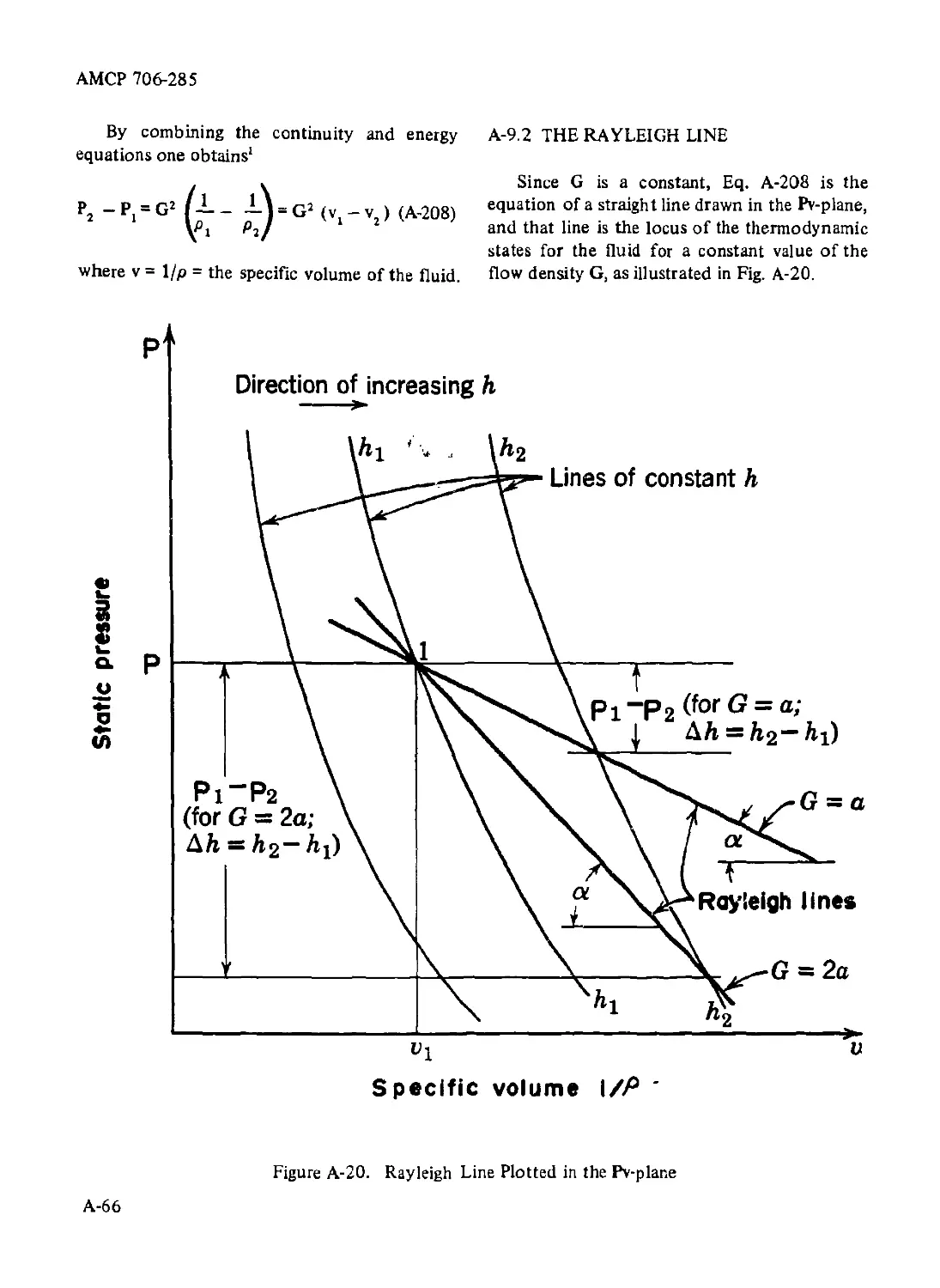
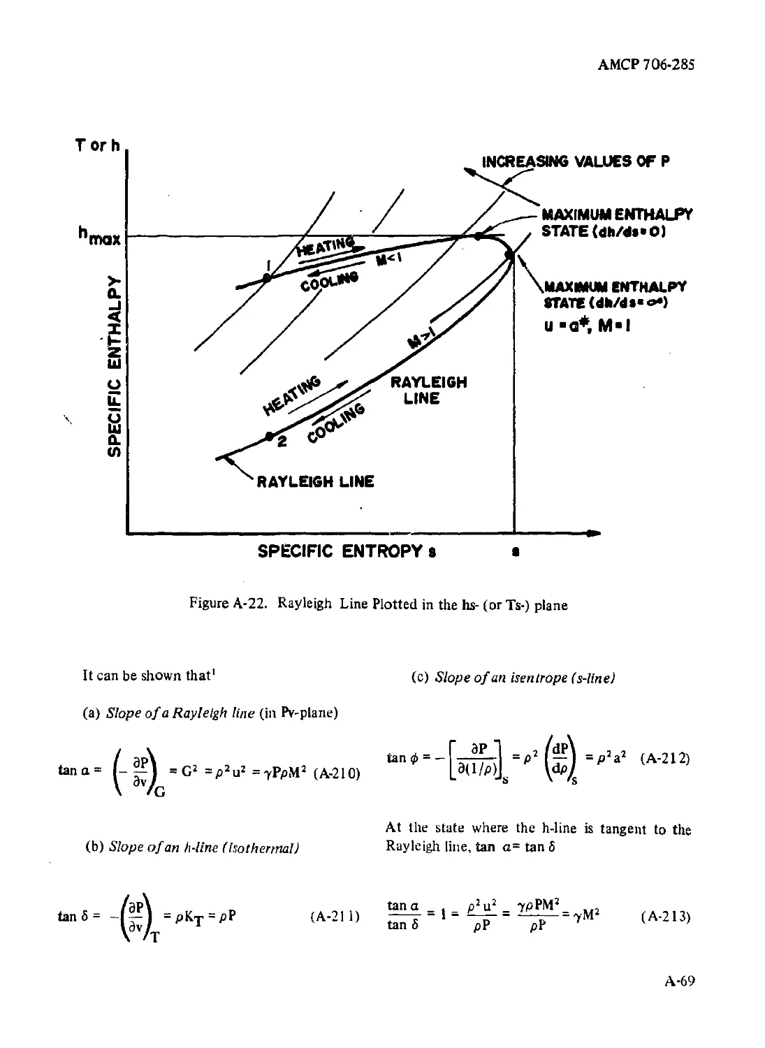
Text
AMC PAMPHLET
АМСР 706*285
ENGINEERING DESIGN
HANDBOOK
ELEMENTS OF AIRCRAFT
AND
MISSILE PROPULSION
5ТАТЯМЖТ #2 U
This document is subject to speiiexport controls and ead&
transmittal to foreign governpje.'vt > or foreign nationals may be
made’.only with prior approval of_
- ----------------------------------------------------
НЕМШТНВ, U.S. ARMY MATERIEL COMMAND
Ш19Й
Reproduced by the
CLEARINGHOUSE
for Federal Scientific & Technical
Information Springfield Va. 22151
AMC PAMPHLET
No. 706-285*
HEADQUARTERS
UNITED STATES ARMY MATERIEL COMMAND
WASHINGTON. D. C. 20315
ENGINEERING DESIGN HANDBOOK
ELEMENTS OF AIRCRAFT AND MISSILE PROPULSION
29 July 1969
Paragraph Page
LIST OF ILLUSTRATIONS...................... xxiii
LIST OF TABLES ............................. xxxh
PREFACE .................................... xxxvii
PART ONE- CHEMICAL ROCKET PROPULSION
CHAPTER 1- CLASSIFICATION AND ESSENTIAL
FEATURES OF ROCKET JET PROPULSION SYSTEMS
1-0 Principal Notation for Chapter 1........................... 1-1
1-1 Purpose and Scope of handbook.............................. 1-1
1-2 Scope of the Field of Propulsion........................... 1-2
1-3 The Reaction Principle ........................................ 1-3
1-4 The Jet Propulsion Principle .............................. 1-3
1-5 Classification of Jet Propulsion Systems............... 1-3
1-5.1 Air-breathing Jet Engines............................. 1-4
1-5.2 Rocket Jet Propulsion Systems ........................ 1-5
1-5.3 Classification of Rocket Propulsion Systems....... 1-5
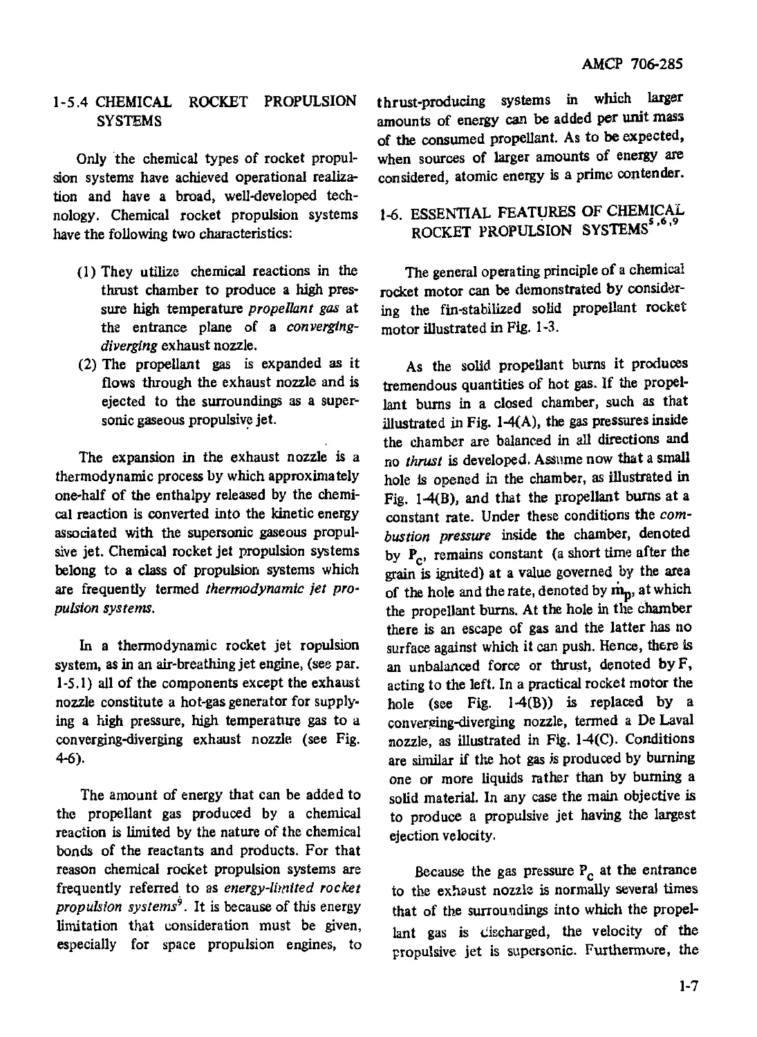
1-5.4 Chemical Rocket Propulsion Systems.................... 1-7
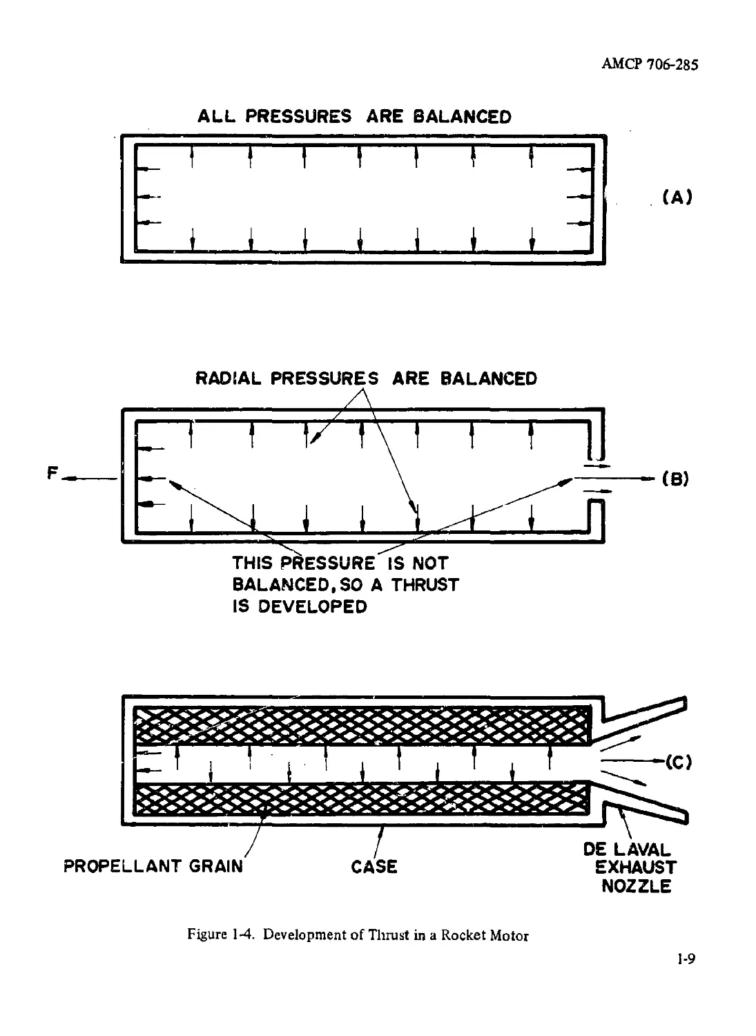
1-6 Essential Features of Chemical Rocket Propulsion Systems. 1-7
1-6.1 Classification of Rocket Propulsion Systems ......... 1-10
1-6.2 Liquid Bipropellant Rocket Engine.................... 1-11
1-6.3 Liquid Monopropellant Rocket Engine ................. 1-11
1-6.4 Solid Propellant Rocket Motor .................... 1-11
1-6.5 Hybrid Rocket Engine................................. 1-11
1-7 Units of Measurement................................... 1-11
References .............................................. 1-17
CHAPTER 2. MOMENTUM THEORY APPLIED
TO PROPULSION
2-0 Principal Notation for Chapter 2........................... 2-1
2-1 Momentum Theorem of Fluid Mechanics ....................... 2-3
2-1.1 Transport of a Fluid Property Across a
Control Surface ................................... 2-3
2-1.2 Momentum of a Fluid in Steady Flow.................... 2-4
2-1.3 External Forces Acting on a Flowing Fluid............. 2-6
2-1.4 Steady Flow Momentum Theorem ......................... 2-7
2-2 Application of Momentum Theorem to
Propulsion Systems................................................ 2-7
2-2.1 General Thrust Equation............................... 2-9
*This panphlet supersedes AMCP 706-282, Propulsion and Propellants, August 1963.
i
АМСР 706-285
TABLE OF CONTENTS (Continued)
Paragraph Page
2-2.2 Effective Jet Velocity.............................. 2-12
2-2.3 Exit Velocity of the Propulsive Jet............... 2-13
2-3 Thrust Equations for Rocket Propulsion................... 2-13
2-4 Power Definitions for Propulsion Systems ................ 2-14
2-4.1 Thrust Power (Py) .................................. 2-14
2-4.2 Propulsive Power (P) ............................... 2-14
2-4.3 Exit Loss .......................................... 2-14
2-4.4 Jet Power (Pj)...................................... 2-15
2-5 Performance Parameters for Jet Propulsion System ........ 2-15
2-5.1 Specific Thrust .................................... 2-15
2-5.2.1 Specific Impulse (Igp)......................... 2-15
2-5.2.2 Specific Impulse ana Jet Power ................ 2-15
2-5.3 Overall Efficiency (rjQ) ........................... 2-16
2-5.4 Thermal Efficiency (Чф)............................. 2-16
2-5.5 Propulsive Efficiency (i?p) ........................ 2-16
2-5.6 Ideal Propulsive Efficiency (чр) ................... 2-16
References ............................................. 2-18
CHAPTER 3. ELEMENTARY GAS DYNAMICS
3-0 Principal Notation for Chapter 3.......... 3-1
3-1 Introduction ............................................. 3-4
3-2 The Ideal Gas ............................................ 3-5
3-2.1 The Thermally Perfect Gas ........................... 3-5
3-2.2 Specific Heat ....................................... 3-5
3-2.2.1 Specific Heat at Constant Volume (Cy) .......... 3-6
3-2.2.2 Specific Heat at Constant Pressure (Cp) ........ 3-6
3-2.2.3 Specific Heat Ratio (7) ........................ 3-6
3-2.2.4 Specific Enthalpy and Specific Heat ............ 3-6
3-2.3 Calorically Perfect Gas.............................. 3-6
3-2.4 Specific Heat Relationships......................... 3-6
3-2.5 Acoustic or Sonic Speed in an Ideal Gas ............. 3-7
3-2.6 Mach Number.......................................... 3-7
3-3 General Steady One-dimensional Flow ........................... 3-7
3-3.1 Continuity Equation ................................. 3-7
3-3.2 Momentum Equation ................................... 3-8
3-3.2.1 General Form of Momentum Equation .............. 3-8
3-3.2.2 Momentum Equation for Steady, Ohe-
dimensional, Reversible Flow ................. 3-8
3-3.3 Energy Equation for Steady One-dimensional Flow... 3-8
3-4 Steady One-dimensional Flow of an Ideal Gas................... 3-10
3-4.1 Continuity Equation '............................... 3-10
i i
АМСР 706-285
TABLE OF CONTENTS (Continued)
Paragraph Page
3-4.2.1 Momentum Equations for the Steady One-
dimensional Flow of an Ideal Gas................................... 3-12
3-4.2.2 Momentum Equation for a Reversible, Steady,
One-dimensional Flow .......................... 3-12
3-4.3 Energy Equation...................................... 3-12
3-4.3.1 Energy Equation for a Simple Adiabatic Flow... 3-12
3-4.3.2 Energy Equation for the Simple Adiabatic
Flow of an Ideal Gas........................... 3-13
3-5 Steady One-dimensional Isentropic Flow......................... 3-13
3-5.1 Energy Equation for the Steady One-dimensional
Isentropic Flow of an Ideal Gas.................... 3-14
3-5.2 Stagnation (or Total) Conditions..................... 3-15
3-5.2.1 Stagnation (or Total) Enthalpy (h°) ............ 3-15
3-5.2.2 Stagnation (or Total) Temperature (T°).......... 3-15
3-5.2.3 Stagnation (or Total) Pressure (P°)............. 3-15
3-5.2.4 Relationship Between Stagnation Pressure
and Entropy.................................... 3-17
3-5.2.5 Stagnation (or Total) Density (p°).............. 3-17
3-5.2.6 Stagnation (or Total) Acoustic Speed (a0)....... 3-17
3-5.3 Isentropic Exhaust Velocity ......................... 3-17
3-5.4 Critical Conditions for the Steady, One-dimensional,
Isentropic Flow of an Ideal Gas.................... 3-18
3-5.4.1 Definition of Critical Area and Critical
Acoustic Speed............................... 3-18
3-5.4.2 Critical Thermodynamic Properties for the
Steady, One-dimensional, Isentropic Flow
of an Ideal Gas ............................... 3-18
3-5.5 Continuity Equations for Steady, One-dimensional,
Isentropic Flow of an Ideal Gas.................... 3-20
3-5.5.1 Critical Area Ratio (A/A*) ..................... 3-20
3-5.5.2 Critical Area Ratio in Terms of the Flow
Expansion Ratio (P/P°) ........................ 3-20
3-5.5.3 Critical Area Ratio in Terms of the Flow
Mach Number ................................... 3-20
3-5.6 Reference Speeds (a0 ), (a*), and (co)....................... 3-20
1-5.6.1 Continuity Equations in T rms of
Stagnation Conditions ......................... 3-21
3-5.6.2 Critical Mass Flow Density (G*)................. 3-21
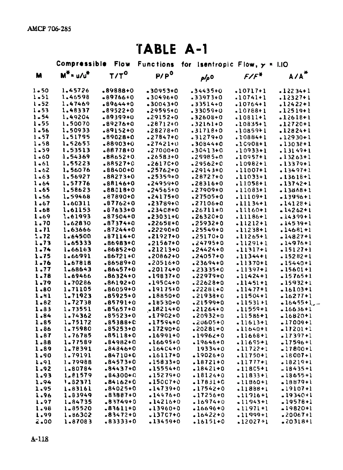
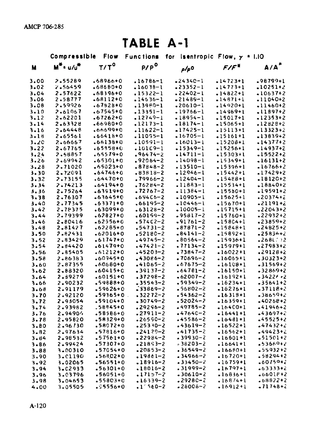
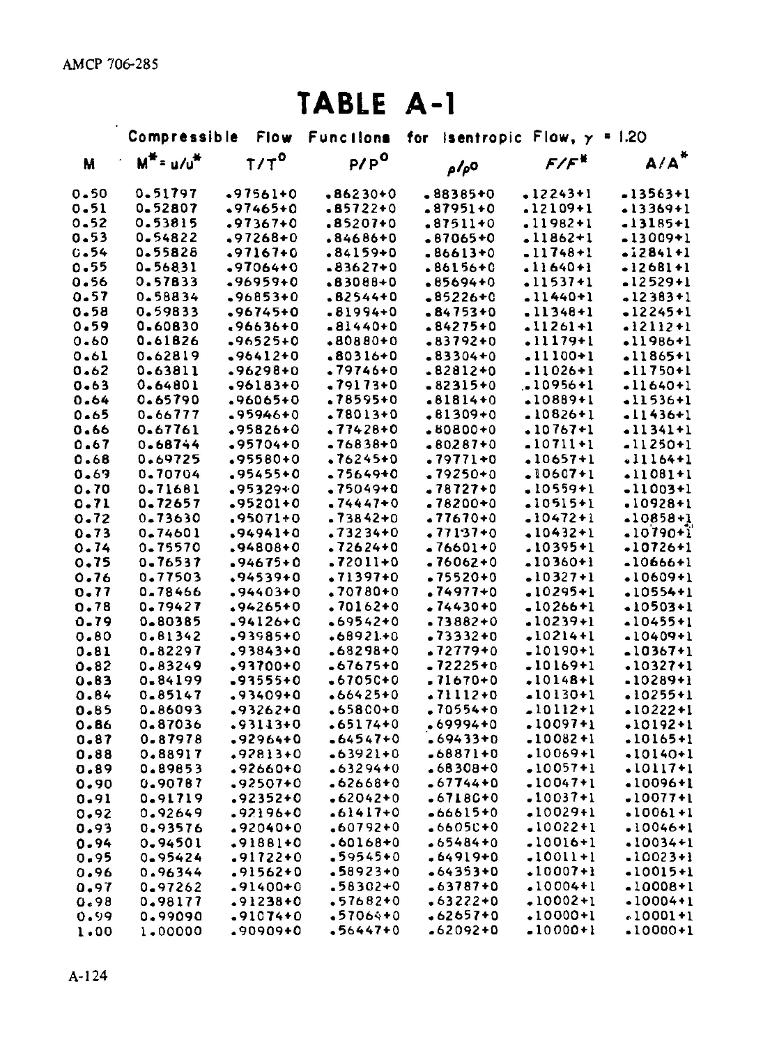
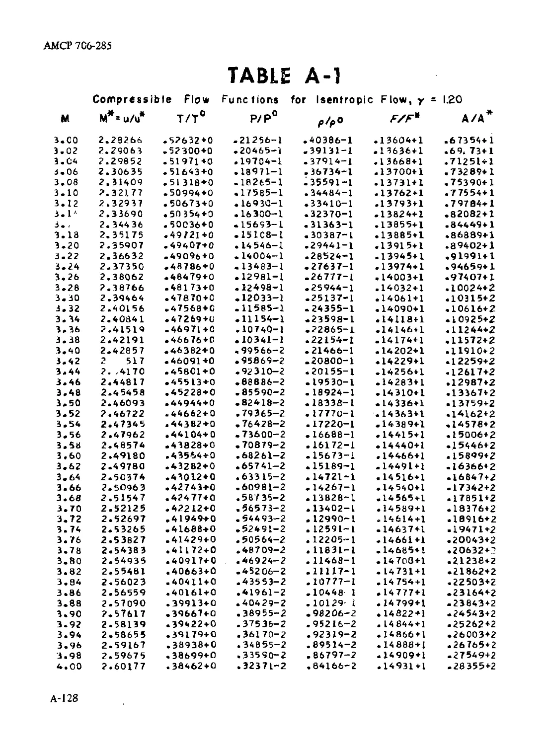
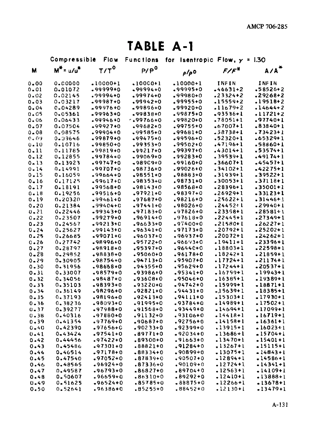
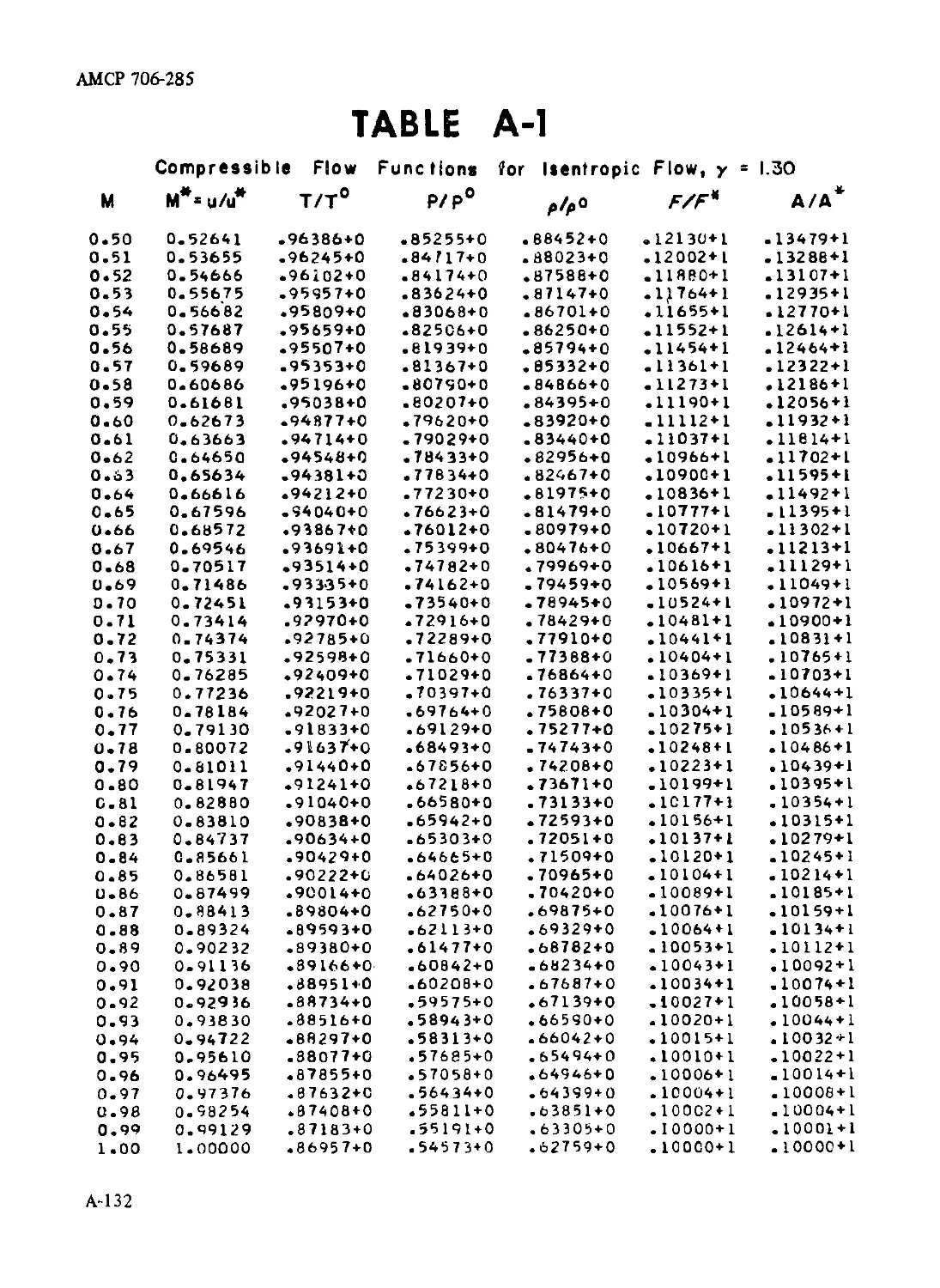
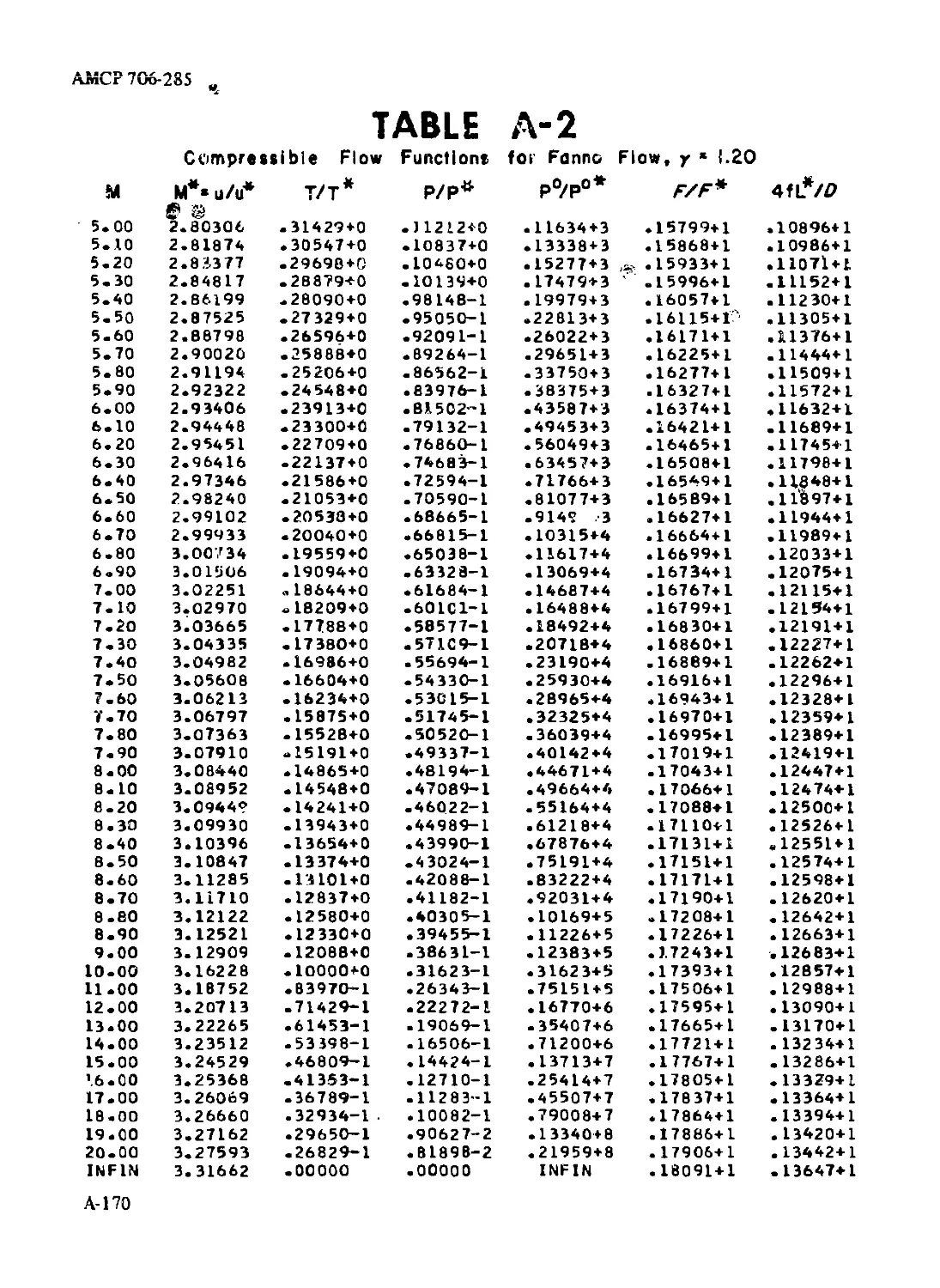
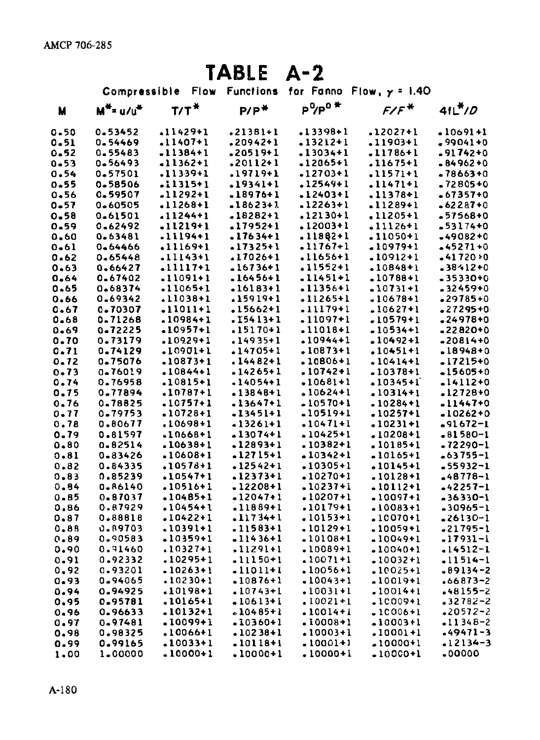
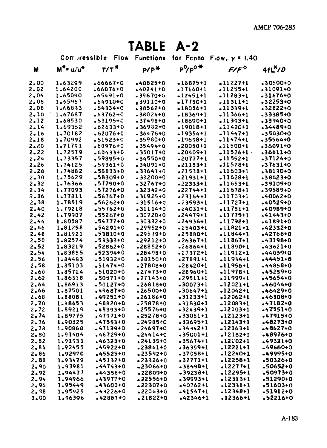
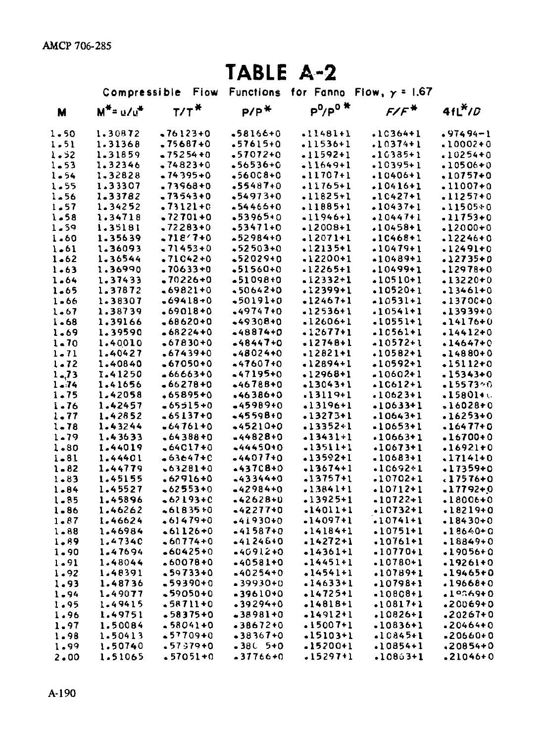
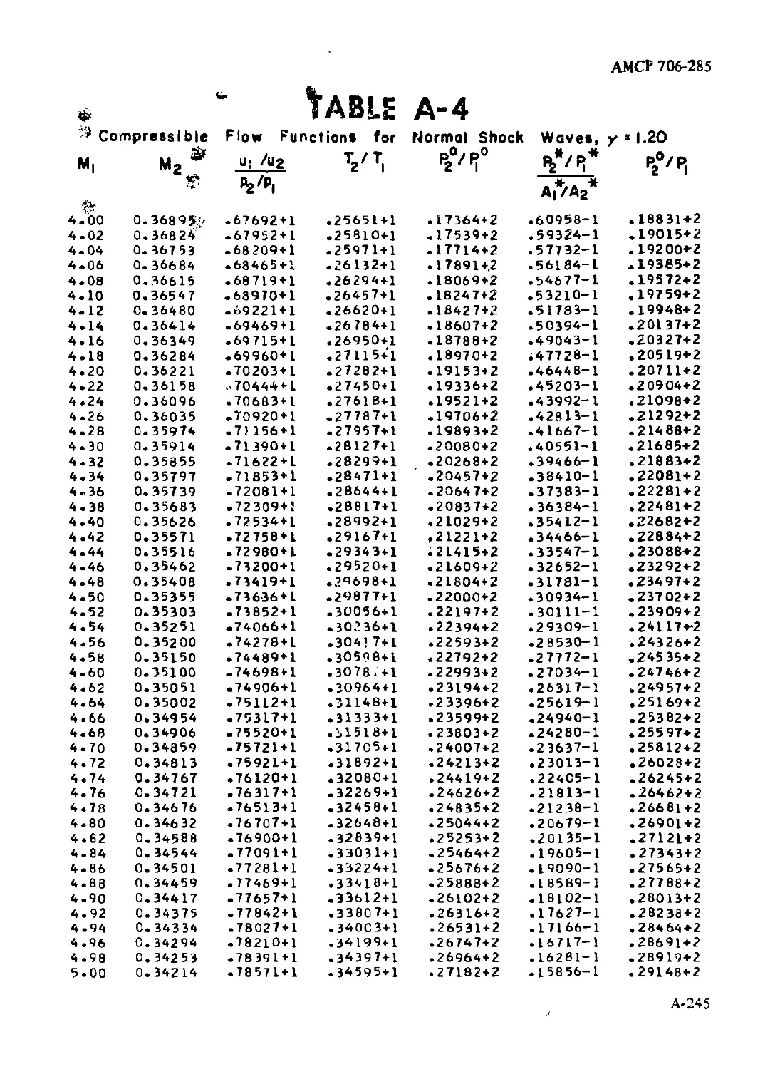
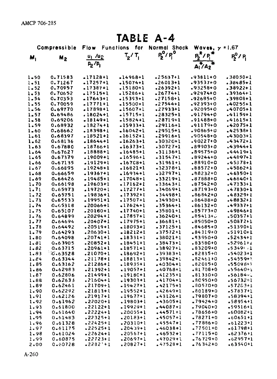
3-5.7 Tables of Isentropic Flow Functions for Ideal Gases... 3-21
3-6 Steady One-dimensional Adiabatic Flow in a Constant
Area Duct With Wall Friction (Fanno Flow).......................... 3-23
3-6.1 Friction Coefficient (f) ............................ 3-23
3-6.2 Principal Equations for Fanno Flow .................. 3-23
iii
АМСР 706-285
TABLE OF CONTENTS (Continued)
Paragraph Page
3-6.3 Fann о Line Equation ................................ 3-23
3-6.4 Fanno Flow With Ideal Gases ......................... 3-26
3-6.4.1 Principal Equations............................. 3-26
3-6.4.2 Critical Duct Length for the Fanno Flow of
an Ideal Gas ................................. 3-27
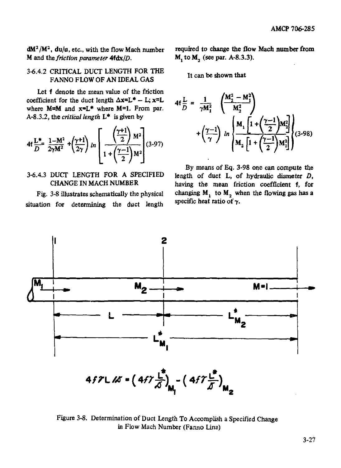
3-6.4.3 Duct Length for a Specified Change in
Mach Number .................................. 3-27
3-6.4.4 General Characteristics of the Fanno Flow
of an Ideal Gas .............................. 3-28
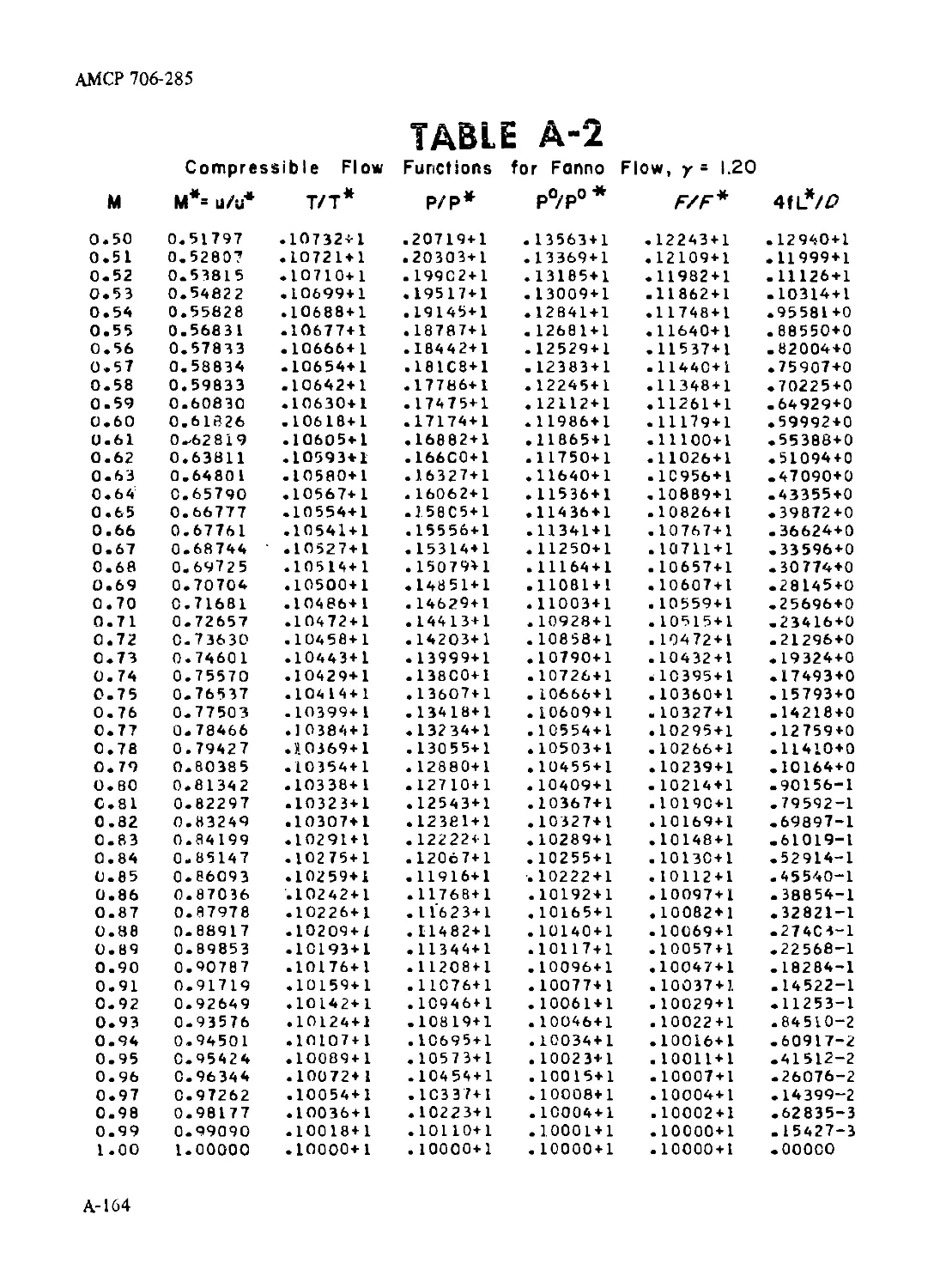
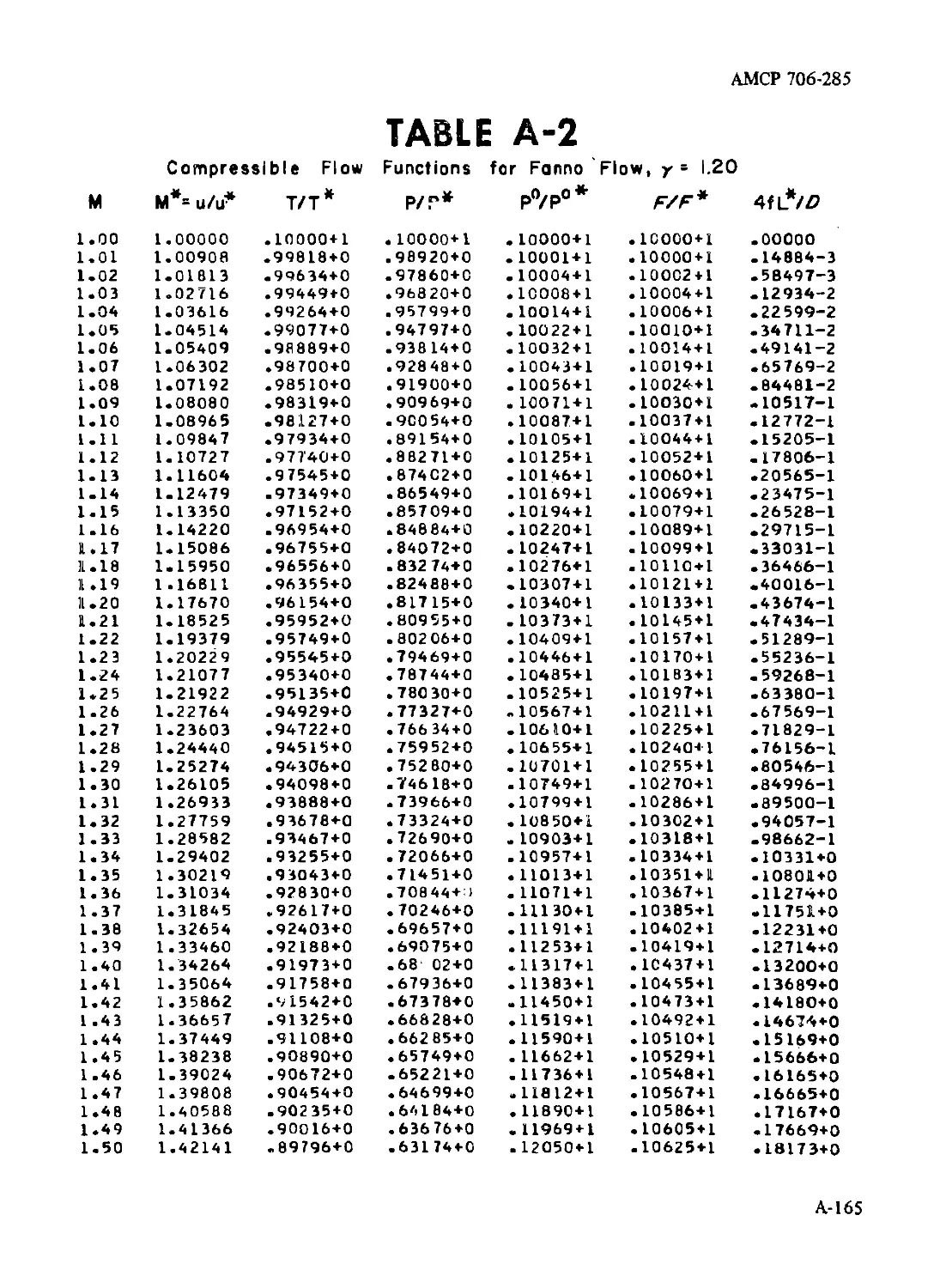
3-6.5 Equations for Compiling Tables for Fanno Flow
Functions, for Ideal Gases......................... 3-28
3-7 Steady One-dimensional Frictionless Flow in a Constant
Area Duct With Stagnation Temperature Change
(Rayleigh Flow)......................................... 3-29
3-7.1 Principal Equations for a Rayleigh Flow.............. 3-29
3-7.2 Rayleigh Line ....................................... 3-32
3-7.2. i General Characteristics .......................... 3-32
3-7.2.2 Characteristics of the Rayleigh Line for the
Flow of an Ideal Gas.......................... 3-32
3-7.3 Rayleigh Flow Equations for Ideal Gases............. 3-34
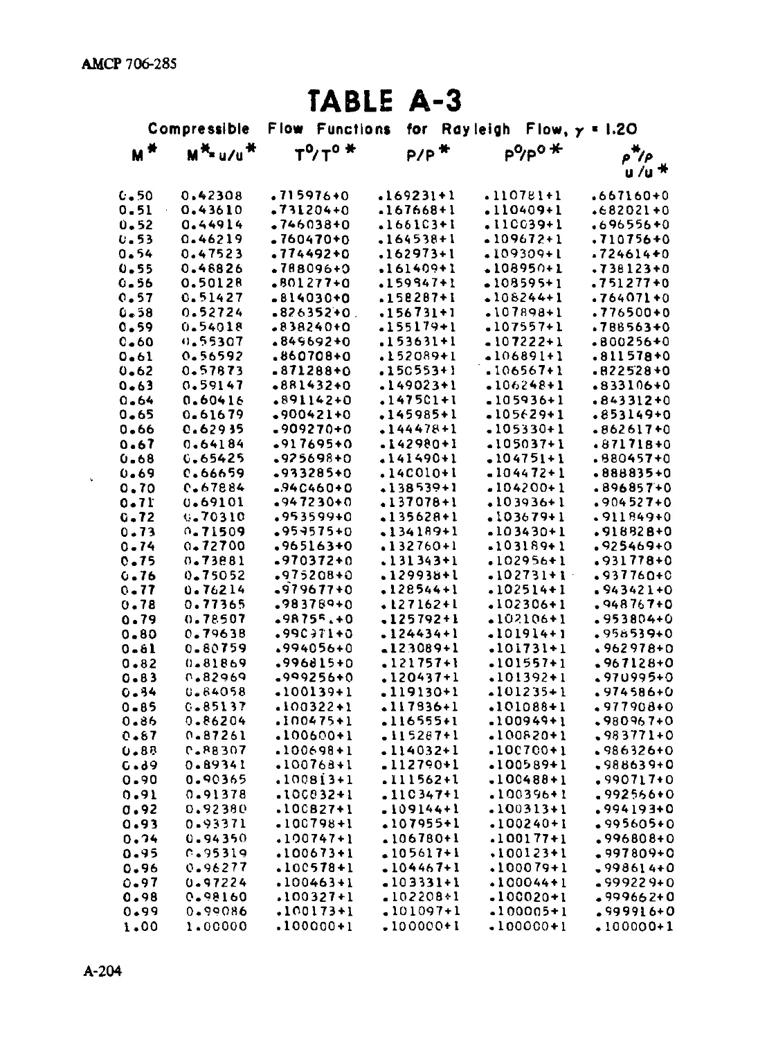
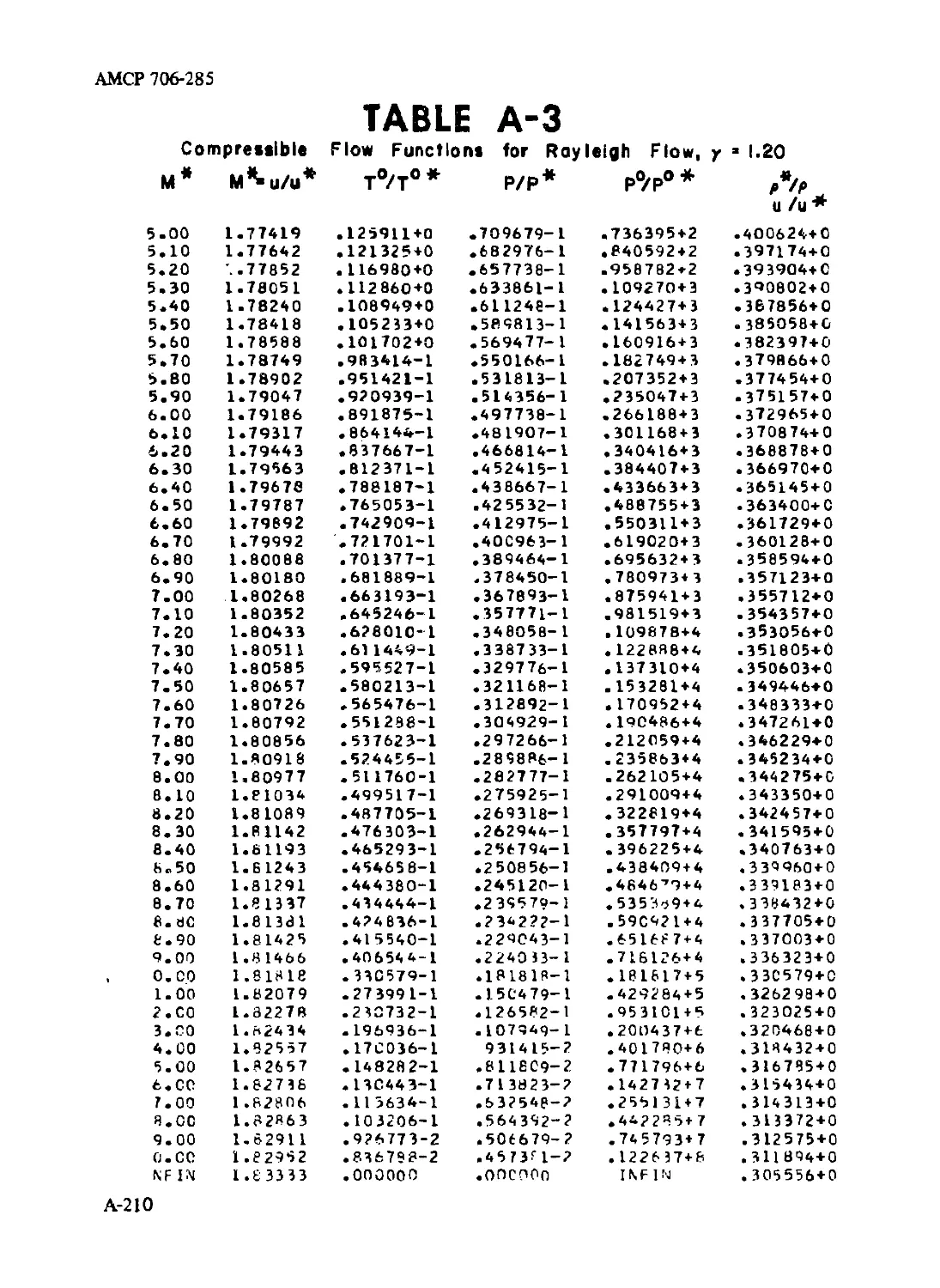
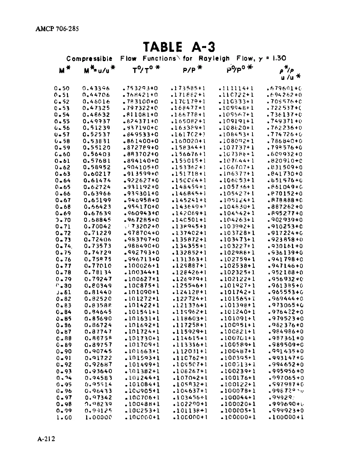
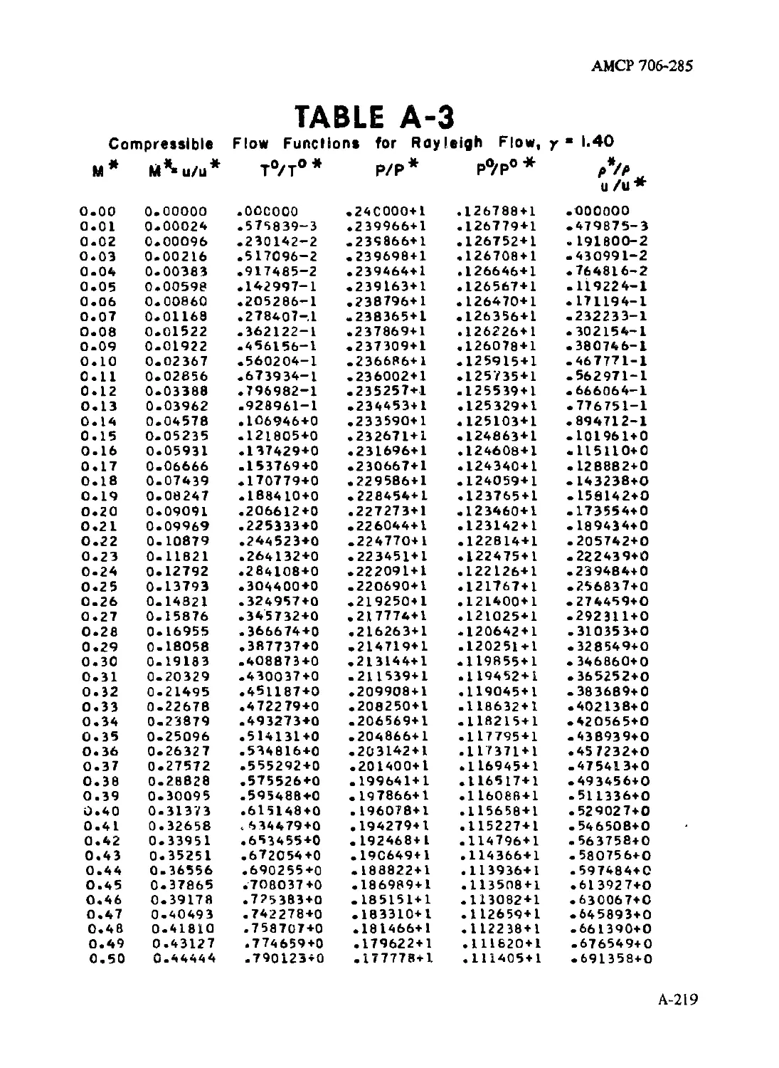
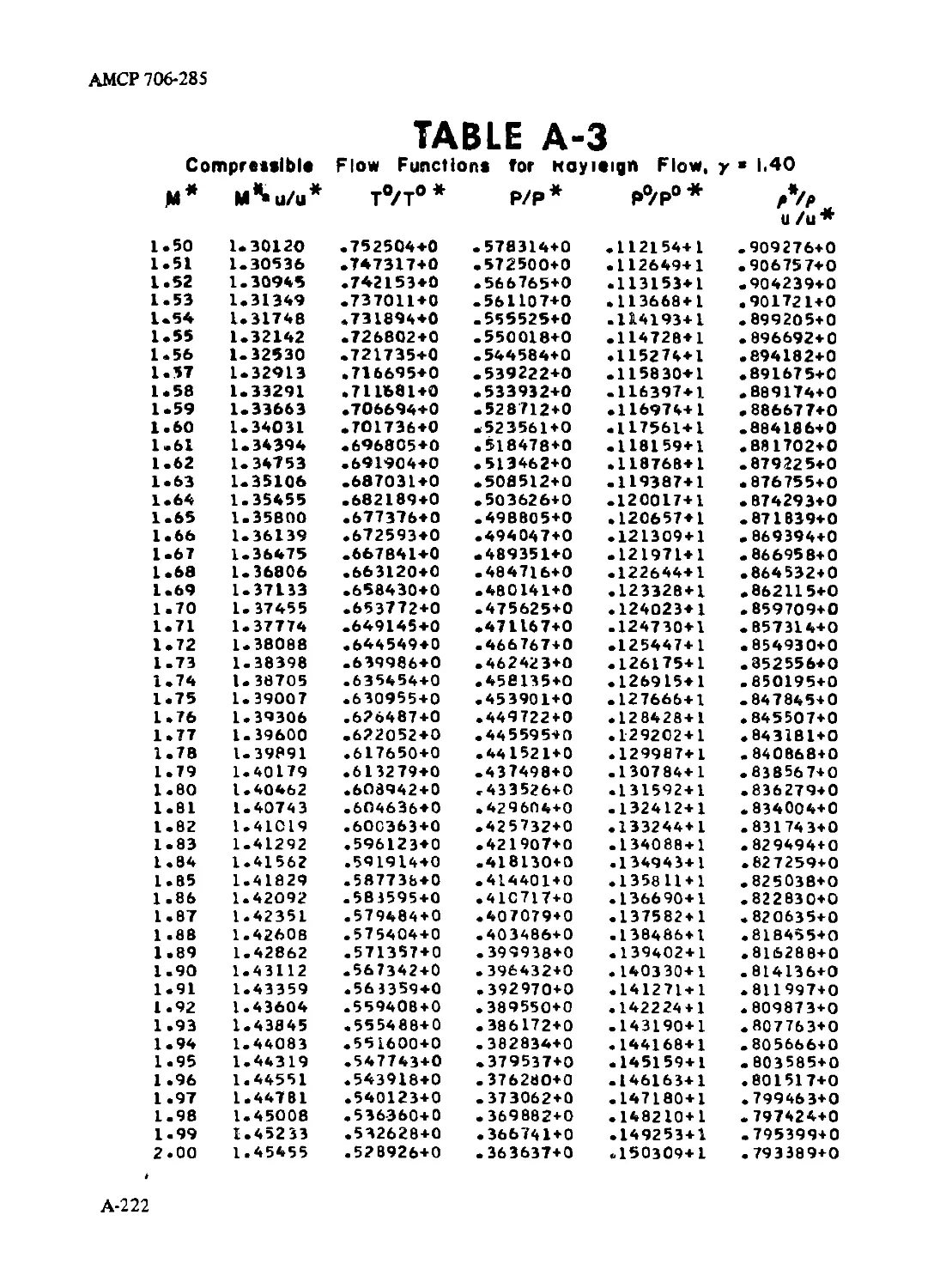
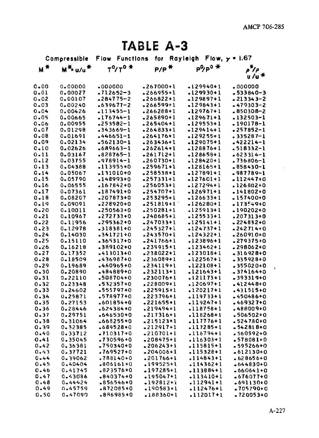
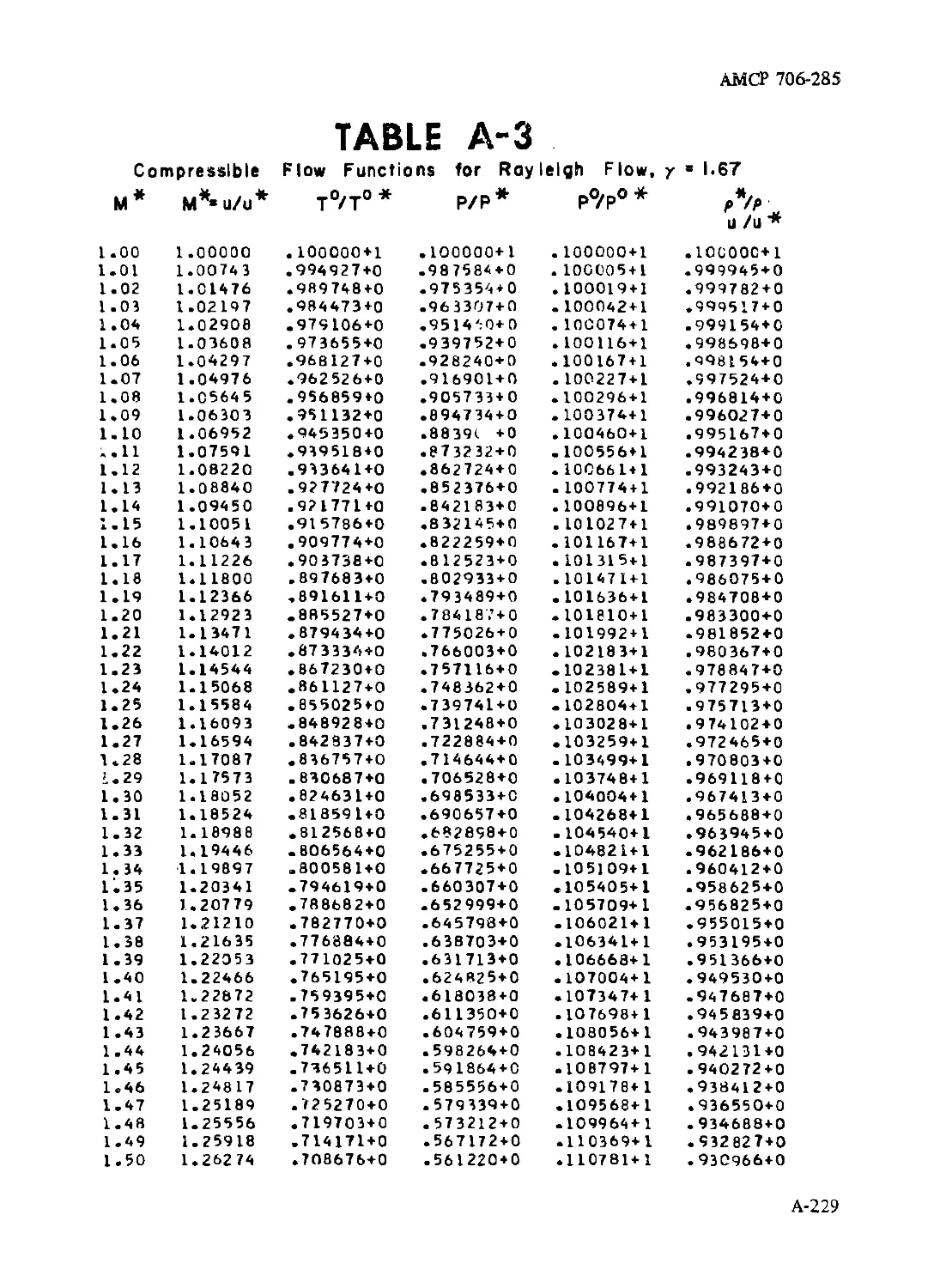
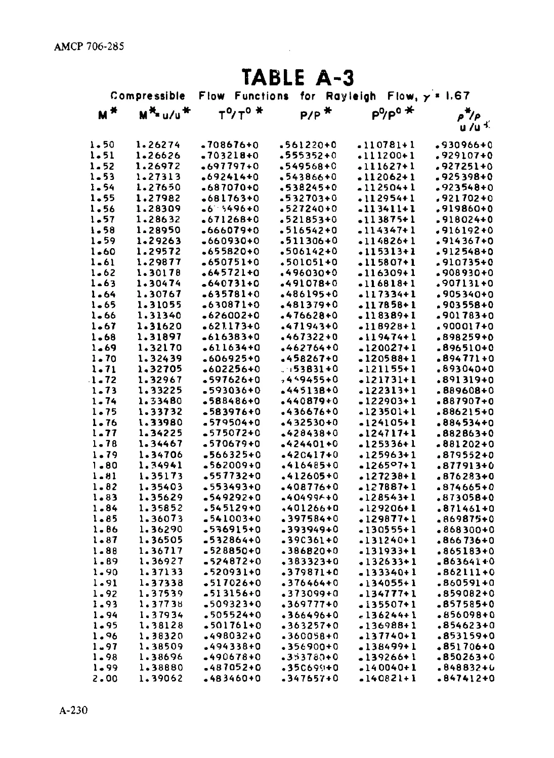
3-7.4 Equations for Tables of Rayleigh Flow Functions
for Ideal Gases .................................................. 3-35
3-7.5 Development of Compression Shock .................... 3-37
References .............................................. 3-39
CHAPTER 4.C OMPRESSIBLE FLOW IN NOZZLES
4-0 Principal Notation for Chapter 4.......... 4-1
4-1 Introduction ............................................ 4-3
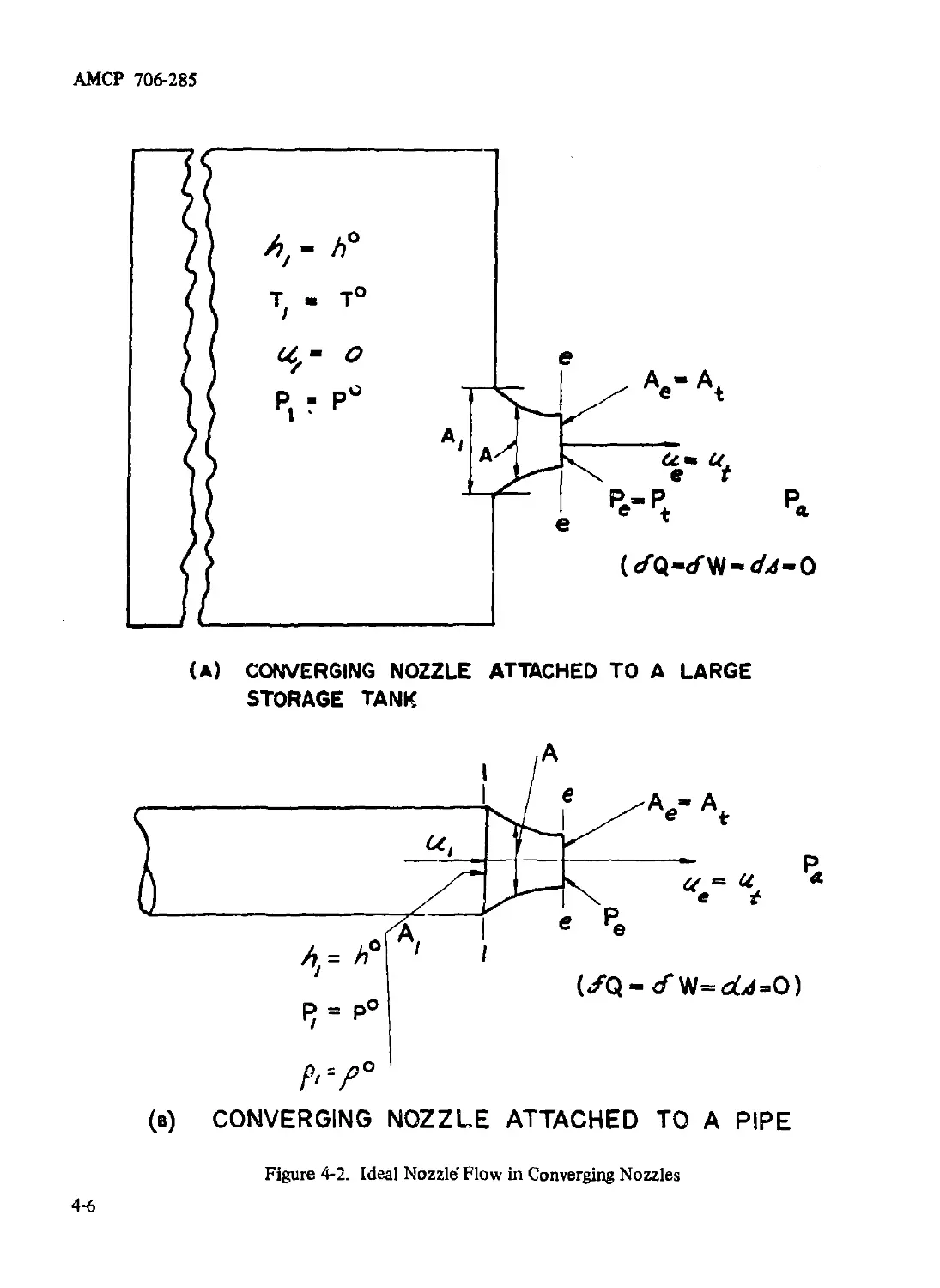
4-2 Ideal Flow in a Converging Nozzle ......................... 4-5
4-2.1 Isentropic Exit Velocity for a Converging Nozzle . . 4-5
4-2.2 Isentropic Throat Velocity for the Flow of a Perfect
Gas in a Converging Nozzle ......................... 4-5
4-2.3 Effect of Varying the Back Pressure Acting on a
Converging Nozzle................................... 4-7
4-2.4 Mass Flow Rate for Ideal Nozzle Flow (Converging
and Converging-diverging Nozzles)................... 4-8
4-3 Ideal Flow in a Converging-diverging (or De Laval) Nozzle. . 4-10
4-3.1 Area Ratio for Complete Expansion of the Gas
Flowing in a Converging-diverging Nozzle........... 4-14
4-3.2 Effect of Varying the Back Pressure Acting on a
Converging-diverging Nozzle........................ 4-20
4-3.2.1 Underexpansion in a Converging-diverging
Nozzle ....................................... 4-20
iv
АМСР 706-285
TABLE OF CONTENTS (Continued)
Paragraph Page
4-3.2.2 Overexpansion in a Converging-diverging Nozzle . 4-21
4-3.3 Effect of Varying the Inlet Total Pressure of a Nozzle... 4-24
4-4 Flow in Real Nozzles .................................... 4-26
4-4.1 Losses in Nozzles.................................... 4-26
4-4.2 ; Area Ratio for an Adiabatic Nozzle................. 4-26
4-5 Nozzle Performance Coefficients............................... 4-27
4-5.1 Nozzle Efficiency (i7n).............................. 4-27
4-5.2 Nozzle Velocity Coefficient (0) ..................... 4-27
4-5.3 Nozzle Discharge Coefficient (C^) ................... 4-27
4-6 Mass Flow Rate for a Nozzle Operating With Adiabatic
Flow and Wall Friction........................................... 4-28
4-7 Nozzle Design Principles................................. 4-28
4-8 Nozzle Design Configurations............................. 4-29
4-8.1 Conical N ozzle...................................... 4-30
4-8.1.1 Thrust Equation for a Conical Nozzle........... 4-31
4-8.1.2 Factors for Determining Adequacy of a
Conical Nozzle .............................. 4-32
4-8.2 Contoured or Beil-shaped Nozzle..................... 4-34
4-8.3 Annular Nozzle ...................................... 4-36
4-8.4 Plug Nozzle.......................................... 4-36
4-8.5 Expansion-deflection or E-D Nozzle .................. 4-39
References ............................................. 4-40
CHAPTER 5. PERFORMANCE CRITERIA FOR
ROCKET PROPULSION
5-0 Principal Notation for Chapter 5....................... 5-1
5-1 Introduction ............................................. 5-2
5-2 Effective Jet (or Exhaust) Velocity (c) .................. 5-2
5-3 Specific Impulse (Igp).................................... 5-3
5-3.1 Specific Propellant Consumption (Wjp) ................ 5-4
5-3.2 Weight-flow Coefficient (Cw).......................... 5-4
5-3.3 Mass-flow Coefficient (Cm)............................ 5-4
5-4.1 Thrust Coefficient (Cp) .............................. 5-4
5-4.2 Relationship Between ISp, Cw, and Cp ................. 5-5
5-5 Characteristic Velocity (c*).............................. 5-5
5-6 Jet Power (Fj)............................................ 5-5
5-7 Total Impulse (ly) ....................................... 5-5
5-8 Weight and Mass Ratios ................................... 5-6
5-8.1 Propulsion System Weight (Wpg)........................ 5-6
5-8.2 Specific Engine Weight (r) ........................... 5-7
5-8.3 Payload Ratio (Wpay/W0 ) ............................. 5-7
• V
АМСР 706-285
TABLE OF CONTENTS (Continued)
Paragraph Page
5-8.4 Propellant Weight (Wp) .............................. 5-7
5-8.5 Propellant Mass Ratio (J)............................ 5-7
5-8.6 Vehicle Mass Ratio (A) .............................. 5-7
5-8.7 Relationship Between the Propellant Mass Ratio (£)
and the Vehicle Mass Ratio (A)..................... 5-8
5-8.8 Propellant Loading Density (5 p)..................... 5-8
5-8.9 Impulse-weight Ratio for a Rocket Engine ............ 5-8
5-9 Vehicle Performance Criteria .................................. 5-8
5-9.1 Linear Motion With Drag and Gravity.................. 5-9
5-9.1.1 Thrust of Rocket Engine With Linear Motion
of Vehicle.................................... 5-9
5-9.1.2 Aerodynamic Drag .............................. 5-11
5-9.1.3 Approximate Solution of Differential Equation
for Linear Motion With Drag and Gravity...... 5-11
5-9.2 Burnout Velocity (Vb) .............................. 5-13
5-9.2.1 Burnout Altitude (z^).......................... 5-14
5-9.2.2 Coasting Altitude After Burnout (zc) .......... 5-14
5-9.2.3 Maximum Drag-free Altitude (zmax) ............. 5-14
5-9.3 Ideal Burnout Velocity (Vy) ........................ 5-14
References ............................................. 5-16
CHAPTER 6. THERMODYNAMIC RELATIONSHIPS FOR
CHEMICAL ROCKET PROPULSION
6-0 Principal Notation for Chapter 6.......................... 6-1
6-1 Introduction ............................................. 6-3
6-2 Assumptions in Thermochemical and Gas Dynamic
Calculations ........................................... 6-4
6-2.1 Exothermic and Endothermic Chemical Reactions.... 6-5
6-2.2 Conditions for Thermochemical Equilibrium ........... 6-6
6-2."3 Dissociation and Reassociation Reactions ............ 6-6
6-3 ThermodynamicEquationsforRocketPerformanceCriteria . 6-6
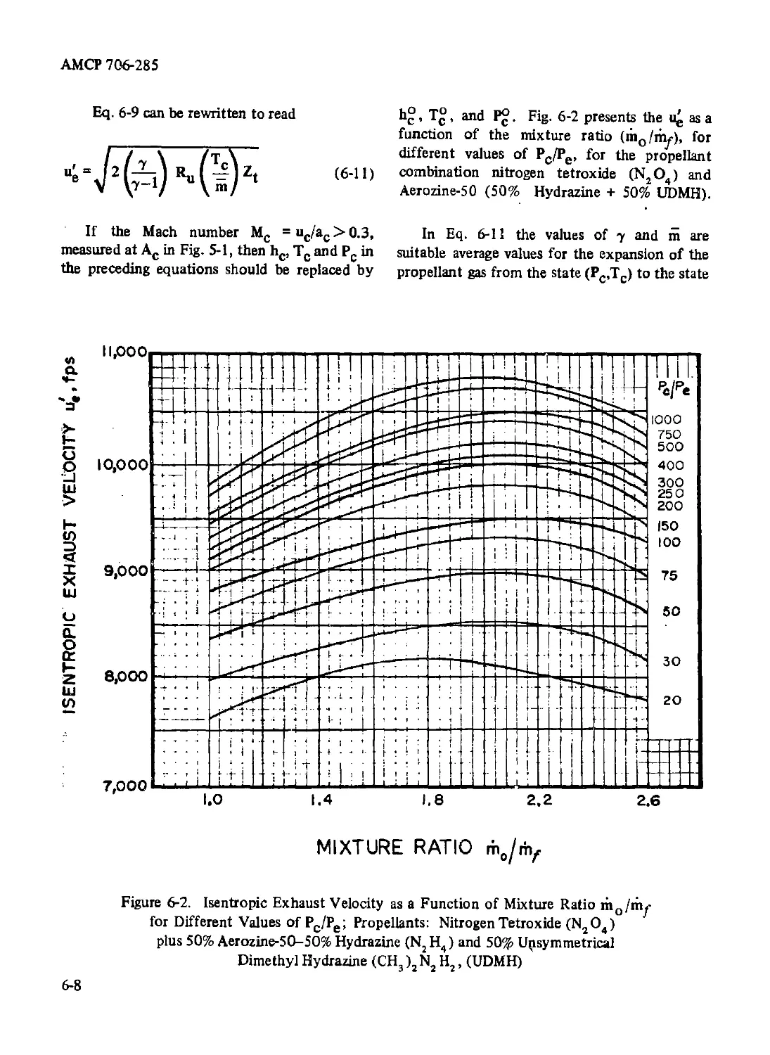
6-3.1 Isentropic Exit Velocity (ug) ....................... 6-7
6-3.2 Actual or Adiabatic Exit Velocity (ue) .............. 6-9
6-3.3 Propellant Flow Coefficients ....................... 6-11
6-3.3.1 Mass Flow Rate of Propellant Gas (m)........... 6-11
6-3.3.2 Weight Flow Coefficient (Cw)................... 6-11
6-3.4 Thrust (F) ......................................... 6-11
6-3.4.1 Effective Jet (or Exhaust) Velocity (c) ....... 6-13
6-3.4.2 Thrust Coefficient (Cp) ....................... 6-13
6-3.5 Nozzle Area Ratio for Complete Expansion .......... 6-13
6-3.6 Characteristic Velocity (c*)........................ 6-18
vi
АМСР 706-285
TABLE OF CONTENTS (Continued)
Paragraph ^а8е
6-3.7 Theoretical Specific Impulse (I^j) ........................... 6-20
6-3.7.1 Reduced Specific Impulse ........................ 6-20
6-3.7.2 Density Specific Impulse (Ij) ................... 6-23
References ............................................... 6-26
CHAPTER 7 .PROPERTIES AND CHARACTERISTICS OF
SOLID PROPELLANTS
7-1 Classification of Solid Propellants ............................. 7-1
7-2 Homogeneous Propellants .................................... 7-1
7-2.1 Polymers for Homogeneous Propellants................... 7-2
7-2.2 Oxidizer-plasticizers for Homogeneous Propellants ... 7-2
7-2.3 Fuel-plasticizers for Homogeneous Propellants ......... 7-2
7-2.4 Additives to Double-base Propellants .................. 7-2
7-2.5 General Characteristics and Applications of Double-
base Solid Propellants .............................. 7-2
7-3 Heterogeneous or Composite Propellants...................... 7-4
7-3.1 Binders for Composite Propellants ..................... 7-4
7-3.2 Oxidizers for Composite Propellants ................... 7-5
7-3.3 Additives to Composite Propellants..................... 7-6
7-4 Factors Governing the Selection of a Solid Propellant..... 7-7
7-4.1 Specific Impulse (ISp)................................. 7-7
7-4.2 Density of Propellant (pp) ............................ 7-7
7-4.3 Hygroscopicity ........................................ 7-7
7-4.4 Controllable Linear Burning Rate (r0).................. 7-7
7-4.5 Coefficient of Thermal Expansion ...................... 7-7
7-4.6 Thermal Conductivity................................... 7-7
7-4.7 Chemical Stability .................................... 7-7
7-4.8 Toxicity .............................................. 7-8
7-4.9 Shock Sensitivity...................................... 7-8
7-4.10 Explosive Hazard....................................... 7-8
7-4.11 Smoke in Exhaust ...................................... 7-8
7-4.12 Attenuation of Electromagnetic Signals................. 7-8
7-4.13 Availability of Raw Materials ......................... 7-9
7-4.14 Fabrication and Process Control........................ 7-9
7-4.15 Cost................................................... 7-9
7-5 Mechanical Properties of Solid Propellants.................. 7-9
7-5.1 Ultimate Tensile Strength ............................. 7-9
7-5.2 Elongation in Tension................................. 7-10
7-5.3 Modulus in Tension.................................... 7-10
7-5.4 Stress Relaxation..................................... 7-10
7-5.5 Creep ................................................ 7-10
vii
АМСР 706-285
TABLE OF CONTENTS (Continued)
Paragraph Page
7-5.6 Compressive Strength ................................ 7-10
7-5.6.1 Deformation At Rupture in Compression .......... 7-10
7-5.6.3 Modulus in Compression.......................... 7-10
7-5.7 Shear Properties .................................... 7-11
7-5.8 Brittle Temperature.................................. 7-11
References .............................................. 7-12
CHAPTER Я SOLID PROPELLANT ROCKET MOTORS
8-0 Principal Notation for Chapter 8........................... 8-1
8-1 Internal Ballistics of Solid Propellant Rocket Motors... 8-3
8-1.1 Burning of a Solid Propellant (Piobert’s Law)...... 8-3
8-1.2 Combustion Temperature ............................... 8-3
8-1.3 General Characteristics of the Combustion Process ... 8-4
8-1.4 Combustion Characteristics of Double-base
Solid Propellants .................................. 8-5
8-1.5 The Flame Reaction Zone for a Double-base Solid
Propellant.......................................... 8-7
8-1.6 Combustion Characteristics of Composite (Non-
homogeneous) Solid Propellants ..................... 8-7
8-1.7 Linear Burning Rate (Saint-Robert’s Law) ............. 8-7
8-1.8 Weight Rate of Propellant Consumption (Wp) ........... 8-9
8-1.9 Volumetric Rate of Propellant Consumption (Qp) ... 8-9
8-1.10 Equilibrium Combustion Pressure and Its Stability ... 8-11
8-1.11 Effect of Propellant Area Ratio (Kn) ................ 8-11
8-1.12 Stability of the Shape of the Burning Surface... 8-12
8-1.13 Pressure Deflagration Limit and Pressure Limit ...... 8-12
8-1.14 Effect of the Temperature of a Solid Propellant. 8-12
8-1.14.1 General Effects of Temperature ................. 8-12
8-1.14.2 Temperature Sensitivity ........................ 8-13
8-1.15 Erosive Burning ..................................... 8-13
8-2 Combustion Pressure Oscillations in Solid Propellant
Rocket Motors (Unstable Burning) .................................. 8-14
8-2.1 Terminology Employed in Unstable Burning of
Solid Propellant Rocket Motors..................... 8-14
8-2.2 Acoustic Instability in Solid Propellant Rocket
Motors ............................................................ 8-14
8-3 Ignition of Propellant Grain ............................. 8-19
8-4 Solid Propellant Grain Configurations..................... 8-20
8-5 Port-to-throat Area Ratio (1/J) .......................... 8-23
8-6 Heat Transfer in Solid Propellant Rocket Motors .......... 8-23
8-6.1 Aerodynamic Heating.................................. 8-24
viii
АМСР 706-285
TABLE OF CONTENTS (Continued)
Paragraph Page
8-6.2 Effect of Aerodynamic Heating on Integrity of
Rocket Motor Chambers ............................. 8-24
8-7 General Design Considerations................................. 8-25
8-7.1 Selection of Combustion Pressure .................... 8-25
8-7.2 Estimate of the Weight and Volume of the Solid
Propellant Grain .................................. 8-25
8-7.3 Determination of Nozzle Throat Area.................. 8-26
8-7.3.1 General Considerations ......................... 8-26
8-7.3.2 Effect of Propellant Grain Configuration...... 8-26
8-7.4 Rocket Motor Chamber and Insulation ................. 8-26
8-7.5 Nozzles for Solid Propellant Rocket Motors........... 8-27
8-7.6 Control of Vehicle Range ............................ 8-28
8-7.7 Thrust Vector Control (TVC) of Solid Propellant
Rocket-propelled Vehicles ......................... 8-28
8-7.7.1 Mechanical Means for Achieving TVC.............. 8-30
8-7.7.2 Movable Nozzles................................. 8-32
8-7.7.3 Secondary Injection for TVC .................... 8-32
References ............................................. 8-35
CHAPTER 9. PROPERTIES AND CHARACTERISTICS OF
LIQUID PROPELLANTS
9-1 Factors To Be Considered in Selecting Liquid Propellants . 9-1
9-2 Principal Physical Properties of Liquid Propellants........9-1
9-2.1 Enthalpy of Combustion............................. 9-1
9-2.2 Chemical Reactivity.................................. 9-2
9-2.3 Chemical Structure.................................... 9-2
9-2.4 Average Density of Propellant System (Pp)............. 9-2
9-2.5 Boiling Point and Vapor Pressure..................... 9-2
9-2.6 Freezing Point........................................ 9-3
9-2.7 Dynamic or Absolute Viscosity ........................ 9-3
9-2.8 Specific Heat ........................................ 9-3
9-2.9 Chemical Stability ................................... 9-3
9-2.10 Corrosivity .......................................... 9-3
9-2.11 Toxicity ............................................. 9-4
9-2.12 Availability.......................................... 9-4
9-2.13 Cost.................................................. 9-4
9-3 Liquid Monopropellants ................................... 9-8
9-3.1 Hydrazine (NjH4) ..................................... 9-9
9-3.2 Hydrogen Peroxide (Ha Oj)............................ 9-10
9-3.3 Ethylene Oxide (CjH4O) .............................. 9-12
9-3.4 Mixtures of Nitroparaffins .......................... 9-12
ix
АМСР 706-285
TABLE OF CONTENTS (Continued)
Paragraph Page
9-3.5 Mixtures of Nitric Acid, Nitrobenzene and
Water (Dithekites)............................... 9-12
9-3.6 Mixtures of Methyl Nitrate and Methanol (Myrols)... 9-12
9-4 Oxidizers for Liquid Propellant Systems...................... 9-12
9-4.1 Liquid Fluorine (F2) .............................. 9-13
9-4.2 Liquid Oxygen (LOX)............................... 9-16
9-4.3 Oxidizers Containing Fluorine...................... 9-17
9-4.3.1 General Considerations ....................... 9-17
9-4.3.2 Chlorine Trifluoride (C1F3)................... 9-17
9-4.4 Oxidizers Containing Oxygen ....................... 9-17
9-4.4.1 Liquid Ozone (LOZ) ........................... 9-18
9-4.4.2 Hydrogen Peroxide (H2O2)...................... 9-18
94.4.3 Nitric Acid (HNO3)............................ 9-18
9-4.4.4 Mixed Oxides of Nitrogen (MON) ............... 9-19
9-4.5 Oxidizers Containing Fluorine and Oxygen .......... 9-20
9-4.5.1 Oxygen Bifluoride (OF2)....................... 9-22
9-4.5.2 Perchlorylfluoride (C1O3F).................... 9-22
9-5 Fuels for Liquid Bipropellant Systems........................ 9-22
9-5.1 Cryogenic Fuels Rich in Hydrogen................... 9-22
9-5.2 The Borohydrides .................................. 9-24
9-5.3 Organic Fuels .................................... 9-24
9-5.3.1 Ethyl Alcohol (C2HSOH) ....................... 9-29
9-5.3.2 Light Hydrocarbon Fuels....................... 9-29
9-5.3.3 Unsymmetrical Dimethylhydrazine (UDMH) ... 9-29
9-5.3.4 Aerozine-50 (N2 H4 + UDMH- 50/50) ............ 9-30
9-5.3.5 Diethylenetriamine (DETA) .................... 9-30
9-5.4 Nitrogen Hydrides ................................. 9-31
9-5.4.1 Anhydrous Ammonia (NH3) ...................... 9-31
9-5.4.2 Hydrazine (N2H4) ............................. 9-31
9-5.4.3 Mixtures of Hydrazine and Ammonia............. 9-31
9-6 Gels, Slurries, and Emulsions (Heterogeneous
Propellants).................................................... 9-32
9-6.1 Thixotropic Gels................................. 9-32
9-6.2 Thixotropic Slurries............................... 9-33
9-6.3 Emulsions ......................................... 9-33
9-6.4 Summary............................................ 9-33
References ........................................... 9-34
CHAPTER 10 .LIQUID PROPELLANT ROCKET ENGINES
10-0 Principal Notation for Chapter 10 ..................... 10-1
10-1 Introduction .......................................... 10-2
АМСР 706-285
TABLE OF CONTENTS (Continued)
Paragraph Page
10-2 Essential Components of a Liquid Bipropellant
Rocket Engine .................................................... 10-2
10-3 The Thrust Chamber ........................................... 10-3
10 3.1 The Injector......................................... 10-3
10-3.2 The Combustion Chamber .............................. 10-5
10-3.2.1 Characteristic Length for a Liquid Propellant
Thrust Chamber (L*)........................... 10-6
10-3.2.2 Gas-side Pressure Drop in a Liquid Propellant
Thrust Chamber.............................. 10-8
10-3.3 The Exhaust Nozzle.................................. 10-9
10-4 Heat Transfer in Liquid Propellant Thrust Chambers ........... 10-9
10-4.1 Classification of Thrust Chamber Cooling Systems ... 10-10
10-4.2 Nonregenerative Cooling Systems .................... 10-11
10-4.2.1 Heat-sink Cooling of Thrust Chambers .......... 10-11
10-4.2.2 Heat-barrier Cooling of Thrust Chambers ....... 10-11
10-4.2.3 Compound Heat-sink and Heat-barrier Cooling
of Thrust Chambers .......................... 10-14
10-4.3 Regenerative Cooling Systems........................ 10-14
10-4.4 Internal Cooling Systems............................ 10-16
10-4.4.1 Film Cooling .................................. 10-16
10-4.4.2 Transpiration Cooling.......................... 10-17
10-4.4.3 Ablation Cooling............................... 10-17
10-5 Feed Systems for Liquid Propellant Rocket Engines ....... 10-20
10-5.1 Stored (Inert) Gas Pressurization................... 10-20
10-5.2 Chemical Gas Pressurization ........................ 10-21
10-5.3 Turbopump Pressurization ......................... 10-22
10-6 Thrust Vector Control.................................... 10-22
10-7 Variable Thrust Liquid Rccket Engines ................... 10-24
References ............................................. 10-25
CHAPTER Ц. COMPOSITE CHEMICAL JET
PROPULSION ENGINES
11-1 Introduction ............................................. 11-1
11-2 Hybrid-type Rocket Engines ............................... 11-1
11-2.1 Classification of Hybrid-type Rocket Engines............... 11-2
11-2.1.1 Head-end Injection Hybrid Rocket Engine........ 11-2
11-2.1.2 Afterburning (Conventional) Hybrid Rocket
Engine ....................................... 11-3
11-2.1.3 Tribrid Rocket Engines ......................... 11-3
11-3 Potential Advantages of the Hybrid Rocket Engine............. 11-4
11-3.1 Safety in Handling Hybrid Propellants....................... 11-4
xi
АМСР 707-285
TABLE OF CONTENTS (Continued)
Paragraph Page
11-3.2 Thrust Termination and Restart........................ 11-4
11-3.3 Volume-limited Propulsion Systems ............ 11-4
11-3.4 Variable Thrust Operation ............................ 11-5
11-3.5 Mechanical Properties of the Solid Fuel Grain....... 11-5
11-3.6 Storability of High Energy Propulsion Systems ........ 11-5
11-3.7 Flexibility in Propellant Selection .................. 11-5
11-3.8 Simplicity ........................................... 11-5
11-4 Theoretical Specific Impulses for Hybrid Rocket
Propellant Systems ...................................... 11-5
11-4.1 Characteristics of the Propulsive Gas of a Hybrid
Rocket Engine ...................................................... 11-7
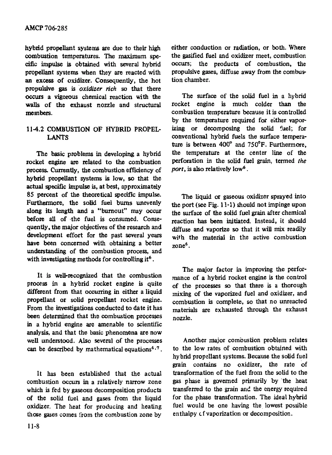
11-4.2 Combustion of Hybrid Propellants ............................ 11-8
11-5 Performance Parameters for Hybrid Rocket Engines ......... 11-9
11-5.1 Specific Impulse of a Hybrid Rocket Engine .................. 11-9
11-5.2 Characteristic Velocity for a Hybrid Rocket Engine.. . 11-9
11-6 Internal Ballistics of the Hybrid Rocket Engine .............. 11-10
11-6.1 Thrust Equation ..................................... 11-11
11-6.2 Burning Rate of Hybrid Propellants................... 11-11
11-7 General Design Considerations Pertinent to Hybrid-type
Rocket Engines.......................................... 11-12
11-7.1 Pressurization of the Liquid Oxidizer ...................... 11-13
11-7.1.1 Chemical Gas Pressurization ................. 11-13
11-7.1.2 Bladders 11-13
11-7.1.3 Oxidizer Tank Pressure Requirements........... 11-13
11-8 Design Considerations Pertinent to the Head-end Injection
' Hybrid Rocket Engine ...................................... ’М3
11-8.1 The Combustion Chamber .............................. 11-14
11-8.2 Exhaust Nozzle Design ............................... 11-14
11 -8.3 Injectors for the Liquid Oxidizer.................... 11-14
11-8.4 Ignition of Hybrid Rocket Engines.................... 11-14
11-9 Design Considerations Pertinent to the Afterburning
(Conventional) Hybrid Rocket Engine .................... 11-16
11-9.1 General Discussion .................................. 11-16
11-9.2 Afterburner Chamber.................................. 11-16
References ............................................. 11-17
PART TWO. AIR-BREATHING JET PROPULSION ENGINES
CHAPTER 12. CLASSIFICATION AND ESSENTIAL
FEATURES OF AIR-BREATHING PROPULSION ENGINES
12-0 Principal Notation for Part Two .......................... 12-1
12-1 Classification of Air-breathing Propulsion Engines ....... 12-7
xii
АМСР 706-285
TABLE OF CONTENTS (Continued)
Paragraph Page
12-1.1 Propulsive Duct Engines .................................... 12-8
12-1.2 The Ramjet Engine.................................... 12-8
12-1.3 The SCRAMJET Engine ................................ 12-10
12-2 Gas-turbine Jet Engines ..................................... 12-11
12-2.1 The Turbojet Engine ................................ 12-11
12-2.2 The Afterburning Turbojet Engine ................... 12-11
12-2.3 The Turbofan Engine ................................ 12-14
12-2.4 The Turboramjet or Dual-cycle Engine ............... 12-16
12-2. The Turboshaft Engine .............................. 12-16
12-2.6 The Turboprop Engine ............................... 12-17
12-3 General Thrust Equations for Air-breathing Engines ...... 12-18
12-3.1 General Thrust Equations ........................... 12-18
12-3.2 General Thrust Equations in Terms of Fuel-air Ratio.. 12-19
12-4 Thrust Equations for Specific Air-breathing Engines ... 12-20
12-4.1 Thrust Equations and Coefficients for the Ramjet
Engine ......................................... 12-20
12-4.2 Thrust Equation for Simple Turbojet Engine ......... 12-21
12-4.3 Thrust Equation for Afterburning Turbojet Engine ... 12-21
12-4.4 Thrust Equation for Turbofan Engine................. 12-22
12-5 Efficiency Definitions....................................... 12-23
12-5.1 Propulsive Efficiency (tjp) ........................ 12-23
12-5.2 Thermal Efficiency (Tjjii).......................... 12-24
12-5.3 Overall Efficiency (ij0) ........................... 12-24
12-5.3.1 Thrust Specific Fuel Consumption (TSFC)...... 12-24
12-5.3.2 Specific Fuel Consumption (SFC) ............... 12-24
12-6 Performance Parameters for Air-breathing Jet Engines ... 12-27
12-6.1 Air Specific Impulse or Specific Thrust (Ia)............... 12-27
12-6.2 Fuel Specific Impulse (Igp)......................... 12-27
12-6.3 Specific Engine Weight (We/F0 ).................... 12-27
12-6.4 Turbine Inlet Temperature (TJ1) ................... 12-28
12-7 General Comments Regarding Air-breathing Engines ........ 12-28
References ............................................. 12-31
CHAPTER 13. COMPRESSIBLE FLOW IN DIFFUSERS
13-1 Introduction ............................................. 13-1
13-2 Subsonic Intake-diffusers ................................ 13-2
13-2.1 Subsonic External-compression Diffusers .................... 13-2
13-2.1.1 Static Temperature Ratio for an External-
compression Diffuser.......................... 13-2
13-2.1.2 Static Pressure Ratio for an External-
compression Diffuser.......................... 13-3
xi ii
АМСР 706-285
TABLE OF CONTENTS (Continued)
Paragraph Page
13-2.2 Subsonic Internal-compression Diffusers................ J.3-3
13-3 Performance Criteria for Diffusers .......................... 13-5
13-3.1 Isentropic (Adiabatic) Diffuser Efficiency (г?д)........ 13-5
13-3.2 Stagnation (or Total) Pressure Ratio (rp) .............. 13-5
13-3.3 Energy Efficiency of Diffuser (rjjQ?) .................. 13-6
13-4 Supersonic Inlet-diffusers .................................. 13-7
13-4.1.1 Normal Shock Diffuser ............................. 13-7
134.1.2 Ram Pressure Ratio for a Normal Shock
Diffuser........................................ 13-8
134.2 The Reversed De Laval Nozzle Supersonic Diffuser ... 13-9
134.3 External Compression Supersonic Diffusers............... 13-9
134.4 Operating Modes for External Shock Diffusers .......... 13-11
134.4.1 Critical Operation ............................... 13-11
134.4.2 Supercritical Operation .......................... 13-11
134.4.3 Subcritical Operation ............................ 13-11
13-5 Diffuser Performance Characteristics and Design
Considerations ............................... 13-11
References ............................................... 13-15
CHAPTER 14. PROPULSIVE DUCT ENGINES
14-1 Introduction ................................................ 14-1
14-2 Thrust Developed by a Propulsive Duct Engine .............. 14-1
14-2.1 Cold Flow Through Shaped Duct ................................. 14-1
14-2.2 Methods for Supporting a Static Pressure Higher Than
the External Static Pressure Inside a Duct........................... 14-1
14-2.2.1 Restriction of the Exit Area ...................... 14-1
14-2.2.2 Heat Addition to the Internal Flow................. 14-5
14-3 Definitions of Terms Employed in Ramjet Engine
Technology ............................................... 14-5
14-3.1 Gross Thrust (Fg) ...................................... 14-5
14-3.2 External Drag (De) ..................................... 14-7
14-3.3 Net Thrust (Fn) ........................................ 14-7
14-3.4 Effective Jet (or Exhaust) Velocity (Vj)................ 14-7
14-3.5 Net Thrust Coefficient (Cpn)........................... 14-8
14-3.6 Gross Thrust Coefficient (Cj?g) ........................ 14-8
14-3.6.1 Effect of Altitude (z) on Cpg (T§ = const) .... 14-10
14-3.6.2 Effect of Fuel-air Ratio on Cpg (z = const.) .... 14-10
14-4 Critical, Supercritical, and Subcritical Operation of the
Ramjet Engine ........................................... 14-10
14-4.1 Critical Operation of the Ramjet Engine................ 14-13
14-4.2 Supercritical Operation of the Ramjet Engine....... 14-13
xiv
АМСР 706-285
TABLE OF CONTENTS (Continued)
Paragraph Page
14-4.3 Subcritical Operation of the Ramjet Engine ................ 14-13
14-5 Losses in the Ramjet Engine ........................... 14-13
14-6 Diffuser Performance in a Ramjet Engine ................. 14-14
14-7 Burner Efficiency (t?b) ................................. 14-16
14-8 Overall Efficiency of the Ramjet Engine (r?0)............ 14-16
14-9 Gross Thrust Specific Fuel Consumption of the Ramjet
Engine (FgSFC)......................................... 14-16
14-10 Variable-geometry Ramjet Engine ......................... 14-16
14-11 SCRAMJET Engine Performance Parameters .................. 14-17
14-11.1 Gross Thrust (Fg) ................................... 14-17
14-11.2 Gross Thrust Specific Impulse (Ipg) ................. 14-17
14-11.3 Inlet Kinetic Energy Efficiency (hKE) ............... 14-18
14-11.4 Nozzle Thrust Efficiency (r^np) ..................... 14-18
References ............................................. 14-20
CHAPTER 15, GAS-TURBINE AIR-BREATHING ENGINES
15-1 Introduction ............................................. 15-1
15-2 Gas-turbine Powerplant Engines............................ 15-1
15-3 Efficiencies of Components of Gas-turbine Engines...... 15-2
15-3.1 Diffusion Process........................................... 15-2
15-3.1.1 Diffuser Isentropic Efficiency ................. 15-2
15-3.1.2 Diffuser Temperature Ratio (ад)................. 15-2
15-3.1.3 Diffuser Pressure Ratio Parameter (вд) ......... 15-2
15-3.2 Compression Process ........................................ 15-4
15-3.2.1 Compressor Isentropic Efficiency (r?c)........... 15-4
15-3.2.2 Compressor Pressure Ratio Parameter (вс)...... 15-4
15-3.2.3 Temperature Rise in Air Compressor (ДТС)...... 15-4
15-3.3 Combustion Process.................................... 15-6
15-3.3.1 Burner Efficiency Ofjj) ......................... 15-6
15-3.3.2 Dimensionless Heat Addition Parameter
(Qi»lB/epBTo).................................. 15'6
15-3.4 Turbine Expansion Process................................... 15-6
15-3.4.1 Turbine Work for Turboshaft, Turboprop, and
Turbojet Engines .............................. 15-7
15-3.4.2 Turbine Isentropic Efficiency Gif) .............. 15-8
15-3.5 Nozzle Expansion Process and Isentropic
Efficiency (r?n) .................................. 15-8
15-3.6 Machine Efficiency (тцс).............................. 15-8
15-4 The Turboshaft Engine ........................................ 15-8
15-4.1 Design Criteria for Turboshaft Engine................. 15-9
15-4.1.1 Thermal Efficiency (17th)..................... 15-9
xv
АМСР 706-285
TABLE OF CONTENTS (Continued)
Paragraph Page
15 4.1.2 Specific Output (£)............................... 15-9
15-4.1.3 Air-rate (A)................................... 15-9
15-4.1.4 Work-ratio (U).................................... 15-9
15-4.2 Thermodynamic Cycle for Turboshaft Engine and
Thermal Efficiency of Ideal Turboshaft Engine (r^).. 15-10
15-4,3 Losses in a Turboshaft Engine Cycle ................. 15-12
15-4.4 Simplified Analysis of the Turboshaft Engine Cycle .. 15-12
15-4.4.1 Compression Work (Ahc)........................... 15-13
15-4.4.2 Turbine Work (4ht)............................... 15-13
15-4.4.3 Specific Output (L).............................. 15-13
15-4.4.4 Heat Added (Qj).................................. 15-13
15-4.4.5 Thermal Efficiency (ijjh)........................ 15-13
15-4.4.6 Air-rate (A)..................................... 15-14
15-4.4Л Work-ratio (U).................................. 15-15
15-4.4.8 Specific Fuel Consumption (SFC) ................ 15-15
15-4.5 Performance Characteristics of the Turboshaft Engine. 15-15
15-4.5.1 Effect of Cycle Pressure Ratio (в) .............. 15-15
15-4.5.2 Effect of Cycle Pressure Ratio (в) and Turbine
Inlet Temperature (TJ)........................ 15-15
15-4.5.3 Air-rate (A)..................................... 15-18
15-4.5.4 Work-ratio (U = L/L^............................. 15-18
15-4.5.5 Effect of Machine Efficiency (4tc) .............. 15-18
15-4.5.6 Effect of Ambient Air Temperature (To = T2)... 15-19
15-4.5.7 Effect of Pressure Drops......................... 15-20
15-4.6 Modifications to Basic Turboshaft Engine to Improve
Its Performance.................................... 15-21
15-5 Regenerative Turboshaft Engine................................ 15-24
15-5.1 The Regeneration Process ................................... 15-25
15-5.1.1 Regenerator Effectiveness (er) .................. 15-27
15-5.1.2 Effect of Pressure Drops in the Regenerator ... 15-27
15-5.2 Regenerator Heat Transfer Surface Area and
Regenerator Effectiveness.......................... 15-28
15-5.3 Cycle Analysis for Regenerative Turboshaft Engine... 15-28
15-5.3.1 Temperature of Air Leaving Air Compressor (T3). 15-29
15-5.3.2 Temperature of Gas Leaving Turbine (T5) ......... 15-29
15-5.3.3 Heat Supplied the Regenerative Turboshaft
Engine (Qir)................................ 15-29
15-5.3.4 Specific Output of Regenerative Turboshaft
Engine (£/cpT0) .............................. 15-29
15-5.3.5 Thermal Efficiency of Regenerative Turboshaft
Engine Cr?th) ................................ 15-30
XV i
АМСР 706-285
TABLE OF CONTENTS (Continued)
Paragraph Page
15-5.3.6 Woik ratio for Regenerative Turboshaft
Engine (O').................................. 15-30
15-5.4 Performance Characteristics of the Regenerative
Turboshaft Engine................................ 15-30
15-6 Turboprop Engine ........................................... 15-30
15-6.1 Thermodynamic Analysis of the Turboprop Engin
Cycle............................................ 15-32
15-6.1.1 Propeller Thrust Horsepower (PprOp)........... 15-34
15-6.1.2 Jet Thrust Power (Ppj)........................ 15-34
15-6.1.3 Total Thrust Horsepower for Turboprop
Engine (P turboprop)......................... 15-34
15-6.2 Performance Characteristics for the Turboprop
Engine .......................................... 15-34
15-6.2.1 Effect of Altitude and Turbine Inlet
Temperature.................................. 15-36
15-6.2.2 Effect of Machine Efficiency (t?jc) and Tiffbine
Inlet Temperature (Tj )...................... 15-38
15-6.3 Operating Characteristics of Turboprop Engine ............ 15-38
15-7 Gas-turbine Jet Engines .................................. 15-38
15-8 Turbojet Engine .......................................... 15-38
15-8.1 Dimensionless Heat Addition for Turbojet
Engine (О|Чв/с_вТо)................................................ 15-41
15-8.2 Turbine Pressure Ratio (Pj/Pj*)........................... 15-41
15-8.3 Dimensionless Enthalpy Change for the Propulsive
Nozzle (Ahn/cpT0) ................................. 15-41
15-8.4 Dimensionless Tlirust Parameter (X) ................ 1.5-43
15-8.5 Thermal Efficiency of Turbojet Engine frtjh) ........ 15-43
15-8.6 Overall Efficiency of Turbojet Engine (r?o)........ 15-43
15-8.7 Performance Characteristics of Turbojet Engine..... 15-44
15-8.7.1 Effect of Cycle Temperature Ratio (a) and
Compressor Pressure Ratio (P? /P°) for a
Constant Flight Speed ....................... 15-44
15-8.7.2 Effect of Flight Mach Number (Mo) and Cycle
Temperature Ratio (a) on the Dimensionless
Tlirust Parameter (X)........................ 15-46
15-8.7.3 Effect of Flight Speed and Compressor Pressure
Ratio (P° /P°) on Performance of Turbojet
Engine ...................................... 15-46
15-9 Turbofan Engine............................................. 15-48
15-9.1 Definitions Pertinent to the Turbofan Engine.............. 15-49
15-9.1.1 Bypass Ratio (P) ............................. 15-49
xvii
АМСР 706-285
TABLE OF CONTENTS (Continued)
Paragraph Page
15-9.1.2 Fan Isentropic Efficiency (np) ................. 15-49
15-9.1.3 Fan Pressure Ratio Parameter (®p)......... 15-49
15-9.1.4 Fan Power (Pp) ................................. 15-51
15-9.2 Analysis of Processes in Turbofan Engine ........... 15-51
15-9.2.1 Diffusion for Hot Gas Generator Circuit... 15-51
15-9.2.2 Compressor Power for Turbofan Engine (PCTF)- • 15-51
15-9.2.3 Burner Fuel-air Ratio for Turbofan Engine (f) .. 15-52
15-9.2.4 Turbine Power for Turbofan Engine (PtTF).. 15-52
15-9.2.5 Nozzle Expansions for Turbofan Engine..... 15-53
15-9.2.5.1 Nozzle Expansion Work for Gas Generator
Nozzle ................................ 15-54
15-9.2.5.2 Nozzle Expansion Work for Cold Air-
stream .......................................................... 15-54
15-10 Performance Parameters for Turbofan Engine .............. 15-54
15-10.1 Thrust Equation (F) ............................... 15-54
15-10.2 Mean Jet Velocity for Turbofan Engine (Vj-jp) ...... 15-54
15-10.3 Air Specific Impulse (or Specific Thrust) (Ia).... 15-55
15-10.4 Conclusions ...................................... 15-55
References ............................................. 15-56
APPENDIX A. ELEMENTARY GAS DYNAMICS
A-0 Principal Notation for Appendix A.......................... A-l
A-l Introduction .............................................. A-5
A-2 The Ideal Gas ............................................. A-7
A-2.1 The Thermally Perfect Gas............................. A-7
A-2.2 The Calorically Perfect Gas........................... A-7
A-2.3 Specific Heat Relationships for the Ideal Gas..... A-8
A-2.4 Some Results from the Kinetic Theory of Gases..... A-9
A-2.5 Some Characteristics of Real Gases................ A-11
A-2.6 Acoustic or Sonic Speed (a)....................... A-12
A-2.6.1 Isentropic Bulk Modulus (Kg).................. A-13
A-2.6.2 Acoustic Speed in an Ideal Gas ............... A-14
A-2.7 Mach Number............................................... A-14
A-3 Steady One-dimensional Flow.............................. A-14
A-3.1 Continuity Equation .......................... A-15
A-3.2 Momentum Equation .......................... A-l8
A-3.2.1 Impulse Function ............................. A-19
A-3.2.2 Rayleigh Line Equation ....................... A-19
A-3.3 Energy Equation for Steady One-dimensional Flow... A-20
A-3.4 Entropy Equation for Steady One-dimensional Flow.. A-24
A-4 Steady One-dimensional Flow of an Ideal Gas.................... A-25
xvii i
АМСР 706-285
TABLE OF CONTENTS (Continued)
Paragraph Page
A-4.1 Continuity Equation for an Ideal Gas....................... A-25
A-4.2 Momentum Equation for the Steady One-dimensional
Flow of an Ideal Gas................................. A-26
A-4.2.1 Reversible Steady One-dimensional Flow of an
Incompressible Fluid......................... A-26
A-4.2.2 Reversible Steady One-dimensional Flow of a
Compressible Fluid .......................... A-26
A-4.2.3 Irreversible Steady One-dimensional Flow ..... A-26
A-4.2.4 Irreversible Steady One-dimensional Flow of an
Ideal Gas ................................... A-27
A-4.3 Energy Equation for Steady One-dimensional Flow... A-27
A-4.3.1 Energy Equation for a Simple Adiabatic Flow... A-28
A-4.3.2 Energy Equation for the Simple Adiabatic Flow
of an Ideal Gas ............................. A-28
A-4.4 Entropy Equation for the Steady One-dimensional
Flow of an Ideal Gas................................. A-29
A-5 Steady One-dimensional Isentropic Flow....................... A-29
A-5.1 Energy Equation for the Steady Isentropic One-
dimensional Flow of an Ideal Gas................................. A-30
A-5.2 Stagnation (or Total) Conditions........................... A-33
A-5.2.1 Stagnation (or Total) Enthalpy (h°) .......... A-33
A-5.2.2 Stagnation (or Total) Temperature (T°)........ A-33
A-5.2.3 Stagnation (or Total) Pressure (P°)........... A-34
A-5.2.4 Relationship Between Stagnation Pressure and
Entropy...................................... A-34
A-5.2.5 Stagnation (or Total) Density (p°)............ A-35
A-5.2.6 Stagnation Acoustic Speed (a0)................ A-35
A-5.2.7 Nondimensional Linear Velocity (w=u/a°)....... A-36
A-5.3 Adiabatic Exhaust Velocity (ue).................... A-36
A-5.4 Isentropic Exhaust Velocity (u')................... A-36
A-5.4.1 Nozzle Efficiency G?n)........................ A-37
A-5.4.2 Nozzle Velocity Coefficient (ф) .............. A-37
A-5.5 Maximum Isentropic Speed (co)...................... A-37
A-5.6 Continuity Equation for Steady One-dimensional
Isentropic Flow of an Ideal Gas in Terms of
Stagnation Conditions ............................ A-38
A-6 Critical Condition for the Steady One-dimensional
Isentropic Flow of an Ideal Gas.......................... A-39
A-6.1 Critical Thermodynamic Properties for the Isentropic
Flow of an Ideal Gas................................. A-40
A-6.1.1 Critical Acoustic Speed (a*) ................. A-40
xix
АМСР 706-285
TABLE OF CONTENTS (Continued)
Paragraph Page
A-6.1.2 Critical Static Temperature (T*)................ A-41
A-6.1.3 Critical Expansion Ratio (P*/P°) ............... A-41
A-6.1.4 Critical Density Ratio (p*/p °) ................ A-41
A-6.1.5 Dimensionless Velocity (M*B u/a*) .............. A-41
A-6.2 Relationships Between the Reference Speeds a0, a*,
and co ........................................................... A-42
A-6.2.1 Relative Values of Reference Speeds for a Gas
Having 7= 1.40................................ A-42
A-6.2.2 Energy Equations in Terms of the Reference
Speeds a° and c0.............................. A-42
A-6.3 Critical Area Ratio for the Steady One-dimensional
Isentropic Flow of an Ideal Gas.................... A-42
A-6.3.1 Critical Area Ratio (А/A*) ..................... A-43
A-6.3.2 Mass Flow Rate (rn) and Critical Area
Ratio (A/A*).................................. A-43
A-6-4 Flow Area Changes for Subsonic and Supersonic
Isentropic Flow.................................... A-44
A-6.5 Dimensionless Thrust Function (F/F*) ........................ A-44
A-7 Flow of an Ideal Gas in a Converging-diverging One-
dimensional Passage ............................................... A-46
.A-7.1 Maximum Flow Density................................. A-47
\a-7.2 Critical Flow Density (G*) .......................... A-49
A-8 Steady One-dimensional Adiabatic Flow With Wall
Friction........................................................... A-49
A-8.1 Adiabatic Flow With Wall Friction in a Constant
- Area Duct.................................................. A-51
A-8.1.1 Friction Coefficient (f) ......................... A-5 2
A-8.1.2 Friction Coefficient for Compressible and
Incompressible Flows ........................ A-5 2
A-8.2 Fanno Line Equation for Steady Adiabatic Flow in
a Constant Area Duct ............................................. A-53
A-8.3 Fanno Line Equation for the Flow of an Ideal Gas
in a Constant Area Duct ............................................ A-5 7
A-8.3.1 Friction Parameter for a Fanno Flow ........... A-5 7
A-8.3.2 Critical Duct Length for a Fanno Flow .......... A-57
A-8.3.3 Duct Length and Mach Number Change for
Fanno Flow ..................................... A-5 8
A-8.3.4 Entropy Increase Due to Wall Friction for the
Fanno Flow of an Ideal Gas ..................... A-5 9
A-8.3.5 Entropy Gradient for the Fanno Flow of an
Ideal Gas .................................... A-59
XX
АМСР 706-285
TABLE OF CONTENTS (Continued)
Paragraph Page
A-8.3.6 Gradient of the How Mach Number for Adiabatic
Flow of an Ideal Gas in a Constant Area Duct... A-60
A-8.4 Relationships Between Dependent How Variables and
Friction Parameter for Adiabatic Flow of an Ideal
Gas in a Constant Area Duct....................... A-60
A-8.5 Equations for Compiling Tables for Conditions Along
a Fanno Line..................................................... A-61
A-8.5.1 Choking Due to Wall Friction for a Fanno Line in
a Constant Area Duct ........................ A-63
A-8.5.2 Subsonic or Supersonic Flow in a Duct ......... A-63
A-9 One-dimensional Steady Frictionless Flow With Heat
Addition (Simple Diabatic or Rayleigh Flow) ........... A-64
A-9.1 Principal Equations for a Rayleigh Flow............. A-65
A-9.2 The Rayleigh Line .................................. A-66
A-9.3 Condition for Maximum Enthalpy on a Rayleigh Line.. A-67
A-9.4 State of Maximum Entropy on a Rayleigh Line ...... A-67
A-9.5 Rayleigh Line Equations for an Ideal Gas ........... A-70
A-9.6 Equations for Compiling Tables of Flow Parameters
Along a Rayleigh Line ............................ A-71
A-9.7 The Development of a Compression Shock..................... A-71
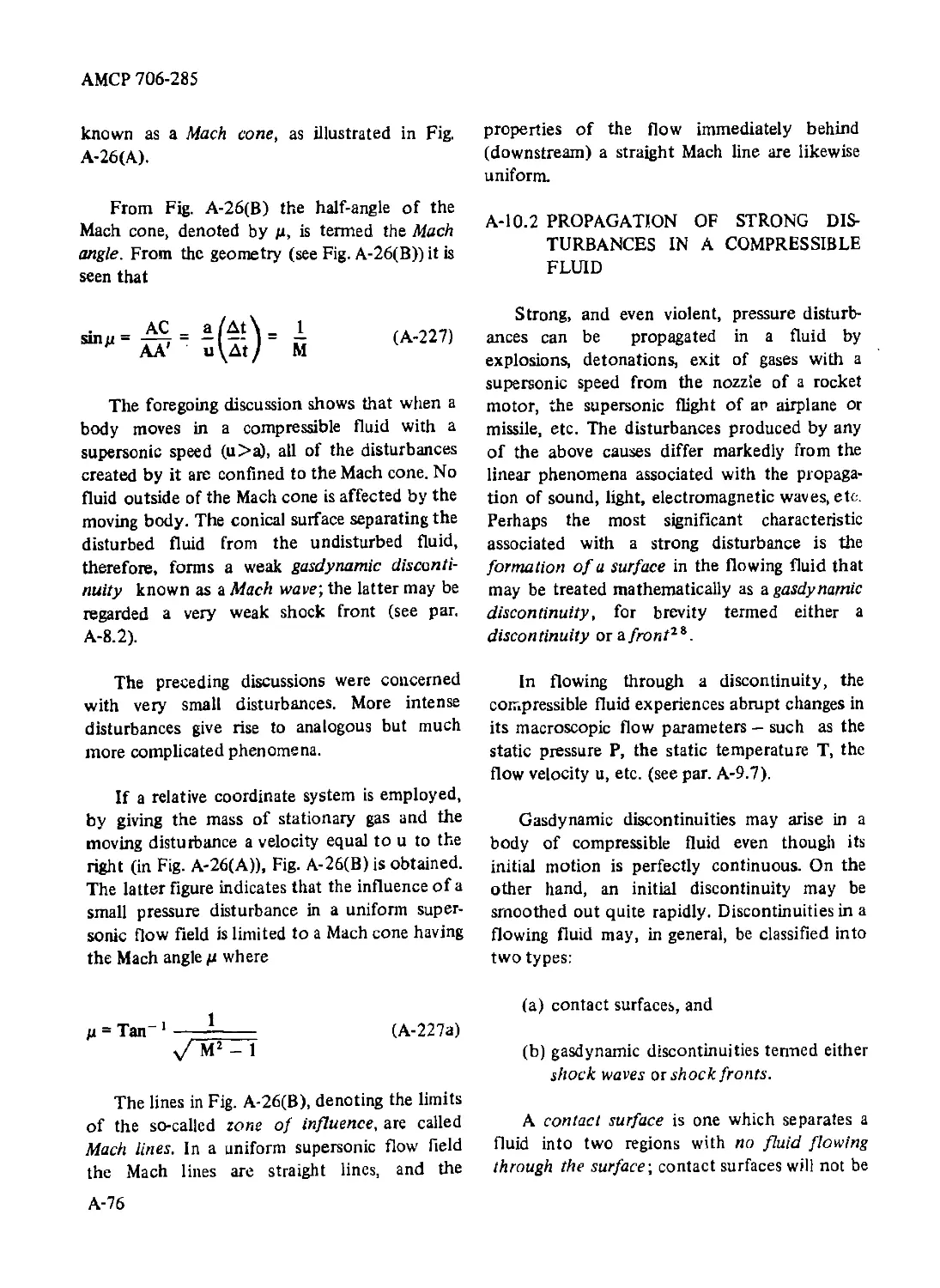
A-l 0 Disturbances in a Compressible Fluid........................ A-72
A-l 0.1 Propagation of Small Disturbances in a Compressible
Huid............................................................. A-72
A-l 0.2 Propagation of Strong Disturbances in a Compressible
Huid............................................................. A-76
A-l0.2.1 Shock Wave or Shock Front ..................... A-77
A-l 0.2.2 Examples of Gasdynamic Discontinuities ........ A-77
A-l 0.3 The Normal Shock Wave.................................... A-79
A-10.3.1 Basic Equations for the Normal Shock .......... A-79
A-10.3.2 Rankine-Hugoniot Equations for aNormal Shock . A-81
A-10.3.3 Parameters for the Normal Shock as Function of
the Flow Mach Number in Front of Shock .... A-81
A-10.3.4 The Rayleigh Pitot Tube Equation .............. A-82
A-l 0.4 The Oblique Shock Wave................................... A-83
A-l 0.4.1 Basic Equations for the Oblique Shock ......... A-84
A-10.4.2 Oblique Shock Parameters as Functions of the
Mach Number in Front of the Shock and the
Wave Angle (e) .............................. A-86
A-l0.4.3 Prandtl Relationship for Oblique Shocks......... A-87
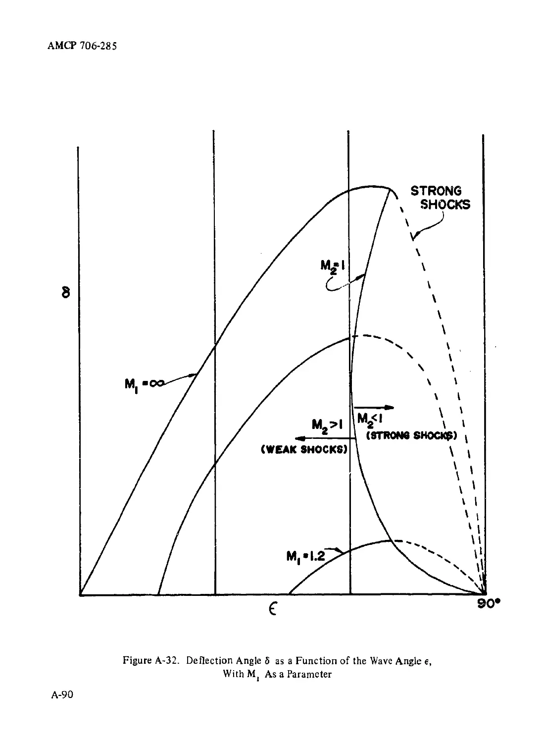
A-l 0.4.4 Charts Presenting Relationships Between the
Parameters for Oblique Shocks................ A-89
xxi
АМСР 706-285
TABLE OF CONTENTS (Continued)
Paragraph Page
A-l 0.4.5 Application of Normal Shock Table to Oblique
Shocks ..................................... A-93
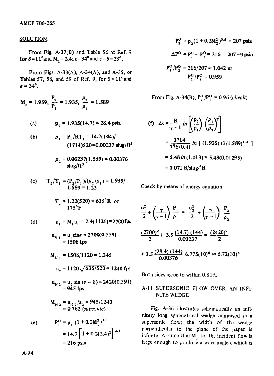
A-11 Supersonic Flow Over an Infinite Wedge ............... A-94
A-l 2 Supersonic Flow Over a Cone........................... A-98
A-13 Prandtl-Meyer Expansion Flow ......................... A-99
References .......................................... A-l 12
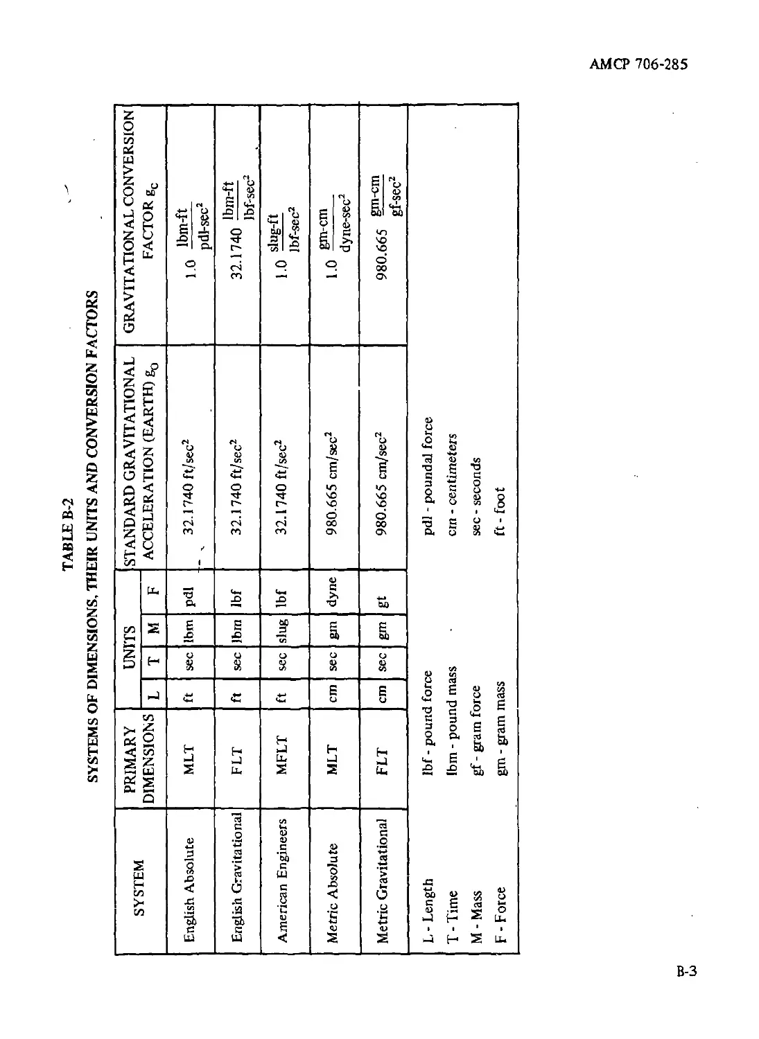
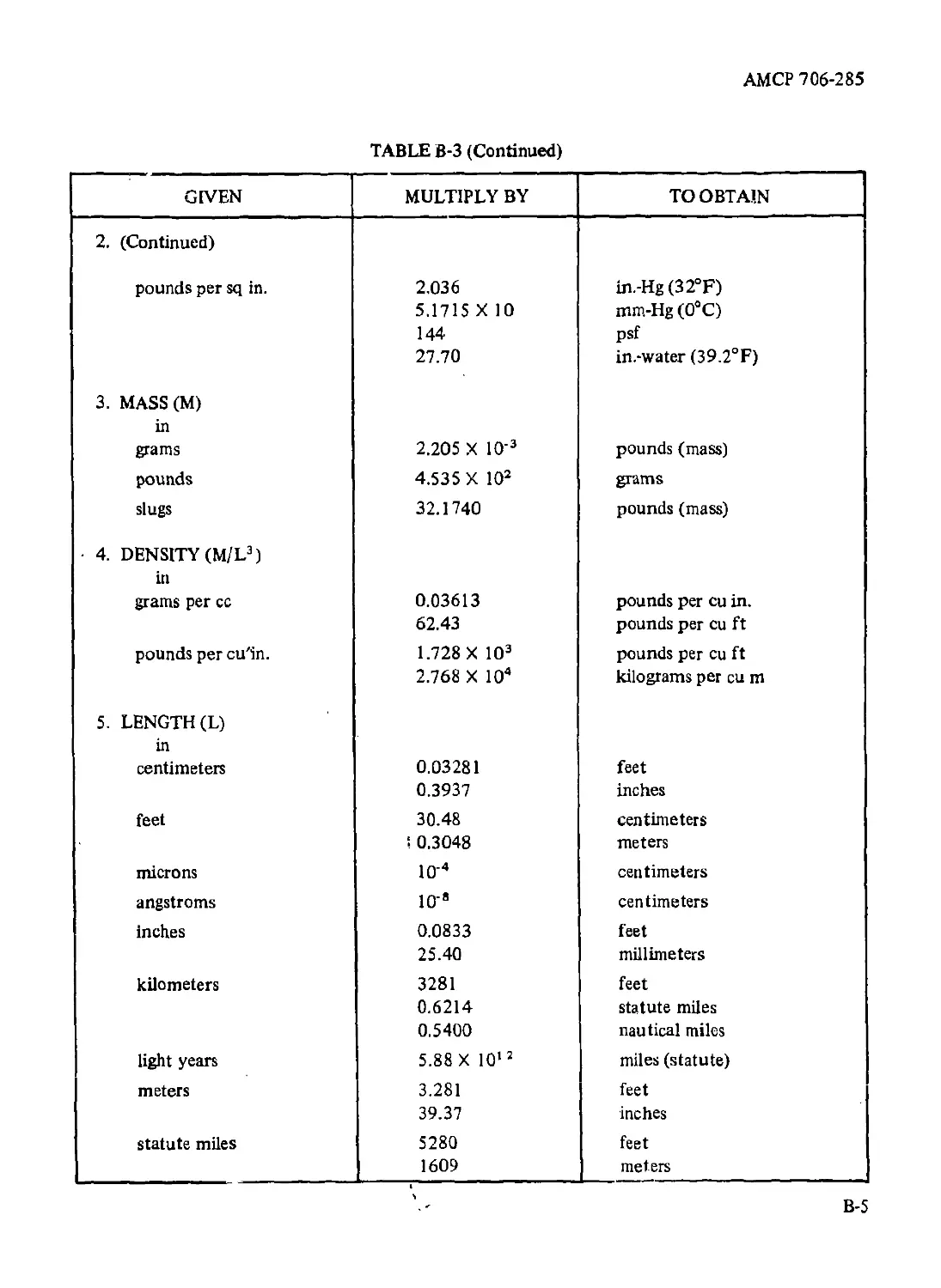
APPEND J. USEFUL TABLES............................. В-1
INDEX............................................... 1-1
хх i i
АМСР 706-285
LIST OF ILLUSTRATIONS
Figure No. Title Page
1-1 Essential Elements of an Air-breathing Jet Engine .......... 1-6
1-2 Essential Elements of a Jet Propulsion System .............. 1-8
1-3 Fin-stabilized Rocket Motor ................................ 1-8
1-4 Development of Thrust in a Rocket Motor..................... 1-9
1-5 Essential Elements of a Liquid Bipropellant Rocket
Engine .................................................. 1-12
1-6 Principal Elements of an Uncooled Liquid Bipropellant
Rocket Engine ................................................... 1-13
1-7 Essential Elements of an Internal-burning Case-bonded
Solid Propellant Rocket Motor.................................... 1-14
1-8 Essential Features of a Hybrid Chemical Rocket Engine ... 1-15
2-1 Control Surface and Control Volume Enclosing a Region
of a Flowing Fluid................................................ 2-5
2-2 Transport of Momentum by a Flowing Fluid ................... 2-5
2-3 Forces Acting on a Flowing Fluid ........................... 2-8
2-4 Air-breathing Jet Engine in a Relative Coordinate System . . 2-8
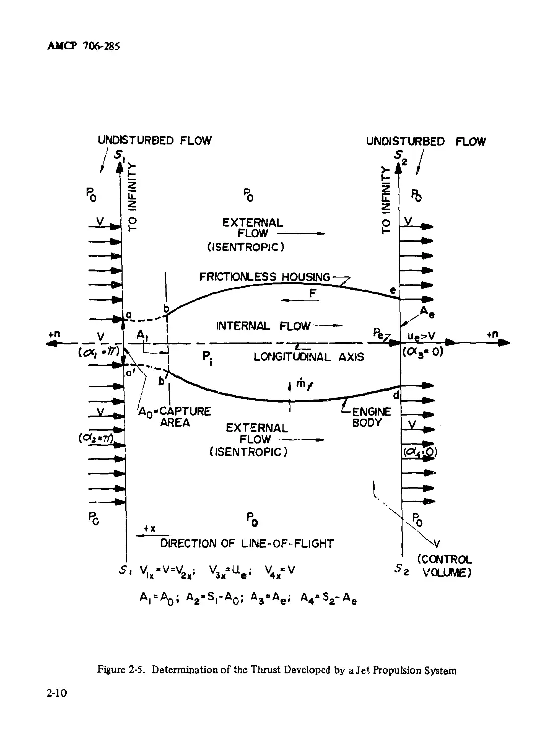
2-5 Determination of the Thrust Developed by a Jet
Propulsion System................................................ 2-10
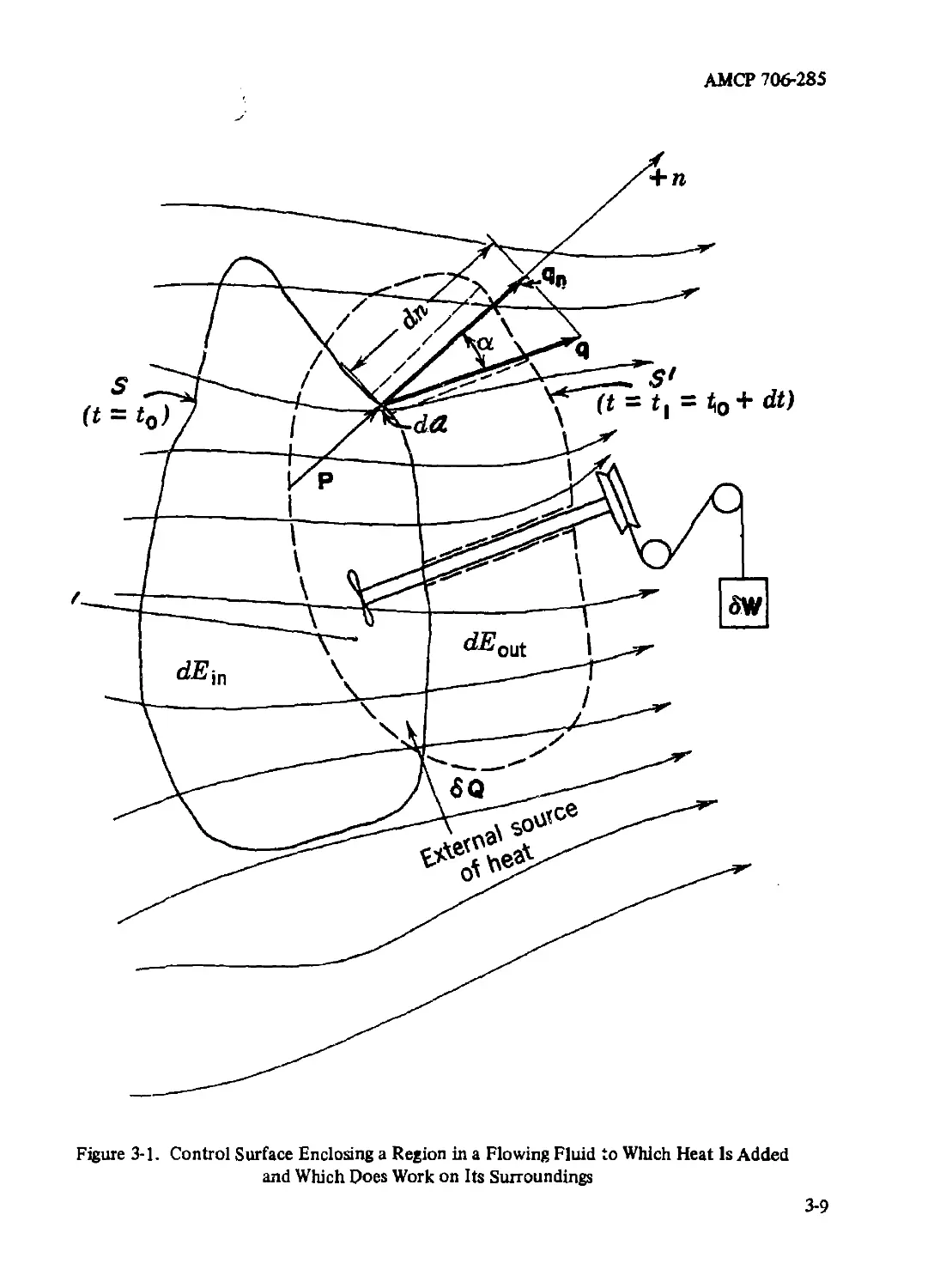
3-1 Control Surface Enclosing a Region in a Flowing Fluid to
Which Heat Is Added and Which Does Work on Its
Surroundings.............................................. 3-9
3-2 Element of a Control Surface Which Encloses a Region in
a Flowing Fluid........................................ 3-10
3-3 Energy Balance for a One-dimensional Steady Flow ............... 3-11
3-4 Comparison of Adiabatic and Isentropic Flow Processes
on the hs-plane ......................................... 3-16
3-5 Isentropic Flow Expansion of a Gas to the Critical
Condition (u = a*)............................................... 3-19
3-6 A Fanno Line Plotted in the hs-plane............................ 3-24
3-7 Comparison of Fanno Lines for Two Different Values of
the Flow Density (G = m/A)....................................... 3-25
3-8 Determination of Duct Length Tо Accomplish a Specified
Change in Flow Mach Number (Fanno Line).......................... 3-27
3-9 Flow Parameters for a Fanno Line for a Gas with
7 = 1.40 ........................................................ 3-30
3-10 Physical Situation for a Rayleigh Flow ........................ 3-31
xxiii
АМСР 706-285
LIST OF ILLUSTRATIONS (Continued)
Figure No. Title Page
3-11 Rayleigh Line Plotted in the Pv-plane.................... 3-33
3-12 Rayleigh Line Plotted in the hs- (or Ts-) plane.......... 3-34
3-13 Flow Parameters for a Rayleigh Flow as a Function of
M, for y = 1.40 .................................................. 3-36
3-14 Development of Compression Shock ........................ 3-38
4-1 Two Basic Types of Nozzles Employed in Jet
Propulsion Engines ................................................ 4-4
4-2 Ideal Nozzle Flow in Converging Nozzles .................. 4-6
4-3 Flow Factor for a Converging Nozzle As a Function of
the Expansion Ratio rt ................................. 4-9
4-4 Mass Flow Rate As a Function of the Nozzle Expansion
Ratio, for a Fixed Value of 7..................................... 4-11
4-5 Enthalpy Converted into Kinetic Energy by Isentropic
Expansions in Converging and Converging-diverging
Nozzles........................................................... 4-12
4-6 Flow Characteristics of a Converging-diverging (or De Laval)
Nozzle Passing the Critical Mass Flow Rate m*..................... 4-13
4-7 Parameter (G^/yRT6)/?0 As a Function of Pt/P° for
Ideal Nozzle Flow (7 = 1.25)...................................... 4-15
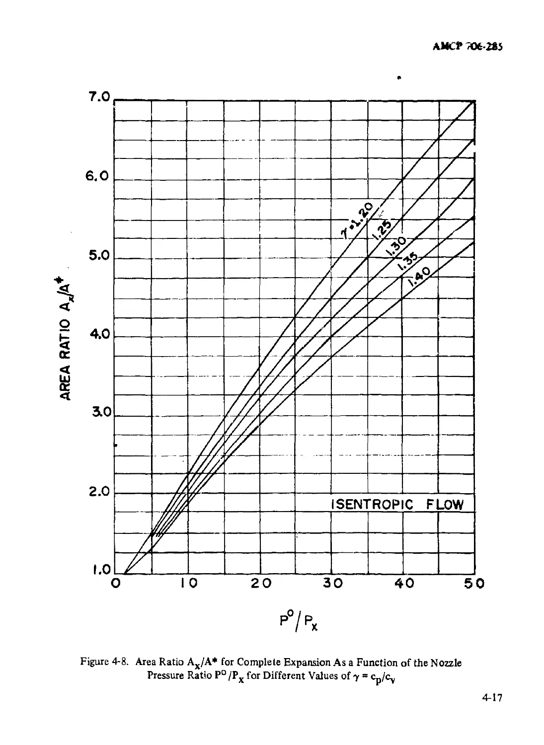
4-8 Area Ratio Ax/A* for Complete Expansion As a Function
of the Nozzle Pressure Ratio P° /Px for Different Values
of7=cp/cv ........................................................ 4-17
4-9 Ratio of the Isentropic Exit Velocity ux to the Isentropic
Throat Velocity u* As a Function of the Nozzle Pressure
Ratio P° /Px for Different Values of 7 = ср/су ................... 4-18
4-10 Expansion Ratio Pg/P° and Exit Mach Number Mg As
Function of the Area Ratio A*/Ag for a Converging-
diverging Nozzle Passing the Critical Mass Flow Rate m*.. 4-21
4-11 Pressure Distributions in a Converging-diverging Nozzle
Under Different Operating Conditions ............................. 4-22
4-12 Conical Converging-diverging Nozzle Operating With
Overexpansion .................................................... 4-23
4-13 Correlation of Data on Jet Separation in Conical Nozzles
for Rocket Motors (According to Reference 10) .................... 4-25
4-14 General Characteristics of a Conical Converging-
diverging Nozzle ................................................. 4-30
4-15 Radial Flow in a Conical Nozzle.............................. 4-32
4-16 Divergence Loss Coefficient X as a Function of the Semi-
divergence Half-angle a for a Conical Nozzle...................... 4-33
xxiv
АМСР 706-285
LIST OF ILLUSTRATIONS (Continued)
Figure No. Title Page
4-17 General Features of a Contoured or Bell-shaped Nozzle ... 4-35
4-18 Essential Features of an Annular Nozzle.................. 4-37
4-19 Essential Features of a Plug Nozzle...................... 4-38
4 '_Э Essential Features of an Expansion-deflection or
E-D Nozzle ............................................ 4-39
5-1 Thermodynamic Conditions for a Chemical Rocket Nozzle
Operating Under Steady State Conditions............................ 5-3
5-2 Forces Acting on a Rocket-propelled Body in
Rectilinear Motion................................................ 5-10
5-3 Drag Coefficient As a Function of the Flight Mach Number
for Two Angles of Attack.......................................... 5-12
5-4 Ideal Burnout Velocity for a Single Stage Vehicle As
a Function of Effective Jet Velocity c for Different
Values of Vehicle Mass Ratio m0 /m^ .............................. 5-15
6-1 Dissociation in Percent as a Function of Gas Temperature
for CO,, H, О, H,, O,, HF, CO, and N, at 500 psia............... 6-7
6-2 Isentropic Exhaust Velocity as a Function of Mixture
Ratio mo /riy for Different Values of Pc/P^Propellants:
Nitrogen Tetroxide (N,O4) Plus 50% Aerozine-50-
50% Hydrazine (N4H4) and 50% Unsymmetrical
Dimethyl Hydrazine (CH3), N, H,, (UDMH)................. 6-8
6-3 Velocity Parameter ие/^-^Лг1^/т as a Function of P°/Pe
(for a Range of 10 to 50) for Different Values of
7 = Cp/Cy ............................................ 6-9
6-4 Velocity Parameter ujtp у/т£ / in as a Function of P° /Pe
(for a Range of 40 to 200) for Different Values of
7 = %/^ ............................................. 6-10
/ I 2
6-5 Values of the Parameter Г = v 71-----------1 and
V + 1/
Г j = Г\7т as Functions of у .......................... 6-12
6-6 Parallel Flow Vacuum Thrust Coefficient (Cp)Q as a
Function of Nozzle Area Ratio e .................................. 6-14
6-7 Parameter (Pe/Pc)e as a Function of the Nozzle Area
Ratio e .......................................................... 6-15
6-8 Nozzle Area Ratio e as a Function of Pc/Pe (0 to 20)
for Different Values of у ........................................ 6-16
XXV
АМСР 706-285
LIST OF ILLUSTRATIONS (Continued)
Figure No.
Title
Page
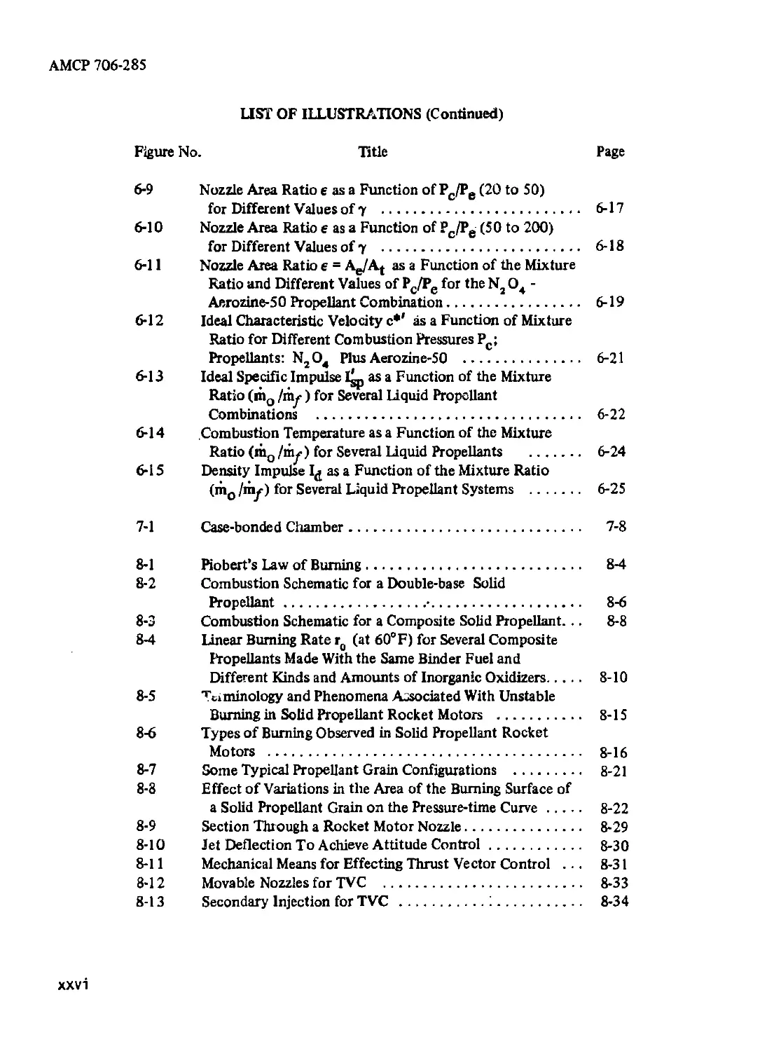
6-9
6-10
6-11
6-12
6-13
6-14
6-15
Nozzle Area Ratio e as a Function of Pc/Pe (20 to 50)
for Different Values of 7 ....................................... 6-17
Nozzle Area Ratio e as a Function of Pc/Pe (50 to 200)
for Different Values of 7 ....................................... 6-18
Nozzle Area Ratio e = as a Function of the Mixture
Ratio and Different Values of Pc/Pe for the N2 O4 -
Aerozine-50 Propellant Combination....................... 6-19
Ideal Characteristic Velocity c*' as a Function of Mixture
Ratio for Different Combustion Pressures Pc;
Propellants: N2O4 Plus Aerozine-50 ...................... 6-21
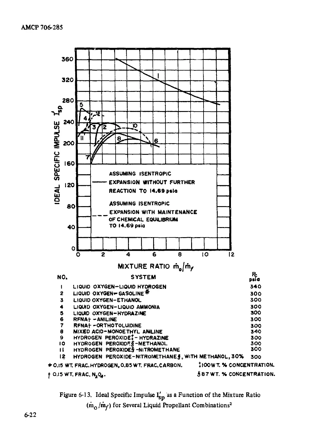
Ideal Specific Impulse 1^, as a Function of the Mixture
Ratio (riio /lily) for Several Liquid Propollant
Combinations ............................................ 6-22
Combustion Temperature as a Function of the Mixture
Ratio (m0 /riy ) for Several Liquid Propellants ......... 6-24
Density Impulse 1^ as a Function of the Mixture Ratio
(mo /riy) for Several Liquid Propellant Systems ........ 6-25
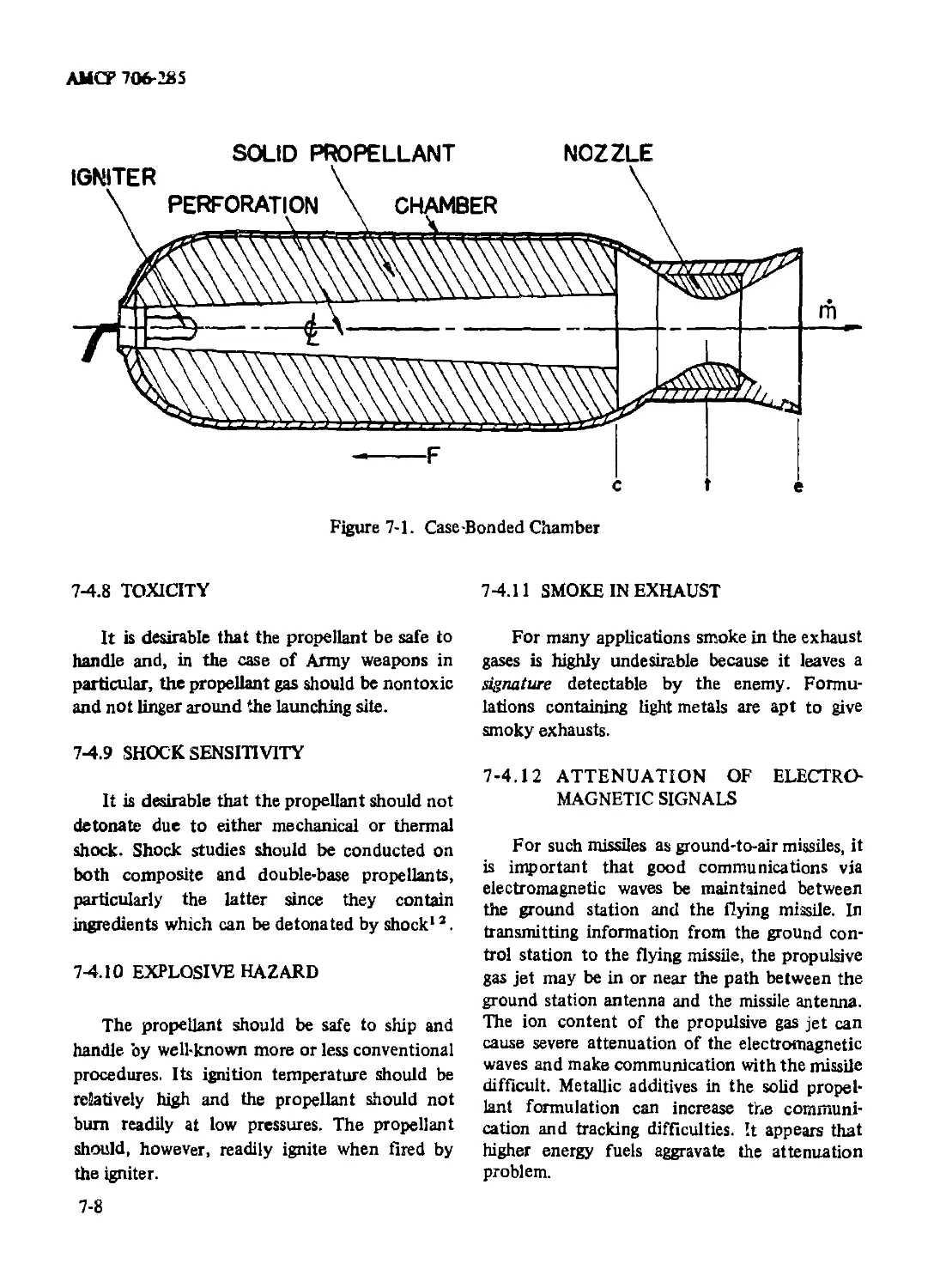
7-1 Case-bonded Chamber....................................... 7-8
8-1 Piobert’s Law of Burning....................................... 8-4
8-2 Combustion Schematic for a Double-base Solid
Propellant............................................. 8-6
8-3 Combustion Schematic for a Composite Solid Propellant... 8-8
8-4 Linear Burning Rate rQ (at 60°F) for Several Composite
Propellants Made With the Same Binder Fuel and
Different Kinds and Amounts of Inorganic Oxidizers..... 8-10
8-5 Terminology and Phenomena Associated With Unstable
Burning in Solid Propellant Rocket Motors ............. 8-15
8-6 Types of Burning Observed in Solid Propellant Rocket
Motors ................................................ 8-16
8-7 Some Typical Propellant Grain Configurations ................. 8-21
8-8 Effect of Variations in the Area of the Burning Surface of
a Solid Propellant Grain on the Pressure-time Curve.... 8-22
8-9 Section Through a Rocket Motor Nozzle.................... 8-29
8-10 Jet Deflection To Achieve Attitude Control............... 8-30
8-11 Mechanical Means for Effecting Thrust Vector Control ... 8-31
8-12 Movable Nozzles for TVC ................................. 8-33
8-13 Secondary Injection for TVC ........................... 8-34
xxvi
АМСР 706-285
LIST OF ILLUSTRATIONS (Continued)
Figure No. Title Page
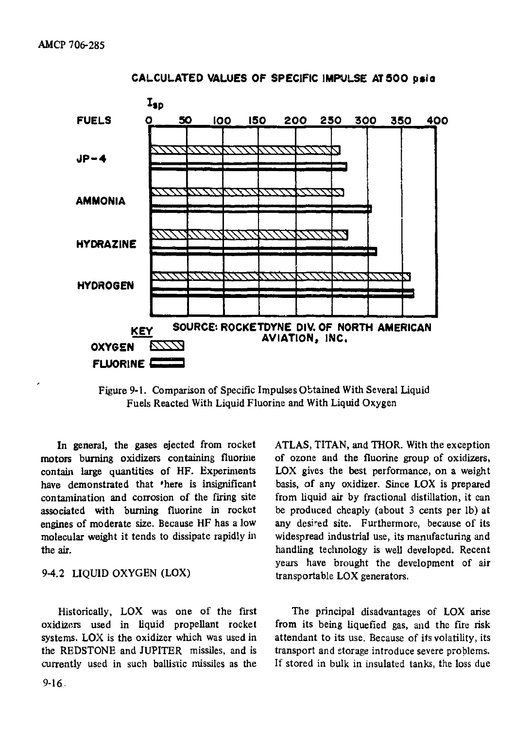
9-1 Comparison of Specific Impulses Obtained With Several
Liquid Fuels Reacted With Liquid Fluorine and With
Liquid Oxygen .......................................... 9-16
9-2 Enthalpy of Combustion of Several Fuels With Liquid
Oxygen............................................................ 9-25
10-1 Essential Elements ofa Liquid Bipropellant Thrust
Chamber ................................................ 10-4
10-2 Nine Different Injector Patterns for Liquid Bipropellant
Thrust Chambers ........................................ 10-6
10-3 Cooling Systems for Rocket Thrust Chambers.............. 10-12
10-4 Typical Mean Circumferential Heat Flux Distribution
Along a Thrust Chamber Wall ........................... 10-13
10-5 Application of an Ablating Material to a Liquid
Propellant Thrust Chamber.............................. 10-18
10-6 Heat Balances for Ablation Cooling.......................... 10-19
10-7 Diagrammatic Arrangement of a Stored Gas Pressurization
System ................................................ 10-21
10-8 Schematic Arrangement of the Components of a Turbo-
pump Pressurization System............................ 10-23
11-1 Essential Features of a Hybrid Rocket Engine With Head-
end Injection of the Liquid Oxidizer.............................. 11-2
11 -2 Essential Features of an Afterburning Hybrid Rocket
Engine ................................................. 11-3
11-3 Variations in Instantaneous and System Specific Impulse
During the Firing of a Hybrid Rocket Engine ........... 11-10
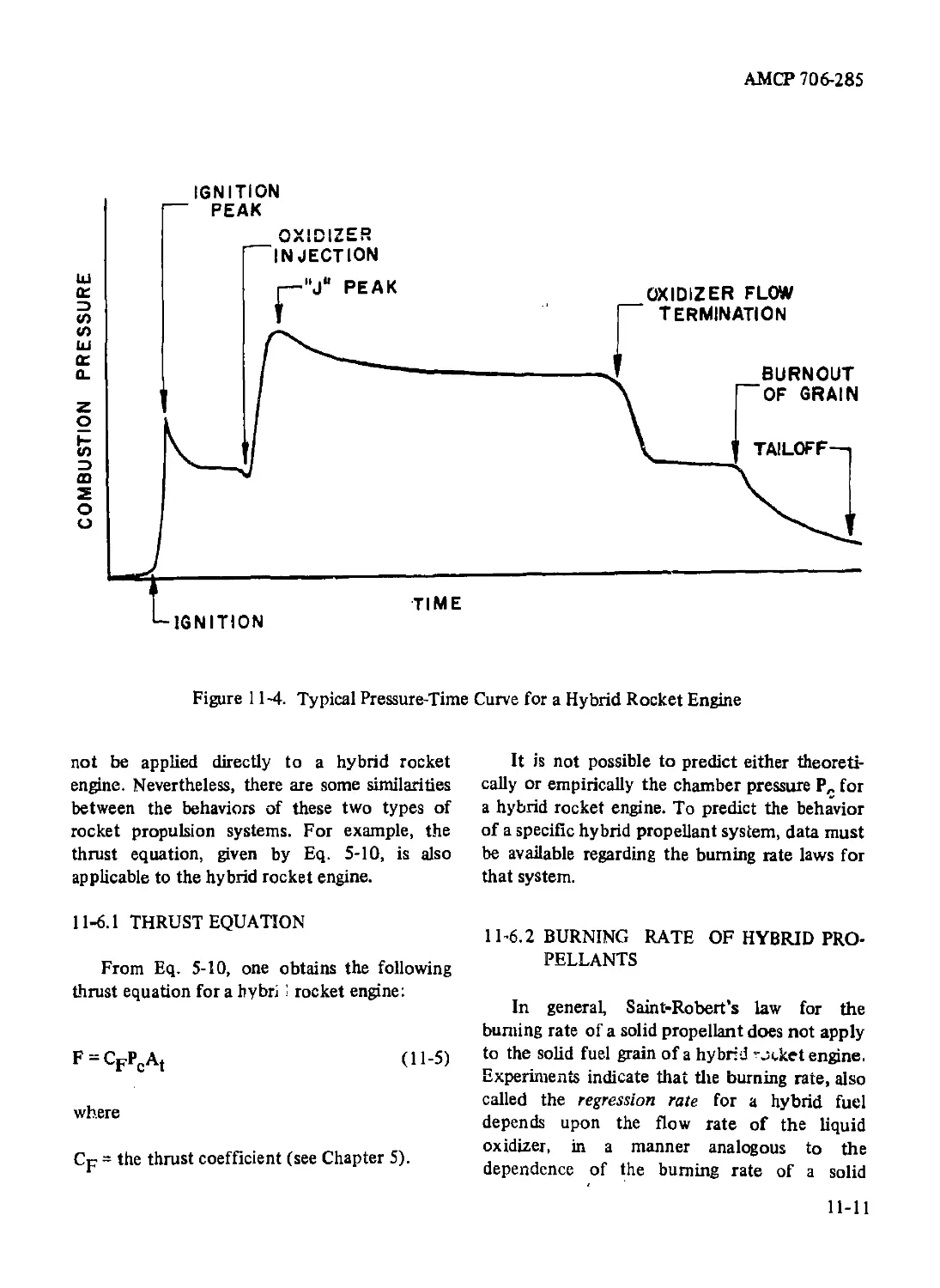
11-4 Typical Pressure-time Curve for a Hybrid Rocket Engine... 11-11
11-5 Three Types of Injectors That Have Been Utilized in
Hybrid Rocket Engines.................................. 11-15
12-1 Essential Features of the Ramjet Engine.................. 12-9
12-2 Essential Features of the Turbojet Engine .............. 12-12
12-3 Components of Gas Generator for an Afterburning
Turbojet Engine........................................ 12-13
12-4 Arrangement of the Components of an Afterburning
Turbojet Engine........................................ 12-14
12-5 Essential Features of a Turbofan Engine................. 12-15
12-6 Essential Features of a Turboshaft Engine .............. 12-16
12-7 Essential Features of a Turboprop Engine ............... 12-18
12-8 Historical Trend in the Maximum Allowable Temperatures
for Turbine Disk, Blade, and Vane Materials............ 12-22
xxvii
АМСР 706-285
LIST OF ILLUSTRATIONS (Continued)
Figure No. Title Page
12-9 Increase in Overall Efficiency of Gas-turbine Jet
Engines Since 1945 .................................... 12-25
12-10 Comparison of TSFC’s for Air-breathing and Rocket
Engines .............................................. 12-26
12-11(A) Specific Output Characteristics As a Function of Cycle
Pressures ............................................. 12-29
12-11(B) Specific Fuel Consumption Characteristics As a Function
of Cycle Pressures..................................... 12-30
13-1 Subsonic Inlet With Solely External Compression .......... 13-3
13-2 Subsonic Internal-compression Diffuser ................... 13-4
13-3 Diffusion Processes Plotted on the hs-plane............... 13-6
13-4 Design and Off-design Operation of the Normal Shock
Diffuser................................................ 13-8
13-5 Schematic Diagram of a Conical Shock (Ostwatitsch
type) Supersonic Diffuser.............................. 13-10
13-6 Three Principal Operating Modes for Supersonic External
Compression Diffusers ............................................ 13-12
13-7 Multiple Conical Shock Supersonic Diffusion System .... 13-13
13-8 Total and Static Pressure Ratios As a Function of the
Free-stream Mach Number for Supersonic Diffusers
With Different Numbers of Shocks ...................... 13-14
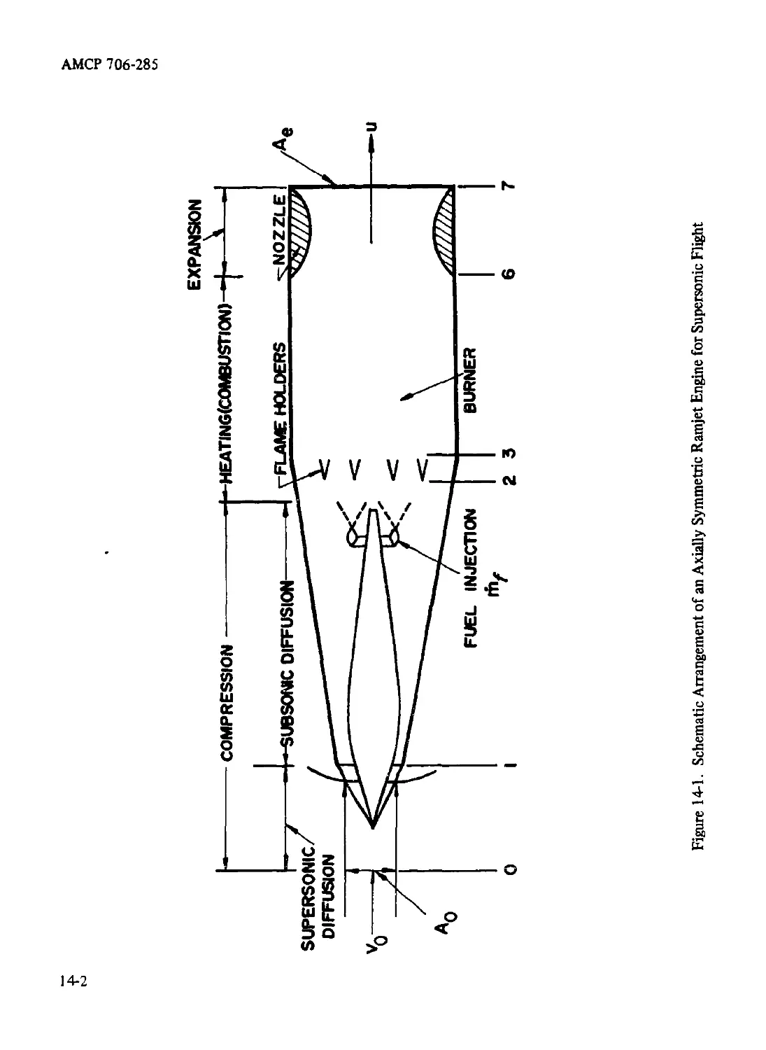
14-1 Schematic Arrangement of an Axially Symmetric Ram-
jet Engine for Supersonic Flight .................................. 14-2
14-2 Flow of Cold Air Through a Shaped Duct ................... 14-3
14-3 Effect of Varying the Exit Area of a Shaped Duct Passing
an Internal Flow of Cold Air............................ 14-4
14-4 Variation in the Static Pressure and Gas Velocity Inside
a Ramjet Engine (Mo = 2.0) ........................................ 14-6
14-5 Calculated Values of the Net Thrust of Ramjet Engines
As a Function of the Flight Mach Number ................ 14-9
14-6 Gross Thrust Characteristics of a Fixed-geometry Ramjet
Engine As a Function of the Flight Mach Number
(Constant Fuel-air Ratio/and a Fixed Altitude z)..... 14-11
14-7 Variation of Gross Thrust Coefficient Cpg for a Fixed-
geometry Ramjet Engine With Flight Mach Number MQ;
(A) With a Constant Combustion Stagnation Tempera-
ture T^ at Two Altitudes; and (B) With Two Different
Fuel-air Ratios at a Fixed Altitude............................... 14-12
xxvi i i
АМСР 706-285
LIST OF ILLUSTRATIONS (Continued)
Figure No. Title Page
14-8 Best Operating Ranges for Supersonic Diffusers for
Fixed-geometry Ramjet Engines .................................. 14-15
14-9 Diagrammatic Cross-section Through a SCRAMJET
Engine ......................................................... 14-17
14-10 SCRAMJET Engine Diffusion Process Plotted in the
hs-plane........................................................ 14-19
15-1 Isentropic Diffusion and Air Compression Processes
Plotted in the hs-plane ......................................... 15-3
15-2 Diffuser Performance Charts ................................ 15-5
15-3 Expansion Processes for Turboshaft, Turboprop, and
Turbojet Engines Plotted in the hs-plane .............. 15-7
15-4 Ideal Thermodynamic Cycle for a Turboshaft Engine .... 15-11
15-5 Comparison of Actual and Ideal Turboshaft Engine
Cycles ............................................... 15-14
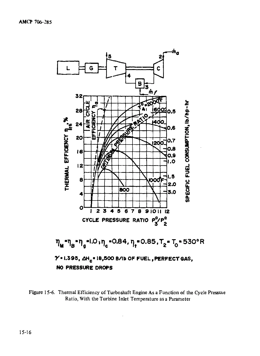
15-6 Thermal Efficiency of Turboshaft Engine As a Function
of the Cycle Pressure Ratio, With the Turbine Inlet
Temperature as a Parameter ........................... 15-16
15-7 Specific Output of Turboshaft Engine as a Function of
the Cycle Pressure Ratio, With the Turbine Inlet
Temperature as a Parameter ........................... 15-17
15-8 Air-rate of the Turboshaft Engine as a Function of the
Cycle Pressure Ratio, With the Turbine Inlet Tempera-
ture as a Parameter ............................................ 15-19
15-9 Work-ratio of Turboshaft Engine as a Function of the
Cycle Pressure Ratio, With the Turbine Inlet Tempera-
ture as a Parameter ................................ 15-20
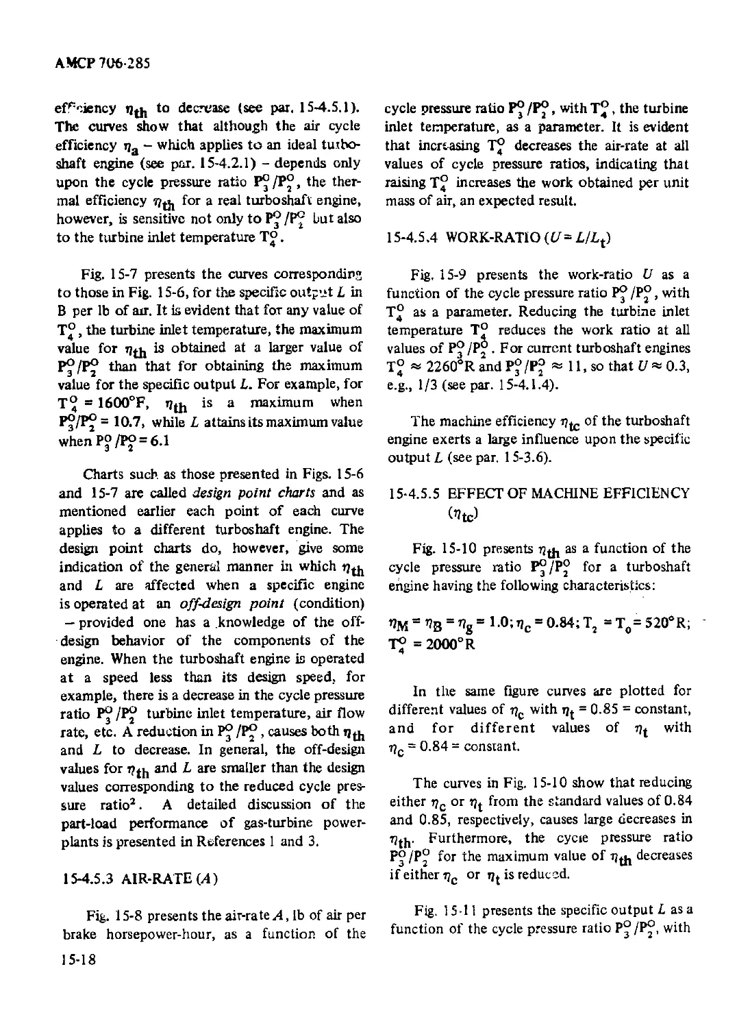
15-10 Thermal Efficiency of Turboshaft Engine as a Function
of the Cycle Pressure Ratio, With j?c and as
Parameters...................................................... 15-21
15-11 Specific Output of Turboshaft Engine as a Function of
the Cycle Pressure Ratio for Different Values of
Machine Efficiency ............................................. 15-22
15-12 Turbine Inlet Temperature T° as a Function of the
Optimum Cycle Pressure Ratio for Maximum Specific
Output (Turboshaft Engine)............................ 15-23
15-13 Effect of Air Intake Temperature (To = T2) Upon the
Designpoint Performance Characteristics of Turbo-
shaft Engine .......................................... 15-24
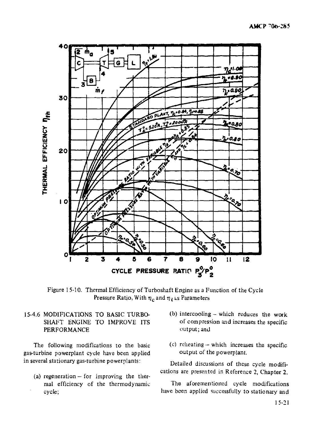
15-14 Effect of Pressure Drop on the Specific Output and
Thermal Efficiency of Turboshaft Engine................ 15-25
xxix
АМСР 706-285
LIST OF ILLUSTRATIONS (Continued)
Figure No. Title Page
15-15 Component Arrangements for a Regenerative Turbo-
shaft Engine .................................................. 15-26
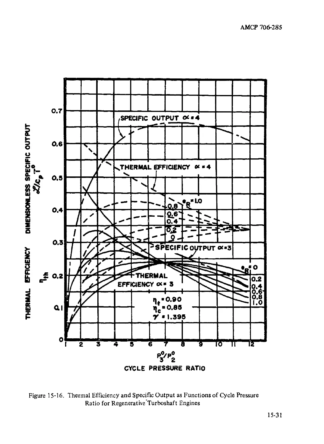
15-16 Thermal Efficiency and Specific Output as Functions
of Cycle Pressure Ratio for Regenerative Turbo-
shaft Engines................................................ 15-31
15-17 Thermal Efficiency for Regenerative Turboshaft Engines
as a Function of Cycle Pressure Ratio, With as a
Parameter, for Three Different Turbine Inlet
Temperatures................................................. 15-32
15-18 Component Arrangement and Thermodynamic Cycle
for the Turboprop Engine.............................. 15-33
15-19 SFC as a Function of Compressor Pressure Ratio With
Flight Speed as a Parameter (Turboprop Engine) .... 15-35
15-20 SFC as a Function of the Percent of Energy in Jet,
With Flight Speed as a Parameter (Turboprop Engine) .. 15-36
15-21 Effect of Altitude on the SFC of Turboprop Engines.... 15-37
15-22 Effect of Turbine and Compressor Isentropic Efficiencies
and Turbine Inlet Temperature Upon the Performance
Characteristics of Turboprop Engines .............. 15-39
15-23 Operating Characteristics of a Typical Turboprop Engine.. 15-40
15-24 Thermodynamic Cycle and Component Arrangement for
the Turbojet Engine................................ 15-42
15-25 Dimensionless Enthalpy Change for Propulsive Nozzle
as a Function of the Compressor Pressure Ratio, With
Flight Mach Number as a Parameter (Turbojet Engine) .. 15-44
15-26 Dimensionless Thrust Parameter X and Overall Efficiency
r}o as Functions of the Compressor Pressure Ratio
(Turbojet Engine).................................. 15-45
15-27 Dimensionless Thrust Parameter X for Turbojet En; :ne,
and Its Overall Efficiency tjo as Functions of the Cycle
Temperature Ratio a, With Flight Mach Number as a
Parameter.................................................... 15-47
15-28 TSFC and Specific Thrust Ia as Functions of the Com-
pressor Pressure Ratio, With Flight Speed as a
Parameter (Turbojet Engine)........................... 15-48
15-29 Arrangement of Components for a Turbofan Engine .... 15-50
A-l Specific Heats of Ideal Gases as Functions of the
Specific Heat Ratio .................................. A-l 1
A-2 Control Surface Enclosing a Control Volume in a
Region of Flowing Fluid .............................. A-l 6
xxx
АМСР 706-285
LIST OF ILLUSTRATIONS (Continued)
Figure No. Title Page
A-3 Control Volume for a One-dimensional Flow.................. A-l 7
A-4 Control Surface Enclosing a Region in a Flowing Fluid
to Which Heat is Added and Which Does Work on
Its Surroundings ................................... A-21
A-5 Element of a Control Surface Which Endow з a Region
in a Flowing Fluid.............................................. A-22
A-6 Energy Balance for a Steady One-dimensional Flow .... A-23
A-7 Comparison of Isentropic and Adiabatic Flow Processes
in the hs-plane ...................................... A-32
A-8 Isentropic Flow Expansion of a Gas to the Critical .
Condition ............................................ A-40
A-9 Area Configuration for Nozzle or Diffuser Action, for
the One-dimensional Flow of an Ideal Gas.............. A-45
A-10 Converging-diverging Flow Passage........................... A-45
A-11 Converging-diverging Flow Passage Which Passes the
Critical Mass Flow Rate m* ........................... A-47
A-l2 Functional Relationship Between dA/dx and x for the
Flow of an Ideal Gas in a Converging-diverging Flow
Passage .............................................. A-48
A-13 One-dimensional Passage With Adiabatic Flow ................ A-50
A-l4 One-dimensional Flow Passage Passing an Adiabatic Flow
in the Presence of Wall Friction...................... A-50
A-15^^~'Adiabatic Flow in a Constant Area Duct in the Presence
of Wall Friction (Fanno Flow) ........................ A-53
A-l 6 A Fanno Line Plotted in the hs-plane ................... A-54
A-17 Two Fanno Lines Plotted in the hs-plane................. A-55
A-18 Determination of the Duct Length Required for
Accomplishing a Specified Change in the Flow Mach
Number, for a Fanno Flow .........x................... A-58
A-l 9 Frictionless Flow in a Constant Area Duct With Heat
Addition (Rayleigh Flow).............................. A-65
A-20 Rayleigh Line Plotted in the Pv-plane....................... A-66
A-21 Conditions for Maximui i Enthalpy and for Maximum
Entropy for a Rayleigh Line in the Pv-plane........... A-68
A-22 Rayleigh Line Plotted in the hs- (or Ts-) plane......... A-69
A-23 Development of a Compression Shock...................... A-72
A-24 Propagation of Sound Waves from a Point Source ......... A-73
A-25 Pressure Waves Produced by a Body Moving With Sub-
sonic Speed (Small Disturbances)...................... A-74
A-26 Propagation of a Smail Disturbance by a Body (A)
Moving at Supersonic Speed, and (B) in a Uniform
Supersonic Flow Field ................................ A-75
xxxi
АМСР 706-285
LIST OF ILLUSTRATIONS (Continued)
Figure No. Title Page
A-27 Stationary Shock Wave (Normal Shock)..................... A-77
A-28 The Oblique Shock Wave................................... A-83
A-29 Coordinate System for an Oblique Shock .................. A-85
A-30 Maximum Deflection Angle 5m and Wave Angle for
Oblique Shocks as Functions of the Mach Number in
Front of the Shock (7 = 1.40) .................................... A-88
A-31 Illustration of Detachment of an Oblique Shock Due to
Flow Deflection Angle 5 Exceeding 5m.............................. A-89
A-32 Deflection Angle 6 as a Function of the Wave Angle e,
WithM, as a Parameter............................................. A-90
A-33(A) Mach Number in Back of Oblique Shock M2 as a Function
of the Mach Number in Front of the Shock M}, for
Different Values of the Deflection Angle 6 (7 = 1.40) .... A-91
A-33(B) Oblique Shock Wave Angle e as a Function of the Mach
Number in Front of the Shock M,, for Different
Values of the Deflection Angle 6 (7= 1.40) ............ a-91
A-34(A) Static Pressure Ratio P2/Рj as a Function of M,, the
Mach Number in Front of an Oblique Shock,for
Different Values of Deflection Angle 6 (7= 1.40).................. А-92
A-34(B) Stagnation Pressure Ratio /P^ as a Function of Mt, the
Mach Number in Front of an Oblique Shock, for
Different Values of Deflection Angle 6 (7 = 1.40)...... A-92
A-35 Static Density Ratio P-Jp^ as a Function of , the
Mach Number in Front of the Oblique Shock, for
Different Values of the Deflection Angle 5 (7 = 1,40) .... A-93
A-36 Supersonic Flow Over a Symmetrical Wedge .................... A-95
A-37 . Supersonic Flow Over a Symmetrical Cone at Zero Angle
of Attack ............................................. A-99
A-38 Comparison of Streamlines for the Supersonic Flow Over
a Frictionless Infinite (A) Symmetrical Wedge, and
(B) Symmetrical Cone, at Zero Angle of Attack.......... A-100
A-39 Conical Shock Wave Angle €c as a Function of Mj, the
Mach Number in Front of the Conical Shock, for
Different Semi-cone Angles £?c (7 = 1.40)............. A-101
A-40 Shock Wave Detachment Angles (for Semi-wedge and
Semi-cone) as Functions of the Mach Number Mt in
Front of the Shock Wave ................................. A-l 02
A-41 Mach Number at the Cone Surface Mc, in Back of a
Conical Shock, as a Function of the Mach Number M1
in Front of the Shock, for Different Semi-cone
Angles 6C (7 • 1.40) ................................. A-103
xxxit
АМСР 706-285
LIST OF ILLUSTRATIONS (Continued)
Figure No. Title Page
A-42 Stagnation Pressure Ratio P° /P° for a Conical Shock
as a Function of Mj, the Mach Number in Front of
the Shock, for Different Semi-cone Angles
0C(7= 1.40)...................................................A-l 04
A-43 Pressure Ratio Pc/P° as a Function of M,, the Mach
Number in Front of a Conical Shock, for Different
Semi-cone Angles 6c(t= 1.40).........................A-105
A-44 Prandtl-Meyer Expansion Flow Around a Convex Corner .. A-l06
A-45 Prandtl-Meyer Angle fi * as a Function of M2, for
Different Values of 7 (M2 = 1.0 to 3.0).............A-l 08
A-46 Prandtl-Meyer Angle fi * as a Function of M2, for
Different Values of 7 (M2 = 3.0 to 5.0).................:......A-109
A-47 Maximum Value of the Prandtl-Meyer Angle 6 as a
Function of the Specific Heat Ratio 7..........................A-l 10
I
xxxiii
АМСР 706-285
LIST OF TABLES
Table No. Title Page
1-1 Classification of Propulsion Engines ...................... 1-2
1-2 Rocket-propelled Weapons................................. 1-16
3-1 Flow Processes in Jet Propulsion Engines .................. 3-4
3-2 Integral Equations for Isentropic Flow Functions
Applied to Two Arbitrary Cross-sections of
Flow Channel ........................................... 3-22
3-3 Isentropic Functions for the Flow of Ideal Gases .............. 3-22
3-4 Equations for Computing Fanno Flow Functions for
Ideal Gases............................................ 3-28
7-1 Properties of Double-base Propellants...................... 7-3
7-2 Binders for Composite Propellants ......................... 7-4
7-3 Oxidizers for Composite Propellants ....................... 7-5
7-4 Typical Composite Propellant Formulations ................. 7-6
8-1 Some Effects Due to Acoustic Instability in a Solid
Propellant Rocket Motor ........................................... 8-17
8-2 Principal Conclusions from Experiments Concerned
With Acoustic Instability ......................................... 8-18
8-3 ? xethods for Suppressing Acoustic Instability (Solid
Propellant Rocket Motors) .............................. 8-18
9-1 Calculated Specific Impulses for Several Liquid
Propellant Systems ................................................. 9-5
9-2 Physical Properties of Water Solutions of Hydrogen
Peroxide ................................................ 9-10
9-3 Physical Properties of Several Liquid Oxidizers .......... 9-14
9-4 Physical Properties of Oxides of Nitrogen ................ 9-21
9-5 Physical Properties of Several Oxidizers Containing
Fluorine and Oxygen............................................... 9-23
9-6 Physical Properties of Liquid Fuels....................... 9-26
9-7 Physical Properties of Light Hydrocarbon Fuels............ 9-30
11-1 Performance of Hybrid Fuels With Fluorine and Oxygen
Oxidizers ......................................................... 11-6
11-2 Performance of Hybrid Fuels With Hydrogen Peroxide
Chlorine Trifluoride Oxidizers ......................... 1.1-7
xxxiv
АМСР 706-285
LIST OF TABLES (Continued)
Table, No.
Title Page
12-1 Classification of Air-breathing Engines ................................ 12-8
15-1 Army Aircraft and Their Engines..................................... 15-2
15-2 Values of Loss in Specific Output (Ah^) As a Function
of Regenerator Effectiveness (e^)....................................... 15-28
A-I Critical Pressure PCT and Critical Temperature Тст for
Several Gases........................................... A-13
A-II Relationships Between Dependent Flow Variables and
the Friction Parameter ........................................... A-61
A-III Changes in the Flow Variable With Increase in Flow
Mach Number ...................................................... A-61
A-IV Equations for Conditions Along a Fanno Line................... A-62
A-l Compressible Flow Functions for Isentropic Flow ....... A-l 15
A-2 Compressible Flow Functions for Fanno Flow ............. A-l 55
A-3 Compressible Flow Functions for Rayleigh Flow ......... A-l 95
A-4 Compressible Flow Functions for Normal Shock
Waves................................................... A-235
B-l Abbreviations for Principal Units of Measurement ............. B-l
B-2 Systems of Dimensions, Their Units and Conversion
Factors........................................................... B-3
B-3 Conversion Factors (American Engineers System
of Units) ........................................................ B-4
B-4 Dimensional Formulas and Units................................ B-8
B-5
B-6
B-7
B-8
B-9
B-10
Functions of the Specific Heat Ratio 7 .....
Values of (Pg/Pp)...........................
Values of the Parameter t?t = (Pe/Pg)........
Values of the Parameteras a Function of
p2/₽e.......................................
Molar Specific Heats at Constant Pressure for C-H-N-0
Compounds ...................
Enthalpy of C-H-N-O Compounds above To= 298.16°K— :
B-10
B-14
B-l 8
B-l 9
B-20
B-21
xxxv/xxxvi
АМСР 706-285
PREFACE
The Engineering Design Handbook of the Army Materiel Command is a
coordinated series of handbooks containing basic information and funda-
mental data useful in the design and development of Army materiel and
systems. The Handbooks are authoritative reference books of practical
information and quantitative facts helpful in the design and development of
materiel that will meet the needs of the Armed Forces.
S This Handbook replaces AMCP 706-282, Propulsion and Propellants
Handbook; it is not merely a revision to up-date the text material. As
suggested by the title, the main emphasis has been placed on propulsion.
However, the properties and characteristics of both liquid and solid
propellants have been updated and are included in the text.
The Handbook is divided into two parts: Part One “Chemical Rocket
Propulsion” and Part Two ‘ Air-breathing Jet Propulsion Engines”. Part Two
— devoted to air-breathing engines, other than piston engines, employed for
propelling winged aircraft, helicopters, and target drones — represents the
new addition. ( )
This Handbook was prepared for the U. S. Army Materiel Command.
The text was authored by Dr. Maurice J. Zucrow under contract with Duke
University. Technical assistance was provided by Mr. J. Swotinsky and Mr. E.
Costa, both of Picatinny Arsenal, and Mr. W. D. Guthrie, U. S. Army Missile
Command.
The Handbooks are readily available to all elements of AMC including
personnel and contractors having a need and/or requirement. The Army
Materiel Command policy is to release these Engineering Design Handbooks
to other DOD activities and their contractors, and other Government
agencies in accordance with cunent Army Regulation 70-31, dated 9
September 1966. Procedures for acquiring these Handbooks follow:
a. Activities within AMC and other DOD agencies should direct their
request on an official form to:
Publications Distribution Branch
Letterkenny Army Depot
ATTN: AMXLE-ATD
Chambersburg, Pennsylvania 17201
xxxvi i
АМСР 706-285
PREFACE (Continued)
b. Contractors who have Department of Defense contracts should
submit their request, through their contracting officer with proper justifica-
tion, to the address indicated in par. a above.
c. Government agencies other than DOD having need for the
Handbooks may submit their request directly to the Lettferkenny Army
Depot, as indicated in par. a above, or to: (
Commanding General
U. S. Army Materiel Command
ATTN: AMCAD-PF
Washington, D. C. 20315
or
Director
Defense Documentation Center
ATTN: TCA
Cameron Station
Alexandria, Virginia 22314
d. Industry not having a Government contract (this includes
Universities) must forward their request to:
Commanding General
II. S. Army Materiel Command
ATTN: AMCRD-TV
Washington, D. C. 20315
e. All foreign requests must be submitted through the Washington,
D.C. Embassy to:
Office of the Assistant Chief of Staff
for Intelligence
ATTN: Foreign Liaison Office
Department of the Army
Washington, D. C. 20310
xxxviii
АМСР 706-285
PREFACE (Continued)
All requests, other than those originating within DOD, must be
accompanied by a valid justification.
Comments are invited and should be addressed to Commanding Officer,
U. S. Army Research Office—Durham, Box CM, Duke Station, Durham,
North Carolina 27706.
xxxix/xl
АМСР 706-285
PART ONE
CHEMICAL ROCKET PROPULSION
CHAPTER 1
CLASSIFICATION AND ESSENTIAL FEATURES OF ROCKET
JET PROPULSION SYSTEMS
1-0 PRINCIPAL NOTATION FOR CHAPTER 1 *
A cross-sectional area
Ae cross-sectional area of nozzle
exit section
Ap frontal area
D drag, lb
F thrust, lb
m mass, slug
rn mass rate of consumption,
slug/sec
nip mass rate of propellant consump- ,
tie..
Pc gas pressure at entrance to exhaust
nozzle (combustion pressure)
Pe pressure in exit plane of the exhaust
nozzle
TSFC thrust specific fuel consumption, lb
of fuel per hr per lb of thrust
uc velocity of propellant gas at en-
trance cross-section of exhaust
nozzle
*Any consistent set ofjniits may be employed; the units
presented here are for the American Engineers System (see
par, 1-7).
u velocity of propellant gas at
e exit cross-section Ae of exhaust
nozzle
W weight, lb
Wg dry weight of rocket engine
1-1 PURPOSE AND SCOPE OF HANDBOOK
This handbook is intended to provide a
general description of the characteristics and
design features of the propulsion systems for
missiles and aircraft either employed in or being
developed for weapon systems of interest to the
Department of the Army. The handbook
assumes that the reader has a technical
background equivalent to the bachelor’s degree
in either engineering, physics, or chemistry, but
no previous experience in either propulsion or
propellant technology.
For convenience the handbook is divided
into the following two parts:
PART ON E CHEMICAL ROCKET
PROPULSION
and
PART TW O AIR BREATHING
JET PROPULSION
ENGINES
1-1
АМСР 706-285
1-2 SCOPE OF THE FIELD OF PROPULSION
Since World War II there has been a
tremendous broadening of the field of
propulsion particularly as applied to aircraft,
missiles, space vehicles, and reaction control
devices. An appreciation of the scope of propul-
sion as a technology can be inferred by examin-
ing Table 1-1.
Piston and turboprop engines (see A-(l) and
A-(4), Table 1-1) employ propellers for develop-
ing the propulsive force, called the thrust. In
such systems the propeller is the propulsive
element of the system. A system which utilises a
propeller for producing thrust is termed propel-
ler propulsion. The turboshaft engine is em-
ployed for powering the rotors of helicopters
and as a general gas turbine powerplant.
TABLE 1-1
CLASSIFICATION OF PROPULSION ENGINES
A. AIR-BREATHING CHEMICAL SYSTEMS
(1) Piston Engine-Propeller Systems
(2) Turboshaft Engine
(3) Regenerative Turboshaft Engine
(4) Turboprop Engines
(5) Turbojet Engines
(6) Ramjet Engines
(7) Turbofan or By-pass Engines
(8) Turbo-ramjet Engines
B. AIR-BREATHING NUCLEAR ENGINES
(1) Nuclear Turboprop Engines
(2) Nuclear Turbojet Engines
(3) Nuclear Ramjet Engines
C. ROCKET PROPULSION SYSTEMS (NON-AIR-BREATHING SYSTEMS)
(1) Chemical Rocket Propulsion Systems
(2) Nuclear (Heat-transfer) Rocket Engines
(3) Electric Rocket Engines
D. COMPOSITE PROPULSION SYSTEMS
(1) Hybrid Type Rocket Engines
(2) Combinations of Chemical Rocket Engines Using Atmospheric Air
1-2
АМСР 706-285
All of the propulsion systems listed in Table
1-1, except A-(l), A-(2), and АЧЗ), utilize the
jet propulsion principle, discussed in par. 1-3,
for developing propulsive thrust. It should be
noted, however, that a turboprop engine de-
velops a portion of its thrust by jet propulsion
and the balance by propeller propulsion.
1-3 THE REACTION PRINCIPLE2 ♦
The verb to propel means to drive or push
forward or onward, and the force which propels
a body is called the thrust, and is denoted by F.
Experience has demonstrated that every method
for propelling a body in either a fluid medium or
in space is basically an application of Newton’s
reaction principle. According to that principle,
forces always occur in equal and opposite pairs;
i.e., to every action (force) there is an equal, but
oppositely directed, reaction (force). Thus,
swimming in water, rowing a boat, the screw
propelling a ship, the propeller causing the flight
of an airplane, and jet propulsion are examples
of the application of the reaction principle to
propulsion problems.
In each of the above examples, the applica-
tion of the reaction principle involves increasing
the momentum of a flowing mass of fluid in one
direction so that the reaction to the action force
causing the time rate of increase in the momen-
tum of the fluid produces a thrust for propelling
the body. Hence, the thrust acts in the direction
of the desired motion for the body and is
produced by increasing the momentum of a
flowing fluid in the direction opposite io that
desired for the body.
1-4 THE JET PROPULSION PRINCIPLE113
Jet propulsion difiers from other propulsion
methods in that the rate of increase in the
momentum of the propulsive fluid is achieved
by causing that fluid to be ejected from within
the propelled body in the form of a high speed
•Superscript numbers refer to References at the end of the
Chapter.
fluid jet. A characteristic of all other propulsion
schemes is that the propulsive fluid is caused to
flow around the propelled body as, for example,
in the case of an airplane propeller. Hence, the
thrust produced by zjet propulsion engine is the
reaction produced by accelerating a propulsive
fluid as it flows from the inlet section of the
engine through the exist planes of one or more
suitable exhaust nozzles. The high speed jet of
fluid ejected from an exhaust nozzle is termed a
propulsive jet and the fluid comprising the jet is
called a propellant.
There is no restriction, at least in the
abstract, upon the material which can be used
for producing the propulsive jet. It may be a
liquid, a vapor, solid particles, the gas produced
by a chemical reaction, a plasma, ions, electrons,
and combinations thereof1 ’4. The choice of the
most appropriate propellant materials is dictated
by the propulsion requirements of the mission.
A common feature of all of the propulsion
systems for propelling either missiles or aircraft
is that the propulsive element of the system is
the exhaust nozzle (or nozzles), also called the
propulsive nozzle.
1-5 CLASSIFICATION OF JET PROPULSION
SYSTEMS
For propelling either an aircraft or a missile
in and through the atmosphere surrounding
earth, the most suitable fluid for forming the
propulsive jet is a hot gas. Consequently, the jet
propulsion engines for propelling such vehicles
are basically devices for producing a hot gaseous
propellant. They may be grouped into two
broad classes depending upon the method em-
ployed for producing the hot gaseous propulsive
jet1,s.
In general, every jet propulsion system that
uses a hot gaseous exhaust jet as its propulsive
jet comprises two principal subassemblies: (1) a
hot gas generator and (2) an exhaust nozzle, the
propulsive element. Regardless of its com-
plexity, the only function of the hot gas
1-3
АМСР 706-285
generator is to supply a gas at the desired
pressure, temperature, and mass flow rate to the
propulsive nozzle.
Because there are different methods and
means for producing the hot gaseous propellant,
there can be differences in the thermodynamic
cycle for producing the hot gas. Consequently,
the different types of jet propulsion systems for
propelling aircraft and missiles are related to the
design of the hot gas generator. In general, the
jet propulsion systems employing hot gaseous
propulsive jets can be divided into two groups:
(1) Air-breathing Jet Propulsion Systems
(2) Rocket Jet Propulsion Systems
Hereafter, the above will be termed air-breathing
jet engines, and rocket propulsion systems,
respectively. Obviously, air-breathing jet engines
can propel vehicles only within the atmosphere
of earth, and have maximum altitudes (or
ceilings) above which they are inoperable.
Rocket propulsion systems, ou the other hand,
since they do not use atmospheric air in then-
functioning, can be employed for propelling
vehicles in any environment; Le„ in the atmo-
sphere of earth, in space, and in or on water.
1-5.1 AIR-BREATHING JET ENGINES
A basic characteristic of an air-breathing jet
engine is that it inducts atmospheric air contin-
uously so that its propulsive (exhaust) jet
contains air as a major ingredient. If the heating
of the inducted air is accomplished by burning a
fuel with it (a liquid hydro-carbon, a cryogenic
fuel such as either liquid hydrogen or liquid
methane, or a solid fuel); the propulsion engine
is called a chemical air-breathing jet engine. The
propulsive jet in that case contains a small
amount of combustion products admixed with
the hot air ’ .
If the inducted atmospheric air is heated by
heat-transfer, either direct or indirect, with a
1-4
nuclear source of energy the propulsion engine is
termed a nuclear air-breathing jet engine. The
name air-breathing jet engines as employed
hereafter will refer to the chemical engines.
There will be no discussion hereafter of the
nuclear air-breathing engines.
All air-breathing jet engines utilize one or
more of the following gas dynamic processes in
their functioning:
(1) The induction of atmospheric air.
(2) Compression of the inducted air by
diffusion, i.e., by converting the kinetic
energy of flowing air into a rise in static
pressure.
(3) Adiabatic flow with friction.
(4) Compression of the flowing air by trans-
ferring energy to it as it flows through
some form of turbo-compressor, axial
flow or radial flow machine.
(5) Heating of the compressed flowing air by
burning it with a fuel, usually a liquid
fuel.
(6) Expansion of the compressed heated air,
admixed with combustion products, in
some form of turbine which furnishes
the power for driving the compressor.
(7) Expansion of the hot propellant gas in
an appropriate exhaust nozzle and its
ejection to the surroundings, as a pro-
pulsive jet.
In view of its utilization of one or more of
the above processes in its functioning, an air-
breathing jet engine is frequently referred to as a
gas dynamic propulsion engine.
Air-breathing jet engines may be grouped
into two main groups:
(1) Propulsive duct jet engines which em-
ploy no machinery in the hot gas gener-
ator.
(2) Gas-turbine jet engines which employ
machinery in the hot gas generator.
АМСР 706-285
Fig. 1-1 is a block diagram illustrating the
essential elements of an air-breathing jet engine.
In a propulsive duct jet engine, the air compres-
sion is due entirely to diffusion, the conversion
of the kinetic energy associated with a flowing
fluid into static pressure rise, and the turbine
element is omitted. The components 1, Il and III
coact to form the hot gas generator.
In a gas-turbine engine the components I, II,
ligand IV coact to form the hot gas generator.
The air heating system III for either type of
engine is termed either the burner or the
combustor.
Detailed discussions of the different types of
air-breathing jet engines are presented in Part
Two of this handbook.
1-5.2 ROCKET JET PROPULSION SYSTEMS
By definition, a rocket jet propulsion system
is one which does not use any atmospheric air in
producing the hot gaseous propulsive jet. Conse-
quently, a rocket propulsion system can propel
bodies both within and beyond the atmosphere
of earth. Air-breathing jet engines can function
only within that atmosphere5,6,9.
Fig. 1-2 illustrates diagrammatically the es-
sential elements of a rocket jet propulsion
system. It comprises the following:
(1) A supply of a propellant material (or
materials) stored in appropriate tanks
carried in the rocket-propelled vehicle.
(2) Means for metering the rate at which the
propellant material is forced into the
rocket motor, wherein energy is added
to it.
(3) One or more rocket motors (also called
thrust chambers, thrusters, or acceler-
ators) from which the propulsive high
speed jet is ejected to the surroundings.
In every rocket propulsion system, irrespec-
tive of its type, means must be provided for
adding energy to the propellant material as it
moves through the rocket motor.
Refer to Fig. 1-2. Propellant material from
the Propellant Supply (A) is metered and fed by
the Feed and Metering System (B) to the Rocket
Motor (C), wherein energy is added to the
propellant material. As a consequence of the
energy addition, a propellant gas is ejected from
the rocket motor as a propulsive jet. Accord-
ingly, a thrust force, denoted by F, is produced
acting in the direction opposite to that for the
jet velocity, denoted by ue; the latter is mea-
sured with respect tc the walls of the rocket
motor.
If one considers rocket jet propulsion from
the broadest point of view so that it includes
space propulsion engines, then consideration
must be given to the feasibility of utilizing one
or more of the following forms of energy for
propulsion purposes: (a) chemical energy,
(b) solar energy, (c) nuclear energy, and (d) elec-
trical energy9•
1-5.3 CLASSIFICATION OF ROCKET PRO-
PULSION SYSTEMS
Rocket propulsion systems may be grouped
in accordance with the forms of energy they use
in their functioning. Thus there are four groups:
(1) Chemical Rocket Propulsion Systems
(2) Solar Energy Rocket Engines
(3) Nuclear (Heat-transfer) Rocket
Engines
(4) Electrical Rocket Engines
The discussions in Part One of this hand-
book will be limited to chemical rocket propul-
sion systems; hereafter referred to as rocket
propulsion systems.
1-5
AMCP 706-285
(T-TURBINE, N-PROPULSIVE NOZZLE)
HOT GAS GENERATOR
EXPANSION SYSTEM
PROPULSIVE DUCT JET ENGINE
(I + H+ Jtt + V )
GAS TURBINE JET ENGINE
Figure 1-1. Essential Elements of an Air-breathing Jet Engine
АМСР 706-285
1-5.4 CHEMICAL ROCKET PROPULSION
SYSTEMS
Only the chemical types of rocket propul-
sion systems have achieved operational realiza-
tion and have a broad, well-developed tech-
nology. Chemical rocket propulsion systems
have the following two characteristics:
(1) They utilize chemical reactions in the
thrust chamber to produce a high pres-
sure high temperature propellant gas at
the entrance plane of a converging-
diverging exhaust nozzle.
(2) The propellant gas is expanded as it
flows through the exhaust nozzle and is
ejected to the surroundings as a super-
sonic gaseous propulsive jet.
The expansion in the exhaust nozzle is a
thermodynamic process by which approximately
one-half of the enthalpy released by the chemi-
cal reaction is converted into the kinetic energy
associated with the supersonic gaseous propul-
sive jet. Chemical rocket jet propulsion systems
belong to a class of propulsion systems which
are frequently termed thermodynamic jet pro-
pulsion systems.
In a thermodynamic rocket jet ropulsion
system, as in an air-breathing jet engine, (see par.
1-5.1) all of the components except the exhaust
nozzle constitute a hot-gas generator for supply-
ing a high pressure, high temperature gas to a
converging-diverging exhaust nozzle (see Fig.
4-6).
The amount of energy that can be added to
the propellant gas produced by a chemical
reaction is limited by the nature of the chemical
bonds of the reactants and products. For that
reason chemical rocket propulsion systems are
frequently referred to as energy-limited rocket
propulsion systems9. It is because of this energy
limitation that consideration must be given,
especially for space propulsion engines, to
thrust-producing systems in which larger
amounts of energy can be added per unit mass
of the consumed propellant. As to be expected,
when sources of larger amounts of energy are
considered, atomic energy is a prime contender.
1-6. ESSENTIAL FEATURES OF CHEMICAL
ROCKET PROPULSION SYSTEMS®’6,9
The general operating principle of a chemical
rocket motor can be demonstrated by consider-
ing the fin-stabilized solid propellant rocket
motor illustrated in Fig. 1-3.
As the solid propellant bums it produces
tremendous quantities of hot gas. If the propel-
lant bums in a closed chamber, such as that
illustrated in Fig. 1-4(A), the gas pressures inside
the chamber are balanced in all directions and
no thrust is developed. Assume now that a small
hole is opened in the chamber, as illustrated in
Fig. 1-4(B), and that the propellant bums at a
constant rate. Under these conditions the com-
bustion pressure inside the chamber, denoted
by Pc, remains constant (a short time after the
grain is ignited) at a value governed by the area
of the hole and the rate, denoted by nip, at which
the propellant burns. At the hole in the chamber
there is an escape of gas and the latter has no
surface against which it can push. Hence, there is
an unbalanced force or thrust, denoted byF,
acting to the left. In a practical rocket motor the
hole (see Fig. 1-4(B)) is replaced by a
converging-diverging nozzle, termed a De Laval
nozzle, as illustrated in Fig. 1-4(C). Conditions
are similar if the hot gas is produced by burning
one or more liquids rather than by burning a
solid material. In any case the main objective is
to produce a propulsive jet having the largest
ejection velocity,
Because the gas pressure Pc at the entrance
to the exhaust nozzle is normally several times
that of the surroundings into which the propel-
lant gas is discharged, the velocity of the
propulsive jet is supersonic. Furthermore, the
1-7
АМСР 706-285
VEHICLE,...
SPEEDtvoJ
THRUST (F)
Figure 1-2. Essential Elements of a Jet Propulsion System
Figure 1-3. Fin-stabilized Rocket Motor
1-8
АМСР 706-285
ALL PRESSURES ARE BALANCED
(A)
IS DEVELOPED
Figure 1-4. Development of Thrust in a Rocket Motor
1-9
АМСР 706-285
mean velocity of the gas crossing the throat
section may be assumed to be equal to the local
speed of sound (see Chapter 3).
The following two characteristics of a rocket
jet propulsion system are mainly responsible for
the fundamental differences in its operation and
in that of an air-breathing jet engine2 ’3.
(1) A rocket propulsion system consumes no
atmospheric air.
(2) The thrust developed by a rocket jet
propulsion system depends almost en-
tirely upon the velocity of the propulsive
jet, while the thrust of an air-breathing
jet engine depends upon the difference
between the momentum of the propel-
lant gas leaving and entering the engine.
Because of the above two characteristics, rocket
jet propulsion systems have the following ad-
vantages compared with other jet propulsion
systems:
(1) The thrust is essentially independent of
flight speec and altitude.
(2) The thrust per unit of cross-sectional
area F/Ap is the largest for all known
types of propulsion systems.
(3) The thrust per unit of engine weight
F/Wg is the largest for all known types
of propulsion systems.
(4) A rocket jet propulsion system has no
altitude ceiling.
Experience has amply confirmed the predic-
tions of the pioneers in rocketry, that from a
propulsion standpoint, all of the space missions
so far conceived can be achieved by properly
applying the rocket jet propulsion principle,
hereafter termed rocket propulsion.
Because the oxygen for burning with the
fuel is not obtained from the surrounding
atmosphere, the rate at which a rocket propul-
sion system consumes its propellant materials
(fuel plus oxidizer) is several times the rate at
which an air-breathing jet engine consumes fuel,
in developing an equivalent thrust.
The most important parameters governing
the flight speed of a propelled vehicle are:
(1) F/Ap-the thrust per unit of frontal
area, and
(2) F/Wg - the thrust per unit of engine
weight.
As mentioned earlier, judged by the above
parameters rocket propulsion is unsurpassed.
The range of flight for winged aircraft
depends in large measure upon the thrust spe-
cific fuel consumption (TSFC) of the propulsion
system, measured in pounds of fuel per hour per
pound of thrust. To obtain a long range for a
rocket-propelled vehicle, such as an inter-
continental guided ballistic missile (ICBM), a
trajectory must be utilized which takes ad-
vantage of its large values of F/Ap and F/Wg,
but minimizes the adverse effects of its large
TSFC. To achieve a long range, the large thrust
of the rocket engine is utilized for propelling the
vehicle to a very high altitude (several tens of
miles) and for imparting to it a very large
velocity (several thousands of feet per second),
at the end of the operating period for the rocket
engine, termed the powered flight. The velocity
at the end of the powered flight is called either
the cut-off velocity, burnout velocity, or burned
velocity. The kinetic energy of the vehicle after
it reaches the cut-off velocity is then used for
coasting along a ballistic trajectory5.
1-6.1 CLASSIFICATION OF ROCKET PRO-
PULSION SYSTEMS
It is convenient to group rocket propulsion
systems into four principal categories:
(1) Liquid bipropellant rocket engines
(2) Liquid monopropellant rocket engines
1-10
АМСР 706-285
(3) Solid propellant rocket motors
(4) Hybrid rocket engines
Brief descriptions of the above engines will
be presented in this chapter, primarily for
identification purposes.
1-6.2 LIQUID BIPROPELLANT ROCKET EN-
GINE
Fig. 1-5 illustrates the essential elements of a
liquid bipropellant rocket engine employing a
turbo-pump (a gas turbine driving the propel-
lant pumps) for feeding a liquid fuel and a liquid
oxidizer to a rocket motor. Fig. 1-6 illustrates
the principal elements of an uncooled liquid
bipropellant rocket engine.
1-6.3 LIQUID MONOPROPELLANT ROCKET
ENGINE
Fig. 1-5 also illustrates schematically the
essential elements of a monopropellant rocket
engine, if one removes the oxidizer supply tank,
oxidizer pump, oxidizer lines, etc. A mono-
propellant contains the oxygen for combustion
in either its chemical or physical structure, or
both. Consequently, an oxidizer supply, meter-
ing, and feed system is unnecessary. '
1-6.4 SOLID PROPELLANT ROCKET
MOTOR
Fig. 1-7 illustrates diagrammatically a solid
propellant rocket motor employing an internal-
burning case-bonded solid propellant grain; the
latter bums radially at a substantially constant
rate. A solid propellant contains both its fuel
and the requisite oxidant for burning it, either in
the solid propellant molecule (double-base pro-
pellants) or as an intimate mechanical mixture
(termed either a heterogeneous or composite
propellant), (see Chapters 7 and 8 for details).
The chemical reaction is initiated by means of
an electrically fired igniter.
1-6.5 HYBRID ROCKET ENGINE
Fig. 1-8 illustrates diagrammatically the es-
sential elements of one form of hybrid (chem-
ical) rocket engine. The solid propellant grain,
which may or may not contain a small amount
of oxidizer, is reacted with a liquid oxidizer and
bums in the radially outward direction at a
substantially constant rate. Of course, the re-
verse of the above is possible.
Of the chemical rocket propulsion systems
presented above, only the liquid bipropellant
engine and the solid propellant rocket motor
have attained an operational state of develop-
ment for missile propulsion. Thus the ATLAS
and TITAN ICBM’s employ liquid bipropellant
rocket engines; the MINUTEMAN ICBM and
POLARIS IRBM utilize solid propellant rocket
motors. Monopropellant engines have found
application in reaction control devices.
Table 1-2 lists some Army weapons which
employ rocket propulsion systems.
1-7 UNITS OF MEASUREMENT
The units of measurement employed in this
handbook, unless specifically stated to be otheir-
wise, are listed below: Unit of Measurement
Dimension Symbol
MASS M 1 slug
FORCE F 1 pound (lb)
LENGTH L 1 foot (ft)
TIME T 1 second (sec)
The following tables pertinent to units and
measurement are presented in the Appendix В
to this handbook:
Table B-l Abbreviations for Principal
Units of Measurement
Table B-2 Systems of Dimensions,
Their Units and Conversion
Factors
Table B-3 Conversion Factors (Ameri-
can Engineers System of
Units)
Table B-4 Dimensional Formulas and
Units
1-11
1-12
AMCP 706-285
Figure 1-5. Essential Elements of a Liquid Bipropellant Rocket Engine
F • THRUST
1-13
Figure 1-6. Principal Elements of an Uncooled Liquid Bipropellant Rocket Engine
AMCP 706-285
АМСР 706-285
CROSS-SECTION THROUGH A STAR SHAPED BONDED
SOLID PROPELLANT ROCKET MOTOR
Figure 1-7. Essential Elements of an Internal-burning Case-bonded ’Solid Propellant Rocxet Motor
1-14
АМСР 706-285
K7L PRESSURIZED
INERT GAS
GAS
TURBINE
GAS
GENERATOR
Figure 1-8. Essential Features of a Hybrid Chemical Rocket Engine
1-15
АМСР 706-285
TABLE 1-2
ROCKET-PROPELLED WEAPONS
NAME STATUS PROPULSION
SURFACE-TO-SURFACE MISSILES
HONEST JOHN 0 Single Stage SPRM
LITTLE JOHN 0 Single Stage SPRM
PERSHING 0 Two Stage SPRM
SERGEANT 0 Single Stage SPRM
LANCE ED Storable LPRE
SURFACE-TO-AIR MISSILES
REDEYE 0 Dual Stage SPRM
HAWK (MIN-234) 0 Dual Stage SPRM
CHAPPARAL ED SPRM
NIKE HERCULES (MIM-14B) 0 Two Stage SPRM
SPRING ED Two Stage SPRM
SPARTAN ED Three Stage SPRM
ANTITANK MISSILES
SHILLELAGH 0 SPRM
MAW ED SPRM
TOW ED SPRM
M72 ROCKET GRENADE 0 SPRM
ENTAC 0 SPRM
0 - Operational; SPRM - Solid Propellant Rocket Motor; LPRE - Liquid Propellant Rocket Engine;
ED - Engineering Development
!-16
АМСР 706-285
REFERENCES
1. M.J. Zucrow, Panel on Science and Tech-
nology Fourth Meeting, Committee on
Science and Astronautics, U.S. House of
Representatives, 87th Congress, Second
Session, March 21 and 22, 1962, p. 19.
2. M.J. Zucrow, Jet Propulsion and Gas
Turbines, John Wiley and Sons, Inc., 1948,
p. 38.
3. M.J. Zucrow, Aircraft and Missile Pro-
pulsion, John Wiley and Sons, Inc., Vol. 1,
1958, Ch. 2.
4. W.J. Hesse and N.V. Mumford, Jet Pro-
pulsion for Aerospace Applications, Pitman
Publishing Corporation, 2nd Ed., 1964, Ch.
2.
5. M.J. Zucrow, Aircraft and Missile Pro-
pulsion, John Wiley and Sons, Inc., Vol. 2,
2nd Printing, 1964.
6. G.P. Sutton, Rocket Propulsion Elements,
John Wiley and Sons, Inc., 1963, Ch. 1.
7. C.W. Smith, Aircraft Gas Turbines, John
Wiley and Sons, Inc., 1956, Ch. 1 and 2.
8. D. Kuchermann and J. Weber, Aerodynamics
of Propulsion, McGraw-Hill Book Company,
Inc., 1953.
9. M.J. Zucrow, Science in Progress,
Fourteenth Series, Yale University Press,
1964, p. 241.
1-17/1-18
АМСР 706-285
CHAPTER 2
MOMENTUM THEORY APPLIED TO PROPULSION
2-0 PRINCIPAL NOTATION FOR CHAPTER 2*
A cross-sectional area
Aj cross-sectional area of inlet to a propul-
sion system
Ag cross-sectional area of exit section of ex-
haust nozzle
c effective jet velocity, fps
d diameter
D drag force, lb
f fuel-air ratio
F thrust or net external force acting on a
body of fluid enclosed by a control sur-
face 5, lb
F magnitude of the force vector F, or
thrust developed by a propulsion sys-
tem, lb
F^ available thrust, lb
Fexf net external force, lb
g local acceleration due to the gravitational
attraction of earth, ft/sec2
gc gravitational correction fac-
tor = 32.174 slug-ft/lb-sec2
h static specific enthalpy, B/slug
•Any consistent set of units may be employed; the units
presented here are for the American Engineers System (see
par. 1*7).
h° total or stagnation specific enthalpy
AHC lower heating value of a fuel, B/slug
ДНр calorific value of propellant material,
B/slug
i unit vector along x-axis
Ia F/gcma = specific thrust or air specific
impulse, sec
F/gcmf = fuel specific impulse, sec
L_ ₽/w = F/(w_ + w -) = specific impulse, sec
° j
j unit vector along y-axis
к unit vector along z-axis
m mass, slug
rh mass rate of flow of propellants, slug/sec
riiy mass rate of flow of fuel, slug/sec
ma muss rate of flow of air, slug/sec
mQ mass rate of flow of oxidizer, slug/sec
M momentum vector
M dM/dt = rate of change of momentum,
slug ft/sec2
n unit vector along normal to a surface;
positive direction is outward from surface
p static pressure intensity, psia
AMCF mt-.’eS
pe static prescuie inletsiiy in exit area
оГ exhaust nozzle, pssa
po static pressure of the surroundings
P static pressure intensity, psi
Pe static pressure in area Ae, psf
P propulsive power, ft-lb/sec
Pg required power output
Py thrust power, ft-lb/sec
PKE exit loss associated with propulsive jet,
ft-lb/sec
Px power loss, ft-lb/sec
q velocity vector
q magnitude of velocity vector, fps
qn normal velocity, normal to a flow area,
fps
Qv volumetric rate of flow, cfs
riio/m r = mixture ratio of a propellant
j material combination
R resultant force vector due to the inter-
action of the internal flow with surfaces
of the propulsion system, lb
R magnitude of R, lb
s static specific entropy
S area of a control surface, or a projected
area, sq ft
t time, sec
u velocity component parallel to x-axis, fps
u* velocity of jet crossing area Ae of ex-
haust nozzle, fps
V control volume, i.e., volume inclosed
by S
V flight speed, fps ,
Vj effective jet velocity
v velocity of a fluid parallel to у-axis, fps
w velocity of a fluid parallel to z-axis, fps
W body force = mg
w weight rate of flow, Ib/sec
wa weight rate of flow of atmospheric air,
Ib/sec
wy weight rate of flow of fuel, Ib/sec
w0 weight rate of flow of oxidizer, Ib/sec
X net external force in direction of
x-axis, lb
Y net external force in direction of
у-axis, lb
Z net external force in direction of
z-axis, lb
z altitude or elevation, ft
GREEK LETTERS
a angle between velocity vector and nor-
mal to flow cross-section
P m^ /ma = the bypass ratio
efficiency
4g energ'- conversion efficiency
2-2
АМСР 706-285
т?о overall efficiency of propulsion system
i)n propulsive efficiency
ideal propulsive efficiency
thermal efficiency
v V0IVi = effective speed ratio
p density, slug/ft3
Ф characteristic property of a flowing
fluid inside control volume, per unit
volume
SUBSCRIPTS
Fig. 2-2. Consequently, at the instant t» tf + dt
the mas of fluid enclosed by 5 at t “ te is now
enclosed by the fictitious surface S'.
When a fluid flows into or out of a control
volume it can transport, in addition to its mass,
other characteristics or properties associated
with its mass; such as momentum, energy,
enthalpy, entropy, etc. It is assumed in all of the
discussions which follow that the fluid is a
continuum1.
2-1.1 TRANSPORT OF A FLUID PROPERTY
ACROSS A CONTROL SURFACE. If Ф de-
notes a characteristic property of a flowing fluid
per unit volume, that is transported across a
control surfaces (see Fig. 2-1) then
a air
amb ambient or air, as specified in test
e exit area of exhaust nozzle
f fuel
о oxidizer
i internal
о undisturbed atmosphere
2-1 MOMENTUM THEOREM OF FLUID
MECHANICS
Fig. 2-1 illustrates diagrammatically a region
of a fluid flow field that is enclosed, at the
instant t = t0, by a fictitious stationary control
surface S. The volume of the fluid instanta-
neously enclosed by 5 is termed the control
volume and is denoted by K. At some later in-
stant of time, t = tQ + dt, the same mass of fluid
is no longer enclosed by S, due to fluid entering
and leaving the control volume V, as illustrated in
where
_d
at
Э
dt
D
dTW =
+ J'Pq • ndS
V S
the flow
of'Wz
(2-1)
or particle derivative
the local rate of change of Ф;
i.e., the rate at which Ф, fluid
property per unit volume,
changes inside the control vol-
ume V
Фд • ndS = the convective rate of change of
Ф due to fluid crossing the
control surface S; i.e., leaving
and entering V
q=iu+jv + kw=the velocity
vector at the point under con-
sideration
L j ,k = unit vectors along the Cartesian
coordinate axis; x,y,z, respec-
tively
J 4'dF =
V
2-3
АМСР 706-285
u,v,w = rectangular components of q
parallel to the x-,y-,z- axis, re-
spectively
n= unit normal vector at dS', its
positive direction is outward
from V (see Figs. 2-1 and 2-2)
q • n = scalar product of q and n
~ = q cos a ~ ~
qn = the normal velocity = q cos a
In Eq. 2-1 there is no restriction upon Ф—it
may be either a vector or a scalar. In general, the
right-hand side is the sum of a nonstationary
term and a convective term.
The nonstationary term arises from the fact
that in an unsteady flow the density of the fluid
inside the control volume V varies with the time t.
The convective term expresses the condition
that the mass of fluid entering and leaving the
control volume also transports Ф, the character-
istic or property of the fluid.
Eq. 2-1 is the general form of the integral
equation for determining the rate of change of
Ф for a flowing fluid; it applies to both unsteady
and steady flows. To obtain the corresponding
differential equation, the surface integral in Eq.
2-1 is transformed into a volume integral by
applying the divergence theorem2,3. Thus
J"I'q • n d5 =
J
y*div(^q) dK
V
(2-2)
In Eq. 2-3, the differential dH has the same
value in both of the integral terms. Hence
D (<№\
Э^(ф1л) = +div('l'q) (2-4)
V
In Cartesian coordinates3
div(^q) =V-(^q) (2-5)
The operator V, called del or nabla, is
defined by
v( )=i£;< > + kr-< > (2-6)
~ ox ~ Sy ~ oz
In the case of steady flow, the nonstationary
terms in Eqs. 2-1 and 2-4 vanish, so that
'I'q • ndS
and
^-(Ф7) = 4к(ФЧ) = V (ФЧ)
ot ~ ~
(2-7)
(2-8)
2-1.2 MOMENTUM OF A FLUID IN STEADY
FLOW. By definition, the momentum of a
flowing fluid of density p, occupying instanta-
neously the control volume V, see Fig. 2-2, is
given by
Ms(pF)q (2-9)
In the subject case, Ф is given by
M
Ф = = p q = momentum per unit (2-10)
volume
By analogy with Eq. 2-1
Substituting Eq. 2-2 into Eq. 2-1, yields
(ФЮ = —
at at
j" divf'tqjdK
(2-3)
V V
DM э /
"^t=dt / (P4)dK+ I (pq)q-ndS (2-11)
J V S
2-4
AMCT 7O6-2&5
Figure 2-1. Control Surface and Control Volume Enclosing a
Region of a Flowing Fluid
Figure 2-2. Transport of Momentum by a Flowing Fluid
2-5
АМСР 706-285
By analogy with Eq. 2-4, one obtains the
following differential equation:
dM
dT = <tt7 + div(^)9. (2-12)
V
If the flow is steady, then
я f (oM\
3t / (^dK= U =°
JV V
For & steady flow-the type of flow assumed
in all of the future discussions unless it is
specifically stated to be otherwise - the integral
equation for the rate of change of momentum is
given by
dM f
-~= j (pq)qndS (2-13)
5
The corresponding differential equation is
dM
г s div (pq) q (2-14)
dt ~ ~
By Newton’s second law of motion, the net
external force acting upon a mass of fluid
instantaneously enclosed by a stationary control
surface S is equal to the rate of change in the
momentum of the fluid.
Let denote the net external force, and
dM
M = =the rate of changein the momentum of
dt the fluid.
Then
Fext =Й = J (РЧ ) 4 • nds
(2-15)
Eq. 2-15 is a vector equation. It applies to
either a steady or a mean steady flow, and to
steady viscous and nonviscous flows.
Let X denote the external force acting in the
direction of the x-coordinate axis, and u denote
the fluid velocity in the same direction, then
X = Mx = J (pqn)udS = J jufqcosaldS (2-16)
5 J
Similar equations can be written for the
forces Y and Z acting in the directions of the y-
and z-coordinate axes, respectively.
Accordingly, the magnitude of the net exter-
nal force Fext is given by
Fext = VX2 + Y2 + Z2 (2-17)
The magnitude of the velocity vector q
q= | q | = \/u2 + v2 + w2 (2-18)
2-1.3 EXTERNAL FORCES ACTING ON A
FLOWING FLUID. In general, the external
forces acting on a body of fluid can be divided
into two types: (l)surface forces,and (2)body
forces.
Surface forces are those which are distri-
buted over the surface of a body, such as the
pressure exerted by one body on another; as for
example, the hydrostatic pressure in a body of
liquid . The component of a surface force acting
perpendicular to the surface of a body is termed
a normal force, and the component parallel to
the surface of a body is called either a tangential
or a shearing force.
A body force is one which is distributed over
the entire volume of a body of material; for
example, the forces due to the gravitational
attraction of earth, magnetic fields, electrostatic
fields, and the like. In the absence of all fields of
force except the gravitational field of earth, the
net external force Fext acting on the fluid
instantaneously enclosed by the control surface
S' (see Fig. 2-3) has the following components:
(1) The body force W = mg acting toward
the center of earth, due to gravitational
attraction.
2-6
АМСР 706-285
(2) The foilowing two surface forces:
(a) The pressure force Fp where
Fp = pn dS = У*(Po— Pj) d?
5 5
(2-19)
where
(p0—Pp = the excess pressure.
(b) The net force R due to contact
between the body of flowing fluid
and solid surfaces.
Hence, the net external force F'exf *is the
vector sum of tie body and surface forces. Thus
.Eext “ ~ + £p + 5
(2-20)
2-1.4 STEADY FLOW MOMENTUM THE-
OREM. Combining Eqs. 2-13 and 2-19, one
obtains
W — J pn dS + R =
5
(pqtan115
(2-21)
If the propulsive fluid is a gas W =s 0.
Eq. 2-21 is known as the momentum the-
orem of fluid mechanics for a steady flow4.
z If X denotes the component of force R in the
‘ x-direction, then from Eqs. 2-16 and 2-21
(2-22)
If no solid bodies are wetted by the flowing
fluid and the gravitatir J attraction of earth is
negligible, the Eq. 2-22 reduces to
(2-23)
where u is the velocity of the fluid parallel to
the x-direction.
The application of Eq. 2-21 for determining
the thrust of a jet propulsion system is illus-
trated in par. 2-2.1.
2-2 APPLICATION OF THE MOMENTUM
THEOREM TO PROPULSION SYSTEMS. The
application of Eq. 2-21 to determine the thrust
of a jet propulsion system will now be illus-
trated.
Fig. 2-4 illustrates diagrammatically some
form of air-breathing engine which is held
stationary while atmospheric air flows toward it
with the free stream velocity Vo. The stream of
air that enters the engine and wets its internal
surfaces will be called the internal flow. Simi-
larly, the air stream flowing past the external
surfaces or housing of the engine will be termed
the external flow.
The interactions of the internal flow with
the interna] surfaces of the engine produce a net
component of force parallel to the longitudinal
axis of the engine, termed the net internal axial
force, and is denoted by Fj. In the relative
coordinate system (see Fig. 2-4), if an axial force
acts in the direction opposite to that for the free
stream velocity, it is called a thrust.
On the other hand, an axial force which acts
in the same direction as the free stream velocity,
in the relative coordinate system, is called an
internal drag and is denoted by Dj.
For the external flow, the net force acting
parallel to the lonfutuduial axis of the engine -
due to the interaction of external flow with the
engine housing - is termed the external drag De.
Hence, the force available for accelerating the
vehicle to be propelled by the air-breathing jet
engine, termed the available thrust Рд, is given
by
FA = Fi-(De--Di) (2-24)
2-7
АМСР 706-285
гск.тллт CONTROL SURFACE
CONTACT FORCE
R
CONTROL volume
2-8
АМСР 706-285
The available thrust F^ depends not only
upon the interactions between the internal flow
and the internal surfaces of the engine, but also
upon the configuration of the engine housing, as
dictated by the installation requirements of the
propelled vehicle. It is not a direct measure of
the thrust-producing capability of the engine
(Fj -Dj), but involves the design features of
the engine housing.
In a jet propulsion engine the rate at which
propulsive work is performed, termed the pro-
pulsive power, is denoted by A It is a conse-
quence of causing the internal flow to undergo
suitable energy transformations as it moves
along its flow path. In the case of an air-
breathing jet engine, heat is added to the
atmospheric air flowing through the engine. In a
rocket propulsion system, on the other hand, no
atmospheric air is inducted into the propulsion
system.
2-2.1 GENERAL THRUST EQUATION. It is
desirable that the thrust-producing capability of
a jet propulsion system be expressed in a manner
which is independent of the configuration of the
engine and its installation in the propelled
vehicle. In general terms, the thrust produced by
a jet propulsion system is the resultant axial
component of the static pressure acting upon
the surfaces of the engine wetted by the internal
flow. In determining the thrust it is convenient
to employ a relative coordinate system.
Fig. 2-5 illustrates diagrammatically an arbi-
trary jet propulsion system held stationary in a
uniform stream of atmospheric air having the
velocity Vo relative to the propulsion system.
The jet propulsion system is shown as a hollow
body of arbitrary shape; it has an inlet area A.l
and an exit area Ae, both areas are measured
perpendicular to the velocity Vo. The ducted
body may enclose struts, burners, rotating
machinery, and may be unsymmetrical. For
simplicity, however, it is assumed to be sym-
metrical with respect to its longitudinal axis; the
latter is parallel to the x-axis. The positive
direction of the x-axis is in the same direction as
the thrust F. It should be noted that F points in
the same direction as the line-of- flight when the
engine is propelling a vehicle in the atmosphere.
The thrust due to the internal flow, denoted
by Fj, is given by
Fi= / Pi £ <^i
Si
where
(2-25)
Sj = area of internal surfaces wetted by the
internal flow
Pi = the internal static pressure
Pi • n = axial component of Pj
n = unit normal vector in the axial direction
Because it is extremely difficult, if not
impossible, to evaluate the integral in Eq. 2-25,
the thrust Fj will be determined by applying the
momentum theorem.
EXAMPLE 2-1.
Determine the thrust of a jet propulsion sys-
tem by applying the momentum theorem of
fluid mechanics (Eq. 2-21).
SOLUTION.
To apply Eq. 2-21, a control surface must be
established. Since the location and configuration
of the control surface is arbitrary, it can be
arranged so that it is convenient for the analysis.
Let 5] and S2 be two infinite planes drawn
perpendicular to the longitudinal axis of the
propulsion system. Plane Sj is located suffi-
ciently far upstream from the propulsion system
so that the static pressure pQ acting on is
identical with the value it has when there is no
propulsion system between 5] and .
2-9
АМСР 706-285
DIRECTION OF LINE-OF-FLIGHT
5, V. -V=V_ ; V, »IL; V. «V
’ lx 2x 3x e 4x
(CONTROL
5 2 VOLUME)
^2в^Г^0’ ^зе^е;
Figure 2-5. Determination of the Tlirust Developed by a Jet Propulsion System
2-10
АМСР 706-285
The infinite plane S2 is located where,
except for the area affected by the propulsive
jet, the static pressure over S2 is equal to that
over Sj.
The following assumptions are introduced:
(1) The atmospheric pressure acting on the
housing of the propulsion system is
uniform.
(2) The internal flow is one-dimensional and
steady.
(3) The body forces are negligible, so that
W«0; this is substantially correct when
the flowing fluid is a gas of low' density.
(4) All of the internal flow undergoes identi-
cal thermodynamic transformations and
the addition of energy is uniformly
distributed over its mass flow rate.
(5) All of the openings through which the
internal flow enters the engine can be
replaced by a single equivalent inlet area,
denoted by A;.
(6) All of the openings through which the
internal flow is ejected from the propul-
sion system can be replaced by a single
exit area, denoted by Ae.
(7) The areas A! and Ae are normal to the
free stream velocity VQ ; the latter is the
relative velocity of the atmospheric air at
the inlet section of the engine.
(8) The engine body is at rest, or moving
with the constant velocity Vo, at a fixed
altitude.
(9) The relative velocity of the gases ejected
through the exit area Ae, denoted by ue,
is normal to and uniformly distributed
over A_. Moreover, u_ > V..
с с и
(10) The external flow is adiabatic and fric-
tionless; i.e., isentropic.
(11) The Hne-of-flight is coincident with the
free-stream velocity VQ, but oppositely
directed.
(12) The static pressure of the fluid crossing
the exit plane of area Ae, denoted by pe,
either exceeds or is equal to the undis-
turbed atmospheric pressure pQ.
The internal flow crosses the capture area
Ao, located in plane , and flows through the
bounding streamtube ал' bb* into the jet pro-
pulsion system. The internal flow is ejected
through the exit area located in S2; the
ejection velocity ue is perpendicular to Ac.
The rate of change in the momentum of the
internal flow is given by
Mx = I (pu) Vfl cos a dA
A
(a)
where A denotes flow area.
The flow areas, the velocities crossing them,
and the corresponding values of the angle a are
presented in Fig. 2-5. Hence, Eq. (a) above can
be rewritten in the form
Mx= / PjVjxVjCos adA
Ai
j" P2^2X V2 C0S a2 dA
A2
y*03V3XV3COSa3 dA
A3
₽4V4XV4COSa4 dA
(b)
2-11
АМСР 706-285
In Eq. (b)
Hence
а,=а2 =тг;а3 =a4 =0
сое a, = cos a, = - 1; cos a, = cos a = 1
12 3 4
Pi = P2 =Po’ ₽3 =₽e; =₽0
V = V V = V • V =u
IX ’2X T4X 0’ 3X “e
Mx = M X-M = me ue-m V (2-26)
Л л .Л Д /Ъ %* XV
Since it is assumed that the body forces are
negligible (W = 0), the x-component of the
external of the external force acting on the
internal flew is given by
The expressions under the integral signs are
constant and uniformly distributed over their
respective flow areas. Hence, Eq. (b) becomes
^x “ ^e^eue ~ Ao Po + ^2—A^Pq ^0
~f P°dA+ J pedA + J Pt,dA] <0
Aj A3 A4
-^-AO)POVJ
(c)
where, as before
In Eq. (c)
(Aepeu|-AopoV’) = rate of
change in the
x-Momentum
for the inter-
nal flow (d)
<VAe)P0 V’ - (S, - Ao) pfl = r a t e of
change in
x-momentum
for the exter-
nal flow (e)
Because the external flow is isentropic (As-
sumption 9), no external force arises from its
interaction with the external housing. Hence,
Eq. (e) is equal to zero and Eq. (c) reduces to
PeueAe Po^oAo
(0
But
PeueAe=me = mass rate of flow crossing Ae (g)
and
p0AoV0=m1= mass rate of fluid into the jet
propulsion system (h)
A^ Aq , Ад Ад , A3 Ag, A4 \ Ag
Hence
X= Rx-<Pe-Po> Ae
(j)
Combining Eqs. 2-26 and (j)> yields
Rx = me Ug-riij Vo + (pe- p0 )Ae (2-27)
where Rx is the action force causing the rate of
change in the momentum of the internal flow.
By the reaction principle (see par. 1-3), the
thrust F = — R^ and acts in the opposite
direction to ue, as shown in Fig. 2-5. Hence, the
equation for calculating the thrust produced by
a jet propulsion system is
F = me ue-m0 Vo + (pe-p0) Ae (2-28)
The thrust equations for rocket propulsion
systems are discussed in par. 2-3 and for
air-breathing engines in par. 12-3.
2-2.2 EFFECTIVE JET VELOCITY
It is convenient to eliminate the pressure
thrust from Eq. 2-28. In order to do this, a
2-12
fictitious velocity, called the effective jet
velocity c is introduced. It is defined by
F = t^ec-ni0V0 = meue-m0 VQ
+ (Pe-P0)Ae (2-29)
Hence, the effective jet velocity c is given by*
c = ue + (pe-p0)^- = Vj (2-30)
me J
In the special case where the static pres-
sure pe of the propellant gas crossing Ae is
equal to the atmospheric pressure p0 (into
which the jet is ejected), so that pe = p0, the
pressure thrust is equal to zero and с - V; = u„.
J c
2-2.3 EXIT VELOCITY OF THE PROPUL-
SIVE JET
The flow through the exhaust nozzle of a jet
propulsion system, the propulsive element of the
system (see par. 1-5), may be assumed to be
adiabatic. If h° denotes the stagnation (or total)
enthalpy of the propellant gas at the entrance
section of the exhaust nozzle, then
ue = \/2Ah^ = <201°-}^) (2-31)
where
h° = stagnation specific enthalpy of the pro-
pellant gas at the entrance cross-section of
the exhaust nozzle.
2-3 THRUST EQUATIONS FOR ROCKET
PROPULSION
In a rocket propulsion system the hot gas
generator is the combustion chamber of the
rocket motor (see par. 1-6.1 and Fig. 1-6). For a
rocket engine M1X = 0 (see Eq. 2-26). Hence,
AMCP 706-285
the axial thrust of a rocket propulsion engine is
given by
F = MJX = meue + (pe- p0)Ae (П>) (2-32)
where ue is the velocity of the propulsive jet
perpendicular to Ae, aud p0 = p^j, = the static
pressure of the ambient atmosphere. Let
mo = the mass rate of consumption of oxidizer
riy = the mass rate of consumption of fuel
m= m0 + ny= the mass rate of consumption
of propellant materials
Introducing the effective jet velocity c, one
obtains the following equation for the thrust of
a rocket propulsion system:
F = me (lb) (2-33)
The ratio m0/riy is termed the mixture ratio
and is denoted by r. Thus
“o
r = -— = mixture ratio (2-34)
ny
EXAMPLE 2-2.
A rocket propulsion system is to develop
15,000 lb thrust and bums red fuming nitric
acid (RFNA) and aniline (AN), at the rate of 78
Ib/sec at a mixture ratio of 3.0. The propulsive
gas is to enter the exhaust nozzle at a combus-
tion pressure of 500 psi and expand so the
pe = 16 psia at sea level; the ambient atmospheric
pressure is p^j, = 14.7 psia. The exit area of
the exhaust nozzle is Ae = 106 sq in. Calculate
the effective jet velocity for the propulsive jet,
and its exit velocity ue.
SOLUTION.
‘Both c and Vj are employed interchangeably for the effective
jet velocity in the literature on jet propulsion engines. The
symbol c is employed mainly for rocket jet propulsion.
Eq. 2-33; F =15,000 lb; m = 78/32.17
= 2.42 slug/sec;
2-13
АМСР 706-285
с =-=15,000 ^=6190 fps
m 78 r
ue=c-^₽e-Po)Ae
„пп (16-14.7)
= 619°__—_2106
= 6190 -57 = 6133 fps
The aniline flow rate (try)
— =r+1=4
mf
Hence
nif = — = 19.5 Ib/sec = 0.608 slug/sec
J 4
The RFNA flow rate
mQ = 3ny= 1.824 slug/sec
Thrust at 100,000 ft altitude
Pamb = 14 7 (0 0106) = 0.1558 psia
F = ^!~73) + (16-0.1558) 106
= 16,5201b
2-4 POWER DEFINITIONS FOR PROPUL-
SION SYSTEMS
The power definitions which follow are
useful in studies of propulsion systems.
2-4.1 THRUST POWER (PT). The rate at which
useful work is done on a vehicle propelled at a
constant speed VQ is termed the thrust power.
Hence, for a vehicle in uniform flight
PT = FV0=DV0 (2-35)
where D is the drag of the vehicle.
2-14
2-4.2 PROPULSIVE POWER (P). By definition,
the rate at which energy is supplied to the
propulsive element of a propulsion system is
called the propulsive power.
In the case of a piston-engine propeller
system, the propulsive power is the power
delivered to the propeller shaft. In the case of
a turboprop engine, the propulsive power is the
sum of the power supplied to the propeller shaft
and that supplied to the exhaust nozzle.
In a jet propulsion system, the propulsive
power is the rate at which energy is supplied to
the exhau t nozzle, the propulsive element.
In general
P = PT + PX (2-36)
where PK denotes the sum of the power losses in
the propulsion system. Thus
Л = 'К1?А1+'ь +................... (2-37)
where Рвд denotes the kinetic energy associated
with the propulsive jet and is called the exit loss',
PLi > PLi — refer to °^1ег losses associated
with the system4.’
2-4.3 EXIT LOSS (P^)
An ideal propulsion system, by definition, is
one in which all of the extraneous power losses
'Lp PL> - -are zero; i.e., the only loss is the
exit loss.
The exit loss Pj^£ is given by
* 2 •
'ke=2f=7(c-vo)j (2 38)
where v = c - Vo = the effective absolute
velocity of d,e propulsive jet.
If it is assumed that there are no ex-
traneous power losses and that all linear
momentum changes are in the direction of
motion of the vehicle, then the propulsive power
P is given by
P = -PT + PKE (2-39)
2-4.4 JET POWER (P-). The power associated
with the propulsive jet of a jet propulsion
system is termed the jet power. By definition
pj = H5- = Tvj? f2-40*
For power limited systems, such as electric
rocket engines, the power output of the source
of electric power Pg carried in the propelled
vehicle is related to the jet power Pj. Thus, by
definition
PE = J- (2-41)
E ”e
where is the energy conversion efficiency.
It will be shown in par. 2-5 that the jet
power can be related to the thrust F and the
specific impulse I—; the latter is defined in that
paragraph.
2-5 PERFORMANCE PARAMETERS FOR
JET PROPULSION SYSTEM
The performance parameters discussed in
this paragraph are based on the assumption that
the propulsion system operates under steady
conditions.
2-5.1 SPECIFIC THRUST. In the case of an
air-breathing jet engine, the specific thrust is
defined by the following equation:
F F
Ia= — =— (sec)
ma/8c wa
(2-42)
where gc = 32.174 slug-ft/lb-sec2, and wa is the
weight rate of air induction per sec.
ЛМСР 706-285
Ia is frequently termed the air specific
impulse.
2-5.2.1 SPECIFIC IMPULSE. In the case of
rocket propulsion, the specific impulse, de-
noted by Ijp, is defined by
I F F c
SST* " 32Л7 <“> (M3>
where
rh = mo + my= the mass rate of consumption of
propellant material, slug/sec
w = wo + wy = the weight rate of consumption
of propellant material, Ib/sec
In the case of an air-breathing jet engine the
fuel specific impulse, denoted by Ip is defined
by
F F
I/=^=-F- (sec) (2-44)
7 m//8c w/
where
Wy. = the rate of fuel consumption for the air-
breathing jet engine, Ib/sec
2-5.2.2 SPECIFIC IMPULSE AND JET
POWER. The jet power Pj (see par. 2-4.4) is
related to the specific impulse 1^ by the
following equation:
<M5)
For electric rocket engines it is convenient
to express Pj in kilowatts. Thus
FISD
' 4^8 (kW) (2'46)
Hence, the required power output from the
electric power source installed in the propelled
vehicle is accordingly (see par. 24.4).
2-15
АМСР 706-285
2”е
(2-47)
2-5.3 OVERALL EFFICIENCY (т?о). By de-
finition, the overall efficiency of a propulsion
system is given by
PT_
*?o =Ejjj ^th (2-48)
where
Pj = FV = thrust power
Ein = rate at which energy is supplied the sys-
tem
4^= thermal efficiency of the system
”p
= propulsive efficiency of the system
By de-
ls given
2-5.4 THERMAL EFFICIENCY (rj^).
finition, the thermal efficiency r)
. th
by
(2-49)
The thermal efficiency measures the ef-
fectiveness with which the energy Ej,, sup-
plied the propulsion system is converted into
propulsive power P. In a jet propulsion sys-
tem the thermal efficiency is a criterion of
the effectiveness with which the energy sup-
plied to the system is utilized for increasing
the kinetic energy of the propulsive fluid as
it flows through the system.
In the case of an air-breathing jet engine
the rate at which energy is supplied the
engine is given by
(2-50)
where
AH_ = the calorific value of the fuel, B/slug
V2/2 = the kinetic energy associated with the
fuel due to the flight speed of the
vehicle, B/slug
rny = the rate at which fuel is consumed,
slug/sec
The energy flow nyV2/2 was supplied by
fuel that was consumed previously.
In the case of a rocket propulsion system,
Ejj, is given by
/ V2\
Ein = rii^AHp+^l (2-51)
where
ДНр = the calorific value of the propellant
material burned in the rocket motor,
B/slug
ih = ih0 + riy= the mass rate of consumption
of propellant material, slug/sec
2-5.5 PROPULSIVE EFFICIENCY (»?„)- The
propulsive efficiency is defined by the rela-
tionship
The propulsive efficiency r? measures the
effectiveness with which the propulsive power P
is converted into the thrust power P-p.
2-5.6 IDEAL PROPULSIVE EFFICIENCY
(r?p). The propulsive efficiency defined by Eq.
2-51 makes no assumption regarding the power
losses in the propulsion system.
2-16
АМСР 706-285
In the ideal case where the only power loss is ЛСЕ <see par- 2-4.2), the ideal propulsive effi- ciency, denoted by ri^, is defined by For a simple turbojet engine frO so that n = (2-55) P 1 + v
Пр=— (2-53) ?T + ?KE where v = VQ/c. (b) Rocket propulsion systems
It is readily shown that for5 „ = _ (2-56) ;P 1+r2
(a) Air-breathing jet engines Eqs. 2-53 and 2-54 demonstrate that for any propulsion system the ideal propulsive efficiency
= W* 1-У) ’’P 2v(f+ l-v)+(f+ 1)(1—p)2 (2-54) is primarily a function of the effective speed ratio v = Vfl /с.
2-17
АМСР 706-285
REFERENCES
1. А.Н. Shapiro,Handbook of Fluid Mechanics,
V.L. Streeter, Editor-In-Qiief, McGraw-Hill
Book Company, Inc., 1961, Section 2.
2. I.S. Sokolnikoff and R.M. Redheffer, Math-
ematics of Physics and Modem Engineering,
McGraw-Hill Book Company, Inc., 1958, p.
388.
3. H. Wayland, Differential Equations Applied
in Science and Engineering, D. Van Nostrand
Company, 1957, Ch. 2.
4. M.H. Zucrow, Aircraft and Missile Pro-
pulsion, John Wiley and Sons, Inc., 1958,
Vol. l,Ch. 2.
5. M.J. Zucrow, Aircraft and Missile Pro-
pulsion, John Wiley and Sons, Inc., 1958,
Vol. 2.
2-18
АМСР 706-285
CHAPTERS
ELEMENTARY GAS DYNAMICS
3-0 PRINCIPAL NOTATION FOR CHAPTER 3*
d diameter, ft or in,, as specified in text
D
a acoustic or sonic speed, fps
D
a* critical acoustic speed, where M= 1, fps
a0 stagnation or total acoustic speed, fps
e
A flow cross-sectional area, sq ft or sq
in., as specified in text E
A* critical cross-sectional area where
u=a*
f
Ajn maximum cross-sectional area
В British thermal unit
c effective jet or exhaust velocity ?
co maximum isentropic speed =\ЛсрТ° 8c
Cp instantaneous specific heat constant
pressure, B/slug-°R ®
c"p mean value of c₽ for a specified G*
temperature range
Cy instantaneous value of the specific
heat at constant volume
h°
Cc contraction coefficient
Cj discharge coefficient
•Any continent xt of unit. may be employed; the units pre- Ah-
tented here are for the American Engineers System (see • v
par. 1-7).
drag force, lb
hydraulic diameter = 4R, where R is
the hydraulic radius
stored energy per unit mass of fluid
total amount of stored energy associ-
ated with a system
friction coefficient in the Fanning
equation for ptessure loss
thrust, lb
impulse function, lb
gravitational conversion factor =
32.174 slug-ft/lb-sec2
flow density or mass velocity = m/A
critical flow density, value of G where
M=1
static specific enthalpy, B/slug
stagnation or total specific enthalpy,
B/slug
finite change in specific enthalpy
finite change in specific enthalpy for a
compression, B/slug
3-1
АМСР 706-285
Ahg finite change in specific enthalpy for
an isentropic compression, B/slug
Aht finite change in specific enthalpy for
an expansion, B/slug
Ah? finite change in specific enthalpy for
an isentropic expansion, B/slug
J meclianical equivalent of heat * 778
ft-lb/B
L length, unit as specified in text
m mass, slug
m molecular weight, slug/mole
M Mach number (q/a or u/a) or magni-
tude of momentum vector, as speci-
fied in text
M* dimensionless velocity (u/a* or q/a*)
M momentum vector
M rate of change in momentum = dM/dt
p absolute static pressure, psia
pa ambient static pressure, psia
p* critical static pressure, where u=a*,
psia
P absolute static pressure, psf
P* critical static pressure, where u=a*,
psf
q velocity vector
q magnitude of q or the dynamic pres-
sure, as specified in text
q' isentropic velocity, fps
4max maximum isentropic speed = co
Q volumetric rate of flow, cfs
r pressure ratio
rc pressure ratio for a compression
process = P2/Pj (or pj/pJ, where
Р2>Р,
г* expansion ratio for an expansion
process - P2 /Pj, where Pj > P2
expansion ratio which makes u = a*
R gas constant = Яц/т
R hydraulic radius, in ft or in., as spec-
ified in text
Ru universal gas constant = 49,717 ft-lb/
slug-mole °R = 63.936 В/ slug-mole-°R
°R degrees Rankine
s static specific entropy, B/slug-°R
s* critical value of s, where u = a*
t time, sec
T absolute static temperature
(°F + 460), °R
T* critical static temperature, value of T
where u = a*
T° stagnation or total temperature, °K
u velocity parallel to the x-axis, fps
ue adiabatic exhaust velocity
3-2
АМСР 706-285
I
u* critical value of u, where u=a*
u' isentropic exhaust velocity =
v specific volume = 1/p = cu ft/slug
v° stagnation value of specific volume
= l/p°
V control volume in a region of a flowing
fluid
w weight = mg^ lb
W shaft work
jW2 shaft work done by system in going
from state 1 to state 2
w weight rate of flow = ihj^, Ib/sec
7-1
Zc compression factor = (rc) 7 — 1
7-1
Zt expansion factor = 1 — (rt) 7
GREEK LETTERS
a angle between velocity vector and nor-
mal to flow cross-sectional area
7 specific heat ratio = Cp/Cy
jj efficiency
p density, slug/ft3
p* critical density = 1/v*,value of p where
u=a*
p° stagnation or total density
т shear stress (friction force per unit area)
SUBSCRIPTS
Numerals
0 free stream
1 initial state, or reference state 1
2 final state, or reference state 2
Letters
a ambient or atmospheric
c compression or entrance section of a
nozzle
e exit cross-sectional area normal to flow
direction
ext external
f friction
int internal
max maximum value
min minimum value
n nozzle
t expansion or turbine,as specified in text
th thermal
SUPERSCRIPTS
' (prime) denotes the value is obtained
by means of an isentropic process
♦ critical value, where u=a*. and M=1
о stagnation or total value
3-3
АМСР 706-285
3-1 INTRODUCTION*
Gas dynamics, which is the theory of the
flow of a compressible fluid, is of fundamental
importance to the analysis and design of the
chemical rocket and air-breathing engines
described in Chapter 1. By applying the
principles of gas dynamics to such engines one
can determine the parameters which characterize
the motion of the compressible fluid and its
thermodynamic state at pertinent stations in its
flow path through a jet propulsion engine or a
turboshaft engine. In most cases it may be
assumed the flow of fluid through the engine is
steady and one-dimensional. Consequently, the
basic principles of steady one-dimensional flow
are of great importance to the studies concerned
with the engines discussed in this handbook.
Table 3-1 presents the flow processes of
major importance to the engines to be studied.
TABLE 3-1
FLOW PROCESSES IN JET PROPULSION ENGINES
FLOW PROCESS TYPE OF ENGINE
1. Compression by diffusion Ramjet, turbojet, turboprop
2. Compression by mechanical means Turbojet, turboprop, turbomachinery
3. Flow expansion Ranyet, turbojet, turboprop, chemical rocket, nuclear rocket, electrothermal rocket
4. Flow with friction Ramjet, turbojet, turboprop, nuclear rocket
5. Flow with heat transfer Ramjet, turbojet, turboprop, chemical rocket, nuclear rocket, electrothermal rocket
6. Flow with mass addition Solid propellant rocket, hybrid rocket
•Appendix Д presents mote detailed information on elementary
gas dynamic*.
3-4
АМСР 706-285
For analyzing the flow processes listed in
Table 3-1, the following physical principles are
available:
(a) The principle of the conservation of
matter for a flowing fluid.
(b) The principle of the conservation of
momentum which is expressed by the
momentum theorem of fluid mechanics.
(c) The principle of the conservation of
energy which was first demonstrated for
an isolated mechanical system by
Liebnitz (1693). For a flowing fluid the
energy principle leads to the so-called
energy equation.
(d) The second law of thermodynamics from
which one obtains the entropy equation
for a flowing fluid.
(e) The thermodynamic properties of the
flowing compressible medium under con-
sideration; these lead to some form of
defining equation {equation of state)
relating the static pressure, density, and
temperature of the flowing fluid.
Flows which are steady and one-dimensional
are those for which the variables—P, p, q or
their equivalents-at a point in the fluid are
invariant with time and change appreciably in a
single direction. Unless it is specifically stated to
be otherwise, it is assumed in all of the
subsequent discussions in this chapter that the
flow is steady and one-dimensional.
3-2 THE IDEAL GAS
The ideal gas is the simplest thermodynamic
working fluid; the propulsive gas ejected from
the exhaust nozzle of a jet propulsion engine
approximates the ideal gas.
3-2.1 THE THERMALLY PERFECT GAS
A gas is said to be thermally perfect if it
satisfies the following equation. Thus
P=pRT = pRaT/m (3-1)
where in the American Engineers System of
units (see par. 1-7)
T = absolute temperature of the gas,0R
P = absolute pressure of the gas, psf
p = density of gas, slug/ft3
R^ = universal gas constant = 49,717
ft-lb/slug-mole-R = 63.936
B/slug-mole-R
R = Ry/m = gas constant
m = molecular weight of the gas,
slug/mole
Hence, for a thermally perfect gas
p
pRT "1 (3‘2)
For a real gas, the deviations of the ratio
Р/pRT from unity become significant at very
high pressures, such as those occurring in guns,
and at very low tempera ures. The deviations
arise from the fact that every real gas can be
liquefied, while an ideal gas cannot.
3-2.2 SPECIFIC HEAT
By definition, the specific heat c of a
medium is given by
c = 6Q/dT (B/slug-’R) (3-3)
The magnitude of the specific heat c
depends upon the manner in which the heat
increment 6Q is added to the medium. Two
3-5
АМСР 706-285
specific heats are of importance; Cy the specific
heat at constant volume, and Cp the specific heat
at constant pressure.
3-2.2.1 SPECIFIC HEAT AT CONSTANT
VOLUME (Cy)
If 6Q is added to a mass of gas while its
volume is held constant, then
<B/s,Ug'°R) (34)
where
du = the specific internal energy of the
gas, B/slug
From Eq. 3-4 the specific internal energy of
a gas is given by
Гт
u= I CydT + u0 (B/slug) (3-5)
To
3-2.2.2 SPECIFIC HEAT AT CONSTANT
PRESSURE (cp)
If heat is added to a mass of gas under
isobaric conditions (dP = 0), then
(B/slug-°R) (3-6)
3-2.2.4 SPECIFIC ENTHALPY AND SPECIFIC
HEAT
By definition, the specific enthalpy h, which
is a property of the gas, is defined by
h = u + P/p (B/slug-°R) (3-8)
and
Cp = dh/dt (B/slug-°R) (3-9)
3-2.3 CALORICALLY PERFECT GAS
A gas is said to be calorically perfect if the
specific heat Cy is independent of the gas
temperature. If a gas is thermally perfect but
calorically imperfect; then
P = pRT and Cy = f(T) (3-10)
A gas which is both thermally and calorically
perfect is called an ideal gas', frequently such a
gas is termed a polytropic gas4.
3-2.4 SPECIFIC HEAT RELATIONSHIPS
For an ideal gas Cy, Cp, and у are constants
independent of the gas temperature. These
constants are related by the equations which
follow.
Thus
It follows from Eqs. 3-4 and 3-6 that
Cp > Cy
Cp - Cy = R (Regnavh Relationship) (3-11)
3-2.2.3 SPECIFIC HEAT RATIO (7)
and
By definition
7 = = the specific heat ratio (3-7)
4
Су = И(-Ц) and cB = R(—2Л (3-12)
\7-l) p \7-l/
3-6
АМСР 706-285
3-2.5 ACOUSTIC OR SONIC SPEED IN AN
IDEAL GAS
The speed with which a sound wave (or a
very small pressure disturbance) is propagated in
a medium is termed either the acoustic or sonic
speed, and is denoted by a. If the medium is an
ideal gas, then
- /~₽ - - Л" A" (313)
v p v v u-v m
problems. The assumptions underlying the ap-
proximation are presented in par. A-3; the A
denotes Appendix A-*
3-3.1 CONTINUITY EQUATION
For a steady one-dimensional flow, the
continuity equation is given by (see par. A-3.1,
Eq. A-45)
where m is the molecular weight of the gas.
p + u^ = 0
3-2.6 MACH NUMBER Зх Эх
(3-16)
When there is a large relative speed between
a body and the compressible fluid in which it is
immersed, the compressibility of the fluid,
which is the variation of its density with speed,
affects the drag of the body. The ratio of tire
local speed of the body u, to its acoustic speed
a, is called the local Mach number, which is
denoted by M. For an ideal gas
The corresponding integral equation is
(pu)dA = d(puA) = 0
Hence
(3-17)
or
(3-14)
rim
m = — = puA = constant
dt
(3-18)
Eq. 3-18 states that if the flow is steady, the
same mass rate of flow crosses every cross-
section of a one-dimensional flow passage.
M2 =
a2
(3-15)
By definition, the mass velocity, also called
the flow density, denoted by G, is given by
The speed u measures the directed motion of
the gas molecules, and u2 is a measure of the
kinetic energy of the directed flow. According
to the kinetic theory of gases the temperature T
is a measure of the random kinetic energy of the
gas molecules. Hence, M2 =u2 /a2 is a measure of
the ratio of the kinetic energies of the directed
and random flows of the gas molecules.
3-3 GENERAL STEADY ONE-DIMENSIONAL
FLOW
The steady one-dimensional flow approxi-
mation gives the simplest solutions to flow
G = pu = m/A (slug/sec-sq ft) (3-19)
Logarithmic differentiation of Eq. 3-18,
yields the following differential equation for a
steady one-dimensional flow:
=o (3-20)
A p u
'The letter Л preceding a paragraph, equation, table, or figure
number indicates that the paragraph,equation, etc..are located
in Appendix A.
3-7
АМСР 706-285
The values of u and p in the equations for a
steady one-dimensional flow are the effective
mem values for the cross-sectional area A.
3-3.2 MOMENTUM EQUATION
3-3.2.1 GENERAL FORM OF MOMENTUM
EQUATION
The general form of the momentum equa-
tion is given by Eq. 3-11 which for a steady flow
and fluids of small density-such as a gas-
reduces to
R = / pqnqdS / PndS (psmall) (3-21)
If there are no solid bodies immersed in the
fluid, no body forces, and no friction, then
0 (W=R=0) (3-22)
where
c[= fluid velocity
qn = velocity normal to the element dS of the
control surface 3
P = static pressure
n = unit normal to dS
3-3.2.2 MOMENTUM EQUATION FOR
STEADY, ONE-DIMENSIONAL, RE-
VERSIBLE FLOW
It is readily shown that for a steady,
one-dimensional frictionless flow the momen-
tum equation reduces to 1 л
dP „
udu + у = 0 (3-23)
or
udu + vdP = 0
(3-24)
Eq. 3-23 is a form of Euler’s equation of
motion and applies only to a reversible flow. To
integrate Eq. 3-23 requires a relationship be-
tween P and p. In integral form, Eq. 3-23 is
Ц-+ — = constant (3-25)
2 p
3-3.3 ENERGY EQUATION FOR STEADY
1 ONE-DIMENSIONAL FLOW
Figure 3-1 illustrates diagrammatically a
stationary ’control surface 5 enclosing the con-
trol volume V in a region of a flowing fluid.
According to the first law of thermodynamics, if
5Q denotes the amount of heat added to the
mass of fluid instantaneously enclosed by S, and
6W* denotes the amount of work done by the
same mass of fluid on the surroundings in time
dt, then
dE = 6Q —5W* (3-26)
By convention 5Q is positive if heat is
transferred to the system, and 6W* is positive if
the system does work on its surroundings. The
notation signifies that 6Q and <5W* are inexact
differentials because Q and W are not properties
of the system. The stored energy E is a property,
and dE is an exact differential1,6.
Figure 3-2 illustrates schematically the con-
ditions at an arbitary element dS of the control
surface S if the flow is steady. In that case the
stored energy associated with the fluid occu-
pying the control volume V does not change
with time. For a steady flow the integral form of
the energy equation is1 л
,/p (h + y+gz) qndS
dt dt 1 2
(B/slug-sec)
(3-27)
3-8
АМСР 706-285
<0 II
Figure 3-1. Control Surface Enclosing a Region in a Flowing Fluid to Which Heat Is Added
and Which Does Work on Its Surroundings
3-9
АМСР 706-285
Figure 3-2. Element of a Control Surface Which Encloses a Region in a Flowing Fluid
where
6Q = the heat added to the fluid, B/slug
5W = the shaft work done by the fluid, B/slug
h = u + P/p = specific enthalpy of the fluid,
B/slug
u = specific internal energy of the fluid, B/slug
qn = qcosa = velocity of fluid normal to flow
area dS, fps
q = magnitude of velocity vector <^, fps
a = angle between normal to dS and the veloc-
ity vector
Fig. 3-3 illustrates the application of Eq.
3-27 to a one-dimensional flow (see Example
A-3).
3-4 STEADY ONE-DIMENSIONAL FLOW OF
AN IDEAL GAS
If the flowing medium is an ideal gas, the
mathematical analysis of compressible media is
greatly simplified, (see par. 3-2).
3-4.1 CONTINUITY EQUATION
The steady one-dimensional flow of a com-
pressible medium is given by Eq. 3-18. For an
3-10
АМСР 706-285
4г’’^Г
Aoirt
u cos Of d A
u? u®
- (из*^з) m3 * (h4 m4 + (h3 ♦/ye) rh8
( h2> u^2) m2
Figure 3-3. Energy Balance for a One-dimensional Steady Flow
3-11
АМСР 706-285
ideal gas, the density p can be expressed in terms
of the local flow Mach number M. Thus
(3-28)
where 7 = Cp/Cy = the specific heat ratio =
constant Combining Eqs. 3-18 and 3-28 yields
the continuity equation for the steady one-
dimensional flow of an ideal gas. Thus
(slug/sec) (3-29)
where A is the flow area, sq ft; P is the absolute
static pressure, psf; and rn is the molecular
weight of the gas.
Eq. 3-29 gives the mass flow rate of an ideal
gas crossing the area A with a flow Mach number
equal to M.
3-4.2.1 MOMENTUM EQUATIONS FOR THE
STEADY ONE-DIMENSIONAL FLOW
OF AN IDEAL GAS
The general momentum equation for the
steady one-dimensional flow of a compressible
fluid is Eq. 3-25.
Hence
dP , 142 du л
- + M --0 (3-32)
The subscript s indicates an isentropic process
(ds = 0).
3-4.3 ENERGY EQUATION
It is shown in par. A-4.3 that the energy
equation for the steady one-dimensional flow of
a gas is given by
6Q-6W = dh + d^y (3-33)
In Eq. 3-33 the heat added to the fluid
6Q includes the heat transferred through the
walls to the fluid plus that transferred to the
fluid by bodies immersed within it.
3-4.3.1 ENERGY EQUATION FOR A SIMPLE
ADIABATIC FLOW
A simple adiabatic flow is characterized by
the following:
6Q = 0; 5W = 0;dz = O;ds> 0 (3-34)
3-4.2.2 MOMENTUM EQUATION FOR A
REVERSIBLE, STEADY, ONE-
DIMENSIONAL FLOW
From Eq. 3-23 one obtains
udu+i^l — =0
M p
(3-30)
But
a2 = (acoustic speed)2
(3-31)
The flow of a gas through such passages of a
jet propulsion engine as a diffuser, duct, nozzle,
etc., may be assumed to be a simple adiabatic
flow, and the corresponding energy equation is
(3-35)
Eq. 3-35 applies to both reversible (ds=0)
and irreversible flows (ds>0). Integrating be-
tween any two cross-sections of a flow passage,
denoted by the subscripts 1 and 2, yields
u? u?
h, +7- = h + -7 = constant (3-36)
3-12
АМСР 706-285
3-4.3.2 ENERGY EQUATION FOR THE
SIMPLE ADIABATIC FLOW OF AN
IDEAL GAS
The simple adiabatic flow of an ideal gas is
characterized by the following:
6Q = 0; 6W = 0;gdz = 0;Cp = ?R/(7 - 1);
Cy = R/(7 — 1): dh = CpdT; a2 = yP/p = 7RT;
and 7 = Cp/Cy
(3-37)
For an ideal gas Eq. 3-35 becomes
(3-38)
Similarly, Eq. 3-36 becomes
u* ц*
cpT, + y =CpT2 + у = constant (3-39)
Let Mj = Uj /at and M2 = u2/a2, and
substituting for Cp from Eq. 3-37 into Eq. 3-39,
yields the following equations:
i (-
м0-Н|+Ч-‘)
= constant • (3-40)
or
u? a2
-a + = constant
2 7-1
(3-41)
and
(3-42)
Eqs. 3-38 through 3-42 are different forms
of the energy equation for the steady one-
dimensional flow of an ideal gas.
Refer to Eq. 3-42. A flow process for which
the gas velocity u2 > u2 is called a flow
expansion and the flow passage for achieving the
expansion is termed either a nozzle or an
effuser. Conversely, a passage which causes a
flow compression, one in which the velocity
u2 < Uj, is called a diffuser.
3-5 STEADY ONE-DIMENSIONAL ISEN-
TROPIC FLOW
In general, a steady one-dimensional
isentropic flow is characterized by the fol-
lowing:
5Q = 6W = dm = dz = ds = 0 (Le., no friction)
(М3)
The assumption of isentropicity is valid in
those regions of a flow field where the velocity
gradients perpendicular to the direction of flow
are negligible, i.e., to the regions of an adiabatic
flow field that are external to boundary layers.
According to boundary layer theory all fric-
tional effects in a flowing fluid are confined to
the boundary layers adjacent to the surfaces
wetted by the flowing fluid, wherein the veloc-
ity gradients are large. Consequently, the fluid in
'the regions external to the boundary layers may
be assumed to be a perfect fluid, Le., a fluid
characterized by the following two properties:
(a) It possesses bulk elasticity so that К 0.
(b) It has no rigidity so that the shear
modulus N is equal to zero; i.e., it is
inviscid.
If an ideal gas undergoes an isentropic
change of state, then
Pv7 = constant (3-44)
3-13
АМСР 706-285
Furthermore
(3-45)
where the superscript prime ' attached to T2
indicates that the change of state from state 1 to
state 2 is accomplished by an isentropic process.
The assumption of isentropicity is realistic
for subsonic and supersonic flows when the
isentropic conditions are closely approximated.
It should be noted, however, an adiabatic
diffusion of a compressible fluid may be as-
sumed to be isentropic-when <5Q 0 and
friction is negligible—only if the flow is subsonic
throughout.
If a supersonic compressible fluid is being
diffused the flow may be assumed to be
isentropic - when 6Q = 0 and friction is
negligible—only if no shock waves are produced
in the flow Held. Shock waves increase the
entropy of the flowing fluid. Consequently, even
though the flow is adiabatic and frictionless in
front of and in back of л shock wave, which is a
discontinuity in the flow, a flow in which
shock waves are present cannot be an isentropic
flow.
3-5.1 ENERGY EQUATION FOR THE
STEADY ONE-DIMENSIONAL ISEN-
TROPIC FLOW OF AN IDEAL GAS
be denoted by 2’ for an isentropic flow, and by 2
for an adiabatic flow. Hence
(a) Simple adiabatic flow
(6Q = 8W = dm = dz = 0; ds > 0)
In general
f2 C2
| dh + I udu = constant
J1 4
so that
h2 + у = h, + у = constant (3-46)
If hj < h,, then u2 > Uj and the processes
is a flow expansion. Hence, the specific enthalpy
change for a simple adiabatic flow expansion,
denoted by Aht - h( - h2, is given by
= —(u2 — u*) (B/slug)
2
For a simple adiabatic flow compression,
h2> hj and u2<u(, the corresponding change in
the specific enthalpy of the fluid is denoted by
AhP = h, - h, , so that
V i 1
&hc = |(uj-u2) (B/slu«) (З-47)
it
The differential forms of the energy
equation — i.e., Eqs. 3-35 and 3-38-apply to
either a simple adiabatic or an isentropic steady
one-dimensional flow. The latter equations do
not indicate explicitly the effect of any irre-
versibility which may be present upon the flow
parameters. To distinguish an isentropic flow
from a simple adiabatic flow, the upper limit of
the integration of Eq. 3-35 (and Eq. 3-38) will
The corresponding equations for an
isentropic flow are presented below.
(b) Isentropic flow
(8Q = 6W - dm = dz = ds = 0)
u, (<>’ “5
n2 + — = hj + у = constant (3-48)
3-14
АМСР 706-285
АЦ-h, — h’j =у[(и'г.) 2 — u2] (3-49)
Ah; = Ц - hj = | [u2 - (u'2)2 ] (3-50)
X
Figs. 3-4(A) and 3-4(B) compare the simple
adiabatic and the isentropic How expansion and
compression processes on the hs-plane.
3-5.2 STAGNATION (OR TOTAL) CONDI-
TIONS
Consider the integrated form of the energy
equation for the steady, one-dimensional,
adiabatic flow between sections 1 and 2 of a
flow passage i.e., Eq. 3-46
u2 .. U2
h. + — = h + — = constant
1 2 г 2
The above equation applies to both isen-
tropic and irreversible adiabatic flows.
3-5.2.1 STAGNATION (OR TOTAL) EN-
THALPY(h°)
Assume that the flowing fluid is decelerated
isentropically to zero flow velocity (i.e., u2 = 0).
By definition
enthalpy (3-51)
Eq. 3-51 applies to both reversible (isen-
tropic) and irreversible steady one-dimensional
adiabatic flows.
3-5.2.2 STAGNATION (OR TOTAL) TEMPER-
ATURE (T°)
If the flowing fluid is an ideal gas (see par.
3-2.3), then from Eqs. 3-9 and 3-51 one obtains
Eq. 3-52 is the energy equation for the
steady one-dimensional flow of an ideal gas
under either adiabatic or isentropic conditions.
According to Eq. 3-52 the total or stagna-
tion temperature of an ideal gas remains con-
stant along its flow path for either a simple
adiabatic or an isentropic flow. Such a flow is
said to be isoenergetic.
From Eq. 3-42, if u2 =0 the corresponding
value of Т2 is the stagnation or total temper-
ature T°. Hence
~ = 1 +^~ M2 (3-53)
X X
The total temperature T° may be conceived
to be the temperature of the gas contained by an
infinite reservoir from which it flows adia-
batically to the actual gas velocity u. The
corresponding value of the static pressure inside
that infinite reservoir is termed either the
stagnation pressure or the total pressure, and is
denoted by P°.
3-5.2.3 STAGNATION (OR TOTAL) PRES-
SURE (PJ)
The density of the gas in the aforementioned
infinite reservoir is termed the stagnation or
total density, and is denoted by p°. For a
thermally perfect gas
Po =p°T°R
(3-54)
For the isentropic flow of an ideal gas, one
obtains from Eq. 3-44
T 2cpT
(3-52)
(3-55)
3-15
АМСР 706-285
Figure 3-4. Comparison of Adiabatic and isentropic Flow Processes on the hs-plane
3-16
АМСР 706-285
Combining Eqs. 3-53 and 3-55, yields
(isentropic) (3-56)
It should be noted that the total pressure P*5
for a flow can always be calculated by merely
assuming that it is accelerated isentropically
from an infinite reservoir to the actual values of
Pand M.
3-5.2.4 RELATIONSHIP BETWEEN STAG-
NATION PRESSURE AND ENTROPY
It is shown in par. A-5.2.4 that the entropy
change for an ideal gas is related to T°and P° by
added to a compressible fluid causes the total
pressure to decrease even if the heating process
is reversible. If the heating process is irreversible
the decrease in the total pressure is larger than it
would be for a corresponding reversible heat-
exchange process.
3-5.2.5 STAGNATION (OR TOTAL) DEN-
SITY (p°)
From Eqs. 3-53 and 3-54 one obtains the
following relationship between the total density,
denoted by p°, and the flow Mach number M.
Thus
(3-60)
!T°
Zn —---
[j0 (7-1 )/T
>0 (3-57)
3-5.2.6 STAGNATION (OR TOTAL) ACOUS-
TIC SPEED (a°)
For a real isoenergetic flow (T°= constant),
since ds > 0, the total pressure P°must decrease
in the direction of flow. If the flow is isentropic,
however, ds = 0 and Eq. 3-57 shows that P°
remains constant. In other words, the decrease
in the stagnation pressure of the gas may be
regarded as a measure of the increase in the
specific entropy of the gas.
For an irreversible simple adiabatic flow
process (see par. A-5.2.4)
As = s2 -s, = R ln_(I^/P?) > 0 (3-58)
or
P°
— =e-As/R (3-59)
P?
If heat is transferred to a flowing gas or if
the gas performs external work, there cannot be
a conservation of the total pressure. The heat
From par. A-5.2.6, the stagnation acoustic
speed in an ideal gas, denoted by aP, is given by
a°=vVP%5 = v^RT0 (3-61)
where, as before, the gas constant R = Ry/fn.
Hence
(3-62)
3-5.3 ISENTROPIC EXHAUST VELOCITY
Let a flowing gas, having the stagnation
enthalpy h°, expand isentropically to the static
specific enthalpy h'. The velocity of the gas
corresponding to that expansion is termed the
isentropic exhaust velocity and is denoted by u.
Thus
u = >/2(h°-h') =л/2ДЬ'/ (3-63)
3-17
АМСР 706-285
Let
Zt=l-
= expansion factor (3-64)
a0 = RyT0/m = total acoustic speed (3-65)
Then, the isentropic exhaust velocity is given by
3-5.42 CRITICAL THERMODYNAMIC PROP-
ERTIES FOR THE STEADY, ONE-
DIMENSIONAL, ISENTROPIC FLOW
OF AN IDEAL GAS
From par. A-6.1 one obtains the following
relationships for the critical flow parameters:
(a) Critical speed of sound (a*)
u = a°
(3-66)
a*sy/rV*/p* = v^RT*
(3-68)
In terms of the flow Mach number M
(combining Eqs. 3-13, 3-14, and 3-53) one
obtains
(b) Critical static temperature ratio (T* /Т0)
= / = J.
T° a0 T+
(3-69)
(3-67)
(c) Critical expansion ratio (P* /P°)
(3-70)
3-5.4 CRITICAL CONDITIONS FOR THE
STEADY, ONE-DIMENSIONAL ISEN-
TROPIC FLOW OF AN IDEAL GAS
3-5.4.1 DEFINITION OF CRITICAL AREA
AND CRITICAL ACOUSTIC SPEED
(d) Critical density ratio (p* lp°)
/ = v° = p^ JJLV’1
p° v* P° \7+l/
(3-71)
Assume an ideal gas flows isen tropically out
of an infinite reservoir wherein u = 0, T = T°,
P = P°, and p = p°. The gas flows in a variable
area one-dimensional adiabatic frictionless duct
as illustrated schematically in Fig. 3-5. At a
particular cross-sectional area of the duct, the
gas velocity u is equal to the local acoustic speed
a; i.e., M = u/a - 1 (see par. A-6).
The cross-sectional area where M=l, called
the critical area, is denoted by A*. The value of
the acoustic speed a in A*, called the critical
acoustic speed, is denoted by a*; i.e., u = u* =
a*.
3-18
where v denotes the specific volume of
the gas, cu ft/slug
(e) Dimensionless velocity (M*2)
It is readily shown that (see par. A-6.15)
where a* is given by Eq. 3-68.
АМСР 706-285
“lx— JU2 = ^2 = a*', (М2 = 1) = A* = critical area //
Infinite reservoir P = P° T= T u = 0 —O—O 0 , P ,T , s remain constant u increases, P,T,and 0 decrease / - u= a* / Л T= T* Isentropic flow p- p* Expansion ~
Figure 3-5. Isentropic Flow Expansion of a Gas to the Critical Condition (u = a*)
3-19
АМСР 706-285
3-5.5 CONTINUITY EQUATIONS FOR
STEADY ONE-DIMENSIONAL,
ISENTROPIC FLOW OF AN IDEAL
GAS
In general, the continuity equation for a
steady one-dimensional flow is given by Eq.
3-18, which is repeated here for convenience.
Thus
in = puA = constant
If the flowing fluid is an ideal gas and the
flow is isentropic, the last equation may be
rewritten as follows:
m puA = p* u* A* (3-73)
or
(3-76a)
3-5.5.3 CRITICAL AREA RATIO IN TERMS
OF THE FLOW MACH NUMBER
where A* denotes the critical flow area (where
uea*). By definition
G = m/A = flow density or mass velocity (3-74)
3-5.5.1 CRITICAL AREA RATIO (A/A*)
From Eqs. 3-73 and 3-74, for a given flow
passage, the critical area ratio A/A* is given by
A x 9! (3-75)
A* G
(3-77)
and
M2
(3-78)
where G* denotes the critical flow density; i.e.,
G* = m*/A*, m ° rii* where A s A*.
3-5.5.2 CRITICAL AREA RATIO IN TERMS
OF THE FLOW EXPANSION RATIO
(P/P°)
For a given stagnation pressure P° and static
pressure P, the ratio P/P° is termed the expan-
sion ratio. From par. A-6.3
The dimensionless velocity M* is propor-
tional to the flow speed u of the ideal gas, while
the Mach number M is not; a* = f(y) = constant,
while a B f(T).
3-5.6 REFERENCE SPEEDS (a°), (a*), AND
<co)
The following reference speeds are charac-
teristics for a given flow of an ideal gas:
(a) Stagnation acoustic speed (a°)
3-20
АМСР 706-285
<з-79)
where
а°У yRT°
(b) Maximum isentropic speed (co)
The maximum isentropic speed is defined in
par. A-5.5, it is related to a° and a*. Thus
(3-80)
3-5.6.2 CRITICAL MASS FLOW DENSITY
(G*)
For a given ideal gas and stagnation con-
ditions the flow density becomes a maximum
where M=l, that flow density is called the
critical flow density and is denoted by G* (see
par. A-7). Thus
3-5.6.1 CONTINUITY EQUATIONS IN
TERMS OF STAGNATION CONDI-
TIONS
G*=ih*/A* = %
3
7+1
2ГР11
(3-83)
Eq. 3-29 gives the mass rate of flow of gas
for a steady one-dimensional flow, where A
is the cross-sectional area where the flow is
measured, and M is the Mach number in A. Thus
m = APMv/ RT
In terms of the stagnation temperature 1°
and stagnation pressure P°, the last equation (see
par. A-5.6) becomes
The last equation can be transformed to read
(see par. A-5.6)
where, as before,
а°=>/ ?RT°
Eq. 3-83 applies to the steady one-
dimensional isentropic flow of an ideal gas.
3-5.7 TABLES OF ISENTROPIC FLOW
FUNCTIONS FOR IDEAL GASES
Table 3-2 is a summary table giving the
equations for calculating ua /u,, P2 /Р,, P2/Р,,
T2 /Tt, and A2 /Aj for the steady,one-dimensional
isentropic flow of an ideal gas between stations
1 and 2 of a flow channel.*
Table 3-3 lists the equations employed for
calculating the values of M*, P/P°, p/p°, T/T°,
A/A*, and FfF* presented in Table A-l. The
latter table presents the values of those isen-
tropic flow functions as functions of M, with 7
as a parameter.
(3-82)
-Since T° = 7 [1 +1*7 2 - )Мг] appliea to all enerjoticnowi,
the equation Гог T/T° in Table A-l appliea to both iaentropic
and adiabatic ateady one41imenaional flown.
3-21
АМСР 706-285
TABLE 3-2
INTEGRAL EQUATIONS FOR ISENTROPIC
FLOW FUNCTIONS APPLIED TO TWO
ARBITRARY CROSS-SECTIONS OF
FLOW CHANNEL
TABLE 3-3
ISENTROPIC FUNCTIONS FOR THE
FLOW OF IDEAL GASES
The impulse function is discussed in pars.
A-3.2.1 and A-6.5. For a perfect gas
F=PA(1 + 7M2)
3-22-
АМСР 706-285
3-6 STEADY ONE-DIMENSIONAL ADIA-
BATIC FLOW IN A CONSTANT AREA
DUCT WITH WALL FRICTION (FANNO
FLOW)
The adiabatic flow of a compressible fluid in
a constant area duct is characterized by the
following conditions:
6Q = 6W = dm = d? = din = 5D/A = d A/A = 0
ds 0, and f u #= 0 (3-84)
2D
where D the hydraulic diameter of the duct, dx
is an element of the duct length, A is the area of
the duct, D is the drag of bodies immersed in the
fluid, and f is the friction coefficient for the duct.
3-6.1 FRICTION COEFFICIENT (f)
If т denotes the wall shearing stress, then
(see par A-8.1.1)
f= J—
|pu2
Experiments show that
f=f(Re, e/D)
(3-85)
(3-86)
where e denotes the roughness of the wall sur-
face.
3-6.2 PRINCIPAL EQUATIONS FOR FANNO
FLOW
The continuity, momentum, and energy
equations are as follows:
(a) Continuity
G = m/A = pu (3-87)
(b) Momentum
(c) Energy
u2
h - h + — = constant (3-89)
3-6.3 FANNO LINE EQUATION
From Eqs. 3-84 and 3-86 one obtains
h] +l(GVj)2 = h + 1 (Gv)2 = constant (3-90)
Eq. 3-90 is called the Fanno line equation. It
relates the local values of h and p = 1/v for
different specified initial values of h, and p, =
1 /Vj. Figure 3-6 illustrates schematically a
Fanno line, for a specified G=m/A, plotted in
the hs-plane.
A Fanno line is the locus of the thermo-
dynamic states for a compressible fluid flowing
adiabatically (h° = constant) in a constant area
duct in the presence of wall friction alone. A
Fanno flow has the following characteristics:
(a) The stagnation enthalpy h° remains
constant.
(b) Each value of G=ih/A—for the same
initial values ofh, andpj = 1/v,-gives
rise to a separate Fanno line, as il-
lustrated in Fig. 3-7.
(c) If the initial conditions (hj, p^l/Vj)
are held constant, all Fanno lines for
those initial conditions intersect at ht,
Pi-
(d) The length of constant area duct, de-
noted by L, for accomplishing a speci-
fied change in the thermodynamic state
of the fluid depends upon
3-23
AMCP 706-285
P INCREASING
(-CONSTANT-a
M<
M>l
SPECIFIC ENTHALPY h, B/SLUG
hi
G.-0
FANNO LINE
STATE OF
MAXIMUM
ENTROPY
8
SPECIFIC ENTROPY S, B/SLUG-°R
Figure 3-6. A Fanno Line Plotted in the hs-plane
(i) the friction coefficient f, and
(ii) the entropy gradient ds/dx.
(e) The path of a compressible fluid along a
Fanno line is always in the direction of
increasing 'entropy, so that the second
law of thermodynamics will be satisfied.
(f) The lower branch of a Fanno line, that
lying to the left of the state cor-
responding to s = (see Fig. 3-6),
cannot be reached by a continuous flow
process starting from the upper branch.
The lower branch represents the locus of
the thermodynamic states for the
flowing compressible fluid starting at
3-24
AMCP 706-285
Tor h
SPECIFIC ENTHALPY h,B/SLUG
SPECIFIC ENTROPY e.B/SLUG-°R
Figure 3-7. Comparison of Fanno Lines for Two Different Values of the Flow Density (G=ib/A)
values of h, s, and P which are smaller
than those corresponding to s = Sj^ax-
Such a process is a supersonic flow
compression (diffusion).
Friction and drag effects alone are responsible
for the change in the thermodynamic state of
the fluid as it flows through the constant area
duct. Because the adiabatic is irreversible, the
entropy of the fluid must increase in the
direction of flow. Consequently the direction of
flow along a Fanno line must always be that
which leads to s = The velocity of the
fluid when s = s^^ is equal to the local acoustic
speed, i.e., u = u* = a*. Hence, = s*.
The acoustic speed a* for a Fanno line
should not be confused with the critical acoustic
speed a* for an isentropic flow (see par.
A-6.1.1). The asterisk attached to a symbol —
such as a, u, P, T, etc. - merely denotes the
value of the pertinent quantity when M = 1 for
the flow process under consideration.
The following conclusions are applicable to a
Fanno flow:
3-25
АМСР 706-285
(1) If the flow is subsonic (M < 1), then:
(a) u and M increase in the direction of
flow, and
(b) simultaneously h and P decrease.
(2) If the flow is supersonic (M > 1), then:
(a) u and M decrease in the direction of
flow, and
(b) simultaneously h and P increase.
(8) Because the entropy of the fluid in-
creases in the direction of flow, due to
the wall friction, the stagnation pressure
P° decreases in the direction of flow.
3-6.4 FANNO FLOW WITH IDEAL GASES
3-6.4.1 PRINCIPAL EQUATIONS
The following principal equations govern the
Fanno flow of an ideal gas (see par. A-8.3)
(a) Continuity
(3) A subsonic Fanno flow cannot be trans-
formed into a supersonic flow; it can
only approach a sonic flow (M=l), as a
limit.
(4) A supersonic Fanno flow cannot be
transformed by a continuous process
into a subsonic flow; it can only be
reduced to a sonic flow (M=l) as a.limit.
For a supersonic flow to be transformed
into a subsonic flow some form of
discontinuity in the flow, such as a
compression shock, must occur.
(5) There is a definite length of the duct,
denoted by L*, that causes the flow
Mach number to become unity. When
M=1 the flow is said to be choked.
(6) Reducing the static pressure of the sur-
roundings, denoted by P°, into which
the flow from the duct is discharged to
a value P° < P* has no effect upon
the fluid flowing inside the duct when
“exit = u* = a*; a small pressure distur-
bance cannot be propagated into the
core of the flow.
(7) When Pexjt = P*, the expansion of the
fluid from P* to Pa takes place beyond
the exit section of the duct.
G = m/A = pu = PM^/y/RT = constant (3-91)
(b) Momentum
y + ?M3
l+(7-l)MH/1fdx\_o
2(1-M3) J\ D!
(3-92)
(c) Energy
cpdT° = CpdT-! = 0 (3-93)
(d) Equation of state
P = pRTor^=^+^ (3-94)
r p T
(e) Mach number
dM2 = dul _dT=2u^_.dI (3.95)
M3 u3 T u T
(f) Impulse function
dF _dPj 7M3 \dM3
F P Д1 + 7My M2 (3‘96)
Eqs. 3-91 through 3-96 form a system of
linear equations relating the dependent variables
3-26
АМСР 706-285
dM2/M2, du/u, etc., with the flow Mach number
M and the friction parameter Atdx/D-
3-6.4.2 CRITICAL DUCT LENGTH FOR THE
FANNO FLOW OF AN IDEAL GAS
Let f denote the mean value of the friction
coefficient for the duct length Ax=L* — L; x=L
where M=M and x=L* where M=l. From par.
A-8.3.2, the critical length L* is given by
,.L*_ 1-M1
4,d- w
3-6.4.3 DUCT LENGTH FOR A SPECIFIED
CHANGE IN MACH NUMBER
Fig. 3-8 illustrates schematically the physical
situation for determining the duct length
required to change the flow Mach number from
Mj to M2 (see par. A-8.3.3).
It can be shown that
By means of Eq. 3-98 one can compute the
length of duct L, of hydraulic diameter D,
having the mean friction coefficient f, for
changing to M2 when the flowing gas has a
specific heat ratio of 7.
4/ZL4T-(4/7j£) -(4/Г^)
4 Д 'm2
Figure 3-8. Determination of Duct Length To Accomplish a Specified Change
in Flow Mach Number (Fanno Line)
3-27
АМСР 706-285
From the equations of the entropy gradient
ds/dx and the Mach number gradient dM/dx for
the Fanno flow of an ideal gas (see pars. A-8.3.5
and A-83.6) one obtains the characteristics of
the Fanno flow.
3-6.4.4 GENERAL CHARACTERISTICS OF
THE FANNO FLOW OF AN IDEAL
GAS
(1) If the flow is initially subsonic (M < 1),
the effect of wall friction is to increase
the Mach number in the direction of
flow.
(2) If the flow is initially supersonic (M >
1), the effect of wall friction is to
decrease the Mach number in the direc-
tion of flow.
(3) Regardless of whether the initial flow is
either subsonic or supersonic at a given
cross-section of the constant area duct,
the flow Mach number approaches the
value M=1 as a limiting value. When the
flow Mach number attains the value M=1
the flow is said to be choked, and that
the condition (M=l) corresponds to the
thermodynamic state where the specific
entropy of the fluid is a maximum (see
par. A-8.3.6).
3-6.5 EQUATIONS FOR COMPILING
TABLES FOR FANNO FLOW FUNC-
TIONS, FOR IDEAL GASES
For calculation purposes it is convenient to
employ the flow condition where M = 1 as a
reference condition, which condition is denoted
by attaching a superscript asterisk (*) to the
pertinent variables. Since the variables P/P*,
P° /Р° *, T/T*, etc., are functions of M and y,
tables for the preceding variables as functions of
M for different values of у are readily computed.
3-28
Table 3-4 presents the equations employed for
calculating Table A-2 (Compressible Flow Func-
tions for Fanno Flow).
TABLE 3-4
EQUATIONS FOR COMPUTING FANNO FLOW
FUNCTIONS FOR IDEAL GASES
АМСР 706-285
EXAMPLE 3-1.
Compute LID as a function of the initial
Mach number M, for air (7 = 1.40), to cause
choking in a smooth constant area duct. As-
sume air is an ideal gas, and that the average
value of the friction coefficient is f = 0.0025.
SOLUTION.
From Table A-2, for M, = 0.2,4fL*/D= 14.553
Hence L/D= - = 1453
4(0.0025)
In a similar manner one obtains the results
presented below
M, 4fL*/D LTD pO /pO * p°»/po
0 00 CO CO 0
0.2 14.53 1,453 2.96 0.338
0.4 2.31 231 1.59 0.629
0.6 0.491 49.1 1.19 0.8 :o
0.8 0.072 7.2 1.038 0.963
1.0 0 0 1.00 1.000
1.5 0.136 13.6 1.176 0.850
2.0 0.305 30.5 1.688 0.592
4.0 0.633 63.3 10.72 0.924
10.0 0.787 78.7 535.9 .0018
00 0.821 82.1 CO 00
The results tabulated in Example 3-1 show that
for a purely supersonic flow (M>1) the max-
imum value of L/D is limited by choking to
L/D=82.1 irrespective of the value ofMt (based
on 7=1.4 and f=0.0025).
3-7 STEADY ONE-DIMENSIONAL FRIC-
TIONLESS FLOW IN A CONSTANT
AREA DUCT WITH STAGNATION TEM-
PERATURE CHANGE (RAYLEIGH
FLOW)
A Rayleigh flow is defined as one which is
steady, one-dimensional, frictionless, takes place
in a duct of constant area, and is accompanied
by a change in stagnation enthalpy (dh°=# 0).
Such a flow is characterized by the following:
6W = 6Ff = dm/m = dA/A = 0 (SQ #= 0) (3-99)
In general, a flow which is accompanied by
heat transfer to (or from) the flowing fluid is
called a diabatic flow. A flow characterized by
Eq. 3-99 is termed either a Rayleigh flow or a
simple diabatic flow (see par. A-9).
For a Rayleigh flow, all changes in the
stagnation enthalpy of the flowing fluid are due
to heat transfer to (or from) the fluid. Conse-
quently, the analytical results pertinent to a
Rayleigh flow are limited to the following:
(a) simple diabatic flows for which the
effect of heat transfer overwhelms any
effects due to fluid frictions, and
(b) flows where the heat transfer process is
confined to such a short length of the
duct that the effects of friction may be
ignored.
Fig. 3-9 illustrates the manner in which the
flow parameters for a Fanno flow vary with the
initial flow Mach number, for an ideal gas with
7=1.40.
3-7.1 PRINCIPAL EQUATIONS FOR A
RAYLEIGH FLOW
Fig. 3-10 illustrates schematically the phys-
ical situation governing a Rayleigh flow. The
3-29
АМСР 706-285
Figure 3-9. Fiow Parameters for a Fanno Line for a Gas with у = 1.40
3-30
АМСР 706-285
Figure 3-10. Physical Situation for a Rayleigh Flow
following principal equations apply (see par.
A-9):
(a) Continuity
u-G/p (3-100)
(b) Momentum
—+udu=0 (3-101)
P
(c) Energy
(3‘1O2)
z *
where , Q2 is the heat added per unit
mass of fluid between Station 1 and 2.
(d) Rayleigh line equation
Combining Eqs. 3-100 and 3-101, one
obtains
P2 + Gu2 = Pj+ GUj = constant (3-103)
Introducing the impulse function F(see Eq.
A-56), one obtains
F = PA + mu = P + Gu
(3-104)
Combining Eqs. 3-100 and 3-lC_, yields
P2-P, =G2 (-L- —Vg2 (v,-v2) (3-105)
V, pj
where v = 1/p = the specific volume of the fluid.
3-31
АМСР 706-285
Since G is a constant, Eq. 3-105 is the
equation of a straight line drawn in the Pv-plane,
and that line is the locus of the thermodynamic
states for the fluid for a constant value of the
flow density G, as illustrated in Fig. 3-11.
A curve which is the locus of the thermo-
dynamic states of a fluid, for a Rayleigh flow, is
called a Rayleigh line.
3-7.2 RAYLEIGH LINE
3-7.2.1 GENERAL CHARACTERISTICS
Fig. 3-11 illustrates a Rayleigh line plotted
in the Pv-plane, and Fig. 3-12 illustrates a
Rayleigh line plotted in the hs-(or Ts-)plane.
Refer to Fig. 3-11. A Rayleigh line in the
Pv-plane is a straight line having a negative slope.
Thus
\tv) = tona = G2 (3-106)
' 'G
Each value of G corresponds to a different
Rayleigh line. Lines of constant enthalpy are
also illustrated schematically in Fig. 3-11, and
one may conclude from Fig. 3-11 as follows:
(a) Increasing h for the fluid, from h} to h2,
causes its density p and its static pressure
P to decrease.
(b) Decreasing h, from h3 to hj < h2 by
cooling the fluid, increases both p and P.
Refer to Fig. 3-12. It is evident that a
Rayleigh line plotted in the hs-plane has two
branches. As in the case of the Fanno line, each
branch corresponds to a different type of flow.
The upper branch is the locus of the thermo-
dynamic states attainable by a subsonic flow
(M<1) by heating the fluid from an initial state
(such as state 1) having a value of specific
3-32
entropy smaller than Sn,av= s*; the state cor-
responding to s* is termed the thermal choking
state.
The lower branch of the Rayleigh line (see
Fig. 3-12) is the locus of the thermodynamic
states which are attainable by heating a super-
sonic flow (M>1) from an initial state, such as
state 2, where s <s* to s*.
Hence, heating a compressible fluid flowing
in a frictionless constant area duct accelerates
the fluid toward M=l, as a limit, if the flow is
subsonic, but decelerates to M=l, as a limit, if
the initial flow is supersonic.
3-7.2.2 CHARACTERISTICS OF THE
RAYLEIGH LINE FOR THE FLOW
OF AN IDEAL GAS
If the flowing fluid is an ideal gas, the
Rayleigh line has the following characteristics:
(a) If the initial flow is subsonic, heating it
results in an increase in the Mach
number and a decrease in the static of
the fluid; the drop in the static pressure
is due to the rate of change in the
momentum of the fluid, and it is called
the momentum pressure loss.
(b) Heating the gas in the subsonic flow
range causes its temperature to increase
until a maximum value of T is reached
when M = 1Д/7 •
(c) Heating the gas in the subsonic flow
range will cause the flow to become
thermally choked, when M=l, unless the
initial conditions are altered
(d) Increasing the initial Mach number of
the gas, in the subsonic flow range,
reduces the amount of static enthalpy
which can be added to the flowing gas.
АМСР 706-285
SPECIFIC VOLUME V- \fP ,CU FT/SLUG
Figure 3-11. Rayleigh Line Plotted in the Pv-plane
3-33
АМСР 706-285
Figure 3-12. Rayleigh Line Plotted in the hs-(or Ts-} plane
(e) Heating the flowing gas in the supersonic
flow range causes the Mach number to
decrease and the static pressure to in-
crease. The flow becomes thermally
choked when M=1 if the initial con-
ditions are not altered.
3-7.3 RAYLEIGH FLOW EQUATIONS FOR
IDEAL GASES
Let the subscripts 1 and 2 refer to tw'o
stations in a frictionless constant area" duct.
Then for the Rayleigh flow of an ideal gas
(a) Impulse function per unit area (F/A)
F/A = P (1+?M2)= constant (3-107)
(b) Static pressure ratio (P2 /Р,)
P-JPj = (I+7MJ) I ( l+7Mj) (3-108)
3-34
АМСР 706-285
(с) Density ratio (р2 /р1)
P2IPt =«14
= М2 (1 + 7М2)/[м’(1+7М*)] (3-109)
(d) Static temperature ratio (T2 /Tt)
Tini = (P2m2)2/(p,m2)
= (M2/M1)J(l+yMj)7(l +?M2)2 (3-110)
(e) Stagnation temperature ratio (T2/T°)
т° Гм,(1+7м;>у 14r)Ml
T? [M.ll+TiqiJ nfci'lM;
depends upon the initial flow Mach number Mt
and the stagnation temperature ratio T^/T^. Eq.
3-112 shows that the stagnation pressure ratio
P£/P° depends upon the change in Mach number
fromMj toM2.
3-7.4 EQUATIONS FOR TABLES OF RAY-
LEIGH FLOW FUNCTIONS FOR IDEAL
GASES
For calculation purposes it is desirable to
relate the flow parameters for the Rayleigh flow
of an ideal gas to a reference state. As was done
for Fanno flow, the reference state for a
Rayleigh flow is that corresponding to M=l.
Employing an asterisk superscript (*) to denote
the reference state where M=l, one obtains the
following equations1 (see par. A-9):
(f) Stagnation pressure ratio (P°/P°)
(3-114)
(3-112)
(g) Entropy change (As/R)
Л»
T*
/ 1+tV
И + 7M2j
P _ 1 +7
P* I+7M2
M2
(3-115)
л /Т P
Д8 = /л[ЬЛ
R \Tj P2
(3-113)
P _ u* _ 1 _ 1 + 7M2
p* u = M* " (7+l)M2
It is seen from Eq. 3-111 that the Mach
number M2 for the Rayleigh flow of an ideal gas
Table A-3 presents the variables T°/T °*,
T/T*, P/P*,P°/P0*, andu/u* as functions ofM,
for different values of 7. Fig. 3-13 presents the
3-35
АМСР 706-285
Figure 3-13. Flow Parameters for a Rayleigh Flow As a Function of M, for у = 1.40
3-36
АМСР 706-285
flow parameters for a Rayleigh flow as a
function of the Mach number M for 7=1.40.
3-7.5 DEVELOPMENT OF COMPRESSION
SHOCK
If a Fanno and a Rayleigh line for the same
value of the flow density G are plotted on the
Ts-plane, they will intersect at two states, such
as a and b illustrated in Fig. 3-14. Because all of
the states on the same Fanno line have the same
stagnation temperature T° , and because F/A
has the same value for all states on the same
Rayleigh line, the states a and b have identical
values of G, T, and F/A. It can be shown (see
par. A-10) that the flow through a normal
compression shock wave satisfies the continuity
and energy equations for a Fanno line and also
the momentum equation for a Rayleigh line.
Consequently, a spontaneous change from state
a to state b can be accomplished by a shock
wave. Since state b is at a larger value of entropy
than state a, a spontaneous change from state a
to state b does not violate the second law of
thermodynamics.
It is seen from Fig. 3-14 that the static
pressure at state b is larger than that at state a.
Hence, the spontaneous change of state (a -»b) is
termed a compression shock. In view of the
second law, a change of state from b to a is
impossible; Le., a spontaneous change from a
subsonic to a supersonic flow is impossible. Only
the reverse can occur. The abrupt compression
of the gas by the compression shock increases
the static pressure and temperature, and the
entropy of the gas. Its velocity after flowing
through the shock wave, however, is reduced to
a subsonic value (M < 1).
For a detailed discussion of shock waves and
supersonic flow see Appendix A.
3-37
АМСР 706-285
Enthalpy к, В/SLUG
Entropy s,8/SLUG-*R
Figure 3-14. Development of Compression Shock
3-38
АМСР 706-285
REFERENCES
1. MJ. Zucrow, Aircraft and Missile Propulsion,
John Wiley and Sons, Inc.,Vol. 1, 1958, Ch.
3.
2. K. Brenkert, Elementary Theoretical Fluid
Mechanics, John Wiley and Sons, Inc., 1960,
Ch. 3.
3. H.W. Liepmann and A. Roshko, Elements of
Gas Dynamics, John Whey and Sons, Inc.,
1957, Ch. 2.
4. R. Von Mises, Mathematical Theory of
Compressible Fluid Flow, Academic Press,
1958, Ch. 1 & 2.
5. E.R.C. Miles, Supersonic Aerodynamics,
McGraw-Hill Book Co., Inc., 1950, Ch. 1 &
2.
6. A. H. Shapiro, The Dynamics and Thermo-
dynamics of Compressible Fluid Flow, The
Ronald Press Company, Vol. 1, 1953.
7. V. L. Streeter (Editor-in-Chief), Handbook
of Fluid Mechanics, McGraw-Hill Book Co.,
Inc., 1961.
8. L. Crocco, “Fundamentals of Gas
Dynamics”, Vol. Ш, High Speed Aero-
dynamics and Jet Propulsion, Section B,
Princeton University Press, 1958.
9 J. H. Keenan and J. Kaye, Gas Tables, John
Wiley and Sons, Inc., 1945.
3-39/3-40
АМСР 706-285
CHAPTER 4
COMPRESSIBLE FLOW IN NOZZLES
4-0 PRINCIPAL NOTATION FOR CHAPTER „
4* E
a acoustic speed = xZyRT
a* critical acoustic speed, in cross-section
A* where M=1 Бур
a° stagnation acoustic speed = V7RT0 Epg
= а*л/(7+1)/2
f
A flow cross-sectional area, in general
A* critical cross-section area, where M=1 F
for a steady one-dimensional isen-
tropic flow 8
A* cross-sectional area of throat of nozzle
«с
В British thermal unit
G
co maximum isentropic speed = a / ——
N 7-1
h
Cp specific heat at constant pressure
h°
Cy specific heat at constant volume
Ah
Cc contraction coefficient for a fluid jet
Cjj discharge coefficient for a nozzle (or
orifice) = ФСс
d diameter Ahn
D drag
D hydraulic diameter
*Any continent »et of unit» m»y be employed; the unit» me-
Mnted here are far the American Engineers System (see
par. 1«7).
energy, in general
energy expended in overcoming fric-
tion
kinetic energy
potential energy
friction coefficient in the Fanning
equation
thrust, lb
acceleration due to gravitational at-
traction of earth, ft/sec2
gravitational correction factor =
32.174 slug-fi/lb-sec2
flow density = m/A
static specific enthalpy, B/slug
stagnation specific enthalpy, B/slug
a finite change in static specific
enthalpy
increase in static specific enthalpy due
to a compression of the fluid, B/slug
change in the static specific enthalpy
of a compressible fluid due to its
expansion in a nozzle, B/slug
decrease in the static specific enthalpy
of a compressible fluid due to an
expansion process, B/slug
4-1
AMLT 706-285
J mechanical equivalent of heat ~ 778
ft-lb/B
L length, unit as specified in text
m molecular weigh*
tn mass flow rate
th* critical mass flow rate
M local Mach number
p static pressure, psia
P static presrc:?, psfa
P° to *al or stagnation pressure
Pf static pressure in throat of nozzle
rc pressure ratio for a compression
process, rc = Ра /Р,, where P2>Pt
rt expansion ratio for an expansion in a
nozzle (rt = Pt/P°)
R gas constant = Ru/m
R,, universal gas constant = 49,717
ft-lb/slug-mole-R = 63.936
B/siug-mole-R
s static specific entropy, B/slug ° R
s° stagnation specific entropy
S surface area
t time, sec
T static temperature, °R
T° total or stagnation temperature, °R
u velocity of fluid parallel to the x-axis
fps, or specific internal energy, as
specified in text
v velocity of fluid parallel to the y-axis,
fps, or specific volume (v=l/p), as
specified in text
w velocity of fluid parallel to the z-axis,
fps, or weight, as specified in text
w weight rate of flow, Ib/sec
z elevation or altitude
7-1
Z_ compression factor = r„ 7 — i
и и
expansion factor = 1 — (Pe/P°/ 7
GREEK LETTERS
a semi-angle of diverging portion of a
nozzle
0 semiangle of cone for an annuls
nozzle (Fig. 4-18)
7 specific heat ratio = Cp/cy
A finite change in the parameter
e area ratio (A^Ap for a nozzle
v efficiency
X flow divergence loss coefficient for a
nozzle
P density
ф velocity coefficient for a nozzle;
Ф=^Га
ф flow factor for a nozzle (see Eq. 4-11)
Ф* critical flow factor corresponding to
maximum mass rate for ideal nozzle
flow (see Eq. 4-16)
4-2
АМСР 706-285
SUBSCRIPTS
a ambient or environment
c compression or combustion, as speci-
fied in text
e exit cross-section of nozzle
f friction
g gas
max maximum
n nozzle
t throat section
SUPERSCRIPTS
* critical condition where M=l, for an
isentropic flow
' value to which prime is attached is
reached by an isentropic process
о stagnation value
4-1 INTRODUCTION
The present chapter is concerned with the
application of the gas dynamic theory, presented
in Chapter 3 and Appendix A, to the flow of
compressible fluids in nozzles. It will be recalled
from Chapter 1 that some form of nozzle serves
as the propulsive element in every type of jet
propulsion system. In paragraph 3-4.3.2 a nozzle
was defined as a flow passage which causes an
expansion (dP<0) of the compressible fluid
flc mg llirough it.
The nozzles employed in current jet propul-
sion engines can be grouped into two broad
classes :(1) converging nozzles, and (2)
converging-diverging or De Laval nczzle. Figure
4-1 illustrates schematically the maimer in which
the flow area varies in the two general classes of
nozzles. It should be pointed out, however, that
the longitudinal axis of a nozzle need not be a
straight line, as is shown in Fig. 4-1.
In the analytic treatment of the flow of a
compressible fluid in a nozzle, regardless of
type, it will be assumed unless it is specifically
stated to be otherwise that the flow is steady,
one-dimensional, and isentropic. Such a flow
will be termed ideal nozzle flow.
Experiments have demonstrated that the
effects of friction upon the changes in the
thermodynamic properties of the compressible
fluid and its pertinent flow parameters, in the
case of nozzle flow, are considerably smaller
than the effects produced by the changes in the
cross-sectional area of the nozzle. It is
customary to account for the effects of friction
in actual nozzle flow by applying pertinent
empirical coefficients to the results obtained
from analyses based on ideal nozzle flow. One
may, therefore, regard the results obtained by
assuming ideal nozzle flow as a close approxima-
tion to the actual flow in a nozzle.
A basic characteristic of nozzle flow is that
the compressible fluid moves in the direction of
a negative pressure gradient which enables the
fluid layers adjacent to the walls of the nozzle to
follow the contour of the nozzle quite readily,
despite the decelerating influence of wall fric-
tion upon the flowing fluid. Consequently, wall
friction exerts only a minor influence upon the
flow of a compressible fluid in a well-designed
nozzle.
Since the results obtained by analyzing ideal
nozzle flow in a converging nozzle can be readily
applied to a converging-diverging (De Lavel)
nozzle, the converging nozzle will be discussed
first.
4-3
АМСР 706-285
(a) IDEAL NOZZLE FLOW IN A CONVERGING NOZZLE
(B) IDEAL NOZZLE FLOW IN A CONVERGING-DIVERGING
OR DE LAVAL NOZZLE
Figure 4-1. Two Basic Types of Nozzles Employed in Jet Propulsion Engines
44
АМСР 706-285
4-2 IDEAL FLOW IN A CONVERGING NOZ-
ZLE
The converging nozzle, see Fig. 4-1, is.
suitable for applications where the pressure ratio
Pj /Pe is small. It is the type of nozzle employed
in gas-turbine jet engines for propelling aircraft
at subsonic flight speeds (see Part Two, Chapters
12 and 15).
Figure 4-2(A) illustrates schematically the
flow through a converging nozzle attached to a
large storage tank (infinite reservoir), and Fig.
4-2(B) illustrates a converging nozzle attached to
a pipe. Ideal nozzle flow is assumed (see par.
4-1).
Let subscripts 1 and 3 refer to the entrance
and exit cross-sections of the converging nozzle,
respectively, and the subscript a to the environ-
ment into which the nozzle discharges. The
assumed ideal nozzle flow is characterized by
the conditions (see pars. A-5.1 and A-5.2)
h° = a constant and P° = a constant
4-2.1 ISENTROPIC EXIT VELOCITY FOR A
CONVERGING NOZZLE
If h denotes the static specific enthalpy of
the flowing compressible fluid at an arbitrary
cross-sectional area of a converging nozzle, de-
noted by Ax, and h° denotes its stagnation
specific enthalpy, then the velocity of the fluid
crossing Ax is given by (see par. A-5.3)
Ux’^ZOi0-^) (4-1)
Eq. 4-1 applies to any isoenergetic flow
(reversible or irreversible) and comes directly
from the energy equation. The isentropic velo-
city of the fluid crossing the nozzle exit cross-
sectional area A(J is obtained by setting Ae =
Ax, hg = hx, and u^ = ux, in Eq. 4-1.
Hence
Ug = uj - ^/2(Ь° - h'e)=isentropic exit (4-2)
velocity
In the case of a converging nozzle, however,
the exit area Ae is the smallest cross-sectional
area of the nozzle, i.e.,
Ae = At = nozzle throat area
Hence, for a converging nozzle
Ug = Uj = the isentropic throat velocity (4-3)
Hereafter, in discussing converging nozzles the
subscript e will be replaced by the subscript t
4-2.2 ISENTROPIC THROAT VELOCITY
FOR THE FLOW OF A PERFECT GAS
IN A CONVERGING NOZZLE
From par. 3-5.3 it follows that if the flowing
fluid is an ideal gas, then - for ideal nozzle flow
in a converging nozzle - the isentropic throat
velocity u^ is given by Eq. A-l30 which is
repeated and renumbered here for con/enience.
Thus
ut= zt =
-^(Й) («>
where (see par. A-6.2)
a0»^^ = stagnation acoustic speed
co= pHrA RT° = maximum isentropic
у v / speed
a*=-y/yRT* = critical speed of sound
v-i
Zt= 1 — rt = expansion factor
г* = Pf/P° = Pe/P° = nozzle expansion ratio
(for a converging nozzle)
4-5
АМСР 706-285
(A) CONVERGING NOZZLE ATTACHED TO A LARGE
STORAGE TANK
Figure 4-2. Ideal Nozzle'Flow in Converging Nozzles
4-6
АМСР 706-285
In most cases the initial flow conditions for
the gas flowing in the nozzle (T° and P°) are
known, so that the reference speeds a°, co, and
a* are constants.
It is frequently useful to express ut' in
dimensionless form by introducing the dimen-
sionless isentropic throat velocity w^ = wa, for a
converging nozzle. Combining Eqs. A-124 and
A-l25, one obtains the following equations for
the dimensionless isentropic throat velocity for a
converging nozzle:
Furthermore, the throat (or exit) area is identi-
cal with the critical flow area A* (see par.
A-6.3.1). Accordingly, when At = A*, the nozzle
passes the critical mass flow rate m* and the
corresponding value of the flow density is the
critical flow density G* = ih*/A*. If the flowing
fluid is an ideal gas, then it follows from Eq.
A’ 164 that for a converging nozzle
G* = m*/A* =
(4-6)
Hence
VvRT0
(4-5)
G*a°
P°
(4-6a)
4-2.3 EFFECT OF VARYING THE BACK.
PRESSURE ACTING ON A CONVERG-
ING NOZZLE
Consider a converging nozzle which operates
with constant values of h°and P°at its entrance
cross-section A, (see Fig. 4-2(A)) but with a
varying back pressure Pa; where Pa is the static
pressure of the surroundings into which the
nozzle discharges a compressible fluid. The
effect of Pa will now be studied by considering
four different operating modes or cases.
Case I. (Pa = P°). In this case, since P = P° at all
cross-sections of the nozzle, there is no flow of
fluid through the nozzle, i.e., the mass flow rate
m = 0-
Case 11. (Pt = Pa < P*). In this case, termed
subcritical operation, the pressure in the exit
cross-section of the nozzle P* = P_.
I Л
Case III. (Pt = Pa = P*). This mode is termed
critical operation. The isentropic exit or throat
velocity Uf = a* = the critical speed of sound.
Case IV. (Pt = P* > Pa). This mode of opera-
tion is termed supercritical operation. Decreasing
the static pressure Pa from Pa = P* to Pa = О has
no influence upon the throat pressure Pt; the
latter remains constant the critical value P*,
where
(4-7)
Because the upstream conditions are assumed
constant, rhe throat velocity also remains con-
stant at the value (see Eq. 4-4)
2?RT°
7+1
(4-8)
Hence, when a converging nozzle is operated
under super-critical conditions, reducing Pa
causes the rarefaction wave to be propagated
toward the converging nozzle with a wave speed
a* which is equal to the speed with which the
4-7
АМСР 706-285
flowing ideal gas is ejected from the nozzle.
Consequently, the flow in the nozzle is unaf-
fected by the reduction in Pa even if it is
reduced to zero. As a result the mass flow rate
remains constant at the value m*. If a larger
flow is desired the upstream conditions (see Eq.
4-6) must be altered or the throat area increased.
Since the static pressure of the gas in the
exit cross-sectional area of the converging nozzle
(At = Ae)isP*>Pa, the adjustment of the static
pressure of the gas discharged by the nozzle to
the back pressure Pa takes place in the environ-
ment external to the nozzle. The finite
differences in the radial pressure in the exhaust
jet produce transverse accelerations of the gas
molecules and nonuniformities in the flow that
cannot be analyzed on the basis of one-
dimensional flow, which is a major assumption of
ideal nozzle flow.
4-2.4 MASS FLOW RATE FOR IDEAL NOZ-
. ZLE FLOW (CONVERGING AND CON-
VERGING-DIVERGING NOZZLES)
The mass flow rate through either a con-
verging or a converging-diverging nozzle (see Fig.
4-1) is obtained by applying the one-dimensional
continuity equation (Eq. 3-18) to the throat
area of the nozzle, denoted by At. Thus, for an
ideal nozzle flow
m' = m’ = ma = AtptUf (4-9)
If the flowing fluid is an ideal gas (see pars.
3-2 and 3-4), then Eq. 4-9 can be written in the
following form1;
(4-10)
where
rt=Pt/P°.
Eq. 4-10 presents the isentropic mass flow
rate m' for ideal nozzle flow in either a
converging or converging-diverging (De Laval)
nozzle.
It is apparent from Eq. 4-11 that for fixed
initial conditions (P° and T°) and a given value
of rt = Pt/P° the flow factor ф is a function only
of the specific heat ratio y. For fixed values of
rt, At, and P°the mass flow rate in' for a given
ideal gas depends only upon its total tempera-
ture T°; increasing T° reduces m*.
Figure 4-3 presents the flow factor ф as a
function of Pt/P°for у equal to 1.135.1.3, and
1.4. For a given value of Pt/P°the flow factor ф
decreases slightly as y, is reduced. For all values
of y, the flow factor ф=0 when Pj/P° is equal to
either zero or unity; between those limiting
values of г* the flow factor ф has a maximum
v"’re.
By differentiating Eq. 4-11, it is readily
shown that the expansion ratio Pt[P° which
makes ф a maximum is given by (see Eq. 4-7)
(4-12)
From par. A-6.1, when Pj/P° is equal to the
critical expansion ratio P*/P°, then At=A*,the
critical flow area, and the following conditions
obtain in the nozzle throat:
Uf = a* = \/yRT'
(4-13)
where
flow
factor
(4-H)
Jts= T* _ 2
'J'O jO y+1
(4-14)
4-8
АМСР 706-285
Figure 4-3. Flow Factor ф for a Converging Nozzle As a Function of the Expansion Ratio
4-9
ЛИСТ /00-28 Э
А =^.= м\тч
р° Р° \7+1)
(4-15)
Combining Eqs. 4-11 and 4-12 gives the
following equation for V'max = Ф*-
** = ^max =
(4-16)
Hence, the equation for the maximum isen-
tropic mass flow rate m^,nv can be written in
the form
п,*=“тах = ^*А*
(4-17)
Figure 4-4 illustrates the functional relation-
ship between in' and rt = Pt/P°, as calculated
from Eqs. 4-10 and 4-11, for a given value of 7.
.Is one might expect its characteristics are
similar to those for the functional relationship
between ф and r^see Fig. 4-3).
It is seen in Fig. 4-4 that the critical, mass flow
rate in* is attained when Pt/P° = P*/P°. Experi-
ments demonstrate that the calculated curve for
m' vs rt is correct for the range rt = Pt/P°
=1.0toP*/P? For that range of expansion ratios
the static pressure Pt = Pe, for a converging
nozzle is always equal to the back pressure Pa
(see Fig. 4-1(A)). If either P° is increased or Pa
reduced so that Pa/P°<P*/P° the pressure Pe no
longer equals Pa but remains constant at the
value which gives Pt=Pe=P*. Consequently, the
calculated broken line segment of the curve in
Fig. 4-4 does not exist physically. Reducing
Pa/P° below the value which yields Pt/P°
= P*/P° = Pe/P° for a converging nozzle has no
effect upon the isentropic mass flow rate. It
remains constant at the value m'= m*.
4-10
It should be noted here, that although the
equations for the critical mass flow rate m*
were derived for a converging nozzle, they
apply also to the converging portion of a
converging-diverging (De Laval) nozzle.
4-3 IDEAL FLOW IN A CONVERGING-
DIVERGING (OR DE LAVAL) NOZZLE
The discussions of ideal nozzle flow in a
converging nozzle indicate that such a nozzle
can expand a gas only through the pressure
range (P°/P*), as illustrated in Fig. 4-5. Conse-
quently, the transformation of the static specific
enthalpy of the gas into kinetic energy is limited
to the area lying above the line or curve
corresponding to P* = constant. The enthalpy
corresponding to the area below the line P* =
constant cannot be converted into kinetic
energy by expanding the gas in a converging
nozzle.
The Swedish engineer, De Laval (1883),
showed that the enthalpy transformation into
kinetic energy corresponding to an isentropic
expansion of the fluid from P* to Pa could be
effected by adding a diverging portion to a
converging nozzle, as illustrated in Fig. 4-1(B).
Figure 4-6 illustrates the characteristics.
Converging-diverging nozzles are employed
for nozzles which must operate with large values
of the pressure ratio P°/Pa- In general, the
propulsive nozzles for chemical rocket engines
are converging-diverging nozzles and they
operate with inlet total pressures ranging from
150 to 3000 psia, the back pressure Pa being
that of the surroundings into which the nozzle
ejects its propellant gas.
Converging-diverging nozzles have not been
used widely for turbojet engines until more
АМСР 706-285
Figure 4-4. Mass Flow Rate As a Function of the Nozzle Expansion Ratio,
for a Fixed Value of 7
recent years, when supersonic aircraft were
developed. Because of the high ram pressure of
the air entering the engine, the pressure ratio of
the nozzle became large enough to warrant
employing the converging-diverging type of
nozzle.
Fig. 4-6 illustrates the characteristics of the
flow in a converging-diverging nozzle when it is
passing the critical mass flow rate m^nax = in*,
and the entrance velocity ut is subsonic. In
general, the upstream operating conditions at
the cross-sectional area AJ and the exit
cross-sectional area Ae may be assumed to be
given, and also the area of the throat At of the
converging-diverging nozzle. It is assumed that
the flow is an ideal nozzle flow (see par. 4-1)
and the flowing fluid is an ideal gas.
The gas velocity increases as it flows from
the entrance cross-section Al to the exit
cross-section Ae, due to the decrease in pressure
P°—Pe; the ratio I'°/Pe is called the nozzle
pressure ratio and is larger than unity. As before,
the ratio Pg/P0 is called the nozzle expansion
ratio and is denoted by «n.
If a converging-diverging nozzle is operated
so that the gas velocity at every cross-section is
subsonic, the maximum gas velocity occurs in
4-11
АМСР 706-285
SPECIFIC VOLUME— v - Ур
(A) P-v DIAGRAM
h
h°
hi
ENTHALPY CONVERTED
INTO KINETIC ENERGY
IN A CONVERGING
NOZZLE.
ENTHALPY CONVERTED INTO
KINETIC ENERGY IN THE
DIVERGING SECTION OF
A DE LAVAL NOZZLE
WITH COMPLETE
EXPANSION
ENTROPY
(B) h-s DIAGRAM
Figure 4-5. Enthalpy Converted Into Kinetic Energy by Isentropic Expansions
in Converging and Converging-Diverging Nozzles
4-12
АМСР 706-285
the tliroat area At. Decreasing the exit pres-
sure Pe> by reducing the ambient pressure Pa,
causes the gas velocities at every cross-section to
increase, but the largest gas velocity will be the
throat velocity uj in the area At.
Once the throat velocity Up however, be-
comes equal to the local acoustic speed a*, then
At = A*, Pj = P*, and the isentropic mass flow
rate m' = m* = the critical mass flow rate. It is
then impossible to increase the throat velocity
above a* by reducing Pe, assuming fixed values
fcr P° and T°.
Assume now that with the entrance con-
ditions for the nozzle held constant, the static
pressure in the exit section Pe is reduced so that
the flow in the diverging portion of the nozzle
becomes supersonic. The flow in the nozzle is
then unsymmetrical with respect to the throat,
(IDEAL NOZZLE FLOW)
Figure 4-6. Flow Characteristics of a Converging-Diverging (or DeLaval) Nozzle
Passing the Critical Mass Flow Rate m*
4-13
wherein the pt velocity яшшш constant at the
value ж»‘ The latter conditions are illustrated
chematicalb й Г<. 4-6.
Fig. 4-' presents the dnneasioalea para-
meter (G ^/yRT6 )/P°as a function of Р(/Р*Л foe
7-1.25
The operating characteristics of the con-
verging-diverging nozzle can be explained by the
equations presented earlier for ideal nozzle flow
of an ideal gas in a converging nozzle. Thus, the
isentropic exit velocity is given by Eq. 4-4,
which is repeated here for convenience. Thus
“e = Уг(Ь°-Ь;) = cov/z; (4-18)
the velocity Ug is the velocity crossing the exit
cross-section of the converging-diverging nozzle
in Eq. 4-18
The isentropic mass flow rate m' for a
converging-diverging nozzle is given by Eq. "4-10
and its critical flow rate is given by Eq. 4-17.
Hence
4-3.1 AREA RATIO FOR COMPLETE EX-
PANSION OF THE GAS FLOWING IN A
CONVERGING-DIVERGING NOZZLE
For a converging-diverging nozzle, the ratio
of its exit area Ae to its throat area At is called
the nozzle area ratio and is denoted by e. Thus
e = A.e/A.t = nozzle area ratio (4-20a)
Fig. 4-6 illustrates a converging-diverging
nozzle which passes the critical mass flow rate
rii*; ideal nozzle flow is assumed. Let Ax denote
an arbitrary cross-sectional area of the nozzle
located a distance x from the entrance cross-
section Ar From continuity and Eq. 4-10 one
obtains
m* = A* p* a* = Axpxux - ^A* —-— (4-21)
Vrt°
Hence, for an ideal nozzle flow
P°
m* = ^*A* -
x/rt°
»А*ро /ZE IT
"5/кт0\тн \т+1/
(4-19)
It is convenient to express the mass flow rate
m- in terms of the flow density G = rn^Aj.Eq.
4-10 can be transformed to read
Ax _ ф* _ p*a*
A* " Pxu'x
(4-22)
Substituting for ф and ф* from Eqs. 4-11
and 4-16, respectively, yields
(4-23)
4-14
1.0
P°
4-15
3
Figure 4-7. Parameter ^G^/yRT0 )/P°As a Function of Pt/P° for Ideal Nozzle Flow (7 = L2S)
А.М< Р
Figure 4-8 presents the area ratio Ах/А^ »
VA' as a function of P°/?x for different
values of 7. The curves give the required area
ratio A^/Af for expanding an ideal gas isentropi-
caliy from the stagnation conditions P° and T°
to the static pressure Px in the cross-sectional
area Ax, when the nozzle passes the critical flow
m*.
Fig. 4-9 presents the velocity ratio ux/u^ as a
function of P°/Px for gases having different
values of 7. The curves apply to the isentropic
flow of ideal gases. The gas velocities u^and u|
apply to the cross-sectional areas Ax and At>
respectively.
For some purposes it is convenient to
express Ax/A^ as a function of Mx, the Mach
number in Ax. Rewriting Eq. A-153 yields1
Ax „ Ax
At " A*
_ 1
Mx
(4-23)
The dimensionless velocity M*
A-6.1.5), is given by
(see par.
(4-24)
When т'<1П*, the area of the nozzle throat
At>A*, and u|<a*; i.e., the flow is subsonic
throughout the converging-diverging nozzle, as
explained in par. 4-3. In that case, the static
pressure of the flowing gas decreases between
A j and A| (see Fig. 4-6), attains its smallest
value in Aj, and then increases between At and
When Ax coincides with exit cross-sectional
area A^, then Px=Pe and Mx=Me. Furthermore,
the ratio u^/a* is obtained from Eq. 4-24 by set-
ting Px=Pe-
The maximum value of Ux exit velocity
is obtained when the nozzle is designed so that
e« A^Af* Ag/A* gives a static pressure Pe, in
the exit cross-sectional area A^, exactly equal to
the back pressure Pa- Such a nozzle is said to
operate with either the optimum area ratio or
the area ratio for complete expansion, denoted
ЬУ eopt
When a nozzle operates with eopt, Pe=Pa
and all of the available enthalpy for the ideal
nozzle flow is transformed into jet kinetic
energy. Hence, for such a nozzle
u;=y2 (h°-l4) (for eopt) (4-25)
EXAMPLE 4-1.
A converging-diverging nozzle discharges air,
assumed to be an ideal gas, into a receiver where
the static pressure Pa = 15 psia. The nozzle is
designed so that the nozzle passes the maximum
mass flow rate under conditions of ideal nozzle
flow. The nozzle is attached to a pipe and at the
entrance cross-sectional are of the nozzle the
following conditions obtain; p, = 100 psia., TJ =
800° R, M,= 0.3, and AJ = 1 sq ft. Calculate:
(a) the stagnation values of the properties of
the air (T°, P°, p°, and a°):
(b) the weight rate of air flow in lb per sec;
(c) the values of P, T, p, and u* in the
throat;
(d) the throat area At;
(e) The area of the exit cross-section Ae, to
give complete expansion of the flowing
air, and the corresponding values of P
Pe, u', Me, and Te.
4-16
AMC? 7O6-2S5
AREA RATIO AjA
Figure 4-8. Area Ratio Ax/A* for Complete Expansion As a Function of the Nozzle
Pressure Ratio P° /Px for Different Values of 7 = CpjCy
4-17
Figure 4-9. Ratio of the Isentropic Exit Velocity ux to the Isentropic Throat Velocity u't
As a Function of the Nozzle Pressure Ratio P° /Px for Different Values of 7 = cp/cy
4-18
ХМСР
SOLLT1OS
(a) Stagnation values of the /lowingair
Assume
7= 1.40: a, = 49.02 v/§00 = 1390 fps;
M] = 0.09
uI =Mta, = 0.3 (1390) = 417 fps;
Rak = 1712 ft-lb/shig’R
P, =Pl/(RTI)= 1^1^-0.01052 dug/ff
т°=т1 (1+0.2X0.09) = 814°R
P°= 14400 (1.018)3 5 = 15,420 psf = 107 psia
p° = P°/(RT°) = 15,420/1(1712)814]
= 0.01106 slug/ft3
a° =v/7RTO= 49.02^/814 = 1400 fps
(b) Weight rate of flow
m' = m* = w'/gc = plAlu1/sc
w' = 32.174 (m*) = 32.174 (0.01052)(l) (417)
= 141 Ib/sec
m* = 4.38 slug/sec
(c) Throat conditions
Since the nozzle passes the critical flow rate
m*, from Eqs. 4-12 to 4-15:
p =p* = f_2\35 P°= 0.5283(15,420)
‘ \2-4/
= 8,150 psf = 56.50 psia
Tt = T* = (2/2.4)814 = 678°R
pt = р* = ^Л_у’ (0.01106) =0.01)06,1577
= 0.00698 riug/ft3
uj = a* = a°v/2/2.4 = 1400(0.912) = 1277 fps
(d) Throat area
Since m z= m* from Eqs. 4-16 and 4-17:
j -) \ 2.5 h e
U,* = ( _£ \ = (0.634) 1.08 = 0.686
\2-4y V2-4
Hence
= 70.7 sq in.
Check
m* = 0.00698 (0.492) 1277 = 4.38 slug/sec
(e) Area of exit cross-section (Ae)
When
£ = eopt- pe = pa = 15<144> “ 2160
(P \ у 0-28Ь
-*Г =( 21”°-Д =(0.140) =0.5702
poj \15,420/
0 - 0.5702 = 0.6556
From Eq. 4-24:
ue г
M*= 4 =0.6556 J6= 1.608
е а*
4-19
/ЦО-ZBO
Hence
u' • a* M* = 1277 (1.608) = 2050 fps
Since flow is isentropic:
(_ » 0.286 0-286
=68o/——\
P*/ \S150/
= 680(0.696) = 472°R
ae = 49.02/472 = 1063 fps
ме = — = ^1.93
e ae 1063
From Eq. 4-20a:
_ Ae _
eopt“ ~
rkJl (1-756>” ‘1616
Ae = 1.616 (0.492) = 0.796 sq ft = 114.5 sq in.
pe = 0.01052 (^2
e 1472
2160
14,400
= 0.00267 slug/ft3
When the noz/.e passes the critical tnau flow
rate m*, only two exit pressures satisfy the
requirements for an isentropic flow throughout
the converging-diverging nozzle, as illustrated
schematically in Fig. 4-11. The gas can expand
isentropically to the throat pressure Pt = P*;
then it may either continue to expand isentropi-
cally, along curve a, to the lower exit pressure
Pei<P* or it may diffuse isentropically, along
curve b, to a higher exit pressure Pe2>P*. If the
gas expands isentropically to Pei, the exit
velocity u^ will be supersonic (M^>1). On the
other hand, if the gas undergoes an isentropic
diffusion along curve b, then Me<l. None of the
exit pressures between Pei and Pe2 can be
reached by an ideal nozzle flow.
A converging-diverging nozzle having a fixed
area ratio Ag/A* and operating with fixed inlet
conditions gives complete expansion of the
flowing gas, only when Pe = Pa = back pressure.
Consequently, such a nozzle can be designed to
operate with the optimum area ratio at only one
altitude or back pressure. Consequently, at all
but one back pressure Pa, the nozzle operates
with either P_>Pa or P_<Pa.
cd w a
4-3.2 EFFECT OF VARYING THE BACK
PRESSURE ACTING ON A CONVERG-
ING-DIVERGING NOZZLE
Fig. 4-10 presents the expansion ratio Pe/Pa
and the exit Mach number Me as functions of
the area ratio Ag/A*. It is evident from the fig-
ure that for each value of Ag/A* there are two
values of Me, one is subsonic and the other
supersonic. The back pressure Pa determines
which value of Me will occur.
If a converging-diverging nozzle passes an
isentropic mass flow rate m'<rh*, the flow is
subsonic throughout the nozzle, and there is a
small range of exit pressures which can be
attained with a subsonic isentropic flow, as
indicated in Fig. 4-11.
4-3.2.1 UNDEREXPANSION IN A
CONVERGING - DIVERGING
NOZZLE
When P^>Pa, the gas expansion from Pe to
Pa takes place beyond the nozzle exit area Ae. A
nozzle operating with P^>Pa is said to operate
with underexpansion. Conversely, if the fixed
area nozzle operates with Pe<Pa, it is said to
operate with overexpansion.
As long as a converging-nozzle is operated
with underexpansion (P- > P„), the flow
conditions inside the nozzle are unaffected by
any variations in the back pressure. The super-
sonic gas jet ejected from the nozzle expands in
4-20
АМСР 706-2Й5
Figure 4-10. Expansion Ratio Pg/Po and Exit Mach Number Me As Function of the Area
Ratio A*/Ae for a Converging-Diverging Nozzle Passing the Critical Mass Flow Rate m*
much the same manner as that discharged by a
converging nozzle operated supercritically. Con-
sequently, the thrust produced by an underex-
panded jet is less than that obtained from a
nozzle operating with complete expansion
(Pe=Pa), and a pressure thrust term equal to
(₽e“ Pa>Ae enters into the thrust equation for a
propulsive nozzle (see pars. 2-3 and 2-4).
4-3.2.2 OVEREXPANSION INA CONVERG-
ING-DIVERGING NOZZLE
If a converging-diverging nozzle is operated
with overexpansion, the gas flowing inside the
nozzle may expand to a static pressure Pe lower
than that corresponding to the back pressure Pa.
The gas is compressed to the back pressure by
flowing through one or more oblique shock
waves, as illustrated schematically in Fig. 4-12.
The problem of overexpansion has been studied
by several investigators, but a general and
accurate procedure for predicting separation in
all types of nozzles is lacking10J1 ,l2113.
Consider a converging-diverging nozzle hav-
ing a fixed area ratio Ae/At and assume it is
4-21
АМСР "Ob-2*5
4SUBSONIC EXIT
VELOCITIES,Mg*!,
i FLOW ISENTROPIC
j ACOUSTIC velocity
IN THROAT FOLLOW-
ED BY SHOCK
*WAVES IN DIVER-
GENCE, FLOW NON—
ISENTROPIC
SUPERSONIC FLOW
___i IN DIVERGENCE
/with JET SEPARA-
___ TION AND OBUQUE
Г SHOCKS
—A OBLIQUE SHOCKS
---MN EXIT SECTION
WITH NO JET
1 SEPARATION
M>l, EXPANSION
WAVES AT NOZZLE
EXIT
Figure 4-11. Pressure Distributions in a Converging-Diverging Nozzle
Under Different Operating Conditions
4-22
АМСР 706-285
Figure 4-12. Conical Converging-Diverging Nozzle Operating With Overexpansion
designed so that Pe=Pa. The flow in the diverg-
ence is isentropic and supersonic. Assume now
that the back pressure is raised slightly above
the design value for the exit pressure Pe, i.e.,
Ag is larger than that required for expanding
the gas to Pa > Pe.
When Pa is only slightly larger than Pe,
oblique shocks are formed in exit comer of the
diverging portion of the nozzle, and the shock
angle depends on the pressure ratio Pa/Pe and
Me. Increasing Pa causes the oblique shocks to
steepen and become stronger. The range of
values of Pa that cause oblique shocks without
jet separation is indicated schematically in Fig.
4-11.
It should be noted that in an actual nozzle
the back pressure Pa can propagate upstream
through the boundary layer adjacent to the walls
of the nozzle; within the boundary layer the gas
velocities decrease from supersonic at its inter-
face with the main gas stream to subsonic
velocities and to zero at the walls. When Pa is
only slightly larger than Pe, as mentioned earlier,
weak oblique shocks are formed in the exit
4-23
АМСР 706-285
comer of the diverging section of the nozzle and
the gas is compressed by the shocks to the back
pressure Pa, a nonisentropic process which re-
sults in a reduction of the exit velocity of the jet.
If the back pressure P* is raised further, the
oblique shocks steepen which gives rise to
shock-boundary layer interactions; if the shock-
induced compression of the gas Is high enough,
the boundary layer will separate from the wall
slightly upstream from the shock. If the back
pressure is increased further, the shock moves
upstream steepens and its propagation speed
increases. The shock will become substantially
normal to the Dow and locate itself in the
diverging portion of the nozzle where the
pressure rise of the shock-induced compression
of the gas is insufficient to cause boundary layer
separation. The gas leaves the shock front with a
subsonic velocity (see Fig. 4-11).
Fig. 4-13 presents a correlation of the data
obtained by several experimenters with conical
rocket motor nozzles having a semidivergence
angle of a = 15°. The parameter (Pa-Ps)/P° is
plotted as a function of P°/Pa.
Experiments indicate that for a given value
of <z, the separation pressure ratio Ps/₽a is a
function of the nozzle pressure ratio P°/Pa.
It is desirable to have some control of the
separation phenomena especially for the nozzles
of jet propulsion engines which must operate
over a wide range of altitudes as, for example,
the nozzles of rocket motors for propelling
launch vehicles. Efforts to reduce the tlirust loss
resulting from operating a nozzle with over-
expansion have led to the development of
nozzles having different configurations than the
conventional internal flow converging-div ergbg
nozzle. Such nozzles are the plug nozzle, the
expansion-deflection nozzle, and the ejector
nozzle. They are discussed briefly in par. 4-8.
4-24
4-3.3 EFFECT OF VARYING THE INLET
TOTAL PRESSURE OF A NOZZLE
Assume ideal nozzle flow and the operation
of a nozzle with a constant back pressure Pa. Let
the inlet total pressure P° be varied with T° held
constant. As P° is increased from the value P° =
Pa, the flow of gas through the nozzle increases.
At some value of P° the ratio Pt/P° - P*/P° and
the nozzle passes the critical mass flow rate m*
which is given by Eq. 4-17. Further increase in
P° has no effect upon the critical pressure ratio
P*/P°, because it is a function of 7 alone (see
Eq. 4-7). Consequently, P*/P° remains constant
for all values of P° larger than
7
ро=/гну-1ра (4-26)
When the nozzle passes the critical mass flow
rate rii*, the isentropic throat velocity a* is given
by Eq. 4-8, which is repeated here • for
convenience
uj=a* = a0 /2/(ГН) (4-27)
Eq. 4-27 shows that for a given gas, the gas
velocity in the throat of the nozzle depends only
upon its inlet total temperature T°, it is indepen-
dent of the total pressure P°, because a° is a
constant. Hence, when the critical condition
prevails in the throat of a nozzle, increasing the
total pressure has no effect upon u,' = a*.
The static pressure in the throat is given by
7
7-1
P. = P* = (_2_\ p° (4-28)
1 v+v
Hence, if ?a is held constant, and P° is increased,
and the nozzle is operated supercritically, so
that P*>Fa; then the following conditions are
realized:
(a) The static pressure in the nozzle throat
increases linearly with P°.
4-25
О
Figure 4-13. Correlation of Data on Jet Separation in Conical Nozzles for Rocket Motors (According to Reference 10)
AMCP 706-285
АМСР 706-285
(b) The static temperature of the gas in the
throat remains constant at the value
Tf = T*= (—\ T°
(c) The gas density in the throat is given by
pt = P* =
It
RT
or
Hence, pj = p* increases linearly with P°.
(d) Since T°, R, and 7 are constants—so that
the critical flowfactor ф* is a constant—the
mass flow rate for the nozzle is given by
m'=m* = А*ф* --P° = (constant)(P°) (4-29)
ч/ит'-
In the Last equation all terms except P° are
constants. Hence, if a nozzle is operated with a
constant back pressure, once Pt = P* an increase
in P° causes the mass flow rate of gas to increase
linearly with P°.
4-4 FLOW IN REAL NOZZLES
4-4.1 LOSSES IN NOZZLES
Up to this point the discussions have been
concerned with nozzles operating with ideal
nozzle flow. Although it is reasonable to assume
in most cases that in an actual well-designed
nozzle the flow is steady and one-dimensional,
the expansion process in the nozzle may be
assumed adiabatic but not isentropic. The loss of
available energy in a well designed nozzle operat-
ing at its design point is quite small and is due
primarily to wall friction. Other losses can arise
due to operating the nozzle with either underex-
pansion or overexpansion. As pointed out in par.
4-26
4-3.2.1 when a nozzle is operated with underex-
pansion, there is a loss due to the expansion
from the exit pressure Pe to the back pressure Pa
taking place in the free jet- The loss due to
underexpansion is not serious if the difference
between the actual and operating pressure for
the nozzle is not too large because the variations
in back pressure have negligible effect upon the
flow conditions in a nozzle. For example, if a
converging nozzle for a subsonic turbojet engine
is designed to operate with a pressure ratio P^/P°
= 1.89 it can be operated supercritically atpt/P°
= 6 with a thrust loss of approximately 5
percent5 ,l 3. In par 4-3.2.2 it was explained why
serious thrust loss can be encountered if a
converging-diverging nozzle operates with
serious overexpansion.
The discussions in this paragraph are con-
cerned with the loss due to wall friction.
4-4.2 AREA RATIO FOR AN ADIABATIC
NOZZLE
In general, the conditions at the inlet to a jet
propulsion nozzle are known and the usual
problem is to determine the flow area for
passing a specified mass flow rate. Because of
the wall friction, Eq. 3-74, which applies to an
isentropic flow, must be modified.
Let the subscripts 1 and 2 denote any two
stations in a nozzle, and assume the flowing
fluid is an ideal gas. Applying Eq. 3-29 io
Stations 1 and 2, and solving for the area ratio
Aj/Ap yields
A2 _ Mt P
A, M2 P2
(4-30)
For an adiabatic flow T° = constant, but
P^>P^. It is readily shown, that
A, _ M,
Aj M2
7*1
2(7-1)
P?
P?
(4-31)
АМСР 706-285
Let s( A/A*)j^ denote the area ratio corres-
ponding to an isentropic flow from M = M. to M
= l.Then’
If the flowing fluid is an ideal gas, then Eq.
4-34 can be transformed to read
A, sP°
A pO
i r2
ие = Фи^= фсо7^Г
(4-35)
(4-32)
where
co= a° /— and a°=VyRT°
Eq. 4-32 shows that because of friction the
throat area of a real nozzle must be larger than
that for a comparable isentropic nozzle; Eq.
4-35 applies to any one-dimensional flow chan-
nel in which an ideal gas flows adiabatically.
4-5 NOZZLE PERFORMANCE COEFFICIENTS
To correct the results obtained by assuming
ideal nozzle flow, certain empirical coefficients
are employed. These are discussed below.
4-5.1 NOZZLE EFFICIENCY (r?n)
If ue denotes the actual exit velocity of the
gas crossing the exit cross-section Ag of a nozzle
and Ug is the corresponding isentropic exit
velocity, then by definition (see par. A-5.4.1)
the nozzle efficiency rjn is given by
_ h° - he / u \ 3
’In = -----s = (—
h°-h' w
(4-33)
The nozzle efficiency is the ratio of the
kinetic energy of the jet ejected from the nozzle
to that for an isentropic expansion between the
same values of P° and Pe’
4-5.2 NOZZLE VELOCITY COEFFICIENT^)
By definition the nozzle velocity coefficient
is given by
Ф = or u = фи'
Ue ее
(4-34)
Zf=l
т-i
7
The effects of friction may be assumed to be
confined to the boundary layer adjacent to the
walls of the nozzle, and the core flow may be
assumed to be isentropic. The choking of the
flow occurs in the core flow when the local
Mach number is unity. The flow cross-sectional
area where M=1 based on isentropic flow can
then be increased by the thickness of the
boundary layer to obtain the required throat
area for a real nozzle. The result would, of
course, be approximate because the isentropic
flow is assumed to be one-dimensional11 >2 °.
4-5.3 NOZZLE DISCHARGE COEFFICIENT
(Cd)
By definition, the discharge coefficient, de-
noted by Cd, for either a nozzle or an orifice is
actual mass flow rate (th)
Cj = — — — _. (4-36)
u isentropic mass flow rate (m )
In those cases where the fluid jet contracts
beyond the exit section Ae, a contraction coef-
ficient (Cc<l) earn be introduced so that
Cd = Ссф = discharge coefficient (4-37)
The value of Cj for a given nozzle must be
determined experimentally. Data on converging
4-27
АМСР 706-285
nozzles are presented in Reference 14. If there is
no jet contraction Cc = 1, and Cd = Ф1,2.
In general, the discharge coefficient depends
upon the configuration of the nozzle, the
roughness of its walls, its dimensions, the kind
of gas, and the expansion ratio for the nozzle. If
the nozzle passes the critical mass flow rate then
Cd depends only upon the conditions upstream
to the throat section. For large nozzles the
discharge coefficient is usually close to unity,
while for small nozzles Cd can be smaller than
unity.
If there is little or no reassociation of
combustion products as a gas flows through a
nozzle, the values of Cd will range from 0.93 to
1.0 depending upon the configuration of the
nozzle and the density of the flowing gas. If
there occurs significant reassociation of the
dissociated combustion products, Cd may be
appreciably larger than unity, app-oxima tely
1.152>21.
4-6 MASS FLOW RATE FOR A NOZZLE
OPERATING WITH ADIABATIC FLOW
AND WALL FRICTION
It is convenient to express the mass flow rate
through a real nozzle, denoted by in, in terms of ;
the stagnation conditions at the entrance cross*^
section of the nozzle, the discharge coefficient
Cd, and the throat area A*. Thus
m=CdAtptu't (4-38)
Hence
The maximum flow rate, denoted by m^,
for a real nozzle occurs when ф = ф* (see Eqs.
4-16 and 4-19). Hence
mmax = CdAtP0
V RT° \ v*1/
The above equations-since they involve
only the stagnation conditions P° and T°, the
throat area A*, the gas constant R, and its
specific heat ratio y—apply to both converging
and converging-diverging nozzles.
4-7 NOZZLE DESIGN PRINCIPLES
Propulsive nozzles for rocket engines and
air-breathing engines are usually axisymmetric
and have circular cross-sections. The nozzles for
rocket engines-and also for ramjet and turbojet
engines for propelling vehicles at supersonic
speeds-are of the converging-diverging type. For
the purpose of studying the flow in such a
nozzle it is convenient to divide a converging-
diverging nozzle into the following three por-
tions:
(a) the converging portion wherein the flow
Is subsonic (M<1).
(b) the throat section, wherein the flow is
sonic (Mt=l).
(c) the diverging portion, wherein the flow
is supersonic (M>1).
rh = CdAt у2(Ь°-Ц) (4-39)
If the flowing fluid is an ideal gas, then Eq.
4-39 transforms into (see Eq. 4-10)
(4-40)
It is assumed in the discussions which follow
that the nozzle operates with complete nozzling;
i.e., the expansion ratio rt i. ss than the critical
value (see Eq. 4-12). Although the remarks will
be concerned primarily with converging-
diverging nozzles for rocket engines, they also
apply to such converging-diverging nozzles for
air-breathing engines.
4-28
АМСР 706-28S
4-8 NOZZLE DESIGN CONFIGURATIONS
The objective in a nozzle design problem is
to determine the physical dimensions of the
nozzle in terms of prescribed quantities. In
general, the following are prescribed:
(a) The thermodynamic properties of the
flowing gas; these include its specific
heat at constant pressure Cp, its specific
heat ratio -y=Cp/cv, its molecular weight
m, and the pertinent chemical equi-
librium constants.
(b) The total temperature T° and the total
pressure P° of the gas entering the
nozzle.
(c) The equation of state for the gas; for
rocket motor nozzle design the perfect
gas law P/p =RT gives satisfactory results
in most cases.
(d) The ambient pressure Pa into which the
nozzle discharges the propellant gas. For
a rocket nozzle which is to operate over
a range of altitudes, the design value for
the back pressure is usually determined
as a separate problem which is related to
optimizing some operating conditions;
e.g., the “burnout velocity” of a rocket-
propelled missile (see par. 5-9.2).
(e) Physical operating conditions; e.g., one
or more of the following may be
prescribed:
(1) Total thrust of the nozzle
(2) Overall weight of the nozzle
(3) Overall length of the nozzle
(4) Exit area of nozzle
(5) Parallel flow at nozzle exit cross-
section
(6) The throat area or mass flow rate
(7) The nozzle contour for maximizing
the thrust, for either a given nozzle
length or weight.
In the initial design of a nozzle the effects of
heat loss due to radiation, incomplete com-
bustion, changes in the chemical properties of
the flowing gas as it expands, and wall friction
are neglected. The nozzle contour so determined
is corrected subsequently for those secondary
effects. In other words, the initial design is based
on the assumption of potential flow, and the
contour based on that assumption is called the
potential wall contour.
The design of a converging-diverging pro-
pulsive nozzle involves the determination of the
following:
(a) The shape of the converging portion
(b) The shape and dimensions of the throat
section
(c) The configuration of the diverging
portion
(d) The corrections for boundary layer and
other effects to the potential wall con-
tour.
The flow in the converging portion is an
accelerating flow and is subsonic (M<1) until
the throat section, the minimum flow area, is
reached. Because the subsonic flow in the
converging portion is governed by elliptic type
partial differential equations, its contour is not a
solution of those equations that is uniquely
dependent upon the initial flow conditions.
The exact geometry of the converging
portion of either a converging or a converging-
diverging nozzle is not too critical because of the
favorable (negative) pressure gradient. All that is
4-29
АМСР 706-285
required is'that the contour and the transition to
the throat be smooth*. For a correctly designed
nozzle having a well-polished interior surface the
velocity coefficient will range from Ф = 0.96 to
0.98. A well-rounded converging portion,
though not essential, decreases the length of that
part of the nozzle. The throat section can be
quite short.
Major differences in nozzle configurations
are concerned with the design of the diverging or
supersonic flow portion of the nozzle. The
different nozzle configurations which have
either been applied or considered for propulsive
nozzles are:
(a) Conical Nozzle
(b) Contoured or Bell-shaped Nozzle
(c) Annular Nozzle
(d) Plug Nozzle
(e) Expansion Deflection or E-D Nozzle.
4-8.1 CONICAL NOZZLE
Until a few years ago the problem of
designing a rocket motor nozzle was based on
the one-dimensional conical flow approxi-
mation. Investigations indicated that an
optimum divergence angle could be specified for
a conical nozzle that would minimize pressure
losses and achieve satisfactory performance over
an anticipated range of exit pressures.
Fig. 4-14 illustrates the general features of a
conical nozzle employed in rocket jet pro-
pulsion. The semiangle of the convergence,
Figure 4-14. General Characteristics of a Conical Converging-diverging Nozzle
4-30
АМСР 706-285
denoted by 0, is usually between 12° and 35°.
The semiangle of the divergence, denoted by <z,
should not exceed 18е to avoid the jet separating
from the wall of the diverging (supersonic)
portion of the nozzle. From the viewpoints of
nozzle weight and heat losses, the semi-
divergence angle should be as large as is per-
missible. Experiments indicate that the most
favorat e value of a for a rocket motor nozzle is
between 12° and 15° 22.
The conical nozzle finds a wide application
in rocket engines employed in Army weapons,
particularly, where low fabrication cost is
important and the nozzle area ratio (Ae/At) is
relatively small.
The design of a conical nozzle is based on
one-dimensional gas dynamic theory. For the
initial expansion from the throat, where M=l, to
the diverging portion, where M>1, almost any
smooth curve is satisfactory. Two widely used
designs are employedr for the throat: (Da
circular arc having a radius equal to approxi-
mately Rt/2, where Rt is the throat radius, and
(2) a sharp corner.
The design of the supersonic diverging
conical portion can be done nondimensicnally
and scaled to any desired value of thrust. Only
two geometric parameters are involved: the
semidivergence angle a and the nozzle length. To
minimize the nozzle weight and reduce the
friction losses, a short nozzle having a large
divergence angle would appear desirable. The
larger the divergence angle, however, the larger is
the thrust loss due to nonaxial flow in the exit
plane Ae(see Fig. 4-16). Л nozzle having a= 15°
is commonly termed a 15° nozzle and has be-
come almost a standard for propulsive nozzles
because it achieves a good compromise between
the effects discussed above.
4-8.1.1 THRUST EQUATION FOR A
CONICAL NOZZLE
The axial thrust F obtainable from a conical
nozzle can be determined by integrating the rate
at which momentum crosses a control surface at
the nozzle exit, as illustrated in Fig. 4-15. Let
m = mass rate of flow of gas through the
nozzle
Aj = area of the spherical exit surface
ue = adiabatic velocity of the gas crossing
Hence
f °
F= I (4^2)
J A
It is evident from Eq. 4-42 that, because of
the radial flow in the diverging portion of the
nozzle (see Fig. ’4-15), the velocity ue and the
static pressure Ps are referred to the spherical
control surface As and not to the nozzle exit
planar area Ae.
It is convenient to express the thrust in
terms of tre adiabatic exit velocity ue (see Eq.
4-34), the exit area Ae, and the static pressure
P . To do this, we introduce the divergence loss
coefficient X2 3 ’ 24
Hence*
F = X[mue+(Pe-Pa) Ae] (443)
where
X = | (1 + cosa) (4-44)
and
ие=фи;.-ф2(Ь°-Ье) (445)
‘When the divergence loss coefficient wu first derived, see
Reference 23, it was applied only to ihu and not to
(₽e - The resulting thrust equation is F = Amue
+ (P - Pa)Ae- The Latter equation is still widely used.
431
АМСР 706-285
Figure 4-15. Radial Flow in a Conical Nozzle
Fig. 4-16 presents X as a function of a.
When Р^Рд, the nozzle is said to be
underexpanded and develops less than the maxi-
mum possible thrust. If Pe<Pa, the nozzle is
overexpanded and there are losses in thrust due
to oblique shock waves forming in the exit
section. Maximum thrust is obtained only when
P = P
re a'
If the nozzle must be operated over a range
of altitudes (or back pressures), the design point
altitude is selected so that the thrust is close to
the maximum for the widest anticipated oper-
ating range.
The optimum semidivergence angle for a
conical nozzle is approximately 15°. If such a
nozzle is to expand air (7=1.40) from P°=300
psia to Pa=14.7 psh, the required dimensionless
length for the diverging portion of L/Rt=2.5,
4-32
where Rt is the throat radius. For an expansion
frorm 300 psia to 0.5 psia, the required dimen-
aonle^ length increases to L/Rt = 15.7. Conical
nozzles\are not well suited to large expansion
ratios.
4-8.1.2 FACTORS FOR DETERMINING ADE-
QUACY OF A CONICAL NOZZLE
\
The following factors should be considered
in determining^ the adequacy of a conical pro-
pulsive nozzle: '
\
(a) The desigri\ altitude. For operation at
close to sea level altitudes, the perform-
ance characteristics of a 15° conical
nozzle are not significantly different
from those obtainable with more elabo-
rate and expensive designs. For high
altitude operations\other designs yield
significant reductionsXjn size and weight,
•, and may yield an increased thrust.
AMCP 706-285
DIVERGENCE LOSS COEFFICIENT A
Figure 4-16. Divergence Loss Coefficient X as a Function of the Semidivergence
Half-angle a for a Conical Nozzle
4-33
АМСР 706-285
(b) Effects due to changes in the properties
of the propellants. The main diiiiculty
encountered in determining the effects
due to the properties of the propellant
gas changing as it expands in the nozzle
arises from the lack of knowledge of the
chemical reaction rate equations. Con-
sequently, it is customary to consider
the following two limiting cases.
(1) Frozen flow, which assumes the
composition of the gas to be identi-
cal at all sections of the nozzle.
(2) Equilibrium flow, which assumes
that the gas is in equilibrium at the
calculated values of pressure and '
temperature at every point in the
flow.
The actual condition is between the
above limiting cases2 4. The effect of the
changing properties of the gas can be
taken into account if equations for the
change are available. The algebraic work
is complicated but computer solutions
• can be readily obtained.
(c) Effect of heat transfer. The accurate
determination of the optimum wall con-
tour should take into consideration the
effect of heat transfer upon the pro-
perties of the propellant gas. In many
cases, however, the flow may be assumed
to be adiabatic without introducing a
serious error.
(d) Effect of wall friction. Cunent methods
for calculating the effect of wall friction
are empirical26. The application of the
techniques of boundary layer theory
appears to be the most successful of the
analytical methods for predicting the
effects of friction. It permits separate
solutions of the potential and wall fric-
tion problems. The potential flow
solution is employed as a boundary
condition in analyzing the wall friction.
(e) Cost and ease of fabrication. Any gains
in performance obtainable from more
complicated and expensive nozzle con-
figurations must be justified economi-
cally.
Although the above factors apply specifi-
cally to conical nozzles they apply in a general .
way to all nozzles.
4-8.2 CONTOURED OR BELL-SHAPED
NOZZLE
Fig. 4-17 illustrates schematically the general
features of a contoured, also called bell-shaped,
nozzle. The nozzle wall is contoured in such a
manner that the exit flow is nearly axial thereby
reducing the thrust loss due to radial flow that is
inherent to a conical nozzle. Fig. 4-16 illustrates
one-half of such an axisymmetric nozzle. The
throat radius is denoted by Rt and the radius of
the exit section Ae is Re2 7.
From the viewpoint of flow analysis the
contour nozzle comprises a subsonic flow con-
verging portion, a transonic flow portion in. the
vicinity of the throat, and a supersonic expan-
sion portion.
The converging portion is designed so that it
produces an irrotational subsonic flow that can
be expanded in the supersonic portion in a
prescribed manner28,29,3°. The transition from
the subsonic flow into a supersonic flow must be
smooth and depends upon: (1) the design of the
throat section, which is a region of transonic
flow, and (2) a mixture of subsonic and super-
sonic flows that has no exact mathematical
solution. The design of the supersonic expansion
portion depends, however, upon the solution of
the transonic flow or initial expansion section,
denoted by I in Fig. 4-17. Several approximate
methods have been developed for obtaining
4-34
4-35
CONVERGENT
PORTION
SECTION
INITIAL
SUPERSONIC
EXPANSION ---------
₽ORT,ON FLOW
------STRAIGHTENING
SECTION
SECTION
Figure 4-17. General Features of a Contoured or Bell-shaped Nozzle
AMCP 706-285
АМСР 706-285
either an approximate solution to the transonic
flow problem31,32,33 or for circumventing the
transonic flow problem in the design of the
supersonic flow portion of the nozzle34.
It is apparent from Fig. 4-17 that the design
of the wall contour of the supersonic portion
involves the design of the initial expansion
section TI and the design of the flow straighten-
ing section IE. The details of the nozzle design
are based on the application of the method of
characteristics to the flow and is beyond the
scope of this handbook; for detailed information
on the method of characteristics see References
27, 37,39,40,41.
The problem of determining the nozzle wall
contour for an axisymmetiic nozzle that will
maximize the thrust for a nozzle of given length
has been solved by Reference 35. The results
indicate that the wall contour for the initial
expansion section TI in Fig. 4-17 should be
designed to cause as rapid as possible shock-free
expansion of the gas. The contour TI has a wall
angle of 28° to 30° that turns the gas away from
the nozzle axis3 6. The contour IE of the flow
straightening section redirects the flow toward
the nozzle axis and, in the nozzle exit plane, the
wall makes an angle of 10° to 14° with the
nozzle axis depending upon the nozzle length
and its area ratio Ag/At.
The step-by-step determination of the super-
sonic flow field is widely employed in propulsive
nozzle design. Several Government agencies and
industrial companies have developed computer
programs for designing contour type
con veiging-diverging nozzles. In general, such
nozzles are used in large thrust chemical rocket
engines.
4-8.3 ANNULAR NOZZLE
Fig. 4-18 illustrates schematically the es-
sential features of an annular nozzle. In this
nozzle the throat section is an annulus formed
4-36
between an external diverging housing and a
central converging conical plug. The gases ex-
pand in the diverging annular passage formed
between the diverging external housing and the
converging conical plug. The assembly is
assumed to be axisymmetric.
If the vertex of the conical plug lies in the
exit plane Ae, the divergence loss coefficient for
the annular nozzle illustrated in Fig. 4-18 is
given by .|
4 (sin a. + sin /3)2
X =-----2------,------------ (4-46)
(a + /3)sin /3 + cos /3 — cos a
For the area ratios A^A* and nozzle length,
the thrust loss due to radial flow is smaller than
for the equivalent conical nozzle.
By contouring the nozzle walls the thrust
loss due to flow divergence can be further
reduced and the nozzle length decreased some-
what. The mathematical procedure for
optimizing a contoured annular nozzle is more
complicated than it is for a conventional
bell-mouth nozzle because the inner and outer
wall contours have to be optimized simulta-
neously.
4-8.4 PLUG NOZZLE
The nozzles discussed up to this point have
the common feature that the expansion of the
flowing gas is regulated entirely by the con-
figuration of the walls wetted by that gas; the
ambient static pressure Pa has no effect upon
the flow inside the nozzle. As the ambient
pressure is reduced, by operating the nozzle
above the design altitudes the propellant gas can
be overexpanded, and if Pa is sufficiently small
the overexpansion phenomena (see par. 4-3.2.2)
could cause the flow to separate from the walls
of the nozzle with an a attendant loss in thrust.
In recent years, considerable effort has been
expended upon developing propulsive nozzle
АМСР 706-285
Figure 4-18. Essential Features of an Annular Nozzle
designs which utilize the ambient static pressure
Pa for regulating the flow so that it adjusts itself
automatically to the prevailing ambient pressure.
Such nozzles are frequently called self-adjusting
nozzles and there are two principal types: (1)
the plug nozzle, and (2) the expansion-
deflection nozzle36. The plug nozzle is discussed
in this paragraph and the expansion-deflection
nozzle is discussed in par. 4-8.5.
The design of a plug nozzle is based upon
the application of the Prandtl-Meyer type of
expansion to an expanding flow (see par. A-13);
the details of plug nozzle design are discussed in
Reference 42. Fig. 4-19 illustrates schematically
the basic features of a plug nozzle design giving
full external expansion of the gas. There are
several variations of the basic concept. The
throat of the nozzle is the annulus between the
plug and the outer diameter. The propellant gas
is discharged in an inward direction. The flow of
the exhaust gas stream is controlled by the
expansion waves emanating at the cowl-lip in
much the same manner as in a Prandtl-Meyer
expansion over a comer. In the plug nozzle,
however, the flow is three-dimensional instead
of two-dimensional and the turning of the gas is
effected by the plug.
The contour of the plug can be designed so
that the gas flows parallel to the axis of the plug
after it has been expanded to the ambient
pressure Pa. In that case external diameter of the
nozzle (2Re) would be the same as that for a
4-37
АМСР 705-285
Figure 4-19. Essential Features of a Plug Nozzle
4-38
АМСР 706-285
bell-type nozzle giving uniform axial flow at its
exit plane. The plug nozzle, however, would be
shorter. Furthermore, because of the free jet
flow there is a self-adjustment of the flow to
variations in the ambient pressure Pa. Con-
sequently, a plug nozzle, when operated at less
than the design pressure ratio, gives better thrust
performance than the corresponding con-
ventional nozzle4 3
Studies of the effect of the contour of the
plug and the plug length are reported in Refer-
ences 44, 45, and л6. The results indicate that
no serious penalty in thrust performance is
incurred if the contoured plug is replaced by a
simple conical plug. Conical plugs having in-
cluded angles of 60° to 80° give performances
close to 99 percent of that for a contoured plug
and have the same insensitivity to variations in
the ambient pressure Pa.
4-8.5 EXPANSION-DEFLECTION OR E-D
NOZZLE
Fig. 4-20 illustrates schematically the essen-
tial features of the E-D nozzle41. In this nozzle
design the annular throat is formed by a
contoured nozzle wall and a short internal plug.
The propellant gas is discharged from the throat
in a radially outward direction and expands
around the shoulder of the central plug. The
contoured nozzle wall turns the expanding gases
so that they cross the exit plane in a
substantially axial direction.
The flow in an E-D nozzle, like that in the
plug nozzle, is insensitive to variations in the
ambient static pressure Pa. The base pressure at
the base of the central plug limits the amount of
expansion of the exhaust gas of the shoulder of
the plug, thereby causing self-adjustment of the
flow. For detailed discussion of the flow inside an
E-D nozzle the reader is/referrred to Reference 47.
Figure 4-20. Essential Features of an Expansion-deflection or E-D Nozzle
4-39
АМСР 706-285
REFERENCES
1. M.J.Zu crow, Aircraft and Missile Pro-
pulsion, John Wiley and Sons, Inc. 1958.
2. L. Crocco, “One-Dimensional Treatment of
Steady Gas Dynamics”, Section B, “Fund-
amentals of Gas Dynamics”, High Speed
Aerodynamics and Jet Propulsion,
Princeton University Press, 1958.
3. H. W. Liepmann, Elements of Gas
Dynamics, John Wiley and Sons, Inc.,
1957.
4. 1R. von Mises, Mathematical Theory of
Fluid Flow, Academic Press, Inc., 1958.
5. W. J. Hesse and N.V.S. Mumford, Jet
Propulsion for Aerospace Application,
Pitman Publishing Corporation, 2nd Ed.,
1964, Chapters 3 and 5.
6. G. P. Sutton, Rocket Propulsion Elements,
John Wiley and Sons, Inc., 3rd Ed., 1963.
7. M. Summerfield, C. R. Foster and W. G.
Swan, “Flow Separation in Overexpanded
Supersonic Nozzles,” Jet Propulsion,
September-October 1954, p. 319.
8. A. Stodola, Steam and Gas Turbines,
McGraw-Hill Book Co., Inc., 1927.
9. C. R. Foster and F. B. Cowles, Experi-
mental Determination of a Static Pressure
Distribution in an Overexpanded Rocket
Motor Exhaust Nozzle, JPL-CIT Prog.
Report 4-125, March 21, 1951.
10. L. Green, “Flow Separation in Rocket
Nozzle,” ARS Jour., January-February
1953, p. 34.
11. D. Altman, J. M. Carter, S. S. Penner and
M. Summerfield, Liquid Propellant
Rockets, (Princeton Aeronautical Paper-
backs), Princeton University Press, 1960.
12. С. E. Campbell and J. M. Farley, Perform-
ance of Several Conical Convergent-
Divergent Rocket-Type Exhaust Nozzles,
NASA TN D467, September 1960.
13. C. W. Smith, Aircraft Gas Turbines, John
Wiley and Sons, Inc., 1956.
14. R. E. Gray and H. D. Wilsted, Performance
of Conical Jet Nozzles in Terms of Flow,
NACATN 1757, November 1948.
15. W. O. Meckley, “Jet Nozzles for Aircraft
Turbines” Aero. Eng, Rev., October 1950,
p. 696.
16. R. P. Fraser, P. N. Rowe and M. 0. Coulter,
“Efficiency of Supersonic Nozzles for
Rockets and Some Unusual Designs”, Inst.
Meeh. Eng’rs., 1957.
17. W. T. Snyder,- “Nonisentropic Nozzle
Flow,” ARS Jour., March 1960, p. 270.
18. G. V. R. Rao, “Recent Developments in
Rocket Nozzle Configurations,” ARS
Jour., November 1961, pp. 1488-1494.
19. E. L. Knuth, “Optimum Contours for
Propulsion Nozzles,” ARS Jour., October
1960, p. 983.
20. R. A. A. Bryant, “Adiabatic Nozzle
Flows,” ARS Jour., June 1961, p. 828.
21. M. J. Zucrow, Aircraft and Missile Pro-
pulsion, John Wiley and Sons, Inc., Vol. 2;
1964, Ch. 10.
4-40
АМСР 706-285
REFERENCES (Continued)
22. M. Валете, A. Jaumatte, B. F. DeVeubeke
and J. Vanderherckhave, Rocket Pro-
pulsion, Elseiver, New York, 1960.
23. F. Malina, “Characteristics of the Rocket
Motor Unit Based on the Theory of Perfect
Gases,** J. Franklin Inst., Vol. 230, 1940,
p. 433.
24. E. M. Landsbaum, “Thrust of a Conical
Nozzle” ARS Jour., March 1959, p. 212.
25. F. J. Krieger, Chemical Kinetics and
Rocket Nozzle Design, USAF, Project
Rand, R-203, August 15,1960.
26. J. H. Ahl berg, S. Hamilton D. Migdal and
E. N. Nilson, “Truncated Perfect Nozzles in
Optimum Design,” ARS Jour., Vol 31,
May 1961, p. 614.
27. H. D. Thompson, Design Procedure for
Optimization of Rocket Motor Nozzles,
Report No. TM-63-6, Jet Propulsion
Center, Purdue University, May 1963.
28. K. O. Friedrichs, Theoretical Studies on the
Flow through Nozzles and Related Prob-
lems, NRDC, 82.1R, Applied Math. Group,
New York University, April 1944.
29. K. O. Friedrichs, On Supersonic Compres-
sors and Nozzles, AMP Report 82.2R,
Supplement to AMP Report 82.1R, AMG,
New York University, October 1944.
30. R. J. Baron, Analytical Design of a Family
of Supersonic Nozzles by the Friedrichs
Method, WADC Tech. Report 54-279,
Naval Supersonic Laboratory, MIT, June
1954.
31. R. Sauer, General Characteristics of the
Flow Through Nozzles at Near Critical
Speeds, NACA TM No. 1147, June 1947,
pp. 1-18.
32. K. Ostwatitsch and W. Rothstein, Flow
Pattern in a Converging-Diverging Nozzle,
NACA TM No. 1215, March 1949, pp.
1-43.
33. S. G. Hooker, Flow of a Compressible
Fluid in the Neighborhood of the Throat of
a Constriction in a Circular Wind Channel,
ACRREM 1429, 1931.
34. K. Foelsch, “The Analytical Design of an
Axially Symmetric Laval Nozzle for a
Parallel, and Uniform Jet,” Jour. IAS, Vol.
16, March 1949, p. 161.
35. G. V. R. Rao, “Exhaust Nozzle Contour
for Optimum Thrust,” Jet Propulsion, Vol.
28, June 1958, p. 377.
36. G. V. R. Rao, “Recent Developments in
Rocket Nozzle Configurations,” ARS
Jour., November 1961, p. 1488.
37. A. H. Shapiro, The Dynamicsand Thermo-
dynamics of Compressible Fluid Flow,
Vols. 1 and II, Ronald Press, 1958.
4-41
АМСР 706-285
REFERENCES (Continued)
38. R. Courant and К. O. Friedrichs, Super-
sonic Flow and Shock Waves, Interscience
Publishers, Inc., Vol. 1, 1948.
39. J. D. Hoffman, An Analysis of the Effects
of Gas-Particle Mixtures on the Perform-
ance of Rocket Nozzles, Report No.
TM-63-1, Jet Propulsion Center, Purdue
University, Jan. 1963.
40. R. von Mises, Mathematical Theory of
Compressible Fluid Flow, Academic Press,
Inc., 1958.
41. A. R. Graham, NASA Plug Nozzle Hand-
book, General Electric Company, Contract
NAS 9-3748, New York State Atomic and
Space Development Authority.
42. K. Berman, “The Plug Nozzle: A New
Approach to Engine Design,” Astronautics,
April 1960.
43. H. G. Krull and W. T. Beale, Effect of Plug
Design on Performance Characteristics of
Convergent-Plug Exhaust Nozzles, NACA
RME 54 Ho5, October 1954.
44. H. G. Krull, W. T. Beale and R. F.
Schmiedlen, Effect of Several Design Vari-
ables on Internal Performance of
Convergent-Plug Exhaust Nozzles, NACA
RME 56, October 1956.
45. G. V. R. Rao, “Spike Nozzle Contour for
Optimum Thrust,” Ballistic Missile and
Space Technology, Vol. 2, C. W. Morrow,
Editor, Pergamon Press, N. Y., 1961.
46. G. V. R. Rao, “Analysis of a New Concept
Rocket .Nozzle,” Progress in Astronautics
and Rocketry, Vol. 2, I960, p, 669.
47. G. V. R. Rao, “The E-D Nozzle,” Astro-
nautics, September 1960.
4-42
АМСР 706-285
CHAPTERS
PERFORMANCE CRITERIA FOR ROCKET PROPULSION
5-0 PRINCIPAL NOTATION FOR CHAPTER 5*
a acoustic speed
A cross-sectional area perpendicular to the
flow
Ae area of exit cross-section of the exhaust
nozzle
At area of the cross-section of the throat of
the exhaust nozzle
c effective jet or exhaust velocity for the
gas ejected from the exhaust nozzle
c* characteristic velocity ' for a chemical
rocket motor
CD drag coefficient
Cp thrust coefficient = F/AtPc
cm mass flow coefficient = m/AjPc
D aerodynamic drag
F thrust
g local acceleration of gravity, ft/sec2
g_ gravitational conversion factor = 32.174
slug-ft/lb-sec2
Isp specific impulse, sec
I total impulse of a rocket system
L aerodynamic lift force
m mass, slug
m molecular weight
•Any conststenl set of units may be employed; the units
presented here are for the American Engineers System (see
par. 1-7).
nt- mass of propellants prior to initiation of
burning
in mass rate of flow, slug/sec
m. mass of rocket-propelled vehicle at take-
off
mjj mass of rocket-propelled vehicle at
instant when all propellants are con-
! sumed
M Mach number
p static pressure, psia
P static pressure, psfa
Pa ambient static pressure
Pc static pressure in the inlet cross-section
of the rocket nozzle (the combustion
pressure)
Pe static pressure in the exit cross-section
Ae of a rocket nozzle
fj jet power, ft-lb/sec
P° stagnation pressure of the gas in tile
inlet cross-section of the rocket nozzle
t time
tg burning time for a rocket motor or
engine
T static temperature, °R
Tc combustion temperature measured in
the inlet cross-section of the rocket
nozzle
Te static temperature of the gas in the exit
cross-section Ae of the rocket nozzle
5-1
AMQP 706-285
Tf static temperature of the gas in the
throat cross-section At of the rocket
nozzle
T* static temperature in cross-section A*
T° stagnation or total temperature
u velocity parallel to the x-axis
ue velocity of gas crossing exit cross-
section Ag of the rocket nozzle
V linear velocity of a rocket-propelled
vehicle
Vbj ideal burnout velocity
w weight, lb
W gravitational force, lb
w weight rate of flow, lb/sec
WE engine weight
Wp propellant weight
GREEK LETTERS
a semidivergence angle for a conical
rocket nozzle
a angle of attack
fi semiconvergence angle for a conical
rocket nozzle
6p propellant loading density
X flow divergence loss coefficient
Л vehicle mass ratio = m0/m|)
i propellant mass ratio = nip/m0
r specific engine weight for chemical
or nuclear (heat-transfer) rocket
engines
те specific engine weight for electric
rocket engine
5-1 INTRODUCTION
In most applications of chemical rocket
propulsion the objective is to produce a large
thrust for a specified time, called the burning
time. Consequently, the criteria of performance
for a rocket engine are related to its thrust and
burning time rather than to its thermal ef-
ficiency and thrust power (see par. 2-5.1). In
most applications the rocket engine is operated
under steady state conditions so that the com-
bustion parameters at the entrance section of
the rocket nozzle may be assumed to be
constant; i.e., the values of Pc, Tc, pc, and uc
do not change with the burning time tg.
Fig. 5-1 illustrates the thermodynamic con-
ditions at the inlet and exit sections of a conical
rocket nozzle. Unless it is specifically stated to
be otherwise,, steady state operating conditions
are assumed.
5-2 EFFECTIVE JET (OR EXHAUST) VELOC-
ITY (c)
When a rocket engine (liquid or solid pro-
pellant) is fired statically, the thrust F is'readily
measured. Furthermore, the average rate at
which the propellants are consumed (гПр/tg) can
be determined with good accuracy. It is unfea-
sible, however, to measure the exit pressure Pe
with accuracy (see Fig. 5-1). From Eq. 4-43, the
thrust of the rocket engine is given by (see par.
4-8.1.1)
F = x[”mUp + (P_— P«)A 1 (5-1)
where m is the rate at which propellants are
consumed, and Ug = Xue.
Introducing the effective jet velocity c (see
par. 2-4), one can write
F = me = — c
8c
(5-2)
5-2
АМСР 706-285
Figure 5-1. Thermodynamic Conditions for a Chemical Rocket Nozzle
Operating Under Steady State Conditions
where w is the weight rate of propellant
consumption. Hence
F Ц: Г- 1
c= riT * |mue+(Pe-pa) AeJ (5'3)
It should be noted that from the firing
test of a rocket engine or motor one com-
putes the effective jet velocity c and not
the exit velocity ue-
5-3 SPECIFIC IMPULSE (L_)
' Sp'
By definition, the specific impulse Цр is
the thrust developed in burning one pound
(weight) of propellants. Hence
L -F«_L
SP w Wp
(sec)
(5-4)
where Wp is the total weight of propellants
consumed (assuming constant gravitational
attraction) in the burning time tg a Jdt and
w =dw/dt,isthe corresponding weight rate of
propellant consumption.
The specific impulse and the effective jet
velocity are related by (see Eqs. 5-3 and 5-4)
^>ec/8c“F/* (5-5)
5-3
АМСР 706-285
The specific impulse 1^- like the effective
jet velocity c - is basically a property of the
propellants burned in the rocket motor. For a
given propellant combination — fuel plus its
oxidizer - the theoretical value of 1^, denoted
by can be calculated by the methods of
thermochemistry9. Because of heat losses,
imperfect combustion of the propellants, fric-
tional losses in the exhaust nozzle, and vari-
ations in back pressure, the measured values of
Igp are somewhat smaller than 1^; the latter
assumes that the gases are expanded isen-
tropically and completely to the atmospheric
back pressure. Well-designed rocket motors give
values of ranging from 0.92 to more than
0.98 of I'.
In the case of a solid propellant rocket
motor the instantaneous rate of propellant
consumption w cannot be measured. Conse-
quently, the measured specific impulse is an
average value calculated from the curve of thrust
as a function of the burning time, called the
thrust-time curve, and the weight of the solid
propellant consumed during the burning time.
5-3.1 SPECIFIC PROPELLANT CONSUMP-
TION (wsp)
By definition Wgp is the weight of propel-
lants (fuel plus oxidizer) consumed in producing
an impulse of 1 Ib-sec. Hence
=
c
w _ 1
wsp = F "Г
r sp
(5-6)
5-3.2 WEIGHT-FLOW COEFFICIENT (C. J
It is convenient to express the weight rate of
propellant consumption w in terms of the
combustion pressure Pc, the throat area of the
nozzle А^, and an experimentally determined
weight-flow coefficient Cw By definition
Cw = w/(PcAt)
(5-7)
Curves of Cw as a function of Pc for a
given propellant combination give the
information for determining the required
weight rate of propellant consumption for an
application of that propellant combination.
The curves of = f(Pc) are obtained from
firings of small rocket motors.
If the Mach number for the combustion gas
entering the exhaust nozzle is larger than
M = 0.3, then the static values Pc and Tc
should be replaced by their stagnation values
(see pars. A-5.2.2 and A-*.2.3).
5-3.3 MASS-FLOW COEFFICIENT (Cm)
By analogy with Eq. 5-6, one obtains
Cm = m/(PcAt) =Cw/gc (5-8)
5-4.1 THRUST COEFFICIENT (CF)
In conducting a static firing of a rocket
engine the following parameters can be mea-
sured accurately with relative ease: the com-
bustion pressure at the nozzle inlet Pc, the
thrust F, the area of the nozzle throat A*
before and after the firing test, and the weight
rate of propellant consumption w = F/Ijp. It is
convenient, therefore, to relate F, Pc, and At.
Introducing the thrust coefficient Cp, defined
by an equation analogous to Eq. 5-7, one
obtains
Cf = F/ (PcAt) (5.9)
Strictly speaking, the value of At that should
be used in Eq. 5-9 is the throat area during the
firing run. Since that area cannot be measured,
the value of A* used in the equation is one that
is estimated from the value of At measured prior
to the firing run and the temperature of the
nozzle material.
Curves of Cp as a function of Pc obtained
experimentally for several different mixture
ratios r = w0/wf and for different propellant
5-4
АМСР 706-285
combinations, comprise the basic data for estab-
lishing the throat area of the exhaust nozzle.
When experimental data are unavailable, theo-
retical values of Cp denoted by Cp, can be
calculated by thermodynamic methods, see
Chapter 6.
5-4.2 RELATIONSHIP BETWEEN Ln, Cw,
□P vt
ANDCp
From Eqs. 5-4, 5-7, and 5-9 it is seen that
F = wISp = CwAtPcISp = CFAtPc (5-10)
Hence
Isp = Cf/Cw (5-11)
5-5 CHARACTERISTIC VELOCITY (c*)
The characteristic velocity, denoted bye*, is
frequently employed for comparing the per-
formance of different rocket engines. This
parameter measures the effectiveness with which
the chemical reaction is accomplished in the
combustion chamber, c* is defined by
c* = c/Cp (5-12)
One of the advantages of employing c* as a
performance criterion is that its experimental
determination does not require measuring the
thrust F. Substituting for Cp = F/(PcAt) into
Eq. 5-12, yields
c* = PcAt«c/*' = PcAt/"1
(5-13)
Basically, c* measures the effectiveness of
the combustion process in the gas generator
which supplies the propellant gas to the exhaust
nozzle (see par. 1-6). Consequently, c* is related
to the specific impulse Isp. Thus
сШ= _L=BcllsE = «£ =_Jc_ (5.14)
Cp Cp Cw wspCF
5-6 JET POWER (Pj)
The power associated with the pro-
pulsive jet ejected from a rocket engine is
termed the jet power and is denoted by
Pj. Thus
Pj = i me2 (ft-lb/sec) (5-15)
In the case of electric rocket engines- for
space propulsion it is useful to express Pj in
kilowatts, the thrust F, and the specific impulse
Lip. Thus
Pj = FIsp/45.8 (kw) (5-16)
where F is in pounds and in seconds.
It is seen from Eq. 5-16 that for a fixed
value of the jet power Pj the specific impulse 1^
varies inversely with the thrust F.
5-7 TOTAL IMPULSE (IT)
From Eq. 5-4 the total impulse Ip also
called the impulse, is the integral of the thrust
over the burning time tg. Hence, by integrating
the thrust-time curve for a firing test over the
burning time, one obtains
Jb 2в
IT= f Fdt = f IspwdtaWpIsp (5-17)
•Л) •'o
It follows from Eq. 5-17 that if all other
factors remain unchanged for a given rocket
engine, the same total impulse can result from
either a small thrust over a long time or from a
large thrust over a short time.
EXAMPLE 5-1.
A liquid propellant rocket motor is to be
designed to burn RFNA and JP-4 at a mixture
ratio of 4.1 to 1. The motor is to develop
50,000 lb thrust at standard sea level, when the
combustion total pressure is 500 psia. Two small
rocket motors are tested with the same propel-
lants, and the data tabulated below are obtained.
Pc, psia F, lb A(,in.2 w, Ib/sec wo/wf
548 543 0.660 —2.375 ~4J~
478 512 0.712 2.255 4.1
5-5
АМСР 706-2.85
Determine the required propellant flow rate for
the 50,000-lb-thrust rocket motor, the throat
diameter of its exhaust nozzle, the characteristic
velocity, the effective jet velocity, and the
specific impulse.
SOLUTION.
From data obtained with small rocket motors:
<- - - 543 _. ,oc.
F1 PcAt " 548(0.660) " *
512
478 (0.712)”
1.505
Value of Cp at Pc = 500 psia: by inter-
polation, Cp = 1.50.
Weight flow coefficients:
2.375
0.66 (548)
Чу2 =
= 0.00655
2.255
478 (0.712)
- 0.0066
Value of Cw, by interpolation, is Cw = 0.00658.
Required throat area for exhaust nozzle:
A* = = 66.6 in.2
1 CFPc 1.5(500)
Required propellant flow rate:
w = CwPcAt = 0.00658(500)66.6 = 218 lb/sec
Characteristic velocky:
c* = = 4885 fps
Cw 0.00658 H
Effective jet velocity:
c = 32.174(25,000) =73S0fps
109
Check: Eq. 5-14
c*= ^-= ~ =4880 fps
CF 1.50
5-8 WEIGHT AND MASS RATIOS
Certain weight and/or mass ratios are em-
ployed for evaluating the performance of a
rocket-propelled vehicle. The gross weight or
take-off weight of a fully loaded rocket-
propelled vehicle, denoted by WQ, is given by
Wo=Wstr + Wpay+WE + WP (5'18)
where
Wsjr = structural weight of the vehicle (includ-
ing the control systems)
Wmv = the payload carried in the vehicle
pay
Wp = dry weight of the rocket engine
Wp = weight of propellant
For a liquid propellant rocket engine,
Wp includes the weight of the propellant tank-
age, gas generator equipment, inert gas storage
system, turbopump, valves, plumbing, rocket
engine controls, and rocket motors. The propel-
lant weight Wp includes the weight of all the
auxiliary fluids, if any are used, in the operation
of the liquid propellant rocket engine.
In the case of a solid propellant rocket
engine, the engine weight Wp includes the
weights of the cylindrical casing, fore and aft
caps, exhaust nozzles, restriction (inhibiting)
liner, insulation of the fore and aft cap, thrust
termination equipment, and the means for
achieving thrust vector control.
In the case of an electric rocket engine the
engine weight includes the weights of the power
source, energy conversion equipment, acceler-
ator or thrust chamber, propellant tankage, and
engine control systems.
5-8.1 PROPULSION SYSTEM WEIGHT (Wpg)
The propulsion system weight is defined by
WpS=WE + Wp (5-19)
5-6
АМСР 706-285
5-8.2 SPECIFIC ENGINE WEIGHT (т)
For either a chemical or a nuclear (heat-
transfer) rocket engine, the specific engine
weight is denoted by т which is defined by
r = WE/F (5-20)
In the case of an electric rocket engine
which is equipped with nuclear electric power
plant, the specific engine weight is denoted by
re, where
re = WE/Pj (S’21)
5-8.3 PAYLOAD RATIO
By definition
= + (5-22)
W. w. w.
In general, it is desirable that the payload
ratio be as large as possible.
5-8.4 PROPELLANT WEIGHT (Wp)
The propellant weight W_ is the weight of
the fuel plus oxidizer required to achieve a given
flight objective in the powered flight or burning
time tg. Hence
Wp=FtB/Isp (5-23)
Eq. 5-23 shows that if the value of F and of
tg are fixed, t. n Wp varies inversely with the
specific impulse ISp. Consequently, a large value
for is desirable.
5-8.5 PROPELLANT MASS RATIO (J)
Consider a rocket-propelled vehicle, such as
a missile, at any instant t=t during its powered
flight i.e., when t<tg, where tg is the time
during which propellant is being burned. As-
suming steady state operating conditions, the
mass rate of propellant consumption m is a
constant. Hence, if g denotes the local value of
gravity.
m = w/g =mp/tB (5-24)
Furthermore, the thrust F may be assumed
constant so that
F = me = nipC/tg (5-25)
where nip is the mass of propellants (fuel plus
oxidizer) consumed in time tg.
The consumption of propellants reduces the
total mass of the propelled vehicle. If m0 de-
notes the mass of the vehicle at take-off (t = 0),
then its instantaneous mass, denoted by m, at
any time t < tg is given by
(mn t \
1 — -E« — I (5-26)
n>° tB;
At the instant when all of the propellants are
consumed, the instantaneous mass m is denoted
by mg, where
mb = m0 (1 -mp/m0) (5-27)
The ratio m_/m0 is called the propellant
mass ratio and is denoted by J. Thus
_ mp _ effective propellant mass (5 28'
m0 initial mass of vehicle
From the point of view of achieving a long
range, the propellant mass ratio should be as
large as possible.
5-8.6 VEHICLE MASS RATIO (Л)
The ratio m0/(m0 -mp) is called the
vehicle mass ratio and is denoted by A.
Thus
д _ m0 _ initial mass of vehicle (5-29)
mb (mass of vehicle after
consuming propellants)
where
mj, = mQ — mp = mass of vehicle at
burnout
5-7
АМСР 706-285
5-8.7 RELATIONSHIP BETWEEN THE PRO-
PELLANT MASS RATIO (£) AND THE
VEHICLE MASS RATIO (A)
From Eqs. 5-28 and 5-29 it is seen that the
propellant mass ratio f and the vehicle mass
ratio A are related by the equation
£ = 1 - 1/Л (5-30)
5-8.8 PROPELLANT LOADING DENSITY
(«₽)
The ratio of total weight of the propellant in
a rocket-propelled vehicle, denoted by Wp, to
the weight of the rocket engine, denoted by Wg,
is termed the propellant loading density, or
engine weight efficiency, and is denoted by 8p
p we yww
(5-31)
It is usually desirable that the propellant
loading density have a large value.
5-8.9 IMPULSE-WEIGHT RATIO FOR A
ROCKET ENGINE
If a rocket engine operating under steady
state conditions develops a thrust F for a
burning time tg, then the impulse-weight ratio
for the rocket engine denoted by Rj/yy, is given
by
R - ‘‘
Ri/w-
(5-32)
where, as before,
tB
If F is constant, then It = Ftp. The
impulse-weight ratio is a criterion of the overall
design of the rocket jet propulsion system, and a
large value is desirable. The items to be included
in Wg for liquid and solid propellant engines are
discussed in par. 5-8.
5-9 VEHICLE PERFORMANCE CRITERIA
In general, the analysis of the flight of a
rocket-propelled vehicle, such as a missile, is a
particular application of the dynamics of a rigid
body in three dimensions; actually the vehicle is
usually elastic and its design must take that into
account. In applying rigid body dynamics to a
rocket-propelled vehicle it is convenient to
divide the study into the following two parts.
(a) The determination of the motion of
the center of mass or centroid of the
vehicle.
(b) The determination of the motion of
the vehicle about its center of mass.
The studies concerned with the motion of
the centroid of the vehicle comprise the theory
of its flight performance. On the other hand, the
studies concerned with the motion of the vehicle
around its centroid comprise the theory of
flight stability and control10’11 -1211 3.
A recurring problem in rocketry is the rapid
determination of the overall design parameters
affecting the flight of a rocket-propelled vehicle,
as for example, a ballistic missile. An accurate
analysis of the flight of a rocket-propelled body
involves the application of rigid body dynamics
in three dimensions. To obtain an understanding
of the parameters influencing the flight of a
rocket-propelled vehicle, however, a simple two-
dimensional analysis is sufficient. It is assumed,
therefore, that
(a) The motion of the vehicle is determined
from the motion of its centroid.
(b) The motion is planar.
(c) The flight path is a straight line.
5-8
АМСР 706-285
It is desired to obtain relationships be-
tween the specific impulse L-p, the mass ratio
Л = and the burnout velocity Vj,
which is the velocity attained by a rocket-
propelled body at the instant t=tjj; i.e., the
instant when the rocket engine consumes the
propellant load mp.
5-9.1 LINEAR MOTION WITH DRAG AND
GRAVITY
Fig. 5-2 illustrates schematically a rocket-
propelled body at an instant t during its
powered flight, i.e.,t<tg. It is assumed that the
vehicle moves along the linear path S-S, and that
the motion is planar. It is seen from Fig. 5-2 that
the following forces act on the vehicle:
(a) Aerodynamic dragD.
(b) Thrust F produced by the rocket engine.
(c) Gravitational force W=moc
~ Iе-
The general differential equation of motion,
in vector form, for the position of the centroid
of the vehicle along the linear path S-S,is given
by
d2s dV
in- = = F-D-W (5-33)
at at ~ ~ ~
Let 7 denote the angle made by the linear
trajectory of the centroid G of the vehicle,
denoted by S-S in Fig. 5-2, and the line of action
of the weight W = mgc. Further, assume that the
line of action of the thrust F is coincident with
the longitudinal axis of the vehicle. Since
F, D, W and path S-S are coplanar, the equation
of motion for the vehicle is given by
гп'Ц = m^ = F- D- mg cos-y (5-34)
dt2 dt L
At any instant t<tjj,the instantaneous mass of
the vehicle, denoted by m, is given by
m = mQ—mt (5-35)
where m0 is the launch mass of the vehicle, and
rii the propellant consumption which is assumed
constant Hence, Eq. 5-34 can be transformed to
read
• d2c
(m0-mt) ^=F-D-g (m0-mt)cosy (5-36)
\ Eq. 5-36 is a
differential equation
cients. It can only
merical methods.
nonlinear second order
with variable coeffL
be integrated by nu-
5-9.1.1 THRUST OF ROCKET ENGINE WITH
LINEAR MOTION OF VEHICLE
If the propellant consumption rate rii is
maintained constant during the powered flight,
then from Eq. 5-1
F = mc = X[mue + (Pe-Pa) Aj (5-37)
Let x denote the fraction of the propellant
load Шр consumed per unit time. The thrust F is
accordingly given by
F= (xnip)c (5-38)
The effective jet velocity c, and hence the
tlirust F is influenced by the variations in the
ambient atmospheric pressure Pa as the altitude
of the vehicle changes. Thus, if F^ denotes the
thrust in the vacuum space above the atmo-
sphere, then the thrust F at any lower altitude z
in the atmosphere, assuming no flow separation
occurs in the exhaust nozzle, is given by
F = FOO — PaAe (5-39)
The analysis is simplified, without sensible
loss in accuracy, if the variable effective jet
velocity c in Eq. 5-38 is replaced by an
appropriate constant mean value, denoted by
c. Hence
F= (xmp) c (5-40)
5-9
АМСР 706-285
Figure 5-2. Forces Acting on a Rocket-Propelled Body in Rectilinear Motion
5-10
АМСР 706-285
5-9.1.2 AERODYNAMIC DRAG
where
In general, the drag force acting on a missile
is composed of the following:
(a) Nose drag
(b) Skin friction drag
(c) Tail drag
The nose drag is due to high pressure regions
in the vicinity of the nose where, due to the
deceleration of the vehicle, the static pressure
becomes higher than that of the undisturbed air,
because of the shock waves formed in front of
the nose.
The tail drag arises as a result of the air in
the vicinity of the tail separating from the
propelled body, thereby causing a suction
effect in the vicinity of the tail of the propelled
body.
It is difficult to assess the influence of the
gaseous propulsive jet ejected from the rocket
motor on the nose and skin friction drags. The
action of the exhaust jet does, however, exert a
large influence on the tail drag because it
overcomes the suction effect which is present
when there is no exhaust jet15.
At high supersonic speeds the nose drag,
owing to the formation of shock waves, is
considerably larger than the sum of the skin
friction and the tail drag. Consequently,the effect
of the exhaust jet upon the total drag of the
vehicle is much reduced at high supersonic flight
speeds.
If Am denotes the maximum cross-sectional
area of the propelled body and Cq is an
experimentally determined drag coefficient, then
D = CDAm(|pV2^ <lb> (5-41)
Am = maximum cross-sectional (frontal) area of
the vehicle
Сд = the drag coefficient
V = the velocity of the vehicle
p = the density of the atmospheric air
The drag coefficient is a function of the
Mach number M and the angle of attack a of the
vehicle. Fig. 5-3 illustrates schematically the
manner in which CD varies with the flight Mach
number of a ballistic missile.
Combining Eqs. 5-36, 5-40, and 5-41 yields1
(m0 - mt) xmpc - 1 рУг AnjCj,
-g (m0-mt) cosy (5-42)
or
dV xm c pVJAmCD
—= -----E----g cosy-----------(5-43)
dt m0-xmp 2(m0-xmpt)
5-9.1.3 APPROXIMATE SOLUTION OF DIF-
FERENTIAL EQUATION FOR
LINEAR MOTION WITH DRAG AND
GRAVITY1
Let denote a constant mean value for the
drag coefficient CD. Also,x = l/t, and nip = Am0
(see par. 5-8.5), then Eq. 5-43 can be trans-
formed to give the following equation for the
vehicle velocity at any instant t < tfi:
t
V = — = / Ac
~dt"J tB-At
t
dt — I g cosydt
“Ъ
/lpV2)cDAm/mn
I ^4* f
'o l-At/tg
dt + V0
(5-44)
5-11
АМСР 706-285
Figure 5-3, Drag Coefficient As a Function of the Flight Mach Number
for Two Angles of Attack
5-12
АМСР 706-285
where Vo denotes the initial or launching velocity
of the rocket-propelled vehicle.
The ratio the take-off mass per unit
of frontal area, is a measure of the relative
importance of the drag term in Eq. 5-44. The
larger value of m0/Am the less influential is the
drag term, as can be seen from the qualitative
analysis below. Thus, if one considers a family
of similar vehicles which have the same ballistic
properties, then
(a) the drag D a Am “ L2, where L is a
typical dimension of the vehicle
(b) the launch mass of the vehicle m0 a L3.
Hence
D/m0 a L’ /L3 a 1/L (5-45)
The last expression demonstrates that
lengthening a rocket-propelled vehicle decreases
СрАт/т0; i.e., reduces the effect of the drag
term in Eq. 5-44.
For a ballistic missile having a launch weight
of approximately 100,000 lb, the aerodynamic
drag reduces the burnout velocity of the vehicle,
the value of V whent=tg, by approximately 5
percent. Consequently, the effect of aero-
dynamic dragon the burnout velocity for larger
missiles, such as IRBM’s and ICBM’s, is so small
that it may be neglected in studies concerned
with determining the effect of vehicle and
engine parameters upon the burnout velocity. It
should be noted that the assumed constant
effective jet velocity actually increases some-
what during the powered flight since Pa de-
creases with the altitude.
For small missiles, however, the neglect of
aerodynamic drag introduces a serious error.
Consider now thcgrai’fn- term in Eq. 5-44,i.e.,
t
j g coS7dt
•Л)
As the altitude of the vehicle above the
surface of the earth increases, the local value of
g changes in accordance with the following
relationship
_L =
8o
(5-46)
where g0 is the gravitational acceleration at
standard sea level, Rf? is the radius of the earth,
and z the altitude of the body.
One can assume, therefore, a mean constant
value of g B g corresponding to the altitude z at
the time t. Hence, the gravitational term can be
transformed to read
t
I gcos?dt
'o
(5-47)
Hence, Eq. 5-44 can be rewritten in the follow-
ing form:
(5-48)
5-9.2 BURNOUT VELOCITY (Vb)
The burnout velocity Vb is obtained by
setting t=tp in Eq. 5-48. The result is
(in -m_\
~ ~ £)-&*В
, о /
- П.СоАпХ + Vo
where
(5-49)
n,=
1 - At/tB dt
(5-50)
5-13
АМСР 706-285
5-9.2.1 BURNOUT ALTITUDE (zb)
Let zb denote the altitude of the vehicle at
the instant t = tg, then
- + Vb + zo
(5-51)
where
(5-52)
5-9.2.2 COASTING ALTITUDE AFTER BURN-
OUT (zc)
At the end of the powered flight the vehicle
coasts to a vertical distance zc above the
burnout altitude zb. If it is assumed that at all
altitudes above zb the density of the atmosphere
is negligbly small, then the drag force opposing
the motion of the coasting vehicle may be
neglected during the coasting period. In that
case the coasting altitude zc is given by
5-9.2.3 MAXIMUM DRAG-FREE ALTITUDE
(zmax)
If it is assumed that there is no drag during
the coasting period, the maximum altitude de-
noted by Zjh^ attained by the vehicle is given by
zmax " zb + zc (5-54)
5-9.3 IDEAL BURNOUT VELOCITY (Vbi)
The ideal burnout velocity denoted by Vbj,
is the maximum velocity a rocket-propelled
vehicle would attain if it were propelled in a
5-14
frictionless medium without doing work against
gravity, i.e., the vehicle moves in a vacuum
space where there is no force Held. Although the
equations obtained for the above hypothetical
conditions cannot be applied directly to a
practical case, they are useful for determining
the relative performances obtainable from dif-
ferent rocket engines when propelling a single
stage vehicle. The ideal burnout velocity Vbj is
often termed the vacuum burnout velocity.
Assume that the rocket engine operates
under steady state conditions so that it con-
sumes propellants at the constant rate m and
that its effective jet velocity c remains constant.
For the case in question the drag and gravity
terms in Eq. 5-49 vanish, and the ideal burnout
velocity Vbj is given by
Vbi = c In
(5-55)
The velocity difference Vy —Vo is termed
the ideal burnout velocity increment and is
denoted by Д Vy. Thus
AVbi = Vbi“ Vo (5-56)
If Vfl = 0, then the ideal burnout velocity is
given by
Vbi = go1sp/«A (5-57)
where
Л = m0 /mb = vehicle mass ratio
mb = m0 — mp = vehicle mass at burnout
Eqs. 5-56 and 5-57 indicate that the ideal
burnout velocity (increment) depends on the
specific impulse obtainable from the propellants
and the vehicle mass ratio A = m0 /mb.
Fig. 5-4 presents Vb; as a function of c = g0 ISp
for different values of vehicle mass ratio mQ /mb,
for a single stage rocket-propelled vehicle.
AMCP 706-285
IDEAL BURNOUT VELOCITY Vbj,fps
EFFECTIVE JET VELOCITY c, fps
Figure 5-4. Ideal Burnout Velocity for a Single Stage Vehicle As a Function of Effective
Jet Velocity c for Different Values of Vehicle Mass Ratio m0/m|j
5-15
АМСР 706-285
REFERENCES
1. M.J. Zucrow, Aircraft and Missile Propul-
sion, John Wiley and Sons, Inc., New York,
2nd Printing, Vol. 2, 1964, Ch. 10.
2. F.J. Malina, “Characteristics of a Rocket
Motor Unit Based on the Theory of Perfect
Gases,” Jour. Franklin Inst., Vol. 230, No.
4, October 1940, pp. 433-454.
3. CPIA Publication No. 80, Solid Propulsion
Nomenclature, Chemical Propulsion Informa-
tion Agency, The Johns Hopkins University,
Applied Physics Laboratory, Silver Spring,
Md„ May 1965.
4. G.P. Sutton, Rocket Propulsion Elements,
John Wiley and Sons, Inc., 3rd Ed., 1963.
5. W.J. Hesse and N. V.S. Mumford, Jet Propul-
sion, Pitman Publishing Company, 2nd Ed.,
1964.
6. H.S. Tsien, “A Method for Comparing the
Performance of Power Plants for Vertical
Flight,” ARS Jour. Vol. 22, No. 4, July-
Aug., 1952.
7. J.W. Wiggens, “The Use of Solid Propellant
Engines for Achievement of Super Veloc-
ities,” Jet Propulsion, Vol. 26, No. 12,
December 1956, pp. 1084-7.
8. S.S. Penner, Chemistry Problems in Jet
Propulsion, Pergamon Press, New York,
1957.
9. R.B. Dow, Fundamentals of Advanced Mis-
siles, John Wiley and Sons, Inc., 1958, Ch. 3.
10. E. A. Bonney, M. J. Zucrow and C. W.
Besserer, “Aerodynamics, Propulsion, and
Structures,” Principles of Guided Missile
Design, G. Merrill, Editor, D. Van Nostrand
Company, Inc., 1956.
11. A.E. Puckett and S. Ramo, Guided Missile
Engineering, McGraw-Hill Book Company,
Inc., 1959, Ch. 3.
12. B.Etkin, Dynamics of Flight - Stability and
Control, John Wiley and Sons, Inc., 1959.
13. R.A. Struble and H.D. Black, “A Gener-
alized Closed Form for the Burnt Velocity,”
Jet Propulsion, Vol. 27, No. 151, 1957.
14. P.H. Blatz, “Kinematics of a Vertical
Booster,” Jet Propulsion, Vol. 24, No. 37,
1954.
15. J.B. Rosser, R.R. Newton, and G.L. Gross,
Mathematical Theory of Rocket Flight,
McGraw-Hill Book Company, Inc., 1947.
5-16
АМСР 706-285
CHAPTER 6
THERMODYNAMIC RELATIONSHIPS FOR CHEMICAL ROCKET PROPULSION
6-0 PRINCIPAL NOTATION FOR CHAPTER 6*
a acoustic speed
a0 stagnation acoustic speed
a* critical acoustic speed (where M = 1)
Ac area of the inlet crosssection of a rocket
nozzle
Ae area of exit cross-section of a rocket
nozzle
At area of throat cross-section of rocket
nozzle
A* cross-section of nozzle where M = 1
В British thermal unit
c effective jet (or exhaust) velocity
c* characteristic velocity for a rocket motor
c*' ideal characteristic velocity
Cp specific heat at constant pressure
specific heal at constant volume
Cp mean value of the specific heat at con-
stant pressure
Cj f discharge coefficient for a rocket nozzle
Cp thrust coefficient = F/AtPc
•Any Continent set of units may be employed; *,ne units
presented here are for the American Engineers System (see par.
p)0 parallel-flow vacuum thrust coefficient
Cw weight flow coefficient= w/А^?с
d diameter
D drag
F thrust
gc gravitational conversion factor® 32.174
slug-ft/lb-sec2
h static specific enthalpy, B/slug
hc static specific enthalpy at inlet cross-
section Ac of the rocket nozzle
he static specific enthalpy at exit cross-
section Ae of the rocket nozzle
h° stagnation specific enthalpy
h£ stagnation specific enthalpy at cross-
section Ae
Igp specific impulse = Fgc/m, sec
Igp theoretical specific impulse
= 6.94 УТе/m д/^/Су-!)
I<j density impulse
J mechanical equivalent of heat «778
ft-lb/B
m mass, slug
6-1
АМСР 705-285
m molecular weight 1? stagnation temperature of the com- bustion gas
th mass rate of flow of propellants = ihy-+mo, slug/sec ue adiabatic exhaust velocity
riy mass rate of fuel consumption w weight rate of propellant consumption <y _ j
mQ mass rate of oxidizer consumption Zt expansion factor = 1 - (Pe/Pc) 7
р static pressure, in psia
F static pressure, in psf
Pa ambient static pressure
Pc static pressure in Ac, the combustion
pressure
Pe static pressure in nozzle exit cross-
section A„
c
P° stagnation (or total) pressure
P£ combustion stagnation pressure
R gas -vv'stant = Ry/m
Rjj universal gas constant = 49,717
ft-lb/slug-mole-R
GREEK LETTERS
a semiangle of diverging section of nozzle
7 specific heat ratio • Cp/cv
Гч/7
Г (see Eq. 6-16)
4n nozzle efficiency
к see Eq. 6-3 9b
X divergence loss coefficient
P density
Ф nozzle velocity coefficient
SUPERSCRIPTS
T static temperature, °R
Tc static temperature of gas in the inlet
cross-section Ac of the rocket nozzle;
the combustion temperature
T° stagnation or total temperature
* critical conditions where M = 1 for an
isentropic flow
' value to which prime is attached is
reached by an isentropic process
о stagnation value
6-2
АМСР 706-285
6-1 INTRODUCTION
where
In the preliminary design of a rocket engine
good estimates are required of the engine per-
formance parameters, discussed in Chapter 5,
over the anticipated range of operating con-
ditions. In most cases the prediction of the
performance of a rocket engine is desired with
more than one propellant combination. Good
estimates of the important design parameters
should be available before any of the engine
components are designed or manufactured.
It has been pointed out (see Chapter 1) that
a rocket engine comprises a propulsive nozzle,
the thrust-producing element, and a gas gener-
ator; the latter comprises the combustion
chamber wherein the propellants axe burned and
its appurtenances. The foregoing remarks apply
to chemical, nuclear heat-transfer, electro-
thermal, and solar-heating rocket engines. In
fact, to any rocket engine which utilizes the
thermodynamic process of expanding a com-
pressible fluid by ejecting it through a nozzle for
the production of a propulsive exhaust jet.
The discussions in the subject chapter are
concerned specifically with chemical rocket
engines but they apply equally well to the
prediction of the performance of an exhaust
nozzle for a nuclear heat-transfer, electro-
thermal, and solar-heating rocket engine.
Fig. 5-1 illustrates schematically the thermo-
dynamic states of a propulsive gas as it expands
in a propulsive nozzle. All of the subsequent
discussions assume steady state operating con-
ditions.
For preliminary design purposes it is desir-
able to predict the adiabatic exhaust velocity ue
with a high degree of accuracy. Since ue is given
by (see par. A-3)
h° = the stagnation specific enthalpy of the
inlet cross-section of the nozzle
he = static specific enthalpy at the exit cross-
section of the nozzie, after an adiabatic
expansion from the inlet cross-section
In Eq. 6-1, h° is given by
uc
b§ehc+ у
It is apparent from Eq. 6-1, that two kinds
of information are needed for calculating ue.
(a) The nature and chemical composition of
the propellant gas at A,., the inlet
cross-section of the nozzle, and the
thermodynamic properties of the pro-
pellant gas (hJ’.T.etc.) at Stations c, t,
and e in Fig. 5-1.
(b) The heat added to the working fluid
prior to its arrival at plane Ac (see Fig.
5-1). In a chemical rocket engine the
heat is supplied by the enthalpy of
combustion or chemical reaction for the
specific chemical reactants involved. In a
nuclear-transfer, electrothermal, or solar
heating rocket engine it is the heat
transferred to the working fluid by
nuclear, electric, or solar energy, respec-
tively. All of the aforementioned rocket
engines, including the chemical rocket
engines, employ the same type thermo-
dynamic process for producing thrust.
Hence, they are called thermodynamic
roc’ ' engines (see par. 1-5.4).
The working fluid entering the exhaust
nozzle of a thermodynamic rocket engine is in the
6-3
АМСР 706-285
gaseous state. In the nonchemical engines the
working fluid is ordinarily a single-component
gas; e.g.. hydrogen, ammonia, helium, etc. In a
chemical rocket motor the gas is composed of
the gaseous products due to the combustion of a
fuel (liquid or solid) with an oxidizer (liquid or
solid). For example, the fuel used in a liquid
bipropellant rocket engine (see par. 1*6.2) may
be hydrocarbon, such as octane CgH] g, and the
oxidizer could be liquid oxygen (LOX). The
thermochemical energy released by the com-
bustion reaction raises the temperature of the
combustion products to quite high values. De-
pending upon the propellant combination and
their mixture ratio (iho /riy), the static tempera-
ture Tc of the gas entering the exhaust nozzle
will range from 5,000°R to approximately
8,500°R. For a nuclear-heat transfer rocket
engine equipped with a carbon solid core nuclear
reactor the corresponding temperature will be
approximately 4,500°R and for an arcjet elec-
trothermal rocket engine it may be higher than
15,000°R1 .The aforementioned temperatures
are well above the critical temperatures Ta for
the gaseous constituents forming the propellant
gas of a rocket engine (see par. A-2 and Table A-I).
In those cases where the propellant gas contains
condensable products - such as vaporized light
metals - and the static pressure Pc at the
entrance to the exhaust nozzle is high, the
pressure Pc may approach the critical pressure
for that constituent3.
In view of the foregoing, no sehsible error is
introduced in the large majority of cases if it is
assumed that the equation of state for each
gaseous constituent of the propellant gas at the
inlet cross-section Ac (see Fig. 5-1) of the rocket
nozzle is given by (see par. A-2.1)
P/p = RT (6-3)
It is further assumed that the specific heats
Cp and Cy, and their ratio у = cp/cv are functions
only of the gas temperature. '
6-4
To obtain the thermodynamic properties of
the propellant gas, the methods of thermo-
chemistry are employed2 ,s‘6.
6-2 ASSUMPTIONS IN THERMOCHEMICAL
AND GAS DYNAMIC CALCULATIONS
The calculation of .the composition and the
thermodynamic properties of the propellant gas
are based on the following simplifying assump-
tions.
(a) The propellants react chemically and bum
under steady state conditions.
(b) The walls of the combustion chamber do
not influence the combustion process.
(c) The dimensions of the combustion
chamber are sufficiently large so that
thermochemical equilibrium conditions
prevail at the inlet cross-section of the
exhaust nozzle.
(d) The equation of state of each con-
stituent gas entering the exhaust nozzle
is given by Eq. 6-3.
(e) The combustion process is adiabatic and
is also isobaric (dP = 0).
(f) One of the two following assumptions is
generally introduced:
(11 The equilibrium composition of the
gases in the combustion chamber is
unaltered during the expansion pro-
cess in the nozzle. Calculations
employing that assumption are said
to be based on frozen equilibrium, or
frozen flow.
(2) Chemical equilibrium is maintained
throughout the expansion process;
the composition and molecular
weight of the gas changing because
АМСР 706-285
of the chemical reactions occurring
during the expansion process. Cal-
culations employing this assumption
are said to be based on either equilib-
rium flow, shifting, mobile, or main-
tained equilibrium.
In addition to the foregoing thermodynamic
assumptions the following gas dynamic assump-
tions are introduced.
(a) The flow through the nozzles is steady
and one-dimensional, and the velocity ue
of the gas crossing the exit section (Area
Ae) is parallel to the axis of the exhaust
nozzle (see Fig. 5-1).
(b) The velocity of the gases in the com-
bustion chamber is negligibly small com-
pared to the velocity of the gases
crossing the exit section of the exhaust
nozzle.
(c) The flow through the nozzles is
isentropic (ds = 0).
(d) The gases are expanded completely to
the surrounding atmospheric pressure Pa,
i.e., the pressure Pe in the exit section of
the nozzles is equal to Pa.
In view of the above assumptions, the
equilibrium composition of the propellant gas
entering the exhaust nozzle and its thermo-
dynamic properties are determined uniquely by
the equilibrium combustion temperature Tc and
the equilibrium combustion pressure Pc; here-
after Tc and Pc will be termed the combustion
temperature and the combustion pressure, re-
spectively.
In view of gas dynamic assumption (b)
(uc « 0) the stagnation specific enthalpy h£ in
Eq. 6-1 may be replaced by its corresponding
static specific enthalpy hc. Hence
ue = Jl (hc- hj= 6.96^/hc- he (fps) (6-4)
where l^ and hg are in B/slug. If ii^ and hc are
in ВДЬт, then the 6.96 in Eq. 6-4 is replaced
by 223.7.
When the Mach number Mc<0.3, the static
values Tc and Pc may be employed instead of
the corresponding stagnation values T£ and P°
without introducing a significant error. The
static and stagnation values are related by (see
par. A-5.2)
hg = hc + u’/2
(6-5)
(6-6)
(6-7)
where Mc = uc/ac = Mach number for the gas at
the inlet cross-section Ac of the exhaust nozzle
and ac =5/7RTC = the acoustic speed in the gas
at the combustion temperature Tc.
For a chemical rocket engine the com-
bustion temperature depends primarily upon the
kind of propellants, their mixture ratio (rn0/ny),
and to a small extent upon Pc the combustion
pressure. The magnitude of Pc is governed by
the propellant consumption rate m and the
throat area At of the nozzle; the latter state-
ment is applicable to nonchemical as well as
chemical thermodynamic rocket engines.
6-2.1 EXOTHERMIC AND ENDOTHERMIC
CHEMICAL REACTIONS
A chemical reaction between the reactants
aA and bB that yields the products mM and nN,
may be represented by the following equation:
Reactants Products
---------- ----------- / \ (6-8)
aA + bB mM + nN (±) ДНу
where ДНГ is the enthalpy of reaction.
6-5
АМСР 706-285
If the sign preceding AHf is negative (-)the
reaction is said to be exothermic', if the sign is
positive (+), the reaction is said to be endo-
thermic.
6-2.2 CONDITIONS FOR THERMO-
CHEMICAL EQUILIBRIUM
Thermochemical equilibrium for the propel-
lant gas is attained when the rate at which
products are formed equals the rate at which
reactants are produced by the reversible chemi-
cal reaction. At equilibrium there is no change in
the free-energy function, i.e., ДЕрр = 0 (see
Reference 2, pp. 529-535). The conditions
which must be satisfied for chemical equilibrium
to be attained at a given Tc and Pc determine
the composition of the propellant gas.
6-2.3 DISSOCIATION AND REASSOCIATION
REACTIONS
Dissociation reactions may be considered to
be the decomposition of a chemical compound
due to exposing it to a high temperature.
Because of the dissociation phenomena a
portion of the thermochemical energy associated
with a propellant combination becomes unavail-
able for producing jet kinetic energy when the
propellant gas is expanded in the exhaust nozzle.
As the gas expands in flowing through the
nozzle it cools and its pressure falls, conditions
which favor reassociation reactions. Any reasso-
ciation reactions that might occur are governed
by reaction kinetics, and take place at a lower
temperature than their corresponding dissociation
reactions. Consequently, reassociation reactions
can recover only a portion of the energy used in
producing dissociation. The effect of the reasso-
ciation reactions that do occur is to reduce the
decrease in temperature due to the expansion
process which results in an apparent increase in
the specific heat ratio 7.
Very large values of Tc favor dissociation
reactions. Moreover, if Tc is sufficiently high
6-6
(above approximately 10,000°R) as in an arc-jet
thermoelectric rocket motor, all of the molec-
ular species are decomposed into atoms and
ions. As a consequence of the dissociation
reactions the maximum realizable value of Tc, at
a given Pc, is limited. In general, the higher the
gas temperature, the greater is the dissociation
of the products. Increasing the static pressure Pc
tends to reduce the amount of the dissociation.
Fig. 6-1 presents the percent dissociation for
CO2, HjO, Hj, O2, HF, CO, and N2 as
functions of the gas temperature at 500 psia. It
is seen that N2, CO, and HF do not dissociate
appreciably at temperatures below 9,000°F. On
the other hand, H.O, H, ,andO„ are dissociated
appreciably at 8,000 F.
The occurrence of dissociation and reasso-
ciation reactions is not related to rocket motor
design, as is the occurren.ee of incomplete
combustion; in the case of incomplete com-
bustion, burning occurs during the expansion
process in the rocket nozzle. The occurrence of
dissociation and reassociation reactions is related
to the specific propellant combination, the
combustion temperature Tc, and the com-
bustion pressure Pc. The effect of reassociation
reactions upon the jet ..velocity of the exhaust
gas may be as large as 10 percent for the
LH-LOX* and LH-LF* propellant systems. For
systems in which the fuel component is a
hydrocarbon, the effect of reassociations upon
the jet velocity is usually less than 5 percent.
6-3 THERMODYNAMIC EQUATIONS FOR
ROCKET PERFORMANCE CRITERIA
In the preliminary design of a rocket motor
for developing a specified thrust, the specific
impulse 1^ of the suitable propellant systems
(oxidizer plus fuel) must be known for a range
•LH - liquid hydrogen; LOX * liquid oxygen
LF * liquid fluorine
АМСР 706-285
GAS TEMPERATURE, °F
Figure 6-1. Dissociation in Percent as a Function of Gas Temperature for
CO2, H2O, H2> O2, HF, CO, and N2 at 500 psia
of mixture ratios (m0/ny) and different values
of combustion temperature Tc and combustion
pressure Pc, respectively. It will be assumed that
the aforementioned data are available either
from experimental data or from thermochemical
calculations. The design is then concerned with
determining the dimensions of the main compo-
nents, and predicting the performance criteria
(see Chapter 5).
The subject paragraph is concerned with the
basic gas dynamic equations for calculating the
performance parameters. It combines the gas
dynamic equations based on steady isentropic
fiou with the practical performance parameters
discussed in Chapter 5.
6-3.1 ISENTROPIC EXIT VELOCITY (u£)
Since the flow in the exhaust nozzle is
assumed isentropic, the isentropic exit velocity
Ug is given by (see par. A-5.4)
u£ =72 <hc"he) = V2Wt (6’9)
where Cp is the mean value of for the expan-
sion process (from Pc, Tc to Pe, Tg), and
(7-1 )/V
(6-10)
6-7
AMCP 706-285
Eq. 6-9 can be rewritten to read
If the Mach number Mc = uc/ac > 0.3,
measured at Ac in Fig. 5-1, then hc, Tc and Pc in
the preceding equations should be replaced by
h°, T°, and P£. Fig. 6-2 presents the u^ as a
function of the mixture ratio (ih0/riy), for
different values of Pc/Pe> for the propellant
combination nitrogen tetroxide (N2O4) and
Aerozine-50 (50% Hydrazine + 50% UDMH).
In Eq. 6-11 the values of 7 and m are
suitable average values for the expansion of the
propellant gas from the state (PC,TC) to the state
ISENTROPIC EXHAUST VELOCITY
MIXTURE RATIO m0/fnf
Figure 6-2. Isentropic Exhaust Velocity as a Function of Mixture Ratio mo/mr
for Different Values of Pc/Pe; Propellants: Nitrogen Tetroxide (N2 O4)
plus 50% Aerozine-50-50% Hydrazine (N2H4) and 50% Upsymmetrical
Dimethyl Hydrazine (CH3 )2N2 H2, (UDMH)
6-8
АМСР 706-285
(Ре, Т^. Careful consideration must be given to
the selection of the values of 7 and in . The
selection of the appropriate value for 7 is
basically the determination of the appropriate
value for mcp.
Substituting for Ru = 49.717 ft-lb per slug
mole °R into Eq. 6-11, yields
Ug~ 31J Zt (fps) (6-12)
6-3.2 ACTUAL OR ADIABATIC EXIT VELOC
ITY (ue)
In real nozzle flow, the actual or adiabatic
exit velocity, denoted by ue, is given by
ие = Фие (6-13)
where ф =\/^7 ~ t*ie n0^e velocity coefficient
(see par. 4-5.2).The value of ф ranges from 0.95
to 0.98 for well-designed rocket nozzles.
It is evident from Eq. 6-12 that for a given
expansion ratio Pe/Pc the main parameter affect-
ing Ug is 7tc/m.
Figs. 6-3 and 6-4 present the velocity para-
meterue/<t> у/г°/т as a function of the pressure
ratio P£/Pe for different values of 7 = Cp/Cy.
f igure 6-3. Velocity Parameter u^^/lg/mas a Function of P° /Pe
(for a Range of 10 to 50) for Different Values of 7 = cp/Cy
6-9
VELOCITY PARAMETER
Figure 6-4. Velocity Parameter ие/ф >/Г° /m as a Function of P° /Pe (for a Range
of 40 to 200) for Different Values of ? = Cp/Cy
AMCP 706-285
АМСР 706-285
It is preferable to estimate the parameter
^/T°/m from experimental data when they are
available.
6-3,3 PROPELLANT FLOW COEFFICIENTS
6-3.3.1 MASS FLOW RATE OF PROPELLANT
GAS (m)
Since the nozzle pressure ratio P£ /Pa for a
rocket nozzle is always supercritical (see par.
4-3.3), a rocket motor nozzle is said to operate
with either complete nozzling or with choked
flow, Le., critical conditions prevail in the throat
(see par. A-6) and Pt = P*, Tt = T*, and ui = u*.
Hence
where
gc = 32.174 slug-ft/lb-sec2
w = weight flow rate of propellants, lb/sec
Values of Г as a function of 7 are presented
in Fig. 6-5 and are tabulated in Appendix B,
Table B-4.
6-3.3.2 WEIGHT FLOW COEFFICIENT (Cw)
The weight rate of propellant flow, from Eq.
6-17, is given by
w = gjjns 144.3(1 OF3 CdAtPc
Г
4= 315.3
(lb/sec)
(6-18)
(6-14)
From Eq. 4-41 it follows that the mass rate
of gas flow through the nozzles of a rocket
engine is given by
The weight flow coefficient Cw (see Eq. 5-7)
is accordingly given by
Cw = 144.3(10)"3 Cd -=£=. (6-19)
vTcm
(6-15)
where Cd is the discharge coefficient for the
nozzle (see par. 4-5.2) and its value ranges from
approximately 0.93 to 1.15.
Eq. 6-19 is employed for estimating the
value ofv^Tc/in from measured values of C^. A
small error in the calculated value of 7, from
thermo chemical calculations, exerts an insignif-
icant effect on the value of ^/r^m calculated
from
Jt^S = 144.3(10)'3 (6-20)
’ Vn.
Let
6-3.4 THRUf (F)
Then
rii = ± = 4.48(10) -3 CdAtPc -=£=
8c Jljm
(slug/sec)
(6-16)
(6-17)
It is shown in par. 4-8.1.1 that if the exit
flow from a propulsive nozzle diverges, as in a
conical nozzle, then there is a reduction in
thrust termed the divergence loss. In general,
therefore, the thrust is given by Eq. 4-43 which
is repeated here for convenience. Thus
F = X mu.+
I *
(6-21)
6-11
АМСР 706-285
Figure 6-5. Values of the Parameter Г =
andr^rV?" as Functions of 7
6-12
АМСР 706-285
The divergence loss coefficient X is given by
Hence
X = ^(1 + cosa)
(6-22)
Cp = X
(6-27)
where a is the semi divergence angle for the
conical nozzle (see Fig. 5-1).
Combining Eqs. 6-14, 6-18, and 6-21 one
can have the following equation for thrust F:
where Z* is given by Eq. 6-10, Pa denotes the
ambient static pressure, and Pe is the static
pressure in exit cross section of the nozzle Ae
(see Fig. 5-1).
6-3.4.1 EFFECTIVE JET (OR EXHAUST)
VELOCITY (c)
The effective jet velocity c is defined by Eq.
5-3, which is repeated here for convenience.
c = F/m
Combining Eqs. 6-17, 6-23, and 5-3 one
obtains the following thermodynamic equation
for c:
where
For a given value of у the thrust coefficient
depends only on Pa/Pc and X; the effect of the
ambient pressure Pa is to decrease Cp by the
quantity (Pa/Pc)e. When Pa = 0, as in space, Cp
attains its maximum value. It can be shown that
for a fixed value of Pa/Pc there is a value of e
which yields a maximum value of Cp. That value
of e is called the optimum nozzle area ratio and
occurs when Pe/Pc = Pa/Pc; i.e., when the
pressure thrust (Pe - Pa)Ae = 0.
Let (Cp)0 denote the so-called parallel flow
vacuum thrust coefficient, which assumes that
X=1 and Pa/Pc = 0; then the thrust coefficient Cp
is given by
Fig. 6-6 presents (Cp)0 as a function of e
and Fig. 6-7 presents (Pe/Pc)e as a function of e.
Detailed tables for those parameters are pre-
sented in Reference 13.
(6-28)
6-3.5 NOZZLE AREA RATIO FOR COM-
PLETE EXPANSION
(6-25)
The thrust F attains it maximum value when
the nozzle is designed so that the propellant gas
is expanded completely to the ambient pressure
Pa; i.e., when Pe = Pa. The area ratio is e is given
by (see par. 4-3.1)
e = Ae/At = area ratio of the nozzle
6-3.4.2 THRUST COEFFICIENT (CF)
The thrust coefficient Cp is defined by Eq.
5-9, and can be written in the form
Cp = me/ (PcAt ) (6-26)
2
Figs. 6-8, 6-9, and 6-10 present e as a
function <>f Pc/Pe for values ranging up to Pc/Pe
= 200, for different values of y.
6-13
NOZZLE AREA RATIO 6
Figure 6-6. Parallel Flow Vacuum Thrust Coefficient (Cp)0 as a Function of
Nozzle Area Ratio e
AMCP 706-285
АМСР 706-285
Figure 6-7. Parameter (P^P^ as a Function of the Nozzle Area Ratio e
Since the flow through the rocket nozzle is
assumed to be one-dimensional, the area ratio e
is given by
e = ^. = (6-30)
Af Peue
The maximum flow density occurs at the
throat of the nozzle, and is determined in the
computer program for calculating the thermo-
dynamic equilibrium properties of the pro-
pellant gas14. Fig. 6-11 presents e as a function
of the mixture ratio (mo /riy) for different values
of Pc/Pe for the propellant combination nitro-
gen tetroxide and Aerozine-50.
For rocket engines which must operate over
a wide range of altitudes it may be advisable to
6-15
АМСР 706-285
Figure 6-8. Nozzle Area Ratio e as a Function of Pc/Pe (0 to 20)
for Different Values of у
6-16
АМСР 706-285
Figure 6-9. Nozzle Area Ratio e as a Function of Pc/Pe (20 to 50)
for Different Values of у
6-17
АМСР 706-285
Figure 6-10. Nozzle Area Ratio e as a Function of Pc/Pe (50 to 200)
for Different Values of у
operate with underexpansion to avoid the large
nozzle weight accompanying large expansion
ratios (see par. 4-8).
6-3.6 CHARACTERISTIC VELOCITY (c*)
When experimental data for determining c*
are lacking, its value can be calculated with
satisfactory accuracy from the thermodynamic
properties for the propellant gas obtained by
applying thermochemical calculations to the
chemical reaction equation for the propel-
lants7,8’11. From Eq. 5-13, which is repeated
here for convenience, c* is given by
c*=-^- (6-31)
where gj. = 32.174 slug-ft/lb-sec2
6-18
AMCP 706-285
NOZZLE AREA RATIO €*Ae/Af
MIXTURE RATIO m0/mz
OXIDIZER: NITROGEN TETROXIDE Nz04
FUEL*. AEROZINE-50 ( 50% NZH4+ 50% UDMH )
Figure 6-11. Nozzle Area Ratio e = Ae/At as a Function of the Mixture
Ratio and Different Values of Pc/Pe for the NaO4-Aerozine-50
Propellant Combination
6-19
АМСР 706-285
Combining Eqs. 6-19 and 6-31 one obtains
the following thermodynamic equation for c*:
с’Ч(^Уиз-° ^(t₽s’ (6'32)
where the acoustic speed in the propellant gas
at the temperature Tc is given by
Hence
(Pe“ pa) Ae'w = c/«c 1:6-3 6)
(6-33)
It is readily shown that1
(6-37)
The parameters Г and Г j are given by Eqs.
6-14 and 6-24. Their values as functions of 7 are
presented graphically in Fig. 6-4 and in tabular
form in Appendix B, Table B-4.
where
= 9.797
If it is assumed that = 1.0, the corre-
sponding value of c* is termed the ideal char-
acteristic velocity and is denoted by c*'. Thus
, \ZtJhi
(6-34)
If Х=ф=1 then the flow is isentropic with no
divergence and the corresponding value of the
specific impulse is denoted by I^which is the
theoretical specific impulse. Fig. 6-13 presents
the l^p as a function of the mixture ratio
(rii0/riy) for several liquid propellant com-
binations reacted at Pc = 300 psia.
Eqs. 6-32 and 6-34 show that c* and c*'
depend only upon 7 and 1 c/m, i.e., primarily
upon the propellant combination (fuel +
oxidizer) and the mixture ratio (iho /riy). The
combustion pressure has less influence because
of its much smaller effect upon Tc, m, and 7.
Fig. 6-12 illustrates the effect of mixture ratio
(riio /riy) and combustion pressure Pc upon the
c*' for the propellant combination nitrogen
tetroxide and Aerozine-50.
6-3.7 THEORETICAL SPECIFIC IMPULSE (l'_ )
эр
From Eqs. 5-3 and 5-5 it follows that the
thrust F and the specific impulse are related
by
F = wlsp (6-35)
6.3.7.1 REDUCED SPECIFIC IMPULSE
The calculated specific impulse based on
one-dimensional flow is denoted by Ier., where
^sp “ ^sp
Hence
The ratio ISp/X0vTc/mis sometimes called
the reduced specific impulse. Its magnitude is a
function of the specific heat ratio for the
combustion gas mixture.
6-20
AMCP 706-285
5800
IDEAL CHARACTERISTIC VELOCITY С», fps
5700
5600
5500
5400
MIXTURE RATIO Mo/ny
OXIDIZER'- NITROGEN TETROXIDE (N2 04)
FUEL: AEROZINE - 50
(50% N2 H4 + 50%UDMH)
Figure 6-12. Ideal Characteristic Velocity c*' as a Function of Mixture Ratio for
Different Combustion Pressures Pc; Propellants: N2O4 Plus Aerozine-50
It is seen from Eq. 6-37 that I$p depends
upon two factors
(p \(7 l)/7
Г A |
— I = expansion
^c/ factor (6-39a)
m
RuTc
1/2
(6-39b)
The magnitude of the expansion factor Zt
depends mainly upon the expansion ratio Pe/Pc
and it is only slightly influenced by variations in
y. The value of к depends primarily upon
^/тс/т .Hence, raising Tc, lowering in, or doing
both, are helpful in increasing the specific
impulse.
In general, for any propellant combination
the combustion temperature depends primarily
6-21
AMCP 706-285
IDEAL SPECIFIC IMPULSE 4
MIXTURE RATIO rh0/riy
NO. SYSTEM
I LIQUID OXYGEN-LIQUID HYDROGEN
2 LIQUID OXYGEN’-GASOLINE*
3 LIQUID OXYGEN-ETHANOL
4 LIQUID OXYGEN-LIQUID AMMONIA
5 LIQUID OXYGEN-HYDRAZlNE
6 RFNAf - ANILINE
7 RFNAt -ORTHOTOLUIDINE
8 MIXED ACID-MONOETHYL ANILINE
9 HYDROGEN PEROXIDE*-HYDRAZINE
10 HYDROGEN PEROXIDES-METHANOL
11 HYDROGEN PEROXIDES -NITROMETHANE
12 HYDROGEN PEROXIDE-NITROMETHANE J, WITH METHANOL, 30%
Pc
psia
340
300
300
300
300
300
300
340
300
300
300
300
♦ 0.15 WT. FRAC.HYDROGEN,0.85WT. FRAC.CARBON. JlOOWT. % CONCENTRATION.
| 0.15 WT. FRAC. Nz04.
S87WT. % CONCENTRATION.
Figure 6-13. Ideal Specific Impulse I^p as a Function of the Mixture Ratio
(m0/riy) for Several Liquid Propellant Combinations2
6-22
АМСР 706-285
upon the mixture ratio (mo/riy)as can be seen
from Fig. 6-14. The maximum combustion
temperature is, however, limited by dissociation
reactions (see par. 6-3.3). From an engine design
standpoint, however, the maximum permissible
combustion temperature is limited by the avail-
able construction materials and the ability to
cool them.
The possibility of increasing the specific
impulse by using fuels rich in hydrogen suffers
from certain restrictions due to their low
density. Furthermore, many of them are
cryogenic and their storage becomes a problem
in Army applications.
6-3.7.2 DENSITY IMPULSE (Id)
A criterion which must be considered in
selecting a propellant combination for a specific
rocket jet propulsion application is the so-called
density impulse, denoted by Id, which is de-
fined as the product of Ц, and the specific
gravity of the propellant system. Hence
JdBlsp x (M0)
where sp.gr. denotes the specific gravity of the
propellant system, and I^p is the theoretical
specific impulse.
A high value Id is desirable, especially for
single stage rocket propelled vehicles. Fig. 6-15
presents the values of Id as a function of mo/riy
for the same propellants for which the 1^, is
presented in Fig. 6-13.
6-23
AMCP 706-285
IDEAL COMBUSTION TEMPERATURE
(FOR KEY: SEE FIG. 6-13)
Figure 6-14. Combustion Temperature as a Function of the Mixture Ratio
(mQ/ny) for Several Liquid Propellants2
6-24
AMCP 706-285
320
f ,6
/ / / 8
5/Г Zz /S' - — - 10
4 TP //
7 y"2
* 1^. ^•*^***
CALCULATED VALUES OF DENSITY IMPULSE Id-I,p(SPECIFlC GRAVITY)
280
240
200
160
120
80
40
ASSUMING ISENTROPIC
—EXPANSION WITHOUT FURTHER
REACTION TO 14.69 psia
ASSUMING ISENTROPIC
— EXPANSION WITH MAINTENANCE
OF CHEMICAL EQUILIBRIUM
TO 14.69 psia
MQ
8
10
12
MIXTURE RATIO m0[rhf
( FOR KEY: SEE FIG.6-13)
Figure 6-15. Density Impulse as a Function of the Mixture Ratio
(rhQ/ny) for Several Liquid Propellant Systems2
6-25
\4, F
REFEXENCES
1. MJ. Zucrow, Space Propulsion Engines
Their Characteristics anti Problems, 14th
Series, Science in Progress, Edited by W.R.
Brode, Yale University Press, 1964.
2. MJ. Zucrow, Aircraft and Missile Pro-
pulsion, John Wiley and Sons, Inc., 2nd
Printing, 1964, Ch. 10.
3. J.D. Hoffman, An Analysis of the Effects
of Gas-Particle Mixtures on the Perform-
ance of Rocket Nozzles, Rept. No.
TM-63.1, JPC 348, Jet Propulsion Center,
Purdue University, Jan. 1963.
4. D.W. Netzer, Calculation of Flow Char-
acteristics for Two-Phase Flow in Annular
Converging-Diverging Nozzles, Rept. No.
TM-62.3, JPC 305, Jet Propulsion Center,
Purdue University, June 1962.
5. S.S. Penner, Chemistry Problems in Jet
Propulsion, Peragamon Press, New York,
1957.
6. L.E. Steiner, Introduction to Chemical
Thermodynamics, McGraw-Hill Book
Company, Inc., 1941.
7. V.N. Huff, S. Gordon, and V.E. Morrell,
General Method and Thermodynamic
Tables for Computation of Equilibrium
Composition and Temperature of Chemical
Reactions, NACA Report No. 1037, 1951.
8. T.O. Dobbins, Thermodynamics of Rocket
Propulsion and Theoretical Evaluation of
Some Prototype Propellant Combinations,
Wright Air DevelopmeTt Center, ARDC,
WPAFB, WADC TR-59-757, December
1959.
9. H.N. Browne, M.M. Williams and D.R.
Cruise, The Theoretical Computation of
Equilibrium Compositions, Thermo-
dynamic Properties and Performance Char-
acteristics of Propellant Systems, U.S.
NOTS, China Lake, Calif. NOTS-TR2434,
NAVWEPS Report 7043, June 1960.
10. S. Gordon, F.J. Zeleznik and V.N. Huff, A
General Method for Automatic Compu-
tation of Equilibrium Compositions and
Theoretical Performance of Propellants,
NASA, TN D-132, October 1959.
11. S.R. Goldwasser, Calculation of Equilib-
rium Gas Temperature, Aerojet-General
Corporation, Tech. Memo. No. 126 LRP,
29 April 1957.
12. J.S. Martinez and G.W. Elverum, A Method
of Calculating the Performance of Liquid-
Propellant Systems Containing the Species
ClHtOlNlFt and @ne Other Halogen
with Tables of Required Thermochemical
Properties to 6000йК, JPLMemo 20-121,6
December 1955.
13. H.S. Seifert and J. Crum, Thrust Coef-
ficient and Expansion Ratio Tables
Ramo-Wooldridge Corporation, Los
Angeles, Cal., 29 February 1956.
14. Performance and Properties of Liquid Pro-
pellants, Aerojet-General Corporation, LRP,
7 March 1961.
6-26
AMlP tlA-JB'-
CHAPTER 7
w
PROPERTIES AND CHARACTERISTICS OF SOLID PROPELLANTS
7-1 CLASSIFIcA.ION OF SOLID PROPEL-
LANTS
The performance criteria and thermo-
dynamic equations presented in Chapters 5 and
6, respectively, are applicable to rocket engines
burning either solid or liquid propellants. The
attractiveness of solid propellants for many
Army applications arises from the following
considerations:
(a) The greater simplicity of solid propellant
rocket motors
(b) The greater ease with which they can be
handled in field
(c) Their instant readiness for use
(d) Then good storage properties
(e) Their lower first cost
(f) Their lower susceptibility to malfunc-
tioning because of fewer moving parts
In general, once the characteristics of a spe-
cific solid propellant have been established, the
development of solid propellant rocket motors
using that propellant for widely different thrusts
and burning times tg is a relatively straight-
forward, though often expensive, engineering
development problem. Furthermore, if a solid
propellant rocket motor application takes full
cognizance of its characteristics and handling re-
quirements, excellent rocket motor reliability
should be obtained.
A solid propellant is a material which con- ,
tains both a fuel and an oxidizer; the fuel and
oxidizer, however, do not react chemically
below some fixed temperature, called the igni-
tion temperature. When ignited, the solid propel-
lant bums but does not require atmospheric
oxygen for its ignition or combustion. A charac-
teristic feature of a solid propellant is that the
exothermic conversion of the solid phase to the
gas phase, when conducted under appropriate
conditions, does not produce explosions or
detonations. The production of the propulsive
gas proceeds at a controlled rate1’2.
Since a solid propellant is a single phase
containing both its fuel and oxidizer, it is also
termed a solid monopropellant (see par. 1-6.4).
It is convenient to divide solid propellants
into two principal types based on their physical
structure:
(a) Homogeneous propellants which are
solid solutions of organic substances
co taining the fuel and oxidizer ele-
r i ts in their chemical structure.
(b) Heterogeneous propellants, also called
composite propellants; these are mechan-
ical mixtures of a combustible (the fuel)
and a solid oxidizer.
7-2 HOMOGENEOUS PROPELLANTS
A homogeneous propellant, more commonly
called a double-base propellant is a plastic solid
monopropellant comprising three principal
ingredients: a polymer, an oxidizer-plasticizer,
and a fuel plasticizer2.
7-1
АМСР ’Об->5
7-2.1 POLYMERS FOR HOMOGENEOUS
PROPELLANTS
The most widely used polymer is nitro-
cellulose (NC) but others can be and have been
used. The common formula for nitrocellulose is
C6H,(OH)3n(ONO2)n
where n = 1,2,3 indicates the number of (ONO2)
groups corresponding to the completeness of the
nitration of the cellulose.
Nitrocellulose is characterized by its nitro-
gen content and viscosity as independent vari-
ables. If the cellulose is completely nitrated, its
nitrogen content is 14.15 percent2. The higher
the nitrogen content, the larger is the contri-
bution of the nitrocellulose to the calorific value
of the propellant.
7-2.2 OXIDIZER-PLASTICIZERS FOR
HOMOGENEOUS PROPELLANTS
The oxidizer-plasticizer must be compatible
physically with the polymer. Furthermore, it
must add fuel elements to the solid propellant
formulation. In this country, the most widely
used oxidizer-plasticizer is nitroglycerin (NG);
its chemical formula is
CHj (ONO2 )CH(ON02 )CH2 (ONO2)
In Germany, probably because of the short-
age of glycerin, propellants were developed
that used diethylene glycol dinitrate, DEGN
(NO2)(OC2H4)2ONO2 instead of nitroglycerin
as the oxidizer-plasticizer. The feasibility of us-
ing nitrocompounds other than nitroglycerin
has been established2.
Originally, only those propellants which
contained nitroglycerin as a colloidal plasticizer
for nitrocellulose were called double-base pro-
pellants, i.e., propellants containing two ex-
plosive ingredients (NC and NG). Today all
7-2
colloidal propellant systems of nitro-groups with
NC are called double-base propellants.
7-2.3 FUEL-PLASTICIZERS FOR HOMO-
GENEOUS PROPELLANTS
The fuel-plasticizer must be compatible
physically with the nitrocellulose. Because they
contribute little or no oxidizing elements to the
propellant formulation they tend to reduce the
combustion temperature. Frequently, the fuel-
type plasticizer is some form of plastic.
7-2.4 ADDITIVES TO DOUBLE-BASE PRO-
PELLANTS
Both NC and NG tend to deteriorate in
storage due to thermal decomposition. It is
essential, therefore, that additives called stabi-
lizers be incorporated in the propellant formu-
lations. Common stabilizers are ethyl centralite,
diphenylaniine, and others (see Reference 2).
7-2.5 GENERAL CHARACTERISTICS AND
APPLICATIONS OF DOUBLE-BASE
SOLID PROPELLANTS
The ballistic properties of a double-base
solid propellant are determined primarily by its
calorific value. Its physical properties, however,
are related to its polymer content. The best
known double-base propellants are the ballistites
(low nitrogen content) and the cordites (high
nitrogen content).
Double-base propellants find their widest
applications in weaponry; e.g., artillery and
aircraft rockets, antitank missiles, surface-to-air
missiles, ICBM’s, etc. Table 7-1 presents data on
three different double-base propellants.
Until a few years after World War II,
double-base propellant grains were made by
extrusion, which limited the size of the grain
which could be fabricated. Since that time, a
castable process has been developed which
АМСР
TABLE 7-1
PROPERTIES OF DOUBLE-BASE PROPELLANTS*
JPN JP RUSSIAN CORDITE
Weight, %
Nitrocellulose 51.50 52.2 56.5
Nitroglycerin 43.00 43.0 28.0
Diethyl Phthalate 3.25 3.0 —
Ethyl Central! te 1.00 — 4.5
Other Additives 1.25 1.8 11.0
Manufacturing method Extruded Extruded Extruded
Specific gravity 1.61 1.60 —
Safe storage temperature, °F 120 120 120
Storage stability Good — —
Ignition temperature, °F 300 300 —
Firing temperature limits, °F -20,+140 — —
Lower pressure limit, psi 500 500 —
Smoke and toxicity Smokeless Smokeless Smokeless
Specific impulse at 1000 psi, sec 230 230 —
Burning rate at 1000 psi and
70°F, in./sec 0.65 0.67 0.29
Pressure exponent n 0.69 0.71 0.80
Temperature coefficient flj^, %/°F 0.7 0.9 0.7
Adiabatic flame temperature, °F 5300 5300 3750
Molecular weight of combustion gases 27.8 28 —
Composition of combustion gases at
1000 psi, mole %
co2 25.1 — — —
CO 26.0 — —
H2O 28.6 — —
H2 5.0 — —
N2 15.1 — —
OH 0.5 — —
Ratio of specific heats 1.21 1.22 —
Characteristic velocity c*, fps 5000 5000 —
Approximate cost, $/lb 5 5 —
•Taken from Reference 1.
7-3
ЛЫС? 706-285
nukes it posable to manufacture cast double-
base grains of any desired size and shape. The
cast grains are homogeneous and can be case-
bonded and may have the same range of
compositions as the extruded propellants1.
7-3 HETEROGENEOUS OR COMPOSITE
PROPELLANTS
The development of composite propellants
started during World War II with the develop-
ment of aircraft JATO’s (Jet Assisted Take-Off).
The solid propellant used in a JATO unit was
basically a mechanical mixture of an asphalt, the
fuel, with finely powdered potassium perchlo-
rate (КСЮ4), the oxidizer. The asphalt was the
binder for the KC1O4.
Modem composite propellants have three
principal ingredients: (1) a fuel which is an
organic polymer, called the binder, (2) a finely
powdered oxidizer, and (3) additives for cata-
lyzing the combustion process, increasing the
density, increasing the specific impulse, improv-
ing physical properties, increasing storage life,
etc. After the ingredients have been thoroughly
mixed, the resulting viscous fluid is poured—
usually under a vacuum to eliminate voids-into
the rocket chamber which contains a suitable
mandrel for obtaining the desired grain con-
figuration.
The propellant is then cured by polymer-
ization-at a controlled temperature-to a firm,
rubbery material; the polymerization is usually
an exothermic process. Consequently, there is a
shrinkage of the grain, which must be allowed
for, when the propellant is cooled slowly from
the curing temperature to the ambient temper-
ature. There are new formulations which can be
cured at room temperature, thereby eliminating
the grain shrinkage phenomena.
The important characteristic of a solid pro-
pellant is its calorific value because that deter-
mines the combustion temperature and the
7-4
composition of the propulsive gas at the en-
trance cross-section of the rocket nozzle. From
the chemical composition of the propellant, the
combustion temperatures and the composition
of the propulsive gas-for different combustion
pressures—are determined by thermochemical
calculations, usually conducted on a computer.
The ballistic properties of a composite pro-
pellant are determined by the weight fraction of
oxidizer in the formulation. Its physical prop-
erties depend not only upon the binder material
and its weight fraction, but also on the particle
size and particle size distribution of the oxidizer.
7-3.1 BINDERS FOR COMPOSITE PROPEL-
LANTS
Several organic materials have been investi-
gated as possible binders (fuels). Those used in
modem formulations are elastomeric monomers.
Of the large number of organic binders which
have been investigated, those listed in Table 7-2
have either received the most development
effort or the widest application.
TABLE 7-2
BINDERS FOR COMPOSITE
PROPELLANTS
Polysulfides
Polyurethanes
Butadiene Pyridine Copolymers
Butadiene Acrylic Acid Copolymers (PBAA)
Polyvinyl Chloride
Petrinacrylate
For a detailed discussion of the binders for
composite propellants, see Reference 2.
All of the binders listed in Table 7-2 Lave
been used in making castable propellant; except
the butadiene pyridine copolymers; these have
been used for making molded propellants prin-
cipally with ammonium nitrate (NH4NO3) as
the oxidizer.
It is desirable that the binder contain a small
amount of oxygen so that a close approach to
the stoichiometric oxygen balance can be
achieved without having such a large fraction of
solid oxidizer that the propellant has either poor
mechanical or rheological (plastic) properties.
7-3.2 OXIDIZERS FOR COMPOSITE PRO-
PELLANTS
Only a few solid oxidizers are available for
use in solid propellant formulations. Table 7-3
lists the oxidizers with which a substantial
background of experience has been obtained,
excepting lithium perchlorate (1дСЮ4).
All perchlorate oxidizers produce hydro-
chloric acid (HC1) in the exhaust gas which
condenKs into a fog on a moist day. The
propulsr.e gas from a propellant based on
КСЮ* is smoky because it contains condensed
potassium chloride (KC1) which is a white
powder. Practically all of the high performance
castable composite propellants are based on
using ammonium perchlorate as the oxidizer.
Composite propellants based on metallic
nitrate oxidizers such as KNO3 and sodium
nitrate NaNO3 produce smoky exhausts. Con-
siderable effort has been expended on de-
veloping propellants based on NH4NO3 as the
oxidizer, because of its abundance. Due to its
small available oxygen content, 20 percent, and
the effect of temperature on its crystalline
structure, it is difficult to make a high per-
formance castable propellant having good
rheological properties with NH4NO3 as the
oxidizer.
For detailed information on the oxidizers
listed in Table 7-3, see Reference 2.
TABLE 7-3
OXIDIZERS FOR COMPOSITE PROPELLANTS
NAME FORMULA m DENSITY Ib/cu in. %o2 AVAILABLE
Ammonium Nitrate NH.NO, 4 3 80.05 0.061 20.0
Ammonium Perchlorate NH4C1O4 117.49 0.070 34.0
Potassium Nitrate KNO3 101.10 0.076 39.5
Potassium Perchlorate KC1O4 138.55 0.090 46.5
Lithium Perchlorate LiC104 106.40 0.087 60.0
7-5
АМСР 706-285
7-3 3 ADDITIVES TO COMPOSITE PROPEL-
LANTS
The energy content of a solid propellant can
be increased by including certain light metals in
the propellant formulation. Currently the most
widely used light metal additive is aluminum in
finely powdered form. The addition of the
aluminum increases the combustion temperature
Tc, and thus thereby the specific impulse
Ijpcc \/Тс/й1 (see par. 6-3.7). In addition, it
increases the propellant loading density 3p (see
par. 5-8.8). Another important advantage of
adding powdered aluminum is that it is effective
in suppressing high frequency combustion pres-
sure oscillations1,2.
Considerable research effort is being directed
to investigating additives which will reduce the
molecular weight of the propulsive gas without
increasing the combustion temperature to un-
manageable values.
The use of metal additives introduces prob-
lems. At high temperatures the aluminum incor-
porated in a solid propellant bums to the oxide
A1O which is extremely active chemically. The
АЮ reacts with the oxidizable structural mate-
rials which come in contact with it. Moreover, as
the aluminum oxide cools it forms a higher
oxide A12Oj which condenses at 3800°F. Con-
sequently, as the propulsive gas expands and
cools, as it flows through the exhaust nozzle,
condensed particles of АЦО3 impinge upon the
nozzle walls, producing severe erosion of the
walls. Furthermore, the A12O3 particles exert
drag upon the gas molecules surrounding them;
therefore, since the particles pass through the
nozzle rapidly, a considerable portion of the
thermal energy of the particlesis lost in the
exhaust gases. Consequently, there is signif-
icant reduction in the specific impulse compared
to isentropic thermochemical predictions5,4 7.
Table 7-4 presents some typical castable,
composite propellant formulations3. It is im-
portant for such propellants that the binder-
oxidizer slurry flow readily into the chamber or
mold wherein it is to be cast and cured. The
fluidity of the slurry depends upon the
oxidizer/binder ratio, the particle size, and the
particle size distribution of the oxidizer and any
solid additives. The above consideration limits
the useful oxidizer/ binder ratio.
TABLE 7-4
TYPICAL COMPOSITE PROPELLANT FORMULATIONS
(Taken from Reference 3)
INGREDIENT POLYSULFIDE % POLYURETHANE % POLYBUTADIENE %
NH.C1O. 4 4 71.00 62.00 68.00
Binder 26.00 21.40 16.00
Catalysts 2.00 — —
Additives 1.00 1.10 —
Aluminum — 15.50 16.00
7-6
АМСР 706 285
7-4 FACTORS GOVERNING THE SELEC-
TION OF A SOLID PROPELLANT
The factors to be considered in judging the
merit of a solid propellant for a given appli-
cation are presented below1 >2,3.
7-4.1 SPECIFIC IMPULSE (1^)
The specific impulse of the solid propellant
should have the largest possible value because
the ideal burnout velocity (see par. 5-9.3) is
directly proportional to the 1^.
For modem composite propellant formu-
lations the basic ingredients are such that the
combustion gases are compounds of the follow-
ing elements: carbon (C), hydrogen (H), nitro-
gen (N), oxygen (0), and chlorine (Cl). For
C-H-N-0-C1 systems the maximum obtainable
specific impulses are in the range 240 to 250 sec.
For a given composite propellant the specific
impulse increases with the ratio of oxidizer to
binder. There is a limit, however, to the quantity
of oxidizer which can be incorporated into a
given binder2. Various light metals are added to
both composite and double-base propellant
formulations for increasing the specific impulse.
7-4.2 DENSITY OF PROPELLANT (pp)
It is desirable that the density of the
propellant be high, so that a large value can be
achieved for the propellant loading density,
8p=Wp/Wg (see para. 5-8.8). Formost composite
solid propellants2 the propellant density pp will
range from approximately 1.65 to 1.70g/cc.
7-4.3 HYGROSCOPICITY
Most solid propellants nave ingredients
which are hygroscopic and it is necessary to
protect such ingredients from moisture. The
effect of moisture absorbed by a propellant is
tantamount to adding the amount of that
moisture to the propellant formulation The
absorption of moisture can be prevented by
hermetically sealing the rocket engine in its
storage container. For a fuller discussion of
hygroscopicity see Reference 2.
7Л.4 CONTROLLABLE LINEAR BURNING
RATE(r0)
It is desirable to have the capability of
varying the linear burning rate rfl over a wide
range. Currently, solid propellant formulations
have been developed having linear burning rates
ranging from approximately 0.1 in./sec to ap-
proximately 4.0 in./sec. A wide range of avail-
able burning rates increases the design flexibility
of solid propellant rocket motors. Also, it is
desirable that the linear burning rate be rather
insensitive to the small variations in combustion
pressure and ambient pressure.
7-4.5 COEFFICIENT OF THERMAL EX-
PANSION
If a grain is to be case-bonded to the
chamber, see Fig. 7-1, it is not usually feasible to
match the thermal expansion coefficients of the
chamber, the liner, and the propellant. It is
essential, therefore, that the propellant grain be
formulated so that it can withstand the stresses
due to differential expansion.
7Л.6 THERMAL CONDUCTIVITY
Solid propellants are poor conductors of
heat. For that reason it can be assumed without
sensible error that the unbumed portion of a
propellant grain is at the initial temperature of
the propellant prior to its ignition. Because of its
low thermal conductivity, it takes several hours
and even days to bring a large propellant grain to
a uniform temperature following a change in its
environmental temperature (see Reference 2).
7-4.7 CHEMICAL STABILITY
High chemical stability is desirable so that
the solid propellant will have good aging
characteristics, i.e., performance should not
deteriorate with long time storage.
7-7
АМСР 706-285
SOLID PROPELLANT NOZZLE
c t e
Figure 7-1. Case-Bonded Chamber
7-4.8 TOXICITY
It is desirable that the propellant be safe to
handle and, in the case of Army weapons in
particular, the propellant gas should be nontoxic
and not linger around the launching site.
7-4.9 SHOCK SENSITIVITY
It is desirable that the propellant should not
detonate due to either mechanical or thermal
shock. Shock studies should be conducted on
both composite and double-base propellants,
particularly the latter since they contain
ingredients which can be detonated by shock13.
7-4.10 EXPLOSIVE HAZARD
The propellant should be safe to ship and
handle by well-known more or less conventional
procedures. Its ignition temperature should be
relatively high and the propellant should not
bum readily at low pressures. The propellant
should, however, readily ignite when fired by
the igniter.
7-8
7-4.11 SMOKE IN EXHAUST
For many applications smoke in the exhaust
gases is highly undesirable because it leaves a
signature detectable by the enemy. Formu-
lations containing light metals are apt to give
smoky exhausts.
7-4.12 ATTENUATION OF ELECTRO-
MAGNETIC SIGNALS
For such missiles as ground-to-air missiles, it
is important that good communications via
electromagnetic waves be maintained between
the ground station and the flying missile. In
transmitting information from the ground con-
trol station to the flying missile, the propulsive
gas jet may be in or near the path between the
ground station antenna and the missile antenna.
The ion content of the propulsive gas jet can
cause severe attenuation of the electromagnetic
waves and make communication with the missile
difficult. Metallic additives in the solid propel-
lant formulation can increase the communi-
cation and tracking difficulties. It appears that
higher energy fuels aggravate the attenuation
problem.
АМСР 706-2*5
If possible the antenna on the missile should
be located so that the gaseous exhaust jet from
the rocket motor is not directly in the path
between it and the ground antenna’ •10 •11.
7-4.13 AVAILABILITY OF RAW MATE-
RIALS
If the propellant will be used in large
quantities during an emergency the raw mate-
rials from which the binder and oxidizer are
made should be available in abundant quantities.
7-4.14 FABRICATION AND PROCESS CON-
TROL
The propellant should be compatible with
the usual construction materials and should lend
itself to process control methods for assuring
product uniformity in all respects when pro-
duced in large quantities.
The propellant should have a low shrinkage
during cure and its curing exotherm should be
low. A low curing temperature enhances safety
in the manufacturing process.
7-4.15 COST
It is desirable, of course, that the propellant
be relatively inexpensive.
7-5 MECHANICAL PROPERTIES OF SOLID
PROPELLANTS
The mechanical properties of a solid propel-
lant refer to its stress-strain relationship,
Poisson’s ratio, and its resistance to rupture
characteristics. It is essential that the propellant
grain withstand the loads imposed upon it
during storage under different ambient temper-
atures, shipping, handling, and firing. The actual
loads, of course, will depend upon the applica-
tion and design of the rocket engine. For many
Army applications it is desirable that the solid
propellant have good mechanical properties over
the temperature range —60° to +165°F, and be
capable of withstanding temperature cycling
between those temperatures.
In general a solid propellant grain is subject
to three types of loads: (1) thermal loads due to
temperature difference within the grain, (2)
pressure loads due to the ignition and com-
bustion processes, and (3) inertial loads due to
its acceleration.
A solid propellant is not an elastic solid but
a viscoelastic material, therefore, its stress-strain
behavior is not elastic but depends upon the rate
of strain and the type of load. Consequently, it
is difficult to predict with accuracy the effect of
different types of loads upon the stress-strain
relationships of a solid propellant.
The JANAF Panel on Physical Properties of
Solid Propellants in its publications describes
standard tests for solid propellants. The results
of such tests are significant only in that they
compare the behavior of different propellants
under the same test conditions. Whether or not
the comparison is valid under actual operating
conditions is open to question.
The results obtained by standard JANAF
tests show that the results depend upon the rate
of loading, and that the faster the rate of loading
the stronger the propellant. In the actual oper-
ation of a rocket motor the rate of loading varies
from slow rates due to temperature changes in
storage, to very fast rates during the ignition
period.
7-5.1 ULTIMATE TENSILE STRENGTH
A large ultimate tensile strength is im-
portant for propellant grains which are sup-
ported at the head end and are subject to
appreciable accelerations. Otherwise, it is use-
ful as an index of the adequacy of the
quality control in manufacturing the propel-
lant; uniform values of ultimate tensile
strength are interpreted as uniformity in the
manufacture of the propellant2.
7-9
АМСР 706-285
7-5.2 ELONGATION IN TENSION
In general, the propellant grain and the
chamber (see Fig. 7-1) have different coef-
ficients of therma’ expansion. Consequently, a
case-bonded grain must be capable of deforming
to accommodate changes in dimensions of the
chamber due to changes in environmental
temperature. Otherwise, the case-bonded pro-
pellant would pull away from the chamber
thereby exposing additional burning surface
which could be disastrous. Although the require-
ments vary with different rocket motor designs,
a minimum of 15 percent elongation at rupture
in tension at low temperature is a typical
requirement for large case-bonded propellant
grains.
7-5.3 MODULUS IN TENSION
For case-bonded propellant grains it is
desirable that the modulus in tension be
relatively low, 300 to 600 psi, to avoid
rupture of the adhesive bond or distorting the
case when the rocket motor is cooled. The
same test determines the tensile strength of
the propellant, its elongatation, and its
modulus in tension2.
7-5.4 STRESS RELAXATION
A case-bonded propellant grain, if it. is not
of the cigarette-burning type, contains an
internal perforation, as illustrated in Fig. 7-1.
The geometrical configuration of the perfora-
tion can be a cylinder, a star, a gear, or some
other. In perforations where there are sharp
turns, points, or grooves, stress concentrations
are apt to occur. When the propellant grain is
stressed by either pressure or thermal loads,
cracks may occur at the sites of the stress
concentrations. The effect of such cracks is to
expose additional burning surface causing large
unanticipated increases in the combustion pres-
sure that may destroy the rock?t motor.
7-10
It is advantageous, therefore, if the stresses
due to distortion can be relaxed as the pro-
pellant grain accommodates itself to its new
environment so that the residual stress does
not cause cracking in the areas of stress con-
centration.
The relaxation under tension of a propel-
lant is determined by measuring the tensile
stress at fixed elongation as a function of
time2.
7-5.5 CREEP
It is essential that a propellant grain does ;
not change its dimensions appreciably under
its own weight. This requirement imposes a
lower limit upon the modulus in tension.
Such a deformation is termed creep. As
pointed out in Reference 2, experience is still
the best criterion for assessing the tendency
of a propellant to creep.
7-5.6 COMPRESSIVE STRENGTH
Ordinarily the compressive strength of a
propellant is of the same order of magnitude
as its tensile strength; it is readily measured2.
7-5.6.1 DEFORMATION AT RUPTURE IN
COMPRESSION
The propellant should not be so brittle
that its deformation under the gas pressure
generated by firing the igniter will cause
rupture. Usually, a minimum deformation of
30 percent at rupture is specified for a solid
propellant2.
7-5.6.2 MODULUS IN COMPRESSION
The deformation of the propellant grain
under compressive loads must not cause
АМСР 706-285
significant changes from its design geometry.
This requirement imposes a lower limit on
the modulus in compression.
7-5.7 SHEAR PROPERTIES
When a case-bonded grain attains its
operating combustion pressure, the chamber to
which it is bonded will stretch a small amount
Under accelerating conditions the weight of the
propellant grain must be supported by the shear
strength of the bond between the propellant
grain and the chamber.
7-5.8 BRITTLE TEMPERATURE
Plastic materials exhibit a so-called brittle
temperature below which their mechanical
properties decrease.
7-11
АМСР 706-285
REFERENCES
1. M.J. Zucrow, Aircraft and Missile Propul-
sion, John Wiley and Sons, Inc., Vol. 2, 2nd
Printing, Ch. 10.
2. AMCP 706-175, Engineering Design Hand-
book, Explosives Series, Solid Propellants,
Part One.
3. R.D. Geckler and K. Klager, “Solid Propel-
lant Rocket Engines” Handbook of Astro-
naut tc Engineering, McGraw-Hill Book
Company, Inc., Edited by It. Koelle, Ch. 19,
1961.
4. J.I. Shafer, Solid Rocket Propulsion Space
Technology, John Wiley and Sons, Inc.,
Edited by H.S. Seifert, Ch. 16, 1959.
5. R.F. Hoaglund, “Recent Advances in Gas-
Particle Nozzle Flows”, ARS Journal, Vol.
32, No. 5, May 1962, pp. 662-671.
6. J.D. Hoffman, An Analysis of the Effects of
Gas-Particle Mixtures on the Performance of
Rocket Nozzles, Report No. TM-63-1, Jet
Propulsion Center, Purdue University, Jan.
1963.
7. J.D. Hoffman and SA. Lorenc, “A Paramet-
ric Study of Gas-Particle Flows in Conical
Nozzles”, AIAA Jour, Vol., 3, No. 1, Jan.
1965.
8. G.P. Sutton, Rocket Propulsion Elements,
John Wiley and Sons, Inc., 3rd Edition,
1963.
9. D.J. Povejsil, R.S. Raven and P. Waterman,
“Airborne Radar”, Principles of Guided
Missile Design, Edited by G. Merrill, D.
Van Nostrand Company, Inc., 1960, p.
230.
10. E.I. Capener, J.B. Chown, L.A.
Dickenson and J.E. Nanevicz, “Studies on
Ionization Phenomena Association with
Solid Propellant Rockets”, AIAA Jour., Vol.
4, No. 8, August 1966, p. 1349.
ll. D.E. Rosner, “Correlation of Radar
Attenuation with Rocket Exhaust
Temperature”, Jour, of Spacecraft, July-
August 1965, p. 601.
12. N.L. Colebum, “Sensitivity of Composite
and Double-Base Propellants to Shock
Waves”, AIA Jour., Vol. 4, Ko. 3, March
1966, p. 521.
13. G.M. Dicken and J.H. Thatcher, “Shear-
Strain Measurement in Solid-Propellant
Rocket Motors”, Jour, of Spacecraft, Vol. 2,
No. 5, Sept.-Oct. 1965, p. 765.
14. R.D. Geckler, “Thermal Stresses in Solid
Propellant Grains”, Jet Propulsion, Vol, 26,
No. 2, February 1956, p. 93.
15. D.D. Ordhal and M.L. Williams, “Preliminary
Photoelastic Design Data for Stresses in
Rocket Grains”, Jet Propulsion, Vol. 27, No.
6, June 1957, p. 657.
7-12
АМСР 706-285
CHAPTERS
SOLID PROPELLANT ROCKET MOTORS
8-0 PRINCIPAL NOTATION FOR CHAPTER 8*
a coefficient of pressure in the burning
rate equation, r = apn
ac acoustic speed for propulsive gas at
entrance section of the exhaust noz-
zle, fps
aj moles of ith species of reactants
A cross-sectional area
A*, area of burning surface for a solid
propellant
Ac cross-sectional area of entrance section
Of nozzle
A^ cross-sectional area of chamber en-
closing the solid propellant
Ад cross-sectional area of solid propellant
grain
Am maximum cross-sectional area
Ap port area for a solid propellant rocket
motor
Af area of nozzle throat
В British thermal unit
c effective exhaust velocity =
c* characteristic (exhaust) velocity =
_________^t8c/mp
•Any consistent set of units may be employed; the units
presented here are for the American Engineers System (see
par. 1*7).
Cj nozzle discharge coefficient
Cp nozzle thrust coefficient = F/PcAt
Cp specific heat at constant pressure
Cy specific heat at constant volume
Cy, weight flow coefficient = Wp/ppA*
dj inner diameter of a tubular grain
do outer diameter of a tubular grain
F thrust
%. gravitational conversion factor
32.174 slug-ft/Ib-sec2
G m/A = flow density
I impulse
Ijp specific impulse, sec
Ito t total Impulse, sec
J mechanical equivalent of heat« 778
ft-lb/B
1/J port-to-throat area ratio = Ар/Ац
Kn propellant area ratio = Ab/At
L* ratio of the chamber volume to the
nozzle throat area
m mass
8-1
АМСР 706-285
mass at burnout; mass of motor,
including unburned propellant, at
completion of propellant burning
m mass rate of flow
nip mass rate of flow of propulsive gas =
mass rate of propellant consumption
mnl motor gross mass; includes mass of
propellant, liner, case, nozzle, and
igniter (if attached)
m molecular weight
M Mach number
n pressure exponent in the linear
burning rate equation (see Eq. 8-3)
p static pressure in psia
pc static pressure at the entrance cross-
section of the exhaust nozzle, the
chamber pressure
P static pressure in psf
ГашЪ ambient barometric pressure
Pc chamber pressure in psf
Pe exit plane pressure; the static pressure
in the flowing gas in the exit plane of
the exhaust nozzle
Pmax maximum chamber pressure
Pjjnax maximum ignition chamber pressure
r linear burning rate or regression rate
of burning surface of a solid propel-
lant
r0 linear burning rate for Vg = 0 and TQ
held constant
rb average regression rate for burning
surface of a solid propellant =
t time
t0 zero time; application of firing voltage
to the igniter squib
tap pressure action time; the time between
the initial 10% maximum pressure
level and the final 10% maximum
pressure level
tjj/p 100 psia burning time; the time be-
tween the initial 100 psia level and
the web burnout point of maximum
rate of change of curvature on the
pressure-time record
tjjp pressure delay time; the time between
t0 and the initial 10% maximum pres-
sure level
ttf thrust ignition interval; time between
t0 and the initial 75% maximum
thrust level
T temperature
Tp propellant temperature
TQ motor firing temperature; temperature
of the propellant and motor just
before ignition and firing
Tc chamber temperature
Tj temperature of gases in nozzle throat
Te exhaust gas static temperature at the
exit plane of nozzle
w web thickness
8-2
АМСР 706-285
w weight rate of flow = m/j^.
Wp weight rate of propellant
consumption = riip/^.
GREEK LETTERS
a semiangle of diverging nortion of
exhaust nozzle
7 specific heat ratio = Cp/Cy
7p specific weight of propellant, Ib/cu in.
e nozzle expansion ratio = Ae/At
Пк temperature sensitivity of pressure at a
particular value of Kn
p density, slug/ft3
pc density of gas at entrance section of
exhaust nozLc
Pp density of propellant = 7p/gc
ap temperature sensitivity of propellant
burning rate at a particular value of
pressure
/Э In r\
aP" \“эт7р
8-1 INTERNAL BALLISTICS OF SOLID PRO-
PELLANT ROCKET MOTORS
The flight characteristics of a rocket-
propelled vehicle depend (among other things)
on the performance of the propellant.
Important flight performance (ballistic)
properties are described in the paragraphs
which follow’113,14
8-1.1 BURNING OF A SOLID PROPEL-
LANT (PIOBERT’S LAW)
The combustion process for a solid pro-
pellant involves a series of chemical and
physical processes that convert the solid pro-
pellant into a propulsive gas; the overall com-
bustion process is exothermic. For a com-
bustible material to be a satisfactory solid
propellant, its burning characteristics must be
such that the operating combustion pressure
Pc is self-regulating, Le., the design value for
Pc is maintained solely by the mechanisms
governing the combustion process.
A solid propellant, double-base or a
composite, bums at the surface and as the
burning proceeds the burning surface recedes
in layers which are parallel to each other. In
other words, the burning surface recedes into
the solid propellant grain in the direction of
its negative, or inwardly drawn, normal (see
Fig. 8-1). The burning characteristic just de-
scribed is known as Piobert’s law6; the
validity of Piobert’s law has been confirmed
by experience. Because a solid propellant
grain bums in parallel layers, the general
geometric configuration of the burning surface
maintains itself until the web of the grain has
burned through.
8-1.2 COMBUSTION TEMPERATURE
The propulsive gas formed by burning a
solid propellant under pressure is in thermo-
dynamic equilibrium at the prevailing com-
bustion temperature Tc. The thermodynamic
properties of the propulsive gas are deter-
mined by applying thermochemical cal-
culations, as pointed out in par. 6-3. Signifi-
cant deviations from thermochemical
equilibrium may occur if any of the following
nditions prevail during the combustion
8-3
АМСР 706-285
SURFACE
Figure 8-1. Piobert’s Law of Burning
process: (1) very low pressures, (2) an atmos-
phere, different from the propellant combustion
gas, that tends to quench the combustion reac-
tions, and (3) when the residence or stay time
for the chemical reactions of the gases inside the
combustion space, also called the free volume, is
too short for attaining chemical equilibrium.
8-1.3 GENERAL CHARACTERISTICS OF
THE COMBUSTION PROCESS
Since the burning of a solid propellant is
in accordance with Piobert’s law, the burning
8-4
process may be assumed to be one-dimensional
along the negative (inward) normal to the
burning surface (see par. 8-1.1). All double-base
and composite solid propellants have low
thermal conductivities (see par. 7-4.6). Conse-
quently, of the heat liberated at the burning
surface only a small portion is conducted a short
distance into the propellant grain immediately
behind the burning surface. It is in this subsur-
face zone that the chemical reactions for the
combustion process are initiated. Artificial
means can, of course, be employed for con-
ducting heat to regions behind the subsurface
АМСР 706-285
zone, for example, it is possible to incorporate
metal wires or staples in the propellant grain
with the object of increasing the burning rate.
Because of the chemical reactions in the
subsurface zone the local temperature of the
propellant is increased, so that liquefaction may
occur in the case of some propellants or the
propellant may be decomposed into volatile
reactive fragments at the burning surface. The
products of the decomposition of the propellant
react in the gas phase and are ultimately
converted into the propulsive gas arriving at the
entrance cross-section Ac of the exhaust nozzle.
Tile actual combustion process for a solid
propellant is extremely complex and has been
the subject of many investigations. Despite its
complexity some rather simple concepts have
been established that are helpful in giving an
insight into the characteristics of the com-
bustion of a solid propellant2,6•”,8.
8-1.4 COMBUSTION CHARACTERISTICS OF
DOUBLE-BASE SOLID PROPELLANTS
Observations of the combustion charac-
teristics of double-base propellants have been
conducted for many years. They indicate that
when a double-base solid propellant bums at the
usual combustion pressures employed in rocket
motors, the gas-phase reaction zone has a
definite but complicated structure. Because a
double-base propellant is a homogeneous propel-
lant it may be assumed that the gas-phase
reaction zone is likewise homogeneous in every
plane parallel to the burning surface.
Several theories have been proposed for
explaining the combustion of a double-base
propellant. Fig. 8-2 illustrates schematically the
combustion scheme employed in most of those
theories. In general, the theories assume the
following:
(a) All of the heat is evolved in the fizz
and flame zones (see Fig. 8-2); the fizz
zone is very thin; it extends only a few
hundredths of a centimeter beyond the
burning surface.
(b) The temperature of the products at the
end of the preparation zone is higher
than at the end of the fizz zone.
(c) The increased temperature of the
products is attributed to heat conducted
back from the flame zone into the
preparation zone.
(d) It is in the flame zone that the final
chemical reaction occurs; the heat liber-
ated by that chemical reaction raises the
temperature of the combustion gases to
the final (isobaric) combustion temper-
ature, denoted by Tc.
(e) The reactants formed at the burning
surface diffuse outward from that sur-
face toward the flame zone. Conse-
quently, the concentration of com-
bustible gases decreases as they proceed
from the fizz zone through the flame
zone.
The propellant layers in the subsurface zone
(see par. 8-1.3) are heated by thermal con-
duction from the hot burning surface of the
propellant grain. The resulting temperature rise
initiates the decomposition of the nitroglycerin
and nitrocellulose immediately behind the
burning surface. The temperature of the burning
surface, termed the surface temperature, is
difficult to either define or to measure. There is,
however, a steep temperature gradient in the
subsurface zone.
The exact location of the burning surface is
also difficult to determine because of liquefac-
tion and foaming phenomena. Nevertheless,
because of the great utility of the concept of a
surface temperature in studying the combustion
process, at least an approximate value must be
8-5
АМСР 706-285
DIRECTION OF RECESSION
OF BURNING SURFACE
ARK ZONE
LUMINOUS FLAME
FLAME ZONE (4)
PREPARATION ZONE (3)
FIZZ ZONE (2)
TEMPERATURE
-----— x
BSURFACE ZONE (I)
SURFACE
(INDUCTION)
NOTES:
CONCENTRATION OF COMBUSTIBLE
GASES DECREASES
BURNING SURFACE
TEMPERATURE
£
I. PROPERTIES ARE CONSTANT ON ANY PLANE PARALLEL TO y-AXIS.
2. AT SURFACE PROPELLANT IS COMPLETELY DECOMPOSED INTO
VOLATILE PRODUCTS WHICH REACT FURTHER IN THE GAS PHASE.
3. FIZZ ZONE IS A FEW HUNDREDTHS OF A CENTIMETER THICK AND IS
NON-LUMINOUS.
Figure 8-2. Combustion Schematic for a Double-Base Solid Propellant
8-6
АМСР 706-285
established for the temperature in the vicinity of
the burning surface. Although there is no com-
pletely satisfactory method for predicting or
measuring the surface temperature, it appears
probable that the surface temperature of a double-
base solid propellant burning at a moderate
pressure is approximately 300° C (Ref. 2).
8-1.5 THE FLAME R2ACTION ZONE FOR A
DOUBLE-BASE SOLID PROPELLANT
If an end-burning strand of a double-base
solid propellant is burned in an inert atmos-
phere, at pressures less than 200 psia, the flame
is nonluminous. As the inert gas pressure is
raised a luminous flame region appears at some
distance in front of the burning surface. Further
increases in the inert gas pressure cause the
luminous flame to approach the burning surface
and reduce the thickness of the dark region.
When the inert gas pressure is approximately
1000 psia, it becomes difficult to detect the
dark region between the burning surface and the
luminous flame. It is estimated that the heat
produced by the dark region is less than one-half
of that produced by the complete reaction,
including that in the luminous flame zone.
8-1.6 COMBUSTION CHARACTERISTICS OF
COMPOSITE (NONHOMOGENEOUS)
SOLID PROPELLANTS
Upon ignition, the binder (fuel) and the
solid oxidizer particles exposed on the burning
surface of the composite solid propellant grain
decompose (pyrolize) separately and recede at
slightly different rates. In a few milliseconds,
however, a quasi-steady state is attained. Because
of the difference in the recession rates of the
binder and oxidizer, the surface of the propellant
is rough and dry. The gaseous decomposition
products are mixed by molecular diffusion, and
the ensuing chemical reactions complete them-
selves within a thin flame zone extending
approximately 0.1 mm from the burning sur-
face. If the propellant contains metallic, additives
in its formulation, it appears that the vaporized
metal also bums in that flame zone. The com-
bustion process is sustained by heat being
transferred from the flame zone back to the
propellant burning surface that maintains the
induction and decomposition processes.
Fig. 8-3 illustrates schematically a com-
bustion model frequently employed in studying
the combustion of composite solid propellants.
Heat is transferred to Regions I and II, from
Regions III to VI, primarily by conduction, but
radiation may also be important. Under normal
operation a uniform burning rate is obtained.
8-1.7 LINEAR BURNING RATE (SAINT-
ROBERT’S LAW)
The rate at which the burning surface of a
solid propellant recedes normal to itself is
termed the linear burning rate, and is denoted
by r; it is usually measured in in. per sec and its
dimension (L/T) is that of velocity. The linear
burning rate is a characteristic property of a
given solid propellant. For constant values of the
propellant temperature To and the combustion
or chamber pressure Pc the linear burning rate is
independent of the dimensions and geometric
configuration of the solid propellant grain. By
definition, the propellant temperature TQ, also
called the motor firing temperature, is the
temperature of the propellant and motor cham-
ber just before ignition and firing9.
If the propellant grain is designed so that it
can bum in only one direction, it is termed a
restricted-burning grain. A propellant grain
which can burn simultaneously on all of its
surfaces is called an unrestricted-burning grain.
For a given propellant, the linear burning
rate is a function of the combustion pressure Pc,
the propellant temperature TQ, the velocity of
the propellant gas parallel to the burning surface
Vg (for an end-buming grain Vg = 0), and the
8-7
АМСР 706-285
О.ООО5
0.0001
GAS PHASE
INDUCTION
REGION
DISTANCE, INCHES
COMBUSTION EFFECTS UNOBSERVABLE
COMPRESSIBILITY AND DAMPING
EFFECTS ARE IMPORTANT.
HEAT CONDUCTION AND RADIATION, ANO
< SOLID PHASE REACTIONS ARE
IMPORTANT.
SOUD PHASE DECOMPOSITION REACTIONS
1 AND A DECOMPOSITION TIME LAG*
HEAT AND MASS TRANSFER, DIFFUSION,
, OXIDIZER AND FUEL VAPOR MIXING, AND
VISCOUS AND TURBULENCE EFFECTS
ARE IMPORTANT.
EXOTHERMIC GAS PHASE REACTIONS
AND A GAS PHASE TIME LAG.
COMBUSTION PRODUCTS IN STATE OF
NEAR CHEMICAL EQUILIBRIUM.
Figure 8-3. Combustion Schematic for a Composite Solid Propellant
8-8
АМСР 706-285
elapsed time t after the grain is ignited. It has
been pointed out, however, that the burning rate
of a combustible material must be independent
of the time t if it is to be a satisfactory solid
propellant Hence, one may write, in general, for
a solid propellant
r=F(pc,T0,Vg) (in./sec) (8-1)
where pc is the combustion pressure in psia.
The effect of the velocity Vg of the propel-
lant gases past the surface of a given propellant
is a secondary effect which causes erosive
burning, this effect is discussed in par. 8-1.14.
Because the instantaneous linear burning rate r
cannot be determined, it is not possible to
measure the instantaneous effect of Vg upon the
value of r- In view of the foregoing, the
experiments for determining the linear burning
rate of a solid propellant are conducted under
conditions where Vg = 0. The linear burning rate
with Vg = 0 is denoted by rQ. Hence
ro=F(Pc>TJ <8"2)
where r0 = r = linear burning rate when Vg = 0.
The form of the functional relationship
expressed by Eq. 8-2 is determined. experi-
mentally; in the experiments To is held con-
stant. The results of such experiments indicated
that
r0==₽c (8-3)
where a and n are termed 'TKe pressure coef-
ficient and pressure exponent (or index), respec-
tively.
Eq. 8-3 is known as Saint-Robert’s law, and
in applying that law it is assumed that the
coefficient a depends on To and is independent
of pc while the pressure exponent n is inde-
pendent of both TQ and pc. For the different
solid propellants the value of the pressure
exponent varies from approximately 0.1 to
0.85. Th^re are some double-base propellant
formulations, termed mesa propellants, for
which n = 0 and n may even be negative, for a
usable pressure range.
The burning rates of modem solid propel-
lants can be varied over a wide range from less
than 0.1 in./sec to more than 4.0 in./sec. For a
large solid propellant rocket motor developing
several hundreds of thousands of pounds of
thrust a low burning rate with a small pressure
exponent is desirable. For several Army
weapons, such as antimissile missiles, a fast
burning rate is highly desirable.
8-1.8 WEIGHT RATE OF PROPELLANT CON-
SUMPTION (wp)
From Eq. 5-6 it follows that
wp= CwpcAt (Ib/sec) (8-4)
In terms of the linear burning rate r0
S = roAb7P <8"5)
where
A* =area of the nozzle throat, sq in.
A|j= area of burning surface for the solid propel-
lant, sq in.
7p = specific weight of the solid propellant,
Ib/cu in.
Fig. 8-4 presents r0, at To = 60° F, for
several composite propellants made by com-
pounding the same binder (fuel) with different
amounts and kinds of inorganic oxidizers.
8-1.9 VOLUMETRIC RATE OF PROPEL-
LANT CONSUMPTION (Qp)
Let Vch denote the internal volume of the
rocket motor chamber before the propellant
grain is inserted therein, and VD the volume of
the propellant grain. By definition
8-9
AMCP 706-285
LINEAR BURNING RATE fcJN./SEC
COMBUSTION PRESSURE P.psla
c
Figure 8-4. Linear Burning Rate rfl (at 60° F) for Several Composite Propellants Made With
the Same Binder Fuel and Different Kinds and Amounts of Inorganic Oxidizers
8-10
АМСР 706-285
Vf = Vcjj - Vp = the free volume (8-6)
As the propellant bums, the combustion gas
flows into the free volume Vf. Simultaneously,
Vo decreases and Vj increases. The volumetric
rate of propellant consumption, denoted by Qp,
is accordingly
Qp = Vf = r0Ab (8-7)
8-1.10 EQUILIBRIUM COMBUSTION PRES-
SURE AND ITS STABILITY
8-1.11 EFFECT OF PROPELLANT AREA
RATIO (Кд)
When a solid propellant bums under steady-
state conditions, the combustion pressure pc
equals the equilibrium combustion pressure1.
Let
Au
*n- — = the propellant area ratio (8-9)
whereAb is the area of the burning surface.
The combustion pressure can be expressed in
When a solid propellant bums, the law of the
conservation of matter yields1
terms of Kn, the weight flow coefficient Cw,
ДТр«> and the pressure coefficient a. Thus
mass rate
of
propellant
consumption
mass rate
of
increase of
gas occupying
the free volume
(8-10)
where
A7pg = 7p-7g
(8-11)
mass rate
of
flow of gas
through ex-
haust nozzle
(8-8)
By applying Eq. 8-8 it is found that if the
pressure exponent n for a solid propellant is less
than unity, then the equilibrium pressure for
steady state operation is inherently self-
regulating as far as small perturbations of the
burning rate are concerned1. The larger th^value
of n, the more sensitive is the combustion
pressure pc to minor irregularities in the com-
bustion process. Such irregularities may arise
from slight variations in the homogeneity of the
propellant grain and small variations in the area
of the burning surface due to small fissures or
cracks in the grain, etc. Since n<l for the solid
propellants used in rocket motors, the equilib-
rium combustion pressure is stable.
7p = specific weight of the propellant, Ib/cu
in.
7g = specific weight of the combustion gas,
Ib/cu in.
Pce =equilibrium combustion pressure, psia
Eq. 8-11 shows that the propellant area ratio
exerts a predominant influence upon the
combustion pressure pc. Since n is less than
unity, the exponent l/(l-n) is always larger than
unity. Consequently, an increase in Кд from
any cause results in a much larger increase in pc.
It is important, therefore, tha the value of Кд
be held within close limits if the design value for
pc is to be realized.
Because of the strong dependence of pc upon
it is important that the propellant grain be
free of cracks, fissures, and porous material.
Also the propellant grain should not become
8-11
АМСР 706-285
separated from the materials employed for
inhibiting it from burning.
For a fixed value of propellant temperature
experiments demonstrate that the propellant
area ratio K„ and the combustion pressure pc
can be related by1
Kn’bpJT- (8-12)
In Eq. 8-12 it is generally assumed that the
coefficient b varies with To, the propellant
temperature, and the exponent m is independent
ofT0.
8-1.12 STABILITY OF THE SHAPE OF THE
BURNING SURFACE
Because the linear burning rate of a solid
propellant is substantially the same at all points
in the burning surface and also because the
combustion pressure is uniform over that sur-
face, the burning surfaces recede parallel to
themselves. As a result the geometry of the
burning surface does not change during the
combustion process.
8-1.13 PRESSURE DEFLAGRATION LIMIT
AND PRESSURE LIMIT
For practically every solid propellant there is
a minimum combustion pressure, termed the
pressure deflagration limit, below which the
burning of the propellant is erratic. Depending
upon the propellant formulation, the pressure
deflagration limit ranges from 100 to 500 psia,
approximately.
Experiments indicate that if the combustion
pressure of a solid propellant is raised to higher
and higher values, a combustion pressure may be
eventually attained where only a small increase
in the propellant area ratio causes the
propellant to bum in a more or less uncon-
trollable manner. The aforementioned limiting
combustion pressure is termed the pressure
limit.
8-1.14 EFFECT OF THE TEMPERATURE OF
A SOLID PROPELLANT
The temperature of a solid propellant affects
its physical characteristics and behavior, and also
its linear burning rate. It is important, therefore,
to have a knowledge of the effect of temper-
ature over the anticipated range to be expected
in the application of the solid propellant rocket
motor.
8-1.14.1 GENERAL EFFECTS OF TEMPER-
ATURE
At low propellant temperatures the elastic
properties of practically all solid propellants
become poor, and in some cases the grain may
become so brittle that it may crack when
subjected to either shock or temperature
cycling. Differences in the thermal expansion of
the motor case, the liner of a case-bonded grain,
and of the propellant may cause the grain to
crack. When the flame reaches the crack, there is
a large increase in the burning surface with a
corresponding increase in Кд. As a result the
combustion pressure may reach prohibitive
values.
Certain propellants become more difficult to
ignite as the propellant temperature is lowered,
thereby increasing the ign'.riui* clay (time
elapsed between firing the ijni; r ,»Л complete
ignition of the burning surface . .
At high propellant te- .pr j- oui? above
140°F many solid propelUc is tend to soften
and become piustic. They may not be able to
withstand the sudden pressure application
during ignition without appreciable deformation
of the grain.
Some propellants are subject to cold flow or
slump when stored at the higher ambient
temperatures, changing the configuration of the
grain and hence the performance of the rocket
motor.
8-12
АМСР 706-285
Because of the influence of the propellant
temperature upon the physical characteristics of
a solid propellant, it is important that serious
attention be given to the recommendations for
storing, handling, and shipping solid propellant
rocket motors.
8-1.14.2 TEMPERATURE SENSITIVITY
The linear burning rate for a given propellant
burning in a rocket motor having a fixed value
of K,, is affected by the propellant temperature
To. In general r0 increases if To is increased and
vice versa. The effect of To onrQ for a given solid
propellant is termed its temperature sensitivity1,16
It is customary to express the temperature
sensitivity of the ballistic parameters (r0, pc,F),
in percent change per degree Fahrenheit from
their values at some standard firing temperature
To • Tstd (usually Tstd = 60°F), under a
constant condition of Kj,. When To >Tstd, the
parameters have values larger than those cor-
responding to TQ = Tstd, and vice versa.
Thus the temperature sensitivity coefficient
for the linear burning rate, denoted by is
defined by 0
where (ЭГд/ЭТд)!^ is the rate of change for the
linear burning rate with temperature for a
constant value of Кд.
For thrust F and combustion pressure pc,
one can write
"F-l
= thrust
temperature
sensitivity
coefficient
and
Эрс"]
—- Кд = combustion pressure
temperature
sensitivity
coefficient (8-15)
The temperature sensitivity of a solid propel-
lant is an undesirable property. In those appli-
cations where the rocket-propelled vehicle can
be stored under controlled temperature con-
ditions, as in the case of ABM’s and ICBM’s, no
problems are introduced by temperature sen-
sitivity. It can cause serious problems in systems
which must operate over a wide temperature
range (-40° to +160°F). Consequently, the
effect of the temperature sensitivity upon the
performance of a rocket-propelled vehicle must
be studied and means for overcoming its adverse
effect incorporated in the system design.
For some applications the cold weather
problems introduced by the temperatuTe sen-
sitivity of the propellant can be circumvented by
employing heating blankets for keeping the solid
propellant at a specified temperature.
Many additives to the solid propellant
formulation for either reducing or eliminating its
temperature sensitivity have been investigated,
but no satisfactory solution of the problem has
been achieved. Because it is highly desirable to
have some method for controlling the temper-
ature sensitivity of solid propellants, research for
attaining that objective should receive strong
support.
8-1.15 EROSIVE BURNING
The velocity of combustion gases parallel to
the burning surface has an effect upon the linear
burning rate called erosive burning. Although
the exact mechanism whereby the burning rate
increases as the combustion gas velocity is
increased is only incompletely understood, its
8-13
АМСР 706-285
occurrence has been observed. Since erosive
burning increases with increased gas velocity, the
effect is more pronounced in a restricted flow
cross-section such as the nozzle end of an
internal-burning case-bonded grain during the
initial phases of combustion. Erosive burning is
evidenced by peaks in the combustion pressure
during the early phase of the combustion of the
propellant grain*’*0,11’*2,13,14,1 s
No completely satisfactory relationship has
been developed for correlating data on the
erosive burning of solid propellants. It is custom-
ary, however, to express the erosive burning of a
solid propellant in terms of the erosion ratio e as
a function of the gas velocity V„, where
О
e=r/r0 (8-16)
and r is the linear burning rate with erosive
burning.
From the limited data available it appears
that e increases with the gas velocity Vg when
the latter is above some minimum value.
Furthermore, it appears that e is larger for the
slower-burning propellants, and is independent
of Tp. More research is required to obtain a
better understanding of, and more reliable data
on, erosive burning. When it becomes available
this lacking information will be of great value to
the designers and developers of solid propellant
grains.
8-2 COMBUSTION PRESSURE OSCIL-
LATIONS IN SOLID PROPELLANT
ROCKET MOTORS (UNSTABLE BURN-
ING)
Under certain operating conditions the com-
bustion pressure, and hence the thrust, of a solid
propellant rocket motor equipped with an
internal-burning grain may increase practically
instantaneously to several times its design value
for no apparent reason. Experiments indicate
that the phenomenon is always accompanied by
8-14
dangerous, large-amplitude, high frequency
oscillations in the combustion pressure. The
aforementioned type of burning has been
termed combustion pressure oscillations,
resonant burning, sonant burning, unstable com-
bustion, combustion instability, and others; it
has been a subject of study since World War
II16,27. Consequently, a voluminous literature
pertinent to combustion pressure oscillations in
solid propellant rocket motors has been devel-
oped, and References 16 to 34 inclusive are
illustrative of the types of investigations which
have been and are being conducted.
8-2.1 TERMINOLOGY EMPLOYED IN UN-
STABLE BURNING OF SOLID PROPEL-
LANT ROCKET MOTORS
In general, unstable burning in a solid
propellant rocket motor is characterized by
undesirable irregularities in the combustion
pressure and in the linear burning rate. Fig. 8-5
presents the terminology pertinent to the dif-
ferent types of burning that have been obseived
together with brief descriptions of the principal
phenomena associated with the principal types
of unstable burning. Although both low and
high frequency combustion pressure oscillations
have been observed the discussion will be re-
stricted to high frequency oscillations, generally
termed acoustic instability, because they are the
most damaging. The frequencies of such oscil-
lations correspond to one or more of the
acoustical modes pertinent to the geometry of
the cavity wherein the combustion occurs, hence
the term resonant burning.
8-2.2 ACOUSTIC INSTABILITY IN SOLID
PROPELLANT ROCKET MOTORS
Fig. 8-6 illustrates the pressure-time curves
for the different types of burning noted in the
figure. Table 8-1 summarizes the harmful effect
due to oscillatory burning in a solid propellant
rocket motor.
АМСР 706-285
Figure 8-5. Terminology and Phenomena Associated With Unstable Burning in
Solid Propellant Rocket Motors
8-15
AMCP 706-285
PRESSURE —*- PRESSURE —— PRESSURE
OSCILLATORY
AND IRREGULAR
BURNING
Figure 8-6. Types of Burning Observed in Solid Propellant Rocket Motors
8-16
АМСР 706-285
TABLE 8-1
SOME EFFECTS DUE TO ACOUSTIC
INSTABILITY IN A SOLID
PROPELLANT ROCKET MOTOR
(1) Initiation of irregular burning.
(2) Several-fold increase in the normal
heat transfer rates.
(3) Vibrations of the vehicle structure
and, unless they are vibration iso-
lated, the components of guidance,
electronics, and other subsystems.
(4) Fatigue failure of the metal com-
ponents of the rocket motor and
vehicle structure.
(5) Changes in the physical and chemical
properties of the propellant due to
oscillations in the heat transfer rates
and vibrations.
(6) Variations in specific impulse due to
incomplete combustion.
(7) Overexpansion or underexpansion of
the propellant gas due to oscillations
in the combustion pressure, thus
affecting the flight program of the
vehicle.
It is evident from Table 8-1 that for the
satisfactory operation of a vehicle propelled by a
solid propellant rocket motor, oscillatory
burning and irregular burning of the solid
propellant should be avoided.
Oscillatory burning has been observed at
almost any time during the burning of a solid
propellant grain. It has occurred almost im-
mediately after the onset of burning, and
continued through the duration of burning, of
ceased at some time during the burning process.
Obviously, no generalizations can be drawn
regarding when in the burning period oscillatory
burning may occur.
Experimental observations indicate that
oscillatory burning “triggers” irregular burning.
Consequently, an understanding of the factors
causing oscillatory burning and the development
of means for either avoiding or suppressing it
should be helpful in preventing the occurrence
of irregular burning. Because of dur ignorance of
the precise effects and the relative importance of
the different pertinent physical and chemical
parameters, the current methods for suppressing
oscillatory burning are of necessity based on
experience combined with “cut-and-try” experi-
ments on full-scale rocket motors. Although the
solutions obtained in that manner are expensive
and very time consuming, that method of
solution will remain the only sound approach
until the much needed information that is
lacking has been obtained from well-planned
experimental investigations. Without such in-
formation for guidance, it is less than realistic to
expect a solu >n to the oscillatory burning
problem by mathematical reasoning alone. More-
over, with the increasing application of larger
and larger thrust solid rocket engines to the
solution of propulsion problems it is essential
that strong support be given to research con-
cerned with obtaining a better understanding of
the cause and effect processes leading to
acoustic instability.
Table 8-2 presents some general conclusions
which can be derived from the experimental
programs concerned with acoustic instability”.
Table 8-3 summarizes the principal methods
investigated for suppressing acoustic instability.
Of course, the most desirable method is Method
3.
It should be noted that there is considerable
variation among the experimental results
8-17
АМСР 706-85
TABLE 8-2
PRINCIPAL CONCLUSIONS FROM
EXPERIMENTS CONCERNED WITH
ACOUSTIC INSTABILITY
(1) Stability decreases with increasing
energy release rate (гДН^р).
(2) Oscillatory burning is responsive to
oscillation of pressure at the burning
surface of the propellant.
(3) Irregular burning is responsive to the
oscillations in gas velocity at the
burning surface, and not to changes
in mean gas velocity.
r — linear burning rate.
ДНС — enthalpy of combustion.
Pp — density of the propellant.
reported in the literature, and much of the work
is still uncorrelated. Nevertheless, the experi-
mental effort which has been expended together
with that in progress is gradually establishing a
basic understanding of the pertinent concepts
that should be helpful in developing a sound
theoretical approach in the problem of acoustic
instability.
In summary, there is still no completely
satisfactory theory for explaining the cause of
acoustic instability or for predicting whether
or not it will occur in a specific design of a
solid propellant rocket motor. It has been
demonstrated by experiment and firings of
large solid propellant rocket motors that the
addition of small amounts of either powdered
aluminum or aluminum oxide to either com-
posite or double-base propellant formulations
effectively reduces or completely eliminates
acoustic instability3 5.
TABLE 8-3
METHODS FOR SUPPRESSING ACOUSTIC INSTABILITY
(Solid Propellant Rocket Motors)
DESIGNATION DESCRIPTION EXAMPLES
(1) Acoustic Inter- ference (2) Damping of Acoustic Energy (3) Acoustic Uncou- pling Arrangement of geometric factors to make excitation of the acoustic modes difficult. Utilization of viscous effects and heat transfer to dampen the acoustic energy in the flow field. Damping in the solid propellant and bulk damp- ing in the gases to rob the acoustic field of energy. Making the propellant unresponsive to pressure oscillations. Resonance rods; baffles; fore-end free-volume; elimination of aft-end irregularities. Turbulence generators in regions of high stream velocity; bare metal wall heat sinks in regions of large temper- ature oscillation; solid or liquid particles in the gas flow. Proper location of burning surface; metallic powders in propellant formu- lation.
8-18
АМСР 706-285
8-3 IGNITION OF PROPELLANT GRAIN
A solid propellant will not ignite until
the temperature of its burning surface is
brought above some minimum temperature
called the ignition temperature. Furthermore,
the burning surface must be held at a suf-
ficiently high temperature for a sufficient period
of time. In other words, the rate at which heat is
transferred uniformly to the burning surface of
the propellant grain must exceed the rate at
which it is conducted from that surface to the
interior of the grain, i.e., until the required
activation energy for self-sustaining combustion
has been transferred to the burning surface. The
igniter for achieving the ignition process must
produce a sufficient quantity of high temper-
ature gas for raising the chamber pressure to an
adequate level; the latter is particularly im-
portant in those cases where the propellant grain
is to be ignited at high altitude, as in the last
stage of an ICBM. In some cases it may be
necessary to seal the hot ignition gas in the
motor chamber by incorporating a rupture disc
in the nozzle construction.
The igniter charge, usually a pyrotechnic
mixture, is located in the fore-end of a small
internal-burning combustible grain. Many dif-
ferent igniter materials have been used either in
the form of pellets, or as a single slug. Small
rocket motors are frequenctly used as the
igniters for large solid propellant rocket motors.
An electrical signal which acts on a heat
sensitive material, called the squib, initiates the
ignition process. The ignition train proceeds
through a series of boosters which cause hot
igniter particles to be sprayed over the burning
surface of the propellant grain, in addition to
the heat transferred to that surface by convec-
tion and radiation from the hgniter gases. It is
helpful to the ignition process if the igniter gases
are rich in oxygen. If the binder (fuel) does not
produce volatile gases readily under the ignition
conditions, ignition will be difficult to accom-
plish.
The time interval from signal t0 (zero time)
to 75% of the maximum pressure level on the
pressure-time record is called the pressure igni-
tion interval and is denoted by tjp, and is usually
of the order of 200 milliseconds. The initial
maximum pressure, due to ignition, is termed
the ignition peak and it should not exceed the
design value of the combustion pressure by more
than approximately 10 percent.
Fig. 8-5 presents chuffing or chugging as a
form of unstable burning which may occur if the
igniter does not have sufficient capacity to give
complete ignition of the burning surface of the
solid propellant grain, i.e., the surface actually
ignited is smaller than the design value of the
burning surface. Consequently, the propellant
area ratio Kn is also smaller than the design
value. Consequently, the combustion pressure
becomes abnormally low. The aforementioned
situation can occur either when the propellant
temperature is low or if the igniter releases
insufficient energy for igniting the entire
burning surface. Either condition is apt to give
rise to chuffing or chugging. The combustion
process becomes periodic with a low frequency,
and there are large amplitude changes in the
combustion pressure. Moreover, the average
value of pc is generally low. The propellant grain
usually bums in a pulsating manner until it is
consumed or burning ceases. In some cases, the
propellant grain may be fractured by the pulsa-
tions, especially if the propellant temperature
Tp is very low and the propellant is brittle, with
the result that there is an inordinately large
increase in the actual value of Кд. The com-
bustion pressure may then become so large that
the chamber is damaged. Because of the dangers
associated with improper ignition of the propel-
lant grain, the igniter employed for initiating
burning of the propellant should furnish
8-19
АМСР 706-285
sufficient heat to the burning surface so that the
propellant ignites properly under all operating
conditions. In some motors a thin blow-out
diaphragm is installed in the throat of the
exhaust nozzle to confine the gases produced by
the igniter, thus aiding in building up the igniter
combustion gas pressure. In other designs the
igniter is designed to scatter burning particles
over a sufficiently large area of the propellant
burning surface to assure positive ignition of the
grain 1.
The igniter capacity should not be such that
the high pressure generated by its explosion will
crack the propellant grain, fail the chamber,
damage the nozzle or the hardware associated
with the thrust vector control system.
Some experiments have been conducted
wherein a solid propellant grain is ignited by
injecting a liquid which reacts spontaneously
with the solid propellant. In general, however,
the results have been unsatisfactory because of
the intolerably large values of the pressure
ignition interval tjp.
8-4 SOLID PROPELLANT GRAIN CON-
FIGURATIONS
Fig. 8-7 illustrates schematically six com-
monly used solid propellant grain configur-
ations, namely:
(1) The end-burning (also called cigarette-
burning) grain illustrated in Fig. 8-7(A)
is a restricted-burning grain and gives a
substantially constant chamber pressure,
or thrust, with burning time. This
burning characteristic is termed neutral
burning and is illustrated in Fio. 8-8(A).
(2) Fig. 8-7(B) illustrates the internal-
burning star grain which can be designed
to give neutral burning. The burning
takes place on the surface of the star-
shaped perforation. The grain is usually
bonded to the chamber (case-bonded)
which reduces the heat transferred to the
chamber during the burning process. By
changing the geometry of the star the
grain can be made either regressive-
burning (see Fig. 8-8(B)) or progressive-
bumint (see Fig. 8-8(C) instead of
neutral burning.
(3) Fig. 8-7(C) illustrates schematically a
single-perforated or tubular solid
propellant grain which is a com-
monly used unrestricted-burning grain.
Its geometry is defined by its
length Lp, which is assumed to remain
constant during the burning period, and
the propellant grain cross-sectional area
Ab = ir (d’ - d?)/4, and the web
thickness w = (dQ — dp/2. The tubular
grain suffers from the disadvantage that
the combustion pressures acting upon its
inner and outer surfaces may be dif-
ferent. Consequently, the differential
pressure acting on the grain may cause it
to fracture at some instant in the
burning -period when the web is thin. If
it is necessary to equalize the pressures
on the two sides of the web, small radial
holes may be drilled through it at regular
intervals along the grain.
(4) Fig. 8-7 (D) illustrates the cruciform
grain, a design for eliminating the un-
equal pressure distribution of the afore-
mentioned tubular grain (Fig. 8-7(C)). A
cruciform grain with the outer surface of
only two of its legs inhibited against
burning yields a neutral-burning curve
(Fig. 8-8(A)). If all of the outer surfaces
are inhibited the area of the burning
surface increases with time yielding a
progressive-burning curve (Fig. 8-8(C)).
If none of the outer surfaces are in-
hibited, then the area of the burning sur-
face decreases with time and a regressive-
burning curve is obtained (see Fig. 8-8(B)).
8-20
АМСР 706-285
<В)
INTERNAL
BURNING
STAR
(F)
MULTIPLE
TUBULAR
Figure 8-7. Some Typical Propellant Grain Configurations
8-21
АМСР 706-285
(A) NEUTRAL BURNING
(в) REGRESSIVE BURNING
(C) PROGRESSIVE BURNING
Figure 8-8. Effect of Variations in the Area of the Burning Surface of a Solid Propellant
Grain on the Pressure-Time Curve
8-22
АМСР 706-285
The cruciform grain is strong and free of
erosive burning.
(5) Fig. 8-7(E) illustrates schematically a rod
and tube grain design. The burning sur-
face is the sum of the internal surface of
the tube and the external surface of the
rod; one of these surfaces increases (the
tube) while the other decreases. If the
linear burning rates of the tube and
the rod are equal, a neutral-burning
curve can be obtained. By using
different propellants for the tube and
the rod, the shape of the thrust-time
curve can be varied to give a desired
variation of thrust as a function of time,
within practical limits. Problems are
frequently encountered in supporting
the rod in applications where the motor
is subjected to large accelerations. Fig.
8-7(F) illustrates a multiple-tubular grain
design.
(6) Fig. 8-7(G) illustrates schematically a
multiple-perforated grain design. In
such designs the perforations are dis-
posed so that all of the burning surfaces
are approximately equal distances apart.
Such an arrangement can be designed so
that the burning surface will be only
slightly progressive.
8-5 PORT-TO-THROAT AREA RATIO (1/J)
Consider the tubular grain illustrated
schematically in Fig. 8-7(C). Assume that the
inner and outer surfaces of the tube have the
same linear burning rate, then dj increases at the
same rate that d0 decreases. Consequently, the
area of the burning surface A^ remains constant,
and if there is no erosion of the nozzle throat,
then
Аь
K_ = — = propellant area ratio = constant
At
The duration of the burning time tb depends
on the web thickness w = (d0 — dp/2.
If Acjj denotes the cross-sectional area of the
chamber housing the tubular grain, then the
ratio Aw/A(,j1 is termed the loading density,
where
Aw= J
The cross-sectional area through which the
combustion gas can flow, adjacent to the propel-
lant grain, is termed the port area and is denoted
by Ap. Hence
Ap = Acb - AG = port area (8-17)
By definition, the port-to-throat area ratio,
denoted by 1/J, is given by
1/J=^E = Ach_~ A*! (8-18)
At At
In general, rocket motors are designed so
that the port-to-throat area ratio is approxi-
mately 1/J 2.0. Because of demand for higher
loading density, values of 1/J < 2 are used where
the resulting erosive burning can be tolerated
(see par. 8-1.15).
8-6 HEAT TRANSFER IN SOLID PROPEL-
LANT ROCKET MOTORS
Heat is transferred from the hot combustion
gases to those surfaces in contact with them by
convection, radiation, and conduction. Of those
inodes of heat transfer, convection is the dom-
inant one. The quantity of heat transferred to
the surfaces in contact with the combustion
gases is a complex function of several variables
such as the flame temperature, the physical
properties of the combustion gases, the grain
design, the combustion pressure, and the con-
figuration of the motor case and exhaust nozzle.
Since the total weight of the inert metal parts
must be held to a minimum, the internal-burning
case-bonded grain design is favored since only
8-23
АМСР 706-285
the fore-cap and nozzle are exposed to the hot
gases. In general, for short burning durations, less
than approximately 5 sec, the problems due to
heat transfer are not serious. For applications
such as ballistic missiles where the duration of
burning is relatively long, as much as 90 sec, the
problems arising from heat transfer are difficult
and challenging.
Because of the extremely high mass velocity
of the combustion gases and their high temper-
ature (4500° to 55OO°F for high performance
propellants), the heat transfer rates to the
aft-cap and nozzle are large, but those in the
nozzle throat are several-fold those for the
aft-cap. The aft-cap is protected from reach-
ing dangerously high temperatures by protect-
ing it with layers of a suitable insulating
material In general, the exhaust nozzle is
equipped with a ceramic or carbon liner for
protecting the outer metal case surrounding the
liner. Propellants which contain metals in their
formulation may introduce problems because of
the tendency of their exhaust gases to erode the
throat of the exhaust nozzle. Considerable
research and development effort is required for
developing satisfactory temperature resisting
materials for protecting the inert parts of solid
propellant rocket motors.
Of importance is the fact that the heat
transferred to the burning surface of a solid
propellant grain by the hot combustion gases
flowing past the surface does not penetrate far
below that surface, because of the rapid rate
with which the surface recedes. Consequently,
the changes in temperature of the propellant
grain due to the heat transfer need not be
considered in internal ballistic studies.
Under transportation and short time storage
conditions the temperature of the propellant
grain in a solid propellant rocket motor will
generally be different from that of the ambient
atmosphere. The heat transfer from the atmos-
phere to the propellant takes place at a slow
rate and, when the temperature difference is
8-24
substantial, significant temperature gradients can
arise in the grain that cause severe thermal
stresses. If the grain is being cooled by the
ambient temperature, assuming a case-bonded
internal-burning grain, the grain tries to pull
away from the case and there are large tensile
stresses at its inner and outer surfaces.
8-6.1 AERODYNAMIC HEATING34,34,39140
If a rocket-propelled vehicle moves through
the air with very large velocities, as for example
an antimissile missile, the thin layer of air
adjacent to the surfaces of the vehicle cannot be
assumed to be a perfect gas; this thin layer of air
is characterized by its steep velocity gradient.
Because of this velocity gradient, very high local
temperatures are produced by the friction (vis-
cosity) resulting from the adjacent layers of air
moving at different velocities. Moreover, at
stagnation points there are high stagnation
temperatures due to bringing the air to stagna-
tion from a high velocity relative to the moving
vehicle (see par. A-5.2). For air assumed to be a
perfect gas, the stagnation temperature T° is
TO’Tamb<1+0-2M2)
where
M = V/a = the Mach number, V the flight speed,
and
а “х/тК^атЬ = ^oca^ acoustic speed
8-6.2 EFFECT OF AERODYNAMIC HEATING
ON INTEGRITY OF ROCKET MOTOR
CHAMBERS
It is apparent from the last equation that the
aerodynamic heating increases with the square
of the flight Mach number. Aerodynamic heat-
ing affects the structural integrity of both steel
and glass-filament wound rocket motor am-
bers; the former loses strength by annealing and
the latter due to charring of the resin or plastic.
The problem is particularly critical on the
leading edges of aerodynamic control surfaces
АМСР 706-285
employed for steering the vehicle, as in low
altitude intercept missions of incoming
ICBM’s.
8-7 GENERAL DESIGN CONSIDERATIONS
The design details of a solid propellant
rocket motor will depend upon the mission it
must fulfill, the storage temperatures and
temperature cycling it will encounter, and the
conditions it will be subjected to under field
handling conditions. By and large most of the
requirements to be satisfied are of a practical
nature and are not subject to an accurate
analytical study. Once the specific propellant
formulation has been decided upon, the designer
has considerable latitude in selecting such
parameters as the combustion pressure, burning
rate, grain configuration, and the design of the
chamber.
The problems which must be solved in
developing solid propellant motors are primarily
those pertinent to obtaining precise thrust ter-
mination, accurate thrust vector control, and
means for taking into account the temperature
sensitivity of the propellant.
8-7.1 SELECTION OF COMBUSTION PRES-
SURE
For a rocket motor equipped with a con-
ventional type of exhaust nozzle having fixed
geometry, the following design criteria apply:
(1) The combustion pressure pc should be at
least 100 psia above the deflagration
pressure limit (see par. 8-1.13) cor-
responding to the lowest value of propel-
lant temperature T₽ which is to be
encountered.
(2) The combustion pressure should be well
below the pressure limit corresponding
to the highest value of Tp to be en-
countered (see par. 8-1.13). In general,
higher combustion pressures are em-
ployed for short duration boost applica-
tions where a large but brief thrust is
desired, and moderate combustion pres-
sures for long duration applications
where the weight of the inert parts of
the rocket motor must be kept as light as
possible.
(3) The combustion pressure depends upon
the selection of the linear burning rate r0
obtainable from the propellant formu-
lation. Note that the relation between
pc and r0 is exponential (see Eq. 8-3).
8-7.2 ESTIMATE OF THE WEIGHT AND
VOLUME OF THE SOLID PROPEL-
LANT GRAIN
The total weight of a solid propellant grain,
denoted by Wp, depends upon the total impulse
required for satisfying the requirements of the
mission. If F denotes the thrust required (as-
sumed to remain constant during the burning
time tjj) and 1^ is the specific impulse of the
propellant, then
Wp^b'kp (8-19)
Eq. 8-19 gives the minimum weight of solid
propellant for the required total impulse. This
weight should be increased by 1 to 3 percent,
depending upon the uniformity of the product
and the closeness with which it meets the design
specifications, to allow for slivers of the propel-
lant that are not consumed. It cannot be
overemphasized that the development and ap-
plication of reliable process control procedures
are as much a part of the development of a
satisfactory solid propellant as is the chemical
research which enters into determining the most
satisfactory propellant formulation.
If 7p denotes the specific weight of the
propellant and Vp the volume of the grain, then
8-25
АМСР 706-285
Vp = Wp/7p (8-20)
8-7.3 DETERMINATION OF NOZZLE
THROAT AREA
8-7.3.1 GENERAL CONSIDERATIONS
The exact dimensions of the propellant grain
depend upon the configuration which is se-
lected: internal-burning star, rod and tube,
etc1 3. In general, the shape of the grain must be
such that its burning area A^ has the correct
value for producing the required thrust through-
out the burning period.
The throat area of the exhaust nozzle A*
may be determined from any one of the
following three relationships1: Thus
At = Ab/Kn (8-21)
A^Wp/C^ (8-22)
At = F/Cwpc (8-23)
where the weight flow coefficient Cw (see Eq.
5-7) is obtained from experimental data perti-
nent to the propellant.
The u,xit area for the nozzle depends on the
expar uon ratio for the exhaust nozzle (pe/pc)
and the specific heat ratio 7, for the combustion
gases (see Chapter 4).
8-7.3.2 EFFECT OF PROPELLANT GRAIN
CONFIGURATION
The thrust of a solid propellant rocket
motor, like the combustion pressure, varies with
the area of the burning surface A^. Conse-
quently, variation in the area of the burning
surface can be utilized for programming the
thrust as a function of the burning time. The
programming is accomplished by shaping the
grain in such a manner that the desired
amount of burning surface is provided
8-26
at each instant during the burning
period.
With case-bonded, internal-burning, star-
shaped, or cruciform grain, it is possible by
proper arrangement of the geometric pro-
portions between the number of points of the
star, the angle between those points, and web
thickness, to obtain either neutral, progressive,
or regressive burning characteristics.
In addition to the aforementioned
geometric type of control, the area of the
burning surface can also be varied by em-
ploying inhibiting coatings so that certain
areas of the grain are prevented from burning.
A third method of thrust program control
which may be preferable for certain appli-
cations can be accomplished by constructing
the grain from propellants having different
burning rates.
8-7.4 ROCKET MOTOR CHAMBER AND IN-
SULATION39,41,41
The chamber (see Fig. 7-1) must support
the solid propellant grain and also contain the
propulsive gas at the design chamber pressure
Pc. Such items as the igniter, the nozzle, etc.,
are attached to or mounted on the chamber.
If the rocket motor propels either the first or
an intermediate stage of a multistage vehicle,
means must be provided for attaching the
other stage. If the rocket motor propels
either the last stage of a multistage vehicle or
propels a single-stage vehicle, means must be
provided for attaching the payload to it.
The chamber is designed as a pressure vessel,
and its weight must be as small as feasible be-
cause of the effect of its empty weight on the
burnout velocity (see par. 5-9.2). Care must be
exercised to avoid large stress concentrations, due
to discontinuities, at such locations as the igniter
boss and the nozzle attachment section.
АМСР 706-285
Because of the demand for chambers having
high strength and low weight, the criterion for
selecting materials for chambers is the strength-
to-weight ratio of the material. In other words, a
light material having a moderate allowable de-
sign stress may be more suitable to a heavier
material which can carry higher design stresses.
Because of its high strength-to-weight ratio,
glass-filament wound cases have found favor
particularly for the larger rocket motors.
The cylindrical portion of the chamber
requires only light lateral heat insulation, but
heavy insulation is needed on the aft and
forward domes particularly on the aft dome. As
the perforation in the grain—considering a
case-bonded internal-burning grain (see Fig. 7-1)
—increases during burning, the aforementioned
domes become exposed to the hot combustion
gases.
The gas velocities are highest at the aft end
of the perforation and they generally experience
somewhat sudden changes in direction as they
leave the perforation and impinge upon the aft
dome insulation, with considerable turbulence.
Consequently, there is severe erosion of that
insulation. It is difficult, however, to predict
where the most severe erosion will occur. Be-
cause the flow conditions are not amenable to
mathematical analysis, the development of the
proper shape, kind, and amount of insulation
needed at the aft dome is determined primarily
by experience.
At the temperatures of the combustion
products of modem solid propellant no heat
insulating material is completely stable. Most of
the heat insulating materials are high temper-
ature plastic materials containing carbon, silicon,
and others. Some thermal decomposition of the
insulating material occurs and is utilized as a
part of the mechanism of insulation, termed
ablation™. The exposed surface of the insula-
tion decomposes thereby absorbing heat, and
the flow of the gaseous decomposition products
away from the surface cause a slight thickening
of the thermal boundary with a consequent
reduction in the rate of heat transfer to the
insulating material.
Another cause of serious erosion of the
insulation arises from condensed phases in the
propellant gas from propellants containing
metallic additives. The relative large density of
the condensed products prevents them from
changing their direction as rapidly as the gaseous
products, consequently they are ejected from
the gas stream by their inertia and impinge
on certain areas of the insulation. Some of the
high temperature gaseous components such as
carbon dioxide (CO2) and water vapor cause
oxidation of the materials lining the exhaust
nozzle, thereby aggravating erosion.
8-7.5 NOZZLES FOR SOLID PROPELLANT
ROCKET MOTORS
The gas dynamic considerations affecting the
design of the rocket motor (propulsive) nozzle
are presented in par. 4-8. Regardless of the
nozzle configuration, it is desirable that the
throat area of the nozzle A* remain constant
during the burning period for the rocket motor.
Unfortunately, two influences cause the throat
area tu change during the burning period: (1)
the temperatures of the propulsive gas exce; d
the melting temperatures of all but a few
materials, and (2) the converging portion and
the throat are subject to severe erosion.
With modem propellants, the throat of the
nozzle—the region of maximum heat flux-
will reach the melting temperature of steel in
approximately 5 sec. If the burning time tg
exceeds approximately 5 sec, materials having
higher melting temperatures than steel must be
employed. Although graphite withstands high
temperature per se, it oxidizes readily and be-
cause of its softness is susceptible to both
mechanical and chemical (oxidation) erosion.
Hard, refractory metals such as hot
8-27
АМСР 706-285
molybdenum and tungsten have good thermal
and erosion resistance, and can be employed in a
hot reducing atmosphere; for example, the
melting temperature of tungsten is approxi-
mately 6100°F. Unfortunately such materials
have low thermal conductivities, are brittle, and
have low resistance to thermal stress, due to
large temperature gradients in the material.
Experience indicates that the maximum thermal
stress occurs in approximately 0.09 sec, almost
coincident with the ignition peal:;thereafter the
thermal stress decreases.
The thermal stress problem can be alleviated
by using thin sections of the refractory metal,
thus avoiding large temperature gradients in the
material. In practice—because some erosion
always occurs, and in the interest of reducing
the cost and weight of the nozzle-the re-
fractory metal is usually surrounded by an
insulating material and then assembled in either
a steel or titanium shell.
The portion of the nozzle downstream from
the throat is a region of decreasing heat flux,
decreasing density of the propulsive gas, and has
little or no impact of the condensed phases upon
the walls. For those reasons a refractory liner is
unnecessary; the diverging portion ordinarily is a
steel shell protected by a high temperature
plastic liner. Fig. 8-9 illustrates schematically a
cross-section through a rocket motor nozzle of
the type discussed above.
For short duration rocket motors, tg less
than approximately 3 sec, the heating and ero-
sion problems are greatly reduced and much
simpler nozzle constructions can be employed.
8-7.6 CONTROL OF VEHICLE RANGE
A solid propellant rocket motor produces
propulsive thrust as long as the burning propel-
lant produces a supply of propulsive gas. At
tail-off, where the grain finally completes
burning, the chamber pressure and thrust
8-28
decrease to zero. The consumption of the
propellant cannot be used as a parameter for
controlling the range of a rocket-propelled
vehicle because of its inadequate precision for
that purpose and also a shorter range may be
desired than that corresponding to the complete
consumption of the propellant grain. Range
control is, therefore, based on either eliminating
or neutralizing the propulsive thrust, and the
time for actuating the range control must be
predicted accurately.
One scheme is to provide the rocket motor
with one or more ports through which a gas
flow, in the direction opposite to that of the
propulsive (nozzle) jet, produces a thrust op-
posing the main propulsive thrust. The ports are
closed until the reversed thrust is desired at
which time the ports are opened explosively by
an electrical signal. Opening the ports increases
the area for the discharging propulsive gas,
consequently, the chamber pressure decreases.
As a result, the linear burning rate decreases, and
there may be irregular burning.
Another scheme is to equip the vehicle with
suitable drag brakes.
Experiments have shown that positive ter-
mination of thrust and some thrust modulation
can be achieved by injecting water into an
operating solid propellant rocket motor47.
Thrust termination and payload separation are
discussed in Reference 48.
8-7.7 THRUST VECTOR CONTROL (TVC)
OF SOLID PROPELLANT ROCKET-
PROPELLED VEHICLES
In many applications of solid propellant
rocket motors means must be provided for
steering the rocket-propelled vehicle, particu-
larly for the larger vehicles which are required to
maneuver at very high altitudes where aero-
dynamic surfaces are ineffective. Even at low
altitudes, disturbances during the launch phase
АМСР 706-285
Figure 8-9. Section Through a Rocket Motor Nozzle
of the flight path and cross-winds may cause
unacceptable deviations in the flight path which
must be corrected. Where efficient aerodynamic
forces are inadequate, the propulsive jet ejected
by the exhaust nozzle can be utilized for
furnishing the forces for changing the attitude of
the vehicle.
The thrust F acting on a rocket-propelled
vehicle is, of course, due to the reaction to the
momentum flux of the propulsive (exhaust) jet.
If the line-of-action of F coincides with the
longitudinal axis of the rocket-propelled vehicle
and if that axis passes through the centroid of
the vehicle, the thrust F acts in the axial
direction and produces no moment on the
vehicle. Suppose now that a means is provided
which deflects the propulsive jet laterally, as
illustrated in Fig. 8-10. Because of the lateral
deflection of the propulsive jet, the thrust force
F makes an angle a with the longitudinal axis of
the vehicle and the resulting lateral force com-
ponent produces a turning moment which
changes the attitude of the vehicle. The deflec-
tion of the propulsive jet for achieving attitude
control of the rocket-propelled vehicle is termed
thrust vector control, or briefly TVC.
There are several means for achieving TVC.
In the case of liquid propellant systems, TVC is
achieved by gimballing the thrust chamber
(rocket motor plus nozzle). That form of TVC is
usually inapplicable to solid propellant rocket
motors because of their size and weight. Conse-
quently, other means of TVC had to be de-
veloped for solid propellant rocket motors, and
these may be divided into three main groups: (1)
mechanical means, based on inserting an adjust-
able obstruction in the supersonic exhaust gas
stream; (2) movable nozzles, which are
8-29
АМСР 706-285
CENTROID
LATERAL FORCE DUE TO JET DEFLECTION
Figure 8-10. Jet Deflection To Achieve Attitude Control
analogous to gimballing the thrust chamber of a
liquid propellant rocket engine; and (3) fluid
mechanical means, termed secondary injection,
wherein a fluid (a liquid or a gas) is injected
latterally into the supersonic stream flowing in
the diverging portion of the rocket motor
nozzle.
8-7.7.1 MECHANICAL MEANS FOR ACHIEV-
ING TVC
Fig. 8-11 illustrates schematically four dif-
ferent mechanical means for achieving TVC, The
8-30
oldest .j the jet-vane (Fig. 8-11(A)). Its major
disadvantages are its weight and the fact that the
jet-vanes are immersed in the hot gas stream
during the entire burning period for the rocket
motor. With the higher flame temperatures of
modern solid propellants with their condensible
exhaust products, the problem of finding a
material capable of withstanding the higher
temperature gases with their increased erosive
effect has become insurmountable from an
engineering viewpoint.
АМСР 706-285
(a) JET VANE '
(в) JETEVATOR
(с) JET TAB
Figure 8-11. Mechanical Means for Effecting Thrust Vector Control
(о) PADDLE VANE
Since there are periods in the burning period
tB when no attitude control is required, it is
reasonable to provide a TVC means which
removes the jet deflection means from the hot
gas stream during such periods. Fig. 8-11(B)
illustrates such a TVC means known as a
jetevator. When it is rotated into the propulsive
jet, the supersonic gas stream is disturbed so that
it separates from the nozzle wall. A high
pressure is developed in the separated region
which is not balanced by the stable flow on the
opposite wall, hence a lateral force component is
produced. An additional force component is
produced by the deflection of the propulsive jet
as it flows through the oblique shock wave, as
illustrated in Fig. 8-11 (B).
Figs. 8-11(C) and 8-ll(D) illustrate
schematically how the jet tab or spoiler*2 and
the paddle vane achieve jet deflection to ac-
complish TVC.
All of the mechanical TVC systems il-
lustrated schematically in Fig. 8-11 cause losses
8-31
АМСР 706-285
in axial thrust due to the thermodynamic
irreversibilities they introduce into the flow
field. To eliminate such losses, movable nozzles
were introduced.
8-7.7.2 MOVABLE NOZZLES
Fig. 8-12(A) illustrates schematically the
essential features and operating principle of the
swivel nozzle. In this system there is no loss in
the magnitude of the thrust vector, only its
direction is changed as the diverging portion of
the nozzle is rotated, and the control is limited
to a direction perpendicular to the axis of
rotation. By employing a ball-and-socket type of
joint, a lateral force can be developed in any
desired direction.
Fig. 8-11(B) illustrates schematically the
essential features and operating principle of the
rotatable nozzle which is a modification of the
swivel nozzle. The nozzle can be rotated about a
plane which is inclined to the nozzle axis.
Control is obtainable in all directions.
The movable nozzles which have been built
are bulky, heavy, and complicated. It is essential
that the joint be sealed against the high temper-
ature, high pressure propellant gas which is a
difficult design problem. Moreover, the control
forces required for actuating the movable por-
tion of a large nozzle can become so large that
they cause a severe drain upon the electric
power source (battery, etc.) installed in the
vehicle.
Because of the higher flame temperatures
and large amounts of solid particles or liquid
droplets in thepropulsive gas formed by burning
modem high performance solid propellants, the
TVC systems illustrated in Figs. 8-11 and 8-12
have become inadequate, especially for long
burning times or large thrust solid propellant
rocket motors.
8-32
8-7.7.3 SECONDARY INJECTION FOR TVC
Secondary injection appears to be ideally
suited for TVC in the case of rocket motors
burning modem solid propellants. Fig. 8-13
illustrates schematically the principle of em-
ploying secondary injection for TVC. A fluid,
called the injectant is injected into the nozzle,
downstream from the throat where the primary
flow is supersonic. The disturbance of the
primary flow by the injectant causes a shock
wave to form a region of flow separation, as
illustrated in Fig. 8-13. The local high pressures
associated with the shock wave can yield large
lateral forces which are not balanced on the
opposite wall of the nozzle. Hence, a net lateral
force is produced which is the sum due to the
momentum force of the injectant and that due
to the induced shock. In general, the total lateral
force, also called the side force is approximately
1.5 times that due to the momentum flux of the
injectant.
In theory, the best injectant would be hot
propellant gas drawn from the rocket motor
chamber, but two major problems are en-
countered. First, to obtain side force modu-
lation, which is a requirement, a suitable hot-gas
flow-control valve which will maintain its
integrity in a high temperature gas containing
condensed phases is needed. Second, the open-
ing and closing of the hot-gas valve causes
variations in the chamber pressure that may be
intolerable. It is, of course, possible to use a
separate hot-gas generator for producing the
flow of injectant if its dimensions and weight
can be tolerated ^.sa.ss.se.se
To avoid the aforementioned problems, the
current secondary injection TVC systems are
based on using a liquid injectant; a liquid having
a high vapor pressure is desirable. The ideal
liquid injectant is one which evaporates almost
immediately upon its exposure to the hot
primary gas flow. Since the temperature of the
АМСР 706-285
(в) ROTATABLE NOZZLE
Figure 8-12. Movable Nozzles for TVC
8-33
АМСР 706-285
liquid mjectant is low, its specific impulse will
likewise be low so that large amounts of
inj ectant are required.
The quantity of injectant (liquid or gas) per
pound of desired side force can be reduced if the
injected fluid reacts chemically with the primary
gas flow. Since the propellant gas forming the
primary flow is usually rich in fuel components,
a fluid containing oxidizing materials should be
helpful. Many problems have to be studied
before the appropriate domain for the appli-
cation of secondary injection TVC systems can
be established.
8-34
АМСР 706-285
REFERENCES
1. М. J. Zucrow, Aircraft and Missile Propul-
sion, John Wiley and Sons, Inc., 2nd Print-
ing, Vol 2, 1964, Ch. 10.
2. C. Huggeti, С. E. Bartly, and M. M. Mills,
Solid Propellant Rockets, Princeton Aero-
nautical Paperbacks, No. 2, Princeton Uni-
versity Press, 1960.
3. R. N. Wimpress, Internal Ballistics of Solid
Fuel Rocket, McGraw-Hill Book Company,
Inc., 1950.
4. M. Barrere, A. Jaumotte, B. F. de Veubeke
and J. Vandenkerckhave, Rocket Propulsion,
Elsevier Publishing Company, Amsterdam,
1960.
5. R. D. Geckler and D. F. Sprenger, “The
Correlation of Interior Ballistic Data for
Solid Propellants”, ARS Jour., Vol. 24, No.
1, Jan.-Feb. 1954, p. 22.
6. R. D. Geckler, The Mechanism of Com-
bustion of Solid Propellants,Selected Com-
bustion Papers, AGARD 1954, p. 289.
7. M. Summerfield, G. S. Sutherland, M. J.
Webb, H. J. Taback and К. P. Hall, Burning
Mechanism of Ammonium Perchlorate Pro-
pellants, Progress in Astronautics and
Rocketry, Vol. 1, Academic Press 1960, p.
141.
8. D. W. Blair, E. K. Bastress, С. E. Hermance,
К. P. Hall and M. Summerfield, Some
Research Problems in the Steady State
Burning of Composite Solid Propellants,
Progress in Astronautics and Rocketry, Vol.
1, Academic Press, 1960, p. 183.
9. CPIA Publication No. 80, Solid Propellant
Nomenclature, Chemical Propulsion In-
formation Agency, The Johns Hopkins Uni-
versity, Applied Physics Laboratory, Silver
Spring, Md., May 1965.
10. L. Green, Erosive Burning of Some Com-
posite Solid Propellants, ARS, Preprint
441-57, Semi-Annual Mtg., June 10-13,
1957.
11. J. A. Vandenkerckhove, “Erosive Burning of
a Colloidal Solid Propellant”, Jet Propulsion,
Vol. 28, No. 9, Sept. 1958, p. 599.
12. M. J. Zucrow, J. R. Osborn, and J. M.
Murphy, “Propellant Erosive Burning”,
Chemical Engineering Progress, Vol. 60, No.
2, Feb. 1964, p. 43.
13. M. J. Zucrow, J. R. Osborn, and J. M.
Murphy, An Experimental Investigation of
the Erosive Burning Characteristics of Mon-
Homogeneous Solid Propellant, AIAA Solid
Propellant Rocket Conference, Palo Alto,
Calif., Preprint No. 64-107, January 29-31,
1964.
14. T. Markland and A. Lake, “Experimental
Investigation of Propellant Erosion”, ARS
Jour., Vol. 30, No. 2, February 1960.
15. T. Markland, Erosion Studies of Propellants,
Research Inst, of National Defense, Sweden,
November 1962.
16. F. T. McClure, et al., A General Review of
Our State of Knowledge, Report of the
Working Group on Solid Propellant Com-
bustion Instability, Applied Physics
Laboratory, Johns Hopkins University TG
371-1, July 1960.
17. M. J. Zucrow and J. R. Osborn, Unstable
Burning in Liquid and Solid Propellant
Rocket Motors, Symposium on Missiles and
Rockets, Naval Ammunition Depot, Con-
cord, Calif., 18-21 April 1961.
18. E. W. Price, “Terminology in Rocket Com-
bustion Instability”, Jet Propulsion, Vol. 28,
No. 3, March 1958, p. 197.
8-35
АМСР 706-285
RthEKENCES (Continued)
19. R. D. Geckler, Unsolved Problems in Solid-
Propellant Combustion, Fifth Symposium
on Combustion, Reinhold Publishing Corp.,
New York, 1955, p. 29.
20. F. T. McClure, R. W. Hart, and J. R. Bird,
“Acoustic Instability in Solid Fuel Rocket”,
ARS Jour., Vol. 30, No. 9, Sept, 1960, p.
908.
21. R. H. Wall, Resonant Burning of Solid
Propellants: Review of Causes, Cures, and
Effects, Solid Propellant Rocket Research,
Progress in Astronautics and Rocketry, Vol.
1, Academic Press, 1960, p. 603.
22. R. W. Hart and F. T. McClure, “Combustion
Instability: Acoustic Interaction with a
Burning Propellant”, The Journal of Chemi-
cal Physics, Vol. 30, No. 6, June 1959, p.
1501.
23. F. T. McClure, R. W. Hart and J. F. Bird,
“Acoustic Resonance in Solid Propellant
Rockets”, The Journal of Chemical Physics,
Vol. 31, No. 5,-May 1960, p. 884.
24. H. Grad, “Resonance Burning in Rocket
Motors”, Comm, on Pure and Applied
Mathematics, Vol. II, No. 1, 1949, p. 79.
25. T. Angelus, Unstable Burning Phenomena in
Double-Base Propellants, Progress in Astro-
nautics, Vol. 1, Academic Press, New York,
1960, p. 527. Also ARS Preprint No.
1066-60, ARS, 1960.
26. Sin-I Cheng, “High Frequency Combustion
Instability in Solid Propellant Rockets”, Part
I, Jet Propulsion, Vol. 24, No. 1, Jan.-Feb.
1954, p. 27; Part II, Jet Propulsion, Vol. 24,
No. 2, March-April 1954, p. 102.
8-36
27. J. E. Crump and E. W. Price, “Catastrophic
Changes in Burning Rate of Solid Propellants
During Combustion Instability”, ARS Jour.,
Vol. 30, No. 7, July 1960, p. 705.
28. R. P. Smith and D. F. Sprenger, Combustion
Instability in Solid Propellant Rockets,
Fourth Symposium on Combustion, The
Williams and Wilkins Company, Baltimore,
Md., 1953, p. 893.
29. R. W. Hart, J. R. Bird and F. T. McClure,
The Influence of Erosive Burning on
Acoustic Instability in Solid Propellant
Rocket Motors, Solid Propellant Rearch,
Progress in Astronautics and Rocketry, Vol.
1, Academic Press, New York, 1960, p. 423.
30. M. J. Zucrow and J. R. Osborn, “An
Experimental Study of High-Frequency
Combustion Pressure Oscillations”, Jet Pro-
pulsion, Vol. 28, No. 10, October 1958, p.
654.
31. M. J. Zucrow, J. R. Osborn and A. C.
Pinchak, “Luminosity and Pressure Oscil-
lations Observed with Longitudinal and
Transverse Modes of Combustion Insta-
bility”, ARS Jour., Vol. 30, No. 8, August
1960, p. 758.
32. Aviation Age, Vol. II, 1958-1959, Research
and Development Technical Handbook,
Section D: “Propulsion”.
33. H. J. Allen, “Hypersonic Flight and the
Re-Entry Problem”, Journal IAS, Vol. 25,
No. 4, April 1958, p. 217.
34. J. W. Bond, К. M. Watson and J. A.
Welch, Atomic Theory of Gas Dynamics
Addison-Wesley, 1965.
35. W. H. Dorrance, Viscous Hypersonic Flow,
McGraw-Hill Book Company, 1962.
АМСР 706-285
REFERENCES (Continued)
36. J. M. Keible and J. E. Bernardos, “High-
Temperature Nonmetallic Materials”, Aero-
space Engineering, January 1963, p. 56.
37. S. W. Scala, “The Hypersonic Environment”,
Aerospace Engineering, January 1963, p. 10.
38. R. M. Bushong, “Graphite as an Aerospace
Material”, Aerospace Engineering, January
1963, p. 40.
39. T. D. Cooper and О. O. Srp, “Refractory
Metals and Their Protection”, Aerospace
Engineering, January 1963, p. 46.
40. G. Kraus, Uncooled Rocket Nozzles for
Ultra-High Temperature Propellants, SAE
National Aerospace Engineering and Manu-
facturing Meeting, Los Angeles, Calif., SAE
595 J, October 8-12, 1962.
41. T. E. Chappell and J. I. Gonzalez, “Ana-
lyzing the Temperature Gradients in Super-
Speed Vehicles”, Space!Aeronautics, May
1962, p. 105.
42. E. V. Stupochenko et al., “Thermodynamic
Properties of Air in the Temperature Interval
From 1000°K to 12,000°K and the Pressure
Intervals from 0.001 to 1000 atm”, Trans-
lated from “Physical Gasdynamics,” USSR
Acad. Sci., ARS Journal Supplement,
January 1960, p. 98.
43. M. L. Hill, “Materials for Structural Use
Above 3000°F”, APL Technical Digest, The
Johns Hopkins University, Silver Spring,
Md., March-April 1964, p. 2.
44. R. Jaroudi and A. J. McDonald, “Inject
Thrust Termination and Modulation in Solid
Rockets”, AIAA Jour., Vol. 2, No. 11,
November 1964, p. 2036.
45. C. J. Green and F. McCullough, “Liquid
Injection Thrust Vector Control”, AIAA
Jour., Vol. 1, No. 3, March 1963, p. 573.
46. G. F. Hausman, Thrust Axis Control of
Supersonic Nozzles by Airjet Shock Inter-
ference, United Aircraft Corporation,
R-63143-24, May 1952.
47. H. J. Hollstein, “Jet Tab Thrust Vector
Control”, Journal of Spacecraft, Vol. 2, No.
6, Nov.-Dec. 1965, p. 927.
48. R. Sehgal, “Payload Separation and Thrust
Termination in a Solid-Propellant Rocket
Motor,” Aerospace Engineering, May 1962,
p. 6.
49. S. N. B. Murthy, The Upstream Effects Due
to Injecting a Jet of Gas Through the Wall of
an Axi-Symmetric Nozzle, Jet Propulsion
Center, Purdue University, Report No.
TM-63-3, January 1963.
50. H. D. Thompson, J. D. Hoffman and S. N. B.
Murthy, Note on a Parametric Analysis of
Thrust Vector Control by Secondary Gas
Injection, Jet Propulsion Center, Purdue
University, Report No. TM-63-5, February
1963.
51. R. D. Guhse, An Experimental Investigation
of Thrust Vector Control by Secondary
Injection, NASA CR-297, September 1965.
52. Robert Sehgal and Jai-Ming Wu, “Thrust
Vector Control by Liquid Injection in
Rocket Nozzles”, Journal of Spacecraft,
Vol. i, No. 5, Sept.-Oct. 1964, p. 545.
53. G. W. Hawk and L. H. Geyer, “Secondary-
Injection Thrust-Vector Control Systems”,
Aerospace Engineering, May 1962, p. 31.
8-37
АМСР 706-285
REFERENCES (Continued)
54. M. Shandor, A. R. Stone and R. E. Walker,
“Secondary Gas Injection Thrust Vector
Control”, APL Technical Digest, Johns
Hopkins University, Silver Spring, Md.,
March-April 1963, p. 2.
55. T. Inouye and H. B. Nottage, “Experiments
on Rocket Thrust Control by Hot Gas
Injection”, Journal of Spacecraft, Vol. 3,
No. 5, May 1966, p. 737.
56. В. M. Dunn and A. F. Emery, “Thrust
Vectoring Produced by a Supersonic Nozzle
With an Oblique Exit Plane”, Journal of
Spacecraft, Vol. 3, No. 10, October 1966, p.
1500.
57. A. I. Ormsbee, R. E. Gardner, N. Rott and
R. H. Nunn, “Thrust Magnitude Control for
a Solid Rocket by Injection at the Throat”,
AIAA Jour., Vol. 4, No. 8, August 1966, p.
1424.
8-38
АМСР 706-285
CHAPTER 9
PROPERTIES AND CHARACTERISTICS OF LIQUID PROPELLANTS
9-1 FACTORS -TO BE CONSIDERED IN SE-
LECTING LIQUID PROPELLANTS
From a broad viewpoint the term liquid
propellant refers to any liquid which is injected
into the combustion chamber of a liquid rocket
motor. By convention., however, the term is
applied to any liquid chemical which is an
essential component of the liquid chemical
reactants, called the liquid propellant system, for
producing the high temperature propellant gas
which is expanded in the rocket exhaust nozzle.
Considerable research and development ef-
fort has been expended on synthesizing new
propellants and improving the properties of the
older ones. As a result there is a large number of
liquid propellant systems (oxidizer + fuel) to
choose from. There is no shortcut, however, for
selecting the most suitable propellant system for
a given application. The selection is greatly
influenced by the operating requirements
imposed upon the rocket engine .
For example, many military applications of
liquid rocket engines requite that the perform-
ance of the engines be unaffected by variations
in the temperatures of the liquid over the range
-65° to+165°F. These operating specifications
impose stringent limitations upon the number of
liquid chemicals that can be considered as
propellants for such applications. For ground-
based ballistic missiles, as the 1RBM and ICBM
types, the operating temperature specifications
can be relaxed materially so that there is a
broader choice of liquid propellants for those
applications.
In general, there are no liquid propellants
which are ideal from all viewpoints-such as
performance, handling, storage, etc. Con-
sequently, one must assess the relative impor-
tance of the advantages and disadvantages of the
specific liquid propellant with regard to the
particular application being considered.
From a strictly technical viewpoint the
selection of a propellant system (fuel + oxidizer)
should be governed by the factors pertinent to
achieving the largest value of impulse-to-weight
ratio for the liquid rocket-propelled vehicle.
Sound engineering—combined with military needs
-dictates that the selection consider the logis-
tics, handling, storage, transportation, avail-
ability, toxicity, the use of strategic materials,
and other practical factors. Consequently, the
selection of a propellant system always involves
a compromise between the technical and the
practical factors pertaining to the application1.
9-2 PRINCIPAL PHYSICAL PROPERTIES OF
LIQUID PROPELLANTS1,2,3
The properties to be considered in selecting
a liquid propellant are discussed in this chapter.
Detailed information on liquid propellants can
be found in Liquid Propellant Handbook,
Battelle Memorial Institute (Confidential), or
obtained from Chemical Propellant Information
Agency, Applied Physics Laboratory, Johns
Hopkins University, Silver Spring, Maryland.
9-2.1 ENTHALPY OF COMBUSTION
It is desirable that the calorific value per unit
weight of a bipropellant system be as large as
possible.
9-1
АМСР 706-285
9-2-2 CHEMICAL REACTIVITY
The bipropellants should react rapidly so
that the required residence time for complete
combustion is short. Otherwise, large values of
the characteristics length L* will be necessary
(see par. 10-3.2.1).
If the propellants are hypergolic the engine
design is simplified by not requiring ar ignition
system.
High chemical reactivity is desirable in that
there is less danger of explosions from unburned
propellants accumulating in the combustion
chamber. Furthermore, there is evidence that
combustion pressure oscillations are related to
chemical reactivity and the susceptibility to
them decreases with increased reactivitys.
9-2.3 CHEMICAL STRUCTURE
The chemical structures of the liquid propel-
lants are important because they determine the
composition of the propellant gas. From Eq. 6-3
it is apparent that the specific impulse 1^ is
proportional у/Tc/in .Table 9-1 presents cal-
culated values of specific impulse for several
liquid propellant systems, based on shifting
equilibrium, assuming isentropic expansion of
the propellant gas from the nozzle inlet pressure
Pc = 1000 psia to the nozzle exit pressure ₽e =
14.7 psia. It is seen from Table 9-1 that values of
1ф as large as 411 sec are possible in the ideal
case4.
To obtain large values of specific impulse the
liquid propellants must be selected from those
chemicals formed from the atoms listed in the
first two rows of the periodic table; i.e.,
molecules containing one or more of the
following elements: H, O, N, F, В, C, and Cl.
9-2
9-2.4 AVERAGE DENSITY OF PROPELLANT
SYSTEM (Pp)
The average density of the propellant system
(fuel plus oxidizer), denoted by pp, should be
high so that the dimensions and weights of the
propellant tanks, the propellant pressurizing
system, and the associated plumbing are mini-
mized. In general, liquid fuels have smaller
densities than liquid oxidizers; hence, those
propellant systems giving satisfactory values of
specific impulse with large values of mixture
ratio r (where r = m0 /riy) yield large values of
average propellant density pp, and in most cases
large values of density impulse Ij (see Eq. 6-34).
The density of a liquid propellant system is a
function of its temperature. In the case of a
petroleum fuel-such as JP-4, JP-5 or RP-1 -the
density also varies with the fuel chemical com-
position. Ordinarily, it is desirable to maintain a
constant mixture ratio r for the propellants
burned during the powered flight of the rocket-
propelled vehicle, so that both fuel and oxidizer
tanks will be emptied practically simultaneously.
To achieve that objective, some form of auto-
matic propellant utilization system must be
provided for maintaining r at the required value.
In the case of a long-range ballistic missile,
such as an ICBM, the variations in the density of
the propellants due to aerodynamic heating are
generally quite small because such a missile
reaches a very low density atmosphere (high
altitude) in less than one minute of the powered
flight.
9-2.5 BOILING POINT AND VAPOR PRES-
SURE
A high boiling point, preferably above
100°F, is desirable so that the liquid propellants
can be stored in lightweight tanks without
incurring excessive loss by evaporation. For
Army applications it is desirable for the vapor
АМСР 706-285
pressure to be small at temperatures up to
approximately 160°F. Otherwise, the evapo-
ration of the propellant in storage will be
excessive.
The boiling point and vapor pressure char-
acteristics of a propellant exert a major influ-
ence upon the design and operating character-
istics of the pressurizing system, particularly in
the case of a turbopump system. Because of
their low weight, high speed centrifugal pumps
are employed exclusively in the turbopumps of
large liquid propellant ballistic missiles. Propel-
lants having low boiling points and high vapor
pressures tend to induce cavitation phenomena
in the pumps and supply lines. To prevent the
occurrence of cavitation and vapor lock prob-
lems, the propellant tanks have to be pressurized
with an inert gas, usually nitrogen or helium, so
that pressures at all points in the feed system are
above that inducing cavitation6. Propellants
having large vapor pressures increase the re-
quired gas pressures and may necessitate in-
creasing the thickness, and consequently the
weights, of the propellant tanks.
9-2.6 FREEZING POINT
It is desirable that the propellant remain
liquid at the lowest temperature to be encoun-
tered in storage on the ground and in flight. For
certain applications some liquid chemicals can-
not be considered for use as rocket propellants if
their freezing points are above -65°F.
9-2.7 DYNAMIC OR ABSOLUTE VISCOSITY
A low dynamic viscosity is desirable at all
operating temperatures; preferably less than 10
centipoises at -65°F. Otherwise, the pressure
drop required for transferring the liquid propel-
lant from the supply tank and injecting it into
the rocket motor becomes excessive.
9-2.8 SPECIFIC HEAT
If the liquid propellant is utilized for cooling
the rocket engine by forced convection, as in a
regeneratively cooled rocket motor (see par.
10-4.3), a high specific heat is advantageous. The
total amount of heat a regenerative coolant can
absorb is equal to the product of its flow rate,
specific heat, and the temperature rise between
its inlet and saturation temperatures. From a
cooling standpoint a high saturation temperature
is also desirable. The saturation temperature
should be at least 300°F but should not exceed
approximately 700°F if the wall temperatures
are to be kept from becoming dangerously
high’.
9-2.9 CHEMICAL STABILITY
The liquid propellant should be stable
chemically when stored within the desired tem-
perature range for reasonable periods of time. It
must also be stable at the temperatures it will
encounter in the operation of the rocket engine.
In that connection liquid chemicals which de-
compose and deposit salts when utilized as a
regenerative coolant may not be usable for
certain applications1.
It is preferable that the liquid propellant not
decompose violently when heated, nor be sen-
sitive to shock.
9-2.10 CORROSIVITY
It is desirable that the liquid propellant have
a low chemical reactivity with the materials
employed for storage containers, valves, piping,
rocket motors, bearings, pumps, gaskets, etc.
Otherwise, problems arise concerned with the
storage and handling of the propellant, and the
design of the engine components.
Ordinarily, the fuel component of a bipro-
pellant combination introduces fewer material
9-3
АМСР 706-285
selection problems than the oxidizer. Never-
theless, the compatibility of the fuel with the
available construction materials should be con-
sidered since several of the possible fuels do
attack the more common metals and plastics.
The selection of the most appropriate mate-
rials for all of the components of a liquid
propellant rocket engine is one of the major
problems entering into the design and construc-
tion of a satisfactory engine8.
9-2.11 TOXICITY
It is desirable that the toxicity of the liquid
propellant be low so that it can be handled with
conventional equipment and procedures.
9-2.12 AVAILABILITY
Rocket propellants which would be used in
large quantities during an emergency must either
be readily available or their production potential
must be ample to meet the anticipated demand.
9-2.13 COST
In determining the cost of the propellants for
powering a liquid rocket-propelled vehicle, the
total amount of propellants supplied to the
vehicle from the time it is placed in service
readiness to the completion of its firing must be
taken into account. It is the total impulse of the
missile divided by the cost of all of the
propellant consumed that determines the
impulse per unit of cost. Obviously, a large value
of impulse per unit of cost is desirable.
It was pointed out earlier that the energy for
propulsive purposes, in the case of a chemical
rocket engine, is derived from a chemical re-
action which produces gaseous products and
liberates heat; the heat of the reaction raises the
temperature of the reaction products to between
5000°F and 8500°F depending upon the
specific propellants involved. Only a portion,
ordinarily between 50 and 60 percent of the
heat of reaction, can be used for achieving a
large exhaust jet velocity. Consequently, the
specific impulse obtainable from a chemical
rocket engine, regardless of type, is limited by
the heat of reaction of the propellants burned in
the rocket motor.
Propellant systems are generally compared at
the same combustion pressure (usually 1000 psia
for liquid propellants) assuming complete
(isentropic) expansion of the combustion gases
to standard sea level pressure (14.7 psia).
For any thermodynamic rocket engine-
chemical, nuclear, electrothermal—the specific
impulse, therefore, increases with the square
root of the fraction of the available enthalpy
converted into jet kinetic energy and the avail-
able enthalpy change is, of course, limited by
the heat of reaction for the propellants. As
mentioned earlier only 50 to 60 percent of the
enthalpy can be converted into jet kinetic
energy. There are substantial differences, how-
ever, in the percent of the enthalpy of the
different propulsive gases that can be converted
into jet kinetic energy.
Currently, the specific impulses obtainable
with typical liquid bipropellant systems exceed
those obtainable with solid propellant systems.
For liquid systems it will be shown later that the
maximum obtainable specific impulse is approx-
imately 400 sec, compared with a possibility
that specific impulses approaching 300 sec may
be obtainable with solid propellants in perhaps a
decade.
As can be inferred from par. 9-2, high
specific impulse by itself is insufficient as a
criterion for selecting a chemical propellant
system. One must also consider—and this applies
also to the propellants for electric rocket engines
-the stability of the propellants under storage
9-4
АМСР 706-285
TABLE 9-1
CALCULATED SPECIFIC IMPULSES FOR SEVERAL LIQUID
PROPELLANT SYSTEMS*
(Shifting Equilibrium, Isentropic Expansion; Adiabatic Combustion; One-dimensional Flow;
Pc = 1000 psia -» Pe = 14.7 psia)
Oxidizer Fuel 1 г C4 Л IQ. T 3 жс c*4 Isp +
Chlorine (N Н ) Hydrazine 2.80 1.50 6553 5961 293.1
Trifluoride
(C1F3) (N2H3CH3)MMH6 2.70 1.41 5858 5670 286.0
(Bs H9) Pentaborane 7.05 1.47 7466 5724 289.0
Fluorine (F2) (NH3) Ammonia 3.30 1.12 7797 7183 359.5
n2h4 2.30 1.31 8004 7257 364.0
(H2) Hydrogen 7.70 0.45 6902 8380 411.1
(CH4) Methane 4.32 1.02 7000 6652 343.8
n2h3ch3 2.50 1.25 7612 6825 346.2
b,h, 4.45 1.20 8584 7135 360.Й
RP-1 2.62 1.21 6839 6153 318.0
Oxygen (В Н ) Diborane 3.73 1.00 7764 7209 365.1
Biflouride
of2 1.54 1.27 6689 6736 339.0
Aerozine-507 2.15 1.25 7093 6795. 341.8
нг 6.04 0.39 5880 8188 401.1
CH4 5.10 1.07 7334 6917 347.3
n2h3ch3 2.32 1.24 7202 6819 342.8
B5H, 3.88 1.18 8357 6969 354.4
RP-1 3.82 1.28 7766 6838 340.7
Based on Theoretical Performance of Rocket Propellant Combinations, Rocketdyne, a Division
of North American Aviation, Inc.
9-5
АМСР 706-285
TABLE 9-1 (Continued)
Oxidizer Fuel r1 - 2 Pp tc3 c*4 V
Hydrazine BaH6 1.16 0.63 4080 6788 338.6
(N2H4) BSH, 1.28 0.80 4661 6503 328.2
Hydrogen Peroxide n2h4 2.00 1.26 4814 5765 287.4
(100%) N,H,CH, 3.44 1.26 4928 5665 284.8
(H2O2) BSH, 2.42 1.04 5000 5990 307.6
IRFNA9 Hydine*9 3.17 1.26 5198 5367 270.3
ch3n2h3 2.57 1.24 5192 5479 275.5
Nitrogen Tetroxide n2h4 1.30 1.22 5406 5871 292.2
(N2O4) Aerozine-507 2.00 1.21 5610 5740 289.2
n2h3ch3 2.15 1.20 5653 5730 288.7
bsh, 3.40 1.12 6866 5862 299.0
Liquid Oxygen (LOX) n3h4 0.91 1.07 5667 6208 312.8
(O2) Ha 4.00 0.28 4910 7982 291.2
CH4 3.35 0.82 6002 6080 310.8
BSH, 2.21 0.91 7136 6194 318.1
RP-1 2.60 1.02 6164 5895 300.0
г = mixture ratio = mQ /iiy
pp = mean density of propellant system, g/cc
Tc = chamber temperature, °F
9-6
АМСР 706-285
TABLE 9 ' (Continued)
4 с* = characteristic velocity, ft/sec
5 Isp = theoretical maximum specific impulse, sec
t To obtain I— for values of nozzle inlet pressure P other than Pc = 1000 psia:
ifPc= 300 400 500 600 700 800 900 Ц 000, multiply values
in Table 9-1
by 0.88 0.91 0.93 0.95 0.97 0.98 0.99 1.00
6 MMH: Monomethyl Hydrazine - N2H3CH3
7 Aerozine-50: 50% Hydrazine + 50% UDMH8
8 UDMH: Unsymmetrical Dimethylhydrazine - (CH3 )2 N2 H2
9 IRFNA: Inhibited Red Fuming Nitric Acid; HNO3-84.4%; N2O4-14%; H2O-1%; HF-0.6%
10 Hydine: UDMH8 (60%), DETA11 (40%)
11 DETA: Diethylene Triamine - C2Ht 3N3
conditions, its density, the safety and ease of
handling, the combustion characteristics, the
flame temperature, the compatibility with mate-
rials of construction, the physical and
mechanical properties, etc. The propulsion
system giving the highest specific impulse is not
necessarily the best when all of the technological
application factors are considered. The most
appropriate system is that which satisfies the
propulsion requirements with the lowest overall
cost and also gives an engine having the required
reliability. Hence, in judging the merits of
different systems for a given mission it is the
cost of placing a unit weight of payload in the
desired location that is the main criterion,
assuming equal reliabilities. In military appli-
cations the "instant readiness’’ of the propulsion
system may be an overriding criterion, and there
is no assurance that “instant readiness” will not
become in the future an important criterion for
certain space missions.
In a multistage space vehicle, such as an
ICBM, the propulsion engine for each stage must
impart a specified “burnout” velocity increment
to the stages it propels. The “burnout” velocity
increment depends on the specific impulse of
the engine and the mass ratio (see par. 5-9.2),
i.e., the ratio of the mass of the vehicle at
"lift-off" to its mass after the propulsion engine
has consumed its propellants.
In a multistage vehicle each stage is designed
to furnish a specified burnout velocity incre-
ment and, because of the small aerodynamic
resistance encountered by the upper stages,
calculations show that it is desirable that the
upper stages contribute larger speed increments
than the lower stages. Hence, the propellants
with larger values of specific impulse, if they can
be used, should be burned in the later stages; it
should be noted that each succeeding stage
forms a part of the payload for the stage
9-7
АМСР 706-285
preceding it. The importance of the specific
impulse of the propellants depends primarily
upon the incremental speed required from a
giver, stage; the larger the required increment of
speed, the more important is a high specific
impulse. For a space vehicle the most important
parameters are the payload and the speed of the
final stage after all of the propellants have been
consumed.
Nitroethane c2h5no2
Nitroethanol HOC2-H4-.402
Diethylene Glycol (C2H4ONO2)20
Dinitrate (DEGN)
Nitroglycerin C3Hs(ONO2)3
Picric Acid C6H2(N02)3OH
For the foreseeable future a’l spacecraft will
be multistage vehicles, requiring large thrust
chemical rocket engines for the first or booster
stage. Until the nuclear heat-transfer rocket
engine becomes operational, the upper stages
will use high-energy propellants such as
LOX-Liquid H2 .As payloads increase—and as
our knowledge of space increases, the desired
missions will become more ambitious—it is rea-
sonable to expect that the booster thrust re-
quirements will continue to increase.
9-3 LIQUID MONOPROPELLANTS
A liquid monopropellant is a liquid chemical
which requires no auxiliary liquid (oxidizer) to
cause it to decompose and release its
thermochemical energy. Liquid monopropellants
may be grouped into three classes1121:
1. Class A. Materials which contain both
the fuel and oxidizer in the same molecule.
Some of the compounds in tills group wh'ch
have been considered as monopropellants are
listed below.
Compound
Hydrogen Peroxide
Ethylene Oxide
Nitromethane
Ethyl Nitrate
Methyl Nitrate
Chemical Formula
H2O2
c2h4o
CH3NO,
c2h5no3
CH3NO3
2. Class B. Liquids which contain either the
oxidizer or the fuel constituents in an unstable
molecular arrangement. Their decomposition re-
leases thermal energy. Compounds in Class В
have positive enthalpies of formation. Typical
compounds are listed below.
Compound Chemical Formula
Hydrazine n2h4
Acetylene C2H2
Ethylene C2H4
Nitric Oxide NO
Hydrogen Peroxide h2o2
3. Class C. This class of compounds com-
prises synthetic mixtures of liquid fuels and
oxidizers. To this class belong such materials as
Diver’s solution, NH3 (liq.) = NH4NO3, Myrol,
CH3 NO3-CH3 OH, mixtures of hydrogen
peroxide and methanol, ammonium nitrate mix-
tures, etc.
Since the beginning of World War II a large
number of monopropellants have been investi-
gated in the United States and other countries.
Only the principal ones, those listed below, will
be discussed.
1. Hydrazine
2. Concentrated hydrogen peroxide
3. Ethylene oxide
9-8
АМСР 706-285
4. Mixtures of nitroparaffins
5. Mixtures of nitric acid, nitrobenzene and
water, called dithekites
6. Mixtures of methyl nitrate and meth-
anol, called myrols
In general, it appears that liquid mono-
propellants combine a high energy content with
a high shock sensitivity, and yield specific
impulse values smaller than those obtainable
from liquid bipropellant systems. Of the mono-
propellants listed above only hydrazine (N2H4)
and concentrated hydrogen peroxide have found
applications as monopropellants-and also as the
fuel and oxidizer component, respectively-in
liquid bipropellant systems.
The gaseous decomposition products of
hydrazine and of hydrogen peroxide are used for
the reaction controls for space veiiicles, such as
Gemini and Apollo, for vernier rocket motors
for adjusting the cut-off velocity of an ICBM to
the desired value, for man-maneuvering space
units, and for the high temperature gas for
driving the turbines of turbopumps, and of
auxiliary power units (APiTs) for long-range
ballistic missiles.
9-3.1 HYDRAZINE (N2H4)
Hydrazine is a toxic colorless liquid having
the following physical properties: molecular
weight 32.048, density 1.01 g/cc, freezing point
35.1°F, normal boiling point 236.3°F, and heat
of vaporization 540 B/lbm- Its vapor pressure at
100°F is approximately 7 psia, and its specific
heat cn ranges from 0.76 B/lb °F at 80°F to
0.853 at 4OO°F910.
Hydrazine can be used either as a mono-
propellant or as the fuel in a liquid bipropellant
system. It is readily soluble in water, alcohol,
and certain organic liquids. The water solution,
hydrazine hydrate (N2H4H2O), was used as the
fuel with concentrated hydrogen peroxide as the
oxidizer in the Walter rocket engine which
propelled the German ME 163 airplane in World
War II. It is hypergolic with hydrogen peroxide
and also with nitric acid. The propellant system
for the TITAN II missile is composed of a 50/50
mixture of hydrazine and unsymmetrical
dimethylhydrazine as the fuel, and nitrogen
tetroxide as the oxidizer.
Hydrazine and its hydrates are toxic; inhala-
tion of their vapors and prolonged contact of
the skin to the liquid are harmful11.
Because it is thermally unstable, hydrazine
can be caused to undergo an exothermic decom-
position which apparently takes place in the
following two steps:
(a) 3N2H4 = 4NH3 +N2 + 144,300 В
(b) 4NH3 = 2N2+6H2 - 79,200 В
Consequently, the specific impulse obtained
from the thermal decomposition of hydrazine
denends upon which reaction products are
formed. Because reaction (b) is endothermic the
decomposition according to reaction (a) gives
the higher specific impulse. The decomposition
of ammonia (NH3), reaction (b), is generally a
slow process. Hence, if the reaction time is
limited as is usually the case, only a small
portion of the ammonia formed by reaction (a)
will become dissociated. Consequently, the de-
composition of hydrazine gives a larger specific
impulse if the characteristic length L*, which is
a measure of the time available for decomposing
the hydrazine, is short enough to prevent any
substantial decomposition of the ammonia
formed by reaction (a).
Experiments have demonstrated that the
decomposition reaction for hydrazine is influ-
enced by temperature and the presence of
9-9
АМСР 706-285
TABLE 9-2
PHYSICAL PROPERTIES OF WATER SOLUTIONS OF HYDROGEN PEROXIDE
Concentration in Percent by Weight
Property
70 80 90 100
Freezing Point, °F -38.2 -10.8 12.6 30.4
Boiling Point, °F 254 269 288 312
Specific Gravity (at 64.4°F) 1.291 1.341 1.394 1.450
Viscosity, centipoise (at 64.4°F) 1.287 1.297 1.301 1.307
Vapor Pressure, psia (at 100°F) 0.023 0.016 0.012 0.007
Heat of Vaporization, B/lbm 682 634 588 540
catalysts. Accordingly, it is difficult to specify
the exact stoichiometry in a given case. Hence, if
x denotes the fraction of the ammonia which is
decomposed, reactions (a) and (b) can be
combined to give2 3
(c) 3N2H4 = 4(l-x)NH3 +(l+2x)NH3
+ 6xH2 + (144,300—79,200x)B
If the performance parameters for hydrazine
are plotted as a function of the percent of
ammonia dissociated, it is found that when x =
0, Igp = 192 sec and when x = 100, ISp = 168 sec.
Several materials, such as metallic iron,
nickel, and cobalt supported on porous alumi-
num oxide, catalyze the decomposition of
hydrazine. A relatively new catalyst which
causes a spontaneous decomposition of hydra-
zine has made the latter an attractive mono-
9-10
propellant, particularly for reaction control
systems. The gaseous decomposition products,
using the new catalyst, are at a temperature of
approximately 1800°F and yield a vacuum
specific impulse of approximately 235 sec, to.
an area ratio of 50 13.
The principal disadvantage encountered in
the application of hydrazine is its high freezing
point of 35°F. Experiments have shown that the
freezing point can be depressed by adding nitric
acid (HNO3) and water to the hydrazine. Solu-
tions containing more than 17 percent nitric
acid by weight tend to become unstable and
shock sensitive.
9-3.2 HYDROGEN PEROXIDE (H2 O2)
Hydrogen peroxide is used as a rocket
propellant in concentrations ranging from 70 to
98 percent. Table 9-2 presents the physical
properties of hydrogen peroxide solutions as a
function of H2 O2 concentration.
АМСР 706-285
Hydrogen peroxide can be readily decom-
posed either thermally or with suitable catalysts
according to the following equation:
H2O,(liq) = H2O(gas) + %O2 (gas) + 23,000В
The heat of decomposition of 98% H2 O2 (at
77°F and 1 atm) is 1215 B/lbm, and the
adiabatic decomposition temperature (at 1 atm)
is 1735°F. The corresponding decomposition
products are 53.1% H2O and 46.9% O2 ; their
specific heat ratio т=Ср/Су= 1.251. When 100%
H2O2 is used as a monopropellant (at
Pc=30Q-*Pe=14.7) the gas temperature Tc =
1800°F and the theoretical specific impulse is
146 sec.
The kinetics of the catalytic decomposition
of H2 О2 solutions has been investigated exten-
sively in this and other countries. Concentrated
calcium and sodium permanganate solutions are
effective materials (catalysts) for decomposing
hydrogen peroxide. Calcium permanganate,
Ca(MnO4)2, is preferred because of its greater
solubility in water. The decomposition equation,
using Ca(MnO4)2, is
H2O2 +Ca(MnO4)2 =Ca(OH)2+2MnO2+2O2
Alundum pellets soaked in a strong solution
of calcium permanganate for several hours,
dried, and packed into a decomposition chamber
present a large catalytic surface of Ca(MnO4)2to
the H2O2 flowing through the decomposition
chamber. Once the decomposition of the hydro-
gen peroxide has been initiated, it proceeds
smoothly.
In the United States the most widely used
catalyst is the solid samarium oxide coated silver
screen. The coated silver screens are usually
arranged as a tightly compressed pack in the
decomposition chamber, thereby exposing a
large surface to the hydrogen peroxide passing
over and around the screens. Silver ions pass into
the solution of H2O2 and react with the H2O2
decomposing it into H20 and Oa with the
liberation of heat, which increases the rate of
decomposition and raises the temperature of the
screens and the H2O2. The adiabatic decom-
position temperature for the H2 O2 is attained in
a few milliseconds, and, in theory, the reaction
rate would remain constant indefinitely, if re-
quired, unless the catalyst is poisoned by foreign
matter. In practice, however, there are several
factors which limit the useful life of the catalyst
pack16.
As a rocket propellant, hydrogen peroxide
suffers from the following disadvantages: it is
thermally sensitive, chemically unstable at high
temperature, and has a relatively high freezing
point. The problems of handling and storing
solutions of H2O2, however, have been
thoroughly investigated. Experience has demon-
strated that the pure material can be stored for
reasonable periods in vented containers made
from specially treated aluminum. The aluminum
content of the container should be 99.7% and its
copper content should not exceed 0.06%. Great
care must be exercised to prevent impurities—
such as iron oxide (rust), organic matter, dust,
copper, etc.-from entering the container.
It is found that oxygen gas is continuously
evolved from concentrated hydrogen peroxide
solutions, even at ambient temperatures, bur at
low temperatures the rate of gas evolution is low
enough to be considered negligible.
The relatively high freezing points of con-
centrated hydrogen peroxide solutions (see
Table 9-2) are disadvantageous for many appli-
cations. Considerable research has been ex-
pended on investigating materials for depressing
the freezing points of concentrated hydrogen
peroxide solutions. The three which have been
investigated most thoroughly are water,
ammonium nitrate, and glycols.
9-11
АМСР 706-285
Much effort has also been expended on
investigating the ternary system hydrogen
peroxide-ethylene glycol-water. To obtain a low
freezing point with the latter mixture, the water
content must be relatively large (more than 20
percent by weight). This reduces the oxygen
content of the mixture and makes the latter
unsuitable for application as the oxidizer in a
bipropellant system. It does, however, have
application as a monopropellant; the ethylene
glycol increases its energy content.
9-3.3 ETHYLENE OXIDE (C2H4O)
Because of the safety with which it can be
handled, ethylene oxide (C2H4O) has received
extensive study during the past decade. This
material decomposes into carbon monoxide
(CO) and methane (CH4).
Because it has a low flash point it must be
handled as carefully as gasoline. Although it is
insensitive to shock it will ignite if in contact
with catalytic surfaces. It can be stored in steel
or stainless steel drums and is readily available
commercially 18,19
9-3.4 MIXTURES OF NITROPARAFFINS
Nitromethane, a somewhat oily colorless
liquid, has been investigated quite thoroughly as
a monopropellant. It gives a reasonable spe-
cific impulse 220 sec at Pc = 300 psia and
Tc’»400Q°F). It is neither toxic nor corrosive.
Because of its shock sensitivity and the problem
of obtaining efficient combustion in a motor
having a reasonable characteristic length, it has
found no application.
Studies of mixtures of nitromethane with
nitropropane to reduce shock sensitivity demon-
strated that as the shock sensitivity of the
mixture was reduced—by increasing the per-
centage of nitropropane-the specific impulse
obtained became unacceptably low.
9-12
9-3.5 MIXTURES OF NITRIC ACID, NITRO-
BENZENE AND WATER (DITHEKITES)
These monopropellants were investigated
during World War II. It was found that unless
the mixture contained at least 20 percent water
by weight it was too sensitive for use as a
monopropellant. The specific impulses obtain-
able with dithekites ranged from 190 to 208 sec.
9-3.6 MIXTURES OF METHYL NITRATE
AND METHANOL (MYROLS)
The Germans investigated such mixtures
during World War II, and concluded that they
gave unacceptably low specific impulses
(approximately 180 sec). Furthermore, they
were too sensitive to shock. It is worth noting
that methyl nitrate is almost as shock sensitive
as nitroglycerin.
9-4 OXIDIZERS FOR LIQUID PROPELLANT
SYSTEMS
The performance of a liquid bipropellant
system depends upon the thermodynamic pro-
perties of the oxidizer and of the fuel. Reference
to Table 9-1 shows that the characteristics of the
oxidizer have a greater effect upon the specific
impulse than do those of the fuel. Only a few
liquid chemicals are suitable as practical oxi-
dizers. Consequently, when selecting a bipro-
pellant system for a given application, the usual
procedure is first to select the oxidizer and then
that fuel which when used with the oxidizer
gives the most favorable bipropellant system
from all points of view (see par. 9-2).
The atoms that are useful as oxidizers in
rocket propellant systems are oxygen and
fluorine since they give highly exothermic com-
bustion reactions. Consequently, the suitable
liquid oxidizers are either the elements oxygen
and fluorine or compounds containing a large
proportion of those elements’. For a material to
be a suitable oxidizer it should not have a large
АМСР 706-285
enthalpy of formation, otherwise, its enthalpy
of combustion will be relatively small20. Alow
enthalpy of formation indicates low bond ener-
gies between the atoms in the molecule. The
requirement of low bond energies suggests that
the most suitable compounds are those con-
taining the nonmetallic elements (Groups V, VI,
and VII of the periodic table). The single
exception is hydrogen which occurs in many
oxygenated compounds. The large bond energy
of hydrogen (103.4 kcal/mole) causes a loss in
combustion energy, but the low atomic weight
of hydrogen partially compensates for that loss.
For those reasons the liquid oxidizers which are
useful in rocket1' are primarily compounds
containing the elements fluorine, hydrogen,
nitrogen, and oxygen. The prime oxidizers are,
of course, fluorine and oxygen. Table 9-3
presents the physical properties of the more
important oxidizers in the following groups:
A. Oxidizers containing fluorine and no
oxygen.
B. Oxidizers containing oxygen and no
fluorine.
Only the more important oxidizers in the
above two groups will be discussed.
9-4.1 LIQUID FLUORINE (F2)
A given fuel yields a larger enthalpy of
reaction with liquid iluorine than with liquid
oxygen because the hydrogen in the fuel forms
HF which does not dissociate as much as the
H2O formed with oxygen (see Fig. 6-1). Because
fluorine is monovalent while oxygen is divalent,
more fluorine than oxygen is required for
burning a given fuel. Since the specific gravities
of oxidizers are, in general, larger than those of
fuels, the larger mixture ratios required with
fluorine oxidizers result in the propellant system
(fuel plus oxidizer) having a higher average
density. To illustrate, consider the combustion
of anhydrous liquid ammonia (NH3) in stoichio-
metric proportions with fluorine and with
oxygen. The specific impulse obtained from the
'F2-NH3 system is 313 sec and its average
density is 1.20 g/cc. For theO2NH3 system the
corresponding values are 255 sec and 0.89 g/cc.
Fig. 9-1 is a bar-graph chart which compares the
performances of several fuels when burned with
either liquid fluorine or liquid oxygen,at 500
psia combustion pressure 22,23,2,t. it is seen that
the largest value of specific impulse is obtained
with the fluorine-hydroger " ’stem (373 sec at
500 psia). The corresponding . ame temperature
is 7940°F and the molecular weight of the
propulsive gas is 8.9.
Although iiquid fluorine is the best oxidizer
for obtaining high specific impulse and a large
average density, it has several disadvantages, the
three principal ones being (1) its low boiling
point (—188°C), (2) its extreme chemical
activity, and (3) its high toxicity. Compared to
liquid oxygen it is much more expensive, less
available, and more hazardous to handle. The
logical application for liquid fluorine is in the
upper stages of long-range missiles where the
superior performance obtainable with florine
can be utilized advantageously.
Fluorine reacts readily with most metals,
organic matter, concrete, glass, and water. Con-
sequently, water cannot be used to quench the
reaction of fluorine with metals, organic matter,
etc., once the reaction has started. Fluorine can
be stored, however, at temperatures, below
100°C, in clean dry containers made from
copper, nickel, monel metal, and aluminum; a
protective film of metal fluoride is formed that
adheres tenaciously to the metal surface.
Because of the difficulties in handling liquid
fluorine and its low availability, it appears that
for the next few years ai least, liquid fluorine
will be considered only for special applications.
9-13
АМСР 706-285
TABLE 9-3
PHYSICAL PROPERTIES OF SEVERAL LIQUID OXIDIZERS
Oxidizer Formula m1 2 P ДН^ 1 F.PT.4 B.PT.’ T 6 cr P 1 er
A. OXIDIZERS CONTAINING FLUORINE
Fluorine F2 37.95 i.5O8 -3.03s -217.96 -187.97 -129.2 55.0
Nitrogen Trifluoride NF3 71.00 1.548 -34.8s -206.79 -129.01 -39.1 44.7
Chlorine Trifluoride C!F3 92.45 1.81ю -44.310 -76.3 11.75 174. 57.
Tetrafluoro Hydrazine N F 2 4 104.01 1.58 -5.2s -163. -73. 36. 77.
Chlorine Pentafluoride C!FS 130.45 1 7410 -60.10 -103. -13.6 119. 41.2
Bromine Pentafluoride BrFs 174.90 2.47 -109.6 -62.5 40.3 196.8 53.6
B. OXIDIZERS CONTAINING OXYGEN
Oxygen 02 32.0 1.14* -3.08s -218.8 -183.0 -118.9 49.7
Ozone o3 48.0 1.468 +30.28 -142.5 -111.9 -12.1 54.6
Hydrogen Peroxide (90%) H20^ 33.38 1.39 -49.1’ -11.5 141. 395. 214.7
Hydrogen Peroxide (100%) H2O2 34.02 1.44 -44.8 -0.89 151.4 457. 214.
Nitrogen Tetroxide N2°4 92.01 1.4310 -4.6610 -11.23 21.15 157.8 99.0
MON-25 N2O4 75% NO 25% n2oW2 81.13 1.37е +6.689’10 -54. -15. —
T etranitromethane cn4o8 196.0 1.63 + 10.3 14.1 126. Ex- plodes
TNM eutectic CN4O8 64% N2o4 36% 306.4 1.55 +4.7 -30.5 32.2 Ex- plodes
9-14
АМСР 706-285
TABLE 9-3 (Continued)
Oxidizer Formula — i m p3 AHf 3 F.PT.4 B.PT.S T 6 cr p 7 er
Nitric Acid HN03 63.01 1.50 -41.6 -42.0 86.0 255. 84.4
RFNA-III
HNO3 85.7% N2O4 14.7 H2o 2.6 HN1.02°2.9S 62.49 1.55 -41.69 -54. 60. — —
* Molecular weights, freezing points, and meeting points (where available) were taken from the
Handbook of Chemistry and Physics, College Edition, 46th Edition, 1965-1966. All other data
were taken from Liquid Propellant Handbook, CPIA.
1 m - molecular weight
2 p - density at 25°C, g/cc
3 AHf - enthalpy of formation at 25°C, unless otherwise noted, kcal/mole
4 F.PT. - freezing or melting point, °C
5 B.PT. - boiling point, °C
6 Тд. - critical temperature, °C
1 - critical pressure, atm
8 liquid at normal boiling point
9 heat of mixing included
10 liquid at 25°C under own vapor pressure
9-15
АМСР 706-285
CALCULATED VALUES OF SPECIFIC IMPULSE AT SOO psi a
Figure 9-1. Comparison of Specific Impulses Obtained With Several Liquid
Fuels Reacted With Liquid Fluorine and With Liquid Oxygen
In general, the gases ejected from rocket
motors burning oxidizers containing fluorine
contain large quantities of HF. Experiments
have demonstrated that *here is insignificant
contamination and corrosion of the firing site
associated with burning fluorine in rocket
engines of moderate size. Because HF has a low
molecular weight it tends to dissipate rapidly in
the air.
9-4.2 LIQUID OXYGEN (LOX)
Historically, LOX was one of the first
oxidizers used in liquid propellant rocket
systems. LOX is the oxidizer which was used in
the REDSTONE and JUPITER missiles, and is
currently used in such ballistic missiles as the
9-16.
ATLAS, TITAN, and THOR. With the exception
of ozone and the fluorine group of oxidizers,
LOX gives the best performance, on a weight
basis, of any oxidizer. Since LOX is prepared
from liquid air by fractional distillation, it can
be produced cheaply (about 3 cents per lb) at
any desired site. Furthermore, because of its
widespread industrial use, its manufacturing and
handling technology is well developed. Recent
years have brought the development of air
transportable LOX generators.
The principal disadvantages of LOX arise
from its being liquefied gas, and the fire risk
attendant to its use. Because of its volatility, its
transport and storage introduce severe problems.
If stored in bulk in insulated tanks, the loss due
АМСР 706-285
to evaporation is of the order of 2 percent per
day but, stored in vacuum jacketed tanks, the
evaporation loss can be reduced to a fraction of
a percent per day. It does not appear feasible at
this time either to transport or store LOX in the
oxidizer tanks of either launch vehicles for
spacecraft or ballistic missiles, hence these tanks
must be filled with LOX in the field or at the
launching site. Consequently, LOX generators
must be provided to replace the losses of LOX
due to evaporation.
Even though a relatively small quantity of
LOX is actually consumed in firing a missile, its
real cost is much greater than might be assumed
from the factor that LOX is plentiful and can be
produced cheaply, The cost of storage tanks,
LOX generators, evaporation losses, and the
maintenance of an extensive crew to service
launch vehicles or missiles using LOX must be
included in the actual cost of LOX consumed.
Thus, despite its plentiful supply, low cost of
production, and broad background of industrial
and military use, LOX is really unsuitable as the
oxidizer for tactical missiles. In fact, when all
the problems and costs concerned with handling,
storaging, servicing, complexity, and cost of
LOX missiles are considered, it appears probable
that LOX may not even be the best choice of
oxidizer for some of the missiles in which it is
currently being used.
9-4.3 OXIDIZERS CONTAINING FLUORINE
9-4.3.1 GENERAL CONSIDERATIONS
The compounds of fluorine with the non-
metallic elements nitrogen, chlorine, bromine,
and iodine are of interest because the fluorine
atoms are relatively loosely held in those com-
pounds. The properties of several fluorine com-
pounds are presented in Table 9-3 (see A.
Oxidizers Containing Fluorine).
Of the compounds listed in Table 9-3, only
C1F3 and NF3 contain a large enough per-
centage by weight of fluorine to give good
performance. Bromine pentafluoride (BrFs)
may be of interest because of its high density,
2.47 g/cc at25°C.
9-4.3.2 CHLORINE TRIFLUORIDE (ClF3)
Although nitrogen trifluoride (NF3) gives
higher performance than chlorine trifluoride
(CIFa) it has not received as much attention as
C1F3 because NF3 is a liquefied gas at ambient
temperatures (see Table 9-3). Chlorine
trifluoride has a large density (1.81 g/cc), a low
freezing point (~76.3°C) , and can be handled as a
liquid at ambient conditions; its vapor pressure
is less than 100 psia at 7 ГС. Reference to Table
9-1 shows that if C1F3 is reacted with hydrazine
(N2H4) at 1000 psia, the specific impulse
obtained - based on shifting equilibrium - is
293.1 sec.
Since C1F3 is produced by the direct re-
action between gaseous chlorine and gaseous
fluorine its availability depends upon the
potential supply of fluorine.
The exhaust products of a rocket motor
burning C1F3 contain both hydrogen fluoride
(HF) and hydrogen chloride (HC1). The higher
molecular weight of the latter can cause it to
persist in the launching area especially on a
humid day.
9-4.4 OXIDIZERS CONTAINING OXYGEN
The principal oxidizers containing oxygen
atoms and no fluorine atoms are liquid ozone
(O3), hydrogen peroxide (H2O2), nitric acid
(HNO3), and a mixture of nitric oxide (NO)
9-17
АМСР 706-285
with nitrogen textroxide (N2O4) for brevity
termed mixed oxides of nitrogen (MON). Table
9-3 presents the physical properties of the
principal oxidizers containing oxygen.
94.4.1 LIQUID OZONE (LOZ)
Liquid ozone, for brevity designated as LOZ,
is a deep blue liquid. It boils at -112°C, its
density is 1.46 g/cc at -183°C and it has a
negative heat of formation (-30.2 kcal/mole at
-112°C).Propellant systems based on LOZ give
specific impulse values comparable to those
based on liquid fluorine (see Table 9-1). LOZ is
made by the silent discharge of electricity
through oxygen gas 4S,M. The O3 molecule is
thermaDy unstable and sensitive to shock. These
factors combined with its large oxidizing
potential make LOZ hazardous to handle. It
decomposes with explosive violence according to
the equation
203 * 3O3 + 34.5 kcal
It is important to keep LOZ chemically
pure. Hence, the oxygen used in making LOZ
must be free of even traces of impurities. The
sensitivity of LOZ can be reduced by making
mixtures of LOZ in LOX. Thus a solution of
LOX containing approximately 25 percent LOZ
is quite stable to shock, and the mixture boils as
a single phase at -112°C. Calculations show,
however, that burning the 75LOX-25LOZ mix-
ture with gasoline increases the specific impulse
above that when LOX alone is used by approxi-
mately 6 sec. Since LOX is more volatile than
LOZ (see Table 9-3), the 75-25 mixture tends on
storage to increase the LOZ content due to the
evaporation of LOX. When the LOZ concentra-
tion exceeds approximately 30 percent,
explosions of extreme violence can result from
contamination with minute traces of organic
matter26.
Since LOZ has not as yet been effectively
stabilized, and because of the small increase in
performance with the 75LOX-25LOZ mixture,
LOZ cannot be considered to be a promising
oxidizer at this time.
94.4.2 HYDROGEN PEROXIDE (H2 O2)
For completeness, hydrogen peroxide is
listed here as an oxidizer. The principal char-
acteristics of concentrated solutions of H2O2
were presented in par. 9-3.2 where its use as a
monopropellant was discussed. Despite their
relatively high freezing points, water solutions of
H2O2 containing 90 percent or more H2O2 have
been considered for certain applications. The
high density, high boiling point, and good
performance (see Table 9-1) obtainable with
such solutions make them attractive as a replace-
ment for liquid oxygen. In applications where a
large value of density impulse is of importance,
certain hydrogen peroxide propellant systems
may be suitable. Furthermore, in a missile using
hydrogen peroxide as the oxidizer, “mono-
propellant runout” can be employed if the fuel
is consumed but not all of the hydrogen
peroxide.
94.4.3 NITRIC ACID (HN03 )
The following fuming nitric acids have been
considered as oxidisers: white fuming nitric add
(WFNA), red fuming nitric acid (RFNA), and
mixed acid (MA), lire principal disadvantages of
nitric acids are the tendency to decompose
thermally, and their high corrosivity. These
disadvantages introduce storage problems.
WFNA has been used in this country in
several liquid propellant engines for rocket-
9-18
АМСР 706-285
assisted take-off (RATO) and in-flight-thrust-
augmentation (IFTA). Its composition is 98
percent HNO3, 2 percent H2O with traces of
n2o4-
Considerable effort has been expended on
improving the stability of fuming nitric acid and
decreasing its corrosivity. The thermal decom-
position of HNO3 may be expressed by the
equilibrium equation 27’28,59
2HNO3 * 2NO2 + H2O + >/2O2
Studies of the above reaction indicate that
its rate is slow at temperatures below 71 °C but
increases rapidly above that temperature.
Because the oxygen gas formed is relatively
insoluble in the acid, very high storage pressures
can be encountered in containers having small
ullages. Moreover, since the NO2 and H2 О are
more soluble in the acid than the oxygen, the
composif a of the acid changes with the storage
time wit, m the range of the initial and equilib-
rium concentrations of NO2 and H2O. If the
thermal decomposition is accompanied by cor-
rosion of the container material, * then the
composition of the acid changes continuously in
storage, which is undesirable32.
Although a great deal of effort has been
expended, no inhibitor has been discovered for
reducing the rate of thermal decomposition to a
negligible value. Consequently, attention has
been given to the use of additives for lowering
the equilibrium decomposition pressure 30,33.
It is apparent from the decomposition
equation for nitric acid that the addition of NO2
and H2O to the acid should decrease the amount
of O2 formed, since they appear in the equation
and. consequently, reduce the equilibrium
storage pressure. A satisfactory red fuming nitric
acid (RFNA) - containing on a weight basis
approximately 83-84% HNO3, 14% NG2, and 2
to 3% water-will reduce the oxygen pressure to
less than 100 psia where filling voids are of the
order of 10%. The latter storage pressure is
satisfactory for many purposes.
It has been found that the addition of small
amounts of hydrofluoric acid (HF) to fuming
nitric acid will reduce its corrosion attack on
certain stainless steels and aluminum alloys33.
A fuming nitric acid containing 84.4%
HNO3, 14% N2O4, 1% H2O, and 0.6% HF is
known as IRFNA, inhibited red fuming nitric
acid. It freezes at —65°F, has a density of 1.56
g/cc at 65°F, and can be stored for practically
indefinite periods, at temperatures up to
160°F, in either aluminum or stainless steel
containers with no serious corrosion. Where the
ullage volume is of the order of 10 percent of
the storage container volume, the equilibrium
storage pressure does not exceed 100 psia.
IRFNA was the oxidizer used in the
CORPORAL missile and is currently used in the
LANCE missile.
IRFNA is the only oxidizer in current use
that has a w freezing point (-65°F), a high
density (1-5 g/cc) a reasonable vapor pressure
at ambient temperature (7 psia at 120°F), and a
low viscosity. Propellant systems based on
IRFNA (see Table 9-1) do not give as high a
specific impulse values as those based on either
F2 or LOX. IRFNA appears to be ideally suited,
however, to those applications where the propel-
lant system must be storable and the lower
specific impulse is acceptable; for example, for
prepackaged storable tactical missiles for short
and medium ranges such as BULLPUP,
CONDOR, and LANCE8.
9-4.4.4 MIXED OXIDES OF NITROGEN
(MON)
Table 9-4 presents the physical properties of
the seven known oxides of nitrogen: N2O, NO.
9-19
АМСР 'Л>-285
N2O3, NOj , N2O4, N2O5and N03. It is evident
from the data listed in Table 9-4 that N2O3,
N2Os , and NO3 are too unstable under ordinary
conditions to be satisfactory liquid propellants.
Of the remaining oxideffonly nitric oxide (NO)
and nitrogen tetr oxide (N2O4) have been
applied as oxidizers in liquid bipropellant
systems. NO and N2O4 appear together in a
mixture termed mixed oxides of nitrogen
(MON) (See Table 9-3).
The principal advantage of nitrogen tetrox-
ide is that at low concentrations of water (less
than 0.1 percent by weight) it can be stored
practically indefinitely in either mild steel or
aluminum containers. Its two principal dis-
advantages are its high melting point (11.2°C)
and its extreme toxicity.
A number of freezing point depressants have
been investigated and the most promising one is
nitric oxide (NO). Because of the high volatility
of the NO, the vapor pressure of solutions of NO
in N2O4 becomes quite high at a storage
temperature of 160°F. Thus a solution con-
taining 16.85 percent NO by weight has a
freezing point of approximately —29°F, and a
vapor pressure of approximately 240 psia. Refer-
ence 35 presents data on the freezing point and
vapor pressure of solutions of NO in N2 O4 -i.e.,
MON solutions—as a function of the NO con-
centration.
As noted above, MON is extremely toxic.
The maximum tolerable concentrations are quite
small, 500 parts per million being rapidly fatal
and exposure for 30 to 60 minutes to a
concentration of 100 parts per million being
dangerous. Since missiles using MON or N2O4 as
the oxidizer could be filled at the factory,
thereby eliminating the need for handling it in
the field, its toxicity should not rule it out as a
possible oxidizer. Where space is limited, how-
ever, as on board a ship or submarine the
dangers from accidental damage to a storage
tank may be sufficiently great to prohibit its
9-20
use. Recent experience with N, O4 has been
favorable from the standpoints of handling and
hazard to personnel8. It is the oxidizer used in
the TITAN II missile.
9-4.5 OXIDIZERS CONTAINING FLUORINE
AND OXYGEN
Fuels containing hydrogen, carbon, and
certain metals, such as boron, yield the maxi-
mum values of specific impulse when they are
burned with an oxidizer containing both
fluorine and oxygen. The combustion products
obtained by burning such fuels with either
oxygen or fluorine are tabulated below.
Combustion Products
Element With Oxygen With Fluorine
Hydrogen (H) h2o HF
Carbon (C) co, co2 cf4,cf3,cf2,cf
Boron (B) B2O3 BF3
The molecular weights of H2O and HF are
comparable, 18.016 and 20.008, respectively,
but HF is much more stable thermally than
H2O. Hence, if the predominant constituent of a
fuel is hydrogen, then it will give a larger specific
impulse with fluorine than with oxygen.
The molecular weights of CO and CO2, on
the other hand, are smaller than those of the
fluorocarbon species. Hence, if a fuel has a large
carbon content, it gives its largest specific
impulse with oxygen as the oxidizer.
АМСР "'06-285
TABLE 9-4
PHYSICAL PROPERTIES OF OXIDES OF NITROGEN
Oxide Formula — 1 m 2 P F. PT.3 B.PT.4 днр5 Stability at Room Temp.
Nitrous Oxide n2o 44.01 1.226'89 -90.8 -88.5 19.496 Stable
Nitric Oxide NO 30.01 1.269*“ -163.6 -151.8 21.66 Stable
Nitrogen Trioxide n2o3 76.01 1.4472 -102 3.5 20.06 Unstable
Nitrogen Dioxide no2 46.01 1.4520 -11.2 21.2 8.096 Stable
Nitrogen Tetroxide n2o4 92.01 1.45 20 -11.2 21.2 2.316 Stable in equilibrium with NO2
Nitrogen Pentoxide n2o5 108.01 1.6318 -32.4* 47 0.706 Low stability
Nitrogen Peroxide no3 62.00 ——- -142** — 13.06 Very unstable
m - molecular weight
2 p - density at °C temperature indicated, g/cc
3 F.PT. - freezing or melting point, °C
4 B.PT. - boiling point, °C
s AHj - enthalpy of formation at 25°C, kcal/mole (Values of AHp are taken from
Reference 38)
&
- gas
* - NjO5 sublimes and decomposes rapidly.
** - Solid NO3 trapped at —185°C began decomposing rapidly at -143°C
9-21
АМСР 706-285
The carbon fluorides-CF4, CF3, CF2, CF -
are seldom found in the propulsive gas ejected
from the exhaust nozzle of a rocket motor
burning fluorine and a carbonaceous fuel.
Instead, one finds that the gas contains free
carbon.
It appears, therefore, that in the case of fuels
containing the elements H and C, the maximum
values of 1^ are obtained with oxidizers con-
taining both fluorine and oxygen; the hydrogen
reacting with the fluorine and the carbon with
the oxygen. A similar situation occurs in the
case of fuels containing boron. Calculations
show that the maximum specific impulse is
obtained with an oxidizer containing oxygen
and fluorine.
Table 9-5 presents the physical properties of
some oxidizers which are compounds containing
fluorine and oxygen. A few of these oxidizers
are discussed below.
9-4.5.1 OXYGEN BIFLUORIDE (OF,)
Oxygen bifluoride (OF2), also called
fluorine monoxide, and the 70% F2 + 30% O2
mixture give reasonably high values of specific
impulse with noncarbonaceous fuels, and also
with fuels containing boron. OF3 has a higher
boiling point than the aforementioned mixture
and is easier to handle. Moreover, there is the
advantage that the proportions of a fluorine-
oxygen mixture can be adjusted to the carbon-
hydrogen ratio of a carbonaceous fuel. Since
OF2 is made from fluorine and the process gives
a low yield of OF2, it is more expensive than
either fluorine or fluorine-oxygen mixtures.
9.4.5.2 PERCHLORYLFLUORIDE (C1O3F)
This oxidizer is a relatively recent develop-
ment. Its basic advantages are that it is com-
patible with most materials of construction, and
its density is relatively high (1.41 g/cc at 25°C).
Its principal disadvantages are the HC1 and HF
in the exhaust products, its low availability, and
high cost.
9-22
From an overall standpoint C1O3F does not
appear to offer any substantial advantages over
oxidizers such as H2O2, IRFNA, and MON.
Moreover, its high vapor pressure is a dis-
advantage in using it in prepackaged missiles,
and also in turbopump pressurizing systems
without refrigerating the C1O3F.
9-5 FUELS FOR LIQUID BIPROPELLANT
SYSTEMS
The factors to be considered in selecting a
liquid chemical compound which will be a
satisfactory rocket fuel have been discussed in
par. 9-1. From a performance viewpoint they
must have high enthalpies of combustion and
yield gas products having a low value of molec-
ular weight m. As pointed out earlier, while the
number of practical oxidizers is limited, there
are many fuels suitable for rocket propellant
systems and the physical properties of several of
them are presented in Table 9-6. For convenience
the fuels are grouped into the following classes:
1. Cryogenic fuels rich in hydrogen
2. Borohydride fuels
3. Organic fuels containing С, H, and 0
4. Organic fuels containing С, H, and N
5. Hydrocarbon fuels
6. Nitrogen hydrides and their derivatives
Some of the more important fuels will be
discussed below.
9-5.1 CRYOGENIC FUELS RICH IN HYDRO-
GEN
Liquid hydrogen gives the largest values of
Im of all fuels, and with all liquid oxidizers (see
Table 9-1). Because of its low boiling point
(-259°C), its handling and storage is a difficult
АМСР 706 285
TABLE 9-S
PHYSICAL PROPERTIES OF SEVERAL OXIDIZERS CONTAINING
FLUORINE AND OXYGEN*
Name Formula m‘ P2 AHf 3 F.PT.4 B.PT.’ T 6 cr p 7 cr
Oxygen Bifluoride of2 54.0 1.53s -8.4a -224.0 -144.8 -57.96 48.9
Nitrosyl Trifluoride °NF3 87.0 1.55s -41.8 9 -160. -87.5 29.5 63.5
Nitryl Fluoride o2nf 65.0 1.508 -22.5s -166. -72.4 76.3 96.
Perchloryl Fluoride C1O3F 102.5 1.41’ -9.2’ -146. -46.8 95.2 53.
* Based on Liquid Propellant Handbook, CPIA.
1 m - molecular weight
2 P - density at 25°C, g/cc
3 AHf - enthalpy of formation at 25°C, unless otherwise noted, kcal/mole
4 F. PT. - freezing or melting point, °C
5 B. PT. - boiling point, °C
6 Tcr - critical temperature, °C
7 Pcr - critical pressure, atm
8 liquid at normal boiling point
9 liquid at 25°C under its own vapor pressure
9-23
АМСР 706-285
problem; and its small specific gravity (0.07 g/cc
at —259°C) is a disadvantage. It must be handled
with caie because hydrogen gas forms explosive
mixtures with air. The experience with liquid
hydrogen indicates tliat it can be handled in
much the same manner as liquid oxygen. It
appears that liquid hydrogen will be used in
those special applications as for example, the
upper stage engines for space propulsion, for
which a high specific impulse is of prime
importance.
Light metals appear to be attractive as fuels
for rocket motors because, when they combine
with oxygen to form oxides, they have large
enthalpies of combustion. Since the gaseous
combustion products must have a low molecular
weight, only such light metal elements as
lithium, beryllium, boron, and aluminum are of
interest. In all cases the combustion temper-
atures are very high and when allowance is made
for the evaporation and dissociation of the
oxides, it is found that they give major gains in
specific impulse. Figs. 9-1 and 9-2 are bar graphs
comparing the enthalpies of combustion of
several fuels.
A disadvantage accompanying the use of
light metals as rocket fuels is that their oxides
appear in the exhaust and make it smoky.
Moreover, beryllium is extremely toxic, and
lithium is quite scarce.
9-5.2 THE BOROHYDRIDES
Table 9-6 presents some of the physical
properties of the borohydrides. Calculations
show that after hydrogen the next highest
performance fuels are the boron compounds
containing hydrogen. In this country much
research has been devoted to diborane (B2H6)
and pentaborane (BSH9).
The borohydride fuels when reacted with
F,O, F , O,, and HO, offer theoretical
2’22’ 22
maximum specific impulses, based on mobile
9-24
equilibrium, of approximately 3G0 sec12. The
borohydride fuels, however, have certain
undesirable properties. Thus, diboranc (B2H6)
boils at -92.5°C and is unstable. It decomposes
slowly to form large quantities of hydrogen.
Pentaborane (B5H9) has more favorable prop-
erties than diborane. It melts at-46.86C and
its rate of decomposition at room temperature is
comparatively slow. Decaborane is a solid at
room temperature.
Neither pure diborane nor pure pentaborane
appear to ignite spontaneously when in contact
with air. Apparently they decompose to form
self-igniting boron hydrides, and the mixture
increases in inflammability. None of the
borohydrides decompose explosively, and they
decompose slowly even when heated. Violent
decomposition can occur when they are in
contact with other metals.
Considerable effort was expended, until
approximately a decade ago, on the develop-
ment of boron compounds for use as additives
to conventional hydrocarbon fuels (IP fuels) for
use in rocket engines and air-breathing engines
When reacted with oxygen these fuels yield 60
percent more heat of combustion than does a
conventional jet engine fuel. Unfortunately, the
solid boron oxides which deposit in the flow
passages of the engines—such as nozzles and
turbine blade passages—preclude the use of such
fuels in rocket and gas-turbine type air-breathing
engines (see Chapter 12). Moreover, the solid
particles in the propulsive gas decrease the
efficiency of the nozzle expansion process, due
primarily to their effect upon the average
properties of the propulsive gas, and the
velocity lag of the solid particles with reference
to the gas (see Chapter 4, Reference 39).
9-5.3 ORGANIC FUELS
All liquid fuels containing carbon and hydro-
gen are termed organic fuels, and several have
been investigated for use in liquid rocket
АМСР 706-285
ENTHALPY OF COMBUSTION , B/lb m
з
10 20 30 40 50 xio
HYDROGEN beryllium HYDRIDE DIBORANE PENTABORANE TETRABORANE DECABORANE UTHIUM HYDRIDE JP- 4 ETHYL ALCOHOL FURFURAL HYDRAZINE
ЛЗАЛХЧ S3
S3
WAV ЧЬЛЛЛЧ
5^5. КЧ' 3
ИЧЧЧЛЧ
SOURCE:OUN MATHIESON CHEMICAL CORP.
Figure 9-2. Enthalpy of Combustion of Several Fuels With Liquid Oxygen
9-25
АМСР 706-285
TABLE 9-6
PHYSICAL PROPERTIES OF I JQL’ID FUELS*
Name Formula m1 p2 AHf 3 F.PT.4 B.PT.5 rp 6 xcr P 7 rcr
1. CRYOGENIC FUELS RICH IN HYDROGEN
Liquid Hydrogen (LH) 2.016 0.0708 -2.508 -259.2 -252.8 -240.2 12.8
Liquid Methane (LM) CH4 16.043 0.424s -21.6s -182.5 -161.5 -82.1 45.8
2. BOROHYDRIDE FUELS
Diborane B2H6 27.67 0.433s +2.7 Is -165.5 -92.5 16.7 39.5
Penta borane BSH, 63.13 0.618 +7.8 -46.8 58.4 Pyrolizes
Decaborane 122.3 0.94 99.5 213
3. ORGANIC FUELS CONTAINING (С, H, and 0)
Furfuryl Alcohol СЛ°: 98.10 1.129 -68.0 -31.0 169.3 —
Methanol снло 4 32.04 0.787 -57.0 -97.8 64.9 240. 78.5
Ethanol сгн6о 46.07 0.785 -66.4 -117.3 78.5 243. 63.0
Denatured Alcohol (ЗА): Ethanol 88.2 Methanol 4.7 Water 7.1 С1.42°Н5.:4 40.74 0.814 -66.1410 (Other properties close to these of ethanol)
Isopropanol сзн8° 60.1 0.780 -74.3 -89.5 82.4 235.6 53
4. ORGANIC FUELS CONTAINING (С, H, and N)
TEA11 C6H1SN 101.2 0.729 -39.9 -114.7 89.4 259. 30.
DETA12 C4Hl3N3 103.2 0.95J -15.4 -35. 207.1 —
Commercial DETA contains approximately 9%N. amino ethyi piperazine
Acetonitrile c2h3n 41.05 0.783 +13.9 -45.7 80.0 474.7 47.7
9-26
AfdCP 706-285
TABLE 9-6 (Continued)
Name Formula m 1 p2 ДНр3 F.PT.4 B.PT.S T 6 cr P 7 Jcr
Aniline C6H7N 93.13 1.021 +7.34 -6.2 184.3 425.6 52.3
NEA 13 C.H..N 121.18 0.962 -1.28 0 11 -63.5 204.7
Commercial NEA contains approximately 10% N, N, diethylaniline 26% aniline
5. HYDROCARBON FUELS
N-octane CH, 114.2 0.703 -59.7 О AO -56.5 125.7 296.7 24.61
RP-1 <CHl.»5>a 13.98 °’807 -5-76 -48. 219. 406. 23.1
RP-1 is a mixture of naphthenes, paraffins and olefins in the C12 region. All values in table are approximate.
Diethyl Cyclohexane CJOH20 140.3 0.805 -73.5s <-79. 207.1 366. 25.
6. NITROGEN HYDRIDES AND THEIR DERIVATIVES
Ammonia NH3 17.03 0.682s -17.14s 0.603’ -16.05’ -77.7 -33.4 132.3 111.3
Hydrazine N2H4 32.05 1.004 +12.0 1.4 113.5 380. 145.
MMH14 CH6N2 46.07 0.874 +12.7 -52.4 87. 312. 81.3
UDMH1’ C2HSN2 60.1 0.786 +12.74 -57.2 63. 250. 53.5
* Based on Liquid Propellant Handbook, CP1A.
1 m - molecular weight
2 P - density at 25°C, unless otherwise noted, g/cc
3 дн£ - enthalpy of formation at 25°C, unless otherwise noted, kcal/mole
4 F.PT. - freezing or melting point, ’C
9-27
АМСР 706-285
5
6
7
8
9
10
11
12
13
14
IS
TABLE 9-6 (Continued)
Name Formula m1 p2 ДНр 3 F.PT.4 B.PT.’ TCT6 Pcr7
B. PT. - boiling point, °C
TCT - critical temperature, °C
PCT - critical pressure, atm
- liquid at normal boiling point
• liquid at 25°C under its own vapor pressure
- heat of mixing included
TEA - Triethylamine, C6 H4 (NH)
DETA - Diethylene triamine, C2H13 N3
NEA - Normal Ethylaniline, C3Hn N
MMH - Monomethyl Hydrazine, N2 H3 CH3
UDMH - Unsymmetrical Dimethyl Hydrazine, (CH3) N H2
9-28
АМСР 706-285
bipropellant systems. The discussions here will
be limited to those organic fuels that are of
either current or recent interest:
1. Ethyl alcohol
2. Light hydrocarbons (JP fuels)
3. Unsymmetrical dimethylhydrazine
(UDMH)
4. Diethylenetriamine (DETA)
9-5.3.1 ETHYL ALCOHOL (C2H5OH)
Ethyl and methyl alcohols are the only
lower alcohols which have been investigated and
used as fuels in rocket engines. They are slightly
inferior to the hydrocarbons in performance.
Ethyl alcohol was used in the German V-2
missile and has been used in the REDSTONE
missile.
Ethyl alcohol (C2H5OH), also called
ethanol, melts at - 117°C and boils at 78.5°C. It
is plentiful and inexpensive and is a good
regenerative coolant. Its main disadvantage is its
low specific gravity (0.79 at 20°C). It is com-
patible with most normal construction materials,
is nontoxic, and noncorrosive. Hot ethanol is
said to etch aluminum. With LOX the maximum
obtainable specific impulse is approximately 240
sec (based on frozen composition) and its
combustion is smooth. Ethanol is nonhypergolic
with most oxidizers.
9-5.3.2 LIGHT HYDROCARBON FUELS
Table 9-6 presents the physical properties of
some hydrocarbon fuels, The common light
hydrocarbon fuels are mixtures of aromatics,
olefins, paraffins, and naphthenes that are
termed jet engine fuels, and are designated by
“JP” with a numerical suffix. In general, they
have a carbon-hydrogen ratio of approximately
6 and a lower heating value of approximately
18,500 B/lb. Table 9-7 presents some of the
characteristics of several such fuels. JP fuels are
used in air-breathing engines.
The JP fuels are plentiful and inexpensive,
have good handling characteristics, are com-
patible with most of the common materials of
construction, are nontoxic, have good storage
properties, and give reasonable high values of
specific impulse either with oxygen or mixtures
of oxygen and fluorine.
The disadvantages of JP fuels as rocket fuels
are their low density and their tendency to
pyrolize or crack and deposit solids when used
as regenerative coolants. They also tend to
deposit solids in the nozzles of the gas turbine
for driving propellant pumps when burned with
LOX in fuel-rich reactions to produce gases for
driving the gas turbine.
With nitric acid and MON, the JP fuels give
rather low values of and the combustion is
apt to be rough. It is found advantageous to
employ additives to the JP fuel when it.is used
with either IRFNA or MON to improve the
combustion characteristics,
In applying JP fuels to long-range
rocket-propelled missiles, problems arise due to
the variations in the density and composition of
the fuel. These changes materially affect the
performance of the engine and also complicate
the accurate fueling of the missiles.
The JP fuels are nonhypergolic with most
liquid oxidizers.
9-5.3.3 UNSYMMETRICAL DIMETHYL-
HYDRAZINE (UDMH)
This fuel is currently being produced in
relatively large quantities under the trade name
“Dimazine.” UDMH possesses excellent physical
properties and is compatible with common
9-29
АМСР 706-285
TABLE 9-7
PHYSICAL PROPERTIES OF IIGHT HYDROCARBON FUELS
Hydrocarbon Fuel Distillate Range, °F Gravity deg, API Freeze Point °F, max Flash Point, °F, min General Description
JP-1 400-570 50-60 -76 110 Low freeze kerosene
JP-3 150-500 50-60 -76 NR1 High vapor pressure JP-4
JP-4 200-550 45-57 -76 NR* Wide-cut gasoline
JP-5 350-550 36-48 -40 140 High flash kerosene
JP-6 250-550 37-50 -65 NR* Thermally stable kerosene
RJ-1 400-600 32.5-36.5 -40 190 Thermally stable, heavy kerosene
RP-1 380-525 42-45 -40 110 Pure, light cut kerosene
1 NR: No requirement.
construction materials. It bums smoothly with
most oxidizers and gives relatively high perform-
ance (see Table 9-1). Its density is rather low
being 0.786 g/cc at 25°C.
UDMH is thermochemically unstable and has
the potentialities of being used as a monopro-
pellant, but this requires more investigation. It is
hypergolic with fuming nitric adds at very low
temperatures and gives extremely short ignition
delays, approximately 2 milliseconds at —75°F. It
appears to be the most suitable fuel for use with
IRFNA because of its excellent combustion
characteristics with that oxidizer.
9-5.3.4 AEROZINE - 50 (N2H4 +UDMH-50/50)
Aerozine-50 is a 50/50 mixture of hydrazine
and UDMH. It has the following physical pro-
perties:
9-30
m =41.797, F.Pt. = 18°F,B.Pt.= 170°F,
AHj = 11.789 kcal/mole, p = 0.9 g/cc at 70°F,
ДНу = 425.8 B/lbm, cp = 0.69 B/lbm°F
Aerozine-50 is hypergolic with nitrogen
tetroxide, and is used in the TITAN IIICBM.
9-5.3.5 DIETHYLENETRIAMINE (DETA)
There are several organic amines which may
be useful as rocket fuels. Some of them give
reasonably high values of specific impulse and
have good physical properties. All of them are
toxic to some degree. Since they are reasonably
stable at high temperatures, they may be good
regenerative coolants.
DETA, (NH2(CH2)212NH, has a relatively
high density, 0.95 g/cc at 25°C, (see Table 9-6),
is available in large quantities at fairly low cost,
АМСР 706-285
has a moderately low freezing point (-38°F), and
gives a larger Igp with LOX than the JP fuels
give. It also gives better general performance
with fuming nitric acid (FNA), being hypergolic
with very short ignition delays. It can be
substituted for the JP fuels in missiles designed
originally for JP fuels, without introducing any
major problems. Because of the greater density
of DETA the performance of the missile is
improved. DETA is compatible with common
construction materials and has good storage,
handling, and heat transfer characteristics.
9-5.4 NITROGEN HYDRIDES
Two stable nitrogen hydrides are of interest
as rocket fuels: ammonia (NH3) and hydrazine
(N2H4).
9-5.4.1 ANHYDROUS AMMONIA (NH3)
Ammonia (NH3) is available commercially in
large quantities, is cheap, and can be stored in
steel containers. It is moderately toxic but its
presence is easily detected. NH3 gives reasonably
high values of specific impulse with most
oxidizers and is nonhypergolic with most of
them.
Ammonia has a low specific gravity (0.61 at
70°F) and a high vapor pressure (493 psia at
160°F). When used as a liquefied gas, the vapor
pressure problem is eliminated by applying
refrigeration. Its low density detracts from its
usefulness as a rocket fuel, but it appears to be
of interest when used with fluorine as the
oxidizer. Information is lacking, however, on the
capabilities of ammonia as a regenerative coolant
under the high heat flux conditions occurring
when it is burned with fluorine.
Ammonia gives smooth combustion with
1RFNA and RFNA. The starting and stopping of
the rocket engine is also smooth. Although it is
nonhypergolic with FNA, ignition can be made
hypergolic by causing liquid NH3 to flow over a
small amount of lithium before entering the
combustion chamber.
9-5.4.2 HYDRAZINE (N2H4)
The physical characteristics of hydrazine
(N2H4) as well as its storage and handling
characteristics are discussed in paragraph 9-3.1,
where its use as a monopropellant was described.
Reference to Table 9-1 shows that when used as
a fuel in a bipropellant system, it gives high
values of specific impulse with every oxidizer.
Its main disadvantage is its high freezing point
(35°F), and the lack of adequate information as
to its characteristics as a regenerative coolant. In
a missile application it offers the advantage of
monopropellant runout, i.e., complete utili-
zation of propellant.
Hydrazine is hypergolic and gives small
ignition delays with all of the common oxidizers
except LOX. It appears to be the best fuel for
use with liquid fluorine, C1F3 H2O2, and MON.
It is worth noting that the high freezing point of
N2H4 (35°F) is of the same order of magnitude
as the freezing points of N2O4 (12°F) and
H2O2 (30°F).
9-5.4.3 MIXTURES OF HYDRAZINE AND
AMMONIA
There is interest in N2H4-NH3 mixtures
because they have certain properties which are
superior to those of the individual con-
stituents12. It has been pointed out that NH3is
cheap, plentiful, stable under storage conditions,
has a low freezing point (-78°C), gives rea-
sonable values of specific impulse, but has a low
density and a high vapor pressure. Hydrazine, on
the other hand, is relatively expensive and has a
high freezing point (35°F), but its density is
high and it gives larger values of specific impulse
than does NH3. By adding NH3 to N2H4 a
mixture can be made that has a reasonably low
freezing point, good performance, and a reason-
able density. For example, a mixture of 38
9-31
АМСР 706-285
percent by weight NH3 in N2H4 freezes at
—30° F, while the 50 percent NH3-50 percent
N2H4 mixture freezes at-40°F. As the NH3
content is increased the vapor pressure increases,
especially at high temperatures. For 36 percent
NH3 in N2H4, the vapor pressure at 158°F is
18.5 The mixture 37 percent NH3, 59
percent N2H4> and 4 percent water gives an
experimental value of specific impulse of
approximately 280 sec when burned with liquid
fluorine at 300 psia combustion pressure.
9-6 GELS, SLURRIES, AND EMULSIONS
(HETEROGENEOUS PROPELLANTS)*
Early in the history of rocketry (1909)
consideration was given to the idea of increasing
the performance •?. liquid bipropellant system
by adding a finely divided active light metal to
the liquid fuel39 The object was to take
advantage of the large enthalpy of combustion
of the metal to increase the specific impulse of
the resulting fuel,—hereafter termed a hetero-
geneous propellant—and simultaneously increase
density impulse (see par. 6-3.7.2). It was soon
found that the problem of developing a stable
uniform dispersion of a high energy solid
material in a liquid fuel was a difficult one.
Consequently, for many years the concept of a
heterogeneous propellant remained in the con-
ceptual stage.
Approximately a decade ago, the idea of
gelling liquid propellants received earnest con-
sideration, due primarily to the interest in
prepackaged missiles equipped with liquid pro-
pellant rocket engines. It was argued that a
gelled propellant having the consistency of a
stiff jelly would greatly reduce, and might even
eliminate, the fire hazard presented by a leak in
a propellant tank of a prepackaged missile.
•Paragraph 9-6 is based on private communications from
Dr. John D. Clark, LRPL, MUCOM, Picatinny Arsenal, and
Dr. Paul Winternitz, New York University.
9-32
9-6.1 THIXOTROPIC GELS
Because a gelled propellant must - in
addition to behaving as a solid under storage and
handling conditions—be capable of flowing like
a liquid when its tank is pressurized for feeding
it into a rocket motor, the development of
thixotropic gels was undertaken. A thixotropic
gel is a material which behaves like a solid when
it is subjected to a shear stress smaller than a
specified value, hereafter termed the yielding
stress but flows like a liquid when it is subjected
to a shearing stress exceeding the yielding stress.
Furthermore, the gel reverts to the semi-solid
state when the shear stress falls below tiie
yielding stress. For most gelled propellants the
yielding stress is in the range of 300 to 2,000
dynes/cm2 (1 dyne/cm2 = 14.5 x 10'6 psia
10'6 atm). Its proper value, however, depends
upon the application.
Thixotropic gels have been prepared for
several liquid fuels and liquid oxidizers. As to be
expected, the formation of gels from liquid
oxidizers entails problems not encountered with
liquid fuels because organic gelling agents cannot
be used with oxidizers. In any case, however, the
gelling agent must be compatible with the liquid
propellant. For a gel to be satisfactory for
military use it must be stable-i.e., the solids
do not separate out-under high g-loadings,
mechanical shock, and mechanical vibration. In
addition, it must be thermally stable under
temperature cycling conditions over the required
operating and storage range (usually -60°F to
+ 160°F).
Thixotropic gels, as such, are considered
primarily as a means for improving safety and
handling, and for preventing or reducing sloshing
in propellant tanks. The research and develop-
ment effort in that connection has been and is
considerably smaller than that devoted to the
development of gelled heterogeneous fuels. A
typical gelled heterogeneous fuel consists of the
liquid fuel, approximately 50%, by weight, of a
АМСР 706-285
powdered solid-such as aluminum, boron, etc.-
plus less than 5% of a gelling agent.
9-6.2 THIXOTROPIC SLURRIES
If the solid material is sufficiently finely
divided, a gelling agent may not be needed to
keep it in suspension. The resulting mixture is
called a slurry and has the appearance of a
jelly-like mud. Heterogeneous fuels in the form
of thixotropic slurries are desirable because they
contain no gelling agents. Thixotropic slurries
must, of course, satisfy all of the requirements
discussed under thixotropic gels.
Several thixotropic slurries have been made
of aluminum, boron, and other high energy
solids in both amine-type and hydrocarbon
fuels. Such slurries are expected to raise the
specific impulse of current storable liquid bipro-
pellant systems and simultaneously increase
their density impulse. For volume-limited pro-
pulsion systems, the larger density impulse
yields a larger burnout velocity for the missile
(see par. 5-9.2).
The compatibility of the solid constituent of
a thixotropic slurry with its liquid carrier
appears to be a more serious problem than it is
for a gel. For example, it is only recently that
the continuous gassing of Alumizine, a slurry of
30-45 percent of aluminum in hydrazine, has
been eliminated. Alumizine. is the best known
and furthest developed heterogeneous propel-
lant. Its application is limited, however, because
it freezes at 1.5°C. Moreover, many promising
heterogeneous fuels, such as a slurry of boron in
amine-type fuels, show slow chemical reactions
at ambient or somewhat higher temperatures.
Several slurry-type fuels are being studied,
but none has progressed as far as Alumizine. At
this time the only heterogeneous fuel which
appears ready for engineering applications is a
slurry of boron in a hydrocarbon; it can be used
in ramjet engines.
9-6.3 EMULSIONS
Emulsions are being studied because they
offer the possibility of allowing higher loadings
of solids in the liquid fuel than do gels or
slurries. It has been difficult, however, to
develop emulsions having the desired thixotropic
properties.
9-6.4 SUMMARY
Heterogeneous propellants offer perform-
ance advantages, in certain applications, over
neat liquid propellant. The difficulties en-
countered in developing a satisfactory hetero-
geneous propellant have been, and are,
formidable. Many common fuels, such as the
hydrazines, are sensitive to catalytic decom-
position and a finely divided metal dispersed in
the hydrazine aggravates its catalysis. Moreover,
it is difficult to attain complete combustion of
the powdered metal, and solid or liquid particles
may be formed in the propulsive gas with the
result that the anticipated increase in specific
impulse is not realized. Nevertheless, thixotropic
slurry-type propellants offer the only tangible
approach at this time toward substantially
advancing the technology of chemical propel-
lants for both rocket and air-breathing engines.
9-33
АМСР 706-285
REFERENCES
1. MJ. Zucrow, Aircraft and Missile Pro-
pulsion, John Wiley and Sons, Inc., Vol 2.
Second Printing, 1964, Ch. 10.
2. C.W. Besserer, Missile Engineering Hand-
book, Principles of Guided Missile Design,
Edited by G. Merrill, D. Van Nostrand
Company, 1958.
3. G.P. Sutton, Rocket Propulsion Elements,
John Wiley and Sons, Inc., Third Ed.,
1963, Ch. 8.
4. J.F. Tormey, “Liquid Rocket Propellants”,
Aero. Eng. Rev., Vol. 16, October 1957, p.
55.
5. M. J. Zucrow and J.R. Osborn, “An
Experimental Study of High Frequency
Combustion Pressure Oscillations”, Jet Pro-
pulsion, Vol. 28, No. 10, October 1958, p.
654.
6. A.J. Stepanoff, Centrifugal and Axial Flow
Pumps, John Wiley and Sons, Inc., 1958.
7. D.R. Bartz, Factors Which Influence the
Suitability of Liquid Propellants as Rocket
Motor Regenerative Coolants, Jet Pro-
pulsion Laboratory, Calif., Institute of
Technology, Technical Memorandum No.
20-139, Dec. 1956.
8. C.J. Grelecki and S. Tannenbaum, “Survey
of Current Storable Propellants”, ARS
Jour., August 1962, p. 1189.
9. Performance and Properties of Liquid Pro-
pellants (Revision A), Aerojet-General
Corporation, Liquid Rocket Plant,
Sacramento, Cal., 8160-6S, June 1961.
10. H.A. Liebhafsky, “Use of Hydrazine
Hydrate as a Fuel”, Chemie et Industrie,
Vol. 56, 1946, p. 19.
11. T.C. Hill and J.F. Sumner, “The
Freezing-Point Diagram of the Hydrazine-
Water System,” J. Chem Soc., March 1951,
p. 838.
12. L.F. Audrieth and P.H. Mohr, “Autoxida-
tion of Hydrazine”, Ind. Eng. Chem., Vol.
43, August 1951, p. 1774.
13. G.S. Sutherland and M.E. Maes, “A Review
of Microrocket Technology 10'6 to 1 Ibf
Thrust”, Journal of Spacecraft and
Rockets, Vol. 3, No. 8, August 1966, p.
1153.
14. High Strength Hydrogen Peroxide Mono-
propellant and Bipropellant Performance
Data, Becco Chemical Division, Food
Machinery and Chemical Corporation, Bul-
letin No. 107.
15. J.G. Tschinkel, “Calculation of a Mollier
Diagram for the Decomposition Products
of Agueous Hydrogen Peroxide Solutions
of 90 Percent H2O2 Content”, Jet Pro-
pulsion, Vol. 26, No. 7, Pt. 1, July 1956, p.
569.
16. N.S. Davis, Jr., and J.C. McCormick, Design
of Catalyst Packs for the Decomposition of
Hydrogen Peroxide, ARS Preprint 1246-60,
ARS Propellants, Combustion and Liquid
Rockets Conference, The Ohio State Uni-
versity, July 18-19, 1960.
17. R.J. Matt, “The Problems of Sealing
Hydrogen Peroxide in a 3000°F Environ-
ment”, Trans. Am. Sec. Meeh. Engrs., Paper
No. 61-WA-76, July 19, 1961.
18. L.G. Hess and V.V. Tilton, “Ethylene
Oxide Hazards and Methods of Handling”,
Ind. Eng. Chem., Vol. 42, 1950, p. 1251.
9-34
АМСР 706-285
REFERENCES (Continued)
19. E.M. Wilson, “The Stability of Ethylene
Oxide”, ARS Jour., Vol. 23, No. 6,
Nov.-Dec. 1953, p. 368.
20. P.F. Wintemitz and D. Horvitz, “Rocket
Propellant Performance and Energy of the
Chemical Bond”, ARS Jour., Vol. 21, No.
85, June 1951, p. 51.
21. D. Altman and S.S. Penner, “Combustion
of Liquid Propellants”, Princeton Aero-
nautical Paperbacks, C. Du P. Donaldson,
General Editor, Liquid Propellant Rockets,
Princeton University Press, 1960, Section
L, p. 84.
22. “Fluorine Figures Rig”, Jet Propulsion, Vol.
27, No. 6, June 1957, p. 678.
23. Physical Properties and Thermodynamic
Functions of Fuels, Oxidizers and Products
of Combustion, II - Oxidizers, R-l 29, Rand
Corporation February 1949.
24. D. Altman, “A Review of Liquid Propellant
Oxidizers”, Office of the Ass’t Sec. of
Defense (R&D), Symposium on Liquid
Propellants, Washington, D.C., Vol. 1, 13
May 1955.
25. A.H. Taylor, Ozone Preparation and
Stability in High Concentrations, Air Re-
duction Sales Company, Final Report, Vol.
1,27 December 1949.
26. Research on the Properties of Ozone, Linde
Air P oducts Company Progress Report
No. 13, 1 January 1955 (Confidential).
27. W.B. Kay and S.A. Stem, “Phase Relation
of Nitric Acid at Physicochemical Equilib-
rium”, Ind. Eng. Chem., Vol. 47, July
1955, p. 1463.
28. G.D. Robertson, D.M. Mason and W.H.
Corcoran, The Kinetics of the Thermal
Decomposition of Nitric Acid in the Liquid
Phase, JPL, CIT, Prog. Report No. 20-223,
29 January 1954.
29. H.S. Johnston, L. Foering and T.
Yu-Sheng, The Kinetics of the Thermal
Decomposition of Nitric Acid Vapor,
Stanford University (Final Report to M-W.
Kellogg Co.).
30. D.M. Mason, “Properties of Fuming Nitric
Acid Affecting its Storage and Use as a
Rocket Propellant”, Jet Propulsion, Vol.
26, No. 9, Sept. 1956, p. 741.
31. C.E. Levoe and D.M. Mason, Inhibiting
Effect of Hydrofluoric Acid in Fuming
Nitric Acid on Corrosion of Austenitic
Chromiuni-Nickel Steels, JPL, CIT, Prog.
Report 20-253, 14 January 1955.
32. D.M. Mason and L.L. Taylor, Inhibiting
Effect of Hydrofluoric Acid in Fuming
Nitric A cid on Liquid and Gas-Phase Cor-
rosion of Several Metals, JPL, CIT, Prog.
Report 20-255, 24 January 1955.
33. E.C. Fetter, “Nitric Acid Versus Con-
struction Materials”, Chemical Engineering
Corrosion Forum, Vol. 55, Feb., March,
April 1948, pp. 233-225-219.
34. Nitrogen retroxide, Allied Chemical and
Dye Corp., Solvay Process Division, New
York, Product Development Booklet NT-1.
35. A.G. Whitaker et al., “Vapor Pressuresand
Freezing Points of the System Nitrogen
Tetroxide-Nitric Oxide”, J. Am. Chem.
Soc., Vol. 74 ' 952, p. 4794.
9-35
АМСР 706-285
REFERENCES (Continued)
36. L.G. Cole, “The Nitrogen Oxides as Rocket
Fuel Oxidants Including the Theoretical
Performances of Propellant Systems
Employing Nitrogen Tetroxide”, JPL CIT,
Prog. Report 9-23, 18 Oct. 1948.
37. “Gasoline to Kerosene to ‘Zip’ — With
Energy Calling the Signals”, Jet Propulsion,
Vol. 27, No. 6, June 1957, p. 682.
38. S.S. Penner, Chemistry Problems in Jet
Propulsion, Pergamon Press, 1957, p. 57.
39. F.A. Tsander, Problems of Flight by Jet
Propulsion, (Russian translation by Israel
Program for Scientific Translations'),
Published by National Aeronautics and
Space Administration and National Science
Foundation, Washington, D.C., 1964, p.
185.
40. M.C. Hardin and A.I. Masters, “Lithium
Propellant Shows Low Combustion Loss,”
Space/Aeronautics, September 196l,p. 63.
41. A.H. Mitchell and H.A. Kirschner,
“Compression-Ignition Studies of a Liquid
Monopropellant,” AIAA Jour., Vol. 1, No.
9, September 1963, p. 2083.
9-36
АМСР 706-285
CHAPTER 10
LIQUID PROPELLANT ROCKET ENGINES
10-0 PRINCIPAL NOTATION FOR CHAP- mass rate of fuel flow
TER 10* m mass rate of oxidizer flow
ao stagnation acoustic speed =a/7RT0 о
A cross-sectional area tiip mass rate of propellant flow = riy + m0
Ac area of entrance cross-section of M Mach number
exhaust nozzle P static pressure, psia
area of exit cross-section of exhaust nozzle P static pressure, psf
At area of throat cross-section of exhaust Po stagnation or total pressure
nozzle Др static pressure drop
A* critical area where M = 1 for an q heat flux, B/sq in.-sec
isentropic flow
c effective jet velocity Q volumetric rate of flow
Cd discharge coefficient Qch volumetric rate of flow of gas in the combustion chamber
8c gravitational conversion factor 32.174 slug-ft/lb-sec5 = r mixture ratio = m0 /riy
h8 gas film conductance coefficient t time
hL liquid film conductance coefficient ts stay or residence time
*sp specific impulse = Fgc/m T static temperature, °R
L* characteristic length = V^/A^ Tc static temperature at entrance section of exhaust nozzle, °R
m mass To stagnation temperature, °R
m mass rate of flow, slug/sec V volume
•Any consistent set of units may be employed; the units presented here are for the American Engineers System (see par. 1-7). Vch volume of combustion chamber
10-1
АМСР 706-'285
SUBSCRIPTS
amb ambient
c entrance section of exhaust nozzle
ch combustion chamber
e exit section of exhaust nozzle
g gas
i injection
p propellant
GREEK LETTERS
T specific heat ratio = Cp/Cy
\<7 + 0/11(7-1)1
7+1/
A increment or finite change
e area ratio = A/At
p density
Pch density of the gas flowing in the
combustion chamber
Ф velocity coefficient
10-1 INTRODUCTION
As indicated in par. 1-6.1, liquid propellant
rocket engines may be classified into two broad
groups: (1) liquid bipropellant rocket engines,
and (2) liquid monopropellant rocket engines.
Although the latter type of engine has a sim-
plicity advantage over the former, because a
single propellant is involved, it appears doubtful,
at least, that a liquid monopropellant will either
be developed or discovered that will give a
specific impulse equal to that obtainable from
10-2
current liquid bipropellant systems. Conse-
quently, the use of liquid monopropellants will
be restricted to such applications as reaction
control devices, the generation of gas for pres-
surizing liquid propellants, and for driving the
turbines for auxiliary power units (APU’s) and
turbopumps. In view of the foregoing the
discussions which follow will be concerned, in
the main, with liquid bipropellant rocket en-
gines.
10-2 ESSENTIAL COMPONENTS OF A LIQ-
UID BIPROPELLANT ROCKET ENGINE
A liquid bipropellant rocket engine (see Fig.
1-5) comprises four principal subassemblies:
1. One or more thrust chambers or rocket
motors, into which the liquid propellants
are injected, atomized, mixed, and
burned to produce large quantities of
propulsive gas; the latter is then ex-
panded in a suitable exha «st nozzle
thereby developing a propulsive force
(Jhrusf).
2. Tanks for storing the liquid fuel and
liquid oxidizer, hereafter termed the
propellant tanks.
3. A pressurizing system for removing the
liquid propellants from their storage
tanks, and raising their pressure so they
can flow through an injector, into the
thrust chamber, against the combustion
pressure; the injector meters the liquid
flow rates.
4. A control system for controlling the
operation of the engine so that it per-
forms in the desired manner and also
incorporates means for protecting the
engine against damage in the event of a
malfunction.
АМСР 706-285
In general, the requirements imposed upon a
liquid rocket engine stem from its application.
In several military applications the performance
of the engine should be independent of the
engine and its liquid propellant temperatures
over the range -60° to rl60°F. Because the
physical properties of practically all chemicals
vary with their temperature, the number of
liquid chemicals that can satisfy the above
temperature requirements is quite limited. As a
consequence, one finds that a large portion of
the engineering effort in developing a new liquid
rocket engine is devoted to making the engine
operate satisfactorily and reliably over a wide
range of temperatures. One of the costly and
time-consuming phases of liquid rocket engine
development is that concerned with obtaining
reliable operation at very low temperatures
(below-20°F). In view of the foregoing, the
specifications for the required range of operating
temperatures should not be made any wider
than is warranted from a realistic appraisal of
the conditions under which the rocket-propelled
vehicle is to be used. Furthermore, wherever it is
practicable, means should be provided for pro-
tecting the engine and its propellants against
cold weather (for example, by employing heat-
ing blankets).
10-3 THE THRUST CHAMBER
Figs. 1O-1(A) and 10-l(B) illustrate schemat-
ically the essential elements of an uncooled and
a regeneratively cooled thrust chamber, respec-
tively, fora liquid bipropellant rocket engine. In
Fig. lO-l(B), the fuel is circulated around the
walls of the combustion chamber and nozzle
that are wetted by the hot flowing propulsive
gas; this method of cooling the walls is known
as regenerative cooling. The following principal
elements are involved1,2:
(1) The injector for introducing the pro-
pellants into the combustion chamber,
and for metering their rates of flow (see
par. 10-3.1).
(2) The combustion chamber, wherein
occurs the chemical reaction between
the propellants. Its dimensions must
provide adequate stay time for the com-
bustion reaction to produce a propulsive
gas having a substantially equilibrium
composition when it reaches the en-
trance cross-section Ac of the exhaust
nozzle (see Fig. 10-1).
(3) The converging-diverging (De Laval) ex-
haust nozzle for expanding and ejecting
the propulsive gas as a supersonic gas-
eous jet.
In addition to the three principal elements
listed above, there are such pertinent auxiliary
devices as various valves and pressure regulators.
If the propellants are diergolic, they do not react
on contact with each other; hence, some form of
ignition system must be provided. This may be
an electrically heated glow plug, a spark plug, a
small quantity of liquid fuel which is hypergolic
with the oxidizer leading the main fuel, or a
pyrotechnic igniter which will bum for one or
two seconds.
10-3.1 THE INJECTOR
The injector is ordinarily located in the
fore-end of the thrust chamber, as illustrated in
Fig. 10-1. Its function is to introduce the liquid
propellants into the combustion chamber
through several injection orifices or nozzles,
atomize them to promote their vaporization,
and meter and mix the propellants so that they
will bum smoothly and efficiently.
If m0 and ny denote the mass flow rates of
oxidizer and fuel, respectively, the mixture ratio
r is accordingly
r = mo/riy (10-1)
10-3
АМСР 706-285
(A) UNCOOLED LIQUID BIPROPELLANT THRUST CHAMBER
, INJECTOR
' COMBUSTION CHAMBER
c
e
NOZZLE---------
CHAMBER
Figure 10-1. Essential Elements of a Liquid Bipropellant Thrust Chamber
10-4
АМСР 706-285
In general, the mass flow rate of a liquid
propellant through an injector nozzle, is given
by
m = AjVjp = CdAjp x/lAPj/p (10-2)
The injection velocity Vj is given by
v,= Фу/ггщр do-3)
where
p = density of the injected liquid
Aj = exit cross-sectional area of an injec-
tor nozzle or orifice
APj = pressure drop across an injector
nozzle or orifice
ф = velocity coefficient
Let
Ao = the total exit area of the oxidizer
nozzles
Aj- = the total exit area of the fuel
nozzles
APQ = the pressure drop across Ao
APf = the pressure drop across Aj
(Cd)o = the discharge coefficient for Ao
(Cd)f = the discharge coefficient for Af
Hence, the mixture ratio r is given by
r= (Cd^o ^0 / Pq
<cd>fAf у PfApf
(10-4)
The injection nozzles are essentially short
tubes with either well-rounded or chamfered
inlets, and their discharge coefficients are func-
tions of their Reynolds numbers. Consequently,
the injector should be designed so that the
injector nozzles operate in a range where their
discharge coefficients are not affected appre-
ciably over the anticipated range of variations in
Reynolds number. For well-rounded inlets to
the nozzles the discharge coefficient Cd, assum-
ing turbulent flow, will have a value between
0.95 and 0.99. For chamfered inlets a value of
Cd = 0.80 to 0.84 may be assumed.
Sharp-cornered inlets to short tubular passages
should be avoided because they are apt to
introduce jet contraction phenomena and flow
instabilities; for sharp-edged inlets, with steady
flow, Cjwill range from 0.6 to 0.75.
Fig. 10-2 illustrates schematically nine dif-
ferent types of injectors’. In some injector
designs an effort is made to assist the processes
of atomizing and mixing the liquid oxidizer and
liquid fuel streams by causing them to impinge
upon each other.
No rational principles have as yet been
formulated for relating injector design para-
meters to the combustion performance. Con-
sequently, there are no rational principle for
"scaling” injectors from one size to another, and
the development of an injector for a new and
larger thrust chamber is a costly, time-
consuming empirical process. The success of the
development depends upon experience com-
bined with trial and error model experiments. It
is not unreasonable to state that the main
problems concerned with scaling liquid
bipropellant rocket engines are primarily in-
jector development problems.
10-3.2 THE COMBUSTION CHAMBER
Refer to Fig. 10-1. The combustion chamber
of a liquid b oropellant thrust chamber is de-
fined as the volume located between the down-
stream face of the injector and the entrance
cross-section Ac of the exhaust nozzle. It is in
the combustion chamber that the liquid pro-
pellants are burned at a substantially high
pressure; ordinarily chamber pressure Pc has a
10-5
АМСР 706-285
(I) UNLIKE IMPINGING. (2) LIKE-ON-LIKE IMPINGING. (3) NONIMPINGING
(SHOWERHEAD). (4) SPLASH PLATE. (5) MIX PLATE (ENZ1AN).(6) CON-
VERGING-DIVERGING CONES. (7) INTERSECTING CONES AND JETS(V-2
ROSETTE) WITH OgIN CENTER. (8) PREMIX. (9) COAXIAL.
Figure 10-2. Nine Different Injector Patterns for Liquid Bipropellant Thrust Chambers
value of 300 to 1200 psia. In more advanced
designs Pc may exceed 3000 psia.
The combustion chamber is utilized for
completing such processes as the injection of the
liquid bipropellants in the form of several liquid
streams, the pulverization and atomization of
those liquid streams, the mixing of the atomized
liquids, the vaporization of the liquid droplets,
the mixing of the vaporized fuel and oxidizer,
the thermal decomposition of the oxidizer to
release its oxygen when required, the ignition of
the fuel-oxidizer mixture, and combustion of
that mixture. To obtain the maximum specific
impulse obtainable from a given propellant
system, its chemical reaction should be com-
pleted when the gaseous products of combustion
10-6
reach the entrance section of the exhaust nozzle.
In the interest of keeping the weight of the
thrust chamber as low as possible, the com-
bustion volume should be the minimum that is
consistent with no appreciable decrease in the
characteristic velocity c* (see par. 6-3.6) obtain-
able from the equilibrium combustion of the
pr- ellants at the prevailing chamber pressure Pc
anu mixture ratio r.
10-3.2.1 CHARACTERISTIC LENGTH FOR A
LIQUID PROPELLANT THRUST
CHAMBER (L*)
Let Vch denote the combustion chamber
volume for providing the required residence or
stay time ts for completing the physical and
АМСР 706-285
combustion processes discussed above. It is
difficult, if not impossible, to measure tg dir-
ectly. In general, the more reactive either the
propellant system or the conditions prevailing
during combustion, the smaller the magnitude of
*S'
A measurable criterion which is closely
related to tg can be derived by assuming the
following: (1) the propellants are completely
mixed as they enter the combustor, (2) the
entire combustor is filled with flowing gaseous
products at a constant static temperature Tc and
density pch, and (3) the gas flow is isentropic. In
view of tire aforementioned assumptions, the
stay time tg is given by
where c* is the characteristic velocity (see par.
6-3.6), and
Hence
‘s Cdc*r
_Z2—
2(7-1)
(10-9)
(10-10)
In Eq. 10-10, the parameter r is a function
only of 7, i.e., the propellents and their mixture
ratio r = mo /riy. Similarly, c* depends upon the
propellant system and its mixture ratio r. It
follows, therefore, that the stay time is primarily
a function of the specific propellant system, its
mixture ratio, and the characteristic length L* =
Vch/At-
«a, ”p
where tiip is the mass rate of propellant con-
sumption and is the volumetric rate of gas
flow for the combustion chamber.
It is customary to express the size of the
combustion chamber in terms of a characteristic
length, denoted by L*, which is defined by
L*= — = — (10-6)
А^ A*
since for the assumed isentropic flow At = A*
(see Chapter 3).
From Eq. A-134 it follows, since M=1 in A*,
that
From Eq. 10-10, it follows directly that
L*-tgCdc*r
(10-11)
If is expressed in cu in. and At is in sq
in., then L* is expressed in inches.
It is desirable, in a thrust chamber design,
that L* be as small as possible consistent with
the maximum c* obtainable from the propellant
system under the design operating conditions.
The minimum usable value of L* is determined
experimentally; hereafter the symbol L* will
refer to the minimum usable value.
(10-7)
It can be shown that
ao=V^^=Cdc*r (10-8)
Experiments indicate that although the mix-
ture ratio r = m0 /пу has a measurable effect on
c*, its influence upon L* is much smaller.
Furthermore, the L* for a specific propellant
system burned at a given combustion pressure
and mixture ratio r is substantially independent
of the size of the thrust chamber. Consequently,
the L* data for a given propellant system are
obtained from experiments with small scale
thrust chambers.
10-7
АМСР 706-285
As indicated earlier, the L* for a specific
propellant system will, of course, be related to its
chemical reactivity faster-reacting liquid pro-
pellants have the smallest values for L*. Some
typical values are listed below:
Propellant System L*, in.
Diesel fuel and gaseous oxygen 80
Alcohol-water mixtures with LOX 80-120
WFNA - hydrocarbon fuels 60
RFNA - hydrocarbon fuels 40-60
For a cylindrical combustion chamber it is
customary to include the volume of the con-
verging portion of the exhaust nozzle in calcu-
lating Vch, in L* = Vch/At.
The minimum value for L* is desirable not
only from the viewpoint of small weight, but
from heat transfer considerations (see par. 104).
The total amount of heat transferred from the
hot propulsive gas to the walls of the com-
bustion chamber decreases with a decrease in the
surface area exposed to the hot gas. On the
other hand, decreasing the volume of the com-
bustion chamber increases the gas velocity past
its walls, which tends to increase the heat flux
B/L2T to those walls. For a given thrust
chamber configuration, size, and propellant
system there will be a volume for which the
product of the exposed surface area and heat
flux is a minimum.
10-3.2.2 GAS-SIDE PRESSURE DROP IN A
LIQUID PROPELLANT THRUST
CHAMBER
It is desirable that the pressure drop for the
gas flowing through the combustion chamber be
small because any reduction in the static pres-
sure of the gas at the entrance cross-section Ac
of the exhaust nozzle (see Fig. 10-1) reduces the
exhaust velocity of the propulsive gfr and,
hence, the thrust.
10-8
The pressure drop in a combustor is due
primarily to the addition of heat to the gaseous
products of the chemical reaction (combustion)
and increases with the Mach number of the
flowing gas. Because of the complicated fluid
dynamic and combustion phenomena occurring
in the combustion chamber of a liquid rocket
thrust chamber, it is well-nigh impossible to
make an accurate analysis of the pressure drop
caused by the aforementioned heat addition
process. An approximate estimate, can be made,
however, by assuming the process is a steady
frictionless one-dimensional flow of an ideal gas
with heat addition (see par. A-9). From Eq.
A-220
P? _ 1+yM2
Pj° 1+yM2
(10-12)
From Eq. A-216, the static pressure ratio
P2 /P1, is given by
P, = 1+yM2
Pi 1 + yM2
(10-J3)
At the downstream face of the injector, it
may be assumed that M^ 0. Hence, one obtains
the following equations for the stagnation pres-
sure ratio P^/P^ and the static pressure ratio
p2/pr
_ 1
Pf 1 + yM2
(10-14)
and
= 1
pt 1 + yM2
(10-15)
Assume now that the flow through the
exhaust nozzle is an ideal nozzle flow (see par.
АМСР 706-285
4-3), then from Eq. 4-23, letting Ax = Ac =
entrance cross-section of exhaust nozzle, and
M2 = Mx = Mach number in Ac, one obtains
TH
^c
A*
1 +
m2 b+i LJ
M’
2(7-0
(10-16)
Eq. 10-16 can be employed for estimating
the Mach number M2 from the contraction ratio
for the exhaust nozzle Ac/A* = and the
specific heat ratio 7 for the propulsive gas.
If M2 is known, the static pressure drop
(?! — P2) can be estimated from Eq. 10-15 and
the stagnation pressure drop (P^ — P°) from
Eq. IQ-14. Typical values for the contraction
ratio for liquid bipropellant rocket nozzles are
between 1.5 and 2.0; the corresponding values
of M2 range from approximately 0.4 to 0.3.
10-3.3 THE EXHAUST NOZZLE
As in all jet propulsion engines (see par. 1-4)
the exhaust nozzle is the propulsive element of
the liquid propellant rocket thrust chamber. The
nozzle throat area At and its configuration
determine the combustion chamber pressure Pc,
the propellant flow rate mp, the effective jet
velocity c, and the thrust F. The gas dynamics of
exhaust nozzles, their general design con-
siderations, and the different nozzle con-
figurations are discussed in Chapter 4 and will
not be considered here.
It is essential that the nozzle be cooled
adequately. Experiments indicate that overall
heat flux for the nozzle is approximately 3 to 4
times the overall heat flux for the combustion
chamber5,6. The most critical region from the
viewpoint of heat transfer is the region im-
mediately upstream of the throat. The local heat
transfer for that region can be 3 to 6 times the
overall heat flux for the nozzle, and increases
with the chamber pressure.
10-4 HEAT TRANSFER IN LIQUID PRO-
PELLANT THRUST CHAMBERS
Reference to Table 9-1 indicates that the
temperatures attained by the propulsive gas
flowing in a liquid propellant thrust chamber are
too high for measurement with conventional
measuring instruments. For most propellant
systems the gas temperature exceeds the melting
temperatures of the stainless steels, Inconel, the
titanium alloys, and some refractories. It should
be noted that such high melting point materials
as tantalum, tungsten, and carbon cannot be
used at high temperatures in the presence of
oxidizing substances. The propulsive gas temper-
ature Tc depends primarily upon the specific
propellant system and the mixture ratio r =
m0/riy, as indicated in Table 9-1. To a minor
degree, however, Tc is also influenced by the
chamber pressure Pc.
In general, heat is transferred from the hot
flowing propulsive gas to the walls of the thrust
chamber that it wets, by forced convection,
radiation, and conduction. It is estimated that
the total amount of heat transferred to the
thrust chamber wall amounts to 0.5% to
possibly 5% of the heat released by the heat of
reaction of the propellants; for example, the
overall heat transfer for the V2 thrust chamber
amounted to 0.7% of the heat of combustion for
its propellants2,3. It is difficult to determine by
measurement the exact contributions of each of
the aforementioned three modes of heat transfer
to the total amount of transferred heat. Studies
indicate, however, that the amount of heat
transferred by conduction is so small that it may
be assumed that all of the heat is transferred by
the other two modes; forced convection and
radiation7 ,s •’. Furthermore, the transfer of
heat by radiation is of significance only in the
combustion chamber (see Fig. 10-1), and is
responsible for approximately 5 to 30 percent of
the total amount of transferred heat for temper-
atures ranging from approximately 4000° to
7500° R (Ref. 2).
10-9
АМСР 706-285
Fig. 10-4 illustrates schematically the aver-
age heat flux distribution along the wall of a
thrust chamber of cylindrical cross-section.
There is a slow increase in the heat flux to the
combustion chamber wall, due to the progress of
the combustion process, as one proceeds from
the injector face to the nozzle. The maximum
heat flux occurs in the vicinity of the nozzle
throat, due primarily to intense heat transfer by
forced convection, where the local heat flux can
exceed 25 B/sq in.-sec depending upon the
combustion pressure and the mixture ratio.
Beyond the throat the heat flux decreases
rapidly due to the expansion of the propulsive
gas and the boundary layer build-up. The heat
flux attains its minimum value in the vicinity of
the exit section of the nozzle1,3. The mixture
ratio r for a propellant system that produces the
largest values of heat flux is that value of r
which gives the highest flame temperature.
Increasing the combustion pressure increases the
heat flux due to increasing the density of the
propulsive gas and the conductance of the
boundary layer’.
The design of the cooling system for a liquid
propellant thrust chamber involves two distinct
steps: (1) the determination of the heat flux
transferred to the walls by the hot propulsive
gas, and (2) the analysis of the several pertinent
cooling systems3.
The heat flux to the walls depends upon the
velocity of the propulsive gas, its velocity
distribution, the gas composition and its distri-
bution, and the temperature distribution in the
flowing gas. Because the flow process in the
thrust chamber is quite complicated, it is not
possible to predict the heat fluxes to the wall
with precision. At best it may be possible to
calculate what may be assumed to be the
probable maximum heat flux for a given Pc and
mixture ratio. The effect of changes in com-
bustion pressure, mixture ratio, chamber and
nozzle configurations may then be estimated. In
any case, the calculated results must be checked
10-10
experimentally; they should be regarded only as
a first approximation to the actual heat fluxes.
Ordinarily, it is desirable that the weight of
the thrust chamber be as small as possible, which
calls for thin, highly stressed walls. For the walls
to be capable of maintaining an adequate stress
level, they must be cooled to a low enough
temperature for maintaining the structural integ-
rity of the thrust chamber while it is exposed to
the hot flowing propulsive gas. To accomplish
that objective some form of cooling system must
be provided that will maintain the local wall
temperature at any point in the thrust chamber
below the critical structural temperature, i.e.,
the temperature above which the structural
integrity of the wall starts to deteriorate. The
phrase cooling system, as employed here, in-
cludes those systems where there is no real
cooling of the wall, but the thermal capacity of
the thrust chamber materials are employed for
maintaining the walls below the critical struc-
tural temperature.
10-4.1 CLASSIFICATION OF THRUST
CHAMBER COOLING SYSTEMS
Thrust chamber cooling systems that have
either been applied or conceived can be classi-
fied into three broad groups:
1. Nonregenerative systems which are based
on either employing the thermal ca-
pacity of the material as a heat sink or
the thermal resistance of materials as
heat barriers.
2. Regenerative systems which circulate
either the liquid fuel or the liquid
oxidizer, or both, around the com-
bustion chamber and nozzle; these are
basically external cooling systems.
3. Internal cooling systems which are based
upon interposing some form of coolant
between the hot propulsive gas and the
internal surface of the wall to be pro-
tected.
АМСР 706-285
Fig. 10-3 summarizes diagrammatically the
different systems either employed or conceived
for cooling rocket thrust chambers which bum
either liquid or solid propellants.
10-4.2 NONREGENERATIVE COOLING
SYSTEMS
The earliest cooling systems were of the
nonregenerative type and were based on employ-
ing structures which were capable of either
absorbing or resisting the heat flux.
10-4.2.1 HEAT-SINK COOLING OF THRUST
CHAMBERS
The heat flux q to the walls of a liquid
propellant thrust chamber is ordinarily ex-
pressed in B/sq in.-sec, and its magnitude de-
pends upon the propellant system, its mixture
ratio, the characteristics of the injector, and the
part of the thrust chamber being considered.
Because of the uncertainty of the values of q
obtained by calculations based on theory alone
(convection and radiation), it has become the
practice to base the heat sink design on mea-
sured values of the average flux for the com-
bustion chamber, the overall heat flux for the
nozzle, and the average heat flux for the entire
thrust chamber (see Fig. 10-4). The afore-
mentioned values of heat flux are based on
thermocouple measurements in an experimental
thrust chamber made of the materials to be
employed in the design. It is necessary to know
the thermal conductivity k, density p, and
specific heat c₽ of the materials involved.
A heat-sink cooled liquid propellant thrust
chamber, and also a solid propellant rocket
motor, does not, of course, attain a state of
thermal equilibrium; its local temperatures in-
crease with the operating duration. Conse-
quently, the safe operating duration for such a
thrust chamber is limited. The allowable dura-
tion is governed by such factors as the con-
struction materials, the propellant system and its
mixture ratio, and the chamber pressure. The
general problem is to design the thrust chamber
so that its walls stay below the critical structural
temperature, defined above, and to maintain the
surface temperature of the nozzle throat suffici-
ently low so that it does not soften and erode.
Uncooled liquid propellant thrust chambers
can be used in applications where the smaller
specific impulse obtained with low mixture
ratios, for reducing the combustion temperature,
can be tolerated. Experiments conducted with
the RFNA-aniline propellant system, at a mix-
ture ratio r = 1.5, indicated that the average heat
flux for a heat-sink cooled thrust chamber was
q=0.8 B/sq in.-sec. For the nozzle the average
heat flux was approximately 1.6 B/sq in.-sec.
From a heat transfer standpoint the nozzle of a
thrust chamber which is to operate heat-sink
cooled should be made of a material having a
high thermal conductivity so that the heat will
be transmitted rapidly through the nozzle
material.
For short-duration, one-shot applications,
having burning times of less than approximately
2 sec, heat-sink cooled thrust chambers have the
advantages of simplicity and low cost.
10-4.2.2 HEAT-BARRIER COOLING OF
THRUST CHAMBERS
Heat-barrier cooling (see Fig. 10-3) can be
effected by applying refractory liners, special
refractory deposits from one (or both) of the
liquid propellants, or a compound design com-
prising several liners of different materials to the
internal surfaces of the thrust chamber 11,12_
Recent experience with large solid propellant
rocket motors, such as POLARIS and MINUTE-
MAN, has demonstrated that ceramic materials
are satisfactory heat barriers. They must, how-
ever, be carefully selected so that they are
10-11
10-12
Figure 10-3. Cooling Systems for Rocket Thrust Chambers
AMCP 706-285
AMCP 706-285
AVERAGE CIRCUMFERENTIAL HEAT FLUX q,
В/SQ. IN.-SEC
Figure 10-4. Typical Mean Circumferential Heat Flux Distribution
Along a Thrust Chamber Wall
10-13
АМСР 706-285
compatible with the constituents of the pro-
pulsive gas. The selection of the ceramic material
should consider the following12:
(1) It should have good thermal insulating
properties.
(2) It should have a high melting or sub-
limation temperature.
(3) It should be resistant to oxidation at
high temperatures.
(4) It should be resistant to thermal shock.
(5) It should not undergo changes in phase
in the thermal range of opera-
tion.
Experiments have demonstrated that inter-
nal coatings, applied either as a paint before
firing or deposits formed from materials added
to one of the propellants, :an be used as
heat-barriers. They suffer from the serious
disadvantage that their thicknesses vary dur-
ing operation, and hence their effectiveness is
unpredictable. Experiments with liquid pro-
pellant thrust chambers burning fuels such as
JP-4 or RP-1 indicated that the deposition of
carbon may be effective as a heat-barrier
deposit5,16.
10-4.2.3 COMPOUND HEAT-SINK AND
HEAT-BARRIER COOLING OF
THRUST CHAMBERS
Compound designs have in the main been
utilized for constructing the exhaust nozzles
for solid propellant rocket motors (see par.
8-6.5 and Fig. 8-9). The compound designs are
based on utilizing the favorable properties of
metallic and nonmetallic materials to provide
both heat-sink and heat-barrier functions for
maintaining the structural integrity of the noz-
zle.
A typical compound design of an ex-
haust nozzle would comprise a relatively thin
outer metallic shell of molybdenum faced on a
thick wall of a refractory material—for exam-
ple, refrasil, asbestos fiber, zirconium oxide,
a silicate, glass fiber, etc.—followed by a layer
of graphite, and finally, exposed to the hot pro-
pulsive gas, a layer of a ceramic material having a
fusion temperature exceeding 4700°F.
10-4.3 REGENERATIVE COOLING SYSTEMS
Figure 10-1(B) illustrates schematically how
regenerative cooling is employed for liquid
propellant thrust chambers. In the figure the
fuel is circulated hi a helical fashion around the
inner walls before it is injected into the com-
bustion chamber. For large thrust chambers and
for those to be operated at combustion pressures
above approximately 1800 psia the thrust
chamber configuration may comprise an array of
truncated or pie-shaped, thin-walled tubes which
are formed so that when they are either brazed
or welded together their inner surfaces form the
passage for the propulsive gas. The propellant
used for cooling the heated surfaces flows
through the tubes. As pointed out earlier, heat is
transferred to the coolant through the tube wall
by forced convection and radiation.
It is not possible to predict the heat
fluxes from the hot propulsive gas to the heated
surfaces with good accuracy because the detailed
phenomena are incompletely understood, as
explained earlier. Consequently, to calculate
predicted values of heat flux one must extra-
polate experimental data which are representa-
tive for the thrust chamber under consideration.
It should be noted that even if the overall heat
fluxes could be calculated accurately, their
values cannot be regarded as sound criteria of
the ability of the thrust chamber to operate with
no "burnout". There is experimental evidence
indicating that, for a given thrust chamber
configuration, the design of the injector can
exercise a major influence in producing local
"hoi spots".
10-j4
АМСР 706-285
Despite the inadequacies of the current
methods for estimating heat transfer rates, the
predicted and the experimental values of the
heat flux distribution along the wall of the
thrust chamber are instructive. They may be
considered as preliminary qualitative informa-
tion regarding the severity of the cooling
problem.
For the metals employed for construct-
ing liquid propellant chambers - such as stainless
steel, Inconel, nickel, etc. — it is desirable to
maintain the surface temperature of the hot gas
side of the wall in the range 1500° to 2000° F
depending upon the construction material. The
choice of the propellant to be the regenerative
coolant is based upon its ability to absorb the
heat transferred with only local or nucleate
boiling; the bulk of the liquid must not reach
either its boiling or decomposition tem-
perature1 9,2 °.
If the temperature rise of the liquid (pro-
pellant) coolant is measured between any two
sections of the thrust chamber, the heat flux q
is given by
mLcpLATL
(10-17)
where
Aq = area perpendicular to the heat flux q
m, = mass flow rate of coolant
c_j = average value of specific heat of the liquid
coolant over the temperature range T^,
toTL2
T^j = temperature of liquid coolant at Station 1
Tl2 = temperature of liquid coolant at Station 2
Ordinarily the heat flux for a complete
thrust chamber is subdivided into measurement
of the flux to the combustion chamber portion
AqC, to the nozzle converging portion including
the throat Aqt, and to the nozzle diverging (or
exit) portion Aqe.
The heat to the walls of the thrust chamber
is conducted not only through the wall but also
through the gas film on the hot side of the wall
and the liquid film on the cooled side. The rate
at which heat flows through a wall of thickness
L is given by
Q = ^ALAT? Ьк Al (TwL- Tl)(1O-18)
where 1^ is the thermal conductivity of the wall
material at its average operating temperature,
TwL is the/'wall temperature on the liquid
coolant side, and T^ is the mean temperature of
the main body of liquid coolant.
The ratio k^y/L is termed the liquid film
conductance coefficient and is denoted by h^.
Thus
hL = kw/L (10-19)
If the measurement of the heat flow through
the wall is based on the area of the heated wall
area A^, then the wall temperature on the
coolant side T^ is given by
Qw
TwL = TL+ (10-20)
WL L hLAp
where
TLi +TLi
TL= —4 - dO-21)
10-15
АМСР 706-285
and
Ар = Ац/A^j (10-22)
The temperature of the inner wall wetted by
the hot propulsive gas, denoted by Twg, is given
by
Twg=^+TwL 00-23)
where
hw = is the conductance of the wall material
q = the heat flux, B/sq in.-sec
If Rt and R2 denote the radii to the gas
and liquid sides of the wall, respectively, then
h = ------—------- (10-24)
°* ^ta(R2/R,)
The denominator in Eq. 10-24 is termed the
effective wall thickness; it is a convenient
parameter for accounting for the increase in the
heat flow area from the hot gas side to the liquid
coolant side.
After Twl and TWg have been calculated
from Eqs. 10-20 and 10-23, respectively, the
average wall temperature Tw is calculated to
determine the allowable stress for the wall
material. It is assumed that Tw is given by
Tw = <TwL + Twg>/2 (10-25)
Because the thermal conductivity of the wall
material 1^ varies with the wall temperature
Tw, and the latter is an unknown, the final
solution for Eqs. 10-20, 10-23, and 10-25 can be
obtained only by trial and error.
10-16
In designing the regenerative cooling system
it is important that the pressure drop required
for forcing the liquid coolant through the
cooling passages is not excessive.
The effectiveness of regenerative cooling
depends upon the ability of the liquid coolant,
usually the fuel, to absorb all of the heat
transferred to it without vaporizing. In many
current thrust chambers the regenerative cooling
is supplemented with a form of Internal cooling,
termed curtain cooling, which is a fuel-rich
boundary layer of gas adjacent to the walls of
the thrust chamber formed by injecting fuel
through the outermost ring of injector
nozzles2 4.
10-4.4 INTERNAL COOLING SYSTEMS
Fig. 10-3 indicates that all internal cooling
systems are based on injecting mass into the
thrust chamber so that the injected mass pro-
tects the thrust chamber walls from the hot
propulsive gas. Internal cooling systems are of
three main types:
(1) Film cooling
(2) Transpiration cooling
(3) Ablation cooling
10-4.4.1 FILM COOLING
Film cooling is based on interposing a thin
film of fluid, usually the liquid fuel, between the
hot propulsive gas and the wall of the thrust
chamber to be protected from it. The liquid for
formin' the film is injected into the thrust
chamber at a low velocity and in a manner that
will produce a stable liquid film on the wall to
be protected21,22. As the film moves down-
stream it becomes thinner due to evaporation,
and a new injection station is located close to
the region where all of the liquid in the film is
evaporated. For the application of film cooling,
АМСР 706-285
the parameter of interest is the mass flow rate of
film coolant rhyc per unit area of the surface
which is film-cooled. Thus
”Ус h Ту)______
cpL (Ту ~ ToL)+ AHy
(10-26)
where
To inlet temperature of the liquid coolant
T= temperature of the flowing gas
О
Tv = temperature of the surface of the liquid
film, assumed to be saturation temper-
ature of the liquid coolant
ДНу = enthalpy of evaporation of the liquid
coolant
= area of film-cooled surface
= specific heat of the liquid coolant
cpL
In Eq. 10-26 the parameter h is the heat
transfer coefficient for the two-phase flow.
Methods for evaluating h theoretically are given
in References 25, 26, 27, and 28.
10-4.4.2 TRANSPIRATION COOLING
This type of cooling refers to methods for
establishing a protective fluid film by forcing a
fluid, usually a liquid, through a porous mate-
rial. For the practical realization of transpiration
cooling porous walls having the required per-
meability, flow resistance and light weight are
needed. If the porosity is too fine, the porous
wall may filter out any solid impurities in the
liquid coolant and become “plugged”, thereby
causing a local hot spot which causes a “bum-
out”.
In relatively recent years a porous metal
made from sintered woven-wire cloth, known as
“Rigimesh”, has been developed for transpira-
tion cooling applications. It is reported that
most of the U.S. liquid hydrogen-liquid oxygen
rocket thrust chambers have injectors employing
Rigimesh plate2 9.
10-4.4.3 ABLATION COOLING
The problem of providing tnermal protec-
tion to surfaces wetted by hot flowing gases has
received considerable study in recent years,
particularly for protecting re-entry bodies from
aerodynamic heating. A similar problem is
encountered in developing means for reducing
the thermal flux to the metal portion of the
exhaust nozzle of a solid propellant rocket
motor. The solution of the aforementioned
problems has resulted in the development of
ablating materials as means for protecting sur-
faces from high temperature gases. The ablating
material is applied to the metal walls of tire
thrust chamber, as illustrated in Fig. 10-5.
Due to the flow of hot propulsive gas past
the ablating material, heat is transferred to the
latter and a phase change occurs in the ablating
material which results in what is essentially a
mass transfer, i.e., the injection of gaseous
ablated material into the hot gas boundary layer.
The injection of the gas into the boundary layer
produces a thermal blocking effect to the
transfer of heat to the ablating material that is
commonly termed either the mass-transfer effect
or the transpiration factor29,30. As stated in
Reference 31, “The outstanding assets of suc-
cessful ablative materials are their high sensible
and latent heat capabilities and their suitability
for the creation in situ of high surface tempera-
ture, low-density insulative char layers”.
Two different ablative processes are pos-
sible:
(1) Ablation with fusion of the ablative
material and evaporation of the melted
layer (liquid film) as illustrated in Fig.
10-6(A).
10-17
АМСР 706-285
METAL SHELL
Figure 10-5. Application of an Ablating Material to a Liquid Propellant Thrust Chamber
(2) Ablation by sublimation of the solid
ablating material, as illustrated in Fig.
10-6(B).
Figs. 1O-6(A) and 10-6(B) illustrate schem-
atically the heat balances for the two ablation
processes.
Let
q^the incident heat flux, transferred by
convection, from the hot propulsive gas to
the ablating material
=the heat flux due to chemical reactions of
the ablative materials because of its ex-
posure to the high temperature gas stream
(e.g., combustion, decomposition, etc.)
q£ = the heat flux absorbed by the liquid
(melted) layer of ablative material; the
melted material ’flows downstream and
absorbs more heat than if it remained
stationary
q₽ = the heat flux absorbed in melting the
ablative material
qv= the heat flux absorbed in vaporizing the
melted ablative material
qs = the heat flux absorbed in raising the
temperature of the ablative material from
its initial temperature to the fusion
temperature
q& =the heat flux emitted by radiation to the
gas layer
q^ = the heat flux absorbed by conduction to
the solid ablating material
10-18
АМСР 706-285
НОТ GAS
Tg » Ug )
q-INCIDENT HEAT FLUX
c
GAS LAYER
FILM
SOLID ABLATING
MATERIAL
(A)
ABLATION BY FUSION AND VAPORIZATION
HOT GAS
(lg»Ug)
qc« INCIDENT HEAT FLJUX
GAS LAYER
4 sub
SOLID ABLATING
MATERIAL
(в) ABLATION BY SUBLIMATION
Figure 10-6. Heat Balances for Ablation Cooling
10-19
АМСР 706-285
If steady state conditions are assumed, the
heat balance equations for the two cases of
ablation illustrated in Fig. 10-6, are as follows:
1. Ablation with fusion and evaporation
%*qch-(%i+4L+qf+qv+<is+<iR+4k)=0
(10-27)
2. Ablation with sublimation
4c ± qch - <qm + 4sub +4s + flR + flk) = 0
(10-28)
In Eq. 10-28, «is denotes the heat flux
absorbed in raising the temperature of the
ablating material from its initial temperature to
the ablation temperature, i.e., the sensible and
latent heats of ablation. The term denotes
the thermal flux absorbed in causing the
sublimation of the ablating material.
Regardless of the type of ablation process,
the most significant term is the mass-transfer
effect qm. Introducing gas into the boundary
layer causes it to thicken with a simultaneous
reduction in skin friction and heat transfer2 9.
Ablative materials have been applied to give
thermal protection to the metal walls of liquid
propellant thrust chambers employed in the
LANCE missile. As is to be expected they can
only be applied where the limited operational
life for the thrust chamber satisfies the
operational requirements.
10-5 FEED SYSTEMS FOR LIQUID PRO-
PELLANT ROCKET ENGINES
There are three principal systems for forcing
liquid propellants from the propellant tanks into
the thrust cylinder; stored inert gas pressuriza-
tion, chemical gas pressurization, and turbo-
pump pressurization. ’
10-20
10-5.1 STORED (INERT) GAS PRESSURI-
ZATION
Fig. 10-7 illustrates schematically the es-
sential elements of a stored gas pressurization
system. A gas such as nitrogen or helium is
stored under pressure (1800 to 4000 psia,
depending upon the desired chamber pressure)
and used for pressurizing the propellant tanks.
The system is simple and reliable. Gas is supplied
to the propellant tanks at a regulated pressure
which maintains the propellant flow rates at the
desired values. The gas pressure in each
propellant tank exceeds the combustion pressure
by the sum of the pressure drops in the
propellant feed line and the injector. Conse-
quently, the propellant tanks must be designed
to withstand relatively high pressures.
It is usually desirable that the pressurizing
gas should not react chemically with, or dissolve
in, either the fuel or the oxidizer. Where one or
both of the propellants is a liquefied gas, such as
liquid oxygen, the pressurizing gas must not
condense when it comes in contact with the
liquefied gas.
The stored gas pressurization system is most
applicable to either short-duration or small
thrust rocket engines because of the large
weights of the high pressure tanks for the stored
gas and for the propellants. It may End
application to missiles having a relatively short
range (up to approximately 75 miles) where
simplicity and reliability are more important
than the weight of the missile.
The weight of pressurizing gas required for a
given set of operating conditions depends upon
the molecular weight and specific heat ratio for
the stored gas. Thus, the weight of helium
required in a given case, compared to air or
nitrogen, is approximately 65 percent. The
decrease in the weight of stored gas achieved by
using helium has only an insignificant influence
upon the overall weight of the pressurization
system because the weights of the stored gas and
the propellant tanks are practically unchanged.
АМСР 706-285
Figure 10-7. Diagrammatic Arrangement of a Stored Gas Pressurization System
10-5.2 CHEMICAL GAS PRESSURIZATION
In a chemical gas pressurization the pres-
surizing gas is produced by a chemical reaction
as it is used, thereby essentially eliminating a
large part of the weight of the high pressure tank
required in a stored gas pressurization system.
The pressurizing gas is produced in a special gas
generator either by reacting liquid bipropellants,
decomposing a monopropellant such as hydra-
zine, or by burning a solid propellant.
Irrespective of the method employed, it is
important that there be no chemical reaction
between the pressurizing gas and the liquid
propellant. Neither should they react physically.
Moreover, the temperature should be low
enough to preclude structural problems due to
heating.
Low temperature gases which will not react
chemically with the propellants can be obtained
by employing two gas generators; one for
10-21
АМСР 706-285
pressurizing the oxidizer, and the other the fuel.
The former is operated rich in oxidizer and the
latter rich in fuel.
10-5.3 TURBOPUMP PRESSURIZATION
The large tank weights required with either
the inert gas or the stored gas pressurization
systems are greatly reduced by employing a
turbopump pressurization system. The latter
consists of a set of propellant pumps driven by a
turbine which is powered by gases generated in
some form of gas generator, as illustrated
schematically in Fig. 10-8.
As the thrust of the rocket engine is
increased, there is a reduction in the operating
duration for which the turbopump pressurizing
system becomes lighter than the inert gas
pressurizing system; e.g., for a 5000 lb thrust
engine the operating duration is approximately
25 sec and for a 50,000 lb thiust engine it is
approximately 7 sec. Turbopump pressurization
is particularly suitable in the case of liquid
rocket engines which must develop either large
thrusts, or operate for long durations, or both.
This type of engine is particularly adaptable to
the propulsion of internr. hate and long-range
surface-to-surface missiles.
Because of the importance of low weight in
the liquid propellant engines for such missiles,
the turbines and pumps must be light in weight.
Such turbines and pumps are generally operated
at high speeds in order to hold weight to a
minimum. The pumps are usually centrifugal
pumps with radial bladed impellers of high
specific speed design and operate with high fluid
velocities at their entrance sections 33,34,3s.To
avoid cavitation, which occurs when the static
pressure in the flowing fluid is smaller than its
vapor pressure, the propellants must be pres-
surized 36,37. Hence, the selection of the pump
10-22
speed requires optimization of two influences:
(1) the decreasing weight of higher speed pumps,
and (2) the increasing weight of the gas
pressurizing apparatus required for minimizing
cavitation effects.
In most turbopump systems the gases for
operating the turbine are produced in a separate
gas generator either by reacting suitable
propellants or by decomposing a monopropel-
lant. The gases must be supplied at a
temperature which the turbine blades can safely
withstand.
In cases where the propellants burned in the
gas generator are the same as those burned in the
thrust cylinder, the mixture ratios must be
either fuel-rich or oxidizer-rich in order to limit
the* gas temperature to approximately 1800°F.
If the fuel is a hydrocarbon and the gases are
fuel-rich, problems due to carbon depositing in
critical passages of the gas generator and turbine
are apt to be encountered. If the gases are
oxidizer-rich severe corrosion problems may he
met.
Gases produced by decomposition of high
strength peroxide (HTP) for operation of the
turbine consist of steam and oxygen at less than
1000°F. Gases produced by the decomposition
of hydrazine (see par. 9-3.1) are at approxi-
mately 1800°F.
10-6 THRUST VECTOR CONTROL
Thrust vector control has been discussed in
detail in par. 8-7.7.1 and much of the discussion
in that paragraph also applies to liquid propellant
rocket engines. In many current liquid propel-
lant engines, thrust vector control is achieved by
gimballing the complete thrust chamber and its
turbopump so that the thrust chamber can be
pivoted with respect to the thrust axis. The
hydraulic actuators for moving the assembly are
usually operated by liquid fuel tapped from the
fuel pump discharge.
10-23
STORED HIGH PRESSURE INERT GAS
Figure 10-8. Schematic Arrangement of the Components of a Turbopump Pressurization System
AMCP 706-285
АМСР 706-285
10-7 VARIABLE THRUST LIQUID ROCKET
ENGINES
The thrust of a rocket thrust chamber is
given by Eq. 5-10 which is repeated here for
convenience
F = CFAtPc = wljp “ w ^Тс/т <1 °'29)
where, as before, in is the molecular weight of
the propulsive gas.
Eq. 10-29 indicates that the thrust of a
liquid propellant thrust chamber can be varied
by varying the mass rate of propellant flow,
while the mixture ratio r = m0/ny and the
nozzle throat area are maintained constant. The
combustion pressure Pc will then vary almost
linearly with the propellant flow rate. Decreas-
ing the flow rate, in addition to reducing Pc also
reduces the specific impulse 1^. If r =mo/riyis
held constant, the thrust can be varied by
varying simultaneously the throat area A*— by
means of a form of plug inserted in the throat —
and the propellant flow rate. This method of
variable thrust operation keeps Pc, Tc, and m
essentially constant so that the specific impulse
L_ remains substantially constant over the
thrust range.
A method for varying thrust by varying the
propellant flow rate without causing too small a
pressure drop across the injector is to design the
latter so that the number of injector orifices
through which the liquid fuel and liquid oxidizer
can flow can be varied. A mechanical sjstem
employing the latter principle is employed in the
sustainer motor of the LANCE missile.
10-24
АМСР 706-285
REFERENCES
1. М. J. Zucrow, Aircraft and Missile Propul-
sion, John Wiley and Sons, Inc., Vol. 2,
Second Printing, 1964, Ch. 10.
2. G. P. Sutton, Rocket Propulsion Elements,
John Whey and Sons, Inc., 3rd Edition,
1963, Ch. 4 and 9.
3. M. Summerfield, “Liquid Propellant Rocket
Engine”, Liquid Propellant Rockets, Prince-
ton Aeronautical Paper Backs, Princeton
University Press, Section G, 1960, p. 159.
4. H. S. Seifert, “Twenty-Five Years of Rocket
Development”, Jet Propulsion , Vol. 25,
Nov. 1955, p. 594.
5. M. J. Zucrow and С. M. Beighley,
“Experimental Performance of WFNA-JP-3
Rocket Motors at Different Combustion
Pressures”, ARS Jour., Vol. 22, Nov.-Dec.,
1952, p. 323.
6. D. R. Bartz, “A Simple Equation for Rapid
Estimation of Rocket Nozzle Convective
Heat Transfer Coefficients”, Jet Propulsion,
Vol. 27, Jan. 1957, p. 49.
7. M. Jacob, Heat Transfer, John Whey and
Sons, Inc., Vol I, 1949, Vol. II, 1957.
8. H. Grober, S. Erk and U. Grigull,
Fundamentals of Heat Transfer, McGraw-
Hill Book Company, Inc., 1961.
9. E. R. G. Eckert and R. M. Drake, Heat and
Mass Transfer, McGraw-Hill Book Com-
pany, Inc., 1959.
10. R. D. Tumacliff,. “Rocket Cooling Tech-
niques”, Trans. Am. Soc. Meeh. Engrs.,
Series C, Journal of Heat Transfer, August
1960, p. 158.
11. J. H. Robinson and K. G. Englar, “Nozzle
Wall Materials”, Trans. Am. Soc. Meeh.
Engrs., Series C, Journal of Heat Transfer,
August 1960, p. 159.
12. С. C. Mu, “Advanced Uncooled Nozzle for
Solid Propellant Rockets”, ARS Jour., Vol.
31, No. 3, March 1961.
13. R. I. Jaffee and D. K. Maykuth, “Refrac-
tory Materials - High Temperature
Behavior”, Aerospace Engineering, July
1960, p. 39.
14. L. E. Dean and L. A. Shurley, “Analysis of
Regenerative Cooling in Rocket Thrust
Chambers”, Jet Propulsion, February 1958,
p. 104.
15. D. R. Bartz, “Factors Which Influence the
Suitability of Liquid Propellants as Rocket
Motor Regenerative Coolants”, Jet Propul-
sion, Jan. 1958, p. 46.
16. J. P. Sellers, “Effect of Carbon Deposits on
Heat Transfer in a LOX/RPP-1 Thrust
Chamber”, ARS Jour., Vol. 31, No. 5, May
1961, p. 662.
17. E. Mayer, “Analysis of Convective Heat
Transfer in Rocket Nozzles”, ARS Jour.,
Vol. 31, No. 7, July 1961, p. 911.
18. A. B. White and E. Y. Harper, “Experi-
mental Investigation of Heat Transfer Rates
in Rocket Thrust Chambers”, ALIA Jour.,
Vol. l,No. 2, Feb. 1963, p. 443.
19. С. M. Beighley and L. E. Dean, “Study of
Heat Transfer to JP-4 Jet Fuel”, Jet
Propulsion, May-June 1954, p. 180.
10-25
АМСР 706-285
REFERENCES (Continued)
20. R. H. Sabersky and H. E. Mulligan, “On the
Relationship Between Fluid Friction and
Heat Transfer in Nucleate Boiling”, Jet
Propulsion, Vol. 25, No. 1, Jan. 1955.
21. M. J. Zucrow, С. M. Beighley and E. L.
Knuth, Progress Report on the Stability of
Liquid Films for Cooling Rocket Motors,
Tech. Report No. 23, Purdue University,
Nov. 1950.
22. M. J. Zucrow and H. R. Graham, “Some
Considerations of Film Cooling for Rocket
Motors”, Jet Propulsion, June 1957, p. 650.
23. C. F. Warner and D. L. Emmons, “Effects
of Selected Gas Stream Parameters and
Coolant Properties on Liquid Film Cool-
ing”, Trans. Am. Soc. Meeh. Engrs. Journal
of Heat Transfer, Paper No. 63-HT-38.
24. M. J. Zucrow and J. P. Sellers, “Experi-
mental Investigation of Rocket Motor Film
Cooling”, ARS Jour., Vol. 31, No. 5, May
1961, p. 668.
25. J. P. Sellers, Experimental and Theoretical
Study of the Application of Film-Cooling to
a Cylindrical Rocket Thrust Chamber, Ph.
D. Thesis, Purdue University, 1958.
26. E. L. Knuth, “The Mechanics of Film
Cooling”, Part 1, Jet Propulsion, Nov.-Dec.
1954, p. 359; Part 2, Jet Propulsion, Jan.
1955, p. 16.
27. J. P. Hartnett and E. R. F. Eckert,
“Mass-Transfer Cooling in a Laminar
Boundary Layer with Constant Fluid
Properties”, Trans. Am. Soc. Meeh. Engrs.,
Vol. 79, February 1957.
10-26
28. D. B. Spalding, “Prediction of Adiabatic
Wall Temperatures in Film-Cooling Sys-
tems”, AIAA Jour., Vol. 3, No. 5, May
1965, p. 965.
29. R. Barnhart, “‘Rigimesh’ Now Heavily Used
in Cooling”, Technology Week, December
19, 1966, p. 36.
30. W. H. Dorrance, Viscous Hypersonic Flow,
McGraw-Hill Book Company, Inc., 1962.
31. M. C. Adams, “Recent Advances in
Ablation”, ARS Jour., Vol. 29, No. 9’, Sept.
1959, p. 625.
32. S. J. Tick, G. R. Huson and R. Griese,
“Design of Ablative Thrust Chambers and
Their Materials”, Journal of Spacecraft,
Vol. 2, No. 3, May-June 1965, p. 325.
33. J. R. Wilhelm, “Ablation of Refrasil-Phen-
olic Nozzle Inserts in Solid Propellant
Exhausts”, Journal of Spacecraft, Vol. 2,
No. 3, May-June 1965, p. 337.
34. M. J. Zucrow, Jet Propulsion and Gas
Turbines, John Wiley and Sons, Inc., 3rd
Printing, 1951, Ch. 2, 9, and 10.
35. A. J. Stepanoff, Centrifugal and Axial Flow
Pumps, John Wiley and bons, Inc., 2nd Ed.,
1957.
36. A. G. Thatcher, ‘The Turborocket Propel-
lant Feed System”, ARS Jour., Sept. 1950,
p. 126.
37. С. C. Ross, “Principles of Turbopump
Design”, ARS Jour., March 1951, p. 21.
38. С. C. Ross and G. Bamerian, “Some Aspects
of High-Suction Specific-Speed Pump In-
ducers”, Trans. Am. Soc. Meeh. Engrs.,
November 1956, p. 1715. ‘
АМСР 706-285
CHAPTER И
COMPOSITE CHEMICAL JET PROPULSION ENGINES
11-1 INTRODUCTION
For several years theoretical and experi-
mental studies have been conducted for deter-
mining the characteristics of composite jet pro-
pulsion engines. In such engines the propulsive
gas which is to be expanded in an exhaust
nozzle, the propulsive element, is produced by
reacting chemicals which are in different phases.
From a general point of view composite engines
may be grouped as follows:
(1) Air-augmented rocket engines. In these
engines air is inducted as the oxidant for
burning either a fuel-rich liquid or solid
propellant.
(2) Air-turborocket engines. These are es-
sentially turbojet engines (see Chapter 1)
in which the turbine which drives the air
compressor is powered by gas produced
by reacting chemicals, usually liquid
propellants, in a special gas generator.
These gases are fuel-rich and, after
flowing through the turbine, are burned
in a combustor with compressed air
supplied by the air compressor. The
products of combustion, the propulsive
gas, then expand in a suitable exhaust
nozzle.
(3) Hybrid rocket engines. These are bipro-
pellant rocket engines in which the
oxidizer is a liquid and the fuel is a solid.
If the phases of the oxidizer and fuel are
reversed the engine is termed a reversed
hybrid rocket engine.
To date the above composite engines have
not emerged from the research and development
stage.
It is frequently stated that an engine which
is an outgrowth of two different engines cannot
be superior to its parent engines over the entire
range of operation. Nevertheless, the composite
engine may iiave improved characteristics over
certain ranges of altitude and flight speeds, and
its greater design flexibility may be advanta-
geous for some applications.
In general, the stimuli for developing the
composite engines in Groups (1) and (2) are
their potential for achieving improved perfor-
mance at altitude, and faster rate-of-climb for
vehicles propelled by conventional air-
consuming engines.
The discussions in this chapter will be
confined to hybrid-type rocket engines.
11-2 HYBRID-TYPE ROCKET ENGINES
The name hybrid rocket engine applies
currently to a bipropellant rocket engine which
uses a liquid oxidizer and a solid fuel. The two
propellants are stored in separate tanks or
chambers within the propelled vehicle. In
general, the solid fuel will not bum in the
absence of the liquid oxidizer. The solid fuel is
normally in the form of a simple internal-
burning cylindrical grain, and may or may not
be case-bonded. If the solid fuel contains no
solid oxidizer, the propellant system is termed a
true hybrid propellant system.
11-1
АМСР 706-285
То achieve ease of ignition, the solid fuel
grain may in some hybrid propulsion systems
contain varying amounts of a solid oxidizer,
ranging from a few percent to an amount which
will sustain combustion of the fuel indepen-
dently of the injection of liquid oxidizer.
Compositions not materially different from
those for conventional solid propellants have
been investigated, as well as fuel-rich solid
propellant grains. Such systems are termed
conventional hybrid rocket engines.
Because the solid fuel in a true hybrid rocket
engine, hereafter referred to as a hybrid rocket
engine, contains no solid oxidizer the hybrid
rocket engine is capable of thrust termination
and restart by proper regulation of the flow of
liquid oxidizer; it is assumed that the liquid
oxidizer and solid fuel are hypergolic.
11-2.1 CLASSIFICATION OF HYBRID-TYPE
ROCKET ENGINES
Hybrid rocket engines can be segregated into
two groups based on the methods employed for
injecting the liquid oxidizer, mixing the oxidizer
and fuel gases, and achieving combustion. The
two principal methods are:
(1) Head-end Injection
(2) Afterburning Combustion
11-2.1.1 HEAD-END INJECTION HYBRID
ROCKET ENGINE
Fig. 11-1 illustrates schematically the essen-
tial elements and their arrangement in a
Figure 11-1. Essential Features of a Hybrid Rocket Engine With Head-End Injection
of the Liquid Oxidizer
11-2
АМСР 706-285
head-end (or fore-end) injection hybrid rocket
engine. The injector through which the liquid
oxiuizer is sprayed into the perforation in the
solid fuel grain is located at the head-end of the
single combustion chamber.
11-2.1.2 AFTERBURNING (CONVEN-
TIONAL) HYBRID ROCKET EN-
GINE
Fig. 11-2 illustrates diagrammatically the
essential features of an afterburning (conven-
tional) hybrid rocket engine. In this type of
engine the solid propellant grain contains
sufficient solid oxidizer to sustain combustion.
The fuel-rich gases formed by the combustion of
the solid propellant flow toward the afterburner
wherein the liquid oxidizer is injected. The
fuel-rich gases are mixed with vaporized oxidizer
and burned in the afterburner.
A hybrid propellant system cannot be
employed in an afterburner engine because the
solid fuel has no oxidizer for sustaining its
combustion.
Thrust termination in an afterburning con-
ventional hybrid engine cannot be achieved by
merely stopping the flow of liquid oxidizer.
11 -2.1.3 TRIBRID ROCKET ENGINES
The tribrid rocket engine is an engine
employing the hybrid concept, but is uses a
tripropellant system. A typical tribrid system is
one using a solid fuel (such as aluminum
hydride), a liquid oxidizer (such as chlorine
trifluoride), and a gaseous fuel (such as
hydrogen). The liquid oxidizer reacts with the
solid fuel to produce high temperature gases,
Figure 11-2. Essential Features of an Afterburning Hybrid Rocket Engine
11-3
АМСР 706-285
and the hydrogen gas is heated by them so that a
low molecular weight propulsive gas is pro-
duced. In essence, the tribrid rocket engine is a
chemical analogy to a nuclear rocket engine
using hydrogen as the working fluid. The hybrid
gives higher theoretical values of specific impulse
than any of the known chemical bipropellant
systems. Only limited experiments have been
conducted with tribrid propellant systems.
11-3 POTENTIAL ADVANTAGES OF THE
HYBRID ROCKET ENGINE
it is frequently stated, as may be inferred
from par. 11-1, that the hybrid rocket engine
combines the disadvantageous features of the
liquid and solid propellant rocket engines. The
proponents of the hybrid rocket engine, how-
ever, claim the opposite; ie., that type of engine
combines the most desirable features of its par-
ent engines 4>3. The truth probably lies some-
’here between the aforementioned extremes.
The principal a hrntages of the hybrid
rocket engine, real and potential, are related to
the following:
(1) Safety in Handling
(2) Thrust Termination and Restart
(3) Volume-limited Propulsion Systems
(4) Variable Thrust Operation
(5) Mechanical Properties of the Solid Fuel
Grain
(6) Storability
(7) Flexibility in Selection of Propellant
Systems
(8) Simplicity
11-4
i 1-3.1 SAFETY IN HANDLING HYBRID
PROPELLANTS
Separate storing of the fuel and oxidizer is
utilized in liquid bipropellant rocket engines. In
a solid propellant rocket motor no such
separation is possible. As the performance of
solid propellants has been increased, they have
become more shock sensitive ', some formulations
are not far different from explosives. The hybrid
rocket propellant system eliminates the shock
sensitivity associated with high performance
solid propellants by separating the fuel and
oxidizer until the firing of the engine is desired.
.11-3.2 THRUST TERMINATION AND RE-
START
The thrust of a true hybrid rocket engine is
terminated by terminating the flow of liquid
oxidizer. If the liquid oxidizer is hypergolic with
the solid fuel, the hybrid rocket engine is
restarted by merely restarting the flow of liquid
oxidizer.
11-3.3 VOLUME-LIMITED PROPULSION
SYSTEMS
The density impulse (see par. 6-3.7.2) is a
criterion which gives an approximate indication
of the adequacy of a propellant for application
to a volume-limited propulsion system. In such a
system the amount of energy per unit volume of
propellant is important. Since the density
impulse is an important parameter - where Ip
is the product of the specific impulse and the
density of the propellants in cc — the higher the
density impulse, the larger is the amount of
propellant that can be loaded into a given
volume.
The density impulse of some hybrid propel-
lant systems is between 400 ?• Ji 500 gsec/cc,
and some have values exceeding . gsec/cc. In
comparison, for liquid bipropellant systems,
density impulse values are less than 400 gsec/cc,
АМСР 706-285
and for solid propellants they range from 400 to
500 gsec/cc. Consequently, hybrid rocket
engines have the potential for storing large
amounts of energy per unit volume.
11-3.4 VARIABLE THRUST OPERATION
Hybrid rocket engines offer a relatively
simple means for varying the thrust i'vel over a
wide range, by merely varying the liquid
oxidizer flow rate. Unfortunately, for many
hybrid propellant systems the transformation of
the solid fuel into the gaseous fuel which reacts
with the vaporized (liquid) oxidizer does not
vary directly with the oxidizer flow rate.
Consequently, the ratio - oxidizer flow rate to
fuel flow rate -does not remain constant over
the range of thrust variation, and there is a
decrease in the specific impulse 6.
11-3.5 MECHANICAL PROPERTIES OF THE
SOLID FUEL GRAIN
The increase in the specific impulses of
modem conventional solid propellants has been
achieved in large measure by (1) increasing the
percentage of solids (metal additives and
powdered crystaline oxidizers)in the propellant
formulation and (2) simultaneously reducing the
percentage of the binder (see par. 7-3). As a
result, the mechanical properties of such solid
propellant grains have been reduced (see par.
7-5). Since no solid oxidizer or additives are in
the formulation for the solid fuel of a hybrid
rocket engine, the fuel grain has superior
mechanical properties. Furthermore, the solid
fuel grain in a conventional hybrid rocket engine
has improved mechanical properties compared
to a solid propellant because of its lower content
of solid oxidizer.
11-3.6 STORABILITY OF HIGH ENERGY
PROPULSION SYSTEMS
It is possible to use optimum combinations
of solid fuel and liquid oxidizer, and there is a
great flexibility in the choice of the individual
propellants. In fact, almost any known material
which can be handled is a possible candidate as a
propellant Currently, the maximum theoretical
specific impulse for hybrid propellant systems is
approximately 360 sec, which is comparable
with liquid cryogenic bipropellant systems, but
with the added feature of starability.
11-3.7 FLEXIBILITY IN PROPELLANT SE-
LECTION
The hybrid concept offers the capability of
using optimum propellant systems regardless of
the mutual incompatibility of the liquid oxidizer
and solid fuel. This gives the engine designer
greater flexibility in overcoming the limitations
of both solid and liquid propellant rocket
propulsion systems 6.
11-3.8 SIMPLICITY
The hybrid rocket engine is simpler than a
liquid bipropellant rocket engine, but not as
simple as a conventional solid propellant rocket
motor. If variable thrust, thrust termination, and
restart are necessary; then the hybrid rocket
engine becomes the simplest rocket engine.
114 THEORETICAL SPECIFIC IMPULSES
FOR HYBRID ROCKET PROPELLANT
SYSTEMS10
Table 11-1 presents the theoretical specific
impulse and the corresponding combustion
temperature for hybrid rocket propellant sys-
tems using solid fuels and either liquid fluorine
or oxygen as the oxidizers. The combustion
pressure is Pc = 100f psia in all cases, and the
propulsive gas is assumed to expand to standard
sea level (Pamb = 14.7 psia). The calculations are
based on shifting equilibrium and a mixture
ratio (w0/wy) corresponding to the maximum
specific impulse; where w0 and wy are the
.weights of the oxidizer and fuel consumed,
respectively.
11-5
АМСР 706-285
TABLE 11-1+
PERFORMANCE OF HYBRID FUELS WITH FLUORINE
AND OXYGEN OXIDIZERS t
HYBRID PROPELLANT SYSTEM MIXTURE RATIO, SPECIFIC IMPULSE Pc= 1000 psia SEA LEVEL COMBUSTION TEMP.,°K CHARACTERISTIC VELOCITY <:♦, ft/sec
O2/Mg 2.00 222.5 4014 4296
O2/Li 1.50 238.4 3769 4537
02/B 2.20 260.8 4591 5059
o2/aih3 0-64 308.2 3758 5902
O2/LiBH4 2.40 307.6 3773 6035
02/LiAlH4 0.85 307.3 3534 5864
O2/BeH2 1.40 379.6 4712 7339
O3/Si 2.00 218.9 3979 4237
O2/SiH2 0.80 305.4 4111 6048
02/Be(BH4)2 1.77 330.8 3624 6431
Fj/Al 2.81 299.7 5480 5903
f2/aih3 3.20 349.0 5247 6872
F2/Be 5.00 355.0 6491 6957
F2/BeH2 4.00 391.4 5349 7744
f2/b 5.18 317.5 5278 6241
F2/LiBH4 6.00 360.8 4950 7112
f2/liaih4 3.50 353.2 5144 6962
F2/Li 2.50 378.0 5584 7527
F2/LiH 5.00 362.6 4939 7219
F2/Mg 2.00 302.1 5594 5955
F2/MgH2 1.50 367.2 5181 7303
F2/Si 5.00 287.9 4641 5615
F2/SiH2 3.00 326.8 5358 6439
fData given at a mixture ratio approximately corresponding to maximum specific impulse.
Shifting equilibrium.
^Unpublished information furnished by Rocketdyne. •
11-6
АМСР 706-285
It is seen that the F2 - BeH2 system gives a
theoretical specific impulse of 391,4 sec, which
is comparable to the liquid bipropellant system
H2 - F2, which for the same conditions gives a
theoretical specific impulse of 410 sec.
Table 11-2 presents the same type of
information as in Table 11-1 for hybrid solid
fuels reacted with hydrogen peroxide and
chlorine trifluoride as the liquid oxidizers (see
pars. 9-3.2 and 9-4.3.2).
11-4.1 CHARACTERISTICS OF THE PRO-
PULSIVE GAS OF A HYBRID
ROCKET ENGINE
It is evident from the propellant systems
listed in Tables 11-1 and 11-2 that the chemical
reaction of a hybrid propellant system usually
produces a propulsive gas having relatively large
molecular weight, compared to that of a
conventional liquid or solid propellant rocket
engine. The higher specific impulse values for
TABLE ll-l'f
PERFORMANCE OF HYBRID FUELS WITH HYDROGEN PEROXIDE
CHLORINE TRIFLUORIDE OXIDIZERS J
HYBRID PROPELLANT SYSTEM MIXTURE RATIO, SPECIFIC IMPULSE Pc = 1000 psia, SEA LEVEL COMBUSTION TEMP.,°K CHARACTERISTIC VELOCITY c*, ft/sec
H2O2/.33 Al-.67(CH2)n 1.30 290.0 3520 5632
H2O2/(CH2)n 7.30 277.5 2993 5467
H2O2/LiH 1.28 266.3 2245 5143
h2o2/ai 2.50 266.1 3948 5129
h2o2/aih3 0.90 321.7 3579 6160
H2O2/LiAlH4 1.07 310.7 3211 6052
H2O2/SiH2 1.00 303.1 3256 5880
ClF3/LiH 5.50 290.0 4086 5893
C1F3/19 LiH-l(CH2)n 5.50 288.9 4060 5837
ClF3/(CH2)n 3.32 257.8 3543 5165
cif3/aih3 4.00 289.0 4637 5725
ClF3/BeH2 5.00 323.8 4717 6398
ClF3/LiAlH4 4.00 290.2 4437 5759
ClF3/SiH2 5.00 274.0 4461 5339
ClF3/MgH2 3.00 278.0 4444 5507
fData given at a mixture ratio approximately corresponding to maximum specific impulse.
Shifting equilibrium
All H202caIcuiationsfor 100%H202.
^Unpublished information furnished by Rocketdyne.
( 11-7
АМСР 706-285
hybrid propellant systems are due to their high
combustion temperatures. The maximum spe-
cific impulse is obtained with several hybrid
propellant systems when they are reacted with
an excess of oxidizer. Consequently, the hot
propulsive gas is oxidizer rich so that there
occurs a vigorous chemical reaction with the
walls of the exhaust nozzle and structural
members.
11-4.2 COMBUSTION OF HYBRID PROPEL-
LANTS
The basic problems in developing a hybrid
rocket engine are related to the combustion
process. Currently, the combustion efficiency of
hybrid propellant systems is low, so that the
actual specific impulse is, at best, approximately
85 percent of the theoretical specific impulse.
Furthermore, the solid fuel bums unevenly
along its length and a “burnout” may occur
before all of the fuel is consumed. Conse-
quently, the major objectives of the research and
development effort for the past several years
have been concerned with obtaining a better
understanding of the combustion process, and
with investigating methods for controlling it6.
It is well-recognized that the combustion
process in a hybrid rocket engine is quite
different from that occurring in either a liquid
propellant or solid propellant rocket engine.
From the investigations conducted to date it has
been determined that the combustion processes
in a hybrid engine are amenable to scientific
analysis, and that the basic phenomena are now
well understood. Also several of the processes
can be described by mathematical equations6,7.
It has been established that the actual
combustion occurs in a relatively narrow zone
which is fed by gaseous decomposition products
of the solid fuel and gases from the liquid
oxidizer. The heat for producing and heating
those gases comes from the combustion zone by
11-8
either conduction or radiation, or both. Where
the gasified fuel and oxidizer meet, combustion
occurs; the products of combustion, the
propulsive gases, diffuse away from the combus-
tion chamber.
The surface of the solid fuel in a hybrid
rocket engine is much colder than the
combustion temperature because it is controlled
by the temperature required for either vapor-
izing or decomposing the solid fuel; for
conventional hybrid fuels the surface tempera-
ture is between 400° and 750°F. Furthermore,
the temperature at the center line of the
perforation in the solid fuel grain, termed the
port, is also relatively low6.
The liquid or gaseous oxidizer sprayed into
the port (see Fig. 11-1) should not impinge upon
the surface of the solid fuel grain after chemical
reaction has been initiated. Instead, it should
diffuse and vaporize so that it will mix readily
with the material in the active combustion
zone6.
The major factor in improving the perfor-
mance of a hybrid rocket engine is the control
of the processes so that there is a thorough
mixing of the vaporized fuel and oxidizer, and
combustion is complete, so that no unreacted
materials are exhausted through the exhaust
nozzle.
Another major combustion problem relates
to the low rates of combustion obtained with
hybrid propellant systems. Because the solid fuel
grain contains no oxidizer, the rate of
transformation of the fuel from the solid to the
gas phase is governed primarily by the heat
transferred to the grain and the energy required
for the phase transformation. The ideal hybrid
fuel would be one having the lowest possible
enthalpy cf vaporization or decomposition.
АМСР 706-285
11-5 PERFORMANCE PARAMETERS FOR
HYBRID ROCKET ENGINES
The performance parameters for chemical
rocket propulsion systems, discussed in Chapter
5, are applicable to hybrid rocket engines. For
example, the specific impulse Ijp, the character-
istic velocity c*, and the effective jet velocity c
have the same meanings for all rocket propulsion
systems. Some modifications to some of the
performance criteria are needed in applying
them to hybrid rocket engines. Two such
modifications will be discussed.
11-5.1 SPECIFIC IMPULSE OF A HYBRID
ROCKET ENGINE
Two interpretations of the specific impulse
are employed quite generally; namely, the
instantaneous specific impulse, and the system
specific impulse.
The instantaneous specific impulse is defined
by Eq. 5-4, which is repeated here for
convenience. Thus
lspsFic/nipBF/Wp (11-1)
where
F = instantaneous thrust, lb
irip = instantaneous mass rate of consumption of
propellants, slug/sec
Wp = instantaneous weight rate of consumption
of propellants, Ib/sec
g„ = gravitational conversion factor =32.174
slug-ft/lb-sec2
The system specific impulse is defined by
rt=tB
lsp= (Fdt/Wp) (П-2)
Л=0
where
t = time
tg = time to consume the propellant weight Wp
Eq. 11-1 defines the specific impulse at any
instant of time. Its value may vary throughout a
firing because it is a function of the combustion
conditions. In general, the instantaneous specific'
impulse corresponds to the maximum value
obtainable from the engine. Fig. 11-3 illustrates
the manner in which the instantaneous specific
impulse could vary during a typical firing of a
hybrid rocket engine. The system specific
impulse defined by Eq. 11-2 gives the average
value for the engine for a complete firing; it,
therefore, includes the inefficiencies due to
ignition, flow rate variation, sliver loss, etc. In
many liquid and solid propellant rocket engines
the difference between the two values of specific
impulse may not be great In the case of a
hybrid rocket engine, however, values of the
instantaneous and system specific impulses may
be quite different because of such difficulties as
the proper sequencing of the oxidizer liquid
flow, fluctuations in its mass flow rate, pressure
variations, etc. Fig. 11-4 illustrates a typical
pressure-time curve for a hybrid rocket engine.
The system specific impulse more nearly
presents the actual capability of a hybrid rocket
engine. Moreover, there is no method for
accurately determining the fuel consumption
rate, hence any stated values of instantaneous
specific impulse for a hybrid rocket engine are
open to question.
11-5.2 CHARACTERISTIC VELOCITY FOR A
HYBRID ROCKET ENGINE
The comments in par. 11-5.1 with regard to
the specific impulse are also applicable to the
characteristic velocity c*. The characteristic
velocity is defined by Eq. 5-13, which’ is
repeated here for convenience. Thus, the
11-9
АМСР 706-285
•»
о
•Е
__soup FUEL
------- LIQUID OXIDIZER m0
TIME, SEC
Figure 11-3. Variations in Instantaneous and System Specific Impulse During the
Firing of a Hybrid Rocket Engine
instantaneous characteristic velocity is defined
by
c* = PcAtgc/Wp (11-3)
where
Pc = the chamber pressure
At = the area of the nozzle throat
Accordingly, the system c* is given by
ft=tB
c*= I (PtAtgc/wp)dt (11-4)
^t=0
A problem is encountered in determining the
system characteristic velocity because the throat
of a hybrid rocket engine erodes during the
firing. To obtain an average value for the throat
area At during the complete firing, two methods
have been used. One assumes that the throat
diameter increases linearly with time, and the
other assumes that the value of the throat area is
the arithmetic average of the nozzle throat areas
before and after the firing.
11-6 INTERNAL BALLISTICS OF THE
HYBRID ROCKET ENGINE
In general, the internal ballistic data for
designing solid propellant rocket motors may
11-10
АМСР 706-285
Figure 11-4. Typical Pressure-Time Curve for a Hybrid Rocket Engine
not be applied directly to a hybrid rocket
engine. Nevertheless, there are some similarities
between the behaviors of these two types of
rocket propulsion systems. For example, the
thrust equation, given by Eq. 5-10, is also
applicable to the hybrid rocket engine.
11-6.1 THRUST EQUATION
From Eq. 5-10, one obtains the following
thrust equation for a bybri 1 rocket engine:
F=CFPcAt (U-5)
where
Cp = the thrust coefficient (see Chapter 5).
It is not possible to predict either theoreti-
cally or empirically the chamber pressure P„ for
a hybrid rocket engine. To predict the behavior
of a specific hybrid propellant system, data must
be available regarding the burning rate laws for
that system.
11-6.2 BURNING RATE OF HYBRID PRO-
PELLANTS
In general, Saint-Robert’s law for the
burning rate of a solid propellant does not apply
to the solid fuel grain of a hybrid -Jcket engine.
Experiments indicate that tlie burning rate, also
called the regression rate for a hybrid fuel
depends upon the flow rate of the liquid
oxidizer, in a manner analogous to the
dependence of the burning rate of a solid
11-11
АМСР 706-285
propellant upon the combustion pressure. The
mass flux of the oxidizer has such a
predominant influence that, for many hybrid
propellant systems, the burning rate depends
only slightly on temperature. In general, the
regression rate of several nonmetallized solid
fuels appears to be independent of the chamber
pressure®.
Conventional hybrid propellant systems, be-
cause they contain oxidizer in the solid fuel
grain, are capable of sustaining combustion, and
the burning rate follows Saint-Robert’s law (see
Eq. 8-3). The addition of a liquid oxidizer in the
combustion zone alters the behavior of the
propellant system, but in a rather predictable
manner. For example, the burning rates of
several solid propellants are increased approxi-
mately 10 percent when they are used in a
hybrid application. The increase in burning rate
is attributed to the increase in the flame
temperature of the hybrid combustion process.
Although several (true) hybrid propellant
systems have burning rates which are indepen-
dent of the chamber pressure, this characteristic
does not apply to all hybrid propellant
systems1 °.
The solid fuel grain of a hybrid rocket
engine does bum in accordance with Piobert's
<aw, ie., the burning surface recedes normal to
itself. There are, however, several reservations to
that statement For example, in regions of high
concentrations of the oxidizer fluid, the burning
surface recedes faster than in those of low
oxidizer concentration. This gives rise to what
are termed “worm holes" in the solid fuel grain.
The dependence of the burning rate of the
hybrid fuel (solid) upon the mass flux of liquid
oxidizer has a predominating influence upon the
design of the grain configuration for the solid
fuel. If the flow of liquid oxidizer is held
constant, then the thrust of a hybrid rocket
11-12
engine is a function of the solid fuel consump-
tion rate; the latter depends on the rate of
production of gaseous fuel per unit area of the
grain surface (see par. 8-1.1). Consequently, as
the solid fuel surface regresses the port area
increases. If the burning surface has a configura-
tion which maintains a constant burning surface,
such as an internal burning star, then the thrust
will decrease. For the thrust to remain constant,
however, the area of the burning surface must be
increased. For this reason a tubular internal-
burning grain is used in most cases, and is found
to give the required increase in burning surface
as the burning surface regresses.
11-7 GENERAL DESIGN CONSIDERATIONS
PERTINENT TO HYBRID-TYPE
ROCKET ENGINES
The unique features of hybrid type rocket
engines introduce new design problems in addi-
tion to those pertinent to liquid and solid
propellant rocket engines. Furthermore, some of
the latter design problems are intensified. Some
of the new problems still await solutions.
The (true) hybrid rocket engine has been
investigated more extensively than the conven-
tional hybrid rocket engine, and as pointed out
earlier the hybrid propellants are burned in
engines having head-end injection of the liquid
oxidizer (see Fig. 11-1). More recently, to
improve the combustion efficiency of the hybrid
rocket engine, the post-combustion chamber-
which is inserted between the aft-end of the
hybrid combustion chamber and the exhaust
nozzle-has been investigated. The arrangement
allows a longer “ stay time" for mixing of the
fuel and oxidizer gases, and improves the com-
bustion process. It must be designed so that it
introduces a negligible loss in the stagnation
pressure (see par. 10-3.2.2).
In general, the oxidizers used in hybrid type
rocket engines are highly reactive chemically.
For example, chlorine trifluoride (CTF) reacts
АМСР 706-285
violently with many metals and organic materi-
als (see par. 9-4.3.2). To make use of such an
oxidizer, all metal parts exposed to it must be
chemically clean and passivated. Passivation of a
metal surface can be achieved by producing a
terihous and impervious fluoride coating on the
metal surface so that the metal is never wetted
by the liquid oxidizer. It is important that there
be no cracks or “pin-holes” in the passivation
coating.
It is important that a thorough study be
made for determining those metals, organic and
inorganic material, and lubricants that will be
compatible with the oxidizer over the required
storage life for the hybrid type engine.
11-7.1 PRESSURIZATION OF THE LIQUID
OXIDIZER
For all types of hybrid rocket engines the
liquid oxidizer which is stored in its own supply
tank, must be forced into the combustion region
against the combustion pressure. The following
pressurizing methods may be employed for
injecting the liquid oxidizer into the combustion
region: inert gas pressurization, chemical gas
pressurizing, or turbopump pressurization (see
par. 10-5). Most of the hybrid propulsion
systems built to date use inert gas pressurization,
but the weight of that pressurizing system is
quite high.
11-7.1.1 CHEMICAL GAS PRESSURIZATION
Although chemical gas pressurization sys-
tems for hybrid type rocket engines have re-
ceived considerable attention, some problems
are still unresolved. Problems arise because it is
essential that the pressurizing gas be clean and
that it not react chemically with either the
liquid oxidizer or the metal parts of the engine,
including the oxidizer storage tank material.
Most chemical gas generators use solid propel-
lant grains having formulations which produce
fuel-rich gases which are cool enough to prevent
chemical reSetion with the metal parts of the
engine.
Solid propellant chemical gas generators for
producing cool oxidizer-rich gases have received
scant investigation. Also, chemical gas generators
using liquid propellant have not been investi-
gated extensively. In .the latter connection, no
experiments h ve been reported on the concept
of pressurizing the liquid oxidizer by injecting.
small amounts of a liquid fuel directly into the
oxidizer storage tank.
11-7.1.2 BLADDERS
The possibility of using stainless steel roll-up
bladders or separating the liquid oxidizer from
the chemical pressurizing gas has been given
consideration. The problem of achieving effec-
tive separation still remains unsolved.
11-7.1.3 OXIDIZER TANK PRESSURE RE-
QUIREMENTS
The pressure inside the oxidizer tank must
be raised sufficiently, by gas pressurization, to
insure a steady flow of liquid oxidizer across the
injector orifices. For design purposes it can be
assumed that a pressure differential of approxi-
mately 250 psi will be required across the
injector orifices with either head-end injection
(true hybrid) or afterburner injection (conven-
tional hybrid).
11-8 DESIGN CONSIDERATIONS PERTI-
NENT TO THE HEAD-END INJECTION
HYBRID ROCKET ENGINE
As pointed out earlier, head-end injection
can be employed only with a true hybrid rocket
engine, i.e., one using a solid fuel grain contain-
ing no solid oxidizer (see Fig. 11-1).
11-13
АМСР 706-285
11-8.1 THE COMBUSTION CHAMBER
The design of the combustion chamber for
housing the solid fuel grain is similar to that for
a solid propellant rocket motor (see par. 8-7.4).
It should be noted that the propulsive gas
temperature Tc (see Tables 11-1 and 11-2) in a
hybrid rocket engine is usually higher than in a
solid propellant rocket motor, and must be
taken into consideration in designing the metal
parts.
Certain problems arise with regard to install-
ing the solid fuel grain. Many of them cannot be
cast directly into the combustion chamber but
must be pressed, sintered or extruded to the
required configuration. Additional design pro-
blems may be encountered because of the
toxicity, vapor pressure, and hygroscopicity of
the solid fuel. It may be required, in some cases,
that the combustion chamber be sealed and
contain an inert dry gas under pressure to satisfy
storage requirements.
11-8.2 EXHAUST NOZZLE DESIGN
The propulsive gas produced in a hybrid
rocket engine is apt to be oxidizer-rich, and at a
temperature of 5400° to 7200°R. Consequently,
the materials for the exhaust nozzle must be
selected carefully if excessive erosion of the
throat and walls of the exhaust nozzle is to be
avoided. Experiments indicate that it is more
difficult to find suitable materials for hybrid
rocket engines burning oxygen-based oxidizers
than those burning fluorine-based oxidizers.
Graphite has been found to be a suitable nozzle
material when burning fluorine-based
oxidizers10. Experimental studies concerned
with materials for use in hybrid engines and
transpiration cooling (see par. 10-4.4.2) of the
nozzles are presented in Reference 6.
11-14
11-8.3 INJECTORS FOR THE LIQUID OXI-
DIZER
There are little data available for guiding the
designer of the injector for a hybrid rocket
engine. Fig. 11-5 illustrates schematically three
types of injectors that have been investigated
with some degree of thoroughness; (A) the
impinging jet, (B) the shower head, and (C) the
vortex. The combustion efficiencies obtained
with all of these injectors have been unsatisfac-
tory.
The low values of specific impulse obtained
with the aforementioned injectors are attributed
to the poor mixing of the fuel gases and the
oxidizer. For the hybrid concept to be success-
ful, the oxidizer vapors and the gases from the
solid fuel must be thoroughly mixed. All of the
injection schemes illustrated in Fig. 11-5 pro-
duce a central core of cool gas in the perforation
in the solid fuel grain. Consequently, chemical
reaction, if it occurs, is confined to a region
exterior to the central cool gas core and is
between the fuel vapors evolved from the solid
fuel grain and the oxidizer vapor surrounding
the core of axially flowing oxidizer stream. It
appears that there is no large scale turbulence in
the performation to promote adequate mixing
of the fuel and oxidizer vapors. As a conse-
quence, the combustion process is incomplete.
That achieving complete combustion is a pro-
blem, is demonstrated by the increased combus-
tion efficiency obtained with post-combustion
chambers (see par. 11-7).
The problem of achieving efficient combus-
tion with a relatively simple and reliable oxidizer
injection system is still a major obstacle to the
development of an efficient hybrid rocket
engine.
11-8.4 IGNITION OF HYBRID ROCKET EN-
GINES
To ignite the solid fuel component a certain
amount of oxidizer must be close to its surface.
АМСР 706-285
(A) IMPINGING JET
(В)SHOWER HEAD
(C)VORTEX
HEAD-END INJECTORS
Figure 11-5. Three Types of Injectors That Have Been Utilized
in Hybrid Rocket Engines
11-15
АМСР 706-285
If the fuel and oxidizer are hypergolic no
auxiliary ignition system is required. For non-
hypergolic (also termed ergolic) hybrid propel-
lant systems, auxiliary ignition schemes are, of
course, necessary. One such scheme is based on
_oating the solid fuel with a material which is
hypergolic with the oxidizer, another utilizes an
igniter for vaporizing some of the solid fuel
before the oxidizer is introduced inb'1 the
grain perforation (see Fig. 11-1).
The use of hypergolic hybrid propellant
systems to not only be the most reliable,
but also zives “soft'' ignition. i.e., no large
ignition pressure peaks. Moreover, hypergolic
propellant systems make it possible to terminate
and restart the operation of the hybrid rocket
engine.
11-9 DESIGN CONSIDERATIONS PERTI-
NENT TO THE AFTERBURNING (CON-
VENTIONAL) HYBRID ROCKET
ENGINE
11-9.1 GENERAL DISCUSSION
Fig. 11-2 illustrates the essential features of
the afterburning hybrid rocket engine. As
painted out earner, this engine is not a true
hybrid engine but is essentially a solid propei’uit
rocket motor with an afterburner chamber
attached to the outlet of the chamber housing
the solid propellant grain. A liquid oxidizer is
injected into the afterburner and reacts with the
hot combustion gases produced by burning the
solid propellant grain.
The design of the solid propellant grain and
its combustion chamber is based on the princi-
ples, discussed in par 8-6, applicable to conven-
tional solid propellant rocket motors.
The main reason for the interest in the
afterburning (conventional) hybrid engine stem-
med from the unsatisfactory combustion effi-
mc;ts obtained with (true) hybrid rocket
11-16
engines. The after burning hybrid engine does
give improved combustion efficiency but at the
expense of a larger engine weight, due to adding
the afterburner. Experiments indicate, however,
that conventional hybrid propellants can be
burned with head-end injection with practically
the same combustion efficiency as in an after-
burning engine. A true hybrid propellant system
cannot be burned in an afterburning hybrid
engine because a solid fuel containing no solid
oxidizer cannot sustain combustion in the ab-
sence of a supply of liquid oxidizer.
11-9.2 AFTERBURNER CHAMBER
Refer to Fig. 11-2. The afterburner chamber
is similar to the combustion chamber of a liquid
propellant rocket motor, in which me fuel is a
gas and the oxidizer is a liquid. Insufficient data
are available for predicting the required after-
burner dimensions for a given (conventional)
hybrid propellant system. The available data
indicate that, for the propellant systems which
have been investigated, a characteristic length
(see par. 10-3.2.1) of approximately L* = 100 is
satisfactory.
The afterburner chamber may or may not be
cooled depending on the application of the
rocket engine. It is difficult, however, to cool
both the chamber and nozzle of small rocket
engines because only the oxidizer is available for
cooling purposes, and only relatively small
amounts of liquid oxidizer are used to obtain
the maximum performance of an afterburner
hybrid rocket engine. Consequently, the cooling
problem is quite difficult, especially in view of
the high pressures and temperatures of the
propulsive gases used in afterburning hybrid
rocket engines.
li is important to design the afterburner so
th"t i's stagnation pressure loss is small.
АМСР 706-285
REFERENCES
1.0. Lutz, Some Special Problems of Power
Plants, History of German Guided Missiles
Development, Agardograph 20, Appelhaus,
Brunswick, Germany, 1957.
2. E. Ring, Hybrid Rocket Motor, General
Electric Report R 53AO52O, DDC AD
38444, December 1953.
3. F. J. Hendel, Storable Hybrid Propulsion
Systems, ARS Preprint 1268-60, July 1960.
4. D. D. Ordahl, “Hybrid Propulsion Systems,”
Astronautics, Vol. 4, October 1959, p. 42.
5. J. Gustavson, The Hybrid Rocket Motor and
Its Unique Capabilities, ARS Preprint
1167-60.
6. D. D. Ordahl and W. A. Rains, “Recent
Developments and Current Status of Hybrid
Rocket Propulsion,” Journal of Spacecraft,
Vol. 2, No. 6, Nov.-Dec., 1965, p. 923.
7. D. D. Ordahl, “Hybrid Propulsion,”
SpacelA eronautics, April 1964, p. 108.
8. L. D. Smoot and C. F. Price, “Pressure
Dependence of Hybrid Fuel Regression
Rates,” AIAA Jour., Vol. 5, No. 1, Jan.
1967, p. 102.
9. L. D. Smoot and C. F. Price, “Regression
Rates of Nometalized Hybrid Fuel Sys-
tems,” AIAA Jour., Vol. 3, No. 8, Aug.
1965, p. 1408.
10. R. J. Zabelka, Studies in Hybrid Combus-
tion, First Annual Report, Jet Propulsion
Center, Purdue University, JPC-I-63-2,
March 1963.
11. A. T. Robinson, R. L. Alexander, J. D.
Ramsdell, and M. R. Wolfson, “Transpira-
tion Cooling with Liquid Metals,” AIAA
Jour., January 1963, p. 89.
H-17/11-18
АМСР 706-285
PART TWO
AIR-BREATHING JET PROPULSION ENGINES
CHAPTER 12
CLASSIFICATION AND ESSENTIAL FEATURES OF AIR-BREATHING
JET PROPULSION ENGINES
12-0 PRINCIPAL NOTATION FOR PART
TWO* ______
a acoustic speed =^yVlp, ft/sec
a0 stagnation or total acoustic speed =
^7°RT°, ft/sec
a* critical acoustic speed =</7*P*/p*>
ft/sec
a0 acoustic speed in free-stream =
тДЛК > ft/sec
A cross-sectional area, sq in. or sq ft
A air-rate for a turboshaft engine, slug
air/shp-hr
Ac cross-sectional area of entrance
cross-section of the exhaust nozzle
Ae cross-sectional area of the exit cross-
section of the exhaust nozzle
Ap frontal area of engine
Am maximum cross-sectional area of an
engine body
At cross-sectional area of the throat of a
nozzle
A* cross-sectional area, for an isentropic
flow, where M = 1
*Any consistent set of units may be employed*, the units pre-
sented here are for the American l-'ngineers System (see par. 1 -7).
bhp brake horsepower
bhp-hr brake horsepower-hour
В British thermal unit
Cp specific heat at constant pressure,
B/slug-°R
specific heat at constant volume,
B/slug-°R
cpC mean value of Cp for a compression
process
cpt mean value of Cp for turbine expan-
sion process
cpn mean value of c₽ for a nozzle expan-
sion process
C coefficient
C(j discharge coefficient of a nozzle or
orifice
drag coefficient = D/q
Cp thrust coefficient for a rocket motor
= F/PcAt
<--Fg gross thrust coefficient for a ramjet
engine = Fg/q0 Am
Cpn net thrust coefficient for a ramjet
engine = Fn/q0Am
PRECEDING PAGE BLANK
12-1
АМСР 706-285
D drag, lb
D hydraulic diameter = 4R
Da additive drag for an iniet-diffuser
De external drag = Da + Df
Df skin friction drag
D: ram drag = m„Vn
A A U
ejj regenerator effectiveness =
(T3R-T3)/(T5-T3)
fy calorific value of fuel, ft-lb/slug
^in rate at which energy is supplied to an
engine, ft-lb/sec
f fuel-air ratio = riy/ma
f' ideal fuel-air ratio = //i?g
f friction coefficient in the Fanning
equation for pressure drop
F thrust, lb
Fa thrust of an afterburning engine, lb
F gross thrust for a ramjet engine = Fj=
g ih,Vj-m0V0
Fj thrust due to the internal flow =
™eue — ^i^o + ~ Famb^Ae
F; jet thrust = rhpV;
J c J
Fn net thrust = Fg - De
Fp pressure thrust = (Pe - Pamb)Ae
F SFC gross thrust specific fuel consump-
- tion, lb fuel per hr per lb gross thrust
12-2
FnSFC net thrust specific fuel consumption,
lb fuel per hr per lb net thrust
g acceleration due to gravity, ft/sec2
Sc gravitational correction factor =
3 2.174 slug-ft/lb-sec2
G flow density or mass velocity = m/A
G* critical flow density, value of G
where M = 1
h static specific enthalpy, B/slug
h° stagnation or total specific enthalpy,
B/slug
Ah a finite change in specific enthalpy,
B/slug
AhB increase in specific enthalpy due to
combustion process
Ahc increase in specific enthalpy due to a
compression process
Ahn decrease in specific enthalpy due to
expansion in a nozzle, B/lb
AhR heat transferred in regenerator =
h5 - h3, B/slug
Aht decrease in specific enthalpy due to
expansion in a turbine, B/lb
AHC lower heating value of a liquid fuel,
B/slug
lSp specific impulse = Fgc/rii, sec
la air specific impulse or specific thrust
= Fgc/ma’ sec
Ipg gross thrust specific impulse
АМСР 706-285
J mechanic?! equivalent of heat* 778
B/ft-lb
L length
L specific output of a gas-turbine
powerplant or turboshaft engine,
shp/lb-air per sec
Lc specific output required for driving
air compressor
£t specific output furnished by turbine
tn mass, slug
rii mass rate of flow, slug/sec
riy mass rate of air induction by the
engine, slug/sec
riyp fan air flow rate for a turbofan
engine
me mass rate of flow of gas crossing exit
cross-section of exhaust nozzle
liy mass rate of fuel flow, slug/sec
riya mass rate of fuel flow to the after-
burner, slug/sec
пуаь total fuel flow to an afterburning
engine = riy + riy, slug/sec
riij mass rate of gas flow into an engine,
slug/sec
rii molecular weight of a gas = Ru/R
M local Mach number = M/a
Mo Mach number of free-stream air
(flight Mach nu.nber) = V0/afl
Mj effective Mach number of exhaust jet
Mg momentum of gases crossing Ae,
slug-ft/sec
Mj momentum of gases inducted by
engine, slug-ft/sec
p static pressure, psia
pa ambient static pressure, psia
pc static pressure in Ac, psia
pe static pressure in Ae, psia
p° stagnation (or total) pressure, psia
Pstd standard static pressure - 14.7 psia
p static pressure, psf
Pst(] standard static pressure = 2116 psfa
P° stagnation (or total) pressure, psfa
P° stagnation pressure in cross-section
Ac, psfa
P° stagnation pressure in cross-section
Ae, psfa
P propulsive power, energy per unit
time
Pp fan power for turbofan engine
Pj jet power = FIjp/45.8, kw
P^ leaving (or exit) loss
Pp thrust power = FV0/550, thp
Лц jet thrust power = FjVo/55O, thp
^cTF compressor power for turbofan
engine
12-3
АМСР 705-285
?jTF ?tTF jet thrust power for turbofan engine turbine power for turbofan engine Ru universal gas constant = 49,717 ft-lb/slug-mole°R=63.936 B/slug- inole °R
^aux power for driving engine auxiliaries power for overcoming parasite-loss in engine R Re hydraulic radius = (flow area)/ (wetted perimeter), ft Reynolds number = uLp/g
^sh shaft power s static specific entropy, B/slug-°R
Bp SFC thrust power specific fuel consump- tion = ggriy/P-p, Ib/thp s° stagnation specific entropy
q dynamic pressure = pu2 /2, psf S entropy for a system
% dynamic pressure of free-stream air = pV2/2 = 7₽0M2/2 S’ surface area, or control surface, as specified in text
Qi heat supplied to ideal burner = gcmyAHc, B/sec shp shaft horsepower
Qi QiR heat supplied to burner 8с™а^ДНс>В/8ес heat supplied to regenerative turbo- shaft engine (par. 15-5.3.3) shp-hr SFC shaft horsepower-hour specific fuel consumption = = 2545/ijthAHc, lb fuel/hp-hr
Qr heat transferred by regenerator to compressed air from the hot gas = ma(h°R-h3>’ B/sec t thp time, sec or hr, as specified in text thrust horsepower = FVo/550
Qavail heat available for heat transfer in regenerator = m„cno(T, - T,), B/sec T T *a static temperature, °R static temperature of ambient air
Qf?B cpTo rD R Ra dimensionless heat addition parameter (see par. 15-8.1) stagnation pressure ratio gas constant = Ru/m gas constant for air Те Tt Tstd yO static temperature in Ag static temperature in standard static temperature = 5I9°R stagnation temperature at section in- dicated by subscript, °R
R6 gas constant for hot gas rO xa stagnation temperature of air flow
12-4
АМСР 706-285
TSFC thrust specific fuel consumption =
3600 gjjnyFUbjn of fuel per hour
per lb thrust
u velocity parallel to the x-axis, fps
ue velocity of gas crossing Ae
U work-ratio, Р^/Р^ь
U overall heat transfer coefficient for
regenerator, B/(hr) (sq ft) (°R)
V velocity, fps
Vj effective jet velocity, fps
Vo free-stream velocity (flight speed),
fps
VjF
VjTF
effective jet velocity for fan airflow
тдр of turbofan engine
mean effective jet velocity for turbo-
fan engine
w weight, lb
w weight rate of flow, Ib/sec
wa weight rate of flow of air = gcma,
Ib/sec
wy weight rate of flow of fuel = gcriy
Wp engine weight, lb
z altitude, ft
Zc compression factor for air compres-
sor = 0C—1 (see par. 15-3.2.2)
*d
compression factor for diffusion
process = 0J—1 (see par. 15-3.1.3)
Zp compression factor for fan of turbo-
fan engine = —1 (see par. 15-9.1.4)
Z expansion factor for propulsive noz-
zle = 1— 6n
expansion factor for tubine expan-
sion = 1 —
GREEK LETTERS
a cycle temperature ratio = a^a
T^/To for a gas-turbine engine
T° /T0for a ramjet engine
cd diffuser temperature ratio = T°/To
д тО/т О
1 * 1 * * * 5 * *4,“2
a2 compressor temperature ratio =
T°/To
0 bypass ratio for turbofan engine =
map/nia (“в Раг- 15"9-
7 specific heat ratio = Cp/Cy
7 mean value of 7 for process indicated
by subscript
5 corrected pressure = P° /Pst(j
V efficiency
air cycle efficiency = 1-1 /0C
burner efficiency = f'//' = Qj/Q:
hc isentropic compressor efficiency =
(T°'-T°)/(T° -T°)
isentropic diffuser efficiency =
(T°'-T°)/(T?-T°)
t?g mechanical efficiency of gearbox
II II
1 ,'.s
АМСР 706-285
mechanical efficiency
’’Me mechanical efficiency of compressor
*?Mt mechanical efficiency of turbine
4n isentropic efficiency of exhaust noz-
zle
i?0 overall efficiency - 4p4th = Py/Qj
”p
propulsive efficiency Py/P
4p ideal propulsive efficiency =
Py/(PT+PL) = 2v/( 1 + «0 for a turbo-
jet engine
’’prop efficiency of propeller
4f isentropic efficiency of turbine
4jc machine efficiency = i?f?c
thermal efficiency
©n nozzle expansion ratio parameter =
7-1
(P,/P°) 7
©t turbine expansion ratio parameter =
(pO/pO) V
®co compressor pressure ratio parameter
under static conditions (Vo=0)
X dimensionless specific thrust =
Vj (1 - n)/c0
v effective speed ratio = Vo Vj
P density, slug/ft3
Po density of ambient air, slug/ft3
a density ratio = p/pfr
Ф velocity coefficient for a nozzle =
© cycle pressure ratio parameter =
7 - i
(P?/Po) 7
©c compressor pressure ratio parameter =
(P^/pop2
©j diffuser pressure ratio parameter =
7-1
(P°/P°) 7
©p fan pressure ratio parameter for
7- i
turbofan engine = (₽°p/P°) 7
SUBSCRIPTS В
a air, or ambient
A afterburning
В burner or combustor
c compressor, or nozzle inlet section,
as specified in text
d diffuser
e exit cross-section, or external to
engine, as specified in text
f fuel
f friction
12-6
АМСР 706-285
F fan
g gas, or gearing, as specified in text
i internal, or internal flow
id ideal
j jet
m maximum value
n nozzle
о overall
p propulsive
prop propeller
P ideal propulsive
R regenerator
t turbine
TF turbofan engine
NUMBERS
0 free-stream or ambient, as specified
in text
1 inlet to diffuser
2 exit from subsonic diffuser; also inlet
to burner for a ramjet engine (see
Fig. 12-1), and inlet to air compres-
sor for a gas-turbine jet engine (see
Fig. 12-2)
2F iniet to fan of turbofan engine (see
Fig. 15-29)
3 inlet to burner, also exit from air
compressor (for a ramjet engine, it
denotes exit from burner) (see Fig.
12-1)
- 3F exit from fan of turbofan engine
4 inlet to turbine
5 exit from turbine, also inlet to
afterburner (see Fig. 12-4)
6 inlet to propulsive nozzle
6F inlet to propulsive nozzle for cold
air-stream in a turbofan engine
7 exit from propulsive nozzle
7F exit from propulsive nozzle for cold
air-stream in a turbofan engine
SUPERSCRIPTS
’ state is reached by an isentropic
process
о stagnation value
mean value of variable
* critical value where M=1
12-1 CLASSIFICATION OF AIR-BREATHING
PROPULSION ENGINES
This chapter discusses the essential features
of those air-breathing engines, other than piston
engines, that are employed for propelling winged
aircraft, helicopters and target drones. For con-
venience the engines may be grouped into three
main groups, as indicated in Table 12-1.
Engines in Groups A and C are air-breathing
jet engines and utilize several common gas
12-7
АМСР 706-285
TABLE 12-1
CLASSIFICATION OF AIR-BREATHING
ENGINES
A. PROPULSIVE DUCT ENGINES
1. Rainjet Engine
2. SCRAMJET Engine
B. GAS-TURBINE POWERPLANT
ENGINES
1. Turboshaft Engine
2. Turboprop Engine
C. GAS-TURBINE JET ENGINES
1. Turbojet Engine
2. Turbofan Engine
3. Turboramjet Engine
dynamic processes in their functioning (see par.
1-5.1). Engines in Group В are basic gas-turbine
powerplants which are employed for driving
helicopter rotors, aircraft propellers, and the
like. It should ’be noted, however, that the
turboprop engine develops a portion of its thrust
by jet propulsion.
The descriptions presented of the different
air-breathing engines are primarily for identi-
fication purposes; more detailed technical in-
formation pertinent to those engines are pre-
sented in Chapters 13, 14, and 15. In all of the
discussions of Part Two a relative coordinate
system (see par. 2-2.1) is assumed unless it is
specifically stated to be otherwise.
12-1.1 PROPULSIVE DUCT ENGINES
The propulsive duct engines considered here
are continuous flow jet engines, and maybe
classified into two groups:
12-8
(1) Ramjet engine utilizing subsonic com-
bustion.
(2) Ramjet engine employing supersonic
combustion, hereafter referred to as the
SCRAMJET engine.
It is possible, of course, to have combina-
tions of gas-turbine and propulsive duct engines,
i.e., the turboramjet engine.
Moreover, it is possible to have combinations
of air-breathing and rocket engines such as the
air-turbo rocket, the air-augmented rocket, etc.
The discussions in Part Two will be limited
to the primary air-breathing engines.
12-1.2 THE RAMJET ENGINE
Fig. 12-1 illustrates diagrammatically the
essential features of the ramjet engine for
propelling bodies at supersonic flight speeds.
The atmospheric air inducted into the ramjet
engine forms the so-called internal flow and the
air flowing past the external housing of the
engine is called the external flow. The internal
flow is decelerated, from the flight Mach num-
ber MO>1 to a low subsonic Mach number M2 at
the entrance to the burner, by a diffusion
system comprising a supersonic diffuser fol-
lowed by a subsonic diffuser (see pars. 3-4.3.2
and 3-5). The highly compressed air flows into
the burner with a subsonic Mach number of
approximately M2 =0.2. A liquid fuel is injected
into the low velocity compressed air and mixes
with it before the fuel-air mixture enters the
burner, wherein the flameholders are located.
The hot combustion gases, at approximately
T°=4000°R, are expanded in an appropriate
exhaust nozzle and ejected to the surroundings
with a supersonic speed; the nozzle is the
propulsive element of the engine, the remaining
components comprise the hot gas generator (see
par. 1-5).
АМСР 706-285
X
Figure 1.2-1. Essential Features of the Ramjet Engine
From a purely mechanical viewpoint the
ramjet engine is the simplest of all air-breathing
jet engines. Although the ramjet engine can be
designed to operate at subsonic flight speeds, the
nozzle expansion ratio P,/P° is too small to give
a high thermal efficiency.
The higher the flight Mach number at a given
altitude, the larger the cycle pressure ratio
P°/Po and the more efficient is the ramjet
engine. For fligh t Mach numbers above approxi-
mately MQ=3, has a lower fuel consumption rate
than any gas-turbine jet engine. It should be
noted that the isentropic deceleration of a
supersonic free air-stream to a subsonic velocity
is always accompanied bythe formation of shock
waves so that only a fraction of the isentropic
stagnation pressure is achieved by the diffusion
process, and the loss in the total pressure
increases rapidly at values of MQ exceeding
approximately Mo=2 (see par. A-10).
If the ramjet engine is to operate over a wide
range of flight Mach numbers, a variable area
inlet and a variable area exhaust nozzle-which
complicates the engine and increases its weight-
are required.
The materials employed for constructing the
walls of the combustion chamber, also called the
burner, and nozzle must be protected from the
hot propulsive gas so that their temperatures do
12-9
АМСР 706-285
not exceed approximately 2200°R. For engines
that are to propel vehicles at flight Mach
numbers above MQ=3 to 4, it becomes necessary
to apply regenerative cooling, using the liquid
fuel as the coolant, to the burner and nozzle
walls.
If the fuel is a liquid hydrocarbon, its
cooling effectiveness is limited by the temper-
ature at which pyrogenesis, (500°-600°F), with
its attendant formation of coke, is initiated. The
temperature at which coke formation becomes a
serious problems limits the flight Mach number of
the ramjet engine to approximately M = 5.
Higher flight Mach numbers than M = 5 are
possible if the fuel flow for regenerative cooling
exceeds that required for stoichiometric com-
bustion, and the excess fuel may be "dumped
overboard" which is wasteful. It may be pos-
sible, however, to use special coolants having
superior heat transfer characteristics, film or
transpiration cooling, or a nonhydrocarbon fuel.
These solutions to the cooling problem need
further study.
If a satisfactory solution to the cooling
problem can be developed or a nonhydrocarbon
fuel-like liquid hydrogen-can be used, the
operating flight regime of the ramjet portion of
a turboramjet engine could be extended.
When T° exceeds approximately 4000°R,
there may be significant dissociation of the
combustion products and the result of injecting
more fuel may cause further dissociation in-
stead of an increase in T°. At flight Mach
numbers exceeding approximately Mo = A,
the stagnation pressure recovery of the diffusion
system decreases rapidly due to strong shocks,
and the static temperature and pressure of the
air entering the burner become too high for
obtaining a satisfactory ramjet engine. The static
temperature can become so high that no heat
release can be achieved in the burner.
12-10
The basic disadvantage of the ramjet engine,
and this also applies to the SCRAMJET engine,
is that the nozzle pressure ratio P^/P7 depends
entirely upon the flight Mach number and the
performance of the diffusion system. Conse-
quently, a ramjet engine cannot develop static
thrust. It must be boosted to a flight Mach num-
ber which will make it self-operating by some ex-
ternal means, e.g., a rocket booster engine.
At this time there are no Army missiles
employing ramjet engine propulsion, but a
supersonic target drone utilizing ramjet engines
is under development.
12-1.3 THE SCRAMJET ENGINE
The difficulties which limit the operating
flight Mach number of the ramjet engine arise
primarily from the necessity of decelerating the
inducted air to approximately M2=0.2 at the
entrance to the burner so that satisfactory
combustion of the fuel can be achieved in a
subsonic stream of air. The obvious solution is
to bum the incoming air without decelerating it
to a low subsonic speed. If that can be achieved
the static air temperatures and pressures
throughout the engine will be considerably
below those for a conventional ramjet engine
opeating at the same flight Mach number. As a
result, the cooling problem is less severe. More-
over, since the Mach numbers would be super-
sonic throughout the engine; its inlet geometry,
and possibly that of the exhaust nozzle, may be
simplified. It appears, therefore, that by de-
veloping the technology of the supersonic com-
bustion ramjet termed the SCRAMJET engine,
the high flight Mach number limitations of
air-breathing propulsion could be raised
markedly, thus enhancing the possibility of
achieving hypersonic aircraft flight with air-
breathing engines.
The possibilities of the SCRAMJET engine
has been investigated for approximately ten
АМСР 706-285
years, and the scope and research programs
pertinent to that type of engine have been
greatly increased in the past four years. Most of
the research has been conducted using liquid
hydrogen as the fuel but other possible fuels are
being considered. Several difficult problems have
to be solved before a practical SCRAMJET
engine can be developed4.
12-2 GAS-TURBINE JET ENGINES
Brief descriptions of the essential features of
the different gas-turbine jet engines will now be
presented (see Table 12-1).
12-2.1 THE TURBOJET ENGINE
It was pointed out in par. 12-1.1 that the
propulsive duct engines (the ramjet and SCRAM-
JET engines) suffer from the disadvantage, that
they cannot develop a static or takeoff thrust, at
zero flight speed. When Vo = 0, no air flows
through the propulsive duct and the thrust F is
zero. A gas-turbine engine overcomes the above
deficiency by installing a mechanical compressor
between the inlet diffuser and the burner sys-
tem, so that air is inducted into the engine at all
flight speeds, including V = 0. Fig. 12-2 il-
lustrates diagrammatically the general arrange-
ment of the components of a turbojet engine. It
is seen from the figure that the gas generator
comprises the following components: an air
intake and diffuser, a mechanical air compressor
(axial or radial flow), a gas-turbine which drives
the air compressor, and a burner or combustion
system.
If a subsonic flight Mach number is assumed,
the air inducted into the engine is partially
compressed in the subsonic intake-diffuser and
then further compressed in the air compressor.
The high pressure air is then heated by burning a
liquid fuel with it in the burner system, the
stagnation temperature of the gas entering the
turbine T° is limited by metallurgical con-
siderations. For uncooled blades the turbine
inlet temperature for cruise of modem com-
mercial aircraft is limited to approximately
1960°R; the combustion in the burners occurs
at sensibly constant pressure. The high tempera-
ture gas expands in the turbine which develops
just enough power to drive the air compressor
and the pertinent auxiliaries. The gas leaves the
turbine with a static pressure higher than that of
the surrounding atmosphere and at a tempera-
ture ranging from 1360° to 1800°R, depending
upon the operating condition. The turbine
haust gases are then discharged to the atmos-
phere through a suitably shaped nozzle; current
turbojet engines operate with compressor pres-
sure ratios ranging between 5 and 18 to 1.
Like the ramjet engine, the turbojet engine is
a continuous flow engine. Although it does not
depend upon the ram pressure of the inducted
air for functioning, the effectiveness with which
the ram pressure is recovered in the diffuser has
a significant influence upon its fuel consump-
tion. A 20 percent loss in rain pressure recovery
increases the fuel consumption per pound of
thrust by approximately 10 percent.
The turbojet engine is eminently suited for
propelling aircraft at flight Mach number ranging
from Mo =0.65 to Mo =3 to 4. As the flight
Mach number is increased from M = 0.9 the ram
pressure increases rapidly and when Mo is
between 3 and 4, the characteristics of the
turbojet merge into those for the ramjet, i.e., the
optimum compressor pressure ratio /P3
approaches unity.
Turbojet engines which do not have to
develop thrusts exceeding approximately 7,00(1
lb may employ radial (also called centrifugal) air
compressors. By far the majority of modem
turbojet engines employ axial flow compressors.
12-2.2 THE AFTERBURNING TURBOJET
ENGINE
Several methods have been investigated for
augmenting the thrust of the turbojet engine.
12-11
АМСР 706^85
Figure 12-2. Essential Features of the Turbojet Engine
12-12
АМСР 706-285
The most common method is termed either
"afterburning" or “post-combustion". In an
afterburning engine the hot gas generator, as
illustrated schematically in Fig. 12-3, comprises
the following components: (1) an inlet diffuser,
(2) an axial flow compressor, (3) a burner or
combustor, (4) an axial flow turbine for driving
the air compressor, and (5) a tailpipe equipped
with an afterburner.
In an afterburning engine the area of the
exhaust nozzle must be variable.
Because of the low fuel-to-air ratio (approx-
imately 1/50) utilized in the primary burner of a
turbojet engine, the gas exhausted from the
turbine contains a large amount of oxygen, so
that additional fuel can be burned in the tailpipe
section between the turbine and the entrance to
the exhaust nozzle. Due to the additional fuel
burned in the afterburner, the temperature of
the gas entering the exhaust nozzle T° can be
as high as approximately 4000°R. As a result the
jet velocity and, consequently, the thrust of
engines operated at turbine inlet temperatures of
approximately 1800°F can be increased approxi-
mately 50 percent above that for the corre-
sponding turbojet engine. Increasing the turbine
inlet temperature reduces the percentage in-
crease obtainable by afterburning.
M*.l
D-DIFFUSER (SUBSONIC)
C-AIR COMPRESSOR
AB
T
FUEL
.10 NOZZLE
B-BURNERS OR COMBUSTOR
T-TURBINE
AB-AFTERBURNER
Figure 12-3. Components of Gas Generator for an Afterburning Turbojet Engine
12-13
АМСР 706-285
If the afterburning engine is to propel
aircraft at supersonic speeds, a diffusion system
similar to that for the ramjet engine (see Fig.
12-1) must precede the air compressor.
Fig. 12-4 illustrates schematically the
arrangement of the components for an after-
burning turbojet engine for propelling an aircraft
at supersonic speeds.
12-2.3 THE TURBOFAN ENGINE
Fig. 12-5 illustrates diagrammatically the
essential features of an afterburning turbofan
engine. It differs from the afterburning turbojet
engine by the addition of a fan which com-
presses a stream of cold air which flows through
a duct surrounding the hot gas generator.
Because of the additional power required for
driving the fan, a larger turbine is required.
If the afterburner is omitted, then the engine
in Fig. 12-5 becomes a turbofan engine. Further-
more, if fuel is burned in the duct surrounding
the gas generator then the engine is called a
duct-burning turbo fan engine.
To obtain satisfactory performance from a
gas-turbine jet engine, it is essential that its
'omponents (compressor and turbine) of the hot
gas generator have high isentropic efficiencies. In
addition the burner must operate with a high
burner efficiency 17g, a low total pressure loss,
have a small frontal area, and be light in weight.
Figure 12-4. Arrangement of the Components of an Afterburning Turbojet Engine
12-14
АМСР 706-285
D-SUBSONIC DIFFUSER
F- FAN
C-AIR COMPRESSOR
B- BURNERS
Tj-TURBINE STAGE WHICH
DRIVES C
T2-TURBINE STAGE WHICH
DRIVES F
AB- AFTERBURNER
SHAFT
T2
BYPASS COLD FLOW
---TO. EXHAUST NOZZLE
'"'"HOT GASFLOW
AB
TO
EXHAUST
NOZZLE
(a) GAS GENERATOR FOR TURBOFAN ENGINE
(в) DUCT-BURNER TURBOFAN ENGINE
Figure 12-5. Essential Features of a Turbofan Engine
12-15
АМСР 706-285
The gas leaving the hot gas generator of a
turbofan engine—which is operated with the same
turbine inlet, temperature as its equivalent turbo-
jet engine-has a lower temperature than that
leaving the hot gas generator of the equivalent
turbojet engine. The reduction in the hot gas
temperature is due to the turbine extracting
additional energy, required for driving the fan,
from the hot gas flowing through it. Most of the
aforementioned additional energy is impu ted to
the cold air which is by-passed around the hot
gas generator. The average velocity for the gases
ejected from the turbofan engine is smaller than
that for the equivalent turbojet engine.
12-2.4 THE TURBORAMJET OR DUAL-
CYCLE ENGINE
The turboramjet engine, also called a dual-
cycle engine, combines the components of the
two engine types in such a fashion that the
entire flight regime from take-off (MQ = 0) to
cruise, at approximately Mo = 4, is accomplished
in a single engine. The turbojet operates from
Mo =0 until at a predetermined value of Mothe
engine is then switched to ramjet operation. The
engine utilizes a common inlet-diffuser system,
tailpipe equipped with an afterburner, and ex-
haust nozzle for both the turbojet and ramjet
operations. An air-value switches the air flowing
from the diffuser so that it by-passes the
turbo-compressor set and primary burners, and
flows directly into the tailpipe. The feasibility of
such an engine was demonstrated more than a
decade ago, but its flight characteristics have not
been determined.
12-2.5 THE TURBOSHAFT ENGINE
Fig. 12-6 illustrates (Ungrammatically two
arrangements of the components of a turboshaft
engine which is an open cycle gas-turbine power-
plant1 . The simplest configuration is that illus-
trated in Fig. 12-6CA), where a single air
compressor and turbine assembly drives the load
-such as a helicopter roter- through a gearbox
G. The arrangement illustrated in Fig. 12-6(A) is
termed a fixed-shaft turboshaft engine. The
arrangement illustrated in Fig. 12-6(B) is a dual
turbine configuration termed a free-turbine
turboshaft engine.
C-AIR COMPRESSOR.
B-BURNERS.
HPT-TURBINE FOR
DRIVING C.
LPT-FREE POWER
TURBINE FOR
DRIVING G.
G-HELICOPTER ROTOR
GEAR BOX.
L-LOAD.
TO EXHAUST DUCT
Figure 12-6. Essential Features of a Turboshaft Engine
12-16
АМСР 706-285
In Fig. 12-6(B) compressor (C) and a high
pressure turbine (HPT) are direct connected
with a hollow shaft, and a free low pressure
turbine (LPT), also called the power-turbine,
drives the load through the reduction gearbox G.
The shaft connecting the power-turbine and the
load passes through the hollow shaft connecting
the air compressor (C) and the (HPT). The
power-turbine has “torque converter”
characteristics, so no clutch is required between
the load an the turboshaft engine. Because the
free-turbine configuration has the flexibility for
satisfying a wide range of performance require-
ments, it is the favored configuration for
modern helicopter turboshaft engines.
An arrangement similar to that shown in Fig.
12-6(B) can be employed where the air compres-
sion is accomplished by two air compressors in
series; a low pressure compressor (LPC)
followed by a high pressure compressor (HPC).
In such an engine, the power turbine (LPT)
drives the (LPC) in addition to the load1. The
air compression is, therefore, accomplished by
two air compressors which rotate independently
of each other because they are driven by
separate turbines. Such an engine is termed a
two-spool turboshaft engine.
The air compression system for a turboshaft
engine usually has a pressure ratio /P° in the
range 6 to 1 to 13 to 1. It may comprise a single
axial flow compressor, an axial flow compressor
followed by a radial compressor stage, or a
twin-spool axial flow compressor, etc.
In a turboshaft engine the turbines are
designed so that the gas leaving the engine (at
Station 6) is ejected with the lowest practical
velocity. The object is to keep the kinetic energy
associated with the ejected gas, termed the exit
loss as small as possible because it does not
contribute any significant thrust.
Modem turboshaft engines in the 3000 to
3500 shp class have ratios shaft horsepower-to-
engine weight of approximately 5.0, and operate
with a SFC of approximately 0.50 lb fuel/hp-hr.
12-2.6 THE TURBOPROP ENGINE
Fig. 12-7 illustrates diagrammatically the
essential elements of a turboprop engine, which
is a turboshaft engine driving an aircraft propel-
ler. In its essential features these engines are
quite similar to the turbojet engine (see Fig.
12-2), the major difference being that the
turbines of the turboshaft and turboprop en-
gines are designed to produce shaft power. The
turboprop engine differs from the turboshaft
engine in that in addition to developing shaft
power for driving an aircraft propeller it also
delivers some jet thrust (see par. 2-3). In some
turboprop engines a separate power turbine is
employed for driving the propeller, as explained
in par. 12-2.5.
The turboprop engine is well adapted to
propelling aircraft in the moderate speed range
(300-375 knots). To achieve a satisfactory SFC
(lb fuel/hp-hr) the engine components must have
high efficiencies. The turbine inlet stagnation
temperature T° must be as high as possible so
that a large value of thrust-to-weight ratio can be
realized.
The proportioning of the total thrust of a
turbojet engine into propeller thrust and jet
thrust is determined by the application of the
engine. It is estimated that the jet thrust
practically compensates for the nacelle drag and
the propeller losses. Consequently, the shaft
horsepower obtained from a turboprop engine
installed in an aircraft is substantially equal to the
net thrust horsepower (thp) available for pro-
pelling the airplane.
The horsepower rating of a turboprop engine
must be based on the power required for
12-17
АМСР 706-285
PITCH CONTROL
Figure 12-7. Essential Features of a Turboprop Engine
propelling the airplane at a constant flight speed
Vo at the design altitude. Consequently, at
lower altitudes the specific power output of the
engine increases, and there is considerable excess
shp, and hence propeller thrust, available at sea
level for accelerating the aircraft. A turboprop
engine has, therefore, excellent take-off char-
acteristics.
Regenerative turboshaft engines are dis-
cussed in Chapter 15.
of that assumption, the air velocity Vo and the
ambient static pressure Po are constant over the
entire control surface, except over the exit area
of the exhaust nozzle Ae (see par. 2-2.1).
12-3.1 GENERAL THRUST EQUATIONS
For a single propellant stream, the thrust F-
which acts in the opposite direction to the
relative exit velocity ue— is given by Eq. 2-28,
which is repeated here for convenience. Thus
12-3 GENERAL THRUST EQUATIONS FOR
AIR-BREATHING ENGINES
Equations for the thrust developed by an
air-breathing jet eigine can be obtained by
applying the momentum equation of fluid
mechanics to a control surface, fixed in space,
enclosing a stationary jet (propulsion) engine.
Employing a relative coordinate system, a gen-
eral equation can be derived for the thrust
produced by the propellant stream flowing
through an engine, i.e., the thrust produced by
the internal flow. The external flow is assumed
to be thermodynamically reversible and, because
12-18
Р = теие-т,У1+(Ре-Р0) Ae (12-1)
If the exit velocity ue is supersonic, the
static pressure Pe can be different from the
ambient static pressure Po. In Eq. 12-1
rheue is called the jet thrust
m1 VJ is called the ram drag
(Pe - Po )Ae is called the pressure thrust
АМСР 706-285
It is convenient to eliminate the pressure
thrust term (Pe-P0)Aefrom Eq. 12-1 by intro-
ducing a fictitious velocity Vj termed the effec-
tive jet velocity. Hence, one may write
F = rheVj-m]V1 (12-2)
Eqs. 12-1 or 12-2 are applicable to each
propellant stream flowing through an air-
breathingjet engine.
In the special case where the propulsive gas
(assumed to be thermally and calorically per-
fect) flowing through the exhaust nozzle is
expanded completely, so that Pe = P0, then
Vj = ue. Thus (see pars. 4-3 and 4-5)
Vj = -1%)= Фп <12-3)
where
(12-4)
where
he = static specific enthalpy of the propul-
sive gas in the exit cross-section of the
exhaust nozzle Ae, B/slug
h£ = stagnation specific enthalpy of the
propulsive gas in the inlet cross-section
of the exhaust nozzle Ac, B/slug
R = gas constant = 1545/in, ft-lb°R
m = molecular weight of propulsive gas
T° = stagnation temperature of the propul-
sive gas at the inlet cross-section of the
exhaust nozzle, °R
7 = Cp/Cy = specific heat ratio
P£ = stagnation pressure in Ac
Pe = static pressure in Ae
Eq. 12-3 shows that the exit velocity of the
propulsive jet depends upon the following
parameters;
1. The expansion ratio for the exhaust
nozzle, Pe/Pj
2. The stagnation temperature of the gas
entering the exhaust nozzle, T£
3. The molecular weight of the propellant
gas, m = Ru/1545
4. The specific heat ratio of the gas, 7
5. The velocity coefficient for the exhaust
nozzle, фп
For a simple turbojet engine (see Fig. 12-2)
the stagnation temperature of the gas entering
the exhaust nozzle, T°, will range from 900° F
to 1300°F depending upon the design of the
engine. In the case of an afterburning turbojet
engine, (see Fig. 12-3) T£ can be as high as
approximately 3600° F.
12-3.2 GENERAL THRUST EQUATIONS IN
TERMS OF FUEL-AIR RATIO
Air-breathing engines induct atmospheric air
at the mass rate of flow ma and bum a fuel,
usually a hydrocarbon liquid, in the air at the
rate riy.
Let
mt = ma = the mass rate of air flow into the
engine
12-19
АМСР 706-285
and
me = ma + ny= the mass rate of gas flow
leaving engine
By definition
and
12-4.1 THRUST EQUATIONS AND COEFFI-
CIENTS FOR THE RAMJET ENGINE
Refer to Fig. 12-1. The thrust produced by
the internal flow of the ramjet engine is termed
the gross thrust and is denoted by Fg. The fuel
flow for such an engine can be large enough for
the fuel-air ratio to have a value of approxi-
mately f = 0.08. Hence, the gross-thrust of the
ramjet engine is given by Eq. 12-7 which is
repeated here for convenience.
Thus
v = vo /Vj = the effective speed ratio (12-6)
Combining Eqs. 12-2, 12-5, and 12-6 one
obtains the foliowin? general equation for the
thrust produced by an air-breathing engine:
F = maV0
(12-7)
Eq. 12-7 is the general equation for the
thrust F of an air-breathing jet engine. For
chemical engines f= ny/maX); f°r nuclear heat-
transfer engines f= 0.
For given values of ma, f, and Vo the thrust
increases as the effective jet velocity Vj = V0/v
increases, i.e., as more energy is added to the air.
Because of structural and thermodynamic con-
siderations, however, tire effective jet velocity Vj
is limited by the maximum amount of energy
that can be added to the inducted air. Conse-
quently, there is a definite limit to the thrust
obtainable per unit mass flow of air through an
air-breathing jet engine.
12-4 THRUST EQUATIONS FOR SPECIFIC
AIR-BREATHING ENGINES
The general thrust equations presented in
the preceding paragraphs will now be applied to
specific types of air-breathing engines.
12-20
Fg = gross thrust = maV0 I —~ - 1
If D denotes the total drag force acting on
the ramjet engine, the net thrust, denoted by
Fn, is defined by
Fn = Fg-D
(12-8)
In discussions of the performance character-
istics of a ramjet engine, two thrust coefficients
are employed:
1. Cpg - the gross thrust coefficient, and
2. Cpn - the net thrust coefficient
If Am denotes the maximum cross-sectional
area of a nmjet engine body, then by definition
CFg In v2A
ortm
and
c =
Fn 1 о V2A
2 t'o Y олт
(12-9)
(12-10)
АМСР 706-285
where pQ is the density of the atmospheric air in
slug/ft3.
12-4.2 THRUST EQUATION FOR SIMPLE
TURBOJET ENGINE
Refer to Fig. 12-2. The current and antici-
pated limitations on the turbine inlet stagnation
temperature T° of turbojet engines to be
developed in the next decade are such that the
fuel flow rate riy will not exceed approximately
3 percent of the inducted air flow rate nig. It
can be assumed that the air bled from the
compressor for cooling the bearings and disk will
be approximately 0.03 ma. Hence,
= ma
and
m, =ma+m/-mcool«ma
Hence, for a simple turbojet engine, the thrust
due to the internal flow is
F = ma(Vj-V0) = -p) (12-11)
The mass rate of air flow rria is determined
by the demands of the turbojet engine and not
the relative velocity Vo of the atmospheric air to
the turbojet engine. Only for a simple propulsive
duct enclosing no flow-controlling devices-such
as compressors, burners, etc. - is rha dependent
only on Vo.
Eq. 12-11 shows that-for constantvalues of
the jet velocity Vj and air mass flow rate m—the
thrust F increases as the flight speed decreases,
i.e., as the speed ratio v = Vo /Vj is decreased. An
important characteristic of a gasiturbine jet
engine is that it is capable of providing thrust at
zero and low flight speeds. As indicated in
earlier paragraphs, a basic disadvantage of pro-
pulsive duct jet engines arises from the fact that
their cycle pressure ratios are entirely dependent
upon the flight speed and the efficiency of the
diffusion processes. They cannot accelerate a
vehicxe from standstill.
The fuel flow rate riy for a turbojet engine
depends upon the required turbine inlet temper-
ature (T° in Figs. 12-2 and 12-3). Currently,
the maximum permissible turbine inlet temper-
ature is limited by metallurgical considerations,
assuming uncooled stator vanes and rotating
blades, to approximately 1800°F. If higher
turbine inlet temperatures are required, the
turbine must be codied. Currently,’assuming no
cooling of the turbine, the permissible turbine
inlet temperature for cruising flight is approxi-
mately 1500°F.
Fig. 12-8 illustrates the historical trends in
the maximum allowable temperatures for tur-
bine disk, blade, and vane materials6. It is
evident from the figure that even the most
modern materials uncooled are inadequate for
operation at the required turbine inlet tempera-
ture, approximately 2300°F, for a Mach 3
supersonic transport6. The utilization of such a
high turbine inlet temperature in the case of the
turbojet engine of a Mach 3 SST, combined with
the high reliability and the durability so essential
to commercial aircraft engines, are the major
problems to be solved in developing a satis-
factory turbojet engine for such an aircraft.
Undoubtedly, the advances in cooled turbine
technology will contribute to the development
of such an engine.
12-4.3 THRUST EQUATION FOR AFTER-
BURNINGTURBOJET ENGINE
Refer to Fig. 12-4. For a simple turbojet
engine, riy is the fuel consumption rate for the
primary burners. For the afterburning engine
additional fuel is burned in the afterburner at
the rate of riya. The total fuel rate for an
afterburning engine is, therefore, the sum riy +
m/a = m/ab-
12-21
АМСР 706-285
Figure 12-8. Historical Trend in the Maximum Allowable Temperatures for
Turbine Disk, Blade, and Vane Materials
For a simple turbojet engine the thrust
equation is (see Fig. 12-2)
F = ^(U,-Vo)+(P7-Po)A7
= Fj-maV0 (i2’12>
For the afterburning jet engine the thrust
due to the internal flow is denoted by F^>F,
and is given by
fA = (ma + m/+ m/a ) VjA - maVo
= FjA-mav0 (12-13)
The ratio Рд/F is termed the augmented
thrust ratio. It can be shown that1
where
= stagnation temperature of propulsive
gas entering the exhaust nozzle with no
afterburning
T^A = stagnation temperature of propulsive
gas entering the exhaust nozzle with
afterburning
12-4.4 THRUST EQUATION FOR TURBO-
FAN ENGINE
Refer to Fig. 12-5. The internal flow of the
turbofan engine comprises two gaseous propel-
lant streams; a hot gas stream leaving the hot gas
generator and a cold air stream flowing through
the bypass duct, The thrust produced by the
engine is the sum of the thrusts produced by the
hot and cold gas streams. It can be shown that
the thrust developed by a turbofan engine can
12-22
АМСР 706-285
be calculated by means of the following equa-
tion:
F = (ma riy) Vj - riiaV0
+ ^aF(VjF-V0) (12-15)
where
rha = the mass rate of flow of air through
the hot gas generator, slug/sec
riiap = the mass rate of flow of cold air
through the bypass duct, slug/sec
Vj = the effective jet velocity obtained by
expanding the hot gas stream to
ambient pressure, fps
Vjp = the effective jet velocity obtained by
expanding the bypassed cold air to
the ambient pressure, fps.
It is readily shown that the mean effective
jet velocity Vj-pp for a turbofan engine is given
by
V =(l+/)Vi3VjF
v TF ----------—
J (l + n
(12-16)
where /3 = riiap/rria = the bypass ratio
Increasing the turbine inlet temperature af-
fects only the temperature of the air flowing
through the hot gas generator. Consequently,
the thrust increase achieved by raising the
turbine inlet temperature is small, and decreases
as the bypass ratio 0 is raised (see par. 15-10.4).
For the same flight speed Vo and turbine
inlet temperature k'or comparable turbofan and
turbojet engines, one may write
fTFE< FTJE: \jTF < VjTJE:
where TFE and TJE refer to turbofen and
turbojet engines, respectively.
Increasing the bypass ratio — while holding
the hot gas generator conditions constant —
reduces the mean jet velocity Vj-pp of the
turbofan engine, which increases its propulsive
efficiency (see par. 12-5).
12-5 EFFICIENCY DEFINITIONS
The performance of an air-breathing jet
engine is expressed in terms of the efficiencies
presented in par. 2-5.5.
12-5.1 PROPULSIVE EFFICIENCY (ijp)
By definition, in general, the propulsive
efficiency is defined by (see par. 2-4)
thrust power (PT)
4n =-----------------— (12-18)
H propulsive power (P)
(a) Propeller efficiency (ЧргОр)
If P^ denotes the shaftpower delivered to
propeller, and FpfOp the propeller thrust, then
F V
Vop=£^ (12-19)
(b) Ideal propulsive efficiency of a jet pro-
pulsion engine (i?p)
From par. 2-5.6, for an air-breathing jet
engine
4P~ 1 + p
(12-20)
pTfe> PTJE
(12-17)
where v = Vo /Vj
12-23
АМСР 706-285
12-5.2 THERMAL EFFICIENCY (4th)
For air-breathing jet engines, the thermal
efficiency is defined by
power supplied to propulsive
dement (R,)
’’th = —E------------------7---- (12-21)
111 rate of energy consumption
in form of fuel (E^)
If ДНС denotes the lower calorific value of
the fuel and riy the rate of fuel consumption,
then
(12-22)
and
Ep= {[(ri^ + m^Vj-riiaV’] (12-23)
(a) Air-breathing jet engine
(1+/)V?—u2
”th= - V (12‘24)
(b) Turboshaft engine
Let denote the power output of a
turboshaft engine; its thermal efficiency is given
by
’’th " (12-25)
(c) Turboprop engine
The total thrust power developed by a
turboprop engine, denoted by Pt, is given by
P’Y — Ppp + ^Tj
12-24
(12-26)
where
P-pp = the thrust power developed by the pro-
peller
= Fjvj = thrust power of the jet
Hence, for a turboprop engine
?ТР/ (”ргор^ )+fTj (12.27)
’’th “ myAHc
where r?prOp *s the propeller efficiency, and rig is
the efficiency of the reduction gearbox.
12-5.3 OVERALL EFFICIENCY (ijo )
Neither the thermal efficiency nor the
propulsive efficiency when considered alone,
is a significant criterion of engine performance.
The significant criterion is the overall efficiency
40 because it determines the thrust specific fuel
consumption (TSFC) of the propulsion system.
By definition the overall efficiency tj0 is given
by
FV
П7 <1M8>
12-5.3.1 THRUST SPECIFIC FUEL CON-
SUMPTION (TSFC)
The thrust specific fuel consumption-in lb
fuel per hr per lb thrust - is given by
TSFC = 3600 riiyg^/F (12-29)
12-5.3.2 SPECIFIC FUEL CONSUMPTION
(SFC)
For turboshaft engines, P^ denotes the
shaft horsepower and the specific fuel con-
sumption - in lb fuel per hp hr - is given by
SFC = 3600 hy^/P^ (12-30)
АМСР 706-285
Typical values of TSFC for turbojet and
turbofan engines are as follows:
Engine Type TSFC (Ib/hr-lb)
Turbojet (V = 0) 0.75 to 1.0
Turbofan (V = 0 and (3 « 2.0) 0.5 to 0.6
Fig. 12-9 illustrates the increase, since 1945,
in the overall efficiency of gas-turbine jet en-
gines for propelling aircraft at subsonic speeds.
The following is evident from the figure;
(a) The gain in overall efficiency (from
16.0% to 21%) during the period 1945
to 1960 was due mainly to increasing the
cycle pressure ratio of the turbojet en-
gine.
(b) The large gain in overall efficiency (from
21% to 25%>) since 1960 was due to the
introduction of the turbofan engine with
its high propulsive efficiency.
The propulsive efficiency of the turbofan
engine can be raised by increasing the bypass
ratio. When the bypass ratio (3 is increased above
(3 = 3 the rotational speed required for an
efficient lightweight turbine for driving the
larger fan becomes incompatible with the re-
quired peripheral speed for the fan that yields
the optimum fan efficiency. If the bypass ratio
is to be increased to between 4 and 5, it may
become necessary to install a reduction gear if
the optimum combination of overall efficiency
i?o and engine weight Wg is to be obtained.
The increase in thrust Др, due to adding a
fan to a basic turbojet engine, is obtained at the
expenseof increased nacelle drag ADjq because of
the larger diameter of the resulting turbofan
engine. Hence, the optimum bypass ratio is the
one which maximizes the gain in net thrust, i.e.,
(AF - ADN).
Fig. 12-10 compares the TSFC’s for rocket
engines and air-breathing engines as functions of
the flight Mach number MQ.
12-25
АМСР 706-285
FLIGHT MACH NUMBER
Figure 12-10. Comparison of TSFC’s for Air-Breathing and Rocket Engines
12-26
АМСР 706-285
12-6 PERFORMANCE PARAMETERS FOR
vIR-BREATHING JET ENGINES
The performance parameters for jet propul-
sion engines are discussed in par. 2-5, in a
general manner, but with specific emphasis on
rocket engines. In this paragraph the parameters
are discussed with reference to air breathing
engines.
There is no single criterion for comparing
jet propulsion engines because the mission for
the propelled vehicle has almost a decisive
influence upon the performance characteristics
desired for the propulsion engine.
12-6.1 AIR SPECIFIC IMPULSE OR SPECIFIC
THRUST (y
This parameter is the net thrust developed
per pound of air flowing through an air-
breathing engine, and is defined by Eq. 2-42
which is repeated here for convenience. Thus
V^a <12'31)
The nozzle inlet temperature can, of course,
be raised by employing an afterburner. Esti-
mates indicate that the specific weight Wg/F0 of
an afterburning turbojet engine will be approxi-
mately 80% of its nonafterbuming counterpart;
Fo is the thrust developed when Vo = 0. The
reduction is specific engine weight is obtained,
however, at the expense of a large increase in
TSFC. Consequently, the net advantage of em-
ploying an afterburning engine for achieving a
given mission can be determined only from an
analysis which compares the flight performance
and ranges for the same aircraft with after-
burning and nonafterburning engines.
Another approach to raising nozzle inlet
temperature is to cool the turbine vanes and
blades, and increase the turbine inlet temper-
ature Tj. Considerable research effort is being
devoted to developing the technology pertinent
to cooled turbines. A cooled tu’bine offers the
additional advantage that its dimensions for a
given thrust would be smaller than for its
uncooled counterpart.
The air specific impulse is a criterion of the
physical size of the engine. A large value of
specific thrust is desirable. For some aircraft
applications a large specific thrust Ia is as
important as a high overall efficiency r?0.
In Eq. 12-31, ma is the mass rate of flow of
atmospheric air into the engine. For a turbojet
engine m1 = ma; for a turbofan engine
rhj =ma+maF.
The specific thrust depends primarily upon
the nozzle inlet stagnation temperature T° and
the nozzle pressure ratio P^/P7. If the nozzle
inlet temperature can be increased, then a given
thrust can be developed with a smaller mass rate
of flow of air, thus making it possible to reduce
the frontal area of the engine.
12-6.2 FUEL SPECIFIC IMPULSE (Ц,)
By definition
i = = J600
rhy TSFC (12-32)
where the fuel flow rate my is in slug/sec.
12-6.3 SPECIFIC ENGINE WEIGHT (WE/F0)
The specific engine weight has a direct effect
on the weight of fuel plus payload that can be
carried in an airplane of gross weight Wo. A
small specific weight is, of course, desirable.
12-27
АМСР 706-285
The principal factors which affect the
specific engine weight are the following:
(1) Pressure ratio of the compressor
(2) Air induction capacity of the inlet
(3) Frontal area of the engine
(4) Length of the engine
(5) Turbine inlet temperature T° because it
determines the nozzle inlet temperature
T4
(6) Allowable stresses for the materials used
in constructing the components of the
engine
A low specific engine weight Wj?/F0 is
probably the most important characteristic for
an engine for propelling a supersonic transport.
In general, the specific engine weight can be
reduced by
(1) Increasing the turbine inlet temperature.
(2) Improving the aerodynamic and
mechanical design of the engine.
(3) Developing improved materials for
engine components.
12-6.4 TURBINE INLET TEMPERATURE
O?)
Cunent technology limits the turbine inlet
temperature at takeoff to approximately
1800°F, with uncooled blades, and to 2100°F
with cooled blades. The corresponding temper-
ature for cruise with uncooled blades is 1500°F.
Thermodynamic analyses indicate that for a
Mach 3 transport the optimum turbine inlet
temperature for cruise is between 2300°F and
2500°F depending upon rhe cycle pressure8 . To
achieve those high temperatures, the turbine
blades and disk must be cooled with air bled
from the air compressor. It is essential that the
“bleed” air flowing through the turbine blades
does not cause an appreciable degradation of the
isentropic efficiency of the turbine.
A thermodynamic study of the application
of gas-turbine jet engines to a Mach 3 transport
indicates that the required ratios of static thrust
Fo to engine weight Wg range from 9.3 to 11.3
for turbine inlet temperatures ranging from
2300°F to 25OO°F. Some idea of the current
“state of the art” may be inferred from the GE
YJ93 afterburning tuibojet engine for the Mach
3 XB70 aircraft (USAF). Its thrust-to-weight
ratio is 5.
12-7 GENERAL COMMENTS REGARDING
AIR-BREATHING ENGINES
Because of their low TSFC’s air-breathing
engines are the optimum propulsion engines for
vehicles which cruise in the atmos’there.
For accelerating trajectories—such as satel-
lite launchers and sounding rockets-the after-
burning jet engine is currently penalized by its
poor specific weight characteristics and low top
speed limit. If the technology pertinent to the
SCRAMJET engine can be developed, the useful
operating range of air-breathing jet engines may
be increased thereby making them suitable for
accelerating trajectories.
In the years immediately ahead, the air-
breathing jet engines which are needed for
missions requiring high values of overall effi-
ciency will achieve these objectives by increases
in, first, the propulsive efficiency, and second,
the thermal efficiency. The increases in propul-
sive efficiency will be accomplished by in-
creasing the bypass ratios of turbofan engines to
values between 3 and 8.
The future will see efforts to achieve signifi-
cant reductions in the specific powerplant
12-28
АМСР 706-285
Figure 1 2-11(A). Specific Output Characteristics As a Function of Cycle Pressures
weight of turbojet and turbofan engines by
increasing the turbine inlet temperatures by
applying cooling techniques to the turbine, and
improvements in aerodynamic design of the
rotating machinery.
The air-breathing jet engines for supersonic
aircraft must have a good balance between the
operating requirements for subsonic and super-
sonic flight. Consequently, they must have low
specific weight and efficient components so that
a high overall efficiency will be realized over the
subsonic and supersonic flight regimes. Con-
siderable research and development are required
for accomplishing these objectives.
Finally, to extend the flight range of the
air-breathing engines into the hypersonic regime,
it is necessary that the technology pertinent to
12-29
АМСР 706-285
Figure 12-11 (В). Specific Fuel Consumption Characteristics As a Function of
Cycle Pressures
the SCRAMJET be greatly expanded, so that the
hypersonic flight with air-breathing engines can
become a reality.
The turbine inlet temperature T° has a
profound influence upon the specific output
(see Fig. 12-11(A))-hp per lb of air per sec-of
turboshaft and turboprop engines. Research and
development for increasing the turbine inlet
temperatures of these engines are highly desir-
able for increased specific output and for SFC
reduction for regenerative engines as shown in
Fig. 12-11(B). An increase in T4 results in a
signifigant reduction in SFC for a non-
regenerative engine (see Fig. 12-11(B)). Further-
more, higher pressure ratio engines are also
desirable. Higher turbine inlet temperatures
combined with higher pressure ratios for the
engine cycle not only reduce the SFC but
decrease its sensitivity to decreased loads, a
desirable characteristic for an engine which must
furnish shaftpower over a wide range of power
levels, as in helicopter missions.
12-30
АМСР 706-285
REFERENCES
L M.J. Zucrow, Aircraft and Missile Propul-
sion, John Wiley and Sons, Inc., Vol. II, 2nd
Printing, 1964.
2. C.W. Smith, Aircraft Gas Turbines, John
Wiley and Sons, Inc., 1956.
3. A. Ferri, Review of SCRAMJET Propulsion
Technology, AIAA Third Annual Meeting,
Boston, Mass., Nov. 29-Dec. 2, 1966, AIAA
Paper No. 66-826.
4. M.J. Zucrow, “The Problems of the Turbojet
Engine as a Propulsion Engine for Super-
sonic Flight”, Aero Eng. Rev., Vol. 15, No.
12, December 1956.
5. B. Pinkel and I.M. Karp, A Thermodynamic
Study of the Turbojet Engine, NACA
Report No. 891, 1947.
6. D.J. Jordan and H.S. Crim, “Evaluation of
Modem Air-Transport Power Plants”, Jour,
of Aircraft, Sept.-Oct. 1964, p. 225.
7. J.F. Dugan, R.W. Koenig, J.B. Whitlow, and
T.B. McAuliffe, “Power for the Mach 3
SST”, Astro, and Aero., September 1964, p.
45.
8. P.W. Pratt, “Aircraft Propulsion
Systems—An Evaluation”, Astro and Aero.,
March 1965, p. 60.
12-31/12-32
АМСР 706-285
CHAPTER 13
COMPRESSIBLE FLOW IN DIFFUSERS
13-1 INTRODUCTION
The efficient diffusion (flow compression)
of the air entering an air-breathing engine is
essential to the efficient functioning of all
air-breathing engines, whether they propel vehi-
cles at either subsonic or supersonic speeds. For
a ramjet engine, for example, the combustion
process requires that M2 «0.2 (see Fig. 12-1),
and for a gas-turbine engine satisfactory perfor-
mance of the axial flow compressor requires that
M2 <0.4 (see Fig. 12-2). Hence, since the air
intake duct for either type of engine acts as a
subsonic diffuser, it must be designed so that it
will decelerate the entering air in an efficient
manner, i.e., it should operate with a minimum
stagnation-pressure loss. Furthermore, the flow
over the external surfaces of the air intake
should produce the minimum possible external
drag and the flow leaving the intake-diffuser
system should be uniform; a distorted velocity
pattern at the inlet of the air compressor can
seriously affect its aerodynamic performance.
If the velocity of the free-stream air relative
to the intake is supersonic (assuming a relative
coordinate system), the diffusion problem is
complicated by the formation of shock waves at
the inlet (Station 1, Figs. 12-1 and 12-2).
Diffusion, also called flow compression, ap-
pears at first blush to be merely the reverse of
nozzle flow (see Chapter 4). It is considerably
more difficult, however, to achieve an efficient
diffusion - since the flow moves in the direction
of a positive pressure gradient - than it is for a
flow expansion where the flow has a negative
pressure gradient. The difference is due to the
difference in the behavior of the boundary layer
in the two types of flow2.
•The boundary layer is characterized by being
a thin layer of fluid adjacent to a solid surface,
and in that layer the velocity increases from zero
at the surface to practically the main stream
velocity in a very short distance perpendicular to
the surface, called the boundary layer thickness-,
i.e., the velocity gradient in the boundary layer
is large. The variation in the velocity of the fluid
in the boundary layer is due to viscous drag. If
the static pressure of the fluid increases in the
flow direction, as in a diffusion process, the rate
of deceleration of the fluid in the boundary due
to the viscous forces exceeds that for the main
stream outside of the boundary, where there is
no friction. Consequently, the fluid inside the
boundary comes to rest while the main stream
of fluid has a considerable amount of kinetic
energy associated with it. As a result, with
further diffusion of the main stream a pressure
force is exerted on fhe stagnant boundary layer
- in the direction opposite to that of the main
flow - that causes flow separation with its
attendant large energy dissipation. An expansion
process, as in a nozzle, on the other hand adds
energy to the boundary layer thereby tending to
keep it stable.
A flow passage which converts kinetic en-
ergy associated with a subsonic gas flow (M < 1)
into a static pressure rise will be termed a
subsonic diffuser, and one for decelerating a
supersonic gas flow (M> 1) to approximately
the local acoustic speed (M = 1), will be called a
supersonic diffuser. If a vehicle is propelled at a
supersonic speed by either a ramjet or turbojet
13-1
PRECEDING PAGE BLANK
АМСР 706-285
engine, the complete diffusion of the free air
stream from Mo > 1 is achieved in two steps: (1)
a supersonic diffusion to M, « 1, and (2)
followed by a subsonic diffusion from M1 « 1
toM2 < 1 (see Figs. 12-1 and 12-2).
Intake-diffusers may be classified into two
main groups: (1) subsonic intake-diffusers, and
(2) supersonic diffusers. The principal require-
ments imposed on the intake-diffusers for air-
breathing engines are that they convert kinetic
energy into static pressure rise with high effi-
ciency; and that the exterior flow over their ex-
ternal surfaces produces the smallest possible
drag; and the flow leaving the diffuser should be
substantially uniform.
13-2 SUBSONIC INTAKE-DIFFUSERS
All gas-tLrbine jet engines for propelling
aircraft at subsonic flight speeds are equipped
with subsonic intake-diffuser systems. In such an
intake-diffuser the captured air is subsonic
throughout its flow path. In general, the flow
compression of the air inducted by the engine
involves two steps: (1) an external compression
of the free-stream upstream to the intake
(Station 1, Fig. 12-1), and (2) a compression of
the air flowing in the duct connecting Stations 1
and 2; see Fig. 12-1. Subsonic diffusers may be
grouped into two basic types:
(1) External-Compression Subsonic Dif-
fusers
(2) Internal-Compression Subsonic Diffusers
13-2.1 SUBSONIC EXTERNAL-COMPRESSION
DIFFUSERS
passage has a constant area, all of the diffusion
of the entering air (the internal flow) takes place
upstream to the inlet (Station 1). The flow
streamtube entering tire intake has^UftTcapture
area A. far removed from A., where Poo = P„,‘
and its cross-section increases to A( >A0 at the
inlet. All of the transformation of the kinetic
energy of the air into pressure rise takes place
external to the inlet where there are no solid
service, hence the external diffusion is isentropic
(ds = 0).
Because the capture area Ao < A3, some of
the flowing air is deflected as it approaches the
inlet and is accelerated as it flows over the
,diffuser lip-, the flow is said to “spill over" the
inlet. Because of the increased local Mach
number due to its acceleration, the “spilled”
flow causes external drag. It is important that the
local Mach number in the vicinity of the lip be
less than unity to avoid the formation of shock
waves with their attendant large external drag.
Consequently, the type of diffuser illustrated in
Fig. 13-1 is not satisfactory in the high subsonic
speed range.
There is no satisfactory way for designing a
subsonic external-compression diffuser; the cur-
rent theory is quite similar to the airfoil theory
employed in analyzing incompressible flow.
13-2.1.1 STATIC TEMPERATURE RATIO
FOR AN EXTERNAL.
COMPRESSION DIFFUSER
If the subscript 0 denotes the free stream
and the subscript 1 the inlet cross-section (Fig.
12-1) then, because the flow is isoenergetic, it
follows from Eq. A-109 that
Fig. 13-1 illustrates schematically a subsonic
external-compression diffuser; for simplicity it is
assumed to be of circular ci s-section. Its
general appearance is a constant area duct with a
contoured intake lip. Because the internal flow
L.
To
1 +
Mo
1 +
(13-1)
13-2
АМСР 706-285
Figure 13-1. Subsonic Inlet With Solely External Compression
13-2.1.2 STATIC PRESSURE RATIO FOR AN
EXTERNAL-COMPRESSION DIF-
FUSER
Because the free-stream flow in the region
0-1 (see Fig. 13-1) may be assumed to be
isentropic, the relationships presented in par.
A-6 are applicable to that flow. Hence, the static
pressure ratio Pt / Po, is given by
There is, of course, no loss in stagnation
pressure between Stations 0 and 1.
Ordinarily the subsonic intake-diffuser of a
gas-turbine jet engine accomplishes only a small
portion of the total compression of the atmos-
pheric air by external diffusion, the balance of
the static pressure rise is achieved by internal
compression in duct 1-2 (see Fig. 12-2).
13-2.2 SUBSONIC INTERNAL-COMPRESSION
DIFFUSERS
Subsonic internal-compression diffusers are
used in all air-breathing engines. It is accom-
plished in the duct 1-2 connecting the intake
cross-section At and the burner, in a ramjet
engine (see Fig. 12-1), and in the duct 1-2
connecting A, and the compressor inlet cross-
section, in a gas-turbine engine (see Fig. 12-2),
13-3
АМСР 706-285
It was pointed out in Chapter 3, that for a
one-dimensional isentropic flow the flow area
change dA/A, the static pressure change dP/P,
and the flow Mach number M are related by Eq.
A-156, which is repeated here for convenience.
Thus
dA_ 1 Zj Л dP
A ~ 7 \M2 ) P
(13-3)
Although Eq. 13-3 applies strictly speaking
to an isentropic flow (ds=0), it can be em-
ployed for obtaining qualitative information
regarding an adiabatic flow (ds =# 0). The equa-
tion shows that area ratio A2 /Aj for a duct
which is to diffuse an isentropic flow must
exceed unity, i.e., the flow streamlines must
diverge. Hence, u subsonic internal-compression
diffuser is a diverging duct such as that illus-
trated schematically in Fig. 13-2.
Internal-compression subsonic diffusers have
received extensive study but, due to the lack of
an adequate theory, their design is largely
empirical.
It is apparent from the discussion of the
effect of the boundary layer in par. 13-1 that, to
prevent the energy losses in an internal-
compression diffuser from becoming excessive,
the positive pressure gradient dP/dx should be
kept small; i.e., the area increase in the direction
of flow should be gradual. If the pressure
gradient is to be kept small, then the length of
ENGINE
2
>C
Figure 13-2. Subsonic Internal-Compression Diffuser
13-4
АМСР 706-285
the diffuser for accomplishing a specified reduc-
tion in the flow Mach number may become so
large that the losses in stagnation pressure due to
wall (skin) friction may be excessive. For a
conical internal-compression diffuser, the maxi-
mum semiangle of the divergence to avoid flow
separation phenomena is between 5° and 7° for
a substantially incompressible flow (Mo<0.4)
and decreases approximately as(l—M2)for
higher subsonic Mach numbers5. Due to the
restrictions on the available space and weight, it
is rarely possible to utilize such small divergence
angles. Consequently, the design of a subsonic
internal-compression diffuser is usually a com-
promise between stagnation pressure recovery
and allowable length.
In terms of the diffuser pressure ratio
P^ /Po, the isentropic diffuser efficiency is given
by
”d =
where
(13-5)
(13-6)
From Eq. 13-5 one obtains the following
equation for the diffuser pressure ratio P° /Po.
Thus
13-3 PERFORMANCE CRITERIA FOR DIF-
FUSERS
1+f?d(V) M°
(13-7)
The performance of a diffuser may be
expressed by several different criteria and, if
confusion is to be avoided, the bases for defining
the different performance criteria should be
clearly understood. Three of those criteria will
be discussed*12.
13-3.1 ISENTROPIC (ADIABATIC) DIFFUSER
EFFICIENCY (rjd)
Refer to Fig. 13-3. The isentropic efficiency
qd of a diffusion is given by
h?'“ho T°'-T°
i?d =---------- ~ --------------
h° — h T° -T°
“fl 0 2 *0
(13-4)
where
T°' = the stagnation temperature corresponding
to a fictitious isentropic diffusion from Po
to the actual stagnation pressure P°
13-3.2 STAGNATION (OR TOTAL) PRES-
SURE RATIO (rD)
By definition the stagnation or total pressure
ratio is given by
rD = P2°/P0
(13-8)
The stagnation pressure ratio Tq is finding
increasing favor as a criterion of diffuser per-
formance for supersonic diffusers and for the
overall performance of a supersonic diffuser
followed by a subsonic internal-compression
diffuser, as in a ramjet engine (see Fig. 12-1).
The stagnation pressure ratio гд and the isen-
tropic diffuser efficiency r?d are related by 1
T° = the total temperature in the free-stream
au-Tc 1+ (Ч~)Мо
”d =
(13-9)
13-5
АМСР 706-285
Figure 13-3. Diffusion Processes Plotted on the hs-plane
where
T°/To = 1 + (iJ) M’
(13-11)
(13-10) 13'3"3 ENERGY EFFICIENCY of diffuser
(’’KE)
The energy efficiency is based on
comparing the kinetic energy which would be
and
13-6
АМСР 706-285
obtained by expanding the diffused air isen-
tropically from state 2 (see Fig. 13-3) to the
static pressure Po, with that obtainable by
expanding the air from the initial stagnation
pressure P° to the initial static pressure Po.
Hence
(13-12)
By suitable transformations1,2
„ 1 — 2Zp
4ke (7-1 )M2
where
(13-13)
(13-14)
For gases with 7 = 1.40, Eq. 13-14 reduces
to
- 1 I 5\ 7
4KE“ 1 “ if ZD
\ 0/
(13-15)
13-4 SUPERSONIC INLET-DIFFUSERS
All air-breathing engines which propel vehi-
cles at supersonic speeds, except the SCRAM-
JET engine (see par. 12-1.1.2), require that the
air flow leaving the inlet have subsonic velocity.
The design of an efficient supersonic intake is
critical because neither the external nor internal
compression of a supersonic air stream can be
isentropic due to the formation of shock waves
(see par. A-l0.2.1). The shock waves are
accompanied by an increase in the entropy of
tile flowing air and hence by energy dissipation.
One of the problems in designing a supersonic
diffuser is to produce a shock wave pattern
which will not cause too large an increase in the
entropy of the air. It should be pointed out that
in addition to desiring the smallest possible
decrease in stagnation pressure (see par.
A-5.2.4), the supersonic diffusion should be
accomplished with a minimum of external drag.
In most cases those two requirements are con-
flicting, hence a practical design is usually a
compromise. Furthermore, the inlet must be
capable of operating stably over a range of
angles of attack and at conditions other than the
design point with stability, and without serious
adverse effects upon either the stagnation pres-
sure recovery or the external drag.
13-4.1.1 NORMAL SHOCK DIFFUSER
From the equations for a normal shock (see
par. A-l0.3) it is seen that for low supersonic
flight Mach numbers a normal shock will give
subsonic flow without an excessive loss in
stagnation pressure (see par. A-l 0.3.3). Refer to
Fig. 13-4. The maximum static pre-sure recovery
is attained when the normal shock attached to
the inlet; this condition corresponds to the
design point. When operating at the design
point, the capture area Ao for the. streamtube of
air entering the diffuser has its largest value, and
Ao = A,. Since Vo = M0a0, the mass rate of air
induction, at the design point, is
то = МоА« 03-16)
The flow leaving the shock is subsonic and is
further compressed in the subsonic internal-
compression diffuser -downstream from the
shock.
If the engine requires a smaller mass rate of
air flow than m0 (Eq. 13-16) —due to an
increase in back pressure - the excess must be
spilled-over the lips (leading edges) of the
diffuser. To accomplish the spill-over of air. the
13-7
АМСР 706-285
Figure 13-4. Design and Off-Design Operation of the Normal Shock Diffuser
normal shock detaches from the diffuser lips, as
illustrated in Fig. 13-4(B), and a bow wave
forms upstream from the intake. One may
assume that the portion of the bow wave
immediately in front of the inlet is a normal
shock, and the conditions in front of and behind
the bow wave may be computed by means of
the equations for a normal shock (see par.
A-10.3.3).
13-4.1.2 RAM PRESSURE RATIO FOR A
NORMAL SHOCK DIFFUSER
The ram pressure ratio for the type of
normal shock diffuser illustrated in Fig. 13-3 is
defined as the ratio of the stagnation pressure
P° (Station 2) to the static pressure of the
free-stream air PQ. Let vjj be the insentropic
efficiency of the subsonic internal-compression
diffuser (1-2), then from Eq. 13-7
If the back pressure in the outlet section of
the diffuser is decreased, the air flow rate into
the diffuser increases and the shock wave is swal-
lowed, i.e., the shock locates itself inside the
diffuser.
(13-17)
13-8
АМСР 706-285
Непсе, the ram pressure ratio P° /Р is given by
P° / A Mo +7?ri6 + M2)
2 P’-lXLv'"! 0 / “\ 2 7
(13-18)
The values of P° /Po obtained from Eq.
13-18 are larger than those obtainable with an
actual normal shock diffuser because of bound-
ary layer effects and wall friction8.
The normal shock diffuser is suitable for
supersonic Mach numbers less than MQ « 1.85.
When Mo > 1.85, the ram pressure ratio P° /Po
decreases rapidly from that for the correspond-
ing isentropic diffusion (see Eq. A-l 12).
13-4.2 THE REVERSED DE LAVAL NOZZLE
SUPERSONIC DIFFUSER
It would be natural to expect that reversing
the flow of air through a converging-diverging
nozzle, a device for obtaining large supersonic
exhaust velocities with high efficiency (see par.
4-5.1), would achieve an efficient supersonic
internal compression of the reversed supersonic
air flow. Unfortunately, it is practically impos-
sible to achieve shockless diffusion with such a
device due to the interactions of the boundary
layer and the positive pressure gradient. Further-
more, the presence of shock waves in the
converging-diverging passage causes a large in-
crease in the entropy of the air so that the main
stream flow is no longer isentropic. Even if it
were possible to design a converging-diverging
flow passage to achieve a substantially isentropic
diffusion at the design point, its poor off-design
operating characteristics would make it im-
practical1,2. A fixed-geometry converging-
diverging passage having an inlet area A; and a
throat area At could give isentropic diffusion
because of its fixed contraction ratio A, /A^. at
only one operating point, namely the design
point. Furthermore, the starting of such a
diffuser, as explained in References 1 and 2,
presents a critical problem.
13-4.3 EXTERNAL COMPRESSION SUPER-
SONICDIFFUSERS
It was pointed out by K. Ostwatitsch that
the large decrease in stagnation pressure behind
a normal shock could be reduced by decelerating
the free-stream air by means of one or more
oblique shocks, followed by a weak normal
shock7. By the employment of this principle, an
efficient external compression of the air is
achievable before the air flows into a subsonic
internal-compression diffuser (see par. 13-2.2).
Fig. 13-5 illustrates schematically the essen-
tial features of a conical shock supersonic
diffuser employing the aforementioned external
compression principle. A central body, or
conical spike, is placed inside an efficient sub-
sonic internal-compression diffuser, so that the
system is axisymmetrical. The conical nose
protrudes through the inlet section of the
subsonic diffuser into the free-stream.
When a supersonic flow impinges upon the
cone, a conical shock is produced (see par.
A-l2), as illustrated in Fig. 13-5. The com-
pressed air leaving the conical shock then enters
the subsonic internal-compression diffuser
through the annular opening formed between
the surface of the central body and the housing
of the subsonic diffuser. Theoretically, a weak
normal shock BB is formed at the lip of the sub-
sonic diffuser, and the air enters that diffuser
with a subsonic velocity.
It is evident from Fig. 13-5 that the conical
central body deflects the supersonic airstream
from its initial flow direction so that the weak
normal shock is perpendicular to the direction
13-9
АМСР 706-285
zzzzzzzzzz
INTERNAL
FLOW
CONICAL SHOCK
WAVE
М<1Л
DlFFUSER LIP
USING
SUBSONIC DIFFUSER
Figure 13-5. Schematic Diagram of a Conical Shock (Ostwatitsch type) Supersonic Diffuser
STREAMTUBE 2^
NORMAL SHOCK
CENTRAL BODY
> > > >
of the stream-lines at the inlet to the subsonic
diffuser, and not to the direction of the free-
stream air. The supersonic diffusion is accom-
plished externally before the air enters the
subsonic diffuser, and the capture area Ao for
the streamtube entering the diffuser has a radius,
assuming circular cross-section throughout,
equal to that of the inlet to subsonic diffuser
passage. The annular flow area for the internal
13-10
fl v is smaller the Ao; the external compression
achieved by the conical shock is, therefore, quite
strong.
The position of the normal shock with
respect to the inlet has a profound influence
upon the performance of the diffusion system.
If the normal shock occurs near the tliroat of a
converging-diverging section downstream from
АМСР 706-285
the inlet section, the problem of unstable
operation encountered with a converging-
diverging internal-compression diffuser is also
encountered with a spike-type diffuser.
To eliminate the aforementioned instability
problem, A. Ferri developed an inlet design
employing a conical central body but the
housing of the subsonic diffuser is designed so
that the annular flow passage beyond the inlet
forms an entirely diverging flow channel10.
If there is a change in the back pressure of
the outlet of the diffusion system, due to either
increasing fuel flow rate to the engine or
decreasing the exit area of the exhaust nozzle,
the normal shock may be forced out in front of
the diffuser lips with the result that air will
“spill” over the diffuser lips. As a result there
will be an alteration of the flow pattern entering
the subsonic diffuser. There is also a distortion
of the conical shock wave pattern.
13-4.4 OPERATING MODES FOR EXTER-
NAL SHOCK DIFFUSERS
There are three distinct operating conditions
under which the supersonic diffusion system for
an air-breathing engine can operate. Refer to
Fig. 13-6.
13-4.4.1 CRITICAL OPERATION
When the normal shock is positioned at the
diffuser lip, as illustrated in Fig. 13-6(A), the
operations is said to be critical, and that
condition usually corresponds to the design
point operation.
13-4.4.2 SUPERCRITICAL OPERATION
This type of operation is illustrated in Fig.
13-6(B). It occurs when the exit pressure P2, in
the subsonic internal-compression diffuser, is
too low for keeping the no.mal shock at the lip
of the inlet. Consequently, the air flows into the
subsonic diffuser when a supersonic speed, and
the excess energy is dissipated by the formation
of a strong shock wave in the diverging portion
of the subsonic diffuser.
13-4.4.3 SUBCRITICAL OPERATION
If the exit pressure from the subsonic
diffuser P2 exceeds the static pressure which can
be accomplished by the diffusion system, the
normal shock is expelled from the diffuser and
moves upstream toward the vertex of the conical
center body, as illustrated in Fig. 13-6(C).
Behind the normal shock the flow is subsonic
and, because the normal shock is detached from
the intake lips, there is spillover of the incoming
air over the diffuser cowling, thus the external
drag is increased.
In general, the position of the normal shock
with reference to the inlet and the amount of
spillover air foi the diffusion system of an
air-breathing engine depends upon the flight
Mach number, the fuel-air ratio, the combustion
efficiency, and the area of the nozzle exit
cross-section A-.
V
13-5 DIFFUSER PERFORMANCE CHARAC-
TERISTICS AND DESIGN CONSIDERA-
TIONS
Up to this point the maximum recovery of
stagnation pressure, at zero angle of attack, has
been emphasized as a performance criterion.
Inlet diffusers for air-breathing jet engines must,
however, give satisfactory performance over the
anticipated range of angles of attack. Experience
has demonstrated that the conical spike type of
diffuser (see par. 13-4.3) has satisfactory charac-
teristics with regard to variations in the angle of
attack. Ordinarily, a decrease of 20 percent in
stagnation pressure recovery results at an angle
of attack of 5°.
13-11
АМСР 706-285
Figure 13-6. Three Principal Operating Modes for Supersonic External Compression Diffusers
Another factor to be considered is the
external drag of the diffusion system. A conical-
spike diffuser introduces a drag component
known as additive drag which arises from the
pressure forces acting on the streamtube AABB;
these give rise to a net force acting in the flight
direction in the relative coordinate system. By
positioning the conical shock at the lip of the
inlet the additive drag may be eliminated with
only a small decrease in the stagnation pressure
recovery. The longer the distance between the
conical shock wave and the inlet lip, the larger
the additive drag.
It is not possible, if the diffuser has a fixed
geometry, for the conical shock to be at the
13-12
diffuser lip under all operating conditions. For
this reason, some diffusers have a movable
central body for varying the area of the inlet so
that the conical shock is always positioned at
the diffuser lip.
In general, high pressure recoveries with a
conical-spike diffuser are accompanied by large
external drag, and vice versa. In addition to the
additive drag, the external drag is high because
the large cowling angles employed may induce
flow separation on the exterior housing. By
careful aerodynamic design, however, the exter-
nal drag may be kept at tolerable values.
АМСР 706-285
Larger stagnation pressure recoveries are
obtainable if several successive weak shocks are
utilized for decelerating the air instead of one or
two relatively strong conical shocks. To increase
the number of shocks, several “breaks" are made
on the projecting cone, as illustrated schemat-
ically in Fig. 13-7. In the extreme case the spike
configuration should be a curved surface giving
an infinite number of infinitely weak shocks,
i.e., Mach waves (see par. A-10.1). In theory,
such a surface would achieve shockless decelera-
tion of a supersonic flow to a sonic velocity, i.e.,
the compression would be isentropic. A. spike of
this cur.figuiaiion is termed an isentropic spike.
Unfortunately, an isentropic spike is satisfactory
for only one flight Mach number and is sensitive
to changes in the angle of attack. Furthermore,
at high flight Mach numbers the flow has to be
turned through large angles to enter the subsonic
internal-compression diffuser, which can in-
crease the additive drag to prohibitive values and
may also affect the pattern of the flow into the
subsonic diffuser.
In general, the losses encountered with a
conical-spike diffuser system may be grouped
into two classes; (1) those pertinent to the
external shock compression in the supersonic
inlet, and (2) losses due to wall friction and
separation phenomena in the subsonic internal-
compression diffuser. It is desirable for the
normal shock in front of the inlet to be weak, in
order to reduce the tendency for the flow to
separate as it flows in the direction of a positive
pressure gradient, in the subsonic diffuser.
It appears that a conical-spike diffuser for
air-breathing engines for propelling vehicles at
Mach numbers up to Mo = 2.0 need have only a
single conical shock. For flight Mach numbers
above Mo= 2.0, two or more conical shocks may
be needed for achieving the desired stagnation
pressure recovery. Increasing the number of
conical shocks makes the diffusion system more
sensitive to changes in the flight Mach number
and in the angle of attack. It appears that two
conical shocks are sufficient for a design flight
Mach number of approximately Mo = 2.75.
Fig. 13-8 presents the total pressure recovery
ratio P°/P° as a function of the free-stream
Mach number Mo for several types of superso: lie
diffusers1.
NORMAL SHOCK
13-13
АМСР 706-285
LEOENO :
Pq>free stream total pressure
Pq>free stream static pressure
P°>TOTAL PRESSURE after n SHOCKS
P «STATIC PRESSURE AFTER n SHOCKS
«NUMBER OF SHOCKS
Figure 13-8. Totai and Static Pressure Ratios As a Function of the Free-Stream Mach
Number for Supersonic Diffusers With Different Numbers of Shocks
13-14
АМСР 706-285
REFERENCES
1. М. J. Zucrow, Aircraft and Missile Propul-
sion, John Wiley and Sons, Inc., Vol. 1,
1958, Chapter 5.
2. E. A. Bonney, M. J. Zucrow and C. W.
Besserer, “Aerodynamics, Propulsion, and
Structures,” Principles of Guided Missile
Design, Editor, G. Merrill, D. Van Nostrand
Company, Inc., 1956, Chapter 5.
3. H. Schlichting, Boundary Layer Theory,
(Translated by J. Kestin), McGraw-Hill
Book Company, Inc., 1955.
4. D. Kuchermann and J. Weber, Aerody-
namics of Propulsion, McGraw-Hill Book
Company, Inc., 1953, Chapters 4 and 9.
5. J. V. Foa, Elements of Flight Propulsion,
John Wiley and Sons, Inc., 1960, Chapter 8.
6. R. Hermann, Supersonic Diffusersand In-
troduction to Internal Aerodynamics,
Minneapolis-Honeywell Regulator Co.,
Aeronautic Division, Minneapolis, Minn.
7. K. Ostwatitsch, The Efficiency of Shock
Diffusers, FEH Report No. 1005, Trans.,
NACATM 1140, 1947.
8. J. D. Stanitz, “Note on the Simple Ram-
Intake Preceded by Normal Shock in
Supersonic Flight,” Jour IAS, Vol. 15, No.
3, March 1948.
9. A. Ferri and L. Nucci, Preliminary Investi-
gation of a New Type of Supersonic Inlet,
NACA TN 2286, April 1951. -
10. A. Ferri, Elements of Aerodynamics of
Supersonic Flows, The McMillan Company,
1949.
11. De M. Wyatt, “Aerodynamic Forces Associ-
ated with Inlets of Turbojet Installations,”
Aero. Eng. Rev., Vol. 10, No. 10, October
1951, p. 20.
13-15/13-16
АМСР 706-285
CHAPTER 14
PROPULSIVE DUCT ENGINES
14-1 INTRODUCTION
The essential features of the propulsive duct
engines, the ramjet and SCRAMJET engines, are
presented in par. 12-1, and the thrust equations
for the ramjet engine together with the pertinent
thrust coefficients are presented in par. 12-4.
The purpose of this chapter is to discuss some of
the performance parameters of propulsive duct
engines and their performance characteristics.
Fig. 14-1 illustrates the essential features of
a ramjet engine for propelling a vehicle at
supersonic flight speeds.
14-2 THRUST DEVELOPED BY A PROPUL-
SIVE DUCT ENGINE
Fig. 14-2 illustrates schematically a rotation-
ally symmetrical duct which is stationary in a
supersonic flow of air. Assume that no heat is
added to the internal flow, that a relative
coordinate system is employed, and that the
flow is one-dimensional and steady (see Chapter
3).
if an area is provided upon which the internal
pressure can act in the direction of u7, then a
net axial forward force will be produced, i.e., a
thrust F will be produced.
Thus
J 7
(Pi- P0)dS (14-1)
i
where
Pj = internal static pressure
Po = external (atmospheric) static pressure
S = surface wetted by the air flow
14-2.2 METHODS FOR SUPPORTING A
STATIC PRESSURE HIGHER THAN
THE EXTERNAL STATIC PRESSURE
INSIDE A DUCT
14-2.1 COLD FLOW THROUGH SHAPED
DUCT
Because of external and internal compres-
sion of the air between Stations 0 and 2, the
static pressure P2 > Pfl. If no provision is made
in designing the duct for supporting the in-
creased static pressure achieved by diffusion, the
static pressure P2 of the internal flow will
rapidly decrease to PQ as the air flows through
the duct and no gross thrust will be developed.
However, if provisions are incorporated inside
the duct that enable maintaining a higher pres-
sure inside the duct than the external pressure
acting on the external surfaces of the duct, and
There are basically two methods for support-
ing a static pressure P2 > Po inside a duct
through which there is a flow of atmospheric air.
1. Restricting the exit area so that
A7>A,.
2. Heat addition to the flowing air.
14-2.2.1 RESTRICTION OF THE EXIT AREA
Fig. 14-3 illustrates schematically the effect
of reducing the exit area A7 for a duct passing a
cold flow of air.
PRECEDING PAGE BLANK
14-1
14-2
AMCP 706-285
EXPANSION
HEATIN6(C0MBUSTI0N)-*|—------
COMPRESSION
Figure 14-1. Schematic Arrangement of an Axially Symmetric Ramjet Engine for Supersonic Flight
АМСР 706-285
Figure 14-2. Flow of Cold Air Through a Shaped Duct
Fig. 14-3(A) illustrates the condition where
the exit area of the duct has no restriction, and a
static pressure in the duct higher than the
external static pressure cannot be supported.
Let some form of nozzle be installed be-
tween Stations 6 and 7, so that A7 < Af, as
illustrated in Fig. 14-3(B). Assume that the air
approaches the duct with a free-stream Mach
number Mo > 1.0, and that a normal shock is
formed in the entrance section A1. Suppose now
that the exit area A? is reduced gradually, all
other conditions remaining unaltered, and that
the flow downstream from the normal shock is
isentropic.
Decreasing A7 causes the static pressure
inside the duct to increase until the area
A7 =A*= the critical area (see par. A-6.3).
When that condition is attained M? = Land
u =a* = critical acoustic speed (see par.
A-6.1.1). The stagnation pressure at Station 6,
P?, is such that
P7 P0 P*
— = — = — = critical expansion ratio
po po po
о 0 0
From Eq. A-141
(14-2)
For air, t = 1.4, and P£ /Р7 ®» 1.8.
If A, is decreased further so that
A? < A* - illustrated in Fig. 14-3(C) — the
pressures P£ and P7 increase, M7 remains
constant at the value M? = 1.0 (see par. 4-3.3),
14-3
АМСР 706-285
( ) INTERNAL FLOW—у 7
Mo — ^/-BURNER / po
— — - V V
(A) NO EXIT AREA RESTRICTION
Figure 14-3. Effect of Varying the Exit Area of a Shaped Duct Passing
an Internal Flow of Cold Air
14-4
АМСР 706-285
the duct operates with choked flow, and the
expansion of the air from P, > Po to Po takes
place in the surroundings beyond A?.
When choking occurs, a detached bow shock
wave is formed upstream from the inlet section
At and air is “spilled over" the lips of the inlet.
Further reductions in A7 cause the detached
shock to move further and further upstream and
the amount of air “spilled over" the inlet lips is
increased, accordingly. A point is finally reached
where the flow is completely blocked, i.e., the
static pressure inside the duct becomes equal to
that downstream from a normal shock having an
inlet Mach number equal to the free-stream
Mach number Mo. Under the blocked condition
no gross thrust can be developed because the
interior projected area of the diffuser, which
produces the forward force, is exactly'equal to
that of the exhaust nozzle which produces an
equal backward force.
14-2.2.2 HEAT ADDITION TO THE INTER-
NAL FLOW
A high static pressure can be supported in a
shaped duct by adding heat to the compressed
internal flow by burning a fuel with the com-
pressed (diffused) air. Heating the air causes a
large increase in its specific volume and, because
the dimensions of the duct (ramjet engine) are
fixed, the volumetric rate of flow increases so
that the internal flow must be accelerated away
from the heat addition region. The geometrical
configuration of the duct combined with the
high static pressure of the diffused air entering
the burner (see Figs. 14-1 and 14-3) causes the
air to be accelerated toward the exit section A?.
The corresponding reaction force supports the
high static pressure (due to diffusion) acting on
the forward portion of the duct. Increasing the
heat addition, by increasing the fuel consump-
tion, raises the acceleration of the internal flow
and consequently the gross thrust. The maxi-
mum amount of heat that can be added to the
internal flow is limited by the calorific value of
the fuel and the efficiency of the burner.
Ordinarily, the maximum heat release is ob-
tained when the fuel-air ratio f (where
/'=my/ma) is slightly richer in fuel than the
stoichiometric ratio; for the conventional liquid
hydrocarbon fuels, such as jet engine fuels, the
stoichiometric fuel-air ratio is close to/= 0.067.
The maximum value of the static pressure which
can be attained by the air entering the burner
section of a ramjet engine depends, of course,
upon the free-stream Mach number Mo and the
overall effectiveness of the diffusion process
(supersonic and subsonic).
Fig. 14-4 illustrates diagrammatically the
variation in the static pressure and velocity
inside a ramjet engine equipped with a spike-
type supersonic diffuser; the curves apply to a
flight Mach number of Mo = 2.0.
14-3 DEFINITIONS OF TERMS EMPLOYED
IN RAMJET ENGINE TECHNOLOGY
Fig. 14-1 illustrates schematically a static
rotationally symmetrical ramjet engine im-
mersed in a uniform supersonic flow of atmos-
pheric air. As before, a relative coordinate
system is employed, and in that coordinate
system an axial force acting in the forward
direction (i.e., opposite to Vo) is called a thrust,
and a force acting in the backward direction
(i.e., in the same direction as V ) is termed a
drag.
14-3.1 GROSS THRUST (F )
О
For a one-dimensional flow the impulse
function F is given by Eq. A-56. Thus
F = mu + PA (14-3)
where u denotes the velocity of the gas parallel
to the x-axis.
14-5
АМСР 706-285
Figure 14-4. Variation in the Static Pressure and Gas Velocity Inside
a Ranjet Engine (Mo = 2.0)
14-6
АМСР 706-285
By convention, the gross thrust of a ramjet
engine, denoted by Fg, is defined by
Fg = ^-*o-Po(A,-Ao) (14-4)
Eq. 14-2 can be transformed to yield1 2
Fg = m7u7 -m0Vo + A? (P7 —Po J (14-5)
For the one-dimensional flow of a perfect
gas the impulse function in terms of the local
Mach number MJ is given by Eq. A-157. Thus
Г = РА(1+?М2) (14-6)
Hence, the gross thrust equation can be
written in the form
Fg = P7A7 (1 +?7M2)
-(poAo7oM2 +PoA7) (14-7)
Eq. 14-5 shows that for a given engine
configuration operating at a fixed altitude
(Po = constant) the gross thrust Fg depends
upon Mp.
14-3.2 EXTERNAL DRAG (De)
The external drag De comprises the skin
friction drag Df, the pressure drag Dp, and the
additive drag Da; as mentioned in par. 13-5, the
drag Da arises from the change in the momen-
tum of the fluid in the diverging streamtube
externa) to the engine (see Fig. 13-1). The
external drag De is given by
(14-8)
and shear forces re acting on the outer surface
of the ramjet engine and the streamtube bound-
ing the airflow into the engine.
In general, operating a supersonic ramjet
engine at off-design flight speeds produces simi-
lar effects irrespective of the type of inlet. If
Mo < Mod, where Mo(j is the design flight Mach
number, the drag coefficient Cp and the pres-
sure recovery P° /P° both increase. On the other
hand if Mo > M0(j the reverse effects occur. The
variation inCp is due primarily to changes in the
pressure and additive drag coefficients. The
additive drag increases with the amount of air
'‘spilled over” the intake lips.
14-3.3 NET THRUST (Fn)
By definition
Fn = Fg-De
(14-9)
14-3.4 EFFECTIVE JET (OR EXHAUST)
VELOCITY (Vj)
Let Vj denote the effective jet velocity,also
called the effective exhaust velocity (see par.
2-2.1), then
Fg = m7Vj - m0V0 (14-10)
where
V: = u + (P7 -Po) (14-11)
J 7 m7
If the exhaust nozzle operates with complete
expansion, then P7 = Po and Vj = u7.
It can be shown that if f= riy/ma s the
fuel-air ratio and Mj = Vj/A? = the effective jet
Mach number, then1
Eq. 14-8 represents the summation of the
axial components of the external pressure Pe
= m7 1 +
(14-12)
14-7
АМСР 706-285
and the gross thrust Fg
is given by
F 2F
= ____8____ =------1--- (14-16)
FS iP.VjA» F.AmT.MJ
F =A -у M2
(1 +
^7 ^7 _ j
To
(14-13)
In terms of the effective jet Mach number
Mj, the gross thrust coefficient is given by1
14-3.5 NET THRUST COEFFICIENT (CFn)
By definition, the net thrust coefficient CFn
is given by
c -2A°
--—
(l+n
- 1
(14-17)
n g e
4oAm ЬЛоАщ
(14-14)
By eliminating Mj from Eq. 14-17, by means
of Eq. 14-12, one obtains
2 A, / Am
Fg T0M2
+ t7m2) -
1
Since a2 =70P0/P0 = the acoustic speed for
tiie free stream, Eq. 14-14 can be expressed in
terms of the free-stream Mach number
*VVo/ao Thus
, 2(Fg~De)
Fn VmV'i
(14-15)
where 70 = Cp/c^, = specific heat ratio for the
free-stream air.
Fig. 14-2 presents CFn as a function of the
flight Mach number for three fixed-geometry
ramjet engines and one variable-geometry en-
gine. The design Mach numbers for the three
fixed-geometry engines are 1.5, 2.3, and 3.5,
respectively3. The calculations apply to nacelle-
type engines, and the net thrust is the net force
transmitted to the strut supporting the engine.
The calculations assumed a combustion effi-
ciency ijg=0.9, and that the diffuser pressure
recovery characteristics were those indicated on
the upper left-hand corner of Fig. 14-5.
14-3.6 GROSS THRUST COEFFICIENT (CFg)
The gross thrust coefficient CFg for a ramjet
engine is defined by Eq. 12-9, which can be
transformed to read1
- 2(A0/Am)
(14-18)
In practically all ramjet engine designs the
maximum cross-sectional area Am is identical
with A3 the cross-section area of the burner (see
Fig. 14-1).
The gross thrust coefficient determines the
speed range wherein the ramjet engine can
propel itself and, consequently, the maximum
flight speed. Eq. 14-17 indicates that for con-
stant values of yQ, MQ, and PQ (fixed values of
altitude and flight speed), Cp„ for a fixed-
geometry ramjet engine (A0/Am = constant)
depends primarily upon the effective jet speed
Vj, where
vj = u, + (P, - Po) = Mj ч/ГЛГ; (14-19)
For calculation purposes it is convenient to
express CFe in terms of P° /Pfl and P° /P?.
Thus1
C -2A^/Am Г—
Fg T0M2 j PQ [ PO-: 7 _!
2Ao
Am
(14-20)
14-8
АМСР 706-285
V
Figure 14-5. Calculated Values of the Net Thrust of Ramjet Engines As a Function
of the Flight Mach Number
For a fixed-geometry ramjet engine, M7
depends upon the combustion temperature T6,
the fuel-air ratio f = ny/riia, the combustion
pressure P6, and the nozzle efficiency rjn.
Hence, for fixed values of Mo,altitude, and heat
addition the thrust coefficient is proportional to
the pressure ratio P° I PQ; the value of that
pressure ratio, and hence the thrust, can be
regulated by varying the fuel flow rate rty. As
pointed out in par. 14-2.2.2, the heat added in
the burner is the means utilized for maintaining
the high static pressure inside the ramjet re-
quired for developing gross thrust.
For estimating purposes one may assume
y0 =1.4 and 7, = 1-28; the latter value assumes
that a liquid hydrocarbon fuel is burned at
substantially the stoichiometric fuel-air ratio.
The following parameters must be either known
or determin- ie: T° = T° , P° , Mft,
po _ po _ др^в (where AP\p is the stagnation
pressure decrease in the burner), and the area
ratio Ao/A?. Ordinarily, the ramjet engine oper-
ates with a choked exhaust nozzle. Hence,
Mt = throat Mach number = 1.0. For the choked
operating condition the nozzle area ratio
A,/At = A?/A* is given by (see Chapter 4)
14-9
АМСР 706-285
(14-21)
The pressure ratio P°/Po depends upon Mo,
the stagnation pressure ratio Pj/Pj, the pres-
sure drop in the burner AP^g, and the decrease
in stagnation pressure in the exhaust nozzle.
The pressure ratio P°/Po is obtained from
the relationship
5Л 5 I? 4
Po po P? p^ P°
(14-22)
Some general conclusions will now be pre-
sented regarding the effect of altitude z, flight
Mach number Mo, and fuel-air ratio / upon Cpg
for a ranyet engine having a fixed geometry.
14-3.6.1 EFFECT OF ALTITUDE (z) ON Cpg
(T^1 = constant)
Assume that a fixed geometry ramjet engine
propels a vehicle at a constant altitude
(z • const) and the/ueZ controls maintain T^ ,
the combustion total temperature, at a fixed
value(see Fig. 14-1).
As the engine accelerates the vehicle the net
thrust Fn -(F„-De), the flight Mach number,
the internal air flow ih0, and stagnation pressure
P^1, at the diffuser exit section all increase. At
a particular value of Mo one or more shock
waves attach themselves to the inlet, and the
capture area Ao (see Fig. 14-1) becomes fixed.
Ordinarily, the latter condition is established
when MQ is slightly smaller than Mo j, the design
flight Mach number (see Fig. 14-6). If the engine
continues to accelerate the vehicle, a flight Mach
number is attained where the flow in the
14-10
exhaust nozzle becomes choked. Further accel-
eration causes the normal shock to become
detached from the intake lips, air is “spilled
over” the intake lips, and the gross thrust
decreases as indicated in Fig. 14-6.
Since CFg= Fg/q0Am, the variation of Cpg
with MQ, at z = constant, depends on both Fg
and the dynamic pressure = y0P0M*/2. After
the exhaust nozzle operates with choked flow,
q0 increases faster than F , so that Cpg de-
creases with Mo, as illustrated in Fig. 14-7(A),
for sea level and altitude z.
It is seen from Fig. 14-7(A) that the thrust
coefficient, when Tfj’ is constant increases with
the altitude z. At altitude, the air temperature
T£ entering the burner is lower than it is at ssa
level, so that more heat can be added to the air
for achieving the same value of T° .
14-3.6.2 EFFECT OF FUEL-AIR RATIO ON
Cpg (z = const.)
Fig. 14-7(B) illustrates schematically the
effect of fuel-air ratio / and Mo on a fixed
geometry ramjet operating at a constant alti-
tude.
14-4 CRITICAL, SUPERCRITICAL, AND
SUBCRITICAL OPERATION OF THE
RAMJET ENGINE
It was pointed out in par. 13-4.4 that a
diffuser employing external shocks has three
basic modes of operation-critical, supercritical,
and subcritical—depending upon the value of the
diffused pressure at Station 2 (see Figs. 13-2 and
13-5). The external shock pattern may be
produced by either a normal shock diffuser or a
conical spike diffuser (see Fig. 13-6). The
general conditions in the diffuser are illustrated
in Fig. 13-7.
In a ramjet engine the magnitude of the
restriction for sustaining a high internal pressure
AMCP 706-285
GROSS THRUST Fn,LB
Figure 14-6. Gross Thrust Characteristics of a Fixed-Geometry Ramjet Engine
As a Function of the Flight Mach Number (Constant Fuel-Air
Ratio f and a Fixed Altitude z)
Sfg IN LB OF FUEL PER LB OF THRUST
14-11
АМСР 706-285
(FIXED GEOMETRY RAMJET ENGINE)
(A) EFFECT OF ALTITUDE FOR A CONSTANT COMBUSTION
(в) EFFECT OF FUEL-AIR RATIO AT A CONSTANT ALTITUDE
Figure 14-7. Variation of Gross Thrust Coefficient CFa for a Fixed-Geometry Ramjet
Engine With Flight Mach Number MQ ;(A) With a Constant Combustion Stagnation
Temperature T°at Two Altitudes; and (B) With Two Different
Fuel-Air Ratios at a Fixed Altitude
14-12
АМСР 706-285
comes from the heat added in the burner.
Hence, the basic operating conditions for a
ramjet engine are related to the amount of heat
added to the air flowing through the burner, i.e.,
to the heat released in the burner.
14-4.1 CRITICAL OPERATION OF THE
RAMJET ENGINE
If the heat released in the burner is sufficient
for maintaining the normal shock (see Fig.
13-7(A)) at the inlet, the operation of the ramjet
is said to be critical.
14-4.2 SUPERCRITICAL OPERATION OF
THE RAMJET ENGINE
If the heat released in the burner is too small
for achieving critical operation, the excess pres-
sure in the air is dissipated within the diffusion
system by a discontinuous process, i.e., by a
shock wave. Consequently, the air flows into the
internal compression (subsonic) diffuser with
supersonic velocity. Since dA/A is positive and
the flow is supersonic, the flow Mach number
increases. Consequently, the excess kinetic en-
ergy associated with the air stream is dissipated
by a strong shock wave, as illustrated in Fig.
13-7(B).
14-4.3 SUBCRITICAL OPERATION OF THE
RAMJET ENGINE
If the heat release in the burner is large
enough, the static pressure P2 may exceed the
static pressure achieved by the diffusion system.
Consequently, the internal flow becomes choked
and the normal shock is expelled from the
subsonic diffuser and moves upstream toward
the vertex of the conical diffuser, as illustrated
in Fig. ]3-7(C).
The flow behind the detached normal shock
is subsonic, Because of the detachment of the
normal shock air is "spilled over” the diffuser
lips. The“spillm'er” reduces the internal flow.
i.e., there is a reduction in the capture area Ao
(see Fig. 14-1). Because of the subsonic flow and
high static pressure acting on the diffuser cowl,
the external drag of the engine is increased.
Although the gross thrust of the engine increases
due to the decrease in ram dra^ mV0 (see par.
12-3.1), the increased external drag may cause
the net thrust Fn to decrease.
If MQ decreases during subcritical operation
of the ramjet engine, the “spillover” increases
and the gross thrust Fg decreases. Unless the
decrease in Mo can be halted, the gross thrust
will become less than the external drag. There is
only one way for increasing Fg when the ramjet
operation is subcritical; the internal area which
produces forward thrust must be й creased. To
accomplish the latter requires reducing the inlet
area A] or, in other words, increasing the area
ratio Aj/Aj of the internal compression sub-
sonic diffuser. In other words, a variable-area
subsonic diffuser is required.
In general, flights at low Mach numbers
require large values of A.2lA.l than do flights at
high Mach numbers.
The discussions of critical, supercritical, and
subcritical eperation of the ramjet engine indi-
cate that the position of the normal shock at the
inlet to the engine and the amount of
“spillover” air depend upon the flight Mach
number MQ, the fuel-air ratio/, and the burner
efficiency r?g.
14-5 LOSSES IN THE RAMJET ENGINE
An actual ramjet engine encounters losses in
the internal flow. The following are the princi-
pal sources of loss:
1. Increase in the entropy of the interna]
flow due to the presence of shock waves
in the supersonic diffusion process.
14-13
АМСР 706-285
2. Pressure losses due to skin friction and
flow separation phenomena in the sub-
sonic diffuser.
3. Pressure loss due to such obstructions in
the flow, as injection nozzles, flame-
holders, etc.
4. Loss in stagnation pressure due to heat
addition in the burner.
5. Loss due to friction in the exhaust
nozzle.
For a typical fixed geometry ramjet con-
figuration operating with MQ=1.8, test results
indicate that with M2’»0.2 and ~3800°R
the total pressure ratio across the engine will be
of the order of 0.72. Typical values for the
stagnation pressure ratios across different parts
of the ramjet engine are presented below:
Part of Engine
Supersonic diffuser
Subsonic diffuser
Flameholders
Combustion chamber
Exhaust nozzle
Pressure Ratio
Pf>/P£«0.92
P2°/P°«0.90
PO/P° «= 0.97
po/po * 0 92
po/po Q 97
14-6 DIFFUSER PERFORMANCE IN A RAM-
JET ENGINE
It is important that the supersonic and
subsonic diffusers convert a large portion of the
kinetic energy associated with the free-stream air
into pressure rise at the entrance to the burner.
The selection of the most appropriate con-
figuration for the supersonic diffuser of a ramjet
engine depends primarily upon the design flight
Mach number MQ j, but also upon the configura-
tion of the propelled vehicle. The supersonic
diffusers for some vehicles may be either of the
nose-inlet type or the side, scoop, or aft inlet
type. The nose-inlet has the advantage that it
gives a somewhat larger pressure recovery than
the side-inlet. With a side-inlet, however, the
ducting of the combustion air through the nose
of a missile, for example, is eliminated and the
burner can be moved forward in hack of the
payload; the latter can then be located in the
nose. Such an arrangement offers the possibility
of reducing the frontal area of the missile and
consequently the external drag. Alternatively, it
permits “forward looking” radars, etc., to be
located in the nose. Few data on the perform-
ance of side-inlets have appeared in the unclas-
sified literature. Irrespective of the type of inlet,
the development of the supersonic diffuser is
concerned with the following problems:
1. The achievement of the largest possible
stagnation pressure recovery.
2. The minimizing of the effect of angle of
attack upon the pressure recovery and
upon the uniformity of the flow pattern
entering the burner.
3. Decreasing the external drag during sub-
critical operation (where the free-stream
Mach numbers are less than the design
Mach number).
4. Limiting the subcritical operating range
to avoid the occurrence of the oscil-
latory phenomena at the inlet, com-
monly called diffuser buzz.
The engine designer must make the best
possible compromise between the desired high
values of pressure recovery and the overall drag
of the missile. For that reason and several
others, there must be a good coordination
between the design and development engineers
of the engine and the vehicle manufacturers.
Fairly high pressure recoveries can be obtained
with the different types of supersonic diffusers
14-14
АМСР 706-285
if they are operated within their optimum
ranges.
For supersonic flight Mach numbers less
than approximately Mo= 1.8, the normal shock
supersonic diffuser (see par. 13-4.1) gives satis-
factory values of stagnation pressure recovery.
For values of Mo exceeding 1.8, the stagnation
pressure recovery of the normal shock diffuser
deteriorates quite rapidly. The spike-type dif-
fuser (with a single cone) with one conical shock
at the cone vertex and one normal shock at the
intake gives good values of stagnation pressure
recovery for Mach numbers ranging from
approximately 1.6 to 2.6. For higher pressure
recoveries it is necessary to increase the number
of conical shocks. It is found, however, that in-
creasing the number of conical shocks also
increases the external drag so that there may be
little gain in the net thrust Except at Mach
numbers above approximately 2.75, there is no
advantage in using more than two conical
shocks. Fig. 14-8 illustrates diagrammatically the
best operating ranges for the different super-
sonic diffusers for fixed-geometry ramjet
engines.
FLIGHT MACH NUMBER Mo
Figure 14-8. Best Operating Ranges for Supersonic Diffusers for Fixed-Geometry
Ramjet Engines
14-15
АМСР 706-285
14-7 BURNER EFFICIENCY (ijb)
Let Q| denote the heat actually imparted to
the internal flow. Thus
Q! =maCpB^T" - T“) (B/unittime) (14-23)
It can be shown1 that
where cpB is the mean specific heat for the gases
raised from to in the burner.
Let
a = T^/To = the cycle temperature ratio (14-24)
and
= the mean value of 7 for the burner.
Then1
Qi= AoPoVo
Mo
(14-25)
Because of inevitable losses, some of the
heat supplied to the engine in the form of fuel is
not utilized for increasing the enthalpy of the
working fluid. Let /’ denote the ideal fuel-air
ratio corresponding to the ideal heat input Q-
and f the actual fuel-air ratio, then the burner
efficiency ijg is defined by
nB = Qi/Qi =f'lf (14-26)
14-8 OVERALL EFFICIENCY OF THE RAM-
JET ENGINE (r?o)
In general, the overall efficiency of a propul-
sion system, denoted by r?o, is given by
%^T/Qi = FgV0/(Q<MB)
14-16
(14-27)
(14-28)
14-9 GROSS THRUST SPECIFIC FUEL CON-
SUMPTION OF THE RAMJET ENGINE
(F»SFC)
o~----------
The gross thrust specific fuel consumption,
denoted by F^SFC, is measured in lb of fuel per
hr per lb of thrust. It is defined by
r -rr „ <360°) (З600)
(14-29)
In terms of the fuel-air ratio/= ny/ma,
riy = /riia=/(p0V0A0) (14-30)
Combining Eqs. 14-29 and 14-30, one ob-
tains
F SFC =7200 gJ —) [/-) l—ГГГ14-31)
-g--- ^\Am/\CFg/ la0MJ
For fixed values of f and Mo, the F^SFCof
a fixed - geometry ramjet engine decreases as
Cpg is increased, as indicated in Fig. 14-6.
14-10 VARIABLE-GEOMETRY RAMJET EN-
GINE
The main advantage of the fixed-geometry
engine is its simple construction, but from an
aerodynamic and thermodynamic point of view
it leaves much to be desired. Its performance
decreases rapidly with off-design operation and
АМСР 706-285
if the Mach number at which it becomes
self-operating (thrust>drag) is high, the boosters
or launching rockets become large and expen-
sive.
A ramjet engine having variable intake and
exit areas gives improved performance at low
flight speeds and thus reduces the size of the
booster rockets. The cruise performance can also
be improved because it is not necessary to
compromise the design performance.
14-11 SCRAMJET ENGINE PERFORMANCE
PARAMETERS
It was pointed out in par. 12-1.2 that the
maximum flight Mach number for the rainjet
engine, because it utilizes subsonic combustion,
is limited to approximately Mo = 5. The limit is
due to the high stagnation temperatures and
pressures resulting from decelerating the free-
stream air to approximately M2 = 0.2, see Fig.
14-1.
The SCRAMJET engine by eliminating the
need for decelerating the incoming air to a
subsonic Mach number removes the limitations
described above. Consequently, such an engine
has the potentiality of developing thrust at
hypersonic flight speeds and possibly up to
orbital speeds. Moreover, it appears that it may
be feasible to operate a SCRAMJET engine over
a wide range of Mach numbers with fixed
geometry. Moreover, its internal pressure and
temperature at the entrance to the burner will
not be excessive since the diffused flow is
supersonic throughout; u2 is not too far dif-
ferent from V .
Fig. 14-9 illustrates schematically a longi-
tudinal cross-section through a SCRAMJET
engine.
14-11.1 GROSS THRUST (F )
c
The gross thrust F is given by
О
Fg=(li,7U7 +P7A7) -(m0V0+P0A0)
-P0(A7-A0) (14-32)
Rearranging
Fg=(4U7 +P7A7) -(lil0V0 +P0A,)( 14-33)
14-11.2 GROSS THRUST SPECIFIC IMPULSE
(IFg)
By definition
F_gp
IFg=-^ (14-34)
my
Figure 14-9. Diagrammatic Cross-Section Through a SCRAMJET Engine
14-17
АМСР 706-285
where, as before, ny is the fuel consumption
rate.
14-11.3 INLET KINETIC ENERGY EFFI-
CIENCY 0} Щ?)
Fig. 14-10 illustrates diagrammatically the
deceleration of the incoming air from the
velocity Vo to the velocity u,. By deflnition,
the kinetic energy efficiency is given by
(14-35)
14-11.4 NOZZLE THRUST EFFICIENCY
(Чпр)
By definition
’’nF=₽r (14-36)
where
F7 = m7u7 +P7A, = stream thrust for the ac-
tual nozzle
F?’ = stream thrust for an isentropic nozzle
To date, no operating SCRAMJET engine has
been developed, but there is considerable re-
search and development activity pertinent to
that engine6.
14-18
АМСР 706-285
SPECIFIC ENTHALPY
h»T3
Figure 14.10. SCRAMJET Engine Diffusion Process Plotted in the hs-plane
14-19
АМСР 706-285
REFERENCES
1. M.J. Zuciow, Aircraft and Missile Propul-
sion, John Wiley and Sons, Inc. Vol. 2, 2nd
Printing, 1964, Ch. 9.
2. M. Harned, “The Rainjet Power Plant’’, Aero
Digest, July 1 954, p. 38.
3 M. Harned, “The Application of the Ramjet
Engine io Aircraft Propulsion”, Aero Digest,
Feu. r 953, p. 44.
4. W.H. Goss and E. Cook, The Ramjet as a
Supersonic Propulsion Plant, SAE, Annual
Meeting, Detroit, Mich., Jan 12 to 16, 1948.
5. J.R. Henry and J.B. Bennett, Method for
Calculating Ram-Jet Performance, NACA
TN 2357, June 1951.
6. A. Ferri, Review of SCRAMJET Technol-
ogy, AIAA, 3rd. Annual Mtg., Boston, Mass.,
Nov. 29-Dec. 2, 1966, AIAA Paper No.
66-826.
14-20
АМСР 706-285
CHAPTER 15
GAS-TURBINE AIR-BREATHING ENGINES
15-1 INTRODUCTION
The essential features of the different types
of gas-turbine engines are presented in paragraph
12-2 and illustrated schematically in Figs. 12-2
through 12-7. For convenience of discussion the
gas-turbine engines may be classified into the
following two groups:
1. Gas-turbine Powerplant Engines
2. Gas-turbine Jet Engines
15-2 GAS-TURBINE POWERPLANT EN-
GINES
These engines may be grouped into the
following types:
(a) Basic turboshaft engine, for brevity
termed the turboshaft engine (see par.
12-2.5)
(b) Regenerative turboshaft engine
(c) Turboprop engine (see par. 12-2.6)
Both types of turboshaft engine (a) and (b),
are designed for producing shaft power only. As
pointed out in par. 12-2.6, the turboprop engine
develops a small jet thrust in addition to shaft
power.
A turboshaft engine - and its modification
the regenerative turboshaft engine - is basically
an adaptation of the stationary gas-turbine
I werplant to aircraft requirements: e.g., low
weight, large thrust per unit weight, etc. Con-
sequently, the thermodynamic methods devel-
oped for analyzing stationary gas-turbine power
plants are directly applicable to the analytical
studies of all of the types of gas-turbine power-
plant engines1 л.
The turboshaft engine is employed for
driving electric generators, large ground vehicles,
ship propellers, helicopter rotors, and airplane
propellers. Table 15-1 lists some of the current
Army aircraft and their gas-turbine engines.
Because of the large difference in rotative
speed of the output shaft of a gas-turbine
powerplant engine and its load — helicopter
rotor, aircraft propeller, etc. — the load is driven
through some form of gearbox, as illustrated in
Figs. 12-6 and 15-17. The speed of the output
shaft for the larger horsepower engines will
range from 10,000 to 14,000 rpm and for the
smaller horsepower engines the rotative speed
may be as large as 40,900 rpm. The rotative
speeds of helicopter rotors* are ordinarily close
to 250 rpm while those for aircraft propellers
range from 1,000 to 1,500 rpm'. To achieve the
required reduction in rotational speed, two
stages of speed reduction are generally em-
ployed. For a well-designed and well-constructed
gearbox one may assume for estimation pur-
poses that the mechanical efficiency of the
gearbox, denoted by rj„, will have a value of
rjg^O.98.
‘Characteristics of helicopter rotors are presented in Reference 10
15-1
АМСР 706-285
TABLE 15-1
ARMY AIRCRAFT AND THEIR ENGINES
AIRCRAFT DESIGNATION NAME ENGINE hp/ENGINE
UH-1 Iroquois l-LycomingT53 1400
CH47 Chinook 2-Lycoming T55 2850
OH-6A Cayuse 1-Allison T63 317
OV-1 Mohawk 2-Lycoming T53 1160
CH-54 Flying Crane 2-P&W JFTD-12 4500
U-21A (Utility Airplane) 2-P&W T74 550
AH-56 Cheyenne 1-GET64 3400
15-3 EFFICIENCIES OF COMPONENTS OF
GAS-TURBINE ENGINES
In this paragraph the definitions of the
efficiencies of the components employed in the
gas-turbine discussed in Chapter 15 will be
presented.
15-3.1 DIFFUSION PROCESS
The flow in an inlet-diffuser m v >e. assumed
to be adiabatic, so that T° = T° “= constant. Fig.
15-1(A) illustrates schematically the diffusion
process on the hs-plane. The states 0 and 2
correspond to the ambient air and the exit
cross-section of the diffuser, respectively, as
indicated in Fig. 15-18 (turboprop engine) and
Fig. 15-24 (turbojet engine). The diffuser com-
presses the atmospheric air from P° to P°.
15-3.1.1 DIFFUSER ISENTROPIC EFFI-
CIENCY (ijd)
By definition, the isentropic diffuser effi-
ciency j;d is given by
15-2
(15-1)
15-3.1.2 DIFFUSER TEMPERATURE RATIO
(ad)
By definition, the diffuser temperature ratio
is given by
a<J=To = 1 + vr)*1" (15’2)
15-3.1.3 DIFFUSER PRESSURE RATIO
PARAMETER (®d)
The diffuser pressure ratio P° /Po (see Fig.
15-1(A)) can be related to the flight Mach
number Mo, the diffuser isentropic efficiency 17^,
and the diffuser pressure ratio parameter ©d,
where
/рД7-^
©d=|— I = diffuser pressure ratio
\o) parameter (15-3)
АМСР 706-285
B/SLUG - eR
(A) SUBSONIC DIFFUSION PROCESS
(TURBOPROP, TURBOJET, AND TURBOFAN ENGNES)
SPECIFIC ENTROPY •.
B/SLUG-eR
(B) COMPRESSION PROCESS IN AIR COMPRESSOR
Figure 15-1. Isentropic Diffusion and Air Compression Processes
Plotted in the hs-plane
15-3
АМСР 706-285
It is readily shown that 1,2
®d=1 + ”d (^y) M2
(15-4)
Fig. 15-2 presents diffuser performance charts
obtained by applying Eqs. 15-2 and 15-4. The
chart shows that to obtain a large value for 0^,
for a given Mo, a large value for 77^ is required.
For a well-designed inlet-diffuser one may
assume for estimation purposes that 77 д ranges
from 0.7 to 0.9, depending uponM0-
15-3.2 COMPRESSION PROCESS
In a turbine-driven air compressor, single- or
twin-spool (see par. 12-2.5), the air inducted by
a gas-turbine engine is compressed from state 2
to state 3 (see Figs. 15-18 and 15-24).
15-3.2.1 COMPRESSOR ISENTROPIC EFFI-
CIENCY (t?c)
Let Ahc denote the work actually required
to compress the air, in B/slug, from P° to P°,
and AhJ. the corresponding work for an isen-
tropic compression; where
Ahc=hO-hO-CpC(T?-TO) (15-5)
and
Ah; = h°'-h° =Epc(T?'_l^) (15-6)
where Cpc is the mean value of cp for the
temperature change accompanying the com-
pression process.
By definition, the compressor isentropic
efficiency 77c is given by
For estimation purposes one may assume that tjc
will range from 0.85 to 0.90.
15-3.2.2 COMPRESSOR PRESSURE RATIO
PARAMETER (0f)
The air compressor raises the stagnation
pressure of the air from P° to P^. The ratio
P°/P° is called the compressor pressure ratio.
By definition 1 >2
where
— = Zf. + 1
To L
l2
(15-8)
Zc - Oc — 1 = compression factor for air
compressor (15-9)
accoidingly
Ahc-Cpc’1?2.; (15-10)
and
< c T°
Ahc = y^= (15-11)
'c 7'C
where, as before, c„P is the mean value of the
pu
specific heat for the compression process.
15-3.2.3 TEMPERATURE RISE IN AIR COM-
PRESSOR (ДТС)
The compression process increases the speci-
fic enthalpy of the air by the amount ДЬС where
ДЬС is given by Eqs. 15-5 and 15-11. Hence
AhJ, h°'-h° T^'-T°
I = -- = ----- 2»----------
c д}1с h“-h° -т°г
(15-7)
ДТ„ = T° - T9 = —
v J 2 —
cpc
(15-12)
15-4
DIFFUSER PRESSURE RATIO
Figure 15-2. Diffuser Performance Charts
00
DIFFUSER TEMPERATURE
RATIO <Xd
AMCP 706-285
АМСР 706-285
It is readily shown that the compressor
discharge temperature T° is given by 1
(15-13)
15-3.3 COMBUSTION PROCESS
The combustion process has the same func-
tion in all gas-turbine engines, i.e., to bum a fuel
in the compressed air flowing through the
burner Jso called the comb'ustor - with a
minimum pressure loss and with as complete a
utilization of the fuel as possible. Liquid hydro-
carbon fuels are the most widely used.
15-3.3.1 BURNER EFFICIENCY (чв)
L^t Qj denote the heat added in the ...'.rner
in the form of fuel, having the lower enthalpy of
combustion AHC in B/slug, and riy the fuel flow
rate in slug/sec, then
Qj = riiyAHc (B/sec) (15-14)
An ideal burner, due to the absence of losses
due to heat conduction, radiation, and incom-
plete combustion, would require the ideal heat
input Qj'< Qj to achieve the same temperature
in the burner, i.e., T° to T^. Hence, the ideal
fuel flow rate, denoted by riy < riy, and
Q- = riiyAHc (15-15)
By definition, if riia denotes the air flow rate
for the burner, then
f = riy/riia = fuel-air ratio (15-16)
and
= riy/riia = ideal fuel-air ratio (15-17)
The effectiveness with which the fuel burned
in the burner is converted intj enthalpy rise is
termed the burner efficiency which is denoted
by Чв- Hence
(15-19)
(15-20)
for the
(15-21)
The burner efficiency 43 is the fraction of
the enthalpy riyAHc that is released in the
burner, and is usually between 95 to 99 percent.
15-3.3.2 DIMENSIONLESS HEAT ADDITION
PARAMETER (Qfta/^T,,)
The heat addition Qj is also given by
Qi = CI4 - 1? ) (B/slug of air)
4B
It can be shown that1
QtfB ®c" 1 .
-- a 1
CpB^o---------”c
where cpB is the mean value of c₽
burner, and
a = T^/To = cycle temperature ratio
The parameter Qi4ij/cpBT0 is called the
dimensionless heat addition.
There is always a decrease in the total
pressure in a combustor due to the momentum
increase resulting from heat addition and the
friction losses (see pars. 3-6 and.3-7).
15-3.4 TURBINE EXPANSION PROCESS
The expansion process in the turbine of a
gas-turbine engine may be assumed to be adia-
batic. Fig. 15-3(A) illustrates the turbine expan-
sion for a turboshaft engine, and Fig. 15-3(B)
15-6
АМСР 706-285
(A) EXPANSION PROCESS IN A TURBOSHAFT ENGINE
(B) EXPANSION PROCESS IN TURBOPROP ANO TURBOJET ENGINES
Figure 15-3. Expansion Processes for Turboshaft, Turboprop, and
Turbojet Engines Plotted in the hs-plane
illustrates the expansion process for turboprop
and turbojet engines. Let T° denote the turbine
inlet temperature and h° the corresponding
stagnation enthalpy. The expression for the
work performed by a turbine, denoted by Aht,
will depend upon whether or not useful wc. к is
obtained from the kinetic energy of the gas
leaving the turbine, i.e., the gas crossing
Station 5.
15-3.4.1 TURBINE WORK FOR TURBO-
SHAFT, TURBOPROP, AND TURBO-
JET ENGINES
(a) Turboshaft engines (see Fig. 15-3(A))
4ht = h°-h5 =cpt(T°-Ts) (15-22)
15-7
АМСР 706-285
and for an ideal turbine AhJ = h°-h; = cpt(T^-T') (15-23) Fig. 1 5-3(B)) is used for developing jet thrust, i.e., useful thrust power.
(b) Turboprop and turbojet Fig. 15-3(B)) engines (see 15-3.5 NOZZLE EXPANSION PROCESS AND ISENTROPIC EFFICIENCY (j?n'
^t = ha -h?=cpt(T°-^) and (15-24) Exhaust nozzles for developing thrust are employed in turboprop and gas-turbine jet en- gines.
4h't = h?-h°'=Ept(T? -TO') (15-25) The flow in a well-designed nozzle is close to being isentropic. By definition (see Fig. 15-24)
15-3.4.2 TURBINE ISENTROPIC EFFI-
CIENCY (r?t)
By definition, the turbine isentropic effi-
ciency is given by
Aht
4t=Ai7 (15-26)
Hence, for
(a) Turboshaft engines
h°-h5 T?-T5
”t = hj-h; t^-t;
(b) Turboprop and turbojet engines
h«-h°
7.--------
h?-h°'
4 5
*pO
17
(15-28)
tO _ TO >
4 5
The values of for turboshaft engines will
range from 0.85 to 0.90. For the turboprop and
gas-turbine jet engines, will range from 0.88
to 0.95. The larger values for r?t are obtained
because there is no exit loss charged against the
turbines of the latter engines, the kinetic energy
associated with the gas leaving Station 5 (see
h°-h, ^T°-T7
ho_h< To„T,
(15-29)
The value of for a well-designed exhaust
nozzle will range from 0.95 to 0.99 (see Chapter
4).
15-3.6 MACHINE EFFICIENCY (ijtc)
By definition
’Ifc = ’It’Jc
(15-30)
15-4 THE TURBOSHAFT ENGINE
Fig. 12-6 illustrates schematically two ar-
rangements for the components for a turboshaft
engine; (A) a so-called single shaft arrangement,
and (B) the free-turbine arrangement where the
load is driven by a separate power turbine which
is mechanically independent of the hot gas
generator. The free-turbine arrangement has
greater flexibility for meeting the load demands
than does the single shaft configuration. From
the viewpoint- of thermodynamic analysis the
operating cycle is identical for both of the
configurations illustrated in Fig. 12-6.
15-8
АМСР 706-285
15-4.1 DESIGN CRITERIA FOR TURBO-
SHAFT ENGINE
The following criteria are useful for judging
the design and performance of a turboshaft
engine:
(a) The thermal efficiency (r?^)
(b) The specific output (/,)
(c) The air-rate (A)
(d) The work-ratio«,!/)
15-4.1.1 THERMAL EFFICIENCY (пл)
The thermal efficiency of a turboshaft en-
gine is defined as the ratio of the net useful
work delivered by the engine to the heat
supplied it in the form of fuel.
Let Pcomp denote the power expended in
driving the air compressors, Р[игь the power
developed by the turbines, and P^ the parasite
power for overcoming losses. The useful or
shaftpower delivered to the load (helicopter
rotor, etc.), denoted by P^ is accordingly
^sh ~ ^turb _ Лютр ~ (15-31)
If Qj denotes the rate at which heat is
supplied to the turboshaft engine, then the
thermal efficiency 17^ is given by
_ l°sh
*4
where Qj = пу ДНС, and ДНС is in B/slug.
The specific fuel consumption, denoted by
SFC measured in lb of fuel per hp-hr, is
accordingly
SFC= —------------- (lb fiiel/hp-hr) (15-32)
’1Л’"/8сДНс
where gc = 32.174 slug-ft/lb-sec2.
15-4.1.2 SPECIFIC OUTPUT (L)
If ma denotes the rate at which the turbo-
shaft engine inducts air, in slug/sec, and
denotes the shaftpower, in hp, then the specific
output L is given by
£= —(hp/lb of air per sec) (15-33)
8c*”a
15-4.1.3 AIR-RATE (A)
The air-rate A is a criterion of the size of the
air compressor needed for developing a specified
shaftpower P^. By definition, the air-rate is the
quantity of air that must be inducted by the
turboshaft air to develop one shaft horsepower
(1-shp). The air-rate is generally expressed in lb
of air entering the compressor per shp-hr.Hence1
A = 2545 (B/hE-hr) (lb of air/hp-hr) (15-34)
L (B/lb of air)
where the specific output L is in B/lb of air.
In the interest of small weight and dimen-
sions for the turboshaft engine, A should be
small.
15-4.1.4 WORK-RATIO (U)
The work-ratio U is a criterion of the size of
the turbine required for developing a specified
shaftpower Psb By definition1
U ^sh^turb
(15-35)
The larger the work-ratio, the smaller is the
required turbine. A characteristic of all gas-
turbine type engines is that their work ratios are
15-9
АМСР 706-285
small compared to other types of powerplants.
For a turboshaft engine U* 1/3 compared to
approximately 0.99 for a modern steam power-
plant.
The reason for the small work-ratio of a gas
turbine engine is that the turbine of such an
engine must furnish a large amount of power for
driving the air compressor. To obtain values of U
exceeding approximately 0.3 the thermody-
namic cycle for a gas-turbine type engine must
be complicated by incorporating devices such as
intercoolers (in the air compression circuit) and
reheaters (in the hot gas expansion circuit) (see
Reference 2, Chapters 6 and 7).’
A turboshaft engine (see Fig. 12-6) operating
with a turbine inlet total temperature
Tj * 2,000°R will have a work-ratio U1/3,
i.e., 2 hp of every 3 hp developed by the turbine
is used for compressing the air inducted by the
engine and only 1 hp is available as shaftpower
for driving the load. Moreover, a 5 percent
reduction in the isentropic efficiency of the
turbine results in a 15 percent reduction in
the shaftpower, and a 5 percent reduction in r?c
decreases the shaftpower by 10 percent. The
foregoing indicates why high values of r}* and i?c
are essential if good performance is to be
obtained from a gas-turbine engine.
The low work-ratio of the turboshaft engine
makes its specific output L sensitive to the
values of rjc, and the turbine inlet tempera-
ture T°. The interdependence of L, T°, r?t, and
rjc is a fundamental characteristic of gas-turbine
powerplant engines.
15-4.2 THERMODYNAMIC CYCLE FOR
TURBOSHAFT ENGINE AND THER-
MAL EFFICIENCY OF IDEAL TURBO-
SHAFT ENGINE (4a)
Fig. 15-4 illustrates schematically the
thermodynamic cycle for an ideal turboshaft
engine, plotted in the Pv- and Ts-planes. The
15-10
cycle applies to both the fixed-shaft and free-
turbine turboshaft engines (see Fig. 15-6). The
ideal cycle assumes the following:
(a) Working fluid is an ideal gas.
(b) Engine components are perfect, i.e.,
’?c = T,B=T?t = 10
(c) Chemical and physical properties of the
working fluid do not change as it flows
through the turboshaft engine.
(d) Mass flow rate of flow of working fluid
is the same at all stations in the engine.
(e) All of the heat added to the working
fluid is transferred to it completely and
instantaneously.
(f) Working fluid expands completely in the
turbine, i.e., the static pressure of the
fluid leaving the turbine is equal to the
ambient static pressure Po.
It is seen from Fig. 15-4 that the ideal cycle
for the turboshaft engine comprises the isen-
tropic compression process 2-3' followed by the
isobaric (dP = 0) heating process 3-4', and the
isentropic expansion process 4-5'. It should be
noted that in the turboshaft engine all of the
compression of the gas occurs in the compressor
and the entire expansion process occurs in the
turbine. For the turboprop engine in flight and
gas-turbine jet engines a portion of the gas
compression is accomplished by ram compres-
sion in a diffuser located upstream to the
compressor. Furthermore, only a portion of the
expansion of the gas occurs in the turbine and
the remainder is accomplished in an exhaust
nozzle.
The numerical results obtained by analyzing
the ideal cycle for the turboshaft engines are of
theoretical interest c.dy. Nevertheless, the gen-
eral conclusions regarding the effects of the
АМСР 705-285
C-AIR COMPRESSOR
T-TURBINE
B-BURNER
L-LOAD
G-GEARBOX
EXHAUST
AIR,PC
(WVh0)
Figure 15-4. Ideal Thermodynamic Cycle for a Turboshaft Engine
cycle pressure ratio (P° /P°) and cycle tempera-
ture ratio (a = Tj /To) upon the performance of
the ideal turboshaft engine are indicative of their
influences upon actual gas-turbine powerplant
engines.
It is readily shown that the thermal effi-
ciency of the ideal turboshaft engine, termed the
air-cycle efficiency which is denoted by т?а is
given by 1,2
where
е=^Г< ,
v ly I - cycle pressure ratio
' parameter"'
^t* cPT2a
(15-37)
(15-38)
Ah^=cpT2 a(O-1) (15-39)
- r, = Aht ~ _ 0 - 1
7?a-7?th- q< @
(15-36)
•If the Mach number for lhe working* fluid is leu than M - 0.3
‘ the stagnation values Pu and T° may be replaced by their static
values P and T, respectively.
15-11
АМСР <*->'
Qj = CpT2(a 0)= heat added per slug
of air (15-40)
Eq. 15-36 shows that the air cycle efficiency
4a is independent of the cycle temperature, a
surprising result which is untrue for an actual
engine.
1^4.3 LOSSES IN A TURBOSHAFT ENGINE
CYCLE
There are several aspects in which the cycle
for a real iurboshaft engine differs from the
ideal cycle illustrated in Fig. 15-4. The major
deviations are summarized below.
(a) The air inducted by the engine must
ordinarily flow through ducting which
introduce pressure drops at different
state points in the cycle and may distort
the flow pattern fcr the air entering the
air compressor.
(b) The air compressor does not compress
the air isentropically, so that t?c < 1.0.
Consequently, the compressed air leaves
the compressor at a temperature T3 <T3.
(c) Some of the compressed air, approxi-
mately 2 percent of the total flow, is
utilized for cooling the bearings of the
engine and the turbine disk.
(d) Gas-turbine engines, in general, induct
tremendous quantities of atmospheric air
and with it foreign material and water
vapor. Consequently, the power require-
ments for the air compressor are affected
by the water vapor in the air. It is
difficult to predict with accuracy what
will be the'effect of dust and foreign
matter in the air upon the performance
of an engine. Experience has demon-
strated that operating an axial flow
compressor in a dusi-laden atmosphere
for a short period of time can reduce its
isentropic efficiency r?c by at least 2
percentage points.
(e) Losses occur in the burner due to incom-
plete combustion, and heat, losses by
thermal conduction and radiation.
(f) There is a decrease in stagnation pressure
in the burner due to momentum change
and friction (see pars. 3-6 and 3-7).
(g) The turbine exhaust gas is discharged
from the engine with a high temperature,
above the saturation temperature for
water vapor. Consequently, the water
vapor formed by burning the fuel leaves
the engine as superheated vapor and its
enthalpy of vaporization is lost.
(h) There are mechanical losses due to fric-
tion in the bearings of the compressor
and turbine, and in gearboxes.
(i) The thermodynamic constants for the
working fluid may have different values
in the different components of the en-
gine.
(j) In a regenerative turboprop engine, there
are pressure drops in the air (cold) side
and the exhaust gas (hot) side of the
regenerator.
In view of the deviations listed above an
exact thermodynamic analysis of the thermo-
dynamic cycle of a gas-turbine engine is a
tedious step-by-step procedure involving engi-
neering judgment based on experimental data 1.
15-4.4 SIMPLIFIED ANALYSIS OF THE
TURBOSHAFT ENGINE CYCLE
The comments presented in par. 15-4.3,
while made specifically to the turboshaft engine,
are also applicable to gas-turbine engines in
15-12
АМСР 7C6-2S5
general. Similarly, the simplified thermodynamic
analysis presented in this paragraph for the
turboshaft engine applies in a general way to
other gas-turbine engines. The simplified ther-
modynamic analysis of the turboshaft engine
cycle is based on the following assumptions:
(a) Working fluid is a perfect gas
(b) Effect of fuel addition is negligible
(c) There are no pressure drops
(d) Compressor and turbine isentropic effi-
ciencies are adjusted to account for
bearing and parasite losses
(e) Specific heat ratio 7 is constant
The numerical results obtained by employ-
ing the simplified analysis based on the assump-
tions listed above are quite satisfactory for
studies concerned with determining the general
characteristics of gas-turbine engines, as in pre-
liminary design studies.
Fig. 15-5 compares the actual and ideal
cycles for the turboshaft engine, in the Ts-plane.
15-4.4.1 COMPRESSION WORK (Ahc)
The enthalpy added to the air flowing
through the compressor is given by Eq. 15-11.
Thus
/ TQ\
д^с ~ - h° - cp j Zc
(B/slug of air)
(15-41)
where the compression factor Zc is defined by
Eq. 15-9.
15-4.4.2 TURBINE WORK (Aht)
From Eq. 15-22, one obtains
Aht=h°-hs =cp7?tT°Zt (15-42)
where rjt is defined by Eq. 15-27, and the
expansion factor Zt is given by
Zt = l-®t (15-43)
where
(15-44)
15-4.4.3 SPECIFIC OUTPUT (£)
If rha denotes the rate at which air enters the
engine, xma the amount of air bled for cooling
purposes, and / is the fuel-air ratio; then the
specific output L in B/slug of air, is given by
L = (1 - x) (1 +/)4Mt Aht--------- -2ДЬХ
’’Me
(B/slug of air) (15-45)
where £ДЬХ denotes the sum of the parasite
losses.
15-4.4.4 HEAT ADDED (Qp
If ДЬС denotes the calorific value of the fuel,
in B/slug, and Qj is the heat added, then
Qj = /ДЬС = (1 +/)h? - h°( B/slug of air) (15-46)
15-4.4.5 THERMAL EFFICIENCY (т?л)
By definition
_ L
”th " Qi
АМСР 706-285
f* >0.98 P, peia
* R«l4.7p»lq
т/
P2-I4.7
LOAD -L
т2- 52dR,T°- !70dR, T|c- 0.85, Т]в«0.98
7) -0.87, 11 -Tl -0.98,11 -1.00
*c 'Me 'Mt >g
Figure 15-5. Comparison of Actual and Ideal Turboshaft Engine Cycles
If x = 0, and Cp = constant, then1
• 0
. ’", ъ
’tb-’a—
a.-----------
"c
where
0 =
p°\ ~
— j = cycle pressure ratio parameter
‘ 2' (Eq. 15-37)
(15-47)
15-4.4.6 AIR-RATE (Л)
By definition (see tq. 15 34)
r?a = air cycle efficiency = (0 — 1 )/0
a = T°/T2 = cycle temperature ratio
2545
A = -------------------дь---------(15‘48)
r?MtO -x)(l+/)Aht------- - SAhx
4 Me
15-14
АМСР 706-285
15-4.4.7 WORK-RATIO (U)
By definition (see par. 15-4.1.4)
U = ----------------- (15-49)
where L is given by Eq. 15-45.
15-4.4.8 SPECIFIC FUEL CONSUMPTION
(SFC)
The specific fuel consumption in pounds of
fuel per horsepower-hour, denoted by SFC, is
accordingly
SFC =
2545
^thAHc
where ДНС is in B/lb.
If the analysis takes into account the pres-
sure drops at the pertinent states in the cycle,
then the only parasitic loss that needs to be
considered is that for supplying the power to
drive the auxiliary equipment.
15-4.5 PERFORMANCE CHARACTERISTICS
OF THE TURBOSHAFT ENGINE
It is apparent from par. 15-4.4 that the
performance parameters for a turboshaft engine
- i.e., t?^, L, A, and U - depend on a large
number of variables. Consequently, the design
performance characteristics of such an engine
are determined by selecting a reference engine
and then determining the effect due to varying
one parameter at a time. It should be noted that
the performance characteristics are sets of curves
developed for a series of engines having constant
values for specified parameters. These param-
eters cannot be maintained constant when a
single engine is operated over a wide range of
conditions. Each point of a curve in a perform-
ance characteristic chart represents the perform-
ance of a different engine.
When a specific engine is operated over a
range of conditions — such as altitude, flight
speed, turbine inlet temperature, etc. - the
corresponding performance curves are termed
the operating characteristics for the engine.
The equations presented in par. 15-4.4 can
be employed for determining the performance
characteristics of turboshaft engines.
15-4.5.1 EFFECT OF CYCLE PRESSURE
RATIO (©)
If parameters — such asT0 = Тг, r?c, and
a = T° - are held constant, Eq. 15-47 shows
that ijfh = 0 for two conditions: (a) 6 = 1 and
(b) 0 = ai7ti?c. This signifies that has a
maximum value between those two values of 0.
The cycle pleasure ratio P°/P° = Pj /Р° which
yields the maximum value for is termed the
optimum pressure ratio2.
15-4.5.2 EFFECT OF CYCLE PRESSURE
RATIO (0) AND TURBINE INLET
TEMPERATURE (T^)
Fig. 15-6 presents as a function of the
cycle pressure ratio P° /Pj with the turbine inlet
temperature T° as a parameter. Fig. 15-7 pre-
sents the corresponding curves for the specific
output £ as a function of P^ /P^.
Fig. 15-6 presents the thermal efficiency
for turboshaft engines as a function of the cycle
pressure ratio P° /Р£ = P° /P£, with turbine
inlet temperature T° as a parameter. For com-
parison, the air cycle efficiency (see Eq. 15-36)
is also plotted. Each point on every curve refers
to a different turboshaft engine, and the param-
eters for the reference engine are presented on
the chart.
Fig. 15-6 shows that, for a given value of
T°, increasing the cycle pressure ratio P^ /P^
increases 17^ until a maximum value is attained.
Further increases in P°/P° causes the thermal
15-15
АМСР 706-285
%Л’Пяя|-о‘%-°-84'Го-85’тгяТов53Овк
Г« 1.395, ЛНе« 18,500 B/lb OF FUEL, PERFECT GAS,
NO PRESSURE DROPS
Figure 15-6. Thermal Efficiency of Turboshaft Engine As a Function of the Cycle Pressuie
Ratio, With the Turbine Inlet Temperature as a Parameter
15-16
AMCP 706-285
SPECIFIC OUTPUT L , B/lb
CYCLE PRESSURE RATIO P°/P«
3 2
’NT ’’b’ I.O.VO.85, ’7c=0.84, T2- 53O°R, / = 1.395,
ДНС« 18,500 B/lb, PERFECT GASES, NO PRESSURE DROPS.
Figure 15-7. Specific Output of Turboshaft Engine as a Function of the Cycle
Pressure Ratio, With the Turbine Inlet Temperature as a Parameter
15-17
АМСР 706-285
efp,:iency q^ to decrease (see par, 15-4.5,1).
The curves show that although the air cycle
efficiency qa - which applies to an ideal turbo-
shaft engine (see par. 15-4.2.1) - depends only
upon the cycle pressure ratio P^/P°, the ther-
mal efficiency q^ for a real turboshaft engine,
however, is sensitive not only to P^ /Р® but also
to the turbine inlet temperature T°.
Fig. 15-7 presents the curves corresponding
to those in Fig. 15-6, for the specific output L in
В per lb of air. It is evident that for any value of
T°, the turbine inlet temperature, the maximum
value for q^ is obtained at a larger value of
P^/P^ than that for obtaining the maximum
value for the specific output L. For example, for
T° = 1600°F, q^ is a maximum when
P^/P^= 10.7, while L attains its maximum value
when P°/PO = 6.1
Charts such as those presented in Figs. 15-6
and 15-7 are called design point charts and as
mentioned earlier each point of each curve
applies to a different turboshaft engine. The
design point charts do, however, give some
indication of the general manner in which q^
and L are affected when a specific engine
is operated at an off-design point (condition)
— provided one has a knowledge of the off-
design behavior of the components of the
engine. When the turboshaft engine is operated
at a speed less than its design speed, for
example, there is a decrease in the cycle pressure
ratio P^ /P£ turbine inlet temperature, air flow
rate, etc. A reduction in Pj /Pi/, causes both q^
and L to decrease. In general, the off-design
values for q^ and L are smaller than the design
values corresponding to the reduced cycle pres-
sure ratio2. A detailed discussion of the
part-load performance of gas-turbine power-
plants is presented in References 1 and 3.
15-4.5.3 AIR-RATE (A)
Fig. 15-8 presents the air-rate A, lb of air per
brake horsepower-hour, as a function of the
15-18
cycle pressure ratio P^ /P^, with T^, the turbine
inlet temperature, as a parameter. It is evident
that increasing T° decreases the air-rate at all
values of cycle pressure ratios, indicating that
raising T° increases the work obtained per unit
mass of air, an expected result.
15-4.5.4 WORK-RATIO (£/= £/£t)
Fig, 15-9 presents the work-ratio V as a
function of the cycle pressure ratio P^ /P°, with
T° as a parameter. Reducing the turbine inlet
temperature T° reduces the work ratio at all
values of P° /P°. For current turboshaft engines
T° ® 2260°R and P°/P° ® 11, so that U* 0.3,
e.g., 1/3 (see par. 15-4.1.4).
The machine efficiency of the turboshaft
engine exerts a large influence upon the specific
output L (see par. 15-3.6).
15-4.5.5 EFFECT OF MACHINE EFFICIENCY
(”tc)
Fig. 15-10 presents q^ as a function of the
cycle pressure ratio P^/P° for a turboshaft
engine having the following characteristics:
»lM=’?B = ng= l.°;qc = 0.84;T2 =To=520°R;
T? = 2000° R
In the same figure curves are plotted for
different values of qc with qt = 0.85 = constant,
and for different values of qt with
qc = 0.84= constant.
The curves in Fig. 15-10 show that reducing
either qc or qt from the standard values of 0.84
and 0.85, respectively, causes large decreases in
q^jj. Furthermore, the cycie pressure ratio
P°/P° for the maximum value of q^ decreases
if either qc or q^ is reduced.
Fig. 15-11 presents the specific output £ as a
function of the cycle pressure ratio P° /P^1, with
АМСР 706 285
COMPRESSOR PRESSURE RATIO P°/P°
3 2
WVLO1V°WO‘04,To,53O‘R
дне-18,500 B/lb OF FUEL,PERFECT GAS,NO PRESSURE
DROPS
Figure 15-8. Air-rate of the Turboshaft Engine as a Function of the Cycle Pressure
Ratio, With the Turbine Inlet Temperature as a Parameter
the machine efficiency 5цс as a parameter, and
withT? = 1500° F= constant.
4
The curves show that to increase L, both
and P° /P° have to be increased, and that for
each value of r?tc (and also of T°) there is an
optimum value for /P°. Furthermore, for a
given value of 17ц,, the value P° /P^ which is
optimum for the specific output L, is smaller
than that required to give the maximum value
for 73^ (see Fig. 15-11). If i?tc>0.75 approxi-
mately, L is less sensitive to increases in the
cycle pressure ratio than tj^.
Fig. 15-12 is a chart for determining the
optimum cycle pressure ratio P^/P° for dif-
ferent values of the turbine inlet temperature
T° and (assuming r?t = »?c). Increasing
while holding rjtc constant requires raising the
cycle pressure ratio if the maximum value is to
be obtained for L, the specific output. If T° is
to be maintained constant and L is to be maxi-
mized, then if Tjjc is increased the pressure ratio
P^ /P^ must also be increased. ,
15-4.5.6 EFFECT OF AMBIENT AIR TEM-
PERATURE^ = T2)
The specific output of an air-breathing en-
gine is practically proportional to the mass rate
at which it inducts atmospheric air. Further-
more, the work required for compressing the air
15-19
АМСР 706-285
V WL01 V0’04; v°-05. V V 530°R
У -1.395, ДНС» 18,500 S/lb OF FUEL, PERFECT GAS
NO PRESSURE DROPS
Figure 15-9. Work-ratio of Turboshaft Engine as a Function of the Cycle Pressure
Ratio, With the Turbine Inlet Temperature as a Parameter
ДЬ£„ in B/slug, is directly proportional to T° all
other factors remaining unchanged.
Fig. 15-13 presents t?^, U,A, and L as
functions of the air intake temperature T2 = To
for turboshaft engines having fixed values for
the parameters presented in the figure. The chart
shows that the intake air temperature affects the
design-point performance of the basic turboshaft
engine. A low value forT2 is beneficial.
15-4.5.7 EFFECT OF PRESSURE DROPS
It is important that a turboshaft engine be
designed so that it operates with small pressure
15-20
drops. The pressure drops which lower P° make
it necessary to increase the pressure ratio of the
compressor if the cycle pressure is to be main-
tained; consequently, the compression work is
increased. Pressure drops either upstream from or
downstream from the turbine reduce the turbine
expansion ratio P°/P° and hence, the specific
output of the turbine £t.
Fig. 15-14 presents 7?^ and L as functions of
P°/P° for a turboshaft engine, with pressure
drop ДР? as a parameter. If ДРХ= 0.2 P°, with
P° /P2 = 8, the thermal efficiency 1?^ decreases
from 0.26 to 0.19 and L from 58 B/lb of air to
42 B/lb of air, compared to the engine with
ДРХ= 0.
АМСР ’Ob-285
Figure 1 5-10. Thermal Efficiency of Turboshaft Engine as a Function of the Cycle
Pressure Ratio, With rjc and as Parameters
15-4.6 MODIFICATIONS TO BASIC TURBO-
SHAFT ENGINE TO IMPROVE ITS
PERFORMANCE
The following modifications to the basic
gas-turbine powerplant cycle have been applied
in several stationary gas-turbine powerplants:
(a) regeneration — for improving the ther-
mal efficiency of the thermodynamic
cycle;
(b) intercooling - which reduces the work
of compression and increases the specific
output; and
(c) reheating — which increases the specific
output of the powerplant.
Detailed discussions of these cycle modifi-
cations are presented in Reference?, Chapter 2.
The aforementioned cycle modifications
have been applied successfully to stationary and
15-21
АМСР 706-285
VW10 •т? '5O(fr.To-T2. TrfF.r-1395
PERFECT GASES, NO PRESSURE DROPS
Figure 15-11, Specific Output of Turboshaft Engine as a Function of lit г Cycle
Pressure Ratio for Different Values of Machine Efficiency
15-22
AMCP 706-285
TURBINE INLET TEMPERATURE T
2000
V 1900
1800
1700
1600
1500
1400
1300
1200
1100
1000
OPTIMUM CYCLE PRESSURE RATIO P°/P°
W V l‘°* T°’ Тг” 530<>К’Г“к395’
PERFECT GAS, NO PRESSURE DROPS
Figure 15-12. Turbine Inlet Temperature T° as a Function of the Optimum Cycle
Pressure Ratio for Maximum Specific Output (Turboshaft Engine)
15-23
АМСР 706-285
-1.0,i), -0.85,-0.84,T^-ISSO^.pJ/P®-6.0,7-1.395
PERFECT GAS, NO PRESSURE DROPS
Figure 15-13. Effect of Air Intake Temperature (T = T2) Upon the Designpoint
Performance Characteristics of Turboshaft Engine
marine gas-turbine powerplants, where weight
and volume limitations are not as severe as they
are for aircraft and ground vehicle turboshaft
engines. Currently, the application of regenera-
tion to turboshaft engines for helicopter and/or
ground vehicle application is receiving serious
development and engineering test.
15-5 FEGENERATIVE TURBOSHAFT EN-
GINE
The thermal efficiency of the turboshaft
engine can be raised by incorporating a gas-to-
gas heat exchanger, called a regenerator, in the
manner illustrated schematically in
15-24
АМСР 706-285
•л
Figure 15-14. Effect of Pressure Drop on the Specific Output and
Thermal Efficiency of Turboshaft Engine
Figs. 15-15(A) and 15-15(B). The compressed
air discharged by the air compressor C flows
through the cold-side of the regenerator R and is
heated by the hot gas discharged from the
turbine T that flows through the hot-side of the
regenerator. A portion of the enthalpy of the
turbine exhaust gas is transferred to the com-
pressed air entering the burner B. Consequently,
hJR >h3 and less fuel is required to raise the
temperature of the working fluid to the turbine
inlet temperature T^
.. 5-5.1 THE REGENERATION PROCESS
The compressed air and the turbine exhaust
gas — hereafter termed the hot gas - flowing
through the regenerator may be arranged to
form either a counterflow heat exchanger, as
illustrated in Fig. 15-15, or a parallel flow heat
exchanger.
Let h° denote the specific stagnation en-
thalpy for the air entering the cold-side of the
regenerator, h° the specific stagnation enthalpy
for the hot gas entering the hot-side, and
denote the specific enthalpy available for heat
transfer in the regenerator. Thus*
AhR=h° - h°a= h5 - h3 (B/slug) (15-50)
•Usually the flow velocities in the regenerator are small enough
that t he static values may be employed.
15-25
АМСР 706-285
(A) SINGLE SHAFT REGENERATIVE TURBOSHAFT ENGINE
me
GEARBOX
(B) FREE TURBINE (LPT) ARRANGEMENT OF A REGENERATIVE
TURBOSHAFT ENGINE
Figure i 5-15. Component Arrangements for a Regenerative Turboshaft Engine
15-26
АМСР 707-285
As a result of the heat transfer, the specific
enthalpy of the compressed air is raised from h3
to h3 *. Simultaneously, the specific enthalpy of
the hot gas decreases from h5 to h6.
Let Qr denote the amount of heat trans-
ferred from the hot gas to the compressed air.
Then
OR = mg (h° - h“) = ma (h°R -h°) (15-51)
where
nig= mass rate of flow of hot gas, slug/sec
ma = mass rate of flow of compressed air,
slug/sec
Let Cpa and Cpg denote the mean values of
the specific heats of the compressed air and hot
gas, respectively, for their respective tempera-
ture ranges. Then
й^а сра^зк — Тз)_ mgcpg (Ts — T6) (B/sec)
(15-52)
15-5.1.1 REGENERATOR EFFECTIVENESS
(eR)
By definition, the regenerator effectiveness
(also called the thermal ratio), denoted by eR, is
given by
e = Qfrans _ nra(h3H - h3)
R Qavail mglhj -h3)
mac JT „ - T )
= , а_РУ ,2R----IL (15-53)
“^pg^s- Тз >
For engineering purposes it introduces no
significant error if one assumes that
Vpa’V'pg’ Hence
In most designs the velocities of the air and hot
gas are kept low enough to avoid excessive
pressure drops in the cold-side and hot-side,
respectively. Consequently, the stagnation values
are not used in Eqs. 15-53 and 15-54.
The heat not recovered in the regenerator,
denoted by XR, is given by
XR=1-eR (15-55)
15-5.1.2 EFFECT OF PRESSURE DROPS IN
THE REGENERATOR
To obtain a high thermal efficiency from a
regenerative turboshaft engine, the pressure
drops ДРа and APg for the cold-side and
hot-side of the regenerator must be kept low.
This requirement is inconsistent, however, with
the demand that the convective heat transfer
rates be as large as possible.
The pressure drop ДРа reduces the cycle
pressure ratio P4/P2 below that for the air
compressor P3/P2- Similarly, the pressure drop
ДР increases the turbine back pressure.
О
Let Д1гл R denote the decrease in the specific
output of a regenerative turboshaft engine due
to pressure drops in the regenerator. It can be
shown that2
ДЬ^ « 7.73(l+n(V)T;»Jt
ДР. ДРЯ
о + ______?
(PK) (Pa)
So “ О
(15-56)
where
/=ny/ma = fuel-air ratio for the regenera-
tive turboshaft engine
7 = mean specific heat ratio for the air
flowing through the' cold-side of the
regenerator
15-27
АМСР 706-285
Tj - the. isentropic value of Ts based on
ДРа= APg = 0
(Pg)0 ~ pressure of air leaving the compressor
based on APg = 0
(Pa)0 ~ pressure of hot gas leaving the turbine
based on APa = 0
a
APa= pressure drop in cold-side of the regener-
ator
ДР_ = pressure drop in hot-side of the regener-
ator
r?t = isentropic efficiency of the turbine (see
par. 15-3.4.2)
Eq. 15-56 is an approximate equation which
expresses the loss in specific output, in B/slug of
air, in terms of the pressure drops ДРа and APg.
If APa = APg, then APg has a larger deleterious
effect upon the thermal efficiency of the regen-
erative turboshaft engine.
In preliminary design point studies, it is
convenient to neglect the influence of APa and
APg upon the actual pressures in the engine
cycle, and to subtract the loss AhxB from the
output of the basic turboshaft cycle. The value
of Ahx R, in B/slug of air, in general, increases
with the regenerative effectiveness eR. The
values of AhXR listed in Table 15-2 as a function
of eR, are recommended for preliminary studies
only. For an accurate performance analysis the
actual cycle pressures should be employed to-
gether with pertinent experimental data.
For aircraft applications the requirement of
lowest possible regenerator weight indicates that
to achieve values of eR ~ 0.9 would require
rotary regenerators.
15-28
TABLE 15-2
VALUES OF LOSS IN SPECIFIC OUTPUT
(AhXR ) AS A FUNCTION OF REGENERATOR
EFFECTIVENESS (eR) (FOR APPROXIMATE
PRELIMINARY DESIGN STUDIES)
eR Ahx R (B/slug of air)
0.50 17.7
0.75 32.2
0.90 70.1
15-5.2 REGENERATOR HEAT TRANSFER
SURFACE AREA AND REGENERA-
TOR EFFECTIVENESS
The required regenerator heat transfer sur-
face area denoted by S, the regenerator effec-
tiveness eR, and the shaft horsepower of the
engine are related by
5//’sh = CPa U (15'57)
1\
where
A = the air-rate, slug of air per hp-hr
U = the overall heat transfer coefficient for the
regenerator, B/(hr) (sq ft) (°R)
S = effective heat-transfer surface, sq ft
^sh ~ slla^ horsepower of the engine
15-5.3 CYCLE ANALYSIS FOR REGENERA-
TIVE TURBOSHAFT ENGINE
The analysis is based on the same assump-
tions as those for the turboshaft engine (sec
par. 15-4.4).
АМСР 706-285
15-5.3.1 TEMPERATURE OF AIR LEAVING
AIR COMPRESSOR (T3)
From Eq. 15-13, s .ice T2 =T0, one obtains
Тз = Т0(1+-—) (15-58)
*1С
where cycle pressure ratio parameter © is given
by
15-5.3.2 TEMPERATURE OF GAS LEAVING
TURBINE (Ts)
From Eq. 15-27, replacing T° by T4, one
obtains
Т5=Т4-^(Т4-Т'5) (15-59)
The isentropic turbine exhaust temperature
T' is given by
T5-^ (15-60)
Introducing the cycle temperature ratio
a=T4/T0 and Eq. 15-60 into Eq. 15-58, yields
Ts =aT0(l -^Ча) (15-61)
where r;a is the air cycle efficiency given by
Eq. 15-36, and 0 is the cycle pressure ratio
parameter given by Eq. 15-37, with P° /P2 re-
placed by P3/Po-
15-5.3.3 HEAT SUPPLIED THE REGENERA-
TIVE TURBOSHAFT ENGINE (QiR)
The heat added to the working fluid is the
enthalpy change (h4 — h3) less the heat QR
transferred to the compressed air flowing
through the regenerator; QR depends on the
regenerator effectiveness eR. Hence
QiR = -T3) -eR(Ts - T3)] (15-62)
Substituting for T3 andTs front Eqs. 15-58 and
15-60, respectively, into Eq. 15-62, yields
QiR = (ay - z)
where
У = 1 - (I -’?ti?a)eR
and
z = (1 — eR) (1+0
(15-63)
(15-64)
(15-65)
(15-66)
where
15-5.3.4 SPECIFIC OUTPUT OF REGENERA-
TIVE TURBOSHAFT ENGINE
(b/CpT0)
Assuming, for convenience, that the mechan-
ical efficiencies = +?Mt = ’Ig ~ 1» tlle specific
output for г. regenerative turboshaft engine is
given by
n (B/slug of air)
a
The dimensionless specific output L/CpT0 is
accordingly
L / Q\
(15-67)
Eq. 15-67 applies to both the turboshaft and
regenerative turboshaft engines.
15-29
АМСР 706-285
15-5.3.5 THERMAL EFFICIENCY OF RE-
GENERATIVE TURBOSHAFT
ENGINE (4th)
The thermal efficiency is obtained from
Eqs. 15-63 and 15-67. Thus
’’“‘“Ой
I
/ ”B’»a
(15-68)
Eq. 15-68 is a general expression for the
thermal efficiency of a gas-turbine powerplant
engine. It applies to both the regenerative and
nonregenerative turboshaft engines. The numeri-
cal results obtained from Eqs. 15-67 and 15-68
are sufficiently accurate for obtaining the per-
formance characteristics for turboshaft engines.
To apply Eq. 15-68 to a turboshaft (nonre-
generative engine), one sets = 0, so that
у = 1, and z = 1 + &ri Ji]c. Substituting the later
values for у and z into Eq. 15-68, one obtains
Eq. 15-47, the thermal efficiency equation for
the turboshaft (nonregenerative) engine.
15-5.3.6 WORK-RATIO FOR REGENERA-
TIVE TURBOSHAFT ENGINE (IT)
The incorporation of a regenerator in the
cycle has no effect on the work-ratio U, which is
given by
U= — = 1--------—
£t a’?tT,c
(15-69)
Eq. 15-69 applies to turboshaft and regenerative
turboshaft engines (see par. 15-4.4). It shows
that - for fixed values of tjc, r?t, and 6 - in-
creasing the cycle temperature ratio a increases
U.
15-5.4 PERFORMANCE CHARACTERISTICS
OF THE REGENERATIVE TURBO-
SHAFT ENGINE
Fig. 15-16 presents calculated values of ther-
mal efficiency (Eq. 15-68) and dimensionless
specific output (Eq. 15-67) as functions of the
cycle pressure ratio P3/P0. In the chart, the
cycle temperature ratio a=T4/T0 and the re-
generator effectiveness ец are parameters.
It is seen from Fig. 15-16 that for each value
of a there is an optimum pressure ratio which
maximizes the thermal efficiency. The curve for
eR = 0 corresponds to the turboshaft (nonregen-
erative) engine.
There is also an optimum pressure ratio
which maximizes the output When the specific
output is a maximum the air rate 4 is a
minimum.
The pressure ratio for optimizing r?th is
smaller than that for optimizing L.
In general, increasing always increases the
thermal efficiency of the engine, but reduces
the optimum value of P3/Po that gives the
maximum value of The reduction in the
optimum cycle pressure ratio results in an
increase in the air rate A, so that the turbo-
machines for a given power output tend to
become larger dimensionally.
Fig. 15-17 presents the thermal efficiency
TJth as a function of the cycle pressure ratio
Pj/P0, with the regenerator effectiveness e^ as a
parameter, for three different turbine inlet
temperatures; viz, T° = 1200°F, 1350°F, and
1500°F.
15-6 TURBOPROP ENGINE
The essential features of the turboprop
engine were discussed in par. 12-2.6 and are
illustrated schematically in Fig. 15-18. The
15-30
АМСР 706-285
CYCLE PRESSURE RATIO
Figure 15-16. Thermal Efficiency and Specific Output as Functions of Cycle Pressure
Ratio for Regenerative Turboshaft Engines
15-31
АМСР 706-285
CYCLE PRESSURE RATIO f> /Р0—- CYCLE PRESSURE RATIO P /Р0
5 3
VV-98ilc'0-847!’l1"0-908iV0-98;%"l-0iV'ro53°R
Ah -0.54 B/Ь; Ah. -0.60B/lb
AB AP
Figure 15-i 7. Thermal Efficiency for Regenerative Turboshaft Engines as a Function
of Cycle Pressure Ratio, With ед as a Parameter, for Three Different
Turbine Inlet Temperatures
turboprop engine differs from the turboshaft
engine in that it develops a small amount of jet
thrust as well as shaft power. In other words, of
the total amount of enthalpy decrease between
stations 4 and 6, the portion (h° — h7) occurs
in the exhaust nozzle; the latter produces a
significant jet velocity. Hence, if 4ht and Ahn
denote the specific enthalpy drops in the turbine
and exhaust nozzle, respectively, then (see
Fig. 15-18(D))
h° - h6 = 4ht + 4hn (B/slug) (15-70)
15-32
The enthalpy drop 4h( furnishes the energy
for driving the air compressor, gearbox, and
aircraft propeller, and 4hn is the specific en-
thalpy which is converted into the jet kinetic
energy V? /2. Ordinarily, the engine designer
endeavors to achieve a ratio of Ahj./4hn, at the
design point, that maximizes the thrust power
15-6.1 THERMODYNAMIC ANALYSIS OF
THE TURBOPROP ENGINE CYCLE
The thermodynamic cycle for the turboprop
engine is illustrated schematically in
АМСР 706-285
Рл
0 (А)
РО (В)
Figure 15-18. Component Arrangement and Thermodynamic Cycle for the Turboprop Engine
Fig. 15-18(D), and it applies to fixed-
shaft; free-turbine, and twin-spool con-
figurations.
State point 2 (Fig. 15-18(D)) depends upon
the flight speed Vo of the vehicle propelled by
the turboprop engine and the characteristics of
the air inlet-diffuser system. The work expended
in diffusing the air entering the engine, is given
by*
4hd=h°-h° (B/slug)
If f denotes the fuel air ratio for the burner,
x the fraction of the inducted air flow iiia that is
bled from the air compressor for cooling and
*lf the Mach number 0.3. the stagnation values h°, P°, T°,
etc., may be replaced by the static values ii, P, T. etc.
15-33
АМСР 706-285
other purposes, h° the stagnation specific en-
thalpy of the hot gas entering the turbine (or the
HPT, Fig. 15-18), and h° the stagnation specific
enthalpy of the gas discharged by the turbine (or
the LPT), then the work delivered by the
turbine per slug of inducted air is given by
*Aht= (h°-h°)(l+/)(1-x) (15-71)
Of the turbine work Aht, an amount equal
to Ahc/r)Mc is required for driving the air
compressor; where т?одс is its mechanical effi-
ciency. Hence, the work delivered to the gear-
box, denoted by 4h„, is given by
Ahg = “ A^Mc (15‘72)
where is the mechanical efficiency of the
turbine.
15-6.1.1 PROPELLER THRUST HORSE-
POWER (Pprop)
If ijg denotes the mechanical efficiency of
the reduction gearbox, the shaft work delivered
to the propeller denoted by Wprop, is given by
W D = ЧВДЬВ (B/slug of air) (15-73)
Г1 Vf* £ 5
к
Let ma denote mass flow rate of inducted air
and r?prop the propulsive efficiency of the
aircraft propeller, then the thrust horsepower
(thp) delivered by the propeller denoted by
Pprop, is accordingly
/’prop = WgW ДЬс^Мс> w
(15-74)
where gc = 32.174 slug-ft/lb-sec2, ma is in slug/
sec, and Aht and Ahc are in B/slug.
15-6.1.2 JET THRUST POWER (PTj)
Let P-pj denote the thp developed by the
exhaust jet; the effective jet velocity is Vj. Thus
Vj = V2(h? ~h7) (15-75)
The jet thrust Fj is given by
Fj = riia(l+/)(1 -x)(Vj-V0)
Hence
F-V V
?Ti= 55O=Sclba(1+/)(1“X)(Vj“V»)
(15-76)
where Vo is the flight speed in fps, x is the
fraction of rha bled for cooling purposes, and / is
the fuel-air ratio.
15-6.1.3 TOTAL THRUST HORSEPOWER
FOR TURBOPROP ENGINE
(/"turboprop-*
The total thp developed by the turboprop
engine, denoted by /’turboprop-is ^Уеп ЬУ
/’turboprop ~ /’prop + /’Tj
For information on the aircraft propeller the
reader is referred to References 1,6, and 9.
15-6.2 P FORMANCE CHARACTERISTICS
FOR THE TURBOPROP ENGINE
The static performance of the turboprop
engine (i.e., Vfl = 0) is identical with that for the
corresponding turboshaft engine. Hence, the
discussions under par. 15-4 are applicable to the
turboprop engine under static operating condi-
tions.’ ,
15-34
АМСР 706-285
Fig. 15-19 presents the SFC of the turbo-
prop engine as a function of the compressor
pressure ratio P°/P^*, with the flight speed V ,
in mph, as a parameter. The curves are based on
the assumption that (P£ /P7 = P^ [¥%) (see
Fig. 15-18). The curves show that increasing the
compressor ratio improves the fuel economy of
the engine at all flight speeds.
Fig. 15-20 presents the SFC as a function of
the percent of the total energy in the propulsive
jet, with the flight speed as a parameter. It is
apparent that the optimum division of the
energy supplied to the engine — between the
exhaust nozzle and the turbine — from the
viewpoint of minimum SFC, varies with the
flight speed. In general, the optimum division of
energy is obtained when P^/P7 = P° /P£. In the
region where the energy in the exhaust jet in
near the optimum value, both the SFC and the
Bj- are not affected appreciably by relatively
large changes in Vj. Consequently, the ratio
T) =0.98, rj = 0.85, X} =0.83, 7) =0.98, у =1.395, ДР =0.03P°,
Be t nc 3*4 2
cpB = 0.26 8/lbm-R, cpt =0.276 8/lbm-R, ^=1.33,
To = 518.4eR, ДНС = 18,55О B/lbm OF FUEL, T’ =!960°R
(BASED ON REFERENCE 8)
Figure 1 5-19. SFC AsaFunction of Compressor Pressure Ratio With
Flight Speed as a Parameter (Turboprop Engine)
15-35
АМСР 706-285
(BASED ON ENGINE PARAMETERS IN FIG. 15-19)
Figure 15-20. SFC As a Function of the Percent of Energy in Jet, With Flight
Speed as a Parameter (Turboprop Engine)
Ahn/Ahf in a turboprop engine is more apt to be
based on the consideration of minimum engine
weight - including the weight of the propeller,
and reduction gearbox - than on the minimum
SFC.
15-6.2.1 EFFECT OF ALTITUDE AND TUR-
BINE INLET TEMPERATURE
Fig. 15-21 illustrates the effect of turbine
inlet temperature at static sea level and at
30,000 ft altitude with a flight speed of 400
15-36
mph. It is seen that under static sea-level and
altitude conditions the minimum SFC is ob-
tained with compressor pressure ratios of 20 to
i and 60 to 1, approximately, for turbine inlet
temperatures of 2000°R and 3000°R, respec-
tively. Fig. 15-22 illustrates the effect of altitude
and turbine inlet temperature on the specific
power. For each value of T° the specific power
obtained from the engine is larger at the higher
altitude (30,000 ft). The beneficial effects of
altitude upon both the SFC and specific power
indicate that the best performance is obtained if
the flight is conducted at a high altitude.
SPECIFIC FUEL CONSUMPTION
SFC ,lb/bhp-hr
COMPRESSOR PRESSURE RATIO P*/P?
(A)
Figure 15-21. Effect of Altitude on the SFC of Turboprop Engines
AMCP 7O6-28S
АМСР 706-285
15-6.2.2 EFFECT OF MACHINE EFFICIENCY
(fjte) AND TURBINE INLET TEM-
PERATURE (T°)
Figs. 15-22(A) and 15-22(B) illustrate the
potential gains in the specific power of turbo-
prop engines resulting from increasing r?c> 7t’
and T°. It is apparent that research and
development efforts for raising the allowable
turbine inlet temperature T° should be encour-
aged. Successful developments in that field will
contribute materially to reducing the size and
weight of gas-turbine engines for a given power
output.
15-6.3 OPERATING CHARACTERISTICS OF
TURBOPROP ENGINE
Fig. 15-23 presents the operating characteris-
tics of a typical turboprop engine.
15-7 GAS-TURBINE JET ENGINES
The gas-turbine jet engines to be discussed
here are the turbojet and turbofan engines for
propelling aircraft at subsonic speeds (see pars.
12-2.1 and 12-2.3). The general thrust equations
for gas-turbine jet engines are presented in
paragraph 12-3.
For a simple turbojet engine, the thrust
equation is Eq. 12-11, which is repeated here for
convenience. Thus
F = ma(Vj - V0)=maVj(l-И(1Ь) (15-78)
For a turbofan engine the thrust equation is
given by Eq. 12-.' 5. Thus
F= (ma+m^Vj-r^Vo+ingptVjF-Vo)
(15-79)
or
F = I"aVo + ™aFV0 (”F ~ 1)
4 7 (15-79a)
where
v = Vo/Vj and i>F= Vo/VjF
The mean effective jet velocity VjFF for the
turbofan engine is given by Eq. 12-16. In
that equation
/3 = m^/iha = bypass ratio
15-8 TURBOJET ENGINE
Fig. 15-24 illustrates the arrangement of the
components for the turbojet engine and its
thermodynamic cycle plotted in theTs-plane. As
pointed out in Chapter 12, the inlet-diffuser, air
compressor, combustor, and turbine constitute a
gas-generator for supplying the propulsive nozzle
- between Stations 6 and 7 in Fig. 15-24 - with
a high temperature, high pressure gas.
Fig. 15-24(A) illustrates the flow circuit for
the turbojet engine, and Fig. 15-24(B) its
thermodynamic cycle.
Because of energy loss in the air intake-
diffuser system, the diffusion process (0-2) is
not isentropic, and the total pressure of the air
leaving the diffuser P° < P£. The air compres-
sor (axial or radial flow) raises the total pressure
of the air from P° to P° . In the burner (3-4)
there is a decrease in the total pressure of the
working fluid (see par. 15-3.3). If ДР34 denotes
the decrease in stagnation pressure in the burner,
then P° is accordingly
Р4°=Р^-ДРИ (15-80)
The most significant characteristic of the
turbojet engine cycle is that the work done by
the gases which expand in flowing through the
turbine is exactly equal to that required to drive
the air compressor plus the engine auxiliaries.
15-38
АМСР 706-285
SPECIFIC FUEL CONSUMPTION, Ib/bhp-hr
(A)
Figure 15-22. Effect of Turbine and Compressor Isentropic Efficiencies and Turbine
Inlet Temperature Upon the Performance Characteristics of Turboprop Engines
15-39
АМСР 706-285
NACA STANDARD ALTITUDE, IOOOFT
PERFORMANCE DATA ARE AT STANDARD SEA'LEVEL STATIC CONDITIONS
RATINOS Rpm TUR0ME INLET TEMPERATURE, •F EQUIVALENT •hp PROPELLER •hp JET THRUST, lb FUEL CONSUMPTION Ib/hr ««hp
TAKE-OFF 13*020 1700 3730 3480 726 0.640
MAX. CONT. 13*020 1700 3378 3094 702 0Л82
CLIMB 92% 13*020 1848 3108 2630 884 0.888
CRUISE 80% 13Л20 1807 2700 2437 087 0889
so IDLE 10/XX) Ю18 88 40 120 6L28O
Figure 15-23. Operating Characteristics of a Typical Turboprop Engine
15-40
АМСР 706-285
An accurate thermodynamic analysis of the
turbojet engine cycle is time-consuming and
requires a step-by-step calculation of each
process, taking into account the changes in the
mass flow rates of the working fluid, the change
in its chemical composition, the fact that its
specific heat varies with the temperature, the
different energy losses that are encountered, etc.
For a preliminary design analysis for obtaining
general performance characteristics (see Ref. 2,
Chap, 7), such an analysis is unwarranted.
The component efficiencies for the gas-
turbine jet engines are discussed in par. 15-3 and
will not be repeated here.
15-8.1 DIMENSIONLESS HEAT ADDITION
FOR TURBOJET ENGINE ( 1
\cpBTo/
The heat supplied to a turbojet engine in
flight, denoted by Qj, is given by
employed for determining the influences of Mo,
0C, a, and »jc upon the heat which must be
supplied to the turbojet engine.
15-8.2 TURBINE PRESSURE RATIO (P? /P° )
A characteristic of the turbojet engine is that
Aht = Ahc (see Eqs. 15-11, 15-24, and 15-28).
From those equations it is readily shown that if
it is assumed that CpC =» Cp* = Cp, then2
(15-84)
where r?tc = machine efficiency (see par. 15-3.5).
15-8.3 DIMENSIONLESS ENTHALPY
CHANGE FOR THE PROPULSIVE
/Ah_\
NOZZLE I 1
\cPTo/
-T°) (B/slug of air) (15-81)
ПВ
It is assumed that the propulsive gas expands
completely in the exhaust nozzle, i.e., P7 = P0.
Then
From Eqs. 15-7 and 15-13
___• yO
•О — tO J 3 2 qpO
3 2 »?c 1
1+—£—I (15-82)
( ”c /
Combining Eqs. 15-81 and 15-82, and noting
that T° =a(T° ,T° = adT° and a = ada1 ,one
obtains on rearranging terms
®d®c
(15-85)
See Eqs. 15-3, 15-4, 15-8, and 15-84.
The enthalpy change for the propulsive noz-
zle, denoted by Ahn (see Eq. 1 5-29), is given by
(15-83)
where ©c= T°'/T° = cycle pressure ratio
parameter (see Eq. 15-8).
The parameter О^в/СрТд is called the
dimensionless heat addition. Eq. 15-83 can be
A^n = cpn^e* (1 ®n^n (15-86)
Since the flow from Station 5 to Station 6
(see Fig. 15-24) is adiabatic T° =T° so that
jO' __ yO
To = T? = T°- -----2- (15-87)
^c
15-41
АМСР 706-285
SPECIFIC VOLUME V
SPECIFIC ENTROPY S
(B)
Figure 15-24. Thermodynamic Cycle and Component Arrangement for the Turbojet Engine
15-4:
АМСР 706-285
Substituting Eq. 5-87 into Eq. 5-86 and
rearranging, one obtains
It can be shown that2
_/ЧЛ
Uv
(15-91)
_____________^l^tC_____________|
ec(? +2?d<ad-1)] 177tc- <ec~1)])
(15-88)
where а,=Т°ГГО, ad =T°/Т0,а = T°/То,
and ес = т?7т°.
The parameter Ahn/CpTQ is termed the
dimensionless enthalpy change for the propul-
sive nozzle (see Fig. 15-25).
Fig. 15-25 presents the dimensionless en-
thalpy change for the propulsive nozzle
(Ahn/CpTfl) as a function of the compressor
pressure ratio Fj* /P° , with the flight Mach
number Mo as a parameter.
15-8.4 DIMENSIONLESS THRUST PARAM-
ETER (X)
The specific thrust also called the air specific
impulse, denoted by Ia, is given by Eq. 2-42 (see
also par. 12-6.1). Thus
, F«c
Ia = ~ (sec) (15-89)
ma
By definition, the dimensionless thrust pa-
rameter X is given by2
In Eq. 15-91 the first parameter on the
right-hand side is calculated by means of
Eq. 15-88.
15-8.5 THERMAL EFFICIENCY OF TURBO-
JET ENGINE (1}Ш)
By definition
= ^n_ Vg _ FV0
”th Qj 2Q, riyAhc
(15-92)
The thermal efficiency is primarily of
theoretical interest. The important criterion is
the overall efficiency t)o which is discussed in
the next paragraph.
15-8.6 OVERALL EFFICIENCY OF TURBO-
JET ENGINE (tjo)
By definition t)q is given by (see Eq. 12-28)
FVft
7’o = 4th’’p= rxr (15’93)
nyAHc
where from Eq. 12-28, the ideal propulsive
efficiency т?р is given by
Ja Vi
X = - gc= - (1 -v) (15-90)
co co
It can be shown that2
7?o=2t’B,1c
XM0
where cQ
speed.
2CpT” = maximum isentropic
“v(1 + M2V+ec-l)
(15-95)
15-43
АМСР 706-285
7» 1.4
<х=1^/Т0"5?0
1]с«0.85
т^«0.90
V0.93
i]d« 0.91 FOR Mo"0.8,1.2
l)d« 0.90 FOR M0«l.6
T)d-0.89F0RMQ» 2.0
T)d-0.88F0R M0»2.4
Figure 15-25. Dimensionless Enthalpy Change for Propulsive Nozzle as a Function
of the Compressor Pressure Ratio, With Flight Mach Number
as a Parameter (Turbojet Engine)
15-8.7 PERFORMANCE CHARACTERISTICS
OF TURBOJET ENGINE
The equations in the preceding paragraphs
are useful for determining the performance
characteristics of the turbojet engine. Each point
on a characteristic curve represents a different
engine. Detailed consideration of the characteris-
tics curves for a turbojet engine are presented in
References 2 and 7.
15-8.7.1 EFFECT OF CYCLE TEMPERA-
TURE RATIO (a) AND COMPRES-
SOR PRESSURE RATIO (P^/P°)
FOR . CONSTANT FLIGHT SPEED
Fig. 15-26 illustrates the effect of a = T° /To
and P°/P° on the subsonic flight performance
of the turbojet engine. In the figure r?0 and X
are plotted as functions of ©c, P°/P°, and a.
15-44
AMCP 706-285
DIMENSIONLESS SPECIFIC THRUST PARAMETER
OVERALL EFFICIENCY
I I I 1 I » I » I I I
1.0 1.5 1.75 2.0 2.25
COMPRESSOR PRESSURE RATIO PARAMETER @c
T)d=0.9l 7«l.4
Hc"0.85 z« 30,000 FT
q «0.96 M0«0.82
v0-93
Figure 15-26. Dimensionless Thrust Parameter X and Overall Efficiency
as Functions of the Compressor Pressure Ratio (Turbojet Engine)
15-45
АМСР 706-285
The curves are for Mo = 0.82 at an altitude of
30,000 ft.
Curve A, Fig. 15-26, presents tjo as a
function of 0„ with a = T° /Т. = 5.0 = constant.
As 0C is increased, the overall efficiency
increases rather slowly and approaches a maxi-
mum value at approximately 0C = 2.3; i.e.,
P^/P^ ~ 19 to 1. The curve for ric = f(&c) for
a « 5 is rather flat beyond 0C » 1.75.
Curve B, Fig. 15-26, presents rjQ = /(a) for
©c= 1.932 = constant; i.e., P°/P£ =10 to 1.
The curve shows that if the state of the art
pertaining to air compressors limits the compres-
sor pressure ratio, from an isentropic efficiency
standpoint, little improvement in TSFC is
achieved by increasing the turbine inlet tempera-
ture T° above a certain value at the altitude
4
being considered. The curve for tjo for
0C= 1.932, decreases rather slowly for a wide
range of values of a. It is essential that a have a
sufficiently large value, however, because r?o
decreases rapidly when a is less than 3. If ©c is
limited, the value for a should be that which is
consistent with reasonable overall efficiency and
long engine life.
Eq. 15-93 shows that rjQ is the product of
and 4p. The thermal efficiency tj^j, increases
with Ahn, and the latter increases with
a = T° /T° (see Eq. 15-88). The ideal propulsive
efficiency т?р, on the other hand, decreases as Vj
increases; i.e., as Ahn increases. Hence, if the
flight speed Vo is constant, as assumed in this
discussion, the value of rjp decreases as the cycle
temperature ratio a is increased. Hence, if Vo is
constant, rjincreases while decreases as a is
raised. These characteristics of»?th an^ ’Ip cause
the curve В for i?o =f(a) to be quite flat for a
large range of values fora.
Curve C, Fig. 15-26, presents the dimension-
less thrust parameter X (see Eq. 15-90) as a
function of ©c, for a = 5.0 = constant. The
curve shows that the maximum specific thrust is
15-46
obtained at a relatively low compressor pressure
ratio; i.e., at approximately ©c=1.6 or
P^/P° «5 to 1.
Curve D, Fig. 15-26, presents X as a function
of a for P° /P° = 10 It shows that X increases as
a increases. A comparison of curves В and D
hows that although tjo decreases slightly as a is
increased, in the range under consideration, large
values of specific thrust can be obtained only by
increasing the turbine inlet temperature T°. For
a fixed value of compressor pressure ratio
P^/P£, the iiigher T° the larger will be thrust
per unit area (F/Ap) for the turbojet engine.
15-8.7.2 EFFECT OF FLIGHT MACH NUM-
BER (Mo) AND CYCLE TEMPERA-
TURE RATIO (a) ON THE DIMEN-
SIONLESS THRUST PARAMETER
(X)
Fig. 15-27 presents the dimensionless thrust
parameter X and цо as functions of the cycle
temperature ratio a = T° /To, with the flight
Mach number as a parameter. Curves are
presented for two different compressor pressure
ratios P° /P° = 4 to 1 and 12 to 1. It is seen that
for any value of a, increasing the flight Mach
number Mo causes X to decrease. For any value
of Mo, however, increasing a increases X.
15-8.7.3 EFFECT OF FLIGHT SPEED AND
COMPRESSOR PRESSURE RATIO
(P°/P2°) ON PERFORMANCE OF
TURBOJET ENGINE
Fig. 15-28 presents the specific thrust Ia and
the TSFC as functions of the compressor
pressure ratio P° /P° for different values of the
flight speed — i.e., 500, 1000, and 1500 mph —
at an altitude of 30,000 ft. The curves show that
in the range of compressor pressure ratios
employed in current turbojet engines (6 to
16 approximately), theflight speed exerts only a
small effect on the thrust specific fuel consump-
tion TSFC. The specific thrust Ia in the same
AMCP 706-285
DIMENSIONLESS SPECIFIC THHJST PARAMETER
7 1.4 %*0-91 FOR Mo* 0.8
qet0.85 J|*0.90 FOR MQ« 1.6
П/0.90 Па'0-08 FOR Mo- 2.4
V0*3
Figure 15-27. Dimensionless Thrust Parameter X for Turbojet Engine, and Its
Overall Efficiency tjq as Functions of the Cycle Temperature
Ratio a, With Flight Mach Number as a Parameter
15-47
АМСР 706-285
0.85 7» 1.40 FOR COMPRESSIONS
« 0.90 7 1.34 FOR EXPANSIONS
rfo 0.95 z«30,000FT ALTITUDE
T°« 2000°R M «18,700 B/lb
4 c
Figure 15-28. TSFC and Specific Thrust la as Functions of the Compressor
Pressure Ratio, With Flight Speed as a Parameter (Turbojet Engine)
range of compressor pressure ratios, decreases
markedly when the flight speed exceeds 1000
mph.
The curves show that the optimum values of
P^/P^ for Ia and TSFC both decrease as the
flight speed is increased. When the flight speed
Vo 1500 mpli, the compressor pressure ratio
for maximizing Ia reduces to 1 to 1, indicating
that turbo-machinery is unnecessary. The re-
quirement for maximum la would be satisfied
by a ramjet engine.
15-48
15-9 TURBOFAN ENGINE
The essential features of the turbofan en-
gines are presented in par. 12-4.4, and illustrated
schematically in Fig. 12-5. From the point of
view of analysis it is convenient to assume that
the hot gas and cold air-streams are ejected from
the engine through two separate nozzles, as
illustrated in Figs. 15-29(A) and 15-29(B);
which illustrate schematically the arrangements
of the components for an aft-fan and a
АМСР 706-285
ducted-fan turbofan engine, respectively. A
turbofan engine, like a turboprop engine (see
par. 15-6), accelerates the hot gas from the hot
gas generator to the effective jet velocity Vj (see
Fig. 15-29) but it also accelerates a large flow of
cold air to a smaller effective jet velocity V:p
(see par. 12-4.4 and Eqs. 12-16 and 12-17). For
convenience it is assumed that the propulsive gas
from the hot gas generator and the cold air from
the fan are ejected through individual nozzles, as
illustrated in Fig. 15-29.
15-9.1 DEFINITIONS PERTINENT TO THE
TURBOFAN ENGINE
The parameters discussed below are pertin-
ent to the analysis of the turbofan engine for the
purpose of developing the equation for its
performance characteristics. The interest here is
in turbofan for subsonic aircraft. It is assumed
that converging propulsive nozzles are employed
for ejecting the individual streams of hot gas and
cold air (see Fig. 15-29). The propulsive nozzles
have the exit areas A7 for the hot gas generator,
and A7F for the cold air; and in those exit areas
P? = P7 F = Po = static pressure of the ambient
air.
15-9.1.1 BYPASS RATIO 0?)
Let ma and rhap denote the mass rates of
airflow for the hot gas generator and the fan
circuits, respectively. By definition, the bypass
ratio /3 is given by
™aF
/3 = ---= bypass ratio (15-96)
nla
Current turbofan engines operate with by-
pass ratios of approximately /3 = 1.5, or less, and
have reduced cruise TSFC by approximately 15
percent compared with their counterpart turbo-
jet engines11. All studies pertinent to turbofan
engines for long-range, long-endurance subsonic
aircraft conclude that future turbofan engines
for such aircraft will have larger bypass ratios,
the optimum value for /3 will depend upon the
allowable turbine inlet temperature T°, i.e.,
increasing T° increases the optimum value for
011,12,13
15-9.1.2 FAN ISENTROPIC EFFICIENCY
The fan isentropic efficiency, denoted by
tjp, is defined in an analogous manner to the
definition for r?c (see par. 15-3.2.1). Hence, (see
Fig. 15-29)
_Ah^_h°;-h°F^irF-ifF
Ahp ftO _ vo _ T°
r ,l3F U2F 13F 2F
«pO 'rO
A3F *0
T — T
13F *0
(15-97)
Since the flow from Station 0 to Station 2F
is adiabatic, h° = h°F = constant. Assuming the
specific heat of the air to remain constant
between these stations, one obtains (see Eq.
3-52)
(15-98)
15-9.1.3 FAN PRESSURE RATIO PARAM-
ETER (0p)
The fan pressure ratio P^F/P°F influences
the mean effective jet velocity VjTp for the
turbofan engine (see par. 12-4.4). In general, the
optimum fan pressure ratio is that which makes
VjTF a maximum12.
Let 0p denote the fan pressure ratio
parameter. By definition
(15-99)
15-49
АМСР 706-285
(A) AFT-FAN TURBINE ENGINE
Figure 15-29. Arrangement of Components for a Turbofan Engine
15-50
АМСР 706-285
The stagnation pressure P^F depends upon
the isentropic efficiency of the intake-diffuser
4dF preceding the fan. From Eqs. 15-3 and 15-4
(15-100)
where is the diffuser isentropic efficiency
for the air-stream entering the fan.
15-9.1.4 FAN POWER (PF)
Let
Zp = ©p - 1 = compression factor (15-101)
for the fan
The work done by the fan upon the air
flowing through it, in raising its pressure from
P^F to P°F> is given by
_ Iе' -T°
A^cF “ cpF To ~ cpF —----------- (B/lb)
H ^F »if
(15-102)
Hence, the fan power Pp is given by
„ Zp
?F = ^macpFTo — <B/sec) (15-103)
15-9.2.1 DIFFUSION FOR HOT GAS GENER-
ATOR CIRCUIT
The equations presented in par. 15-3.1 are
directly applicable to the intake-diffuser pre-
ceding the hot gas generator (Stations 0 to 2)
and need not be repeated here. By means of Eqs.
15-2 and 15-3, the values of T° and P° can be
determined. Since the diffusion process is
isoenergetic (see par. 3-5.2.2), T° =T° and is
defined by Eq. 15-98.
15-9.2.2 COMPRESSOR POWER FOR TUR-
BOFAN ENGINE (ZcTF)
The total compression work performed on
the air inducted by a turbofan engine is the sum
of the work performed by the air compressor,
denoted by Ahc, and that performed by the fan
Ahp (see Eq. 15-102). The work Ahc, in B/slug
of air, is given by Eqs. 1 5-6 and 15-11, and the
compressor isentropic efficiency i]c is given by
Eq. 15-7. Hence, the total compression work,
AhcTF, noting that T°F = T° = T°, is given by
(see Eq. 15-102)
AhcTF =
maAhc + 0ma4hcF
rha(l + 0)
(B/slug) (15-104)
wnere ma is mass rate of flow of air into the hot
gas generator. To obtain Pp in horsepower
divide Eq. 15-103 by 0.707 B/hp-sec.
15-9.2 ANALYSIS OF PROCESSES IN
TURBOFAN ENGINE
The diffusion and compression processes in
the cold air circuit have been discussed in par.
15-9.1. The remaining gas dynamic processes
will now be discussed.
In Eq. 15-104, it is assumed that CpC=CpF
which introduces no significant error. The
compression factor Zc is given by Eq. 15-8, ZF
by Eq. 15-101; ma is in slug/sec, and Ahc-pp is in
B/slug.
Hence, the power required for compressing
the air inducted by a turbofan engine, denoted
by Pctf> is given by
Z’cTF = 1.413 ma(l +3)AhcTF (hp) (15-105)
15-51
АМСР 706-285
In Eq. 15-105, the constant 1.413 transforms
B/sec into hp.
15-9.2.3 BURNER FUEL-AIR RATIO FOR
TURBOFAN ENGINE (f)
In the case of turbofan engines for
propelling aircraft at subsonic speeds fuel is
burned only in the hot gas generator circuit,
between Stations 3 and 4 (see Fig. 15-29(B)).
Turbofan engines for supersonic propulsion
utilize afterburning in the hot gas stream (see
par. 12-4.3) and also coburning in the cold air
stream. The discussion here is limited to
turbofan engines for propelling subsonic aircraft.
The heat added in the combustor Qj raises
the enthalpy of the working fluid from tnah° at
the entrance to the burner to ma( 1 + /)h° at its
exit section. If the sensible enthalpy of the
inject fuel is neglected2, then
"yQi= ™a(1 +f'>h° -h°
In terms of the mean specific heat for the
burner Cpg and the temperature ratio
a = T° /То, a2 = T“ /To, and the fuel-air ratio
f = ny/ma, the last equation can be transformed
to read
/Qi
-—L=(i+pa_a (15-106)
cpBTo
Hence, the fuel-air ratio/'is given by
fluid are given by Eqs. 15-28 and 15-24,
respectively, and need not be repeated here.
The turbine expansion ratio parameter,
denoted by is given by Eq. 15-84. Hence
Aht “ cpt’?tT?zt
(15-108)
where
Zt = I - ©t = 1
(15-109)
The turbine furnishes the power for
compressing the air, overcoming friction in the
bearings of the engine, gearing, and auxiliary
power.
The turbine delivers the power for compress-
ing the air P^p plus that required to overcome
mechanical inefficiencies in the machinery,
auxiliary power, and any other losses. For
simplicity the aforementioned parasitic power
requirements will be neglected. Hence, the
turbine power Pfrp is given by
ptTF = lila<1+/’W1-0t)
= ma(l +/)cpt(T°-T$°) (15-110)
a - a2
<Qi/CpBTo)-a
(15-107)
where is given by Eq. 15-28 and
15-9.2.4 TURBINE POWER FOR TURBOFAN
ENGINE (FtTp)
The efficiency r?t of the turbine and the
turbine work Aht in В/unit mass of working
15-52
= turbine expansion ratio
parameter
(15-111)
АМСР 706-285
In view of the above assumptions, Pffp =^’CTF' ®ne таУ wr*te, therefore, that
tV1 ^)5*(Т?-Т?) = та^Т?
- 1
T? ;
For the adiabatic flow between Stations 0 and 2 and 2F (see Fig. 15-29(B)) T° =T°= T°F. Hence,
the last equation becomes
^а+Л^-^) = "а‘рсТо0
(15-112)
The last equation can also be written in terms of the pressure ratios P^/P°, P^F/P^F, and the
turbine expand" ratios P^ /Pj. Thus
(P° \ — /
— | 7 -1 -1(15-113)
P?J M
__ 1Г f "I
Solving Eq. 15-113 for the turbine expansion ratio P^ /Pj one obtains
— (0C- i)+£(eF-i)
(15-114)
where 7^ is the mean value of 7 for the turbine
expansion process. The variables ©c, tjc> 0p, ijp,
and rjf are given by Eqs. 15-8, 15-7, 15-99,
15-97 and 15-28, respectively.
15-9.2.5 NOZZLE EXPANSIONS FOR TUR-
BOFAN ENGINE
It is assumed that the hot gas generator
propulsive nozzle (see Fig. 15-29, section 6-7)
and the cold air propulsive nozzle (section 6F -
7F) both expand the gas flowing through them
to the atmospheric back pressure Po. Further-
more, it is assumed that there are no pressure
drops between Stations 3 and 6, and 3F and 6F.
Also each nozzle has the same nozzle isentropic
efficiency t?n. Hence
po — po. pO _ po . p — p — p
lS *6’ 3F r6F’r7 Г7Г Г0
15-53
АМСР 706-285
also
h° = h° = h?;h°F=h^=h?F
15-9.2.5.1 NOZZLE EXPANSION WORK FOR
GAS GENERATOR NOZZLE
ди,,=- h, = срХа -0Л (ВДЬ)
(15-115)
where
(15-116)
where ?n is the mean value of 7 for the nozzle
expansion.
From Eq. 15-75, the effective jet velocity Vj
for the gas flowing through the hot gas generator
nozzle is accordingly
у “n 1
(15-117)
where ©n is given by Eq. 15-116, Rg is gas
constant for hot gas, and
0n = = nozzle velocity
coefficient
(15-118)
15-9.2.5.2 NOZZLE EXPANSION WORK FOR
COLD AIR-STREAM
where 7^ is the mean value of 7 for the cold air
nozzle expansion process, and СрПр is the mean
specific heat for that process.
By analogy with Eq. 15-118, one obtains for
the cold air nozzle
/ 27nF
YjF = ^nF /=-— W (l"®nF) C15'12»
V 7nF - 1
where Ra is the gas constant for air, and ©jj? is
given by Eq. 15-120.
15-10 PERFORMANCE PARAMETERS FOR
TURBOFAN ENGINE
The equations for the more important
performance parameters are presented below.
15-10.1 THRUST EQUATION (F)
The thrust of the turbofan engine is given by
Eq. 12-15 which is repeated here for conven-
ience. Thus
F= rha( 1 +/)Vj +^ihaVjF-ihaV0 (1+/3) (15-122)
15-10.2 MEAN JET VELOCITY FOR TURBO-
FAN ENGINE (\др)
By the introduction of a fictitious mean jet
velocity Vj-pp, the thrust equation becomes
F = iha(l+/)VjTF-riiaV0(i+^) (15-122a)
AhnF ~ hjF I*?-cpnF^6F (1 ®nF^n (15*119)
where
7F
T°
1 6F
(15-120)
Equating Eqs. 15-122 and 15-122a and
solving for Vjjp yields
(1+/)V.+^ViF
VjTF= -----<15-123>
15-54
АМСР 706-285
15-10.3 AIR SPECIFIC IMPULSE (OR SPE-
CIFIC THRUST) (la)
By definition (see pars. 12-6.1 and 15-8.4)
Fg.
L = -r“ = (l+/)V-TF — VQ (1+/3) (15-124)
where the mean effective jet velocity is given by
Eq. 15-123, which shows that its value depends
on /, Vj, Vjp, and fi. Studies of the effect of
varying the bypass ratio are presented in
Reference 11. In general, increasing the bypass
ratio increases the air specific impulse Ia-
15-10.4 CONCLUSIONS
The following conclusions may be derived
from studies of propulsion system requirements
for long-range subsonic aircraft.
(a) For each selected turbine inlet tempera-
ture T° there is an optimum value for
the bypass ratio /3, for a given pressure
ratio.
(b) To achieve the maximum possibilities
from the turbofan engine, high turbine
inlet temperatures are required; Le.,
cooled turbine blading must be devel-
oped. There is a limit, however, to the
maximum T°, above which the TSFC
increases.
(c) At very high values of T°, increasing Tj
raises the optimum value for /3, because
excessive leaving losses must be pre-
vented.
(d) The TSFC is improved by increasing the
cycle pressure ratio, particularly for the
higher values T°.
(e) Design studies show that incorporating a
regenerator in the turbofan engine cycle
can effect significant reductions in the
TSFC n.
15-55
АМСР 706-285
REFERENCES
1. М. J. Zucrow, Jet Propulsion and Gas
Turbines, John Wiley and Sons, Inc., 3rd
Printing, 1951, Chapter 7.
2. M. J. Zucrow, Aircraft and Missile Propul-
sion, John Wiley and Sons, Inc., 2nd
Printing, 1964.
3. W. M. Rosenhow and J. P. Hunsaker, Part
Load Characteristics of Marine Gas-Turbine
Plants, ASME, Annual Mtg., New York
December 2-6, 1946.
4. W. J. Hesse and N. V. S. Mumford,'Jr., Jet
Propulsion for Aerospace Applications, Pit-
man Publishing Corporation, 2nd Ed.,
1964.
5. C. R. Soderberg and R. B. Smith, “The Gas
Turbine as a Possible Marine Prime Mover”,
Trans. Soc. Naval Architects and Marine
Eng., November 11, 1943.
6. M. J. Zucrow, “Potentialities and Develop-
ment Problems of the Turboprop Engine”,
ARS Jour., September 1949, p. 116.
7. B. Pinkel and I. M. Karp, A Thermody-
namic Study of the Turbine-Propeller En-
gine, NACA TN 2653, March 1952.
8. F. W. Godsey and C. D. Flagle, “The Place
of the Gas Turbine in Aviation”, Westing-
house Engineers, July 1945.
9. K. S. Coward, “Propeller Static Thrust”,
Aerospace Eng., March 1959, p. 64.
10. J. Shapiro, Principles of Helicopter Engi-
neering, McGraw-Hill Book Co., Inc., 1955.
11. R. E. Neitzel and M. C. Hemsworth,
“High-Bypass Turbofan Cycles for Long
Range Subsonic Transports”, Jour, of Air-
craft, July-Aug. 1966, p. 354.
12. C. L. Bagby and W. L. Anderson, “Effect
of Turbofan Cycle Variables on Aircraft
Cruise Performance”, Jour, of Aircraft,
Sept.-Oct. 1966, p.385.
13. J. A. Bogdanoric, A. Feder, and R. J.
Wheaton, “A Method of Determining Pro-
pulsion System Requirements for Long-
Range, Long-Endurance Aircraft”, Jour, of
Aircraft, Nov.-Dec. 1965, p. 499.
14. B. J. Piearcy and F. L. Versnyder, “New
Development in Gas Turbine Materials: The
Properties and Characteristics of PWA
664”, Jour, of Aircraft, Sept.-Oct., 1966,
p. 390.
15. J. T. Kutney, “Propulsion System Develop-
ment for V/STOL Transports”, Jour, of
Aircraft, Nov.-Dec. 1966, p. 489.
16. R. J. E. Glenny and J. F. Barnes, “Some
Materials and Cooling Techniques Appli-
cable to Air-Breathing Engines at High
Flight Speeds”, Jour, of Aircraft, Nov.-Dec.
1966, p. 507.
15-56
АМСР 706-285
APPENDIX А
ELEMENTARY GAS DYNAMICS
A-0 PRINCIPAL NOTATION FOR APPEN-
DIX A*
a acoustic or sohic speed, fps
a* critical acoustic speed, where M= 1,
fps
a0 stagnation or total acoustic speed, fps
A flow cross-sectional area, sq ft or sq
in., as specified in text
A* critical cross-sectional area where
u = a*
Am maximum cross-sectional area
В British thermal unit
c effective jet or exhaust velocity;
specific heat, B/slug-°R
c0 maximum isentropic speed =
Чщах = 2cpT°
Cp instantaneous specific heat a constant
pressure, B/slug-°R
Cp mean value of Cp for a specified tem-
perature range
Cy instantaneous value of the specific
heat at constant volume
•Any consistent set of units may be employed; the units pre-
sented here аге for the American Engineers Syslem (sec
par. 1-7).
Cc contraction coefficient
discharge coefficient
d diameter, ft or in., as specified in text
D drag force, lb
D hydraulic diameter = 4Л where R is
the hydraulic radius
e stored energy per unit mass of fluid
E total amount of stored energy associ-
ated with a system
Ejy7 kinetic energy
EPE potential energy
6Ef energy expended in overcoming fric-
tion
f friction coefficient in the Fanning
equation for pressure loss
F thrust, lb
Ff friction force, lb
F impulse function, lb
g local acceleration due to gravitational
attraction of earth, ft/scc2
gc gravitational conversion factor =
32.1 74 slug-ft/lb-sec2
A-l
АМСР 706-285
G flow density or mass velocity = m/A,
slug/sec-ft2
G* critical flow density, value of G where
M = 1
h static specific enthalpy, B/slug
11° stagnation or total specific enthalpy,
B/slug
Ah finite change in specific enthalpy
Ahc finite specific enthalpy change for a
compression process, B/slug
Ahg finite specific enthalpy change for an
isentropic compression process,
B/slug
Aht finite specific enthalpy change for an
expansion process, B/slug
AhJ. finite specific enthalpy change for an
isentropic expansion p'"'~.ess, B/slug
J mechanical equivalen* of heat 778
ft-lb/B
kg Boltzmann’s constant =
1.3804(10)-16 erg/moie-°K
К ulk modulus of fluid
L length, unit as specified in text
m mass, slug
in mass flow rate, slug/sec
m molecular weight, slug/mole
M Mari. number (q/a or u/р.), or magni-
tude of momentum vector, as speci-
fied in text
A-2
M* dimensionless velocity (q/a* or u/a*)
M momentum vector
M rate of change in momentum =
dM/dt, (ML/T)
i number of degrees of freedom of a
gas molecule
Мд Avogadro’s number, (6.02472 ±
0.006) (10)23 molecules/gram-mole;
corresponds to 2.70(10)*9 molecules/
cc (at 0°C and 760 mmHg) = 2.7237
x 1026 molecules per lb mole
p absolute static pressure, psia
pa ambient static pressure, psia
p* critical static pressure, where u=a*,
psia
P absolute static pressure, psf
P* critical static pressure, where u = a*,
psf
P power, dW/dt
APX pressure loss
q velocity vector
q magnitude of q or the dynamic pres-
sure, as specified in text
q„ velocity of fluid normal to flow area
dS, fps
q’ isentropic velocity, fps
^rnax maximum i_sen tropic so^ed
= co=/2^
АМСР 706-285
Q volumetric rate of flow, cfs
5Q heat added, B/slug
Qr heat added reversibly, B/slug
r pressure ratio
rc pressure ratio for a compression pro-
cess = Pj/P, (or P2/P,), where
P2>P,
rt expansion ratio for an expansion pro-
cess = P2/P( (or p2/p,), where
P,>P2
r* expansion ratio which makes u = a*
R force due to interaction of flowing
fluid with surfaces wetted by fluid, lb
R gas constant = Кц/т
R hydraulic radius = DI4, ft or in. as
specified in text
Re Reynolds number
Иц universal gas constant = 49.717
f t-1 b / si ug-mole-°R = 63.936
B/slug-mole-°R
s static specific entropy, B/slug-0 R
s* critical value of s, where u = a*
As finite change in static specific entropy
S control surface
S entropy for a system, В/°R
Sw area of interior surface of flow, i.e.,
passage wetted by flowing fluid
t time, sec
T absolute static temperature (°F +
460), °R
T* critical static temperature, value of T
where u = a*
T° stagnation or total temperature, °R
u specific internal energy, B/slug
u velocity parallel to the x-axis, fps
ue adiabatic exhaust velocity
u* critical value of u, where u = a*
u' isentropic exhaust velocity =
U internal energy Of a system, В
v specific volume = 1/p, ft3/slug
v velocity parallel to the y-axis
v° stagnation value of specific volume =
l/p°
V total volume or velocity, as specified
in text
V control volume in a region of a
flowing fluid
w weight, mgc, lb
w velocity in direction of z-axis, or
dimensionless linear velocity (w =
u/a°)
(wp) wetted perimeter
A-3
АМСР 706-285
W work
jW2 work done by system in going from
state 1 to state 2
w weight rate of flow = mgc Ib/sec
W power P, rate of doing work, dW/dt
X net force acting parallel to x-axis
Y net force acting parallel to y-axis
z elevation above datum line
Z net force acting parallel to z-axis
т-i
Zc compression factor = rc7 -1
7~1
Zj expansion factor = 1 — r^ 7
GREEK LETTERS
a angle between velocity vector and
normal to flow cross-sectional area
3 angle between the flow leaving an
oblique shock and the shock front
7 specific heat ratio = Cp/Cy
6 angle for the deflection of a flow
after passing through an oblique
shock
e angle between the incident flow and
an oblique shock
r] efficiency
0C semi-cone angle, deg
semiangle for a symmetrical wedge
A-4
@c pressure ratio parameter for a com-
pression process
0t pressure ratio parameter for an expan-
sion process
X mean free path for gas molecules
g absolute or dynamic viscosity of a
fluid
g Mach angle, or compressibility factor
for a real gas
p density, slug/ft3
p* critical density = 1/v*, value of p
where u = a*
p° stagnation or total density
т shear stress (friction force per unit
area)
ф velocity coefficient = u/u'
SUBSCRIPTS
Numerals
0 free stream
1 initial state, or reference Station 1
2 final state, or reference Station 2
Letters
a ambient or atmospheric
В burner or combustion chamber
c compression
d diffuser
АМСР 706-285
е exit cross-sectional area normal to
flow direction
ext external
f friction
h hydraulic
imp impact
int internal
L limitingvalue
max maximum value
min minimum value
n nozzle
p propulsive
P ideal propulsive; at constant pressure
s at constant entropy
t expansion or turbine, as specified in
text
T at constant temperature
th thermal
V at constant volume
A-l INTRODUCTION
Gas dynamics, which is the theory of the
flow of a compressible fluid, is of fundamental
importance to the design and analysis of all jet
propulsion systems. The thrust developed by a
jet propulsion system is governed in large mea-
sure by the interactions of the compressible
fluid flowing through the system with its in-
ternal surfaces.
The object of applying gas dynamic analysis
to a jet propulsion system is to determine,
thereby, those parameters which characterize
the motion of the compressible fluid and its
thermodynamic states at pertinent locations in
the flow path of the compressible fluid as it
flows through the jet propulsion system.
In most jet propulsion engines the gas
dynamic processes are such that, except for
transients, the flow may be assumed to be
steady and one-dimensional. The results calcu-
lated from the relationships derived for one-
dimensional flow will be correct in principle but
only approximate if the flows are multidimen-
sional. There are certain flow processes that
occur in the functioning of the jet propulsion
engines, see Chapter 1, and several of them are
essentially one-dimensional in character.
For analyzing the flow processes pertinent
to jet propulsion engines, the following physical
principles are available:
SUPERSCRIPTS
' (prime) denotes the value is obtained
by means of an isentropic process
* critical condition, where u=a* * and the
Mach number is unity
о stagnation or total value
(a) The principle of the conservation of
matter for a flowing fluid, which is
discussed in par. A-l.
(b) The principle of the conservation of
momentum which is expressed by the
momentum theorem of fluid mechanics
discussed in par. 2-1 (see Eqs. 2-11 and
2-21).
A-5
АМСР 706-285
(с) The principle of the conservation of
energy which was first demonstrated for
an isolated mechanical system by Lieb-
nitz (1693). For a flowing fluid the
principle leads to the so-called energy
equation, discussed in par. A-3.3.
(d) The second law of thermodynamics from
which one obtains the entropy equation
for a flowing fluid (discussed in par.
A-3.4).
(e) The thermodynamic properties of the
flowing compressible medium under
consideration; these can be represented
by either some form of defining
equation relating the static pressure,
density, and temperature of the flowing
fluid, or by tables.
The pertinent equations derived by applying
the principles listed above are then combined to
obtain the relationships between the variables of
interest. In many cases the desired information
can be obtained without applying all of the
aforementioned principles.
The motion of a compressible fluid is
considered to be determined when the three
rectangular components of a velocity vector q,
the static pressure P, and the density of the fluicl
p, are known as functions of the Cartesian
coordinates x, y, z and of the time t.
In general, any two of the following
thermodynamic properties of the fluid must
either be known or calculable so that the
(macroscopic) thermodynamic state of the fluid
can be determined; P, the absolute static
pressure; T, the absolute static temperature; p,
the static density;h, the static specific enthalpy;
ands, the static specific entropy.
The thermodynamic state of a system is
determined by its thermodynamic properties
just insofar as they are measured directly or
A-6
indirectly by experiment. The properties give no
information of the previous history of the state
of the system.
The equations of motion for a fluid can be
written in either the Eulerian or Lagrangian
form. In the Eulerian form, the one employed in
this handbook, unless it is specifically stated to
be otherwise, the parameters for characterizing
the state of a flowing compressible fluid are
referred to a fixed point in space and time.
From the thermodynamic state of the fluid,
assuming that either its equation of state is
known or that appropriate tables of its
thermodynamic properties are available, the
thermodynamic state of the fluid at the point
under consideration can be determined.
From the rectangular components of the
momentum equation (see par. 2-1.2) one obtains
three equations of motion, one referred to each
of the three Cartesian coordinate axes. The
conservation laws for matter (or mass) and
energy yield two additional equations. Conse-
quently, one obtains a system of five equations
for determining five unknown quantifies; the
velocity components (u,v, and w), the static
pressure P, and the fluid density p. In general,
the equations are nonlinear, first order, partial
differential equations4 • 2 8.
The mathematical methods employed in gas
dynamic studies are concerned with solving the
aforementioned system of nonlinear first order
differential equations. Exact mathematical solu-
tions are obtained for flows which are steady
and one-dimensional; i.e., flows in which the
variables P, p, and q, or their equivalents, change
appreciably only ui a single direction and do not
vary with time. It will be assumed in the
discussions, unless it is specifically stated to be
otherwise, that the flow is steady and
one-dimensional.
The thermodynamic properties of a flowing
fluid are related to the flow variables by relating
АМСР 706-285
the fluid velocity to its density. If the flowing
fluid is an ideal gas—one which is both thermally
or calorically perfect-the solution of the gas
dynamic equations is greatly simplified. The
characteristics of the ideal gas are discussed in
par. A-2.
A-2 THE IDEAL GAS
The ideal gas is the simplest working fluid in
thermodynamics. Consequently, it is a most
valuable concept in the study of gas dynamic
processes. Moreover, as will be seen later, the
propellant gas which flows through the exhaust
nozzle of a jet propulsion system approximates
the ideal gas.
A-2.1 THE THERMALLY PERFECT GAS
It was shown empirically by the early
experimenters that the so-called permanent
gases, air, nitrogen, oxygen, hydrogen, etc.,
under ordinary conditions of pressure and
temperature behaved in accordance with the
following equation of state:
Ru
P = pRT = (psf) (A-l)
m
where, in the AES system of units (see par. 1-7)
T = absolute temperature of the gas, °R
P = absolute pressure of the gas, psf
p = density of gas, slug/ft3
R,, = universal gas constant = 49.717 ft-lb/slug-
mole-°R = 63.936 B/slug-mole-°R
m = molecular weight of the gas, slug/mole
A medium which behaves in accordance with
Eq. A-l is called a thermally perfect gas.
Experimental studies of the behavior of real
gases indicate that Eq. A-l is an approximation
to the correct equation of state for a real gas. In
general, the correct equation of state is a
functional relationship of the form
P=P(p,T) (Az.)
or
p = p (P,T) (A-2a)
In the case of a thermally perfect gas
For a real gas, the deviations of the ratio
P/pRT from unity become significant at very
high pressures, such as those occurring in guns,
and at very low temperatures. The deviations
arise from the fact that every real gas can be
liquefied.
Logarithmic differentiation of Eq. A-l gives
the following differential equation for the
behavior of a thermally perfect gas:
A-2.2 THE CALORICALLY PERFECT GAS
For a unit mass of gas (1-slug) that has
undergone a reversible change of state, the first
law of thermodynamics yields
6Qr = du + Pdv (B/slug) (A-5)
where
5Qr = the heat added reversibly, B/slug
du = the change in the specific internal energy
of the gas, B/slug
dv= l/dp = the change in the specific volume
of the gas, cu ft
P = the absolute pressure of the gas, psf
A-7
АМСР 706-285
By definition, the specific heat of a medium
is given by
c= (B/slug-°R) (A-6)
dt
In Eq. A-6 the magnitude of the specific
heat c depends upon the manner by which the
heat increment 5Q, which is not an exact
differential because Q is not a thermodynamic
property, is added to the medium.
The specific internal energy u see Eq. A-5, is
a property of the system and depends only upon
its state. For a simple system one may
write: ’’ 61 19
For a gas which is thermally perfect but not
calorically perfect
P = pRT and cv = f (T)
An ideal gas is one which is both thermally
and calorically perfect. Such a gas is often called
a poly tropic gas4.
A-2.3 SPECIFIC HEAT RELATIONSHIPS
FOR THE IDEAL GAS
If the heat is added to a gas under isobaric
conditions (dP = 0), then the specific heat at
constant pressure Cp is given by
u=u(T, v) (B/slug)
(A-7)
Eq. A-7 is known as the caloric equation of
state. The exact differential du, is accordingly
(B/slug)
(A-12)
(A-8)
It is apparent from Eq. A-12 that cp >Cy as
is to be expected. In Eq. A-12
If 5Q is added to a unit mass of gas under
isovolumic conditions (dv = 0), then
work done against external
forces
and
specific heat at
constant volume
(A-9)
work done against internal
forces
From Eq. A-9 the specific internal energy of
a gas can be calculated from
T
u= J CydT + u0 (B/slug)
(A-10)
For a gas which is calorically perfect the
specific hcatcv is a constant, independent of the
gas temperature so that
u-uQ =cv (T-To)
(A-ll)
For an ideal gas, the specific heat Cp is given
by
CD=^ (B/dug) (A’13)
н ai
By definition, the specific enthalpy h which
is a property of the gas, is defined by
h = u + Р/р (B/slug) (A-14)
By definition
cn
7 = -E = the specific heat ratio (A-15)
cv
A-8
АМСР 706-285
For an ideal gas c^Cp, and 7 are constants
independent of the gas temperature. These
constants are related by the equations which
follow. Thus
Cp - cv = R (Regnault Relationship) (A-l 6)
and
(A-17)
The changes of state of usual interest for an
ideal gas may be regarded as special cases of the
polytropic change of state Pvn = constant. Thus
Value of n Process
1 Isothermal (dT = 0)
0 Isobaric (dP = 0)
00 Isovolumic (dv= 0)
7 Isentropic (ds = 0)
A-2.4 SOME RESULTS FROM THE KINETIC
THEORY OF GASES
From kinetic theory, the following principal
equations are obtained for an ideal
gas I.15.17.2O.2S
(a) Molecular mean free path (X)
X = — - - (cm) (A-18)
V2(irnd2)
where
n = number of molecules per cc
d = effective diameter of molecule, cm
(b) Temperature (T)
If (Ej^g)tr is the kinetic energy of an ideal
gas due to its random translatory motion, N is
the number of molecules in volume K, and m is
the mass of each molecule then
(EKE>tr = 1 /2 NmE* “ T (A-l 9)
where (Ej^jj)^ constitutes the internal energy of
the gas, and ч/с2 is the rzzis-velocity. If T
is fixed then the internal energy of the gas is
also fixed.
(c) Pressure (P)
According to the kinetic theory the pressure
P acting upon the walls of a container, of
volume V, is due to the impacts of the gas
molecules on these walls. It can be shown that
PP= |(l/2NmC?) = |(EKE)to (A-20)
Since, the density of the gas is given by
NM
P- —
Hence
(A-21)
(d) Boltzmann’s Constant (kg)
If NA is Avogadro's number, and Ry the
universal gas constant, then, by definition
kBs Ru/Na (A-22)
where
Na = (6.02472 ± 0.006)(10)23 molecules/
gram-mole, which corresponds to 2.70
(10)1 9 molecules/cc at 0°C and 760 mm
Hg
kB= 1.3804(10)-'6 erg/mole-°K
A-9
АМСР 706-285
It is readily shown that
RuT-|(EKE)tt (A-23)
(e) Viscosity (p)
For an ideal gas
д = 0.49pCX«C«T (A-24)
As p decreases, the mean free path X
increases so that the product pX tends to remain
constant. The equation indicates that for an
ideal gas the viscosity depends only on the gas
temperature T, and increases with T.
(f) Maxwell’s Equipartition Law
For one mole of a monatomic gas
= |RuT (B/mole) (A-25)
If mcy= the molar heat capacity of the gas
at constant volume, then
ms = = у (63.94) = 95.91 B/slug-mole-°R
Л» Л*
According to the above law, the kinetic
energy of a gas molecule is equally divided
among all of its degrees of freedom. Since a
monatomic gas has 3 degrees of freedom, the
energy per mole of gas is
тсу= |RU (A-26)
A rigid diatomic molecule has 5 degrees of
freedom, so that
- - So
mcv“ 2R«
(A-27)
In general, if n is the number of atoms in the
ideal gas molecule the number of degrees of
freedom for translatory, rotational, and vibra-
tory motions is 3n. Since each molecule has 3
degrees of translatory freedom, the number of
degrees of freedom for rotation and vibration is
3n — 3. Consequently, a monatomic molecule
(n=l) has no rotational or vibratory degrees of
freedom 17’26.
(g) Specific Heat Ratio (7)
The kinetic theory indicates that the specific
heat ratio 7 has the following values depending
upon the atoms in the gas molecule:
(1) Monatomic gases 7 = 1.66
(2) Diatomic gases 7 = 1.40
(3) Triatomic gases 7 = 1.30
The above values are accurate for mon-
atomic gases, less accurate for diatomic gases,
and least accurate for triatomic gases.
For air under ordinary values of P and T,
7a s 1-40. At high air temperature 7a decreases
from the value 1.40. If one assumes that air is an
ideal gas with 7 = 1.40 = constant, then
7+1 _3. 2
2(7 - 1) ’ 7 - 1
(A-28)
where 7 = 7a.
Fig. A-l presents the dimensionless ratios
cv/R and co/R for ideal gases as functions of the
specific heat ratio 7 = Cp/Cy (from par. A-2,
Ru= 63.936 B/slug-mole-°R and R = Ru/m).
A-10
АМСР 706-285
Figure A-l. Specific Heats of Ideal Gases as Functions of the Specific Heat Ratio
A-2.5 SOME CHARACTERISTICS OF REAL
GASES
The ideal gas laws do not hold exactly for
real gases. Every real gas is characterized by the
magnitudes of the parameters which follow:
(a) The critical temperature T'cr which is the
highest temperature at which a gas can
be liquefied.
(b) The critical pressure Pcr, the pressure
corresponding to Tcr.
(c) The critical density pcr, the density
corresponding to Tcr and Pcr
(A-29)
from the
nonideal
Thus Tcr, Pcr, and pcr are characteristic
properties of a real gas; their values are related
to the intermolecular forces of the gas. The
deviation of a real gas from the ideal gas is
expressed in terms of the so-called compressi-
bility factor, denoted by p, defined by
P
pRT
The degree to which p departs
value unity is a measure of the
character of a gas*a.
For a given gas it is customary to plot the
compressibility factor p as a function of the
A-ll
АМСР 706-285
reduced pressure Pr and reduced temperature Tr
where
p т
Pr= —and Tr- -i- (A-30)
er ‘cr
Such plots are presented in several texts on
thermodynamics19,20,31. They show that ifPr
and Tr are close to unity, there can be large
deviations from the perfect gas law; g becoming
less than unity due to the cohesive forces
between the gas molecules.
If Tt is close to unity but Pr is larger than
unity, deviations occur in the opposite direction
due to the covolume of the molecules.
Many special forms of the equation of state
for a real gas have been suggested; e.g., the
Noble-Able equation commonly used in the
interior ballistics for guns7. Because it is
impossible to have a single equation which holds
over a wide range of conditions, empirical
methods are employed3 3,2 3.
The temperatures (3500° to 8000°F) en-
countered in jet propulsions systems are well
above the critical temperatures of the individual
component gases entering the exhaust nozzle,
and the combustion pressures (250-3000 psia)
are moderate compared to the critical pressures.
It is reasonable, therefore, to assume for
engineering calculations that the propellant gas
flowing through the exhaust nozzle of a jet
propulsion system, air-breathing or rocket,
behaves as a thermally perfect gas1 ’*2. Only in
exceptional cases is it necessary to employ an
empirical equation of state.
On the other hand, the assumption that the
propellant gas is calorically perfect over a wide
range of temperatures is unreliable except for
monatomic gases1,9,10,1 *.
The specific heat at constant pressure for
propellant gases depends primarily on the
A-l 2
molecular weight of the gas m. For estimation
purposes it can be assumed that14
(B/slug-°R) (A-31)
F m
When the temperature of a gas is high
enough to cause dissociation, caution must be
exercised in employing the perfect gas laws
because the chemical composition of the gas
becomes variable. If it is assumed that
thermochemical equilibrium is achieved at every
condition, the gas composition can be calculated
as a function of P and T23,34. Even though each
component of the gas mixture obeys the law
P = pRT, the latter law is not applicable to the
dissociated gas mixture. The temperature at
which that law ceases to be applicable increases
with the pressure because increasing the pressure
decreases the dissociation.
In summary, for most of the problems
encountered in jet propulsion systems, excepting
dissociation, the equation of state of a flowing
gas may be assumed to be P = pRT, with
engineering accuracy. The assumption is of
advantage because it greatly simplifies the gas
dynamic equations. One should be aware,
however, that inaccuracies result if the simplifi-
cation is employed outside the range of its
applicability.
Table A-I lists the values of Pcr and Tcr for
several common gases.
A-2.6 ACOUSTIC OR SONIC SPEED (a)
The speed with which a sound wave (or a
very small pressure disturbance) is propagated in
a fluid is termed either the acoustic or sonic
speed, and is denoted by a. If the fluid may be
assumed to be a continuum-molecular free path
X very small compared to mean diameter of
molecules—then the acoustic speed depends
only upon the isentropic bulk modulus of the
fluid K$ and its density p.
АМСР 706-285
TABLE A-I
CRITICAL PRESSURE PCT AND CRITICAL TEMPERATURE TCT
FOR SEVERAL GASES
GAS CHEMICAL FORMULA Pcr (atm) Tcr(°R)
Carbon Dioxide co2 73 547
Carbon Monoxide CO 35 241
Chlorine CI2 76 751
Hydrogen H2 84 653
Hydrogen Sulfide H2S 89 673
Nitric Oxide NO 65 322
Nitrous Oxide n2o 72 558
Nitrogen 34 227
Hydrogen Chloride HC1 82 585
Oxygen °г 50 277
Sulfur Dioxide so2 78 764
Water Vapor H2o 218 1165
To obtain P„r and T„r for a mixture of gases, the molal averages of P„- and T„_ for the con-
stituent gases are employed.
A-2.6.1 ISENTROPIC BULK MODULUS (Kg)
The isentropic bulk modulus is defined by1 s
where v = 1/p = specific volume of the fluid, and
dv/v --dp/p. Hence, the acoustic speed depends
on the derivative dP/dp. Thus
(A-32)
(A-33)
A-13
АМСР 706-285
where the subscript s denotes that the
compression process is isentropic, i.e., at
constant entropy.
A-2.6.2 ACOUSTIC SPEED IN AN IDEAL
GAS
For ал ideal gas
*8 = (A-34)
to rhe kinetic theory of gases the temperature T
is a measure of the random kinetic energy of the
gas molecules. Hence, M2 =u2/a2 is a measure
of the ratio of the kinetic energies of the
directed and random flows of the gas molecules.
For an ideal gas one obtains the equation
below by differentiating Eq. A-37a log-
arithmically. Thus
where 7 = Cp/cv is the specific heat ratio for the
gas.
Hence, for an ideal gas
(A-35)
For an ideal gas, the density p can be
expressed in the form
P = “йн (A-39)
u2/M
Logarithmic differentiation of a2 = yP/p
yields
da2 _ d7 + JP _ dp
a2 7 P p
A.-2.7 MACH NUMBER
When there is a brge relative speed between
a body and the compressible fluid in which it is
immersed, the compressibility of the fluid—
•/hidi is the variation of its density with
peed-affects the drag of the body. The ratio of
die local speed of the body u, to its acoustic
s,; ced a, is called the local Mach number which is
deno ed by M. For an ideal gas
M= —H— ;
a У 7RT
(A-37)
or
M2-
u2
7RT
(A-37a)
The speed u measures the directed motion of
the gas molecules, and u2 is a measure of the
kinetic energy of the directed flow. According
The Mach number M is a useful dimension-
less parameter.
A-3 STEADY ONE-DIMENSIONAL FLOW*
The one-dimensional approximation to the
flow of a fluid gives the simplest solutions to the
flow equations. It is based upon the assumptions
presented below:
(a"> The flow passage-diffuser, pipe, nozzle,
etc.—has a small divergence and the
streamlines of the flow have large radii
of curvature.
(b) The flow is steady, the variations of the
flow parameters with time are negligible.
(c) The area of the flow passage is small
compared to the radius of curvature of
its axial streamline.
(d) The transverse pressure gradients are
negligible, so that the static pressure at
•The equations in this paragraph apply to the atesdy one-
dimensional flow of any compressible fluid.
A-14
АМСР 706-285
any cross-section of the flow passage can
be assumed constant over that cross-
section. Hence, the static pressure of the
fluid is a function only of the axial
coordinate of the flow passage.
(e) The velocity components of the flow
normal to the axial line of the flow
passage are negligible compared to the
axial velocity components.
(f) At every section of the flow passage the
acceleration components norma! to the
axial line for the passage are negligible
compared to those along the axial line.
(g) At each point in a given cross-section of
the flow passage the static pressure P,
the static temperature T, the concentra-
tions of the different chemical species,
and all of the parameters related to the
chemical conditions of the fluid are
uniformly distributed.
(h) No fluid is either injected into or
extracted from the flow passage between
the selected reference cross-section.
The assumption that the flow passage has a
small divergence (Assumption a) is approxi-
mated in a large number of practical flow
passages. On the other hand, the uniformity
assumption (Assumption g) is rarely realized
even in a one-dimensional flow passage. The
flow in a real flow passage is characterized by
the following;
It is assumed quite generally, however, that
if one defines proper mean values for the static
pressure. P, the static temperature T, the velocity
u, and other physical variables, one can
approximate the actual nonuniform flow at a
cross-section by an equivalent uniform flow
characterized by the values of pressure, tempera-
ture, velocity, and other physical parameters
equal to the aforementioned mean values.
The important consequence of the uni-
formity assumption (Assumption g) is that all
changes—physical and chemical—are restricted
to the axial direction of the flow passage.
Consequently, each variable becomes a function
of a single spatial coordinate defined along the
axial line.
If the flow passage has a large divergence,
caution must be exercised in applying the
one-dimensional approximation. Also there are
cases where large transverse velocities may occur
in a “well-behaved” duct due to separation of
the fluid from the walls.
Despite the simplifying assumptions, approx-
imate relations of great engineering usefulness
are obtained. Moreover, they are often of good
engineering accuracy. In fact the interior
ballistics theory of rocket motors is based on the
one-dimensional, steady flow assumptions.
A-3.1 CONTINUITY EQUATION
Fig. A-2 illustrates diagrammatically a
control surface S enclosing a control volume V in
a region of a flowing fluid. In general, the
continuity equation in its integral form is
(i) the velocity at a cross-section is never
uniform because it must be zero at the
bounding wall; and
(ii ) The transfer of heat and mass into the
control volume requires that there be
gradients of temperature or of concen-
trations at the walls.
(A-40)
If the flow is steady which is assumed here,
it sitjiifies that even though the fluid inside the
control volume changes continuously with time,
A-l 5
АМСР 7Q6-285
VOLUME А + VOLUMF г 1
- Сйютвл “ C0NT*0L VOLUME
CONTROL SURFace
Р^гед.2. Control Sarface EnH
nC10S,nSaControlVolumeinaRe£i.
lnaRe^nofFlowjngF[ui(}
а f
at J p<w=o
p
A-16
Hence’ {°Taste^yflow
A^-o
J •’s (A-41)
Wj^cre ci ”*
ve'oCity nolXo шХТГТ"0'’i e-’the
u*e now area d5.
АМСР 706-285
Let dA denote an element of flow area or
perpendicular to qn; Ajn and Aout, the total
cross-sectional areas crossed by fluid entering
and leaving the control volume, respectively. Eq.
A-40 can be rewritten in the fonn
Л (pu) + ~ (pv) + ~ (pw) = 0
ox 9y dz
(A-43)
P4ndA
The differential equation corresponding to
Eq. A-40 is
div(pq) = V • pq = 0
(A-42)
(a) One-dimensional steady flow.
Fig. A-3 illustrates an element of length dx
of a one-dimensional flow passage. In view of
the assumption of one-dimensional flow, no
fluid crosses the mantel surface (be and ad) of
the control surface S, Let denote the velocity
of fluid crossing surface ab, area Aj; and u2 the
velocity of the fluid crossing surface be, area A2,
Figure A-3. Control Volume for a One-dimensional Flow
A-l 7
АМСР 706-285
u, and u2 are normal to A, and A2,
respectively.
For an unsteady, one-dimensional flow, it
follows from Eq. A-38 that
or
+ p — + u — = 0 (A-44)
dt dx dx
For a steady one-dimensional flow (dp/dt)
= 0, and Eq. A-44 reduces to
pd«+u*P = 0 (A-45)
dx dx
The corresponding integral equation is
As pointed out in the foregoing (see par.
A-3), the values of u and p in the equations for a
steady one-dimensional flow are the effective
mean values for the cross-sectional area A.
A-3.2 MOMENTUM EQUATION
The general form of the momentum
equation is given by Eq. 2-11, which is repeated
here for convenience. Thus
EEext = £ / (P4)dK+ /(pq)qndS
Jv Js
dM
—- = M
dt
where the net external force Fex^ is given by
/(pu)dA = d(puA) = 0
A
(A-46)
E£ext = W+R -
or
dm _ . _ . ,
m = — = puA = constant
dt
(A-47)
Eq. A-47 states that if the flow is steady, the
same mass rate of flow crosses every cross-
section of a one-dimensional flow passage.
By definition, the mass velocity, also called
the flow density G, is given by
G = pu = in/A (slug/sec-ft2) (A-48)
Logarithmic differentiation of Eq. A-47,
yields the differential equation for a steady
one-dimensional flow. Thus
+ + du = Q (A.49)
A p u
(a) Steady flow. For a steady flow the
volume integral on the right-hand side of
Eq. 2-11 vanishes, and
LEext- |P44ndS = 0
Js
(A-50)
Eq. A-50 is a vector equation and is
applicable to
(1) A steady flow or a mean steady flow,
and
(2) steady viscous and nonviscous flows.
For fluids of small density, such as gases, the
body force is negligible so that W == 0. In that
A-18
АМСР 706-285
case, the momentum equation for a steady flow
is
Уp"d5'
(p small)
(A-51)
If there are no solid bodies immersed in the
fluid, no body forces, and no friction, then
pqnqdS = 0 (W=R=0) (A-52)
(b) One-dimensional reversible steady flow.
It is readily shown that for a one-
dimensional steady frictionless flow, the
momentum equation reduces to ‘,2’27
udu + —= 0
P
or
udu + vdP = 0
(A-53)
(A-54)
where v = 1/p = the specific volume, ft3/slug
Eq. A-53 is a form of Euler's equation of
motion and applies only to a reversible flow. To
integrate Eq. A-53 requires a relationship
between P and p. In integral form, Eq. A-53 is
Hl
2
dP ♦ .
— = constant
P
(A-55j
A-3.2.1 IMPULSE FUNCTION
In certain cases the interest is in the force
exerted by a flowing stream of flird rather than
in the characteristics of the flow. In the general
case where friction is present, the force will arise
both from the reaction of the projected wall
area to the mean hydrostatic pressure and to the
shearing force.
The dimensional formula for the rate of
change in momentum M is [MLT2 ] which is the
same as that for a force. Consequently, the value
of M in the direction of the normal to a flow
cross-section is often termed the stream effective
force acting on that cross-section. By definition,
the impulse function is given by
F= PA + M= PA + mu (lb) (A-56)
wh<_
A = area of cross-section normal to P, sq ft
u = velocity of fluid normal to A, fps
m = mass rate of flow, slug/sec
For a steady one-dimensional flow one may
write
Pj Aj + p, A,u2 = P2A2 +p2A2u2 (A-57)
Eq. A-57 is frequently called the momentum
equation for the steady one-dimensional flow of
a flowing fluid27. By applying Eq. A-56 one can
compute the thrust, or total force acting on the
flow passage, as the difference between thevalues
of r2 and F at A2 and Aj, respectively. The
impulse function F is useful for computing the
thrust of an air-breathing jet engine.
A-3.2.2 RAYLEIGH LINE EQUATION
If the cross-sectional area of a one-
dimensional flow passage is sensibly constant, so
that it may be assumed that
A( = A2~ A= constant, then Eq. A-55 becomes
- = P + Gu = constant
A
(A-58)
A-19
АМСР 706-285
where
G = m/A = mass velocity, slug/sec-ft2
Eq. A-58 states that the value of F/A does
not change in a duct having a constant
cross-sectional area, wherein the flow is steady
and reversible. Eq. A-5 8 is known as the
Rayleigh line equation (see also par. A-9.1).
A-3.3 ENERGY EQUATION FOR STEADY
ONE-DIMENSIONAL FLOW
The concept termed energy and the principle
regarding its conservation in an isolated (or given)
system originated in tne science of mechanics.
The principle of the conservation of energy for
an isolated system states that if E denotes the
total energy associated with the system, then
E = + Epg = constant (A-59)
tere
E]£g=the kinetic energy associated with the
system
EpE= the potential energy associated with the
system
Eq. A-59 indicates that if the system
interacts with its surroundings, so that external
forces act upon it, then E^g and Epg are
converted into work done against external
forces. Otherwise, there can only be changes of
E]£e into Epg and vice versa.
Because heat and mechanical energy are
generically equivalent quantities which are
mutually interconvertible, the principle of the
conservation of energy is embodied in the first
law of thermodynamics: the mechanical equiva-
lent of heat J is accordingly
J = 778.26 = 778 ft-lb/B (A-60)
Л-20
If Е denotes the total energy associated with
a closed system, called the stored energy, then E is
a function of the thermodynamic state of the
system. Consequently, E can be changed only b'
changing the state of the system.
Fig. A-4 illustrates diagrammatically a station-
ary control surface S enclosing the control
volume К in a region of a flowing fluid.
According to the first law of thermodynamics, if
SQ denotes the amount of heat added to the
mass of fluid instantaneously enclosed by S, and
5W* denotes the amount of work done by the
same mass of fluid on the surrounding in time
dt, then
dE = 5Q-5W* (A-61)
By convention 5Q is positive if heat is
transferred to the system, and 6VV* is positive if
the system does work on its surroundings. The
notauon signifies that 5Q and 6W* are inexact
differentials because Q and W are not properties
of the system. The stored energy E is a property
and dE is, therefore, an exact differential1,6.
Fig. A-5 illustrates schematically the condi-
tions at an arbitary element dS1 of the control
surface 5. If the flow is steady, the stored energy
associated with the fluid occupying the control
volume V does not change with time. For a
steady flow the integral fonn of the energy
equation is1
5Q <5W f /. u2 \
dt" d?= JP(h+2
(B/slug-sec) (A-62)
where
3Q = the heat added to the fluid, B/slug
5W = the shaft work done by the fluid, B/slug
АМСР 706-285
<sw
Figure A-4. Control Surface Enclosing a Region in a Flowing Fluid to Which
Heat is Added and Which Does Work on Its Surroundings
where
h = u + P/p = specific enthalpy of the fluid,
B/slug
u = specific internal energy of the fluid, B/slug
qn = qcosa = velocity of fluid normal to flow area
dS, fps
q = magnitu de of velocity vector q, fps
a = angle between normal to dS and the
velocity vector
EXAMPLE A-l.
Apply the energy equation (Eq. A-62) to
the physical model illustrated in Fig. A-6.
Assume that the velocities, Uj.Uj.Uj,
u4, and us are parallel to the x-axis, and are
normal to the areas A,, A,, A,, A., and A„,
respectively. Obtain a general equation for the
conservation of energy for a steady one-
dimensional flow (see Eq. A-63).
SOLUTION.
From Fig. A-6;
at = a2 = tt; cosrr = — 1
a = a = a = 0; cosO = 1
3 4 5
Let
A3 + Ал -r As= Aout
A; + A2 - AjH
A-21
АМСР 706-285
Applying Eq. A-62, yields
SQ <5W
dt dt
(A-63)
Eq. A-63 is the integral form of the energy
equation for a steady one-dimensional flow. For
such a flow
‘"out - ‘"in " 2^uA>out = 2?(puA>in
A-22
For a single one-dimensional flow passage,
integration of Eq. A-62, between reference
sections 1 and 2, yields
+ (Z2-Zt)g (B/slug) (A-64)
where
j Q2 = the heat added per unit mass between the
reference sections 1 and 2, B/slug
! W2 = the work done by the fluid between
reference sections 1 and 2, B/slug
h = specific static enthalpy, B/slug
АМСР 706-285
-jpp- ^dF Ус*’*Т*//'/>исова<1А_У^,1*!Г*/^У>иооша<1А
Aout А|п
(h»*
U? 2 •
Figure A-6. Energy Balance for a Steady One-dimensional Flow
A-23
АМСР 706-285
u = velocity of fluid, fps
z= elevation of fluid above a datum line, ft
A-3.4 ENTROPY EQUATION FOR STEADY
ONE-DIMENSIONAL FLOW
Subscripts 1 and 2 refer to the reference
cross-sections A! and A2
Eq. A-63 applies to a unit mass of fluid in
steady one-dimensional flow between cross-
sections A] and A2 ; it is assumed that no fluid is
either injected or extracted between the two
reference sections. The differential form of Eq.
A-63 is
The second law of thermodynamics presents
an inequality which cannot be violated in any
real process1’6,23. Thus for a closed system the
change in entropy, denoted by dS is given by
(A-69)
5Q - 6W = dh + d
(B/slug) (A-65)
For fluids of small density, such as is the
case for most of the gases used in jet propulsion
systems, gdz st 0, Eq. A-64 reduces to
(ij2
2
(A-66)
If there is no heat transfer (5Q=0) and the
fluid does not do any external work (5W=0) the
flow is said to be adiabatic. By definition, an
adiabatic flow is an irreversible flow which is
characterized by 5Q=0, 5W=0, and dS>0.
Hence, the adiabatic energy equation is
The inequality A-69 imposes a limitation
which must be observed in obtaining the
solution to a gas dynamic problem, if the result
is to be a meaningful solution. For a natural
process, due to its irreversibility, the entropy
change dS is always positive. Only for a
reversible process is dS = 5Q/T.
Consider now the rate of change in the
entropy per unit volume for the fluid instantane-
ously occupying a control volume К in a region
of a flowing fluid (see Figs. A-3 and A-4). For a
steady flow
(ps)qndS
(A-70)
(A-67)
Assume now that the fluid is expanded as it
flows adiabatically through an exhaust nozzle
and let
u2
h° = h + — = total or stagnation (A-68)
enthalpy
Then integrating Eq. A-67 between the
entrance and exit sections of a nozzle yields
u2
~ + hex = h° (A-68a)
where
Q = rate of heat transfer per unit area per unit
time to fluid inside control volume
T = temperature at which a reversible heat
exchange occurs
s = specific entropy of fluid, B/slug-°R.
Flow processes that are rapid, such as the
flow through a rocket exhaust nozzle, are
substantially adiabatic due to the short time
available for heat transfer. Such processes are
never isentropic because they are invariably
A-24
АМСР 706-285
accompanied by turbulence, eddies, wall fric-
tion, etc., — all irreversible processes. Conse-
quently, in gas dynamic problems a first
approximation is to assume the change of state
to be reversible and then modify the resulting
equation to account for the effect of the
irreversibility of the actual process*.
For a reversible change of state, the first law
of thermodynamics yields
Tds = dh ^ (A-71)
P
Eq. A-71 is applicable if the following
conditions are fulfilled:
(a) The medium is homogeneous and has a
fixed composition (frozen chemical
equilibrium'), and
(b) the medium is in thermal equilibrium.
Eq. A-71 may be applied to the reactants
comprising a combustible mixture provided the
mixture is physically and chemically homo-
geneous throughout. The equation is also
applicable to the products of combustion
provided the chemical transformations are either
(a) so slow that thermodynamic equilibrium
is observed, or
(b) so rapid that the chemical composition of
the products does not change appreci-
ably, so that the composition may be
assumed to be frozen.
Eq. A-71 does not apply to the products
formed in the intermediate stages of a chemical
reaction where chemical reaction kinetics plays a
predominant role; i.e., where time enters as a
significant parameter, a parameter which is
essentially independent of the thermodynamic
properties that govern the state of a system.
A-4 STEADY ONE-DIMENSIONAL FLOW OF
AN IDEAL GAS
The assumption that the flowing medium is
an ideal gas greatly simplifies the mathematical
analysis of compressible media and reduces the
complexity of the resulting equations (see par.
A-2).
A-4.1 CONTINUITY EQUATION FOR AN
IDEAL GAS
The continuity equation for the steady
one-dimensional flow of a compressible medium
is given by Eq. A-47 which is repeated here for
convenience. Thus
m = puA = constant
If the flowing compressible medium is an
ideal gas, its density p can be expressed in terms
of the local flow Mach number M by employing
Eq. A-39 which is repeated here for conven-
ience. Thus
where 7 = Cp/cv = the specific heat ratio = con-
stant. Combining Eqs. A-47 and A-39 yields the
continuity equation for the steady one-
dimensional flow of an ideal gas. Thus
- APM / (slug/sec)
V Kux
V (A-72)
where A is the flow area in sq ft, P is the
absolute static pressure in psf, and in is
the molecular weight of the gas.
Eq. A-72 gives the mass flow rate of an ideal
gas crossing the area A with a flow Mach number
equal to M.
A-25
АШР "Ос -'г5
EXAEiPLLA^.
A duct is designed for the isothermal flow of
an ideal gas. At Station 1, where the
cross-sectional area is At the static pressure pt is
to be 30 psia, and the Mach number Mj =0.4. It
is desired that at Station 2, where A2=0.8A, that
the Mach number be M2=0.75. What must be
the decrease in the static pressure Др between
Aj and A2 7
A-4.2.1 REVERSIBLE STEADY ONE-
DIMENSIONAL FLOW OF AN
INCOMPRESSIBLE FLUID
If the flowing fluid is a liquid or if the Mach
number for the flow of compressible fluid is
less than 0.3, the flow may be regarded as one in
which p is a constant. Hence, for an
incompressible flow Eq. A-55 integrates to
SOLUTION.
From data:
!1+
P 2 p
U2
— = constant
(A-73)
T1 = т2 = T, A2 = 0.8Aj, Pj = 30 psia
= 0.4, M2 = 0,75, 7] = 72= 7,
Rj = R2 = R
Eq. A-72
Hence
V^=o<8A*p’(0-75)7i&
A-4.2.2 REVERSIBLE STEADY ONE-
DIMENSIONAL FLOW OF A COM-
PRESSIBLE FLUID
For a compressible flow it is desirable to
express the flow equation in terms of the Mach
number. Rewrite Eq. A-53 in the form
Aj P1 (0.4) =0.8A1p2 (0.75)
p2 = 20 psia
and
Др = P; - p2 = 10 psia
But
= (acoustic speed)2
Hence
A-4.2 MOMENTUM EQUATION FOR THE
STEADY ONE-DIMENSIONAL FLOW
OF AN IDEAL GAS
The general momentum equation for the
steady reversible one-dimensional flow of a
compressible fluid, in the absence of body
forces, is given by Eq. A-55, which is repeated
here for convenience.
Thus
Hi +
2
f dP
/ — = constant
У p
—+M2—= 0
P u
(A-74)
A-4.2.3 IRREVERSIBLE STEADY ONE-
DIMENSIONAL FLOW
Let 5Fj denote the x-component of the wall
friction force acting on a fluid element, and 5D
the x-component of the internal drag due to
obstructions submerged in the flowing fluid; for
example, struts, baffles, screens, etc. The
irreversibility of the flew is due to the forces
6Ff and 5D, which act in the direction opposite
A-26
АМСР 'Оо-2Й5
io that for the flow velocity. In this case, the
momentum equation takes the following form1 :
Introducing the preceding relationships into
Eq. A-79 yields
d?+ Pudu+ pMfedLY 1 /5D/a\ = 0
P P P\2j\D J 2\ q /
dP ,
P + 7
+ 7M2
4f dLf 8D/A
D |(7₽M2)
=0
(A-75)
(A-80)
where
q = ^-pu2 = dynamic pressure (psf)
At
(A-76)
Eq. A-80 is the differential form for the
momentum equation, also called the dynamic
equation for the irreversible, steady one-
dimensionaPflow of an ideal gas.
A-4.3 ENERGY EQUATION FOR STEADY
ONE-DIMENSIONAL FLOW
and
f = т/q = friction coefficient (A-77)
5Ff = rdSw = wall friction force
dSw = area of interior surface of the flow
passage wetted by the flowing fluid
dL = length of the flow passage
т = SFf/dSw = shearing stress
D = 4A/(wp) = 4A(dL/dSw) = hydraulic
diameter (A-78)
(wp) = A(dL/dSw) = wetted perimeter of the
flow passage (A-79)
A-4.2.4 IRREVERSIBLE STEADY ONE-
D1MENS1ONALFLOW OF AN IDEAL
GAS
For an ideal gas (see par. A-2)
The differential equation for the steady
one-dimensional flow of a fluid of small density
is given by Eq. A-66 which is repeated here for
convenience. Thus
5Q-5W = dh + d
In the above equation the enthalpy ciiange
dh may be due to one or both of the following
causes:
(a) A physical change in the state of the
flowing fluid.
(b) Chemical reactions inside the flow
passage, as in the combustor of a ramjet
engine (see Fig. 2-6).
The heat addition term 6Q include; all of
the heat which is transferred to the fluid across
the control surface. In general, 8Q includes the
following:
(a) 5QW the heat transferred through the
walls of the flow passage, and
a2 = yP/p;? = Cp/c^M2 =u2/a2; p = 7P(M/u)2
(b) 8Q[j the heat transferred to the fluid by
bodies immersed in the fluid.
A-27
АМСР 707-285
Непсе, in general
5Q=5Qw + 5Qb (A-81)
A-4.3.1 ENERGY EQUATION FOR A SIMPLE
ADIABATIC FLOW
The energy equation for the simple adiabatic
flow of ideal gas is accordingly
(A-84)
In the flow passages of a jet propulsion
system-such 8s ducts, diffusers, and nozzles—the
flowing medium is a gas (low density) and, due
to the speed of the flow, the flow process may
be assumed to be adiabatic (6Q = 0). By
definition, the simple adiabatic flow of a fluid is
characterized by
5Q = 0;5W = 0; dz = 0; ds > 0
The energy equation for a simple adiabatic
flow is accordingly
(u2\
— 1=0 (A-82)
2/
Eq, A-82 applies to both irreversible (ds = 0)
and reversible flows (ds>0). Integrating between
any two cross-sections of a flow passage,
denoted by the subscripts 1 and 2, yields
U1 U2
h, + — = h, + — = constant (A-83)
1 2 2 2
Eqs. A-55 and A-56 give no indication of the
effect of irreversibility (friction) upon a simple
adiabatic flow.
A-4.3.2 ENERGY EQUATION FOR THE SIM-
PLE adiabatic flow of an
IDEAL GAS
For an ideal gas, the simple adiabatic flow is
characterized by the following:
Integrating between Stations 1 and 2 yields
u, u2
c„T, + — = c_T + — = constant (A-85)
P 1 2 P 2 2
Let Mj = Uj /at and M2 = u2/a2 and substituting
for Cp yields
= constant
(A-86)
or
r a; u; a,
— + —— = — + __2— = constant (A-87)
2 7-1 2 7-1
From Eq. A-86 one obtains1
5Q - 0; 6W - 0;gdz - 0; Cp = ?R/(7— 1);
cv = R/(7-l);dh= cpdT; a2 = yP Ip = 7RT;
and 7 = cp/cv.
A-28
A flow process for which u2 >Uj is called a
flow expansion and the flow passage for
achieving the expansion is termed either a nozzle
or an effuser. Conversely, a passage which causes
a flow compression, u2<u1, is called a diffus'.r.
АМСР 706-285
А-4.4 ENTROPY EQUATION FOR THE
STEADY ONE-DIMENSIONAL FLOW
OF AN IDEAL GAS
In general (see par. A-3.4) the entropy
change for a system is given by
Because entropy is a thermodynamic prop-
erty, the change in the entropy of a system can
be calculated by the value of (6Q/T) for any
arbitrarily selected reversible process connecting
the same initial and final states Hence
Eqs. A-91 can also be written in exponential
form; for example
AS = S2
dU + PdV
T
(A-89)
(ideal gas) (A-9 2)
For a unit mass of a thermally perfect gas
Pv = RT, du = CydT, and dh = CpdT.
Introducing these relationships into Eq. A-89
yields
- l^i\y
It is convenient for some purposes to express
the entropy equation for an ideal gas in the
following form1
a - dT Ddv
ds - — + R—
v T v
41 _ 54^ (thermally perfect gas) (A-90)
T p
ds = Cp d
(A-93)
dP
CP p
- c
P P
P T
- R—
P
Integrating Eq. A-90 between states 1 and 2,
and assuming an ideal gas yields
A-5 STEADY ONE-DIMENSIONAL ISEN-
TROPIC flow
The assumption that the flow is isentropic
infers that the flow is adiabatic and reversible;
i.e., that the flowing fluid is inviscid. A steady
one-dimensional isentropic flow is characterized
by the following conditions:
5Q = 5W=dm=ds=O
A-29
АМСР 706-285
The assumption of iseniropicity is valid in
those regions of a flow field where the velocity
gradients perpendicular to the direction of flow
are negligible; i.e., to the regions of an adiabatic
flow field that are external to boundary layers.
According to boundary layer theory all fric-
tional effects in a flowing fluid are confined to
the boundary layers adjacent to the surfaces
wetted by the flowing fluid, wherein the
velocity gradients are large. Consequently, the
fluid in the regions external to the boundary
layers may be assumed to be a perfect fluid-, i.e.,
a fluid characterized by the following two
properties.
(a) It possesses bulk elasticity so that K¥=0.
(b) It has no rigidity so that the shear
modulus N is equal to zero, i.e., it is
inviscid.
If the fluid is an ideal gas, then1 s
(a) its isothermal bulk modulus is given by
(A-94)
(b) its isentropic bulk modulus is given by
(A-95)
If an ideal gas undergoes an isentropic
change of state, then
у
Pv = constant
(A-96)
To indicate that a state is reached by an
isentropic process the superscript prime (') will
be attached to the pertinent properties of the
fluid corresponding to the state reached by the
isentropic change of state. For example, if an
ideal gas at a static pressure P( and a static
temperature Tt is compressed isentropically to
the static pressure P2, then the temperature of
the gas corresponding to P2 is denoted by T2
and computed from the relationship
(A-97)
The assumption of isentropicity is realistic
for subsonic and supersonic flows when the
conditions discussed above are closely approxi-
mated. It should be noted, however, an adiabatic
diffusion of a compressible fluid may be
assumed to be isentropic—when 5Qa*0 and
fr: ion is negligible—only if the flow is subsonic
throughout.
If a supersonic compressible fluid is being
diffused the flow may be assumed to be
isentropic-when 5Q = 0 and friction is negligi-
ble-only if no shock waves are produced in the
flow field. Shock waves increase the entropy of
the flowing fluid. Consequently, even though
the flow is adiabatic and frictionless on both
sides of a shock wave which may be regarded as a
discontinuity in the flow, a flow in which one or
more shock waves are present cannot be an
isentropic flow.
A-5.1 ENERGY EQUATION FOR THE
STEADY ISENTROPIC ONE-
DIMENSIONAL FLOW OF AN IDEAL
GAS
The differential form of the energy equation
for either a reversible (ds=0) or an irreversible
adiabatic flow is given by Eq. A-67 which is
repeated here for convenience. Thus
/ц2 i
dh + df—1=0 (B/slug)
A-30
АМСР 706-285
Eq. A-67 does not indicate explicitly the
effect of irreversibility, if present, upon an
adiabatic flow process. The effect of irreversibil-
ity in the flow is indicated in the integration of
Eq. A-67. If a simple adiabatic flow is reversible
(isentropic) then it is characterized by
5Q = 0; = 0; dm = 0; dz = 0; ds = 0.
To distinguish an isentropic flow from a
simple adiabatic flow, the upper limit of the
integration of the adiabatic energy equation is
denoted by 2', while for the simple adiabatic it
is denoted by 2 (without a prime sign). Thus
(a) Simple adiabatic flow
(dm/m = 5Q = 6W = dz = 0, ds > 0 )
The corresponding equations for an isen-
tropic flow are presented below.
(b) Isentropic flow (dm/m=5Q=5W=dz=ds=0)
(ui)2 u?
h' + —- hj + — = constant (A-100)
At
Al»t = hi -h2 = I Bu2>2 -U1] (A-l01)
= h'2 - \ = 1 [UJ - (U’2 V] (A-l 02)
Figs. A-7(A) and A-7(B) compare the simple
adiabatic and the isentropic flow expansion and
compression processes in the hs-plane. It is seen
that for identical values of the initial and final
static pressures Pj and P2 , respectively
(a) flow expansions
so that
u2 u?
h2 + -=- -h, + — = constant (A-98)
Ah't > Aht, < h2, u'2 > u2
If h2<ht, then u2 >u( and the process is a
flow expansion. Hence, the specific enthalpy
change for a strrole adiabatic flow expansion,
denoted by Aht - —h2, is given by
| (u’ -u]) (B/slug)
For a simple adiabatic flow compression,
h2>hj and u2<u(, the corresponding change in
the specific en’halpy of the fluid is denoted by
Ahc= h2 - It, , so that
(b) flow compressions
Ah[, < Aht, h2 < h2, u'2 > u2
The difference between the specific enthalpy
changes for an isentropic flow and its corre-
sponding simple adiabatic flow is equal to the
energy expended in overcoming irreversible
processes. To illustrate: if 5Qf denotes the
energy per unit mass expended in overcoming
irreversible phenomena, then for an expanding
flow process
Aht = Ah[- 6Qf
(A-l 03)
Ahc=^(U|—u2) (B/slug)
(A-99)
For an isentropic process 8Qf = 0.
A-31
АМСР 706-285
SPECIFIC ENTHALPY
Aht > Ahf Ahc>Ah'
U2>U2 *>U2
h2 > h2 h2>h'2
(A) (B)
Figure A-7. Comparison of Isentropic and Adiabatic Flow Processes in the hs-plane
A-32
АМСР 706-2Е5
А-5.2 STAGNATION (OR TOTAL) CONDI-
TIONS
Consider the steady, one-dimensional, adia-
batic flow of a compressible fluid between
sections 1 and 2 of a flow passage. The
integrated form of the energy equation, from
Eq. A-9 8* is
U1 U2
hj + — = h2 + ~ = constant
Eq. A-98 applies to both reversible and
irreversible adiabatic flows.
A-5.2.1 STAGNATION (OR TOTAL) EN-
THALPY (h°)
Consider the case where the fluid is
decelerated isentropically to zero speed (u2 = 0);
i.e., the process is an isentropic diffusion or flow
compression. Then by definition
If the fluid is an ideal gas (Cp=constant), and
if T° denotes the stagnation temperature, also
called the total temperature, one may write
„2
cp T° = h° = Ср T + — = constant (A-106)
or
n2
T°=h°/c =T+ -- = constant (A-l 07)
P 2cp
Eq. A-107 is the energy equation for the
steady one-dimensional flow of an ideal gas
under either adiabatic or isentropic conditions.
According to Eq. A-107, the total tempera-
ture remains constant along the flow path for
either a simple adiabatic or an isentropic flow of
an ideal gas. Such a flow is said to be
isoenergetic.
For an ideal gas
h° = h + у = constant (A-104)
cp=R
T P 2 - TP
, T = — , a2 = —
pR p
where hG is the stagnation or total enthalpy.
Eq. A-104 applies to either a simple
adiabatic or an isentropic one-dimensionai
steady flow of a compressible fluid.
A-5.2.2 STAGNATION (OR TOTAL) TEM-
PERATURE (T°)
If the flowing fluid is a thermally perfect
gas. then dh = CpdT, and Eq. A-67 becomes
cpdT+dlyl=0 (A-105)
Applying Eq. A-107 to reference sections 1
and 2 of a one-dimensional flow path, and
solving forT2, yields
(adiabatic) (A-108)
If the flow process is isentropic, T2 is
replaced by T' and u2 by u'2,
In Eq. A-108 if u2=0, the corresponding
value ofT, is denoted by T° and is called either
the stagnation or the total temperature.
A-33
АМСР 706-285
Непсе
М2 = constant
(А-109)
Combining Eqs. A-109 and A-l 12, yields the
following relationship between the siagnaticn
pressure ratio and the flow Mach number:
Logarithmic differentiation of Eq. A-109
yields
P°
P
M2
у—1 •
(isentropic)
(A-l 13)
I 1_L 1 М2
dT° _ dT + \ 2 / dM2
10'T 1 ♦ (LzJ w M’
\ 2 }
(A-l 10)
A-5.2.3 STAGNATION (OR TOTAL) PRES-
SURE (P°)
The total temperature T° may be consid-
ered to be the temperature of the gas in an
infinite reservoir from which it flows and
accelerates (under the conditions dm/rh = 5Q =
5W = 0) to the actual gas velocity u. The
corresponding value of the static pressure in the
infinite reservoir (where u=0) is called either the
stagnation or the total pressure, and is denoted
by P°.
It should be noted that the total pressure P°
for any flow can always be calculated by merely
assuming that it originated from an infinite
reservoir and accelerated isentropicaliy to its
actual values of static pressure P and flow Mach
number M.
Table A-l presents T/T°, P/P°, and p/p° as
functions of M for the isentropic flow of several
gases.
A-5.2.4 RELATIONSHIP BETWEEN STAGNA-
TION PRESSURE AND ENTROPY
For a unit mass of an ideal gas, the change in
entropy ds for a closed system is given by Eq.
A-93, which is repeated here for convenience.
Thus
In a corresponding manner the density of
the gas in the infinite reservoir is termed the
stagnation or total density, and is denoted by
p- p° . Hence, for a thermally perfect gas, one
may write
P° =p°RT°
(A-l 11)
Substituting for T from Eq. A-109 and forP
from Eq. A-l 13, one obtains
In the case of the isentropic flow of an ideal
gas
ds= Cp d
>0
(A-l 14)
7
/ л \ У~ *
po /то \
- = I у J (isentropic)
(A-l 12)
For an isoenergetic flow (see par. A-5.1.3)
the total temperature T° remains constant
A-34
АМСР 706-285
throughout the flow path. Hence, for a real
isoenergetic flow, since ds>0, the total pressure
P° decreases in the direction of flow. For an
isentropic flow, however, ds = 0 and the total
pressure remains constant throughout the flow
path. In other words, the decrease in the
magnitude of the stagnation pressure of the gas
may be regarded as a measure of the increase in
its specific entropy, i.e.., a measure of gas
irreversibility of the flow process.
From Eq. A-l 14 one obtains for an
irreversible simple adiabatic flow (T° = const.)
that
process is irreversible, the decrease in the total
pressure is larger than it would be for a
corresponding reversible heat-exchange process.
A-5.2.5 STAGNATION (OR TOTAL) DEN-
SITY (p°)
The stagnation density is calculated from
Eq. A-l 11. Thus
P° = = (S1US/f‘3) (A'119)
As = s2 — Sj = Rln (P°/P° ) > 0 (A-l IS)
where v° - l/p° = the total specific volume.
Combining Eqs. A-l 13 and A-l 19 yields the
following relationship between the stagnation
density ratio p° Ip and the flow Mach number
M. Thus
e-As/R
(A-l 16)
Eq. A-l 14 can be transformed to read
(A-120)
ds _ dT^
Cp" T°
7 ~ Л
< 7 /
dP°
po
(A-l 17)
The relative change in total pressure,
dpo ypo > js obtajneci by logarithmic differentia-
tion of Eq. A-l 13. Thus
A-5.2.6 STAGNATION ACOUSTIC SPEED
(a°)
It was shown in par. A-5.2.1 that the energy
equation for the steady one-dimensional isoener-
getic flow of an ideal gas can be written in the
form of Eq. A-109, which is repeated here for
convenience. Thus
dP? = dP+T ?M2/2 ~]d_M2 (A-l 18)
p° p , /7 -i\ m2 To / д
1 + \~) M т 1 + (2 / M2
It should be noted that if heat is transferred
to a flowing gas or if it performs external work,
there cannot be a conservation of the total
pressure. The heat added to a compressible fluid
causes the total pressure to decrease even if the
heating process is reversible. If the heating
It is seen from the above equation that the
local gas temperature T in an isoenergetic flow
varies with the velocity of the flowing ideal gas.
Consequently, the local value of the acoustic
speed a (see par. A-2.6.2) is a variable. An
isoenergetic flow is characterized by T° =
constant, hence an acoustic speed referred to T°
A-35
АМСР 706-285
is a constant and can be employed as a reference speed for the flow. By definition, the stagnation acoustic speed a0 is given by a°= V/7RT0 (idealgas) (A-121) where R is the gas constant = Ru/ni- Hence ^ = 1+ (Ц-Д M2 (A-l22) a 1 A 2 / A-5.2.7 NONDIMENSIONAL LINEAR VELOC- ITY (w=u/a°) The nondimensiona’ linear velocity w is defined by* W=ao= T (A-123> 1 + |2 - ) M2 2 \ 2 / In terms of the expansion ratio P/P° (A-l 24) A-5.3 ADIABATIC EXHAUST VELOCITY (ue) The gas velocity obtained by expanding a propulsive gas flowing through the exhaust nozzle of a jet propulsion system is obtained directly from Eq. A-98. Thus ue = У2(Ь° - he) (A-125) A-36 where he denotes the specific enthalpy (B/slug) in the flow cross-section Ae, and h° is the stagnation specific enthalpy. The expansion process is assumed to be a simple adiabatic process (6 Q = 5W = 0). For an ideal gas, h°=CpT0 andh=cDT, so that P 1/ t\ “e= a/2cPT° t1" fsj (A-126) One may write, in general, that if T is the static temperature of an ideal gas moving with the velocity u, then T.T»- (A-127) p In Eq. A-127 the ratio u2/2cp is often called the impact temperature rise and is denoted by ^Timp- A-5.4 ISENTROPIC EXHAUST VELOCITY (u') Let h' denote the final specific static enthalpy of a flowing compressible fluid which undergoes an isentropic flow expansion. The corresponding velocity of the fluid is termed the isentropic exhaust velocity, and is denoted here by u'. Let h° denote the stagnation specific enthalpy of the fluid, then ’ u= ^/2(11° — h') = >/2Ahf
АМСР 706-285
If the flowing fluid is an ideal gas, then P/p7
= constant and
u2 + / 1 \ P° /po\(1-7J"_ 7 po
2 yy - у p° \ Py y-l p°
(A-128)
For an ideal gas
po _ RuT°
P° m
Eq. A-129 is known as the St. Venant-
Wantzel equation and applies to the steady,
one-dimensional isentropic flow of an ideal gas.
It is apparent from Eq. A-l29 that forgiven
values of the expansion ratio P/P°, specific heat
ratio у, and total temperature T°, the isentropic
exhaust velocity u' depends directly upon the
parameter ^/T° /in. For the same initial and
final flow conditions, gases having small
molecular weights give the larger values of the
isentropic exhaust velocity u', the latter is also
termed the isentropic discharge speed.
Combining the last equation with Eq. A-128,
yields
(A-l 29a)
Let
Zt = l-
= expansion factor
The isentropic exhaust velocity u' is the
highest speed which can be attained by
expanding an ideal gas, under isentropic
conditions, by discharging it through an exhaust
nozzle. Since an actual flow through an exhaust
nozzle is irreversible, the velocity u’ cannot be
obtained in a real flow expansion even when it is
conducted under practically adiabatic condi-
tions. Consequently, the adiabatic exhaust
velocity ue (see par. A-5.3) is always smaller
than the isentropic exhaust velocity u'.
A-5.4.1 NOZZLE EFFICIENCY (r?n).
The efficiency of a nozzle is defined by
nn s Ahtl&ht = (“eM2 (A-l 31)
a° = V7RuT°/m = stagnation acoustic speed
A-5.4.2 NOZZLE VELOCITY COEFFICIENT
(«)
By definition
Then, the isentropic exhaust velocity is given by
(A-132)
A-5.5 MAXIMUM ISENTROPIC SPEED (cQ)
(A-130) Referring to Eqs. A-128 and A-129, one can
show that the isentropic exhaust velocity attains
A-37
АМСР 706-285
its maximum value when the expansion ratio
P/P° is zero; i.e., when Zt = 1. The value of u'
corresponding to Zt= 1 is called the maximum
isentropic speed and is denoted by cQ. Hence
In terms of the stagnation temperature T°
and the stagnation pressure P°, m is given by
= constant
(A-134)
The speed co = Uj^^ is a fictitious charac-
teristic quantity for a given flow. If T° is given
then for a given gas, the speed co is determined.
Physically, the speed co is that which would be
attained by an ideal gas if all of its random
kinetic energy were transformable into directed
kinetic energy, .-'ince T = 0 \ hen P = 0, all real
gases liquefy be.'cr? the condition T = 0 can be
attained.
The maximum isentropic speed co is the
maximum speed which can be obtained by the
isoenergetic flow of an ideal gas from an infinite
reservoir. It does not apply to the motion of a
body in a gas, such as a missile moving through
the atmosphere. The limitation on the maximum
speed attainable by such a body is the difference
between the available thrust and the drag of the
body.
A-5.6 CONTINUITY EQUATION FOR
STEADY ONE-DIMENSIONAL ISEN-
TROPIC FLOW OF AN IDEAL GAS IN
TERMS OF STAGNATION CON-
DITIONS
The mass rate of flow of a gas m, assumirg
steady one-dimensional flow, is given by Eq. A-72
which is repeated for convenience. Thus
The flow density G = m/A = pu is accord-
ingly given by1
(A-l 35)
In Eq. A-l35, when P=Pe = the static
pressure in the exit section of a propulsive
nozzle having the cross-sectional area Ac, the
mass rate of flow m = GeAe.
Let rt - P/P° = the expansion ratio. Then
Eq. A-l35 can be rewritten in the form
G = pu =
2
7-1
Z/7 (T+l)/7
rt -rt
(A-l 35a)
Eq. A-13 5a can be rewritten in the form
(7+1 )/7
t (A-l 35b)
G
where
a° = 5/7RT0 = stagnation acoustic speed.
A-38
АМСР 706-285
Table В-5 presents values of functions of 7 —
such as (7 + I)/7, I/7, etc. — as functions of 7.
Table B-6 presents values of(P° /Pe)as a function
of 7. Hence
The ratio Ga°/P° is often termed the
dimensionless flow density parameter.
For a given gas flowing under prescribed
conditions, all of the terms in Eq. A-13 5a are
constants except the expression involving rt. The
equation for G shows that there is a particular
value of rt = P/P°, termed the critical expansion
ratio (denoted by г**), that makes G a
maximum. The critical expansion ratio
r^* = P*/P° is determined by differentiating the
radical involving r^ in Eq. A-l35a and setting the
result equal to zero. The result is
Eq. /.-137 applies to the steady, o.ne-
dimensional isentropic flow of an ideal gas.
It will be seen later that the maximum flow
density for the isentropic flow in a nozzle occurs
in the throat of the nozzle.
Table B-5 presents the parameters I-
\V +
TH
/ 7
and I------1 as functions of 7.
\7+ 1/
A-6 CRITICAL CONDITION FOR THE
STEADY ONE-DIMENSIONAL ISEN-
TROPIC FLOW OF AN IDEAL GAS
Assume that an ideal gas is discharged from
an infinite reservoir wherein u = 0, T = T°,
P = P°, and p = p°; and that the gas expands
isentropically (ds = 0) as it flows through a
variable area one-dimensional discharge duct.
Fig. A-8 illustrates schematically the physical
situation due to the flow expansion of the gas.
/ 2 \
V+1/
7/(7-1)
(A-136)
It will be seen in par. A-6,1.3 that when
rt = rt* the Mach number in the flow area where
P = P* has the value M = 1.
If the value of r = P/P° is reduced
continuously from unity to r=r* the flow
density G increases continuously. Reducing r
below the value r* does not increase the flow
density G because u' increases to the value cQ
when г^ =0, and the density p decreases and is
zero when rt = 0.
When r, = rt*, the corresponding flow
density is G = G* and is given by
The isentropic flow expansion causes the
following physical changes in the properties of
the gas as it flows through the variable area
duct:
(a) The stagnation pressure P° and the total
temperature T° remain constant
throughout the flow path.
(b) The static pressure P of the fluid
decreases in the direction of flow.
(c) The static temperature T of the fluid
decreases.
(d) The isentropic velocity u' of the fluid
increases.
2(7-1)
(e) The local acoustic speed a = -y 7RT of
the fluid decreases.
(A-13 7)
(f) The local Mach number M = u'/a
increases.
A-39
АМСР 706-285
Figure A-8. Isentropic Flow Expansion of a Gas to the Critical Condition
(g) At a particular cross-sectional area of the
duct, denoted by A*, the velocity u' is
equal to the local acoustic speed, i.e.,
M = u'/a = 1.
The cross-sectional area A* is called the
critical area and the value of a in A* is called the
critical acoustic speed which is denoted by a*,
i.e., u' = u* = a*. The corresponding Mach
number is unity. Thus
= 1
A-6.1 CRITICAL THERMODYNAMIC PROP-
ERTIES FOR THE ISENTROPIC FLOW
OF AN IDEAL GAS
It was shown in the foregoing that if an ideal
gas is expanded isentropically in a steady
one-dimensional flow, there is a critical area
A* where the gas velocity u' = a* - critical
acoustic speed.
A-6.1.1 CRITICAL ACOUSTIC SPEED (a*)
By definition
a* = -/vRT*
(A-138)
A-40
АМСР 706-285
The critical acoustic speed a* and the local
acoustic speed at an arbitrary cross-sectional
area A can be related by the following form of
the energy equation for an isoenergetic flow:
A-6.1.4 CRITICAL DENSITY RATIO (p*/p°)
For an ideal gas which experiences an
isentropic change of state
u2 + a2
2 7-I
_ 7 + 1
p
— = constant
07
Eq. A-139 applies to the steady one-
dimensional isentropic flow of an ideal gas.
Since 7 and R are constants for a given gas, the
critical acoustic speed (see Eq. A-139) is a
constant which can be employed as a reference
velocity for the flow.
A-6.1.2 CRITICAL STATIC TEMPERATURE
(T*)
From Eqs. A-122, A-136, and A-138, it
follows that
T* _ a* _ 2
po ao 7+1
(A-140)
or
•p*
Hence
Table B-5 presents the functions of 7 that are
equal to the ratios T*/T°, P*/P° , and p*/p° as
functions of the specific heat ratio 7.
A-6.1.5 DIMENSIONLESS VELOCITY
(M* = u/a*)
The local Mach number M = u/a suffers from
the disadvantage that it is not proportional to
the flow speed of a flowing fluid because the
acoustic speed a varies with the temperature of
the fluid. A so-called dimensionless velocity,
denoted by M*, is useful because it is
proportional to the flow speed u. By definition
A-6.1.3 CRITICAL EXPANSION RATIO
(P*/P°)
For an isentropic process
M* = -H- = dimensionless velocity
(A-143)
The dimensionless velocity M* can be
related to the local Mach number1 . Thus
(A-141)
Eq. A-141 was presented earlier in par. A-5.6
and is the critical expansion ratio for the flow of
an ideal gas.
(A-l 44)
A-41
АМСР 706-285
Solving Eq. А-144 for М2, yields where
M2 =
(M*)2
(A-145)
Inspection of Eqs. A-144 and A-145 shows
that
a* = VvRT* (A-148)
A-6.2.2 ENERGY EQUATIONS IN TERMS OF
THE REFERENCE SPEEDS a0 AND
(a) If M = 0, M* = 0
(b) M= 1, M* = 1
(c) M-. OO, M*->/(7+l)/(7-l)
The energy equation for the steady one-
dimensional isentropic flow of an ideal gas in
terms of a* is given by Eq. A-139. The
corresponding equations in terms of the
stagnation acoustic speed a ° and the maximum
isentropic speed co are as follows:
Table A-l presents M* as a function of M.
A-6.2 RELATIONSHIPS BETWEEN THE REF-
ERENCE SPEEDSa°, a* AND cQ
The critical acoustic speed a* can be related
to the stagnation acoustic speed a° and the
maximum isentropic speed co. Thus1
(A-146)
Also
(A-147)
A-6.2.1 RELATIVE VALUES OF REFER-
ENCE SPEEDS FOR A GAS HAVING
7 = 1,40
The reference speeds a°, co, and a* have
the following relative values for an ideal gas
having a specific heat ratio 7 = 140:
u2 + (—} a2 = (a°)2 (A-149)
\7 —1/ 7 — 1
and
a2 = c2
(A-150)
A-6.3 CRITICAL AREA RATIO FOR THE
STEADY ONE-DIMENSIONAL ISEN-
TROPIC FLOW OF AN I DEAL GAS
The general continuity equation for a steady
one-dimensional flow is given by Eq. A-47 which
is repeated here for convenience. Thus
hi = puA = constant
If the flowing fluid is an ideal gas and the
flow is isentropic, one may write
a° = 1.095 a*, cQ = 2.449 a*
A-42
rii = puA = p*a*A* = constant
АМСР 706-285
where A*, the critical flow area, is the flow area
where the gas speed u = a*. The critical flow
density G’ is introduced, which is defined by
G* = ii.,A* = p*a*
But
G = m/A = pa
Eq. A-153 relates the local Mach number to
the location in a one-dimensional flow passage
where the area ratio is A/A*. For each value of
A/A* there are two values of M which satisfy
Eq. A-l 53; one value is a subsonic flow (M<1)
and the other is a supersonic flow (M>1). The
value M<1 corresponds to subsonic flow in a
converging flow passage and the value M>1
corresponds to flow in a diverging flow passage.
Hence
Table A-l presents values of A/A* as a
function of the flow Mach number M.
— = — = the critical area ratio (A-15i)
A’ G
A-6.3.2 MASS FLOW RATE (m)AND CRITI-
CAL AREA RATIO (A/A*)
A-6.3.1 CRITICAL AREA RATIO (A/A*)
The ratio A/A* in terms of the ratio
rt = P/P° is given by1
From Eq. A-134 (see par. A-5.6) and Eq.
A-153 one obtains the following relationships
between the mass flow rate rii and the critical
area ratio A/A* for a one-dimensional flow
passage1 :
i(A-154)
Eq. A-l52 relates the static pressure at a
given flow cross-section to the area of that
cross-section.
The critical area ratio can be expressed as
function of the flow Mach number M by
eliminating the ratio P/P° from Eq, A-152 by
means of Eq. A-l 13 (see par. A-5.2.3). The
result is
A-l
A* M
(7+ D/2
*
M2
rH
2(T-1)
(A-153)
The advantage of Eq. A-154 is that Table
A-l, which lists values of A/A* as a function of
Mach number for the steady one-dimensional
isentropic flow of an ideal gas, can be employed
for determining the flow Mach number directly,
as is seen from the example which follows.
EXAMPLE A-3.
At a particular station in a converging
passage the weight rate of flow of air at standard
sea level is 25 lb per sec. The stagnation
temperature and pressure of the air are 900°R
and 30 psia, respectively. The cross-sectional
A-43
АМСР 706-285
area is А = 0.4 sq ft and the flow is subsonic.
Calculate the Mach number.
SOLUTION.
P° = 30 psia; T° =900°R; 7 = 1.40;
R = 52.35 ft-lb/°R.
Eq. A-154
(30)A
1.88-У 900
Hence
A_ 30 (144) (0.4) = 1 225
A* 2.88vz90O (25)
From Table A-1, M = 0.57
A-6.4 FLOW AREA CHANGES FOR SUB-
SONIC AND SUPERSONIC ISEN-
TROPIC FLOW
Eq. A-153 relates the critical area ratio A/A*
and the local Mach number M for a steady
one-dimensional isentropic flow of an ideal gas.
The relative change in flow cross-sectional area
dA/А, the relative change in velocity du/u, and
the relative change in the static pressure dP/P are
related tc the flow Mach number M. It can be
shown that1
5Л (M1-!) —
A u
(A-155)
and
dA a j_ /j_ _ Д dP
A " 7 IM2 ) P
(A-156)
Eqs. A-155 and A-156 govern the manner in
which the flow area A of a flow passage must be
varied to accomplish either nozzle action (dP/P
negative) or diffuser actions (dP/P positive) for
either the subsonic (M<1) or supersonic (M>1)
steady one-dimensional isentropic flow of an
ideal gas.
Fig. A-9 illustrates the configurations of the
flow passages for nozzle and diffuser actions.
From the consideration of Eqs. A-155 and
A-l56 one derives the following conclusions:
(a) A continuous flow passage for accelerat-
ing the isentropic one-dimensional flow
of an ideal gas must comprise a
converging passage followed by a diverg-
ing passage, as illustrated in Fig. A-l 0.
(b) A continuous flow passage ror decelerat-
ing an ideal gas from an initially
supersonic flow to a subsonic flow must
comprise a converging passage followed
by a diverging passage.
(c) The back pressure P° acting on the exit
cross-sectional area Ae of the diverging
flow passage determines whether that
portion of complete flow passage accom-
plishes either nozzle or diffuser action.
A-6.5 DIMENSIONLESS THRUST FUNCTION
(F/F*)
The thrust function (see par. A-3.2.1) is
defined by Eq, A-56, which is repeated here for
convenience. Thus
F= PA + M = PA + pAu2
A-44
АМСР 706-285
Nozzle
и increases
P decreases
M < 1
Diffuser
u decreases
P increases
Figure A-9. Area Configuration for Nozzle or Diffuser Action, for the
One-dimensional Flow of an Ideal Gas
Figure A-10. Converging-diverging Flow Passage
A-45
АМСР 706-285
For an ideal gas a2 = yP/p and M2 = u2/a2
so that
F=PA(1 +?M2)
(A-15 7)
Eq. A-157 applies to the steady one-
dimensional flow of an ideal gas. Let F* be the
value of the thrust function when it is evaluated
for M= 1. Hence, the dimensionless thrust
function F/F* is given by
where s* is the value of s where M = 1. Hence, if
the flow is steady, one-dimensional, and
adiabatic
F
F*
(A-l 60)
For solving some types of problems the
product of the following ratios (A/A*XP/P°) is
useful. It is tabulated as a function of M, for
different values of the specific heat ratio 7 in
Table A-l. Multiplying Eq. A-153 by Eq. A-l 13,
gives
For P/P* one may write
P /A /рЛ
p* - |p*;
Employing Eq. A-l 13 forP/P°, Eq. A-141
for P*/Po, and Eq. A-153 for A/A*, one obtains
F _ ______(1 +?M2)_______
F* I-----r / A
M 2(7 + 1) 1+(Х_2)м2
| \ X /
Eq. A-159 applies to the steady one-
dimensional isentropic flow of an ideal gas.
For a steady one-dimensional adiabatic flow,
the stagnation pressure ratio is given by Eqs.
A-l 13 and A-l 16 (see par. A-5.2.4), and can be
rewritten in the form
(A-l 61)
A-7 FLOW OF AN IDEAL GAS IN A
CONVERGING-DIVERGING ONE-
DIMENSIONAL PASSAGE
Fig. A-11 illustrates schematically a
converging-diverging flow passage through which
an ideal gas flow isentropically. The continuity
equation for a one-dimensional flow of an ideal
gas (see par. A-4) is given by Eq. A-72 which is
repeated here for convenience. Thus
m= apm Ут/Rf"
The dimensionless flow density parameter
Ga° /P° is obtained from Eq. A-135c. Thus
— = exp Г- (s* — s)/c.
po L 1
where the expansion ratio rt = P/P°.
A-46
АМСР 706-285
Figure A-l 1. Converging-diverging Flow Passage Which Passes the Critical Mass Flow Rate m*
The parameter Ga°/P° vanishes for two
conditions: (I) if the velocity u = 0, or (2) if the
density p = 0. These two cases will now be
examined.
Case 1. (P/P° = 1)
In this case P° - P = 0, so that u = 0 and p =
p°. Consequently hi = 0.
Case 2. (P/P° = 0)
point between the two aforementioned values of
P/P° ; actually, there is a single maximum point
A-7.1 MAXIMUM FLOW DENSITY
Fig. A-11 illustrates schematically the
isentropic flow through a converging-diveiging
flow passage. Assume that the passage passes the
maximum mass flow rate of an ideal gas,
denoted by rii*. Hence, one may write for any
arbitrary cross-sectional area of the flow passage
A that
In this case the gas expands into a vacuum,
and since the flow is isentropic, the gas attains
the maximum isentropic speed (see par. A-5.5).
Hence
co = a° у/ 2/(7 - 1)
Since P = 0andT=0, then for a perfect gas
p = 0. Consequently, G = pu = 0 and rii = 0.
It would appear from the preceding that if G
is plotted as a function of P/P°, then G=0
when P/P° “0 and when P/P° = 1. Conse-
quently, G would have at least one maximum
rii - rii* = pAu = constant
Logarithmic differentiation of the last equation
with respect to x, the length of the converging-
diverging flow passage, yields
= о (A-162)
\AJ dx \u/dx \p / dx
Fig. A-l 2 presents dA/dx as a function of x.
It is evident that at the smallest cross-sectional
area of the flow passage, called the throat and
denoted by At, the derivative (dA/dx)t=0.
A-47
АМСР 706-285
Figure A-l 2. Functional Relationship Between dA/dx and x for the Flow of an Ideal
Gas in a Converging-diverging Flow Passage
Substituting dA/dx = 0 into Eq. A-151, one
obtains
'du\ = _ 4. МЛ
.dx ) pt \dx/
' t ‘ ' s
where the subscript t refers to the throat section
At> and the subscript s denotes that the
expansion of the gas is isentropic. Because the
flow is assumed to be isentropic, the momentum
equation referred to the throat (see par. A-4.2.3'
becomes
dP + pudu = 0
or
Equating the two expressions for (du/dx)t and
solving for the velocity in the throat section At
yields
The last equation demonstrates that when a
converging-diverging passage passes the maxi-
mum flow rate hi*, assuming isentropic flow, the
fluid speed crossing the throat of the passage is
equal to the local acoustic speed, i.e.,
u=U|=u* = a*. Hence, in the case of the
steady, one-dimensional, isentropic flow of an
ideal gas if m=rii*; then ut = a*, Pt=P*.
Tt = T*, and Mjf = ut/a* = 1. Consequently,
At = A* = critical flow area
A-48
АМСР 706-285
It follows from par. A-6.3.2 that the mass
flow rate for the converging-diverging passage is
given by Eq. A-154, which is repeated here for
convenience. Thus
Fig. A-14. The flow under consideration is
characterized by the following conditions:
5Q = 5W = dm/rh = dy/y = din/ in = SD/A = 0,
but ds #=o and f/—\
\2 / \ D
Accordingly the principal equations govern-
ing the flow are as follows:
The flow density G = m/A is accordingly
A-7.2 CRITICAL FLOW DENSITY (G*)
When the flow Mach number is unity
G = G* = m*/A*
(A-164)
where
(a) Continuity equation (See Eq. A-47)
rii = pAu = Au/v = constant
G = m/А = pu
u = Gv
du = Gdv + vdG
where v = 1/p = the specific volume of the fluid
(L3/M).
Since the cross-sectional area A of the flow
passage, illustrated in Fig. A-13, varies with the
distance x, measured from reference Station 1, it
is apparent that
G = f(x) =£ a constant
r>i
2(7-1)
(A-16 5)
Eqs. A-163 and A-l65 apply to the one-
dimensional steady isentropic flow of an ideal
Differentiating logarithmically the equation
G = m/A one obtains a relationship between a
change in the flow density dG and a relative
change in the flow cross-sectional area dA/A.
Thus
gas.
th
/ 2 V<7-‘)
Table B-5 presents values of I----1
\ 7+ 1/
(A-166)
as a function of y.
A-8 STEADY ONE-DIMENSIONAL STEADY
ADIABATIC FLOW WITH WALL FRIC-
TION
Consider a steady one-dimensional adiabatic
flow parallel to the x-direction, as illustrated in
Eq. A-l66 is a differential form of the
continuity equation for the steady flow of a
fluid through a one-dimensional flow passage
having a variable cross-sectional area.
(b) Momentum equation
Fig. A-14 illustrates schematically an
element dx of a one-dimensional adiabatic
flow passage with wall friction.
A-49
АМСР 706-285
&Q-0
(tW-O
Sd/a-o
Figure A-14. One-di’ 'ensional Flow Passage Passing an Adiabatic Flow
in the Presence of Wall Friction
A-50
АМСР 706-285
From par. A-4.2.3, Eo. A-75, since
<5D/A = 0
dP + du2 + f /иЛ/4dx\ _ q
p 2
(A-l 67)
It is desirable that u2/2 in Eq. A-167 be
expressed in terms of G, dA/A, and v. The
desired relationship is obtained by substituting
for dG from Eq. A-166 into expression for du
(see continuity equation}. Thus
(A-168)
From Eq. A-168 and и = Gv (see continuity
equation), one obtains
To integrate Eq. A-169 the relationships
between P, v = 1/p, A, G, and f are needed.
(c) Energy equation
The flow under consideration is isoener-
getic. Hence, the energy equation is
dh° =dh+ —=0
2
A-8.1 ADIABATIC FLOW WITH WALL FRIC-
TION IN A CONSTANT AREA DUCT
For a constant area duct one may write
dA = dG = 0
Hence, for constant area duct the momen-
tum equation (Eq. A-167) reduces to
. du2_ (' dA
udu = —r- = vG Idv - v —
2 I A
dP + & dv + f fadx
V v 2 \D f
(A-170)
Combining the expressions for и = Gv and
the last equation, and dividing through by
v2 = l/p2, yields the following momentum
equation:
The integrated form of Eq. A-170, between
Stations 1 and 2, is accordingly
d£+ dA\ f/h\/4dxV0
V А/ \2J\DJ (A-l 69)
Eq. A-169 is the momentum equation (also
called the dynamic equation) for the steady
one-dimensional flow of a compressible fluid in
a duct of arbitrary shape. It is subject only to
the following restrictions:
where
5W = 5D/A = djn/m = d?/? = dm/m = 0
dx = x2
- Xj = length of duct
where D denotes the drag of bodies submerged
in the flow.
i
f = £ / fdx = mean value of f fora duct of
J' len8thL (A-l 72)
A-51
АМСР 706-285
То complete the integration of Eq. A-170
the relationship between P and v = 1/p must be
determinable.
A-8.1.1 FRICTION COEFFICIENT (f)
The friction coefficient f is defined by Eq.
A-77. Thus
Experiments conducted with air in super-
sonic flow in a pipe, indicate that fcomp
depends on L/D as well as Re. The experiments
were conducted over the Mach number range M
= 0.27 to M = 3.87, and for Reynolds numbers
ranging from Re = 1 x 10s to 8.7x10s. From the
experiments, the investigators concluded the
following31 ;
f = I = —-— = Fanning friction coefficient
« Ipu*
2P
If dPj denotes the pressure drop due to
friction for a duct length dx, then
(a) For LID <50, fcomp
equal values of Re; and
^incomp’
for
(b) For L/D > 50, it is difficult to maintain
supersonic flow, and the value of the
Mach number limits the range of values
for L/D.
dPf =f Г?" if— I = 2fG2 dx (A-l73)
’ 12 Rd I d
Dimensional analysis indicates that for a
steady compressible flow in a constant area
duct, the friction coefficient f is a function of
the Reynolds number Re, the Mach number M,
and the roughness ratio e/D for the duct. Thus
f=F(Re,M, e/D) (A-l 74)
Experiments conducted with subsonic flows,
in the regime of well-developed turbulence,
indicate that it may be assumed that
^comp ** incomp = pi (A-l 75)
where fconSp und fjncoinp are friction
coefficients for the same duct for compressible
and incompressible flow, respectively.
Several equations have been suggested for
relating f, Re, and e/D for incompressible flow,
and the pertinent data for incompressible flow
have been correlated by L. F. Moody30.
Other experiments with the flow of air
indicate that if . the flow is supersonic, the
friction coefficient for a compressible flow is
smaller than it is for an incompressible flow.
A-8.1.2 FRICTION COEFFICIENT FOR COM-
PRESSIBLE AND INCOMPRESSIBLE
FLOWS
The friction coefficient for compressible
flow is incompletely understood; this is due in
part because its accurate measurement for a
supersonic flow is difficult. Furthermore, the
current theories regarding the friction coeffi-
cient involve assumptions which do not
represent the actual physics of the situation. In
addition, the magnitude off is not constant for
a given duct but varies from station to station.
Consequently, one cannot deal with local values
but with an apparent average value.
For estimating purposes one may assume as
follows:
(a) Subsonic Compressible Flow
For equal values of Re,
^conip ~ ^incomp
A-5 2
АМСР 706-285
(b) Supersonic Compressible Flow
For equal values of Re,
f comp * ^incomp
A-8.2 FANNO LINE EQUATION FOR
STEADY ADIABATIC FLOW IN A
CONSTANT AREA DUCT
The integrated form of the energy equation
for the adiabatic flow of a compressible fluid in
a constant area duct is given by Eq. A-68. Thus
h° = h + у - constant
Introducing the flow density (G = m/A = pu)
into the last expression and eliminating the
velocity term u2 yields
h° = h + i (G/p)2 = constant (A-l 76)
Fig. A-15 illustrates diagrammatically the
physical model under consideration. Applying
Eq. A-l76 to Stations 1 and 2 of the constant
area duct, one obtains
hj + (Gv( )2 = h2 + i (Gv2 )2 = constant
(A-177)
where v = 1/p = specific volume of fluid (M/L3).
и2
л2+с2-^=н
. 2
dx
2
+ G2
(<5Q = 6L = dA = 0)
G =-?-
Figure A-l 5. Adiabatic Flow in a Constant Area Duct in the Presence
of Wall Friction (Fanno Flow)
A-53
АМСР 706-285
Eq. A-177 is known as the Fanno Line
Equation. It relates the local values of the
specific static enthalpy h and the density or
specific volume (v = 1/p) of a flowing compres-
sible fluid, for different specified initial values of
the density of the fluid, when the fluid flows
adiabatically in a constant area duct.
Eq. A-177 gives no information concerning
the law of friction prevailing between any two
consecutive thermodynamic states for the
flowing compressible fluid. Fig.A-16 illustrates
schematically the general characteristics of a
Fanno line plotted in the hs-plane for a given
value of the flow density G = m/A. Each value
of G gives rise to a different Fanno line, as
illustrated in Fig. A-17.
A Fanno line is the locus of the thermody-
namic states for an adiabatic flow
G-CONSTANT
P INCREASING
• a
ш
Id
FANNO LINE
STATE OF
MAXIMUM
EMTROPY
*
ENTROPY s
Figure A-l 6. A Fanno Line Plotted in the hs-plane
A-54
АМСР 706-285
Figure A-l7. Two Fanno Lines Plotted in the hs-plane
(h° = constant) at a constant value of flow
density G, for a compressible fluid flowing in a
constant area duct in the presence of wall
friction alone. The characteristics of such a flow
are listed below:
(a) The stagnation enthalpy h° remains
constant.
(b) Each value of G = m/A — for the same
initial values of h, v (or p), and s — is
represented by a separate Fanno line
(see Fig. A-l7).
(c) Ordinarily, the initial values of h, v, and
G are specified.
(d) If the initial values of h, v, and s are
maintained constant, all Fanno lines will
intersect at the initial values of h, v, and
s.
(e) A Fanno line gives no information on
the length of the constant area duct for
accomplishing a change from one ther-
modynamic state to another.
A-55
АМСР 706-285
(f) The length of constant area duct
required to accomplish a specified
change in the thermodynamic state of
the fluid depends upon
(i) the friction coefficient f, and
(ii) the entropy gradient for the duct
ds/dx.
(g) The path a compressible fluid follows
along a Fanno line must always be in the
direction of increasing entropy, so that
the second law of thermodynamics will
be satisfied.
(h) The lower branch of a Fanno line, that
lying to the left of the state correspond-
ing to s = smax (see Fig. A-16), cannot
be reached by a continuous process
starting from the upper branch. The
lower branch represents the locus of the
thermodynamic states for the flowing
compressible fluid starting at values of h,
s, and P which are smaller than those
corresponding to s = smax. Such a
process is a supersonic flow compression
(diffusion).
(i) It is seen from Fig. A-l7 that for each
value of the flow density G there is a
limiting value of velocity that can be
attained by the flowing fluid. The
limiting value occurs when s = smax = s*.
From the preceding one may conclude the
following for the steady adiabatic flow of a
compressible medium in a constant area duct in
the presence of wall friction alone:
(a) If the flow is subsonic (M < I) then
(i) u and M increase in the direction of
flow, and
(ii) simultaneously h and P decrease.
(b) If the flow is supersonic (M > 1), then
(i) u and M decrease in the direction of
flow, and
(ii) simultaneously h and P increase.
(c) It is apparent from Fig. A-16 that a
subsonic adiabatic flow cannot be
transformed into a supersonic flow. It
can only approach a sonic flow (M = 1)
as a limit.
(d) A supersonic adiabatic flow cannot be
transformed by a continuous process
into a subsonic flow; it can only be
reduced to a sonic flow (M = 1), as a
limit. For a supersonic flow to be
transformed into a subsonic flow some
form of discontinuity in the flow, such
as a compression shock, must occur.
(e) There is a definite length of the duct,
denoted by L*, that causes the flow
Mach number to become unity. When M
= 1, the flow is said to be choked.
(f) Reducing the static pressure of the
surroundings, denoted by Po, into which
the flow from the duct is discharged to a
value Po < P* has no effect upon the
fluid flowing inside the duct when
uexit = u*=a*: a smaM pressure distur-
bance cannot be propagated into the
core of the flow.
(g) When Pexjt = P*, the expansion of the
fluid from P* to Pa takes place beyond
the exit section of the duct.
(h) Because the entropy of the fluid
increases in the direction of flow, due to
the wall friction, the stagnation pressure
P° decreases in the direction of flow.
A-5 6
АМСР 706-285
А-8.3 FANNO LINE EQUATION FOR THE
FLOW OF AN IDEAL GAS IN A
CONSTANT AREA DUCT
If the flowing fluid may be assumed to be an
ideal gas, the analysis of the flow of a
compressible medium in a constant area duct is
greatly simplified; for brevity such a flow will be
termed a Fanno flow. The basic equations for a
Fanno flow are presented below.
(a) Continuity equation (see par. A-4.1)
G = m/A = pu = PM ~ constant
(b) Momentum equation (see par. A-4.2)
dP_ м2
p-~ “IM2
1 +(7- 1)M2 z4fdx\
2(1 -M2) d)
(c) Energy equation (see par. A-4.3)
CpdT° =CpT+ = 0
(d) Equation of state (see par. A-2.1)
P=pRT
or
dP _ dp + dT
P p T
(e) Mach number (see par. A-2.7)
dM21 _ du2 dT = - du dT
M2 " u2 ~ T u T
(f) Impulse function (see par. A-3.2.1) For
an ideal gas the impulse function F is
defined by
F=PA(1 + 7M2)
Differentiating the preceding impulse function
equation logarithmically and noting that dA/A =
0 for a constant area duct, one obtains
df = dP + / 7M2 \ dM2
F P 11+ 7M2) M2
The last seven equations form a system of
linear equations relating the dependent variables
dM2/M2, du/u, dP/Р, dT/T, dpjp, etc., to the
flow Mach number M, and the frict tori'
parameter MdxjD.
A-8.3.1 FRICTION PARAMETER FOR A
FANNO FLOW
For the adiabatic flow of an ideal gas in a
constant area duct, the friction parameter is
defined by
0f=4f£
(A-178)
For the assumed flow conditions (dA/A =
dT°/T° = 6D/A = 0), the following equation
relates the friction parameter ф^ and the flow
Mach number M (Reference 1, p. 223):
«f = 4fd-X =
1 - M2_____ dM2
1 + m2] M2
\ 2 / (A-l 79)
where, as before, D is the hydraulic diameter of
the constant area duct.
A-8.3.2 CRITICAL DUCT LENGTH FOR A
FANNO FLOW
It is convenient for calculation purposes, in
integrating Eq. A-179, to select as one of the
limits of integration that length of the constant
area duct which causes the flow Mach number to
attain the value M = 1 i.e.. u = a*. That
particular length of duct is termed either the
АМСР 706-285
critical or the limiting duct length, and is
denoted by L*.
Let f denote the mean value of the friction
coefficient for the length of duct Ax = L* — L;
x = L; where M = M, and x = L* where M = 1.
Integrating Eq. A-l72 between the indicated
limits
A-8.3.3 DUCT LENGTH AND MACH NUM-
BER CHANGE FOR FANNO FLOW
1 -M2
dM2
one obtains^
ЧТ
1 -M2 +
2?M2
(A-l 80)
Let it be supposed that it is desired to
determine the length duct required for accom-
plishing a change in flow Mach number from Mj
to Mj. Fig. A-18 illustrates the physical
situation.
It is seen from Fig. A-18, that
.. L _ L, L*|
4%- Гй)
(A-181)
In Eq. A-181 the subscripts Mj and M2 refer
to the Mach number for which the friction
parameters are evaluated.
Figure A-18. Determination of the Duct Length Required for Accomplishing
a Specified Change in the Flow Mach Number, for a Fanno Flow
fSee В. O. Pierce, Л Short Table of Integrals, Ginn & Co., p. 11,
Nos. 78 and 80.
A-58
АМСР 706-285
If the flow fluid is an ideal gas, one obtains
L i /м2 - мА
4f—= -Ц I—-;-)
D -yMf \ M2 /
(A-l 82)
The entropy change and the stagnation
pressure for a thermally perfect gas are related
by the following equation1 :
ds _ R dP
e-p--RP
(A-l 85)
Integrating the last equation between s, P,
and s*, P*, — where P* denotes the magnitude
of the total pressure where M = 1 - one obtains
Eq. A-182 can be employed for calculating
directly the value of L required for changing the
flow Mach number from Mj to M2 for the
Fanno flow of an ideal gas.
A-8.3.4 ENTROPY INCREASE DUE TO
WALL FRICTION FOR THE FANNO
FLOW OF AN IDEAL GAS
It is readily shown that the increase in the
entropy of an ideal gas flowing adiabatically in a
constant area duct, in the presence of wall
friction alone, is related to the flow Mach
number by the following equations1 :
=m
R
(A-186)
Hence, for an ideal gas (see Eq. A-177)
1 +(~rOM2
(7 + l)/2
2(7-1)
(A-l 87)
ds
R
The relative change in total pressure is given
by1
F = " 4f (f) = ~ 7M20f (A188)
A-8.3.5 ENTROPY GRADIENT FOR THE
FANNO FLOW OF AN IDEAL GAS
1 — M2
I-ZI^Am2
\ 2 /
(A-l 83)
Integrating Eq. A-183 between the limits M
= M, s = s, and M = 1, s = s*, one obtains1
From Eq. A-179 the entropy gradient ds/dx
is given by
ds = R 1 - M2
dx м 1+/t-i\m2
dM
dx
(A-l 89)
s* — s
R
'"m
(l + D/2
th
2(7-1)
(A-184)
If the entropy gradient ds/dx is plotted as a
function of M, it is seen that ds/dx = 0 when M
= 1. Hence, at the station in the constant area
duct where M = 1 the entropy of the flowing
ideal gas is a maximum.
E!= 1
p м
A-S9
АМСР 706-285
А-8.3.6 GRADIENT OF THE FLOW MACH
NUMBER FOR ADIABATIC FLOW
OF AN IDEAL GAS IN A CONSTANT
AREA DUCT
From Eq. A-175 the equation which follows
is obtained for gradient of M with respect to the
duct length. Thus dM/dx is given by
dM = 2f?M3 1 \ 2 /M*
dx D 1 - M2
(A-190)
From an examination of Eq. A-190 one
obtains the following conclusions regarding the
steady adiaoatic flow of an ideal gas in a
constant area duct in the presence of wall
friction:
(a) If the flow is initially subsonic (M < 1),
the. effect of the wall friction is to
Increase the Mach number in the
direction of fiow.
(b) If the flow is initially supersonic
(M > 1), the effect of wall friction is to
decrease the Mach number in the
direction of flow.
(c) Regardless of whether the initial flow is
either subsonic or supersonic at a given
cross-section of the constant area duct,
the flow Mach number approaches the
value M = I as a limiting value. When the
flow Mach number attains the value M =
1, the flow is said to be a choked flow. It
will be seen in par. A-8.2 that the
condition M = 1 corresponds to the
thermodynamic state where the specific
entropy of the fluid is a maximum.
The conclusions presented above apply to
the flow changes between sections of a constant
area duct due to the presence of wall friction.
They do not apply to modifications in the flow
A-60
of a compressible fluid that are caused by
introducing friction into a flow which is initially
isentropic.
A-8.4 RELATIONSHIPS BETWEEN DEPEN-
DENI' FLOW VARIABLES AND FRIC-
TION PARAMETER FOR ADIABATIC
FLOW OF AN IDEAL GAS IN A
CONSTANT AREA DUCT
It can be shown that the dependent flow
variables dM2/M2, du/u, dT/T, dp/p, dP/P, etc.,
are functions of M and the friction parameter
<l>f = as indicated in Table A-II.
From the equations listed in Table A-II, it is
evident that when an ideal gas flows adiabati-
cally in a constant area duct the following
conditions obtain:
(a) P° decreases, F decreases, and s
increases
(b) The equations for dM2/M2 du/u, dT/T,
dpfp, and dP/P all contain the expression
(1 — M2) in the denominator.
Accordingly, the directions of the changes
for the variables listed under (b) above, are
determined by whether the flow is either
subsonic or supersonic. A continuous transition
of the flow from either M < 1 to M > 1 or from
M > 1 to M < 1 is impossible.
For given initial conditions, the maximum
possible length for a constant area duct that will
neither cause the initial flow conditions to
change nor introduce discontinuities in the flow
is the duct length which will cause the Mach
number in the exit section of the duct to attain
the value M = 1 as a limiting value. It will be
seen later that the condition M = 1 corresponds
to the thermodynamic state for the gas where its
specific entropy has its maximum value.
АМСР 706-285
TABLEA-П
RELATIONSHIPS BETWEEN DEPENDENT
FLOW VARIABLES AND THE
FRICTION PARAMETER
($f = 4fdx/Z? = Friction Parameter)
7M2 1 + M2
dM2/M2 =-----Ч-—
1 — M*
Table A-III presents the manner in which the
flow variables change for initially subsonic
(M < 1) and supersonic (M > 1) flows.
TABLE А-П1
CHANGES IN THE FLOW VARIABLE
WITH INCREASE IN FLOW
MACH NUMBER
(Adiabatic flow in a constant area duct)
(A’192)
dT/T= ~7*7 ~ *)м4 ф. (A-193)
2(1-M2) f
‘Wp= aTT^P)*» <A’,94)
dP/P = ~---Q + (L~1)M*J *f (A‘195)
1 — Mx
dP°/P° =-7^.^ (A-196)
<A'197)
- = 7^0f = _ dPf (A-198)
R 2 f po
Conditions:
SQ= SW = dA/A = dT°/T = din/in * d7/7
= SD/A = 0
VARIABLE INITIAL FLOW
SUBSONIC (M<1) SUPERSONIC (M> 1)
P Decreases Increases
T Decreases Increases
P Decreases Increases
pO Decreases Decreases
F Decreases Decreases
M Increases Decreases
u Increases Decreases
5 Increases Increases
yO Remains Remains
Constant Constant
Flow Mach Number Always Tends to Unity
A-8.5 EQUATIONS FOR COMPILING
TABLES FOR CONDITIONS ALONG A
FANNO LINE
For calculation purposes it is convenient to
employ the flow condition where M = 1 as a
reference condition. At the reference flow
condition L = L*. P = P*, T = T*, etc. Ratios —
such as P/P*, T/T*, etc. — are readily computed
as functions of M, for several values of 7, from
integral relations for Pj/P;. T2/T|t etc., by
setting Mj = 1, dropping all subscripts, and
replacing the subscript 1 with the asterisk (*)
superscript.
A-61
АМСР 706-285
То illustrate the procedure, consider the
ratio T2/T(. For an isoenergetic flow between
Stations 1 and 2 (see par. A-5.2.2)
TABLE A-IV (Continued)
T2
T,
(A-l 99)
p _ u* _ _i__ 2
p* U M*~ M
(A-202)
where T° = T°.
Let T2 = T,Tj = T*. and = 1. Eq. A-l 99
then transforms to
(A-203)
(A-200)
By employing the procedure illustrated
above, one obtains the relationships presented in
Table A-IV for the conditions along a Fanno
line.
М>ЛЦ?+1)
1 +
(A-204)
TABLE A-IV
EQUATIONS FOR CONDITIONS
ALONG A FANNO LINE
(Adiabatic Flow of an Ideal Gas in a Constant
Area Duct, A = A*, T° = T° ♦)
4fL* _ 1 - M2
D ~ 2?M2
T
T*
1 +
M2
(A-200)
(A-201)
Values of the ratios listed in Table A-IV, as a
function of the Mach number M, are presented
in Table A-2, for ideal gases having different
values of 7.
To obtain the ratio of two properties — such
as T2/Tj, for example — where the correspond-
ing Mach numbers are and M , the following
relationship is employed
T2 _ (T2/T*)M2
T\ " (T,/T*)M|
(A-205)
A-62
АМСР 706-285
A-8.5.1 CHOKING DUE ТО WALL FRICTION
FOR A FANNO LINE IN A CON-
STANT AREA DUCT
Consider a constant area duct through which
an ideal gas flows adiabatically. Assume that the
parameter 4fL/D remains sensibly constant
between Stations 1 and 2 of the duct. One may,
therefore, write
*5’
(A-206)
For each value of M( there will be a
corresponding value of M2, and Eq. A-180 can
be employed for developing a curve of
M2 = f(M(), for different values of 4fL/D. There
is a limiting case where 4fL/D = 0, which
corresponds to the trivial solution M = M2.
It should be realized, however, that a
compression shock can occur in a duct of
vanishingly short length. It will be shown later
that a compression shock can occur in a flow
with T° = constant, and A = constant. Hence,
the nontrivial solution for the case where 4fL/D
= 0 corresponds to the formation of a
compression shock.
A-8.5.2 SUBSONIC OR SUPERSONIC FLOW
IN A DUCT
When there are no shock waves in the flow,
the relative magnitudes of and M2, for a
fixed length of duct, depend upon whether
is subsonic or supersonic.
Fanno flow for the following two character-
istics - for the friction parameter 4fL/D — are
of particular interest.
(a) 4fL/D has a constant value
(i) Subsonic flowfMj < 1)
There is a minimum value for Mj for which
a solution is possible.
(b) 4fL/D has increasing values
(i) Subsonic flow (M; < 1)
Mj decreases until steady static operation is
attained with M2 = 1 at the exit cross-section of
the constant area duct. Further increase in
4fL/D causes a decrease in the flow rate; the
flow is said to be choked by friction
(ii) Supersonic flow (Mj > 1)
Increasing 4fL/D beyond its critical value
4fL*/D, first causes a shoe к wave to form in the
duct and the shock wave travels upstream. After
the shock wave reaches the inlet cross-section of
the duct, a further increase in the length of the
duct causes the shock wave to move into the
system supplying the compressible fluid to the
duct. As a consequence thereof, the Mach
number of the fluid entering the duct, i.e.,
Mj, becomes subsonic.
EXAMPLE A-4.
Compute L/D as a function of the initial Mach
number M2 for air (7 = 1.40), to cause choking
in a smooth constant area duct. Assume air is an
ideal gas, and that the average value of the fric-
tion coefficient is f = 0.0025.
SOLUTION.
From Table A-2, for M =0.2,
4fL*/D = 14.553.
Hence L/D = —14 55 = 1455
4(0.0025)
A-63
АМСР 706-285
In a similar manner one obtains the results
presented below
4fL*/D L/D po/po * po */pO
0 00 OO QQ 0
0.2 14.53 1,453 2.96 0.338
0.4 2.31 231 1.59 0.629
0.6 0.491 49.1 1.19 0.840
0.8 0.072 7.2 1.038 0.963
1.0 0 0 1.00 1.000
1.5 0.136 13.6 1.176 0.850
2.0 0.305 30.5 1.688 0.592
4.0 0.633 63.3 10.72 0.924
10.0 0.787 78.7 535.9 0.0018
OQ 0.821 82.1 00 0
The results tabulated in Example A-4 show
that for a purely supersonic flow (M > 1) the
r maximum value of L/D is limited by choking to
* L/D = 82.1, irrespective of the value of M(
(based on 7 = 1.40 and f = 0.0025).
A-9 ONE-DIMENSIONAL STEADY FRIC-
TIONLESS FLOW WITH HEAT ADDI-
TION (SIMPLE DIABATIC OR RAY-
LEIGH FLOW)
Consider the steady one dimensional flow of
a compressible medium subject to the following
conditions:
dA/A = 8W = 5Ff = dih/m = 0, and SQ ¥= 0
AH practical diabatic flows involve friction.
Furthermore, if the heat added to the flowing
fluid is due to the chemical reaction of the fluid
and a fuel - the latter being injected into the
flowing fluid as in the combustion chamber of
an air-breathing jet engine (see par. 1-5.1) —
there are changes: in the mass rate of flow of the
fluid flowing through the duct, in its mean
molecular weight in, mean specific heat ratio 7,
and in its mean density p.
The Rayleigh flow may be regarded as a first
approximation to the one-dimensional diabatic
flow of a compressible fluid. In analyzing a
Rayleigh flow it is convenient to introduce the
assumptions presented below in addition to
those listed above. These assumptions are
(a) The rate at which heat is transferred to
the flowing fluid at any section of the
duct is constant, i.e., it is monotonic.
(b) There are no obstructions in the flow
passage (SD/A = 0).
(c) The molecular weight of the flowing
fluid in, its specific heat ratio 7, and its
chemical composition are constant for
the entire length of the constant area
duct.
In view of the assumptions for a Rayleigh
flow, the changes in the stagnation enthalpy h°
of the flowing fluid are due entirely to heat
transfer. Consequently, the analytical results
obtained from studying a Rayleigh flow are
limited to the following:
A flow which is frictionless and is
accompanied by the addition of heat to the
flowing fluid is termed a diabatic flow. A simple
diabatic flow, such as that conducted under the
conditions presented above, will be called
Rayleigh flow.
(a) Those diabatic flows where the influence
of heat transfer overwhelms the effects
of friction, and
(b) where the heat transfer is confined to
such a short length of duct that the
effect of friction may be ignored.
A-64
АМСР 706-285
In the limit, case (b) above corresponds to a
compressible flow which experiences an abrupt
change in its thermodynamic properties, at some
section of the flow passage, such as a
detonation.
A-9.1 PRINCIPAL EQUATIONS FOR A RAY-
LEIGH FLOW
Fig. A-19 illustrates schematically the
physical situation for a Rayleigh flow. The
principal equations governing such a flow are
presented below.
(a) Continuity equation (see par A-4.1).
Since dA = dG = 0 one obtains
u = G/p or G = pu
(c) Energy equation (see par. A-8). Since
SW = dm = 0 the energy equation is
u? u2
A functional relationship between P, G, and
p is obtained by combining the continuity and
energy equations. The result is
P2 +Gu2 = P] + GU] = constant
(A-207)
It was shown in par. A-3.2.2 that the
Rayleigh line equation is given by Eq. A-58,
which is repeated here for convenience. Thus
where G = m/A
(b) Momentum or dynamic equation (see
par. A-4.2). Since there is no friction and
there are no obstructions in the flow,
one obtains
P 2
— = P + Gu = constant
and by definition the impulse function F is
given by
F = PA + mu = P + Gu
Figure A-19. Frictionless Flow in a Constant Area Duct With Heat Addition (Rayleigh Flow)
A-65
АМСР 706-285
By combining the continuity and energy
equations one obtains1
P, - P, = G2 I —
Vi
= G2 (Vj-v2) (A-208)
where v = 1/p = the specific volume of the fluid.
A-9.2 THE RAYLEIGH LINE
Since G is a constant, Eq, A-208 is the
equation of a straight line drawn in the Pv-plane,
and that line is the locus of the thermodynamic
states for the fluid for a constant value of the
flow density G, as illustrated in Fig. A-20.
Specific volume I//3
Figure A-20. Rayleigh Line Plotted in the Pv-plane
A-66
АМСР 706-285
A curve which is the locus of the
thermodynamic states of a fluid, for a Rayleigh
flow, is called a Rayleigh line. Fig. A-20
illustrates schematically a Rayleigh line for
G=C1 = constant, plotted in the Pv-plane. It is
seen that the Rayleigh line has a negative slope
(A-209)
Each value of flow density G gives rise to an
individual Rayleigh line, and the larger the value
of G the steeper the Rayleigh line. Lines of
constant enthalpy or h-lines are also illustrated
diagrammatically in Fig. A-20, and the following
conclusions can be drawn from that figure:
(a) Increasing the static specific enthalpy of
the fluid - e.g., from 1^ to h2 — causes
both its static pressure and density p to
decrease.
(b) Decreasing the static specific enthalpy
from h2 to i^Chj-e.g., by cooling the
fluid - causes both its static pressure
and density to increase.
A-9.3 CONDITION FOR MAXIMUM EN-
THALPY ON A RAYLEIGH LINE
Fig. A-21 illustrates diagrammatically two
h-lines for a fluid plotted in the Pv-plane. It is
seen that the h-lines become increasingly curved
(concave upward) for large values of v= 1/p,i.e.,
for small values of P. Consequently, if a
Rayleigh line is extended to larger and larger
values of v = 1/p it will eventually become
tangent to an h-line, thereafter, the Rayleigh line
will intersect h-lines having smaller values of
static specific enthalpy h. Hence, the h-line
tangent to the Rayleigh line corresponds to the
maximum static specific enthalpy for any state
on the Rayleigli line.
When the flowing fluid is in the state where
its static specific enthalpy is a maximum, any
further addition of heat to the fluid does not
increase its static specific enthalpy but is
converted into an increase in the kinetic energy
of the fluid. Moreover, if the back pressure
acting on the fluid is reduced, a part of the static
enthalpy of the fluid is converted into kinetic
energy thereby decreasing its static specific
enthalpy h, i.e,, the increase in the kinetic
energy of the fluid is obtained from the energy
stored in the fluid. As a result, the static specific
enthalpy of the fluid decreases and its state
point moves in the direction of larger values of
specific volume v. From Fig. A-21 it is evident
that the state point moves to the condition
where the entropy of the fluid is a maximum is
attained, i.e., the point where the Rayleigh line
is tangent to an isentrope in the Pv-planc.
A-9.4 STATE OF MAXIMUM ENTROPY ON A
RAYLEIGH LINE
The entropy of the fiuid is a maximum at a
larger value of specific volume than the one
corresponding to the maximum enthalpy state.
At the maximum entropy state, the velocity of
the fluid is equal to the local acoustic speed.
Thus
u = u* = a* (when s = smax = s*)
Fig. A-22 illustrates schematically a Rayleigh
line plotted in the hs-plane.
Since the velocity of the fluid u=a* when
s=s*, for a given set of initial conditions
(ht .U] ,P'), a steady Rayleigh flow can support a
continuous thermodynamic process only until
the static specific entropy of the fluid attains
the state s=s*. When that state is reached the
flow is said to encounter thermal choking.
Adding heat to the fluid, thereafter, cannot
cause it to attain states which are to the right of
s=s*, but causes the upstream conditions to
change.
A-67
АМСР 707-285
Р
Direction of Incroaolne h
P-Static Pressure
v- Specific Volume
h -Specific Enthalpy
s-Specific Entropy
(A) CONDITION FOR MAXIMUM CHANGE IN ENTHALPY
(B) CONDITION FOR MAXIMUM ENTROPY
Figure A-21. Conditions for Maximum Enthalpy and for Maximum Entropy
for a Rayleigh Line in the Pv-plane
Fig. A-22 indicates that a Rayleigh line
plotted in the hs- (or Ts-) plane has two
branches; an upper one and a lower one. The
two branches, as in the case of the Fanno line,
correspond to different physical situations. The
upper branch of the Rayleigh line is the locus of
the thermodynamic states which can be attained
by a subsonic flow (M< 1) by heating the fluid
when its initial state is at a smaller entropy than
s*. the thermal choking state, e.g., state 1 in Fig.
A-22.
The lower branch of t..e Rayleigh line is the
locus of the thermodynamic states which are
attainable by heating a supersonic flow (M > 1)
from an initial state, such as state 2, that is at a
smaller entropy than s = s*.
The foregoing shows that heating a compres-
sible fluid flowing in a frictionless constant area
duct accelerates the fluid toM=l, as a limit, if
the initial flow is subsonic, and decelerates it to
M=l. as a limit, if the initial flow is supersonic.
A-68
АМСР 706-285
Figure А-22. Rayleigh Line Plotted in the hs- (or Ts-) plane
It can be shown that1
(c) Slope of an isentrope (s-line)
(a) Slope of a Rayleigh line (in Pv-plane)
tan a =
= G2 = p2u2 = yPpM2 (A-210)
9v/g
tan ф = —
ЭР "I 2 /dp\
------ = P I — I
d(l/p)J K I dpi
Js x 's
= p2a2
(A-212)
(b) Slope of an h-line (isothermal)
At the state where the h-line is tangent to the
Rayleigh line, tan a= tan 6
tan 6 =
I =pKT = pP
T
(A-211)
= 1= р2ц2 - 7pPM2-ум2
tan 6 pP pP 7
(A-213)
A-69
АМСР 706-285
At the state where tan a = tan ф the Rayleigh
line is tangent to an s-line, so that
tail = i = = M2 (A-214)
tan<f pa2
It follows from Eq. A-213 that at the
maximum enthalpy state the flow Mach number
is given by
и= i/yV
(A-215)
In summary, it is seen that for the Rayleigh
flow of an ideal gas the following conditions are
obtained
(a) If the initial flow is subsonic, heating the
gas results in an increase in the Mach
number and a decrease in the static
pressure of the gas. The drop in the
static pressure is due to the rate of
change in the momentum of the fluid,
and is called the momentum pressure
loss.
(b) Heating the gas in the subsonic flow
range causes its temperature to increase
until a maximum value of T is reached
when M =
(c) Heating the gas in the subsonic flow
range will cause the flow to become
thermally choked, when M= 1, unless the
initial conditions are altered.
(d) Heating the gas in the subsonic flow
range between the flow Mach numbers
M= l/^/yand M= 1 is accompanied by
decrease in the static temperature and
static pressure of the gas.
(e) Increasing the initial Mach number of
the gas, in the subsonic flow range,
reduces the amount of static enthalpy
which can be added to the flowing gas.
(f) Heating the flowing gas in the supersonic
flow range causes the Mach number to
decrease and the static pressure to
increase. The flow becomes thermally
choked when M= 1 if the initial condi-
tions are not altered.
A-9.5 RAYLEIGH LINE EQUATIONS FOR
AN IDEAL GAS
It was shown in par. A-3.2.2 that for a
Rayleigh flow the impulse function per unit area
(F/А) is a constant. Hence, for an ideal gas1
— = P (1 + 7M2) = constant
A
Hence, if subscripts 1 and 2 refer to two
Stations of a frictionless constant area duct
wherein there flows an ideal gas under diabatic
conditions, then
_ I+7M2
Pt “ 1 +7M2
(A-216)
From the continuity equation for the flow
of an ideal gas, Eq. A-72, one obtains
т2 /Р2МД2 M22
T, ’ \P,mJ ’ MJ
(A-217)
Also1
P_2_ =
P, u2
MJ /I+7MJ
M2 I 1 + 7Mj
(A-218)
A-70
АМСР 706-285
If Т° and Т° denote the stagnation tempera-
tures at Stations 1 and 2, respectively, then
'T'O
Д2
т°
M2 /1+7М;\ 2 1 + Мг
(А-219)
The stagnation pressure ratio /Р° is given by
As was done for Fanno lines, the reference state
for Rayleigh flow is that corresponding toM = l.
Employing an asterisk superscript (*) to denote
the condition where M=l, one obtains the
following equations' :
2(y + 1)M2
2
(1+7M2)
(A-222)
pO p /'роЧ
P° P2 \T°/
1» (J tZ.YM*
t* \i + 7M2/
(A-223)
1 +1MJ
1 +7M2
(A-220)
p = 1+7
p* 1 + 7M2
(A-224)
The entropy equation for an ideal gas is
(A-221)
It is evident from Eq. A-219 that the flow
Mach number of an ideal gas in a Rayleigh flow
depends upon the initial Mach number Mj and
the ratio of the stagnation temperatures. It is
also seen from Eq. A-220 that the stagnation
pressure ratio Р^/Fj3 depends upon the Mach
number.
A-9.6 EQUATIONS FOR COMPILING
TABLES OF FLOW PARAMETERS
ALONG A RAYLEIGH LINE
For calculation purposes it is desirable to
relate the flow parameters to a reference state.
(A-225)
p _ u* _ 1 _ 1 + 7M2
p* u M* (7+l)M2
(A-226)
A-9.7 THE DEVELOPMENT OF A COMPRES-
SION SHOCK
If a Fanno line and a Rayleigh line for the
same value of the flow density G are plotted on
the Ts-piane, they will intersect at two states,
such as a and b illustrated in Fig. A-23. Because
all of the states on the same Fanno line have the
same stagnation temperature T°, and because
F/A has the same value for all states on the same
Rayleigh line, the states a and b have identical
values of G, T°, and F/A. It can be shown that
the flow through a normal compression shock
wave satisfies the continuity and energy
equations for a Fanno line and also the
momentum equation for a Rayleigh line.
A-71
АМСР 706-285
SPECIFIC ENTROPY ft (S^
Figure A-23. Development of a Compression Shock
Consequently, a spontaneous change from state
a to state b can be accomplished by a shock
wave. Since state b is at a larger value of entropy
than state a, a spontaneous change from state a
to state b does noi ..elate the second law of
thermodynamics.
It is seen from Fig. A-23 that the static
pressure at state b is larger than that at state a.
Hence, the spontaneous change of state (a-*b) is
termed a compression shock. In view of the
second law, a change of state from b to a is
impossible — i.e., a spontaneous change from a
subsonic to a supersonic flow is impossible -
only the reverse can occur. The abrupt
compression of the gas by the compression
shock increases the static pressure, temperature,
and the entropy of the gas. Its velocity after
flowing through the shock wave, however, is
reduced to a subsonic value (M < 1).
A-Ю DISTURBANCES IN A COMPRESSIBLE
FLUID
A disturbance created in a fluid — e.g., by a
body moving in the fluid — is communicated to
АЛ2
other regions of the fluid by wave motion-, the
latter is the motion of a disturbance relative to
the fluid in which it is propagating. The speed of
the disturbance is called the wave speed.
It was pointed out in par. A-2.6 that an
infinitely small disturbance is propagated in a
fluid with the local acoustic speed a. Large
disturbances, however, such as explosions for
example, are. propagated in a fluid with a wave
speed which depends upon the strength or
intensity of the disturbance.
A-l0.1 PROPAGATION OF SMALL DIS-
TURBANCES IN A COMPRESSIBLE
FLUID
An acoustic wave is propagated in a
compressible medium with the wave speed a, the
acoustic speed. Thus
The propagation of an acous‘;' wave will now be
employed for demonstrating ditatively the
АМСР 706-285
differences in the basic phenomena associated
with subsonic and supersonic flight speeds.
Consider the motion of a spherical acoustic
wave emanating from a point source 0 in a body
of fluid at rest, as illustrated schematically in
Fig. A-24, prior to the propagation of the
disturbance in it. From the point source O,
acoustic waves are propagated in ail directions
with the acoustic wave speed a. Each wave
traverses the same distance r - aAt in equal time
increments At.
Now suppose that a body moves with the
linear velocity u in an isothermal homogeneous
fluid, as illustrated in Fig. A-25. Assume that the
pressure disturbances created by the moving
body are small enough to be treated as acoustic
waves. As each point of the moving body
contacts undisturbed fluid, the point of contact
becomes a source of disturbance from which
acoustic waves are propagated through the fluid
with the acoustic speed a = x/ 7RT = constant.
Let the starting point for the subsequent
discussion be the instant when point P on the
body is at A, as indicated in Fig. A-25. In the
time increment At, the pressure wave emanating
from point P will have traversed the distance aAt
from ihe starting point A. In the same time
interval, however, the point P moves the
distance AA - uAt < aAt, because u<a for a
subsonic speed. In a second time Interval At,
the point P moves to point A";i.e., the distance
A'A" - uAt. In the same time interval At, the
pressure wave moves the distance a'a" =
aAt > uAt.
Figure A-24. Propagation of Sound Waves from a Point Source
A-73
АМСР 706-285
Figure А-25. Pressure Waves Produced by a Body Moving With Subsonic
Speed (Small Disturbances)
Because a>u the wave front produced by the
moving body is always ahead of the body.
Consequently, the body continually moves into
fluid which has been disturbed by pressure
waves that have been propagated in it. In other
words, when a body moves with a subsonic
speed (u<a) in a compressible fluid, the fluid
ahead of the body may be said to be aware of
the presence of the body because the latter
propagates disturbance signals upstream of itself,
i.e., the disturbances created by the body are
said “to clear away" from it.
Fig. A-26(A) illustrates diagrammatically the
case where the body moves with a uniform
supersonic speed u>a. In the time interval At,
point P on the body will traverse the distance
AA' = uAt while the front of the pressure wave
traverses the distance aAt < uAt, because u> a.
Consequently, the wave front lags behind the
point on the body which created the distur-
bance Moreover, the wave front cannot
overtake the moving body. Hence, in all of its
successive positions A', A", etc., the moving
body is outside and upstream of the fronts of
the disturbance waves it has produced. Indeed,
the body in moving along its flight path passes
through every wave front emanating from the
successive positions which the body has
occupied. The different wave fronts due to the
moving body are enveloped by a conical surface
A-74
АМСР 706-285
ZONE
OF
SILENCE
(A) PROPAGATION OF A SMALL DISTURBANCE
BY A BODY MOVING WITH A SUPERSONIC
SPEED u>a
Figure А-26. Propagation of a Small Disturbance by a Body (A) Moving
at Supersonic Speed, and (B) in a Uniform Supersonic Flow Field
А-75
АМСР 706-285
known as a Mach cone, as illustrated in Fig.
A-26(A).
From Fig. A-26(B) the half-angle of the
Mach cone, denoted by д, is termed the Mach
angle. From the geometry (see Fig. A-26(B)) it is
seen that
. _ AC_ a/At\_ 1 /л -mA
™Д TT7 ~ “H; I G (A-227)
AA u \At / M
The foregoing discussion shows that when a
body moves in a compressible fluid with a
supersonic speed (u>a), all of the disturbances
created by it are confined to the Mach cone. No
fluid outside of the Mach cone is affected by the
moving body. The conical surface separating the
disturbed fluid from the undisturbed fluid,
therefore, forms a weak gasdynamic disconti-
nuity known as a Mach wave', the latter may be
regarded a very weak shock front (see par.
A-8.2).
The preceding discussions were concerned
with very small disturbances. More intense
disturbances give rise to analogous but much
more complicated phenomena.
If a relative coordinate system is employed,
by giving the mass of stationary gas and the
moving disturbance a velocity equal to u to the
right (in Fig. A-26(A)), Fig. A-26(B) is obtained.
The latter figure indicates that the influence of a
small pressure disturbance in a uniform super-
sonic flow field is limited to a Mach cone having
the Mach angle д where
properties of the flow immediately behind
(downstream) a straight Mach line are likewise
uniform.
A-l0.2 PROPAGATION OF STRONG DIS-
TURBANCES IN A COMPRESSIBLE
FLUID
Strong, and even violent, pressure disturb-
ances can be propagated in a fluid by
explosions, detonations, exit of gases with a
supersonic speed from the nozzle of a rocket
motor, the supersonic flight of an airplane or
missile, etc. The disturbances produced by any
of the above causes differ markedly from the
linear phenomena associated with the propaga-
tion of sound, light, electromagnetic waves, etc.
Perhaps the most significant characteristic
associated with a strong disturbance is the
formation of a surface in the flowing fluid that
may be treated mathematically as a gasdynamic
discontinuity, for brevity termed either a
discontinuity or a front2*.
In flowing through a discontinuity, the
compressible fluid experiences abrupt changes in
its macroscopic flow parameters — such as the
static pressure P, the static temperature T, the
flow velocity u, etc. (see par. A-9.7).
Gasdynamic discontinuities may arise in a
body of compressible fluid even though its
initial motion is perfectly continuous. On the
other hand, an initial discontinuity may be
smoothed out quite rapidly. Discontinuities in a
flowing fluid may, in general, be classified into
two types:
д = Tan 1 —
У m”2 -1
(A-227a)
The lines in Fig. A-26(B), denoting the limits
of the so-called zone of influence, are called
Mach lines. In a uniform supersonic flow field
the Mach lines are straight lines, and the
A-76
(a) contact surfaces, and
(b) gasdynamic discontinuities termed either
shock waves or shock fronts.
A contact surface is one which separates a
fluid into two regions with no fluid flowing
through the surface-, contact surfaces will not be
АМСР 706-285
discussed. A shock wave, on the other hand, is
characterized by the fact that there is a flow of
fluid through the shock front.
A Mach wave (see par. A-8.1) may be
regarded as a discontinuity in a compressible
fluid across which there occurs an infinitely
small change in the flow parameter.
А-10.2.1 SHOCK WAVE OR SHOCK FRONT
The shock wave illustrated in Fig. A-27 is
called a normal shock because it is normal to the
streamtube. The side through which the gas
enters the shock wave with the supersonic speed
Uj will be termed the front side, and the side by
which the gas leaves with the subsonic speed
u2<Uj is termed the back side of the shock
wave.
A-10.2.2 EXAMPLES OF GASDYNAMIC DIS-
CONTINUITIES
Fig. A-27 illustrates a stationary shock front
in a gas flowing in a streamtube having a
constant cross-sectional area. It is assumed that
the stream tube is far removed from boundary
layers.
Three familiar examples of gasdynamic
discontinuities are as follows:
(a) The combustion wave which is character-
ized by a chemical reaction, i.e.,
Figure A-27. Stationary Shock Wave (Normal Shock)
A-77
АМСР 706-285
combustion, occurring in the disconti-
nuity.
(b) The condensation shock wave is charac-
terized by the gas entering the front side
of the shock wave containing supersatu-
rated vapor which condenses in the
shock wave.
(c) The compression shock waves formed at
the nose of a projectile, at the leading
edges of bodies moving through the
atmosphere at supersonic speeds, at the
intake of a supersonic ramjet engine, etc.
In the case of the combustion wave and the
condensation shock, the fluid entering the
discontinuity does not obey the same equation
of state as the fluid leaving. Only in the case of
the compression shock does the fluid entering
and leaving the shock wave have the same
equation of state, except for secondary effects.
Such a gasdynamic discontinuity is known as
either a compression shock wave, shock front, or
shock. A shock when observed from its front
side moves with a supersonic speed (M>1).
In general, a shock wave is not a
discontinuity in a strict sense because its
thickness, denoted by 6, is finite. The physical
properties of the flowing medium change in a
continuous manner in flowing through the
shock; this is true for all gasdynamic disconti-
nuities. The changes in the flow parameters P,T,
p, etc., are smoothed out by heat conduction
and diffusion.
If the shock is sufficiently strong, it may
cause the static temperature of the gas flowing
through the shock wave to be raised to values
which are so high that the gas becomes
dissociated and even ionized; there may be
significant radiation heat transfer.
If the shock wave thickness S is very small
compared to an appropriate dimension of the
A-78
flow field — as for example the radius of
curvature of a curved shock front - the shock
front may be treated as a mathematical
discontinuity.
Consideration must be given to the effect of
the shock wave upon the thermodynamic
equilibrium of the gas flowing through the
shock. When the thermodynamic equilibrium of
a system is disturbed by an abrupt change in its
thermodynamic properties a finite characteris-
tic time - denoted by rR, called the relaxation
time - must elapse before equilibrium can be
reestablished, approximately.
If ii denotes the mean velocity of the gas
flowing through a shock, then
a = tr u" = a characteristic distance
Ordinarily, a is as large or larger than a
molecular free path A; where X®0.2(10)'6 ft.
If the thickness of the shock, denoted by 5,
is large compared to a, one may assume that
thermodynamic equilibrium is established ap-
proximately when the gas reaches the back side
of the shock. In that case, the continuum
concept and the Navier-Stokes equations are
applicable to the shock process29,33,3 6. If
thermodynamic equilibrium is absent, the
continuum concept is inapplicable to the flow
and some other concept, such as kinetic theory,
must be employed1 °,37 .
The theories regarding the causes leading to
the formation of gasdynamic discontinuities are
still incomplete, but the theories concerned with
the effects they produce are well developed and
can be applied to feveral practical cases. In
general, the engineering problems concerned
with shock fronts are ordinarily concerned with
determining the values of the flow parameters at
the front and back sides of the gasdynamic
discontinuity.
АМСР 706-285
А-10.3 THE NORMAL SHOCK WAVE
As pointed out in par. A-10.2,1 the
engineering analysis is concerned with relating
the flow variables at the front side of a normal
shock to those at the back side. Fig. A-27
illustrates the physical model.
The control surface S comprises the
cross-sectional areas A, = A and A2 = At = A
and the walls of the streamtube1 ‘-22. There is
no restriction on either the size or details of the
region of energy dissipation; it must, however,
be inside the control volume V enclosed by S.
In most engineering problems one is
interested in relating the abrupt changes in the
equilibrium values of h, p, and P, etc., to their
initial values in front of the normal shock. Since
the distance between the reference Stations 1-1
and 1-2, denoted by dx, and also the
cross-sectional area of the streamtube A are
arbitrary, they may be as small as desired.
Hence, the results of an analysis based on the
physical model illustrated in Fig. A-27 apply to
the local conditions on the front and back sides
of any normal shock.
The basic relationships between the flow
parameters and state properties for the fluid
entering and leaving a normal shock are obtained
by applying the laws of conservation of mass,
momentum, and energy to the fluid flowing
through a control surface which encloses the
normal shock (see Fig. A-27). In addition, the
second law of thermodynamics or the entropy
principle is employed to verify that the entropy
of the fluid flowing through the shock increases,
i.e.,s2 >sr
The following assumptions are employed:
(a) The shock wave is stationary and normal
to the streamlines for the flowing fluid.
(b) The flow is steady and one-dimensional.
(c) The flow passage is frictionless; it is
equivalent to a streamtube of constant
cross-sectional area.
(d) The fluid entering the front side of the
stationary shock and leaving through its
back side obeys a known equation of
state, and has definable values for its
thermodynamic properties and the fluid
velocities.
(e) The energy exchanged between the fluid
flowing through the shock and its
surroundings is negligible.
Most of the shock waves occurring in nature
do not satisfy all of the foregoing assumptions.
Nevertheless, the assumptions do not introduce
any essential lack of generality. For example, if
the shock is not stationary but in motion, its
motion can be eliminated by having the observer
move with same velocity as the shock wave.
If the shock wave is not perpendicular to the
flow streamlines but makes an angle with them
- i.e., it is an oblique shock — the obliquity may
be removed by having the observer move along
the shock so that its tangential components are
zero.
A-10.3.1 BASIC EQUATIONS FOR THE NOR-
MAL SHOCK1,2 8
Unsteadiness and nonuniformity of the flow
through a normal shock can be eliminated by
taking a sufficiently macroscopic point of view,
with small scales of space and time. Assuming
steady one-dimensional adiabatic flow, one may
apply the following basic equations to the fluid
instantaneously inside a control volume which
encloses the normal shock:
(a) Continuity equation
G = m/A = p( Uj = p2 u2 = Vj /u. = V2/u2
A-79
АМСР 706-285
(b) Momentum equation
F/A = P2 + P2 u2 = Pi + Pju] = constant
(c) Energy equation
Q = W = dm = dA = dT° =0
h° = h2 + u2/2 =h( + u2/2 = constant
If the fluid is an ideal gas, h°=CpT°,
then
T°=T2 +u2/2cp = T1 + u2/2cp = constant
In the above system of equations, the only
one that involves the thermodynamic properties
of the fluid is the energy equation.
(d) Entropy equation
m(s2 - s,) > 0
By combining the energy and momentum
equations, which are independent of the
thermodynamic properties of the flowing fluid,
one obtains the following equation:
P2 -P, = mfuj-up’pjuj -p2u22
= m2 (v, - v2) (A-228)
Conclusions can be drawn from Eq. A-228
that are valid for any compressible fluid
irrespective of its equation of state. Thus, for a
steady flow (m = constant) one notes the
following:
(a) A decrease in the flow velocity (u2<Uj)
is accompanied by an increase in the
static pressure of the fluid (P2- P(> 0)
and an increase in the flow density
(p2>P{ orv2 < v,).
(b) An increase in the flow velocity (u2 >u( )
is accompanied by (P2 - Pj < 0), and
(p2<p or v2 >Vj).
One might conclude from Eq. A-228 that
two types of shock waves are possible; a
compression shock wave which reduces the
velocity of the fluid flowing through the shock,
and an expansion shock which makesu2>u1. A
real shock wave, however, must satisfy the
entropy equation (see (d) above). It can be
shown from entropy considerations that only
the compression shock wave satisfies the
requirement that s2 must be larger than Sj1.
Hence, all real shock waves are compression
shock waves; hereafter the word compression
will be omitted in referring to shock waves.
The principal equations for a normal shock
wave satisfy the following four conditions: (1)
h° = constant; (2) G=m/A = constant; (3)
F/A = constant; and (4) dA/A = constant.
It will be recalled that conditions (I), (2)
and (4) are satisfied by a Fanno line (see par.
A-8.3), and that conditions (2), (3), and (4) are
satisfied by a Rayleigh line (see par. A-9.2).
Refer to Fig. A-22. Let state a, the
intersection of a Rayleigh and a Fanno line for
identical values of the flow density G, denote
the state of the fluid entering the front side of
the normal shock. State b denotes the state of
the fluid in the back side of the normal shock
and is also the intersection of the same Rayleigh
and Fanno lines. The compression shock is in
the direction a-*-b (see par. A-9.7). As pointed
out earlier in the present paragraph, only
compression shock waves are physically possible.
A-80
АМСР 706-285
А-10.3.2 RANKINE-HUGONIOT EQUATIONS
FOR A NORMAL SHOCK
Rankine-Hugoniot relationship for a normal
shock1 :
By manipulating the equations presented in
the preceding paragraph and assuming the fluid
is an ideal gas, one obtains the following
equation1,28:
U2 "“J
\f>2/ \P1
(A-229)
From the continuity and momentum equa-
tions one obtains
P2 i
1 + — ) (A-230)
and (see par. A-6.2)
и, u2 = (a*)2 = -|r (a0)2 = -^7RT°
7 1 (A-231)
Eqs. A-229 and A-330 are basically expres-
sions which measure the reduction in the kinetic
energy of the fluid due to the irreversibility of
the shock process.
Eq. A-231 is an expression which must be
satisfied by the gas velocities on the front and
back sides of the shock front. It will be recalled
the a* is the critical speed of sound in a gas
which is expanded isentropically to the speed u*
(see par. A-6.1.1), the corresponding Mach
number isM=l. Eq. A-231, which is known as
the Prandtl relationship for a normal shock,
shows that a supersonic flow is reduced to a
subsonic flow when it passes through a normal
shock; the converse is, of course, impossible.
From Eqs. A-229 and A-230 one obtains the
following relationship, which is known as the
p2 (T+DPj+fr-l)?,
Pj (7+ l)Pj + (1 - 1 )P2
From the continuity equation
A-10.3.1)
(A-232)
(see par.
— = - (A-233)
U. ?2
Eq. A-232 relates the densities of the ideal
gas in back (p2) and in front (p,) of the normal
shock to the corresponding static pressures P2
and Pj. For an isentropic change of state, the
relationship between P and p is p2/p, =
(P2/P1)1/T which is quite different from Eq.
A-232.
A-10.3.3 PARAMETERS FOR THE NORMAL
SHOCK AS FUNCTION OF THE
FLOW MACH NUMBER IN FRONT
OF SHOCK
For computation purposes it is desirable to
express the parameters characterizing the flow
through the normal shock in terms of M(, the
Mach number of the fluid in front of the shock.
It is readily shown that for an ideal gas',3,2 8,3 3
M.M M2
1 2 7+1v \ 2 / 1V \ 2 / 2
(A-234)
from which one obtains the following equation
for M2 the Mach number in back of the shock
(see Fig. A-27):
(7-1) MJ+2
M2 = ----ч—5----
2 27MJ - (7 - 1)
(A-235)
A-81
АМСР 706-185
The static temperature ratio T2/T( for the
shock front, in terms of is given by
(T° = constant)
The increase in the entropy of the gas due to
the normal shock process, is given by1
T2 T2 T° _ aj
" f° T\ "a2
As s2 si _, P?
— =-------- -In —
R R po
2
2 7
3 (7+I)2
(MJ - I)3
(A-240)
[2М»-(7-1)] [(T-DMf
(7+D2 M,
+ 2
(A-236)
Eq. A-240 shows that the entropy increase is
large when M( is significantly larger than unity.
For weak shocks, M( close to unity, the shock
process may be assumed to be isentropic.
The static pressure ratio P2/Pt = p2/p( for the
shock front is given by
P2 p2 1+7MJ 27Mj—(7—1)
— = — = -------r= -------:----(A-2.5/)
?! P; 1 + ?mJ 7 +1
The static density ratio p2//?] is given by
p, (7+I) MJ u
11 = -il_L = —-------= -b (A-23 8)
Pi Pi/T. (V-DM +2 u2
The loss in stagnation pressure is a measure
of the irreversibility of the normal shock
process. Hence, the stagnation pressure ratio
P^/pO is of interest.
Table A-4 presents the pertinent flow
parameters for a normal shock as a function of
M,.
A-10.3.4 THE RAYLEIGH PITOT TUBE
EQUATION
The ratio P^/P( is the ratio of the
stagnation pressure — which will be indicated on
a pitot tube immersed in a subsonic stream - to
the free-stream static pressure P2. When the
free-stream Mach number M; is supersonic,
however, a bow shock wave forms upstream to
the mouth of the pitot tube. Since the radius of
the bow shock is large, it may be assumed to be
a normal shock. In the latter case the ratio
P°/P, is given by
P.
P?= P2=P_2=
if A2 P2 Pl Pf
In terms of M, the last relationship becomes
(7+ 1)MJ
_(7-l)Mj +2_
7 + 1
27Mj-(7- 1)
po Г(7+1)мЛ 7-1
P/L 2 J
27MJ - (7 - 1)
(A-239)
(A-241)
A-82
АМСР 706-285
For air, assuming 7 = 1-40, Eq. A-241 becomes
P?
= 1.2Mf
’7.2 м] Vs
7 м? - у
(A-241 a)
Eq. A-24.1 is known as the Rayleigh pitot
tube equation.
A-10.4 THEOBLIC IE SHOCK WAVE
Consider the normal shock illustrated in Fig.
A-28(A) and let uN j and uN 2 denote at the
front and back sides of the shock front,
respectively. Now assume that a tangential
velocity uT, parallel to the shock front, is
superimposed upon the entire flow field. The
NORMAL SHOCK
(B)
Figure A-28. The Oblique Shock Wave
A-83
АМСР 706-285
result is illustrated in Fig, A-28(B), wherein u
and u2 denote the resulting gas velocities at the
front and back sides of the shock, respectively.
From Fig. A-?8(B)
uj=u’,+u’ (A-242)
and
u?2 = «4 + u2 (A-243)
variable, such as MJ, determines the characteris-
tics of a normal shock, two independent
variables, such as Mj and fi, are needed for
determining the characteristics of an oblique
shock.
A-10.4.1 BASIC EQUATIONS FOR THE OB-
LIQUE SHOCK
The basic equations for an oblique shock are
(a) Continuity equation (dA/A = 0)
Asfu-ce that the coordinate system is
rotated Sv that the velocity Uj is parallel to the
x-axis, as illustrated in Fig. A-29. The latter
figure demonstrates that if the flow direction of
an isentropic supersonic planar flow of a
compressible fluid is altered so that the fluid is
compressed, dA/А decreasing, then an oblique
shock is formed; the shock is inclined to the
initial supersonic flow velocity uh.
Figure A-29 shows that the superimposition
of the uniform tangential velocity upon the flow
field changes the characteristics of fhe flow from
that for a normal shock. It is seen that u2 the
gas velocity leaving the oblique shock ir smaller
than ur Furthermore, after passing through the
oblique shock ,1 streamline is deflected toward
the shock front OL. The angle through which
the flow is deflected is called the deflection
angle which is denoted by S is always positive.
Another important angie is that between the
shock front OL and the direction of Uj , it is
termed the wave angle, and is denoted by e. If
e = 90\ the oblique shock becomes a normal
shock.
Referring to Fig. A-29 it is apparent that for
a given value of the incident velocity uN1, the
component of u >a( normal to the oblique
shock, the tangential velocity component uT can
be varied arbitrarily. Hence, an oblique shock
has an additional degree of freedom compared
;o s normal shock. Whereas a single independent
A-8 4
Piuni=P2uN2 (A'244>
(b) Momentum equations
(i) tangential direction
Uj. = constant; MT = 0
(ii) normal direction
P2 -P1 = P1UN! -P2UN2 (A-245)
(c) Energy equation (ideal gas, Q= W = 0)
— (u2 — u2
2 ' N1 UN2
(A-246)
(d) Equation of state (ideal gas)
T = P/Rp
АМСР 706-285
Figure А-29. Coordinate System for an Oblique Shock
A-8 5
АМСР 706-285
(е) Fronigeometry (see Fig. А-29)
Eq. A-235, which relates M2 and Mj fora
normal shock, for an oblique shock becomes
Wave angle e = Tan-1 (uN1 /uT ) (A-247)
uNi=UiSine (A-248)
uN2= u2sin(e -5) (A-249)
uN1/a, =M,sine (A-250)
M2 sin2 (e - 5) =
(7—1 )M2 sin2 e + 2
27M2 sin2 e — (7 — 1)
(A-252)
For an oblique shock the Rayleigh pitot
tube equation (see Eq. A-241) becomes
Figure A-29 shows that superimposing a
uniform tangential velocity uT upon a planar
flow does not affect the relationships between
the parameters - P, T, p, etc. — for the normal
components uN j and uN2. Hence Table A-4
which tabulates the flow parameters as a
function of M( for a normal shock can be
employed for oblique shocks by replacing M( by
Mj sin e and M2 by M2sin(e—5). Moreover, the
Rankine-Hugoniot relationship (Eq. A-232) is di-
rectly applicable to oblique shocks because it
does not contain either u( oru2.
A-l0.4.2 OBLIQUE SHOCK PARAMETERS
AS FUNCTIONS OF THE MACH
NUMBER IN FRONT OF THE
SHOCK AND THE WAVE ANGLE (e)
Replacing Mj by Mj sine in the equations for
T2/T,. a’/aj, P2/P,, p2/Pl, and P°/P°
presented in par. A-10.3.3, one obtains the
corresponding equations for those ratios for
oblique shock waves. To illustrate consider Eq.
A-238 for P2/p,. The ratio p2/p, for an oblique
shock is accordingly
^2 _ tane _ uni _ ui s‘ne
P] tan (e - 5) uN2 u2sin(e-6)
(7+ 1 )M2 sin2 e (A-251)
(7 - 1 )M2 sin2 e + 2
pj
7*1
2yM’ sinae-(y —1
(A-253)
It is a characteristic of an oblique shock that
the ratios T2/Tp p2!Pl, etc., depend only upon
the magnitude of uN j entering the oblique
shock. Moreover, uN ( must be supersonic for an
oblique shock to occur. Hence, for an oblique
shock to be formed the condition M sine>l
must be satisfied.
To calculate the properties of the gas on the
two sides of an oblique shock, Mj and either the
flow deflection angle 6 or static pressure P2
must be known. The deflection angle 5, Mj, and
the wave angle e are related by 38
tane
(A-254)
(M2 sin2 e — 1 \
-------------------I cote
M2 (7 + cos2e) + 2/
(A-254a)
Examination of Eq. A-254a shows that
tan6=Ofor two different values of the wave
angle e; i.e., when е = тг/2 (normal shock), and
e=Sin_ 1 (1 /Mj) which corresponds to no shock.
Since the angle 6 is always positive, as pointed
out in par. A-10.4, it must have a maximum
A-8 6
АМСР 706-285
value, denoted by 6m and called the maximum
deflection angle. If 5 is plotted as a function of e
the maximum deflection angle lies between e
= Sin-1 (1/Mj) and e = rr/2.
By means of Eq. A-254 it can be shown that
for an ideal gas with у = 1.40, such as air at
ordinary temperatures and pressures, the maxi-
mum deflection angle 6m = 45°22'. The value of
e corresponding to 5m is denoted by em which
is given by38
(A-255)
Fig. A-30 presents 5m and em as functions
of M , the Mach number in front of the oblique
shock, for an ideal gas with 7= 1.40 (air). If the
deflection angle S is larger than Sm then the
oblique shock detaches from the comer 0.
Increasing 5 beyond 5m causes the shock to
move upstream and it tends to transform into a
normal shock, as illustrated schematically in Fig.
A-31.
If 5 is plotted as a function of e with M( as a
parameter, as is illustrated schematically in Fig.
A-32, then the following conclusions may be
drawn:
(a) For each value of Mj there is a
maximum value for 6.
(b) If 8>8m, then for each value of Mj, and
6 there are two possible values for e.
(c) The larger value of e corresponds to a
strong shock and the smaller to a weak
shock; it is the weak shock that normally
occurs.
(d) From the curve in Fig. A-32 that
corresponds to the locus of the condi-
tions corresponding to Mj= 1, the follow-
ing are obtained:
(i) solutions for strong shocks always
give M2 < 1.
(ii) solutions for weak shocks always
give > 1, except for a small range of
values where fi is only slightly larger
thanSm.
A useful relationship between fi and e can be
obtained from Eq. A-251 by dividing the
numerator and denominator of the last expres-
sion on the right-hand side by (M2sine)/2 and
solving for 1/(M2 sin2e). After some algebraic
reduction one obtains
M2 sin- e - 1 =(Ш\М2 esin5
‘ \ 2 / * cos(e —6)
(A-256)
For small deflection angles, i.e., S->0, Eq.
A-256 may be approximated by
M2sin2 e —1 M2 tan5 (A-257)
A-10.4.3 PRANDTL RELATIONSHIP FOR
OBLIQUE SHOCKS
The Prandtl relationship for a normal shock
is given by Eq. A-231, which is repeated here for
convenience
u u = (a*)2 = -L- (a° )2 = (-^3 RT°
7+1 \7 + 1 /
A-87
АМСР 706-285
Figure Л-30. Maximum Deflection Angle 5m and Wave Angle em for Oblique
Shocks as Functions of the Mach Number in Front of the Shock (7 = 1.40)
A-8 8
АМСР 706-285
Streamlines
Figure A-31. Illustration of Detachment of an Oblique Shock Due to Flow
Deflection Angle S Exceeding 5m
In Eq. A-231, u1 and u2 are the gas
velocities normal to the shock front, i.e., they
correspond to the normal velocity components
uN1 and uNJ in the case of an oblique shock.
Hence, the stagnation temperature T° in Eq.
A-231 corresponds to that based on the velocity
component uNf °ruN2-
If T° is the stagnation temperature corre-
sponding to either Uj or u2 for the oblique
shock, then it exceeds the stagnation tempera-
ture based on uN101 uN2 by
2cp 2R7 t
Hence, the stagnation temperature based on uN ;
or uN 2 is accordingly
tO = _L
2R
Substituting U] = uN , u2 = uN2, and the
above equation into Eq. A-231 gives the Prandtl
relationship for an oblique shock. The result is
UN1UN2 = <a*)2
(A-258)
In Eq, A-258, either u( or u2 can be
employed for calculating a* (see par. A-6.1.1).
A-l0.4.4 CHARTS PRESENTING RELATION-
SHIPS BETWEEN THE PARAM-
ETERS FOR OBLIQUE SHOCKS
There is no entirely satisfactory graphical
method for presenting quantitative information
pertaining to oblique shocks. Because of the two
degrees of freedom of an oblique shock, one of
the parameters must be specified. Consequently,
several charts are required for presenting the
desired information. The charts presented in this
paragraph are listed below; all of them apply to
a gas having a specific heat ratio of 7 = 1.40.
Fig. A-33(A) M2 as a function of M( for
different values of 6.
Fig. A-33(B) Wave angle e as a function of
M( for different values of 5.
Fig. A-34(A) Static pressure ratio P2/Pj as
a function of Mj for differ-
ent values of fi.
Fig. A-34(B) Stagnation pressure ratio
P°/Р° as a function of Mj
for different values of 6.
A-89
АМСР 706-285
Figure A-32. Deflection Angle 5 as a Function of the Wave Angle e,
WithM( As a Parameter
А-90
АМСР 706-285
Mj-MACH NUMBER IN FRONT OF SHOCK
Figure A-33(A). Mach Number in Back of Oblique Shock M2 as a Function
of the Mach Number in Front of the Shock Mj, for Different Values
of the Deflection Angle 6 (7 = 1.40)
M(-MACH NUMBER IN FRONT OF SHOCK
Figure A-33(B). Oblique Shock Wave Angle e as a Function of ths Mach Number
in Front of the Shock , for Different Values of the
Deflect ' n Angle 6 (7 = 1.40)
A-91
АМСР 706-285
Figure А-34(А). Static Pressure Ratio P2/P, as a Function of M,, the Mach
Number in Front of an Oblique Shock, for Different Values of
Deflection Angle 6 (7 = 1.40)
M'-MACH NUMBER IN FRONT OF SHOCK
Figure A-34(B). Stagnation Pressure Ratio /P° as a Function of M(, the Mach
Number in Front of an Oblique Shock, for Different
Values of Deflection Angle 6 (7 = 1.40)
A-92
АМСР 706-285
Fig. А-35 Density ratio P2IPX as a
function of Mj for different
values of 6.
A-10.4.5 APPLICATION OF NORMAL
SHOCK TABLE TO OBLIQUE
SHOCKS
(c) From the data giving Mj, e, and 6,
compute M2 in back of the normal
shock from
_ ^Normal Shock Table
sin(e —S)
The tables for a normal shock can be
employed for obtaining relationships for oblique
shocks. To do that the following procedure is
recommended:
(a) From given values of M2 and e compute
MN1 = M, sine
(b) Replace Mj in die normal shock table by
MN1 ; the values of P2/P1,p2/p1,T2/T1,
and P°/P° can then be read directly
from the normal shock tables.
EXAMPLEA-59
Air having an initial Mach number M, = 2.4,
a free-stream static pressure p( = 14.7 psia, and
an initial static temperature of 60° F is deflected
through an angle 5 = 11° by a smooth surface
(see Fig. A-29). Calculate (a) the static pressure
p2, (b) the density p2, (c) the static temperature
T2, (d) the normal velocities uN, and uN2, (e)
the decrease in total pressure, (f) the entropy
change, and (g) the Mach angles in front and in
back of the shock. Check the results obtained by
the energy equation.
NUMBER IN FRONT OF SHOCK
Figure A-35. Static Density Ratio p2/pt as a Function of Mj, the Mach
Number in Front of the Oblique Shock, for Different Values
of Deflection Angle 5 (y = 1.40)
A-93
АМСР 706-285
SOLUTION.
From Fig. A-33(B) and Table 56 of Ref. 9
for6=ll0andM1 = 2.4;e=34°and e-8=23°.
From Figs. A-33(A), A-34(A), and A-35, or
Tables 57, 58, and 59 of Ref. 9, for 5 = ll°and
e » 34°.
P p
M, = 1.959, = 1.935, — = 1.589
2 Pi
P? = p2( 1 + 0.2M2 )3 S = 207 psia
дро =po_ p° = 216 - 207 =9 psia
P°/P° =216/207=1.042 or
P°/P° =0.959
From Fig. A-34(B), P^1 /P° = 0.96 (check)
(a) p2 = 1.935( 14.7) = 28.4 psia
(b) p, =P1/RT, = 14.7(144)/
(1714)520=0.00237 slug/ft3
p2 = 0.00237(1.589) = 0.00376
slug/ft3
(c) TjTt =(P2/P1)/(p2/p1)= 1.935/
1.589= 1.22
T2 = 1.22(520)= 635°R or
175°F
(d) Uj =M1a1 = 2.4(1120)=2700fps
j = Uj sine = 2700(0.559)
= 1508 fps
MN1 = 1508/1120= 1.345
a2 = 1120^/635/520= 1240 fps
uN 2 = u2 sin (e — 8) = 2420(0.391)
= 945 fps
MN2=UN24 = 94S/1240
= 0.762 (subsonic)
(e) P? =p, (1+0.2M2)35
= 14.7 [1 + 0.2(2.4)2] 3’5
= 216 psia
(0
1714
In I (1.935) (1/1.589)'•« ]
= 5.48 In (1.013)= 5.48(0.01295)
= 0.071 B/slug-0 R
Check by means of energy equation
\ Pi _ U2 / 7 \ P*
2 \7-l/ Pi 2 \7 -1/ p2
(2700)2 + 3 5 (14.7) (144) _ (2420)2
2 0.00237 " 2
+ 3.5 (28.4) (144) 6 77S(10)6 « 6.72(10)6
0.00376
Both sides agree to within 0.81%.
A-l 1 SUPERSONIC FLOW OVER AN INFI-
NITE WEDGE
Fig. A-36 illustrates schematically an infi-
nitely long symmetrical wedge immersed in a
supersonic flow; the width of the wedge
perpendicular to the plane of the paper is
infinite. Assume that M( for the incident flow is
large enough to produce a wave angle e which is
A-94
АМСР 706-285
Figure A-36. Supersonic Flow Over a Symmetrical Wedge
A-91
АМСР 706-285
equal to or greater than the semi-angle of the
wedge, denoted by 0W. If 0w<6m an oblique
shock will emanate from the apex of the wedge,
as shown in Fig. A-36, and the streamlines for
the flow are deflected so that they become
parallel to the surfaces of the wedge. Because
the gas is compressed by the shock front, the
streamlines parallel to a surface of the wedge are
spaced closer together than those for the
incident flow.
Because of the symmetry of the flow over
the wedge, the flow pattern for the complete
wedge can be obtained by considering the flow
over only one of its surfaces. For an
unsymmetrical wedge, however, the flow over its
two surfaces must be studied separately.
As pointed out in the preceding paragraph,
for a given value of M] there is a maximum
value of the deflection angle Sm for the shock to
remain attached to the vertex of the wedge, and
the corresponding wave angle is em (see Fig.
A-30 and Eq. A-255). Hence, when the wedge
angle 0V is smaller than 5m, the shock front is
attached to the vertex of the wedge and the
supersonic flow is deflected through the angle
3=ew. Consequently, for a shock front to
remain attached to the vertex of a symmetrical
wedge, assuming the flowing gas has a 7=1.40,
the maximum permissible wedge semi-angle is
0m=5m=45° 22', which corresponds to Mj =°°.
In other words, for the shock to remain attached
to its apex the wedge angle 2#w cannot exceed
the 26 m corresponding to the Mach number Mj
for the incident flow. If the wedge is unsym-
meirical, the shock remains attached as long as
neither of its two semi-angles is larger than the
Sm corresponding to the Mach number Mj for
the incident flow.
also called a b»w shock, moves a distance
upstream from the vertex of the wedge that
depends upon 0W and . The portion of the
bow shock immediately in front of the vertex of
the wedge is practically normal to the incident
flow and may be considered to be a normal
shock.
On either side of the portion of the bow
shock that may be assumed to be a normal
shock, the shock front becomes oblique and
decreases in strength in the directions normal to
the incident flow. At large distances from the
apex of the wedge the oblique shock degenerates
into a Mach wave with the inclination sin px =
1/Mt. The exact position and configuration
of the detached shock cannot be determined by
calculation.
The larger the wave angle e, the stronger the
shock front for a given supersonic Mach number
Mj and the larger the “shock drag" of a body
wetted by a supersonic flow. Consequently, if a
body in a supersonic flow is to have a small drag,
it should not produce a large wave angle e, i.e., it
should be sharp rather than blunt so that the
flow deflection angle 6 will be small.
In a practical device, the wedge would be of
finite length. Consequently, the gas after flowing
over the wedge is deflected by the change in the
configuration of the surfaces wetted by it, and
the flow conditions in back of the shock front
are influenced accordingly.
To determine the characteristics of the
supersonic flow over a wedge, the equations and
charts presented in par. A-10.4 are employed.
The following two steps are required:
If the wedge semi-angle dw> 6m for a given
M(, the shock front becomes detached, as
illustrated in Fig. A-36(B); the detached shock,
A-96
(a) For the given value o’ Mt, the
corresponding value of 6m is determined
from Fig. A-30.
АМСР 7ОЛ-285
(b) If 6m>0w, the shock is attached and
M2 > Pj • P? ’ P2 ’ etc-> can be calculated
from the equations for oblique shocks or
read directly from Figs. A-33(A), A-33(B),
A-34(A), A-34(B), and Fig. A-35.
EXAMPLE A-6.
Air at standard sea level flows toward an
infinite frictionless symmetrical wedge with a
Mach number M2 = 2.0. The included angle of
the wedge is 20w = 30°. Calculate the following:
(a) the wave angle e, (b) the Mach number M2 in
back of the oblique shock if one is formed, (c)
the static pressure on the wedge surfaces, (d) the
change in the stagnation pressure of the air, and
(e) the static temperature of the air flowing over
the wedge surfaces.
SOLUTION.
From Fig. A-30, for Mj = 2.0, = 26°
From data, 8 ~ 0W = 15° which is less than
8m. Hence, an oblique shock is attached to the
vertex of the wedge
tan8 = tan 15° =0.26795.
(a) Wave angle (e). From Eq. A-254
M2sin2(e -8) =
(O.4)MJ sin^ e + 2
(2.8)Mjsin2e —0.4
(e - 8)= 45°20' - 15° = 30°20'
sin (c — 8) = 0.50503,sine = 0.7112,M1 =2.0
Substituting the above values into Eq. A-252,
yields
M2 = 1.447 (check by Fig. A-33(A))
(c) Static pressure (P2)
Replace Mj in Eq. A-237 by MjSine to
obtain Pj/Pj for an oblique shock. Hence
(7=1.40)
2vM2 sin2e - (7 - 1)
P /Р, = -----!---------------
21 7+1
or
7 1
Pj/Pj = -^M2sin2e----=2.19 (Check with
6 6 Fig. A-34(A))
P2 = 2.19, F1 =2.19(14.7) = 32.2 psia
1/0.26795 = {(2.4/2) (4/(4sin2e - 1) - 1 ]) tane
Solving the above equation yields e -
45°20'; sine = 0.7112
Check by Fig. A-33(B).
(b) Mach number M2 in back of shock
Eq. A-252
(d) Change in stagnation pressure (P°- P^1)
(' ч „ 1
1+1—1
M2 = 1.447)
= 32.2 [1 + 0.2(1.447)2] x = 32 .2/3.395
= 110 psia
P° = 14.7(1+0.2M2) 3 S=14.7/7.825
= 115 psia
A-97
АМСР 706-285
Р?/Р° =110/115 =0.995 (Check with
Fig. A-34.(B))
(b) The flow is steady and isentropic in
front of and in back cf the conical shock
wave attached to the vertex of the cone.
(e) Temperature (T2)
Eq. A-251
= ton (£~s) = tan (30°20') _ 0,5851
P2 tan e tan (45°20')" 1.012
= 0.580
(Check by Fig. A-35)
T2 = 520(1.27) = 660°R
A-12 SUPERSONIC FLOW OVER A CONE
The supersonic flow of air over a cone is of
interest to propulsion engineers because the
cone can be employed for diffusing the
supersonic airstream entering an air-breathing
engine for propelling a vehicle at supersonic
speeds (see par. 1-5). Furthermore, the “noses"
of supersonic missiles and the fuselages of
supersonic aircraft have conical shapes.
The flow of a gas over a cone is
three-dimensional which leads to complexities
beyond the scope of this handbook. Solutions of
the basic differential equations have been
obtained, however, fora limited number of cone
angles. The experimental and the theoretical
results are in good agreement14’40,41. The
results presented herein assume the following:
(a) The flow is symmetrical with respect the
axis of the cone, as illustrated schemat-
ically in Fig. A-36.
(c) The properties of the flowing gas (P,p)
and its velocity u are constant along any
conical surface, located between the
conical shock wave and the cone.
Fig. A-37 illustrates schematically the flow
of a gas over a symmetrical cone at zero angle of
attack. In view of the aforementioned assump-
tions, the study of the flow over a cone is based
on the study of a meridian section AOR having
the polar coordinates r, t?w. {
Fig. A-38 compares the isentropic supersonic
flow of a gas over a cone having the semi-cone
angle 0C with that over a wedge with semi-wedge
angle 6W=6C. To satisfy the continuity
requirement for steady Row, the mass flow rate
of the gas flowing in a streamtube entering the
shock must remain constant as the gas flows
over the cone. Consequently, the streamlines
must curve after passing through the conical
shock. In the case of the supersonic flow of a
wedge, the conditions in back of the shock
remain uniform and the streamlines are parallel
to the surface of the wedge.
Because cf the convergence of the stream-
lines after passing through the conical shock,
isentropic flow compression (diffusion) of the
gas occurs between the conical shock and the
surface of the cone.
Fig. A-39 presents the conical shock angle ec
as a function of the Mach number in front of the
conical shock M(, for different values cf the
seini-cone angle вс (for a gas with 7 = 1.40) for a
symmetrical cone. Curve A is the locus for the
values Mj and 0C that cause shock detachment.
A-98
АМСР 706-285
Figure А-37. Supersonic Flow Over a Symmetrical Cone at Zero Angle of Attack
Fig. A-40 compares the detachment angles
for a cone and wedge as a function of Mr It is
seen that the cone has the larger detachment
angles. Fig. A-41 presents Mc, the Mach number
at the cone surface, as a function of M( for
different semi-cone angles 0C, for gases with
7 = 1.40.
Fig. A-42 presents the stagnation pressure
ratio P°/P° as a function of Mj for different
semi-cone angles, for gases with 7 = 1.40.
Fig. A-43 presents the ratio Pc/P° > where Pc
is the static pressure on the cone surface, as a
function of Mj , for different semi-cone angles
0C for gases with 7 = 1.40.
A-13 PRANDTL-MEYER EXPANSION FLOW
In par. A-10.4.3 it was shown that the
supersonic flow of an incompressible fluid into a
concave comer, dA/А negative, caused the fluid
to be turned through the positive angle 5 by an
oblique shock wave, as illustrated in Fig. A-29.
If a gas flows supersonically toward a convex
corner however, a centered expansion wave
occurs instead of a shock wave. The type of
flow which occurs when an ideal gas flows
supersonically around a convex comer under
isentropic conditions is known as Prandtl-Meyer
yjow3, 35, 43, 44, 45
Fig. A-44 illustrates the case where the
steady, isentropic, two-dimensional, supersonic
flow of an ideal gas flows parallel to a
A-99
AMrP 706-285
Figure А-38. Comparison of Streamlines for the Supersonic Flow Over a
Frictionless Infinite (A) Symmetrical Wedge, and (B) Symmetrical
Cone, at Zero Angle of Attack
frictionless plane AO with the Mach number M(
At О the flow encounters the convex corner
formed by the intersection of AO with the
frictionless plane OB; the frictionless plane OB
slopes away from the direction of the incident
flow of the ideal gas. Obviously, if the flow is
eventually to become parallel to plane OB it
must accelerate and rotate about the comer О
due to the disturbance it causes. Hence, the
flowing gas must expand so that P2 <Pj and
p2 <Pj, where the subscript 2 denotes the
condition where the flow velocity is parallel to
plane OB.
A-100
АМСР 706-285
Mach number before shock
Figure A-39. Conical Shock Wave Angle ec as a Function of , the Mach Number
in Front ot the Conical Shock, for Different Semi-cone Angles Sc (7 = 1,40)
A-101
АМСР 706-285
Mach number before shock
Figure 4-40. Shock Wave Detachment Angles (for Semi-wedge and Semi-cone) as Functions of
the Mach Number Mj in Front of the Shock Wave
The theory of the Prandtl-Meyer flow is
based on the following assumptions:
(a) The fluid is an ideal gas and the flow is
steady, isentropic, and two-dimensional
throughout.
(b) The streamlines of the incident flow are
parallel before the gas turns around the
convex comer.
(c) All the properties of the fluid-after the
turn around the comer is completed—are
constant throughout so that the stream-
lines are parallel to OB after the turning
is completed.
(d) During the turn all of the fluid
properties are constant along a radial
line, called either a Mach line or a
characteristic line, which is drawn
outward from the comer O.
Because the disturbance produced by the
comer is very weak — a Mach line, or Mach
wave, OD is propagated radially outward from
the corner О — and makes the Mach angle
g=sin_| 1/MjWith the incident flow velocity
u(; the supersonic flow is unaware of the
disturbance produced by the convex comer О
(see par. A-10). The flu J velocity normal to
Mach line OD is equal to the local acoustic speed
aj since uN1 =u, sin/^ = = a,.
The flow turns after it crosses Mach line OD,
and all of the changes in the static pressure of
the gas are transmitted across a series of Mach
lines emanating from O. The expansion process
A-102
AMCP 706-285
Mach number at the cone surface M
Figure A-41. Mach Number at the Cone Surface Mc, in Back of a Conical Shock, as a
Function of the Mach Number Mj in Front of the Shock, for Different Semi-cone
Angles в c(7 = 1.40)
A-l 03
MAC? 706-285
Total pressure ratio P^P^
Figure A-42. Stagnation Pressure Ratio P° /P° for a Conical Shock as a Function of Mj,
the Mach Number in Front of the Shock, for Different Semi-cone Angles 0C(7 = 1.40)
A-104
АМСР 706-285
Figure A-43. Pressure Ratio Pc/Pf as a Function of Mj, the Mach Number
in Front of a Conical Shock, for Different Semi-cone Angles 6C (7 = 1.40)
is completed after the gas crosses the last Mach
line, denoted by OE in Fig. A-44(A); thereafter,
the streamlines are parallel to OB and the gas
velocity is u2. The region bounded by the Mach
lines OD and OE is called the “expansion fan”,
and it is within the expansion fan that the
expansion of the gas occurs. As a consequence
of the expansion, the static pressure of the gas
decreases from P( = P* to P2<P*, the density
decreases from p( = p* top2<p, and the velocity
of the gas increases from u^a^a* tou^Uj.
Furthermore, the streamlines of the flow are
deflected through the angle 6, called the
Prandtl-Meyer angle.
A characteristic of any Mach line drawn
within the expansion fan DEO, Fig. A-44(A) is
that the thermodynamic properties of the gas
and its Mach number are constant along its
entire length. The angle between a Mach line
A-l 05
АМСР 706-285
(A) FLOW EXPANSION FROM M( TO М2*
Mach lino for M-l
q
A
(3T-u+6-90*)
D
р-р*
М»
В
Mach line for
М-М>1
flew dt f lecf len
angle from M"l
(B)FLOW expansion from m-i to m-m
Figure A-44. Prandtl-Meyer Expansion Flow Around a Convex Corner
corresponding to the Mach number M and the
direction of the flow is the Mach angle д, where
д= sin’1 (1/M) (A-259)
Fig. A-44(B) illustrates the case where the
Mach number of the incident flow is
M^Uj /a =1. In the case OD, the initial Mach
line of the expansion fan is perpendicular to u(.
The Mach line corresponding to the sonic flow is
a convenient line from which to measure the
angular rotation of the two-dimensional gas
flow. The Prandtl-Meyer angle for the sonic flow
is denoted by 6*.
A-106
Let в denote the angle between the sonic
Mach line ОС and the Mach line OD,
corresponding to M = M2. Then the Prandtl-
Meyer angle 6* is given by
S*= 0 - (rr/2 - д) (A-260)
It should be observed that the streamline
illustrated in Fig. A-44 may be assumed to be
the frictionless bounding surface required for
obtaining an isentropic expansion of a sonic
flow starting at the point a', and extending
beyond point O'; the required length for the
bounding surface depends upon the back
pressure P2.
АМСР 706-285
It can be shown that S * is given by
a* = b Tan-1 - tan-' /м^П
(A-261)
where
For gases with 7 = 1.40(air)
flow, the possible deflection angle without flow
separation will be smaller than that predicted by
theory. Furthermore, the theoretical maximum
deflection angle for a sonic flow is8*j = 130.4°
corresponds to a final static pressure P2 =O;at
very low static pressures the assumption that the
gas is a continuum is invalid.
Ordinarily, the greatest interest is in the
static pressure of the gas after the Prandtl-Meyer
expansion. It is readily determined when Mj and
M2 are known for the isentropic expansion. In
terms of the constant stagnation pressure P°
one obtains
8* =\/~6 Tan"1 ------------—Tan-1 Ap^i
vA- v (A-263)
(A-265)
The deflection angle 6 for a flow which
expands from M( to M2 is given by
8 = 8*-8* =b Tan"1
M’ - 1
“b
+ tan Mj — 1
(A-264)
The maximum expansion of the flow occurs
when MJ=oo,and the corresponding deflection
angle is the limiting deflection angle 8m for any
value initial Mach number. IfM^l.then the
limiting value of 8*, denoted by 8 for a gas
witn 7 = 1.40, is given (using Eq. A-264) by
5m ='^5 6 * * (n^2) " w/2 = 1-449(9°)= 130.4°
According to the Prandtl-Meter theory the
supersonic flow of an ideal gas can be turned
through quite large angles without separation
phenomena occurring. In the case of a real gas
The static pressure ratio for the expansion is
given by
Fig. A-45 presents the Prandtl-Meyer angle
8* as a function of M2, for different values of 7.
Fig. A-46 presents the Prandtl-Meyer turning
angle 8* as a function of the final Mach number
M2 for different values of 7.
Fig. A-47 presents the maximum Prandtl-
Meyer turning angle 6*j as a function of the
ratio of specific heats 7.
EXAMPLE A-7,
Air approaches a convex comer with
supersonic velocity. After expanding around the
corner, its final direction is 10° clockwise from
A-l 07
АМСР 706-285
Figure А-45. Prandtl-Meyer Angle 6* as a Function of M2, for Different
Values of 7 (M = 1.0 to 3.0)
A-108
AMCP 706-285
PRANDTL-MEYER TURNING ANGLE
Figure A-46. Prandtl-Meyer Angle 6* as a Function of M , for Different
Values of 7 (M2 = 3.0 to 5.0)
A-109
AMCP 706-285
MAXIMUM PRANDTL-MEYER TURNING ANGLE
Figure A-47. Maximum Value of the Prandtl-Meyer Angle as a Function of
the Specific Heat Ratio 7
A-l 10
АМСР 706-285
its initial flow direction. The initial flow
conditions are Mh = 2.0, P, = 14.7 psia, and
Tj = 520°R. Assume that 7= 1.40 and the
expansion process is isentropic. Calculate the
following: (a) the final Mach number MJ( (b)
the final static pressure P2, and (c) the final
temperature of the air T2.
SOLUTION.
For M( = 2.0, УМ* - 1 = 1.732,
У (M* - l)/6 = 0.7071 /6 = 2.449,
fi^Sin-1 1/2 = 30° (from Eq.A-259)
Tan’1 0.7071 = 35.27°,
Tan-' 1.732 = 60°
(b) Final static pressure (P2)
₽! P° P!
(po = po = po for an isentropic flow)
Hence
\ I7"1
• )m*
/ 1 _ 0.0708
0.128
= 0.553
P2 = 14.7(0.553) = 8.13 psia
Eq. A-263
6 * = 2.449 (35.27) - 60 = 26.38°
8* = 8* + 10° = 26.38° + 10° = 36.38°
(a) Final Mach number (M2)
From Eq. A-264 (by trial and error)
M2 = 2.383, M2 =5.69, p2=Sin-'(l/2.383)
= 24.8°
(c) Final temperature (T2)
Flow is isoenergetic so that T° = T° = T° =
constant. Using Eq. A-109
т T to
= _2 _ = 1 + °-2*4) = 1-80
Tj T° T, “ 1+0.2(5.69) 2.138
Hence
T2 = 520(1.80)/2.138 = 439°R
A-l 11
АМСР 706-285
REFERENCES
1. M.J. Zucrow, Aircraft and Missile Propul- •.
sion, John Wiley and Sons, Inc., Vol. 1,
1958, Ch. 3.
2. K. Brenkert, Elementary Theoretical Fluid
Mechanics, John Wiley and Sons, Inc.,
1960, Ch 3.
3. H.W. Liepnian and A. Roshko, Elements of
Gas Dynamics, John Wiley and Sons, Inc,,
1957, Ch. 2.
4. R. von Mises, Mathematical Theory of
Compressible Fluid Flow, Academic Press,
1958, Ch. 1 & 2.
5. E.R.C. Miles, Supersonic Aerodynamics,
McGraw-Hill Book Co., Inc., 1950, Ch. 1 &
2.
6. G.N. Hatsopoulos and J.H. Keenan, Princi-
ples of General Thermodynamics, John
Wiley and Sons, Inc., 1964, Part 1.
7. AMCP 706-175, Engineering Design Hand-
book, Solid Propellants, Part One.
8. M.J. Zucrow, Aircraft and Missile Propul-
sion, John Wiley and Sons, Inc., Vol. 11,
1964, Ch. 10.
9. J.H. Keenan and J. Kaye, Gas Tables, John
Wiley and Sons, Inc., 1945.
10. J.F. Clarke and M. McChesney, The
Dynamics of Real Gases, Butterworths,
London, 1964.
II. J.W. Bond, K.M. Watson and J.A. Welch,
Atomic Theory of Gas Dynamics,
Addison-Wesley Publishing Company, Inc.,
1965.
12. A.D. Lewis, Gas Power Dynamics, D. Van
Nostrand Company, Inc,, 1962.
13. L. Crocco, “Fundamentals of Gas Dynam-
ics”, Vol. Ill, Section B, High Speed Aero-
dynamics and Jet Propulsion, Princeton
University Press, 1958.
14. J. Hilsenrath, Sources of Transport Coeffi-
cients and Correlations of Thermodynamic
and Transport Data, Selected Combustion
Problems II, Butterworths Scientific Publi-
cations, 1956.
15. L. Page, Introduction to Theoretical
Physics, D. Van Nostrand Co., Inc., 3rd Ed.
1952, Ch. 7, pp. 307-313.
1. 6. L.B. Loeb, The Nature of a Gas, John
Wiley and Sons, Inc., 1931.
17. F.K. Richtmyer and E.H. Kennard, Intro-
duction to Modern Physics, McGraw-Hill
Book Company, Inc., 1947,
18. L.C. Nelson and E.F. Obert, “Generalized
pvT Properties of Gases,” Trans. Am. Soc.
Meeh. Engrs, October 1954, p. 1057'
19. B.F. Dodge, Chemical Engineering Thermo-
dynamics, McGraw-Hill Book Company,
Inc., 1944.
20. J.G. Ashton and J.J. Fritz, Thermodynam-
ics and Statistical Thermodynamics, John
Wiley & Sons, Inc., 1959.
21. E.F. Obert and R.L. Young, Elements of
Thermodynamics and Heat Transfer,
McGraw-Hill Book Company, Inc., 2nd
Ed., 1962.
A-l 12
АМСР 706-285
REFERENCES (Continued)
22. J.A. Beattie, Thermodynamic Properties
of Real Gases and Mixtures of Real
Gases”, High Speed Aerodynamics and Jet
Propulsion, Part C, Vol. I, Princeton
University Press, 1955.
23. G.N. Lewis and M. Randall (Revised by
K.S. Pitzer and L, Brewer), Thermodynam-
ics, McGraw-Hill Book Company, Inc., 2nd
Ed. 1961.
24. S.S. Penner, Chemistry Problems in Jet
Propulsion, Pergamon Press, 1957.
25. J.E. Mayer and M.G. Mayer, Statistical
Mechanics, John Wiley and Sons, Inc.,
1940.
26. F.D. Rossini, “Fundamentals of Thermody-
namics”, Part A, Vol. I, High Speed
Aerodynamics and Jet Propulsion, Prince-
ton University Press, 1955.
2. 7. A.B. Cambel, Handbook of Fluid Mechan-
ics, (V.L. Streeter, Editor-in-chief) “Com-
pressible Flow,” Section 8, McGraw-Hill
Book Company, Inc., 1961.
28. R. Courant and K.O. Friedrichs, Supersonic
Flow and Shock Waves, Interscience
Publishers, Inc., 1948.
29. H. Schlichting, Boundary Layer Theory,
McGraw-Hill Book Company, Inc., 2nd
Ed., 1960.
30. L.M.F. Moody, “Friction Factors for Pipe
Flow,” Trans. Am. Soc. Meeh. Engrs,,
November 1944.
31. J.H. Keenan and E.P. Neumann, “Measure-
ment of Friction in a Pipe for Subsonic and
Supersonic Flow,” J. App. Meeh., Vol. 68,
1946, pp. A91-A100.
32. J. Kaye, T.Y. Toong and R.H. Shoolberg,
“Measurements of Recovery Factors and
Friction Coefficients for Supersonic Flow
of Air into a Tube”, J. App. Meeh., June
1952.
33. A.H. Shapiro, The Dynamics and Thermo-
dynamics of Compressible Fluid Flow,
Vols. I and II, The Ronald Press Company,
1953.
34. W.D. Hayes, “The Basic Theory of Gas
Dynamic Discontinuities,” High Speed
Aerodynamics and Jet Propulsion, Section
D, Princeton University Press, 1958.
35. A.H. Shapiro, Handbook of Fluid Mechan-
ics, (V.L. Streeter, Editor-in-Chief), Section
2, McGraw-Hill Book Company, Inc., 1961.
36. S.l. Pai, Handbook of Fluid Mechanics,
(V.L. Streeter, Editor-in-Chief). Section 5,
McGraw-Hill Book Company, Inc., 1961.
37. J.W. Bond, K.M. Watson and J.A. Welch,
Atomic Theory of Gas Dynamics,
Addison-Wesley. 1965.
38. A. Ferri, Elements of Aerodynamics of
Supersonic Flow, McMillan Company,
1949.
39. M.M. Neice, Tables and Charts of Flow
Parameters Across Oblique Shocks, NACA
TN 1673, August 1948.
40. G.I. Taylor and J.W. Maccoll, “The Air
Pressure on a Cone Moving at High
Speeds,” Proc. Boy. Soc. (London), Series
A, Vol. 139. 1933, pp. 279-31 1.
A-l 13
АМСР 706-285
REFERENCES (Continued)
41. J.W. Maccoll, “The Conical Shock Wave
Formed by a Cone Moving at High
Speeds,” Proc. Roy. Soc. (London), Series
A, Vol. 159, 1937, pp. 459-472.
42. W.F. Hilton, High Speed Aerodynamics,
Longmans, Green and Company, 1951, Ch.
12.
43. A.R. Graham, AC4SA Plug Nozzle Hand-
book, Contract NAS 9-3748 New York
State, Atomic and Space Development
Authority.
44. L.I. Sedov, Two-Dimensional Problems in
Hydrodynamics and Aerodynamics, Trans-
lated by C.K. Chu, H. Cohen, and B.
Seckler, Interscience Publishers, 1965.
45. M. Lotkin, Supersonic Flow of Air Around
Corners, Ballistic Research Labs. Report
757, Aberdeen. Proving Ground, Md., 1951.
A-l 14
АМСР 706-285
TABLE A-l
Compressible Flow Function» for Isentropic Flow, у s I.IO
M M = u/u T/T° P/P° /»/P° FZF* A/A*
o.co C.00000 .10000+1 . 1C0CC+1 .10000+1 INF IN INFIN
C.Ol 0.01025 .10000+1 .99995+0 .99995+0 .48800+2 .59915+2
O.O2 0.02049 .99998+0 .99978+0 .99980+0 .24408+2 .29962+2
O.U3 0.03074 .99996+0 .99951+0 .99955+0 .16281+2 .19980+2
0.04 0.04099 .99992+0 .99912+0 .99920+0 •12220+2 .14991+2
0.C5 0.05123 .99968+0 .99863+0 .99875+0 .97852+1 .11998+2
0.06 0.06148 .99982+0 .99802+0 .99820+0 .81640+1 .10004+2
C.07 0.07172 .«9976 + 0 .99731+0 .99755+0 .70074+1 .85809+1
0.C8 0.08196 .99968+0 .99649+0 .99681+0 .61413+1 .75142+1
0.09 0.C9220 .99960+0 .99556+0 .99596+0 .54689+1 .66852+1
0.10 0.10244 .99950+0 .99452+0 .99501+0 .49319+1 .60227+1
0.11 0.11268 .99940+0 .99337+0 .99397+0 .44936+1 .54812+1
0.12 0.12292 .99928+0 .99211+0 .99283+0 .41292+1 .50305+1
0.13 0.13315 .99916+0 .99075+0 .99159+0 .38216+1 .46497+1
0.14 0.14339 •99902+C .98928+0 .99025+0 .35588+1 .43237+1
0.15 0.15362 .99888+0 .98771+0 .98882+0 .33316+1 .40416+1
0.16 0.16385 .99872+0 .98603+0 .98729+0 .31336+1 .37951+1
0.17 0.17407 .99856Ю .98424+0 .98566+0 .29594+1 .35781+1
0.18 0.14430 .99838+0 .98235+0 .98394+0 .28052+1 .33855+1
0. 19 0.19452 199820+0 .98036+0 .98213+0 .26677+1 .32135+1
0.20 0.20473 .99800+0 .97826+0 .98022+0 .25446+1 .30591+1
0.21 0.21495 .99780+0 .97606+0 .97822+0 .24336+1 .29197+1
0.22 0.22516 .99759+0 .97376+0 .97612+0 .23332+1 .27933+1
0.23 0.23537 .99736+0 .97136+0 .97393+0 .22420+1 .26781+1
0.24 0.24557 .99713+0 .96886+0 .97165+0 .21588+1 .25729+1
0.25 0.25577 .99688+0 .96626+0 .96928+0 .20827+1 .24763+1
и • 2 6 0.26597 .99663+0 .96356+0 .96682+0 .20129+1 .23874+1
0.27 0.27616 .99637+0 .96077+0 .96427+0 .19486+1 .23054+1
0.28 0.28635 .99610+0 .95788+0 .96163+0 .18893+1 .22294+1
0.29 0.29654 .99581+0 .95489+0 .95891+0 .18344+1 .21590+1
0. 30 0.30672 .99552+0 .95181+0 .95609+0 .17835+1 .20935+1
0.31 0.31690 .99522+0 .94864+0 .95320+0 .17363+1 .20324+1
0.32 0.32707 .99491+0 .94537+0 .95021+0 .16923+1 .19754+1
0.33 0.33723 .99458+0 .94202+0 .94715+0 .16513+1 .19220+1
0.34 0.34739 .99425+0 .93857+0 .94400+0 .16130+1 .18720+1
0.35 0.35755 .99391+0 .93504+0 .94076+0 .15772+1 .18251+1
0.36 0.36770 .99356+0 .93142+0 .93745+0 .15437+1 .17810+1
0.37 0.37785 .99320+0 .92771+0 .93406+0 .15’22+1 .17395+1
0.38 0.38799 .99283+0 .92392+0 .93059+0 . 1'>827+1 .17003+1
0.39 0.39812 .99245+0 .92004+0 .92704+0 . 14550 + 1 .16634+1
U.40 0.40825 .99206+0 .91608+0 .92341+0 .14289+1 .16285+1
0.41 0.41837 .99167+0 .91204+0 .91971+0 .14043+1 .15955+1
C.42 0.42849 .99126+0 .90752+0 .91593+0 .138Ц + 1 .15643+1
0.4 3 0.43860 .99084+0 .90373+0 .91208+0 .13593+1 .15346+1
0.44 0.44870 .99041+0 .89945+0 .90816+0 .13387+1 .15066+1
0.45 0.45880 .98998+0 .89510+0 .90417+0 .13192+1 .14799+1
0.46 0.46889 .98953+0 .89068+0 .90010+0 .130C8+1 .14546+1
0.47 0.47897 .98908+0 .88619+0 .89597+0 .12834+1 .14306+1
0.4 8 0.48904 .98861+0 .88162+0 .89178+0 .12660+1 .14077+1
C.49 0.4991 1 .98814+0 .87698+0 .88751+0 .12513+1 .13859+1
0.50 0.50918 .98765+0 .87228+0 .88318+0 . 12366 + 1 .13652+1
A-l 15
о о о о
• • • • ♦
О «О
О so CD с>
ооооооооооо
• ••••••аааа
«OsOsO^^sOODCDOOOOCD
СЛ>|>»МНО'0®^С'Л
ооооооосоо
• ••••«•••а
ЪЛ#'ШГи*-"*О'й00-49к
О О О О О
а а • а а
О* О4 о О О
Л £ w N) н
ооооооооооо
Окллллулшш^лл
О-£)ОЧОл£1ММнО
wqOOOOOOOO
ааеааааааа
O«0OO«<iJO,*m.f4u>N>>M>
OOQhhnNwWW
O^JW^Oi-NMODtf
ооооооооо
ааааасаа»
чОООООООООСОСОСООО
0*OCD*40^kfl^lMfM
#-4ч^кЯкЛШкЯРкО
н£ -4OUifr 0N£
O4*-JCDCD-^kJIN)«4
ооооооооооо
• aaaaataaaa
фьС^<ч^1"><4«4^Фооаоа>
HU)*403-d[>/>O(ZOl>)
ооооооооооо
aaa»«a»aaaa
os CO 00 ^0 ^0 *O *t) *O
fr-JCDsOOH^NNlMW
(>«4^ЧЛЫ<ОО1'ОкР0'
oooooooooo
aastaaaaaa
ЛЛЛЛ1>ЛЛЛЛЛ<Г1
чО0Э*4^<Л#'^^^-О
«О «А >D >D
UJblUJlMkallMkprUM**^
ООчОчООО*4кЛ^О>и>СО
г
*
II
с
\
с*
3
ъл
0D
00
♦
О
кЛЬЯ0чО<‘0,*^0к&>0ч£>Ок&'№О,>^^^СЪМ*4*"4
«ПчООО»->ь;г,ч>кр>>кЛклс>*>1*4ооао4>оон|
ОР»Шч0кЛ(»~.^о;ОР'№а4>>ОФЮчОкЯ1"*«иш
С0ЛОГк)1>1Л,ЧФОь-1М/' Л^Ф»ОООнмм
HW^^'Dt’OJ'H^O^^OHHO^WSsO
ооооооооооооооооооооо
*J^J-U^j-U-^-4-4^j-^-J^j-^-»4OOO0ODO0OOO0GS
hnww^/'vioo' -4«*j®a^oo»—#—ruruw
>0mh*«»JN)CD«**O04r**>Jl»0D«*kOkn»-*9kHl-4N)
\0-ЧЬОкЛкЛГиО«ЧкЛ»Д%йС>®-Ч»-‘Н‘ООММ*4
++++♦++♦++++♦+++♦+♦♦♦
ооооооооооооооооооооо
00 00 00 00
u> #» U)
-J N) *J rs>
л -4j sj CD
О 00 M
♦ * * *
о о о о
00 СО СО 00
и> о* о -и
-J ги -ч! N)
-»J О* \Л ю
*4-dH со
+ * * *
о о о о
"П
э
>
со
m
>
^^O>Ol>Cb^Cb^O,>CbOCb0,*OkOkM4a^"U‘^^^J*J^^J«J^Ja^+>l*<U^J-4>4«4S0CDOOOOaoaOOO0CD0CDCDODOOODCDOD
H-h-r0b>W^‘«^krO'ff‘*J’4ODCO^OO^-,^-r0rVlBh>i*^kJlU)OO‘*J‘JOO\D'aOO^“,^ro^l»>'»'^'#4<nknQ'akff‘-4j*«JDD
UJ4>Ul**‘4l»'O£«O0kN)aOUJ*aUli~>-4N)OO4S£knk*C>N)4lMCD4>'tOmOlAO&*“l&*~t> >*-Ф г-(>И*кЛО<Л*0>С01*)
^«»10*^*иа1-^ОСООкЛШ^*0*4ЧЛГМ0^4ч'м|СХ)4кОО-Ги*^ги«4ГиОкОЫ »-pWuiC>(ykC>O,i<nu>»“,*DO,‘N)00UJ’'J*-
^OM^^oo^OD^u^^^MOOOkM^uo^^ChUJao^^M^fMO^^^^^ooinin^i-^^^rvM^rJWsOCD
л
о
с
10000+
oooooooooooooooooooo^hhhhhhhhhnnnnnmmwwuw
^r~w^<V<VMUJWW^*>VTU>Ch№-4aD<»>OO^fV6jW>UIOOOOO^<M4-U1*W>210fM>0'
oiw^«4Qu>aowar>'>4N4weoifl>-'minu>f*o№ecBca№o>-'>40£-'Oin>~<et>inin
Он-1Лг-01-‘и1>-‘>а|-1П1—^^-04>1-'^ОчОкЛОО>ОМОМЛ>-‘ЛММ*иЛ«4ЫО-40^Ю
о
>
>
*
АМСР 706-285
TABLE A-l
Compressible Flow Functions for Isentropic Flow, у « 1.10
M M*= u/u* T/T° P/P° P7/»0 F/F* A/A*
1.00 1.00000 .95238+0 .58468+0 .61391+0 .ICOCO+l .10000+1
1.01 1.00952 .95147+0 .57856+0 .60807+0 .10000+1 .10001+1
1.C2 1.01902 .95055+0 .57245+0 .60223+0 .10002+1 .10004+1
1.03 1.02851 .94963+0 .56635+0 .59639+0 .10004+1 .10008*1
1.04 1.03799 .94869+0 .56026+0 .59056+0 .1C0C7+1 .10015+1
1.05 1.04745 .94776+0 .55419+0 .58474+0 .10011+1 .10023+1
1.C6 1.05689 .94681+0 .54813+0 .57892+0 .10015+1 .10034+1
1.07 1.06633 .94585+0 .54209+0 .57312+0 .10021+1 .10046+1
1.08 1.07575 .94489+0 .53606+0 .56732+0 .10027+1 .10059+1
1.09 1.08515 .94393+0 .53005+0 .56154+0 .10033+1 .10075+1
1.10 1.09454 .94295+0 .52406+0 .55577+0 .10041+1 .10092+1
1.11 1.10392 .94197+0 .51809+0 .55001+0 .10049+1 .10111+1
1.12 1.11328 .94098+0 .51214+0 .54427+0 .10058+1 .10132+1
1.13 1.12262 .93999+0 .50622+0 .53854+0 .10067+1 .10154*1
1.14 1.13195 .93898+0 .50032+0 .53283+0 .10077+1 .10179+1
1.15 1.14127 .93798+0 .49444+0 .52713+0 .10087+1 .10205*1
1.16 1.15057 .93696+0 .48858+0 .52145+0 .10099+1 •10232+1
1.17 1.15986 .93594+0 .48275+0 .51580+0 .10110+1 .10262+1
1.18 1.16913 .93491+0 .47695+0 .51016+0 .10122+1 .10293+1
1.19 1.17838 .93388+0 .47118+0 .50454+0 .10135+1 .10326+1
1.20 1.18762 .93284+0 .46543+0 .49894+0 .10148+1 .10360+1
1.21 1.19685 .93179+0 .45972+0 .49337+0 .10162+1 .10397+1
1.22 1.20606 .93073+0 .45403+0 .48782+0 .10176+1 .10435+1
1.23 1.21525 .92967+0 .44838+0 .48229+0 .10191+1 .10474+1
1.24 1.22443 .92861+0 .44275+0 .47679+0 .10206+1 .10516*1
1.25 1.23359 .92754+0 .43716+0 .47131+0 .10221+1 .10559+1
1.26 1.24273 .92646+0 .43160+0 .46586*0 .10237+1 .10604+1
1.27 1.25186 .92537+0 .42608+0 .46044+0 .10253+1 .10651+1
1.28 1.26098 .92428+0 .42058+0 .45504+0 .10270+1 .10699+1
1.29 1.27007 .92319+0 .41513+0 .44967+0 .10287+1 .10749+1
1.30 1.27915 .92208+0 .40971+0 .44433+0 .10305+1 .10801+1
1.31 1.28822 .92098+0 .40432+0 .43902+0 .10322+1 .10855+1
1.32 1.29727 .91986+0 .39898+0 .43374+0 .10341+1 .10911+1
1.33 1.30630 .91874+0 .39367+0 .42848+0 . 10359 + 1 .10968+1
1.34 1.31532 .91762+0 .38839+0 .42326+0 .10378+1 .11027+1
1.35 1.32431 .9164940 .38316+0 .41808+0 .10397+1 .11088*1
1.36 1.33330 .91535+0 .37797+0 .41292+0 . 10417+1 .11151+1
1.37 1.34226 .91421+0 .37281+0 .40780+0 .10436+1 .11216*1
1.38 1.35121 .91306+0 .36769+0 .40270+0 .10456+1 .11282+1
1.39 1.36014 .91191+0 .36262+0 .39765+0 .10477+1 .11351+1
1.40 1.36906 .91C75+C .35758+0 .39262+0 .10497+1 .11421+1
1.41 1.37795 .90958+0 .35259+0 .38764+0 .10518+1 .11493+1
1.42 1.38683 .90841+0 .34763+0 .38268+0 .10540+1 .11568+1
1.43 1.39570 .90724+0 .34272+0 .37776+0 .10561+1 .11644+1
1.44 1.40454 .90606+0 .33785+0 .37288+0 . 10583 + 1 -11722+1
1.45 1.41337 .90488+0 .33302+0 .36803+0 -10605+1 .11802+1
1.46 1.42218 .90369+0 .32824+0 .36322+0 .10627+1 .11884+1
1.47 1.43098 .90249+0 •32350+0 •35845+0 .10649+1 .11969+1
1.48 1.43976 .90129+0 • 31880 + 0 .35371+0 .10672+1 .12055+1
1.49 1.44851 .90009+0 .31414+0 .34901+0 .10694+1 .12144+1
1.50 1 .45726 .89888+0 . 30953 + 0 .34435+0 .10717+1 .12234+1
A-l 17
АМСР 706-285
TABLE A-l
Compressible Flow Functions for Isentropic Flow, у 1 I.IO
M M*« u/u* T/T° P/P° F/F* A/A*
1.50 1.45726 .89888*0 .30953+0 .34435+0 .10717+1 . 122 34+1
1.51 1.46598 .89766+0 .30496+0 .33973+0 .10741+1 .12327+1
I .52 1.47469 .89644+0 .30043+0 .33514+0 .10764+1 .12422+1
1.53 1.48337 .89522+0 .29595+0 .33059+0 .10788+1 .12519+1
1.54 1.49204 .89399+0 .29152+0 .32608+0 .10811+1 .12618+1
1.55 1.50070 .89276+0 .28712+0 .32161+0 .10835+1 .12720+1
1.56 1.50933 .89152+0 .28278+0 .31718+0 .10859+1 .12824+1
1.57 1.51795 .89028+0 .27847+0 .31279+0 .10884+1 .12930+1
1.58 1.52655 .88903+0 .27421+0 .30844+0 .10908+1 .13038+1
1.59 1.53513 .88778+0 .27000+0 .30413+0 .10933+1 .13149+1
1 .60 1.54369 .88652+0 .26583+0 .29985+0 .10957+1 .13263+1
1.61 1.55223 .88527+0 .26170+0 .29562+0 .10982+1 . 13379+1
1.62 1.56076 .88400+0 .25762+0 .29143+0 .11007+1 . 13497+1
1.63 1.56927 .88273+0 .25359+0 .28727+0 .11033+1 . 13618 + 1
1 .64 1.57776 .88146+0 .24959+0 .28316+0 .11058+1 .13742+1
1 .65 1.58623 .88018+0 .24565+0 .27909+0 .11083+1 .13868+1
1.66 1.59468 .87890+0 .24175+0 .27505+0 .11109+1 .13996+1
1.67 1.60311 .87762+0 .237'89+0 .27106+0 .11134+1 .14128+1
1 .68 1.61153 .87633+0 •234C8+0 .26711+0 .11160+1 .14262+1
1 .69 1.61993 .87504+0 .23031+0 .26320+0 .11186+1 .14399+1
1.70 1.62830 .87374+0 .22658+0 .25932+0 .11212+1 .14539+1
1.71 1.63666 .87244+0 .22290+0 .25549+0 .11238+1 .14681+1
’..72 1.64500 .87114+0 .21927+0 .25170+0 .11265+1 .14827+1
1.73 1.65333 .86983+0 .21567+0 .24795+0 .11291+1 . 14976+1
1.74 1.66163 .86852+0 .21213+0 .24424+0 .11317+1 . 15127 + 1
1.75 1.66991 .86721+0 .20862+0 .24057+0 .11344+1 . 15282 + 1
1.76 1.67818 .86589+0 .20516+0 .23694+0 .11370+1 .15440+1
1.77 1.68643 .86457+0 .20174+0 .23335+0 .11397+1 . 15601 + 1
1.78 1.69466 .86324+0 . 19837+0 .22979+0 .11424+1 .15765+1
1.79 1.70286 .86192+0 .19504+0 .22628+0 .11451+1 .15932+1
1 .80 1.71105 .86059+0 .19175+0 .22281+0 .11477+1 . 16103 + 1
1.И1 1.71923 .85925+0 .18850+0 .21938+0 .11504+1 . 16277 + 1
1.82 1.72738 .85791+0 .18530+0 .21599+0 .11531+1 .16455+1,
1.83 1.73551 .85657+0 .18214+0 .21264+0 .11559+1 .16636+1
1 .84 1.74362 .85523+0 .17902+0 .20932+0 .11586+1 .16820+1
1 .85 1.75172 .85388+0 .17594+0 .20605+0 .11613+1 .17009+1
1.86 1.75980 .85253+0 .17290+0 .20281+0 .11640+1 .17201+1
1.87 1.76785 .85118+0 .16991+0 . 19962 + 0 .11668+1 .17397+1
1 .88 1.77589 .84982+0 .16695+0 . 19646 + 0 .11695+1 .17596+1
1.89 1.78391 .84846+0 .16404+0 19334+0 .11722+1 .17800+1
1.90 1.79191 .84710+0 .16117+0 .19026+0 .11750+1 .18007+1
1.91 1.79988 .84573+0 .15833+0 .18721+0 .11777+1 . 18219 + 1
1.92 1.80784 .84437+0 .15554+0 .18421+0 .11805+1 - 18435 + 1
1.93 1.81579 .84300+0 .15279+0 .18124+0 .11833+1 . 18655 + 1
1.94 ’.82371 .84162+0 .15007+0 .17831+0 .11860+1 . 18879 + 1
1.95 1.83161 .84025+0 . 14739+0 .17542+0 .11888+1 .19107+1
1.96 1.83949 .83887+0 . 14476+0 .17256+0 .11916+1 .19340+1
1 .97 1.84735 .83749+0 .14216+0 .16974+0 .11943+1 .19578+1
1.98 1.85520 .83611+0 .13960+0 .16696+0 .11971+1 .19820+1
1.99 1.86302 .83472+0 .13707+0 .16422+0 .11999+1 .20067+1
2.00 1.87083 .83333+0 .13459+0 .16151+0 . 12027+1 .20318+1
A-118
АМСР 706-285
TABLE A-l
Compressible Flow Functions for Isentropic Flow, у « 1.10
M M - u/u T/T° P/P° ?//»O F/F* A/A*
2.CO 1.87083 .83333+0 .13459+0 .16151+0 .12027+1 .20318+1
2.02 1.88638 .83055+0 .12973+0 .15619+0 .12082+1 .20836+1
2.04 1.90185 .82776+0 .12501+0 .L51O2+O .12138+1 .21374+1
2.06 1.91725 .82496+0 .12044+0 .14599+0 .12194+1 .21933+1
2.09 1.9 3256 .82215+0 . 116CC+0 .14110+0 .12250+1 .22514+1
2.10 1.94780 .81934+0 .11171+0 .13634+0 .12306+1 .23117+1
2.12 1.96296 .31651+0 .10755+0 .13171+0 .12362+1 .23744+1
2.14 1.97604 .81368+0 . 10352 + C .12722+0 .12418+1 .24396+1
2.16 ,1.99305 .81085+0 .99614-1 .12285+0 .12474+1 .24073+1
2.19 2.CC797 .80300+0 .95839-1 .11861+0 .12530+1 .25776+1
2.20 2.02282 .30515+0 .92186-1 .11449+0 . 12586+ 1 .26507+1
2.22 2.03758 .80230+0 .88653-1 . 11050 + U .12642+1 .27267+1
2 .24 2.05227 . 79944 + 0 .852 37-1 .10662+0 .12698+1 .28056+1
2.26 2.06698 .79657+0 .81936-1 .10286+0 .12754+1 .28876+1
2 ;’2e 2.08.141 .79370+0 .78746-1 .99214-1 .128C9+1 .29729+1
2.30 ' 2.09586 .79083+0 .75665-1 .95678-1 .12865+1 .30615+1
2.32 2. 11024 .78795+0 .72689-1 .92252-1 .12921+1 .31536+1
2.34 2.12453 .78507+0 .698 17-1 .88932-1 .12976+1 .32493+1
2.36 2.13875 .78218+0 .67045-1 .85716-1 .13032+1 .33488+L
2.36 2. 15289 .77929+0 .64371-1 .82602-1 .13087+1 .34522+1
2.40 2.16694 .77640+0 •61791-1 .79587-1 .13142+1 .35597+1
2.42 2. 19093 .77350+0 .59304-1 .76669-1 .13197+1 .36715+1
2.44 2. 19483 •77C61+0 .56906-1 .73846-1 .13252+1 .37 8 78 + 1
2.46 2.20865 .76771+0 .54595-1 .71114-1 .13307+1 .39086+1
2.49 2.22240 .76481+0 .52368-1 .68473-1 .13362+1 .40343+1
2.50 2.23607 .76190+0 .50224-1 .65919-1 .13416+1 .41650+1
2.52 2.24966 .75900+0 .48158-1 .63450-1 .13471+1 .43009+1
2.54 2.26317 .75610+0 .46170-1 .61064-1 . 13525+1 .44423+1
2.56 2.27661 .75319+0 .44256-1 .58758-1 .13579+1 .45894+1
2.58 2.28996 .75029+0 .42415-1 .56531-1 .13633+1 .47423+1
2.60 2.30324 .74738+0 .40643-1 .5438C-1 .13687+1 .49015+1
2.62 2.31645 .74448+0 .38939-1 .52303-1 .13741+1 .50670+1
2.64 2.32957 .74158+0 .373CC-1 .50299-1 .13794+1 .52 393 + 1
2.66 2.34262 .73867+0 .35725-1 • 48 364—1 . 13847 + 1 .54186+1
2.68 2.35559 .73577+0 .342 11-1 .46497-1 . 139C1 + 1 .56051+1
2.70 2.36849 .73287+0 .32756-1 .44696-1 .13963+1 .57992+1
2.72 2.38131 .72997+0 .31358-1 .42959-1 .14006+1 .60012+1
2.74 2.39405 .72 707 + 0 .30016-1 .41283-1 .14059+1 .62115+1
2.76 2.40672 .72418+0 .28727-1 .39668-1 .14111+1 .64 304 + L
2.78 2.41931 .72128+0 •27489—1 .38111-1 - 14163 + 1 .66583+1
2.90 2.43183 .71839+0 .26301—1 .36611-1 .14215+1 .68955+1
2.82 2.44427 .71550+0 .25161-1 .35165-1 .14267+1 .71425+1
2.84 2.45663 .71262+0 .24067-1 .33772-1 .14318+1 .73996+1
2.86 2.46893 .70973+0 .23017-1 .32430-1 .14370+1 .76674+1
2.88 2.481 14 .70685+0 .22010-1 .31138-1 .14421+1 .79462+1
2.90 2.49328 .70398+0 .21045-1 .29894-1 .14472+1 .82366+1
2.92 2.50535 .70111+0 .201 19-1 .28697-1 . 14522 + 1 .85390+1
2.94 2.51735 .69824+0 . 192 32-1 ,27544-1 .14573+1 .88540+1
2.9o 2.52927 .69537+0 .18322-1 .26435-1 .14623+1 .91821+1
2.98 2.54111 .69251+0 . 17567-1 .25367-1 .14673+1 .95239+1
3.00 2.55289 .68966+0 . 167.86-1 .24340-1 . 14723+1 .98799+1
A-l 19
АМСР 706-285
TABLE A-l
M Compressible Flow Func lions p/p° for Isentropic />4’° Flow, у a F/F* 1.10 A/A*
M*» u/u* T/T°
3.00 2.55289 .68966+0 . 16786-1 .24340-1 . 14723+1 .98799+1
3.02 2.56459 .68680+0 .16038-1 .23352-1 .14773+1 .10251+2
3.04 2.57622 .68396+0 .15322-1 .22402-1 .14822+1 .10637+2
3.06 2.58777 .681 112 + 0 . 14636-1 .21489-1 .14871+1 .11040+2
3.06 2.59926 .67828+0 .13980-1 .20610-1 .14920+1 .11460+2
3.10 2.61067 .67545+0 .13351-1 . 19766-1 .14969+1 .11897+2
3.12 2.62201 .67262+0 . 12749-1 . 18954-1 .15017+1 .12353+2
3.14 2.63328 .66980+0 .12173-1 .18174-1 .15065+1 .12828+2
3.16 2.64448 .66699+0 .11622-1 .17425-1 .15113+1 .13323+2
3.18 2.65561 .66418+0 .11095-1 .16705-1 .15161+1 .13839+2
3.20 2.66667 .66138+0 .10591-1 .16013-1 .15208+1 .14377+2
3.22 2.67765 .65858+0 .101C9-1 .15349-1 .15256+1 .14937+2
3.2 4 2.68857 .65579+0 .96474-2 .14711-1 .15303+1 .15522+2
3.2 6 2.69942 .65301+0 .92064-2 .14098-1 . 15 349+1 .16131+2
3.28 2.71020 .65023+0 .87848-2 .13510-1 .15396+1 .16766+2
3.30 2.72091 .64746+0 .83818-2 .12946-1 .15442+1 .17429+2
3.32 2.73155 .64470+0 .79966-2 .12404-1 .15488+1 .18120+2
3.34 2.74213 .64194+0 .76284-2 .11883-1 .15534+1 .18840+2
3.36 2.75264 .63919+0 .72767-2 .11384-1 .15580+1 .19591+2
3.38 2.76307 .63645+0 .694C6-2 .10905-1 .15625+1 .20374+2
3.40 2.77345 .63371+0 .66195-2 .10446-1 .15670+1 .21191+2
3.42 2.78375 .63099+0 .63128-2 .10005-1 . 15715 + 1 .22043+2
3.44 2.79399 .62827+0 .60199-2 .95817-2 .15760+1 .22932+2
3.46 2.80416 .62556+0 .574C2-2 .91761-2 .15804+1 .23859+2
3.48 2.81427 .62285+0 .54731-2 .87871-2 . 15848 + 1 .24825+2
3.50 2.82431 .62016+0 .52180-2 .84141-2 .15892+1 .2583^+2
3.52 2.83429 .61747+0 .49745-2 .80564-2 .15936+1 .2681.' >2
3.54 2.84420 .61479+0 .47421-2 .77134-2 .15979+1 .27983+2
3.56 2.85405 .61212+0 .45203-2 .73847-2 .16022+1 .29128+2
3.58 2.86383 .60945+0 .43086-2 .70696-2 .16065+1 .30323+2
3.60 2.87355 .60680+0 .41065-2 .67675-2 . 161C8+1 .31569+2
3.62 2.83320 .60415+0 .39137-2 .64781-2 .16150+1 .32869+2
3.64 2.89279 .60151+0 .37298-2 .62007-2 .16192+1 .3422Г.2
3.66 2.90232 .59888+0 .35543-2 .59349-2 . 16234+1 .35641+2
3.68 2.91179 .59626+0 .’33869-2 .56802—2 .16276+1 .37118+2
3.70 2.92120 .59365+0 .32272-2 .54362-2 .16319+1 -38659+2
3.72 2.93054 .59104+0 .30749-2 .52024-2 .16359+1 .40268+2
3.74 2.93982 .58845+0 .29296-2 .49785-2 . 164C0+1 .41946+2
3. 76 2.94904 .58586+0 .27911-2 .47640—2 .16441+1 •43697+2
3.78 2.95820 .58329+0 .26590-2 .45586-2 .16481+1 .45525+2
3.80 2.96 730 .58072+0 .253+0-2 .43619-2 . 16522 + 1 .47432+2
3.82 2.97634 .57816+0 .24120-2 .41735-2 .16562+1 .49423+2
3.84 2.98532 .57561+0 .22984-2 .39930-2 .16601+1 .51501+2
3.86 2.99424 .57307+0 .21893-2 .38203-2 .16641+1 .53660+2
3.88 3.00310 .57054+0 .20853-2 .36549-2 .16680+1 .55932+2
3.90 3.C1190 .568,02 + 0 .19861—2 .34966-2 .16720+1 .58294+2
3.92 3.02065 .56551+0 .18916-2 .33450-2 .16759+1 .6075°+2
3.94 3.C2933 .56301+0 .18016-2 .31999-2 .16797+1 .63333+2
3.96 3.03796 .56051+0 .17157-? .30610-2 .16836+1 .66018+2
3.98 3.04653 .55803+0 .16339-2 .29280-2 . 16874+1 .68822+2
4.00 3.05505 .55556+0 . 1 560-2 .28006-2 •16912+1 .71748+2
A-120
АМСР 706-285
TABLE A-l
Compressible Flow Functions for Isentropic Flow, у = 1.10
M M*= u/u* T/T° P/P° ?4»° F/F* A/A*
4.00 3.C55O5 .55556+0 .1556C-2 .28008-2 .16912+1 .71748+2
4.02 3.06351 .55309+0 . 14817-2 .26790-2 .16950+1 .74803+2
4.04 3.07191 .55064+0 .14110-2 .25624-2 .16987+1 .77991+2
4.06 3.C8025 .54819+0 .13436-2 .24509-2 .17025+1 .81319+2
4. OP. 3.08855 .54576+0 .12793-2 .23442-2 .17062+1 .84794+2
4.10 3.09678 .54333+0 . 12182-2 .22420-2 .17098+1 .88420+2
4 . 12 3.10496 .54092+0 .11599-2 .21443-2 .17135+1 .92206+2
4.14 3.11309 .53851+0 .11044-2 .20508-2 .17172+1 .96158+2
4. 16 3.12116 .53611+0 .10515-2 .19614-2 .17208+1 .10028+3
4.18 3.12918 .53373+0 .10012-2 .18758-2 .17244+1 .10459+3
4.20 3.13714 .53135+0 .95321-3 .17939-2 .17280+1 .10909+3
4.22 3.14505 .52898+0 .90753-3 .17156-2 .17315+1 .11378+3
4.24 3.15291 .52663+0 .86403-3 . 16407-2 .17350+1 .11868+3
4.26 3. 16072 .52428+0 .82261-3 .15690-2 .17385+1 .12379+3
4.28 3.16847 .52194+0 .78316-3 .15005-2 .17420+1 .12913+3
4.30 3.17617 .51962+0 .74560-3 .14349-2 .17455+1 .1 34 70+3
4.32 3. 183Я2 .51730+0 .70983-3 .13722-2 .17490+1 .14052+3
4.34 3.19142 .51499+0 .67578-3 •13122-2 .17524+1 .14660+3
4.36 3.19897 .51269+0 .64335-3 .12548-2 .17558+1 .15294+3
4.38 3.20647 .51041+0 .61247-3 .12000-2 .17592+1 .15955+3
4.40 3.21392 -50813+0 .58308-3 .11475-2 .17625+1 .16646+3
4.42 3.22131 .50586+0 .55509-3 - 10973-2 .17659+1 .17368+3
4.44 3.22866 -50361+0 .52845-3 .10493-2 .17692+1 .18121+3
4.46 3.23596 .50136+0 .50308-3 .10034-2 .17725+1 .18907+3
4.48 3.24321 .49912+0 .47893-3 .95955-3 .17758+1 .19727+3
4.50 3.25042 .49689+0 .45594-3 .91758-3 .17790+1 .20584+3
4.52 3.25757 -49468+0 .43406-3 .87745-3 .17823+1 .21478+3
4.54 3.26468 .49247+0 .41322-3 .83908-3 .17855+1 .22411+3
4.56 3.27174 -49027+0 .39339-3 .80239-3 .17887+1 .23385+3
4.58 3.27875 -48809+0 .37451-3 -76730-3 .17919+1 .24402+3
4.60 3.285 71 .48591+0 .35654-3 .73375-3 .17950+1 .25464+3
4.62 3.29263 .48374+0 .33943-3 .70168-3 .17982+1 .265 72 + 3
4.64 3.29950 .48158+0 .32315-3 .67101-3 .18013+1 .27729+3
4.66 3.30633 .47944+0 .30765-3 .64168-3 .18044+1 .28936+3
4.68 3.31311 -47730+0 .29289-3 .61364-3 .18075+1 .30196+3
4.70 3.31985 .47517+0 .27885-3 .58683-3 .18105+1 .31512+3
4.72 3.32654 .47306+0 .26548-3 .56120-3 .18136+1 .32885+3
4.74 3.33318 -47095+0 .25275-3 .53669-3 .18166+1 .34318+3
4.76 3.33978 .46885+0 .24064-3 .51326-3 .18196+1 .35814+3
4.78 3.34634 .46676+0 .22911-3 .49086-3 .18226+1 .37375+3
4.80 3.35285 .46468+0 .21814-3 .46944-3 .18256+1 .39004+3
4.82 3.35932 .46262+0 .20770-3 •44896-3 .18285+1 .40705+3
4.84 3.36575 .46056+0 .19776-3 .42938-3 .18314+1 .42480+3
4.86 3.37213 .45851+0 . 18829-3 .41066-3 .18343+1 .44332+3
4.88 3.37848 .45647+0 . 17929-3 .39277-3 .18372+1 .46265+3
.4.90 3.38478 .45444+0 . 170 71-3 .37566-3 .18401+1 .48282+3
4.92 3.39103 .45242+0 .16255-3 .35930-3 .18430+1 .50387+3
4.94 3.397,25 .45041+0 . 15479-3 .34365-3 .18458+1 .52584+3
4.96 3.40342 -44841+0 . 147 39-3 .32870-3 .18486+1 . 54877+3
4.98 3,40956 .44642+0 .14036-3 .31440-3 .18514+1 .57270+3
5.00 3.41565 .44444+0 .13366-3 .30073-3 .18542+1 .59766+3
A-121
АМСР 706-285
TABLE А-1
Compressible Flow Functions for Isentropic Flow, у ® 1.10
M M*= u/u* T/T° P/P° p//>° F/F* A/A*
5.CO 3.41565 • 44444 + 0 .13366-3 .30073-3 .18542+1 .59766+3
5.10 3.44551 .43469+0 . 10470-3 .24087-3 .18679+1 .73973+3
5.20 3.47440 .42517+0 .82072-4 . 19303-3 .18811+1 .91537+3
5.30 3.50234 .41589+0 .64377-4 .15479-3 .18939+1 .11324+4
5.40 3.52937 .40684+0 .50536-4 . 12422-3 . 19064+1 .14003+4
5.50 3.55553 .39801+0 .397C4-4 .99757-4 .19184+1 .17309+4
5.60 3.58084 .38941+0 .31222-4 .80178-4 .19301+1 .21383+4
5.70 3.60534 .38103+0 .24575-4 .64497-4 . 19414+1 .26401+4
5.80 3.62905 .37286+0 .19362-4 .51930-4 .19523+1 .32576+4
5.90 3.65201 .36490+0 .15271-4 .41851-4 .19629+1 .40167+4
6.00 3.67423 .35714+0 . 12058-4 .33762-4 .19732+1 .49490+4
6.10 3.69576 .34959+0 .95311-5 .27264—4 .19832+1 .60928+4
6.20 3.71660 .34223+0 .75426-5 .22040-4 -19928+1 .74948+4
6.30 3.73680 .33506+0 .59761-5 .17836-4 .20022+1 .92113+4
6.40 3.75636 .32808+0 .47407-5 .14450-4 .20113+1 .11311+5
6.50 3.77532 .32129+0 .37653-5 . 11720-4 .20201+1 .13875+5
6.60 3.7Q369 .31466+0 .29944-5 .95162-5 .20286+1 .17005+5
6.70 3.81150 .30821+0 .23844-5 .77362-5 .20369+1 -20820+5
6.80 3.82876 .30193+0 .19011-5 .62965-5 .20450+1 .25465+5
6.90 3.84550 .29581+0 . 15178-5 .51309-5 .20528+1 .31114+5
7.00 3.86174 .28986+0 . 12134-5 .41861-5 .20603+1 .37976+5
7.10 3.87749 .28405+0 .97131-6 .34195-5 .20677+1 .46302+5
7.20 3.89277 .27840+0 .77858-6 .27967-5 .213748 + 1 .56391+5
7.30 3.90760 .27289+0 .62495-6 .22901-5 .20818+1 .68603+5
7.40 3.92199 .26752+0 .50231-6 .18776-5 .20885+1 .83366+5
7.50 3.93596 .26230+0 .40429-6 .15414-5 .20950+1 .10119+6
7.60 3.94953 .25720+0 .32585-6 .12669-5 .21014+1 .12269+6
7.70 3.96270 .25224+0 .26299-6 .10426-5 .21075+1 .14859+6
7; 80 3.97549 .24 740 + 0 .21254-6 .85909-6 .21135+1 .17975+6
7.90 3.98792 .24269+0 .17201—6 .70877-6 .21193+1 .21720+6
8.00 4.00000 .23810+0 . 13940-6 .58548-6 .21250+1 .26214+6
8.10 4.01174 .23362+0 .11313-6 .48424-6 .21305+1 .31602+6
8.20 4.02314 .22925+0 .91931-7 .40100-6 .21359+1 .38053+6
8.30 4.03424 .22500+0 . 748C9-7 .33249-6 .21411+1 .45769+6
8.40 4.04502 .22085+0 .60958-7 .27602-6 .21461+1 .54985+6
8.50 4.05551 .21680+0 .49740-7 .22942-6 .21510+1 .65981+6
8.60 4.06571 .21286+0 .40641-7 . 19093-6 .21558+1 .79085+6
8.70 4.07564 .20901+0 .33251-7 .15909-6 .21605+1 .94683+6
8.80 4.08530 .20525+0 .27241-7 .13272-6 .21650+1 .11323+7
8.90 4.09470 .20159+0 .22347-7 .11085-6 .21695+1 .13525+7
9.00 4.10385 .19802+0 .18357-7 .92702-7 .21738+1 .16137+7
10.00 4.18330 .16667+0 .27564-8 .16538-7 .22112+1 .88735+7
11.00 4.24515 .14184+0 .46765-9 .32970-8 .22404+1 .43863+8
12.00 4.29407 . 12195 + 0 .88726-10 .72755-9 .22635+1 .19650+9
13.00 4.33333 . 10582 + 0 .18632-10 .17607-9 -22821+1 .80464+9
14.00 4.36527 .92593-1 .42889-11 .46320-10 .22972+1 .30362+10
15.00 4.39155 .81633-1 .10728-11 .13141-10 .23096+1 .10638+11
16.00 4.41342 .72464-1 .28929-12 .39922-11 •232CO+1 .34843+11
17.00 4.43179 .64725-1 .83520-13 .12904-11 .23287+1 .10735+12
18.00 4.44737 .58140-1 .25656-13 .44128-12 .23361+1 .31281+12
19.00 4.46068 .52493-1 .83398-14 .15887-12 -23424+1 .86627+12
20.00 4.47214 .47619-1 .28549-14 .59953-13 .23479+1 .22897+13
INFIN 4.58258 .00000 •OOOCO .00000 -24004+1 INFIN
A-l 22
АМСР 706-285
TABLE A-l
Compressible Flow Functions for Isentropic Flow, у = 1.20
M M = u/u T/T° P/P° F/F* A/A*
0.00 0.00000 .10000*1 . lOOCO+1 . 10000+1 INFIN INFIN
0.01 C.01049 .99999+0 .99994+0 .99995+0 .47679+2 .59206+2
0.02 0.02098 .99996+0 .99976+0 .99980+0 .23848+2 .29608+2
0.03 0.03146 .99991+0 .99946+0 .99955+0 .15907+2 .19744+2
0.04 0.04195 .99984+0 .999C4+0 .99920+0 .11940+2 .14814+2
0.05 0.05243 .99975+0 .99850+0 .99875+0 .95620+1 .11857+2
0.06 0.06292 .99964+0 .99784+0 .99820+0 .79784+1 .98866+1
0.07 0.07340 .99951+0 .99707+0 .99755+0 .68488+1 .84803+1
0.08 0.08388 .99936+0 .99617+0 .99681+0 .60030+1 .74264+1
0.09 0.09435 .99919+0 .99515+0 .99596+0 .53463+1 .66074+1
0.10 0.10483 .99900+0 .99402+0 .99502+0 .48221+1 .59529+1
0.11 0.11530 .99879+0 .99277+0 .99397+0 .43942+1 .54180+1
0.12 0.12577 .99856+0 .99140+0 .99283+0 .40385+1 .49727+1
0.13 0.13623 .99831+0 .98992+0 .99159+0 .37384+1 .45965+1
0.14 0.14669 .99804+0 .98832+0 .99026+0 .34819+1 .42745+1
0.15 0.15714 .99776+0 .98661+0 .98883+0 -32604+1 .39959+1
0.16 0.16760 .99745+0 .98478+0 .98730+0 .30672+1 .37526+1
0.17 0.17804 .99712+0 .98283+0 .98567+0 .28974+1 .35382+1
0.18 0.18848 .99677+0 .98078+0 .98396+0 .27470+1 .33481+1
0.19 0.19891 .99640+0 .97861+0 .98214+0 .26131+1 .3178'3+1
0.20 0.20934 .99602+0 .97633+0 .98024+0 .24931+1 .30258+1
0.21 0.21977 .99561+0 .97394+0 .97824+0 .23850+1 .28882+1
0.22 0.23018 .99518+0 .97145+0 .97615+0 .22873+1 .27634+1
0.23 0.24059 .99474+0 .96884+0 .97396+0 .21985+1 .26498+1
0.24 0.25099 .99427+0 .96613+0 .97169+0 .2 1176+1 .25459+1
0.25 C.26139 .99379+0 .96331+0 .96933+0 .20436+1 .24507+1
0.26 0.27177 .99329+0 .96038+0 .96687+0 .19757+1 .23630+1
0.27 0.28215 .99276+0 .95735+0 .96433+0 .19132+1 .22821+1
0.28 0.29252 .99222+0 .95422+0 .96171+0 .18555+1 .22072+1
0.29 0.30288 .99166+0 .95099+0 .95899+0 .18022+1 .21377+1
0.30 0.31324 .99108+0 .94766+0 .95619+0 .17529+1 .20731+1
0.31 0.32358 .99048+0 .94423+0 .95330+0 .170,0+1 .20129+1
0.32 0.33391 .98986+0 .94070+0 .95034+0 .16644+1 .19567+1
0.33 0.34424 .98923+0 .93708+0 .94728+0 .16246+1 .19041+1
0. 34 0.35455 .98857+0 .93336+0 . 94415 + 0 .15875+1 .18549+1
0.35 0.36486 .98790+0 .92955+0 .94094+0 .15528+1 .18087+1
G. 36 0.37515 .98721+0 .92565+0 .93765+0 .152C4+1 .17652+1
0.37 0.38543 .98649+0 .92166+0 .93427+0 .14900+1 . 1 7243+I
0.38 0.39570 .98577+0 .91758+0 .93083+0 .14614+1 . 16858+ 1
0.39 0.40596 .98502+0 .91341+0 .92730+0 .14346+1 .16494+1
0.40 0.41621 .98425+0 .90915+0 .92370+0 .14094+1 .16151+1
0.41 0.42644 .98347+0 .90482+0 .92003+0 .13857+1 .15826+1
0.42 0.43667 .98267+0 .90040+0 .91628+0 .13634+1 .15519+1
0.43 0.44688 .98185+0 .89590+0 .91246+0 .13423+1 .15228+1
0.44 0.45707 .98101+0 .89132+0 .90858+0 .13225+1 .14952+I
0.45 0.46726 .98015+0 .88667+0 .90462+0 .13037+1 .14690+1
0.46 0.47743 .97928+0 .88194+0 .90060+0 .12860+1 .14441+1
0.47 0.48758 .97839+0 .87713+0 .8965 1 + 0 . 12693+ 1 .14205+1
0.48 0.49773 .97748+0 .87226+0 .89235+0 .12534+1 .13980+1
0.49 0.50786 .97655+0 .86731+0 .88814+0 .12385+1 .13766+1
0.50 0.51797 .97561+0 .86230+0 .88385+0 .12243+1 .13563+1
A-123
>
<
о
о
о
о
о
о о
о о
о
о
о о о о
«о
«о
N)
«о
4)
00
00
00
IP
00
00
оо
кО
о
кЛ
о оо
кЛ
кЛ
£
OOOOOOOOOOOOOOOOOOOQO
0>0*0>0>0^ч0>0^>0ч0000009 00 00 00 00 00 00 00 00
OO**rvkP'C,'U1kJ>O‘<4«<iJODs0<£OO»~*b~N)rk)UJkP
0^'UO'AruO,’J.f'H®Jl^sW'£^<I)A>OACP
OO**«JK)‘C'*>wC>«Ds0-<>JkP*>4aoOkP-4s0'i0**JN)4n
^^\J»'J)kTO‘O,,ff‘O-J*>J*J*J'*J*4ODODODOOOOOOODOOOOOOOO®0O*4 С "
-4Oo>«4OH-O-J»-‘^\Jl>>-*-MOr-h-'50OOUJX'kP»-,®N)kJl*4-J с* (А
* Ф
к0 50 *0 *0 »р 50 >0 >0 50 50 <0 «0 50 <0
50Оги4к‘кЛ«4а>О»-*1М1ЛООО50
D«4l»OC>N)ao>40lAOC>’~*C>
504<ОООГЧ>М^~ООкГи-<4О1А''Г
♦ + + + + + ++ ++ + ++ +
оооооооооооооо
50400ЧО5050>0505040Ч05050>05О1050104О5050<0050'050чО50505010505050\О5050
♦"-М^кЛ-ЧСО^»— Гк)^,,-кЛО®и)ОГОкР><Л-4®50О»-,Гч)#ккЛО-^ОО0О^-Г'Окл1-^кЛ
^-*CbOvnO^OON)CbO^P*40<*kw«JON)U)OOOf,uJSOODkObrff,UkP^'inm9kO>9kCbOk94
WfkJ>OknOkMJi^JlW^'J'a)WMH.OipO^(Z(>kJlWCOK)Jl(ZJlW<0^">J05SJlH
♦ ♦♦♦♦♦♦♦♦♦♦♦♦♦ + ♦*♦♦♦♦♦♦♦♦♦ + ♦♦♦♦♦♦ + ♦♦♦
ооооооооооооооооооооооооооооооооооооо
ф
о
с
КЛ<ЛчЛкЛЪЛ<ЛОС>С>С>ООРкС>С>0чС>(>ОС>ОСГ*^-Р-4«4«4*4^1^^*<4^-4^М‘>Ч^">4ОООО®®ООООФОООО®ПП
£>-»4-»4Сва}5ООО*-Г^Мк*’кл»#'кЛкЛа'*4->4ао®5ООО*-,ГОМ1Р1Р^,,“кЛкЛОО"»1ОО®505ООО>-Н-^и\Л/1М-^^'<ЛкЛ^
44OOkp5D\J)»-,--l44OON)*Cm»-,®^OON)*Dkfli“»’JU>O(>‘N)®A‘OC>rk)®«roui*--'JUJ®^'0tnOC>»-,C>N)’JK.»
«₽,-O®Of\J^'O5n^-^,‘O'50rQ^'-*jr>hJkJl*^»0rkJ«r,kO'®50»--r4)UJ^*>^*4*^<kPf4)r-«0">Jt,‘b-»®^^>^®r4>kJl®ONJl*>
*'JZ,NrwLMJl(X>r'J^J\JCD£,r-'-4.t'OJ’OkriODHrjf5jO*J’‘4£/'tkJ40<Dir’®ODlk)JlkJJOfrC>OJ'.f'®",J>OOsrvO
OOOOOOOOOOOaGOOQOOOOOOOOOOOOOOOOOOOOOOOOQOOOOOOOOOO
*и
о
00
m
10000
O'
сос&оосоооаооо<з>оосоазха)йэооаооооосоаосвооооаоаоооссооаБ)Сса9лаБ>Фа>аоСс>ооаэаэаоаосзооао<о^|Л<£^чО
>— H-i\jr\)n0\j!\jub;lb>J1>J1jJkA;^4s^<^<^'4sai\P4r'-^1-^C>O!>O^-^-^'*J'*J-J-^OCJCDaoaJaO’X)-D>D’X)’«D<^OOOQOO
"П
Ш
m
2050+
н-^-н-^-^-н-^н-г-н-н-^Н-^-^-ОООООООСОО
>й®в>-«4СТ'<Я\»Л^‘ -J P* in J)
^^HW^^r*U'0Dr-^>0WSH<flCUlO^OU' -ON
OOroON)O^OUJ*JWwQ^-i»-*IUJO»iO’<D’-* 3 -J <Л
ooooooooooooooooooooooooo
Xs J4 ^wwwNNN»- ^-b-’wc—’OOOOOOOOOOO
OD^O^^O-J^f^sOO^rvOOO-JUl^wMh-OOOO
UlC>^3U)O^IC>**JO><Z)C>^^*^^C>b>K)r>0>00«*k^O
A-l 26
I
ОчД\0<Л'Д'Д*0<|0»а\0»Д(ЮСООоОпаэооООСООООО^*Ч-и-и->^>*и«Ч^*Ч*ЧОО,,0,,ОчСУчОСУчОчСТ,СУч<Л1ьЯ<Л<Л<Л\ЛчЛ<ЛкЛ'Л
O'0®«d^Jl^u>NwO^0S"«Jt>knfklMNHO'0CD-JC>Ul£lMNHO'D00-4t>Jlf'lMNJHO'fl®,'4C>Ji^WN’"‘‘O
о
<r
Ю
00
СЛ
II
АМСР 706-285
TABLE A-l
Compressi ble Flow Func tions for Isentropic : FI0W, / • 1.20
м М*» u/u* T/T° P/P° F/F* A/A*
2.00 1.77281 .71429*0 .13281+0 .18593+0 .11684+1 .18837+1
2.02 1.78542 .71021+0 .12832+0 .18069+0 .11728+1 .19247+1
2.04 1.79792 .70614+0 .12397+0 .17557+0 .11771+1 .19671+1
2.06 1.81031 .70207+0 .11975+0 .17057+0 .11814+1 .20109+1
2.08 1.82260 .69801+0 .11566+0 . 16570 + 0 .11856+1 .20560+1
2.10 1.83478 .69396+0 .11169+0 . 16095 + 0 .11899+1 .21027+1
2.12 1.84685 .68992+0 .10784+0 .15631+0 .11942+1 .21508+1
2.14 1.85882 .68589+0 .10412+0 .15180+0 .11984+1 •22005+1
2.16 1.87068 .68187+0 .10051+0 . 14740 + 0 .12026+1 .22518+1
2.18 1.88244 .67786+0 .97012-1 .14312+0 .12068+1 .23048+1
2.20 1.89410 .67385+0 .93626-1 .13894+0 .12110+1 .23594+1
2.22 1.90565 .66986+0 .90349-1 .13488+0 .12152+1 .24158+1
2.24 1.91710 .66589+0 .87176-1 .13092+0 .12194+1 .24740+1
2.26 1.92844 .66192+0 .84106-1 .12706+0 .12235+1 .25340+1
2.28 1.93969 .65796+0 .81136-1 .12331+0 . 12276+1 .25959+1
2.30 1.95083 .65402+0 .78263-1 .11966+0 .12317+1 .26598+1
2.32 1.96188 .65009+0 .75484-1 .11611+0 . 12358 + 1 .27257+1
2.34 1.97282 .64618+0 .72797-1 .11266+0 .12399+1 .27937+1
2.36 1.98367 .64228+0 .70200-1 .10930+0 .12439+1 .28639+1
2.38 1.99442 .63839+0 .67689-1 .10603+0 .12479+1 .29362+1
2.40 2.00507 .63452+0 .65263-1 .10285+0 .12519+1 .30108+1
2.42 2.01562 .63066+0 .62918-1 .99765-1 .12559+1 .30878+1
2.44 2.02608 .62682+0 .60653-1 .96763-1 .12598+1 .31672+1
2.46 2.03644 .62299+0 .58464-1 .93845-1 .12637+1 .32490+1
2.48 2.04671 .61918+0 .56351-1 .91009-1 .12676+1 .33335+1
2.50 2.05688 .61538+0 .54310-1 .88254-1 .12715+1 .34205+1
2.52 2.06696 .61161+0 .52340-1 .85577-1 .12754+1 .35103+1
2.54 2.07695 .60784+0 .50437-1 .82978-1 .12792+1 .36029+1
2.56 2.08684 .60410+0 .48601-1 .80452-1 . 12830+1 .36983+1
2.58 2.09665 .60037+0 .46829-1 .78000-1 .12868+1 .37968+1
2.60 2.10636 .59666+0 .45119-1 .75619-1 .12906+1 .38983+1
2.62 2.11598 .59297+0 .43469-1 .73307-1 .12943+1 .40029+1
2.64 2.12552 .58929+0 .41877-1 .71063-1 .12980+1 .41108+1
2.66 2.13496 .58563+0 .40341-1 .68884-1 .113017 + 1 .42221+1
2.68 2.14432 .58199+0 .38860-1 .66770-1 .13053+1 .43368+1
2.70 2.15359 .57837+0 .37431-1 .64718-1 .13090+1 .44550+1
2.72 2.16277 .57477+0 .36053-1 .62727-1 .13126+1 .45769+1
2.74 2.17187 .57118+0 .34725-1 .60795-1 .13162+1 .47026+1
2.76 2.18088 .56761+0 .33444-1 .58921-1 .13197+1 .48321+1
2.78 2.18981 .56407+0 .32210-1 .57102-1 .13232+1 .49657+1
2.80 2.19865 .56054+0 .31019-1 .55338-1 .13267+1 .51033+1
2.82 2.20742 .55703+0 .29872-1 .53628-1 .13302+1 .52452+1
2.84 2.21609 .55354+0 .28767-1 .51968-1 .13337+1 .53915+1
2.86 2.22469 .55007+0 •277C1-1 .50359-1 .13371+1 .55423+1
2.88 2.23321 .54662+0 .26674-1 .48799-1 .13405+1 .56977+1
2.90 2.24165 .54318+0 .25685-1 .47286-1 .13439+1 .58578+1
2.92 2.25001 .53977+0 .24732-1 .45819-1 .13472+1 .60229+1
2.94 2.25828 .53638+0 .23813-1 .44397-1 .13505+1 .61931+1
2.96 2.26649 .53300+0 .22929-1 .43018-1 .13538+1 .63684+1
2.98 2.27461 .52965+0 .22077-1 .41682-1 .13571+1 .65491+1
3.00 2.28266 .52632+0 .21256-1 .40386-1 .13604+1 .67354+1
А-127
АМСР 706-285
TABLE А-1
Compressible Flow Functions for Isentropic Flow, у = 1.20
M M*= u/u* T/T° P/P° A/A*
3.C0 2.28266 .52632*0 •21256-1 .40386-1 .13604+1 .67354+1
3.02 2.29063 .52300+0 .20465-1 .39131-1 .13636+1 .69. 73+1
3.04 2.29852 .51971+0 .19704-1 .37914-1 .13668+1 .71251+1
3.06 2.30635 .51643+0 .18971-1 .36734-1 .13700+1 .73289+1
3.08 2.31409 .51318+0 .18265-1 .35591-1 .13731+1 .75390+1
3.10 2.32177 .50994+0 .17585-1 .34484-1 .13762+1 .77554+1
3.12 2.32937 .50673+0 .16930-1 .33410-1 .13793+1 .79704+1
3.1z 2.33690 .50354+0 .16300-1 .32370-1 .13824+1 .82082+1
3. . 2.34436 .50036+0 .15693-1 .31363-1 .13855+1 .84449+1
3.18 2.35175 .49721+0 -151C8-1 .30387-1 .13885+1 .86889+1
3.20 2.35907 .49407+0 .14546-1 .29441-1 .13915+1 .89402+1
3.22 2.36632 .49096+0 .14004-1 .28524-1 .13945+1 .91991+1
3.24 2.37350 .48786+0 .13483-1 .27637-1 .13974+1 .94659+1
3.26 2.38062 .48479+0 .12981-1 .26777-1 .14003+1 .97407+1
3.26 2.38766 .48173+0 .12498-1 .25944-1 .14032+1 .10024+2
3.30 2.39464 .47870+0 .12033-1 .25137-1 .14061+1 .10315+2
3.32 2.40156 .47568+0 .11585-1 .24355-1 .14090+1 .10616+2
3. 34 2.40841 .47269+0 .11154-1 .23598-1 .14118+1 .10925+2
3.36 2.41519 .46971+0 .10740-1 .22865-1 .14146+1 .11244+2
3.38 2.42191 .46676+0 .10341-1 .22154-1 .14174+1 .11572+2
3.40 2.42857 .46382+0 .99566-2 .21466-1 .14202+1 .11910+2
3.42 2 517 .46091+0 .95869-2 .20800-1 .14229+1 .12259+2
3.44 2..4170 .45801+0 .92310-2 .20155-1 .14256+1 •12617+2
3.46 2.44817 .45513+0 .88886—2 .19530-1 .14283+1 .12987+2
3.48 2.45458 .45228+0 .85590-2 . 18924-1 .14310+1 .13367+2
3.50 2.46093 .44944+0 .82418-2 . 18338-1 .14336+1 •13759+2
3.52 2.46722 .44662+0 .79365-2 .17770-1 .14363+1 .1*162+2
3.54 2.47345 .44382+0 .76428-2 .17220-1 .14389+1 .14578+2
3.56 2.47962 .44104+0 .73600-2 .16688-1 .14415+1 .15006+2
3.58 2.48574 .43828+0 .70879-2 .16172-1 .14440+1 .15446+2
3.60 2.49180 .43554+0 .68261-2 .15673-1 .14466+1 .15899+2
3.62 2.49780 .43282+0 .65741-2 .15189-1 .14491+1 .16366+2
3.64 2.50374 .43012+0 .63315-2 .14721-1 .14516+1 .16847+2
3.66 2.50963 .42743+0 .60981-2 .14267-1 .14540+1 .17342+2
3.68 2.51547 .42477+0 .58735—2 .13828-1 .14565+1 .17851+2
3.70 2.52125 .42212+0 .56573-2 .13402-1 .14589+1 .18376+2
'3.72 2.52697 .41949+0 .54493-2 . 12990-1 .14614+1 .10916+2
3.74 2.53265 .41688+0 .52491-2 . 12591-1 .14637+1 .19471+2
3.76 2.53827 .41429+0 .50564-2 . 12205-1 .14661+1 .20043+2
3.78 2.54383 .41172+0 .48709—2 . 11831-1 .14685+1 .20632+?
3.80 2.54935 .40917+0 .46924-2 .11468-1 .14703+1 .21238+2
3.82 2.55481 .40663+0 .45206-2 .11117-1 .14731+1 .21862+2
3.84 2.56023 .40411+0 .43553-2 .10777-1 . 14754 + 1 .22503+2
3.86 2.56559 .40161+0 .41961-2 .10448 1 . 14777 + 1 .23164+2
3.88 2.57090 .39913+0 .40429-2 . 10129- L . 14799 + 1 -23843+2
3.90 2.57617 .39667+0 .38955-2 .9820b-2 . 14822 + 1 -24543+2
3.92 2.58139 .39422+0 .37536-2 .95216-2 . L4844+1 -25262+2
3.94 2.58655 .39179+0 .36170-2 .92319-2 .14866+1 .26003+2
3.96 2.59167 .38938+0 .34855-2 .89514-2 .14888+1 -26765+2
'3.98 2.59675 .38699+0 .33590-2 .86797-2 .14909+1 .27549+2
4.00 2.60177 .38462+0 .32371-2 .84166-2 .14931+1 .28355+2
A-128
АМСР 706-285
TABLE A-l
Compressi ible Flow Functions for Isentropic Flow, y « 1.20
M M*= u/u* T/T° p/p° F/F* A/A*
4.00 2.60177 .38462+0 .32371-2 .84166-2 .14931+1 .28355+2
4.02 2.60675 .38226+0 .31199-2 .81617-2 .14952 + 1 .29185+2
4.04 2.61169 .37992+0 .30070-2 .79148-2 .14973+1 .30038+2
4.06 2.61658 .37759+0 .28983-2 .76757-2 . 14994+1 .30916+2
4.08 2.62142 .37529+0 .27936-2 .74441-2 .15014+1 .31819+2
4.10 2.62622 .37300+0 .26929-2 .72197-2 .15035+1 .32748+2
4.12 2.63098 .37072+0 .25959-2 .70023-2 .15055+1 .33704+2
4.14 2.63569 .36847+0 .25025—2 .67918-2 .15075+1 .34686+2
4.16 2.64036 .36623+0 .24126-2 .65878-2 .15095+1 .35697+2
4.18 2.64499 .36400+0 .23261-2 .63903-2 .15115+1 .36736+2
4.20 2.64958 .36179+0 .22427-2 .61989-2 .15135+1 .37805+2
4.22 2.65412 .35960+0 .21625-2 .60134-2 .15154+1 .38904+2
4.24 2.65862 .35743+0 .20852-2 .58338-2 .15174+1 .40034+2
4.26 2.66309 .35527+0 .20107-2 .56597-2 .15193+1 .41196+2
4.28 2.66751 .35313+0 .19391-2 .54911-2 .15212+1 .42391+2
4.30 2.67189 .35100+0 .18700-2 .53277-2 .15231+1 .43619+2
4.32 2.67623 .34889+0 . 18035-2 .51694-2 .15249+1 .44882+2
4.34 2.68053 .34679+0 .17395-2 .50160-2 .15268+1 .46180+2
4.36 2.68480 .34471+0 .16778-2 .48674-2 .15286+1 .47515+2
4.38 2.68903 .34265+0 .16184-2 .47233-2 .15305+1 .48887+2
4.40 2-69321 .34060+0 .15612-2 .45838-2 .15323+1 .50297+2
4.42 2.69736 .33857+0 .15061-2 .44485-2 .15340+1 .51747+2
4.44 2.70148 .33655+0 .14530-2 .43174-2 .15358+1 .53236+2
4.46 2.70556 .33454+0 .14019-2 .41904-2 .15376+1 .54768+2
4.48 2.70960 .33255+0 .13526-2 .40673-2 .15393+1 .56341+2
4.50 2.71360 .33058+0 .13051-2 .39480-2 .15411+1 .57958+2
4.52 2.71757 .32862+0 .12594-2 .38323-2 .15428+1 .59620+2
4.54 2.72150 .32667+0 .12153-2 .37203-2 .15445+1 .61328+2
4.56 2.72540 .32474+0 .11728-2 .36116-2 .15462+1 .63082+2
4.58 2.72927 .32283+0 .11319-2 .35063-2 .15478+1 .64885+2
4.60 2.73310 .32092+0 .10925-2 .34042-2 .15495+1 .66737+2
4.62 2.73690 .31904+0 .10545-2 .33052-2 .15511+1 .68640+2
4.64 2.74066 .31716+0 .10179-2 .32093-2 .15528+1 .70595+2
4.66 2.74439 .31530+0 .98257-3 .31163-2 .15544+1 .72603+2
4.68 2.74809 .31346+0 .94856-3 .30261-2 .15560+1 .74666+2
4.70 2.75175 .31162+0 .91577-3 .29387-2 .15576+1 .76784+2
4.72 2.75538 .30981+0 .88416-3 .28539-2 .15592+1 .78961+2
4.74 2.75899 .30800+0 .85369-3 .27717-2 .15607+1 .81196+2
4.76 2.76256 .30621+0 .82432-3 .26920-2 .15623+1 .83492+2
4.78 2.76609 .30443+0 .79601-3 .26148-2 .15638+1 .85850+2
4.80 2.76960 .30266+0 .76871-3 .25398-2 .15653+1 .88271+2
4.82 2.77309 .30091+0 .74239-3 .24671-2 .15668+1 .90757+2
4.84 2.77653 .29917+0 .71701-3 .23967-2 .15683+1 .93310+2
4.86 2.77995 .29745+0 .69254-3 .23283-2 .15698+1 .95931+2
4.88 2.78333 .29573+0 .66895-3 .22620-2 .15713+1 .98623+2
4.90 2.78669 .29403+0 .64619-3 .21977-2 .15728+1 .10139+3
4.92 2.79002 .29234+0 .62425-3 .21353-2 .15742+1 .10422+3
4.94 2.79332 .29067+0 •603J9-3 .20748-2 .15757+1 .10714+3
4.96 2.79660 .28900+0 .58267-3 .20161-2 .15771+1 .11012+3
4.98 2.79984 .28735+0 .56299-3 .19592-2 .15785+1 .11319+3
5.00 2.80306 .28571+0 .54399-3 .19040-2 .15799+1 .11634+3
A-129
АМСР 7O&-285
TABLE A-l
Compressible Flow Functions for Isentropic Flow, у = 1.20
M M*= u/u* T/T° p/p° PZP° F/F* A/A*
5.00 2.80306 .28571+0 .54399-3 .19040-2 .15799+1 .11634+3
5.10 2.81874 .27770+0 "63-3 .16515-2 .15868+1 .13338+3
5.20 2.83377 .26998+0 . /24-3 .14343-2 .15933+1 .15277+3
5.30 2.84817 .26254+0 .32744-3 .12472-2 .15996+1 .17479+3
5.40 2.86199 .25536+0 •27730—3 .10859-2 .16057+1 .19979+3
5.50 2.87525 .24845+0 .23518-3 .94661-3 .16115+1 .22813+3
5.60 2.88798 .24178+0 .19977-3 .82623-3 .16171+1 .26022+3
5.7C 2.90020 .23535+0 .16993-3 .72205-3 .16225+1 .29651+3
5.80 2.91194 .22915+0 . 144 78-3 .63180-3 .16277+1 .33750+3
5.40 2.92322 .22316+0 .12352-3 .55351-3 . 16327 + 1 .38375+3
6.00 2.93406 •21739+C .10555-3 .48553-3 • 16 374+1 .43587+3
6.10 2.94448 .21182+0 .90323-4 .42642-3 .16421+1 .49453+3
6.20 2.95451 .20644+0 .774C7—4 .37496-3 .16465+1 .56049+3
6.30 2.96416 .20125+0 •66434—4 .33011-3 .16508+1 .63457+3
6.40 2.97346 .19623+0 .57099-4 .29097-3 . 16549+1 .71766+3
6.50 2.98240 .19139+0 .49146-4 .25679-3 .16589+1 .81077+3
6.60 2.99102 .18671+0 .42360--4 .22688-3 .16627+1 .91499+3
6.70 2.99933 .18218+0 • 36563—4 .20069-3 .16664+1 .10315+^
6.80 3.00734 .17781+0 .31603-4 . 17774-3 .16699+1 .11617+4
6.90 3.01506 .17358+0 .27354-4 .15758-3 .16734+1 .13069+4
7.00 3.02251 .16949+0 .237C8-4 .13988-3 .16767+1 .14687+4
7.10 3.02970 .16554+0 .20575-4 .12430-3 .16799+1 .16488+4
7.20 3.03665 .16171+0 .17881-4 .11057-3 .16830+1 .18492+4
7.30 3.04335 .15800+0 .15559-4 .98475-4 .16860+1 -20718+4
7.40 3.04982 .15442+0 .13557-4 .87795-4 .16889 + 11 .23190+4
7.50 3.05608 .15094+0 .11827—4 .78356-4 .16916+1 .25930+4
7.60 3.06213 .14758+0 .10331-4 .70006-4 .16943+1 .28965+4
7.70 3.06797 .14432+0 .90361—5 .62611-4 .16970+1 .32325+4
7.80 3.07363 .14116+0 .79128-5 » 56054—4 .16995+1 .36039+4
7.90 3.07910 .13810+0 .69376—5 .50235-4 .17019+1 .40142+4
8.00 3.08440 .13514+0 .60899-5 .45065-4 .17043+1 .44671-4
8.10 3.08952 .13226+0 .53521-5 .40467-4 .17066+1 .49664+4
8.20 3.09449 .12947+0 .47092-5 .36374-4 .17088+1 .55164+4
8.30 3.09930 .12676+0 .41483-5 .32726-4 .17110+1 .61218+4
8.40 3.10396 .12413+0 .36584-5 .29472-4 .17131+1 .67876+4
8.50 3.10847 .12158+0 .32299-5 .26566-4 .17151+1 .75191+4
8.60 3.11285 .11910+0 .28548-5 .23968-4 .17171+1 .83222+4
8.70 3.11710 .11670+0 .25259-5 .21645-4 .17190+1 .92031+4
8.80 3.12122 .11436+0 .22374—5 .19564-4 .17208+1 .10169+5
8.90 3.12521 .11210+0 . 19839-5 .17698-4 .17226+1 .11226+5
9.00 3.12909 •10989+0 . 176 10-5 .16025-4 .17243+1 .12383+5
10.00 3.16228 .90909-1 .56448-6 .62092-5 .17393+1 .31623+5
11.00 3.18752 .76336-1 .19787-6 .25921-5 .17506+1 .75151+5
12.00 3.20713 .64935-1 .74968-7 .11545-5 .17595+1 .16770+6
13.00 3.22265 .55866-1 .30401-7 .54417-6 .17665+1 .35407+6
14.00 3.23512 .48544-1 . 13086-7 .26957-6 .17721+1 .71200+6
15.00 3.24529 .42553-1 .59374-8 . 13953-6 .17767+1 .13713+7
16.00 3.25368 .37594-1 .28230-8 .75092-7 .17805+1 .25414+7
17.00 3.26069 .33445-1 .13995-8 .41845-7 .17837+1 .45507+7
18.00 3.26660 .29940-1 .72032-9 .24059-7 .17864+1 .79008+7
19.00 3.27162 .26954-1 .38349-9 .14228-7 .17886+1 .13340+8
20.00 3.27593 .24390-1 .21052-9 .86314-8 .17906+1 .21959+8
1NFIN 3.31662 .0G00Q .OOOCO .00000 .18091+1 INFIN
A-130
АМСР 706-285
TABLE A-l
M Compressible Flow Func lions P/P° for Isentropic PfP° : Flow, у F/F* = 1.30 A/A*
M*= u/u* T/T°
0.00 0.00000 .10000+1 .100C0+1 .10000+1 INFIN I NF IN
0.01 0.01072 .99999+0 .99994+0 .99995+0 .46631+2 .58526+2
0.02 0.02145 .99994+0 .99974+0 .99980+0 .23324+2 .29268+2
0.03 0.03217 .99987+0 .99942+0 .99955+0 .15559+2 .19518+2
0.04 0.04289 -99976+0 .99896+0 .99920+0 .11679+2 .14644+2
0.05 0.05361 .99963+0 .99838+0 .99875+0 .93536+1 .11721+2
0.06 0.06433 .99946+0 - .99766+0 .99820+0 .78051+1 .97740+1
0.07 0.07504 .99927+0 .99682+0 .99755+0 .67007+1 .83840+1
0.08 0.08575 .99904+0 .99585+0 .99681+0 .58738+1 .73423+1
0.09 0.09646 .99879+0 .99475+0 .99596+0 .52320+1 -65329+1
0. 10 0.10716 .99850+0 .99353+0 .99502+0 .47196+1 .58860+1
0.11 0.117Б5 .99819+0 .99217+0 .99397+0 .43014+1 .53574+1
0. 12 0.12855 .99784+0 .99069+0 .99283+0 .39539+1 .49174+1
0- 13 0.13923 .99747+0 .98909+0 .99160+0 .36607+1 .45457+1
0.14 0.14991 .99707+0 .98736+0 .99026+0 .34102+1 .42275+1
0.15 0.16059 .99664+0 .98551+0 .98883+0 .31939+1 .39522+1
0. 16 0.17125 .99617+0 .98353+0 .98731+0 .30053+1 .37118+1
0.17 0.18191 .99568+0 .98143+0 .98568+0 .28396+1 .35001+1
0.18 0.19256 .99516+0 .97921+0 .98397+0 .26929+1 .33123+1
0.19 0.20320 .99461+0 .97687+0 .98216+0 .25622+1 .31446+1
0.20 0.21384 .99404+0 .97441+0 .98026+0 .24452+1 .29940+1
0.21 0.22446 .99343+0 .97183+0 .97826+0 .23398+1 .28581+1
0.22 0.23507 .99279+0 .96914+0 .97618+0 .22445+1 .27349+1
0.23 0.24567 .99213+0 .96633+0 .97400+0 .21580+I .26227+1
0.24 0.25627 .99143+0 .96341+0 .97173+0 .20792+1 .25202+1
0.25 0.26685 .99071+0 .96037+0 .96937+0 .20072+1 .24262+1
0.26 0.27742 .98996+0 .95722+0 .96693+0 .19411+1 .23396+1
0.27 0.28797 .98918+0 .95397+0 .96440+0 .18803+1 .22598+1
о.г'в 0.29852 .98838+0 .95060+0 .96178+0 .18242+1 .21859+1
0-29 0.30905 .98754+0 .94713+0 .95907+0 .17724+1 .21174+1
0.30 0.31956 .986'68+0 .94355+0 .95629+0 .17244+1 .20537+1
0.31 0.33007 .98579+0 .93986+0 .95341+0 .16799+1 .19943+1
0.32 0.34056 .98487+0 .93608+0 .95046+0 . 16385+1 .19389+1
0.33 0.35103 .98393+0 .93220+0 .94742+0 .15999+1 .18871+1
0.34 0.36149 .98296+0 .92821+0 .94431+0 ..15639+1 .18385+1
0.35 0.37193 .98196+0 .92413+0 .94111+0 .15303+1 . 17930+1
0.36 0.38236 .98093+0 .91995+0 .93784+0 . 14989+1 . 17502 + 1
0.37 0.39277 .97988+0 .91568+0 .93449+0 . 14694+1 . 17099+1
0.3b 0.40316 .97880+0 .91132+0 .93106+0 . 14418+1 . 16719+1
0.39 0.41354 .97769+0 .90687+0 .92756+0 . 14158+1 . 16361 + 1
0.40 0.42390 .97656+0 .90233+0 .92399+0 .13915+1 . 16023+1
0.41 0.43424 .97541+0 .89771+0 .92034+0 .13686+1 .15704+1
0.42 0.44456 .97422+0 .89300+0 .91663+0 .13470+1 . 15401 + 1
0.43 0.45486 .97301+0 .88821+0 .91284+0 .13267+1 . 15115 + 1
0.44 0.46514 .97178+0 .88334+0 .90899+0 . 13075 + 1 - 14843+1
0.45 0.47540 .97052+0 .87839+0 .90507+0 .12894+1 .14586+1
0.46 0.48565 .96924+0 .87336+0 .90109+0 .12724+1 . 14341 + 1
0.47 0.49587 .96793+0 .86827+0 .89704+0 . 12563 + 1 .14109+1
0.48 0.50607 .96659+0 .86310+0 .89292+0 .12410+1 . 13888+1
0.49 0.51625 .96524+0 .85785+0 .88875+0 .12266+1 . 13678+1
0.50 0.52641 .96386+0 .85255+0 .88452+0 .12130+1 .13479+1
A-131
А-132
Н- о с О О О С
>0 *0 *0 *0 <0 *0
О 0 СО О* 4>
ооооооосо
«0O00ODODODODOD
i№ho»^o»oao«*joai
оооеоосоо
00®a>0D00N’<J"iJ’'J
X-UJrj»— О0ОО-^СЛ
оооооосоо
Jlf'^NHQ'OOON
С
•
О'
О'
ооаооооеооооооао
• ••••••••••«••«•
0'0 6'ОСЛСЛкЛ^<ЛкЛ<Л\Л<пи1чЛ^^
кЛ4><МГ'Он-0>ОаО-ЛОчЛ.Г‘иЛ!'0»-,0
О’
п
n
A-133
АМСР 706-285
TABLE A-l
Compressible Flow Functions for Isentropic Flow, у * 1.30
M M*« u/u* T/T° P/P° /•ZP° F/F* A/A*
1.50 1.39089 .74766+0 .28361+0 .37933+0 .10549+1 .11895+i
1.51 1.39781 .74515+0 .27950+0 .37510+0 .10566+1 .11970+1
1.52 1.40469 .74263+0 .27544+0 .37089+0 .10583+1 .12046+1
1.53 1.41153 .74012+0 .27142+0 .36672+0 .10600+1 .12124+1
1.54 1.41834 .73760+0 .26745+0 .36259+0 .10617+1 .12203+1
1.55 1.42512 .73509+0 .26352+0 .35849+0 .10634+1 .12284+1
1.56 1.43186 .73258+0 .25964+0 .35442+0 .10651+1 .12367+1
1.57 1.43857 .7300,7+0 .25580+0 .35038+0 .10669+1 .12451+1
1.58 1.44524 .72 756+0 .25202+0 .34639+0 .10686+1 .12536+1
1.59 1.45188 .72505+0 .24827+0 .34242+0 .10703+1 .12624+1
1.60 1.45848 .72254+0 .24457+0 .33849+0 .10721+1 .12712+1
1.61 1.46505 .72004+0 .24092+0 .33459+0 .10738+1 .12803+1
1.62 1.47159 .71754+0 .23731+0 .33073+0 .10756+1 .12895+1
1.63 1.47809 .71503+0 .23375+0 .32691+0 .10773+1 .12988+1
1 • 64 1.48455 .71254+0 .23023+0 .32311+0 .10791+1 .13083+1
1.65 1.49099 .71004+0 .22675+0 .31935+0 .10808+1 .13180+1
1.66 1.49739 .70754+0 .22332+0 .31563+0 .10826+1 .13279+1
1.67 1.50375 .70505+0 .21993+0 .31194+0 .10844+1 .13379+1
1.68 1.51008 .70256+0 .21659+0 .30828+0 .10861+1 .13481+1
1.69 1.51638 .70008+0 .21329+0 .30466+0 .10879+1 .13585+1
1.70 1.52265 .69759+0 .21003+0 .30108+0 .10897+1 .13690+1
1.71 1.52888 .69511+0 .20681+0 .29752+0 .10915+1 ,13797+1
1.72 1.53508 .69264+0 .20364+0 .29400+0 .10933+1 .13906+1
1.73 1.54124 .69016+0 .20050+0 .29052+0 .10950+1 .14016+1
1.74 1.54737 .68769+0 .19741+0 .28706+0 .10968+1 .14129+1
1.75 1.55347 .68523*0 .19436+0 .28365+0 .10986+1 .14243+1
1.76 1.55954 .68276+0 .19135+0 .28026+0 .11004+1 .14359+1
1.77 1.56557 .68030+0 .18838+0 .27691+0 .11022+1 .14476+1
1.78 1.57157 .67785+0 .18545+0 .27359+0 .11039+1 .14596+1
1.79 1.57754 .67540*0 .18257+0 .27031+0 .11057+1 .14717+1
1.80 1.58348 .67295+0 .17972+0 .26706+0 .11075+1 .14841+1
1.81 1.58938 .67050+0 .17611+0 .26384+0 .11093+1 .14966+1
1.82 1.59525 «66 80 7+v .17413+0 .26065*0 .11111+1 .15093+1
1.83 1.60109 .66563+0 . 17140 + 0 .25750+0 .11128+1 .15222+1
1.84 1.60690 .66320+0 .16870+0 .25438+0 .11146+1 .15353+1
1.85 1.61268 .66077+0 .166C5+0 .25129+0 .11164+1 .15486+1
1.86 1.61842 .65835+0 .16343+0 .24824+0 .11182+1 .15621+1
1.87 1.62413 .65594+0 .16084+0 .24521+0 .11199+1 .15758+1
1.88 1.62981 .65353+0 .15830+0 .24222+0 .11217+1 .15897+1
1.89 1.63546 .65112+0 .15579+0 .23926+0 .11235+1 .16038+1
1.90 1.64108 .64872+0 .15331+0 .23633+0 .11252+1 .16182+1
1.91 1.64667 .64632+0 .15087+0 .23343+0 .11270+1 .16327+1
1.92 1.65223 .64393+0 .14847+0 .23057+0 .11287+1 .16474+1
1.93 1.65775 .64155+0 . 14610 + 0 .22773+0 .11305+1 .16624+1
1.94 1.66325 .63917+0 .14377+0 .22493+0 .11322+1 .16775+1
1.95 1.66871 .63679+0 . 14147 + 0 .22215+0 .11340+1 .16929+1
1.96 1.67415 .63442+0 . 13920 + 0 .21941+0 .11357+1 .17085+1
1.97 1.67955 .63206+0 .13697+0 .21670+0 .11375+1 .17243+1
1.98 1.68492 .62970+0 . 13477 + 0 .21402+0 .11392+1 .17404+1
1.99 1.69027 .62735+0 .13260+0 .21136+0 •114C9+1 .17567+1
2.00 1.69558 .62500+0 .13046+0 .20874+0 .11427+1 .17732+1
A-134
АМСР 706-285
TABLE A-l
Compressible Flow Functions for Isentropic Flow, у = 1.30
M M*= u/u* T/T° P/P° PfP0 F/F* A/A*
2.00 1.69558 .62500+0 .13046+0 .20874+0 .11427+1 .17732+1
2.02 1.70612 .62032+0 . 12628 + 0 .20358+0 . 11461+1 .18069+1
2.04 1.71654 .61567+0 .12223+0 .19853+0 .11496+1 .18416+1
2.06 1.72684 .61105+0 .11830+0 .19360+0 .11530+1 .18772+1
2.08 1.73703 .60644+0 .11449+0 .18878+0 . 1 1564+1 .19138+1
2.10 1.74710 .60187+0 .11079+0 .18408+0 .11597+1 . 19514+1
2.12 1.75706 .59731+0 .10720+0 .17948+0 .11631+1 .19901+1
2.14 1.76690 .59279+0 .10373+0 . 1 7499+0 .11664+1 .20298+1
2.16 1.77664 .58829*0 .10036+0 .17060+0 .11697+1 .20706+1
2.18 1.78626 .58382+0 .97097-1 . 16631+0 .11730+1 .21125+1
2.20 1.79577 .57937+0 .93934-1 .16213+0 .11763+1 .21555+1
2.22 1.80518 .57496+0 .90870-1 .15805+0 .11796+1 .21997+1
2.24 1.81447 .57057+0 .87902-1 .15406+0 .11828+1 .22451+1
2.26 1.82366 .56621+0 .85027-1 .15017+0 .11860+1 .22916+1
2.28 1.83275 .56187+0 .82243-1 .14637+0 .11892+1 .23394+1
2.30 1.84173 .55757+0 .79548-1 .14267+0 .11923+1 .23885+1
2.32 1.85061 .55329+0 .76938-1 .13905+0 .1 195,5+1 .24388+1
2.34 1.85938 .54905+0 .74411-1 .13553+0 .11986+1 .24904+1
2.36 1.86806 .54483+0 .71966-1 .13209+0 .12017+1 .25434+1
2.38 1.87663 .54064+0 .69599-1 .12873+0 .12048+1 .25978+1
2.40 1.88511 .53648+0 .67308-1 .12546+0 .12078+1 .26535+1
2.42 I.89349 .53235+0 .65092-1 .12227+0 .12108+1 .27107+1
2.44 1.90177 .52825+0 .62947-1 .11916+0 .12138+1 .27694+1
2.46 1.90996 .52418+0 .60872-1 .11613+0 . 12168 + 1 .28295+1
2.48 1.91805 .52014+0 .58865-1 .1 1317+0 .12197+1 .28912+1
2.50 1.92605 .51613+0 .56923-1 .11029+0 .12226+1 .29545+1
2.52 1.93396 .51215+0 .55045-1 .10748+0 .12255+1 .30193+1
2.54 1.94177 .50820+0 .53228-1 .10474+0 .12284+1 .30858+1
2.56 1.94950 .50428+0 .51471-1 .10207+0 .12312+1 .31540+1
2.58 1.95713 .50039*0 .49772-1 .99468-1 .12340+1 .32238+1
2.60 1.96468 .49652+0 .48129-1 .96932-1 .12368+1 .32954+1
2.62 1.97214 .49269+0 .46541-1 .94462-1 .12396+1 .33688+1
2.64 1.97952 .48889*0 .45005-1 .92055-1 .12423+1 .34440+1
2.66 1.98681 .48512+0 .43520-1 .89709-1 .12451+1 .35211+1
2.68 1.99401 .48138+0 .42084-1 .87424-1 .12478+1 .36001+1
2.70 2.00113 .47767+0 .40696-1 .85197-1 .12504+1 .36811+1
2.72 2.00817 .47399+0 .39354-1 .83028-1 .12531+1 .37640+1
2.74 2.01513 .47034+0 .38057-1 .80915-1 . 12557+1 .38489+1
2.76 2.02201 .46671+0 .368C3-1 .78856-1 .12583+1 .39360+1
2.78 2.02881 .46312+0 .35592-1 .76851-1 .126C9+1 .40251+1
2.80 2.03553 .45956*0 .34420-1 .74898-1 . 12634+1 .41165+1
2.82 2.04217 .45603+0 .33288-1 .72996-1 .12659+1 .42100+1
2.84 2.04874 .45252+0 .32194-1 .71143-1 .12684+1 .43058+1
2.86 2.05523 .44905+0 .31136-1 .69338-1 . 12-709+1 .44039+]
2.88 2.06165 .44560+0 .30114-1 .67581-1 . 12733+1 .45044+1
2.90 2.06799 .44218+0 .29126-1 .65869-1 .12758+1 .46073+1
2.92 2.07426 .43880+0 .28171-1 .64202-1 .12782+1 .47126+1
2 .94 2.08046 .43544*0 .27249-1 .62578-1 .12806+1 .48205+1
2.96 2.08659 .43211+0 .26357-1 .60997-1 . 12829+1 .49310+1
2.98 2.09264 .42881+0 .25495-1 .59457-1 .12853+1 .50440+1
3.00 2.09863 .42553+0 .24663-1 .57957-1 .12876+1 .51598+1
A-135
АМСР 706-285
TABLE A-l
Compressi ble Flow Functions for Isentropic Flow, у = 1.30
м М*« u/u* T/T° P/P° f>№ F/F* A/A*
3.00 2.09863 .425-53+0 .24663-1 .57957-1 .12876+1 .51598+1
3.02 2.10455 .42229+0 .23858-1 .56497-1 .12899+1 .52782+1
3.04 2.11040 .41907+0 .23080-1 .55075-1 .12921+1 .53995+1
3.06 2.11619 .41588+0 .22329-1 .53690-1 .12944+1 .55236+1
3.08 2.12191 .41272+0 .21602-1 .52342-1 .12966+1 .56507+1
3.10 2.12756 .40958+0 •209C0—1 .51028-1 .12988+1 .57807+1
3.12 2.13315 .40648+0 .20222-1 .49750-1 .13010+1 .59137+1
3.14 2.13868 .40340+0 .19567-1 .48504-1 .13031+1 .60499+1
3.16 2.14414 .40035+0 .18933-1 .47292-1 .13053+1 .61892+1
3.18 2.14954 .39732+0 .18321-1 .46111-1 .13074+1 .63317+1
3.20 2.15489 .39432+0 .17729-1 .44961-1 .13095+1 .64776+1
3.22 2.16017 .39135+0 .17157-1 .43841-1 .13115+1 .66268+1
3.24 2.16539 .38840+0 .16605-1 .42751-1 .13136+1 .67794+1
3.26 2.17055 .38548+0 .16071-1 .41689-1 .13156+1 .69355+1
3.28 2.17565 .38259+0 .15554-1 .40655-1 .13176+1 .70953+1
3.30 2.18070 .37972+0 .15055-1 .39648-1 . 13196+1 .72586+1
3.32 2.18569 .37688+0 .14573-1 .38668-1 .13216+1 .74257+1
3.34 2.19063 .37406+0 .14107-1 .37713-1 .13236+1 .75966+1
3.36 2.19550 .37127+0 .13656-1 .36783-1 .13255+1 .77713+1
3.38 2.20033 .36851+0 .13221-1 .35877-1 .13274+1 .79500+1
3.40 2.20510 .36576+0 .12800-1 .34995-1 .13293+1 .81328+1
3.42 2.20982 .36305+0 .12393-1 .34136-1 .13312+1 .83196+1
3.44 2.21448 .36036+0 .12000-1 .33299-1 .13330+1 .85107+1
3.46 2.21910 .35769+0 .11619-1 .32485-1 . 13349+1 .87060+1
3.48 2.22366 .35504+0 .11252-1 .31691-1 .13367+1 .89057+1
3.50 2.22817 .35242+0 .10896-1 .30918-1 .13385+1 .91098+1
3.52 2.23264 .34983+0 .10553-1 .30165-1 •134C3+1 .93185+1
3.54 2.23705 .34725+0 .10220—1 .29432-1 .13420+1 .95318+1
3.56 2.24141 .34470+0 .98993-2 .28718-1 . 13438+1 .97498+1
3.58 2.24573 .34218+0 .95887-2 .28022-1 .13455+1 .99726+1
3.60 2.25000 .33967+0 .92883-2 .27345-1 .13472+1 .10200+2
3.62 2.25422 .33719+0 .89979-2 .26685-1 .13489+1 .10433+2
3.64 2.25840 .33474+0 .87171-2 .26042-1 .13506+1 .10671+2
3.66 2.26253 .33230+0 .84455-2 .25415-1 .13523+1 .10914+2
3.68 2.26662 .32989+0 .81829-2 .24805-1 .13539+1 •11162+2
3.70 2.27066 .32749+0 .79289-2 .24211-1 .13555+1 .11416+2
3.72 2.27466 .32512+0 .76832-2 .23632-1 .13571+1 . 11675 + 2
3.74 2.27861 .32277+0 .74456-2 .23067-1 .13587+1 .11940+2
3.76 2.28252 .32045+0 .72157-2 .22518-1 .13603+1 .1221L+2
3.78 2.28639 .31814+0 .69934-2 .21982-1 .13619+1 . 12487 + 2
3.80 2.29022 .31586+0 .67783-2 .21460-1 .13634+1 . 12769+2
3.82 2.29401 .31359+0 .65702-2 .20952-1 .13660+1 .13058+2
3.84 2.29775 .31135+0 .63690-2 .20456- 1 .13665+1 .13352+2
3.86 2.30146 .30913+0 .61742-2 . 19973-1 .13680+1 .13653+2
3.88 2.30512 .30692+0 .59858-2 .19503-1 .13695+1 .13960+2
3.90 2.30875 .30474+0 .58035-2 .19044-1 .13709+1 .14274+2
3.92 2.31234 .30258+0 .56271-2 .18597-1 .13724+1 .14594+2
3.94 2.31589 .30043+0 .54564-2 .18L62-1 .13738+1 .14921+2
3.96 2.31940 .29831+0 .52911-2 .17737-1 .13753+1 .15255+2
3.98 2.32288 .29620+0 .51313-2 .17323-1 .13767+1 .15596+2
4.00 2.32632 .29412+0 .49765-2 .16920—1 .13781+1 .15944+2
A-I36
АМСР 706-285
TABLE A-l
Compressible Flow Functions 1 For Isentropic : Flow, у « 1.30
м М*1 u/u* Т/Т° Р/Р° F/F* A/A*
4.00 2.32632 .29412+0 .49765-2 .16920-1 . 13781+1 .15944+2
4.02 2.32972 .29205+0 .48268-2 .16527-1 .13795+1 .16299+2
4.04 2.33309 .29000+0 .46818-2 . 16144-1 .13809+1 .16662+2
4.06 2.33642 .28797+0 .45415-2 . 15770-1 .13822+1 .17033+2
4.08 2.33972 .28596+0 .44056-2 . 15406-1 .13836+1 .17410+2
4.10 2.34298 .28397+0 .42741-2 . 15051-1 .13849+1 .17796+2
4.12 2.34621 .28200+0 .41468-2 . 14705-1 .13862+1 .18190+2
4.14 2.34941 .28004+0 .40236-2 . 14368-1 .13875+1 .18592+2
4.16 2.35257 .27810+0 .39042-2 .14039-1 .13888+1 .19002+2
4.18 2.35570 .27618+0 .37887-2 .13718-1 .13901+1 .19420+2
4.20 2.35879 .27427+0 .36767-2 .13405-1 .13914+1 .19847+2
4.22 2.36186 .27239+0 .35684-2 .13100-1 .13926+1 .20283+2
4.24 2.36489 .27052+0 .34634-2 .12803-1 .13939+1 .20728+2
4.26 2.36789 .26866+0 .33618-2 . 12513-1 .13951+1 .21181+2
4.28 2.37086 .26683+0 .32633-2 . 12230-1 .13963+1 .21644+2
4.30 2.37381 .26501+0 .31679-2 .11954-1 .13975+1 •22116+2
4.32 2.37672 .26320+0 .30756-2 .11685-1 .13987+1 .22598+2
4.34 2.37960 .26141+0 .29861-2 .11423-1 .13999+1 .23089+2
4.36 2.38245 .25964+0 .28994-2 .11167-1 .14011+1 .23590+2
4.38 2.38527 .25789+0 .28154-2 .10917-1 .14023+1 •24101+2
4.40 2.38807 .25615+0 .27340-2 .10673-1 .14034+1 .24622+2
4.42 2.39083 .25442+0 .26551-2 .10436-1 .14045+1 .25154+2
4.44 2.39357 .25271+0 .25787—2 .10204-1 .14057+1 .25696+2
4.46 2.39628 .25102+0 .25046-2 .99777-2 .14068+1 .26248+2
4.48 2.39897 .24934+0 .24328-2 .97570-2 .14079+1 .26812+2
4.50 2.40162 .24768+0 .23633-2 .95417-2 .14090+1 .27387+2
4.52 2.40425 .24603+0 .22959-2 .93316-2 .14101+1 .27973+2
4.54 2.40686 .24440+0 .22305-2 .91266-2 .14112+1 •2857C+2
4.56 2.40944 .24278+0 .21671-2 .89265-2 .14122+1 .29179+2
4.58 2.41199 .24117+0 .21057—2 .87313-2 .14133+1 .29800+2
4.60 2.41452 .23958+0 .20462-2 .85407-2 .14143+1 .30433+2
4.62 2.41702 .23800+0 .19884-2 .83547-2 .14154+1 .31079+2
4.64 2.41950 .23644+0 .19325-2 .81732-2 .14164+1 .31736+2
4.66 2.42195 .23489+0 .18782-2 .79960-2 .14174+1 .32407+2
4.68 2.42438 .23335+0 .18255-2 .78231-2 .14184+1 .33090+2
4.70 2.42679 .23183+0 .17745-2 .76542-2 .14194+1 .33786+2
4.72 2.42917 .23032+0 .17250-2 .74894-2 .14204+1 .34496+2
4.74 2.43153 .22883+0 .16770-2 .73285-2 .14214+1 .35219+2
4.76 2.43387 .22734+0 .16304-2 .71715-2 .14224+1 .35956+2
4. 78 2.43618 .22587+0 .15852-2 .70181-2 .14233+1 •36707+2
4.80 2.43847 .22442+0 .15414-2 .68683-2 .14243+1 .37472+2
4.82 2.44074 .22297+0 . 14968-2 .67221-2 .14252+1 .38251+2
4.84 2.44299 .22154+0 .14576-2 .65793-2 .14262+1 .39046+2
4. 86 2.44521 .22012+0 .14176-2 .64399-2 .14271+1 .39855+2
4.88 2.44742 .21872+0 .13787-2 .63037-2 .14280+1 .40679+2
4.40 2.44960 .21732+0 .13410-2 .61707-2 .14289+1 .41518+2
4.92 2.45176 .21594+0 .13045-2 .60409-2 .14298+1 .42374+2
4.94 2.45390 .21457+0 .12690-2 .59140-2 .14307+1 .43245+2
4.96 2.45603 .21321+0 .12345-2 .57901-2 .14316+1 .44132+2
4.98 2.45813 .21186+0 .12011-2 .56690-2 .14325+1 .45036+2
5.00 2.46021 .21053+0 .11686-2 .55508-2 .14333+1 .45956+2
А-137
АМСР 706-285
TABLE A-l
Compress! ble Flow Func tlone for isentropic Flow, y • 1.30
M M*= u/u* T/T° P/P° p/p° F/F* A/A*
5.00 2.46021 .21053+0 .11686-2 .55508-2 .14333+1 .45956+2
5.10 2.47033 .20402+0 .10199-2 .49993-2 .14376+1 .50818+2
5.20 2.47998 . 19779 + 0 .89160-3 .45079-2 .14416+1 .56137+2
5.30 2.48920 .19181+0 .78062-3 .40698-2 .14455+1 .61950+2
5.40 2.49801 .18608+0 .68451-3 .36785-2 .14492+1 .68297+2
5.50 2.50642 .18059+0 .60114-3 .33288-2 .14527+1 .75219+2
5.60 2.51447 .17532+0 .52872-3 .30158-2 .14561+1 .82761+2
5.70 2.52218 .17026+0 .46571-3 .27353-2 .14593+1 .90968+2
5.80 2.52955 .16540+0 .41061-3 .24838—2 .14624+1 .99890+2
5.90 2.53661 .16073+0 .36290-3 .22578-2 .14654+1 .10958+3
6.00 2.54337 .15625+0 .32104-3 .20546-2 .14683+1 .12010+3
6.10 2.54986 .15194+0 .28440-3 .18718-2 .14710+1 .13149+3
6.20 2.55608 .14780+0 .25229-3 .17070-2 .14737+1 .14384+3
6.30 2.56205 .14381+0 .22411-3 .15583-2 .14762+1 .15719+3
6.40 2.56778 .13998+0 .19934-3 .14241-2 .14786+1 .17163+3
6.50 2.57329 .13629+0 . 17754-3 .13027-2 .14809+1 .18722+3
6.60 2.57858 .13273+0 . 15833-3 .11928-2 .14832+1 .20404+3
6.70 2.58366 .12931+0 .14138-3 .10933-2 .14854+1 .22217+3
6.80 2.58855 .12601+0 .12639-3 .10031-2 .14874+1 .24171+3
6.'90 > 2.59326 .12283+0 .11314-3 .92113-3 .14894+1 .26273+3
7.00 2.59779 .11976+0 . 10140-3 .84667-3 .14914+1 .28534+3
7. 10 2.60215 .11680+0 .90981-4 .77894-3 .14932+1 .30963+3
7. 20 2.60635 .11395+0 .81730-4 .71727-3 .14950+1 .33571+3
7.30. 2.61040 .11119+0 .73504-4 .66106-3 .14967+1 .36369+3
7.40 2.61431 .10853+0 .66180-4 .60978-3 .14984+1 .39368+3
7.50 2.61807 .10596+0 .59652-4 .56296-3 .15000+1 .42581+3
7.60 2.62171 .10348+0 .53826-4 .52017-3 .15016+1 .46020+3
7.70 2.62521 .10108+0 .48620-4 .48103-3 .15031+1 .49698+3
7.80 2.62860 .98756-1 .43965-4 .44519-3 .15045+1 .53630+3
7.90 2.63187 .96511-1 .39796-4 .41234-3 .15059+1 .57830+3
8.00 2.63503 .94340-1 .36059-4 .38222-3 .15073+1 .62312+3
8.10 2.63809 .92238-1 .32705-4 .35457-3 .15086+1 .67094+3
8.20 2.64104 .90204-1 .29692-4 .32917-3 .15098+1 .72190+3
8.30 2.64390 .88234-1 .26983-4 .30581-3 .15111+1 .77620+3
8.40 2.64666 .86326-1 .24544-4 .28432-3 .15122+1 .83400+3
8.50 2.64934 .84477-1 .22346-4 .26453-3 .15134+1 .89550+3
8.60 2.65193 .82686-1 .20364-4 .24628-3 .15145+1 .96090+3
8.70 2.65444 .80949-1 . 18574-4 .22946-3 .15156+1 .10304+4
8.80 2.65687 .79265-1 . 1695 7—4 .21393-3 .15166+1 .11042+4
8.90 2.65923 .77631-1 .15493-4 .19958-3 .15176+1 .11825+4
9.00 2.66151 .769*6-1 . 14169-4 .18632-3 .15186+1 .12656+4
10.00 2.68095 .62500-1 .60555-5 .96888-4 .15270+1 .24161+4
11.00 2.69561 .52219-1 .27793-5 .53224-4 .15333+1 .43743+4
12.00 2.70692 .44248-1 . 13558-5 .30641-4 .15382+1 .75664+4
13.00 2.71583 .37951-1 .69708-6 .18368-4 .15420+1 .12581+5
14.00 2.72295 .32895-1 .37516-6 . 11405-4 .15451+1 .20209+5
15.00 2.72874 .28777-1 .21015-6 .73027-5 .15476+1 • 31494+5
16.00 2.73351 .25381-1 . 12195-6 .48049-5 .15497+1 .47783+5
17.00 2.73748 .22548—1 .73023-7 .32386-5 .15514+1 .70789+5
18.00 2.74082 .20161-1 .44969-7 .22305-5 .15528+1 .10266+6
19.00 2.74366 .18132-1 .28399-7 .15662-5 .15541+1 .14605+6
20.00 2.74609 .16393-1 . 18347-7 .11192-5 .15551+1 .20420+6
INFIN 2.76887 .00000 .00000 .00000 .15650+1 INFIN
A-138
АМСР 706-285
TABLE A-l
Compressible Flow Functions for Isentropic Flow, у x 1.40
M M*= u/u* T/T° P/P° />6>° F/F* A/A*
0.00 0.00000 .10000+1 .10000+1 .10000+1 INF IN INFIN
0.01 0.01095 .99998+0 .99993+0 .99995+0 .45649+2 .57874+2
0.02 0.02191 .99992+0 .99972+0 .99980+0 .22834+2 .28942+2
0.03 0.03286 ,99982+0 .99937+0 .99955+0 .15232+2 .19301+2
0.04 0.04381 .99968+0 .99888+0 .99920+0 .11435+2 .14481+2
0.05 0.05476 .99950+0 .99825+0 .99875+0 .91584+1 .11591+2
0.06 0.06570 .99928+0 .99748+0 .99820+0 .76428+1 .96659+1
0.07 0.07664 .99902+0 .99658+0 .99755+0 .65620+1 .82915+1
0.08 0.08758 .99872+0 .99553+0 .99681+0 .57529+1 .72616+1
0.09 0.09851 .99838+0 .99435+0 .99596+0 .51249+1 .64613+1
0.10 0.10944 .99800+0 .99303+0 .99502+0 .46236+1 .58218+1
0.11 0.12035 •99759+C .99158+0 .99398+0 .42146+1 .52992+1
0.12 0.13126 .99713+0 .98999+0 .99284+0 .38747+1 .48643+1
0.13 0.14217 .99663+0 .98826+0 .99160+0 .35881+1 .44969+1
0.14 0.15306 .99610+0 .98640+0 .99027+0 .33432+1 .41824+1
0.15 0. 16395 .99552+0 .98441+0 .98884+0 .31317+1 .39103+1
0.16 0.17482 .99491+0 .98228+0 .98731+0 .29474+1 .36727+1
0.17 0.18569 .99425+0 .98003+0 .98569+0 .27855+1 .34635+1
0.18 0. 19654 .99356+0 .97765+0 .98398+0 .26422+1 .32779+1
0.19 0.20739 .99283+0 .97514+0 .98218+0 .25146+1 .31123+1
0.20 0.21822 .99206+0 .97250+0 .98028+0 .24004+1 .29635+1
0.21 0.22904 .99126+0 .96973+0 .97829+0 .22976+1 .28293+1
0.22 0.23984 .99041+0 .96685+0 .97620+0 .22046+1 .27076+1
0.23 0.25063 .98953+0 .96383+0 .97403+0 .21203+1 .25968+1
0.24 0.26141 .98861+0 .96070+0 .97177+0 .20434+1 .24956+1
0.25 0.27217 .98765+0 .95745+0 .96942+0 .19732+1 .24027+1
0.26 0.28291 .98666+C .95408+0 .96698+0 .19088+1 .23173+1
0.27 0.29364 .98563+0 .95060+0 .96446+0 .18496+1 .22385+1
0.28 C.30435 .98456+0 .94700+0 .96185+0 .17950+1 .21656+1
0.29 0.31504 .98346+0 .94329+0 .95916+0 .17446+1 .20979+1
0.30 0.32572 .98232+0 .93947+0 .95638+0 .16979+1 .20351+1
0.31 0.33637 .98114+0 .93554+0 .95352+0 . 16546+1 .19765+1
0.32 0.34701 .97993+0 .93150+0 .95058+0 .16144+1 .19219+1
0.33 0.35762 .97868+0 .927 36+0 .94756+0 .15769+1 .18707+1
0.34 0.36822 .97740+0 .92312+0 .94446+0 .15420+1 .18229+1
0.35 0.37879 .97609+0 .91877+0 .94128+0 .15094+1 .17780+1
0.36 0.38935 .97473+0 .91433+0 .93803+0 .14789+1 .17358+1
0.37 0.39988 .97335+0 .90979+0 .93470+0 .14503+1 .16961+1
0.38 0.41039 .97193+0 .90516+0 .93130+0 . 14236+1 .16587+1
0.39 0.42087 .97048+0 .90043+0 .92782+0 .13985+1 .16234+1
0.40 0.43133 .96899+0 .89561+0 .92427+0 .13749+1 .15901+1
0.41 0.44177 .96747+0 .89071+0 .92066+0 .13527+1 .15587+1
0.42 0.45218 .96592+0 .88572+0 .91697+0 .13318+1 .15289+1
0.43 0.46257 .96434+0 .88065+0 .91322+0 •13122+1 .15007+1
0.44 0.47293 .96272+0 .87550+0 .90940+0 .12937+1 .14740+1
0.45 0.48326 .96108+0 .87027+0 .90551+0 .12763+1 .14487+1
0.46 0.49357 .95940+0 .86496+0 .90157+0 . 12598 + 1 .14246+1
0.47 0.50385 .95769+0 .85958+0 .89756+0 .12443+1 .14018+1
0.48 0.51410 .95595+0 .85413+0 .89349+0 . 12296 + 1 .13Г01+1
0.49 0.52433 .95418+0 .84861+0 .88936+0 .12158+1 .13595+1
0.50 0.53452 .95238+0 .84302+0 .88517+0 .12027+1 .13398+1
A-l 39
§
ь-оооеоооооо
• ••••••••»•
D0000000000
О »Д 00 \Л 1д> ГЧ) о
ООООООООО
• ••••••••
OOOOOOOOODOOODOcOD
sOCD4^U1J4WNh
ооооооооооо
• ••••••••••
30-4ЧЧЧЧЧ-ЧЧЧЧ
О0СОЧОкЛ>1»Гик*О
ооооооооооо
0OO4frU>WN*-OO
соооооооо
Ч)П \Л кЛ КЛ кЛ кЛ кЛ кЛ кЛ
СО-и^кЛХоЦ^ГО^О
о
о
о
о
о
о о о о
• • • •
0 0 0 0
0 оо 4 а
г- кМ 4* О
9* № 0Э 1М
кЛ кЛ ►* Ш
о о
• •
0 «0
КЛ
Ч 40
00 NJ
►— кЛ
о о о о
• • • •
0 0 0 0
Ш NJ »-
О N w
О О 1М э*
чл г* м о
О
40
О
кЛ
со
1*>
о
•
00
40
О
1*>
о
•
00
00
00
г-
00
о
00
<0
ГЧЭ
40
00
о
00
а
t—•
о
о
•
СР
кЛ
FV
и>
0
о
•
СР
4>
ы
КЛ
о
•
00
1*>
N)
а
о
•
00
N)
кЛ
О
со
м
кЛ
0
о
•
со
о
о*
ооооооооооооо
• ••••••••••••
Ч44ччч4ччччоо
0ООЧСЛОкЛ^Ш№*-'О0СВ
•чсрю^ооь-^nnwwim
кЛМ0\Ль-ЧГк>ЧК>(ЛО>Ч
кМ\Л>бВ0О00кЯООЧ^)^
ооооооооооооо
ОООСЪР^О'С'Р^кЛЧЛкЛкЛкЛ
ЧСГЧЛ'Г'КРГЧ^ООООЧФКЛ
Х«>4>4>^*^кЛкЛкЛкЛкЛ4,к4,‘
ОГ^^СЛООкОООООО'ООО
ги Ч 00 О И- № I— кЛ Ч о »-• чй кР
О о
• •
кЛ кЛ
4* ы
0* чЛ
•О Гк>
2
*
и
с
С*
О
о
3
т>
о
<•
<•
ы
00
00 00 00 00 00 00 00
ъМ О» ЧМ
W 0» 00 4* ч 40
W н оо W Н 00
W н -4N -d ON
♦ + + + + +
О О О О О О О
00 ао 00 00 00 со оо
кЛ чЛ ЧЛ 04 О 04 04
чл -ч о а» чл оо
кЛ (\) >0 кЛ ГЧ 00 кЛ
ЧМ ЧМ h-> 0 ^4 40 Гч)
>+++++♦
о о о о О О о
оооосооооосооооооооооо
-44*4-400 00 3009000
►*U>OOOh*X40»0«-»U>0»
^«4Ы0'*кОкЛОКЛч0£4
^>4чк*1О04ОГик*1Г\О04ч
++*++>++♦♦+
ооооооооооо
00000000000000
0OOOOr**-h-»-*^M\)N>
Ш^иУООООи^ЪЛЧ^ГЧ^О4
COr\>C>O*44Ol»04QDON)£4
CO00fr|_»u)0|.\j)hJ(y>goQopt
+++♦++>++♦+♦+
ооооооооооооо
0000000000000
QOON^O'CDON)> ООООГк)
944OO00000GBO№Vll»
»-•(>>- ₽чГ*^ООО9кЛ0»— 0кЛОО
+♦++++♦+♦♦♦++
ооооооооооооо
»•••«••••••••!••••••••
кЛкЛкЛкЛкЛЧЛкЛкЛчЯкЛкЛКЛСЪСЪО^СЪСЪСЪОО^оч
NW>^J1UIQ'4-4JO50^OhhNWIM4>^ кЛ 9^
Ф>О(>1М0и>ЮС&^г««4<^ O4WOO4W0PAJ
^Х'О‘0ч-#»«4ч-1*О9МСЛи-ЧЛОкЛОчЛОкЛОкЛ
00^4н-4^0Эн000'0‘0ЭГУЧ'^^ОООнгиЛ‘
♦ + + ^ + +>*+4’+4** + + 4’* + ++ * +
оооооооооооооооооооооо
9>С>С>р4фЧЧЧЧЧЧЧЧЧЧЧ*4ЧЧЧЧСВООООООаооООСВ
^40000000HNNW^^Jlji^s4CD\0>flOOH’NNWUJf-
^yifwauiHtt^Oswoc'Nxoa»H4^op'Na>o^'-'4w
O^OJ)OJiO^.Ow^HkraH^^OOOHNNNHOOO^WO
ЧЛО-4-^-ЧкЛк^С0(>>кЛО4,>-ОиМЧ^ОЧ4Х’Оим^-^‘Ч№«ЧкЛ00кЛ-4Г4
+ ♦♦ + ♦ + + ++ ++ + * + ++ + ♦* + + + + + + *♦+ +
OOOOOOOOOOOOOOOOOOOOOOOOOOOOO
W
гп
......................................................................................................... 5 J
O49l,9‘O'O49,O9O4Q4Q4^Q4^Jw4»4J_J^J->|«4^J^1J_4|eJ^1J_J«_J_4J-^J»4_J^JQOQQ0CJQQ^D0CJQQQQg30DQQQQ(4pQQQ50CJQQQOQ3
и>кМ4ч«*к<чЛО49‘*4-ЧС0ав00ОО^^ЮГ4^кМ^кЛкЛО94-4Ч<Х)ОО00ОО|"*Ь-|ЮГЧи>Ш4ч<₽ч^ЧЛкЛО4(ЛЧ*4СОаЭ “ I
UJ0.r-0VlOU1l--»O^-4fkl).^lfe)QOl>>Q£l40£>0lflQUJQp4hrtp4pM>pk^0st_>p^04^0l.e|j;QU)0'*bOOUJ4fkI’OkOUl ® •* №
0Ги\ЛОО^#*ЧО^4ЧОКМООи>СЪ0^4|4-40ГЧ^>О4ООО^к*>>(,*кЛкЛО49ч^лкЛ^ч^р-0Ч1||^<.г--4кл>04>,ООЬч)О40^ J4 JJ
4>кмГЧ)К)кМ^ООООЮ4>ОООО>-‘*-,1--,0’4>0кМа,-*4ОХ40ГОЫГОООн-ГО0кМ^‘Гк>9‘СЛкРкЛ^чО5-4К)Ск>ООаОк^1МЧ X
+ + + + + + + + ++ + + + + + + + ++ + + + + + + + + + + ++ + + + + + + + + + + + + + + + + ++ + + о
OOOOOOOOOOOOOQOOOOOOOOOOOOOOOOOOOOOOOOOOOOOOOOOOOOO о
•о
г>
к-i— h-OQOOOOOOOO
O'000*JC>4n4>LMN)H-O»a00-^ff‘^>t*LMNJI--Ox000*JO\J»i*ljjrUH-O\000*J0*'Jl^,Wr^^-O'000-*|O'Jl>Wru»-‘Q
2!
о
c
NtijNNNNNWWWW
-JsJttODOOdsOOOOH
MOO£®NOhU1>D£
^ц;(>>^кЛ"ЧъО^4чФГЧ)
ОЧ'ОкЛОМУ'О^.*1*
+ + + + + ++ + ++ +
OOOOOOOOOOO
wrvt\)KpC^>>lflinO'Ok’J
00W4N7'H^r-!>OJlO
^►-•«jwO^^'^O'OOO®
+ + + 4‘**+4‘* + 4‘*
oooooooooooo
WWWU.’l*'£^'£J>££
-JCOCC,DOQOhhNN)
inO^HO'W’UNNW®
CD^C3N)^-*jr>LM-*JhJ'^J
OOiO'WknH-rUOOQDl^ro
*♦♦+♦♦♦♦ + ♦ +
OOOOOOOOOOO
UJUJX'miT&O^CBOOtOtO
Л.01Л»-(>гиф^01Пмч
bjOD4<b«aiuiLMwO'£a>a>
+ + + ♦ + + ♦+ ♦ + + +
OOOOOOOOOOO©
\л \л vi ui v» ^^9
OOHNN °
w <o tz n ® J in
ф о н m j* q
£ £ N W 00 V ₽
* * * * ♦ О S L—
О О О О О Пи
о
и
11762+
^(>Ulin£WWNN^OOON005®
*0ЮРкО4--иг\)ОО4'к^.£'»Д#-х0.£‘
IJ)»OU1HO'OQ|^U1JJU1NOOON
ООО
1Л in £*
£. о Ok
ги > со
%
о
*
т
К)
оо
LZ1
%
3
<?
кЛ УЛ ьл
УЛ кЛ УЛ УЛ
УЛ кЛ
□О CD OD 00
де ю
кЛ 00
ЛИГУ)
о о
о о
УЛ УЛ УЛ
sD 00 О кЛ Ш I4J
ул о in о
О кЛ
WOO ON
nJ bJ
УЛ УЛ
кЛ УЛ СР
о де
а kj
О чО
ги м
Ki hJ
л*
N) rv
00 со
1122^+1 .16875+
гм км in а де
ю h> ги М М Гч)
кЛ W К> ►- »-»
О !ч: 4> 0* чО И*
К> ЛХ > О' оо
АМСР 706-285
TABLE А-1
Compressi ble Flow Func lions for Isentropic : Flow, у « 1.40
м М*= u/u* Т/Т° Р/Р° р6»° F/F* А/А*
2.СО 1.63299 .55556+0 .12780+0 .23005+0 .11227+1 .16875*1
2.02 1.64200 .55064+0 .12389+0 .22499+0 .11255+1 .17160+1
2.04 1.65090 .54576+0 ,120С9+0 .22004+0 .11283+1 .17451+1
2.06 1.65967 .54092+0 .11640+0 .21519+0 . 11311 + 1 .17750+1
2.00 1.66833 .53611+0 .11282+0 .21045+0 .11339+1 .18056+1
2.10 1.67687 .53135+0 .10935+0 .20580+0 .11366+1 .18369+1
2.12 1.68530 .52663+0 .10599+0 .20126^0 .11393+1 .18690*1
2.14 1.69362 .52194+0 .10273+0 .19681+0 .11420+1 .19018+1
2.16 1.70182 .51730+0 .99562-1 .19247+0 .11447+1 .19354+1
2.10 1.70992 .51269+0 .96495-1 .18821+0 .11474+1 .19698+1
2.20 1.71791 .50813+0 .93522-1 .18405+0 .11500+1 .20050+1
2.22 1.72579 .50361+0 .90640-1 .17998+0 .11526+1 .20409+1
2.24 1.73357 .49912+0 .87846-1 .17600+0 .11552+1 .20777+1
2.26 1.74125 .49468+0 .85139-1 .17211+0 .11578+1 .21153+1
2.28 1.74882 .49027+0 .82515-1 .16830+0 .11603+1 .21538+1
2.30 1.75629 .48591+0 .79973-1 .16458+0 . 11628 + 1 .21931+1
2.32 1.76366 .48158+0 .77509-1 .16095+0 .11653+1 .22333+1
2.34 1.77093 .47730+0 .75122-1 .15739+0 .11678+1 .22744+1
2.36 1.77811 .47306+0 .72810-1 .15391+0 .11703+1 .23164+1
2.38 1.78519 .46885+0 .70570-1 .15052+0 .11727+1 .23593+1
2.40 1.79218 .46468+0 .684С0-1 .14720+0 .11751+1 .24031+1
2.42 1.79907 .46056+0 .66297-1 .14395+0 .11775+1 .24479+1
2.44 1.80587 .45647+0 .64261-1 .14078+0 .11798+1 .24936+1
2.46 1.81258 .45242+0 .62289-1 .13768+0 .11821+1 .25403+1
2.40 1.81921 .44841+0 .60378-1 .13465*0 .11844+1 .25880+1
2.50 1.02574 .44444+0 .58528—1 .,13169+0 .11867+1 .26367+1
2.52 1.83219 .44051+0 .56736-1 . 12879 + 0 .11890+1 .26864+1
2.54 1.83855 .43662+0 .55ОС0-1 . 12597 + 0 .11912+1 .27372+1
2.56 1.84483 .43277+0 .53319-1 .12321+0 .11934'1 .27891+1
2.50 1.85103 .42895+0 .51692-1 .12051+0 .11956+1 .28420+1
2.60 1.85714 .42517+0 .50115-1 .11787+0 .11978+1 .28960+1
2.62 1.8631» .42143+0 .48589-1 .11530+0 .11999+1 .29511+1
2.64 1.86913 .41773+0 .471 10-1 .11278+0 .12021+1 .30073+1
2.66 1.R75C1 .41406+0 .45679-1 .11032+0 .12042+1 .30647+1
2.60 1.8000 1 .41043+0 .44293-1 .10792+0 .12062+1 .31233+1
2.70 1.88653 .40684+0 .42950-1 .10557+0 .12083+1 .31830+1
2.72 1.0921 (. .40328+0 .416,50-1 .10328+0 .12103+1 .32439+1
2.74 1.89775 .39976+0 .40391-1 .10104+0 .12123*1 .33061+1
2.76 1 .9031 -> .39627+0 .39172-1 .98852-1 .12143+1 .33695+1
2.78 1.9С868 .39282+0 .37992-1 .96714-1 .12163+1 .34342+1
2.80 1.91404 .38941+0 .36848-1 .94627-1 .1218 Ч .35001+1
2.82 1.91933 .38603+0 .35741-1 .92587-1 .122^ + 1 .35674+1
2.S4 1 .%55 .30268+0 .34669-1 .90595-1 .12221+1 .36359+1
2.86 1.9/970 .37937+0 .33631-1 .88648-1 .12240+1 .37058+1
2.88 1 .9 J479 .37610+0 •32625-1 .86747-1 .12258+1 .37771+1
г.чс 1 .0398 1 .37286+0 .31652-1 .84890-1 .12277+1 .38498+1
2.42 1 .94477 .36965+0 .307С8-1 .83075-1 .12295+1 .39230+1
2.94 1 .94966 .36647+0 .29795-1 .81302-1 .12313+1 .39993+1
2.96 1 .95449 .36333+0 .28910-1 .79571-1 .12331+1 .40762+1
2.98 1 .95925 .36022+0 .28054-1 .77879-1 .12348+1 .41547+1
3.00 1 .96396 .35714+0 .27224-1 .76226-1 .12366+1 .42346+1
А-143
АМСР 706-285
TABLE A-l
Compressi bie Flow Func tions for Isentropic Flow, у = 1.40
м М*= u/u* т/т° P/P° F/F* A/A*
3.00 1.96396 .35714+0 .27224-1 .76226-1 .12366+1 .42346+1
3.02 1.96861 .35410+0 .26420-1 .74612-1 .12383+1 .43160+1
3.04 1.97319 .35108+0 .25641-1 .73035-1 •124C0+1 .43989+1
3.06 1.97772 .34810+0 .24887-1 .71494-1 .12417+1 .44835+1
3.08 1.98219 .34515+0 .24157-1 .69988-1 .12433+1 .45696+1
3.10 1.98661 .34223+0 .23449-1 .68517-1 .12450+1 .46573+1
3. 12 1.99097 .33934+0 .22763-1 .67080-1 .12466+1 .47467+1
3.14 1.99527 .33648+0 .22099-1 .65676-1 .12482+1 .48377+1
3.16 1.99952 .33365+0 .21455-1 .64304-1 .12498+1 .49304+1
3.18 2.00371 .33085+0 .20832-1 .62964-1 .12514+1 .50248+1
3.20 2.00786 .32808+0 .20228-1 .61654-1 .12530+1 .51209+1
3.22 2.01195 .32534+0 . 19642-1 .60375-1 .12545+1 .52189+1
3.24 2.01599 .32263+0 .19075-1 .59124-1 .12560+1 .53186+1
3.26 2.01998 .31995+0 .18526-1 .57902-1 .12575+1 .54201+1
3.28 2.02392 .31729+0 .17993-1 .56708-1 .12590+1 .55234+1
3.30 2.02781 .31466+0 .17477-1 .55541-1 .12605+1 .56286+1
3.32 2.03165 .31206+0 .16977-1 .54401-1 .12619+1 .57357+1
3.34 2.03545 .30949+0 .16492-1 .53287-1 .12634+1 .58448+1
3.36 2.03920 .30694+0 .16022-1 .52198-1 .12648+1 .59558+1
3.38 2.04290 .30443+0 .15566-1 .51133-1 .12662+1 .60687+1
3.40 2.04656 .30193+0 .15125-1 .50093-1 .12676+1 .61837+1
3.42 2.05017 .29947+0 .14697-1 .49076-1 .12690+1 .63007+1
3.44 2.05374 .29703+0 .14282-1 .48082-1 .12703+1 .64197+1
3.46 2.05726 .29461+0 .13879-1 .47111-1 .12717+1 .65409+1
3.48 2.06075 .29222+0 .13489-1 .46161-1 .12730+1 .66642+1
3.50 2.06419 .28986+0 .13111-1 .45233-1 .12743+1 .67896+1
3.52 2.06759 .28752+0 .12744-1 .44325-1 .12756+1 .69172+1
3.54 2.07094 .28520+0 .12389-1 .43438-1 .12769+1 .70470+1
3.56 2.07426 .28291+0 .12044-1 .42571-1 .12782+1 .71791+1
3.58 2.07754 .28064+0 .11709-1 .41723-1 .12794+1 .73134+1
3.60 2.08077 .27840+0 .11385-1 .40894-1 .12807+1 .74501+1
3.62 2.08397 .27618+0 . 11070-1 .40084-1 .12819+1 .75891+1
3.64 2.08713 .27398+0 .10765-1 .39291-1 .12831+1 .7 7304+1
3.66 2.09026 .27180+0 . 10469-1 .38516-1 .1284^+1 .78742+1
3.68 2.09334 .26965+0 .10182-1 .37758-1 .12855+1 .80204+1
3.70 2.09639 .26752+0 .99029-2 .37017-1 .12867+1 .81690+1
3.72 2.09941 .26542+0 .96326-2 .36292-1 .12879+1 .83202+1
3.74 2.10238 .26333+0 .93703-2 .35584-1 .12890+1 .84739+1
3.76 2.10533 .26127+0 .91157-2 .34891-1 .12902+1 .86302+1
3.78 2.10824 .25922+0 .88687-2 .34213-1 .12913+1 .87890+1
3.80 2.11111 .25720+0 .86290—2 .33549-1 .12924+1 .89506+1
3.82 2.11395 .25520+0 .83963-2 .32901-1 .12935+1 .91147+1
3.84 2.11676 .25322+0 -817C5-2 .32266-1 .,12946+1 .92816+1
3.86 2.11954 .25126+0 .79514-2 .31646-1 .12957+1 .94513+1
3.88 2.12228 .24932+0 .77386-2 .31039-1 .12967+1 .96237+1
з.чо 2.12499 .24740+0 .75321-2 .30445-1 .12978+1 .97989+I
3.92 2.12767 .24550+0 .73316-2 .29863-1 .12988+1 .99770+I
3.94 2.13032 .24362+0 .71369-2 .29295-1 .12999+1 .10158+2
3.96 2.13294 .24176+0 .69479-2 .28739-1 .I 3009 + 1 .10342+2
3.98 2.13553 .23992+0 .67643-2 .28194-1 .13019+1 .10529+2
4.00 2.13809 .23310+0 .65861-2 .27662-1 .13029+1 .10719+2
А-144
АМСР 706-285
TABLE A-l
Compressible Flow Functions for Isentropic Flow, у = 1.40
M M*= u/u* T/T° P/P° p/p0 F/F* A/A*
4.00 2.13809 .23810*0 .65861-2 .27662-1 .13029+1 .10719+2
4.02 2.14062 .23629+0 .64130-2 .27140-1 .13039+1 .10912+2
4.04 2.14312 .23450+0 .62449-2 .26630-1 .13049+1 .11108+2
4.06 2.14560 .23274+0 .60817-2 .26131-1 .13058+1 .11307+2
4.06 2.14804 .23099+0 .59231-2 .25643-1 .13068+1 .11509+2
4. 10 2.15046 .22925+0 .57690-2 .25164-1 .13077+1 .11715+2
4.12 2.15285 .22754+0 .56194-2 .24696-1 -13087+1 .11923+2
4.14 2.15522 .22584+0 .54740-2 .24238-1 .13096+1 .12135+2
4.16 2.15756 .22416+0 .53327-2 .23790-1 .13105+1 .12351+2
4.18 2.15987 .22250+0 .51955-2 .23351-1 .13114+1 .12569+2
4.20 2.16215 .22085+0 .50621-2 .22921-1 .13123+1 .12792+2
4.22 2.16442 .21922+0 .49325-2 .22500-1 .13132+1 .13017+2
4.24 2.16665 .21760+0 .48065-2 .22088-1 .13141+1 .13246+2
4.26 2.16886 .21601+0 .46841-2 .21685-1 .13150+1 .13479+2
4.28 2.17105 .21442+0 .45651-2 .21290-1 .13158+1 .13715+2
4. 30 2.17321 .21286+0 .44495-2 .20903-1 .13167+1 .13955+2
4.32 2.17535 .21131+0 .43370-2 .20525-1 .13175+1 .14198+2
4.34 2.17747 .20977+0 .42277-2 .20154-1 .13184+1 .14446+2
4.36 2.17956 .20825+0 .41214-2 .19791-1 .13192+1 .14696+2
4.38 2.18163 .20675+0 .40181-2 .19435-1 .13200+1 .14951+2
4.40 2.18368 .20525+0 .39177-2 .19087-1 .13208+1 .15210+2
4.42 2.18571 .20378+0 •382C0-2 .18746-1 .13216+1 .15472+2
4.44 2.18771 .20232+0 .37250-2 . 18411-1 .13224+1 .15739+2
4.46 2.18970 • 200Г87+0 .36326-2 .18084-1 .13232+1 .16009+2
4.48 2.19166 .19944+0 .35427-2 .17763-1 .13240+1 .16284+2
4.50 2.19360 .19802+0 .34553-2 .17449-1 .13247+1 .16562+2
4.52 2.19552 .19662+0 .33702-2 .17141-1 .13255+1 .16845+2
4.54 2.19742 .19522+0 .32875-2 .16840-1 -13262+1 .17132+2
4.56 2.19930 .19385+0 .32070-2 .16544-1 .13270+1 .17423+2
4.58 2.20116 . 19248 + 0 .31287-2 .16255-1 .13277+1 .17718+2
4.60 2.20300 .19113+0 .30526-2 .15971-1 .13285+1 .18018+2
4.62 2.20482 .18979+0 .29784—2 .15693-1 .13292+1 .18322+2
4.64 2.20662 . 18847 + 0 .29063—2 .15421-1 .13299+1 .18630+2
4.66 2.20841 .18716+0 .28361-2 .15154-1 .13306+1 .18943+2
4.68 2.21017 .18586+0 .27678-2 .14892-1 .13313+1 .19261+2
4.70 2.21192 .18457+0 .27013-2 .14635-1 .13320+1 .19583+2
4.72 2.21365 .18330+0 .26365-2 .14384-1 .13327+1 .19909+2
4.74 2.21536 .18203+0 .25735-2 .14138-1 .13334+1 .20241+2
4.76 2.21705 .18078+0 .25122-2 .13896-1 .13340+1 .20577+2
4.76 2.21872 .17954+0 .24524-2 •13659-1 .13347+1 .20918+2
4.80 2.22038 . 17832 + 0 .23943-2 .13427-1 .13354+1 .21264+2
4.82 2.22202 . 17710 + 0 .23377-2 .13199-1 .13360+1 .21614+2
4.84 2.22365 .17590+0 .22825-2 .12976-1 .13367+1 .21970+2
4.86 2.22526 .17471+0 .22288-2 .12758-1 .13373+1 .22331+2
4.88 2.22685 .17352+0 .21765-2 .12543-1 .13380+1 .22696+2
4.90 2.22842 .17235+0 .21256-2 .12333-1 .13386+1 .23067+2
4.92 2.22998 .17120+0 .20760-2 .12126-1 .13392+1 .23443+2
4.94 2.23153 .17005+0 .20277-2 .11924-1 .13398+1 .23824+2
4.96 2.23306 .16891+0 .19806-2 .11726-1 .13404+1 .24211+2
4.98 2.23457 .16778+0 .19347-2 .11531-1 .13410+1 .24603+2
5.00 2.23607 .16667+0 .18900-2 .11340-1 .13416+1 .25000+2
A-145
АМСР 706-285
TABLE A-l
Compressible Flow Functions for isentropic Floww у = |.4O
M M*= u/u* T/T° p/p° F/F* A/A*
5.00 2.23607 .16667*0 .18900-2 .11340-1 .13416+1 .25000*2
5.10 2.24334 .16124+0 . 16832-2 . 10439-1 .13446*1 .27069*2
5.20 2.25026 .15606+0 .15013-2 .96204-2 .13473+1 .29283*2
5.30 2.25685 .15110+0 .13411-2 .88753-2 .13500*1 .31649+2
5.40 2.26313 .14637+0 .11997-2 .81966-2 .13525*1 .34175*2
5.50 2.26913 .14184+0 .10748-2 .75775-2 .13549*1 .36869*2
5.60 2.27484 .13751+0 .96430-3 .70124-2 .13572*1 .39740*2
5.70 2.28030 .13337+0 .86635-3 .64959-2 .13594*1 .42797*2
5.80 2.28552 .12940+0 .77941-3 .60233-2 .13615*1 .46050*2
5.90 2.29051 . 12560+0 .70214-3 .55904-2 .13635+1 .49507*2
6.00 2.29528 .12195+0 .63336-3 .51936-2 .13655*1 .53180+2
6.10 2.29984 .11846+0 .57206-3 .48293-2 .13673*1 .57077*2
6.20 2.30421 .11510+0 .51735-3 .44947-2 .13691*1 .61210*2
6.30 2.30840 .11188*0 .46845-3 .41870-2 .13708*1 .65590+2
6.40 2.31241 .10879*0 .42469-3 .39037-2 .13724*1 .70227*2
6.50 2.31626 .10582*0 .38547-3 .36427-2 .13740+1 .75134-2
6.60 2.31996 .10297*0 .35029-3 .34020-2 .13755+1 .80322*2
6.70 2.32351 . 10022+0 .31868-3 .31797-2 .13769*1 .85805+2
6.80 2.32691 .97580-1 .29025-3 .29744-2 .13783*1 .91593*2
6.90 2.33019 .95039-1 .26464-3 .27846—2 .13797*1 .97701*2
7.00 2.33333 .92593-1 .24156-3 .26088-2 .13810*1 .10414*3
7.10 2.33636 .90237-1 .22072-3 .24460—2 .13822+1 .11093*3
7.20 2.33927 .87966-1 .20189-3 .22950-2 .13834*1 .11808*3
7.30 2.34208 .85778-1 .18485-3 .21550-2 .13845+1 .12560+3
7.40 2.34478 .836’68-1 .16942-3 .20249-2 .13856+1 .13352*3
7.60 2.34738 .81633-1 .15543-3 .19040-2 .13867+1 .14184*3
7.60 2.34989 .79669-1 .14273-3 .17915-2 .13877+1 .15058*3
7.70 2.35231 .77773-1 .13119-3 .16868-2 .13887*1 .15977+3
7.80 2.35464 .75942-1 . 12069-3 .15893-2 .13897*1 .16940*3
7.90 2.35690 .74173-1 .11114-3 .14984-2 .13906*1 .17951+3
8.00 2.35907 .72464-1 .10243-3 .14135-2 .13915+1 .19011*3
8.10 2.36117 .70812-1 .94485-4 .13343-2 .13923*1 .20121*3
8.20 2.36320 .69214-1 .87232-4 .12603-2 .13932*1 .21285*3
8.30 2.36516 .67668-1 .80602-4 .11911-2 .13940+1 .22502*3
8.40 2.36706 .66173-1 .74538-4 .11264-2 .13948*1 .23776+3
8.50 2.36889 .64725-1 .68985-4 .10658-2 .13955*1 .25109*3
8.60 2.37067 .63323-1 .63896-4 . 10090-2 .13962+1 .26501*3
8.70 2.37238 .61966-1 .59228-4 .95582-3 .13970*1 .27957+3
8.80 2.37405 .60650-1 .54943-4 .90590-3 .13976+1 .29477+3
8.90 2.37566 .59375-1 .51006-4 .85905-3 .13983+1 .31063*3
9.00 2.37722 .58140-1 .47386-4 .81504-3 .13989+1 .32719+3
10.00 2.39046 .47619-1 .23563-4 .49483-3 .14044+1 .53594*3
11.00 2.40040 .39683-1 .12448-4 .31369-3 .14085+1 .84191*3
12.00 2.40804 .33557-1 .69222-5 •20628—3 .14117*1 .12762*4
13.00 2.41404 .28736-1 .40223-5 . 13998-3 . 14141*1 .18761*4
14.00 2.41883 .24876-1 .24278-5 .97597-4 .14161*1 «26854*4
15.00 2.42272 .21739—1 .15148-5 .69680-4 .14177*1 .37552*4
16.00 2.42591 .19157-1 .97309-6 .50795-4 .14191+1 .51445+4
17.00 2.42857 .17007-1 .64148-6 .37719-4 .14202*1 .69205*4
18.00 2.43081 .15198-1 .43272-6 .28473-4 .14211*1 .91593*4
19.00 2.43270 .13661-1 .29800-6 .21813-4 .14219+1 .11946>5
20.00 2.43432 .12346-1 .20908-6 . 16935-4 .14226+1 .15377*5
INFIN 2.44949 .00000 .00000 .00000 . 14289 + 1 INFIN
A-146
OOOCCOOOQOOCOOOOOOOOOQOOOQOOOOOOOOOOOOCCOOOOOOOCOOO
О0®"^®\Л4||‘1а>ПЗ^*О0®'’'4О-1Л*£*1МГО*1 * **О0®*-4О‘ЧЛ^1МГ\)’">*О0®«<|1О-\Л4||‘1ыСО>-^О0СО''ЧО'^4||‘ЩГ\3»-^О
dCF'WOO^!ZHji0NJltnaNtyf'jiui7iJl ’'ШМОФО^г-00Л1\)Х4'ОСГ'К)'4кл1Ф^СС^а>\)-ч]^Р'НлО О
^ООфмОЛ0'К)£\)ОО^1МН<Л1Л\)ЛЛ\)иШК)фФфК)О1-4\ЛЬ'[>®ОО0'1>;ф\^1Л1ЛШнсо\ла(У>^ло СР
CP
50 *0 >0 »0 50 ^3 <0 >Л *0 к0 *0 *0 0 0 <0 *0 0 >0 *0 >0 0 *0 >0 >0 0* *0 *0 ^3 0 ^5 0 >0 *0 0
\)f\J\>jJ^aJW.l4 * * *f'A£j)JlJ15r(J'(Z[>CFCrs-J-J-J’4-‘JCD®OOC»COfttt’£
Nk/TttHtM^'0>-J4^,£^UJOcriC)l\j£'i>roON)£t>‘’J’X)*-rv^LnC,®i£Q
•j^Wr-CD£OOnJ0'^Ol®Htu|Ul-4®®aJ"4Cr'^r-OO£C>UlO£-JC)N-t'
oooooqoooooooooooooooooooooocqoooo
>D 0 0 ^3 0 0 0 50 50 0 0 50 50 50 50 50 b-
0 0 50 *© *0 *0 0 ^3 0 0 0 *0 0 0 50 *0 ^3
«0 чО 5© 500
Л^^'ШМчОР'МОО^ООН^^ООЛО
OrU00-5jOOC>'0OOOO0‘O-4-JO
♦ + ♦♦♦+ + ♦♦♦♦♦♦♦♦♦♦
OOOOOOOOOOOOOOOO»-
ОСООСРОРООФООФООООФОООО99ОО50 50^<010505050Ф^'0<0ф50500Ф'050505050чО50^50«0Ч0Ч0'050'05050чОЬ*
wl\JU>U^#»^l,“^n0‘O'-^-4a>CD'O5OOO*— H-nJI\JUJU5»-₽44>-P‘Ul\Jl&‘O'O-*J-*J-U*JQO®aJODOD0’0»04O50»D4O>05040O
®-fr‘O^W’0u)Oor<>eJi*»®^,»o-t4*O-^'»0^®w-^»^\/’’0i^"*jo^,4Ouja'®>^iMO®40»-,uj-r'VJ-5j-«j®i05o^o
MJO’‘®40OOOCcfy-uM'D*‘40'4JX’O&‘U)i*iO0'C34,»O-«Jt>-^***J*-l>>-fr‘l*N)5Oi*®OO^«JN)OM3n’0CT“N)O’10n
Ц1 \)^'10«4ODK)ODO'O'N'ON'JlJ)NAk>*JC>X'>OK)^^-(J'®O'O^>J®Vi-«JX,O'NU>i®^O"d®tUO\)4'J),4r'JO
+ + + + + + + + + ++• + ♦•» + + ++ ♦♦ + ♦♦♦ + + ♦ + + + + * + + + • + ♦ + ♦ + ++ ♦ + + + * + * +
OOOOOOOOOOOOOOOOOOOOOOOOOQOOOOOOCOOOOOOOOOOOOOOOOO —
ФФ®ОО5О 50 50 Ч00Ч©50«0Ч0\С5050«О5050505О50Ч00ЧО«050^)
®»05Оч0ОО*-₽-г--ГиЮГЭи^иД1М^'^^\Л<_П<ЛкЯОО0‘^-Ч-»4
ОО^®ГОО'О#»-и>-,\Л®ь-\Л®*-^’-ч|Ои>^50ГЧ)^,‘Ч'О*--(,‘
®050«0®Ok4,*l\J®^OU)»OrO\in-<<.|®>O5O®®uj0^i>-«Vi®^
CCin-^^Wtt4JKOD'D'*Jb-^Cf''f' f4 "d N □ r-'LOTO^UJWJUlOOtXJ
+ + + <,. + + + + + + + + + + + + + ++ + + + + + + ++ +
oooooooooooooooooooooooooooo
0 0 0 0 0 0 0 0 0 0 0 0 0 0 0 0 0 0 0 0 0 0
-J-^a3<X®ODOD®005050400000050<00»0O
СГ®О1М^кЛ«4ФО^«Ги1М<ЛкЛО*4®®0000О >s.
roUJkKCQO^UJ®rVO®0O0®4nrUa^fQ^®0O
tt’J^UJl^jruM^'J»®^ #»®ru®h-&‘Ok#iQ>J»O<nO О
♦ ♦ + ♦♦ + ♦♦♦♦♦♦♦♦♦ + ♦♦♦ + ♦♦♦
QOOOOOQOOOOOOOOOOOOOOOb-
I
k-j-»f4)h.)N)MrOCOr\Jl>)U^k>>W/'44*w^,,“'4nU^U»0‘(y‘M*J®®0Qh-wrs1>4,»U10‘®0^-^®OU*®^»\,h>)0»O^»-,UJZ
«4^О^и*4<О**<и0^кми)®Оо1чЛ®ГЧ)ЧЛ0и»«4\>«<1<и»0^ЛГОО00ОГ\)чЛОСО®^®О0ООк^чЛ®®^,>9кЬ5)^
ФО\|0'01^'^®0,1Л1ПчО^’’-,'0*0\)-^-?'^Я|ЛФ^ ^-*j»00O‘/VOOU*®rv>»—
<nuj^?ruUJujr'JH-*»--f5jC>UJX'h-ai-Nj0W*-'<r®WL>JUJ^0-J®OuJ0^,,,(y,C>l*>,^®f~*O4,,>l*>-4^UiX'UJ<r^4Oh— z
+ + + 4* + ++ +’++ + + + ++ Ч* + ++ + + + + + + + + + + + + + + + + + + + + + + т + ++ +- + + + +
13201*
R-K-^i^h-H'^-wi-»^-wwK-i-‘K-b-'r-»-,»-,h-rvrvroj\,C\>rVMfVfVfV4MUJW<*brfUJ44^44UlLr>®-4OD0i--k*^-fV4n>M
иэц»1>>#*^^^кЧЛчЛЧЛКЛ(^О,ч4*|4а*4®ОО00О^*^*^и>4чЧЛОк«<и®Оь-*к*>1Л®ОШ<Ч*^®СиООи>^*#к®®О2
UJkne4Ofv-r-JOMU>0rua'O^®b>’JU>®^*-®(>.£‘U>UJUJ\JlO9UJ0-J-4QO-4WC,IO®UlU10№O-i4»-<fU’n
®®0H4^*Cb^,>^00^^^OOU>O0fk<J®044U>^«<^U^i~,0-4a*J^Mi~,^4ll‘tJT<0 4>>»->i>>O^®0^O-*j«Mnf,UujM
♦ ♦♦ + + + * + + + + + + + + + + + + + + + + + 4‘+ + + + + + + + + + + + ++ + + + + + ++ + + +
и- ►-W ISjr^hJNJh.)
A-148
►- о о о о О С
• ••••••
о ф
Q <£ 00 4 о ЧЛ <*•
о с
• •
4© 4©
l*> N)
OOOOOOQO
ч04©ООООООООСООО
1-‘О©ОО40‘ЧЛ4>
оооооооо
000000004444
4*l!\)»—O*0CO40<
ооооооос
4444440*0
tn^4wr^b-0’000
соосоооооо
0‘О0*(Л‘ОСЛС>0*ЧЛЧЛ
40ЧЛ^*Ч*1Гч>1-'0<©00
>- о о о о о о
• ••••at
о >о о «© •© *о о
О «О 00 4 0* О- ЧЛ
О N I4 >4 М
О ф ГО ЧЛ ® О
О 00 »— 4 СВ 4>
ооооооооо
• •••••••»
'©«©©«©©^ЭСОСООО
-ГЧ*>Ч»К>^Оч0ОООО
O'CPONAfr-JxOH-
^-rofUrv^-OOO^AJ
ОО0‘\0ЧЛ4ЬОГЧ)ЧЛХ*
о о о о
• I • •
00 00 00 00
4 О ЧЛ -Г
ГО 4> ЧЛ 4
00 4> «0 ЧМ
О ЧМ 4- 0
о о о о
• I • I
00 00 00 00
W w N Н
000 Н N
4 w > 0<
00М О W
О О О О
• • • •
00 4 4 -4
О «0 00 4
UJ о
4 4) «О
«0 О СУ* ЧЛ
о о о о О О
• •«ее»
-J 4 4 4 4 0<
4> W N) ** О 40
О •-< н- NJ ГО ЧМ
•— -4 UJ 0 •₽“
00 о О 4 г\> м
о о о о о о о
о о о» о о о о
00 4 О ЧЛ LM ГЧ)
ЧР £ «I* 4> ЧЛ ЧЛ чЯ
00 Ю 04 ПО »-• W >
4 0» О 40 N О W
о о о о о о о
(••••••
04 0* ЧЛ ЧЛ ЧЛ ЧЛ чл
>— О 4© 00 4 О ЧЛ
ЧЛ ЧЛ ЧЛ ЧЛ ЧЛ ЧЛ €•
ЧЛ ЧЛ ЧЛ 44 1*> !-• 4©
г- 4> N) ЧЛ UJ 0< 4>
4 4 4 4 4 4 4 4444444000000
4к«ЛчЛ0к0<^444ХаО4О4О40ЭОО
4>ГЧ>0*О4ч4Г-*чЛ«0ГЧ>ОкО^4ь-*чЛ№
ОООЧЛЧ»ь-®0<и1ОООкЛ^О4^ь-СО
ОГЧ>ОО4<ОчЛОчЛ40Ч^4'©^и>ЧРЧМГЧ>
+ ♦♦♦♦♦♦♦♦♦♦♦♦♦♦♦ +
ооооооооооооооооо
0OOOOOOOOOODOOCDOOOOODOOCOOOOD
Ь‘»-*^(М1>Ч?и>1йЧ»>4*£к^|>и>ЧЛчЛС>
Г\) О «0Ч*»4О4ч4^*#к 00 J4J ЧЛ <0 Г4>
>^0O>O0<rvOO^<0inOOlO^
•О0*н-ЧЛаО404©4>\0ГОЮГиОЧЛ
♦ ♦♦♦♦♦♦♦♦♦♦♦♦♦♦
оооооооооооооосэ
QDOOC0OOOOOOOOQOOOODOO040«040\0\0s00
О*О444ОООООО40<0ЛООО»-^И-^-^
ЧЛ40Гч)0кОГч>\Л«О(МчЯОО*-«>4^*ЧМСЛ4О(М
ОО№0кОЧМО,,40*-ч*1<Л4ОО'0'0О40*0®4
4ОО0<г<ф4.Г>ГЧ>0<ОО4Г\>^1»ч0М«О^ЧЛГЧ)
♦ + ♦♦♦♦♦♦♦♦♦♦♦♦♦♦♦♦♦
oaaaaoooooooooooooo
>4‘>4чЧЛЧЛ1ЛЧЛЧЛЧЛЧЛчЛ1ЛЧЛчЛчЛЧЛЧЛЧЛ0'0'*0к040'*0'*040'040к
ОО4©40О^ь»Г^и>\>1Х*ГьЧЛСЛ^4ОООО4©ОО^1МГи|ам4чЧЛЧЛ(Я
СЛГ^ОО\Л^4Ч*1ОО1*>400‘(Ч,)40чЛГи40чЛГи40О,>Г^<0ОкЧМО4>
О4’0^-Чк)0»ОЧУ4\>0'Ги4^40ЧЛГч)4ООч^Ю40ОО0'^ЧО»^О
4X^U>(Dt>40C'^^sOOUl^,J1^4t>J)^'»-,400N[>H4W
♦ ♦ ♦ ♦ ♦ ♦ ♦♦♦♦♦♦♦♦♦+++++++++++
ооооооооооооооооооооооооооос
... ............................... =
O‘0‘O‘0‘Cfr444444444444444COODOO ~
44ОО4О4©О»-^-М1*>Ч^^ЧЛЧЛ0<44ОО<040О»-^ ,t 0
О44ч’--ООЧЛГч)ООчЛГЧ>4О0кГЧ>^ОГ^«ОО‘Ги40ЧЛГиОО
404СЯчЛ£'Гч>»~**040'ЧМ1"‘«0С>1»4Ои1ь-*4Ь*0'ОЧМ Q
OXUlWO^wO'JJOsOO'HWHSX^O'OWHOI Т> э
♦ ♦♦♦♦♦♦♦♦♦♦♦♦♦♦♦♦♦♦♦♦♦+ о в
ооооооооооооооооооооооо
>
С9
гп
о
>
0^0<OkOkO0^OkOk0^^0<4444444444 4 4444M4444CDCOOOCDCDaooCDOOOOODOOOOOOOOOOCOOOOO9O
^JlJ10't>-*i4XX'04flOO^HNMlPW^J''J:Jl(ZP'44XX40'OOOHHNNWWW^^Jl’JlO{>4440SOO *Ъ —
'©4ч4О>чО^О^ООЧ»СОЫОО1»>ООЧРСОЧМСОч»1аО1РАШ4Г^4Л^4ГМ4^0<^0>ОчЛОХк40и>ОО(М4»м|ЧЛО>ЬООГч>О ^4 •"
4ЧЛ^и<*Гч)^*ОО4©40а94440*0кЧЛЧЛ^ЧРЧл>\>1-*О4©а«4ЧЛ^Г^ООЭчЛШО4Ч>ЗО0*^4Ю{>Ь«41»ОО^ЫО*4СВ а 2
ОСООчЛ0<44ОГЧ>04О^'>О4чОчЛОЧЛОЧЛ40ГМЧЛ0к44ЧЛГиСОЬ-*>>К>ООГ4ЧМ^ОО^^аО^^4ОООЧМЧМОО4ОО ° ".
+ + +♦♦+ ♦♦ + + + + + + + + + + + + + + + + + ++ + + + 4. + 4. + + + + + + + + + + + + + + + + + + Z*
OOOOOOOOOOOOOOOOOOOOOOOOOOOOOOOOOOOOOOOOOOOOOOOOOOQ О
•о
э
и
ооооооооооооооооо
OOOOOOOOOOOOH-^-wr-M
OOOOHHhJUJOlO'OO^HWO'XH
О»~|<-44№40СО>0к*ЧЛр-ОООО«01Мч04
OOOOOOOOOOOOOOQH-h-
ЛЭГЧ)1»1»Ш4*^1ЛЧЛаОкМОООО<0ОО
>4н-чЛ4ОЧл>4Л44ГЧ>СО>О44ч»-,40
4<£*>Ь*МЧ»ООи»0'40ЧЛЧЯОО'**4чООЧЛ
♦ ♦♦ + + *+ + + ++ + + 4’ + + +
н<• Ь- н- I— w »-• »— Г4 f4J ги гч» ги гч> и> чя
^ЬаЧР#'ЧЛ0‘4в'0Ь-ГЧ?1РЧЛО‘ООО^
40‘ЧЛ4*4?-ГчЛ4чОГЧ)чЛ4Ои4ОЧЯГиО
04(М№0'ЧЛ4040Ш41кО1МГЧООГЧ>и>Ы1~*
♦ ♦♦♦♦♦♦♦♦♦♦♦♦♦♦♦♦
*
АМСР 706-285
TABLE A-l
Compressible Flow Functions for Isentropic Flow, у 1.67
M M*1 u/u* T/T° P/P° PZP° F/F* A/A*
1.00 1.00000 .74906+0 .48667+0 .64970+0 . 10000 + 1 .10000+1
1.01 1.00746 .74530+0 .48060+0 .64484+0 .10000+1 .10001+1
1.02 1.01487 .74155+0 .47459+0 .63999+0 .10001+1 .10003+1
1.03 1.02222 .73779+0 .46861+0 .63516+0 .10002+1 .10007+1
1.04 1.02951 .73403+0 .46269+0 .63034+0 .10004+1 .10012+1
1.05 1.03675 .73028+0 .45682+0 .62554+0 .10007+1 .10018+1
1.06 1.04393 .72653+0 .45099+0 .62075+0 .10009+1 .10026+1
1.07 1.05106 .72278+0 .44522+0 .61598+0 .10012+1 .10035+1
1.08 1.05813 .71904+0 .43949+0 .61122+0 .10016+1 .10046+1
1.09 1.06515 .71530+0 .43382+0 .60648+0 .10020+1 .10057+1
1.10 1.07211 .71157+0 .42820+0 .60176+0 .10024+1 .10070+1
1.11 1.07902 .70784+0 .42262+0 .59706+0 .10029+1 .10085+1
1.12 1.08588 .70411+0 .41710+0 .59238+0 .10034+1 .10100+1
1.13 1.09268 .70040+0 .41164+0 .58772+0 .10039+1 .10117+1
1.14 1.09942 .69669+0 .40622+0 .58308+0 .10045+1 .10135+1
1.15 1.10611 .69298+0 .40086+0 .57846+0 .10051+1 .10154+1
1.16 1.11275 .68929+0 .39555+0 .57386+0 .10057+1 .10174+1
1.17 1.11934 .68560+0 .39030+0 .56928+0 .10064+1 .10196+1
1.18 1.12587 .68192+0 .38510+0 .56473+0 .10070+1 .10219+J
1.19 1.13235 .67825+0 .37995+0 .56019+0 .10077+1 .10242+1
1.20 1.13878 .67458+0 .37485+0 .55568+0 .10085+1 .10267+1
1.21 1.14515 .67093+0 .36981+0 .55120+0 .10092+1 .10293+1
1.22 1.15148 .66728+0 .36483+0 .54673+0 .10100+1 •10320+1
1.23 1.15775 .66365+0 .35989+0 .54230+0 .10107+1 .10348+1
1.24 1.16397 .66002+0 .35501+0 .53780+0 .10115+1 .10377+1
1.25 1.17014 .65641+0 -35019+0 .53349+0 .10124+1 .10408+1
1.26 1.17626 .65281+0 .34542+0 .52913+0 .10132+1 .10439+1
1.27 1.18233 .64922+0 .34070+0 .52479+0 .10141+1 .10471+1
1.28 1.18835 .64563+0 .33604+0 .52047+0 .10149+1 .10504+1
1.29 1.19432 .64207+0 .33142+0 .51618+0 .10158+1 .10539+1
1.30 1.20024 .63851+0 .32687+0 .51192+0 .10167+1 .10574+1
1.31 1.20611 .63496+0 .32236+0 .50769+0 .10176+1 .10610+1
1.32 1.21193 .63143+0 .31791+0 .50348+0 .10185+1 .10648+1
1.33 1.21770 .62791+0 .31351+0 .49929+0 .10195+1 .10686+1
I. 34 1.22343 .62440+0 .30917+0 .49514+0 .10204+1 .10725+1
1.35 1.22910 .62091+0 .30487+0 .49101+0 .10214+1 .10766+1
1.36 1.23473 .61743+0 .30063+0 .48691+0 .10223+1 .10807+1
1.37 1.24032 .61396+0 .29644+0 .48283+0 .10233+1 .10849+1
1.38 1 .24585 .61051+0 -29230+0 .47878+0 .10243+1 .10892+1
1.39 1.25134 .60707+0 .28822+0 .47476+0 .10252+1 .10936+1
1.40 1.25678 .60365+0 .28418+0 .47077+0 .10262+1 .10981+1
1.41 1.26218 .6'4024 + 0 .28019+0 .46681+0 .10272+1 .11027+1
1.42 1.26753 .59684+0 .27626+0 .46287+0 .10282+1 .11074+1
1.43 1.27283 .59346+0 .27237+0 .45896+0 .10292+1 .11122+1
1.44 1.27809 .59009+0 •26854+0 .45508+0 .10303+1 .11170+1
1.45 1.28331 .58674+0 .26475+0 .45123+0 .10313+1 .11220+1
1.46 1 .28848 .58340+0 .26101+0 .44740+0 .10323+1 .11270+1
1.47 1.29360 .58008+0 .25733+0 .44361+0 .10333+1 .11322+1
1.48 1.29869 .57677+0 .25369+0 .43984+0 .10343+1 .11374+1
1.49 1.30373 .57348+0 .25009+0 .43610+0 .10354+1 .11427+1
1.50 1.30872 .57021+0 .24655+0 .43238+0 .10364+1 .11481+1
A-149
£
A-l 50
O^a-J(Ztnf'WfUHOJJ0D-Jt>Ul£ljJrUh- Od00’Jt>UlJ'WNr-O'D00>)!ZVl^wK)H‘Od00'4fr<nJ'wNHO
n
о
O\
tb
co
*-Oe>OdsO<DOOMOO«4Sfrfrff'UlUl‘Jl.t‘*£WWNN)Nr'HOOD££ODOO'4«4frfrD'Jlin£-J'WwNf'J'-HO
0-44"-0*4>€‘0-JU>’OOl*>'OOI>JOOWlh--*j4s0^kruao^OOkN)aD^40'J’i-*-4i»ua04,<-’X)\J>0^kh-,*4*4J,*JLMOOLMOOWro
<nOw«>H<n-JfrH4>j'O4>£Mfr-JU)jjH,0w/>N>J00frOO>4OOC''0,’JNwO*W>0Ha)tuN-d00O1»DM\)
S'ON^S^fy.frSONinSOWJIttH^frdNJISOWfr'ONUlOOI-^C'
WCDN4jl’JNlM®*Off'N00Y»HQ0aiNO4UlWr's0Sfr.frWN>»-OOO'D
Ulr-00fr’.j*0N*’J*,N)Nf‘*’JNC0S*Jffl>-0'NHONWO0'Ulf‘(Z'0-*H50
+ + + + 4 + + + + + + + + + + + + + + + + + + + + + + + + + + + + +
OOOOOOOOOOOOOOOOOOOOOOOOOOOOOOOOOO
\Л<Ли)кЛчЛи1и1и>ЧЛ^ЛЧЛчЛ^ЯчЛ<Л^Лк/>
sOWO'fiN^ttr-^NO^NOtpO'O
»nOOO»-,l4jl>>^,-'Jl*JOOON)4>’4'DNJ
dOlMOOUlWW£CSN'0,4frC»O</''-
++++♦++++++++♦++♦
ooooooooooooooooo
NNMruNNWl*>WU)W-*-t‘>*,#‘UlUlJlU'0'00‘7‘ff‘-J-*J'’J4aOOOD'fid'fldOOOHHHr-NNNU>WlM£^
QHi*iji-jiOONj-frooON-*froorfwu>NON£*J*ON£*j\ONJ4*JOujuiooHj‘-40i*>0'>dWfr<fii\jfr\Owfr
нСВО>К)ОЛСг:*ЛО'СГ'0'О'-4Ф£Н1>)ЛФн£*^мО'О1Л'-'О'1МЛС>1*»»“‘'О'1СЛ<Л''ЛЛО'^®ОК)кЛСОь-ОО1Л
tfOOlP»-,NinHONsJ\J1JldUlJl(Bi‘WC'Nl“'WsOODHOOCDHsOOailM[>^W4J''O‘J10'»-H£KjjlNW£OtfJ>
hJ N)
0 ®
i- UJ
ut
U)
♦ ♦
о о
hjruhJN)N)N>UJUJujl>>l>>l»>UJUJ
ConsOsOsOsOOOOOt^^MM
0'®OU>kn»b-U>C>®b-^**4«1D
O^O^sOUi^^U/OOU'O*^
ОО4ч>«'4Ю0ОГЧ>Фи>Ш1Л'6
oooooooooooooo
WWWWWWWWWWlл^lMl*)WkUWWWU;wwWWWl>)^^'i'^^AAЛ^^
rurMN)U>U>U>U>444S^*k/><n\iflO®C>*4*4’U®®®’fi*OsOOOOb-*-“rufvrvU>
Г^кЛ®ь-и>0к»ЛГичЛ®»-«^^1О>*4ОЫСТ‘Ои>0О1МС>ОЫ,^О4*-*1ь-$1Я®ГЧ>
<AU1wO®^*J9k0kOt®9k«M®O^U^V>®OvM9kO#>*®/V«4^«<JfU®^Oa^U>
®tn*jrv»0®O’Jlf\)rv^»0'^-«4>-lC>in04DOC>aiPOH->O'0O>^NJX'Oa
ooooooooooooooooooooooooooooooooooo
OOOOOOOOCOOOOOOOOOOOOOOOOOOOOOOOOOOOOOOOOOOOOOOOOOO —
СР05СР®Я>ФС0Ч'1'Ч^ЧЧ,Ч,Ч"4ЧЧ0'^0,'ОСУ'£>|>(},£>1>и1>1Л1ЛЛ1Ли1<ЛЛЛ^4'^^^-£'*,1'^^1М1и1\*11Л .Л ®
C>4ri4>Wf\>b-Ox0®®-U0\J'>Wr4>^O»n®^4Cy‘'J14>l*>rvr-O\Dtt’40k’bfl4>4PN)r-‘O®-4O<n^UJMr-Ox0®“«JO X £
U>44U19k0k^®®«DOO^^^^MfVFVrvu^WlMU»U>U>kprvruh;ruf,U»>*^i->^,*OO'<0s0*0®®*>l*I^^0404^U><r4* П -
*0000>-^*^Wt'\flO^*J«'OH‘rv#kin4'^>r*Win*J'0^4*0**DM’»fc*IOWO'<lwaoW*JOt'®N)00^*'OWtt
-JOU)-4CO®tnUJ^»-*P~rO4ll‘‘'4>'rfUlh-‘«liJ4>>rUwp-‘N)UJt>^>UJ®4>>l>rf®-4t>Cb‘a4*ON)VnOUl**®CbmmUl*'J\0r4)®H*
*
АМСР 706-285
TABLE A-l
Compressible Flow Func tlons tor Isentropic Flow, у s 1.67
м M*= u/u* т/т° P/P° F/F* A/A*
2.00 1.51065 .42735*0 .12015*0 .28115+0 .10863*1 .15297*1
2.02 1.51705 .42249*0 .11677*0 .27638+0 .10881*1 .15495*1
2.04 1.52334 .41769*0 .11349*0 .27171+0 .10899*1 .15697*1
2.06 1.52952 .41295*0 .11031*0 .26712+0 .10917*1 .15902*1
2.08 1.53560 .40827*0 .10722*0 .26262+0 .10934*1 .16110*1
2.10 1.54158 .40366*0 .10423*0 .25820*0 .10951*1 .16323*1
2.12 1.54746 .39910*0 .10132*0 .25387+0 .10968+1 .16538*1
2.14 1.55323 .39461*0 .98498-1 .24961*0 .10985*1 .16758*1
2.16 1.55891 .39017*0 .95761-1 .24543*0 .11002*1 .16981*1
2.18 1.56450 .38579*0 .93106-1 .24134*0 .11018*1 .17208*1
2.20 1.56999 .38148*0 .90530-1 .23731+0 .11035+1 .17438*1
2.22 1.57539 .37721*0 •88030-L .23337*0 .11051*1 .17672*1
2.24 1.58070 .37301*0 .85605-1 .22950*0 .11067+1 .17910*1
2.26 1.58592 .36886*0 .83251-1 .22570+0 .11082+1 .18151*1
2.28 1.59105 .36477+0 .80968-1 .22197*0 .11098*1 .18396+1
2.30 1.59610 .36073*0 .78752-1 .21831*0 .11113*1 .18646*1
2.32 1.60106 .35675*0 .76603-1 .21472+0 .11128+1 .18898*1
2.34 1.60595 .35282*0 .74517-1 .21120+0 .11143+1 .19155*1
2.36 1.61075 .34894+0 .72492-1 .20775+0 .11158+1 .19415*1
2.38 1.61547 .34512+0 .70528-1 .20436+0 .11172+1 .19680*1
2.40 1.62012 .34134+0 .68622-1 .20104+0 .11187*1 .19948*1
2.42 1.62469 .33762+0 .66772-1 . 19777 + 0 .11201+1 .20220*1
2.44 1.62919 .33395+0 .64977-1 . 19457 + 0 .11215+1 .20496+1
2.46 1.63361 .33033+0 .63235-1 . 19143 + 0 . 11229+1 .20776*1
2 .48 1.63796 .32676+0 .61544-1 . 18835 + G .11242*1 .21060*1
2.50 1.64224 .32323+0 •599C3-L .18532+0 .11256*1 .21347+1
2.52 1.64646 .31976+0 .58310-1 . 18236+G . 11269*1 .21639*1
2.54 1.65060 .31633+0 .56764-1 . 1 7945 + 0 .11282+1 .21935+1
2.56 1.65468 .31294+0 .55263-1 . 1 7659+0 .11295+1 .22235+1
2.58 1.65869 .30961+0 .53806-1 .17379+0 .11308 1 .22539*1
2.60 1.66264 .30632+0 .52391-1 . 17104 + 0 .11320*1 .22847+1
2.62 1.66653 .30307+0 .51013-1 . 16934 + 0 .11333*1 .23159+1
2.64 1.67035 .29987+0 .49685-1 .16569+C .11345+1 .23475+1
2.66 1.67412 .29671+0 .48350-1 . 16309 + 0 .11357+1 .23796*1
2.68 1.67782 .29359+0 .47133-1 . 160 54 + 0 .11369+1 .24120+1
2.70 1.68147 .29052+0 .45913-1 .L5B04+0 .11381*1 .24449+1
2.72 1.68506 .28748+0 .44727-1 .15558+0 .11393*1 .24782+1
2.74 1.68860 .28449*0 .43576-1 .15317+0 .11404*1 .25119*1
2.76 1.69207 .28154*0 .42453- 1 .15O«l+C . 11415 + 1 .25461+1
2.78 1.69550 .27863+0 .413 72-1 .14+48+0 . 11426 + 1 .25807+1
2.80 1.69887 .27576+0 .40 3 1 7-I .14621+0 .11437+1 .26157+1
2.82 1.7021'5 .27292+0 .39292-1 .14397+0 .11448*1 .26512+1
2.84 1.70546 .27013+0 .38297-1 .14177+0 .11459*1 .26871+1
2.86 1.70868 .26737*0 .37329-1 .13962*0 .11470*1 .27234+1
2.88 1.71185 .26465*0 .36389-1 .13750+0 .11480*1 .27602+1
2.90 1.71497 .26196*0 .35476-1 .13543+0 .11490*1 .27974+1
2.92 1.71805 .25931*0 .34589-1 .13339+0 .11501*1 .28351*1
2.94 1.72108 .25670*0 .33726-1 .13138+0 .11511*1 .28732*1
2.96 1.72406 .25412*0 .32888-1 .12942+0 .11520*1 .29118*1
2.98 1.72700 .25158*0 .32074-1 .12749+0 .11530+1 .29508*1
3.00 1.72989 .24907*0 .31282-1 .12560+0 .11540*1 .29903*1
A-l 51
АМСР 706-285
'Ъъ. TABLE А-1
Compressible Flow Func Hons for isentropic : Flow, у = 1.67
м М*« u/u* Т/Т° Р/Р° />//>° F/F* A/A*
3.00 1.72989 .24907+0 .31282-1 .12560+0 .11540+1 .29903+1
3.02 1.73274 .24659+0 .30512-1 .12374+0 .11549+1 .30303+1
3.04 1.73555 .24414+0 .29764-1 .12191+0 .11559+1 .30707+1
3.06 1.73832 .24173+0 .29036-1 .12012+0 .11566+1 .31116+1
3.08 1.74104 .23935+0 .28329-1 .11836+0 .11577+1 .31529+1
3.10 1.74373 .23700+0 .27641-1 .11663+0 .11586+1 .31947+1
3.12 1.74638 .23469+0 .26972-1 .11493+0 .11595+1 .32370+1
3.14 1.74899 .23240+0 .26322-1 .11326+0 .11604+1 .32798+1
3.L6 1.75156 .23014+0 .25689-1 .11162+0 .11612+1 .33231+1
3.18 1.75409 .22791+0 .25073-1 . 11001 + 0 .11621+1 .33668+1
3.20 1.75658 .22571+0 .24475-1 .10843+0 .11629+1 .34110+1
3.22 1.75904 .22354+0 .23892-1 . 10688*0 .11638+1 .34557+1
3.24 1.76147 .22140+0 .23326-1 .10536+0 .11646+1 .35009+1
3.26 1.76386 .21929+0 .22774-1 .10386+0 .11654+1 .35466+1
3.28 1.76622 .21720+0 .22238-1 .10239+0 .11662+1 .35928+1
3.30 1.76854 .21514+0 .21716-1 .10094+0 .11670+1 .36395+1
3.32 1.77083 .21311+0 .21208-1 .99519-1 .11678+1 .36867+1
3.34 1.77309 .21110+0 .20714-1 .98123-1 .11685+1 .37344+1
3.36 1.77531 .20912+0 .20232-1 .96751-1 .11693+1 .37825+1
3.38 1.77750 .20716+0 .19764-1 .95403-1 .11700+1 .38312+1
3.40 1.77967 .20523+0 .19308-1 .94079-1 .11708+1 .38805+1
3.42 1.78180 .20332+0 .18864-1 .92777-1 .11715+1 .39302+1
3.44 1.78391 .20144+0 .18431-1 .91498-1 .11722+1 .39804+1
3.46 1.78598 .19958+0 .18010-1 .90241-1 .11729+1 .40312+1
3.48 1.78803 .19775+0 .17601-1 .89005-1 .11737+1 .40825+1
3.50 1.79004 .19593+0 .17201-1 .87791-1 . 11743 + 1 .41343+1
3.52 1.79204 .19415+0 .16812-1 .86597-1 .11750+1 *41866+1
3.54 1.79400 .19238+0 .16434-1 .85424-1 .11757+1 .42395+1
3.56 1.79594 .19063+0 .16065-1 .84270-1 .11764+1 .42929+1
3.58 1.79785 .18891+0 .15705-1 .83136-1 .11770+1 .43468+1
3.60 1.79973 .18721+0 .15355-1 .82021-1 .11777+1 .44013+1
3.62 1.80159 .18553+0 .15014-1 .80925-1 .11783+1 .44563+1
3.64 1.80342 .18387+0 .14681-1 .79847-1 .11790+1 .45119+1
3.66 1.80523 .18223+0 .14357-1 .78787-1 .11796+1 .45680+1
3.68 1.80702 .18061+0 .14042-1 .77745-1 .11802+1 .46247+1
З.ТО 1.80878 .17901+0 .13734-1 .76720-1 .11808+1 .46819+1
3.72 1.81052 .17744+0 .13434-1 .75712-1 .11814+1 .47397+1
3.74 1.81224 .17588+0 .13142-1 .74721-1 .11820+1 .47980+1
3.76 1.81393 .17433+0 . 12856-1 .73746-1 .11826+1 .48569+1
3.78 1.81560 .17281+0 .12579-1 .72787-1 .11832+1 .49163+1
3.80 1.81725 .17131+0 .12308-1 .71844-1 .11834+1 .49763+1
3.82 1.81888 .16982+0 . 12043-1 .70916-1 .11843+1 .50369+1
3.84 1.82048 .16836+0 .11786-1 . 70004-1 .11849+1 .50981+1
3.86 1.82207 .16691+0 . 1 1534-1 .69106-1 .11854+1 .51598+1
3.88 1.82364 .16547+0 . 11289-1 .68223-1 .11860+1 .52221+1
3.90 1.82518 .16406+0 . 1105С-1 .67354-1 .11865+1 .52850+1
3.92 1.82671 .16266+0 .10817-1 .66499-1 .11871+1 .53485+1
3.94 1.82821 .16128+0 . 1С5н9-1 .65657-1 .11876+1 .54126+1
3.96 1.82970 .16991+0 . 1С36 7-1 .64830-1 .11881+1 .54772+1
3.98 1.83117 .15857+0 .10161-1 .64015-1 . 11886 + 1 .55425+1
4.00 1.83262 .15723+0 .99393-2 .63214-1 .11891+1 .56083+1
А-152
АМСР 706-285
TABLE A-l
Compressible Flow Functions for Isentropic Fl i, у « 1.67
M M*» U/U* T/T° P/P° F/F* A/A*
4.00 1.83262 .15723+0 .99393-2 .63214-1 .11891+1 .56083+1
4.02 1.83405 .15592+0 .97330-2 .62425-1 .11896+1 .56747+1
4.04 1.83546 .15461+0 .95317-2 .61649-1 .11901+1 .57418+1
4.06 1.83686 .15333+0 .93352-2 .60884-1 .11906+1 .58094+1
4.08 1.83824 .15206+0 .91435-2 .60132-1 .11911+1 .58777+1
4.10 1.83960 .15080+0 .89563-2 .59392-1 .11916+1 .59465+1
4.12 1.84095 .14956+0 .87735-2 .58664-1 .11921+1 .60160+1
4.14 1.84227 .14833+0 .85951-2 .57946-1 .11925+1 .60860+1
4.16 1.84359 .14712+0 .84209-2 .57240-1 .11930+1 -61567+1
4.18 1.84488 .14592+0 .82508-2 .56545-1 .11935+1 .62281+1
4.20 1.84616 .14473+0 .80847-2 .55861-1 . 11939+1 .63000+1
4.22 1.84743 .14356+0 .79225-2 .55187-1 .11944+1 .63726+1
4.24 1.84868 .14240+0 .77641-2 .54523-1 .11948+1 .64457+1
4.26 1.84991 .14125+0 .76093-2 .53870-1 .11952+1 -65196+1
4.28 1.85113 .14012+0 .74582-2 .53226-1 .11957+1 .65940+1
4.30 1.85233 .13900+0 .73105-2 .52593-1 .11961+1 .66691+1
4.32 1.85352 .13790+0 .71663-2 .51969-1 .11965+1 .67448+1
4.34 1.85470 .13680+0 .70253-2 .51355-1 .11969+1 .68212+1
4.36 1.85586 .13572+0 .68876-2 .50749-1 .11973+1 .68982+1
4.38 1.85701 .13465+0 .67530-2 .50153-1 .11978+1 .69759+1
4.40 1.85815 .13359+0 .66215-2 .49566-1 .11982+1 .70542+1
4.42 1.85927 .13254+0 .64930-2 .48988-1 .11986+1 .71332+1
4.44 1.86038 .13151+0 .63674-2 .48418-1 .11990+1 .72128+1
4.46 1.86147 .13049+0 .62446-2 .47857-1 .11993+1 .72931+1
4.48 1.86256 .12947+0 .61246-2 .47304-1 .11997+1 .73741+1
4.50 1.86363 .12847+0 .60073-2 .46759-1 .12001+1 .74557+1
4.52 1.86468 .12748+0 .58926-2 .46223-1 .12005+1 .75380+1
4.54 1.86573 .12650+0 .57805-2 .45694-1 .12009+1 .76209+1
4.56 1.86676 .12554+0 .56708-2 .45173-1 .12012+1 .77046+1
4.58 1.86779 .12458+0 .55636-2 .44659-1 .12016+1 .77889+1
4.60 1.86880 .12363+0 .54588-2 .44154-1 .12019+1 .78738+1
4.62 1.86979 .12269+0 .53562-2 .43655-1 .12023+1 .79595+1
4.64 1.87078 .12177+0 .52559-2 .43164-1 .12027+1 .80459+1
4.66 1.87176 .12085+0 .51578-2 .42680-1 .12030+1 .81329+1
4.68 1.87272 .11994+0 .50619-2 .42202-1 .12034+1 .82206+1
4.70 1.87368 .11905+0 .49680-2 .41732-1 .12037+1 .83091+1
4.72 1.87462 . 11816+0 .48762-2 .41268-1 .12040+1 .83982+1
4.74 1.87556 .11728+0 .47863-2 .40811-1 .12044+1 .84880+1
4.76 1.87648 .11641+0 .46984-2 .40361-1 .12047+1 .85785+1
4.78 1.87739 .11555+0 .46124-2 .39917-1 .12050+1 .86697+1
4.80 1.87829 .11470+0 .45282-2 .39479-1 .12053+1 .87617+1
4.82 1.87919 .11386+0 .44458-2 .39047-1 .12057+1 .88543+1
4.84 1.88007 .11303+0 .43652-2 .38622-1 .12060+1 .89477+1
4.86 1.88094 .11220+0 .42863-2 .38202-1 .12063+1 .90418+1
4.88 1.88181 .11139+0 .42091-2 .37788-1 .12066+1 .91365+1
4.90 1.88266 .11058+0 .41335-2 .37380-1 .12069+1 .92321+1
4.92 1.88351 .10978+0 .40595-2 .36978-1 .12072+1 .93283+1
4.94 1.88434 .10899+0 .39870-2 .36581-1 .12075+1 .94253+1
4.96 1.88517 . 10821 + 0 .39161-2 .36190-1 .12078+1 .95230+1
4.98 1.88599 .10743+0 .38466-2 .35804-1 .12081+1 .96214+1
5.00 1.88680 .10667+0 .37786-2 .35424-1 .12084+1 .97206+1
A-153
ЛМСР 706-285
TABLE A-l
Compressible Flow Functions for Isentropic Flow, у 1.67
M M* = u/u* T/T° p/p° F/F* A/A*
5.00 1.88680 .10667+0 .37786-2 .35424-1 .12084+1 .97206+1
5.10 1.89072 .10295+0 .34590-2 .33598-1 .12098+1 .10228+2
5.20 1.89443 .99420-1 •317C7-2 .31893-1 .12111+1 .10753+2
5.30 1.89796 .96060-1 .29104-2 .30298-1 .12124+1 .11298+2
5.40 1.90132 .92863-1 .26749-2 .28805-1 .12136+1 -11863+2
5.50 1.90451 .89817-1 •24615—. .27406-1 .12148+1 .12448+2
5.60 1.90754 .86914-1 .22680-2 .26095-1 .12159+1 .13052+2
5.70 1.91043 .84146-1 .20922-” .24864-1 .12169+1 .13678+2
5.80 1.91318 .81504-1 .19323—2 .23708-1 .12179+1 .14324+2
5.90 1.9158» .78981-1 .17866-2 .22621-1 .12189+1 .14992+2
6.00 1.91? .32 .76570-1 .16538-2 .21598-1 .12198+1 .15681+2
6.10 1.920? .74265-1 . 15324-2 .20635-1 .12207+1 .16393+2
6.20 1.92300 .72060-1 .14215-2 .19727-1 .12215+1 .17127+2
t .30 1.92518 .69949-1 .13200-2 .18871-1 .12223+1 .17883+2
6.40 1.92727 .67927-1 .12270-2 . 18063-1 .12231+1 .18663+2
C.'jO 1.92927 .65990-1 .11416-2 . 17299-1 .12238+1 .19467+2
6.60 1.93119 .64133-1 .10632-2 .16578-1 .12245+1 .20294+2
6^70 1.93303 .62351-1 .99108-3 .15895-1 .12252+1 •21145+2
6.80 1.93479 .60641-1 .92471-3 . 15249-1 .12258+1 .22021+2
6.90 1.93648 .58999-1 .86356-3 .14637—1 .12264+1 •22922+2
7.00 1.93810 .57422-1 .80’! 15-3 .14056-1 .12270+1 .23849+2
7.10 1.93966 .55906-1 .75506-3 .13506-1 .12276+1 .24800+2
7.20 1.94116 .54447-1 .70693-3 .12984-1 .12282+1 .25778+2
7.30 I., 94260 .53044-1 .66239—3 .12488-1 .12287+1 .26783+2
7.40 1.94398 .51694-1 .62116-3 .12016-1 .12292+1 .27814+2
7.5C 1.9453? .50394-1 .58294-3 .11568-1 .12297+1 .28872+2
7.60 . .94660 .49141-1 .54749-3 . 11’41-1 .12302+1 .29958+2
7.70 1.94783 .47934-1 .51458-3 .10735-1 .12306+? .31071+2
7 c 80 1.94902 .46770-1 .48339—3 .10348-1 .12311+1 .32213+2
7.90 1 .95017 .45647-1 .45554—3 .99798-2 .12315+1 .33383+2
8.00 1.95128 .. 44563-1 .42907-3 .96283-2 .12319+1 .34582+2
8.10 1.95235 .43517-1 40440-3 .92929-2 .12323+1 .35810+2
8.20 1.95338 .42507-1 •38141—3 .89729-2 .12327+1 .37068+2
8c30 1.95437 .41531-1 .35996-3 .86672—2 .12330+1 .38356+2
8.40 .'..95533 .40588-1 .33993-3 .83751-2 .12334+1 .39674+2
8.50 1.95626 .39677-1 .32122-3 .80958-2 •12337+1 .41023+2
8.60 1.95716 .38795-1 •30372—3 .78288-2 .12341+1 .42403+2
f^.70 1.95803 .37942-1 .28734-3 .75732-2 .12344+1 .43814+2
8.80 1.95887 .37116-1 .27201-3 .73286-2 .12347+1 .45257+2
8.90 1.95968 .36317-1 .25764—3 .70943-2 .12350+1 .46732+2
9.00 1.9604 7 .35543-1 .24417-3 .68698-2 .12353+1 .48240+2
10.00 1.96712 28986-1 .14687-3 .50670-2 .12377+1 .65183+2
11.00 1.97209 .24076-1 .92479-4 .38411-2 .12396+1 .85769+2
12.00 1.97589 .20309-1 .60511-4 .29796-2 .12410+1 .11036+3
1 3.00 1.97387 .17357-1 .40907-4 .23569-2 .12421+1 .13930+3
1 >.00 1.93124 .15002—! .28441-4 .’8959-2 .12430+1 .17297+3
15.00 1.98315 .13093-1 .20262-4 . 15475-2 .12437+1 .21171+3
16.00 1.98473 .11526-1 . 14746-4 .12793—2 .12443+1 .25587+3
17.00 1.9860? . 10223-1 •10936—4 .10697-2 .12448+1 .30583+3
18.00 1.98713 .91291-2 .82469-5 .90336-3 .12452+1 ->36193+3
19.00 J.98806 .82011-2 .63132-5 .76980-3 .12455+1 .42453+3
20.00 1.93886 .74074-2 .48985-5 .66130-3 .12458+1 .49398+3
INF IN 1.99627 .00000 .00000 .000'0 .12486+1 INFIN
A-154
АМСР 706-285
м Compressible Flow TABLE Functions Р/Р* А-2
for Fanno P°/P°* Flow, у * I.IO
М*= u/u* Т/Т* F/F* 4fL*/Z7
0.00 0.00000 .10500+1 INFIN INFIN INFIN INFIN
0.01 0.01025 .10500+1 .10247+3 .59915+2 .48800+2 .90813+4
0.02 0.02049 .10500+1 .51234+2 .29962+2 .24408+2 .22644+4
0.03 0.03074 .10500+1 .34156+2 .19980+2 .16281+2 .10025+4
0.04 0.04099 .10499+1 .25616+2 .14991+2 .12220+2 .56117+3
0.05 0.05123 .10499+1 .20493+2 .11998+2 .97852+1 .35705+3
0.06 0.06148 .10498+1 .17077+2 .10004+2 .81640+1 .24629+3
0.07 0.07172 .10497+1 .14637+2 .85809+1 .70074+1 .17959+3
0.08 0.08196 .10497+1 .128С7+2 .75142+1 .61413+1 .13636+3
0.09 0.09220 .10496+1 .11383+2 .66852+1 .54689+1 .10677+3
0.10 0.10244 .10495+1 .10244+2 .60227+1 .49319+1 .85650+2
0.11 0.11268 .10494+1 .93126+1 .54812+1 .44936+1 .70054+2
0.12 0.12292 .10492+1 .85361+1 .50305+1 .41292+1 .58220+2
0.13 0.13315 .10491+1 .78789+1 .46497+1 .38216+1 .49034+2
0.14 0.14339 .10490+1 .73157+1 .*43237 + 1 .35588+1 .41765+2
0.15 0.15362 .10488+1 .68275+1 .40416+1 .33316+1 .35919+2
0.16 0.16385 .10487+1 .64002+1 .37951+1 .31336+1 .31149+2
0.17 0.17407 .10485+1 .60233+1 .35781+1 .29594+1 .27210+2
0.18 0. 18430 .10483+1 .56881+1 .33855+1 .28052+1 .23921+2
0.19 0.19452 .10481+1 .53883+1 .32135+1 .26677+1 .21148+2
0.20 0.20473 .10479+1 .51184+1 .30591+1 .25446+1 .18790+2
0.21 0.21495 .10477+1 .48741+1 .29197+1 .24336+1 .16770+2
0.22 0.22516 .10475+1 .46521+1 .27933+1 .23332+1 .15027+2
0.23 0.23537 .10472+1 .44493+1 .26781+1 .22420+1 .13514+2
0.24 0.24557 .10470+1 .42634+1 .25729+1 .21588+1 .12193+2
0.25 0.25577 .10467+1 .40924+1 .24763+1 .20827+1 .11033+2
0.26 0.26597 .10465+1 .39345+1 .23874+1 .20129+1 .10011+2
0.27 0.27616 .10462+1 .37883+1 .23054+1 .19486+1 .91048+1
0.28 0.28635 .10459+1 .36525+1 .22294+1 .18893+1 .82991+1
0.29 0.29654 .10456+1 .35260+1 .21590+1 .18344+1 .75799+1
0.30 0.30672 .10453+1 .34080+1 .20935+1 • 17835+1 .69357+1
0.31 0.31690 •10450+1 .32976+1 .20324+1 .17363+1 .63569+1
0.32 0.32707 .10447+1 .31940+1 . 19754 + 1 . 16923+1 .58352+1
0.33 0.33723 .10443+1 .30967+1 .19220+1 .16513+1 .53637+1
0.34 0.34739 .10440+1 .30051+1 .18720+1 .16130+1 .49365+1
0.35 0.35755 .10436+1 .29188+1 . 18251 + 1 .15772+1 .45486+1
0.36 0.36770 .10432+1 .28372+1 . 17810+1 .15437+1 .41955+1
0.37 0.37785 .10429+1 .27600+1 .17395+1 .15122+1 .38734+1
0.38 0.38799 .10425+1 -26869+1 .17003+1 .14827+1 .35791+1
0.39 0.39812 .10421+1 .26175+1 . 16634 + 1 .14550+1 .33096+1
0.40 0.40825 .10417+1 .25516+1 . 16285 + 1 .14289+1 .30624+1
0.41 0.41837 .10412+1 .24888+1 .15955+1 .14043+1 .28354+1
0.42 0.42849 .10408+1 .24291+1 .15643+1 .13811+1 .26265+1
0.43 0.43860 .10404+1 .23721+1 .15346+1 .13593+1 .24341+1
0.44 0.44870 .10399+1 .23177+1 .15066+1 .13387+1 .22567+1
0.45 0.45880 . 10395 + 1 .22657+1 .14799+1 .13192+1 .20928+1
0.46 0.46889 .10390+1 .22159+1 .14546+1 .13008+1 .19412+1
0.47 0.47897 .10385+1 .21683+1 .14306+1 .12834+1 .18010+1
0.48 0.48904 . 10380+1 -21226+1 .14077+1 .12669+1 .16710+1
0.49 0.49911 . 10375+1 .20788+1 .13859+1 .12513+1 .15505+1
0.50 0.50918 .10370+1 •20367+1 .13652+1 .12366+1 .14387+1
А-155
£
A-156
►-осэооооеооеооооа
О^к0<0»С42к0Л>Э»0>£)С0®С0£Г£Ю
OxOa-JO'Ul^'^NJ*— ОЛ®-ч|^чП
OOCOOOOOOOOCOOGOOOCOGOOOOOOOOOOOCOO
®®C3®®^Jwj«j«j»J*4«J-^4j-«JC7‘(y,P‘C7‘C7‘C7‘C7‘G‘G‘CJ‘<nvnm\JlKflU5U>tf>UlKA
/‘ЫГиг-О'0С0-М^,<Л-₽‘^КЗ»— O'D0C-4O<ji^Wf^h-OO®"^G‘4n-₽‘Wf\)^O
г-ооооооооэоооооооооеооооооооооооооооооооооооооооооо
O*D*O*O'fi'O'O'lC'O'O'£®O5aDCO3OO5®OD®®"4**4eJ',J-4'“^'“J*4'“J**4O‘'CJ‘0‘^^<7bCJ‘C7‘O'O''nU,'-nW''JlU,V'lflmm * !?
O£C0-JtfJlX'W\:H‘O.£)a)>|frj!t-vjfUK-O42ej44&'in-f'W№HO*D®N(>irt*Wf‘J^-O£®*'JfrJl£WN’“‘O Z,
0*--OU)CEMO'Oiy-^r-*--JOwO>'aKJ*-MJ>iJ>)>»n~J^>“’'0-»‘VnO-4a)iOOr->-rUMwUJl»IWWUlWU»WMMf“ 2> "O
I
Ю
TI
о
>1 "
♦ ,—
о
O->4»— Cr*O-«Js0Q4r4)C>GUif—-qX'»— \0'DsO*00»^bJ-₽,'C>"M>0*--WC>®r--f4-«J»--^,'®t\)e»Jh--4jKJ®-€‘r-®OH-fvUJ^
О O' -J ₽- o-> «>j ►-*,» 4Ji-*ja,^’*f\JO0'»0OO‘Dh-X'®UJO-«J*4-«J'Du:®OmCy'OOLft"J О U1 4^‘^O'^wbJW
OKJ<_o^uJOxJ^O^-*JUJOU)vAOMO'Ok®®^«<4\Of^'OD^^I>^<40^«DOk®KnH*Ok*)^tOOQ\^0>00®i*®
Or4)OOOW-4s0*J»«“*-CbO'-^*-*-’--bJ’jJO,‘UJ«4OD-Uf4)4O{>OOO'««JX'mv>JOX'M»DX'O4«-J»O'DJ>‘OJsO’«O'>O4nW®-4i
I I I I I ( I | I ( I I I | I I I I I+ + + + + + + + + + + + + + + + + + ++ + + + + 4- + + + 4- + +
кг w M M M~. b- H Г- CDOOOOOOCOOCO OOOOOOOOOOOCO*-»-r-*-»-
АМСР 706-285
TABLE А-2
м Compressible Flow Functions Р/Р* for Fanno Р°/Р°* Flow, у = 1.10 F/F* 4fL*/Z?
М*« u/u* Т/Т*
1.00 1.00000 .10000+1 .10000+1 • 10000+1 . 10000 + 1 .00000
1.01 1.00952 .99904+0 .98963+0 • 10001+1 .10000+1 .17021-3
1.02 1.01902 .99808+0 .97945+0 • 10004+1 .100С2+1 .66931-3
1.03 1.02851 .99711+0 .96947+0 • 10008+1 .10004+1 .14807-2
1.04 1.03799 .99613+0 .95968+0 • 10015+1 .10007+1 .25887-2
1.05 1.04745 .99514+0 .95007+0 • 10023+1 .10011+1 .39784-2
1.06 1.05689 .99415+0 .94063+0 10034+1 .10015+1 .56357-2
1.07 1.06633 .99315+0 .93137+0 • 10046+1 .10021+1 .75470-2
1.08 1.07575 .99214+0 .92228+0 • 10059+1 .10027+1 .96998-2
1.09 1.08515 .99112+0 .91335+0 • 10075+1 .10033+1 .12082-1
1.10 1.09454 .99010+0 .90458+0 • 10092+1 .10041+1 .14682-1
1.11 1.10392 .98907+0 .89596+0 о 10111+1 .10049+1 .17488-1
1.12 1.11328 .98803+0 .88750+0 • 10132+1 .10058+1 .20491-1
1.13 1.12262 .98699+0 .87918+0 • 10154+1 .10067+1 .23681-1
1.14 1.13195 .98593+0 .87100+0 • 10179+1 .10077+1 .27048-1
1.15 1.14127 .98488+0 .86296+0 10205+1 .10087+1 .30583-1
1.16 1.15057 .98381+0 .85506+0 а 10232+1 .10099+1 .34278-1
1.17 1.15986 .98274+0 .84729+0 • 10262+1 .10110+1 .38124-1
1.18 1.16913 .98166+0 .83965+0 • 10293+1 . 10122 + 1 .42114-1
1.19 1.17838 .98057+0 .83213+0 • 10326+1 .10135+1 .46241-1
1.20 1.18762 .97948+0 .82474+0 • 10360+1 . 10148 + 1 .50497-1
1.21 1.19685 .97838+0 .81746+0 • 10397+1 .10162+1 .54876-1
1.22 1.20606 .97727+0 .81030+0 • 10435+1 .10176+1 .59372-1
1.23 1.21525 .97616+0 .80326+0 • 10474 + 1 .10191+1 .63977-1
1.24 1.22443 .97504+0 .79632+0 • 10516+1 .10206+1 .68687-1
1.25 1.23359 .97391+0 .78950+0 • 10559+1 .10221+1 .73497-1
1.26 1.24273 .97278+0 .78278+0 • 10604+1 . 10237+1 .78400-1
1.27 1.25186 .97164+0 .77616+0 • 10651+1 .10253+1 .83391-1
1.28 1.26098 .97050+0 .76964+0 • 10699+1 .10270+1 .88466-1
1.29 1.27007 .96935+0 .76322+0 • 10749+1 .10287+1 .93621-1
1.30 1.27915 .96819+0 .75690+0 • 10801+1 . 10305+1 ’.98850-1
1.31 1.28822 .96702+0 .75067+0 • 10855+1 .10322+1 .10415+0
1.32 1 .29727 .96585+0 .74453+0 • 10911+1 .10341+1 .10952+0
1.33 1.30630 .96468+0 .73848+0 • 10968+1 . 10359+1 .11495+0
1.34 1.31532 .96350+0 .73252+0 • 11027+1 .10378+1 .12043+0
1.35 1.32431 .96231+0 . 72665+0 • 11088+1 .10397+1 .12598+0
1.36 1.33330 .96112+0 .72086+0 • 11151+1 .10417+1 .13157+0
1.37 1.34226 .95992+0 .71515+0 а 11216+1 .10436+1 .13722+0
1.38 1.35121 .95871+0 .70952+0 11282+1 .10456+1 .14291+0
1.39 1.36С14 .95750+0 .70397+0 • 11351+1 .10477+1 .14864+0
1.40 1.36906 .95628+0 .69850+0 • 11421+1 .10497+1 .15442+0
1.41 1.37795 .95506+0 .69310+0 • 11493+1 .10518+1 .16023+0
1.42 1.38683 •95383+С .68778+0 • 11568+1 . 10540+1 .16608+0
1.43 1.39570 .95260+0 .68253+0 • 11644+1 .10561+1 .17196+0
1.44 1.40454 .95136+0 .677 35 + 0 • 11722+1 .10583+1 .17786+0
1.45 1.41337 .95012+0 .67224+0 • 11802+1 .10605+1 .18380+0
1.46 1.42218 .94887+0 .66719+0 9 11884+1 . 10627+1 .18976+0
1.47 1.43098 .94762+0 .66221+0 • 11969+1 .10649+1 .19575+0
1*48 1.43976 .94636+0 .65730+0 • 12055+1 . 10672 + 1 .20176+0
1.49 1.44851 .94509+0 .65246+0 • 12 144 + 1 .10694+1 .20778+0
1.50 1.45726 .94382+0 • 64 7 6 7 + 0 • 12234+1 .10717+1 .21383+0
А-157
АМСР 706-285
TABLE A-2
м Compressible Flow M*« u/u* Т/Т* Functions P/P* for Fanno P°/P°* Flow, у = 1.10 F/F* 4fL*/P
1 .50 1.45726 .94382+0 .64767+0 .12234+1 .10717+1 .21383+0
1.51 1.46598 .94255+0 .64295+0 .12327+1 .10741+1 .21989+0
1.52 1.47469 .94127+0 .63828+0 .12422+1 .10764+1 .22596+0
1.53 1.48337 .93998+0 .63368+0 .12519+1 .10788+1 .23205+0
1.54 1.49204 .93869+0 .62913+0 .12618+1 .10811+1 .23815+0
1.55 1.50070 .9 4740+0 .62464+0 . 12720+1 .10835+1 .24426+0
1.56 •1.50933 .93610+0 .62021+0 .12824+1 .10859+1 .25038+0
1.57 1.51795 .93479+0 .61583+0 .12930+1 .10884+1 .25650+0
1.58 1.52655 .93348+0 .61150+0 .13038+1 .10908+1 .26263+0
1.59 1.53513 .93217+0 .60723+0 .13149+1 .10933+1 .26877+0
1.60 1.54369 .93085+0 .60300+0 .13263+1 .10957+i .27490+0
1.61 1.55223 .92953+0 .59883+0 .13379+1 .10982+1 .28104+0
1.62 1.56076 .92820+0 .59471+0 .13497+1 .11007+1 .28718+0
1.63 1.56927 .92687+0 .59064+0 .13618+1 .11033+1 .29332+0
1.64 1.57776 .92553+0 .58661+0 .13742+1 .11058+1 .29946+0
1.65 1.58623 .92419+0 .58264+0 .13868+1 .11083+1 .30560+0
1.66 1.59468 .92285+0 .57871+0 .13996+1 .11109+1 .31174+0
1.67 1.60311 .92150+0 .57482+0 .14128+1 .11134+1 .31787+0
1.68 1.61153 .92015+0 .57098+0 .14262+1 .11160+1 .32399+0
1.69 1.61993 .91879+0 .56718+0 .14399*1 .11186+1 .33012+0
1.70 1.62830 .91743+0 .56343+0 .14539+1 .11212+1 .33623+0
1.71 1.63666 .91607+0 .55972+0 .14681+1 .11238+1 .34234+0
1.72 1.64500 .91470+0 .55605+0 .14827+1 .11265+4 .34844+0
1.73 1.65333 .91333+0 .55242+0 .14976+1 .11291+1 .35453+0
1.74 1.66163 .91195+0 .54883+0 .15127+1 .11317+1 .36061+0
1.75 1.66991 .91057+0 .54528+0 . 15282+1 .11344+1 .36668+0
1.76 1.67818 .90919+0 .54177+0 .15440+1 .11370+1 .37275+0
1.77 1.68643 .90780+0 .53830+0 .15601+1 .11397+1 .37880+0
1.78 1.69466 .90641+0 .53486+0 .15765+1 .11424+1 .38484+0
1.79 1.70286 .90501+0 .53146+0 .15932+1 .11451+1 .39087+0
1.80 1.71105 .90361+0 .52810+0 .16103+1 .11477+1 .39688+0
1.81 1.71923 .90221+0 .524 78 + 0 .16277+1 .11504+1 .40289+0
1.82 1.72738 .90081+0 .52149+0 .16455+1 .11531+1 .40888+0
1.83 1.73551 .89940+0 .51823+0 .16636+1 .11559+1 .41485+0
1.84 1.74362 .89799+0 .51501+0 . 16820+1 .11586+1 .42082+0
1.85 1.75172 .89657+0 .51183+0 .17009+1 .11613+1 .42676+0
1.86 1.75980 .89516+0 .50867+0 .17201+1 .11640+1 .43270+0
1.87 1.76785 .89374+0 .50555+0 .17397+1 .11668+1 .43861+0
1.88 1.77589 .89231+0 .50246+0 .17596+1 .11695+1 .44451+0
1.89 1.78391 .89088+0 .49940+0 .17800+1 .11722+1 .45040+0
1.90 1.79191 .88945+0 .49637+0 .18007+1 .11750+1 .45627+0
1.91 1.79988 .88802+0 .49338+0 . 18219+1 .11777+1 .46212+0
1.92 1.80784 .88658+0 .49041+0 . 18435+1 .11805+1 .46796+0
1.93 1.81579 .88515+0 .48747+0 .18655+1 .11833+1 .47377+0
1.94 1.82371 .88370+0 .48457+0 .18879+1 .11860+1 .47958+0
1.95 1.83161 .88226+0 .48169+0 . 19107+1 .11888+1 .48536+0
1.96 1.83949 .88081+0 .47884+0 .19340+1 .11916+1 •49112+0
1.97 1.84735 .87936+0 •476C1+0 .19578+1 .11943+1 .49687+0
1.98 1.85520 .87791+0 .47322+0 .19820+1 .11971+1 .50260+0
1.99 1.86302 .87646+0 .47045+0 .20067+1 .11999+1 .50831+0
2.00 1.87083 .87500+0 .46771+0 .20318+1 .12027+1 .51400+0
A-l 58
«л
00
сч
чЬ
&
3
Omiflr-CODOr-'O^O'OH^trrtjstirin^'
'<1С'0К®ФО^«М»П«14'^>Г1П1Л1П1П1П
HNin + <i4ioO'0^6jrt^<n-fis®oio
1Л1Л1П1А<Л<Г)1А<Л'Л'ОЧ>'Л'О>0>0'О'О^Зг~
• •» •••••••«••«••«••
оооооооооо
+ + + + + + + + + +
Dein-jr-ojoa'^m
(ЧЛ^|ГО»'ЬВ1ТО
СО CD СО Ф ОО СО СО Ф СО &
оооооооооо
+ + + + + + + + +
ЬО 1Л 1Л о t*b о
н(?Г-1АгАОГО'4Л
О' О' О' О' О' О'
о
я
к
о
*
723+1 .98117+
ООООООООООООООООООООООООООООООООООООСОООООООООООООО
И □ СО Ч> I * О' IT О'«f О 43 н о о и Q N ’t (? ^ н rs О Г* 41 <N О (Г О'Ifi аз (Г О Н ГП 1Л 00 ’Т Го OJ О
Г>С4Г>»ц>0'Ч4)'-<ъ>С4Г*(^0'4,043(\С04’0>СГ4ЯЗ'},-<^4,ОГ*'ХОГ'^нг«^ ₽ч.ф lA f<l О «t О' 4J н CD 4) f<l
43-С1Л^4,М,(Т1(<,'ГМГМННОООа'(7'СОСОа)Г'-Ь-4343'С1Г11А1Г<'Т'Т<СПЛт{МС\<М^^ннОООа’а'а'(Г®®Ф
•т <t *r 't «t <t 't *r 'J >t «t <*) cn m л <n m fn m »n m r<> m r*' m r*' i*> »*) <л л сл гл cn <n m m c*i cn cj сч гм см сч <м си
о о о о о
+ + + + +
О со UA *4 'О
О о гм ГМ
Щ гм О' о СП
л- г* МЭ *0 «О
со оо со со со
OOOOOOOOOOOQQOO
+ + + ++ + + + + + + + + + +
О4,Г-С'Он^но(ГГ*»АСМа'1А
т<ЛСПГ>'^«Г'4,'4,^’С*>сПСПС*)СЧГМ
OS'^H®inc\U'^(t1Oh-'t^CD
'01Л1Г1Л^'Т^сл(п«'глемгмгм«-4
со со со со со со со со оо со со со СО CD со
ON4,43®Of\<X43®ON't43COON’X'0®ON'4,'CiroCfN’X43CDON’t43CDQf\4’'OroO<'J'T^roON4f'OCOO
ооооО'^^«-^*ч*^гмгмсмсмгмслтснспсП'Г«^'^'Г'Г1г\1Л1Л1Л1Л'0'0'0'0'ОГ“Г,*г*г*.г-соаосоаоаоа'а'0‘а‘а'0
СМСМГМО4О4СМГМГМСМГМГМ(\|ГМСМГМСЧСМСМГМСЧСМГМСМСМСМГМГМГМСМГМСМ7МГМГМГМГМГМСМО4О4ГМСМСМГМСМГЧСЧГМСЧСЧт
АМСР 706-285
TABLE А-2
Compressible Flow Functions for Fanno Flow, у = 1.Ю
M M*» u/u* T/T P/P* P°/P° F/F* 4fL*/P
3.00 2.55289 .72414+0 .28365+0 .98799+1 .14723+1 .9Ы17+0
3.02 2.56459 .72114+0 .28119+0 .10251+2 .14773+1 .98856+0
3.04 2.57622 .71816+0 .27876+0 . 10637+2 .14822+1 .99589+0
i.06 2.58777 .71517+0 .27637+0 .11040+2 .14871+1 .10032+1
3.08 2.59926 .71219+0 .27400+0 .11460+2 .14920+1 .10104+1
3.10 2.61067 .70922+0 .27166+0 .11897+2 . 14969+1 . 10175 + 1
3.12 2.62201 .70625+0 .26936+0 .12353+2 .15017+1 .10246+1
3.14 2.63328 .70329+0 .26708+0 .12828+2 . 15065+1 .10316+1
3.16 2.64448 .70034+0 .26483+0 .13323+2 .15113+1 •10385+1
3.18 2.65561 .69739+0 .26261+0 .13839+2 .15161+1 . 10454 + 1
3.20 2.66667 .69444+0 .26042+0 .14377+2 .15208+1 .10522+1
3.22 2.67765 .69151+0 .25825+0 .14937+2 .15256+1 . 10589+1
3.24 2.688*7 .68858+0 .25611+0 .15522+2 .15303+1 .10656+1
3.26 2.6994^ .68566+0 .25400+0 .16131+2 .15349+1 .10722+1
3.28 2.71020 .68274+0 .25192+0 .16766+2 .15396+1 .10788+1
3.30 2.72091 .67983+0 .24985+0 .17429+2 .15442+1 .10853+1
3.32 2.73155 .67693+0 .24782+0 .18120+2 .15488+1 . 10918 + 1
3.34 2.74213 .67404+0 .24581+0 .18840+2 .15534+1 . 10982 + 1
3.36 2.75264 .67115+0 .24382+0 .19591+2 .15580+1 .11045+1
3.38 2.76307 .66827+0 .24186+0 .20374+2 .15625+1 .11108+1
3.40 2.77345 .66540+0 .23992+0 .21191+2 .15670+1 . 11170 + 1
3.42 2.78375 .66254+0 .23800+0 .22043+2 .15715+1 .11232+1
3.44 2.79399 .65968+0 .23611+0 .22932+2 .15760+1 .11293+1
3.46 2.80416 .65683+0 •234?4+0 .23859+2 .15804+1 .11353+1
3.48 ь.81427 .65399+0 .2323+0 .24825+2 .15848+1 . 11413 + 1
3.50 2.82431 .65116+0 .23056+0 .25834+2 .15892+1 .11473+1
3.52 2.83429 .64834+0 .22875+0 .26886+2 .15936+1 .11532+1
3.54 2.84420 .64553+0 .22696+0 .27983+2 .15979+1 .11590+1
3.56 2.85405 .64272+0 .22520+0 .29128+2 .16022+1 .11648+1
3.58 2.86383 .63992+0 .22345+0 .30323+2 .16065+1 .11705+1
3.60 2.87355 .63714+0 .22172+0 .31569+2 .16108+1 .11762+1
3.62 2.88320 .63436+0 .22002+0 .32869+2 . 16150+1 . 11818 + 1
3.64 2.89279 .63159+0 .21833+0 .34226+2 . 16192 + 1 .11874+1
3.66 2.90232 .62883+0 .21666+0 .35641+2 .16234+1 .11929+1
3.68 2.91179 .62607+0 .21501+0 .37118+2 .16276+1 .11984+1
3.70 2.92120 .62333+0 .21338+0 .38659+2 . 16318 + 1 .12038+1
3.72 2.93054 .62060+0 .21177+0 .40268+2 . 16359+1 „12092+1
3.74 2.93982 .61787+0 .21017+0 .41946+2 . 16400+1 . 12146 + 1
3.76 2.94904 .61516+0 .20860+0 .43697+2 .16441+1 .12199+1
3.78 2.95820 .61245+0 .20704+0 .45525+2 . 16481+I «. 12251 + 1
3.80 2.96730 .60976+0 .20549+0 .47432+2 - 16522 + 1 . 12303 + 1
3.82 2.97634 .60707+0 .20397+0 .49423+2 .16562+1 . 12354 + 1
3.84 2.98532 .60439+0 .20246+0 .51501+2 .16601+1 . 12405 + 1
3.86 2.99424 .60173+0 .20096+0 .53669+2 . 16641+1 . 12456+1
3.88 3.00310 .59907+0 .19948+0 .55932+2 . 16680+1 .12506+1
3.90 3.01190 .59642+0 .19802+0 .58294+2 .16720+1 .12556+1
3.92 3.02065 .59378+0 .19658+0 .60759+2 .16759+1 .12605+1
3.94 3.02933 .59116+0 .19514+0 .63333+2 .16797+1 . 12654 + 1
3.96 3.03796 .58854+0 .19373+0 .66018+2 .16836+1 .12702+1
3.98 3.04653 .58593+0 .19233+0 .68822+2 .16874+1 . 12750 + 1
4.00 3.05505 .58333+0 . 19094+0 .71748+2 . 16912+1 .12798+1
A-160
0»э^О'П4)'Оа.'а5а>(хсоч*1'ч«чЧСГ'00'001Л^'Л^1
ocDO'«f'tvoaDO'^rooac>-**N>o®ff'-**rvoa^'«>tv
jit'^X'^i'WWW^lwfsJMfOfuNiM ►-•►-r-t—OOO^O
OC0O-f*fVO®^-f,^O03^^MO®(?-f‘NO®OI'NO
f'tf'WW^wJWWWuJUJ^^WWWWNrvrVN^Nh.'NJ
^-оо>0'0®-<ч(?ллХ'^^|\)*-^о>Э'£®-^ча'Л1л
tflOWSH-f'Cu\IJ14)\)0l'£)WCy'-£)W^>0NJ’®>-‘-fr"4O
O' jiX'Mo^JX4*- -•juJm^-'j^vjnoDt—‘□JvjnO'^J—J-'JO'Vi-F'
\/’tf'N'flwCC0DW'JlNJ'X,'®®-F,V'l-‘WOt>'HJi:' 00 -4 CO
□J^UJUJ^WJUJUJjJ^ljJ^^wjJl^LM^kPVMUJuJUJUJoJ^
• •••••••••••&♦»••>*•*•»
X*WK>hJ>— 0’OsO®-"4&‘0'unX'U)N>rj^-*0'0«®-JO'’J»
UJ\POD^*UMO'®^U>a'ODON>4n^«D^UMf'Gk®O^UJ^
hJ<OOiU).£.£»<D£>aDh*£'*»'J«0O»-”l~‘*~O^-d\J)hJ'O4nO
►-o&'b-Kj-j-wjhJfv-^-uru»— чЛХ'0го»ао‘®1л<ли-1-,1л
in Л JI Ifl kf £ &
^-^->гч>оаэо*х*
-JMCDJwNMW
O'-’J-JOOCOOC'CT'UJ
CrO*JX'-Mr4)\J>rj
+++++^++
uiimujwwiuujw
А.-161
£
A-l 62
Z0<’00-«j0'l_n^‘ujf4;»- 0^cr00f»0000
T • •••••*••••»•••••
-*ООООООООООООЛ®-^О\Л
ZOCQOOOOOOOOOOOOOO
®®®®®*4*J-*J*4*J*J-*J*4"*I-«JO‘0'
XlvMHO«D®>JCy'U).t'jJhJ^O'0CD
ооооооооооооооооо
0- 0'ОС>О&'С>‘С>‘ЛЛкЛ1Л1ЛЛ1П|Л^1и1
©ооооооооооооооооо
4
кЛ^^^Х^Х^кР^крЮЮи-г-ООООО
0D-<JO£'*V>r~<£(?>L*J<££*®O<D®*<JC?'m
ГиГ^О*<^ь*и>^1Л1»^и)и>Ы^1ЛЪЛи>кЛ
Jlh-Q'W^XJlMWOH^OS-MW^-^Jl
00 X* Ф Ч 4) M л M W Л О Л О О X
X4X4-₽‘X4X‘kPkPWkPkPkPuJk>JUJUJ^»A’
00000*0’0*00ллл»аэ»®00
a£»L*JN)>**0®-<<lO'£'‘UJN>0<£**J&'^>',,U
ОМн«цОЛ^«ЦЛЛ«1)О^Х^^^
ФЧЧ*'^Ч0'ОО'0'(>Л'ЛЛЛХ^Х
<->Л^Лк*>^^Ч<ПМОФЛ(\}О-^Хн
>-1Ри1СУ'£У1?'^'Х'М'С^'ОЛЛМХ>\Л\Л
jicrwwttfrNNOOuJODJiwwJ'V’tf'
OON>ff1OOOu)H-\J>X'X'U)-U^Oi--U>
OlJ’V'(>(>^OO^^HH*-rj^njnJNt\j\>hJNPUNhJ\JNN\)\}fVNNWWWl>>WWbJWWWWWWX-f,*XX*^'f‘
□ О kA >- 4 J> S N £ N О н
OOr-OJO'JtVM®(0;n-J^-iri>Dl>JSHOOvnOX>0*OiJlO&'fva3XO’<JWO4X‘>-‘>D«4JlujHO®*'J-<lCy'(?'P^
OOHX>Ct'®HMHOdC5sDfrJlXjlfr®M4WO®-4®OXJ)<J)WhJWfrOPXWX®WOO*-J'O®d*-PXXfr'
00®«J^--4XhrQH-vnX,*Orj-*JrQ^OX‘*Dvnr'JOOtV'*JtJlCy‘i-*OkPf'JtJliJ1^-'JJhJOvn'Dr4)X‘«JOX,‘0®®>-*ro®l»Jfyj“^
Qr-r-HHHHKjfvNuJXjl7lVlJlUiyiUlVlJlC?'frCyiCyi{>0'O^4>iS'J®®5>®OD£'0£’0^^MKKH^Krr-H
O^W-4WMJINO®OODO‘fr-’J®OHWtf®>-;n(SwawdO'WOdOD-JOD'OOuJ-'jH(?WfvX-40>^‘-‘-f‘aNO
0®JlNI>lX>->MX№®l>IO.£)\J.t>4i>>JM0'WX'OsOXU.'N-<JNN«CH^--4C)O<£)V)Oin®Nn-£)a’1Or-JlOO'XXC>
OOfrfrJlO®KlHOXWJf££'^\)№.qHWJlOJ)wfr®WM4hJs0*-r-f4)®>-‘.^ttO[>N0'i-'®-JJ)^w®|£*JW
illlTi|||||]|liiiiii|iii|iiiii|iillliii|l+ + + + + + + + 4- + +
►- t— r^H-h-OOOOOOOOOOO
о
Os
tb
oo
^№WH-UJHlj}a)HX»r-Hh‘>D4O'UIXWU)N>Mr-b‘H
AJO^-OX',OOO^W®0‘W^*-X‘'eui-₽*Ut®^0‘/-rf-^4l*AJ
®OhJ«<4®OUJ^O®»'J*-illfliuOO<D'D''JOOr\)»'J<D®hJ
4M®U)£‘OJ^OUIOl*>lMr\>r\)®®CB&OinOi->f4)-*IU)<Zb
ч *i >- jiwaKjj'OWJi-jjiwwuiMui'Owfaxoji'O'D
+ ♦♦♦♦♦+•++♦♦ + ♦♦ + +♦ + + + +• + ♦♦♦ +
h- ь- и- и- и- Ф ® *4 О O' O' О О O' О О O' Ch O'
u»> NJ tv ►- >-* О
^-WOWW^^XWOaWr-'D'DXHjlXWWOWJl'^*^
«->0'OsOOMWOhOO-4jM**»»^rV400'a^O®OOr^l*’a^O'
J)t?lPHhJ5>X'JtOlfluib-WC3CDO*4(>h-W'DwJ'-^bJ&'
«•♦«•♦♦♦ + + + + + ++ 4* + ++ + 4* + + + + + + *
O''JllffaiUiyiknkflUlvn\1n'J)X4X'.^'X4X4-€'X4-€,X4X'-?'UJ'JJU«>
о
«
о
АМСР 706-285
TABLE A-2
Compres sible Flow Functions for Fanno Flow, / = 1.20
м М*= u/u* Т/Т* Р/Р* P°/P°* F/F* 4fL*/0
0.00 0.00000 .11000+1 INFIN INFIN INFIN INFIN
0.01 0.01099 .11000+1 . 10*88 + 3 .59206+2 .97679+2 .83291+*
0.02 0.02098 .11000+1 .52*39+2 .29608+2 .23898+2 .2075*+*
0.03 0.03196 .10999+1 .3*959+2 .197*9+2 .15907+2 .91875+3
0.0* 0.09195 .10998+1 .26218+2 .1*819+2 .11990+2 .51*19+3
0.05 0.05293 .10997+1 .20979+2 .11857+2 .95620+1 .32709+3
0.06 0.06292 . 10996+1 .17977+2 .98866+1 .79789+1 .22558+3
0.07 0.07390 . 10995+1 . 19979 + 2 .89803+1 .68988+1 .16*95+3
0.08 0.08388 .10993+1 .13106+2 .79269+1 .60030+1 .12983+3
0.09 0.09935 .10991+1 .11699+2 .66079+1 .53963+1 .97719+2
0.10 0.10983 .10989+1 . 10983+2 .59529+1 .98221+1 .78365+2
0.11 0.11530 .10987+1 .95289+1 .59180+1 .93992+1 .6*077+2
0.12 0.12577 .10989+1 .87338+1 .99727+1 .90385+1 .53236+2
0.13 0.13623 .10981+1 .80610+1 .95965+1 .37389+1 .9*822+2
0.19 0.19669 . 10978 + 1 .79892+1 .927*5+1 .39819+1 .38165+2
0.15 0.15719 . 10975 + 1 .69892+1 .39959+1 .32609+1 .32811+2
0.16 0.16760 . 10972 + 1 .65967+1 .37526+1 .30672+1 .28*99+2
0.17 0.17809 .109'68 + 1 .61606+1 .35382+1 .28979+1 .2*838+2
0.18 0.18898 . 10969 + 1 .58173+1 .33*81+1 .27970+1 •21827+2
0.19 0.19891 . 10960+1 .55101+1 .31783+1 .26131+1 .19290+2
0.20 0.20939 .10956+1 .52336+1 .30258+1 .29931+1 .17133+2
0.21 0.21977 .10952+1 .99839+1 .28882+1 .23850+1 .15285+2
0.22 0.23018 . 10997+1 .97558+1 .2763*+! .22873+1 .13691+2
0.23 0.29059 . 10992+1 .95980+1 .26998+1 .21985+1 .12308+2
0.29 0.25099 .10937+1 .93575+1 .25959+1 .21176+1 .11100+2
0.25 0.26139 .10932+1 .91822+1 .2*507+1 .20936+1 .100*0+2
0.26 0.27177 . 10926+1 .90203+1 .23630+1 .19757+1 .91056+1
0.27 0.28215 .10920+1 .38709+1 .22821+1 .19132+1 .82781+1
0.28 0.29252 .10919+1 .37311+1 .22072+1 .18555+1 .75*29+1
0.29 0.30288 . '.0908 + 1 .36015+1 .21377+1 .18022+1 .68858+1
0.30 0.31329 .10902+1 .3*809+1 .20731+1 .17529+1 .62978+1
0.31 0.32358 .10895+1 .33671+1 .20129+1 .17070+1 .57696+1
0.32 0.33391 . 10839 + 1 .32609+1 .19567+1 .16699+1 .52938+1
0.33 0.39929 .10882+1 .31610+1 .190*1+1 .16296+1 .98638+1
0.39 0.35955 . 10879+1 .30671+1 . 185*9 + 1 .15875+1 .997*9+1
0.35 0.36986 . 10867+1 .29789+1 .18087+1 .15528+1 .*1209+1
0.36 0.37515 . 10859 + 1 .28997+1 .17652+1 .15209+1 .37992+1
0.37 0.38593 .10851+1 .28159+1 .172*3+1 .1*900+1 .35059+1
0.38 0.39570 . 10893+1 .27903+1 .16858+1 .1*619+1 .32380+1
0.39 0.90596 .10835+1 .26690+1 .16*99+1 .1*396+1 .29928+1
0.90 0.91621 .10827+1 .26013+1 .16151+1 .1*099+1 .27680+1
0.91 0.92699 .10818+1 .25368+1 .15826+1 .13857+1 .25615+1
0.92 0.93667 . 10809+1 .29759+1 .15519+1 .13639+1 .23717+1
0.93 0.99688 .10800+1 .2*168+1 .15228+1 .13923+1 .21969+1
0.99 0.95707 .10791+1 .23609+1 .1*952+1 .13225+1 .20357+1
0.95 0.96726 .10782+1 .23079+1 .19690+1 .13037+1 .18870+1
0.96 0.97793 .10772+1 .22563+1 .19991+1 .12860+1 .17*95+1
0.97 0.98758 .10762+1 .22073+1 .1*205+1 .12693+1 .16222+1
0.98 0.99773 .10752+1 .21603+1 .13980+1 .12539+1 .150*9+1
0.99 0.50786 .10792+1 .21152+1 .13766+1 .12385+1 .13953+1
0.50 0.51797 . 10732 + 1 .20719+1 .13563+1 .12293+1 . 129*0+1
А-163
АМСР 706-285
м Compressible Flow TABLE A-2 Flow, / = 1.20
Functions Р/Р* for Fanno P°/P° *
М*= u/u* Т/Т* F/F* 4fL*/Z?
0.50 0.51797 .10732+1 .20719+1 . 13563+1 .12243+1 . 12940 + 1
0.51 0.52807 .10721+1 .20303+1 .13369+1 .12109+1 . 11999+1
0.52 0.53815 .10710+1 . 199C2+1 . 13185+1 .11982+1 .11126+1
0.53 0.54822 .10699+1 .19517+1 .13009+1 .11862+1 .10314+1
0.54 0.55828 .10688+1 .19145+1 .12841+1 .11748+1 .95581+0
0.55 0.56831 .10677+1 .18787+1 . 12681 + 1 .11640+1 .88550+0
0.56 0.57833 .10666+ 1 .18442+1 . 12529 + 1 .11537+1 .82004+0
0.57 0.58834 -10654+1 .181C8+1 . 12383+1 .11440+1 .75907+0
0.58 0.59833 .10642+1 .17786+1 .12245+1 .11348+1 .70225+0
0.59 0.60830 .10630+1 .17475+1 . 12112+1 .11261+1 .64929+0
0.60 0.61826 .10618+1 .17174+1 .11986+1 .11179+1 .59992+0
0.61 0-628'19 .10605+1 .16882+1 .11865+1 .11100+1 .55388+0
0.62 0.63811 .10593+1 .16600+1 .11750+1 .11026+1 .51094+0
0.63 0.64801 .10580+1 . 16327+1 .11640+1 .10956+1 .47090+0
0.64 0.65790 .10567+1 .16062+1 .11536+1 .10889+1 .43355+0
0.65 0.66777 .10554+1 .15805+1 .11436+1 .10826+1 .39872+0
0.66 0.67761 .10541+1 .15556+1 .11341+1 .10767+1 .36624+0
0.67 0.68744 ' .10527+1 .15314+1 . 11250+1 .10711+1 .33596+0
0.68 0.69725 .10514+1 . 15079+1 .11164+1 . 10657+1 .30774+0
0.69 0.70704 .10500+1 . 14851+1 .11081+1 .10607+1 .28145+0
0.70 0.71681 .10486+ 1 . 14629+1 .11003+1 .10559+1 .25696+0
0.71 0.72657 .10472+1 . 14413+1 . 10928+1 .10515+1 .23416+0
0.72 0.73630 .10458+1 .14203+1 .10858+1 .10472+1 -21296+0
0.73 0.7460 1 .10443+1 .13999+1 .10790+1 .10432+1 .19324+0
0.74 0.75570 .10429+1 .13800+1 .10726+1 .10395+1 .17493+0
0.75 0-76537 .10414+1 .13607+1 . 10666+1 .10360+1 .15793+0
0.76 0.77503 . 10399+1 .13418+1 . 10609+1 . 10327 + 1 .14218+0
0.7? 0.78466 .10384+1 .13234+1 .10554+1 .10295+1 .12759+0
0.78 0.79427 .10369+1 .13055+1 .10503+1 .10266+1 .11410+0
0.79 0-80385 •10354+1 . 12880+1 .10455+1 .10239+1 .10164+0
0.80 0.81342 .10338+ 1 .127 10+1 . 10409+1 . 10214 + 1 .90156-1
С.81 0.82297 .10323+1 . 12543 + 1 .10367+1 .10190+1 .79592-1
0.82 0.83249 .10307+1 .12381+1 .10327+1 .10169+1 .69897-1
0.83 0.84199 .10291+1 . 12222+1 . 10289+1 .10148+1 .61019-1
0.84 0.85147 .10275+1 .12067+1 .10255+1 . 10130+1 .52914-1
0.85 0.86093 .10259+1 .11916+1 .10222+1 .10112+1 .45540-1
0.86 0.87036 .10242+1 .11768+1 . 10192 + 1 .10097+1 .38854-1
0.87 0.87978 .10226+1 .11623+1 . 10165+1 .10082+1 .32821-1
0.88 0-88917 .10209+1 .11482+1 . 10140 + 1 .10069+1 .27403-1
0.89 0.89853 .10193+1 .11344+1 .10117+1 .10057+1 .22568-1
0.90 0.90787 .10176+1 . 1 1208 + 1 . 10096+1 .10047+1 .18284-1
0.91 0.91719 .10159+1 .11076+1 .10077+1 .10037+1 .14522-1
0.92 0.92649 .10142+1 . 10946+1 .10061+1 .10029+1 .11253-1
0.93 0-93576 .10124+1 .10819+1 .10046+1 .10022+1 .84510-2
0.94 0.94501 .10107+1 .10695+1 .10034+1 .10016+1 .60917-2
0.95 0.95424 .10089+1 .10573+1 .10023+1 .10011+1 .41512-2
0.96 0.96344 .10072+1 .10454+1 . 10015+1 .10007+1 .26076-2
0.97 0.97262 .10054+1 .1C337+1 .10008+1 .10004+1 .14399-2
0.98 0.98177 .10036+1 .10223+1 . 10004+1 .10002+1 .62835-3
0.99 0-99090 .10018+1 .10110+1 .10001+1 .10000+1 .15427-3
1.00 1.00000 .10000+1 .10000+1 .10000+1 .10000+1 .00000
A-164
АМСР 706-285
TABLE A-2
Compressible Flow Functions for Fanno Flow, y = 1.20
M M*= u/u* T/T* p/r* P°/P°* F/F* 4fL*/Z7
1.00 1.00000 .10000+1 .10000+1 . 10000+1 .10000+1 .00000
1.01 1.00908 .99818+0 .98920+0 .10001+1 .10000+1 .14884-3
1.02 1.01813 .99634+0 .97860+0 .10004+1 .10002+1 .58497-3
1.03 1.02716 .99449+0 .96820+0 .1C008+1 .10004+1 .12934-2
1.04 1.03616 .99264+0 .95799+0 . 10014+1 .10006+1 .22599-2
1.05 1.04514 .99077+0 .94797+0 .10022+1 .10010+1 .34711-2
1.06 1.05409 .98889+0 .93814+0 .10032+1 .10014+1 .49141-2
1.07 1.06302 .98700+0 .92848+0 .10043+1 .10019+1 .65769-2
1.08 1.07192 .98510+0 .91900+0 .10056+1 . 10024+1 .84481-2
1.09 1.08080 .98319+0 .90969+0 . 10071+1 .10030+1 .10517-1
1.10 1.08965 .98127+0 .90054+0 .10087+1 .10037+1 .12772-1
1.11 1.09847 .97934+0 .89154+0 . 10105 + 1 .10044+1 .15205-1
1.12 1.10727 .97740+0 .88271+0 .10125+1 .10052+1 .17806-1
1.13 1.11604 .97545+0 .87402+0 .10146+1 .10060+1 .20565-1
1.14 1.12479 .97349+0 .86549+0 .10169+1 .10069+1 .23475-1
1.15 1.13350 .97152+0 .85709+0 .10194+1 .10079+1 .26528-1
1.16 1.14220 .96954+0 .84884+0 . 10220+1 .10089+1 .29715-1
1.17 1.15086 .96755+0 .84072+0 . 10247+1 . 10099 + 1 .33031-1
IL. 18 1.15950 .96556+0 .832 74+0 .10276+1 .10110+1 .36466-1
11.19 1.16811 .96355+0 .82488+0 .10307+1 .10121+1 .40016-1
11.20 1.17670 .96154+0 .81715+0 .10340+1 .10133+1 .43674-1
11.21 1.18525 .95952+0 .80955+0 . 10373+1 .10145+1 .47434-1
1.22 1.19379 .95749+0 .80206+0 .10409+1 .10157+1 .51289-1
1.23 1.20229 .95545+0 .79469+0 .10446+1 .10170+1 .55236-1
1.24 1.21077 .95340+0 .78744+0 . 10485+1 .10183+1 .59268-1
1.25 1.21922 .95135+0 .78030+0 .10525+1 . 10197 + 1 .63380-1
1.26 1.22764 .94929+0 .77327+0 .10567+1 .10211+1 .67569-1
1.27 1.23603 .94722+0 .76634+0 .106H0+1 .10225+1 .71829-1
1.28 1.24440 .94515+0 .75952+0 .10655+1 .10240+1 .76156-1
1.29 1.25274 .94306+0 .75280+0 .10701+1 . 10255+1 .80546-1
1.30 1.26105 .94098+0 .74618+0 .10749+1 .10270+1 .84996-1
1.31 1.26933 .93888+0 .73966+0 .10799+1 .10286+1 .89500-1
1.32 1.27759 .93678+0 .73324+0 .10850+1 .10302+1 .94057-1
1.33 1.28582 .93467+0 .72690+0 . 10903+1 .10318+1 .98662-1
1.34 1.29402 .93255+0 .72066+0 .10957+1 . 10334 + 1 .10331+0
1.35 1.30219 .93043+0 .71451+0 .11013+1 .10351+1 .10801+0
1.36 1.31034 .92830+0 .70844+) . 11071 + 1 .10367+1 .11274+0
1.37 1.31845 .92617+0 .70246+0 .11130+1 .10385+1 .11751+0
1.38 1.32654 .92403+0 .69657+0 .11191+1 .10402+1 .12231+0
1.39 1.33460 .92188+0 .69075+0 .11253+1 .10419+1 .12714+0
1.40 1.34264 .91973+0 .68 02+0 .11317+1 .1C437+1 .13200+0
1.41 1.35064 .91758+0 .67936+0 .11383+1 . 10455 + 1 .13689+0
1.42 1.35862 .‘/1542 + 0 .67378+0 .11450+1 .10473+1 .14180+0
1 .43 1.36657 .91325+0 .66828+0 .11519+1 .10492+1 .14674+0
1 .44 1.37449 .91108+0 .66285+0 .11590+1 .10510+1 .15169+0
1.45 1.38238 .90890+0 .65749+0 . 11662+1 . 10529 + 1 .15666+0
1.46 1.39024 .90672+0 .65221+0 .11736+1 .10548+1 .16165+0
1.47 1.39808 .90454+0 .64699+0 .11812+1 .10567+1 .16665+0
1.48 1.40588 .90235+0 .64184+0 . 11890+1 .10586+1 .17167+0
1.49 1.41366 .90016+0 .63676+0 .11969+1 .10605+1 .17669+0
1.50 1.42141 .89796+0 .63174+0 .12050+1 .10625+1 .18173+0
A-165
АМСР 706-285
TABLE A-2
Compressible Flow Functions for Fonno Flow, 1.20
M u/u* T/T* P/P* P°/P°* F/F* 4fL*/P
’ *50 1.42141 .89796+0 .63174+0 .12050+1 .10625+1 .18173+0
1.51 1.42913 .89576+0 .6'2679+0 .12133+1 .10644+1 .18677+0
1.52 1.43682 .89355+0 .62189+0 .12218+1 .10664+1 .19182+0
1.53 1.44449 .89135+0 .61707+0 - .12304 + 1 .10684+1 .19687+0
1.54 1.45212 .88913+0 .61230+0 .12393+1 .10704+1 .20193+0
1.55 1.45973 .88692+0 .6075'9+0 .12483+1 .10724+1 .20699+0
1.56 1.46731 .88470+0 .60294+0 .12575+1 .10744+1 .21205+0
1.57 1.47486 .88248+0 .59835+0 . 12669+1 .10764+1 .21712+0
1.58 1.48238 .88025+0 ...5930+0 .12764+1 .10785+1 .22218+0
1.59 1.48988 .87803+0 .58933+0 .12862+1 .10805+1 .22723+0
1.60 1.49734 .87580+0 .58490+0 .12962+1 .10826+1 .23229+0
1.61 1.50478 .87356+0 .58053+0 .13063+1 .10847+1 .23734+0
1.62 1.51219 .87133+0 .57620+0 .13167+1 .10867+1 .24239+0
1.63 1.51957 .86909+0 .57193+0 .13273+1 .10888+1 .24743+0
1.64 1.52692 .86685+0 .56771+0 .13380+1 .10909+1 .25246+0
1.65 1.53424 .86461+0 .56354+0 .13490+1 .10930+1 .25749+0
1.66 1.54154 .86237+0 .55942+0 .13601+1 .10951+1 .26251+0
1.67 1-54880 .86012+0 .55535+0 .13715+1 .10972+1 .26752+0
1.68 1.55604 .85787+0 .55132+0 .13831+1 .10993+1 .27252+0
1.69 1.56325 ..85563 + 0 .54734+0 .13949+1 .11015+1 .27751+0
1.70 1.57043 .85337+0 .54340+0 .14070+1 .11036+1 .28249+0
1.71 1.57758 .85112+0 .53951+0 .14192+1 .11057+1 .28746+0
1.72 1.58471 .84887+0 .53566+0 .14317+1 .11079+1 .29242 + 0
1.73 1.59180 .84662+0 .53186+0 .14444+1 .11100+1 .297 36 + 0
1.74 1.59887 .84436+0 .52810+0 .14573+1 .11122+1 .30229+0
1.75 1.60591 .84211+0 .52438+0 .14704+1 .11143+1 .30721+0
1.76 1.61292 .83985+0 .52070+0 .14838+1 .11165+1 .31211+0
1.77 1.61990 .83759+0 .51706+0 .14974+1 .1 1186+1 .31700+0
1.78 1.62686 .83533+0 •51346+0 .15113+1 .11208+1 .32187+0
1.79 1.63378 .83307+0 .50990+0 .15254+1 .11229+1 .32673+0
1 .80 1.64068 .83082+0 .50638+0 .15398+1 .11251+1 .33158+0
1.81 1.64755 .82856+0 .50290+0 .15544+1 .11273+1 .33640+0
1.82 1.65440 .82630+0 .49946+0 .15692+1 .11294+1 .34121+0
1.83 1.66121 .82404+0 .49605+0 .15843+1 .11316+1 .34601+0
1.84 1.66800 .82178+0 .49267+0 .15997+1 .11338+1 .35078+0
1.85 1.67475 .81952+0 .48934+0 .16153+1 .11359+1 .35556+0
1.86 1.68149 .81726+0 .48604+0 . 16312 + 1 .11381+1 .36028+0
1.87 1.68819 .81500+0 .48277+0 .16473+1 .11403+1 .36501+0
1.88 1.69486 .81274+0 .47953+0 .16638+1 .11424+1 .36971+0
1.89 1.70151 .81049+0 .47633+0 . 16805+1 .11446+1 .37440+0
1.90 1.70813 .80823+0 .47317+0 .16975+1 .11468+1 .37907+0
1.91 1.71472 .80597+0 .47003+0 .17148+1 .11490+1 . 38372 + 0
1 .92 1.72129 .80372+0 .46693+0 .17323+1 .11511+1 .38835+0
1.93 1.72782 .80146+0 .46386+0 . 17502+ 1 .11533+1 .39297+0
1.94 1.73433 .79921+0 .46082+0 .17683+1 .11555+1 .39756+0
1.95 1.74081 .79696+0 .45781+0 .17868+1 .11576+1 .40213+0
1 .96 1.74727 .79471+0 .45483+0 .18055+1 .11598+1 .40669+0
1.97 1.75369 .79246+0 .45188+0 .18246+1 .11620+1 .41122+0
1.98 1.76009 .79021+0 .44896+0 . 18440+1 .11641+1 .41574+0
1.99 1.76646 .78796+0 .44607+0 .18637+1 .11663+1 .42023+0
2.00 1.77281 .78571+0 .44320+0 .18837+1 .11684+1 .42470+0
A-166
WMMKjN>N>r>KjKJN)l\JI\jr\)MtVN>N>N>
О <£ *C <Л Л CO CO ® ® OD -*J •*! *4 *4 -*J O4
OCOO^-MOODO^-roOOD^-f-f'JOXa4
NirvhjfvrurvruMhJhJhjr^MruMKJM
£MOCDfr£’MQQj0l^MO®Cbf'N
NNNNNNN|\)NN\>MMl\)\jM
WNMMNMHHHHt-OOOOO
OCDO^NJOOOO^rUOOOa^^rvO
►-►-к-ООООООООООФЛЛЛ'ЛчО
rvh-0'D®-«JO‘4n^‘tMbJ>-,ooaD*jakv-»iui
mv»0'<>a‘^oo‘&'0h^4nvn^wf\)»^o*o
UJkDijJO‘®»D>0®-«jX4OOO#4C>ttttC0C'
1\>ао^м1.Р'ьлочао>**'Р,'Оогч)«4Г'о-<и*4аош«0
*0 0*OCOQD®ODQD®QD®«J«J-J
hjF~0«0®-’>4'J)£>lUK>»-"*<£®''J
С0«4ЧЛ^ЮО®О^МОМкЛГ'й
^м-ок^сгаси^оус j* ®
tojiGi'-arjviaoHMNH*
^кЛкЛчЛчПкЛСТ‘ОчОчСТ'О'ОчОчОч^^ОчСТ‘^ОчО‘^0*
0)l\)frC)W-Jr-knCDfVtfO.> (ХГ'ЭО‘ОХ'С31\>0'ОХ'
<D^WO«4JlhjQa3"J'JlX'WWf'JrU*-h-\)rUWX'lJ'
UiroorVx/)0®-440lP'£-^CDO-X,,>-*»D^tV^hJH-t—
+ + + + + + + + + + + + + + + 4-+ + + + ++ +
OOOOOOCOOOOOOOOCOOOOOOO
hJ
tv ru
ru
®
rs)
ISJ
W
tv
кЛ
1Л
0*
®
о м
®
кЛ
о
о
о
о
о
tv
♦
о
о
о
о
+
о
о
®
о
кЛ
®
N>
+
о
*
2J
о
с
ч
и
§
7238
?
W
A-l 68
U> IP
fV
1Л кЛ
M MW
кЛ кЛ
in <o
00 о
о о
ООО
ООО
МОЛ
00 СО кЛ л
rv
ru
го
rv
rv
rv rv ги
rv
МММ
N
00 oo
кЛ О
00 00
00 кЛ
кЛ кЛ
ru
кЛ
кЛ л
м л
О О О
rv IV
«о
rv
idmoo
rv cr
kO о
о о
АМСР 706-245
TABLE A-2
Compressible Flow Functions for Fanno Flow, у « 1.20
M M*= u/u* T/T* P/P* P°/P°* F/F* 4fL*/P
4.00 2.60177 .42308*0 . 16261 + 0 .28355+2 .14931+1 .97177+0
4.02 2.60675 .42048+0 .16131+0 .29185+2 .14952+1 .97476+0
4.04 2.61169 .41791+0 .16001+0 .30038+2 14973+1 .97772+0
4.06 2.61658 •41535+0 .15874+0 .30916+2 "*.14994+1 .98065+0
4.08 2.62142 .41281+0 .15748+0 .31819+2 . 19014+1 .98354+0
4.10 2.62622 .41030+0 .15623+0 .32748+2 .15Q35+1 .98641+0
4.12 2.63098 .40779+0 .15500+0 .33704+2 .15655+1 .98925+0
4.14 2.63569 .40531+0 .15378+0 .34686+2 .15075+1 .99206+0
4.16 2.64036 .40285+0 . 15257 + 0 .35697+2 . 15095+1 .99483+0
4.18 2.64499 .40040+0 .15138+0 .36736+2 .15115+1 .99759+0
4.20 2.64958 .39797+0 .15020+0 .37805+2 . 15135+1 . 10003 + 1
4.22 2.65412 .39556+0 . 14904 + 0 .38904+2 .15154+1 .10030+1
4.24 2.65862 .39317+0 .14789+0 •40034+2 . 15174+1 . 10057 + 1
4.26 2.66309 .39080+0 . 14675 + 0 .41196+2 .15193+1 . 10083+1
4.28 2.66751 .38844+0 .14562+0 .42391+2 . 15212 >1 .10109+1
4.30 2.67189 .38610+0 .14450+0 .43619+2 .15231+1 .10135+1
4.32 2.67623 .38378+0 .14340+0 .44882+2 .15249+1 .10161+1
4.34 2.68053 .38147+0 .14231+0 .46180+2 .15268+1 .10186+1
4.36 2.68480 .37919+0 . 14123 + 0 .47515+2 .15286+1 .10211+1
4.38 2.68903 .37691+0 .14017+0 .48887+2 .15305+1 .10236+1
4.40 2.69321 .37466+0 . 13911 + 0 .50297+2 .15323+1 . 10261 + 1
4.42 2.69736 .37242+0 .13807+0 .51747+2 .15340+1 .10285+1
4.44 2.70148 .37020+0 .13704+0 .53236+2 .15358+1 .10309+1
4.46 2.70556 .36800+0 .13602+0 .54768+2 .15376+1 .10333+1
4.48 2.70960 .36581+0 .13500+0 .56341+2 .15393+1 .10357+1
4.50 2.71360 .36364+0 .134C1+0 .57958+2 .15411+1 .10380+1
4.52 2.71757 .36148+0 .13302+0 .59620+2 .15428+1 .10403+1
4.54 2.72150 .35934+0 .13204+0 .61328+2 .15445+1 .10426+1
4.56 2.72540 .35722+0 .13107+0 .63082+2 .15462+1 .10449+1
4.58 2.72927 .35511+0 . 13011 + 0 .64885+2 .15478+1 .10471+1
4.60 2.73310 .35302+0 .12916+0 .66737+2 .15495+1 .10493+1
4.62 2.73690 .35094+0 .12823+0 .68640+2 .15511+1 .10516+1
4.64 2.74066 .34888+0 .12730+0 .70595+2 .15528+1 .10537+1
4.66 2.74439 .34683+0 .12638+0 .72603+2 .15544+1 .10559+1
4.68 2.74809 .34480+0 .12547+0 .74666+2 .15560+1 .10580+1
4.70 2.75175 .34279+0 . 12457 + 0 .76784+2 .15576+1 .10602+1
4.72 2.75538 .34079+0 .12368+0 .78961+2 .15592+1 .10623+1
4.74 2.75899 .33880+0 .12280+0 .81196+2 .15607+1 .10643+1
4.76 2.76256 .33683+0 .12193+0 .83492+2 .15623+1 .10664+1
4.78 2.76609 .33487+0 . 12106 + 0 .85850+2 .15638+1 .10684+1
4.80 2.76960 .33293+0 . 12021+0 .88271+2 .15653+1 .10705+1
4.82 2.77308 .33100+0 .11936+0 .90757+2 .15668+1 .10725+1
4.84 2.77653 .32909+0 .11853+0 •93310+2 .15683+1 .10744+1
4.86 2.77995 .32719+0 .11770+0 .95931+2 .15698+1 .10764+1
4.88 2.78333 .32531+0 . 11688 + 0 .98623+2 .15713+1 . 10783+1
4.90 2.78669 .32343+0 .116C6+0 .10139+3 .15 728+ L .10803+1
4.92 2.79002 .32158+0 . 11526 + 0 . 10422+3 .15742+1 .10822+1
4.94 2.79332 •31973+0 . 11446 + 0 .10714+3 .15757+1 .10841+1
4.96 2.79660 .31790+0 . 11 368 + 0 .11012+3 .15771+1 .10859+1
4.98 2.79984 .31609+0 . 11290+0 .11319+3 .15785+1 .10878+1
5.00 2.80306 .31429+0 . 112 12 + 0 .11634+3 .15799+1 .10896+1
A-169
АМСР 706-285 „
TABLE A-2
M Compressible Flow Functions P/P* for Fanno pO/pO* Flow, у « 1.20
M*« u/u* Xs T/T* F/F* 4fL*/0
5.00 2.80306 .31429+0 .11212+0 .11634+3 .15799+1 .10896+1
5.10 2.81874 .30547+0 .10837+0 .13338+3 .15868+1 .10986+1
5.20 2.83377 .29690+0 .10460+0 .15277+3 )Я?, .15933+1 .11071+1
5.30 2.84817 .28879+0 .10139+0 . 17479+3 .15996+1 .11152+1
5.40 2.86199 .28090+0 .98148-1 .19979+3 .16057+1 .11230+1
5.50 2.87525 .27329+0 .95050-1 .22813+3 .16115+1'' .11305+1
5.60 2.88798 .26596+0 .92091-1 .26022+3 .16171+1 .11376+1
5.70 2.90020 .25888+0 .89264-1 .29651+3 .16225+1 .11444+1
5.80 2.91194 .25206+0 .86562-1 .33750+3 .16277+1 .11509+1
5.90 2.92322 .24548+0 .83976-1 .38375+3 .16327+1 .11572+1
6.00 2.93406 .23913+0 .81502-1 .43587+3 .16374+1 .11632+1
6.10 2.94448 -23300+0 .79132-1 .49453+3 .16421+1 .11689+1
6.20 2.95451 .22709+0 .76860-1 .56049+3 .16465+1 .11745+1
6.30 2.96416 .22137+0 .74683—1 .63457+3 .16508+1 .11798+1
6.40 2.97346 .21586+0 .72594-1 .71766+3 .16549+1 .11848+1
6.50 2.98240 -21053+0 .70590-1 .81077+3 .16589+1 .11Й97+1
6.60 2.99102 .20538+0 .68665-1 .9149 -3 .16627+1 .11944+1
6.70 2.99933 -20040+0 .66815-1 .10315+4 .16664+1 .11989+1
6.80 3.00734 .19559+0 .65038-1 .11617+4 .16699+1 .12033+1
6.90 3.01506 . 19094+0 .63328-1 .13069+4 .16734+1 .12075+1
7.00 3.02251 . 18644+0 .61684-1 .14687+4 .16767+1 .12115+1
7.10 3.02970 . 18209+0 •601C1-1 .16488+4 .16799+1 .12154+1
7.20 3.03665 .17788+0 .58577-1 .18492+4 .16830+1 .12191+1
7.30 3.04335 .17380+0 .57109-1 .20718+4 .16860+1 .12227+1
7.40 3.04982 .16986+0 .55694-1 .23190+4 .16889+1 .12262+1
7.50 3.05608 .16604+0 .54330-1 .25930+4 .16916+1 .12296+1
7.60 3.06213 .16234+0 .53015-1 .28965+4 .16943+1 .12328+1
7.70 3.06797 .15875+0 .51745-1 .32325+4 .16970+1 .12359+1
7.80 3.07363 .15528+0 .50520-1 .36039+4 .16995+1 .12389+1
7.90 3.07910 -15191+0 .49337-1 .40142+4 .17019+1 .12419+1
8.00 3.08440 .14865+0 .48194-1 .44671+4 .17043+1 .12447+1
8.10 3.08952 .14548+0 .47089-1 •49664+4 .17066+1 .12474+1
8.20 3.0944? -14241+0 .46022-1 .55164+4 .17088+1 .12500+1
8.30 3.09930 .13943+0 .44989-1 .61218+4 .17U0vl .12526+1
8.40 3.10396 .13654+0 .43990-1 .67876+4 .17131+1 «12551+1
8.50 3.10847 .13374+0 .43024-1 .75191+4 .17151+1 .12574+1
8.60 3.11285 .13101+0 .42088-1 .83222+4 .17171+1 •12598+1
8.70 3.11710 .12837+0 .41182-1 .92031+4 .17190+1 .12620+1
8.80 3.12122 .12580+0 .40305-1 .10169+5 .17208+1 .12642+1
8.90 3.12521 .12330+0 .39455-1 .11226+5 .17226+1 .12663+1
9.00 3.12909 .12088+0 .38631-1 .12383+5 .17243+1 .12683+1
10.00 3.16228 .10000+0 .31623-1 .31623+5 .17393+1 .12857+1
11.00 3.18752 .83970-1 .26343-1 .75151+5 .17506+1 . 12988+1
12.00 3.20713 .71429-1 .22272-1 .16770+6 .17595+1 .13090+1
13.00 3.22265 .61453-1 .19069-1 .35407+6 .17665+1 .13170+1
14.00 3.23512 .53398-1 .16506-1 .71200+6 .17721+1 .13234+1
15.00 3.24529 .46809-1 .14424-1 .13713+7 .17767+1 .13286+1
',6.00 3.25368 .41353-1 .12710-1 .25414+7 .17805+1 .13329+1
17.00 3.26069 .36789-1 .11283-1 .45507+7 .17837+1 .13364+1
18.00 3.26660 .32934-1 .10082-1 .79008+7 .17864+1 .13394+1
19.00 3.27162 .29650-1 .90627-2 .13340+8 .17886+1 .13420+1
20.00 3.27593 .26829-1 .81898-2 .21959+8 .17906+1 .13442+1
INFIN 3.31662 .00000 .00000 INFIN .18091+1 .13647+1
A-170
АМСР 706-285
TABLE А-2
м Compressible Flow Functions P/P* for Fanno P°/P°* Flow, / « 1.30 F/F* • 4fL*/Z>
M*» u/u* T/T*
0.00 OiboOQO .11500+1 INFIN INFIN INFIN INFIN
0.01 0.01072 .11500+1 .10724+3 .58526+2 .46631+2 .76835+4
0.02 0.02145 .11499+1 .53617+2 .29268+2 .23324+2 .19155+4
0.03 0.03217 .11498+1 .35744+2 .19518+2 .15559+2 .84785+3
0.04 0.04289 .11497+1 .26806+2 .14644+2 .11679+2 .47443+3 „
0.05 0.05361 .11496+1 .21444+2 .11721+2 .93536+1 .30175+3 *
0.06 0.06433 .11494+1 .17868+2 .97740+1 .78051+1 .20805+3
0.07 0.07504 .11492+1 .15314+2 .83840+1 .67007+1 .15163+3
0.08 0.08575 . 11489+1 .13398+2 .73423+1 .58738+1 .11508+3 fi
0.09 0.09646 .11486+1 .11908+2 .65329+1 .52320+1 .90060+2 »
0.10 0.10716 .11483+1 .10716+2 .58860+1 .47^6 + 1 .72202+2 -
0.11 0.11785 .11479+1 .97401+1 .53574+1 .43014+1 .59020+2 •
0.12 0.12855 .11475+1 .89269+1 .49174+1 .39539+1 .49020+?
0.13 0.13923 .11471+1 .82386+1 .45457+1 .36607+1 .41259+2
0.14 0.14991 .11466+1 .76486+1 .42275+1 .34102+1 .35120+2
0.15 0.16059 .11461+1 .71372+1 .39522+1 .31939+1 .30183+2
0.16 *0.17125 .11456+1 .66895+1 .37118+1 .30053+1 .26157+2
0.17 0.18191 .11450+1 .62945+1 .35001+1 .28396+1 .22833+2
Oiie 0.19256 .11444+1 .59432+1 .33123+1 .26929+1 .20058+2
О.РЭ 0.20320 .11438+1 .56289+1 .31'46+1 .25622+1 .17720+2
0,20 0.21384 .11431+1 .53459+1 .29940+1 .24452+1 .15732+2
0.21 0.22446 .11424+1 .50898+1 .28581+1 .23398+1 -14030+2
0.22 0.23507 .11417+1 .48569+1 .27349+1 .22445+1 .12562+2
0.23 0.24567 .11409+1 .46441+1 .26227+1 .21580+1 .11288+2
0.24 0.25627 .11401+1 .44491+1 .25202+1 .20792+1 .10177+2
0.25 0.26685 .11393+1 .42696+1 .24262+1 .20072+1 .92012+1
0.26 0.27742 .11385+1 .41038+1 .23396+1 .19411+1 .83413+1
0.27 0.28797 .11376+1 .39502+1 .22598+1 .18803+1 .75801+1
0.28 0.29852 .11366+1 .38076+1 .21859+1 .18242+1 .69035+1
0.29 0.30905 .11357+1 .36748+1 .21174+1 .17724+1 .62999+1
0.30 0.31956 .11347+1 .35507+1 .20537+1 .17244+1 .57594+1
0.31 0.33007 .11337+1 .34346+1 .19943+1 .16799+1 .52741+1
0.32 0.34056 .11326+1 .33257+1 . 19389 + 1 .16385+1 .48370+1
0.33 0.35103 .11315+1 .32234+1 .18871+1 .15999+1 .44422+1
0.34 0.36149 .11304+1 .31271+1 .18385+1 .15639+1 .40848+1
0.35 0.37193 .11293+1 .30362+1 .17930+1 .15303+1 .37604+1
0.36 0.382" ' .11281+1 .29503+1 .17502+1 .14989+1 .34653+1
0.37 0.39277 .11269+1 .28690+1 .17099+1 .14694+1 .31963+1
0.38 0.40316 .11256+1 .27920+1 .16719+1 .14418+1 .29507+1
0.39 0.41354 .11243+1 .27189+1 .16361+1 -14158+1 .27259+1
0.40 0.42390 .11230+1 .26493+1 .16023+1 .13915+1 .25200+1
0.41 0.43424 .11217+1 .25832+1 .15704+1 .13686+1 .23310+1
0.42 0.44456 .11204+1 .25202+1 .15401+1 .13470+1 .21572+1
0.43 0.454&6 .11190+1 .24600+1 .15115+1 .13267+1 . 19973 + 1
0.44 0.46514 ,1?175+1 .24026+1 .14843+1 .13075+1 .18499+1
0.45 0.47540 .11161+1 .23477+1 .14586+1 .12894+1 .17139+1
0.46 0.48565 .11146+1 .22951+1 .14341+1 .12724+1 .15882+1
0.47 0.49587 .11131+1 .22448+1 .14109+1 .12563+1 .14720+1
0.48 0.50607 .11116+1 .21965+1 .13888+1 .12410+1 .13645+1
0.49 0.51625 .11100+1 .21502+1 .13678+1 .12266+1 .12648+1
0.50 0.52641 .11084+1 .21056+1 .13479+1 .12130+1 .11724+1
A-l 71
HH^OOOOOOOOOOOOOOOOOOOOOOOOOO^^HHH^^Hrqr<^'-'r<\Nf\NftfUtftf
++*++++++++++++++++++++++++++I I I I I I I I I I ( I 1 I I ( 1 I I I I
^Ь^ОМГн(?^Г»<ЙОФОСООСОн^ФСО^си^ЮО'^гииО|'^^Пн’йаОО®!>^С'^1П^4)0^4’а'СС
scooff4,ooifirtinoo'Of*oooo'H<){‘'jo(FO<,n'0Hf‘-tf^b.<ra'tf(n*iriPH(<WN®Ncoo'r‘’OMr'0
0000+1 .00000
Ф£1П(^НОФ'04,синО'МЛг<|^СП^1Л<ЛнСПГ‘*4иОф,0(^нСП^..$,(ЧрЬ.1П(\оЬ1Л(\О^'1Л<\ОГ«1ЛМО
OOOUOOO'0'C‘C‘G'®®®®®C,,r*“f^r*‘rw'O'O'©-O'OmiAU,'tf>’T«^«^*ri*imrr\mc*>c>jrM<M<M-*:«*H^M — OOOQ
^^eH^^xHQOOOOOOOOQOOOOoOOOOOOOOOOOOCOOCOOOQOOOQOOOOOO
мО'ОСМ^ОЬ-
^O* h. >t н
О U> tf> tf> lC
*0 r* OD cr О
Ю Ю •c *o C-
« • • • «
о о о о о
о
О -< (М
Ш 1Л ю
1Л
см
СМ
tn
хО
а*
О «-* оц «Л
СО СО ® СО
со
со б4
си
о
О'
Ю
®
о
о
о
о
о
о
о о
Q
Q
О О
О
ООО 000 О
о о
Q
ООО
А-173
o^f\jm4’u>''Ori‘-coao~4<Ncn'4'Ln'Or**'a>CFO~4c\icn4?in'Ob-a)CPO’-4c\jcn'4'tf'Or**'COC7«o«"4r\j(ri'^u>''Or,'»aofro
ooqooooooqooooooooooooooooooooooooooooooooooooooooo
+ + + + + + + + +>+++ + + + + + ++ + + ++ + + + + + + + + + + + + + + + + + + + + + + + + + + + *
OonjO'm«-^f*njr,-^mcDO*4Csl*-<Or,*rtCD*4rt’4,’4,«-4CDrt<OCOCDr*’rtCrqrtrt«-4CDC\|mm'4-*- 'OCT-HOr^rt’O
'J,’CC?H4,b’0'N4h'C'^4’4)®QNrtir>C®0'0^fNNrtfnfr)(*iH(^C\iCJ--iQO'^^4,f\jOcD(PfMO^fnO^
ФО'1(Г^Гь’^<)0<СО^Г|“^АО^СО^'00'*!>СПГ‘'Н1Л(Г||ПГ‘’Н(Л(Г^Ь-Н<ГФ(’и^О’ТЬ'Н1Г(?(Ч'СО<П
in£43<0b.t*cDcD(T(?O'oo^'-t<\jf\fxjtff*W'ttfinif'£'0’Cb-r«cDcDCD(?(rooOHHNfxj(\jtf(ntf4-4-u,Mfl
35 728
о
го
э
о
Ll.
3
о
Ll.
V
ха
о о о
in 1П 1Л
о о о о о
* + + + +
—I си rt *£ Ш
со о* о •-< cq
О' \О *f *"• со
if in u> in 4
со со со со со
о о о о о
<> f*» СО & «н
rt 4- 1Г О СО
1П (\1 О' О rt
«Г rt rt rt
CD СО СО CD CD
О О О О Q О
+ ♦ + + + +
OJ »tco (Г
«Г tr *0 CD О' о
СГ О rt о Г- 1Л
о о
СО <8 СО СО СО СО
ооооооооооо
rtOOrt&<n~4COirnjOCT
CMrtcn'OCOOwrtcnf*®
rM(F<OrtOCDirnj(rq3rt
0^04C'0'oooocOh*^"f4’
CObr-r*r-r*r*-r-r-r*-r*»
OOOOOOOOOOOOOOOOOOOO
+ + + + + + + + + s * + + +4-+++ + +
cococD®O'*^rt<e^rtf*c\jcO’^’-‘cpf*u,\<nm
OCMtfOCD^rt<cr-Or4<n^*OrtirtOO*H*tr-
*4cDmnjO'^»«r*<4eO'Crtorik-ircq^>o<<r*~«ao
r*-'£4J'6irtrtCir'^'^<<£'^rtirtrtc\jc\jC4t\^
O^C\lrt«4-inq3r-®C'O^r4rt^irq3r-C0a'O»-<<\lrt4“Lr'0b“C0CrO^C\J<r^inq?r*-CD(bOwnjrt’^in<0^C00,'O
_ ЩЩ (Pinu,\u‘\iriifi(fiir^^4)^’0'C4)^’C’Os,b,^,^f*,f4,^NNSC0C0C0C0®CDCDCDC0C0(T(?C'(FC?Q'7i(FCr(?O
2 •••••♦•••••••••
АМСР 706-285
TABLE А-2
Compressible Flow Functions for Fanno Flow, у 1.30
M M*« u/u* T/T* P/P* P°/P°* F/F* 4fL*/P
2.00 1.69558 .71875+0 .42390+0 .17732+1 .11427+1 .35728+0
2.02 1.70612 .71337+0 .41813+0 .18069+1 .11461+1 .36445+0
2.04 1.71654 .70802+0 .41247+0 .18416+1 .11496+1 .37154+0
2.06 1.72684 .70270+0 .40693+0 .18772+1 .11530+1 .37856+0
2.08 1.73703 .69741+0 .40150+0 .19138+1 .11564+1 .38550+0
2.10 1.74710 .69215+0 .39617+0 . 19514+1 .11597+1 .39235+0
2.12 1.75706 .68691+0 .39094+0 .19901+1 .11631+1 .39913+0
2.14 1.76690 .68171+0 .38582+0 .20298+1 .11664+1 .40583+0
2.16 1.77664 .67653+0 .38080+0 .20706+1 .11697+1 .41246+0
2.18 1.78626 .67139+0 .37586+0 .21125+1 .11730+1 .41900+0
2.20 1.79577 .66628+0 .371C3+O .21555+1 .11763+1 .42547+0
2.22 1.80518 .66120+0 .36628+0 .21997+1 .11796+1 .43186+0
2.24 1.81447 .65615+0 .36162+0 .22451+1 .11828+1 .43817+0
2.26 1.82366 .65114+0 .35705+0 .22916+1 .11860+1 .44441+0
2.28 1.83275 .64615+0 .35256+0 .23394+1 .11892+1 .45057+0
2.30 1.84173 .64120+0 .34815+0 .23885+1 .11923+1 .45666+0
2.32 1.85061 .63629+0 .34383+0 .24388+1 .11955+1 .46267+0
2.34 1.85938 .63140+0 .33958+0 .24904+1 .11986+1 .46861+0
2.36 1.86806 .62655+0 .33540+0 .25434+1 .12017+1 .47447+0
2.38 1.87663 .62174+0 .33130+0 .25978+1 .12048+1 .48027+0
2.40 1.88511 .61695+0 .32728+0 .26535+1 .12078+1 .48599+0
2.42 1.89349 .61220+0 .32332+0 .27107+1 .12108+1 .49163+0
2.44 1.90177 .60749+0 .31943+0 .27694+1 .12138+1 .49721+0
2 .46 1.90996 .60281+0 .31561+0 .28295+1 . 12168 + 1 .50272+0
2.48 1.91805 .59816+0 .31186+0 .28912+1 .12197+1 .50816+0
2.50 1.92605 .59355+0 .30817+0 .29545+1 . 12226+1 .51353+0
2.52 1.93396 .58897+0 • 304 54 + 0 .30193+1 .12255+1 .51883+0
2.54 1.94177 .58443+0 .30098+0 .30858+1 .12284+1 .52407+0
2.56 1.94950 .57992+0 .29747+0 .31540+1 .12312+1 .52923+0
2.58 1.95713 .57544+0 .29402+0 .32238+1 .12340+1 .53434+0
2.60 1.96468 .57100+0 .29063+0 .32954+1 .12368+1 .53938+0
2.62 1.97214 .56660+0 .28730+0 .33688+1 .12396+1 .54435+0
2.64 1.97952 .56223+0 .284C2+0 .34440+1 .12423+1 .54926+0
2.66 1.9868 1 .55789+0 .28080+0 .35211+1 . 12451 + 1 .55411+0
2.68 1.99401 .55359+0 .27763+0 .36001+1 .12478+1 .55890+0
2.7C 2.00113 .54932+0 .27450+0 .36811+1 .12504+1 .56363+0
2.72 2.00817 .54509+0 .27143+0 .3764C+1 .12531+1 .56829+0
2.74 2.C151 3 .54089 l0 .26841+0 .38489+1 .12557+1 .57290+0
2.76 2.02201 .53t72+0 .26544+0 .39360+1 -.12583+1 .57745+0
2.78 2.02881 .53259+0 .26251+0 .40251+1 .12609+1 .58194+0
2.80 2.03553 .52849+0 .25963+0 .41165+1 .12634+1 .58638+0
2.82 2.04217 .52443+0 .25680+0 .42100+1 .12659+1 .59075+0
2.84 2.04874 .52040+0 .254C1+0 .43058+1 .12684+1 .59508+0
2.86 2.05523 .51640+0 .25126+0 .44039+1 .12709+1 .59934+0
2.88 2.06165 .51244+0 .24856+0 .45044+1 .12733+1 .60356+0
2.90 2.06799 .50851+0 .24590+0 .46073+1 .12758+1 .60772+0
2.92 2.07426 .50462+0 .24328+0 .47126+1 .12782+1 .61183+0
2.94 2.08046 .50075+0 .24069+0 .48205+1 .12806+1 .61588+0
2.96 2.08659 .49692+0 .23815+0 .49310+1 .12829+1 .61989+0
2.98 2.09264 .49313+0 .23565+0 .50440+1 .12853+1 .62384+0
3.00 2.09863 .48936+0 .23318+0 .51598+1 .12876+1 .62774+0
A-l 75
A-176
£
ГМ ГМ fM ГМ ГМ ГМ
«О О <Л Mi
О -U О
CD
ifi -4 VJl Ш ГМ
WN О CO
ООО
О О О О
ГМ гм
CD
АМСР 706-285
TABLE А-2
м Compressible Flow Functions Р/Р* for Fanno p°/p°* Flow, у = I.3O F/F* 4fL*/0
М*« u/u* Т/Т*
«.00 2.32632 .33824+0 . 14540+0 .15944+2 .13781+1 .77259+0
А.02 2.32972 .33586+0 .14416+0 .16299+2 .13795+1 .77469+0
А.04 2.33309 .33350+0 .14295+0 .16662+2 .13809+1 .77678+0
4.06 2.33642 .33117+0 .14174+0 .17033+2 .13822+1 .77884+0
4.08 2.33972 .32886+0 .14055+0 .17410+2 .13836+1 .78088+0
4.10 2.34298 .32657+0 .13938+0 .17796+2 .13849+1 .78290+0
4.12 2.3462 1 .32429+0 .13822+0 .18190+2 .13862+1 .78489+0
4.14 2.34941 .32204+0 .13707+0 .18592+2 .13875+1 .78686+0
4.16 2.35257 .31981+0 .13594+0 .19002+2 .13888+1 .78881+0
4.18 2.35570 .31760+0 .13482+0 .19420+2 .13901+1 .79074+0
4.20 2.35879 .31541+0 .13372+0 .19847+2 .13914+1 .79264+0
4.22 2.36186 .31324+0 .13263+0 .20283+2 .13926+1 .79453+0
4.24 2.36489 .31109+0 .13155+0 .20728+2 .13939+1 .79639+0
4.26 2.36789 .30896+0 .13048+0 .21181+2 .13951+1 .79823+0
4.28 2.37086 .30685+0 .12943+0 .21644+2 .13963+1 .80006+0
4. 30 2.37381 .30476+0 .12838+0 .22116+2 .13975+1 .80186+0
4.32 2.37672 .30268+0 .12735+0 .22598+2 .13987+1 .80365+0
4.34 2.37960 .30063+0 .12634+0 .23089+2 .13999+1 .80541+0
4.36 2.38245 .29859+0 .12533+0 .23590+2 .14011+1 .80716+0
4.38 2.38527 .29657+0 .12433+0 .24101+2 .14023+1 .80888+0
4.40 2.38807 .29457+0 .12335+0 .24622+2 .14034+1 .81059+0
4.42 2.39083 .29259+0 .12238+0 .25154+2 .14045+1 .81228+0
4.44 2.39357 .29062+0 .12142+0 .25696+2 .14057+1 .81395+0
4.46 2.39628 .28867+0 .12047+0 .26248+2 .14068+1 .81560+0
4.48 2.39897 .28674+0 .11953+0 .26812+2 .14079+1 .81724+0
4.50 2.40162 .28483+0 .11860+0 .27387+2 .14090+1 .81886+0
4.52 2.40425 .28293+0 .11768+0 .27973+2 .14101+1 .82046+0
4. 54 2.40686 .28105+0 .11677+0 .28570+2 .14112+1 .82204+0
4.56 2.40944 .27919+0 .11587+0 .29179+2 .14122+1 .82361+0
4.58 2.41199 .27735+0 •11499+0 .29800+2 .14133+1 .82516+0
4.60 2.41452 .27552+0 .11411+0 .30433+2 .14143+1 .82670+0
4.62 2.41702 .27370+0 .11324+0 .31079+2 . 14154 + 1 .d2B22+O
4.64 2.41950 .27190+0 .11238+0 .31736+2 .14164+1 .82972+0
4.66 2.42195 .27012+0 .11153+0 .32407+2 .14174+1 .83121 + 0
4.68 2.42438 .26836+0 .11069+0 .33090+2 .14184+1 .83268+0
4. 70 2.42679 .26661+0 .10986+0 .33786+2 . 14194+1 .83414+0
4.72 2.42917 .26487+0 .109С4+0 .34496+2 .14204+1 .83558+0
4.74 2.43153 .26315+0 .10822+0 .35219+2 .14214+1 .83700+0
4.76 2.4 3387 .26144+0 .10742+0 .35956+2 . 14224+1 .83842+0
4. 78 2.43618 .25975+0 .10662+0 .36707+2 .14233+1 .83981+0
4.80 2.43847 .25808+0 .10584+0 37472+2 .14243+1 .84120+0
4.82 2.44074 .25642+0 .105С6+0 .38251+2 .14252+1 .84257+0
4.84 2.44299 .25477+0 .10429+0 .39046+2 .14262+1 .84392+0
,.86 2.44521 .25314+0 .10352+0 .39855+2 .14271+1 .84526+0
4.88 2.44742 .25152+0 .10277+0 .40679+2 .14280+1 .84659+0
4.90 2.44960 .24992+0 .10202+0 .41518+2 .14289+1 .84790+0
4.92 2.45176 .24833+0 .10129+0 .42374+2 .14298+1 .84921+0
4.94 2.45390 .24675+0 .10056+0 -43245+2 .14307+1 .85049+0
4.96 2.45603 .24519+0 .99832-1 .44132+2 .14316+1 .85177+0
4.98 2.45813 .24364+0 .99117-1 .45036+2 .14325+1 .85303+0
5.00 2.46021 .24211+0 .9В4С9-1 .45956+2 .14333+1 .85428+0
А-177
АМСР 706-285
м TABLE A-2
Compressible Flow Functions P/P* for Fanno P°/P°* Flow, / = 1.30 F/F* 4fL*/0
М*= u/u* Т/Т*
5.00 2.46021 .24211+0 .98409-1 .45956+2 .14333+1 .85428+0
5.10 2.47033 .23462+0 .94976-1 .50818+2 . 14376+1 .86035+0
5.20 2.47998 .22745+0 .91715-1 .56137+2 .14416+1 .86612+0
5.30 2.48920 .22058+0 .88615-1 .61950+2 .14455+1 .87162+0
5.40 2.49801 .21399+0 .85666-1 .68297+2 .14492+1 .87687+0
5.50 2.50642 .20768+0 .82857-1 .75219+2 .14527+1 .88187+0
5.60 2.51447 .20161+0 .80181-1 .82761+2 . 14561 + 1 .88664+0
5.70 2.52218 .19579+0 .77629-1 .90968+2 .14593+1 .89120+0
5.80 2.52955 .19021+0 .75195-1 .99890+2 .14624+1 .89555+0
5.90 2.53661 .18484+0 .72870-1 . 10958+3 .14654+1 .89972+0
6.00 2.54337 .17969+0 .70649-1 . 12010+3 . 14683 + 1 .90370+0
6.10 2.54986 .17473+0 .68526-1 .13149+3 .14710+1 .90751+0
6.20 2.55608 .16997+0 .66495-1 . 14384+3 .14737+1 .91116+0
6.30 2.56205 .16338+0 .64552-1 .15719+3 .14762+1 .91466+0
6.40 2.56778 .16097+С .62690-1 . 17163 + 3 .14786+1 .91801+0
6.50 2.57329 .15673+0 •609С6-1 .18722+3 .14809+1 .92122+0
6.60 2.57858 .15264+0 .59196-1 .20404+3 .14832+1 .92431+0
6.70 2.58366 .14870+0 .57555-1 .22217+3 .14854+1 .92727+0
6.80 2.58855 .14491+0 .55981-1 .24171+3 . 14874 + 1 .93012+0
6.90 2.59326 .14125+0 .54469-1 .26273+3 .14894+1 .93285+0
7.00 2.59779 .13772+0 .53016-1 .28534+3 .14914+1 .93548+0
7.10 2.60215 .13432+0 .51620-1 .30963+3 .14932+1 .93801+0
7.20 2.60635 .13104+0 .50277-1 .33571+3 .14950+1 .94045+0
7.30 2.61040 .12787+0 .48985—1 ,36369+3 .14967+1 .94279+0
7.40 2.61431 .12481+0 .47741-1 .39368+3 .14984+1 .94505+0
7.50 2.61807 .12185+0 .46544-1 .42581+3 .15000+1 .94722+0
7.60 2.62171 .11900+0 .45390-1 .46020+3 .15016+1 .94932+0
7.70 2.62521 .11624+0 .44278-1 .49698+3 .15031+1 .95134+0
7.80 2.62860 .11357+0 .43205-1 .53630+3 .15045+1 .95329+0
7.90 2.63187 .11099+0 .42171-1 «57830+3 .15059+1 .95517+0
8.00 2.63503 .10849+0 .41172-1 .62312+3 .15073+1 .95699+0
8.10 2.63809 .10607+0 .40209-1 .67094+3 -15086+1 .95874+0
8.20 2.64104 .10373+0 .39278-1 .72190+3 .15098+1 .96044+0
8.30 2.64390 .10147+0 .38379-1 .77620+3 .15111+1 .96208+0
8.40 2.64666 .99275-1 .37509-1 .83400+3 .15122+1 .96366+0
8.50 2.64934 .97149-1 .36669-1 .89550+3 .15134+1 .96520+0
8.60 2.65193 .95089-1 .35856-1 .96090+3 .15145+1 .96668+0
8.70 2.65444 .93091-1 .35070-1 .10304+4 .15156+1 .96812+0
8.80 2.65687 .91154-1 .34309-1 . 11042 + 4 .15166+1 .96951+0
8.90 2.65923 .89275-1 .33572-1 .11825+4 .15176+1 .97085+0
9.00 2.66151 .87453-1 .32858-1 . 12656 + 4 .15186+1 .97216+0
<0.00 2.68095 .71875-1 .26810-1 .24161+4 .15270+1 .98323+0
11.00 2.69561 .60052-1 .22278-1 .43743+4 .15333+1 .99154+0
12.00 2.70692 .50885-1 .18798-1 .75664 +4 .15382+1 .99793+0
L3.00 2.71583 .43643-1 .16070-1 .12581+5 .15420+1 .10030+1
14.00 2.72295 .37829-1 .13893-1 .20209+5 .15451+1 .10070+1
15.00 2.72874 .33094-1 .12128-1 .31494+5 .15476+1 .10102+1
16.00 2.73351 .29188-1 .10678-1 .47783+5 .15497+1 .10129+1
L7.00 2.73748 .25930-1 .94723-2 .70789+5 .15514+1 .10151+1
<8.00 2.74082 .23185-1 .84593-2 .10266+6 .15528+1 .10170+1
19.00 2.74366 .20852-1 .76002-2 . 14605 + 6 .15541+1 '.10186+1
+ 0.00 2.74609 .18852-1 .68652-2 .20420+6 .15551+1 .10199+1
(NFIN 2.76887 .00000 .00000 INFIN .15650+1 .10326+1
А-178
АМСР 706-285
м TABLE A-2 4fL*/0
Compres М*= u/u* isible Flow T/T* Functions P/P* tor Fanno P°/P°* Flow, у • 1.40 F/F*
0.00 0.00000 . 12000 + 1 INFIN INFIN INFIN INFIN
О.С1 0.01095 . 12000 + 1 .10954+3 .57874+2 .45649+2 .71344+4
0.02 0.02191 .11999+1 .54770+2 .28942+2 .22834+2 .17784+4
0.03 0.03286 .11998+1 .36512+2 . 19301+2 .15232+2 .78708+3
0.04 0.04381 . 11996 + 1 .27382+2 . 14481+2 .11435+2 .44035+3
0.С5 0.05476 .11994+1 .21903+2 . 11591+2 .91584+1 .28002+3
0.06 0.06570 .11991+1 .18251+2 .96659+1 .76428+1 .19303+3
0.07 0.07664 .11988+1 .15642+2 .82915+1 .65620+1 .14066+3
0.08 0.08758 .11985+1 . 13684 + 2 .727 6+1 .57529+1 .10672+3
0.09 0.09851 .11981+1 . 12162 + 2 .64613+1 .51249+1 .83496+2
0.10 0.10944 .11976+1 . 10944 + 2 .58218+1 .46236+1 .66922+2
0.11 0. 12035 .11971+1 .99466+1 .52992+1 .42146+1 .54688+2
0.12 0.13126 .11966+1 .91156+1 .48643+1 .38747+1 .45408+2
0.13 0.14217 .11960+1 .84123+1 .44969+1 .35881+1 .38207+2
0.14 0.15306 .11953+1 .78093+1 .41824+1 .33432+1 .32511+2
0.15 0. 16395 .11946+1 .72866+1 .39103+1 .31317+1 .27932+2
0.16 0.17482 .11939+1 .68291+1 .36727+1 .29474+1 .24198+2
0.17 0.18569 .11931+1 .64253+1 .34635+1 .27855+1 .21115+2
0.18 0.19654 . 11923 + 1 .60662+1 .32779+1 .26422+1 .18543+2
0.19 0.20739 .11914+1 .57448+1 .31123+1 .25146+1 .16375+2
0.20 0.21822 .11905+1 .54554+1 .29635+1 .24004+1 .14533+2
0.21 0.22904 .11895+1 .51936+1 .28293+1 .22976+1 .12956+2
0.22 0.23984 .11885+1 .49554+1 .27076+1 .22046+1 .11596+2
0.23 0.25063 .11874+1 .47378+1 .25968+1 .21203+1 .10416+2
0.24 0.26141 .11863+1 .45383+1 .24956+1 .20434+1 .93865+1
0.25 0.27217 .11852+1 .43546+1 .24027+1 .19732+1 .84834+1
0.26 0.28291 .11840+1 .41851+1 .23173+1 .19088+1 .76376+1
0.27 0.29364 .11828+1 .40279+1 .22385+1 .18496+1 .69832+1
0-28 0.30435 .11815+1 .38820+1 .21656+1 .17950+1 .63572+1
0.29 0.31504 .11801+1 .37460+1 .20979+1 .17446+1 .57989+1
0.30 0.32572 .11788+1 .36191+1 .20351+1 .16979+1 .52993+1
0.31 0.33637 .11774+1 .35002+1 .19765+1 .16546+1 .48507+1
0.32 0.34701 .11759+1 .33887+1 .19219+1 .16144+1 .44467+1
0.33 0.35762 .11744+1 .32840+1 .18707+1 .15769+1 .40821+1
0.34 0.36822 .11729+1 .31853+1 .18229+1 .15420+1 .37520+1
0.35 0.37879 .11713+1 .30922+1 .17780+1 .15094+1 .34525+1
0.36 0.38935 .11697+1 .30042+1 .17358+1 .14789+1 .31801+1
0.37 0.39988 .11680+1 .29209+1 .16961+1 .14503+1 .29320+1
0.38 0.41039 .11663+1 .28420+1 .16587+1 .14236+1 .27054+1
0.39 0.42087 .11646+1 .27671+1 .16234+1 .13985+1 .24983+1
0.40 0.43133 .11628+1 .26958+1 .15901+1 .13749+1 .23085+1
0.41 0.44177 .11610+1 .26280+1 .15587+1 .13527+1 .21344+1
0.42 0.45218 .11591+1 .25634+1 .15289+1 .13318+1 .19744+1
0.43 0.46257 .11572+1 .25017+1 .15007+1 .13122+1 . 182 72+1
0.44 0.47293 .11553+1 .24428*1 .14740+1 .12937+1 .16915+1
0.45 0.48326 .11533+1 .23865+1 .14487+1 .12763+1 .15664+1
0.46 0.49357 .11513+1 .23326+1 . 14246+1 .12598+1 .14509+1
0.47 0.50385 .11492+1 -22809+1 .14018+1 .12443+1 .13441+1
0.48 0.51410 -11471+1 .22313+1 .13801+1 .12296+1 . 12453+1
0.49 0.52433 .11450+1 .21838+1 .13595+1 .12158+1 .11539+1
0.50 0.53452 .11429+1 .21381+1 .13398+1 .12027+1 .10691+1
А-179
«-4OOOCOOOOOOOOOOOOOOOOOOOOOOO-<.M~4^-^^^»-i-4^~4.-«^^C\irM0JNr’-J0-J^cn
+ + + + + + + + ++ + + * + + + + + + + +♦ + + + ++ +1 I I I I I I I I I I I I I I I I I I I I I
^-чгиг^0>1ЛГ*-г-сО'Л-с\|<-*омоО'«Г1Лооо^«1Л1Лл*оог-смл*ОО1пе\1оог-Оюа(Лгмс4^<т<л:мсмсо^4О
С'ЧГ’^'0'00«/>оО'ОЬ-оог*-ги»-^т(н«осгг*-см—
flOF*0'OC0^NTl^ON^\*t<,>^'b'fNC'CDC07lN,CHr«<(\j^infNb’(Tb-fXJf<l(?^b-C'(riinHa2HNincn<t^O
о о* 7 ® n г- n f* смл н ю ifi n О' ь- 4 <n о ® s in 4 n н о н н n in со n о о н г» j н су ® cq о н с» n о
о
(I
к
♦
U.
*
а
о
m
ао
сч
40
О
а»
<Л
•
Ь_ f\jO(*^C<>^'Or*“ir\r-<(\|»~i^5COr-CN^r4P,’ttlH040'OCT’CO’^ir't*^f*’f,,-*4’Oir'a'Ot*’Cr®ccif^Or4'^ir*lA₽M^wir\mO
Q. inOQOOOOOQOO'CD'fl'i,NON<fO'CNt4Nb’^in^(N<ff*Q'HM(*i{<)4,i* t\-4O®^f^O<flNCD^CDf\)'fiO
° цЛ<Ли,\<Ли,\1Г\1С’О,О’Ю'О'О'О'©’О'О’ОП*Г*»^Ь"Т*»Г*»П*Г*-Р*“Г*»Ь-®®®®®Ю®®®®®^ГГО'О'О'О'О'О*0чО'ОчО
о •••••••••••••••••••«•••«««••••••••••*•••«••••••••••
2 ooooooooooooooooooooooocooooooaooeaooooQQcoooooooo^
О
%
О Н N
1Л m ir
• • •
ООО
fH’^tf\'Or»®Q'0^rMcn^tf>’Or-®^0*^CU^,^U,''Ofw®0‘0^<\jm'4,U,\^r«-®0‘0^rjt^^tr'iO>-®040
U‘\U‘\tf\U^U‘\tnU>'0'0^)'0'0'0^),0'0'0^“^f*’^^*^,’ffc“,*“^^"®®®®®®®®®®^‘^0'^*0'^^0'0*G'0
• •••••••••••••••••«••••••••«•••••«••••••••••••а»
ООООООООООООООООООООООООООООООООООООСОООООООООО^
А-180
и7Х*Х*Х‘Х*Х*Х*Х*ХчХ*Х"иэкРкР^иЭ1*)кРк»ЧРкРГ,аЛэЛЭГиЛЭЛэЛЭЛэЛЭЛЭ*-‘>—1—н-*— r-r-r-h-r-OOOOOQOOOO
ОЛ®*40‘Э1Хи1№*-О>Оаз-^(?и1Х'1рМнО>1)Ф-4Ои1Х<ШЛ^О'О®-4С>‘^ХыМ^О>О®^СУ'кЛХШЛЭн1О
0‘ЧЛкЛХ‘ЫЫЛЭг-*-»О4)4)®-4-*1ОЛкЛХ‘кР1МЛЭг-ООЛ®®-4О\ЛкЛХ‘кУЛэЛэ»-*О*0
X‘®r,J1tflN0'£WO‘nOl')O4)f'JO'>DNJ1CDH1.₽‘O£N\in>|O^ina3awU)-JC)N.₽‘&'
ЧЛЛЭ^кЛ^-^ЛЭ-ЭЬ-Щ®»— Х*СЛ®О*— "ЦМ-ЧМ^^МкЛ-^-О
ФХЛф^№^01У№-^Ф\ЛФ^нМфн££,ХО\)1С1*1К)Ч'£)Э1П5’4нн4'ОСЛ£'4)
О О О О
® ® -4 о»
>О к— 1л> \Л
>-• ЛЭ tM u>
QJ X* H- QJ
h- кЛ X* О
о о о о
U1 X* X» U)
4J О г- W
QJ ЛЭ »— О
фф(ЙОЗСВФ®фСй®ФФФСЙФФ®ФСВП}ФХ'0'0'0’СЛ'С'Х)Л^)^'С'й'01й'0\0'С'С'0\0>0'С'£>0'0'С\2'£>н
^H£-jHX®HkA®NkAnONUl£\)0‘-fiW(?OW*JOX'*J^'r'Cfi^Ui®to7lCDNUi>CNO'>DWO'DL>JO-£)WOQ
U»OX®W-JbJa‘r-0‘ODiOX'flX*DX‘awa3l*J®Wttf'J.JfV-4fvpr-0'OJl>OI'a>W’JHfrOX®fVJi£WfrO
чОь-и1®ЦЭ-ЧЛЭФХ*0“4Х*г-*ОСЛХ‘ЛЭГ-'Л®ОччЛ’>л1ЛЭО'Л-4<Л1*)ОООа>>-,®Х>ОХчОЛЭО®ОЛЭЛЭЛЭО®1Л^-0*0
+ + + Ч’4++4-+++ + ++ + ++ + + + + + + + + + ++ + *+ + + + + + + + + + ** + + + ** + + + *
OOOOOOOOOOOOOOOOOOOOOOOOOOOOOOOOOOOOOQOOQOOOOOOOOOh-
о о о
О л- к-
О I— -4
X* оо *J
® г- rs)
4> + +
ООО
сл о*
N> ЛЭ
ЛЭ ®
О лэ
кЛ
4* +
О о
сл сл о
W ЦЭ Xй
u> 4> U1
оо 1Л о)
-4 СО О'
+ + +
ООО
13605+
Wr^^MWH*MOOOOIV«OVJH*®4ni^®^b«tt^H«nkn
Г\)®ЧЛ»~>»'ЭХ*О0'1М-4**\ЛО1Л«01ЛООЛЭ®Х*ЛЭ<0''4кЛХ*
£>«4^х»ф^1лч0к»1>>\Л®ШОчОО^ООкР4>ОХ,'1>>-4-'Э
OLnH-0'ro*00'X‘U>®X*CrknUJh-kpH--JUJfV-Ji-‘-J»OeO
+ + + + + + + + + I it I । । ill i । I i ii i i
ООООООООООк-н*н*л-г-г-н-г-л-и-и-л-н*г-н-г-»-
₽‘WWWWrjNb>NHHH‘h->OK>^UlWrjHK-f‘WQ
К)4)СЛ<Э»ОСЮкЛЛ0О®кЛи>1и‘'0*-‘ЧЛ*-а-4-4Ои1'-*О
X*X'**>0'®'-lUi<D4n>**<D®®UJ®®kPUJWO'b-*®C>O
н*ЛЭ<0ШчлХ*н‘»'Эи4®Х*ЛЭг~чл®Хк»**"->11ы®1>>0'®О
Ю^ЮЮНМЛ^^ЮфУО'ОО’^^Ю^Ш^ЛЛО
I I I I I I I I I I I I I t I I I । I I I T I
I— Г-Г-»“*К*-*»-**-»Н*Н-Н-^-Н-ЛЭЮЛЭЛЭЛЭК)ЛЭГЧ)к>1и|)
АМСР 706-285
TABLE А-2
м Compressible Flow Functions P/P* for Fanno P°/P°* Flow, s 1.40 F/F* 4fL*/P
M*« u/u* T/T*
1.50 1.36458 .82759+0 .60648+0 .11762+1 .1C487+1 .136C5+0
1.51 1.37083 .82416+0 .60122+0 .11830+1 .10502+1 .13970+0
1.52 1.37705 .82075+0 .59602+0 .11899+1 .10516+1 .14335+0
L.53 1.38322 .81734+0 .59089+0 .11970+1 .10531+1 .14699+0
1.54 1.38936 •81393+0 .58583+0 .12042+1 .10546+1 .15063+0
1.55 1.39546 .81054+0 .58084+0 . 12116+1 .10560+1 .15427+0
1.56 1.40152 .80715+0 .57591+0 .12190+1 .10575+1 .15790+0
1.57 1.40755 .80376+0 .57104+0 . 12266 + 1 .10590+1 .16152+0
1.58 1.41353 .80038+0 .56323+0 .12344+1 .10605+1 - 16514+0
1.59 1.41948 .79701+0 .56148+0 . 12422 + 1 .10620+1 .16875+0
1 .60 1.42539 .79365+0 .55679+0 . 12502 + 1 .10635+1 .17236+0
1 .61 1.43127 .79030+0 .55217+0 . 12584 + 1 .10650+1 .17595+0
1 .62 1.43710 .78695+0 .54759+0 .12666+1 .10665+1 .17953+0
1.63 1.44290 .78361+0 .54308+0 .12750+1 .10680+1 .18311+0
1 .64 1.44866 .78027+0 .53862+0 . 12836+1 .10695+1 .18667+0
1.65 1-45439 .77695+0 .53421+0 .12922+1 .10710+1 .19023+0
1.66 1.46008 .77363+0 .52986+0 .13010+1 . 10725 + 1 .19377+0
1.67 1.46573 .77033+0 .52556+0 .13100+1 .10740+1 .19729+0
1.68 1.47135 .76703+0 .52131+0 .13190+1 .10755+1 .20081+0
1.69 1.47693 .76374+0 .51711+0 . 13283 + 1 .10770+1 .20431+0
1.70 1.48247 .76046+0 .51297+0 . 13376 + 1 .10785+1 .20780+0
1.71 1.48798 .75718+0 .50887+0 .13471+1 .Ю8С0+1 .21128+0
1.72 1.49345 .75392+0 .50482+0 .13567+1 .10815+1 .21474+0
1.73 1.49889 .75067+0 .50082+0 .13665+1 .10830+1 .21819+0
1.74 1.50429 .74742+0 .49686+0 . 13764 + 1 .10845+1 .22162+0
1.75 1.50966 .74419+0 .49295+0 .13865+1 .10860+1 .22504+0
1.76 1.51499 .74096+0 .48909+0 .13967+1 .10875+1 .22844+0
1.77 1.52029 .73774+0 .48527+0 .14070+1 .10890+1 .23182+0
1.78 1.52555 .73454+0 .48149+0 .14175+1 .10905+1 .23519+0
1.79 1.53078 .73134+0 .47776+0 .14282+1 .10920+1 .23855+0
1.80 1.53598 .72816+0 .47407+0 .14390+1 .10935+1 .24189+0
1.81 1.54114 .72498+0 .47042+0 .14499+1 .10950+1 .24521+0
1.82 1.54626 .72181+0 .46681+0 .14610+1 .10965+1 .24851+0
1.83 1.55136 .71866+0 .46324+0 .14723+1 .10980+1 .25180+0
1.84 1.55642 .71551+0 .45972+0 .14836+1 .10995+1 .25507+0
1.85 1.56145 .71238+0 .45623+0 .14952+1 .11009+1 .25832+0
1.86 1.56644 .70925+0 .45278+0 .15069+1 .11024+1 .26156+0
1.87 1.57140 .70614+0 .44937+0 .15187+1 .11039+1 .26478+0
1.88 1.57633 .70304+0 .44600+0 .15308+1 .11054+1 .26798+0
1.89 1.58123 .69995+0 .44266+0 .15429+1 .11068+1 .27116+0
1.90 1.58609 .69686+0 .43936+0 .15553+1 .11083+1 .27433+0
1.91 1.59092 .69379+0 .43610+0 .15677+1 .11097+1 .27748+0
1.92 1.59572 .69074+0 .43287+0 .15804+1 .11112+1 .28061+0
1.93 1.60049 .68769+0 .42967+0 .15932+1 .11126+1 .28372+0
1.94 1.60523 .68465+0 .42651+0 .16062+1 .11141+1 .28681+0
1.95 1.60993 .68162+0 .42339+0 .16193+1 .11155+1 .28989+0
1.96 1.61460 .67861+0 .42030+0 .16326+1 .11170+1 .29295+0
1.97 1.61925 .67561+0 .41724+0 .16461+1 .11184+1 .29599+0
1.98 1.62386 .67262+0 .41421+0 .16597+1 .11198+1 .29901+0
1.99 1.62844 .66964+0 .41121+0 .16735+1 .11213+1 .30201+0
2.00 1.63299 .66667+0 .40825+0 .16875+1 .11227+1 .30500+0
A-l 82
о о о о
о о
о о
о о о о о
о о оо
ООО
о
*0 СП СМ
*4 СМ
00 со
сн m m m ш
(ONQ
сП
о о о о о о
СМ >0
О Ф
*4 см см
со со о
«О *0 <£
см
см л
in tn tn tc. m
cm cm cm
CO CO *1
о о
СЭ ГТ
CO OD
CO in
m q
CM CM
СТ Г- <П cn
<P in in tn tn
tn tn
w m
03 о
N cm
CM CM
in
co
СП 1П 1П
см см
сп сп сп сп сн
CM CM CM CM CM
CD in
P- co
CM О
CM CM
co
CM *4
<4 CM
CM CM
r4 CM
CM CM
CM CM CM CM
см r-
cr cr
® co
52216*0
CM
АМСР 706-285
TABLE А-2
Compressible Flow Functions for Fanno Flow, у = 1.40
M M** u/u* T/T* P/P* P°/P°* F/F* 4fL*/0
3.00 1.96396 .42857+0 .21822+0 .42346+1 .12366+1 .52216+0
3.02 1.96861 .42492+0 .21585+0 .43160+1 .12383+1 .52516+0
3.04 1.97319 .42130+0 .21351+0 .43989+1 .12400+1 .52812+0
3.06 1.97772 .41772+0 .21121+0 .44835+1 .12417+1 .53105+0
3.08 1.98219 .41418+0 .20895+0 .45696+1 .12433+1 .53393+0
3.10 1.98661 .410'68+0 •20672+0 .46573+1 .12450+1 .53678+0
3.12 1.99097 .40721+0 .20453+0 .47467+1 . 12466+1 .53958+0
3.14 1.99527 .40378+0 .20237+0 .48377+1 . 12482 + 1 .54235+0
3.16 1.99952 .40038+0 .20024+0 .49304+1 .12498+1 .54509+0
3.18 2.00371 .39703+0 .19814+0 .50248+1 .12514+1 .54778+0
3.20 2.00786 .39370+0 . 196C8+0 .51209+1 . 12530+1 .55044+0
3.22 2.01195 .39041+0 . 19405 + 0 .52189+1 . 12545 + 1 .55307+0
3.24 2.01599 .38716+0 .19204+0 .53186+1 .12560+1 .55566+0
3.26 2.01998 .38394+0 .19007+0 .54201+1 .12575+1 .55822+0
3.28 2.02392 .38075+0 .18812+0 .55234+1 .12590+1 .56074+0
3.30 2.02781 .37760+0 .18621+0 .56286+1 .12605+1 .56323+0
3.32 2.03165 .37448+0 .18432+0 .57357+1 .12619+1 -56569+0
3.34 2.03545 .37139+0 .18246+0 .58448+1 .12634+1 .56812+0
3.36 2.03920 .36833+0 .18063+C .59558+1 .12648+1 .57051+0
3.38 2.04290 .36531+0 .17882+0 .60687+1 . 12662 + 1 .57287+0
3.40 2.04656 .36232+0 •177C4+0 .61837+1 .12676+1 .57521+0
3.42 2.05017 .35936+0 .17528+0 .63007+1 .12690+1 .57751+0
3.44 2-05374 .35643+0 .17355+0 .64197+1 .12703+1 .57978+0
3.46 2.05726 .35353+0 .17185+0 .65409+1 .12717+1 .5820? .0
3.48 2.06075 .35066+0 .17016+0 .66642+1 .12730+1 .58424+0
3.50 2.06419 .34783+0 .16851+0 .67896+1 .12743+1 .58643+0
3.52 2.06759 .34502+0 •16687+C .69172+1 .12756+1 .58859+0
3.54 2.07094 .34224+0 .16526+0 .70470+1 .12769+1 . 59072+0
3.56 2.07426 •33949+0 416367+0 .71791+1 .12782+1 .59282+0
3.58 2.07754 .33677+0 .16210+0 .73134+1 . 12794 + 1 .59490+0
3.60 2.08077 .33408+0 .16055+0 .74501+1 .12807+1 .59695+0
3.62 2.08397 .33141+0 .15903+0 .75891+1 .12819+1 .59898+0
3.64 2.08713 .32877+0 .15752+0 .77304+1 .12831+1 .60098+0
3.66 2.09026 .32617+0 . 15604 + 0 .78742+1 .12843+1 .60296+0
3.68 2.09334 .32358+0 .15458+0 .80204+1 .12855+1 .60491+0
3.70 2.09639 .32103+0 . 15313 + 0 .81690+1 .12867+1 .60684+0
3.72 2«09941 .31850+0 .15171+0 .83202+1 .12879+1 .60874+0
3.74 2.10238 31600+0 .15030+0 .84739+1 .12890+1 .61062+0
3.76 2.10533 .31352+0 .14892+0 .86302+1 .12902+1 .61247+0
3. 78 2. 10824 .31107+0 .14755+0 .87890+1 .12913+1 .61431+0
3.80 2.11111 .30864+0 .14620+0 .89506+1 .12924+1 .61612+0
3.82 2.11395 .30624+0 .14487+0 .91147+1 .12935+1 .61791+0
3.84 2.11676 •3O3S7+O .14355+0 .92816+1 .12946+1 .61967+0
3.86 2.1'1954 .30151+0 .14225+0 .94513+1 . 12957 + 1 .62142+0
3.88 2.12228 .29919+0 .14097+0 .96237+1 . 12967 + 1 .62314+0
3.90 2.12499 .29688+0 .13971+0 .97989+1 . 12978 + 1 .62485+0
3.92 2.12767 .29460+0 .13846+0 .99770+1 .12988+1 .62653+0
3.94 2.13032 .29235+0 .13723+0 . 10158 + 2 . 12999 + 1 .62819+0
3.96 2.13294 .29011+0 .13602+0 . 10342 + 2 .13009+1 .62984+0
3.98 2.13553 .28790+0 .13482+0 .10529+2 .13019+1 .63146+0
4.00 2.13809 .28571+0 .13363+0 .10719+2 .13029+1 .63306+0
A-l 84
АМСР 706-285
TABLE A-2
Compressible Flow Functions for Fanno Flow, y* 1.40
M M*. u/u* T/T* P/P* рО/р.« F/F* 4fL*/0
4.00 2.13809 .28571+0 .13363+0 .10719+2 .13029+1 .63306+0
4.02 2.14062 .28355+0 .13246+0 .10912+2 .13039+1 .63465+0
4.04 2.14312 .28141+0 .13131^0 .11108+2 .13049+1 .63622+0
4.06 2.14560 .27928+0 .13017+0 .11307+2 .13058+1 .63776+0
4.08 2.14804 .27718+0 .12904+0 .11509+2 .13068+1 .63929+0
4.10 2.15046 .27510+0 .12793+0 .11715+2 .13077+1 .64080+0
4.12 2.15285 .27305+0 .12683+0 .11923+2 .13087+1 .64230+0
4.14 2.15522 .27101+0 .12575+0 .12135+2 .13096+1 .64377+0
4.16 2.15756 .26899+0 .12467+0 .12351+2 .13105+1 .64523+0
4.18 2.15987 .26699+0 .12362+0 .12569+2 .13114+1 .64668+0
4.20 2.16215 .26502+0 .12257+0 .12792+2 .13123+1 .64810+0
4.22 2.16442 .26306+0 .12154+0 .13017+2 .13132+1 .64951+0
4.24 2.16665 .26112+0 .12052+0 .13246+2 .13141+1 .65090+0
4.26 2.16886 .25921+0 .11951+0 .13479+2 .13150+1 .65228+0
4.28 2.17105 .25731+0 .11852+0 .13715+2 .13158+1 •65364+C
4.30 2.17321 .25543+0 .11753+0 .13955+2 .13167+1 .65499+0
4.32 2.17535 .25357+0 .11656+0 .14198+2 .13175+1 .65632+0
4.34 2.17747 .25172+0 .11560+0 .14446+2 .13184+1 .65763+0
4.36 2.17956 .24990+0 .11466+0 .14696+2 .13192+1 .65893+0
4.38 2.18163 .24809*0 .11372+0 .14951+2 .13200+1 .66022+0
4.40 2.18368 .24631+0 .11279+0 .15210+2 .13208+1 .66149+0
4.42 2.18571 .24453+0 .11188+0 .15472+2 .13216+1 .66275+0
4.44 2.18771 .24278+0 .11098+0 .15739+2 .13224+1 .66399+0
4.46 2.18970 .24105+0 .11008+0 .16009+2 .13232+1 .66522+0
4.48 2.19166 .23933+0 .10920+0 .16284+2 .13240+1 .66643+0
4.50 2.19360 .23762+0 .10833+0 .16562+2 .13247+1 .66763+0
4.52 2.19552 .23594+0 . 10746+0 .16845+2 .13255+1 .66882+0
4.54 2.19742 .23427+0 .10661+0 .17132+2 .13262+1 .67000+0
4.56 2.19930 .23262+0 .10577+0 .17423+2 .13270+1 .67116+0
4.58 2.20116 .23098+0 .10494+0 .17718+2 .13277+1 .67231+0
4.60 2.20300 .22936+0 .10411+0 .18018+2 .13285+1 .67345+0
4.62 2.20482 .22775+0 .10330+0 .18322+2 .13292+1 .67457+0
4.64 2.20662 .22616+0 .10249+0 .18630+2 .13299+1 .67569+0
4.66 2.20841 .22459+0 .10170+0 .18943+2 .13306+1 .67679+0
4.68 2.21017 .22303+0 .10091+0 .19261+2 .13313+1 .67788+0
4.70 2.21192 .22148+0 .10013+0 .19583+2 .13320+1 .67895+0
4.72 2.21365 .21995+0 .99363-1 .19909+2 .13327+1 .68002+0
4.74 2.21536 .21844+0 .98602-1 .20241+2 .13334+1 .68107+0
4.76 2.21705 .21694+0 .97850-1 .20577+2 .13340+1 .68211+0
4.78 2.21872 .21545+0 .971C6—1 .20918+2 .13347+1 .68315+0
4.80 2.22038 >21398 + 0 .96371-1 .21264+2 .13354+1 .68417+0
4.82 2.22202 .21252+0 .95643-1 .21614+2 .13360+1 .68518+0
4.84 2.22365 .21108+0 .94924-1 .21970+2 .13367+1 .68618+0
4.86 2.22526 .20965+0 .94212-1 .22331+2 .13373+1 .68716+0
4.88 2.22685 .20823+0 .93509-1 .22696+2 .13380+1 .68814+0
4.90 2.22842 .20683+0 .92812-1 .23067+2 .13386+1 .68911+0
4.92 2.22998 .20543+0 .92124-1 .23443+2 .13392+1 .69007+0
4.94 2.23153 .20406+0 .91443-1 .23824+2 .13398+1 .69102+0
4.96 2.23306 .20269+0 .90769-1 .24211+2 .13404+1 .69196+0
4.98 2.23457 .20134+0 .901C2-1 .24603+2 .13410+1 .69288+0
5.00 2.23607 .20000+0 .89443-1 .25000+2 .13416+1 .69380+0
A-185
АМСР 706-285
м Compressible Flow TABLE Functions P/P* A-2 for Fanno p’/F0* Flow, у » 1.40 F/F* 4fL*/0
М*« u/u* T/T*
5.00 2.23607 .20000+0 .89443-1 .25000+2 .13416+1 .69380+0
5.10 2.24334 .19349+0 .86249-1 .27069+2 .13446+1 .69826+0
5.20 2.25026 .18727+0 .83220-1 .29283*2 .13473+1 .70249+0
5.30 2.25685 .18132+0 .80344-1 .31649+2 .13500+1 .70652+0
5.40 2.26313 .17564+0 .77611-1 .34175+2 .13525+1 .71035+0
5.50 2.26913 .17021+0 .75013-1 .36869+2 .13549+1 .71400+0
5,60 2.27484 .16302+0 .72540-1 .39740+2 .13572+1 .71748+0
5.70 2.28030 .16004+0 •70185—1 .42797+2 .13594+1 .72080+0
5.80 2.28552 .15528+0 .67941-1 .46050+2 .13615+1 .72397+0
5.90 2.29051 .15072+0 .’65800—1 .49507+2 .13635+1 .72699+0
6.00 2.29528 .14634+0 .63758-1 .53180*2 .13655+1 .72988+0
6.10 2.29984 .14215+0 .61807-1 .57077*2 .13673+1 .73264+0
6.20 2.30421 .13812+0 .59943-1 .61210+2 .13691*1 .73528+0
6.30 2.30840 .13426+0 .58161-1 .65590*2 .13708+1 .73780+0
6.40 2.31241 .13055+0 .56455-1 .70227*2 .13724+1 .74022+0
6.50 2.31626 .12698+0 .54823-1 .75134*2 .13740+1 .74254+0
6.60 2.31996 .12356+0 .53259-1 .80322*2 .13755+1 .74477+0
6.70 2.32351 .12026+0 .51760-1 .85805*2 .13769+1 .74690+0
6.80 2.32691 .11710+0 .50323—1 .91593*2 .13783*1 .74895+0
6.90 2.33019 .11405*0 •48943—1 .97701*2 .13797*1 .75091+0
7.00 2.33333 .11111+0 .47619-1 .10414*3 .13810+1 .75280+0
7.10 2.33636 .10828+0 .46347-1 .11093+3 .13822+1 .75462+0
7.20 2.33927 .10556+0 .45125-1 .11808*3 .13834+1 .75636+0
7.30 2.34208 .10293+0 .43950-1 .12560+3 .13845*1 .75804+0
7.40 2.34478 .10040+0 .42819-1 .13352*3 .13856*1 .75966+0
7.50 2.34738 .97959-1 .41731-1 • 14184*3 .13867+1 .76121+0
7.60 34989 .95602-1 .40684-1 .15058*3 .13877+1 .76271+0
7.70 2.35231 .93327-1 .39675-1 .15977*3 .13887+1 .76416+0
7.80 2.35464 .91130-1 .38702-1 .16940*3 .13897*1 .76555+0
7.90 2.35690 .89008—1 .37765-1 .17951*3 -13906+1 .76689+0
8.00 2.35907 .86957-1 .36861-1 .19011*3 .13915*1 .76819+0
8.10 2.36117 .84974-1 .35988-1 .20121*3 .13923*1 .76944+0
8.20 2.36320 .83057-1 .35146-1 .21285*3 .13932+1 .77065+0
8.30 2.36516 .81202-1 .34332-1 .22502*3 .13940*1 .77182+0
8.40 2.36706 .79407-1 .33547-1 .23776*3 .13948+1 .77295+0
8.50 2.36889 .77670-1 .32787-1 .25109*3 .13955+1 .77404+0
8.60 2.37067 .75988-1 .32053-1 .26501*3 .13962*1 .77509+0
8.70 2.37238 .74359-1 .31343-1 .27957*3 .13970*1 .77611+0
8.80 2.37405 .72760-1 .30657-1 .29477*3 .13976*1 .77710+0
8.90 2.37566 .71251-1 .29992-1 .31063*3 .13983*1 .77806*0
9.00 2.37722 .69768—1 .29348-1 .32719*3 .13989*1 .77899+0
10.00 2.39046 .57143-1 .23905-1 .53594*3 .14044*1 .78683+0
11.00 2.40040 .47619-1 .19838-1 .84191*3 .14085*1 .79270+0
12.00 2.40804 .40268-1 .16723-1 .12762*4 .14117*1 .79721*0
13.00 2.41404 .34483-1 .14284-1 .18761+4 .14141*1 .80074+0
14.00 2.41883 .29851-1 .12341-1 .26854+4 .14161*1 .80356+0
15.00 2.42272 •26087-1 .10768-1 .37552+4 .14177*1 .80584+0
16.00 2.42591 .22989-1 .94762-2 .51445+4 .14191*1 .80772+0
17.00 2.42857 .20408-1 .84034-2 .69205+4 .14202*1 .80928*0
18.00 2.43081 . 182 37-1 .75025-2 .91593+4 .14211*1 .81059+0
19.00 2.43270 .16393-1 .67388-2 . 11946+5 .14219*1 .81170*0
20.00 2.43432 .14815-1 •60856—2 .15377*5 .14226*1 .81265+0
INFIN 2.44949 .00000 .OOOCO INFIN .14289*1 .82151+0
А-186
АМСР 706-285
TABLE A-2
Compressible Flow Functions for Fanno Flow, у = 1.67
м М*= u/u* Т/Т* P/P* P°/P°* F/F* 4fL*/0
0.00 0.00000 .13350+1 INFIN INF IN INF IN INFIN
0.01 0.01155 .13350+1 .11554+3 .56235+2 .43281+2 .59803+4
0.02 0.С2311 .13348+1 .57767+2 .28123+2 .21650+2 .14904+4
0.03 0.03466 .13346+1 .38508+2 .18755+2 . 14444 + 2 .65936+3
0.04 0.04620 .13343+1 .28878+2 .14073+2 .10845+2 .36874+3
0.05 0.05775 .13339+1 .23099+2 .11265+2 .86873+1 .23436+3
0.06 0.06928 .13334+1 . 19245+2 .93943+1 .72514+1 . 16147 + 3
0.07 0-08081 .13328+1 . 16492+2 .80593+ I .62275+1 .11758+3
0.08 0.09233 .13321+1 .14427+2 .70589+1 .54612+1 .89155+2
0.09 0.10385 .13314+1 .12821+2 .62817+1 .48667+1 .69706+2
С.10 0.11535 .13305+1 .11535+2 .56607+1 .43923+1 .55828+2
0.11 0.12684 .13296+1 .10483+2 .51533+1 .40054+1 .45588+2
0.12 0.13832 .13286+1 .96054+1 .47310+1 .36840+1 .37822+2
0.13 0.14978 .13275+1 .88628+1 .43744+1 .34131+1 .31798+2
0.14 0.16123 .13263+1 .82261+1 .40692+1 .31818+1 .27035+2
0.15 0.17266 .13250+1 .76739+1 .38052+1 .29821+1 .23206+2
0.16 0.18408 .13236+1 .71906+1 .35747+1 .28083+1 .20086+2
0.17 0.19548 .13222+1 .67639+1 .33718+1 .26556+1 .17511+2
0.18 0.20686 .13207+1 .63845+1 .31919+1 .25206+1 .15363+2
0.19 0.21821 .13190+1 .60447+1 .30313+1 .24004+1 .13555+2
0.20 0.22955 .13173+1 .57388+1 .28871+1 .22929+1 .12018+2
0.21 0.24087 .13156+1 .54618+1 .27571+1 .21963+1 .10704+2
0.22 0.25216 .13137+1 .52099+1 .26392+1 .21090+1 .95705+1
0.23 0.26342 .13118+1 .49796+1 .25319+1 .20298+1 .85879+1
0.24 0.27466 .13097+1 .47685+1 .24339+1 . 19577+1 .77311+1
0.25 0.28588 .13076+1 .45741+1 .23440+1 .18919+1 .69800+1
0.26 0.29706 .13054+1 .43945+1 .22614+1 .18317+1 .63186+1
0.27 0.30822 .13032+1 .42280+1 .21852+1 .17763+1 .57335+1
0.28 0.31935 .13008+1 .40734+1 .21147+1 .17253+1 .52140+1
0.29 0.33045 .12984+1 .39292+1 .20494+1 .16783+1 .47510+1
0.30 0.34152 .12959+1 .37946+1 .19886+1 .16348+1 .43369.-1
0.31 0.35255 .12934+1 .36686+1 . 19321 + 1 .15945+1 .39654+1
0.32 0.36355 .12907+1 .35503+1 .18794+1 .15571+1 .36312+1
0.33 0.37452 .12880+1 .343=1+1 .18301+1 .15223+1 .33296+1
0. 34 0.38545 . 12852+ 1 .33344+1 .17839+1 .14899+1 .30569+1
0.35 0.39635 .12824+1 .32355+1 .17406+1 .14597+1 .28097+1
0.36 0.4072 1 .12795+1 .31420+1 .17000+1 .14315+1 .25852+1
0.37 0.41803 .12765+1 .30535+1 . 16618 + 1 .14051+1 .23807+1
0.38 0.42881 .12734+1 .29696+1 .16258+1 .13804+1 .21943+1
0.39 0.43956 .12703+1 .28899+1 .15919+1 .13573+1 .20239+1
0.40 0.45026 .12671+1 .28141+1 .15599+1 .13356+1 .18680+1
0.41 0.46092 .12638+1 .27420+1 . 15297 + 1 .13152+1 .17251+1
0.42 0.47154 .12605+1 .26732+1 .15011+1 .12961+1 .15939+1
0.43 0.48212 .12571+1 .26075+1 .14740+1 .12781+1 .14733+1
0.44 0.49266 .12537+1 .25447+1 . 14484 + 1 12612+1 .13623+1
0.45 0.50315 .12502+1 .24847+1 . 14242 + 1 .12453+1 .12601+1
0.46 0.51360 .12466+1 .24272+1 . 14011 + 1 . 12303 + 1 .11658+1
0.47 0.52401 .12430+1 .23721+1 . 13793 + 1 .12162+1 .10787+1
0.48 0.53436 .12393+1 .23193+1 .13585+1 .12029+1 .99823+0
0.49 0.54468 .12356+1 .22685+1 .13388+1 . 119СЗ+1 .92379+0
0.50 0.55494 .12318+1 .22198+1 . 13201 + 1 .11785+1 .85488+0
А-187
АМСР 706-285
TABLE A-2
M Compressible Flow Functions P/P* for Fanno P°/P°* Flow, у = 1.67 F/F* 4fL*/0
u/u* T/T*
0.50 0.55494 .12318+1 .22198+1 .13201+1 .11785+1 .85488+0
0.51 0.56516 .12280+1 .21728+1 .13023+1 .11673+1 .79104+0
0.52 0.57533 .12241+1 .21277+1 . . .128,53+1 .11567+1 .73186+0
0.53 0.58545 .12202+1 .20842 + 1 ; '’.l^i/92+1 .11468+1 .67696+0
0.54 0.59552 .12162+1 .20422+1j fl 2538+1 .11374+1 .62601+0
0.55 0.60554 .12122+1 .20018+1 - '.12392+1 .11285+1 .57870+0
0.56 0.61551 .12081+1 .19627+11/ .12253+1 .11201+1 .53474+0
0.57 0.62543 . 12040+1 . 19250 + 1 .12120+1 .11122+1 .49390+0
0.58 0.63530 .11998+1 .18885 + 1,' .11994+1 . 11-047+1 .45593+0
0.59 0.64512 .11956+1 . 18533+1 .11873+1 .10976+1 .42062+0
0.60 0.65489 . 11913 + 1 .18191+1 .11759+1 .10909+1 .38778+0
0.61 0.66460 .11870+1 .17861+1 .11649+1 .10846+1 .35723+0
0.62 0.67426 .11827+1 .17541+1 .11545+1 .10787+1 .32881+0
0.63 0.68387 .11783+1 .17230+1 .11446+1 .10731+1 .30237+0
0.64 0.69342 .11739+1 .16929+1 .11352+1 .10678+1 .27778+0
0.65 ‘0.702 92 .11695+1 . 16637 + 1 .11262+1 .10628+1 .25490+0
0.66 0.712 37 .11650+1 .16354+1 .11176+1 .10581+1 423361+0
0.67 0.72176 .11605+1 .16078+1 .11095+1 .10536+1 .21383+0
0.68 0.73110 .11559+1 .15811+1 .11018+1 .10495+1 .19543+0
0.69 0.7-Л38 .11514+1 .15551+1 .10944+1 .10455+1 .17834+0
0.70 0.74961 .11468+1 .15298+1 .10874+1 .10418+1 .16246+0
0.71 0.75878 .11421+1 .15052+1 .10808+1 .10383+1 .14772+0
0.72 0.76789 .11375+1 .14813+1 .10745+1 .10351+1 .13405+0
0.73 0.77695 .11328+1 .14580+1 .10685+1 .10320+1 .12137+0
0.74 0.78596 .11281+1 .14353+1 .10629+1 .10291+1 .10962+0
0. 75 0.79490 .1123'3+1 .14132+1 .10576+1 .10265+1 .98752-1
0. 76 0.80379 .11186+1 .13916+1 .10525+1 .10239+1 .88704-1
0.77 0.81263 .11138+1 .13706+1 .10478+1 .10216+1 .79425-1
0.78 0.82140 .11090+1 .13501+1 .10433+1 .10194+1 .70869-1
0.79 0.83012 .11042+1 .13301+1 .10391+1 .10174+1 .62992-1
0.80 0.83878 .10993+1 .13106+1 .10351+1 .10155+1 .55752-1
0.81 0.84739 .10944+1 .12916+1 .10314+1 .10137+1 .49112-1
0.82 0.85594 .10896+1 .12730+1 .10279+1 .10121+1 .43034-1
0.83 0.86443 . 10847+1 .12548+1 . 10247+1 .10106+1 .37486-1
0.84 0.87286 .10798+1 .12370+1 .10217+1 .10093+1 « 32435-1
0.85 0.88124 .10748+1 .12197+1 .10189+1 .10080+1 .27854-1
0.86 0.88955 .10699+1 .12028+1 .10163+1 .1C069+1 .23712-1
0.87 0.89782 .10650+1 .11862+1 . 10139+1 .10058+1 .19986-1
0.88 0.90602 .10600+1 .11700+1 .10’18+1 .10049+1 .16651-1
0.89 0.91417 .10550+1 .11541+1 .1 98+1 .10040+1 .13683-1
0.90 0.92225 .10501+1 .11386+1 .10081+1 .10033+1 .11062-1
0.91 0.93029 .10451+1 .11234+1 . 10065+1 .10026+1 .87662-2
0.92 0.93826 .10401+1 .11085+1 .10051+1 .10020+1 .67782-2
0.93 0.94618 .10351+1 .10940+1 .10039+1 .10015+1 .50795-2
0.94 0.95404 .10301+1 .10797+1 .10028+1 .10011+1 .36535-2
0.95 0.96184 .10251+1 .10658+1 .10019+1 .10008+1 .24844—2
0.96 0.96958 .10201+1 .10521+1 .10012+1 .10005+1 .15572-2
0.97 0.9772 7 .10151+1 .10387+1 .10007+1 .10003+1 .85804-3
0.98 0.98491 .10100+1 .10255+1 .10003+1 .10001+1 .37362-3
0.99 0.99248 .10050+1 .10126+1 . 10001 + 1 .10000+1 .91528-4
1.00 l.OOOCG .10C00+1 .100CC+1 .10000+1 .10000+1 .00000
A-l 88
00
(S
3
О
о
о
о
О
I I I I I I I I I I I I I I I I I I I I I I I I I
HP-Of'«tf©®Hifi4lAOO'bHlflfi'flinf‘-®lA£iON
-Ttt^>Om(\J^®ff’J,4)CD'yO'(XJHh-(Tr4Cx<-0O(T't
cr*rOf\icnr-n»-*oo^c^®’^ojocor-r*e®o*4fn4o
a'^yNQ^(^mr*®ON4,^0'’4(flin
ОЭ(ПГ"->^ГМо;с*)'Г'ОЬ-Ф>-ЧгЧ|-4*4г4~4СМ<МСМСМ.'М<*)СЛ<П
7777777777777 i 77 । 777 । <7 । ।
fftyinH^4iriccj(PHtf<0'0Ntfa‘fflfflCPOOfflN4
ftjt^r*yt^yb-(\^<04)<of,»CPf\ju,\cDN4)Oif'<PN^)0'
СГСМ1А^СИГ*-*4>0О1ЛО1ЛОи'М^*нГ-СМ®СЛ®^СГ^
SONyS(pM4SO'(M4,b-0'Nyb-(PNy^-0'fXj’i,N
• • • « • «***•«*•••'••****•••
to
II
X
о
*
к
к
ш i *
ооооооооооооооооо
+ + + + + + + + + + + + + + + + +
О^'0'Т4,«0ОУ®(\1Л'01ЛНГ>’®'0
O-fl<incQtf(4(JHiriOr‘*^^(ptf(F
Of*lP(<1^O(T®P,4)Otf'U,'lA(f'^4)
О00Ь..£1Су{ЧнО(ЮÑ’'О1ЛУ^(Ч
Н(РСР£Т£Т(?£Р(Р(РЮСОСОСОЮСО®®
ООООООООООООООООО
+ + + + + + + + + ++ + + + 4- + +
сгатги>от1лн(р^и'ноо^1ло
^31ГО00^ОСМО®(ГОтг-(МС01Л^-
№0'0^'Л1Г'Г>-ДО'’,'1ЛР*ОМ1Л®
R^OG'04®^*'OU>\^^'f4^^4»>4*4QG'Q0
®®^»r“»^^»h»b« Г* Г* 'О О
ооооооооооооооооо
1рХХтОЛС>1Х^’4,43Г*^**4,0'Г'0
С*)«4’1П®<ММ0Си®’О,4,ИЛ^’С<ГС4'в
О'0'О<ОЧЭ®'С^0ЧЭ,|ОФ*ОЧЭ1А|Л1ЛЦ>
*4000000
+ + + + + + +
О CD О Ю сл СМ С\1
О О' (? О О' (Р
О *У СГ СТ* *У О'
о О ® ® г* г- о
С* СТ* О4 & О'
ооооооооооооооооо о оооо
+ + + + + + + + + + + +♦ + + + + + + ++ +
СМСМГ)’4,Оа*ГП®СПОГ*ЧЗ’ОГ*’(Г СМ/Г- *4 о О см
^(FCO'Q>asOO*4CMCMtri'^u*i'0®&>*4Cniftrik-(F
•f <7* -ТСГ •У’СГи,\01Л01ЛОи,'Ои,'01Г1~*’0»М'0*4
'01Г‘1П’У4,с*'«'(**СМСМ»-’«^СО^^®®Г*-^-’0'0
G*O*^9'G*^^C^C^9'^^^G*®®®®®®®®
OOOOOQOOOOOOOOOOOOOQOO
+ + + + + + + + ++ ++ ++ *4-++'4’ + + +
^HC043^®fNb,^^4,fs*4CDr*r-O't"4(?O^
я4<у,О^СМ:Аа'СМ'£0|4*®<*1^*СМГв»СПШ'^0''ОСМ
р*-смг»<моо^®'«уа*и,\ои,1₽м,0гиг1-4>®'Уа'1Л~4
lCtf'’4,’^cr,c*,<M(M*,-'—^-OGCycr®®r*r*'0,0,|0
ЛвввЮсОСО®®®®®®^^^^^^^^^
OOf*»CM»-'U,\f^'Ocntf>*4CM®®CM'-‘U,\'yr*’tn®(A®lCr,*^^)f^tn(M’4,*4t<SOt^Of^CMtf><4,®®cnf’>Ok^4a>00'^CM
О,У®<МС^Г*С7'О'-4^н^О®’Л’У*-Г*»ГЛЮ(0^»^4’1у^*0,''-,СМСПСг’СОС\|^4(7'^*«у—
Or».^CM^t0t^^H®mcM^tr\(M^'OCM^tf>CM®lAw<4b><>nOt0f\j®«tO'0*4ri>(^9>'^OlA*4«OcMrhBCM®f*>®<^®l>^®
oo^^^H'T'f'^obh-®c'(poHl-<N(^(nyinir'4)N^®acroQ^H(>jf\(ti>y4,^tr\1oofk-r.a)®(P(pao
OOCOOoOOOOOOOOO"<«4H^rt^HHHH-<^HHrtf\NfXlf\NC\lf'JfXINf'J<NNNNNfNOJfX|fXJ^ff
QHCjnyiP43r«®a'04NfH^ir^N®C,OH^(nytAONe(POHNmyin^N®C‘Q«4Nf*iyifOf*ffl(PO
A-190
Г
bJ
ОС
ь- о о о о о о^^л^юлсссосо^
О ® СТ* J* М О ilCT*JkhJO®CT*-₽*r\JO"*<
^•СТ»ОкО'(7*СЬ>^СТ‘СТ'СТ1^‘^и>и-ОчО
O^C^-J-DdCDJI^^sOOO'OCT'N
+ ++ 4*4*4*4*4*-t4* + +t + + + 4
оооооооооооооооо’о
UJWMhJNMMHWMMOQCOM
Г>ГМ'0*^^*Г\)ОМ\ЛМОМ\ЛГЭОФ>
OM^W»D-bOtfOtfOJ10^0tf
HO0DU1H0'OU)^-J44O£‘ rsj Х'
f-t4+-t+<’t'r+’t + + + + |
ooooooooooooooo*—
A
Пк
"V.
АМСР 706-285
TABLE A-2
M Compressible Flow Functions P/P* for Fanno Flow, у = 1.67 F/F* 4fL*/Z>
M*= u/u* T/T*
2.00 1.51065 .57051+0 .37766+0 .15297+1 .10863+1 .21046+0
2.02 1.51705 .56402+0 .37179+0 .15495+1 .10881+1 .21427+0
2.04 1.52334 .55761+0 •366C5+0 .15697+1 .10899+1 .21803+0
2.06 1.52952 .55129+0 .36043+0 .15902+1 .10917+1 .22173+0
2.08 1.53560 .54504+0 .35494+0 .16110+1 .10934+1 .22537+0
2.10 1.54158 .53888+0 .34957+0 .16323+1 .10951+1 .22896+0
2.12 1.54746 .53280+0 -34431+0 .16538+1 .10968+1 .2 3249+0
2.14 1.55323 .52680+0 .33916+0 .16758+1 .10985+1 .23597+0
2.16 1.55891 .52088+0 .33413+0 .16981+1 .11002+1 .23939+0
2.18 1.56450 .51504+0 .32920+0 .17208+1 .11018+1 .24277+0
2.20 1.56999 .50927+0 .32438+0 .17438+1 .11035+1 .24609+0
2.22 1.57539 .50358+0 .31966+0 .17672+1 .11051+1 .24936+0
2.24 1.58070 .49797+0 .31503+0 .17910+1 .11067+1 .25250+0
2.26 1.58592 .49243+0 .31050+0 .18151+1 .11082+1 .25574+0
2.28 1.59105 .48697+0 .30607+0 .18396+1 .11098+1 .2 5 886+0
2.30 1.59610 .48158+0 .30172+0 .18646+1 .11113+1 .26193+0
2-32 1.60106 .47626+0 .29746+0 .18898+1 .11128+1 .26496+0
2.34 1.60595 .47101+0 .29329+0 .19155+1 .11143+1 .26793+0
2.36 1.61075 .46584+0 .28920+0 .19415+1 .11158+1 -27086+0
2.38 1.61547 .46073+0 .28520+0 .19680+1 .11172+1 .27374+0
2.40 1.62012 .45569+0 .28127+0 .19948+1 .11187+1 -27650+0
2.42 1.62469 .45073+0 .27742+0 .20220+1 .11201+1 .27937+0
2.44 1.62919 .44582+0 .27365+0 .20496+1 .11215+1 -28212+0
2.46 1.63361 .44099+0 .26995+0 .20776+1 .11229+1 .28483+0
2.48 1.63796 .43622+0 .26632+0 .21060+1 .11242+1 -28749+0
2.50 1.64224 .43152+0 .26276+0 .21347+1 .11256+1 .29011+0
2.52 1.64646 .42687+0 .25927+0 .21639+1 .11269+1 -29270+0
2-54 1.65060 .42230+0 .25584+0 .21935+1 .11282+1 .29524+0
2.56 1.65468 .41778+0 .25248+0 .22235+1 .11295+1 -29774+0
2.58 1.65869 .41333+0 .24919+0 .22539+1 .11308+1 .30020+0
2.60 1.66264 .40893+0 .24595+0 .22847+1 .11320+1 -30262+0
2.62 1.66653 .40460+0 .242 78 + 0 .23159+1 .11333+1 .30501+0
2.64 1.67035 .40032+0 .23966+0 .2347’5 + 1 .11345+1 .30736+0
2.66 1.67412 .39610+0 .23660+0 .23796+1 .11357+1 .30967+0
2.68 1.67782 .39194+0 .23360+0 .24120+1 .11369+1 .31195+0
2.70 1.68147 .38784+0 .23065+0 .24449+1 .11381+1 .31419+0
2.72 1.68506 .38379+0 .22776+0 .24782+1 .11393+1 .31639+0
2.74 1.68860 .37980+0 .22492+0 .25119+1 .11404+1 .31857+0
2.76 1.69207 .37586+0 -22213+0 .25461+1 .11415+1 .32070+0
2.78 1.69550 .37197+0 .21939+0 .25807+1 .11426+1 .32281+0
2.80 1.69887 .36813+0 .21669+0 .26157+1 .11437+1 .32488+0
2.82 1.70219 .36435+0 .21405+0 .26512+1 .11448+1 .32693+0
2.84 1.70546 .36062+0 .21145+0 .26871+1 .11459+1 -32894+0
2.86 1.70868 .35694+0 .20890+0 .27234+1 .11470+1 .33092+0
2.88 1.71185 .35330+0 .20639+0 .27602+1 .11480+1 .33287+0
2.90 1.71497 .34972+0 .20392+0 .27974+1 .11490+1 .33479+0
2.92 1.71805 .34618+0 .20150+0 .28351+1 -11501+1 -33668+0
2.94 1.72108 .34269+0 . 19912 + 0 .28732+1 .11511+1 .33855+0
2.96 1.72406 .33925+0 . 19677 + 0 .29118+1 .11520+1 -34038+0
2.98 1.72700 .33585+0 .19447+0 .29508+1 .11530+1 .34219+0
3.C0 1.72989 .33250+0 .19221+0 .29903+1 .11540+1 .34397+0
A-191
АМСР 706-285
TABLE A-2
Compressible Flow Functions for Fanno Flow, y- 1.67
M M*= u/u* T/T* P/P* P°/P®'* F/F* 4fL*/0
3.00 1.72989 .33250+0 . 19221+0 .29903+1 .11540+1 .34397+0
3.02 1.73274 .32920+0 .18999+0 .30303+1 .11549+1 .34572+0
3.04 1.73555 .32593+0 . 1078C + O .30707+1 .11559+1 .34745+0
3.06 1.73832 .32271+0 .18565+0 .31116+1 .11568+1 •34915+0
3.08 1.74104 .31954+0 .18353+0 .31529+1 .11577+1 .35083+0
3.10 1.74373 .31640+0 . 18145 + 0 .31947+1 -11586+1 .35249+0
3.12 1.74638 .31331+0 . 1794C + 0 .32370+1 .11595+1 .35411+0
3.14 1.74899 .31025+0 .17739+0 .32798+1 .11604+1 .35572+0
3.16 1.75156 .30724+0 .17541+0 .33231+1 .11612+1 .35730+0
3.18 1.75409 .30426+0 .17346+0 .33668+1 .11621+1 .35886+0
3.20 1.75658 .30133+0 .17154+0 .34110+1 .11629+1 .36039+0
3.22 1.75904 .29843+0 .16965+0 .34557+1 .11638+1 .36191+0
3.24 1.76147 .29557+0 .16780+0 .35009+1 .11646+1 .36340+0
3.26 1.76386 .29275+0 . 16597 + 0 .35466+1 .11654+1 .36487+0
3.28 1.76622 .28996+0 .16417+0 .35928+1 .11662+1 .36632+0
3.30 1.76854 .28721+0 .16240+0 .36395+1 .11670+1 .36775+0
3.32 1.77083 .28450+0 . 16066 + 0 .36867+1 .11678+1 -36915+0
3.34 1.773C9 .28182+0 . 15894 + 0 . 37344 ^1 .11685+1 .37054+0
3.36 1.77531 .27917+0 . 15725 + 0 .37825+1 .11693+1 .37191+0
3. 38 1.77750 .27656+0 . 15559+0 .38312+1 .11700+1 .37326+0
3.40 1.77967 .27398+0 .15395+0 .38805+1 •117СЯ+1 .37459+0
3.42 1.78180 .27144+0 .15234+0 .39302+1 .11715+1 .37590+0
3.44 1.78391 .26892+0 . 15075+0 .39804+1 .11722+1 .37719+0
3.46 1.78598 .26644+0 .14919+0 .40312+1 .11729+1 .37847+0
3.48 1.78803 .26399+0 .14764+0 .40825+1 .11737+1 .37973+0
3.50 1.79004 .26157+0 . 146 13 + 0 .41343+1 .11743+1 .38097+0
3.52 1.79204 .25918+0 .14463+0 .41866+1 .11750+1 .38219+0
3.54 1.79400 .25683+0 . 14316 + 0 .42395+1 .11757+1 .38340+0
3.56 1.79594 .25450+0 .14171+0 .42929+1 .11764+1 .38459+0
3.58 1.79785 .25220+0 .14028+0 .43468+1 .11770+1 .38576+0
3.60 1.79973 .24993+0 .13887+0 .44013+1 .11777+1 .38692+0
3.62 1.80159 .24768+0 .13748+0 .44563+1 .11783+1 .38806+0
3.64 1.80342 .24547+0 .13611+0 .45119+1 . 11790+1 .38918+0
3.66 1.80523 .24328+0 . 13476 + C .45680+1 .11796+1 .39030+0
3.68 1.80702 .24112+0 .13343+0 .46247+1 .11802+1 .39139+0
3.70 1.80878 .23398+0 .13212+0 .46819+1 .11808+1 .39247+0
3.72 1 .81052 .23688+0 .13083+0 .47397+1 .11814+1 .39354+0
3.74 1.81224 .23479+0 .12956+0 .47980+1 .11820+1 .39459+0
3.76 1.81393 .23274+0 .12831+0 .48569+1 .11826+1 .39563+0
3.78 1.81560 .23071+0 . 127C7 + 0 .49163+1 .11832+1 .39666+0
3.80 1.81725 .22870+0 . 12585 + 0 .49763+1 .11838+1 .39767+0
3.82 1.81888 .22672+0 .12465+0 .50369+1 .11843+1 .39867+0
3.84 1.82048 .22476+0 .12346+0 .50981+1 .11849+1 .39965+0
3.86 1.82207 .22282+0 .12229+0 .51598+1 .11854+1 .40063+0
3.88 1.82364 .22091+0 .121 14 + 0 .52221+1 .11860+1 .40158+0
3.90 1.82518 .21902+0 .12000+0 .52850+1 .11865+1 .40253+0
3.92 1.82671 .2 1715 + 0 .11888+0 .53485+1 .11871+1 .40347+0
3.94 1.82821 .21531+0 .11777+0 .54126+1 .11876+1 .40439+0
3.96 1.82970 .21349+0 .11668+0 .54772+1 .11881+1 .40530+0
3.98 1.83117 .21169+0 .11560+0 .55425+1 .11886+1 .40620+0
4.00 1.83262 .20991+0 .11454+0 .56083+1 .11891+1 .40709+0
A-192
АМСР 706-285
TABLE A-2
Compressible Flow Functions for Fanno Flow, у « 1.67
M M*« u/u* T/T* P/P* P°/P°* F/F* 4fL*/0
4.00 1.83262 .20991+0 .11454+0 .56083+1 .11891+1 .40709+0
4.02 1.83405 .20815+0 .11349+0 .56747+1 .11896+1 .40797+0
4.04 1.83546 .20641+0 .11246+0 .57418+1 .11901+1 .40883+0
4.06 1.83686 .20469+0 .11144+0 .58094+1 .11906+1 .40969+0
4.08 1.83824 .20299+0 .11043+0 .58777+1 .11911+1 .41053+0
4.10 1.83960 .20132+0 .10944+0 .59465+1 .11916+1 .41137+0
4.12 1.84095 .19966+0 .10845+0 .60160+1 .11921+1 .41219+0
4.14 1.84227 .19802+0 .10749+0 .60860+1 .11925+1 .41300+0
4.16 1.84359 .19640+0 .10653+0 .61567+1 .11930+1 .41381+0
4.18 1.84488 .19480+0 .10559+0 .62281+1 .11935+1 .41460+0
4.20 1.84616 .19322+0 .10466+0 .63000+1 .11939+1 .41538+0
4.22 1.84743 .19165+0 .10374+0 .63726+1 .11944+1 .41616+0
4.24 1.84868 .19010+0 .10283+0 .64457+1 .11948+1 .41692+0
4.26 1.84991 .18857+0 .10194+0 .65196+1 .11952+1 .41768+0
4.28 1.85113 .18 ?06 + 0 .10105+0 .65940+1 .11957+1 .41842+0
4.30 1.85233 .18557+0 .10018+0 .66691+1 .11961+1 .41916+0
4.32 1.85352 .18409+0 .99319-1 .67448+1 .11965+1 .41989+0
4.34 1.85470 .18263+0 .98468-1 .68212+1 .11969+1 .42061+0
4.36 1.85586 .18118+0 .97628-1 .68982+1 .11973+1 .42132+0
4.38 1.85701 .17976+0 .96798-1 .69759+1 .11978+1 .42202+0
4.40 1.85815 .17834+0 .95979-1 .70542+1 .11982+1 .42271+0
4.42 1.85927 .17695+0 .95170-1 .71332+1 .11986+1 .42340+0
4.44 1.86038 .17556+0 .94370-1 .72128+1 .11990+1 .42408+0
4.46 1.86147 .17420+0 .93581-1 .72931+1 .11993+1 .42475+0
4.48 1.86256 .17285+0 .928C1-1 .73741+1 .11997+1 .42541+0
4.50 1.86363 .17151+0 .92031-1 .74557+1 .12001+1 .42606+0
4.52 1.86468 .17019+0 .91270-1 .75380+1 .12005+1 .42671+0
4.54 1.86573 •16888+0 .90519-1 .76209+1 .12009+1 .42735+0
4.56 1.86676 .16759+0 .89776-1 .77046+1 . 12012+1 .42798+0
4.58 1.86779 .16631+0 .89042-1 .77889+1 .12016+1 .42860+0
4.60 1.86830 .16505+0 .88317-1 .78738+1 .12019+1 .42922+0
4.62 1.86979 .16380+0 .87601-1 .79595+1 .12023+1 .42983+0
4.64 1.87078 .16256+0 .86894-1 .80459+1 .12027+1 .43043+0
4.66 1.87176 .16133+0 .86194-1 .81329+1 .12030+1 .43103+0
4.68 1.87272 .16012+0 .85503-1 .82206+1 .12034+1 .43162+0
4.70 1.87368 .15893+0 .84820-1 .83091+1 .12037+1 .43220+0
4.72 1.87462 .15774+0 .84145-1 .83982+1 .12040+1 .43277+0
4.74 1.87556 .15657+0 .83478-1 .84880+1 .12044+1 .43334+0
4.76 1.87648 .15541+0 .82819-1 .85785+1 .12047+1 .43391+0
4.78 1.87739 .15426+0 .82167-1 .86697+1 .12050+1 .43446+0
4.80 1.87829 .15312+0 .81523-1 .87617+1 .12053+1 .43501+0
4.82 1.87919 .15200+0 .80887-1 .88543+1 .12057+1 .43556+0
4.84 1.88007 .15089+0 .80257-1 .89477+1 .12060+1 .43610+0
4.86 1.88094 .14979+0 .79635-1 .90418+1 .12063+1 .43663+0
4.88 1.88181 .14870+0 .79020-1 .91365+1 .12066+1 .43716+0
4.90 1.88266 .14762+0 .784 12-1 .92321+1 .12069+1 .43768+0
4.92 1.88351 .14656+0 .77810-1 .93283+1 . 12072 + 1 .43819+0
4.94 1.88434 .14550+0 .77216-1 .94253+1 .12075+1 .43870+0
4.96 1.88517 .14446+0 .76628-1 .95230+1 .12078+1 .43921+0
4.98 1.88599 .14342+0 .76047-1 .96214+1 .12081+1 .43970+0
1 .88680 .14240+0 .75472-1 .97206+1 .12084+1 .44020+0
A-193
АМСР 706-285
TABLE A-2
Compressible Flow Functions for Fanno Flow, у = 1.67
M M*= u/u* T/T* P/P* P°/P°* F/F* 4fL*/Z?
5.00 1.88680 .19290+0 .75972-1 .97206+1 . 12089+1 .99020+0
5.10 1.89072 .13799+0 .72692-1 .10228+2 .12098+1 .99259+0
5.20 1.89993 .13273+0 .70061-1 .10753+2 . 121 11+1 .99985+0
5.30 1.89796 .12829+0 .67567-1 .11298+2 .12129+1 .99700+0
5.AO 1.90132 .12397+0 .65203-1 .11863+2 . 12136+1 .99909+0
5.50 1.90951 .11991+0 .62959-1 .12998+2 .12198+1 .95098+0
5.60 1.90759 .11603+0 .60827-1 .13052+2 .12159+1 .95282+0
5.70 1.91093 .11233+0 .58801-1 .13678+2 .12169+1 .95958+0
5.BO 1.91318 .10881+0 .56872-1 .19329+2 .12179+1 .95625+0
5.90 1.91581 .10599+0 .55036-1 .19992+2 .12189+1 .95785+0
6.00 1.91832 .10222+0 .53287-1 .15681+2 .12198+1 .95937+0
6.10 1.92071 .99193-1 .51618-1 .16393+2 .12207+1 .96082+0
6.2Q 1.92300 .96200-1 .50026-1 .17127+2 . 122 15+1 .96221+0
6.30 1.92518 .93382-1 .98506-1 .17883+2 .12223+1 .96353+0
6.90 1.92727 .90683-1 .97053-1 .18663+2 . 12231+1 .96980+0
6.50 1.92927 .88097-1 .95663-1 .19967+2 . 12238+1 .96601+0
6.60 1.93119 .85618-1 .99339-1 .20299+2 .12295+1 .96718+0
6.70 1.93303 .83239-1 .93062-1 .21195+2 .12252+1 .96829+0
6.80 1.93979 .80956-1 .91892-1 .22021+2 .12258+1 .96936+0
6.90 1.93698 .78769-1 .90679-1 .22922+2 . 12269+1 .97038+0
7.00 1.93810 .76658-1 .39553-1 .23899+2 .12270+1 .97136+0
7.10 1.93966 .79639-1 .38978-1 .29800+2 .12276+1 .97230+0
7.20 1.991 16 .72687-1 .37995-1 .25778+2 . 12282 + 1 .97321+0
7.30 1.99260 .70819-1 .36953-1 .26783+2 .12287+1 .97908+0
7.90 1.99398 .69012-1 .35500-1 .27819+2 .12292+1 .97992+0
7.50 1.99532 .67276-1 .39583-1 .28872+2 .12297+1 .97572 + 0
7.60 1.99660 .65603-1 .33702-1 .29958+2 . 12302+1 .97650+0
7.70 1.99783 .63992-1 .32853-1 .31071+2 .12306+1 .97725+0
7.80 1.99902 .62938-1 .32035-1 .32213+2 .12311+1 .97797+0
7.90 1.95017 .60939-1 .31298-1 .33383+2 .12315+1 .97866+0
8 .00 1.95128 .59992-1 .30989-1 .39582+2 .12319+1 .97933+0
8.10 1.95235 .58096-1 .29757-1 .35810+2 .12323+1 .97997+0
8.20 1.95338 .56797-1 .29051-1 .37068+2 .12327+1 .98060+0
8.30 1.95937 .55995-1 .28369-1 .38356+2 .12330+1 .98120+0
8.90 1.95533 .59186-1 .27712-1 .39679+2 . 12339+1 .98178+0
8.50 1.95626 .52968-1 .27076-1 .91023+2 .12337+1 .98239+0
8.60 1.95716 .51791-1 .26962-1 .92903+2 . 12391 + 1 .98288+0
8.70 1.95803 .50652-1 .25869-1 .93819+2 .12399+1 .98390+0
8.80 1.95887 .99550-1 .25295-1 .95257+2 .12397+1 .48391+0
8.90 1.95968 .98983-1 .29790-1 .96732+2 .12350+1 .98990+0
9.00 1.96097 .97950-1 .29203-1 .98290+2 .12353+1 .98988+0
10.00 1.96712 .38696-1 .19671-1 .65183+2 . 12377+1 .98889+0
11.00 1.97209 .32192-1 .16298-1 .85769+2 .12396+1 .99188+0
12.00 1.97589 .27112-1 .13721-1 . 1 1036 + 3 .12910+1 .99917+0
13.00 1.97887 .23171-1 .11709-1 .13930+3 .12921+1 .99596+0
19.00 1.98129 .20027-1 .10108-1 .17297+3 .12930+1 .99739+0
15.00 1.98315 .17980-1 .88190-2 .21171+3 .12937+1 .99859+0
16.00 1.98973 .15387-1 .77528-2 .25587+3 .12993+1 .99999+0
17.00 1.98603 .13698-1 .68721-2 .30583+3 .12998+1 .50027+0
18.00 1.98713 .12187-1 .61331-2 .36193+3 .12952+1 .50093+0
19.00 1.98806 .10998-1 .55071-2 .92953+3 .12955+1 .50199+0
20.00 1.98886 .98889-2 .99721-2 .99398+3 .12958+1 .50197+0
INFIN 1.99627 .00000 .OOOCC INFIN .12986+1 .50691+0
A-194
АМСР 706-285
TABLE А-3
Compressible Flow Functions for Ray lelgh Flow, у » 1.10
М* М*жи/и* T°/T°* P/P* p°/p° *
u/u *
о.со 0.00000 .000000 •21C000+1 .122783+1 .COCOQO
С . 01 0.0002 1 .440903-3 .209977+1 .122776+1 .419910-3
0.02 0.00084 .176245-2 .209908+1 .122756+1 .167856-2
0.03 0.00189 .396115-2 .209792+1 .122722+1 .377270-2
0.04 0.00335 .703123-2 .209631+1 .122675+1 .669694-2
0.05 0.00524 .109646-1 .209424+1 .122614+1 .104438-1
0.06 0.00753 . 157510-1 .209172+1 . 122541+1 . 150037-1
G.C7 0.01023 •213779-1 .208874+1 .122454+1 .203649-1
0.08 0.01335 .278308-1 .208532+1 .122354+1 .265140-1
0.09 0.01686 .350929-1 .208145+1 .122242+1 .334353-1
0.10 0.02077 .431456-1 .207715+1 .122116+1 .411116-1
0.11 0.02508 .519684-1 .207242+1 .121979+1 .495237-1
0.12 0.02977 .615390-1 .206725+1 .12 1829+1 .586508-1
0.13 0.03484 .718334-1 .206167+1 .121667+1 .684706-1
0.14 0.04029 .828260-1 .205568+1 . 12 1493+1 .789592-1
0.15 0.04611 .944899-1 .204928+1 .121306+1 .900916-1
0.16 0.05229 • 106797 + 0 .204248+1 .121112+1 .101841+0
0.17 0.05882 .119716+0 .203530+1 .120905+1 .114180+0
0.18 0.06570 •133219+C .202773+1 .120687+1 .127081+0
0.19 0.07291 .147272+0 .201979+1 .120459+ 1 .140513+0
0.20 0.08046 .161844+0 .201149+1 .120221+1 • 154446 + 0
0.21 0.08833 .176902+0 .200284+1 .119974+1 .168849+0
0.22 0.09650 .192411+0 .199385+1 .119717+1 .183692+0
0.23 0.10498 .208337+0 .198452+1 .119452+1 .198941+0
0.24 0.11375 .224647+0 .197487+1 .119178+1 .214566+0
0.25 0.12281 .241305+0 .196491+1 .118896+1 .230532+0
С. 26 0.13213 .258277+0 .195465+1 .118606+1 .246809+0
0.27 0.14173 .275528+0 .194410+1 .118309+ 1 .263364+0
0.28 С.15157 .293024+0 .193327+1 .118005+1 .280164+0
0.29 0.16166 .310730+0 .192218+1 .117695+1 .297178+0
С. 30 0.17197 .328614+0 .191083+1 .117379+1 .314374+0
0.31 0.18252 .346641+0 .189923+1 .1 17056+ 1 .331720+0
0.32 0.19327 .364778+0 .188740+1 .116729+1 .349187+0
С. 33 0.20423 .382995+0 .187535+1 .116397+1 .366743+0
0.34 0.21537 .401259+0 .186309+1 .116060+1 .384361+0
0.35 0.22670 .419541+0 .185063+1 .115720+1 .402010+0
0.36 0.23820 .437810+0 .183798+1 .115376+1 .419664+0
0.37 0.24986 .456038+0 .182515+1 .115028+1 .437295+0
С. 38 0.26168 .474197+0 .181216+1 .114678+1 .454877+0
0.39 0.27363 .492261+0 .179901+1 .114326+1 .472385+0
0.40 0.28571 .510204+0 .178571+1 .113971+1 .489796+0
0.41 0.29792 .528002+0 .177229+1 .113615+1 .507086+0
0.42 0.31024 .545631+0 .175874+1 . 113258+1 .524232+0
0.43 0.32266 .563070+0 .174507+1 .112900+I .541215+0
0.44 0.33518 .580298+0 .173130+1 .112541+1 .558014+0
0.45 0.34778 .597294+0 .171744+1 .112183+1 .574611+0
0.46 0.36046 .614041+0 .17C349+1 .111824+1 .590988+0
0.47 0.37320 .630520+0 .168947+1 .111467+1 .607128+0
0.48 0.38601 .646716+0 .167539+1 .111110+1 .623016+0
0.49 0.39887 .662615+0 .166125+1 .110754+1 .638637+0
0.50 0.4Ц76 .678201+0 .1647C6+1 .110401+1 .653979+0
А-195
о о
о о
о
о
о о
а
00
а а?
«о аэ
чО
KJ
О КЛ КЛ
CD CD
О
лига
Ш ГК) О
КЛ О Ф U> U> *0
Ю Ю Л
КЛ W
о о
l\) NJ
D 0J
U7 kJ)
О КЛ
00 03 CD
ОСООО
114152+1 .870607+0
О Л ОО
О *о оо
Ы 1Л с> со о
N) NJ
N> NJ
«О сл
О О
ООО
О О О О О
ООО
NJ 00 л
со л
N) Л 00
00 о
4) 4) К)
О
л л
М 00
о
ООО
о о о о о о
о о о о
о о о о о
о о
ООО
о
о
о о о о
о
ООО
о о
о л м о оо со оо
ON Л
О О О О О
АМСР 706-285
TABLE A-3
Compressible Flow Functions for Rayleigh Flow, у « l.iO
M* M^u/u* T°/T° * P/P* P°/P° * u/u *
1.50 1.35971 .321697+0 .004317+0 . 114152* 1 .870607+0
1.51 1.36490 .817045+0 .598613+0 . 114766+ 1 .866850+0
1 .52 1.37002 .812393+0 .592979+0 .1154C 1+ 1 .863086+0
1.53 1.37508 .807741+0 .587415+0 .116048+1 .859317+0
1.54 1.38007 .803090+0 .581918+0 . 116712+1 .855543+0
l.q5 1.35501 .798442+0 .576488+0 .117392+1 .851767+0
1. 1.38989 .793798+0 .571124+0 .1180B8+1 .847988+0
1.57 1.39470 .789160+0 .565826+0 .118801+1 .844209+0
1.58 1.39946 .784527+0 . 56C592 + 0 .119530+1 .840430+0
1.59 1.40416 .779903+0 .555422+0 . 120276+1 .836653+0
1.60 1.40880 .775286+0 .550315+0 .121040+1 .832879+0
1.61 1.41339 .770679+0 .545269+0 .121821+1 .829107+0
1.62 1.41792 .766082+0 .540285+0 . 122619+1 .825341+0
1.63 1.42240 .761497+0 .535361+0 . 123435+1 .821579+0
1.64 1.42682 .756924+0 .530496+0 .124270+1 .817823+0
1.65 1.43119 .752363+0 .525690+0 .125122+1 .814075+0
1.66 1.43551 .747816+0 .520942+0 .125993+1 .810334+0
1.67 1.43977 .743284+0 .516251+0 . 126884+1 .806601+0
1.68 1.44309 .738767+0 .511616+0 .127793+1 .802877+0
1.69 1.44815 .734265+0 .507037+0 .128721+1 .799163+0
1.70 5226 .729780+0 .502513+0 .129670+1 .795460+0
1.71 1.45632 .725312+0 .496043+0 . 130638+1 .791768+0
1.72 1.46034 .720861+0 .493626+0 .131626+1 .788087+0
1.73 1.46431 .716429+0 .489261+0 .132635+1 .784418+0
1.74 1.46823 .712015+0 .484949+0 .133665+1 .780762+0
1.75 1.47210 .707621+0 .480687+0 .134716+1 .777119+0
1.76 1.47593 .703246+0 .476476+0 . 135789+1 .773490+0
1.77 1.47971 .698891+0 .472315+0 .136883+1 .769875+0
1.78 1.48345 .694556+0 .468203+0 . 137999+1 .766274+0
1.79 1.48715 .690243+0 .464139+0 .139138+1 .762688+0
1.80 1.49080 .685950+0 .460123+0 . 140300+1 .759118+0
1.81 1.49441 .681679+0 .456154+0 . 141485+1 .755563+0
1.82 1.49797 .677430+0 .452232+0 . 142694+1 .752025+0
1.83 1.50150 .673203+0 .448355+0 . 143926+1 .748503+0
1.84 1.50498 .668999+0 .444524+0 .145183+1 .744997+0
1.85 1.50842 .664817+0 .440737+0 .146464+1 .741508+0
1.86 1.51182 .660658+0 .436994+0 . 147771 + 1 .738037+0
1.87 1.51519 .656522+0 .433295+0 . 149103+1 .734583+0
1.88 1.51851 .652410+0 .429638+0 . 150461 + 1 .731146+0
1.89 1.52180 .64832 1+0 .426023+0 .151845+1 .727728+0
1.90 1.52504 .644256+0 .422451+0 .153256+1 .724328+0
1-91 1.52826 .640215+0 .418919+0 . 15' 695+1 .720946+0
1.92 1.53143 .636198+0 .415427+0 • 15< 161 + 1 .717582+0
1.93 1.53457 .632205+0 .411976+0 .157655+1 .714238+0
1.94 1.53767 .628236+0 .408564+0 .159177+1 .710912+0
1.95 1.54074 .624292+0 .405191+0 . 160729+1 .707605+0
1.96 1.54377 .620372+0 •401856+0 . 162310+1 .704317+0
1.97 1.54676 .616477+0 .398559+0 . 163922 + 1 .701048+0
1.98 1.54973 .612606+0 .395299+0 . 165564+1 .697799+0
1.99 1.55266 .608760+0 .392076+0 . 167237+1 .694569+0
2.00 1.55556 .604939+0 .388889+0 . 168942 + 1 .691358+0
A-198
АМСР 706-285
TABLE A-3
Compressible Flow Functions for Rayleigh Flow, у » I.IO
M* M^»u/u* T°/T°* P/P* P°/P° * 8% u/u *
2.00 1.55556 .604939+0 .388889+0 . 168942 + 1 .691358+0
2.02 1.56125 .597371+0 .382623+0 .172448+1 .684996+0
2.04 1.56682 .589902+0 .376496+0 .176088+1 .678713+0
2.0b 1.57227 .582532+0 .370504+0 .179865+1 .672508+0
2.08 1.57760 .575262+0 .364644+0 .183786+1 .666383+0
2.10 1.58281 .568090+0 .358913+0 .187855+1 .660337+0
2.12 1.58790 .561018+0 .353307+0 .192076+1 .654371+0
2.14 1.59289 .554043+0 .347823+0 .196457+1 .648484+0
2.16 1.59777 .547166+0 .342457+0 .201002+1 .642676+0
2.18 1.60254 .540387+0 .337207+0 .205718+1 .636946+0
2.20 1.60721 .533704+0 .332069+0 .210611+1 .631296+0
2.22 1.61178 .527117+0 .327040+0 .215688+1 .625723+0
2.24 1.61626 .520625+0 .322118+0 .220955+1 .620228+0
2.26 1.62064 .514227+0 .317299+0 .226419+1 .614810+0
2.28 1.62493 .507923+0 .312582+0 .232080+1 .609468+0
2.30 I .62912 .501711+0 .307963+0 .237970+1 .604203+0
2.32 1.63324 .495590+0 .303440+0 .244073+1 .599012+0
2.34 1.63726 .489560+0 .299011+0 .250405+1 .593896+0
2.36 1.64121 .483619+0 .294673+0 .256974+1 .588854+0
2.38 1.64507 .477766+0 .290423+0 .263791+1 .583885+0
2.40 1.64Я85 .472001+0 .286260+0 .270864+1 .578988+0
2.42 1.65256 .466322+0 .282181+0 .278204+1 .574162+0
2.44 1.65620 .460728+0 .278184+0 .285820+1 .569407+0
2.46 1.65976 .455218+0 .274268+0 .293724+1 .564721+0
2.48 1.66325 .449790+0 .270429+0 .301927+1 .560105+0
2.50 1.66667 .444445+0 .266667+0 .31Q44O+1 .555556+0
2.52 1.67002 .439180+0 .262979+0 .319276+1 .551074+0
2.54 1.67331 .433994+0 .259363+0 .328448+1 .546659+0
2.56 1.67653 .428887+0 .255818+0 .337968+1 .542309+0
2.58 1.67969 .423856+0 .252342+0 .347850+1 •538023+0
2.60 1.68279 .418902+0 .248933+0 .358110+1 .533801+0
2.62 1.68583 .414023+0 .245590+0 .368762+1 .529641+0
2.64 1.68881 .409217+0 .242311+0 .379821+1 .525543+0
2.66 1.69173 .404483+0 .239094+0 .391304+1 .521506+0
2.68 1.69460 .399822+0 .235938+0 .403228+1 .517529+0
2.70 1.69742 .395230+0 .232842+0 .415610+1 .513610+0
2.72 1.70018 .390707+0 .229804+0 .428470+1 .509750+0
2.74 1.70289 .386253+0 .226822+0 .441826+1 .505947+0
2.76 1.70555 .381866+0 .223896+0 .455699+1 .502201+0
2.78 1.70816 .377544+0 .221024+0 .470109+1 .498509+0
2.80 1.71072 .373288+0 .218205+0 .485078+1 .494873+0
2.82 1.71324 .369095+0 .215437+0 .500629+1 .491290+0
2.84 1.71571 .364965+0 .212720+0 .516786+1 .487760+0
2.86 1.71813 .360897+0 .210052+0 .533574+1 .484282+0
2.38 1.72052 .356889+0 .207431+0 .551018+1 .480855+0
2.90 1.72286 .352941+0 .204858+0 .569145+1 .477479+0
2.92 1.72515 .349052+0 .202331+0 .587983+1 .474152+0
2.94 1.7274 1 .345221+0 .199849+0 .607562+1 .470874+0
2.96 1.72963 .341446+0 .197410+0 .627912+1 .467644+0
2.98 1.73180 .337727+0 .195015+0 .649065+1 .464462+0
3.00 1.73394 . 33406 .+0 .192661+0 .671053+1 .461325+0
A-l 99
АМСР 706-285
TABLE А-3
Compressible Flow Functions for Rayleigh Flow, / * 1.10
M* M*»u/u* T°/T° * P/P* P°/P° * P 4» u/u *
3.00 1.73394 .334063+0 .192661+0 .671053+1 .461325+0
3.02 1.73605 .330453+0 ’90348+0 .693912+1 .458234+0
3.04 1.73811 .326896+0 .188075+0 .717678+1 .455189+0
3.06 1.74014 .323391+0 .185842+0 .742388+1 .452187+0
3.08 1.74214 .319937+0 .183646+0 .768081+1 .449229+0
3. 10 1.74410 .316534+0 .181488+0 .794798+1 .446313+0
3.12 1.74603 .313181+0 .179367+0 .822583+1 .443440+0
3. 14 1.74793 .309875+0 .177282+0 •851478+1 .440607+0
3.16 1.74979 .306618+0 .175232+0 .881532+1 .437816+0
3.18 1.75162 .303408+0 .173216+0 .912791+1 .435064+0
3.20 1.75342 .300244+0 .171233+0 .945307+1 .432352+0
3.22 1.75520 .297126+0 .169284+0 .979132+1 .429678+0
3.24 1.75694 .294052+0 .167366+0 .101432+2 .427042+0
3.26. 1.75865 .291022+0 .165480+0 .105093+2 .424443+0
3.28 1.76034 .288036+0 .163625+0 .108902+2 .421882+0
3. 30 1.76200 .285092+0 .161800+0 .112865+2 .419356+0
3.32 1.76363 .282189+0 .16C005+0 .116990+2 .416866+0
3.34 1.76524 .279328+0 .158238+0 .121281+2 .414411+0
3.36 1.76682 .276507+0 .156500+0 .125747+2 .411990+0
3.38 1.76837 .273725+0 „154789+0 .130396+2 .409602+0
3.40 1.76990 .270983+0 .153106+0 .135234+2 .407248+0
3.42 1.77141 .268279+0 .151449+0 .140269+2 .404927+0
3.44 1.77289 .265612+0 .149819+0 .145511+2 .402638+0
3.46 1.77435 .262983+0 .148214+0 .150967+2 .400380+0
3.48 1.77579 .260390+0 .146633+0 .156647+2 .398153+0
3.50 1.77720 .257833+0 .145078+0 .162560+2 .395957+0
3.52 1.77859 .255311+0 .143546+0 .168716+2 .393791+0
3.54 1.77997 .. .252823 + 0 . 142038 + 0 .175126+2 .391654+0
3.56 1.78132 .250370+0 .14C553+0 .181800+2 .389547+0
3.58 1.7 02 64. .247950+0 .139091+0 .188749+2 .387468+0
3.60 1.78395 .245563+0 .137651+0 .195985+2 .385417+0
3.62 1.78524 .243208+0 .136233+0 .203521+2 .383393+0
3.64 1.78651 .240885+0 .134835+0 .211368+2 .381397+0
3.66 1.78776 .238594+0 .133459+0 .219541+2 .379427+0
3.68 1.78900 .236333+0 .132104+0 .228053+2 .377484+0
3.70 1.79021 .234102+0 .13C768+0 .236918+2 .375567+0
3.72 1.79141 .231901+0 .129452+0 .246151+2 .373675+0
3.74 1.79259 .229730+0 .128156+0 .255769+2 .371808+0
3.76 1.79375 .227587+0 .126878+0 .265787+2 .369965+0
3.78 1.79489 .225473+0 . 125619 + 0 .276223+2 .368147+0
3.80 1.79602 .223386+0 . 124378 + 0 .287094+2 .366353+0
3.82 1.79713 .221327+0 . 123155 + 0 .298419+2 .364582+0
3.84 1.79623 .219294+0 .121950+0 .310217+2 .362834+0
3.86 1.74931 .217288+0 .120762+0 .322508+2 .361108+0
3.88 1.800 37 .215309+0 .119591+0 .335314+2 .359405+0
3.90 1.80142 .213355+0 .118437+0 .348656+2 .357724+0
3.92 1.80246 .21 1426 + 0 .117299+0 .362558+2 .356065+0
3.94 1.80348 .209522+0 .116177+0 .377042+2 .354427+0
3.96 1.80448 .207642+0 .115070+0 .392134+2 .352809+0
3.98 1.80547 .205786+0 .113979+0 .407860+2 .351213+0
4.00 1.80645 .203954+0 .112903+0 .424247+2 .349636+0
A-200
АМСР 706-285
TABLE A-3
Compressible Flow Functions for Rayleigh Flow, у * I.IO
M * M*au/u* T°/T° * P/P* P°/P° * Лр. u/u*
4.00 1.80645 .20395440 .112903+0 .424247+2 .349636+0
4.02 1.80742 •202146+0 .111842+0 .441323+2 .348079+0
4.04 1.80837 .200360+0 .110796+0 .459117+2 .346543+0
4.06 1.80931 .198597+0 .109764+0 .477661+2 .345025+0
4.08 1.81023 .196856+0 .108746+0 .496985+2 .343526+0
4.10 1.81114 .195137+0 .107742+0 .517123+2 .342046+0
4.12 1.81204 .193439+0 .106752+0 .538111+2 .340585+0
4.14 1.81293 .191762+0 .105775+0 .559984+2 .339141+0
4.16 1.81381 . 190106 + 0 .104811+0 .582779+2 .337716+0
4.18 1.8’467 .188471+0 .103860+0 .606537+2 .336308+0
4.20 ;. 8 15 5 3 .186856+0 .102921+0 .631298+2 .33491'7+0
4.22 1.81637 .185261+0 .101995+0 .657106+2 .333543+0
4.24 1.81720 .183685+0 .101081+0 .684003+2 -332186+0
4.26 1.81802 .182129+0 .100180+0 .712038+2 - 330846+0
4.28 1.81883 .180591+0 .992898-1 .741259+2 .329522+0
4.30 1.81963 .179072+0 .984115-1 .771715+2 .328213+0
4.32 1.82041 .177572+0 .975446-1 .803460+2 .326921 + 0
4.34 1.82119 .176089+0 .966890-1 .836549+2 . 325644+0
4.36 1.82196 .174625+0 .958443- 1 .871038+2 .324382+0
4.38 1.82272 .173177+0 .950106- 1 .906987+2 . 323136+0
4.40 1.82347 .171748+0 .941874-1 .944459+2 . 321904+0
4.42 1.82420 .170335+0 .933748-1 .983517+2 .320687+0
4.44 1.82493 .168939+0 .925725-1 .102423+3 .319484+0
4.46 1.82565 .167559+0 .917803-1 .106667+3 .318295+0
4.48 1.82637 .166196+0 .909981-1 .111090+3 .317120+0
4.50 1.82707 .164848+0 .902257-1 .115701+3 - 315959+0
4.52 1.82776 .163517+0 .894629-1 .120508+3 .314812+0
4.54 1.82845 .162201+0 .887097-1 .125518+3 . 313678+0
4.56 1.82912 .160900+0 .879658-1 .130740+3 .312557+0
4.58 1.82979 .159614+0 .872310-1 .136184+3 . 31 1449+0
4.60 1.83045 .158344+0 .865053-1 .141859+3 .310353+0
4.62 1.83110 .157087+0 .857885-1 .147774+3 .309271+0
4.64 1.83175 .155846+0 .85080^-1 .153939+3 .308200+0
4.66 1.83238 .154618+0 .643810-1 .160366+3 - 307142 + 0
4.68 1.83301 .153405+0 .836900-1 .167065+3 .306096+0
4.70 1.83363 . 152205 + 0 .830074-1 . 1 74048+3 .305062+0
4.72 1.83424 . 151019 + 0 .823329-1 .181326+3 .304039+0
4.74 1.83485 .149846+0 .816666-1 .188913+3 .303028+0
4.76 1.83545 .148686+0 .81008 1-1 .196822+3 .302028+0
4.78 1.83604 .147540+0 .803576-1 .205065+3 .301039+0
4.80 1.83662 .146406+0 .797147-1 .213657+3 .300062+0
4.82 1.83720 .145285+0 .790794-1 .222613+3 .299095+0
4.84 1.83777 .144176+0 .784515-1 .231947+3 .298139+0
4.86 1.83834 . 143080 + 0 .778311-1 .241677+3 .297194+0
4.88 1.83889 .141995+0 .772178-1 .251818+3 .296259+0
4.90 1.83944 .140923+0 .766117-1 .262388+3 .295334+0
4.92 1.83999 .139862+0 .760126-1 .273405+3 .294419+0
4.94 1.84053 .138813+0 .754204-1 .284887+3 .293515+0
4.96 1.84106 .137776+0 .748351-1 .296854+3 .292620+0
4.98 1.84159 .136749+0 .742564-1 .309327+3 .291735+0
5. CO 1.84211 .135734+0 .736843-1 .322327+3 .290859+0
A-201
А-202
£
N>
00
оо
Oft oo oo
о
о
о
о
о
о о о о
ООО
л чО
О 00
U1 О Л Л ш
О Л AJ
К) IP
'О
ftj
кЛ
кЛ
чО
о
о со
ОСО
о
о о
о
ООО
о
о
о
о о
о о
о
о
оо
о
АМСР 706-285
TABLE А-3
Compressible Flow Functions for Rayleigh Flow, / » 1.20
М* M*-u/u* T°/T° * P/P* P°/P° * //>>
u/u *
0.00 0.00000 .oocooo .22CCOO+1 .124184+1 .000000
0.01 0.00022 .483884-3 .219974+1 .124177+1 .439899-3
0.02 0.00088 .193414-2 .219896+1 .124154+1 . 175838-2
0.03 0.00198 .434661-2 .219763+1 .124117+ 1 .395182-2
0.04 О.ОС351 .771435-2 .219578+1 .124065+1 .701417-2
0.05 0.00548 .120277-1 .219342+1 .123999+1 .109370-1
0.06 0.00789 .172744-1 .219054+1 .123917+1 .157097-1
0.07 0.01072 .234395-1 .218714+1 .123822+1 .213191-1
0.09 0.01397 .305056-1 .218323+1 .123712+1 .277501-1
0.09 0.01765 .384528-1 .217382+1 .123588+1 .349854-1
0.10 0.02174 .472590-1 .217391+1 .123450+1 .430057-1
0.11 0.02624 .568996-1 .216851+1 .123298+1 .517895-1
0.12 0.031 14 .67 3483-1 .216263+1 .123133+1 .613139-1
0.13 0.03644 .785766-1 .215627+1 .122955+1 .715540-1
0.14 0.04213 .905542-1 .214944+1 .122764+1 .824834-1
0.15 0.04820 . 103249+0 .214216+1 .122561+ 1 .940742-1
0.16 0.05464 .116628+0 .213443+1 .122346+1 .106297+0
0.17 0.06145 .130657+0 .212626+1 .122118+1 .119122+0
0.18 0.06861 .145298+0 .211767+1 .121879+1 .132517+0
0.19 0.07612 . 160516 + 0 •21C865+1 .121629+1 . 146450 + 0
0.20 0.08397 .176272+0 .209924+1 .121369+1 .160888+0
0.21 0.09214 . 192528 + 0 .208943+1 -121098+1 .175797+0
0.22 0.10064 .209244+0 .207924+1 .120817+1 .191143+0
0.23 0.10943 .226382+0 .206868+1 .120527+1 .206891+0
0.24 0. 1 1853 .243902+0 .205777+1 .120228+1 .223006+0
0.25 0.12791 .261763+0 .204651+1 .119921+1 .239454+0
0.26 0.13756 .279927+0 .203493+1 .119605+1 .256199+0
0.27 0. 14748 .298353+0 .202303+1 .119261+1 .273207+0
0.28 0.15765 .317003+0 .201082+1 .118951+1 .290444+0
0.29 0.16806 .335838+0 .199833+1 .118613+1 .307875+0
0.30 0.17870 .354820+0 .198556+1 .118270+1 .325467+0
0.31 0.18956 .373912+0 .197253+1 .117920+1 .343187+0
0. 32 0.20063 .393078+0 .195925+1 -117566+1 .361003+0
0.33 0.21184 .412281+0 .194573+1 .117206+1 .378883+0
0.34 0.2^334 .431489+0 .193199+1 .116842+1 .396797+0
0.35 0.23496 .450666+0 .191805+1 .116474+1 .414715+0
6. 36 0.24675 .469781+0 .19C39C+1 .116103+1 .432608+0
0.37 0.25868 .483803+0 .188958+1 .115728+1 .450450+0
0.38 0.27076 .507'702+0 .187509+1 .115351+1 .468212+0
0.39 0.28297 .526450+0 .186043+1 .114972+1 .485871+0
0.40 0.295 30 .545020+0 .184564+1 .114592+1 .503401+0
0.41 С.30774 .563386+0 .183071+1 .114209+1 .520779+0
0.42 0.32028 .581524+0 .181566+1 .113827+1 .537984+0
С.43 0.33291 .599412+0 .180050+1 .113443+1 .554995+0
0.44 0.34562 .617026+0 .178525+1 •113C60+1 .571793+0
0.45 0.35841 .634349+0 .176991+] «112677+1 .588353+0
0.46 0.37125 .651360+0 .175450+1 .112295+1 .604676+0
0.47 0.38415 .668044+0 .173902+1 - 111914+ 1 .620728+0
0.48 0.39709 .684384+0 .172349+1 .111534+1 .636502+0
0.49 0.41007 .700366+0 . 17C792 + 1 .111157+1 .651983+0
0.50 0.42308 .715976+0 .169231+1 -110781+1 .667160+0
А-203
АМСР 706-285
TABLE A-3
Compressible Flow Functions for Rayleigh Flow, у 1.20
M* M*»u/u* T°/T°* P/P* P°/P° * u/u *
0.50 0.42308 .715976+0 .169231+1 . 110781 + 1 .667160+0
0.51 0.43610 .731204+0 .167668+1 .110409+1 .682021+0
0.52 0.44914 .746038+0 .166103+1 . 11CC39+1 .696556+0
0.53 0.46219 .760470+0 .164538+1 . 109672+1 .710756+0
0.54 0.47523 .774492+0 .162973+1 . 109309+I .724614+0
0.55 0.46826 .788096+0 .161409+1 . 108950+1 .738123+0
0.56 0.50128 .801277+0 .159847+1 .108595+1 .751277+0
0.57 0.51427 .814030+0 .158287+1 .108244+1 .764071+0
0.58 0.52724 .826352+0 .156731+1 .107898+1 .776500+0
0.59 0.54018 .838240+0 .155179+1 .107557+1 .788563+0
0.60 0.55307 .849692+0 .153631+1 . 107222+1 .800256+0
0.61 0.56592 .860708+0 .152089+1 .106891+1 •811578+0
0.62 0.57873 .871288+0 .150553+1 .106567+1 .822528+0
0.63 0.59147 .881432+0 .149023+1 .106248+1 .833106+0
0.64 0.60416 .891142+0 .147501+1 .105936+1 .843312+0
0.65 0.61679 .900421+0 .145985+1 .105629+1 .853149+0
0.66 0.629 55 .909270+0 .144478+1 .105330+1 .862617+0
0.67 0.64184 .917695+0 .142980+1 .105037+1 .871718+0
0.68 0.65425 .925698+0 .141490+1 .104751+1 .880457+0
0.69 0.66659 .933285+0 .14C010+1 .104472+1 .888835+0
0.70 0.67884 ..940460 + 0 .138539+1 .104200+1 .896857+0
0.71 0.69101 .947230+0 .137078+1 .103936+1 .904527+0
0.72 0.703 10 .953599+0 .135628+1 .103679+1 .911849+0
0.73 0.71509 .959575+0 .134189+1 .103430+1 .918828+0
0.74 0.72700 .965163+0 .132760+1 .103189+ 1 .925469+0
0.75 0.73881 .970372+0 .131343+1 .102956+1 .931778+0
0.76 0.75052 .975208+0 .129938+1 . 102731+ 1 .937760+0
0.77 0.76214 .979677+0 . 128544 + 1 .102514+1 .943421+0
0.78 0.77365 .983789+0 . 127162+1 .102306+1 .948767+0
0.79 0.78507 .9875s.+0 .125792+1 .102106+1 .953804+0
0.80 0.79638 .9ЧС971+0 .124434+1 .101914+1 .956539+0
0.81 0.80759 .994056+0 .123089+1 .101731+1 .962978+0
0.82 0.81869 .996815+0 .121757+1 .101557+1 .967128+0
0.83 0.82969 .999256+0 .120437+1 .101392+1 .970995+0
0.84 0.84058 .100139+1 .119130+1 .101235+1 .974586+0
0.85 G.85137 .100322+1 .117836+1 .101088+1 .977908+0
0.86 0.86204 .100475+1 .116555+1 .100949+1 .980967+0
0.87 0.87261 .100600+1 . 115267 + 1 .100820+1 .983771+0
0.86 0.88307 .100698+1 . 114032+1 •10C700+1 .986326+0
0.89 0.8934 1 .100768+1 .112790+1 .100589+1 .988639+0
0.90 0.90365 .100813+1 .111562+1 .100488+1 .990717+0
0.91 0.91378 .100832+1 .110347+1 .100396+1 .992566+0
0.92 0.92380 .100827+I .109144+1 .100313+1 .994193+0
0.93 0.93371 .100798+1 .107955+1 .100240+1 .995605+0
0.94 0.94350 .100747+1 . 106780+1 .100177+1 .996808+0
0.95 0.95319 .100673+1 .105617+1 .100123+1 .997809+0
0.96 0.96277 .100578+1 .104467+1 .100079+1 .998614+0
0.97 0.97224 .100463+1 .103331+1 .100044+1 .999229+0
0.98 0.98160 .100327+1 . 102208 + 1 .100020+1 .999662+0
0.99 0.99086 .100173+1 .101097+1 .100005+1 .999916+0
1.00 1.00000 .100000+1 .100000+1 .100000+1 .100000+1
A-204
АМСР 706-285
TABLE А-3
Compressible Flow Functions for Rayleigh Flow, у 1.20
M* T°/T° * P/P* P°/P° * u/u *
1.00 1.00000 .100000+1 . 100000+1 .100000+1 . 100000+1
1 .Cl 1.00904 .998095+0 .989155+0 .100005+1 .999918+0
1.C2 1.01797 .996019+0 .978439+0 .100020+1 .999677+0
1.03 1.02679 .993780+0 .967850+0. .100045+1 -999282+0
1.0* 1.03551 .991385+0 .957388+0 .ioooeo+i .998739+0
1.C5 1.04412 .988839+0 .947051+0 .100125+1 .998053+0
1.06 1.05263 .986149+0 .936840+0 .100180+1 .997230+0
1.07 1.06104 .983321+0 .926753+0 .100245+1 .996274+0
1.08 1.06934 .980361+0 .916789+0 .100321+) .995192+0
1.09 1.07754 .977276+0 .906947+0 .100407+1 .993987+0
1.10 1.08564 .974069+0 .897227+0 .100503+1 .992665+0
1.11 1.09364 .970748+0 .887627+0 .100610+1 .991231+0
1.12 1.10155 .967317+0 .878146+0 .100727+1 .989689+0
1.13 1.10935 .963782+0 .868783+0 . 100654 + 1 .988043+0
1.14 1.11705 .960148+0 .859536+0 .100992+1 .986299+0
1.15 1.12466 .956419+0 .850406+0 .101140+1 .984459+0
1.16 1.13217 .952601+0 .841391+0 .101299+1 .982530+0
1.17 1.13959 .948698+0 .832489+0 .101469+1 •980514+0
1.18 1.14692 .944715+0 .823699+0 .101649+1 .978415+0
1.19 1.15415 .940656+0 .815020+0 .101840+1 .976238+0
1.20 1.16129 .936525+0 .806452+0 .102042+1 .973985+0
1.21 1.16834 .932326+0 .797992+0 . 102254+1 .971662+0
1.22 1.17530 .926064+0 .789640+0 .102473+1 .969270+0
1.23 1.18217 .923742+0 .781395+0 .102712+1 .966814+0
1.24 1.18895 .919364+0 .773254+0 .102958+1 .964296+0
1.25 1.19565 .914934+0 .765218+0 .103214+1 .961720+0
1.26 1.20226 .910455+0 .757284+0 .103482+1 .959090+0
1.27 1.2OP79 .905930+0 .749452+0 .103760+1 .956407+0
1.28 1 .21523 .901363+0 .741720+0 .104050+1 .953675+0
1.29 1.22159 .896757+0 .734087+0 .104352+1 .950896+0
1.30 1.22787 .892114+0 .726553+0 .104664+1 .948074+0
1.31 1.23407 .887438+0 .719114+0 .104988+1 .945211+0
1.32 1.24019 .882732+0 .71 1772 + 0 .105324+1 .942309+0
1.33 1.24623 .877999+0 .704523+0 .105671+1 .939370+0
1.34 1.25219 ,873240+0 .697368+0 .106029+1 .936399+0
1.35 1 .25808 .868458+0 .690305+0 .106400+1 .933395+0
1.36 1.26389 .863656+0 .683332+0 .106782+1 .930362+0
1.37 1.26963 .858837+0 .676449+0 .107176+1 .927302+0
1.38 1.27529 .854002+0 .669654+0 .107582+1 .924216+0
1.39 1.28088 .849154+0 .662946+0 .108000+1 .92 1103+0
1.40 1.28640 .844294+0 .656325+0 .108430+1 .917977+0
1.41 1.29184 .939424+0 .649788+0 .108872+1 .914828+0
1.42 1.29722 .834548+0 .643335+0 .109327+1 .911660+0
1.43 1.30253 .829666+0 .636965+0 .109794+1 .908476+0
1.44 1.30777 .824779+0 .630676+0 .110273+1 .905278+0
1.45 1.31294 .819891+0 .624468+0 .110765+1 .902067+0
1.46 1.31805 .815002+0 .618339+0 . 1 11270 + 1 .898844+C
1.47 1.32309 .810115+0 .612288+0 .111788+1 .895611+0
1.48 1.32807 .805229+0 .606315+0 .112313+1 •892369+0
1.49 1.33299 .800348+0 .600417+0 . 112861 + 1 . 889121 + 0
1.50 1.33784 .795471+0 .594595+0 .113418+1 . 885866 + 0
A-205
АМСР 706-285
TABLE A-3
Compressible Flow Functions for Rayleigh Flow, у 1.20
M Т7Т° * P/P* P7P° * p Ур^ u/u*
1.50 1.33784 .795471+0 .594595+0 .113418+1 .885866+0
1.51 1.34263 .790602+0 .588847+0 .113987+1 .882606+0
1.52 1.34736 .785740+0 .583171+0 .114570+1 .879343+0
1.53 1.35203 .780887+0 .577568+0 .115167+1 .876077+0
1.54 1.35664 .776044+0 .572035+0 .115777+1 .872810+0
1.55 1.36119 .771213+0 .566573+0 .116400+1 .869542+0
1.56 1.36568 .766393+0 .561179+0 .117038+1 .866275+0
1.57 1.37012 .761587+0 .555854+0 .117689+1 .863010+0
1.58 1.37450 .756795+0 .550595+0 .118355+1 .859747+0
1.59 1.37883 .752018+0 .545403+0 .119034+1 .856487+0
1.60 1.38310 .747257+0 .540275+0 .119728+1 .853231+0
1 .61 1.38732 .742513+0 .535212+0 .120437+1 .849981+0
1.62 1.39149 .737785+0 .530213+0 .121160+1 .846736+0
1.63 1.39560 .733077+0 .525276+0 .121697+1 .843498+0
1.64 1.39967 .728387+0 .520400+0 . 122650 + 1 .840267+0
1.65 1 .40368 .723716+0 .515585+0 .123418+1 .837043+0
1.66 1.40764 .719066+0 .51C830+O .124201+1 .833828+0
1.67 1.41156 .714436+0 .506134+0 . 124999+1 .830622+0
1.68 1 .41542 .709827+0 .50 1496+0 .125813+1 .82 7426+0
1.69 1 .41924 .705240+0 .496915+0 .126643+1 .824240+0
1.70 1.423C1 .700676+0 .492391+0 .127488+1 .821064+0
1.71 1.42673 .696134+0 .487922+0 .128350+1 .817900+0
1.72 1 .43041 .691615+0 .483508+0 .129228+1 .814747+0
1.73 1.43404 .687120+0 .479149+0 .130122+1 .81 1607+0
1.74 1.43763 .6R2648+0 .474842+0 .131033+1 .808479+0
1.75 1.44118 .678201+0 .470589+0 .131960+1 .805364+0
1.76 1.44468 .673778+0 .466387+0 .132904+1 .802262+0
1.77 1 .44814 .669381+0 .462236+0 .133866+1 .799173+0
1.78 1.45155 .665008+0 .458135+0 .134845+1 .796099+0
1.79 1 .45493 .660661+0 .454084+0 .135841+1 .793039+0
1.80 1.45826 .656339+0 .450082+0 .136856+1 . 789993+0
1 .81 1.46156 .652043+0 .446128+0 .137888+1 .786963+0
1.82 1.46481 .647773+0 .442222+0 .138938+1 .783947+0
1.83 1.46803 .643530+0 .438363+0 .140007+1 .780947+0
1.84 1.47121 .639313+0 .434549+0 .141094+1 .777962+0
1.85 1.47435 .635122+0 .430782+0 .142200+1 .77499 3+0
1.86 1.47745 .630958+0 .427059+0 .143326+1 .772041+0
1.87 1.48052 .626821+0 .42 3380+0 .144470+1 .769104+0
1 .88 1.48355 .622711+0 .419745+0 . 145634+1, .766184+0
1.89 1.48.654 .616628+0 .416153+0 .146818+1 .763280+0
1.90 1.48950 .614572+0 .412604+0 .148021+1 .760393+0
1.91 1.49242 .610543+0 .409096+0 .149245+1 .757522+0
1.92 1.49531 .606541+0 .405629+0 .150490+1 .754669+0
1 .93 1.49816 .602566+0 .402203+0 .151755+1 .751832+0
1.94 1.50099 .598619+0 .398817+0 .153041+1 .749013+0
1 .95 1.5C377 .5=4698+0 .395470+0 . 154349+1 .746211+0
1 .96 1 .50653 .590805+0 .392163+0 .155678+1 .743426+0
1.97 1.50=26 .586940+0 .388894+0 .157029+1 .740659+0
1.9» 1.51195 .583101+0 .385662+0 .158402+1 .737909+0
1.99 1.51461 .579290+0 .382468+C .159797+1 .735177+0
2.00 1.51724 .575506+0 .379311+0 .161215+1 .732462+0
A-206
АМСР 706-285
TABLE А-3
Compressible Flow Functions for Rayleigh Flow, у 1.20
M* M*«u/u* T°/T°* P/P* p^pO * л u/u*
2.00 1.51724 .575506+0 .379311+0 .161215+1 .732462+0
2 .02 1.52241 .568019+0 .373104+0 .164121 + 1 .727085+0
2.04 1.52747 .560640+0 .367039+0 .167120+1 .721778+0
2.06 1.53241 .553369+0 .361111+0 .170217+1 .716542+0
2.OS 1.53724 .5«<6204 + C .355316+0 .173412+1 .711377+0
2.10 1.54196 .539147+0 .349651+0 .176710+1 .706282+0
2.12 1.54657 .532194+0 .344112+0 .160112+1 .701257+0
2.14 1.55109 .525346+0 .338695+0 .183622+1 .696303+0
2.16 1.55550 .518602+0 .333398+0 .187243+1 .691418+0
2.19 1.55982 .511960+0 .328217+0 .190977+1 .686603+0
2.20 1.56404 .505419+0 .323150+0 .194827+1 .681857+0
2.22 1.56817 .493980+0 .318192+0 .198798+1 .677179+0
2.24 1.57222 .492639+0 .313341+0 .202891+1 .672565+0
2.26 1.57617 .486397+0 .308594+0 .207111+1 .668026+0
2.28 1.58004 .480251+0 .303948+0 .211461+1 .663550+0
2.30 1.58383 .474202+0 .299402+0 .215944+1 .659140+0
2.32 1.58754 .468246+0 .294951+0 .220565+1 .654796+0
2.34 1.59117 .462384+0 .29C594+0 .225327+1 .650516+0
2.36 1.59473 .456614+0 .286327+0 .230234+1 .646300+0
2.38 1.59821 .4509.34 + 0 .282150+0 .235291+1 .642147+0
2.40 1.60162 .445344+0 .278059+0 .240501+1 .630056+0
2.42 1.60496 .439842+0 .274052+0 .245869+1 .634027+0
2.44 1.60823 .434426+0 .270127+0 .251399+1 .630060+0
2.46 1.61143 .429096+0 .266282+0 .257096+1 .626152+0
2.48 1.61457 .423849+0 .262515+0 .262964+1 .622303+0
2.50 1.61765 .418686+0 .258824+0 .269009+1 .618512+0
2.52 1.62066 .413603+0 .255206+0 .275236+1 .614780+0
2.54 1.62362 .408601+0 .251661+0 .281649+1 .611104+0
2.56 1.62651 .403678+0 .248186+0 .288254+1 .607483+0
2.58 1.62935 .398832+0 .244780+0 .295056+1 .603918+0
2.60 1.63213 . 394062+0 .241440+0 .302062+1 .600408+0
2.62 1.63486 .389368+0 .238166+0 .309276+1 .596950+0
2.64 1.63754 .384747+0 .234955+0 .316706+1 .593546+0
2.66 1.64016 .380199+0 .231806+0 .324356+1 .590193+0
2.68 1.64274 .375722+0 .228717+0 .332234+1 .586891+0
2.70 1.64526 . 371315 + 0 .225688+0 .340346+1 .583639+0
2.72 1.64774 .366977+0 .222716+0 .348698+1 .580437+0
2.74 1.65017 .362706+0 .219800+0 .357297+1 .577283+0
2.76 1.65255 .358502+0 .216939+0 .366151+1 .574177+0
2.78 1.65489 .354364+0 .214131+0 .375267+1 .571118+0
2.80 1.65719 .350290+0 .211376+0 .384651+1 .568106+0
2.82 1.65944 .346278+0 .208672+0 .394313+1 .565139+0
2.84 1.66165 .342329+0 .206017+0 .404260+1 .562216+0
2.86 1.66382 .338441+0 .203412+0 .414500+1 .559338+0
2.88 1.66596 .334613+0 .20C853+0 .425040+1 .556503+0
2.90 1.66805 .330843+0 .198341+0 .435891+1 .553711+0
2.92 1.67010 .327131+0 .195875+0 .447061+1 .550960+0
2.94 1.67212 . 32 3476+0 .193452+0 .458559+1 .548251+0
2.96 1.67411 .319877+0 .191073+0 .470394+1 • 54S'5«2+O
2 .98 1.67605 .316332+0 .188736+0 .482575+1 .542952+0
3.00 1.67797 .312841+0 .186441+0 .495114+1 .540362+0
A-207
00<£<D<>D*DO>®®®®-M->J«w*4-40'P»0'P»0,'Mtu)MiKJiKfl£*£>-4>-<*,‘4kKMlMKMKMuliftJfM№fMftJ**^*r*p**'*OOOQO
Oa5frt'MOCDfrM'JOJ)aitNO®04‘NOC)frf'NQ®0'J‘NO®IJ'*NO»O*NO®0'*NO®0‘*NO
о
X't‘J'uj(j)(>)^ljJWWl>JlPWl*)NNNf'JMNK)Mr'Jr-r-r-r-HHMHOObOOOOJ)*D'OC<D*D®®®®tt>,4«'J
\lf-0<Ofl®St>U)^^NHO'0®4’Jl|'WNHO,0-1JOui^tQHO®-4'J’<'WHOODO'JlU)MO®4<nWHO^
JiNCC4JO*-h-MMMs»WfUM^HO^®^jt^fuO®vn^O4^O*JW434kO<DOifl^U>'^H^4ONini>®>0
S»-f'Ji>Jfs)O-JW«<J4)OQ®JlO^a‘0'kAN-J*,NNOfrON\)OfrOHO*'Jh-WWOJ'OkCy'Nfrl>*<Or-<Okfl'’4
к
Л
с
с
*
TO
•o
О
ГМ N)
IM
IM
IM
Ml
ГМ
on
о
КЛ
со
о
КЛ гм
КЛ 00
КЛ
км
«о
КЛ
КЛ
гм
о
СО w \Л
о кл w
кл О
® •-
о
СВ
КЛ co
КЛ
чО
ООО
о
о
о
о о
О О »— н- ь- г~ »-• >•* »^^ГМ1МГмГмГМГМГМГМКМКМКМШКМКМКМ^^^4ь<€,>^^кПКЛКЛкПкЛКЛО№0'ООаМжМ<а4жМа<«|®®®
DJT»—гис*1Х'кл<Т'-мсво»~*,мш^,,^-м®Ог-гм^кл-^аоо^-1М<*оч«и*Ог-гм^,,^ао-0*—к**кя^»о»—
'ОООО^ГМКМЦ,1ОЛООК)>**Г>'ОГМкЛСО»~кП<Х)КМ«4>*>»С7»>**0'>***>МШ'ОчЛГМ'О<ЛК»**£ЧО>>КЛ£‘£>.₽'4кКЛ0'-<'|чО1-|-£'
►— \J1^-'T.’-4->J'DnjJ5X,tMUJ^-O'-HKMKM^4®KM^*— 1М**4^',МКМ-иКМ^МС*ГМг-и^С0кЛ^АР^Оч<СчЛКЛ®,^*КЛчД-М®^
— Ь^-.^^-ХчК*)ЛОО\Л®0»0"^-^00'^-®КЛиикл<КЛОГО'0^*,^‘,0<ОСЛ<0*0-Мк*»,0^‘*ОкЛКМкМСЛкМ^,*^,-КМ1МОСЛи-
+ + + + + ++ + ++ + + + + 4-+++ + + + + + 4. + + ++ ++ 4.4++fr+++++4- + + + + + + + + + +
ооеоооооооооооооооооооооооооооооооооооооооооаоооооо
>
00
m
>
।
СО
АМСР 706-285
TABLE А-3
Compressible Flow Functions for Rayleigh Flow, /• 1.20
M* M^u/u* T°/T° * P/P* P°/P° * u/u *
4.00 1.74257 .189786+0 .108911+0 .189912+2 .448584+0
4.02 1.74343 .188087+0 .107883+0 .195192+2 .447311+0
4.04 1.74428 .186410+0 .106869+0 .200617+2 .446054+0
4.06 1.74511 .184754+0 .105870+0 .206193+2 .444813+0
4.08 1.74593 .183119+0 .104884+0 .211924+2 .443588+0
4.10 1.74674 .181506+0 .103911+0 .217813+2 .442378+0
4.12 1.74754 .179912+0 .102952+0 .223865+2 •441184+G
4.14 1.74833 .178339+0 .102005+0 .230083+2 .440004+0
4.16 1.74911 .176785+0 .101072+0 .236473+2 .438839+0
4.18 1.74987 . 175252+0 ", .100151+0 .243039+2 .437689+0
4.20 1.75063 .173737+0 .992423-1 .249785+2 .436552+0
4.22 1.75138 .172241+0 .983458-1 .256716+2 .435430+0
4.24 1 .75212 .170763+0 .974612-1 .263837+2 .434322+0
4.26 1.75284 .169304+0 .965883-1 .271153+2 .433227+0
4.28 1.75356 .167863+0 •957269-1 .278668+2 .432146+C
4.30 1.75427 .166439+0 .948768-1 .286389+2 .431078+0
4.32 1.75497 .165033+0 .940378-1 .294319+2 .430023+0
4.34 1.75566 .163644+0 .932097-1 .302466+2 .426980+0
4.36 1.75634 .162272+0 .923924-1 .310834+2 .42 7950 + 0
4.38 1.75701 .160917+0 .915856-1 .319428+2 .426933+0
4.40 1 .75768 .159578+0 .907892-1 .328255+2 •425928+C
4.42 1.75833 .158255+0 .900029-1 .337321+2 .424934+0
4.44 1.75898 . 156948+0 .892267-1 .346631+2 .423953+0
4.46 1.75962 .155656+0 .8846C4-1 .356193+2 .422983+0
4.48 1 .76025 .154380+0 .877038-1 .366011+2 .422025+0
4.50 1.76087 .153119+0 .869567-1 .376094+2 .42 1078+0
4.52 1.76148 .151873+0 .8621R9- 1 .386447+2 .420142+0
4.54 1.76209 .150642+0 •854904—1 .397077+2 .419217+0
4.56 1.76269 .149425+0 .847710-1 .407991+2 .418303+0
4.58 1.76328 .148222+0 .840605-1 .419197+2 .417399+0
4.60 1.76387 .147034+C .833587-1 .430702+2 .416506+0
4.62 1.76445 .145859+0 .826656-1 .442513+2 .415623+0
4.64 1.76502 .144698+0 .819810-1 .454637+2 .414751+0
4.66 1.7655P .143550+0 .813048-1 .467084+2 .413888+0
4.68 1.76614 .142415+0 .806368-1 .479860+2 .413036+0
4.70 1.76669 . 141294+0 .799769-1 .492974+2 .412193+0
4.72 1.76723 .140185+0 .793249-1 .506434+2 .411359+0
4.74 1 .76777 .139089+0 .786808-1 .520249+2 .410535+0
4.76 1.76830 . 1 38006 + 0 •78C444-1 .534427+2 .409721+0
4. 78 1.76882 .136934+0 .774156-1 .548978+2 -4.08915 + 0
4.80 1.76934 .135875+0 .767943-1 .563911+2 .4081194-0
4.82 1.76985 .134828+0 .761804-1 .579234+2 .407331+0
4.84 1.77036 .133792+0 .755737-1 .594958+2 .406553+0
4.86 1.77085 .132768+0 .749741-1 .611093+2 .405783+0
4.88 1.77135 .131756 + 0 .743815-1 .627648+2 .405021+0
4.90 1.77184 .130754+0 .73 7959-1 .644634+2 .404268+0
4.92 1.77232 .129764+0 .732171-1 .662060+2 .403523+0
4.94 1.77280 .12н785+0 .726450-1 .679939+2 .402787+0
4.96 1.77327 .127816+0 .720795-1 .698280+2 .402058+0
4.98 1.77373 .126858+0 .715205-1 .717095+2 .401337+0
5.00 1.77419 . 125911 + 0 .705679-1 .736395+2 .400624+0
A-209
АМСР 706-285
TABLE А-3
Compressible Flow Functions for Rayleigh Flow, у 1 1.20
M* M^u/u* T°/T° * P/P* P°/P°* u/u *
5.00 1.77419 .125911+0 .709679-1 .736395+2 .400624+0
5.10 1.77642 .121325+0 .682976-1 .840592+2 .397174+0
5.20 '..77852 . 116980+0 .657738-1 .958782+2 .393904+0
5.30 1.78051 .112860+0 .633861-1 . 109270 + 3 .390802+0
5.40 1.78240 .108949+0 .611248-1 .124427+3 .367856+0
5.50 1.78418 .105233+0 •589813-1 .141563+3 .385058+0
5.60 1.78588 .101702+0 .569477- 1 .160916+3 .382397+0
5.70 1.78749 .983414-1 .550166-1 .182749+3 .379866+0
5.80 1.78902 .951421-1 .531813-1 .207352+3 .377454+0
5.90 1.79047 .920939-1 .514356-1 .235047+3 .375157+0
6.00 1.79186 .891875-1 .497738-1 .266188+3 .372965+0
6.10 1.79317 .864144-1 .481907-1 .301168+3 .370874+0
6.20 1.79443 .837667-1 .466814-1 .340416+3 .368878+0
6.30 1.79563 .812371-1 .452415-1 .384407+3 .366970+0
6.40 1.79678 .788187-1 .438667-1 .433663+3 .365145+0
6.50 1.79787 .765053-1 .425532-1 .488755+3 .363400+0
6.60 1.79892 .742909-1 .412975-1 .550311+3 .361729+0
6.70 1.79992 .721701-1 .40C963-1 .619020+3 .360128+0
6.80 1.80088 .701377-1 .389464-1 .695632+3 •358594+0
6.90 1.80180 .681889-1 .378450-1 .780973+ 3 .357123+0
7.00 1.80268 .663193-1 .367893-1 .875941+3 .355712+0
7.10 1.80352 .645246-1 .357771-1 .981519+3 .354357+0
7.20 1.80433 .628010-1 .348058-1 . 109878+4 .353056+0
7.30 1.80511 .611449-1 .338733-1 .122888+4 .351805+0
7.40 1.80585 .595527-1 .329776-1 .137310+4 .350603+0
7.50 1.80657 .580213-1 .321168-1 .153281+4 .349446+0
7.60 1.80726 .565476-1 .312892-1 . 170952 + 4 .348333+0
7.70 1.80792 .551288-1 .304929-1 .190486+4 .347261+0
7.80 1.80856 .537623-1 .297266-1 .212059+4 .346229+0
7.90 1.ЯО918 .524455-1 .289886-1 .235863+4 .345234+0
8.00 1.80977 .511760-1 .282777—1 .262105+4 .344275+0
8.10 1.81034 .499517-1 .275925-1 .291009+4 .343350+0
8.20 1.8 1089 .487705-1 .269318-1 .322819+4 .342457+0
8.30 1.81142 .476303-1 .262944-1 .357797+4 .341595+0
8.40 1.61193 .465293-1 .256794-1 .396225+4 .340763+0
8.50 1.81243 .454658-1 .250856-1 .438409+4 .339960+0
8.60 1.81291 .444380-1 .245120-1 .4646’’9 + 4 .339183+0
8.70 1.81337 .434444-1 .239579-1 .5353^9+4 .338432+0
8. ac 1.81381 .424836-1 .234222-1 .59C421+4 .337705+0
8.90 1.81425 .415540-1 .229043-1 .651607+4 .337003+0
9.00 1.81466 .406544-1 .2240 33-1 .716126+4 .336323+0
o.co 1.01818 .33C579-1 .181818-1 . 181817 + 5 .330579+0
1.00 1.82079 .273991-1 .15C479-1 .429284+5 .326298+0
2.CO 1.82278 .230732-1 .126582-1 .953101+5 .323025+0
3.00 1.82434 .196936-1 .107949- 1 .200437+6 .320468+0
4.00 1.82557 .17C036-1 931415-2 .401780+6 .318432+0
5.00 1.82657 . 148282-1 .811809-2 .771796+6 .316785+0
6.00 1.82738 .130443-1 .713823-2 .142732+7 .315434+0
7.00 1.82806 .115634-1 .632548-2 .255131+7 .314313+0
Ч.СС 1.82863 .103206-1 .564392-2 .442285+ 7 .313372+0
9.00 1.82911 .926773-2 .506679-2 .745793+ 7 .312575+0
O.CC 1.02952 .836798-2 .45734-2 .122637+8 .311894+0
NF IN 1.83333 .000000 •OOCOOO INFIN .305556+0
A-210
АМСР 706-285
TABLE А-3
Compressible Flow Functions for Rayleigh Flow, у « 1.30
M* T°/T° * P/P* pO/pO# A, u /u *
0.00 0.00000 .000000 .23C000+1 . 125517+1 •oocooo
0.01 0.00023 .528862-3 .229970+1 . 125509+1 .459887-3
0.02 0.00092 .211380-2 .229880+1 . 125485+1 .183820—2
0.03 0.00207 .474988-2 .229731+1 . 125444+1 .413089-2
0.04 0.00367 .842890-2 .229523+1 . 125387+1 .733124-2
0.05 0.00573 . 131395-1 .229255+1 . 125314+1 .1 14299-1
0.06 0.00824 .188670-1 .228929+1 . 125225+1 .164149-1
0.07 0.01120 .255939-1 .228544+1 .125121+1 .222719-1
0.08 0.01460 .332996-1 .228102+1 .125000+1 .289840-1
0.09 0.01844 .419607-1 .227603+1 .124865+1 .365319-1
0.10 0.02270 .515510-1 .227048+1 . 124714+1 .448942-1
0.11 0.02740 .620418-1 .226438+1 . 124548+1 .540473-1
0.12 0.03251 .734021-1 .225774+1 .124368+1 .639658-1
0.13 0.03803 .855985-1 .225056+1 . 124174 + 1 .746221-1
0.14 0.04396 .985956-1 .224285+1 .123966+1 .859873-1
0.15 0.05028 .112356+0 .223464+1 .123744+1 .980306-1
0.16 0.05698 .126841+0 .222592+1 .123509+1 .110720+0
0.17 0.06406 .142010+0 .221672+1 .12 3261+1 .124022+0
o.ie 0.07151 .157821+0 .220704+1 . 123001+1 .137903+0
0. 19 0.07931 .174232+0 .219690+1 . 122730+1 .152326+0
0.20 0.0B745 .191198+0 .218631+1 .122446+1 .167257+0
0.21 0.09593 .208676+0 .217529+1 .122152+1 .182653+0
0.22 0.10473 .226621+0 .216385+1 . 12 1848+1 .198492+0
0.23 0.11384 .244987+0 .215201+1 . 121533+1 .214722+0
0.24 C.12325 .263729+0 .213977+1 .121209+1 .231311+0
0.25 0.13295 .282803+0 .212717+1 . 120876+ 1 .248221+0
0.26 0.14292 .302162+0 .211420+1 .120534+1 .265414+0
0.27 0.15316 .321764+0 .210090+1 .120184+1 .282854+0
0.28 0.16364 .341564+0 .208727+1 .119827+1 .300505+0
0.29 0.17437 .361518+0 .207332+1 .119464+1 .318329+0
0.30 0. 18532 .381585+0 .205909+1 .119093+1 .336293+0
C.31 0.19648 .401724+0 .204457+1 .118717+1 .354361+0
0.32 0.20785 .421894+0 .202979+1 .118335+1 .372500+0
0.33 0.21941 .442057+0 .201477+1 .117949+1 .390677+0
0.34 0.231 14 .462175+0 .199951+1 .117558+1 .408860+0
0.35 0.24305 .482211+0 .198404+1 .117164+ 1 .427019+0
0.36 0.25510 .502132+0 .196837+1 .116766+1 .445125+0
0.37 0.26730 .52 1904 + 0 .195251+1 .116365+1 .463149+0
0.38 0.27963 .541495+0 .193648+1 .115962+1 .481064+0
0.39 0.29208 .560876+0 .192C3C+1 .115558+1 .498846+0
0.40 0.30464 .580018+0 .19C397+1 .115152+1 .516468+0
0.41 0.31729 .598895+0 .188752+1 .114745+1 .533910+0
0.42 0.33004 .617482+0 .187095+1 .114337+1 .551148+0
0.43 0.34236 .635755+0 .185429+1 .113930+1 .568163+0
0.44 0.35575 .653694 + 0 . 183753 + 1 .113523+1 .584937+0
0.45 0.36869 .6712 77 + 0 . 182070 + 1 .113117+1 .601450+0
0.46 0.38169 .688488+0 .180381+1 .112712+1 .617688+0
0.47 0.39472 .705309+0 .178687+1 .112309+ I .633634+0
0.48 0.40778 .721726+0 .176988+1 .111908+1 .649277+0
0.49 0.42087 .737724+0 .175288+1 .111510+ 1 .664603+0
0.50 0.43396 .753293+0 . 173585+1 .111114+1 .679601+0
A-211
АМСР 706-285
TABLE А-3
Compressible Flow Functions4 for Rayleigh Flow, у = 1.30
M* мЧ/u* T°/T° * P/P* P°/P°* /> //> u/u *
C. 50 0.43396 .753293+0 .173585+1 .111114+1 .679601+0
0.51 0.44706 .768421+0 .171882+1 .11C722+ 1 .694262+0
C. 52 0.46016 .783100+0 .170179+1 .110333+1 .708576+0
0.53 0.47325 .797322+0 .168477+1 .109948+ 1 •722537+C
0.54 0.46632 .8!1081+0 .166778+1 . 1095^7+ 1 .736137+0
0.55 0.49937 .824371+0 .165082+1 .109191+1 .749371+0
0.56 0.51239 .837190+C .163389+1 . 108820+ 1 .762236+0
0.57 0.52537 .849533+0 .161702+1 . 108453+ 1 .774726+0
0.58 0.53831 .861400+0 .160020+1 . 108092+ 1 .786840+0
0.59 0.55120 .872789+0 .158344+1 . 107737+ 1 .798576+0
C.60 0.56403 .883702+0 .156676+1 . 107388* 1 .809932+0
0.61 0.57681 .894140+0 .155015+1 .107044 + 1 .820910+0
0.62 0.58952 .904105+0 .153362+1 .1G6707+1 .831509+0
0.63 0.60217 .913599+0 .151718+1 .1П6377+1 .841730+0
0.64 0.61474 .922627+0 .15CC64+1 . 106053+1 .851576+0
0.65 0.62724 .931192+0 .148459+1 .105736+1 .861049+0
0.66 0.63966 .939301+0 .146845+1 .105427+ 1 .870152+0
0.67 0.65199 .946958+0 .145241+1 . 105124+1 .878888+0
0.68 0.66423 .954170+0 .143649+’ .104830+1 .887262+0
0.69 0.67639 .960943+0 .142069+1 .104542+1 .895277+0
0.70 0.68845 .96 7285 + 0 .140501+1 .104263+1 .902939+0
0.71 0.70042 . : 73202 + 0 .138945+1 . 10 3992+ 1 .910253+0
0.72 0.71229 .978704+0 .137402+1 .103728+1 .917224+0
0.73 0.72406 .983797+0 .135872+1 .103473+1 .923858+0
0.74. 0.73573 .986490+0 .134355+1 .103227+1 .930161+0
0.75 0.74729 .992793+0 .132852+1 . 102988+ 1 .936139+0
0.76 0.75875 .996713+0 .131363+1 . 102759+ 1 .941798+0
0.77 0.77010 .100026+1 .129887+1 .102538+1 .947146+0
0.78 0.78134 .100344+1 .128426+1 .102325+1 .952188+0
0.79 0.79247 .100627+1 .126979+1 .102122+1 .956932+0
f'.30 0.80349 .100875+1 .125546+1 .101927+1 .961385+0
J.61 0.81440 .101090+1 .124128+1 .101742+1 .965553+0
0.82 0.82520 . 101272 + 1 .122724+1 .101565+1 .969444+0
0.83 0.83588 . 101.422 + 1 .121336+1 .101398+1 .973065+0
0.84 0.84645 .101541+1 .119962+1 .101240+1 .976422+0
0.85 0.85690 . 101631 + 1 .118603+1 .101091+1 .979523+0
0.36 0.86724 .101692+1 .117258+1 .100951+1 .982 376+0
0.87 0.87747 . 101724 + 1 .115929+1 .100821+1 .984986+0
0.88 0.88758 . 101730+1 .114615+1 .100701+1 .987361+0
0.89 0.89757 . 101709 + 1 .1 13316 + 1 .100589+1 .989509+0
0.90 0.90745 . 101663 + 1 .112031+1 .100487+1 .991435+0
0.91 0.91722 . 101593+1 .110762+1 .100395+1 .993147+0
0.92 0.92687 . 101499 + 1 .109507+1 . 100313+1 .994652+0
0.93 0.93640 . 10 1382 + 1 .108267+1 .100239+1 .995956+0
0.^4 0.94583 .101244+1 .107042+1 . 100176+1 .997065+0
0.95 0.95514 .101084+1 .105832+1 .100122+1 .997997+0
0. 96 0.96433 .1CC905+1 .104637+1 .100078+1 .99872°
0.97 0.97342 . 10C706+1 .103456+1 .100044+1 .99929;
0.98 0.982 39 .100488+1 .102290+1 .100020+1 .999690+0
0.99 0.99125 .10C253+1 .101138+1 .100005+1 .999923+0
1.00 1.00000 .LOCOGO+1 •10CO00+1 .100000+1 . Ю0О00+ 1
A-2 J 2
AMC)’ 706-285
TABLE A-3
Compressible Flow Functions for Rayleigh Flow, у « 1.30
M* T°/T° * P/P* p°/p°* 8% u/u *
1.00 i .ccooc . 10C00C + 1 .1OCCCO+ 1 . lOCOCO+1 .100000+1
1.01 1 .Cuf-64 .997311+0 .988767+0 . 10CC05 + 1 .999925+0
1.02 1.01717 .994465+0 .977675+0 . 100020+1 .999705+0
1.03 1.02560 .aa1469+0 .966724+0 .100044+1 .999345+0
1.04 1.03391 .98°,331+0 .955912+0 . 100079+1 .998850+0
1.05 1.04212 .985C56+0 .945238+0 . 100123+1 .998226+0
1.06 1.05023 .981651+0 .934701+0 . 1CC178+1 .997477+0
1.07 1.05823 .978.123 + 0 .924300+0 . 100242+1 .996609+0
1.0S 1.06613 .974477+0 .914033+0 .100316+1 .995627+0
1.09 1.07392 .970719+0 .90.3900 + 0 . 1064(11+ 1 .994535+0
1. 10 1.08162 .966855+0 .893898+0 . 100495+1 .993339+0
1.11 1.08921 .962891+0 .884027+0 . 100599 + 1 .992042+0
1.12 1.09670 .958832+0 .874286+0 . 1OC713+1 .990648+0
1.13 1.10410 .954683+0 .864672+0 . 100638+1 .989163+0
1. 14 1.11140 .950449+0 .855184+0 . 10C972+1 .987591+0
1.15 1.11860 .946135+0 .845822+0 .101117+1 .985934+0
1.16 1.12571 .941746+0 .836583+0 . 101271 + 1 .984198+0
1.17 1.13272 .937286+0 .827466+0 .101436+1 .982386+0
1.1? 1.13964 .932760+0 .818471+0 . 101611 + 1 .980501+0
1.19 1.14647 .928172+0 .809594+0 . 101796+1 .978548+0
1.20 1.15320 .923527+0 .800836+0 . 101992 + 1 .976529+0
1.21 1.15985 .918827+0 .792194+0 . 102197+1 .974448+0
1.22 1.16641 .914077+0 .783667+0 .102413+1 .972308+0
1.23 1.17288 .909281+0 .775254+0 . 102639+1 .970112+0
1.24 1.17927 .904442+0 .766953+0 . 102876+1 .967863+0
1.25 1.18557 .899564+0 .758763+0 . 103122+1 .965565+0
1.26 1.19178 .894650+0 .750682+0 .103379+1 .963219+0
1.27 1.19792 .889704+0 .742710+0 .103647+1 .960829+0
1.28 1.20397 .884727+0 .734843+0 . 103925+1 .958398+0
1.29 1.20994 .879723+0 .727082+0 .104213+1 .955927+0
1.30 1.21583 .874696+0 .719425+0 .104512+1 .953419+0
1.31 1.22164 .869648+0 .711870+0 .104821+1 .950076+0
1.32 1.22737 .864580+0 .704415+0 .105141+1 .94B302+C
1.33 1.23303 .859497+0 .697061+0 .105472+1 .945697+0
1.34 1.23861 .854400+0 .689804+0 .105813+1 .943064+0
1.35 1.24412 .849292+0 .682645+0 . 106165+1 .940406+0
1.36 1.24955 .844174+0 .675581+0 .106528+1 .937723+0
1.37 1.25491 .839050+0 .668611+0 . 106901+1 .935018+0
1.38 1.26020 .833920+0 .661734+0 . 107285+1 .932293+0
1.39 1.26542 .828787+0 .654948+0 . 107680+1 . = ’’9550+0
1.40 1.27057 .823654+0 .648253+0 . 108G86+1 . -6789+0
1.41 1.27566 .818521+0 .641647+0 . 1085C3+ 1 .924013+0
1.42 1.28067 .813390+0 .635 128 + 0 .108930+1 .921224+0
1.43 1.28562 .808263+0 .628696+0 .109369+1 .918422+0
1.44 1.29050 .803142+0 .622349+0 . 109819+1 .915609+0
1.45 1.29532 .798027+0 .616086+0 . 110280+1 .912787+0
1.46 1.3C007 .792921+0 .609905+0 .110753+1 .909=56+0
1.47 1.30476 .787825+0 .603806+0 . 11 1236+1 .=07119+0
1.48 1.30939 .782740+0 .597788+0 .111731+1 .904275+0
1.49 1.31396 .777667+0 .591849+0 .112238+1 .901*28+0
1.50 1.31847 .772608+0 .585988+0 .112755+1 . 6 = 85 76 + 0
A-213
АМСР 706-285
TABLE А-3
Compressible Flow Functions for Rayleigh Flow, у « 1.30
M* mW T°/T° * P/P* pO/pc * />% u/u*
1.50 1.31847 .772608+0 .585988+0 .112755+1 .898576+0
1.51 1.32292 .767563+0 .580203+0 .113285+1 .895 722 + 0
1.52 1.32731 .762534+0 .574495+0 .113826+1 .892867+0
1.53 1.33165 .757521+0 .568861+0 .114378+1 .890011+0
1.54 1.33592 .752526+0 .563301+0 .114942+1 .887156+0
1.55 1.34014 .747549+0 .557813+0 •115518+1 .884302+0
1.56 1.34431 .742592+0 .552396+0 .116106+ 1 .881450+0
1.57 1.34842 .73 7655 + 0 .547050+0 .116706+1 .878601+0
1.58 1.35248 .732739+0 .541773+0 .117318+1 .875756+0
1.59 1.35649 .727844+0 .536565+0 .117942+1 .872916+0
1 .60 1.36044 .722972+0 .531424+0 .118579+1 .870081+0
1 .61 1.36435 .718122+0 .526349+0 .119227+1 .867251+0
1.62 1-36820 .713296+0 .521339+0 .119888+ 1 .864428+0
1 .63 1.37200 .708495+0 .516394+0 .120561+1 .861612+0
1 .64 1.37576 .703717+0 .511512+0 .121247+1 .858804+0
1.65 1.37947 .698965+0 .506692+0 .121945+1 .856004+0
1.66 1.38313 .694239+0 .501934+0 .122657+1 .853213+0
1.67 1.38674 .689538+0 .497236+0 .123381+1 .850431+0
1.68 1.39031 .684864+0 .492599+0 .124117+1 .847659+0
1.69 1.39383 .680217+0 «488020+0 .124867+1 .844897+0
1.70 1.39711 .675597+0 .483498+0 .125630+1 .842146+0
1.71 1.40074 .671004+0 .479034+0 .126406+1 .839405+0
1.72 1.40413 .666439+0 .474626+0 .127196+1 .836676+0
1.73 1.40748 .661902+0 .470274+0 .127999+1 .833959+0
1.74 1.41079 .657393+0 .465976+0 .128815+1 .831253+0
1.75 1.41405 .652913+0 .461732+0 .129645+1 .828561+0
1.76 1.41728 .648462+0 .457541+0 .130489+1 .825880+0
1.77 1.42046 .644039+0 .453402+0 .131346+1 .823213+0
1.78 1.42360 .639645+0 .449314+0 .132218+1 .820559+0
1.79 1.42671 .635281+0 .445277+0 .133103+1 .817918+0
1.80 1.42978 .630946+0 .441290+0 .134003+1 .815292+0
1.81 1.43281 .626640+0 .437352+0 .134917+1 .812679+0
1.82 1.43580 .622364+0 .433462+0 .135845+1 .810080+0
1.83 1.43875 .618118+0 .429620+0 .136788+1 .807495+0
1 .84 1.44167 .613901+0 .425825+0 .137746+1 .804925+0
1.85 1.44456 .609714+0 .422077+0 .138719+1 .802370+0
1.86 1.44740 .605556+0 .418374+0 .139706+1 .799829+0
1.87 1.45022 .601429+0 .414716+0 .140709+1 .797303+0
1 .88 1.45300 .597331+0 .411102+0 .141727+1 .794793+0
1 .89 1.45574 .593263+0 .407532+0 . 142760 + 1 .792297+0
1.90 1.45846 .549225+0 .404005+0 .143808+1 .789817+0
1.91 1.46114 .585216+0 .400521+0 .144873+1 .787352+0
1 .92 1.46379 .581237+0 .397078+0 .145953+1 .784902+0
1.93 1.46640 .577288+0 .393676+0 .147049+1 .782468+0
1.94 1.46899 .573368+0 .390315+0 .148161+1 .780050+0
1.95 1.47154 .569478+0 .386994+0 .149289+1 .777647+0
1 .96 1.47407 .565618+0 .383712+0 .150433+1 .775260+0
1 .97 1.47656 .561787+0 .380469+0 .151595+1 .772889+0
1.98 1.47903 .557985+0 -377265+0 .152772+1 .770533+0
1.99 1.48146 .554212+0 .374098+0 .153967+1 .768193+0
2.00 1.48387 .550469+0 .37C968+O .155179+1 .765869+0
A-214
оо
A-215
в
3
оооооооооооо
+ + ♦+ ♦+ ++ 4- + + +
CMOt^KcOOQOCJ'lAOO
*^®CMCM®00*«nCM®G'f*
СМСТ®Ь-<)Г«Г'»(Г»йсИ'О<3
04'J>O'£C\l4D^Ot>a-m(>'0
оооооооооо
+ + + ♦ + + ++ + +
Or-CnCsIiACir^COCA
^смпиг-^нсгаг*
СМС01П<М®1ГСМ®1ПСМ
(7*®®®f*»r*r*»’i)*CO
ОООООООООООО
+ + + + + + + + + + + +
'О1ЛО«С0>-4®О'<>'О~4ОСЧ
fr'O^OMANO'tff^O'
1Г1Л1П(П4,'4’4,',С(*'^(АМ
я
OOOOOOOOOOO
+ + + + + ♦+ + * + ♦
^О1Л^Г*->ТОФ1ГС1н
(XJ^ji^Jrhh^^OOOO
X
ОООООООООООО©.О СООСООООООООО
+ ++ + + + + + + ++ ++ + + + + + +*t + ++ + 4.*
®®O~4O~4'^O'0®'f~4'^C\jf>jO'^C4©®*4(r®f*a»t,ntf'*’4
^-i^^ooNS(^Hf-ifMf*'(fr*0'QH^a'reojo®aino
7,®®(7чСМ'0*м|Ь*1Г\%Т<^и>\Г,»О,^СГ,|О^<^^О,>О^сП«ООЮ
О>У®ГЧС‘,-^ООиП©1ПО1Л^МЭ^Н-СНСГ 4ОГ^^СМЛ(\С0
f**»'0UAU>\'^'^rtrtC\JC4*4^4OO(rC74®®r,a>ri‘*Fa"O'0U>'tf>U>'«^
си сн cn cn cn cn r> m л cn <n oj oj cm cm cm cm oj cm oj oj cm cm oj
©оооооооооооо
OOtflONCDCOCOO'C'^S <4*cn
^©4)c0>0-<CMOfUHif(ro
ООСМОкЬ"'Ои>''4'1Л'ОГ|‘-СГСМ
1ЛНС04,Н(Х11Л(\(7,^Г’10®
CMCMCMCMCMCMCM<M<MCMCM<MCM
OOOOOOOOOOO
+ + + + + +* + + + +
OlflPOO'J’^’^^'^0
|С®СМГ*ЖСМГ*СН^'ОСТ’»^
tfxCMOh-tOCMOP*1^**'*4
OOOC’G'CT'G'®®®®
*
(ft
«•
©
u
a
E
о
О
Z
*
2
ON4-i!<nON4'J)aJON4,i!iI>ON^'0«!ONji!OOON^ieOrj^OaON4''0<OON^'a52_^5SS
00000^*"«-*-*^СМСЧ<\ЛГи<М<^<<'^<*‘»<П.$..Т.4‘-$,.4'»Л1Л1Л1ЛичЛ'0'0'0'вГ*Г~Г-Г*-Г~СОСО®а>СОСча‘0'С4*^^
CMr\J«M<M<'d<MCMC4<NrM<\J<N<N<N<N<MCM<N<Mf\jru<Mrq<\J<N<N<NCJ<N<\|<N<^<N<N<N<Nr'a(M<N<^<MCMr'l<Nr'4<^<4J('Jt'ieJ
АМСР 706-285
TABLE A-3
Compressible Flow Functions for Rayleigh Flow, у 1.30
M* T°/T° * P/P* P°/P° * и /и *
3.00 1.62992 .295183+0 .181103+0 .400737+1 .603199+0
3.02 1.63162 .291893+0 .178898+0 .409211+1 .601060+0
3.04 1.63328 .288653+0 .176732+0 .417879+1 .598952+0
3.06 1.63492 .285464+0 .174604+0 .426744+1 .596877+0
3.08 1.63653 .282323+0 .172513+0 .435810+1 .594832+0
3.10 1.63811 .279230+0 .170459+0 .445082+1 .592818+0
3.12 1.63966 .276185+0 .168440+0 • 454563+1 .590833+0
3.14 1.64119 .273186+0 .166456+0 .464259+1 .588878+0
3.16 1.64269 .270232+0 .164506+0 .474172+1 .586952+0
3.18 1.64416 .267323+0 .162589+0 .484308+1 .585055+0
3.20 1.64561 .264457+0 .160705+0 .494670+1 .583185+0
3.22 1.64704 .261635+0 .158852+0 .505264+1 .581343+0
3.24 1.64844 .258855+0 .157030+0 .516094+1 .579528+0
3.26 1.64982 .256116+0 .155239+0 .527165+1 .577739+0
3.28 1.65117 .253418+0 .153478+0 .538481+1 .575976+0
3.30 1.65250 .250760+0 .151745+0 .550048+1 .574239+0
3.32 1.65381 .248141+0 •15C041+0 .561870+1 .572527+0
3.34 1.65510 .245560+0 .148365+0 .573952+1 .570839+0
3.36 1.65637 .243018+0 .146717+0 .586299+1 .569176+0
3.38 1.657 62 .240512+0 .145095+0 .598917+1 .567537+0
3.40 1.65885 .238043+0 .143499+0 .611810+1 .565921+0
3.42 1.66005 .235610+0 .141929+0 .624985+1 .564328+0
3.44 1.66124 .233212+0 .140384+0 .638447+1 .562757+0
3.46 1.66241 .230848+0 .138863+0 .652200+1 .561209+0
3.48 1.66356 .228518+0 .137367+0 .666252+1 .559683+0
3.50 1.66470 .226222+0 .135894+0 .680606+1 .558178+0
3.52 1.66581 .223958+0 .134444+0 .695271+1 .556694+0
3.54 1.66691 .221727+0 .133017+0 .710250+1 .555231+0
3.56 1.66799 .219527+0 .131612+0 .725551+1 .553788+0
3.58 1.66906 .217358+0 .130228+0 .741179+1 .552365+0
3.60 1.67010 .215220+0 .128866+0 .757141+1 .550962+0
3.62 1.67113 .213111+0 .127525+0 .773443+1 .549578+0
3.64 1.67215 .211032+0 .126204+0 .790091+1 .548213+0
3.66 1.67315 .208982+0 .124903+0 .807092+1 .546867+0
3.68 1.67414 .206960+0 .123622+0 .824453+1 .545539+0
3.T0 1.67511 .204966+0 .122360+0 .842180+1 .544230+0
3.72 1.67606 .203000+0 .121117+0 .860280+1 .542938+0
3.74 1.67701 .201060+0 .119892+0 .878761+ 1 .541663+0
3.76 1.67793 .199147+0 .118686+0 .897628+1 .540406+0
3.78 1.67885 .197260+0 .117497+0 .916890+1 .539165+0
3.80 1.67975 .195399+0 .116326+0 .936553+1 .537941+0
3.82 1.68064 .193563+0 .115172+0 .956626+1 .536734+0
3.84 1.68151 .191751+0 .114035+0 .977115+1 .535542+0
3.86 1.68237 .189964+0 .112914+0 .998028+1 .534366+0
3.88 1.68322 .188200+0 .111810+0 .101937+2 .533206+0
3.40 1.68406 .186461+0 .110721+0 .104116+2 .532061+0
3.92 1.68489 .184744+0 .109648+0 . 106339+2 .530931+0
3.94 1.66570 .183050+0 .108590+0 .108608+2 .529815+0
3.96 1.68650 .181378+0 .107547+0 .110923+2 .528714+0
3.98 1.68729 .179728+0 .106519+0 .113286+2 .527628+0
4.00 1.68807 .178100+0 .105505+0 .115697+2 .526555+0
A-216
A-217
I
IP МН
«0 -4 чЛ
DOO
KJ
МММ
KJ
KJ KJ
KJ
NJ KJ
*0 О
U1 ч0 КЛ
О О О О О О О
ООО
К) о
К) NJ
о
to
OQOOQOOOOOOOOOOOaOOOaOQOQO
*+++++++♦+♦♦♦+♦♦♦♦♦+++*♦♦♦
^г>0'гм^®г^гсФ0'Г*(Г0'гс>С4,4,(^(Лн>йГ’т^О1П
4ШГ*^мГ*-1Л1Л’0<'Ои>СМГ*-0^и>Г*1Г®^0®^®®СО
Г-С0.-4'О*4С0<£1П!Л'0СС)~4'4'0«СЛ0,>1ЛСМОГ'»'£'1?'|?М^'4*
ОИНЦЗ<|^^0'Г>-(Л(Л(\0®Г*1Л^Г*)нО(?®Г**^<Л'У
OOOOOOOOOOOOOOOOQOOOOOOOOOO
+ + +♦ + ♦’►♦ + + ’#•♦♦ + ♦ + ♦ + + ♦ + + ♦ + ♦ + ’►
Л(М*4О(ГЛОО'Т^О-мтгЛС*)вк^’С0ПГ*СМОЮ1*»Ь*Г*-^
И(*)СС>043С'Ь-<'^НГ‘’1С(П^*4^1Л1Л(ПГ,“^-4(Г1-<(Г^а
in4r‘-cr^tf4^N4crfcs^offlm>oin«irtftfr*0'tN
fnNiHOOCrcOt»f*<fiU,'ir4,'4’flWir\NOCONOlf4 4(<'e5
<МСМСЧСМГмСЧСМ<МГчСМСиси<ЧГП»ОсП<СтсС0Л(<\(ПСЛ(ПС<>т
+ + + + + + + + + + + + + + + + + + + + ♦ + + + + +
4’Г**4’спаоо1,»<чоч^&'Осо1Г<**1‘>"Г‘*1С'о,>1Г1Л10«н1(\сч&
CM O' О ® fiOO‘NuAfn®<oC'lf®b-H^Ny(J(\JU,\lfa^43
434^1Л(\Ь-Г<1^СГ’^®О<4,О'У(Ли>'Х(*1ПИ(Л(гг«-а;
0(ОСГ®»-<Г-®<*'Л^-Г*М«0<ОЛ4)^*(ГЛ/>0^?*'ТСМ^С*’
(\in0O(\f»H'O<\®’4,HO'f«-QHN^ •Т О О' ocv J1 -О ОТ
fG fH ГИ 4 NrinU>4)*Ot,,“®®O'*H^*H^«-«*H*"4r-‘CMrMCMCM<'4
mtcen<ofH(TfO(r fntocnfntncnffl'j 4 4^1гамл1Г1Л1ЛО
+ + + + + + + + + + + + + + + ♦ + + + + + + + + + +
®1ПО'0^Ю^®О|'®нС'ОЬ-®ЮООн4,ОЛДлЬ. ® O'
r*»4*£~4*4'^rtb»&l«H^tf\u>\rB»aocuO'*4*0(T>04’9*0^»07
ОО€4Л4С0^Н^^0'С0^^03!Л^1ЛО^Ф'0^^’-«Ц.
<ncc m m 4 4 *M/\inin^<ot4r*®^N4®^Nn»y'00'»4i-
tn
00
сч
чЬ
о
&
со
I
<
LU
СО
<
777777777 *777777 *77 * * * *77 *7 *7 *7777777777 * *7777777777
®>}-<Т'ОСГГ>СМСПчГ4)СМ<МО'®а'<ОСМ^0а'*4Г><ТГ*>Г-СОГ-(М^О,^9'4>'0^®Г»СМ'О®СМ9'СО^^<4я4^4)ф^0'0ОС>С
Of*QlT<fO>0'OU,'F^'Or*’^CMXr**0«^®,wnC®a'^r««-4®®®p«-cnircr. чГ®с*“. С‘1ПО'^-4<ОГ*О'-ин7чГГ*ИГ0 1Г'1ГО
lP4)ruo~4fO'£Cr~4CM~4aOrac\jCrcM~44't*'^'‘^'^CMCM'OCMCMir~4Q^lA~4CrOOjr*triCMC4rtirC4CMC4«>*'OOirir-04'0
«ooo^^uo-<>jr*i-<ifHt<-<*i^O'r«>c(nirir>osooo<\'/so<*i'00(flcccM^-4^₽Momir>fM*yo4m<To4C‘*40
CO^nH^f*lP^HO(Il^lAfflNH(P®f,»’fiir»t^NrM^O(7®CON«4)Oin4<t^^NfXJHf*^NOa'®®H4®4’0
+ + + ++ **ll*|*ll*)llllllillllll
4f04*r<*0,'®CM®<nu>xcrt>4>ir9'>-4«00>OCM^^®®04'Crk-OCM
®«Г’41ГЮОа'<0<ЛГ*4,’44>0*0*4>ЮОСГГ-СМ’^СМГ*-®и>Г*-1ЛГ-
HHCCCtEir-<a:’dro®ifi*r-<pr‘i(fi*’»-'Ocor»ir''Tf'j<-io
l-4^pM^4wtf'04(r®aoaocor,*t>'-r,*t>a>o,|<)04>ooiCif>LHu>\iriir*un
I I I I I I I I * I I I I I I I I I I I I I I
NN<JN4^^CD^tn0^MMO^Ik-«i1^O'lfN'XO
и 41 O' 1ЛОч04>Ц>Г»0*^0<^СОГк- 41ПЬ-4с<1Г*'О4О
4’1АООт(-н^иГА(Мг^^эсмГч14О1Г'4*-'1ЛГ“1П4,4ЛО
О» Ь» о 1С «4 4 4 »> «Л 4J ^XlCincnett^bi^cOO* О
®f*ou‘4«4c*'<4*Hoa‘xr*-oir\—<®tf'(*,{\(C'0'0h-o
44,44’4,4’4’4’4,f^c*^f*^<*iCMCM^—• «-• ~* ^4 О' от г- О
(\|*чОчГ*-4)'ОГ*»Нф®СМОО*СГСМа‘<ИСЧСОО(Г4,'0'ОСМ'ОЮГ-^<ГСМС^<МСГ1Ла'СМС*Чс*'^а'тсл(Г>^4^4от«»>ГР*тт
4’^СЧОГ*ГО®«*1Ч)СГсМ’41Л1Л4)а'\«Л^М^®’4Э<*чО^-С<,'С'<П|Н«ССЧ^-<М4)^<ЛС4СС^*ЛГ*0®Л*<г>си^<ЛО^®Ги
^5®Огч^^'С?®0'ОсМ<*'4’«>'ОГ-ОТСГО*-<'^СМгЛ4-4-1Г1т'Ог-Ь^ОТотО'0'00^»-<—4СЧ(чич®а*~4СЧг^сЛ4*1Л<Г1П0'
Г-ГоГ-1^.Г.г-Г-Г*Г-Г*-Г-Г-Г-Ь.Г“^-Г^Г“Г*-Г*Ь*Г*Г*-Г*-Г*-Г*-Г*-Г-Г*.Г-Г-Г*-Г«^-Г-Г*Г-^Г*.Г*-?*Г-Г-Г-^Г-Р*Ь-Г-Г-Г-Г*-Г-
OOOOOOOOQ00000000000000000000000000000000000000000007
О^Г4т^1Л4>Г*-®ОчО^сиГП^1П4>Ь-®а'О*йСМсО4“1П4)Г-Ю^О*нСМ0>^1ЛОГ*-Ха'ОООООООООООО —
НгЧН^^Н-4НННГЧ1Н
А-218
£ <"N(NNrtHrtrfrtHHHHHOOOOOOOOOOOOOOOOOOQOOOOOOOOOOOOOaaOO
* 'll I I I I I I I I I I I + + + + + + + + + + + + + + + + + + + + + + + + + + + + + + + + + + + +
л а?4 V 0Г'0<ТоСМ<ТГП1Г4'Г-Г~Л1АоЛОС0гГ>-4-1Г*П4'тс0т1Го1П-1-^51ЛС0т0тто1Л»П(М01Л1Л<ПГХ4Л<Та'-Л'^
О э OCDCOC'COtM^MHr**r-C'Of4b-O^COCM^ir«ltS<t4-c04W'^^COfM<3Hiri(?CM't‘t<*10U,'f4-^^ff'0®ff’l^fr’
ОСР₽ИО^(Г^СЧсиоГ*си«О'С^^Ц>®т®<Л<Т1ЛСМСГ’О^СМО®'О1Лг*>(‘иОСО**1Пг<">-^<Т'0г<"1О^<<'»О1Л-*'*5~4
м • ••••••<«•••«*•••••*•••«•••••*•••••«•*•••••********
к
О * 'fiO<*'aiO0Df\){\^'0
O(\J(?^0QtfOOf\(\'Oir
ОООМ^ШСОНШО'^СО
OOOOOOOHn^fXJfN
оооооооооооо
• <<«•«««««!«
оооооооооооо
®c\i®ir^'O<rf*^
вог^слтот^о*
fflCMnMO'O'JftJO
ооооооооо
«'«'•«ее*
ооооооооо
C'Cr^CMHlw^ir.
СГвООГ-Г-СОООО4
СУ'О^си^^Ш'Л
оооооооо
ttcn^jreC'Of*"^®®^®
0»Hf<i4‘'C®0^^®0(^'0
CQQtQ^oj^uA^r^SO^^
^•-|О4Гч1СМСЧ(МСМС\1<\1#*>Г^#*>
ooooooooooooo
tnU>ONO'Q^f2’
• •!««••**
ООООООООО
OOOOOOOOOOO—<—<—,
OOOOOOOOOOOOOOOOOOOOOOOOOOOOOOOOOOOOOOOOOOOOOOOOO00
кЛ кЛ кЛ
DOO
Мн О
кЛ кЛ
Ш *> I—
I— 00
а о о о
3 О О О О О О
«О О оо чл
<о и» и о
л ш н л
М кЛ кЛ
кЛ кЛ кЛ
ЧЛ 00 м
кЛ 00 кЛ
о чл
ГЧЭ -4 «О
I— кЛ
кЛ кЛ кЛ кЛ
I- кО ®
м о «о
кЛ ш «о ы
чО Гк) U1
1М 00 М
000+1 .1000
ГО кЛ 00
Ч нмО
А-221
О U1 U1
43 43 СО
Л Ы О
00 со со
00 00
Л **J
Л К) и*
I— К)
ПО Л КЗ 00
К) о о
N W W W
43 О
О UJ
о w
л о*
00 00
00
К)
00 43
АМСР 706-285
TABLE А-3
Compressible Flow Functions for xayieign Flow, у > 1.40
M* mW T°/T° * P/P* P°/P° * Л/» u/u*
1.50 1.30120 .752504+0 .578314+0 .112154+1 .909276+0
1.51 1.30536 .7*7317+0 .572500+0 .112649+1 .90675 7+0
1.52 1.30945 .742153+0 .566765+0 .113153+1 .904239+0
1.53 1.31349 .737011+0 .561107+0 .113668+1 .901721+0
1.54 1.31748 .731894+0 .555525+0 .114193+1 .899205+0
1.55 1.32142 .726802*0 .550018+0 .114728+1 .896692+0
1.56 1.32530 .721735+0 .544584+0 .115274+1 .894182+0
1.57 1.32913 .716695+0 .539222+0 .115830+1 .891675+0
1.58 1.33291 .711681+0 .533932+0 .116397+1 .889174+0
1.59 1.33663 .706694+0 .528712+0 .116974+1 •886677+0
1.60 1.34031 .701736*0 .523561+0 .117561+1 .884186+0
1.61 1.34394 .696805*0 .518478+0 .118159+1 .881702+0
1.62 1.34753 .691904*0 .513462+0 .118768+1 .879225+0
1.63 1.35106 .687031*0 .508512+0 .119387+1 .876755+0
1.64 1.35455 .682189*0 .503626+0 .120017+1 .874293+0
1.65 1.35800 .677376+0 .498805+0 .120657+1 .871839+0
1.66 1.36139 .672593+0 .494047+0 .121309+1 .869394+0
1.67 1.36475 .667841+0 .489351+0 .121971+1 .866958+0
1.68 1.36806 .663120*0 .484716+0 .122644+1 .864532+0
1.69 1.37133 .658430*0 .480141+0 .123328+1 .862115+0
1.70 1.37455 .653772+0 .475625+0 .124023+1 .859709+0
1.71 1.37774 .649145+0 .471167+0 .124730+1 .857314+0
1.72 1.38088 .644549+0 .466767+0 .125447+ 1 .854930+0
1.73 1.38398 .639986*0 .462423+0 .126175+1 .852556+0
1.74 I.38705 .635454+0 .458135+0 .126915+1 .850195+0
1.75 1.39007 .630955+0 .453901+0 .127666+1 .847845+0
1.76 1.39306 .626487+0 .449722+0 .128428+1 .845507+0
1.77 1.39600 .622052+0 .445595+0 .129202+1 .843181+0
1.78 1.39891 .617650+0 .441521+0 .129987+1 .840868+0
1.79 1.40179 .613279+0 .437498+0 .130784+1 .838567+0
1.80 1.40462 .608942+0 .433526+0 .131592+1 .836279+0
1.81 1.40743 .604636*0 .429604+0 .132412+1 .834004+0
1.82 1.41C19 .600363+0 .425732+0 .133244+1 .831743+0
1.83 1.41292 .596123+0 .421907+0 .134088+1 .829494+0
1.84 1.41562 .591914+0 .418130+0 .134943+1 .827259+0
1.85 1.41829 .587738+0 .414401+0 .135811+1 .825038+0
1.86 1.42092 .583595+0 .410717+0 .136690+1 .822830+0
1.87 1.42351 .579484+0 .407079+0 .137582+1 .820635+0
1 .88 1.42608 .575404+0 .403486+0 .138486+1 .818455+0
1.89 1.42862 .571357+0 .399938+0 .139402+1 .816288+0
1.90 1.43112 .567342+0 .396432+0 . 140330+1 .814136+0
1.91 1.43359 .563359+0 .392970+0 .141271+1 .811997+0
1 .92 1.43604 .559408+0 .389550+0 .142224+1 .809873+0
1.93 1.43845 .555488+0 .386172+0 .143190+1 .807763+0
1.94 1.44083 .551600+0 .382834+0 .144168+1 .805666+0
1.95 1.44319 .547743+0 .379537+0 .145159+1 .803585+0
1 .96 1.44551 .543918+0 .376280+0 .146163+1 .801517+0
1 .97 1.44781 .540123+0 .373062+0 .147180+1 .799463+0
1.98 1.45008 .536-360+0 .369882+0 .148210+1 .797424+0
1.99 1.45233 .532628+0 .366741+0 .149253+1 .795399+0
2.00 1.45455 .528926+0 .363637+0 .150309+1 .793389+0
A-222
АМСР 706-285
TABLE А-3
Compressible Flow Functions for Rayleigh Flow, у » 1.40
M* M*»u/u* T°/T° * P/P* P°/P° * u/u *
2.00 1.45455 .522926+0 .36 3637+0 .1503C9+1 .793389*0
2.C2 1 .45890 .521614+0 .357539+0 .152462+1 .789410*0
2.04 1 .46315 .514423+0 .351585+0 . 154668 + 1 .785489*0
2.06 1.46731 .507351+0 .345770+0 .156928+1 .781624*0
2.08 1.47136 .500396+0 •34C090+0 .159244+1 .777816+0
2.10 1 .47533 .493559+0 .334542+0 .161616+1 .774064*0
2.12 1 .47920 .486835+0 .329121+0 .164044+1 .770368*0
2. 14 1.48298 .480225+0 .323824+0 . 166531 + 1 .766728*0
2.16 1.48668 .473727+0 .318648+0 .169076+1 .763142*0
2.18 1.49029 .46 7338 + 0 .313588+0 .171680+1 .759612*0
2.20 1.49383 .461058+0 .308642+0 . 174344+1 .756135+0
2.22 1.49728 .454884+0 .3O38C7+O .177070+1 .752712*0
2.24 1.50066 .448815+0 .299079+0 .179858+1 .749342+0
2.26 1.50396 .442850+0 .294456+0 . 182708+1 .746024+0
2.28 1.507^9 .436985+0 .289934+0 .185623+1 .742758+0
2.30 1.51035 .431221+0 .285511+0 .188602+1 .739543+0
2.32 1.51344 .425554+0 .281184+0 . 191647+1 .736379+0
2.34 1.51646 .419985+0 .276950+0 .194759+1 .733264+0
2.36 1.51942 .414509+0 .272807+0 . 197938 + 1 .730199*0
2.38 1.52232 .409127+0 .268752+0 .201187+1 .727182*0
2.40 1.52515 .403837+0 .264784+0 .204505+1 .724213+0
2.42 1.52793 .398636+0 .260899+0 .207894+1 .721291+0
2.44 1.53065 .393523+0 .257096+0 .211356+1 .718415*0
2.46 1.53331 .388497+0 .253372+0 .214890+1 .715585*0
2.48 1.53591 .383556+0 .249726+0 .218499+1 .712800*0
2.50 1.53846 .373699+0 .246154+0 .222183+1 .710059*0
2.52 1.54096 .373923+0 .242656+0 .225943+1 .707362+0
2.54 1.54341 .369228+0 .239229+0 .229781+1 .704708*0
2.56 1.54581 .364612+0 .235872+0 .233698+1 .702096*0
2.58 1.54816 .360073+0 .232582+0 .237695+1 .699525+0
2.60 1.55046 .355610+0 .229358+0 .241774+1 .696995+0
2.62 1.55272 .351222+0 .226199+0 .245935+1 .694506+0
2.64 1.55493 .346907+0 .223102+0 .250179+1 .692056+0
2.66 1.55710 .342664+0 .220066+0 .254509+1 .689644+0
2.68 1.55922 .338491+0 .217090+0 .258925+1 .687271*0
2.70 1.56131 .334387+0 .214171+0 .263428+1 .684935+0
2.72 1.56335 .330-351+0 .211310+0 .268021+1 .682636+0
2.74 1.56535 .326381+0 .208503+0 .272703+1 .680374+0
2.76 1.56732 .322477+0 .205750+0 .277478+1 .678147+0
2.78 1.56925 .318636+0 .203050+0 .282345+1 .675954+0
2.80 1.57114 .314859+0 .200401+0 .287307+1 .673797+0
2.82 1.57300 .311142+0 .197802+0 .292365+1 .671673+0
2.84 1.57482 .307486+0 .195252+0 .297521+1 .669582+0
2.86 1.57661 .303890+0 .192749+0 .302774+1 .667523+0
2.88 1.57836 .300351+0 .190293+0 .308129+1 .665497+0
2.90 1.58008 .296869+0 .187882+0 .313585+1 .663502+0
2.92 1.58177 .293443+0 .185515+0 .319144+1 .661538+0
2.94 1.58343 .290072+0 .183192+0 -324808+1 .659604+0
2.96 1.58506 .286755+0 .180911+0 .330578+1 .657700+0
2.98 1.58666 .283490+0 .178671+0 .336457+1 .655825+0
3.00 1.58824 .280277+0 .176471+0 .342445+1 .653979+0
A-223
АМСР 706-285
TABLE А-3
Compresslbt" Flow Functions for Rayleigh Flow, / 1.40
M M^u/e* To/To * P/P* P°/P° * u/u*
5,00 1.58824 .280277+0 .176471+0 .342445+1 .653979+0
3.02 1.58978 .277115+0 .174310+0 .348544+1 .652162+0
3.04 1.59129 .274002+0 .172188+0 .354755+1 .650371+0
3..06 1.59278 .270939+0 •17Clu4+O .361081+1 .648608+0
3.0B 1.59425 .267923+0 . 161’056+0 .367524+1 .646872+0
3.10 1.59568 .264954+0 .166J44+0 .374084+1 .645162+0
3.12 1.59709 .262031+0 .164067+0 .380763+1 .643478+0
3.14 1.69ft.+ 8 .259153+0 . 162125+0 .387564+1 .641819+0
3.16 1, s -.’905 «256320+0 .160216+0 .394488+1 .640185+0
3.18 1.6C 19 .253530+0 .158339+0 .401536+1 .638575+0
3.20 1.60250 .260783+0 .156495+0 .408711+1 .636989+0
3.22 1.60330 .248078+0 . 154682+0 .416014+1 .635427+0
3.24 1.60507 .245414+0 . 152899+0 .423448+1 .633888+0
3.26 1.60632 «242790+0 . 151147 + 0 .431013+1 .632371+0
3.28 1.60755 •24G206+0 . 149423 + 0 .438713+1 .630877+0
3.30 1.60877 .237661+0 .147729+0 .446548+1 .629405+0
3.32 1.60996 .235154+0 .146062+0 .454521+1 .627954+0
3.34 1.61113 .23268-,+0 .144423+0 .462634+1 .626525+0
3.36 1.61228 .230251+0 .142811+0 .470888+1 .625116 + 0
3.38 1.61341 .227854+0 . 141225+0 .479286 + 1 .623727+0
3.40 1.61453 .225493+0 .139665+0 .487829+1 .622359+0
3.42 1.61562 .223166+0 .138130+0 .496520+1 .621010+0
3.44 1.61670 .220873+0 .136620+0 'L .505361+1 .619681+0
3.4ft 1.61776 .218614+0 - 1351.33 + 0 .514354+1 .618370+0
3.48 1.61881 .216387+0 .133671+0 .523500+1 .617079+0
3.50 1.61983 .214793+0 .132232*0 .532802+1 .615805+0
3.52 1.62085 .212031+0 ..30315+0 .542263+1 .614550+0
>.54 1.62184 .209900+0 .129420+0 .551883+1 .613312+0
3.56 1.62282 .207799+0 .128048+0 .561666+1 .612091+0
3.58 1.62379 .205728+0 .12669ft,0 .571614+1 .610888+0
3.60 1.52474 «203687+0 .125366+0 .581728+1 .609702+0
3.62 1. 52567 •201674+0 .124056+0 .592012+1 .608531+0
3.64 ..62660 .199690+0 .122766+0 .602467+1 .607378+0
3.66 1.62750 .197734+0 .121496+0 .613095,1 .606240+0
3.68 1.62840 .195606+0 .120245+0 .623900+1 .605117+0
3.70 1.62928 •193904+0 .119012+0 .634883+1 .604011+0
3.72 1.63014 .192029+0 .117799+0 .646046+1 .602919+0
3.74 1.63100 .190180+0 .116603+0 .657393+1 .601842+0
3.76 1.63184 .188356+U .115426+0 .668925+1 .600780+0
3.78 1.<53267 ,186557+0 . 114265 + 0 .680645+1 .599732+0
3.80 1.63348 .184784+0 .113122+0 .692555+1 .598698+0
3.82 1.63429 .183034+0 .111996+0 .704658+1 .597678+0
3.84 1.6’508 .(81308+0 .110886+0 .716956+1 .596672+0
3.86 1.63586 .179605+0 .109793+0 .729452+1 .595679+0
3.88 1.63663 .177926+0 .108715+0 .742149+1 .594699+0
3.40 1.63739 .176269+0 .107652+0 .755048+1 .593733+0
3.92 1.63814 .174634+0 .106605+0 .768154+1 .592779+0
3.94 1.63868 .173022+0 .105573+0 .781467+1 .591837+0
3»96 1.63960 .171430+0 .104556+0 .794991+1 .590900+0
3.98 1.64032 .169860+0 .103553+0 .808729+1 .589991+0
4.Ou • .64103 .168311+0 .102564+0 . ,22683+1 .589086+0
A-22 4
АМСР 706-285
TABLE А-3
Compressible Flow Functions for Rayleigh Flow, / 1.40
M* M«-u/u* T°/T° * P/P* P°/P° * u/u*
4.00 1.64103 .168311+0 . 102564+0 .822683+1 .589086+0
4.02 1.64172 .166781+0 . 101589+0 .836856+1 .588193+0
4.04 1.64241 . 165272 + 0 . 10C628 + 0 .851250+1 .587311+0
4.06 1.64309 .163783+0 .996802-1 .865869+1 .586441+0
4.08 1.64375 .162313+0 .987454-1 .880715+1 .585582+0
4.10 1.64441 .160862+0 .978236-1 .895792+1 .584734+0
4.12 1.64506 .159430+0 .969144-1 .911101+1 .583896+0
4.14 1.64570 .158016+0 .960177-1 .926646+1 .583069+0
4.16 1.64633 .156621+0 .951331-1 .942430+1 .582253+0
4.18 1.64696- .155243+0 .942606-1 .958456+1 .581447+0
4.20 1.64757 .153883+0 .933999-1 .974726+1 .580651+0
4.22 1.64818 .152540+0 .925507-1 .991244+1 .579865+0
4.24 1.64878 .151214+0 .917130-1 .Д00801+2 .579089+0
4.26 1.64937 .149905+0 .908864-1 .102503+2 .57832 3+0
4.28 1.64995 .148612+0 .900707-1 .104231+2 .577566+0
4.30 1.65052 .147336+0 .892659-1 .105985+2 .576818 + 0
4.32 1.65109 .146075+0 .884717-1 .107765+2 .576080+0
4.34 1.65165 .144830+0 .876879-1 .109572+2 .575350+0
4.36 1.65220 .143600+0 .869143-1 .111406+2 .574630+0
4.38 1.65275 .142386+0 .861508-1 .113267+2 .573918+0
4.40 1.65329 .141186+0 .853972-1 .115155+2 .573215+0
4.42 1.65382 .140001+0 .846533-1 .117071+2 .572521 + 0
4.44 1.65434 .138831+0 .839190-1 .119016+2 .571834+0
4.46 1.65486 .137675+0 .831941-1 .120989+2 .571157+0
4.48 1.65537 .136533+0 .824784-1 .122991+2 .570487+0
4.50 1.65588 .135504+0 .817718-1 .125022+2 .56982 5+0
4.52 1.65638 .134289+0 .810742-1 .127083+2 .569171+0
4.54 1.65687 .133188+0 .803853-1 .129174+2 .568525+0
4.56 1.65735 .132100+0 .797051-1 .131295+2 .567886+0
4.58 1.65783 .131024+0 .79C334-1 .133446+2 .567255+0
4.60 1.65831 . 129962+0 .783700-1 .135628+2 .566632+0
4.62 1.65878 .128912+0 .777149-1 .137842+2 .566015+0
4.64 1.65924 .127874+0 .770678-1 .140087+2 .565406+0
4.66 1.65969 .126848+0 .764288-1 .142365+2 .564804+0
4.68 1.66014 . 125835+0 .757975-1 .144675+2 .564209+0
4.70 1.66059 .124833+0 .751740-1 .147017+2 .563621+0
4.72 1.66103 .123843+0 .745580-1 .149393+2 .563039+0
4.74 1.66146 .122864+0 .739495-1 .151802+2 .562465+0
4.76 1.66189 .121897+0 .733483-1 .154244+2 .561896+0
4.78 1.66232 .120941+0 .727544-1 .156721+2 .561334+0
4.80 1.66274 .119996+0 .721675-1 .159233+2 .560779+0
4.82 1.66315 .119061+0 .715877-1 .161780+2 .560230+0
4.84 1.66356 .118137+0 .710148-1 .164362+2 .559687+0
4.86 1.66397 .117224+0 .704486-1 .166980+2 .559150+0
4.88 1.66436 .116321+0 .698891-1 .169634+2 .558619+0
4.90 1.66476 .115428+0 .693362-1 .172324+2 .558094+0
4.92 1.66515 .114545+0 .687898-1 .175051+2 .557575+0
4.94 1.66554 .113672+0 .682497-1 .177816+2 . 55 7062 + 0
4..96 1.66592 .112809+0 .677159-1 .180619+2 .556554+0
4.98 1.66629 .111955+0 .671883-1 .183459+2 .556052+0
5..,0 L.66667 .111111+0 .666668-1 .186338+2 .555556+0
A-225
А-226
^•••••••••»
(-«ОООООООООО
20000000000
О «ОСОСОСОСОССОЭФФ
OO«DCD*HiOU)X*Mru
оооооооооо
• *••••••••«
ооооооооооо
9> 9> О* СТ* &• &
• •«•••••••«
OsOOO—J^U1-₽‘UJf'J*—O
ооооооооооо
ьЛи«\Л\Л\Л\Л1Л1Л1Кк|Л
*»**••••••
sDWnOUIX'WMhO
оооооооооо
ц«4«ц«'1>а4>а4>а4«<
^*-OOOOC°OdM^X*ruOODaoCO«4->l-^Olk04nvn^>^^uJrorv»-aOO^ODOD-JC^Vt4l«uJU)tVO«DOD*4^^‘U>^OnD04
NN£jlOJl®OOO5MHUjtffrN(DknMfrNOD^®WCDl*)4M0'dW0'<)N*O^'D'aOO'A®0'**-,’JW-J^*fr
%O UJ О t— ONO'9'4MwwC)-JM0450H>>D4bJ(>o<1OCDWI^Hr*»OWfflJlH^o>^0'®HOWM-f‘r-(- Ж* О —J «4 "*1 *4
О **41 CD <£«"*»— *— ^ЛкЛЛШЛСЛ^^^^-^-^^^фФФФ’ЛЛ^ННН
QNnWH£d®NN)O,0(J'X'MM^tt®^*j0D£OrWOdNP(-(y,M£O.frl>,NjJ.^frO*O^frJ'SO*lM*’J*‘
OO®O*-’-"4®£OO-<J-f'£‘VtO^®>-®4)^HhjaD>Df>.r'>D'OUl>lfr*-WWOOQ.r'®W®ff'0‘Qffl^H.QHOH
□ N^*®’J1OD7lW-4v>M'OOa*®N®a>MNOOD®l>JkPWWS®'Of^O'HkflWd®-jMNN£NW0'0^frN>-'
0*4^f,^®*4HMN№f>4-fifrO№S®OCbHj*0<Dp-SQ-fr®-D1X)>2CDO|J’®-t^tffUbJWO^K>jWJl®(-4j«-
O-₽*X'vnvn^-Jai^-*r-r-^-FQf'Jf*JlsJhJbuK)rQf'JhJh3rQhJrUhJW\1MkPU*WkPkPU>JWkPlP^,*^h^,*^4t*^‘^h\/lvnvnvnkr03'3'
ON>'4N>4O0'Ul-4O’~***>"''lOH~^*r4;rvl».r»£‘U)tn<b-J-JCD*0QOr~*JUJ‘*k4nO-4CD'O’~*N>iwin0'CO«0»~*Min-J<£r~«F*0'
O-^u»-J*--J*fi*-^-®OO'0X*«10^,'0^4r>0Fv®^H-XWlU>O^^iChm*‘X4\JI^-4^r-l,‘-4^>>®‘N>«0^^Wu)4n-JH*C>'
0®«£4D-J<a44b^*0 4l®hJ-<l^*k*)U>U1'AKnhJf*>J^*«fiU14n^^«fi04b*«U*®^0«D^O^M®O^U>Orv^*^®^^^>Qk
OOUJkP^-®'DCy‘r-^X'r-'D0D^»-JO^NJ*D-J-*jO-^O^-JXsrUuJ*Dh-Nl^*DO43O\jn00tVhJN3a*Oa0-JWVJvn^-JCy'
O<X^-j^O-₽fcOOOtJlUJO»0-J^-4D4DOh-wwh-uJO-₽,‘Or--₽‘O-₽‘®®-J**Jvn-ji*»^‘^,*^>1D"4®UJkr-4,*-4,*^,*O&khJ0D
I I I I I I I « I I К I I I I I I I I I I I I I I I I I I I I I I I I I I I I I I I I I I I I I I I I I
О-^^ОЭ^ОФШ
«O^«JfV^*DN>
OF-vnthl^A®^^
ONNJOU^-UtM^
♦ ♦ + ♦+♦ + ♦
00
m
i
CJ
о
Ж
<Г'£»^£>£'£»£»4>**>Л\Л\Ли1*>ЛкЛ1Л1Л^1КЛ\Л'Л\Л\Л\Л\Ли1КЛ'чЛ'Л\Л\Л<Ли11П1Л1Я\ЛКЛ^1\Л\ЛКЛКЛи1^Л*>Л\Л\Л\Ли1*>Л1Л1Л1Л
aD^^4£^'£4040QOOOwr~h-H**h~l--*H*h-l— h-^*r~h-h-h~hJfVF4>r\)hJtVK)K)Nr\Jft>>l*»lUlPl>Jl*>U»U»^>'£'*'P,>.P'£4U»tD«J1
«0^к^>чЛ^9к-Ч®Ог-Ж*-и0^г-Г^Г^1й^>^>а1КЛО-4->1Ф'ОООг-1МчМ^>^Л01к-МФ«£)ОЬЭ1Д*^>0-^«£^М*^>^®Оъ*1'Л
-4F*a*^aOkJIUlOO®OO*O^«D^«4)-^O^f^®^4^C&K/*r4>OOCbm>U>U>U>^knO*0^^*®U»OO^>i^®*>^O-J®iM*Ln C w
№Г\)***»«ОС>а^^Ог-Гч)Ч«^чОФШ^Г\)чО^«^ОчО^%О1иш^Г\)Ы0®О^^Ы^Ф«ЧМ^«О^«О^СВ-^КЛОСВ-4и)О E
ooooooooooooooooooooonooooooooooooooooooooooooooooooo +
ooooooooodooooooooooooooooooooooooonooooooooooooooo
r-H-*-H*h-*-h-OOOOOOOOOO
0‘Da>-JO,,'^-€4«^TV*-»0*D®**JO'JJ^‘QJKJH-0»0®-wja‘xJl^uJr4>*-»0<£>®-JOkvn^uJtVt-*O^OCO-4^'Ji^U»Mh-0
®Cy‘^4^JO'401^0®04UJ»-'XO^h-sD-jkr\>0®Oi4^i-‘*J>0
<OOOOi'H*®LDMa3i'0^l»>DJlH®JI№0®4->JsttHUJ®®
JlM^Wtt»D"4ljJ^OD»OsOOHW*4WW‘Mvn^®-f‘CD^OsO^^
®\jnO-#‘J>-j-^-^X'>Ovjn-jkprj-j^-h-f\jujujouj>—rvjkPoai-₽‘\ji
♦ ♦♦♦ + + +-4- + + + + + +> + 4-+++ + + +>+ + + + + I I
OOOOOOOOOOOOOOOOOOOOOOOOOOOh-h-
4^OOO^^OJiJlUVlJltfl£X'i',££WWWWWN|\jM№NtoHh-i-‘HHHd)0Q4OUl£W№Hr'-®£\JU)Q
rvO^**4^-₽*f>J>-,»D-JO-#‘r'JO®O'\JlU,J>-,'D-J<nk*J^-»D-^O-₽*,\)O'0-*JLnX'tV»—a0UlUJpvJK-,rsJL»JLn»DU»vn-Jr-WO
O4flHfrOl'®f'J^ttOf'')*'^CD’0Or-Nlj)J,VlWCyia)-flONIk’JOW"4HC>‘N^CDpjja)fVij.^ONO£W|>}Q
\J)«0U»-J*₽uWvnwa‘®«i)»-“®OOM®h-^‘^-a‘MMruO-4»-'»-'^*»*-»O4‘OOO^‘»WO^-Wr-®Ul-JOOO#4^O
lAJ03^HOCbOCr'H-r'J»ON£e'Jfr^®^*0®®N|-nO^N)WNdONN-4£OPI‘N*SN®WODU>WOO
4.4. + + + + + + ++ + + *,+* + ++ + + + + + + + * + + + + + + 4’ + + +l I । I । I I I I I I I I I
OOOOOQOOOOOOOOOOOOOOOOOOOOOOOOOOOOOOt-r-^-H-WH-^wr-^-fvrjrj^
X
и
*
LIZ-N
II
ооооооооо
4 + 4 + 44444
Ю>С'О^и“. •«З'слспт
(\О'Т4’О(\О'У 4*
ШЬ-СОО'ОООО'аО
coo'0^f04’ir\m^
t^f^CDCDcOCOCOOOCD
ооооооооо
444 + 44 + 4 +
cnm^^cocuoCT'cr
orooar-^ootoinm
^inmo^-r^r^cn
b-cOO'OOHNMm
cOqOCDO'CTQ'O'O'C'
ооооооооо
4 + 4 + + ++ + +
r’HON430'HO'H
^OhNiTI.ON,4N
СО^О'СПСОГМ^ОСГСП
CO 4 IP (Л О О f*-
0'CT'Q'G*CT‘0'Q*<^0'
ООООООООО
4 + 4+ 4 + + + +
«ONUWSOfUG'CO
«0^*ч«^*>ОФО>^(Н
st'“Cococo®(?^C'
СТ>^СТ’СТ'С'СГОчОчО'
ООООООООО^4
+ + 4 + + + ++ + +
'ООЮО‘СО'>а-СМСРсПО
b-ChCrr-^Q4'r-<FO
^1ПОГ-СОО'0'СГО,>0
а'СЬ0'0'0’СТ'0'0,'а>о
O'O'<?7 0'(T^0'Q'H
,_4 ^ч ^ч ^ч ^ч ^4 г-Ч ^Ч г>4 ^Ч
+ + 4 4 4 4 4 * + + 4 + * * 4 4 * + + 4 4 + 4- + 4 4 + + 4 4 4 4 4 4 4 + 4 4 4 + 4 + 4 4 4 4 4 4 4 4 4
с* гО 1Г» О' о г*- Ц> ^ч г- си О си и> 00 О' О' О О О О О О О О О О СП О аз аз а> Г- *0 СМ О СО см О' О
Г“4 *0 сн ст г- Г- 00 О СП СП О СО р- ас О аз СП О' о СП СП >у 1Л 00 СМ Р*- СП О аз f*- f*- СО О СП Г* ^4 о О
О 1Л гЧ <0 ГМ СО СП О' ш уъ» я- о о гп а* яз СП О' СП О со 1Л см О 1Л СП О' 1Н сП см О О' Ф 0 in >у СП m см О О О о о
см о о О' о СО ф со г- г— >0 >0 ш и> и> «г МА сО СП см см см гм f-4 ^4 ^ч о О о о О О О о о О О О О о о
^ч ₽Ч ^ч •«ч о о О о о о о о о о О О О ООО О О о О О о О О о а О о О О О о О о о о о О О о а О О о о о
мЧ ^ч ^Ч ^Ч ^4 ₽ч ^4 ^ч ^4 ₽ч ₽ч ^4 ^ч ^Ч ^ч <-ч ^ч ^ч ^ч »-ч ^ч ^ч •-* ^4 ^ч г“4 ^4 *4 ^Ч ₽ч ₽ч г“4 ^ч «*ч *4 «*ч *" ^4 ^4 ^ч ^ч ^ч ^4 ^ч ^ч
_O >4 (У’^ч^Ш'О'ОтсП —1Ь-МГ*0^4'?(\ОО^и>Г^ХСОГ,“4С''УЬ,0'С'С'^'г'Ш’\1Г'0'Д1ЛГМ®1*1^^,ннОЬ-^С1
— 3 г> *^г*|«п.Лгкл11Лк.г>л11А*»17|^*Я1ЛЛГО^Г)»иЛ]К\хУ^1Л1Л1Л1П|1П1Л1Л1+^?СМг^ПГЬК.1Л.+ Г<]^ГЬ*.^ГиП
Е
00
гм
\6
о
о
О Ж О*нсмсП^и‘'»СР,*аО^О*-СМС*'’^<Л^Р*-СО(7'О^(МсП'4,и,'’0Т*’аоа'О*^СМ*Н’^1Г''0Ь-СО^,О«-‘СМсП«^и>^Ь*ФО'О
OOOOOOOOOOOOOOOOOOOOOOOOOOOOOOOOOOOOOOOOOQOOOOOOOO—
А-228
3
* Q<F0,‘(FO*Q*(yQ‘^^O'^G*O,‘O,‘OOeDQDC0COooCDQOt—Г—
^4O»a‘CrC4O'Q‘U'G'G'a,Q‘G'G'0'G'G»a,0‘G'(7»O,^O»^a'C‘0,‘(7'(J'O'(7'^(J'^^0'04^,(7'CrU40,‘Q'0,‘(7'0,‘Cr(7'U4
» .......................................
»
о
£
с»
93096
*
о
о.
o'*
о.
Qfn<jr,“aj®S>Cini*'PUHQOO-
OS^HO'<]Nff''0(^C'inc\J®>yOOM®fnC'«yoiAOir'OiriOU,'QinC''ycOmt,“C^^04^<\J'flO«t®^lfO,'N
OCOOOOOOOOOOOOQHHHH^H^HrtHHH<-<HHHr4r-<H^f\fN^NNN(\04fXJfNNN(\J!\i\JCM
O^nj«'<tlf'10b-CC(?QHnj(^>yU,\^b-(X)^O'-<N^4,(f43r’C0Q'O^Nf<l4,U,\^^®a'Q^Nf<l‘J'tr^b-CC(?O
А-230
cd ru
ui ui
cd ho
N N N
Л IM I-
o N
NJ *D
кЛ NJ
кЛ ЧП
1Л cr
H-
DO -q
NJ no nj tv
О M w JI
0-X>'0'0'^'0®33CD®CC-^-«J-4-wJ~iJP‘?‘0‘0‘&‘\/14nU14Jl’Jl^,'X4-€4X4X4WU>LMU>U*f4Jrvror4)r4)>— *-h-r~r-OOOOO
2J.'CJ'.t'rvOa3tf.F'roO!I>O£'f'JOa!C?.|,NO3DOX'NOCD0'-f‘MO®(?-f‘NOaO£MOOD(?J'^OODG-J'MO
^£lD£X)1£)£C0®CLCD®IDCD^4,M-<l,M''JOOPfrfrJ"Jl<n'JliD.f‘f'X''.₽*WW0JWNNNHr-*-t-OOO£*D>£)
OOC4rbJ®kJ»r-**JuJ®urf®l\>“40^,e^OuJ^-«J®'0000'D®^-€»r^»Ocy'ro-^jr\)C?iOoJ'-n*J.O»0'DttakX4h-C?iruO‘
C'*-f^rv'0UixJl#4>-'Vi,JlW®O»D^‘-wjJlr-r^O<Jl’Jl*-^r4)xJltnJ>’0>’J>OO-^,W0'W-^O®O<nuJUJ-MruO'0OrJ
MKJKJhJN>fsjrvrvN>r4)KJKJMbOf\jKJlWU)U>UJU>)U)
X* J1jiJiO?'(>-»J*^4®CdOD'0«DsOOO*-h,>-'\j
OhJlZCC^^ODH^ -J >~• -f* ® fv Ui bO t»J —J ►— tFi «0 U>
frfrCy'fr-’JaOwO^ttt.f'O-dtNOOOOtV
®hJ^-<n^®-JMW’D^'CW<.yOuJMC3r'Jrt)>D^>
♦•♦•+4’ + + + + ++ + + + + +4’4’ + + + + +
©ооооооооооооооооооооо
M H p. H м !-►- h* N) pj nj ГО M hJ M ru M ro'KJ N К) \> M N ГО N N № № № \J M Г0 W W W W uJ W W W W
p>^-^«4.^.0.<jC0ffl®C04).£.0£OOQH‘Hr-\)r'j\)wwwJ>£.f‘JlJlvnOO^S®CDCD‘D|£OOb-'HMWWX'£‘
OIXOMJ1SJ5MX‘?'^(- N Л M m СЭ ►“ X>40W{>OWO'C)X,-*JHj)>OW*^»-
w OfDO*J-UMhJa,‘<P4D®r'JKJ'>-4rk>t*N)^(J*Qjff‘-J^®00*JWO<fiOO^®-4C>^^,eJO^kO’Oi-*CTlkln®’Jl
t^J4tn^®^O3»DOOO»DCD-*J-«dO®O^-JUl-r--^J-r-®OUJ®"*ib>-<l\j»DWX'Vnv0»fi-J-J>-,l*<vnr-UlO^O-^J®\JlU>-J
+ ++-++- + ++-+- + + +- + + ++ + + + + + + + + + + + + + + + + ++ *+ + + + + + + + + +- + +-+- + +-+-
ОЭООООООООООООООООООООООООООООООООООООООООООООООООО
...................................... N
-^J-»J-4j-*4-«J-*J-4j»JeJ"^"^»J^<J"«J'^**4**J"4l**J",J'^,M"44-*4*J4Je*J*J^Je4le4l®®®®to®®®®®®®®®®®®®®®
C?r4>t>.‘J4a'-«d®O^-rv-r-Ul-<®OP0L>Ui^®OK>i>*vn-^<D»—WUl-«JsD>--WLn«J'i)h-X'^®^-kP3'®i— кРЗ'чО*-^*-^ Q)
'0^'0^0£PA’4)Ct^O®<?^u1iMr-000*-NWV)’J'£)roV)a3Mff'Hff'fv®i'i-»®0'^ G ”.
LM®0k'J’e4»^*w«flU1®W00^-J^‘^‘-4r^Or-\Jlh>>>-»^O*0^-CT‘Kn-4Wrj^*OO-^'-*^*-JCT‘»^CT‘b-o-₽‘hJ#kO*-» >У
чЛ'О^'О1ЛГО*~гч)1ЛГч>|~‘1Ли»чП1»-МОШО'-М0''?,'«\>«£0'.Р'£*\Л*ОО-'<4Гч;г~‘'4®\ЛО№К)г~О®фОО'10£»н*г«\Л№ С ”Ъ
Ооооооооооооооооооооооооооооооооооооооооооооооооооо *
A-231
A-232
O-£)£^££UCDa®CD-4S*J*<"4ff'P0'C>7'J1J',J''JV'^^'i^‘-f‘0JL>',WWl*if'JNfVfvrv’-^^->“’-OC)OOO
0®OXi'f'jOCD>.f.\)Oaff'-f*hJOOO^f'NO®^f‘MO®(?>NOODO't,NOXfr£MO®<>l'NO®fr*‘MO
^t't'W^lMWUiWLij^i.MlP^WWWWMfvMMNhJNNfVNrjMMHr-HHK^Hi-HHQOOOOOOOO^
►-OO'Oai®''J'’J(?J>Jl£LwWN^h-O'£)eOD^^''JIUil'WN»-OOO®N0'\MkWNHO<>®4JCJ'Jll>Jr'JHO£
HinO-t'COfvOOj'‘4^4k®^->ODMtvfr0Hj>O‘OD>-rjM>a>4)OMMW.fr^UlUltnkfl**uJ^^O®Nj)wO
fQ NJ
♦
...............................•••»•••••••••••••••» •• • «to».»*»» •
-f'^»^X'^^,«^kX'X'^‘^‘X«.^»^‘X'L>Jb>kPkPljJLUUJUJUJUJlPl-Ub>WuJU>JbJkPWlP'JJkPkPLMNJNjNJNjN)NJNjNJN>hjN)N) О
АМСР 706-285
TABLE А-3
Compressible Flow Functions for Rayleigh Flow, / = 1.67
M* T°/T° * P/P* P°/P° * ///» u /u *
4. CO 1.54113 .148442+0 .963205-1 .471626+1 .707183+0
4.02 1.5416Я .147074+C .953986-1 .477011+1 .706585+0
4.04 1.54222 .145724+0 .944898-1 .482444+1 .705996+0
4.06 1.54276 .144392+0 .935937-1 .487926+1 .705413+0
4.08 1.54329 .143078+0 .927101-1 .493456+1 .704839+0
4.10 1.54381 .141782+0 .918389-1 .499036+1 .704272+0
4.12 1.54432 .140502+0 .909797-1 .504665+1 .703712+0
4.14 1.54483 .139239+0 .901324-1 .510343+1 .703159+0
4.16 1.54533 .137993+0 .892967-1 .516071+1 .702614+0
4.18 1.54582 .136763+0 .884725-1 .521848+1 .702075+0
4.20 1.54631 .135549+0 .876595-1 .527676+1 .701544+U
4.22 1.54679 .134351+0 .868576-1 .533554+1 .701019+0
4.24 1.54727 .133168+0 .860664-1 .539482+1 .700500+0
4.26 1.54773 .132000+0 .852860-1 .545462+1 .699989+0
4.28 1.54819 .130847+0 .845159-1 .551492+1 .699483+0
4.30 1.54865 .129709+0 .837562-1 .557573+1 .698984+0
4.32 1.54910 .128585+0 .830065-1 .563706+1 .698491+0
4.34 1.54954 .127476+0 .822667-1 .569890+1 .698005+0
4.36 1.54998 .126380+0 .815367-1 .576127+1 .697524+0
4.38 1.55041 .125298+0 .808163-1 .582415+1 .697049+0
4.40 1.55084 .124230+0 .801052-1 .588756+1 .696581+0
4.42 1.55126 .123175+0 .794035-1 .595149+1 .696117+0
4.44 1.55167 .122133+0 .787108-1 .601595+1 .695660+0
4.46 1.55208 .121104+0 .780270-1 .608094+1 .695208+0
4.48 1.55248 .120088+0 .773520-1 .614646+1 .694762+0
4.50 1.55288 .119084+0 .766857-1 .621252+1 .694321+0
4.52 1.55328 .118092+0 .760278-1 .627911+1 .693885+0
4.54 1.55367 .117113+0 .75 3783-1 .634624+1 .693454+0
4.56 1.55405 .116145+0 .747370-1 .641391+1 .693029+0
4.58 1.55443 .115189+0 .741038-1 .648213+1 .692609+0
4.60 1.55480 .114245+0 .734785-1 .655089+1 .692193+0
4.62 1.55517 .113312+0 .728611-1 .662020+1 .691783+0
4.64 1.55554 .112390+0 .722513-1 .669006+1 .691377+0
4.66 1.55590 .111479+0 .716490-1 .676047+1 .690977+0
4.68 1.55625 .110578+0 .710542-1 .683144+1 .690580+0
4.70 1.55661 .109689+0 .704667-1 .690296+1 .690189+0
4.72 1.55695 .108810+0 .698864-1 .697505+1 .689802+0
4.74 1.55730 .107941+0 .693131-1 .704769+1 .689419+0
4.76 1.55764 .107083+0 .687469-1 .712090+1 .689041+0
4.78 1.55797 .106234+0 .681874- 1 .719467+1 .688668+0
4.80 1.55830 .105395+0 .676348-1 .726901+1 .688298+0
4.82 1.55863 .104566+0 .670B87-1 .734393+1 .687933+0
4.84 1.55895 . 103747+0 .665492-1 .741941+1 .6875 72 + 0
4.86 1.55927 .102937+0 .660161-1 .749547+1 .687215+0
4.88 1.55959 .102136+0 .654894-1 .757211+1 .686862+0
4.90 1.55990 . 101345+0 .649688-1 .764933+1 .686513+0
4.92 1.56021 . 100562+0 •644544—1 .772713+1 .686168+0
4.94 1.56051 .997885-1 .639461-1 .780551+1 .685827+0
4.96 1.56081 .990236-1 .634436-1 .788448+1 .685490+0
4.98 1.5611l .982672-1 .629471-1 .796404+1 .685156+0
5.00 1.56140 .975194-1 .624562-1 .804419+1 .684826+0
A-233
АМСР 706-285
TABLE А-3
Compressible Flow Functions for Rayleigh Flow, у » 1.67
M * M* u/u* T°/T° * p/p* p°/p° * P IP u/u *
5.00 1.56140 .975194-1 .624562- 1 .804419+1 .684826+0
5.10 1.56282 .939031-1 .600856- 1 .845388+1 .683230+0
5.20 1.56416 .904812-1 .578464-1 .887868+1 .681719+0
5.30 1.56543 .872403-1 .557292-1 .931889+1 .680287+0
5.40 1.56663 .841680-1 .537254-1 .977478+1 .678929+0
5.50 1.56777 .812529-1 .518271-1 .102466+2 .677639+0
5.60 1.56885 .784847-1 .500271-1 .107348+2 .6764!4+0
5.70 1.5698 7 .758539-1 .483186-1 .112394+2 .675249+0
5.60 1.57084 .733515-1 .466957-1 .1 17609 + 2 .674141+0
5.90 1.57176 .709695-1 .451527-1 .122995+2 .673085+0
6.00 1.57264 .687003-1 .436846-1 .128555+2 .672079+0
6.10 1.57348 .665371-1 .422866-1 .134292+2 .671119+0
6.20 1.57428 .644734-1 .409542-1 .140209+2 .670204+0
6.30 1.57504 .625032-1 .396836- 1 . 146308 + 2 .669329+0
6 о 40 1.57577 .606211-1 .384709-1 .152593+2 .668494+0
6.50 1.57646 .588220-1 .373127-1 .159067+2 .667694+0
6.60 1.57712 .571010-1 .362058-1 .165731+2 .666930+0
6.70 1.57776 .554537-1 .351472-1 .172590+2 .666198+0
6.80 1.57836 .538761-1 .341342-1 .179645+2 .665496+0
6.90 1.57894 .523643-1 .331642-1 .186901+2 .664824+0
7.00 1.57950 .509148-1 -322347- 1 .194359+2 .664180+0
7.10 1.58003 .495241-1 .313437-1 .202022+2 .663561+0
7.20 1.58055 .481892-1 .304890-1 .209895+2 .662967+0
7.30 1.58104 .469071-1 .296686-1 .217978+2 .662396+0
7.40 1.58151 .456752-1 .288808-1 .226276+2 .661848+0
7.50 1.58196 .444908-1 .281238-1 .234791+2 .661320+0
7.60 1.58240 .433515-1 .273961-1 .243526+2 .660813+0
7.70 1 .58282 .422552-1 .266962-1 .252484+2 .660325+0
7.80 1.58322 .411997-1 .260227-1 .261667+2 .659854+0
7.90 1.58361 .401830-1 .253743-1 .271079+2 .659401+0
8.00 1.58398 .392032-1 .247498-1 .280723+2 .658965+0
8.10 1.58434 .382586-1 .241479-1 .290601+2 .658544+0
8.20 1.58469 .373475-1 .235677- 1 .300716+2 .658138+0
8.30 1.58503 .364684-1 .230081-1 .311071+2 .657746+0
8.40 1.58535 .356198-1 .224681-1 .321669+2 .65 7367+0
8.50 1.58566 .348003-1 .219469-1 .332513+2 .657002+0
8.60 1.58596 .340086-1 .214435-1 .343606+2 .656649+0
8.70 1.58625 .332435-1 .209573-1 .354950+2 .656307+0
8.80 1.58653 .325038-1 .204873-1 .366549+2 .655977+0
8.90 1.58681 .317884-1 .200329-1 .378406+2 .655658+0
9.00 1.58707 .310962-1 .195935-1 .390522+2 .655349+0
10.00 1.58929 .252583-1 .158929-1 .526630+2 .652742+0
11.00 1.59093 .209178-1 .131482-1 .691920+2 .650803+0
12.00 1.59218 .176045-1 .110568-1 .889260+2 .649321+0
13.00 1.59316 .150187-1 .942698-2 .112152+3 .648164+0
14.00 1.59393 .129624-1 .813232-2 .139155+3 .647244+0
15.00 1.59456 .113005-1 .708693-2 .170222+3 .646500+0
16.00 1.59507 .993849-2 .62 3075-2 .205640+3 .645890+0
17.00 1.59550 .880834-2 .552075-2 .245692+3 .645384+0
18.00 1.59585 .786033-2 .492548-2 .290664+3 .64'959+0
19.00 1.59615 .705737-2 .442148-2 .340842+3 .644599+0
2 0.,00 1.59641 .637134-2 .399103-2 .396510+3 .644292+0
INFIN 1.59880 .000000 .cocooo INFIN • 6414 36+0
A-234
|«*
(«WO'tffoNC'OriOOtfCDNO'tflOCtf
Oaj'ClA^4fc’X'Tlf'CbCQOMf'aDH4
rfc-f*“r*rfc-b-®«0®®®G'G'6*G'G'OOOO
СЧ
CM CM
inQ.JQ,tfOifir-(f‘-4Qr‘*lf(40C'OMfCfN^OOG'OOC-<N
₽-<~4C\j(\|<’MCUC<4Mf<4cn<fr'r*r'rU1U,\U1O'£OOf’»r,“r,,1“a0<3000G'Cs
гмсигмсх|<'мгмсмгмсисисх|с\)гмгчгмгмгчгчсмгмсчсмсмгмгмгчг\|смс\1
296 39
tl
Of
о
0(У'ГМ1ЛСУ'(\1Г’СОС\1ГСОСМ1ЛС'<\'00'Г<1<30(^^’'
43Нн(\1ЛН®азО4^^О^а'Ч)<ЗС0(\(7’Ьюн'й
^СМОС0'01ЛсП<МСи^^О^-<гчСМсП’4,ч0Г-СГ^44’'О
7» rrt Г«- О «^ООСЧ'ОО 4,с0<ЧОО4,Ф('4'£О>Т<Х)сСГ-^
00(7СГООО^»нсмсМСМГПт^^4’<А1Л>0'О^Г*>Г*>аО
си сп сп *} *$ *$ *$ *$ *$ *$ *$ *у чу *i"
♦
I*
см
о
о
о
о
о
о
о
о
о
|<Ч
*
со
ГМ
о
о
со
m
о
см
о
со
tr
О'
О'
со
со
со со со
1Л
оо
со
1Л
со
fi
ж
о
о
UJ
со
«чоттсоас-Г'ОГчто
НМ^-1НМ'Г'йС'(\|'й
г» О' in г* а» ш <м ф
f-r*-'0<04>trir«4,4’,4’<*t
ООООООООООО
•"•СОСО^^СОГ^ОСОО4
O'ta'iAwr-4?ru&r*»
СПГ^СМГМСМ^*й*йОО
оооооооооо
и*\'4*г|‘-1Г'Ооа‘0'0
Ocr^^^tAtTHCO
HCD<PM(T'0l*lOS
ООО^^СОСОСОСОГ*"
<Ои\1Л1П1Л1Л(Л1Л1Л
«••••«•••
О ООО оооо о
1ГГъ-ГМ^СЛСОГ1к-СОСМО
ОСЧЮфгМ^СОСМ^СМ
ц*\ГЧС*'О|*Ф>-4С0'вг<1~4
b-r^O'OOOtAirtntA
mirtrmir\[f(icmmir
• •••«••••«
оооооооооо
O**>OCDG'cnOCA**'0fn
ь» см я* л а* гп сл ь> ># ем
ro^m^cQ^)<tHQ>r».in
•* 41 41 «Г «Л сП «1 С\| си СМ
mmictAiAJCirmminir
ооооооооооо
о*нсмгг»*уи,'Ос-вэо'О'-,с4си^1С'ОГ“СОСГО^смсП’^*пм?ь-сос‘о^4<\1сИ'ут’Сг*-®0чо»4ги#и^т'Ог,“аос'О
1Ли‘\и,,*иП1Г\т1Н(Р1Лц,\О^5*0'0'0'0’0'Л'ЛО?,*Сч-С-^“Г*С*-^*,С-^а^*С0®С0С0С0С0®С0®С0СТ'СТ'СТ’СГСТ'СГ0'СТ'СТ'0'О
Н**Нп*^^Нн<-*НН^г*^^ННН^ННН^Нп*»^-4,-«Н|»ЧНи4ННННННг<ННН»^гЧ>-1ННг-1НН^
А-236
r,»cocc)^ni(>c^<0Qb&aou>f>jF*>BOrt'^rt~4aO'^R4a«
'O'0r,**G*c\jmOtf>>-iCOotnu^mf*»G9rv<l£«Hocn'«T^)
<Л<ОЬ*сО0ч*^ГМ1*'’^и,\'ОсО(7'О^<М4’1Л<Ог-а»оО
^•ГчЬ-Г‘-Ь,ФФСОФСОАОООФ(?С'(?^'(?(у(7>(^,^н
к
m it
in co
OD IP
A-237
АМСР 706-285
TABLE A-4 4?*
Compressible i^Tlow Functions for uj Pg/Pj Normal Shock Waves, Y * 1.10
Mt « М2 ^8* A*/A 2* Рг°/Р| Й
3.00 0.38368 .65 172 + 1 . 14394+1 .93809+1 .17070+0 .10169+2
3.02 0.38191 .65771+1 . 14455+1 .95071+1 .16517+0 .10298+2
3.04 0.38018 .66369+1 <14516+1 .96340+1 .15978+0 .10428+2
3.06 0.37847 .66966+1 .14577+1 .97619+1 . 15454+0 .10559+2
з.ов 0.37678 .67561+1 .14639+1 .98905+1 .14945+0 .10691+2
3.10 0.37512 .68156+1 S$47C2+1 .10020+2 .14450+0 . 10823+2
3.12 0.37349 .68749+1 Л4764+1 .10150+2 .13969+0 .10957*2
3.14 9 0.37188 .69342+1 .14827+1 .10281 + 2 >13502+0 ••11091+2
3.16 0.37030 .69933+1 .14891+1: . 10413 + 2 .13048+0 .11226+2
3.18 0.36873 .70523+1 .14955+1 .10546+2 .12607+0 .11362+2
3.20 0.36719 .71111+1 .15019+1 .10680+2 . 12179 + 0 j. 114 99+2
3.22 0.36568 .71698+1 .15083+1 .10814+2 .11763+0 . 11637+2
3.24 0.36418 .72284+1 .15148+1 .10950+2 .11360+0 .11776+2
3.26 0.36271 .72869+1 .15214+1 .11086+2 .10970+0 .11915+2
3.28 0.36126 .73452+1 .15279+1 .11223+2 .10590+0 .12055+2
3.30 0.35983 .74034+1 .15346+1 .11361+2 . 10223 + 0 .12197+2
3.32 0.35841 .74614+1 .15412+1 .11500+2 .98667-1 . 12339 + 2
3.34 0.357С2 .75193+1 .15479+1 .11639+2 .95215-1 . 12482+2
3.36 0.35565 .75770+1 .15546+1 .11780+2 .91871-1 .12625+2
3.38 0.35430 .76346+1 .15614+1 .11921+2 .88632-1 .12770+2
3.40 0.35297 .76920+1 .15682+1 .12063+2 .85495-1 .12916+2
3.42 0.35165 .77493+1 .15751+1 .12206+2 .82458-1 .13062+2
3.44 0.35036 .78064+1 .15820+1 .12349+2 .79518^-1 .13209+2
3.46 0.34908 .78633+1 .15889+1 . 12494+2 .76674-1 .13357+2
3.48 0.34782 .79201+1 .15959+1 .12639+2 .73921-1 .13506+2
3.50 0.34657 .79767+1 .16029+1 .12786+2 .71258-1 .13656+2
3.52 0.34534 .80332+1 .16099+1 .12933+2 .68683-1 .13807+2
3.54 0.34413 .80895+1 .16170+1 .13081+2 .66192-1 .13958+2
3.56 0.34294 .81456+1 .16241+1 .13229+2 .63785-1 .14111+2
3.58 0.34176 .82015+1 .16313+1 .13379+2- .61458-1 .14264+2
3.60 0.34060 .82573+1 .16385+1 .13530+2 - .59209-1 .14418+2
3.62 0.33945 .83129+1 .16457+1 .13681+2 .57035-1 . 14573 + 2
3.64 0.33832 .83683+1 - 16530+1 .13833+2 .54936-1 . 14729+2
3.66 0.33720 .84235+1 •166C3+1 .13986+2 .52908-1 .14886+2
3.68 0.33610 .84785+1 .16677+1 .14140+2 .50950-1 .15043+2
3.70 0.33501 .85334+1 .16751+1 .14294+2 .49059-1 .15202+2
3.72 0.33394 .85881+1 .16825+1 .14450+2 .47233-1 .15361+2
3.74 0.33288 .86425+1 .16900+1 .14606+2 .45471-1 . 15521+2
3.76 0.33183 .86968+1 .16975+1 .14763+2 .43770-1 .15682+2
3.78 0.33080 .87510+1 .17051+1 . 1.4921 + 2 .42129-1 «15844+2
3.80 0.32978 .88049+1 .17127+1 .15080+2 .40546-1 .16007+2
3.82 0.32877 .88586+1 .17203+1 .15240+2 .39018-1 . 16171+2
3.84 0.32778 .89121+1 .17280+1 .15400+2 .37545-1 . 16335 + 2
3.86 0.32679 .89655+1 .17357+1 .15561+2 .36124-1 .16500+2
3.88 0.32583 .90186+1 .17435+1 . 1572.4+2 .34754-1 .16666+2
3.90 0.32487 .90716+1 .17513+1 .15887+2 .33433-1 .16834+2
3.92 0.32392 .91243+1 .17591+1 .16050+2 .32160-1 .17001+2
3.94 0.32299 .91769+1 .17670+1 .16215+2 .30933-1 .17170+2
3.96 0.32207 .92292+1 .17749+1 .16381+2 .29750-1 .17340+2
3.98 0.32116 .92814+1 .17828+1 .16547+2 .28611-1 .17510+2
4.00 0.32026 .93333+1 .17908+1 .16714+2 .27512-1 .17682+2
А-238
АжС?^20б-2о5
О
MBLEJl-4 ®
ztloni'^for Normal 4ЙЙск Waves, у «1.10
C^n possible Flew Functloni'^for Normal ^1Йск Waves, у «1.10
М, м2 Ui /иг T2/Tl P'/Pl
А|%г*
4.00 0.32026 .93333+1 .17908+1 .167^+2 .27512-1 .17682+2™
4.0&,; 0.31937 .93851+1 .17988+1 .168Й2+2*Л .26455-1 .17854+2
4.04 0.31849 .94366+1 .18069+1 . 17051+2У& .25436-1, .18027+2
4.06 0.31762 .94880+1 .18150+1 .17221+2 .24454-1 .18201+2
4.08 0.31677 .95391+1 .18232+1 .17391+2 .23509-1 .18376+2
4. 10 0.31592 .95900+1 .18314+1 .17563+2 .22599-1 .18551+2
4.12 0.31508 .96408+1 .18396+1 .17735+2 .21722-1 .18728де
4.14 0.31426 .96913+1 .18479+1 .17908+2 .20879-1 .1890^®
4.16 0.31344 .97416+1 .18562+1 .18082+2 .20067-1 .19083+2
4.18 0.31263 .97917+1 .18645+1 .18257+2 .1,9285-1 .19263+2
4.20 0.31183 .98417+1 .18729+1 .18432+2 j. .18533-1 .19442+2
4.22 0.31105 .98914+1 .18813+1 .18609+2 .17809-1 .19623+2
4.24 0.31027 .99408+1 .18898+1 .18786+2 >17112-1 .19805+2
4.26 0.30950 .99901+1 .18983+1 .18964+2 .16442-1 .19987+2
4.28 0.30874 .10039+2 .19068+1 .19143+2 .15797-1 .20171 + 2
4.30 0.30798 .10088+2 .19154+1 .19323+2 .15177-1 .20355+2
4.32 0.30724 .10137+2 .19240+1 .19503+2 .14580-1 .20^40+2
4.34 0.30651 .10185+2 .19327+1 .19685+2 .14006-1 .20726+2
4.36 0.30578 . 10233 + 2 .194144 1 .19867+2 .13454-1 • 20913+2)
4.38 0.30506 .10281+2 .19501+1 .20050+2 .12924-1 .21101+2
4.40 0.30435 .10329+2 . .19589 + 1 .20234+2 .12413-1 .21289+2
4.42 0.30365 .10377+2 .19677+1 .20419+2 .11923-1 .21479+2
4.44 0.30295 .10424+2 .19766+1 .20605+2 .11451-1 .21669+2
4 • А 6 0.30227 .10471+2 .19855+1 .20791+2 .10997-1 .21860+2
4.48 0.30159 .10518+2 .19944+1 .20978+2 .10561-1 .22052+2
4.50 0.30092 .10565+2 .20034+1 .21167+2 .10142-1 .22245+2 "
4.52 0.30025 .10612+2 .20124+1 .21356+2 .97396-2 .22439+2
4.54 0.29960 .10658+2 .20215+1 .21545+2 .93525-2 .22633+2
4.56 0.29895 .10704+2 • .20306+1 .2 1736 + 2 .89805-2 .22829+2
4.58 0.29831 .10750+2 .20397+1 .21928+2 .86231-2 .23025+2
4.60 0.29767 .10796+2 .20489+1 .22120+2 .82796-2 .23222+2
4.62 0.29704 .10841+2 .20581+1 .22313+2 .79495-2 .23420+2
4*64 0.29642 .10887+2 .20674+1 .22507+2 .76324-2 .23619+2
4.66 0.29581 .10932+2 .20767+1 .22702+2 .73277-2 .23819+2
4.68 0.29520 .10977+2 .20860+1 .22898+2 .70351-2 .24019+2
4.70 0.2946С .11С21+2 .20954+1 .23094+2 .67539-2 .24221+2
4.72 0.29400 .11066+2 .21048+1 .23292+2 .64838-2 .24423+2
4.74 0.29341 .11110+2 .21143+1 .23490+2 .62244-2 .24626+2
4.76 0.29283 .11 154 + 2 .21238+1 .23689+2 .59753-2 .24830+2
4.78 0.29225 .11198+2 .21333+1 .23589+2 .57359-2 .25035+2
4.80 0.29168 .11242+2 .21429+1 .24089+2 .55061-2 .25241+2
4.82 0.29112 .11285+2 .21525+1 .24291+2 .52854-2 .25448+2
4.84 0.29056 .11328+2 .21622+1 .24493+2 .50734-2 .25655+2
4.86 0.29001 .11371+2 .21718+1 .24697+2 .48699-2 .25863+2
4.88 0.28946 .11414+2 .21816+1 .24901+2 .46745-2 .26073+2
4.90 0.28892 .11457+2 .21914+1 .25106+2 .44868-2 .26283+2
4.92 0.28839 .11499+2 .22012+1 .25311+2 .43066-2 .26494+2
4.94 0.28786 .11541+2 .22110+1 .25518+2 • 41336—2 . 26705 + 2
4.96 0.28733 .11583+2 .22209+1 .25725+2 .39675-2 .26918+2
4.98 0.28681 .11625+2 .22304+1 .259 34+2 .38081—2 .27131+2
5.00 0.28630 .11667+2 .224С8+1 .26143+2 .36550-2 .27346+2
А-239
К) Н М )-
NJ N)
nj nj rv
nj h>ui о
©
Nj 09 КЛ 0*
M N M
tv NJ N ro
и>чл x*
O NJ \Л ОСЛО U>
fe|
ОСЛ
CD
TABLE A-4
АМСР 706-285
* •
«Compressi b!a Flow Functions for Normal Shock Waves, у A|%2 " l~0 ЖГ'И
M2 U| Alg eg/Pi ¥Ti
1.00s $*1.00000 .10000*1 .lOOCO+l .10000+1 A0000+1 •Я71Ь+1
1.01 \y. 0.99012 .10182+1 .10036+1 .10219jff .10000+1 .№11+1
1.02 0.93046 .10366+1 .10072+1 .10441+1 .99JJ99 + 0 .ИЧ 09+1
1.03 0,97103 • 1055-1 + 1 .10108+1 .10664+1 .99997+0 .lipi2+i
1.04 0.96181 .10736+1 .10143+1 .10890+1 .99992+0 JB517+1
1.05 0.95279 .10923+1 .10178+1 .11118+1 .99985+0 «8727+1
1.06 0.94 397 .11111+1 .10213+1 .11348+1 .99974+0 Л *.18939+1
1.07 0.93535 .11300+1 .10248+1 .11581+1 .99960+0 J f.19155+1
1.08 0.926Я1 .114^0+1 .10283+1 .11815+1 .9994i+qJF .19374+1
1.09 0.91885 . 11 №1+1 .10317+1 .12052+1 .99917+0™ .19596+1
1.10 0.91057 .11873+1 .10352+1 .12291+1 .99888+0 .19827;+!
I.11 0.90266 .12006+1 .103,86+1 .12532+1 .99854+0 .20051+1
1.12 0.89491 .12260+1 .10420+1 .12775+1 .99813+0 .20282+1
1.13 0.88732 .12455+1 .10454+1 .13021+1 .99766+0 .20517+1
1.14 0.87989 -12651+1 .10488+1 .13268+1 .99712+0 .20755+1
1.15 0.87260 '4.12 848+1 .10521+1 .13518+1 .99652+0 .20996+1
1.16 0.86546 .13046+1 •10555+1 .13770+1 .99584+0 .21240+1
1-17 0.85846 .13245+1 .10589+1 .14024+1 .99508+0 .21487+1
1.18 0.85160 .13444+1 .10622+1 .14281+1 .99425+0 .21736+1
1 . 19 0.84487 .13645+1 .10655+1 .14539+1 .99334+0 .21989+1
1.20 0.83827 .13846+1 .10689+1 .14800+1 .99235+0 .22244+1
1.21 0.83180 .14048+1 .10722+1 .15063+1 .99128+0 .22503+1
1.22 0.82545 .14251+1 .10756+1 .15328+1 .99012+0 .22764+1
1.23 0.81922 .14455+1 .10789+1 .15595+1 .98888+0 .23028+1
1.24 0.81310 .14660+1 .10822+1 .15865+1 .98755+0 .23294+1
1.25 0.80710 .14865+1 .10855+1 .16136+1 .98614+0 .23566+1
1.26 0.80121 .15071+1 .10889+1 .16410+1 .98463+0 .23836+1
1.27 0.79542 .15278+1 .10922+1 .16686+1 .98304+0 .24111+1
1.28 0.78974 .15485+1 .10955+1 . 16964+1 .98136+0 .24389+1
1.29 0.78415 .15694+1 .10988+1 .17245+1 .97959+0 .24669+1
1.30 0.77867 .15902+1 <11022+1 .17527+1 .97773+0 .24952+1
1.31 0.77328 •16112+1 .11055+1 .17812+1 .97578+0 .25238+1
1.32 0.76799 .16322+1 .11088+1 .18099+1 .97373+0 .25526+1
1.33 0.76279 •16533+1 .11122+1 .18388+1 .97160+0 .25817+1
1.34 0.75768 .16745+1 .11155+1 .18679+1 .96938+0 .26110+1
1.35 0.7526 .16957+1 .11189+1 .18973+1 .96707+0 .26407+1
1.36 0.74771 •17170+1 .11222+1 .19268+1 .96467+0 .26705+1
1.37 0.74285 -17383+1 .11256+1 .19566+1 .96217+0 .27007+1
1.38 0.73807 .17597+1 .11289+1 .19866+1 .95960+0 .27311+1
1.39 0.73338 .17812+1 .11323+1 .20168+1 .95693+0 .27617+1
1.40 0.72375 .18027+1 .11357+1 .20473+1 .95417+0 .27926+1
1.41 0.72421 - 18242+1 • 11391+1 .20779+1 .95133+0 .28238+1
1.42 0.71974 .18458+1 .11425+1 .21088+1 .94840+0 .28552+1
1.43 0.71534 .18675+1 .11459+1 .21399+1 .94539+0 .28869+1
1.44 0.71100 .18892+1 .11493+1 .21712+1 .94229+0 .29188+1
1.45 0.70674 .19110+1 .11527+1 .22027+1 .93911+0 .29510+1
1 • 4 6 0.70255 .19328+1 .11561+1 .22345+1 .93585+0 .29834+1
1.47 0.69842 .19546+1 .11595+1 .22664+1 .93251+0 .30161+1
1.48 0.69435 .19765+1 .11630+1 .22986+1 .92908+0 .30490+1
1.49 0.69035 .19984+1 .11664+1 .23310+1 .92558+0 .30822+1
1.50 0.6864 1 •20204+1 .11699+1 .23636+1 .92200+0 .31156+1
A-241
АМСР 706-285
TABLE A-4
Comoussible Flow Functions Normal Shock i Waves, у = 1.20
*1 м2 U| /Uj> BT2ZT| P°/P|
^/Fl v-' В a*/a2*
1.50 0.68641 .20204+1 .11699+1 .2 363*4. J. .92200+0 .31156 + 1.,-
1.51 0.68252 .20424+1 .11734+1 .2 3965Й4. .91834+0 .31493 + 1^
1.52 0.67870 .20645+1 .11768+1 .24295+1^4 fi. 9 1461 + 0 .31832+1
1.53 0.67494 .20865+1 . 118C3+1 .24628+1 ^91рв1*0 <.32174+1
1.54 0.67123 .21087+1 .U838+1 .24963+1 .$0A93*tf, z.3^518+1
1.55 0.66757 .21308+1 • 9'873+1 .25300+1 .9029140 .32865+1
<.56 0.66397 .21530+1 .11909+1 .25639+1 -9989|+0 • 3331,4 + 1
а.57 0.66042 .21752+1 .,11944+1 .25981+1 •8948940 .33566+1
п.58 0.65693 .21975+1 <1979 + 1 .26324+1 .89072*0 .33920+1
31 .59 0.65348 .22197+1 <2015+1 .26670+1 .38650*0 .34276+1
f 1.60 0.65009 .22420+1 ^12051+1 .27018+1 .88222*0 .34635+1
1•6 1 0.64674 .22644+1 . 12087+1 .27368+1 .87788*0 .34996+’
*l.t^ 0.64344 .22867+1 .12123+1 .27721+1 .87347*Q .35360+1
1.63 0.64018 .23091+1 .12159+1 .28075+1 .8690140 .35726+1
1.64 0.63698 .23315+1 .12195+1 .28432+1 .86449*0 .36095+1
® 1.65 0.63381 .23539+1 .12231+1 .28791+1 .85991+0 .36466+1
1.66 0.63070 .23763+1 .12268+1 .29152+1 .85528+0 .36839+1
* 1,67 0.62762 .23988+1 .12304+1 .29515+1 .85059+0 .37215+1
® 1.68 ^3.62459 .24213+1 .12341+1 .29881+1 .84585+0 .37593+1
1.69 0.62159 .24437+1 .12378+1 .30248+1 .84107+0 .37974+1
1.70 0./1864 .24663+1 .12415+1 .30618+1 .83624+0 .38357+1
1.71 0.61573 .24888+1 .12452+1 .30990+1 .83136+0 .38743+1
1.72 0.61286 .25113+1 .12489+1 .31364+1 .82643+0 .39130+1
1.73 0.61003 .25338+1 .12527+1 .31741+1 -82146+0 .39521+1
1.74 0.60723 .25564+1 .12564+1 .32119+1 .81645+0 .39913+1
1.75 0.60447 .25789+1 .12602+1 .32500+1 .81141+0 .40308+1
1.76 0.60175 .26015+1 .12640+1 .32883+1 .80632+0 .40706+1
1.77 0.59906 .26241+1 . 12678+1 .33268+1 .80120+0 -41106+1
1.78 0.59641 .26467+1 .12716+1 .33655+1 .79604+0 .41508+1
1.79 0.59379 .26693+1 .12754+1 .34045+1 .79084+0 .41912+1
1.80 0.59121 .26918+1 .12793+1 .34436+1 . 78562 + 0 .42319+1
1.81 0.58866 .27144+1 .12831+1 .34830+1 .78036+0 .42729+1
1.82 0.58614 .27370+1 .12870+1 .35226+1 .77508+0 .43140+1
1 .83 0.58365 .27596+1 .12909+1 .35624+1 .76977+0 .43555+1
1.84 0.58120 .27822+1 . 12948+1 .36025+1 .76443+0 .43971+1
1.85 0.57877 .28048+1 .12987+1 .36427+1 .75907+0 .44390+1
1.86 0.57638 .28274+1 .13027+1 .36832+1 .75369+0 .44811+1
1.37 0.57401 .28500+1 .13066+1 .37239+1 .74828+0 .45235+1
1.88 0.57168 .28726+ 1 .13106+1 .37648+1 .74286+0 .45660+1
1.89 0.56937 .28951+1 .13146+1 .38059+1 .73742+0 .46089+1
1.90 0.56/10 .29177+1 .13186+1 .38473+1 . /3196 + 0 .46519+1
1.91 0.56485 .29403+1 .13226+1 .38888+1 .”2648+0 .46952+1
1.92 0.56262 .29628+1 .13266+1 .39306+1 .72099+0 .47388+1
1.93 0.56043 .29854+ 1 .13307+1 .39726+1 .71549+0 .47825+1
1.94 0-55826 .30079+1 .13348+1 .40148+1 .70998+0 .48266+1
1 .95 • 0.55612 .30304+1 .13388+1 .40573+1 .70446+0 .48708+1
1.96 0.55400 .30529+ 1 .13429+1 .40999+1 .69893+0 .49153+1
1.97 0.55191 .30754+1 .13471+1 -41428+1 .69339+0 .49600+1
1.98 0.54984 .30979+1 .13512+1 .41859+1 .68784+0 .50049+1
1.99 0.54780 .31204+1 . 13553+1 .42292+1 .68229+0 .50501+1
2.00 0.54578 .31429+ 1 .13595+1 .42727+1 .67674+0 .50955+1
'А-242
... АМСР 706-28Я
V TABLE A-ji
Compressi bit Flow Functions for Norma^hock у « 1.20
M, M2 U| /U2 VT< Р20/Г
Pg/Pi A|*/AZ*
2.00 0.54578 .31429+1 .13595+1 .42727+1 .^674+0 .^0955+1
2-02 0.54181 .31877+1.,. 13679+1 .4 3604+lij# .66563+0 WB1871+1
2.04 0.53793 .32325+1 W .13763+1 .44490+1 .65452+0 .52795+1
2.06 0.534 1Vi4;k«3Z772 + l 44?. 13848 + 1 .45385+1 .64342+0 .53730+1
*2.08 С.5304$£: V33219+1 **.13934+1 .46288+1 .63234+0 .54673+1
'-2.10 Q*526B^>J .33664+1 . 14021 + 1 .47200+1 .62129+0 .55626+1
2.12 0.523 28^ .34109+1 .14108+1 .48121+1 .61027+0 .56588+1
2.14 0.51982 ,? ,..34552 + 1 .14196+1 .49050+1 .59930+0 .57560+1
2.16 0.51644 * V.34995+l .14285+1 .49988+1 .58838+0 .58540+1
2.10 0.51313* s. 35436+1 .14374+1 .50935+1 .57752+0 .59531+1
2.20 0.50989 -35JB76+1 .14464+1 .51891+1 .56672+0 .60530+1
2.22 0.50672 .36315+1 .14555+1 .52855+1 .55600+0 .61539+1
£.24 0.50361 .36753+1 . 14646+1 .53828 + Vf .54535+0 .62557+1
2.26 0.50058 .37189+1 .14738+1 .54810+1 .534Д8+0 -6A5^f+l
2.20 0.49760 .37624+1 .14831+1 .55801+1 .52441+0
2.30 0.49469 .38058+1 .14925+1 .56800+1 .51393+0 ‘^65667 + 1
2.32 0.49184 .38490+1 .15019+1 .57808+1 .50365+0 .66722+1
2.34 0.48904 .38920+1 .15114+1 .58825+1 .49347+0 .67787+1
2.36 0.48631 .39349+1 .15210+1 .59850+1 .48340+0 ..48861 + 1
2.38 0.48362 .39777+1 .15306+1 .60884+1 .47344+0 .69944+1
2.40 0.48100 .40203+1 .15404+1 .61927+1 .46360+0 .71036+1
2.42 0.47842 .40627+1 . 15502 + 1 .62979+1 .45388+0 .72138+1
2.44 0.47589 .41050+1 .15600+1 .64039+1 .44427+0 .73249+1
2.46 0.47342 .41471+1 .15700+1 .65108+1 .43479+0 .74369+1
2.48 0.47099 .41890+1 .15800+1 .66186+1 .42544+0 .75499+1
2.50 0.46861 .42308+ 1 . 1590 1+1 .67273+1 .41622+0 .76637 + 1
2-52 0.46627 .42723+1 . 16002 + 1 .68368+1 .40713+0 .77785+1
2.54 0.46398 .43137+1 . 16105+1 .69472+1 .39817+0 .78943+1
2.56 0.46174 .43549+1 . 16208+1 .70585+1 .38934+0 .80109+1
2.58 0.45953 .43959+1 .16312+1 .71706+1 .38065+0 .81285+1
2.60 0.45737 .44368+1 .16417+1 .72836+1 .37209+0 .82470+1
2.62 0.45525 .44774+1 .16522+1 .73975+1 .36368+0 .83664+1
2.64 0.45316 .45178+1 .16628+1 .75123+1 .35540+0 .84867+1
2.66 0.45112 .45581+1 .16735+1 .76279+1 .34725+0 .86080+1
2-68 0.44911 .45981+1 .16843+1 .77444+1 .33925+0 .87302+1
2.70 0.44714 .46379+1 .16951+1 , .78618+1 .33139+0 .88533+1
2.72 0.44520 .46776+1 .17060+1 .79801+1 .32366+0 .89774+1
2.74 0.44330 .47170+1 .17170+1 .80992+1 .31608+0 .91023+1
2.76 0.44143 .47562+1 .17281+1 .82192+1 .30863+0 .92282+1
2.78 0.43960 .47953+1 .17392+1 .83401+1 .30132+0 .93550+1
2.80 0.43779 .48341+1 .17504+1 .84618+1 .29415+0 .94827+1
2.82 0.43602 .48727+1 .17617+1 .85844+1 .28711+0 .96114+1
2.84 0.43428 .49111+1 .17731+1 .87079+1 .28021+0 .97410+1
2.86 0.43257 .49493+1 .17846+1 .88323+1 .27345+0 .98715+1
2.88 0.43089 .49872+1 .17961+1 .89575+1 .26682+0 .10003+2
2.90 0.42924 .50250+1 .18077+1 .90836+1 .26032+0 . 10135+2
2.92 0.42762 .50625+1 .18194+1 .92106+1 .25396+0 .10268+2
2.94 0.42602 .50998+1 .18311+1 .93385+1 .24772+0 . 10403+2
2 .96 0.42445 .51370+1 .18430+1 .94672+1 .24162+0 .10538+2
2.98 0.42291 .51738+1 .18549+1 .95968+1 .23564+0 .10674+2
3.00 0.42139 .52105+1 .18668+1 .97273+1 .22979+0 .10811+2
А-243
60958-1 .18831
3
й О
ЧЛ о
ЧЛ чл
*J ги
е
и» о
М О ЧЛ
МММ
Ь) KJ ги К) Гк) ftJ
чл гчэ О
Г\) чП
tjr^
№ м
. £
ги м
is
IO
FV UJ
ЧЛ ЧЛ \Л ЧЛ
О ЧЛ
r»TJ 3
©
Si®
> rjo «
©
sa *
<«₽>
АМСР 706-285
& Vable A-4
Compress i ble Flow Functions for Normal Shock Waves, у »1.20
M| мЛ U; /ug Vti P°/P° P2°/Pl
•J* *•> ^/Р| A*/A2*
4.00 0.36895/ .67692+1 .25651+1 .17364+2 .60958-1 .18831+2
4.02 0.3682$ .67952+1 .25810+1 .17539+2 .59324-1 .19015+2
4.04 0.36753 .68209+1 .25971+1 .17714+2 .57732-1 .19200+2
4.06 0.36684 .68465+1 .26132+1 .17891+2 .56184-1 .19385+2
4.08 0.36615 .68719+1 .26294+1 .18069+2 .54677-1 .19572+2
4.10 0.36547 .68970+1 .26457+1 .18247+2 .53210-1 .19759+2
4.12 0.36480 .69221+1 .26620+1 .18427+2 .51783-1 .19948+2
4.14 0.36414 .69469+1 .26784+1 .18607+2 .50394-1 .20137+2
4.16 0.36349 .69715+1 .26950+1 .18788+2 .49043-1 .20327+2
4.18 0.36284 .69960+1 .27115+1 .18970+2 i47728-l .20519+2
4.20 0.36221 -70203+1 .27282+1 .19153+2 .46448-1 .20711+2
4.22 0.36158 >>70444+1 .27450+1 .19336+2 .45203-1 .20904+2
4.24 0.36096 .70683+1 .27618+1 .19521+2 .43992-1 .21098+2
4.26 0.36035 .70920+1 .27787+1 .19706+2 .42813-1 .21292+2
4.28 0.35974 .71156+1 .27957+1 .19893+2 .41667-1 .21488+2
4.30 0.35914 .71390+1 .28127+1 .20080+2 .40551-1 .21685+2
4.32 0.35855 .71622+1 .28299+1 .20268+2 .39466-1 .21883+2
4.34 0.35797 .71853+1 .28471+1 .20457+2 .38410-1 .22081+2
4.36 0.35739 .72081+1 .28644+1 .20647+2 .37383-1 .22281+2
4.38 0.35683 .72309+1 .28817+1 .20837+2 .36384-1 .22481+2
4.40 0.35626 .72534+1 .28992+1 .21029+2 .35412-1 .22682+2
4.42 0.35571 .72758+1 .29167+1 ,21221+2 .34466-1 .22884+2
4.44 0.35516 .72980+1 .29343+1 .21415+2 .33547-1 .23088+2
4.46 0.35462 .73200+1 .29520+1 .21609+2 .32652-1 .23292+2
4.48 0.35408 .73419+1 .2q698+l .21804+2 .31781-1 .23497+2
4.50 0.35355 .73636+1 .29877+1 .22000+2 .30934-1 .23702+2
4.52 0.35303 .73852+1 .30056+1 .22197+2 .30111-1 .23909+2
4.54 0.35251 -74066+1 .30236+1 .22394+2 .29309-1 .24117+2
4.56 0.35200 .74278+1 .304’7+1 .22593+2 .28530-1 .24326+2
4.58 0.35150 .74489+1 .30598+1 .22792+2 .27772-1 .24535+2
4.60 0.35100 .74698+1 .30781+1 .22993+2 .27034-1 .24746+2
4.62 0.35051 .74906+1 .30964+1 .23194+2 .26317-1 .24957+2
4.64 0.35002 .75112+1 .31148+1 .23396+2 .25619-1 .25169+2
4.66 0.34954 .75317+1 .31333+1 .23599+2 .24940-1 .25382+2
4.68 0.34906 .75520+1 .31518+1 .23803+2 .24280-1 .25597+2
4.70 0.34859 .75721+1 .31705+1 .24007+2 .23637-1 .25812+2
4.72 0.34813 .75921+1 .31892+1 .24213+2 .23013-1 .26028+2
4.74 0.34767 .76120+1 .32080+1 .24419+2 .22405-1 .26245+2
4.76 0.34721 .76317+1 .32269+1 .24626+2 .21813-1 .26462+2
4.78 0.34676 .76513+1 .32458+1 .24835+2 .21238-1 .26681+2
4.80 0.34632 .76707+1 .32648+1 .25044+2 .20679-1 .26901+2
4.62 0.34588 .76900+1 .32839+1 .25253+2 .20135-1 .27121+2
4.84 0.34544 .77091+1 .33031+1 .25464+2 .19605-1 .27343+2
4.86 0.34501 .77281+1 .33224+1 .25676+2 .19090-1 .27565+2
4.88 0.34459 .77469+1 .33418+1 .25888+2 .18589-1 .27788+2
4.90 0.34417 .77657+1 .33612+1 .26102+2 .18102-1 .28013+2
4.92 0.34375 .77842+1 .33807+1 .26316+2 .17627-1 .28238+2
4.94 0.34334 .78027+1 .34003+1 .26531+2 .17166-1 .28464+2
4.96 0.34294 .78210+1 .34199+1 .26747+2 .16717-1 .28691+2
4.98 0.34253 .78391+1 .34397+1 .26964+2 .16281-1 .28919+2
5.00 0.34214 .78571+1 .34595+1 .27182+2 .15856-1 .29148+2
А-245
АМСР 706-285
TABLE А-4
Compressible Flow Functions for Normal Shock Waves, у* 1.20
Ml M2 ul /ц г т2/т. Р2°^° ?//Pt
₽2ZP| A|/A2
5.00 v 0.34214 .78571+1 .34595+1 .27182+2 .15856-1 .29148+2
5.10 0.34021 .79453+1 .35598+1 .28284+2 .13899-1 .30305+2
5.20 0.33839 .80302+1 .36621+1 .29407+2 .12193-1 .31486+2
5.30 0.33665 .81121+1 .37663+1 .30553+2 .10704-1 .32690+2
5.40 0.33501 .81910+1 .38725+1 .31720+2 .94051-2 .33917+2
5.50 0.33345 .82671+1 .39807+1 .32909+2 .82706—2 .35166+2
5.60 0.33196 .83404+1 .40909+1 .34120+2 .72792-2 .36439+2
5.70 0.33055 .84112+1 .42031+1 .35353+2 .64124-2 .37735+2
5.80 0.329’0 .84794+1 .43172+1 .36607+2 .56539-2 .39053+2
5.90 0.32792 .85452+1 .44333+1 .37884+2 .49897-2 .40394+2
6.00 0.32669 .86087+1 .45514+1 .39182+2 .44076-2 .41759+2
6.10 0.32552 .86700M .46715+1 .40502+2 .38971-2 .43146+2
6.20 0.32441 .87291+1 .47935+1 .41844+2 .34489-2 .44556+2
6.30 0.32334 .87863+1 .49176+1 .43207+2 .30553-2 .45989+2
6.40 0.32232 .88414+1 .50436+1 .44593+2 .27091-2 .47445+2
6.50 0.32134 .88947+1 .51716+1 .46000+2 .24044-2 .48925+2
6.60 0.32041 .89462+1 .53016+1 .47429+2 .21361-2 .50426+2
6.70 0.31951 .89960+1 .54335+1 .48880+2 .18995-2 .51951+2
6.80 0.31865 .90441+1 .55675+1 .50353+2 .16907-2 .53499+2
6.90 0.3173"’ .90906+1 .57034+1 .51847+2 .15064-2 .55070+2
7.00 0.31703 .91356+1 .58413+1 .53364+2 .13434-2 .56664+2
7.10 0.31627 .91791+1 .59812+1 .54902+2 .11991-2 -582P0+2
7.20 0.31554 .92212+1 .61230+1 .56462+2 .10714-2 .59920+2
7.30 0.31484 .92620+1 .62669+1 .58044+2 .95818-3 .61582+2
7.40 0.31417 .93014+1 .64127+1 .59647+2 .85772-3 .63268+2
7.50 0.31352 .93396+1 .65605+1 .61273+2 .76850-3 .64976+2
7.60 0.31289 .93766+1 .67103+1 .62920+2 .68919-3 .66708+2
7.70 0.31229 .94125+1 .68621+1 .64589+2 .61863-3 .68462+2
7.80 0.31171 .94472+1 .70158+1 .66280+2 .55579-3 .70239+2
7.90 0.31115 .94809+1 .71716+1 .67993+2 .49978-3 •72039v2
8.00 0.31061 .95135+1 .73293+1 .69727+2 .44982-3 .73862+2
8.10 0.31009 .95452+1 .74890+1 .71484+2 .40520-3 .75708+2
8.20 0.30959 .95759+1 .76507+1 .73262+2 .36533-3 .77577+2
8.30 0.30910 .96057+1 .78143+1 .75062+2 .32966-3 .79469+2
8.40 0.30864 .-96346+1 .79800+1 .76884+2 .29773-3 .81384+2
8.50 0.30818 .9662'6+1 .81476+1 .78727+2 .26912-3 .83321+2
8.60 0.30775 .96899+1 .83172+1 .80593+2 .24346-3 .85282+2
8.70 0.30732 .97163+1 .84888+1 .82480+2 .22043-3 .87266+2
8.80 0.30691 .97420+1 .86624+1 .84389+2 .19974-3 .89272+2
8.90 0.30652 .97670+1 .88380+1 .86320+2 .18113-3 .91302+2
9.00 C.30613 .97912+1 .90155+1 .88273+2 .16439-3 .93354+2
10.00 0.30289 . 10000 + 2 .109C0+2 .10900+3 .64993-4 .11514+3
11.00 0.30047 .10160+2 .12983+2 .13191+3 .27547-4 .13922+3
12.00 0.29862 .10286+2 .15264+2 .15700+3 .12414-4 .16559+3
13.00 0.29717 .10385+2 .17743+2 . 18427+3 .59055-5 .19425+3
15.00 0.29601 . 10466 + 2 .20421+2 .21373+3 .29471-5 .22521+3
15.00 0.29508 . 10532 + 2 .23297+2 .24536+3 . .15346-5 .25846+3
16.00 0.29431 ,10586+2 .26372+2 .27918+3 .82999-6 .29401+3
1 7.00 0.29367 .10632+2 .29644+2 .31518+3 146442-6 .33185+3
18.00 0.29313 .10671+2 .331’5+2 .35336+3 .26794-6 .37198+3
19.00 0.29268 . 10704 + 2 .36785+2 .3937 3+ 3' .15892-6 .41440+3
20.00 0.29229 . 10732 + 2 .40653+2 .43627+3 .96655-7 .45912+3
INFIN 0.28868 .11C0O+2 IN* IN INFIN .00000 INFIN
A-246
АМСР 706-285
TABLE А-4
Compressible Flow Functions for Normal Shock Waves, у = 1.30
м2 U| /u2 T2/Ti P2°/Ff° p0/p *2 ' rl
bg/p. a*/a2*
1.00 1.00000 . 10000+1 . 1COCO+1 .10000+1 .10000+1 .18324+1
1.01 0.99012 . 10174+1 . 10052 + 1 .10227+1 .10000+1 . 18533+1
1.02 0.98049 .10349+1 . 1C1C4+1 .10457+1 .99999+0 .18746+1
1.СЗ 0.97109 . 10525 + 1 .10155+1 .10688+1 .99997+0 .18963+1
1.04 0.96192 .10702+1 . 1C2C6 + 1 .10922+1 .99992+0 .19183+1
1.05 0.95297 . 10880+1 .10257+1 . 1 1159+1 .99985+0 .19407+1
1.06 0.94422 .11058+1 •103C7+1 .11397+1 .99975+0 .19634+1
1.07 0.93568 .11237+1 . 1C357+1 .11638+1 .99960+0 .19865+1
1.08 0.927 33 . 11416+1 . 10407 + 1 .1188 1+ 1 .99942+0 .20099+1
1.09 0.91918 .11596+1 . 10457+1 .12126+1 .99919+0 .20337+1
1. 10 0.91120 .11777+1 .10506+1 .12374+1 .99891+0 .20578+1
1.11 0.90340 .11959+1 .10556+1 .12624+1 .99857+0 .20822+1
1.12 0.89578 .12141+1 .10605+1 .12876+1 .99817+0 .21070+1
1.13 0.88832 . 12324+1 .10654+1 .13130+1 .99771+0 .21321+1
1.14 0.88102 . 12507 + 1 .10703+1 .13387+1 .99719+0 .21575+1
1.15 0.87388 .12691+1 .10752+1 .13646+1 .99660+0 .21832+1
1.16 0.86688 .12876+1 .10801+1 .13907+1 .99595+0 .22092+1
1. 17 0.86004 .13061+1 .10850+1 .14170+1 .99522+0 .22355+1
1.18 0.85333 .13246+1 .10898+1 .14436+1 .99441+0 .22622+1
1.19 0.84676 .13432+1 .10947+1 .14704+1 .99353+0 .22891+1
1.20 0.84033 . 13618 + 1 .10996+1 .14974+1 .99258+0 .23164+1
1.21 0.83403 . 13805 + 1 .11044+1 .15246+1 .99155+0 .23439+1
1.22 0.82785 .13993+1 .11092+1 .15521+1 .99043+0 .23718+1
1.23 0.82179 .14180+1 .11141+1 .15798+1 .98924+0 .23999+1
1.24 0.81585 .14368+1 .11189+1 .16077+1 .98796+0 .24283+1
1.25 0.81003 .14557+1 .11238+1 .16359+1 .98661+0 .24571+1
1.26 0.80432 . 14746 + 1 .11286+1 .16642+1 .98517+0 .24861+1
1.27 0.79872 .14935+1 .11335+1 .16928+1 .98365+0 .25154+1
1.28 0.79322 .15125+1 .11383+1 .17217+1 .98204+0 .25449+1
1.29 0.78783 . 15314+1 .11432+1 .17507+1 .98(J35 + 0 .25748+1
1.30 0.78253 . 15505+1 .11480+1 .17800+1 .97858+0 .26050+1
1.31 0.77734 .15695+1 .11529+1 .18095+1 .97672+0 .26354+1
1.32 0.77224 . 15886 + 1 .11578+1 .18392+1 .97478+0 .26661+1
1.33 0.76723 .16077+1 .11627+1 .18692+1 .97275+0 .26971+1
1.34 0.76232 . 16268 + 1 .11676+1 .18994+1 .97064+0 .27283+1
1. 35 0.75749 .16459+1 .11725+1 .19298+1 .96845+0 .27599+1
1.36 0.75274 .16651+1 .11774+1 .19604+1 .96618+0 .27917+1
1.37 0.74808 . 16843 + 1 .11823+1 .19913+1 .96382+0 .282 38+1
1.38 0.74351 .17035+1 .11872+1 .20224+1 .96139+0 .28561+1
1.39 0.73901 . 17227 + 1 . 11922 + 1 .20537+1 .95887+0 .28888+1
1.40 0.73459 <17419+1 .11971+1 .20852+1 .95627+0 .29217+1
1.41 0.73024 .17611+1 .12021+1 .21170+1 .95359+0 .29548+1
1.42 0.72597 .17804+1 .12070+1 .21490+1 .95084+0 .29883+1
1.43 0.72177 .17996+1 . 12120 + 1 .21812+1 .94801+0 .30220+1
1.44 0.71764 .18189+1 .12170+1 .22136+1 .94510+0 .30559+1
1.45 0.71358 .18382+1 .12220+1 .22463+1 .94211+0 .30902+1
1.46 0.70958 .18574+1 .12271+1 .22792+1 .93906+0 .31247+1
1.47 С.70566 .18767+1 .12321+1 .23123+1 .93592+0 .31595+1
1.4Я 0.70179 .18960+1 . 12372+1 .23457+1 .93272+0 .31945+1
1.49 0.69799 .19153+1 .12422+1 .23792+1 .92944+0 .32298+1
1 .50 0.69425 .19346+1 .12473+1 .24130+1 .92610+0 .32654+1
А-247
АМСР 706-285
TABLE А-4
Compressible Flow Functions for Normal Shock Waves, у = 1.30
М, Mg U| /ilg T2/T| P°Z P r2 ' “
a*/a2*
1.50 0.69425 .19346+1 . 12473+1 .24130+1 .92610+0 .32654+1
1 .51 0.69057 .19539+1 .12524+1 .24471+1 .92269+0 .33012+1
1.52 0.68695 . 19731+1 .12575+1 .24813+1 .91921+0 .33373+1
1.53 0.68338 .19924+1 .12627+1 .25158+1 .91566+0 .33736+1
1.54 0.67987 .20117+1 .12678+1 .25505+1 .91205+0 .34102+1
1.55 0.67642 .20310+1 .12730+1 .25854+1 .90838+0 .34471+1
1.56 0.67301 .20502+1 .12782+1 .26206+1 .90464+0 .3'4842 + 1
1.57 0.66966 .20695+1 . 12834+1 .26560+1 .90084+0 .35216+1
1.58 0.66637 .20887+1 . 12886 + 1 .26916+1 .89699+0 .35593+1
1.59 0.66312 .21079+1 .12939+1 .27274+1 .89308+0 .35972+1
1 .60 0.65992 .21272+1 .12991+1 .27635+1 .88911+0 .36353+1
1.61 0.65677 .21464+1 .13044+1 .27998+1 .88508+0 .36737+1
1.62 0.65366 .21656+1 .13097+1 .28363+1 .88101+0 .37124+1
1.63 0.65061 .21847+1 .13150+1 .28730+1 .87688+0 .37514+1
1.64 0.64759 .22039+1 . 13204+1 .29100+1 .87270+0 .37906+1
1.65 0.64463 .22230+1 . 13257 + 1 .29472+1 .86847+0 .38300+1
1 .66 0.64170 .22422+1 .13311+1 .29846+1 .86419+0 .38697+1
1.67 .63882 .22613+1 .13365+1 .30222+1 .85987+0 .39097+1
1.68 0.63598 .22803+1 .13419+1 .30601+1 •85550+0 .39499+1
1.69 0.63317 .22994+1 .13474+1 .3098Z+1 .85109+0 .39903+1
1.70 0.63041 .23185+1 . 13529+1 .31365+1 .84664+0 .40311+1
1.71 0.62769 .23375+1 .13583+1 .31751+1 .84214+0 .40720+1
1.72 0.62501 .23565+1 .13638+1 .32138+1 .83761+0 .41133+1
1.73 0.62236 .23754+1 .13694+1 .32528+1 .83304+0 .41548+1
1.74 0.61975 .23944+1 .13749+1 .32921+1 .82844+0 .41965+1
1.75 0.61718 .24133+1 .13805+1 .33315+1 .82380+0 .42385+1
1.76 0.61465 .24322+1 .13861+1 .33712+1 .81913+0 .42807+1
1.77 0.61214 .24510+ 1 . 13917 + 1 .34111+1 .81442+0 .43232+1
1.78 0.60967 .24698+1 . 13973 + 1 .34512+1 .80969+0 .43660+1
1.79 0.60724 .24886+1 . 14030+1 .34916+1 .80493+0 .44090+1
1.80 0.60484 .25074+1 <. 14087+1 .35322+1 .80014+0 .44522+1
1.81 0.60247 .25261+1 .14144+1 .35730+1 .79532+0 .44957+1
1.82 0.60013 .25448+1 .142C1+1 .3614C+1 .79048+0 .45395+1
1.83 0.59783 .25635+1 . 14259+1 .36553+1 .78561+0 .45835+1
1.84 0.59555 .25821+1 . 14317+1 .36968+1 .78073+0 .46278+1
1.85 0.59330 .26007+1 .14375+1 .37385+1 .77582+0 .46723+1
Д.86 0.59109 .26193+1 .14433+1 .37804+1 .77089+0 .47170+1
1.87 0.58890 .26378+1 . 14491+1 .38226+1 .76595+0 .47621+1
1.88 0.58674 .26563+1 . 14550+1 .38650+1 .76099+0 .48073+1
1.89 0.58461 .26747+1 .14609+1 .39076+1 .75601+0 .48528+1
1.90 0.58251 .26932+1 . 14668 + 1 .39504+1 .75102+0 .48986+1
1.91 0.58043 .27115+1 . 14 728 + 1 .39935+1 .74601+0 .49446+1
1.92 0.57838 .27299+1 . 14788 + 1 .40368+1 .74100+0 .49909+1
1.93 0.57636 .27481+1 . 14848 + 1 .40803+1 .73597+0 .50374+1
1.94 0.57436 .27664+1 . 149C8 + 1 .41241+1 .73093+0 .50842+1
1.95 0.57238 .27846+1 .14968+1 .41680+1 .72589+0 .51312+1
1.96 0.57043 .28028+1 . 15029+1 .42122+1 .72083+0 .51784+1
1.97 0.5685 1 .28209+1 . 15090+1 .42567+1 .71577+0 •52259+1
1.98 0.56661 .28390+1 .15151+1 .43013+1 .71071+0 .52737+1
1.99 0.56473 .28570+1 .15212+1 .43462+1 .70564+0 .53217+1
2.00 0.56288 .28750+1 . 15274 + 1 .43913+1 .70057+0 .53700+1
А-248
АМСР 706-285
TABLE A-4
Compressible Flow Functions for Normal Shock Waves, у = 1.30
M2 U| /«£ T2/Tl P°/P° r2 1 4 p2*/p(* P2°/P(
^/P| ♦ ♦ Aj /Д2
2.00 0.56288 .28750+1 . 152 74+1 .43913+1 .70057+0 .53700+1
2.02 0.55924 .29108+1 . 15398+ 1 .44822+1 -69042+0 .54672+1
2.04 0.55569 .29465+1 .15523+1 .45740+1 .68028+0 .55655+1
2.06 C.55222 .29820+1 .15650+1 .46667+1 .67014+0 .56647+1
2.08 0.54383 .30173+1 .157 77+1 .47603+1 .66002+0 .57650+1
2.10 0.54553 .30524+1 .15905+1 .48548+1 .64992+0 .58662+1
2.12 0.54230 .30’73+1 .16034+1 .49502+1 .63985+0 .59684+1
2.14 0.53915 .31219+1 .16165+1 .50465+1 .62981+0 .60717+1
2.16 0.53606 .31564+1 .16296+1 .51437+1 .61982+0 .61759+1
2.18 0.53305 .31907+1 .16428+1 .52418+1 .60987+0 .62811+1
2.20 0.53011 .32248+1 .1656 +1 .53409+1 .59998+0 .63872+1
2.22 0.52723 .32587+1 .16696+1 .54408+1 .59015+0 .64944+1
2.24 0.52442 .32923+1 .16832+1 .55416+1 .58038+0 «66026+1
2.26 0.52167 .33257+1 .16969+1 .56434+1 .57068+0 .67117+1
2.28 0.51898 .33590+1 .171C6+1 .57460+1 .56105+0 .68219+1
2.30 0.51635 .33920+1 .17245+1 .58496+1 .55150+0 .69330+1
2.32 0.51377 .34248+1 .17385+1 .59540+1 .54203+0 .70451+1
2.34 0.51125 .34573+1 .17526+1 .60594+1 .53265+0 .71582+1
2.36 0.50878 .34896+1 .17668+1 .61656+1 .52335+0 .72722+1
2.38 0.50637 .35218+1 .17812+1 .62728+1 -51415+0 .73873+1
2.40 0.50400 .35536+1 .17956+1 .63809+1 .50504+0 .75033+1
2.42 0.50169 .35853+1 .18101+1 .64898+1 .49602+0 .76204+1
2.44 0.49942 .36167+1 .18248+1 .65997+1 .48711+0 .77384+1
2.46 0.49720 .36479+1 .18395+1 .67105+1 .47829+0 .78574+1
2.48 0.49503 .36789+1 .18544+1 .68222+1 .46958+0 .79773+1
2.50 0.49290 .37097+1 .18694+1 .69348+1 .46098+0 .80983+1
2.52 0.49081 .37402+1 .18845+1 .70483+1 .45248+0 •82202+1
2.54 0.48876 .37705+1 .18997+1 .71627+1 .44409+0 .83432+1
2.56 0.48676 .38005+1 .19150+1 .72780+1 .43581+0 .84671+1
2.58 0.48479 .38304+1 .193C4+1 .73942+1 .42764+0 .85920+1
2.60 0.48286 .38600+1 .19459+1 .75113+1 .41958+0 .87178+1
2.62 0.48097 .38893+1 .19616+1 .76293+1 .41164+0 .88447+1
2.64 0.47912 .39185+1 .19774+1 .77482+1 .40381+0 .89725+1
2.66 0.47730 .39474+1 .19932+1 .78681+1 .39609+0 .91013+1
2.68 0.47552 .39761+1 .20092+1 .79888+1 .38848+0 .92311+1
2.70 0.47377 .40045+1 .20253+1 .81104+1 .38099+0 .93619+1
2.72 0.47205 .40328+1 .20415+1 .82330+1 .37361+0 .94930+1
2.74 0.47037 .40608+1 .20578+1 .83564+1 .36635+0 .96263+1
2.76 0.46871 .40885+1 .20743+1 .84808+1 .35920+0 .97600+1
2.78 0.46709 .41161+1 .20908+1 .86060+1 .35217+0 .98947+1
2.80 0.46550 .41434+1 .21075+1 .87322+1 .34525+0 .10030+2
2.82 0.46394 .41705+1 .21243+1 .88592+1 .33844+0 .10167+2
2.84 0.46240 .41973+1 .21412+1 .89872+1 .33175+0 .10305+2
2.86 0.46089 .42240+1 .21582+1 .91161+1 .32516 + 0 .10443+2
2.88 0.45941 .42504+1 .21753+1 .92458+1 .31869+0 .10583+2
2.90 0.45796 .42766+1 .21925+1 .93765+1 .31233+0 .10723+2
2.92 0.45653 .43026+1 .22099+1 .95081+1 .30608+0 .10865+2
2.94 0.45513 .43283+1 .22273+1 .96406+1 .29994+0 .11007+2
2.96 0.45375 .43538+1 .22449+1 .97740+1 .29391+0 .11151+2
2.98 0.45240 .43792+1 .22626+1 .99083+1 .28798+0 .11295+2
3.00 0.45107 .44043+1 .22804+1 .10043+2 .28216+0 .11441+2
A-249
АМСР 706-285
TABLE A-4
Compressible Flow Functions for Normal Shock Waves, у » 1.30
M| м2 U| /uj VTi р2°/г>° _ # P2 / F* Р2°/ P.
BjZp, ♦ < Al /Az
3.00 0.45107 .44043+1 .22804+1 .10043+2 .28216+0 .11441+2
3.02 0.44976 .44291+1 .22983+1 .10180+2 .27645+0 .11587+2
3.04 0.44848 .44538+1 .23164+1 .10317+2 .27084+0 .11735+2
3.06 0.44721 .44783+1 .23345+1 .10454+2 .26533+0 .11883+2
3.08 0.44597 .45025+ 1 .23528+1 . 10593 + 2 .25993+0 .12032+2
3.10 0.44475 .45265+1 .23711+1 .10733+2 .25463+0 .12183+2
3.12 0.44355 .45503+1 .23896+1 .10874+2 .24942+0 .12334+2
3.14 0.44237 .45739+1 .24082+1 .11015+2 .24432+0 .12486+2
3.16 0.44121 .45973+1 .24270+1 .11158+2 .23931+0 .12640+2
3.18 0.44007 .46205+1 .24458+1 .11301+2 .23440+0 .12794+2
3.20 0.43895 .46435+1 .24648+1 .11445+2 .22958+0 .12949+2
3.22 0.43784 .46663+1 .24838*1 .11590+2 .22485+0 .13105+2
3.24 0.43676 .46889+1 .25030+1 .11736+2 .22022+0 .13263+2
3.26 0.43569 .47113+1 .25223+1 . 11883 + 2 .21568*0 .13421+2
3.28 0.43464 .47335+1 .25417+1 .12031+2 .21123+0 .13580+2
3.30 0.43360 .47555+1 .25613+1 . 12180+2 .20686+0 .13740+2
3.32 0.43259 .47772+1 .25809+1 . 12330*2 .20258+0 .13901+2
3.34 0.43159 .47988+1 .26007*1 .12480+2 .19839+0 .14063+2
3.36 0.43060 .48202+1 .26206+1 . 12632 + 2 .19428+0 .14226+2
3.38 0.42963 .48415+1 .26405+1 . 12784+2 .19025+0 .14390+2
3.40 0.42867 .48625+1 .26607+1 .12937+2 .18631+0 .14555+2
3.42 0.42773 .48833+1 .26809*1 . 13092+2 .18244+0 .14721+2
3.44 0.42681 .49039+1 .27012+1 .13247+2 .17865+0 .14888+2
3.46 0.42590 .49244+1 .27217*1 . 13403+2 .17494+0 .15056+2
3.48 0-42500 .49447+1 .27423+1 .13560+2 .17131+0 .15225+2
3.50 0.42411 .49648+1 .27630+1 .13717+2 .16775+0 .15395+2
3.52 0.42324 .49847+1 .27838+1 .13876+2 .16426+0 .15566+2
3.54 0.42239 .50044+1 .28047*1 .14036+2 .16084+0 .15738+2
3.56 0.42154 .50239+1 .28257+1 .14196+2 .15750+0 .15910+2
3.58 0.42071 .50433+1 .28469*1 . 14358 + 2 .15422+0 .16084+2
3.60 0.41989 .50625+1 .28681*1 .14520+2 .15102+0 .16259+2
3.62 0.41908 .50815+1 .28895+1 .14683+2 .14788+0 .16435+2
3.64 0.41829 .51004+1 .29110+1 .14847+2 .14480+0 .16611+2
3.66 0.41750 .51190+1 .29327+1 .15012+2 .14179+0 .16789+2
3.68 0.41673 .51375+1 .29544+1 .15178+2 .13884+0 .16968+2
3.70 0.41597 .51559+1 .29762+1 .15345+2 .13596+0 .17147+2
3.72 0.41522 .51741+1 .29982+1 .15513+2 .13313+0 .17328+2
3.74 0.41448 .51921+1 .30203+1 .15682+2 .13037+0 .17509+2
3.76 0.41375 .52099+1 .30425+1 .15851+2 .12766+0 .17692+2
3.78 0.41304 .52276+1 .30648+1 .16022+2 . 12501 + 0 .17876+2
3.80 0.41233 .52451+1 .30873+1 .16193+2 .12242+0 .18060+2
3.82 0.41163 .52625+1 .31098+1 . 16365 + 2 .11988+0 .18246+2
3.84 0.41094 .52797+1 .31325+1 .16538+2 .11739+0 .18432+2
3.86 0.41026 .52967+1 .31553+1 .16713+2 .11496+0 .18619+2
3.88 0.40959 .53136+1 .31782+1 .16888+2 .11258-0 .18808+2
3.90 0.40893 .53303+1 .32012+1 .17063+2 .11025+0 .18997+2
3.92 0.40828 .53469+1 .32243+1 .17240+2 .10797+0 .19188+2
3.94 0.40764 .53634+1 .32476+1 .17418+2 .10574+0 .19379+2
3.96 0.40701 .53796+1 . 327 10+1 .17597+2 .10355+0 -19571+2
3.98 0.40639 .53958+1 .32944+1 .17776+2 .10142+0 .19765+2
4.00 0.40577 .54118+1 .33180+1 .17956+2 .99326-1 .19959+2
А-250
АМСР 706-285
TABLE A-4
Compressi ble Flow Functions for Normal Shock Waves, у • 1.30
M, M2 U| /и2 УТ1 F»° Pg/pl Pg0/ Pt
Pg/P! ♦ A| /Az
4.00 0.40577 .54118+1 .33180+1 .17956+2 .99326-1 .19959+2
4.02 0.40516 .54276+1 .33418+1 .18138+2 .97279-1 .20154+2
4.04 0.40456 .54433+1 .33656+1 .18320+2 .95276-1 .20350+2
4.06 0.40397 .54589+1 .33896+1 .18503+2 .93316-1 .20548*2
4.08 0.40339 .54743+1 .34136+1 .18687+2 .91398-1 .20746+2
4.10 0.40281 .54896+1 .34378+1 .18872+2 .89521-1 .20945+2
4.12 0.40225 .55047+1 .34621+1 .19058+2 .87684-1 .21145*2
4.14 0.40169 .55197+1 .34866+1 .19245+2 .85887-1 .21346+2
4.16 0.40113 .55346+1 .35111+1 .19432+2 .84129-1 .21548+2
4.18 0.40059 .55493+1 .35357+1 .19621+2 .82408-1 .21751+2
4.20 0.40005 .55639+1 -35605+1 .19810+2 .80724-1 .21955+2
4.22 0.39952 .55784+1 .35854+1 .20001+2 .79076-1 .22160*2
4.24 0.39899 .55927+1 .36104+1 .20192+2 .77463-1 .22366+2
4.26 0.39847 .56069+1 .36355+1 .20384+2 .75885-1 .22573+2
4.28 0.39796 .56210+1 .36608+1 .20577+2 .74341-1 .22781+2
4.30 0.39746 .56350+1 .36861+1 .20771+2 .72831-1 .22990*2
4.32 0.39696 .56488+1 .37116+1 .20966+2 .71352-1 .23200*2
4.34 0.39647 .56625+1 .37372+1 .21162+2 .69906-1 .23411+2
4.36 0.39598 .56761+1 .37629+1 .21359+2 -68490-1 .23622+2
4.38 0.39550 .56895+1 -37888+1 .21556+2 .67105-1 .23835+2
4.40 0.39503 .57029+1 .38147+1 .21755+2 .65749-1 .24049+2
4.42 0.39456 .57161+1 .38408+1 .21954+2 .64423-1 .24264+2
4.44 0.39410 .57292+1 .38669+1 .22154+2 .63125-1 .24479+2
4.46 0.39364 .57422+1 .38932+1 .22356+2 .61854-1 .24696+2
4.48 0.39319 .,57550 + 1 .39197+1 .22558+2 .60611-1 .24914+2
4.50 0.39275 .57678+1 .39462+1 .22761+2 .59395-1 .25132*2
4.52 0.39231 .57804+1 .39728+1 .22965+2 .58205-1 .25352+2
4.54 0.39187 .57930+1 .39996+1 .23170+2 .5 704 0-1 .25573+2
4.56 0.39144 .58054+1 .40265+1 .23375+2 .55900-1 .25794+2
4.58 0.39102 .58177+1 .40535+1 .23582+2 .54784-1 .26017+2
4.60 0.39060 .58299+1 .40806+1 .23790+2 .53692-1 .26240+2
4.62 0.39019 .58420+1 .41078+1 .23998+2 .52624-1 .26465+2
4.64 0.38978 .58540+1 .41352+1 .24207+2 .51578-1 .26690+2
4.b6 0.38938 .58659+1 .41627+1 .24418+2 .50554-1 .26917+2
4.68 0.38898 .58776+1 .41903+1 .24629+2 .49553-1 .27144+2
4.70 0.38858 .58893+1 .42180+1 .24841+2 .48572-1 .27373+2
4.72 0.38819 .59009+1 .42458+1 .25054+2 .47613-1 .27602+2
4.74 0.38781 .59123+1 .42737+1 .25268+2 .46674-1 .27832*2
4.76 0.38743 .59237+1 .43018+1 .25482+2 .45754-1 .28064+2
4.78 0.38705 .59350+1 .43300+1 .25698+2 .44855-1 .28296+2
4.80 0.38668 .5946)+1 .43582+1 .25915+2 .43974-1 .28529+2
4.82 0.38631 .59572+1 .43867+1 .26132+2 .43112-1 .28763*2
4.84 0.38595 .59682+1 .44152+1 .26351+2 .42268-1 .28999+2
4.86 С.38559 .59791+1 .44438+1 .265 Г0 + 2 .41442-1 .29235+2
4.88 0.38523 .59898+1 .44726+1 .26790+2 .40634-1 .29472+2
4.90 0.38488 .60005+1 .45015+1 .27011+2 .39842-1 .29710+2
4.92 0.38454 -60111+1 .45305+1 .27233+2 .39067-1 .29949+2
4.94 0.38419 .60216+1 -45596+1 .27456+2 .38309-1 .30189+2
4.96 0.38385 .60321+1 •45888+1 .27680+2 .37566-1 .30430+2
4.98 0.38352 .60424+1 .46182+1 .27905+2 .36839-1 .30672*2
5.00 0.38319 .60526+1 .46476+1 .28130+2 .36128-1 .30915+2
A-251
АМСР 706-285
TABLE А-4
Compress! ble Flow Functions for Normal Shock Waves, у = i.3O
М; M2 U| Zug T2/Tl P2/₽l P2°Z f>° _£"L* Л * A| /Д2 P0/ P r2 / q
5.00 0.38319 .60526+1 .46476+1 .28130+2 .36128-1 .30915+2
5.10 0.38158 .61025+1 .47967+1 .29272+2 .32786-1 .32145+2
5.20 0.38006 .61503+1 .49488+1 .30436+2 .29779-1 .33399+2
5.30 0.37863 .61961+1 .51037+1 .31623+2 .27070-1 .34678+2
5.40 0.37726 .62400+1 .52617+1 .32833+2 .24629-1 .35980+2
5.50 0.37597 .62822+1 .54225+1 .34065+2 .22427-1 .37307+2
5.60 0.37474 •63226+1 .55863+1 .35320+2 .20440-1 .38659+2
5.70 0.37357 .636)4 + 1 .57531+1 .36597+2 .18645-1 .40035+2
5.80 0.37246 .63986+1 .59227+1 .37897+2 .17022-1 .41435+2
5.90 0.37140 .64344+1 .60954+1 .39220+2 .15554-1 .42860+2
6.00 0.37039 .64687+1 .62709+1 .40565+2 .14225-1 .44309+2
6.10 0.36943 .65018+1 .64495+1 .41933+2 .13020-1 .45782+2
6.20 0.36852 .65335+1 .66309+1 .43323+2 .11928-1 .47280+2
6.30 0.36764 .65641+1 .68153+1 .44736+2 .10937-1 .48802+2
6.40 0.36680 .65935+1 .70027+1 .46172+2 .10036-1 .50348+2
6.50 0.36600 .66218+1 .71930+1 .47630+2 .92176-2 .51919+2
6.60 0.36524 .66491+1 .73862+1 .49111+2 .84727-2 .53514+2
6.70 0.36450 .66753+1 .7-5824+1 .50615+2 .77945-2 .55133+2
6.80 0.36380 •67006+1 .77815+1 .52141+2 .71763-2 .56777+2
6.90 0.36313 .67250+1 .79836+1 .53689+2 .66125-2 .58445+2
7.00 0.36248 .67485+1 .81886+1 .55261+2 .60978-2 .60138+2
7.10 0.36186 .67712+1 .83966+1 .56855+2 .56276-2 .61855+2
7.20 0.36127 .67931+1 .86075+1 .58471+2 .51977-2 .63596+2
7.30 0.36070 .68142+1 .88213+1 .60110+2 .48043-2 .65361+2
7.40 0.36015 .68346+1 .90381+1 .61772+2 .44441-2 .67151+2
7.50 0.35962 .68543+1 .92579+1 .63456+2 .41139-2 .68966+2
7.60 0.35911 .68733+1 .94806+1 .65163+2 .38111-2 .70804+2
7.70 0.35862 .68917+1 .97062+1 .66893+2 .35331-2 .72667+2
7.80 0.35815 .69095+1 .99348+1 .68645+2 .32778-2 .74555+2
7.90 0.35770 .69267+1 .10166+2 .70420+2 .30430-2 .76467+2
8.00 0.35726 .69434+1 .10401+2 .72217+2 .28271-2 .78403+2
8.10 0.35684 .69595+1 .10638+2 .74037+2 .26283-2 .80363+2
8.20 0.35643 .69751+1 .10879+2 .75880+2 .24451-2 .82348+2
8.30 0.35604 .69902+1 .11122+2 .77745+2 .22762-2 .84357+2
8.40 0.35566 .70048+1 .11368+2 .79633+2 .21204-2 .86391+2
8.50 0.35529 .70190+1 . 11618+2 .81543+2 . 19765-2 .88448+2
8.60 0.35494 .70327+1 .11870+2 .83476+2 .18436-2 .90531+2
8.70 0.35+60 .70461+1 . 12125 + 2 .85432+2 .17207-2 .92637+2
8.80 0.35427 , .70590+1 . 12383+2 .87410+2 .16070-2 .94768+2
8.90 0.35395 .70715+1 .12644+2 .89411+2 .15017-2 .96923+2
9.00 0.35364 .70836+1 . 129C8 + 2 .91435+2 . 14041-2 .99103+2
10.00 0.35103 .71875+1 .15710+2 . 11291 + 3 .74022-3 . 12224+3
11.00 0.34908 .72663+1 .18806+2 . 13665 + 3 .41081-3 .14781+3
12.00 0.34760 .73274+1 .22193+2 . 16265 + 3 .23837-3 .17582+3
13.00 -0.34644 .73757+1 .25884+2 . 19091 + 3 . 14378-3 .20626+3
14.00 0.34551 .74145+1 .29865+2 .22143+3 .89715-4 .23914+3
15.00 0.34477 .74460+1 .3414L+2 .25422+3 .57676-4 .27445+3
16.00 0.34416 .74721+1 .38712+2 .28926+3 .38073-4 .31220+3
17.00 0.34365 . 74938+1 .43578+2 .32656+3 .25732-4 .35238+3
18.CO . 0.34322 .75121+1 .48739+2 .36613+3 . 17 763-4 .39500+3
19.00 0.34286 .75277+1 .54194+2 .40796+3 .12497-4 .44006+3
20.00 0.34255 .75410+1 .59945+2 .45204+3 .89452-5 .48755+3
INFIN 0-33968 .76667+1 INFIN INFIN .00000 INFIN
A-252
АМСР 706-285
TABLE А-4
Compressible Flow Functions for Normal Shock Waves, у « 1.40
М) мг U| /ug T2/T< p2°/f»0 _* P2 ZF» P20/ P(
Pg/P, * < A| /A2*
1.0С 1.00000 .10000+1 .10000+1 .10000+1 .10000+1 .18929+1
1.01 0.99013 .10167+1 .10066+1 .10234+1 .10000+1 .19152+1
1.02 0.98052 .10334+1 .10132+1 .10471+1 .99999+0 .19379+1
1.03 0.97115 .10502+1 .10198+1 .10710+1 .99997+0 .19610+1
1.04 0.96203 .10671+1 .10263+1 .10952+1 .99992+0 .19844+1
1.05 0.95313 .10840+1 .10326+1 .11196+1 .99985+0 .20083+1
1.06 0.94445 .11009+1 .10393+1 .11442+1 .99975+0 .20325+1
1.07 0.93598 .11179+1 .10458+1 .11690+1 .99961+0 .20570+1
1.08 0.92771 .11349+1 .10522+1 .11941+1 .99943+0 .20819+1
1.09 0.91965 .11520+1 .10586+1 .12194+1 .99920+0 .21072+1
1.10 0.91177 .11691+1 .10649+1 .12450+1 .99893+0 .21328+1
1.11 0.90408 .11862+1 .10713+1 .12708+1 .99860+0 .21588+1
1.12 0.89656 .12034+1 .10776+1 .12968+1 .99821+0 .21851+1
1.13 0.88922 .12206+1 .10840+1 .13230+1 .99777+0 .22118+1
1.14 0.88204 .12378+1 .10903+1 .13495+1 .99726+0 .22388+1
1.15 0.87502 .12550+1 .10966+1 .13762+1 .99669+0 .22661+1
1.16 0.86816 .12723+1 .11029+1 .14032+1 .99605+0 .22937+1
1.17 0.86145 .12896+1 .11092+1 .14304+1 .99535+0 .23217+1
1.18 0.85488 .13069+1 .11154+1 .14578+1 .99457+0 .23500+1
1.19 0.84846 .13243+1 .11217+1 .14854+1 .99372+0 .23786+1
1.20 0.84217 .13416+1 .11280+1 .15133+1 .99280+0 .24075+1
1.21 0.83601 .13590+1 .11343+1 .15414+1 .99180+0 .24367+1
1.22 0.82999 .13764+1 .11405+1 .15698+1 .99073+0 .24663+1
1.23 0.82408 .13938+1 .11468+1 .15984+1 .98958+0 .24961+1
1.24 0.81830 .14112+1 .11531+1 .16272+1 .98836+0 .25263+1
1.25 0.81264 .14286+1 .11594+1 .16562+1 .98706+0 .25568+1
1.26 0.80709 .14460+1 .11657+1 .16855+1 .98568+0 .25875+1
1.27 0.80164 .14634+1 .11720+1 .17150+1 .98422+0 .26186+1
1.28 0.79631 .14808+1 .11783+1 .17448+1 .98268+0 .26500+1
1.29 0.79108 .14983+1 .11846+1 .17748+1 .98107+0 .26816+1
1.30 0.78596 .15157+1 .11909+1 .18050+1 .97937+0 .27136+1
1.31 0.78093 .15331+1 .11972+1 .18354+1 .97760+0 .27459+1
1.32 0.77600 .15505+1 .12035+1 .18661+1 .97575+0 .27784+1
1.33 0.77116 .15680+1 .12099+1 .18970+1 .97382+0 .28112+1
1.34 0.76641 .15854+1 .12162--1 .19282+1 .97182+0 .28444+1
1.35 0.76175 .16028+1 .12226+1 .19596+1 .96974+0 .28778+1
1.36 0.75718 .16202+1 .12290+1 .19912+1 .96758+0 .29115+1
1.37 0.75269 .16376+1 .12354+1 .20230+1 .96534+0 .29455+1
1.38 0.74829 .16549+1 .12418+1 .20551+1 .96304+0 .29798+1
1.39 0.74396 .16723+1 .12482+1 .20874+1 .96065+0 .30144+1
1.40 0.73971 .16897+1 .12547+1 .21200+1 .95819+0 .30492+1
1.41 0.73554 .17070+1 .12612+1 .21528+1 .95566+0 .30844+1
1.42 0.73144 .17243+1 .12676+1 .21858+1 .95306+0 .31198+1
1.43 0.72741 .17416+1 .12741+1 .22190+1 .95039+0 .31555+1
1 .44 0.72345 .17589+1 .12807+1 .22525+1 .94765+0 .31915+1
1-45 0.71956 .17761+1 .12872+1 .22862+1 .94484+0 .32278+1
1.46 0.71574 .17934+1 .12938+1 .23202+1 .94196+0 .32643+1
1.47 0.71198 .18106+1 .13003+1 .23544+1 .93901+0 .33011+1
1.48 0.70829 .18278+1 .13069+1 .23888+1 .93600+0 .33382+1
1 .49 0.70466 .18449+1 .13136+1 .24234+1 .93293+0 .33756+1
1.50 0.70109 .18621+1 .13202+1 .24583+1 .92979+0 .34133+1
А-253
АМСР 706-285
TABLE A-4
Compressible Flow Functions for Normal Shock Waves, у = 1.40
M2 U| /ug УТ1 y P2°/P(
p2/pl ♦ 41 A|*/A2
1.50 0.70109 . 18621 + 1 . 13202+1 .24583+1 .92979+0 .34133+1
1.51 0.69758 . 18792+1 . 13269 + 1 .24934+1 .92659+0 .34512+1
1.52 0.69413 . 18963+1 .13336+1 .25288+1 .92332+0 .34894+1
1.53 0.69073 . 19133+1 .13403+1 .25644+1 .92000+0 .35279+1
1.5 a 0.68739 . 19303+1 .13470+1 .26002+1 .91662+0 .35667+1
1.55 0.68410 .19473+1 .13538+1 .26362+1 .91319+0 .36057+1
1.56 0.68087 . 19643 + 1 .13606+1 .26725+1 .90970+0 .36450+1
1.57 0.67769 .19812+1 .13674+1 .27090+1 .90615+0 .36846+1
1.58 0.67455 .19981+1 .13742+1 .27458+1 .90255+0 .37244+1
1.59 0.67147 .20149+1 .13811+1 .27828+1 .89890+0 .37646+1
l<60 0.66844 .20317+1 .13880+1 .28200+1 .89520+0 .38050+1
1.61 0.66545 .20485+1 .13949+1 .28574+1 .89145+0 .38456+1
1.62 0.66251 .20653+1 .14018+1 .28951+1 .88765+0 .38866+1
1.63 0.65962 .20320+1 .14088+1 .29330+1 .88381+0 .39278+1
1.64 0.65677 .20986+1 .14158+1 .29712+1 .87992+0 .39693+1
1.65 0.65396 .21152+1 . 14228+1 .30096+1 .87599+0 .40110+1
1.66 0.65119 .21318+1 .14299+1 .30482+1 .87201+0 .40531+1
1.67 0.648^7 .21484+1 .14369+1 .30870+1 .86800+0 .40953+1
1.68 0.64579 .21649+1 . 14440+1 .31261+1 .86394+0 .41379+1
1.69 0.64315 .21813+1 .14512+1 .31654+1 .85985+0 .41807+1
1.70 0.64054 .21977+1 .14583+1 .32050+1 .85572+0 .42238+1
1.71 0.63798 .22141+1 .14655+1 .32448+1 .85156+0 .42672+1
1.72 0.63545 .22304+1 .14727+1 .32848+1 .84736+0 .43108+1
1.73 0.63296 .22467+1 . 14800 + 1 .33250+1 .84312+0 .43547+1
1.74 0.63051 .22629+1 .14873+1 .33655+1 .83836+0 .43989+1
1.75 0.62809 .22791+1 .14946+1 .34062+1 .83457+0 .44433+1
1.76 0.62570 .22952+1 .15019+1 .34472+1 .83024+0 .44880+1
1.77 0.62335 .23113+1 .15093+1 .34884+1 .82589+0 .45330+1
1.78 0.62104 .23273+1 .15167+1 .35298+1 .82151+0 .45782+1
1. 79 0.61875 .23433+1 .15241+1 .35714+1 .81711+0 .46237+1
1.80 0.61650 .23592+1 .15316+1 .36133+1 .81268+0 .46695+1
1.81 0.61428 .23751+1 .15391+1 .36554+1 .80823+0 .47155+1
1.82 0.61209 .23909+1 .15466+1 .36978+1 .80376+0 .47618+1
1.83 0.60993 .24067+1 .15541+1 .37404+1 .79927+0 .48034+1
1.84 0.60780 .24224+1 .15617+1 .37832+1 .79476+0 .48552+1
1.85 0.60570 .24381+1 •15693+1 .38262+1 .79023+0 .49023+1
1.86 0.60363 .24537+1 .15770+1 .38695+1 .78569+0 .49497+1
1.87 0.60159 .24693+1 .15847+1 .39130+1 .78113+0 .49973+1
1.88 6.59957 .248s8+l .15924+1 . 39568+1 .77655+0 .50452+1
l.„ 89 6.59758 .25003+1 .16001+1 .7,0008+1 .77196+0 .50934+1
1.90 0.59562 .25157+1 .16079+1 .40450+1 .76736+0 .51418+1
1.91 0.59368 .25310+1 .16157+1 .40894+1 .76274+0 .51905+1
1.92 0.59177 .25463+1 .16236+1 .41341+1 .75812+0 .52394+1
1.93 0.58988 .25616+1^ .16314+1 .41790+1 .75349+0 .52886+1
1.94 0.58802 .25767+1 .16394+1 .42242+1 .74884+0 .53381+1
1.95 0.58619 .25919+1 .16473+1 .42696+1 .74420+0 .53878+1
1.96 0.58437 .26069+1 .16553+1 .43152+1 .73954+0 .54378+1
1.97 0.58258 .26220+1 .16633+1 .43610+1 .73488+0 .54881+1
1.98 0.58082 .26369+1 .16713+1 .44071+1 .73021+0 .55386+1
1.99 0.57907 .26518+1 .16794+1 .44534+1 .72555+0 .55894+1
2.00 0.57735 .26667+1 .16875+1 .45000+1 .72087+0 .56404+1
A-254
АМСР 706-285
TABLE А-4
Compress! ble Flow Functions for Normal Shock Waves, у » 1.40
M| м2 U| /иг T2/T, P°/P° *2 4 # * P20/ P;
♦ It A|/AZ
2.00 0.57735 .26667+1 .16875+1 .45000+1 .72087+0 .56404+1
2.02 0.57397 .26962+1 .17038+1 .45938+1 .71153+0 .57433+1
2.04 0.57068 .27255+1 .172C3+1 .46885+1 .70218+0 .58473+1
2.06 0.56747 .27545+1 .17369+1 .47842+1 .69284+0 .59523+1
2.08 0.56433 .27833+1 .17536+1 .48808+1 .68351+0 .60583+1
2.10 0.56128 .28110+1 .17704+1 .49783+1 .67420+0 .61654+1
2.12 0.55829 .28402+1 .17875+1 .50768+1 .66492+0 .62735+1
2.14 0.55538 .28683+1 .18046+1 .51762+1 .65567+0 .63827+1
2.16 0.55254 .28962+1 .18219+1 .52765+1 .64645+0 .64929+1
2.18 0.54977 .29238+1 .18393+1 .53778+1 .63727+0 .66042+1
2.20 0.54706 .29512+1 . 18569+1 .54800+1 .62814+0 .67165+1
2.22 0.54441 .29784+1 .18746+1 .55831+1 .61905+0 .68298+1
2.24 0.54182 .30053+1 .18924+1 .56872+1 .61002+0 .69442+1
2.26 0.53930 .30319+1 .19104+1 .57922+1 .60105+0 .70597+1
2.28 0.53683 .30584+1 .19285+1 .58981+1 .59214+0 .71761+1
2.30 0.53441 .30845+1 . 19468 + 1 .60050+1 .58330+0 .72937+1
2.32 0.53205 .31105+1 .19652+1 .61128+1 .57452+0 .74122+)
2.34 0.52974 .31362+1 . 19838+1 .62215+1 .56581+0 .75318+1
2.36 0.52749 .31617+1 .20025+1 .63312+1 .55718+0 .76525+1
2.38 0.52528 .31869+1 .20213+1 .64418+1 .54862+0 .77742+1
2.40 0.52312 .32119+1 .20403+1 .65533+1 .54014+0 .78969+1
2.42 0.52100 .32367+1 .20595+1 .66658+1 .53175+0 .80207+1
2.44 0.51894 .32612+1 .20788+1 .67792+1 .52344+0 .81455+1
2.46 0.51691 .32855+1 .20982+1 .68935+1 .51521+0 .82713+1
2.48 0.51493 .33095+1 .21178+1 .70088+1 .50707+0 .83982+1
2.50 0.51299 .33333+1 .21375+1 .71250+1 .49902+0 .85261+1
2.52 0.51109 .33569+1 .21574+1 .72421+1 .49105+0 .86551+1
2.54 0.50923 .33803+1 .21774+1 .73602+1 .48318+0 . ' .87851 + 1
2.56 0.50741 .34034+1 .21976+1 .74792+1 .47540+0 .89161+1
2.58 0.50562 .34263+1 .22179+1 .75991+1 .46772+0 .90482+1
2.60 0.50387 .34490+1 •22383+1 .77200+1 .46012+0 .91813+1
2.62 0.50216 .34714+1 .22590+1 .78418+1 .45263+0 .93154+1
2.64 0.50048 .34936+1 .22797+1 .79645+1 .44522+0 .94506+1
2.66 0.49883 .35156+1 .23006+1 ..80882 + 1 .43792+0 .95868+1
2.68 0.49722 .35374+1 .23217+1 .82128+1 .43071+0 .97241+1
2.70 0.4956.3 .35590+1 .23429+1 .83383+1 .42359+0 .98624+1
2.72 0.49408 .35803+1 .23642+1 .84648+1 .41657+0 .10002+2
2.74 0.49256 .36015+1 .23858+1 .85922+1 .40965+0 .10142+2
2.76 0.49107 .36224+1 .24074+1 . .87205 + 1 .40283+0 .10283+2
2.78 0.48960 .36431+1 .24292+1 .88498+1 .39610+0 .10426+2
2.80 0.48817 .36635+1 .24512+1 .89800+1 .38946+0 .10569+2
2.82 0.48676 .36838+1 .24733+1 .91111+1 .38293+0 .10714+2
2.84 0.48538 .37039+1 .24955+1 .92432+1 .37649+0 .10859+2
2.86 0.48402 .37238+1 .25179+1 .93762+1 .37014+0 .11006+2
2.88 0.48269 .37434+1 .25405+1 .95101+1 .36389+0 .11154+2
2.90 0.48138 .37629+1 .25632+1 .96450+1 .35773+0 .11302+2
2.92 0.48010 .37821+1 .25861+1 .97808+1 .35167+0 .11452+2
2.94 0.47884 .38012+1 .26091+1 .99175+1 .34570+0 .11603+2
2.96 0.47760 .38200+1 .26322+1 .10055+2 .33982+0 .11754+2
2.98 0.47638 .38387+1 .26555+1 . 10194 + 2 .33404+0 .11907+2
3.00 0.475 19, .38571+1 .26790+1 .10333+2 .32834+0 .12061+2
А-2 5 5
АМСР 706-285
TABLE А-4
Compressible Flow Function* for Normal Shock Waves, у = 1.40
М, м2 U| /и2 T2/TI %°'n° p2 'pi P°/ P(
^/P| ♦ ♦ A|/Ag*
3.00 0.47519 .38571+1 .26790+1 .10333+2 .32834+0 .12061+2
3.02 0.47402 .38754+1 .27026+1 .10474+2 .32274+0 .12216+2
3.04 0.47287 .38935+1 .27264+1 .10615+2 .31723+0 .12372+2
3.06 0.47174 .39114+1 .275C3+1 .10758+2 .31180+0 .12529+2
3.08 0.47063 .39291+1 .27744+1 .10901+2 .30646+0 .12687+2
3.10 0.46953 .39466+1 .27986+1 .11045+2 .30121+0 . 12846+2
3.12 0.46846 .39639+1 .28230+1 .11190+2 .29605+0 .13006*2
3.14 0.46741 .39811+1 .28475+1 .11336+2 .29097+0 .13167+2
3.16 0.46637 .39981+1 .28722+1 .11483+2 .28597+0 .13329+2
3.18 0.46535 .40149+1 .28970+1 .11631+2 .28106+0 .13492*2
3.20 0.46435 .40315+1 .29220+1 .11780+2 .27623+0 .13656+2
3.22 0.463 36 .40479+1 .29471+1 .11930+2 .27148+0 .138 21 + 2
3.24 0.46240 .40642+1 .29724+1 .12081+2 .26681+0 .13987+2
3.26 0.46144 .40803+1 .29979+1 .12232+2 .26222+0 .14155+2
3.28 0.46051 .40963+1 .'30234 + 1 .12385+2 .25771+0 .14323+2
3.30 0.45959 .41120+1 .30492*1 .12538+2 .25328*0 .14492+2
3.32 0.45868 .41276+1 .30751+1 .12693+2 .24892+0 .14662+2
3.34 0.45779 .41431+1 .31011+1 .12848+2 .24464+0 .14834+2
3.36 0.45691 .41583+1 .31273+1 .13005+2 .24043+0 .15006+2
3.38 0.45605 .41734+1 .31537+1 .13162+2 .23629+0 .15180+2
3.40 0.45520 .41884+1 .31802+1 .13320+2 .23223+0 .15354+2
3.42 0.45437 .42032+1 .32069+1 .13479+2 .22823+0 .15530+2
3.44 0.45354 .42178+1 .32337+1 .13639+2 .22431+0 . 15706+2
3.46 0.45273 .42323+1 .32607+1 .13800+2 .22045+0 .15884+2
3.48 0.45194 .42467+1 .32878+1 .13962+2 .21667+0 .16062+2
3.50 0.45115 .42609+1 .33150+1 .14125+2 .21295+0 .16242+2
3.52 0.45038 .42749+1 .33425+1 .14289+2 .20929+0 . 16423+2
3.54 0.44962 .42888+1 .33701+1 .14454+2 .20570+0 .16604+2
3.56 0.44887 .43026+1 .33978+1 .14619+2 .20218+0 .16787+2
3.58 0.44814 .43162+1 .34257+1 .14786+2 .19871+0 .16971+2
э.60 0.44741 .43296+1 .34537+1 .14953+2 .19531+0 .17156*2
3.62 0.44670 .43429+1 .34819+1 .15122+2 .19197+0 .17341+2
3.64 0.44600 .43561+1 .35103+1 .15291+2 .18869+0 . 17528 + 2
3.66 0.44530 .43692+1 .35388+1 .15462+2 .18547*0 .17716+2
3.68 0.44462 .43821*1 .35674+1 .15633+2 .18230+0 .17905+2
3.70 0.44395 .43949+1 .35962+1 .15805+2 .17919+0 . 18095 + 2
3.72 0.44329 .44075+1 .36252+1 .15978+2 .17614+0 . 18286*2
3.74 0.44263 .44200+1 .36543+1 .16152+2 .17314+0 .18478+2
3.76 0.44199 .44324+1 .36836+1 .16327+2 .17020+0 .18671+2
3.78 0.44136 .44447+1 .37130+1 .16503+2 .16731+0 .18865+2
3.80 0.44073 .44568+1 .37426+1 .16680+2 .16447+0 .19060+2
3.82 0.44012 .44688+1 .37723+1 .16858+2 .16168+0 . 19256 + 2
3.84 0.43951 .44807+1 .38022+1 .17037+2 .15895+0 .19454+2
3.86 0.43891 .44924+1 .38323+1 .17216+2 .15626+0 .19652+2
3.88 0.43832 .45041+1 .38625+1 .17397+2 .15362+0 .19851+2
3.90 0.43774 .45156+1 .38928+1 .17578+2 .15103+0 .20051+2
3.92 0.43717 .45270+1 .39233+1 .17761+2 .14848+0 .20253+2
3.94 0.43661 .45383+1 .39540+1 .17944+2 .14598+0 .20455+2
3.96 0.43605 .45494+1 .39848+1 .18129+2 .14353+0 .20658+2
3.98 0.43550 .45605+1 .40157+1 .18314+2 . 14112 + 0 .20863+2
4.00 0.43496 .45714+1 .40469+1 .18500+2 .13876+0 .21068+2
А-256
АМСР 706-285
TABLE А-4
Compressible Flow Functions for Normal Shock P°/P° *2 ' *1 Waves, у = 1.40
M| м2 U| /u2 Рг/Pi VTi jzi* Aj*/A2* P2°/P|
4.00 0.43496 .45714+1 .40469+1 .18500+2 .138/6+0 .21068+2
4.02 0.43443 .45823+1 .40781+1 . 18687+2 . 13643 + 0 .21275+2
4.04 0.43390 .45930+1 .41096+1 .18875+2 .13415+0 .21482+2
4.06 0.43338 .46036+1 .41412+1 .19064+2 .13191+0 .21690+2
4.08 0.43287 .46141+1 .41729+1 .1925442 .12972+0 .21900+2
4.10 0.43236 .46245+1 .42048+1 . 19445 + 2 . 12756 + 0 .22111+2
4.12 0.43186 .46348+1 .42368+1 . 19637+2 .12544+0 .22322+2
4.14 0.43137 .46450+1 .42690+1 .19830+2 .12336+0 .22535+2
4.16 0.43089 .46550+1 .43014+1 .20023+2 . 12131+0 .22749+2
4.18 0.43041 .46650+1 .43339+1 .20218+2 .11930+0 .22963+2
4.20 0.42994 .46749+1 .43666+1 .20413+2 .11733+0 .23179+2
4.22 0.42947 .46847+1 .43994+1 .20610+2 .11540+0 .23396+2
4.24 0.42901 .46944+1 .44324+1 .20807+2 .11350+0 .23614+2
4.26 0.42856 .47040+1 .44655+1 .21006+2 .11163+0 .23832+2
4.28 0.42811 .47135+ 1 .44988+1 .21205+2 .10980+0 .24052+2
4.30 0.42767 .47229+1 .45322+1 .21405+2 .10800+0 .24273+2
4.32 0.42723 .47322+1 .45658+1 .21606+2 .10624+0 .24495+2
4.34 0.42680 .47414+1 .45995+1 .21808+2 .10450+0 .24718+2
4.36 0.42638 .47505+1 .46334+1 .22011+2 . 10280 + 0 .24942+2
4.38 0.42596 .47595+1 .46675+1 .22215+2 . 10112+0 .25167+2
4.40 0.42554 .47685+1 .47017+1 .22420+2 .99481-1 .25393+2
4.42 0.42514 .47773+1 .47361+1 .22626+2 .97868-1 .25620+2
4.44 0.42473 .47861+1 .47706+1 .22832+2 .96283-1 .25848+2
4.46 0.42433 .47948+1 .48053+1 .23040+2 .94727-1 .26077+2
4.48 0.42394 .48034+1 .48401+1 .23249+2 .93199-1 .26307+2
4.50 0.42355 .48119+1 .48751+1 .23458+2 .91698-1 .26539+2
4.52 0.42317 .48203+1 .49102+1 .23669+2 .90224-1 .26771+2
4.54 0.42279 .48287+1 .49455+1 .23880+2 .88777-1 .27004+2
4.56 0.42241 .48369+1 .49810+1 .24092+2 .87355-1 .27238+2
4.58 0.42205 .48451+1 .50166+1 .24306+2 .85958-1 .27474+2
4.60 0.42168 .48532+1 .50523+1 .24520+2 .84587-1 .27710+2
4.62 0.42132 .48612+1 .50882+1 .24735+2 .83240-1 .27947+2
4.64 0.42096 .48692+1 .51243+1 .24951+2 .81916-1 .28186+2
4.66 0.42061 .48771+1 .51605+1 .25168+2 .80617-1 .28425+2
4.68 0.42026 .48849+1 .51969+1 .25386+2 .79340-1 .28666+2
4.70 0.41992 .48926+1 .52334+1 .25605+2 .78086-1 .28907+2
4.72 0.41958 .49002+1 .52701+1 .25825+2 .76854-1 .29150+2
4.74 0.41925 .49078+1 .53070+1 .26045+2 .75644-1 .29393+2
4.76 0.41891 .49153+1 .53440+1 .26267+2 .74455-1 .29638+2
4.78 0.41859 .49227+1 .53811+1 .26490+2 .73287-1 .29884+2
4.80 0.41826 .49301+1 .54184+1 .26713+2 .72140-1 .30130+2
4.82 0.4 1794 .49374+1 .54559+1 .26938+2 .71013-1 .30378+2
4.84 0.41763 .49446+1 .54935+1 .27163+2 .69906-1 .30627+2
4.86 0.41731 .49518+1 .55313+1 .27389+2 .68818-1 .30876+2
4.88 0.41701 .49589+1 .55692+1 .27617+2 .67749-1 .31127+2
4.90 0.4 1670 .49659+1 .56073+1 .27845+2 .66699-1 .31379+2
4.92 0.41640 .49728+1 .56455+1 28074+2 .65667-1 .31632+2
4.94 0.41610 .49797+1 .56839+1 .28304+2 .64653-1 .31886+2
4.96 0.41581 .49865+1 .57224+1 .28535+2 .63657-1 .32141+2
4.98 0.41552 .49933+1 .57611+1 .28767+2 .62678-1 .32396+2
5.00 0.41523 .50000+1 .58000+1 ‘ .29000+2 .61717-1 .32653+2
А-257
АМСР 706-285
TABLE A-4
Compressible Flow Functions for Normal Shock № Waves, у * 1,40
M, M 2 U| /Ug J^P| T2/Tl р2*/рЛ Рг“/Р1
А|*/Аг*
5.00 0.41523 .50000-t-l .58000+1 .29000+2 .61717-1 .32653+2
5.10 0.41384 .50326+1 .59966+1 .30178+2 .57151-1 .33954+2
5.20 0.41252 .50637+1 .61971+1 .31380+2 .52966-1 .35280+2
5.30 0.41127 .50934+1 .64014+1 .32605+2 .49126-1 .36631+2
5.40 0.41009 .51218+1 .66097+1 .33853+2 .45601-1 .38009+2
5.50 0.40897 .51489+1 , .68218+1 .35125+2 .42362-1 .39412+2
5.60 0.40791 .51749+1 .70378+1 .36420+2 .39383-1 .40841+2,
5.70 0.40690 .51998+1 .72577+1 .37738+2 .36643-1 .42296+2
5.80 0.40594 .52236+1 .74814+1 .39080+2 .34120-1 .43777+2
5.90 0.40503 .52464+1 .77091+1 .40445+2 .31795-1 .45283+2
6.00 0.40416 •52683+1 .79406+1 .41833+2 .29651-1 .46815+2
6.10 C.40333 .52893+1 .81760+1 .43245+2 .27672-1 .48373+2
6.20 0.40254 .53094+1 .84153+1 .44680+2 .25845-1 .49957+2
6.30 0.40179 .53287+1 .86584+1 .46138+2 .24156-1 .51566+2
6.40 0.40107 .53473+1 .89055+1 .47620+2 .22594-1 .53201+2
6.50 0.40038 .53651+1 .91564+1 .49125+2 .21148-1 .54862+2
6.60 0.39972 .53822+1 .94112+1 .50653+2 .19808-1 .56549+2
6.70 0.39909 .5,3987+1 .96699+1 .52205+2 .18566-1 .58261+2
6.80 0.39849 .54145+1 .99325+1 .53780+2 .17414-1 .59999+2
6.90 0.39791 .54298+1 .10199+2 .55378+2 .16345-1 .61763+2
7.00 0.39736 .54444+1 .10469+2 .57000+2 .15352-1 .63553+2
7.’0 0.39683 .545863-1 .10744+2 .58645+2 .14428-1 .65368+2
7.;,o 0.39632 .54722+1 .11022+2 .60313+2 .13569-1 .67209+2
7.30 0.39583 .54853+1 .11304+2 .62005+2 .12769-1 .69076+2
7.40 0.39536 .54980+1 .11590+2 .63720+2 .12023-1 .70969+2
7.50 0.39491 .55102+1 .11,879+2 .65458+2 .11329-1 .72887+2
7.60 0.39447 .55220+1 .12173+2 .67220+2 .10680-1 .74831+2
7.70 0.39405 .55334+1 .12471+2 .69005+2 .10075-1 .76801+2
7.80 0.39365 .55443+1 .127,72+2 .70813+2 .95102-2 .78797+2
7.90 0.39326 .55550+1 .13077+2 .72645+2 .89820-2 .80818+2
8.00 0.39289 .5'5652 + 1 .13387+2 .74500+2 .84879-2, .82865+2
8.10 0.39253 .55751+1 .13700+2 .76378+2 .80254—2 .84938+2
8.20 0.39218 .55847+1 .14017+2 .78280+2 .75924-2 .87037+2
8.30 0.39185 .55940+1 .14338+2 .-80205+2 .71866-2 .89161+2
8.40 0.39152 .56030+1 .14662+2 .82153+2 .68061-2 .91312+2
8.50 0.39121 .56116+1 .14991+2 .84125+2 .64492-2 .93488+2
6.60 0.39091 .56201+1 .15324+2 .86120+2 .61141-2 .95689+2
8.70 0.39062 .56282+1 .15660+2 .88138+2 .57994-2 .97917+2
8.80 s 0.39034 .56361+1 .16000+2 .90180+2 .55037-2 .10017+3
8.90 0.39006 .56437+1 .16345+2 .92245+2 .52255-2 .10245+3
9.00 0.38980 .56512+1 .16693+2 .94333+2 .49639-2 ,10475+3
10.00 0.38758 .57143+1 .20387'2 .11650+3 .30448-2 .12922+3
11.00 0.38592 .57619+1 .2447..2 .14100+3 .19451-2 .15626+3
12.00 0.38466 .57987+1 .28943+2 .16783+3 .12866-2 .18587+3
13.00 0.38368 .58276+1 .33805+2 . 19700+3 .87709-3 .21806+3
14.00 0.38239 .58507+1 .39055+2 .22850+3 .61380-3 .25282+3
15.00 0.38226 .58696+1 .44694+2 .26233+3 .43953-3 .29016+3
16.00 0.38174 .58851+1 .50722+2 .29850+3 .32119-3 • 33008+ 3
17.00 0.38131 .58980+1 .57138+2 .33700+3 .23899-3 .37256+3
18.00 0.38095 .59088+1 .63944+2 .37783+3 .18072-3 .41763+3
19.00 0.38065 .59180+1 .71138+2 .42100+3 .13865-3 .46527+3
20.00 0.38039 .59259+1 .7S722+2 .46650+3 .10778-3 .51548+3
INFIN A-258 0.37796 .60000+1 INFIN INFIN .00000 INFIN
АМСР 706-285
TABLE А-4
Compress! ble Flow Functions for Normal Shock Waves, f «1.67
M| M2 U| /ug УТ1 P°/P° ₽20/ Pl
I^/Pl a*/a2*
1.00 1.00000 . 10000+1 .10CCC+1 .10000+1 .10000+1 .20548+1
1.01 0.99015 . 10150+1 . 101CO + 1 .10251+1 .10000+1 .20807+1
1.02 0.98058 .10300+1 .10200+1 .10505+1 .99999+0 .21071+1
1.0,3 0.97129 . 10449+1 .10299+1 .10762+1 .99997+0 .21339+1
1.04 0.96227 . 10599+1 . 10398+1 .11021+1 .99993+0 .21611+1
1.05 0.95349 .10749+1 . 10497 + 1 . 11282 + 1 .99986+0 .21888+1
1.06 0.94496 .10898+1 . 10595+1 .11546+1 .99976+0 .22168+1
1.07 0.93666 .11047+1 .10693+1 .11813+1 .99963+0 .22453+1
1.08 0.92858 .11196+1 .10790+1 .12082+1 .99946+0 .22741+1
1.09 0.92072 .11345+1 . 10888 + 1 .12353+1 .99925+0 .23034+1
1.10 0.91307 .11494+1 .10985+1 .12627+1 .99899+0 .23330+1
1.11 0.90561 .11643+1 . 11083 + 1 .12903+1 .99868+0 .23631+1
1.12 0.89834 .11791+1 .11180+1 .13182+1 .99832+0 .23935+1
1.13 0.89126 .11939+1 .11277+1 .13464+1 .99791+0 .24242+1
1.14 0.88435 .12087+1 .11374+1 .13748+1 .99744+0 .24554+1
1. 15 0.87761 .12235+1 .11471+1 .14034+1 .99692+0 .24869+1
1. 16 0.87104 .12382+1 . 11568 + 1 .14323+1 .99633+0 .25188+1
1. 17 0.86463 .12529+1 .11665+1 .14615+1 .99568+0 .25511+1
1.18 0.85837 .12676+1 .11761+1 .14909+1 .99497+0 .25837+1
1.19 0.85226 .12822+1 .11858+1 .15205+1 .99419+0 .26167+1
1.20 0.84629 . 12963+1 .11956+1 .15504+1 .99335+0 .26500+1
1.21 0.84046 .13114+1 • 12053 + 1 .15806+1 .99245'0 .26836+1
1.22 0.83476 .13259+1 .12150+1 .16110+1 .99148+0 .27177+1
1.23 0.82919 .13404+1 .12247+1 .16416+1 .99044+0 .27520+1
1.24 0.82375 .13548+1 .12345+1 .16725+1 .98934+0 .27867+1
1.25 0.81843 .13692+1 .12442+1 .17037+1 .98816+0 .28218+1
1.26 0.81323 .13836+1 .12540+1 .17350+1 ;98692+0 .28572+1
1.27 0.80813 .13979+1 . 12638 + 1 .17667+1 .98562+0 .28929+1
1.28 0.80315 .14122+1 .12736+1 .17986+1 .98424+0 .29290+1
1.29 0.79828 . 14264+1 . 12835+1 .18307+1 .98280+0 .29654+1
1.30 0.79351 .14406+1 .12933+1 .18631+1 .98130+0 .30021+1
1.31 0.78884 .14547+1 .13032+1 .18958+1 .97972+0 .30392+1
1.32 0.78427 . 146 88+1 .13131+1 .19287+1 •978C8+0 .30766+1
1.33 0.77979 . 14828+1 .13231+1 .19618+1 .97638+0 .31143+1
1.34 0.77540 .14968+1 .13330+1 .19952+1 .97461+0 .31524+1
1.35 0.77111 .15107+1 .13430+1 .20289+1 .97277+0 .31908+1
1.36 0.76690 .15246+1 . 13530 + 1 .20628+1 .97087+0 .32295+1
1.37 0.76277 . 15384+1 .13631+1 .20969+1 .96891+0 .32685+1
1.38 0.75873 .15521+1 .13732+1 .21313+1 .96689+0 .33078+1
1.39 0.75476 .15659+1 .13833+1 .21660+1 .96481+0 .33475+’
1.40 0.75088 . 15795+1 .13934+1 .22009+1 .96266+0 .33875+1
1.41 0.74706 .15931+1 .14036+1 .22360+1 .96046+0 .34278+1
1.42 0.74333 .16066+1 . 14138 + 1 .22715+1 .95820+0 .34685+1
1.43 0.73966 .16201+1 .14240+1 .23071+1 .95588+0 .35094+1
1.44 0.73606 .16335+1 .14343+1 .23430+1 .95350+0 .35507+1
1.45 0.73253 . 16469 + 1 .14446+1 .23792+1 .95107+0 .35923+1
1.46 0.72907 .16602+1 .14550+1 .24156+1 .94858+0 .36342+1
1.47 0.72567- .16734+1 .14654+1 .24522+1 .94604+0 .36764+1
1.48 0.72233 .16866+1 .14758+1 .24891+1 .94345+0 .37190+1
1.49 0.71905 .16997+1 .14863+1 .25263+1 .94081+0 .37618+1
1.50 0.71583 .17128+1 .14968+1 .25637+1 .93811+0 .38050+1
A-2 59
АМСР 706-285
TABLE А-4
Compressi ble Flow Functions for Normal Shock Waves, r = 1.67
М| м2 U| /u2 T2/Tl P2°ZF?° ♦ ar a? P°/P1
* # A17A2
1.50 0.71583 .17128+1 .14968+1 .25637+1 .93811+0 .38050+1
1.51 0.71267 .17257+1 .15074+1 .26013+1 .93537+0 .38485+1
1.52 0.70957 .17387+1 .15180+1 .26392+1 .93258+0 .38922+1
1.53 0.70652 .17515+1 .15286+1 .26774+1 .92974+0 .39364+1
1.54 0.70353 . 17643+1 .15393+1 .27158+1 .92685+0 .39808+1
1.55 0.70059 .17771+1 .15500+1 .27544+1 .92393+0 .40255+1
1.56 0.69770 .17898+1 .15607+1 .27933+1 .92095+0 .40705+1
1.57 0.69486 . 18024 + 1 .15715+1 .28325+1 .91794+0 .41159+1
1.58 0.69206 . 18149+1 .15824+1 .28719+1 .91488+0 .41615+1
1.59 0.68932 .18274+1 .15933+1 .29116+1 .91179+0 .42075+1
1.60 0.68662 . 18398 + 1 .16042+1 .29515+1 .90865+0 .42538+1
1.61 0.68397 . 18521 + 1 .16152+1 .29916+1 .90548+0 .43003+1
1.62 0.68136 .18644+1 .16263+1 .30320+1 .90227+0 .434 72+1
1.63 0.67880 . 18766 + 1 .16373+1 .30727+1 .89903+0 .43944+1
1.64 0.67627 . 18888 + 1 .16485+1 .31136+1 .89575+0 .44419+1
1.65 0.67379 . 19009 + 1 . 16596 + 1 .31547+1 .89244+0 .44897+1
1.66 0.67135 .19129+1 -167C8+1 .31961+1 .88910+0 .45378+1
1.67 0.66895 . 19248 + 1 .16821+1 .32378+1 .88572+0 .45862+1
1.68 0.66659 . 19367 + 1 .16934+1 .32797+1 .88232+0 .46350+1
1.69 0.66426 . 19485+1 .17048+1 .33219+1 .87888+0 .46840+1
1. 70 0.66198 .19603+1 .17162+1 .33643+1 .87542+0 .47333+1
1.71 0.65973 .19720+1 .17277+1 .34069+1 .87193+0 .47830+1
1.72 0.65751 . 19836 + 1 . 17392 + 1 .34498+1 .86842+0 .48329+1
1.73 0.65533 . 19951 + 1 .17507+1 .34930+1 .86488+0 .48832+1
1.74 0.65318 .20066+1 .17624+1 .35364+1 .86132+0 .49337+1
1.75 0.65107 .20180+1 .17740+1 .35801+1 .85773+0 .49846+1
1.76 0.64899 .20294+1 .17857+1 .36240+1 .85413+^ .50357+1
1. 77 0.64694 .20407+1 .17975+1 .36681+1 .85050+0 .50872+1
1.78 0.64492 .20519+1 .18093+1 .37125+1 .84685+0 .51390+1
1.79 0.64293 .20630+1 .18212+1 .37572+1 .84319+0 .51910+1
1.80 0.64098 .20741+1 .18331+1 .38021+1 .83950+0 .52434+1
1.81 0.63905 .20852+1 .18451+1 .38473+1 .83580+0 .52961+1
1.82 0.63715 .20961+1 .18571+1 .38927+1 .83209+0 .5349',1
1.83 10.63528 .21070+1 .18692+1 .39383+1 .82835+0 .54023+1
1.84 0.63344 .21178+1 .18813+1 .39842+1 .82461+0 .54559+1
1.85 0.63162 .21286+1 .18935+1 *40304+1 .82085+0 .55098+)
1.86 0.62983 .21392+1 .19057+1 .40768+1 .81708+0 .55640+1
1.87 0.62806 .21499+1 .1918C+1 .41235+1 .81330+0 • 56184v:_
1.88 0.62633 .21604+1 .19303+1 .41704+1 .80950+0 .56732+1
1.89 0.62461 .21709+1 .19427+1 .42175+1 .80570+0 •57203+1
1.90 0.62292 .21813+1 .19552+1 .42649+1 .80189+0 -57837+1
1.91 0.62126 .21917+1 .19677+1 .43126+1 .79807+0 .58394+1
1.92 0.61962 .22020+1 .19803+1 .43605+1 .79424+0 .58954+1
1.93 0.61800 .22122+1 . 19929+ 1 .44087+1 .79040+0 .59516+1
1.94 0.61640 .22224+1 .20055+1 .44571+1 .73656+0 .60082+1
1.95 0.61483 .22325+1 .20183+1 .45057+1 .78271+0 .60651+1
1.96 0.61328 .22425+1 .20310+1 .45547+1 .77386+0 -61223+1
1.97 0.61175 .22525+1 .20439+1 .46038+1 .77501+0 -61798+1
1.98 0.61024 .22624+1 .20567+1 .46532+1 .77115+0 -62376+1
1.99 0.60875 .22723+1 .20697+1 .47029+1 .76729+0 .62957+1
2.00 0.60728 •2282’+! .20827+1 .47528+1 .76342+0 .63540+1
А-260
АМСР 706-285
TABLE A-4
Compressi ble Flow Functions for Normal Shock Waves, у = 1.67
Ml M2 Ш 'a2 T2/TI P°/P° * ar V P20/Pl
Рг/Pi A|*/A2
2.00 0.60728 .22821+1 .20827+1 .47528+1 .76342+0 .63540+1
2.02 0.60441 .23014+1 .21089+1 .48534+1 .75569+0 .64717+1
2.04 0.60161 .23206+1 .21352+1 .49550+1 .74796+0 .65906+1
2.06 0.59888 .23394+1 .21619+1 .50575+1 .74024+0 .67106+1
2.08 0.59623 .23581+1 .21887+1 .51611+1 .73252+0 .68319+1
2.10 0.59364 .23765+1 .22158+1 .52657+1 .72481+0 .69543+1
2.12 0.59112 .23946+1 *22431+1 .53713+1 .71713+0 .70780+1
2.14 0.58867 .24125+1 .22706+1 .54778+1 .70946+0 .72028+1
2.16 0.58628 .24302+1 .22983+1 .55854+1 .70182+0 .73288+1
2.18 0.58395 .24477+1 ,23263+1 .56940+1 .69420+0 .74560+1
2.20 0.58167 .24649+1 .23545+1 .58036+1 .68662+0 .75844+1
2.22 0.57945 .24818+1 .23830+1 .59142+1 .67906+0 .77140+1
2.24 0.57729 .24986+1 .24117+1 .60258+1 .67155+0 .78448+1
2.26 0.57518 .25151+1 .24406+1 .61383+1 .66408+0 .79768+1
2.28 0.57312 .25314+1 .24697+1 .62519+1 « 65664+0 .81099+1
2.30 0.57111 .25475+1 .24991+1 .63665+1 .64926+0 .82443+1
2.32 0.56914 .25634+1 .25287+1 .64821+1 .64192*0 .83798+1
2.34 0.56723 .25791+1 .25586+1 .65987+1 .63462+0 .85165+1
2.36 0.56535 .25945+1 .25886+1 .67163+1 .62738+0 .86545+1
2.38 0.56352 .26098+1 .26190+1 .68349+1 .62019+0 .87936+1
2.40 0.56174 .26248+1 .26495+1 .69544+1 .61306+0 .89338+1
2.42 0.55999 .26396+1 .26803+1 .70750+1 .60598+0 .90753+1
2.44 0-55828 .26543+1 .27114+1 .71966+1 .59896+0 .92180+1
2.46 0.55661 .26687+1 .27426+1 .73192+1 .59199+0 .93618+1
2.48 0.55498 .26829+1 .27741+1 .74428+1 .58509+0 .95068+1
2.50 0.55339 .26970+ 1 .28059+1 .75674+1 .57825+0 .96531+1
2.52 0.55183 .27108+1 .28379+1 .76930 + 1 .57146+0 .98005+1
2.54 0.55030 .27245+1 .28701+1 .78196+1 .56475+0 .99490+1
2.56 0.54881 .27380+1 .29026+1 .79472+1 .55809+0 .10099+2
2.58 0.54734 .27513+1 .29353+1 .80758+1 .55150+0 .10250+2
2.60 0.54591 .27644+1 .29683+1 .82054+1 .54497+0 .10402+2
2.62 0.54451 .27773+1 .30014+1 .83360+1 .53851+0 .10555+2
2.64 0.54314 .27901+1 .30349+1 .84676+1 .53211+0 .10710+2
2.66 0.54180 .280'27 + 1 .30686+1 .86002+1 .52578+0 .10865+2
2.68 0.54049 .28151+1 .31025+1 .87338+1 .51952+0 .11022+2
2.70 0.53920 .28273+1 .31366+1 .88684+1 .51332+0 .11180+2
2.72 0.53794 .28394+1 .31710+1 .90040+1 .50719+0 .11340+2
2.74 0.53671 .28514+1 .32057+1 .91406+1 .50112+0 .11500+2
2.76 0.53550 .28631+1 .32406+1 .92782+1 .49512+0 .11662+2
2.78 0.53431 .28747+1 .32757+1 .94168+1 .48919+0 .11824+2
2.80 0.53315 .28862+1 .33111+1 .95564+1 .48333+0 .11988+2
2.82 0.53201 .28975+1 .33467+1 .96970+1 .47753+0 .12153+2
2.84 0.53090 .29086+1 .33826+1 .98386+1 .47180+0 .12320+2
2.86 0.52980 .29196+1 .34187+1 .99812+1 .46614+0 .12487+2
2.88 0.52873 .29304+1 .34551+1 . 10125+2 ,46054+0 .12656+2
2.90 0.52768 .29411+1 .34917+1 .10269+2 .45501+0 .12826+2
2.92 0.52664 .29517+1 .35285+1 .10415+2 .44954+0 .12997+2
2.94 0.52563 .29621+1 .35656+1 .10562+2 .44415+0 .13169+2
2.96 0.52464 .29724+1 .36029+1 .10709+2 .43881+0 .13342+2
2.98 0.52366 .29825+1 .36405+1 .10858+2 .43354+0 .13517+2
3.00 0.52271 .29925+1 .367(83 + 1 .11007+2 .42834+0 .13693+2
A-261
АМСР 706-285
TABLE А-4
Compressible Flow Functions for Normal Shock P/ZfJ0 Waves, у « 1.67
М( М2 U| Zug 2L2L Ai/Ag P/7 F,
3.00 0.52271 .29925+1 .36783+1 .11007+2 .42834+0 .13693+2
3.02 0.52177 .30024+1 .37164+1 .11158+2 .42320+0 .13870+2
3.04 0.52085 .30121+1 .37547+1 .11310+2 .41812+0 .14048+2
3.06 0.51994 .30218+1 . 37933 + 1 . 11462 + 2 .41310+0 .14227+2
3.08 0.51906 .30312+1 .38321+1 .11616+2 .40815+0 .14408+2
3.10 0.51818 .30406+1 .38711+I .11771+2 .40326+0 .14589+2
3.12 0.51733 .30498+1 .39104+1 .11926+2 .39844+0 .14772+2
3.14 0.51649 .30590+1 .39500+1 . 12083 + 2 .39367+0 .14956+2
3.16 0.51566 .30679+1 .39898+1 .12240+2 .38897+0 .15141+2
3.18 0.51485 .30768+1 .40298+1 .12399+2 .38432+0 .15328+2
3.20 0.51405 .30856+1 .40701+1 .12559+2 .37974+0 .15515+2
3.22 0.51327 .30942+1 .41106+1 . 12719 + 2 .37521+0 .15704+2
3.24 0.51250 .31028+1 .41514+1 .12881+2 .37074+0 .15894+2
3.26 0.51175 .31112+1 .41924+1 .13C43+2 .36633+0 .16085+2
3.28 0.51101 .31195+1 .42337+1 •13207+2 .36198+0 .16277+2
3.30 0.51028 .31277+1 .42752+1 .13372+2 .35768+0 .16471+2
3.32 0.50956 .31358+1 .431700. .13537+2 .35344+0 .16666+2
3.34 0.50885 .31438+1 .43590+1 .13704+2 .34926+0 .16861+2
3.36 0.50816 .31517+1 .44013+1 .13872 + 2. .34513+0 .17058+2
3.38 0.5074Я .31595+1 .44438+1 .14040*2 .34106+0 .17257+2
3.40 0.50681 .31672+1 .44865+1 .14210+2 .33704+0 .17456+2
3.42 0.50615 .31748+1 .45295+1 .14380*2 .33307+0 .17656+2
3.44 О.5055О .31823+1 .45728+1 .14552+2 .32915+0 .17858*2
3.46 0.50486 .31897+1 .46163+1 . 14725 + 2 .32529+0 .18061+2
3.48 0.50424 .31970+1 .46601+1 .14898*2 .32148+0 .18265+2
3.50 0.50362 .32043+1 .47041+1 .15073+2 .31 772*0 .18470+2
3.52 0.50301 .32114+1 .47483+1 .15249+2 .31400+0 .18677+2
3.54 0.50242 .32184+1 .47928+1 .15425+2 .31034+0 .18884+2
3.56 0.50183 .32254+1 , .48375+1 .15603+2 .30673+0 .19093+2
3.58 0.50125 .32322+1 ,.488 25+1 .15782+2 .30316+0 .29303+2
3.60 0.50068 .32390+1 .49278+1 . 15961 + 2 .29965+0 .19514+2
3.62 0.50012 .32457+1 .497 33+1 .16142+2 .29618+0 .19727+2
3.64 0.49957 .32523+1 .50190+1 .16323+2 .29275+0 .19940+2
3.66 0.49903 .32589+1 .50650+1 .16506+2 .28937+0 .20155+2
3.68 0.49849 .32653+1 .51112+1 .16690+2 .28604+0 .20371+2
3.70 0.49797 .32717+1 .51577+1 .16874+2 .28275+0 .20583+2
3.72 0.49745 .32780+1 .52044+1 .17060+2 .27951+0 .20806+2
3.74 0.49694 .32842+1 .52514+1 .17247+2 .27631+0 .21025+2
3.76 0.49644 .32903+1 .52986+1 .17434+2 .27315+0 .21246+2
3.78 0.49594 .32964+1 .53461+1 .17623*2 .27003+0 .21468+2
3.80 0.49546 .33024+1 .53938+1 .17813+2 .26696+0 .21691+2
3.82 0.49498 .33083+1 .54418+1 .18003+2 .26393+0 .21915+2
3.84 0.49450 .33142+1 .54900+1 .18195+2 .26093+0 .22140+2
3.86 0.49404 .33199+1 .55385+1 .18387+2 .25798+0 .22367+2
3.88 0.49358 .33256+1 .55872+1 .18581+2 .25507+0 .22594+2
3.90 0.49313 .33313+1 .56362+1 .18776+2 .25220+0 .22823+2
3.92 0.49268 .33369+1 .56854+1 .18971+2 .24936*0 .23053+2
3.94 0.49224 .33424+ 1 .57349+1 .19168+2 .24656+0 .23284+2
3.96 0.49181 . 31478+1 .57846+1 .19366+2 .24380+0 .23517+2
3.98 0.49138 .33532+1 .58346+1 .19564+2 .24108+0 .23750+2
4.00 0.49096 .33585+1 .58848+1 .19764+2 .23839+0 .23985+2
А-262
АМСР 706-285
TABLE А-4
Compress! Ые Flow Functions for Normal Shock Waves. у =1.67
М| М2 Ц| /u2 T2/T| 1в'1’ * ♦ ♦ # A|7Az Р2°/ P(
А. ОС 0.49096 .33585+1 .58848+1 .19764+2 .23839+0 .23985+2
4.02 0.49055 .33637+1 .59353+1 .19965+2 .23574+0 .24221+2
4.04 0.49014 .33689+1 .59860+1 .2Q166+2 .23312+0 .24458+2
4.06 0.48974 .33741+1 .60369+1 .20369+2 .23054+0 .24696+2
4.08 0.48934 .33791+1 .60882+1 .20573+2 .22800+0 .24935+2
4. 10 0.48895 .33841+1 .61346 + U .20777+2 .22548+0 .25176+2
4.12 0.48857 .33891+1 .61913+1 .20983+2 .22300+0 .25418+2
4.14 0.48819 .33940+1 -62433+1 .21190+2 .22056+0 .25661+2
4.16 0.48781 .33988+1 .62955+1 .21397+2 .21814+0 .25905+2
4.18 0.48744 .34036+1 .63480+1 .21606+2 .21576+0 .26150+2
4.20 0.48708 .34083+1 -640C7+1 .21816+2 .21341+0 .26397+2
4.22 0.48672 .34130+1 .64537+1 .22026+2 .21109+0 .26644+2
4.24 0.48636 .34176+1 .65069+1 .22238+2 .20880+0 .26893+2
4.26 0.48601 .34222+1 .65603+1 .22451+2 .20654+0 .27143+2
4.28 0.48566 .34267+1 .66140+1 .22664+2 .20431+0 .27395+2
4.30 0.48532 -34311+1 .66680+1 .22879+2 .20211+0 .27647+2
4.32 0.48499 .34356+1 .67222+1 .23095+2 .19994+0 .27900+2
4.34 0.48466 .34399+1 .67767+1 .23311+2 .19780+0 .28155+2
4.36 0.48433 .34442+1 .68314+1 .23529+2 .19568+0 .28411+2
4.38 0.48401 .34485+1 .68863+1 .23747+2 .19360+0 .28668+2
4.40 0.48364 .34527+1 .69416+1 .23967+2 .19154+0 .28926+2
4.42 0.48337 .34569+1 .69970+1 .24188+2 .18950+0 .29186+2
4.44 0.48306 .34610+1 .70527+1 .24409+2 .18750+0 .29447+2
4.46 0.48275 .34651+1 .71087+1 .24632+2 .18552+0 .29708+2
4.48 0.48245 .34691+1 .71649+1 .24856+2 .18356+0 .29971+2
4.50 0.482 15 .34731+1 .72214+1 .25080+2 .18163+0 .30235+2
4.52 0.48186 .34770+1 .72781+1 .25306+2 • 1.7973 + 0 .30501+2
4.54 0.48157 .34809+1 .73350+1 .25533+2 .17785+0 .30767+2
4.56 0.48128 .34848+1 .73922+1 .25760+2 .17599+0 .31035+2
4.58 0.48100 -34886+1 .74497+1 .25989+2 .17416+0 .31304+2
4.60 0.48072 .34924+1 .75074+1 .26219+2 •17235+0 .31574+2
4.62 0.48044 .34961+1 .75654+1 .26450+2 .17057+0 .31845+2
4.64 0.48017 .34998+1 .76236+1 .26681+2 .16881+0 .32118+2
4.66 0.47990 .35035+1 .76820+1 .26914+2 .16707+0 .32391+2
4.68 0.47963 .35071+1 .774C8+1 .27148+2 .16535+0 .32666+2
4.70 0.47937 .35107+1 .77997+1 .27382+2 .16366+0 .32942+2
4.72 0.479Ц .35142+1 .78589+1 .27618+2 .16198+0 .33219+2
4.74 0.47885 .35177+1 .79184+1 .27855+2 .16033+0 .33497+2
4.76 0.47860 .35212+1 .79781+1 .28092+2 .15870+0 .33777+2
4.78 0.47835 .35246+1 .80381+1 .28331+2 .15709+0 .340571-2
4.80 0.47810 .35280+1 .80983+1 .28571+2 •15550+0 .34339+2
4.82 0.47785 -35313+1 .81587+1 .28811+2 .15392+0 .34622+2
4.84 0.47761 .35347+1 .82194+1 .29053+2 .15237+0 .34906+2
4.86 0.47737 .35379+1 .82804+1 .29296+2 .15084+0 .35192+2
4.88 0.47714 .35412+1 .83416+1 .29539+2 .14933+0 .35478+2
4.90 0.47691 .35 444 +1 .84031+1 .29784+2 .14784+0 .35766+2
4.92 0.47668 .35476+1 .84648+1 .30030+2 .14636+0 . 36055 + 2
4.94 0.47645 .35507+1 .85268+1 .30276+2 .14491+0 .36345+2
4.96 0.47622 .35539+1 .85890+1 .30524+2 .14347+0 .36636+2
4.48 0.47600 .35569+1 .86514+1 .30773+2 .14205+0 .36929+2
5.00 0.47578 .35600+1 .87142+1 .31022+2 .14065+0 .37222+2
А-263
АМСР 706-285
TABLE A-4
Compressi ble Flow Functions for Normal Shock Waves, у = 1.67
M, M2 U| /ug T2/T. ♦ ar P2O/ Р|
₽2/₽l A|*/A2
5.00 0.47578 .35600+1 .87142+1 .31022+2 .14065+0 .37222+2
5. 10 0.47472 .35748+1 .90315+1 .32286+2 .13389+0 .38708+2
5.20 0.47372 .35889+1 .93551+1 .335J4+2 .12754+0 ..40223 + 2
5.30 0.47277 .36023+1 .96850+1 .3488^+2 .12156+0 .41767+2
5.40 0.47187 .36150+1 .10021+2 .36226+2 .11593+0 .43341+2
5.50 0.47103 .36271+1 .10363+2 .37590+2 .11063+0 .44945+2
5.60 0.47022 .36387+1 .10712+2 .38978+2 .10564+0 .46577+2
5.70 0.46946 .36497+1 .11067+2 .40392+2 .10093+0 .48240+2
5.80 0.46873 .36603+1 .11428+2 .41831+2 .96481-1 .49931+2
5.90 0.46804 .36703+1 -.11796 + 2 .43294+2 .92282-1 .51652+2
6.00 0.46739 .36799+1 .12169+2 .44783+2 .88315-1 .53403+2
6.10 0.46676 .36891+1 .12549+2 .46296+2 .84564-1 .55183+2
6.20 0.46617 .36979+1 .12936+2 .47835+2 .81016-1 .56992+2
6.30 0.46560 .37063+1 .13328+2 .49399+2 .77657-1 .58831+2
6.40 0.46506 .37144+1 .13727+2 .50987+2 .74475-1 .60699+2
6.50 0.46454 .37221+1 .14132+2 .52601+2 .71460-1 .62597+2
6.60 0.46404 .37295+1 . 14543 + 2 .54240+2 .68600-1 .64524+2
6.70 0.46357 .37366+1 . 14961 + 2 .55904+2 .65887-1 .66480+2
6.80 0.46312 .37434+1 .15385+2 .57592+2 .63311-1 .68466+2
6.90 0.46269 .37500+1 .15815+2 .59306+2 .60865-1 .70481+2
7.00 0.46227 .37562+1 . 16252+2 .61045+2 .58539-1 .72526+2
7.10 0.46187 .37623+1 .16694+2 .62809+2 .56328-1 .74600+2
7.20 0.46149 .37681+1 .17143+2 .64598+2 .54224-1 .76704+2
7.30 0.46112 . 37737 + 1' . 17599 + 2 .66411+2 .52221-1 .78837+2
7.40 0.46077 .37791+1 . 18060 + 2 .68250+2 .50313-1 .80999+2
7.50 0.46043 .37843+1 .18528+2 .70114+2 .48496-1 .83191+2
7.60 0.46011 .37892+1 .19002+2 .72003+2 .46763-1 .85412+2
7.70 0.45980 .37941+1 .19482+2 .73917+2 .45109-1 .87663+2
7.80 0.45950 .37987+1 • 19969+2 •75856+2 .43532-1 .89943+2
7.90 0.45921 .38032+1 .20462+2 .77820+2 .42025-1 .92253+2
8.00 0.45893 .38075+1 .20961+2 .79809+2 .40586-1 .94592+2
8.10 0.45866 .38117+1 .21467+2 .81823+2 .39211-1 .96960+2
8.20 0.45840 .38157+1 .21978+2 .83862+2 .37896-1 .99358+2
8. 30 0.45815 .38196+1 .22496+2 .85926+2 .36639-1 .10179+3
8.40 0.45791 .38233+1 .23021+2 .88015+2 .35435-1 .10424+3
8.50 0.45768 .38270+1 •23551+2 .90129+2 .34283-1 .10673+3
8.60 0.45745 .38305+1 .24088+2 .92268+2 .33179-1 .10924+3
8.70 0.45724 . 38?Л + 1 .24631+2 .94432+2 .32122-1 .11179+3
8.80 0.45703 . 38 372 + 1 .25180+2 .96621+2 .31108-1 .11436+3
8.90 0.45682 .38403+1 •25736+2 .98836+2 .30136-1 .11697+3
9.00 0.45663 .38434+1 .26298+2 .10107+3 .29203-1 .11960+3
10.00 C.45497 .38696+1 .32263+2 .12484+3 .21671-1 .14755+3
11.30 0.45375 .38891+1 .38855+2 .15111+3 .16502-1 .17844+3
12.00 0.45282 .39041+1 -46075+2 .17983+3 .12845-1 .21228+3
13.00 0.45209 .39159+1 .53923+2 .21116+3 .10188-1 .24906+3
14.00 0.45151 .39253+1 .62399+2 .24493+3 .82131-2 .28877+3
15.00 0.45104 .39329+1 .7150'2+2 .28121+3 .67154-2 .33144+3
16.00 0.45066 .39391+1 .81233+2 .31999+3 .55597-2 .37704+3
17.00 0.45035 .39443+1 .91592+2 .36127+3 .46540-2 .42559+3
18.00 0.45008 .39487+1 . 10258 + 3 .40505+3 .39344-2 .47707+3
19.00 0.44986 .39524+1 .11419+3 .45134+3 .33555-2 .53150+3
20.00 0.44966 .39556+1 •12644+3 .50012+3 .28846-2 .58888+3
INFIN 0.44788 .39851+1 1NFIN INFIN .00000 INFIN
A-264
АМСР 706-285
TABLE B-l
ABBREVIATIONS FOR PRINCIPAL UNITS OF MEASUREMENT
QUANTITY ABBREVIATION
Atmospheres atm
Brake Horsepower bbp
British Thermal Unit В
Calotie cal
Centimeter cm
Centimeters of Mercury cm-Hg
Cubic Centimeter cc
Cubic Feet cu ft
Cubic Inches cu in.
Cubic Meters m3
Degrees Centigrade °C
Degrees Fahrenheit °F
Degrees Kelvin . °K
Degrees Rankine °R
Dynes dyne
Feet ft
Gram (force) gf
Gram (mass) gm
Gallons gal
' K-., Horsepower hp
Inches in.
Inches of Mercury , in.-Hg
Kilograms kg
Kilocalories kcal
Kilowatts kw
Kilowatt Hours kwh
Meters in
Pound (force) lb
Pound (mass) lbm
Pounds per Cubic Foot pcf
B-l
АМСР 706-285
TABLE B-l (Continued)
QUANTITY ABBREVIATION
Pounds per Square Foot psf
Pounds per Square Foot Absolute psfa
Pounds per Square Inch psi
Pounds per Square Inch Absolute psia
Poundals (force) pdl
Seconds sec
Shaft Horsepower shp
Thrust Horsepower ’ •, । thp
B-2
TABLE В 2
SYSTEMS OF DIMENSIONS, THEIR UNITS AND CONVERSION FACTORS
SYSTEM PRIMARY DIMENSIONS UNITS STANDARD GRAVITATIONAL ACCELERATION (EARTH) go GRAVITATIONAL CONVERSION FACTOR gc
L T M F
English Absolute MLT ft sec Ibm pdl 32.1740 ft/sec2 i o pdl-sec2
English Gravitational FLT ft sec Ibrn Ibf 32.1740 ft/sec2 32.1740 Ibf-sec2
American Engineers MFLT ft sec slug Ibf 32.1740 ft/sec2 i.o slug~ft Ibf-sec2
Metric Absolute MLT cm sec gm dyne 980.665 cm/sec2 t gm-cm dyne-sec2
Metric Gravitational FLT cm sec gm gt 980.665 cm/sec2 980.665 m- gf-sec2
L - Length Ibf - pound force pdl - poundal force
T - Time Ibm - pound mass cm - centimeters
M - Mass gf- gram force sec - seconds
F - Force gm - gram mass ft - foot
AM CP 706-285
АМСР 706-285
TABLE B-3
CONVERSION FACTORS
(American Engineers System of Units)
GIVEN MULTIPLY BY TO OBTAIN
1. FORCE OR WEIGHT (F)
in
dynes 1.020 X 10'3 grams
2.248 X 10’6 pounds
grams 980.665 dynes
2.2046 X 10’3 pounds
0.0709 poundals
kilograms 2.205 pounds
Newtons 10s dynes
7.233 poundals
0.2248 pounds
poundals 0.03108 pounds
1.383 X 10⁴ dynes
14.098 grams
pounds 32.1740 poundals
4.448 X 10⁵ dynes
2. PRESSURE (F/L2)
in
atmospheres 76.0 cm Hg (at 0°C)
29.9213 in. Hg (at 32°F)
1013.25 millibars
14.696 psi
2116.22 psf
1.033 X 10⁴ kg per sq m
bars 106 dynes per sq cm
0.98692 atmospheres
14.504 pounds per sq in.
dynes per sq cm 2.953 X IO'5 in.-Hg(at 32°F)
7.501 X IO’4 millimeters of Hg
grams per sq cm 2.048 pounds per sq ft
kilograms per sq m 0.2048 pounds per sq ft
millibars 0.00142 pounds per sq in.
9.869 X 10’4 atmospheres
pounds per sq ft 4.882 kg per sq m
B-4
АМСР 706-285
TABLE В-3 (Continued)
GIVEN MULTIPLY BY TO OBTAIN
2. (Continued)
pounds per sq in. 2.036 in.-Hg (32°F)
5.1715 X 10 mm-Hg(0°C)
144 psf
27.70 in.-water (39.2°F)
3. MASS(M)
in
grams 2.205 X IO’3 pounds (mass)
pounds 4.535 X 10² grams
slugs 32.1740 pounds (mass)
• 4. DENSITY (M/L3)
in
grams per cc 0.03613 pounds per cu in.
62.43 pounds per cu ft
pounds per cu'in. 1.728 X 10³ pounds per cu ft
2.768 X 10⁴ kilograms per cu m
5. LENGTH (L)
in
centimeters 0.03281 feet
0.3937 inches
feet 30.48 centimeters
: 0.3048 meters
microns 10’4 centimeters
angstroms 10’8 centimeters
inches 0.0833 feet
25.40 millimeters
kilometers 3281 feet
0.6214 statute miles
0,5400 nautical miles
light years 5.88 X 10” miles (statute)
meters 3.281 feet
39.37 inches
statute miles 5280 feet
1609 | meters
В-5
АМСР 706-285
TABLE B-3 (Continued)
GIVEN MULTIPLY BY TO OBTAIN
5. (Continued)
statute miles 0.8690 nautical miles
nautical miles 6076.1 feet
1.1507 statute miles
yards 0.9144 meters
6. AREA(L2)
in
sq centimeters 0.1550 sq inches
sq feet 144.0 sq inches
929.0 sq centimeters
sq inches 0.006944 sq feet
6.452 sq centimeters
106 sq mils
sq yards 1296 sq inches
7. VOLUME (L3)
in
cubic centimeters 0.06102 cubic inches
0.001 liters
cubic feet 2.832 X 10⁴ cubic centimeters
7.481 gallons
28.32 liters
cubic inches 16.387 cubic centimeters
5.787 X IO'4 cubic feet
1.639 X 10 s cubic meters
cubic meters 35.31 cubic feet
264.2 gallons
1000 liters
gallons 0.1337 cubic feet
231 cubic inches
liters 0.03532 cubic feet
0.2642 gallons
8. ENERGY (ML2/Т2)
in
British Thermal Units 251.8 calories
- 2.931 X IO'4 kilowatt houTs
B-6
АМСР 707-285
TABLE В-3 (Continued)
GIVEN MULTIPLY BY TO OBTAIN
8. (Continued) British Thermal Units ergs (oct-pounds joules kilowatt-hours 9. POWER (ML2/Т3) in В per min В per sec foot-pounds per sec horsepower 10. TEMPERATURE m degrees Kelvin degrees Centigrade degr ees Rankine 1055 778 3.93 X IO’4 1.055 X 10¹⁰ 1.0 7.376 X 10'8 1.0 X 10’7 5.050 X IO’7 3.766 X 10‘7 1.2854 X IO"3 0.7376 3.72 X 10’7 3413 0.02358 12.96 17.57 0.2520 1.414 1.813 X IO’3 0.7062 550 745.7 1.0 1.8 1.8 1.0 joules foot-pounds horsep о wer-ho urs ergs dyne-centimeters foot-pounds joules horsepower-hours kilowatt-hours British thermal units foot-pounds horsepower-hours British thermal units horsepower foot-pounds/per sec watts kilogram-calories/per min horsepower horsepower В per sec foot-pounds per sec watts degrees Centigrade + 273.2°C degrees Rankine degrees Fahrenheit -32°F degrees Fahrenheit + 459.7°F
В-7
АМСР 706-285
TABLE В-4
DIMENSIONAL FORMULAS AND UNITS
QUANTITY 1 UNITS AMERICAN ENGINEERS SYSTEM DIMENSIONAL (M,L, T) FORMULAS (F, L, T)
Acceleration ft/sec2 L/T2 L/T2
Angular velocity • rad/sec I/T 1/T
Angular acceleration rad/sec2 1/T2 I/T2
Area sq ft L2 L2
Compressibility ft2/lb LT2/M L2/F .
Density slug/ft3 M/L3 FT2/L4
Dynamic viscosity lb-sec/ft2 M/LT FT/L2
Energy ft-lb ML2/T2 FL
Force lb ML/T2 F
Gravitational acceleration ft/lb2 L/T2 L/T2
Impulse Ib-sec ML/T FT
Kinematic viscosity ft2/sec L2/T L2/T
Length (linear dimension) ft L L
Mass slug M FT2/L
Mechanical equivalent of heat ft-lb ML2/T2 FL
Modulus of elasticity lb/ft2 M/LT2 F/L2
Moment ft-lb ML2/T2 FL
Momentum slug-ft/sec ML/T FT
Peripheral velocity ft/sec L/T L/T
Pressure intensity lb/ft2 M/LT2 F/L2
Power ft-lb/sec ML2/T3 FL/T
Revolutions per time rev/sec I/T 1/T
Rigidity modulus ( lb/ft2 M/LT2 F/L2
Surface tension lb/ft M/T2 F/L
Specific weight lb/ft3 M/L2 T2 F/L3
B-8
АМСР 706-285
TABLE В-4 (Continued)
QUANTITY UNITS AMERICAN ENGINEERS SYSTEM DIMENSIONAL (M, L,T) FORMULAS (F, L, T)
Specific volume cu ft/slug L3/M l4/ft2
Time sec T T
Torque ft-lb ML2/T2 FL
Weight lb ML/T2 F
Work ft-lb ML2/T2 FL
В-9
АМСР 706-285
TABLE В-5
Functions of the Specific Heat Ratio r
Y Y Jy УТ77 7 £ 77 Y* -J— 7-1 V 7-1
1.10 .90909*0 •10488*1 •95346*0 •95346*0 •18182*1 .19069*1 • 12100*1 •10000*2 •31623*1
1.11 •90090*0 .10536*1 •94916*0 •94916*0 •18018*1 .16983*1 • 12321*1 •90909*1 • 30151*1
1.12 •89286*0 •10583*1 .94491*0 .94491*0 •17857*1 •18896*1 •12544*1 •63333*1 •28868*1
1.13 •88496*0 .10630*1 •94072*0 •94072*0 •17699*1 •18814*1 • 12769*1 .76923*1 .27735*1
1.14 •87719*0 •10677*1 •93659*0 •93659*0 •17544*1 •18732*1 • 12996*1 •71429*1 •26726*1
1.15 .86957*0 .10724*1 •93250*0 •93250*0 •17391*1 .13650*1 •13225*1 •66667*1 •25820*1
1.16 •86207*0 •10770*1 •92848*0 •92848*0 •17241*1 .18570*1 • 13456*1 •62500*1 • 25000*1
1.17 •85470*0 •10817*1 •92450*0 •92450*0 •17094*1 •18490*1 • 13689*1 .56824*1 •24254*1
1.18 .84746*0 •10863*1 .92057*0 .92057*0 •16949*1 •16411*1 •13924*1 •55556*1 •23570*1
1.19 •84034*0 •10909*1 •91670*0 .91670*0 •16807*1 •18334*1 • 14161*1 •52632*1 .22942*1
1.20 .83333*0 •10954*1 •91287*0 •91267*0 •16667*1 •18257*1 •14400*1 •50000*1 •22361*1
1.21 •82645*0 .11000*1 •90909*0 •90909*0 •16529*1 •16162*1 • 14641*1 •47619*1 •21822*1
1.22 •81967*0 •11045*1 •90536*0 •90536*0 •16393*1 •18107*1 •14884*1 •45455*1 • 21320*1
1.2а •81301*0 •11091*1 •90167*0 •90167*0 •16260*1 •16033*1 •15129*1 •43476*1 •20851*1
1.24 •80645*0 •11136*1 •89803*0 .69803*0 •16129*1 •17961*1 j • 15376*1 •41667*1 •20412*1
1.25 •80000*0 •11180*1 •89443*0 •69443*0 •16000*1 •1786941 •15625*1 •40000*1 •20000*1
1.2b •79365*0 •11225*1 •89087*0 .69087*0 •15873*1 •17817*1 • 15876*1 •36462*1 • 19612*1
1.27 •78740*0 •11269*1 •88736*0 •68736*0 •15748*1 •17747*1 •16129*1 •37037*1 • 19245*1
1*28 •78125*0 •11314*1 •88388*0 •68368*0 •15625*1 •17676*1 • 16364*1 •35714*1 •16898*1
1.29 .77519*0 •11358*1 •86045*0 •88045*0 •15504*1 •17609*1 •16641*1 •34483*1 • 18570*1
1.30 •76923*0 •11402*1 •87706*0 •67706*0 .15365*1 •17541*1 •16900*1 .33333*1 • 16257*1
1.31 •76336*0 •11446*1 •87370*0 •67370*0 •15267*1 •17474*1 • 17161*1 .32256*1 •17961*1
1.32 •75758*0 •11489*1 •87039*0 •87039*0 •15152*1 •17406*1 .17424*1 .31250*1 • 17676*1
1.33 •75188*0 •11533*1 •86711*0 •66711*0 •15038*1 •17342*1 .17669*1 .30303*1 • 17406*1
1.34 •74627*0 •11576*1 •86387*0 •66367*0 •14925*1 •17277*1 • 17956*1 •29412*1 •17150*1
1.35 .74074*0 .11619*1 •86066*0 «66066*0 •14615*1 •17213*1 .16225*1 •26571*1 •16903*1
1.36 •73529*0 •11662*1 •85749*0 .85749*0 •14706*1 •17150*1 •18496*1 .27776*1 •16667*1
1.37 •72993*0 .11705*1 •85436*0 •65436*0 •14599*1 •17067*1 • 187 69*1 •27027*1 •16440*1
1.38 •72464*0 .11747*1 •85126*0 •85126*0 •14493*1 .17025*1 .19044*1 •26316*1 •16222*1
1.39 •71942*0 .11790*1 •84819*0 .64819*0 .14386*1 •16964*1 •19321*1 •25641*1 • 16013*1
1.40 .71429*0 .11832*1 •84515*0 •64515*0 •14266*1 .16903*1 •19600*1 •25000*1 • 15811*1
1.41 •70922*0 • 11874*1 .84215*0 •64215*0 •14164*1 •16843*1 •19881*1 •24390*1 •15617*1
1.42 •70423*0 .11916*1 •83918*0 .63918*0 .14065*1 •16764*1 •20164*1 •23810*1 .15430*1
1.43 •69930*0 •11958*1 .83624*0 •63624*0 .13966*1 •16725*1 •20449*1 •23256*1 •15250*1
1.44 •69444*0 •12000*1 •83333*0 .83333*0 •13869*1 •16667*1 •20736*1 •22727*1 •15076*1
1.45 •68966*0 .12042*1 •83045*0 •63045*0 •13793*1 •16609*1 •21025*1 •22222*1 •14907*1
1.46 •68493*0 .12083*1 •82761*0 •82761*0 .13699*1 •16552*1 .21316*1 •21739*1 •14744*1
1.47 •68027*0 •12 ^4*1 •82479*0 •62479*0 .13605*1 .16496*1 •21609*1 •21277*1 •14567*1
1.48 •67568*0 •'/166*1 •87200*0 •82200*0 .13514*1 •16440*1 •21904*1 •20833*1 •14434*1
1.49 •67114*0 .12207*1 .81923*0 •61923*0 •13423*1 •16365*1 •22201*1 •20406*1 • 14286*1
1.50 •66667*0 •12247*1 .81650*0 •81650*0 .13333*1 •16330*1 •22500*1 •20000*1 •14142*1
1.51 •66225*0 •12288*1 .81379*0 •61379*0 •13245*1 •16276*1 • 22801*1 •19606*1 • 14003*1
1.52 .65789*0 .12329*1 •81111*0 •61111*0 •13156*1 •16222*1 •23104*1 .19231*1 • 13868*1
1.53 .65359*0 .12369*1 •80845*0 •80845*0 •13072*1 •16169*1 • 23409*1 •16868*1 •13736*1
1.54 •64935*0 .12410*1 •80582*0 •60582*0 .12967*1 •16116*1 •23716*1 .18519*1 • 13608*1
1.55 •64516*0 .12450*1 •80322*0 •60322*0 .12903*1 •16064*1 •24025*1 .16182*1 •13484*1
1.56 .64103*0 •12490*1 •80064*0 •60064*0 •12621*1 •16013*1 •24336*1 .17857*1 • 13363*1
1.57 •63694*0 •12530*1 .79609*0 •79609*0 •12739*1 .15962*1 • 24649*1 •17544*1 .13245*1
1.58 .63291*0 .12570*1 .79556*0 •79556*0 •12658*1 •15911*1 •24964*1 •17241*1 •13131*1
1.59 .62893*0 .12610*1 •79305*0 •79305*0 •12579*1 •15861*1 •25281*1 •16949*1 •13019*1
1.60 .62500*0 .12649*1 .79057*0 .79057*0 .12500*1 .15611*1 • 25600*1 •16667*1 • 12910*1
1.61 .62112*0 •12689*1 •78611*0 •78611*0 •12422*’ .15762*1 • 25921*1 •16393*1 • 12804*1
1.62 •61728*0 .12728*1 .78567*0 .78567*0 .12346*1 •15713*1 •26244*1 •16129*1 •12700*1
1.63 .61350*0 .12767*1 •78326*0 •78326*0 .12270*1 •15665*1 •26569*1 •15873*1 •12599*1
1.64 •60976*0 •12806*1 •78067*0 .78067*0 •12195*1 •15617*1 •26696*1 •15625*1 •12500*1
1.65 •60606*0 .12845*1 •77650*0 •77650*0 .12121*1 •15570*1 •27225*1 •15365*1 • 12403*1
1.66 •60241*0 •12884*1 •77615*0 •77615*0 .12046*1 •15523*1 .27556*1 •15152*1 .12309*1
1.67 .59880*0 .12923*1 •77382*0 .77362*0 •11976*1 .15476*1 .27669*1 •14925*1 • 12217*1
1-68 •59524*0 •12961*1 .77152*0 •77152*0 •11905*1 •15430*1 •26224*1 •14706*1 •12127*1
1.69 •59172*0 •13000*1 •76923*0 •76923*0 •11634*1 •15385*1 • 28561*1 •14493*1 • 12039*1
B-10
АМСР 706-285
TABLE В-5
Functions of the Specific Heat Ratio /
Y -I
У 2
У —I
31621+0 33166*0 14641*0 36056*0 37417*0 •47619*0 .47393*0 .47170*0 .46948*0 .46729*0 .69007*0 .68843*0 .68680*0 .68519*0 •68359*0 •14491+1 •14526+1 •14560+1 .14595+1 •14629*1 .20000*2 .18182*2 •26667*2 •15385*2 •14286*2 .11000*2 .10091+2 •93333+1 •86923+1 •81429+1 •95238*0 •94787*0 •94340+0 •93897+0 •93458+Q .52381+0 .52607*0 .52830*0 •53052+0 •53271+0 .72375*0 .72530*0 •72684*0 .72837*0 •72987+0 •33166*1 •31766*1 .30551*1 •29483*1 .26536*1
30730*0 •46512*0 •68199*0 «14663*1 . 13333* 2 •76667+1 .93023*0 .53488*0 •73136*0 •27689*1
40000*0 .46296*0 .68041*0 .14697*1 •12500*2 •72500+1 •92593*0 •53704+0 •73283*0 «26926*1
41231*0 •46083*0 .67884*0 .14731*1 .11765*? •68824*1 •92166*0 .53917*0 •73428*0 •26234*1
42426*0 •45872*0 •67729*0 •14765*1 •11111*2 .65556+1 .91743+0 •54126*0 .73572*0 .25604*1
41509*0 •45662*0 .67574+0 .14799*1 •10526+2 .62632+1 •91324+0 .54338+0 •73714*0 .25026*1
44721*0 •45455*0 .67420*0 .14832*1 •10000*2 .60000+1 .90909+0 •54545*0 •73855+0 .24495*1
45026*0 .45249*0 • 6 72 6 7 *0 •14866*1 .95238*1 •57619+1 .90498+0 .54751*0 .73994*0 •24004*1
46904*0 .45045*0 .67116*0 •14900*1 •90909*1 •55455+1 •90090*0 •54955*0 •74132+0 •23549*1
47950*0 •44841*0 •66965*0 .14933*1 •86957*1 .53478*1 •89686*0 .55157*0 •74268*0 •23125*1
40990*0 •44641*0 •66815*0 .14967*1 .83333*1 •51667+1 .89286+0 .55357*0 •74402*0 .22730*1
50000*0 .44444*0 •66667*0 •15000*1 •80000*1 •50000+1 • 88889*0 .55556+0 •74536*0 •22361*1
50990*0 .44248*0 •66519*0 .15033*1 .76923*1 •48462*1 •88496+0 •55752+0 •74667*0 •22014*1
51962*0 •44053*0 .66372*0 .15067*1 .74074*1 .47037+1 •88106+0 •55947*0 •74796*0 •21688*1
52915*0 .43660*0 •66227+0 •15100*1 •71429*1 .45714*1 •87719*0 .56140*0 .74927*0 .21381*1
51052*0 •43668*0 .66082+0 .15133*1 •68966*1 •44483*1 .87336*0 •56332*0 .75055*0 •21091*1
54772*0 .43478*0 .65938*0 •15166*1 •66667*1 • 4-J333+1 •86957+0 •56522*0 .75181*0 .20617*1
55670*0 .43290*0 •65795*0 •15X99*1 • 64516* 1 .42258+1 •86580+0 •56710+0 .75306*0 .20557*1
56569*0 .41103*0 • 65653*0 •15232*1 •62500*1 .41250+1 .86207+0 .56897+0 •75430+0 .20310*1
57446*0 .42918*0 •65512*0 .15264*1 .60606*1 •40303+1 •85837*0 .57082*0 .75552*0 •20076*1
50309*0 •42715*0 •65372*0 .15297*1 •58824*1 •39412*1 •85470*0 •57265*0 .75674*0 •19652+1
59161*0 • 42551*0 •65233+0 •15330+1 .57143*1 •38571*1 .85106+0 .57447*0 .75794*0 . 19640*1
60000*0 • 42173*0 .65094*0 •15362*1 •55556*1 •37778+1 •84746+0 .57627*0 .75913*0 •19437*1
60020*0 .42194*0 .64957*0 .15395*1 •54054*1 •37027+1 •84388*0 •57806*0 .76030*0 •19242*1
61644*0 •42017*0 .64820*0 •15427*1 •52632*1 •36316+1 .84034*0 .57983+0 .76147*0 • 19057* 1
62450*0 •41641*0 •64685*0 .15460*1 •51282*1 • 35641+1 •63662+0 .58159+0 •76262+0 .18679*1
63246*0 •41667*0 .64550+0 •15492*1 • 50000* 1 •35000+1 •63333*0 •58333*0 .76376*0 •16708*1
64011*0 •41494*0 •64416+0 •15524*1 .48781*1 •34390+1 •62988*0 .58506*0 .76489*0 •18545*1
64007*0 •41322*0 •64282+0 •15556*1 .47619+ 1 .33810+1 •82645*0 .58676+0 .76601*0 .18387*1
65574*0 .41152*0 .64150+0 •15588+1 •46512+1 •33256+1 .82305+0 .58848+0 .76712*0 •18236*1
66332*0 .40984*0 •64018*0 •15620*1 •45455*1 •32727+1 •61967+0 .59016+0 .76822*0 .16091+1
67082*0 •40616*0 • 63888*0 •15652*1 ♦4^444*1 •32222+1 • 81633*0 .59184+0 .76931+0 • 17951*1
67023*0 .40650*0 •63758*0 •15684*1 .43478* 1 •31739+1 •61Э01+0 •59350+0 .77039*0 •17615+1
60557*0 .40486*0 • 63628*0 •15716*1 •42553*1 .31277+1 .80972*0 .59514*0 .77145*0 •17685*1
69282*0 .40323*0 .63500+0 .15748+1 .41667* 1 .30833+1 • 80645 + 0 .59677*0 .77251*0 .17559*1
70000*0 .40161*0 •63372*0 .15780+1 •40816*1 •30408+1 •60321*0 .59839+0 .77356*0 •17438*1
70711*0 .40000*0 .63246*0 .15811*1 •40000*1 .30000+1 •60000+0 •60000+0 .77460+0 •17321*1
71414*0 .39841*0 .63119+0 •15843*1 .39216*1 •29608+1 .79681+0 .60159*0 .77562*0 .17207+1
72111*0 .39683*0 .62994+0 .15875*1 «38462*1 • 292 31+1 • 79365*0 .60317+0 .77664*0 .17097+1
72001*0 • 39526*0 .62869+0 •15906+1 .37736*1 .28868*1 .79051*0 .60474+0 .77765*0 .16991+1
71485*0 .39370*0 •62746+0 .15937+1 .37037*1 .28519*1 •78740*0 .60630*0 .77865*0 .16687*1
74162*0 .39216*0 .62622+0 .15969+1 •36364*1 •28182*1 • 78431*0 .60784*0 .77964*0 •16787+1
74033*0 • 39063*0 .62500+0 •16000+1 • 35714* 1 •27857+1 •78125+0 .60937*0 .78062+0 . 16690+1
75490*0 • 3891 1*0 .62378*0 .16031*1 .35089*1 .27544*1 .77821+0 .61089+0 .78160+0 . 16596+1
76150*0 .38760*0 .62257*0 .16062*1 .34483+1 .27241+1 .77519+0 .6 1240 + 0 .78256+0 .16505*1
76011*0 .38610*0 .62137*0 .16093+1 .33898*1 •26949+1 .77220*0 .61390+0 .78352+0 •16416+1
77460*0 • 38462*0 .62017+0 •16125*1 .33333+ 1 •26667+1 .76923+0 .61538*0 •H446*0 .16330*1
70102*0 •38314*0 .61898+0 .16155+1 .32787*1 .26393+1 •76628+0 .61686*0 .r8540*0 •16246*1
70740*0 .38168*0 .61780+0 .16186+1 .32258+1 .26129+1 .76336+0 .61832+0 .78633*0 •16164*1
79373*0 .38023*0 .61663*0 .16217+1 .31746* 1 .25873+1 • 76046 + 0 .61977+0 .78726*0 .16085+1
00000*0 . 37879*0 .61546*0 .16248*1 .31250+1 .25625+1 .75758+0 •62121*0 .78817+0 •16008+1
80623*0 .37736+0 .61430+0 .16279+1 .30769+ 1 •25385*1 .75472*0 .62264*0 .78908*0 •15933+1
01240*0 .37594*0 •61314*0 •16310+1 .30303+1 .25152*1 • 75188*0 .62406*0 .78997*0 •15659+1
81853*0 . 37453+0 .61199+0 .16340+1 .29851+1 .24925*1 .74906*0 .62547*0 .79087*0 •15788+1
02462*0 . 3731 3*0 .61085+0 .16371+1 .29412+ 1 .24706+1 .74627+0 .62687*0 .79175*0 •15718+1
03066*0 .37175*0 .60971+0 .16401+1 .28986+1 .24493+1 .74349+0 .62825+0 .79262+0 .15650*1
B-l 1
АМСР 706-285
TABLE В-5
Functions of the Specific Heat Ratio r
r-l X-I r+ 1 /^l A+l /гч /ЙТ / 2
7 T r +1 r- 1 r V r v r+i / Г-1 V r+i
1.10 •90909-1 •19091*1 •47619-1 •21000*2 .30151*0 •13617*1 .21822*0 .45826*1 •97590*0
1.11 .99099-1 •19009*1 •52133-1 •19182*2 •31460*0 r13767*1 .22633*0 •43797*1 .97358*0
1.12 • 10714*0 •16929*1 •56604-1 •17667*2 .32733*0 •13758*1 .23792*0 •42032*1 •97129*0
1.13 .11504*0 •18850*1 •61033-1 .16365*2 .33918*0 •13729*1 •24705*0 .40478*1 •96900*0
1.14 •12281*0 •16772*1 •65421-1 .15266*2 •35044*0 •13701*1 .25577*0 •39097*1 •96674*0
1.1$ . .13043*0 •16696*1 •69767-1 •14333*2 .36116*0 . .12673*1 «2^14*0 .37859*1 •96449*0
1.16 .13793*0 •18621*1 .74074-1 .13500*2 .37139*0 •13646*1 ’‘.27217*0 .36742*1 •96225*0
1.17 • 14530*0 •16547*1 .78341-1 .12765*2 .38118*0 •13619*1 .27989*0 .35728*1 •96003*0
1.18 .15254*0 •18475*1 •82569-1 .12111*2 . 390V+0 •13592*1 .28735*0 •34801*1 •95783*0
1.19 •15966*0 •16403*1 •86758-1 •11526*2 •39958*0 ' .13566*1 -29455*0 •33950*1 •95564*0
1.20 • 16667*0 •16333*1 .90909-1 •11000*2 .40625*0 .13540*1 •30151*0 .33166*1 .95346*0
1.21 •17355*0 •16264*1 •95023-1 •10524*2 •41660*0 .13515*1 .30826*0 .32440*1 •95130*0
1.22 •16033*0 •18197*1 •99099-1 •10091*2 .42465*0 .13490*1 .31480*0 .31766*1 .94916*0
1.23 •16699*0 •18130*1 •10314*0 .96957*1 •43243*0 .13465*1 .32115*0 •31138*1 •94703*0
1.24 .19355*0 •18065*1 •10714*0 •93333*1 .43994*0 •13440*1 .32733*0 .30551*1 •94491*0
1.25 •20000*0 •18000*1 .11111*0 •90000*1 •44721*0 •13416*1 •33333*0 •30000*1 •94281*0
1.26 •20635*0 •17937*1 •11504*0 •66923*1 •45426*0 •13393*1 .33918*0 .29483*1 •94072*0
1.2? •21260*0 •17674*1 •11694*0 •84074*1 •46108*0 •13369*1 •34468*0 •28996*1 •93865*0
1.28 .21875*0 •17613*1 •12281*0 •81429*1 .46771*0 .13346*1 . J50+++0 •28536*1 •93659*0
1.29 .22481*0 .17752*1 • 12664*0 •78966*1 .47414*0 .13324*1 •35566*0 •28101*1 •93454*0
1.10 • 23077*0 •17692*1 •13043*0 •76667*1 •46030*0 .13301*1 .36116*0 •27689*1 •93250*0
1.31 .23664*0 •17634*1 • 134 2 0 *0 .74516*1 •48646*0 .13279*1 •36633*0 •27296*1 •93046*0
1.32 .24242*0 •17576*1 •13793*0 •72500*1 .49237*0 .13257*1 •37139*0 •26926*1 •92646*0
1.33 .24612*0 .17519*1 •14163*0 •70606*1 .49612*0 .13236*1 .37634*0 •26572*1 •92646*0
1.34 •25373*0 .17463*1 • 14530*0 •68624*1 •50372*0 •13215*1 •38118*0 •26234*1 •92450*0
1.35 • 2 5926*0 •17407*1 •14694*0 •67143*1 •50917*0 .13194*1 •38592*0 •25912*1 •92253*0
1.36 •26471*0 .17353*1 •15254*0 .65556*1 .51450*0 .13173*1 •39057*0 •25604*1 •92057*0
1.37 •27007*0 •17299*1 •15612*0 •64054*1 •51969*0 •13153*1 .39512*0 .25309*1 •91863*0
1.38 .27536*0 .17246*1 •15966*0 •62632*1 .52475*0 •13133*1 •39958*0 •25026*1 •91670*0
1.39 •26058*0 •17194*1 •16318*0 •61282*1 •52969*0 .13111+1 •40396*0 •24755*1 •91476*0
1.40 .28571*0 •17143*1 • 1666 7*0 •60000*1 •53452*0 •13093*1 •40825*0 •24495*1 •91267*0
1.41 •29078*0 .17092*1 • 17012*0 •58781*1 .53924*0 •13074*1 •41246*0 •24245*1 •91096*0
1.42 •29577*0 •17042*1 .17355*0 •57619*1 .54365*0 •13055*1 •41660*0 .24004*1 •90909*0
1.43 .30070*0 .16993*1 •17695*0 •56512*1 •54636*0 .13036*1 •42066*0 •23772*1 •90722*0
1.44 •30556*0 .16944*1 • 18033*0 •55455*1 .55277*0 •13017*1 .42465*0 •23549*1 •90536*0
1.45 .31034*0 •16697*1 •16367*0 •54444*1 •55709*0 •12999*1 •42657*0 •23333*1 •90351*0
1.46 •31507*0 • 16849*1 •18699*0 .53476*1 .56131*0 .12960*1 •43243*0 •23125*1 .90167*0
1.47 •31973*0 •16603*1 •19026*0 .52553*1 .56544*0 «12963*1 •43621*0 •22924*1 •69964*0
1.48 •32432*0 •16757*1 •19355*0 .51667*1 •56949*0 .12945*1 •43994*0 •22730*1 .69803*0
1.49 •32886*0 •16711*1 •19679*0 •50616*1 •57346*0 •12927*1 •44361*0 •22542*1 •69622*0
1.50 .33333*0 .16667*1 .20000*0 •50000*1 .57735*0 •12910*1 .**721+0 .22361*1 •69443*0
1.51 •33775*0 •16623*1 •23319*0 •49216*1 •58116*0 •12693*1 •45076*0 .22165*1 •69264*0
1.52 •34211*0 .16579*1 •20635*0 •46462*1 •56490*0 .12676*1 •45426*0 .22014*1 .69087*0
1.53 •34641*0 •16536*1 •20949*0 •47736*1 •58856*0 .12659*1 .45770*0 •21649*1 •68911*0
1.54 •35065*0 •16494*1 •21260*0 .47037*1 •59216*0 •12643*1 •46108*0 •21668*1 •68736*0
1.55 « 35484*0 •16452*1 •21569*0 •46364*1 •59568*0 .12826*1 •464*2*0 •21532*1 •66561*0
1.56 •35897*0 •16410*1 •21675*0 •45714*1 •59914*0 •12610*1 •46771*0 .21381*1 •88366*0
1.57 • 36306*0 •16369*1 •22179*0 •45088*1 •60254*0 •12794*1 •47095*0 •21234*1 •66216*0
1.58 •36709*0 •16329*1 .22481*0 •44483*1 •60560*0 .12779*1 •47414*0 •21091*1 •66045*0
1.59 .37107*0 •16289*1 •22780*0 •43698*1 •60915*0 •12763*1 •47728*0 •20952*1 .67675*0
1.60 •37500*0 • 16250*1 •23077*0 •43333*1 •61237*0 .12748+1 .48036*0 •20817*1 •67706*0
1.61 .37686*0 •16211*1 .23372*0 •42787*1 •61553*0 .12732*1 .46344*0 •20685*1 •87538*0
1.62 • 38272*0 • 16173*1 .23664*0 •42258*1 •61664*0 .12717*1 •48646*0 •20557*1 •67370*0
1.63 • 38650*0 •16135*1 •23954*0 •41746*1 .62169*0 •12702*1 .48943*0 •20432*1 •67204*0
1.64 •39024*0 •16098*1 •24242*0 •41250*1 •62469*0 •12668*1 •49237*0 .20310*1 •67039*0
1.65 •39394*0 • 16061*1 .24528*0 •40769*1 .62765*0 .12673*1 •49526*0 .20191*1 .8687**0
1.66 • 39759*0 .16024*1 •24612*0 •40303*1 •63055*0 .12659*1 •49812*0 •20076*1 •66711*0
1.67 •40120*0 •15968*1 • 25094*<* .39651*1 •63340*0 .12644*1 •50094*0 •19963*1 .86546*0
1.68 •40476*0 .15952*1 .25373*0 •39412*1 .63621*0 .12630*1 .50372*0 .19852*1 •86367*0
1.69 •40628*0 .15917*1 •25651*0 .38966*1 .63897*0 .12616*1 .50646*0 •19745*1 •66226*0
B-l 2
АМСР 706-285
TABLE В-5
Functions of the Specific Heat Ratio r
/2" w* w5 У7 Г г г
4*721*1 • 16289*1 •61391*0 •56468*0 •59912*0 •70783*3 •26605*2 .61*636*0 • 358 94*0 • 65903*0
42640*1 .16270*1 .61463*0 •56259*0 •59639*0 •64933*3 •25462*2 • 63045*0 •35806*0 • 66422*0
40625*1 .16251*1 •61534*0 •56051*0 •59767*0 •60056*3 •24507*2 .63252*0 •35722*0 .66940+0
19223*1 •16232*1 •61605*0 •57645*0 •59696*0 •55933*3 .23650*2 •63457*0 • 35636*0 • 67456*0
37796*1 •16214*1 •61676*0 .57641*0 •59624*0 .52396*3 •22691*2 •63661*0 •35551*0 • 67972*0
36515*1 •16195*1 •61746*0 •57436*0 •59553*0 .49333*3 •22211*2 .63664*0 •35466*0 • 664 8 6+0
35355*1 .16177*1 •61616*0 •57237*0 •59483+C .46652*3 .21599*2 .64065*0 •35362+0 • 69000+0
34300*1 • 16159*1 •61886*0 •57037*0 •59412*0 •44287*3 •21044*2 •64264*0 • 35298+0 • 69512+0
33333*1 .16141*1 .61955*0 •56639*0 •59342*0 •42184*3 •20539*2 •64462*0 •35215*0 .7002 3+0
32444*1 •16123*1 •62024*0 •56643*0 .59272*0 •40302*3 •20075*2 • 64658*0 •35132+0 • 70534+0
31623*1 . 16105*1 •62092*0 •56447*0 • 59203*0 •36609*3 •19649*2 • 64653*0 •33049*0 • 71043*0
30861*1 • 16087*1 •62160*0 .56254*0 •59133*0 •37077*3 .19255*2 • 65047*0 •34967*0 • 71551+0
30151*1 .16070*1 .62228*0 •56061*0 •59064*0 • 35684*3 •16690*2 .65239*0 •34866*0 • 72056+0
29488*1 •16053*1 .62296*0 •55670*0 .56996*0 •34412*3 .18551*2 .65429*0 •34805+0 • 72565+0
28866*1 •16035*1 •62363*0 .55661*0 •58927*0 •33246*3 •18234*2 •65629*0 «34724*0 • 73070+0
28284+1' .16016*1 •62430*0 •55493*0 •58659*0 •32174+3 .17937*2 •65806*0 «34644*0 • 735 7 4+0
27735*1 • 16001*1 •62496*0 •55306*0 •58791*0 •31164+3 •17659*2 .65993*0 •34564*0 • 74077+0
27217*1 •15984*1 •62562*0 •55121*0 •58724*0 •30267*3 •17398*2 •66176*0 •34485*0 • 74579*0
26726*1 • 15967*1 •62626*0 •54937*0 •56656*0 •29416*3 .17151*2 • 66362*0 •34406*0 •75080+0
26261*1 •15951*1 •62693*0 .54754*0 .56589+C •26624+3 •16919*2 .66545*0 •34327*0 • 75580*0
25820*1 .15934*1 •62759*0 •54573*0 •56523*0 •27684*3 •16699*2 •66726*0 •34249+0 • 76080*0
25400*1 .15916*1 •62624*0 •54393*0 •58456*0 •27192+3 .16490*2 •66906*0 «34171*0 • 76576*0
25000*1 •15901*1 .62688*0 •54214*0 •58390*0 •26544+3 .16292*2 •67085*0 •34094+0 • 77075*0
24618*1 • 15885*1 •62952*0 •54036*0 •58324*0 •25934+3 •16104*2 .67263*0 •34017+0 • 77571+0
24254*1 .15869*1 •63016*0 •53660*0 •58259*0 •25361*3 .15925*2 .67439*0 •33941+0 • 78067+0
23905*1 • 15853*1 •63080*0 •53665*0 •58193*0 •24620+3 .15754*2 •67614*0 •33865+0 • 78561+0
23570*1 •15837*1 •63143*0 .53511*0 •56128*0 •24309+3 .15591*2 .67789*0 •33769*0 • 79054+0
23250*1 •15821*1 .63206*0 •53339*0 •58063*0 ,23826*3 •15436*2 •67961*0 •33714*0 •79547*0
22942*1 .15805*1 .63269*0 •53167*0 .57999*0 •23366+3 •15287*2 .68133*0 «33639+0 • 60036+0
22646*1 «15790*1 •63332*0 •52997*0 .579 34*0 •22934+3 .15144*2 .68304*0 •33564+0 • 60529+0
22361*1 .15774*1 •63394*0 •52628*0 •57670*0 .22522+3 .15007*2 .68473*0 •33490*0 • 61019*0
22086*1 • 15759*1 •63456*0 •52660*0 •57607*0 •22129*3 •14676*2 •68641*0 •33416+0 • 61507+0
21822*1 . 15744*1 .63517*0 .52494*0 .57743*0 •21756+3 .14750*2 .68609*0 .33343*0 .61995+0
21567*1 •15729*1 •63579*0 • 52326*0 •57660*0 .21399+3 .14629*2 .68975*0 •33269*0 • 62482*0
21320*1 •15713*1 •63640*0 .52164*0 .57617*0 •21059+3 •14512*2 .69140*0 .33197*0 • 62968*0
21082*1 • 15696*1 .63700*0 • 52000*0 .57554*0 •20734+3 •14399*2 .69304*0 .33124*0 • 63453*0
20851*1 .15684*1 •63761*0 •51638*0 .57491*0 .20424+3 •14291*2 •69467*0 •33052*0 • 63937*0
20628*1 . 15669*1 •63621*0 .51677*0 •57429*0 •20126+3 •14167*2 .69629*0 • 32961*0 • 64420*0
20412*1 • 15654*1 .63681*0 •51517*0 •57367*0 • 19641*3 •14066*2 • 69790*0 • 32910*0 • 6490 3+0
20203*1 • 15640*1 .63941*0 .51358*0 •57305+0 .19567+3 •13968*2 .69950*0 •32839*0 •65384+0
20000*1 .15625*1 •64000*0 •51200*0 •57243*0 • 19304+3 .13894*2 .70106*0 •32766*0 •85665*0
19803*1 • 15611*1 •64059*0 .51043*0 .57162*0 • 19052+3 •13803*2 .70266*0 •32696*0 •66345*0
19612*1 .15596*1 .64116*0 •50687*0 «57121+0 • 18609*3 •13715*2 .70423*0 •32628*0 • 66824+0
19426*1 .15562*1 .64177*0 •50732*0 .57060*0 .18576+3 •13629*2 .70579*0 •32558*0 • 67302+0
19245*1 • 15566*1 .64235*0 .50579*0 •56999*0 • 16351*3 .13547*2 .70734*0 •32489*0 • 67779+0
19069*1 •15554*1 .64293*0 •50426*0 • 56939+C • 18134*3 .13466*2 •70886*0 .32420*0 • 68255+0
18896*1 • 15540*1 .64351*0 .50274*0 .56879+0 • 17926+3 . 13389*2 .71041*0 .32352*0 • 68731+0
18732*1 .15526*1 ,64408*0 .50123*0 •56819*0 •17724+3 .13313*2 .71193*0 •32284*0 • 69205+0
18570*1 .15512*1 .64466*0 .49973*0 ♦56759*0 .17529+3 .13240*2 .71345*0 • 32216*0 •89679*0
18411*1 •15498+1 •64523*0 .49624+0 .56699*0 • 17341*3 .13169*2 .71495*0 •32146*0 .90152+0
18257*1 .15465*1 •64579*0 .49677+0 •56640*0 • 17159*3 •13099*2 .71644*0 •32061*0 .90624+0
16107*1 •15471*1 •64636*0 .49530+0 .56581*0 • 16984*3 .13032*2 .71793*0 .32014*0 • 91095+0
17961*1 • 15456*1 •64692*0 •49383+0 .56522*0 • 16814*3 •12967*2 .71941*0 .31947*0 • 91566+0
17817*1 .15444*1 •64748*0 •49238*0 •5646Э+С .16649+3 .12903*2 .72087*0 •31681*0 •92035*0
17676*1 . 15431*1 .64604*0 •49094*0 •56405*0 • 16469+3 • 12841*2 .72233*0 .3(815*0 • 92504*0
17541*1 •15418*1 .64660*0 .48951+0 .56347*0 .16334*3 • 12781*2 .72378+0 .31749*0 • 92972*0
17408*1 • 15405*1 •64915*0 •48608*0 •56289*0 .16165*3 .12722*2 .72523*0 • 31684*0 •93439+0
17277*1 • 15392*1 .64970*0 .48667+0 •56231*0 • 16039*3 • 12665*2 •72666*0 •31619*0 •93905+0
17150*1 • 15379*1 •65025*0 .48526+0 .56173*0 .15898*3 .12609*2 .72809*0 •3(554*0 •94371*0
17025*1 . 15366*1 •65080*0 .48386+0 •56116*0 • 15761*3 .12554*2 .72950*0 .31490+0 •94836+0
B-13
В-14
TABLE В-6
р? Ре 1.10 1.15 1.20 Values of (р£/ Ре)*^г Р. STATIC PRESSURE IN EXIT SECTION OF NOZZLE « TOTAL PRESSURE AT ENTRANCE SECTION OF EXHAUST NOZZLE (f»>P,)
1.21 у- gamma
1.25 1.26 1.27
1.22 1.23 1.2*
1 .10000*1 •10000+1 •10000+1 .10000*1 .10000+1 •10000+1 .10000*1 .10000+1 .10000*1 •10000+1
2 .18779*1 .18271*1 •17816+1 .17733*1 , .17650+1 .17569+1 •17489*1 •1T411+1 •17335+1 •17260*1
3 .27149*1 .25995*1 .24980+1 .24792+1*' .24608+1 •24429+1 •24254*1 .24082*1 .23915*1 .23751*1
4 •35264*1 .33383*1 .31748*1 .31446*1 •31152*1 .30866*1 .30587*1 .30314*1 •30049+1 •29789+1
5 .43194*1 .40532*1 .38236+1 .37815+1 .37405+1 •37006+1 .36617*1 .36239+1 •35871*1 •35512+1
6 •50981*1 •47496*1 .44510+1 •43964+1 •43434+1 •42918*1 .42417*1 •41930+1 •41455*1 •40994+1
7 •58650*1 •54309*1 •50611+1 •49938*1 •49284+1 «48649+1 .48032*1 .47433*1 .46850+1 •46284+1
В •66220*1 .60995+1 •56569+1 •55764+1 •54984+1 •54227*1 .53493*1 •52780*1 •52088*1 •51416+1
9 .73704*1 •67573+1 .62403+1 •61465*1 •60557+1 •59677*1 .58823*1 .57995+1 .57192+1 •56412+1
10 .81113*1 •Т4057+1 .68129+1 •67057+1 • 66019+1 .65014+1 .64040+1 .63096+1 .62180+1 .61292+1
11 .88455*1 •80456*1 .73761+1 .32553+1 •71384+1 •70252+1 .69156+1 .68095*1 •67066*1 •66068*1
12 .95736*1 •86780+1 .79308+1 •77962*1 .76661+1 •75402*1 .74184+1 •73004+1 .71861+1 •70754+1
13 •10296*2 .93035+1 .84779*1 .83294*1 Л1859+1 .80472*1 .79130+1 •77831*1 .76574+1 .75357*1
1* «11014*2 •99226+1 .90179+1 •88555+1 •86986*1 •85470*1 .84003+1 •82585+1 .81213+1 .79885+1
15 .11727+2 .10536+2 .95516*1 .93751+1 .92047+1 •90401*1 .88810+1 •87272*1 .85784+1 •84344*1
16 .12435*2 .11145*2 .10079*2 .98887*1 .97047+1 .95271*1 .93554+1 •91896*1 •90292*1 •88741*1
17 •13140*2 • 11748 +2 .10602+2 .10397+2 •10199+2 •10008+2 .98242+1 •96463+1 .94743+1 •93080+1
1ft .13841*2 •12346+2 .11119+2 •10900*2 .10688*2 •10484*2 .10288*2 •10098*2 •99140+1 •97365+1
19 .14538*2 .12941+2 •11631+2 •11398+2 .11173+2 .10956+2 .10746*2 •10544*2 •10349+2 .10160+2
20 .15232+2 .13531+2 -12139+2 • 11891+2 •11652+2 .11422+2 .11200*2 •10986+2 .10779+2 .10579*2
21 .15923*2 •14117+2 '2643+2 •12381+2 •12128*2 .11884+2 .11649+2 •11423+2 .11204*2 .10993+2
22 .16611+2 •14700*2 .13143*2 .12866*2 .12599*2 •12342+2 .12095+2 •11856*2 .11626*2 .11403*2
23 •17296*2 •15280*2 .13639+2 .13347*2 •13067*2 .12797+2 .12536*2 •12285*2 .12043+2 .11809+2
24 .17970+2 .15656+2 .14131+2 .13825+2 .13531+2 .13247+2 .12974*2 .12711+2 •12457+2 •12212+2
25 .18658+2 . 16429+2 . 14620+2 .14300+2 .13991*2 •13694+2 .13408*2 .13133+2 .12867*2 .12611*2
26 .19335*2 •16999*2 •15106*2 .14771+2 .14448+2 •14138+2 .13839+2 .13551+2 • I 3274 + 2 .13006+2
27 .20010*2 .17566+2 .15588+2 .15239*2 .14902+2 .14578+2 .14267*2 .13967*2 .13677*2 .13399+2
28 •20682*2 •18130*2 •16068+2 •15704*2 . 15353+2 •15016+2 .14691*2 • 14379+2 .14078+2 .13788+2
29 .21353*2 .18692+2 .16545+2 .16166*2 .15801*2 .15450*2 .15113+2 .14788*2 .14475+2 .14174*2
30 .22021*2 .19251+2 .17019+2 .16625*2 .16246+2 .15882+2 .15532+2 .15195+2 .14870*2 .14558+2
32 .23352*2 •20362+2 .17959+2 .17536+2 .17129+2 • 16738 + 2 .16362+2 .16000+2 .15652+2 •15316+2
34 .24675+2 .21465*2 •18890+2 •18437*2 •18002+2 .17583*2 .17182*2 •16795*2 •16423+2 •16065+2
36 .25991+2 .22558+2 .19812+2 «19329+2 .16665*2 .18420+2 .17992+2 •17581+2 .17165+2 .16805+2
38 .27300+2 .23644*2 .20725*2 •20212*2 •19720+2 .19248*2 .18794+2 •18358+2 .17939+2 .17536+2
АМСР 706-285
TABLE В-6
В-15
“□1 “0 ® 1о О 1.15 1*20 Values of (P?/Pe)l/y Р. • STATIC PRESSURE IN EXIT SECTION OF NOZZLE f£« TOTAL PRESSURE AT ENTRANCE SECTION OF EXHAUST NOZZLE (PC>P.)
1.21 у- gamma 1.24
1.25 1.26 1.27
1.22 1.23
40 .28603*2 .2*725+2 .21630+2 .21087+2 .20567+2 .20067+2 .19588+2 .19127+2 •18664*2 •18258*2
42 .29901*2 .25794+2 •22527*2 .21955+2 .21406+2 .20879+2 .20374+2 .19888+2 •19422*2 •18974*2
44 .31192*2 .26859+2 •23418*2 .22815+2 .22238+2 .21684+2 .21153+2 .20642+2 • 2015г--- •19681*2
46 .32479*2 .27917+2 •24301*2 .23669+2 .23063+2 .22482+2 .21925+2 .21390+2 .20876*2 •20383*2
48 .33760*2 .28970+2 .25179*2 .24516+2 .23882+2 .23274+2 .22690+2 .22131+2 -21593*2 •21077*2
50 .350364-2 .30017+2 .26050*2 .25358+2 .24694+2 .24059+2 .23450+2 .22865+2 •22504*2 •21766*2
55 .38207*2 .32611+2 •28703*2 .27436+2 .26701+2 .25997+2 .25323+2 .24677+2 •24057*2 •23462*2
60 .41352*2 .35174+2 •30324*2 .29481+2 .28675+2 .27903+2 .27164+2 .26456+2 •25777*2 •25126*2
65 .44474*2 .37709+2 •32416*2 .31497+2 .30619+2 .29779+2 .28975+2 .28205+2 •27468*2 •26760*2
70 .47573*2 .40219+2 •34481+2 •33487+2 .32537+2 .31629+2 .30760+2 .29928+2 .29132*2 •28368*2
75 .50653*2 .42706+2 .36522+2 .35452+2 .34430+2 .33453+2 .32520+2 .31626+2 •30771*2 •29952*2
80 .53713*2 .45171+2 •38540*2 .37399+2 .36300+2 .35256+2 .34257+2 .33302+2 •32388*2 •31513*2
85 .56757*2 .47616+2 •40537*2 .39315+2 .38150+2 .37037+2 .35974+2 .34957+2 •33985*2 .33054*2
90 .59784*2 .50043+2 •42514*2 .41217+2 .39980+2 .38799+2 .37671+2 .36593+2 •35562*2 •34576*2
95 .62796*2 .52452+2 •44474+2 .43100+2 .41791+2 .40542+2 .39349+2 .38210+2 •37121*2 .36080*2
100 .65793*2 .54844+2 •46416+2 .44967+2 .43586+2 .42268+2 .41011+2 .39811+2 •38664*2 •37567*2
110 .71748*2 .59583+2 •50753+2 .48652+2 .47127+2 .45674+2 •44288+2 .42965+2 •41702*2 .40494*2
120 .77654*2 .64266+2 •54032*2 .52280+2 .50611+2 .49022+2 .47507+2 .46062+2 •44683*2 •43366*2
130 .83515*2 .68899+2 .577 5 9*2 .55855+2 .54043+2 .52318+2 .'50675+2 .49108+2 />47614*2 •46187*2
140 .89336*2 •73485+2 •61438*2 .59383+2 .57428+2 .55567+2 .53796+2 .52108+2 .50498*2 •48963*2
150 .95118+2 .78028+2 •65074*2 .62867+2 .60769+2 .58773+2 .56874+2 .55065+2 •53340*2 •51696*2
160 .10087*3 .82533+2 • 68670+2 .66311+2 .64070+2 .61939+2 .59912+2 .57982+2 •56144*2 •54391*2
170 .10658*3 .87000+2 •72728*2 .69718+2 .67334+2 .65069+2 .62914+2 .60864+2 •58911*2 •57050*2
180 .11227*3 .91434+2 •75752+2 .73091+2 .70564+2 .68164+2 .65882+2 .63712+2 •61645*2 •59677*2
190 .11792*3 .95835+2 .79243*2 •76431+2 •73762+2 .71227+2 .68818+2 .66528+2 •64348*2 .62272*2
200 .12355*3 •10021+Э •82704*2 .79740+2 .76929+2 .74260+2 .71725+2 .69314+2 .67022*2 .64839*2
250 .15134*3 .12166+3 •99605+2 .95889+2 .92369+2 •89032+2 .85866+2 .82861+2 •80007*2 .77293*2
300 .17862*3 .14257+3 •11595*3 .11148+3 .10726+3 .10326+3 .99467+2 .95873+2 .92463*2 •89226*2
350 .20549*3 .16302+3 •13184+3 .12663+3 .12170+3 .11704+3 .11263+3 .10846+3 •10450*3 •10074*3
400 .23201*3 .18309+3 •14736+3 .14140+3 >13578+3 .13047+3 .12544+3 .12068+3 .11618*3 .11191*3
450 .25823*3 .20283+3 •16256+3 .15586+3 .14934+3 .14358+3 .13794+3 .13261+3 •12756*3 .12278*3
500 .28419*3 .22230+3 •17748*3 .17004+3 .16303+3 .15642+3 .15017+3 .14427+3 .13869*3 •13341*3
600 .33542*3 .26049+3 •20660+3 .19769+3 .18931+3 .18141+3 .17396+3 .16692+3 •16028*3 •15400*3
700 .38588*3 .29785+3 •23492+3 .22455+3 .21481+3 .20563+3 .19699+3 .18883+3 •18114*3 •17387*3
АМСР 706-285
В-16
TABLE В-6
VflluAS ftf (P°/P P." STATIC PRESSURE IN EXIT
values от irc<re/ • section of nozzle
P*» TOTAL PRESSURE AT
/— gamma entrance section or
AMCP 706-285
t 1.28 1.29 1.30 1.35 1.40 1.45 1.50 1.55 1.60 1.65 ,
1 •10000+1 .10000+1 .10000+1 .10000+1 •10000*1 .loooo+i .10000+1 . .loooo+i .10000+1 .10000*1
? •17186*1 .1?114+1 .17044+1 .16710+1 .16407*1 .16129+1 .15874+1 .15639+1 .15422+1 .15221*1
Э •23591*1 .23435+1 •23282+1 .22564+1 .21918*1 .21333+1 .20801+1 .20315+1 .19870+1 .19461+1
4 .29537*1 .29290+1 .29048+1 .27924+1 •26918*1 .26014+1 .25198+1 •24458+1 .23784+1 .23168+1
5 •35162*1 .34821*1 .34488+1 .32942*1 •31589*1 .30342+1 .29240+1 .28245+1 .27344+1 .26523+1
b •40544*1 .40107+1 .39681+1 .37706+1 •35960*1 .34408+1 .33019+1 .31771+1 .30644*1 .29621+1
1 •45733*1 •45198+1 .44676+1 .42267+1 •40146*1 •38267+1 .36593+1 .35093+1 .33743+1 .32522+1
в •50762*1 .50127+1 .49509+1 .46661+1 •46166*1 .41959+1 .40000+1 .38251+1 .36680+1 .35264+1
9 •55655+1 .54919+1 .54204+1 .50915+1 •48040*1 .45509+1 .43267+1 .41271+1 .39+82+1 .37873+1
10 •60430*1 .59593+1 .58780+1 .55048+1 •51795*1 .48939+1 .46416+1 .44173+1 .42170+1 .40370+1
11 •65101*1 .64162+1 .63252+1 .59075+1 •55444*1 .52264+1 .49461+1 .46975+1 .44758+1 .42771+1
12 •69680*1 .68640+1 .67630+1 .63008+1 •58999*1 .55496+1 .52415+1 .49687+1 .47259+1 .45087+1
13 .74177+1 .73033+1 .71925+1 .66856+1 •62470*1 .58646+1 .55233+1 .52321*1 .49684+1 .47328+1
14 •78598*1 .77352+1 .76144*1 .70629+1 •65866*1 .61721+1 .58080+1 .54883+1 .52039+1 .49502+1
15 •82951+1 .81602+1 .80294+1 .74332+1 .69193*1 .64729+1 .60822+1 .57381 + 1 .54332+1 .51616+1
IB •87241*1 .85788+1 .84381+1 .77972+1 •72458*1 .67675+1 •63496+1 .59821*1 .56569+1 .53675+1
17 •91472*1 .89916+1 .88410+1 .81554+1 •75664*1 .70564+1 .66115+1 .62207+1 .58753+1 .55684+1
18 •95649*1 .93990+1 .92383+1 .85081+1 •78818*1 .73402+1 .68683+1 .64544+1 .60890+1 •57546+1
19 •99776*1 .98013+1 .96307*1 .88557+1 • 81921*1 .76190+1 .71204+1 .66835+1 .62983+1 .59567+1
20 •10386+2 .10199+2 •10318*2 .91987+1 •84978*1 .78934+1 .73681+1 .69083+1 .65034*1 .61447+1
21 •10789*2 .10592+2 .10401+2 .95372+1 .87992*1 .81635+1 .76117+1 .71293+1 .67048+1 •6329'1+1
22 •11188*2 .10981+2 .10780+2 .98716+1 •90965*1 .84296+1 .78514+1 .73465+1 .69026+1 .65101*1
23 •11584*2 .11366+2 .11155*2 .10202+2 •93899*1 .86921+1 .80876+1 .75602+1 .70971+1 .66879+1
24 •11975+2 .11747+2 •11527+2 .10529+2 •96798*1 .89510+1 .83203+1 .77707+1 .72884+1 .68626*1
25 •12363*2 .12125+2 .11894+2 .10852+2 •99662*1 .92065+1 .85499+1 .79781+1 .74767+1 .70346+1
26 •12748*2 .12499+2 .12259+2 .11172+2 •10249*2 .94590+1 .87764+1 .81825+1 .76623+1 .72038+1
2T •13130*2 .12870+2 .12620+2 .11489+2 •10529*2 .97084+1 .90000+1 .83842+1 .78452+1 .73704+1
23 •13508*2 .13231+2 .12978+2 .11802+2 •10806*2 .99550+1 .92209+1 .85832+1 .80255+1 .75947+1
29 •13803*2 .13603+2 .13333+2 .12113+2 .11081*2 .10199+2 .94391+1 .87798+1 .82035*1 .76967+1
30 •14256*2 .13965+2 .13685+2 •12421+2 •11352*2 .10- '•0+2 .96549+1 .89739+1 .83792*1 .78564+1
32 •14993*2 .14682*2 .14382+2 .13029+2 •11888*2 .10915+2 .10079+2 .93554+1 .87241+1 .81698+1
34 •15721*2 .15388+2 .15068+2 .13628+2 •12414*2 .11381+2 .10495+2 .97286+1 .90610+1 .84756+1
36 •16438*2 .16086+2 .15745+2 .14217+2 •12931*2 .11839+2 .10903+2 .10094+2 .93905+1 .87743+1
38 •17148+2 .16774+2 .16414+2 .14798+2 •13441*2 .12289+2 .11303+2 .10452+2 .97133*1 .90666+1
TABLE В-6
В-17
fc Values of (Рс/Рв)1/У Р- • STATIC PRESSURE IN EXIT SECTION OF NOZZLE p“- TOTAL PRESSURE AT ENTRANCE SECTION OF EXHAUST NOZZLE (P.>P.)
1.35 у— gamma 1.50
1.55 1.60 1.65
Pg 1.2а 1.29 1.30 1.40 1.45
*0 .178*9*2 .17454*2 .17075+2 .15371*2 .13942*2 .12731+2 .11696+2 .10804*2 .10030+2 .93529+1
42 .18562*2 .18127*2 .17728*2 .15937*2 .14437*2 .13167*2 .12083+2 .11150+2 .10340*2 .96336*1
44 .19229*2 .18793*2 .18374+2 .16496*2 . 14924*2 .13596+2 .12463+2 .11489+2 .10645+2 .99090+1
46 .19908*2 .19452*2 .19013*2 .17048*2 .15406*2 .14019+2 .12838+2 .11024+2 .10945*2 .10180*2
48 .20581*2 .20104+2 .19645+2 .17594*2 .15881*2 .14437+2 .13208+2 .12153+2 .11240+2 .10446+2
50 .21248*2 .20751*2 .20272+2 .18134*2 .16351*2 .14849*2 .13572+2 .12477+2 .11531+2 .10707+2
55 .22891*2 .22342*2 .21814+2 .19461+2 .17503*2 .15858*2 . 14462+2 .13268+2 .12238+2 .11344*2
60 .24501*2 .23901*2 ;23324*2 .20756*2 .18626+2 .16839*2 .15326*2 .14034*2 .12922*2 .11958+2
65 .26082*2 •25431*2 .24106*2 •22024*2 •19721+2 .17794*2 .16166+2 .14778*2 .13585+2 .12553+2
ТО .27636*2 .26934*2 •26261*2 .23267*2 .20793*2 .18728*2 .16985+2 .15502*2 .14229*2 .13129+2
75 .29167+2 .28414*2 .27692*2 .24487*2 .21844*2 .19640*2 .17784+2 .16208*2 .14856+2 .13690*2
80 .30675*2 .29872*2 .29101*2 .25686*2 .22874*2 •20534+2 .18566+2 .16897*2 .15468+2 .14236+2
85 .32163*2 .31309*2 .30491*2 .26866*2 .23887*2 .21411*2 .19332+2 .17571*2 .16065+2 .14769*2
90 .33632*2 .32728+2 .31861*2 .28028*2 .24882*2 .22272*2 •20083+2 .18231*2 .16650+2 .15289*2
95 .35083*2 .34129*2 .33214+2 .29173*2 .25862*2 .23118*2 .20820+2 •18878+2 .17222+2 .15799+2
109 .36517*2 .35513*2 .34551*2 .30303*2 268S7+2 .23950*2 .21544+2 .19513*2 .17783+2 .16298*2
110 .39340*2 .38236*2 .37179*2 .32519*2 .28717+2 .25577*2 .22958*2 .20750+2 .18874+2 .17267+2
120 .42108*2 .40904*2 .39753*2 .34684*2 .30558*2 .27159*2 .24329+2 .21949*2 .19929+2 .18202*2
130 .44825+2 .43523*2 .42278+2 .36803*2 • 32356*2 .28701+2 .25662*2 •23112+2 .20951+2 .19106+2
140 .47497+2 .46096*2 .44758*2 .38880*2 .34115*2 .30206+2 .26962*2 .24244*2 .21945+2 .19984+2
150 .50127*2 .48629*2 .47197*2 .40918*2 .35839*2 .31678+2 .28231+2 .25347*2 .22912+2 .20837*2
160 .52719*2 .51123+2 .49599+2 .42922*2 .37529+2 .33119+2 .29472*2 .26425*2 .23855+2 .21669+2
170 .55276*2 .53583*2 .51967*2 .44894+2 .39190*2 .34534+2 .30688+2 .27479*2 .24776*2 .22480*2
180 .57801*2 .56011*2 .54303+2 .46835*2 .40823+2 .35922+2 .31880+2 .28511*2 .25677+2 .23272+2
190 .60294*2 .58408*2 .56609+2 .48749+2 .42431*2 .37287+2 .33050+2 .29523*2 .26560*2 .24047*2
200 .62760*2 .60778*2 .58887+2 .50637*2 •44014*2 .38629+2 .34200+2 .30517*2 .27425+2 .24806*2
250 .74712+2 •72255+2 .69915+2 .59738*2 .51620*2 .45056+2 .39685+2 .35242*2 .31529+2 .28399*2
300 .66149*2 .83224*2 .80441+2 .68376*2 .58799*2 .51093+2 .44814+2 .39641*2 .35335+2 .51717*2
350 .97175*2 .93788*2 .90568+2 .76647*2 .65643+2 .56824+2 .49664*2 .43786*2 .38908+2 .34822*2
400 .10766*3 .10402*3 .10037*3 .84616*2 .72213*2 .62305+2 .54288*2 .47725*2 •42295+2 .37758*2
450 .11826*3 .11396*3 .10988*3 .92330*2 .78551*2 .67577+2 .58723+2 .51493*2 .45526+2 .40552*2
500 .12840*3 .12366*3 .11916+3 .99824*2 .84691+2 .72671+2 .62996*2 .55115*2 -.48625+2 .43225*2
600 .14806*3 .14243*3 .13710+3 .11426*3 .96470*2 .82407+2 .71138*2 •61995+2 .54493+2 •48276*2
700 .16701*3 .16051*3 .15636*3 .12808*3 .10770+3 .91651*2 .76837+2 .68477+2 .60005+2 .53003*2
АМСР 706-285
АМСР 706-285
TABLE В-7 VALUES OF THE PARAMETER 6* • (Р./РЛ
I w V
For >£/Рф x 1.0 to 500.0
RATIO OF SPECIFIC HEATS
Vpc 1.10 1.15 ’0 1.25 1. 10 1.35 1.40 1.67
1.3 1.00000 . 10000*1 . 10000*1 .10000*1 •10000+1 .10000+1 .10000*1 .10000*1 • 10000*1
1). 5GOOO • 93H9i*0 •51356*0 .89090*0 •87055+0 .85218*0 .83552*0 •62034*0 •75723*0
0.Ill'll .9049540 •86650*0 .83268*0 .80274+0 .77606*0 .752 15*0 • 73060*0 «64355*0
4.0 0.95000 .НЯ159+0 •83456*0 .79370*0 •75786+0 .72621*0 •69809*0 • 672 95*0 • 57340+0
5.1) 0.70000 .H61S9+Q .61064*0 .76472*0 .72478*0 .68976*0 •65885+0 ,63139+0 •52429*0
6.0 0.16667 • 84969*0 • 751 59*0 • 74184+0 .69883*0 .66134+0 •62843+0 •59934*0 • 48731*0
7.0 0.14РЯ6 .ЫГЙ6*0 • 77584*0 .72302*0 .67761,0 .63823+0 •60381+0 • 57351+0 «45809*0
A.O 0.19500 •Я2775+О .76244*0 .70711*0 •65975*0 •61886+0 .58326*0 .55204+0 • 434 1 9*0
V.) 0.11111 •Я1н94*0 • 75082*0 .69336+0 .64439+0 •60227+0 •56572*0 •53378*0 • 41415*0
1 n.o 0.10000 • HU 13*0 .74057*0 •68129+0 .63096*0 .58780*0 •55048*0 • 51795+0 • 39701*0
M.J П.С9091 • :io413*o .73142+0 •67C56+0 .61904+0 .57501*0 .53704*0 •50403*0 •38212*0
П.0А111 .79780*0 •72316*0 •66C9O+0 .60836*0 •56358*0 .52506*0 •49166+0 .36901*0
1 1.0 П.С76Р? •79901*0 •71565+0 •65214*0 •5987C+0 .55327+0 • 51428*0 •48054*0 • 35735*0
14.) 0.07141 .7R670*0 .70877*0 .64414+0 •58989*0 .54389*0 .50449+0 • 47047+0 • 34686*0
15.0 0.06667 • 7H1?fi*Q .7C242+0 .63677*0 •58181+0 .53530*0 .49555*0 •46129+0 •33741+0
16.0 O.C6950 •77790*0 .65t53*0 .62596*0 .57435+0 .52738*0 .46733+0 •45266*9 .32676*0
I 7.0 П.О5НН2 .77793*0 • 69105*0 .62363*0 .56743*0 «52006+0 •47973*0 .««509*0 .3208 6*0
1Я..1 0.П5556 •76891*0 •68591*0 •61771+0 .56098+0 .51324+0 .47267+0 •43768+0 • 31361+0
19.Л 0.05961 .765 16*0 .6Я1С9+0 .61217+0 .55494*0 .50688*0 •46609*0 • 431 16+0 .3068 8*0
»n.a 0.05000 •7e»l 60*0 • 67655*0 .60696+0 •54928+0 .50091*0 ,45993*0 .42469*0 • 30063+0
J 1.0 0.04767 .75823*0 «67926+0 .60205+0 • 54395+0 .49530*0 .45415*0 •41901*0 •29480+0
0.Ой545 .75501*0 • 66819+0 .59740+0 .53891*0 .49002*0 .44871*0 •41348+0 •28935*0
JI. n 0.0444Я •7519Я+О • 66433*0 .59299*0 .53414+0 .48501*0 .44357*0 •40826*0 • 28424*0
74.П 0.04167 «74908*0 • 66065+0 .58880*0 •52961+0 .48027+0 •43870*0 .40332*0 • 27942*0
95.0 0.С40ОП . 74610*0 «65714*0 • 58480*0 .52531*0 .47577+0 •43408+0 • 39665+0 • 27486+0
96.n O.01R46 /4465+0 ,65379*0 .58099*0 .52120+0 •47148+0 •42969+0 •39420+0 • 270 59*0
9/«0 О.О17П4 •74110*0 •65058*0 • 57735*0 .51728*0 .46740*0 .42551+0 •38998+0 • 266 5 3*0
2 P.O 11.015” .71065*0 ,64750*0 .57386+0 •51353+0 .46349+0 .42151*0 •38595+0 •26267*0
99.0 0.014' •73d1O*O • 64454*0 .57C51+0 •50994+0 • 45975*0 .41770*0 • 38210^0 •25699*0
10.0 3.0111'» •73401*0 •64170+0 .56730+0 •50650*0 •45617+0 •41404*0 •37841+0 •25550*0
14.0 О.О9Я57 .79382*0 •62893*0 •55291+0 .49112+0 .44023+0 .39782*0 • 36211+0 «24017*0
40. fl 1.09500 •71509+0 •61807*0 .54074+0 •47818+0 .42687+0 .38428*0 •34655+0 •22764*0
45.0 П.0979? .,70747*0 .6C864+0 .53023*0 •46704*0 .41542+0 .37273*0 •33702+0 •21714*0
*>0.0 0.09000 .70073*0 •6CC34+0 • 52100*0 .45731*0 .40544+0 .36268*0 .32 702*0 • 20o 15*0
45.0 a.niaiR .69468*0 • 55992*0 .51279*0 •44867+0 .39662+0 .35383+0 31824+0 •20034*0
60.n 0.0)667 •68971*0 •56623*0 •50541*0 .44093+0 .38874+0 .34594+0 •31043+0 • 19347+0
A >•<*• 0.0)54H .68421*0 • 58014*0 .49871+0 •43393+0 .38162*0 •33H83+0 •30341+0 •18735*0
<1.01 499 .67969*0 .57456*0 .49259*0 •42754+0 •37515*0 .33238+0 •29705*0 •18187*0
75.'? Л.П111) .67537*0 .56941+0 •48696*0 .42168*0 ,36923*0 .32649+0 •29125+0 •17690+0
ЯП,.} ‘ ,0.01950 •67149*0 • 56464*0 .48175*0 .41628*0 •36377+0 .32 IC7 + C •28593+0 .17238+0
Я4.Г - 0.01176 .66773*0 • 56019*0 .47690+0 .41126*0 •35071*0 •316C7+0 .28102*0 • 16824+0
J n.o 0.01 111 .66497*0 • 55603+0 • 472 18*0 .40659*0 «35401*0 .31142*0 •27647*0 • 16442+0
45.U 0.01051 .66101*0 .55217*0 .46814*0 •40221+0 • 34962+0 .3C7C8+0 •27223*0 • 16069+0
I П0.0 0.0)000 •65793*0 • 54844*0 • 46416 + 0 .39811*0 .3/551+0 • 30303*0 .26827*0 • 15762*0
110.) 0.00909 .65226*0 .54167*0 • 45684*0 • 3905^+0 .33799+0 .29563*0 •26106*0 •15170*0
I 90.0 О.ООЯЧ1 .64712*0 .53555*0 • 45C27+0 • 38385+0 .33128*0 •28904*0 •25465*0 •14650*0
3 1П.0 о. (к) 76V .64943*0 • 59999*0 .44430*0 .37776+0 .32521*0 •28310+0 •24890*0 •14187*0
1 4D.«) O.O0714 .e3rtil*0 .59489+0 • 43685+0 .37220*0 .31970+0 .27 771 + 0 .24368*0 •13771+0
1 5П.Э 0 .Cl06o7 .61412*0 .52019+0 • 43383+0 • 36710+0 .31465*0 .27279*0 •23892+0 •13395*0
1 А П.0 0.00695 .65P.41+0 .51583*0 •42919+0 . 36239*0 .31000*0 • 26826*0 .13456+0 «13053*0
1 70. 3 0.СП5ЯЯ .09695+0 .511?7*0 • 42487*0 .35802*0 .30569+0 .26408+0 .23053+0 •12739+0
1 МП.0 0.00556 .69 370+0 .50797*0 • 42084*0 ,35395*0 .30168*0 •2602C+0 •22680+0 •12451+0
I 40.0 0.00596 •i 9064*0 • !G44C*0 .41707*0 •35015*0 .29794*0 .25657+0 .22332*0 •12183*0
ЛОО.0 O.OCi 50»1 .61775*0 .50103*0 .41352+0 .34657*0 .29444+0 .25318*0 •22007+0 •11935+0
9 50.0 .1« 004111) .60535*0 .48666*0 .39642+0 . 33145*0 .27966*0 •23895*0 •20648+Q .10913*0
IflJ.O 0.00) 1 1 .59540+0 .47522*0 . 384 50+0 • 31958*0 .26814+0 • 22792'0 .>9600+0 •10143*0
i «».».•) a. Q09H6 .5Я711+0 .46576*0 . 37669+0 •30997*0 .25877*0 .2 189 • 18 755+0 .95351-1
400. 0 П.00950 .56003+0 .45772+0 • 36840+0 •30171*0 .25091*0 • 2115- 18053*0 ^90377-1
4'iG. ? O.C0997 .57386+0 .45074*0 •36124+0 • 2946 8*0 .24419+0 .20518*0 •17456+0 •86206-1
5П0- 0 0.00900 .5hfi38+O .44459*0 • 35495+0 .28864*0 •23832*0 • 199t>5*0 •16938+0 >62638-1
B-18
АМСР 706-285
TABLE В-8 VALUES OF THE PARAMETER л/Z? AS A FUNCTION OF P£/Pe
Z, . I- </-*>// (Wh«r« P, P®) For P®/P, • 1.0 to 500.0
RATIO OF SPECIFIC HEATS
Pc/P. P./Pc 1.10 1.15 1 .20 1.25 1.30 1.35 1.40 1.67
1.0 1.00000 0. 0. 0. 0. 0- 0. 0. 0.
7,0 0.50000 .24712*0 .29401*0 .33G30+0 •35979*0 •38447+0 .40557+0 •42387+0 .49272*0
1. ) n.33131 .30H30+0 . 3u538*0 •40904*0 •44414+0 •47322*0 .49785+0 • 51904*0 .59704+0
4.0 0.75000 .34411*0 .4O6'*0 .45420*0 .49208+0 •52325*0 .54946*0 .57186*0 .65315*0
S.Q 0.70000 .36893*0 .43515*0 •48505+0 • 52461*0 .55699+0 .58408*0 .60714*0 .66971*0
6.0 0.1 6667 .38770*0 .45652*0 •50810*0 .54879*0 •58194*0 .60957*0 .63298+0 .71602*0
r.n 0 . 1 4 ?ft 6 .40266*0 .47346*0 .52629*0 .56779*0 .60147*0 •62944*0 .65306*0 .73615*0
ft.J 0.12500 .41503*0 .48740*0 ♦54120*0 • 58331*0 •61736*0 •64555+0 •66929*0 •75220*0
9..) 0.1 I 111 .42551*0 .49918*0 .55375*0 .59633'0 ,63066+0 •6590A+0 .66261*0 •76541*0
1 n.u 0.10000 .4 3459*0 •5034*0 .56454*0 •60749*0 .64203*0 .67046+0 .69430*0 .77652*0
1 1 .n 0.09091 .44257*0 .51025*0 .57397*0 •61722+0 .65191*0 •68041+0 .70425*0 «76606*0
1 7.0 О.ОЯЧЗЗ .44967*0 .52615*0 .58232*0 •62581+0 .66062*0 •63916*0 • 7 7,29 6*0 .79435*0
I 4.0 0.07692 •45606*0 •53324*0 • 58979*0 •63348+0 •66838*0 .69694+0 • 72074*0 .aoibb-io
1 4.0 0.07143 .46185*0 ♦53966*0 •59654*0 •64039*0 •67536*0 •70392*0 •72769*0 .80816*0
15..) 0.06667 .46714*0 • 54551*0 «•60268*0 •64668*0 •68169*0 •71025*0 .73397*0 •81400*0
1 6.0 0.06250 .47201*0 .55088*0 .60831*0 •65242+0 •68747*0 •71601+0 .73969*0 .81926*0
1 7.0 .3.06RH7 .47652*0 • 55584*0 .61349*0 .65770*0 •69278*0 .72130*0 .74493*0 •82409*0
1 A.U 0.05556 .46070*0 .56043*0 .61829*0 •66259+0 •69768*0 .72617*0 •74975*0 .8:849*0
1 9.0 0.05263 •4H461*0 .56472*0 • 62 2 76*0 .66713*0 .70223*0 •73069+0 .75421*0 .63254*0
70.Г) П.05000 •4ЯЯ27+0 .56873*0 •62693*0 .67136+0 .70646*0 •73469*0 .75836*0 .83628+0
71.Л 0.04 762 .49171*0 .57249*0 •63084*0 .67532*0 .71042+0 .73681*0 •76223+0 •83976*0
7 7. J 0.04545 .49495*0 .57603*0 •63451*0 .67904+0 •71413+0 .74249*0 •76585*0 .84300*0
7,1.0 П.0434ft .49807*0 .57937*0 •63798*0 .66254*0 .71762*0 •74594+0 .T6925+0 •84603*0
7 4.0 0.04167 .50092*0 .58254*0 .64125*0 .68585*0 •72092*0 .74920*0 •77245*0 .84867+0
79.0 0.04000 •50368*0 .58554*0 •64436*0 .68898+0 .72404*0 •75228*0 .77547*0 ,85154*0
76.0 0.03A46 .50631*0 .5E?4C*0 .64731*0 •69195*0 •72699*0 .75519+0 .77833+0 •65405*0
7 Г.П 0.03704 .50882*0 .59112*0 •65012*0 •69476*0 •729RQ+0 •75795+0 .78104*0 .85643*0
7ft.) П.03571 .51122*0 • 59372*0 .65279*0 • 69 747+0 •73247*0 •76058+0 .78362*0 .85966*0
7 9.0 0.0344ft .51352*0 •59620*0 •65535*0 .70004*0 •73502+0 •76309+0 • 78607*0 .66062*0
10.0 0.03333 .51572*0 .59858*0 •657B0+0 .70250*0 .73745*0 •76548+0 .78841*0 .86205*0
46.0 П.07857 .52553*0 •60916*0 .66865*0 .71336*0 .748 18*0 .77600*0 • 79866*0 ,87168+0
4 0.0 0.07500 .53377*0 •61801*0 .67769*0 .72237*0 .75705*0 • 78468*0 •60712*0 •87864*0
46.1 0.02277 .54086*0 •6255Я+0 .68540*0 .73004*0 .76458*0 •79201*0 .61424+0 •80480*0
60.0 0.07000 .54706*0 .63219*0 •69210*0 •73668*0 .77108+0 •79832*0 • 62035*0 .889.6+0
66.n 0.01818 .55256'0 .63803*0 .69800*0 •74252*0 .77677+0 •Я0385+0 •62569+0 .69424*0
60.0 0.01667 .55749*0 .64325*0 .70327*0 .74771*0 .78183+0 .80874+0 • 83041*0 .89807*0
65. r) 0.0153H .56195*0 .64797*0 .70802*0 .75238*0 .78637+0 •81312+0 .63462*0 .90147*0
70.П 0.01429 .56607*0 .65226*0 •71233*0 •75661*0 •79047+0 •817СЯ+О • 63842*0 .90451*0
7 5.0 0.01333 .56977*0 • 65619*0 .71627*0 .76047*0 .79421+0 • 82068+0 • 64187*0 •90725+0
HO.') O.O126O .57322*0 .65982+0 .71990*0 •76402+0 .79764+0 •82397*0 • 64503*0 •90974*0
ft 5.0 0.01 176 .57643*0 .66318*0 .72325*0 .76729*0 •BC080+0 •82700+0 .84793*0 • 91201*0
90.0 0.01111 .5794 1*0 .66631+0 .72637*0 .77033*0 .ЯО373+О •82981*0 • 65061*0 .91410*0
95.П П.О1С53 .58223*0 •66924*0 •72928*0 .77317*0 •80646+0 «83242*0 • 65309+0 .91603*0
1 oo.n 0.01000 ..5Я486+0 .67198*0 .73201*0 .77582*0 .80901+0 •83465+0 • 65541+0 .91781*0
1 10.0 O.G0909 •5ЯЧ70+0 .67700*0 . 73699*0 • 7806 5*0 .81364+0 •83927+0 • 65961*0 • 92103*0
170.0 O.OO831 .59404*0 .68150*0 •74144*0 .78495*0 .81776+0 •84319*0 •86334*0 •92385*0
I 40.0 J.00 769 .59797*0 .68557*0 • 74545*0 .78882+0 •R2145+0 •84670+0 • 66666*0 .92635+0
<4.0.0 П.0ГЛ14 .60157*0 •6Я52А+0 .74910+0 .79234*0 .82480*0 •84987+0 .8696 7*0 •92859+0
16 0.0 0.00467 •604ftR*0 .69268*0 •75244*0 .79655*0 .82786*0 •85277*0 .87240+0 .93062+0
1 60.0 0 .0062 5 .60794*0 • 69582+0 .75552*0 .79850*0 •83066*0 15542*0 •8749C+0 .93245+0
1 70.0 П.ЛС5ЯЯ .6I07H+0 • 69874 + 0 • 7583 7*0 •80124*0 .83325*0 •85766+0 .87719+0 .93413+0
1 rtO.O 0.00556 .61343*0 .70145+0 . 76102*0 .80377*0 •83565+0 •Я6012+0 .87932+0 •93568+0
1 90.0 0.00526 •61592*0 •7С399+П • 76350*0 .80614*0 .83789+0 •86222*0 • 88129+0 .93710*0
700.0 0.0 0 500 •61H7h*0 .70638*0 .76582*0 .80835*0 •ВЭ998+0 .86419+0 • 883 14+0 • 93843*0
7 50.0 0.00400 .62821*0 • 71648*0 .77561*0 .81765*0 •84873*0 •87238*0 • 990 8 0+0 .94386+0
400.0 0.001 .63608*0 .72442*0 •78326*0 •62488*0 .85549*0 .87868+0 .89666*0 •94793*0
45ЛЛ O.ODPftb .64256*0 .73C92+0 .78950+0 .83074*0 .86095+0 .88375+0 .90136+0 .95113+0
4ПП..Э 0.00250 •64Я05+П .7364C+0 .79473*0 .83564*0 •86550*0 .88795*0 .90524*0 •95374+0
450.0 0.00277 .ob?ft0+0 .74112+0 .79922*0 ♦039H3+O .86938+0 .89153*0 .90854+0 • 95593+0
5 Ji). 0 0.011200 •65б9Н*П .74526+0 .80315+0 .8434B+0 •87274*0 .89462+0 .91138+0 .95779*0
B-19
В-20
TABLE В-9. MOLAR SPECIFIC HEATS AT CONSTANT PRESSURE
FOR C-H-N-O COMPOUNDS
(Cp in cal/mol °K)
(Gordon, J. S., Wright Air Development Center, TR57-33, January 1957)
Temperature •K *R c (su) c <cr*phite) CH* CO corf H Hj HeO N № NO NOi N1O NHj 0 0» 0» OH
208.16 437 4.080 2.OM 8.522 6.965 8.874 4.988 8.892 8.025 6.960 7.189 9.07 9.232 8.605 5.236 7.021 9.372 7.146
300 540 4.980 2.063 8.538 6.965 8.895 4.968 6.895 8.026 6.961 7.138 9.08 9.253 8.52 5.234 7.023 9.393 7.145
400 720 4.974 2.851 9.689 7.013 9.877 4.968 6.974 8.186 6.991 7.160 9.83 10.207 9.18 5.184 7.196 10,43 7.077
600 •00 4.072 3.498 11.08 7.121 10.665 4.968 6.093 8.415 7.070 7,289 10.54 10.965 9.92 5.080 7.431 11.26 7.050
600 1080 4.971 4.03 12.49 7.276 11.310 4.968 7.008 8.676 7.196 7.468 11.14 11.590 10.65 5.049 7.670 11.86 7.064
700 1260 4.970 4.43 13.82 7.450 11.846 4.968 7.035 8.954 7.351 7.656 11.63 12.110 11.35 . 5.028 7.883 12.80 2.067
800 1440 4.969 4.75 15.05 7.624 12.292 4.968 7.078 9.245 7.513 7.833 12.02 12.452 12.11 5.815 8.063 12.62 2.14»
900 1620 4.969 4.98 16.16 7.786 12.667 4.968 7.139 9.M6 7.670 7.990 12.32 12,903 12.78 5.006 8.212 12.86 7.233
1000 1800 4.969 5.14 17.17 7.931 12.979 4.968 7.219 9.850 7.815 8.125 12.54 13.206 13.40 4.999 8.336 13.04 7.332
1100 1980 4.969 5.27 18.05 8.057 13.243 4.968 7.310 10.151 7.945 8,240 12.75 13.458 13.98 4.994 8.439 13.17 7.440
1200 2160 4.969 5.42 18.85 8.168 13.465 4.968 7.407 10.440 8.060 8.338 12.93 13.671 14.51 4;«89 8.627 13,28 7.552
1300 2340 4.970 5.57 19.54 8.283 13.656 4.968 7.509 10.723 8.162 8.422 13.0 13.854 14.99 4.986 8.604 13.87 7.663
1400 2520 4.972 5.67 20.15 8.846 13.815 4.968 7.615 10.986 8.250 8.494 13.1 14.009 15.42 4.984 8.674 13,44 7.771
1500 2700 4.974 5.76 20.69 8.417 13.952 4.968 7.720 11.233 8.328 8.555 13.2 14.142 15.80 4.982 8.738 13.50 7.874
1600 2880 4.978 5.83 21.15 8.480 14.073 4.968 7.823 11.462 8.396 8.614 13.3 16.15 4.981 8.800 13.54 7.272
1700 3060 4.963 5.90 21.58 8.535 14.177 4.968 7.923 11.673 8.456 8.600 13.3 16.46 4.979 8.858 13.58 8.064
1800 3240 4.989 5.95 21.95 8.883 14.268 4.968 8.019 11.868 8.509 8.702 13.4 16.73 4.878 8.916 13.62 8.150
1000 3420 4.998 6.01 22.27 8.626 8.664 14.351 4.968 8.109 12.048 8.556 8.734 13.4 16.93 4.978 8.973 13.65 8.231
2000 3600 5. OCT 5.05 22.56 14.423 4.968 8.195 12.213 8.698 8.766 13,5 17.19 4.978 9.029 13.67 8.806
2100 3780 5.018 6.10 22.82 8.698 14.489 4.968 8.276 12.365 4.970 8.636 8.796 17.40 4.978 9.084 13.69 8.876
2200 3960 5.031 6.14 23.05 8.728 14.546 4.968 8.354 12.505 4.971 8.670 8.823 17.58 4.978 9.139 13.71 8.441
2300 4140 5.045 6.18 23.25 8.756 14.599 4.968 8.427 12.634 4.972 8.700 8.847 17.75 4.979 9.194 9.248 13,73 8.503
2400 4320 5.060 6.22 23.44 8.781 14.648 4.968 8.498 12.753 4.975 8.728 8.870 17.89 4.981 13.74 8.660
2500 4500 10.09 ' 6.26 23.60 8.804 14.691 4.968 8.565 12.862 4.978 8.753 8.891 18.01 4.983 9.301 13.75 8.614
2600 4680 11.50 6.29 23.75 8.825 14.733 4.968 8.629 12.964 4.982 8.776 8.910 18.12. 4.986 4.990 0.354 13.76 8.665
2700 4860 12.01 6.32 23.89 8.844 14.771 4.968 8.690 13.058 4.987 8.798 8.928 18.23 9.405 13.77 8.714
2800 5040 12.52 6.36 24.01 8.863 14.807 4.968 8.748 13.146 4.994 8.818 8.946 18.33 4.994 9.455 13.78 8.760
2900 5220 13.03 6.39 24.13 8.979 14.840 4.968 8.804 13.227 5.002 8.836 8,962 18.42 4.999 5.004 9.503 13.79 8.8M
3000 5400 13.55 6.42 24.23 8.895 14.872 4.968 8.859 13.303 5.011 8.852 8.977 18.50 9.551 13.80 8.846
3100 5580 14.07 6.45 24.32 8.910 14.902 4.968 8.912 13.374 5.022 8.868 8.992 13.58 5.010 9.596 13.81 0.807
3200 5760 14.59 8.48 24.41 8.924 14.929 4.968 8.964 13.440 5.035 8.882 9.006 5.017 9.640 13.81 8.926
3300 5940 15.11 6.51 24.49 8.937 14.956 4.968 9.014 13.503 5.050 8.897 9.020 5.025 9.682 13.82 8.264
3400 6120 15.63 6.54 24.56 8.949 14.981 4.968 9.064 13.561 5.068 8.910 9.033 5.033 9.723 13.82 2.001
3500 6300 16.16 6.57 24.63 8.951 15.005 4.968 9.113 13.616 5.087 8.922 •.046 5.041 9.762 13.83 9.0S7
3600 6480 16.68 6.60 24.60 8.973 15.02£ 4.968 9.160 13.668 5.108 8.934 9.058 5.050 9.799 13.83 9.072
3700 6660 17.21 6.63 24.75 8.984 15.053 4.968 9.207 13.718 5.131 8.946 9.070 5.060 9.835 13.84 9.107
3800 6840 17.74 6.66 24.80 8.994 15.075 4.968 9.253 13.764 5.157 8.956 9.082 5.070 9.869 13.84 9.141
3900 7020 18.27 6.6i» 24.85 9.004 15.097 4.968 9.298 13.809 5.184 8.967 9.094 5.081 9.901 13.84 9.175
4000 7200 18.81 6.72 24.00 9.014 15.118 4.968 9.342 13.849 5.214 8.977 9.105 5.091 9.932 13.85 9.209
4100 7380 19.34 24.94 9.024 15.138 4.968 9.386 13.890 5.246 8.988 9.117 5.103 9.960 13.85 9.243
4200 7560 19.88 24.98 9.033 15.158 4.968 9.428 13.927 5.280 8.996 9.128 5.114 9.987 13.85 9.276
4300 7740 20.42 25.02 9.042 15.178 4.968 9.470 13.964 5.316 9.006 9.139 5.126 10.013 13.115 9.310
4400 7920 20. 26 25.05 9.051 15.196 4.968 9.512 13.997 5.353 9.014 9.150 5.138 10.037 13.86 9.844
4500 8100 21.50 25.08 9.059 15.216 4.968 9.553 14.031 5.393 9.022 9.161 5.130 10,060 13.u 2.370
4600 8280 22.94 9.068 15.234 4.968 9.693 14.061 5.434 9.030 9.171 5.162 10.081 2.412
4700 8460 22.58 9.075 15.254 4.968 9.632 14.09? 5.476 9.039 9.182 5.174 10.103 9.446
4M0 8640 23.13 9.084 15.272 4.968 9.671 14.120 5.520 9.046 9.193 5.185 10.121 9.480
4900 8820 23.67 9.092 15.289 4.968 9.710 14.149 5.565 9.053 9.203 5.198 10.139 2.618
5000 9060 24.22 9.100 15.305 4.968 9.748 14.174 5.611 9.061 9.214 5.210 10.156 9.549 9.527
5180 •180 24.76 9.107 15.327 4.968 9.785 14.193 5.658 9.063 9.224 5.222 10.172
5203 •360 25.31 9.115 15.349 4.968 9.822 14.212 5.706 9.092 9.234 5.234 10.187 10.301 9.553
5300 9540 25.86 9.123 15.371 4.968 9.859 14.230 5.765 9.100 9.244 5.246 9.577
5400 0720 26.41 9.130 15.393 4.968 9.895 14.249 5.805 9.109 9,255 5.258 10.215 2.601
5500 9900 26.96 •.138 15.415 4.968 9.930 •4.267 5.856 9.118 9.265 5.270 10.228 9.623
6600 10.080 27.51 9.145 15.437 4.968 9.965 14.286 5.902 9,127 9.274 5.282 10.239 • .644
8700 10.260 28.06 9.153 15.459 4.968 9.990 14.304 5.959 6.011 9.137 9,284 5.293 10.250 2.004
5800 10.440 28.61 9.160 15.481 4.968 1СГ.034 14.322 • .146 9.294 5.305 10.261 9,683
5900 10.620 29.16 9.167 IS. 503 4.968 10.067 14.340 6.064 9.156 9.303 5.316 10.270 9.700
6000 IO.NO 2D.71 9.176 15.625 4.968 10.100 14.358 6.118 9.168 9.313 5.327 10.2П 2.716
AMCP 706-285
TABLE B-IO. ENTHALPY OF C-H-N-O COMPOUNDS ABOVE TQ- 2tt.U*K
(h in к cal/g-mol)
(Gordon, J. S.,Wright Air Development Center, TR 57-33, January 1957)
Temperature eK eR c (<u) c (graphite) CH* CO COa H Ha HaO N Na NO NOi NaO NH> О Or O> OH
298.16 300 437 540 0 0.00916 0 0.0045 0 0.0157 0 0,013 0 0.017 0 0,0091 0 0.013 0 0.014 0 0.013 0 0.013 0 0.017 0 0.016 0 0.016 0 0.010 0 0,013 0 0.01726 0 0.013
400 720 .5069 .2512 0-234 .7110 .94! .5059 0.7072 .823 .709 .726 .963 .991 .906 .528 .723 1.0102 •723
600 900 1.0042 0.5694 1.9616 1.4172 1.986 1.003 1.406 1.653 1.412 1.250 1.98 2.051 1.869 1.038 1.4541 2.0973 1.429
000 1ЛЯП 1.5014 .9466 3.1414 2.1370 3.085 1.450 2.105 2.508 2.135 2.187 3.07 3.180 2.927 1.544 2.2094 8.2556 2.135
700 1260 1.9984 1.3703 4.4585 2.8730 4.244 1.996 2.808 3.389 2.852 2.942 4.21 4,366 4.029 2049 2.9873 4.«58 2.840
800 1440 2.4954 1.8300 5,9035 3.6269 5,452 2.493 3.514 4.298 3.595 3.715 5Л9 5.599 5.204 2.650 3.7849 6.7130 3.552
000 1620 2.9924 2 3179 7.4657 4.3977 6.700 2,990 4.224 5.238 4.354 4.506 6.61 6.872 6.448 3.501 4.5990 6.9879 4.271
1000 mm 3.4893 2 8234 9.1336 5.1837 7.983 3.487 4.942 6.208 5.129 5312 785 8.178 7.759 3.551 5.4265 8.2834 5.000
1100 1980 3.9862 3.344 10.896 5.9627 9.293 3.984 5.669 7.208 5.917 6.040 9.13 9.511 9.121 4.051 6.265 9.5946 5.738
1200 2160 4.4832 3.878 12.742 6.7943 10.630 4.480 0,404 8.238 6.717 6.960 10.42 10.867 10.557 4.550 7.114 10.918 6.488
1300 2340 4.98G2 4 428 14.663 7.8161 11.987 4 977 7.150 9.297 7.529 7.798 11,00 12.224 12.075 5.049 7.970 12.251 7.249
1400 2520 5.4773 4.990 16.646 8,4466 13.360 5.474 7.906 10.382 8.349 •.644 12.98 13.638 13.638 5.547 8.834 13.592 6.020
1500 2700 5.9746 5.572 18.692 9.2847 14.749 5.97) 8.673 11.494 9.178 9.497 14.29 15.045 15.244 6.046 9.704 14.939 8.803
1600 2800 6.4722 6,149 20.79 10.129 16.150 6.468 9.450 12.627 10.014 10.356 15.63 16.872 6.544 10.582 16.292 9.695
1700 3060 6.9703 6,735 22.92 10.980 17.563 6.964 10.237 13.785 10.857 11.219 15.95 18.53 7.042 11.464 17.649 10.397
1800 3240 7.4690 7,330 25.10 11.836 18.985 7.461 11.035 14 962 11.705 12.087 18.30 20.19 7.540 12.353 19.009 11.208
1900 3420 7.9684 7.928 27.31 12.696 20.416 7.958 11.841 16.157 12.559 12.960 19.84 21,88 8.038 13.248 20.37 12.027
2000 3W0 8.4686 8.528 29.55 13.561 21,855 8,455 12.656 17.372 13.417 13.835 20.99 23.58 8.535 14.148 21.74 12.854
2100 3780 8.9699 9.138 31.82 14.430 23.301 8.952 13.480 18.600 8.949 14.278 14.714 35.32 9.033 15.053 23.11 13.689
2200 3960 9.4724 9.748 34.12 15,301 24.753 9.448 14.311 19.843 9.449 15.144 15.595 2704 9.531 15.965 24.« 14.530
2300 4140 9.9763 10,363 36.43 16.175 25.210 9.945 15.150 21.101 9.946 16.012 16.479 28.79 10.029 16.881 36.85
94ОП 4320 10.481 10.98 38.77 17.052 27.672 10.441 15,997 22.371 10.443 16.884 17.365 30.55 10,527 17.803 27.23 16.230
2500 4500 10.99 11.60 41 12 17.931 29.140 10.938 16.850 23.652 10.491 17.758 18.254 32.33 11.025 18.731 28.600 17.089
2 ПОО 4 ПЯЛ 11.50 12.23 43.49 18.812 30 610 11.435 17.709 24.942 11.439 18.634 19.144 34.10 11.524 19.663 29.976 17.953
'*700 4860 12.01 12.85 45.87 19.696 32.066 11.932 18.575 26.244 11.938 19.513 20.037 35.88 12.022 20.601 31.354 15.53^
?МШ 5040 12.52 13.49 48.27 20.581 33.564 12.429 19.447 27.553 12Л37 20.393 20.931 37.65 12.S22 21.544 32.732 19.695
2900 5220 13.03 14.14 50.68 21,488 35.047 12.925 20.325 28874 12.936 21.276 21.826 20.41 13,021 22.492 84.112 20.572
3000 5400 13 55 14.78 53.10 22.357 36.532 13.422 21.208 30.200 13,437 22.160 22.724 41.19 1X521 23,445 35.492 21.436
3100 5580 14.07 15.42 55.52 23.246 38.021 13.919 22.210 31.530 13939 23.046 23.622 43.04 14.022 24.402 36.873 22.342
3'200 5700 14.59 16.07 57.96 24.138 39.513 14.416 22.990 32.874 14.442 23,934 24.523 14.523 25.364 38.264 23.233
ЖИЮ 5940 15.11 16.72 60.41 25.031 41.007 14.913 23.889 34.220 14.946 24 823 25.424 15.025 26.330 39.636 24.127
3400 6120 J5.63 17.37 62.86 25.926 42.504 15.409 24.793 35.573 15.452 25,713 36.328 15.528 27 J01 41.018 25.026
3500 6300 16.16 18.02 65.32 26.821 44,003 15,906 25.702 36.933 15.959 26.605 27.232 18.029 28.274 42.401 25.938
3»X)0 64ЯП 16.68 18.68 67.79 27.718 45.505 16.403 26.616 38.298 16,469 27.497 28.137 16.537 29.252 43.785 36.833
3700 6660 17 21 19.34 70.26 28.616 47.009 16,900 27.534 39.667 16.981 28.392 29.044 17.042 30.235 45.169 37.742
яялп СЛ40 17.74 20.01 72.74 29.514 48.516 17.307 28.457 41,039 17.506 29.287 29.952 17.548 31.220 46.653 38.654
3900 7020 18.27 20.68 75.22 30.4)4 50.024 17.893 29.384 42.421 18.013 30.182 80,851 18.056 32.208 47.937 39Л09
4000 7200 18.81 21.35 77.71 31.315 51.535 18.398 30.316 43.804 18.532 31.080 31.771 18.665 ЗЗ.ЙМ 49,322 30,488
4HY1 7.ЧЯП 19.34 22.02* 80.20 32,219 53.048 18.887 31.253 45.191 19.055 31.979 32.682 19.074 34.194 60.708 31.410
4’200 7560 19.88 22.70 82.70 33.121 54.563 19.384 32.193 46.579 19.582 32.880 33 595 19.585 35.192 52.093 32.333
4300 7740 20.42 23 39 85.20 34.025 56.079 19.881 33.138 47.975 20.111 33.781 34.508 20.097 36.192 53.479 33.264
4400 7820 20.96 24,07 87.70 34.929 57.598 20.377 34.087 49.372 20.645 34.683 35.422 20.610 37.194 54Л65 34Д95
4500 Sl00 21.50 24.77 90.21 35,835 59.119 20.874 35 041 50.775 21.182 35.592 36.338 21,125 88.199 56.251 35.1»
4600 Я7ЯЛ 22.04 25,46 36.741 60.641 21.37? 35.998 52.179 21.724 36.496 37.254 21.640 39.206 36,667
4700 8460 22 58 26.16 37 648 62.165 21.868 3&.9&9 53.587 22,269 37.400 38Д71 22.1» 40.215 S7.0OT
4800 8640 23.13 26.86 38.556 63.692 22,365 37.924 54.997 22.819 38.306 29.090 22.675 41,227 37.930
4900 8820 23,67 27.57 39.4K5 05.220 22.861 38.984 56.411 23.373 20.212 40.004 23.194 42.240 28.896
5000 9000 24 22 28,28 40.374 66.749 23.358 39.866 57.827 23.932 40.119 40.923 23.715 43.255 39.846
'>100 «1Я0 24.76 28.99 41 285 68.309 23.855 40.843 6». 180 24.495 41.037 41.845 M.2S7 44.272 40.797
5’200 8360' 25.31 29.70 42 196 69,870 24.352 41.823 60.535 25.053 41.935 42.768 24.788 45.280 41.781
5300 9540 25.86 30.42 «108 71.434 24.849 42.808 61,802 25.637 42.845 43.892 25.280 46.310 42.707
5400 9720 26 41 31.15 44.021 73.001 25.345 43.795 63.251 20.216 43.755 44.617 28.Я17 <7.330 43.668
5500 0900 26.96 31.88 44 934 74.569 25.842 44.787 64.611 20.799 44.667 45.543 26.339 48.353 44.627
5600 10 080 27 51 32.61 45.848 76.140 26,339 45.781 65.974 27.387 45,579 46.470 26.863 49.376 45.591
5700 10.260 28.06 33,34 46.763 77.713 26,836 45.780 67.338 27.980 46.492 47.398 27.300 50.400 43 Мв
5800 10 440 28.61 34.08 47,679 79.288 27.333 47.781 68.704 20.579 47.406 46.327 27.825 51.425 47.523
5900 10 620 29.16 34.82 48.595 80.865 27.829 48.788 70.072 29.182 48.321 49.256 28.450 52.448 48.493
<чюо 10,800 29.71 35.57 49.512 82,445 28326 49.795 71.441 29.790 49.237 50.187 29,980 53,479 40.483
Va.luea of C (gnphile) above 400Q°K are measured from « ИСО°К.
АМСР 706-285
INDEX
Ablation cooling systems 10-17
Acoustic instability
principal conclusions 8-18
solid propellant motors 8-17
suppression methods 8-18
Aerodynamic heating
rocket motors 8-24
Aerozine 9-30
Afterburning
turbofan engines 15-52
Air-augmented engines 11-1
Air-augmented rocket engine 12-8
Air-breathing engines
classification 12-7
efficiency 12-23
overall propulsive efficiency 12-23
thermal propulsive efficiency 12-24
general comments 12-28
performance expressed terms
of efficiencies 12-23
performance parameters 12-27
specific engine weight 12-27
factors affecting 12-28
specific fuel consumption 12-24
specific impulse
air specific impulse 12-27
fuel specific impulse 12-27
thrust equations 12-18
specific air-breathing engines 12-20
terms of fuel-air ratio 12-19
turbine inlet temperature 12-28
Aircraft (Army) 15-2
Air-turborocket engines 11-1, 12-8
Altitude
burnout 5-14
Altitude (con’t)
coasting 5-14
coasting after burnout 5-14
maximum drag-free 5-14
ramjet engine, effect on 14-10
Alumizine 9-31
Ammonia
and hydrazine mixtures 9-31
anhydrous 9-31
Area ratio
adiabatic nozzle 4-26
complete expansion of gas flow in a
converging-diverging nozzle 4-14
critical area ratio in terms of flow expansion
ratio 3-20
nozzle, for complete expansion 6-13
Ballisites 7-2
Ballistics
solid propellant rocket motors 8-3
Binder s
composite propellants 7-4
raw materials of 7-9
Bipropellant liquid engines 10-2
Bipropellant rocket systems
fuels for 9-22
Borohydride fuels 9-24
Boundary layer
in a flow 13-1
Burning rate
controllable linear 7-7
Burning surface
effect of shape 8-12
l-l
АМСР 706-285
Burning time
rocket engine 5-2
Burnout velocity
rocket-propelled body 5-9, 5-13
ideal 5-14
vacuum 5-14
Cavitation
turbopumps of liquid propelled missiles 9-3
Chemical jet propulsion systems 11-1
Chemical reactions
endothermic 6-5
exothermic 6-5
Chlorine trifluoride 9-16
Cobuming
turbofan engines 15-52
Coefficients
divergence loss 4-31
gross thrust 14-8
mass flow 5-4
net thrust o^ramjet engine 14-8
nozzle discharge 4-27
nozzle performance/ 4-27
nozzle velocity 4-27
propellant flow 6-11
thermal expansion 7-7
thrust 5-4, 6-13
weight flow 5-4, 6-11
Cooling systems
ablation cooling 10-17
classification of thrust chambers 10-10
compound heat-sink/heat-barrier
cooling 10-14
film 10-16
heat barriers in thrust chambers 10-11
heat sinks in thrust chambers 10-11
internal systems 10-16
nonregenerative systems 10-11
transpiration cooling 10-17
Compression shock
development of 3-37
Combustion chamber
hybrid engine 11-14
Combustion products
reassociation into gas flow through a
nozzle 4-28
Conductivity
thermal 7-7
Configurations
nozzle design 4-29, 4-30
Continuity equation
steady one-dimensional flow 3-7
steady one-dimensional isentropic flow of
an ideal gas 3-20
steady one-dimensional flow of an ideal
gas 3-10
terms of stagnation conditions 3-21
Contour
potential wall 4-29
Control
flight control 5-8
Control surface
fictitious control surface 2-3
stationary control surface 2-3
transport of a fluid property across 2-3
Cordites 7-2
Counterflow heat exchanger 15-25
Critical area
critical area ratio 3-20
critical area ratio in terms of flow expansion
ratio 3-20
1-2
АМСР 706-285
Critical area (con’t)
critical area ratio in terms of flow Mach
number 3-20
definition of 3-18
Cryogenic fuels
liquid bipropellant systems 9-22
physical properties 9-23
Design
diffuser 13-11
hybrid rocket engines 11-12, 11-16
nozzle design configuration 4-29
nozzle design principles 4-28
Design point charts 15-18
Density
critical mass flow density 3-21
impulse 6-23
propellant, density of 7-7
propellant loading, density of 5-8
Differential equation
solution of, for linear motion with drag and
gravity 5-11
Diffuser
axisymmetrical diffuser system 13-9
compressible flow 13-1
conical spike diffuser 13-11
additive drag of a conical spike
diffuser 13-12
design of 13-11
drag
additive drag of a conical-spike
diffuser 13-12
external drag of the diffusion system 13-12
efficiency
energy efficiency of a diffuser 13-6
isentropic diffuser efficiency 13-5
external-compression diffuser
static pressure ratio 13-2
static temperature ratio 13-2
external shock diffusers, operating
mode 13-11
isentropic diffuser efficiency 13-5
isentropic spike diffuser 13-13
normal shock diffuser 13-7
ram pressure 13-8
operation
critical operation of a diffuser 13-1Г
subcritical operation of a diffuser 13-11
supercritical operation of a diffuser 13-11
performance
characteristics 13-11
criteria 13-5
in a ramjet engine 14-14
stagnation pressure ratio as a criterion
of 13-5
ramjet engine, diffuser performance in 14-14
ram pressure for normal shock diffuser 13-8
subsonic diffuser 13-1
subsonic external-compression diffuser 13-2
subsonic intake diffuser 13-2
subsonic internal-compression diffuser 13-3
supersonic diffuser 13-1
external compression 13-9
reversed DeLaval nozzle 13-9
supersonic-inlet diffuser 13-7
Diethylenetriamine (DETA) 9-30
Dimazine 9-29
Dimethylhydrazine (unsymmetrical) 9-29
Dissociation reactions 6-6
Dithekites 9-9, 9-1 2
Divergence loss 6-11
Drag
additive drag of a conical spike diffuser 13-12
aerodynamic drag 5-11
external dragin a diffusion system 13-12
linear motion with drag and gravity 5-9
nose drag 5-11
1-3
АМСР 706-285
Drag (con’t)
skin friction drag 5-11
tail drag 5-11
viscous drag 13-1
Dual-cycle engine 12-6
Duct length
critical duct length for Fanno flow of ideal
gas 3-27
for specified change in Mach number 3-27
Efficiency
engine weight efficiency 5-8
ideal propulsive efficiency 2-16
isentropic diffuser efficiency 13-5
nozzle efficiency 4-27
overall propulsion system efficiency 2-16
propulsive efficiency 2-16
thermal efficiency 2-16
Elastomeric monomers 7-4
Electromagnetic signals
attenuation of electromagnetic signals 7-8
Emulsions
possible liquid propellants 9-33
Energy equation
simple adiabatic flow 3-12
simple adiabatic flow of an ideal gas 3-13
steady one-dimensional flow 3-8, 3-12
steady one-dimensional flow of an ideal
gas 3-14
Engine
characteristic velocity and performance of
different rocket engines 5-5
engine weight efficiency 5-8
hybrid rocket engine 1-11
liquid bipropellant rocket engine 1-11
liquid monopropellant engine 1-11
liquid monopropellant rocket engine 1-11
specific engine weight 5-7
Enthanol 9-26
Equilibrium
combustion pressure 6-5
combustion temperature 6-5
composition of a gas propellant 6-5
frozen equilibrium 6-4
thermochemical equilibrum 6-6
Erosive burning
solid propellants 8-13
Ethyl alcohol
ethyl alcohol as an organic fuel 9-29
Ethylene oxide
ethylene oxide as a liquid propellant 9-12
Euler’s equation of motion 3-8
Exhaust
smoke in exhaust gases 7-8
E/pansion
/ thermal expansion ratio 7-7
overexpansion in a converging-diverging
nozzle 4-20
underexpansion in a converging-diverging
nozzle 4-21
Feed systems
liquid propellant rocket engines 1 0-20
Film cooling systems 10-16
Flight
flight control of a rocket-propelled
vehicle 5-8
flight performance of a rocket-propelled
vehicle 5-8
flight stability of a rocket-propelled
vehicle 5-8
Flow
adiabatic flow
energy equation for simple adiabatic
flow 3-1 2
1-4
АМСР 705-285
Flow (con’t)
energy equation for simple adiabatic flow
of an ideal gas 3-13
choked flow 6-11
compressible flow in nozzles 4-3
compression 13-1
cold flow through a shaped duct 14-1
critical area ratio in terms of flow
expansion 3-20
critical flow density 3-21
critical flow parameters 3-18
external flow 2-7
equilibrium flow 4-34
energy equation
simple adiabatic equation 3-12
simple adiabatic equation of an ideal
gas 3-13
steady one-dimensional flow 3-7
steady one-dimensional isentropic flow
of an ideal gas 3-14
expansion
critical area ratio in terms of 3-20
Fanno flow
characteristics of 3-23, 3-24, 3-25
equations for 3-23
ideal gases
characteristics of the Fanno flow of an
ideal gas 3-28
critical duct length for Fanno flow of
ideal gas 3-26
equation for computing Fanno flow
functions for ideal gases 3-28
example problem for computation of
Fanno flow functions for ideal gases 3-29
Fanno line equation
frozen flow 4-34, 6-4
internal flow 2-7, 2-11
isentropic flow
critical conditions for steady one-dimensional
isentropic flow of an ideal gas 3-18
critical thermodynamic properties for steady
isentropic flow of an ideal gas 3-18
energy equation for steady one-dimensional
isentropic flow of an ideal gas 3-14
Fanno line equation (con’t)
functions for ideal gases 3-21, 3-22
steady one-dimensional 3-13
isoenergetic flow 3-15
losses in a ramjet engine 14-13
mass flow
coefficient 5-4
rate for ideal nozzle flow 4-8
rate for nozzle operating with adiabatic
flow and wall friction 4-28
rate of piopellant gas 6-11
momentum equation
steady one-dimensional flow of an ideal
gas 3-12
steady one-dimensional reversible flow
3-8
perfect gas flow in a converging nozzle
(isentropic throat velocity) 4-5
nozzle
ideal flow in a nozzle 4-3
ideal flow in a converging nozzle 4-5
ideal flow in a DeLaval nozzle 4-10
flow in real nozzles 4-26
Rayleigh flow
definition 3-29
equations for 3-29, 3-31, 3-32
functions for ideal gases, equations for
tables of 3-35
ideal gases, equations for 3-34, 3-35
reversible flow
Euler’s equation of motion 3-8
momentum equation for reversible, steady
one-dimensional flow 3-12
steady flow 2-4
steady one-dimensional flow
energy equation for steady one-
dimensional flow 3-7
ideal gas 3-10
unsteady flow 2-4
weight flow coefficient 6-11, 5-4
Fluorine
fluorine monoxide 9-22
liquid fluorine as a propellant 9-13
oxidizers 9-17, 9-20
1-5
АМСР 706-285
Fluid compressibility 3-7
Forces
body force 2-6
drag force
external drag force 2-7
internal drag force 2-7
external force on a flowing fluid 2-6
hydrostatic force 2-6
net component of force 2-7
net internal axial force 2-7
normal force 2-6
surface force 2-6
tangential force 2-6
Friction
friction coefficient 3-23
wall friction
decelerating influence of wall friction 4-23
mass flow rate for a nozzle operating with
adiabatic flow & wall friction 4-28
Fuel
consumption, rate of 2-15
fluorine and oxygen oxidizers, fuel
performance with 11 -6
hybrid fuels 11-6
hydrogen peroxide, chlorine oxidizers, fuel
performance with 11-7
mixture ratio 2-13
Fuel-plasticizers
homogeneous propellants 7-2
Gas
calorically perfect gas 3-6
flow in a converging-diverging nozzle, area
ratio for complete expansion of 4-14
gas dynamics 3-4
assumptions in calculations 6-4, 6-5
hot gas 15-25
hot gas generators 1-3
hybrid engine, gas characteristics 11-7
ideal gas 3-5, 3-7
acoustic or sonic speed 3-7
adiabatic flow, energy equation for 3-13
Gas (con’t)
Fanno flow
characteristics of 3-28
critical duct length 3-27
equations for computing Fanno flow
for an ideal gas 3-28
equations governing the Fanno
flow 3-26
example problem for computation of
Fanno flow functions 3-29
with ideal gases 3-26
isentropic flow functions 3-21, 3-22
isentropic flow, steady one-dimensional
critical conditions for 3-18
critical thermodynamic properties 3-18
energy equation for 3-13
pressure drop
gas side pressure drop in a thrust
chamber 10-8
pressurization
chemical gas 10-21
stored inert 10-20
steady one-dimensional flow 3-10
momentum equations 3-12
Gas-turbine engines
combustion process 15-6
compressor
pressure ratio parameter 15-4
temperature rise in air-compressor 15-4
compression process 15-4
conclusions about gas turbine engines 15-55
cycle of engine
cycle losses 15-12
thermodynamic analysis 15-12
diffuser
pressure ratio parameter 15-2
temperature 15-2
diffusion process 1 5-2
dimensionless heat parameter 15-6
efficiency
burner 15-6
components’efficiency 15-2
isentropic diffuser 15-2
How rate
ideal fuel flow rate 15-6
1-6
АМСР 706-285
Gas-turbine engines (con’t)
jet engines 15-38, 12-11
types 15-1
turbine
expansion process 15-6
inlet temperature 15-7
Gels
thixotropic gels 9-32
Grain configuration 8-20
Gravity
differential equation for linear motion with
drag and gravity, solution of 5-11
linear motion with drag and gravity 5-9
Handbook
division of handbook 1-1
purpose and scope of handbook 1-1
units of measurements employed 1-11
Hazards
explosive hazards of propellants 7-8
Heat-barrier cooling 10-11
Heat-sink cooling 10-11
Heat transfer
liquid propellant thrust chambers 10-9
solid propellant rocket motors 8-23
Hybrid rocket engines
advantages of 11-4
afterburner chamber 11-16
afterburning conventional engine 11 -3
burning rate 11-11
classification 11-1
combustion of propellants 11-8
definition 11-1
design considerations 11-12
exhaust nozzle design 11-14
gas characteristics 11-7
head-end injection 11-2, 11-13
ignition injectors 11-14
Hybrid rocket engines (con’t)
internal! lis tics 11-10
safety in Handling propellants 11 -4
simplicity 11-5
specific impulses 11-5
specific performance 11-9
thrust equation 11-11
thrust termination and restart 11-14
velocity 11 -9
Hydrazine
fuel in a bipropellant system 9-3 1
liquid propellant 9-9
mixtures of hydrazine and ammonia 9-3 1
Hydrocarbon fuels 9-27, 9-29, 9-30
Hydrogen peroxide
liquid propellant 9-10
oxidizer 9-18
water solution of hydrogen peroxide 9-10
Hygroscopicity 7-7
Ignition
hybrid rocket engines 11-14
propellant grain 8-19
Impulse
density impulse 6-23
specific impulse 2-15, 5-3, 7-7
jet power 2-15
reduced 6-20
theoretical 6-20
total impulse 5-5
weight ratio for rocket engines 5-8
Injectors, hybrid engines 11-14
Insulation, rocket motor chamber 8-26
Jet engines
air-breathing jet engines 1-4, 1-16,2-17
chemical air-breathing jet engine 1-4
nuclear air-breathing jet engine 1-4
flow processes in jet propulsion engines 3-4
1-7
АМСР 706-285
Jet engines (con’t)
gas-turbine jet engine 1-4
propulsive duct jet engine 1-4
Jet power 5-5
Jet propulsion systems
classification 1-3
performance parameters 2-15
Jetevator 8-31
JP fuels 9-29
Mach number 3-7
critical area ratio in terms of flow Mach
number 3-2U
duct length for specified change in Mach
number 3-27
effect on thrust 15-46
Measurements
units employed in handbook 1-11
Methanol 9-12
Me’hyl nitrate 9-12
Mixture ratio 2-13
Momer urn
equation 3-8
equation for reversible, steady one-
dimensional flow of an ideal gas 3-12, 3-8
equation for steady, one-dimensional,
reversible flow 3-8
fluid in a steady flow 2-7
theorem of fluid mechanics 2-3
theorem for propulsion systems 2-7
theorem for steady flow 2-7
Monopropellants (liquid)
classes 9-8, 9-9
definition 9-8
Monc'propellant runout 9-31
1-8
Motion i
Euler’s equation of motion 3-8
linear motion
differential equation for linear motion
with drag and gravity, solution of 5-11
thrust of rocket engine with linear motion
of vehicle 5-9
with drag and gravity 5-9
Mycols 9-9, 9-1'2
Nitric acid’
use as tin oxidizer 9-18
use as a propellant 9-12
Nitrobenzene
use as a propellant 9-12
Nitrogen
oxides of nitrogen
mixed oxides of nitrogen 9-19
physical properties of oxides of
nitrogen 9-21
nitrogen hydrides and derivatives 9-27,
9-31
Nitromethane
use as a propellant 9-12
Nitroparaffins
use as an oxidizer 9-18
use as a propellant 9-12
Nitropropane
use as a propellant 9-12
Nozzles
adiabatic nozzle
area ratio 4-26
annular nozzle 4-3
area ratio for complete expansion 6-13
choked exhaust nozzle 14-9
complete nozzling 4-28, 6-11
compressible flow 4-3
АМСР 706-285
Nozzles (con’t)
conical nozzle 4-30
adequacy 4-32
thrust equation 4-31
contoured (bell-shaped) nozzle 4-34
initial expansion section 4-34
converging nozzle
back pressure acting on 4-7
ideal flow 4-5
isentropic throat velocity 4-5
for the flow of a perfect gas 4-5
DeLaval nozzle
area ratio for complete expansion of gas
flow 4-14
back pressure acting on 4-20
ideal flow 4-10
overexpansion 4-21
underexpansion 4-20
real nozzles
flow in a real nozzle 4-26
losses in a real nozzle 4-26
self-adjusting nozzle 4-37
subsonic flow
transition into supersonic flow 4-34
solid propellant rocket motors 8-27
swivel nozzle 8-22, 8-33
thrust equation for conical nozzle 4-31
velocity coefficients 4-27
Off-design point 15-18
Organic fuels
containing carbon, hydrogen and oxygen 9-24
containing carbon, hydrogen and nitrogen
9-24, 9-29
Oxidizer-plasticizers
for homogeneous propellants 7-2
Oxidizers
composite propellants 7-5
containing fluorine 9-17
containing fluorine and oxygen 9-19, 9-22
containing oxygen 9-20
liquid oxidizers, physical properties 9-14, 9-1 5
Oxidizers (con’t)
liquid propellant systems 9-12
materials of 7-9
Oxidizer tank, pressure requirements 11-13
Oxygen
liquid oxygen 9-16
bladders 11-13 '
injectors, hybrid engines 11-14
pressurization in hybrid engine 11-13
tank pressure requirements 11-13
oxygen bifluoride 9-22
oxidizers 9-17
Ozone
liquid ozone as an oxic izer 9-18
Parallel heat exchanger 15-25
Payload ratio 5-7
Perchlorylfluoride 9-21
Performance criteria
diffuser performance 13-5
flight performance 5-8
rocket performance criteria, thermodynamic
equations 6-6
vehicle performance 5-8
Piobert’s law 8-5
Poisson’s ratio 7-9
Post-combustion 12-13
Power
definition for propulsive system 2-14
exit loss 2-14
jet power 2-15, 5-5
limited systems 2-15
propulsive power 2-14
thrust power 2-14
1-9
АМСР 706-285
Pressure
back pressure
modes of operation 4-7, 4-8
varying on a converging nozzle 4-7
varying on a converging-diverging
nozzle 4-20
equilibrium combustion pressure 6-5
inlet total pressure of a nozzle, effect of
varying 4-24
static pressure inside a duct, support of 14-1
Principles
jet propulsion principle 1-3, 1-10
nozzle design principle 4-28
reaction principle 1-3
Propellants
ballistite propellants 7-2
composite propellant
additive to composite propellants 7-6
binders for composite propellants 7-4
formulations 7-6
heterogeneous or composite propellants
7-4
oxidizers for composite propellants 7-5
cordite propellants 7-2
homogeneous (double-base) propellants 7-1
additives 7-2
applications 7-2
characteristics 7-2
fuel plasticizers 7-2
oxidizer-plasticizers 7-2
polymers for 7-2
properties of 7-3
hybrid, combustion 11-8
liquid propellants
availability 9-4
boiling point 9-2
chemical reactivity 9-2
chemical stability 9-3
chemical structures 9-2
corrosivity 9-3
cost 9-4, 9-7
density 9-2
enthalpy of combustion 9-1
freezing point 9-3
1-10
Propellants (con’t)
gelled liquid propellants 9-32
grains 7-2
heterogeneous liquid propellants 9-32
oxidizers 9-12
selection of 9-1
specific heat 9-3
specific impulse 9-5, 9-6, 9-7
toxicity 9-4
vapor pressure 9-2
viscosity 9-3
loading density 5-8
mass flow rate of a propellant gas 6-11
mass ratio 5-7
mesa propellants 8-9
plastic propellants, brittle temperature 7-11
rocket engines
bipropellant engines 10-2
combustion chambers 10-5
cooling systems 10-10
feed systems 10-20
heat transfer in thrust chambers 10-9
injectors 10-3
thrust chambers 10-3, 10-6
variable thrust 10-24
safety in handling 11-4
solid propellants
acoustic instability 8-14
ballistics, internal 8-3
burning 8-3
combustion pressure oscillations 8-14
compression strength 7-10
cost 7-9
creep 7-10
deformation at rupture in
compression 7-10
density 7-7
elongation in tension 7-10
fabrication 7-9
modulus in compression 7-10
modulus in tension 7-10
process-control 7-9
properties of 7-9, 11-5
Piobert’s law 8-3
selection of 7-7
sensitivity 8-13
АМСР 706-285
Propellants (con’t)
shear strength between propellant and
chamber 7-11
storability 11-5
stress relaxation 7-10
stress-strain behavior 7-9
temperature effect 8-12
tensile strength 7-9
vehicles 8-29
Propulsion
jet propulsion, differentiation from other
propulsion methods 1-3
performance criteria for rocket propulsion 5-5
rocket propulsion 1-10
scope of the field of propulsion 1-2
Propulsion engines
air-breathing jet engines 1-4
classification of 1-2
flow processes 3-4
Propulsion systems
high energy 11-5
ideal system 2-4
jet propulsion systems
classification 1-3
subassemblies 1-3
thermodynamic 1-7
momentum theorem 2-7
performance parameters 2-15
readiness of 9-7
rocket propulsion systems
chemical rocket propulsion systems 1-7
classification 1-5
rocket jet propulsion systems 1-5, 2-17
volume limited propulsion systems 9-33, 11-4
weight 5-6
Propulsive duct engine
heat addition to internal flow of a shaped
duct 14-5
performance parameters 14-1
restriction of exit area of a shaped duct 14-1
static pressure 14-1
thrust developed by 14-1
Propulsive jet engine
definition of 1-3
exit velocity parameters 12-19
Ramjet engine 12-8
altitude, effect on 14-10
choked exhaust nozzle 14-9
diffuser performance 14-14
drag (external) 14-7
efficiency
burner efficiency 14-16
overall efficiency 14-16
fixed geometry ramjet engine 14-10
flow passes (internal) 14-13
fuel-air ratio, effect 14-10
operation
critical operation 14-13
modes of operation 14-10
subcritical operation 14-13
supercritical operation 14-13
thrust
gross thrust 14-5
gross thrust coefficient 14-8
gross thrust specific fuel consumption 14-16
net thrust 14-7
net thrust coefficient 14-8
technology, definition of terms
employed 14-5
thrust coefficients 12-20
thrust equations 12-20
variable ramjet engine 14-16
Ratios
fuel-air ratio, effect on ramjet engine 14-10
impulse-weight ratio for rocket engine 5-8
payload ratio 5-7
propellant mass ratio 5-7
relationship with vehicle mass ratio 5-8
ram pressure ratio for normal shock
diffuser 13-8
vehicle mass ratio 5-7
relationship with propellant mass ratio 5-8
weight and mass ratios 5-6
work ratio for regenerative turboshaft
engine 15-24
1-11
АМСР 706-285
Rayleigh line
characteristics (general) 3-32
characteristics for the flow of an ideal gas
3-32, 3-34
Reassociation reactions 6-6
Regeneration, cooling systems 10-14
Regenerative turboshafi engine 15-24
cycle analyses for regenerative turboshaft
engine 15-28
heat supplied to 15-29
performance characteristics 15-30
regeneration process 15-25
regenerator
effect of pressure drops 15-27
effectiveness 15-27
effectiveness, specific output loss as a
function of 15-28
heat transfer surface area 15-28
temperature of air leaving air
compressor 15-29
temperature of gas leaving turbine 15-29
specific output 15-29
thermal efficiency 15-30
work ratio 15-30
Regenerator 15-24
Rocket motors
air-augmented engines 11-1
air-turborocket engines 11-1
chamber insulation 8-26
heat transfer 8-23
hybrid engines 11-1
design considerations 8-25
propellants
liquid propellant 10-1
solid propellant 8-1
thrust vector contol 8-28, 10-22
vehicle range, control of 8-28
Saint-Robert’s Law 8-9
SCRAMJET engine 12-10
gross thrust 14-17
gross thrust specific impulse 14-17
inlet kinetic energy efficiency 14-18
nozzle-thrust efficiency 14-18
performance parameters 14-17
Shock sensitivity 7-8
Signals, attenuation of electromagnetic 7-8
Signatures 7-8
Slurry, thixotropic 9-33
Specific heat 3-5
constant pressure 3-6
constant volume 3-6
ratio 3-6
relationships 3-6
specific enthalpy 3-6
Speed
acoustic or sonic speed 3-7, 3-17
critical acoustic speed 3-18
isentropic speed 3-21
stagnation acoustic speed 3-20
Stability
chemical stability 7-7
flight stability 5-8
Stabilizers 7-2
Stagnation
acoustic speed 3-17
conditions 3-15
continuity equations in terms of stagnation
conditions 3-21
density 3-17
enthalpy 3-15
entropy, relationship with stagnation
pressure 3-17
pressure 3-15
temperature 3-15
i
1-12
АМСР 706-285
Stress, yielding 9-32
Tensile strength
ultimate tensile strength of propellant
grains 7-9
Thermochemical emulations, assumptions 6-4
Thermochemical equilibrium, conditions for 6-6
Thermodynamic equations for rocket perform-
ance criteria 6-6
Thermodynamic properties
critical thermodynamic properties for steady
one-dimensional, isentropic flow of an
ideal gas 3-18
flow of an ideal gas 3-18
Thermodynamic rocket engines 6-3
Thrust
available thrust 2-7
chambers
cooling systems 10-10
characteristic length 10-6
gas-side pressure drop 10-8
liquid propellants 10-3
coefficient 5-4, 6-13
definition 1-3
equations
air-breathing engines 12-18, 12-19
conical nozzle 4-31
general 2-9
rocket propulsion 2-13
hybrid engines 1 1-5
jet propulsion system, calculation of
thrust 2-9
liquid engines 10-24
power 2-14
propulsive duct engine 14-1
ramjet engine 14-5
rocket engine with linear motion of
vehicle 14-1
specific thrust 2-15
time cure 5-4
Thrust (con’t)
vector control
ablation 10-18
mechanical means 8-30
movable nozzles 8-32
secondary injection 8-32
Toxicity 7-8
Tribrid rocket engines' 11 -3
Turbofan engine 12-14
air specific impulse 15-55
burner fuel-air ratio 15-52
bypass ratio 15-49
compressor 15-51
definitions 15-49
diffusion for hot gas generator 15-51
duct burning turbofan engine 12-14
gas dynamic processes 15-51
isentropic efficiency 15-49
jet velocity (mean) 15-54
nozzle expansion 1 5-53
for cold-air stream 15-54
for gas generator nozzle 15-54
performance parameters 15-54
pressure ratio parameter 15-49
turbine power 1 5-52
thrust equation 15-54
Turbojet
compressor pressure ratio
effect on constant flight speed 15-44
effect on engine performance 1 5-46
cycle temperature ratio
effect on constant flight speed 15-44
effect on dimensionless thrust
parameter 15-46
dimensionless heat addition 1 5-41
dimensionless thrust parameter 15-43
flight Mach number, effect on dimensionless
thrust parameter 15-46
flight speed, effect on engine performance
15-46
isentropic efficiency 15-8
1-13
АМСР 706-285
Turbojet (con’t)
machine efficiency 15-8
nozzle expansion process 15-8
overall efficiency 15-43
performance characteristics 15-44
thermal efficiency 15-43
turbine
isentropic efficiency 15-8
pressure ratio 15-ч *
work 15-8
Turboprop engine
altitude, effect on 15-36
isentropic efficiency 15-8
jet thrust 12-17
machine efficiency 15-8, 15-38
nozzle expansion process 15-8
operating characteristics i 5-38
performance characteristics 15-34
propeller thrust 12-17
p-opeller thrust horsepower 15-34
total thrust horsepower 15-34
turbine
inlet temperature 15-36, 15-38
isentropic efficiency 15-8
work 15-8
Turboramjet engine 12-16
Turboshaft engine
air cycle efficiency 15-11
air-rate 15-9, 15-14, 15-18
air ratio 15-9
ambient air-temperature 15-19
compression work 15-13
cycle pressure ratio 15-15
design criteria 15-9
engine cycle, analysis of 15-12
fixed shaft turboshaft engine 12-16
free turbine turboshaft engine 12-16
heat addition 15-13
ideal turboshaft engine, thermal
efficiency 15-10
losses 15-12
machine efficiency 15-8, 15-18
optimum pressure ratio 15-15
1-14
Turboshaft engine (con’t)
modifications 15-21
performance characteristics 15-15
performance improvement 15-21
pressure drops 15-20
specific fuel consumption 15-15
specific output 15-9
thermal efficiency 15-9
thermodynamic cycle 15-10
turbine
isentropic efficiency 15-8
turbine work 15-7
two-spool turboshaft engine 12-17
work ratio 15-15, 15-18
Unsymmetrical dimethylhydrazine 9-29
Vector control, thrust 8-28, 10-22
Vehicle centroid 5-8
' chicle performance criteria 5-8
adiabatic exhaust velocity 6-3,6-9
burnout velocity 5-9, 5-13
ideal burnout velocity 5-14
vacuum burnout velocity 5-14
characteristic velocity
calculation when lacking experimental
data 6-18
performance of different rocket
engines 5-5
dimensionless isentropic velocity 4-7
effective absolute velocity 2-14
effective jet (exhaust velocity) 2-12, 5-2,
6-13, 14-7
exit velocity of the propulsive jet 2-13
gradient in a boundary layer 13-1
isentropic exhaust velocity 3-17
isentropic exit velocity 6-7
isentropic exit velocity for converging
nozzle 4-5
isentropic throat velocity for flow of a
perfect gas in a converging nozzle 4-5
jet velocity of a propulsive jet, calculation of
2-13
АМСР 706-285
Vehicle performance criteria (con’t) mass velocity 3-7 nozzle velocity coefficient 4-27 Weapons rocket-propelled weapons 1-16 Weight engine weight 5-7 engine weight efficiency 5-8 propulsion system weight 5-6 weight flow coefficient 6-11 weight and mass ratios 5-6
1-15
АМСР 706-285
(AMCF.D-TV)
FOR THE COMMANDER:
OFFICIAL
LEO B. JONES
Major General, USA
Chief of Staff
/ P. JCHORNE
( LTC, GS
Chief, Administrative Office
DISTRIBUTION:
Special
o U. s. GOVERNMENT PRINTING OFFICE : 1969 О 359-641
ENGINEERING DESIGN HANDBOOK
Listed below are the Handbooks which have been published or are currently being printed. Handbooks with publication
dates prior to 1 August 1962 were published as 20-series Ordnance Corps pamphlets. AMC Circular 310*38» 19 July 1963,
redesignated those publications as 706-series AMC pamphlets (i.e., CROP 20-138 was redesignated AMCP 706-138). All new,
reprinted, or revised Handbooks are being published as 706-series AMC pamphlets.
No.
Title
No.
Title
100 Design Guidance for Producibility
104 Value Engineering
106 Elements Of Armament Engineering, Part One,
Sources of Energy
107 Elements of Armament Engineering, Part Two,
Bal listics
108 Elements of Armament Engineering, Part Three,
Weapon Systems and Components
110 Experimental Statistics, Section 1, Basic Con-
cepts and Analysis of Measurement Data
111 Experimental Statistics, Section 2, Analysis of
Enumerative and Classificatory Data
112 Experimental Statistics, Section 3, Planning
and Analysis of Comparative Experiments
113 Experimental Statistics, Section 4, Special
Topics
114 Experimental Statistics, Section 5, Tables
115 Basic Environmental Concepts
121 Packaging and Pack Engineering
123 Hydraulic Fluids
125 Electrical Wire and Cable Design
127-128 Infrared Military Systems (2 vols)
130 Design for Air Transport and Airdrop of
Materiel
134 Maintainability Guide for Design (Revised)
135 Inventions, Patents, and Related Matters
(Revised)
136 Servomechanisms, Section 1, Theory
137 Servomechanisms, Section 2, Measurement and
Signal Converters
138 Servomechanisms, Section 3, Amplification
139 Servomechanisms, Section 4, Power Elements
and System Design
140 Trajectories, Di ft ereo t ia 1 Effects, and Oata
for Projectiles
145 Dynamics of a Tracking Gimbal System
150 Interior Ballistics of Guns
160(S) Elements of Terminal Ballistics, Part One, Kill
Mechanisms and vulnerability (U)
161(S) Elements of Terminal Ballistics', Part Two,
Collection and Analysis of Data Concerning
Targets (U)
162(S-RD)Elements of Terminal Ballistics, Part Three,
Application to Missile and Space Targets (U)
165 Liquid-Filled Projectile Design
170(C) Armor and Its Application to Vehicles (U)
175 Solid Propellants, Part One
176(C) Solid Propellants, Part Two (U)
177 Properties of Explosives of Military Interest
179 Explosive Trains
180 Principles of Explosive Behavior
185 Military Pyrotechnics, Part One, Theory and
Application
186 Military Pyrotechnics, Part Two, Safety,
Procedures and Glossary
187 Military Pyrotechnics, Part Three, Properties
of Materials Used in Pyrotechnic Compositions
189 Military Pyrotechnics, Part Five, Bibliography
190 Army Weapon System Analysis
205 Timing Systems and Components
2 10 Fuzes, General and Mechanical
2 II (C) Fuzes, Proximity, Electrical, Part One (U)
120 Design Criteria for Environmental Control
of Mobile Systems
195- Development Guide for Reliability (6 vols)
200
201- Rotorcraft Engineering (3 vols)
203
212(S) Fuzes, Proximity, Electrical, Part Two (U)
213(S) Fuzes, Proximity, Electrical, Part Three (U)
214(S) Fuzes, Proximity, Electrical, Part Four (U)
215(C) Fuzes, Proximity, Electrical, Part Five (U)
235 Hardening Weapon Systems Against RF Energy
238 Recoilless Rifle Weapon Systems
239 Small Arms Ammunition
240(C) Grenades (U)
241 Land Mines
242 Design for Control of Projectile Flight
Characteristics
244 Ammunition, Section 1, Artillery Amnunition--
General, with Table of Contents, Glossary
and Index for Series
245(C) Ammunition, Section 2, Design for Terminal
Effects (U)
247 Ammunition, Section 4, Design for Projection
248 Ammunition, Section 5, Inspection Aspects of
Artillery Ammunition Design
249 Ammunition, Section 6, Manufacture of Metallic
Components of Artillery Ammunition
250 Guns--Gcneral
251 Muzzle Devices
252 Gun Tubes
255 Spectral Characteristics of Muzzle Flash
260 Automatic Weapons
270 Propellant Actuated Devices
280 Design of Aerodynamically Stabilized Free Rockets
281 (S-RD)Weapon System Effectiveness (U)
282 Propulsion and Propellants
283 Aerodynamics
284(C) Trajectories (U)
285 Elements of Aircraft and Missile Propulsion
286 Structures
290(C) Warheads--General (U)
291 Surface-to-Air Integration Missiles, Part One, System
292 Surface-to-Air Missiles, Part Two, Weapon
293 Control Surface-to-Air Missiles, Part Three, Computers Missiles, Part Four, Missile
294(S) Surface-to-Air
295(S) Armament (u) Surface-to-Air Missiles, Part Five, Counter-
296 measures (U) Surface-to-Air Missiles, Part Six, structures
297($) and Power Sources Surface-to-Air Missiles, Part Seven, Sample
327 329 Problem (U) Fire Control S; Fire Control /stems--General Computing Systems
331 Compensating Elements
335 Nuclear Effects on Weapon Systems
340 Carriages and Mounts--General
341 Cradles
342 Recoil Systems
343 Top Carriages
344 Bottom Carriages
345 Equil i ora tors
346 Elevating Mechanisms
347 Traversing Mechanisms
355 Ine Automotive Assembly (Revised)
356 Automotive Suspensions
357 Automotive Bodies and Hulls
350 Wheeled Amphibian Design
352 Military Bridges and Stream-Crossing Equipage
360 Military Vehicle Electrical Systems