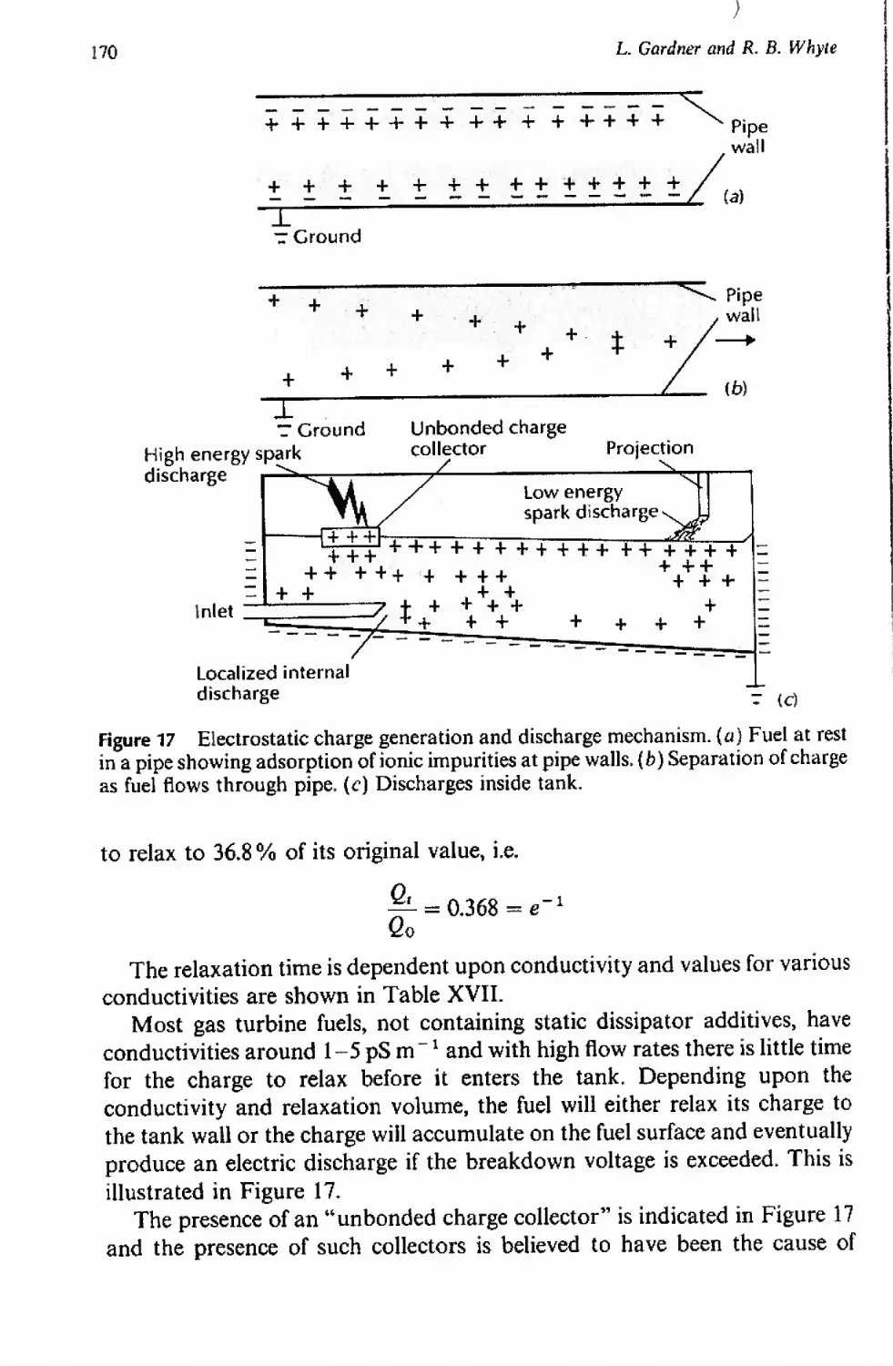
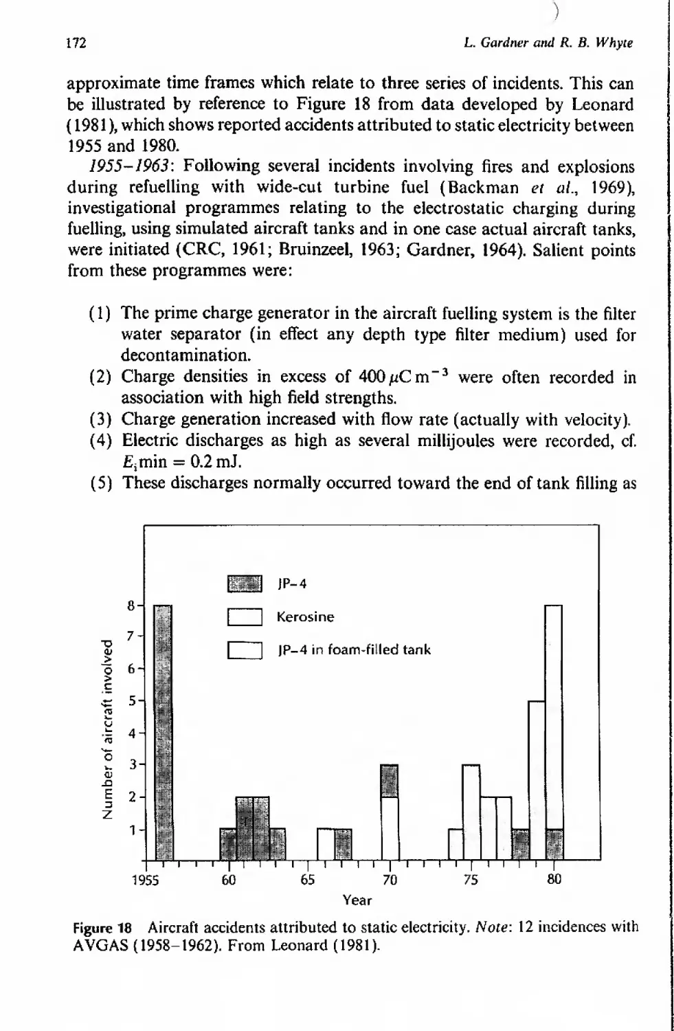
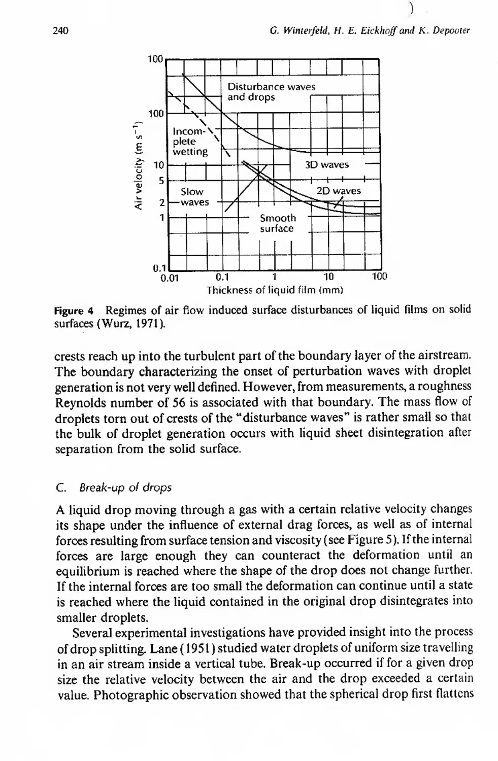
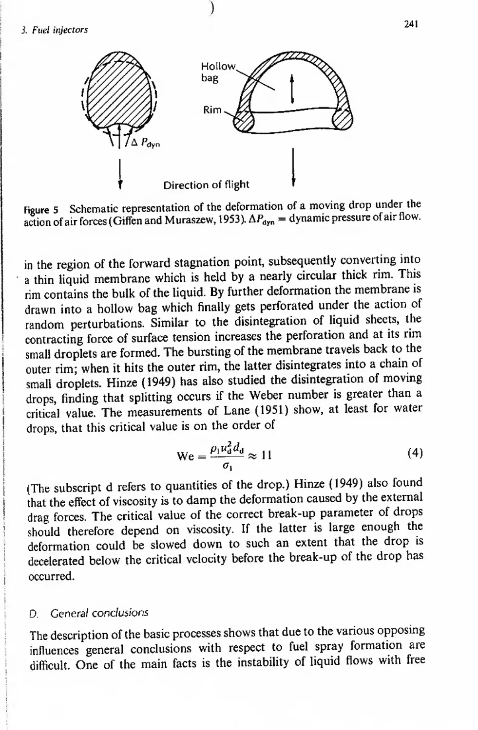
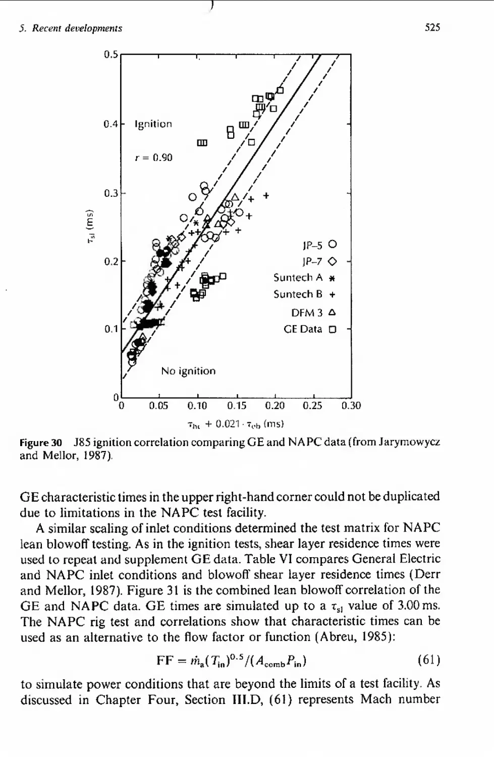
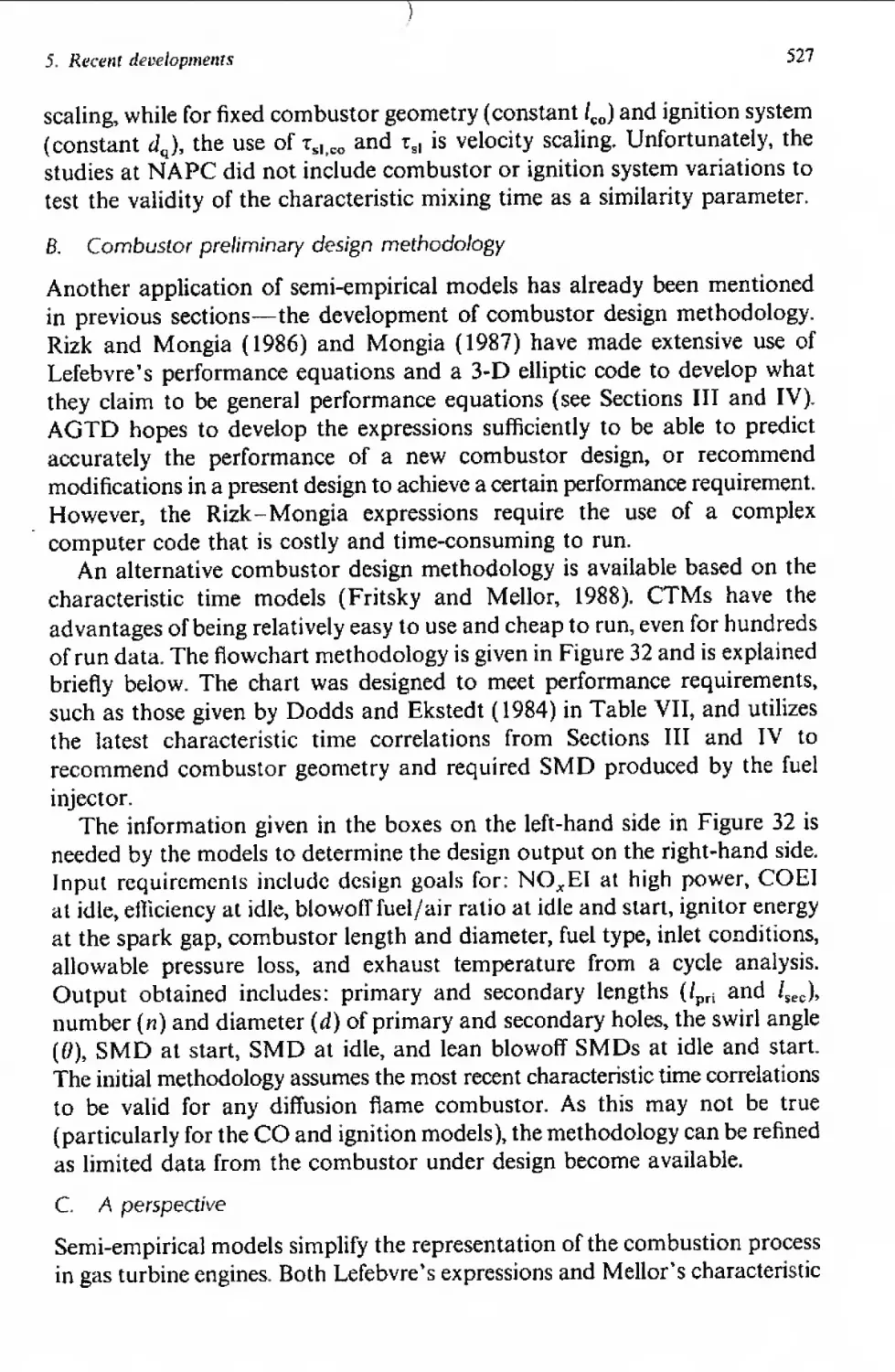
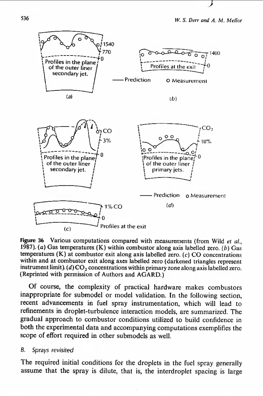
/


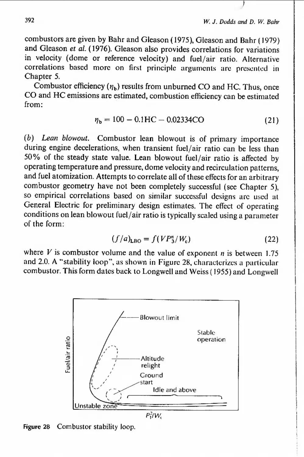


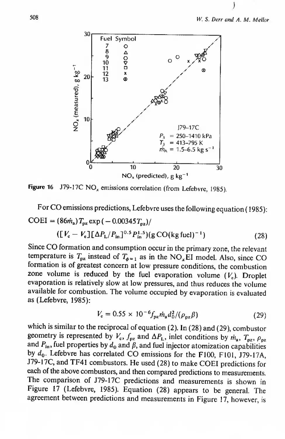


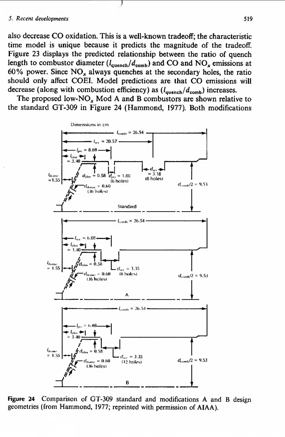


Text
Design of Modern Turbine
Combustors
Edited by
A. M. MELLOR
Vanderbilt University
Nashville, Tennessee, USA
INSTITUTO SUPE^GG 7TCNJCO
D. E. Ы. -
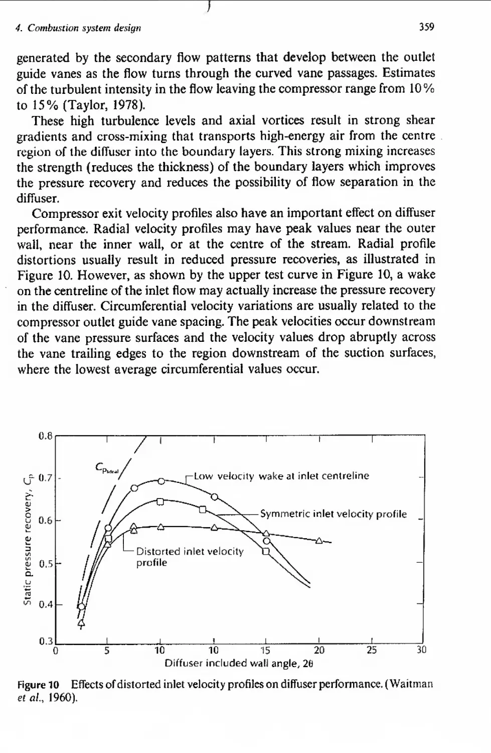
W-A
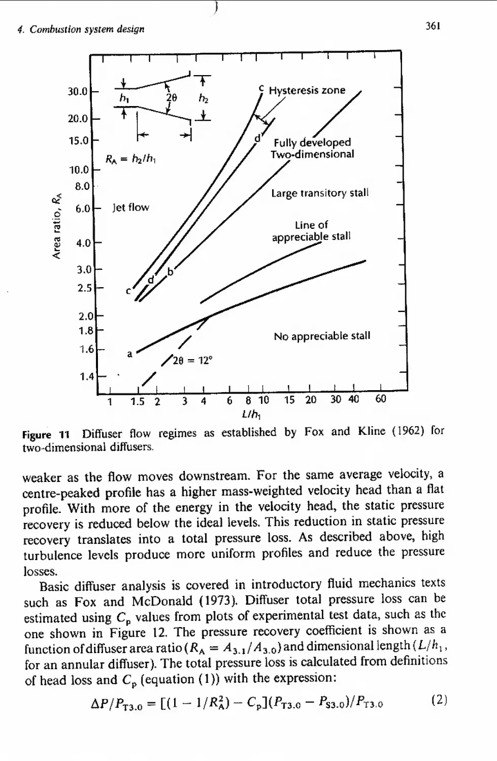
... ..-------— --- •-*
INSTITUTO SUPERIOR TECNICO
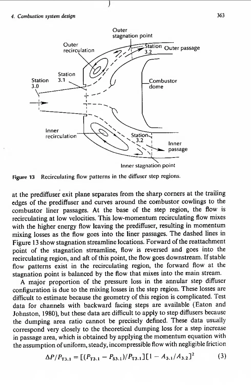
iUinill
7100699955
ACADEMIC PRESS
Harcourt Brace Jovanovich, Publishers
London San Diego New York
Boston Sydney Tokyo Toronto
ACADEMIC PRESS LIMITED
24/28 Oval Road,
London NW1
United States Edition published by
ACADEMIC PRESS INC.
San Diego, CA 92101
Copyright © 1990 by
ACADEMIC PRESS LIMITED
except Chapter 2,
Pages 81-227 Crown Copyright © 1990
This book is printed on acid-free paper
AH Rights Reserved
No part of this book may be reproduced in any form by photostat, microfilm, or
any other means without written permission from the publishers
British Library Cataloguing in Publication Data
Is available
ISBN 0-12-490055-0
Typeset by P&R Typesetters Ltd, Salisbury, Wilts
Printed in Great Britain by Galhard (Printers) Ltd,
Great Yarmouth, Norfolk
Contributors
D. W. Bahr, Mail Drop A-309, Aircraft Engine Business Group, General Electric
Company, One Neumann Why, Cincinnati, OH 45215-6301, USA
W. S. Derr, 106 Clarrige Drive, Willow Grove, PA 19090, USA
K. Depooter, Gas Dynamics Laboratory, Division of Mechanical Engineering, National
Research Council Canada, Ottawa KIA 0R6, Canada
W. J, Dodds, Mail Drop A-309, Aircraft Engine Business Group, General Electric
Company, One Neumann Why, Cincinnati, OH 45215-6301, USA
H. E. Eickhoff, DLR-Institute for Propulsion Technology, Postfach 906058, D-5000
Cologne-90, W#st Germany
L. Gardner, Fuels and Lubricants Laboratory, Division of Mechanical Engineering,
National Research Council Canada, Ottawa KIA 0R6, Canada
D. C. Hammond, Jr. Vehicle Aerodynamics, Section of Fluid Mechanics Department,
General Motors Research Laboratories, W'arren, MI 48090-9055, USA
A. M. Mellor, Department of Mechanical Engineering, Box 6019, Station B, Vanderbilt
University, Nashville, TN 37235, USA
J. E. Peters, Department of Mechanical and Industrial Engineering, University of Illinois
at Urbana-Champaign, 144 Mechanical Engineering Building, 1206 Whst Green St.,
Urbana, IL 61801, USA
R. B. Whyte, Fuels and Lubricants Laboratory, Division of Mechanical Engineering,
National Research Council Canada, Ottawa KIA 0R6, Canada
G. Winterfeld, DLR-Institute for Propulsion Technology, Postfach 906058, D-5000
Cologne-90, West Germany
Preface
North American and European experts participated in writing Design of
Modern Turbine Combustors. Dialogue was established between the various
contributors as chapter outlines were prepared and final text was submitted.
The intent was to offer comprehensive treatment of modern practice, as
perceived by authorities from widely differing backgrounds. Accordingly,
industry, government laboratories and universities are represented, and the
audience for the book will include both those in the field and newcomers
interested in research and development for gas turbine combustors.
Lower pollutant emissions and broader multifuel flexibility are recent
driving forces for advancing aircraft, vehicular and industrial engine
performance and versatility. Both are inherently connected with the design
of the fuel injector and combustor system. The traditional concerns, improving
durability and fuel economy over the life of the engine, remain additional
requirements. Empirical design methodologies are advancing toward more
sophisticated and fundamental multidimensional computational fluid dynamic
procedures, but use of the latter has demonstrated the need to improve their
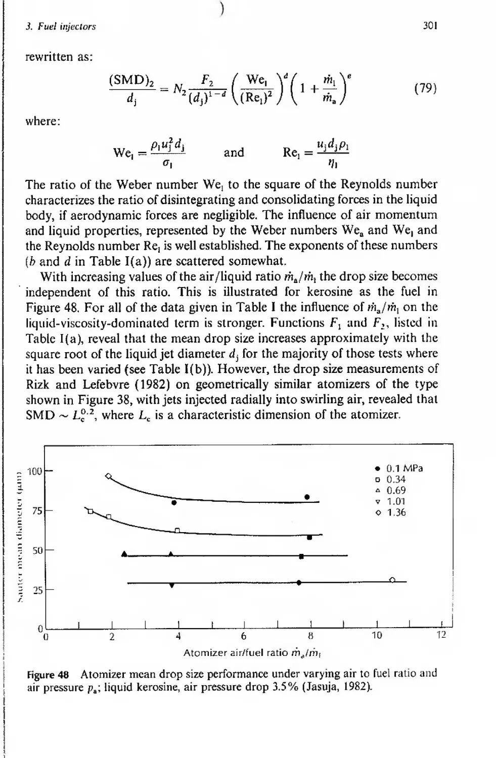
ultimate predictive ability for the complex flows encountered in airbreathing
engine combustors. Progress in this field requires better measurement
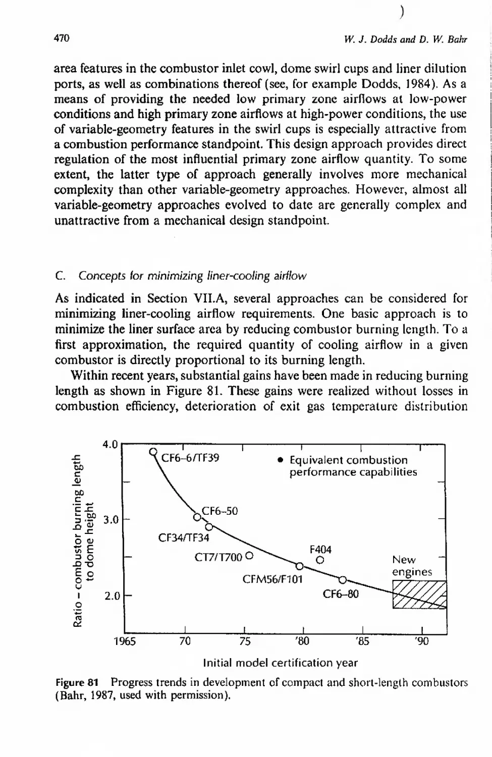
capabilities than available in the past, and modern laser diagnostics are now
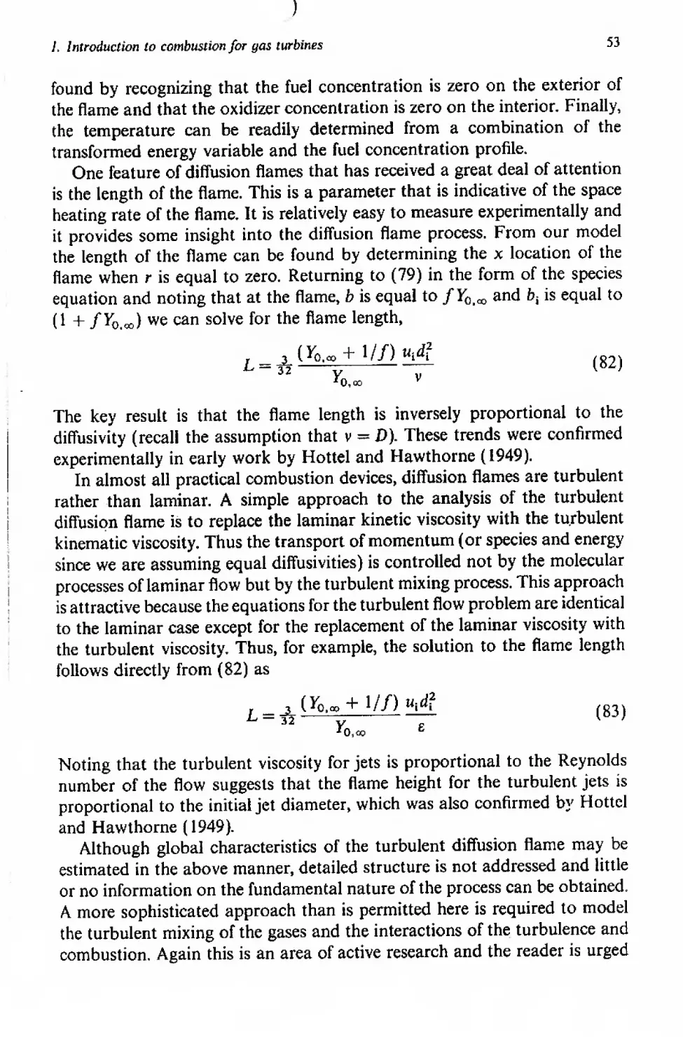
applied both to the fuel atomizer in representative burner fiowfields and to
ingredients of the building blocks for combustor design, such as recirculation
zones, shear layers, air penetration jets in crossflows and film cooling
passages.
To establish terminology, review appropriate fundamentals, and introduce
the subject, Chapter 1 treats combustion theory including turbine-oriented
pollution chemistry and highlights modelling for turbulent fuel spray
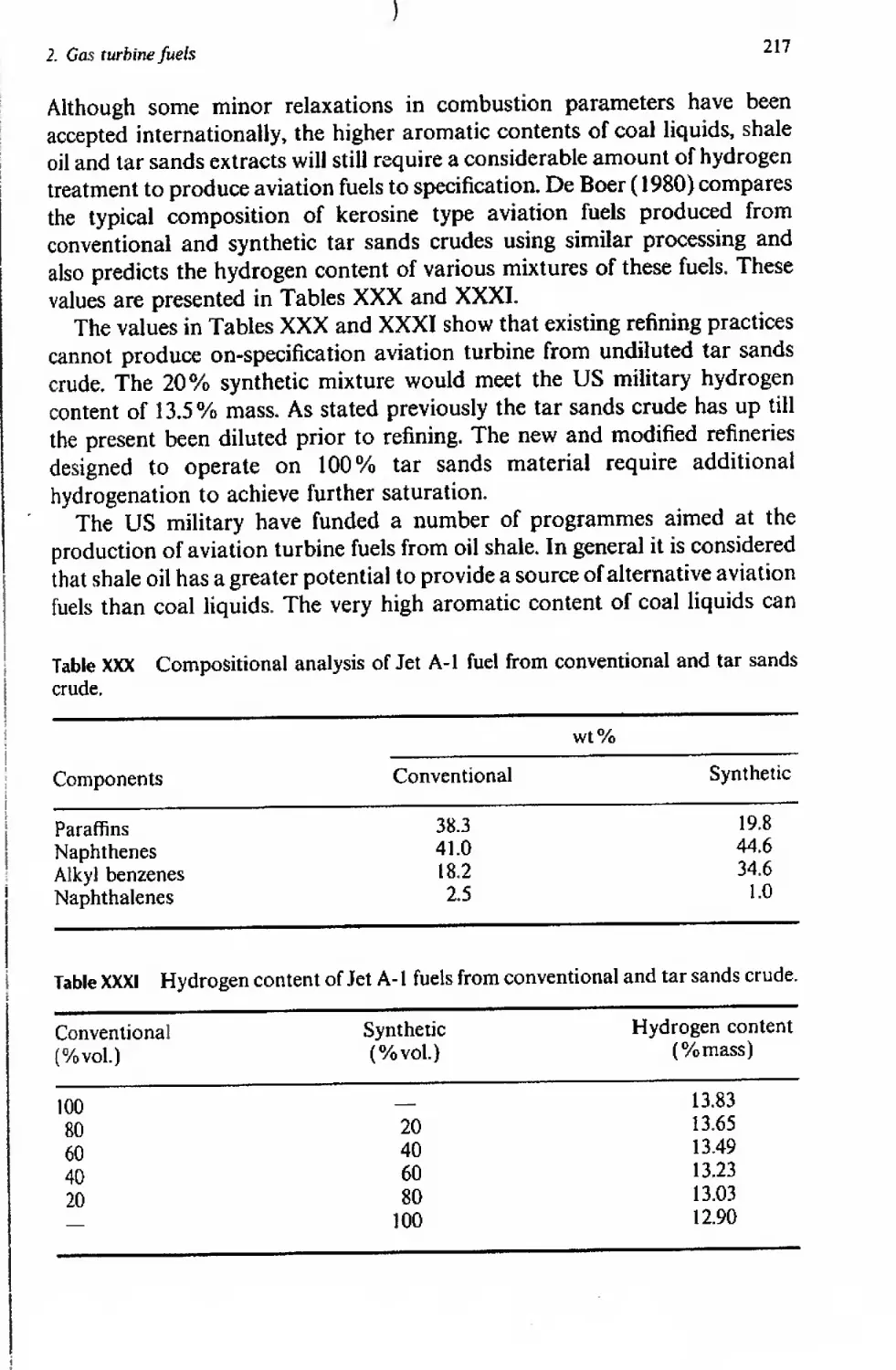
combustion. Chapter 2 explains how specifications for liquid and gaseous
fuels evolved, those properties most important to define combustion quality,
handling, storage and safety, and traditional and alternative sources for
transportation and industrial fuel feedstocks.
viii
Preface
Fuel injectors for both gases and liquids form the topic for Chapter 3.
The distribution of fuel downstream of the nozzle and, in the case of liquids,
the quality of the atomization enjoy major emphasis. Those injectors used
in the past as well as more modern designs are discussed in detail. Spray
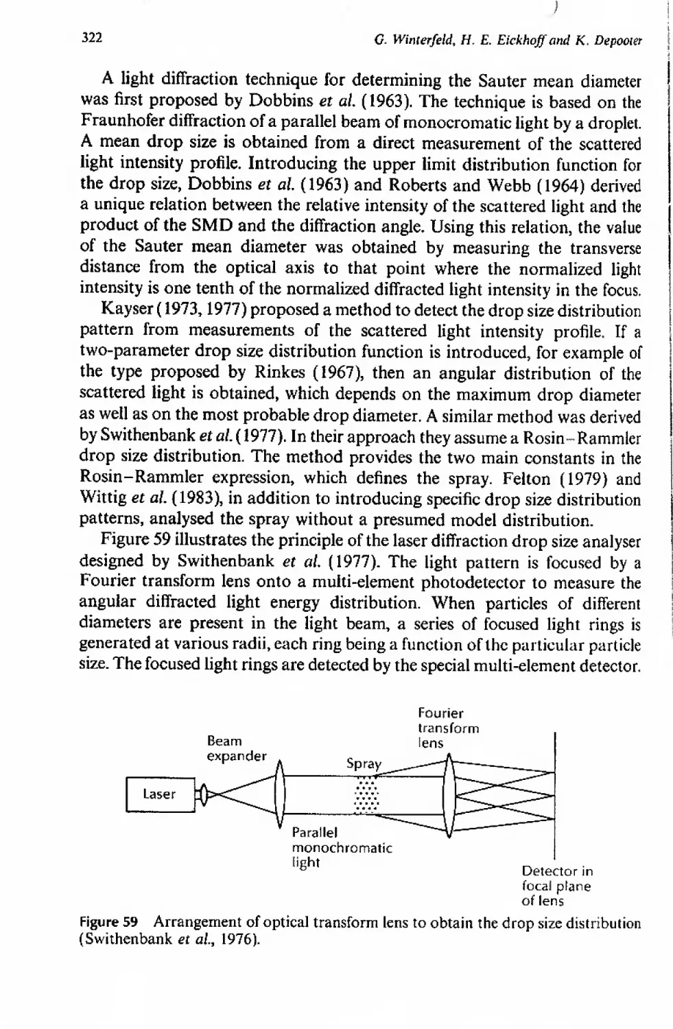
measurement techniques are also introduced in this section.
Integrating the injector into the front end of the combustor and specific
design requirements for the resulting injection/combustion system are
explained in Chapter 4. Empirical aerothermal design methodology, in some
cases supplemented with advanced modelling and diagnostics, is clarified by
an example procedure for a generic annular aircraft combustor.
The final chapter identifies recent work not included in depth in the
preceding chapters. Examples are system models for fuel effects on the engine
and airframe, more advanced modelling techniques for combustor design
now coming into wider use, and powerful new laser-based measurements
capable of providing significantly more complete detail on spray atomization
and penetration into the combustor flowfield. Throughout the book the
authors share with the reader their enthusiasm for the evolving technology
characteristic of next generation, higher-performance engines.
A. M. Mellor
Nashville, Tennessee
Contents
Contributors v
Preface vii
1 Introduction to Combustion for Gas Turbines 1
/. E. Peters and D. C. Hammond, Jr
I. Introduction 4
IL Fundamentals of combustion and the first law of thermodynamics 11
Ilk Equilibrium 18
IV. Simple chemical kinetics 24
V. Premixed flames 34
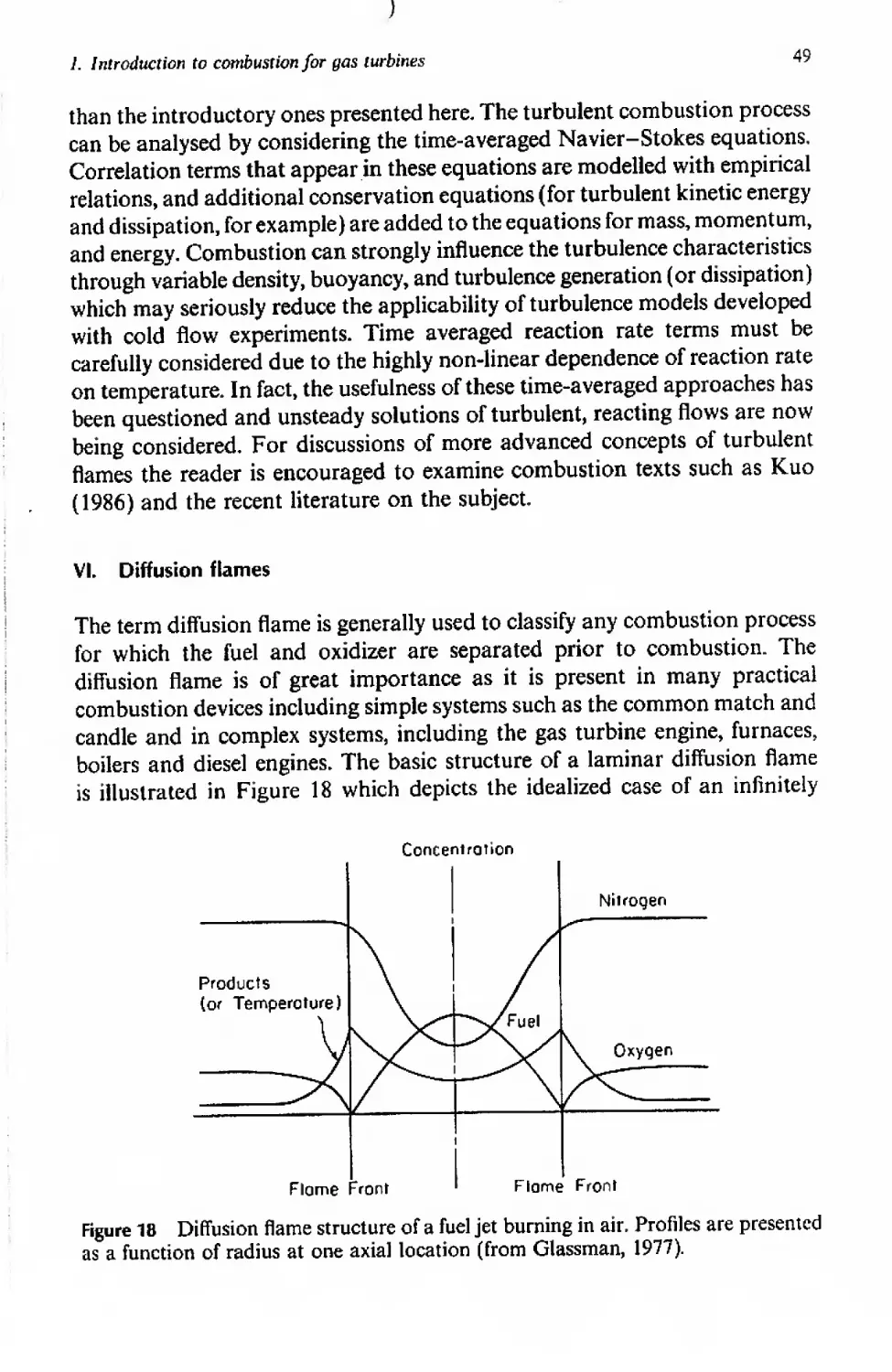
VI. Diffusion flames 49
VII. Ignition 66
VIII. Flame stabilization 71
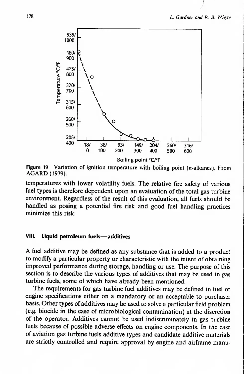
2 Gas Turbine Fuels 81
L Gardner and R. B. Whyte
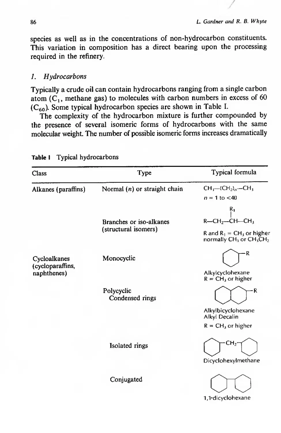
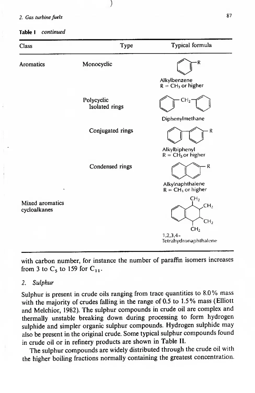
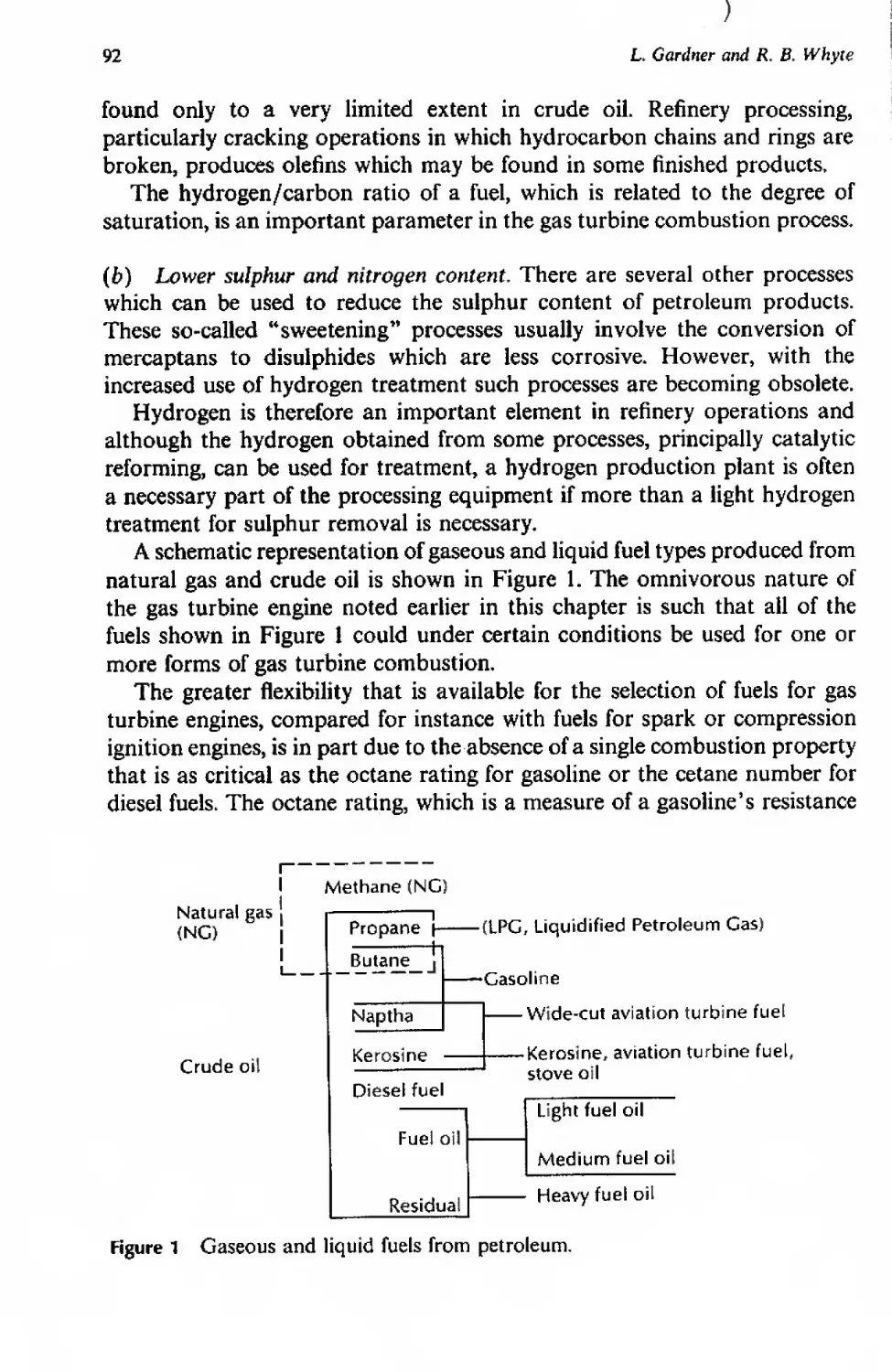
1. Introduction 82
11. Liquid petroleum fuels—derivation 85
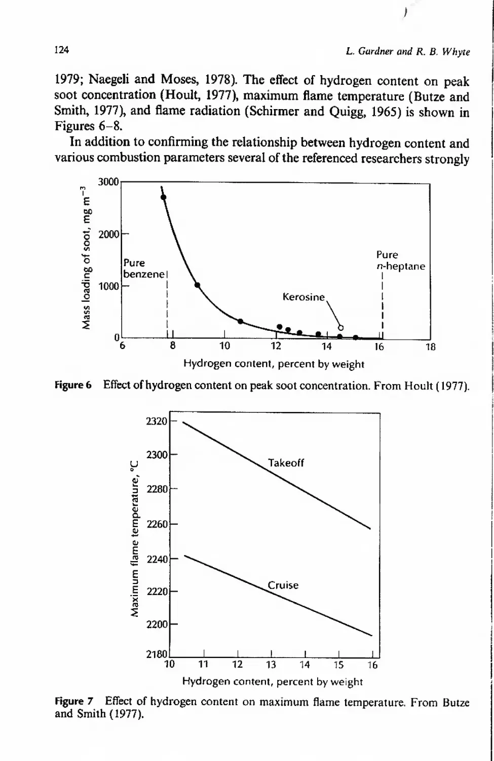
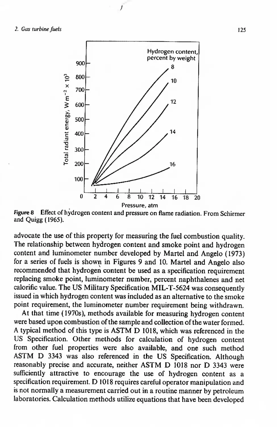
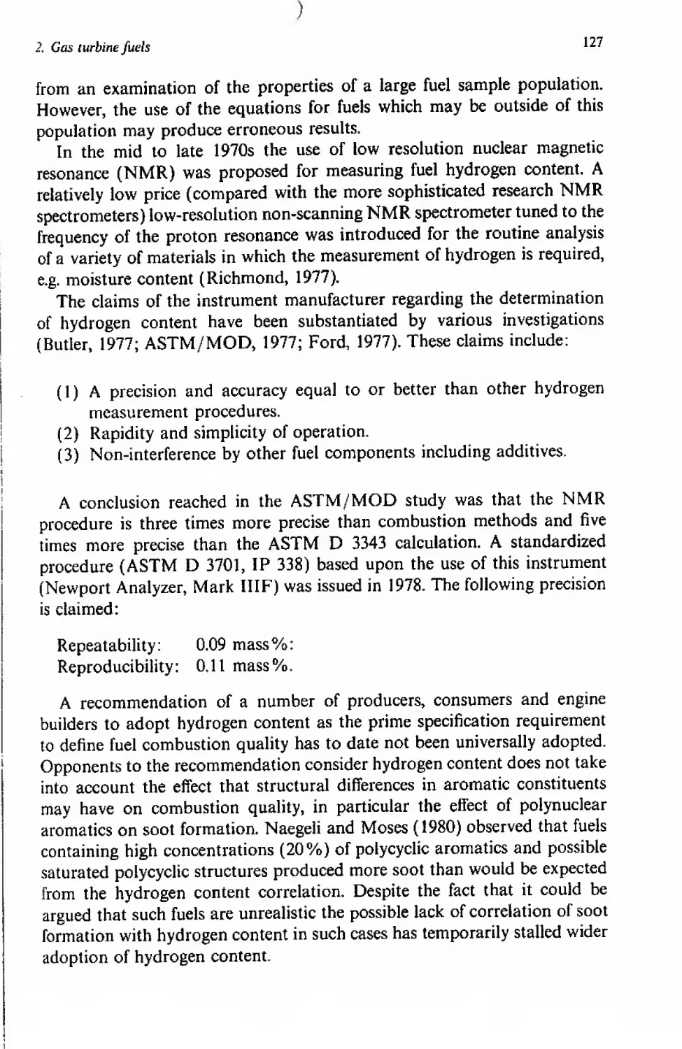
Ilk Properties of liquid petroleum fuels 93
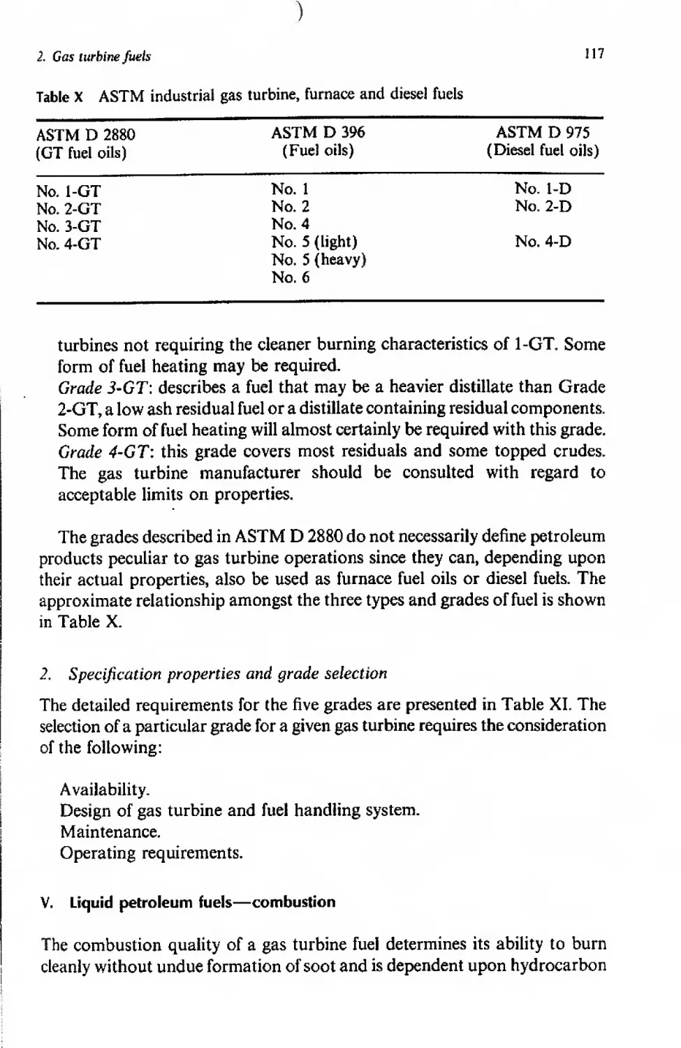
IV. Liquid petroleum fuels—types, grades 107
V. Liquid petroleum fuels—combustion 117
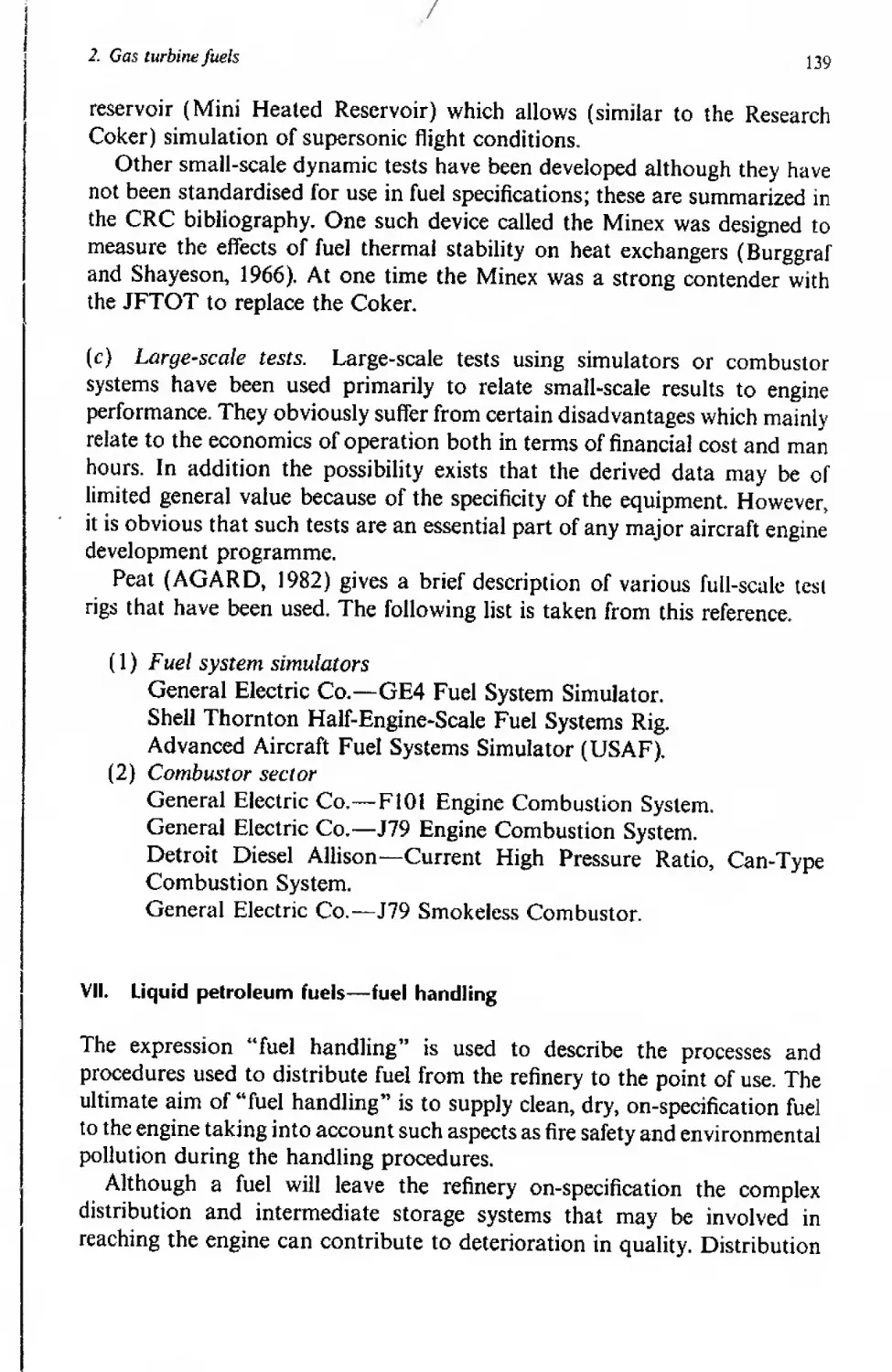
VI. Liquid petroleum fuels—-stability 128
VII. Liquid petroleum fuels—fuel handling 139
VIII. Liquid petroleum fuels—additives 178
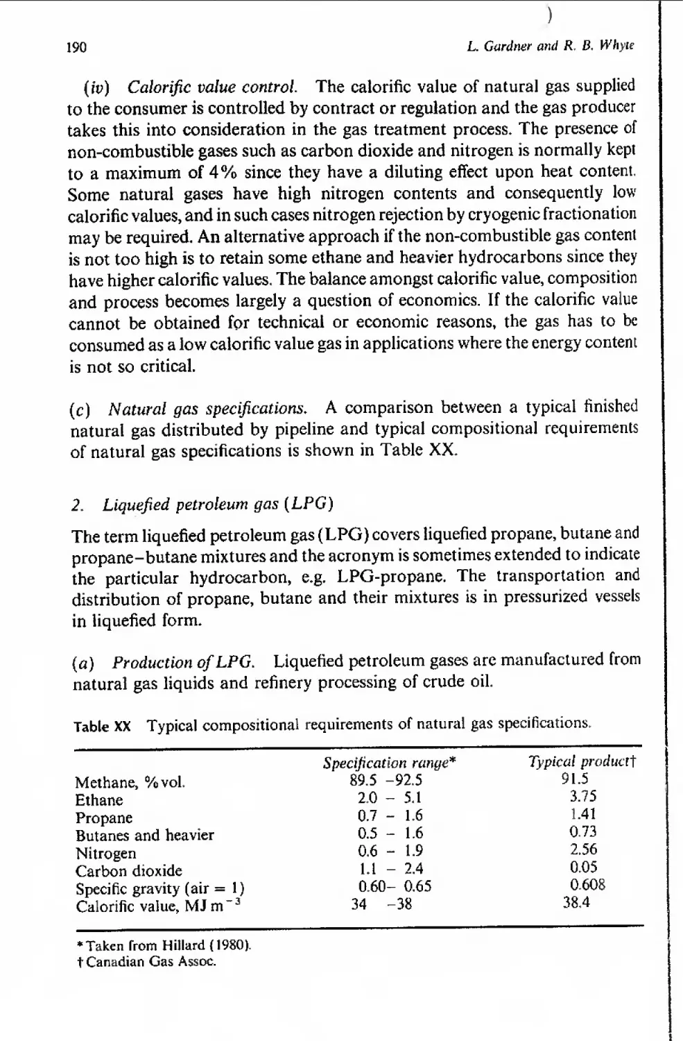
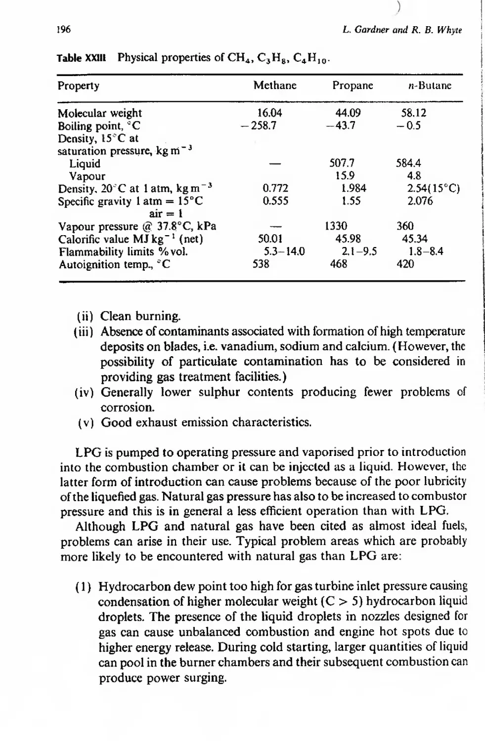
IX. Caseous fuels for industrial gas turbines 186
X. Alternative fuels 197
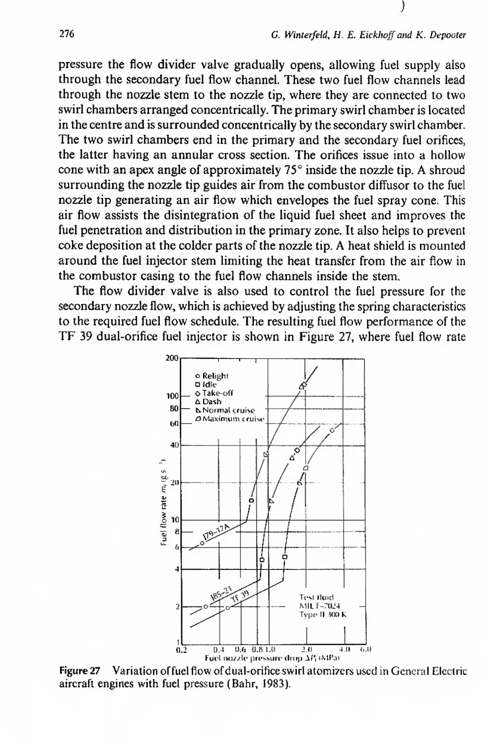
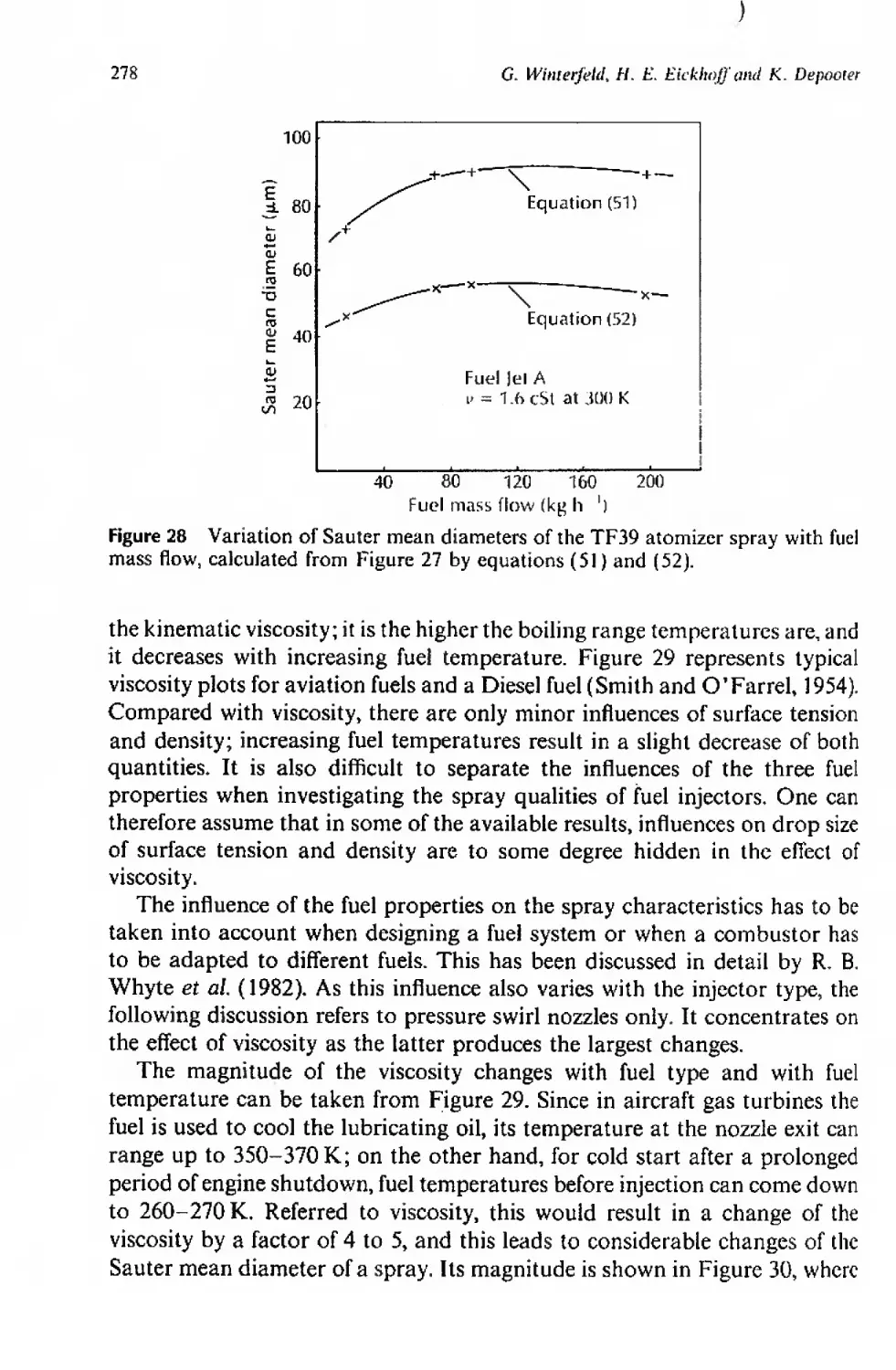
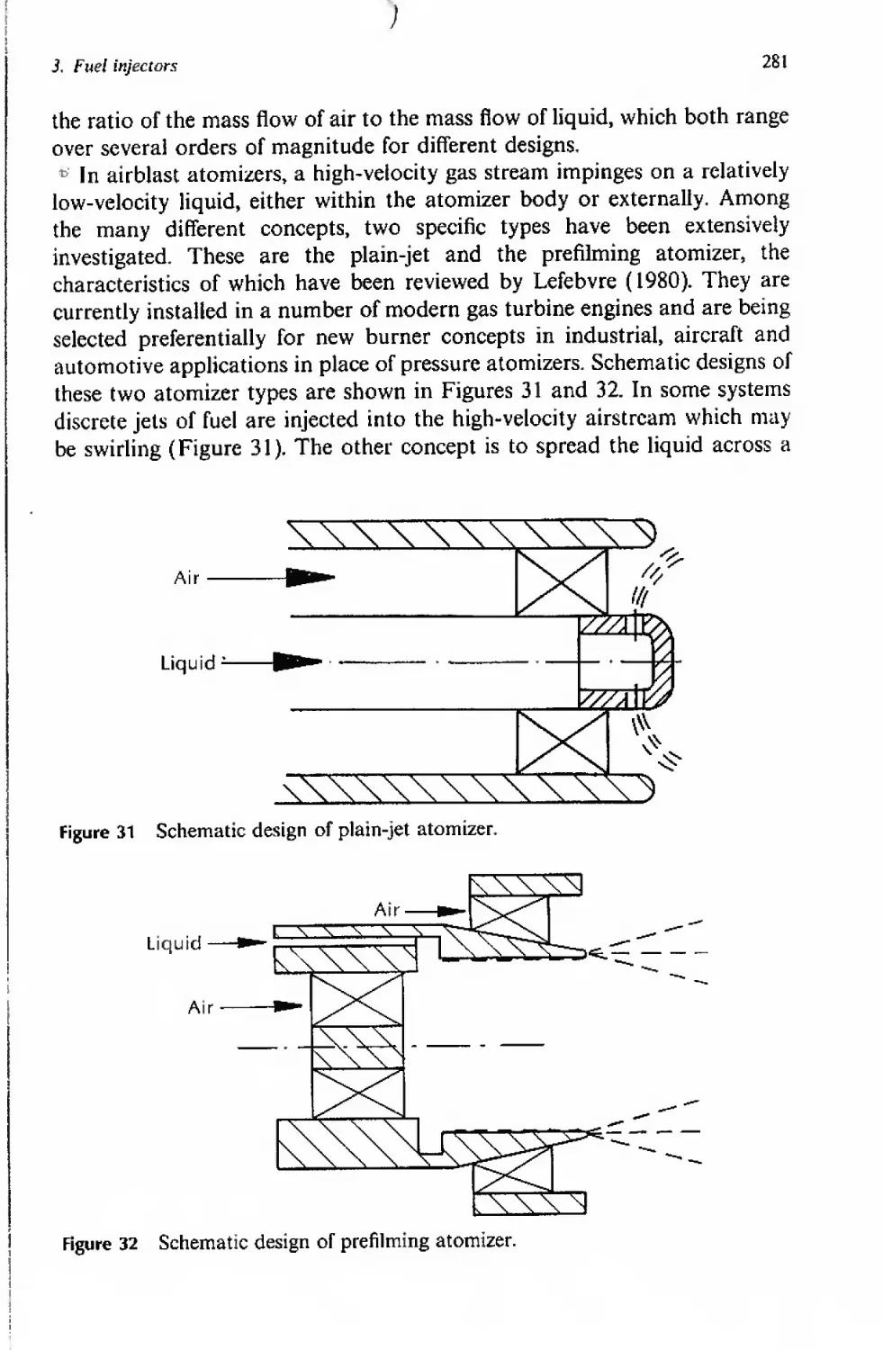
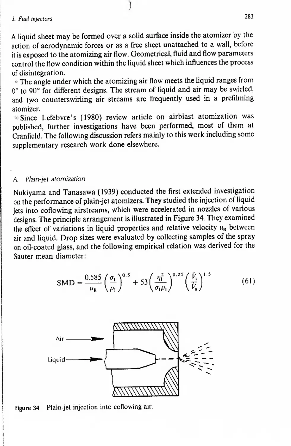
3 Fuel Injectors 229
C. Winterfeld, H. E. Eickhoff and K. Depooter
I. Introduction 231
Ik Fundamental processes in liquid fuel atomization 234
III. Definition of characteristic parameters of fuel sprays 242
2
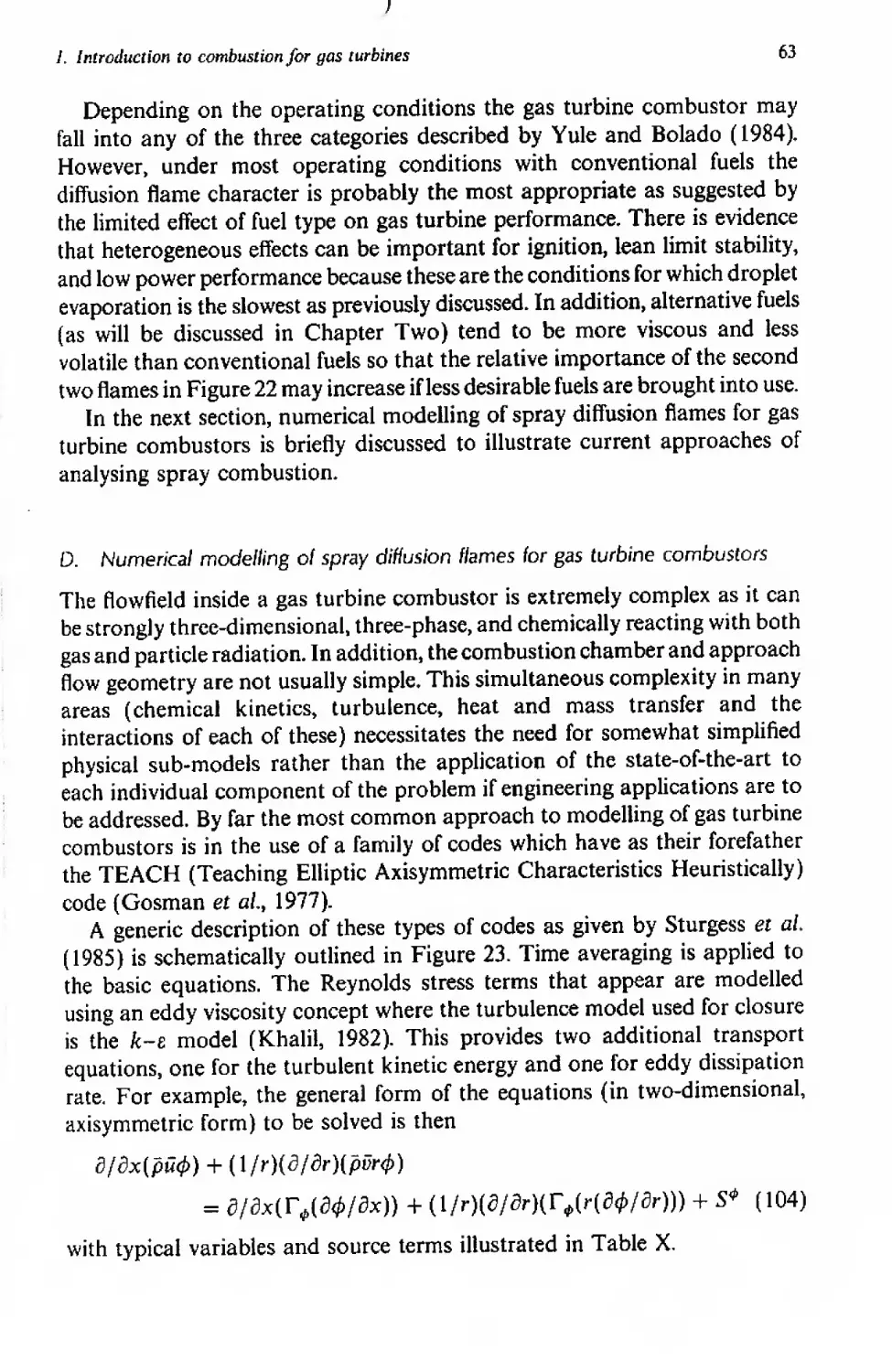
J. E. Peters and D. C. Hammond, Jr
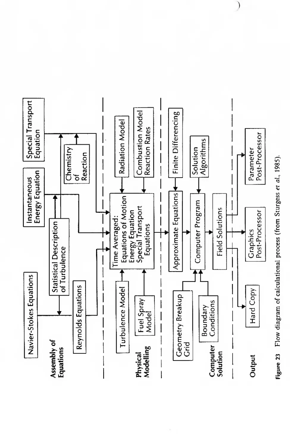
D. Numerical modelling of spray diffusion flames for gas
turbine combustors 63
VII. Ignition 66
A. Introduction 67
B. Ignition of liquid fuel sprays 68
VIII. Flame stabilization 71
Notation
Л, В, C, D hypothetical species
Л pre-exponential factor, area
В transfer number, blockage ratio
C concentration
D mass diffusivity
E activation energy
Emjn minimum ignition energy
Gy Gibbs free energy
H heating value
Kc equilibrium constant based on concentration
Kp equilibrium constant based on partial pressure
L flame length, latent heat of vaporization
M number of chemical compounds in a reaction
N number of chemical elements in a reaction
MW molecular weight
Nu Nusselt number
P pressure, steric factor
Pr Prandtl number
Q heat transfer
Q heat transfer rate
net calorific value
R universal gas constant, radical species, reaction rate
Re Reynolds number
S flame speed, source term
Sh Sherwood number
T temperature
T* adiabatic flame temperature
Тф=1 stoichiometric, adiabatic flame temperature
V velocity, volume
X mole fraction
У mass fraction
a, b, c, d stoichiometric coefficients
b non-dimensional variable
cp specific heat at constant pressure
d drop diameter, injection hole diameter, flameholder diameter
L Introduction to combustion for gas turbines
3
rf4 quenching distance fuel stoichiometric mass coefficient, flame
h All к heat transfer coefficient, enthalpy mass transfer coefficient specific heat release due to combustion rate coefficient, Boltzmann constant, thermal conductivity, turbulent kinetic energy
I m th n 4 r t и и’ V w X a turbulent length scale mass mass flow rate, evaporation rate constant, moles volumetric heat release rate reaction rate, radial coordinate time velocity component in the x direction turbulent intensity radial velocity component volumetric reaction rate spatial coordinate, coefficient of air in the global reaction equation thermal diffusivity, number of carbon atoms in the global reaction equation
fi evaporation coefficient, number of hydrogen atoms in the global reaction equation
Г У 5 E 4 V V v' ff V 4 p о T Ф diffusion coefficient number of oxygen atoms in the global reaction equation flame thickness turbulent diffusivity combustion efficiency reduced mass, viscosity kinetic viscosity reactant coefficient product coefficient defined by equation (80) density collision diameter time equivalence ratio, general flow variable
Subscripts
Л, В, C, D
В
a
b
species
boiling
annular, air
burned
4
J. E. Peters and D. C. Hammond, Jr
bo e eb eff f g he i i in J L 1 blowoff exhaust evaporation or burning effective forward, fuel gas phase, generation hydrocarbon kinetics ignition, initial species inlet species laminar liquid, loss
m 0 P г rad s T u CO si mass oxidizer, initial, standard state product reverse radiation surface, stoichiometric thermal, turbulent unburned infinity mixing
I. Introduction
A Terminology
Certain conventional terminology is traditionally used in discussing gas
turbine combustors. As this text will be no exception, this notation will now
be defined. Refer to Figure 1 which is a cross-section of a generic diffusion-
flame combustor. Deviations from, or additions to this notation, will be given
in the sections on specific designs.
The outer container of the combustor is called a casing. Proceeding in the
flow direction, air exits the compressor and enters the diffuser. A portion of
the air is captured for the primary zone by the snout. The usually hemispherical
upstream end of the combustor proper is called the dome. The fuel atomizer,
surrounded by a swirler, is situated in the centre of the dome. Air captured
by the snout enters the primary zone through the swirler. The body of the
combustor is called the flame tube. Several rows of holes and slots penetrate
1. Introduction to combustion for gas turbines
5
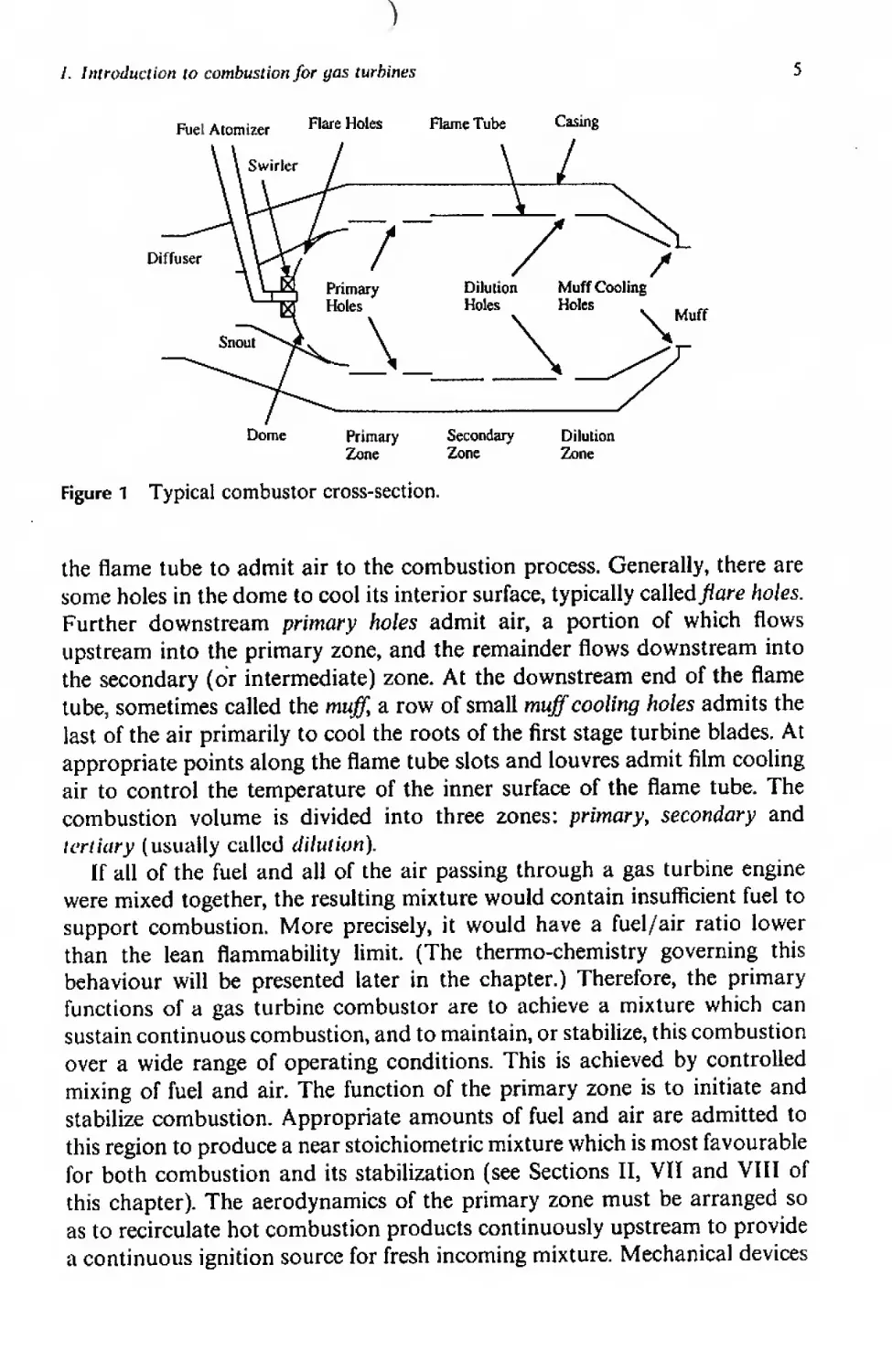
Figure 1 Typical combustor cross-section.
the flame tube to admit air to the combustion process. Generally, there are
some holes in the dome to cool its interior surface, typically called flare holes.
Further downstream primary holes admit air, a portion of which flows
upstream into the primary zone, and the remainder flows downstream into
the secondary (or intermediate) zone. At the downstream end of the flame
tube, sometimes called the muff, a row of small muff cooling holes admits the
last of the air primarily to cool the roots of the first stage turbine blades. At
appropriate points along the flame tube slots and louvres admit film cooling
air to control the temperature of the inner surface of the flame tube. The
combustion volume is divided into three zones: primary, secondary and
tertiary (usually called dilution).
If all of the fuel and all of the air passing through a gas turbine engine
were mixed together, the resulting mixture would contain insufficient fuel to
support combustion. More precisely, it would have a fuel/air ratio lower
than the lean flammability limit. (The thermo-chemistry governing this
behaviour will be presented later in the chapter.) Therefore, the primary
functions of a gas turbine combustor are to achieve a mixture which can
sustain continuous combustion, and to maintain, or stabilize, this combustion
over a wide range of operating conditions. This is achieved by controlled
mixing of fuel and air. The function of the primary zone is to initiate and
stabilize combustion. Appropriate amounts of fuel and air are admitted to
this region to produce a near stoichiometric mixture which is most favourable
for both combustion and its stabilization (see Sections II, VII and VIII of
this chapter). The aerodynamics of the primary zone must be arranged so
as to recirculate hot combustion products continuously upstream to provide
a continuous ignition source for fresh incoming mixture. Mechanical devices
6
J. E. Peters and D. C. Hammond, Jr
used to achieve this function are called flameholders. In a diffusion-flame
combustor the primary zone must additionally serve as a region for fuel
atomization and evaporation prior to combustion. The gases exiting the
primary zone are high-temperature, partial combustion products.
Additional air must be added to the primary zone effluent gases to more
completely oxidize the fuel fragments. This is accomplished in the secondary
zone. The resulting reduction in temperature also shifts the equilibrium
composition (see Section III of this chapter) toward more complete combustion.
If additional air were not added the combustion efficiency would be extremely
low due to the escape of incompletely oxidized species.
The temperature of the gases leaving the secondary zone is still too high
for. the materials of the turbine section to tolerate. Therefore, additional air
is added in the tertiary or dilution zone to reduce the gas temperature. Further
increases in combustion efficiency are possible because of the favourable shift
in equilibrium composition; although, the occurrence of actual combustion
reactions will be minimal.
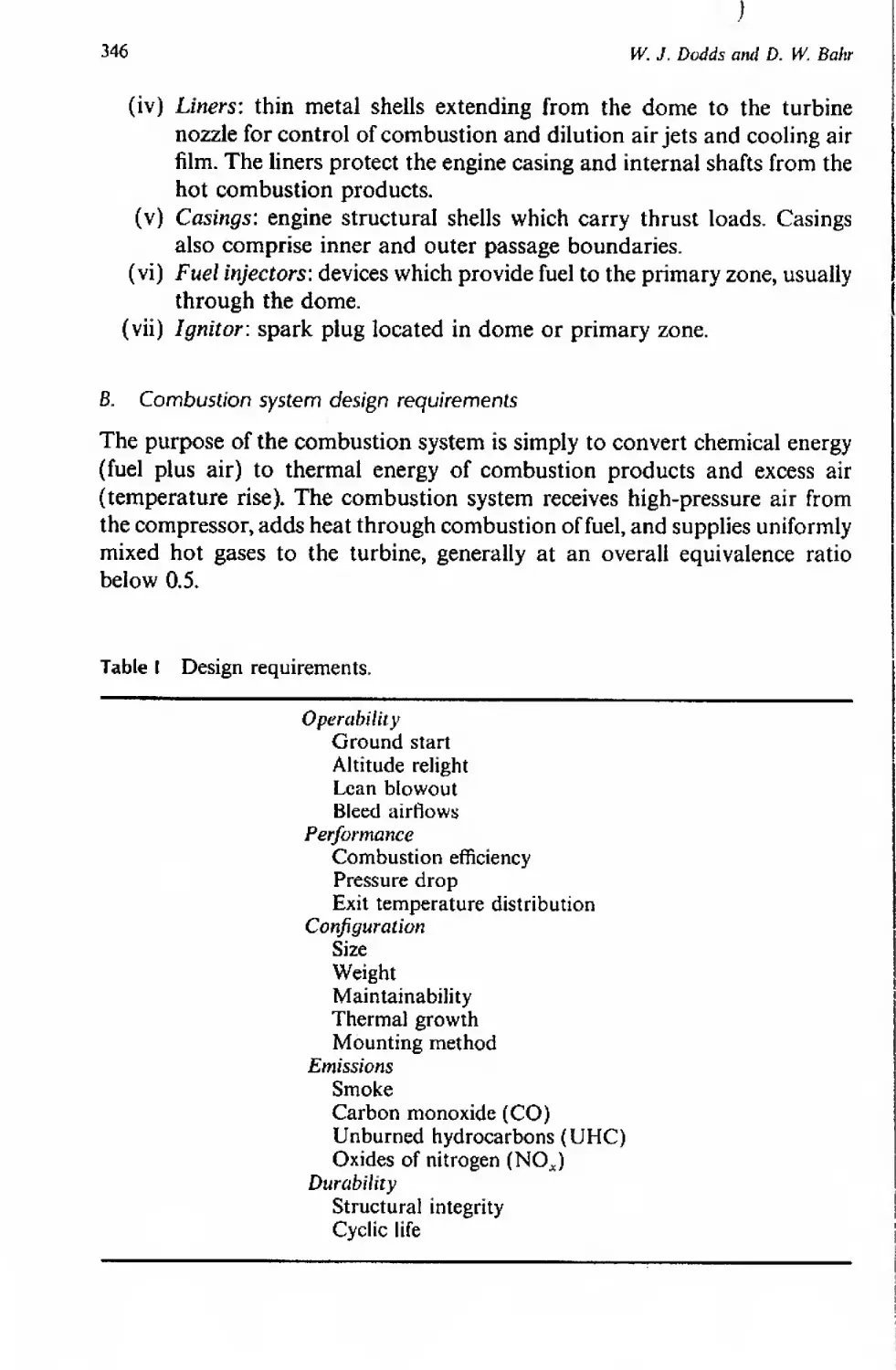
B. Combustor types
Combustors can be classified by three general criteria: geometry, aerodynamics
and application. All three criteria are currently used in the literature; therefore,
we will briefly discuss the salient features of the common categories arising
from each criterion. A number of unique designs not fitting these general
designs have appeared in response to special application requirements, and
these will not be enumerated here.
/. Geometric
Tubular combustors have approximately cylindrical flame tubes and casings.
Each flame tube is totally enclosed by its own casing, and the entire assembly
replicated in multiple-combustor engines (see Figure 2(a)). “Can type” is a
popular term for describing these combustors. Industrial and vehicular
applications predominantly employ tubular combustors. Older aircraft
applications, particularly shaft-power engines, commonly used this combustor
configuration. Newer aircraft applications seldom incorporate tubular
combustors because they do not provide the maximum combustion volume
for a given annular space. Multiple igniters and/or interconnection tubes
are required. However, within the individual combustor units, aerodynamic
and combustion problems are minimized by tubular designs.
Annular combustors have a single annular flame tube and a concentric
annular casing (see Figure 2(b)). This arrangement offers maximum utilization
of available volume, and thus, is widely used in modern aircraft applications.
1. Introduction to combustion for gas turbines
7
Figure 2 Three common geometric configurations, (a) Tubular, (b) Annular. (<?)
Tubo-annular.
Light-around1 problems are minimal, but the aerodynamic performance and
structural integrity are generally lower than tubular designs. Achieving a
uniform distribution of fuel around the annular space using a fixed number
of fuel injectors is difficult Maldistribution of fuel can result in non-uniform
combustor outlet temperatures.
Tubo-annular combustors are hybrids of the previous two types. They have
a number of cylindrical flame tubes contained in an annular casing (see
Figure 2(c)). Such combustors are also called “can-annular”. The conventional
flame-tube geometry offers improved structural integrity over the annular
combustor. The primary problem is ensuring uniform air distribution among
the flame tubes. Ignition problems parallel those of tubular designs.
2. Aerodynamic
Diffusion flame combustors (see Figure 1) are the historical choice for gas
turbine use. The distinguishing feature is the initial unmixedness of the fuel
and air. Typically, pure fuel is injected directly into the primary zone of the
combustor. Therefore, mixing via turbulent and molecular diffusion must
precede combustion itself. For liquid fuels, evaporation must also occur prior
1 Light-around refers to the propagation of combustion around the entire circumference of
the combustor from a small number of igniters.
8
J. E. Peters and D. C. Hammond, Jr
to molecular mixing. The fuel/air ratio at the design point is close to
stoichiometric. As will be shown, diffusion flame combustors have excellent
combustion stability, correspondingly high turndown ratios (ratio of the
maximum fuel flow rate to the minimum stable fuel flow rate), and superior
low-pressure ignition performance. However, care must be taken to minimize
the emissions of smoke and oxides of nitrogen. The reduction of emissions
has been the primary motivation for the relatively recent exploration and
application of other combustor design types.
Prefixing combustors represent an attempt to control the pollutant
emissions. Some examples of these designs are shown in Figure 3. In such
designs, a major portion of the combustion air is mixed with the fuel, and
time allowed to permit evaporation (of liquid fuels) and mixing prior to
combustion. Note that the fuel injection point is located significantly upstream
of any flameholders to permit sufficient time for fuel evaporation and mixing
with air to occur prior to combustion. Thus, the fuel/air ratio at which
combustion occurs can be somewhat controlled. Some well-designed units
can operate at fuel-lean mixture ratios approaching the lean flammability
limit. The reduced fuel/air ratio lowers combustion temperatures significantly
Figure 3 Premixing combustors.
1. Introduction to combustion for gas turbines
9
and oxides of nitrogen emissions, correspondingly. Smoke emissions also fall
dramatically because locally fuel-rich regions are largely eliminated by
operating the primary zone fuel-lean overall. Unfortunately, emissions control
comes at the price of increased mechanical and operational complexity. High
turndown ratios usually require the use of variable geometry to modulate
primary zone air flow (in concert with fuel flow) in order to maintain the
primary zone fuel/air ratio within a rather narrow band, which is bounded
on the top by excessive emissions and on the bottom by blowout.
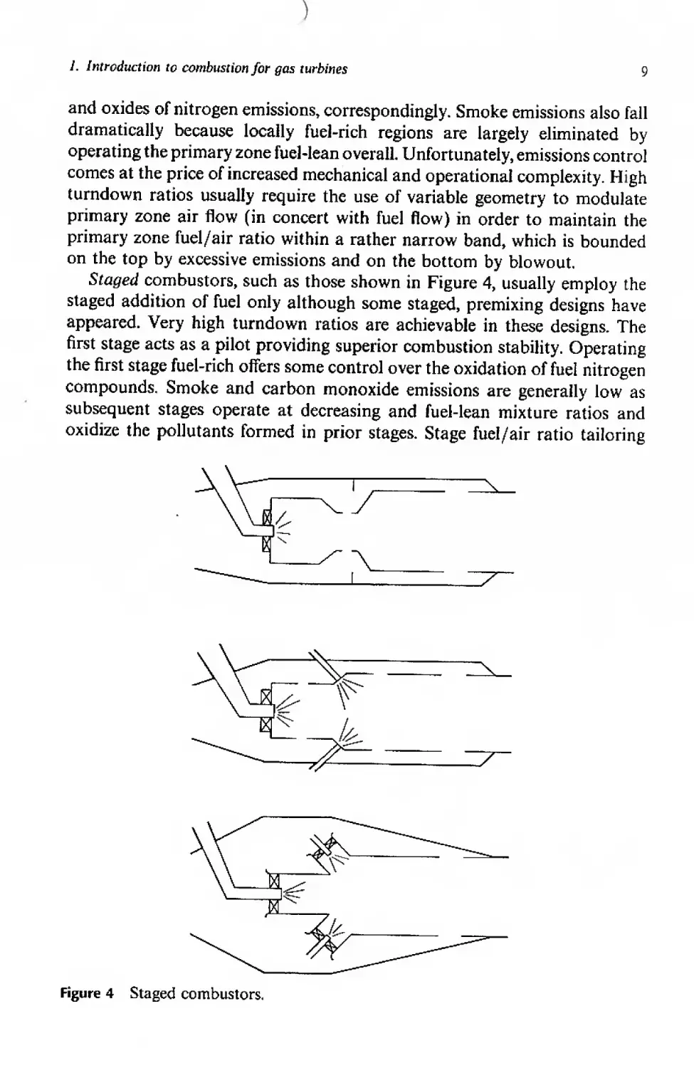
Staged combustors, such as those shown in Figure 4, usually employ the
staged addition of fuel only although some staged, premixing designs have
appeared. Very high turndown ratios are achievable in these designs. The
first stage acts as a pilot providing superior combustion stability. Operating
the first stage fuel-rich offers some control over the oxidation of fuel nitrogen
compounds. Smoke and carbon monoxide emissions are generally low as
subsequent stages operate at decreasing and fuel-lean mixture ratios and
oxidize the pollutants formed in prior stages. Stage fuel/air ratio tailoring
Figure 4 Staged combustors.
10
Л Е. Peters and D. C. Hammond, Jr
Figure 5 Catalytic combustor.
can also be employed to control thermal oxides of nitrogen emissions.
Fuel-staged designs offer considerable mechanical simplicity over premixing
designs because only the fuel flow rate to each stage must be modulated,
thereby obviating the need for mechanically variable geometry.
Catalytic combustors use the catalytically augmented reaction rates to
stably burn very fuel-lean mixtures. These are essentially premixing combustors
with catalytic combustion stabilizers (see Figure 5). Very few catalytic designs
operate on the fuel-rich side of stoichiometric in order to control the oxidation
of fuel nitrogen compounds and these always have a subsequent fuel-lean
stage. In either case, emissions are minimal, but the operating temperature
of the catalyst (and, hence, equivalence ratio) must be very carefully controlled
to prevent destruction of the catalyst. The permissible band of fuel/air ratios
is bounded on one side by temperatures leading to catalyst failure, and on
the other by extremely rapid increases in the emissions of unburned
constituents (primarily carbon monoxide). Variable geometry for air
modulation is almost always required; the requirements are generally more
stringent than with premixing designs. This complexity combined with high
weight generally prohibits aircraft use.
3. Application
Aircraft combustors are usually now annular or tubo-annular designs. Light
weight, low cross-sectional area and reliability are primary concerns. Older
aircraft designs employed multiple tubular units. The ability to ignite at a
low ambient pressure is critical to high-altitude operation. Aerodynamically,
almost all aircraft combustors are diffusion flame; however, increasing interest
in emission reduction, particularly smoke, has prompted the trial of some
fuel-staged and partially premixing designs. Fuel properties are controlled
to a relatively narrow specification band.
Industrial combustors are subject to the least stringent physical requirements.
Volume is not a major consideration. The emphasis is on extremely high
combustion efficiencies, low pressure losses, and long-term durability.
Multifuel capability is often required. Very stringent emission standards
combined with “dirty” fuels requires the use of unconventional aerodynamic
I. Introduction to combustion for gas turbines
11
designs, and all of these mentioned above have been employed. This seems
to be the most appropriate application for catalytic designs.
Vehicular combustor requirements are positioned midway between those
for aircraft and industrial applications. Size and weight are important, but
are not the driving concerns. Multifuel capability is desirable, but not critical.
Very low emissions seem to dictate the form of modern designs which were
historically diffusion flame. As a result, premixing designs are now popular.
II. Fundamentals of combustion and the first law of thermodynamics
A. Stoichiometry
The most common gas turbine fuel is a liquid or gaseous hydrocarbon or
partially oxidized hydrocarbon. Such compounds have the approximate
overall chemical formula CaH₽Oy with the precise molecular structure being
irrelevant to a macroscopic treatment of the overall combustion process.
Other elements such as nitrogen, N, and sulphur, S, are commonly present,
but negligibly impact the overall stoichiometry and will be ignored here
(although they can be critical from an emissions standpoint).
All gas turbine combustors operate with sufficient air to oxidize all of the
fuel; therefore, the combustion is termed “fuel-lean”. Under lean conditions
the global reaction equation is
С.Н„О, + x(O2 + 3.76N,)-»aCO2 + |h2O +
+ 3.76xN2
(1)
where only the major product species are shown. The coefficients on the
right-hand side of this equation were determined by applying mass balances
for each chemical element, С, H and O. These mass balances have the form:
м
Z (*; - = 0
j= 1
i= 1,2,...N
(2)
where
/V = the number of elements involved,
M — the number of chemical compounds,
v} — the coefficient of compound j as a reactant in (1),
v'j = the coefficient of compound j as a product in (1),
= the subscript of element i in compound j.
12
J. E. Peters and D. C. Hammond, Jr
For example, the О balance, where у is the unknown coefficient of О2, is
у + 2x = 2a +
2
(3a)
' - 2 ; 4 (3b)
The global reaction (1) can be used to derive formulas for the commonly
used measures of mixture ratio, the proportions of fuel and air present in
the reactants. The air/fuel mass ratio is:
/r x(MWOj + 3.76MWNi)
MWCeHA
where MWj is the molecular weight of compound j.
Approximately,
(4a)
MWOi ~ 32,
MWNi ~ 28
(4b,c)
and
Thus,
MWt;HA ~ 12a + /? + 16y
(4d)
,, 137.3x
a!f = . о .
(5a)
The fuel/air mass ratio is simply
//n = (a//)-1
If there is exactly enough oxygen to consume the fuel—and no excess—then
the mixture is termed “stoichiometric”. Referring to the global reaction (1),
the coefficient of oxygen as a product must vanish, i.e.,
(5b)
2
(6a)
2
(6b)
where the subscript “s” denotes stoichiometric conditions. Substituting into
(4),
(«//)E =
a + ^_L (MWOi + 3.76MWNi)
*+ Z J
MWc,H,o,
(7a)
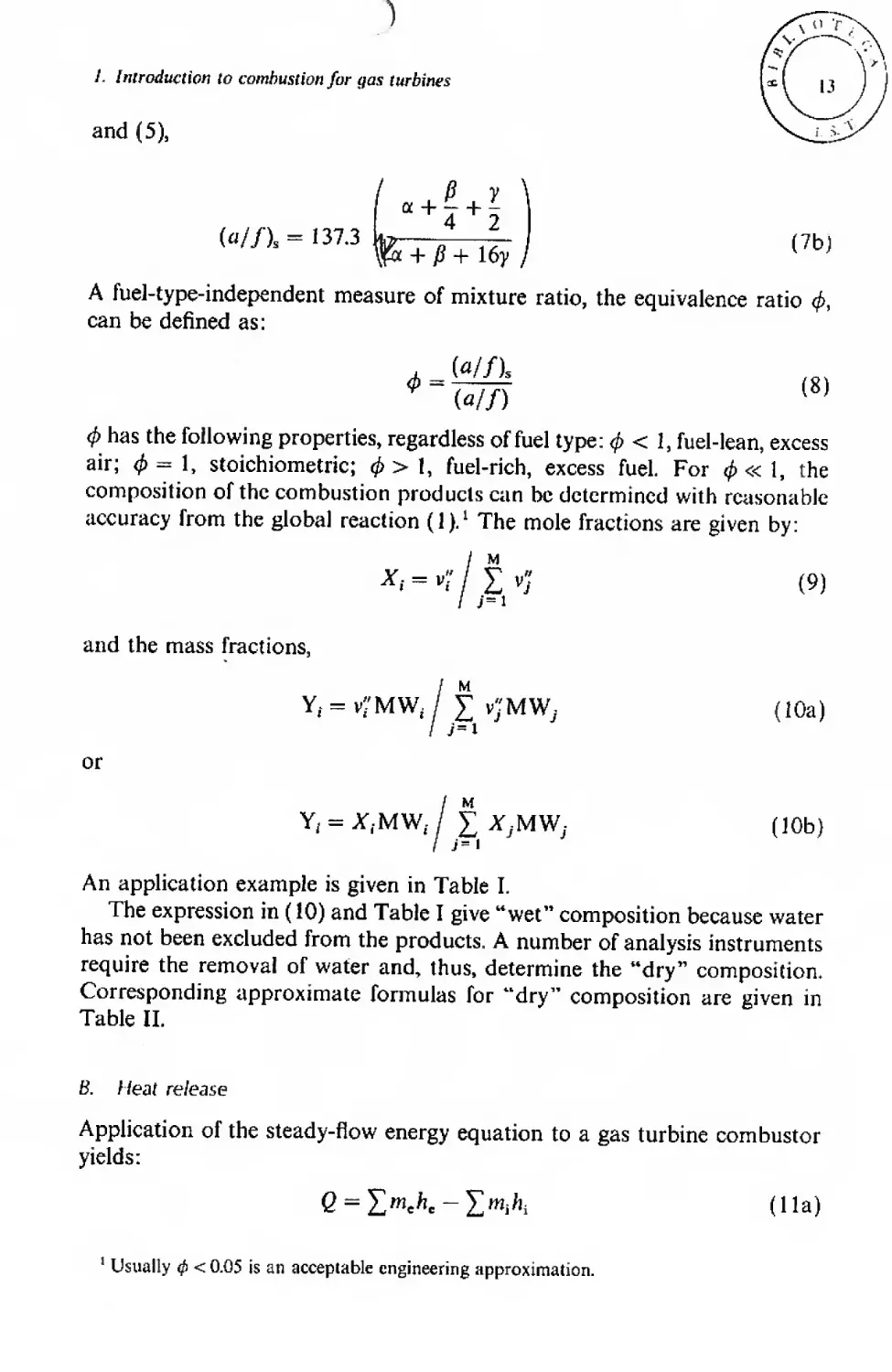
1. Introduction to combustion for gas turbines
and (5),
(«/Л = 137.3
(7b)
A fuel-type-independent measure of mixture ratio, the equivalence ratio ф,
can be defined as:
(a/f)s
(8)
ф has the following properties, regardless of fuel type: ф < 1, fuel-lean, excess
air; ф = 1, stoichiometric; ф > I, fuel-rich, excess fuel. For ф « 1, the
composition of the combustion products can be determined with reasonable
accuracy from the global reaction (1)? The mole fractions are given by:
/ M
= -?/ I»;
/ J=1
(9)
and the mass fractions,
/ м
Yf = vJ'MWi / J vJMWj
/ J=i
or
(10a)
/ M
Y^X.-MWJ £ XjMW;
/ j= •
(10b)
An application example is given in Table I.
The expression in (10) and Table I give “wet” composition because water
has not been excluded from the products. A number of analysis instruments
require the removal of water and, thus, determine the “dry” composition.
Corresponding approximate formulas for “dry” composition are given in
Table IL
В. I leal release
Application of the steady-flow energy equation to a gas turbine combustor
yields:
Q = '£mchc-'£mihi
(Ila)
’ Usually ф < 0.05 is an acceptable engineering approximation.
Table I Product composition formulas, “wet”.
Species j Xj r,
CO2 a 44a
В у - + - + 4.76x 4 2 12a + /? 4- 16y 4- 137.3x
H2O /3/2 9Д
в у - + - 4- 4.76* 4 2 12a + Д 4- 16y + 137.3*
o2 , У ft x d a 2 4 / у B\ 32 lx 4-- —a- - I \ 2 4/
В У - + - 4- 4.76x 4 2 12a 4- /? 4- 16y 4- 137.3x
n2 3.76* 105.3*
й у H + 4-7foc 12a 4- Д 4- 16y 4- 137.3*
Table II Product composition formulas, “dry”.
Species j
CO2 a 44a
- - S + 4.76* 2 4 у (i 12a — 8/J 4- 16y 4- 137.3* , У
o2 x 4 a 2 4 321 x H a ) \ 2 4/
N2 у В ~ - - 4- 4.76* 2 4 3.76x 12a- 8/? d- 16y 4- 137.3* 105.3x
- - - 4- 4.76x 2 4 12a - 8/? + 16yd- 137.3x
1. Introduction to combustion for gas turbines
15
or in molar units,
= (Hb)
as there is no shaft work and negligible changes in kinetic and/or potential
energy in the combustor. Both equations have been integrated over an
arbitrary time interval to convert the mass flow and heat loss rate to absolute
quantities (as it is conventional to do so). Here m denotes the mass, n the
number of moles, h the enthalpy, and g the heat transfer. Overbars denote
molar quantities. Considering fuel and air to be the only incoming reactants
and assigning mean properties to the products mixture:
mphp = + mrht + Q (12a)
np/ip = nA + nf/Tf + g (12b)
These equations give the overall energy balance for any steady-flow combustion
device.
C. Enthalpy of formation
The thermochemical properties of common elements and compounds are
available in the JANNAF tables (JANNAF, 1971 et seq.) for simple
compounds and in Bahn (1973) for more complex C-H-O species. Certain
conventions are employed which require explanation.
(i) The reference temperature is 298.15 K.
(ii) The reference pressure is one standard atmosphere.
(iii) The enthalpy of all elements in their naturally occurring state at
reference temperature and pressure is zero.
(iv) The enthalpy of formation of a compound is the energy (heat removal
or addition) required to form one mole of it from elements (in their
naturally occurring states) at reference temperature and pressure.
Thus, the enthalpy of compound i at temperature T is:
^i,T = “ ^298.1s)i,T + Ahf.i (13)
where both quantities on the right-hand side are tabulated in the tables. The
first right-hand term is called sensible enthalpy (because it is determined by
thermodynamic temperature) and the second right-hand term is called
enthalpy of formation (which is determined by chemical binding energies in
the molecule). These quantities (as well as the others given) can be computed
from statistical thermodynamics and the interested reader should consult
McBride and Gordon (1967).
For example, the naturally occurring state of oxygen at reference conditions
is O2. Thus, we write the formation equation for О as:
i02-O (14)
16
J. E. Peters and D. C. Hammond, Jr
Using (12b):
b4ft?.0 = iO + Q
Дй/.о — Q — 59.559 kcal g-mole-1
D. Adiabatic flame temperature
If the combustion process is adiabatic, i.e., no heat transfer, the products
assume the “adiabatic flame temperature*’ (also called “adiabatic combustion
temperature”), T*. From (12b):
«рЙр = «Ла + "Л (16)
where h, are given by (13). Now T* is the product temperature which satisfies
(16). Substituting,
w. + Д'й]
nf p
rif a
+ + Ab°f] (17)
Assume that the fuel enters at 298.15 K; then:
~ — ^298 )i = — X — ^29вХ‘
P a
- -2-------------s----------A/i?f (18a)
\ nr ' I
which can be solved for T*. The last term on the right-hand side of (18a)
does not depend on T*; therefore, to simplify the notation we will denote it H,
- En. A/ip.i
и _ p_______________?_______
Д/ifj (18b)
which is commonly called the heat of combustion of the fuel. This formulation
involving H in terms of enthalpies of formation is strongly preferred if enthalpy
of formation data are available for the fuel(s) of interest. For realistic gas
turbine fuels it is often necessary to resort to empirically determined measures
of the heat of combustion which is sometimes reported as the fuel’s calorific
value. The Net Calorific Value (see Chapter Two) is the quantity of heat
released when a unit mass of fuel is combusted at a constant pressure of one
1. Introduction to combustion for gas turbines
17
atmosphere (101325 kPa) and temperature of 298.15 К with any water
present in the products remaining in the vapour state. Thus
e„ = H/MW, (19)
Further, assuming constant specific heats and complete reaction (equilibrium
considerations are treated later),
T* = —^(T„- 298.15) - — -Д- +298.15 (20)
cp.p °p Cp.p
where cp is the molar specific heat at constant pressure. For ф « 1, then,
and thus,
(21a)
(21b)
In either (21a) or (21 b) H is fixed once the mixture is specified since it involves
only air/fuel ratio and enthalpies of formation; therefore, T* can be calculated
directly. Again the reader is reminded that (20) and (21) give the theoretical
maximum adiabatic flame temperature. Physically realizable adiabatic flame
temperatures are strongly limited by product dissociation which will be
discussed later in this chapter. The use of the preceding equations must be
limited to those cases where ф « 1.
E. Combustion efficiency
Combustion efficiency is used as a measure of the completeness of combustion
and the magnitude of heat loss from the combustion device. It is defined as:
the gas sensible enthalpy rise produced in passing through the combustor
divided by the maximum possible such enthalpy rise. The maximum sensible
enthalpy rise occurs when combustion is complete and the products exit the
combustor at the adiabatic flame temperature of the incoming reactant
mixture. Starting with (18a), in which the sensible enthalpy of the fuel is
neglected, the left-hand term is the sensible enthalpy of the products and the
first right-hand term is the sensible enthalpy of the reactants (namely air);
therefore, a little algebra shows that H is the maximum sensible enthalpy
rise. A theoretical sensible enthalpy rise can be determined from equilibrium
18
J. E. Peters and D. C. Hammond, Jr
products composition as described later in this chapter; however, the actual
sensible enthalpy rise must be determined by measurements of the combustor
exhaust because it involves the net heat loss and escape of partially reacted
fuel which are not determinable from thermodynamics. Assuming that
product enthalpy has been measured, then combustion efficiency can be
calculated from:
(1 4-a/f )fip - Q///Ta
H
(22a)
or for the same assumptions as (20)
(22b)
In computing T*, the overall air/fuel ratio is used. Typically t] exceeds 98%
for well-designed combustors. Recent modelling work on efficiency in gas
turbine combustors is discussed in Chapter Five.
111. Equilibrium
In the previous sections, flame temperature and heat release calculations were
based on first law considerations and the assumption of complete combustion.
In reality, however, complete combustion does not occur due to limitations
imposed by the second law of thermodynamics. To illustrate this point
consider Figure 6. One can see that the complete combustion calculation
overpredicts the fuel lean equilibrium flame temperature for temperatures in
excess of 1900 K, for this particular case. Therefore, in order to determine
the final temperature and composition of a reaction the second law must be
employed. The application of the second law and its implications for
combustion reaction calculations are presented below.
A. Equilibrium constant
For the reaction
aA +bB*±cC + dD (23)
the law of mass action states that the forward reaction rate, rf, is given by
rf = kfC^ (24)
where rf may be expressed as the change in concentration of species A or В
with time with typical units of moles (s cm3)" \ k{ is referred to as the forward
/. Introduction to combustion for gas turbines
19
Figure 6 Adiabatic flame temperature calculations for Jet A and air at a constant
pressure of 101 kPa and an initial temperature of 300 K.
rate coefficient and C, is species concentration (moles cm 3). Similarly the
reverse reaction rate is given by
(25)
At equilibrium the forward and reverse reaction rates are equal which gives
(26)
and the equilibrium constant is defined as
CccCi
(27)
The equilibrium constant given in the previous equation is based on
concentrations. A more convenient form of the equilibrium constant defined
on the basis of partial pressures is given by
yc yd
ЛСЛР
ya yb
л ЛЛВ
(P/Poy:+i~l‘~t
(28)
20
J. E. Peters and D C. Hammond, Jr
where Po is the standard state pressure, 101 kPa. From the ideal gas law
(29)
The equilibrium constant can be developed not only from the law of mass
action as shown in the preceding discussion but also from thermodynamic
considerations of equilibrium. One can show, using the first and second law
of thermodynamics, that at constant temperature and pressure, the Gibbs
free energy is minimized at equilibrium conditions. For the chemical
equilibrium of (23) this requires that for an ideal gas
— KT In
= -KTlnKp (30)
For a detailed discussion of Gibbs free energy and the equilibrium constant
see any good undergraduate thermodynamics text (Sonntag and Van Wylen
(1982) or Wark (1983), for example).
Equations (24)—(30) hold for the reaction of (23). These are readily
extended to any reaction and can be expressed using the general notation
noted in (2). For example in that notation, the law of mass action is
м
rr = П cp
J=l
and the equilibrium constant can be written as
Kc = П c?'-9
J=1
(31)
(32)
Note that Kp is not a function of pressure and for a given equilibrium
reaction is a function of only temperature. (This does not imply, however,
that equilibrium compositions are independent of pressure.) An extensive
tabulation of Kp values for species formed from elements in their normal
states can be found in the JANNAF thermochemical tables. With this
information one can determine equilibrium products, temperatures, and heat
release. An example is given below.
Consider the combustion of 1 kmole of C and one kmole of О2 at a
constant pressure of 0.2 MPa and an initial temperature of 298 K. If heat is
released so that the final temperature is 2400 К the equilibrium products can
be determined in the following manner. The reaction equation is
1C + 1O2 - v£O2CO2 + VcOCO + v^O2 (33)
where CO2, CO, and O2 are assumed to be the only products. (This
1. Introduction to combustion for gas turbines
21
assumption will be addressed shortly.) A species balance yields
vco2 + vco — 1
(34)
and
2vco2 + vco + 2v^ = 2 (35)
The third equation needed is determined from the equilibrium of the products
with the following equation
CO2t±CO+|O2 (36)
Now in most thermodynamic texts the lnKp for this reaction at 2400 К
would be listed as — 3.860 or Kp — 2.107 x 10“2. The JANNAF tables list
only elementary reactions so Kp for (36) is determined from
C + O2 CO2, KP) = 4.23 X 10⁸ (37)
C+JO2^CO, KPi = 8.83 X 10⁶ (38)
where Kp for (36) is given by Kp /KPi. Thus, the third equation required for
the solution of the equilibrium composition is
2.107 xlO-2 =
~',cqVq‘/2~
- vco2 _
(vco^Vco + v^'W)1'2
(39)
The solution of (34), (35) and (39) yields
1C + 1O2 0.984CO2 + 0.016CO + 0.00802 (40)
The preceding discussion and example illustrates the calculation of
equilibrium concentrations given the final temperature. In the example, CO2,
CO and O2 were assumed to be the only products although there are, in
small quantities, other products such as О atoms formed from the dissociation
reaction
O2^2O (41)
The number of species that appear in quantities sufficiently large that they
should be included in the products of combustion depends on the species in
question and the pressure and temperature of the reaction. Some specific
examples will be given in the next section where the effects of equilibrium
on combustion are discussed.
S. Equilibrium implications
As illustrated in Figure 6, the flame temperature for equilibrium conditions
can be substantially lower than the so-called “complete” combustion flame
temperature. This is a direct result of dissociation effects and the appearance
22
J. E. Peters and D. C. Hammond, Jr
Equivolence Ratio
Figure 7 Species equilibrium concentrations for adiabatic combustion of propane
and air at a constant pressure of 101 kPa and an initial temperature of 300 K.
of species other than CO2 and H2O in the products. In Figure 7 the
equilibrium concentrations of various species are shown for the adiabatic
combustion of C3H8 with air. The results clearly indicate the increased
importance of dissociation for the high temperature regime near equivalence
ratios of unity.
Table III lists some important dissociation reactions and the temperatures
required for 1 % of the reactants to dissociate. Since dissociation reactions
are quite endothermic their effect on flame temperature can be substantial.
Consequently, in practice an iterative solution for flame temperature is
I. Introduction to combustion for gas turbines
23
Table 111 One percent dissociation temperatures for P = 100 kPa.
Reaction Temperature, К
CO2 CO + 0.5O2 H2O 0.5H2 + OH H2O«±H2 + 0.5O2 H2?±2H O2 20 N2^2N 1930 2080 2120 2430 2570 3590
required where, for example, the final temperature is assumed, equilibrium
concentrations are determined and the assumed flame temperature is checked
based on the enthalpy of the products and reactants. A new temperature is
then assumed and the process is repeated until convergence is achieved.
Certainly the greater the number of species included, the more involved the
calculation. However, computer codes exist to perform flame temperature
calculations and except for instructional purposes equilibrium flame
temperature calculations are rarely performed by hand. A relatively simple
subroutine to compute equilibrium composition and temperature for
C-H-O-N systems is listed by Strehlow (1984). This sub-routine considers
a limited flame temperature (700 < T < 4700 K) range but is quite sufficient
for many gas turbine applications. A much more comprehensive program by
Gordon and McBride (1971) is available which includes thermodynamic data
for 62 reactants and 421 reaction species over a temperature range from 300
to 5000 K. The reader is also referred to Reynolds (1981).
The effects of typical gas turbine inlet temperature and pressure on the
stoichiometric, adiabatic flame temperature of Jet A (see Chapter Two for a
description of gas turbine fuels, including Jet A) are illustrated in Figure 8.
Note that an increase in inlet temperature is not followed by an equal increase
in flame temperature since increased effects of dissociation negate to some
extent the higher initial temperatures. In fact, Figure 8 indicates, as suggested
by Blazowski (1978), that an increase in inlet temperature of a gas turbine
combustor will increase the flame temperature by approximately only one
half the amount of the inlet temperature increase. Increasing the pressure
inhibits dissociation due to Le Chatelier’s principle and thus the slight
increase in flame temperature with increasing pressure is seen.
In this section the effects of chemical equilibrium have been illustrated.
We now address the situation where chemical equilibrium has not been
reached and reaction rates or chemical kinetics must be taken into account.
24
J. E. Peters and D. C. Hammond, Jr
2700
2200'------------1-----------1-----------L-
300 500 700 900
Inlet Air Temperature, К
Figure 8 Adiabatic flame temperatures for the stoichiometric combustion of Jet A
and air.
IV. Simple chemical kinetics
To account for the performance of a gas turbine combustor, chemical
equilibrium considerations are not sufficient. Several parameters, such as
combustion efficiency, NOX emission, soot formation, destruction, and
emission can be strongly influenced and in some cases controlled by chemical
kinetics. That is to say that the rates of reactions are important because all
reactants and products are not relaxed to equilibrium values due, for example,
to insufficient residence time in high temperature reacting regions.
A. Reaction order
From the generic reaction of (23) and the law of mass action we had an
expression for the forward rate of reaction
rf = k,CACB (24)
The forward rate can be expressed as the rate of disappearance of any reactant
I. Introduction to combustion for gas turbines
25
or appearance of any product. Expressing the reaction rate in terms of
disappearance of Л we have
_ АСЛ _ a dCB ______ a dCc__a dCD
r,~ ~~dF~ ~ b~dt~ ~ c~dt~ ~ d~dT 1 '
The order of a reaction is determined by the sum of the powers to which the
concentrations are raised in a rate equation as shown in (24). The overall
order of (24) is a + b while the order with respect to species Л is a and with
respect to species В is b.
B. Arrhenius reaction rate
We now address the determination of the rate coefficient, which, as will
be shown, is a strong function of temperature. Arrhenius (1889) observed
experimentally that
k = Лехр(-£/КТ) (43)
A is a so-called pre-exponential factor, E is activation energy, R is the universal
gas constant, and T is the reaction temperature. Thus, an Arrhenius reaction
rate for the forward reaction of (23) would be
rf = C°ACbBA exp( - E/RT) (44)
Arrhenius postulated that only molecules which possess a sufficient amount
of energy will react when they collide. Thus, the exponential term can be
thought of as the fraction of molecules which possess that required “activation”
energy. The numerical value for activation energy of a given reaction is readily
determined from experimental measurements of reaction rate as a function
of temperature by plotting Ink versus 1/7? For a true Arrhenius reaction
this will yield a straight line with a slope of —E/R. Such a curve for the
elementary reaction of
О + H2-> OH + H (45)
is shown in Figure 9.
The pre-exponential factor in (43) is related to the rate of molecular
collisions and may be calculated from kinetic theory as
A = <г2(8тскТ/р)1/2Р (46)
where a is the collision diameter, к is the Boltzmann constant, д is the reduced
mass, and P is the steric factor. The steric factor is included to account for
geometric orientation of the molecules (0 < P 1, determined experimentally).
Because of the temperature dependence in (46) the “modified Arrhenius”
26
J. E. Peters and D. C. Hammond, Jr
Figure 9 Rate coefficient for the reaction of О 4- H2 -> OH + H (from Wagner, 1973).
expression is often used,
к = A’Ttt — E / RT) (47)
where n would be 1/2 based on collision theory and A' = A/Tli2,
A more detailed approach for determining the pre-exponential factor which
accounts for molecular structure through quantum mechanics (where an
intermediate “activated complex” is considered) is the absolute rate theory.
However, for many applications (43) and (47) are sufficient where 4 or A‘
is frequently determined by fitting experimental rate data.
C. Reaction models
Although the single step reaction of, say,
CO+JO2->CO2 (48)
correctly describes the overall stoichiometry of CO oxidation, it does not
represent the actual steps in the reaction process. In general, several
1. Introduction to combustion for gas turbines
27
elementary reactions take place sequentially or simultaneously and reaction
rates must be determined by consideration of the chain reaction scheme.
The five types of elementary reactions that take place are illustrated below.
A 4 -B-> C 4-R initiation (49)
A 4 - R-> C 4-R propagation (chain carrying) (49b)
A 4 - R-* C 4" Rj 4* Rj propagation (chain branching) (49c)
Ri inhibition (49d)
A 4 -R-+ termination (49e)
In (49) А, В and C refer to any molecules and R refers to a radical (highly
reactive species due to at least one unpaired electron) species. Thus, the
reaction classifications refer to the generation or consumption of radical
species.
As an example, consider the elementary reactions listed in Table IV for
the H2-O2 system. The selection of appropriate elementary reactions is made
by consideration of the likelihood or rate of the individual reactions and
their impact on the combustion process.
Table IV Some elementary reactions in the H2-O2 system (from Westbrook and
Dryer, 1984).
H 4- O2 О + OH
О 4- H2 Ft H + OH
H2 + OH H2O + H
O + H2Of±OH4-OH
H + H + MfH2 + M
О + О + M 02 + M
О 4- H + M # OH + M
H 4- OH + M Ft H2O + M
H 4- O2 4- M Ft HO2 + M
HO2 + H Ft H2 + o2
HO2 4- H Ft OH 4- OH
HO2 4-H Ft H2O 4-о
HO2 4-OH Ft H2O 4-O2
HO2 + О Ft O2 4- OH
HO2 4- HO2 Ft H2O2 4- o2
H2O2 + OH Ft H2O + HO2
H2O2 4-H Ft H2O 4* OH
H2O2 + H Ft HO2 4- H2
H2O2 + M Ft OH 4- OH 4- M
Note: M is any third body molecule not participating chemically.
28
J. E. Peters and D. C. Hammond, Jr
Unfortunately, detailed reaction mechanisms have only been developed
and verified on relatively simple (compared with gas turbine) fuels. In addition
when one begins to model the gas turbine combustor (including fuel spray
formation and evaporation, three-dimensional turbulent mixing, chemical
reactions and heat transfer), the computational time required, even on today’s
advanced computers, becomes excessive. Therefore a simplified kinetic scheme
is often desired.
Probably the simplest kinetic form is obtained from a global reaction
equation. Following Westbrook and Dryer (1984) the overall reaction is
written in the form
Fuel + v^O2 - v£OiCO2 + v£jOH2O (50)
and the reaction rate is given by a modified Arrhenius expression,
г = 4Гехр(-£/ЛТ)(Сг)‘,(С0)6 (51)
The constants Л, n, a and b are empirically determined by comparing
computed laminar flame speeds with experimentally determined values.
Table V lists values suggested for the constants for several different fuels
where n was assumed equal to zero. Note that the constants are not uniquely
determined. For example, by selecting different values of activation energy
similar rate expressions and agreement with flame speeds can be found by
Table V Global reaction constants (from Westbrook and Dryer, 1984).
Fuel A* £a, kcal mol 1 a b
CH4 1.3 x 10⁹ 48.4 -0.3 1.3
CH4 8.3 x 10⁵ 30.0 -0.3 1.3
C2H6 1.1 x 10¹² 30.0 0.1 1.65
C3H8 8.6 x 10¹¹ 30.0 0.1 1.65
C4H10 7.4 x 10¹¹ 30.0 0.15 1.6
CSH12 6.4 x 10¹¹ 30.0 0.25 1.5
C6H14 5.7 x 10¹¹ 30.0 0.25 1.5
C7H16 5.1 x 10й 30.0 0.25 1.5
CeH18 4.6 x 10¹¹ 30.0 0.25 1.5
C8H18 7.2 x 10¹² 40.0 0.25 1.5
C9H20 4.2 x 10¹¹ 30.0 0.25 1.5
С10Н22 3.8 x 10¹¹ 30.0 0.25 1.5
CH3OH 3.2 x 10¹² 30.0 0.25 1.5
C2HSOH 1.5 x 10¹² 30.0 0.15 1.6
C6H6 2.0 x 10¹¹ 30.0 -0.1 1.85
C7H8 1.6 x 10¹¹ 30.0 -0.1 1.85
*The units on 4 are such that the reaction rate of the hydrocarbon will be in
moles cm“3 s1 when the concentrations are expressed in moles cm-3.
1. Introduction to combustion for gas turbines
29
changing the pre-exponential factor. This is illustrated for methane and
octane.
A compromise between the detailed reaction mechanisms and the
oversimplified global reaction is the quasi-global approach. In this case an
overall reaction is written for the decomposition of the fuel to simpler
compounds (or even to CO and H2O) and then a detailed reaction mechanism
for the simpler molecules such as the oxidation of CO in the presence of H
is used. In a spray combustion analysis Harsha and Edelman (1984) employed
this type of quasi-global model. Their kinetics model, as indicated in Table VI,
includes increasing levels of sophistication from the overall reactions of the
fuel to the detailed CO-O2-H2 mechanism.
The proper kinetic scheme to be used in practice is always a compromise.
The choice depends on several factors including the intended use of the model
(data correlation, trend predictions or fundamental understanding of
mechanisms), the state-of-knowledge concerning the detailed mechanism (is
the mechanism generally accepted as correct and are reliable rate constants
available?), and the level of sophistication of other aspects of the overall
combustion model (turbulence effects, two- or three-dimensional and number
of phases involved).
D. Gas turbine emissions
Gas turbine engines serve as energy conversion devices in a wide range of
industrial and transportation applications. As a result their exhaust emissions
of pollutant species contribute to the overall levels of air pollutants in many
localities. The pollutants discussed in the following sections are those
commonly accepted as being emitted from gas turbine engines in “significant”1
quantities.
The minimization of the efflux of undesirable pollutant species in the
exhaust of gas turbine engines requires an understanding of the chemical
kinetic processes which control the existence of these species. Pollutants are
either products of incomplete combustion, e.g. soot, carbon monoxide, or
products of the excessive oxidation of otherwise neutral species, e.g. the
various oxides of nitrogen. Emissions of the former are controlled by
augmenting their destruction, i.e. oxidation, while the latter must be controlled
by inhibiting their formation. Often these two control techniques are mutually
incompatible leading to the all-too-familiar trade-off between the emissions
of carbon monoxide and those of oxides of nitrogen.
1 When dealing with atmospheric pollutants, trace quantities in the parts-per-million range
are often significant.
Table VI Quasiglobal kinetics model (from Harsha and Edelman, 1984).
(a) Sub-global steps. Fuel = CNHM, kf — ATnexp(—E/RT).
Sub global mechanism A* n E/R,K Power dependence
Primary fuel CNHM-.yC2H4 + l —— Jhz 1.0473 E12 0 3.5229 E3 [C5H12]10
N M CNHM + “Oj •“’* NCO + — H2 x. 1.2900 E9 1 2.5160 E4 [С5Н12Г5[О2]10
/2N - 1 \ /М- 2N+1\ CNHM + OH - — C2H4 + 0.5CO + 0.5H2O + H2 \ 4 / \ 2 / 2.0000 E17 0 1.4919 E4
Secondary fuel
C2H4 + 6OH -+2CO + 2H2O + H, 2.2020 El 5 0 1.2079 E4 [с2н4]’“[он]10
C2 H4 + 2OH - 2CO + 3H2 2.1129 E27 -3.0 6.3062 E3 [CjHJ'-’COH]1-5
C2H4 + M^C2H2 + H2 + M 2.0893 E17 0 3.9810 E4 [СЛГЧМ]1»
C2 H2 + 6OH -> 2H2O + 2CO 4.7850 El 5 0 1.3883 E4
C2H2 + 2OH-2C0 + 2H2 2.8000 El 6 0 0 [С2Н2]‘ °[ОН]'5
* The units on A are such that the reaction rate of the hydrocarbon will be in moles cm 3 s-1 when the concentrations are expressed in moles cm-3.
I, introduction to combustion for gas turbines
31
Table VI continued
(b) Elementary steps.* k( — AT"exp(— E/RT).
Elementary mechanism n E/R,K
co + он н + co2 4.0000 E12 0 4.026 E3
OH + H2<=tH2O 4- H 2.1900 E13 0 2.5900 E3
OH-OHpO + H20 6.0230 E12 0 5.5000 E2
О + H2 2 H + OH 1.8000 ЕЮ 1.0 4.4800 E3
H + O2 О + OH 1.2200 E17 -0.91 8.3090 E3
O2 + H2 e OH + OH 1.7000 E13 0 2.4070 E4
CO + o2 о + co2 3.0000 E12 0 2.5000 E4
M+O+H^OH+M 1.0000 E16 0 0
M + H + H<±H2 + M 5.0000 E15 0 0
M + H + OH^H2O + M 8.4000 E21 -2.0 0
M + CO 4* О CO2 4- M 6.0000 E13 0 0
M + O2i±O + O + M 2.5500 E18 -1.0 5.9380 E4
* The reaction rate is first order with respect to each reactant.
+The units on A are such that the reaction rate will be in moles cm"3 s-1 when the
concentrations are expressed in moles cm-3.
The purpose of this section is to provide a background summary of the
chemical kinetics involved in the control of emissions of both types of
pollutant emissions thereby laying a foundation for the discussions in
Chapter Four on low emission combustors and Chapter Five on emission
models.
Unburned hydrocarbons are partially oxidized fuel fragments or unaltered
fuel components. The escape of these species from the combustion process
represents a potentially significant reduction in combustion efficiency (see
equation (22a)). These species are generally thought to be benign from a
toxicity standpoint;1 however, partially oxidized hydrocarbons are a major
component in the formation of photochemical smog. Aldehydes are usually
a significant component of unburned hydrocarbon emissions and produce a
local odour problem, particularly in the vicinity of airports.
As discussed in the previous section, the detailed chemical kinetic
mechanisms, i.e. sequences of elementary reaction steps, governing the
oxidation of hydrocarbon fuels are extremely complex. However, the overall
energy release rate can be predicted with reasonable accuracy by approximating
the detailed mechanism with two finite rate steps. The first step is a fairly
rapid partial oxidation of the parent hydrocarbon to carbon monoxide. The
1 Excepting benzene compounds which are carcinogenic but rarely present in gas turbine
exhaust.
32
J. E. Peters and D. C. Hammond, Jr
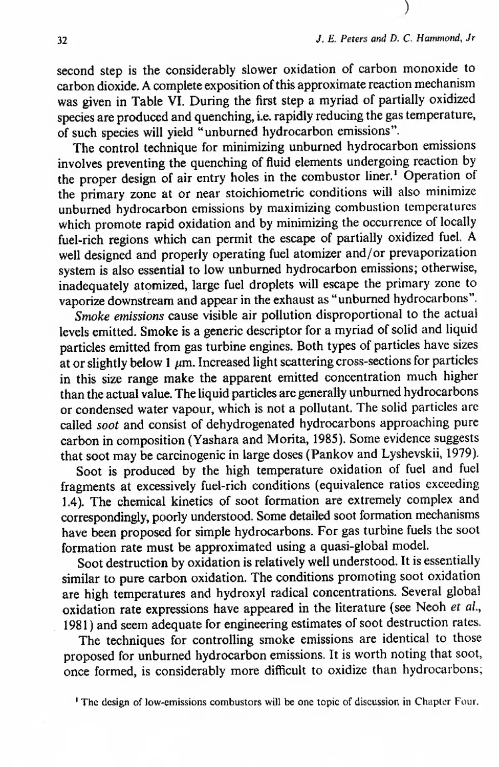
second step is the considerably slower oxidation of carbon monoxide to
carbon dioxide. A complete exposition of this approximate reaction mechanism
was given in Table VI. During the first step a myriad of partially oxidized
species are produced and quenching, i.e. rapidly reducing the gas temperature,
of such species will yield “unburned hydrocarbon emissions”.
The control technique for minimizing unburned hydrocarbon emissions
involves preventing the quenching of fluid elements undergoing reaction by
the proper design of air entry holes in the combustor liner.1 Operation of
the primary zone at or near stoichiometric conditions will also minimize
unburned hydrocarbon emissions by maximizing combustion temperatures
which promote rapid oxidation and by minimizing the occurrence of locally
fuel-rich regions which can permit the escape of partially oxidized fuel. A
well designed and properly operating fuel atomizer and/or prevaporization
system is also essential to low unburned hydrocarbon emissions; otherwise,
inadequately atomized, large fuel droplets will escape the primary zone to
vaporize downstream and appear in the exhaust as “unburned hydrocarbons”.
Smoke emissions cause visible air pollution disproportional to the actual
levels emitted. Smoke is a generic descriptor for a myriad of solid and liquid
particles emitted from gas turbine engines. Both types of particles have sizes
at or slightly below 1 дт. Increased light scattering cross-sections for particles
in this size range make the apparent emitted concentration much higher
than the actual value. The liquid particles are generally unburned hydrocarbons
or condensed water vapour, which is not a pollutant. The solid particles arc
called soot and consist of dehydrogenated hydrocarbons approaching pure
carbon in composition (Yashara and Morita, 1985). Some evidence suggests
that soot may be carcinogenic in large doses (Pankov and Lyshevskii, 1979).
Soot is produced by the high temperature oxidation of fuel and fuel
fragments at excessively fuel-rich conditions (equivalence ratios exceeding
1.4). The chemical kinetics of soot formation are extremely complex and
correspondingly, poorly understood. Some detailed soot formation mechanisms
have been proposed for simple hydrocarbons. For gas turbine fuels the soot
formation rate must be approximated using a quasi-global model.
Soot destruction by oxidation is relatively well understood. It is essentially
similar to pure carbon oxidation. The conditions promoting soot oxidation
are high temperatures and hydroxyl radical concentrations. Several global
oxidation rate expressions have appeared in the literature (see Neoh et aL,
1981) and seem adequate for engineering estimates of soot destruction rates.
The techniques for controlling smoke emissions are identical to those
proposed for unburned hydrocarbon emissions. It is worth noting that soot,
once formed, is considerably more difficult to oxidize than hydrocarbons;
1 The design of low-emissions combustors will be one topic of discussion in Chapter Four.
I. Introduction to combustion for gas turbines
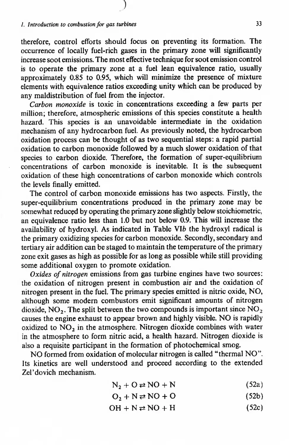
33
therefore, control efforts should focus on preventing its formation. The
occurrence of locally fuel-rich gases in the primary zone will significantly
increase soot emissions. The most effective technique for soot emission control
is to operate the primary zone at a fuel lean equivalence ratio, usually
approximately 0.85 to 0.95, which will minimize the presence of mixture
elements with equivalence ratios exceeding unity which can be produced by
any maldistribution of fuel from the injector.
Carbon monoxide is toxic in concentrations exceeding a few parts per
million; therefore, atmospheric emissions of this species constitute a health
hazard. This species is an unavoidable intermediate in the oxidation
mechanism of any hydrocarbon fuel. As previously noted, the hydrocarbon
oxidation process can be thought of as two sequential steps: a rapid partial
oxidation to carbon monoxide followed by a much slower oxidation of that
species to carbon dioxide. Therefore, the formation of super-equilibrium
concentrations of carbon monoxide is inevitable. It is the subsequent
oxidation of these high concentrations of carbon monoxide which controls
the levels finally emitted.
The control of carbon monoxide emissions has two aspects. Firstly, the
super-equilibrium concentrations produced in the primary zone may be
somewhat reduced by operating the primary zone slightly below stoichiometric,
an equivalence ratio less than 1.0 but not below 0.9. This will increase the
availability of hydroxyl. As indicated in Table VIb the hydroxyl radical is
the primary oxidizing species for carbon monoxide. Secondly, secondary and
tertiary air addition can be staged to maintain the temperature of the primary
zone exit gases as high as possible for as long as possible while still providing
some additional oxygen to promote oxidation.
Oxides of nitrogen emissions from gas turbine engines have two sources:
the oxidation of nitrogen present in combustion air and the oxidation of
nitrogen present in the fuel. The primary species emitted is nitric oxide, NO,
although some modern combustors emit significant amounts of nitrogen
dioxide, NO3. The split between the two compounds is important since NO2
causes the engine exhaust to appear brown and highly visible. NO is rapidly
oxidized to NO2 in the atmosphere. Nitrogen dioxide combines with water
in the atmosphere to form nitric acid, a health hazard. Nitrogen dioxide is
also a requisite participant in the formation of photochemical smog.
NO formed from oxidation of molecular nitrogen is called “thermal NO”.
Its kinetics are well understood and proceed according to the extended
Zel’dovich mechanism.
N2 + О NO + N (52a)
O2 + N^NO + O (52b)
OH + N<+NO + H (52c)
34
J. £. Peters and D. C. Hammond, Jr
The rate of thermal NO formation is strongly temperature dependent;
therefore, its formation can be effectively controlled by limiting the maximum
temperatures reached during combustion. This always involves reducing the
primary zone equivalence ratio to values approaching 0.9.
NO that results from the oxidation of nitrogen in the fuel is formed during
the rapid partial oxidation step of hydrocarbon combustion. As discussed
by De Soete (1975) the formation kinetics are extremely complex and involve
the HCN intermediate. During the early stages of combustion the “fuel” and
“thermal” NO formation mechanisms interact. The control of fuel NO is
best achieved by eliminating nitrogen from the fuel.1 When the removal of
fuel-N is not possible some control of its oxidation can be obtained by staged
combustion with a very fuel rich first stage.
The explicit control of nitrogen dioxide emissions is rarely attempted. NO2
is thought to be formed in low-temperature dilution zones having long gas
residence times.
Oxides of sulphur arise entirely from the oxidation of sulphur originally
present in the fuel. The dominant species emitted is sulphur dioxide, SO2,
which can oxidize to sulphur trioxide, SO3, in the atmosphere. Ambient
water vapour combines with sulphur trioxide to form sulphuric acid, H2SO4,
which subsequently precipitates as “acid rain”. Other undesirable species are
also formed from SO2, including sulphurous acid, H2SO3, and various
sulphate aerosols produced from reactions with ambient particulate. These
compounds are a well known air and water pollution hazard.
Three control techniques are currently applied: the use of low sulphur
fuels, the removal of fuel sulphur prior to combustion, and exhaust gas
treatment to remove sulphur oxides. The third alternative is not practical for
gas turbine engines because unacceptable corrosion would occur in the
turbine section. The latter two alternatives are discussed in any treatise of
emission control for coal-fired stationary power plants and will not be
discussed here.
In conclusion, recent work on modelling of emissions from gas turbine
combustors is discussed in Chapter Five.
V. Premixed flames
The category of premixed flames encompasses any combustion process for
which the fuel and oxidizer are combined to form a homogeneous mixture
prior to combustion. This can include simple devices such as the Bunsen and
1 Since the presence of nitrogen degrades the storage stability of the fuel, this is the preferred
control technique for all but stationary industrial engines burning residual fuels.
/. Introduction to combustion for gas turbines
35
flat flame burners and more complex systems such as the truly prevaporizing/
premixing gas turbine combustor. Through consideration of the conservation
equations of mass, momentum, and energy, the Hugoniot relation can be
found which relates the product properties to the unburned gas conditions
for a flame propagating through a fuel and oxidizing mixture. Two types of
solutions are possible, detonations or deflagrations.
Simply stated, a detonation is a supersonic combustion wave. Since the
detonation is in part a shock wave, it travels through the mixture at a high
rate of speed (kilometres per second) and causes a large increase in the
pressure and density of the gases. While detonations are important for some
aspects of combustion they do not occur in the normal operation of gas
turbine combustors and are not considered in the following discussions.
Conversely, a deflagration is a subsonic wave supported by combustion.
The structure of a deflagration (hereafter referred to as simply a premixed
flame) is shown in Figure 10. In this figure the unburned gases are stationary
and the flame propagates through the mixture at a rate SL, known as the
laminar flame speed. Note that the coordinate system could be arranged such
that the flame is stationary and the unburned gases approach at a rate equal
to 5l and that this stationary reference frame is convenient for many analyses.
The temperature of the gases rises from the initial value to the adiabatic
flame temperature (assuming no heat losses) over a small distance which is
on the order of 1 mm at atmospheric pressure. The exact flame thickness, <5,
is subjective since reactions occur at any temperature; the flame thickness
shown in Figure 10 is defined by
AT
(dT/dx)^
(53)
Figure 10 Premixed flame structure (following Kanury, 1975).
36
J. E. Peters and D. C. Hammond^ Jr
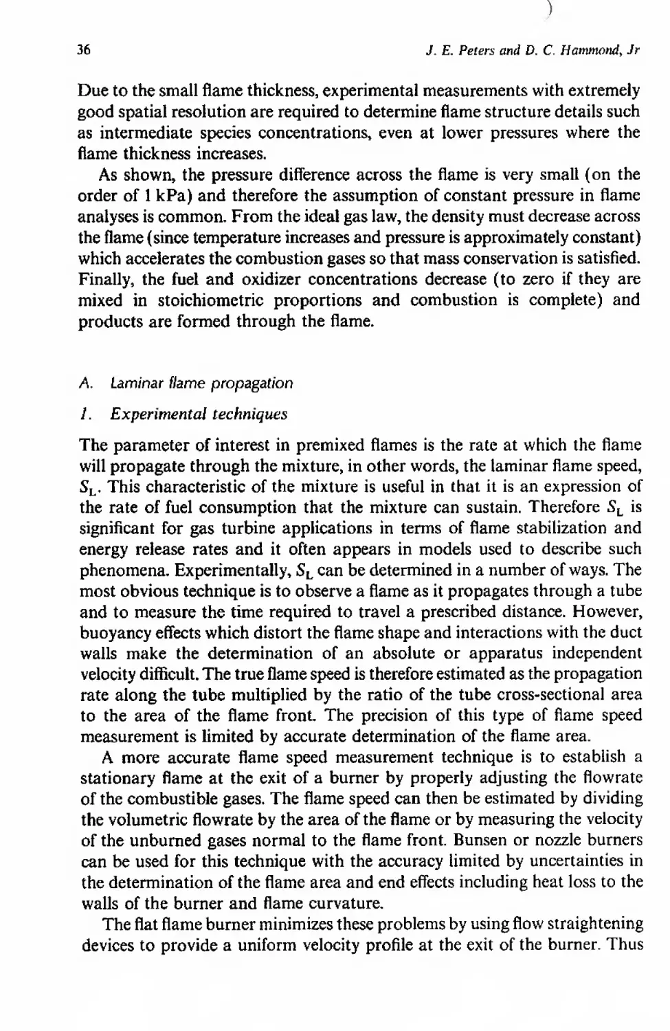
Due to the small flame thickness, experimental measurements with extremely
good spatial resolution are required to determine flame structure details such
as intermediate species concentrations, even at lower pressures where the
flame thickness increases.
As shown, the pressure difference across the flame is very small (on the
order of 1 kPa) and therefore the assumption of constant pressure in flame
analyses is common. From the ideal gas law, the density must decrease across
the flame (since temperature increases and pressure is approximately constant)
which accelerates the combustion gases so that mass conservation is satisfied.
Finally, the fuel and oxidizer concentrations decrease (to zero if they are
mixed in stoichiometric proportions and combustion is complete) and
products are formed through the flame.
A. Laminar flame propagation
1. Experimental techniques
The parameter of interest in premixed flames is the rate at which the flame
will propagate through the mixture, in other words, the laminar flame speed,
SL. This characteristic of the mixture is useful in that it is an expression of
the rate of fuel consumption that the mixture can sustain. Therefore SL is
significant for gas turbine applications in terms of flame stabilization and
energy release rates and it often appears in models used to describe such
phenomena. Experimentally, SL can be determined in a number of ways. The
most obvious technique is to observe a flame as it propagates through a tube
and to measure the time required to travel a prescribed distance. However,
buoyancy effects which distort the flame shape and interactions with the duct
walls make the determination of an absolute or apparatus independent
velocity difficult. The true flame speed is therefore estimated as the propagation
rate along the tube multiplied by the ratio of the tube cross-sectional area
to the area of the flame front. The precision of this type of flame speed
measurement is limited by accurate determination of the flame area.
A more accurate flame speed measurement technique is to establish a
stationary flame at the exit of a burner by properly adjusting the flowrate
of the combustible gases. The flame speed can then be estimated by dividing
the volumetric flowrate by the area of the flame or by measuring the velocity
of the unburned gases normal to the flame front. Bunsen or nozzle burners
can be used for this technique with the accuracy limited by uncertainties in
the determination of the flame area and end effects including heat loss to the
walls of the burner and flame curvature.
The flat flame burner minimizes these problems by using flow straightening
devices to provide a uniform velocity profile at the exit of the burner. Thus
1. Introduction to combustion for gas turbines
37
the flame is one-dimensional in nature and the area of the flame is easily
determined. The drawback to this sytem is the limited operating range over
which a stable flame is formed; the range can be extended by cooling the
burner which brings the flame closer to the burner and helps to stabilize it.
Additional accuracy can be obtained with the stationary flame techniques
by measuring the unburned gas velocity normal to the flame front which
provides a direct measurement of SL.
Finally, a widely used technique to determine laminar flame speeds is the
measurement of a spherically growing flame front. Typically a spark is used
to ignite a mixture, and the growth rate of the spherical flame can be related
to the flame speed; both constant volume and constant pressure procedures
have been used. In a constant volume experiment, the mixture is housed in
a spherical “bomb” and the pressure and growth of the flame are continually
monitored after ignition. For the constant pressure case the mixture is
surrounded by a soap bubble which will expand as combustion occurs to
maintain a constant pressure. A critical review of the various techniques used
to measure laminar flame speeds is provided by Andrews and Bradley (1972).
2. Theoretical considerations
From a theoretical standpoint, three approaches have been employed to
analyse laminar flame propagation in premixed gases: thermal, diffusive, and
comprehensive theories. As the names imply, the thermal approach considers
the transfer of heat through the unburned gas as the driving mechanism for
flame propagation while diffusive theories consider the diffusion of highly
reactive radical species as the controlling factor. The so-called comprehensive
theories include both species diffusion and thermal effects. The fact that all
three techniques can be used successfully is indicative of the similarities
between the mass and heat transfer mechanisms and the role of both in the
propagation process.
A great deal of physical insight into flame propagation can be obtained
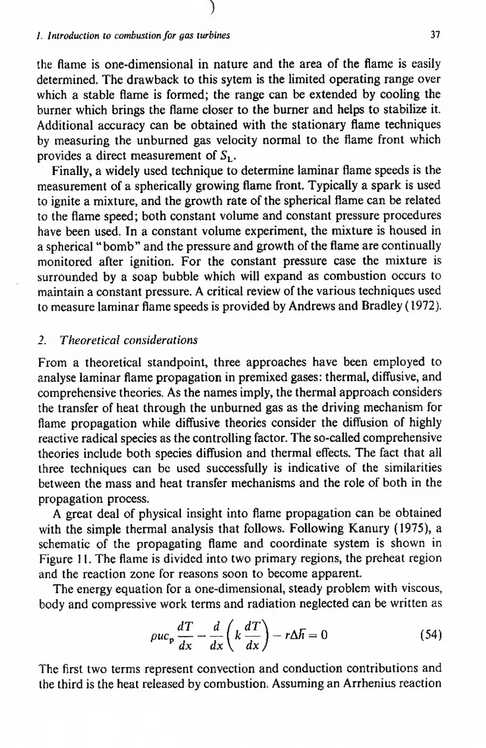
with the simple thermal analysis that follows. Following Kanury (1975), a
schematic of the propagating flame and coordinate system is shown in
Figure 11. The flame is divided into two primary regions, the preheat region
and the reaction zone for reasons soon to become apparent.
The energy equation for a one-dimensional, steady problem with viscous,
body and compressive work terms and radiation neglected can be written as
dT d f dT\ j-
puc_----------------------------к — — r&n = 0 (54)
p dx dx\ dxj
The first two terms represent convection and conduction contributions and
the third is the heat released by combustion. Assuming an Arrhenius reaction
38
J. E. Peters and D. C. Hammond, Jr
Figure 11 Simplified premixed flame propagation model (following Kanury, 1975).
rate, the third term is dependent on both concentration and temperature and
thus must also be a function of position (x). Also note that from conservation
of mass
pu = constant = puSL
(55)
Now in order to solve the problem a major simplifying assumption is
made. The propagating wave is considered to consist of the two distinct
regions shown in Figure 11. In the preheat region the increase in temperature
due to combustion is neglected. In other words the conduction and convection
terms are much larger than the reaction rate term. This is justified due to
the fact that the reaction rate is exponentially dependent on temperature so
that at the relatively low temperatures of the preheat zone the reaction rate
is indeed quite small as illustrated in Figure 11. Therefore the governing
equation for this region is
„ dT d (dT\
₽“SlCp dx dx\dx)
with the boundary conditions given by
for x -> + oo,
(56)
(57)
Integrating and assuming a constant specific heat and thermal conductivity
yields
dT _ P»SLcp
dx j fc
(58)
1. Introduction to combustion for gas turbines
39
In the reaction zone where the temperature is nearing its maximum,
convection is small compared with the reaction and conduction terms.
Consequently, the energy equation reduces to (again assuming a constant
thermal conductivity)
d2T
dx2
гД/Г
with the boundary conditions
for x -► - oo, -3— -► О, T Th
dx
Now using the relation
_d_/ V —
dx \ dx J \dx ) \ dx2 J
(59)
(60)
(61)
and multiplying (61) by 2(dT/dx) gives
d fdT\2 2( —Д/i) dT
— r --- I =---------г---
dx \ dx J к dx
After integrating the final reaction zone result is
dT 2( - А/Г)
1 ~ L k
(63)
The solutions from the two zones are combined by matching the
temperature gradients in (58) and (63) at point i (which is sometimes referred
to as the ignition point). This results in
к ГГ,Т2(-Д/Г)
---(7i-ru)
puCp _ к
(64)
In its present form, (64) cannot be used to calculate laminar flame speeds
because the ignition temperature is unknown. However, if one assumes (as
we did in the derivation of (64)) that little heat is released by chemical
reactions in the preheat zone, then 7] can be replaced by Tu as the integration
limit in the reaction rate term. In addition, the assumption that convection
is negligible in the reaction region suggests that (7j — Tu) can be replaced by
(Tb — 7^). Note that the errors introduced by these two approximations tend
to offset one another. Our final equation (introducing thermal diffusivity) is
then
SL = (2a)1/2
у4
(-ДЯ) rdT
_______________
PUCp(rb“ Tu)
(65)
40
J, E. Peters and D. C. Hammond, Jr
The importance of (65) is not its ability (or lack thereof) to predict
accurately numerical values of laminar flame speed but rather the clear picture
it provides on some important features of flame propagation. First the term
in parentheses is the thermal diffusivity of the mixture; flame speed is
proportional to the square root of the diffusivity. The numerator in the
brackets is an average energy release rate which is normalized by the total
energy release given in the denominator. Thus the flame speed is also
proportional to the square root of the reaction rate. The key result of the
analysis is then
SL ~ (thermal diffusivity x reaction rate)1/2 (66)
Certainly, there are more detailed analyses of the laminar flame propagation
process than presented here and the interested reader is referred to Toong
(1983), Strehlow (1984) and Kuo (1986) for further discussions.
3. Laminar flame speed trends
Now that experimental techniques for measuring SL and a simple theoretical
approach have been considered, some important parameters and their effects
on flame speed are discussed. The key factors for gas turbine applications
are the effects of temperature, equivalence ratio, pressure, and fuel type. Few
data exist on the flame speed for standard gas turbine fuels. Instead data are
available for simple fuels or mixtures of simple fuels. Gibbs and Calcote
(1959) provide flame speed data as a function of fuel structure but for our
purposes the predominant fuel effect is that the flame speed should correlate
with the adiabatic flame temperature of the fuel in question. Thus the effect
of temperature is now addressed.
A typical result of flame temperature as a function of inlet temperature
and equivalence ratio is shown in Figure 12. As shown the flame speed
increases with temperature and peaks on the rich side of stoichiometric at
approximately an equivalence ratio of 1.1. From equation (66) the flame
speed is proportional to the square root of the reaction rate which is a strong
function of temperature. Therefore, the increase of flame speed with temperature
is expected. The peak flame speeds occur near the equivalence ratios at which
the flame temperatures arc maximized again confirming the trends suggested
by the previous analysis.
Pressure effects are more complex. Kuehl (1962) indicates that for relatively
slow burning fuels, flame speed and pressure exhibit a weak inverse relation
but for the more rapidly burning fuels, flame speed increases with an increase
in pressure. Typical hydrocarbon fuels would fall into the former category
as illustrated in Figure 13 for iso-octane. In terms of our theoretical analysis,
Figure 12 Laminar burning velocities for propane and air at 101 kPa (from Kuehl,
Figure 13 Burning velocities of iso-octane-air mixtures (from Metghalchi and Keck,
1982).
42
J. E. Peters and D. C. Hammond, Jr
if we assume an" nth” order reaction rate and note that the thermal diffusivity
is inversely proportional to pressure, (65) can be written as
“ / 1 \ / Pn \ “| 1/2
= (P"-2)1/2
(67)
Sl
for ф <. 1.0
If the common second order reaction rate is assumed, then the theory predicts
that laminar burning velocity is independent of pressure. The results in
Figure 13 indicate a weak pressure dependence suggesting an overall reaction
order of slightly less than two for typical hydrocarbons.
A number of empirical equations exist in the literature for relating burning
velocity to pressure and temperature variations. For example, a recent
correlation by Sharma et al. (1981) for methane is
SL = C4(TU/300)'W^
SL = C4(T„/300)148^ for Ф > 1.0 (68)
where C4 = -418 + 1.287/</> - 1.196/ф2 + 360/ф3 - !50(logloP). As written,
(68) gives SL in cms4 when Tu is expressed in К and P in atm. This
correlation was obtained in methane-air mixtures for pressures of 100-800 kPa,
temperatures of 300-600 К and equivalence ratios of 0.8-1.2 in a constant
volume spherical bomb. Caution should, however, be exercised in applying
empirical correlations because reported flame speed measurements have been
subject to a wide range of variability as indicated by Figure 14. One general
rule of thumb that can be drawn from the literature is that the typical
hydrocarbon fuel will have a maximum laminar flame speed of roughly
40cms-1 at an equivalence ratio of approximately 1.1 for an initial
temperature and pressure of 300 К and 101 kPa. Using (68) to extrapolate
to the more realistic inlet conditions of a gas turbine combustor (600 К and
800 kPa) gives a maximum laminar flame speed of 80 cm s“ *.
Finally, this discussion is concluded with Table VII which gives the
maximum burning velocity for seven different mixtures to indicate the
variations that are obtainable for deflagration speeds. Note that the pure
oxygen systems have much higher flame speeds than their air oxidizer
counterparts as expected since the flame temperatures and hence the reaction
rates of the pure oxygen systems are much higher. For further flame speed
data, see the review article by Andrews and Bradley (1972) and NACA (1957).
B. Turbulent Нате propagation
In turbulent premixed systems, flame speeds can be substantially larger than
those found in otherwise similar laminar mixtures. Despite the fact that
turbulent combustion is used in virtually all practical combustion systems
Method
-----Flat Flame Burner
-----Nozzle Burner
-----Horizontal 2.5 cm Square Tube
-----Bomb, Adiabatic Density Ratio
-----5 cm dia. Horizontal Tube
———Bomb, Adiabatic Density Ratio
—--—Bomb, Hot-Wire and Corrected Density
Ratio
-----Bomb
45
СЛ
-40
о
30-
25-
£D
15-j
10
5o.6
08
i
1.0
1.2
1,4
E
Equivalence Ratio
Figure 14 Variation of burning velocity of methane and air mixtures at a constant
pressure of 101 kPa (from Sharma er a!., 1981).
Table VII Selected values of burning velocity (from Andrews and Bradley, 1972).
Mixture
Maximum burning velocity, cm s
Methane-air
Ethylene-air
Acetylene-air
Hydrogen-air
Methane-oxygen
Acetylene-oxygen
Hydrogen-oxygen
45
79
158
310
450
Ц40
; ? ?140O
44 J. E. Peters and D. C. Hammond, Jr
the exact mechanisms of flame propagation enhancement by turbulence are
not well understood. Conceptual and mathematical models abound in the
combustion literature with varying degrees of sophistication and also various
levels of agreement with experimental data. In keeping with the established
style of this introductory chapter, some simple concepts of turbulent flame
propagation are presented along with the observed trends of turbulent flames.
First we consider some general features of a turbulent flame by referring
to Figure 15 which shows a schlieren photograph (sensitive to density
gradients) where the regions of steep temperature gradients can be visualized.
ib)
<<n
Figure 15 Laminar ((a) and (b)) versus turbulent ((c) and (</)) flames; («) and
(c) are long-exposure photographs, (b) and (d) are short-exposure schlieren photographs
(from Lewis and von Elbe, 1961).
1. Introduction to combustion for gas turbines
45
The laminar flame exhibits a generally smooth shape with a well-defined,
thin, high-temperature zone as was discussed in the previous section. In
contrast is the turbulent flame which appears wrinkled in nature showing
the disjointed regions of reacting flow. The wrinkled appearance is characteristic
of turbulent flames with relatively low turbulence intensities (velocity
fluctuations) and large scale (macroscopic eddy sizes). At high levels of
turbulence intensity and small scale the flame is much more rough in
appearance. This transition of flame character is shown in Figure 16. Visually,
a turbulent flame appears “bushy” as the eye averages over time the
fluctuating location of the luminous portion of the flame.
Id
(/}
Figure 16 Long exposure photographs ((«)"(<)) and short duration schlieren
photographs of turbulent flames (from Suzuki el al, 1979).
46
J. E. Peters and D. C. Hammond, Jr
Some of the same techniques used for laminar flame speed measurements
have been employed for turbulent flame studies. Burner and nozzle systems
are used with the flame speed again determined by dividing the incoming
volumetric flow rate of gases by the area of the flame. Another technique
similar to laminar flame work is the measurement of a spherically growing
flame front after the ignition of the mixture by a spark.
A widely used method for turbulent flame studies is illustrated schematically
in Figure 17. A turbulent flow is generated with a wire mesh grid placed in
the gas flow upstream of the flame region. Turbulence parameters such as
the turbulence intensity and scale can be varied by changing the grid. The
flame is stabilized with a small (1 to 2 mm diameter) rod mounted transversely
across the flow or with a small pilot ignition source. Depending on the
technique used the flame front is located using either schlieren photographs
or with a thermocouple. The velocity components are measured at the flame
front location and the component normal to the flame front is considered
the turbulent flame speed. In some cases the normal component of velocity
at the flame front is determined simply from geometric considerations of the
flame spread angle and approach flow velocity although local measurements
of the velocity at the flame front yield more accurate results.
For a discussion of the modelling of turbulent reacting flows, one first
must recognize that the turbulent flame speed is not a fundamental property
of the mixture as is the laminar flame speed. Instead, ST depends not only
on the physical and chemical properties of the mixture but also on the
Figure 17 Schematic of turbulent flame speed measurement technique (from Dandekar
and Gouldin, 1982).
1, Introduction to combustion for gas turbines 47
turbulence characteristics of the approach flow. (The fact that these approach
characteristics are often dependent on the experimental apparatus undoubtedly
accounts for some of the apparently conflicting experimental results in the
literature.) Thus, we will be looking at turbulent flame speed models and
trends in various regimes of turbulent flow.
First we consider the case of low turbulence intensity and large scale
(/ > <5). As discussed this flow type results in a relatively smooth but wrinkled
flame. The widely accepted mechanism of flame speed enhancement under
these conditions is that the wrinkling of the flame is caused by the different
gas velocities of the flow and that the wrinkling increases the effective surface
area of the flame. Since its introduction by Damkohler (1947), this approach
has been used by several investigators. Generally, the increase in area is
related to the turbulence intensity, u', and in some cases also the length scale,
/, and then the turbulent flame speed is correlated with equations as shown
in Table VIII, taken from the review by Andrews et al, (1975). Note the
variety of approaches.
The turbulent regime of small scale (/ < <5) and high turbulence intensity
has also been modelled with some success in a relatively simple manner.
Under these conditions, the flame speed enhancement is considered by many
to be due to the increased exchange of species and energy through turbulent
transport as opposed to the molecular transport of laminar flames. Ballal
and Lefebvre (1975) suggest that the high intensity and small-scale turbulence
disrupt the flame front which results in a relatively thick (compared with <5)
flame zone consisting of many individual small reacting eddies. This results
in a rapidly burning mixture because of the large surface area available for
Table Vtll Some correlations of Sr from wrinkled laminar flame models (from
Andrews et al., 1975).
I. ST = SL(1 +u'/SL)
2. ST = SL(1 + B(i//SL)2)1'2 (B is a constant)
3. ST = (SLu'),/2
4. ST = SL + (2SLu')1'2
5. ST = Sl(2[u'/Sl ~ 0-5 exp(- «'/SL)]),/2
(Tb 2u'/Sl \
\TU (in(i +«7SL))V2J
7. * ST = SL(1 + u‘/SL) | ° F(n)dn + (1 + £/v) I F(n)dn
JO Jne
*и0 is frequency separating large and small scale fluctuations, and F(n) is a spectral
function.
48
J. E. Peters and D, C. Hammond, Jr
Table IX Some correlations of ST based on turbulent transport (1-3, Andrews et al.,
1975; 4, Ballal and Lefebvre, 1975).
1. ST = SJe/v)1'2
2. * ST = SL(1
3. S,- = SM v)(V<5,
4. St = 0.5u,<51(£/v)0-25
* kJ к represents the ratio of turbulent to molecular heat transfer rate.
reaction. Their suggested correlation of turbulent flame speeds as well as
those for some turbulent transport approaches are given in Table IX.
Given the variety of correlations in Tables VIII and IX it is difficult to
draw any general conclusions regarding the effect of variables on turbulent
flame speeds. However, some observations are in order. First note that in
many cases the turbulent flame speed varies directly with the laminar flame
speed. That is to say that factors which influence SL, such as temperature,
will similarly affect ST. There are, however, conditions for which the flame
propagation is almost completely controlled by the turbulent flow (correlation 4
in Table IX) and other factors play only a secondary role at most. In most
of the correlations turbulent flame speed increases with the turbulence
intensity and since intensity is usually proportional to the Reynolds number
of the flow, plots of ST/SL versus Reynolds number are sometimes used to
correlate flame speed data.
As discussed earlier in this chapter, most gas turbine combustors do not
operate with a premixed combustion system, but rather in a diffusion flame
mode. The notable exception to this is the prevaporizing/premixing combustor.
Here the general characteristics of turbulent premixed flames that we have
discussed can be applied. As turbulence enhances flame speed, so can increased
turbulence improve volumetric heat release rates. Also, the flame speed takes
on an important role in the undesirable flashback that is a hazard in
prevaporizing/premixing systems. Flashback occurs when the flame travels
upstream into the vaporizing and mixing regions which can cause a
catastrophic failure. This upstream propagation is caused when the flame
speed exceeds the approach flow velocity. This can occur in the low velocity
boundary layers of the mixing tube, in recirculation zones present in the
mixing region or during a sudden reduction in flow through the mixing tube
due to combustion instability or compressor surge, for example.
Before closing this discussion of turbulent flame propagation, we should
recognize that the area of turbulent combustion is a very active area of
ongoing research. Many basic questions regarding turbulent flames still
remain and much more advanced modelling concepts have been put forth
1. Introduction to combustion for gas turbines
49
than the introductory ones presented here. The turbulent combustion process
can be analysed by considering the time-averaged Navier-Stokes equations.
Correlation terms that appear in these equations are modelled with empirical
relations, and additional conservation equations (for turbulent kinetic energy
and dissipation, for example) are added to the equations for mass, momentum,
and energy. Combustion can strongly influence the turbulence characteristics
through variable density, buoyancy, and turbulence generation (or dissipation)
which may seriously reduce the applicability of turbulence models developed
with cold flow experiments. Time averaged reaction rate terms must be
carefully considered due to the highly non-linear dependence of reaction rate
on temperature. In fact, the usefulness of these time-averaged approaches has
been questioned and unsteady solutions of turbulent, reacting flows are now
being considered. For discussions of more advanced concepts of turbulent
flames the reader is encouraged to examine combustion texts such as Kuo
(1986) and the recent literature on the subject.
VI. Diffusion flames
The term diffusion flame is generally used to classify any combustion process
for which the fuel and oxidizer are separated prior to combustion. The
diffusion flame is of great importance as it is present in many practical
combustion devices including simple systems such as the common match and
candle and in complex systems, including the gas turbine engine, furnaces,
boilers and diesel engines. The basic structure of a laminar diffusion flame
is illustrated in Figure 18 which depicts the idealized case of an infinitely
Figure 18 Diffusion flame structure of a fuel jet burning in air. Profiles are presented
as a function of radius at one axial location (from Glassman, 1977).
50
J. E. Peters and D. C. Hammond, Jr
thin reaction zone. This implies infinitely fast reaction rates and in practice
the reactions are often rapid enough (in comparison with diffusion or mixing
rates) to result in at least a very thin reaction zone. Thus the fuel and oxidizer
diffuse toward the flame in stoichiometric proportions and their concentrations
fall to zero at the flame surface. Products which are formed at the flame then
diffuse from the surface. As expected the temperature is highest at the flame
surface. This maximum flame temperature is not limited by the overall
stoichiometry of the system but by the stoichiometric adiabatic flame
temperature.
A. Caseous jet diffusion flames
The theoretical approach to diffusion flame analysis will be illustrated with
the classical analysis of an axisymmetric laminar jet issuing into a quiescent
atmosphere. Here the jet will be considered the fuel which flows or diffuses
to the surrounding oxidizing environment and then reacts in a thin flame
zone located where the fuel and oxidizer reach stoichiometric proportions.
The geometry of the problem is illustrated in Figure 19. The assumptions
include constant pressure, the usual boundary layer approximations, a very
small initial jet diameter, negligible potential core of the jet, constant and
equal fluid properties for both the fuel and oxidizer (including density) and
buoyancy and radiation effects are neglected. The assumption concerning
properties and density is admittedly unrealistic; however, the dominating
physics of the problem can be illustrated without the complications that arise
if the true variations are included. In addition, the variable density problem
can be reduced to the incompressible one solved here by the variable
transformation illustrated in Toong (1983). Now, for the laminar jet diffusion
flame, under the assumptions listed above the conservation equations for
Figure 19 Fuel jet schematic and coordinate system (from Kanury, 1975).
1. Introduction to combustion for gas turbines
51
mass, x-momentum, energy and species are
5(r«) d(rv)
—----k* --- =
dx dr
du du d i du\
dx dr dr \ dr J
dT dT d ( dT\ qr
ru — + rv — = a — r — 4- —
dx dr dr \ dr J pc?
dYt dYi „ d f dYA wfr
dx dr ' dr \ dr J p
(69)
(70)
(71)
(72)
where i is either f, о or p for fuel, oxidizer or products. Note that the species
and energy equations are coupled due to the reaction and heat release rate
terms and they are also non-homogeneous. The momentum equation is
uncoupled due to the constant density assumption.
First, consider the overall reaction
(/)F + (1)O-(1+/)P (73)
where the coefficients are the stoichiometric mass coefficients and the energy
released by the reaction is -fAh. From this reaction
JM
(74)
Now we assume that the kinematic viscosity, v, the thermal diffusivity, a, and
the species diffusion coefficients, Db are all equal. Transformation of the
dependent variables in the energy equation to a non-dimensional temperature
gives
d (c^T-T^X d (c^T-TA\
dx \ — An ) dry — An /
d/4(T-Tj\\ qr
dr \ dr \ — A/i / J pAh
Adding the species equation for fuel and (75) results in
db db d fdb\
dx dr drydrj
(75)
(76)
where
b — bfy
cp(T-TJ
-Ah
(77)
52
J. E. Peters and D. C. Hammond, Jr
This technique, known as the Schvab-Zel’dovich formulation, can be applied
to eliminate the reaction rate term from all the equations except one. Thus,
only one non-homogeneous equation must be solved. The solution of the
non-homogeneous equation would, however, require knowledge of the
reaction rate expression.
To simplify matters further for our discussion we will assume that the
reaction rate is infinitely fast so that no fuel exists on the oxidizer side of the
flame and no oxidizer exists on the fuel side; the fuel and oxidizer
concentrations fall to zero at the flame as illustrated in Figure 18. For this
problem the conservation equations all reduce to the form of (76) with the
variables for the momentum, energy and species equations given by u,
(T — Д/ilf/Cp) — Tm and (Vf — /Уо) + /У0со, respectively. The boundary
conditions are
r = 0:
x — 0:
r -> co:
db/dr = 0
b = bj
b = Q
(78>
The transformed variables for temperature and species are chosen so that
the same boundary condition applies to each equation. This form of the
species variable was originally introduced in the Burke and Schumann (1928)
analysis of a confined diffusion flame.
The diffusion flame problem has now been reduced to the classical jet
mixing problem discussed by Schlichting (1968). His solution gives
where
and
This solution is not valid inside the potential core (small values of x/dj of
the flow. The profile given in (79) is shown as velocity in Figure 19. Of course,
the profiles of the transformed energy and species variables must be similar
because of the similar equations and boundary conditions. The flame location
is determined by setting the fuel and oxidizer concentrations equal to zero
and solving for x and r. The actual concentrations of fuel and oxidizer are
L Introduction to combustion for gas turbines
53
found by recognizing that the fuel concentration is zero on the exterior of
the flame and that the oxidizer concentration is zero on the interior. Finally,
the temperature can be readily determined from a combination of the
transformed energy variable and the fuel concentration profile.
One feature of diffusion flames that has received a great deal of attention
is the length of the flame. This is a parameter that is indicative of the space
heating rate of the flame. It is relatively easy to measure experimentally and
it provides some insight into the diffusion flame process. From our model
the length of the flame can be found by determining the x location of the
flame when r is equal to zero. Returning to (79) in the form of the species
equation and noting that at the flame, b is equal to /У0>со and b-t is equal to
(1 + /УОсо) we can solve for the flame length,
з (Ур.со + l//) urf
(82)
The key result is that the flame length is inversely proportional to the
diffusivity (recall the assumption that v — P). These trends were confirmed
experimentally in early work by Hottel and Hawthorne (1949).
In almost all practical combustion devices, diffusion flames are turbulent
rather than laminar. A simple approach to the analysis of the turbulent
diffusion flame is to replace the laminar kinetic viscosity with the turbulent
kinematic viscosity. Thus the transport of momentum (or species and energy
since we are assuming equal diffusivities) is controlled not by the molecular
processes of laminar flow but by the turbulent mixing process. This approach
is attractive because the equations for the turbulent flow problem are identical
to the laminar case except for the replacement of the laminar viscosity with
the turbulent viscosity. Thus, for example, the solution to the flame length
follows directly from (82) as
L = Д (83)
Noting that the turbulent viscosity for jets is proportional to the Reynolds
number of the flow suggests that the flame height for the turbulent jets is
proportional to the initial jet diameter, which was also confirmed by Hottel
and Hawthorne (1949).
Although global characteristics of the turbulent diffusion flame may be
estimated in the above manner, detailed structure is not addressed and little
or no information on the fundamental nature of the process can be obtained.
A more sophisticated approach than is permitted here is required to model
the turbulent mixing of the gases and the interactions of the turbulence and
combustion. Again this is an area of active research and the reader is urged
54
J. E, Peters and D. C. Hammond, Jr
to examine the literature on this topic. For examples of more detailed
theoretical and experimental approaches to both laminar and turbulent
diffusion flame analyses see the texts by Chigier (1981) and Kuo (1986).
Combustion in conventional gas turbines is similar, in some ways, to the
turbulent diffusion flames we have discussed in this section. Putting aside for
the moment the recirculating flow necessary for flame stabilization (to be
discussed in Section VIII of this chapter), we note that fuel is first injected
into the centre of the primary zone and then it must combine with air through
turbulent mixing. As in the diffusion flame case, this mixing can control the
combustion process by limiting the rate of heat release when kinetics and
droplet evaporation are rapid. In addition, the fuel and oxidizer can come
together in stoichiometric proportions so that the maximum temperature in
the primary zone is not limited by the overall equivalence ratio but by the
maximum adiabatic flame temperature of the fuel.
8. Droplet evaporation and burning
In most gas turbine applications the fuel is injected into the combustor in
the liquid phase. As will be discussed in Chapter Three the fuel injector serves
to distribute the fuel in the primary zone of the combustor in a manner which
will provide proper mixing of the fuel and air. Certainly, this mixing process
can be influenced by the evaporation rate of the fuel. We will begin this
discussion by first considering the evaporation characteristics of a single drop
and then discussing the behaviour of spray flames.
The classical single drop evaporation model contains the following
assumptions:
(i) Quasi-steady evaporation (the gas phase processes are considered
to be steady since changes in the liquid phase, such as drop radius,
occur much more slowly).
(ii) No free or forced convection.
(iii) Uniform and constant drop temperature.
(iv) Constant pressure (the velocities in the gas phase are very small
and the viscous effects are negligible; therefore the momentum
equation reduces to a statement of constant pressure).
(v) Local thermodynamic equilibrium at the drop surface.
(vi) Spherical drop.
(vii) Single component drop.
(viii) Radiation heat transfer neglected.
(ix) Constant specific heat.
(x) Lewis number of unity.
1. Introduction to combustion for gas turbines
55
(84)
(85)
(86)
(87)
Under these assumptions the gas phase conservation equations in spherical
coordinates reduce to
d -j
— (pwr2) = 0
dr
^-(pur2b) — ^-[parzdb/dr~\ — 0
dr dr
where
b _ cp,g(^ ~ У»)
for the energy equation and
, ^~yf
1 - n,.
for the species equation for fuel. The boundary conditions for (84) and (85) are
r = rs, m = 4nrz pD(db/dr)s and b — bs
r — co, b — 0
Using the assumption that pD is constant, the solution, in terms of the
evaporation rate, m, is
m = 4rcpeagrs In (1 + B) (88)
where В is known as the transfer number and is equal to — bs or 7
7- 1 —
Physically, the transfer number is a measure of the “driving force” for
evaporation. In terms of the energy equation, В (sometimes called BT) is the
ratio of the energy available for evaporation divided by the energy required.
From the species equation for fuel, В (sometimes called BM) is the difference
in fuel vapour mass fractions between the environment and the surface divided
by the difference between the surface and the liquid (YfJ — 1). Note that these
two forms of В will not be equal when the time dependent solution is obtained
for an evaporating drop with an unsteady droplet temperature.
In order to compute B, the temperature (or, equivalently, the mass fraction)
must be determined at the surface. The temperature at the surface may be
determined from (89) and a relation between the temperature and vapour
pressure of the fuel such as the Clausius-Clapyeron equation. However, if
T*. » TB then 7^ « TB is a good approximation for use in (89).
56
J. E. Peters and D. C. Hammond, Jr
To determine expressions for the evaporation time or the droplet diameter
as a function of time, one recognizes that m is given not only by (90) but also by
. d
m = —
dt
4тг ,
Pr^-r*
(90)
Equating (88) and (90) letting d — 2rs and integrating gives the well known
“d2 law” result
d2 —
(91)
where the evaporation coefficient, /?, is given by
8k
/? =-----In(l+B) (92)
Pl Cp.8
Equation (91) indicates that the square of the droplet diameter decreases
linearly with time. Experimental results obtained under conditions for which
the assumptions hold, particularly assumptions (iii) and (vi), confirm this
linear relationship as shown in Figure 20.
A droplet evaporation time is easily estimated from (91) by setting d equal
to zero and solving for
(93)
The key result here is that droplet evaporation time is proportional to the
Figure 20 Variation of drop diameter squared with time for a normal decane drop
burning in a 12 kPa 40% Oz, 60% N2 environment (from Miyasaka and Law, 1981).
I. Introduction to combustion for gas turbines 57
square of the diameter. Therefore, any changes in fuel type or injection
equipment which change the drop size can strongly influence the evaporation
rate. Also, fuel property effects influence droplet evaporation primarily
through their effect on the atomization process (viscosity and surface tension
effects on d0 as discussed in Chapter Three) and on the evaporation coefficient
(volatility effects on B).
The preceding analysis assumed a quiescent atmosphere surrounding the
evaporating drop. A droplet in a combustor can experience strong forced
convection effects which are typically taken into account with empirical
correlations. A widely used correlation due to Ranz and Marshall (1952) is
)Uv==/?(l +0.3Re1'2Pr1'3) (94)
The preceding analysis for an evaporating drop can easily be extended to
a burning drop with the additional assumption that the drop is surrounded
by an infinitely thin spherically symmetric diffusion flame. The analysis
follows directly from the previous diffusion flame problem combined with
the droplet evaporation model and the result is identical to the evaporating
drop case with the transfer number now given as
B _ Cp.8(T„-T5) + (-Ah)/y0.„
L
Even though the d2 law is useful for providing estimates of droplet
evaporation characteristics, several assumptions were made in its derivation.
These assumptions do not hold for many cases and more detailed consideration
of the droplet evaporation and combustion problem is required. We now
address some of these issues and suggest that the reader refer to the reviews
of droplet combustion by Sirignano (1983) and Faeth (1977) for more details.
In most cases, the temperature of the fuel at injection is substantially lower
than the steady state temperature achieved during evaporation of the drop.
This heat-up period can be responsible for little or no decrease in diameter
of the drop during the first part of the droplet lifetime. Droplet heat-up is
modelled by solving the species equation as before to again give the mass
fraction part of (88) where В = BM. Note that this is not the solution of the
energy equation for the unsteady case since the boundary condition at the
surface now says that only part of the heat transferred to the drop is used
to evaporate the fuel and the remainder goes to heating the droplet.
Energy conservation, therefore, requires that
mcpfdTJdt = 4тгг2/1(Тоэ - TJ — mL (96)
where the heat transfer coefficient is evaluated from the Nusselt number
58
J. E. Peters and D. C. Hammond, Jr
relation
hrs/k = Nu (97)
Using the mass and energy transfer analogy,
Nu = Sh (98)
where
Sh = h^rJD (99)
and
hD = [wrm=j/(y- yj (юс)
= (D/r)ln(l+BM)/BM (101)
Combining (88), (96-98) gives
dTs mL BT t
—“ =----- „ 1
dt mcpj |_ BM
(W2)
The droplet heat-up and evaporation problem can now be solved numerically
through (88), (89) and (102). Of course, a relation between the droplet
temperature and the fuel vapour pressure is still required. Finally, note that
(102) indicates that the steady state solution requires that BT = BM, as we
determined earlier in the d2-law analysis.
A second area of concern with the d2 law is the assumption of uniform
droplet temperature because the temperature must vary to some degree inside
the drop. In addition since the droplet is liquid and not a solid, internal
circulation (driven by the shear forces on the surface of the drop as it moves
relative to the gas phase) can be present inside the drop. The previous uniform
temperature calculations are sometimes said to correspond to the mixing
limit case where the circulation within the drop is sufficiently vigorous to
remove any spatial variations. (However, this mixing limit, according to
Sirignano (1983), should not be physically expected.) On the other end of
the spectrum is the “conduction limit” where the liquid is essentially
considered to be a solid and temperature gradients within the drop are
determined using an unsteady heat conduction in a sphere approach. The
most complete analysis would involve the solution of the equations of motion
and energy within the drop. There is currently no consensus as to the level
of sophistication required to model droplet behaviour in a spray flame
properly. However, most models applied to gas turbine applications employ
a t/2-law approach with modifications for droplet heating as outlined above
as a compromise between accuracy and computational effort.
i. Introduction to combustion for gas turbines
59
In addition to the temperature variations discussed in the preceding
paragraphs, practical fuels are composed of several different compounds
instead of a single component as considered in the d2-law analysis. The effects
of the multicomponent nature of the fuel on the evaporation characteristics
depend on the internal transport mechanisms of the drops and the physical
properties of the various constituents of the fuel. In a manner similar to the
discussion for temperature variations within a drop one can consider two
limits in the evaporation of a multicomponent fuel, the diffusion limit and
the distillation limit. In the diffusion limit the droplet concentration in the
inner region is practically constant since diffusion of species is relatively slow.
Gradients in droplet composition exist only near the surface of the drop with
each component evaporating at a rate equal to its mass fraction times the
total evaporation rate. The overall process produces a d2-law type of
behaviour. For the distillation limit, rapid mixing within the drop brings the
volatile components to the surface as they evaporate so that the evaporation
resembles a distillation process where the components evaporate in the order
of their volatility starting with the most volatile components. A plot of
diameter squared versus time for this case would appear as a series of straight
lines with different slopes representing the different volatilities of the evaporating
components. Experimental evidence exists to support both the diffusion and
the distillation processes. Of course, a complete analysis would again require
the solution of the equations of motion, energy and species within the drop.
A third area of great current interest in multicomponent drops is
microexplosions caused by the superheating of a volatile component trapped
in the droplet interior. Under certain conditions this component will vaporize
and build up pressure internally causing the drop to explode violently (see,
for example, Lasheras et al. (1981) and Wang et al. (1984)).
Finally, an area of importance in droplet calculations that we have
neglected up to this point is the determination of properties such as specific
heats and thermal conductivities. These properties, contrary to the assumptions
in our analysis, are not constant and care must be taken in their selection.
A common approach is to evaluate the gas phase properties at an average
temperature as determined, for example, by the | rule of Sparrow and Gregg
(1958),
t=ts + (M-t;) (W3)
Even without including the details that are discussed in the preceding
paragraphs, the d2 law in (93) can provide useful information. For example,
consider the droplet evaporation results presented in Figure 21. This figure
was generated assuming constant values for liquid density, initial drop size
and latent heat of vaporization as noted in the figure caption. The gas phase
properties used were those of air evaluated at the temperature given by (103).
60
J. E. Peters and D. C. Hammond, Jr
Figure 21 Variation of droplet evaporation time with surface temperature for
pL — 800 kg m^3. L = 300 kJ kg-1, and d0 = 50 pm.
Some important points relative to gas turbine combustion performance can
be drawn from this figure.
As reference values, note that the average (50% by volume) boiling points
of JP-4, Jet A and Diesel fuel # 2 are approximately 390 K, 500 K, and 550 K,
respectively. These are representative of two standard gas turbine fuels (JP-4
and Jet A) and an alternative fuel. As expected, the evaporation time decreases
with increasing surrounding temperature. Also, at the lower surrounding
temperatures, the evaporation time is very sensitive to the surface temperature
(or essentially the boiling point) of the drop. Thus, switching from JP-4 to
Jet A or diesel fuel will cause a significant change in the evaporation rate.
However, at high surrounding temperatures the evaporation rate is relatively
insensitive to surface (boiling) temperature. This implies little change in
evaporation rate with a change from JP-4 to Jet A or diesel fuel in the
high-temperature environment.
These trends help explain the fact that at full-power conditions (high
temperature) gas turbines are relatively insensitive to fuel type but at low
power (particularly ignition conditions) gas turbine performance can be
significantly influenced by fuel type. Of course, other factors such as the larger
drop sizes usually associated with lower fuel flow rates and higher viscosities
(to be discussed in Chapter Three) are also important.
1. Introduction to combustion for yas turbines
61
In conclusion, the simple d2-law approach can be used to estimate droplet
evaporation effects, particularly when the modification for droplet heat-up
is included. These calculations can be especially useful for comparisons of
the effect of different fuels and gas turbine operating conditions. However,
exact agreement with data for evaporating drops will not be obtained because
of the effects discussed in the preceding paragraphs.
C. Spray diffusion flames
The previous section considered the evaporation and burning of single drops
in an infinite gaseous environment. In a gas turbine combustor, a drop of fuel
evaporates in an environment heavily influenced by the evaporation and
burning of the remainder of the spray. The simplest method to account for
the effect of surrounding drops on the evaporation rate of a particular drop
is to determine the effect of the evaporating spray on the ambient environment.
However, experimental and theoretical evidence suggests that the behaviour
of a burning fuel spray can, under many conditions, behave more like a
gaseous diffusion flame than a collection of individually burning drops.
Yule and Bolado (1984) suggest three classes of spray flames as shown in
Figure 22. The first sketch applies to a situation where the droplets evaporate
very rapidly and the oxidation of the fuel is primarily controlled by the
diffusion or turbulent mixing of the fuel vapour and oxidizer (just as in the
case of a gaseous diffusion flame). The third case considers slow evaporation
for which the droplets can burn individually. This type of flame would be
most likely to occur with sprays of large drops and heavy or low volatility
fuels; droplet evaporation characteristics would be expected to play a large
role in the size and structure of this flame. The second glass is a compromise
of the two extremes and represents the case where droplet evaporation affects
the spray flame behaviour but individual droplet burning does not control
the combustion process.
Several theoretical approaches (Labowsky (1978), Chiu et al. (1982), and
Correa and Sichel (1982), for example) have considered the problem of droplet
interactions for the overall or group combustion of a large collection or cloud
of drops. In one technique, the evaporation and combustion of a cloud of
drops is analysed and the conservation equations are written for the entire
cloud with evaporation rates for individual drops determined from the
classical single drop approach. However, the drops do not necessarily burn
individually; they may simply evaporate and then the fuel must diffuse
outward from the fuel-rich core to burn in a sheath flame that surrounds the
entire cloud. According to Chiu et al. (1982), the manner in which the spray
burns is controlled by a parameter they denote as “G", the group combustion
number. This non-dimensional parameter is the ratio of the rate of droplet
62
J. E. Peters and D. C. Hammond, Jr
Figure 22 Three possible types of spray flames (from Yule and Bolado, 1984).
vaporization to the transport of gaseous species by diffusion. Basically at
low G numbers, the drops burn individually and as G increases, the burning
mode changes to an external flame phenomenon. Of particular interest is the
fact that many practical spray flames have relatively large G numbers (greater
than 1) so that group combustion is expected to be the primary combustion
mode.
Unfortunately, most of the theoretical approaches to date, including those
referenced in the preceding paragraph, have considered only quiescent
mixtures for their droplet “cloud” analyses. The extension to the turbulent
flowing mixtures of interest for gas turbine combustion systems is not easily
done in terms of developing and solving the detailed governing equations.
However, conceptually, one can conceive of a G number based on the ratio
of the rate of droplet vaporization to the rate of turbulent mixing of the fuel
with air. In fact, we shall see that comparing the rates of the important
physical processes (such as mixing and evaporation) can be used in practical
systems for the analysis of combustion performance.
/. Introduction to combustion for gas turbines
63
Depending on the operating conditions the gas turbine combustor may
fall into any of the three categories described by Yule and Bolado (1984).
However, under most operating conditions with conventional fuels the
diffusion flame character is probably the most appropriate as suggested by
the limited effect of fuel type on gas turbine performance. There is evidence
that heterogeneous effects can be important for ignition, lean limit stability,
and low power performance because these are the conditions for which droplet
evaporation is the slowest as previously discussed. In addition, alternative fuels
(as will be discussed in Chapter Two) tend to be more viscous and less
volatile than conventional fuels so that the relative importance of the second
two flames in Figure 22 may increase if less desirable fuels are brought into use.
In the next section, numerical modelling of spray diffusion flames for gas
turbine combustors is briefly discussed to illustrate current approaches of
analysing spray combustion.
D. Numerical modelling of spray diffusion flames for gas turbine combustors
The flowfield inside a gas turbine combustor is extremely complex as it can
be strongly three-dimensional, three-phase, and chemically reacting with both
gas and particle radiation. In addition, the combustion chamber and approach
flow geometry are not usually simple. This simultaneous complexity in many
areas (chemical kinetics, turbulence, heat and mass transfer and the
interactions of each of these) necessitates the need for somewhat simplified
physical sub-models rather than the application of the state-of-the-art to
each individual component of the problem if engineering applications are to
be addressed. By far the most common approach to modelling of gas turbine
combustors is in the use of a family of codes which have as their forefather
the TEACH (Teaching Elliptic Axisymmetric Characteristics Heuristically)
code (Gosman et aL, 1977).
A generic description of these types of codes as given by Sturgess et aL
(1985) is schematically outlined in Figure 23. Time averaging is applied to
the basic equations. The Reynolds stress terms that appear are modelled
using an eddy viscosity concept where the turbulence model used for closure
is the k-E model (Khalil, 1982). This provides two additional transport
equations, one for the turbulent kinetic energy and one for eddy dissipation
rate. For example, the general form of the equations (in two-dimensional,
axisymmetric form) to be solved is then
д/дх(рйф) + /г)(д/дг)(рйгф)
= &/аХ(гф(дф/еХ)) + (1/г)(8/ег)(Гф(г(ёф/дг)У) + s* (км)
with typical variables and source terms illustrated in Table X.
Figure 23 Flow diagram of calculational process (from Sturgess er aL, 1985).
/. /mroJucrion to combustion for gas turbines
65
Table X Diffusion coefficients and source terms for equation (104).
Ф
1 0
“ Pm
d du
0
1 d Г dv "I dP
+ r dr ^et{ dx dx
V Peff
d du
к ^eff/ffk
H P'H
Ij ДеГГ
G — pe
Ct(B/k)G - C2p(s2/fc)
rad
Q/?
/<dT = P + CpP^/E).
C, = 1.44, C2 = 1.92, C, = 0.09, <7k = 1.0, ac = 1.22.
Fuel spray modelling is usually accomplished by discretizing an assumed
inlet spray distribution (ideally, size, velocity and angular distributions) into
several droplet groups and trajectory calculations are performed for these
droplets as they proceed through the flow domain. The droplets are allowed
to interact with the gas phase and mass, momentum and energy that arc
deposited (or absorbed) in the individual computational cells of the flow
domain are added as source terms in the gas phase equations.
The droplet trajectory calculations are generally divided into two classes,
deterministic and stochastic. In the deterministic case, the gas phase velocity
field that the droplets “see” is based on the average velocity (no turbulent
fluctuations of that velocity) of the gas phase in each computational cell. In
the stochastic approach, the gas phase velocities are based on the mean
velocity plus a fluctuating component of velocity. The fluctuating component
is determined by randomly sampling a velocity distribution that is based on
the turbulence levels of the flow. Thus, for the deterministic case, each drop
with the same inlet conditions follows an identical trajectory while for the
stochastic case each drop follows a somewhat different path based on the
velocity field that it encounters. Thus, the stochastic approach provides for
turbulent dispersion of the drops. The thermodynamic droplet calculations
are generally based on the d2-law approach discussed in the previous sections
with the properties of the gas phase allowed to change as the evaporation
66
J. E. Peters and D, C. Hammond, Jr
and combustion of the droplets modify the gas phase. Mean properties are
generally used for the gas phase although fluctuating properties can be treated
in a manner similar to that discussed for the velocity field (Shuen, 1987).
Radiation calculations are usually performed with some type of flux model
(Khalil, 1982) where the radiation transfer equation is reduced to a system
of partial differential equations for the radiation flux. These equations are
solved in conjunction with the flow equations represented by (104) and
provide the radiation source term for the energy equation.
Reaction rates are generally handled in one of three ways. The mixing of
the fuel and air can be assumed to control the heat release by permitting
instantaneous formation of products when fuel and oxidizer come together.
The heat release may be assumed to depend on an Arrhenius reaction rate
with either a one-step global reaction or perhaps a two-step oxidation of the
fuel first to CO and the subsequent oxidation of the CO to CO2. Finally,
the mixing and chemistry can be simultaneously considered as the reaction
rate is taken to be the smaller of either an Arrhenius or mixing rate.
Now the equations must be put in finite difference form. The most
frequently used differencing scheme is hybrid differencing which uses central
differencing unless the cell Peclet number is greater than two for which case
an upwind differencing scheme is employed for stability purposes. The
geometric constraints and boundary conditions must then be imposed on
the problem. The most common technique used to solve the finite difference
equations is a tri-diagonal matrix algorithm equation solver with relaxation.
Current work to advance the modelling of gas turbine combustors includes
improved treatment of boundary layer flows, advanced gridding schemes to
accurately simulate complex geometric shapes without excessive computational
time, improved differencing schemes, further development of physical sub-
models such as droplet behaviour and turbulence-chemistry interactions and
the combination of semi-empirical and numerical models for combustor
designs. Some examples of current gas turbine combustion modelling are
provided in Chapter Five. In addition, for a review of spray modelling and
recent work in gas turbine combustion modelling, the reader is referred to
Faeth (1983), Mongia et al. (1986) and Peters (1988).
VII. Ignition
In the final two sections on gas turbine combustion fundamentals we will
consider two important topics, flame initiation by spark ignition and the
subsequent stabilization of that flame. Both cases will be examined to
determine the controlling parameters and their effects on ignition and flame
stabilization.
!. Introduction to combustion for gas turbines
67
A. Introduction
Most of the fundamental work on spark ignition has focused on determining
minimum ignition energies of premixed gaseous mixtures as a function of a
wide range of parameters. Some particularly significant studies include Swett
(1949) (spark duration), Fenn (1951) (pressure and temperature), Calcote
et al. (1952) (fuel composition), Lewis and von Elbe (1961) (electrode
geometry and gap width, mixture ratio and oxygen concentration), De Soete
(1971) (turbulence) and Ballal and Lefebvre (1977) (mixture conditions).
As an example, consider the relatively simple case of the ignition of a
quiescent homogeneous mixture. The energy of the spark is assumed to be
deposited in a sphere whose diameter is defined as the diameter of a sphere
heated to the adiabatic flame temperature. This sphere is called the spark
kernel and the diameter is given by (assuming constant properties)
£min
£pcp(Tf- 70)
(W5)
Heat loss from the sphere is governed by conduction so that
Q^knd^dT/drj^knd^-To) (106)
where for this simple analysis the temperature gradient is approximated by
a linear decrease over the diameter. The heat generation rate is determined
by the product of the heat of combustion times the reaction rate,
_ 71
Qs = Д/ГгУ = Д/ГС^Л exp( - - d* (107)
where an Arrhenius reaction rate is assumed with an overall order of a + b.
Setting the heat loss and heat generations terms equal and combining them
with (105) one can solve for the minimum ignition energy,
min
7i . 6k (7r — To)
6PCp ' ° [ Д/Гс;с‘л exp (- E/RTf)
(108)
The preceding equation for minimum ignition energy can be used to correlate
ignition data accurately, particularly if the activation energy and reaction
order are selected to fit the data. Even without this “curve fitting” the equation
does predict the correct trends.
An alternative to using the Arrhenius expression in the heat generation
term is to make use of flame speed information if it is known. In this case,
(107) would be
Qt = c„p(Tf - T0)SL^q2
(109)
68
J, E. Peters and D. C. Hammond, Jr
This approach was used successfully to correlate ignition data by Ballal and
Lefebvre (1977).
With this brief introduction to spark ignition, we now turn to the ignition
of liquid fuel sprays where the concepts considered here are simply expanded
to include the effects of droplet evaporation on the ignition process.
B. Ignition of liquid fuel sprays
Ignition data obtained on gas turbine engines indicate that fuels with high
volatilities and low viscosities tend to have good ignition characteristics. Both
of these fuel properties promote droplet evaporation since an increase in
volatility increases the transfer number and (as will be discussed in Chapter
Three on fuel injectors) a decrease in viscosity results in smaller drop sizes.
Therefore, in terms of the previous discussion on ignition, the heat generation
rate for the ignition of liquid fuel sprays in gas turbines is not controlled
solely by the reaction rate but also by the rate of fuel evaporation. Since we
now have two processes, droplet evaporation and chemical kinetics, limiting
the heat generation, it is more convenient to express the ignition criterion in
terms of times rather than rates. Thus, at the ignition limit the heat loss time
is equal to the sum of a kinetic time plus an evaporation time.
This approach has been successfully applied to correlate ignition data by
Peters (1981) and Ballal and Lefebvre (1981). To illustrate some of the
important characteristics of liquid fuel spray ignition we follow the analysis
of Peters. This analysis has been used to correlate ignition data from a wide
variety of gas turbine combustor configurations (Peters, 1984; Peters and
Mellor, 1982a,b).
First, only the ignition of flowing systems is considered and the heat loss
is assumed controlled by turbulent mixing. Therefore, the heat loss time is
estimated by a mixing time,
Tsl=dq/P (HO)
where the spark kernel diameter is defined as discussed for the homogeneous
case except that the stoichiometric flame temperature is used and V is the
mean flow velocity at the spark gap. The kinetic time is expressed in Arrhenius
form as
_ 10“5 exp(Е/ЯТФ=1)
^hc t (111)
ФР$
where the units on 10"5 are ms m3 kg"1. The activation energy is taken to
be 26100 cal mole"1 and the temperature is the stoichiometric flame
temperature. Finally, the time required for a given amount of fuel to evaporate
I. Introduction to combustion for gas turbines
69
is estimated as
rfoPr^p,g________
8^/cB ln(l + B)(0.185Re°6)
(112)
All gas phase properties in this analysis are assumed constant and evaluated
for air at an average temperature of 1300 K.
The ignition limit equation written by Peters (1981) was
+ (113)
where the weighting factor,a, and the proportionality were deemed necessary
due to the approximations used in the determination of each of the times.
The validity of this equation was determined by examining ignition data
from Ballal and Lefebvre (1979a).
Their experiments consisted of measuring the drop sizes, equivalence ratios
and velocities at the spark gap in a simplified ignition tunnel. After these
measurements were conducted, the minimum ignition energies were determined
for the conditions of interest. The data from their experiments were used to
obtain d4 by (105) and the times were calculated from (110)—(L12). The
mixing time is plotted against the kinetic and droplet evaporation time in
Figure 24; as (113) suggests the data do collapse to a linear fit. The fit of the
data to a straight line is quite good over a wide range of conditions which
include pressures from 20 to 100 kPa, drop sizes from 20 to 170^m,
equivalence ratios from 0.43 to 1.0 and air velocities from 15 to 40 ms-1.
Included in the figure is an illustration of how changes in mixture conditions
can move one from the region of "ignition” to a position in the “no ignition”
area. For example, a decrease in equivalence ratio (10) or increase in drop
size (|J0) causes one to horizontally approach the ignition limit line.
To illustrate the effect of drop size and velocity on ignition, Figures 25
and 26 are included. The data are from Figure 24 and the curves were obtained
by expanding the terms in the best fit line to give
з
(H4)
IO-5 exp(£/R7^ = 1) O.OI4pfcp,,dg
X[_ ps + *,ln(l +B)Re°6
where the small у-intercept is dropped.
In Figure 25 the strong influence of drop size on minimum ignition energy
as indicated by (114) is shown. Also, by the separation of the fuels and the
improved ignitability of iso-octane over diesel oil and heavy fuel oil, the effect
of volatility is shown. Finally, the effect of velocity (and again volatility) is
shown in Figure 26. The influence of other parameters on ignition energy
rhc + 0,021 теЬ/ф, ms
Figure 24 Correlation of Ballal and Lefebvre’s (1979a) ignition data (from Peters, 1981).
1. Introduction to combustion for gas turbines
71
Figure 25 Effect of drop size on ignition (from Peters, 1981).
can be determined from (114); additional details are provided by Peters
(1981X
The agreement of the model with the data over a wide range of parameters
strongly suggests that the rather simplified approach of the spray ignition
model accounts for the important features in the ignition process. Additional
recent applications of ignition modelling for gas turbine combustors are
discussed in Chapter Five.
& VIII. Flame stabilization
Typical reference velocities (approximately 30 m s"1 )in gas turbine combustors
far exceed the burning velocities of hydrocarbon and air mixtures; any flame
initiated in such a high velocity region would be swept downstream.
72
J. E. Peters and D. C. Hammond, Jr
Figure 26 Effect of velocity on ignition (from Peters, 1981).
Consequently, to stabilize a flame in the combustor, a low velocity region is
required. In gas turbines this is accomplished aerodynamically by swirling
the inlet air and using properly placed air injection holes in the liner to
create flow recirculation in the primary zone of the combustor. Recirculation
zones can also be generated behind bluff bodies placed in high Reynolds
number flows. This latter technique is often used in afterburner and ramjet
systems to provide flame stabilization.
A recirculation zone can be used to stabilize a flame only over a limited
range of operating conditions and the extent of this range is a key performance
parameter, particularly for aviation gas turbines. A standard method of
characterizing the stability of a system is the “stability loop” plot illustrated
in Figure 27. Stable burning is possible anywhere inside the loop but any
change in operating conditions that would result in a move across the curve
would cause the flame to blow out. For example, if a combustor is operating at
a fixed equivalence ratio an increase in velocity (mass flow rate) sufficient to
move the combustor operating point horizontally across the stability limit
curve would extinguish the flame. Similarly, at a fixed mass flow rate the
equivalence ratio can be decreased (or increased) so that the lean (or rich)
L Introduction to combustion for gas turbines
73
Figure 27 Typical stability loop.
limit is crossed vertically. In gas turbine applications it is usually the lean
limit that is of concern. Also note that the most stable point (maximum flow
rate) occurs near the stoichiometric condition; this corresponds to the
condition of maximum flame temperature and flame speed. This signifies a
general trend that changes in conditions which would correspond to an
increase in flame speed should also improve flame stability. Most approaches
to model or correlate data for the flame stabilization process are similar in
concept to the one discussed for ignition simply because flame stabilization
and ignition are similar phenomena. In both cases, a fuel and air mixture
must be heated so that the heat generation rate is sufficient for establishing
a flame. The difference between ignition and flame stabilization is the energy
source which initiates combustion, hot recirculating gases for flame stabilization,
and a spark for ignition. Consequently, it is not surprising that the lean
blowoff limit is usually determined by equating a heat generation time with
a heat loss time in or around the recirculation zone.
The primary difference in the various existing models centres around the
evaluation of the generation and loss times. Longwell et al. (1953) suggested
that the recirculation zone behind a bluff body could be treated as a “well
stirred reactor”. A well stirred reactor is a hypothetical volume which instantly
mixes incoming fuel and air with the burned gases within the volume so that
the temperature and concentrations are uniform throughout the volume. The
products leaving the reactor are identical to the interior mixture. The
performance of such a reactor is characterized by Figure 28 where the heat
release rate is plotted versus the temperature of the reactor. The solid line
represents the heat release rate from the reactor as a function of the reactor
74
J. E. Peters and D. C. Hammond, Jr
Figure 28 Well stirred reactor operation.
temperature and the dashed line represents the heat release required for
various mass loadings. Their intersections represent possible operating points.
The heat release rate increases with temperature in a manner similar to the
increase in flame speed with initial temperature shown in Figure 12, until a
maximum is reached. The subsequent reduction in heat release is due to the
reduced reaction rates that must be associated with the consumption of the
final remnants of unburned fuel and oxidizer (recall that reaction rate is
directly related to concentration).
The reaction rate of the fuel can be written as
ff= -~=-С?сьол exp(-E/K7) (115)
Noting that
C‘ = KW = P1/RT (116)
we can write
^d^/di = Pa + bf(T) (117)
Therefore, for a second order reaction
^5 = ЛТ) = /(ф) (118)
1. Introduction to combustion for gas turbines 75
Thus a commonly used correlating parameter for blowoff is
£p = /(0bo) (119)
Frequently one is interested in the maximum velocity for which a flame
can be stabilized. In that case
mb0 = ~ PFb0J2 (120)
where J is a characteristic size of the stabilizer. The recirculation zone volume
is taken to be proportional to d3 so that the correlating parameter is then
^ = /(L) (121)
ra
This type of correlation is shown in Figure 29. Note that the region of
maximum stability occurs near ф — 1. This indicates the desirability (from
a stabilization viewpoint) of having a nearly stoichiometric primary zone in
a gas turbine combustor as described in Section I of this chapter.
A similar approach employed by Ballal and Lefebvre (1979b) also considers
the rate of entrainment of fresh mixture into the recirculation zone. The
entrainment rate is given by
1-0
Equivalence Ratio
Figure 29 Typical correlation plot for flame stabilization.
76
J. E. Peters and D. C. Hammond, Jr
where В is the ratio of the stabilizer area to the duct area. Blowoff is said to
occur when the heat required to ignite this entrained mixture exceeds the
heat release rate in the wake region. The heat release rate is determined from
a global Arrhenius expression.
In another approach to analysing flame stabilization data, Zukoski and
Marble (1956) suggested that the blowoff limit can be determined by a
comparison of a reaction time not with the residence time of a fluid element
in the recirculation zone but with a mixing time associated with the shear
layer separating the recirculating flow from the main stream. Therefore,
blowoff will occur if the time a particle spends .in the shear layer is less than
an ignition delay time. The recirculation zone provides heat and free radicals
to the shear layer and in the time that a fresh mixture passes through the
shear layer the mixture must be ignited to provide heat and free radicals for
subsequent mixture elements. Altenkirch and Mellor (1973) compared this
approach to the previously described Longwell et al. (1953) model and
concluded that the shear layer mixing time concept is to be preferred to the
residence time in the recirculation zone. The Zukoski and Marble analysis
is considered here following the application of the theory developed by Plee
and Mellor (1979).
The blowoff limit for homogeneous mixtures is given by the condition
where the shear layer mixing time is equal to the ignition delay time of the fuel,
TS1 — ^hc
(123)
where the mixing time, ts,9 is given by the ratio of the characteristic size of
the bluff body stabilizer (diameter of a circular disc, for example) divided by
the annular velocity of the flow past the stabilizer,
ts1 ~ L/K
(124)
Note that the use of the annular velocity accounts for the acceleration of the
flow around a bluff body confined in a duct and that the velocity is evaluated
at the temperature of the shear layer. Thus, Иа is given by
where В is the blockage ratio, T is the shear layer temperature, 7^ is the
inlet temperature and Pref is the reference velocity.
The ignition delay time suggested by Plee and Mellor (1979),
is based on an Arrhenius rate expression for lean hydrocarbon and air
/. Introduction to combustion for gas turbines
77
mixtures. Further details on the evaluation of the various parameters for
specific applications can be found in Plee and Mellor (1979). An illustration
of the model is shown in Figure 30 where blowoff data for premixed propane
and air mixtures are correlated.
As previously discussed the form of the correlation is very similar to that
used for the ignition model in the previous section. Therefore, the extension
of the flame stabilization model to mixtures containing liquid fuel sprays is
straightforward. The heat release rate is controlled not only by reaction
kinetics but also by droplet evaporation rates so that the model is now written
as
rsi ~ Tjjg 4“ (127)
in analogy with the ignition discussion. Equation (127) has been used by
Plee and Mellor (1979) to correlate data from fundamental experiments and
by Leonard and Mellor (1983) and Peters (1984) to correlate data from gas
Figure 30 Correlation of lean blowoff data (from Plee and Mellor, 1979).
78
J. E. Peters and D. C. Hammond, Jr
turbine engines. In addition, other applications of flame stabilization models
are discussed in Chapter Five.
This concludes the introductory material on combustion in gas turbines.
With this background the reader should be able to appreciate better the
discussions in the following chapters including, for example, fuel specifications,
fuel injection techniques, combustor design and emissions, and how these
various factors affect combustor performance.
References
Altenkirch, R. A. and Mellor, A. M. (1975) Fifteenth Symposium (International) on
Combustion, pp. 1181-1189, The Combustion Institute, Pittsburgh.
Andrews, G. E. and Bradley, D. (1972) Combust. Flame 18, 133-153
Andrews, G. E., Bradley, D. and Lwakabamba, S. B. (1975) Com/wxr. Flame 24,
285-304.
Arrhenius, S. (1889) Z. Phys. Chem. 4, 226.
Bahn, G. S. (1973) NASA CR-2178.
Ballal, D. R. and Lefebvre, A. H. (1975) Proc. R. Soc. London Ser. A 344, 217-234.
Ballal, D. R. and Lefebvre, A. H. (1977) AIAA Paper No. 77-185.
Ballal, D. R. and Lefebvre, A. H (1979a) Combust. Flame 35, 155-168.
Ballal, D. R. and Lefebvre, A. H. (1979b) J. Engr. Power 101, 343-348.
Ballal, D. R. and Lefebvre, A. H. (1981) Eighteenth Symposium (International) on
Combustion, pp. 1737-1746. The Combustion Institute, Pittsburgh.
Blazowski, W. S. (1978) AFAPL-TR-78-52 (G. C. Oates, ed).
Burke, S. P. and Schumann, T. E. W. (1928) Ind Engr. Chem. 20, 998-1004.
Calcote, H. F., Gregory, Jr., C. A., Barnett, С. M. and Gilmer, R. B. (1952) hid. Engr.
Chem. 44, 2656-2662.
Chigier, N. A. (1981) Energy, Combustion and Environment. McGraw-Hill, New York.
Chiu, H. H., Kim, H. Y. and Сгоке, E. H. (1982) Nineteenth Symposium (International)
on Combustion, pp. 971-980. The Combustion Institute, Pittsburgh.
Correa, S. M. and Sichel, M (1982). Nineteenth Symposium (International) on
Combustion, pp. 981-991. The Combustion Institute, Pittsburgh.
Damkohler, G. (1947) NACA TM 1112.
Dandekar, К. V. and Gouldin, F. C. (1982) AIAA J. 20, 652-659.
De Soete, G. G. (1971) Thirteenth Symposium (International) on Combustion,
pp. 735-743. The Combustion Institute, Pittsburgh.
De Soete, G. G. (1975) Fifteenth Symposium (International) on Combustion,
pp. 1093-1102. The Combustion Institute, Pittsburgh.
Faeth, G. M. (1977) Prog. Energy Combust. Sci. 3, 191-224.
Faeth, G. M. (1983) Prog. Energy Combust. Sci. 9, 1-76.
Fenn, J. B. (1951) Ind. Engr. Chem. 43, 2865-2869.
Gibbs, G. J. and Calcote, H. F. (1959) J. Chem Engr. Data. 4, 226-237.
Glassman, I. (1977) Combustion. Academic Press, New York.
Gordon, S. and McBride, B. J. (1971) NASA SP-273.
Gosman, A. D., Lockwood, F. C. and Syed, S. A. (1977) Sixteenth Symposium
(International) on Combustion, pp. 1543-1555. The Combustion Institute,
Pittsburgh.
I. Introduction to combustion for gas turbines
79
Harsha, P. T. and Edelman, R. B. (1984) AIAA-84-1317.
Hottel, H. C. and Hawthorne, W. R. (1949) Third Symposium (International) on
Combustion, pp. 254-266. Williams and Wilkins, Baltimore.
JANNAF Thermochemical Tables (1971) Second Edition, NSRDS-NBS-37, Catalog
Number Cl3.48:37, U.S. Government Printing Office.
JANNAF Thermochemical Tables (1974) Supplement. J. Phys, Chem Ref. Data 3 2,
311-480.
JANNAF Thermochemical Tables (1975) Supplement. J. Phys. Chem Ref. Data 4 1,
1-175.
JANNAF Thermochemical Tables (1978) Supplement. J. Phys. Chem Ref. Data 7 3,
793-940.
JANNAF Thermochemical Tables (1982) Supplement. J. Phys. Chem. Ref. Data II,
3, 695-940.
Kanury, A. M. (1975) Introduction to Combustion Phenomena. Gordon and Breach,
New York.
Khalil, E. E. (1982) Modeling of Furnaces and Combustors. Abacus Press, Tunbridge
Wells.
Kuehl, D. K. (1962). Eighth Symposium (International) on Combustion, pp. 510-521.
Williams and Wilkins, Baltimore.
Kuo, К. K. (1986) Principles of Combustion. Wiley and Sons, New York.
Labowsky, M. (1978) Combust. Sci. Tech. 18, 145-151.
Lasheras, J. C., Fernandez-РеПо, A. C. and Dryer, F. L. (198!) Eighteenth Symposium
(International) on Combustion, pp. 293-305. The Combustion Institute,
Pittsburgh.
Leonard, P. A. and Mellor, A. M. (1983) Л/ЛЛ J. Energy 7, 729-732.
Lewis, B. and von Elbe, G. (1961) Combustion, Flames and Explosions of Gases, Second
Edition. Academic Press, New York.
Longwell, J. P., Frost, E. E. and Weiss, M. A. (1953) Ind. Engr. Chem. 45, 1629-1633.
McBride, B. J. and Gordon, S. (1967) NASA TN D-4097.
Metghalchi, M. and Keck, J. C. (1982) Combust. Flame 48, 191-210.
Miyasaka, K. and Law, С. K. (1981) Eighteenth Symposium (International) on
Combustion, pp. 283-292. The Combustion Institute, Pittsburgh.
Mongia, H. C., Reynolds, R. S. and Srinivasan, R. (1986) Л/ЛЛ J. 24, 890-904.
NACA (1957) Report 1300.
Neoh, K. G. et al. (1981) Proceedings of the International Symposium on Particulate
Carbon Formation in Combustion, pp. 261-282. Plenum, New York.
Pankov, A. K. and Lyshevskii, A. S. (1979) Лй Pollution and Industrial Hygene 7,
41-42.
Peters, J. E. (1981) Ph.D. Thesis, Purdue University.
Peters, J. E. (1984) Л/ЛЛ J. Aircraft 21, 787-791.
Peters, J. E. (1988) Л/ЛЛ J. Prop. Power 4, 193-206.
Peters, J. E. and Mellor, A. M. (1982a) Л/ЛЛ J. Energy 6, 272-274.
Peters, J. E. and Mellor, A. M. (1982b) Л/ЛЛ J. Energy 6, 439-441.
Plee, S. L. and Mellor, A. M. (1979) Combust. Flame 35, 61-80.
Ranz, W. E. and Marshall, W. R., Jr (1952) Chem. Engr. Prog. 48, 141-146, 173-180.
Reynolds, W. C. (1981) STANJAN—Interactive computer programs for chemical
equilibrium analysis. Department of Mechanical Engineering, Stanford University.
Schlichting, H. (1968) Boundary Layer Theory, Sixth Edition. McGraw-Hill, New
York.
Sharma, S. P., Agrawal, D. D. and Gupta, С. P. (1981) Eighteenth Symposium
80
J, E. Peters and D. C. Hammond, Jr
(International) on Combustion, pp. 493-501. The Combustion Institute, Pittsburgh.
Shuen, J.-S. (1987) ЛМД J. Prop. Power 3, 105-111
Sirignano, W. A. (1983) Prog. Energy Combust. Sci. 9, 291-322.
Sonntag, R. E. and Van Wylen, G. (1982) Introduction to Thermodynamics, Classical
and Statistical, Second Edition. Wiley and Sons, New York.
Sparrow, E. M. and Gregg, J. L. (1958) ASME Trans. 80, 879-886.
Strehlow, R. A. (1984) Combustion Fundamentals. McGraw-Hill, New York.
Sturgess, G. J., James, R. H. and Syed, S. A. (1985) ASME Proceedings, Computers
in Engineering 3, 261-275.
Suzuki, T., Oba, M., Hirano, T. and Tsuji, H. (1979). JSME Bulletin 22, 848-856.
Swett, Jr., С. C. (1949) Third Symposium on Combustion and Flame and Explosion
Phenomena, pp. 353-361. Williams and Wilkins, Baltimore.
Toong, T. Y. (1983) Combustion Dynamics. McGraw-Hill, New York.
Wagner, H. G. (1973) Fourteenth Symposium (International) on Combustion, pp. 27-36.
The Combustion Institute, Pittsburgh.
Wang, С. H., Liu, X. Q. and Law, С. K. (1984) Combust. Flame 56, 175-197.
Wark, K. (1983) Thermodynamics, Fourth Edition. McGraw-Hill, New York.
Westbrook, С. K. and Dryer, F. L. (1984) Prog. Energy Combust. Sci. 10, 1-57.
Yashara, A. and Morita, M. (1985) Kokuritsu Kogai Kenkyusho Kenkyu Hokoku 79,
103-115.
Yule, A. J. and Bolado, R. (1984) Combust. Flame 55, 1-12.
Zukoski, E. E. and Marble, F. E. (1956) Proceedings of the Gas Dynamics Symposium
on Aerothermochemistry, Northwestern University.
Chapter Two
Gas Turbine Fuels
L GARDNER and R. B. WHYTE
Fuels and Lubricants Laboratory, Division ol Mechanical Engineering, National
Research Council Canada, Ottawa K1A 0R6, Canada
I. Introduction 82
A. Specific requirements for aviation gas turbine fuels 83
B. Specific requirements for industrial gas turbine fuels 84
C. Specific requirements for marine gas turbine fuels 84
II. Liquid petroleum fuels—derivation 85
A. Petroleum crude oil 85
B. Refinery processing 89
III. Properties of liquid petroleum fuels 93
A. Density, gravity 93
B. Calorific value 96
C. Volatility 99
D. Viscosity 102
E. Low-temperature flow properties 103
IV. Liquid petroleum fuels—types, grades 107
A. Aviation gas turbine fuels 108
B. Industrial gas turbine fuels 116
V. Liquid petroleum fuels—combustion 117
A. Soot formation 119
B. Combustion characteristics measurement 120
VI. Liquid petroleum fuels—stability 128
A. Auto-oxidation and instability 129
B. Storage stability 130
C. Thermal oxidative stability 133
VII. Liquid petroleum fuels—fuel handling 139
A. Fuel cleanliness 140
B. Decontamination 146
C. Fire safety 161
VIII. Liquid petroleum fuels—additives 178
A. Antioxidants or oxidation inhibitors 179
B. Metal deactivators 180
C. Static dissipator additives (conductivity improvers) 180
DESIGN OF MODERN TURBINE COMBUSTORS
ISBN 0 12-490055-0
Copyright © 10W Crown Copyriylu
All rights of reproduction in any form reserved
82
L. Gardner and R. B. Whyte
D. Fuel system icing inhibitors 181
E. Fuel soluble corrosion inhibitors (lubricity improvers) 183
F. Cold flow improvers 184
G. Dispersants 185
H. Biocides 185
IX. Gaseous fuels for industrial gas turbines 186
A. Petroleum gases 187
X. Alternative fuels 197
A. Introduction 197
B. Alternative or synthetic gaseous fuels 200
C. Alternative or synthetic liquid fuels 205
I. Introduction
As a general statement it can be said that the gas turbine is a relatively
omnivorous engine sinde it is capable of operation on a wide variety of fuels.
However, subsequent discussions will show that there are many reservations
to this statement that have to be taken into account to achieve efficient,
low-maintenance operation. The majority of gas turbines are currently
operated upon hydrocarbon type fuels normally derived from conventional
petroleum sources, although non-conventional crude sources are being
utilized to a limited extent in some areas of the world to supplement
petroleum crude. The majority use of hydrocarbon type fuels is not
expected to change appreciably until some time in the twenty-first century,
although the diminishing conventional crude resources will require increasing
supplementation with tar sands, shale oil and coal-derived products. The
continued use of liquid hydrocarbon fuels for aircraft propulsion within this
time frame is virtually assured since current and immediate future aircraft
designs and the world-wide fuelling systems are based upon such fuels.
Industrial gas turbines, possibly to satisfy localized applications, will have
better opportunities to operate on non-hydrocarbon or special hydrocarbon
fuels as the need arises and some of these fuels will be discussed.
Although the gas turbine engine was used for industrial purposes prior
to 1939 it was the development of gas turbine powered aircraft that initiated
the need to define the fuel characteristics most suitable for efficient, low-
maintenance operation. Even then it was a long time before the relationship
between fuel properties and combustion processes was taken into serious
consideration.
2, Gas turbine fuels
83
In a similar manner it was the conversion of aircraft-derived gas turbines
to industrial applications in the early 1960s that produced an increased
interest in the use of fuels outside the range of the kerosine and kerosine/
naphtha types adopted for aviation use. The ability to operate on a wider
range of more readily available lower cost fuels was necessary at that time
to enable the gas turbine to be competitive with other prime movers.
The fuel used in the United Kingdom during the development of the
aviation gas turbine engine was a grade of kerosine used for illuminating
purposes. This fuel was selected because it was less volatile than gasoline and
also because during the period of development there was an urgent need to
conserve wartime supplies of gasoline. In addition since in its original
application the kerosine was burned via a wick to produce illumination one
of its required properties was that it should burn with the minimum of soot
formation, a property considered favourable for turbine combustion. It is
ironic that despite considerable research effort over the years to develop
alternative laboratory procedures to evaluate the combustion characteristics
of aviation turbine fuels, the smoke point, which is based on a test developed
for wick-burning lamp fuel, remains an important specification requirement.
Since the objective of this chapter is to cover fuels for all types of gas
turbine engines it will be preferable to classify the engines into three basic
types, i.e.
(i) Aviation gas turbines.
(ii) Industrial gas turbines.
(iii) Marine gas turbines.
Differences amongst the fuels that are used for these classes are dictated by
operating conditions and economics. The definition of operating conditions
must be extended beyond the engine itself to cover the total environment in
which the engine is operated. In the light of this definition it becomes obvious
that fuels for aviation purposes have to satisfy a greater number of more
restrictive requirements than fuels for the other two gas turbine types.
Although fuel properties will be discussed in more detail in other parts of
this chapter it is of interest to highlight the requirements that may be
considered specific for a particular application.
A. Specific requirements for aviation gas turbine fuels
(1) Ability to burn cleanly with minimal flame luminosity to minimize
soot formation, carbon deposition and high radiant energy release.
The virtual elimination of fuel soluble metallic components is also
essential.
84
L. Gardner and R. B. Whyte
(2) Ability to withstand thermal stress from hot surfaces within the aircraft
fuel system to avoid thermal oxidative degradation and subsequent
deposit formation.
(3) Ability to flow without hold up in the fuel system at temperatures
approximating to outside ambient air temperatures at altitude.
(4) Ability to provide sufficient vapour to provide easy starting and relight
capabilities without being so volatile that excessive vapour losses
through tank vents occur at altitude.
(5) Ability to provide sufficient thermal energy per unit volume or mass
to minimize refuelling stops on long range flights.
(6) Availability in sufficient quantity and quality to meet internationally
accepted standards at fuelling locations in all areas of the world.
In addition to these specific requirements the high level of quality and
reliability that is inherent in all aspects of aviation practises has to be reflected
in all fuel properties and handling.
B. Specific requirements lor industrial gas turbine fuels
It would be difficult to select specific fuel properties that would require strict
control in every type of industrial gas turbine operation. In general, however,
fuels for industrial gas turbines should be clean burning with a minimal
tendency to form carbon deposits and liquid fuels should be relatively free
from fuel-soluble metallic components and fuel-insoluble contaminants.
Industrial gas turbines are operated on gaseous fuels and liquid fuels
ranging from naphtha to fuel containing residual components. Selection of
a fuel will be dependent upon the design, maintenance and operating
requirements of the gas turbine. The fuel handling system for a particular
installation will dictate the degree of cleanliness that can be accepted on
receipt of the fuel. Unlike the aviation application weight and size restrictions
are not normally critical. Thermal stability is therefore not a real problem
with current quality fuels; neither is fluidity since fuel heating can be used.
The basic consideration is in effect one of economics and establishing a
balance between fuel costs including fuel pretreatment and engine maintenance
costs. One property that may be of importance if lower quality fuels are used
is that of storage stability. This property, other fuel properties and fuel
treatment processes will be discussed more fully later in this chapter.
C. Specific requirements lor marine gas turbine fuels
Although the requirements for marine gas turbine fuels are not so stringent
as those for aviation fuels there are certain areas of commonality that arise
2. Gas turbine fuels
85
due to their use for transportation purposes. Typically therefore marine gas
turbine fuels should have the following characteristics-
(1) Be liquid fuels available in sufficient quantity and quality to meet
internationally accepted standards at marine installations in various
areas of the world.
(2) Possess combustion properties that although not as demanding as
those for aviation fuels, will enable the fuel to burn cleanly with
minimal carbon formation.
(3) Have reasonable good low temperature flow properties, again not as
restrictive as for aviation fuels.
(4) Have volatility characteristics that enable the regulated on-board flash
point requirement to be met.
(5) Have sufficient thermal energy per unit volume to minimize refuelling.
Requirements for marine gas turbines fuels therefore are a compromise of
some of the requirements for aviation fuels. The question of economics is
again of importance since the marine gas turbine has to be competitive with
other forms of propulsion.
II. Liquid petroleum fuels—derivation
As already indicated the major source of gas turbine fuels at the present time
and well into the future will be those derived from conventional petroleum
sources including natural gas and crude oil. Petroleum crude oil will be
supplemented by crude sources such as tar sands, shale oil and coal liquids
as utilization of these sources advances. Regardless of the crude source the
chemistry of these alternative liquid fuels will be based upon hydrocarbons
and the crude will be processed in refineries which are basically similar
to current refineries. Before describing in more detail the properties of
hydrocarbon fuels it will be beneficial to give a brief outline of their derivation
from petroleum.
A. Petroleum crude oil
Petroleum crude oil is a complex mixture of hydrocarbons together with
small but nevertheless significant quantities of sulphur, nitrogen and oxygenated
compounds. In addition the crude oil contains metals, present as organic
complexes or entrained salts. The composition of crude oil varies with
geographic location and can also vary from well to well in a specific location.
The variation in composition is evidenced by differences in hydrocarbon
86
L. Gardner and R. B. HTiyte
species as well as in the concentrations of non-hydrocarbon constituents.
This variation in composition has a direct bearing upon the processing
required in the refinery.
1. Hydrocarbons
Typically a crude oil can contain hydrocarbons ranging from a single carbon
atom (Сп methane gas) to molecules with carbon numbers in excess of 60
(C60). Some typical hydrocarbon species are shown in Table I.
The complexity of the hydrocarbon mixture is further compounded by
the presence of several isomeric forms of hydrocarbons with the same
molecular weight. The number of possible isomeric forms increases dramatically
Table I Typical hydrocarbons
Class Type Typical formula
Alkanes (paraffins) Normal (n) or straight chain CHt—CHt n = 1 to <40 I'
Branches or iso-alkanes (structural isomers) Cycloalkanes Monocyclic (cycloparaffins, naphthenes) Polycyclic Condensed rings Isolated rings Conjugated R— ch2—CH—CH j R and Rj = CHj or higher normally CH3 or CHtCH2 R Alkylcyclohexane R - CHj or higher Alkyibicyclohexane Alkyl Decalin R - CH4 or higher Dicyclohexylmethane
1,1-dicyclohexane
2. Gas turbine fuels
87
Table I continued
Class
Type
Typical formula
Aromatics
Monocyclic
Polycyclic
Isolated rings
Alkylbenzene
R = CHj or higher
Conjugated rings
Alkylbiphenyl
R = CHjor higher
Condensed rings
Alkylnaphthalene
R = CH3 or higher
Mixed aromatics
cycloalkanes
Tctrahydronaphlhalene
with carbon number, for instance the number of paraffin isomers increases
from 3 to C5 to 159 for Cn.
2. Sulphur
Sulphur is present in crude oils ranging from trace quantities to 8.0% mass
with the majority of crudes falling in the range of 0.5 to 1.5% mass (Elliott
and Melchior, 1982). The sulphur compounds in crude oil are complex and
thermally unstable breaking down during processing to form hydrogen
sulphide and simpler organic sulphur compounds. Hydrogen sulphide may
also be present in the original crude. Some typical sulphur compounds found
in crude oil or in refinery products are shown in Table II.
The sulphur compounds are widely distributed through the crude oil with
the higher boiling fractions normally containing the greatest concentration.
88
L. Gardner and R. В WTiyfe
Table II Typical sulphur compounds
Class Type Typical formula
Mercaptans Aliphatic R —SH Alkylthiol R = CH2 and higher
Aromatic Thiophenol
Sulphides Aliphatic R—S—R, R or R| = CH{ or higher
Cyclic Alkyl tetrahydrothiopyran R = CH3 or higher
Disulphides Aliphatic R_S—S—R, R or R| = CHj or higher
Aromatic |^J|—S —S —R Alkyl phenyl disulphide R = CHj or higher
Polysulphides R—(S)n—R R = CHt or higher n >2
Thiophenes U Thiophene Benzothiophene
Sulphur is an undesirable constituent of crude oil (and its products) and
refinery treatment is frequently required to reduce the sulphur content of
finished products to acceptable levels.
3. Nitrogen
Nitrogen is present in most crude oils at concentrations normally less than
0.2% mass; however, some crudes may contain up to 1.6% mass (Elliott
2. Gas turbine fuels
89
and Melchior, 1982). Nitrogen compounds in crude oil are concentrated in
the higher boiling fractions and the residuals. The nitrogen compounds are
normally aromatic in nature and can be basic or non-basic; their presence
can cause poisoning of catalysts used in refinery processing.
4. Oxygenates
Oxygenated compounds present in crude oil are usually carboxylic acids,
phenols, cresols and lesser amounts of non-acidic compounds such as esters,
amides, ketones and furans. The primary acidic constituents are naphthenic
acids which are extracted by caustic washing and utilized as petrochemicals.
5. Metals
Several metals have been detected in crude oil, of which vanadium and nickel
are the most important to the gas turbine application. Sodium, calcium and
other metals may also be present as salts dissolved in emulsified water. The
metals such as vanadium and nickel, present as soluble organo-metallic
compounds, may occur in a range of 0.1 mg L"1 to 1000 mg L”1. These
metals concentrate in the heavy fuels and residuum and as will be discussed
later can cause problems during combustion, producing deposits and causing
corrosion.
B. Refinery processing
The crude oil can be processed in the refinery to manufacture a wide range
of products including gaseous and liquid fuels, solvents, petrochemical
feedstocks, lubricating oils, asphalt and coke. The type of products
manufactured by a refinery will depend upon the origin and quality of the
crude oil, processing available at the refinery and market requirements.
Petroleum refining is a complex operation involving a number of processes
integrated to maximize efficient use of the crude oil. More than a very general
discussion of basic refinery procedures is beyond the scope of this chapter
and further references such as Hatch and Matar (1981) should be consulted
for more definitive information.
In very general terms refinery processing can be said to involve two basic
procedures:
(1) Separation processes.
(2) Conversion processes.
Separation processes are used to isolate fractions of several or individual
90
L. Gardner and R. B. Whyte
chemical species whereas conversion processes are used to upgrade fractions,
either to enhance a particular property or reduce the concentration of an
undesirable constituent, e.g. sulphur.
7. Separation processes
Separation processes include:
(i) Distillation.
(ii) Adsorption.
(iii) Absorption.
(iv) Solvent extraction.
Although adsorption, absorption and solvent extraction are useful processes
their description is beyond the scope of this chapter. However, a description
of the distillation process will be useful since it provides some insight into
fuel composition and is an essential part of refining.
(л) Distillation. Distillation is the first and one of the most important
processes used in a refinery. As previously stated crude oil is a complex
mixture of hydrocarbons ranging from to in excess of C60 with a
correspondingly wide boiling range. Distillation is a separation process based
upon the difference in boiling points of the hydrocarbons. The complexity
of the hydrocarbon mixture and the closeness of boiling points of many of
the hydrocarbons in crude oil precludes their separation into individual
hydrocarbons (apart from very low boiling point hydrocarbons) but rather
a separation into narrower boiling fractions is achieved during the initial
distillation process. The initial process is carried out at atmospheric pressure
in distillation columns or towers, separates hydrocarbon fractions boiling
below approximately 350 to 400°C and leaves a residue. The fractions are
taken as side-streams located in relation to their boiling ranges. Typically
naphtha, gas oil and fuel oil fractions could be obtained from the distillation.
These fractions are in many cases then passed through a conversion process
(or processes) to achieve upgrading. The extent of the conversion required
will depend upon the quality of the crude oil and upon the type of product
required. For instance, the naphtha or gasoline fraction will require conversion
processing to increase the concentration of components that can be used to
blend gasolines with good anti-knock quality. A good quality low sulphur
crude can produce distillate fuels in the kerosine to fuel oil range without
the need for conversion processing. These "straight-run” distillates normally
make good gas turbine fuels, particularly for aviation use.
The residue taken from the bottom of the atmospheric distillation column
2. Gas turbine fuels
91
can then be transferred to a vacuum distillation unit, where the reduced
pressure prevents thermal cracking of the hydrocarbons and allows increased
production of the gas oil fraction. Lubricating oil base stocks are also
produced by the vacuum distillation processes. The residue may also be used
as a fuel normally blended with lighter compounds to control its viscosity.
These “residual” fuels are an important source of fuels for industrial and
marine gas turbine applications.
2. Conversion processes
The products separated by the atmospheric and vacuum distillation processes
can be used as feedstocks for other processes primarily aimed at conversion.
The general objective of conversion processes is to achieve one or more
of the following:
(1) An increase in yield of a product.
(2) An upgrading in quality of the product by changes in molecular
structure.
(3) An upgrading in quality by reduction of the concentration of undesirable
elements such as sulphur, nitrogen or metals.
The primary aim of conversion processes has been to increase the yield
and quality of gasolines. This normally entails an initial “cracking” reaction
which breaks down the larger hydrocarbon molecules in heavy gas oil to
produce lower boiling range hydrocarbon species with good octane quality.
Thermal cracking was the first process used, but is rarely now used for
gasoline production although still used for residual upgrading. Cracking
operations used for gasoline production now use catalytic and hydrocatalytic
processes. Other conversion processes such as catalytic reforming, alkylation
and isomerization are used to produce even higher octane value blending
components.
Although fuels such as aviation kerosine and middle distillates, which are
used for gas turbine operations, were traditionally made by straight run
distillations from suitable crudes, other processing is required to obtain
improved yields and to overcome the deficiencies of the lower quality crudes.
Therefore although conversion processing for gasoline has always been of
importance, its use for other fuels is becoming increasingly common. Processes
using hydrogen, i.e. hydrocracking, hydrogen refining and hydrogen treatment
are often used for the production of kerosines and middle distillates. Two
major benefits obtained by the use of hydrogen are as follows.
(«) Greater saturation of unsaturated hydrocarbons such as aromatics and
olefins. Olefins (or alkenes) are reactive unsaturated acyclic hydrocarbons
92
L. Gardner and R. B. Whyte
found only to a very limited extent in crude oil. Refinery processing,
particularly cracking operations in which hydrocarbon chains and rings are
broken, produces olefins which may be found in some finished products.
The hydrogen/carbon ratio of a fuel, which is related to the degree of
saturation, is an important parameter in the gas turbine combustion process.
(b) Lower sulphur and nitrogen content. There are several other processes
which can be used to reduce the sulphur content of petroleum products.
These so-called “sweetening" processes usually involve the conversion of
mercaptans to disulphides which are less corrosive. However, with the
increased use of hydrogen treatment such processes are becoming obsolete.
Hydrogen is therefore an important element in refinery operations and
although the hydrogen obtained from some processes, principally catalytic
reforming, can be used for treatment, a hydrogen production plant is often
a necessary part of the processing equipment if more than a light hydrogen
treatment for sulphur removal is necessary.
A schematic representation of gaseous and liquid fuel types produced from
natural gas and crude oil is shown in Figure 1. The omnivorous nature of
the gas turbine engine noted earlier in this chapter is such that all of the
fuels shown in Figure 1 could under certain conditions be used for one or
more forms of gas turbine combustion.
The greater flexibility that is available for the selection of fuels for gas
turbine engines, compared for instance with fuels for spark or compression
ignition engines, is in part due to the absence of a single combustion property
that is as critical as the octane rating for gasoline or the cetane number for
diesel fuels. The octane rating, which is a measure of a gasoline’s resistance
Methane (NC)
Natural gas
(NC)
Propane |-----(IPG, Liquidified Petroleum Gas)
Butane Г
----Gasoline
Crude oil
Naptha
Kerosine
Diesel fuel
Fuel oil
Wide-cut aviation turbine fuel
Kerosine, aviation turbine fuel,
stove oil
Light fuel oil
Medium fuel oil
Residual------ HeavVfuel oil
Figure 1 Gaseous and liquid fuels from petroleum.
2. Gas turbine Juels
93
to detonation and resultant engine knock in spark ignition engines, and the
cetane number, which is a measure of ignition delay in diesel fuel combustion,
are properties that are very dependent upon fuel composition. Fuels that are
satisfactory for spark or compression ignition engines are therefore more
restricted in composition and hence selectability than gas turbine fuels.
However, the absence of a single critical combustion property should not
detract from the effect of fuel composition on gas turbine combustion
performance and this effect is discussed more fully later.
III. Properties of liquid petroleum fuels
A number of properties both physical and chemical are used to define the
composition and performance of a gas turbine fuel. These properties may
form part of a specification against which the fuel is produced or the properties
may be used to define operational parameters. General fuel properties include
the following.
Д. Density, gravity
The expression of the mass/volume relationship for fuels that is used in
accordance with standard metric practice is density (mass per unit volume)
expressed in kgm-3 at 15 °C. The mass/volume relationship is, however,
frequently expressed in terms of specific gravity (ratio of fuel density to density
of water), a dimensionless quantity normally referenced to 15.6°C (60°F).
The term gravity, expressed as ° API (American Petroleum Institute) is widely
used in the petroleum industry. The relationship between API gravity and
specific gravity is inverse and obtained from the following equation:
141.5
° A PI =__________——_____________131.5
specific gravity (60°F)
The density of a fuel decreases with increase in temperature and the effect
of temperature on the densities of various fuels is shown in Figure 2. The
density of a fuel is used for two main purposes:
(1) Mass-volume relationships.
(2) An empirical estimation of calorific value.
Upper density limits for fuels are sometimes also controlled for combustion
purposes, since too high a density would be indicative of the presence of
heavy ends which may cause problems in the combustion process.
94
L. Gardner and R. B. Whyte
-40 -20 0 20 40 60 80 100 120 140
Temperature °C
Figure 2 Density versus temperature.
1. Mass-volume relationship
The relationship between mass and volume of crude oil and liquid petroleum
products at various temperatures is important from the point of view of
commercial transactions. The custody transfer of bulk volumes of product
is based upon the expression of volume at a fixed reference temperature.
Standard petroleum measurement tables (API, 1980) are available which can
be used to convert volumes of various products, covering a wide range of
densities over a wide temperature range, to the reference temperature volumes.
Densities of gas turbine fuels are also used for flow calculations where
consumption is required on a mass basis. The design of fuel metering and
quantity gauging systems for aircraft is based upon fuel densities, a factor
which is also taken into account in aircraft fuel tank design where load effects
on the aircraft structure are important. Specification limits for the densities
of aviation turbine fuels are therefore based upon a compromise amongst
design factors, availability from a wide-range of crude sources and cost.
The density of aviation fuels is also used in calculating aircraft operational
loads, since the fuel is metered on board volumetrically.
2. Gas turbine fuels
95
2. Calorific value and density
The calorific value of a fuel can be estimated empirically from the density
and this relationship is illustrated in Figure 3. The value so obtained is only
an approximation since it does not take into account:
(1) Presence of non-hydrocarbons, of which sulphur, water and ash
forming constituents are the most important.
(2) Variation in hydrocarbon species.
More accurate methods of calculation are available and these are discussed
under Calorific Value below.
A point of consideration of particular importance to aircraft operations
is the difference in calorific value expressed on a mass basis and that expressed
on a volume basis and the effect this has on aircraft range. As can be seen
from Figure 3, the calorific value of a hydrocarbon fuel expressed on a mass
basis decreases with increasing density, but increases if expressed on a volume
basis. Although variations in densities within a particular type or grade of
Net calorific value MJ L 1
Figure 3 Calorific value, weight and volume basis versus density.
96
L. Gardner and R. B. Whyte
Table 111 Effect of density on calorific value.
Net calorific value (MJ) Wide-cut fuel Kerosine Difference (%)
Per kilogram 43.7 43.2 Per litre 33.1 34.8 - 1.2 + 5.1
fuel are normally not significant, the two principal types of aviation turbine
fuel, kerosine and wide-cut have distinctly different densities. This difference,
coupled with the difference between calorific value expressed by mass and
volume, can influence the selection of fuel for a particular operation.
This is illustrated in Table III where typical calorific values of kerosine
(D = 810kgm-3) and wide-cut fuel (D — 760 kg m"3 * * * * B.) are compared.
The data in Table III show that a litre of kerosine type fuel contains
approximately 5% more energy than 1 L of wide-cut fuel. On the other hand,
1 kg of wide-cut fuel contains approximately 1 % more energy than a 1 kg
of kerosine. Therefore when an aircraft is volume limited, maximum range
can be obtained with kerosine, and when the aircraft is weight limited,
maximum payload can be obtained with wide-cut fuel.
3. Measurement of density1
Density or gravity is normally measured by hydrometer. The two most
commonly used procedures are ASTM D 287, for API gravity and
ASTM D 1298, IP 160 for density, relative density or API gravity. In both
methods the temperature of the fuel is recorded and conversion of the
hydrometer reading to a reference temperature is made by using petroleum
measurement tables. A method using a digital density meter (ASTM D 4052)
has recently become accepted as a rapid and accurate method of density
measurement.
B. Calorific value
The calorific value of a fuel is a measure of the energy available in that fuel
for conversion to mechanical work. Heat of combustion and specific energy
are terms that are synonomous with calorific value. The unit for calorific
value for hydrocarbon fuels used in accordance with SI metric practice is the
1 The majority of test procedures for petroleum products that are used for specification and
other purposes are produced by Committee D-2 of the American Society for Testing and
Materials (ASTM) and the Institute of Petroleum (IP) in the UK. The procedures are published
annually (ASTM, 1989a; IP, 1989) and the year of last revision for a particular test procedure
is noted in the method number e.g. ASTM D 2550-76.
2. Gas turbine fuels
97
megajoule (MJ), expressed on a mass basis in kilograms, or volume basis in
litres. Fuel specification requirements for calorific value are normally
expressed on a mass basis, MJ kg-1. The non-metric expression of calorific
value is normally as British Thermal Units (BTU) per pound or gallon, the
conversion factor being:
1 MJ kg”1 = 429.92 BTU lb-1
/. Calorific value, definition
The definition of calorific value is based upon its laboratory measurement
in a bomb calorimeter and from this two values for calorific value can be
obtained.
(a) Gross calorific value (Qs). The quantity of heat released corrected where
necessary to the international reference temperature of 25°C, when a unit
mass of fuel is combusted in a constant volume bomb with substantially all
of the water formed condensed to the liquid state.
(b) Net calorific value (^n). The quantity of heat released when a unit
mass of fuel is combusted at a constant pressure of 1 atmosphere (0.1 MPa)
with water remaining in the vapour state.
In a gas turbine engine (as in all internal combustion engines) the water
produced during combustion leaves in the vapour phase. The net calorific
value is therefore used for any assessment of the energy content of gas turbine
fuels. In the bomb calorimetric determination of calorific content the value
Qs is measured, and Qn is then obtained by correcting for the heat due the
condensation of the water vapour:
Qn(25°C) = &(25ОС) - 0.2122Я
where H = hydrogen content (% mass) of the fuel.
2. Calorific value—determination and calculation
The two methods of measuring calorific value by bomb calorimeter, i.e. ASTM
D 240 and ASTM D 2382, may be referenced in specifications that have
calorific value requirements. These are normally listed as reference methods
and the use of alternative procedures based upon calculation is allowed. The
bomb calorimetric procedure is thus rarely used since it is tedious and
time-consuming and, unless conducted by a laboratory on a frequent basis,
can give misleading results.
98
L. Gardner and R. B. Whyte
Typical methods for calculating the net calorific value of fuels include the
following.
(a) Gas turbine fuels. A method based on density and providing for
corrections for sulphur, water and ash is published by the Canadian General
Standards Board (CGSB) as 3-GP-O Method 23.4a. The calculation does not
make any correction for hydrocarbon composition. The equation is:
Gn = Qn “ 0.01Q„(% H2O 4- % Ash + % S) + X(%S) - У(% H2O)
where
Sn = corrected net calorific value, BTU lb"
Gn = calorific value determined from density, BTU lb"1,
X = 40.5,
У = 10.53.
(Z?) ЛотаП'оп turbine fuels, (i) ASTM D 1405. This method uses API
gravity and aniline point (related to aromatic content; see ASTM D 611),
the combination of which provides a correction for high aromatic content.
A correction is also applied for sulphur and it is assumed that, as would be
expected, the fuel does not contain significant ash forming constituents or
water.
Four equations are given in the method to cover (i) aviation gasolines,
(ii) wide-cut fuels, (iii) high flash point fuels and (iv) kerosine fuels. The
equation for kerosine type fuels is:
gp(net) = 41.6796 + 0.000025407(Л x G)
where
Qp(net) — net heat of combustion, MJ kg-1 on a sulphur free basis,
A ~ Aniline point, °F,
G — ° API gravity.
The correction for sulphur is applied as:
61 = Qp(net) x [1 - 0.01 (S)J 4- 0.1016(5)
where
(21 = corrected net heat of combustion, MJ kg \
S = Sulphur, % mass.
(ii) Method, Institute of Petroleum. This method uses density, hydrogen
content to compensate for fuel composition and corrections applied for
2. Gas turbine fuels
99
sulphur. The equation used in this calculation is:
= 37.2889 + 0.566173(H) - 0.3266(S) - 2.3003(D)
where
= net calorific value, MJ kg"
H = Hydrogen content % mass,
S = Sulphur content % mass,
D = Density at 15°C, kgL"1.
This calculated value is considered to be accurate to ± 0.2 MJ kg"1 (with
95% probability) if fuel properties utilized fall within the following range:
Hydrogen content: 13.00-14.14% mass.
Sulphur content: 0.01-0.33% mass.
Density: 789-830 kg m-3.
C. Volatility
The ease with which a fuel can be converted into the vapour state is defined
by its volatility. Since a petroleum fuel does not have a single boiling point
but a boiling range, its volatility characteristics are variable. The volatility
of the lower boiling components present in aviation fuels influences such
factors as ease of engine starting and fuel “boil-off” at altitude. The volatility
of the higher boiling components may be indicative of material difficult to
vaporize. The volatility of the lowest boiling components in a fuel can be
related to its flammability and safety in handling.
Fuel properties relating to volatility are:
(a) Distillation characteristics.
(b) Vapour pressure.
(c) Flash point.
1. Distillation characteristics
The distillation characteristics of a fuel provide information on its boiling
range and the boiling point distribution of its component fractions. The 10 %
and 20% distillation points (temperatures at which 10% and 20% of the
product has been recovered (or collected)) of aviation turbine fuels are
measures of volatility used to assess ease of starting. The 90% distillation
point is frequently used to control the quantity of higher boiling components
which may be difficult to vaporize and whose presence may affect engine
performance.
100
L. Gardner and R. B. Whyte
The distillation characteristics of gas turbine fuels containing residual
components are not normally considered significant. The typical distillation
characteristics of three gas turbine type fuels are shown in Figure 4.
The distillation characteristics used in practice, i.e. for specifications or
performance evaluation, are measured using ASTM Method D 86/IP 213.
The values so obtained are empirical since they are apparatus dependent and
do not represent the true boiling point distribution. ASTM D 86 is a relatively
simple test, compared with methods for determining true boiling point
distribution, and the results obtained have been found to correlate with engine
performance and other characteristics related to volatility. ASTM D 2887
describes a simulated distillation procedure in which gas chromatography is
used to determine the boiling point distribution. The data obtained from
D 2887 are more closely related to true boiling point distribution and give
lower initial boiling points and higher final boiling points. A correlation
between D 86 and D 2887 distillation data has been established and simulated
distillation results can be used to show compliance with US military aviation
turbine fuel specifications.
Figure 4 ASTM D86 distillation curves for three GT fuels.
2. Gas turbine fuels
101
2. Vapour pressure
The vapour pressure of a pure hydrocarbon is only dependent upon
temperature, increasing with temperature. For a hydrocarbon mixture such
as a fuel the vapour pressure will depend upon temperature and the boiling
point distribution of its components. When exposed to the atmosphere the
volatile components of a fuel can evaporate and the vapour pressure will
change. The extent of evaporation is dependent in part upon the ratio of
vapour to liquid volumes (P/L), with the maximum vapour pressure
occurring when V/L = 0. The vapour pressure of volatile petroleum products
(products containing naphtha or gasoline fractions) are measured as the Reid
Vapour Pressure (RVP) at a temperature of 100°F in a bomb type apparatus
which has a V/L = 4. The RVP method is described in D 323.
The term ‘‘True Vapour Pressure” (TVP) is used to describe the vapour
pressure of an air free fuel at a specified temperature and a V/L ratio
approaching zero. The true vapour pressure of a fuel can be measured
experimentally by mass spectrometry, gas chromatography or by gauge
(Ross, 1968). Empirical correlation with other fuel properties such as
distillation (ASTM D 2889) or Reid vapour pressure (CRC 1946) can also
be used to calculate the true vapour pressure.
The CRC correlation with RVP is:
TVP = RVP + 0.0223RVP +
0.0119RVP x 5
1 - 0.00368RVP
where TVP, RVP and in psi and S — 10% distillation point slope.
As stated, the RVP is only measured on volatile fuels and the only gas
turbine fuels where this property is of importance are those containing
naphtha, e.g. ASTM Grade O-GT and wide-cut aviation turbine fuel.
Specifications for wide-cut fuel stipulate a maximum RVP of 21 kPa and
this limit is used to control excessive loss of fuel vapour through aircraft
tank vents. Military specifications for wide-cut fuel also stipulate a minimum
RVP of 14 kPa to provide sufficient vapour for engine relight.
The vapour pressure of kerosine and higher boiling fuels is not normally
a significant property since values are comparatively very low. Data obtained
from an investigation of kerosine type aviation fuel vapour pressures over a
wide temperature range (Ross, 1968), conducted in relation to supersonic
commercial transport operations, showed that at 40° C vapour pressures
(V/L — 1) were typically 0.6 to 1.6kPa. The majority of petroleum derived
liquid industrial gas turbine fuels would have even lower vapour pressures.
102
L. Gardner and R. B. Whyte
3. Flash point
The flash point of a fuel is the minimum temperature at which its vapour
pressure is sufficient to form a flammable vapour-air mixture at atmospheric
pressure. The flash point in effect, therefore approximates to the lower
flammability limit (see page 162). Flash point has no technical significance
in terms of engine operation but it is used solely to provide an indication of
the maximum temperature at which a fuel may be handled or stored in a
normal manner without a serious fire hazard. The safety precautions and
regulations that have to be followed in storing or handling a product normally
relate to its flash point. Regulations covering the minimum flash point
requirements for fuels and the safety precautions that should be followed are
established by various levels of government and other regulatory bodies.
Although regulations vary widely throughout the world and even within a
nation, a flammable liquid is frequently defined as having a flash point below
100°F (38°C). The flash point of fuels containing naphtha or gasoline
fractions that have an appreciable vapour pressure is very low (normally
well below 0°C). The measurement of flash point of these fuels is difficult
and not particularly meaningful.
Shipboard fuels are normally required by international agreement to have
a minimum flash point of 60°C unless they are handled and stored in protected
systems. Marine gas turbine fuels therefore must normally meet this
requirement. Shipboard aviation turbine fuels used on board navy carriers
or any naval ship carrying aircraft must also meet the 60° C flash point
requirement. Military specifications covering a high flash point turbine fuel
are used for defining this product which is frequently referred to as JP-5 (US
designation).
Typical laboratory methods used for measuring the flash point of gas
turbine fuels are:
(i) ASTM D 93/IP 34 covering the Pensky-Martens closed-cup tester,
which is normally used for industrial and marine gas turbine fuels.
(ii) Л5ТМ D 56 covering the Tag closed-cup tester, which is normally
used for kerosine type aircraft turbine fuels.
The results obtained by the Pensky-Martens are usually higher (typically
by 2-4°C) than Tag results.
D. Viscosity
The viscosity of a fuel (or any fluid) is a measure of its internal resistance to
flow caused by intermolecular forces. These forces appear as shear stresses
between the moving layers of fuel. The ratio between the shear stress and
the rate of shear is the coefficient of dynamic viscosity t]. The viscosity of fuel
2. Gas turbine fuels
103
is normally determined in conjunction with density since the fuel flows
through the viscometer under gravity. The viscosity so measured is called
the kinematic viscosity (v):
v = tjp
where p = density of fuel at temperature of viscosity measurement.
Kinematic viscosity is measured by ASTM D 445/IP 71 and is expressed
in mm2 s'1. 1 mm2s-1 = 1 centistoke (cSt).
The viscosity of a gas turbine fuel is a very important property since it is
related to the flow characteristics of the fuel through the fuel system and also
to the ease with which the fuel can be atomized in the burner nozzle, as
discussed in the following chapter. Minimum viscosity may be specified to
ensure efficient pump operation while the maximum viscosity may be limited
to avoid excessive pressure losses in the fuel system and to avoid poor
atomization.
The viscosity of a fuel is also in some part related to instances of undue
wear in fuel pumps and aircraft fuel control units. The ability of the fuel to
act as lubricant relates to a property termed fuel “lubricity”. However, the
viscosity of the fuel only plays a significant part under conditions of
hydrodynamic lubrication. Fuel lubricity problems have been particularly
severe in aircraft operations and although a considerable amount of research
effort has been expanded in this area the problem still remains. However, it
has been established that fuel processing—particularly hydrogen and clay
treatment—can remove trace quantities of material that naturally impart
good lubricity to the fuel. Such treated fuels therefore frequently have poor
lubricity.
The minimum viscosity of aviation kerosine type fuels is not normally
specified however a maximum viscosity is usually referenced. A typical
maximum allowable viscosity is 8 mm2 s'1 at — 20°C. Viscosity limits for
wide-cut fuels are not usually specified.
The viscosity of a fuel increases with a decrease in temperature and typical
viscosity/temperature relationships for various fuels are shown in Figure 5.
E. Low-temperature flow properties
The ability to store and pump fuel in the liquid state at low ambient
temperature is an obviously desirable property, particularly if it is not
economical or feasible to provide some form of fuel heating. The case of an
aircraft exposed to extreme low ambient temperatures at altitude is a critical
example of this desirability. The low temperature flow properties of fuels in
most applications are therefore very important.
On cooling, the viscosity of the fuel is increased, making it more difficult
104
L. Gardner and R. B. Whyte
Figure 5 Viscosity/temperature relationship for three GT fuels.
to flow. On continued cooling, high molecular weight hydrocarbons can be
precipitated from the fuel in the form of wax crystals. In addition to reducing
the flow rate the wax crystals can cause blockage of screens or filters in a
fuel system.
Laboratory measured properties used to assess low temperature flow
characteristics are as follows.
I. Pour point
The pour point of a fuel is defined as the lowest temperature expressed as a
multiple of 5°F (3°C) at which the fuel is observed to flow when cooled
under prescribed conditions. The pour point procedure is described in
ASTM D 97/IP 15. Basically this method involves cooling a fuel sample in
a glass jar at a controlled rate and observing the temperature at which the
fuel fails to move when the jar is held horizontal.
The pour point test suffers from certain disadvantages which detract from
its usefulness:
(1) The temperature to which the fuel has been subjected prior to the test
influences the pour point recorded.
(2) The precision of the method is not very good.
(3) The pour point is related to fuel movement under gravity and does
not relate to pumping.
2. Gas turbine fuels
105
Despite these disadvantages, the pour point is frequently quoted in
industrial and marine gas turbine fuel specifications covering products not
containing residuals. For cold weather operations the pour point should be
specified 6°C below the lowest ambient temperature at which the gas turbine
is to be operated, except where fuel heating facilities are provided. The pour
point is not a requirement for aviation fuels (see Freezing Point, below).
2. Cloud point
The cloud point of a fuel is used to detect the first appearance of wax crystals
as the fuel is cooled under prescribed conditions. The procedure is described
in ASTM D 2500 and the method and equipment are essentially the same
as for pour point, the major difference being location of the thermometer
towards the bottom of the test jar. Cloud point, which normally occurs at a
higher temperature than pour point is used to predict the temperature at
which wax crystals, which could block filters, begin to form. The cloud point
is, like the pour point, only specified for industrial or marine gas turbine
fuels and even for these fuels is not so widely used as pour point.
3. Freezing point
The prime specification requirement covering the low temperature flow
properties of aviation turbine fuels is the freezing point. The freezing point
is measured by ASTM D 2386/IP 16 and actually represents the temperature
at which the wax crystals that first precipitate re-dissolve on allowing the
sample to warm up by removing it from the coolant.
The freezing point of an aviation fuel is as already stated a critical property
of direct concern to flight safety. The temperature of the fuel in the aircraft
tanks decreases in proportion to the duration of the flight and is also
influenced by the altitude, route structure and flying speed. The maximum
freezing point allowed has to take these parameters into account. Current
freezing point requirements are summarized in Table IV.
A considerable amount of effort was expanded in the 1950s in the study
of the low temperature flow behaviour of aviation turbine fuels (IP, 1962).
One of the primary aims of this work was to develop a flow test that would
more closely predict low temperature flow in an aircraft fuel system than the
freezing point, which was felt to be too conservative. Investigations (Ford
and Robertson, 1977) showed that fuel would still flow below its freezing
point due to the breakdown of solid wax deposits by shear, thixotropic action
producing a flowable slurry. This action could take place when the gravitational
force from the fuel weight produced sufficient shear to overcome the yield
stress of the wax. A point is reached as the tank empties when the yield stress
106
L. Gardner and R. B.
Table IV Aviation turbine fuel freezing point requirements (1989).
Fuel
Freezing point °C, max.
Aviation kerosine
(Jet A)*
(Jet A-l)*
Wide-cut
(Jet B)*
(JP-4)f
-40
-47
-50
-58
*ASTM D 1655.
fMIL-T-5624.
is not overcome and the wax stabilized fuel is held up in the tank. At this
point the inlet to the fuel boost pump becomes fuel starved. One conclusion
reached at that time (Strawson, 1959) was that fuel supplied to a — 50°C
freezing point could still flow at — 55°C and it was recommended that a
flow test be used in specifications instead of the freezing point. The flow test
recommended was the Shell Cold Flow Tester and this was issued as a
tentative Institute of Petroleum procedure (IP 217) in 1966. Basically the
tester consists of two compartments placed one above the other and connected
by a valve. The fuel is placed in the upper compartment and cooled to a
specified temperature and the valve is then opened for a specified period.
After closing the valve the fuel is restored to ambient temperature and the
fuel volumes recorded. A 30% hold-up point was recommended for a
specification requirement. The method was withdrawn in 1972 because of
lack of use. Despite this the Shell Cold Tester has found use in recent years
when interest in the freezing point and cold flow properties of aviation fuels
was revived.
The failure of flow tests to gain acceptance in place of freezing point
resulted in the latter requirement remaining as the primary property
describing the low-temperature flow of kerosine fuels. The freezing point is
one of the major limiting factors in the production of aviation kerosine.
However, in the 1960s, with the plentiful supply and variety of crude oil
available at that time, the internationally accepted freezing point of — 50°C
could be met by the selection of crude from suitable crude sources. The
exception to this was in the United States where the paraffinic nature of most
domestic crudes is not best suited to manufacturing to the — 50°C limit. To
cover the US situation the ASTM DI655 specification includes a grade Jet
A which has a — 40° C freezing point maximum. Jet A is the basic fuel used
by US carriers on domestic and many international flights. To satisfy the
requirements of foreign carriers Jet A-l fuel with a freezing point maximum
2, Gas turbine fuels
107
of — 50°C was imported into the US. In the early 1970s crude oil shortages
and rapidly increasing costs made it difficult for refiners to supply to the
— 50°C limit. To increase availability pressure was applied to relax the
— 50°C limit to — 47°C and by 1985 the — 47°C limit became more or
less an internationally accepted norm. The crisis period of the 1970s was
instrumental in stimulating interest in increasing aviation fuel availability by
specification relaxations. Several areas of research have been initiated that
relate to low-temperature flow properties. Topics covered include:
(1) Inflight fuel temperatures (Pasion, 1979; Nastrom and Jasperson,
1983).
(2) Studies of low-temperature behaviour in simulated aircraft tanks
(CRC 1983a; Friedman and Stockemer, 1980; Stockemer, 1979;
McConnell et al., 1982).
(3) Fuel heating (Friedman and Stockemer, 1982; Pasion, 1979).
(4) Use of flow-improving additives (Stockemer and Dean 1982).
(5) Study of low-temperature flow measurement methods (CRC, 1983a).
In summary, for low-temperature flow in relation to aviation operations
the experience of US carriers operating with a — 40°C freezing point fuel
for domestic and transatlantic operations has shown that the — 50DC (or
— 47°C) freezing point is very conservative for most operations. However,
the limited number of flights that require a lower freezing point, such as
extended duration polar flights, have to be protected in fuel specifications.
It would be hoped that results of the programmes noted previously will
provide useful information both in the short term if further moderate
relaxations are considered necessary and in the long term when aircraft design
and fuel modifications provide for more substantial relaxation.
A conclusion reached in the CRC report (CRC, 1983a) that is worth
repeating is:
“No single bench test of fuel low temperature properties has yet been identified
as better suited than freezing point for specifying low temperature operating
limits. Freezing point is a conservative measure of these limits.”
IV. Liquid petroleum fuels—types, grades
Petroleum derived liquid gas turbine fuels can be classified into two basic
categories:
(1) Aircraft propulsion fuels.
(2) Industrial and marine gas turbine fuels.
108
L. Gardner and R. B. Whyte
Although aircraft propulsion fuels can be used in other forms of turbine
engines, fuels specifically intended for industrial or marine engines would not
normally be suitable for aviation purposes.
A. Aviation gas turbine fuels
In the Western world, aircraft jet propulsion fuels can be defined in general
by two principle types:
(1 ) Aviation kerosine: a relatively high flash point petroleum distillate with
a typical boiling range of 170°-270°C (Shelton and Dickson, 1984).
Included in this category is a kerosine with a minimum flash point of
60°C for shipboard storage for aircraft propulsion.
(2 ) Wde-cut fuel: a relatively wide boiling range volatile petroleum
distillate including both gasoline (naphtha) and kerosine fractions
with a typical boiling range of 60°-240°C.
Civil operations are currently based largely upon aviation kerosine with
limited use of wide-cut fuel. Wide-cut fuel is used in areas which can benefit
from the better low-temperature properties of the more volatile fuel or where
local kerosine shortages exist.
The military use of wide-cut fuel is quite extensive (virtually 100% in
North America for land-based aircraft). The selection of wide-cut fuel for
military operations is based upon low temperature superiority (particularly
for relight capability) and availability (maximum yield from crude oil).
Kerosine fuel is widely used in other parts of the world for military aircraft
because of considered safety advantages.
As pointed on page 102 a high flash point fuel is used for aircraft operating
from ships to satisfy the normally accepted minimum flash point requirement
for onboard storage of 60°C. In addition two special fuels—a low volatility
grade and a high thermal stability grade of kerosine—are used by the USAF
for specific operations.
I. Aviation turbine fuel specifications
The most widely used specifications for aviation turbine fuel are written by:
(1) American Society of Testing and Materials—civil.
(2) United States Air Force—military.
(3) United Kingdom, Ministry of Defence—civil and military.
The various specifications (civil and military) are listed in Table V. It
should be pointed out that although the main specification number, e.g.
2. Gas turbine fuels
109
Table V Aviation turbine fuel specifications.
American Society for Testing and Materials United States Air Force United Kingdom Ministry of Defence
Aviation kerosine Civil ASTM D 1655 Jet A, JET A-l DERD2494
Military Aviation kerosine high flash point MIL-T-83133 (JP-8) DERD2453
Military Wide-cut fuel — MIL-T-5624 (JP-5) DERD2498 DERD2452
Civil ASTM D 1655, JET В DERD2486
Military — MIL-T-5624 (JP-4) DERD2454
ASTM D 1655 and grade designations, e.g. Jet A remain unchanged, other
designations used to denote issues, amendment or date are normally in a
continuous state of change. The designations used in Table V are applicable
as of July 1984-
In addition to the civil specifications noted in Table V the International
Air Transport Association (IATA) issues a guidance document defining fuel
requirements, “IATA Guidance Material for Aviation Turbine Fuels”, which
is approximately based on ASTM D 1655. Probably the most significant
document defining civil aviation fuels is “Aviation Fuel Quality Requirements
for Jointly Operated Systems”. This document defines the quality of aviation
turbine fuels (and aviation gasoline) introduced into jointly operated systems
and is in effect an agreement amongst some twelve aviation fuel producers.
The “Joint Fuelling System Check List” included in the document embodies
the most stringent requirements of the IATA guidance material and requirements
of Specifications listed in Table V, i.e.
Joint Fuelling System Check List (Jet A-l): DERD2498, IATA Guidance
Material (kerosine), ASTM D 1655-Jet A-l.
Joint Fuelling System Check List (Jet B): DERD 2486, MIL-T-5624( JP-4),
IATA Guidance Material—Wide-Cut Fuel, ASTM D 1655, Jet B.
2. Aviation turbine fuel grades and nomenclature
The various grades of aviation turbine fuel are commonly referred to by
designations defined in Table VI.
по
L. Gardner and R. B. Whyte
Table VI Aviation turbine fuel grades.
Designation Specification Description
JP-1 (obsolete) MIL-F-5616 Original US gas turbine fuel, kerosine Freeze point — 60°C max. Limited availability
JP-2 (obsolete) AN-F-34 Initial attempt to increase availability, never adopted
JP-3 (obsolete) MIL-T-5624 Wide-cut fuel with RVP of 7 psi
JP-4 MIL-T-5624 Wide-cut fuel with RVP of 2-3 psi
JP-5 MIL-T-5624 Kerosine, flash point 60°C min. for shipboard use
J P-6 (obsolete) MIL-F-25656 Kerosine, developed for B-70 supersonic operations
JP-7 MIL-T-38219 Kerosine, low volatility, use limited to specific USAF operations
JP-8 MIL-T-83133 Kerosine, essentially equivalent to JET A-l civil kerosine, plus additives
JP-9, JP-10 MIL-P-87107 Synthetic hydrocarbon blends, high density for turbine powered missiles
TS MIL-T-25524 Kerosine, thermally stable, for specific USAF operational use only
Jet A* ASTM D 1655 Kerosine, civil use, freeze point — 40°C max.
Jet A-l* ASTM D 1655 Kerosine, civil use, freeze point —47°C max.
Jet В ASTM D 1655 Wide-cut, civil use (limited), essentially same as JP-4
*The only difference between Jet A and Jet A-l is in the freezing point requirement.
Jet A is used by airlines in continental USA and also on other routes.
3. Aviation turbine fuel specification requirements
Specification properties for aviation kerosines and wide-cut fuel are presented
in Tables VII and VIII.
4. Essential differences between civil and military fuels
The differences between the civil and military requirements within a particular
grade are relatively slight and producers with civil and military contracts in
all probability make a single product that meets the severest requirements
of both specifications. The differences between the requirements such as
freezing point and thermal stability are related to the increased severity
imposed by military operations. The higher aromatics (compared with
non-reportable civil level) and sulphur (JP-4) of military requirements are
an attempt to maintain maximum availability. However, the main difference
between civil and military fuels is to be found in the additive content since
Table VII Specifications covering kerosine-type aviation turbine fuels.
ASTM D 1655-88
Jet A and A-l
Properties
Units
Fluidity Freezing point,
max. °C Jet A = -40 Jet A-l = -47
Viscosity @ — 20°C, cSt 8
max.
Volatility Distillation °C
10% recovered, max. 205
20% recovered, max. —
50% recovered, max. Report
90% recovered, max. Report
Final boiling point, max. 300
Residue, max. % vol. 1.5
Loss, max. % vol. 1.5
Flash point, min. °C 37.8
775-840
kgm 3
Density @ 15°C
Combustion
Net heat of
combustion, min.
MJ kg-1
42.8
MIL-T-83133C JP-8 DERD 2494 Iss. 10* Test methods
D 2386
— 47 -47 IP 16
8 8 D445 IP 71
D86
205 205 IP 123
Report Report
Report Report
Report Report
300 300
1.5 1.5
1.5 1.5
38 38 D 3243 D 56 IP 170 IP 303
775-840 775-840 D 1298 IP 160
D 1405
42.8 42.8 D 2382
cont.
Table VII Continued.
ASTM D 1655-88
Properties Units Jet A and A-l
Luminometer no. min., or 45
smoke point, min. mm 25.0
or
smoke point, min. -1- naphthalenes, max. Hydrogen content, min. Composition Aromatics, max. Olefins, max. Acidity, max. Sulphur, max. Mercaptan Sulphur, max. Stability Thermal stability*! ДР, max. Tube deposit rating Corrosion Copper strip, 2h @ 100°C, max. mm 20.0J % vol. 3.0 % mass — % vol. 20.0Ц % vol. — mgKOHg"1 0.1 % mass 0.3 % mass 0.003 mmHg 25 code 3 — 1
Silver corrosion
MIL-T-83133C
JP-8
DERD 2494
Iss. 10*
Test
methods
— 45 D 1740
19f 26.0 D 1322
20.0 D 1322
3.0 D 1840 D 3701
13.4 Report§ IP 338
25.0 22.0 D 1319 IP 156 D 1319
— 5.0 IP 150
0.015 0.015 D 974 or D 3242
0.3 0.3 D 1266 IP 107
0.002 0.002 D 1323
D 3241
25 25
3 3
lb 1 D 130
IP 154
1 IP 227
Contaminants
Existent Gum, max. mg 100 mL'1 7 7 7 D 381 IP 131
Particulates, max. mgL-1 — 1 — D 2276
Water reaction D 1094 IP 289
Interface, max. — lb lb lb
Separation, max. — 2 — 2
WSIM, min. — — 70 or 85** 70 or 85** D 2250
Additives
Fuel system icing inhibitor (EGME) % vol. 0.10-0 15 0.10-0.15 0.10-0.15 FTMS
(option) 5327
Antioxidant Option Mandatory Mandatory for hydrotreated
fuels
Metal deactivator Corrosion Option Option Option
inhibitor Option Mandatory Mandatory (optional for DERD 2494)
Conductivity improver Electrical Option Mandatory Mandatory
conductivity pS m -1 50-450 150-600 100-600 D 2624
(with conductivity IP P274
improver)
* DERD 2494 is the UK specification covering kerosine fuel intended for civil use Military fuel is covered by DERD 2453.
t Combustion property requirements for MIL-T-83133 are either smoke point, 19 mm minimum or hydrogen content of 13.4% minimum.
{Smoke point of 18 mm + 3% maximum naphthalenes is allowed on a reportable basis,
§ Hydrogen content is not a mandatory requirement, if conducted an aromatic content up to 25% is allowed.
|| Aromatic content up to 25% allowed on a reportable basis.
T Heater tube temperature for all specifications is 260°C. ASTM D 1655 however allows retest at 245°C if sample fails.
** WSIM rating of 85 applied to fuel without corrosion inhibitor and conductivity improver. Rating of 70 applies to fuel after addition of corrosion
inhibitor. WSIM of fuel containing both of these additives is not limited.
Table VIII Specifications covering wide-cut type aviation turbine fuels.
Properties Units ASTM D 1655-88 Jet В MIL-T-5624N J P-4 Test methods
Fluidity Freezing point, °C -50 -58 D 2386
max.
Volatility Distillation Initial boiling point °C Report D86
10% recovered — Report
20% recovered, max. 145 145
50% recovered, max. 190 190
90% recovered, max. 245 245
Final boiling — 270
point, max. Residue, max. % vol. 1.5 1.5
Loss, max. % vol. 1.5 1.5
Density Reid vapour kgm-3 751-802 751-802 D 1298
pressure kPa 21 max. 14-21 D 323
Combustion Net heat of D 1405
combustion, min. MJ kg"’ 42.8 42.8 D 3282
Luminometer no. mm —- 45 — D 1740
or smoke point, min. mm 25.0 20.0* D 1322
or smoke point, min. mm 20.0t — D 1740
+ naphthalenes, max. % vol. 3.0 — D 1840 D 86
Hydrogen content, min. % mass — 13.6 D 3701
Composition Aromatics, max. % vol. 20.0* 25.0
Acidity, max. mgKOHg'1 0.1 0.015 D 974, D 3242
Sulphur, max. % mass 0.30 0.40 D 1266
Mercaptan sulphur, max. % mass 0.003 0.002 D 1323
Stubilit r
Thermal stability ДР, max.§ mmHg 25 25
Tube deposit rating Code 3 3
Corrosion Copper strip 2 h
(д 10СГС max. — 1 lb D 130
Contaminants Existent gum, max. mg 100mL"1 ' 7.0 7.0 D 381
Particulates, max. mgL-1 — 1.0 D 2276
Filtration time, max. Min 10 App. A in spec.
Water reaction Interface, max. — lb lb D 1094
Separation, max. — 2 —
WSIM, min. — — 70 or 85|| D 2550
Additives
Fuel system icing inhibitor (EGME) % vol. 0.10-0.15 (option) 0.10-0.15 FTMS 5327
Antioxidant Option Mandatory
Meta! deactivator Corrosion Option Option
inhibitor Option Mandatory
Conductivity improver Electrical Option Mandatory
conductivity (with conductivity improver) pS m-1 50-450 150-600 D 2624
* Combustion property requirements for MIL-T-5624 are either smoke point, 20 mm, minimum or hydrogen content of 13.5% maximum.
t Smoke point of 18 mm + 3 % maximum naphthalenes is allowed on a reportable basis.
J Aromatic content up to 25% allowed on a reportable basis.
tjHeatcr tube temperature for both specifications is 260"C. ASTM D 1655 however allows retest al 245“C if sample fails.
|| WSIM rating of 85 applies to fuel without corrosion inhibitor and conductivity improvers. Rating of 70 applies to fuel after addition of corrosion
inhibitor, WSIM of fuel containing both of these additives is not limited.
116
L. Gardner and R. B. Whyte
Table IX Civil versus military fuels
Jet A-l JP-8 Jet В JP-4
Freezing point, °C Max. -47 -47 -50 -58
RVP, kPa N/R N/R 21 max. 21 max. 14 min.
Acidity, kgKOHg-1, max. 0.1 0.015 0.1 0.015
Mercaptan sulphur, % mass Thermal stability 0.003 0.002 0.003 0.002
JFTOT temp., °C (min.) 245 260 245 260
Aromatics, % vol., max. 20* 25 20* 25
Sulphur, % mass, max. 0.3 0.3 0.3 0.4
Additives FSII Optional Mandatory Optional Mandatory
Conductivity improver Optional Mandatory Optional Mandatory
Corrosion inhibitor or antioxidant Optional t Optional t
* Non-reportabie,
t In hydro-treated fuels.
more additives types are mandatory in military fuels. The essential differences
are noted in Table IX.
B. Industrial gas turbine fuels
Although specifications describing the properties of non-aviation gas turbine
fuels are issued by consumers and turbine engine manufacturers the most
comprehensive document is issued by the ASTM as D 2880—Standard
Specification for Gas Turbine Fuel Oils. ASTM D 2880 describes five grades
of gas turbine fuels and the designation used for each of those grades is widely
accepted and understood.
1. Industrial gas turbine fuel grades (ASTM)
The five grades defined by ASTM are:
Grade 0-GT: describes a naphtha, a fuel containing naphtha such as
wide-cut aviation turbine fuel (Jet B) or other light hydrocarbons that have
low flash points compared with kerosine or middle distillates.
Grade 1~GT: describes a light distillate fuel oil suitable for use in nearly
all gas turbines.
Grade 2-GT: describes a heavier distillate than Grade 1-GT suitable for
2. Gas turbine fuels
117
Table X ASTM industrial gas turbine, furnace and diesel fuels
ASTM D 2880 (GT fuel oils) ASTM D 396 ASTM D 975 (Fuel oils) (Diesel fuel oils)
No. 1-GT No. 2-GT No. 3-GT No. 4-GT No. 1 No. 1-D No. 2 No. 2-D No. 4 No. 5 (light) No. 4-D No. 5 (heavy) No. 6
turbines not requiring the cleaner burning characteristics of 1-GT, Some
form of fuel heating may be required.
Grade 3-GT: describes a fuel that may be a heavier distillate than Grade
2-GT, a low ash residual fuel or a distillate containing residual components.
Some form of fuel heating will almost certainly be required with this grade.
Grade 4-GT: this grade covers most residuals and some topped crudes.
The gas turbine manufacturer should be consulted with regard to
acceptable limits on properties.
The grades described in ASTM D 2880 do not necessarily define petroleum
products peculiar to gas turbine operations since they can, depending upon
their actual properties, also be used as furnace fuel oils or diesel fuels. The
approximate relationship amongst the three types and grades of fuel is shown
in Table X.
2. Specification properties and grade selection
The detailed requirements for the five grades are presented in Table XI. The
selection of a particular grade for a given gas turbine requires the consideration
of the following:
Availability.
Design of gas turbine and fuel handling system.
Maintenance.
Operating requirements.
V. Liquid petroleum fuels—combustion
The combustion quality of a gas turbine fuel determines its ability to burn
cleanly without undue formation of soot and is dependent upon hydrocarbon
Table XI Detailed requirements for gas turbine fuel oils at time and place of custody transfer to user.
Designation Grade of gas turbine fuel oil Flash point ”C(OF) Pour point 'C(’F) Water and sediment vol. % Carbon residue on 10% residuum, wt% Ash, Wt% Distillation temperature, 90% point Kinetic viscosity cSt Saybolt viscosity, S Specific gravity 60/60°F (“API)
40°C(104“F) at 50°C (122°F) Universal 38°C(1OO°F) ruiai ai 50°C (122“F)
°C(CF)
min. max. max. max. max. min. max. min. max. max. min. max max. max.
No. 0-GT Naphtha or other low-flash hydrocarbon liquid —* — 0,05 0.15 0.01 — — —— — — — —
No. 1-GT Distillate for gas turbines requiring a fuel that burns cleaner than No. 2-GT 38 (100) - 18T (0) 0.05 0.15 0.01 288 (500) 1.3 2.4 (34.4) 0.850 (35 min)
No. 2-GT Distillate fuel of low ash suitable for gas turbines not requiring No. 1-GT 38 (100) -6t (20) 0.05 0.35 0.01 282 (540) 338 (640) 1.9 4.1 (32.6) (40.2) 0.876 (30 min)
No. 3-GT Low-ash fuel that may contain residual components 55 (130) — 10 0.03 — — 5.5 638 (45) (300)
No. 4-GT Fuel containing residual components and having higher vanadium content than No. 3-GT 66 (150) 1.0 5,5 638 (45) (300)
*When flash point is below 38CC or when viscosity is below 7 3cSt at 40°C, or when both conditions exist the turbine manufacturer should be
consulted with respect to safe handling and fuel system design.
tThe pour point should be specified 6°C below the ambient temperature at which the turbine is to be operated except where fuel heating facilities
arc provided. When a pour point less than - 18° Cis specified for No. 2-GT the minimum viscosity shall be 1.7 cStand the minimum 90% point waived.
2. Gas turbine fuels
119
composition and to a large extent the hydrogen/carbon ratio. In addition
to hydrogen/carbon ratio the presence of higher molecular weight hydro-
carbons in the higher boiling components, typically polynuclear aromatics,
which are difficult to react in the combustion process can result in the
formation of carbonaceous deposits. The combustion characteristics of
aviation gas turbine fuels are more critical than those for industrial gas
turbines because of the high heat release rates and space limitations of aircraft
gas turbine combustion systems. The combustion systems of industrial gas
turbines can be designed to overcome some of the combustion deficiencies
of the heavier fuels to the extent that fuels containing residual components
can be used.
The combustion characteristics of industrial gas turbine fuels are controlled
by limiting the carbon residue and the distillation end point although these
limitations are not applicable to fuels containing residual components. The
carbon residue is usually measured by the Ramsbottom method described
m ASTM D 524/1P 14 which essentially involves pyrolysis of the fuel at
55O°C in a glass bulb. In the initial part of the test all the volatile matter is
evaporated out of the bulb and then the residue is cracked to form a coke
with some oxidation taking place as a limited amount of air breathes into
the bulb. The Ramsbottom carbon residue can be measured directly on the
fuel. However, for industrial gas turbine fuels the determination is usually
made on the 10% distillation residue (residue after distilling off 90% of the
fuel by the ASTM D 86 distillation procedure). The weight of residue
expressed as a percentage of the original charge placed in the bulb is the
carbon residue; typically maximum allowable values range from 0.15 to
0.35% mass.
The presence of non-combustible materials in a gas turbine fuel such as
metallic salts or organo-metallic compounds will result in the formation of
ash during combustion. A limitation is therefore placed upon the ash content
of industrial gas turbine fuels. However, of equal importance is the type of
metals present in the ash. This subject is discussed in more detail in Section
VH.B.3.
The presence of ash forming constituents in aviation gas turbine fuels is
avoided and although an ash content requirement is not utilized in specifications
control is exerted by general and thermal stability requirements.
Д Soot formation
The formation of soot during the gas turbine combustion process is
detrimental to engine performance since it results in smoke formation with
a resultant, but relatively insignificant, loss of efficiency and increase in fuel
consumption. However, its greatest potential detriment is to combustion
120
L. Gardner and R. B. Whyte
hardware. The formation of soot during combustion increases flame luminosity,
flame temperature and total flame radiation. The consequent increased
radiative load on combustion liners can result in decreased hardware life and
durability.
Although the terms soot and carbon are used synonomously, the use of
“carbon” is a misnomer since the carbonaceous products of combustion
(soot) can contain between 1 -3 % hydrogen (AGARD, 1982). The production
of soot takes place in a fuel rich atmosphere at temperatures of about 1300 К
in areas where there is insufficient residence time to complete the several
reactions of the combustion process or where the reaction is quenched. One
of the initial reactions involves oxidation of hydrogen from the hydrocarbon
molecule and the lower the H/C ratio of the molecule the greater the
propensity for the formation of carbon rich solid particles. The oxidation
rate of solid particles is sufficiently slow that the final reaction may not be
completed. The tendency of a fuel to produce soot, hence its combustion
quality, is therefore related to its H/C ratio (hydrogen content) although as
previously noted higher molecular weight hydrocarbons requiring relatively
long reaction times will also tend to produce carbonaceous deposits.
Since combustion quality is related to hydrogen content it is also obviously
related to the hydrocarbon species present in a fuel. The order of decreasing
hydrogen content and hence combustion quality of typical hydrocarbon
species found in petroleum derived fuels is paraffins (alkanes), naphthenes
(cycloalkanes) and aromatics. Olefins have reasonably good combustion
properties but are normally limited in aviation gas turbine fuels because of
their instability and consequent gum forming tendency.
B. Combustion characteristics measurement
Several test procedures are currently used in aviation turbine fuel specifications
to measure combustion quality.
1. Aromatics content (ASTM D 1319/IP 156)
Since aromatic compounds have the greatest soot forming tendency of fuel
hydrocarbons their level in aviation turbine fuels is normally controlled by
specifying a 20% by volume maximum for kerosine fuels. A limit upon
aromatics (probably around 30%) is also required for elastomer/fuel
compatibility.
2. Smoke point (ASTM D 1322) and naphthalene content (ASTM D 1840}
The smoke point method uses a standardized wick and lamp configuration
and is a measure of the maximum flame height before smoking is observed.
2. Gas turbine fuels
121
A 25 mm or better flame height is considered acceptable. Naphthalenes which
are bmuclear aromatic compounds are known to have poor combustion
properties and probably represent the highest boiling material likely to be
found in petroleum derived aviation turbine fuels with distillation end points
around 300°C maximum. If the measured naphthalene content is below 3%
mass a reduction of smoke point to 20 mm is normally allowable in fuel
specifications.
3. Luminometer number (ASTM D 1740)
Luminometer number is defined as being a measure of flame temperature at
a fixed flame radiation level in the green-yellow band of the visible spectrum.
The procedure involves burning the fuel in a simple wick lamp and obtaining
a curve of flame radiation against temperature rise across the burner. The
temperature rise is compared with that of two reference fuels at a constant
radiation level. The reference fuels used are tetralin (1,2,3,4-tetrahydro-
naphthalenc) and iso-octane.
Luminometer number and smoke point are in effect measuring essentially
the same property and the relationship between the two is shown in
ASTM D 1740. '
4. Combustion characteristics—aviation fuel requirements
The combustion characteristics of aviation turbine fuels are defined in fuel
specifications by using a combination of the previously discussed properties.
Typically the following would be required:
(1) Satisfaction of a maximum aromatics content;
(2) satisfaction of a smoke point minimum; or
(3) satisfaction of a luminometer number minimum; or
(4) satisfaction of a 3% max. naphthalene content and a reduced smoke
point is allowable.
For many years this “hodge-podge” of combustion parameters appeared
to be mutually satisfactory to consumer and producer. This satisfaction
however was mainly because the ready availability of good quality crude
posed no problems in producing fuels to meet specification combustion
requirements. However, with the crude oil shortages of the early 1970s, a
situation similar to that previously mentioned for freezing point arose. The
introduction of higher aromatic crudes meant the suppliers were experiencing
122
L. Gardner and R. B. Whyte
problems in providing sufficient fuel that met the previously noted combustion
requirements. This fuel shortage resulted in the following actions:
(a) Pressure to relax specification requirements.
(b) A re-assessment of the significance of the methods of measuring
combustion quality.
(c) An assessment of a hydrogen content measurement as a specification
combustion parameter.
(d) Initiation of many combustion programmes to relate fuel properties
to combustion performance.
(a) Specification relaxations. The relaxation of civil fuel specification
requirements using ASTM D1655 as an example was achieved by maintaining
the existing limits but allowing specified relaxations on a “reportable” basis.
This procedure is defined in the specification by means of footnotes and
essentially requires the producer to notify the consumer of the quantity and
quality of the “relaxed” property fuel supplied. Allowable relaxations in
D 1655, which are typical of those used by other specification writing bodies
are:
Aromatics: 20% -+ 25% reportable.
Smoke point + naphthalenes: 20 mm + 3% 18 mm + 3% reportable.
These relaxations once considered a “temporary” measure have allowed
operators to assess the effects of the use of higher aromatic and/or lower
smoke point fuel on combustion hardware and hence maintenance costs.
(b) Critique of combustion quality assessment procedures. As commented
earlier although the shortcomings of the combustion quality measurement
procedures were realized (Schirmer, 1962) their use posed no serious problems
as long as fuel supplies were plentiful. When fuel properties started to
approach specification limits closely a re-assessment of the measurement
methods was required. The shortcomings of the various procedures are
discussed briefly.
(i) Aromatic content. Although not a combustion method per se the
aromatic content is an indicator of possible combustion performance.
Determination of hydrocarbon types by ASTM D 1319 is essentially a
chromatographic technique using a precision bore adsorption column packed
2. Gas turbine fuels
123
with silica gel and utilising a fluorescent dye to act as an indicator. Criticism
of this procedure is mainly concerned with:
(1) Precision of the method when used for kerosine type fuels, particularly
those with higher molecular weight aromatics. The precision of the
method has not been established for fuels other than those derived
from petroleum sources.
(2) The accuracy of the method, particularly in classifying aromatics with
long paraffinic side chains, polynuclear aromatics and mixed aromatic/
naphthene molecules. This point is of particular importance with
heavier crude derived products and products from non-petroleum
crudes,
(ii) Smoke point. The major shortcoming of the smoke point is that the
laminar flow diffusion flame of the wick lamp differs from the turbulent
diffusion flame of gas turbine combustors. The tendency of a fuel to smoke
was shown to be a function of the type of flame. A diffusion flame burns
cleanest with normal paraffins whilst premixed flames burn cleanest with
iso-paraffins (Schirmer, 1962; Martel and Angelo, 1973). In actual gas turbine
combustion iso- and normal paraffins have similar burning characteristics.
(iii) Luminometer number. Since this method also uses a simple wick
lamp the comments on smoke point are relevant for luminometer number.
(iv) Naphthalenes. This specification requirement is limited to the
measurement of naphthalene, acenaphthene and alkylated derivatives of these
hydrocarbons. The criticism of this requirement is really twofold:
(1) The significance of the 3% maximum limit in terms of combustion
quality is not known.
(2) The presence of other polycyclic aromatic compounds, which may
become more significant with the use of heavier crudes and crudes
derived from non-petroleum sources, is not covered.
(c) Hydrogen content. Hydrogen content, or more correctly H/C ratio,
influences the reactions that lead to the formation of soot in the combustion
process and consequently hydrogen content has been shown in several
research programmes to relate to flame luminosity, combustor liner
temperatures, smoke and gaseous emissions (Blazowski, 1976,1979; Blazowski
and Jackson 1978; Butze and Ehlers, 1975; Butze and Smith, 1977; Friswell,
1979; Gleason and Bahr, 1976; Gleason et al., 1979a,b; Gleason and Martone,
1980; Horstman and Jackson, 1962; McClelland, 1963; Moses and Naegeli,
124
L. Gardner and R. В Whyte
1979; Naegeli and Moses, 1978). The effect of hydrogen content on peak
soot concentration (Hoult, 1977), maximum flame temperature (Butze and
Smith, 1977), and flame radiation (Schirmer and Quigg, 1965) is shown in
Figures 6-8.
In addition to confirming the relationship between hydrogen content and
various combustion parameters several of the referenced researchers strongly
Figure 6 Effect of hydrogen content on peak soot concentration. From Hoult (1977).
Hydrogen content, percent by weight
Figure 7 Effect of hydrogen content on maximum flame temperature. From Butze
and Smith (1977).
2. Gtjs turbine fuels
125
Figure 8 Effect of hydrogen content and pressure on flame radiation. From Schirmer
and Quigg (1965).
advocate the use of this property for measuring the fuel combustion quality.
The relationship between hydrogen content and smoke point and hydrogen
content and luminometer number developed by Martel and Angelo (1973)
for a series of fuels is shown in Figures 9 and 10. Martel and Angelo also
recommended that hydrogen content be used as a specification requirement
replacing smoke point, luminometer number, percent naphthalenes and net
calorific value. The US Military Specification MIL-T-5624 was consequently
issued in which hydrogen content was included as an alternative to the smoke
point requirement, the luminometer number requirement being withdrawn.
At that time (1970s), methods available for measuring hydrogen content
were based upon combustion of the sample and collection of the water formed.
A typical method of this type is ASTM D 1018, which was referenced in the
US Specification. Other methods for calculation of hydrogen content
from other fuel properties were also available, and one such method
ASTM D 3343 was also referenced in the US Specification. Although
reasonably precise and accurate, neither ASTM D 1018 nor D 3343 were
sufficiently attractive to encourage the use of hydrogen content as a
specification requirement. D 1018 requires careful operator manipulation and
is not normally a measurement carried out in a routine manner by petroleum
laboratories. Calculation methods utilize equations that have been developed
16
О 10 20 30 40 50
Smoke point (mm)
Figure 9 Percent hydrogen versus smoke point. From Martel and Angelo (1973).
Figure 10 Percent hydrogen versus luminometer number. From Martel and Angelo
(1973).
2. Gas turbine fuels
127
from an examination of the properties of a large fuel sample population.
However, the use of the equations for fuels which may be outside of this
population may produce erroneous results.
In the mid to late 1970s the use of low resolution nuclear magnetic
resonance (NMR) was proposed for measuring fuel hydrogen content. A
relatively low price (compared with the more sophisticated research NMR
spectrometers) low-resolution non-scanning NMR spectrometer tuned to the
frequency of the proton resonance was introduced for the routine analysis
of a variety of materials in which the measurement of hydrogen is required,
e.g. moisture content (Richmond, 1977).
The claims of the instrument manufacturer regarding the determination
of hydrogen content have been substantiated by various investigations
(Butler, 1977; ASTM/MOD, 1977; Ford, 1977). These claims include:
(1) A precision and accuracy equal to or better than other hydrogen
measurement procedures.
(2) Rapidity and simplicity of operation.
(3) Non-interference by other fuel components including additives.
A conclusion reached in the ASTM/MOD study was that the NMR
procedure is three times more precise than combustion methods and five
times more precise than the ASTM D 3343 calculation. A standardized
procedure (ASTM D 3701, IP 338) based upon the use of this instrument
(Newport Analyzer, Mark IIIF) was issued in 1978. The following precision
is claimed:
Repeatability: 0.09 mass %:
Reproducibility: 0.11 mass %.
A recommendation of a number of producers, consumers and engine
builders to adopt hydrogen content as the prime specification requirement
to define fuel combustion quality has to date not been universally adopted.
Opponents to the recommendation consider hydrogen content does not take
into account the effect that structural differences in aromatic constituents
may have on combustion quality, in particular the effect of polynuclear
aromatics on soot formation. Naegeli and Moses (1980) observed that fuels
containing high concentrations (20%) of polycyclic aromatics and possible
saturated polycyclic structures produced more soot than would be expected
from the hydrogen content correlation. Despite the fact that it could be
argued that such fuels are unrealistic the possible lack of correlation of soot
formation with hydrogen content in such cases has temporarily stalled wider
adoption of hydrogen content.
128
L. Gardner and R. B. Whyte
Hydrogen content is currently specified in US Military turbine fuel
specifications as an alternative to smoke point using the following limits:
MIL-T-5624
JP-4 13.6 mass % minimum.
JP-5 13.4 mass % minimum.
MIL-T-83313
JP-8 13.4 mass % minimum.
UK Specifications issued by the Ministry of Defence covering both civil
and military fuels allow the determination of hydrogen content. If a hydrogen
content of 13.8 mass % minimum is obtained the requirements for the
determination of olefins, calorific value, aniline gravity product, smoke point
and naphthalenes are waived. The use of hydrogen content in this manner
is along the lines of that advocated by previously reported investigators. The
limit of 13.8% is, however, quite high and may be considered too ideal.
Therefore, in summary, although hydrogen content appears to be a fuel
combustion quality property closely related to engine combustor performance
and is a property that can be measured accurately and precisely, its adoption
in specifications in a universal manner will be dependent upon the resolution
of the role that polynuclear molecules have in soot formation. It is possible
that hydrogen content plus a determination of polynuclear aromatic content
may be a compromise specification requirement. With the increasing use of
heavy oils and non-conventional crude the effect of the higher molecular
weight hydrocarbons on combustion quality becomes more critical.
VI. Liquid petroleum fuels—stability
A problem that can be encountered with hydrocarbon based gas turbine fuels
is instability, i.e. the tendency of a fuel to undergo chemical change, which
can ultimately result in physical change, from the time of its manufacture to
the point and time of use. Chemical reactions normally but not necessarily
involving oxygen can result in the formation of both fuel soluble and insoluble
degradation products. Fuel instability can be related to degradation during
storage and to degradation due to exposure to the temperature levels
encountered in engine fuel systems. Fuel instability can therefore be classified
into two forms, i.e. storage stability and thermal oxidative stability. In general,
storage instability is more frequently encountered and is a more serious
problem with the lower quality industrial and marine gas turbine fuels,
whereas thermal oxidation stability is normally of greater concern with
aviation turbine fuels because of the higher fuel system temperatures involved.
2. Gas turbine fuels
129
A. Auto-oxidation and instability
All hydrocarbon fuels are susceptible to breakdown by auto-oxidation from
the oxygen in air dissolved in the fuel. A typical aviation kerosine can contain
approximately 10-12% by volume of air at normal ambient temperature
and pressure. The process of auto-oxidation is considered to be one of the
first steps in the degradation processes that ultimately relate to fuel instability.
It is generally agreed that this process is common to both storage and thermal
instability processes (Taylor, 1979).
Auto-oxidation is a “chain” reaction initiated and propagated by free
radicals and the course of the reactions is related to:
(i) Catalytic influence of metals.
(ii) Oxygen content.
(iii) Temperature.
Typically the initiation can be illustrated by typical free radical forming
reactions (Lodwick, 1964) and (Hobbs, 1980):
RH + O2->R* + HO2*
hydroperoxy radical
Alternatively, a reaction requiring a lower activation energy can be postulated:
2RH + O2-> 2R* 4-H2O2
The initiation reaction can be relatively slow and is of importance only
during the induction period. When sufficient free radicals have been formed
the total reaction rate increases rapidly. The essential steps that follow the
initiation reaction result in the formation of alkylperoxy radicals and
alkylhydroperoxides.
R • + O2
ROO*
alkylperoxy
ROO- + RH->ROOH + R*
alkylhydroperoxide
Alkoxy and hydroxy radicals can then be produced by decomposition of
hydroperoxides or by the reaction of two peroxy radicals:
ROOH->RO* + HO-
2ROOH -> RO* 4- ROO* 4- H2O
2ROO*->2RO* + O2
130
L. Gardner and R. B. Whyte
Following these reactions further oxidation can yield alcohols, aldehydes,
ketones and eventually acids, hydroxyketones and esters.
Other reactions possibly include the production of small hydrocarbons
and addition of oxygen across olefinic double bonds.
RO- + RH-ROH + R-
R- + R--+R—R
RO-+ C = C-> ROC—-O
8. Storage stability
Aviation gas turbine fuels normally have better storage stability than marine
or industrial fuels because specifications defining their properties are more
restrictive. To satisfy these specification requirements necessitates the use of
good quality crude to produce a straight run product processed to satisfy a
maximum sulphur level or the use of processing involving catalytic hydro-
treatment if lower quality crudes are used.
Requirements which can influence storage (as well as thermal) stability
that are defined in military aviation fuel specifications include:
(i) Thermal stability test.
(ii) Low sulphur requirement.
(iii) Limit on olefin content.
(iv) Restriction on final boiling point.
(v) Mandatory use of a metal deactivation additive for copper sweetened
fuels.
(vi) Mandatory use of antioxidant for hydrogen treated fuels.
(vii) Sensitive acidity test.
Another factor that accounts for the absence of significant evidence of
aviation turbine fuel storage instability is that, particularly with civil
operations, storage times are normally very short. Many major civil airports
are supported by tank farms supplied directly from local refineries and fuel
residence time is very limited. Strategic military stocks and civil supplies at
remote locations are stored for much longer periods. However, aviation fuel
storage and handling facilities are normally of premium quality, and are
specifically designed to maintain the fuel in an uncontaminated condition.
2. Gas turbine fuels
131
Fuel tanks and pipelines are frequently internally coated with a corrosion
resistant material that will not affect fuel quality. To this end, metals such
as copper, lead and zinc and alloys containing these metals, which are known
to catalyse oxidation, are prohibited in several facility specifications.
There has been very little evidence reported of significant problems related
to the formation of fuel insoluble degradation products during aviation
turbine fuel storage. Problems that have been reported have been associated
with severe fuel peroxidation which resulted in attack on aircraft fuel system
elastomers. These problems were first reported in the early 1960s (Peat, 1963)
in Japan and Australia and were found to be due to a combination of:
(1) Fuel hydrogen treatment removing naturally occurring oxidation
inhibitors.
(2) High temperatures encountered at problem locations.
Evidence of a reappearance of the problem in the early 1980s, again in a
Pacific location, has been reported. However, the problem can be controlled
by the use of antioxidants and it is for this reason that military fuel
specifications have a mandatory requirement for antioxidant in hydrogen
treated fuel. To be effective the antioxidant has to be added to the fuel
immediately after refining to inhibit the free radical forming initiation reaction
(see Section VIILA).
Therefore, in summary, although no major or widespread problems have
been reported due to the presence of insoluble instability products in aviation
turbine fuels, fuel soluble auto-oxidation products (peroxides) have produced
major aircraft fuel system problems in certain geographical areas. It is also
considered that storage deterioration can contribute to the thermal degradation
problems in the aircraft fuel system.
Distillate fuels typical of the types used for industrial and marine gas
turbines can exhibit instability in storage which may result in fuel handling
and operational problems. The instability of these fuels is related to their
composition and olefins, reactive sulphur compounds (thiophenols), nitrogen
compounds and acidic compounds (naphthenic and fatty acids) are considered
to be contributory. The initial stages of degradation in storage are believed
to be those of auto-oxidation. The role of sulphur and nitrogen compounds
in the oxidation process is not certain; however, their presence has a definite
derogatory effect. It is postulated that thiophenols may catalyse the oxidation
process (Powers and Wotring, 1981) and eventually become oxidised to
sulphonic acids which then enter into the reactions that yield fuel insoluble
degradation products. The reaction mechanisms that lead to the production
of fuel insoluble from the fuel soluble oxidation products are not fully
132
L. Gardner and R. B. Whyie
understood but are believed to be extremely complex and may involve the
following processes (Sauer et al.t 1958):
(1) Rearrangement and condensation reactions.
(2) Polymerization.
Instability is at first noted by darkening of the fuel followed by the
precipitation of solids. The precipitated solids range from brown-coloured
gums with a resinous consistency to dark brown/black sludge. These solids
can cause serious problems in fuel handling and engine operations by the
rapid premature plugging of screens and filters and other fuel system
components. The fuel soluble degradation products can also cause problems
by nature of their acidity and they can also act as stabilizers which hinder
or prevent the removal of extraneous solid matter and undissolved water
from the fuel. This in turn can lead to the development of an environment
conducive to microbiological growth Distillate fuel instability problems and
contamination problems are therefore quite frequently coincident.
Although many problems associated with distillate fuel stability have been
reported (Stavinoha and Henry, 1981) the increased use of hydrogen
treatment in certain areas (Tharby, 1981) has allowed for some improvement.
However, the increasing use of cracked stocks for distillate fuel manufacture
still remains a concern.
Fuel stability can be improved by refinery processing that is aimed at
removing active sulphur and nitrogen compounds and unstable hydrocarbons.
In this respect hydrogen treatment will be of considerable benefit. In the
absence of hydrogen treatment caustic washing can be used to remove acidic
constituents including thiophenols. A combination of caustic washing and
additive treatment is utilized with fuels containing cracked stocks to improve
stability (Powers and Wotring, 1981). Additives recommended are multi-
functional containing an antioxidant, metal deactivator and a dispersant.
A considerable effort has been expended to develop accelerated storage
tests that can be used to predict storage life. Storage tests at 43°C are
considered adequate to predict storage life with I week at 43°C being
equivalent to 4 weeks at ambient temperature. However, this test temperature
is too low for quality control purposes since the test period is too long.
Attempts to increase the severity by increasing the temperature and
supplementing the oxygen have resulted in the production of a multitude of
tests with little correlation amongst themselves or with the long-term storage
tests. Most methods rely upon the measurement of total insolubles formed,
normally by filtration and weighing. ASTM Method D 2274, “Oxidation
Stability of Distillate Fuel Oil (Accelerated Method)” which is referenced in
some fuel specifications is conducted at 95° C for a period of 16 hours.
2. Gas turbine fuels
133
Specification requirements normally allow a maximum of 1.5 mg 100 mL 1
of sediment by this procedure.
C. Thermal oxidative stability
I. General
The first problems reported that were subsequently attributed to fuel thermal
instability occurred in 1953, when severe distortion and heat damage to the
turbine section of an advanced aviation gas turbine engine under test was
observed by an engine manufacturer. The pattern of failure was traced back
to partial plugging of fuel nozzles by carbon and varnish deposits (Jonke
and Nelson, 1955). This and other similar problems were found to be more
severe at simulated altitude conditions and in engines using the fuel as a heat
sink. US military studies of thermal stability which included a flight evaluation
program (Rodgers, 1959) showed that the life of many J-57 engines was
severely reduced by operation on wide-cut fuel of poor thermal stability. The
reduction in life was attributed to poor flame distribution caused by deposits
in fuel nozzles. The inability of the fuel to withstand the thermal stress
encountered in the engine fuel system and resulting degradation was therefore
considered to be the cause of the deposition, with the fuel quality being a
major contributory factor. Although fuel breakdown was accepted as the
source of the deposits, many experts believed that fuel system design was the
major problem. In spite of this divergence of opinion the vulnerability of fuel
to thermal stress was recognized and the probability that the severity of the
stress would increase as engine development progressed sponsored an interest
in fuel thermal stability. This interest has continued to the present time
receiving impetus from commercial supersonic transport fuel studies in the
1960s and fuel shortages in the late 1970s.
Earlier investigations of the thermal stability related problems defined
three major areas in fuel systems which were prone to deposition problems
(CRC, 1979a):
(1) Heat exchangers in which the fuel acts as a cooling medium for other
fluids. Heat transfer across the wails of the heat exchanger is adversely
affected by deposits.
(2) Fuel control units which are very susceptible to malfunction due to
deposits in the small clearances between moving components. In this
particular location fuel residence time is relatively long increasing the
chance of thermal degradation.
(3) Fuel injection nozzles where deposit fouling can affect spray patterns.
134
L, Gardner and R. B. Whyte
The earlier thermal stability problems were concerned mainly with
advanced and military engines and very few problems were encountered when
gas turbine powered aircraft were introduced into commercial service in the
late 1950s. The major commercial fuel thermal stability problem occurred in
the mid 1960s when fuel system deposits in a particular gas turbine engine
resulted in turbine blade failures. These problems were found to be related
to the carryover of copper from copper sweetening processes which had an
adverse effect on thermal stability. Since that time thermal stability has not
been reported as a wide-spread major civil problem but isolated cases have
occurred, including a serious problem in the mid-1980s initially associated
with fuel produced in Brazil.
The rate at which deposits form is dependent upon temperature and follows
an Arrhenius relationship with an activation energy of approximately
lOkcal/mol (AGARD, 1982). Although one of the earlier thermal stability
problems involved fuel in a secondary manifold at a temperature of
320-370° C deposits can begin to form at temperatures as low as 100°C
(Taylor, 1979).
Since temperature is a critical parameter in the deposition process it would
be expected that fuel instability could be a problem in supersonic operations
where aerodynamic heating and the extended use of the fuel as a heat sink
contribute to thermal stress. The US military experience with certain strategic
flight missions had shown the desirability of using premium thermally stable
grades of kerosine for such types of operation (McCoy, 1980). In the early
1960s commercial SST programmes were started in the US (Mach 3) and
UK/France (Mach 2.7) and both programmes stipulated that the fuel should
be conventional commercial aviation kerosine. A considerable amount of
work relating to fuel thermal stability was generated by these programmes
and was subsequently reported (CRC, 1965). Past experience with deposition
problems was beneficial in helping designers to keep the thermal load on the
fuel to a minimum in locations prone to deposition.
In the US, programmes operated by the Co-ordinating Research Council
in large scale testing found that at Mach 3 conditions, deposits could be
formed in fuel tanks; vapour phase deposits were also observed in vent
systems. It was also observed that these problems were not evident at
Mach 2.5. As a result of these observations the design speed for the US SST
was reduced to Mach 2.7.
Although the US SST programme was eventually cancelled, the UK/French
programme was completed and the Concorde was put into operation using
commercially available aviation kerosine.
The initial degradation process in thermal instability is generally accepted
as being that of auto-oxidation and although the subsequent reactions that
lead from fuel soluble to fuel insoluble degradation products are not fully
2. Gas turbine fuels
135
understood there appear to be many similarities between the thermal and
storage stability reactions.
Peat (AGARD, 1982) for instance in discussing thermal stability and
commenting upon reaction mechanisms lists the following routes, which are
similar to those suggested for storage instability:
(1) Polymerization—possible dimerization with MWs of 340 to 414
(Mayo et al. 1975).
(2) Increased polarity of degradation products as oxidation proceeds.
(3) Rearrangement and condensation reactions.
The actual mechanism of deposition is also unclear. It is suggested however
that the insolubles agglomerate to form micelles with dimensions of several
hundred Angstroms and these impinge and accumulate on surfaces in the
form of gums, lacquers or cokes (CRC, 1979a; Schirmer, 1970).
The considerable research effort into fuel thermal stability has been
adequately surveyed and summarized in the Co-ordinating Research Council
(CRC) bibliography (CRC 1979a). While a complete understanding of
thermal instability has obviously not been achieved a considerable amount
of useful information is available and is discussed in this bibliography. Some
of this information, which is derived from the research work of many authors
listed in the bibliography, is summarized as follows:
(1) Thermal instability deposits can exist as gums, hard lacquers or brittle
deposits.
(2) Analysis of typical deposits shows that:
(i) There is a lower H/C ratio in the deposit than in the fuel.
(ii) There is a high percentage of sulphur, nitrogen and oxygen in the
deposit (co. 40%).
(3) Deoxygenation in most cases reduces deposit formation, confirming
the influence of oxygen. However, lower quality fuels may not react
so well to deoxygenation and it is postulated that a higher temperature
deposit forming process may exist which is not dependent upon
molecular oxygen.
(4) Soluble metals, particularly copper, iron and zinc, have an adverse
effect on thermal stability. This is illustrated in CRC (1983) where the
effect of these three metals on JFTOT breakpoint is shown. (JFTOT
breakpoint is discussed in Section VI.C.2.(a).) It is known that some
of the oxidation reactions, particularly the free radical initiation
reaction, are catalysed by metals.
(5) Metal surfaces may also catalyse the degradation reactions and it is
136
L. Gardner and R. B. IV/iyre
for this reason that metals such as copper and its alloys should not
be used in aviation ground and aircraft fuel systems,
(6) Fuel composition plays a significant part in thermal stability with the
influence of compounds of trace elements such as nitrogen, sulphur and
oxygen playing an important role. Hydrogen species, excepting olefins,
do not have a significant effect on instability. Refinery processing such
as hydrogen treatment to remove or reduce the trace elements is
beneficial to thermal stability.
(7) Fuel additives such as antioxidants and metal deactivators which
inhibit the fuel auto-oxidation process and sequester soluble metals
respectively can improve thermal stability.
2. Measurement and prediction of thermal stability
A number of procedures have been used to predict the degradation of aviation
turbine fuels under thermal stress. In general the procedures can be classified
into three major types.
(a) Small-scale static laboratory tests. This type of test generally involves
subjecting the fuel to some form of thermal stress under static conditions
and then measuring the results of this stress, typically by a measurement of
insolubles formed.
Two typical tests of this type are the Phillips “5 ml Bomb” (CRC 1979a)
and the Shell Thornton Flask Test, both of which use a measurement of
degradation based on light transmission. Neither of these methods has been
used for specification control purposes and their main use has been for
screening.
US Military specification MIL-T-38219, low volatility jet fuel JP-7
contains a “Thermal Precipitation Rating”. In this test the fuel is heated to
149°C in a specified cycle and the insolubles formed collected by filtration
on a membrane filter. The colour rating of this filter is used as an assessment
of degradation. Two static tests which use a weight measurement of insolubles
have been used in Russian specifications.
(h) Small-scale dynamic tests. The two most significant tests in terms of
both wide acceptance and use in aviation turbine fuel specifications come
under this category. Both methods, the ASTM-CRC Fuel Coker and the Jet
Fuel Thermal Oxidation Tester (JFTOT), attempt to represent conditions
in an aircraft fuel system.
(i) ASTM-CRC Fuel Coker. The ASTM-CRC Fuel Coker was published
as a standard test procedure in the late 1950s and was included as a
2. Gas turbine fuels
137
requirement in US specifications at that time. Wider acceptance of the
procedure—published as ASTM Method D 1660—occurred later. Basically
the fuel is pumped over a preheated tube and through a heated 20 /zm filter
and the fuel performance is rated by the visual appearance and colour of
deposits on the preheater tube and the pressure drop across the filter, at the
end of a test. A fuel volume of 22.7 L is used in the test and controlled
variables include:
(1) Fuel temperature, preheater exit = 149°C.
(2) Filter temperature = 204°C
(3) Fuel flow rate = 2.7 kg h-1.
(4) Test duration = 300 minutes.
Typical specification requirements are 10 kPa maximum pressure drop and
preheater deposit rating of less than 3.
The Coker was used as a specification requirement for several years,
however its use is declining. The method does suffer from some drawbacks
which include:
(1) Large sample size.
(2) The test controls fuel rather than metal temperatures.
(3) Operating conditions differ quite widely from those encountered in
aircraft engine fuel systems.
Two modified forms of the standardized Coker were produced although
neither found wide acceptance.
(1) Research Coker (Rodgers, 1959), The Research Coker, developed to
evaluate fuels for high speed applications, included a heated fuel
reservoir to enable additional thermal stress to be applied to the fuel
representing fuel heated in an aircraft tank. The Research Coker
procedure was not standardized although it is a requirement of
the JP-7 specification using the following temperature conditions:
reservoir = 149°C; preheater = 260°C; filter = 316°C.
(2) Gas Drive Coker (CRC, 1969). The gas drive modified Coker included,
as the name indicates, a nitrogen pressurized fuel supply and also an
insulated preheater section which permitted higher test temperatures.
Modifications in flow rate also allowed a decrease in sample volume.
Although the modified Coker was shown to have equivalent precision
to the standard Coker it was not widely accepted.
138
L. Gardner and R. B. Whyte
(ii) Jet Fuel Thermal Oxidation Tester (JFTOT). The JFTOT was
developed to simplify the ASTM-CRC Fuel Coker procedure and was issued
as a standard method in 1973 and currently exists as ASTM D 3241 /IP 323.
In the JFTOT procedure the maximum preheater tube temperature is
controlled throughout the test rather than the fuel temperature which was
considered one disadvantage of the Coker. To avoid pump wear problems
the fuel is displaced by a nitrogen pressured floating piston.
Other major advantages of the JFTOT over the Coker are:
Reduced sample size (600 mL).
Reduced time.
System operates under pressure which overcomes volatility problems.
The performance of the fuel is, in a similar manner to the Coker, rated
on pressure drop across the filter (normally 3.4 kPa maximum) and heater
tube rating (less than 3). Typical operating conditions are:
(1) Heater tube temperature = 260°C.
(2) Fuel system pressure = 3.45 MPa.
(3) Flow rate = 3 mLmin-1.
(4) Test duration = 150 min.
Despite some criticism concerning the continued discrepancy between test
and aircraft conditions and problems in the evaluation of deposits the JFTOT
has been widely adopted as the standard method of evaluating fuel thermal
stability and has replaced the Coker in many specifications. A procedure for
rating deposits based on the photoelectric measurement of light reflectance
is available but at the present time a suitable limit has not been established.
The JFTOT can be used to satisfy the type of specification requirements
noted previously at a standard test temperature or it can be used to determine
the maximum temperature at which these requirements can be met. This
temperature is referred to as the “break point temperature”.
Although there is some equivalence between Coker and JFTOT results
(CRC, 1972; USAF, 1971; Angello and Bradley, 1975) particularly for tube
ratings there can be significant differences in pressure drop ratings (CRC,
1979a). There is also some concern over the relative severity of the two
procedures and although the 260°C tube temperature for the JFTOT is called
up in both civil and military specifications, several civil specifications allow
a retest at 245°C if the fuel fails at the higher temperature. The 245°C
temperature is considered by some operators to relate more closely to the
Coker test conditions.
A modification that can be applied to the JFTOT is the use of a heated
2. Gas turbine fuels
139
reservoir (Mini Heated Reservoir) which allows (similar to the Research
Coker) simulation of supersonic flight conditions.
Other small-scale dynamic tests have been developed although they have
not been standardised for use in fuel specifications; these are summarized in
the CRC bibliography. One such device called the Minex was designed to
measure the effects of fuel thermal stability on heat exchangers (Burggraf
and Shayeson, 1966). At one time the Minex was a strong contender with
the JFTOT to replace the Coker.
(c) Large-scale tests. Large-scale tests using simulators or combustor
systems have been used primarily to relate small-scale results to engine
performance. They obviously suffer from certain disadvantages which mainly
relate to the economics of operation both in terms of financial cost and man
hours. In addition the possibility exists that the derived data may be of
limited general value because of the specificity of the equipment. However,
it is obvious that such tests are an essential part of any major aircraft engine
development programme.
Peat (AGARD, 1982) gives a brief description of various full-scale test
rigs that have been used. The following list is taken from this reference.
(1) Fuel system simulators
General Electric Co.—GE4 Fuel System Simulator.
Shell Thornton Half-Engine-Scale Fuel Systems Rig.
Advanced Aircraft Fuel Systems Simulator (USAF).
(2) Combustor sector
General Electric Co,—Fl01 Engine Combustion System.
General Electric Co.—J79 Engine Combustion System.
Detroit Diesel Allison—Current High Pressure Ratio, Can-Type
Combustion System.
General Electric Co.—J79 Smokeless Combustor.
VII. Liquid petroleum fuels—fuel handling
The expression “fuel handling” is used to describe the processes and
procedures used to distribute fuel from the refinery to the point of use. The
ultimate aim of “fuel handling” is to supply clean, dry, on-specification fuel
to the engine taking into account such aspects as fire safety and environmental
pollution during the handling procedures.
Although a fuel will leave the refinery on-specification the complex
distribution and intermediate storage systems that may be involved in
reaching the engine can contribute to deterioration in quality. Distribution
140
L. Gardner and R. B. Whyte
may involve one or more forms of transportation e.g. pipeline, road or rail
tanker, barge or ocean tanker and more than one storage location. Since
these systems may not be dedicated to a single product type, cross
contamination with other products can occur if poor handling procedures
are used. In addition the product can become contaminated with solids from
tank and pipeline corrosion, water, surface active agents and microbiological
organisms from tank bottoms. Since it is not possible to avoid the extraneous
contamination completely, filtration and other decontamination processes
have to be used at strategic locations in the distribution system. Very
frequently, large volumes of fuel are moved at very high flow rates and the
various aspects of fire safety and the danger to the environment of spillage
have to be considered and controlled. "Fuel handling” therefore involves
expertise from several engineering and scientific disciplines and covers many
subject areas beyond the scope of this book. The "fuel handling” aspects
concerned with fuel quality and safety will be discussed under the following
headings.
(A) Fuel cleanliness: water contamination; solid and microbiological
contamination.
(B) Decontamination: filtration/water separation; contamination moni-
toring and measurement.
(C) Fire safety.
A. Fuel cleanliness
For the reliable and economic operation of gas turbine engines their fuels
should be kept relatively free from solid impurities and undissolved water.
This is of particular importance with aviation turbine fuels since aircraft fuel
systems are very sensitive to both forms of contamination. Operation on
contaminated fuel can result in abrasive wear and stiction of high-pressure
fuel pumps and fuel control units and the freezing of airframe filters and
transfer valves due to undissolved water. Fuel filter heaters are sometimes
used to prevent icing although their use incurs a weight and cost penally. In
non-aviation gas turbines solid contaminants can cause similar fuel system
problems to those encountered in aviation gas turbines. Although icing
problems due to undissolved water freezing are not normally encountered
in other than aviation applications the presence of water can lead to corrosion
and microbiological growth.
Shortly after the introduction of one of the first turbopropeller driven
commercial aircraft in the 1950s some operators reported premature fuel
pump failures which were found to be due to abrasive wear from particulates
in the fuel. These problems and related problems of fuel contamination in
2. Gas turbine fuels
141
military aircraft confirmed that the standards of fuel cleanliness accepted for
piston engine aircraft were not suitable for turbine engines. Several factors
contribute to the increased cleanliness required for gas turbine engines:
(I) The higher density of kerosine type aviation fuels (and to a lesser
extent wide-cut fuel) significantly decreases the settling rate of solid
contaminants and undissolved water.
(2) Turbine engines operate at much higher volumetric fuel flow rates and
pressures.
(3) Higher altitude flight of turbine powered aircraft increases the risk due
to water freezing.
(4) As previously stated fuel systems in turbine powered aircraft are much
more sensitive to abrasive wear and freezing problems.
The need to increase and improve the filtration of turbine fuels was thus
established together with the development of an ability to remove undissolved
water.
/. Undissolved water contamination
Water is only soluble to a limited extent in hydrocarbon fuels (% 80-100 mg L“1
at 25°C); it is however frequently encountered in “free” or undissolved form
in storage systems. This water may be present as settled water in tank bottoms
or in a suspension in the fuel. The undissolved water can originate from
various sources.
(a) Precipitation of dissolved water. The solubility of water in fuel is
dependent upon the hydrocarbon composition and the temperature of the
fuel and typical temperature/solubility curves for three high flash point
aviation turbine fuels are shown in Figure 11. The values shown are the
saturated water levels and as a fuel is cooled water is precipitated from
solution in accordance with this curve. A typical rule of thumb is that 3 mg
of water per litre of fuel will be precipitated for every degree Celsius that the
fuel is cooled. The precipitated water will appear initially as a faint haze
(water droplet size less than 1 pm) and the droplets will agglomerate with
time and eventually settle, as long as the temperature remains constant or
decreases.
(b) Atmospheric moisture. A major source of water in fuel storage systems
is moisture in the atmosphere that is introduced into the ullage. Temperature
cycling overnight or during ambient fluctuations will cause water to condense
inside the tank, depositing on walls etc. and then entering the fuel. This
142
L Gardner and R. B. Whyte
Figure 11 Solubility of water in jet fuels. From Afiens et al. (1981).
process also occurs in an aircraft fuel tank during descent and a considerable
amount of moisture can be introduced into the fuel tank via the vent system
by condensation on the sub-zero inner surfaces. Atmospheric moisture in the
form of rain or snow can also enter storage tanks during fuelling, transfer
operations and through defective floating roof tanks.
(c) Seepage. Water can be introduced into underground storage tanks
and pipes by seepage through poor fitting flanges or corrosion pits.
(d) Ballasting. Sea water is frequently taken onboard ships as ballast as
fuel tanks become depleted and this water can act as a contaminant.
Undissolved water is therefore a frequent contaminant in fuel storage
facilities and fuel handling procedures are designed to ensure that it is kept
to a minimum. Regular tank drainings (where possible), particularly on
vehicles, are used to eliminate or keep water bottoms to a minimum. Water
suspended m the fuel i.e. from precipitated dissolved water or emulsions
produced during pumping is more difficult to remove requiring water
coalescing and separating procedures (see VILB, Decontamination).
2. Solid contamination
Particulate matter found as a contaminant in fuel is normally a heterogeneous
mixture which may vary somewhat in composition depending upon locality.
2. Gas turbine fuels
143
Typical contaminants and their sources are as follows:
Contaminant Iron oxides (Fe2O3, Fe3O4) Source Rust and pipescale from unlined tanks and pipes
Mineral matter, silica, clays, etc. Wind blown dusts (vary with locale)
Iron and other metallic wear particles Pump wear, valve threads and closure threads
Elastomers Seals, glands from pumps and valves and gaskets
Fibres (fibreglass, cotton, paper) Resinous particles Paint flakes Filter media migration Filter media migration Exterior paints used on fuel systems
Organic debris Various sources
The abrasive nature of the solid contaminant is important; however, even
relatively soft material can cause interferences between sliding surfaces.
3. Microbiological contamination
Microbiological contamination of fuel is due to the presence and growth of
micro-organisms of which bacteria and fungi are the most commonly
encountered forms. Bacteria are single-celled organisms which multiply by
division and exist in rod-shaped form (1 to 10 pm by 1 pm or less). Aerobic
bacteria require elemental oxygen for growth and this is normally available
in the air dissolved in the fuel or the water. Anaerobic bacteria grow in the
absence of elemental oxygen by utilizing oxygen from oxygen containing
salts. The most significant form of anerobic bacteria that has been associated
with fuel storage problems is Desulfovibrio desulfuricans which will be
referenced later. Fungi are non-flowering plants without chlorophyll which
therefore require organic matter for growth. The main growth of fungi consists
of thread-like stems or hyphae which can form an interwoven mat called a
mycelium, easily visible to the naked eye which provides very evident signs
of microbiological contamination in fuel systems. Certain hyphae terminate
in bodies called conidia which detach as spores and allow further reproduction
(Landsdown, 1965). The most serious and obvious problems related to
microbiological contamination of fuel systems have been associated with
fungi because of the physical nature of the mycelium. The predominant species
of fungi virtually universally found in fuel systems is Cladosporium resinae
the so-called “kerosine” fungus.
144
L. Gardner and R. B. Whyte
The spores by which fungi reproduce and bacteria are widely distributed
throughout nature occurring on the ground, in waters and in the atmosphere.
Their unintentional introduction into a fuel system is therefore not difficult.
Consequently it is not unusual for sampled fuels to show the presence of
micro-organisms when cultured in the laboratory. Although a significant
viable count may indicate a potential contamination problem this may not
materialize if the micro-organisms remain dormant. Fungi, for instance, have
been shown to be able to remain viable in a hydrocarbon medium for several
years. Micro-organisms that utilize the carbon of the fuel for food require
water, oxygen, nutrient salts and suitable pH and temperature conditions to
grow. Once this growth has started the effects can be both rapid and
widespread. Locations in a fuel system that have the ability to provide the
requirements for growth are where a fuel/water interface exists, i.e. tank
bottoms in a storage tank or low lying areas of aircraft fuel tanks.
The major problems associated with microbiological contaminations are
due to:
(i) Physical effects associated with the growths, i.e. fungal mycelium,
causing filter blockage, deposits on internal surfaces, injector blockages
and fuel quantity gauge malfunctions.
(ii) Electrochemical effects, i.e. tank and other metallic component corrosion.
Corrosion is produced by the incomplete biological oxidation of the
hydrocarbon leading to the production of low molecular weight organic acids
(Chater, 1953). Corrosion is also assisted by the physical contact of the
mycelium mats trapping water and solids against a metallic surface.
Anaerobic bacteria, which utilize oxygen from sulphate ions, i.e. so called
sulphate reducing bacteria Desulfovibrio desulfuricans can also cause corrosion
by the production of sulphides and other corrosive sulphur compounds in
the sulphate reduction process.
Problems of aviation gasoline rendered corrosive to copper and silver by
this bacterial species have been documented as far back as the 1930s. In the
early 1950s a spate of aviation turbine aircraft fuel pump corrosion problems
was attributed to sulphate reducing bacteria (Smith, 1970). The corrosion of
ship-board aviation fuel storage tanks in which sea water displacement was
used has also been reported (Klemme, 1968). Corrosion of steel tanks by
bacterial action is reported to be capable of penetrating half-inch thick steel
in a six-month period (O’Brien et al., 1982).
The problems of microbiological contamination in aviation fuel storage
systems, including aircraft fuel tanks, reached almost epidemic proportions
in certain locations in the early 1960s. Severe cases of microbiological
contamination resulted in aircraft fuel tank corrosion, fuel quantity gauge
2. Gas turbine fuels
145
malfunctions and filter plugging. Corrosion was so severe in some instances
that penetration of the aircraft skin was observed. These problems were
mainly associated with fungal contamination and involved aviation turbine
fuels of which the C9 to C18 kerosine fractions offer a readily oxidizable food
source for the fungi. The shorter chain C5 to C9 hydrocarbons found in
aviation gasoline are not utilized by fungi (Chater, 1953) and microbiological
contamination of this fuel is mainly associated with bacteria.
As a result of these outbreaks of contamination problems a considerable
number of research and development programmes were initiated to obtain
a better understanding of their nature and control. A bibliography covering
the results of some of this work was issued by the Co-ordinating Research
Council in 1974 (CRC, 1974a). The most effective method of controlling the
aviation fuel problem that can also be extended to include all hydrocarbon
fuels is the elimination (as far as possible) of undissolved water and to a
lesser extent excessive solid contamination. The aviation problems of the
1960s receded dramatically when the following measures were introduced or
strengthened:
(i) Increased use of filter/water separators to attempt to keep water out
of aircraft fuel tanks.
(ii) Introduction of frequent and efficient tank draining procedures and
filter maintenance.
(iii) Introduction of improved quality control procedures for checking for
undissolved water and solids.
It is also considered that some credit for the control that was achieved
and subsequently maintained over microbiological contamination in military
turbine fuels is due to the use of a fuel additive that was introduced specifically
for fuel system icing inhibition. Ethylene glycol monomethyl ether (EGME)
was introduced into US military wide-cut fuel in the early 1960s and its use
eventually extended to all NATO countries. This glycol ether was found,
purely by coincidence, to control fungal growth in water bottoms and drains
to which it is partitioned while performing its icing inhibition role. The
inhibitor does not appear to act as a biocide, but rather as a biostat in the
water bottoms. Prolonged exposure of fuel systems to fuel containing the
EGME apparently has produced reasonable sterility and controlled the
contamination problem.
Although the secondary usefulness of EGME as a biostat in aviation fuel
systems has been proven, the extension of its use to other gas turbine fuels is
not considered a practical solution to the microbial contamination problem.
EGME is not inexpensive and is used in relatively high concentrations (0.10
to 0.15% by volume) in aviation fuels where it serves at least two functions.
146
L. Gardner and R. B. PWiyfe
The primary reason for the use of EGME i.e. ice inhibition is not required
for most other gas turbine fuels. In addition aviation fuel systems probably
represent the best conditions regarding freedom from water. The use of
EGME at higher concentrations and possibly re-injection may be required
in industrial and marine gas turbine fuels to compensate for the excess water
that could be encountered during their distribution. EGME has been shown
to be effective with kerosine fuels which are susceptible to contamination by
fungi, i.e. Cladosporium resinae. A broader spectrum biocide or biocide
mixture would be preferable for controlling the more varied forms of
micro-organisms likely to be encountered with storage of non-aviation gas
turbine fuels because of possibly greater range in hydrocarbon composition
expected with such fuels.
Although several biocides have been evaluated and used (Neihof et at
1981) the most well known material currently used is a proprietary mixture
of organoborates. A CRC survey of aircraft operators shows that the use of
a biocide to clear up a microbiological contamination problem had at some
time been undertaken by 65 % of responders and 62 % of the treatment had
involved the boron compound (CRC, 1979b). The requirements for an ideal
biocide are, however, quite extensive (Neihof et al.y 1981; O’Brien et a/., 1982)
and its development still requires further effort. Other proprietary biocides
evaluated for middle distillate fuels used in marine applications are referenced
in Section VIII.H.
B. Decontamination
The fuel insoluble contamination described previously can be detrimental to
the operation of a gas turbine having possible adverse effects on both the
engine and engine fuel system. Gas turbine fuels therefore have to be
decontaminated prior to use to reduce insolubles to a level capable of digestion
by the total turbine system. Some form of decontamination treatment may
be applied at an intermediate stage between refinery and point of use but
this may be more concerned with protecting the distribution/storage system
than cleaning up the fuel. The final decontamination treatment aimed at
protecting the engine is normally applied as close to the point of use as
possible since contamination can be generated in the distribution system.
The increased use of corrosion resistant construction materials such as
stainless steel and fibreglass reinforced plastics and corrosion resistant
coatings has, however, reduced the contribution of the fuel system to solid
contaminant generation. In addition, the now preferred use of above ground
storage tanks with efficient water drains has helped reduce undissolved water
contamination. Well designed up-to-date fuel facilities thus have the capability
of maintaining the cleanliness of the fuel at the level at which it is received.
2. Gas turbine fuels
147
Filtration or some other form of decontamination into such a system may
eliminate the need for subsequent treatment.
The type and extent of decontamination required will depend upon:
(i) The type of fuel.
(ii) The end application.
(iii) The contamination load of the influent fuel.
Of all gas turbine applications the aircraft gas turbine engine has the
strictest requirement for fuel cleanliness and the decontamination of aviation
fuels will be treated as a separate issue. Although industrial and marine gas
turbine fuels may have less stringent requirements for insoluble contamination
than aviation fuels the potentially heavier, less refined and unstable nature
of these fuels can make decontamination difficult. In addition decontamination
of industrial and marine fuels may also involve treatment with fuel additives
near the point of use to control the production of low melting point ash
mainly associated with the presence of vanadium in fuel.
Decontamination or treatment processes used close to the point of use
are summarized as follows:
(a) Settling.
(b) Filtration (including clay and salt filtration).
(c) Filtration/water separation.
(d) Centrifugal separation.
(e) Electrostatic precipitation.
(f) Water wash followed by (d) or (e).
(g) Additive treatment (inhibition for vanadium).
1. Aviation turbine fuel decontamination
Aviation turbine fuels are normally decontaminated by:
(a) Settling
(b) Filtration/water separation.
(c) Filtration.
(a) Settling. Decontamination by settling simply involves maintaining
freshly delivered fuel in a dormant condition in the storage tank for a specified
period of time to allow undissolved water and dirt to settle by gravity. The
rate of settling depends upon the contaminant and fuel densities. A commonly
used settling time for aviation kerosine was one hour per foot of tank depth,
148
L. Gardner and R. B. Whyte
which was frequently found to be too restrictive for operations where a rapid
turnover of fuel was required. The use of settling as an essential part of the
aviation fuel decontamination process has become rare because of time
restriction and because modern fuelling systems provide filtration for receipt
of fuel into storage. The increased use of improved tank design and materials
of construction noted previously has also enabled “clean and dry” segregated
facilities to be established which make a mandatory settling period superfluous.
(b) Filtration/water separation. Although various methods of decontami-
nating aviation turbine fuels have been proposed and evaluated the principal
process used is that of filtration. The use of electrostatic precipitators (for
water removal) and centrifugal separators has been evaluated (Jefferson,
1970; Gammon, 1972) but to date neither has found any significant use in
the aviation field. The filtration process is considered the best approach since
it can most easily handle the relatively low contamination levels encountered
with aviation fuels at the very high flow rates required for aircraft fuelling.
Aviation gas turbine fuel filtration for fuel transfer and aircraft servicing
involves the use of dual purpose filters which are specifically designed to
remove solids by depth filtration and coalesce and separate undissolved water.
Filter water separators are normally designed to accommodate two stages
in the same housing. A typical filter water separator is illustrated in Figure 12
Figure 12 Filter separator schematic.
2. Gas turbine fuels
149
and consists of two stages:
(1) Inside to outside flow filter/coalescer elements. The number and size
of the elements dictates the acceptable flow rate.
(2) Whter separator element (s).
The first stage filter/coalescer elements are normally manufactured from
resin treated paper and/or fibreglass and are covered with an outer cotton
sock. These elements remove solids by filtration through the filter bed and
coalesce micron-sized water droplets which may be present as a haze in the
fuel to water droplets typically 5 mm and larger in diameter. This coalescence
lakes place in the fibrous bed of the element (CRC, 1973a; Hazlett and
Carhart, 1972) and is a critical part of the function of the filters since the
water droplets have to be of sufficient size to rapidly settle to the bottom of
the filter separator housing when they emerge through the outer sock.
The second stage shown in Figure 12 consists of a Teflon or Teflon-coated
screen (typically 200 mesh opening) the hydrophobic characteristics of which
will repel water droplets that may be carried up from the first stage. These
water droplets will either settle or mix with other droplets to increase in size
and then settle. Other materials can be used for second stage elements, e.g.
replaceable paper elements. The advantage of the Teflon screen is its
permanent nature since it only requires periodic cleaning. A history of filter
water separator development and a bibliography of water/fuel separation
are given by Gammon (1972) and CRC (1973a) respectively.
Filter water separators are manufactured to cover a wide range of flow
rates from a single coalescer element unit operated at about 50 Lmin-1 for
refuelling light aircraft and helicopters from drum stocks to about 4000 L min -1
for fuel transfer and high-speed, high-volume refuelling.
(i) Fuel water separator performance. The performance of a filter water
separator in terms of its filtration efficiency, solids retention capacity,
structural strength and other parameters is usually defined by the specification
against which it has been produced. Two widely used specifications that
define the performance testing of filter water separators are:
US Military Specification MIL-F-8901D. “Military Specification Filter
Separators, Liquid Fuel: and Filter-Coalescer Elements, Fluid Pressure:
Inspection Requirements and Test Procedures for”.
American Petroleum Institute (API Bulletin 1581). “Specifications and
Qualification Procedures Aviation Jet Fuel Filter/Separators”.
Both specifications require the satisfaction of performance tests in which
150
L. Gardner and R. B. Whyte
fuel containing standard solid contaminants (red iron oxide and/or silicious
dust (AC Coarse Dust)) and undissolved water are filtered. Measurements
are made to determine the total solids and undissolved water contents of the
effluent fuel.
A comparison of the influent contamination levels and the maximum
allowable effluent contaminants shown in Table XII illustrates the stringency
of the filter water separator approval required by either specification.
Modern filter water separators are therefore capable of operating at very
high efficiency levels.
(ii) Surface active contamination. The efficiency of the water separation
process in a filter water separator is dependent upon the ability to coalesce
water droplets across the filter bed. This is particularly true if the water is
present in a highly dispersed state in the fuel. The coalescing process can be
adversely affected by the presence of materials in the fuel which exhibit some
form of surface activity. These materials originate in aviation and other fuels
from three main sources:
(1) Introduced during refinery processing e.g. sodium sulphonates or
naphthenates produced by cuastic washing.
(2) Introduced accidently during transportation—particularly pipeline
shipping—e.g. carburettor detergents from motor gasoline and corrosion
inhibitors.
(3) Introduced as approved fuel additives to control or inhibit certain
properties, e.g. static dissipator additive and lubricity improvers.
Surface active contaminants of the type defined in (1) and (2) are commonly
referred to as “surfactants” and in general they have more of a detrimental
effect on coalescence than the fuel additives defined in (3). The need to use
additives in aviation turbine fuels is recognized in the filter water separator
specifications where water removal performance tests are performed using
Table XII Efficiency of approved filter water separators *
Solid contaminants (mg L ’) Undissolved water
Influent Effluent Influent (% vol.) Effluent (mgL-i)
MIL-F-8901D 540 0.5 max. 0.5 to 10 5 max.
API1581 150-750 0.26 max. 0.01 to 10 15 max.
* Influent concentrations depend upon test and size of unit; values given are considered
typical and sufficient to illustrate efficiency.
2. Gas turbine fuels
151
additive-treated test fuel. Filter/coalescer elements approved against these
specifications should therefore perform satisfactorily in the presence of either
or both additives defined in (3). The effect of surfactants can be a sudden or
gradual impairment of coalescing ability. In addition, some loss of filtration
efficiency may occur due to dispersion of particulate agglomerates into fine
sub-micron particles.
The need to provide a better definition of the water separation characteristics
of a fuel was recognized several years ago when it was found that the interfacial
tension between a fuel and water was not sufficiently sensitive to identify the
separation characteristics. The work of Krynitsky and Garrett (1961) led to
the development of the Water Separometer which was evaluated by the
Co-ordinating Research Council (CRC, 1962) and subsequently, after further
development, issued as an ASTM Method.
This method (ASTM D255O) describes the water separating properties of
a fuel in terms of the Water Separation Index, Modified (WSIM) which is
an arbitrary rating from 0 to 100, with 100 representing excellent water
separation. The Water Separometer consists of a fuel circulation loop
containing a small fibreglass filter. A water-fuel emulsion is pumped through
the filter and the clarity of the fuel effluent is measured optically. Other
versions of the Water Separometer called the MiniSonic Separometer and
the MicroSep, covered by ASTM Methods D3602 and D3948 respectively
have subsequently been developed to make the apparatus portable and
suitable for field use. All three methods use the expression WSIM to define
the water separating characteristics of a fuel, although the correlation amongst
the three sets of ratings will depend on the fuel-additive combination being
measured.
The relationship between the WSIM of a fuel and filter water separator
performance is rather tenuous and for this reason a Water Separation Index,
Modified requirement has not been universally adopted. An evaluation of
the relationship using a single element test rig (Gardner, 1970) established
a WSIM of 75 as being a suitable minimum and this value has been used
Гог several years in Canadian fuel specifications. Lower values (70) have been
used in US and UK military fuel specifications and a combination of static
dissipator additives and corrosion inhibitor is accepted without a final limit.
Because of the poor precision of WSIM methods and the lack of universal
correlation with filter water separator performance the specification
requirement is one of frequent debate. Despite the disadvantages of the WSIM
it is still considered to provide some control over the quality of aviation
turbine fuel in terms of effect upon filter water separator performance.
(c) Filtration, Although the majority of aviation turbine fuel is de-
contaminated by dual purpose filter water separators the use of supplementary
152
L. Gardner and R. B. Whyte
filtration designed to remove solid impurities only is not too unusual. Earlier,
filtration processes were also used to remove undissolved water by absorption
in addition to removing solids. The obvious disadvantage to this type of filter
was its lack of ability to remove water in a continuous manner and its
tendency to become rapidly saturated with water in the case of excessive
water contamination. The principle of water absorption however has been
applied to fuel filter/monitors which are sometimes used as final filtration
in fuelling vehicles, or in portable filters for light aircraft or helicopter fuelling
from drum stocks. The filter/monitor acts as a filter to remove solids and
also absorbs undissolved water. The water absorption process is used to
restrict or shut-off fuel flow in cases of excessive water contamination.
Two other forms of.filtration can be used to process aviation turbine fuels.
(i) Clay filtration. Clay filtration which preferentially adsorbs surfactants
from a fuel is widely used in the United States. These filters are normally
located at pipeline terminals upstream of a filter/separator which removes
any clay carried over with the fuel. Portable clay filters (Estabrooke and
Figert, 1968) have been recommended for temporary use at locations where
an outbreak of surfactant contamination has occurred. Clay does an excellent
job in removing surfactants; however, disadvantages to its use are (a) cost,
(b) removal of fuel additives and (c) removal of naturally occurring lubricity
agents. Clay life is difficult to predict and for economic operation this life
should be as long as possible. Methods of evaluating clay life include
monitoring the water separation characteristics of the fuel before and after
treatment.
(ii) Salt driers. Salt driers have previously been used in refineries and
bulk terminals to remove excessive water from distillate fuels. There has been
some extension of their use to airport installations that have a need to reduce
water levels in fuel below saturation. The driers are normally large towers
packed with rock salt which is capable of removing undissolved water and
some dissolved water. An evaluation of a 1800 Lmin-1 salt drier containing
approximately 30 tons of rock salt showed, for instance, that fuel could be
dehydrated to about 75% of saturation (Porter, 1971). The use of salt driers
is dependent upon local circumstances where use may be made economical
by eliminating some of the filter water separators in the fuelling system. The
use of normal micronic filtration is necessary downstream of the drier to
prevent salt carryover.
Clay filters or salt driers are used mainly in airport fuel systems in the
United States and their use will be dependent upon local conditions and
requirements.
2. Gas turbine fuels
153
2. Aviation fuel contamination measurement. The requirements for maximum
allowable solids contamination and undissolved water levels are sometimes
stipulated in fuel specifications, but in most instances they are described in
quality control documents covering fuelling operations. It would be difficult
to quote standardized limits that are accepted world-wide since there is some
variation in numerical levels and point of measurement. However, in general,
typical total solids maxima would be up to about 1 mg L“1 and undissolved
water from 10 to 30 mg L “l. Since representative sampling of the heterogeneous
mixture represented by fuel containing solids and water is difficult, values
recorded in excess of these limits are frequently checked before taking
corrective actions. Methods used for contamination measurement are as
follows.
(a) Solids (total solids or particulate matter}. The most widely used and
accepted method of determining total particulate matter in aviation fuels is
by the membrane filter technique described in ASTM/IP Method D 2276/
IP 216. This method involves filtering a known volume of fuel through a
pre weighed micro porous membrane of controlled porosity (normally 0.8 /an).
The amount of contamination is then obtained by reweighing the membrane.
To avoid errors due to the settling out of contaminants, the recommended
sampling procedure is to sample from the flowing fuel using a plastic monitor
containing two superimposed membrane filters. The lower filter is used as a
control to compensate for any interaction between the fuel and the membrane.
A variation of this technique that is frequently used is to have two “matched
weight” membranes so that the contamination is calculated by simple weight
difference. Matched weight membranes—membranes of suitably equivalent
weight—are supplied by the manufacturer in the same plastic monitors used
for the standard membranes. The advantage of the “matched weight”
procedure is that the membranes do not have to be weighed prior to use and
the monitors can be stored in the field without possible membrane weight
changes affecting the determination.
A variation of the two gravimetric procedures is the colorimetric rating
method which is probably the most widely used technique for routine day
to day monitoring of a fuel system’s condition. In this procedure a single
membrane is used and its colour after filtration is compared against a “Colour
Rating Booklet” containing numerical ratings of 0 to 10 in three colour
shades. The colorimetric procedure is used to obtain an “on the spot”
estimation of fuel system condition and requires frequent checks to monitor
any significant changes. Since the colour of the membrane or rather the
contaminant on the membrane is strongly associated with local conditions,
e.g. local soil type, the results are not transferable from one location to another.
154
L. Gardner and R. B. W/ijre
(b) Undissolved water. Undissolved water is a difficult property to measure
at the levels acceptable to gas turbine operations. In the case of aviation
fuels when levels of 15-30 mg L-1 are important, interference from the
50-100 mg L-1 of dissolved water in the fuel can be significant. The
undissolved water content can change by water going into or coming out of
solution as the fuel temperature fluctuates. Methods of measuring undissolved
water therefore have to be in situ field procedures.
Three techniques are used:
(i) Visual examination.
(ii) Go/no-go colorimetric.
(iii) Quantitative methods.
(i) Visual examination. Useful but subjective information can be derived
about the condition of a fuel by visual examination using a clear glass
container with background light. In the absence of undissolved water and
excessive particulate the fuel should be clear and bright. Some slight lack of
lustre could be due to a very faint cloud of water droplets such as would be
obtained by cooling a fuel saturated with dissolved water. The lowest level
of detection by human eye in such a condition is equivalent to about
15-30 mg L"1 of undissolved water. The presence of small but distinctive
water droplets could be indicative of poor coalescence and if observed would
probably exceed the 30mgL-1 level. These droplets can be distinguished
from small air bubbles by observing if they settle or rise as the container is
inverted (water droplets settle).
(ii) “Go/no-go” colorimetric methods. Proprietary water detectors are
available that provide a “go/no-go” indication at a fixed water level. One
detector involves adding a reagent capsule to 100 mL of fuel and if the reagent
changes colour after shaking a minimum of 30mg L-1 undissolved water is
present. A second type of detector uses treated paper in a capsule which is
placed on the tip of a syringe. Fuel is drawn through the capsule and the
volume recorded when the paper changes colour. Although this procedure
can be used to provide a narrow range of undissolved water contents by
varying the sample size it probably operates best as a go/no-go device at
30 mg L"l.
(Hi) Quantitative analysis. The most widely used quantitative field
method is described in ASTM Method D3240 which essentially describes a
device known as the Aqua-Gio Detector. The fuel is sampled from a flowing
stream, in a similar manner to that used for particulate measurements,
excepting that it is passed through a porous pad treated with a uranine dye
2. Gas turbine fuels
155
The pad is then examined under ultra-violet light in the Aqua-Gio detector
where the fluorescence (due to reaction between undissolved water and the
dye) is matched against standards using a photocell comparator. A workable
range of 1 to 60 mg L “1 of undissolved water is possible with the method.
3. Decontamination and treatment of non-aviation gas turbine fuels
((?) Procedures and equipment. While the procedures and equipment used
to decontaminate aviation fuels can be considered to be relatively standardized
throughout most civil and military operations, the purification of non-
aviation gas turbine fuels is often a much more varied operation. The
procedures and equipment used for naval and industrial gas turbine fuel
treatment will depend upon the requirements of the engine and the type of
fuel. The complexity of the purification process (and its cost) will determine
the economics of operating on lower cost/quality fuel versus higher cost/
quality fuel (Frieder et al., 1974). The decontamination and treatment of the
fuel can involve:
(i) Removal of contaminants such as insoluble particulates and water,
(ii) Removal of sodium and other metallic salts.
(iii) Additive treatment to control deposition of and corrosion by ash
(residual fuels).
The removal of insoluble particulates of the types described previously,
i.e. rust, pipe-scale and mineral matter (wind blown dust) and undissolved
water can be achieved with the lighter fuels by using the filtration and
coalescence processes described for aviation fuels. Since the fuels may not
have the dirt and water shedding quality of aviation fuels, filter water
separators in such cases are frequently operated at less than their rated flow
to compensate for this deficiency. The potentially higher dirt loads (including
the presence of fuel instability compounds) may necessitate more frequent
element changes. In addition the greater potential for the presence of surface
active contaminants may more rapidly impair the coalescing ability of the
equipment. Other filtration devices such as screens, cartridge filters, plate
filters and mechanical edge filters, which can be periodically cleaned by back
flushing or other means, can also be used to remove solids and such devices
may be used upstream of a more efficient filter water separator to provide
protection against high contamination loads. Filter coalescer elements are
not normally cleanable.
In addition to, or in place of filtration, solids and water can be removed
by centrifugal separators or electrostatic separators (or purifiers) (Hilts, 1972;
Greenlee and Lucas, 1972). Both types of equipment operate on a continuous
156
L. Gardner and R. B. Whyte
basis and can lose efficiency as their internal geometry is changed by
compacted solids. Periodic purging with clean fluids can be used to help
restore efficiency; however, a complete internal cleaning is necessary from
time to time. Both centrifugal and electrostatic separation processes can
handle fairly high contaminant loads although their efficiency is not as good
as a good quality filter water separator. Where low contamination levels are
required and high loads are anticipated either equipment can be used as a
preliminary process upstream of the filter separator. A typical application of
centrifugal or electrostatic separators is in the desalination process that is
discussed below.
The removal of sodium chloride and other fuel insoluble metallic salts
such as those of potassium and calcium is necessary to avoid high temperature
corrosion of turbine blades (sodium and potassium) and the formation of
strongly adherent deposits (calcium). Vanadium, present in a fuel soluble
form also causes corrosion. The problems of corrosion associated with trace
metals and the treatment to achieve control is discussed in the next section.
(b) Trace metal content and corrosion. Gas turbine engines operating with
turbine inlet temperatures in excess of 650°C can experience turbine blade
corrosion and fouling due to the combustion of fuels containing certain trace
metals (ASTM, 1989b). The metals of primary interest and their source are
as follows.
(i) Vanadium. Vanadium can be present in crude oil, its origin being
related to the origin of petroleum. It is present as vanadyl porphyrins which
are co-ordination compounds of vanadium and nitrogen containing hydro-
carbon ring compounds. The vanadium content of crude oil varies widely
and depends on well depth and geographic location and can range from a
few milligrams per litre to in excess of 1000mgL-1 in some Venezuelan
crudes. During refining the low volatility of the vanadium compounds
concentrates the vanadium in the residual fractions. However, some carryover
of vanadium into the distillate fractions, particularly the heavier fractions,
may occur.
(ii) Sodium, potassium and calcium. These elements occur in crude oil
most frequently as fuel-insoluble salts, or aqueous solutions of salts, dispersed
through the fuel, the most common salts being chloride and sulphate. These
salts are a form of contamination originating from the well, or picked up
during marine transportation or storage in salt caverns.
Because of the heterogeneous nature of the contaminants it is difficult to
accurately define typical contamination levels; however, as with vanadium
there is a tendency to concentrate into the residual components. Although
2, Gas turbine fuels
157
calcium is listed along with sodium and potassium, it does not contribute to
corrosion but it does form strongly adherent deposits that are not easily
removed by turbine washing. Calcium is therefore controlled and removed
in the same treatment process used for the alkali metals.
(Hi) Lead. The concentration of naturally occurring lead in crude oil is
insignificant and corrosion problems associated with its presence are usually
due to extraneous lead contamination. Lead can be introduced into fuel by
reaction between acidic constituents and lead-based alloys. However, the
most significant source is lead alkyl contamination from gasoline picked up
during transportation.
(c) Turbine corrosion processes. Sodium (and potassium) and vanadium
are the principal metals involved in fuel-related gas turbine corrosion and
in some corrosion reactions sulphur also plays a significant role. The corrosion
reaction mechanisms involved depend upon the turbine operating temperature,
the sodium and vanadium contents (and their ratio) and fuel sulphur content.
Although the corrosion mechanisms are quite complex, three basic reaction
processes have been defined (ASTM, 1989b; Frieder et at., 1974; Stevens and
Tidy, 1981).
(i) Alkali sulphate corrosion is a high temperature reaction associated
with the formation of alkali sulphates and pyrosulphates by reactions
between trace alkali metals and sulphur oxides. The sulphates can
react with the blade metal or primary metal oxide layer to produce
oxidation and also form sulphides.
(ii) Vanadium pentoxide and other low melting compounds of vanadium
are formed depositing on blades and allowing transfer of oxygen to
the metal surface producing oxidation.
(iii) A third reaction mechanism involves both the alkali metals and
vanadium, and again sulphur. This mechanism is in effect a
combination of the first two mechanisms. Low melting eutectics are
formed by the reaction between vanadium and the alkali metals which
can combine with sulphur to produce sulphates with melting points
in the range of turbine operating temperature.
The significance of operating temperature and the vanadium/sodium ratio
on the corrosion reactions is that the latter will influence the composition
of the eutectic (and hence its melting point) whereas the temperature will
dictate whether the eutectic remains molten and corrosive.
ASTM D 2880 states that corrosion problems associated with vanadium
and alkali metals are minimal for gas turbines operating at inlet temperatures
158
L. Gardner and R. B. Whyte
below 650° C and can be further controlled by the use of silicon based
additives. It is further stated that a high sodium content is even beneficial
below the 650° C operating temperature since deposits are more soluble in
water and removed by turbine washing.
While lead can produce corrosion it also adversely affects the inhibiting
action of the additive treatment process used to produce a high melting point
ash. The lead content of gas turbine fuels is therefore strictly controlled. Since
no economic method of reducing lead contamination has been developed,
fuels containing excessive lead have to be either diluted with a more
satisfactory fuel or used in an alternative application where the lead content
is not critical.
(d) Trace metal content requirements. To avoid corrosion problems it is
necessary to impose strict limitations upon the trace metal content of gas
turbine fuels. The requirements for the five grades of gas turbine fuel defined
by ASTM D 2880 are shown in Table XIII.
The No 4-GT grade covers a fuel containing residual components and as
indicated trace metal limits are dictated by the engine manufacturer. A
comparison of typical metal contents for various fuels and the requirements
of a major turbine manufacturer’s residual fuel specification (Cullen and
Urbas, 1972) are shown in Table XIV.
(e) Fuel treatment (Cullen and Urbas, 1972; Krulls, 1974; Hillsborg, 1975).
Fuel metal contents in excess of operating specification requirements may
have to be reduced or modified to avoid corrosion problems. Treatment of
fuel to achieve metal reduction or inhibition should take place immediately
prior to the point of combustion. Two treatment processes are required to
remove sodium, potassium, calcium and vanadium:
Table XIII Maximum trace metal limits.
Designation Trace metals limits, mg L 1 by wt max* V Na + K Ca Pb
No. 0-GT No. 1-GT No. 2-GT No. 3-GT No. 4-GT 0.5 0.5 0.5 0.5 0.5 0.5 0.5 0.5 0.5 0.5 0.5 0.5 0.5 0.5 0.5 0.5 Consult turbine manufacturers
* Entering combustor.
2 Gas turbine fuels
159
Table XIV Typical trace metal contents.
Metal (ppm)
Lead Calcium Sodium + potassium Vanadium
Manufacturers specification max. 5 10 5,10 Untreated 2 Treated 500
Naphtha 0-2 0-2 0-2 0-2
Kerosine 0-2 0-2 0-2 0-2
Light distillate 0-2 0-2 0-2 0-2
Heavy distillate (true) 0-2 0-2 0-2 0-2
Heavy distillate (blend) 0-2 0-5 0-20 0-20
Residual oil 0-2 0-20 0-100 0-400
Crude oil 0-2 0-20 0-100 0-300
(i) Fuel washing: the fuel is washed with water to remove water soluble
salts such as those of sodium, potassium and calcium.
(ii) Additive treatment (inhibition): the fuel is blended with an additive
containing an element, such as magnesium or silicon, which will
combine with the vanadium to increase the melting point of the
combustion residues. The vanadium is therefore not removed or
reduced, but its combustion behaviour is modified.
Since both treatments involve fluid movement it is necessary to heat heavier
fuels to reduce their viscosity prior to processing.
(0 Fuel washing. Fuel washing is a two-step procedure involving first
the addition of water and secondly the removal of the saline solution produced
by solution of metal salts. Each step may involve more than one stage since
it may be necessary to wash two or three times, separating the extracted
saline solution each time, to achieve specification requirements. Separation
of the used wash water can be achieved by centrifugal and/or electrostatic
separators. Final separation may also include settling and the use of filtration.
In a multi-wash process the water from final washes may be re-used for the
initial wash. This measure is used to save water and reduce costs of purifying
the effluent prior to disposal.
To assist in water removal, particularly for heavier fuels, a chemical
demulsifier may be added with the wash water.
(и) Additive treatment or inhibition. Vanadium porphyrins, being oil
soluble, are not removed in the water washing process and other methods
160
L. Gardner and R B. Whyte
of removing vanadium would not be economical. However, by inhibiting the
fuel it is possible to increase the melting point of the combustion ash to in
excess of the turbine operating temperatures. The deposition of corrosion
inducing vanadium “melts” on the blading is therefore avoided. The high
melting solids that are produced can subsequently be removed by water
washing the turbine.
The inhibitors most frequently used are based upon magnesium, although
less expensive magnesia-silica mixtures can be used. The inhibitor is used
to provide a 3.0-3.5 to 1 Mg/V ratio. Three general classes of magnesium
compounds are used:
(1) A fine dispersable solid, magnesium oxide MgO.
(2) A water soluble, magnesium sulphate, MgSO47H2O.
(3) An oil soluble magnesium sulphonate or naphthenate.
The selection and use of a particular inhibitor is largely a question of
economics. Magnesium oxide is normally the least expensive but may cause
some wear of turbine components. The oil soluble magnesium sulphonates
and naphthenates are the most expensive; however, they are easier to use
and control and may prove more economic than other inhibitors in situations
where low vanadium contents are expected. Magnesium sulphate is normally
added as an aqueous dispersion, and as such requires blending facilities
However, it is widely used because of its world-wide availability (a necessity
for marine operations).
(/) Trace metal analysis. The determination of trace metals using procedures
that are sufficiently sensitive to measure accurately and precisely the trace
concentrations that may be in the fuel can be achieved most efficiently by
atomic absorption or flame emission spectroscopy. ASTM D 3605 is a typical
method covering both atomic absorption and flame emission spectroscopy.
The requirement to measure trace metal contents will depend upon the
design of the total gas turbine system, manufacturer’s recommendations and
operator’s quality control programme. Typical points in the total gas turbine
fuel system from which samples should be taken for trace metal analysis are:
(i) On receipt and in initial storage.
(ii) Ahead and downstream of water wash system (water extractable
elements only).
(iii) At storage after inhibition (to include Mg).
(iv) Immediately prior to use.
Sampling at (ii) is aimed at determining the effectiveness of the desalting
process. Another procedure for checking this effectiveness which is rapid but
2. Gas turbine fuels
161
less precise involves the measurement of the electrical conductivity of the
wash water.
C. Fire safely
Petroleum derived liquid gas turbine fuels cover a wide volatility range from
the low boiling naphthas and naphtha/kerosine mixtures to products
containing residual components that require preheating for combustion.
Although flammability based on volatility is an important property in an
assessment of fire risk, a review of laboratory measured properties related
to volatility such as vapour pressure, distillation characteristics and flash
point is not necessarily sufficient to define the risk fully. The total operating
environment, including the type and availability of ignition sources, has to
be considered. This comment can be illustrated by reference to the controversy
that existed for many years regarding the relative safety of wide-cut and
kerosine type aviation turbine fuels. As a result of this controversy, at least
four separate studies have been convened to define the relative risk associated
with the two fuels, Ministry of Aviation (1962), CRC (1964), CRC (1975a)
and Ministry Of Transport (1975). The results of at least one study show
that taking into account the total operational environment, the safety margin
associated with the use of kerosine is less than that predicted from a study
of laboratory defined properties. For aviation operations, other flight safety
aspects such as low-temperature starting and engine relight at altitude have
also to be considered in an overall safety evaluation.
/. Flammability and fuel properties
Fuel properties related to flammability are essentially those that define
volatility such as vapour pressure, distillation characteristics and flash point.
These properties have been discussed earlier and are obviously interrelated.
Another fuel property, called the autoignition temperature, which relates to
ignition without a discrete energy source is also of importance.
The accidental ignition of a fuel by two basic mechanisms will therefore
be considered:
(a) Ignition by a discrete energy source such as a spark or open flame.
(b) Ignition by heating the fuel to its autoignition temperature.
(a) Spark ignition. In a failure or accident situation involving a gas turbine
operation the possibility of a spark being produced by arcing or shorting is
probable. In addition, electrostatic discharges sufficient to produce ignition
can be produced during fuel transfer into storage, transport or aircraft tanks.
162
L, Gardner and К. B, Whyle
An aircraft accident can also result in the production of frictional sparks
which can be incendive. It is therefore apparent that there are several potential
ignition sources available to produce a fire.
To ignite a liquid fuel by a discrete ignition source requires that the fuel
is volatilized to produce a mixture of vapour and oxidant (normally air), the
composition of which falls within specific limits. In addition, the ignition
source has to have a certain minimum energy. The fuel vapour/air concentration
that is flammable falls within two limits defined as:
(1) Lower (or lean) flammability (or explosive) limit: the minimum
concentration of fuel vapour in air to allow combustion and below
which the mixture is too lean to support the combustion reaction,
(2) Upper (or rich) flammability (or explosive) limit: the maximum
concentration of fuel vapour in air to allow combustion and above
which the mixture is too rich to support the combustion reaction.
Flammability limits expressed as fuel/air ratios can be converted to
temperatures at which the vapour concentrations are produced for a
particular fuel. These temperature/flammability limits are more significant
in terms of operational environment than concentration limits in a practical
assessment of fuel hazards.
Standard laboratory methods are not available for measuring flammability
limits although the lean limit at ambient pressure by definition does
approximate to fuel flash point. A number of researchers including Zabetakis
(1965), Kuchta (1973), Nestor (1967), NFPA (1973) and Affens(1976) have
reported flammability limits for pure hydrocarbons and various fuels most
of which are gasolines or aviation fuels. In addition, flammability limits can
be calculated from fuel properties such as initial boiling point (Klinkenberg
and Van der Minne, 1958) and vapour pressure (Nestor, 1967). Examination
of published data shows a wide variation in flammability limits for a particular
fuel type. This variation is due in part to differences in procedures used for
measurement but is largely due to the considerable variations in composition
that can exist within a fuel type. This variation will also affect calculated
flammability limit data. Flammability limits should therefore be taken to be
only an approximate assessment of a fuel’s flammable range and values
outside of the range would not be unexpected. It should also be emphasized
that the reference of flammability limits so far discussed applies to equilibrium
conditions i.e. when fuel vapour-air-liquid fuel are in thermal equilibrium
and the resultant vapour-air mixture has been allowed to attain physical
equilibrium.
Typical equilibrium flammability limits expressed as fuel concentration
and temperature for aviation turbine fuels (and gasoline) are shown in
Table XV.
2. Gas turbine fuels
163
Table XV Equilibrium flammability limits for aviation fuels.
Fuel type Flammability limn Reference
Lean Rich
% vol. °C % vol. °C
Gasoline Wide-cut 1.4 -45 7.6 0 NFPA(1973)
turbine fuel Aviation 0.8 -23 56 38 NFPA(1973)
kerosine 0.6 35 4.9 74 NFPA(1973)
Aviation kerosine 32 — 75 Nestor (1967)
(high flash point) 0.6 64 4.6 102 Affens(1976)
In a practical situation it is conceivable that thermal equilibrium between
liquid and vapour and/or physical equilibrium with the surrounding
atmosphere have not been established, i.e. поп-equilibrium conditions. In a
partially filled fuel tank that has remained untouched for several hours at a
reasonably constant temperature, the fuel vapour and liquid could have
equilibrated sufficiently to define approximately the flammability risk
associated with the tank atmosphere. If the fuel is a middle distillate or less
volatile fuel and the temperature is normal ambient or lower, the atmosphere
will in all probability be too lean to support combustion. If the fuel is a more
volatile fuel such as naphtha or a wide-cut aviation turbine fuel, the tank
atmosphere may be too rich to support combustion. In a situation where
thermal and physical equilibrium has not been established, such as during
the initial stages of filling a tank, it would be expected that with the less
volatile fuels the tank atmosphere would remain non-flammable, i.e. below
the lean limit (an exception to this caused by spray, mist or foam formation
will be covered later). However, with the more volatile fuels, a situation can
exist, due to vapour being diluted by the surrounding atmosphere where
zones ranging from too lean to too rich passing through a flammable zone
can be co-existent because of the absence of adequate mixing. This situation
would also exist in a fuel spill where the less volatile fuels would remain
non-flammable whereas the more volatile fuels could be flammable at some
distance from the spill surface. Therefore, in considering flammability limits
the apparent over-rich nature of the more volatile fuels should not be
considered an assurance of safety if non-equilibrium conditions can exist.
(i) Dynamic flammability limits. The formation of fuel sprays, mists or
foams such as may occur during the splash filling of a tank or in an aircraft
164
L. Gardner and R. B. Whyte
fuel tank during a turbulent flight can cause an extension of the flammability
limits. This extension is of particular significance with kerosine and heavier
fuels where the lower or lean flammability limit can be reduced by 20-30°C,
Nestor (1967). The dynamic environment to which the fuel is exposed causes
the fuel droplets to shear to produce mists and foams, and a discrete ignition
source of sufficient energy can increase vapour formation from this mist or
foam thus producing an atmosphere richer than that predicted from the
equilibrium flammability limits. The degree of extension of the lean limit to
lower temperatures is indeterminate but will depend upon the fuel droplet
size which in turn depends on the degree of agitation or turbulence. The
energy of the spark required to ignite a fuel spray or mist is greater than
that required to ignite a fuel vapour-air mixture because some of the spark
energy is utilized in producing vapour from the fuel droplets. (The ignition
of fuel sprays at temperatures below the lean flammability limit using a high
energy electric spark is of course the method used for starting gas turbines
and fuel oil furnaces.)
As discussed previously, the fuel in an aircraft tank during flight can
become agitated due to turbulence producing sprays, mists and foams. In
addition, vibrations in the aircraft structure, rapid accelerations and
decelerations and certain fuelling operations can contribute to the fuel
agitation. The flammability of aircraft fuel tank atmospheres under slosh and
vibration conditions has been studied (Nestor, 1967). The effect of dynamic
conditions on the flammability envelopes of kerosine and wide-cut aviation
turbine fuel is shown in Figure 13 (CRC, 1983b). (A flammability loop shows
the effect of pressure (altitude) on the fuel vapour/air ratio and is of interest
in studying aircraft tank atmospheres during flight.) The extension of the
lean flammability limit of the kerosine fuel down into the upper flammability
of wide-cut fuel is clearly seen.
(ii) Energy requirements for ignition (vapour). The spark ignition of a
flammable fuel-air mixture requires a spark of a certain energy (Ejmin)
which is defined as the minimum electrical energy stored in an electric circuit
required to initiate the weakest spark capable of igniting a flammable mixture.
The Ejmin for several pure hydrocarbons have been measured by several
workers (Lewis and von Elbe, 1951; Blanc et aL, 1974; Moorhouse et al.,
1974) and were found to be of the order of 0.2 mJ under ideal conditions.
The actual Ejmin levels may be higher and depend upon:
(1) Hydrocarbon concentration.
(2) Hydrocarbon composition.
(3) Oxygen concentration.
2. Gas turbine fuels
165
Figure 13 Effect of tank dynamics on the relative flammability limits of aviation
fuels. Broken lines are not fixed but are a function of the type and degree of agitation.
From CRC (1983b).
(4) Mixture velocity.
(5) Pressure and temperature.
(6) Electrode configuration.
The effect of these parameters on Е,тт is summarized in AGARD (1979);
however, the effects of hydrocarbon concentration and composition are worth
considering further.
Hydrocarbon concentration: the energy required to ignite a flammable
hydrocarbon-air mixture is dependent upon the hydrocarbon concentration;
Ejmin normally occurs above the stoichiometric point (see next paragraph).
A marked increase in energy is required on either side of the ^min point.
This is illustrated in Figure 14 (Kuchta, 1973) where it can be seen that the
Ej level increases near the flammability limits by approximately two orders
of magnitude above the minimum value. Although ^min normally occurs
at a point on the rich side of the stoichiometric point, Figure 14 shows that
methane is an exception.
Hydrocarbon composition: the T^min requirements for ignition of hydro-
carbons in an homologous series are approximately the same being independent
of carbon number. The Е\тт point, however, occurs at higher equivalence
ratios as the homologous series is ascended.
Theoretically, the ignition energy for a hydrocarbon-oxygen mixture
166
L. Gardner and R. B. fV/iyte
Figure 14 Variation of ignition energy with hydrocarbon concentration for methane
in air at atmospheric pressure. From Kuchta (1973).
should be at a minimum with an equivalence ratio (ф) close to that at which
the maximum laminar burning velocity occurs (ф ~ LI). However, this is
not observed experimentally through a homologous series; deviations from
the 1.1 value for ф are attributed (Spalding, 1955) to the relative diffusivity
of the reacting species. The lighter species (hydrocarbon or oxygen) with the
higher coefficients of diffusion will be enriched in the incipient preheat zone
causing a shift in equivalence ratio (Strehlow, 1984). This shift is proportional
to the difference in diffusivity between the hydrocarbons and oxygen and
consequently the molecular weight (chain length) of the hydrocarbon will
determine the deviation from ф = 1.1. This is illustrated in Table XVI.
Methane being lighter than oxygen will exhibit a decrease in ф below 1.1
and this is noted in Figure 14. Restrictions in molecular flexibility due to
branching and unsaturation, which decrease the diffusion coefficient, will
have a similar effect to molecular weight changes.
The hydrocarbon concentration, composition and other referenced
parameters have a significant effect on ignition energy requirements and in
a practical situation much higher values are required to initiate combustion.
In a practical situation however, sparks produced by shorting or arcing have
2. Gas turbine fuels
167
Table XVI Equivalence ratios for E-t minimum of the alkanes.
Alkane % alkane at £j min. Equivalence ratio (ф)
Methane 8.45 0.89
Ethane 6.61 1.17
Propane 5.07 1.26
«-Butane 4.53 1.42
«-Pentane 400 1.56
n-Hexane 3.64 1.69
«-Heptane 3.36 1.80
a significant energy content. Ignition systems on servicing and support
vehicles used around parked aircraft, for instance, have typical energies of
40-80 mJ.
(Hi) Spark ignition of fuel sprays and foams. Discussion so far has
concerned the ignition of gases or vapours; a special case exists for the ignition
of fuel sprays and foams which can form flammable mixtures.
The E-, requirement for the ignition of sprays and foams will be greater
than for vapour because part of the energy is dissipated in vapourizing the
fine fuel droplets. The minimum energy required to ignite a fuel spray
decreases with increasing temperature and with increasing fuel volatility.
Liebman (1965) studied the ignition of fuel sprays and the relation between
Ejinin and temperature for three fuels is shown in Figure 15. The ^min for
ignition of a kerosine spray is shown to be approximately two orders of
magnitude greater than that for a vapour.
The energy to ignite flowing kerosine-air mixtures was studied by Rao
and Lefebvre (1976) who demonstrated the strong influence of spray droplet
size on ignition energy requirements. This is illustrated in Figure 16. It was
also shown that the ignition of larger droplet sizes cannot be accomplished
any more easily by using increased energy.
(iv) Electrostatic charge generation. Electrostatic charge generation can
occur during fuel transfer as fuel is pumped through pipes, valves, filters or
allowed to free fall into a tank. The charge is generated in the fuel and a
hazardous electric potential can accumulate in a receiving tank, sufficient
eventually to exceed the breakdown voltage of air. As a result an electric
discharge is produced which can have sufficient energy to ignite a flammable
tank atmosphere. Electrostatic induced explosions due to generation of charge
in a hydrocarbon fuel are a real hazard and there have been many serious
168
L. Gardner and R. B. Whyte
Figure 15 Minimum spark energies for fuel-air spray mixtures. From Licbman (1956),
incidents involving fatilities during tank filling, truck filling, and aircraft
refuelling operations throughout the world (Bustin and Dukek, 1983).
Although pure hydrocarbons are virtually perfect insulators, commercial
fuels contain trace quantities (parts per billion) of electro-kinetically active
material which can impart a charging tendency to the fuel. The generation
of static charge in the flowing fuel is (in a simplified description of the
generation process) attributed to the adsorption of one ionic species (negative
or positive ions) on pipe walls or filter media. This adsorption leaves an
electrical unbalance in the fuel with the predominance of unadsorbed ions
acting as a streaming current. This is illustrated in Figure 17.
The streaming current or the charge density can be measured using
appropriate instrumentation and these properties are related as follows (CRC,
1974b):
i = gu
where i = streaming current (дА), Q = charge density (дСш-3).
The charge density is a function of the flow rate (r), the area (a), and
2. Gas turbine fuels
169
Figure 16 Influence of atomization quality on ignition limits. From Rao and Lefebvre
(1976).
characteristics (x) of the fuel surface interface where ionic separation is taking
place.
Q = /(»,fl,x)
x represents the charging tendency, an unpredictable factor depending
upon the charging tendency of the fuel (type and quantity of ionic species)
and the activity of the fuel surface interface.
The charge generated in the fuel will relax and the rate of charge relaxation
is defined by the ohmic equation as follows:
<2, = <2oe"f/t
where £)f = charge density after t seconds (/£пГ3), т = relaxation time
(t = E£0/k, where e0 = absolute dielectric constant of vacuum (8.854 x
lO-l2AsV-1m“1)5 e — relative dielectric constant (^2 for most hydro-
carbons) and к — electric conductivity of fuel (S m-1)).
The relaxation time is normally defined as the time required for the charge
170
L. Gardner and R. B. JV/iyte
T Ground
T Ground Unbonded charge
Localized internal
discharge
" (c)
Figure 17 Electrostatic charge generation and discharge mechanism, (a) Fuel at rest
in a pipe showing adsorption of ionic impurities at pipe walls, (b) Separation of charge
as fuel flows through pipe, (<?) Discharges inside tank.
to relax to 36.8 % of its original value, i.e.
= 0.368 = «’1
Co
The relaxation time is dependent upon conductivity and values for various
conductivities are shown in Table XVII.
Most gas turbine fuels, not containing static dissipator additives, have
conductivities around 1 -5 pS m ~1 and with high flow rates there is little time
for the charge to relax before it enters the tank. Depending upon the
conductivity and relaxation volume, the fuel will either relax its charge to
the tank wall or the charge will accumulate on the fuel surface and eventually
produce an electric discharge if the breakdown voltage is exceeded. This is
illustrated in Figure 17.
The presence of an “unbonded charge collector” is indicated in Figure 17
and the presence of such collectors is believed to have been the cause of
2. Gas turbine fuels
171
Table XVII Relaxation times for various conductivities.*
k(pSm ’) T (s)
0.01 0.1 1.0 10 100 1800 180 18 1.8 0.18
•Relaxation of low conductivity fuels (<pSm-1) is considered to be hyperbolic rather than
exponential and shorter relaxation times have been observed (Bustin and Dukek, 1983) than
those presented here for such fuels.
several electrostatic explosions. The collector can be an internal tank
component such as a clip or clamp that is not bonded to the main tank
structure. Such components can be present as the result of bad design or due
to a floating suction structure failure. Other metallic objects that float on
the fuel surface, e.g. cans, have been found inside tanks. A charge collector
is hazardous because even under low charging conditions the charge
accumulation with time can be significant and as the fuel surface approaches
the tank top, a discharge to an internal tank protrusion can occur.
(a) Electrostatic incidents and investigations. The hazards associated
with electrostatics in the petroleum industry have been realized for many
years and the phenomenon was studied by Shell as far back as the late 1920s.
In 1954, two explosions in two days at Shell’s Pernis refinery prompted Royal
Dutch Shell to initiate new studies into the problem making use of the
improvements in electrical measurements that had been developed since the
first study. This work together with general information about static electricity
generation and dissipation was subsequently published by Klinkenberg and
Van der Minne (1958) and this book has remained one of the standard texts
on the subject.
Since that time, several programmes relating to electrostatic charge
generation have been conducted the majority of which were concerned with
the hazard developed during aircraft refuelling. However, the problem is not
confined to aviation turbine fuels although their highly refined (low
conductivity) nature, high refuelling rates and the widespread and extensive
use of filtration have all contributed to the aviation hazard. Problems have
occurred with middle distillates during tank truck loading and these have
also been studied.
Aviation turbine fuelling investigations. Investigations into the generation
of electrostatic charge during aircraft fuelling can be divided into three
172
L. Gardner and R. В. кИЛуге
approximate time frames which relate to three series of incidents. This can
be illustrated by reference to Figure 18 from data developed by Leonard
(1981), which shows reported accidents attributed to static electricity between
1955 and 1980.
1955-1963: Following several incidents involving fires and explosions
during refuelling with wide-cut turbine fuel (Backman et al., 1969),
investigational programmes relating to the electrostatic charging during
fuelling, using simulated aircraft tanks and in one case actual aircraft tanks,
were initiated (CRC, 1961; Bruinzeel, 1963; Gardner, 1964). Salient points
from these programmes were:
(1) The prime charge generator in the aircraft fuelling system is the filter
water separator (in effect any depth type filter medium) used for
decontamination.
(2) Charge densities in excess of 400pCm-3 were often recorded in
association with high field strengths.
(3) Charge generation increased with flow rate (actually with velocity).
(4) Electric discharges as high as several millijoules were recorded, cf.
Ejmin = 0.2 mJ.
(5) These discharges normally occurred toward the end of tank filling as
Figure 18 Aircraft accidents attributed to static electricity. Note: 12 incidences with
AVGAS (1958-1962). From Leonard (1981).
2. Gas turbine fuels
173
charged fuel approaches the tank inner surface (profusions). Discharges
however, were also detected in initial stages of fuelling at the tank inlet.
(6) The effectiveness of a static dissipator additive (conductivity improver)
was demonstrated. A fuel conductivity of 50pSm-1 was considered
necessary to eliminate inlet discharges.
1966-1970: In 1966, an explosion occurred during the refuelling of a
commercial Britannia aircraft at London airport and in 1970, two explosions
occurred during refuelling Boeing 727 aircraft at Minneapolis. All three
incidents, attributed to electrostatic discharges, were considered unusual and
produced interest because:
(1) They were the first electrostatic explosion incidents involving reasonably
large commercial aircraft.
(2) In all cases the fuel was kerosine and temperatures were below the
expected lower flammability limit of the fuel.
(3) The two Minneapolis incidents occurred at the same location.
In an attempt to provide an explanation for the explosions, the Co-
ordinating Research Council sponsored a number of investigations (CRC,
1973b, 1974c, 1975b). Three major points of interest derived from these
programmes were:
(1) The existence of “hot” fuels, i.e. fuels with strong prostatic properties
was established.
(2) The existence of filter media with high charging characteristics was
established.
(3) The medium noted in (2) was the paper used in the replaceable
separator stage of the filter separator. In general, an increased hazard
exists with filter water separators containing replaceable separator
elements since the fuel can be charged at both the coalescer and
separator elements. Permanent coalescers in general produce little
charging.
1974-1980: The latest series of aviation related electrostatic incidents is
concerned with military aircraft that have fuel tanks filled with polyurethane
polyester and polyether foam. These foams are used to act as a flame arrester
to suppress ignition of fuel vapour by incendiary projectiles. Although a cause
of the problem the foam normally functions in its intended role as a flame
arrester and damage is limited to charring. To determine the cause of these
explosions the US Air Force initiated a series of programmes to determine
the effect of the foam on the charging process and to evaluate the effectiveness
174
L. Gardner and R. B. Whyte
of a fuel static dissipator additive. Several reports have been issued describing
the results of these programmes (Affens and Leonard, 1978; Dukek et aL,
1978; Kirklin, 1978; Radgowski and Albrecht, 1978; Radgowski and
Dantuono, 1978). Some of the main conclusions derived were:
(1) The foam at the tank inlet acts as a secondary and significant charge
generator.
(2) The design of the tank inlet is significant in terms of extent of charging.
(3) The newer polyether type foam generates approximately six times the
charge generated by the polyester foam.
(4) The electrical conductivity of the fuel has to be at least 100 pS m“1 at
the aircraft to afford protection against inlet charging in foam filled
tanks.
Tank truck incidents. During the period 1960-1973, at least 129 static-related
truck loading accidents occurred, 116 in the US and 13 in Canada and Europe
(Backman, 1975; Backman and Popkin, 1969). The American Petroleum
Institute (API, 1982) also provides an analysis of 121 tank truck ignitions
between 1960 and 1981 These are considered conservative numbers, since
some incidents may not get officially reported. The major differences between
aircraft fuelling and tank truck filling operations that would affect the static
hazard are the type of fuels involved and the less widespread use of filters in
the truck operation. In truck filling the fuels involved are normally middle
distillates (diesel, heating, industrial gas turbine fuels) which would not
normally produce a flammable atmosphere in the truck tank. However, the
majority of explosions have involved “switch” loading when the distillate
fuel is added to a tank truck which previously carried a more volatile product
such as gasoline. The distillate fuel provided the electrostatic charge and the
gasoline vapours mixed with the heavier fuel provided the flammable
atmosphere. Investigations of the variables associated with spark production
during tank truck loading have been studied (Herzog, 1967; Backman, 1975),
showing significant differences in spark generation during splash loading which
are related to inlet design, fuel charge level and the presence or absence of
“charge collectors”. Under splash loading conditions in the absence of filters
and “charge collectors” there was very little hazard. However, a hazard exists
when an electrically charged foam is produced by splash filling in the presence
of a “charge collector”, even when the charge generated in the fuel entering
the tank is of a low order. In the presence of filtration and absence of a
“charge collector” the extent of the hazard can be high depending upon the
electrical activity of the fuel and filter. The API (1982) review of incidents
found evidence of only one clearly defined “charge collector”; however, in
2. Gas turbine fuels
175
most cases probes or projections which can act in a similar manner were
present.
(vi) Reduction of electrostatic hazards.
Reduction in charge generation: the elimination of depth filtration in the
fuel transfer system will result in a reduction in the electrostatic charge
generated. This measure is not practical, however, because of the need to
maintain product cleanliness. A reduction in charge generation can also be
achieved by using decreased linear velocities. Again this measure is not very
practical because of the increased time required for the fuel transfer. A
reduction in linear velocity to 1ms4 is, however, a widely used and
recommended practice for the initial phase of a tank filling operation. Once
the inlet pipe is submerged the flow rate can be increased to a linear velocity
of 7 m s'1 if the fuel is clean and dry. Some reduction in secondary charge
generation can be achieved by correct design of inlet filling pipes.
Relaxation of charged fuel: if the fuel is allowed sufficient time downstream
of the prime charge generator (normally the filter) before entering the aircraft
tank, the charge produced can relax to a safe level. The provision of a
relaxation volume to allow a 30 s minimum hold-up is commonly accepted;
however, this value is not based upon any real technical evidence. A preferred
relaxation volume can best be calculated from the operating parameters. The
provision of relaxation tanks suffers from the obvious disadvantages of cost
and space and is not a widely used practice.
Increased fuel conductivity (static dissipator additives): the most widely
used measure to reduce the electrostatic charging hazard is to increase the
electrical conductivity of the fuel artificially by adding a static dissipator
additive (conductivity improver). The electrostatic charge generation is not
reduced, and in fact may increase as a result of the conductivity increase;
however, the relaxation or charge decay rate is increased considerably and
becomes the dominant reaction. As noted in Table XVII, the relaxation time
(t) decreases from about 180 s for a typical hydrogen treated aviation turbine
fuel to about 0.18 s when the conductivity is increased to 100 pSm’1.
A static dissipator additive, Shell ASA-3, was approved for use in aviation
turbine fuels and was introduced as a mandatory requirement in Canadian
aviation fuel specifications in 1964. The use of this additive in other parts of
the world for aviation fuels followed quite rapidly. A more recent approval
has been given to another additive DuPont Stadis 450 for aviation use and
this approach is reflected in several aviation fuel specifications. The majority
of aviation turbine fuel (civil and military) dispensed in the Western World
contains one of the two approved additives. The major exception to this is
in US civil operations where the more frequent use of clay filtration makes
additive use difficult.
176
L. Gardner and R. B. Whyte
Aviation approval for ASA-3 is for a maximum of 1 mg L“1 and Stadis 450
for a maximum of 3mgL"\ although the concentrations are not used in
specifications to control additive levels. The fuel conductivity normally
allowable in civil fuel specifications is 50-450 pS m"1 at time of delivery.
Electrical conductivity increases with temperature and a maximum conductivity
is included to protect the accuracy of capacitance type fuel quantity gauges
in aircraft
Gardner and Moon (1983) studied the behaviour of both additives in
aviation turbine fuels and developed the following temperature/conductivity
relationship:
Log kt = n(t - + log kh
where
kt = electrical conductivity, pS m”1 at t°C,
kh = electrical conductivity, pSm-1 at t^C,
n = a factor ranging from 0.008 to 0.018 (Jet A-l)
0.003 to 0.019 (Jet B).
Static dissipator additives are also widely used in middle distillate fuels
in Canada and the US to prevent tank truck explosions during “switch”
loading. Shell ASA-3, Stadis 450 and other additives are used and normally
a minimum conductivity of 50 pS m"1 is specified.
Grounding or bonding. Although static dissipator additives and other
measures are used to limit the hazard associated with electrostatic charging
during fuel transfer, the use of bonding procedures and grounding procedures
(where applicable) must still be strictly followed.
(c) Autoignition or thermal ignition. Accidental ignition discussed so far
relates to the ignition produced by an external energy source such as an electric
spark or flame in contact with a flammable air-fuel vapour mixture. Ignition
is also possible by autoignition which can be defined as the ignition of a fuel,
usually in air, as the result of heat liberation due to an exothermic oxidation
reaction in the absence of an external ignition source such as a spark or
flame. Such ignition could be associated with fuel sprays from leaks or
ruptures in system components contacting hot engine surfaces or hot gases.
The autoignition (or spontaneous ignition) temperature AIT or SIT is defined
in ASTM E 659 as the lowest temperature at which the fuel will produce
hot-flame ignition in air at atmospheric pressure without the aid of an external
source such as a spark or flame. It is the lowest temperature to which a
combustible mixture must be raised so that the rate of heat evolved by the
exothermic oxidation reaction exceeds the rate at which heat is lost to the
surroundings, causing ignition.
2. Gas turbine fuels
177
The AIT is not purely a function of the fuel consumption but is also
strongly dependent upon the environment in the ignition area. Laboratory
determined values of autoignition temperatures are thus very dependent upon
the method used and these values will not necessarily correspond to
temperatures at which ignition would take place in a practical situation.
A variety of ignition tests using heated pipes, manifolds and spheres have
been used to attempt to assess the autoignition characteristics of a number
of fluids under conditions approximating those found in an engine environment.
The most favourable condition for ignition by hot surfaces exists in a
uniformly heated enclosure. In a non-uniformly heated environment the
surface temperature can be appreciably higher and higher still with forced
convection or ventilating flow. Laboratory measurements of AIT can
therefore be considered the minimum ignition temperature and actual ignition
temperatures on hot surfaces in a practical situation may be higher.
The National Fire Protection Association (NFPA) typical AIT temperatures
for aviation fuels are
Aviation gasoline: 440-515°C
Wide-cut turbine fuel: 240°C
Aviation kerosine: 225°C
Examination of AIT data shows that there is an apparent volatility effect
with the more volatile fuels having the higher ignition temperatures. The
volatile fuel generates mixtures which are very rich near the hot surface, while
those mixtures in a flammable mode occur where the gas temperature is too
low for combustion. To produce ignition, therefore, requires a much higher
temperature at the surface to provide a flammable mixture at a sufficiently
high temperature. With less volatile fuels, the flammable mixtures are formed
doser to the hot surface and hence a lower surface temperature is required
for ignition. The influence of volatility on AIT is illustrated in Figure 19
(AGARD, 1979) which shows the relationship between boiling point and
AIT for a series of normal aliphatic hydrocarbons.
2. Fire safely—summary
With the availability of sources of both spark and hot surface ignition in a
gas turbine operating environment a fire hazard can exist regardless of the
fuel type used. While the equilibrium flammability limits would appear to
indicate a greater hazard with the more volatile fuels such as wide-cut aviation
fuel and ASTM No 0-GT fuel, dynamic conditions can extend this hazard
to cover the less volatile middle distillates and kerosines. In addition, hot
surface ignition or any form of thermal ignition can often occur at lower
178
L. Gardner and R. B. Whyte
Boiling point ’C/^F
Figure 19 Variation of ignition temperature with boiling point (n-alkanes). From
AGARD (1979).
temperatures with lower volatility fuels. The relative fire safety of various
fuel types is therefore dependent upon an evaluation of the total gas turbine
environment. Regardless of the result of this evaluation, all fuels should be
handled as posing a potential fire risk and good fuel handling practices
minimize this risk.
VIII. Liquid petroleum fuels—additives
A fuel additive may be defined as any substance that is added to a product
to modify a particular property or characteristic with the intent of obtaining
improved performance during storage, handling or use. The purpose of this
section is to describe the various types of additives that may be used in gas
turbine fuels, some of which have already been mentioned.
The requirements for gas turbine fuel additives may be defined in fuel or
engine specifications either on a mandatory or an acceptable to purchaser
basis. Other types of additives may be used to solve a particular field problem
(e.g. biocide in the case of microbiological contamination) at the discretion
of the operator. Additives cannot be used indiscriminately in gas turbine
fuels because of possible adverse effects on engine components. In the case
of aviation gas turbine fuels additive types and candidate additive materials
are strictly controlled and require approval by engine and airframe manu-
2. Gas turbine fuels
179
facturers and regulatory authorities. ASTM Method D 4054—“Standard
Practice for Evaluating the Compatibility of Additives with Aviation Turbine
Fuels and Aircraft Fuel System Materials” has recently been prepared to
assist in the progression of the long and tedious process of additive approval.
Additive types most frequently encountered in gas turbine fuels include
the following.
A. Antioxidants or oxidation inhibitors
Fuel degradation due to oxidation can manifest itself in several ways ranging
from darkening in colour to the formation of deposits and gums. Peroxidation,
an initial oxidation process, can cause attack on elastomeric fuel system
materials. The auto-oxidation process is believed to be one of the initial
reactions of storage and thermal instability. The oxidation process is a free
radical chain reaction and inhibitors function by breaking this chain. Alkyl
phenols and aromatic diamines with sterically hindered phenolic and amine
groups are the most widely used materials. Lodwick (1964) uses the following
reaction to describe inhibitor function:
ROO- + AH - ROOH + A-
peroxy radical- inhibitor hydroperoxide inhibitor radical
The inhibitor donates a hydrogen atom from its active centre to the peroxy
radical and the radical A • is then stabilized by resonance enhanced by the
steric hindrance. A * can react with itself (dimerization) or another free radical:
A- + ROO--ROOA-
The oxidation process is such that if the peroxidation reaction is initiated,
it is difficult to break the chain reaction with an antioxidant. Antioxidant
treatment of fuels has therefore to be applied immediately on refining.
Several phenolic type antioxidants have been approved for aviation use,
some of which are mixtures of individual sterically hindered phenols. Diamine
antioxidants, although approved for use in some gas turbine fuels, are not
allowed in the US military and UK D.Eng. R.D. aviation specifications. This
ban on amine oxidants is because of a reported detrimental effect upon nitrile
rubber seals. The US and UK specifications also include a mandatory
requirement for antioxidant in all hydrogen treated fuel. Typical allowable
antioxidant concentrations are 17 mg L-1 min. to 24 mg L-1 max. (for
hydrogen treated fuel) and 24mgL“1 max. (no minimum) for other fuels.
The selection and use of antioxidants, apart from the mandatory requirements
noted, is a purchaser’s option and will depend upon fuel type, quality and
predicted storage time. Commercial aviation fuels, for instance, in locations
where turnover is very rapid rarely use antioxidants.
180
L. Gardner and R. B. Whyte
B. Metal deactivators
Metal deactivators are organic materials that react with metallic compounds
to form stable inactive chelates in which the metal is prevented from acting
as a catalyst in the auto-oxidation reaction.
2R-H + O, ———>2R- + H2O,
catalyst
The metal is deactivated by chelate formation and the fuel becomes more
resistant to oxidative degradation. Metal deactivators were originally used
in copper chloride sweetened fuels to react with any carryover of copper
chloride during refining. Although copper chloride sweetening is no longer
used to any appreciable extent, metal deactivators are considered important
because of their ability to form chelates with other metals which can influence
the auto-oxidation reaction that leads to storage and thermal instability. The
only known approved metal deactivator for aviation fuels is N,№-disalicylidenc
1,2-propane diamine and this material is also most frequently specified in
other fuel type standards. N,NL-disalicylidene 1,2-ethane diamine was also
previously used but the poor fuel solubility of both additive and chelate have
put it into disfavour. Normal concentrations of metal deactivator are up to
5.7 mg L-1.
Although the development and evaluation of new metal deactivators has
been reported by Beale and O’Dell (1975) and Edwards (1978), N,N!-
disalicylidene 1,2-propane diamine remains the predominantly used additive
of this type.
C. Static dissipator additives (conductivity improvers)
The function and use of static dissipator additives has already been discussed,
such additives providing a means of controlling the hazard associated with
electrostatic charge generation. Static dissipator additives are proprietary
materials normally containing a mixture of organic or metallo-organic
compounds. Shell Aviation Technical Service Bulletin No. 113 describes
ASA-3 as being essentially a mixture of the chromium salt of an alkylated
salicyclic acid, the calcium salt of an organic acid and a non-metallic polymeric
stabilizer. Stadis 450 is described in US Patent 3 917466 as comprising
olefin-sulphur dioxide copolymers in combination with polymeric amines.
The maximum approved additive concentrations (for aviation use) and
typical conductivities are summarised as follows:
2. Gas turbine fuels
181
(i) Additive concentrations
Maximum
Additive approved concentration
Shell ASA-3 ImgL^1
Stadis450 3mgL-1
(ii) Typical conductivity limits
(at time, temperature of delivery)
50-450 pSnT1 (civil)
200-600 pSm”1 (military)
50-100 (minimum) pSm"1 (middle distillates)
The use of higher conductivity limits i.e. 200-600 pSm-1 is required in
the case of certain military fuels to provide protection against the secondary
inlet charging associated with plastic foam filled tanks.
Other proprietary static dissipator additives are available for use in
non-aviation products.
To promote the formation of ionic species necessary to produce the
enhanced conductivity, static dissipator additives may have surface active
properties that have a slight to moderate adverse effect upon the water
separating properties of a fuel, as measured by the Water Separation Index,
Modified (WSIM): However, in practice the effect of both aviation approved
additives on the performance of filter water separators is considered
controllable and this has been confirmed in several evaluations ranging from
those conducted by Gardner and Moon (1964) to more recent work reported
by Martel and Morse (1980).
Conductivity depletion during transportation is not unusual and can be
significant enough to require re-injection of additive. Blending to satisfy
conductivity limits at point of delivery is a difficult operation that requires
experience of both the fuel response to a particular additive and the
temperature cycling expected during shipment. It is essential that the
conductivity does not become depleted to a point where the enhanced
charging due to the additive becomes a more significant process than the
relaxation. In such an occurrence the additive would be creating a hazard
rather than controlling one. It is difficult to establish at which conductivity
level this situation would occur because of variations in the relaxation volume
downstream of the point of charge generation; however, a value of 5-15 pS m "1
probably represents a typical “hazardous range”.
D. Fuel system icing inhibitors
Ethylene glycol monomethyi ether (EGME) can be used in aviation turbine
fuels to inhibit fuel system icing. The use of EGME is mandatory in most
182
L. Gardner and R. B. Whyte
military specifications for wide-cut and kerosine type fuels and a requirement
of 0.10 %-0.15 % by volume is specified. Depending upon the temperature
and the quantity of water involved, EGME can provide protection against
icing at lower concentrations e.g. 0.05%. The additive functions by partitioning
between the fuel and undissolved water thus reducing the freezing point
of the water phase. The partition coefficient, which is dependent upon
temperature, is normally such that icing protection is afforded to fuel control
units, pumps, filters, transfer valves and drains at normal operational
temperatures. If ice formation does occur because of excess water, additive
depletion or excessively low temperatures, the resultant frozen inhibitor-water
mixture is “soft” or “mushy” and does not normally impede fuel system
operation.
The EGME type inhibitor is mandatory in military fuels because as a
result of its introduction it was possible to eliminate the need for fuel filter
heaters in new fuel system designs. Civil aircraft do not have such an urgent
requirement for icing protection because of fuel filter heater usage. However,
the icing inhibitor is specified for certain aircraft types including helicopters
which have fuel systems prone to icing problems.
After exposure of both fuel storage and aircraft fuel systems to fuel
containing the inhibitor, it was discovered that water drains showed evidence
of reduced fungal activity. The biocidal effectiveness of the inhibitor has been
investigated by several researchers including Hitzman et al. (1963). EGME
is therefore a dual purpose additive and it is not unusual for light aircraft
operators to use the additive solely for its biostatic properties.
Another fuel system icing inhibitor is diethylene glycol monomethyl ether
(Di-EGME) and this material is used essentially for shipboard aviation fuels
to satisfy the need to maintain a 60°C minimum flash point. EGME with a
flash point of 41 °C at a concentation of 0.15 % vol. will depress the kerosine
flash point by about 3°C. To compensate for this depression requires a
kerosine fuel with a higher flash point, a product which is difficult to produce.
The US and UK Navies evaluated the use of Di-EGME both for its
effectiveness as an icing inhibitor and a biostat. Di-EGME is currently being
introduced into service by the Navies of the NATO nations.
The properties of ethylene glycol monomethyl ether (EGME) for use as
a fuel system icing inhibitor are defined in the following specifications.
Civil: ASTM D4171, Fuel System Icing Inhibitor Type 1.
US Military: Mil-I-2768E Amd 2 (1984).
UK military: DERD 2451 (AL-31) (1984).
Specifications covering Di-EGME are:
US military: Mil-I-85470 (AS) (1984).
UK military: DERD 2451 (AL-41) (1984).
2. Gas turbine fuels
183
E Fuel soluble corrosion inhibitors (lubricity improvers)
The internal corrosion of fuel distribution and storage systems is in part due
to the poor protection provided by the non-polar hydrocarbons which are
easily displaced from the metal surface by undissolved water. Fuel soluble
corrosion inhibitors are polar organic compounds which provide protection
against corrosion by forming a protective monomolecular layer on the metal
surface. Corrosion inhibitors are proprietary materials that may contain
chemical classes such as complex carboxylic acids and their derivatives,
organo-phosphorous acids and their salts and ammonium mahogany
sulphonates. Use concentration limits are normally determined in accordance
with the requirements of US Military Specification Mil-I-25017 (Inhibitor,
Corrosion, Fuel Soluble) when a relative effective concentration is determined
in a laboratory rust test for each approved inhibitor. Products approved for
use are listed in a Qualified Products List which also gives use limits and
applicability to particular fuel types. Typical use concentrations are 5 to
40 mg L"*.
The use of fuel soluble corrosion inhibitors in gas turbine fuels solely for
corrosion prevention is normally established by contractual agreement
between the purchaser and the pipeline operator since the protection is
required for the pipeline and may not be advantageous to the purchaser.
1. Lubricity improvers
In 1965 US Military Specification Mil-T-5624 was amended to prohibit the
use of corrosion inhibitors in wide-cut turbine fuel (JP-4) because of adverse
effects on waler separation and other problems. Almost immediately upon
removing the inhibitor, fuel control malfunctions which were attributed to
poor fuel lubricity were experienced in several engine models. The subsequent
re-introduction of corrosion inhibitors into JP-4 provided the answer to the
problem and fuel control unit malfunctions ceased.
From 1964 on, several other fuel pump and fuel control unit failures
attributed to poor fuel lubricity were reported principally in the United
Kingdom and Europe. Several investigations into the total problem of fuel
lubricity were initiated in the US and UK and although the majority of these
have been concluded, the subject is still one of active interest. The ability of
fuel soluble corrosion inhibitors to improve lubricity was demonstrated in
laboratory and bench tests thus supporting the USAF experience.
The use of corrosion inhibitors, primarily for lubricity improvement, is a
mandatory requirement in US and UK military specifications. The US
specification allows the use of any corrosion inhibitor listed on the
Mil-I-25017 Qualified Products List. The UK Ministry of Defence, however,
restricts the selection of corrosion inhibitors to products that have been tested
184
L. Gardner and R, B. JV/iyte
to show amongst other things good lubricity. These products are listed in
an Approved Products List (APL 2461) and are summarized in Table XVIII.
F. Со/d flow improvers
On cooling a middle distillate gas turbine fuel, «-paraffinic waxes will separate
as their temperature of saturation is reached. The waxes separate as an
interlocking three-dimensional network which entraps the remainder of the
fuel and retards and eventually prevents flow, particularly through filters and
narrow pipes. As little as 2-3 % of precipitated wax can cause a flow problem.
To improve low temperature flow, the fuel can of course be heated but
this is not an economic approach. However, the fuel can be modified by the
refiner by:
(i) Adding more kerosine or other low-pour stock.
(ii) Reducing the amount of wax by producing the fuel to a lower final
boiling point.
(iii) Using a cold flow improving additive.
The use of cold flow improvers often provides the most economic measure.
Cold flow improvers are used typically at a concentration range of 0.02 %-0.1 %
by weight and are normally proprietary polymeric materials which include
polyolefins, polymethacrylates, ethylene-vinyl acetate copolymers and aliphatic
amine oxides. The cold flow improver co-precipitates and absorbs on the
surface of wax crystals to produce a smaller, less cohesive gel structure which
does not retard flow.
Cold flow improvers do not:
(i) Lower the cloud point.
(ii) Reduce the quantity of wax.
(iii) Alter fuel physical properties other than Pour Point.
Table XV 111 Approved corrosion inhibitors/lubricity improvers.
Type Trade name Concentration of corrosion inhibitor (mgL-1)
min. max. Supplier
1 Hitec E580 8.5 23 Edwin Cooper Inc.
2 Apollo PRI-19 8.5 23 Apollo Chemical Corp.
3 Emery 9855 12.5 34 Unilever Emery Inc.
4 DuPont DCI 4A 8.5 23 E. I. DuPont de Nemours & Co.
2. Gas turbine fuels
185
Cold flow improvers can be used in middle distillate fuels and fuels
containing residual materials. They are not approved for aviation turbine
fuel use at the present time.
C. Dispersants
Dispersants in middle distillate and heavier fuels function essentially by
keeping the particle size of insoluble residues and gums to a minimum. By
restricting particle size and preventing agglomeration, the insolubles can
remain dispersed through the fuel. The use of dispersants will, therefore, be
applicable to fuels which tend to be unstable or to fuels which are incompatible
and form precipitates on blending. This dispersive property can have several
benefits:
(i) Improvement in combustion by preventing nozzle blockage or
fouling.
(ii) Prevention of tank sludging.
(iii) Reduction in incompatibility of fuel blends.
(iv) Reduction in instability.
(v) Reduction in fuel darkening.
Typically dispersants are proprietary materials frequently supplied as part
of a multifunctional additive package, the active or dispersant ingredient
being one of many chemical classes such as ethoxylated alkyl phenols,
polybutane alkylated succinimides or polyglycol esters of alkylated succinnic
anhydride.
Dispersant additives are a class of additive that may be used to solve a
short term field problem or be used by an operator to obtain a more economic
operation on a poorer grade of fuel. The use of dispersants is not normally
defined by a specification requirement.
H. Biocides
Biocides are materials used to combat contamination by the various forms
of microbes that can inhibit fuel systems. The method of application and
type of biocide used to combat or prevent microbial contamination in gas
turbine fuel systems are practises that have not been widely standardized or
for that matter 100% successful. The exception to this comment would appear
to be the apparent success of a proprietary organo-boron additive Biobor
JF in aviation turbine fuel systems as reported by the CRC (1979b). As noted
earlier in this chapter, the predominant fungus found in aviation kerosine is
Cladosporiutn resinae and Biobor appears to be a reasonably good biocide
186
L. Gardner and R. R kV/iyte
against this species. A major problem with biocides is that they may not be
universally successful against all bacteria, fungi and yeasts. Without knowing
the predominant species to be attacked, it may be difficult to prescribe the
most suitable biocide. Neihof et al. (1981), for instance, have shown the
relative ineffectiveness of Biobor against a mixed population of sulfate
reducing bacteria. The problem of biocide selection is more severe with
industrial and marine turbine fuels containing higher carbon number
hydrocarbons and also more prone to contamination.
The use of ethylene glycol monomethyl ether as a fuel system icing inhibitor
and its side effect as a biostat in water bottoms has already been discussed,
although this approach is not considered practical for industrial fuels.
A number of proprietary biocides have been evaluated for use in marine
fuels by the navies of Canada, US and UK. Experience with Biobor JF in
marine applications showed that the tendency for the additive to partition
to any water present was a major disadvantage. Varying degrees of success
with proprietary biocides, Biotreat 1489, omadines, benomyl benolate and
Carbendazim have been reported. However, a problem reported with some
of these biocides is their adverse effect on the water separation properties of
the filter separators used onboard ship.
Although no universally successful biocide or treatment process appears
available at present, CRC (1979b) list the following as desirable properties:
Requirements of a fuel biocide
Toxic to bacteria and fungi at low concentrations (10 ppm).
Non-toxic to mammals.
Fuel and/or water soluble.
Temperature stable (65-125°F).
Compatible with metals, fuel additives, tank coatings.
Does not form soaps or emulsions.
Low ash content.
Easy to handle.
Stable in storage.
Easy to detect.
Economical.
No effect on engines.
IX. Gaseous fuels for industrial gas turbines
Gaseous fuels, and in particular natural gas, are widely used in industrial
gas turbine applications. The large increase during the past twenty years in
the use of gas turbomachinery in the process industry is in part attributed
2. Gas turbine fuels
187
by Hefner (1976) to the outstanding success of natural gas as a fuel in this
area. Gaseous fuels are currently only commercially utilized in land based
gas turbines although the use of hydrogen and liquid natural gas in marine
and aviation applications has been studied. The use of hydrogen in industrial
gas turbine engines has been studied, although at present no commercial
applications are known. Gaseous fuels that will be discussed in the section
are methane, propane and butane.
A Petroleum gases
For the purpose of this chapter petroleum gases will include natural gas
(NG), which is predominantly methane, and propane, butane and propane-
butane mixtures. The last three gases are normally supplied in liquid form
under pressure as liquefied petroleum gas (LPG).
/. Natural gas
(a) Occurrence. Natural gas is typically a mixture of hydrocarbons in
which methane is the main constituent, and other hydrocarbons can include
ethane, propane, butanes and pentanes. In addition, inorganic gases such as
nitrogen, carbon dioxide, hydrogen sulphide, helium and water vapour can
be present. Natural gas occurs in porous reservoirs or wells which can be
purely gaseous or contain gas in association with liquid ranging from C3,
C4, C5 hydrocarbons (natural gas liquids or condensable hydrocarbons) to
a full boiling range crude oil. The natural gas derived from gaseous wells
normally contains no natural gas liquids and consequently the gas contains
only trace quantities of propane, butanes and pentanes. The gas recovered
from the wet reservoirs contains natural gas liquids and the concentration
of propane, butanes and pentanes is appreciably higher. The latter gas is
called associated natural gas. Terms used to categorize natural gas are:
И££ natural gas: natural gas containing condensable hydrocarbons such
as propane, butanes and pentanes.
Lean natural gas: natural gas from which condensable hydrocarbons are
virtually absent.
Dry natural gas: natural gas from which water vapour has been removed.
Sour natural gas: natural gas containing hydrogen sulphide sufficient to
be “sour” or “corrosive”.
Sweet natural gas: natural gas processed to remove hydrogen sulphide or
natural gas taken from the well in a “sweet” condition.
The composition of four natural gases from four locations is shown in
Table XIX.
188
L. Gardner and R. B. FVftyte
Table XIX Composition of four untreated natural gases.
Composition mol % Leman Bank* Libyan* Olds Albertaf Amarillo Texasf
CH4 95.05 66.8 52.34 65.8
с2нб 2.86 19.4 0.41 3.8
C3He 0.49 9.1 0.14 1.7
C4H10 0.17 3.5 0.16 0.8
c5 + 0.11 1.2 0.41 0.5
n2 1.26 — 2.53 25.6
co2 0.04 — 8.22
He 0.02 1 8
H2S — — 35.79 —
* Data from Lorn (1973).
fData from Hillard (1980).
(b) Natural даъ treatment. Natural gas has to be conditioned prior to use
and in fact normally prior to transmission by pipeline or liquefaction to
liquid natural gas (LNG) for transportation since both methods of supply
are affected by natural gas liquids, corrosive gases and water vapour.
Treatment of natural gas is therefore normally performed in small plants in
the field or at nearby centrally located plants.
The amount and type of treatment will depend upon the composition and
the end use of the gas. The recovery of natural gas liquids (NGL) and sulphur
as part of the treatment process can become economically viable or at least
compensate for treatment cost.
Treatment or conditioning of natural gas is concerned essentially with:
(i) Removal of water vapour.
(ii) Removal of carbon dioxide and hydrogen sulphide.
(iii) Removal of natural gas liquids.
(iv) Adjustment of calorific value.
(i) ИЫег vapour. At the temperature and pressures used in pipeline
operations, water vapour and gaseous hydrocarbons can undergo clathration,
forming gas hydrates. These hydrates are white ice-like crystals which can
restrict flow in pipelines or other transmission systems. The natural gas is
therefore normally treated to obtain a water dew point temperature below
the lowest temperature expected in the pipeline system. Water to this level
is normally removed by absorption using alcohols or glycols, e.g. ethylene,
diethylene or triethylene glycol. However, natural gas for liquefaction has to
be further dried to a level of about 10 mg L-1 using solid desiccants.
2. Gas turbine fuels
189
(ii) Carbon dioxide and hydrogen disulphide. Hydrogen disulphide and
carbon dioxide can produce acids in the presence of water and cause pipeline
corrosion. In addition the high toxicity of hydrogen sulphide is undesirable.
A variety of processes can be used to reduce the carbon dioxide and hydrogen
sulphide levels:
(1) Chemical solvent treatment. Involves separation following a chemical
reaction with a suitable solvent followed by solvent regeneration.
Mono- and diethanolamines are typical solvents used.
(2) Physical solvent treatment. Physical adsorption instead of chemical
absorption is used in a number of commercial processes. One such
process, the Selexol Process, uses the dimethylether of polyethylene
glycol.
(3) Adsorption on solids. Adsorption on solids such as zeolites and other
materials with active surfaces is used to reduce carbon dioxide and
hydrogen sulphides to the levels necessary for natural gas liquefaction.
(in) Natural gas liquids (condensable hydrocarbons). Natural gas liquids
are removed from natural gas for two principal reasons:
(1) Their condensation and subsequent accumulation in transmission
systems causes flow restrictions and creates a fire hazard.
(2) The recovery of ethane, propane, butanes and pentanes for use in the
manufacture of ethylene, LPG and gasoline is economically worthwhile.
Natural gas liquids were originally reduced in natural gasoline by
absorption in a gas oil fraction called absorber oil from which individual
hydrocarbons could be regenerated. The absorption process was subsequently
improved by carrying out the absorptions at reduced temperature (— 45°C)
and lowering the molecular weight of the absorption oil However, there are
limitations to the efficiency of the absorption process particularly in respect
to ethane extraction and low temperature fractionation has become a widely
used process. Several methods of cryogenic gas processing have been reported
(Crawford et al., 1969) one of which—the turboexpander process—can
achieve separation of 90% ethane and virtually all butanes and higher by
cooling to — 118°C. The turboexpander can also be used to separate helium
and reject nitrogen.
The extent of separation is of course dependent upon the liquid content
of the natural gas and the market requirements for the extracted gases. This
is particularly true of ethane, which is the most difficult hydrocarbon to
remove by fractionation but is used for ethylene production.
190
L. Gardner and R B. B'/iyie
(it?) Calorific value control. The calorific value of natural gas supplied
to the consumer is controlled by contract or regulation and the gas producer
takes this into consideration in the gas treatment process. The presence of
non-combustible gases such as carbon dioxide and nitrogen is normally kepi
to a maximum of 4% since they have a diluting effect upon heat content.
Some natural gases have high nitrogen contents and consequently low
calorific values, and in such cases nitrogen rejection by cryogenic fractionation
may be required. An alternative approach if the non-combustible gas content
is not too high is to retain some ethane and heavier hydrocarbons since they
have higher calorific values. The balance amongst calorific value, composition
and process becomes largely a question of economics. If the calorific value
cannot be obtained for technical or economic reasons, the gas has to be
consumed as a low calorific value gas in applications where the energy content
is not so critical.
(c) Natural gas specifications. A comparison between a typical finished
natural gas distributed by pipeline and typical compositional requirements
of natural gas specifications is shown in Table XX.
2. Liquefied petroleum gas (LPG)
The term liquefied petroleum gas (LPG) covers liquefied propane, butane and
propane-butane mixtures and the acronym is sometimes extended to indicate
the particular hydrocarbon, e.g. LPG-propane. The transportation and
distribution of propane, butane and their mixtures is in pressurized vessels
in liquefied form.
(a) Production of LPG. Liquefied petroleum gases are manufactured from
natural gas liquids and refinery processing of crude oil.
Table XX Typical compositional requirements of natural gas specifications.
Specification range* Typical product^
Methane, % vol. 89.5 -92.5 91.5
Ethane 2.0 - 5.1 3.75
Propane 0.7 - 1.6 1.41
Butanes and heavier 0.5 - 1.6 0 73
Nitrogen 0.6 - 1.9 2.56
Carbon dioxide 1.1 - 2.4 0.05
Specific gravity (air = 1) 0 60 - 065 0608
Calorific value, MJ m-3 34 -38 38.4
* Taken from Hillard (1980).
t Canadian Gas Assoc.
2. Gas turbine fuels
191
(0 Natural gas liquids (NGL). The processes previously discussed, i.e.
absorption and low temperature fractionation used to separate natural gas
liquids from natural gas (associated) include separation of butane and
propane streams for LPG manufacture.
(ii) Refinery processing. LPG can be recovered by distillation from
crude oil; however, production from conversion processes provides the major
refinery source of LPG. Williams and Lorn (1982) describe five processes
from which LPG is produced as a by-product:
Catalytic reforming.
Catalytic cracking.
Polymenzation/alkylation.
Thermal cracking (visbreaking).
In North America approximately 70-80% of LPG is manufactured from
natural gas liquids because of the prevalence of associated natural gas in this
region. In Europe the natural gas is mainly non-associated and LPG is
essentially manufactured by refinery processing. Since the refinery processing
is aimed at higher butane production LPG-butane is more widely used in
Europe as a fuel than- in North America where the majority of butane is used
for refinery or chemical processing.
(b) Purification of LPG. Purification of LPG is aimed essentially at the
removal of hydrogen sulphide, organic sulphur compounds (particularly
mercaptans) and water. The removal of sulphur compounds (sweetening)
can involve one or more of the following processes:
(i) zbnme treatment (Girbotol Process): Amine treatment is aimed mainly
at removing hydrogen sulphide and elemental sulphur, since the
process will not remove mercaptans. The process involves extraction
of the hydrogen sulphide with mono or diethanolamine and a
modification using diglycolamine can be used to remove carbonyl
sulphide.
(ii) Caustic treatment. Caustic treatment (5-20% by weight of sodium or
potassium hydroxide) will remove mercaptans and low concentrations
of hydrogen sulphide. The combination of amine treatment followed
by caustic washing is frequently used.
(iii) Molecular sieve absorption. Molecular sieves (solid bed units) are used
to remove hydrogen sulphide, mercaptan sulphur and water.
192
L. Gardner and R. B. Whyte
Other processes for removing water include:
(iv) Solid bed dehydrators (silica gel, activated alumina or molecular
sieves).
(v) Calcium chloride towers.
(vi) Fractionation.
(c) Composition of LPG. LPG is generally marketed as commercial grade
and specifications do not closely define composition per se. The quality of
the product is controlled by the physical properties of the gas (see Specifications,
below). LPG can in effect be defined as a mixture of C3 or C4 saturated and
unsaturated liquefiable hydrocarbons (propylene and butylenes)
LPG—Propane: propane/propylene.
LPG—Butane: n-butane/iso-butane/butylenes.
LPG—Propane/Butane: mixture of above two LPG.
The exception to this is a higher purity propane, referred to in the ASTM
nomenclature as Special Duty Propane and Propane HD-5 by the Gas
Processors Association. The propylene content of this propane is limited to
5 % by volume maximum and it is generally specified for use in spark ignition
engines because of its good anti-knock properties.
The variation in composition of the LPG is due to the variation in the
processes used for manufacture and the market demands for propylene and
butylenes. The unsaturated propylene and butylenes are generally not present
when the LPG is produced from natural gas liquids.
The composition of typical LPG produced in four European refineries is
shown in Table XXI and illustrates the wide variation in composition that
occurs.
(d) Specifications, use and significance of properties of LPG. Specifications
covering LPG are issued by several countries usually by governmental or
other agencies related to the production, testing or use of the gases. Typical
specifications are:
US/4: Gas Processors Association (GPA 2140); ASTM (ASTM D 1835).
UK: British Standard 4250.
Germany: DIN 51622.
Specification requirements have been summarized in Table XXII from the
GPA 2140 and D 1835 specifications.
Table XXI Composition of refinery produced LPG.*
Component mol. % LPG-Propane LPG-Butane
A в C D
Methane 0.05 — —
Ethane 2.8 1.9 — —
Propane 87.0 61.1 2.5 2.1
Propylene 9.0 36.3 - — 0.1
n-Butane 0.1 0.1 66.8 39.6
Isobutane 1.0 0.4 29.7 37.2
Isobutene —- 0.1 0.2 . 14.4
trans Butene-2 — — — 5.7
cis-Butene-2 — — 0.1 0.4
Pentanes + — -— 0.7 0.5
♦Taken from Williams and Lorn (1982).
Table XXII Liquefied petroleum gas specifications.
Characteristic Commercial propane Commercial butane Commercial butane-propane mixtures Propane HD-5
Composition Predominantly Predominantly Predominantly Not less than
propane and/ butane and/or mixtures of 90 liq. vol. %
or propylene butylenes butanes and/ or butylenes with propane and/or propylene propane; not more than 5 liq. vol. % propylene
Vapour pressure, max. (at 37.78QC) 1434 kPa 482 6 (Note) 1434
Temperature at 95% evaporation, max. -38.3 °C 2.2 2.2 — 38.3
Corrosion, copper strip, max. No. 1 No. 1 No. 1 No. 1
Volatile, sulphur, gm~3 (grams/ 100 ft3) 5.3(15) 5.3(15) 5.3(15) 5.3(10)
Moisture content Pass " — Pass
Free water content — None None —-
.Vote: The permissable vapour pressure of propane/butane mixtures must not exceed 1380 kPa
nor that calculated as follows: vapour pressure, max. - 1167-1880 (density at 15"C).
J 94 £, Gardner and R. B. Whyte
The use of the four grades of LPG may be summarized as follows:
(i) LPG-Pro pane: preferred fuel for all applications in locations where
low ambient temperatures are expected.
(ii) LPG-Propane/Butane: fuel blending permits a broad compositional
range that can be tailored to an application and climatic requirements.
(iii) LPG-Butane: as previously indicated, this gas finds limited application
as a fuel in North America because, amongst other factors, of its
poorer low temperature properties. (This statement applies to other
locations such as Europe if low temperatures are encountered.) It can,
however, be used if fuel vaporization is not a problem.
(iv) LPG-HD Propane: this fuel is designed for spark ignition engine use.
Because of the relatively simple composition of LPG only a few properties
need to be controlled to obtain a satisfactory product and these properties
were summarised in Table XXII. The significance of some of these requirements
are as follows.
(i) kfrpour pressure. Vapour pressure is used for predicting the maximum
pressures that the storage vessel will encounter at the temperatures of storage
and use. The variation of vapour pressure with temperature is shown in
Figure 20 using data from Williams and Lorn (1982). Vapour pressure is
also an indication of volatility and is useful in predicting the lowest temperature
at which the initial vaporization will take place. The vapour pressure
however becomes more significant when it is related to the “volatility"
requirement.
(ii) Volatility. The volatility expressed in terms of the 95% evaporated
temperature of the product is a measure of the quantity of the least volatile
components present. Considering volatility in conjunction with the vapour
pressure limit assists in assuring essentially single-component products—in
the case of LPG-propane and LPG-butane. In the case of LPG-propane/
butane, consideration of volatility in conjunction with a vapour pressure
limit that has been related to gravity serves to assure essentially two
component mixtures for such fuels.
(iii) Specific gravity. As noted previously gravity related to vapour
pressure and volatility serves a purpose in defining composition. Gravity is
also used for transportation, storage and regulatory requirements.
(fo) Residue. Residue is a measure of the combustibles which are
substantially less volatile than the gas and its limitation controls deposits in
fuel systems.
2. Gas turbine fuels
195
Figure 20 Saturated vapour pressure-temperature relationship for LP gases. From
Williams and Lom (1982).
(i?) Bter. Water content is controlled to limit separation and subsequent
freezing of regulators and controllers. (This is applicable only to propane.)
Water however can form gas hydrates with LPG in a similar manner to
methane.
3. Physical properties of petroleum gases
Physical properties of petroleum gases are presented in Table XXIII.
4. The application of NG and LPG in gas turbines
Natural gas and LPG are excellent fuels for gas turbine engines possessing
several advantages over the majority of conventional liquid fuels:
(i) High hydrogen content producing low radiant energy and consequent
savings on hot end maintenance.
196
L. Gardner and R. В. IFhyre
Table XXIII Physical properties of CH4, C3H8, C4H10.
Property Methane Propane n-Butane
Molecular weight 16.04 44.09 58.12
Boiling point, 'C Density, 15CC at saturation pressure, kg m~3 — 258.7 -43.7 -0.5
Liquid — 507.7 584.4
Vapour 15.9 4.8
Density, 20’C at 1 atm, kgm3 0.772 1.984 2.54(15°C)
Specific gravity 1 atm = 15°C air = I 0.555 1.55 2.076
Vapour pressure @ 37.8°C, kPa — 1330 360
Calorific value MJ kg-1 (net) 50.01 45.98 45.34
Flammability limits % vol. 5.3-14.0 2.1-9.5 1.8-8.4
Autoignition temp., eC 538 468 420
(ii) Clean burning.
(iii) Absence of contaminants associated with formation of high temperature
deposits on blades, i.e. vanadium, sodium and calcium. (However, the
possibility of particulate contamination has to be considered in
providing gas treatment facilities.)
(iv) Generally lower sulphur contents producing fewer problems of
corrosion.
(v) Good exhaust emission characteristics.
LPG is pumped to operating pressure and vaporised prior to introduction
into the combustion chamber or it can be injected as a liquid. However, the
latter form of introduction can cause problems because of the poor lubricity
of the liquefied gas. Natural gas pressure has also to be increased to combustor
pressure and this is in general a less efficient operation than with LPG.
Although LPG and natural gas have been cited as almost ideal fuels,
problems can arise in their use. Typical problem areas which are probably
more likely to be encountered with natural gas than LPG are:
(1) Hydrocarbon dew point too high for gas turbine inlet pressure causing
condensation of higher molecular weight (C > 5) hydrocarbon liquid
droplets. The presence of the liquid droplets in nozzles designed for
gas can cause unbalanced combustion and engine hot spots due to
higher energy release. During cold starting, larger quantities of liquid
can pool in the burner chambers and their subsequent combustion can
produce power surging.
2. Gas turbine fuels
197
(2) High water dew point can cause flow restrictions due to formation of
gas hydrates or freezing of separated water.
(3) Particulates can cause problems due to abrasion and deposition.
(4) Variation in gas composition can cause variation in calorific value and
density requiring adjustment of operating conditions.
The treatment of natural gas at the field to adjust the hydrocarbon and
water dewpoints to satisfy the pipeline operating pressures and temperature
has already been discussed. However, this does not guarantee that changes
in both dew points have not occurred during transmission or that the dew
points are low enough to satisfy the pressure at the turbine inlet. To avoid
problems of the type described therefore requires a gas treatment process
that will provide clean, dry natural gas at operating temperatures and
pressures.
To know the condition of the natural gas on receipt, some form of analytical
capability is required from which calorific value, density and dew points can
be calculated. For this purpose, gas chromatographic analysis using systems
similar to those described by Leisey et al. (1977) is a widely used technique.
Commercial equipment is also available to
(i) Separate liquids (oil and water in droplet form) from the gas.
(ii) Dehydrate,.i.e. reduce dissolved water content of the gas.
(iii) Remove particulates.
To achieve the above normally requires a combination of centrifugal and
electrostatic precipitators and separators, coalescers, demisters and filters.
The operating conditions of this equipment are based upon the analytical
data. Normally a total solids content of 30 ppm (by weight) maximum with
particle size restricted to 10 /лп is specified.
Because of difficulties in accurately calculating dew points, Mills (1982)
recommends a very high-efficiency coalescer liquid removal filter which is
reported capable of removing 99.9% of all droplets below 6 /zm. This system,
which under the worst conditions can produce natural gas at dew point,
includes a heater which raises the gas after treatment by 15-20°C, virtually
eliminating any change of liquid separation.
X. Alternative fuels
A. introduction
1. Alternative fuel sources
The depletion of conventional petroleum resources with time will create an
increasing dependence upon lower quality petroleum crude and also upon
198
L. Gardner and R. B. Whyte
fuels derived from alternative energy sources. The transition to alternative
energy source derived fuels will take place over an indeterminate period of
time that will be dependent upon economic, political and geographical factors
in addition to the technical considerations involved. During the transition it
will be necessary, at least in the short term, that alternative fuels have similar
properties and performance characteristics to current petroleum fuels so that
minimum modifications are required for engine operation and fuel distribution.
In the longer term, future fuels (as opposed to alternative fuels) may require
more extensive modifications to both engine and fuel distribution systems.
Fuels derived from coal, shale oil and tar sands (and heavy oil) would
appear to offer the best prospects as alternatives to petroleum fuels. These
alternative sources occur in relative abundance in various areas of the world
and since their chemistry is essentially based upon hydrocarbons they can
be used to produce fuels similar in composition to petroleum fuels.
The handling and processing required to produce fuels from coal, shale
oil and tar sands is more extensive than production from petroleum crude
oil and consequently they suffer an economic penalty. Additional factors
involved include:
(i) Mining the source (pit or open cast).
(ii) Conversion of the source to produce a “crude” oil (or gas).
(iii) Processing to overcome the hydrogen deficiency present in most
alternative crude sources (liquid fuels).
(iv) Processing to reduce the levels of sulphur and/or nitrogen to satisfy
environmental and other restraints.
To reduce processing costs and consequently make the use of alternative
fuels a more attractive proposition, the utilization of fuels with properties
somewhat degraded from currently accepted norms is an area of research
that is of considerable interest to potential consumers. This investigation is
in effect an extension of the efforts that have been underway since the
mid-1970s with petroleum derived fuels, i.e. to maximize the yield of certain
critical products from lower quality crude oil by specification relaxations.
The term synthetic fuel is used widely to define liquid fuels produced from
non-petroleum resources. In the strictest sense this definition is incorrect
since it infers production by synthesis. The Fischer-Tropsch synthesis is one
of the few true examples of fuel synthesis since it involves the reaction between
carbon monoxide and hydrogen to produce a range of liquid and gaseous
hydrocarbons. Fuels produced directly from coal, shale oil or tar sands are
derived from naturally occurring products not by synthesis. Although the
term is technically incorrect, it is widely used and received some form of
official blessing by the formation in the United States of the now defunct
2. Gas turbine fuels
199
Synthetic Fuel Corporation. The terms “alternative” and “synthetic” fuel
will therefore be used synonymously in this chapter.
2. Synthetic fuel industry
The production of gaseous and liquid fuels from sources other than petroleum
has been of interest for over 200 years and in fact predates the petroleum
industry. Producers of coal gas and coal oil (kerosine) for heating and
illuminating purposes were fluorishing industries in the early nineteenth
century. The activity of the coal oil industry diminished rapidly with the
discovery of the ability to produce kerosine from petroleum crude oil.
However, the production of gaseous fuels of various energy contents, of which
“town” gas was the most predominant, did continue until comparatively
recently. The discovery of natural gas in many parts of the world and the
establishment of systems for its wider distribution ultimately caused the
closure of most local gas producing plants. The use of gaseous fuels produced
from coal for industrial purposes has continued in certain areas of the world,
although at a significantly reduced level. A by-product of town gas production
was a coal tar from which a variety of chemicals was produced, including a
highly aromatic fraction (mainly benzene) referred to as benzole, used for
gasoline blending. The production of liquid and gaseous fuels from shale and
tar sands has also been the subject of fluctuating interest. The strength of
the “synthetic fuel” industry is directly dependent upon the cost and
availability of conventional petroleum crude oil. At times of petroleum
shortages, efforts to produce synthetic fuels from coal, shale oil, tar sands
and other resources are at a maximum. When the supply of the normally
lower price, better quality petroleum crude is plentiful, interest in synthetic
fuels wanes because of economic factors. The German synthetic fuel industry
for instance peaked during the 1939 -1945 World War when fuels produced
from coal were an essential part of the war effort. Similarly in the US the
US Synthetic Fuels Act of 1944 was introduced to investigate the production
of fuels from various resources including coal and shale oil. The more recent
interest in synthetic fuel production was the result of the 1970s oil embargo
which again resulted in political action in the U.S with the introduction of
The Energy Security Act and the establishment of the Synthetic Fuel
Corporation. The 1985 surplus of petroleum crude oil, the result of world-wide
economic recession and energy conservation, has already had a significant
effect in reducing the advancement of synthetic fuel programmes in various
parts of the world.
At the present time the major commercially active synthetic fuel projects
involve the production of fuels from tar sands bitumen in Alberta, Canada
and the production of fuels by Fischer-Tropsch synthesis using synthesis
200
L. Gardner and R. B. kFftyfe
gas from coal gasification in South Africa. The production of fuels from shale
oil in Colorado and neighbouring states in the USA can be considered as a
development that could progress to be a significant contribution to the
synthetic fuel industry. The development of synthetic crude production from
coal, shale and tar sands is also in progress in South America, USSR and
Europe.
B. Alternative or synthetic gaseous fuels
/. Production of gaseous fuels
Operator satisfaction with gaseous fuels (mainly natural gas) has created a
continuous and increasing demand for reliable supplies of petroleum gases
for gas turbine operations. Natural gas shortages that occurred in some areas
during the 1970s alerted operators to the possibility of future and more severe
disruption in supplies and created an interest in alternative gaseous fuels.
The gasification of coal, heavy fuel oil and shale oil have been considered as
sources of such fuels with the major research effort being extended in coal
conversion. The following discussion will be limited to coal conversion.
Although, as noted previously, coal gasification has been used to produce
fuels for many years, improvements in gasifier and process technology have
been investigated to make conversion more efficient. Eckhart (1981)
comments that low and medium energy content gases can be produced from
coal by 13 existing and 24 emerging processes.
Current large-scale commercially proven processes that have been operated
for several decades include the Lurgi, Wellman-Galusha, Winkler and
Koppers-Totzeck gasifiers. These gasifiers are classified by Goyal ef al.
(1983) as being first generation gasifiers and current efforts arc concerned
with second and third generation gasification processes. The British Gas
Corporation/Lurgi siagger, Shell/Koppers and Texaco are classified as
second generation processes that have been used in pilot plants in Europe
for several years. The third generation processes referenced by Goyal include
the high-pressure Lurgi, synthane and Saarberg/Otto. A description of these
processes can be found in Hebden and Stroud (1981), Heubler and Janka
(1980) and Thumann (1981).
(a) Gasification processes. The basic reactions in coal gasification processes
can include the following:
Oxidative reactions (exothermic)
C + |O2->CO
C + o2 -» co2
CO + |O2-> CO2
2. Gas turbine fuels
201
Reaction with steam (endothermic)
C 4- H2O -> CO + H2 (water-gas reaction)
CO + H2O -+ CO2 + H2 (water-gas shift reaction)
Reaction with hydrogen (exothermic)
C + 2H2 -> CH4
Gasification processes are controlled by balancing the endothermic and
exothermic reactions.
(b) Synthetic gas manufacture and composition. Synthetic gases that are
being considered as potential gas turbine fuels can be roughly categorised
by energy level. The energy content of the gas mixture is essentially dependent
upon the conditions used in the total gasification process. Three distinct
energy levels are achieved:
BTU ft"3 MJm~3
Low energy content (low BTU gas): 90- 180 3.3- 6.7
Medium energy content (medium BTU gas): 250- 380 9.3-14.2
High energy content (high BTU gas): 900-1050 36.5-39.1
The three classifications are distinct because of significant differences m
the process conditions used for gasification. However, the actual energy levels
within each category are only approximate and other values may be
encountered in the literature.
(0 Low energy content synthetic gas. Low-energy (low BTU) gases are
produced from coal by partial combustion in air in the presence of steam.
C + |O2->CO
C + H2O->CO 4- H2
C + 2H2O->CO2 + 2H2
The final gas mixture consists of carbon monoxide and hydrogen with
traces of low molecular weight hydrocarbons. Dilution by nitrogen from the
air and carbon dioxide reduce the combustible content of the gas, hence its
energy level.
(ii) Medium energy content synthetic gas. Medium-energy (medium
BTU) gases are produced by a similar series of reactions to those used to
produce low-energy gases except that oxygen is used instead of air thus
avoiding the diluting effect of nitrogen.
202
L. Gardner and R. B. Whyte
(Hi) High energy content synthetic gas. High-energy (high BTU) gas is
normally referred to as synthetic natural gas (SNG) since its composition is
essentially pure methane. SNG is prepared from a synthesis gas (carbon
monoxide and hydrogen) such as that produced by a medium-energy gas
process by methanation (a low-temperature catalytic process)
CO + 3H2->CH4 + H2O
The medium-energy synthesis gas produced by coal (or other carbonaceous
material) gasification is purified to remove sulphur compounds and its
composition adjusted prior to methanation by the water-gas shift reaction:
CO + H2O^CO2 + H2
(it?) Composition of low- and medium-energy gases. The composition of
low- and medium-energy gases produced by a variety of gasifiers is shown
in Table XXIV.
2. Gas turbine operation on synthetic gaseous fuels
Operation of gas turbines on coal derived gases will require an assessment
of gas properties and operating experience to evaluate the various parameters
involved in the conversion from a clean burning, contaminant free, high-
energy fuel such as natural gas. High-energy coal gas or SNG being essentially
methane should pose no problems after clean-up and if necessary SNG can
be transmitted in systems designed for natural gas distribution. However,
the major interest concerns low- and medium-energy gases which cannot be
economically distributed over any significant distance. Low- and medium-
energy gases will therefore be essentially used for in situ applications. A coal
Table XXIV Low- and medium-BTU gas composition.*
Component (% vol.) Bureau of mines (Morgantown) Air Lurgi (wet) Air Lurgi (dry) o2 Lurgi (dry) o2 Koppers Tolzck Air Winkler No. 1 o2 Winkler No. 2
N, 54.5 30.2 40.26 0.32 1.13 55.3 1
CO2 7.2 10.7 14.18 28.87 6.21 10 19
CO 2.0 10.7 16.71 19.52 55.11 22 38
H, 15.5 15.7 22.98 38.80 37.18 12 40
CH4 2.8 4.4 4.97 11.20 0 0.7 2
H2O 0 27.8 0.257 0.26 0.37 — —
H,S 0 0.5 0.63 1.0 0 0.912 0.705
LHV, BTU sef 1 132 121 172 279 279 110 250
MJ m-3 4.9 4.5 6.4 10.4 10.4 4.1 9.3
’Taken from Schiefer and Sullivan (1974) and Hefner (1976).
2. Gas turbine fuels
203
gasification process could be integrated with a gas and steam turbine
combined-cycle generation system for conversion to electricity. A description
of an integrated gasification combined-cycle (IGCC) power plant being
evaluated by General Electric is given by Doermg et al. (1983). Alternatively,
the coal gasification plant could be an entirely separate part of a gas turbine
operation.
Two of the major areas of concern arising from operation on low and
medium BTU gases are:
(i) Contamination of the gas.
(ii) Operational problems related to low energy content and composition
of the gas.
(a) Decontamination. Impurities present in coal gases will depend to a
large extent upon the nature of the coal and also the operating conditions
of the gasifier. Fuel-bound nitrogen, for instance, can be converted to
ammonia, which at higher process temperatures will be dissociated into
nitrogen and hydrogen and consequently would no longer be a problem.
However, at low process temperatures the ammonia may persist. An extensive
list of constituents that can be found in coal gas is given by Goyal et al.
(1983) and Marlow et al. (1983) and typically includes:
Solids: overheat fines, iron sulphide, ash.
Organic liquids: tars, oil, phenols, cresylic acids.
Hydrocarbons.
Water.
Halogen acids: HC1, HF,
Sulphur compounds: H2S, COS, CS2, mercaptans, sulphides.
Nitrogen compounds: ammonia, cyanides, thiocyanates.
Metals (numerous): sodium, potassium, vanadium, iron, etc.
The objective of gas decontamination is:
(i) Protection of turbine against erosion and corrosion.
(ii) Satisfaction of combustion emission requirements.
The removal of particulates including elements such as sodium, potassium
and vanadium which can produce turbine blade corrosion, the removal of
acid/alkali mists, and desulphurization are therefore the basic aims of
treatment processes. The decontamination of coal gas to remove particulates
can only partially be achieved by the use of high-efficiency cyclones since
particulate loads may still exceed some turbine specifications after cycloning
204
L. Gardner and R. B. Whyte
because of the difficulty in removing particles less than 2 /zm in size (Goyal
et al., 1983).
Although the use of high-temperature (dry) particulate removal systems
involving various separation processes has been investigated (Anderson,
1979) current technology normally involves gas quenching and wet scrubbing
in which diffusion, impaction and interception are used to collect particles.
This type of system, which is defined by Marlow et al. (1983) as a “wet
(cold) clean-up system”, is compatible with the lower temperature wet
desulphurisation processes. Additional wet scrubbing is also required to
prevent carryover of absorbants used in potassium carbonate, Selexol organic
solvent or Stretford oxidation-reduction desulphurisation processes (Doering
et al., 1983). The quenching and subsequent scrubbing will also remove
halogen acid mists, ammonia, cyanides, carbon dioxide, water vapour, tars
and oils. Although the compatibility of the wet clean-up and desulphurisation
processes is advantageous a high-temperature (dry) treatment system for all
contaminants offers distinct benefits. The obvious benefit is the avoidance of
the inefficient use of energy in the cooling and subsequent reheating cycles.
In addition the loss of mass from the gas by the absorption of water and
carbon dioxide which could be used to assist in driving the gas turbine is
avoided. Goyal et al. (1983) postulate a loss of 6-8% total energy when
these constituents are removed. The development of high-temperature
treatment systems for particulate removal and desulphurisation is discussed
in detail by Anderson (1979).
(b) Operational properties of low energy gases. Fuel properties of low
energy gases that are of major significance in terms of compatibility with the
gas turbine are as follows.
(i) Calorific value. The use of gases with significantly lower energy
contents than natural gas in a gas turbine developed for natural gas
consumption will involve design changes to accommodate the increase in
volumetric fuel flow into the primary combustion zone. A comparison of the
stoichiometric fuel/air ratios of methane and a typical low-energy coal gas,
which have similar gravities (see Table XXV), shows that the volumetric
flow is increased by a factor of approximately 10. This increase in volume
will require changes to control valves, piping and fuel nozzles (Hefner, 1976),
in addition to modifications required to balance the mass flow through the
turbine and compressor. A minimum energy content will therefore be required
for a particular gas turbine configuration beyond which design changes and
operational modification are impracticable. Hefner (1976), discussing the
operation of various gas turbine configurations, considers a low heating value
of 110 BTU scf“1 to be a minimum for the equipment covered in the reference.
2. Gas lurbme fuels
205
A process gas, such as blast furnace gas, with a low heating value of
90 BTU scf“1 is considered marginally unacceptable.
(ii) Flammability. The ratio of the upper and lower flammability limits
(UL and LL) of a gas has to exceed a certain minimum for its flammability
characteristics to be satisfactory for gas turbine combustion. The flammability
limits may be determined experimentally using the US Bureau of Mines
method described in their Bulletin 503, or can be calculated from the gas
composition. Typically a UL/LL ratio of about 2 is considered a minimum,
but lower values have been used in special equipment (Marlow et al. 1983).
Most coal derived gases have good UL/LL ratios because of the high
hydrogen contents, hydrogen having a wide flammability range. Typical
flammability limits are given in Table XXV.
C. Alternative or synthetic liquid fuels
1. Liquid fuels from coal
Coal liquefaction involves the breakdown of the highly aromatic polymeric
coal molecules to produce lower molecular weight liquids. Because of the
relatively low hydrogen/carbon ratio of coals (typically ca. 0.07) to that of
petroleum crude (co. 0.14) the processing has to include hydrogenation at
some stage to produce acceptable engine fuels. Hydrogenation is also
necessary to reduce the sulphur and nitrogen contents to acceptable levels.
Processes that have been used to produce liquid fuels from coal are:
(a) Indirect liquefaction via synthesis gas produced by coal gasification
(b) Direct conversion by thermal processes.
(c) Direct conversion by coal hydrogenation.
Table XXV Comparison of combustion properties.*
Natural gas Low-BTU gas (Lurgi) Blast furnace Gas
Specific gravity (air = 1.0) Calorific value 0.600 0.772 1.01
(net), BTU scf"1 930 121 92.3
F/A (stoic.) wt 0.062 0.712 1.462
Upper flammability limit, % 15.08 60.6 73.06
Lower flammability limit, % 5.83 18.0 37.59
Upper/lower ratio 2.59 3.36 1.94
•Schiefer and Sullivan (1974).
206
L. Gardner and R. B. Whyte
(a) Indirect liquefaction—Fischer-Tropsch Synthesis. Gasification of coal
in the presence of oxygen is used to produce a synthesis gas (CO + H2)
similar in energy content to “medium” BTU gas. After purification the
synthesis gas is heated under pressure in the presence of catalysts to produce
a variety of hydrocarbons ranging from the petroleum gases (propane and
butane) to waxes.
Typical reactions are:
(2n + 1)H2 4- лСО = C„H2n( + 2) + нН2О
2иН2 + иСО = СлН2п + иН2О
(п 4- 1)Н2 + 2иСО = CnH2n( + 2J + мСО2
иН2 4- 2иСО = С„Н2л 4- иСО2
The reaction conditions including reactor design, temperature, pressure
and catalyst composition have a strong influence on the type of hydrocarbons
synthesised. The Fischer-Tropsch synthesis is therefore reasonably flexible
in terms of the type of product that can be produced.
The production of liquid fuels by the Fischer-Tropsch synthesis was the
basis of the German synthetic fuel industry during World War II. In the
1950s the South African Coal, Oil and Gas Corporation (SASOL) started
production of liquid fuels from coal by the synthesis as an initial step in a
government policy to make South Africa energy self-sufficient by utilizing
their large coal reserves. The SASOL I plant was designed to use two reactor
systems, the German Lurgi fixed bed reactor (Arge process), which produced
straight chain hydrocarbons in the diesel fuel range and a fluid bed reactor
developed in the USA (Synthol process) which produces branched olefins in
the gasoline range. The catalyst in both processes is based upon iron activated
with promoters. Subsequent expansion of the SASOL operation to include
SASOL II and III has been reported.
The flexibility of the Fischer-Tropsch synthesis is an advantage in the
South African operation where a total range of fuels has to be produced to
achieve self-sufficiency. The economics of the synthesis are not considered
very attractive and the majority of development work in various parts of the
world in coal liquefaction is based upon the direct conversion processes
discussed later. Nevertheless the Fischer-Tropsch synthesis with plants in
South Africa, Germany and Australia remains the only process used for large
scale coal liquefaction.
(h) Dhect conversion by thermal processes. Coal breakdown by pyrolysis
(in presence of air), carbonization (absence of air) or hydrocarbonization (in
presence of hydrogen) are possible routes for the production of liquid fuels.
2. Gas turbine fuels
207
Pyrolysis and carbonization of coal are long established processes originally
used mainly for gasification and are not considered very efficient because of
the large quantity of char residues. The processes have however been
improved by new technology and developed to the pilot plant and demonstration
stage. Such processes include COED (Char-Oil-Energy Development), the
TOSCOAL (The Oil Shale Corp)—being based upon the TOSCO process
for Shale oil—and the Occidental Petroleum Coal Conversion Process.
The COED process, which is a staged fluidized-bed coal pyrolysis, is
designed to recover gaseous, liquid and solid fuel components. The oil
condensed from the released volatiles is filtered and catalytically hydrotreated
to produce a synthetic crude oil. A description of the process and an evaluation
of fuels derived from a pilot plant operation are given by Greene et al. (1974)
and summarized by Shaw et al. (1975).
(c) Direct conversion by hydrogenation. The conversion of coal to liquid
fuels by processes involving direct hydrogenation can be achieved by:
(i) Catalytic hydroliquefaction.
(ii) Solvent extraction/liquefaction.
The reaction mechanisms of the two processes are basically similar
involving reaction between coal slurried with a recycle oil or donor solvent
and hydrogen. Current processes utilize temperatures of 400-500°C and
pressures of 14-28 MPa for the reaction.
Catalytic hydroliquefaction involves hydrogenating the slurried coal in
the presence of Co/Mo catalysts. Hydrogenation is achieved by molecular
hydrogen involving transfer from the hydrogenation of the recycle oil.
In the solvent extraction process the organic constituents of the crushed
coal are dissolved in an aromatic recycle solvent (donor solvent) at the
reaction temperature. Hydrogenation essentially proceeds by transfer of
hydrogen atoms from the solvent to the solubilized coal. The inorganic
constituents from the extracted coal act as catalysts in the reaction process.
Molecular hydrogen is used to rehydrogenate the donor solvent.
Examples of catalytic hydroliquefaction processes that have reached the
pilot plant stage are the US Bureau of Mines Synthoil process and the
Hydrocarbon Research Inc., H-Coal Process. Active development of the
Synthoil process has been terminated due to the short catalyst life. The
H-Coal process however remains an active project and a commercial
demonstration plant capable of producing 100-300 tons of product per day
is currently under development (Eccles et al., 1981). The H-process can be
used to produce an all-distillate yield or under less severe conditions a
distillate and a heavy fuel oil.
208
L. Gardner and R. B. Whyte
Solvent extraction processes include the Solvent Refined Coal (SRC-I),
which produces a highly refined solid fuel. The SRC-II process has recently
been developed in which hydrocracking is used to produce a low viscosity
fuel oil and some naphtha and LPG. Another solvent extraction process
under active development is the Exxon Donor Solvent (EDS) Coal liquefaction
process. In this process the aromatic donor solvent is hydrogenated separately
in a fixed-bed catalytic reactor before recycling to the main reactor. The UK
National Coal Board (NCB) process uses solvent extraction and after
filtration the solubilized coal is hydrocracked (Goodger, 1980).
2. Liquid fuels from oil shale
Although oil shale deposits are found in several areas of the world their
current exploitation as a source of synthetic fuels is of minimal significance.
The largest recoverable known reserves are found in the United States and
although a shale oil industry existed there one hundred years ago, the
production of synthetic fuels from this resource has only more recently
reached a commercial level. In 1980 the announcement of a proposal to build
a 50000 bbl per day plant in Colorado (Hartley, 1980) with provisions for
further expansion was considered a major step towards commercial exploitation
of the US oil-shale reserves. As with all synthetic fuel industries however the
success or failure of shale oil conversion programmes has always depended
upon the cost and availability of conventional petroleum crude and these
factors will undoubtedly influence the progress of the Colorado and other
developments.
Oil shales are solidified mixtures of sedimentary inorganic material and
complex organic polymers of high molecular weight (kerogen) the composition
of which, like petroleum crude, varies with geographic region. A typical
composition of a Green River (US) oil shale is shown in Table XXVI (Dickson,
1981).
Apart from a small amount of bitumen present the oil shales are not
soluble in standard solvents and extraction of shale oil has to be achieved
by thermal decomposition to produce gas, oil and coke, possibly via a bitumen
intermediary. The thermal decomposition which is accompanied by cracking
increases rapidly above 400°C and secondary cracking occurs as the
temperature is increased. The extent of the cracking processes influences the
boiling point distribution and composition of the raw shale oil. A number
of processes have been proposed for shale oil production including in situ
retorting or decomposition which avoids the necessity for mining, transporting,
crushing and external retorting. In situ decomposition schemes ranging from
hydraulic fracturing and combustion to explosives have been proposed (Shaw
et al. 1975). Although in situ production offers distinct advantages, economics
2. Gas turbine fuels
209
Table XXVI Typical composition of Green River oil shale (104 L t ’)*.
Mineral (inorganic, 85 wt% of total)
Carbonates 48.0
Feldspars 21.0
Quartz 15.0
Clays 13.0
Pyrite and analcite 3.0
Kerogen (organic, 15 wt% of total)
Carbon 78.0
Hydrogen 10.0
Nitrogen 2.0
Sulphur 1.0
Oxygen 90
•Dickson (1981).
are considered speculative and the commercial exploitation of oil shale
resources in the United States will initially involve mining and surface
retorting processes.
The essential differences amongst the processes in the United States that
have progressed to-pilot or demonstration plant stage are in the retort design,
including the method for transferring heat to the oil shale. Four main types
of retort are defined by Dickson (1981):
Type 1—Heat transferred through vessel wall to the oil shale.
Type 2—Heat transfer via a combustion zone within the oil shale bed.
Type 3—Heat supplied by externally heated gases.
Type 4—Heat transfer from externally heated solids.
Typical processes whose retort designs fit into this classification are:
(i) TOSCO II Process (The Oil Shale Corporation, Calgary Oil Shale
and Development)—Type 4.
(ii) Union Oil Company of California—Types 2 and 4.
(iii) Paraho Development Corporation—Type 3.
(iv) Gas Combustion Retort (GCR, Bureau of Mines)—Type 2.
(v) Petrobas (Brazilian National Oil Company)—Type 3.
(vi) USSR Kiviter—Type 3.
(vii) USSR Galator—Type 4.
A description of processes (i)-(iv) including more detailed references is
presented by Shaw et al. (1975).
210
L. Gardner and R. B. Whyte
(a) Composition of shale oil. The composition of crude shale oil depends
upon the source of the oil-shale and the retorting process, with the latter
having a significant effect on the boiling point distribution of the components.
Crude shale oil contains olefins and diolefins and has a high nitrogen content
and a high pour point compared with conventional petroleum. In addition,
metallic contents, particularly iron and arsenic can be high. The high pour
point associated with the high residuum content make the pipeline transmission
to the refinery a difficult operation while the other characteristics prevent
conventional refining without some pretreatment.
The composition of a typical crude shale oil from the TOSCO II process
is shown in Table XXVII.
(b) Upgrading shale oil. Several process schemes have been evaluated for
upgrading shale oil to a level at which the crude can then be refined using
conventional techniques to produce a range of fuels. One process described
(Braun et al.t 1980) involves low pressure hydrotreating to provide for metals
removal and some olefin saturation. High-pressure hydrotreatment is used
to reduce the nitrogen content which would have the ability to poison catalysts
used in subsequent hydrocracking processes. After nitrogen and metal
reduction and saturation the crude oil is ready for hydrocracking, the primary
conversion step towards fuel production.
Other upgrading processes leading to the production of aviation turbine
fuels are described by Long et al. (1981), Reif et al. (1981a), Tait and Hensley
(1981) and US Navy Energy R & D (1983). AU processes involve hydrogen
treatment and produce a desirable refinery paraffinic feedstock with low
residuum, nitrogen and sulphur contents.
Table XXVII Crude shale oil composition (Atwood, 1974).
Property
Pour point, °C
Gravity, ° A PI
Sulphur, % mass
Nitrogen, % mass
H/C (mass)
Distillation
IBP to 205°C
205 to 315°C
315 to 480°C
480 and heavier
22.0
0.8
1.8
0.13
18% vol.
24% vol.
34% vol.
24% vol.
2. Gas turbine fuels
211
3. Liquid fuels from tar stands
The term “tar sands” is used to describe sand deposits impregnated with
bitumen that occur in several areas of the world frequently in the same
geographical regions in which conventional petroleum is found. The largest
known deposits occur in Canada, Venezuela, USSR, USA and Europe. The
Athabasca tar sands in Alberta, Canada are estimated to have 100 billion m3
in place while also in that Province significant deposits are found at Cold
Lake, Peace River and Wabasca.
The tar sands consist of sand layers in which each sand particle is
surrounded by a film of water which in turn is surrounded by bitumen. The
bitumen content of the tar sands is variable ranging up to about 18% by
weight; however, its chemical composition is relatively constant over a wide
area.
(a) Bitumen extraction. In situ processes proposed for extracting the
bitumen from the sand include fire flooding (combustion), steam drive, steam
stimulation and electric heating. Processing of mined tar sands using coking,
hot and cold water and steam extraction and solvent extraction have also
been proposed. The Great Canadian Oil Sands (now Suncor) and the
Syncrude Canada Ltd operations in Alberta, which are the only known
significant current commercial projects, use extraction from mined (open-pit)
tar sands. The Syncrude operation which produces about 129 000 bbl per
day of synthetic crude uses steam and hot water extraction to remove bitumen
followed by settling and froth flotation with naphtha as a solvent. The bitumen
extracted for upgrading contains approximately 0.7 % mass of solids. Typical
properties of an Athabasca derived bitumen are presented in Table XXVIII.
(fc) Bitumen upgrading. The bitumen extracted from tar sands is hydrogen
deficient compared with conventional petroleum crude because of the high
aromatic content. In addition the high pour point and viscous nature of the
bitumen make it difficult to transport or transmit by pipeline. Bitumen
upgrading is therefore required close to the point of extraction and this
upgrading also has to reduce the high sulphur, metal and nitrogen contents
to levels acceptable for standard refinery processing techniques. Bitumen
upgrading is aimed at increasing the hydrogen/carbon ratio by carbon
removal or by hydrogenation and also at cracking the bitumen to produce
lighter products which are more easily processed at a refinery. Secondary
upgrading usually involving hydrogenation is used to reduce sulphur and
nitrogen and achieve further cracking. A brief description of bitumen
upgrading processes with additional references is provided by Towson (1983).
212
L. Gardner and R. B. Whyte
Table XXVIII Typical properties of bitumen from Athabasca tar sands.*
Property
Specific gravity, 15.6°C
Pour point, °C
Elemental analysis, %mass
Carbon
Hydrogen
H/C
Nitrogen
Oxygen
Sulphur
Hydrocarbon types, %mass
Saturates
Aromatic
Resins
Asphaltenes
Metals, mg L~* l (ii)
Vanadium
Nickel
Distillation, °C
IBP
5% recovered, vol.
10% recovered, vol.
30% recovered, vol.
50% recovered, vol.
1.00-1.1014
10
83.1
10.6
0.13
4.8
LI
0.4
22
21
39
18
250
100
260
285
320
428
530
* Taken from Meyer and Steele (1981).
The Syncrude Canada Ltd operation for upgrading utilizes two stages:
(i) Primary upgrading. Fluid coking is used to thermally crack the bitumen
with the vapour product passing through cyclones and a scrubber to
remove heavy hydrocarbons and coke fines. The final vapour product
from the first stage reactor is separated into gas, naphtha and gas-oil
fractions.
(ii) Secondary upgrading. Hydrotreatment of the coker naphtha and
gas-oil streams is used to reduce nitrogen and sulphur and achieve
product stabilisation. The gas-oil stream (2/3) and naphtha stream
(1 / 3) are recombined for pipeline transmission from the Syncrude site.
4. Alternative fuel production
The previous section concerned discussion of synthetic crude production
from sources considered to offer the best potential for alternative fuel
2. Cns turbine fuels
213
manufacture. With the exception of the Alberta, Canada tar sands operations,
the production of synthetic crudes from coal, oil shale and bitumen has barely
reached commercialization. Shale oil conversion, particularly in the US, can
be considered to be on the threshold of advancing commercially and is ahead
of direct coal liquefaction operations. As stated previously, however, the
success of all synthetic fuel operations is very dependent upon economic
conditions and petroleum cost and availability. The methods of utilising
synthetic crude during the period when conventional crude is still available
in reasonable quantity and at reasonable cost will depend on the quality
level that is considered acceptable for the alternative fuels.
The methods will have to compensate for, or at least in part accept, the
deficiencies of the synthetic crudes.
(a) Synthetic crude deficiencies. The synthetic crudes from all three sources
have certain features that can be considered undesirable compared with
conventional petroleum. The extent of those shortcomings will be dependent
upon the upgrading used in crude production.
The synthetic crude characteristics that may cause problems in subsequent
refinery processing and could adversely influence the properties of fuels
produced are:
(i) Low hydrogen to carbon ratio associated with the presence of a large
number of aromatic compounds, including polynuclear aromatics.
(ii) Moderate to high nitrogen contents.
(iii) Moderate to high sulphur contents.
(iv) Moderate to high metallic contents.
(v) Boiling point distribution.
Problems encountered can be summarized as follows.
(i) Hydrogen contents. Typical hydrogen contents for synthetic crudes
(dependent upon upgrading utilized in production) are:
Coal liquids: ca. 0.07% mass
Shale/tar sands crudes: ca. 0.11 -0.13 % mass
Light Arabian crude: ca. 0.15% mass
Hydrogen deficiency can cause combustion problems associated with high
flame luminosity (high radiant heat) and smoke formation. The significances
of the deficiency is in part related to the gas turbine design. The aromatic
content of the synthetic crudes (in particular coal liquids) may also consist
in part of higher molecular weight polynuclear compounds which can have
214
L. Gardner and R. B. H'ftyte
a greater adverse effect on combustion than predicted from hydrogen content
(Naegeli and Moses, 1980).
(ii) Nitrogen contents. High nitrogen contents, which can be as high as
4% by weight in shale oil, cause the following problems:
(1) Poisoning of catalysts used in downstream processing.
(2) They can act as precursor for subsequent fuel instability products
(3) Fuel-bound nitrogen can increase oxides of nitrogen in exhaust
emissions.
(iii) Sulphur contents. The problem of high sulphur content is mainly
related to the oxides of sulphur produced during combustion and subsequently
appear in engine emissions. Sulphur in combination with trace metals can
also produce turbine blade corrosion. Fuel instability may also be associated
with high sulphur contents.
(ir) Metals. High metallic contents can adversely affect catalyst
performance and metals such as sodium, potassium and vanadium can
produce turbine blade corrosion.
(u) Boiling point distribution. The boiling distribution of the components
of the synthetic crudes may be dissimilar to conventional petroleum crudes
and this fact has to be considered during processing if current gas turbine
fuel specifications are to be retained. Higher than normal end points and
different volatility characteristics may influence engine performance.
(b) Utilization of synthetic crudes. Options that can be considered to
overcome or compensate for the differences between petroleum and synthetic
crudes include the following.
(i) Dilution with petroleum crude. Until 1984 the majority of the tar
sands crude produced in Canada was processed in conventional refineries
after mixing with conventional crude, the final feedstock being a 10% tar
sands, 90% conventional crude mixture. This dilution process obviously
reduces the severity of handling 100% tar sands crude. However, in the tar
sand crude production a considerable amount of processing, including
cracking and hydrotreating, has already been used to reduce sulphur, nitrogen
and aromatics and provide a suitable boiling distribution. Therefore, although
dilution may offer a possible route for handling synthetic crudes, there are
limitations to this approach, dependent upon the upgrading already applied
2. Gus turbine fuels
215
since excessive nitrogen and metallic contents will deleteriously effect catalytic
reactions.
In late 1984 a refinery in Alberta designed to operate exclusively on tar
sands crude was brought on stream and another refinery was also modified
to handle undiluted synthetic crude. Both refineries use extensive hydro-
treatment to produce products conforming to current specifications. Amero
et al. (1983) and Dunning (1983) also report the possibility of refining shale
oil/petroleum mixtures. While the mixing of synthetic and petroleum fuels
is also a possibility, problems of incompatibility, particularly with some coal
liquids, have to be considered.
(ii) Upgrading by hydrogen treatment. One or more of the various forms
of hydrogen treatment, including hydrocracking, can be used to upgrade the
synthetic crudes prior to and during subsequent refining. Advantages expected
from the various treatments can include:
(i) Conversion of olefins to saturates (shale oil).
(ii) Conversion of aromatics to cycloparaffins.
(iii) Reduction of sulphur, nitrogen and metallic contents.
Amero et al. (1983) summarise the results of a survey conducted by the
American Society of Mechanical Engineers/American National Standards
Institute to obtain information regarding acceptable alternative fuels for gas
turbines. All respondents considered that coal liquids, shale oils and tar sands
could be elevated in quality (at a cost) by hydrogenation to produce
alternative gas turbine fuels. The two main grades of fuel were expected to
be a middle distillate and a heavy distillate corresponding to a no. 2 and
no. 3 GT fuel respectively.
(iii ) Specification relaxation. Although product quality can be improved
by processing, operation upon fuel with somewhat degraded properties
resulting from the synthetic crude deficiencies is at the present time the subject
of a number of evaluations. The basic aim of these programmes is to determine
the extent of the compromise in quality that can be accepted without unduly
decreasing performance and increasing maintenance costs. The combustion
characteristics of a number of potential industrial gas turbine fuels have been
evaluated in laboratory combustion rigs, engine combustor and full scale
engine tests. The results of these evaluations which are beyond the scope of
this chapter can be found in the following references.
216
L. Gardner and R. B. И'/ijje
Author(s)
Caan et al. (1983)
Singh et al. (1980)
Bauserman et aL (1980)
Tong and Mellor (1983)
Whyte et al. (1983)
Karpovich (1981)
US Navy Energy R & D (1983)
Solash et al. (1976)
Alternative fuel type
SRC-П middle distillate (coal)
Coal liquids
Coal liquids
SRC-II middle distillate (coal)
Tar sands distillate
Shale oil
Shale oil
Shale oil
Typical fuel properties are shown in Table XXIX.
The acceptance of lower quality fuels with the provision for additional
clean-up at the gas turbine site was the aim of the fuel quality/processing
study reported by Dunning (1983). This study evaluates the use of blending
with higher quality fuel, fuel washing and additive treatment and exhaust
gas clean-up. The conclusions reached are generally favourable for on-site
treatment as opposed to refinery treatment.
5. Production of aviation gas turbine fuels
Because of stringent requirements of current aviation turbine fuel specifications
very little compromise in fuel quality is possible when using synthetic crudes.
Table XXIX Properties of synthetic fuels (potential gas turbine fuels).
Property No. 2 fuel* from shale oil Tar sandst Coal Raw SRC-11* Middle distillate
(A) (B)
Distillation
IBP’C 177-204 203 28Г 170
FBP°C 266-366 331 427 289
Specific Gravity 0.815-0.875 0.866 0.912 0.973
Pour point, CC -9.4 -59 — 7 -43
Viscosity, mm2s-1
37.8'JC 2.0-4.3 3.1-3.4
40 °C 2.6 14.4
Elements
Carbon, % mass 84.8-87.1 — — 86.0
Hydrogen, % mass 12.9-13.8 12.69 12.14 9.1
Nitrogen, % mass 0.01-1.1 0.03 0.14 0.9-1.1
Sulphur, % mass 0.001-0.3 0.02 0.24 0.2
Aromatics, % vol. ca. 20 36 32 62 to 65
* Amero et al. (1983).
t(A) Tar sands derived gas oil sidestream (Whyte et a/., 1983); (В) Tar sands derived gas oil
(Whyte et al.t 1983).
2. Gas turbine fuels
217
Although some minor relaxations in combustion parameters have been
accepted internationally, the higher aromatic contents of coal liquids, shale
oil and tar sands extracts will still require a considerable amount of hydrogen
treatment to produce aviation fuels to specification. De Boer (1980) compares
the typical composition of kerosine type aviation fuels produced from
conventional and synthetic tar sands crudes using similar processing and
also predicts the hydrogen content of various mixtures of these fuels. These
values are presented in Tables XXX and XXXI.
The values in Tables XXX and XXXI show that existing refining practices
cannot produce on-specification aviation turbine from undiluted tar sands
crude. The 20% synthetic mixture would meet the US military hydrogen
content of 13.5% mass. As stated previously the tar sands crude has up till
the present been diluted prior to refining. The new and modified refineries
designed to operate on 100% tar sands material require additional
hydrogenation to achieve further saturation.
The US military have funded a number of programmes aimed at the
production of aviation turbine fuels from oil shale. In general it is considered
that shale oil has a greater potential to provide a source of alternative aviation
fuels than coal liquids. The very high aromatic content of coal liquids can
Table XXX Compositional analysis of Jet A-l fuel from conventional and tar sands
crude.
Components wt% Conventional Synthetic
Paraffins Naphthenes Alkyl benzenes Naphthalenes 38.3 19.8 41.0 44.6 18.2 34.6 2.5 1.0
Table XXXI Hydrogen content of Jet A-1 fuels from conventional and tar sands crude.
Conventional (% vol.) Synthetic Hydrogen content (% vol.) (% mass)
100 80 60 40 20 13.83 20 13.65 40 13.49 60 13.23 80 13.03
— 100 12.90
218
L. Gardner and R. B. Whyle
be reduced by hydrogenation but results in a fuel with high naphthene content,
low paraffin content and a density in excess of current specifications. Such
a fuel would be distinctly different from the paraffinic fuels that have
traditionally been used as jet fuels. In addition the high concentration of
condensed ring compounds may have a deleterious effect on combustion
performance.
However, the hydrogenated coal liquids have a higher calorific value based
upon volume because of their high densities. Typically a 10-15% increase
in the volumetric calorific value can be expected. Such fuels, referred to as
high-density fuels, have a considerable advantage in volume limited aircraft
fuel tanks typical of those used in tactical aircraft. The requirements of USAF
proposed high-density-fuel (ASCC, 1984) which could be produced from tar
sands, naphthenic crudes or coal liquids are as follows:
Property Density (60°F) Viscosity @ — 4°F Nitrogen, ppm High density requirement 751-908 kgm-3 20 cS max 100 max
Calorific value BTU gal"1 (US)min 135 000
End point, (max) °F Freeze point, °F Aromatics, vol % 700 -72 5-30
The US military sponsored programmes to evaluate the production of
aviation gas turbine fuels from oil shale (Shaw et al., 1975; Kalfadelis, 1976;
UPO Inc., 1981; Ashland Petroleum Co., 1982; Reif et al., 1981a,b; US Navy
Energy R & D, 1983) have concluded that the requirements of military
specifications for J P-4 and JP-5 can be satisfied by suitable processing.
Extensive rig and engine tests and several other test programmes related to
both ground and air operation have concluded that the performance
characteristics of shale derived jet fuels are comparable to conventional fuels.
Two possible areas of concern that result from the severity of the hydrogen
treatment required to reduce the nitrogen content are:
(i) Insufficient aromatics to avoid elastomer shrinkage.
(ii) Poor lubricity.
A USAF operational validation programme at two bases using shale
derived wide-cut fuel (JP-4) allowed some modifications to be made to the
2. Gas turbine fuels
219
JP-4 specification, to overcome the possible problems associated with low
aromatics and lubricity. These modifications are:
(i) Inclusion of a requirement for a minimum 6.5% vol. aromatics.
(ii) Use of corrosion inhibitor as lubricity aid at maximum allowable
concentration.
(iii) A maximum 20 ppm N content.
(iv) Use of antioxidant at maximum allowable concentration.
The lubricity of the fuel was monitored throughout the programme by
on-base ball-on-cylinder wear measurements.
References
Afiens, W. A. (1976) Shipboard safety a meaningful flashpoint requirement for Navy
fuels. Naval Research Laboratory (NRL) Report 7999, Washington, DC.
Allens, W. A. and Leonard, J. T. (1978) Electrostatic charging of JP-4 fuel on
polyurethane foams. Naval Research Laboratory (NRL) Report 8204, Washington,
DC.
Afiens, W. A., Hazlett, R. N. and DeGuzman, J. D. (1981) The solubility of water in
current JP-5 jet turbine fuels. Naval Research Laboratory (NRL) Memorandum
Report 4609, Washington, DC.
AGARD (1979), ЛСЛЯР Advisory Report No. 132, Vol. 2, Aircraft Fire safety.
AGARD, NATO.
AGARD (1982) ЛСЛЯР Advisory Report No. 181, kb/. 2, Alternative Jet Engine
Fuels. AGARD, NATO.
Air Standardization Co-ordinating Committee (ASCC)(1984) App. 2, Report of 29th
Meeting W. P. 15, Wellington, NZ.
Amero, R. C., DeCorso, S. M. and Thomas, R. L. (1983) Survey of gas turbine synthetic
liquid fuels. ASTM STP 809, ASTM, Philadelphia.
Anderson, G. L. (1979) Hot gas cleanup in coal conversion processes. Proceedings,
Symposium on Advances in Coal Utilization Technology, Institute of Gas
Technology, Chicago.
Angello, L. C. and Bradley, R. P. (1975) Correlation study of thermal stability test
methods. USAF AFAPL-TR-75-4, US Air Force Aero Propulsion Laboratory,
WPAFB, Ohio, 45433 USA.
API(1980), Petroleum Measurement Tables, Vols 1 —10(API D2540; ASTM D1250-80;
IP 200/52 (81)).
API (1982) Protection against ignitions arising out of static, lightning and stray
currents. API Recommended Practice 2003.
Ashland Petroleum Co. (1982) Refining on military jet fuels from shale oil. USAF,
AFSC, AFWAL-TR-81-2056. Parts I to IV. WPAFB, OH 45433.
ASTM (1989a) Annual Handbook of ASTM Standards, Section 5, Petroleum Products,
Lubricants and Fossil Fuels, Vols 05.01, 05.02, 05.03. ASTM Headquarters,
Philadelphia, PA.
220
L. Gardner and R. B, IVhyie
ASTM (1989b) Standard specification for gas turbine fuel oils. ASTM D2880-82.
Лптш/ Handbook of ASTM Standards, Section 5, Vol. 0.502, ASTM Headquarters,
Philadelphia, PA.
ASTM/MOD (1977) Hydrogen content of jet fuels. Report of Joint ASTM/MOD
(UK) Study.
Atwood, M. T. (1974) Colony oil shale development. Presented at EPA Symposium
on Environmental Aspects of Fuel Conversion Technology, St Louis, MO.
Backman, К. C. (1975) Variables which influence spark production in tank truck
loading. Proceedings of the 1975 Conference on Lightning and Static Electricity,
Session II, The Royal Aeronautical Society, London.
Backman, К. C. and Popkin, A. H. (1969) Tank truck incidents attributed to static
electricity 1960-1969. Report No. RL-72M-69, Esso Research and Engineering
Co., Linden, NJ.
Backman, К. C., Dukek, W. G. and Popkin, A. H. (1969) Aircraft accidents attributed
to static electricity 1959-1969. Coordinating Research Council Inc. New York,
NY.
Bauserman, G. W., Spengler, C. J. and Cohn, A. (1980) Combustion effects of coal
liquids and other synthetic fuels in gas turbine combustors. ASME Paper
No. 80-GT-68.
Beale, E. W. and O’Dell, R. (1975) Investigation of the effect of various metal
deactivators and their related copper complexes on the properties of aviation
turbine fuel. MQAD Report 232, MQAD, Royal Arsenal East, Woolwich,
London.
Blanc, M. V., Guest, P. G., von Elbe, G. and Lewis, B. (1974) Ignition of explosive
gas mixtures by electric sparks. J. Chem. Phys. IS.
Blazowski, W. S. (1976) Combustion Considerations for Future Jet Fuels. Paper
presented at Sixteenth International Combustion Symposium, Boston, August,
The Combustion Institute.
Blazowski, W. S. (1979) Dependence of Soot Production on Fuel Blend Characteristics
and Combustion Conditions. ASME Paper 79-GT-155.
Blazowski, W. S. and Jackson, T. A. (1978) Evaluation of future jet fuel combustion
characteristics. USAF, AFAPL Report, AFAPL-TR-77-93, WPAFB, Ohio.
Braun, A. O., Gembicki, W. A., Hiifman, L. and Board, T. G. (1980) USAF Shale
Oil to Fuels Program—Phase II. Presented at Jet Fuel Looks to Shale Oil: 1980
Technology Review, Cincinnati, Ohio.
Bruinzeel, C. (1963) Electric discharges during simulated aircraft fueling. J. Inst.
Petrol. 49, no. 473.
Burggraf, F. and Shayesen, M. W. (1966) A new small-scale method for measuring
fuel thermal stability. SAE Transactions, Paper No. 650114.
Bustin, W. M. and Dukek, W. G. (1983) Electrostatic Hazards in the Petroleum
Industry. Research Studies Press, England.
Butler, R. D. (1977) Hydrogen content of hydrocarbon fuels by low resolution nuclear
magnetic resonance method. USAF, AFAPL-TR-77-61, AFAPL, WPAFB, Ohio
45433, USA.
Butze, H. F. and Ehlers, R. C. (1975) Effect of fuel properties on performance of a
single aircraft turbojet combustor. NASA Technical Memorandum TM X-71789.
Butze, H. F. and Smith, A. L. (1977) Effect of fuel properties on performance of a
single aircraft turbojet combustor at simulated idle, cruise and takeoff conditions.
NASA Technical Memorandum, TM-73780.
2. Gas turbine fuels
221
Caan, W., Haasis, J. M, and Williams, R. C. (1983) Fuel property effects on the
performance of a small industrial gas turbine engine. ASTM STP 809, ASTM
Philadelphia.
Chater, K. (1953) Living fuel. Air BP53, 14-19.
CRC (1946) Co-ordinating Research Council Handbook. Co-ordinating Research
Council Inc., New York, NY.
CRC (1961) Electrostatic discharges in aircraft fuel systems. Phase I, April I960, CRC
Project CA-6-58, Phase II July 1961, CRC Report 355. New York.
CRC (1962) Development of research techniques for assessing the water separation
characteristics of fuels and fuel additive combinations. CRC Report No. 388.
New York.
CRC (1964) Aviation fuel safety. CRC Report No. 380. New York.
CRC (1965) An investigation of the performance of jet fuels for supersonic transport
aircraft: summary report. CRC Report No. 393. New York.
CRC (1969) Evaluation and precision of gas drive modified standard coker. CRC
Report No. 428. New York.
CRC (1972) Development of research techniques for determining the oxidative
stability of aircraft gas turbine fuels. CRC Report No. 450. New York.
CRC (1973a) Water/fuel separation characteristics: a bibliography. CRC Report No.
460. New York.
CRC (1973b) Electrostatic charging characteristics of jet fuel filtration equipment.
CRC Report No. 458. New York.
CRC (1974a) Microbiological aircraft fuel tank contamination: a bibliography. CRC
Report 469. New York.
CRC (1974b) Generation and dissipation of electrostatic charge during aircraft
refuelling—a selected literature survey. CRC Report No. 466. New York.
CRC (1974c) Electrostatic charging survey of airport fueling systems. CRC Report
No. 473. New York.
CRC (1975a) Aviation fire safety—1975. CRC Report No. 482. New York.
CRC (1975b) A survey of electrical conductivity and charging tendency characteristics
of aircraft turbine fuels. CRC Report No. 478. New York.
CRC (1979a) Literature survey on thermal oxidation stability of jet fuel. CRC Report
No. 509. Atlanta, GA 30346.
CRC (1979b) A survey of the use and experience of aircraft fuel biocides and their
general properties. CRC Report No. 504. New York.
CRC (1983a) Low temperature behaviour of fuels in simulated aircraft tanks. CRC
Report 532. Atlanta, GA.
CRC (1983b) CRC Handbook of Aviation Fuel Properties. CRC Report No. 530.
Atlanta, GA.
Crawford, D. B., Cronk, J. O. and Norenburg, J. C. (1969) Economic factors in
cryogenic gas processing. The Oil and Gas Journal.
Cullen, P. J. and Urbas, T. A. (1972) The treatment of marine heavy fuels for gas
turbine combustion. ASME 72-GT-97.
DeBoer, C. F. (1980) The Canadian fuel scene. Paper presented at Industry/Military
Energy Symposium, San Antonio, TX.
Dickson, P. F. (1981) Oil Shale. In Kirk-Othmer Encyclopedia of Chemical Technology,
Vol. 16. Wiley Interscience, New York.
Doering, H. Von E., Kimura, S. G. and Smith, D. P. (1983) Properties of low-BTU
coal gas and its combustion products. ASTM, STP 809. ASTM, PA 19103.
222
L. Gardner and R. В IV/jyie
Dukek, W. G, Ferraro, J. M. and Taylor, W. F. (1978) Static hazards in aircraft fuel
systems. USAF AFAPL-TR-78-56, Air Force Systems Command, WPAFB, Ohio
45433.
Dunning, J. W. Jr (1983) Gas turbine fuel processing costs and on-site cleanup options.
ASTM STP809. ASTM, Philadelphia.
Eccles, R. M., DeVaux, G. R. and Dutkiewicz, B. (1981) Current status of H-coal
commercialization. In The Emerging Synthetic Fuel Industry (A. Thomas, ed.).
The Fairmont Press Inc., Atlanta, GA.
Eckhart, M. T. (1981) Low and medium-BTU gasification: industrial markets. In The
Emerging Fuel Industry (A. Thumann, ed.), The Fairmont Press Inc., Atlanta, GA.
Edwards, F. R. (1978) An evaluation of experimental metal deactivators for use in
aviation turbine fuel. Shell Research Std. Report K213, Thornton Research
Centre, Chester, England.
Elliot, J. J. and Melchior, M. T. (1982) Petroleum (composition) In Kirk-Othmer
Encyclopedia of Chemical Technology ,V ok 17,3rd Edition, John Wiley, New York.
Estabrooke, J. C. and Figert, D. M. (1968) Use of portable clay filtration systems.
Industry-Military Jet Fuel Symposium, San Antonio, TX.
Fort, P. T. (1977) Determination of hydrogen content of fuels by low resolution NMR
spectroscopy. Лпд/. Chem. 49, 594.
Ford, P. T. and Robertson, A. G. (1977) Jet fuels—re-defining the low temperature
requirements. Shell Aviation News 441.
Frieder, A. J., Felix, P. C. and Hess, H. J. (1974) Experiences with gas turbines burning
non-refined fuel oils and related investigations. Combustion. May.
Friedman, R. and Stockemer, F. J. (1980) Temperature and flow measurements on
near freezing aviation fuels in wing tank model. NASA TM 79285, ASME
International Gas Turbine Conference, New Orleans, LA.
Friedman, R. and Stockemer, F. J. (1982) Experiments on fuel heating for commercial
aircraft. NASA TM 82878, 18th Jet Propulsion Conference, Cleveland, OH.
Friswell, N. J. (1979) The influence of fuel composition on smoke emission from
gas-turbine type combustors: effect of combustor design and operating conditions.
Combustion Science and Technology 19.
Gammon, H. M. (1972) History and development of water separators. Filtration and
Separation.
Gardner, L. (1964) The generation of static electricity during aircraft refuelling Can.
Aeronaut. Space J. 10.
Gardner, L. (1970) Relationship between WSIM ratings and filter/separator
performance. SAE Paper 700279, SAE Transactions.
Gardner, L. and Moon, F. G. (1964) The waler separation characleristics of aviation
turbine fuel containing anti-static and anti-icing additives. Aeronautics Report
LR-399, National Resarch Council of Canada, Ottawa, Ontario.
Gardner, L. and Moon, F. G. (1983) The relationship between electrical conductivity
and temperature of fuels containing static dissipator additives. Division of
Mechanical Engineering Report DM-1 (NRC No. 22648), National Research
Council of Canada, Ottawa, Ontario.
Gleason, С. C. and Bahr, D. W. (1976) Alternative fuels addendum, phase III
experimental clean combustor program. NASA CR-134972.
Gleason, С C. and Martone, J. A. (1980) Fuel character effects on J79 and F101
engine combustion emissions. ASME Paper No. 80-GT-70.
Gleason, С. C., Oller, T. L., Shayeson, M. W. and Bahr, D. W. (1979a) Evaluation
2. Gas turbine fuels
223
of fuel character effects on J79 engine combustion system. AFAPL-TR-79-2015.
WPAFB, Ohio 45433.
Gleason, С. C., Oller, T. L., Shayeson, M. W. and Bahr, D. W. (1979b) Evaluation
of fuel character effects on F101 engine combustion system. AFAPL-TR-79-2018.
WPAFB, Ohio, 45433.
Goodger, E. M. (1980) Л/ЮТиШ’ие Fuels, Chemical Energy Resources. The Macmillan
Press, London and Basingstoke.
Goyal, A., Fleming, D. K. and Bair, W. G. (1983) Coal gasification for stationary gas
turbine applications. ASTM, STP 809. ASTM, PA 19103.
Greene, M. F., Scotti, L. J. and Jones, J. F. (1974) Low sulfur synthetic crude oil
from coal. Presented at ACS National Meeting, Division of Fuel Chemistry, Los
Angeles, CA.
Greenlee, R. W. and Lucas, R. N. (1972) Electrical purification of gas turbine fuels.
Presented at ASTM D-2 Symposium on Gas Turbine Fuel Requirements,
Handling and Quality Control.
Hartley, F. L. (1980) An energy choice. Presented at USAF Industry-Military Energy
Symposium, San Antonio, TX.
Hatch, L. F. and Matar, S. (1981) From Hydrocarbons to Petrochemicals. Gulf
Publishing Co., Houston, TX.
Hazlett, R. N. and Carhart, H. W. (1972) Removal of water from fuel using a fibrous
bed. Filtration and Separation, July/August.
Hebden, D. and Stroud, H. T. F. (1981) Coal gasification processes. In Chemistry of
Coal Utilization, Supplement, Vol. 2 (M. A. Elliot, ed.). Wiley, New York.
Hefner, W. J. (1976) Alternate fuels capability of gas turbines in the process industry.
ASME 76-GT-119, presented at the Gas Turbine and Fluids Eng. Conference,
New Orleans, LA.
Herzog, R. E. (1967) Fuel conductivity and truck loading safety. Preprint No. 08-67,
presented at 32nd API Division of Refining Meeting, Los Angeles, CA.
Heubler, J. and Janka, J. C. (1980) Fuels, synthetic (gaseous). In Kirk-Othmer
Encyclopedia of Chemical Technology,Vol. 11,3rd Edition. John Wiley, New York
Hillard, J. H. (1980) Gas, natural. In Kirk-Othmer Encyclopedia of Chemical
Technology Vol. 11, 3rd Edition. John Wiley, New York.
Hillsborg, L. (1975) Alfa-Laval residual fuel treatment for gas turbine fuels. Shipbuilding
and Marine Engineering International, July/August, 99.
Hilts, F. H. (1972) Purification of oil by centrifugal force. Presented at ASTM D-2
Symposium on Gas Turbine Fuel Requirements, Handling and Quality Control.
Hitzman, D. O., Shotton, J. A. and Alquist, H. E.( 1963) Biocidal effects of PFA55MB.
SAE Paper 683D.
Hobbs, С. C. (1980) Hydrocarbon oxidation. In Kirk-Othmer Encyclopedia of
Chemical Technology, Vol. 12, 3rd Edition. Hohn Wiley, New York.
Horstman, M. W. and Jackson, J. L. (1962) Combustion characteristics of special
hydrocarbon jet fuels. ASD, TDR-62-682 WPAFB, Ohio.
Hoult, D. D. (1977) Soot formation in turbulent, swirling flow. NASA CP-2021.
IP (1962) Proposed IP standard for cold flow test of aviation turbine fuel. J. Inst.
Petrol. 48, no. 467.
IP (1989) Methods of analysis and testing Part 1, Vol. 1 and 2. Institute of Petroleum,
London, John Wiley and Sons.
Jefferson, T. H. (1970) The US Army fuels surveillance research and development
program. SAE Paper 700877.
224
L. Gardner and R. B. Whyte
Jonke, G. F. and Nelson, R. K. (1955) High temperature stability of jet fuels. Pratt
and Whitney Aircraft, P&W Report FL-55-13.
Kalfadelis, C. D. (1976) Evaluation of methods to produce aviation turbine fuels from
synthetic crude oils phase 2. USAF, AFSC AFAPL-TR-75-10, WPAFB, OH
45433.
Karpovich, P. A. (1981) Acceptability of oil shale JP-5 fuel for Navy aircraft use.
NAPC-PE-52 Trenton, NJ 08628.
Kirklin, P. W. (1978) Facts affecting electrostatic hazards. US Air Force, AFAPL-
TR-78-89, Air Force Systems Command, WPAFB, Ohio 45433.
Klemme, D. E. (1968) Sulfate reducing bacteria in fuel tanks of aircraft carriers. US
Naval Research Laboratory Memorandum Report 1943, Naval Research
Laboratory, Washington, DC.
Klinkenberg, A. and Van der Minne, J. L. (1958) Electrostatics in the petroleum
industry. Elsevier Publishing Co.
Krulls, G. E. (1974) Design of treatment systems for industrial gas turbine fuels—
liquid and gaseous. Power, October.
Krynitsky, J. A. and Garrett, W. D (1961) The separation of water from fuels—
development of laboratory evaluation method. US Naval Research Laboratory
Report, 5685. US Naval Research Laboratory, Washington, DC.
Kuchta, J. M. (1973) Fire explosion manual for aircraft accident investigations. US
Bureau of Mines Report, 4193.
Landsdown, A. R. (1965) Microbiological attack in air fuel systems. J. R. Aeronaut.
Soc. 69, 763-773.
Leisey, F., Potter, G. and McCoy, R. (1977) Measuring gas; chromatograph bests
calorimetry, The Oil and Gas Journal, July 18.
Leonard, J. T. (1981) Generation of electrostatic charge in fuel handling systems: a
literature survey. NRL Report 8484, US Naval Research Laboratory.
Lewis, B. and von Elbe, G. (1951) Combustion, Flames and Explosion of Gases. New
York, Academic Press.
Liebman, I. (1965) Ignition of tank atmospheres during fuel loading. Proceedings of
American Petroleum Institute, Section III—Refining.
Lodwick, J. R. (1964) Chemical additives in petroleum fuels: some uses and action
mechanisms. J. Inst. Petrol. 50, no. 491.
Lorn, W. L. (1973) Petroleum gases. In Modern Petroleum Technology, Chapter 13,
4th Edition (G. D. Hobson and W. Pohl, eds). Applied Science Publishers.
Long, R. P., Moore, H. F., Sutton, W. A. and Turrill, F. H. (1981) Military jet fuels
from shale oil USAF, Technical Report, AFWAL-TR-81-2135, AFSC, WPAFB,
Ohio.
Marlow, J. H., Pavel, J. and Vidt, E. (1983) A projection of coal gas properties
considered from the viewpoint of a coal gas combined-cycle plant. ASTM,
STP 809. ASTM, PA.
Martel, C. R. and Angelo, L. C. (1973) Hydrogen content as a measure of the
combustion performance of hydrocarbon fuels. US Air Force AFAPL-TR-72-103,
WPAFB Ohio 45433.
Martel, C. R. and Morse, F. P. (1980) Service test of two fuel conductivity additives.
US Air Force, Aero Propulsion Laboratory, AFWAL-TR-80-2081, WPAFB,
Ohio 45433.
Mayo, F. R., Richardson, H. and Mayorga, G. D. (1975) The chemistry of jet turbine
fuel deposits and their precursors. Am. Chem. Soc Meeting, Petroleum Chemistry
Division Preprints, Vol. 20, Philadelphia, PA.
Z Gas turbine fuels
225
McClelland, С. C. (1963) Effects of jet fuel constituents on combustor durability. US
Navy Report, NAEC-AEL-1736.
McConnell, P. M., Masserman, L. A., Peterson, G. C. and Tolle, F. F. (1982)
Operational effects of increased freeze point fuels. Boeing Military Airplane Co.,
Seattle, Washington, AFWAL-TR-82-2067.
McCoy, J. R. (1980) Special military fuels: JP-TS, JP-7, JP-9 and JP-10. Presented
at Military-Industry Energy Symposium, San Antonio, TX, October.
Meyer, R. F. and Steele, С. T. (eds) (1981) The future of heavy crude oils and tar
sands. Proc, of 1st International Conference, UNITAR. McGraw-Hill, New York.
Mills, C. W. (1982) Fuel gas treatment for industrial gas turbines. International Power
Generation, September.
Ministry of Aviation (UK) (1962) Report of the working party on aviation kerosine
and wide-cut gasoline. CAP 177.
Ministry of Transport (1975) Aviation turbine fuel study. Ministry of Transport,
Ottawa, Ontario, Canada.
Moorhouse, J., Williams, A. and Maddison, T. E. (1974) An investigation of the
minimum ignition energies of some C, to C7 hydrocarbons. Combust. Flame 23.
Moses, C. A. and Naegeli, D. W. (1979) Fuel property effects on combustion
performance. ASME Paper No. 79-GT-178.
Naegeli, D. W. and Moses, C. A. (1978) Effects of fuel properties on soot formation
in turbine combustion. SAE Paper 781026.
Naegeli, D. W. and Moses, C. A. (1980) Effect of molecular structure on soot formation
in gas turbine engines. ASME 80-GT-62.
Nastrom, G. D. and Jasperson, W. H. (1983) Flight summaries and temperature
climatology at airline cruise altitudes from GASP data. NASA, CR168106.
Neihof, R. A., Klemme, D. E., Patouillet, С. E. and Hannon, P. J. (1981) Microbiol
contamination of ship fuels. Distillate Fuel Stability and Cleanliness Symposium,
ASTM STP 751, ASTM, Philadelphia, PA 19103.
Nestor, L. J. (1967) Investigation of turbine fuel flammability within aircraft fuel
tanks. US Naval Air Propulsion Test Center Report DS-67-7.
NFPA (1973) Aircraft fuel servicing. NFPA No. 407, National Fire Protection
Association, Boston, MA 02210.
O’Brien, W. F., Bogdany, L. J. and Gammons, M. L. (1982) Microbiological growths
in marine fuels and their control. Workboat Show, New Orleans, LA.
Pasion, A. J. (1979) In-flight fuel tank temperature survey data. Boeing Commercial
Airplane Co., Seattle, Washington, NASA Report 159569.
Peat, A. E. (1963) Peroxides in aviation fuels. Presented at 6th Meeting of The IATA
Fuel Study Group, Paris, France, December.
Porter, H. R. (1971) Sall driers assure really dry fuel at aircraft. SAE Paper 710440.
Powers, E. J. and Wotring, W. T. (1981) Stabilization of No. 2 fuel oils with caustic
treatment and additives. Distillate Fuel Stability and Cleanliness Symposium,
ASTM STP 751, ASTM Philadelphia, PA 19103.
Radgowski, E. and Albrecht, R. (1978) Investigation of electrostatic discharge in
aircraft fuel tanks during refuelling. Presented at AIAA Aircraft Systems and
Technology Conference, Los Angeles, CA.
Radgowski, E. and Dantuono, D. (1978) Final report of investigation of electrostatic
discharges in A-10 fuel tanks during refuelling. Fairchild Republic Co. Report
6T160R0164.
Rao, К. V. L. and Lefebvre, A. H. (1976) Minimum ignition energies in flowing
kerosene-air mixtures. Combust. Flame 27.
226
L. Gardner and R. В. И'Луге
Reif, H. E., Schwedock, J. P. and Schneider, Л. (1981a) Production of samples of
military fuels from shale oils. USAF Technical Report AFWAL-TR-81-2135.
AFSC, WPAFB, Ohio 45433.
Reif, H. E., Schwedock, J. P. and Schneider, A. (1981b) An exploratory research and
development program leading to specifications for aviation turbine fuels from
whole crude shale oil, Pt. 1, II and III. USAF, AFSC, AFWAL-TR-81-2087
WPAFB, OH. 45433.
Richmond, I. V. (1977) Measurement of hydrogen content of liquid fuels by low
resolution nuclear magnetic resonance. Newport Instruments Ltd, Newport
Pagnell, England.
Rodgers, J. D. (1959) Turbine fuel thermal stability CFR coker and flight evaluations.
SAE Paper 103T, SAE National Aeronautic Meetings, Los Angeles, October.
Ross, K. (1968) The vapour pressure of aviation turbine fuels at temperatures below
200° C. Shell Research Ltd., Report К175, Thornton Research Centre, Chester,
England.
Sauer, R. W., Weed, H. F. and Headington, С. E. (1958) A mechanism for organic
sediment formation in heating oils. Presented at ACS Meeting, Chicago. PCD
Preprints 3, no. 3.
Schiefer, R. G. and Sullivan, D. A. (1974) Low BTU fuels for gas turbines. ASME
74-GT-21.
Schirmer, R. M. (1962) Specification of jet fuel hydrogen content for control of
combustion cleanliness. Progress Report No. 1, US Navy BuWep Contract
N600(19>58219, Phillips Petroleum Co. R & D Report 3195-62R, Feature
No. 6049.
Schirmer, R. M. (1970) The morphology of deposits m aircraft and engine fuels
systems. SAE Paper 700258.
Schirmer, R. M and Quigg, H. T. (1965) High pressure combustor studies of flame
radiation as related to hydrocarbon structure. Phillips Petroleum Co., Bartlesville,
OK., Report 3952-65R.
Shirmer, R. M. and Quigg, H. T. (1969) Aviation turbine fuels, part I—morphology
of deposits in aircraft and engine fuel systems. Phillips Petroleum Co. R & D
Report No. 5450-69.
Shaw, H., Kalfadelis, C. G. and Jahnig, С E. (1975) Evaluation of methods to produce
aviation turbine fuels from synthetic crude oils phase I. USAF, AFAPL-TR-75-10.
Shelton, E. M. and Dickson, C. L. (1984) Aviation turbine fuels, 1983. NI PER-134PPS,
Bartlesville, Oklahoma 74005.
Singh, P. P., Bazarian, E. R., Muhk, P R., Bauserman, G. W., Cohn, A. and Stein, T. R.
(1980) Comparative testing of petroleum surrogate fuels with coal derived liquids
in a combustion turbine burner. ASME Paper No. 80-GT-64.
Solash, J., Nowack, C. J. and Delfosse, R. J. (1976) Evaluation of a J P-5 type fuel
derived from oil shale. US Navy, NAPTC-PE-82, Trenton, NJ 08628.
Spalding, D. B. (1955) Some Fundamentals of Combustion. Academic Press, New York.
Stavinoha, L. L. and Henry, С. P. (eds) (1981) Distillate fuel stability and cleanliness.
ASTM STP751. ASTM, Philadelphia, 19103.
Stevens, C. G. and Tidy, D. (1981) The mechanism of deposition of fuel derived
sodium in gas turbines. Journal Institute of Energy 3, March.
Stockemer, F. J. (1979) Experimental study of low temperature behaviour of aviation
turbine fuels in a wing tank model. NASA CR 159615.
Stockemer, F. J. and Deane, R. L. (1982) Additional experiments on flowability
improvements of aviation turbine fuels at low temperature. NASA CR 167912.
2. Gas turbine fuels
227
Strawson, H. (1959) The pumpability of aviation turbine fuels at low temperatures.
J, Inst. Petrol. 45, no. 425.
Strehlow, R. A. (1984) Combustion Fundamentals, pp. 390-391. McGraw-Hill Senes
in Energy, Combustion and Environment. McGraw-Hill Inc.
Tait, A. M. and Hensley, A. L. (1981) Jet fuels from shale oil by single-stage
hydrocracking. USAF Technical Report AFWAL-TR-81-2135, AFSC, WPAFB,
Ohio.
Taylor, W. F. (1979) Jet fuel thermal stability. NASA, Report TM-7923.
Tharby, R. D. (1981) Panel discussion. Distillate Fuel Stability and Cleanliness
Symposium, ASTM STP 751, ASTM, Philadelphia, PA, 19103.
Thumann, P. E. (ed.) (1981) The Emerging Synthetic Fuel Industry. The Fairmont
Press Inc., Atlanta, GA,
Tong, E. H. and Mellor, A. M. (1983) Performance of SRC-II fuels in gas turbine
combustors. ASTM, STP 809, ASTM, Philadelphia PA 19103.
Towson, D. (1983) Tar sands. In Kirk-Othmer Encyclopedia of Chemical Technology,
Vol. 22. Wiley Interscience, New York.
UOP Inc. (1981) USAF shale oil to fuels, phase I and II. USAF, AFSC, AFWAL-
TR-81-2116, pts I and II.
USAF (1971) Research on hydrocarbon fuels and related applications. AFAPL-TR-
70-5 pt III. AFAPL WPAFB, Ohio 45433.
US Navy Energy R & D (1983) Joint DOD/DOE Shale Oil Project, Vols 1-3. US
Navy Energy and Natural Resources R & D Office.
Whyte, R. B., Grimsey, R. G. and Glew, C. A. W. (1983) Future distillate trends in
Canada and some preliminary gas turbine results on tar sand products. ASTM
STP 809, ASTM Philadelphia.
Williams, A. F. and Lorn, W. L. (1982) Liquefied Petroleum Gases 2nd Edition. Ellis
Horwood, Chichester, England.
Zabetakis, M. G. (1965) Flammability characteristics of combustible gases and
vapours. US Bureau of Mines Bulk 627.
Chapter Three
Fuel Injectors
C. WINTERFELD
H. E. EICKHOFF
D£R-lnstitute for Propulsion Technology, Postfach 90 60 58,
D-5000 Cologne 90, West Germany
K. DEPOOTER
Gas Dynamics Laboratory, Division of Mechanical Engineering, National Research
Council Canada, Ottawa K1A 0R6, Canada
I. Introduction 231
II. Fundamental processes in liquid fuel atomization 234
A. Break-up of liquid jets 234
B. Break-up of liquid sheets 236
C. Break-up of drops 240
D. General conclusions 241
III . Definition of characteristic parameters of fuel sprays 242
A. Characteristic drop diameters 243
B. Drop size distribution functions 246
IV . Pressure atomization 251
A. Design principles of swirl atomizers 251
B. Flow characteristics in swirl nozzles 253
C. Performance of swirl nozzles 260
D. Application of pressure swirl nozzles to gas turbine
combustors 275
V. Airblast atomization 280
A. Plain-jet atomization 283
B. Atomization of liquid sheets 291
C. Analysis of drop size correlations 298
D. Comparative performance of airblast atomizers 305
VI. Other methods of fuel injection 306
A. Rotary atomization 306
B. Vaporizer elements 314
C. Acoustic atomizers 318
DESIGN OF MODERN TURBINE COMBUSTORS
ISBN 0 12 490055 0
Copyn'y/tt i990 Academic Press Limited
All rights of reproduction in any form reserred
)
230 G. Winterfeld, H. E. Eickhojf and K. Depooler
VII. Spray measurements VIII. Gas fuel injectors A. Introduction B. Injector design principles C. Performance of gaseous fuel injectors D. Fuel property effects on injector design E. Special design considerations F. Conclusions 321 323 323 330 332 335 335 336
Notation
Л bt c, d, e CD D, Dp, D' d ^max FN К k L MMD m л «0 ДР, P bp r SMD s l ui UR V Ц) V L’ V X b* m2 m pm pm pm m kgh -1 MPa - 1/2 m m pm kgh-1, kgs-1 MPa MPa MPa m pm pm s ms-1 ms-1 ms-1 m3 m3 m3 h-1, m3 s-1 ms"1 ms-1 m surface exponents in drop size correlations discharge coefficient diameters {nozzle and spray geometry) drop diameter mean drop diameter maximum drop diameter liquid jet diameter functions in drop size correlations How number of swirl nozzles, equation (25) defined by equation (33) Rosin-Rammler exponent break-up length of liquid jet characteristic length mass mean diameter mass flow rate numbers in drop size correlation drop number total number of drops in spray pressure difference across atomizer static pressure static pressure difference radius (nozzle and spray geometry) Sauter mean diameter liquid sheet thickness time air velocity liquid jet velocity relative velocity between liquid and air volume total drop volume in liquid spray volume flow rate velocity mean velocity drop diameter, normalized with </тах geometric quantities (Figure 13)
3. Fuel injectors
231
Greek symbols
a deg. spray cone angle
Ii deg. liquid jet injection angle
У deg. air swirler vane angle
6 ——* empirical parameter in equations (15), (17)
and (18)
4 kg m-1 s"1 dynamic viscosity
V m2 s-1, cSt kinematic viscosity
P kgm-3, kg dm-3 density
a Nm~* surface tension
a — variance of probability distribution
a) rads“1 rotating speed
Dimensionless numbers
pauld-,
y/e — SLd!_2
u
We, = ^l
<7|
Re, = ^
>b
Subscripts
a
c
d
e
i
j
1
n
P
r
R
s
s
I
u
air
gas core in nozzle orifice
drop
effective
running index
jet
liquid
nozzle orifice
entry port of swirl chamber
ratio
relative
surface
swirl chamber
tangential, peripheral
axial
For definitions of reference drop diameters and empirical parameters used in
distribution functions see Section III.
I. Introduction
Gas turbine combustors are operated with liquid fuels as well as with natural
gas or other gaseous fuels. Whereas the latter will be discussed at the end of
232
G. PVjufej/eW, H. E. Eickhoff and K- Depooier
this chapter and are in a state ready for intimate mixing of fuel and air on
the molecular level, liquid fuels have first to be suitably prepared for mixture
formation, that is, they have to be evaporated. For this purpose the liquid
fuel is atomized into a large number of small drops when injected into the
combustion zone. A combustible mixture is then formed by the subsequent
evaporation and mixing of the fuel vapour from the individual drops into
the surrounding combustion air.
Although for the sake of reduced exhaust pollution, smoke formation, and
flame radiation there is increasing interest in premixing the fuel and air before
feeding them into the combustor, the combustion of fuels in conventional
gas turbine combustors is typically dominated by diffusion flames. Their heat
release rates depend on the rate of mixing of fuel vapour and air. For liquid
fuels, another controlling factor can be the evaporation rate of the fuel, which
depends on the size of the contact area between liquid and air, on the vapour
concentration gradient, and on the mass transfer coefficient. The latter two
quantities are determined by the properties of the liquid fuel and the state
of the surrounding atmosphere. Hence, for given fuel and combustor
conditions, the evaporation rate can be controlled by the magnitude of the
total drop surface area. The main task of the fuel atomizer is to produce
sufficiently large fuel drop surface areas so that evaporation is generally not
rate-controlling. Therefore the drop sizes and drop size distribution of the
fuel spray are important performance characteristics of fuel atomizers or fuel
injectors. They depend on the working principle of the atomizer and its
operating conditions.
The second main task of a fuel atomizer is to distribute the drops as
desired in the combustion zone, thereby promoting a well-controlled mixture
distribution as well as rapid mixing. The spatial distribution depends on the
penetration of the fuel spray into the primary zone and is closely coupled to
the aerodynamic flow pattern which determines the relative motion of the
drops in the gas flow. As this process cannot be discussed without considering
the combustor aerodynamics, fuel penetration and distribution is treated as
part of Chapters Four and Five on combustor design. It is also desirable
that the injector flow characteristics should not lead to the development of
hot streaks in the combustor outlet temperature distribution. Furthermore,
a good and reliable fuel injector should be insensitive to clogging by solid
particle contamination of the fuel and to carbon deposition on the outer
surface of the injector. Last but not least, it should be manufactured with
high accuracy at low cost and require as little maintenance as possible.
In most practical fuel injectors a fuel spray is produced by imparting a
high velocity to the liquid fuel and spreading it out into a thin liquid sheet
or jet, which quickly becomes unstable and subsequently breaks up into
drops. It is convenient to classify fuel atomizers according to the source of
J. Fuel injectors
233
energy used for the acceleration of the fuel in the atomizer. In this way three
main kinds of atomization processes can be distinguished:
(i) Pressure atomization', under the action of high pressure inside the
injector the fuel is forced through a narrow orifice, thereby obtaining
a high velocity. The fuel leaves the orifice as a jet or a sheet, with an
axial or a swirling motion.
(ii) Twin-fluid atomization: high velocity air or steam flows tangentially
past a liquid film on a solid surface drawing the liquid over a
separation edge by the action of shear stresses; in this way a thin free
fuel sheet is formed. In other cases, a thin fuel jet is injected into a
high velocity airstream by which the fuel jet is disintegrated (plain
jet atomization).
(iii) Rotary atomization: the fuel is subjected to centrifugal forces while
flowing along the surface of a rotating disc or cup, or inside bores in
a rotating device, i.e., a shaft or a disc. The liquid breaks away from
the rim of the rotating device forming a liquid sheet or a jet.
Besides these three modes of fuel atomization, there are also other devices
which, for example, make use of the impingement of two fuel jets or of a jet
impinging on a solid surface. Atomization can also be achieved by transferring
ultrasonic energy to the liquid fuel.
Each of these methods of fuel spray generation mentioned above leads to
a different mechanical design of the fuel injector; in practice, however, many
injection devices combine two or all three of the above processes. For example,
the well-known and widely used pressure swirl atomizer makes use of pressure
forces as well as subjecting the liquid to a rotating motion. In many cases,
pressure swirl atomizers are also combined with an airflow which assists the
atomization and distribution of the fuel.
The mechanism governing the disintegration of liquids into drops, the
design of the individual atomizers and their operating conditions, as well as
the properties of the liquid fuel determine the characteristics of the ensuing
fuel spray. Although a large body of information on liquid atomization exists
in the literature the main influences mentioned and their complicated
interactions are only partly understood at present. Therefore experimental
observations and experience with existing atomizers still play an important
role. Nevertheless, the design of fuel injectors and their matching to the gas
turbine combustor operating conditions presume a thorough knowledge of
the individual processes and their interactions. It is therefore appropriate
first to describe the principal physical processes which determine the
disintegration of liquid sheets or jets and the subsequent spray formation.
234
G. Winterfeld, H. E. Eickhoff and K. Depooter
II. Fundamental processes in liquid fuel atomization
A. Break-up of liquid jets
The simplest case is a liquid jet of circular cross section leaving an orifice of
constant diameter under the action of a pressure ДР, which is imparted on
the liquid inside the nozzle or fuel supply system. Visual observation shows
that such a jet is unstable and breaks down into a large number of smaller
fragments, finally forming drops. This phenomenon of disruption of a liquid
jet has been treated theoretically by Rayleigh as early as 1878-79. Assuming
an inviscid fluid as well as laminar flow he found that under the action of
surface tension forces a jet is unstable and disintegrates if the length of the
jet is larger than its circumference. Numerous experimental investigations
carried out later in the disintegration of liquid jets in connection with diesel
engine injection processes have also confirmed, in general, Rayleigh’s (1878)
results for viscous liquids, turbulent flows and non-negligibie effects of the
surroundings. Following the experimental investigations of Haenlein (1931)
on liquid jet injection into stagnant air, several stages of instability and
disruption can be observed as the velocity of the jet at the nozzle exit is
increased. This is illustrated schematically in Figure I.
Figure 1 Disruption of a liquid jet (Giffen and Muraszew, 1953). (a) Oscillating jet.
(b) Oscillating jet supported by air forces, (c) Wavy break-up with air forces.
L = break-up length; / = wavelength of oscillation; d = jet diameter.
J. Fuel injectors
235
(i) At low jet velocities, axisymmetric oscillations of growing amplitude occur
in the jet until it finally breaks up into drops. This takes place under the
action of surface tension forces and internal disturbances in the flow leaving
the nozzle. The measured break-up length L increases linearly with the jet
velocity at the nozzle exit.
(ii) If the velocity is increased the oscillations in the liquid jet are enhanced
by pressure forces arising in the surrounding air. Due to the relative motion
between the jet and in the air, regions of low relative air velocity and hence
of higher pressure are formed in the vicinity of the contracting parts of the
jet, whereas the opposite occurs in regions with larger diameters. In this
regime the break-up length of the jet decreases with increasing jet velocity.
(iii) If the jet velocity is increased still further the jet becomes wavy but it
retains its diameter approximately. The effect is enhanced by similar pressure
forces as above. The break-up length of the wavy region increases slowly
with jet velocity.
(iv) Liquid injection with still higher velocities, as prevail in practical injection
systems, leads to complete disruption of the jet immediately after leaving
the nozzle.
Experimental observations also show that during the disintegration of
liquid jets the individual drops are interconnected by thin liquid threads
before they finally separate. Upon separation these threads contract and
disintegrate into smaller drops as well. These secondary drops are indicated
schematically in the upper part of Figure 1. Processes of this kind thus suggest
that during the disintegration of liquids, drops with greatly varying sizes are
generated.
Theoretical investigations into the disruption of liquid jets paralleling
Haenlein’s experimental work have been carried out by Weber (1931). He
analysed the disintegration of a viscous liquid jet which is subjected to
axisymmetric sinusoidal perturbations of its diameter. By suitably linearizing
the Navier-Stokes equations and first neglecting influences from the
surrounding atmosphere he found that only perturbations with a wavelength
I larger than the circumference of the jet 27irj lead to instability. This confirms
Rayleigh’s earlier result also for viscous liquid jets. Furthermore, the analysis
showed that the oscillations of the perturbed liquid jet lead to growing
amplitudes if the quantity
We = ^ (1)
exceeds a certain value. This quantity, the so-called Weber number, represents
(he ratio of inertia forces to surface tension forces; it defines the stability of
236
G. Winterfeld, H. E. Eickhoff and K. Depooter
a liquid jet. Thus a liquid jet breaks up if the inertia forces are larger than
the surface tension forces.
The time T which passes until the jet breaks up is a function of the physical
properties of the liquid, mainly of its viscosity:
-'I Г1 ______ r ( "in
(2)
Equation (2) shows that the break-up time T = L/iq increases with viscosity.
Also, for a given liquid the break-up length is proportional to the jet velocity
«j as long as there are no additional influences on the jet from its environment
The argument on the right-hand side of (2) represents the ratio of the square
of jet Reynolds number and Weber number.
Re2
rtf We
(3)
Accordingly, the dynamic processes leading to the disintegration of a liquid
jet are governed by internal friction, inertia and surface tension forces. Weber
also analysed the case where the break-up of a liquid jet is supported by
pressure forces in the surrounding atmosphere which are caused by the
oscillating or undulating movement of the jet itself, finding qualitative
agreement with the experimental observations of Haenlein (1931).
B. Break-up of liquid sheets
Whereas in Diesel engines fuel injection by means of liquid jets is widespread,
most of the fuel atomizers used in gas turbine combustors as well as in
industrial furnaces generate fuel sheets. In this way, a better fuel distribution
throughout the combustion zone is obtained. The most well-known example
for this is the pressure swirl atomizer, producing a hollow, cone-like fuel
sheet. The physical forces acting on a liquid sheet and causing its break-up
are the same as discussed with liquid jets. From the very basic nature of
Weber’s analysis one can therefore expect that the disintegration of liquid
sheets proceeds in a way similar to that of liquid jets. There will be
modifications, however, which, for example, arise from the specific way in
which the liquid sheet is produced or from the environment into which the
liquid sheet issues.
The break-up and atomization of liquid fuel sheets have been the subject
of numerous investigations. The following descriptions are mainly based on
the experimental observations of Fraser (1956), Fraser et al. (1955), Eisenklam
(1961), Fraser et al. (1963a,b,c), and Dombrowski and Johns (1963).
Fuel sheets can be generated by issuing the liquid from a suitably shaped
orifice, i.e., from a rectangular or an axisymmetric slot, or by spreading out
J. Fuel injectors
237
the fuel by linear shear forces or by centrifugal forces. In order to form a
sheet and to overcome the counteracting surface tension forces the liquid
velocity at the nozzle exit must exceed a certain minimum value. At low
liquid velocities a first stage of break-up is observed at the rim or at the
leading edge of the sheet, called “rim disintegration”. The liquid boundaries
contract under the action of surface tension forming a thicker rim which is
unstable and breaks up into large droplets. In some cases (two-dimensional
sheets and sheets produced by centrifugal atomizers) it has been observed
that fine threads are forced out of the rim which subsequently disintegrate
into droplets. Since this process is governed by the balance of inertia, internal
friction and surface tension forces, rim disintegration prevails if the liquid
velocity is low, its viscosity is high, or the surface tension is large. With
increasing liquid velocity the growing disturbances in the flow may lead to
perforations of the sheet in regions where its thickness is already small. At
the boundaries of the perforations the described process of rim disintegration
takes place. At still higher liquid velocities as used in practical fuel injectors
the sheet shortens and wave-like disturbances occur in the liquid sheet, which
are mainly due to turbulence in the liquid flow and to effects of the surrounding
air. The individual stages of liquid sheet disintegration are illustrated in
Figure 2, which shows the spray formation of a flat spray nozzle (Nieuwkamp,
1983).
In most cases the wave structures mentioned above show a three-
dimensional character. The wave amplitudes grow and after reaching a critical
value the sheet disintegrates into ligaments, correspondong to half a
wavelength, as is shown in the schematic drawing in Figure 3 (Dombrowski
and Johns, 1963). The ligaments themselves are unstable; they contract under
the action of surface tension and break up into individual drops, much in
the same way as is observed with liquid jets. Experimental observations show
also that fragments of liquid are torn off the wave crests, mainly under the
action of external air motion. These fragments also convert quickly into
droplets. If the liquid velocities are further increased the influence of the
surrounding atmosphere on the liquid sheet becomes dominant. Under the
action of external gas forces (for example shear stresses) disintegration takes
place close to the nozzle exit, where the thickness of the sheet is still larger.
A general observation from these experiments was that rim disintegration
produced larger drops than was observed for wavy disintegration.
If the liquid sheet disintegrates under the action of an external gas stream,
either coflowing or impinging normally on the sheet, the process of break-up
proceeds in quite a similar manner, as has been shown by Fraser et aL
(1963a). In the case of an impinging air stream they observed a fourth mode
of disintegration. If the air/liquid momentum ratio exceeded a critical value,
the continuous wave-like disintegration changed into a vibratory type of
238
C. Winterfeld, Н. Е EickhoJ'f and К. Depooler
Figure 2 High-speed photograph of the liquid sheet break-up of a fiat spray nozzle
(water, pressure ЛР, — 0.5 MPa, nominal cone angle 60") (blieuwkamp, 1983).
sheet break-up resulting in deteriorated atomization and fuel distribution.
In the case investigated this happened at air/liquid momentum ratios larger
than 18, and preferentially at high kinetic energies of the air flow.
Dombrowski and Johns (1963) carried out a theoretical analysis of the
disintegration of a wavy sheet formed from a viscous liquid. Taking into
account the pressure forces in the surrounding atmosphere as well as the
decreasing sheet thickness as the liquid moves away from the nozzle, they
investigated the disintegration of waves into ligaments, and their subsequent
break-down into droplets. They found that the diameter of the drops produced
in that way is a function of Re2/We. Their theoretical results also agreed
well with measured drop sizes.
If the liquid sheet is formed by a coflowing air stream under the action
of shear stresses at the liquid/air phase boundary, for example as with
J. Fuel injectors
239
Figure 3 Disruption of a liquid sheet (after Dombrowski and Johns, 1963), A: growth
of waves in sheet. B: formation of ligaments. C: break-up of ligaments and drop
formation.
prefilming airblast atomization, the conditions in the liquid film at the point
of sheet formation are also important. In this case perturbations are already
generated in the liquid film before a free liquid sheet is formed, which then
can influence the disintegration of the free liquid sheet. Systematic investigations
into the behaviour of airflow-driven liquid films flowing past a solid surface
have been carried out, amongst others by Squire (1953) and Wurz (1971).
The latter investigated water films of average thickness between 0.02 and
0.2mm, with air velocities between 50 and 300ms-1, covering the practical
range of velocities in airblast atomizers. From this and other investigations
it is known that the surface of thin liquid films can attain wavy structures
in which the troughs nearly reach down to the solid surface. The coflowing
airstream senses the wavy film as a rough wall; therefore the wavy surface
acts back on the airstream, increasing the shear stress at the liquid surface.
Figure 4, taken from Wurz (1971), shows a diagram which indicates the
type of disturbance exhibited by the liquid film in terms of air velocity and
film thickness. A smooth surface exists for very low air velocities only. With
increasing velocity, “slow” waves appear which give way to three-dimensional
waves at technically interesting velocities. Nearly regular two-dimensional
waves are observed at larger film thicknesses and in a rather narrow band
of velocities, only. With further increasing velocities a boundary is reached
beyond which irregular “perturbation waves” occur. From the crests of these
waves droplets of very small diameter are torn off such that a droplet spray
moves along with the air stream. This behaviour of the liquid is not yet well
understood; however, it is argued that this phenomenon happens if the wave
240
C. Winterfeld^ Н. £. Eiekhojf and К. Depooter
Figure 4 Regimes of air flow induced surface disturbances of liquid films on solid
surfaces (Wurz, 1971).
crests reach up into the turbulent part of the boundary layer of the airstream.
The boundary characterizing the onset of perturbation waves with droplet
generation is not very well defined. However, from measurements, a roughness
Reynolds number of 56 is associated with that boundary. The mass flow of
droplets torn out of crests of the “disturbance waves” is rather small so that
the bulk of droplet generation occurs with liquid sheet disintegration after
separation from the solid surface.
C. Break-up of drops
A liquid drop moving through a gas with a certain relative velocity changes
its shape under the influence of external drag forces, as well as of internal
forces resulting from surface tension and viscosity (see Figure 5). If the internal
forces are large enough they can counteract the deformation until an
equilibrium is reached where the shape of the drop does not change further.
If the internal forces are too small the deformation can continue until a state
is reached where the liquid contained in the original drop disintegrates into
smaller droplets.
Several experimental investigations have provided insight into the process
of drop splitting. Lane (1951) studied water droplets of uniform size travelling
in an air stream inside a vertical tube. Break-up occurred if for a given drop
size the relative velocity between the air and the drop exceeded a certain
value. Photographic observation showed that the spherical drop first flattens
3. Fuel injectors
241
Direction of flight
Figure 5 Schematic representation of the deformation of a moving drop under the
action of air forces (Giffen and Muraszew, 1953). APdyn = dynamic pressure of air flow.
in the region of the forward stagnation point, subsequently converting into
a thin liquid membrane which is held by a nearly circular thick rim. This
rim contains the bulk of the liquid. By further deformation the membrane is
drawn into a hollow bag which finally gets perforated under the action of
random perturbations. Similar to the disintegration of liquid sheets, the
contracting force of surface tension increases the perforation and at its rim
small droplets are formed. The bursting of the membrane travels back to the
outer rim; when it hits the outer rim, the latter disintegrates into a chain of
small droplets. Hinze (1949) has also studied the disintegration of moving
drops, finding that splitting occurs if the Weber number is greater than a
critical value. The measurements of Lane (1951) show, at least for water
drops, that this critical value is on the order of
We = ^*ll (4)
(The subscript d refers to quantities of the drop.) Hinze (1949) also found
that the effect of viscosity is to damp the deformation caused by the external
drag forces. The critical value of the correct break-up parameter of drops
should therefore depend on viscosity. If the latter is large enough the
deformation could be slowed down to such an extent that the drop is
decelerated below the critical velocity before the break-up of the drop has
occurred.
D. General conclusions
The description of the basic processes shows that due to the various opposing
influences general conclusions with respect to fuel spray formation are
difficult. One of the main facts is the instability of liquid flows with free
242
G. Winterfeld, H. E. Eickhoff and K. Depooter
surfaces which leads to their rapid disintegration. This process is accelerated
by disturbances in the liquid flow, e.g., caused by turbulence, as well as by
the surrounding gas, which gives rise to pressure and shear forces along the
liquid/gas boundary. The internal disturbances as well as part of the external
disturbances are influenced to a large extent by the individual atomizer design
and also by its operating conditions. Since atomizer design varies so greatly,
this is one of the main obstacles to obtaining a general understanding of
spray formation. The influence of the liquid viscosity is to damp disturbances
in the liquid or to slow down their growing rate. Surface tension, on one
hand, determines the stability limit of the liquid. On the other hand, the
generation of a large liquid surface area by drop formation requires that
work is done against the contracting surface tension forces. However, this
effect is rather small because, depending on the individual atomizer design,
only about 1 % or less of the total energy transferred to the liquid by the
atomizer is converted into free boundary surface energy (Mehrhardt, 1978).
The main part of the total liquid energy can be found in the translational,
rotational and vibrational movement of the liquid particles after the
disintegration.
From these conclusions one could deduce that under conditions where
the instability effects dominate, for example high fuel flows as in gas turbine
combustors, surface tension should be of minor influence on spray formation.
Liquid viscosity is of importance for the stability of liquid layers when they
are still in contact with solid surfaces, for example in a swirl atomizer or
along the prefilmer of an airblast atomizer. It therefore influences the type
and growth of disturbances and hence the mechanism of liquid disintegration.
However, it remains that the specific way in which free liquid jets or sheets
are generated by an atomizer and the resulting instability are of prominent
influence on the mechanism of spray formation. Since it is very difficult to
analyse these interaction processes from a basic point of view, knowledge on
spray formation characteristics has been collected to a large extent from
studies of individual classes or types of atomizers.
III. Definition of characteristic parameters of fuel sprays
In an actual fuel spray the various processes of disintegration of liquid jets,
sheets, ligaments and drops occur simultaneously. In addition, there can be
also agglomeration of drops. The whole process is, on one hand, continuous
and depends on the physical properties of the liquid and on the flow field;
on the other hand it is a random process influenced by local perturbations
in the liquid leaving the nozzle. The ultimate disintegration of the liquid
results in a very large number of individual drops with different diameters.
J. Fuel injectors
243
For most practical atomizers the drop diameters in the spray vary by 1.5 to
2 orders of magnitude. This dispersion of drop sizes directly influences
important processes of the combustion of liquid fuels in gas turbine
combustors. For example, in order to achieve good ignition characteristics,
in particular at low temperatures and pressures, a large number of very small,
quickly evaporating drops are required. Similarly, for the reduction of CO
and unburned hydrocarbon emissions a rather narrow drop size distribution
is wanted containing as few large drops as possible. Therefore, proper
combustor design requires knowledge about the drop size distributions in
the fuel spray. In the following paragraph a summary of the various
characteristic drop sizes and distribution functions which are used in practice
will be given.
Due to the large number of individual drops contained in a spray statistical
means are very well suited to describe drop size distributions. Up to now it
has not been possible to derive such functions on a purely theoretical basis;
however, experience shows that logarithmic probability distribution functions
can be used successfully (see for example Mugele and Evans, 1951). In any
case, some constants have to be taken from experimental results. All
distribution functions describe the relationship between the frequency of
drops in a spray by volume or mass and the drop size, i.e., the drop diameter.
The following functions are of interest: the drop number distribution, the
cumulative drop number distribution, the volume or mass distribution and
the cumulative volume or mass distribution. In general, the mathematical
expressions describing these properties are rather complex; therefore, in
engineering practice simpler quantities are needed which can also be used in
correlations to be discussed in Chapters Four and Five for individual parts
for the combustion process, for example for estimations on evaporation,
ignition, or lean blowoff. For such purposes, characteristic drop diameters
arc defined. Although they cannot completely describe the complicated
composition of a spray they are of great practical value; therefore they will
be explained first before dealing with the complete distribution functions.
A. Characteristic drop diameters
If properly chosen, characteristic drop diameters offer a simple possibility of
judging the quality of a spray. For this purpose they have to be defined such
that they characterize essential properties of the spray. Such characteristic
drop diameters are also contained in the distribution functions mentioned
above. Figure 6 shows an example of an experimentally determined drop
number/drop size distribution. It exhibits a maximum at small drop sizes.
The pertinent drop diameter is the most frequent drop diameter, representing
that drop which is found in the spray most frequently. With increasing
244
G. Winterfeld, H. E. Eickhoff and K. Depooter
Figure 6 Experimentally determined drop size distribution of a swirl nozzle spray
(Turner and Moulton, 1953) and analytical representation by a log-probability
function.
diameter the number of drops decreases, rapidly approaching zero at large
diameters. However, one can postulate that in every spray there will be found
a maximum value for the drop diameter. It can be argued from the shattering
of large drops that there exists an upper limit for the stability of drops which
is given by a certain value of the Weber number (see for example Equation (4)).
Above that limit, drops moving in a spray with a velocity relative to the
surroundings are unstable and disintegrate into smaller drops. It is therefore
justified to define the maximum drop diameter as another characteristic
quantity.
The ratio of the most frequent and the maximum diameter characterizes
the dispersion of the spray; it is a measure of the range of drop sizes contained
in the spray. In more monodisperse sprays this ratio is near unity whereas
in heterogeneous sprays it is small. As an example, the above mentioned
reduction of CO and hydrocarbon emissions requires achieving a ratio of
the most frequent and the maximum diameter near unity, i.e., a narrow
dispersion of the spray.
Another characteristic diameter is the mass mean diameter (or volume
mean diameter), usually abbreviated MMD. It is that drop size at which the
normalized cumulative volume distribution (Figure 7) reaches 50% of the
total volume of the spray. Half of the liquid volume is distributed among
smaller drops, and the other half is contained in larger drops.
Widespread use is made of the so-called Sauter mean diameter (SMD).
This characteristic quantity, first used by Sauter (1926), is defined as the
3. Fuel injectors
245
Figure 7 Correlation of drop sizes and cumulative volume distribution for different
kinds of pressure swirl and air atomizers (Simmons, 1977). Drop size normalized with
mass mean diameter MMD.
diameter of that drop for which the ratio of volume to surface area is the
same as for the whole spray. Its significance lies in the fact that for evaporation
of the liquid the necessary heat has to be supplied through the surface of the
drop whereas its volume determines the liquid mass to be evaporated. For
this reason, SMD is widely used in engineering practice. The SMD, sometimes
also designated by is defined as follows. For the whole spray
V i £ n‘d‘
(5)
where nt is the total number of drops of diameter d,. Analogously, for the
Sauter mean diameter
£(SMD)’
Fsmd _ b
^S.SMD 71 (SMD)2
By the above definition SMD follows as
SMD = |^ = 63k.
L nidf ^S.lot
(6)
(7)
In the literature, sometimes the term **volume specific surface” is used which
corresponds to the reciprocal of SMD.
246
G. PFiMier/eW, H. E. Eiekhoff and K. De pooler
Besides the characteristic diameters described above, other mean values
are contained in some distribution functions, as for example in the Rosin -
Rammler distribution; they are used for normalization purposes and have
to be determined in a suitable way.
An example of the use of characteristic diameters for the description of
spray quality is shown in Figure 7 which is taken from the work of Simmons
(1977). If the drop size d( is normalized with the mass mean diameter MMD,
a plot of the square root of di/MMD against the volume fraction on a
logarithmic probability scale yields a very good correlation of results from
different nozzle types and for various operating conditions. They result in
a straight line with only little scatter. The lessons to be learned from this
result are, first, that the mass mean diameter is well suited to characterize
drop size distributions and, second, that irrespective of the individual atomizer
type, the disintegration of the liquid produces a spray which can be well
described by statistical means, i.e., by probability functions. Simmons (1977)
also found that in his experiments the mass mean diameter is approximately
20% larger than the Sauter mean diameter.
B. Drop size distribution Junctions
Drop size distribution functions characterizing liquid sprays have been
intensively discussed for example by Mugele and Evans (1951), Turner and
Moulton (1953), Rinkes (1967), and Tishkoff and Law (1977). From the
shape of the distribution curve in Figure 6 it can be concluded that a normal
probability distribution, which is symmetrical, is not suited for the description
of atomization processes. As mentioned above, measured drop distributions
can be better approximated by logarithmic probability distribution functions.
For the number distribution of drop sizes this function reads:
1 dn
d(di)
(8)
Here, d, is a reference diameter which has to be selected in a suitable way:
for example, MMD or dmax can be used, n0 is the total number of drops in
the spray, and о is the variance of the distribution. The volume distribution
function is given by
1 dV \ 2cr2 /
^(^i) y/lnadi
(9)
J. Fuel injectors
247
The cumulative volume function is obtained by integration of (9)
(10)
If such a cumulative volume/drop size function is plotted in the usual linear
scale, it yields only limited information in the range of the small and large
volume fractions. This disadvantage can be avoided if a probability scale is
used, by which both ends of the volume distribution are stretched. Another
improvement is obtained if, instead of drop diameter, the square root of drop
diameter is plotted against the volume fraction as is shown, for example , by
Simmons (1977). Figure 7 illustrates that under these circumstances a linear
plot is obtained. If the MMD is used as a reference diameter, the straight
line intersects the 50% volume abscissa at the ordinate value of 1.
Another distribution function which has been derived on a statistical basis
has been given by Troesch (1954); it has been reviewed and improved by
Rinkes (1967). They assume that, as mentioned above, the maximum drop
size is determined by a stability law, whereas all other drops are generated
by statistical processes. In his derivation, Troesch investigates how to
distribute the atomized liquid volume over a number of individual cells,
corresponding to individual drop sizes, such that the probability for that
distribution is a maximum. It is additionally assumed that the total liquid
volume as well as the total surface of the originating drops is constant for
all distributions. The size of the individual cells must be fixed such that the
probability of finding a certain mass of liquid in it is the same for all cells.
This decision cannot be made by theory alone; the experiments of Rinkes
(1967) have shown that the best choice is to increase the size of the consecutive
cells proportional to the drop surface area Applying the rules of
mathematical statistics, Troesch succeeds in deriving equations for the drop
number and volume distribution functions as well as for the respective
cumulative functions. These equations are given in terms of the ratio of the
most frequent and the maximum drop diameter, and they contain only one
free parameter which must be determined experimentally. The serious
disadvantage of Troesch's volume distribution function having its maximum
value at the maximum drop diameter has been eliminated by the work of
Rinkes (1967). Together with his improvements the resulting equations are
as follows:
Drop number distribution,
1 dn _ x-5 ехр(-Д/х)
^odx = б/йехр - Д)( 1 + Д + Д2/2 + Д3/6)
(И)
248
G. Winterfeld, H. E. Eickhojf and K. De pooler
with x = di/dmax and Д the mentioned free parameter to be determined
experimentally. Rinkes’ investigations show good agreement if /7 = 0.30.
Cumulative drop number function,
n _ (exp - ff/x)(l + ft + ff2/2 + Д3/6)
n0 (exp -Д)(1 + ft + Д2/2 4- /Р/6)
Volume distribution function,
1 dK (exp — /fyx)x“2
Го dx Д^Чехр-Д)
Cumulative volume function,
E _ exp( — fi/x)
*o exp (- Д)
(12)
(13)
(14)
The latter equation is especially simple and therefore well suited for practical
purposes.
The distribution functions given by Mugele and Evans (1951) have also
been derived on a statistical basis. They are somewhat more complicated
and contain three constants <5, a, and s, which have to be taken from
experiments. Their drop number distribution is:
1 dn df 3 exp( — |<52y2)
1 d V
df3 exp (— | <52y2) dy
Jo
(15)
where
У 1 - (4/dmaJ
(16)
The volume distribution and the cumulative volume functions are:
И <5
exp(—|£2y2)dy
- oo
(17)
(18)
According to the measurements of Rinkes (1967) good agreement with
experiments is obtained if a ~ 1.73, 5 as 0.8 and s = 1.
Other distribution functions have been obtained on a purely empirical
basis, the most well known of which are the Rosin-Rammler distribution
and the function of Nukiyama and Tanasawa (1938a,b,c). The latter has been
derived from experiments with air atomization; it is in principle an exponential
3. Fuel injectors
249
distribution containing three empirical constants a, b and q. The volume
distribution function is given by Nukiyama and Tanasawa (1939) as
77'77T7T7 = a(dl/djsexp(-b(d./dj") (19)
where is a suitably chosen reference diameter, for example the mass mean
diameter. Numerical values of the constants for their particular air atomizer
are a = 286; b = 5.7; q = 1; with different atomizer types other values may
be obtained for the constants. The cumulative volume function is:
r = 1_nw?-6/qj
K> П6/4)
where the second term of the right-hand side is the ratio of the complete and
incomplete Gamma functions.
The Rosin-Rammler distribution function is very well known and was
originally developed for the classification of solid particles in the pulverization
of coal (Rosin and Rammler, 1933). It has also been applied with surprisingly
good success for liquid sprays, the generation of which follows completely
different laws. In principle, it is a simplified form of the Nukiyama-Tanasawa
function, but however needs fewer empirical constants. The volume distribution
function reads
1 dV
17 и i fTi = 1 e*P (- (4/J)‘) (21)
(7is a reference diameter and к is a parameter which determines the dispersion
of the spray. The above function has the disadvantage that for к 1 and
-> 0, the fractional volume tends to infinity. A similar statement holds for
the drop number distribution, which is not written down here; it tends likewise
to infinity if к 4 and d, -> 0. The cumulative volume function of the
Rosin-Rammler distribution is rather simple:
^=l-exp(-(W) (22)
This simplicity may be the reason for its extended use. The reference diameter
7 can be determined from the measured cumulative volume distribution by
putting di = 7 and reading the corresponding Rvalue from V/VQ — 0.632.
If the mass mean diameter MMD of the drop distribution is chosen as
the reference diameter, then another constant must be introduced relating 7
to MMD. For that case Longwell (1960) gives the following equation for
250
G. Winterfeld, H. E. Eickhoff and K. Depooter
the volume distribution
1
177777777^ = 0.639ад/ММО)‘-1 exp(-0.639(<l,;'MMDll) (23)
г q а(ал/ rvl rviD J
This equation has proven quite useful. For pressure atomizers the parameter
k, which determines the dispersion of the spray, depends on the fuel pressure
drop across the nozzle, as will be discussed in Section IV.C.
A comparison of different distribution functions with a measured
distribution of air-atomized water has been given by Rinkes (1967). Figure 8
shows this for the volume distribution. It is quite obvious that the logarithmic
probability distribution function (9), as well as equation (13) given by Rinkes,
come closest to Rinkes’ measurements. The Mugele-Evans function (17),
which is not included in Figure 8, shows greater deviations for the larger
drops, whereas the Rosin-Rammler function (21) gives a somewhat larger
value for the most frequent drop diameter. From this comparison it seems
appropriate to use the logarithmic probability distribution function (9), and
the Rinkes function (13), which necessitates that the largest diameter be
determined with reasonable accuracy. The correlation of drop size distributions
and drop number distributions by the individual functions, however, show
greater discrepancies, which may be attributed to the different methods used
for the determination of the drop size distributions.
Figure 8 Comparison of different drop size distribution functions with a measured
distribution (Rinkes, 1967).
3. Fuel injectors
251
IV. Pressure atomization
о
The simplest way to generate a fuel spray is to force a liquid fuel through
the suitably shaped orifice of a nozzle by means of pressure. By converting
the pressure energy of the liquid into kinetic energy inside the nozzle the
liquid leaves the orifice as a high-velocity jet which subsequently breaks down
into individual drops. The shape of the resulting spray and its properties
depend to a large extent on the flow field inside the nozzle and on the
geometry of the orifice.
° If the axial component of the liquid velocity inside a cylindrical orifice
dominates a liquid jet is generated. During the process of drop formation
this jet develops into the shape of a narrow cone with a cone angle of usually
between 5° and 15°. This type of pressure jet atomization is widely used in
internal combustion engines, as for example in diesel engines. The necessary
penetration of the fuel into the combustion chamber is obtained by applying
high pressures, on order of 10 MPa (100 bar) up to approximately 300 MPa
(3000 bar), depending on the size of the combustion volume. Fuel distribution
inside the cylinder is improved by the use of multihole nozzles, or by nozzles
with conical orifices in connection with suitably shaped needles or pintles.
However, high-pressure jet atomization is not very well suited for gas turbine
combustor application, mainly because of the high fuel pressures necessary
and the problems of achieving a well-controlled fuel distribution inside the
combustor. In recent years, low-pressure fuel injection by jets in connection
with twin-fluid atomization (air atomization) has gained importance. Some
characteristics of plain jet atomization will therefore be described later.
? If the liquid fuel inside a nozzle enters the final orifice with an appreciable
tangential velocity component a liquid sheet with the shape of a hollow cone
is formed downstream of the orifice and subsequently breaks down into a
droplet spray, as shown in Figure 9. If the flow conditions are properly chosen
cone angles of 80° to 100° are obtained which give good fuel distribution in
the adjacent combustion volume. This type of pressure swirl atomization is
therefore widely used in gas turbine combustors as well as in many other
liquid-fuelled industrial burner applications ranging from large boilers down
to small home heating systems. In Figure 10 some examples of swirl nozzles
are shown schematically. The design and performance characteristics of swirl
nozzles have been well investigated and documented in the literature (see,
for example, Giffen and Muraszew, 1953). The following descriptions and
discussions are mainly based on these references.
A Design principles of swirl atomizers
In a swirl atomizer the fuel mass flow is determined by the axial flow velocity
in the orifice. The formation of the spray cone and the fuel distribution is
252
G. Winterfeld, H. E. Eickhojf and K. Depooler
Figure 9 Disintegration of a fuel spray cone from a pressure swirl nozzle (Nieuwkamp,
1983) (water pressure ДР( = 0.5 MPa, nominal cone angle 60°).
dominated by the tangential velocity component. The main feature of a swirl
nozzle is therefore the generation of a swirling motion of the fuel inside the
nozzle. In one of the first applications of a swirl nozzle the fuel was fed to
the orifice by means of helical vanes. Today, the usual design of a swirl nozzle
employs tangential holes or slots, which connect the axial fuel feed annulus
with the cylindrical swirl chamber, Figure 10. Therefore, the fuel enters this
chamber tangentially. In the adjacent conical part the tangential velocity
component of the fuel increases because, neglecting viscous effects, the swirl,
i.e., the product of tangential velocity ц and the local radius r inside the
conical part, is constant. Thus, the liquid fuel leaves the final nozzle orifice
with a high tangential velocity.
The following points are very important for proper operation of a swirl
nozzle. The tangential entry ports into the swirl chamber must be arranged
1 Fuel injectors
253
Swirl nozzle
(Simplex)
Swirl nozzle
with back spill
Swirl nozzle
with shroud air
Fuel
Dual-flow swirl nozzle
(Duplex)
Figure 10 Schematic representation of different types of pressure swirl nozzles.
with good symmetry. There must be enough entry ports to avoid asymmetric
disturbances in the resulting spray cone. The axis of the circular orifice at
the nozzle exit must be coincident with the axis of the swirl chamber. These
requirements demand for very high precision during the manufacturing
process and assembly of swirl nozzles. If this is not guaranteed, nozzle
performance deteriorations will result.
B. Flow characteristics in swirl nozzles
The liquid mass flow тщ through an orifice of cross section depends on
the geometry of the nozzle, on the operating conditions, and on the liquid
properties. If the liquid density and the ideal discharge velocity are denoted
254
G. Winterfeld, H. E. Eickhoff and K. Depooter
by pj and v and if cD the discharge coefficient includes all flow losses, the
liquid mass flow is determined by
= cDp)/lny (24)
The ideal discharge velocity v follows from the pressure difference APj applied
to the liquid in the nozzle
/2ДР?
v - /------
V Pi
hence
/л, = cDXnx/2p|APi (24a)
This relationship holds for all types of pressure atomizers, including swirl
nozzles. The latter are often characterized by the so-called flow number FN:
FN = Д = (25)
This quantity is useful insofar as for a given liquid it is a function of the
nozzle geometry and the discharge coefficient; it therefore characterizes the
“size” of the nozzle for a given application. It must be mentioned here that
the values of flow numbers mentioned in the following paragraphs have been
expressed in ST units(kgh -1 MPa”1/2), whereas values in the older literature
are given in terms of British units (lb h “1 (lb in“2)“1/2); the conversion factor
is 5.459. The discharge coefficient of swirl nozzles includes all flow losses
inside the often complicated flow channels of the nozzle; cD therefore depends
on the interior geometry of the nozzle and on Reynolds number. Average
values for cD derived from experiments with a series of geometrically similar
swirl nozzles and with different liquids (viscosities between 0.6 and 20cSt,
densities between 0.75 and 1.6gem'3) are shown in Figure 11, taken from
Radcliffe (1955) and replotted against Reynolds number based on nozzle
orifice diameter. At small Re values cD varies considerably. In this range the
liquid issuing from the nozzle forms a liquid bubble instead of a conical sheet.
Above Re as 1600 this bubble opens up and for Re > 104 the discharge
coefficient changes only slightly. In this flow range practical values of cD are
between 0.35 and 0.27. Compared with nozzles without swirl these values
are rather low. This can be explained by the fact that in the normal operating
range of a swirl nozzle an air core exists in the nozzle orifice; i.e., the nozzle
does not “run full”.
In order to design a swirl nozzle to a required performance it is important
to understand how the flow field in the nozzle, i.e., the interior nozzle geometry
and the liquid viscosity, affects the discharge coefficient and the resulting
Fuel injectors
255
Figure 11 Reynolds number dependence of average discharge coefficients CD of swirl
nozzles, according to experiments of Radcliffe (1955).
spray cone angle a. G. I. Taylor (1948) has elaborated a theory of swirl nozzle
How, including viscosity effects. However, valuable information on the general
trends of cD and a with nozzle design and operating characteristics can also
be derived from simplified considerations for inviscid flow, as described by
Giffen and Muraszew (1953). The swirl nozzle geometry is shown in Figure
12. The cross-section of the tangential entry holes (or slots if a swirl plate is
used) is /4S, the indices of the cross-sectional areas and the diameters are n
for the cylindrical nozzle orifice, and / for the cylindrical entry section of the
conical swirl chamber. With the assumption of an inviscid liquid there are
no losses, and the total head inside the nozzle is constant. Here, the fluid is
in a swirling motion, having axial, tangential and radial velocity components
Figure 12 Schematic representation of swirl nozzle geometry.
256
G. Winterfeld, H. E. Eickhojf and K. De pooler
which are denoted by ru, ц and vt. The flow can be treated as the superposition
of an axial flow and a free vortex flow. The distribution of the tangential
velocity vt with radius r in the vortex is given by
V r = const. (26)
implying that -> co for r -> 0. Since in an actual liquid flow the vapour
pressure of the liquid would be reached in the central part of the vortex
before that condition is attained, a gaseous core filled with fuel vapour of
air must exist. This corresponds to practical observations. The flow situation
in the nozzle orifice and the adjacent spray cone is illustrated in Figure 13.
For the following analysis it is assumed that the static pressure in the gas
core pc is equal to the back pressure against which the nozzle operates, i.e.,
the static pressure in the combustor primary zone. At the phase boundary
of the gas core as well as the cylindrical orifice the radial velocity component
is zero.
Bernoulli’s equation applied to the flow in the cylindrical orifice yields:
Др t>2 v? ДР.
— + y + ~ = — (27)
Pi 2 2 p.
where Др is the difference between the local static pressure p in the swirling
flow and the back pressure. The same equation applied to a free vortex flow
yields
Др и.2
-----Ь — = const.
Pi 2
(28)
Figure 13 Schematic representation of the liquid flow field in the nozzle orifice and
the adjacent liquid cone.
J. Fuel injectors
257
hence vu = constant in the cylindrical orifice. The axial velocity component
b'u is determined from continuity:
(29)
(Лс — cross section of gas core.) Considering now the swirling flow inside
the cylindrical nozzle orifice one can assume that the static pressure at the
liquid boundary of the gas core equals the back pressure. Application of
Bernoulli’s equation (27) to this surface yields
+ Ф = — (30)
2 2 pj
since the static pressure difference Др is zero with the above assumption. ц с
and vuc denote the tangential and axial liquid velocity components at the
gas core boundary. can be determined from the conservation of swirl
between the entry ports into the swirl chamber and the final orifice.
m.
= vsr, = — rs
Pi^s
Inserting this expression as well as (29) into (30) yields
APi = jT/ ffli У / z»i
Pl Др|А / \Pl(^n -^c) >
(26a)
Introducing the discharge coefficient cD by means of (24), one obtains
, __ Лп2
<-» Лзгс (Л ~ Л?
Using the abbreviations
(32)
(33)
(34)
the above equation converts into
1 1 1
Following Giffen and Muraszew (1953), this equation can be solved if
maximum liquid mass flow is assumed (minimum size of the gas core), that
is, if no change of the discharge coefficient occurs. Setting d/dX (1/c^) = 0,
one obtains
2K2X2 = (1 -X)3
(35)
258
C. Winterfeld, Н. Е. Eickhojf and К. Depooter
Introducing К from this equation into (34) produces the expression
U-x)3
1 + X
(36)
Since X is a function of K, and hence of the nozzle design parameters /4S,
Ds, Dn, the above analysis shows that for an ideal liquid the discharge
coefficient is a function of the geometric atomizer parameter К = As/jirsrn,
which is discussed in more detail in the following paragraphs. The quantity
К relates the atomizer geometry to the spray characteristics.
In a similar way a theoretical relation between the mean spray cone angle
a, the discharge coefficient cD and the nozzle geometry can be derived. The
spray cone angle a can be determined from the analysis of the movement of
a fluid element after leaving the nozzle orifice at radius r, as represented by
Figure 13. If one neglects the curved part of the spray cone immediately
downstream of the nozzle the cone angle a is given by
tan a/2 = -
z
(3?)
The end view onto the nozzle face (right side of Figure 13) shows the projection
of the particle trajectory due to its tangential movement. This trajectory runs
through point Pi where the fluid element left the nozzle, and point P2, fr°m
which the geometric relationship
(P1P2)2 = (P2C)2-(P1C)2
can be deduced. Introducing у and rn:
t\Pi = V(y + rn)2 ~ rj = y/y2 + 2yrn (38)
Since for most nozzles the orifice diameter rn is small compared with the
dimensions of the spray cone, (38) simplifies to
Pi P2 ~ У
(39)
From the right-hand side of Figure 13, showing the velocity diagram of
a fluid element in a plane through PtP2 normal to the drawing plane, it
follows that
У A *>2 =
г ~ z
(40)
Hence
v.
tan a/2 = —
(41)
3. Fuel injectors
259
The spray cone angle a of a swirl nozzle depends on the ratio of the
tangential and axial velocity components. Since varies with r in the liquid
annulus at the nozzle orifice it follows that the cone angle a is not constant
at the nozzle exit. At the boundary of the gas core, ц is larger than at the
orifice wall, and therefore the cone angle is greatest at the gas core. This
means that the liquid sheets will converge after having left the nozzle which
promotes turbulence and thus supports good atomization.
In order to relate a to the discharge coefficient and the nozzle geometry,
Figure 13 shows that
sina/2 = vt/u (42)
where v is the total discharge velocity. Due to the variation of the tangential
velocity vt with radius r inside the nozzle a mean value for has to be used
in (42), which can be obtained from the definition
(43)
c,(r) follows from the conservation of swirl
ц(г)-г = ul<s-rs = (26b)
Pt A
and
V‘(r)==7^'r (44)
Pl^s r
Introducing n,(r) and dmt into (43) yields
1 tii t*
= - (45)
™|jrc Pi/lsr
Using (29) and integrating one obtains
_ 2юп> r,(r„ - rj
' р,А. (4„-Лс)
Introducing (46) as well as the total discharge velocity of (24) into (42) yields
the wanted relation for the cone angle
U 0 Mn(rn - rc)
sin a 2 = - = 27tcD—----
v - Лс)
(47)
260
G. H. E. Eickhoff and K. Depooler
Using again the abbreviations X and К as defined above:
sin a/2 =------2Cp — 0gj
K(1 + y/x)
G Performance of swirl nozzles
Performance criteria for fuel injectors are the fuel mass flow and the discharge
coefficient, the drop size and drop size distribution of the resulting fuel spray,
as well as the spatial distribution of the fuel drops in the spray, the latter
mainly represented by the spray cone angle. In the following it will be
discussed how these criteria are related to the nozzle geometry, the operating
conditions and fuel properties.
Before a detailed discussion of swirl nozzle performance it should be
emphasized that the manufacturing process of a nozzle is of great importance.
Manufacturing tolerances, unavoidable small deviations in shape from one
nozzle to another, and assembling inaccuracies give rise to differences in the
individual nozzle performance which generally increase with decreasing
nozzle size. Also fuel flow related erosion effects can result in performance
deterioration during operation. Therefore, the following performance
characteristics relate to average conditions. In practice, careful calibration
and selection of all nozzles belonging to the same combustor helps to minimize
these effects and to ensure good combustor performance.
1. Discharge coefficient and fuel mass flow
In Figure 14 the dependence of the discharge coefficient cD on the geometric
atomizer parameters К = As/nrsrn is shown (Giffen and Muraszew, 1953).
The solid line represents (36), which was derived for an idea] inviscid fluid.
The upper curves results from experiments with a liquid viscosity of 2.22 cSt,
at a pressure ДР] of 14 bar. It shows that the actual discharge coefficients
are larger than the theoretical ones. This is due to the effect of viscosity which
reduces both the tangential and axial velocity components in the nozzles.
The reduced tangential velocity results in a decreased swirl which in turn
causes the air core diameter to decrease. As a consequence, the effective nozzle
orifice is increased. This effect is much stronger than the reduction of axial
velocity due to wall friction effects. However, the general trend of the
theoretical and the experimental curve is the same, which shows that the
quantity As/-n.r&rn is an important design parameter. The total influence of
nozzle geometry on the discharge coefficient is rather complicated since there
are other geometric parameters which contribute to the effect of viscosity on
nozzle flow as well. From several experimental investigations (for example
J. Fuel injectors
261
K' = AjDsDn
Figure 14 Relationship between the discharge coefficient cD and the atomizer
parameter K' = (n/4)K = AJ(DaDn) (Giffen and Muraszew, 1953); theoretical curve
equation (36); experimental results for Vj = 2.2 cSt and ДР, — 1.4 MPa.
Radcliffe, 1955; Carlisle, 1955) it is known that a high ratio of swirl chamber
diameter to orifice Dn as well as a high length to diameter ratio Ls/D& of
the cylindrical swirl chamber leads to high values of cD and vice versa.
An interesting approach to a correlation between cD and the above
geometric parameters which is useful for the design of nozzles to a required
performance has been given by Carlisle (1955). Taking the experimental
results of Radcliffe (1955), obtained for a large number of nearly similar swirl
nozzles, he corrected them by the deviation between the measured and
calculated inviscid cD values. The influence of Reynolds number, Ds/Dn and
LJDn was considered as well. In this way the effect of viscosity was eliminated
from the experimental results. Figure 15 shows the good correlation between
the corrected cD and the inviscid theory. For more details the reader is referred
to the original literature (Carlisle, 1955).
Another possibility to use the trends given by the inviscid theory for nozzle
design is to modify (36) by a correction factor such that it represents
experimental results. For the case displayed in Figure 14, the correction factor
is 1.17 (Giffen and Muraszew, 1953); hence
Cd=1.I7 дну (36a)
V 1 ’т* ул
However, this result is valid only for nozzles which are geometrically similar
to those used for the correlation, as well as for the same liquid viscosities.
262
G. Winterfeld, H. E. Eickhoff and K. Depooter
Figure 15 Corrected values for measured discharge coefficients cD and comparison
with theory (equation (36)) (Carlisle, 1955)
The effect of viscosity on the tangential velocity component discussed
above must disappear at high viscosities when a further decrease of the air
core diameter is no longer feasible, that is when the nozzle is nearly “running
full”. However, with a further increase of viscosity its effect on the axial
velocity component increases. Hence the discharge coefficient cD decreases
again. This is confirmed by experiments (Giffen and Muraszew, 1953). The
maximum value of cD depends also on the pressure difference ДРР
For practical reasons, i.e., for the design of a nozzle to a specified fuel
mass flow, it is sometimes convenient to have an empirical relationship
between fuel mass flow and the main geometrical parameters of a swirl nozzle.
From Radcliffe’s investigation of a large number of swirl nozzles a correlation
with the final orifice diameter Dn, the diameter of the swirl ports £>p, and the
offset radius of the swirl ports rp has been derived by Wood (1955);
= const. Dn'94Dj‘7r’0,84 (49)
This equation should be taken as an example because for different shapes
and sizes the powers of the geometric parameters can vary. The relationship
between fuel mass flow of a swirl nozzle and the pressure difference ДР, is
given by (24a). Thus, if the nozzle is assumed to run full and the discharge
coefficient were constant, the fuel mass flow should theoretically vary with
the square root of the pressure difference. In practice, both the discharge
coefficient and the cross section of the air core in the nozzle orifice vary with
mass flow rate. Therefore power laws can be derived from experiments in
J. Fuel injectors
263
which the mass flow rate varies more nearly with the 0.41 to 0.45th power
of the pressure difference (Radcliffe, 1955; Eisenklam, 1961).
A consequence of this relationship is that variations in fuel mass flow
require a rather large variation of pressure. For example, a five-fold increase
in fuel mass flow is accompanied by a 35-fold increase in the pressure difference
if the exponent of Д?! is 0.45. For mass flow variations normally encountered
in aircraft engines (up to 100:1) the maximum pressures required would thus
be impractically high. This difficulty has led to the development of specific
types of swirl atomizers. One of them is the dual-orifice or duplex nozzle,
into which two nozzles with different flow numbers have been incorporated
(Figure 10). Each nozzle has an independent fuel supply. During idling and
part-load conditions only the small nozzle is in operation. The second nozzle
with a greater flow number is added at high power levels when the fuel supply
pressure exceeds a certain level. This type of nozzle has found widespread
application in aircraft engines.
Another type is the spill nozzle, which is equipped with a second fuel
outlet from the swirl chamber ducting fuel back into the reservoir (Figure
10). The amount of fuel spilled back can be controlled by a throttle valve,
enabling one in principle to change the fuel mass flow through the final
nozzle orifice between zero and 100%. In effect, at constant fuel feed pressure
a mass flow range of 20:1 can be obtained without difficulty (Joyce, 1949).
This range can be extended considerably by fuel pressure and spill control.
One important drawback is however the change of the spray cone angle
associated with spill control, which affects mainly the axial velocity component
in the nozzle orifice. To a first approximation, the tangential flow velocity
remains unchanged leading to decreasing spray cone angles with increasing
discharge fuel mass flow. The mass flow and cone angle performance of a
spill nozzle are shown in Figure 16, which is taken from Radcliffe (1960).
2. Spray cone angle
The theoretical dependence of the spray cone angle a on the geometric
parameters As/TU\rn given by 48 is plotted in Figure 17; again an experimental
curve for a fuel viscosity of 2cSt has been added (Giffen and Muraszew,
1953). It can be seen that the cone angle increases when the swirl increases,
that is when the diameter D( of the swirl chamber increases or when the
cross-section of the swirl ports decreases. The actually measured cone
angles show the same behaviour, the measured values being lower than the
theoretical ones. This is a consequence of viscosity generally leading to a
decreased swirl. A correlation for the effect of viscosity on the spray cone
angle of swirl plate atomizers has been given by Giffen and Massey (1950).
tan a = 1.03v| 0131
(50)
264
G. Winterfeld, H. E. Eiekhoff and K. De pooler
Spill pressure (bar)
Figure 16 Relationship between fuel flows, spray cone angles of a spill nozzle and
spill pressure (Radcliffe, I960).
K' = AjDsDn
Figure 17 Dependence of the spray cone angle of a swirl nozzle on the atomizer
parameter K' = (n/4)K = 4s/(DsDr) (Giffen and Muraszew, 1953) (theoretical,
equation (48); experimental Vj = 2cSt).
where the kinematic viscosity v, is in cSt. Further experimental results of the
influence of nozzle orifice diameter Dn on the spray cone angle a are given
in Figure 18 (Radcliffe, 1955). They have been obtained for a specific atomizer
size (£>j = 12.7 mm, Dp = 1.96 mm, rp - 5.03 mm). The diagram shows that
3. fuel injectors
265
the spray cone angle increases with increasing nozzle diameter. This tendency
follows also from (48). In the same way the spray cone angle increases if the
swirl port diameter is decreased.
These effects show that there is also a dependence of the spray cone angle
on the discharge coefficient. Carlisle (1955) gives experimental results plotted
in the upper half of Figure 19. They show that with increasing discharge
Orifice diameter Dn (mm)
Figure 18 Variation of the spray cone angle of swirl nozzles with nozzle orifice
diameter (Radcliffe, 1955).
Discharge coefficient CD
Figure 19 Dependence of measured spray cone angles of swirl nozzles and their
corrected values on the discharge coefficient (Carlisle, 1955). Theory equation (48).
266
G. И'глГег/еМ, H. E. Eickhoff and K. De pooler
coefficient the spray cone angle decreases. He also found that small orifice
diameters tended to produce lower cone angles than large orifice diameters,
confirming Radcliffe’s results. Therefore, Carlisle correlated his measured
spray cone angles to the inviscid theory using the correction factor discharge
coefficient times nozzle orifice radius cD*Dn/2. This quantity is a rough
measure of the radial thickness of the annular fuel flow in the nozzle orifice;
it should therefore incorporate deviations of the actual flow caused by
viscosity, etc. from the ideal case. The corrected spray cone angles of Carlisle
are shown in the lower half of Figure 19 again plotted against the measured
discharge coefficient cD. With this correction again a good coincidence with
theory is obtained; correlations of this type can therefore be used to determine
nozzle orifice diameters for a desired spray cone angle.
The spray cone angle depends also on the pressure difference applied
to the nozzle as well as on the environmental conditions of the spray. For a
swirl nozzle of FN = 32.7 and a nominal spray angle of 80° Figure 20 shows
that the spray angle decreases with increasing fuel pressure which might be
attributed to an increasing axial velocity component (De Corso and Kemeny,
1957). There is also a pronounced effect of the ambient pressure on the actual
spray angle: for a constant fuel pressure difference, a pressure increase in the
combustor reduces the spray cone angle. In a practical combustor this can
lead to an undesirable accumulation of fuel in the inner part of the primary
zone at full-load conditions of the combustor. Increased production of soot
Figure 20 Variation of the spray cone angle of swirl nozzles with fuel pressure AP}
and with ambient pressure (De Corso and Kemeny, 1957). Nozzle FN — 32.7, normal
spray angle 80°.
3. Fuel injectors
267
and hot streaks can thus result and have led in large part to air-assist atomizers
replacing pressure atomizers in modern engines.
When discussing measured swirl cone angles it should be kept in mind
that cone angle measurements are difficult to interpret. Cone angles given
by equation (48) refer to the swirling liquid sheet immediately after leaving
the nozzle and before break-up into droplets. Downstream of that region,
photographic observation shows a somewhat diffuse droplet spray for which
the cone angle is several degrees smaller than the liquid cone angle, as a
consequence of air entrainment.
The discussion on swirl nozzle performance should not be concluded
without summarizing some guidelines for the design of swirl nozzles which
can be derived from practical experience (Joyce, 1949; Radcliffe, 1955; Carlisle,
1955). A first recommendation is to avoid excesssive fuel flowpath lengths
in order to keep pressure losses and viscous effects low. The swirl chamber
diameter should be chosen on the order of five nozzle orifice diameters
Dn. The length of the swirl chamber should be kept short, corresponding for
example to a few nozzle orifice diameters. The diameter of the nozzle orifice
Dn can be determined according to the desired spray cone angle from
relationships between cone angle and discharge coefficient as for example
given in Figure 19. The length I of the nozzle orifice is usually taken as 0.5
to 1 orifice diameter. However, it is very appropriate to use this length for
the adjustment of the spray cone angle to the required value.
J. Drop sizes in swirl nozzle spray cones
Important performance characteristics are the mean drop size and the drop
size distribution, which determine evaporation rates. A typical drop size
distribution for a swirl nozzle is shown in Figure 6 (Turner and Moulton,
1953). Drop sizes are not easy to measure and the results accumulated over
the years are not always free from bias. Sometimes results reported in the
literature on the same type of nozzle show considerable differences. However,
H. C Simmons (1977) was able to prove that modern optical drop size
measurement techniques and the older wax-spray method produce nearly
identical results.
The usual drop size correlations relate the Sauter mean diameter SMD
to fuel mass flow riilt pressure difference APh and fuel viscosity by means
of a power law. In a few cases, fuel surface tension is also included. A
thorough evaluation of numerous drop size results has been performed by
Knight (1955). He arrives at the following formula
^.O.2Q9vO.2l5
SMD = 26.58 (51)
268
G. Winterfeld, H. £. Eickhoff and К Depooter
where SMD is in /ди, m, in kgh1, Vt in cSt, ДР| in MPa. The drop size
depends on the thickness of the fuel sheet leaving the nozzle as well as on
its energy content, which is influenced by the internal geometry of the nozzle
and the internal flow pattern. Therefore, when applying correlations of the
above type to different nozzle designs considerable deviations between
calculated and actual drop sizes must be expected (order of 20% reported
by Hunter et al., 1974). For a simplex nozzle without air assist they
recommend a revised form of (51):
•0.205 0.3
SMD = 39.40 (52)
(same units as above). This formula shows an increased influence of viscosity
and a reduced effect of fuel pressure. Compared with (51), for the same fuel
and operating condition it yields drop sizes which are 77% larger but in
better agreement with measurement (Hunter et al, 1974).
Turner and Moulton (1953) report that the drop size is also proportional
to the nozzle orifice diameter to the 0.5 or 0.6th power. When the above
correlations are used for drop size calculations for dual orifice nozzles a mass
flow averaged pressure difference AP; can be used which is also sound from
an energy point of view.
др _ A-Pi.p * (53)
™l,p + ™l,s
where the indices p and s refer to the primary and secondary nozzle (Hunter
et «/., 1974).
The above drop size correlations allow estimation of the influence of
operating conditions on drop size. Using the power law for the dependence
of the fuel mass flow on nozzle pressure difference, (51) and (52) show that
drop sizes increase when the fuel mass flow or the pressure difference is
decreased. A reduction of the mass flow by a factor of two yields drop sizes
which are between 60 and 75 % larger. This unfavourable part load behaviour
of simple swirl nozzles is one of their disadvantages; it can be compensated
for to some extent by the use of dual-orifice nozzles.
Equations (51) and (52) also show that increasing viscosity leads to
increased drop sizes. This cause difficulties particularly for engine starting at
low ambient temperatures and for high altitude relight. Also, if a combustor
is to be operated on a heavier fuel without adjusting the fuel injectors larger
drops will be encountered. Compared with viscosity the fuel surface tension
plays only a minor role. Eisenklam (1961) has derived its influence from
dimensional analysis, arriving at SMD ~ cr^3. Knight (1955) in his extended
evaluation of Radcliffe’s (1955) results related drop sizes to the Weber number
3. Fuel injectors
269
and obtains a correlation
SMD co of115100 257 (54)
In practice, it is rather difficult to separate the effects of surface tension and
viscosity without using fuel additives. Further, the variations of surface
tension tTj between practical hydrocarbon fuels and for different engine
operating conditions (in particular with fuel temperature) are small. Hence,
the influence of surface tension on drop sizes is small also.
In recent years the performance of swirl nozzles has been improved by
enveloping the spray cone with an air stream which assists the break-up of
the conical fuel sheet into drops. This airstream issues from an air shroud
which is placed around the swirl nozzle; a swirling motion is usually imposed
on the shroud air. With this type of air-assist nozzle the formation of smoke
has been noticeably reduced. A schematic representation is shown in
Figure 10.
The mechanism of drop generation by air-assisted nozzles should be a
combination of the swirl cone break-up and of air atomization. Therefore
the effect of shroud air must be taken into account. Sometimes, a very simple
approach is tried to calculate an effective pressure drop APlt(r for the
determination of drop sizes from (51) or (52), which is based on the mass
flow averaged pressures of the liquid and the air flow (Hunter et al., 1974).
лр 3600fflaAPa +
heff 3600ma + riij ( 1
where тй is the shroud air flow in kgs-1 and APa is the shroud air pressure
drop. However, according to Hunter et al. (1974), this approach leads to
large discrepancies between measured and calculated drop sizes. Better results
have been obtained when characteristics of liquid sheet break-up under the
influence of an air flow were taken into account. The above-mentioned
authors recommend a formula for the calculation of the Sauter mean diameter
which is based on the work of Fraser et al. (1963b)
SMD = 7.56- 103v«°‘,sf-°^y (56)
/
where o“t is the fuel surface tension in N m-1, s( the liquid sheet thickness in
pm, pa the gas density in kgm-3, and SMD in pm. ue (m s- 4 is an effective
air velocity, which is based on the root mean square of the relative gas-liquid
velocities on both sides of the fuel sheet. The relative velocity on the side of
the air stream is taken as ua — and the relative velocity on the inner side
of the conical fuel sheet is taken as where ua and U] are the air and fuel
velocities at the nozzle exit. According to Hunter et al. (1974), the following
270
C. Winterfeld, Н. Е. Eickhoff and К. Depooter
equation gave good correlation of measured data:
/ \ 0.1
«e = 0.438 ua(0.5 + (M|/Wa)2 - W|wa)1/2 (57)
\™i /
Here is the shroud air mass flow. The liquid sheet thickness has been
calculated from
1.979-FN
Dn X/pi • cosa/2
(58)
where FN is the flow number of the atomizer (w, in kgh~\ AF] in MPa),
Dn the fuel orifice diameter in mm, the fuel density in kg dm-3, and a the
spray cone angle, s, is calculated in pm. The use of the above (56), (57) and
(58) produced results for drop sizes which agreed with measured results
within 2%. The drop size distributions showed only little difference from
measurements without shroud air. The ratio of the SMD to the mass mean
diameter MMD was found to be 0.85 (Hunter et aL, 1974)
Only a few drop size data are available for spill atomizers. Radcliffe (1955)
gives early results on a spill atomizer, the Sauter mean diameter of which
obeyed the correlation (for the condition with spill closed):
^0.318
SMD = 29.897 ' 4
APp 53
(59)
Assuming that this equation also applies for operating points with spill open,
Radcliffe calculated a curve for the relative drop sizes if the mass flow leaving
the nozzle was reduced by opening the spill. Equation (59) has been used
also for mass flows and pressures with spill open. Figure 21 shows the
calculated drop size/mass flow relationship for the spill nozzle together with
a few experimental results obtained with three spill nozzles of similar design
and different size (Radcliffe, 1955). It gives a rough idea of the order of
magnitude of drop size reduction which can be expected with spill nozzles.
The reduction of drop size can be understood if one assumes that according
to Fraser et aL (1963b) drop sizes are proportional to the thickness of the
liquid sheet sh which in turn is proportional to the liquid mass flow (see
equation (58) above). When the spill is opened, this results in a reduced mass
flow at the nozzle exit which corresponds to a smaller liquid sheet thickness
and hence to smaller drops.
4. Drop size distributions of pressure swirl nozzles
Drop size distributions of pressure swirl nozzles have been extensively studied
by H. C. Simmons (1977), including simplex and dual-orifice nozzles without
and with air assist. High-speed photographs were taken by a TV camera of
J. Fuel injectors
271
Relative discharge mass flow
Figure 21 Relationship between calculated relative Sauter mean diameters for spill
nozzles and the relative fuel flow with spill open and comparison with experimental
values (Radcliffe, 1955).
small regions of the spray; the drop images were evaluated with respect to
size and number and the data were processed by a computer. Using a
square-root scale for the drop diameter and a logarithmic probability scale
for the cumulative volume the measured drop size distributions for the above
kinds of swirl nozzles are represented by straight lines. This is true also for
measured drop size distributions of several air blast atomisers. Figure 22
shows some representative results from this work. The curves for the
individual sprays are characterized by the Sauter mean diameter, and the
slope of the lines increases with increasing SMD. The scatter of the measured
results is remarkably low. For a range of viscosities between 1.5 and 19cSt
the same results were obtained which means that fuels of different viscosities
produce the same drop size distribution if the SMD is the same.
If the measured drop sizes were normalized by the mass median diameter
MMD, the numerous results grouped around one single correlating line, as
shown in Figure 7. From these measurements one can draw the conclusion
that both pressure and air atomizing nozzles show the same drop size
distribution relative to the mass median diameter, and that for different fuel
viscosities. This seems to confirm the statistical nature of the drop formation
process. The ratio of the measured values for the MMD and the SMD was
approximately 1.2, showing again only small deviations for the different
nozzles. Deviations from the observed correlations were only reported for
272
G. Winterfeld, H. E. Eickiwff and K. Depooter
Figure 22 Drop size distributions for a simplex and a dual flow swirl nozzle (Simmons,
1977),
nozzles which» still being in the development phase, showed an unusual high
number oflarge drops. Simmons compared his results with older measurements
by the wax spray method carried out at Shell Research Laboratories,
Thornton, UK; a very good agreement between the two sets of results was
obtained.
The observed correlation between drop size distribution and cumulative
volume fraction can be used to deduce the spray characteristics of a nozzle
if the Sauter mean diameter is known. Working charts can be developed
from the straight line relationship between the square-root of drop diameter
and cumulative volume fraction from which estimates of the volume fraction
greater or less than a particular drop size should be possible with sufficient
accuracy, for example, for ignition processes.
It should be remarked that the above results and conclusions hold for fuel
nozzles for gas turbine applications. With differing nozzle designs deviations
from the observed behaviour must be expected. For example, if the results
of Rinkes (1967) obtained with a plain-jet air atomizer and with water as a
liquid are entered in a diagram like Figure 7, they do not fit Simmons’
correlation; however, they still follow a straight line with a larger slope.
The drop distribution of swirl nozzles has also been described by the
Rosin-Rammler relationship between the cumulative volume fraction and
drop size
К/Ио=1- exp (-<#)*
(60)
3. Fuel injectors
273
where V is the volume of all drops with diameter smaller than dt. The parameter
к which determines the width of the distribution about diameter J has been
found to be a function of the pressure drop APP Figure 23 taken from Wittig
et al. (1983) shows as an example a drop size distribution which was calculated
according to (22). An empirical correlation between к and AP] is given in
Figure 24 (Radcliffe, 1960) for nozzles with flow numbers between 5.5 and
24.5, showing that the width of the drop size spectrum varies with the
operating conditions of the nozzle and respectively the combustor. According
to Figure 24 the value of к is about 1.9 for fuel pressure drops greater than
6-7 bar; at lower values к can increase up to values of 3,5. The larger the
value of k, the smaller is the dispersion of the spray, that is, the narrower is
the range of the drop diameters contained in the spray.
This is confirmed by newer investigations of Wittig et al. (1983) who state
that according to their experience in practical applications, к varies between
1, 2 and 3. This behaviour means that at low nozzle pressure differences a
rather narrow drop size distribution is generated, whereas at high APj a broad
drop size spectrum must be expected. Wittig et al. (1983) have shown by a
theoretical study that as a consequence the variation of к also produces a
variation of the ratio of the mass mean diameter MMD to the Sauter mean
diameter SMD, which is plotted in Figure 3.25 for d — 100 дш. This result
differs from Simmons’ (1977) findings. However, one should not forget that
Figure 23 Relationship between calculated drop diameters and volume density
distribution assuming a Rosin-Rammler distribution law (Wittig et al., 1983).
274
G. Winterfeld, H. E. Eickhoff and K. Depooter
Figure 24 Empirical correlation between Rosin-Rammler exponent к and nozzle
pressure (Radcliffe, 1960); for swirl nozzle flow numbers FN = 5.5 to 24.5.
Figure 25 Dependence of the ratio MMD/SMD on the Rosin-Rammler exponent
к (Wittig et al., 1983).
in practice measured drop size distributions and Rosin-Rammler distributions
do not agree too well (see for example Mugele and Evans, 1951, and Rinkes,
1967). One of the fundamental reasons for this is that the Rosin-Rammler
distribution does not take into account a maximum drop diameter which
follows from stability considerations.
3. Fuel injectors
275
D. Application of pressure swirl nozzles to gas turbine combustors
I. Example for a practical dual-orifice nozzle design
As an example for a pressure swirl nozzle actually used in gas turbine
combustors the dual-orifice injector shown in Figure 26 of the General Electric
TF 39 high-bypass ratio turbofan engine will be described. It is made up of
three parts, the fuel injector head, the stem and the nozzle tip. The fuel injector
is fixed to the combustor casing by means of a mounting flange; it consists
of three main parts, the injector head, the stem and the nozzle tip. The injector
head which is connected to the high-pressure fuel supply system houses the
spring-operated valve mechanism, which divides the fuel flow between the
two nozzle orifices. At low fuel pressures the flow divider valve is closed and
fuel is supplied through the primary flow channel only. Above a certain fuel
Figure 26 Cross-section of a dual-orifice swirl nozzle used in the General Electric
TF39 turbofan engine (Bahr, 1983).
276
G. Wniter/eW, H. E. Eickhoff and K. Depooter
pressure the flow divider valve gradually opens, allowing fuel supply also
through the secondary fuel flow channel. These two fuel flow channels lead
through the nozzle stem to the nozzle tip, where they are connected to two
swirl chambers arranged concentrically. The primary swirl chamber is located
in the centre and is surrounded concentrically by the secondary swirl chamber.
The two swirl chambers end in the primary and the secondary fuel orifices,
the latter having an annular cross section. The orifices issue into a hollow
cone with an apex angle of approximately 75° inside the nozzle tip. A shroud
surrounding the nozzle tip guides air from the combustor diffusor to the fuel
nozzle tip generating an air flow which envelopes the fuel spray cone. This
air flow assists the disintegration of the liquid fuel sheet and improves the
fuel penetration and distribution in the primary zone. It also helps to prevent
coke deposition at the colder parts of the nozzle tip. A heat shield is mounted
around the fuel injector stem limiting the heat transfer from the air flow in
the combustor casing to the fuel flow channels inside the stem.
The flow divider valve is also used to control the fuel pressure for the
secondary nozzle flow, which is achieved by adjusting the spring characteristics
to the required fuel flow schedule. The resulting fuel flow performance of the
TF 39 dual-orifice fuel injector is shown in Figure 27, where fuel flow rate
Figure 27 Variation of fuel flow of dual-orifice swirl atomizers used in General Electric
aircraft engines with fuel pressure (Bahr, 1983).
3. Fuel injectors
277
is plotted against the fuel pressure, for a fuel temperature of 300 К (Bahr,
1983). The two different fuel flow regimes can be identified clearly. With the
primary fuel nozzle operating only, fuel flow rate increases rather slowly. At
a fuel pressure of approximately 1.4 MPa the flow divider valve begins to
open and the secondary fuel flow is added, characterized by a steeper rise of
the fuel flow rate. Similar curves are shown in Figure 27 for the dual-orifice
fuel injectors of the J85 and J79-17A turbojet engines. From the engine
operating points which are entered along the fuel curve one can see that
under the test conditions pertaining to Figure 27, the secondary fuel flow
addition begins just below idle conditions. This switch-over point changes
with flight conditions. In order to achieve a uniform temperature distribution
at the combustor outlet the deviations of the fuel flow characteristics of the
individual nozzles must be kept to a minimum. This requires very careful
tuning of the spring system of the flow divider valve.
In older types of dual-orifice fuel injection systems a common flow divider
valve was used for all fuel injectors; it was located close to the fuel control
unit. Every injector was connected to the high-pressure supply by individual
fuel feed lines for the primary and the secondary flow. With such systems,
problems arose with fuel spray quality and stable operation if the fuel pressure
at the secondary swirl chamber entry was lower than that at the primary
swirl chamber. This can be avoided by using flow divider valves in the
individual injectors, as described above.
The fuel flow characteristic of the TF 39 fuel injector illustrated in
Figure 27 allows also an estimation of the drop sizes which could be expected
if the spray characteristics are described by equations like (51) or (52). For
Jet A fuel with a kinematic viscosity of 1.6 cSt at a constant fuel temperature
of 300 K, application of the two mentioned equations yields results for the
Sauter mean diameter which are plotted in Figure 28. According to the
different constants used in (51) and (52), different values for the Sauter mean
diameters of the sprays are obtained, which lie close to 50 and 90 /on. There
is only little change of the SMD throughout the operation range which is a
result of the fuel pressure control by the flow divider valve. In an actual
engine environment, deviations must be expected because the fuel temperature
at the fuel injector inlet and hence the fuel viscosity changes with the engine
operating conditions.
2. Influence of fuel properties on the spray quality of swirl nozzles
As was shown in the preceding paragraphs the spray characteristics depend
on the properties of the liquid fuel, i.e., mainly on its viscosity, surface tension
and density. These properties change with fuel type and, for a given fuel,
with combustor operating conditions. The principal influence is caused by
278
G. Wituerjeld, H. E. EiekhofJ and K. De pooler
Figure 28 Variation of Sauter mean diameters of the TF39 atomizer spray with fuel
mass flow', calculated from Figure 27 by equations (51) and (52).
the kinematic viscosity; it is the higher the boiling range temperatures are, and
it decreases with increasing fuel temperature. Figure 29 represents typical
viscosity plots for aviation fuels and a Diesel fuel (Smith and O’Farrel, 1954).
Compared with viscosity, there are only minor influences of surface tension
and density; increasing fuel temperatures result in a slight decrease of both
quantities. It is also difficult to separate the influences of the three fuel
properties when investigating the spray qualities of fuel injectors. One can
therefore assume that in some of the available results, influences on drop size
of surface tension and density are to some degree hidden in the effect of
viscosity.
The influence of the fuel properties on the spray characteristics has to be
taken into account when designing a fuel system or when a combustor has
to be adapted to different fuels. This has been discussed in detail by R. B.
Whyte et al (1982). As this influence also varies with the injector type, the
following discussion refers to pressure swirl nozzles only. It concentrates on
the effect of viscosity as the latter produces the largest changes.
The magnitude of the viscosity changes with fuel type and with fuel
temperature can be taken from Figure 29. Since in aircraft gas turbines the
fuel is used to cool the lubricating oil, its temperature at the nozzle exit can
range up to 350-370 К; on the other hand, for cold start after a prolonged
period of engine shutdown, fuel temperatures before injection can come down
to 260-270K. Referred to viscosity, this would result in a change of the
viscosity by a factor of 4 to 5, and this leads to considerable changes of the
Sauter mean diameter of a spray. Its magnitude is shown in Figure 30, where
Figure 29 Temperature dependence of the kinematic viscosity of different hydrocarbon
fuels (Smith and O’Farrel, 1954).
Figure 30 Relative variation of Sauter mean diameter of swirl nozzle sprays with
fuel temperature, calculated with equation (51). Reference fuel Jet A, 293 K.
280
G. Winterfeld, H. E. Eickhoff and K. De pooler
the drop sizes calculated by equation (51) are plotted against fuel temperature
(all other quantities kept constant), for the aviation fuels JP4 and Jet A as
well as for diesel fuel. The Sauter mean diameter of a Jet A spray at 293 К
has been used as a reference (SMDref). The plot shows that in particular for
the fuels with the higher viscosities considerable changes of the drop sizes
occur which will influence the combustor performance. In the range of actual
fuel operating temperatures the SMDs of diesel sprays are approximately
10% larger than those of a Jet A spray, whereas JP4 yields SMDs which are
20% smaller. This calculated trend is at least partly confirmed by
measurements of Opdyke (1979) who found an increase of the SMD of 13%
when comparing the atomization of Jet A and diesel fuel no. 2 at 293 K. Due
to the nearly exponential influence of fuel temperature on viscosity the
increase in drop sizes is much larger at the lower temperatures, i.e., for altitude
relight or cold start conditions. Here, the difference between drop sizes of
Jet A and JP4 sprays can amount up to roughly 26%. For the same fuel a
temperature decrease from 293 К down to 253 К would yield an increase in
SMD of 29% for Jet A and 22% for JP4. These influences of viscosity on
mean drop size are opposite to the requirements for good cold start and
altitude relight, which demand a large number of sufficiently small, quickly
evaporating drops.
Since evaporation time is roughly proportional to the square of the Sauter
mean diameter, the changes in the mean drop sizes caused by fuel viscosity
will lead directly to a longer evaporation time and hence to a deteriorated
fuel evaporation. If such effects are to be avoided with swirl nozzles the only
way to compensate is to increase the pressure drop across the nozzle, which,
however, increases also the fuel mass flow and which would imply a change
of the atomizer size. Another possibility could be to use spill nozzles where,
at a fixed pressure drop, a reduction in fuel mass flow is connected with a
reduction of the Sauter mean diameter (see Figure 21). However, what can
be actually done in practice to avoid deteriorating effects can only be decided
from the specific requirements of the system under consideration.
As equation (50) shows there is also an influence of viscosity on the spray
cone angle. Numerical estimations based on (50) for the same fuels and the
same conditions yield changes of the spray cone angle on the order of 1 ° to
2°. Thus, this influence is very small and in practice can mostly be neglected.
V. Airblast atomization
Atomization of a liquid by a flowing gas is widely applied, and thus existing
designs of airblast atomizers are numerous. Besides “airblast” and “pneumatic”
the term “twin-fluid atomization” is used in the literature. One essential
characteristic of this type of atomization is the level of air pressure drop and
J. Fuel injectors
281
the ratio of the mass flow of air to the mass flow of liquid, which both range
over several orders of magnitude for different designs,
ъ In airblast atomizers, a high-velocity gas stream impinges on a relatively
low-velocity liquid, either within the atomizer body or externally. Among
the many different concepts, two specific types have been extensively
investigated. These are the plain-jet and the prefilming atomizer, the
characteristics of which have been reviewed by Lefebvre (1980). They are
currently installed in a number of modern gas turbine engines and are being
selected preferentially for new burner concepts in industrial, aircraft and
automotive applications in place of pressure atomizers. Schematic designs of
these two atomizer types are shown in Figures 31 and 32. In some systems
discrete jets of fuel are injected into the high-velocity airstream which may
be swirling (Figure 31). The other concept is to spread the liquid across a
Figure 31 Schematic design of plain-jet atomizer.
Figure 32 Schematic design of prefilming atomizer.
282
G. И<гл/ег/ёW, H. E. Eickhojf and K. Depooler
prefilming surface to form a thin film. The sheet of liquid disintegrates into
droplets for the most part immediately behind the atomizing edge, as is
described in Section П.В, above. In order to achieve good atomization, it is
important to expose the sheet on both sides to the air flow as illustrated in
Figure 32 (Lefebvre and Miller, 1966).
> Airblast atomizers offer some advantages over pressure atomizers
particularly for gas turbines of high compression ratio. They require low fuel
injection pressures as opposed to conventional pressure nozzles and produce
a finer spray over a wide fuel flow range except at start-up (Figure 33). They
also ensure thorough mixing of fuel and air, resulting in very low soot
formation. The fuel distribution throughout the combustion zone is determined
by the airflow and, as a consequence, is rather independent of changes in the
fuel flow.
r Disadvantages of the airblast atomizer are the comparatively narrow
stability limits due to the intense fuel-air mixing, and the formation of larger
droplets when the aerodynamic forces are low during start-up. However,
these problems can be solved by using a pilot pressure nozzle.
Many factors influence the spray characteristics, and empirical expressions
correlating mean drop sizes with the liquid and gas flow parameters are often
very specific and apply only to the atomizer investigated.
(j The physical process of airblast atomization is composed of several steps:
formation of a thin liquid jet or sheet, disintegration of the liquid body by
atomization forces to form ligaments and drops, and final spray formation.
Figure 33 Performance of an airblast atomizer and a typical dual orifice pressure
atomizer (Sturgess, 1981).
J. Fuel injectors
283
A liquid sheet may be formed over a solid surface inside the atomizer by the
action of aerodynamic forces or as a free sheet unattached to a wall, before
it is exposed to the atomizing air flow. Geometrical, fluid and flow parameters
control the flow condition within the liquid sheet which influences the process
of disintegration.
The angle under which the atomizing air flow meets the liquid ranges from
0° to 90° for different designs. The stream of liquid and air may be swirled,
and two counterswirling air streams are frequently used in a prefilming
atomizer.
Since Lefebvre’s (1980) review article on airblast atomization was
published, further investigations have been performed, most of them at
Cranfield. The following discussion refers mainly to this work including some
supplementary research work done elsewhere.
A. Plain-jet atomization
Nukiyama and Tanasawa (1939) conducted the first extended investigation
on the performance of plain-jet atomizers. They studied the injection of liquid
jets into coflowing airstreams, which were accelerated in nozzles of various
designs. The principle arrangement is illustrated in Figure 34. They examined
the effect of variations in liquid properties and relative velocity uR between
air and liquid. Drop sizes were evaluated by collecting samples of the spray
on oil-coated glass, and the following empirical relation was derived for the
Sauter mean diameter:
SMD Air Liquid Л SW4 /zr \°-5 / и2 \o.25 / |7 X i s = +53(^-) (£) (61) “r \Pj / ViPi/ \К/
Figure 34 Plain-jet injection into coflowing air.
284
G. Winterfeld, H. E. Eickhoff and K. De pooler
This equation applies to the following range of liquid properties:
Viscosity 0.001 0.050
kg m 1 s
Surface tension 0.019 0.073
L г*
Density
700 sS , P' sS 1200
kg m J
Changes in air properties have not been taken into account. Application of
this equation is limited, therefore, to atmospheric conditions of the air.
Although geometrical variations were studied, a length is lacking in the above
equation and is required to make (61) dimensionally correct.
The right-hand side of (61) is composed of two terms, the second of which
is dominated by liquid viscosity. Later work (Lefebvre, 1980) revealed that
this empirical expression, with some modifications, correlates mean drop
sizes for different plain-jet and prefilming atomizers.
Weiss and Worsham (1959), intending to simulate fuel injection in turbojet
afterburners and in ramjets, studied costream and contrastream injection of
liquid jets into hot airflows. The air velocity ranged up to a maximum of
308 ms-1 at atmospheric pressure. Orifice diameters were varied from 1.2
to 4.8 mm. The liquid was a molten synthetic wax: the droplets were frozen,
and the solid particles analysed by sedimentation and by sieving.
The ranges of property variations were:
Liquid viscosity 0.0032 <----------0.0113
Air density
0.74 < . P° < 4.2
kgm
Other fluid properties were not changed significantly.
Weiss and Worsham derived the following proportionality for the mass
median diameter based on the property variations in their experiments:
MMD~uRL3X°¥34
(62)
where pa0 means the density of air at atmospheric pressure and the liquid
flow rate.
Another detailed study of the atomization of plain liquid jets injected into
3. Fuel injectors
285
coflowing airstreams was conducted by Lorenzetto (1976) and Lorenzetto
and Lefebvre (1977). They investigated the influence of liquid properties,
air/liquid mass flow ratio, flow velocity and atomizer dimensions. The drop
size distribution was measured by the light-scattering technique and the
following dimensionally correct expression was derived:
SMD = 0.95
WrP?’37^030
+ 0.13^
A
^1р|
+ ~
/
(63)
This correlation has been tested for the following ranges of liquid properties:
0.026 —A 0.076
kgs
Surface tension
Viscosity
Density
0.001 ,---_, _T 0.076
kg m 1 s
794 , P' 2180
kg m J
Air velocities ranged from 60 to 180ms-1 at atmospheric pressure.
The influence of gas density on the performance of a plain liquid jet injected
into a coflowing gas stream was studied by Rizk and Lefebvre (1983). Tests
were conducted on two geometrically similar atomizers having liquid orifice
diameters <7j of 0.55 mm and 0.75 mm. The Sauter mean diameter was
correlated by the formula:
SMD/t/j = 0.48
(64)
The flow conditions were varied over the following ranges
Gas velocity
Gas pressure
10 «—120
m s 1
0.1
P.
MPa
0.766
286
G, Winterfeld, H. E. Eickhoff and K. Depooter
Air/liquid ratio
Fuel viscosity
0.0013
-----y- < 0.0183
kg m s
An improved form of the light scattering technique was applied for these
measurements. In order to represent the droplet size distribution, an
expression, derived by Rosin and Rammler (1933) was used1
1 - K = exp(-(<W) (65)
where К is the volume fraction of drops of diameter less than dh d is a
characteristic drop size, and A is a distribution parameter. With increasing
к the spray becomes more uniform. This is beneficial for completion of
vaporization over a given distance due to the smaller number of large droplets,
but has the disadvantage of narrower stability limits. With decreasing
or with increasing air/liquid ratio, uR, and Pa, the value of к increases. This
means that with decreasing Sauter mean diameter the spray becomes more
uniform. An example of droplet size distributions is given in Figure 35.
Figure 35 Influence of air velocity on drop size distribution (Rizk and Lefebvre, 1983).
J, Fuel injectors
287
As jets in coflowing airstreams are of limited use as a basis of plain-jet
atomizer design, Hussein et al. (1982, 1983a,b) studied the atomization of
plain liquid jets injected into cross-flowing airstreams- The test configuration
is sketched in Figure 36. These investigations included a study of the jet
penetration behaviour.
From the experiments the following, dimensionally incorrect expression
for the Sauter mean diameter was derived (Hussein et al.t 1983a):
/ XO.5 / „2 XO-45
SMD = 0.703( -4 + 0-04 — d? 55
\u2J
(66)
The range of air velocities ua covered in these experiments was 35 to
150ms-1 at atmospheric pressure.
Jet velocity
Viscosity
Surface tension
0.001 < --?1 <0.125
Ns m z
0.027 < « 0.074
N m
Figure 36 Schematic diagram of a test rig (Hussein et al., 1983a,b).
288
G. Мигег/еМ, H. E. Eickhoff and K. De pooler
Density
Orifice diameter
812
kgm J
0.75 —i- < 2.55
mm
The influence of the angle of injection, not accounted for in the above
correlation, is illustrated in Figure 37. The decrease of SMD with increasing
injection angle is due to the higher disintegrating aerodynamic forces at larger
angles.
Examination of the low-viscosity experimental data revealed the SMD to
follow the relation:
SMD/dj -
(67)
Hussein et aL (1983b) compared their results for plain-jet injection of
low-viscosity liquid into cross-flowing air with the results of other investigators,
Figure 37 Variation of SMD with the angle of injection for various air velocities
(Hussein et aL, 1983b).
3. Fuel injectors
289
notably Ingebo (1981) who found the proportionality:
SMD~<12, d?'2, <4
(68)
which confirmed once more the dominating influence of air velocity. As the
influence of the air density was not examined, the above droplet size
correlation was left dimensionally incorrect. However, the measurements of
the atomization of a plain liquid jet injected into cross-flowing air at gas
pressures up to 2 MPa revealed that it is the kinetic energy of the gas which
controls the mean drop size (Eickhoff et al., 1983). For low-viscosity liquids
the drop size data of plain-jet injection into cross-flowing air should
therefore follow the dimensionally correct relation:
SMD
(69)
P^ldj J
Investigations of the performance of plain-jet atomizers with the liquid
injected into swirling air were conducted by Jasuja(1979,1982). The atomizer
studied by Jasuja features an air swirler, downstream of which discrete plain
jets of fuel are injected at an angle /J == 90° (Figure 38). Air pressure, air
pressure drop, and air/fuei ratio were varied and an expression similar to
(64) but with different constants was derived (Jasuja, 1982):
SMD = 0.22
J й a
Liquid
+ 14.3 x 10’4( —
(70)
41
Figure 38 Plain-jet atomizer configuration (Jasuja, 1983; Shaw, 1983).
290
G. Winterfeld, H. E, Eickhojf and K. Depooter
The following range of operating conditions was covered:
Liquid viscosity 0.001 0.035
Ns m
Liquid surface tension 0.027 0.074
N m
Til
Air/liquid mass flow ratio 2 12
Ш]
Air velocity 55 Ua_. 150
m s
p
Air pressure 0.1 a < 1.4
MPa
Again, the above correlation was left dimensionally incorrect, because the
influence of fuel orifice diameter and swirler geometry was not examined
experimentally.
Ingebo (1979) studied the characteristics of airblast atomization using a
70° blade-angle air swirler for either coflowing or transverse water injection.
Airflow rate (g cm 2 s 1)
Figure 39 Variation of mean drop diameter with airflow rate for cross stream injection
with spray bars (Ingebo, 1979).
J. Fuel injectors
291
Airflow rate (g cm 2s’1)
Figure 40 Variation of mean drop diameter with airflow rate for axial downstream
injection with single tubes (Ingebo, 1979).
Figures 39 and 40, respectively, illustrate the influence of the airflow rate and
swirl on the drop size. The similar fineness of atomization of small and large
water jets was attributed to a deeper penetration of the larger jets which
provides a larger liquid surface area for break-up.
Jasuja (1983), reviewing the work on airblast atomization, referred to
investigations where the influence of the liquid orifice orientation /? was
studied for the atomizer shown in Figure 38 (Shaw, 1983). He also reported
on the influence of the swirler geometry on the performance of the atomizer
shown in Figure 38, which was recently studied by Hussein (1983a,b). The vane
outlet angle у and the vane shape were the main swirler geometric variables
that were investigated. Figure 41 illustrates the effect of the air swirler
geometry upon the mean drop size. However, the Sauter mean diameter is
plotted versus the axial component of velocity instead of the resultant velocity
vector, on which the atomization depends.
B. Atomization of liquid sheets
As noted above, in a variety of different designs of air-assist or airblast
atomizers the liquid is atomized as a thin continuous sheet instead of a
292
G. Winterfeld, H. E. Eickhoff and K. Depooter
Axial component of air velocity at the
swirler exit (in s ’)
Figure 41 Variation of Sauter mean diameter with airstream velocity for different
swirlers (Hussein, 1983a).
discrete plain jet. Clare and Radcliffe (1954) investigated an atomizer where
the liquid sheet is directed radially inwards into a high-velocity swirling gas
stream, Figure 42. The drop size distributions were measured by the wax
simulation technique and were found to depend mainly upon the air/liquid
ratio mjmi- Air pressure and fuel gap affect the atomization only by altering
which ranged from about 0.05 to 2.
Wigg (1964) analysed the performance of atomizers of the type illustrated
in Figure 43. The swirled liquid flows radially outwards over the face of the
Figure 42 Airblast atomizer (Clare and Radcliffe, 1954).
3. Fuel Injectors
293
Air
Figure 43 NGTE atomizer (Wigg, 1964).
nozzle thus forming a flat sheet which is struck at a right angle by the airflow.
Including in his analysis the results of Clare and Radcliffe (1954), Wigg
derived the following proportionality for the mass median diameter:
MMD
yl0.5^0.1^0.1 ^0.2
(71)
where h = height of air annulus. In his investigation yielding the above
expression, Wigg studied the influence of atomizer scale, atomizing air
pressure from 0.14 to 0.18 MPa, and air/liquid ratios from 1 to 2.7 on the
atomization of water.
Mullinger and Chigier (1974) investigated the performance of a twin-fluid
atomizer, where the liquid is injected into a mixing chamber along with the
gas. With this atomizer, some fuel disintegrates into droplets directly within
the mixing chamber. Mullinger and Chigier found that (71) correlates their
results down to air/liquid ratios as low as 0.005. However, Wigg pointed
out that (71) has to be modified for sprays with high droplet number density,
because of coalescence of droplets.
Fraser et aL (1963a-c) investigated a system where the liquid was fed
onto a rotating surface and spread out to a thin liquid sheet by centrifugal
force. The atomization was accomplished by a high-velocity air stream flowing
through a gap surrounding the spinning cup. The performance of this type
of atomizer is dealt with in greater detail in Section VI.
Kim and Marshall (1971) designed a versatile airblast nozzle. In the
plain-jet configuration, one atomizing gas stream converges and expands
through an annulus around the liquid nozzle. In the other arrangement, a
G. Winterfeld, H. E. Eickhoff and K. De pouter
294
secondary gas nozzle was inserted in the liquid nozzle. Thus an annular
sheet of liquid was produced between two air streams. The effects of relative
air velocity (75 < uR 393), air/liquid mass flow ratio (0.06 < 40),
air density (0.93 < pa kg m~3 < 2.4), and liquid viscosity (0.001
i/i kg m-1 s"1 0.05) were studied. Other properties were nearly invariant,
and drop sizes were measured by the molten wax method. For the concentric
sheet atomizer the effects of the property variations were represented by a
formula for the mass median diameter consisting of two terms similar to that
derived by Nukiyama and Tanasawa (1939):
MMD =
^0.41^0.32
(pa^)07W16
(72)
where e =
Kim and Marshall found that the dynamic force of the atomizing gas and
the ratio of air to liquid mass flow are the most important operating variables
and that the mass median diameter strongly increases with decreasing
air/liquid ratio. The atomizer with the concentric double air nozzle had
nearly the same performance as the plain-jet type. The uniformity of the
spray formed with the single air nozzle was a little worse. Lefebvre and Miller
(1966) conducted a detailed study of different atomizer configurations. The
main conclusion of their work was that minimum drop sizes are obtained if
the liquid is spread into the thinnest possible sheet at the atomizing edge
which is to be exposed on both sides to high-velocity air.
Bryan et al. (1971) demonstrated the beneficial effect on the spray quality
and ignition characteristics of modifications influencing “prefilming” of the
fuel. For the atomizer shown in Figure 44 they found that with increase in
air pressure above 0.2 MPa the Sauter mean diameter decreased according
to the relationship SMD ~ P"0 6. Rizkalla and Lefebvre (1975a,b) and Rizk
(1977) conducted detailed investigations on the performance of prefilming
airblast atomizers. In all of these experiments the light-scattering technique
was used to measure the drop size distribution. The basic form of their drop
size correlations for prefilming airblast atomization was:
SMD = N, F, ( j ( 1 + | + N2F,
W J \ mJ
* (73)
The values of the constants and the ranges of test conditions for the various
investigations will be given in Section V.D below. Equation (73) has the same
form as the bulk of the equations correlating the plain-jet data.
Figure 45 shows a cross-sectional drawing of the atomizer studied by
Rizkalla and Lefebvre (1975a,b). The liquid flows through tangential ports
into a weir before it reaches the prefilming surface. Two separate airstreams
Figure 44
I
Prefilming airblast atomizer (Bryan el al., 1971).
Liquid
Figure 45 Prefilming airblast atomizer (Rizkalla and Lefebvre, 1975a).
296
G. W'lnretf'e/d, H. E. Eickhoff and K. Depooter
are provided in order to expose both sides of the liquid sheet at the prefilmer
lip to the high-velocity air.
In order to examine the influence of the liquid sheet thickness on the drop
size, Rizk (1977) and Rizk and Lefebvre (1977) studied the atomizing
performance of the flat atomizer shown in Figure 46. In this design the liquid
entered the air stream through a thin slot whose height was adjustable to
allow for variations of the sheet thickness. From the drop size measurements
the following proportionality was derived (Rizk, 1977):
SMD = 0.5
/T0.6n0-25C0.5
pa°-854-2
(74)
where s is the sheet thickness. As opposed to prefilming atomizers, where the
liquid is spread into a thin film by the action of aerodynamic forces, the sheet
thickness in this case is controlled by the liquid channel height.
Rizk (1977) also investigated the influence of the flow properties on liquid
film thickness for a flat prefilming atomizer. In this case the liquid was injected
through a porous plate upstream of the atomizing edge and then spread out
into a thin film by the airflow. Because flow conditions of the liquid sheets
are different for the same sheet thickness at the atomizing edge for the two
different designs investigated by Rizk (1977), different drop sizes may result.
However, no comparable drop size measurements were reported for the flat
prefilming atomizer.
The influence of atomizer scale on mean drop size was examined by
El-Shanawany (1978) using atomizers of the type shown in Figure 45. All
atomizer scales were increased linearly by the ratio of 1:2:4. The measurements
revealed that the droplet sizes increased with the atomizer dimension,
Figure 46 Flat airblast atomizer (Rizk and Lefebvre, 1980).
3. Fuel injectors
297
Figure 47 Variation of Sauter mean
(El-Shanawany and Lefebvre, 1980a,b).
diameter with distance along spray axis
Figure 47. Because the ratio of pintle diameter to the airduct height, DP/Dhi
was kept constant, the results may be correlated in the following form, where
only the low-viscosity term is considered for simplicity (El-Shanawany and
Lefebvre, 1980a):
or (El-Shanawany and Lefebvre, 1980b):
/ \ 0.6 / n xo.i / . \
SMD-|—(-) (1+^-W4
\Ра»э/ \Pj \
(75)
(76)
El-Shanawany and Lefebvre (1980) observed that the measured SMD values
vary appreciably with the distance from the nozzle. Therefore, they conducted
the measurement of the drop size at its minimum value, arguing that the
mean drop size increases downstream gradually due to the combined effects
of vaporization and droplet coalescence. However, this effect can also be
298
G. Winterfeld, H. E. Eickhojf and K. Depooter
attributed to the light scattering technique used as noted in Section VII and
Chapter Five.
Jasuja (1979), in a comparative study of different atomizers, investigated
the performance of the prefilming airblast atomizer illustrated in Figure 44
for crude and residual oils. He derived a correlation for the Sauter mean
diameter very similar to the one which was obtained from the measurements
of Rizkalla and Lefebvre (1975). For the same atomizer, Jasuja (1981) also
studied the atomization of alternative petroleum fuels at air pressures up to
1.3 MPa.
C. Analysis ol drop size correlations
1. Plain-jet atomization
Most of the equations describing the dependency of the Sauter mean diameter
on flow properties can be represented by the general form (see Table I):
This equation is in general not dimensionally consistent, which means that
Ni and JV2 in (77) are not dimensionless constants. The reason why most of
the equations in the literature are not given in a non-dimensionalized form
is that properties like air density and liquid jet diameter have not been varied
together with the other flow parameters over a wide range in the same series
of experiments.
Nukiyama and Tanasawa (1939) were the first to introduce an equation
for the Sauter mean diameter consisting of the sum of two terms,
SMD = (SMD)i +(SMD)2. As pointed out by several authors, the low-
viscosity experimental data are satisfactorily represented by the first term
alone. In order to account for high-viscosity effects, a second term is added
which is less dependent on the air velocity. Introducing the liquid jet diameter,
the first term becomes:
(SMD)j
4
(78)
where
We =
This Weber number Wea is the ratio of the disintegrating aerodynamic force
to the consolidation force due to surface tension. The second term can be
Table 1(a) Drop size correlations for plain-jet airblast atomizers.
SMD = NJFIf-^y ) ( 1+^ ( + N2F2
References Fi *2 - f2 b c d e Remarks
Nukiyama and 0.585 /рЛ0’5 53 z^Y's 0.5 0 0.225 0
Tanasawa (1939) Rizk and 0.48 \pj d?6 0.15 \K/ d?5 0.4 0.4 0.5 1 . . Costream ' injection
Lefebvre (1983)
Hussein et al. 0.73 (Mj)05 0.04 d?55 0.5 0 0.45 ° 1
(1983a) Hussein et al. 1.206 0.072 df55 0.6 0 0.45 0 , Cross-stream injection ш,/тя« 1
(1983b)
Jasuja (1979) 0.19 n-o.35^-0-3 P I **a 0.127 0.35 0.25 0.5 1 'I Cross-stream
Jasuja (1982) 0.022 1.43 x IO’3 0.45 0.5 0.4 0.8 f injection ? into J swirling air
Table Kb) Ranges of test conditions (plain-jet atomizer).
References (7| x 103 (Nm-1) rjt x 103 (Nsm-2) p! X 10“ 3 (kgm-3)
Nukiyama and Tanasawa (1939) 19-73 1.0-50 0.7-1.2
Rizk and Lefebvre (1983) 28 1.3-18.3 0.78-0.84
Hussein et al. (1983a) 27-74 1.0-125
Hussein et al. (1983b) 27-74 1.0-125 0.81-1.83
Jasuja (1979) 27-74 1.0-53.4 0.78-1.0
Jasuja (1982) 27-74 1.0-35 0.78-0.91
Рл X 10"5 (N m-2) «а (ms ’) ma/m. 4
1.0 60-340 1-14
1.0-7.66 10-120 2-8 0.55-0.75
1.0 70-150 »1 0.75-1.8
10 70-150 » 1 0.75-2.55
1 0 70-135 2-18
1 0-14 55-150 2-12
3. Fuel injectors
301
rewritten as:
We, = and Re, = №
The ratio of the Weber number Wcj to the square of the Reynolds number
characterizes the ratio of disintegrating and consolidating forces in the liquid
body, if aerodynamic forces are negligible. The influence of air momentum
and liquid properties, represented by the Weber numbers Wea and We( and
the Reynolds number Rej is well established. The exponents of these numbers
(b and d in Table 1(a)) are scattered somewhat.
With increasing values of the air/liquid ratio mjihi the drop size becomes
independent of this ratio. This is illustrated for kerosine as the fuel in
Figure 48. For all of the data given in Table I the influence of on the
liquid-viscosity-dominated term is stronger. Functions Fj and F>, listed in
Table 1(a), reveal that the mean drop size increases approximately with the
square root of the liquid jet diameter di for the majority of those tests where
it has been varied (see Table 1(b)). However, the drop size measurements of
Rizk and Lefebvre (1982) on geometrically similar atomizers of the type
shown in Figure 38, with jets injected radially into swirling air, revealed that
SMD ~ L?‘2, where Lc is a characteristic dimension of the atomizer.
V J V
(iti-ri) lORuiPip up.ни
Figure 48 Atomizer mean drop size performance under varying air to fuel ratio and
air pressure pa; liquid kerosine, air pressure drop 3.5% (Jasuja, 1982).
302
G. Winterfeld, H. E. Eickhojf and K. Depooter
If atomization of low-viscosity fuel is considered only, then the non-
dimensional form of the SMD correlation becomes:
SMD / ci, V 1 / тЛс
----~ I —— I —— I 1 H—- I
dj \PauJdj J dj b \ m.dJ
(80)
with the value of the exponent b about 0.5. The constant of proportionality
in (80) depends on several factors. An important one is the angle between
the direction of the liquid jet and the air stream (Figure 37).
2. Prefilming atomization
The basic form of the equation by which the mean drop sizes are correlated
is the same for prefilming and plain-jet atomization. Details are summarized
in Table II. The scatter in the data representing the influence of the liquid
surface tension, viscosity, and density, and the air momentum is less than
for plain jet atomization:
/ ZT \ь
(SMD). ~ —Ц-|, b = 0.45 to 0.6 (81)
/ «2 у
(SMD), ~ , d = 0.375 to 0.5 (82)
\<7jPi /
However, it is not as evident as it is for the plain-jet which length would be
appropriate for a non-dimensional representation of drop size. It has been
discussed by Rizk and Lefebvre (1980) that the drop size depends on the
liquid film thickness s at the prefilmer lip by SMD — s0,4. But experiments
have not been conducted where film thickness and drop size were both
measured. In their study of flat airblast atomizers, Rizk and Lefebvre (1980)
studied the influence of liquid flow properties on the film thickness s.
Dimensional analysis, combined with analysis of the experimental data,
yielded the following expression for liquid film thickness:
с / и X 0.4 X^-®
* 132(^) f^) (83)
where Dc is an equivalent channel diameter.
Film thickness according to (83) is proportional to liquid viscosity rfr and
liquid flow rate However, spray measurements on prefilming atomizers
(Table II) do not confirm a dependency of the drop size on these liquid
properties according to SMD ~ s0 4. For large values for the air/fuel ratio,
^a/^i » 1, the Sauter mean diameter becomes independent of the liquid flow
rate and for low-viscosity fuel the Sauter mean diameter becomes
7 able Н(д) l>rc»p size corrclitlien .4 for prdilming iurbl ust atomizers
SMD = )'(♦£)' +w2f/^-y \ J \ /
References n2 Fi b c d e
Rizkalla and Lefebvre (1975a,b); 3.33 x 10⁻³ Lefebvre (1980, p. 422) Do.5 (pi A0,5 x — 1 \pa/ 1.3 X 10~2 D?'575 0.5 1 0.425 2
Jasuja (1979) 10“3 'лГ 0.6 x 10~4 MV'425 \Ра/ 0.5 0.5 0.425 0.5
El-Shanawany and 0.33 Lefebvre (1980a,b) (— \Pa, \o-’ Dh ) X D* 6 0.68 x 10"2 A- 0.6 1 0.5 1
Jasuja (1981) 0.17 0.017 pO.625 0.45 0.5 0.375 0.8
Table 11(b) Ranges of test conditions (prefilming atomizers).
References CT] X 103 (Nm“') Ъ x Ю (Nsm-2) Pi x IO"3 (kgm"3) Pa x 10"5 (N m-2) (ms *) ma/m(
Rizkalla and 24-73 1.0-1.20 0.784-2.18 1.0 60-125
Lefebvre (1975a) Rizkalla and 26-73 1.0-44 0.780-1.5 1.0-8.5 70-125 2-11
Lefebvre (1975b) Jasuja (1979) 1.0-86 0.784-0.966 1.0 55-135 1-8
El-Shanawany and 26-74 1.0-44 0.784-1.0 1.0-8.5 60-190 0.5-5.0
Lefebvre (1980a,b) Jasuja (1981) 27-74 1.0-37 0.784-0.913 1 0-13.0 55-135 2-8
304
G. Winterfeld, H. E. Eickhojf and K. Depooter
independent of liquid viscosity. Recent measurements of the influence of liquid
flow rate on the performance of a flat atomizer for values of ma/rii|» 1
revealed that the Sauter mean diameter depends but weakly on this property
(Eickhoff et aL, 1983).
No influence of the liquid flow rate on the Sauter mean diameter was
found by Wittig et aL (1983), who investigated a particular prefilming
atomizer. These authors found, however, that other characteristic droplet
sizes like the mean volumetric diameter D5Q increase with increasing liquid
flow rate (Figure 49). However, these results concerning the drop size
dependency on the liquid flow rate cannot be generalized for the following
reasons: the way in which the specific liquid mass flow per width of prefilmer
lip, Wj/Lp, or the film thickness which depends on it, influences the mean
drop size depends on the specific atomizer design. As the investigation of
El-Shanawany and Lefebvre (1980a,b) revealed, no general information
concerning the influence of atomizer size on mean drop size can be derived
from these measurements, because only geometrically similar atomizers were
investigated. If the area of the annular airflow duct of height £)h and diameter
DP is introduced, one obtains by definition of the air/liquid ratio:
7iDPDhpaua
_ _-------------
wij
Figure 49 Variation of mean diameters with liquid flow rate (Wittig et aL, 1983).
3. Fuel injectors
305
which yields for constant air properties:
^1------(85)
nDP ihjrhi
This means that in these experiments the liquid flow rate per film width and
by that the film thickness increases with the atomizer dimension,. That may
explain why the Sauter mean diameter increases with increasing atomizer
size. From these considerations it appears that the specific liquid flow rate
Wi/TtDp is a correlating quantity. However» how drop sizes depend on this
quantity has not yet been studied in detail. The liquid film flow and the
adjacent airflow influence each other, and this interaction depends on the
specific geometry of the air duct and the prefilmer contour.
(}D. Comparative performance of airblast atomizers
The performance of plain-jet atomizers depends strongly on the angle of
injection (Figure 37). This explains why the prefilming atomization is superior
to the plain-jet atomization with injection into coflowing air (Lorenzetto and
Lefebvre, 1977). Investigations of Jasuja (1982) on the plain-jet atomizer with
cross-stream injection into swirling airflow (Figure 38) and on the prefilming
atomizer illustrated in Fig. 44 revealed that there is not much difference
between the performance of these two atomizers (Figure 50). A comparative
study of a flat prefilming atomizer and a plain-jet atomizer with cross-stream
injection over a wide range of air pressures confirmed this result (Eickhoff
et aL, 1983). However, the influence of scale variations on the mean drop
Figure 50 Comparison of the performance of plain-jet and prefilming airblast
atomizers.
306
G. Winterfeld, H. E. Eickhojf and K. Depooter
diameter has not been studied systematically in these investigations. There
are also some uncertainties connected with the laser diffraction technique by
which these results were obtained. As discussed in Section VII, the measured
value of the mean drop size depends on the location of the measuring volume
within the spray. Changes of the Sauter mean diameter over the distance of
the measuring volume from the atomizer caused by that effect may be larger
than differences between the SMD values of plain-jet and prefilming
atomizers.
VI. Other methods of fuel injection
* Besides pressure and twin-fluid atomization there are other methods of fuel
injection which are of significance in certain gas turbine applications.
Vaporizer elements are used in a number of aircraft engines ranging from
small turbojets like the Rolls Royce “Viper” up to large engines of high
pressure ratio like the Rolls Royce/SNECMA ‘Olympus” or the Turbo-
Union RB 199. Rotary atomization has been applied to small gas turbines
only. Some other methods involving the use of ultrasonic energy or of electric
fields are of minor interest and will be dealt with in the following section
only very briefly.
A. Rotary atomization
With rotary atomization the forces necessary to produce free sheets or jets
of liquid fuel and to disintegrate them are generated by mechanical means.
The common way is to apply liquid fuel to rotating cups, discs or bores from
which the fuel is flung away by centrifugal forces. The principles are illustrated
schematically by Figure 51. Its upper part shows a rotating cup on the inner
surface of which fuel flows towards the edge. The centrifugal motion of the
fuel forces it to leave the sharp lip of the tapered edge as a thin fuel sheet
which subsequently disintegrates as has been discussed earlier. The ratio of
the axial to the tangential flow velocity component determines the resulting
spray cone angle. This method of rotary atomization is widely applied for
industrial burners designed for the use with high-viscosity fuel oils (Joyce,
1953). In many cases fuel injection from the rotating cup is combined with
an airflow in the axial direction such that the fuel sheet break-up is assisted
by the air flow (Fraser et al., 1963c).
In a similar way atomization can be achieved by applying the fuel to the
face of a spinning disc or by feeding the fuel to radial bores in a disc or in
the wall of a hollow shaft (Figure 51; Norster, 1964). In the latter case a
finite number of liquid fuel jets issuing from the bores rotate in the combustor
3. Fuel injectors
307
Fuel
Figure 51 Schematic illustration of rotary atomization devices. Above: rotating cup
atomizer. Below: rotating drum/disc atomizer.
volume and produce a fairly uniform fuel distribution in the combustor space.
This principle, frequently referred to as slinger atomization, has been applied
to small gas turbines for aeropropulsion and other applications, for example
to the well-known Turbomeca engine “Marboree”. The peripheral velocities
of rotating cup atomizers are on the order of 6-30ms-1, whereas with
rotating discs and shafts peripheral velocities of 30-180ms-1 are reported.
It should also be mentioned that rotary atomization of liquids—mainly by
cups and discs—has found widespread use in chemical engineering, e.g., for
spray drying purposes and other applications. A large body of information
on rotary atomization can therefore be found in that literature.
/. Atomization by rotating cups and discs
The mechanism of rotary cup and disc atomization has been investigated for
example by Fraser et al. (1963a,b), by Hinze and Milborn (1950), and by
Mehrhardt (1978). The latter also gives a thorough discussion of the available
literature, mainly for rotary disc atomization. Based on these works, a brief
discussion of the mechanisms of atomization by rotating cups and discs will
308
G. Winterfeld, //. E. EiekhoJJ and K. Depooler
be given in the following; differences from rotary atomization through discrete
bores which is more important for engine applications should be expected.
Liquid fuel applied to the inner surface of a rotating cup similar to
Figure 51 or to a disc is subjected to centrifugal, frictional and Coriolis forces.
Due to wall friction the liquid quickly attains the same tangential velocity
as the cup wall. The Coriolis force acts normal to the radius of the cup and
in the direction opposite to rotation. Therefore a liquid element of the fuel
film follows a spiral path along the surface, and its resulting velocity is less
than the local tangential velocity of the wall. This tends to increase the liquid
sheet thickness when compared with a purely radial flow. The Coriolis effect
is significant only for large diameter ratios of the rotating surfaces (i.e. for
discs) and for low viscosities.
With respect to fuel flow regimes, three distinct cases can be observed. At
very low fuel flows the surface of the rotating device is generally not completely
wetted; in this case drops of different sizes are thrown away from the edge
in an irregular way, producing a wide drop size dispersion. With increasing
fuel flow a state of complete wetting is obtained where the liquid is forced
over the edge of the rotating device, forming a thick rim with a wave-like
shape. In this regime rim disintegration prevails as it was discussed under
Section П.В above. At higher circumferential speeds and fuel flows, flooding
of the disc occurs and a continuous fuel sheet is flung off the edge of the
rotating device. In this sheet, wave structures occur and ligaments and drops
are formed much in the same way as already discussed (see also Figure 2).
In this regime of operating conditions the rotating cup atomizer has been
considered by Fraser (1956) as the limiting case of a swirl atomizer in which
the axial velocity of the liquid is very small compared with its tangential
component.
Numerical results on drop sizes generated by rotating cup atomization
have been given by Dombrowski and Lloyd (1974); for the technically
interesting regime of sheet separation with turbulent disintegration the
following equation is given for a low-viscosity oil:
SMD = 0.809 ко.зоз^-ьзбр-ыв (86)
Here Lis the volumetric flow rate, to is the rotating speed in rad s- 1 and Dc
is the diameter of the cup (all quantities in SI units). At lower rotating speeds
and volume flows, an influence of viscosity has been observed, which is
proportional to the dynamic viscosity qj5,229- If one neglects to a first
approximation the different powers of co and Dc and assumes them to be
approximately equal, the Sauter mean diameter can be considered to be
nearly inversely proportional to the peripheral speed of the rotating device
SMD—F'12 (87)
J. Fuel injectors
309
Similar investigations by Ochmann (1966) using rotating cups with tapered
lids led to somewhat differing results. For the regime of liquid sheet separation
he found a smaller influence of the peripheral speed of the rotating device;
his results indicate that the Sauter mean diameter should be approximately
proportional to
SMD~Ft“06 (88)
Ochmann also found that for his experimental conditions the maximum drop
diameter equalled three times the Sauter mean diameter; the ratio between
the mass mean and the Sauter mean diameters was 0.8. An evaluation of
Ochmann’s equations also indicated that there should be an influence of the
liquid viscosity which is proportional to This compares well with the
influence of the viscosity for pressure swirl atomizers, at least if the order of
magnitude is considered. The influence of the surface tension was found to
be rather small, erf* 083.
Fraser et al. (1963b) have studied the performance of rotating cup
atomizers which are surrounded by an airflow supporting the atomization
process. They found that the resulting drop sizes depend on the thickness of
the liquid sheet s at the line of its impingement on the airflow. From their
measurements they deduced the following equation for the Sauter mean
diameter:
SMD = 6 x 10⁻⁴
o-p.s O-21
+ 0 59------_------------
р°я5(аЦ + я2)025
* (и,3(0.51< - K+ l))(Ctn)
(89)
In this equation Mr, Fr and vr refer to the ratios of air and liquid mass,
velocities, and kinematic viscosities, respectively, pB is the air density, Ц the
liquid volume flow rate, DL is the diameter of the cup at its lip, its peripheral
velocity, and a is the radial distance between the lip and the line of
impingement of the fuel sheet and the airflow; in the above formula all units
are cgs units. This equation in which the liquid sheet thickness .$ has been
expressed by a function of the liquid volume flow is reproduced here in order
to illustrate again the main influences on drop size. Its application to aircraft
engine conditions is rather difficult, unless a reasonable estimation of the
distance a, as well as of the mass flow and velocity ratios of the air and the
fuel can be made.
In general, the investigation which was carried out with liquids of rather
high viscosities (up to 150cSt) shows that for a given peripheral speed the
drop size rapidly diminishes with increasing air velocity, until the latter attains
values of about 100 to 140 ms-1, all other conditions being constant. The
310
G. Winterfeld, H. E. Eickhoff and K. Depooler
drop size decreases also with increasing rotating speed; however, this effect
on drop size is quoted to be smaller than that of the air velocity. Viscosity
and surface tension act much in the same way as observed with swirl nozzles,
where an increase of both quantities leads to an increase in drop size. Results
are also given for the ratio of the maximum and the mean drop size. This
ratio varied between 9 for small Sauter mean diameters on the order of 30 /nn,
and 2 for SMDs of about 300 /лп. The size distribution conformed best to
the Rosin-Rammler distribution.
A comparison of the quoted ratios of the maximum diameter and the
SMD with Simmons’ results in Figure 7 (Simmons, 1977) shows that the
drop size distribution of the fuel sprays from rotary cup blast atomizers can
deviate considerably from those of pressure and air atomizers. The results
of Fraser et al. (1963b) for commercial rotary cup blast atomizers indicate
that in the range of normal operating conditions (air velocities between 60
and 100msH and SMDs between 44 and 99^m) the drop diameter
dispersion in the spray is larger than observed with pressure and air atomizers.
2. Atomization by rotating devices with discrete bores
A basic difference from the preceding cases is that with atomization from
discrete rotating bores a number of fuel jets are generated which rotate in
the combustor volume. The mechanisms of liquid spray generation should
therefore be different and one could expect similarities with the disintegration
of liquid jets or with plain-jet air atomization. However, a basic investigation
into the mechanism of atomization by rotating bores does not seem available
in the open literature. E. R. Norster (1964) has studied the atomization of
aviation kerosine from discrete bores in rotating drums or discs as shown in
Figure 51. These geometries are more interesting for gas turbine application
than the preceding cases of rotating cup and disc atomization. The designs
of Norster’s atomizing devices were chosen to correspond to gas turbine
engine conditions, i.e., a hollow shaft, a hollow drum, and a disc, the walls
of which were intersected by the atomizing bores. Variables which were
changed during the investigation were the rotational speed (up to 4t) 000 rpm),
the diameters of the atomization devices (between 43 mm and 152 mm), and
the length/diameter ratio of the bores as well as the bore diameters (between
0.8 and 2 mm). Droplet sizes were determined by the impact method; i.e., the
impressions left by the droplets impinging on a magnesium oxide coating
were measured. Also, the discharge velocity of the liquid at the exit of the
bore was determined from stroboscopic observations of the individual fuel
jets.
The investigations concentrated on atomizing performance, i.e., on liquid
jet velocity, fuel flow characteristics, and drop sizes and showed that the
3. Fuel injectors
311
velocity of the liquid jets issuing from the bores was somewhat higher than
the tangential velocity at the bore exit. The difference increased with fuel
flow and amounted to up to 7 % for the highest rotational speeds and fuel
flows applied. As could be expected, the jet velocity increased linearly with
rotational speed.
The flow characteristics of the systems were investigated by varying the
fuel supply pressure between 0.7 and 7 bar. At the higher rotational speeds
the flow rate varied in near proportional to the square root of the fuel
differential pressure. Deviations from that relationship were reported at low
rotational speeds. In this range specific flow phenomena were observed in
the inner volume of the hollow drum, for example formation of liquid
fountains etc., indicating a point which needs special care when designing
such a system. Also, the liquid in the rotating bores is accelerated on its way
through the bores. Therefore, with long bores and high rotational speeds the
liquid will not completely occupy the exit cross-section of the bores.
Consequently, the entry cross-section of the bore will be the metering orifice.
The experimental results showed that drop size varied in inverse proportion
to the liquid discharge velocity, which corresponds nearly to the peripheral
speed of the atomizing device. Due to the effect mentioned above on the
liquid discharge velocity there should be also a small influence of fuel mass
flow on the measured drop sizes. The correlation is particularly good at
velocities above 61ms-1; below that value, a bore diameter effect was
observed indicating that smaller bore diameters result in smaller drops.
Figure 52 shows some results for Sauter mean diameter obtained for three
different fuel flows. Neglecting the small influence of fuel flow, Norster (1964)
deduced from these results the following approximation for the dependence
of the drop size on the peripheral speed ц
3962
SMD= (90)
where SMD is in ;un and the peripheral speed of the bore exit in ms' *.
The mean drop diameter was found to be virtually independent of fuel
operating pressure, which is one of the advantages of rotary atomization.
3. Application of rotary atomization to gas turbine combustors
Summarizing the performance of fuel atomization by rotating devices one
can conclude that the peripheral speed of the rotating device, specifically the
liquid velocity at the locus of separation from the rotating device is the main
parameter defining the drop sizes. According to the particular type ot device,
drop size increases in inverse proportion to the 0.6 to 1.2 power o! the
peripheral speed. There should also be an effect oi fuel mass flow because
312
G. Winterfeld, H. E. Eickhoff and K. Depooter
Peripheral velocity (m s ')
Figure 52 Correlation of measured Sauter mean diameters of fuel sprays by rotating
drum atomization from discrete bores with peripheral speed u, (Norster, 1964).
the thickness of the liquid layer separating from the rotating surface or bore
should increase with fuel mass flow, leading to increasing drop diameter. This
effect seems to be small if bores are used for atomization. Furthermore,
increasing viscosity leads to increasing drop size. This should be the case for
atomization from bores, also, because the velocity of the liquid jets issuing
from the bores decreases with increasing wall friction. The influence of surface
tension on drop size should be small.
Rotary atomization possesses much appeal as a fuel injection method
particularly suited for gas turbine applications, where a rotating shaft is
available anyway. One of its advantages is the ability to produce fine fuel
sprays also at part load or idle conditions, a regime where swirl nozzles
exhibit problems with rapidly increasing droplet diameters. Of course, reliable
solutions, e.g., dual-orifice nozzles, have been found, but at the expense of
increasing design and manufacturing complications. With rotary injection
the decrease of shaft speed from 100% at full load to 60% at idle produces
J. Fuel injectors
313
an increase in the drop diameters of about 65%. According to Norster’s
results (Figure 52), this would yield a Sauter mean diameter at idle conditions
of the order of 50 ^m, if the SMD value at full load corresponded to about
30 /tm, without further complications of the control system.
However, the use of rotary atomization in gas turbines also causes specific
design problems. In order to achieve small drop diameters, the exit diameter
of the injection wheel (or drum) must be made large. Furthermore, the annular
combustor design has to be specifically adapted to the rotating injection, and
the fuel has to be supplied through the hollow shaft. Therefore, up to now,
rotary atomization has only been applied to small single-shaft gas turbines.
For two-shaft systems considerable design problems would arise, leading to
unnecessary complication.
Examples of gas turbines with rotary injection are the family of early
turbojet and turboshaft engines developed by Turbomeca in France and
several small single-shaft engines for aeropropulsion and other applications,
for example, developed by KHD and BMW in Germany. Figure 53 shows
the design of the main shaft of the Turbomeca Marboree engine, containing
the injection wheel. It is mounted flush in the main shaft drum, which extends
aft to the turbine and forward to the centrifugal impeller and the front bearing.
Inside this front part of the hollow main shaft the fuel supply tube is mounted
coaxially. It extends into the front end fuel labyrinth seal where a fuel nozzle
injects the fuel into the fuel tube. The fuel flows axially towards the injection
wheel, where it is forced outward along the inner surface of the hollow
injection wheel. A dome-like structure prevents uncontrolled flows and
restricts the fuel to one of the radial inner surfaces. At the crest of the inner
spaces two rows of injection bores originate which are inclined at 35° to the
Figure 53 Schematic representation of the rotating fuel injection wheel used in the
Turbomeca Marbore turbojet engine.
г
314 G. Winterfeld, H. E. Eickhoff and K. Depooter
radial direction, thus improving the fuel distribution in the combustor. A
very important feature of this design is that the combustor shape has been
adapted to accommodate the radial fuel injection. Its primary zone has been
designed in the shape of a radial annulus, whereas in the secondary zone the
flame tube is turned back to the axial direction. This design has proven very
suitable during operation. The fuel supply pressure is on the order of 4 bar.
There have been also attempts to use rotary fuel injection in axial-flow
annular combustors. In this case additional design problems arise from the
fact that the inner annulus air flow between the inner flame tube liner and
the combustor casing has to be bridged by the fuel flow. This has been studied
experimentally by A Kayser (1965) at DFVLR, who solved this problem by
extending the fuel bores by means of radial tubes which protrude like fingers
through the inner air annulus. These tubes ended in a circumferential slot in
the inner combustion liner. Hence the inner liner had to be made up of two
pieces. A fairly uniform distribution was achieved in the circumferential
direction; however, in the initial design the radial fuel concentration decreased
rapidly with radial distance from the inner liner.
With further modification to the flow field in the primary zone, as well as
by optimal dilution air addition, it was possible to arrive at radial temperature
distributions at the combustor exit as they are required for high-pressure
turbine stages. Figure 54 shows an example of these measurements, indicating
that after proper matching of the flow field to the rotary fuel injection
characteristics, radial temperatures distributions were found which changed
only slightly with the combustor operating conditions. The circumferential
temperature distribution mainly reflected the flow field characteristics in the
combustor. The annular combustor with rotary injection has been successfully
tested up to combustor pressures of 11 bar, and air mass flows of 10 kgs-1.
One of the specific problems encountered during these studies was the
generation of a uniform fuel distribution inside the injection wheel, where
non-symmetric fuel admission led also to disturbances of the circumferential
fuel distribution in the primary zone.
л 8. Vaporizer elements
Another concept for fuel injection and mixture preparation is represented by
the vaporizer element. The main features which the promoters of vaporizers
generally quote for combustors using these fuel injectors are similar to those
of combustors with air atomization, namely low smoke emission throughout
the operating range, high combustion efficiencies, particularly at part load
conditions, reduced flame radiation and hence lower combustor liner
temperatures, low fuel pressure requirements and easy adaptation to different
3. Fuel injectors
315
Figure 54 Radial temperature distributions measured at the exit of an annular
combustor with rotary fuel injection (circumferentially averaged) (r - r,)/(ro - r-,) =
relative annulus height.
Pc = 1.23 bar, n — 22500 mm"l, = 92%.
Pc = 3.72 bar, n ~ 20000 min - = 99%.
Pc = 5.1 bar, n = 22300 min-l, tjc = 99%.
Pc = combustor static pressure; n = speed of injection wheel; j;c — combustion
efficiency (Kayser, 1967).
kinds of fuel. In addition, vaporizer elements are considered to facilitate
combustor design and to require lower fabrication costs.
Their origin dates back to the late forties, when first developed and used
in the British Armstrong-Siddeiy Mamba engine. In principle, the vaporizer
is made up of a bent tube which is fixed at the front end of the combustor
and which protrudes into the primary zone. An airflow passes through the
bent tube into which fuel is injected at low operating pressures. From the
earlier shapes of the bent tube it is often referred to as the “walking stick”
vaporizer. Subsequently, the shape of the vaporizer element has been changed
by development.
The bend has been replaced by sharp corners (mitre bends), which create
a strong redistribution of the internal flow as well as increased turbulence,
thus improving wall cooling of the vaporizer tube. Also, the length of the
vaporizers has been decreased, and they are designed with either a single-sided
exit or with two exits as a T-shaped element. Figure 55, taken from Parnell
316
G. Winterfeld, H. E. Elekhojf and K. Depooter
Figure 55 Development stages of vaporizer elements (Parnell and Williams, 1971).
and Williams (1971), shows some examples of vaporizer elements. Vaporizers
are presently used in a number of European aircraft gas turbines, such as
the Rolls Royce Viper, the Pegasus, the Olympus and the RB 199; also the
US-built J65 engine which originated from the Bristol Sapphire engine uses
vaporizers.
The vaporizer elements are generally fixed to the flame tube head, whereas
the fuel injector is fixed in the combustor casing with the injector head being
positioned inside the vaporizer tube. Therefore, if the flame tube is rear
mounted, the relative position of the fuel injector in the vaporizer changes
due to thermal expansion of the combustor. However, the position of the
fuel injector is claimed not to be critical to the performance of the vaporizer
(Parnell and Williams, 1971).
The airflow issuing from the compressor exit diffuser is directed into the
vaporizer. The particular design of the T-shaped vaporizer element is
illustrated by Figure 56 (Low, 1984). The fuel is injected with low supply
pressures, which is one of the advantages of the vaporizer, and in the case
of the T-vaporizer the fuel is equally distributed between the two vaporizer
outlets by the injector head. The air/fuel ratios applied to the vaporizers
range from approximately 6:1 at idle conditions to 3:1 or 2:1 at full load.
Part of the fuel is sprayed to the walls, where it should be torn off at the
sharp corners of the L-shaped or T-shaped elements. Thus, in principle, the
vaporizer element acts much like an air atomization device. The fuel-air
mixture leaving the vaporizer element is directed towards the flame tube
head; thus it supports and reinforces the recirculation flow in the combustor
primary zone.
In previous years much discussion occurred on the actual nature of the
processes going on in vaporizer elements. It centred around the basic question
J. Fuel injectors
317
Figure 56 Cross-section of T-shaped vaporizer element {Low, 1984).
of how much fuel is evaporated inside the vaporizer and whether it actually
operates as an evaporating device or more or less as a special kind of air
atomizer. Recent experimental studies by H. C, Low (1984) have shed light
on these processes. Low investigated the droplet-air mixture leaving the
vaporizer element by means of high-speed spark photography. It was
estimated that with this technique, drops could be identified down to 20 ^m
diameter. From this investigation it is now well established that the extent
of fuel evaporation achieved inside the vaporizer varies according to the
operating conditions: fuel and air temperature, air pressure and air/fuel ratio.
Fuel heating is due to heat transfer from the airflow as well as from the
vaporizer walls, the first heat source supplying the larger amount of heat.
According to thermodynamic estimations the convective and radiative heat
transfer from the combustion gases to the vaporizers accounts for about 20%
of the total heat supplied to the fuel. Low (1984) has found that the degree
of vaporization inside the vaporizer element increases with increasing airflow
temperature and air/fuel ratio. Also, increasing the combustor inlet pressure
contributes to improved vaporization. From these experimental results it can
be concluded that under low-power conditions of the engine the vaporizer
elements actually work as vaporizers whereas under high-power conditions,
particularly at high fuel flow rates, they act more or less as a specific type
of air atomizer. From this it is seen that a careful matching between the
vaporizer performance and the primary zone aerodynamics is essential for
proper operation of vaporizer combustors. This is confirmed also by
observations of Hunter et al. (1974) who studied the performance of L-shaped
vaporizers. They also concluded that development of these elements in an
actual combustor environment is necessary.
It is supposed that the initial drop sizes inside the vaporizer tubes should
be similar to those of an air atomizer (Odgers and Kretschmer, 1981).
However, impact on the tube walls of part of the liquid fuel drops as well as
318
G. IVinfer/eW, H. E. Eickhoff and K. Depooter
secondary drop formation at sharp edges in the flow path and varying degrees
of evaporation inside the vaporizer may lead to completely different drop
size distributions at the vaporizer outlets. Therefore, correlations for mean
drop sizes in the air-fuel mixture leaving the vaporizer are not known at
the present time.
A correlation for the ignition characteristics of different vaporizer
combustors is given by Parnell and Williams (1971), relating the primary
zone air loading to combustor pressure. It is similar to the well known air
loading parameter for combustion efficiency and enables the combustor
design to be adapted to the desired ignition performance.
Vaporizer elements have their disadvantages; therefore, their use has been
subjected to criticism in the past. Discussion on this subject can be found in
Parnell and Williams (1971). An important question is the mechanical
durability of the vaporizer tube, which is exposed to the primary zone
environmental conditions. From Low’s experiments it seems clear that the
vaporizer walls are cooled by the fuel itself, at least to some extent. The main
stem of the vaporizer is also film-cooled (Parnell and Williams, 1971).
However, difficulties may arise during engine transients when a sudden
decrease of fuel flow occurs, leaving insufficient fuel for wall cooling.
Nevertheless, the extended use of vaporizers in modern high pressure ratio
engines shows that solutions to the mechanical problems can be found by
proper design and development in connection with the accumulation of
experience.
Satisfactory operation of vaporizer combustors under high pressure
conditions as they prevail in the Olympus 593 engine under supersonic flight
conditions or in the RB 199 military engine have shown that the vaporizer
elements are a mature fuel injection system if properly developed.
6 C. Acoustic atomizers
For large industrial burners the use of acoustic atomizers has been proposed
in which break-up of a liquid fuel into drops takes place under the action of
acoustic waves. Compared with other atomizers described in this chapter,
the acoustic atomizer represents a more unconventional concept and its
application to gas turbine combustors is difficult; nevertheless for the sake
of completeness it will be described here briefly. The design is usually based
on the Hartmann whistle, the main feature of which is a high-velocity air jet
issuing from an air nozzle and flowing into a cavity which is arranged to be
coaxial to the air nozzle. As the static pressure in the gap between the nozzle
and the cavity is lower than the total pressure in the jet a periodic flow field
develops at the entrance to the cavity with alternating inflow and outflow.
In this way the cavity acts as a resonator and acoustic waves are generated,
i Fuel injectors
319
the energy of which depends on the jet velocity. If the jet is supersonic at
the nozzle outlet, a shock wave can be observed upstream of the cavity. The
frequency of the acoustic wave is determined by the dimensions of the cavity,
in particular by its depth. If a liquid is brought into contact with the acoustic
wave field atomization of the liquid is observed.
An acoustic atomizer which has been tested at the National Gas Turbine
Establishment, Pyestock, UK, has been described by Macfarlane (1971).
Figure 57 shows that it utilizes the basic features outlined above. An air
nozzle with annular cross-section is used, the exit part of which is slightly
divergent, so that supersonic exit flow is achieved. A central rod extends
through the atomizer nozzle into the cavity, which therefore also assumes
an annular cross-section. The fuel is fed through the central rod and issues
from a circumferential slot situated in the nozzle exit plane. Proper selection
of the geometry of the front end of the resonator enables the generation of
a flat droplet spray which is carried outward of the atomization area. The
critical quantity is the angle which the resonator face forms with the axis of
the arrangement. According to Macfarlane (1971) an internal chamfer has
been found to give more stable operation under burning conditions. A second
important feature is the annular fuel nozzle by which the shortcomings of
other acoustic atomizers with fuel introduction from outside the jet are
avoided. These shortcomings consist usually of relatively large drops, and a
lack of symmetry.
The performance of the acoustic atomizer described above has been
investigated using the molten wax technique. Characteristic of the drop size
distribution is a large amount of very small drops of the order of 3 /rm, which
are difficult to detect by optical means. The measured size distributions show
distinct peak values at several drop diameters. In Figure 58 the measured
mass mean diameters are plotted versus the fuel flow with burner air pressure
ratio as a parameter. In general, the mass mean diameter increases with fuel
Annular
air nozzle
Fuel in
Figure 57 Acoustic atomizer of NGTE, Pyestock (Macfarlane, 1971).
320
G. Winterfeld, H. E. Eickhoff' and K. Depooter
Figure 58 Measured mass mean diameters of fuel sprays generated by the acoustic
atomizer of NGTE, for different fuel flows and air pressure ratios (Macfarlane, 1971).
flow; however, this effect is greater for smaller burner air pressure ratios.
Thus with increasing burner air pressure ratio a considerable reduction in
drop size is achieved.
The largest increase in mass mean diameter is observed when the pressure
ratio approaches the critical value, i.e., when the nozzle exit velocity is near
sonic and the energy available for atomization is small. At supersonic air jet
velocities droplet sizes of 10 to 20//m can be observed. The combustion
behaviour of the resulting air-drop mixture approximates that of a premixed
vapour-air flame. The large drop sizes observed at air pressure ratios of 1.25
and 1.50 suggest that under these conditions acoustic wave generation is not
yet fully developed, and the atomizer operates in a fashion similar to an
airblast atomizer. This observation corresponds to unpublished results of
exploratory work by the present author, carried out in the 1950s.
With respect to the application of acoustic atomization to gas turbine
3. Fuel injectors
321
combustors the good atomizing characteristics are opposed by several
disadvantages. An external air supply is needed, the total pressure of which
must at least be double the combustor pressure. The atomizing air flow to
each nozzle must be carefully adjusted to the same level. Finally, it is difficult
to match the air flow from the acoustic atomizer to the primary zone flow field.
Another method of acoustic atomization is the application of ultrasonic
energy to the liquid flow in nozzles. In this way strong vibrations are generated
in the liquid column which lead to disintegration into drops of fairly uniform
size at the nozzle exit. The mechanisms of ultrasonic disintegration have been
studied by Topp (1973) and by Bassett and Bright (1976). Drop size
distributions have been evaluated by Rudakov et al. (1972). Atomizers of
this kind are reported to show little tendency to nozzle clogging by solid
particles if contaminated liquids have to be atomized. The atomization of
liquid jets under the influence of electric charges has been studied for example
by Huebner and Chu (1971). In this case the disintegration of liquids is
enhanced by electrical forces.
VII. Spray measurements
A number of methods for measuring spray characteristics are available and
have been reviewed in recent publications (e.g., Lefebvre, 1980). Therefore,
in the following measuring techniques will be dealt with only briefly.
Complete characterization of the performance of an atomizer requires
detailed information on the local distribution of drop sizes and velocities.
Different techniques like laser Doppler anemometry (e.g., Yule et al., 1977,
1983) and laser dual-beam light-scatter interferometry (Bachalo, 1980;
Mularz et al., 1983) which allow for such detailed measurements are under
development. Drop sizes and velocities can also be obtained from double
light-pulse holography or photography (e.g., Mellor et al., 1970; Chigier
el al., 1974).
Different techniques are available for measuring drop sizes if only this
type of information is desired. Non-opticai methods fall into two categories:
the direct method, where drops impact on coated slides, and the simulating
method of freezing drops of wax or other liquids. These techniques have been
reviewed by Lefebvre (1980). Optical methods fall into groups of either
individual particle measurements, e.g., Wittig et al. (1978), or integral
measurements of clouds of particles by light extinction or diffraction. Because
it is rapid to carry out, the integral light diffraction technique is especially
suitable for nozzle spray measurements. It will be discussed in the following
in greater detail.
322
G. Winterfeld, H E. Eickhoff and K, Depooier
A light diffraction technique for determining the Sauter mean diameter
was first proposed by Dobbins et aL (1963). The technique is based on the
Fraunhofer diffraction of a parallel beam of monocromatic light by a droplet.
A mean drop size is obtained from a direct measurement of the scattered
light intensity profile. Introducing the upper limit distribution function for
the drop size, Dobbins et aL (1963) and Roberts and Webb (1964) derived
a unique relation between the relative intensity of the scattered light and the
product of the SMD and the diffraction angle. Using this relation, the value
of the Sauter mean diameter was obtained by measuring the transverse
distance from the optical axis to that point where the normalized light
intensity is one tenth of the normalized diffracted light intensity in the focus.
Kayser (1973,1977) proposed a method to detect the drop size distribution
pattern from measurements of the scattered light intensity profile. If a
two-parameter drop size distribution function is introduced, for example of
the type proposed by Rinkes (1967), then an angular distribution of the
scattered light is obtained, which depends on the maximum drop diameter
as well as on the most probable drop diameter. A similar method was derived
by Swithenbank et aL (1977). In their approach they assume a Rosin-Rammler
drop size distribution. The method provides the two main constants in the
Rosin-Rammler expression, which defines the spray. Felton (1979) and
Wittig et aL (1983), in addition to introducing specific drop size distribution
patterns, analysed the spray without a presumed model distribution.
Figure 59 illustrates the principle of the laser diffraction drop size analyser
designed by Swithenbank et aL (1977). The light pattern is focused by a
Fourier transform lens onto a multi-element photodetector to measure the
angular diffracted light energy distribution. When particles of different
diameters are present in the light beam, a series of focused light rings is
generated at various radii, each ring being a function of the particular particle
size. The focused light rings are detected by the special multi-element detector.
Figure 59 Arrangement of optical transform lens to obtain the drop size distribution
(Swithenbank et al., 1976).
3. Fuel injectors
323
The analysis of the measured light energy distribution is carried out by a
computer. Kayser (1981) used a somewhat different optical/electronic
receiving system which was designed for achieving a very short measuring
time of a few nanoseconds.
There are problems associated with the accurate representation of drop
size distribution (Raasch and Umhauser, 1977; Tate, 1982) due to the
difference between “spatial” and “temporal” distributions. A “spatial”
distribution is obtained if at a particular instant all particles within a problem
volume are sampled, as in high-speed photographic methods or with drop
size analysers utilizing diffractive light analysis as discussed above. A
“temporal” distribution is obtained if drops that pass through a sampling
zone during a given interval of time are individually counted. Therefore,
temporal distributions are produced by collection techniques and single
particle counters. The spatial and temporal distributions are identical only
if all of the drops travel at the same velocity. See Chapter 5 (Table VIII and
discussion in Section VLB).
With respect to the performance of an atomizer the production rate (the
“temporal” distribution) of droplets of different sizes has to be considered.
However, this is obtained from integral measurements by the diffractive light
technique only if velocities of all drops of different sizes are the same.
The influence of the prevailing different drop velocities on the drop size
measurements conducted by the light diffraction technique was studied in
detail by Wittig et al. (1983) for different atomizers.
If there is a recirculating flow downstream of an atomizer, the small
droplets will follow it preferentially. Diffractive light measurements across
the spray where areas of recirculating flow prevail therefore yield drop
diameters which are too small. The over-representation of small droplets due
to this effect is shown for an airblast atomizer studied by Wittig et aL (1983)
in Figure 60. It illustrates the limitations of this technique.
VIII. Gas fuel injectors
q A. Introduction
As mentioned in Chapter Two, gas turbine combustors are operated on
gaseous fuels as well as liquid fuels. Among the advantages of using gaseous
fuel is the fact that generally no special preparation is required before injection
into the combustor, since it is in a ready state for molecular mixing with the
combustion air. As such it is described in Chapter Two as the almost perfect
fuel. The gaseous fuel injector therefore is simply a device to distribute the
fuel into the combustor in such a way as to promote even and rapid mixing
324
G. Winter/eM, H. E. Eickhoff and K. Depooler
Figure 60 Variation of apparent mean drop size with distance along spray axis (Wittig
et ak, 1983).
with the primary air. As with liquid fuels the combustion is closely determined
by the general flow characteristics in the primary zone of the combustor.
Gaseous fuels may vary from the common natural gas with its closely
controlled heating value, to numerous gas mixtures with a wide range of
heating values as well as pure gases such as hydrogen and propane. The
characteristics important to combustion are described in Chapter Two.
The most important consideration is that gaseous fuels, because of their
low energy per unit volume, are generally restricted to stationary industrial
gas turbines, most of which are of the heavy-duty type. Since combustion
j. Fuel injectors
325
intensity of these combustors is low compared with that of aero engine
combustors, there is considerable leeway in fuel injector design. This is
particularly important when different gaseous fuels with a wide range of
heating values are to be used m a given combustor. Because of proprietary
considerations by the manufacturers and the relative simplicity of burning
gaseous fuel, information on burner design is relatively scarce.
The earliest reported work was performed for the National Advisory
Committee for Aeronautics (NACA) as early as 1950. A series of reports
(McCafferty, 1950, 1951; Norgren and Childs, 1953a,b; Smith and Wear,
1956; Kaufman, 1957) describe the results of gaseous fuel combustion in
various combustors for aeronautical applications. The earliest tests (McCafferty,
1950) used liquid propane injected through single port and multiport injectors
(Figure 61). Norgren and Childs {1953a,b) used eleven injectors distributing
the fuel in axial and radial jets and fans with and without swirl (Figure 62)
The aim was to distribute the gaseous fuel rapidly in the primary zone, aided
by the higher diffusion coefficient and the elimination of vaporization time,
and thereby improve the combustion efficiency over that of liquid fuel. The
results indeed showed the expected improvements. Later work (Kaufman,
1957) was aimed at optimizing the injector design as well as that of the
I) single port injector
У O.D. tubing
2" long
2) multi'port (spoke) injector
5 holes
==' diameter
air'
gas
fAW-
U O.D. tubing
9" long
1WW-
IWA-
32 holes
\ I И
32 holes arranged
in various patterns
3) tube injector (a)
4) tube injector variations
Figure 61 Injector designs of McCafferty (1950, 1951).
326
G. Winterfeld. H. E. Eickhoff and K. Depooler
Kwa—
fuel
Л-iAV-
mW——
a) standard liquid fuel injector
with insert removed
jP
- slot size varied
- length P varied
- length j? varied
c) radial fan injector
b) axial fan injector
fuel
- with and without swirler
d) sharp edged orifice injector
Figure 62 Injector designs of Norgren and Childs (1953).
combustor. It was concluded that too much fuel spreading was undesirable,
and that liner geometry needed to be optimized for gaseous injection. The
simple sharp-edged round orifice was found to perform best in terms of
combustion efficiency.
Smith and Wear (1956) studied fuel property effects using five gaseous
fuels. Injection was done through simple pepper-pot injectors with six holes,
each varying in size from 0.0625" (1.4 mm) to 0.125" (28 mm) at included
angles of 114° and 90° from the axis (Figure 63). The performance varied
significantly with fuel-related properties such as maximum burning velocity
and flammability range. It was found that the small injector performed best,
indicating the importance of jet velocity.
Work continued at NASA laboratories from 1959 to about 1975 on the
use of gaseous fuels (Pawlik and Jones, 1959; Schultz et al. 1969; Trout and
Marchionna, 1969; Marchionna and Trout, 1970a,b; Fear and Tacina, 1970;
Marchionna, 1970; Humenik, 1971; Wear and Schultz, 1972; Wear and Jones,
1978; Norgren and Ingebo, 1973). Of particular interest was the use of
liquefied natural gas in supersonic flight. Pawlik and Jones (1959), Fear and
Tacina (1970), Marchionna (1970) and Marchionna and Trout (1970b) used
J. Fuel injectors
327
Smith and Wear (1956)
I) d = '/^ = 57°
2) d = >8 oc = 45°
ref: Pawlik and Jones (1959)
Marchionna (1970)
Marchionna and Trout (1970,1971)
Figure 63 Other early gas injectors.
experimental swirl-can elements to reduce overall combustor length. The fuel
was injected tangentially at sonic velocity in each element (Figure 63). The
results indicated variable combustion efficiency and stability, depending on
swirl module geometry. In this work, the effects of injector design, combustor
geometry, and fuel gas properties were studied. The most extensive tests were
performed by Wear and Schultz (1972) using 13 injectors with varying
injection velocities, axial position, jet or sheet injection from axial, angled
and radial designs (Figure 64). Again it was found that the method of injection
was of prime importance for good performance. Slightly angled injection was
somewhat superior. As concluded earlier, no single design seemed to excel.
Later INASA work (Marchionna, 1973; Marchionna et al., 1973) was
328
G. Winterfeld, H. E. Eickhoff and K. Depoater
Angled Injectors
Radial Injectors
Axial Injectors
I) straight insert
I) variations in :
a) number of holes
b) size of holes
c) angle °c
I) variations in:
a) length !
b) number of holes
c) size of holes
2) various restrictions "A''
2) variations in hole shape
4) different insert
Figure 64 NASA injector variations.
3) radio1 slot
refs: Wear and Shultz (1972)
Wear and Jones (1973)
Marchionna (1973)
concerned with a topic of current interest, viz. NO x reduction. These references
deal particularly with the problem relating to gaseous fuel as part of a more
general study.
In the 1970s, interest increased significantly, especially in the use of low
heating value gases (due to the energy crisis) and in the use of natural gas
(due to stricter emissions regulations). At the National Research Council of
Canada, several projects were undertaken to study the effects of gaseous fuels
in gas turbines. This work was aimed mainly at natural gas pumping
applications using aero-derived and industrial gas turbines. Work reported
in Orenda (1969) involved the development of a dual fuel injector. Also,
J, Fuel injectors
329
Bachmeier et al. (1974a,b) describe the development of a gas injector for an
industrial gas turbine. Similar work is reported by Lau et aL (1978).
Since gaseous fuel is often used in industrial applications it has been of
interest at the International Flame Research Foundation, Ijmuiden, the
Netherlands. Although this work was aimed at industrial furnaces, many of
the design considerations can be applied to gas turbine injectors.
When burning low heating value gases, injector orifice sizes need to be
increased to handle the extra volumes. Hefner (1976), Hilt and Farrell (1979),
Vogt (1980), Beebe et aL (1983), and Meier et al. (1985) describe some of
the design considerations. Pure hydrogen gas as a fuel has also been of interest
in the past (Kaufman, 1957; Norgren and Ingebo, 1974; Ford, 1977; Nomura
et aL, 1981; Shum and Sampath, 1984). Kaufman (1975) used hydrogen mainly
to study the effect of fuel properties on combustor performance, while the
others intended the gas to be a replacement fuel.
Fuel injector design is often complicated by special requirements (Figure
65) such as the need to inject two fuel types plus water or steam injection
I) premix type injector
gaseous fuel
atomizing air
liquid fuel —
atomizing air
gaseous fuel
2) dual fuel injector (typical)
Figure 65 Miscellaneous types of fuel injectors.
330
G. Winterfeld, H. E. Eickhoff and K. Depooter
for NOX reduction (Touchton, 1984). Size restraints make the design difficult.
For further NOX reduction, burners giving partial or full fuel-air premix are
sometimes used. The disadvantages of such a design are lack of stability and
problems with flashback (Plee and Mellor, 1978).
Other unique combustor designs are sometimes used such as the single
combustor or silo burner described by Krockow (1981), Krockow and
Fiorentino (1981), and Krockow and Schabbehard (1982).
& 8. injector design principles
Fuel injectors are actually orifices which control the flow of fuel gas or a
gas-air mixture into the combustion zone. These orifices may be round or
slotted. To fulfil the above requirements, the following factors and their effect
on performance must therefore be considered:
(1) Discharge coefficient and mass flow rate.
(2) Injector pressure drop.
(3) Turndown ratio.
(4) Velocity of fuel jet(s).
(5) Cone angle or direction of fuel jet(s).
(6) Stabilizing devices.
/. Discharge coefficient and mass flow rate
Since the gas is injected through an orifice, the standard orifice equation can
be used to determine the mass flow rate.
The orifice is sized to provide the required heat input rate to the combustor.
As with liquid injectors, the state of the fuel holes is important (Heitor and
Whitelaw, 1986) and care in manufacture is required to provide holes free
of burrs, of equal diameter, and of uniform pitch and angle in order to ensure
symmetrical flow.
2. Injector pressure drop
The pressure drop of the fuel over the injector orifice is an important
consideration in the design of the injector. Sufficient pressure drop is required
to produce an even fuel flow (Humenik, 1971). Meier et al. (1985) recommend
that for industrial gas turbines the pressure drop over the injector should be
about 10 % of the supply pressure at full load to provide stable, high-efficiency
combustion. This produces a uniform turbine inlet temperature distribution
and maximizes the operating life of the hot components. Such a pressure
drop also improves fuel control, giving stable repeatable operating conditions.
3. Fuel injectors
331
The same reference indicates that with too high a pressure drop, unstable
operation results creating undue stress on hot sections.
3. Turndown ratio
The turndown ratio is a measure of the variability of the operating conditions
for which stability and combustion efficiency are still acceptable. It is,
therefore, directly dependent on orifice geometry and on fuel pressure drop.
For most applications, the ratio should be quite large, requiring significant
attention in the design.
4. Velocity of fuel jet (s')
For any particular fuel the jet velocity is directly related to the orifice size
and pressure drop. The velocity can, however, have a significant effect on
combustor performance since the relative velocities of the air and the fuel
jets determine their mixing rates in the combustion zone. As noted by Lefebvre
(1983), too high a m xing rate can cause a high lean blowout limit, while too
little mixing can generate rough combustion. Mixing rates must therefore be
optimized. For industrial furnaces, Leuckel and Fricker (1976) observed the
existence of two distinct flame types depending on the fuel jet velocity. For
gas turbines, the literature shows the jet velocity varying widely up to sonic
velocity. Wear and Schultz (1972) experiment with fuel jets ranging in velocity
from 50-1000 ft s 1 (13-270 m s“1). The high velocities may cause the fuel
jet to impinge on the combustor wail resulting in higher liner temperatures.
Exhaust temperature distribution can also be affected by jet velocities such
as reported by Bachmeier et al. (1974a,b) where fuel jet velocities around the
annulus of a pepper-pot injector had to be varied to give acceptable
performance. The effect of fuel jet velocity on combustion is therefore critically
related to the aerodynamics and no optimum value can be recommended for
good combustor performance.
5. Cone angle or direction offuel jet(s)
As with the fuel jet velocity, fuel jet direction can also have a significant effect
on combustor performance through its effect on mixing rate. Specific research
dealing with the effect of fuel cone angle on combustor performance is reported
by Leuckel and Fricker (1976) and Wear and Schultz (1972) who experimented
with axial, angled and radial injection. They concluded that no general
recommendation could be given since external influences such as amount of
swirl, overall combustor design and even fuel properties critically affected
the results.
332
C. Winterfeld, Н. Е. Eickhoff and К. Depooter
6. Stabilizing devices
The use of stabilizing devices is essential in burner design, and although it
will be discussed in the section on combustor aerodynamics, it must be briefly
considered here.
Stabilizing devices usually consist of blulT bodies or, more commonly,
swirling devices placed in the annulus around the fuel injector. The primary
use of swirl is to increase the angle of spread and the decay of axial velocity
of a jet. It thereby increases the rate of entrainment and rate of mixing of
the air and fuel jets, providing improved flame stabilization, giving a wide
turndown ratio. A great deal of literature on swirl stabilizer design is available
with the text by Gupta et al. (1984) being particularly useful.
@ C. Performance of gaseous fuel injectors
The performance of gaseous fuel injectors is measured by the effect of their
design on the following parameters:
(1) Ignition.
(2) Stabilization.
(3) Emissions.
(4) Efficiency.
(5) Liner wall temperature.
(6) Temperature distribution quality.
/. Ignition
The basic requirement for good ignition is the placement of a flammable
fuel-air mixture in close proximity to an ignition source for an appropriate
time. The ignition problem is, therefore, one of geometry and aerodynamics
in the primary zone. Ignition requirements in aero gas turbines may be more
severe than in industrial engines, due to their need for high-altitude relight.
Fuel properties obviously affect ignition performance as shown by Wear and
Jones (1973), who compare ignition characteristics for natural gas, propane
and kerosine.
2. Stabilization
Although flame stabilization depends mostly on the design of the stabilizer
(Gupta et al., 1984), it can also depend on injector design and on fuel
properties (Marchionna and Trout, 1970a,b; Wear and Jones, 1973). Good
flameholding is promoted by having the primary zone air/fuel ratio near
3. Fuel injectors
333
stoichiometric. However, this produces high NO* emissions and the air/fuel
ratio is sometimes changed to such an extent that staged fuel injection is
required. The fuel distribution near the injector significantly affects stabilization,
and is determined by jet velocity (Marchionna and Trout, 1970a,b; Meier et al.
1985), angle and mixing rate. Norgren and Childs (1953a,b), Wear and Jones
(1973), and Lefebvre (1983) found that too much spreading of the fuel is
undesirable. Too lean a mixture also causes difficulty, and this is particularly
true for fuels with narrow flammability limits such as natural gas (Wear and
Jones, 1973). Work reported by Wear and Schultz (1972), and Fricker and
Leuckel (1976) on axial, angled, and radial injectors confirms these conclusions.
3. Emissions
Compared with liquid fuels, gaseous fuels with similar calorific value emit
fewer pollutants, particularly NO* and soot. This is because the gas mixes
intensely with the air, forming a homogeneous mixture, away from stoichio-
metric, which burns with low NO* production. In comparison, the unavoidable
local stoichiometric burning in liquid sprays promotes high NO* production.
A large number of papers in the literature describe the general mechanisms
by which exhaust emissions are formed. Tumanovskii et al. (1970) are among
the earliest to give NO* emission levels specifically for various natural gas
burner designs. They found that fuel injector cone angle and gas jet
penetration significantly affected NO* emission. This w?as later recognized to
be related to the general mixture requirements for low NO* emission, i.e.,
lean, well mixed. However, to reach the limiting mixture and maintain good
flameholding, fuel staging is necessary.
In industrial installations, water or steam injection is widely used to reduce
NO* emissions. Special attention to injector design must be given to obtain
proper mixing of water/steam and fuel.
Generally, therefore, the overall combustor aerodynamics must be
considered in order to minimize NO* emissions.
4. Efficiency
The combustion efficiency is measured either by the amount of CO and
unburned hydrocarbons emitted in the exhaust or by the deviation of
measured from theoretical combustor exit temperature. Heavy soot deposits
on fuel nozzles and other combustor components also indicate low efficiency.
The design of the fuel injector can have a large effect on the combustion
efficiency (e.g. Smith and Wear, 1956, Marchionna and Trout, 1970a,b;
Norgren and Ingebo, 1973). Smith and Wear (1956) found their small-
capacity injector to be more efficient than the large one. Aerodynamically,
334
G. Winterfeld, H. E. Eickhoff and K. De pool er
the fuel jet velocity as well as the cone angle was changed, thereby influencing
the fuel distribution and fuel-air mixing. Norgren and Childs (1953) had
found earlier that combustion efficiency could be improved when the
combustor liner was optimized for gaseous fuel. Wear and Jones (1973)
suggested that further improvement in efficiency could be made by adding
extra fuel injectors. They found that different fuels with similar jet velocities
gave different efficiencies. However, when the jet momenta were similar the
efficiencies were the same. Wear and Schultz (1972), who using axial, angled
and radial injectors, varying the jet velocity, axial position, orifice size and
shape to give jets and sheets, found that the efficiency was best with the fuel
jet injected at a slight angle, but found no type clearly superior under all
operating conditions. Norgren and Childs (1953) determined that too much
fuel spreading was undesirable for high efficiency.
The efficiency is also dependent on fuel properties. This is of concern
particularly when burning low heating value gases. Under severe operating
conditions, the differences in efficiency are more dramatic (Smith and Wear,
1956; Wear and Jones, 1973). For several fuels tested, the efficiency generally
increased with increased maximum burning velocity and flammability range,
and decreased minimum spark-ignition energy.
It is therefore clear that the efficiency variation is such that injector/
combustor design optimization is critical.
5. Liner wall temperature
The combustion liner wall temperature can also be affected by injector design.
Often this is an aerodynamic problem, as found by Ford (1977), where the
fuel jet impinged directly on the liner causing hot streaks. It is typically found
that gaseous fuel results in lower wall temperatures than liquid fuel in the
same liner (Norgren and Ingebo, 1973).
6. Temperature distribution quality
The dependence of the exhaust temperature distribution quality on fuel
injector design has been documented in the literature (Kaufman, 1957;
Marchionna and Trout, 1970a,b; Bachmeier et al. 1974a,b). Besides injector
design it is also closely linked to overall combustor aerodynamics which in
turn are affected by combustor pressure drop. For the pepper-pot burner of
Bachmeier et aL (1974a,b), it was found that variable area holes as well as
uniform internal pressure were required so that careful control of the gas jet
velocity distribution could be achieved. Variation in injection rate and limited
change in jet angle had little effect on temperature distribution quality.
)
S. Fuel injectors
335
& D. Fuel property effects on injector design
Fuel injector design may require considerable changes, particularly when
alternative gaseous fuels are to be used. Early NACA interest involved pure
hydrogen, which has combustion properties significantly different from those
of standard gaseous fuels. Later the need to burn low heating value fuels was
precipitated by the energy crisis. The flow rates of low heating value fuels
may be up to one-third of the total engine mass flow. This can result in poor
mixing, causing unstable burning and high emissions. If the mixture is too
lean, ignition and the weak extinction characteristics suffer. The turndown
ratio decreases due to the narrow burning range of fuels with low hydrogen
content. Furthermore, the CO and unburned hydrocarbons emissions increase,
and the exit temperature quality decreases (Hilt and Farrell, 1979; Vogt,
1980). As a result, proper burner and swirler design is important (Beebe
et aL, 1983; Novack et al, 1983). A popular measure of alternative gaseous
fuel quality is the Wobbe Index (WI), mentioned in Chapter Two. Odgers
and Kretschmer (1986) state that, if the jet penetration and the total input
are maintained, injector performance should remain about constant. Some
practices (Meier et aL, 1985) indicate that, if the WI changes by more than
+ 2%, the injector must be changed for start-up, and for + 10 to 15%, it
must be changed for normal operation. For gases with very low heating
values, both injector and combustor must be changed.
Hydrogen fuel has been of some interest as a replacement fuel as well as
for studies of fuel property effects. Nomura et aL (1981) and Shum and
Sampath (1984) describe a swirl injector and a multi-orifice type with angled
jets. General observations show that combustion efficiencies in all cases are
nearly 100%. Both references conclude that injector design and the way it
is tailored to the combustor are critical to good performance.
E. Special design considerations
Injector design methods are affected by several special considerations,
including the following.
/. Dual fuel injectors
These are used in many industrial applications and may include gas-liquid
or gas-gas injectors. The gas fuels may involve low heating value fuels. Size
restraints may prove to be critical in the design. Fuel distribution must be
matched to allow simple, safe changeover. Air purging may be required to
keep fuel passages clear (Hefner, 1976).
i
I
I
336
G. Winterfeld, H. E. Eickhoff and K. Depooter
2. Water/steam injection (Krockow^ 1981)
This is commonly required to meet NOV emissions regulations. Again size
restrictions add extra complexity to injector design.
3. Premixed fuel-air injection
The use of premixed injection has found some application in the last years
for NOX and CO emission reduction (Plee and Mellor, 1978). Various injector
designs are possible from partial premix to full premix. In all cases flashback,
stability and limited turndown ratio problems must be addressed.
4. Other designs
Several other unique designs have been reported. These include staged
combustion and the use of a single “silo” burner (Krockow, 1981). Injector
design is limited by restrictions in these applications.
d F. Conclusions
The general conclusion is that no one gas fuel injector design can be
recommended for all applications. The overall arodynamics in the combustor,
which are affected by general combustor geometry and the fuel properties,
can have a large effect on the performance of the combustor. Therefore, each
situation requires considerable care in design in order to obtain peak
performance.
References
Bachalo, W. D. (1980) Applied Optics 19, 363-370.
Bachmeier, A. J., Lau, J. and Makomaski, A. H. (1974a) Development of natural
gas burners for the industrial RB-211 gas generator— Part 1 — Description of
equipment and development of pepper-pot burners. National Research Council
of Canada, Report LTR-GD-25.
Bachmeier, A. J., Lau, J. and Makomaski, A. H. (1974b) Development of natural
gas burners for the industrial RB-211 gas generator—Part 2—Design and
characteristics of MK. 2 pcppcr-pot burners. National Research Council of
Canada, Report LTR-GD-31.
Bahr, D. W. (1983) Private communication, General Electric Company.
Basset, J. D. and Bright, A. W. (1976) J. Aeros. Sci. 7, 47-51.
Beebe, K. W., Symonds, R. A. and Notardonato, J. (1983) Evaluation of advanced
combustor concepts for dry NOV suppression with coal derived gaseous fuels.
ASME Paper No. 83-GT-14.
3. Fuel injec tors
337
Bryan, R., Godbole, P. S. and Norster, E. R. (1971) In Combustion and Heat Transfer
in Gas Turbine Systems (E. R. Norster, ed.), pp. 343-359. Pergamon Press, Oxford
and New York.
Carlisle, D. A. (1955) Contribution to Radcliffe, A., Proc. Inst. Meeh. Engrs 169,
101-103.
Chigier, N. A., McCreath, C. G. and Makepeace, R. W. (1974) Combust. Flame 23,
11-16.
Clare, N. and Radcliffe, A. (1954) J. Inst. Fuels 27, 510-515.
De Corso, S. M. and Kemeny, G. A. (1957) Trans. Amer. Soc. Meeh. Engrs 79, 607.
Dobbins, R. A., Crocco, L. and Glassman, I. (1963) Я1ЯЯ J. 1, 1882-1886.
Dombrowski, N. and Johns, W. R. (1963) Chem. Eng. Sci. 18, 203-214.
Eickhoff, H., Granser, D. and Krockow, W. (1983) AGARD-CP-353, Paper 14.
Eisenklam, P. (1961) J. Inst. Fuels 24, 130-143.
El-Shanawany, M. S. (1978) Ph.D. thesis, Cranfield Institute of Technology.
El-Shanawany, M. S. and Lefebvre, A. H. (1980a) ASME Paper No. 80-GT-74.
El-Shanawany, M. S. and Lefebvre, A. H. (1980b) J. Energy 4, 184-189.
Fear, J. S. and Tacina, R. R. (1970) Performance of a turbojet combustor using natural
gas heated to 1200°F (922K). NASA TN D-5672.
Felton, P. G. (1979) 2nd Europaisches Symposium “Partikelmesstechnik”, pp.
662-680,
Ford, A. E. (1977) Hydrogen-fueled turbine boat demonstration. SAE 770797.
Fraser, R. P. (1956) In 6th (int.) Symposium on Combustion, pp. 687-701, The
Combustion Institute, Pittsburgh.
Fraser, R. P., Dombrowski, N. and Routley, J. H. (1963a) Appl. Scient. Res. 12,
143-150.
Fraser, R. P., Dombrowski, N. and Routley, J. H. (1963b) Chem. Eng. Sci. 18,339-353.
Fraser, R. P., Dombrowski, N. and Routley, J. H. (1963c) J. Inst. Fuels 36, 316-329.
Fraser, R. P., Eisenklam, P., Dombrowski, N. and Hasson, D. (1955) Contribution
to Radcliffe, A., Proc. Inst. Meeh. Engrs 169, 104.
Fricker, N. and Leuckel, W. (1976) The characteristics of swirl-stabilized natural
gas flames Part 3: The effect of swirl and burner mouth geometry on flame
stability. J. Inst. Fuel 49, 152-158.
Giffen, E. and Massey, B. S. (1950) The Motor Ind. Res. Assoc., Rep. No. 1950/5.
Giffen, E. and Muraszew, A. (1953) The Atomization of Liquid Fuel. Chapman and
Hall, London.
Gupta, A. K., Lilley, D. G. and Syred, N. (1984) Swirl Flows. Abacus Press, Tunbridge
Wells, England.
Haenlein, A. (1931) Forsch. a. d. Geb. d. Ing. -IVes. 2, 139-149.
Harvey, D. W. (1971) In Combustion and Heat Transfer in Gas Turbine Systems
(E. R. Norster, cd.), pp. 3-19, Pergamon Press, Oxford and New York.
Hefner, W. J. (1976) Alternate fuels capability of gas turbines in the process industry.
ASME Paper No. 76-GT-l 19.
Heitor, M. V. and Whitelaw, J. H. (1986) Velocity, temperature and spec ;s
characteristics of the flow in a gas turbine combustor. Combust. Flame 64, 1 32.
Hilt, M. B. and Farrell, R. A. (1979) Low BTU gas capabilities. General Electric Co.
Report Ger-3092.
Hinze, J. O. (1949) Appl. Sci. Res., Al.
Hinze, J. and Milborn (1950) J. Appl. Meeh. 17, 145 — 153.
Huebner A. L. and Chu, H. A. (1971) J. Fluid Meeh. 49, 361-372.
Humenik, F. M. (1971) Conversion of an experimental turbojet combustor from
338
G. Winterfeld, H. E. Eickhoff and K. Depooter
ASTM A-l fuel to natural gas fuel. NASA TM X-2241.
Hunter, S. C., Johansen, K. M„ Mongia, H. C. and Wood, M. P. (1974) Advanced
small high temperature rise combustor program. Vol. I. Analytical model
derivation and combustor element rig tests, Garrett AiResearch, USAAMRDL,
Techn. Rep. 74-3A.
Hussein, G. A., Jasuja, A. K. and Fletcher, R. S. (1982) ASME Paper No. 82-GT-25.
Hussein, G. A., Jasuja, A. K. and Fletcher, R. S. (1983a) Effect of air, liquid and
injector geometry variables upon the performance of the plain-jet airblast
atomizer. 6 th Intern. Symp. on Airbreathing Eng, Paris.
Hussein, G. A., Jasuja, A. K. and Fletcher, R. S. (1983b) ASME Paper No 83-GT-170.
Ingebo, R. D. (1979) ASME Paper No. 79-GT-170.
Ingebo, R. D. (1981) NASA Technical Paper 1791.
Jasuja, A. K. (1979) ASME J. Eng. Power 101, 250-258.
Jasuja, A. K. (1981) ASME J. Eng. Power 103, 514-518.
Jasuja, A. L. (1982) ASME Paper No. 82-GT-32.
Jasuja, A. L. (1983) AGARD-CP 353, Paper 12.
Joyce, J. R. (1949) J. Inst. Fuels 22, 150-156.
Joyce, J. R. (1953) J. Inst. Petroleum 39, 57-81.
Kanury, A. M. (1977) Introduction to Combustion Phenomena. Gordon and Breach,
New York.
Kaufman, H. R. (1957) High-altitude performance investigation of T65-B-3 turbojet
engine with both JP4 and gaseous hydrogen fuels. NACA RM 57 A 11.
Kayser, A. (1965) in DV L-Jahresberichte, Institut fur Luftstrahlantnebe (1965) 57,
(1966) 84,(1967)90.
Kayser, A. (1973) Deutsche Luft- und Raumfahrt-Mitt. 73-20, T. 1, 63.
Kayser, A. (1977) Chemi Ingenieur Technik 49, 845.
Kayser, A. (1981) VDI-Bericht No. 423, 167-173.
Kim, K. Y. and Marshall, W. R. (1971) AlChE J. 17, 575-584.
Knight, В. E. (1955) Contribution to Radcliffe, A. (1955) Proc. Inst. Meeh. Engrs 169,
104-105.
Krockow, W. (1981) Burner development for large industrial gas turbine combustors.
Paper No. GT16, 14th CIMAC Congress Helsinki.
Krockow, W. and Fiorentino, A. J. (1981) Low emissions silo combustor. ASME
Paper No. 81-GT-46.
Krockow, W. and Schabbehard, H. (1982) Alternative fuels: burner concepts and
emission characteristics of a silo combustor. ASME Paper No. 82-GT-29.
Lane, W. R. (1951) Ind. Eng. Chem. 43, 1312-1317.
Lau, J., Depooter, K., Ting, J. K. and Bachmeier, A. J. (1978) Development of the
Combustion System for the Westinghouse CW 352 Gas Generator. National
Research Council of Canada, Report LTR-GD-53.
Lefebvre, A. H. (1980) Prgr. Energy Combust. Set., 6, 233-261.
Lefebvre, A. H. (1983) Gas Turbine Combustion. McGraw-Hill, New York.
Lefebvre, A. H. and Miller, D. (1966) Co A-Report-AERO-193, College of Aeronautics,
Cranfield, England.
Leuckel, W. and Fricker, N. (1976) The characteristics of swirl-stabilized natural gas
flames Part 1: Different flame types and their relation to flow and mixing patterns.
J Inst. Fuel 49, 103-112.
Longweil, J. P. (1960) In High Speed Aerodynamics and Jet Propulsion, И?/. II,
Combustion Processes, Section I, pp. 407-415, Princeton University Press,
Princeton.
3. Fuel injectors
339
Lorenzetto, G. E. (1976) Ph.D. Thesis, Cranfield Inst, of Technology, England.
Lorenzetto, G. E. and Lefebvre, A. H. (1977) AL4A J. 15, 1006-1010.
Low, H. C. (1984) AGARD-CP-353, Paper IL
Macfarlane, J. J. (1971) In Combustion and Heat Transfer in Gas Turbine Systems
(E. R. Norster, ed.), pp, 327-342, Pergamon Press, Oxford and New York.
Marchionna, N. R. (1970) Stability limits and efficiency of swirl-can combustor
modules burning natural gas fuel. NASA TN D-5733.
Marchionna, N. R. (1973) Effect of increased fuel temperature on emissions of oxides
of nitrogen from a gas turbine combustor burning natural gas, NASA TM X-2930.
Marchionna, N. R., Diehl, L. A. and Trout, A. M. (1973) Effect of water injection on
nitric oxide emissions of a gas turbine combustor burning natural gas fuel. NASA
TM-2959.
Marchionna, N. R. and Trout, A. M. (1970a) Turbojet combustor performance with
natural gas fuel. NASA TN D-5571.
Marchionna, N. R. and Trout, A. M. (1970b) Experimental performance of a modular
turbojet combustor burning natural gas fuel. NASA TN D-7020.
McCafferty, R. J. (1950) Vapor-fuel-distnbution effects on combustion performance
of a single tubular combustor. NACA RM E50 J03.
McCafferty, R, J. (1951) Liquid-fuel-distribution effects on combustion performance
of a single turbular combustor. NACA RM E51 B21.
Mehrhardt, E. (1978) Diss., Techn. Univ. Berlin.
Meier, J. G., Hung, W. S. Y. and Sood, V. M. (1985) Development and application
of industrial gas turbines for medium-BTU gaseous fuels. ASME Paper
No. 85-GT-28.
Mellor, R., Chigier, N. A. and Beer, J. M. (1970) ASME Paper No. 70-GT-101.
Mellor, R., Chigier, N. A. and Beer, J. M. (1971) In Combustion and Heat Transfer
in Gas Turbine Systems(E. R. Norster, ed.), pp. 291-308. Pergamon Press, Oxford
and New York.
Mugele, R. A. and Evans, H. D, (1951) Ind. Eng. Chem. 43, 1317-1324.
Mularz, E. J., Bosque, M. A. and Humenik, F. M. (1983) NASA TM 83476.
Mullinger, P. J. and Chigier, N. A. (1974) J. Inst. Fuel 47, 251-261.
Nieuwkamp, W. Ch. (1983) Internal report of Lechler, G.m.b.H., D7012, Fellbach,
Germany.
Nomura, M., Tamaki, H., Morishita, T., Ikeda, H. and Hatori, K. (1981) Hydrogen
combustion test in a small gas turbine. I nt. J. Hydrogen Energy 6, 397-412.
Norgren, С. T. and Childs, J. H. (1953a) Effect of liner air-entry holes, fuel state, and
combustor size on performance of a annular turbojet combustor at low pressures
and high air-flow rates. NACA RM E52 J09.
Norgren, С. T. and Childs, J. H. (1953b) Effect of fuel injectors and liner design on
performance of an annular turbojet combustor with vapor fuel. NACA RM E53
B04.
Norgren, С. T. and Ingebo, R. D. (1973) Effect of fuel vapor concentrations on
combustor emissions and performance. NASA TM X-2800.
Norgren, С. T. and Ingebo, R. D. (1974) Emissions of nitrogen oxides from an
experimental hydrogen-fueled gas turbine combustor. NASA TM-2997.
Norster, E. R (1964) College of Aeronautics, Cranfield.
Novack, A. S., Troth, D. L. and Notardonato, J. (1983) Multifuel evaluation of
rich/quench/lean combustor. ASME Paper No. 83-GT-140.
Nukiyama, S. and Tanasawa, Y. (1939) Trans. Soc. Meeh. Engrs Japan 5, 68-75.
Ochmann, J. (1966) Z. Energietechnik 16, 209-213.
340
G. Winterfeld, H. E. Eickhoff and K. De pooler
Odgers, J. and Kretschmer, D. (1981) Rep. J. O. 96, Universite Laval, Dept. Genie
Mecanique, Lab. Combustion, Quebec, Canada.
Odgers, J. and Kretschmer, D. (1986) Gas Turbine Fuels and their Influence on
Combustion. Abacus Press, Tunbridge Wells.
Opdyke, G. (1979) ASME Paper No. 79-GT-165.
Orenda (1969) Development and testing of OT-3 dual fuel nozzle (part 1). Orenda
Ltd., Technical Report 128 (Comb.)
Parnell, E. C. and Williams, M. R. (1971) In Combustion and Heat Transfer in Gas
Turbine Systems (E. R. Norster, ed.), pp. 91-104, Pergamon Press, Oxford and
New York.
Pawlik, E. V. and Jones, R. E. (1959) Experimental evaluation of swirl-can elements
for propane-fuel combustor, NASA MEMO 5-15-59 E.
Plee, S. L. and Mellor, A. M. (1978) Review of flashback reported in prevaporizing/
premixing combustors. Combust. Flame 32, 193-203.
Raasch, I. and Umhauer, H. (1977) Chemie-1 ng. Techn. 49, 931-941.
Radcliffe, A. (1955) Proc. Inst. Meeh. Engrs 169, 93-106.
Radcliffe, A. (1960) In High Speed Aerodynamics and Jet Propulsion, Fol. XI, Design
and Performance of Gas Turbine Power Plants, pp. 92- 118. Princeton University
Press, Princeton.
Rayleigh, Lord (1878) Proc. London Math. Soc. 10, 4.
Rinkes, H. (1967) Diss. E. T. H. Zurich, No. 3997.
Rizk, N. K. (1977) Ph.D. Thesis, Cranfield Institute of Technology, England.
Rizk, N. K. and Lefebvre, A. H.( 1977) ASME Paper, Winter Annual Meeting, Atlanta,
Gas Turbine Combustion and Fuels Technology, 37-42.
Rizk, N. K. and Lefebvre, A. H. (1980) J. Eng. Power 102, 706-710.
Rizk, N. K. and Lefebvre, A. H. (1982) AIAA-82-IO73.
Rizk, N. K. and Lefebvre, A. H. (1983) ASME Paper No. 83-GT-138.
Rizkalla, A. A. and Lefebvre, A. H. (1975a) ASME J. of Fluids Eng. 97, 316-320.
Rizkalla, A. A. and Lefebvre, A. H. (1975b) ASME J. Eng. Power 97, 173 -179.
Roberts, J. M. and Webb, M. J. (1964) 4//1Л J. 2, 583-585.
Rosin, P. and Rammler, E. (1933) J. Inst. Fuel 7, 29-36.
Rudakov, Y. D., Geller, Z. I., Gaponenko, A. M. and Rukakov, G. Y. (1972) Therm.
Engng 19, 118-211.
Sauter, J. (1926) Forsch. a, d. Geb. d. I ng.-Wes., Nr. 279, also NACA TM 390.
Schultz, D. F., Perkins, P. J. and Wear, J. D. (1969) Comparison of ASTM A-l and
natural gas fuels in an annular turbojet combustor. NASA TM X-52700.
Shaw, S. (1983) Ph.D. Thesis, Cranfield Institute of Technology, England.
Shum, F. and Sampath, P. (1984) Hydrogen combustion research. Final report by
Pratt and Whitney Canada Inc. for National Research Council, Dept, of National
Defence, Transport and Dept, of Supply and Services Canada.
Simmons, H. C. (1977) ASME J. Eng. for Power 99, 309-319.
Smith, A. L. and Wear, J. D. (1956) Performance of pure fuels in a single J33 combustor
III five hydrocarbon gaseous fuels and one oxygenated-hydrocarbon gaseous
fuel. NACA RM E 55 К 04a.
Smith, M. and O’Farrel, M. (1954) In Modern Petroleum Technology. 2nd Edition,
Inst, of Petroleum.
Squire, H. B. (1953) Brit. J. Appl. Physics 4, 167-169.
Sturgess, G. J. (1981) NASA-CR-159656, 24.
Swithenbank, J., Beer, J. M., Taylor, D. S„ Abbott, D. and McCreath, G. C. (1976)
AIAA, 14th Aerospace Sci Meeting Paper No. 76-69.
J. Fuel injectors
341
Swithcnbank, J., Beer, J. M„ Taylor, D. S., Abbott, D. and McCreath, G. C. (1977)
In Experimental Diagnostics in Gas Phase Combustion Systems (В. T. Zinn, ed.),
pp. 421-447, AIAA, New York.
Tate, R. W. (1982) ICLASS-82, 12.4, pp. 341-351.
Taylor, G. I. (1948) In Seventh International Congress of Applied Mechanics, Vol. 2
Part 1, p. 280.
Tishkoff, J. M. and Law, С. K. (1977) ASME J. Eng, Power 98, 684-687.
Topp, M. N. (1973) J. Aeros. Sci, 4, 17-25.
Touchton, G. L. (1984) Influence of gas turbine combustor design and operating
parameters on effectiveness of NOX suppression by injected steam or water.
ASME Paper No. 84-JPGC-GT-3.
Troesch, H. A. (1954) Chemie-Ing.-Teehnik 26, 311-320.
Trout, A. M. and Marchionna, N. R. (1969) Effect of inlet air vitiation on the
performance of a modular combustor burning natural gas fuel. NASA TM
X-5271.
Tumanovskii, A. G., Khristich, V. A. and Shevchenko, A. M. (1970) Influence of the
type of burner on formation of oxides of nitrogen in the combustion chambers
of gas turbine plants when burning natural gas. Teploenergetika 17, 35-38.
Turner, G. M. and Moulton, R. W. (1953) Chem. Eng. Progr. 49, 185-190.
Vogt, R. L. (1980) Low BTU coal gas combustion in high temperature turbines.
ASME Paper No. 80-GT-170.
Wear, J. D. and Jones, R. E. (1973) Comparison of combustion characteristics of
ASTM A-l, propane and natural gas fuels in an annular turbojet combustor.
NASA TN D-7135.
Wear, J. D. and Schultz, D. F. (1972) Effects of fuel nozzle design on performance of
an experimental annular combustor using natural gas fuel. NASA TN D-7072.
Weber, C. (1931) Z.A.M.M. 11, 136-154.
Weiss, M. A. and Worsham, С. H. (1959) 4.R.S.J. 29, 252-259.
Whyte, R. B., Ed. (1982) Alternative jet engine fuels. AGARD-AR 181, Vol. II.
Wigg, C. D. (1964) J. Inst. Fuels 37, 500-505.
Wittig, S., Hirleman, E. D. and Christiansen, J. V. (1978) Xrfpances in Chemistry No.
166, Evaporation—Combustion of Fuels.
Wittig, S., Aigner, M., Sakbani, Kh. and Sattelmayer, Th. (1983) AGARD-CP-353,
Paper 13.
Wood, R. (1955) Contribution to Radcliffe, A. (1955) Proc. Inst. Meeh. Engrs 169,105.
Wu, H. L. and Fricker, N. (1976) The characteristics of swirl-stabilized natural gas
flames Part 2: The behaviour of swirling jet flames in a narrow cylindrical furnace.
J. Inst. Fuel 49, 144-150.
Wurz, D. (1971) Diss., Universitat Karlsruhe.
Yule, A. J., Chigier, N. A., Atakan, S. and Ungut, A. (1977) Л/ЛЛ J. of Energy I,
220-228.
Yule, A. J,, Ereaul, P. R. and Ungut, A. (1983) Combust. Flame 54, 15-22.
& Chapter Four
Combustion System Design
W. J. DODDS and D. W. BAHR
Combustion and Heat Transfer Technology, GE Aircraft Engines, Cincinnati,
Ohio 45215, USA
I. Introduction 344
A. Combustion system components 344
B. Combustion system design requirements 346
C. Combustion system design approaches 350
IL Inlet diffuser design 352
A. Design requirements 353
B. Design concepts 353
C. Inlet conditions 358
D. Empirical analyses 360
E. Detailed flow analysis 366
F. Development testing 367
III. Combustion chamber flowpath design 373
A. Combustion chamber concepts 374
B. Preliminary design procedures 378
C. Flowpath analyses 389
D. Development testing 395
IV. Primary zone design 401
A. Flameholding concepts 401
B. Swirler design approaches 405
C. Primary zone analysis 413
D. Primary zone development 415
V. Liner dilution air insertion design 416
A. Dilution configurations 417
B. Design considerations 421
C. Detailed airflow analysis 424
D. Development testing 427
VI. Combustor cooling 431
A. Requirements 431
B. Liner cooling approaches 432
C. Design and analysis 442
D. Experimental methods 461
DESIGN OF MODERN TURBINE COMBUSTORS
ISBN 0 I? 490055 0
iWt) Academic Press Limited
Ail rights of reproduction in any form reserved
344
И7. J. Dodds and D. VV. Bahr
VII. Combustor design technology trends
A. Technology needs
B. Primary zone stoichiometry modulation concepts
C. Concepts for minimizing liner-cooling airflow
D. Concluding remarks
466
466
468
470
472
I. Introduction
This chapter provides an overview of current practice and procedures for
design, analysis and development of gas turbine combustors. The specific
focus of this discussion is design of an annular combustion system for an
aircraft application; however, most of the design rules will also apply to other
combustor configurations and applications. This emphasis recognizes that
while can and cannular combustor configurations are widely used in existing
engines, the annular combustor is more prevalent in new aircraft designs,
and an increasing number of industrial applications now use engines derived
from aircraft designs.
The discussion will generally flow from the front of the combustor system,
where high-pressure, high-velocity air is received from the compressor, to the
aft of the system, where combustion products enter the turbine nozzle. Specific
combustion system design requirements are reviewed in this section.
Subsequent sections will deal with the design of the inlet diffuser, combustion
chamber flowpath, combustor primary zone design, dilution methods and
liner cooling.
A. Combustion system components
A cross-section of a typical annular combustor is shown in Figure 1. The
function of each of the main components is as follows:
(i) Diffuser: a diverging passage which reduces the velocity of compressor
exit airflow from Mach 0.3 range down to Mach 0.05 to 0.1 in
combustor passages. The diffuser must maintain stable flow with
minimum pressure loss.
(ii) Cow/s: structures attached to dome which guide flow from diffuser
into the combustor passages with minimum pressure loss.
(iii) Dome: front end of the combustor structure which provides shelter
and means of flame stabilization (e.g. swirlers) for the primary
combustion zone.
Figure 1 Typical main combustor (GE CF6-80C).
346
И/. J. Dodds and D. W. Bahr
(iv) Liners: thin metal shells extending from the dome to the turbine
nozzle for control of combustion and dilution air jets and cooling air
film. The liners protect the engine casing and internal shafts from the
hot combustion products.
(v) Casings: engine structural shells which carry thrust loads. Casings
also comprise inner and outer passage boundaries.
(vi) Fuel injectors: devices which provide fuel to the primary zone, usually
through the dome.
(vii) Ignitor: spark plug located in dome or primary zone.
B. Combustion system design requirements
The purpose of the combustion system is simply to convert chemical energy
(fuel plus air) to thermal energy of combustion products and excess air
(temperature rise). The combustion system receives high-pressure air from
the compressor, adds heat through combustion of fuel, and supplies uniformly
mixed hot gases to the turbine, generally at an overall equivalence ratio
below 0.5.
Table 1 Design requirements.
Operability Ground start Altitude relight Lean blowout Bleed airflows Performance Combustion efficiency Pressure drop Exit temperature distribution Configuration Size Weight Maintainability Thermal growth Mounting method Emissions Smoke Carbon monoxide (CO) Unburned hydrocarbons (UHC) Oxides of nitrogen (NO J Durability Structural integrity Cyclic life
4. Combustion system design
347
As shown in Table I, there is a wide range of operating requirements which
must be met to provide high engine efficiency and reliable operation with
acceptable effects on the environment. Key requirements include the following.
I. Operability
The combustor must be capable of lighting off over a wide range of ambient
conditions. For aircraft, stationary and vehicular engines, this means starting
in arctic environments at temperatures below 222 К (— 60° F) and tropical
environments at temperatures above 322 К (120° F). For aircraft applications,
combustor pressure at altitude relight conditions can be below 1 /3 atmosphere.
A typical altitude relight requirement is shown in Figure 2. Ambient
temperatures and pressures at high altitude and low Mach conditions are
very low.
After ignition, the combustor must operate successfully over a wide range
of steady state conditions ranging from idle to maximum power. As illustrated
in Table II, stable operation is required over a very wide range of inlet
temperatures, pressures and fuel/air ratios. The range and severity of
combustor operating conditions is continually increasing as new, higher
performance engines are introduced (see Section VII).
Very rapid transitions between steady state operating conditions are
needed, particularly in aircraft applications. The engine is required to
accelerate from idle to maximum power in a few seconds, and return to idle
Figure 2
348
J. Dodds and D. И'. Bahr
Table 11 Aircraft combustor operating conditions.
Typical combustor inlet conditions
Temperature Pressure Fuel/air Corrected
Operating condition T»(K) PT3 (atm) ratio airflow*
Ground start 220-320 0.8-1.4 0.020 0.75-1.5
Idle 400-475 2-3 0.010-0.015 1.0-1.1
Cruise 700 10 0.015-0.025 1.0
Takeoff 800 30 0.020-0.030 1.0
Altitude ignition 220-340 0.3-1 0.010-0.030 0.75-1.5
Airflow x
J ' 1 J
[Airflow x 7^/PT3] Design poinl
at a similar rate. Highest combustor temperature rise levels with correspondingly
high liner cooling heat loads are generally encountered during accelerations.
The combustor must also be designed to provide stable operation at very
lean conditions encountered during deceleration.
The combustion system design must also distribute cooling airflow from
the compressor to the turbine and provide for high-pressure compressor bleed
air to be used outside of the engine. In an aircraft application, the compressor
bleed can be used for de-icing, cockpit and cabin heating or driving
accessories.
2. Performance
Combustion efficiency is defined as the percentage of available chemical
energy in the fuel which is converted to heat energy within the combustor.
Specific fuel consumption (SFC), the ratio of fuel consumption rate to net
engine thrust, and total fuel consumption are both proportional to combustion
efficiency. Modern combustors typically achieve combustion efficiency levels
above 99.9 % over most of the operating range, with efficiencies above 95 %
at idle conditions.
A second important aspect of combustor performance is pressure drop.
The pressure loss of the combustion system is typically in the range of 4-6%
of the inlet total pressure. Combustor pressure drop is used to provide uniform
airflow distribution, rapid fuel-air mixing within the combustor and effective
cooling of the combustor and turbine. Maintaining low pressure drop is
important since a one percentage point increase in pressure drop can lead
to as much as 1 % increase in SFC, depending on the engine cycle.
4. Combustion system design
349
A final measure of combustor performance is the temperature distribution
at the exit of the combustor. Typical exit pattern goals are shown in
Figure 3. Goals are expressed in the normalized form, (7joc — TaV9)/(T9V9 — T3),
where T3 is the combustor inlet temperature, Tav* is the average temperature
at the combustor exit, and 7jov is the local temperature. Pattern factor is a
measure of the highest local hot streak temperature at the combustor
exit/turbine inlet plane. The static stator vanes in the high-pressure turbine
nozzle must be designed to operate at the maximum hot streak temperature.
The blades of the high-pressure turbine rotor move so rapidly that they
effectively average the circumferential hot streaks at the turbine exit. Thus,
the average radial profile is the key for rotor design.
Completely flat profiles are not necessarily desirable. The shape of the
profile is generally tailored to provide lower temperatures at the root of the
turbine blades, where mechanical stresses are highest, and at the tip of the
blade, which is most difficult to cool.
3. Configuration
Modern high-performance engines require very short-length combustion
systems for reduced engine weight.
The combustor must be designed with realistic tolerances to permit
assembly and disassembly. Tolerances on bolted joints must be considered
relative to air leakage, which can affect pressure drop, and mismatch in
surfaces which can cause high local heat transfer. Tolerance in cooling and
(~ lavg) t TaVg — Tj)
Figure 3 Typical combustor exit temperature profiles.
350 И< Л Dodds and D. И< Baftr
1
dilution hole sizes can also affect the combustor air flow distribution and
exit temperature pattern.
Maintainability considerations may require design compromises to permit,
for example, installation and removal of fuel injectors and ignitors with the
combustor in place, or use of large bolts which are less than ideal from an
aerodynamic standpoint.
During transient and steady state operations, the combustor metal
temperatures will vary considerably from the temperature of the casings.
Provisions for differential thermal growth must be made in design of the
combustor mounts, seals and interfaces between the combustor and fuel
injectors or ignitors. Typical mechanical devices to permit differential thermal
growth are illustrated in Figure 4.
4. Durability
Modern combustors are designed to operate over many thousands of hours
and flight cycles. In order to meet durability requirements, modern superalloys
are used in the combustor structure and a significant portion of the combustor
airflow is used to keep combustor initial temperatures at acceptable levels
(typically below 1150 K). The need for good structural integrity and long life
will often require use of structural members such as dome struts and liner
stiffening rings which must be considered in the aerodynamic design.
5. Pollutant emissions
Combustion-generated pollutant emissions include carbon monoxide (CO),
unburned hydrocarbons (UHC), oxides of nitrogen (NOJ and smoke. CO
and UHC are products of inefficient combustion at idle operating conditions,
while smoke and NO, are formed primarily at high power. Smoke occurs in
locally fuel-rich regions, generally close to the fuel injector. NO, is formed
at high temperatures which occur in near-stoichiometric regions of the flame.
6. Fuel i
The fuel or fuels required will affect virtually all aspects of combustion system
design. In general, use of heavier fuels will increase the difficulty of meeting
all of the design requirements. A discussion of fuel effects is presented in
Chapter Two.
C. Combustion system design approaches
Combustor design and development efforts rely very heavily on experience
with previous successful combustion systems. Design rules usually involve
Figure 4 Combustor mechanical features.
Aft seal
352
IV. J. Dodds and D. Bahr
empirical correlations of data from previous designs. However, to an
increasing extent, design and analysis methods involving computational fluid
mechanics are being used in conjunction with design efforts based on empirical
correlations. Since each engine manufacturer draws primarily from his own
experience base, design rules actually used in industry tend to vary from
manufacturer to manufacturer, and are generally proprietary.
Combustor design and experimental development efforts are very closely
tied throughout the design process. Table III describes the relationship
between design and test through the four phases of preliminary design, detail
design, component test development and engine test development. There are
active, ongoing efforts to reduce reliance on empirical correlation and
development tests by using computational fluid dynamic models. These
computational models will play an increasing role in combustor design and
development in the future and are summarized briefly in Chapter 5.
Design, analysis and development of the inlet diffuser are described in the
following section.
II. Inlet diffuser design
In the combustor inlet diffuser section of an aircraft gas turbine engine,
high-velocity air from the compressor flows into the diffuser, where a
Table III Design/test relationships.
Design phase Test activity
Preliminary design Diffuser flowpath Combustor flowpath Initial airflow distribution Diffuser waler table model Fuel injector drop size Swirler/primary zone flow field (single cup) characlerization Liner heat transfer model
Detail design Refine design features and airflow distribution Low-pressure sector combustor rig Annular diffuser model
Combustor development Final hole patterns and airflow distribution High-pressure sector combustor rig Full-scale annular combustor rig
4. Combustion system design
353
considerable proportion of the inlet velocity head (Ртз — Ps3) is converted
to static pressure (Ps) before the airflow enters the combustor. Modern high
through-flow turbine engine compressors are highly loaded and usually have
high exit Mach numbers. With high compressor exit Mach numbers, the
velocity head at the compressor exit station may be as high as 10% of the
total pressure. The function of the diffuser is to recover a large proportion
of this energy. Otherwise, the resulting higher total pressure loss would result
in a significantly higher level of engine specific fuel consumption. The diffuser
performance must also be insensitive to inlet velocity profiles and geometrical
variations of the combustor relative to the location of the prediffuser exit
flowpath.
Low diffuser pressure losses with high inlet Mach numbers are more readily
achievable with increasing length. However, diffuser length must be short to
minimize engine length and weight. A good diffuser design should have a
well considered balance between the conflicting requirements for low pressure
losses and short engine length.
A. Design requirements
Important design requirements for combustor inlet diffusers that must accept
high compressor exit Mach numbers are listed as follows:
(i) Low pressure losses. In general, the diffuser pressure loss should be
less than 40 % of the compressor exit velocity head.
(ii) Short length. Configurations that have special features, such as annular
splitter vanes can be used, in some cases, to reduce length.
(iii) No flow separation, except in dump regions.
(iv) Uniform flow, both circumferentially and radially.
(v) Dynamic flow stability at all operating conditions.
(vi) Insensitivity to changes in compressor exit flow patterns or exit flow
conditions.
The compressor exit velocity head increases rapidly as the exit Mach
number goes up. Velocity head is shown as a function of Mach number in
Figure 5. For a typical compressor exit Mach number range of 0.25 to 0.35,
the velocity head is 4-8% of the total pressure.
B. Design concepts
/. Step diffuser
The annular step diffuser configuration is illustrated in Figure 6. This
configuration is mechanically simple, aerodynamically efficient, and has a
354
IV. J. Dodds and D. IV. Bahr
Figure 5 Compressor exit total pressure head as a function of exit Mach number.
Figure 6 Typical combustor inlet diffuser designed for high compressor exit Mach
numbers—annular step configuration.
relatively high tolerance to distorted inlet velocity contours and dimensional
tolerances.
In this design, airflow leaving the compressor enters a short constant area
section where wakes from the compressor outlet guide vanes are attenuated
4. Combustion system design
355
before entering the prediffuser section. Wake flows adjacent to the diffuser
wall can cause high losses and separated flow regions (Waitman et al., 1960).
The prediffuser section is carefully designed to avoid flow separation. A high
area ratio is required in the prediffuser section if the compressor exit Mach
number is high. At the end of the prediffuser section, where the Mach number
is relatively low and a large proportion of the velocity head has been
recovered, the flow is dumped into the step region. In this region, the flow
is divided into three streams. The outer and inner streams flow into the outer
and inner combustor liner passages, respectively, and the centre stream flows
into the combustor dome region. In current combustors, the flow is nearly
equally divided among the three streams. Combustors for engines requiring
higher temperature rise generally require more flow into the centre stream.
Pressure losses occur in the step regions where the flow is dumped into
the liner passages, but if the velocity head is relatively low at this point, the
pressure losses are usually acceptable. Free stream diffusion occurs in the
centre stream, ahead of the combustor cowlings. The cowlings produce a
pitot tube effect for this flow, which results in very high pressure recoveries
and low pressure losses in the region ahead of the combustor dome. This
high recovery ahead of the combustor dome results in a high pressure drop
across the dome which causes high velocities through the dome swirlers. High
velocities through the combustor dome openings are required for rapid mixing
of the fuel and air to achieve high combustion efficiency and uniform
temperature distributions inside of the combustor.
2. Controlled diffuser
The controlled diffuser configuration is illustrated in Figure 7. The controlled
diffuser is designed to diffuse the compressor discharge flow smoothly with
no flow separation at any operating condition. This design characteristic
imposes limitations on the overall diffuser area ratio and flow turning
capability of the diffuser walls.
The controlled diffuser has a short prediffuser downstream of the
compressor and long combustor cowlings that extend upstream to the
prediffuser exit plane. The prediffuser typically has an area ratio of 1.5 to
2.0, which reduces the velocity head at the inlet plane of the cowlings and
provides smooth flow around the cowling leading edges without excessive
blockage effects. The outer and inner cowling passages are designed to provide
the remaining passage diffusion in smooth, well-rounded passages that do
not have flow separation. The flow into the centre passage is diffused in a
short, straight diffuser and then dumped into the dome region.
The controlled diffuser has low pressure losses in the outer and inner
passages, but the centre flow pressure losses are usually higher than those in
356
PV. J. Dodds and D. РИ Ba/ir
the annular step diffuser. This centre passage characteristic is unattractive
because the trend in advanced combustion systems is for increased flow in
the centre passage. The controlled diffuser is also more sensitive to mechanical
tolerances. Small radial displacements of the cowlings can result in a
considerable change in the passage area distributions.
3. Multiple passage diffuser
An advanced diffuser concept that features short length and low pressure
losses is illustrated in Figure 8. An annular splitter vane is used in this concept
to reduce the length required to obtain the desired diffuser area ratio and to
provide high-energy flow to the combustor dome region. The splitter vane
divides the flow into two high area ratio parallel passages, each of which has
passage geometries that are designed to exhibit no flow separation (see
Section II.D below).
In this design, each of the prediffuser passages provides flow to a dome
and a combustor liner passage. At the end of the prediffuser section, the outer
and inner passages dump into constant area channels formed between the
combustor cowlings and the outer and inner casing structures. These constant
area channels are long enough to provide a considerable static pressure
recovery before the flow enters liner cooling and dilution holes. The second
dumping area ratio is also small, resulting in low overall dumping losses for
this design. With a high area ratio prediffuser and low dumping losses, the
overall pressure losses for this configuration are very low.
Figure 8 Advanced diffuser design (Burrus et al., 1984),
358
Ж J. Dodds and D. Ж. Bahr
A split diffuser design has been demonstrated with a double annular
combustor in the NASA/General Electric Energy Efficient Engine (Sabla
et al., 1982).
C. Inlet conditions
Turbulence levels have a profound effect on diffuser performance. As
illustrated in Figure 9, increases in turbulence levels can cause a considerable
increase in pressure recovery. Pressure losses are presented in terms of a
static pressure recovery coefficient, Cp, which is the ratio of static pressure
recovery to inlet dynamic pressure
Cp = (^S3-l ~ ^S3.o)/(^T3.O ~ W U)
where station 3.0 is the diffuser inlet and 3.1 is the prediffuser exit. The flow
leaving a modern gas turbine engine compressor has very high turbulence
levels with large-scale, high-intensity eddies and closely spaced axial vortices
that flow downstream from the hub and tip regions of the outlet guide vanes.
This turbulence is generated by the compressor rotor blades as they pass the
stationary vane cascades at very high speeds. The strong axial vortices are
Figure 9 Effects on performance of free-stream turbulence at the diffuser inlet.
(Waitman et aL, 1960).
4. Combustion system design
359
generated by the secondary flow patterns that develop between the outlet
guide vanes as the flow turns through the curved vane passages. Estimates
of the turbulent intensity in the flow leaving the compressor range from 10%
to 15% (Taylor, 1978).
These high turbulence levels and axial vortices result in strong shear
gradients and cross-mixing that transports high-energy air from the centre
region of the diffuser into the boundary layers. This strong mixing increases
the strength (reduces the thickness) of the boundary layers which improves
the pressure recovery and reduces the possibility of flow separation in the
diffuser.
Compressor exit velocity profiles also have an important effect on diffuser
performance. Radial velocity profiles may have peak values near the outer
wall, near the inner wall, or at the centre of the stream. Radial profile
distortions usually result in reduced pressure recoveries, as illustrated in
Figure 10. However, as shown by the upper test curve in Figure 10, a wake
on the centreline of the inlet flow may actually increase the pressure recovery
in the diffuser. Circumferential velocity variations are usually related to the
compressor outlet guide vane spacing. The peak velocities occur downstream
of the vane pressure surfaces and the velocity values drop abruptly across
the vane trailing edges to the region downstream of the suction surfaces,
where the lowest average circumferential values occur.
Figure 10 Effects of distorted inlet velocity profiles on diffuser performance. (Waitman
et aL, 1960).
360
14х. J. Dodds and D. И< Bahr
D. Empirical analyses
Correlations of the basic diffuser geometrical parameters were developed at
Stanford University (Moore and Kline, 1958), and improvements and
verifications of these correlations were published in subsequent years (Reneau
et aL, 1964; Sovran and Klomp, 1967). These correlations, known as the
Stanford diffuser flow regimes, are widely used as a basic diffuser design
technique for non-separating controlled diffusers and prediffusers. Potential
flow techniques are also used to design diffuser contours, especially for curved
passages, where the geometrical correlations do not include the curvature
parameters.
The following paragraphs describe the design of a step diffuser system.
1. Prediffuser
A large fraction of the compressor exit velocity head is recovered in the
prediffuser section of the combustor inlet diffuser. This reduction in velocity
head results in reduced dumping losses at the end of the prediffuser and
reduced parasitic drag losses from frame support struts and fuel nozzle stems.
The prediffuser must be carefully designed to avoid the possibility of flow
separation ahead of the step regions. If flow separation occurs within the
prediffuser section, the separated regions are usually unstable and occur at
isolated locations around the annulus near the exit end of the prediffuser,
sometimes at particular engine operating conditions. These randomly located
flow separations cause severe circumferential distortions of the flow entering
the combustor, which may result in hot streaks at the turbine inlet plane.
These flow separations can also lead to dynamic instability.
The Stanford diffuser flow regimes (Fox and Kline, 1962), illustrated in
Figure 11, are used to specify the prediffuser geometry. The prediffuser length,
for a given area ratio, must be long enough to fall within the region of “no
appreciable stall” based on the Stanford criteria. This design approach is
used to preclude the possibility of flow separation due to distorted inlet
velocity profiles or mechanical distortions in the diffuser wall surfaces. The
distance between the “line of appreciable stall ” and the “line of no appreciable
stall” serves as a design stall margin for the prediffuser. In the engine,
turbulence levels at the diffuser inlet (Taylor, 1978) are considerably higher
than in the tests which have been conducted to derive these design criteria.
The higher turbulence levels reduce the likelihood of flow separation,
providing an additional safety margin.
Pressure losses in the prediffuser are relatively low and nearly all of the
losses are caused by momentum deficiencies in the wall boundary layers. The
velocity profile becomes more centre-peaked and the boundary layers become
4. Combustion system design
361
Figure 11 Diffuser flow regimes as established by Fox and Kline (1962) for
two-dimensional diffusers.
weaker as the flow moves downstream. For the same average velocity, a
centre-peaked profile has a higher mass-weighted velocity head than a flat
profile. With more of the energy in the velocity head, the static pressure
recovery is reduced below the ideal levels. This reduction in static pressure
recovery translates into a total pressure loss. As described above, high
turbulence levels produce more uniform profiles and reduce the pressure
losses.
Basic diffuser analysis is covered in introductory fluid mechanics texts
such as Fox and McDonald (1973). Diffuser total pressure loss can be
estimated using Cp values from plots of experimental test data, such as the
one shown in Figure 12. The pressure recovery coefficient is shown as a
function ofdiffuser area ratio (KA = л/Л3 0) and dimensional length (L/hj,
for an annular diffuser). The total pressure loss is calculated from definitions
of head loss and Cp (equation (1)) with the expression:
ДР/Ртэ.0 = [(1 - 1/*л) - Cp](PT3.o - Лэ.оУРтз.о (2)
362
ИС J. Dodds and D, W. Bahr
Figure 12 Two-dimensional diffuser pressure loss (Reneau el al., 1964).
Example, For a prediffuser having an area ratio ЯА = 2.0, the non-dimensional
length required to meet the stability criterion (line of no appreciable stall)
of Figure 11, is:
L/hl = 5.0
From Figure 12, for RA — 2.0 and L/hl - 5.0
Cp = 0.6
For an inlet Mach number of 0.3, Figure 5 gives
(^тз.о ~ ^S3.o)/^тз.о = 0.0605
Prediffuser total pressure loss is calculated from equation (2):
ДР/Ртз.о = [(1 - 1/22) - 0.6](0.0605) = 0.0091
so total prediffuser pressure loss is 0.91 %.
2. Diffuser step regions
Annular step diffusers are designed to have backward facing steps at the end
of the prediffuser. Typical step regions are illustrated in Figure 13. The flow
4. Combustion system design
363
Figure 13 Recirculating flow patterns in the diffuser step regions.
at the prediffuser exit plane separates from the sharp comers at the trailing
edges of the prediffuser and curves around the combustor cowlings to the
combustor liner passages. At the base of the step region, the flow is
recirculating at low velocities. This low-momentum recirculating flow mixes
with the higher energy flow leaving the prediffuser, resulting in momentum
mixing losses as the flow goes into the liner passages. The dashed lines in
Figure 13 show stagnation streamline locations. Forward of the reattachment
point of the stagnation streamline, flow is reversed and goes into the
recirculating region, and aft of this point, the flow goes downstream. If stable
flow patterns exist in the recirculating region, the forward flow at the
stagnation point is balanced by the flow that mixes into the main stream.
A major proportion of the pressure loss in the annular step diffuser
configuration is due to the mixing losses in the step region. These losses are
difficult to estimate because the geometry of this region is complicated. Test
data for channels with backward facing steps are available (Eaton and
Johnston, 1980), but these data are difficult to apply to step diffusers because
the dumping area ratio cannot be precisely defined. These data usually
correspond very closely to the theoretical dumping loss for a step increase
in passage area, which is obtained by applying the momentum equation with
the assumption of uniform, steady, incompressible flow with negligible friction
AP/PT3.i ” [(^тз.1 ~~ J Г1 — ^эл/^з.з! (3)
364
J. Dodds and D. И'. Bahr
where Лзл and Л3 2 are the passage areas at stations 3.1 and 3.2, which are
located upstream and downstream of the step, respectively (see Figure 13).
One major difficulty in the analysis of dumping loss is to select an
appropriate value for Л3 2, which is the effective cross-sectional area of the
passage at the (unknown) point where the flow reattaches to the wall (the
stagnation point in Figure 13). Dumping losses can also be affected by inlet
velocity profiles and inlet turbulence levels, and by the physical spacing
between the exit plane of the prediffuser and the cowling leading edges. If
this spacing is too small, the flow into the dump region will be accelerated
around the cowling leading edges and the pressure losses will be higher.
Because of these difficulties, rig tests are still needed to characterize diffuser
losses fully.
3. Dome regions
Ideally, the region within the combustor cowls, upstream of the dome, should
be a plenum chamber with very low velocities and a uniform static pressure
to provide uniform flow into the swirl cups and other openings. The upstream
dome region of the annular step diffuser configuration, as illustrated in
Figure 14, approaches this ideal concept. The area ratio of the centre flow
stream, from the exit plane of the prediffuser to the combustor dome region
is very high, typically about ten to one. A controlled diffuser would not be
Figure 14 Diffuser with flow spillage around the outer cowling leading edge.
4. Combustion system design
365
able to achieve the amount of diffusion without flow separation. However,
in the annular step design, a large proportion of this diffusion occurs upstream
of the cowling opening as free stream diffusion. The remaining diffusion takes
place inside of the cowling where the dome blockage effect spreads the flow
out to the inner wall surfaces of the cowlings.
The cowling opening must be properly sized to achieve sufficient free
stream diffusion without flow spillage from the cowling. If the opening is too
small, the static pressure recovery in the dome region will be reduced, but if
the opening is too large, some of the flow entering the cowling will turn
around and flow out around the upper or lower cowling leading edge, as
illustrated in Figure 14. This flow spillage from the cowling will reduce the
pressure recovery in the dome region and will cause higher passage losses,
because the spillage flow, with low momentum, mixes with the higher velocity
passage flow as this flow goes into the combustor liner passages. In some
cases, this spillage flow may cause flow separation from the outer cowling
surfaces. This possibility depends on the detail design of the cowling lip
contours and on the contours around the outer surfaces of the cowling. The
cowling contours should be designed to have smoothly accelerating flow on
the outer surfaces from the stagnation point at the leading edges of the
combustor liner passages. A semi-elliptical shape, with the long axis horizontal,
specified for NASA engine inlet designs (see, for example, Hoerner, 1965),
approaches the ideal configuration.
Pressure losses in the flow that goes into the dome region are very difficult
to estimate. These losses are usually low and they are heavily influenced by
the shape of the inlet velocity profile. In fact, a strong centre-peaked profile
can result in apparent dome region static pressure recoveries greater than
1.0. The loss can be assumed to be about 10% of the inlet velocity head for
preliminary design. Actual losses are measured in rig tests.
4. Combustor liner passages
Static pressures in the combustor liner passages should be as high as possible
to provide uniform flow to the combustion regions. The static pressures
depend on the passage area ratio and the velocity profile in the passages. If
the passage area ratio is too low, the velocity will be high and the static
pressures will be too low. However, if the passage area ratio is designed to
have a high value in an attempt to achieve a low velocity and high static
pressure, the dumping pressure loss will be high and the flow leaving the
step region may not have reattached to the casing wall before entering the
liner passage. In this case, the velocity profile in the passage would be very
distorted, which would result in low static pressures. It is particularly
important to ensure that flow is reattached to avoid dynamic flow instability.
366
ИС J. Dodds and D. W. Bahr
If the flow in one passage is not attached at the design flow distribution, a
disturbance which momentarily increases the flow to that passage would tend
to fill the passage, resulting in reattachment. Under this condition, the passage
static pressure would increase with increasing flow to the passage. This is an
inherently unstable situation which must be avoided. A parametric study of
various values for passage area ratio, using model tests or computational
models, enables the diffuser designer to select the highest area ratio that
ensures reattachment of the step region flow on the inner casing wall ahead
of the liner passage.
E. Detailed flow analysis
Design procedures for annular step diffusers, as described in the preceding
paragraphs, and for advanced diffuser concepts with curved vane passages,
show that the passage curvature has a significant effect on the wall pressure
distributions. For these designs, a potential flow analysis is used to evaluate
the curvature effects. A streamline plot derived from a potential flow analysis
of an advanced dual-passage diffuser concept is presented in Figure 15. An
Radius R
Figure 15 Streamline plot from potential flow analysis of a dual passage diffuser
(Lown et al., 1980).
4. Combustion system design
367
inviscid, potential flow computer program was used to perform this analysis.
This analysis also provides many different flow parameters along the
streamlines in the passages, including the velocities and static pressures along
the wall surfaces. Boundary layers can be simulated by assigning blockage
values to the flow adjacent to the wall surfaces. A plot of outer and inner
casing wall velocity distributions, derived from this analysis, is presented in
Figure 16. These wall velocity distributions were used to find the area ratios
for straight passages equivalent to the curved passages of the dual passage
diffuser. The equivalent straight passages, which included the wall curvature
effects, were then plotted on the Stanford flow regime correlations, where the
points for this dual-passage diffuser concept fell below the line of no
appreciable stall (Figure 11).
These design techniques are also used for controlled diffuser concepts and
for all internal flow passages that have curved wall surfaces.
Computer codes to analyse compressible viscous flow are continually being
improved and are being applied in diffuser analysis. It is expected that current
design procedures will be augmented with improved computer models over
the next decade.
F. Development testing
Two classes of tests are typically used in the experimental development of a
new diffuser design: qualitative flow visualization and quantitative evaluation
of pressure recovery.
Figure 16 Wall velocity distribution from a potential flow analysis of a dual passage
diffuser (Lown et al., 1980).
368
Ж. J. Dodds and D. Ж Bahr
I. Flow visualization
Flow visualization tests are used to identify any locations within the diffuser
passages where flow separation or instability might occur. Flow visualization
tests are typically conducted using a large-scale, two-dimensional model in
a water table.
In the diffuser development programme described by Sabla et al. (1982),
the test hardware was constructed of wood and was a 3 x scale model of
the full annular configuration. All of the key design features of the combustor
inlet diffuser system were simulated, including prediffuser, strut blockage,
turbine cooling airflow extraction and combustor cowlings and dome
blockage.
A two-dimensional water table is shown in Figure 17. The top of the table
is constructed of plexiglass to permit visual observations, photographs and
video recordings of the flow field. Water flow to each of the combustor
passages is controlled by perforated plates at the exit of each passage to
simulate expected combustor flow splits. Turbine cooling and other bleed
flows can also be simulated.
Reynolds numbers in the water table test rig are typically two to three
orders of magnitude lower than would be expected in the full annular test
rig or in an actual engine application. Therefore, only qualitative diagnostic
data are of relevance in the water table tests. In addition, because the
turbulence levels associated with the lower Reynolds number in the water
system are lower than what would be expected in an engine system, the onset
Figure 17 Water table (Lown et al.t 1980).
4. Combustion system design
369
of instability or separation is more likely in the water table. Therefore, the
water table provides a conservative stability evaluation of the diffuser system.
The flow field in the diffuser and combustor passages can be observed by
several different techniques. One method is to inject coloured dye into the
water stream at the diffuser inlet or at selected locations along the flowpath.
The coloured dye is injected at several passage heights and in different
quantities to provide contrast as desired. A photograph of the dye flow
patterns is shown in Figure 18.
An alternative to dye injection is to mark the flow with hydrogen bubbles.
These bubbles are created by using a fine wire with a DC circuit to electrolyse
the water, as described by Schraub et al. (1965). Very small hydrogen bubbles
can be formed. Wires can be positioned to create “streaklines”, which are
equivalent to streamlines for steady flow, or the DC current can be pulsed
at known time intervals to form “time” lines.
Since the water table model is two-dimensional, operates in an ambient
environment and is readily accessible, changes to the model can be made
with little effort. Therefore, a large number of screening or diagnostic tests
can be conducted over a short period of time.
Figure 18 Diffuser water table test with dye injection (Lown et al., 1980).
370
Ж. J. Dodds and D. W. Bahr
2. Atmospheric airflow tests
Sabla et al. (1982) and Lown et al. (1980) have also described the use of a
full-scale airflow model to measure pressure recovery coefficients. Their
full-scale» full-annular airflow model consisted of an inlet annulus, prediffuser,
outer case, inner case and combustor/exhaust plate assembly as illustrated
in Figure 19. The annular diffuser inlet had provisions for a profile to increase
the inlet airflow turbulence level and provide desired radial and circumferential
velocity profiles. Simulation of engine turbulence levels and inlet velocity
profiles is very important. Variations in the radial profile, similar to those
expected in an engine over a wide range of flight conditions, should also be
tested in the model test rig.
Photographs of a full annular diffuser model are shown in Figures 20 and
21. The prediffuser section duplicates the contours of the engine prediffuser.
The turbine cooling air extraction ports at the exit of the prediffuser are
shown in Figure 20. The outer shell and inner body duplicate the engine
flowpath contours to a location just downstream of the combustor zone. The
combustor cowling, contours and flow passage boundaries also stimulate the
engine contours to a location equivalent to the dome mounting plate. The
fuel nozzles and cowling support struts are omitted from the schematic in
Figure 19 for clarity. However, fuel nozzles and support struts, to simulate
the engine design, were installed in the model as shown in Figure 21. A
throttling plate is attached to the combustor model to provide the metering
section for each of the individual combustor flow passages. The throttling
plate comprises a series of holes for each combustor passage which provides
a method of varying each passage flow individually by selectively closing or
opening throttling holes.
Model instrumentation typically consists of over 100 static pressure taps
to provide very detailed pressure data to evaluate diffuser system performance.
Additionally, access ports are provided at the inlet and exit of the prediffuser
to install probes to measure total pressure profiles.
Test conditions are selected to simulate the engine diffuser inlet Mach
number. However, since tests are conducted at ambient temperature and
pressure, Reynolds numbers are roughly an order of magnitude below actual
engine conditions. Tests are conducted with various passage flow splits, inlet
velocity profiles and bleed flow levels spanning the anticipated range of engine
operating conditions.
Test results are typically presented in terms of static pressure recovery
coefficient as a function of passage flow for each of the combustor passages,
as shown in Figure 22. Important values are the level of the static pressure
recovery coefficient at the design passage flow level and the slope of the
Figure 19 Diffuser model cross-section (Lown et al., 1980).
W. J. Dodds and D. W. Vahr
Figure 20 Model prediffuser exit (Lown et al., 1980).
recovery curve at the design flow. A strong negative slope (increased pressure
drop with increasing passage flow) indicates stable operation.
In order to obtain measurements of the performance of the complete
combustor diffuser system, the total pressure loss coefficient for passage i,
CPT f, is used and is defined as:
CpT.t ~ r,i ~ А-з.о)/(^тз.о “ ^S3.o) H)
Since for the specific configuration shown in Figure 19 there are five
distinct passages which include the outer passage, outer dome, centre passage,
inner dome and inner passage, the mean total pressure loss coefficient is
calculated using the mass-weighted average:
(5)
PT,mean
А. И<СРТ,;
И w,
where i corresponds to the respective passage and is the flow to passage i.
Combustion system design
373
Figure 21 Combustor dome and fuel nozzle test model (Lown et aL, 1980).
111. Combustion chamber flowpath design
Design of the combustion chamber flowpath is closely related to, and proceeds
in parallel with, the inlet difluser design. These designs must be coordinated
because the combustor cowl and passage contours are very important to
successful diffuser operation. Conversely, diffuser pressure recoveries must
be known in order to select appropriate cooling and dilution hole sizes to
get the specified airflow distribution.
For most applications, the preferred combustor flowpath design will be
the shortest design that meets all design requirements. Increased length adds
weight to the engine and requires more liner cooling flow, which reduces
available combustion air.
New combustion chamber flowpath designs are generally based on
previous successful designs. Design improvements, therefore, often tend to
374
Ж J. Dodds and D. W. Bahr
Static pressure coefficient (Cp)
Figure 22 Diffuser pressure recovery coefficients (Lown et al., 1980). ф Indicates
design flow, (a) Centre peaked profile; (b) inner peaked profile; (c) outer peaked
profile.
be evolutionary, consisting of, for example, a few percent length reduction
relative to a previous design.
A. Combustion chamber concepts
/. Configurations
The three general combustor configurations, as described in Chapter One,
are can, cannular and annular combustors. This section will concentrate on
4. Combustion system design
375
annular designs, which are predominant in aircraft engines. However, the
basic design concepts and scaling rules are the same for annular, cannular
and can configurations.
2. Design variables
The key design variables for an annular combustor are described in Figure 23.
(a) Combustor dome height (Hd). The dome height of the combustor is
important because it has a significant effect on altitude relight capability.
The dome height must be large enough to permit the combustion system to
satisfy the altitude relight requirements of the engine.
(6) Combustor dome velocity (Fd). The combustor dome velocity is defined
as the average velocity for all of the combustor dome flow (IVJ, immediately
downstream of the dome, between the inner and outer combustor liners. In
* Injector tip to turbine nozzle
Figure 23 Combustor design variables.
376
W. J. Dodds and D. Ж Bahr
general, combustion flame stability is reduced as dome velocity is increased,
which affects altitude relight capability, combustion efficiency (especially at
high values of combustor temperature rise), and pattern factor.
(c) Combustor length to dome height ratio All combustors must
have sufficient volume and length to accommodate a low-velocity flame
stabilization region and a higher velocity mixing region, where the hot
combustion products are mixed with the excess dilution air. The total volume
necessary depends on space rate, residence time and other loading parameters,
but the overall flow patterns required are well established. The desired flow
patterns, which consist of a recirculating pattern in the primary zone and an
air-jet penetration pattern in the mixing region, determine, to a large extent,
the overall shape of the combustor, as defined by the combustor length to
dome height ratio (Lc/f/d). This ratio will be nearly constant for all of the
different combustor flowpath concepts, and since these basic flow patterns
can be scaled to larger and smaller sizes, Lc/Hd is essentially independent of
engine size. LJHd provides, therefore, a useful means of comparing the
combustors of different engine models.
(d) Combustor passage velocity (Ц,). Liner passage velocity for a combustion
system is the velocity of the flow between the inner liner and inner casing
and between the outer liner and outer casing of the systems. The passage
velocities change as the flow in the passage changes and as the passage area
changes along the length of the passage, but the passage velocity is defined
as the velocity at the dome exit plane with the total passage airflow. The
passage velocities should be low enough to provide a uniform flow to the
combustor with high static pressures and low total pressure losses in the
passages, and high enough to provide good convective cooling of the
combustor liner. The effects of passage velocity on liner convective cooling
are established by the cooling system designer.
(e) Fuel injector spacing (B). Ideally, for good combustion system
performance, the fuel should be injected at an optimum number of injection
points. However, practical considerations usually limit the number of fuel
injectors to fewer than the optimum number. Fuel injectors, along with the
swirl cups which are used with each injector, are costly and heavy. Also, a
large number of injectors increases maintenance time and costs. The ratio of
combustor length, Lc, to circumferential spacing of the fuel injectors, B, is a
critical design parameter. If the fuel injectors are too widely spaced and the
Lc/B parameter is too low, high-temperature regions may appear downstream
of each fuel injector at the turbine inlet plane which may cause the pattern
factor to be too high to meet requirements.
4. Combustion system design
377
(/) Space rate (SR). The combustion system space rate is a measure of
the fuel energy released per unit volume of the combustion chamber, corrected
for pressure. Space rate is defined as
SR = (WfLHVf)/(VolcPT3) (6)
where
— fuel flow,
LHVf — fuel heating value,
Volc = internal volume of combustion chamber,
PT3 = compressor exit pressure.
(g) Reference velocity (Kref). Combustion system reference velocity is a
measure of an “average” velocity through the entire cross-sectional area
between the inner and outer casing walls of the combustion chamber
(reference area, Xref, measured at the point of maximum flow area between
the combustor casings). This velocity affects the residence time of fuel-air
mixtures in the burner and the basic flame stability of the system. Although
the reference velocity does not describe a physical velocity at any particular
place in the system, this parameter is easily defined and provides a convenient
method of comparing different designs. The reference velocity is calculated
based on compressor exit flow, and air density (p3) calculated using
compressor exit total pressure and total temperature.
Kef = ^3/(p371rcf) (7)
Reference velocity can also be defined in terms of the maximum combustor
cross-sectional area. This convention is used in the following chapter, for
example.
(h) Reference velocity head (gref). The reference velocity head is the
difference between total and static pressure at the design point inlet air density
and velocity.
4ref = 2P3 ^rcf (8)
The magnitude of gref relative to pressure drop across the combustor dome
and liners is important to uniform air distribution and good dilution jet
penetration.
When liner and dome pressure drop are high relative to gref, uniformity
of airflow distribution and dilution jet penetration and mixing are improved.
(i) Inlet velocity head (qf). The inlet velocity head is the difference between
total and static pressure at the compressor discharge:
= 2P3 ^3 ~ ^T3 “ ^S3 W
378
IV. J. Dodds and D. IV. Bahr
3. Airflow distribution
Combustor airflow is distributed to different combustor locations to achieve
several different design goals. Flows are generally specified as a percentage
of total combustor airflow, И'. The airflow distribution does not vary
significantly with combustor operating conditions. The most important
airflows are:
Из Compressor exit airflow.
WJC Turbine cooling airflow which bypasses the combustor.
И7,. Combustor airflow (И4 = И3 — HQ.
И/ Fuel atomizing airflow admitted through the fuel injector to break
the fuel into small drops.
Hj. Swirler airflow admitted through a swirler around the atomizer to
provide a strong, well-mixed recirculation zone within the primary
zone.
IVp Primary air jets which interact with the swirler flow to close the
primary zone, provide rapid fuel-air mixing and oxygen to
complete combustion reaction in secondary zone.
Dilution air jets downstream of the primary zone to provide the
desired exit temperature profile.
PFdc Dome cooling airflow.
W]C Liner cooling airflow.
W'd Combustor dome flow (Wd = Wa + Щ + И^с)
В. Preliminary design procedures
During preliminary design, the combustion chamber geometry (Hd, Lc, B)
is first specified by considering a single design point, normally a maximum
power point at standard day sea level engine inlet conditions. Simple empirical
correlations are then used to estimate steady state combustion efficiency,
liner cooling adequacy, pressure drop and pollutant emissions at the extremes
of combustor operation, and stability at transient conditions.
A flowchart for preliminary design is shown in Figure 24. Approaches for
each step in the process are described below.
7. Specification of dome flow
Dome flow consists of fuel atomizing flow, swirler flow and dome cooling
airflow.
(a) Fuel atomizing flow. Virtually all modern combustors use some type
of airblast mechanism to atomize the fuel. As described in Chapter Three,
Figure 24 Combustor flowpath design process.
380
И'. J. Dodds and D. Ж Вайг
drop size (SMD) is related to airblast atomizer fuel/air ratio by the
relationship
SMD~(1 + VVf/VK)
From this, it is dear that atomizer airflow should be at least two to three
times atomizer fuel flow. Based on this observation and design point fuel/air
ratio, an initial estimate of atomizing airflow can be generated. For example,
if the design point fuel/air ratio is 0.025, the fuel flow is equivalent to 2.5%
of the combustor airflow. Therefore, for an atomizing air to fuel ratio of 2-3:1,
it would be necessary to use 5-7.5% of combustor airflow in the atomizer.
Lower levels of atomizing flow will compromise atomization. Higher levels
will tend to reduce lean blowout capability. A guideline for maximum
atomizing flow is to provide a stoichiometric mixture (~ 15:1 air/fuel ratio)
at the target lean blowout fuel/air ratio:
WSlS.cr
For a lean blowout target of 0.005 fuel/air ratio (Hj = 0.5% equivalent
airflow), this implies a maximum atomizing airflow of 7.5% (0.5% x 15).
(b) Swirler flow. The swirler is used to set up a recirculation zone for
stability and to provide good fuel/air mixing for low smoke. Based on
laboratory studies of spray flames (see, for example, Hoiderness and
Macfarlane, 1973), primary zone equivalence ratio should be below about
1.4 to 1.5 to avoid excessive smoke formation (Figure 25). The primary zone
Soot carbon/total carbon
Figure 25 Soot (smoke) formation as a function of fuel/air ratio (Hoiderness and
MacFarlane, 1973).
4. Combustion system design
381
equivalence ratio will be determined by primary zone airflow, which includes
atomizing airflow, swirler airflow, and part of dome cooling, and primary
dome flows. As a convenient starting point it is adequate to set the equivalence
ratio at the swirler exit, including both И4 and to a value of 2.0:
и;/(И4 + и')<(2)(А)
n/a + JVS 7.5IFf 1
Thus, for a 0.025 fuel/air ratio (equivalent to 2.5 % HQ
и; + > 7.5(2.5%) = 18.8% w;
For 7.5% atomizing airflow, this results in a minimum swirler of about
11 %. For the sake of low power combustor efficiency and lean stability, a
swirler flow level much higher than the nominal 11 % is not recommended.
(c) Dome cooling flow. The last component of dome flow is dome cooling.
Dome cooling flow is estimated based on the total area to be cooled (dome
area less swirler exit area), and a cooling rate based on previous experience.
A cooling rate of about 0.5 kg s-1 m“2 atm -1 is a reasonable value for this
estimate. It will be necessary to check and update the cooling flow after actual
dome area has been calculated. Cooling flow should match dome area after
two or three iterations. For a typical combustor, dome cooling flow will be
10-15% of combustor airflow.
2. Combustor pressure loss considerations
Several similar approaches have been used to specify dome and passage sizes.
These methods generally depend on scaling of prior designs.
With any of these methods, a key to specification of dome and passage
areas is an appreciation and understanding of pressure losses in the
combustion system. The overall combustion system pressure loss (APC) can
be broken down into several components, as described below.
(a) Diffuser losses. As is discussed in the previous section, there are four
components of difluser loss:
APPd Prediffuser loss, affected by inlet Mach number, inlet velocity
profile and prediffuser geometry (area ratio, length and
curvature).
APCOWi Small diffusion loss into cowl.
APop, APip Dumping pressure losses into the outer and inner passages,
respectively, affected by prediffuser exit Mach number, passage
areas and cowl losses.
382
W. J. Dodds and D. Ж Bahr
An overall diffuser loss (APdlff) can be defined as the mass flow weighted
average of APcowl, APop and APip added to the prediffuser loss.
(b) Combustor losses. There are also four components of combustor
pressure loss:
APdome Pressure drop from the cowl to the combustion chamber.
APOi, ДРП Pressure drop from the outer and inner passages, respectively,
to the combustion zone.
ДРдт Heat addition, or Rayleigh pressure loss.
The dome and liner pressure drops, APdomc, ДРО1 and APid, are essentially
equivalent to losses through a fixed orifice.
ДР = рИ2/2
(12)
Substituting
p = P/(RT) and V = W7(Me)
gives
ДР/Р = (Л/2)[(И'У^/(РзЛ)]2 (13)
where Ле is the effective area of the metering orifice.
Dome and liner flow distributions are set by sizing swirl cup, dilution hole
and cooling flow metering orifice sizes to meter the appropriate flows, using
the calculated diffuser loss.
The heat addition or Rayleigh pressure loss, ДРдг, is a function of Mach
number within the combustion chamber and temperature rise (see, for
example, Zucker, 1977). Mach numbers approaching the flame front are
typically less than 0.05. Thus, heat addition pressure losses are generally very
low compared with diffuser and liner pressure drops.
An overall liner pressure drop (ДРНпсг) can be defined as the mass flow
weighted average of APdomc, ДРП and ДРо1 added to the heat addition loss.
The overall diffuser loss, APdiff, is typically 30-40% of total pressure loss,
while ДРЬпсг is 60-70%. It is desirable to minimize APdjff, since this is a
parasitic loss. On the other hand, APIincr is used to promote uniform air
distribution and provide high swirler and dilution air velocities for uniform
and intense mixing within the combustor.
3. Specification of dome and passage areas
Two commonly used methods to specify dome and passage sizes are the
velocity method and the pressure loss method.
4. Combustion system design
383
(л) Kdochy method. With the velocity method, dome and passage reference
velocities are scaled from previous designs. These reference velocities are
calculated at the design point inlet temperature and pressure. Typical values
for the parameters are shown in Table IV.
Variations from the nominal value will depend on envelope restrictions
and required range of operation. For example, relatively high velocities would
be selected to minimize combustor diameter and volume in a high-performance
application where light weight and small engine cross-section are critical,
while lower velocities would be selected for an application where good
stability and efficiency are important for extended low-power operation.
Once reference velocities are selected, dome and passage areas can be
easily calculated from continuity:
А=И</(р3Ю (14)
In the early stage of design, passage velocities can be calculated assuming
that passage airflow is split equally between inner and outer passages. Passage
areas will normally be recalculated later in the design process, after liner
cooling, dilution and turbine cooling flows have been established.
(b) Pressure loss method. The pressure loss method of combustor sizing
is based on selection of a reference area to provide a value of qrc( which is
typical of previous designs. This method is described in detail by Lefebvre
(1983). Typical values given by Lefebvre for overall system pressure drop
relative to inlet pressure and reference velocity head are:
ДР/Р3 = 0.06
ДР/^сГ = 20
Combining these equations gives
4rcf/P3 = 0.06/20 = 0.003
Substituting,
<7rcf — 2 Pi
Table IV Typical dome and passage reference velocities (Taylor and Sabla, 1988).
Velocity (ms”1) Nominal value Range
Dome Passage 9 7-12 50 35-60
384
РИ J. Dodds and D. W. Bahr
and
рл = P./RT,
gives
r„t = .уо.ообй-Гз
which implies that reference velocity is a function of combustor inlet
temperature. For typical inlet temperatures in the 600-800 К range, annular
combustor reference velocities using this method will be between 32 and
37 ms”1 (105 and 120 ft s”1). On the other hand, Taylor and Sabla (1988)
recommend reference velocities in the 18-30ms”1 range.
Lefebvre (1983) shows that the ratio of liner pressure drop to primary
zone velocity head can be maximized by setting dome area
^d ^opt^ref (15)
where
Kopt =
U-^d)2 — A
(Д^/^ref) ~ Af2
1/3
(16)
where is dome flow,
A = APdiff/APc (17)
is the diffuser loss coefficient, and
? \J Чз! 4rcf
(18)
For the case discussed above, ~ 0.30 (30%). For typical values of
A (0.40) and r (6.0),
Kopt = 0.75
(c) Comparison of areas. Dome and reference areas using each of the above
assumptions are calculated below for an engine having the following design
point:
W3 =45.5 kgs”1
T3 = 775 К
P3 = 27 atm
f/a = 0.025
Pi — 12.4 kg m
И2/И4 = 0.30(7.5 % И4+ 11%1VS+ ~11.5%W'dc)
4. Combustion system design
385
Combustor sizing example—velocity method:
и
r passage
d
passage
Коте = 9 ms 1
^dome ^Котс/Рз Коте
= 0.121 m2
= 50 m s"1
^passage/Рз K^ssage
= 0.052 m2
= 0.121 4- 0.053 = 0.174 m2
A
Kef = ^з/Рз ЛгеГ
— 21.2 ms-1
Combustor sizing example — pressure loss method:
КеГ = УО.ООбКТз
= 36.6 ms-1
= 0.100 m2
^deme ^opt^ref
= 0 075 m2
^Котс/р3 ^dome
= 14.6 ms"1
A — A
^ref ndomc
= 0.025 m2
^Kassage/Рз -^passage
= 102 ms-1
I/
r dome
A
Z1passage
V
T passage
The results are compared in Table V. As indicated in the comparison,
there are significant differences in the designs generated by the two methods.
Velocities are substantially higher with the pressure loss method, although
the ratios of dome to passage areas are similar. Recent experience with
practical aircraft combustors indicates that combustor operability, stability
Table V Combustor sizing comparison.
Velocity Pressure loss method method
,4ref, m2 Kcf, ms * dome / A ref Котс» ГП S 0.174 0.100 21.2 36.6 0.70 0.75 9.0 14.6
386
W. J. Dodds and D. W. Bahr
and pollutant emissions at idle will be marginal with the high velocities
derived by the pressure loss method. Therefore, the pressure loss areas should
be considered a lower limit to be used only when space is very limited.
Once areas have been selected, the assumed dome cooling flow should be
recalculated. If a significant cooling adjustment is needed, dome area should
be recalculated using the adjusted flows.
(d) Effect of temperature rise. Combustors designed for higher temperature
rise levels characteristic of advanced engines require more dome flow to
control smoke. In order to maintain an acceptable dome velocity with higher
dome flow, it is necessary to increase dome area (Table VI).
As described below, increased dome area requires increased dome height,
which in turn requires increased combustor length.
4. Specification of dome and passage heights
Once dome and passage areas are specified, passage heights are easily
calculated. As a first estimate, the combustor pitch diameter (Dp) can be
assumed to be the average of compressor outlet guide vane and turbine nozzle
pitch diameters. The dome height is:
= ЛгсГ/(яРр) (19)
Experience has shown that small combustors having high surface to
volume ratios are often difficult to light off because of surface quenching
effects, where fuel entrained in the dome and liner cooling films is quenched.
Taylor and Sabla (1988) have shown the effect of surface quenching on
ignition capability. If the dome height is too small, relight performance will
be unacceptable.
After allowance is taken for the thickness of liner structure, the passage
heights can be calculated to provide the desired areas. Several iterations on
dome and passage sizing may be required to meet space constraints.
Table VI
Design fuel/air ratio Dome flows, % ITC Dome area, m2
w; Total
0.020 6.0 8.8 9.2 24.0 0.139
0.030 9.0 13.2 13.8 36.0 0.209
0.040 12.0 17.6 18.4 48.0 0.279
4, Combustion system design
387
For the hypothetical combustor considered above, assuming a pitch
diameter of 0,5 m, the dome height is:
HD = ATC(/(nDp) = 0. 174/(0.5tt) = 11.1 cm
5. Specification of combustor length and number of fuel injectors
The number of fuel injectors and dome height are specified to meet the exit
temperature pattern factor. Taylor and Sabla (1988) recommend that the
number of fuel injectors be selected such that injector spacing (B) is about
the same as combustor dome height
Lefebvre (1983) recommends the correlation
PF = 1 - exp (- 20/[(Lc///d)(APliner/^f)]) (20)
which can be used for initial selection of combustor length.
In practice, the ratio of combustor length to dome height has decreased
steadily as new designs have been introduced. Early annular combustors used
Lc/Hd ratios above 3, while LJH6 in more recent designs approaches 2.0.
For the combustor designed according to the velocity method in the
previous example,
Krf = 21ms-1
This is equivalent to a reference Mach number of 0.038, which gives
<7rcf = 0.00! 0P3
while
APiin« = d -Л)ДР = (1 — 0.4)0.06P3
= 0.036P3
Combining the above expressions for grcf and ДРНпег gives
Д-^Нпег/9ref 36
From equation (20), for a pattern factor of 0.25,
(Lc/Hd)(APlincr/^f) = 70
which implies
Lc/Hd = 70/36 = 1.94 ~ 2.0.
Continuing the example from the previous section, combustor length is
2x11.1= 22.2 cm.
It is interesting to note that while the combustor which was sized by the
pressure loss method above will have a smaller dome height (Hd — 6.4 cm),
388
W. J. Dodds and D. W. Bahr
qTef will also be much higher:
<jrcf = 0.031P3
Thus, for the same liner pressure loss and pattern factor, LJHd would
have to be increased in proportion to grcf, or
Lc/Hd = 6.0
which gives a combustor length of 6 x 6.4 = 38.5 cm. This leads to the
conclusion that increasing dome height, thereby reducing grcf, allows
combustor length to be reduced. Obviously, this argument will break down
in the extreme case « 2), but the benefits of reduced dome velocity
would appear to include length, as well as combustor operability and
emissions.
6. Combustor liner airflows
Once the liner length is known, liner area can be calculated, and liner cooling
flow can be specified on the basis of cooling flow per unit area, corrected for
inlet pressure. As will be indicated in Section VI of this chapter, a level on
the order of 0.75 kgs-1 m~2 atm"1 is appropriate for initial sizing.
The next flows to be specified are the primary air holes. These holes are
typically located at an axial location about one dome height downstream of
the dome. Primary air serves two purposes. First, part of the primary air
interacts with the atomizing and swirler airflows and a portion of the dome
cooling air to prevent smoke formation in the primary zone. Second, all of
the primary air, along with all atomizing, swirler and dome cooling air is
needed to reduce the overall equivalence ratio downstream of the primary
holes to less than stoichiometric, thereby providing oxygen to complete the
combustion reactions initiated in the primary zone. The zone immediately
downstream of the primary holes has been called the secondary zone
Although it has become difficult to define the geometric boundary between
the secondary and dilution zones in modern short-length burners, the forward
boundary of the secondary zone is defined by the primary air jets. At the
inlet to the secondary zone, the equivalence ratio based on all dome flow,
primary flow and the portion of liner cooling flow admitted upstream of the
primary air jets should be between 0.6 and 0.8. At higher equivalence ratios,
locally rich or near-stoichiometric regions will persist, with high levels of
equilibrium CO resulting from insufficient oxygen to complete the combustion
reactions. At lower equivalence ratios, the reaction will be quenched.
For an initial estimate, it is sufficient to design for a secondary zone
equivalence ratio (</>sec) of 0.8 at the maximum temperature rise operating
4. Combustion system design
389
condition. For a fuel/air ratio of 0.025, this implies a total flow of:
0.025/(0.8 x 0.068) = 0.46
or 46 % of combustor airflow. Carrying on the combustor design example,
with an assumed liner cooling airflow (of 8 % Wc upstream of the primary
holes, the primary dilution flow can be calculated by difference
%/жс = 0.46 - %c/fyc - wvw;
= 0.08
or 8 % of combustor airflow.
The remainder of combustor airflow is available for liner dilution after
accounting for leakage through seals and/or combustor mounting flanges.
A summary of combustor airflow distribution is given in Table VII.
The initial flowpath design is now complete. The next step is to estimate
emissions, combustion efficiency and lean stability over the range of combustor
inlet conditions. Several iterations may be required before the preliminary
flowpath design is finalized, and detail design is initiated.
C. Flowpath analyses
Flowpath analyses are conducted in two stages. First, simple empirical
correlations are used to estimate pollutant emission levels and performance
over the engine operating range. Then, more detailed flow analyses are
conducted to provide the pressure and velocity profiles needed for final design
of the combustor cooling and dilution features.
/. Empirical correlations
Correlations have been derived based on experience with previous combustor
Table VII Hypothetical combustor airflow distribution {design fuel/air ratio = 0.025).
Location Flow, % Wc Criterion
Atomizing air, 7.5 WJWf = 3.0
Swirler air, И' 11.0 ^(a + s)
Dome cooling, Wzdc 11.5 Cooling rate
Liner cooling, 20.0 Cooling rate
Primary air, Ир 8.0 ^sec = 0-8
Leakage air 2.0 Estimated leakage
area
Secondary dilution, и'™ 40.0 Difference
390
W. J. Dodds and D. W. Bahr
designs to estimate combustor emissions and performance as a function of
combustor geometry and operating conditions.
(a) Emissions and combustion efficiency. Combustor CO, HC and NO*
data have been correlated for several current and advanced combustors as
a function of inlet pressure, fuel/air ratio, reference velocity and temperature
by several investigators (see for example, Gleason et al., 1976, 1979). Initial
emissions estimates for new designs can be generated before prototype tests
are conducted by using characteristics of similar existing combustors. Plots
of CO, HC and NO* for the CF6-50 (Lyon et al., 1980) and the more advanced
CFM56 (Lyon et al., 1979) combustor are shown m Figures 26 and 27,
Combustor inlet temperature, К
Figure 26 Typical CF6-50 gaseous emissions (Lyon et aL, 1980).
4. Combustion system design
391
Figure 27 Typical CFM56 gaseous emissions.
respectively. Both of these engines use annular combustors, but the CFM56
represents more advanced technology in that it is shorter and uses a more
recent swirl cup/fuel ignitor design.
Figures 26 and 27 represent operation at sea level static, standard day
conditions. There is a unique relationship between T3 and P3ref, where P3ref
is the combustor inlet pressure for given T3 at these standard conditions. At
altitude, high Mach number, or non-standard atmospheric conditions, the
actual P3 may be higher or lower than P3rer. Corrections for such P3 variations
(and humidity corrections for NOX) are indicated in Figure 27. Empirical
emissions correlation factors for several other current combustors have been
compiled by Platt and Norster (1979).
Figures 26 and 27 apply to annular combustors designed for a fuel/air
ratio of about 0.025 at the design point. For unusual designs such as staged
low emissions or very high temperature rise combustors, predictions should
be based either on test results with similar designs or to agree with early
component rig test measurements. Correlations for advanced, staged
392
И< J. Dodds and D. W. Bahr
combustors are given by Bahr and Gleason (1975), Gleason and Bahr (1979)
and Gleason et al. (1976). Gleason also provides correlations for variations
in velocity (dome or reference velocity) and fuel/air ratio. Alternative
correlations based more on first principle arguments are presented in
Chapter 5.
Combustor efficiency (»/b) results from unburned CO and HC. Thus, once
CO and HC emissions are estimated, combustion efficiency can be estimated
from:
= 100 - 0.1HC - 0.02334CO (21)
(b) Lean blowout. Combustor lean blowout is of primary importance
during engine decelerations, when transient fuel/air ratio can be less than
50% of the steady state value. Lean blowout fuel/air ratio is affected by
operating temperature and pressure, dome velocity and recirculation patterns,
and fuel atomization. Attempts to correlate all of these effects for an arbitrary
combustor geometry have not been completely successful (see Chapter 5),
so empirical correlations based on similar successful designs arc used al
General Electric for preliminary design estimates. The effect of operating
conditions on lean blowout fuel/air ratio is typically scaled using a parameter
of the form:
(/Мво = ЖВД) (22)
where V is combustor volume and the value of exponent n is between 1.75
and 2.0. A “stability loop”, as shown in Figure 28, characterizes a particular
combustor This form dates back to Longwell and Weiss (1955) and Longwell
Figure 28 Combustor stability loop.
4, Combustion system design
393
et al. (1949). A similar parameter which includes a temperature effect is the
в parameter (Lefebvre, 1983):
0 = P.V75/1refHj5-75 ехр(Т3/Ь)/И; (23)
The effect of combustor geometry and dome velocity can be correlated
with equation (22) by substituting:
v ~ ~ HiDr ~ A^Hd
which assumes that primary zone length is proportional to dome height.
Then, from continuity,
IFd = P3Fdomc^omc/RT3
Substituting for F and ITC in equation (22), the stability loop becomes (for
n = 2)
(f/a)LRO = f(HDP3T3/Vdomc) (24)
Combustor blowout for a new combustor can be estimated using data from
a previous design having similar fuel injector and Пате stabilization (swirler)
features.
The above correlating parameter is also useful for estimating ignition
capability. However, experience has shown that fuel injector design details
and spark ignitor position are also critical to ignition performance. In
Chapter 5, models for blowoff and lightoff which include both fuel properties
and atomizer performance are discussed in detail.
(c) Fuel staging considerations. During the initial preliminary design
analyses, there may be conditions where lean blowout or combustion
efficiency requirements are not met at some low-power conditions. The
correlating parameters may suggest changes to flowpath geometry which are
needed to improve performance, but in many cases other constraints such
as space limitations or high-power operating requirements will limit flowpath
changes. In many cases, ignition and blowout can be improved by fuel staging,
where the proportion of fuel flow to one or more of the fuel injectors is
increased during deceleration and low-power operation. Fuel staging has the
effect of increasing local fuel/air ratio so that the stability criterion is met in
the vicinity of the high-flow injectors.
For example, the overall fuel/air ratio for the deceleration condition shown
in Figure 29 is below the blowout limit according to the correlation. For
constant T3 and P3 (required by the engine cycle) the requirements could be
met either by changing combustor dome height (to reduce velocity) or by
fuel staging (to increase local fuel/air ratio).
In the example, the goal can be met with a 30% increase in the correlating
394
Ж J. Dodds and D. Ж Bahr
ГО
OJ
Figure 29 Options for improving combustor lightoff/blowout.
parameter. This change can be obtained by increasing dome height by about
14%, assuming that dome velocity is inversely proportional to dome height
(actually, increased dome cooling will be needed, so a slightly larger increase
in dome height will be required). Drawbacks of this approach are that
combustor length (Lc) may also have to be increased to maintain an
acceptable length-to-dome height ratio. This requires additional space,
increases engine weight and requires more liner cooling flow.
An alternative approach is to use fuel staging to increase local fuel/air
ratio by 50%, to a level within the stable range. This can be accomplished
by shutting off one-third of the injectors at low power. Total fuel flow to
operate the engine will not change, so each of the fuelled injectors will inject
50% more fuel than when all injectors are provided with equal fuel flows.
Rather than shut off injectors at low power, it may be preferable to use
a few иpilot nozzles” which are valved to flow more fuel than the standard
injectors at low power, low fuel flow conditions. With either method of fuel
staging, the requirement to increase combustor size and weight is avoided.
However, more complex fuel valving is needed to control fuel staging
Fuel staging can also be used to advantage where local enrichment is
needed to improve ignition (increased flow injectors near ignitors) or reduce
low power emissions of CO and UHC.
2. Detailed flow analysis
As a minimum, a detailed one-dimensional flow analysis is needed to
determine pressure distributions within the liner passages and combustion
chamber. Total and static pressure distributions throughout the system are
4. Combustion system design
395
required to determine dilution and cooling hole sizes necessary to obtain the
desired airflow distribution.
For this analysis, the combustor is divided into a large number of short
segments. The start of each segment is defined by two axial positions or
stations as shown in Figure 30. The first station is normally at the combustor
dome. An additional station is located on the centreline of each row of liner
dilution or cooling holes.
The basic compressible flow equations (Samuel, 1961) are solved at each
station. The initial pressures are based on passage recoveries calculated on
diffuser analyses. Between stations, the effects of friction losses and momentum
exchange between the dilution jets and internal flow are calculated and results
are reflected in calculations at the next station. An interactive solution
procedure is used to balance flow and pressure distribution.
One-dimensional computer codes (see, for example, Samuel, 1961, or
Burrus et al.t 1987) are available to calculate required flow areas, given a
target airflow distribution, during early design studies. The same codes can
also be run to calculate the flow and pressure distribution when flow areas
are specified, as required for heat transfer studies. Details of dilution and
cooling hole sizing are described in a later section.
Detailed three-dimensional computational fluid dynamic (CFD) codes are
continually being developed and improved. This active area is reviewed by
Burrus et ak (1987). There are active efforts to improve turbulence models,
droplet evaporation and trajectory models, and chemical kinetics capability.
These codes are intended to reduce the reliance on development testing, and
CFD analysis has become an important part of the combustor design process.
However, with current CFD limitations, testing is still the major part of a
combustor development programme.
D. Development testing
As indicated in the introduction, combustor design and development efforts
are normally conducted in parallel and on an ongoing basis. Even after engine
production has begun, combustor design analyses and component tests are
sometimes needed to define component design improvements and/or solutions
to problems encountered during operation in the field.
Combustor development tests are conducted in a variety of test rigs,
including full-scale test rigs which are provided with air at high temperature
and pressure from a large compressor facility. Such rig tests are favoured
because they are less expensive and more reliable than engine tests. Rig tests
also provide the capability to control combustor inlet pressure, temperature
and fuel/air ratio independently. Either full annular or sector rigs can be
considered for these full-scale combustor tests. In most circumstances, it is
1-D Model station layout
238.59
Calculated results compared with measured data
Figure 30 Example of one dimensional analysis (Burrus et al., 1987).
4. Combustion system design
397
desirable to preheat the air with a heat exchanger. However, in some cases,
it is acceptable to burn a small amount of fuel with the inlet air to increase
inlet temperature. This results in “vitiated” air which contains higher
concentrations of water and carbon dioxide, with less oxygen than ambient
air.
Л Sub-component tests
When new or improved design features are proposed for a new application,
it is often necessary to conduct small-scale tests of simplified systems to
provide or expand the existing design database. The variety of such tests is
wide. A few of the tests which might be required include:
(i) Drop size tests—to measure fuel atomization with a new fuel injector
design. These have been discussed in Chapter 3, and additional studies are
reviewed in Chapter 5.
(ii) Airflow pattern tests—to measure the flowfield behind a single fuel
injector/swirler assembly, a simplified primary zone, or through a dilution
hole. Items of interest include recirculation zone size and recirculation
velocity. An example of such a test is illustrated in Figure 31 (from Mehta
e?t al., 1989).
(iii) Fuel-air mixing tests—-to evaluate the uniformity of fuel-air mixing
or identify and eliminate fuel-rich regions. Examples of this type of test are
presented in Dodds and Ekstedt (1985) and Johnson and Roback (1984).
3 x model of the CFM56 swirler
Figure 31 Swirl cup airflow test set-up (Mehta et aL, 1989, used with permission).
398
W. J. Dodds and D. И< Bahr
(iv) Pressure loss tests—to evaluate pressure loss for flow through conical
passages which may be associated with new liner cooling or bleed air
extraction systems.
Tests such as diffuser water table models and film cooling model tests also
fit within the category of sub-component tests (see Sections 11 and VI).
2. Low-pressure sector tests
A low-pressure sector combustor having the same flowpath as the annular
engine design, but with simplified dome and liner construction, can be
fabricated and tested very early in the design process, at relatively low cost.
These early tests can give very valuable early indications of combustor
operability, idle CO and UHC emissions, low-power combustion efficiency
and exit temperature profiles. Such tests are a necessity when unusual design
features or operating conditions are involved. This approach reduces
combustor airflow required for tests, and also simplifies combustor
modifications.
Typically five of the fuel injector/swirler assemblies will be included in
the sector test combustor, along with the associated dome and liner structures.
For example, for a combustor having 20 fuel injectors, a five-cup sector test
combustor would consist of a 90° (25%) sector of the combustor. Sectors
are typically full-scale (dome height and length same as the annular design).
Cooled walls are used to contain the flame at the ends of the sector. Data
from the two end cups are discarded due to the effects of these end walls,
leaving the three centre cups from which to measure emissions and performance
data.
A typical low pressure sector combustor and rig is shown in Figure 32
(Dodds et al., 1978). The rig is designed to operate from sub-atmospheric
pressures for altitude relight evaluation up to idle pressure for emissions,
efficiency and lean blowout evaluations.
Very simple dome and liner construction can be used since heat and
pressure loads are low in these sector tests. The internal flowpath of the
combustor chamber is duplicated by these structures. However, rather than
duplicate the inlet diffuser and engine casing contours, the combustor may
be fed from a plenum (with cooling and dilution sizes adjusted to give the
proper airflow distribution) to simplify rig fabrication and testing.
Instrumentation for low-pressure sector tests will include multi-element
water-cooled aerodynamic quenching gas sample rakes to measure emissions
and efficiency, several static pressure taps to measure pressure drop, fixed
thermocouples to measure liner temperatures and detect lightoff or blowout,
and multi-element traversing thermocouple rakes to measure exit temperature
(a) Test rig schematic
(b) Photograph of the test rig
Figure 32 Low-pressure sector combustor test rig (Dodds et al., 1978).
400
И1'. J. Dodds and D. ИС Bahr
patterns. Additional instrumentation is used to measure combustor airflow
(ASME orifice or venturi flowmeter) and fuel flow (turbine flowmeter).
Dynamic pressure transducers are also used in some cases to detect acoustic
resonance.
3. High-pressure sector tests
High-pressure testing, at inlet pressures in excess of 30 atmospheres, is needed
to adequately evaluate smoke emissions, liner temperatures, carbon deposition,
and flame radiation at high-power operating conditions. The cost of a
compressor system to conduct annular tests at these high-pressure, high-
airflow conditions can be prohibitive for a large engine combustor. In this
case, the preferred approach is to use a five-cup sector.
The high-pressure sector test rig shown in Figure 33 is very similar to the
low pressure rig except that the combustor flowpath is mounted inside of a
pressure vessel which is rated to 40 atmospheres at 900 K. The same basic
instrumentation is used as in the low-pressure sector except that more rugged
designs are used to withstand the more severe high-power operating
conditions. Combustor liners are extensively instrumented with thermocouples
in addition to temperature sensitive paint which changes colour at a
predetermined temperature to show liner temperature patterns as discussed
in Section V. Radiation measurements are also taken using a total radiation
pyrometer of the thermopile (Dodds and Ekstedt, 1984) or porous plug
(Lohmann and Jeroszko, 1982) type. High-pressure sector tests can range
from two to three hours to measure smoke and liner temperatures, to 24-hour
tests to evaluate carbon deposition over a simulated flight cycle.
4. Full annular tests
The annular test rig is designed to duplicate the internal flowpath of the
engine exactly. Annular tests are conducted to complete development and
evaluation of the entire range of engine operation from subatmosphcric
altitude relight to simulated sea-level takeoff. Two types of tests are conducted,
atmospheric pressure (open-ended) and elevated pressure tests.
Atmospheric tests are used to evaluate ground start, exit temperature
patterns, and to inspect the flame patterns visually. Exit temperature patterns
are measured using traversing thermocouple rakes, each having five to nine
individual elements located at different radial positions across the combustor
exit. The rakes traverse about the combustor exit, so that measurements can
4. Combustion system design
401
be taken at many different circumferential positions. A typical traverse using
seven-element rake measurements at 240 different circumferential positions,
to provide a detailed map of the combustor exit temperature field is described
by Bahr and Gleason (1975).
It is often impractical to test a large annular combustor at full engine
pressure because of the expense of building and operating a large compressor
facility. Thus, most annular tests are run at reduced pressure, usually less
than 10-15 atmospheres. High-power operation is simulated in these tests
by setting the actual engine inlet temperature (T3) and reducing inlet pressure
(P3) airflow (JTJ and fuel flow (Hj) by the same proportions relative to engine
conditions. With this approach, velocities (WCT3/P^\ Mach numbers
(^Кх/^з/^з) and fuel/air ratio (Hj/ tTc) all match the actual engine condition.
Annular pressure tests to measure combustor operability, performance
and emissions are conducted at elevated pressure. These annular tests use
essentially the same type of instrumentation as sector tests.
5. Engine tests
All of the steady-state characteristics of a combustor can be measured in rig
tests. However, engine tests are still needed to evaluate transient response,
interaction with other components of the engine and acoustic resonance.
IV, Primary zone design
The average flow velocity, or reference velocity in a typical combustor is in
the 20-30 ms-1 range—considerably higher than turbulent flame speed. For
flame stability, a sheltered region must be provided to promote recirculation
of hot combustion products and turbulent diffusion of these products into
regions where they will contact unburned fuel/air mixtures, thereby providing
a continuous ignition source for the incoming fuel and air.
A. Flameholding concepts
The general flame stabilization approaches which apply to gas turbine engines
are simple bluff-body flameholders, dilution jet stabilized flames, and primary
zone flames stabilized through the interaction between a swirling flow and
primary air jets.
402
И< J. Dodds and D. W. Bahr
I. Simple flameholders
Simple bluff-body flameholders have been discussed in Chapter 1. Simple
V-gutter type flameholders are of considerable practical interest in afterburners,
but are not used in current production main combustors. However, there is
4. Combustion system design
403
Figure 33 High-pressure sector test rig.
considerable background on the effects of flameholder geometry and operating
conditions on stability limits, which provides insight into operation of the
more complex systems used in practical combustors (see, for example, Hottel
et al., 1963, or Longwell et al., 1949).
404
И< J. Dodds and D. W Bahr
2. Dilution-stabilized flames
Many early combustors had dilution-stabilized flames. An example of this
approach is the early J79 engine combustor can illustrated in Figure 34 In
this design, a minimum amount of air is admitted through the dome. Thus,
the fuel injector is located in a very low velocity, sheltered region. Most of
the primary zone air is admitted through a band of primary air holes. This
configuration provided excellent ignition and lean stability for early engines,
but the lack of strong fuel-air mixing in the region of the fuel injector resulted
in high smoke levels.
3. Swirl-stabihzed flames
In the mid to late 1960s, significant efforts to reduce smoke emissions resulted
in the wide application of swirl stabilization. A swirler mounted in the
combustor dome creates a swirling flow, or vortex. The low static pressure
region in the centre of the vortex induces a recirculating flow as illustrated
in Figure 35. The swirling flow is usually supplemented by bands of primary
air jets from the liners. In an annular combustor, opposed pairs of air jets
in line with each swirl cup are typically used to close the recirculation zone.
Flame stabilization using swirl is a key ingredient in many practical
combustion devices, including the gas turbine engine combustor. As such,
Figure 34 J79 engine combustor—1960s technology (Gleason and Bahr, 1979).
4. Combustion system design
405
Figure 35 Recirculation induced by strong swirl (Gupta et al., 1984).
there is considerable fundamental and practical background on swirling
flames. A comprehensive review of this subject has been prepared by Gupta
et al. (1984).
В Swirler design approaches
As described in the previous section, both the atomizing airflow (1%) and
the swirler airflow (Щ) are typically swirled in modern combustors. Two
examples of swirlers within the dome are shown in Figure 36. The first
approach uses an airblast fuel injector mounted concentrically with a
corotating swirler. The second approach uses a simple pressure atomizer
mounted concentrically with a pair of counter-rotating swirlers. Either of
these systems can be designed to provide needed recirculation by selection
of appropriate flow splits and swirl angles.
There are several different types of swirlers, including axial, radial and
discrete jet designs, as illustrated in Figure 37,
/. /xiai swirlers
Axial swirlers are widely used in current combustors. Variables in the design
of axial swirlers are described in Figure 38. Swirler effective area (Ae), number
406
I4Z. J. Dodds and D. W. Bahr
JT9D engine swirlers (Lohmann and Jeroszko, 1982)
CF6-80A engine swirlers (Dodds and Eksledl, 1984)
Figure 36 Dome swirler arrangements in current engines.
of vanes (NJ, angle (0J, chord (LJ, spacing (Sv), thickness (t J, contour and
“stacking” arrangement are shown. Typical ranges of values for these
variables are:
Vane angle (0J
Vane thickness (tj
Number of vanes (NJ
30°-60°
0.75-1.5 mm
8-16
4. Combustion system design
407
Figure 37 Swirler designs.
The design of a swirler typically starts with a desired airflow, at a given
design point inlet temperature, pressure and pressure drop across the swirler.
Additional design requirements will include an inner radius (rj needed to
provide space for a centrally mounted fuel injector, a minimum vane material
thickness (tv) based on manufacturing considerations, and a vane angle (0J
based on previous successful designs and basic swirler studies.
A useful criterion for selection of swirl angle is the swirl number (Chigier
and Beer, 1964).
S = вф/Схг0
where G# is the axial flux of angular momentum:
'co
pUxU&r2 dr
(25)
(26)
о
408
И'. J. Dodds and D. H< Bahr
Passage shape
Flow
Straight
passage
Converging
passage
Vane contour
Flow
Straight
vanes
Vane dimensions
Contoured
vanes
Vane stacking
Stacked on Stacked on
leading edge trailing edge
Figure 38 Axial swirler design variables.
and Gx is the axial flux of momentum (axial thrust):
pU*rdr 4- 2л
о
prdr
GA = 2n
(27)
In the above, ro is the outer radius of the swirler, and Ux and U& are the axial
and tangential components of velocity at radius r.
For an axial swirler having a uniform swirl angle (same swirl angle at all
radial locations), the swirl number is related to swirl angle 6V, inner radius
4. Combustion system design
409
rj and outer radius ro by (Lilley, 1977):
(28)
For a swirler having a small hub (г,/го « 1), the effects of swirler radius
are small and the swirl number can be approximated by:
S = (i)tan0¥ (29)
This expression is plotted in Figure 39.
The importance of swirl number is that it provides a criterion for
recirculation. Recirculation is obtained for strong swirl, defined by
S>0.6
For a simple axial swirler design, the vane angle to obtain recirculation is
slightly less than 45° for a hubless swirler, and slightly less than 40° for a
typical swirler having rjro = 0.5, as indicated by Figure 39.
The length and diameter of the recirculation zone in an unconfined swirling
jet are both increased as swirl number is increased to S = 1.5 (Lilley, 1977;
Mather and Maccallum, 1967). Above this value, recirculation zone diameter
continues to increase, while recirculation zone length is decreased.
The size and shape of the recirculation zone is also strongly affected by
features of swirler exit geometry such as divergence (Chigier and Beer, 1964)
or size of the central hub, confinement by liner walls, and interaction with
primary dilution and cooling flows.
Figure 39 The effect of vane angle on swirl number for simple axial swirlers (based
on Lilley, 1977).
410
(V. J, Dodds and D. IK Bahr
Concentric counter-rotating swirlers are widely used for flame stabilization
in modern combustors. Vu and Gouldin (1980) have shown that an inner
swirler having a nominal swirl number of 0.68 produced a much larger,
stronger recirculation zone with a counter-swirling outer swirler (5 = 0.38)
than with a coswirling outer swirler. These effects were attributed to increased
diffusion and dissipation of the inner swirl due to higher shear at the boundary
between inner and outer flows, leading to a stronger adverse pressure gradient,
which increased recirculation. Earlier calculations by Kubo and Gouldin
(1975) had predicted that the recirculation zone would be larger, and
recirculating flow would be increased with counter-rotating flows.
Currently, neither the available data base nor available computational
fluid dynamics methods are sufficient to design a swirl-stabilized primary
zone without considerable experimental development. Thus, new primary
zone designs tend to be scaled from previous designs, based on scaling factors
derived from swirling flow studies. Key swirler/primary zone scaling factors
include:
S Swirl number
rjri Outer to inner (hub) radius ratio
И^/И^ Swirler to atomizing airflow ratio
Hd/r0 Combustor dome height to swirler outer radius ratio
И. Swirl cup exit axial velocity
Axial swirl vanes are typically either flat, aerodynamic or helical. Flat or
aerodynamic vanes are typically arranged so that the trailing edges produce
radial wakes.
Whether flat or helical vanes are used, there will be flow separation at the
inlet to the vane passages if high swirl angles are used. Passage length between
vanes must be sufficient to allow the flow to reattach in order to provide
stable flow at the desired swirl angle. In order to provide sufficient passage
length, the vane solidity (Lv/Sv in Figure 38) should be at least 1.0 at the tip
of the swirl vane (outer diameter of the swirler). As indicated in Figure 40
(replotted from Kilik, 1976), the swirl angle is equivalent to the vane angle
for vane solidity above 1.0.
Improved control of flow rate and swirl angle can also be obtained by
using a converging conical contour for the outer surface of the swirl cup.
With this approach, each passage converges from inlet to exit. The flow is
therefore metered at the exit (vane trailing edge), where control of flow
direction and velocity is most critical.
The swirler physical flow area is simply the annulus area corrected for
swirl and flow blockage:
A = it(rl - r?)cos 6V - nvtv(r0 - rj (30)
4. Combustion system design
411
Figure 40 Effect of vane solidity on swirl (data from Kilik, 1976).
The vane flow coefficient will depend to some extent on vane geometry. A
correlation for flow coefficient (Cd) as a function of solidity is shown in
Figure 41. Note that solidity in this case is defined as the percent blockage
(Lv sin 0V/SV). Effective area (Лс) for calculation of swirler airflow is then
Лс = Cd/1
2. Radial swirlers
Radial inflow swirlers are widely used in current combustors. The design
variables for this type of swirler are illustrated in Figure 42. Flow is metered
by the gap at the trailing edge of the vane. In designing for a specific
application, the effective area can be calculated
VMG (31)
where /v is the vane gap, hv is the vane height, and Cd is the vane discharge
coefficient. An estimate of Cd - 0.7 can be used for initial sizing. During later
development, hv can be adjusted to obtain the desired flow.
3. Other swirler designs
Swirling flows can be produced using many different configurations in which
air is injected into a cylindrical chamber with some targeted component of
Figure 41 Variation in swirler discharge coefficient and swirl number with swirler
solidity—helical swirl vanes (Martin, 1988).
Figure 42 Radial swirler design variables.
4. Combustion system design
413
velocity. One such device is the “airblast” swirler used in several current
General Electric aircraft engine combustors.
4. Swirler exit geometry
The geometry of the transition between the swirler exit and the combustor
primary zone can have a strong influence on the primary zone flowfield. For
example, a diverging passage downstream of the swirler exit increases both
the recirculation zone size (Figure 43) and recirculated mass flow (Chigier
and Beer, 1964). These changes will also strongly affect trajectories of fuel
droplets injected into the swirler flowfield.
C. Primary zone analysis
The simple swirl number correlations and scaling factors presented in the
previous section are used to specify the initial swirl cup design, which is
x (cm)
Figure 43 Effect of divergent exit geometry on swirler recirculation zone (Chigier
and Beer, 1964).
414
W J. Dodds and D. W. Bahr
generally scaled from a previous successful design. The literature contains
numerous reports of swirl effects on flame stability (Fricker, 1971; Syred
et al., 1975), combustion efficiency, and pollutant emissions (Owen et al.,
1977), but studies to date have been strongly configuration dependent, and
do not provide general quantitative correlations of emissions and performance
effects due to variations in swirler geometry. Interaction between swirler,
primary jet, and cooling flows are known to be important, but the effects of
these interactions on emissions and performance have not been systematically
studied.
Qualitatively, it is known that recirculation is needed to provide a
continuous ignition source for good lean stability and complete primary zone
fuel/air mixing for low smoke, high combustor efficiency and uniform exit
temperature profile. However, an excessively long and strong recirculation
zone can entrain relatively cool combustor products from the combustor
secondary zone, which can reduce stability and combustion efficiency (Gupta
et al., 1975). These effects become more important as shorter combustors are
used.
Detailed numerical modelling of primary zone flow phenomena is an active
area of interest. Within the past several years, the US National Aeronautics
and Space Administration (NASA) has sponsored several projects and
workshops to evaluate and develop combustor modelling capability (Anon.,
1986). Modelling capabilities were first assessed in 1982 and 1983, with the
objective of identifying model deficiencies (Kenworthy et al., 1983).
These assessments indicated that the internal combustor flowfield could
be qualitatively predicted with current models, but that substantial
improvement in combustor models was needed to provide the combustor
design with quantitative predictions of flame stability and combustion
efficiency. These findings are discussed further in Chapter Five.
As a result of these initial assessments, additional programmes were
sponsored to develop improved numerical methods and to provide high-
quality data for model validation, particularly in the interactions (a) between
swirling flows and circular (dilution) jets and (b) between a fuel spray and
a swirling air flow.
An overview of combustor numerical modelling activities specifically
targeted for the combustor designer has been presented by Burrus et al.,
1987. Near term objectives of computational model development are to
provide useful predictions of exit temperature patterns and liner heat transfer.
Prediction of primary zone performance is a longer term goal. However,
even current models provide useful data on the relative importance of dome
and liner dilution flows. For example, Figure 44 shows that the primary jets
overpower the swirling flow from the dome.
Another example of the use of numerical models as a qualitative guide in
4. Combustion system design
415
Plane midway between
swirl cups
Plane in line
with swirl cups
Figure 44 Primary jet influence on primary zone recirculation pattern (Burrus et al.,
1987).
primary zone design is presented by Sanborn et aL (1987). The effect of
primary air jet location on the combustor flowfield and fuel/air mixing was
studied. This analysis again indicates that recirculation zone length is
primarily dependent on the axial location of primary jets. In this case, the
jets were moved aft in order to eliminate a fuel-rich “hot spot” at the front
of the combustor near the outer liner and to provide a larger recirculation
zone for improved primary zone mixing.
D. Primary zone development
Due to the complexity of primary zone flowfields (particularly with liquid
droplets) and the qualitative nature of available primary zone analyses,
substantial testing is needed to develop an acceptable primary zone.
416
VV'. J. Dodds and D. W. Bahr
Development testing proceeds in parallel with design, starting with simple
tests of swirler components to evaluate swirler effective areas, proceeding to
full scale sector combustor tests to evaluate lean blowout, combustion
efficiency and smoke emissions. A summary of experimental approaches is
given in Table VIII.
V. Liner dilution air insertion design
When selecting a combustor airflow distribution, the dome airflow level is
critical to proper combustor operation, especially with respect to lightoff,
blowout, smoke prevention, efficiency and emissions. The air required for
cooling the liners cannot be safely reduced below a certain level without
danger of liner burning. Although the dilution air is important in determining
exit temperature distribution, and is a contributor to the operation of the
dome region, the total amount of air available for dilution is simply the air
remaining after the cooling dome airflow has been specified. Therefore, the
challenge of dilution design is to meet the exit temperature profile requirement
and minimize pattern factor with a limited amount of airflow.
The dilution hole distribution over a combustor liner consists of “bands”
and “rows” of holes. As illustrated in Figure 45, a row of holes is a group
Table VIII Primary zone development test approaches.
Test vehicle
Single cup—unconfined
Single cup—confined
Multi-cup sector
Test conditions
Cold flow—water (water tunnel)
Cold flow—air
Elevated temperature and pressure airflow
Combustion—gaseous fuel
Combustion—liquid fuel
Instrumentation
Flow orifice—effective flow area
Dye injection (water table)—flow patterns, mixing
Pitot/wedge probes—flow patterns
Tracer gas, bubble injection, laser-induced fluorescence—mixing
Paint injection—fuel droplet impingement
Hot wire/hot film probe, laser floppier velocimeter—flow patterns, turbulence
levels
Temperatures—mixing, ignition, blowout limits
Gas samples—combustion efficiency
4. Combust ion system desif/n
417
Figure 45 Dilution hole nomenclature.
of holes that line up in the axial direction, while a band is a group of holes
that line up circumferentially around the combustor at a given axial location.
A Dilution configurations
1. Dilution patterns
The number of rows of holes chosen for a dilution design will depend on the
number of fuel injectors used in the system. Each fuel injector adds fuel in a
sector of the dome annulus and each of these sectors will have roughly the
same fuel/air ratio patterns at the aft end of the primary zone. The dilution
hole rows must be positioned so as to add more air to the locally fuel-rich
regions, in order to reduce the circumferential temperature variations at the
combustor exit. This means that the number of rows of holes are generally
multiples of the number of fuel nozzles. This allows a row of large holes to
line up with the characteristic hot streak at each nozzle location, with
additional rows of small holes to provide further mixing.
2. Dilution orifice types
Orifices of various types and shapes may be successfully used, and each type
has specific advantages and/or disadvantages. The effects of hole shape and
contour on hole discharge coefficient (Cd) and penetration angle have been
documented by Dittrich and Graves (1956), Dittrich (1958) and Venneman
418
Ж. J. Dodds and D. Ж. ВаЛг
Figure 46 Discharge coefficient and penetration angle of a simple round dilution
hole (Venneman, 1959).
(1959, 1960). As shown in Figure 46, discharge coefficient and penetration
angle have been correlated with pressure parameter which is
(^T,passage J"s,combuslor)/(^T,passage ^S, passage) (32)
The simplest type of dilution orifice, from a manufacturing standpoint, is
the round punched hole. If the punch does not deform the upstream edge of
the hole, the hole will have a flow coefficient similar to a sharp edged hole
illustrated in Figure 46. A disadvantage of the punched or sharp edged hole
is that at lower values of pressure parameter the jet penetration angle is
shallow. At the front of the combustor, where the pressure parameter is low,
the resulting shallow angle does not promote good mixing in the radial
mid-region of the hot gas stream and does not contribute to the dome air
by recirculation as it would if dilution air entered at a steep angle. At the
aft end of the combustor, where the pressure parameter is high, the penetration
angle will be steep and a round hole can serve very well.
The jet penetration angle may be increased significantly by adding a
smooth inlet, or thimble to the hole. Figure 47 shows the penetration angle
from such a hole. Note that with the addition of only a small thimble at the
aft edge, the penetration angle is much higher for low values of pressure
parameter, while the flow coefficient is not greatly affected. This type of hole
may be used in a region of low-pressure parameter, such as the first band,
to provide a dilution jet having deep penetration into the primary zone.
If the pressure parameter at a particular location is very low, a scoop may
4. Combustion system design
419
Pressure parameter
Figure 47 Discharge coefficient and jet penetration angle of a thtmbled dilution hole
(Venneman, 1959).
be added to the hole to take advantage of the velocity of the passage flow.
Note in Figures 46 and 47 that below a pressure parameter of 1.0 the round
holes would not flow (Cd — 0). Figure 48 illustrates that the addition of a
scoop to a round hole shifts the characteristic curve to the left relative to the
pressure parameter so that there would be flow in the region below 1,00
pressure parameter. This figure also illustrates that the design of the scoop
Figure 48 Effect of scoops on discharge coefficient for circular holes (Dittrich, 1958).
420
И , J. Dodd.s and D. И7. Bahr
(face-to-hole area and scoop height) has a significant effect on the coefficient
curve shape and position. The scoop design must be optimized to give the
curve shape desired for the existing flow conditions. Designs such as
configuration four could be of concern if flow conditions change so as to
move the operating condition in and out of the highly peaked region (pressure
parameter between 0.04 and 0.2). This characteristic could cause instability
in the combustion operation.
Hole shape can be important when the distance between film cooling
bands, which must be set for optimum cooling, is relatively close and room
for a round hole of the required size is unavailable. In cases such as this,
holes of other shapes may be necessary. One option is to use elliptical holes
with the long axis in the circumferential direction. Rectangular holes can
also be used but are not as desirable from a manufacturing and mechanical
standpoint. The shape and size of the dilution hole, if it is a sharp edged or
punched hole, does not have a significant effect on the flow coefficient.
Figure 49 illustrates that holes of varying shapes have flow coefficients that
are very similar in characteristic shape and magnitude.
When hole size is limited, the flow coefficient improvement offered by a
round edge or a thimbled hole should be investigated. Figure 50 illustrates
Discharge coefficient
Figure 49 Discharge coefficients for rectangular slots (Dittrich, 1958).
4. Combustion system design
421
Figure 50 Fully thimbled dilution hole characteristics (Venneman, 1959).
the improvement in flow coefficient, and thereby reduction in physical hole
size, that can be obtained by changing hole edge shape. Compared with the
sharp-edged hole of Figure 47, the fully thimbled hole flow coefficient is
increased by about 25%.
B. Design considcralions
1. Dilution flow distribution
The overall combustor fuel/air ratio is determined by the engine cycle at the
design conditions, but the distribution of airflow through the combustor is
determined by the design and is dictated by numerous considerations. Some
of these are stable and efficient combustion, proper cooling, proper discharge
temperature circumferential distribution and radial profile.
Combustion takes place mainly in the primary zone, a region that may
not be sharply defined; the products leaving this zone are then cooled by
adding dilution air to reduce the temperatures to the level required at the
turbine inlet This addition of dilution air must be accomplished in a way
that produces the radial and circumferential temperatures that meet the
requirements of the turbine.
The swirler in the front of the dome creates a low-pressure region in the
422
W. J. Dodds and D. IK Bahr
primary zone. The first band of dilution holes supplements the flow in the
primary recirculation zone. Figure 51 illustrates how part of the flow from
a properly located band of dilution holes recirculates into the primary zone
and helps to determine the fuel/air ratio there. The design can thus affect
the primary zone fuel/air ratio by varying the first band hole sizes rather
than by having to change the swirler design flow areas. This can be a
convenience when primary zone stoichiometry needs to be adjusted to
improve flame stabilization, emissions or smoke.
The secondary dilution air is distributed over the length of the combustor
secondary zone. Figure 52 shows the dilution flow distributions for five
modern annular combustion systems. Note that these five successful designs
have generally similar flow distribution.
2. Mixing uniformity
The dilution air is used to attenuate the repeating hot circumferential
harmonics generated by the fuel nozzles by adding air to these hot regions.
As indicated above, the optimum dilution pattern will generally be a multiple
of the number of fuel nozzles. The penetration and spreading of the jet from
each dilution hole into the hot region will determine how well the chosen
pattern evens out the circumferential temperature pattern, and will establish
the radial temperature profile. The penetration of the dilution jet will
determine radial location of the mixing air and will thus control the radial
temperature profile. The spread and circumferential mixing of the jet
Figure 51 Primary dilution hole pattern.
4. Combustion system design
423
Figure 52 Typical dilution flow distribution in annular combustors.
determines how well the hot circumferential regions will be reduced in
temperature and the desired circumferential temperature will be smoothed
out.
In light of these considerations, it is important to know the important
penetration and mixing characteristics of the dilution holes being considered.
I'he penetration and mixing depend on the hole geometry, the jet size,
circumferential spacing, the initial angle of the jet into the flame zone flow,
the passage height and the distance from the hole to the combustor exit.
J. Profile trim
The final radial profile trim may be accomplished by using a band of holes
very close to the combustor exit. These aft holes will have a greater effect on
profile than more forward holes because there is less distance for the dilution
flow to mix out before reaching the combustor exit. However, it is generally
desirable to avoid adding bands of holes just for the purpose of profile trim,
since bands of trim holes near the exit tend to increase the pattern factor.
424
И< J. Dodds and D. Ж Ikdtr
C. Detailed airflow analysis
The designer needs to determine the airflow distribution of a particular design
given passage, swirler, cooling and dilution hole areas, difluser loss character-
istics for cooling and dilution holes. As described in Section III above,
computer programs (for example Samuel, 1961) have been written that
calculate the airflow distributions, local pressure, temperature and velocity
at each dilution location. These data are needed by the designer to determine
if the initial design of the dome, cooling and dilution flow meets the design
intent. These data are updated during development to determine if proposed
flow changes in any of these regions produce unacceptable results. Whenever
dilution flow changes are made, this kind of flow distribution calculation
program can supply the necessary inputs to determine dilution jet penetration
and mixing characteristics.
Dilution jet penetration and spreading can be estimated based on results
of a comprehensive series of dilution jet penetration studies which has been
sponsored by NASA (Walker and Kors, 1973; Walker and Eberhardt, 1975;
Strinivason et al., 1982, 1984 and 1985). These studies have covered the range
of flow and geometric variables, summarized in Table IX, including variations
of jet mainstream density and momentum ratios; hole spacing, shape and
effects of multiple hole rows; as well as mainstream duct height and
convergence.
Jet penetration correlations based on results of these studies have been
summarized by Holdeman et al. (1987). These correlations provide flexible
and detailed empirical models for jet penetration and spreading. As indicated
in Figure 53, the empirical model provides a detailed prediction of jet
penetration profile. The model also predicts circumferential temperature
variations, as described in Figure 54. As an example, the equation for the
radial location of the jet thermal centreline (Yc) is:
K/Ho = (fll)(0.3575)(J)° 25(S/D)0 I4(H0/D)-°^
X (CJ°-,55(X//V>‘7[cxp(-fc)] (33)
where
«i = min [(1 + S/Ho), 2] (34)
b = (0.091 )(X/H0)2C(H0/S) - (J° 5)/3.5)] (35)
and Ho, J, S, D and X are described in Table IX.
Holdeman et al. (1987) point out that multiple rows of jets, as typically
occur in combustor liners, can be modelled by superposition.
The correlations presented by Holdeman et al. (1987) provide a strong
4. Combustion system design
425
Table IX Range of dilution hole geometric and flow variables (Holdeman et cd., 1987).
Variable Range
J DR Q Sx/^o X/Ho Orifice aspect ratiof Variable mainstream 0 Duct convergence (dli/dX) Wj/H’-j- C = (5/H0)(J°-5) 5-105 O.5-2.5 0.6-0.8 0.125-1 4-16 0.25-0.5 0.25-2 0.36-2.8 0-0.5 0-0.5 0.025-0.1 0.075-0.36 0.5-10
* Not parametrically varied.
t Width/height.
Notation:
J = Jet to mainstream momentum flux ratio (/jj Rf/pm k^)
DR — Jet to mainstream density ratio
Cd = Orifice discharge coefficient
S = Circumferential spacing between orifice centres
Ho — Duct height
D = Orifice diameter
Sx = Orifice band axial spacing
X = Axial distance downstream of orifice centre
Aj/Ani = Jet to mainstream area ratio
0 = Temperature difference ratio (Tm — T}/(Tm — 7])
H’j/wT = Jet to total mass flowr ratio
basis for design and analysis of dilution hole patterns. In the initial design
phase, hole sizes and axial positions can be selected to provide uniform
dilution of the flow leaving the primary zone. Once initial tests have been
conducted to locate primary zone hot streaks, the correlations can be used
to design a hole pattern which provides the distribution of air needed to
dilute the hot streaks.
The NASA dilution data have also been widely used as a benchmark case
for evaluation of three-dimensional computational fluid dynamics (CFD)
models. As described by Burrus et al. (1987), design and analysis of dilution
pattern to meet combustor exit temperature requirements is one of the
primary applications of CFD in day-to-day combustor design and analysis
activities.
о
Figure 53 Schematic of typical radial temperature profile showing empirical scaling
parameters (Holdeman et al., 1987).
(a)
Figure 54 Two-dimensional representation of temperature distributions downstream
of dilution bands (Holdeman et aL, 1987). (a) Single band of holes; (b) double band
of in-line holes.
4. Combustion system design
427
D. Development testing
1. IVater table
A water table can be of help in designing combustion systems. Besides assisting
in visualizing the flow patterns in the diffuser and passages, a water table
may be used to investigate the patterns of dilution flows into the flame zone.
If the water table is made deep and one or more swirlers can be included in
the model then the flow from the dilution holes, especially the first band, can
be observed for patterns. The first band can be moved fore or aft and have
size and shape changes to determine which case gives the most stable
recirculation patterns. Figure 55 illustrates water table flow patterns.
2. Atmospheric airflow tests
There are a number of atmospheric flow tests that can provide the necessary
information to support the proper dilution design.
Knowledge of the flow coefficient and jet penetration angle of a dilution
hole is needed to set hole sizes and understand penetration and mixing of
the jets. An atmospheric flow test stand can be used to make these
measurements. The test stand needs to supply air with crossflow to represent
the passage flow over the dilution hole, and to establish a pressure drop
across the hole. A system to measure the flow through the dilution hole and
pressure measuring instrumentation are also required. Figure 56 shows a
schematic of a device using a vacuum system to supply the pressure drop
across the hole, while Figure 57 shows a system in which all pressures are
above atmospheric pressure. Both methods have been used with success in
the past. The simplest way of measuring the jet penetration angle is to place
a tuft in the jet at the hole and measure with a protractor placed in appropriate
alignment. The flow coefficient of the dilution hole is calculated as the ratio
of the theoretical flow for the conditions set, divided by the measured flow.
This is correlated by plotting against the pressure parameter.
The test devices described above are used to test individual hole samples
in a plate. Another type of flow test device is desirable to measure the flow
across the dilution holes in an actual combustor. This rig can be made by
adding attachments to the type of test devices of Figures 56 and 57. By
measuring the actual flow through a dilution hole, its effective area (which
is dependent on hole size, shape and manufacturing variations) may be
determined. This allows a background of data from manufactured parts to
be available for design information and comparison.
An atmospheric flow visualization can be useful in providing patterns in
a combustor. By installing a sector of a combustor that has had the sides
covered with plexiglass, on a vacuum system such as Figure 58, the internal
(5)
4. Combustion system design
429
flow pattern may be traced. This set-up requires that only the combustor
liner with no casing walls be used. This leaves the dilution holes exposed so
that a tuft, pitot or hot wire probe, or laser doppler velocimeter can be used
to measure flow patterns. A test of this type may be used to look at the
primary recirculation zone. The designer may change hole sizes or move
them to see which promotes the best recirculation. An indication of the
relative depth of penetration of various hole types may be investigated
although with no burning this will not represent the operating case.
As with other tests suggested in this discussion, the comparison of results
with those obtained from successful designs can tell the designer if the design
is acceptable.
5. Combustion testing
Final proof of a design is measured in combustion tests. Atmospheric pressure
tests in which discharge temperatures are measured in detail are important
in establishing the discharge temperature profile of the design. If the radial
profile and/or pattern factor are not as desired, then the amount of dilution
Figure 55 Water table flow visualization of primary dilution jets. («) Improperly
aligned primary dilution holes do not produce good recirculation; (h) properly
opposed primary dilution holes produce recirculation.
Air supply
Figure 57 Pressure flow system.
4. Combustion system design
431
Probe with tuft on end
to determine flow direction
hole area in the outer and/or inner liners must be changed to adjust the
dilution air distribution. Using a flow distribution calculation and jet
penetration correlations, a heat balance can be made at various locations of
the combustor to predict the effect of dilution hole changes on radial
temperature profile.
VI. Combustor cooling
A Requirements
The basic functions of the combustor dome and liners are to contain and
guide the burning fuel-air mixture from the point of fuel injection to the
turbine nozzle inlet, to meter airflow to the various zones within the
combustor chamber and to protect engine structural components from the
burning gases. To fulfil these functions, the dome and liners must be strong
enough to carry the aerodynamic loads of the high-velocity airflow, and must
have good durability in a very demanding environment.
Protection of the combustor dome and liners from the hot gases within
the combustor is extremely important and challenging. Peak gas temperatures
in the primary zone of a modern gas turbine operating at 30 atmospheres
pressure and 800 К inlet temperature exceed 2500 Kc. The structure must be
protected using cooling air at the combustor inlet temperature (~ 800 K).
Current production combustors are typically fabricated from nickel- or
cobalt-based alloys such as Hastelloy X or HS188. These high-temperature
alloys are good for long-term operation at temperature up to 1150 Kc. The
strength of these materials drops to unacceptable levels at temperatures above
432
И7. J. Dodds and D. И4 Bahr
Figure 59 Liner material strength as a function of temperature (Bittence, 1984).
this level (Bittence, 1984) as shown in Figure 59. Rapid oxidation occurs
above 1400 K°, and the liner materials melt in the 1550-1750 К range.
As combustor pressures and operating temperatures have increased,
component durability expectations have also become more ambitious. Life
expectations for combustor components of early engines were only a few
hundred operating hours between repairs. This required frequent inspection
and disassembly of the engine. Goals for current engines call for several
thousands of hours of operation before combustor maintenance is required.
As operating pressures and temperature have increased, the efficient use
of combustion airflow to provide low-smoke operation and meet exit
temperature uniformity requirements has also become increasingly important.
Therefore, it has become extremely important to minimize combustor cooling
flow.
B, Liner cooling Approaches
The established method for protecting combustor components from the hot
products of combustion is to use film cooling, where a film of air at combustor
inlet temperature is injected along the liner surface. Several different types
of liner construction have been used for film-cooled liners, as described below.
Л Louvred liners
Many early combustors used louvred liners similar to those shown in
Figure 60. This method of liner construction uses a simple sheet metal wall
with a series of perforations called louvres installed at intervals along the
surface. Liners of this type are lightweight, inexpensive and easily fabricated.
4. Combustion system design
433
Crack
initiation
point
Figure 60 Louvre liner construction.
Drawbacks associated with the louvred liner construction include short
life due to cracking and poor control of cooling airflow. The base of the
louvre (Figure 60) is a prime location for crack initiation due to very high
stress concentration at the point where the liner has been sheared during
louvre installation.
Cooling airflow through the louvre is metered by the gap between the
depressed portion of the louvre and the surrounding liner surface. This gap
can vary due to manufacturing tolerances, permanent distortion (creep or
cracking) or temporary distortion due to thermal gradients across the liner
material. In any case, the result is a change in liner cooling flow,
Louvred liners are still in use in some existing combustors, but the use of
louvres in new aircraft combustor designs ended at about the time that
annular combustors were introduced. Louvred liners are still useful for
434
И7. J. Dodds and D. И7. Bahr
prototype combustors and special purpose test rigs where long life is not
required.
2. Cooling slots
A majority of current combustor designs use some type of continuous
circumferential annular slots spaced axially at intervals along the liner to
inject a cooling film along the inner surface of the liner. Seven different slot
configurations are shown in Figure 61.
* Cooling air
(a) Splash ring
(bidirectional)
+-Combustion gases
(b) Splash ring
(c) Wiggle strip
Front view
(d) Stacked ring
(e) Machined ring
(f) Z-ring
(g) Rolled ring
Fig ure 61 Film slot configurations.
4. Combustion system design
435
The first four devices (Figure 61(a)-(d)) are all fabricated from sheet
metal. The splash ring design (Figure 61(a) and (b)) uses a simple sheet metal
liner with circumferential rows of holes to meter the cooling airflow. The air
jets from the holes impinge on a deflector which is attached to the inner
surface of the liner. As the cooling air jets impinge on the deflector, they
merge so as to exit the slot as a uniform film directed parallel to the direction
of flow of the combustion gases. In the first configuration (Figure 61(a)),
part of the flow is directed upstream and part downstream. The flow which
is directed upstream only protects the deflector, and is not effective in
enhancing the cooling film. The more common configuration shown in
Figure 61(b) directs all of the cooling flow downstream.
The wiggle strip configuration (Figure 61(c)) uses a corrugated metal strip
to form the film slot. This type of construction provides a stiff structure.
However, cooling flow metering area is very sensitive to variations in metal
thickness and ring diameters. Cooling flow levels are, therefore, more difficult
to control than with the other devices, which use machined holes to meter
cooling flow.
The stacked and machined ring slots shown in Figure 61 (d) and (e) are
aerodynamically similar, differing primarily in the method of construction.
Both of these slots consist of roughly parallel panels which overlap to form
a slot. The stacked ring design, which was widely used in the 1960s and
1970s, is made from a series of sheet metal rings which are stretch-formed.
The rings are secured by tack welds and then brazed.
Stacked ring construction has given way to the machined ring in recent
years. One concern with the stacked ring is the quality of the braze joint
where the rings are connected. Conduction through the braze filler material
is necessary to cool the finer adequately. Voids in the braze joint insulate
the slot overhang, leading to local hot spots. The stacked ring liner also has
inherently high stress concentrations in areas where the panels overlap.
The machined ring liner can be machined from a single piece of metal or
can consist of several rings welded together. This increases initial fabrication
cost, but ensures good structural integrity.
The stacked and machined ring liners, while widely used, both share a
common drawback in that strong thermal gradients occur between the slot
overhang and the region where the cooling air metering holes are located.
Peak metal temperatures normally occur near the aft end of the panel
because the cooling film from the previous slot decays downstream of the
slot. On the other hand, the metal temperature in the cooling hole region is
close to inlet air temperatures since this portion of the finer is bathed in cool
airflow and sheltered from flame radiation. As discussed below, the resulting
thermal gradients lead to high stresses which can cause liner distortion and
cracking.
436
ИС J. Dodds and D. W. Bahr
In order to control slot closure, “dimples” have been installed on the slot
overhang as shown in Figure 62. Film non-uniformity due to these dimples
has not been a significant problem.
An approach which has been taken to minimize thermal gradients is to
minimize the length of the overhang. This involves a tradeoff with film
uniformity, since a long overhang allows the individual air jets issuing from
the coolant metering holes to coalesce and form a uniform film. The extreme
case of overhang length reduction is the Z-ring slot design (Figure 61 (/)),
which eliminates the overhang altogether. This design uses multiple rows of
holes to provide a uniform film.
The rolled ring liner slot used in recent liner designs (Figure 61(g))
combines a short overhang with a reverse flow cooling slot cavity to provide
an effective film. As the name implies, the rolled ring liner is fabricated from
a series of rings which are rolled into shape and welded together.
3. Liner failure modes
The most common liner failure modes are low-cycle-fatigue cracking and
creep distortion.
The source of the high thermal stresses in the liner is the combination of
temperature distribution and liner stiffness. Figure 63 shows a typical
temperature distribution for a machined ring liner. The cooling ring, which
has the greatest stiffness, operates close to the coolant temperature. The aft
portion of each panel operates at much higher temperatures (because of the
decay of the local film) and is connected directly to the next downstream
cooling nugget. Thermal gradients are present in the stiff ring and relatively
weak panel. This gives rise to compressive stress in the panel which produces
plastic deformation and eventual distortion or cracking.
A case of creep distortion is shown in Figure 64. The cooling lip creeps
in such a way as to close the cooling slot in hot streak areas of the combustor.
The associated reduction in film cooling then results in severe over-
temperature of the downstream portion of the liner. The amount of closure
encountered is a function of the hot streak temperature.
In addition to creep distortion, axial cracks can form and pass from one
panel to another until they reach a critical length, at which time the outer
liner may creep inward. This is the result of repeated thermal cycling in the
hot streak area.
The basic cooling slot configuration described above can be improved by
the use of additional cooling features such as thermal barrier coatings,
improved backside cooling, segmented wall construction and quasi-trans-
piration cooling approaches. These features are described below
Figure 62 Combustor liner with overhang dimples (GE CF6-50).
438
PF. J* Dodds and D. IV. Bahr
Figure 63 Typical liner temperature distribution.
and cracking
Figure 64 Combustor creep distortion and cracking failure mode.
4. Thermal barrier coatings (TBC)
The use of ceramic TBC has recently been widely accepted in production
combustors. A TBC typically comprises several layers applied by plasma
flame spray. The different layers include a metallic bond coat (typically 0.1 mm
of Ni Cr Al Y), followed by one or more layers of ceramic (such as yttria
stabilized zirconia). Total coating thickness is typically around 0.4 mm. The
thermal conductivity of the ceramic coating is an order of magnitude lower
than that of the base metal, so that it is an effective insulator. The low
4. Combustion system design
439
emissivity surface of the TBC also reflects flame radiation. Typical metal
temperature reduction with TBC is of the order of 50 K.
5. Augmented backside convection
An increase in the convective heat transfer coefficient on the cool side of the
liner can be obtained by using forced convection or impingement as illustrated
in Figure 65. Both of these approaches use a double-wall liner construction,
and are somewhat heavier and more costly than a simple film slot approach.
In forced convection cooling, the velocity of the cooling air across the
backside of the liner is increased by forcing the flow through a narrow passage
Backside impingement holes
Grommet
Cooling
airflow I
Section A-A
Cooling air
(b)
Figure 65 Improved backside convection with (a) impingement (Burrus et al., 1984):
(b) fins (Lohmann and Jeroszka, 1982).
440
Ж J. Dodds and D. Ж Bahr
upstream of the cooling slot. In impingement cooled liners, cooling air jets
are injected normal to the liner surface such that they impinge on the hot
liner. Both of these methods can provide very efficient heat transfer.
Impingement cooling also provides a second advantage in that the location
of impingement jets can be selected to provide extra cooling on liner hot
spots. Another means of increasing convective heat transfer is to use fins,
also illustrated in Figure 65 (Lohmann and Jeroszko, 1982).
6. Segmented wall construction
A segmented liner is shown in Figure 66. A large number of individual liner
segments are mounted on a support shell or frame. The segments are exposed
to the hot gases. The support structure is protected by the segments. This
method of construction decouples the mechanical stresses (taken by the
support structure) from the thermal stresses (taken by the segments).
Segmented liner construction is well suited to use with impingement
cooling. A perforated shell, used as the support structure, directs cooling air
jets against the liner segments.
7. Quasi-transpiration cooling
Ideal transpiration cooling would use a liner material with a very large
number of small pores, which would expose a very large internal surface area
to the cooling airflow. Small pore size is of critical importance. Smaller pores
provide more surface area for effective cooling and low thermal gradients.
However, potential blocking of the pores by small impurities in the cooling
air limits the practical minimum pore size.
On the flame side of the porous liner, the cooling air exits at low velocity,
which prevents excessive penetration and provides a uniform and effective
cooling film.
A simple approach to simulate transpiration cooling is to use a perforated
metal liner. This approach is called effusion or multihole cooling. Early
evaluations of this concept (Fear, 1969) used relatively large holes installed
normal to the liner (Figure 67). A recent version of this concept (Dodds and
Ekstedt, 1989) uses a large number of very small holes drilled at a low angle
relative to the liner surface. The cooled internal surface of the liner is inversely
proportional to the square of the hole diameter and the sine of the hole angle.
The effectiveness of the cooling film also improves as the hole size and angle
are decreased, thereby reducing the penetration of the cooling air jets. A
practical lower limit for hole size is about 0.5 mm due to hole plugging
considerations. The lowest practical hole angle is around 20°. Installation of
4. Combustion system design
441
guide (dome) segment frame
(a)
Retainer
support
Corrugated
pressure
shell
Backside
rib
Backside
cooling
flow Hook
^zzzzzzzzzzzzzzzzzzzzzzz
Liner
w/z/jj/f/sw
Film
cooling
flow
Film
cooling
grooves
Overhang
lip
'I >
Combustion flow
(b)
Figure 66 Segmented liner approaches. («) Lohmann and Jeroszko (1982), (b) Vogt
ei al. (1977).
these small holes at low angles has become practical with improved laser
drilling capability.
Another approach to simulate transpiration cooling is to use laminated
material with a large number of internal passages. Two liner construction
concepts which use this approach are Lamilloy, a registered trademark of
the General Motors Corporation (Nealy and Reider, 1979), and Transply,
which has been developed by Rolls Royce (Wassell and Bhangu, 1980). These
approaches are shown in Figure 68. Both of these liners are made from three
442
IV. J. Dodds and D. W. Bahr
layers of material. Lamilloy layers are photoetched and diffusion bonded,
while Transply is brazed. In either case, the result is a high internal surface
area for convective cooling and a large number of small, low-velocity jets on
the flame size for effective film cooling.
C. Design and analysis
Dome and liner cooling design and analysis involves five steps:
(1) Selection of cooling approach.
(2) Estimation of cooling airflow.
(3) Definition of detailed design features.
(4) One-dimensional heat transfer analysis.
(5) Multidimensional and transient analyses.
Verification testing of the dome and cooling analyses is also an integral
part of this process, as described in the following section.
Cooling design seldom proceeds simply from step to step. Several
iterations are usually needed to arrive at a satisfactory design. Each of the
steps in a liner design is described, with examples, in the following paragraphs.
The dome cooling design process is similar.
7. Selection of cooling approach
Early in the combustor design process it is necessary to select a liner cooling
approach, or method of liner construction. This selection will be influenced
by operating requirements, including maximum expected combustor inlet
Hole spacing
Hole dia.
Laminate
thickness
Grid
depth
Laminate No.2
Laminate No. 1
Overall
thickness
Laminate No. 3
Grid spacing
standard array
Lamilloy
(Nealy and Retder, 1979)
Figure 68 Laminated liners.
Transply-two ply
(Wassell and Bhangu, 1980)
/
444 И/. J. Dodds and D. W. Bahr
temperature (cooling air temperature), pressure and fuel/air ratio; liner life
requirements; cost; and weight considerations. Candidate concepts would
include liner designs like those used in engines having similar operating
conditions and life requirements, as well as new approaches which have
previously been demonstrated in rig tests and demonstrator engines.
2. Initial cooling flow estimate
Once a liner cooling concept is selected, the total cooling flow is estimated,
based on experience with similar engines and operating requirements of the
new combustor. An approximate, typical, level for film cooling flow rate is
0.75 kg s"1 m-2 atm"1 (Burrus et al, 1984).
3. Detailed design definition
Detailed definition of the liner includes specification of panel lengths (axial
distance from one slot to the next), cooling slot dimensions and coolant
metering hole sizes. Prior to specification of these values, it is necessary to
conduct a detailed flow analysis of the combustor system to calculate pressure
profiles and velocities in the combustor and passages. Computer programs
are available to conduct compressible flow analysis of the combustor
flowpath, as is discussed in Sections III and V.
The first geometric parameter to be specified for a typical film cooled liner
is the panel length. Panel lengths are selected to meet dilution location
requirements. Panel lengths are typically limited to a maximum length of
about 5 cm to ensure good film effectiveness.
Once the panel length has been specified, coolant metering hole area can
be sized to meter the flow, based on a simple incompressible orifice equation:
1Л/
-----7== (36)
Cdy/2pM>
where Ahole is the physical area of the coolant metering holes, Иьо|е is the
target airflow through the hole at the design point, p and ЛР are the design
point air density and liner pressure drop (passage total to internal static),
respectively, and Cd is the hole discharge coefficient. The static discharge
coefficient will depend on the hole diameter, liner metal thickness and method
of drilling, but, a value of 0.8 is sufficient for initial estimates. The static
discharge coefficient is reduced for passage crossflow effects as described in
the discussion of liner dilution design (Figure 46). The incompressible flow
assumption is generally acceptable for liner pressure drop, which is typically
3-5% inlet pressure.
4. Combustion system design
445
After the flow area is calculated, the size and number of holes are calculated
from:
^hole
4 ^hole
П -^hole
(37)
where is hole diameter and Wholc is the number of holes. Considerations
in selection of hole size and number include hole spacing, maximum and
minimum diameters. As a rule, a diameter of about 2.5 mm is a maximum
due to the scale of the slot overhang. Minimum hole diameter depends on
hole spacing. Specific requirements depend on mechanical design analyses,
but generally, a minimum web thickness (distance between holes) of 1.25 mm
is desirable. The relative merit of a slot geometry and coolant metering hole
pattern can be evaluated using the MIXN parameter (Sturgess, 1985):
MIXN =
PSI
dDL
(38)
where geometrical variables are described in Figure 69, and typical values
are given in Table X.
A good practical slot will typically have MIXN < 0.5.
Figure 69 Cooling slot geometry (Sturgess, 1985).
Lip trailing edge thickness
5 Slot outlet height
.4S Slot outlet area (geometric)
L’H Coolant velocity from axial holes
Ph Coolant velocity from normal holes
Лн Total coolant metering area (geometric)
0 Angle of axial metering holes to cooled wall
D Height of mixing chamber at coolant inlet
d Metering port diameter
P Metering port pitch (axial/normal)
L Mixing chamber length
e Downstream position of leading edge of impingement
446
tV. J. Dodds and D. Ж Bahr
Table X
Parameter Definition Typical values (mm)
P S I d D L Pitch between metering holes 2.5 -7.5 Slot height 1.5 2.5 Length of coolant jet prior to impingement 1.5-4 Hole diameter 1-2.5 Internal height of slot mixing chamber 1 5-4 Internal flowpath length 4-6
4. One-dimensional analysis
Once the internal flow conditions are known, cooling flows are selected, and
detailed geometry is specified, one-dimensional heat transfer analyses can be
conducted at several different axial locations to determine whether peak liner
temperatures are acceptable. If not, cooling flows and liner geometry are
adjusted, and analyses are repeated until a satisfactory temperature profile
is obtained.
In this section, we will first examine the analysis of a simple film cooled
liner. The impact of additional design features, including thermal barrier
coatings and improved backside convection, will then be evaluated.
Approaches for calculating liner temperature have been described by Lefebvre
and Herbert (1960), Ballal and Lefebvre (1972) and Kretschmer and Odgers
(1978).
A section of liner wall showing the key liner heat transfer process is
illustrated in Figure 70. The five processes of interest for one-dimensional
analysis are flame side convection and radiation which transfer heat from
the hot combustion gases to the liner surface, radial conduction through the
liner, backside convection cooling of the liner by the cooling air and radiation
from the liner to the engine casing.
For a one-dimensional analysis, it is assumed that axial and circumferential
conduction along the liner wall are negligible. A second simplifying assumption
which will be made for this discussion is that the liner wall is thin compared
with its radius of curvature, so that the inner and outer wall areas may be
assumed to be equal.
With the above assumptions, a basic heat balance acknowledges that the
total heat fluxes into the liner, through the liner and out of the liner are all
equal, or:
(<2M)rf + (Q/Л )hF = (Q/Л )KL = (<2A4)rb + ((2M)hB (39)
where the nomenclature is as defined in Figure 70. The equation can be
4. Combustion system design
447
t| = film effectiveness
Ifilm ~ "0 ^codani)
7g= flame temperature
^octant == coolant temperature
hback side
(QM)rb - Radiation to casing
Coolant flow
Panel
overhang
(QM)hB -КЛ T
Coolant
flow
I—Internal conduction
Л& Gas side (Q^)KL
heat transfer
Tfilm boundary
(Q/Д), F Flame radiation
Figure 70 Model for combustor liner heat transfer (Kenworthy et al., 1983),
solved to determine temperatures on the inner and outer surfaces of the liner
wall. Evaluation of each of the terms of the heat balance for a typical
combustor is described below.
(a) Backside convection. The overall expression for backside convection
is, by definition:
(Q/^)ьв = МЪв ^coolant) (40)
where /iB is the convective heat transfer coefficient, TLIi is the surface
temperature of the backside liner wall, and Tcoolam is the temperature of the
cooling air, which can be assumed to be equal to combustor inlet temperature.
In the case of a simple film slot geometry, the liner backside surface can
be approximated by the entrance region of a duct. The backside convective
heat transfer coefficient can then be estimated using the correlation (Holman,
1972):
hn - 0.036(k/D)Re£8Pr°-33(D/£)° 0555 (41)
where D is the hydraulic diameter of the backside passage (twice the passage
height for an annular passage); к is the thermal conductivity of the cooling
air; Re is the Reynolds number based on passage velocity and D above; and
L is the axial distance from the location being evaluated to the nearest
upstream row of cooling holes. This correlation is recommended for
10 < L/D < 400, whereas, for a typical liner panel, L/D < 10. For L/D — 10,
this equation reduces to:
= 0.032(k/D)Reg-8 Pr033 (42)
A very similar result is obtained starting with the correlation for fully
448
W. J. Dodds and D. И< Bahr
developed turbulent flow (Kays, 1966):
/iB = O.O21(k/P)Reg'8Pr04 (43)
modified for entrance effects (Kreith, 1958):
= 1 + (D/L)0'7 (44)
bB
which applies for 2 < (L/D) < 20. For L/D = 2, this reduces to:
hB = 0.034(k/P)Re£8 Pr° 4 (45)
In cases where liner backside geometry is irregular, it may be feasible to
evaluate the surface as a series of short segments of plates, on each of which
a boundary layer is started. However, it is often necessary to determine local
heat transfer coefficients experimentally, using a large scale model of the liner.
(b) Backside radiation. Radiation heat flux from the backside surface of
the liner to the combustor case can be estimated assuming that the surfaces
are grey, and that surface temperatures of the liner and casing are uniform
in the axial and circumferential directions. With the further assumption that
the surfaces of the liner and casings exchange radiation only with each other
(neglecting end effects), the net heat transfer (Holman, 1972) is:
(6M)RB =
1 /£LB + 1 /£casc 1
(46)
where a is the Stephan Boltzmann constant, TLB and Tcase are liner and casing
temperatures, respectively, and eLB and ecase are surface emissivities of the
liner and casings. If unknown, the casing temperature can be assumed to be
equal to cooling air temperature. Emissivities for alloys can be found in
standard references (see, for example, Hottcl and Sarolim, 1967). Typical
emissivity for oxidized nickel-based alloys used in combustors is about 0.8.
(c) Flame side convection. Flame side convection heat flux can be expressed
as:
(6M)hF = MTfilm-TLF) (47)
where hF is the convective heat transfer coefficient, Tfllm is the hot gas film
temperature adjacent to the liner, and T^F is the flame side liner surface
temperature.
The film temperature for a film-cooled liner is evaluated using the concept
4. Combustion system design
449
of film effectiveness,
4< = (48)
*g ^coolant
where T* is the mainstream hot gas temperature and Tcoolant is the cooling
air temperature leaving the film slot.
Film effectiveness has been determined in many model tests over the years,
and is typically correlated against the group
= or r]( = /[(* -xp)/ms]
where x is the distance downstream of the cooling slot exit, s is the slot
height, and m is the slot blowing parameter:
tn —
(pVU
(P^)meinsiream
(49)
A typical plot of film effectiveness as a function of x/ms is shown in
Figure 71. Potential core length xp is discussed below.
Close to the exit of the slot, the liner is bathed in cooling air, or
Tfilni = TcoolanI, so that the value of film effectiveness is 1.0. Downstream of
the slot, cooling airflow mixes with the hot combustion gases, and film
effectiveness decreases. Far downstream of the slot, the film effectiveness goes
to zero as the cooling air is thoroughly mixed with the hot gases and the
film temperature approaches the hot gas temperature. Juhasz and Marek
(1971) have compared several correlations of film effectiveness from the
literature.
The film slot geometry parameter, MIXN has been used to correlate both
the shape of the film effectiveness curve and the length of the potential core,
Figure 71 Typical film cooling effectiveness correlation (Sturgess, 1985).
450
Ж. J. Dodds and D. Ж Bahr
where Tfilm - Tcoohml. Potential core length can be estimated as a function
on MIXN m and 5 from Figures 72 and 73 (Sturgess and Pfeifer, 1985). For
most practical cases, the potential core length xp will be between two and
four times the slot height s. Since slot height is generally small compared to
panel length, little is lost by assuming that xp/s = 3.0. A more conservative
approach is to evaluate film effectiveness assuming xp = 0.
Mean blowing ratio, m
Figure 72 Effects of slot geometry and blowing rate on potential core length (Sturgess
and Pfeifer, 1985).
re
S x
Ф Ы)
a>
о
& 038
0.58
б О
OO
с* о
do
Unflagged symbols denote optimum values
Flagged symbols denote plateau values
Clean slots
6^/S
VI —
in
<U
С О
о
c 5
2 c
E
2
0
0 0.2 0.4 0.6 0 8 1.0 1.2
MIXN
Practical slots
0.4
0.4
0.54
0.61
0.61
0.72
0.83
Figure 73 Effect of slot geometry on potential core length (Sturgess and Pfeifer, 1985).
4. Combustion system design
451
The effect of slot geometry on the shape of the film effectiveness curve is
shown in Figure 74 (Sturgess, 1985). Film effectiveness values for heat transfer
analyses can be obtained from Figure 74, or from other correlations in the
literature.
The flame side convective heat transfer coefficient is also a function of
distance downstream of the slot exit. Close to the slot, the heat transfer
coefficient depends on the slot flow characteristics. Far downstream, the
heat transfer coefficient depends on the mainstream flow characteristics. For
most practical cases, Ballal and Lefebvre (1972) recommend the following
expressions for as a function of blowing ratio, for 0.5 < m < 1.3
hF « 0.069(k/x)Res°-7(x/s)°-7 (50)
and for m > 1.3
hF = 0.10(/c/x)Re°-8(x/s)°-44 (51)
where the slot Reynolds number, Res is based on slot height and exit velocity.
(d) Flame side radiation. Of the key liner heat transfer processes, flame
side radiation is the most difficult to estimate. Wide variations in gas
composition and temperature within the combustor, and unknown concen-
trations of solid particles (soot) lead to considerably uncertainty in flame
radiation estimates. Therefore, radiation levels are often estimated from
measured liner temperatures for previous, similar combustor designs. Flame
emissivity is back-calculated from previous tests.
If appropriate test data are not available, flame radiation can be estimated
Clean slot
Indirectly metered
Directly metered - single row
Directly metered - double row
Directly metered - single row
stacked rings
Lipless slot
at MIXN = x
о
Clean slot
О
0.8
0.6
0.4
0 2
0
<u
c
CJ
E
(x - xp)/ms
• 15
О 25
O' 40
0.8 1.0 1.2 1.4 1.6 1.8
Geometric group, MlXN
Figure 74 Effect of slot geometry on film effectiveness (Sturgess, 1985).
452
РИ J. Dodds and D. W. Bahr
by assuming that: (1) the gas radiates as a grey body; and (2) concentration
gradients are small.
Heat flux for a gas radiating to a surrounding (black) wall is given by:
(2M)RF = a(£8Tj-a8TiF) (52)
In a practical case, the wall will not be black. Typical wall emissivity is
around 0.8 for metal liners. With this emissivity, 20% of the incident radiation
will be reflected. The reflected radiation will be partially absorbed by the
flame, and partially transmitted to the opposite wall. An accepted (but
non-rigorous) estimate of this effect (Hottel and Sarofim, 1967) is:
(еМ)КР = <т(Ц^\е11Т*-авГ^) (53)
where eL and £g are the liner and flame emissivities, respectively, and ag is
the flame absorptivity. The above correction is reasonable for metal liners
where eL is close to 1, especially considering the uncertainty in flame
temperature and emissivity. However, effects of this term should be considered
for cases where liner emissivity is lower, as in the case of liners with thermal
barrier coatings.
Non-luminous flame emissivity is due primarily to the presence of water
and carbon dioxide in the products of combustion. Data on the emissivity
of combustion products are available, for example, in McAdams (1954). A
simplified correlation due to Reeves (1956) has been recommended by Odgers
and Kretschner (1984) and Lefebvre (1985).
The basic flame emissivity relationship is:
cg=l-e= (54)
where
- 0.286P(./V’5Te-15 (55)
where P is chamber pressure (Pascals), f is local fuel/air ratio, Tg is the gas
temperature (Kelvin) and lb is the effective path length across the flame
(metres).
This equation was based on data at pressures up to five atmospheres, but
has been used with some success to estimate emissivity in modern engines
at much higher pressures. The equation applies to lean local fuel/air ratios
(/). For rich mixtures, the stoichiometric fuel/air ratio should be used. The
effective path length (/b) for an annular combustor is:
lb = (56)
where к is between 1.2 (Kretschmer and Odgers, 1978) and 1.8. Lefebvre
4. Combustion system design
453
(1983) recommends from Hottel (1927);
/b = 3.4(volume/surface area) (57)
For typical jet fuels, actual flame emissivity will depend on soot particle
concentration. Odgers and Kretschmer (1984) recommend a modifier of the
form:
e = 1 - (58)
where
L = 0.0691 (C/H — 1.82)2-71 (59)
where C/H is the carbon to hydrogen ratio, by weight, of the fuel. Note that
L = 1.0 for propane (C/H — 4.5),
Lefebvre (1985) has correlated modern engine combustor data using:
L = 336/H? (60)
where Hf is the fuel hydrogen content (by weight) in percent
Flame absorptivity, ag, is calculated from
= £e(Tg/TLF)15 (61)
where the maximum possible value of ag is 1.0.
The relationships given above are used with average properties to calculate
average liner temperature at a given axial position. In a real liner,
circumferential variations in velocity and fuel/air ratio result in temperature
variations. These variations can be estimated from experience with previous,
similar designs, or from detailed internal flow measurements or calculations.
(e) Example of one-dimensional analysis. Consider the simple film-cooled
liner panel shown in Figure 75. The conditions within the combustion
chamber, at distance x — 4 cm downstream of the slot, are:
Velocity (Ij) 25 m s ’
Temperature (TK) 2000 К
Pressure (P3) 20 atm
Combustion products density 3.5 kg m
Annulus height (HD) 10 cm
Fuel/air ratio 0.040
Fuel C/H 6.0
Fuel hydrogen content (%H) 14%
454
FK J. Dodds and D. W. Ba/ir
Combustion
chamber
Mainstream (flame)
combustion products
Passage
cooling air
Figure 75 Film cooling example.
— Engine casing
Conditions within the passage are:
Velocity (Ff)
Temperature (T3)
Pressure (P3)
Passage height (Яр)
Cooling air density (pp)
Cooling air conductivity (kp)
Cooling air viscosity (^p)
25 m s 1
800 К
20 atm
2 cm
8.7 kgm-3
0.057 W пГ1 K’1
3.7 x 10~5Nsm“2
Liner characteristics are:
Metal thickness (tL)
Thermal conductivity (kL)
Emissivity (eL)
0.15 cm
25Wm’1 K“l
0.8
and slot characteristics are:
Slot height (s) 0.15 cm
MIXN (equation (38)) 0.4
Slot exit velocity (Ю 20ms“
We proceed by writing each of the heat fluxes as a function of liner backside
temperature (7^B) or liner flame side temperature (TLF).
4. Combustion system design
455
Backside convection. Backside convection is calculated with equation (40):
(CM)hB = MTLB-T3)
where is obtained from equation (42).
hn = 0.032(^p/Dp)Reg-8 Pr033
where
kp = 0.057 Wm’TC1
Dp = 2HP = 4cm = 0.04 m
RCd = Pp^p^p/Pp
= (8.7)(25)(0.04)/(3.7 x 10“5)
= 235000
Pr = 0.7
Solving for hB,
ha = (0.032)(0.057/0.04)(235000)o,8(0.7)° 33
— 803Wm~2K-”
The equation for backside convection becomes:
(GM)hB = (8O3)(TLB - 800)
Backside radiation. Backside radiation is calculated using equation (46):
(6M)rb —
- TU)
1 /^LB T 1 /Ecasc ~
with the assumption that:
T; = t3 - 800 К
and for
€cusc — *:lb — 0.8
equation (46) reduces to
(6M)rb =
(5.67 x 10~e)(T£B — 8004)
1.25 + 1.25 - I
(Q/X)RB = (3.78 X 10“8)(T4B - 4.096 x 10”)
Flame side convection. Flame convection is given by equation (47):
(CM)hF ~ МЪ1т “* ^Lf)
Film temperature is obtained by first calculating film effectiveness. For this
456
W. J. Dodds and D. W. Bahr
example, the blowing ratio, m, is first calculated using equation (49):
(рЮз1ог/(Р ^Omainslream
= (8.7)(2O)/(3.5 x 25)
= 2.0
This value of m is typical of a combustor primary zone.
The next step is to calculate:
(x - xp)/(ws)
For conservatism, we assume
xp = 0
Therefore,
(x — xp)/(ms) = 4/(2 x 0.15)
= 13.3
Using this value, we go to Figure 74. For a typical practical slot having
MIXN = 0.4,
= 0.65
From the definition of film effectiveness (equation (48))
^fiim “ ~ ^з)
== 2000 - 0.65(2000 - 800)
= 1220 К
The next step is to calculate the heat transfer coefficient, AF. For m > 3,
we use equation (51)
hv = 0.10(kF/x)Res° 8(x/s)° 44
where
Res = pFVss/pF
= (5.8)(20)(0.0015)/(4.6 x 10-5)
= 3783
which yields
hF = 0.10(0.080/0.04)(3783)°’8(0.04/0.0015)°'44
— 618 W m-2 К“1
4 Combustion system design
457
Equation (47) reduces to:
(6M)hF = 618(1220 -TLF)
Flame side radiation. Flame side radiation heat flux is given by equation
(52):
(2M)RF-<r(l+eL)(£gTj-a8nF)
Flame emissivity is first calculated using equations (55), (58) and (60):
£g = 1 — eUL)
where
z= -0.286Рз(/О°-5(Л"1-5)
Substituting
P3 = 20 atm = 2.03 x 10е Pa
lb= 1.8HD = 0.18 m
gives
z = — 0.286(2.03 x 10⁶)(0.04 x 0.18)О5(2000)'1Л
= - 0.551
Flame luminosity effect (L) is calculated from equation (60):
L= 336/(%W)2
= 336/142
= 1.71
Flame emissivity can then be calculated
eg = 1 — exp ( — 0.551 x 1.71)
= 0.610
Flame absorptivity (ag) is calculated using Equation (61):
ag = £g(Tg/TLr)1-5
= 0.610(2000/Tu.)‘ 5
= 54560/(TLF)15
Flame absorptivity will be 1.0 whenever
TLF^(54560)1/1 5
< 1439 К
458
W. J. Dodds and D. Ж Bahr
Since we must ensure that TLF is below about 1150 К for acceptable liner
life, it is safe to assume for this example that
cc = 1.0
The equation for heat flux due to flame radiation becomes:
(6M)rf = (5.67 x 10“8)( 1 + 0.8/2)(0.610 x 2000“ - TjF)
(6M)rF = (5.1 X 10⁻⁸)(9.76 x 10¹² - TiF)
Liner conduction. Heat flux associated with conduction through the liner
can be calculated:
(eM)KL = (MfL)(7LF-TLB)
if liner curvature is neglected. For this example:
(CM)kl = (25/0.0015)(TLF - TLB)
(2M)kl= 16700(Tlf-Tlb)
Solution. Once all of the heat fluxes have been expressed in terms of TLF
and TLB, equation (39) can be solved:
(Q/Л )RB + (2/4)hB = (CM)KL = (Q/A )RF + (£M)hF
For this example, the equation is
(3.78 x 10“8)(T£B - 4.096 x IO11) + (803)(TLB - 800)
= 16700(TLF- Tlb)
= (5.1 x 10⁻⁸)(9.76 x 10¹² - TfF) + 618(1220 - TLF)
Solving this equation:
TLB = 1199 К
TLF = 1222 К
The magnitudes of the heat fluxes are:
(2M)RB = 62600 W m-2
(QM)hB = 320300 Wm~2
(<2M)RF = 384 100 Wm-2
(2M)hF= -1100 W m-2
Note that all of the heat flux into the liner is due to flame radiation. The
air film on the flame side of the liner actually removes heat. On the liner
backside, nearly 85 % of the cooling is due to convection.
4. Combustion system design
459
These temperatures are somewhat higher than desired, and indicate the
need for additional cooling features. Two additional features will be considered,
including augmented backside convection and thermal barrier coatings.
Effect of improved convective cooling. The maximum liner temperature in
the example above was 1222 K. This is much too high for current materials.
We would like to reduce this temperature to a value below 1150 К for
acceptable life.
Figure 76(a) shows the effect of increased convective cooling. The liner
temperature goal of 1150 К can be met by increasing from 800 to about
1300 W m“2 K-1. Inspecting the equation for hB:
AB = 0.032(kp/Pp)Re£ePr°-33
= 0.032(kp/£>p)(Pp VpDp/^}0B Pr033
Substituting:
|/p = И^/РрЛр
W rr»~- К 1
Figure 76 Effects of (a) improved convective cooling and (b) thermal barrier coatings
on liner temperatures.
460
Ж J. Dodds and D. Ж Bahr
gives
hB = 0.032(Ар/ор)(и;др/^/1р)0еРг033
Given that
Яр = 27сКрЯр = zcRpDp
where Rp is the radius of the passage annulus, we get
hB = O.O32(kp/Dp)(%/7iS^p)°-8Pr0-33
If the passage flow is fixed by turbine cooling and combustor performance
considerations, and jRp is set by engine geometry, the only variable we can
affect by design changes is £)p = 2Hp. Since hB is, in effect, inversely
proportional to Dp, the desired hB increase from 800 to 1300 W m "2 К “1 can
be implemented by reducing local passage height from 2 cm to 1.23 cm. This
passage height reduction will increase passage velocity to about 41 ms-1,
which is still acceptable in terms of liner dilution characteristics (Section III).
Effect of thermal barrier coating. The thermal conductivity of a ceramic
thermal barrier coating (TBC) is an order of magnitude lower than that of
metal liner materials. In the one-dimensional calculation, this effect appears
in the liner conduction term, such that:
(6M)rF + (QM)hF = ШМ)ктнс = (C2M)kl = (QM)rb + (Q/Я)ьв
where
(Q/^Jktbc ~ ^TBc/fTBc( ?TBCF — ^твев)
The effect of adding a 0.045 cm layer of TBC (£ = 2.5 W m “ 1 К ’1) to the
example above (hB — 1300) is to quadruple the thermal resistance of the liner.
This will reduce metal temperatures as shown in Figure 76(h).
Resulting temperatures are:
71H = 1091 К
^lf = Tthcb = 1116 К
TTBCF= 1191 К
Thus, the TBC provides an effective insulating layer which reduces maximum
metal temperature from 1150 to 1115K. Note that the flame side surface
temperature of the TBC is 41 К hotter than the metal surface in the previous
example.
5. Multi-dimensional analyses
Three-dimensional steady state and transient analyses are needed to estimate
4. Combustion system design
461
liner life. These analyses use detailed finite element computer codes with
essentially the same boundary conditions as are discussed above.
D. Experimental methods
Experimental heat transfer evaluations come into play at several points in
liner design and development. During the initial analysis stage, model tests
are often conducted to measure film effectiveness and convective heat transfer
coefficients. Once the full-scale liner has been built, a series of tests is normally
conducted. A typical test sequence starts with airflow calibration tests to
ensure that the liner cooling flow areas are correct. Atmospheric pressure rig
tests are then conducted to determine the locations of liner hot spots, using
temperature sensitive paint. Elevated pressure rig tests are conducted to
evaluate metal temperatures, radiation and liner pressure drop at actual
engine operating conditions. Finally, the combustor is tested in an engine to
evaluate transient effects and durability.
Several of the test methods are described below.
1. Model film effectiveness tests
Recall that film effectiveness is defined as:
= (^g ~ 7film)/(7g ~ ^coolanl)
Film temperature is the gas temperature at the wall. For an adiabatic wall,
^film Twan
Thus, film temperature can be determined by measuring the surface
temperature of an insulated wall.
An example of a test set-up to measure film temperature (from Juhasz
and Marek, 1971) is illustrated in Figure 77. The set-up shown used hot gas
temperatures in the 600-1400 К range, and cooling air temperatures in the
300-600 К range.
As shown in Figure 77, an array of thermocouples at several different axial
and circumferential locations is used to provide an average film temperature
as a function of axial distance from the slot exit. These data are correlated
as discussed earlier.
Film temperature can also be measured directly during combustion tests
by using film thermocouples. A typical film thermocouple installation is
shown in Figure 78. The thermocouple junction is positioned 0.5 mm from
the liner wall. A radiation shield is used to avoid errors due to flame radiation.
This type of instrument is much less precise than the model test because gas
temperature and velocity profiles within the combustor are not as well
462
Ж J. Dodds and D. IV. Bahr
1 in. (2.5 cm)
1 in. (2.5 cm)
No flow below liners
Casing wall
Thermocouples welded
to underside of test surface
Insulation
15°
3.9 in.
(10 cm)
Spacers
Four 1 in. (2.5 cm) spaces
Test surface
Slot exit
1.8 in.
1 in. (2.5 cm)
Pressure tap
Film air
Figure 77 Film effectiveness test set-up (Juhasz and Marek, 1971).
Radiation shield
Thin spacer
Figure 78 Film thermocouple.
Flow
controlled as in model tests. The location of the thermocouple junction is
also critical since the thermal gradient is steep next to the wall. Film
thermocouples do, however, provide a means to estimate film temperatures
in the actual combustor environment.
4. Combustion system design
463
2. Determination of convective heat transfer coefficients
Convective heat flux is calculated with the expression:
Q/л = h(Tfllm - Twall)
The convective heat transfer coefficient, h, can be determined by conducting
model tests in which TfHm, TwaJ1, and heat flux (Q/Л) are measured. By
selecting relatively cool conditions, where radiation effects are small, it is
possible to neglect heat transfer due to radiation.
Film temperature (7}i]m) is measured as described in the previous section.
Wall temperature (Twall) and heat flux (CM) can be measured with heat flux
sensors. These sensors measure the temperature gradient across a known
thickness of material having known thermal conductivity. The wall surface
temperature is also measured.
3. Combustor tests
Full-scale combustor tests are used to verify the heat transfer analysis at
realistic operating conditions. Combustors are evaluated in high-pressure rig
tests and in actual engine tests.
(«) Airflow calibration. The first step in evaluation of a liner is to flow
calibrate the liner cooling and dilution holes to ensure that the design intent
has been met. This process has been described in the previous section.
(/?) Atmospheric tests. The next step is to evaluate the liner under
combustion conditions at atmospheric pressure, with actual design inlet
temperature and combustor fuel/air ratio conditions. Prior to these tests,
temperature sensitive paint is applied to sections of the backside surface of
the liner to evaluate metal temperature patterns (see, for example, Bhangu
et al., 1984). Thermal paints change colour at certain temperatures. Paints
are available which undergo a single colour change at a known temperature.
Others change colours several times at different temperatures. Several
different temperature ranges are available. A large portion of the liner is left
unpainted so that temperature patterns indicated from liner oxidation
patterns can be observed.
(c) High pressure tests. The next step is elevated pressure rig testing. The
full-scale combustor is instrumented with an array of thermocouples installed
as described in Figure 79. Selection of thermocouple locations is guided by
results of temperature sensitive paint tests so that both maximum and average
temperature as well as axial and circumferential gradients can be determined.
Figure 79 Typical liner thermocouple installation (Dodds et al.. 1983).
4. Combustion system design
465
The rig test combustor may also be instrumented with heat flux sensors
and film thermocouples as described above, as well as radiation measurement
devices.
Radiative heat flux has often been measured using a total radiation
pyrometer device (see, for example Dodds and Ekstedt, 1984). The combustor
zone is viewed through a window, or light pipe (usually supplied for
high-temperature capability and infrared radiation transmission capability).
Incident radiation is detected by a photopile or other light sensor. The
detector is protected by the sensor window and its environment is controlled
to eliminate convection effects.
A drawback of the total radiation pyrometer is that the use of a window
limits the field of view. Thus, while the liner has a 180° field of view, the
pyrometer will generally “see” less than 90°. A transpiration radiometer
device (Lohmann and Jeroszko, 1982; see also Rosfjord, 1984) shown in
Figure 80 has been developed which has the same 180° field of view as the
liner surface. In this design, the surface of a porous plug is mounted flush
with the liner wall. The plug is continuously purged with cool gas to maintain
known temperature cooling within the plug and eliminate convective heating
on the hot gas side surface (100% film effectiveness). Thus, the only process
which affects the plug surface is incident radiation. The plug surface
temperature is therefore only a function of incident radiation, and the
difference between plug temperatures and purge gas temperature can be
calibrated to measure radiant heat flux.
During rig test development, several iterations are generally required to
adjust cooling flow to meet liner temperature requirements. “Preferential”
cooling or variations in cooling flow at different circumferential locations is
often used to reduce circumferential temperature gradients. Changes in the
fuel injector or liner dilution pattern will also affect liner cooling performance.
Porous___
disc
Water
out
Differentially connected
thermocouples
Coolant manifold
Water-cooled
copper head
20 mm
dia.
Water
in
Figure 80 Transpiration radiometer (Lohmann and Jeroszko, 1982).
Gas
in
466
И< J. Dodds and D. И< Bahr
During rig tests, the combustor is tested over a range of inlet temperatures,
pressures and fuel/air ratios typical of the engine operating range.
High-pressure rig test data are matched to pretest analytical predictions
to “calibrate” the analytical model, which can then be used to predict metal
temperatures at any operating condition. Hot regions of the liner are identified
and the use of preferential cooling (locally increased cooling flow) or
modifications such as augmented backside cooling and thermal barrier
coatings are considered. A series of several development tests is usually
required to treat all hot regions to meet durability goals.
4. Engine tests
The final step in liner development is engine testing. Rather extensive
combustor liner temperature instrumentation is often applied in early
development engine tests, although the total allowable quantity of instru-
mentation is less than on rig tests due to limited accessibility of the engine
combustor. Steady-state engine tests are used to verify the ng test results and
to get an accurate evaluation of effects such as inlet air turbulence and velocity
profile characteristics of the engine compressor, and changes in engine bleed
flow levels. Most importantly, transient procedures including engine acceleration
and deceleration are evaluated to determine the thermal transients within
the liner. Finally, a series of accelerated mission test cycles will be run to
evaluate liner cyclic life under conditions which are somewhat more severe
than typical engine operation.
VII. Combustor design technology trends
A. Technology needs
Within the next decade, operational capability over a wider range of fuel/air
ratios than those of current technology engines is expected to be an important
requirement. Also, more stringent pollutant emission standards, compared
with those applicable to current technology engines, are expected to apply
(see for example, Anon., 1989). These more stringent emission standards are
expected to include tight limits on allowable nitrogen oxides levels. These
anticipated engine requirements will result in significantly more demanding
combustor performance and operational requirements. Accordingly, future
combustor designs can be expected to be strongly influenced by these
anticipated engine requirements.
The need to operate over wider fuel/air ratio ranges results from the need
for higher turbine inlet temperatures. To improve engine thermodynamic
4. Combustion system design
467
performance and engine thrust-to-weight ratio, many future aircraft turbine
engines are expected to operate with higher turbine inlet temperatures than
those typical of current technology engines. The attainment of these increased
turbine inlet temperatures will require combustors with higher temperature
rise capabilities than those of current technology combustors. Thus, advanced
combustors with acceptable performance, operability and life capabilities,
while operating with significantly higher fuel/air ratios, will be needed.
Because the overall combustor fuel/air ratios at starting and low power
conditions must be essentially the same as those of current technology
combustors to satisfy engine operability needs, these advanced combustors
will have to be capable of operating satisfactorily over significantly wider
fuel/air ratio ranges.
A key high temperature rise combustor design concern is obtaining
acceptable combustion performance and smoke levels at high temperature
rise conditions, while also obtaining acceptable lean blowout fuel/air ratios
at low-power conditions. To obtain these capabilities, provisions for providing
suitably lean primary zone equivalence ratios at high temperature rise
conditions, without adversely impacting low temperature rise operation will
be required. As is discussed by Bahr (1987), such provisions must involve
concepts for modulating primary zone stoichiometry.
Assuming that satisfactory means of modulating primary zone stoichiometry
can be evolved, another key technology need of high temperature rise
combustors is minimizing the required quantities of liner-cooling airflow, as
is also discussed by Bahr (1987). At the high temperature rise operating
conditions, a larger percentage of the combustor airflow must be allocated
to the combustion process. If the required liner cooling airflow quantity is
not minimized, very little dilution airflow is available for the necessary control
and tailoring of the exit gas temperature distributions. In view of the higher
overall liner heat loads associated with high temperature rise operation,
meeting this need is an especially formidable challenge. Clearly, more effective
liner-cooling methods are an important technology need of high temperature
rise combustors.
The key technology needs of high temperature rise combustors are
summarized below. Included are some general design concepts for meeting
these needs.
Concepts for primary zone stoichiometry modulation:
(i) Fuel staging via localized fuel-air enrichment and/or dual combustion
zones.
(ii) Air staging via variable geometry features to adjust combustor airflow
distribution.
468
W. J. Dodds and D. IV. Bahr
Concepts for minimizing liner-cooling airflow.
(i) Reduced combustor length.
(ii) Thermal barrier coatings.
(iii) Enhanced cooling effectiveness.
(iv) Advanced liner structures.
(v) Higher temperature liner materials.
The same basic technology needs shown above also exist in the case of
low NOX emission combustors, especially those designed to operate with lean
fuel-air mixtures at high engine power conditions. To permit the use of this
basic NOX abatement .approach, means of providing the required lean and
uniform primary combustion zone mixtures at high-power operating conditions
and also of providing the required richer primary combustion zone mixtures
at low-power operating conditions are needed. The attainment of these
conflicting operating capabilities necessitates consideration of advanced
concepts involving combustion process staging or of variable geometry
features to modulate the total combustor airflow quantities that are introduced
into the primary combustion zone. In addition to these features, advanced
features to minimize the required quantities of liner-cooling airflow are also
needed. Such features are critically important because the attainment of lean
primary combustion zone fuel-air mixtures at high power conditions requires
the allocation of most of the available combustor airflow to the primary
combustion zone. Thus, the percentage of the available combustor airflow
used for liner cooling must be severely curtailed.
The following is a brief summary of the development status of advanced
concepts for primary zone stoichiometry control and liner-cooling airflow
minimization.
B. Primary zone stoichiometry modulation concepts
Several approaches can be considered for modulating average primary zone
equivalence ratios to provide the values needed for acceptable performance
capabilities at both high- and low-power operating conditions, even though
the overall combustor fuel/air ratios vary over a wide range. As indicated
in Section VILA, these approaches involve either fuel- or air-staging
techniques, or combinations of both. Candidate fuel-staging techniques
include the use of selective fuel injection, which provides local fuel/air ratio
enrichment at low-power conditions, and the use of separate combustion
zones within the combustor. Air-staging techniques involve the use of variable
geometry of various kinds within the combustor.
4. Combustion system design
469
7. Fuel-staging concepts
(«) Selective fuel injection. The use of selective fuel injection provides a
relatively simple means of modulating primary zone stoichiometry. With this
technique, fuel is valved to selected combinations of fuel injectors at lightoff,
altitude relight and idle operating conditions, rather than to the full
complement. At all engine power settings above idle, the full complement of
fuel injectors is operational. The intent of this modulation technique is to
provide increased primary zone fuel/air ratios within portions of the
combustor annulus at the lower temperature rise conditions.
The use of selective fuel injection has been investigated extensively for use
in conventional combustors, as a means of reducing hydrocarbon and carbon
monoxide emission levels (see, for example, Bahr, 1982). The same techniques
have also been found to provide reduced overall lean blowout fuel/air ratios.
(b) Combustion staging. The development of combustors with combustion
process staging via separate combustion zones has been extensively pursued
as a means of obtaining reduced NOX emission levels. In these development
efforts, advanced combustor concepts with separately fuelled combustion
zones were evolved (Gleason and Bahr, 1979). Configurations with zones in
parallel as well as with zones in series were investigated. In addition to offering
the potential for reduced pollutant emission levels, these advanced combustor
concepts are also candidates for high temperature rise applications.
One design concept of this kind is the dual annular combustor (see for
example Figure 8). This concept features the use of two primary combustion
zones in parallel. Both annuli, or zones, are individually fuelled. In this
parallel-staged concept, one of the annuli (usually the outer annulus) is
designed to operate with lower airflows than the other annulus and to serve
as the pilot stage. The other annulus is designed with a high airflow and
serves as the main stage. Only the pilot stage is fuelled at starting, altitude
relight and idle conditions. In this manner, adequately rich fuel/air ratios
and low air velocities are obtained in this annulus at low-power conditions.
At operating conditions above idle, both annuli are fuelled. The fuel flow
splits to the two annuli can be adjusted to provide lean fuel/air ratios in
both annuli at conventional temperature rise conditions and near-stoichio-
metric fuel/air ratios at high temperature rise conditions. Thus, at high
temperature rise conditions, efficient combustion with low smoke levels is
obtainable.
2. Air staging concepts
Several variable-geometry approaches to adjust and regulate the airflow
distributions of combustors are possible. These approaches include variable-
470
И< J. Dodds and D. W. Bahr
area features in the combustor inlet cowl, dome swirl cups and liner dilution
ports, as well as combinations thereof (see, for example Dodds, 1984). As a
means of providing the needed low primary zone airflows al low-power
conditions and high primary zone airflows at high-power conditions, the use
of variable-geometry features in the swirl cups is especially attractive from
a combustion performance standpoint. This design approach provides direct
regulation of the most influential primary zone airflow quantity. To some
extent, the latter type of approach generally involves more mechanical
complexity than other variable-geometry approaches. However, almost all
variable-geometry approaches evolved to date are generally complex and
unattractive from a mechanical design standpoint.
C. Concepts for minimizing liner-cooling airflow
As indicated in Section VILA, several approaches can be considered for
minimizing liner-cooling airflow requirements. One basic approach is to
minimize the liner surface area by reducing combustor burning length. To a
first approximation, the required quantity of cooling airflow in a given
combustor is directly proportional to its burning length.
Within recent years, substantial gains have been made in reducing burning
length as shown in Figure 81. These gains were realized without losses in
combustion efficiency, deterioration of exit gas temperature distribution
Initial model certification year
Figure 81 Progress trends in development of compact and short-length combustors
(Bahr, 1987, used with permission).
4. Combustion system design
471
quality, or losses in other aspects of combustion performance. The positive
impacts on combustion durability and life have been very significant. These
length reductions were achieved primarily by improvements in the fuel
injection and fuel-air mixing provisions. In the case of the short-length
combustors included in Figure 81, the length reductions were specifically
obtained as a result of advanced dome swirl cup configurations. The
significant design features of these advanced configurations are high airflow
levels and counter-rotating swirlers, as shown in the CF6-80A portion of
Figure 36, to provide good fuel atomization and rapid fuel-air mixing at all
combustor operating conditions.
The use of thermal barrier coatings on the liners has also been found to
provide a means of reducing liner-cooling airflow requirements. A specific
example is shown in Section VI.C. Within recent years, layer coatings of
magnesium or yttria zirconate have been evolved and used in operational
engines. The durability characteristics of these coatings have proven to be
excellent.
Larger cooling airflow reductions can be obtained via techniques for
supplementing the film-cooling provisions used in current technology
combustors. The use of both convective and impingement cooling techniques,
in conjunction with film cooling, has been investigated (see Figure 65). In
particular, these investigations have shown that the combined use of
impingement plus film cooling can provide much more effective cooling with
a given quantity of cooling airflow than is obtainable with film cooling only.
To obtain good durability and life characteristics along with minimal
cooling airflow requirements, advanced structural design concepts have also
been developed for use in impingement plus film-cooled designs. One such
concept involves the use of segmented panels, or shingles, in the hot shells
(Figure 66). In this liner design concept, shingles are used as heat shields to
protect the 360° load-carrying support structure. The cooling airflow is first
used to provide impingement cooling of the shingles, and is then used to
provide film cooling. The individual shingles are mounted on the support
structure. As such, the hot shingled panels are mechanically decoupled from
the relatively cool support structure. Consequently, reduced thermal stress
levels within the liner structure and significantly improved liner cyclic life
characteristics are obtained.
Another important means of reducing the required quantity of cooling
airflow in a given combustor design is to allow the liners to operate at higher
temperatures. To obtain acceptable liner life and durability, this approach,
of course, requires the use of higher temperature materials than those generally
used in current combustors. Candidate advanced materials for applications
of this kind include advanced alloys, carbon/carbon composites and ceramic
composites.
472
Ж J, Dodds and D. ИК Bahr
D. Concluding remarks
In summary, considerable technology is available for the design and
development of high temperature rise combustors, especially with respect to
long-life liner designs with minimal cooling airflow requirements. At the
expense of some added fuel injection and primary zone complexity, the use
of advanced combustors with separately fuelled combustion zones offers a
workable means of obtaining the needed primary zone fuel/air ratio
modulation. In particular, the use of dual annular concepts for this purpose
offers considerable promise. However, further development efforts are needed
to improve and simplify the staging capabilities of these combustors.
As an alternative to fuel injection staging, the use of combustion airflow
staging via variable-geometry features is also advantageous from a combustion
performance standpoint. Near-optimum control of primary zone stoichiometry
is potentially obtainable with staging methods of this type. However, the
mechanical implementation of such staging methods is generally complex
and difficult. A key development need of high temperature rise combustors
is, therefore, technology for the design of variable-geometry features, which
are relatively simple, reliable and lightweight. Preferably, systems are needed
that can be positioned without the need for mechanical linkages to external
actuation and control equipment. While some progress has been made in
the development of variable-geometry features, much additional development
is needed before the full potential of this attractive design approach can be
realized in future high temperature rise combustors.
Acknowledgements
The authors wish to thank Messrs J. R. Taylor, В. P. Samuel and P. E. Sabla
in the area of combustor aerodynamic design, and Messrs H, L. Foltz
and M. P. Kenworthy in the area of combustor cooling design, for their
advice and counsel in preparation of this chapter. Special thanks also to
Mrs L. Hake and Mrs V. Cecil for preparation of the manuscript and
illustrations.
References
Anon. (1986) Turbine engine hot section technology. NASA CP2444.
Anon. (1989) Proposed Rule 1134—Emissions of oxides of nitrogen from stationary
gas turbines. South Coast Air Quality Management District (El Monte, CA),
June.
4. Combustion system design
473
Bahr, D. W. (1982) HC and CO emission abatement via selective fuel injection. ASME
Paper 82-GT-178.
Bahr, D. W. (1987) Technology for the design of high temperature rise combustors.
J. Propulsion and Power 3, no. 2.
Bahr, D. W. and Gleason, С. C. (1975) Experimental clean combustor program
Phase I final report. NASA CR-l 34737, June.
Ballal, D. R. and Lefebvre, A. H. (1972) A proposed method for calculating film-cooled
wall temperatures in gas turbine combustion chambers. ASME Paper 72-
WA/HT-24.
Bhangu, J. K., Snape, D. M. and Eardley, B. R. (1984) The design and development
of a low emissions transply combustor for the civil Spey engine. AGARD CP 353.
Bittence, J. C. (ed.) (1984) 1984 Materials Selector. Materials Engineering, Penton/
I PC, Cleveland.
Burrus, D. L., Chahrour, C. A., Foltz, H. L., Sabla, P. E., Seto, S. P. and Taylor,
J. R. (1984) Energy efficient engine combustor test hardware—detailed design
report. NASA CR-168301.
Burrus, D. L., Shyy, W. and Braaten, M. E. (1987) Numerical model for analytical
predictions of combustor aerothermal performance characteristics. AGARD CP
422.
Chigier, N, A. and Beer, J. M. (1964) Velocity and static pressure distribution in
swirling air jets issuing from annular and divergent nozzles. J. Basic Eng. 86,
788-796.
Dittrich, R. T. (1958) Discharge coefficients for combustor-liner air-entry holes, Part
II—Flush rectangular holes, step louvers and scoops. NACA TN 3924.
Dittrich, R T. and Graves, С. C. (1956) Discharge coefficients for combustor-liner
air-entry holes, Part I—Circular holes. NACA TN 3663.
Dodds, W. J. and Ekstedt, E. E. (1984) Broad-specification fuels combustion
technology program—Phase I final report. NASA CR-168179.
Dodds, W. J. and Ekstedt, E. E. (1985) Evaluation of fuel preparation systems for
lean premixing-prevaporizing combustors. ASME Paper 85-GT-137.
Dodds, W. J. and Ekstedt, E. E. (1989) Broad specification fuel combustion technology
program—Phase II final report. NASA Contractor Report in publication.
Dodds, W. J., Gleason, С. C. and Bahr, D. W. (1978) Aircraft gas turbine low-power
emissions reduction program. NASA CR-l 35434.
Dodds, W. J. (1984) AGARD CP 353.
Eaton, J. K. and Johnston, J. P. (1980) Turbulent flow reattachment: an experimental
study of the flow and structure behind a backward-facing step. Report MD-39,
Dept, of Meeh. Engr., Stanford University.
Fear, J. S. (1969) Preliminary evaluation of a perforated sheet film-cooled liner in a
turbojet combustor. NASA TM X-52705.
Fox, R. W. and Kline, S. J. (1962) Flow regime data and design methods for curved
subsonic diffusers. J. Basic Eng. 84 (D), 303-312.
Fox, R. W. and McDonald, A. T. (1973) Introduction to Fluid Mechanics. Wiley, New
York.
Fricker, N. (1971) Flow and combustion phenomena in swirl stabilized gas and oil
diffusion flames. Paper VII, Members’ Conference, Int. Flame Res. Fdn.,
Ijmuiden.
Gleason, С. C. and Bahr, D. W. (1979) Experimental clean combustor program—
Phase III final report. NASA CR-l35384.
Gleason, С. C., Rogers, D. W. and Bahr, D. W. (1976) Experimental clean combustor
474
ИС J. Dodds and D. W. Bahr
program—Phase II final report. NASA CR-134971.
Gupta, A. K., Lilley, D. G. and Syred, N. (1984) Swirl Flows. Abacus Press, Kent-
Gupta, A. K,, Syred, N. and Beer, J. M. (1975) Fluctuating temperature and pressure
effects on the noise output of swirl burners. I5th Symposium (Int.) on Combustion,
p. 1367. The Combustion Inst., Pittsburgh.
Hoerner, S. F. (1965) Fluid Dynamic Drag. Hoerner Fluid Dynamics, Brick Town, NJ.
Holderness, F. H. and Macfarlane, J. J. (1973) Soot formation in rich kerosene flames
at high pressure. AGARD CP 125.
Holdeman, J. D,, Strinivason, R., Coleman, E. B., Meyers, G. D. and White, C. D.
(1987) Effects of multiple rows and noncircular orifices on dilution jet mixing.
J. Propulsion and Power 3, no. 3.
Holman, J. P. (1972) Heat Transfer, pp. 178 and 262, McGraw-Hill, New York.
Hottel, H. C. (1927) Trans. Am. Inst. Chem. Engrs 19, 173.
Hottel, H. C. and Sarofim, A. F. (1967) Radiative Transfer, p. 299. McGraw-Hill, New
York.
Hottel, H. C., Williams, G. C., Jensen, W. P., Tobey, A. C. and Burrage, P. M. R.
(1963) Modeling studies of baffle-type combustors. Ninth Symposium (Inter-
national) on Combustion, p. 923. Academic Press, New York.
Johnson, В. V. and Roback, R. (1984) Turbulent transport and length scale
measurement experiments with confined coaxial jets. NASA CR-174831.
Juhasz, A. J. and Marek, C. J. (1971) Combustor liner film cooling in the presence
of high free-stream turbulence. NASA TN D-6360.
Kays, W. M. (1966) Convective Heat and Mass Transfer. McGraw-Hill, New York.
Kenworthy, M. J., Correa, S. M. and Burrus, D. L (1983) Aerothermal modeling—
Phase I final report. NASA CR-168296.
Kdik, E. (1976) The influence of swirler design parameters on the aerodynamics of
the downstream recirculation region. Ph.D. Thesis, School of Meeh. Eng.,
Cranfield Institute of Technology.
Kreith, F. (1958) Principles of Heat Transfer, p. 349. International Text Book Co.,
Scranton.
Kretschmer, D. and Odgers, J. (1978) A simple method for the prediction of wall
temperatures in gas turbines. ASME Paper 78-GT-90.
Kubo, I. and Gouldm, F. C. (1975) Numerical calculations of turbulent swirling flows.
J. Fluids Eng., 310.
Lefebvre, A. H. (1983) Gas Turbine Combustion. McGraw-Hill, New York.
Lefebvre, A. H. (1985) Influence of fuel properties on gas turbine combustion
performance. AFWAL-TR-84-2104.
Lefebvre, A. H. and Herbert, M. V. (I960) Heal transfer processes in gas turbine
combustion chambers. Proceedings Inst. Meeh. Engr 174, 463-473.
Lilley, D. G. (1977) Swirl flows in combustion: a review. Л1ЛЛ J. 15, 1063.
Lohmann, R. P. and Jeroszko, R. A. (1982) Broad-specification fuels combustion
technology program—Phase I final report. NASA CR-168180.
Longwell, J. P., Chenevey, J. E., Clark, W. W. and Frost, E. E. (1949) Flame
stabilization by baffles in a high velocity gas stream. Third Symposium on
Combustion, Flame and Explosion Phenomena, pp. 40-44. Williams and Wilkins,
Baltimore.
Longwell, J. P. and Weiss, M. A. (1955) High temperature reaction rates in
hydrocarbon combustion. Ind. Eng. Chem. 47, 1634-1643.
Lown, H., Sabla, P. E. and Taylor, J. R. (1980) Energy efficient engine component
development and integration—combustor inlet diffuser aerodynamic performance
evaluation. GE Aircraft Engines Report No. R80AEG61L
4. Combustion system design
475
Lyon, T. F., Dodds, W. J. and Bahr, D. W. (1979) Determination of the effects of
ambient conditions on CFM56 aircraft engine emissions. EPA-460/3-79/011.
Lyon, T. F„ Dodds, W. J. and Bahr, D. W. (1980) Determination of pollutant emissions
characteristics of General Electric CF6-6 and CF6-50 model engines. FAA-EE-80-27.
Martin, C. A. (1988) Air flow performance of air swirlers for gas turbine fuel nozzles.
ASME Paper 88-GT-1OO.
Mathur, M. L. and Maccallum, N. R. L. (1967) Swirling air jets issuing from vane
swirlers—Part I, Free jets. J. Inst. Fuel 40, 214-225.
McAdams, W. H. (1954) Heat Transmission, Third Edition. McGraw-Hill, New York.
Mehta, J. M., Shin, H., Burrus, D. L. and Wisler, D, C. (1989) Flow field and mixing
measurements in an advanced combustor swirl cup. AIAA Paper 89-02-15.
Moore, C. A. and Kline, S. J. (1958) Some effects of vanes and of turbulence on
two-dimensional wide-angle subsonic diffusers. NACA TN 4080.
Nealy, D. A. and Reider, S. B. (1979) Evaluation of laminated porous wall materials
for combustor liner cooling, ASME Paper 79-GT-100.
Odgers, J. and Kretschmer, D. (1984) The effects of fuel composition upon heat
transfer in gas turbine combustors. AGARD CP 353.
Owen, F. K., Spadacini, L. J. and Bowman, С. T. (1977) Pollutant formation and
energy release in confined turbulent diffusion flames. 16th Symposium (Int.) on
Combustion, p. 105. The Combustion Inst, Pittsburgh, PA.
Piatt, M. and Norster, E. R. (1979) Time degradation factors for turbine engine
emissions. FAA-RD-79-8, Vol. 1.
Reeves, D. (1956) Flame radiation in an industrial gas turbine combustion chamber.
NGTE M. 285.
Reneau, L. R., Johnston, J. P. and Kline, S. J. (1964) Diffuser design manual. Report
PD-8, Dept, of Meeh. Eng., Stanford University.
Rosfjord, T. J. (1984) Aviation-fuel property effects on combustion. NASA CR-168334.
Sabla, P. E., Taylor, J. R. and Gauntner, D. J. (1982) Design and development of the
combustor diffuser for the NASA/GE energy efficient engine. J. Energy, 6 (4).
Samuel, В. P. (1961) A jet engine combustor design analysis suitable for electronic
computers, ASME Paper 61-WA-305.
Sanborn, J. W., Lenertz, J. E. and Johnson, J. D. (1987) Design and test verification
of a combustor system for an advanced turbofan engine. AIAA Paper 87-1826.
Schraub, F. A., Kline, S. J., Henry, J., Runstadler, P. W. and Littel, A, (1965) Use of
hydrogen bubbles for quantitative determination of time-dependent velocity fields
in low-speed water flows. ASME J. Basic. Eng. 429.
Sovran, G. and Klomp, E. D. (1967) Experimentally determined optimum geometries
of rectilinear diffusers with rectangular, conical or annular cross-section. In Fluid
Mechanics of Internal Flow (S. Sovran, ed.), pp. 270-319. Elsevier Publishing
Company, Amsterdam.
Srinivasan, R., Berenfeld, A. and Mongia, H. C. (1982) Dilution jet mixing program—
Phase I report. NASA CR-168031.
Srinivasan, R., Coleman, E. and Johnson, K. (1984) Dilution jet mixing program—
Phase 2 report. NASA CR-174624.
Srinivasan, R., Meyers, G., Coleman, E. and White, C. (1985) Dilution jet mixing
program—Phase 3 report. NASA CR-174884.
Sturgess, G. J. (1985) Design of combustor cooling slots for high film effectiveness:
Part I—Film general development. ASME Paper 85-GT-35.
Sturgess, G. J. and Pfeifer, G. D. (1985) Design of combustor cooling slots for high
film effectiveness: Part II—Film initial region. ASME Paper 85-GT-36.
Syred, N., Gupta, A. K. and Beer, J. M. (1975) Temperature and density gradient
476
И< J, Dodds and D. PR Bahr
changes arising with the precessing vortex core and breakdown in swirl burners.
I5th Symposium (Int.) on Combustion, p. 587. The Combustion Inst., Pittsburgh,
PA.
Taylor, J. R. (1978) Experimental clean combustor program—Phase III, Turbulence
measurement addendum. NASA CR-l35422.
Taylor, J. R. and Sabla, P. E. (1988) Combustion systems design. Notes from
University of Tennessee Space Institute.
Venneman, W. F. (1959) Flow coefficients and jet deflection angles for combustor-liner
air entry holes, Part I. G. E. Report No. 59GL25, General Electric Company,
Schenectady, NY.
Venneman, W. F. (1960) Flow coefficients and jet deflection angles for combustor-
liner-air-entry holes, Part II. G. E. Report No. 60GL184, General Electric
Company, Schenectady, NY.
Vogt, R., Touchton, G., Dodds, W. J. and Troeger, R. (1977) Low-Btu combustor
preliminary designs (three concepts). FE-1806-28.
Vu, В T. and Gouldin, F. C. (1980) Flow measurements in a model swirl combustor.
AIAA Paper 80-007.
Waitman, B. A., Reneau, L. R. and Kline, S. J. (1960) Effects of inlet conditions on
performance of two-dimensional subsonic diffusers. Report PD-5, Dept of Meeh.
Eng., Stanford University.
Walker, R. E. and Eberhardt, R. G. (1975) Multiple jet studies correlations. NASA
CR-134795.
Walker, R. E. and Kors, D. L. (1973) Multiple jet study final report. NASA CR-l 21217.
Wassell, A. B. and Bhangu, J. K. (1980) The development and application of improved
combustor wall cooling techniques. ASME Paper 80-GT-66.
Zucker, R. D. (1977) Fundamentals of Gas Dynamics, p. 293. Matrix, Champaign, IL.
Chapter Five
Recent Developments
W. S. DERR
Consultant, Willow Grove,
Pennsylvania 19090, USA
A. M. MELLOR
Department of Mechanical Engineering, Vanderbilt University,
Nashville, Tennessee 37235, USA
I. Introduction 480
IL Alternative and future fuels 482
A. Shale oil and tar sands utilization 482
B. Effects on the combustor and injector 483
C. Fuel-engine-airframe optimization studies 485
III. Semi-empirical models for ignition and blowoff 487
A. Lefebvre models 488
B. Rizk-Mongia models 492
C. Characteristic time models 494
D. Applications of the models 498
E. Discussion 503
IV. Semi-empirical models for emissions and efficiency 506
A. Lefebvre models 507
B. Rizk-Mongia models 510
C. Characteristic time models 512
D. Applications of the models 517
E. Discussion 522
V. Other applications and validation of semi-empirical models 523
A. Combustor rig test matrix design 524
B. Combustor preliminary design methodology 527
C. A perspective 527
VI, Continuum model validation 529
A. Current status of multidimensional code predictions 530
B. Sprays revisited 536
VII. Conclusion 544
DESIGN OF MODERN TURBINE COMBUSTORS
ISBN 0 12 490055 0
CopyHfjltf (f? /4W /kadeniic Press Liniirt'd
/1W of reproduction in anyjbnu rf,wired
478
И7. S Derr and A. M. Mellor
Notation
A A' A Л1 ^2 В b constant for Lefebvre’s lean blowoff expression (4) constant for Lefebvre’s lean blowoff expression (3) combustor cross-sectional area constant for Rizk-Mongia lean blowoff expression (6) constant for Mongia lean blowoff macrovolume expression constant for Lefebvre’s lean ignition expression (5) constant used with temperature m Lefebvre’s performance equations; у-intercept of a linear equation
CD Cpa CO d ^0 ^comb E E *^ГП1П El particle or droplet drag coefficient constant pressure specific heat of air carbon monoxide air penetration hole diameter Sauter mean diameter (SMD) combustor diameter (annulus height) ignition length scale, equation (19) activation energy minimum ignition energy emissions index
Ус fpz fraction of total combustion air employed in combustion (predilution air) mass of fuel vaporized per unit mass air in the primary zone fraction of total combustor air employed in primary zone combustion (^apxMa)
FF HC к ^co flow factor unburned hydrocarbons kinetic energy of turbulence; empirically determined constant characteristic length for lean blowoff, CO emissions, and combustion efficiency in characteristic time models
ino Jpri characteristic length for NOX emissions primary length—distance downstream from fuel injector tip to centreline of first row of air addition holes
^quench quench length—distance downstream from fuel injector tip to quench location
^scc secondary length—distance downstream from fuel injector tip to centreline of second row of air addition holes
LCV m ™a,i (™apzM) "to ^v.i «f.i lower calorific value of fuel slope of a linear equation combustor airflow rate airflow rate in ith volume fraction of airflow in primary zone mass fraction fuel burned in ith volume mass fraction fuel evaporated in ith volume mass fraction fuel participating in evaporation and combustion in ith volume
fl pressure exponent in blowoff expression (1); number of primary or secondary air jets
NO, Л Лп oxides of nitrogen pressure in ith volume combustor inlet air pressure
5 Recent developments
479
?lbo ftio G r R Re SMD 'r T T. rt Tt fuel/air ratio at lean blowoff fuel/air ratio at lean lightoff (ignition) heating value correlation coefficient universal gas constant Reynolds number Sauter mean diameter (do) ratio of evaporation time at blowoff to that at reference conditions temperature; average of burner inlet and outlet temperatures temperature of combustion zone fuel temperature temperature in ith volume
T 'in T Jpz Toul Тф= 1 T и к combustor inlet air temperature primary zone temperature burner outlet temperature adiabatic stoichiometric flame temperature weighted average of burner inlet and outlet temperatures volume combustor volume upstream of dilution holes
к Kef fuel evaporation volume combustor volume upstream of secondary holes reference velocity—velocity at airflow at maximum combustor cross- section area
^1 V (AFL/Pin) ATpz дт;=1 stoichiometric flame zone velocity convective evaporation coefficient in d2 law liner pressure drop as a percentage of inlet pressure temperature rise due to primary zone combustion temperature rise from inlet temperature to adiabatic stoichiometric flame temperature
£ Ф Фрг Ъ Ъе cm 4d) e Pa,in Ppz CT T ‘co Tcb ^hc ^no ^sl.co ^sl,no TS1 r* l4 dissipation rate of turbulence equivalence ratio primary zone equivalence ratio combustion efficiency evaporation rate efficiency mixing rate efficiency reaction rate efficiency swirl angle density of combustor inlet air density of primary zone air standard deviation characteristic time for CO oxidation characteristic time for fuel droplet evaporation characteristic time for chemical kinetics characteristic kinetics time for NOX formation residence time in initial shear layer residence time in final, near stoichiometric shear layer shear layer or ignitor residence time characteristic time for CO and hydrocarbon kinetics modified combustion efficiency kinetic time, equation (57)
480
IV S. Derr and A. M. Mellor
I. Introduction
Previous chapters of this volume have discussed the underlying combustion
theory for gas turbine main combustors and afterburners, how specifications
for liquid and gaseous fuels from petroleum sources have evolved in the past,
as well as prospects for the future, and injection methods for the fuel into
the combustion zone. In Chapter Four the many facets of main combustor
design, including non-reacting fluid flow, heat transfer, and combustion
proper are treated, including advanced design concepts studied in response
to environmental pressures, alternative fuels, and decreased fuel consumption
requirements. The goal of the current chapter is to supplement the previous
presentations in selected areas with emphasis on particular interests of the
present authors.
Accordingly, three main topics will be covered in the sections which follow.
Regarding the first, the utilization of alternative or future fuels, the work of
the last fifteen years on fuel effects in gas turbine combustion has recently
seen application in system models which predict either changes in combustor
durability, and thus engine maintenance, or changes in aircraft performance,
including transient and steady-state behaviour over various missions, for
fuels of relaxed specifications. These system models are based on empirical
information for various combustor/fuel injector designs, obtained primarily
through combustor ng tests in which fuel properties were varied systematically;
then changes in performance from the baseline fuel were observed and
correlated, usually in terms of appropriate fuel properties. We shall see that
general conclusions cannot be drawn from these system models due to the
wide variety of fuel injector and combustor configurations in current use, so
that a problem predicted in one system, for example unacceptable smoke
emissions, is not the main issue for another design in another engine. However,
the very broad data base accumulated on fuel effects since the mid-1970s
suggests appropriate design modifications which are anticipated to accom-
modate deteriorating fuels available in the future from either petroleum or
alternative sources.
The second topic, semi-empirical models, discussed below was also
developed in part from the fuels-combustor data base. Such models, while
still relatively straightforward to use, are based on considerations of combustion
theory instead of empirical correlations, and attempt to describe performance
not only in terms of fuel properties, but also combustor inlet conditions,
which are given by the design of the engine cycle, and gross features of the
fuel injector and combustor hardware, such as placement of air penetration
jets on the liner. If these models are proved reasonably accurate, then the
calibration constants which appear in their equations may be applicable to
many combustion systems, as opposed to only that for which the calibration
5. Recent developments
481
was accomplished. The models are then applicable to preliminary combustor
design, as well as predicting changes in performance due to variations in
combustor inlet conditions, combustor configurations and injector type, and
fuel properties. In general, however, because they were calibrated with data
from traditional diffusion flame combustors, they cannot be extrapolated to
advanced fuel-staged or prevaporizing/premixing configurations. The status
of these models will be presented in Sections III-V.
Full three-dimensional continuum combustion and flow models, our final
major topic, have these eventual goals as well and in principle are not limited
to conventional designs. Although these techniques have matured considerably
in the past twenty years, most of the recent work has confirmed the limitations
of these models in predicting the many aspects of combustor performance,
and emphasis has shifted to model sub-elements in well-defined and
considerably more simple flows, for example the transport of monodisperse
solid particles undergoing no changes in diameter or chemical reactions after
injection into a non-reacting, non-recirculating axisymmetric gaseous turbulent
free jet. Status of the full combustor models will be reviewed, followed by
focus on the fuel spray sub-model. Recent developments in instrumentation
have made possible spatially precise spray measurements yielding correlated
drop size-drop velocity information so that averages can be established by
interrogating many passages of droplets through the optical probe volume.
Experimental configurations are also moving toward more realistic simulations
of the combustor flow including elevated pressures and temperatures, air
swirl and/or recirculation, and aerodynamic design details in airblast
atomizers. Coupled with appropriate continuum flow calculations, the
potential for major progress in the understanding of droplet-turbulence
interactions is truly exciting and will be suggested in Section VLB below.
In a recent review of current work based largely on information supplied
by the US gas turbine manufacturers, Peters (1987) also focused on two of
our three topics, alternative fuels, both for aviation and industrial applications,
and continuum code development. His paper should be consulted for a
discussion of low to medium BTU gas utilization in stationary gas turbines.
Chapter Two contains a discussion of this topic as well. In particular, Peters
addresses chemical kinetics limitations for gaseous fuels operating near the
ignition and blowout limits, large volumetric fuel flow rate requirements for
comparable heat release rates, and minimization of the production of NOX
from fuel nitrogen, typical of these mixtures, through advanced combustion
staging concepts.
For continuum modelling several areas of current study are identified
(Peters, 1987). These include proper specification of combustor wall boundary
conditions where due to adverse pressure gradients the boundary layer can
affect the main flow, as in diffusers and the combustor primary zone, and
482
PF. S. Derr and Л. M. Mellor
where geometries are complex; accuracy improvements for efficient numerical
methods; and code sub-models, such as the time-averaging and k-e. approach
for turbulence, dense spray models required at and near the fuel injector,
spray-turbulence interaction models, and the treatment of heat release
coupling with a turbulent gas flow.
Peters (1987) also devotes attention to spray measurements in realistic,
combustor-like environments, the need for size distribution in addition to
spray mean diameter information, and documentation of the interplay
between internal flows and performance of airblast atomizers. Many of these
topics will be reidentified as areas of current concern in Section VI below,
but as noted above particular attention will fall on recent advances in dilute
spray diagnostics and modelling. We begin with a brief summary of the status
of liquid fuel production from alternative sources.
II. Alternative and future fuels
A. Shale oil and tar sands utilization
In Chapter Two it was noted that the surplus of petroleum crude as of 1985
had significantly scaled down current interest in alternative sources for
refinery feedstocks in North America. The situation remains much the same
in 1988. It has been demonstrated that military aviation specification fuels
can be produced from shale oils in the US, although minor questions remain
concerning tetralin content in the resulting JP-5 (Karpovich and Nowack,
1981). However, with appropriate additives, tests for material compatibility,
storage stability, lubricity and thermal stability were passed. Combustor and
full-scale engine demonstrations were performed further confirming the
acceptability of oil shale JP-5.
Similar results were obtained in combustor and turbine rig tests with JP-4
processed from shale oil, except that the viscosity at room temperature was
approximately 30-40% higher than for the petroleum baseline (Jackson,
1981). However, because of the high degree of hydrotreating required for the
shale-derived material, lubricity was actually the main issue (Jackson, 1987;
see also Section X.C.5 of Chapter Two). In the meantime, due to the relatively
low cost and abundance of petroleum, attention has shifted to production
of military aviation fuels from less desirable conventional feedstocks.
The situation is similar in Canada at the present time (Gardner, 1988):
production of synthetic crude from tar sands bitumen contributes 10-12%
of total crude requirements, and is not expected to increase significantly in
the immediate future. However, there has been an increase in the construction
of facilities for upgrading heavy petroleum oils.
i. Recent developments
483
?. Effects on the combustor and injector
One example of US Navy, Air Force, and NASA programmes conducted in
the late 1970s and early 1980s which included development work to identify
effects of future or alternative fuels was recently summarized by Ciepluch
et al. (1987). The NASA Energy Efficient Engine (E3) programme had as
goals both specific fuel consumption reduction and reduction in deterioration
of specific fuel consumption as the engine aged in service, while meeting noise
and proposed emissions standards, for engines in the 36000 lb takeoff thrust
range. As in the other studies, wide ranges of aviation fuel properties were
considered in order to establish which are most important to combustor (and
engine) performance. The fuels were selected in anticipation of future trends
for petroleum-derived liquids, as well as alternative sources, particularly
oil-shale deposits in the United States. The relevant properties of candidates
from various sources are discussed in Chapter Two, and Chapter Four
summarizes combustor requirements.
Focusing now on the fuel injection and combustion system design, Dodds
(1984) summarized GE experience based on fuels effects programmes funded
primarily by the US Navy, Air Force and NASA. He suggested high-power
performance (smoke and NOX emissions, liner wall temperature, and liner
durability) is affected primarily by fuel hydrogen content, low-power
performance (cold start and altitude relight, lean blowoff, CO and hydrocarbon
emissions, and combustion efficiency) responds to decreased volatility and
increased viscosity of the fuel, and fuel injector life is determined by fuel
thermal stability.
However, areas of most concern reduce to (1) increased smoke production
in the primary zone resulting in reduced combustor durability and higher
smoke exhaust emissions (for similar oxidation rates in a given combustor’s
secondary zone), (2) degraded ignition capability at altitude or on cold days,
and (3) reduced fuel injector durability. The relative importance of each of
these three considerations depends strongly on the combustor in question
(Dodds, 1984); a recent Navy-sponsored workshop (NAPC, 1985) addressed
smoke emissions in general as well as the design tradeoff between ignition
and smoke. In a combustor of fixed geometry and without fuel staging (i.e.,
all injectors operating from a common manifold), high-power increases in
smoke with reduced hydrogen-content fuels are alleviated by leaner primary
zone designs, which is the opposite of the requirement for improved cold
start and altitude relight.
General Electric has found that effects of increased smoke emissions from
the flame can be alleviated by the use of retrofits in some combustors (Dodds,
1984). Thermal barrier coatings on the liner walls and more forward location
of primary air jets, to lean the primary zone, accommodated a fuel with
484
И< S. Derr and A. M Mellor
12.9 wt % hydrogen, a reduction of about 1 % from the design fuel. However,
the initial distillation curve and viscosity were not significantly different
between these two fuels, and thus the control techniques for smoke could be
implemented without severe degradation of low power performance.
In general, more optimal airblast fuel injector/swirler configurations are
expected to eliminate the need for combustors with fuel staging and/or
variable geometry (Dodds, 1984). Work in progress directed toward better
characterization of the interaction between combustor primary zone aero-
dynamics and fuel injection will be discussed in Section VLB below. Fuel
coking and deposit formation can be addressed as well by improved fuel
system and injector design.
The impact of fuel changes which lead to decreased combustor or injector
lifetimes ultimately results in increased engine maintenance. As part of the
Navy’s Alternate Test Procedure for potential fuels, Moses and Karpovich
(1987) conducted an extensive study to link changes in fuel hydrogen content
with maintenance data for engine overhauls (through changes in liner wall
temperature, combustor thermal cycle life modelling, and field data for aircraft
in the Navy inventory). Results for those engines sensitive to combustor hfe
are shown in Figure 1, in terms of hours between scheduled overhauls for
continuous operation on fuels of weight percent hydrogen less than 13.8.
Change in fuel hydrogen content, wt. %
Figure 1 Impact of decreasing fuel hydrogen content on engine/combustor
maintenance (from Moses and Karpovich, 1987; with permission of Authors and
AGARD).
5. Recent developments
485
However, because continuous operation on a fuel of reduced hydrogen
content is not realistic at the present time, Moses and Karpovich also
presented data listed in Table I for the most sensitive engines in terms of
reduction in life due to one aircraft mission, as appropriate to Navy
applications, flown on 12.8 wt% hydrogen fuel. For all other Navy aircraft,
predicted losses in combustor life were less than 0.5 % per mission.
Overall considerations of mission type and frequency led to the following
conclusions. The T58, F402, and J79-10A engines are predicted to first exhibit
increased maintenance costs as the use of JP-5s of lower hydrogen content
becomes more common. For somewhat larger decreases on the order of
0.4-0.5 wt % hydrogen the TF34 is then expected to react, followed by the
T76 and T64 at reductions of 0.5-1.0 wt%. Effects on the other engines in
the inventory are minimal or expected to be minimal, pending acquisition
of maintenance data for more recent designs.
Other evaluations of the real cost of operation on future or reduced quality
fuels arc discussed below.
C. Fuel-engine-airframe optimization studies
Systematic variations in fuel properties, as far as possible, provide insight
into the complex interrelationships between combustor operation and
combustor performance. Additional significant fuel property effects relate to
the performance of the entire aircraft as a system.
In a study completed in 1980, Peacock et al. attempted to relate a change
of 10 C in J P-4 and JP-8 freeze point to losses in performance and durability
for three Pratt and Whitney engines in three Air Force airframes. Fuel
property effects on ignition, lean blowoff, combustion efficiency, and emissions
of CO, HC, NOX and smoke were discussed qualitatively, as the authors
claimed quantitative predictions were impossible. The only anticipated impact
Table I Predicted loss in life for one mission on 12.8 rather than 13.8 weight percent
hydrogen fuel (from Moses and Karpovich, 1987).
Hours of combustor life Percent of combustor life
Engine lost for one mission lost for one mission
T58-5/-16 7.8 0.7
T58-8/-10 5.6 0.9
T64-4 3.2 0.5
J79-1OA 3.0 0.5
F402 (Tactical mission) 2.0 0.7
F402 (Training mission) 1.6 16
486
ИЛ S. Derr and A. M. Mellor
of the freeze point change on performance was a deterioration in ignition
ability, and this was expected to be less than the effect of switching from J P-4
to JP-5. Quantitative estimates of decreased liner durability, on the order of
2%, were based on a thermal analysis of the type discussed in Chapter Four,
which predicted the liner radient heat load and increase in average liner
temperature as functions of luminosity factor or weight percent hydrogen for
the related freeze point fuels.
In another more recent study for the Air Force, General Electric examined
fourteen fuel properties for their impact on such areas as steady state
operation and transients, including mission effects, starting and operating
envelopes, life cycle costs and reliability, and combustor performance (Lyon
and Delaney, 1987). Specific fuel properties addressed were weight percent
hydrogen, naphthalenes, initial and final boiling points, freeze point, viscosity,
true vapour pressure, surface tension, density, net heat of combustion, thermal
stability, aromatics, flash point, and fuel nitrogen content. Fuel lubricity and
dielectric constant were also considered.
The basis for the analytical model used in this evaluation was General
Electric’s engine thermodynamic cycle and mission analysis programme. Fuel
property changes were indexed to JP-4 as a baseline, and empirical sensitivity
coefficients for the combustors in the engines/aircraft of interest were taken
from results of the Air Force, Navy, and NASA programmes discussed in
Chapter Four and above. Figure 2 shows an example in terms of coldest
Relative droplet lifetime, tR
Figure 2 Effect of fuel atomization characteristics on cold day ground start capability
for the TF39 and J79 engines (data from Gleason et al.t 1979 and Oller et al., 1982)
5. Recent developments
487
temperature for ground start versus Sauter mean diameter droplet lifetime
of the fuel in question divided by that of JP-4 for the TF 39 and J79 engines:
as evaporation time requirements increase relative to JP-4 due to increased
viscosity and decreased volatility, the cold start performance of both engines
worsens. Higher starting temperatures are required to obtain sufficient fuel
vapour for ignition. Drop lifetime was selected for the correlations rather
than SMD since it includes fuel specific gravity and volatility, as well as
viscosity changes (Lefebvre et aL, 1978).
Other fuel properties found significant to aircraft performance were freeze
point, weight percent hydrogen (and nitrogen if present in the fuel), thermal
stability as defined quantitatively at breakpoint temperature in the jet fuel
thermal oxidation tester, specific gravity, and enthalpy of combustion. Minor
changes in the latter two, however, are generally compensated for by the
engine’s fuel controls, which contain an adjustment for density.
Three engines used in aircraft for the extremes in military operations were
examined in the study. The nature of the analysis required single variable
relationships between a fuel property and engine performance, such as that
shown in Figure 2, and sensitivity coefficients to curve-fit the functions specific
to each combustor. In this way the overall system model could be calibrated.
Although important effects were predicted were fuel properties to change,
they were unique to each engine/aircraft combination studied and could not
be generalized. This conclusion is a direct result of the differing fuel tank
configurations, fuel systems including injectors, combustor geometries, and
combustor inlet conditions appropriate for each case, as well as the different
missions typical of each aircraft. Similar programmes have been conducted
by Pratt and Whitney with similar results.
For our present purposes, two points emerge from the above discussion:
system analyses to project aircraft performance on alternative or future fuels
require first, extremely simple relationships between combustor response and
fuel property changes and second, calibration constants in such relationships
for each combustor of interest. In the sections which follow, models other
than the empirical approach taken above are discussed, potentially more
useful if their calibration constants are independent of combustor geometry
and inlet conditions, as well as fuel and injector properties. The progress
toward this goal will be reviewed.
III. Semi-empirical models for ignition and blowoff
Interest in generating a reliable method for predicting combustor performance
with alternative fuels has led to the development of various semi-empirical
models that try to represent the processes of ignition and lean blowoff simply.
488
IV. S. Derr anti Д. M. Mellor
Two modelling approaches (developed primarily by Lefebvre, Mellor, and
their students) consider the relative importance of droplet evaporation,
reaction kinetics and mixing to the ignition/lean blowoff process in formulating
expressions for the fuel/air ratio at ignition and blowoff (Lefebvre’s models)
or for the ignition and lean blowoff limit (Mellor’s models). In the following
sections, a basic description is given of each approach along with a discussion
of recent applications including combination with multidimensional codes.
It should be emphasized that both approaches currently use actual combustor
performance to develop ignition and lean blowoff expressions as in the
optimization study just discussed. Neither approach has been shown to
predict combustor performance accurately without utilizing run data from
that combustor.
z A. Lefebvre models
Lefebvre relates the fuel/air ratio at blowoff to properties of the burner inlet
air and the volume of the combustion zone. For homogeneous mixtures (fuel
vapour and air mixture), the relationship is (Lefebvre, 1985):
~ ^2P?„exp(7:„/b) U)
Equation (1) is an empirical expression of the form of equation (119) derived
in Chapter One. For heterogeneous mixtures (liquid fuel), the fuel vaporized
per unit air in the primary zone must also be considered (/f). Lefebvre
approximates the ratio of primary zone residence time to droplet evaporation
time as:
(2)
The overall fuel/air ratio at lean blowoff is expressed as:
_ f ^fPz \ /______\ f dp \
lb° \ УРг / \Л1П+" exp(7]n/b)/\^LCV / ( '
which is derived approximately by dividing (1) by (2). qlbo is now given in
terms of total fuel flow. In (3), the first bracketed term is a function of
combustor design, the second a function of inlet conditions, and the third a
function of fuel properties and fuel injector atomization capabilities. From
correlations of the blowoff fuel/air ratios for various combustors, Lefebvre
recommends values for b and n of 300 К and 0.3, respectively. A' is a
combustor-specific constant that must be determined with actual operation
data.
5. Recent developments
489
Equation (3) can be rewritten as:
4/Pz\ f
К Др‘„’ехр(7;п/300)
t/0 at Tt \2
dQ at 277.5 К J
where Fc (combustion zone volume, combustor volume ahead of the dilution
holes) is substituted for Vpz. The additional bracketed term accounts for
variations in drop sizes from the baseline fuel temperature of 277.5 K.
Figure 30 in Chapter Three shows a relationship between fuel temperature
and droplet sizes for JP-4, Jet A, and a diesel fuel, for example. Equation (4)
has correlated the lean blowoff fuel/air ratio of the following engines: Fl00,
F101, J79-17A, J79-17C, J85, and TF39. The J79-17C correlation is shown
in Figure 3. In this figure, fuel/air ratios determined with (4) are compared
with measured blowoff fuel/air ratios.
Table II lists the values of A and (A/PJ that were determined from the
various engine correlations (Lefebvre, 1985). Lefebvre contends that his
equation is universal because the value of (A/pz) remains nearly constant for
CJu
Figure 3 J79-17C lean blowoil correlation (from Lefebvre, 1985).
490
IV. S. Derr and 4. M. Mellor
Table II Values of A and Afpz for Lefebvre’s lean blowoff expression, equation (4)
(Lefebvre, 1985).
Engine 4 Л/р.
J79-17A 0.95 0.22
J79-17C 0.70 0.22
F101 0.54 0.22
TF39 0.60 0.18
J85 1.00 0.30
F100 0.45 0.16
the combustors. The average (4/pz) value is 0.22 with scatter on the order
of 30%; therefore, if 0.22 is used for (Л/рг) in (4), one should be able to
determine a lean blowoff fuei/air ratio within approximately 30% of the
actual value.
An expression similar to (4) represents the fuel/air ratio at ignition. From
Lefebvre (1985):
a -р-kW W4 V rf°atr> V ,5)
\ К ДР?„5ехр(7]„/300)ДяСУ/ \d0 at 277.5 К /
As before, the first three bracketed terms account for changes in combustor
geometry, inlet conditions, and fuel properties respectively. In equation (5),
the value of (B/pz) should remain nearly constant for all combustors. Lefebvre
has correlated the fuel/air ratios at lightoff for the same six combustors
correlated with his lean blowoff model. Table III lists the values of В and
(Я/pz) for these engines (Lefebvre, 1985). Values of (Bfpx) vary substantially
more than those for (4/~pz). The spread in values is attributed to the different
types of fuel injectors employed on these engines. For the four combustors
fitted with pressure-swirl nozzles—J79-17A, J79-17C, TF39, and J85, the
corresponding values of Bfp2. are 0.109, 0.103, 0.108, and 0.104 respectively.
The F100 engine employes airblast atomizers, and the value of Bfpz is higher
at 0.178, presumably due to the better fuel-air mixing associated with airblast
atomization. The method of fuel injection used in the F101 engine is unique
to the General Electric Company. It is one that generates considerable
interaction between the fuel and the combustion air, to an extent that results
in an exceptionally high value for B/pz of 0.287.
For performance calculations on engines fitted with pressure-swirl fuel
injectors, Lefebvre (1988) recommends a value for Bfp3, of 0.106. For
combustors featuring conventional airblast atomizers, a value for Bfpz of 0.178
is considered appropriate. Figure 4 is the correlation of J79-17C ignition data
5. Recent developments
491
Table 111 Values of В and Bfpz for Lefebvre’s ignition expression, equation (5)
(Lefebvre, 1985),
Engine В Bfpi
J79-17A J79-17C F101 TF39 J85 F100 0.477 0.109 0.544 0.103 0.700 0.287 0.360 0.108 0.335 0.104 0.508 0.178
Qllo (predicted), g kg 1
Figure 4 J79-17C ignition correlation (from Lefebvre, 1985).
(Lefebvre, 1985). The bulk of the data do not follow the 45° line, resulting
in significantly greater scatter than shown in Figure 3. It is not known which
datum point or data points were used to set the value of В to make the
ignition correlation in Figure 4 for the J79-17C.
492
Ж S. Derr and /1. M Mellor
8. Rizk-Mongia models
Rizk and Mongia of the Allison Gas Turbine Division of General Motors
(AGTD) have made extensive use of Lefebvre’s ignition and lean blowoff
models (Rizk and Mongia, 1986; Mongia, 1987). Currently, they are
attempting to link a three-dimensional computer code of the type discussed
in Chapter One and Section VI below with Lefebvre’s models to formulate
a gas turbine combustor design methodology. The multidimensional elliptic
code can estimate local flow and combustion characteristics within a turbine
combustor. Rizk and Mongia used the code to estimate some of the
parameters in equations (4) and (5). In essence, Rizk and Mongia have
developed a hybrid model which is a combination of Lefebvre’s model and
their 3-D code.
Rizk and Mongia merged Lefebvre’s models for ignition, lean blowoff,
efficiency, emissions (CO, NOX, HC, soot) and pattern factor with the 3-D
computer code; the resulting hybrid models were applied to an Allison
annular combustor. Only the results for ignition and blowoff are considered
in the present section. The hybrid equation for the fuel/air ratio at lean
blowoff is of the form (Rizk and Mongia, 1986):
л ____ л _____________^ev,i L
J Ibo 1 •» л-т-» rj 1 Л / *t-» /1_ \ т T
exp(7?n/b) LCV
where subscript i denotes evaluation in the ith volume clement of the 3-D
code grid, Fc has been replaced with and
tT — ratio of evaporation times at Ibo and reference conditions (7)
The code was run for two power conditions (47 % and full power) to determine
the values of the fraction of fuel evaporated (mev,<), temperature (7J, fraction
of fuel evaporated and burned (mfJ), and fraction of fuel burned (mHi), all
in the ith volume element, in the above equation. Comparisons with
combustor data for blowoff at 47 and 100% power were used to set the value
of Л j, which was then held constant for predictions of blowoff fuel/air ratios
at other power levels. However, because actual run data were used to set the
value of Л j, these “predictions” are really correlations. Figure 5 is an example
of the comparison between Rizk and Mongia’s lean blowoff fuel/air ratio
correlations and measurements (Rizk and Mongia, 1986).
More recently, Mongia (1987) has presented a modified expression for
the hybrid model lean blowoff fuel/air ratio with a new coefficient Л2. In his
paper, Mongia also presents hybrid expressions (macrovolume expressions)
for CO, unburned hydrocarbons, NOX, and soot emissions, combustion
efficiency, and pattern factor. Some of these other expressions will be discussed
in Section IV. Each expression has an independent coefficient and Mongia
5. Recent developments
493
П)л V^/Pin
Figure 5 AGTD annular combustor lean blowoff correlation (from Rizk and Mongia,
1986; with permission).
0.02
ODO Data
0.001___________I____________i I_________L
10
20
50 100 200
_l_________I_________I
500 1000 2000
vrcf (Tin/520°R)(Pin/1 atm), ft s’’
Figure 6 Lean blowoff correlation for in-line annular, reverse-flow annular, and
can-annular combustors (from Mongia, 1987; with permission of Authors and
AGARD).
is seeking one set of these coefficients for all combustors. Figure 6 shows a
comparison of lean blowoff fuel/air ratio correlations and measurements for
in-line annular, reverse-flow annular, and can-annular combustors (Mongia,
1987), presumably with a single value of Л2, but Л2 and its evaluation are
not reported. Mongia does not discuss a macrovolume expression for ignition
fuel/air ratios.
494
Ж S. Derr and Л. M. Mellor
& C. Characteristic time models
The other approach to modelling lean blowoff and ignition utilizes
characteristic times of combustion. Characteristic times are order of magnitude
estimates for various combustion subprocesses such as droplet evaporation
and chemical kinetics to occur in distinct regions of the combustor flowfield.
The times are combined in relatively simple algebraic equations that represent
limits of ignition or flame stability. The equation formulated for the lean
blowoff limit seems to be independent of combustor and fuel type.
The characteristic time for lean blowoff was developed by Plee and Mellor
(1979) for simple geometry burners, but has more recently correlated a
universal blowoff limit for both can and annular combustors (Leonard and
Mellor, 1983a; Derr and Mellor, 1987). The model focuses upon the initial
shear layer (see Figure 7) and utilizes three characteristic times: a droplet
evaporation time (reb), a chemical kinetics time (rhc), and a shear layer
residence time (rsl). The foundation for these times is given in Chapter One
(equations (93), (124) and (126)). The underlying premise of the model is: in
order for the flame to continue burning stably, fuel droplets must evaporate
and ignite within the time that they are in the initial shear layer.
The droplet evaporation time, тсЬ, is derived in Chapter One and evaluated
with the d2 law of Godsave (1953):
= ft/P (8)
The initial diameter (d0) is taken to be the Sauter mean diameter of the fuel
spray and /? is the evaporation coefficient corrected for forced convection.
Ignition delay times, rhc, estimate the time for the fuel, once evaporated, to
an shear layer
• Blowoff *СО(НС) emissions "Combustion efficiency
Figure 7 Schematic for shear layer details in combustor.
5. Recent developments
495
ignite. With an Arrhenius expression representing the reaction rate, the
equation for rhc is (Piee and Mellor, 1979):
rhc = 10“4exp[E/K7i=1]/</>pz(ms) (9)
with an activation energy E = 21.0kcalgmole-1 and the adiabatic,
stoichiometric flame temperature.
Shear layer residence time represents the length of time the fuel spray or
vapour is in the initial shear layer For a turbine combustor this time is
defined as a characteristic length divided by the reference velocity (air velocity
at the maximum combustor cross-section based on compressor discharge
conditions):
^sl ^sl,co ^co/^ref (10)
Note that in all characteristic time models, reference velocity is defined in
terms of combustor area; in Chapter Four the cross-sectional area between
inner and outer casing walls is the convention. The characteristic length is
a function of the primary (or secondary) length and combustor annulus
height or diameter (Leonard and Mellor, 1983a):
J- 1 „ 1 I J- 1
*cc 1 pri.scc ' ucomb I 1 1 /
where the choice of the primary or secondary length depends on the ratio
of droplet evaporation time to shear layer residence time (тсЬ/т5|) (Derr and
Mellor, 1987). tsJ is a function of combustor geometry and inlet conditions,
rhc a function of inlet conditions and fuel properties, and rcb a function of
fuel properties and fuel injector atomization capabilities.
For continued combustion, the connection between the times is (Plee and
Mellor, 1979):
^sl T ^cb (12)
or at the blowoff limit:
(7in/7i=lKl ~ ?hc + Kb (13)
The temperature ratio accounts for acceleration due to heat released in the
shear layer. Equation (13) can be rewritten:
*.i ~ th« + (14)
where the prime indicates the inclusion of the temperature ratio. The
proportionality sign and multiplication constant are needed because the times,
determined from inlet conditions, are not the exact local times in the
combustor; they are thought to be proportional to the local times, however.
496
И7. S. Derr and /1. M. Mellor
For continued combustion:
>^(ткс + О-О11<ь) + Ь
(15)
0.011 is the constant к determined by Plee in his lean blowoff studies (1978).
Equation (15) has correlated a universal lean blowoff limit for three
engines: the J85, T-63 and AGT-1500. Derr and Mellor (1987) recommended
the following equation for the lean blowoff limit based on run data for these
three combustors:
rsl — 1.36(4,+ 0.01 l<b) + 0.36
(16)
Figure 8 shows their original correlation with the solid line indicating the
stability limit. The region above the line is the area of stable operation. Once
the stability limit is crossed, by increasing reference velocity (decreasing ts1),
decreasing inlet air temperature and thus flame temperature (increasing rhc),
or decreasing atomization (increasing теЬ), droplet evaporation and fuel
vapour ignition are taking too long, and the flame blows out.
Ъ|-
O DFM3
О JP5
A IP7
+ Suntech В
* GE
# T63/AGT 15(H)
0 Suntech A
---------1.36x + 0.36
---------1.36.x - 0.04
---------1,36.x + 0.76
Figure 8 Lean blowoff limit correlation for J85, T-63, and AGT-1500 (from Derr
and Mellor, 1987).
5. Recenr developments
497
A similar approach models the ignition process, as discussed in Chapter
One. Conceptually similar characteristic times are used as in the blowoff
model, but the shear layer relevant is the volume of air, fuel, and fuel vapour
immediately surrounding the spark gap (see Figure 7) (Peters and Mellor,
1982).
As before, droplet evaporation times are evaluated with the dz-law of
Godsave, specifically equation (91) of Chapter One. Kinetic times are
calculated by (Peters and Mellor, 1982):
thc= 10-5exp(E/K^=1)/(^B,in)(ms) (17)
with E = 26.1 kcal gmole"1, the equivalence ratio at the spark gap assumed
to be 1, and density in units of kgm-3. The density term was included by
Peters and Mellor (1980), who assumed an overall first order reaction and
found the inclusion of the density term improved correlations for sub-
atmospheric pressure ignition data. Best correlations obtained with ф = 1
most likely reflect spray impingement on the spark plug (see e.g., Odgers,
1981), so that a stoichiometric contour (also justifying Тф= L in (17)) always
exists in the gap.
ts1 represents the length of time the fuel-air mixture is in the ignition shear
layer before significant heat loss by mixing with the ambient. It is calculated
from inlet conditions:
t,i = <VK.r (18)
where the reference velocity is assumed to be proportional to the velocity at
the spark gap and dq is the length scale for ignition (Peters and Mellor, 1982).
is the diameter of the small volume of air and fuel vapour heated to the
adiabatic, stoichiometric flame temperature by the minimum ignition energy,
£mjn, at the spark gap. From an energy balance (Peters and Mellor, 1982):
tSi is a function of combustor geometry, igniter energy and inlet conditions.
теЬ is a function of fuel properties and fuel injector operating characteristics,
and rhc is a function of fuel properties and inlet conditions.
The characteristic time model (CTM) for ignition states that in order for
ignition to occur, fuel droplets must evaporate and ignite in the time they
are within the ignition shear layer. This can be represented algebraically as
(Peters and Mellor, 1982):
tSi rhc + rcb (20)
with the equality defining the limit condition. As in the blowoff model, the
times are global times; equation (20) is modified to reflect the proportionality
498
И'. S Derr and A. M. Mellor
between global and local times. Now, at the ignition limit (Peters and Mellor,
1982):
tsi = + 0.021тсЬ) + b (21)
Ideally, (21) should have a universal slope and intercept to represent the
ignition limit for all combustors and fuels. However, a study of 12 engines
at the Southwest Research Institute (SwRI) found that characteristic time
ignition limit correlations tend to fall into three groups with slopes in (21)
of 1, 2 and 4 (Moses, 1984).
A preliminary report on the SwRI study examined ignition data for the
F101, J79-17A, J79-17C, J85, TF39, and TF41 combustors (Naegeli et ah,
1983). CTM correlations of the F101, J79-17A, J79-17C, and J85 ignition
data (best-fit lines through the data with the form of (21)) had slopes of
about 2. The TF39 correlation had a slope of 1, and the TF41 correlation a
slope of 5. The high slope of the last best-fit line is attributed to inaccuracies
in estimating fuel spray Sauter mean diameters (SMDs) (Naegeli et ah, 1983).
D. Applications ol the models
Peters (1984) examined the use of both the ignition and lean blowoff models
in the TF41 combustor (his work with the efficiency model will be discussed
later). The object of his study was to predict changes in combustor
performance resulting from the use of alternative fuels (the baseline fuel was
JP-4). Alternative fuels considered were JP-8 and an AGARD Research Fuel
(ARF). The ARF is not an actual fuel, but its properties, determined by the
Propulsion and Energetics Panel Working Group 13, are representative of
expected future fuel trends—higher boiling points, higher viscosity, and lower
hydrogen content. A characteristic time correlation of lean blowoff data from
the TF41, T-63, and AGT-1500 combustors (Peters, 1984) was used to predict
TF41 lean limit primary zone equivalence ratios at five altitudes using each
of the above fuels. Model predictions were that the TF41 would have the
best performance at each altitude (lowest lean limit primary zone equivalence
ratio) with JP-4 and the worst (highest lean limit primary zone equivalence
ratio) with the ARF. Performance predictions with JP-8 fell between the
other two fuel predictions. These findings agree with expectations when one
considers the values of viscosity and the boiling points of each fuel (see
Table IV); JP-4 is the most volatile of the three fuels. Predictions for TF41
performance with JP-4 and JP-8 were compared with actual measurements
published by Vogel and Troth (1983) and Vogel et al. (1980).
The graphical comparison of predicted and measured lean limit primary
zone equivalence ratios is shown in Figure 9 (Peters, 1984); of course, no
comparison should be made to the ARF performance predictions. It was
5, Recent developments
499
Table IV Properties of JP-4, JP-8 and AGARD research fuels for TF41 performance
predictions (Peters, 1984).
Property JP-4* JP-8* ARFf
Density at 21 °C, gem-3 0.760 0.807 0.800
Viscosity at 25°C, cSt 0.98 1.94 3.75
Surface tension at 21 °C, dynes cm-1 23.7 26.9 26.3
Hydrogen weight, % 14.4 13.9 13.2
Lower heating value, MJ kg ~1 43.5 43.1 43
10% boiling point, К 360 451 473
50 % boiling point, К 438 499 525
* Fuel properties for ignition and lean blowoff tests.
t Properties not defined by the Propulsion and Energetics Panel Working Group 13 were
estimated.
Figure 9 Comparison in lean limit primary zone blowoff equivalence ratio prediction
and measurements forTF41 (from Peters, 1984; reprinted with permission of AIAA).
concluded that the discrepancy in predictions and measurements could be
explained by the scatter in Peters’ multi-engine blowoff correlation (Peters,
1984). From Figure 9, it appears that the characteristic time model cannot
estimate blowoff fuel/air ratios any more accurately than Lefebvre’s expression
(see Table II). Lefebvre has made comparisons for six combustors;
500
И7. S. Derr and /1. M. Mellor
comparisons have been made with only one combustor with the characteristic
time model.
Peters made a similar analysis with the characteristic time ignition model.
Since no universal ignition limit equation was available (Naegeli et al., 1983),
TF41 ignition data with JP-4 and JP-8 fuels (Vogel et aLy 1980; Vogel and
Troth, 1983) were correlated. The following best-fit equation (Peters, 1984):
Tsi = 4.3(zhc + 0.021Teb) + 0.32 (22)
represents the TF41 ignition limit. The slope discrepancy from the SwRI
result (5) most likely represents the uncertainty in evaluating atomizer
performance in terms of dQ. Recall evaporation, not kinetics usually limits
ignition (Lefebvre et al., 1978). Equation (22) was used to Predict TF41
primary zone equivalence ratios required for ignition at five altitudes for the
JP-4, JP-8, and ARF fuels. As in the lean blowoff analysis, the best
performance was predicted with JP-4 (lowest primary zone equivalence ratio),
and the worst with ARF (highest primary zone equivalence ratio); JP-8
predictions fell in between. Figure 10 graphically shows performance
predictions at each altitude; the error bars indicate the expected accuracy.
It is interesting to note that the primary zone equivalence ratios predicted
Figure 10 Ignition limit primary zone equivalence ratio predictions for TF41 (from
Peters, 1984; reprinted with permission of AIAA).
5. Recent developments
501
for the ARF could not be achieved with the TF41 fuel system. Operation
with such a fuel would require system redesign.
In order to provide some comparison between the characteristic time
model and Lefebvre’s expressions, the spread of data from Figure 10 was
compared with that in Figure 4. The error bars from Figure 10 indicate an
expected accuracy in estimating ignition primary air zone equivalence ratios
(fuel/air ratios) of approximately 20%, and the data from Figure 4 indicate
an expected accuracy of about 40%. In addition, the F101 result in Table III
indicates a major uncertainty of Lefebvre’s (B/p2) term for hybrid injectors,
and only one study for an airblast atomizer, while the uncertainty in the
slope for the characteristic time ignition equation (according to Naegeli
et al., 1983) is at least 75 %. Thus one concludes the models are of comparable
accuracy at their current stage of development.
An ignition study by Jarymowycz and Mellor (1987) examined the
sensitivity of the CTM ignition model for the annular J85 combustor to the
slope in equation (21). The SwRI correlation (Naegeli et al, 1983) of
manufacturer’s ignition data (Oller et al., 1982) resulted in:
rgl = 2,00 (тЬс + 0.021reb) + 0.00 (23)
with correlation coefficient r = 0.88 and standard deviation ст = 0.063.
However, a correlation of 164 J85 ignition limit data taken subsequently
at the Naval Air Propulsion Center (NAPC) resulted in the equation
(Jarymowycz and Mellor, 1987):
ts1= L55(rhc + O.O21Tcb) + O.O73 (24)
withr = 0.90 and er = 0.033. Jarymowycz and Mellor examined the discrepancy
in the slope between equations (23) and (24). Using each equation, the change
in the altitude required for relight if a higher viscosity fuel is used relative
to JP-4 was predicted for two power conditions. Predictions for the relative
loss in altitude relight performance for a change in fuel viscosity were
insensitive to the value of the slope (at least in the ranges of 1.55 to 2.00).
The conclusion was that the combined manufacturer’s data/NAPC data
correlation (Jarymowycz and Mellor, 1987):
ts1 = 1.67(тЬс + 0.021rcb) + 0.064 (25)
with r = 0.90 and a = 0.042, could be used to represent the J85 ignition limit
over a wide range of power conditions. Predictions of the effect of slope on
altitude relight performance remain unverified by actual measurements, but
if the above results are correct, then slope changes in the CTM ignition
correlation may not affect too significantly required altitude for relight.
To improve the correlative ability of the characteristic time models, a
study now underway compares global and local expressions for the lean
502
IV S. Derr and A. M. Mellor
blowoff shear layer residence time in a wind tunnel (Mellor et al., 1987). A
splitter plate in the square cross-section establishes a two-dimensional,
non-reacting turbulent shear layer that simulates the initial shear layer in
a gas turbine combustor. Through the use of hot film anemometry, values
of local shear layer residence time (defined as integral scale divided by axial
rms velocity) are measured and compared with global residence times
calculated from basic tunnel operation information only (tunnel geometry,
initial air velocity, shear layer strength). The global calculation is similar to
the global characteristic times in actual turbine combustor lean blowoff
correlations. According to model assumptions, global and local residence
times vary in proportion to one another (Tuttle et al., 1976). Preliminary
results show the global and local values to be proportional; a similar study
is planned for global and local evaporation times (Mellor et al.y 1987). It is
hoped that an improvement in the global representation of local evaporation
times will reduce the scatter in correlations such as that in Figure 8.
For the jet-stirred reactor shown in Figure 11, Abdalla et al. (1981)
computed local tsJ’s, called by them eddy lifetimes, from a two-dimensional
code using the /c-е turbulence model discussed briefly in Chapter One.
Contour maps of the result, in milliseconds, are shown in Figure 12: rsl’s are
shortest in the shear layer surrounding the central jet, increase as the flow
approaches the end and side walls, and then decrease near the exit concentric
to the jet. Viewed as residence times, these calculations are consistent with
intuition. If interpreted as eddy lifetimes, then the decay of turbulent rms
velocity predominates the decrease in integral scale as mixing proceeds along
an average fluid streamline from entrance to exit.
On the В axis of Figure 11, length scales were measured via autocorrelations
of electric current obtained with an ionization probe. The current is produced
by ions and electrons associated with the chemical reactions occurring in the
flame. Figure 13 is a comparison of these integral scales with those computed
with the k-е model. The agreement is poor, particularly near the reactor
wall, which suggests the computed eddy lifetime contour plot is also in error.
It is well known that the k-s turbulence formulation is an oversimplification,
especially for flows with recirculation (see, for example, Pope and Whitelaw,
1976). This and other difficulties with two- or three-dimensional codes for
design will be addressed in Section VI below and offer some justification for
the hybrid approach by Rizk and Mongia (1986). However, in a shear layer
(without the recirculation zone behind the thick annulus separating the inlet
and exit shown in Figure 11) the k-£ model may be more appropriate, and
Mellor et al. (1987) plan measurements of both length scale and ts, for
comparison with an appropriate two-dimensional code. Thus the study will
provide tests of both detailed computational and semi-empirical models for
combustor design.
5. Десен/ developments
503
Figure 11 Jet-stirred reactor of Abdalla et al. (1981) with streamlines computed with
two-dimensional code using k-s turbulence model.
E. Discussion
The characteristic time models may be an improvement over Lefebvre’s
performance equations because they consider proper chemical kinetics.
Characteristic kinetic times are based on the Arrhenius rate expression, not
an exponential term of (Tin/b) as in Lefebvre’s, Rizk and Mongia’s and
Mongia’s expressions. However, the lean blowoff characteristic time model
and Lefebvre’s ignition and lean blowoff expressions may have difficulty
predicting performance in multiple hole combustors where the selection of
the primary, secondary and dilution holes may be arbitrary.
504
И7. S. Dt’rr and Л. M. Mellor
Figure 12 Eddy lifetimes equal to ratio of integral length scale to rms velocity
computed from two-dimensional code (from Abdalla et al., 1981).
Figure 13 Computed and measured integral scales along axis В of Figure 11 (from
Abdalla et al., 1981).
Little comparison has been made between the various models’ ability to
predict or correlate performance data, but the models appear of similar
accuracy. Thus ease of utilization may be the best criterion for selection at
this point. It is not possible to compare scatter with Rizk and Mongia’s
expressions as little of their data has been made available.
5. Recent developments
505
However, an interest in correlations for design remains high in the industry
because it is optimistic to expect current three-dimensional codes to
accurately predict transient performance involving ignition or blowoff. Mosier
(1984) reviews some of the approaches available in the late 1970s, based on
loading parameters like equation (I) or ease of fuel evaporation relative to
a standard.
Recent Air Force-sponsored programmes have focused on multiple engine
correlations such as Figure 8, methods which attempt to include combustor
design details (see equations (10) and (11)). For example, GE performed a
multiple variable regression analysis for fuel/air ratios at lightoff and blowoff
with data from seven engines as a product of terms involving combustor air
flow rate, inlet temperature and pressure, fuel properties, annulus dome height,
swirl cup geometry, penetration jet and igniter locations, and fuel injector
design (Widener and Taylor, 1986). The choice of a product instead of a
summation of terms is surprising, because the authors note that a change in
combustor airflow, pressure, or temperature can increase the fuel/air ratio
for ignition or blowoff in one combustor and lower it in another, or even
alter the performance in the same combustor at different operating points.
Not unexpectedly, no adequate correlation was obtained for ignitability, and
no correlation was attempted for blowoff.
In contrast, Andreadis (1985) studied both Lefebvre’s and Mellor’s
correlating methods discussed earlier in this section. He chose to use equations
(15) and (21) neglecting the multiplicative factors on tcb of 0.011 and 0.021,
respectively, and formulated the three characteristic times in terms of
Lefebvre’s definitions. Working with data from six Pratt and Whitney engines
(preferred over rig data because combustor airflow distortion as well as fuel
controls effects during acceleration/deceleration are included implicitly),
defining lzpz as the volume of the cone within the fuel spray truncated at the
primary jet location, and using laminar flame speed data for C2H6 and
C3H8/air corrected to combustor inlet temperature rather than Lefebvre’s
exp (7]n/h) to represent the chemistry, Andreadis obtained the multiple engine
correlation shown in Figure 14 for ignition. However, as seen in Figure 15,
fewer engines were correlated in the lean blowoff results. He concluded that
better estimates of SMD in the combustor at actual operating conditions,
local values of rms velocity instead of an average based on overall combustor
pressure drop (see also equation (28) below), and more accurate vapour
phase equivalence ratios in the primary zone and at the spark gap are required
to improve the correlations. In principle, of course, all of this information is
provided by a three-dimensional code, which endorses the concept of a hybrid
design methodology proposed by Rizk and Mongia (1986) and Mongia
(1987), and in turn bypasses insofar as possible some of the shortcomings of
the pure computational approach, to be discussed in Section VI below.
506
IV. S. Derr and Л. M. Mellor
Chemical reaction plus evaporation time, ms
Figure 14 Multi-engine ignition correlation (from Andreadis, 1985).
Chemical reaction plus evaporation lime, ms
Figure 15 Multi-engine lean blowoff correlation (from Andreadis, 1985).
IV. Semi-empirical models for emissions and efficiency
cr!n conjunction with the ignition and lean blowoff models discussed in
Section III, Lefebvre and Mellor have each developed semi-empirical models
to correlate and predict combustion efficiency and pollutant emissions.
Lefebvre’s efficiency, CO, NOX, and unburned hydrocarbons emissions (HC)
5. Kectw developments
507
expressions appear to be general; his expressions for soot formation and
oxidation are combustor specific (Lefebvre, 1985). Characteristic time equations
have been developed to represent combustion efficiency (Leonard and Mellor,
1983b) and CO and NO* emissions (Mellor and Washam, 1979). From
correlations of multiple engine data, these expressions appear broadly
applicable. The characteristic time emissions equations have been used to
design a low NOX emissions combustor and successfully predict trends in
the emissions of this combustor (Hammond, 1977). As before, Lefebvre’s
models and recent applications are discussed first, followed by an overview
of the hybrid and characteristic time approaches.
« A. Lefebvre models
From analyses of combustor run data, Lefebvre has developed the ratio of
combustor hot zone residence time to NOX formation kinetics time as the
correlating parameter for NOX emissions (1985):
NOXEI = (9 x 10⁻⁸)Pi’n-25Kexp(0.01^=1)/(maTpz)(gNOx(kgfuel)-1)
(26)
in conventional spray combustors. Tpz is the primary zone temperature. It is
calculated from:
Tpz = Tin + ATpz (27)
where ДТрг is the temperature rise due to combustion at the inlet temperature
and fuel/air ratio; it represents acceleration of the combusting flow due to
heat release and decreases the residence time. Lefebvre recommends the
substitution of Трг for 7^=l in (26) when representing lean premixed/
prevaporized combustor performance.
Equation (26) includes the effects of fuel properties (Tp2 and 7^ = 1), inlet
conditions (Pin, ?na, 7pZ, and 7^=|), and combustor geometry (k'). Droplet
evaporation rates arc not included because NOX concentrations are most
critical at high-pressure conditions, where droplet size has a negligible effect
on NOX formation. Equation (26) has correlated NOX emissions for the F100,
F101, J79-17A, J79-17C, TF33, TF39, and TF41 combustors. The correlation
of J79-17C data is shown in Figure 16. For this figure, equation (26) was
used to predict emission levels at a number of power conditions for which
there were measured data; the plot compares predictions and measurements.
Equation (26) could be considered universals, as it seems to correlate NOX
emissions for all the above combustors rather well (no statistics have been
provided for the agreement between predictions and measurements).
508
Fuel
7
8
9
10
11
12
13
И< S. Derr and .4. M. Mellor
30
О
20
□
x
®
Symbol
О
10
30
10 20
NO* (predicted), g kg
Figure 16 J79-17C NOX emissions correlation (from Lefebvre, 1985).
J79-17C
= 250-1410 kPa
= 413-795 К
mA = 1.5-6.5 kg s“’
For CO emissions predictions, Lefebvre uses the following equation (1985):
COEI = (86ma)Tpz exp (-0.00345 Tpz)/
(LK- Ke][APL/Pin]0SpJns)(gCO(kgfuel)-') (28)
Since CO formation and consumption occur in the primary zone, the relevant
temperature is Tpz instead of T^=1 as in the NOX EI model. Also, since CO
formation is of greatest concern at low pressure conditions, the combustion
zone volume is reduced by the fuel evaporation volume (Ec). Droplet
evaporation is relatively slow at low pressures, and thus reduces the volume
available for combustion. The volume occupied by evaporation is evaluated
as (Lefebvre, 1985):
К — 0.55 x Ю-6/ргта^/(РргД) (29)
which is similar to the reciprocal of equation (2). In (28) and (29), combustor
geometry is represented by Fc, /pz and APL, inlet conditions by ma, Tpz, pp2
and Pin, fuel properties by d0 and Д, and fuel injector atomization capabilities
by d0. Lefebvre has correlated CO emissions for the Fl00, F101, J79-17A,
J79-17C, and TF41 combustors. He used (28) to make COEI predictions for
each of the above combustors, and then compared predictions to measurements.
The comparison of J79-17C predictions and measurements is shown in
Figure 17 (Lefebvre, 1985). Equation (28) appears to be general. The
agreement between predictions and measurements in Figure 17, however, is
5. Recent developments
509
Figure 17 J79-17C CO emissions correlation (from Lefebvre, 1985).
not as good as the agreement in Figure 16, especially when one considers
the axes are logarithmic.
Lefebvre reports that the main factors influencing combustion efficiency
are evaporation rates and chemical reaction rates (Lefebvre, 1985). Mixing
rates are only important at very high efficiencies (near 100%), and so, can
be ignored. To describe overall combustion efficiency, terms for reaction rate
efficiency (j?c0) and evaporation rate efficiency (j?ce) are used (Lefebvre, 1985):
Пс = (исб)(»7«) (30)
Through analyses of combustion efficiency data, Lefebvre determined the
following expressions (1985):
Ъо = 1 -ехр(-0.022Р^3Гсехр[Тс/400]/[/с7па]) (31)
= 1 - exp ([-36 x 106P, J Vc/}/[(32)
The above efficiencies are related to combustor geometry (Kc), inlet conditions
(Pm, Tc, fuel properties (Tc, d0, /?), and fuel nozzle atomization capabilities
(d0). As 100 % combustion efficiency is assumed in the primary zone (Lefebvre,
1988), Tc - Tpzifc = fpz and Fc = kpz. Lefebvre used (30) to predict combustion
efficiencies in the F100, Fl01, J79-17A, J79-17C, J85, TF33, TF39, and TF41
engines. The apparently good agreement between predictions and measurements
(Figure 18 shows a comparison of J79-17C efficiency predictions and
measurements) suggests that (30) is a universal expression (Lefebvre, 1985).
510
И7. S. Derr and A. M. Mellor
84 86 88 90 92 94 96 98 100
Combustion efficiency (predicted), %
Figure 18 J79-17C efficiency correlation (from Lefebvre, 1985; data from Table B-l
of Gleason et aL, 1980).
In addition to the NO* and CO emissions models, Lefebvre has developed
models for unburned hydrocarbon emissions and smoke. The HC model has
had difficulty correlating data well; the difficulty is attributed to the
uncertainty in measuring unburned hydrocarbon levels. Lefebvre’s smoke
model is combustor-specific. Similar to the ignition and lean blowoff models,
the smoke equation has one parameter that must be determined with actual
soot data from each combustor.
g S. Rizk-Mongia models
The most recent application of Lefebvre’s models for emissions and efficiency
has been with AGTD’s three-dimensional elliptic code. As part of their effort
to determine a gas turbine combustor design methodology, Rizk and Mongia
(1986) and Mongia (1987) combined Lefebvre’s efficiency and various
emissions models with the 3-D code. The resulting hybrid equations for
combustor performance are based on Lefebvre’s expressions, but have been
modified to allow input of local information from the 3-D code.
For example, the hybrid equations for CO and NO* emissions utilize local
code estimates of turbulence, evaporation (COEI model only), and heat
release. Similarly, for combustion efficiency, Rizk and Mongia (1986) modified
Lefebvre’s evaporation and reaction rate efficiency terms and considered an
expression for the mixing rate efficiency (^cm). Overall combustion efficiency
is given by:
4c = (^ce)(^)(>/cm)
(33)
J. Recent developments
511
Rizk and Mongia ran the 3-D code for an annular AGTD combustor
operating at two power conditions (47% and full power) with the goal of
obtaining predictions of combustor performance at each power condition.
However, it appears that the equations were correlated with actual test data
to set the values of their various constants similar to Л15 in (6). Correlations
of COEI, NOXEI, and combustion efficiency are shown in Figures 19,20 and
21 respectively. Rizk and Mongia claim the constants to be universal.
Rizk and Mongia also developed hybrid equations for pattern factor,
unburned hydrocarbon emissions, and soot formation and oxidation rates.
No characteristic time models exist for these aspects of combustor performance.
The hybrid equations were correlated with actual run data similar to the
Figure 19 AGTD annular combustor CO emissions index correlation (from Rizk
and Mongia, 1986; with permission).
Figure 20 AGTD annular combustor NOX emissions index correlation (from Rizk
and Mongia, 1986; with permission).
512
И. S Derr and A. M. Mellor
Figure 21 AGTD annular combustor efficiency correlation (from Rizk and Mongia,
1986; with permission).
efficiency and emissions equations. Interested readers can refer to their paper
for further discussion.
Mongia (1987) reported more recent hybrid equations as macrovolume
expressions. The latest equations for CO and NOX emissions both include
finite rate evaporation. Those for combustion efficiency and for unburned
hydrocarbon emissions, pattern factor, and soot formation and oxidation rates
are detailed as well (Mongia, 1987). As in the blowoff and ignition models,
heat release and evaporation terms are evaluated with the 3-D code and
summed over the computational volumes. AGTD apparently has used the
equations for COEI, NOXEI, HCEI, smoke, and pattern factor to predict
the performance of in-line annular, reverse-flow annular, and can annular
combustors. Interested readers should refer to Mongia’s paper for more
information.
e C. Characteristic time models
As an alternative of Lefebvre’s semi-empirical models, characteristic time
approaches have been formulated to model combustion efficiency and
emissions of CO and NOX. The development of these models is discussed in
this section, followed by a discussion of recent applications.
The characteristic time model for CO emissions considers the initial shear
layer (see Figure 7) as the important region for CO oxidation. A kinetics
time represents the time for CO to oxidize to CO2 (rco) and shear layer
residence time represents the length of time a turbulent eddy is in the initial
shear layer (tS|.C0). The relationship between the emissions index of CO and
these two characteristic times is as follows (Mellor and Washam, 1979):
COEI ~ tco/ts1,co (34)
5. Recent developments
513
The relation indicates the expected effects of increasing the time for CO to
oxidize to CO2 or decreasing the residence time in the initial shear layer,
both of which will be to increase CO emissions. Early forms of the model
included a droplet evaporation time (reb) as well. Tuttle et al. (1976) and
later Leonard (1981) for the AGT-1500, F101, T-63 and TF41 combustors,
showed that larger droplet sizes and longer evaporation times increase
emissions levels. This is expected since CO emissions are greatest at low-power
conditions where evaporation is slower; however, because of the lack of
current interest in CO emissions per se, but rather in combustion efficiency,
discussed below, Mellor (1977a) assumed in more recent correlations, with
some justification, that reb is negligible for most aircraft specification fuels
with modern atomization and can be ignored.
Kinetics times are based on an Arrhenius expression for the oxidation of
CO. As determined by Mellor (1977a):
rCD= 10~3 exp (£/RT)(ms) (35)
with an activation energy E — 10.76 kcal gmole-1, and T the average of
burner inlet and outlet temperatures. The pre-exponcntial factor makes tco
the same order of magnitude as ts1co. Kinetic times are functions of inlet
conditions and burner equivalence ratio.
Shear layer residence times are defined as a characteristic length divided
by an appropriate velocity. The characteristic length (lco) depends on the
distance downstream from the fuel injector tip where CO quenches (/4uench)
and the combustor diameter (or annulus height, dcomb). As defined by Mellor
(1977a):
^co ^quench ^conib (^6)
The characteristic length for CO emissions is similar to the length used in
the characteristic time lean blowoff model (see (11)), but a criterion for
selection of primary or secondary holes as quench site is not well-established
for CO, as discussed by Mellor and Washam (1979). They recommend using
that air addition site where overall equivalence ratio first equals or drops
below 0.2; thus if burner equivalence ratio exceeds this value, then total
combustor length is used in (36). The reference velocity (Krcf), which is the
inlet air velocity at the maximum combustor cross-section, is taken proportional
to the local velocity in the initial shear layer. Residence times are now defined
as:
T,1>So = UK.r (37)
and depend on combustor geometry and inlet conditions.
Based on correlations of T-63, GT-309, and JT9D emissions data, the
following equation is recommended for CO emissions predictions (Mellor
514
14'. S. Derr and A. M. Mellor
and Washam, 1979):
COEI = 35(Tco/TsliCO)(gCO(kgfUel)-1) (38)
Equation (38) is reasonably independent of combustor and fuel type. That
accurate predictions of CO emissions require an estimate of the quench length
was noted by Hammond (1977) prior to (he development of the overall
equivalence ratio criterion (Mellor and Washam, 1979).
Leonard (1981) has addressed this issue, as well as the inclusion of droplet
lifetime noted above. He replaces the numerator of (38) with (rco + 0.04reb)
and obtains a slope of 33.2, у-intercept of — 0.25 and correlation coefficient
of 0.961 for 207 data resulting from AGT-1500, F101, T-63 and TF41 rig
tests. The quench length in (36) is taken as the primary air jet location only
if фрг < 1; otherwise secondary length is used. Leonard’s slope agrees well
with that in (38), but a preferred method to establish the appropriate CO
quench location remains lacking.
The NOX characteristic time model analyses the final, near stoichiometric
shear layer (see Figure 7) because it is the area predominantly responsible
for NOX production. As in the CO model, two characteristic times arc used
to represent the emissions index of NOX: rno—the kinetic time for the
formation of oxides of nitrogen, and —the final shear layer residence
time. The relationship between emissions and the times is (Mellor and
Washam, 1979):
NOXEI ~ (т51>по/тпо) (39)
The characteristic time ratio in (39) is the inverse of the ratio used in the
CO model because NOX is produced during combustion (CO is ideally
consumed).
Kinetic times are represented by an Arrhenius expression (Mellor, 1977a):
тпо= 10“12exp(E/R^=1)(ms) (40)
with E = 135 kcal gmole-*. rn0 is a function of inlet conditions. Residence
times depend on a characteristic length (/no) and appropriate velocity (Уф =1).
The characteristic length is defined in terms of the axial distance from the
fuel injector tip to the second row of air addition holes (/scc), the combustor
diameter (or annulus height, dcomb), and the swirl angle (0), if any (Mellor
and Washam, 1979):
C = Usec/cos0)“l + (<Ofnb)“l (41)
The swirl angle is included to reflect the expectation that fuel will travel
further in a swirling flowfield. The stoichiometric flame zone velocity (Уф = 1)
approximates the velocity of stoichiometric eddies flowing down the combustor
liner; it is proportional to the reference velocity, but considers only primary
5. Recent developments
515
zone airflow (Mellor, 1977a):
Уф-, = (mapz/m.)(7;»l/7;n)(Kref) (42)
Now, shear layer residence times can be written as:
*shno = U/^i=i (43)
and arc functions of combustor geometry and inlet conditions.
A multi-combustor characteristic time correlation of NOX emissions data
from the T-63, GT-309, and JT9D engines led to the following recommendation
for NOX emissions predictions (Mellor and Washam, 1979):
NOXEI = 4.5(rs,ino/T„0)(gNO.(kg fuel)’1) (44)
Equation (44) is thought to be valid for any diffusion flame combustor.
It is interesting to note that Lefebvre relates the emissions index of NOX
to a ratio of residence to kinetics times, which of course is the relation used
in the NOX characteristic time model. From (26), a hot flow residence time
can be represented:
(45)
and a kinetic time:
r ~ Pin0'25 exp( — 0.01Тфа1) (46)
Similarly, Lefebvre’s CO emissions equation can be related to a ratio of
kinetic to residence times; from (28), ignoring the pressure drop term, a
residence time can be represented:
(47)
and a kinetic time:
т ~ exp (0.00345 Tpz) (48)
In addition, Lefebvre accounts for the effects of droplet evaporation in his
COEI expression. His expression is more accurately represented with
characteristic times as:
COEI ^kinetic/(^residence ^evaporation) (49)
In contrast, Tuttle et al. (1976) correlated heterogeneous effects by adding
the evaporation delay to the kinetic delay in the numerator of (49); see the
combustion efficiency derivations below.
From the above discussion, the characteristic time models and Lefebvre
performance expressions (and thus the Rizk-Mongia hybrid expressions) for
pollutant emissions may be thought of as similar expressions. Although the
models were developed along different lines of thinking, they have yielded
516
Ж S. Derr and А M. Mellor
similar relationships. Accuracy of the two models is difficult to assess, as
Lefebvre (1985) reports no multi-engine correlations and corresponding
statistics for (26) and (28). From Washam’s (1979) results for three engines,
(44) is estimated valid to ±3 g NOx(kg fuel)-1, but (38) to only ±30 or
40% with the additional uncertainty of correct quench location. As noted
above, the emphasis in the modelling has shifted from CO to combustion
inefficiency.
The efficiency characteristic time model has correlated efficiency in four
engines. Combustion efficiency is related to the amounts of carbon monoxide
and unburned hydrocarbons present in the exhaust; the presence of CO and
HC indicates incomplete combustion, and thus, a degree of inefficiency. A
standard definition is (Blazowski and Henderson, 1974):
= 1 - [(COEI)(Qc0) + (HCEI)(Qhc)]/(gfuel 1000) (50)
where Qs are the heating values for each species and Els arc the emissions
indices.
From the CO emissions model discussion, CO El can be represented by
a characteristic time ratio (Mellor and Washam, 1979):
COEI ~ tco/tSI>co (34)
A similar expression can represent hydrocarbon emissions, since hydrocarbons
are also consumed in the initial shear layer. Letting rhe be the kinetic time
for hydrocarbon reactions, then (50) can be rewritten to include characteristic
time ratios:
(wo - ч) ~ [(Tc<,/rsl)(e„) + (rhc/tsl)(ehc)]/e(ucl (sn
Schmidt and Mellor (1979) created a single kinetics time to represent the
sum of CO and HC kinetics. Based on empirical conditions, this time was
defined as:
Tt,= 10“2 exp(E/K7^)(ms) (52)
where E — 4.5 kcal gmolc-1 and Tr> is a weighted average of combustor inlet
and outlet temperatures.
7; = 0.97^ + 0.17^ (53)
As in the CO and lean blowoff characteristic time models, shear layer residence
times depend on a characteristic length and appropriate velocity:
Lsi.co = L/Kcf (10)
where Fref is the reference velocity. However, for efficiency primary length is
used in lco if the primary zone is lean, and secondary length if rich. A
5. Recent developments
517
substitution of the combined kinetics time into equation (51) yields:
(100-/?W^/tsl.co) (54)
Leonard and Mellor generalized (54) because fuel droplet evaporation
influences efficiency at low-power conditions. Two approaches have accounted
for heterogeneous effects by including the characteristic time for droplet
evaporation—тсЬ. тсЬ is evaluated with the d2 law of Godsave (see equation
(8)). The first approach simply includes теЬ in the numerator of (54) It is
termed the Consecutive Process Model (Leonard and Mellor, 1983b):
(100-^)-(т* + ктсЬ)/т5Ьсо (55)
The other approach, also developed by Leonard and Mellor, is the Separable
Process Model:
(100 - ~ (t*/ts1)(1 +k[Teb/Tj) (56)
where ts, is written for Tshco. The asterisk indicates the following algorithm:
when droplet evaporation is relatively rapid (Tcb/rS| 1.0) and the primary
zone equivalence ratio is lean (</>pz 1.0), then rfJ is divided by </>|V:
= (57)
otherwise, rtf is used in (55) and (56). Equation (57) accounts for a lean
primary zone; its use has resulted in a high correlation coefficient in
multicombustor efficiency correlations (Leonard and Mellor, 1983b).
Both the Separable and Consecutive Process Models have successfully
correlated efficiency data from the AGT-1500, F101, T-63 and TF41
combustors. The multi-engine equations determined from the correlations
are (Leonard and Mellor, 1983b):
(100 — r}) = 3.37(tJ + 0.02тсЬ)/тн1 [Consecutive] (58)
(100 - r/) = 3.21 (t*/tSI)(1 + 0.05[Tcb/rsl]) [Separable] (59)
@ D. Applications ol the models
Mellor (1977b) used original versions of the NOX and CO emissions models
to correlate emissions data from a GT-309 combustor. In addition, he
designed two low-emissions versions of the GT-309. The object of the designs
was to decrease NOX emissions without greatly increasing CO emissions.
With the established characteristic time correlations, the effect of combustor
geometry on emissions was examined. Figure 22 shows the predicted
relationship between the ratio of secondary length to combustor diameter
(UMcomb) and COEI and NOXE1 at 90% power (Mellor, 1977b). The figure
shows that early quenching at high power will decrease NOX formation, but
Figure 22 Predicted NOXEI and COEI versus normalized secondary hole location
for GT-309 at 90% power (from Mellor, 1977b).
Figure 23 Predicted NO^EI and COEI versus normalized quench location for
GT-309 at 60% power (from Mellor, 1977b).
5. Recent developments
519
also decrease CO oxidation. This is a well-known tradeoff; the characteristic
time model is unique because it predicts the magnitude of the tradeoff.
Figure 23 displays the predicted relationship between the ratio of quench
length to combustor diameter (/quench/dcomb) and CO and NOX emissions at
60% power. Since NOX always quenches at the secondary holes, the ratio
should only affect COEI. Model predictions are that CO emissions will
decrease (along with combustion efficiency) as (/quench/deomb) increases.
The proposed low-NOx Mod A and В combustors are shown relative to
the standard GT-309 in Figure 24 (Hammond, 1977). Both modifications
Figure 24 Comparison of GT-309 standard and modifications A and В design
geometries (from Hammond, 1977; reprinted with permission of AIAA).
520
W. S. Derr and Л. M. Mellor
eliminate the primary holes and move the secondary holes upstream (the
Mod В design has more secondary holes than Mod A). The Mod A and В
designs were constructed and, along with the standard GT-309 combustor,
tested by General Motors Research Laboratories. In addition, Hammond
(1977) predicted the CO and NOX emissions indices of the three designs with
the characteristic time approach. The measured NOXEI are compared with
predictions in Figure 25 (notice that the Mod A design did not operate stably
at 50 and 60% gasifier speeds, and the Mod В design did not operate stably
at 50% gasifier speed; this result led to the development of the blowoff and
ignition models discussed in Section Ш.С). Nearly all NOXEI predictions
are within one standard deviation of the measurements. COEI predictions
did not agree so well with measurements; Hammond concluded that the CO
emissions model may require a more gradual variation in the quench length
in order to better represent actual engine emissions. As noted above, this
ambiguity of the CO characteristic time model has not been completely
resolved. Nevertheless, characteristic time models were successfully used to
design a combustor with better performance (lower NOX emissions).
As part of his TF-41 performance analysis, Peters (1984) predicted the
effect of alternative fuels on combustion efficiency using the characteristic
time approach (see Section III.D for more discussion on this work). Peters
correlated TF-41 combustion efficiency data (Vogel et al., 1980, 1983) with
Gasifier speed, %
Figure 25 Comparison of GT-309 NOX emissions predictions and measurements
(from Hammond, 1977; reprinted with permission of AIAA).
5. Recent developments
521
the Separable Process Model. His correlation (Peters, 1984):
(100 - if) = 3.4(t*/ts1)( 1 + 0.05Tcb/rsl) - 0.74 (60)
with r = 0.95 and a = 0.6, agrees well with the universal equation for efficiency
recommended by Leonard and Mellor (see (59)). Equation (60) was then
used to predict TF-41 combustion efficiency at four power conditions with
JP-4, JP-8, and ARF (AGARD Research Fuel). The predictions, shown in
Figure 26 (Peters, 1984), show performance quality (combustion efficiency)
to decrease with increasing fuel boiling points and viscosity; the JP-4 has
the best, and ARF the worst predicted performance. The difference in
predicted performance is greatest at low power, where evaporation rates have
the greatest influence on combustion efficiency. Peters’ predictions have not
been verified with actual measurements.
A direct comparison between the correlative abilities of the Rizk-Mongia
hybrid and characteristic time models for CO, NOX, and combustion
efficiency has been reported recently (Derr et al., 1988). Using more recent
data for the AGTD annular combustor analysed previously by Rizk and
Mongia (1986), the results shown in Figures 27-29 were obtained. Equivalent
or improved (for NOX in Figure 27) correlations are indicated for the
characteristic time model over the hybrid approach, and the former does not
require use of the 3-D combustor code to obtain the results shown.
Quantitative comparisons of accuracy were not performed for these figures,
as the original AGTD data were not available for the study (Derr et al., 1988).
Figure 26 Predictions of TF41 combustion efficiency (from Peters, 1984; reprinted
with permission of AIAA).
522
JV. S. Derr and A. M, Mellor
Fuel/air ratio
Figure 27 Comparison of characteristic time and Rizk-Mongia hybrid model NOX
emissions index correlations for AGTD annular combustor (from Derr et aL, 1988).
Figure 28 Comparison of characteristic time and Rizk-Mongia hybrid model CO
emissions index correlations for AGTD annular combustor (from Derr et ai.y 1988).
< E. Discussion
Lefebvre’s models for combustion efficiency, NOX, CO and HC emissions
appear to be general for conventional combustors. The efficiency and NOX
equations seem to have the best correlation ability, although no statistics
were discussed for any correlations and no multi-engine correlations have
been developed. Rizk and Mongia (1986) and Mongia (1987) have developed
hybrid or macrovolume expressions for combustor performance (CO, NOX,
5. Recent developments
523
Fuel/air ratio
Figure 29 Comparison of characteristic lime and Rizk-Mongia hybrid mode]
combustion efficiency correlations for AGTD annular combustor (from Derr et al.,
1988).
HC and soot emissions, combustion efficiency, lean blowoff fuel/air ratios,
and pattern factor) that are based on Lefebvre’s equations, but utilize input
of local information from a 3-D elliptic code. Mongia (1987) suggests the
expressions are generally valid, based on figures such as Figure 6, but the
constants in the hybrid performance equations are not reported.
General characteristic time expressions for NOX and CO emissions, and
combustion efficiency have been developed. The emissions models appear to
relate the emissions index of CO and NOX to similar factors as Lefebvre’s
performance equations for emissions. Only the predictive ability of the NOX
model has been validated with actual emissions measurements; the generality
claims of the other models are based on multiple engine correlations only.
There is evidence that the CO emissions model requires some modifications
in order to accurately predict combustor performance (Hammond, 1977). A
test programme that fully investigates the predictive, not correlative ability
of the characteristic time models is needed at this stage of model development.
V. Other applications and validation of semi-empirical models
Tn this section, some additional applications of the semi-empirical models
are discussed. Applications beyond performance correlations and predictions
include the scaling of inlet conditions for combustor rig tests and the
development of a combustor design methodology.
524
Ж. S, Derr and Л. M. Mellor
A. Combustor rig test matrix design
In J85 rig tests at the Naval Air Propulsion Center, it was desired to repeat
and supplement manufacturer’s (General Electric’s) ignition and lean blowoff
data (Jarymowycz and Mellor, 1987; Derr and Mellor, 1987) because the
NAPC rig could not duplicate J85 combustor inlet conditions, and the four
power levels tested at GE were too limited to determine a characteristic time
correlation of J85 performance. GE ignition tests had inlet pressures varying
from 0.4 to 1.5 atmospheres, and air and fuel temperatures from 225 to 340 К
(Oller et al., 1982); however, the NAPC test rig could vary inlet pressures
only from 2 to 7 atmospheres, and inlet air temperatures were fixed. To
simulate the GE data, a matrix of test conditions was chosen to simulate the
GE characteristic times. The shear layer residence time (ts1) was selected as
scaling parameter, since it is primarily a function of inlet conditions. Table V
compares the GE and NAPC inlet conditions and expected values of ignition
shear layer residence time (Jarymowycz and Mellor, 1987). For the NAPC
matrix, values of inlet airflow and pressure were chosen to cover a range of
ts1 values from 0.050 to 0.300 ms, with step 0.025 ms. Figure 30, the combined
characteristic time correlation of the NAPC and GE ignition data (NAPC
data are labelled with the five test fuels—JP-5, J P-7, Suntech A and B, and
DFM-3; Jarymowycz and Mellor, 1987) shows that the test matrix varies
power conditions systematically over a range of shear layer residence times.
Table V Comparison of GE and NAPC inlet conditions and shear layer residence
times for J85 ignition testing (Jarymowycz and Mellor, 1987).
^sl.co (ms) GE (Oller et al., 1982) NAPC
(kgs'*1) Pin (atm) Tin (K) (kgs1) Pin (atm) 7,; (K)
0.050 — 13.5 5.0 530
0.100* 4,9 1.45 333 6.8 5.0 530
0.125 — 5.4 5.0 530
0.150* 1.5 0.40 306 4.5 5.0 530
0.175 — 3.9 5.0 530
0.200 — 3.7 4.0 530
0.225 3.3 4.0 530
0.250 — 1.6 2.0 530
0.300 1.4 2.0 530
0.370f 1.33 1.0 272 —
0.450f 1.35 1.0 223 —
* GE altitude relight,
t GE cold start.
5. Яесенг developments
525
О 0.05 0.10 0.15 0.20 0.25 0.30
71к + 0.021 7cb (ms)
Figure 30 J85 ignition correlation comparing GE and NA PC data (from Jarymowycz
and Mellor, 1987).
GE characteristic times in the upper right-hand corner could not be duplicated
due to limitations in the NAPC test facility.
A similar scaling of inlet conditions determined the test matrix for NAPC
lean blowoff testing. As in the ignition tests, shear layer residence times were
used to repeat and supplement GE data. Table VI compares General Electric
and NAPC inlet conditions and blowoff shear layer residence times (Derr
and Mellor, 1987). Figure 31 is the combined lean blowoff correlation of the
GE and NAPC data. GE times are simulated up to a rs] value of 3.00ms.
The NAPC rig test and correlations show that characteristic times can be
used as an alternative to the flow factor or function (Abreu, 1985):
FF = ma(7in)°’5/(>lComb^n) (61)
to simulate power conditions that are beyond the limits of a test facility. As
discussed in Chapter Four, Section III.D, (61) represents Mach number
526
Ж S. Derr and A. M. Mellor
Table VI Comparison of GE and NAPC inlet conditions and shear layer residence
times for J85 lean blowoff testing (Derr and Mellor, 1987).
GE test points (Oller et al., 1982) Hot gas facility test matrix
Air Inlet Air Inlet
Airflow pressure temp. ts1 Airflow pressure temp. tsi
(kgs’1) (atm) (K) (ms) (kgs’1) (atm) (K) (ms)
1.50 0.40 306 0.96 12.47 5.10 530 0.83
4.90 1.45 333 1.04 10.01 5.10 530 1.04
7.51 5.10 530 1.39
6.01 5.10 530 1.73
5.00 5.10 530 2.08
3.65 4.08 530 2.28
1.61 2.00 530 2.53
1.33 1.00 272 3.15 0.77* 1.09 530 3.27
1.35 1.00 223 3.20 0.68* 1.09 530 3.27
* Indicates points not actually obtainable at hot gas facility.
4.0
3.5
3.0
2.5
2.0
1.5
1.0
0.5
0
3.5
"ht +0.011 теЬ (ms)
Figure 31 J85 lean blowoff correlation comparing GE and NAPC data (from Derr
and Mellor, 1987).
5. Recent developments
527
scaling, while for fixed combustor geometry (constant Zc0) and ignition system
(constant dq), the use of rsl co and rs, is velocity scaling. Unfortunately, the
studies at NAPC did not include combustor or ignition system variations to
test the validity of the characteristic mixing time as a similarity parameter.
B. Combustor preliminary design methodology
Another application of semi-empirical models has already been mentioned
in previous sections—the development of combustor design methodology.
Rizk and Mongia (1986) and Mongia (1987) have made extensive use of
Lefebvre’s performance equations and a 3-D elliptic code to develop what
they claim to be general performance equations (see Sections III and IV).
AGTD hopes to develop the expressions sufficiently to be able to predict
accurately the performance of a new combustor design, or recommend
modifications in a present design to achieve a certain performance requirement.
However, the Rizk-Mongia expressions require the use of a complex
computer code that is costly and time-consuming to run.
An alternative combustor design methodology is available based on the
characteristic time models (Fritsky and Mellor, 1988). CTMs have the
advantages of being relatively easy to use and cheap to run, even for hundreds
of run data. The flowchart methodology is given in Figure 32 and is explained
briefly below. The chart was designed to meet performance requirements,
such as those given by Dodds and Ekstedt (1984) in Table VII, and utilizes
the latest characteristic time correlations from Sections III and IV to
recommend combustor geometry and required SMD produced by the fuel
injector.
The information given in the boxes on the left-hand side in Figure 32 is
needed by the models to determine the design output on the right-hand side.
Input requirements include design goals for: NOXEI at high power, COEI
at idle, efficiency at idle, blowoff fuel/air ratio at idle and start, ignitor energy
at the spark gap, combustor length and diameter, fuel type, inlet conditions,
allowable pressure loss, and exhaust temperature from a cycle analysis.
Output obtained includes: primary and secondary lengths (/pri and Zsec),
number (n) and diameter (d) of primary and secondary holes, the swirl angle
(0), SMD at start, SMD at idle, and lean blowoff SMDs at idle and start.
The initial methodology assumes the most recent characteristic time correlations
to be valid for any diffusion flame combustor. As this may not be true
(particularly for the CO and ignition models), the methodology can be refined
as limited data from the combustor under design become available.
C. A perspective
Semi-empirical models simplify the representation of the combustion process
in gas turbine engines. Both Lefebvre’s expressions and Mellor’s characteristic
528
ИС 5. Derr and A. M. Mellor
Table VII Performance and emissions goals (Dodds and Ekstedt, 1984).
Combustion efficiency, as computed from emissions measurements, greater than 99 %
at all operating conditions
Total pressure loss no more than 6% at sea-level takeoff conditions
(Design value — 4.7%)
Combustor exit temperature pattern factor (T4m-K — T4ove)/(T4avc - T3) no more than
0.25 at sea-level takeoff conditions
T3 Average measured total temperature at combustor inlet
T4ave Average measured total temperature at combustor exit
T4max Maximum individual measured total temperature at combustor exit
Combustor exit average radial temperature profile factor (T4pcak - T4avc)/(T4ave - T3)
no more than 0.11 at sea-level takeoff conditions
T+peak Maximum temperature in average radial profile
Idle blowout fuel/air ratio no more than 7.5 g kg-1
Altitude relight capability up to 9.14 km
Carbon-free operation
No significant resonance within flight envelope
For single-annular combustor* For advanced combustor concepts
HC(gkN-*) 6.7 3.0
CO (gkN-1) 36.1 25.0
NO, (gkN-1) 35.3f 33.0
Smoke number 19.2 19.2
* Currently used on CF6-80A production engine.
+ Although no NO, requirement was specified for engines manufactured prior to 1/1/84, this
goal was included to provide NO, technology for engines manufactured after that date.
time models have correlated combustor performance, but model developments
and modifications are expected to continue as they are used in future
combustor design and performance prediction programmes. The ideal model
will be independent of combustor and fuel type. Such a model will be an
important tool because it will accurately assess the performance of a new
combustor design, or an older design with a new type of fuel. The potential
to save significant burner development and testing time and costs will be
realized with a general set of models, but neither the characteristic time
models nor Lefebvre’s equations can be considered in this category at this
stage.
5 Recent developments
529
NO*E1 goal at design (highest power) Combustor length and diameter Fuel type /sec dsec
nsec
Inlet conditions at design Allowable combustor pressure loss 0
COEI goal at idle fpri
Exhaust temperature from cycle analysis s*- dpn
Inlet conditions at idle При
Efficiency goal at idle Primary zone airflow Air properties at 1000 К Fuel properties at fuel temperature SMDjdle, main nuzzle
Rated energy of the ignitor Coldest inlet conditions at start Air properties at 1300 К Fuel properties at fuel temperature 9^ SMDjun, pilul nozzk
Blowout FAR at idle and start -------> смп °' e
Figure 32 Schematic overview of design methodology (from Fritsky and Mellor,
1988).
The macrovolume expressions that link Lefebvre’s expressions with elliptic
code output are encouraging developments. A similar approach using the
characteristic time models is appropriate. The hybrid models designed by
Rizk and Mongia of AGTD utilize recent flow modelling techniques with
the goal of developing a set of performance equations valid for any combustor
design. With further application, such a set of expressions may develop, but
may require first the availability of more accurate three-dimensional
combustor codes.
VL Continuum model validation
The previous sections suggest that detailed models alone, employing
computations based on the conservation equations as discussed in Chapters
530
1И 5. Derr anti /1. M. Mellor
One and Four, are inadequate to quantify combustion performance accurately
enough for the designer’s purposes. However, continuous development and
improvement of these codes is underway. This section will review the
deficiencies in the pure continuum flow predictions, as identified primarily
by the gas turbine combustor design community. Special emphasis on newly
developed instrumentation for and modelling of the liquid fuel spray, always
an essential feature of the engine for transportation applications, will complete
the discussion.
A. Current status of multidimensional code predictions
AGARD’s Propulsion and Energetics Panel hosts symposia every four years
dedicated to combustion and fuels in gas turbines that offer a perspective on
the evolving status of finite difference calculations for actual hardware, which
have largely replaced the modular approaches (based on interconnected
networks of large chemical reactors) attempted in the early 1970s (Mellor,
1972, 1976, 1979). At AGARD’s 1979 meeting, two British papers addressed
combustor calculations involving multidimensional codes and compared their
output with measured data (Swithcnbank et «/., 1980; Jones and McGuirk,
1980). Major deficiencies identified were modelling the interactions between
turbulence and chemistry and numerical methods (Swithenbank et al., 1980),
as well as difficulties with the A-e turbulence model for swirling flows (Jones
and McGuirk, 1980). To this list should be added spray-turbulence interactions
(Mellor, 1979).
By 1983, most AGARD papers accordingly concentrated on various
sub-elements of the detailed models; only the Sheffield group reported on
their progress since 1979, focusing on difficulties of the k-u turbulence model
in predicting swirling or recirculating flows, coupling between the liquid and
gas phases, and procedures for arbitrary combustor geometries (Ayers et al.,
1984). Contemporary research at Allison (Sullivan et al., 1983) was based
on a three-dimensional code developed over a period of many years at Garrett
AiResearch for the US Army (Bruce et al., 1979; Mongia er al., 1979, Mongia
and Reynolds, 1979). An improved combustor boundary simulation technique
was developed and model output compared with several designs for small
combustors. Specific model deficiencies itemized included: angular momentum
calculation errors due to treating circular boundaries as polygons; turbulence-
chemistry interaction; overprediction of spray evaporation by the droplet
model that ignores turbulence effects; and ignorance of the proper initial
conditions for the spray computations.
Subsequently, the Garrett and Sheffield codes have been repackaged and
are available commercially, from Northern Research and Engineering and
Creare, respectively. At the most recent AGARD combustion symposium.
5. Recent developments
53!
MTU (Joos and Simon, 1987) reported on the former used to calculate local
fuel/air ratios and gas temperatures (used in part to compare with combustor
dome temperatures). Spray initial conditions were determined in a separate
study (Cao et al., 1987). The quality of the predictions was determined by
comparisons with experimental data, as shown in Figure 33. Part (a) shows
reciprocal fuel/air ratios at the end of the combustor primary zone, with the
vertical line indicating the centreline of an airblast fuel injector with
counter-rotating swirlers. At this axial station the swirl persisting in the flow
has moved the richer zones off the atomizer position, as demonstrated by
both the predictions and measurements. However, calculations suggest much
leaner conditions overall, probably due to either underprediction of the liquid
fuel evaporation rate or overprediction of the burning rate. Joos and Simon
(1987) prefer the latter explanation, but conclude from this “qualitatively
satisfactory correspondence” that the code has “realistically” computed the
aerodynamics in the front portion of the combustor. Another possibility is
that the probe used for the measurements sampled and evaporated liquid
fuel, thus yielding total, not vapour phase fuel/air ratio.
Figure 33(b) reports measured and calculated temperatures at the exhaust
plane of the combustor. Hot streaks are evident in the experimental data at
eleven o’clock and also at about one-thirty, but are hundreds of degrees hotter
and radially displaced toward the outer part of the annulus in the code
results. Figure 34 shows overprediction of the circumferentially averaged
radial temperature profiles at the larger channel heights as well. These results
at the exhaust plane suggest both inadequate treatment of the mixing and
dilution processes occurring in the secondary zone of the actual combustor
and downstream propagation of computational inaccuracies at the primary
zone exit.
Finally, in Figure 33(c) the code is used to assess heat transfer to the
dome; measured wall temperatures are compared with adjacent computed
gas temperatures. As would be expected, hotter walls are encountered between
the fuel injectors, where the code indicates more reaction has taken place.
At one atmosphere the hot zones occur at the edge of both sectors, while at
13 atm they are somewhat closer to the atomizer. Joos and Simon attribute
this to changes in atomization and spray cone angle with combustor pressure,
and their overall conclusion was that further work on both the various
submodels and numerical methods is required before “reliable determinations”
of local temperatures and fuel/air ratios can be expected.
Note that no attempt was made in the German work to compute any of
the performance parameters concerning emissions, efficiency, or ignition and
flame stabilization, due to the now-general recognition of the inadequacy of
these codes for this purpose. General Electric’s modelling goals are likewise
pattern factor and the liner heat transfer rate (Burrus et al., 1987). They
Measured
z 29.0 о 19.0
x 27.0 л 17.0
♦ 25.0 о 15.0
Calculated
(a)
ЛК]
* 1900
♦ 1800
X 1700
▼ 1600
Л 1500
• 1400
1300
ПК]
• 2300
у 2200
2 2100
w 2000
♦ 1900
О 1800
х 1700
® 1600
а 1500
о 1400
Calculated, р = 1 atm
(Ь)
Measured wall temperature |K], p =13 atm
Measured wall temperature JK], p = 1 atm.
Calculated gas temperature field
near the wall, p - 1 atm, ,v = 1 mm
ЛК|
x 2350
у 2200
2 2050
т 1900
a 1750
♦ 1500
x 1450
+ 1300
* 7150
о 1000
Calculated gas temperature field
near the wall, p = 13 atm, x - 1 mm
ПК)
x 2350
У 2200
z 2050
T 1900
л 1750
♦ 1600
x 1450
+ 1300
л 1150
о 1000
(с)
Figure 33 Various computations compared with measurements (from Joos and Simon, 1987). (a) Air/fuel ratio distributions at
exit of primary zone, (b) Gas temperature distributions at combustor exit, (c) Dome wall versus adjacent gas temperature distributions.
(Reprinted with permission of Authors and AGARD.)
534
IV. S. Derr and Л. M. Mellor
Figure "34 Comparison between measured and calculated average temperature
profiles at combustor exit (from Joos and Simon, 1987; reprinted with permission of
Authors and AGARD).
criticize the Northern Research code as too costly to run, due to the large
number of grid points required, and guilty of numerical diffusion errors larger
than the mixing predicted by its turbulence model. “Second generation”
codes now under development at GE are discussed, but appear of only limited
practicality for design due to their expense and resulting submodel
simplification. Further, typical results shown in Figure 35 for exhaust gas
temperature (defined and reported as pattern factor in the figure) exhibit
discrepancies similar to those in Figure 33(b), although Burrus et al. claim
“good agreement”. They offer inaccurate predictions of overall mixing by
the k-e turbulence scheme and possibly lack of convergence of their solution
as explanations for the inability of their model to more closely reproduce
the experimental data.
The Creare code offers either the algebraic stress or k-e turbulence
submodel, as well as the stochastic spray model for turbulent dispersion of
fuel drops as discussed in Chapter One. Wild et al. (1987) exercised this code
for two gas-fired combustor configurations and made comparisons of local
temperatures. Their conclusion was that the more detailed turbulence model
offered no substantial improvement over the k-e version. In addition, with
a fuel to CO, then CO to CO2 kinetic model integrated into Magnussen and
Hjertager’s (1976) form of the eddy breakup rate, and the less expensive k-e
computations, Wild et al. (1987) compared gas temperatures with measurements
both within (Figure 36(a)) and at the exhaust plane (Figure 36(b)) of the
annular Fl 01 combustor, as well as circumferential profiles of CO at similar
5. Recent developments
535
Figure 35 Comparison between measured and computed local pattern factors at
combustor exit (from Burrus et al., 1987; reprinted with permission of Authors and
AGARD).
positions (Figure 36(c)). CO2, as shown in Figure 36(d), was presented only
in the primary zone. Note carefully the scales in each figure. “Good
agreement” is claimed, with problems at the exit plane attributed to the
stair-step treatment of the inner wall for this combustor using their code.
Mongia (1987) summarized his conclusions based on over ten years
experience working with multidimensional models at both Garrett and
Allison as follows: first, although their predictions exhibit “generally good
agreement” and thus assist in the combustor design process, accurate values
for pattern factor, HC, CO, NOX, smoke, and lean lightoff and blowoff fuel/air
ratios cannot be expected. Second, significant continuum model improvement
and validation will require experimental measurements of higher quality and
definition (e.g., flow or spray inlet conditions), superior numerical methods,
more realistic turbulent chemistry models, and better geometric simulation
of actual combustor hardware. He then offered recent work with the hybrid
modelling discussed in detail in Sections III—V as a more quantitative
alternative for the foreseeable future.
536
FK S. Derr and 4. M. Metier
•j Profiles in the plane'
\of the outer liner /
secondary jet. /
i____________J
Prediction о Measurement
lb)
' Profiles in the plane/ °
\ of the outer liner t
I secondary jet. ‘
----Prediction о Measurement
(d)
Figure 36 Various computations compared with measurements (from Wild et al.,
1987). (a) Gas temperatures (K) within combustor along axis labelled zero, (b) Gas
temperatures (K) at combustor exit along axis labelled zero, (c) CO concentrations
within and at combustor exit along axes labelled zero (darkened triangles represent
instrument limit), (d) CO2 concentrations within primary zone along axis labelled zero.
(Reprinted with permission of Authors and AGARD.)
Of course, the complexity of practical hardware makes combustors
inappropriate for submodel or model validation. In the following section,
recent advancements in fuel spray instrumentation, which will lead to
refinements in droplet-turbulence interaction models, are summarized. The
gradual approach to combustor conditions utilized to build confidence in
both the experimental data and accompanying computations exemplifies the
scope of effort required in other submodels as well.
B. Sprays revisited
The required initial conditions for the droplets in the fuel spray generally
assume that the spray is dilute, that is, the interdroplet spacing is large
5. Recent developments
537
compared to drop diameter, so that droplet atomization has occurred and
subsequent collisions between droplets are negligible (but see Mann and
Tishkoff, 1985). Recent work by Asheim and Peters (1987) and Asheim
et al. (1987) tends to confirm this assumption for gas turbine fuel injectors
a diameter or two downstream of the nozzle. The specification of the starting
conditions for the fuel spray thus involves in general a drop size distribution
at each computational grid point, a (time-mean and rms) velocity direction
and magnitude for each size at the same grid point, and a specification of
droplet temperature (usually assumed uniform within each drop and constant
throughout the injected liquid mass).
In practice, there is frequently little known regarding the state of the spray,
and Sturgess et al. (1985) have shown a stochastic method for generating
initial droplet velocity components when experimental data are lacking. For
the MTU work discussed in the previous section, Cao et al. (1987) provided
mean spray drop diameter and trajectory as functions of air pressure drop
across a prefiiming nozzle for two liquids at ambient pressures up to 10 atm.
The drop sizes are spatially averaged integral measurements, which characterize
the spray as a whole at some axial location, as discussed for laser diffraction
methods in Chapter Three. Clearly some of the discrepancies exhibited in
Figures 33 and 34 result from the global specification of the spray initial
conditions using such instruments, but the provision of some experimental
data for selecting the initial conditions is noteworthy. Only recently has more
powerful instrumentation, capable of providing more of the requisite single
droplet information, become available.
For example, drop size distribution information can be obtained with
single particle counters or with diffraction methods, as discussed in Chapter
Three. Another alternative is the Parker-Hannifin method, which with
television camera and computer sizes and counts droplets and thus yields
both local and averaged information for mean sizes and size distribution
(Simmons, 1976a,b). Useful information has been correlated for many
atomizer configurations so that if a mean diameter (say Sauter mean or mass
median) is known, then the size distribution is also known (see Chapter
Three, Figure 7). An updated version of the same method uses a laser sheet
to select planes in the spray (Hebrard and Lavergne, 1987). Results of this
type have been used to justify the use of a single spray diameter to characterize
the entire spray for the purpose of the semi-empirical models discussed in
Sections III and IV, as well as to characterize the performance of injectors
as detailed in Chapter Three.
Axial variation of averaged or integrated d0 downstream of the injector
(see Chapter Three, Figure 60) was realized a result of differing velocity
distributions for different drop sizes in the spray by several workers (see, e.g.,
Wittig et al.t 1984, and Bachalo, 1984). This laminar dispersion of drops
538
И< 5. Derr and A. M. Mellor
moving fast and slow alters not only the local number density but also local
size distribution, as explained in Table VIII, because initial velocities of all
droplets are not equal to the gas velocity in any situation of practical interest.
Table VIII Comparison of temporal and spatial sampling (Dodge et al., 1986).
Temporal sampling instruments, such as single particle counters, register signals
proportional to temporal frequency, i.e., counts s-1. Spatial sampling instruments,
such as photographic or laser diffraction, register signals proportional (in one
dimension) to spatial frequency i.e., counts m“l.
Atomizer Initial Condition Downstream Condition О О О О О О О О О О аооооооооо ooocooqoooooocoooooo Initial condition
Size Temporal freq. Velocity Spatial freq.
200 pm 100 pm 10 s “1 2 m s “1 5 m “1 20 s-1 2ms'1 10 m'1
Temporal sample
Spatial sample 10 x 200 + 20 x 100 Dl0 — — =133 pm 30 5 x 200 + 10 x 100 Dl0- “ 133 pm Downstream condition
Size Temporal freq. Velocity Spatial freq.
200 fim 100 pm 10s-1 2ms’1 5m'1 20 s' Ims'1 0m1
Temporal sample
10 x 200 + 20 x 100 £>10 = — — = 133 pm 30
Spatial sample 5 x 200 + 20 x 100 Dio = = 120 pm
5. Recent developments
539
Instruments of the diffraction type measure number density and generate
spatial, not temporal information.
The state-of-the-art in spray measurements has changed dramatically in
the past five years with the advent of the Phase Doppler Particle Analyser
(PDPA), a single particle counter with optics similar to a laser Doppler
anemometer which senses both velocity of each drop from the Doppler
frequency of the scattered light and drop size from the spatial frequency of
the same fringe pattern (Bachalo, 1984; Bachalo and Houser, 1984). This
instrument yields droplet volume flux at a point in the flow (see Table VHI),
and correlated temporal size-velocity distributions are obtained by sampling
a large number of laser beam-particle encounters. Since particle velocity is
known for each particle size, temporal distributions can be converted to
spatial distributions by dividing the number of drops in a narrow size class
by the average velocity for that class (see e.g., Bachalo et al., 1986). While
this method is a reasonable first approximation for a quasi-one-dimensional
gas and particle flow, Dodge (1987a) notes that there is in fact a velocity
distribution for each size class, even for an infinitesimal increment in drop
diameter, and that in a recirculating flow some droplets will have a zero
velocity in the direction sensed with an unidirectional, or one-component
PDPA. A method to perform the inverse, to calculate liquid volume flux
from number density, via a droplet number flow rate deduced from the size
distribution measured with a diffraction instrument, has been proposed by
Wittig et al. (1987).
Nevertheless, attempts to reconcile the new spatially precise diagnostics
with the older line-of-sight measurements have been reported (Dodge et al.,
1986; Jackson and Samuelson, 1987). The point PDPA output is integrated
across a line-of-sight to obtain <70 at each radius (see Figure 37(«)), and
through an Abel inversion integral laser diffraction data at various spray
radii are numerically inverted to generate a radial profile of local dos
(Figure 37(h)). The work has culminated in a comparison of 17 instruments
of six types, including both the diffraction-based and PDPA referred to above
(Dodge, 1987b). For the same nozzle tested with the various instruments in
fifteen different laboratories, line of sight Jos agreed within 10 to 15 in a
30 to 90 jum range. Discrepancies between volume flux and number density
comparisons were as large as 25% (Dodge, 1987b), and important errors
remain in integrating PDPA volume flux data to compare with total liquid
flow rate (Dodge et al., 1986), an area under current investigation (Bachalo
et al., 1988). Dodge (1987a) proposes a method to calculate a single Sauter
mean diameter for a spray cross-section at a given axial downstream distance
using data from any of the generally used spray diagnostics.
Another well-recognized shortfall of diffraction-based d0 equations for use
in gas turbine combustor models is that many are based on measurements
540
И< S. Derr and A. M. Mellor
Radial distance from centreline (cm)
Figure 37 Line-of-sight and point Sauter mean diameters for two instruments (from
Dodge et al., 1986). (a) Comparison of line-of-sight dos measured by laser-diffraction
and computed from Phase Doppler measurements at an axial distance of 50 mm and
a fuel pressure drop of 689 kPa. (b) Comparison of dos measured at a point by Phase
Doppler and laser-diffraction (after deconvolution) instruments at an axial distance
of 50 mm and a fuel pressure drop of 689 kPa.
predominantly at standard temperature and pressure in otherwise stagnant
air or in poorly documented but gentle air flows. Various drop-sizing methods
are now' in use to examine the effects of: (1) swirl in the atomizing air and
swirl cup-fuel injector assemblies (Rosfjord, 1984; Taylor, 1985; Hebrard and
Lavergne, 1987); (2) elevated air temperatures and pressures (Dodge and
Moses, 1983; Lefebvre, 1985; Cao et aL, 1987); (3) injection into a recirculation
zone (Rudoff et al., 1987a; Wittig et ak, 1987); (4) injector manufacturing
5. Recent developments
541
tolerances on circumferential fuel distribution (Rosfjord and Eckerle, 1987);
and (5) aerodynamic design internal to the injector (Aigner and Wittig, 1985,
1987; Sattelmayer and Wittig, 1986; Mellor et al., 1987; Rosfjord and Eckerle,
1987; Bliimcke et al. (1987) perform calculations for such effects which show
once again the importance of initial conditions for the liquid). Some of these
studies complement the work discussed in Section V of Chapter Three, but
in genera], older d0 correlations do not include all of the relevant parameters
or are found inadequate to a degree exceeding the imprecision/unreproducibility
of the measurements. Note that for altitude relight correlations or calculations,
sub-atmospheric pressure data are required also.
Given sufficiently detailed specification at droplet initial conditions for a
calculation, the next step is a model for turbulence-droplet interactions which
describes drop trajectories, drop evaporation rates along the trajectories, and
so forth; typical results and conclusions are presented by Sullivan et al. (1983).
It is generally agreed that the stochastic separated flow model described in
Chapter One is the currently “best” model (see, e.g., Faeth, 1987; Mann
and Tishkoff, 1985) to account for the turbulent dispersion of droplets
away from or around their deterministic trajectories. Figure 38 compares
deterministic and stochastic calculations with measurements discussed below.
In fact, a similar model has recently been applied, with some success, to
turbulence-radiation interactions in gas-fired flames (Faeth et al., 1987).
Other effects requiring modelling are turbulence modulation (Mann and
Tishkoff, 1985; Sturgess et al., 1985; Faeth, 1987), the local alteration of
fluctuations in the gas phase by the relatively massive liquid droplets and
their wakes, and droplet drag laws in a turbulent flow (Sturgess et al., 1985;
Shucn et al. 1985; Faeth, 1987).
In order to clarify these momentum exchange effects, experiments and
calculations are in progress for (non-recirculating) turbulent free jets, into
which monodisperse non-evaporating, non-reacting solid particles are injected
(Shuen et al., 1983, 1985; Mostafa et al., 1987; Faeth, 1987). Particulate
loadings employed by Shucn et al. (1985), up to 66% of the air mass flow
rate, were too low to test their turbulence modulation model, and drag
coefficients for their particles were measured in separate free-fall experiments.
Mostafa et al. (1987) claimed “reasonably good comparison” with results
as shown in Figure 38, except for cases where particle mass flow rate equalled
air mass flow rate (not shown in the figure). Faeth (1987) discusses such
experiments and related modelling in considerable detail. Rudoff et al. (1987b)
and Rudoff and Bachalo (1988) have recently compared individual droplet
drag coefficients (measured with the PDPA in airflows with 4% turbulence,
or flows with higher turbulent intensity varied) with classical drag laws (e.g.,
CD ~ Re-0 84); as shown in Figure 39, the discrepancies are strongly
dependent on drop size for these preliminary measurements.
Z!D =
.0 .5 .0 .5 .0 .5 .0 .5 .0 .5 .0 .5 .0 .5 .0 .5 1.0
Z/D =
0 04 0 A? 1 fid 14? ? ПЙ 11П Д П иг;
.0 .1 .0 .1 .0 .1 .0 .1 .0 .1 .0 .1 .0 .1 .0 .1 .2
vw,<
uju,,o
Z!D =
rn 0.04 0.62 1.04 1,45 2.08 3.10 6-20 12.45
-J-U J t 1 I I I I 1 fl
Z/D =
.0 .5 .0 .5 .0 .5 .0 .5 .0 .5 .0 .5 .0 .5 .0 .5 1.0
га 0.04 0.62 1.04 1.45 2.08 3.10 6.20 12.45
i l l i i । 1 t
.0 .5 .0 .5 .0 .5 .0 .5 .0 ,5 .0 .5 .0 .5 .0 .5 1.0
n/nc
Figure 38 Radial profiles of normalized gas axial velocity, particle axial and radial velocity components, and particle number
density at a particle to gas flow rate equal to 0.2. Points are measured, (---) stochastic treatment, (---) deterministic treatment
(from Mostafa et al., 1987; reprinted with permission of Authors and AGARD).
5. Recent developments
543
Low turbulence
tfbuik " 19 ms-1
100000 г
10000 -
CD
1000 -
27Re
ч.
-0.84
О 10 |ХГП
• 20
Д 30 p.m
A 40 pim
d 50 p.m
0.100_____________।____________।____________।
0.100 1.000 10.000 100.000
Re
High turbulence
Uuik “ Ю ms '1
Figure 39 Particle drag coefficients versus Reynolds number for low and high
turbulence (from Rudoff and Bachalo, 1988; reprinted with permission of AIAA).
Other workers continue to focus on airblast atomizers (Smith et aL, 1985;
Wittig et al., 1987; Blumcke et al., 1987), but here the modelling and
instrumentation are less advanced. However, such studies are the link to
requisite combustor design improvements as discussed in Section П.В.
To summarize, rapid advances in experimental methods are encouraging
more detailed modelling approaches applicable to continuum flow predictions
for gas turbine combustors. However, many refinements of both diagnostics
and models are possible to more fundamentally describe all of the relevant
physics (and chemistry). Here we have briefly discussed the two-phase flow's
associated with the injection of liquid fuel into the primary zone as one
example of the effort required before substantial improvements over results
such as shown in Figures 33 36 can be expected. Equally important areas
544
И< S. Derr and Л M. Mellor
such as turbulence-chemistry and turbulence-radiation interactions are
beyond the scope of the treatment here. Depending on the interests and
requirements of a modeller, any of the semi-empirical, continuum, or hybrid
approaches may provide the design guidance desired with the appropriate
expenditures of time and money.
VII. Conclusion
Many of the gas turbine combustion advances discussed in this chapter are
direct results of the fuel effects studies conducted since about 1975 in
recognition of potential shortages of fuel feedstocks from petroleum crudes
of traditional quality. Extensive experimental and developmental programmes
in both laboratory and combustor rigs established the main relationships
between most aspects of combustor performance and fuel properties. Empirical
correlations and semi-empirical models were developed or broadened to
include these new data; the importance of the latter is their intent to generalize
the data for applicability to at least families of similar combustor designs.
Such correlations have also been used to predict practical effects of
altered-specification aviation fuels on engine maintenance and aircraft
performance. Quantitative projections have been made, but await the
implementation of reduced quality fuels on a significant basis for verification.
Because the appropriate time scale is set in part by non-technical considerations,
it is difficult to anticipate a meaningful schedule.
For modelling, the approach has been to emphasize the state-of-the-art
in the three methods now used for combustor design. The semi-empirical
models are based on traditional burner geometries and anticipate how regions
of the flow important to the differing aspects of performance respond to
global cycle, combustor, and injector design variables. Their use is inexpensive
but requires some experience for selection of model constants based on
previous combustor measurements. For fuel-engme-airframe optimizations
such models are currently considered too cumbersome or too inaccurate;
their most logical role is in improving or supplementing the traditional
preliminary design methodology presented in Chapter Four.
Some agree that detailed or continuum flow models even if only qualitative
at the present time offer flow visualization which can suggest local refinements
in combustor design and reduce combustor development cost. For advanced,
non-conventional designs such models have the potential even now to identify
where the action is within the combustor and how to design for impact on
a specific aspect of performance not meeting required specifications. The
hybrid approach is an attempt to improve the accuracy and thus usefulness
of the detailed models in this capacity, while incorporating improved
5. ЯеселГ developments
545
sub-models which are cost-effective as they become available. All approaches,
used with the proper perspective, have relevance for the combustor design
process.
Acknowledgements
Several colleagues have been kind enough to read selected portions of the
manuscript and offer suggestions. These include: W. Bachalo, A. Brena de
la Rosa, M. Houser, and R. Rudolf of Aerometrics, Inc.; L. Gardner of the
National Research Council Canada; D. Hammond of General Motors
Research Laboratories; T. Jackson of the US Air Force Wright Aeronautical
Laboratories; P. Karpovich, B. Nowack, and A. Cifone of the US Naval Air
Propulsion Center; A. Lefebvre of Purdue University; H. Mongia of Allison
Gas Turbine Division, General Motors Corporation; and J. Peters of the
University of Illinois. In addition, K. Tallio of Vanderbilt University
supervised preparation of the figures in final form. To each we extend our
gratitude.
References
Abdalla, A. Y., Ali, В. B., Bradley, D. and Chin, S. B. (1981) Stratified combustion
in recirculating flow. Combust. Flame 43, 131-143.
Abreu, M. (1985) Fuel character effects on the TF34-100 combustor. AFWAL-TR-
84-2040.
Aigner, M. and Wittig, S. (1985) Performance and optimization of an airblast nozzle,
drop size distribution and volumetric air flow. ICLASS-85, Vol. I, pp. IIC/3/1 -
IIC/3/8.
Aigner, M. and Wittig, S. (1987) Swirl and counterswirl effects in prefilming airblast
atomizers. ASME Paper No. 87-GT-204.
Andreadis, D. (1985) Altitude ignition/lean decel study. AFWAL-TR-85-2054.
Asheim, J. P. and Peters, J. E. (1987) Alternative fuel spray behavior. In Combustion
and Fuels in Gas Turbine Engines, AGARD CP P-422.
Asheim, J. P., Kirwan, J. E. and Peters, J E. (1987) Modelling of a hollow-cone liquid
spray including droplet collisions. AIAA Paper No. 87-0135.
Ayers, W. H., Boysan, F., Ewan, В. C. R. and Swithenbank, J. (1984) Problem
independent numerical simulation of two-phase flow in combustors In Combustion
Problems in Turbine Engines, AGARD CP 353.
Bachalo, W. D. (1984) Development and application of optical diagnostics for
atomization and turbulent two-phase flow research. Invited Paper, Fall Meeting,
Eastern Section/The Combustion Institute.
Bachalo, W. D. and Houser, M. J. (1984) Phase doppler spray analyzer for the
simultaneous measurement of droplet size and velocity. Opt. Engng 23, 583.
Bachalo, W. D., Houser, M. J. and Smith, J. N. (1986) Evolutionary behavior of
sprays produced by pressure atomizers. AIAA Paper No. 86-0296.
546
И< S. Derr and A. M. Mellor
Bachalo, W, D.} Rudolf, R. C. and Brena de la Rosa, A. (1988) Mass flux measurements
of a high number density spray system using the phase doppler particle analyzer.
AIAA Paper No. 88-0236.
Blazowski, W. S, and Henderson, R. E. (1974) Aircraft exhaust pollution and its
effect on the US Air Force. AFAPL-TR-74-64.
Blumcke, E., Eickhoff, H., Hassa, C. and Koopman, J. (1987) Analysis of the flow
through double swirl airblast atomizers. In Combustion and Fuels in Gas Turbine
Engines. AGARD CPP-422.
Bruce, T. W., Mongia, H. C. and Reynolds, R. S. (1979) Combustor Design Criteria
Validation. Vol. I. Element Tests and Model Validation. USARTL-TR-78-55A.
Burrus, D. L., Shyy, W. and Braaten, M. E. (1987) Numerical methods for analytical
predictions of combustor aerothermal performance characteristics. I n Combustion
and Fuels in Gas Turbine Engines. AGARD CPP-422.
Cao, M., Eickhoff, H., Joos, F. and Simon, B. (1987) Influence of operating conditions
on the atomization and distribution of fuel by air blast atomizers. In Combustion
and Fuels in Gas Turbine Engines. AGARD CPP-422.
Ciepluch, С. C., Davis, D. Y. and Gray, D. E. (1987) Results of NASA’s energy
efficiency engine program. Л/ЛЛ J. Propuls. Power 3, 560-568.
Derr, W. S. and Mellor, A. M. (1987) Characteristic times for lean blowoff in turbine
combustors. Л/ЛЛ J. Propuls. Power 3, 377-380.
Derr, W. S., Fritsky, K. J., Royds, B. L. and Mellor, A. M. (1988) Correlation of gas
turbine performance with characteristic time models. AIAA Paper No. 88-3225.
Dodds, W. J. (1984) Combustor technology for broadened-specification fuels. In
Combustion Problems in Turbine Engines. AGARD CP-353.
Dodds, W. J. and Ekstedt, E. E. (1984) Broad specification fuels combustion
technology program. Phase I. NASA CR-168179.
Dodge, L. G. (1987a) Representation of average drop sizes in sprays. AIAA Paper
No. 87-2133.
Dodge, L. G. (1987b) Comparison of performance of drop-sizing instruments. Appl.
Opt. 26, 1328-1341.
Dodge, L. G. and Moses, C. A. (1983) Drop size measurements in evaporating realistic
sprays of emulsified and neat fuels. ASME Paper No. 83-GT-231.
Dodge, L. G., Rhodes, D. J. and Reitz, R. D. (1986) Comparison of drop-size
measurement techniques in fuel sprays: Malvern laser-diffraction and Aero metrics
phase/doppler. Spring Meeting, Central States Section/The Combustion Institute.
Faeth, G. M. (1987) Mixing, transport and combustion in sprays. Prog. Energy
Combust. Sci. 13, 293-345.
Faeth, G. M., Gore, J. P. and Sivathanu, Y. R. (1987) Radiation from soot-containing
flames. In Combustion and Fuels in Gas Turbine Engines. AGARD CPP-422.
Fritsky, K. J. and Mellor, A. M. (1988) Turbine combustor preliminary design
approach. 1988 Technical Meeting, Central States Section/The Combustion
Institute. (Submitted to AIAA J. Propuls. Power 1989).
Gardner, L. (1988) National Research Council of Canada, Personal communication.
Gleason, С. C., Oller, T. L., Shayeson, M W. and Bahr, D. W. (1979) Evaluation of
fuel character effects on J79 engine combustion system. AFAPL-TR-79-2015.
Gleason, С. C., Oller, T. L., Shayeson, M. W. and Kenworthy, M. J. (1980) Evaluation
of fuel character effects on J79 smokeless combustor. AFWAL-TR-80-2092 (also
ESL-TR-80-46).
Godsave, G. A. E. (1953) Studies of the combustion of drops in a fuel spray—the
burning of single drops of fuel. Fourth Symposium (International) on Combustion,
pp. 818-830. Williams and Wilkins, Baltimore.
5. Recent developments
547
Hammond, D. C., Jr (1977) Evaluating characteristic time predictions for three
vehicular gas turbine combustors. AIAA J. Energy 1, 250-256.
Hebrard, P. and Lavergne, G. (1987) Etude par simulation des phenomenes de
pulverisation, de ruissellement et de vaporisation lies а Г injection de carburant.
In Combustion and Fuels in Gas Turbine Engines. AGARD CPP-422.
Jackson, T. A. (1981) Air force fuel mainburner/turbine effects program. In Jet Fuel
Looks to Shale Oil’. 1980 Technology Review, pp. 124-134. AFWAL-TR-81-2063.
Jackson, T. A. (1987) Fuels Branch, Air Force Aero Propulsion Laboratory, Personal
communication.
Jackson, T. A. and Samuelson, G. S. (1987) Droplet sizing interferometry: a
comparison of the visibility and phase/doppler techniques. Appl. Opt. 26,
2137-2143.
Jarymowycz, T. A. and Mellor, A. M. (1987) Effects of alternative fuels on ignition
limits of the J85 annular combustor Al A /1 J. Propuls. Power 3, 283-288.
Jones, W. P. and McGuirk, J. J. (1980) Mathematical modelling of gas-turbine
combustion chambers. In Combustor Modelling. AGARD CP 275.
Joos, F. and Simon, B. (1987) Comparison of the performance of a reverse flow
annular combustion chamber under low and high pressure conditions. In
Combustion and Fuels in Gas Turbine Engines. AGARD CPP-422,
Karpovich, P. A. and Nowack, C. J. (1981) Acceptability of shale derived fuel for
Navy aircraft propulsion systems. AIAA Paper No 81-1424.
Lefebvre, A, H. (1985) Influence of fuel properties on gas turbine combustion
performance. AFWAL-TR-84-2104.
Lefebvre, A. H. (1988) Mechanical Engineering, Purdue University, personal
communication.
Lefebvre, A. H., Mellor, A. M. and Peters, J, E. (1978) Ignition/stabilization/
atomization—alternative fuels in gas turbine combustors. In Alternative Hydro-
carbon Fuels: Combustion and Chemical Kinetics, pp. 137-159. AIAA, New York.
Leonard, P. A. (1981) Correlation of the effects of fuel type on gas turbine combustor
efficiency. Ph.D. Thesis, School of Meeh. Eng., Purdue University.
Leonard, P. A. and Mellor, A. M. (1983a) Correlation of lean blowoff of gas turbine
combustors using alternative fuels. А/ЛЛ J. Energy 7, 729-732.
Leonard, P. A. and Mellor, A. M. (1983b) Correlation of gas turbine efficiency. AIAA
J. Energy 1, 596-602.
Lyon, T. F. (Aircraft Engine Business Group, General Electric Company), and
Delaney, C. L. (Fuels Branch, Air Force Aero Propulsion Laboratory) (1987)
Personal communication.
Magnussen, B. F. and Hjertager, В. H. (1976) On mathematical modelling of turbulent
combustion with special emphasis on soot formation and combustion. Sixteenth
Symposium (International) on Combustion, pp. 719-727. The Combustion
Institute, Pittsburgh.
Mann, D. M. and Tishkoff, J. M. (1985) Specialists meeting on atomization and
nondilute sprays. AFOSR-TR-85-0640.
Mellor, A. M. (1972) Current kinetic modelling techniques for continuous flow
combustors. Emissions From Continuous Combustion Systems, pp. 23-53. Plenum
Press, New York.
Mellor, A. M. (1976) Gas turbine engine pollution. Prog. Energy Combust. Sci. 1,
111-133.
Mellor, A. M. (1977a) Characteristic time emissions correlations: The T-63 helicopter
gas turbine combustor, AIAA J. Energy 1, 257-262.
Mellor, A. M. (1977b) Characteristic time emissions correlations and sample
550
Ж. S. Derr and Л. M. Mellor
Widener, S. K. and Taylor, J. R. (1986) Altitude ignition/lean deceleration study.
AIAA Paper No. 86-1530.
Wild, P. N., Boysan, F., Swithenbank, J. and Lu, X. (1987) 3-Dimensional gas turbine
combustor modelling. In Combustion and Fuels in Gas Turbine Engines. AGARD
CPP-422.
Wittig, S., Aigner, M., Sakbani, Kh. and Sattelmayer, Th. (1984) Optical measurements
of droplet size distributions: special considerations in the parameter definition
for fuel atomizers. In Combustion Problems in TUrbine Engines. AGARD CP-353.
Wittig, S., Klausmann, W. and Noll, B. (1987) Turbulence effects on the droplet
distribution behind airblast atomizers. In Combustion and Fuels in Gas Turbine
Engines. AGARD CPP-422.
Index
Accelerated mission tests, 466
Activation energy, 25, 134, 495,
513
Adiabatic flame temperature, 16, 19, 21,
24, 495
Afterburner, 72, 284, 401
AGARD research fuel, 498-500,
521
Air/fuel ratio, 12
Air penetration jets, 373, 395, 416
dilution, 5, 314, 346, 377, 378, 389,
401, 404, 489, 503
primary, 5, 378, 388, 389, 401, 404,
415, 483, 495, 503, 505, 513, 514,
516, 518-520, 527
secondary, 314, 389, 495, 503, 513,
514, 516-520, 527
Alkanes, 86, 120, 178, 196
Alternative fuels, 197, 298, 335,
480-483, 487, 498, 524
Ambient atmosphere effects on
pollutant emissions, 391
Aromatics, 87, 120, 121, 205, 211, 213,
219, 486
Arrhenius reaction rate, 25, 37, 66, 67,
134, 495, 503,514
Atomization, 6, 57, 103, 380
ligaments, 235, 237, 282, 308
of drops, 57, 240
of jets, 234, 282
of sheets, 236, 282, 291, 308
secondary, 239, 318
Atomizer (see Injector)
Aviation fuel requirements, 83, 121, 147,
216
Aviation kerosine, 108, 110
Bleed airflows, 346, 348, 378
Boundary layer strength, 359
Burning velocity (see Laminar flame
speed)
Caloric value of fuel, 16, 94, 125, 190,
197, 204, 333
Carbon monoxide emissions, 9, 29, 33,
243, 244, 333, 335, 336, 346, 350,
388, 390, 391, 469, 483, 506,
508-511, 516, 518, 522, 534, 536
Casing, 4, 5, 7, 345, 346, 365
Cetane number, 92, 93
Chain reactions, 27, 129, 179
Characteristic time models, 68, 76, 494,
497, 512, 524, 527
carbon monoxide, 507, 512, 517, 520,
527
combustion efficiency, 507, 516, 520,
527
lean blowoff, 76, 77, 494, 498, 506,
520, 524, 525, 527
oxides of nitrogen, 507, 514, 517, 520,
527
spark ignition, 68, 70, 494, 497, 501,
506, 520, 524, 525, 527
Chemistry-turbulence interactions, 63,
482, 530, 535, 544
Cold start (see spark ignition)
Combustion efficiency, 10, 17, 24, 31,
314, 315, 318, 325-327, 330, 333,
335, 346, 348, 376, 381, 392, 483,
506,509,510,512,516,523,528,529
Combustion instability, 48, 327, 330,
331,400, 401, 528
552
Index
Combustor, 5, 345, 351, 373, 519
annular, 6, 7, 313-315, 344, 374, 492,
493, 501, 512, 520
can, 6, 7, 344, 374, 494, 517
can-annular or cannular, 7, 344, 374,
493, 512
catalytic, 10, 11
development testing, 395, 415, 416,
427, 461
diffusion flame, 4, 7, 48, 49, 54, 232,
481, 507, 515, 522, 527
double annular, 357, 358, 469, 472
high temperature rise, 355, 376, 386,
391, 466, 472
Industrial (see industrial gas turbines)
inlet conditions, typical, 348
length, 346, 349, 373, 376, 386, 387,
468, 470
operability, 347
pressure drop, 346, 348, 349, 377,
381, 382, 505, 528, 529
prevaporizing/premixed, 8, 35, 48,
232, 330, 336, 481, 507
radial, 313, 314
staged, 9, 34, 333, 336, 391, 393,
467-469, 481, 484
tolerances, 349
variable geometry, 10, 467, 469, 472,
. 484
Combustor empirical models, 352, 378,
389, 480, 486, 487, 505
Combustor hybrid models, 66, 352, 488,
492, 502, 505, 510, 521-523, 527,
529, 535
Combustor modular models, 530
Combustor numerical models, 63, 64,
352, 394, 410, 414, 425, 481,
502-505, 510, 521, 523, 527, 529
Combustor semi-empirical models, 66,
68, 71, 352, 480, 487, 506, 517, 522,
523, 527
Compressor exit velocity profiles, 358,
381, 466
Corrected airflow, 348
Cowl or cowling, 344, 355, 365
Cracking, 91, 191, 208, 210, 211
Creep distortion, 436, 438
Crude sources
coal gases, 199
coal liquids, 85, 123, 198, 205, 218
composition, 85, 209, 210, 212
conventional, 85, 187, 482
natural gas, 85, 187, 199, 200
petroleum, 85, 197, 198, 482, 483
shale oil, 85, 123, 198, 207, 208, 218,
482, 483
tar sands, 85, 123, 198, 211, 212, 217,
218, 482
Cycloalkanes, 86
d -law, 56-59, 65, 494, 497
Deflagration, 35
Dense spray effects, 482, 536
Deterministic spray model, 65, 541, 542
Diffuser, 4, 5, 344, 345, 352, 481
analysis, 360, 366
controlled, 355, 356, 364, 367
development testing, 364,365,367,370
flow characteristics, 353, 358, 359,
361, 363
flow stability, 353, 360, 365, 372
inlet conditions, 353, 358, 381
length, 353, 360
Mach numbers, 353
multiple passage, 356, 357, 366, 367
prediffuser, 345, 353-355, 360, 381
pressure loss, 344, 353, 360, 363, 365,
381, 382
stall, 360
step, 353, 354, 360, 362, 364
velocity head, 353
Diffusion flames, 49, 61, 232
Dilution zone, 5, 6, 345, 388
Distillation, 90
Dome, 4, 5, 344, 345, 364, 378
Drop
agglomeration, 242, 293, 537
atomization, 240, 282, 508
characteristic sizes, 243, 260
cumulative distribution, 247, 271
drag, 541, 543
mass mean diameter, 244, 246, 247,
249, 270, 271, 273, 274, 284, 293,
294, 309, 319, 320, 537
maximum diameter, 244, 246, 247,
274, 309, 310, 322
mean size correlations, 267, 270,
282-285, 287, 294, 298, 308, 309,
318, 539, 541
Index
553
most frequent diameter, 243, 247,
322
Nukiyama-Tanasawa distribution,
248, 294
number distribution, 243, 246-248
Rosin-Rammler distribution, 246,
248, 249, 272-274, 286, 310, 322
Sauter mean diameter, 243, 246,
267-269, 271, 273, 274, 277-280,
283, 285-289, 292, 294, 296-306,
308, 309,311,312, 322, 324, 380,
487, 494, 498, 500, 505, 508, 527,
529, 537, 539, 540
size distribution, 232, 243, 260, 267,
270, 273, 286, 293, 310, 321, 322,
482, 537
size measurement techniques, 270,
283-285, 294, 297, 306, 310, 317,
321, 481, 537
spatial distribution, 232, 323, 538
temporal distribution, 323, 538
upper limit distribution, 322
velocity measurement techniques,
321, 323, 539
volume distribution, 243, 246-250,
271, 272
Droplet combustion, 54
Droplet evaporation, 6, 54, 232, 243,
488, 507, 508
Droplet evaporation time (or rate), 56,
59, 60, 68, 77, 232, 267, 280, 325,
486-488, 492, 494, 502, 509,
513-515, 517
Droplet sizing, 321, 397
forward scattering, 285, 286, 294, 298,
306, 321 -323, 537 539
freezing, 267, 272, 284, 292, 294, 319,
321, 323
holography, 321, 323
impaction, 283, 310, 321, 323
laser Doppler anemometry, 321,
539
light diffraction, 285, 286, 294, 298,
306, 321-323, 537-539
light scattering interferometry, 321
phase Doppler analysis, 539
photography, 267, 270, 317, 321, 323,
537, 538 '
single particle counter, 321, 323, 537,
538
Droplet-turbulence interactions, 63, 65,
481, 482, 530, 536, 541
Dry composition, 13, 14
Durability, 10, 120, 133, 203, 232, 314,
318, 330, 331, 346, 350, 416, 432,
436, 471, 480, 483, 484, 528
Elastomer/fuel compatibility, 120, 179,
218, 482
Electrostatic effects, 167, 180, 321, 486
Elementary reactions, 25, 27, 31
Engine acceleration/deceleration, 347,
350, 392, 393, 466, 480, 505
Enthalpy of formation, 15
Equilibrium, 6, 18, 22, 23
Equilibrium constant, 18
Equivalence ratio, 13
Evaporation (see droplet evaporation)
Evaporation coefficient, 56, 494
Flame luminosity, 120, 123, 213, 453,
457, 486
Flame radiation, 66, 120, 125, 195, 213,
232, 314, 400, 439, 451, 457, 458,
486, 541
Flame stabilization (see lean blowoff
and rich combustion)
Flameholder, 6, 72, 76, 332, 401
Flashback, 48, 330, 336
Flow factor or function, 525
Flow visualization, 367
Film cooling, 5, 318, 431, 467, 471
louvres, 5, 432, 433
slots, 5,434,439,441,444,445,453,459
transpiration, 440, 442, 443
Film effectiveness, 449
Finite difference methods (see
combustor numerical models)
Fuel
additives, 178, 269, 482
API gravity, 93, 96
break-point temperature, 138, 487
calorific value, 16, 94-96, 125, 190,
197, 204
classes of hydrocarbon species, 85,
120, 136
contamination, 132, 140, 155, 185,
196, 203
554
Index
Fuel, continued
density, 93, 94, 96, 254, 270, 277, 278,
284, 285, 288, 300, 302, 303, 486
derivation from petroleum, 85, 89,
187, 191,482
electrical properties, 167, 180,
486
fire safety, 102, 139, 161
flash point, 102, 161, 182, 486
freezing point, 105, 485, 486
hydrogen content, 92, 120, 122, 123,
195, 198, 205, 213, 217, 483, 484,
486, 498
lubricity, 103, 150, 152, 183, 184, 196,
218, 219, 482, 486
metals, 89, 135, 156-158, 181, 203,
210, 213, 214
nitrogen, 9, 11, 33, 34, 88, 92, 131,
136, 190, 198, 203, 205, 210-214,
219, 481, 486
pour point, 104, 184, 210, 211
properties, 10, 93, 190, 193, 196, 202,
216, 217, 232, 483, 485, 507
spatial distribution and penetration,
232, 251, 260, 263, 264, 276, 280,
282, 287, 314, 317, 325, 326, 330,
331, 333, 334, 414, 482, 484, 531,
540, 542
specific gravity, 93, 194
storage stability, 34, 128, 179, 180,
482
sulphur, 11, 87, 92, 131, 136, 157, 189,
191, 198, 202, 203, 205, 211-214
surface tension, 57, 234, 235, 237,
240, 242, 267-269, 277, 278, 284,
285, 287, 290, 300, 302, 303, 309,
310, 312, 486
thermal stability, 128, 133, 136, 179,
180, 482, 483, 486
viscosity, 57, 68, 102, 236, 237, 240,
242, 254, 260, 263, 267-269, 271,
277-280, 284-290, 294, 297, 298,
300-303, 308-310, 312, 482, 483,
486, 498, 501, 521
volatility, 57, 68, 99, 161, 194, 214,
278, 483, 486, 498, 521
Fuel/air ratio, 12
Fuel-Engine-Airframe optimization,
485
Fuel system icing, 145, 181
Global reactions, 11, 28, 32, 33, 66, 200,
534
Heat of combustion, 16, 96, 486, 516
Heat transfer analysis, 446
High BTU gas, 201, 202
High density fuel, 218
Hot streaks, 196, 232, 267, 334, 349,
360, 376, 417, 425, 436, 531
Hydrocarbon
classes, 86, 120, 136, 215
emissions (see unburned hydrocarbon
emissions)
Hydrogen, 187, 324, 329, 335
Hydrogen/carbon ratio (see hydrogen
content)
Hydrogen content, 92, 120, 122-126,
195, 198, 205, 211,213, 217, 335,
453, 483, 484, 486, 498
Hydrogenation, 91, 103, 131, 132, 136,
179, 198, 205, 207, 210, 211, 215,
217,218, 482
Ignition (see spark ignition)
Ignition delay time, 495
Ignition and autoignition temperatures,
39, 161, 176, 178
Ignitor, 345, 346, 351
Industrial fuels and requirements, 84,
91, 102, 116-118, 130, 131, 146,
158, 174, 186, 195, 215, 324, 328,
333, 481
Industrial gas turbines, 10, 34, 83, 84,
186, 281, 318, 324, 329, 330, 332,
333, 335, 344, 481
Injector, 4, 133, 231, 346, 351, 376,
387
acoustic, 233, 318, 319
air swirl, 269, 270, 281, 283, 289-291,
299, 305, 405, 413, 481, 540
airblast, 233, 239, 242, 245, 251, 267,
271, 280, 316, 320, 378, 405, 413,
484, 490, 540, 543
alignment and tolerances, 232, 253,
260, 277, 330, 541
ambient pressure effects, 266, 285,
289, 290, 292, 294, 298, 300, 305,
481, 531, 540
contrastream, 284
Index
55
cross stream, 283, 287-290, 299, 302,
305
deposits, 232, 276, 321, 333, 483, 528
discharge coefficient, 254, 255, 260,
265, 330
dual fuel, 328, 329, 335
dual orifice, 263, 268, 270, 272, 275,
282, 312
duplex, 253, 263
flow number, 254
gas, 323, 325-329
geometric parameters, 254, 255,
260-262, 284, 285, 291, 293, 296,
301, 302, 304, 305, 325, 331, 334,
541
impingement, 233, 317
internal aerodynamics in airblast,
305, 482, 541
pilot, 282, 394
plain jet, 233, 251, 272, 281, 283, 294,
298-300, 302, 305
prefilming, 233, 239, 242, 281, 284,
294-296, 298, 302, 303, 305
pressure, 233, 236, 242, 244, 245,
250-253, 264, 265, 267, 270-272,
274, 278-280, 282, 312, 405, 490
rotary, 233, 237, 293, 306, 307, 312,
313, 315
slinger, 307, 310, 312, 313
spill, 253, 263, 264, 270, 271, 280
swirl, 233, 236, 242, 244, 245,
251-253, 255, 264, 265, 267,
270 -272, 274, 278-280, 312, 490
twin fluid, 233, 251, 280, 293
vaporizer, 314, 316, 317
Isomers, 86
JANNAF tables, 15, 21
Jet A fuel, 19, 23, 24, 60, 106, 109-111,
116, 165, 176, 217, 277-280
Jet В fuel, 106,109,110,114,116,165,176
Jet penetration, 424
JFTOT (Jet Fuel Thermal Oxidation
Tester), 135. 138, 487
JP-4 fuel, 60, 106, 109, 110, 114, 116,
128, 165, 172, 183, 218, 279, 280,
482, 485, 498 -501, 521
J P-5 fuel, 102, 109, 110, 128, 218, 482,
485, 486, 496, 524, 526
JP-8 fuel, 109-111, 116, 128, 165, 485,
498-500, 521
k-e turbulence model, 63, 482, 502, 530
534
Kerosine (see aviation kerosine)
Kinetic time (or rate), 61, 68, 76, 494,
507, 509, 512, 514-516
Laminar flame speed, 35-37, 40, 41, 43,
67, 73, 166, 326, 334, 505
Law of mass action, 18, 24
Lean blowoff, 71, 243, 282, 286,
330-332, 335, 344, 346, 347, 376,
377, 380, 381, 385, 392, 401, 404,
467, 469, 481, 483, 487, 488, 492,
496, 498, 499, 505, 506, 520, 525,
526, 528, 529, 531
Lean combustion, 11, 13, 333
Lean flammability limit, 5, 73, 102, 162,
163, 166, 205, 326, 327, 333 -335
Light-around, 7
Liner, 4, 5, 7, 345, 346, 365
Liner cooling, 5, 346, 373, 376, 378, 381,
388, 395, 431, 442, 467, 468, 470
Liner temperatures (.see wall
temperatures)
Liquified Petroleum Gas (LPG), 187,
190, 193, 195
Low BTU Gas, 200 -202, 204, 328, 329,
334, 335, 481
Low cycle fatigue cracking, 436
Maintainability, 346, 350, 376, 484
Marine fuels and requirements, 84, 91,
102, 130, 131, 146, 158, 182, 186
Marine gas turbines, 83, 187
Mass balance equations, 11
Medium BTU gas, 200-202, 206,
381
Minimum ignition energy, 67, 71, 72,
162, 164, 166, 168, 169, 334, 497
Mixing time (or rate), 54, 61, 66, 68, 76,
232, 331-333, 348, 355, 377, 378,
382, 488, 494, 502, 504, 509, 510,
512, 514, 524, 525
Mixture ratio, 12
Multifuel capability, 10, 314
556
Index
NO* emissions (see oxides of nitrogen
emissions)
Naphthalenes, 87, 120, 121, 486
Natural gas, 85, 187, 188, 199, 200, 231,
324, 326, 328, 332, 333
Nitric oxide, 33
Nitrogen dioxide, 33
Octane number, 92, 192
Operability, 346, 347, 385, 467
Oxides of nitrogen emissions, 8, 24, 29,
33, 328, 330, 333, 336, 346, 350,
390, 391, 466, 468, 469, 483,
506-508, 510, 511, 514, 518, 520,
522, 528, 529
Oxides of sulphur emissions, 34
Pattern factor, 7, 232, 267, 277, 314,
315, 330, 331, 334, 335, 346, 349,
376, 387, 416, 422, 467, 492, 511,
528, 531, 532, 534-536
Pollutant emissions, 29, 123, 196, 203,
232, 333, 346, 350, 386, 466, 483,
506, 531
ambient effects on, 391
Polynuclear aromatic content, 123, 127,
128, 213
Pre-exponential factor, 25, 513
Premixed flames, 34, 35, 42, 44, 45
Pressure drop, 10, 346, 348, 349
Primary zone, 5, 32, 33, 75, 314, 316,
317, 321, 323, 324, 332, 344, 345,
378, 388, 401, 413, 415, 422, 467,
468, 481, 483, 498, 499, 505, 507,
509, 517, 531, 534, 543
Quasi-global reactions, 29,30,32,33,66
Radiation-turbulence interactions, 53,
63, 541, 544
Ramjets, 72, 284
Rate coefficient, 18, 25, 26
Reaction mechanisms, 27, 30, 31, 129,
135
Reaction order, 24, 67, 497
Reaction rate, 18, 24, 40, 495, 503
Residence time, 68, 76, 120, 322, 376,
377, 488, 494, 502, 507, 513, 515,
524, 525
Rich combustion, 9, 32, 73, 162, 163,
166, 205, 350
Scaling, 376, 381, 410, 523
characteristic times, 524, 525
corrected airflow, 348
flow factor (or function), 525
Mach number, 401, 525
velocity, 401, 527
Scrubbing, 204
Secondary zone, 5, 6, 378, 388, 483, 531
Sensible enthalpy, 15
Smoke emissions, 8, 29, 32, 83, 119,
124, 213, 232, 266, 269, 282, 314,
333, 346, 350, 380, 386, 388, 404,
467,483,492,506,510,511,523,528
Smoke point, 83, 120, 121, 126
Soot
emissions, 24, 29, 32, 83, 119, 124,
232, 266, 269, 282, 314, 333, 346,
350, 380, 386, 388, 404, 467, 483,
492, 507, 510, 511, 523, 528
formation, 24, 32, 119, 282, 380, 388,
507, 511
oxidation, 24, 32, 120, 483, 507, 511
Space rate, 376, 377
Spark ignition, 8, 66, 73, 99, 101, 108,
161, 164, 196, 243, 268, 272, 278,
280, 294, 318, 332, 346, 347, 375,
376, 385, 386, 393, 469, 483, 486,
487, 490, 491, 497, 500, 505, 506,
524, 528, 529, 535, 541
Specific fuel consumption, 348, 353, 483
Spray combustion, 61, 62, 65, 66, 163,
167, 232, 333, 481, 530, 536, 541
Static pressure recovery coefficient, 358.
359, 362, 370, 374
Steam injection, 329, 333, 336
Steric factor, 25, 179
Stochastic spray model, 65, 534, 537,
541, 542
Stoichiometric combustion, 12, 13, 124,
204, 333, 350, 380, 495, 497
Stoichiometry, 11, 12
Supersonic transport, 133, 134, 326
Synthetic fuels, 198
т
Index
Synthetic natural gas, 202
Swirler, swirl cup, 4, 5, 332, 335, 344,
345, 355, 364, 376, 378, 380, 401,
404, 406-408, 411, 412, 470, 471,
484, 514, 527, 540
Swirl number, 407, 409, 412
Turbulent flame speed, 46-48, 401
Turbulent intensity, 45, 47, 358, 360,
361, 368, 370, 466, 502, 504, 505
Turbulent scale, 45, 47, 358, 502, 504
Turndown ratio, 8, 331, 332, 335, 336
Thermal barrier coating, 438, 452, 459,
460, 468, 471, 483
Thermal growth, 350
Thermal nitric oxide, 33
Theta parameter, 393
Tolerances, 349, 356, 433
Total pressure loss coefficient, 372
Transfer number, 55, 57
Turbine blade cooling, 348, 349
Turbulence-chemistry interactions, 53,
63, 66, 482, 530, 535, 544
Turbulence-radiation interactions, 53,
63, 541, 544
Turbulence-spray interactions, 53, 63,
65, 66, 481,482, 530, 536, 541
Turbulent dispersion, 65, 534, 541
Turbulent flames, 42, 44, 45
diffusion, 53
premixed, 42, 44, 45
Unburned hydrocarbons emissions, 31,
243, 244, 333, 335, 346, 350, 390,
391,469, 483,506,510,511,516,
522, 528
Vaporizer, 314, 316, 317
Velocity head, 353
Vitiated air, 397
Wall temperatures, 314, 331, 334, 438,
446, 483, 486, 531, 533
Water injection, 329, 333, 336
Weber number, 235, 241, 244, 268, 298
Well stirred reactor, 73, 74, 530
Wet composition, 13, 14
Wide-cut fuel, 108, 110
Wobble index, 335