/
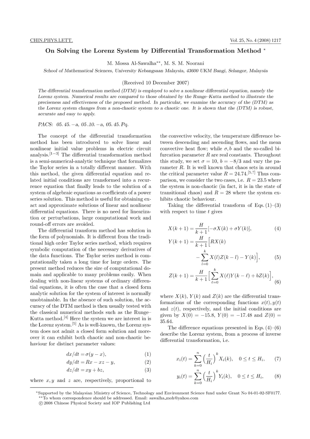






Text
                    CHIN.PHYS.LETT.

Vol. 25, No. 4 (2008) 1217

On Solving the Lorenz System by Differential Transformation Method

∗

M. Mossa Al-Sawalha∗∗ , M. S. M. Noorani
School of Mathematical Sciences, University Kebangsaan Malaysia, 43600 UKM Bangi, Selangor, Malaysia

(Received 10 December 2007)
The differential transformation method (DTM) is employed to solve a nonlinear differential equation, namely the
Lorenz system. Numerical results are compared to those obtained by the Runge–Kutta method to illustrate the
preciseness and effectiveness of the proposed method. In particular, we examine the accuracy of the (DTM) as
the Lorenz system changes from a non-chaotic system to a chaotic one. It is shown that the (DTM) is robust,
accurate and easy to apply.

PACS: 05. 45. −a, 05 .10. −a, 05. 45. Pq.
The concept of the differential transformation
method has been introduced to solve linear and
nonlinear initial value problems in electric circuit
analysis.[1−3] The differential transformation method
is a semi-numerical-analytic technique that formalizes
the Taylor series in a totally different manner. With
this method, the given differential equation and related initial conditions are transformed into a recurrence equation that finally leads to the solution of a
system of algebraic equations as coefficients of a power
series solution. This method is useful for obtaining exact and approximate solutions of linear and nonlinear
differential equations. There is no need for linearization or perturbations, large computational work and
round-off errors are avoided.
The differential transform method has solution in
the form of polynomials. It is different from the traditional high order Taylor series method, which requires
symbolic computation of the necessary derivatives of
the data functions. The Taylor series method is computationally taken a long time for large orders. The
present method reduces the size of computational domain and applicable to many problems easily. When
dealing with non-linear systems of ordinary differential equations, it is often the case that a closed form
analytic solution for the system of interest is normally
unobtainable. In the absence of such solution, the accuracy of the DTM method is then usually tested with
the classical numerical methods such as the Runge–
Kutta method.[4] Here the system we are interest in is
the Lorenz system.[5] As is well-known, the Lorenz system does not admit a closed form solution and moreover it can exhibit both chaotic and non-chaotic behaviour for distinct parameter values:
dx/dt = σ(y − x),

(1)

dy/dt = Rx − xz − y,

(2)

dz/dt = xy + bz,

(3)

where x, y and z are, respectively, proportional to
∗ Supported

the convective velocity, the temperature difference between descending and ascending flows, and the mean
convective heat flow; while σ, b and the so-called bifurcation parameter R are real constants. Throughout
this study, we set σ = 10, b = −8/3 and vary the parameter R. It is well known that chaos sets in around
the critical parameter value R = 24.74.[5,?] Thus comparison, we consider the two cases, i.e. R = 23.5 where
the system is non-chaotic (in fact, it is in the state of
transitional chaos) and R = 28 where the system exhibits chaotic behaviour.
Taking the differential transform of Eqs. (1)–(3)
with respect to time t gives
H
[−σX(k) + σY (k)],
k+1
H [
Y (k + 1) =
RX(k)
k+1
k
]
∑
−
X(l)Z(k − l) − Y (k) ,

X(k + 1) =

(4)

(5)

l=0

Z(k + 1) =

k
]
H [∑
X(`)Y (k − `) + bZ(k) ,
k+1
`=0

(6)

where X(k), Y (k) and Z(k) are the differential transformations of the corresponding functions x(t), y(t)
and z(t), respectively, and the initial conditions are
given by X(0) = −15.8, Y (0) = −17.48 and Z(0) =
35.64.
The difference equations presented in Eqs. (4)–(6)
describe the Lorenz system, from a process of inverse
differential transformation, i.e.

xi (t) =
yi (t) =

n (
∑
t )k
Xi (k),
Hi

k=0
n (
∑
k=0

t )k
Yi (k),
Hi

0 ≤ t ≤ Hi ,

(7)

0 ≤ t ≤ Hi ,

(8)

by the Malaysian Ministry of Science, Technology and Environment Science fund under Grant No 04-01-02-SF0177.
whom correspondence should be addressed. Email: sawalha moh@yahoo.com
c 2008 Chinese Physical Society and IOP Publishing Ltd
°
∗∗ To

1218

M. Mossa Al-Sawalha et al.

zi (t) =

n (
∑
k=0

t )k
Zi (k),
Hi

0 ≤ t ≤ Hi ,

(9)

where k = 0, 1, 2, · · · , n represents the number of terms
of the power series, i = 0, 1, 2, · · · , expresses the ith
sub-domain and Hi is the sub-domain interval.
The accuracy of the DTM is demonstrated against
Maple’s built-in fourth-order Runge–Kutta procedure
rk4 for the solutions of both non-chaotic and chaotic

Vol. 25

systems. The number of significant digits is set to be
16 in all the calculations. We set σ = 10, b = 8/3
and take the initial conditions x(0) = −15.8, y(0) =
−17.48 and z(0) = 35.64. The time range studied in
this work is [0, 20] as considered in Ref. [4]. In addition to the case R = 28 which is considered in Ref. [4]
and corresponds to a chaotic Lorenz system, we also
consider the case R = 23.5, corresponding to a nonchaotic system.

Fig. 1. 10-term DTM (∆t = 0.05 and ∆t = 0.01 ) vs RK4 (∆t = 0.001) solutions for R = 28.
Table 1. Differences between 10-term DTM and RK4 solutions for R = 23.5.
t
∆x
2
4
6
8
10
12
14
16
18
20

∆ = |RK40.001 − DTM0.05 |
∆y
∆z

2.724 × 10⁻⁵
5.464 × 10⁻⁴
7.35 × 10⁻⁴
4.628 × 10⁻⁴
4.452 × 10⁻⁴
2.082 × 10⁻⁴
3.165 × 10⁻³
1.222 × 10⁻³
2.699 × 10⁻³
5.036 × 10⁻³

2.425 × 10⁻⁴
5.157 × 10⁻⁴
1.09 × 10⁻⁴
1.2 × 10⁻³
8.647 × 10⁻⁴
6.395 × 10⁻⁴
4.155 × 10⁻³
5.946 × 10⁻³
1.266 × 10⁻³
4.644 × 10⁻³

4.555 × 10⁻⁴
9.032 × 10⁻⁴
02.776 × 10⁻⁴
8.919 × 10⁻⁴
2.347 × 10⁻³
3.57 × 10⁻³
2.265 × 10⁻³
4.009 × 10⁻³
9.429 × 10⁻³
8.135 × 10⁻³

First we consider the non-chaotic case when σ =
10, b = −8/3 and R = 23.5, in this case the following
approximate solutions are obtained from Eqs. (7)–(9):
−79 84
56523 2 744769 3
− t+
t +
t
5
5
50
750
1601549659 4
−
t − ···,
45000
−437 52323
3570919 2
y(t) =
+
t+
t
25
250
2500
1144338422 3 2074616165 4
t −
t + ···,
−
86411
18447
13110751 2
891 22643
+
t−
t
z(t) =
25
125
7500
781669993 3 3690250604 4
−
t +
t + ···,
56941
33465

x(t) =

∆x

∆ = |RK40.001 − DTM0.01 |
∆y
∆z

1.808 × 10⁻⁹
3.190 × 10⁻⁹
2.675 × 10⁻⁹
1.921 × 10⁻¹⁰
5.985 × 10⁻⁹
1.391 × 10⁻⁸
1.595 × 10⁻⁸
2.811 × 10⁻⁹
1.468 × 10⁻⁸
2.170 × 10⁻⁸

1.854 × 10⁻⁹
4.960 × 10⁻⁹
6.122 × 10⁻⁹
4.999 × 10⁻⁹
1.478 × 10⁻⁹
8.112 × 10⁻⁹
2.481 × 10⁻⁸
2.691 × 10⁻⁸
8.002 × 10⁻¹⁰
2.307 × 10⁻⁸

2.481 × 10⁻⁹
1.431 × 10⁻⁹
3.586 × 10⁻⁹
1.003 × 10⁻⁸
1.645 × 10⁻⁸
1.928 × 10⁻⁸
7.168 × 10⁻⁹
2.452 × 10⁻⁸
4.244 × 10⁻⁸
2.959 × 10⁻⁸

The DTM solutions is compared with RK4 on time
step ∆t = 0.001, which is sufficiently accurate for our
comparison purposes.[4] From the results presented in
Table 1, we present the absolute errors between the 10term DTM solutions at two different time steps (∆t=
0.05 and ∆t = 0.01) and the RK4 solutions on time
step ∆t = 0.001, we choose this time step since a
smaller one is computationally costly, and increasing
the number of terms in the series solutions improves
the accuracy of the DTM solutions, but at the expense
of increased computational efforts. The 10-term DTM
solutions on the slightly larger time step ∆t = 0.05
match the RK4 solutions to at least 2 decimal places,
which is still not accurate enough (see columns 2–4
of Table 2). Obviously, further improvement can be
made on the accuracy of the 10-term DTM solutions

No. 4

M. Mossa Al-Sawalha et al.

by taking a smaller time step. As shown in the last
three columns of Table 2, the 10-term DTM solutions
on the time step ∆t = 0.01 agree with the RK4 solutions to at least seven decimal places. For the non-

1219

chaotic case we see that the DTM has the advantage
over the RK4 on achieving a good accuracy with a
larger time step.

Table 2. Differences between 10-term DTM and RK4 solutions for R = 28.
t
∆x
2
4
6
8
10
12
14
16
18
20

∆ = |RK40.001 − DTM0.01 |
∆y
∆z

4.728 × 10⁻⁹
1.142 × 10⁻⁸
1.344 × 10⁻⁷
3.975 × 10⁻⁷
3.471 × 10⁻⁶
1.523 × 10⁻⁶
1.172 × 10⁻⁴
2.008 × 10⁻⁴
1.653 × 10⁻³
2.208 × 10⁻²

6.261 × 10⁻⁹
6.570 × 10⁻⁹
2.274 × 10⁻⁷
6.426 × 10⁻⁷
2.947 × 10⁻⁵
1.569 × 10⁻⁵
4.623 × 10⁻⁵
2.265 × 10⁻⁴
2.515 × 10⁻⁴
3.658 × 10⁻²

1.121 × 10⁻⁸
9.747 × 10⁻⁹
1.939 × 10⁻⁸
1.908 × 10⁻⁷
2.225 × 10⁻⁵
1.090 × 10⁻⁵
3.496 × 10⁻⁴
2.731 × 10⁻⁴
2.687 × 10⁻³
1.998 × 10⁻²

∆x

∆ = |RK40.001 − DTM0.001 |
∆y
∆z

4.414 × 10⁻⁹
2.045 × 10⁻⁸
3.063 × 10⁻⁸
1.446 × 10⁻⁷
1.165 × 10⁻⁶
4.862 × 10⁻⁷
3.967 × 10⁻⁵
6.787 × 10⁻⁵
5.583 × 10⁻⁴
7.455 × 10⁻³

5.702 × 10⁻⁹
1.910 × 10⁻⁹
5.711 × 10⁻⁸
2.373 × 10⁻⁷
9.924 × 10⁻⁶
5.245 × 10⁻⁶
1.566 × 10⁻⁵
7.657 × 10⁻⁵
8.448 × 10⁻⁵
1.235 × 10⁻²

8.401 × 10⁻⁹
2.868 × 10⁻⁸
7.787 × 10⁻⁹
5.236 × 10⁻⁸
7.501 × 10⁻⁶
3.690 × 10⁻⁶
1.183 × 10⁻⁴
9.226 × 10⁻⁵
9.075 × 10⁻⁴
6.763 × 10⁻³

−437 17274
1782647 2
+
t+
t
25
125
1250
432166367 3 1310245037 4
−
t −
t + ···,
56250
14772
2224519 2 921948012 3
891 22643
+
t−
t −
t
z(t) =
25
125
1875
78493
1491073777 4
+
t + ···.
30137

y(t) =

Fig. 2. Phase portraits using 10-term DTM on ∆t = 0.01
for R = 28.

System (1)–(3) with σ = 10, b = −8/3 and R = 28
exhibits chaotic solutions, and so we should expect solutions which are highly sensitive to time step. In this
case the following approximate solutions are obtained
from Eqs. (7)–(9),
x(t) =

−79 84
19374 2 813947 3
− t+
t +
t
5
5
25
375
554258417 4
−
t − ···,
22500

The accuracy of the DTM is compared to RK4. In
Fig. 1, we plot the 10-term differential transformation
solutions (on ∆t = 0.05 and ∆t = 0.01) against the
RK4 solutions on ∆t = 0.001. Both the 10-term differential transformation solutions on ∆t = 0.01 and RK4
solutions on ∆t = 0.001 seem to overlap on the scale
used in Fig. 1. The details of the differences between
the 10-term differential transformation solutions on
(∆t = 0.01 and ∆t = 0.001) and the RK4 solutions
on ∆t = 0.001 are given in Table 3. In Fig. 2, we reproduce the well-known xy, and xz, phase portraits of
the chaotic Lorenz system using the 10-term differential transformation solutions on ∆t = 0.01.

References
[1] Chen C and Ho S 1996 Appl. Math. Comput. 79 173
[2] Jang M J, Chen C and Liu Y C 2001 Appl. Math. Comput.
121 261
[3] Hassan H I 2004 Appl. Math. Comput. 154 299
[4] Hashim I, Noorani M S M, Ahmad R, Bakar S A, Ismail
E S and Zakaria A M 2006 Chaos, Solitons & Fractals 28
1149
[5] Lorenz E N 1963 J. Atmosph. Sci. 20 130